/


Похожие


Текст
.
11
i 1
Eberhard Zeidler
Nonlinear
Functional Analysis
and its Applications
II/A: Linear Monotone Operators
Translated by the Author and by Leo F. Boront
With 45 Illustrations
Springer
Eberhard Zeidler
Sektion Mathematik
Karl...Marx..Platz
7010 Leipzig
German Democratic Republic
Leo F. Boront
Department of Mathematics
University of Idaho
Moscow, ID 83843
U.S.A.
Mathematics Subject Clas.qficalion (19RO 4611
LiInry cI ConptII Catalo&ialu. NJlicatioD Data
(.... for \tOI. 2 1*. A-B)
Zeidler. Eberhard.
. 2. ptJ. A-B: TP.,laed by the IUIhor and
Leo L. Boron.
\\II. 3: T......1fed by Leo L. Bomn.
Vol. 4; Tn.-liled by Juerpe QuandI.
IftChIdeI bibliographies and indexes.
C (MIlenll : 1. Fixed point IhcoIanI - 2. pt A. U1aI'
monoconc openIOis . PI. B Noalinear operators - (eec.1
- 4. AppiicatioGs 10 mattaem.l icaI pbyIia.
1. NonIiftell' functional....ysis. I. 1itle.
2I.S.7ASI3 I98S 515.7 83-20455
Previous edition, V{)rlr II'" iht, ,,'C''''''rwarr F...Ic'i()nc"tJnoI iJ. Voll. I-III. puhlished by 888
B. Ci. Tcuhner Vcrlal 'lKhan. 1010 Leipzia. Stemwarlen'trasse H. DcUIM:he DcmokraliKhe
Repuhlik.
C> 1990 by S p.. -Y«IIa New "-t 11Ic.
All ti8h. rc rvod. This work may not be translaled or copied in whole 0' in pari wiahout the
wrtuen permi55ion of tbe publisher fSprin,cr-Verlag. 175 Fifth Avcnue. New York. New York
10010. U.S.A. CkCCpt for briei' excerpts in connection with reviews or RChnlarly analysis. Use in
connection with any form of information storage and retrieval. e tronic adaptation. computer
5O(twarc.or hy imilar or diuimil.r methodology now known or herurterdc c1oped is (orbidden.
Reprinted by Wor1d Puhl'-hinl Corporation. BetJ nl. 1992
for distributIOn and sa in The People IS Pe?ublic of Chma only
ISBN 7 - 5062 -1308-7
ISBN O-JR7..96A02-4 Springer. VerJla New York Berlin Heidelberg
ISBN )- f)..96802.4 Sprin,er-VerJal RerJin HcideJher, New York
Preface to Part 11/ A
A theory is the more impressive.
the simpler are its premises.
the more distinct are the thin.. it connects,
and the broader is ils fanF of applicability.
Alben Einstein
This is the second or 8 five-yolume exposition of the main principles of
nonlinear functional analysis and its numerous applications to the natural
sciences and mathematical economics. The presentation is seU-contained and
accessible to a broader audience of mathematicians. natural scientists. and
engineers. The basic content can be undentood even by those readers who
have little or no knowledse or linear functional analysis. The material of the
five volumes is organil.ed as rollows:
Part I: Fixed-point theorems.
Part II: Monotone orerators.
Part III: Variational methods and optimization..
Parts IV IV: Applications to mathematical physics.
The main goals of the work are discussed in detail in the Preface or Part I.
A Table of Contents of Parts I through V can be Cound on page 87 J of
Part I. The emphasis or the treatment is baed on the rollowing considera-
tions:
(a) Which are the basic, guiding concepts, and what relationship exists be-
tween them?
(b) What is the relationship between these ideas and the known results of
classical analysis and or linear functional analysis?
(c) What are some typical applications?
. .
VII
. . .
VIII
Prcrace 10 Part III A
The present Parlll is divided into two subvolumes:
Part II/A: Linear monotone operators.
Part 11/8: Nonlinear monotone operators.
These two subvolumes form a unit. They consist of the following sections;
introductIon to the subject;
hnear Jnonotonc problems;
g ncralization to nonlinear stationary problems;
generalization to nonlinear nonstationary problems;
general theory of discretization methods.
The numerous applications concern differential equations and integral equa-
tions.. as well as numerical methods to their solution.
The Appendix, the Bibliography, and the Jndex material 10 Parts IliA and
11/8 can be found at the end or Part II/B.
l"he modern theory of linear partial differential equations of elliptic, para-
bolic, or hyperboJic type is based on the so-called H ilberl spa(:e n.ethod.f\. In
this connection, boundary value problems and initial value problems arc
transformed Into operator equations in Hilbert space. The solutions of these
opera lor equations correspond to generalized solutions oftbe original classical
problcm . Here, the generalized solutions live in so-called SObO/('I' :iPUL'('S.
Roughly speak ing, Sobolev spaces consist of functions which have sufficiently
reasonable generalized derivatives.
l'he theory of ,nol1olone operators generaliles the Hilbert space methods to
nonlineClr problems. We want to emphasize that the Hilbert space methods
and the theory of monotone operators are connected with the main stream,"
of mathematics. They are closely related to Hilbertts rigorous justification of
the Dirichlet prin£';ple and to the 19th and 20th problems or Hilbert which. he
formulated In his famous Paris lecture in 1900. The relevant historical back-
ground will be discussed in Chapter 18. Fron) the physical pornt of view, the
Hilbert pace methods and the more general theory of monotone operators
are based on the fundamental concept of enerYJ. Roughly speaking. Sobolcv
spact:s can be regarded as spaces of functions which correspond to physicaJ
states of finite energy. We will show that, in our century. the notion of
monotone operators played, both implicitly and explicitly, a fundamental role
in the development or the calculus or variations, in the theory of lInear and
nonlinear partial dilTerential equalions and in numerical analysis.
In order to help the reader understand the basic ideas, the first chapters of
this volume serve as an elementary introduction to the modern functional
analytic theory of linear partial differential equations. In particular, Chapter
1 M contaln an elegant functional analytic justification of the Dirichlet prin-
ciple.. based on a generalization of the classiQtI Pythagorean theorem to
Hilbert spaces. An introduction to the theory of S()btJlev spaces can be found
in Chapter 21. Experience shows that students frequently have trouble with
the tcchnicalitie!-; of Sobolev spaces. In Chapter 21 t for the benefit of the reader 1
Prerace 10 Part iliA
.
IX
we choose an approach to Sobolcv spaces which is as elementary as possible.
To this end we first prove all the embedding theorems in an extremely simple
manner in R 1 before passing to nil. For the convenience or the reader. the
basic properties of the Lebesgue integral are summarized in the Appendix
to Part II/B. In this connection, we choose the simplest definition of the
Lebesgue integral. In contrast to other definitions of the Lebesgue integral,
our definition also applies immediately to runctions with values in B-spaces.
Such functions are nceded in connection with evolution equations. Moreover,
in Chapter 18 we discuss a number of important principles which arc frequently
used in modern analysis. for example, the smoothing principle via mollifiers,
the localization principle via partition of unity, the extension principle, and
the completion principle.
The ba. ic ideas and basic principles of the theory or nonlinear monotone
operators are discussed in detail in a special section at the beginning or Part
II/B. Any reader who wishes to learn about nonlinear monotone operators as
quickly as possible may immediately begin reading Part II/B.
A reference of the form Al (20) and A 2 (20) is to formula (20) in the Appendix
of Parll and II/B. respectively; while (18.20) refers to formula (20) in Chapter
18. Omission of a chapter number means that the formula is in the current
chapter. The References to the Literature at the end of each chapter are of the
following form: Krasnoselskii (1956, M, B, H), etc. The name and the year
relate to the Bibliography at the end of Part II/B. The letters stand for the
folio wi ng:
M: monograph:
L; lect u re notes;
s: survey article;
P: proceedings;
8: exlensivc bibliography in the work cited;
H: comments on the historical development or the subject contained in the
work cited.
.
A List of Symbols may be found at the end of Part II/B. We have tried
to use generally accepted symbols. A few peculiarities, introduced to avoid
confusion, are described in the remarks introducing the List of Symbols.
Basic materia) on linear functional analysis may be found in the Appendix
to Part I.
The theory of monotone operators is related to the simple fact that the
deri,'ut;l'e I' of a convex real function f is a monotone function. However. it is
quite remarkable that the idea of the monotone operator allows many diver..
sified applications. For example. there are applkations to the rollowing topics:
(i) variational problems and variational inequalities;
(ii) nonlinear elliptic, parabolic, and hyperbolic partial differential
equations:
(iii) nonlinear integral equations;
x
Prcracc to Part IliA
(ivJ nonlinear semigroups;
(v) nonlinear eigenvalue problems;
(vi) nonlinear Fredholm alternatives;
(vii) mapping degree for noncompact operators;
(viii) numerical methods such as the Ritz method (e.g.. the method of finite
elements), the Galerkin method. the proje<:tion-iteration method. the
difference method, and the Kanov method for conservation laws and
'Jariational inequaiitieL
Concerning time-dependent problems we emphasize both the Galerkin
InethtHl and the method of semlgroupJ. We also discuss in detail the facl that
the theory of monotone operatoR generalizes both the theory of bou'zded and
unbounded linear operators. To this end we develop, in Chapters 18 and 22
through 24, the theory or linear partial differential ultions based on bounded
linear operators, and in Chapter 19. we study in detail the elegant method of
the Friedrichs extension for unbounded linear operators and its applicHtions
to variational problems and 10 linear and semi linear elliptic. parabolic, and
hyperbolic equations. as well as applications to th..: semiIinear Schrodinser
equation. As we shall show in Parts IV and V. unbounded linear operdtors
playa decisive role in quantum mechanics and quantum field theory (elemen-
tary particle physics). In contrast to this. for example, bounded linear operators
are related to elasticity and hydrodynamics.
At the center or the theory of monotone operators there stands the notion
or the nJuxi,nal monotone operator. which generalizes both the theory of
bounded and unbounded linear monotone operators. The theory of maximal
monotone operators will be studied in detail in Chapter 32.
A number of diagrams contained in the tcxt should help the reader to
discover interrelationships between different topics. In particular, we recom-
mend Figure 27.1 in Section 27.5 or Part II/B where the reader may Dnd
interrelationships between many important operator properties in nonlinear
functional analysis. A list of all these schematic overviews can be found at the
end of Part II/B. A list of the basic theorems and of the basic definitions can
aJso be found there.
In Part I we studied equations involving compact operators. The decisive
advantage of the theory of monotone operators is that it is also applicable to
nun('olnpu(" operators. AloftJ with abstract existence theorems we also stress
the methods of numerical functional analysis. Chapters 20 through 22 (resp.
Ch8ptC 33 through 35) may serve as an introduction to linear (resp. non-
linear) numerical functional analysis. For example, in terms of numerical
functional analysis, monotone operators allow us to justify the rollowing
fundamentKI principle: Consistency and stability imply convergencc. In this
connection. the scneral notion of A-proper maps is crucial.
The connection between the theory of monotone operators and general
variational methods will be studied in detail in Part III. In Parts IV and V we
will consider applications or the theory or monotone operators to interesting
Pre(acc to Pari II, A
.
XI
problems in malhemuli<:al phy ..;cs. For example, the theory of monotone
operators plays an important role in elasticity, hydrodynamics (the Navier-
Stokes equations), gas dynamics (subsonic flow), and semiconductor physics.
I hope that the reader will enjoy discovering a number or interesting
interrelationships in mathematics.
Leip ig
Spring 1989
Eberhard Zeidler
Contents (Part II/A)
Preface to Part 11/ A VII
INTRODUCTION TO THE SUBJECT I
CHAfIEIUB
Variational Problems. the Ritz Method. and
the Idea of Orthogonality 15
18.1. The Space C (G) and the Variational Lemma 17
fi 18.2. Integration by Parts 19
fiI8.3. The First Boundary Value Problem and the Ritz Method 21
18.4. The Second and Third Boundary Value Problems and
th R it7 M thnd 28
18.5. Eigenvalue Problems and the Ritz Method 32
18.6. The Holder Inequality and its Applications 35
18.7. The History of the Dirichlet Principle and Monotone Operators 40
18.8. The Main Theorem on Quadratic Minimum Problems 56
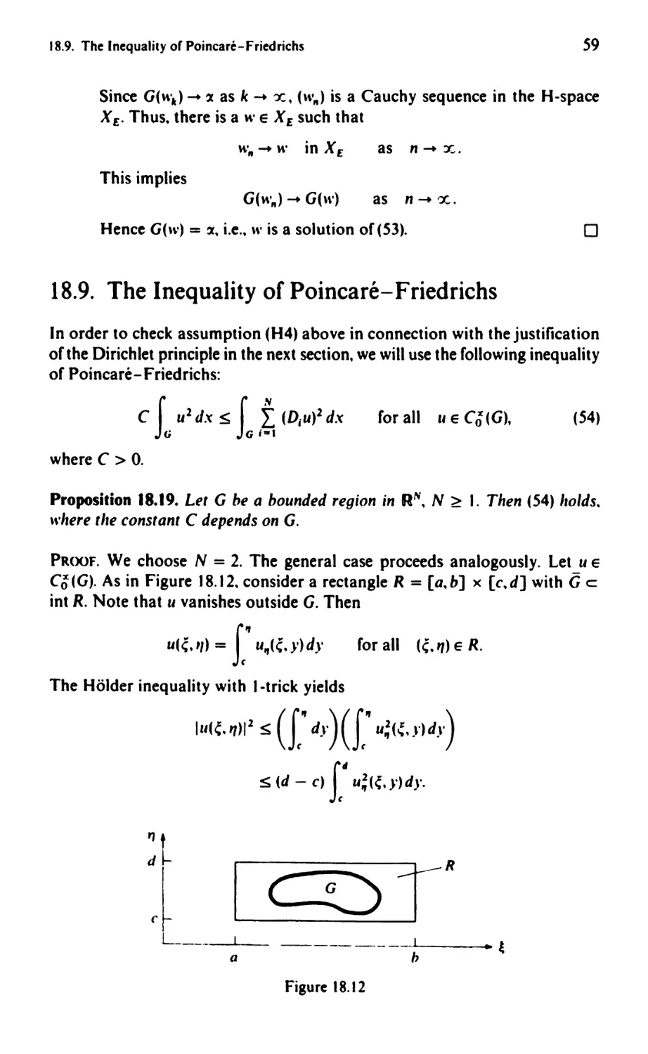
18.9. The Inequality of Poincare- Friedrichs 59
fiI8.10. The Functional Analytic Justification of the Dirichlet Principle 60
18.1 I. The Perpendicular Principle, the Riesz Theorem, and
the Main Theorem on Linear Monotone Operators 64
fi 18.12. The Extension Principle and the Completion Principle 70
18. t 3. Proper Subregions 71
fiI8.t4. The Smoothing Princil'le 72
18. I S. The Idea of the Reaularity of Generalized Solutions and
the Lemma of Weyl 78
18.16. The Localization Principle 79
18.17. Convex Variational Problems. Elliptic Differential Equations.
and Monotonicity 81
. . .
XIII
XIV
Conlenls(Parlll/A)
18.18. The General Euler- Lagrange Equations 85
18.19. The Historical Development of the 19th and 20th Problems of
Hilbert and Monotone Operators 86
18.20. Sufficient Conditions for Local and Global Minima and
Locally Monotone Operators 93
CHAPTER 19
The Galerkin Method for Differential and Integral Equations,
the Friedrichs Extension. and the Idea of Self-Adiointness 101
19.1. Elliptic Differential Equations and the Galerkin Method 108
19.2. Parabolic Differential Equations and the Galerkin Method 111
19.J. Hyperbolic Differential Equations and the Galerkin Method 113
&194. 'nteRral Equations and the Galerkin Method 115
19.5. ('omplete Orthonormal Systems and Abstract Fourier Series 116
19.6. Eigenvalues of Compact Symmetric Operators
(Ifilbert Schmidt Theory) 1 19
19.7. Proof of Theorem 19.8 121
19.8. Self-Adjoint Operators 124
19.9 The Friedrichs Extension of Symmetric Operators 126
&19.10. Proof of Theorem 19.C 129
*19.11. Application to the Poisson Equation 132
19.12. Application to the Eigenvalue Problem for the Laplace Equation 134
19.13. The IncQuality of Poincare and the Compactness
Th,.or m or Rellich I J5
19.14. Functions of Self-Adjoint Operators 138
19.15. Application to the Heat Equation 141
19.16. Application to the Wave Equation 143
19.17. Semigroups and Propagators, and Their Physical Relevance 145
19.18. Main Theorem on Abstract Linear Parabolic Equations 153
19.19. Proof of Theorem 19.D 155
19.20. Monotone Operators and the Main Theorem on
Linear Nonexpansive Semigroups 159
19 21. The Main Theorem on One-Parameter Unitary Groups 160
&19.22. Proof of Theorem 19.E 162
19.23. Abstract Semilinear Hyperbolic Equations 164
19.24. Application to Semilinear Wave Equations 166
19.25. The Semilinear Schrodinger Equation 167
19.26. Abstract Semilinear Parabolic Equations. Fractional Powers of
Operators. and Abstract Sobolev Spaces 168
19.27. Application to Semilinear Parabolic Equations 171
19.28. Proof of Theorem 19.1 171
&19.29. Five General Uniqueness Principles and Monotone Operators 174
19.30. A General Existence Principle and Linear Monotone Operators 175
CHAPTER 20
Difference Methods and Stability 192
20.1. Consistency. Sta!-:ility, and Convergence 195
20.2. Approximation of Differential Quotients 199
Content5 (Part iliA)
xv
20.3. Application to Boundary Value Problems for
Ordinary Differential Equations
20.4. Application to Parabolic Differential Equations
20.S. Application to Elliptic Differential Equations
20.6. The Equivalence Between Stability and Convergence
20.7. The Equivalence Theorem of Lax for Evolution Equations
200
203
208
210
211
ONE PROBLEMS 225
CH.AfiEIUJ
Auxiliary Tools and the Converaence of the Galerkin
Method for Linear Operator Equations 229
21. t. Generalized Derivatives 231
21.2. Sobolev Spaces 235
21.3. The Sobolev Embedding Theorems 237
21.4. Proof of the Sobolev Embedding Theorems 241
21.S. Duality in B-Spaces 25 I
21.6. Duality in H-Spaces 253
21.7. The Idea of Weak Convergence 255
21.8. The Idea or Weak. Convergence 260
21.9. Linear Operators 261
21.10. Bilinear Forms 262
21.11. Application to Embedding! 265
21.12. Proiection Operators 265
21.13. Bases and Galerkin Schemes 271
21.14. Application to Finite Elements 273
21.1 S. Riesz-Schauder Theory and Abstract Fredholm Alternatives 27S
21.16. The Main Theorem on the Approximation-Solvability of Linear
Operator Equations, and the Convergence of the Galerkin Method 279
21.17. Interpolation Inequalities and a Convergence Trick 283
21.18. Application to the Refined Banach Fixed-Point Theorem and
the Converaence of Iteration Methods 285
fi21.19. The Gagliardo-Nirenberg Inequalities 286
21.20. The Strategy or the Fourier Transform for Sobolev Spaces 290
21.21. Banach Algebras and Sobolev Spaces 292
121.22. Moser-Type Calculus Inequalities 294
21.23. Weakly Sequentially Continuous Nonlinear Operators on
Sobolev Spaces 296
CHAPTER 22
Hilbert Space Methods and Linear Elliptic Differential Equations 314
22.1. Main Theorem on Ouadratic Minimum Problems and the
Ritz Method 320
22.2. Application to Boundary Value Problems 325
22.3. The Method of Orthogonal Projection, Duality, and a posterior;
Error Estimates r 335
22.4. Al!Plication to Boundary Value Problems 337
X\'I
2 5.
2 .
22. 7.
22.N.
22.9.
2 . U)
12 U
1 11.
12. Ll
2 IA
2. L.5.
:!2 L6..
12. lL
s ..,., L.8
s-_. .
22.19.
:2 2 20
2 .21.
s" "
..._._... .
Contents (Part II A.
Main Theorem on Linear Strongly Monotone Operators and
the Galerkin Method
Application to Boundary Value Problems
C"ompact Perturbations of Strongly Monotone Operators,
Fredholm Alternatives. and...1he Galerkin Method
Application to Integral Equations
Application to Bilinear Forms
Application to Boundary Value Problems
EiJZen\ aluc Prohlems and the Ritz Method
Application to Bilinear Forms
Al"phcation to Boundary - EiRenvalue Problems
(j,\rdln Forme;;
The (Jardlng I nequality for Elliptic Equations
The Main Theorems on Garding Forms
Application to Stron ly Elliptic Differential Equations of Order 2",
Difference Approximations
Interior Regularity of Generalized Solutions
Proof of Theorem 22.' f
Regulant} of Generalized Solutions up to the Boundary
Proof of Theorem 22.1
CHA£IER..2J
Hilbert Space Methods and Linear Parabolic Differential Equations
23.1.
*23.2.
23.3.
23 4
23 5.
23.6.
s, 7
" - .' . .
23 8
&23.9.
Particularities in the Treatment of Parabolic E q uations
The Lebesgue Space IJ p (O. T; X) of Vector-Valued Functions
T h e Dual Space to t p (O, T; X)
Evolution Tri p les
Generalized Derivatives
The Soholev Space W"I (0, T; V, H)
Main Theorem on First-Order Linear Evolution Equations and
the Galerkin Method
Application to Parabolic Differential Equations
Proof of the Main Theorem
( HAPTER 24
Hilbert Space Methods and Linear Hyperbolic
Differential Equations
24 I. Main Theorem on Second-Order Linear Evolution Equations
and the {.alerkin Method
24.2. Application to Hyperbolic Differential Equations
24 3. Proof of the Main Theorem
11 9
345
147
349
350
351
352
357
361
364
366
369
371
374
376
1 7N
383
lR4
402
402
406
410
416
417
422
42 1
426
430
452
453
456
459
Contents (Part II/B)
Preface to Part II/B VII
GENERALIZATION TO NONLINEAR
STATIONARY PROBLEMS 469
Basic Ideas of the Theory of Monotone Operators 471
CHAPTER 25
Lipschitz Continuous, Strongly Monotone Operators, the
Projection-Iteration Method, and Monotone Potential Operators 49S
CHAPTER 26
Monotone Operators and Quasi-Linear Elliptic
Differential Equations 55J
CHAPTER 27
Pseudomonotone Operators and Quasi-Linear Elliptic
Differential Equations S80
CHAPTER 28
Monotone Operators and Hammerstein Integral Equations 615
CHAPTER 29
Noncoercive Equations, Nonlinear Fredholm Alternatives,
Locally Monotone Operators, Stability, and Bifurcation 639
. .
XVII
XVIII Contents (Part II/B)
GENERALIZATION TO NONLINEAR
NONSTATIONARY PROBLEMS 765
CHAPTER 30
First-Order Evolution Equations and the Galerkin Method 767
CHAPTER 31
Maximal Accretive Operators, Nonlinear Nonexpansive Semigroups,
and First-()rder Evolution Equations R 17
CHAPTER 32
Maximal Monotone Mappings 840
CHAPTER 33
Second-Order Evolution Equations and the Galerkin Method 919
GENERAL THEORY OF DISCRETIZATION METHODS 959
( HAPTER 34
Inner Approximation Schemes, A-Proper Operators, and
the Galerkin Method 963
CHAPTER 35
External Approximation Schemes. A-Proper Operators, and
the Difference Method 978
("HAPTER 36
Mapping Degree for A-Proper Operators 997
Appendix 1009
References 1119
List of Symbols 1163
list of Theorems J 174
List of the Most Important Definitions 1179
List of Schematic Overviews 1182
List of Important Principles 1183
Index 1189
INTRODUCTION TO THE SUBJECT
Each progress in mathematics is based on the discovery of stronger tools and
easier methods, which at the time makes it easier to understand earlier methods.
By making these stronger tools and easier methods his own, it is possible for
the individual researcher to orientate himself in the different branches of
mathematics.
The organic unity of mathematics is inherent in the nature of this science, for
mathematics is the foundation of all exact knowledge of natural phenomena.
David Hilbert (1900)
(Paris lecture)
For me, as a young man, Hilbert became the kind of mathematician which I
admired, a man with an enormous power of abstract thought, combined with a
fully developed sense for the physical reality.
Norbert Wiener (1894-1964)
Hilbert always emphasized that mathematics is a unity, that its different parts
are in permanent interaction with each other and with the natural sciences, and
that this interaction not only provides the key to an understanding of the nature
of mathematics. but also the best cure against a splitting into different and
unrelated parts-a danger which, in our time of huge qualitative growth and
alarming specialization of mathematical research, must always be kept in mind.
Pavel Sergeevi Aleksandrov (t 97 t)
In the modern theory of partial differential equations, generalized solutions
playa fundamental role. We want to explain brieOy the mathematical and
physical background of the notion of a generalized solution. To this end we
consider the first boundary value problem for the Poisson equation
- u = f on G, ( la)
u=g on oG. (I b)
I
")
-
Introduction 10 the Subject
G
Figure 18.1
Here.. G is a bounded region in R J , and i G denotes the boundary of G (Fig.
18. I ).
Let = ( , '1.. ) and
u = u.. + U "" + u...
"'lot -."
The functions.r and 9 are given. We seek the function u. Problem (I) is closely
related to the variational problem
r (UZ + u; + II! - 2fu)dx = min!.
JG
II = g on l'G.
(2)
In addition, let us consider the potential
II(X) = r - fey) dy.
4n J G Ix - yl
Up to a ultiplicativc constant, II represents the potential of a mass distribu-
tion on G which has density .r.
The following observations are important.
(i) Classical solrltions. For sufficiently smooth functions f and g and suffi-
ciently smooth boundary ?G, the original problem (1) has a classical solution.
More precisely, if
(3)
r E C 2 (G).. g E C2' (i G), cG E C 2 . 2 , 0 < 2 < I,
then (I) has a unique classical solution u, where u E C 2 . 2 {G).
(ii) Generalized solutions. Counterexamples show that equation (1 a) need
not have a classical solution u in case f: G .... R is continuous. This surprising
fact depends essentially on the properties of the potential u in (3). If the density
.f: G IR is sufficiently smooth, say f is continuously differentiable, then the
potential u in (3) is a classical solution of (I a). However, if f: G R is only
continuous, then u in (3) need not have second derivatives. Hence, u is not a
classical solution of ( I a).
Consequently, if f: G IR is continuous, then we have the following situa-
tion. The function II in (3) has a well-defined physical meaning, namely, u
represents the potential of a mass distribution with continuous density f. But
Introduction to the Subject
3
u is not necessarily a solution of the differential equation (I a). Therefore it is
reasonable to introduce the notion of a generalized solution of (I a). To this
end we multiply (la) by cp e Co(G) and, using integration b}' parts, we obtain
- L uArp d:< = L frp d:<
for all cp e Co (G)
(4)
(cr. Section 18.2). By definition. a function u is called a generalized solution of
equation (I a) iff relation (4) holds. It can be shown that. in this sen , the
potential II in (3) is a generalized solution of (la) if f is continuous on G.
Obviously. classical solutions of (1 a) are also generalized solutions of (I a).
(iii) Variational problems, generalized solutions. and the idea of completion.
Let us now consider the variational problem (2), which corresponds to the
famous Dirichlet principle. In Chapter 18 we will show that each sufficiently
smooth solution u of (2) is also a classical solution of the original problem (I).
But the point is that the minimum problem (2) need not have a solution u
which has classical first derivatives. This fact caused enormous trouble in the
mathematics of the nineteenth century. related to the justification of the
Dirichlet principle. This will be discussed in Section 18.10.
I n order to understand the typical difficulties. let us first consider the
following simple minimum problem
F(x) = min!,
. e [a. b].
(5)
where F: [a, b] -. R is a continuous function on the compact interval [a. b].
The famous Weierstrass theorem tells us that problem (5) has always a
solution (Fig. 18.2). Suppose now that the unique solution . = 2 of (5) is an
irrational number, and suppose that we consider the modified problem
f(x) = min!,
x e Q n [a, b],
(5.)
where 0 denotes the set of rational numbers. Then problem (5.) has no
solution. Consequently, mathematicians, who do not know irrational num-
bers, cannot prove the Weierstrass existence theorem for (5). We now want to
show that the variational problem (2) corresponds to a similar situation. For
simplicity. let g = O. We set
F(u) = L (u + u + u! - 2fu)d:<
F
a
(J
I
b
Figure 18.2
4
Introduction to the Subject
and
M = {u E C 1 (G): u = 0 on cG}.
Then, problem (2) reads as follows:
(D*) f.(u) = min!, u e M.
This classical variational problem need not have a solution. Roughly speak-
ing, problem (D*) corresponds to (5*). However, as we shall show in Section
18.10. if we introduce the Sobolel' space W 2 1 (G), then we obtain the modified
problem
(D) Ftu) = min!. u E W 2 1 (G).
which has a unique solution u if JGf 2 dx < OC,,'.
By definition. this solution u is called a generalized solution of the original
boundary value problem (I) with g = O. In addition, u is also a generalized
solution of the Poisson equation (Ia) in the sense or(4). Roughly speaking, we
obtain the following:
The introduction of Sobolev spaces corresponds to the introduction of real
numher..'; t ;a irrational numbers in classical mathematics.
To explain this. we start with the abstract problem
( P*)
Ffu) = min!,
U EM.
I n order to solve (P*) we consider the modified problem
(P)
F(u) = mint
U E N.
where N is a completion of M, i.e., the set N is obtained from the set M by
adding appropriate "ideal" elements. For example. in the case of problem (5*),
"'e complete the set of rational numbers to the set of real numbers by adding
irrational numbers. In the case of problem (D*), we complete the set
M = {u E C t (G): u = 0 on cG}
to the Sobolev space N = W 2 1 (G) by adding appropriate functions which have
generalized first-order derivatives. The Sobolev space W 2 1 (G) is a Hilbert space
equipped with the scalar product
(ulr ) = f (Ull 1 + U ., t' ., + u"l',,)dx.
G
The precise definition of Wi (G) will be given in Section 18.10. Roughly
speaking, the Sobolev space ;J,2' (G) is the smallest Hilbert space with the scalar
product (ull') which contains the set of functions CO'. Note that C<f(G) c M.
(iv) Approximation methods. In order to obtain approximate solutions for
the original boundary value problem (I). one frequently uses the so-called Rit:
method. The basic idea of this method is the following. Instead of solving the
Basic St ra tegy
5
variational problem
(D) L (u + u + uf- 2fu)dx = min!, u E WZI(G),
we consider the approximate problem
(D,,) L (ul + u + uf - 2fu)dx = min!, u EX",
where X" is a finite-dimensional subspace of W 2 1 (G), i.e., X" consists of all
functions u of the form
u = C I WI + c 2 "'2 + ... + c" "'"
with "i = 0 on cG for all j, where the so-called basic functions "'1' ..., w.. are
fixed. This way the approximate problem (D,,) is reduced to the determination
of the unknown real coefficients c l' .. . , ell. Let u and UtI denote the solutions
of (D) and (D,,), respectively. Generally, it is not possible to prove the conver-
gence of this Ritz method in the sense of pointwise convergence:
lim u,,(x) = u(x) for all x E G.
,,-x,
However, in Chapter 22 we will prove that the sequence (u,,) converges to u
in the Sobolev space Wl (G), i.e.,
lim (u" - ulu.. - u) = O.
"... x
Explicitly, this means that
. f ( au" CU ) 2 ( au" OU ) 2 ( cu" OU ) 2
! J G 1f - c + e" - 0" + e{ - o{ dx = O.
Consequently, Sobolev spaces also play an important role in modern
numerical analysis. For example, it is not necessary to use smooth basis
functions "'.. ..., ,v" in (D,,) above; it is sufficient to use p;ece,,';se-sn.ooth
functions. This is the basic idea of the important method of finite elements,
where \\'1' .. ., "'" are piecewise polynomial functions.
Basic Strategy
The basic strategy of the modern theory of partial differential equations is the
following:
(S I) We prove the existence of generalized solut;ons.
(S2) We sho,,' that the generalized solutions are even classical solutions if the
data of the problem are sufficiently smooth (method of regularization).
In (S t) we use general results from functional analysis. The analytic sub-
stance of the existence proofs in (5 I) is concentrated in the so-called Sobolet'
6
Introduction to the Subject
e",h('dt/iny III('ore"I.... \\'hich correspond to inequalities for integrals. The proofs
of the Sobolev embedding theorems are based on the Holder inequality. The
Sobolev embedding theorems generalize the famous classical inequalities
of Poincare and Friedrichs. In (S2) we need more sophisticated analytical
methods \vhich are based on the specific properties of the problems under
considera t ion.
Along with the Ritz method and the Galerkin method" difference methods
represent a universally applicable method for the numerical solution of partial
differential equations. This will be considered in Chapter 20. In Chapters 34
and 35. "'e shall construct a general theory of discretization methods for
nonlinear prohlems.
Figure 1 .J sho"'s important interrelationships which will be studied in
("haptcrs 18 and 19. There are two options for giving an introduftory le('ture
011 H ilherl spaC(l "1£11 hods and their applications to integral equations and
Idea of self-adjointness
('hapter 19)
.dea of orthogonality
('haptcr 1 t
!
parallelogram Identlt
IIhe Pythagorean theorem)
ij
quadnuic minimum problem,
U
I perpendicular principle I
ij
theorem of R IC'\/
Friedrichs' - - - - - -.. ltilbert Schmidt
extension theory
(eigenvalue problems)
function
/ calculus
semlgroups
1
elliptic. parabolic.
and hyperbolic differential
equations
(linear and semilinear)
quadratic variational ·
problems
Figure 18.3
Hilbert Spaces
7
partial differential equations:
(i) Chapters 18 and 19;
(ii) Chapters 18,21. and 22.
Approach (ii) is simpler than (i), since we only work with bounded operators.
However, approach (i), based on unbounded operators, gives more insight.
Note that unbounded operators are indispensable in quantum theory. If there
is enough time in an introductory lecture, then one can add Chapters 23 and
24 to (ii) concerning existence theorems for parabolic and hyperbolic equa-
tions via the Galerkin method.
In Chapters 2S through 36, we generalize the basic principles for linear
operators considered in Chapters 18 through 24 to nonlinear operators.
An introductor.\' lecture on nonlinear monotone operators can be based on
Chapters 2S through 27.
Hilbert Spaces
For the convenience of the reader, we recall some basic facts on Hilbert spaces.
Scalar product. Let X be a linear space over K = R, C (cr. A I (22) in the
Appendix of Part I). By definition, a scalar product on X is a function
(u, (.)..... (ul t') from X x X into K which has the following three properties for
all u, l\ w e X and all ;., P e K:
(i) (ul ;.1" + pK') = ; (ul v) + p(ul K').
(ii) (ult") = (vlu).
(iii) (ulu) > 0 iff u #: o.
Here, the bar denotes the conjugate complex number. From (i) and (ii) it
follows that
().v + p"'lu) = l(vlu) + ji(wlu).
Let u, t' EX. Then u is called orthogonal to t. iff
(ulv) = O.
Pre-Hilbert spaces. By definition, a pre-Hilbert space X is a linear space
together with a scalar product. We set
II u II = (u I u) 1/2 .
The convergence
u ll -+ U
as n -+ 00
is defined by
lIu" - ull -+ 0
as n -+ 00.
A sequence (u ll ) is called a Cauchy sequence iff, for each I; > 0, there exists an
8
Introduction to the Subject
110(1:) with
1111" - u'" II < I: for all n, m > no(I:).
Hi/her' spaces. By definition, a Hilbert space is a pre-Hilbert space with the
additional property that each Cauchy sequence is convergent.
Hilbert spaces are briefly called H-spaces.
The Scl,,\'ar: inequality and its consequences. The most important In-
equality in an H-space X is the so-called Schwarz inequality
l{ulr)1 < lIullll('11 for all u. rEX.
This follows from
o < (II - i.I' I u - ; 1') = II U 11 2 - i. ( u It.) - I ( t' III) + I ;.1 2 Ill' 11 2
with i. = 1III\l2/(ulr) in case (ult') o.
It follows from the Schwarz inequality that
1111 + ,." 2 = (II + I' I u + l') = II U 11 2 + (II I (') + (v I u) + Ill' 11 2
< (ilull + 111'(1)2.
This yields the triangle inequality
II II + r II S !lull + 111'11
for all u, I' E X.
Moreover, the generalized triangle inequality
1111111 - III'''' < lIu + I'll < lIuli + 111'11
follo\\'s from
for all u, I' E X
lIull - II f II = II (II - I') + ('" - 111'11 < II u - (' II.
If II" -+ U as " -+ x, then
lIu,,:1 -+ lIuli
as n -+ y ,
since III II" II - II "111 < II II" - u II -. o. Finally.
II" -+ U
and
('" .... ('
as n.... x
Implies
(11,,11',,) -+ (ul(')
as n -+ x.
This follows from
Itu,,'!',,) - (ulr)1 = 1(1I"lr" - (,) + (u" - ull')1
< I (u" 1('" - t.) I + I (II" - u I v) < II U" 1111 t." - ('II + II U" - u 1111 t'li.
Equiralent scalar products. Let Y be an H-space over II< with the scalar
product (.1 .), and let ('1 .). be another scalar product on X. By definition,
t.1 .) and ( '1 .). are called equivalent iff the corresponding norms
lIuli = (UIU)1/2 and lIuli. = (ulu) 2
Hilbert Spaces
9
are equivalent, i.e., there exist positive constants c and d such that
cllull s lIuli. s dllull
for all u eX.
In this case. X is also an H-space with respect to (.1 · )..
In the following let X and Y be H-spaces over k = R. C. and let M be a
subset of X.
Bounded sets. The set M is called bounded iff there is a real number r such
that
lIuli S r
for all u e M.
Open and closed sets. The set M is called open iff for each u E M there is a
number r > 0 such that the ball {t' e X: IIv - ull < r} belongs to M.
The set M is called closed iff for each sequence (u,,) in M,
u" -+ u as n -+ 00 implies u e M.
The closure M of M contains exactly all the elements 14 of X with the
property that there is a sequence (u,,) in M such that u.. -+ u as n -+ 00.
Dense sets. The set M is called dense iff M = X. Obviously. M is dense iff.
for each u e X and each £ > 0. there is an element v in M with IIv - ull < t.
An H-space X is called separable iff X contains an at most countable dense
set.
Compact sets. The set M is called relatively compact iff each sequence in
M has a convergent subsequence.
The set M is called compact iff it is relatively compact and closed, i.e., each
sequence (14,,) in M has a convergent subsequence 14,,- -+ U as n -+ 00 where
ue M.
Linearity. The set M is called a linear subspace of X iff
u,('EM and .{JEk imply 2U+{Jt'EM.
The operator A: D(A) X -+ Y is called linear iff D(A) is a linear subspace of
X and for all u. t' e D(A) and «. {J e k.
A(ocu + fJv) = GlAu + fJAt'.
The linear operator A: D(A) X -+ Y is called bounded iff there is a real
number c such that
"Au" S c 111411 for all 14 e D(A).
If the linear operator A: X -+ Y is bounded. then we define
IIAII = sup IIAuli.
.-a s I
This implies
IIAull s IIAliliuli
for all u eX.
In this connection note the linearity of A.
10
Introduction to the Subject
A tlti!i1Jearity. The operator A: X -+ Y is called antilinear iff. for all II, (' E X
and , II E (K.
A(:xu + fir) = Au + PitU.
Here, the bar denotes the conjugate complex number. If X and Yare real
H-spaces, then antilinear and linear operators coincide.
Continuity. The operator A: X -+ Y is called continuous iff. as n -+ x,
II n -... II
implies
Au" -+ Au.
We \\'ant to prove the following:
A Ii"ear operator /t: X -+ r is hounded ill it ;s continuous.
First suppose that A is bounded. Then it follows from II" -+ II as II -+ that
d .4 "" - .4 III! = II A ( u" - II) II < it A 1111 u II - ull
and hence .4u n -+ Au as " -+ x, i.e.. .4 is continuous.
Conversely. suppose that A is continuous. If A is not bounded. then there
is a sequence (u,,) such that
IIUn'l = I
and
IIAu,,1I > 11
for all IJ.
Sct f" = "" iI.4I1nlll . Then.as1l-'" x,
'Ir,,11 = 1/IIAu"II"2 -... 0
and II A 1',,1. = II .411 n 1 1 --+ x.. This contradicts the continuity of A.
("oulpactness. The operator A: X --+ Y is called compact iff it is continuous
and it maps bounded sets into relatively compact sets. Thus, if A is compact,
then each bounded sequence (u,,) contains a subsequence (u,,-) such that (Au",)
is convergent.
Linc",. IUIICI;OIlClls. A linear continuous map J': X -+ K is called a linear
continuous functional on X. The set of all the linear continuous functionals
on .Y is denoted by X*. Consequently. we have lEX. iff I: X -+ IK is linear
and there is a real number c such that
I l(u)1 < c lIu;1
for all II E X.
We set
11.1 II = sup 1.((u)l.
II I S I
Instead of ((II) we also write <I,ll).
In the Appendix of Part I. the interested reader williind the relationship
between the notions introduced above and general notions in topology.
The notion of an abstract Hilbert space was first introduced by von Neumann
1929). In his basic papers around 1906, Hilbert used the space 1 2 consisting
Hilbert Spaces
I 1
of all sequences :< = ( ,) with , e K for all i and
at
L 1 ,12 < 00.
i=1
Here the scalar product is given by
x
(:<Iy) = L !,'1i.
iel
The space 1 2 generalizes the classical Euclidean space R" to infinite dimensions.
A Look at the History of Hilbert Spaces
The following quotations should help the reader to understand the birth of
the notion of Hilbert space.
Further considerations of the subject led me to the conclusion that the systematic
construction of a general theory of integral equations is of the utmost importance
for the complete field of analysis and, in panicular, for the expansion offunctions
in infinite series, linear differential equations, analytic functions, potential theory,
and the calculus of variations.
David Hilbert (1912)
(From the Preface to his monograph on linear integral equations.)
In order to understand the great achievement of Hilbert (1862-1943) in the field
of analysis, it is necessary to first comment on the state of analysis at the end of
the nineteenth century. After Weierstrass (1815-1897) had made sure of the
foundations of the complex function theory, and it had reached an impressive
level. research switched to boundar}' t'alue problems, which first arose in physics.
The ",.ork of Riemann (1826- t 866) on complex function theory, however, had
shown that boundary value problems have great importance for pure mathe-
matics as well. Two problems had to be solved:
(i) the problem of the existence of a potential function for given boundary
values: and
(ii) the problem of eigenoscillations of elastic bodies. for example, string and
membrane.
The state of the theory was bad at the end of the nineteenth century. Riemann
had believed that by using the Dirichlet principle, one could deal with these prob-
lems in a simple and uniform way. After Weierstrass' substantial criricism of
the Dirichlet principle in t 870, special methods had to be developed for these
problems. These methods, by C. Neumann, Schwarz, and Poincare. were very
elaborate and still have great aesthetic appeal today; but because of their variety
they were confusing, although at the end of the nineteenth century, Poincare
( 1854- 1912), in particular, endeavoured with great astuteness to standardize
the theory. There was, however. a lack of "simple basic facts" from which one
could easily get complete results without sophisticated investigations of limiting
processes.
Hilbert first looked for these "simple basic facts" in the calculus of variations.
He considered so-called regular variational problems which satisfy the Legendre
condition. In 1900 he had an immediate and great success: he succeeded in
just il\'ing the Dirichlet principle.
While Hilbert used variational methods, the Swedish mathematician Fredholm
12
Introduction to the Subject
(1866 19:!7t approached the same goal by developing Poincare.s work by using
linear integral equations. In the winter semester 1900/1901 Holmgren. who had
come from Upsala (Sweden) to study under Hilbert in Gottingen, held a lecture
in Hllberfs seminar on Fredholm's work on linear integral equations which had
been published the previous year. This was a decisive day in Hilbert's life. He
took up Fredholm's new discovery with great zeal, and combined it with his
variational methode;. In this way he succeeded in creating a uniform theory
y.'hich solved problems (i) and (ii) above.
In 1904 H ilberfs first note on the uF oundations of a General Theory of linear
Integral Equations" was published in the Gt)tringer Nachrichren. These results
y.'ere based on lectures which Hilbert had held from the summer of 1901
on\\'ards. Fredholm had proved the existence of solutions for linear integral
equations of the second kind. His result was sufficient to solve the boundary
\'alue prohlems of potential theory. But Fredholm's theory did not include the
eigenscillations and the expansion of arbitrary functions with respect to eigen-
functions Only .Iilhert solved this problem by using finite-dimensional approxi-
mations and a passage to the limit. In this way he obtained a generalization of
the classical principal-axis transformation for symmetric matrices to infinite-
dimenc;ional matrices. The symmetry of the matrices corresponds to the symme-
try of the kernels of 1I1tegrai equations, and it shows that the kernels appearing
In oscillation problems are indeed symmetrical.
From our point of "ley.' today, Hilbert's paper of 1904 appears clumsy.
compared to the elegance of Erhard Schmidfs method (1907a, b) which he
developed in his dissertation written while a student of Hilbert in Gottingen.
But the tirc;t step had been made In the same year. 1904, Hilbert. in his second
note. \\'a ahle to apply his theory to general Sturm -liouville problems. His
third note In 1905 contained a very important result. Of the great problems
whIch Rlernann had posed with the comple function theory, there was still one
left open the proof of the existence of differential equations with a prescribed
monodromy group Iilbert solved this problem by reducing it to the determina-
tion of t 'o functions which are holomorphic in both the interior and exterior
of it closed curve. and whose real and imaginary parts satisfy appropriate linear
relatlon on the curve (the Hilbert Riemann problem I). The solution to this
problem IS a classic example for the axiomatics of limiting processes demanded
hy ' ilbcrt No concrete limiting processes are used, but everything results from
the existence of the Green function for the interior and the exterior of the closed
cur\e. and from the Fredholm alternative which says that either the homoge-
neous Integral equation has a nontrivial solution or the inhomogeneous integral
equation has a solution
Jfilbert soon noticed that limits are set to the method of integral equations.
In order tn overcome these limits he created, in his fourth and fifth notes in 1906,
the general theory of quadratic forms of an infinite number of variables. Hilbert
helie\ed that with this theory he had provided analysis with a general basis
which corresponded to an a.'(iomatics of limiting processe. . The further develop-
ment of mathematice; has proved him to be right.
Otto Blumenthal (1932)
The above quotation constitutes an extract from Hilbert's biography, which
can be found in Volume 3 of his Col/ectec/ Works. We recommend that the
I Toda . Riemann Hilbert problems playa fundamental role In the theory of solitons. See
I addec\ and TakhtadJan (19R7)
Hilbert Spaces
13
reader has a look at these Collected Works. Every single one of Hilbert's
mathematical works and essays is a masterpiece.
In the fall of 1926. the young John von Neumann (1903 - 1957) arrived at
Gottingen to take up his duties as Hilbert's assistant. These were the hectic years
during which quantum mechanics was developing at breakneck speed, with a
new idea popping up every few weeks from all over the horizon. The theoretical
physicists who were developing the new theory were groping for adequate
mathematical tools, trying in succession infinite matrices without any considera-
tions of convergence, differential operators. "continuous matrices" (whatever
that might mean), etc. As late as 1924, most physicists did not even know that
a finite matrix was! It finally dawned upon them that their "observables" had
properties which made them look like Hermitian operators in Hilbert space, and
that by an extraordinary coincidence, the "spectrum" of Hilbert (a name which
he had apparently chosen from a superficial analogy) was to be the central
conception in the explanation of the "spectra" of atoms. It was therefore natural
that they should enlist Hilbert's help in trying to put some mathematical sense
in their computations. With the assistance of Nordheim and von Neumann,
Hilben first tried integral operators in Lz' but that needed the use of the Dirac
ub-function," a concept which was for the mathematicians of that time self-
contradictory. Von Neumann therefore resolved to try another approach.
Jean Dieudonne ( 1981 )
Stimulated by an interest in quantum mechanics, John von Neumann began the
work in operator theory which he was to continue as long as he lived. Most of
the ideas essential for an abstract theory had already been developed by the
Hungarian mathematician Frigyes Riesz (1880-1956), who had established the
spectral theory for bounded symmetric operators in a form very much like that
now regarded as standard. Von Neumann saw the need to extend Riesz's
treatment to unbounded operators and found a clue to doing this in Carleman's
highly original book on integral operators with singular kernels. The result was
a paper von Neumann submitted for publication to the Mathematische Zeit-
schrift but later withdrew. The reason of this withdrawal was that in 1928 Erhard
Schmidt (1876-1959) and I, independently, saw the role which could played in
the theory by the concept of the adjoint operator, and the importance which
should be attached to self-adjoint operators. When von Neumann learned from
Professor Schmidt of this observation. he was at once able to rewrite his paper
in a much more satisfactory and complete form, giving a full spectral theory for
all closed symmetric operators as well as for the self-adjoint operators. This he
did by abandoning Carleman's method. which he had been able to apply only
by use of a transfinite induction, and introducing the Cayley transform, which
served to reduce the theory of unbounded symmetric operators to that of
bounded isometric operators. Incidentally, for permission to withdraw the paper
without penalty. when it was already in page proof, the publisher exacted from
Professor von Neumann a promise to write a book on quantum mechanics. The
book soon appeared and has become one of the classics of modern physics,
particularly valued for its analysis of quantum statistics (Mathematische Grund-
lagen de, Quantenmechanilc. Springer-Verlag, 1932).
Marshall Harvey Stone (1970)
A great master of mathematics passed away when David Hilbert died in
Gottingen on February 14, 1943. at the age of eighty-one. In retrospect, it seems
to us that the era of mathematics upon which he impressed the seal of his spirit,
and which is now sinking below the horizon. achieved a more perfect balance
14
Introduction to the Subject
than has prevailed before or since. between the mastering of single concrete
problems and the form.ltion of general abstract concepts. Hilbert's own work
contributed not a little to bringing about this happy equilibrium. and the
direction in which we have since proceeded can in many instances be traced
back to this impulse. No mathematician of equal stature has risen from our
generation. . . .
Hilbert was singularl)' free from national and racial prejudices: in all public
questions. be they political. social. or spiritual. he stood forever on the side of
freedom. frequently in isolated opposition against the compact majority of his
environment. He kept his head clear and was not afraid to swim against the
current. even amidst the violent passions aroused by the First World War
(1914 1918) that swept so many other scientists ofT their feet. It was not mere
chance. y..hen the Nazis '''purged'' the German universities in 1933 and their hand
fell most heavily on the Hilbert school. that Hilbert's most intimate collaborators
left Germany either voluntarily or under the pressure of Nazi persecution. He
himself was too old. and stayed behind: but the years after 1933 became for him
years of ever-deepening tragic loneliness.
Hermann Weyl (1944)
CHAPTER 18
Variational Problems, the Ritz Method,
and the Idea of Orthogonality
When we do scientific work. we must often step down from our high horse of
grand principles. and dig in the dirt with our noses. When \\'e achieve our
purpose. we cover the tracks of our efforts in order to appear as gods of clear
thought.
Albert Einstein
In Sections 18.1 through 18.5 of this chapter we consider a number of important
concrete examples in order to explain the following:
(i) The connection between variational problems and boundary value prob-
lems for elliptic partial differential equations.
(ii) The equivalence between classical and generalized solutions in case the
solutions are sufficiently smooth.
(iii) The Ritz method for the construction of approximate solutions.
This should help the reader to recognize the simple basic ideas behind the
general theory. In this connection, a fundamental role is played by:
(a) the formula of integration by parts; and
(b) the variational lemma.
A general convergence proof for the Ritz method will be given in Section 22.1.
In the middle of this chapter there stands an elegant functional analytic
justification of the famous Dirichlet principle. Figure 18.4 shows the logical
structure of our existence proof.
(i) In Section 18.8 we use the parallelogram identity in order to prove very
simply a general existence theorem for quadratic minimum problems. The
parallelogram identity is a generalization of the classical Pythagorean
theorem.
15
16
J K Variational Problems. the Ritz Method. and the Idea of Orthogonality
parallelogram identity
(the Pythagorean theorem in
Hilbert spaces)
I
perpendicular
principle
existence principle
for quadratic minimum problems
I
+ the Holder inequality
+ the Poincare- Friedrichs inequality
theorem of R iesz
+ Sobolev spaces
main theorem on
linear monotone
operators
Dirichlet principle
(generalized solutions of the
Dirichlet problem
in Sobolev spaces)
I
regularization of
the generalized solutions
(Lemma of Weyl)
Figure 18.4
(ii) The functional analytic justification of the Dirichlet principle is a special
case of the general existence theorem in (i). To this end, we need the
following three analytical tools: the Holder inequality. the Poincare-
Friedrichs inequality. and Sobolev spaces (Sections 18.9 and 18.10).
(iii) In Section 18.11 we show that the following three principles are mutually
equivalent: the existence principle for quadratic minimum problems, the
perpendicular principle, and the Riesz theorem.
The perpendicular principle says that there exists a perpendicular from each
point of an H-space to a closed linear subspace. Consequently, we obtain the
following:
Tile functional anal)'ti(" justification of ,he Dirichlet principle is based on tlte
idea of orthogonality.
Therefore, the Dirichlet principle is closely related to the classical
Pythagorean theorem.
There are ideas in mathematics which remain eternally young and which
lose nothing of their intellectual freshness, even after thousands of years.
18.1. The Space C tG) and the Variational Lemma
17
Mathematicians of the Pythagorean school in ancient Greece attributed the
Pythagorean theorem to the master of their school, Pythagoras of Samos
(circa S60 B.C. -480 B.C.). It is said that Pythagoras sacrified one hundred
oxen to the gods in gratitude. In fact, this theorem was already known in
Babylon at the time of King Hammurabi (circa 1728 B.C.-1686 B.C.). Pre-
sumably. however, it was a mathelTlatician of the Pythagorean school who
first proved the Pythagorean theorem. This theorem appears as Proposition
47 in Book I of Euclid's Elements (300 B.C.).
The theory of Hilbert spaces is the abstract and very efficient formulation
of the idea of orthogonality. It seems that this idea has deep roots in our real
world. In Part V we shall show that Hilbert spaces represent the right mathe-
matical tool in order to describe the strange nature of quantum phenomena.
In nature we observe a duality between waves and particles. which is typical
for quantum processes. For example. light possesses such a dual structure. In
order to formulate this duality in terms of mathematics. one uses the theory
of Hilbert spaces. The main idea is that the quantization of particle theories
and wave theories lead to equivalent theories in H-spaces.
In Sections 18.7 and 18.19 we discuss briefly the historical development of
the Dirichlet principle, and of the 19th and 20th problems of Hilbert and their
relationship to the modern theory of monotone operators.
One cannot comprehend what it is one possesses if one has not understood what
one.s predecessors possessed.
Johann Wolfgang von Goethe (1749- 1832)
Mathematics has the advantage over many other fields of knowledge. such as
history. for example. that one can sometimes distinguish between true.' and
. false." Because of this mathematics pays dearly for this advantage in that it is
the most remote of all human things. One best notices the mathematician.s
longing for humanity and history in the introductions to mathematical writings.
Wilhelm Blaschke ( 1942)
18.1. The Space C o ( G) and the Variational Lemma
We first list a number of function spaces.
Definition 18.1. Let G be a nonempty open set in R N , N 1.
(a) Ci(G) is the set of all real functions u: G -+ R that have continuous partial
derivatives of orders m = O. I, . . . . k on G. We understand the derivative
of order m = 0 to be the function itself.
(b) CIt(G) is the set of all u E CIt(G) for which all partial derivatives of orders
m = O. .. . . k can be extended continuously to G.
(c) We denote briefly by C(G) (resp. C(G) the continuous real functions on
G (resp. G) instead of CO(G) (resp. CO(G)).
(d) If u e Ci(G) (rc:sp. u e C'(G» for all k = O. 19 .... then we write u e CX(G)
(resp. u e c r (G)).
IN
I" Vanallonal Problems. the Ritz Method, and the Idea or Orthogonality
,
I
I
G
- - -..
fa) ItE(',:(R)
(h)
Figure 18.5
(e) (... ((i) is the set of all functions II E C" (G) which vanish identically outside
a compact subset K of G that depends on II (Fig. 18.5).
The follo\\'ing important result will be used extraordinarily often.
Proposition 18.2 (Variational Lemma). Let G he a '10ne,p'ply open set ;11 {R'''.
.". > I. Let II E L 2 (G and suppose fhClt
f lll'dX = 0
(,
fc)r all l' E C (G).
(6
1'lren "'(' ohtail1
II( =O
alll,ost er'ery,,'here 0" G.
The notion "almost everywhere'" will be used very frequently in this \'olume.
We recall this in the Appendix, A 2 (2).
PR(XU-. We set ..\' = L 2 (G) and use the well-known fact that Co (G) is dense in
.\'. Hence there exists a sequence (un) in C (G) with
"" -+ II in..\'
as II -+ X.
From (6) \\'e obtain f 11111" = 0 for all II. letting II -+ X this implies (u Ill) = 0,
and hence II = O.
The density of C (G) in 1'( will be proved in Section 18.14 as a special
application of smoothing operators. 0
If " E C"(G) in Proposition 18.2, then obviously we obtain u(x) = 0 for all
E G.
In Sections 18.2 through 18.5 we shall make the following assumption:
(i is a hounded re J;(Jn ;n IR ' ,,'illl N > I. 1"he boundary i...
piece,,';se s,nooth. i.e.. to he precise. i'G E Co. 1 holds. 1 (7)
We gave the exact definition of h( G E Co. I ". in Section 6.2. Intuitively. we
think of this to mean all reasonable regions where the boundary can also have
I Throu1Z hout thl \ olume. condition (7) means that G is a bounded open Inter\'al If
\ - I
I R.2. Integration by Parts
19
aGeCO I
aG CU I
/
(8)
(b)
Figure 18.6
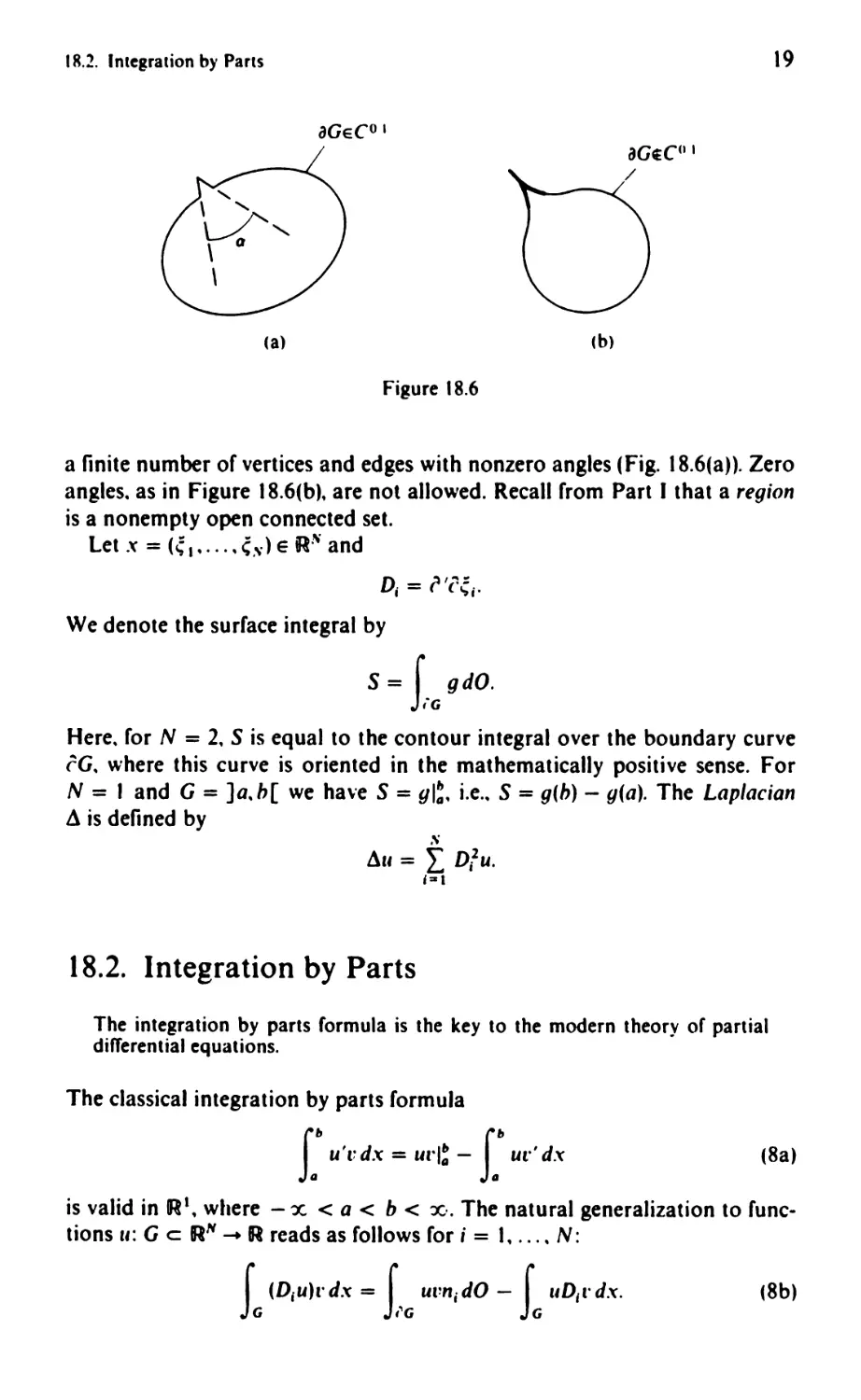
a finite number of vertices and edges with nonzero angles (Fig. 18.6(a)). Zero
angles. as in Figure 18.6(b), are not allowed. Recall from Part I that a region
is a nonempty open connected set.
let x = ( I" . . . .,. ) E H'" and
D / "
i = (- C i'
We denote the surface integral by
S = f gdO.
iG
Here. for N = 2. S is equal to the contour integral over the boundary curve
cG.. where this curve is oriented in the mathematically positive sense. For
N = I and G = ]a. h[ we have S = gl:. i.e.. S = g(b) - g(a). The Laplacian
L1 is defined by
....
II = L Dlu.
i= I
18.2. Integration by Parts
The integration by parts formula is the key to the modern theory of partial
differential equations.
The classical integration by parts formula
f..b U'f dx = mo': - f..b UfO' dx (8a)
is valid in R I , where - x < a < b < x'. The natural generalization to func-
tions II: G c R N ..... R reads as follows for i = I, .. . . N:
f (DfU)l' d.,<: = f u( ni dO - f lIDfl' dx. (8b)
G G G
20
I X. Variational Problems. the Rilz Method. and the Idea of Orthogonality
"
a(i
Figure 18.7
Here Il = (11 I" . . . n,.) denotes the outer unit normal to the boundary ( G (I:ig.
I R. 7). At the houndary points, in which no outer normal is defined. i.e.. in
vert ices a nd edges, let n; = 0, ; = I. . . .. N . We denote the su rface d ifferen t ia I
by dO. For N = I. (8a) and (8b) coincide.
Proposition 18.3 (Integration by Parts). Equation (8b) is ralid .for aI/II. rEel (G)
;n case G sat ;. f;es 1l. SIl"lpt ;011 (7).
If II or r belongs to C (G). then these functions vanish on i'G; therefore. the
boundar} integral drops out in (8b).
Corollar ' 18.4. fOor (8b) to hold. it $( f.r;ce." tllat II. l" tire eleIJ.ellts ,,/ Soholel"
-"relct)s. to he ;"trotJllcetl lat('r. To he precise.
II E . I ( G)..
nUI.c;t Irold.
r E W q I ( G). I < p < x.
p-I + q I = I
A proof of the "'ell-known Proposition 18.3 can be found. for example. in
Nec,ls (1967. M). p. 121. Corollary 18.4 follows by means of a passage to the
limit. since CI(G) is dense in Wpl(G) and I(G).
Definition 18.5. We understand the (outer) normal derivative of II at x E tG
to be
tu(x) \'
- = L II;D;II(X).
tn ;=1
(9)
Oor N = I and G = ](1. h[ we have
( II(a) ,
-:;- -- = - u (a}.
('"
( u(h) ,
- . = II (h).
i' 11
If we write the one-dimensional integration by parts formula (8a) in the form
f: (url' d.y; = 1lt'1 .
then this is precisely the fundamental theorem of calculus, which expresses the
18.3. The First Boundary Value Problem and the Ritz Method
21
relationship between tangent and area discovered by Newton and Leibniz.
The famous Gauss theorem
f D,(uv)dx = f uvn,dO
G i'G
generalizes this relationship to higher dimensions. But this is precisely the
integration by parts formula (8b). We shall see later on that the integration
by parts formula is the key to generalized derivatives, Sobolev spaces, distribu-
tions, and generalized solutions of partial dilTerential equations. Thus, this
formula is a cornerstone of modern analysis.
18.3. The First Boundary Value Problem
and the Ritz Method
18.3a. Equivalent Problems
We want to investigate the connection between the following problems for
the unknown function u. Let M = {v E C 1 (G): v = 0 on cG}.
(A) Variational problem
L ( It (D l u)2 - uf )do'( = min!, u E C'(G),
u = g on eG.
(B) Generalized boundary t'alue problem
f ( t DluD I (, - fV ) dX = 0
G i-I
( 10)
for all
VE M,
( II )
u = 9 on eG.
(C) Boundary value problem
- u =f on G,
( 12)
u = g on aG.
Equation (12) is called the Euler equation to the original variational problem
(10).
Proposition 18.6. Let f E C(G) and 9 E C(oG). Assume that the region G satisfies
(7). Then the following ;S I:alid:
(a) For u E C 2 (G), the variational problem (10), the generalized boundary value
problem (II), and the boundary value problem (12) are mutually equivalent.
.,.,
-..
I X Vanallonal Problems. the Ritz Method. and the Idea of Orthogonahty
(j
a(;
Figure 18 H
(h) f'or II E (., (G), I he rar;al ;ollcll prohleIJ1 ( 10) and the Jel1erali:ed hOIl"c/clr.\"
raille prohle,,, ( II tare eCI"iralent.
I n order to associate a physical picture \\'ith this problem. let G be a region
in 2. Then \\'e can interpret u(x) as the vertical displacement of a membrane
at the point x under the influence of an external force .r (e.g." the force of
gravity). The boundary condition "" = 9 on tG'" means that II is fixed at the
boundary. Figure 18.8 sho\\'s the case y = O. Problem (10) corresponds to the
principle of minimal potential energy.. i.e.. the membrane realizes the state of
minimal potential energy for fixed boundary values.
The following argument (I) is typi('al for the calculus of variations. In Section
18.18 \\'e shall sho\\' that the follo\\'ing implications (10) => (II) => ( 12) can be
generalized in a straightfor\vard manner to general variational problems.
PR( )()J- . We set
f (II) = f ( .r ID,U)2 - ./11 ) dx.
(; -. I
The decisive ,rie" of t he calculus of variations consists of reducing variational
problems to extremal problems for real functions. To this end, we define the
real function
<p(r) = F(1l + If)
for all I E IR
and fixed r E .\1" i.e..
q>IO = 1. G i ID i lll + tl'I1 2 - .fIll + 11'1)dX.
Ad(a). Let II E ("2(G).
(I) (10) => ( II). Suppose that" is a solution of the original variational problem
( I 0). i.e..
f.(II) = min!.
II = y on i' G"
II Eel ( G ).
( I O. )
Recall that J\I = :,. E C t (G): r = 0 on ('G:. Then for all rEM. I E IR'I we
have
" + I r = y on ('G.
II + U- E C1(G).
18.3. The First Boundary Value Problem and the Ritz Method
23
i.e. the functions u + It' are allo\\'ed in the competition in (10.). Hence
the real function <p has a minimum at I = 0: thus we obtain the key
condition
qJ' (0) = o.
This implies
r ( .f D/uDlt' - ft' ) dX = 0 for all l' E M. (II.)
JG .=1
which is precisely the generalized boundary value problem (II).
(II) (11) => (12). By integration by parts, it follows from ( 11.) that
t (- Au - f)t'd:v: = 0 for all t' e M.
in particular for all l" e CO=(G). Application of the variational lemma
(Proposition 18.2) yields
- L\u - f = 0 on G.
Since II = g on cG, we obtain the boundary value problem (12).
(III) (12) => ( 11 ). We multiply (12) by t' E M and integrate over G. Then inte-
gration by parts yields (11).
(IV) (11) (10). Since cp is a quadratic function, the following is valid:
<p has a minimum at I = 0 iff <p/(0) = O.
Recall that <p depends on v. Hence the original variational problem (10)
is equivalent to
cp'(O) = 0
for all t' E M.
But this is identical to (11).
Ad(b). In the proof of(10) (II) we have only used u e C1(G). 0
In addition. we define
bJrF(u; v) = cp(t)(O)
and call IcF(u; t') the kth variation of the variational integral F at the point u
in the direction of ('. In particular, we obtain
t5F(u: v) = r ( f D1uDIv - ft. ) dx.
JG '=1
t5 2 F(u; v) = r t (D 1 t,)2 dx.
J G i-I
Thus the generalized boundary value problem (II) is equivalent to the van-
ishing of the first variation, i.e.,
bF(u; t') = 0
for all t' e M.
24
18 Variational Problems. the Ritz Method. and the Idea of Orthogonality
18.3b. The Ritz Method
We now explain, with the Ritz method for the approximate solution of (10)
and hence of (12). a basic general approximation method for the solution of
variational problems. The basic idea can be formulated brieny as follows:
(R) f'or a girl"1 rarialio'1al prohle," one rarie.4t only o('er finile-dimen."ional
suhset. tltat satis.{y tile side conditions.
The advantage of this method consists in that one can reduce variational
problems in function spaces to variational problems for real functions with
finitely many variables. As a simple example, we first consider the minimum
problem
f( t :: ) - ., (13
I""' N - min. )
for the real function ,r: 1R'\' -+ IR. An approximate solution can be obtained by
varying over only special coordinates. for instance, one can choose I' . . . . ,
to be free and set . + I = ... = .,.. = O. The variational problem (10) transpires.
in contrast to (13), in an infinite-dimensional function space. The Ritz method
for (10) is based on the following two conditions, in accordance with (R):
(i) One varies only over all real linear combinations of finitely many fixed
functions.
(ii) All these linear combinations fulfill the boundary condition u = g on cG..
which corresponds to the side condition in (R).
As a formal simplification.. we first assume that g = 0 and discuss at the end
of this section a general method for reducing problems with inhomogeneous
side conditions to problems with homogeneous side conditions, by means of
a simple subtraction trick. In order to formulate (i), we choose fixed functions
"',. . . ., "'" and make the trial
"
Il" = L c,,, \\',
'=1
for the approximate solution u", with the unknown real foefficients C I ", .....
c"", In order to satisfy condition (ii) with 9 == 0, we require
\\', = 0 on cG
Then the boundary condition
for all k.
u" = 0 on cG
is automatically fullfilled for all II". According to (i), we now replace the
original variational problem (10),
i (2 ! t (D,U)2 - Uf ) dx = min!,
G i=1
U = 0 on cG..
18.3. The First Boundary Value Problem and the Ritz Method
2S
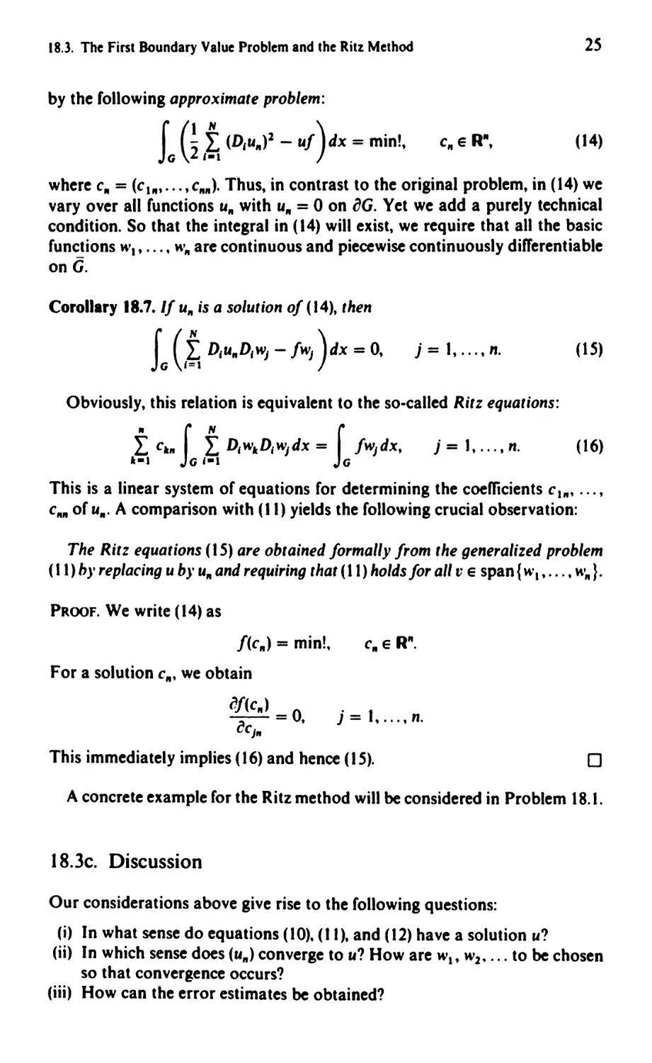
by the following approximate problem:
L G / (D/U,,)2 - uf )dX = mint, e" e R", (14)
where c" = (c l ",..., ClIft). Thus, in contrast to the original problem, in (14) we
vary over all functions u" with u" = 0 on aGe Yet we add a purely technical
condition. So that the integral in (14) will exist, we require that all the basic
functions "', , . . . , "'" are continuous and piecewise continuously differentiable
on G.
Corollary 18.7. If u" ;s a solution of (14), then
f ( f D/u"D/w j - fW j ) dx = 0,
G 1=1
j = I, . . . , n.
(1 S)
Obviously, this relation is equivalent to the so-called Ritz equations:
fCII" f f D/WilD/Wjdx= f fWJdx, j=1,...,n. (16)
i-I G I-I G
This is a linear system of equations for determining the coefficients C I ", ...,
ClIft of U". A comparison with (II) yields the following crucial observation:
The Ritz equations (15) are obtained formally from the generalized problem
(t 1) by replacing u by U" and requiring that (11) holds for all v E span { ""1' . . . , "'" }.
PROOF. We write (14) as
f(c II) = min!,
For a solution e", we obtain
C" E R".
iJf(e,,) = 0,
CCj"
j = I, .. . , n.
This immediately implies (16) and hence (15).
o
A concrete example for the Ritz method will be considered in Problem 18.1.
18.3c. Discussion
Our considerations above give rise to the following questions:
(i) In what sense do equations (10), (II), and (12) have a solution u?
(ii) In which sense does (u,,) converge to u? How are WI' W2. ... to be chosen
so that convergence occurs?
(iii) How can the error estimates be obtained?
26
I R V Jriatlonal Problems. the Ritz Method. and the Idea of Orthogonality
We give the answers to thcse qucstions in Sections 22.1 through 22.3. Here we
content ourselves with a brief explanation. Let g == O.
Ad(i). In the general case. the original variational problem (10) possesses
110 solution II E C I (G). but a unique solution II in the
Sobolev space W 2 1 (G).
I n order for the integral in ( 10) to exist. it suffices that II has generalized first
derivatives DiU that are square integrable. These functions are in W 2 1 (G). One
can motivate the choice of W 2 ' (G) by the boundary condition
II = 0 on ( G.
In this connection. note the following:
(a) the inclusion J I (G) C W 2 1 fG) is valid: and
(b) the functions from AI = {liE ('I (G): u = 0 on ( G: are dense in f21(G).
In fact the functions in the Sobolev space t'21 (G) have even boundary values
in a certain generalized sense, i.e..
II E V2t (G)
implies
II = 0 on i"G
in a certain generalized sense (see Section 21.3).
fOurthermore. we mention the fact that we can allow .r E L 2 (G) in (10). i.e..
Je, ,. 2 clx < x. Thus. the function (may have discontinuities.
The final generalized boundary value problem ( 11 ) reads as follows:
fOor /;r(,11 I E 1.- 2 (G . Cl '/;411CI ion II E W 2 1 (G) is sought so t lIat (II ) is .'lliid .for
all,. E "'21 (Gt. i.e..
(c. )
f ( ,t DjllDjl' - I r ) dx = 0
(i . :: I
for all r E W 2 1 (G).
This problem is called the generalized problem to the classical problem (12),
I.c..
( (-. )
- Il = r on G.
II = 0 on i G.
According to Proposition 18.6. each classical solution of (C) is also a gener-
alized solution. i.e.. it is a solution of (C.). However. the converse is not true.
Only with smooth data f and ?G. can one verify that the generalized solutions
of (C.) are also classical solutions of (C).
F-"rom the physical poilu of vie,v, the generalized solutions are very natural.
namely:
We cleter"Jine SO/ut;OlIS U .(or \\,lJich tlte energy integral (10) of the prin(.;ple
01 mininlal potential energy exists at least in a generalized sense.
In this connection.. note the following. In the original variational problem
( 10) and in the generaliled boundary value problem (II). we only need .(irst-
18.3. The First Boundary Value Problem and the Ritz Method
27
order derivatives. Thus. it is natural to work with the Sobolve space W 2 1 (G)
in (C*). which contains functions having generalized first-order derivatives.
In contrast to this. the classical boundary value problem (C) contains second-
order derivatives.
Ad(ii). In Theorem 22.A we shall see that {\\'1' \\'2'...} must form a basis in
W 2 1 (G) or. more generally, a so-called Galerkin scheme. By A 2 (S7), this occurs,
e.g., with regard to the functions {gPl' gP2' gPJ' ...}, where the Pi are poly-
nomials and g, with certain regularity properties, vanishes on the boundary
eG. Moreover, by A 2 (S9), one can use piecewise linear functions. i.e., so-called
finite elements. Trigonometric polynomials can also serve this purpose (cf.
Problem 18.1).
Ad(iii). In order to obtain error estimates, one makes use of duality theory,
i.e.. one considers a dual maximum problem besides the initial minimum
problem. We discuss a simple special case in Section 22.4. The general duality
theory will be treated in Part III, Chapter 50, within the context of convex
analysis.
Remark 18.8 (Reduction Principle). In conclusion, we describe a simple
method by means of which one can reduce inhomogeneous boundary value
conditions to homogeneous ones. To this end. we consider the inhomo-
geneous boundary value problem
- u = f on G.
u = 9 on cG.
We choose a function g: G --+ R with
g = 9 on eG.
If we now set l = II - g, then we obtain the homogeneous boundary value
problem
- t' = f + g on G,
t' = 0 on cG.
Analogously, the variational problem
L G It (D l u)2 - uf ) d.'t = min!, u = 9 on eG,
is reduced to
L ( I (D,(r + g»2 - (t' + g)f )dX = min!, t' = 0 on ('G.
In order to transform an inhomogeneous differential equation into a homo-
geneous one, we proceed similarly. For example, we consider the inhomoge-
lIeOIlS equation
- u = f on G,
u = 9 on eG.
28
18 Va national Problems, the Ritz Method, and the Idea of Orthogonahty
If one knows a special solution " with
-L1ii = f on G,
then we set r = II - II.. and hence we obtain the homogeneous equation
- L1r' = 0 on G,
r = y - u on ('G.
18.4. The Second and Third Boundary Value
Problems and the Ritz Method
I n this section we first of all encounter the task of explaining the concept of
nalural houlldary conditiolls. These are boundary conditions that do not appear
at all in the original variational problem, and first arise as necessary solvability
conditions. Moreover.. we shall discuss a method which allows us to force
uniqueness for problems that are not uniquely solvable, by going over to a
subspace (cf. Corollary 18.10). We consider the following problems:
fA) 'llr;at;oll£ll prohleIJI
L G , (Dill)! - llf)dX + s'G G 1121t - llg )dO = min!.
II Eel ( G).
( 17)
(B) Ge'lerll!i:ed hou1Jdary I'a/ue prohle,n
L C D,IlD j l" - (I') tlx + f,(; (lw - g)t'dx = 0 for all t' E C. (G). (18)
(C) BOIII,clary raille prohlenJ \\'illl IIalural hou,1dary condition
- L\u =.f on G.
('U
- + "" = g on c'G.
('n
( 19)
"-or II = 0 resp. II 0), (19) is called the second (resp. third) boundary value
problem for the Poisson equation.
Proposition 18.9. Let .r E C(G) and y, h E C(i G). Suppose G satisfie.'i (7). The"
the .follo"';ng are t'alid:
(a) (or II E C 2 (G).. prohleIJls (17), (18), and (19) are mutually equit:'alent;
(b) for If E C1(G), problems (17) and (18) are equ;vale1Jt;
fc) f II E C 1 (G) i... a solution of (17) M!ith h = 0, then the soll'ability condition
f .r dx + f g dO = 0
G i'G
(20)
is redid.
18.4. The Second and Third Boundary Value Problems and the Ritz Method
29
In order to associate a physical picture with these assertions, we again, as
in Figure 18.8 above, interpret u(x) as the vertical displacement of a membrane
at the point x over the region G in R 2 under the influence of the external force
f (e.g., the force of gravity) and the external boundary force g. The membrane
is to be elastically joined to the boundary oG. Problem (17) contains the
requirement for a minimal potential energy. The term 2- 1 Ji'G u 2 h dO describes
the potential energy of the elastic coupling at oG. Whereas no boundary
condition appears in (17), there occurs in (19) the so-called natural boundary
condition
ou
- + hu = g on oG
an
as a necessary solvability condition. This natural boundary condition is a
necessary condition for the boundary forces g and the behavior of the displace-
ment u on the boundary under equilibrium, whereas the solvability condition
(20) represents an equilibrium condition for the external forces f and g.
In contrast to (19), the first boundary condition II = 9 on cG in (12) prescribes
the displacement of the membrane at the boundary points.
PROOF. We use the same strategy as in the proof of Proposition 18.6. To this
end, we set
F(u) = t ( It (D l u)2 - lu )d. + t GU 2 h - ug ) dO.
Moreover, we define the real function
cp(t) = F(u + tv)
for all t E R
and fixed l' eel (G).
Ad(a). Let u E C 2 (G).
(I) (17) (18). If u is a solution of (17), then cp has a minimum at t = 0, i.e.,
q>'(O) = o.
This implies (18).
(II) (18) (19). Integrating (18) by parts yields
f (- u - f)vdx + f ( hU - 9 + oU ) VdO = 0 for all v E C1(G).
G
I t first of all follows from this that
t(- U-f)VdX=O forall veCo(G),
therefore - 4u - f == 0 on G according to Proposition 18.2. Second, it
follows from
f ( hU - 9 + Ou ) v dO == 0
fG en
for all v e C 1 (G)
30
I K Varlallonal Problems, the Rltl Melhod, and the Idea of Orlhogonalit},
that IJII - Y + i"I1/( " = 0 on l'G.. since the boundary values of the func-
tions r E C' (G) are dense in L 2 (l'G).
(III) (19) =>(18). Multiplication of - U =.r by I' E CI(G) and integration by
parts yield ( 18).
(IV) (18)=>(17). One deduces as in the proof of Proposition 18.6(IV).
Ad( b). For ( 17) <:> ( 18) only II E C 1 (G) was used.
Ad(c). Choose r = 1 in (18). 0
One clearly recognizes in the proof that the natural boundary condition
ari es by means of integration by parts.
The second boundary value problem (19) with II = 0 is 1I0t uniquely solvable
since II = I is a trivial solution. It is well known from the classical theory that
the IlIriqlleIJess is forced by means of the normalization condition
f U dx = O. (21 )
(i
We shall see in Section 22.2f that (21) also suffices for the uniqueness of the
corresponding generalized problem. As motivation for Definition 22.13 we
prove the following.
Corollary 18.10. L,ef II = 0 a"d suppose that the sO/l'abilit y c01ldit ;011 (20) ;s
."Cltisfiecl. Then lire eqllil"llience statements in Pr()po. ition 18.9(a), (b) remain
correct ;11 ('a. e olle pla('e. the additional normalization condition (21) on II a"d
r ;11 (17), (18). and (19).
PR()t)r. Let .\1 = : n' E C' (G): Je; \\' d:< = O}. I t suffices to prove that for II = 0
condition ( 18) is equivalent to
r ( t D,IID. '" - rl\' ) c/x + f (hll - g)\V dx = 0 for all ". E M. (IS.)
J G p: I , ,'G
Each f' E (., (G can be represented as r = c + \\. with \\' E AI and a constant
c. Because of (21) and" = O.
r ( t D;IID j c - IC ) dx + f (lIU - g)c dO = 0
J (; , -= I ,"'J(j
holds trivially. Therefore.. (18) follows from (IS.). The converse is obvious. 0
18.4a. Generalized Problems in Sobolev Spaces
Motivated by (IS.).. in Section 22.2f we will formulate the final generalized
problem to the second houJldar.r I'a/ue prohlem (19) with It == 0 as follows. Let
.
M. = {w E WZ1(G): fG wdx = o}.
18.4. The Second and Third Boundary Value Problems and the Ritz Method
31
For given 9 e L 2 (cG) and f e L 2 (G) with (20), we are looking for a function
ue M I
such that (IS.) holds for all \\' E MI'
The choice of the Sobolev space W 2 1 (G) results from the fact that first-order
partial derivatives appear in (IS.).
Motivated by (IS), in Section 22.2g we will formulate the final generalized
problem to the third boundary value problem (19) as follows.
For git'ell g e L 2 (rG) and h e C(cG) ,,'ith h ho > 0 on cG and 1 e L 2 (G)
,,'ith (20), "Ie are looking for a function
u e W 2 '(G)
such that (IS) holds for all '" e W z ' (G).
The condition "h ho > 0 on cG" ensures that the elastic potential energy
! J;IG hu 2 dO is positive.
18.4b. The Ritz Method
In order to formulate the Ritz method for the original variational problem
(17), we proceed from the trial
"
II" = L c." Wi'
'=-1
(22)
where the basis functions "'1' ..., WIt are given. We determine the unknown
real coefficients e I'" ..., e"" in a way parallel to (17) from the variational
problem
f ( - 2 1 f (D,U,,)2 - U"/ ) dx + r (iu:h - u"g)dO = min!, e" E R", (23)
JG i-I JCG
where Crt = (e l ",..., e",,). We assume that all w" ..., ,v" are continuous and
piecewise differentiable on G. In case h == 0, we force the normalization
condition
t u" dx = 0
by means of the requirement JG "', dx = 0 for k = 1, . . . , n.
Corollary 18.11. If u" is a solution 01 (23), then
r ( f D,u"D,w J - IW J ) dx + f (hu.. - g),,'J dO = 0,
JG i-I cG
j = I,..., n. (24)
Because of (22), this is a linear system of equations for determining c I '" . . . , ClIft'
32
I H Va national Problems. the Ritz Method. and the Idea of Orthogonality
The proof runs analogous to that of Corollary 18.7. Equation (24) results
formally from the generalized boundary value problem (18) if one replaces u
there by "n and requires that (18) is valid for allt, E span {"'... . .. "',,}.
Assertions concerning existence. uniqueness. and convergence of the Ritz
method can be found in Sections 22.2f and 22.2g.
18.5. Eigen\'alue Problems and the Ritz Method
In this section it will be shown that eigenvalue problems result from appropri-
ate variational problems with side conditions. The method of Lagrange multi-
pliers is typical for the investigation of variational problems with side condi-
tions. We shall occupy ourselves therewith in detail in Part III. Here we use
a direct method analogous to Sections 18.3 and 18.4. We consider the following
problems. Let AI = : II E C. (G): u = 0 on l'G}.
(A) Variatiollal problenl M'ith side conditions
t i (DjU)2 dx = min!. tI E M.
f U2 dx = I,
(i
[ Uti. dx = O. r = 1..... m - 1.
Je;
(25a)
(25b)
(25c)
This problem is to be understood as follows: We determine u 1 from (25a) and
(25b). Then 1'2 results from (25a)-(25c) with m = 2. and so forth.
(8) Gel1erali:ed bouIJdary eigent'alue problem
f ( ,f DjllMDjl' - JlMUM I ' ) dx = 0 for all l' E M,
G 1=1 (26)
U m = 0 on eG.
(C) Boundary e;genl'alue problenJ
- u'" = JJ",Il", on G,
u'" = 0 on eG.
(27)
(D) Ritz I1lethod
f ( .t DjwDj\\i - Jl""') ) dx = 0, j = I,.... n. (28)
G I-I
The basis functions \\'1' . . . 'I "'n are given. We seek JJ E R and the real coefficients
(' .' . . . , c" of
n
\V = L Clt "'It.
_-I
18.5. Eigenvalue Problems and the Ritz Method
33
Problem (28) is an eigenvalue problem of the type
Ac = JJBc,
(28* )
where A and B are symmetric n x n matrices and the column matrix c contains
the elements c. to c".
Parallel to Sections 18.3 and 18.4 one obtains (28) from the generalized
boundary eigenvalue problem (26) if one only simply requires that (26) holds
for all functions v in span {\v.,. . . , w,,}. So that w in (28) satisfies the boundary
condition
w = 0 on cG
we require that
"', = 0 on oG
for k = I, .. . , n.
So that the integral in (28) is meaningful, we require, !ay, that all w. are
continuous and piecewise continuously differentiable on G. A precise analysis
in Section 22.11 shows that the eigensolutions and eigenvalues of(28) approxi-
mate the eigenfunctions u'" and eigenvalues /.l", of (27) in an appropriate sense.
A numerical example for the Ritz method will be considered in Problem
18.1 b.
Proposition 18.12. Slippose that the region G satisfies (7). Then the following
are t alid:
(a) Et ery solution u'" e C 2 (G) of (25) also satisfies (26) and (27) for m = I, 2,
. .. ",;th suitable JJ", E IR.
(b) Et ery solution u'" eel (G) of (25) also satisfies (26).
(c) For u'" E C 2 (G), the boundary eigenvalue problem (27) and the generalized
problem (26) are equivalent.
PROOF. Ad(a), (c). Let u'" e C 2 (G). We set
r t (D,U)2 d.'(
F(u) = J G 'at .
L u 2 dx
(I) (25) (26). First let m = I. Recall that
M = {u e C1(G): u = 0 on cJG}.
If u I is a solution of (25), then it is also a solution of
F(u) = min!,
We define the real function
cp(t) == F(u. + tv) for all t E R
and fixed t' e M. Since U 1 + tv e M for all t, the real function cp has a
u eM, u o.
(29)
34
I Vanatlonal Problcm4\. the Ritz Method. and the Idea of Orthogonality
minimum at I = O. i.e..
«/,'(0) = o.
This implies
1 4 ( t D," I D. r - Ii." .1' ) c/x = 0
. (i , ': I
for all (' E I.
"'ith I'I = f"(u.). after a simple calculation. This is (26) with In = I.
No\\" let In = 2. We set
.\1. = {" E AI: 1; flU I dx = o}.
Let 112 be a solution of (25). Then II 2 is also a solution of
f.(II) = min!.
II EM. . II f= O.
We set
"'(I) = F(1I 2 + t"')
for dll t E (R
and fixed "" E ,\1." Since 11 2 + ,n' E .\1. for aliI.. the real function'" has a
minimum at t = O. i.e..
""(0) = O.
This yields
L ( D j "2 D j ". - I l 2"2 u) (Ix = 0 for all '" E MI' (301
Furthermore.. it follows from (26) with ,,, = I. l' = 112. that
L; ( DjIl2Djlll - III 1(2 1 '1 ) dx = O. (31)
Each r E .\1 can be represented as
r = CII. + "'.
n' E J\".. (' E R.
From J(; "1"2 c/x = 0 it easily follows that (30) is also valid for all \" E .\'1.
T his is (26) \\' i t h ", = 2.
One deduces the result for 1)1 > 2 analogously.
II) (26t (27). Integrating (26) by parts yields
f - l\u", - JI",II", )1' cI. = 0 for all l' EM.
(;
Proposition 18.2 yields -l\u", - JI",I1", = 0 on G, because Co (G) c: M.
(III) (27):::. (26). Multiplication of - [\lIm = J'm"", by r E J\1 and integration by
parts yields (26).
Ad(b). In the proof of(aJ we used only that II E C.(G). 0
18.6. The Ho1der Inequality and its Applications
35
The final generalized problem in Section 22.13 reads as follows.
We are looking for a function Ulft e W 2 1 (G) and a real number #lift such tllat
relation (26) Iioids for all t' e W 2 1 (G).
As in Section 18.3, this is motivated by the fact that the set M is dense in
the Sobolev space W 2 1 (G). The existence of solutions of the generalized prob-
lem and the convergence of the Ritz method will be proved in Section 22.13.
18.6. The Holder Inequality and its Applications
The most important inequality in modern analysis is the following Holder
; lIeqlla lit.\':
L IfYldx S; (t IfI PdX )' p (t IYI'dX)"
(32)
with
1 1
- + - = 1.
P q
1 < p < x.
(33*)
If we set
Ufll p = (t IfI PdX )' p.
then we may write (32) in the form
tfYdX S; tlfgldXS; UfllplIgU"
(33)
Proposition 18.13 (The Holder Inequality). Let G be a nonenlpty nleasllrable set
;n At" ",;tl, N > I (e.g.. G ;.'i ope" or closed). Then ;t follo,,'.'i .fro,,,
fe L,(G).
g e Lq(G)
"';111 (33.) ,hat (33) holds.
If fe L,(G) and g e Ly(G), tllell (33) holds \\'ir/l p = I and q = x'.
For the convenience of the reader. the basic material of modern analysis is
summarized in the Appendix (e.g., measurable sets and measurable func-
tions. the Lebesgue integral. the Lebesgue spaces L,( G). 1 < P < 'X. etc.). For
example. we have
fe L,(G),
iff .f: G -+ R is measurable and
I sp< 'X.J
IIfll, < x.
36
18 Variational Problems, the Ritz Method. and the Idea of Orthogonality
f-'urthermorc. we have .re L-r(G) iff I: G -. R is measurable and there exists a
real number C such that
I.{(x)l < C
for almost all x e G.
Thcn. II {I: I is equal to the infimum of all possible C. We write
lI.fll x = ess sup 1/(.\')1.
.lEG
For I < p < x.. L p ( G) is a real B-space with the norm n." p' provided
we identify any two functions which differ only on a set of N-dimensional
Lebesgue measurc zero. That is, we identify .r with g iff f(x) = g(x) for almost
all x E G.
Note that only pathological sets and functions are lIot measurable. Never-
t he less. in each case. one has to check that the functions and sets under
consideration are measurable. To this end one can use the tools summarized
in A 2( 1)- A 2( 12). Furthermore, note that in each case, one has to check the
existence of the integrals under consideration. In this connection. the most
important tool is the majorant criterion of Lebesgue A 2 ( 11).
Roughly speaking. Proposition 18.13 tells us the following:
{ the riglu-hantl side ;11 (33) exists. then the remaining integrals also exist al1d
the ;IJeqflalities (33) hold.
The Holder inequality was first proved by Otto Holder (t 859-1937) in 1889
for series. The extension to integrals is due to Fryges Riesz. The following
proof of Proposition 18.13 is based on the Young inequalit.\,:
" l' b"
Clh < + -. for all a, heR. (34)
p q
and all p. q with (33.).
In Part III we shall show that (34) is the germ cell of the general duality
theory.
PRCX)F 01-" PROPCJSITIC)N 18.13.
(I) Proof of (34). If p = q = 2. then (34) follows from (a - h)2 > O. In the
general case, we consider the function
a P h 4
F(a) =. + - - - ab
p q
for fixed b > O. We have
f-(O) > O.
/;(h 4 'P) = O.
lim F(a) = + x .
CI-+X
"Ience f. has a minimum on R.. Thus, there exists a number a o > 0 such
that
F(a) > f'(a o )
for all a E R + .
18.6. The Holder Inequality and its Applications
31
From F'(ao) = 0 it follows that ao = b"", and hence F(ao) = o. This is
(34).
(II) Proof of (33) for 1 < p < 00. We may assume that IIfll" = IIgli. = I.
Otherwise we use a division. Integration of
I/gl S III' + Igl'
p q
over G yields JG Ifgl dx 1. This is (33).
(III) In the case p = 00, we obtain
t Ig d.v: s t I/lIgl d.v: s III II x t Igi d.v:.
o
We now consider some important applications of the Holder inequality
which will be used frequently.
18.6a. The I-Trick
The I-trick means that we apply the Holder inequality (33) with 9 = I. This
is only possible for bounded measurable sets G. Otherwise IIgli. = 00. This
way we obtain
t I/ldx S (measG)I"(t I/IPdx Y'p
for all f e L,,(G) with I < P < .
(35)
EXAMPLE 18.14. Let G be a nonempty bounded measurable set in R N , N I.
Then the embedding
L,(G) s Ls(G),
ISssrsoo
is continuous, i.e., we have
IIhlls const Uhll,
for all h E L,( G).
(36)
PROOF.
(I) Let 1 S s < r < 00 and let h E L,(G). Then (36) follows from (35) with
f = Ihls and p = rise
(II) Let I S s < r = and h E Lao(G). Then Ih(x)1 S C for almost all x E G.
Hence
(t Ihlsdx Y's S CmeasG.
This implies (35), since IIhll2> is the infimum of all C.
o
EXAMPLE 18.15. Let G and H be two nonempty bounded measurable sets
in R N with N I and G s H. Suppose that f E L,(H) with I < p S 00.
JX
I \',anatlondl Problems. the Rllz Method. and the Idea of ()rthogonalit
-"hen
,.
J 1'1 dx < (meas G)I elll.fll / . pclI .'
(,
\\'here'l I ...... P I :..= 1 for 1 < P < _ and 'I = I for r = x.
Thi'\ follo\,." from (J }
Remark 18.16. If 1 < P < -, and I E L"fll). then
I f I d \" -+ () as mcas G o.
I (,
\\'here If and (i arc given as in Example I .15. This follows from the continuity
of the embedding Lp(llt c 141 (H) and the absolute continuity of the integral
(cf. A:!(20H. In the case I < P < x. Example 18.15 contains precise information
about this limiting process.
18.6b. l he Sum Trick
The prototype of the sum trick is the inequality
2tlh < I:" + I: - I h:!
for all u. hER +
(37t
- -
and aliI: > O. which follo\\'s from (,: l:d - h, \, r.t > O. This inequality tells us
that it is possible to estimate a product against a sunl of squares. where one
of the summands can be made arbitrarily small. From the Young inequality
f 34) there follo\vs a generalization of (37). namely.
1."(11' h q
ah < +
- I' ql;q
and alii: > () J ere. I < p < and p - t + C/ - t = I.
for all Cl. hEIR..
(38)
EXA 1PII: 18.17 Let G be a nonempty measurable set in (R". N > 1. Suppose
that I E 14,,(G) and / E L«I((j) with I < p < x. and q-I + p-I = I. Then
i r" i 1 i
I f /I ,,"( < . - I f I p d."( + - . q I g I q d."(
(, p (, ql. (;
holds for alii; > o. In particular.. one can choose p = q = 2.
This follows from the Holder inequality and from (38).
f39)
18.6c. The Nemyckii Trick
For the investigation of nonlinear differential and integral equations. the
Nemyckii operator plays a fundamental role. This operator will be considered
18.6. The Holder I nequality and its Applications
39
in Section 26.3. In this connection, the following result is crucial. Our goal is
to show that the estimate
I \\'(x)1 I u(x)1 + I r(x)I'" on G.
1 S p.. q < .x, 't
(40)
implies
11"'11, s const( lIull, + IIt'II ").
EXAMPLE 18.18. Suppose that:
(i) G is a nonempty measurable set in R N , N > I.
(ii) II e L,(G) and l' e L,(G).
(iii) The function ,,': G -+ R is measurable (e.g., continuous) and (40) holds.
Then we have ". E L,(G).. and (41) holds.
(41 )
PRC)()F. Let r > O. We use the inequality
(a + b)r < C(a r + b r )
for all a. h e R.'t
(41 * )
where the constant C depends on r. From (40) we obtain
1\\'1' < C(lul' + It'I').
Integration over G yields
t Iwl 4 dx S c(t lul 4 dx + t 1l'IPdX).
Now the assertion (41) follows from (41*) with r = Ijq.
o
There are two completely different methods for the investigation of nonlinear
differential and integral equations:
(i) One uses L,tG)-functions.
(ii) One uses C'(G)-functions or C t .2(G}-functions.
Note the following peculiarities. In the case (i). Example 18.18 above is
responsible for the fact that one needs restrictive gro".th conditions for the
nonlinearities. But one has the advantage that the L,(G)-spaces are re.f1exil'e
in case 1 < p < 'X. In the case (ii), no growth conditions are needed, but the
C'-spaces and C'. -spaces are not reflexive. Unfortunately.. many existence
theorems are only valid in renexive B-spaces. The point is that in renexive
B-spaces. each bounded sequence has a weakly convergent subsequence.
In the Appendix, A 2 (29). we will consider the Holder inequality and the
Young inequality for n factors. If we combine these two inequalities. then we
obtain the following Holder- Young inequalit)':
r Ii Ii dx
JG 1=1
" ( i ) I "
S n l.hl" dx
,a 1 G
" I i
< L - l.hl'" dx.
i-I P, G
(42)
40
I R Variational Problems, the Ritz Method, and the Idea of Orthogonality
This inequality holds for all
E L,,(G).
, = 1. . . . , II.
where the real numbers I < PI' . ... p" < x' satisfy the relation
t l =1.
i-I Pi
and G is a nonempty measurable subset of R N , N > 1.
18.7. The History of the Dirichlet Principle
and Monotone Operators
In order to determine integrals of algebraic functions and their inverse func-
tions (elliptic and Abelian functions), one can apply a principle which was used
by Dirichlet in his lectures. This principle allows us to solve boundary problems
for the Laplace equation.
Bernhard Riemann (1857)
By the Dirh'lr/t'l pr;,,(';plt' we understand a method for solving boundary value
problems via minimum problems for variational integrals. This principle goes
back to Gauss (1839), Lord Kelvin. and Dirichlet. Weierstrass (1870) was the
first to underline the shortcomings of this principle. He showed that there are
vari ltional problems which do not have any solution. In 1900 I showed that it
is possible to justify rigorously the Dirichlet principle.
David Hilbert (1901)
Riemann f 1826 - 1866) \\'as a man of outstanding intuition. By his ingenuity he
outshone all his contemporaries. Whereever his interest was awoken. he began
anew, without allowing himself to be misled by tradition and without recognizing
any compulsion of systematology.
Weierstrass (1815-1897) was first and foremost a logician. He proceeded
slowly, systematically, gradually. Whereever he worked. he strove after the final
form.
Certainly mathematics itself pronounces the verdict, even if it does so without
rigorous proof. It will, however. remain for ever the secret of vigorous produc-
tivity to find new questions and to discover new theorems which lead to valuable
results and new interrelations. Without new ideas and without the formulation
of new objectives, mathematics would soon amount to nothing more than the
rigidity of its proofs, and would begin to stagnate, its fuel running out.
So, in a certain sense, mathematics has been furthered most by those who
distinguished themselves more through their intuition than through strong
deduction.
Felix Klein (1926)
The "'ell-known hOll mot that uEurol>ean philosophy". is only a footnote 10 Plato
is perhaps true. but I would venture a much truer one: modern mathematics is
only a footnote to Riemann.
Krys7tof Maurin f 1982)
18.7. The History of the Dirichlet Principle and Monotone Operators
41
18.7a. The Calculus of Variations
As the Dirichlet principle is very closely connected with the calculus of
variations, we will next take a short glance at the history of this fundamental
mathematical discipline.
In Parts III through V we will see that many basic equations of physics
result from an important variational principle, namely from the principle of
critical or stationary action, which is often incorrectly called the principle of
least action. The general theory of relativity and the gauge field theories in
modern elementary particle physics belong here.
It seems that the local symmetries of variational integrals, which lead to the
gauge field theories, provide the key to understanding the four fundamental
interactions in nature: the strong, weak, electromagnetic, and gravitational
interactions. This will be discussed in detail in Part V.
About three hundred years ago, at the beginning of a fascinating develop-
ment in mathematics and physics, there was the following prize competition.
Johann Bernoulli, professor of mathematics, greets the most sophisticated
mathematicians in the world. 1 Experience shows that noble intellectuals are
driven to work for the pursuit of knowledge by nothing more than being
confronted with difficult and useful problems.
Six month ago, in the June edition of the Leipzig Acta Euriditorium, I presented
such a problem. The allotted six-month deadline has now gone by, but no trace
of a solution has appeared. Only the famous Leibniz informed me that he had
unraveled the knot of this brilliant and outstanding problem, and he kindly
asked me to extend the deadline until next Easter. I agreed to this honourable
request. . . . I will repeat the problem here once more.
Two points. at different distances from the ground and not in a vertical line.
should be connected by such a curve so that a body under the influence of
gravitational forces passes in the shortest possible time from the upper to the
lower point.
Johann Bernoulli (January, 1697)
This paper sol\'es my brother's problem, to whom I will set other problems in
return.
Jacob Bernoulli (May, 1697)
How does one apply the methods of maxima and minima in the determination
of unknown curves (solution to variational problems)?
Leonhard Euler ( 1744)
The famous Euler succeeded in tracing back to a general method all investiga-
tions on variational problems. But however sophisticated and fruitful his method
may be, one has to admit that it is not simple. Here one now finds a method
which only uses simple principles of calculus.
Joseph Louis Lagrange (1762)
I leibniz (1646-1716). Johann Bernoulli (1667-1748), Jacob Bernoulli (1654-1705) (brother or
Johann Bernoulli), Daniel Bernoulli (1700-1782) (son of Johann Bernoulli), Euler (1707-1783),
Lagrange (1736-1813), Legendre (1752 -1833), Gauss (1777 -18SSt, Jacobi (1804-185 I), Dirichlet
(180S-18S9). Riemann (1826-1866). Weierstrass (181 S-1897), and Hilbert (1862-1943).
42
I Vanatlonal Problems. the Ritl Method. and the Idea of Orthogonality
The necessary conditions for the solutions of variational problems. found
by Euler and Lagrange, will be considered in Section 18.18. We have already
met the prototype in Proposition 18.6.
Euler lIsed a difference method. Lagrange"s simple method. based on inte-
gration by parts. is still used today. For example. we used Lagrange"s method
to prove Proposition 18.6. In contrast to Euler. Lagrange could also deal with
variational problems for multi-dimensional variational integrals. which lead
to partial differential equations.
In 1110'( of the prohlcm of the calculus of variations it follo\\'s from the nature
of the problem as to \\'hether or not a minimum or maximum is possible. There
arc. ho\\'e\er. case In "' hich this distinction is not so easy. I therefore thought
that the formulation of a criterion. which allows for a distinction between
ma,ima and Inlnlma. \\'ould be useful.
Adrien-Marie Legendre f 1786)
Ttti !ul. alled Legendre condition _ill he Cfll1!1idered in Settion I R.17. It
d_..t. uh .. fl ...., ",." Ui " tUf nu,.Uti. ilt" Iflln'fttMr t...MlHd'lI twh, .1J
that he had found a umcient condition. As Jacobi. however" pointed out.
Legendre.s observations contained a serious mistake.
I ha \ c ucceeded In closing an essential gap in the calculus of variations. lJntl1
no", If" general sufficient condition was known by which to recognize whether
it ma'lmum or minimum existed. For example. the integral. considered in the
principle of least action. can never have a ma,imum. as Lagrange mistakenly
believed: in no way. ho\\'ever. will it always have a minimum.
Carl Gustav Jacob Jacobi (1837)
I n Section 29.12d Vie will consider a general functional analytic formula-
tion of the classical Jacobi theory based on so-called accessory variational
problem,;.
The decisl\c idea con ist of studying a linear eigenvalue problem" which
is closel) connected \\'ith the quadratic form of the second variation. Therefore.
our results on linear eigenvalue problems in ("hapter 22 are of great interest
for general variational problems.
.. rum thl ..Indcpendence theorem" arise not onl) the known sufficient condi-
tions of Jacobi and Weierstrass for the appearance of minima. but also all the
essential conclusions of the Hamilton Jacobi theory.
David Hilbert ( 1906)
Hilbert refer here to his invariant path integral. which we will consider in
Part III \\'ithin the frame\\'ork of field theory in the calculus of variations (see
Proposition 40.17). There \\'e will also elucidate the connection with the
famous Weierstrass £-function.
The Hamilton Jacobi theory describes mathematically the fundamental
propagation of action in nature and the structure of optimal processes in
18.7. The History of the Dirichlet Principle and Monotone Operators
43
nature. technology. and economics. This will be studied in detail in Parts III
through v.
18.7b. The Beginnings of Potential Theory
In 1182 Laplace remarked. in a study on the shape of the planets,. that the
potential
t i p(:<}
u(y) = -- dx
4n G Ix - yl
of a mass distribution of density p on the region G satisfies the following partial
differential equation
(43)
L11l = 0 o tside G,
(44)
which is called the Laplace equation.
Interestingly. he first found this equation in the complex form of spherical
coordinates. In 1181 he discovered the much simpler expression for u in
Cartesian coordinates, namely,
&u = u + u.,,, + u ,.
where x = ( ..". ,). In 1813 Poisson found that for a ball G the following
equation is valid in the case of a constant density p:
-&u=p onG.
This equation is called the Poi. son equation.
(45)
Gauss proved the validity of this equation for more general cases in 1839
in his fundamental paper: "General Theorems about the Forces of Attraction
and Repulsion which are Inversely Proportional to the Square of the Di -
tance.... Such forces are. for example, Newton's gravitational force and the
electrostatical Coulomb force. Gauss also used such forces in order to explain
magnetic phenomena. The above-mentioned work of Gauss is the beginning
of the mathematical foundations of potential theory. In this work, for example,
Gauss proved the fundamental mean value property of potential functions
(solutions of the Laplace equation &u = 0). He had already realized in 1813
that volume integrals can be transformed into surface integrals (Gauss' inte-
gral theorem). The formula of integration by parts. which is at the forefront
of the modern theory of partial differential equations. is equivalent to the
integral theorem of Gauss. We have already discussed the fundamental impor-
tance of this theorem for topology (mapping degree, cohomology) in the
introduction to Chapter 12.
In 1801 Gauss became Professor of Astronomy and Director of the Ob-
servatory in Gottingen. where he worked until his death in 1855.
I Laplace (1749-1827». Poisson (1781-1840). Gauss fl777-18SS). and Green (1793-1841).
44
I H Varaational Problems. the Ritl Method. and the Idea or Orthogonality
For valuable contributions to potential theory we also have George Green
to thank. who. in 1829. discovered the Green integral formulas and who
introduced the important Green function. which allows us to represent the
solutions of elliptic boundary value problems by integral expressions.
18.7c. Riemann and the Dirichlet Principle
From 1846 until 1847 Riemann. studied under Gauss in Gottingen. In the
years 1847 1849 he was a student in Berlin and attended lectures by Dirichlet, I
Jacobi. Eisenstein. and Steiner. He learnt about the Dirichlet principle in
Dirichlcfs Icctures on potential theory. During this time, as a student in Berlin,
the idea matured within Riemann to give a foundation to the theory of
complex analytic functions by means of the theory of partial differential
equations for real functions. To explain this let
.f(:) = " + ir
he an analytic function. Then the real functions" and r satisfy the so-called
("au('II.r Rienrallll di{ferelltial equations
Il = r".
",,= -I' .
where = == + ;'1.
By differentiation. \\'e obtain the Laplace equation
,, + II"" = O.
(46)
and r + r"" = O. i.e.. All = Ar = O. The corresponding variational problem
to (46) is given by
f 2 2 d - .,
(u + u,,) x - min..
G
(47)
II = y on tG.
In this way Riemann was able to give a physical interpretation, in terms of
potential theory. to the mathematical problems of the theory of analytic
functions. During his lifetime Riemann, like his teacher Gauss. tried to find
Jeep COllnf!ctions between mathematics and physics.
In 1849 Riemann returned to Gauss in Gottingen, and in 1851 handed over
his dissertation which was much praised by Gauss. In this fundamental paper
of a mere fourty pages. Riemann laid the foundations for the complex function
theory and proved his famous theorem on conformal mappings. In this paper,
and in his fundamental paper on Abelian integrals on Riemannian surfaces
written in 1857. he placed a general existence principle at the head of the
theory. which he called the Dirichlet principle. In today's language the principle
, Riemann (lH 6 IH66,. Dlrachlet 0805 18591. Jacobi (1804 1851). Eisenstein (1823- IR52t.
Steiner t 1796 -I H63). Weierstrass t t 815-1897).
18.7. The History or the Dirichlet Principle and Monotone Operators
45
is as follows:
(D)
For giren sufficient I}' smooth functions 1,' and g, the minimum problem
t (u( - ('.,)2 + (u( + ('.,)2 dx = min!.
u = g on cG
ah,'aJs has a solution in the set of piecewise continuously differentiable functions.
Here, G is a bounded region in 1R2.
In the special case to = 0, problem (D) corresponds to (47). Like Dirichlet,
Riemann made no attempt to prove this existence principle. Both considered
it to be obvious that problem (D) possesses a solution. In fact, the time was
not yet ripe for an existence proof for (D).
18.7d. The Theory of Abelian Integrals
The theory of Abelian integrals and their inverse functions was at the center
of Riemann's and Weierstrass' research on complex function theory, which
was carried out totally independently from one another.
In his obituary for Weierstrass, Hilbert writes:
Karl Weierstrass studied law in Bonn. In 1839 he decided to study mathe-
matics and therefore went to Munster, where he attended a mathematical lecture
by Gudermann on elliptic functions. That was the only mathematical lecture
which he ever heard in his life. After that Weierstrass worked from 1840 until
1855 as a schoolteacher. totally isolated. in small towns. During this time he
published a series of fundamental papers on the most difficult problems of
complex function theory.
In his academic inaugural speech in t 857 as a newly elected member of the
Berlin Academy. he described how the theory of elliptic functions had tremen-
dously attracted him. even before his studies, and that he regarded it as one of
the main tasks of mathematics to create a general theory on periodic functions
of 5e\'eral complex variables (Abelian functions).
To prepare himself for this difficult task, he first studied the available tools
and occupied himself with less difficult problems. As a result of these studies
he published. during the years 1841-1843. papers on the theory of power series
and on the definition of analytic functions by means of algebraic differential
equations.
In 1854 Weierstrass first succeeded in finding the solution to the famous
"inverse problem" posed by Jacobi in 1832. The generalization of this result to
general Abelian integrals, which was later obtained by Riemann and then by
Weierstrass, is one of the greatest achievements in analysis.
Whereas Riemann based his theory of Abelian functions on the imperfect
nonrigorous Dirichlet principle. Weierstrass' theory is based on purely algebraic
arguments.
46
'X Vandllonal Problems. the Ritz Method, and the Idea of Orthogonaht
We would brlcny like to explain the mathematical background to the
reader. By an Abelian integral we understand an integral of the form
A = f RI:. 1\'1:))d:.
"'here \\ = "'t:) IS an algebraic function and R = R(:. "') is a rational function.
i.e,. the function '" = ".(:) satisfies an algebraic equation of the form
ll"{:),,,n + ... + Cl l f:)\" + a o (:) = O.
"'here tI u . . . .. a" arc polynomials with respect to :. For example. let Pn be a
polynomial of degree II and let
".2 = Pn(:)'
Then. '" = '\ Pn t :). If II = 3.4 (resp. II = 5.6). then tht: integral J R(:. "'(:Ht/:
is called elliptic t resp. hyperelliptic). I n the special case \\,2 = I - :2. we obtain
the Abelian integral
I = f: ,
d:
I - :2
Here. the Inverse function is given by : = sin t.
In 1832 Jacobi formulated the following hypothesis:
CO'I. id('r lire "\'o f,llrctio,rs 1l = r'(l,. h) and r = I'(a. h) I;I"ell hy tire ,(ol/()\\'illO
\\'st£'II' of "yperelliplic inte /rals:
I II d: I ' d:
"II \.-P I:) + "" rp6(:- ) = a.
I " :d: I I :d:
", \. ptol -) + I, \.' ;;6(:) = h.
"flrell IIr£' ,,, 0 fllll( I;OllS II + I' alld Ul' art' ullil'a/f.'lIt and they po, sess ,(ollr diflerent
periods.
Riemann and Weierstrass proved a generalization of this assertion for
systems of II equations with n general Abelian integrals. Whereas Weierstrass
used algebraic methods.. Riemann worked with the topological idea of the
so-called Rie,nanniclll slIr.(ace. To explain this. we shall consider the elliptic
integral
f RI:. wi:)) d:
with ,,'f:) = \. p(:). \\'here p is a polynomial of degree 11 = 3.4 with pair\\'ise
different zeros. Riemann"s idea was to consider this integral on the Riemannian
surface 1. of ". = ,,'f:). Here T is homeomorphic to a two-dimensional torus.
The point is that on the torus. two different paths exist. C 1 and C 2 ' as pictured
18.7. The History of the Dirichlet Principle and Monotone Operators
47
T
Figure 18.9
in Figure 18.9. Set
W, = r R(z, W(Z)) dz,
JC i
Each path on T can be deformed into
nC. + mC 2 ,
where nand m are integers. It follows from the Cauchy theorem that the
deformation of paths on T does not change the corresponding integrals.
Consequently, we obtain, without any calculations. that the elliptic integral
J R(z, ,,'(z))d: has the two additive periods WI and W2. Therefore, the corre-
sponding inverse functions, i.e., elliptic functions. have two periods.
Riemann generalized this argument to general Abelian integrals. He showed
that the corresponding Riemannian surfaces are homeomorphic to spheres
with p handles, and hence the corresponding Abelian integrals have 2p additive
periods (Fig. 18.10(a)). The number p is called the genus of the Riemannian
surface. This is the only topological invariant of Riemannian surfaces which
correspond to algebraic functions. In the special case of a two-dimensional
torus we have p = 1 (Fig. 18.IO(b)).
Ingeniously, Riemann recognized that there are close and deep connections
between analysis, topology, and algebra. With this recognition he decisively
innuenced mathematics in the twentieth century.
At the end of the last century Hilbert discovered that a new powerful
instrument for number theory can be obtained by combining the idea of the
Riemannian surface with the Galois theory. Thus he gave number theory a
i = I, 2.
@) >
p=2
(a)
p=1
(b)
Figure 18.10
48
I H Varaatlonal Problems. the Ritl Method. and the Idea of Orthogonality
decisive new impulse. This is discussed in detail in the famous book by Felix
Klein (1926): The History of Mathematics in the Nineteenth Century.
It is quite interesting that today Riemannian surfaces playa fundamental
role in the so-called string theory of physicists (see Section 76.7) and in the
theory of solitons (see Problem 30.7).
18.7e. The Criticism of the Dirichlet Principle by Weierstrass
In studying Riemann's work, Weierstrass found the Dirichlet principle un-
satisfactory. In 1870 he constructed a counterexample which showed that the
existence of solutions to variational problems is no trivial matter. He considered
the follo\\'ing minimum problem:
Je() d ( f I fxf'fxH 2 dx = min!,
-I (48)
.r ( - 1 ) = a,
with a # h. The sequence of functions
fll('\:) = a_ + b _ _ - b . arctan nx ,
2 2 arctan n
.(( I) = h
n = I, 2, . . .
satisfies the boundary conditions h( - I) = a and f,,( I) = b, and we obtain
J(/,,) -. 0
as 11 -. T.;.
Consequently, the infimum of the integral in (48) is equal to zero. However,
there is no CI-function which solves the minimum problem (48). In fact, if f
is such a function, then it follows from (48) that xf'(x) = 0 on ] - I, 1 [. This
implies _f = constant. But this contradicts the boundary condition I( - 1) i=
{( 1 ).
Because of this. Weierstrass' essential result is as follows:
(a) Each rariat;onal prohle,n \\'hich i.') bounded belo"' possesses an infimum and
"etlce n,i"i,nal seqlle"('e. eX;. t.
(b) Ho"'erer, those minimal sequences do not necessaril}' conl'erge to a sol,,';on
oj' the l'tlr;at iOPlal prohlenl.
As the Dirichlet principle could not at first be justified, one looked for other
methods to save Riemann's theory. To this end, Schwarz (1843-1921), C.
Neumann (1832 - J 925). and Poincare (1854- 1912) developed special methods
to solve the Laplace equation without using the Dirichlet principle.
18.7f. Hilbert's Justification of the Dirichlet Principle
In his Paris lecture in 1900 Hilbert formulated his famous twenty-three
problems, which have substantially innuenced mathematics in this century.
18.7. The History of the Dirichlet Principle and Monotone Operators
49
On this subject we recommend two anthologies by Aleksandrov (1971) and
Browder (1976). In connection with the twentieth problem Hilbert said:
The sophisticated methods ofSchwa C. Neumann, and Poincare essentially
solved the boundary value problem for the Laplace equation. However, these
methods cannot be directly extended to more general cases. . .. I am convinced
that it will be possible to get these existence proofs by a general basic idea.
towards the Dirichlet principle points. Perhaps it will then also be possible to
answer the question or whether or not every regular variational problem pos-
sesses a solution if. with regard to boundary conditions. certain assumptions are
fulfilled and if. when necessary. one sensibly generalizes the concept of solution.
At this time Hilbert had already found a possible means of saving the
Dirichlet principle. He first presented a rough idea in a lecture in 1900, and
then in greater detail in a later paper in 1901 (cf. Hilbert (1932), Vol. 3, pp.
10-37). Hilbert's idea was as follows:
(i) one constructs a minimal sequence; and
(ii) one shows that this minimal sequence contains a converging subsequence
whose limit provides a solution to the original variational problem.
This is a typical compactness argument. In the second volume of the standard
work of mathematical physics by Courant and Hilbert (1937), one finds the
idea (i). (ii) worked out.
In today's terminology one works in Courant and Hilbert (1937) with dense
subsets of the Sobolev spaces
Wl(G) and W 2 '(G),
where these subsets consist of piecewise smooth functions. The decisive com-
pactness argument is based on a compactness theorem of Rellich (1930). which,
in today's terminology, implies that the embedding
W 2 1 (G) c: L 2 (G)
is compact.
In their fundamental paper on difference methods. Courant. Friedrichs, and
Lewy (1928) had already emphasized the advantages of using generalized
solutions of partial differential equations. The concept of generalized solutions
is also stressed in Courant and Hilbert (1937).
In Part III we will formulate two general functional analytic existence
principles for extremal problems, namely:
(a) a compactness principle which generalizes (i) and (ii) above (Chapter 38);
and
(b) a convexity principle which is based on the Hahn- Banach theorem, i.e.,
on the separation of convex sets in B-spaces by hyperplanes (Chapter 39).
Our functional analytic justification of the Dirichlet principle in Section
18.10 is closely related to (b), i.e., in order to give a very elementary existence
proof. we avoid compactness arguments.
50
1 M Variational Prohlems. the Rltl Method. and the Idea of Orthogonaht),
The Ritz method was developed by Walter Ritz in his post-doctoral thesis.
\\'hich he wrote in 1908 in Gottingen. Ritz applied his method, for example.
to obtain numerical results for the clamped plate.
A few more words about Hilbert. The great mathematical tradition which
Gauss founded in Gottingen was continued there by Riemann. Klein. and
Hilbert. On Felix Klein's initiative, Hilbert, at the age of thirty-three, was
appointed to a professorship in Gottingen. where he remained until his
death. In the 1920's Gottingen was the leading center in mathematics and
quantum physics. The r-"ascist seizure of power in t 933 also had the worst
possible consequences for Gottingen. The world famous mathematicians
Emmy Noether. Emil Artin. Paul Bernays. and Richard Courant were driven
a\\'ay. as \vell as the Nobel Prize winner for physics. Max Born. The number
theory specialist Edmund Landau and the Nobel Prize winner for physics
James Franck lost their positions. Hilbert's close personal friend Otto
Blumenthal emigrated to the Netherlands and was murdered in the concentra-
tion camp Thercslcnstadt in 1944. When the Nazi minister for education asked
Hilbert if mathematics in Gottingen was nourishing, Hilbert replied:
"There is no mathematics in Gottingcn anymore."
Hilbert died at the age of ninety-one, in t 943. Scarcely a dozen friends
accompanied the most important mathematician of this century to his final
resting place. The words on his gravestone comprise his epistemological credo:
We must kno\\'.
We will know.
18.7g. The Work of Tonelli
The ideas of Hilbert for justifying the Dirichlet principle were substantially
developed hy the Italian mathematician Leonida Tonelli (t 885 - 1946). The
general compactness principle (a) mentioned in Section 18.7f above is based
on the work of Tonelli.
In 1884 Volterra had proposed the concept of functionals in the real field. and
he considered the integrals of the calculus of variations as typical examples of
functaonals. The Ideas of Volterra I \\'ere actively cultivated by Arzela in Bologna
(ltalyt. It \\'as Arzela who tried unsuccessfully to obtain a direct proof of the
e istence o( the minimum for the Dirichlet integral. Hilbert in 1900 obtained
such a direct proof. but his proof relied on . pe(';f;c properties or harmonic
functions. The ideas were follo\\'ed with enthusiasm by Beppo Levi. Lebesgue.
and Fubini.
In 1905 Balre had introduced his concept of semicontinuity for real (unc-
tions sho\\'ing that. in a compact domain. lower semicontinuous functions had
I VolterrdflR60 1 940t. Ar/ela(1R47 1912). Ac;coh(1RR7 1957). Beppo le\'i(1R75-1961). Fuhlni
flH79 1943t. Lchc ue (l87 -1941). and Bairc (1874-1932).
18.1. The Hi tory of the Dirichlet Principle and Monotone Operators
51
an absolute minimum. and upper semicontinuous functions had an absolute
maximum.
Tonelli became acutely aware that a theory was needed for the direct existence
proof of maxima and minima of general problems of the calculus of variations.
Tonelli realized that in the Ascoli-Arzela compactness theorem and Baire semi-
cont;'lu;ty transferred from real functions to the functionals of the calculus of
variations. he had the perfect tool for a "direct method in the calculus of
variations" based on semicontinuity for an existence theory of maxima and
minima. By this it is meant. as it is meant today. that to prove the existence of
the absolute minimum of a functional F in a class C:
(i) one has to pro\e first that the functional u...... F(u) has a finite infimum on
C (i.e.. F is bounded below on C);
(ii) that the functional F is lower semicontinuous with respect to some type of
convergence; and
(iii) that there is some minimizing sequence which converges in the stated type
of convergence toward an element Uo in C. and which then realizes the
absolute minimum of the functional F in C.
The type of convergence is not assigned, but at the time. and for many more
years. the natural convergence was the uniform convergence of the trajectories.
Indeed. when very young. Tonelli proved in 1911 the existence of the absolute
minimum for general positive regular integrals of the calculus of variations over
parametric continuous rectifiable curves in A Z . The regularity was only a strong
form of co'n'e. it)'. actually a strong form of the Legendre and Weierstrass
conditions. and this assumption implies the lo,,'er sem;continllity of the integrals
with respect to uniform convergence. The realization was reached that the
classical Legendre and Weierstrass conditions are nol so much conditions for a
minimum or a maximum, but conditions for the lower or upper semicontinuity
of the integral. For parametric integrals the conditions. required by Tonelli at
the time. are expressed today by requesting only continuity and convexity.
In 1914-1 S Tonelli proved the existence of the absolute minimum for ordinary
curves in HZ (i.e.. nonparametric). namely, absolute continuous functions. and
under conditions at the time. which are expressed today by requesting only
continuity. convexity. and coercivity.
After World War I. Tonelli collected the new ideas. and the impressive amount
of work he had accumulated in so few years. into a complete theory. which
appeared as his main opus. the Fondamenti di Calcolo delle Varia:;on;. a complex
of 1150 pages. two volumes. in 1921 - 23.
Lamberdo Cesari ( 1987)
18.7h. Further Development
Since the 1930's one has systematically worked on the construction of a
general theory of elliptic differential equations. The Sobolet. .fipaces go back to
Friedrichs (J 934), who worked with the space W 2 1 (G) and other energetic
spaces in connection with elliptic equations, and to Sobolev (J 936). (1937).
(t 938), who studied systematically the spaces W,"'(G) together with his associate
Kondracov and who applied his results to hyperbolic equations.
Friedrichs recognized the fundamental importance of estimates of the form
tC)
(Aulu) > c lIull 2
for all u e D(A)
52
I H Variational Problems. the Ritl Method. and the Idea of Orthogonality
for the functional analytic existence theory for elliptic differential equations.
In the case (' > 0, condition (C) means the strong monotonic;ty of the linear
symmetric operator A: D(A) c: X -. X on the real H-space X. The theory of
the Friedrichs extellsioll will be studied in detail in Chapter t 9.
The most general formulation of the notion of a generalized solution of
partial differential equations can be obtained from within the framework of
the theory of distrihllt;()lJs. which was created by Laurent Schwartz (1950).
I n the 1950's and 1960's the theory of linear elliptic differential equations
\\'as formally completcd. By using interpolation theory, one was able to ex-
plicitly characterize the function spaces. which have the crucial property that
linear elliptic differential operators represent IJon,eomorpIJisins between those
spaces. .or exam pie, let us consider the boundary value problem
- u = r on G.
f49)
" = {IOn tG.
,,'here G is a bounded region in R J with a smooth boundary tG. If we write
(49) in the form
L 1# = ( f g),
then the operator
L: Yl (G) -.. L 2 (G) x Y/ 2({ G)
is a linear homeomorphism. In particular. this means that for the givcn
functions
, E L 2 (G)
and
g E 'i\ 2(l'G).
the boundary value problem (49) has a unique solution u in the Sobolev space
W/(G). Roughly speaking. the functions in the space W 2 2(G) have square-
integrable generalized second derivatives. Note that this final result is based
on the use of Sobolev spaces Y2'"(tG) of the fractionat order m = 3/2. The
precise definitions \vill bc given later on. A dctailed study of interpolation
theory and its applications to partial differential equations can be found in
the monographs by lions and Magenes f 1968), and Triebel f 1978).
The de\'elopment of the theory of partial differential equations in this
century can be characterized by the following headline:
t PI) f.ro", ;lIte /'.(l1 operators to di.llerential operat{)r. .
We want to explain this. The theory of integral equations. formulated by
Fredholm and then by Hilbert around 1900, had its origin in potential theory.
The basic idea was as follows:
(i) In order to solve the boundary value problem (49) in R 3 with r = O. we
look for the function II in the form of a douhle layer potential
II(X) = f D(x. y)l'( y) dO
,. (i
18.7. The History or the Dirichlet Principle and Monotone Operators
53
with charge density p and the kernel
I c I
D(x'Y)=- 4 --;- 1 I '
n (In, Y - x
where c/cn, denotes the outer normal derivative on the boundary cG with
respect to )' (cr. Chapter 83 on electromagnetism).
(ii) To determine the unknown charge density p, we use the jump conditions
for the double layer potential at boundary points. This way the boundary
value problem (49) is transformed into the following integral equation for
p.
· g(:c) = tp(:c) + f D(x, },)p(}') dO.
t'G
Right up to the 1930's one frequently tried to solve differential equations
(D)
Au =f
by a passage to the integral representation
(I) u = A -If,
where the kernel of the integral operator A -I corresponds to the Green
function K of (D), i.e., equation (I) has the form
u(:c) = t K (x, y)f(y) d)'.
For example, if equation (D) corresponds to the boundary value problem (49)
with g = 0, then
I
K(:c, y) = 4 I I + H(:c, .\,).
ny-x
(K)
where, for each }' e G, the function x H(x. }') is uniquely determined by the
following boundary value problem:
AxK(x, )') = 0 for all x e G with . }',
K(x,y) = 0 for all x e eG.
Note that problem (K) is independent of the function f
This method led to many difficulties in more complicated elliptic problems
than (49). Therefore. one began. in the 1930's. to study differential operators
A: D(A) X -+ X
as independent objects in Hilbert spaces. Kurt Otto Friedrichs (1934) was a
pioneer in this field.
The theory of pseudodifferential operators and Fourier integral operators
emerged in the 1960's and 1970's; it combines the theory of linear integral
operators and differential operators. In this connection. one uses the Fourier
transform and the theory of distributions. We refer to the four-volume exposi-
tion of Hormander (1983).
54
'R Vanallonal Problems. the Ritz Method. and the Idea of Orthogonality
18. 7i. Monotone Operators
An operator A: D(A) c X -. X on the real H-space X is called nJO'lotone iff
(M)
(All - Arlll - r) 0
for all II, r E D(A).
Furthermore, the operator A is called strictly monotone iff
tAu - Al'lu - I') > 0
for all u, [' E D(A) with U:F r.
Finally.. the operator A is called strongly monoto'Je iff there is a constant c > 0
such that
(.4 II -- .4 r III - r) > c 1111 - (' II 2
for all II.. r E D(A).
If the operator A is linear.. then the monotonicity condition (M) above is
equivalent to the simpler positivity condition
tAu Ill) > 0
for all U E D(A).
Let X be a real B-space. Then the operator
A: D(A) 5; X --+ X.
is called monotone iff
< All - A l\ U - r) > 0
forall U,l'ED(A).
Recall that < r. u) means the value I(u) of the linear functional f E X. at the
point II. Furthermore, A is called strictly monotone iff
<Au - /1I".1l - r) > 0
for all II.. r E D(A) with u:;: r,
and A is called strongly monotone iff there is a c > 0 such that
(A u - A r, II - r) > c 1111 - l'1I 2 for all u, l' E D(,4).
If X is a complex H-space (resp. complex B-space), then, in the monotonicity
definitions above, we have to replace
f 'I' )
with
Rc( '1' )
tresp, (,..) with Re('.' »). For example, the operator A: D(A) c X -+ X on
the complex H-space X is called monotone iff
Re(Au - Al 'U - (.) > 0 for all u, I' e D(A).
Similarly, the operator A: D(A) c: X -+ X. on the complex B-space X is called
monotone iff
Re(Au - Av,u - 1') > 0
for all u, l' E D(A).
Even in the 1930's. the notion of the monotone operator was implicitly
hanging over the theory of linear elliptic differential equations. One also
encountered this notion in the 1950's when investigating linear parabolic and
hyperholic differential equations by means of the theory of semigroups.
18.7. The History of the Dirichlet Principle and Monotone Operators
55
A further source for the theory of monotone operators is the classical calculus
of variations. In Section 18.11 we shall show that the classical Legendre
condition for minima is closely related to the convexity of the variational
problem and hence to the monotonicity of the corresponding Euler- Lagrange
equations. In order to explain the abstract basic idea, let
F: X ..... R
be a functional on the real 8-space X. Then the minimum problem
(P) F(u) = min!, u e X,
corresponds to a classical variational problem. If u is a solution of (P), then u
satisfies the operator equation
(E)
F'(u) = 0,
which corresponds to the classical Euler- Lagrange equation. The point is that
the convexity of the functional F implies the monotonicit}' of the operator
F': X ..... X..
However, note the following very important fact:
The theory of monotone operators is also applicable to equations which are
not related to a t'ariational problem.
I n the 1960's one recognized that the concept of monotone operators allows
us to deal uniformly with many apparently different problems in a very elegant
manner. A list of such problems is given in the Preface.
In connection with the general principle (PI) in Section t 8.7h above, we
mention the following principle:
(P2) A priori estimates and compactness yield existence.
This principle was used by the Russian mathematician Bernstein I at the
beginning of this century and by Leray and Schauder in the 1930's, in order
to obtain existence proofs for linear and nonlinear elliptic differential equa-
tions. This was discussed in the introduction to Chapter 6. The Leray-
Schauder principle (Theorem 6.A) represents the most fruitful functional
analytic formulation of (P2).
The theory of monotone operators allows us to free ourselves from the
restrictive compactness assumption in (P2). It turns out that (P2) can be
replaced by the following principle:
(P3) Coercivity and monotonicity yield existence.
In this connection the necessary a priori estimates follow easily from the
coercivity condition.
1 Bernstein (1880-1968). Schauder C 1896- 1943). and Leray Cborn 1906).
56
18. Vanational Problems, the Ritl Method, and the Idea of Orthogonahty
The interrelations between the calculus of variations, the development of
the 19th and 20th problem of Hilbert, and the theory of monotone operators
will be discussed in Section 18.19.
18.8. The Main Theorem on Quadratic
Minimum Problems
That's what it was really all about.
Faust
We consider the minimum problem
! a ( U. II) - b ( u) = m in!. " E U 0 + X 0 . ( 50)
In Section 18.10 below we shall show that the Dirichlet problem is a special
case of (50). We also consider the equation
a(II. (') = h(r)
for all (' e Xo.
( 50. )
Here we seek II E "0 + Xo. We make the following assumptions:
(H 1) Xo is a closed linear subspacc of the real H-spacc X.
(H2) The map a: X x X -. R is bilinear and symmetric. i.e., for all u, ", \\' E X
and 2. pER.
a( u + (It'. K') = 2a(u, K') + fJa(v, w),
a(u,l') = a(t', u).
(H3) There is a constant d > 0 such that
la(II. 1')1 tlllulllll'1i
(H4) There is a constant c > 0 such that
Cllllll 2 a(u.II)
for all u, I' EX.
forall ueXo.
(H5) The map h: X -. R is linear and continuous, i.e., for all u, l' e X and ,
fJ e R,
h(214 + pt') = h(u) + flb(t,),
Ib(l')f constllvll.
Theorem 18.A (Main Theorem on Quadratic Minimum Problems). Assume
(H I) through (H5). Let "0 e X he given. Then the original problem (50) has a
Ilnique solut ion. M oreOl'er. problems (50) and (50.) are equivalent.
The key to the proof of Theorem 18.A is the so-called parallelogram identity
II x + .r 11 2 + II x - )'11 2 = 211 X 11 2 + 211 J' 11 2 (51 )
18.8. The Main Theorem on Quadratic Minimum Problems
57
.\' - .f " + .t
o
.f
(a)
(b)
Figure t 8. t I
for all x, y e Y, where Y is a real or complex H-space. This follows from
IIx :t Yill = IIx 11 2 + (xIY) + (ylx) + IIYII 2 .
Figure 18.11 (a) shows the geometrical meaning of this identity. By Figure
18.11 (b) it is obvious that (5 I) generalizes the Pythagorean theorem.
PROOF OF THEOREM IS.A.
(I) Equivalent equation. We show that (SO) is equivalent to (SO.). To this
end. we set
F(u) = !a(u, u) - b(u)
for all u EX.
Moreover. for fixed u e X and fixed v E Xo. we set
(,O(t) = F(u + tv)
for all t e R.
Then
cp(t) = !t 2 a(v, v) + t(a(u, v) - b(v» + !a(u, u) - b(u).
Note that a(t'.l') > 0 for all v E Xo with v #= O. Thus, the original problem
F(u) = min!, u e Uo + Xo
has a solution u iff cp has a minimum at t = 0 for all v E X 0' i.e..
o = cp'(O) = a(u. v) - b(v) for all v E Xo.
(II) Uniqueness. Let u and ii be solutions of the original problem F(u) =
min!, u e U o + Xo. By (I),
a(u, v) = b(v) for all v E X o ,
a(u, v) = b( v).
Letting v = u - U, we get
ellu - ull 2 S a(u - u,u - u) = O.
Hence u = u.
58
I H V dnatlonal Problems. the Ritz Method. and the Idea or Orthogonality
(III) Energetic space. We set
tlllr)f. = afll. r),
I'" IF. = (u III ) 2
for all u, I' E X o.
By (H3) and (H4).
(' H II ji 1 < II II 1\ i < till II 11 2
forall lIeXoo
(52)
Ry definition. the ('II('rget;c space X f. is equal to the set X 0 equipped
with the so-called energetic scalar product ('1' )!" Since "Yo is a real
H-space with respect to the original scalar product ('1'), it follows from
(52 that .\'f. is a real H-space with respect to (". )[,
In fact. let fll,,) be a Cauchy sequence in X E . By (52), (II,,) is also a
("auchy sequence in X o. Since X 0 is an H-space, there is a II E Xc such
that illl" - (II! -+ 0 as It x.. By (52). we obtain 1111" - 1I11F. -+ 0 as n --+ x.
Thus. X f. is an J-I-space.
(IV) Existence proof. Letting '" = II - "0' the original problem (50) is
equivalent to the problem
G( ",} = min!.
,,'eXo.
(53)
where
Gf"' = !(,,'I "')f. - hi (,,')
for all ". E "'Y o .
and hi (n') = h(,,') - a(lI o . "'), By (52). there is a constant B such that
I h If'" ) I \I h 1111 "'II + d 111'0 It II"' II
< B II \"It I. for all '" e X 0 .
(I V -I) Minimal seq uence ("',,). Set
:r = i 11 f G ( '" ),
". E "n
Then there is a sequence ("',,) in Xo such that
Gf"',,) -+
as n -+ x.
"'or all n' e "\'0'
G (",) > II "'II i. - B II n'lI [.
This implies G(,,' -+ + x as Iln'II[.... x. Hence > - 7'_.
(IV-2) (-'auchy sequence, Adding -hit".,,) - h.(\\'",) to the parallelogram
identity (51) in X 1:'
/"'"Ili. + 11"'",11;' = ! II"'" - "'",IIi + ill"'" + "'",lli.
we obtain the key relation
( ", + \" )
(; (1\'") + G (1\'",) = ill\\'" - 1\'", II i + 2G -" -2 -- '"
> ! p "'" - "'"," + 2 .
18.9. The Inequality of Poincare-Friedrichs
59
Since G(,,',) -. 2 as k -+ x, ("',,) is a Cauchy sequence in the H-space
X [. Thus. there is a ". e X E such that
",' -. ". in X
" E
as n -+ x.
This implies
G( "',,) -+ G( "')
as n -+ 'X.
Hence G(\,') = 2, i.e., \\' is a solution of (53).
o
18.9. The Inequality of Poincare- Friedrichs
In order to check assumption (H4) above in connection with the justification
of the Dirichlet principle in the next section, we will use the following inequality
of Poincare- Friedrichs:
C f u2dx s f t (D j U)2dx
(i G i-I
where C > o.
rorall ueCo(G),
(54)
Proposition 18.19. Let G be a bounded region in AN, N > I. Then (54) holds..
"'here tlte constant C depends on G.
PR()()F. We choose N = 2. The general case proceeds analogously. Let u e
Co (G). As in Figure 18.12. consider a rectangle R = [a.b] x [c.d] with G c
int R. Note that u vanishes outside G. Then
u( .'O = 1" u,,( .}') d}' for all ( .'O e R.
The Holder inequality with I-trick yields
lu( . '1)1 2 (1" d Y ) (1" u:( . J)d}')
(d - c) 1 4 u:( . }')d}'.
rJ t
:t
L____
l ) f R
a
1
b
.
Figure t 8.12
60
I R Vanatlonal Problems. the Ritz Method. and the Idea of Orthogonality
By integration over R..
t 11 2 dx (d - c)2 t u dx.
o
Inequalities of the type (54) were considered by Poincare (1890) in a famous
paper on eigenvalue problems for the Laplace equation. Friedrichs (1934)
recognized that such inequalities are the ke)' to a functional analytic existence
theory for linear elliptic differential equations.
18.10. The Functional Analytic Justification
of the Dirichlet Principle
18.10a. The Dirichlet Problem
Let G be a bounded region in H 2 . We consider the Dirichlet problem
I f 2 2 d - .,
2 (i (u + II,,) x - min.,
II = Y on i G.
If we regard u( .. '1) as the vertical displacement of a membrane at the point
( .. '0.. then (55) corresponds to the principle of minimal potential energy.
Below \\'C will use the so-called energetic scalar product
f II If) f: = f ( u to + "" l'., ) d x .
G
Note that 2 -I (ulll)! corresponds to thc potential energy of the membrane.
By Proposition 18.6.. the corresponding Euler equation for (55) reads as
follows:
(55)
II = 0 on G..
(56)
u = g on i G.
J-.urthermore.. the generalized problem for (56) reads as follows:
f (II-:r + 11,,('.,) dx = 0 for all I' E C; (G),
(;
u = g on (''JG.
If II is sufficiently smooth.. then (55), (56).. and (57) are mutually equivalent by
Proposition' 8.6. Formally.. one obtains (57) by muhiplication 0((56) by t" and
subsequent integration by parts. Moreover. integration by parts in (57) yields
(57)
18.10. The Functional Analytic Justification of the Dirichlet Principle
61
the so-called weak problem:
L uAvdx = 0 for all v E Ccf(G),
u = 9 on aGo
Relation (58) says that the differential equation u = 0 holds on G in the sense
of the theory of distributions (cf. A 2 (62». Note that in (58) we do not assume
that u is differentiable.
(58)
18.10b. Generalized Derivatives
The point of departure for the definition of generalized derivatives is the
classical integration by parts formula:
L IID,vdx = - L (D,u)vdx for all v E C:(G), (59)
where U E C I (G). Here. D 1 = c/o and D 2 = 0/0", The simple trick is to set
w = D j u.
Then we obtain
L uDjvdx = - L wvdx for all v E C:(G). (60)
The point is that this formula also remains valid for certain nonsmooth
functions U and w.
Definition 18.20. Let u, W e L 2 (G) and suppose that (60) holds. Then K' is called
a generalized derivatit'e of u on G of type D i .
As in the classical case we write w = Diu.
Proposition 18.21. The generalized derivative K' = DiU is uniquel}' determined
up to the ('alues on a set of measure zero.
PROOF. Suppose that (60) holds for "'t W E Lz(G). This yields
L (w - w)vdx = 0 for all v E C:(G).
and the variational lemma (Proposition 18.2) implies that w(x) = w(x) for
almost all x e G. 0
18.1Oc. The Sobolev Space W 2 1 (G)
Definition 18.22. The space Wzi (G) consists exactly of all the functions u e
L 2 (G) which have generalized derivatives D,u e L 2 (G) for all i. Furthermore,
62
18 Varaational Problems. the Ritz Method. and the Idea of Orthogonality
we set
(ul")1.2 = fG (III' + Il r + 1I,,1',,)d.'(
and lIull1.2 = (ulu):'2 2 .
(61 )
Proposition 18.23. 1.he space W 2 1 (G) together with (.1 .)1. 2 becomes a real
H-space in case "'e identify t,,'o functions whose l'alues differ only on a set of
Ineasure :ero.
PR(X)F. (-'rom (ulu)1.2 = 0 it follows that u = O. Hence (., . )1.2 is a scalar
product. In order to prove the completeness of W 2 1 (G), let (U,.) be a Cauchy
. '.1/1 G .
sequence In ,., 2 ( ), I.e.,
1111,. - 11,"111.2 < c
for all n, m > no(I:).
(62)
Hence (II,,) and (Dill,,) are Cauchy sequences in L 2 (G). This implies
II" -+ II in L 2 (Gt
From
and
Diu" -+ "'; in L 2 (G)
as n -+ x.
J II,.D;I" dx = - J (D;u,,)r dx
(i Ci
forall ("EC (G)
we obtain
L IlD j ,'dx = - L wj,'dx rorall "E C;(G).
Hence "'; = 0;11. This implies U E W 2 1 (G) and
lim 1/ U II - U III. 2 = o.
II-X
In this connection. note that
1111,. - III: f. 2 = lIu" - ull 2 + L IID;u" - D;uU 2 ,
;
where 11'11 denotes the norm on L 2 (G).
o
Definition 18.14. Let J{l2 1 (G) denote the closure of Co (G) in Wi (G).
Consequently, we have II E W 2 1 (G) iff u E W 2 1 (G) and there exists a sequence
(u,,) in C; (G) with
1I1l" - U 111. 2 -+ 0
as n -+ x,
i.e., U" -+ u in L 2 (G) and Dill" -+ D;u in L 2 (G) as n......x for all I. This IS
equivalent to the following two conditions:
(i) u E L 2 (G):
(ii) there exists a sequence (u,,) in C '(G), which is a Cauchy sequence with
respect to 11'111. 2' and we have ",. -+ u in L 2 (G) as n OCJ.
18.10. The Functional Analytic Justification or the Dirichlet Principle
63
Hence it is meaningful to say that the functions u in Wl<G) satisfy
the boundary condition
u = 0 on oG
in a generalized sense. This will be formulated more precisely in Theorem
21.A.
The space W 2 1 (G) is an H -space. since it is a closed linear subspace of
the H-space W 2 1 (G).
18.1Od. The Existence Theorem
We set
a(u, (') = t (u (' + u.,v,,) dx.
The following problem
a(u, u) = min!. u - 9 e W 2 ' (G) (63)
is called the generalized Dirichlet problem.
Obviously, problem (63) generalizes the classical Dirichlet problem (55),
since the condition u - g E W 2 1 (G) can be regarded as a generalization of the
classical boundary condition u - 9 = 0 on eG.
Theorem 18.B. For each given function 9 e W 2 1 (G), problem (63) has a unique
solution u E W 2 1 (G).
Corollary 18.15. For all l' e Co (G),
a(u, v) = o.
t uA('dx = O.
(64)
(65)
PROOF. We want to apply Theorem IS.A. To this end, we set
X = W 2 1 (G), Xo = W 2 1 (G). U o = g.
(I) By the Holder inequality, for all u, t. EX.
la(u,l')1 t r ID,ullD,vl d."C
1= I J G
it (t (D,U)2 dX) 1/2 (t (D,l,)2 dX) 1/2
S "u III. 2 It t' III. 2 ·
64
I R Variational Problems, the Ritz Method. and the Idea or Orthogonality
(II) By the Poincare- Friedrichs inequality, for all t' E Co (G),
C f (.2 dx f L (Oi t ,)2 dx.
G G ;
Adding C JG L; (0;1.)2 dx, we obtain
c f ( 1'2 + L (0;t')2 ) dx < f L (D;l")2 dx
GiG i
for all(' E C <> (G).. where c = C;'( I + C), i.e...
eliI'll i. 2 < ah., 1') for all l' E c; (G).
f III) Density argument. Let" E X o. Then there is a sequence (v,,) in C; (G)
such that 1111 - 1',,11 I. 2 -+ 0 as n -+ oc. Hence
f" -. II in L 2( (i) and D;l'" -+ D;u in L 2 (G) as n -+ .
I-'rom cllr"IIf.2 < a(l'", I',,) we get, as n -+ 00, the key inequality
('lIull:.2 s a(u, u) for all u E Xo.
Now Theorem 18.A yields Theorem 18.8 and Corollary 18.25. 0
In the proof of Theorem IS.A we introduced the energetic scalar product
(ull')f = a(u, t.) = f D;UOil,dx
G I
for all u, f E "'2 1 (G). The corresponding energetic space X I; is equal to the set
W 2 1 (G) equipped with ('1 . )E' Recall that X E is an H-space.
18.10e. Regularity of the Generalized Solution
Corollary 18.26. A.(rer ("hanging tile ('alues of Ille solution u in Theorem 18.8 on
a set of mea, ure zero, if necessary, u belongs to C r (G) and \\'e have u = 0 on
G in the classical sense.
This follows from a more general result which we will prove in Section 18.15
(Lemma of Weyl). The smoothness of u on G, i.e., the smoothness up to the
boundary, will be considered in Section 22.21.
18.11. The Perpendicular Principle,
the Riesz Theorem, and the Main Theorem
on Linear Monotone Operators
The following results will be used freq uently in this volume. Our goal is to
underline the importance of the idea of orthogonality.
18.11. The Perpendicular Principle. the Riesz Theorem. and the Main Theorem 6S
18.11 a. Orthogonal Projection
We consider the minimum problem
II u - vII = min!,
ve M,
(66)
and make the following assumptions:
(H) Let M be a closed linear subspace of the H-space X over k = R, C, and
let u e X be given.
Figure 18.13 shows the geometrical meaning or (66), i.e., we seek the root v
of a perpendicular from the point u to the plane M. Let M 1 denote the
orthogonal complement to M, that is, by definition,
M 1 = {weX:(wlv)=OrorallveM}.
Theorem tB.C (Perpendicular Principle). Assume (H). Then the minimum prob-
lem (66) has a unique solution v, and u - ve M 1 .
Coroiliry 18.17 (Decomposition Theorem). If (H) holds, then there exists a
unique decomposition of u of the form
u=v+w, veM, weM 1 .
PROOF OF THEOREM 18.C. Letting w = u - v, problem (66) is equivalent to
(wlw) = min!, w e u + M. (66.)
(I) Let K = R. By Theorem 18.A, there exists a unique solution w or (66.),
and (wi v) = 0 for all v e M.
(II) Let k = C. Problem (66*) is identical to
a(w, w) = min!,
w e u + M,
where a(v, w) = Re(vlw) for all v, we X. We regard X as a real H-space
with respect to the scalar product (u, v)..-. Re(ulv). By Theorem 18.A, there
exists a unique solution w of (66*). This implies that
(wlw) s (w - lvlw - ;..v)
= (wlw) - )..(wlv) - I(vlw) + 1)..1 2 II vII 2
/ 0
u
M
Figure t 8.13
66
I K Vanatlonal Problems. the Ritl Method. and the Idea of Orthogonality
fOf all rEAl and i. E C. Letting i. = (rl"')/III'1I 2 . we obtain 1t"'lr)1 2 O. i.e..
(\\'Ir) = 0
for all l' e 1"".
o
PR()()f: (}I C()R(U.LAR Y 18.27. The existence of such a decomposition follo\\'s
ffom Theorem 18.C. To prove the uniqueness of the decomposition" let II =
j' + \f. r E .\1. ". E .\1 1 be a second decomposition of II. Then
o = (r - f) + (". - ".).
r - l' E .\1. '" - '" E J\ll. Hence tr - f'l.. - f-') = O. i.e.. l' = .;.
o
18.11 b. The Riesz Theorem
The geometrical meaning of the following theorem of Riesz is that in an
H-space. there is a one-to-one correspondence between nonzero linear con-
tinuous functionals and closed linear subspaces of codimension one.
Theorem 18.0 (RiesL (1934U. Let f: ..\' -+ IK he tllinear ('olui'UIOIIS Jitn('tio'ltll
O'J tlte H"'SPCl('f! ..\' orer = IR'I C. Tlle'J there exists Cl IIniqllely cleter"ri'Jecl
ele",ent r E "'\" SII( II t ha,
r( II) = (1'111)
.lor ,III II EX.
f67)
Corollar) 18.28. COllrer! ely. .I'or eaclt elenJelJt t. E X. equation (67) tlf!.Iines a
linear cont ;nIlOIlS .rullet ;olJal .l on ,,\, ,,'it II lI.r II = II (,'11.
In the case of the special space X = L 2 (G)" this fundamental theorem of
linear functional analysis was proved independently by the Hungarian
mathematician Fryges Riesz (1880 - 1956) and the French mathematician Rene
Maurice Ffechet (1878 1956) in the same issue of Volume 144 of COIJrptes
Rendlls (1907). In 1934. Riesz proved this theorem for abstract H-spaces.
PR(X)F ()f- TIU-()Rf- t 18. D,
(I) LI nlqueness. It follo\\'s from
(rill) = O'lu)
for all II E X
that (,. - rill) = 0 and hence (I' - i'll' - i') = 0 . i.e.. r = f .
t II) Existence.
(II-I) Let [K = iRe By Theorem 18.A" the minimum problem
}(rlr') - .f(l') = min!" l' E X"
has it unique solution r. and (1'111) = f(ll) for all II E X. This IS the
assert ion.
,11...2) Let IK = C. Suppose that .r =F- O. The null space
N=:ueX:f(II)=O}
18.11. The Perpendicular Principle, the Riesz Theorem, and the Main Theorem 61
is a closed linear subspace of X. By the perpendicular principle (Corol-
lary 18.21), there exists an element U o E N 1 with U o #: 0, since N X.
We may assume that I(uo) = 1. For each u E X,
I(u - I(u)u o ) = 0,
i.e.. II - f(u)uo e N. Hence we obtain the orthogonal decomposition
(D) II = \\' + /(U)I'o, \\' eN, 1'0 E N 1.
Scalar multiplication by Uo yields
(uolu) = 1(14)(u o ll' o ).
Letting t' = uo/llu o ll 2 , we obtain (61).
o
Relation (D) of this proof shows that the null space N of f is a closed plane
in X with dim N 1 = I, i.e.,
codim N = 1.
PROOF OF COROLLARY 18.28. The Schwarz inequality yields
Ih'lu)1 S IIt'lIlIull for all u E X.
Hence lI.fll S IIt'll. Because I(t") = 11('11 2 , we obtain 11.(11 = IIl'lI.
o
18.lle. The Duality Map
Let X. be the dual space of X, i.e., X. consists of all linear continuous
functionals I: X -.. K, where X is an H-space over I< = R, C. We define the
so-called duality map
J:X-..X.
by J(r) = .r with
1(11) = (l.lu)
for all II EX.
By Section 18.11 b, the map J is bijective and isometric, i.e.,
IIJ(r)1I = IIt'li for all rEX.
Moreover, J is antilinear, i.e., we have
J(21' + p,..,) = 2J(t.) + pJ(,...)
for all t\ ". E X and 2, p E K. Here, the bar denotes the conjugate complex
number.
Let X. be the space of all antilinear continuous functionals g: X -.. K. Set
1(t") = I(t'). If f e X., then 1 e x.. Conversely, if g e X., then g e X.. We
define the so-called antidllalit y map
J: X -+ X.
68
I H Vanatlonal Problems, the Ritz Method" and the Idea of Orthogonality
by )(1') = y with
Y(II) = (IIII')
for all U EX.
Obviously. J(r) = J(r). The map J is linear, continuous, and isometric.
In the case of a real H-space X.. we have X. = X. and J = J. i.e., the duality
map J is linear.
18.11 d. Equivalent Existence Principles
Tire .1()II()u'i" J three existellce principles are "ultllally equil'alellt:
fi) The e iste"ce principle for quadratic IP,initnuIP' prohlen,s (Theore,,. 18.A).
(ii) Tire perpendicular principle (Tlleoren, 18.C).
(iii) The Riesz t"eorel1' (T"eoren, 18.0).
These three principles represent the idea of orthogonality in H-spaces.
Above we proved that
(i) (ii) (iii).
Thus. it remains to show that (iii) (i).
To this end.. we consider the minimum problem
a(u.. u) - h(u) = min!.. u e "0 + X 0'
as in Section 18.8. By the proof of Theorem 18.A, this problem is equivalent
to the problem
( I' If) I:. - hi (I') = m in!. 1" E X f...
where hi: X f: --+ IR is linear and continuous. By the Riesz theorem there is an
element U' E X £ such that
hi (r) = (" 'Il' ) f: for all rEX £.
Thus we obtain the equivalent problem
!( r - \"Ir" - ".)£ = min!,
which has the unique solution r = "'.
rEX f..
18.11 c. Application to the Main Theorem on
Linear Monotone Operators
Theorem 18.E. Let B: X --+ X be a linear continuous operator on tile H-space
X or'er K = R. C. Suppose that there is a c > 0 such that
(C")
I( BIll u ) I > c II U 11 2
forall ueX.
Then, lor each gil'etJ f EX. tile operator equation
Bu = J, U E X
htls a unique soillt ;0'1.
18.11. The Perpendicular Principle. the Riesz Theorem. and the Main Theorem 69
For example, condition (C) is satisfied iC the operator B is strongly monotone,
i.e., there is a c > 0 such that
Re(Bulu) cllull 2 for all u e X.
The following proof will be based on the perpendicular principle.
Theorem t8.E was proved by Lax and Milgram (1954). It is called the
Lax-Milgram lemma. Applications to elliptic boundary value problems will
be considered in Section 22.6.
PROOf.
(I) Uniqueness. Suppose that BU I = BU2 = f. Set u = U l - U2' Then Bu =
o implies cllull 2 S I(Bulu)1 = 0, and hence u = O.
(II) Existence.
(II-I) Closedness of the range R(B) of B. By the Schwarz inequality, for all
u eX,
cllull 2 s I(Bulu)1 s II Bull Jlull.
Thus, we obtain the crucial a priori estimate
cRul S RBul for all U E X.
This implies the closedness of R(B). In fact, let
Bu" .... v
as n.... oc>.
Thus, (Bu,,) is a Cauchy sequence. Now it Collows Crom
lIu" - u",11 S c- I I1Bu" - Bu",11
that (u,,) is also a Cauchy sequence. Hence there is a U such that
u" .... u
as n.... oc.
The continuity of B implies that Bu = v, i.e., v e R(B). Consequently,
R(B) is closed.
(11-2) We show that R(B)l = to}. To this end, let v e R(B)l. Then
(Bulv) =0 Corall ueX.
Choosing u == v, we obtain ell vII 2 I(Bvl v)1 == 0. i.e., v = o.
(11-3) By the perpendicular principle (Corollary 18.27), the closedness of R(B)
and R(B)l = to} imply R(B) = X. 0
Theorem I8.F (Main Theorem on Linear Monotone Operators). Let A: X ....
X. be a linear continuous operator on the real H-space X. Suppose that A is
strongly monotone, i.e., there is a c > 0 such that
(Au, u) c lIull 2 for all u e X.
Then, for each given b e X., the operator equation
Au = b, u e X
has a unique solution.
70
I N Variational Prohlems. the Rltl Method. and the Idea of Orthogonality
PR()OF. Using the Riesz theorem. we will reduce Theorem 18.F to Theorem
I R. E. Recall that A". denotes the space of all linear continuous functionals on
X. and (All.. I') denotes the value of the functional Au E X. at the point r.
(It Operator B. r:ix II E X. By the Riesl theorem (Theorem 18.D). there is
an element \t' E .t such that
(.411. r) = (,,'h')
r 0 r a II r E .\'.
and Ii \"1' = :1.4111. We set BI, = \\'. Then
II BIIII = II A II II < ",4" II lilt .
No"' consider B" for all II EX. Then the operator B: X --. X is linear and
continuous. Moreover. we have
( 8" III) = (A II. II) > c II U III
forall ueX.
Note that (811111) is real. since X is a real H-space.
(II) Again by the Ries7 theorem. there exists an element .r E X such that
<h. I') = ( f'r)
for all rEX.
(III) Equivalent operator equation. The original operator equation Au = b..
II E o't. is equivalent to
<Au.r) = <h. I')
for all t. EX.
that is.
( Bill r) = ( fir)
for all rEX.
Thi is equivalent to the operator equation
Bu = f:
IIEX.
which has a unique solution according to Theorem 18. E.
o
18.12. The Extension Principle and
the Completion Principle
The cla sical Idca of approximation corresponds to dense sets in functional
analyc;ls.
I n order to simplify proofs. the following extension principle will be used
frequently. We make the following assumptions:
(H I) Let <it and Y be B-spaces over It( = R. C. The linear operator A: D(A) c
X -+ Y satisfies the inequality
hAul! s Cllu!!
for all u E D(A).
f68)
where (.. is a constant. i.e.. A is bou'1ded.
(H2) The set D( A) is a linear subspace of X which is den. e in X. i.e.. D( A) = '(.
18.11 Proper Subregions
71
Explicitly. the density of D(A) in X means that. for each u e X and each
I: > 0, there exists a point v e D(A) with
II u - t' II < E.
Proposition 18.19. Suppose that (H I). (H2) hold. Then:
(a) The operator A can be uniquely extended to a linear continuous operator
A: X... Y with (68) for all u e X.
(b) If A: D(A) s; X .-. Y is compact. then so is A: X ... Y.
PROOF. Ad(a).
(I) Existence. Let u e X and u f D(A). Then there exists a sequence (II..) in
D(A) with u" -+ u as n ... 00. In particular. (u,,) is a Cauchy sequence. By
(68 ).
II Au" - Au",11 s Cllu" - u",lI.
Hence (Au..) is also a Cauchy sequence, i.e.. (Au,,) converges. We define
Au = lim Au".
(69)
"-X
We have to show that this definition of Au is independent of the choice
of (u,,). To this end. let (v,,) be another sequence in D(A} with v".-. u as
n ... . Then
ItAu.. - Av,,11 s C lIu" - 1.,'..11 ... 0
as n... OC;.
Hence At'.. ... Au as n ... 00.
A passage to the limit shows that (68) holds for all u e X.
(II) Uniqueness. Each linear continuous extension A: X ... Y of A: D(A)... Y
satisfies (69). Hence the extension is unique.
Ad(b). Let (u,,) be a bounded sequence in X. Since D(A) = X. there exists
a bounded sequence «(',,) in D(A) with u" - t'" ... 0 as n -+ 00. Since A: D(A)... Y
is compact. there exists a convergent subsequence (At',,-). Hence (Au,,-) is
convergent. 0
In the context of Sobolev embedding theorems. the advantage of the ex-
tension principle is that it is sufficient to prove inequalities of type (68) for
smooth functions.
The completion principle is closely related to the extension principle. This
principle ensures that pre-Hilbert spaces (resp. normed spaces) can be com-
pleted to Hilbert spaces (resp. Banach spaces). This will be considered in
Problem 18.3.
18.13. Proper Subregions
Recall that A s; B and A c B means inclusion and proper inclusion, respec-
tively.
72
I R Variational Problems. the Ritz Method. and the Idea of Orthogonality
G
C H
Figure 18.14
Definition 18.30. Let II and G be regions in fR'''. Then H is called a proper
subregion of G jff
He G.
We write II c c G.
If G is bounded, then this definition means intuitively that a boundary strip
of G is outside H (Fig. 18.14). In the same way, the symbol H c c G will also
be used for arbitrary sets in R N . In particular.. if G is open and H is compact,
then H c G implies H c c G.
Definition 18.31. Let .f: DCf) c IR ft . --+ R be a function. Then the closure of the
set
{ x: .f(:<) # O}
in R'''' is called the support, supp .r. of r.
I n other "'ords, supp./- is the smallest closed set S in A'IV with .r = 0 out-
side s.
Definition 18.32. Let G be a region in IR'IV. A function u: G -. IR belongs to the
space Lp,'oc(G) iff
U E L,(H)
holds for all compact subsets H of G.
Obviously.. we have
Lpt G) c L,.,oc( G).
and the integral J (j ur d.'( exists for all
II E Lp,'oc(G).. I s p Cfv,
I p x,
and all t' E C (G).
18.14. The Smoothing Principle
It is typical for modern analysis to work with nonsmooth functions (e.g.,
functions in Lebesgue spaces or Sobolev spaces). In order to simplify many
investigations. nonsmooth functions u are frequently approximated by smooth
18.14. The Smoothing Principle
73
(2)
Figure 18.15
functions lie. where we set
U c = ScU.
(70)
In this section we want to study the properties of the so-called smoothing
operator St. As a special result, we shall obtain that Co(G) is dense in L,(G)
for I S P < x. Let £ > o.
The point of departure is the integral formula
uc(x) = f qJc(x - y)u( y) dy. (71)
JR
where cp((x) = t-.'Vcp(x/£). and cp has the following properties:
(i) cp e Co (R N ) and fP(x) = 0 for I.tl > 1.
(ii) cp 0 on R'v.
(iii) J R cp(x) dx = 1.
I n particular, we obtain
cp,(x) = 0
for Ixl t.
This implies:
The values of ut(x) depend only on the values of U on a ball
around x of radius t. (72)
If dist(x, sUPP u) > £, then u (. ) = 0 (Fig. 18. t 5). (73)
A special choice is given by
( ) = { c ex P [( I x I 2 _ I) -1 ]
cpx 0
for Ixl s I,
for 1. 1 > 1,
where the positive constant c is chosen in such a way that the normalization
condition (iii) above is satisfied. Fig. 18.16 shows cp, in case N = 1.
Proposition 18.33 (Smoothing Operator). Let G be a nonempty open set in R N
\\'ith N 1 and let
U E L,(G).
I S P < 'X.J.
74
18 Vanatlonal Problems. the Ritz Method. and the Idea of Orthogonality
.
I Y ,
t
-l
E.
Figure 18.16
Ye set u(x) = 0 olltside G. Tllell:
(a) S(II E CY(fR") and IIS(ulip < Itullp./llr all t; > O.
(b) S,II u in l I'(G) as E; + O.
(c) If sUPP II i.ti a cOI"pact subset o.f G, tltell
S,u E C (G)
for all 0 < t; < 1: 0 ,
",here 1:0 is the distallce het"'een tile boundary of G and supp u.
(d) Let the (unction II he cont;nuolI. on an open neighborhood of the contpact
. llhset ( ( f (i. Theil "'f obtain the u'tiform convergence
S,II ::: II on (oo
as E; + O.
(e) Let I p < x. 7"lIell statenlent (a) renlains true. Moreor-er,
(S(II)(X) u(x)
as r. + 0
for almost all x E G.
PR(X)f. Ad(a). Let U E L p ((;). I p < x. Since tp is C'" , the function U r in (71)
has derivatives of arbitrary order. In this connection note that the function u
is integrable on bounded open subsets of G, and hence we have majorants at
hand (cr. A 2(25)). This implies II, E ex (AN).
We set J = J \. 'rom (71) we get
1I.lx) = f cp(:)II(X - r.z) dz.
If p == x, then
1111. I! " < IIlIlIox f cp(z)dz = 111111",..
Now let I < p < x and p -I + q -I = I. Use <p u = tp t/ 4 ( <p Il,u). By the Holder
Inequality.
11I.(x)jP f III(x - E:zWcp(z)dz,
noting that (J tp(z) dZ)"'4 = I. By the Fubini theorem A 2 (23).
flll'X - /;zl!"cp(z)dzdx = f cp(Z)(flll(X - r.ZWdX)d:
= f cp(:) lIull dz = lIull .
Hence 1111,11" < 111111 P'
18.14. The Smoothing Principle
75
Ad(b). Let B = {}' EA....: 1.\'1 < I}. It follows from (71) that
uA ) = f, u(x - Ey)cp(Yldy
and hence
II,(X) - u(x) = f. (u(x - ty) - u(x)lcp( y) dy. (74)
The Holder inequality yields
IU,(xl - u(x)IP d f. lu(x - r.y) - u(x)IP dy.
where d is a constant. By the Fubini theorem A 2 (23).
t ju,(x) - u(xW d. d f. (t lu(x - cy) - lI(xll P 'Ix) dy.
The right-hand side goes to zero as £ -+ + 0 according to the p-mean continuity
of the function U E Lp(G) (cf. A 2 (32)).
Ad(c). This follows from (73).
Ad(d). This follo\\.s from (74) and the uniform continuity of u on an open
neighborhood of C.
Adfe). The validity of (a) for p = x has been proved in fa) abo\'e. Let
Br = :.\' E R : I.r - x I < E::. Then
f ( X - ,, )
lu,(x) - u(xll = t - \' B. cp - (lI(yl - u(x)) Ily
< E-'''C r lu(yl - u(xll dy -+ 0
JB,
as E; --+ 0 for almost all x E G. by the Lebesgue theorem A 2 (25e). 0
Corollary 18.34. Let 1 < P < x and let G be a noneIJ'pt)' open set in R". N > 1.
Then Co (G) is dense in L,,(G).
PROOF.
(I) Let G be bounded and H c: c: G. Let II E L,,(G). We set
{ U(X) on H.
r(x) =
o on G - H.
Then
f IU-ttl"dx= f lul"dx.
G G-H
By the absolute continuity of integrals A 2 (20). the right integral is arbi-
trarily small provided the measure of G - H is sufficiently small. Thus.
76
I Vanatlonal Problems. the Ritz Method. and the Idea of Orthogonality
"'C can choose the set H in such a way that
II II - r II p < t.
Ry Proposition 18.33( b) (c) there is a \\' E C (G) with II r - "." p < I:. Hence
t1" - "'II r < 2,:.
(II) Let G be unbounded. Then for each ,; > 0, there exists a sufficiently large
open ball B such that
f lulP tl.'( < 1:,
(i-II
\vhere II = G n B. Now we can use the same argument as in (I). 0
We no"' consider the derivatives of U , . In order to collect all the important
properties of the smoothing operator in one place, we also investigate the case
that II has generalized derivatives. The definition of D'u can be found in
Section 21. I.
Proposition 18.35 (Derivatives). LeI G he a 110l1enJply bounded opel1 set ;11 R''',
N > I. Let II e LI'.loc( G), I p < x. Suppose that Ihe gel1eralized der;t'at;t'e
D II exists ".;,11 D II e LI'.'oc(G). Tllen:
(a) f.or all I; > 0 alld all '( E G "';111 dist(.'(, ( G) > f... ,,'e hat'e
D'(SfU)(X) = (SfD2 11 ){X).
fht If H c c (i alld H i, "Ieasuruhle tllell
lim ilD 2 (S,u) - D2Ulll.pfH. = o.
, -.0
(75)
(76)
(c) Let (' he a ('o"ll'act suhset 0.1 G. If D ll is ('onli'UIoUS 011 G, then "'e hat'e the
lilt; (or"J COIIl'eryence
D 2 tS, u) ::: D lI 011 C
as I: --+ + o.
f d) J f G = IR ", t 11£1'1 f 7 5 IIold$ .ft)r all '( E IR'" and all t > O.
PR(X)J-. Ad(a). Note that
( ('
.. lp,( - y) = - lpc(x - y).
( '( cy
By differentiation and integration by parts, it follows from (71) that
WIS,II)(X) = L (-I)'J'D;tp.(x - Y)II(y)dy
= L tp.(x - y)D 2 u(y)dy.
This is (75), Note that, by the definition of generalized derivatives, the integra-
tion by parts formula remains true for generalized derivatives.
Ad(b), (c), (d). These follow from Proposition J 8.33. 0
18.14. The Smoothing Principle
77
Proposition 18.36 (Generalized Variational Lemma). Let G be a nonempt y open
set in R N \vith N 1 and let u e LI.1oc(G). Then it follows from
L uvdx = 0 for all v e C (G) (77)
that u(. ) = 0 for almost all x e G.
Corollary 18.37. If (77) holds for all v e CO=(G) with JG I' dx = 0, then u(x) =
constant for almost all x e G.
PROOF. Since each function v e Co(G) vanishes outside a bounded set, we can
assume that G is bounded.
(I) Let H c c G. We set
( { sgn I u(x)I on H,
",' x) = 0
on G - H.
We shall show that
L uwdx = O. (78)
This implies JH lul dx = 0, i.e., u(x) = 0 for almost all x e H. Since H is
arbitrary, we obtain u(x) = 0 for almost all x e G.
(II) We prove (78). Let WIt = 5 1 ,,,\\' for all sufficiently large n no. From (71)
it follows that
sup I w,,(x)1 S sup I w(x)1 S I.
.x.G .x.G
(79)
By Proposition 18.33, we have WIt e q(G) for large nand \v" -+ \\' in L 2 (G)
as n -+ 00. Thus, there exists a subsequence, again denoted by (w,,), such
that w,.(x) -+ \\'(x) as n -+ for almost all x e G (cr. A 2 (36»). By (77),
f uwdx = lim f uw"d. = o.
G ,,- G
In this connection, use (79) and the principle of majorized convergence
A 2 (19). 0
PROOF OF COROLLARY 18.37. Fix h e Co(G) with JG hdx = I. For ,,' e Co(G),
we set
v(x) = w(x) - h(x) t w dy.
Then JG vdx = O. By assumption, JG uvdx = 0, i.e.,
t (u - C)wdx = 0 for all we q(G),
where C = JGuhdx. Proposition 18.36 yields u = c.
o
78
I X. Variational Problems. the Rltl Method. and the Idea of ()rthogonality
18.15. The Idea of the Regularity of Generalized
Solutions and the Lemma of Weyl
We consider the Laplace equation
Il = 0 on G.
(80)
Multiplication of (80) by r E C (G) and integration by parts yield
f 11£\1' dx = 0 for all I' E CO (G). (81)
Each function II e LI. ,Ot ( G) with (81) is called a ,,'eak solution of (80). Obviously..
each classical solution II e C 2 (G) of(80) is also a weak solution. The following
famous so-called Lemma of Weyl tells us that the converse is true. This is the
prototype of regularization theorems. More general results in this direction
will be considered in Chapter 22.
Theorem 18.G (Weyl (1940)). LeI G he " hou'J(/ed reyio'l in n..... N > I. Suppose
tllat II E LI.1o\:(G) is a \\'eak solution 0.( tile Laplace eqllation (80).
Then. a.fter cha"gi'lg the ('allies of U 011 a set oJ' "Ieasure zero.. iJ' 'Jecessary, II
is 'I classical snilltion of (80) ,,'ith u E C-r (G).
PR()()f-, We shall show that the weak solution u has the mean value property..
I.C '.
II(X) = _1- i u( r) dr
JI ..
8,.'.t)
(82)
for all x e G and all sufficiently small r > 0.. where B,(x) is a ball around x of
radius r. and V is the volume of B,(x). By a well-known classical result.. it
follows from (82) that u is a classical solution of (80) and U E cx. (G) (cf. Courant
and Hilbert (t 953.. M ).. Vol. 2).
Step I: The special case II e C(G).. i.e... suppose first that u is continuous.
Let N > 2. The simpler case N = I proceeds analogously.
(I) Choose a fixed ball Bft(x). For 0 < E; < R.. set
{ constant
cp(r) = 0
for r t..
for r > R..
and extend lfJ to a function in C7 (R.). Furthermore.. let
('Lr) = fP( Ix - .\'1)..
\\'(r) = r l -" f u dO.
t Br.xt
(83)
18.16. The Localization Principle
79
(II) We show that ", = constant on ]0, R[. Let
"'(r) = :r (r N - 1 tp'(r)).
Bya suitable choice of cp above, we may obtain each function'" E C (£, R)
which satisfies the normalization condition
f' "'(r) dr = O.
Using polar coordinates, it follows from (81) and (83) that
f' w(r) "'(r) dr = O.
By Corollary 18.37, \\' = constant on [£, R]. This is true for each suffi-
ciently small £ > o. Thus, there exists a constant C(x) depending on the
point x such that
\\'(r) = (7N-l C(x)
for all r E ]0, R[,
where (7N-1 denotes the surface measure of the (N - 1 )-dimensional unit
sphere. In (83.) below, note that V = (7N_lr N /N.
(III) We now prove (82). Multiplication of w by r N - 1 in (83) and subsequent
integration over [0, r] yield
C(x) = r lI(y)dy. (83-)
J 'r(x)
Letting r -+ + 0, we obtain C(x) = u(.. ).
Step 2: The general case u E LI.1oc(G).
We use the same argument as in Step 1. In this connection note the following
peculiarities. By the Fubini theorem A 2 (23), the integral corresponding to w(r)
in (83) is defined for almost all r. If we choose a fixed r, then the absolute
continuity of integrals A 2 (20) implies that x C(x) is continuous in (83.).
Finally, by the Lebesgue theorem A 2 (25e), for almost all. , the right-hand side
of (83*) goes to u(x) as r -+ O. 0
18.16. The Localization Principle
In modern analysis. global results are frequently proved by localization. To
this end. one uses the following proposition.
Proposition 18.38 (Partition of Unity). Let C be a compact set in RN, N I.
Suppose that C is covered by a system {V,} of finitely many nonempty open sets
80
18 Variational Problems. the Rill Method, and the Idea of Orthogonality
V" Then there are .functions !Pi: R N -+ IR K'ith the folloK'ing t"'O properties:
(i) cP; E C; (Vi) .for all i,
(ii) L; cp;(x) = I for all x E C.
Motivated by (ii), {<Pi} is called a partition of unity. For given u: R N -+ R.
the funct ion
u. = In.U
I 'f',
is called a localization of u. By (i). U; vanishes outside a compact subset of Vi'
and by (ii),
II = L u i .
i
PR()()f". The main idea of proof is contained in (85) below. We may suppose
that the sets V; are bounded.
(I) We show that if is open with C C Vi' then there exists a function
t/Ji E C<f( Vi) with
1/1; = I on , 0 < I/Ii < 1 on Vi'
To this end, we choose an open set W with Jti C eWe c V; (Fig. 18.17).
Let
{ Ion W,
X( x) =
. 0 otherwise.
By Proposition 18.33, for sufficiently small r., the function 1/1; = SEX has
t he desired properties.
(II) For sufficiently small > 0, the sets
(t5) = {x E Vi: dist(x, (1 V; ) > t5}
cover C. Otherwise. there exists a sequence (XII) in C with
XII f U (n-I)
for all n.
(84)
v,
Figure 18.17
18.17. Convex Variational Problems. Elliptic Differential Equations. and Monotonicity 8 t
The set C is compact. Hence there exists a subsequence, again denoted
by (XII)' such that XII ..... .'t as n ..... 00, and X e C. Thus, there is a j with
:< e U i , i.e., .'t e J'j(n- 1 ) for sufficiently large n. This contradicts (84).
(III) In (I) we choose = (<<S) for sufficiently small fixed «S > O. Then there
exists an open set Z with
c c Z c U .
i
By (I), Li "', > I on Z. As in (I), we construct a function'" e Co(Z) with
t/J = I on C. Then the desired functions Cf'i are given by
cp = { 'JIIMr., "', )-1 on Z, (85)
I 0 otherwise.
o
18.17. Convex Variational Problems,
Elliptic Differential Equations,
and Monotonicity
In this section we want to explain a number of important interrelations
contained in Figure t 8.18. In particular, we want to show that convex varia-
tional problems lead to elliptic differential equations. The definition of regularly
elliptic equations will be given below. According to Hilbert, a variational
problem is called regular iff the corresponding Euler- Lagrange equation is
regularly elliptic. Then the Legendre condition is fulfilled.
Note that there are elliptic differential equations which are not Euler-
Lagrange equations to variational problems. In Chapters 26 and 27 we shall
use the theory of monotone and pseudomonotone operators in order to treat
elliptic equations which are not necessarily related to variational problems.
This is one of the decisive adt'antages of the theory of monotone operators.
regular variational problem
(convexity)
Euler- Lagrange equation Legendre condition
(necessary conditioll (necessary condition
for a minimum) for a minimum)
1
regularly elliptic
differential equation
(monotonicity)
Figure 18.18
82
I H Varaallonal Problems. the Ritz Method. and the Idea of Orthogon,.hly
In order not to obscure the simple basic ideas by many indices, we begin
with the case of R 2 .
18.17a. Variational Problems in 2
We consider the variational problem
f L(.'(. II, p, q) (Ix = min!, II E C 2 (G),
(i
II = Y on l'G.
Here. let x = ( . '1). P = u . q = u.,. f urthcrmore, let
J' = (x, II. p.. q)
and P(x) = tx, ut X), p( x). q(x)). We make the following assumptions:
(HI) G is a bounded region in (R2.
(H2) The Lagrange function L: G x IR J -+ I( is C 2 .
Important necessary conditions for (86) are given by the following t:uler
Layran /f! equal ;on
(86)
,
( ('
...., L ,, (P( x}) + L q (P{x)) - Lu(Ptx)) = 0 on G (87)
( . (' '1
and by the Leyellclre ('olJd;t;on
L""f p(x) )(12 + 2L pq ( P(x))ah + Lqq( P(x))h 2 > 0 on G (88)
for all real numbers a and h. Note the interesting fact that (88) contains only
second partial derivatives of L with respect to p and q.
Proposition 18.39. (,' "tier the assu"lpl ions (H I ) and (H 2}, if II is a SO/lit ion or
(86). tile" (87) and (88) are sat;s.(ied.
Remark 18.40 (('onvexity). Suppose that L in (86) is convex with respect to
(p. q). Then the Legendre condition is fulfilled automatically. To show this let
rjJ(l) = L(x.lI. p + tel, q + th), t E R.
Then the real function t/J is convex. i.e.,
fj!"(l) > 0
for all I E R.
This implies
L",,( P)a 2 + 2L pq ( P)ah + Lqq{P)h 2 > 0
for all PEG x IR J and all real II and h.
Remark 18.41 (Regularly Elliptic Equations). The partial differential equation
("': j'.
A(P(x)) + B(P(x)) + C(P(x)) = 0
i"" ( '1
(89)
18.17. Convex Variational Problems. Elliptic Differential Equations. and Monotonicity 83
is called regularly elliplic iff
A,(P}a 2 + (A.(P) + B,{P)ab + B.(P)b 2 > 0
holds for all real a and b with a 2 + b 2 :F 0 and all PEG X R 3 . Note that the
Euler- Lagrange equation (87) is a special case of (89) with
A = L,. B = L4' C = - Llf.
The variational problem (86) is called regular ifTthe Euler- Lagrange equation
(81) is regularly elliptic. Then the Legendre condition (88) is fulfilled automati-
cally. Explicity. the regularity of (86) means that
L,,(P} L".,(P) 0 0
>, L,,(P} >
L,.(P) L..(P)
The regularity of the variational problem implies .p"(I) > 0 for aliI in Remark
t 8.40. i.e.. the Lagrange function L is strictly convex with respect to p and q.
Equation (89) is quasi-linear, i.e., it is linear with respect to the highest
derivatives of u. In fact, (89) can be written in the form
for all PEG X R3.
Apu + (A q + B,)u , + B.u" + lower order derivatives = O.
The regular ellipticity of (89) means that the corresponding quadratic form is
positive definite.
PROOF OF PROPOSITION 18.39. Let u be a solution of the minimum problem (86).
(I) Euler- Lagrange equation. We use the same simple idea as in Section 18.3.
To this end. we set
K' = U + I h.
h E Co(G),
I e R.
Since" = 0 on cG, we get K' = g on cG. Thus, the real function
rp(t) = L L(x, "', "'<' "'.,) dx
has a minimum at t = 0, i.e.. cp'(O) = O. Hence
rp'(O) = t (L"h + Lph( + LqI'.,)dx = 0,
where Lu stands for Lu(P(x)}, etc. Integration by parts yields
t [L" - (L p )( - (L,).,]hdx = 0 for all h E Co (G).
By the variational lemma (Proposition 18.2), we get [. . .] = O. i.e., (87) is
satisfied.
(II) Legendre condition. Since cp has a minimum at I = O. q>"(0) > O. i.e.,
rp"(O) = L (Lpph: + 2LPlIh(h., + L"h + F)dx 0 (90)
84
18 Variational Problems. the Ritz Method. and the Idea of Orthogonality
with the "unimportant" term
F = L,,"hl + 2Luphh + 2L.,qhh".
Relation (90) holds for all h e Co"(G). Our goal is to obtain the Legendre
condition from (90) by special choices of h.
First. let the point Xo be fixed in the region G. and let B denote the unit
ball. Je'or each given g e cg (8) and sufficiently small p > 0, the function
( X - x o )
h(x) = PO -p-
lives in the space C (G). Introducing the new variable J' = (x - xo)/p and
letting p 0, it follows immediately from (90) that
is (Lppgf + 2Lpqg g" + Lqqg )dy > 0 (90*)
for all g E Co (8). Here. L pp denotes Lpp at the point Xo. Observe that
x = Xo + P.\'.
We now choose y = III and g = 92' where
Y 1 (\") = t/J(x) cos t(a + h,,).
II 2(X) = t/1(x) sin l(a + hlO,
for fixed tI. hER. 1 > 0, and t/I E Co (B). Adding the two expressions
corresponding to (90.), we get
t 2 ( L pp u 2 + 2L pq ah + Lpph2) is 1/12 dx + (...) > O.
for all t/1 E C (8). \vhere (...) is uniformly bounded with respect to all
t > o. Dividing by I > 0 and letting t --. + x" we obtain the desired
Legendre condition
r 2 L - 2
Ll'pU + 2 pqab + Lpph ? 0
for all a, hER.
o
18.17b. Variational Problems in (RN for
Several Unknown Functions
The preceding results can be generalized immediately to the following varia-
tional problem:
f L(x, u, p)dx = min!, U e C 2 (G)K.
G
II = g on c'G.
(91 )
Here let
.. .. )
x = ( I ' . . . . ... .
" = ("I . . . . . Ill( ).
Furthermore, we set
pt = Dill"..
18.18. The General Euler-Lagrange Equations
85
and denote by p the tuple of all the pre The Euler-Lagrange equations are
given by
C
-L-Jr - Lu. = 0
c , ,,- Ir ·
and the Legendre condition is given by
LJJ':Pja,ajc.c". > 0 (93)
for all a E R N and C E R«. In this connection, the argument of L in (92) and
(93) is (x, u(x), p(x)). We sum over two equal indices where i, j = I, .... N
and k. In = I, ..., K. Condition (93) is also called the Legendre-Hadamard
condition.
k = t, ..., K,
(92)
Proposition 18.41. Let G be a bounded region in R N . N > I. and suppose tlJal
ti,e Lagrange function
L: G x R K + KN ...... R
is C 2 . Tllen each solution u of (91) satisfies (92) and (93).
The proof is the same as the proof of Proposition 18.39.
18.17c. Regularly Elliptic Systems
The system
C . .
C , A, (x, u(x). p(x» + C (x, u(x), p(x» = 0,
is called regularly elliptic iff
cA: Ie III
'" (. , u, p)a, a j > 0 for all a:l: 0 (95)
l'Pj
and for all possible arguments. i.e.,. e G, u e R K , p, a E R«N. We sum over two
equal indices where i, j = t, ..., Nand k, m = 1. .... K. The variational
problem (91) is called regular iff the Euler- Lagrange equations (92) are
regularly elliptic. Then the Legendre condition (93) is fulfilled automatically.
k = t.....K
(94)
18.18. The General Euler- Lagrange Equations
We consider the variational problem
t L(. ,u,Du)dx = min!, u e C 2 "(G)«,
D2 1 , = Y2 on oG for all «: 121 S m - 1.
(96)
86
I Vanatlonal Problems. the Ritz Method, and the Idea of Orthogonality
In this connection we set U = (II,. .... UK). The Lagrange function L depends
on II and all partial derivatives of u up to order nt. Furthermore. D 2 u denotes
an arbitrary partial derivative of order I I. Let Du = (D2 U ). SI,ls",.
Theorem 18.H. Let G he a hounded regioll ;11 R'Y ".ith N > I, and suppose tlrClt
1 he Laf/rCllJge fllnct ion I..: G x RI: -+.'1 -+ IR is C 2 . Then each solut;on 1I of tire
rariatiolJClI prohlenJ (96) is also a solution o..f the Euler- Lagrange equations:
[ iL ]
L (- I )I"D' ' D - ,-- (x. u(x). DII(x)) = O.
12{ $m ( II,
k = I..... K
(97)
lor all x E (i.
:\lor('orer, II ;$ a/so a solutiott ( f the generali:ed £lIler- Lagrattge eqllations:
i ( L
L D ; (. .II(x). Du(x))D 2 h,(x)dx = 0
I'IS'" (i ( U,
lor a/l II, e Co (G) alJd all k. = I,..... K.
The proof.. which proceeds analogously to the proof of Proposition 18.39.
\\'ill be given in Problem 18.2.
The calculus of variations was founded by Euler (1744) who obtained (97)
for N = I by means of a difference method. Lagrange (1762) invented those
elegant methods which we use today. In contrast to Euler. Lagrange obtained
(97) for f\' > I. For brevity in the following. the Euler- Lagrange equations
\vill be simply called the Euler equations.
18.19. The Historical Development of the 19th
and 20th Problems of Hilbert
and Monotone Operators
18.19a. The 20th Problem
The solution of the 20th Hilbert problem was closed in some sense by the study
of monotone operators.
Jindfic Necas (1982)
We consider the regular variational problem
r L(x, 11(.\'), Du(.\')) dx = min!.
J (i
II = Y on rG.
Here. Du denotes the tupel of the first-order partial derivatives of the real
(98)
18.19. The Historical Development
87
function u. In the 20th problem of his Paris lecture, Hilbert asked the following
question.
Is it true that (98) has a solution u in case we generalize the notion of solution
in an appropriate sense?
Today we know a positive answer. There exists a solution u in the Sobolev
space Wi (G), I < p < 00. in the case where the following assumptions are
satisfied:
(i) G is a bounded region in R N , N I.
(ii) The functions Land 9 are sufficiently smooth, and L is convex with
respect to Du. More precisely, let 9 e W,I(G) and L: G x A N + 1 ..... A is Ca.
(iii) There are positive constants a, b, c such that L satisfies the groK,th
condition
IL(x,u.Du)1 S a(1 + lul' + IDul')
and the coerciveness condition
(99)
L(x,u,Ou) > blOul P - c.
(100)
This result and its generalizations will be considered in Chapter 42. The
theory of monotone operators can be regarded as a natural development of
the 20th problem. Roughly speaking, the main idea is the following:
(i) If the function L is convex with respect to u and Ou, then the integral in
(98) corresponds to a convex functional J = J(u) where the derivative J'
is a monotone operator. The Euler equation corresponds to the operator
equation )'(u) = O.
(ii) If L is only convex with respect to OUt then the operator J' is pseudomono-
tone.
(Hi) The existence theorems for monotone and pseudomonotone operator
equations allow us to prove the existence of solutions for nonlinear elliptic
differential equations which are not necessarily the Euler equations to
variational problems.
These results are also valid for problems which contain derivatives up to
order n. In this case the function L in (i) must be convex with respect to u and
all derivatives. In (ii) we only need the convexity of L with respect to the nth
derivatives.
Note that the coerciveness condition (I (0) is not satisfied for the problem
of minimal surfaces, i.e., for
L = J I + u1 + u .
In this case one has to use special sophisticated geometrical methods. In
particular, if the region G is not convex, then there need not exist solutions of
(98). This will be considered in Chapter 52.
Vilik (196 t) was the first to apply monotonicity methods to quasi-linear
elliptic differential equations.
88
18. Variational Problems. the Ritz Method. and the Idea of Orthogonality
18.19b. The 19th Problem
In the 19th problem Hilbert asked the following question: Is it true that the
analyticity of the functon L implies the analyticity of all the solutions of the
regular variational problem (98)? A generalization of this problem can be
formulated as follows. Consider the regular elliptic second-order system
...
(' , "
..- Ai (x. Il(X). DIl(x) + C (x. u(x). Du(x») = 0,
l'<;;
k = I, ....1(, (101)
on the bounded region G in R N where u E IRK. We now ask the following
question:
(Q) Are the solutions u ( r (101) sufficie'ltlJ' smooth if the functions A , C Ic lire
su.fficiently sInooth?
For N = 2. a positive answer to this question was given by Morrey (1940).
For N > 2 and K = I (the case of one equation), a positive answer was given
by De Giorgi (1957) and Nash (1958). By generalizing the classical Harnack
inequality. Moser (1961) simplified the proofs of De Giorgi and Nash.
In very rough terms. the main idea of the regularity proofs for (101) is the
following. We consider (101) with K = I. For the sake of simplicity, we assume
that CIc(.) does not depend on Du. Put
ru
r = ---
i , 1ft
for fixed m.
Then differentiation of (101) with respect to '" yields the key equation
, ( a ij ; ) =.f on G.
(<;i ( j
where aij and .r depend on u.
Step I: Existence of generalized second-order derivatives. Let u E W 2 1 (G) be
a generalized solution of (101). i.e., the function u has first-order generalized
derivatives. We show that u E W 2 2 (G), i.e., u has second-order generalized
derivatives. Hence l' E W 2 1 (G). Furthermore, we show that v satisfies (101.).
(101.)
Step 2: Boundedness of the first-order derivatives. We show that u E Wxl (G),
I.e.,
sup I Du(x)1 < x.
".G
Step 3: Reduction to the regularity theory for linear elliptic equations. For
.fixed u, equation (101.) represents a linear second-order elliptic equation for
I" where we assume that there is a c > 0 such that
aij(x)b;h j c Ihl 2 for all x E G, b ERN.
Essentially, this condition follows from the regular ellipticity of( 101). We now
18.19. The Historical Development
89
use the following two basic results for linear elliptic equations:
(i) Theorem of De Giorgi and Nash. Let G be a bounded region in R N , N > I,
and let a,l,f E L:x;(G) for all i,j. Then, each generalized solution v of equation
(101.) with
t' E Wl(G)
;s locally Holder continuous in G, i.e., there exists an E ]0, 1 [ such that
v E Chx:(G).
This statement remains true if f E L,( G), where p > N /2.
(ii) The smoother the coefficients a'l and the right member f are, the smoother
is the solution v of (101.).
This way we obtain the regularity of the generalized solution U of(101) step
by step. Note that (i) is a very strong result since the functions a'l and fare
"bad," i.e., they are only measurable and bounded. For example, it follows
from (i) that u E C l .« and hence a'l' f E C« for all i,j. Then the regularity theory
for linear elliptic equations tells us that the weak solution t' E Wl of (10 I.)
belongs to C t .« and hence u e C 2 ... This process can be continued if A:, C' in
( 101 ) are sufficiently smooth.
In this connection, note the following. By delinition, the function v is a
generalized solution of equation (101.) iff
J Ct, ccp J
- G a'J o J C , dx = G!cpdx
for all cp e C o ( G). This identity follows formally from (10 I.) by multiplying
( 10 I.) with cp and integrating by parts.
Similarly, the function u is a generalized solution of equation (101) iff
J t ccp(x) J .
A, (.t, u(.t). Du(x» .. dx = C (x, u(x), Du(x)cp(.t) dx
G ( C;, G
for all cp E Co(G) and k = I,..., K.
The regularity theory for linear elliptic equations can be found in Ladyzen-
skaja and Uralceva (1973. M) and in Gilbarg and Trudinger (1983, M). We
also recommend Giaquinta (1983, M) where the following techniques are used:
the Caccioppoli inequality, Campanato spaces, and the freezing of coefficients
(cf. also Problem 18.7).
We now consider the case K > I where (101) represents a regularly elliptic
system. Unfortunately, the answer to Hilbert's question (Q) above is negative.
From the physical point of view this is not completely surprising since the
deformation of elastic bodies can be described by nonlinear elliptic systems
where rupture may occur. Innuenced by the counterexamples of De Giorgi
(1968) and Giusti and Miranda (1968), Neeas (1977) constructed an elliptic
system of the form (101) with analytic functions A', C' which has a generalized
solution being merely Lipschitz continuous. For systems one has two options:
90
I K Variallonal Problems. Ihe Rilz Mcthod. and the Idea of Orthogonality
(a) One proves partial re lularity.. i.e... one shows that the generalized solution
is regular up to a set of small Hausdorff dimension. Therefore.. the set of
singularities is "thin.'"
(b) One proves the full regularity for special systems of so-called Liouville
type.
In this connection, we recommend Giaquinta (1983.. M).. Necas (1983.. M),
and Kohn (1984, S). In Problem 72.11 we shall discuss an important partial
regularity theorem for the Navier - Stokes equations which describe viscous
nows. This theorem allows the interpretation that the possible domain of
irregular behavior (turbulence) is "thin."
As an introduction to the regularity theory for nonlinear problems we
recommend Necas (1982. S), (1983. M), Giaquinta (1983.. M), and Giaquinta
and Hildebrandt ( 1989, M). Furthermore. we recommend the standard works
by Ladyienskaja and Uralceva (1964.. M), (1973.. M), Morrey (1966, M).. and
Gilbarg and Trudinger (1983, M).
18.19c. Two Basic Strategies in Regularity Theory
The main idea of regularity theory is to use the integral identity for the
generalized solution II in order to obtain integral inequalities for appropriate
quantities. From these inequalities one obtains information about II. There
are the following important possibilities:
fat Integral inequalities for difference quotients ensure the existence of gener-
alized derivatives (cf. Section 22.18).
fb) Integral inequalities for "mean values" yield the Holder continuity of
functions (see the Morrey lemma and the theory of Campanato spaces
below).
(c) Let (i be a nonempty measurable set in R'\! with N I and meas(G) < 'X,.
Let 1 PI < P 2 < . . . such t ha t p" -+ X' as n -+ 'YJ and
I
II E n l p"(G)
" I
with
sup flu II," < Xl.
"
Then II E L,(G) and
lIull.. = Ii m /I u " p" .
".. T
Statement (c) can be used to prove the boundedness of the function II via
L,-estimates for II. A simple proof of the well-known result (c) can be found
In K ufner.. John. and Fucik (1977, M).. p. 85.
Fir.f\t ...trCltegy: The difference quotient method.
This is related to (a) above. In Section 22.18fT we will use this method in
order to obtain general regularity results for linear elliptic equations of order
2nl. The same method can be used in Step I from Section 18.19b. The idea is
to use the integral identity for the generalized solution and the ellipticity
18.19. The Historical Development
91
condition in order to obtain integral inequalities for appropriate difference
quotients. These estimates yield the existence of additional derivatives.
Second strateg}': Campanato spaces.
This is related to (b) above. The main idea is contained in the following
lemma.
Fundamental Lemma 18.43. Let G be a nonempty open set in R N , N 1. Set
B,tr) = {. e R N : I. - yl < r} and define the mean value ,,'ith respect to the ball
B,{y) by
14,,= 18 ) 1 u{x)dx.
· me as ,(}' B r (,.)
Let 0 < 2 S 1, I S P < OC, and R > 0 be given. Then the inequality
1 lu(x) - u,.,I' dx const rN+p«
Br('.
for all r < min(R, dist(y, cG)) implies u e Croc(G), i.e.. u is IDea"}' Holder con-
tinuous on G.
PROOF. Cf. Giaquinta (1983. M), p. 72.
o
We want to show that this result generalizes the famous classical Morrey
lemma.
Corollary 18.44. Let u E W,I(G). Then the inequality
1 IDul'dx constrN-'+Jn
Br().)
for all r < dist(},. cG) and y e G implies u e Cfoc(G).
PROOF. Set 8 = 8 1 (y). By A 2 (S3a), the norm
(is IDt'IPdx + is vd:( P)'i P
is an equivalent norm on W,I(B) (inequality of Poincare). Let \\' E W p l (B). We
set t' = \,. - "',. I' Then J B v dx = 0, and hence
Sa I viP dx S canst Sa IDrl P d.x.
Let I' e Wi (G). Using the transformation x rx we get
r lu(x) - u,.rI P dx S canst r P r IDul P dx.
J Br('. J Brb.
The assertion now follows from Lemma 18.43. 0
92
I R Vanational Problems. the Ritz Method. and the Idea of Orthogonality
Finally, we want to formulate a global variant of the Fundamental Lemma
18.43.
Definition 18.45 (Campanato Space y,.A(G)). Let I < p < x, and 0 ;. < x.
Let G be a bounded region in RH, N > I. We set G,(y) = {x e G: Ix - YI < r}
and
[1l],.A = sup r-A. f lu(x) - u).,I"dx,
, E G.'> 0 G r .,..
where
I f
II, , = - - - - u(x)d:(.
. meas G,( Y) Grf)"
The CampalJaro space .,sp,.A(G) consists of all II E L,(G) with [U],.A < (y .
.!I'I'. A( G) is a B-space with the norm II u" l.pfG' + [u],. A'
Let X and }' be B-spaces over 6(. Then X and Yare called equil'alelu
iff there exists a linear homeomorphism h: X -+ Y. In particular, there are
constants c. d > 0 such that
I;h(u)h). < cllullx
and
IIlIlIx dllh(u)U r
for all II E X. lJsually. one identifies h(u> with II.
If X and Yare function spaces, then. by definition, the equivalence between
X and Y includes the fact that u and h(l4) denote the same function.
The two B-spaces X and Yare called normisomorphic iff they are equivalent
and we have
II II( u) II), = 1/ U II.\'
for all u E X.
Proposition 18.46. LeI !\' < i.. N + p and 2 = (). - N)/p. Let G he a hounded
region in A'\' ,,'ith i'aG E ('0.1, N > 1. Then the Campanato space ,.A(G) ;s
equifale,u 10 lite Holder . pace C 2 (G).
PR()()F. cr. Giaq uinta (1983, M), p. 70.
o
In particular. this import'!.nt result tells us that it follows from U E L,(G)
and [u]P.A < x that U E C 2 (G), i.e., u is Holder continuous and
ilulle'fl;) < const(lIuIlLp(G) + [11],..\).
Definition 18.47 (Morrey Spaces LP'.\(G)). We use the same notation as in
Definition 18.45. Set
[II]:.A = sup r" A (f '''1' dx ) I'P,
)'E G.r>O Grf)"
The Morrey space LP.A(G) consists of all u E L,,(G) with [U]:.A < oc...
L". A( G) is a B-space with the norm [u ]:..t.
Problems
93
Proposition 18.48. For each I S P < 00, the Morrey space L,.N(G) is equit'alent
10 L (G) where N = dim G.
Let aG e Co. I. Then. for each I S P < 00 and 0 S i. < N.. the Morrey space
L,.A(G) is equivalent to the Campanato space fi',.A(G).
PROOf. Cf. Neeas (1983, M), p. 35.
o
In particular.. it follows from u E L,(G) and [U]:.N < 00 with I S P < 00
that u E Lx(G), i.e., u is bounded.
18.20. Sufficient Conditions for Local and Global
Minima and Locally Monotone Operators
The Euler- Lagrange equations from Section 18.18 are necessary conditions
for local minima. In order to obtain sufficient conditions for minima, one has
the following four important possibilities:
(i) Monotone operators in the convex case. In Chapter 2S we show that in
the case of the convex minimum problem
(M) F(u) = min!. u E X,
on the real B-space X. the Euler equation
(E) F'(u) = 0, U E X,
is a necessary and sufficient condition for global minima of (M). Here. the
operator F': X X. is monotone.
If F' is strictly monotone, then the unique solution u of (E) is the unique
minimal point of (M).
(ii) Definiteness of the second variation, accessory quadratic problems. eigen-
value criteria and locally regularly monotone operators. This will be studied in
detail in Chapter 29.
In this connection, we will use the theory of eigenvalue problems for bilinear
symmetric functionals in H-spaces and the theory of strongly elliptic differ-
ential equations. These tools will be investigated in Chapter 22.
(iii) Field theory. See Chapter 40.
(iv) Duality theory. See Chapter 52.
PROBLEMS
18.1. E.'(amples for the Ritz m rhod.
18.1 a. Solve the boundary value problem
u"(x) + cos x = 0,
o < x < ft,
u(O) = u(n) = 0
with the aid of the Ritz method.
94
I H. Variational Prohlems. the Ritz Method. and the Idea of Orthogonality
Solution: As basIs functions we choose
"., = sin kx.
= I. 2. . . . .
These functions satisfy the boundary condition. The corresponding variational
problem reads as follows:
i ff (2 I U'2 - II COS x) Jx = min!..
()
u(O) = lI(n) = o.
The Rill method Yields an approximate solution
"
II" = L (, ".,..
, -I
where the unkno\\'n coefficients c" are determined by the minimum problem
flc) dd So" 12 111/ - lI.cosx)dx = min!.
From
tF
= 0..
t'c,
k ::: 1...... n
\\'C obta.n (,. Explicitly.
2" sin2r
"2" = L - 2 - .
n r -I r(4r - I)
As ,. '. this series converges uniformly on [0. n] to the exact solution
IIf \ t = cos - 2n 1 - I.
18.1 b Solve approximately the boundary eigenvalue problem
-II"(X) = Jill(X).. - I < .\ < L
u( - I) = u( I ) = 0
with the normalization condition
f I 11 2 (/ = I
- 1
by means of the Ritl method. This example was considered by Ritz (1909) in
his basic paper.
Solution: In order to compute approximately the even eigenfunctions.. we
proceed from thc trial
,. = (I - X 2 ) h.o + C I X 2 + . .. + c".' 2.. ).
which satisfies the boundary condition Let
Flc) = fll 11,'2 - 1!I,2)dx.
Then the Ritz equation (28) reads as follows:
tf(c)
- - = 0
i ("" ·
k = O. . . . .. ".
Problems
95
(I) Let n = I. We obtain the eigenvalue problem
(35 - 14,.)Co + (7 - 21l)c , = 0,
(21 - 61l)co + (33 - 21l)c, = o.
The determinant of this system must vanish. i.e.,
11 2 - 28,. + 63 = o.
The solutions are
I. = 2.467 440,
11 = 25.6.
The exact solutions of the problem are the eigenfunctions
u = cos rex/2, sin rex, cos 3rex/2, . . .
with the eigenvalues
p = n Z i4 :z: 2.467 401.
p = 7(z,
,. = 97(z /4 = 22.207. . . .
Thus, our approximate eigenvalue p = 2.46 744 is already a good approxi-
mation of the lowest eigenvalue.
(lit let n = 2. Then we obtain
11 = 2.467 401,
and t' = (I - . 2)( I - 0.233 430. 2 + 0.018 962. .) which is a very good
approximation of the lowest eigensolution.
The odd eigenfunctions are obtained through the trial
\\' = (I - xZ)(co' + CIX J +... + C"XZ"+I).
18.2. Proof of Theore,n 18.H.
Solution: We set
". = u + t h,
Then the real function
h e Co (G),
t e R.
tp(r) = t L(. . w. Dw)d.
has a minimum at t = O. i.e.,
tp'(O) = f L L"... D"". d." = o.
J G 2..
Integration by parts yields
t [ ( -I "D"L"...] h. d. = 0
for all h. e Co(G). The variational lemma (Proposition 18.2) implies [...] = o.
18.3. The completion principle for B-spaces. Let D be a normed space over K = R. C,
i.e., 0 is a linear space over f( and there exists a function u lIull on D with the
following properties:
(i) lIuli 0 for all u e D, and lIuli = 0 iff u = 0:
96
I It Variational Problems, the Ritz Method. and the Idea or Orthogonality
(ii) 1111 + I'll S; 111411 + IIvll for all 14, Ii E D;
(iii) 1121411 = 121111411 for all 14 E D, 2 E K.
The B-space X over K is called a completion of D iff D is dense in X and the
"t -norm and the D-norm coincide on D.
Two B-spaces X and Y over k are called normisomorphic iff there exists a
linear bijective map j: X ..... Y with
II j(u)" = Itull
forall UEX.
18.3a. UII;queness ( r completions. Show that two completions X and Y of Dare
normisomorphic.
Solution: Let D X and D £ Y. We define the operator j: D s; X -+ Y by
j(u) = u. Then we have II j(u)" = null on D. By the extension principle in Section
18.12, there exists a unique extension j: X ..... Y with II j(u)U = lIun on X.
In order to prove that j(X) = let (u..) be a sequence in D with 14" -+ I' in Y
as n .... rx. Then (14,,) is a Cauchy sequence in X and Y. Thus, we obtain u" -+ 14
in X as n ..... 'X. i.e., j(u) = v.
18.3b. Existence of a completion. Show that there exists a B-space X which is a
completion of D.
Solution: Two Cauchy sequences (14,,) and (VII) in D are called equivalent iff
II U II - t'" II ... 0 as n..... x.
Let X be the set of the corresponding equivalence classes u = [(u..)]. We define
operations by
[(14,,)] + [(r..)] = [(14.. + VII)]'
2[(U,,)] = [(2U..)].
It is easy to show that these operations are independent of the choice of the
representatives. This way X becomes a linear space.
Furthermore. we define
111411 = lim It 14,,11.
( 102)
" ... r.
Since IlIu,,1/ - Ilu", II I < lIu" - u",lI. this limit exists. Moreover. it follows from
III 14..11 - 11('..111 s II 14 11 - ('..If
that the limit in (102) is independent of the choice of the representative (14..) of
u. It follows easily from (102) that X is a normed space.
Let M' E D. Then the constant sequence (w) is a Cauchy sequence and hence
[h")] lies in X. We identify K' with the equivalence class [(w)]. This way D
becomes a subset of X, i.e., D s; X.
Each Cauchy sequence (u II ) in D converges to 14 = [(14 11 )] in X. This follows
from U - U'" = [(14" - 14",)] for fixed m. Hence D is dense in X.
Finally, we show that X is a B-space. To this end let (w II ) be a Cauchy sequence
in X. We choose a sequence (u,,) in D with 1114.. - w..11 < I/n for all n. Hence (14,,)
is a Cauchy sequence and u.. ..... 14 as n ..... 00. This implies w.. ..... u as n ..... 00.
18.3c. Example. If D is equal to the set of rational numbers, then the completion of D
is X = A. Our method of proof in Problem 18.3b corresponds exactly to
the well-known construction of real numbers due to Cantor (1845-1918). In
Section 19.10 we shall use this completion procedure in order to construct the
Problems
97
Friedrichs extension. This way we shall obtain existence theorems for partial
difTerential equations.
t 8.4. The completion principle for H-spaces. Let D be a pre-Hilbert space over K = R,
C. Then the Hilbert space X over K is called a completion of D ifT D is dense in
X and the X -scalar product and the D-scalar product coincide on D.
Two H-spaces X and Y over K are called H-isomorphic ifTthere exists a linear
bijective map j: X -+ Y with
(j(u)lj(v)) = (ulv)
for all u, veX.
Such operators j are called unitary operators.
18.4a. Existence and uniqueness of completions. Show that there exists an H -space X
which is a completion of D and that two such completions of Dare H-isomorph.
Solution: Let k = C. For scalar products, one has the identity
4(uIL') = lIu + vll 2 - lIu - vtl 2 - illu + it'1I2 + illu - il," 2 . (103)
Hence each normisomorphism between H-spaces is also an H-isomorphism.
According to Problem t 8.3b 9 let X be a B-space which is a completion of D.
Then, by (103), X is also an H-space 9 where the scalar product on X is given
by the limit
(ulv) = lim (u,,1 v,,).
,,-x
Here, (u,,) and (v,,) are sequences in D with u" -+ u and t." .... v as n ..... x>. The
existence of this limit follows from (103).
If K = R, then use (103) with i = o.
18.4b. Example. Let G be a bounded region in R N , N 1. We equip the real linear
space CO(G) with the scalar product
(ulvh.2.0 = r f D,uD,vdx.
JG lei
Show that the Sobolev space W 2 1 (G) is the completion of Co(G) with respect
to ('I'h.2.o.
Solution: By Section 18. to, the space W 2 ' (G) is the closure of CO( G) with
respect to (.I.)..z. Hence W 2 1 (G) is the completion of CO(G) with respect to
('1. ),. 2. By the inequality of Poincare- Friedrichs (54), we have
C(ulu)'.2 S (ulu)"2.0 S (ulu)1.2
for all u e W 2 1 (G), i.e., the convergences with respect to (.1.).. 2 and ('1.).. 2.0
coincide on W 2 1 (G).
18.S. A densit}' criterion in H-spaces. Let S be a set in an H-space X over K. Show
that if the set S is dense in X 9 then
(ulv) = 0
for all v e S
implies
u = o.
(104)
Conversely, it follows from (104) that span S is dense in X.
Solution: Let S be dense in X. Then (ulv) = 0 for all v e S implies (ulv) = 0
for all veX, i.e., in particular, (ulu) 8E O. Hence u == O.
98
18. Variational Problems. the Ritz Method, and the Idea of Orthogonality
Conversely. suppose that (104) holds. If span S is not dense. then the closure
of span S in X is a proper linear subspace of X. By the perpendicular principle
in Section 18.11, there exists a u 0 in X which is orthogonal to span S. This
contradicts (104).
18 6. Dells;ly a"d d,It";IY. Let X and Y be B-spaces over k = R. C, such that the
embedding
x£;t"
f 105)
is continuous. and .,\. is dense in Y. Show the following:
(I) The embedding Y. £; X. is continuous.
(il) If..¥ is renexive, then y* is dense in X..
Solution: Ad(i). It follows from (105) that
I X /I r < co n s t II x II \'
Let .r E }' - be given. Then, for all x EX.
I ( .r * , x » I < iI." */1 r. /I x II )
for all x EX.
f I 06 )
< cons' Ii ."*1 1 ),.11 x II x.
Let y-: ..\" IK denote the restriction of the functional y-: Y --+ &( to the subset
.X of Y. By f 106). we get .r* E X*, where
< r -. x> \' = < y-. x» for all x E ..\".
and
'j'-lix. < constay-I!). for all Y- E Y-.
f 107)
( 1 08 )
We \\'ant to sho\\' that .v. = 0 implies y* = O. In fact, let .,,* = O. Since X is
detJ...e in Y. it follows from ( 107) that < y*, x» = 0 for all x E y, and hence y* = O.
Set jt,,*) = .f., Then, it follows from our considerations above that the
operator
j: Y- -+ ..¥-
is ilJjeclir'e and continuous. Therefore, the functional J'* E Y- can be identified
with the functional .r. E X.. In this sense. we have Y. X.. Moreover, it
follows from (107) and ( 108) that
< .r - , x).\, = (.r - , . »
for a II -" * E Y * , X E ..\'.
( I 09 )
and
II.\'_,I,\,. < const II y. " t.
for all y. E Y..
Ad(ii). If the assertion is not true, then the closure of Y. in the 8-space x-
is a proper closed linear subspace of X.. By the Hahn- Banach rheorem, there
exists a functional.f E (X.). such that
f(x*) = 0
for all x* E r.
( 110)
and .f O. Since X is re.fle. ;r'e, there exists an x E X such that
((x.) = (x. . x)\,
for all . EX..
By (109) and (110).
(X., ' >r = 0
for all x. E Y-.
References to the Literature
99
Since X s; Y, and hence x E y, we get x = O. This implies f =- 0, which contra-
dicts f :;: O.
18.7. Elementar}' approach to the regularity theory for linear and nonlinear elliptic
partial differential equations of second order. Such an approach, including the
theorem of De Giorgi and Nash, can be found in Giusti (1984, M), Appendix
C (approach via the Harnack inequality), and in Kinderlehrer and Stampacchia
(1980, M), Appendix to Chapter 2 (the De Giorgi technique).
More general results can be found in Gitbarg and Trudinger (1983, M)
(Chapter 8), Ladyfenskaja and Uralceva (1973, M), (1986, S), and Krylov (1985,
M). An elegant modern approach to the regularity theory can be found in
Giaquinta (1983. M) and in Giaquinta and Hildebrandt (1989, M).
References to the Literature
Classical works: Euler (1744) and Lagrange (1762) (foundation of the calculus of
variations), Laplace (1782) (Laplace equation Gauss (1839) (potential theory Riemann
(1851), (1857) (foundation of complex function theory), Weierstrass (1870) (criticism of
the Dirichlet principle), Hilbert (1901) (justification of the Dirichlet principle), Fried-
richs(1934), Sobolev (1936), Courant and Hilbert (1937. M). Schwartz (1950) (distribu-
tions).
Collected works: Euler (1911), V ols. 1- 72, Lagrange (1867), V 015. 1-14, Laplace
(1878), Vols. 1-14, Gauss (1863), Vols. 1-12, Riemann (1892), Vols. 1-2, Weierstrass
(1894), V ols. 1-7, Poincare (1916), V ols. 1 -II, Hilbert (1932), V ols. 1 - 3.
History of mathematics of the nineteenth century: Klein (1926, M).
History of functional analysis: Dieudonne (1981, M).
History of calculus from Euler to Riemann and Weierstrass: Bottazzini (1986, M).
Hilberfs problems. their solution, and their influence on the mathematics of the
twentieth century: Aleksandrov (1971, S), Browder (1976, S).
Biographies of Hilbert: Blumenthal (1932), Reid (1970).
History of potential theory and of the theory of partial differential equations:
Burkhardt and Meyer (1900, S), Sommerfeld (1900, S), and Lichtenstein (1921, S) (three
articles in the encyclopedia of mathenlatics), Dieudonne (1981, M).
Collection of important classical papers in analysis: BirkhofT (1973).
Potential theory, integral equations, and boundary value problems: Courant and
Hilbert (1953, M), Gunter (1957, M).
Classical mathematical physics: Courant and Hilbert (1953, M), V ols. I, 2.
Modern mathematical physics: Reed and Simon (1971, M), Vols. 1-4.
Interpolation theory and linear partial differential equations: Lions and Magenes
(1968, M), Vols. 1-3, Triebel (1978, M), (1983, M).
General theory of linear differential operators, pseudodifferential operators, and
Fourier integral operators: Hormander ( 1983, M), V ols. 1 - 4.
Variational methods: Courant and Hilbert (t 953, M) (recommended as an introduc-
tion), Morrey (1966, M) (standard work), Klotzler (1971, M), Velte (1976, M) (ele-
mentary introduction), Blanchard and Bruning (1982, M), Giaquinta and Hildebrandt
(1989, M) (modern standard work).
Survey on minimal surfaces: Osserman (1986, M).
Minimal surfaces, modern geometric measure theory, and functions of bounded
variations: Giusti (1984, M).
Harmonic mappings: Jost (1984, L), (1985, L), (1988. L), Hildebrandt (1985. L),
Hildebrandt and Leis (1989, S).
100
J 8 Variational Problems. the Ritz Method. and the Idea of Orthogonaluy
Essays on mathematics and optimal form: liildebrandt and Tromba (1985, M).
Regularity theory: Netas (1982. S (1983, M) and Giaquinta (1983, M) (introduction).
ladyienskaja and Uralceva (1964, M), (1973, M), Morrey (1966, M), Friedman (1969.
M) (linear equations), Gilbarg and Trudinger (1983, M), Koshelev (1985, L), Giaquinta
and Hildebrandt (1989, M) (cf. also Problem 18.7).
Classical papers on the Ritz method: Ritz (1909), Courant (1943).
Numerical realization of the Ritz method: Velte (1976, M), Stoer and Bulirsch (1976,
M) (elementary introduction), Michlin (1962, M), (1969, M), (1985, M), Rektorys (1977,
M), Glo\\'inski (1984. M), Hackbusch (1986, M).
The Ritl method and the method of finite elements: Ciarlet (1977, M). Cf. also the
References to the literature to the Appendix.
Multigrid methods: Hackbusch (1985, M).
Software system ELlPACK for solving elliptic equations on computers: Rice and
Boisvert (1984. M) (Ritz method and finite elements. finite differences, SFT. multigrid
met hods. eCI.).
Sofl\\'are system for general classes of mathematical problems: I MSl (1987).
Jfandbook of numerical analysis: Ciarlet and Lions (1988, M), V ols. 1 ff (finite
element method, difference method, etc.).
Supercomputing: M urman (1985. P), lichnewsky and Saguez (1987. S). Martin
( 1988. S).
Numerical recipies-the art of scientific computing: Press (1986, M).
CHAPTER 19
The Galerkin Method for Differential
and Integral Equations,
the Friedrichs Extension,
and the Idea of Self-Adjointness
In mathematics, it's the idea that counts.
Sofia Vassilevna Kovalevskaja ( 1850-189 t)
At the very beginning the given elliptic differential operator is only defined on
a space of twice continuously differentiable functions. Then this operator is
extented to an abstractly defined operator by using a formal closure. The main
task is to show that the extended operator is self-adjoint. In this case it is possible
to apply the methods of John von Neumann (1929).
Kurt Otto Friedrichs (1934)
In 1971, I read the beautiful paper by Fujita and Kato (1964) on the quasi-
linear Navier-Stokes equations and was delighted to find that, properly viewed,
it looked like an ordinary differential equation, and the analysis proceeded in
ways familiar for ordinary differential equations. This is perhaps no surprise to
people in partial differential equations, but my training was in ordinary and
functional differential equations, and my attempts to read partial differential
equations usually became bogged down in technalities.
Many partial differential equation problems can be written as ordinary dif.
ferential equations in Banach spaces, involving unbounded operators. Rewritten
as Volterra integral equations via semigroups, unbounded operators no longer
appear in parabolic problems and the analysis is entirely analogous to the case
of ordinary differential equations. One works exclusively with generalized (mild)
solutions, which often turn out to be classical solutions. The major technical
differences with the case of ordinary differential equations are that we work in
''''0 spaces (or more) and the Gronwall inequality must be modified.
Dan Henry (1981)
The Basic Ideas of the Galerkin Method
In the preceding chapter we have seen how generalized problems and the Ritz
method result, in a natural way, in a connection with variational problems.
101
102
19. The Galerk.n Method ror Differential and Integral Equations
In this chapter we shall show how this discussion can be carried over to a
large class of problems which are not related to variational problems. In this
connection. we make use of the following heuristic method:
(i) Multiplication of the differential equation for u by the functions r E K
and integration over G with subsequent integration by parts yield the
gellerali:ed prohlem.
For integral equations the integration by parts naturally drops out.
(ii) In this connection. it is decisive that the function class K is so chosen that
a sufficiently smooth solution fl of the generalized problem is also a
solution of the original classical problem in the case where the data are
sufficiently smooth (boundary. coefficients. boundary and initial values.
etc.),
(iii) Restriction of II and r in the generalized problem to appropriate finite-
dimensional subspaces yields the Galerkin method as a generalization of
the Ritz method.
It is important for the reader that he learns, by a study of the given examples.
to carryover a given problem: first. formalJy to a generalized form and then
to obtain therefrom the Galerkin method in a simple way. In this connection.
one must always pay attention, especially to (ii).
For variational problems, the Ritz method and the Galerkin method coin-
cide. The generalized problems to be defined later in Chapters 22 through 24
result from the generalized problems given in this chapter, if one, roughly
speaking. replaces the classical derivatives by generalized derivatives. For
the practical realization of the Galerkin method one needs the basis functions
"'.. .... "',.. We give a number of possibilities in the Appendix, A 2 (56) - (60)
(polynomials and so-called finite elements. i.e.. piecewise polynomial functions).
Table 19.1 shows those problems that the Galerkin method leads to. The
Galerkin method distinguishes itself by its great universalit..v. It can be applied
to linear as well as to nonlinear problems. However, this method is not only
of great practical significance but also possesses, for nonlinear problems
within the context of the theory of monotone operators. central theoretical
meaning for obtaining existence statements, as we shall explain later in detail.
I n Section 19.4 we justify the designation projection method for the Galerk in
method.
Table 19. J
()riginal problem
Elliptic differential
equation and integral
equation
Differential equation
linear
Approximate problem
System of equations linear
in R'"
nonlinear
nonlinear
parabolic
hyperbolic
System or ordinary
differential equations
first order
second order
19. The Galerkin Method for Differential and Integral Equations
103
The Basic Ideas of the Friedrichs Extension
In the middle of this chapter. there stand existence theorems based on the
notion of self-adjoint operators and the method of the Friedrichs extension.
Figures 19.1 and 19.2 show important interrelations and applications to be
considered in this chapter. We want to show that:
The Friedrichs e.'(tension and the more general energetic extension of sym-
metric operators are the functional analytic core of mathematical physics and
the germ cell of the theory of monotone operators.
Note that such an elegant functional analytic formulation of mathematical
physics is only possible because we use the notion of generalized solutions.
We first discuss stationary problems which are related to elliptic differential
equations and variational problems. Instead of the original operator equation
(A)
Au = I,
where the linear operator A: D(A) X ... X is symmetric and strongly mono-
tone on the real H-space X, we consider the following two operator equations
{B)
AFu = f
and
(C)
A£u = f
with A c: A F c: A£, i.e., A F is an extension of A and, in turn, A£ is an extension
of A F . Here the Friedrichs extension
A F : D(A F ) X .... X
is linear bijective, self-adjoint. and generally unbounded. whereas the energetic
extension
AI:: X £ .... X
is a linear, strongly monotone homeomorphism on the so-called energetic
space X 1:' In particular, AI: is a bounded operator in contrast to A. To be
precise, we have the following situation:
(a) The energetic space X I: is the completion of the set D(A) with respect to
the so-called energetic scalar product defined by
(u I v)1: = (Auf (')
for all u, v e D(A).
(b) The operator AI: is the duality map of X I: which is closely related to the
theorem of Riesz by Section 18.11.
(c) The Friedrichs extension A F of the original operator A is defined through
the relation
AFlf = Ailf
for all f eX.
104
19. The Galerkin Method for Differential and Integral Equations
parallelogram identity
(the Pythagorean theorem)
!
quadratic minimum problems
!
perpendicular principle
1
I theorem of Riesl I
1
energetic +- energetic extension
spaces of symmetric operators
!
Sobolc\'
spaces
· strongly monotone
operators
I extension of Friedrichs I
. maximal monotone
operators
1
semlgroups
!
parabolic and
hyperbolic differential
equations"
Schrodinger equation
(linear and semilinear)
elliptic boundary
and eigenvalue
problems
variational
problems
Figure 19.1
Note that the range X: of the operator AI; leaves the original space X.
51 nce
D(A) c D(A f ) C XI; £; X £; XI.
In applications to elasticity. the elastic energy of the body is given by
Eel.'" = 2- I (ulu)£.
where II corresponds to the deformation. This motivates the designation
....energetic scalar product." Now to the point.
In contrast to tire original equation (A) above. equations (B) and (C) have
a solution u lor each g;l en I e X and I e X:. respectively.
These solutions are called generalized solutions to the original equation (A).
Each solution of (A) is also a solution of (B) and (C). However, the converse
is not always true.
For given I E X. equation (B) is equivalent to the variational problem
(V)
!(III U)E - (II u)x = min!.
U E X E'
19. The Galerkin Method for Differential and Integral Equations
105
self-adjoint operator
bounded
I
unbounded
I
compact
(Hilbert-Schmidt theory)
ex tension
of Friedrichs
1
eigenvalue problems
1
complete orthonormal systems
I
differential
equations in
H-spaces
!
semigroups
1
parabolic and
hyperbolic differential
equations,
Schrodinger equation
(linear and semilinear)
Figure 19.2
which corresponds to the principle of minimal potential energy in elasticity.
In this connection, f is related to the outer forces.
In the special case of the Dirichlet problem, equation (A) corresponds to
the classical problem
(D)
- Au = f on G,
II = 0 on oG,
with D(A) = Co(G) and X = L 2 (G). In Section 19.11, we will obtain that
X E = Wl(G), D(A,) = W 2 2 (G)nX f .
The variational problem (V) above corresponds to
t ( .t(D'U)2 - fu )dX = min!, u e X E .
which generalizes the classical variational problem to (D).
Therefore, we have the following two options:
(a) We consider equation (B) and work with unbounded operators in an
H-space X. This will be done in this chapter.
(b) We consider equation (C) and work with bounded operators between the
t\\'O H-spaces X I; and Xl. This will be done in Chapter 22.
106
19 The Galerkin Method for Differential and I nregral Equations
Later on. the approaches (a) and (b) will be generalized to nonlinear maxi-
mal monotone operators and to nonlinear strongly monotone operators..
respectively.
The theory of nlollotolle optJrators can be regarded as a generalizatiolJ of the
'riedrichs extension and the energetic extension to linear 1Ionsymlnetr;c opera-
tors and to nonlinear operators. The theory of linear monotone operators has
the following t\\'O important sources:
(i) A genera' existence principle for the equation All = b.. where A is a linear
continuous strongly monotone operator on an H-space (Theorem 18.F).
(ii) The generation of linear nonexpansive semigroups by maximal dissipative
operators B. i.e... - B is maximal monotone (Theorem 19.E).
In (I) and (ii) \\'e use linear monotone operators which are not necessarily
symmetric. Theorem 19.E shows that the theory of semigroups leads in a
natural way to the notion of monotone operators. The importance of the
theory of semigroups for the mathematical description of evolution processes
in nature \\'ill he investigated in detail in Section 19.17.
We no\\' discuss brieny I'lJIIstationclry problelns which are related to para-
bolic and hyperbolic differential equations. The classical ordinary differential
equation
X'(l) = Bx(t)
has the solution
f I )
. (l) = eB'x(O)..
and
X"(l) + 8 2 x(t) = 0
has the solution
f II )
(t) = (costB)x(O) + B-1(sin Bt)x'(O).
I n Sections 19.15 and 19.16. we show that the same formulas (I) and (II)
describe the solutions of the heat equation and the wave equation. respec-
tively. To this end.. we only need an appropriate definition of /(8), where .r is
a real function and B is a self-adjoint operator. This shows the heal't..\' and
ele /a"('e of functional analysis.
In particular.. if the operator B has a complete orthonormal system of
eigenvectors (II;) with the corresponding eigenvalues (i.i)' then
BII = L ;.;( II; III )14;
i
for all U e D( B)..
and we simply define
f(B)u = L f(;..)(u.lu)u i
;
for all II for which this series converges.
19. The Galerkin Method for Differential and Integral Equations
107
The Basic Ideas for Semilinear Problems
Along with linear equations we also consider semilinear equations in this
chapter. The basic idea is to transform the semilinear operator equation
(E)
Au = f(u)
into the equivalent equation
(E.)
u=A-1/(u)
and to solve (E.) by using the Banach fixed-point theorem. Here, A is a linear
operator and f is a nonlinear operator. In the case of the operator differential
equation
(D) u' = Bu + f(u)
for u = u(t), which corresponds to parabolic and hyperbolic partial differential
equations. we pass to the integral equation
(D.) u(t) = e'Bu(O) + f e"-SIBf(u(s)) ds
and solve (D*) by using the Banach fixed-point theorem. In order to define
the operator e's.. we need the theory of sem;groups. The solutions of (0.) are
called generalized or mild sol utions of (D).
In connection with (E*) and (0.) we encounter the following typical
difficulty:
In order to handle nonlinear problems, it ;s necessary to choose the appropriate
spaces.
We want to discuss this.
(a) We first consider (D.). In order to be able to apply the Banach fixed-point
theorem to (0.).. we need a space in which e,a and f behave in such a
way that the right-hand side of (D.) has the contractivity property. In
Section 19.26 we shall use spaces defined by fractional powers B of B,
which are closely related to Sobolev spaces and to interpolation theory.
(b) We now consider (E*). Let G be a bounded region in R J and let X = L 2 (G).
Set
f(u) = u J .
Then f is not an operator from X to X, since u e L 2 (G) does not always imply
u J e L 2 (G). However, the operator
f: W 2 1 (G) -+ L 2 (G)
is locally Lipschitz continuous. This follows from the continuous embedding
108
19. The Galerkin Method for Differential and Integral Equations
W 2 I fG) £; L 6 (G) which is a special case of the general Sobolev embedding
theorems. This property of f will be used in Section 19.24 in order to solve
the semilinear wave equation
A 2 · J
II" - uU + m u = -)..u
which is related to mesons of mass m.
Generally. one uses the Sobolev embedding theorems. the Gagliardo-
Nirenberg inequalities. and the abstract methods of interpolation theory in
order to investigate the properties of nonlinear operators. As for (D.), it is
frequently necessary to use more than one space.
As we shall see in this section, Sobolev spaces are closely related to:
(i) the energetic spaces of Friedrichs; and to
(ii) the spaces defined via fractional powers of operators.
In the following Sections 19. t through 19.4 we use cont'ention (7) in Chapter
18. Furthermore. we restrict ourselves to homogeneous boundary conditions.
Inhomogeneous boundary conditions can be reduced to homogeneous bound-
ary conditions by using Remark 18.8.
19.1. Elliptic Differential Equations and
the Galerkin Method
EXAMPLE 19.1. We consider the boundary value problem
Lu =.f on G.
u = 0 on cG.
( I )
with
N
Lu = -6u + L aiDiu + aou
i 1
and a i = ai(x). Multiplication by t' E C (G) and integration yield
L (LII - f)vd:c = 0 for all v E CO'(G). (2)
After integration by parts we obtain the generalized problem corresponding
to ( I ):
r ( .f DjllDjt' + (ajDjll)r- + ao"t' - ft. ) dx = 0
JG 1=1
U = 0 on eG.
for all v E C ( G),
(3)
The designation "generalized problem" is justified by the fact that, for
19.1. Elliptic Differential Equations and the Galerkin Method
109
u e C 2 ( G) and Qo, ..., aN' f e C(G), equation (3) implies (2) after integration
by parts, and, in turn, equation (2) implies (I) by Proposition 18.2.
Remark 19.1. The choice of the generalized problem is not unique. It would
suffice that one requires (3) for all ve M with M = {v e Ct(G): v = 0 on aG}.
The final generalized problem in Section 22.6, for which we prove existence
statements there, reads as follows:
We seek a function u e l(G) so that (3) holds for all v e 21(G).
Note that C:(G) as well as M are dense in W 2 t (G).
Remark 19.3. In the general case, problem (I) does not arise from a variational
problem. In Example 41.7 we shall show that for this it is necessary and
sufficient that the integral on the left-hand side of (3) is symmetric in u and v
for f == O. This means that at = ... = aN == O.
In order to construct an approximate solution of (1) with the aid of the
Galerkin method, we choose functions WI' . . ., W. with
Wi = 0 on oG
for all k
and make the trial
..
u.. = L Cb W ..
.=t
It is thus guaranteed that u.. = 0 on aG. If we now replace u in (3) by u.. and
require that (3) holds only for all
v e span { WI' . . . , w..},
then we obtain the so-called Galerkin equations
r ( t D,u/lD,w j + (a,D,u/I)w j + aOu/lwj - !Wj ) dX = 0, j = 1,..., n. (3.)
JG i-I
This is a linear system of equations for the real numbers C I.., ..., c.... For
ao = ... = aN == 0, equation (3*) is identical to the Ritz equations (16) in
Corollary 18.7.
The following example concerns natural boundary conditions.
EXAMPLE 19.4. We study the second boundary value problem
Lu = f on G,
au = 0 on oG,
on
(4)
whe re L has the same meaning as in Example 19.1. Multiplication by v E
CaJ(G) and integration by parts yield the generalized problem corresponding
to (4):
r ( t D,uD,v + (a,D,u)v + aouv - !V ) dX = 0 for all ve COO(G). (5)
J G ,-.
110
19 The Galerkin Method for Differential and Integral Equations
f-or smooth functions we obtain backwards equation (4) from (5), For
example. let U E C 2 (G) and a o , ,. '. aN' f E C(G), Then (5) implies
f (Lu - .r)r c/x + f () dO = 0 for all (' E C 1 (G), (6)
(i i'JG ( n
after integration by parts. This yields (4) as in the proof of Proposition 18.9.
In contrast to Example 19.1. here we multiply by I' E CX(G) and not by
r E C (G). In the latter case we would not obtain the equivalence of (4)
and (5) for smooth functions. It is remarkable that the boundary condition
u('":U/(111 = 0 on i' G" in (4) docs nol appear in the generalized problem (5). It is
a so-called natural hou"dar." condition.
In order to formulate the Galerkin method for (4)" we choose functions
"'.. . ... "'" and proceed from the trial
"
1'" = L ('." U'A:.
'=1
If we replace II in (5) by II" and require that (5) holds for all
r E span { "'. . . . . " "'" }"
then we obtain for U" the linear system of equations (3-) to determine the real
numbers ('.". .... ClIft. The only difference from Example 19.1 now consists of
the fact that we place no boundary condition on \\'"
As our next example. we consider a nonlinear problem.
EXAMPLF. 19.5. Suppose. for given p > 2. the boundary value problem is
.'i
- L D;UDiul"- 2D.I') + aou =.r on G.
i=1
(7)
II = 0 on i G.
Multiplication by ,. E Co (G) and integration by parts yield the generalized
problenl corresponding to (7):
f ( f I Oi"l p- 2 Oi"Oj (' + QolII' - ft' ) dx = 0
G ,:.
for all I E C o '( G).
(8)
II = 0 on ('G.
For" E C 2 (G). equation (7) easily follows from (8) analogously to Example
19.1. To formulate the Galerkin method we choose functions "'I" . . .. "'II with
"', = 0 on?G
and proceed from the trial
for k = I, . .. . "
"
II" = L e". "',.
'=1
Then we have II" = 0 on t G. If. as usual. we replace u in (8) by II" and require
19.2. Parabolic Differential Equations and the Galerkin Method
1 t I
that (8) holds for all v E span {"'.,. . . , ",..}, then we obtain the Galerkin equa-
tions for j = 1. . . . , n:
f ( t ID,Il.I P - 2 D,Il.D,w j + Qoll.W j - !Wj ) dX = O. (8.)
G ,-.
This is a nonlinear system of equations for determining the real numbers C III ,
.. . . C.... of the form
9 J( C.... . . · , c....) = O. j = I,.... n.
We occupy ourselves with the interative solution of such equations in Sections
26.4 and 26.5. We investigate a difference method for (8) in Chapter 35.
19.2. Parabolic Differential Equations and
the Galerkin Method
EXAMPLE 19.6. Let QT = G x ]0. T[. We consider the parabolic initial-
boundary value problem
u,(x, t) - Au(x. t) = f(x, t) on QT' (9a)
u(x, t) = 0 on cG x [0, T] (boundary condition), (9b)
u(x.O) = uo(x) on G (initial condition) (9c)
(Fig. 19.3). If we interpret u(x, t) as the temperature at the point x E G at time
t, then (9c) means that the temperature at the initial time t = 0 is prescribed.
Condition (9b) means that the temperature on the boundary cG is equal to
zero for all times t E [0. T]. The function f describes an external heat source.
We are given f and Uo. We seek u. A physical motivation for (9) can be found
in Section 69.2.
Multiplication of(9a) by v E CO(G) and subsequent integration over G yield
L (II, - All - f)vdx = 0 for all ve CO(GI. (10)
t
QT
....- - - - --..
G
Figure 19.3
112
19. The Galerkin Method for Differential and Integral Equations
Integration by parts yields the generalized problem corresponding to (9):
d - f lI(X.I)I'(X) dx + f ( t DjuD j (' - f t ' ) dx = 0 for all (: E Co (G),
t G G i=1
u(x, t) = 0 on cG x [0, T],
lI(X, 0) = Ilo(. ) on G.
( II a)
(lIb)
( II c)
We note that the function l' depends only on the space variable x, but not on
time t.
Conversely. for sufficiently smooth" and J, from the generalized problem
( II at one first obtains equation (10) by means of integration by parts and (10)
implies the original classical problem (9), according to Proposition 18.2.
In order to construct an approximate solution U II with the aid of the Galerkin
nlethod. we make the trial
"
lI,,(x, t) = L c,,,(t)w,,(x).
,:: 1
In contrast to Section 19.1, the unknown real coefficients Cle" now depend on
time I. If we replace u in the generalized problem (1Ia) by u" and require that
(I J a) holds for alll e span {"'. .. . . . K',,}. then we obtain the Galerkin equations
for j = 1. . . . . n:
f. c ,,(t) f "."jdx + f. c... f t D,w.DjwJdx = f fKJd. . (12a)
'-=1 G '=1 G ;=1 G
This is a linear system of first-order ordinary differential equations for the real
functions (' I", . . . . c "'" We must still add an initial condition
C j.. (0) = 2 i" , j = I,..., n.
This must correspond approximately to the initial condition
u(x,O) = uo(x) on G
of the original problem. For this we choose a sequence (u"o) with
( 12b)
"
u"o(x) = L ,,, M'.(X)
A:=I
so that (11..0) converges to Uo as n -+ 00.. and indeed does so in- the norm of
L 2 (G). i.e..
t (u"o - uo)2 dx -+ 0
Then the equation
as n -. OCt
u,,(X,O) = u"o(x) on G
corresponds to (12b). An especially favorable choice of u"o results from the
t 9.3. Hyperbolic DilTerential Equations and the Galerkin Method
113
requirement
t (uo(x) - U.. o (X»2 dx = min!. (13)
which corresponds to the least squares method. If we write (13) in the form
g(<< 1,., · · · ,«,.11) = min!,
then from the necessary extremal condition
og == 0, . t
J = ,... , n,
o'J.J"
we obtain a linear system of equations to determine 2.", ..., 2"". In order to
satisfy the boundary condition (11 b) also, i.e.,
u..(x, t) = 0 on oG x [0, T],
we choose w, so that
w,(x) = 0 on cG
for k = 1, . .. , n.
Remark 19.7. If one replaces u in (9) by a nonlinear differential operator,
then there arises in place of the Galerkin equation (12a) a nonlinear system of
ordinary differential equations, but for this one finds in the standard literature
well worked-out approximation methods for numerical computations.
The exact treatment of Example 19.6 will be considered in Section 23.8.
19.3. Hyperbolic Differential Equations and
the Galerkin Method
EXAMPLE 19.8. Parallel to Example 19.6 we consider the hyperbolic initial-
boundary value problem
u,,(x, t) - Au(x, t) = f(x, t) on QT' (14a)
u(x, t) :aI 0 on oG x [0, T] (boundary condition), (14b)
u(x,O) = uo(x) on G (initial conditions), (14c)
u,(x, O) = u. (x) on G.
The functions f, U o , U 1 are given. We seek u.
If we interpret u(x, t) in the case where G c R 2 as the vertical displacement
of a membrane at the point x e G at time t (Fig. 19.4), then (14c) means the
prescription of the displacement U(x, 0) and the displacement velocity u,(x,O)
at the initial time t == O. Condition (14b) means that the membrane remains
tightly coupled with the boundary for all times t e [0. T].
Multiplication of equation (14a) by v e C:(G) and integration by parts yield
114
19. The Galerkin Method for Differential and Integral Equations
" lI(f, I)
G
Figure 19.4
the /elJerali:ed prublenJ corresponding to (14):
Jl f f ( N )
J "" 2 U(X,I )r(x) dx + .L O;IlD;f - ft' dx = 0
t (i (j , :: 1
U(.X. t) = 0 on cG x [0, T].
u(x.O) = "o(.X) on G.
1I,(x,O) = II 1 (x) on G.
for all l' E C (G).
( 15a)
( 15b)
( I 5c)
One again obtains (14). for sufficiently smooth u and f. backward from (15),
by means of integration by parts and an application of Proposition 18.2.
I n order to construct an approximate solution with the aid of the GalerkilJ
,nethod. we again proceed from the trial
n
11,,(X. t) = L ("n(l)"',(.x)"
';1
If we replace II in the generalized problem (15a) by U,. and require that (15a)
holds for all r E span {,\'.'".". ,,",,}. then we obtain the Galerkin equations for
j = 1. "" . ""
II f " f ... f
L c.',,(t) "", \\j (Ix + L C,,,(lt L Oi\,'.Oi"1 dx = f"j dx. (16at
. r I (i . :1 I G i r..q G
This is a linear system of second-order ordinary differential equations for the
real functions ("n' .... C""" To this we add the initial conditions
('j"(O) = ':Xj'" (';,,(0) = Pj", j = I. . . . . ,1.
These are to realize (15c) approximately. To this end. we set
( 16b)
"
finO = L Ic" "'Ic'
'=1
"
II" I = L Pie" "'Ie .
Ice I
Then ( 16b) means that
II,.(X.O) = U,.o(x).
eu
- -,.(x.O) = U"I(" )'
( t
19.4. Integral Equations and the Oalerkin Method
11 S
As in Example 19.6, we choose (u"o) and (U"I) so that
""0 -. "0 and U"I -. "I in L 2 (G) as n -. 00.
In particular. one can choose u"o and U"1 as solutions of the corresponding
minimum problem (13). In order to fulfill the boundary condition (I Sb), i.e.,
",,(x, t) = 0 on aG x [0, T],
we choose Wi so that
w,(x) = 0 on cG for k = 1, .. . , n.
The exact treatment of this problem follows in Section 24.2.
19.4. Integral Equations and the Galerkin Method
EXAMPLE 19.9. We consider the integral equation
u(x) - t k(x, y)u(y) d}' = f(x) for all x e G.
In this connection, let k E L 2 (G x G) and f e L 2 (G), i.e., the integrals
f k(. , y)2 d. dy and f f(X)2 d.
GxG G
exist. Multiplication of (17) by v E CO(G) and integration over G yield the
following problem that is equivalent to (17):
f uvd.'( - f k(x,y)u(y)v(x)dydx = f fvdx
JG JGxG JG
( 17)
for all v E Co(G).
( 18)
Here we take the Fubini theorem A 2 (23) into account. We designate (18) as
the generalized problem corresponding to ( 17).
In order to construct an approximate solution with the aid of the Galerkin
method we make the trial
"
"" = r. Ct" Wt.
.-1
If we replace U in the generalized problem (18) by II" and require that (18) is
valid only for all v E span {WI'. . . , w,,}, then we obtain the Galerkin equations
for j = I. . . . , n:
f u" w} dx - f k(x, y)u.(y)w}(x) d}' dx = f f¥tJ d.'(. (IS.)
JG JGxG G
This is a linear system of equations for the real numbers C I ", ..., C"".
In conclusion, having this example at hand, we shall explain why the
Galerkin method is also designated as a projection method. To this end we set
116
19. The Galerkln Method for Differential and Integral Equations
x = L 2 (G) and write (17) in the form
u - Ku = f,
Let "'I' ..., "'" E X and let
14 e X.
( 19)
X" = span {,,'.,..., "',,}.
Then, by Section 21.12 below, there exists an orthogonal projection operator
P,,: X -+ "\',,
onto X". The operator PIt is self-adjoint. i.e.,
( PIt U f (") = (14 I PIt I' )
for all u, reX.
and P"II = II holds for all 14 e X". Instead of the original equation (19), we
consider the approximate equation
P"(Il,, - K u,,) = P",f,
We shall show that (19a) is equivalent to
(II" -- Ku,,'''}) = (/1"j), II" EX", j = J,.... II. (19b)
These are exactly the Galerkin equations (18*) above. In fact, first of all (19a)
is equivalent to
f PIt (II" - K u" )I f) = (P" .rlt' )
This is equivalent to
(u" - Ku"IP"l') = tfIP"I')
and thus equivalent to
fll" - KII"'r) = (fft')
which is equivalent to ( 19b).
u" EX".
( 19a)
for all l' EX.
forall t'EX,
for all rEX",
19.5. Complete Orthonormal Systems and
Abstract Fourier Series
The following results on orthonormal systems are generalizations of the
classical Fourier expansion and other expansions with respect to important
special functions of mathematical physics. The following propositions will be
used frequently in connection with eigenfunction expansions, functional cal-
culus, convergence of the Ritz and Galerkin methods, etc. We make the
following assumption:
(H) Let X be an H-space over K = IR. C, and let {u,,} be an at most countable
orthonormal system in X, i.e.,
( 11. 1 14' ) = b .
. ') .')
for all i, j.
19.5. Complete Orthonormal Systems and Abstract Fourier Series
117
We consider the partial sum of the Fourier series
III
S'" = L (u..lu)u...
..-I
Our goal is to study the convergence of the Fourier series
:10
U = L (u..lu)u...
..=1
(20)
Definition 19.10. Assume (H). The countable orthonormal system {u..} is called
complete in X iff (20) holds for all u e X. The finite orthonormal system {u..}
is called complete in X iff it is a basis in X.
We want to motivate (20). In order to find a good approximation of u by
a linear combination Cl UJ + ... + c"'u"', we set
... 2
f(c 1 ,...,c...)= u- L C"U"
..=1
and consider the minimum problem
f(c 1 ,..., C",) = min!,
C 1 , . . . , c... e K,
(21 )
according to the least squares method of Gauss.
Proposition 19.11. The unique solution of(21) is given by the Fourier coefficients
c" = (u..lu).
PROOF. A short computation shows that
III '"
f(c) = lIull 2 - L l(u..lu)1 2 + L I(u..lu) - C..,2.
..-1 ..-I
o
In particular, this implies
lIu - s...11 2 f(c)
and the Bessel equation
for all c e K'"
(22)
...
lIu - s...11 2 = lIull 2 - L l(u"lu)1 2
..-I
for all u eX.
(23)
Hence we obtain the important Bessel inequality
...
L l(u"lu)1 2 S 111411 2
,,-I
for all u EX.
(24)
Proposition 19.11 (Convergence Criterion). Assume (H). Then the series
L C.."..,
..
c.. e I<
is convergent iff L.. I C ..1 2 is convergent.
118
19 The Galerkin Method for Differential and Integral Equations
PRCX)F. This follows from
, m...1t 1 2 ",+It
; L e"u" I = L le,,1 2 .
":a,,, n=",
o
Thus.. by (24}.. the Fourier series on the right-hand side of (20) ;s ah,'ays
cotJrergent. The following theorem contains conditions which ensure that the
limit of the Fourier series is equal to u.
Theorem 19.A fCompleteness Criterion). Assunre (H). Then the following four
condit iotls are "Illtually equir-'alenl:
(i) 7'he orthollorlnal systenl {II,,:- is conlplete.
fii) Tire linear Irull 0.( II,,} is dense in X.
{iii} F or aI/II EX.. there holds the Par.fiel'al eqllation
1111" 2 = L 1(11" III )1 2 .
"
(iv) For II gir'en dellse set D ;11 X it .lolloM's.. .{ro," l' E D and (u,,1 l') = 0 for all n.
that,. = o.
PR()()F. (i) <=> (ii) <=> Oii). This follows from (22) and (23).
(i) (iv). Use (iii).
(iv)::>(ii). Let S = span{II t ..u 2 .....}. Denote by Sl the orthogonal comple-
ment to S. By (iv).. S 1 (\ D = {O}. Since D is dense in X. the set Sl (\ D is dense
in Sl. Hence Sl = {O}. Now it follows from X = S Sl that S = X. i.e.. S is
dense in x. 0
As a typical example we consider the classical Fourier expansion. To this
end, let X = L 2 (O. 2n) with the scalar product
(ult.) = So2" UI'dx.
Moreover.. we set U o = L Vi 2n and
I
112. = ---;:- cos kx..
,11[
1 . k
1I 2t ... I = r sin x.
y'n
k = I. 2. . . . .
Then
(u", I u,,) = t5",,,
for all m. n.
i.e... {"m is an orthonormal system in X.
Let Cp[O.. 2n] denote the set of all the continuous functions II: [0.. 2n]
!R with ufO) = u(2n). We equip C p [0.2n] with the usual norm lIull =
max OSX $ 2ft lu(x)l. By the classical theorem of Fejer. for each u E Cp[O. 2n].. we
have the uniform convergence
So + ... + s", - 1 ....
-- ----- - u on [O,2n].
m
19.6. Eigenvalues or Compact Symmetric Operators (Hilbert-Schmidt Theory) 119
where
III
SIll = L (u"lu)u".
,,-0
Hence the linear hull of {u",} is dense in C,,[O, 2n]. Since C,,[O, 2n] is dense in
X = L 2 (0.2n). the linear hull of {u",} is also dense in X. By Theorem 19.A,
{"",} forms a complete orthonormal system in X. i.e.,
f 2.
Urn Iu - s",1 2 dx = 0
'" .. « 0
This means that, for each u e L 2 (0, 2n), the classical Fourier series converges
to u in the sense of the space L 2 (0, 2n).
for all u e L 2 (O, 2n).
19.6. Eigenvalues of Compact Symmetric Operators
(Hilbert-Schmidt Theory)
We consider the eigenvalue problem
Bu = i u,
u EX. ) E K.
(25)
We want to prove the existence of eigensolutions {u". ).,,} and the convergence
of the Fourier series
at
U = L (ulllu)u"
,,-I
for all u eX.
(26)
Definition 19.13. A linear operator B: D(B) c X -+ X on the H-space X is
called symmetric iff D(B) = X and
(Bult ) = (ul Bv)
for all u, v E D(B).
The operator B is called skew-symmetric iff D(B) = X and
(Bulv) = -(uIBv)
for all u, t' E D( B).
We assume:
(H) The operator B: X -+ X is linear, symmetric, and compact on the H-
space X over K = R, C. Let B :F o.
Theorem 19.8. Suppose that (H) holds with dim X = 00 and Bu = 0 implies
u = 0, i.e., zero is not an eigenvalue of B. Then:
(a) The operator B has a countable system {u". ).,,} of eigenso/utions containing
all the eigenr,alues of B.
(b) All the eigent.alues ; " are real and of finite multiplicity, and A" -+ 0 as n -+ 00.
(c) The e;gent'ectors {u,,} form a complete orthonormal system in X, i.e., (26)
holds.
120
19. The Galerkin Method for Differential and Integral Equations
This theorem will be proved in the next section together with the following
more general result.
Proposition 19.14. Suppose that (H) holds. Then:
(a) The operator B has an at most countable system {u... ;....} of eigensolutions
cO'llaining all the nonzero eigent'alue. of B.
(b) All the eigellt'alues i.,. are real. There exists at least one nOllzero eigent alue
o.f B alld all the nonzero eigenl'alues of B have finite multiplicity.
(c) The eige,u'ector. Il..} .form an orthonormal system in X and
Bu = L i..,.(u..lu)u,. for all II E X. (27)
"
If" i. m # O. the" all the ".. corresponding to ;"m form a basis in the eigenspace
to i. m .
(d) If Bu = 0 implies u = 0, then (26) holds.
Corollary 19.15. f (H) holds. "'here X is separable, then the operator B has an
at mo. t countahle complete orthonormal system of eigent'ectors in X.
PRoof- ()f COROLLARY 19.15. We will use the fact that, in each separable
nonzero H-space. there exists an at most countable complete orthonormal
system. This will be proved in Problem 19.16.
Let N = {u E X: Bu = O} and suppose that N #: {O}. Then the linear sub.
space N is closed. and hence N is an H-space. We consider the orthogonal
decomposition
X=N(f)NJ..
Let {I'm} be a complete orthonormal system in N. Then Bv", = 0 for all m, i.e.,
I'm is an eigenvector with the corresponding eigenvalue ).. = O. Furthermore.
B(NJ.) c N 1. In fact. if II E N 1 , then
(Bull') = (uIBt,) = 0 for all r E N,
i.e." Bu E N 1. By Proposition 19.14(d). B has a complete orthonormal system
{II,,} of eigenvectors in the H-space N 1. Thus, all the U"9 v'" form a complete
orthonormal system of eigenvectors of the operator 8 in X. 0
I n order to obtain another important consequence of Proposition 19.14, we
consider the equation
;'u - Bu = f,
U E X.
(28)
Proposition 19.16 (The Fredholm Alternative). Let ;.. #: 0 and assume (H). Then:
(a) If;..;s not an eigenvalue of B, then for each f EX, equation (28) has a unique
solut ion.
19.7. Proof of Theorem 19.8
121
(b) If; is an eigenvalue of B, then equation (28) has a solution iff
<flu) = 0
for all eigenvectors u of B corresponding to )...
PROOF. Let Bu" = )."u". Then
(unIBu) = (Bunlu) = A"(u,,Iu).
From (28) we obtain the key formula
(; - A")(u,,lu) = (unlf).
(29)
Ad(a). Let ; #= A" for all n. Let u be a solution of (28). From (27) and
(29) we obtain
1 ( )
U = 1 f + l _ l" (u"l/)u" ·
Conversely, from Lit l(u n l/)1 2 II f 11 2 and lIt -+ 0 as n -+ 00 we obtain
(30)
; " 2 f 2
). _ )." l(u,,1 )1 < 00.
Hence the right-hand side of (30) converges and represents a solution of (28).
Ad(b). Let l = l", for fixed m. Let u be a solution of (28). It follows from
(29) that (u"lf) = 0 for all u" corresponding to ) ",.
Conversely, suppose that (u"lf) = 0 for all u" corresponding to ; ",. Then (30)
represents a solution of (28) in case we do not sum over all those n which
satisfy A" = )"",. 0
(31 )
19.7. Proof of Theorem 19.B
The basic idea is to use a variational principle in order to obtain the largest
eigenvalue of B.
Lemma 19.17. Let B: D(B) X .... X be a linear symmetric operator on the
H-space X over K = R, C. Then:
(a) (Bulu) is real for all u e D(B) and all the eigenvalues of B are real.
(b) Eigenvectors of B with different eigenvalues are orthogonal.
(c) If {u,,} is a complete orthonormal system of eigenvectors of S, then the
sequence {) ,,} of the corresponding eigenvalues contains all the eigenvalues
of B.
(d) If D(B) = X and B is continuous, where X :I: {OJ, then
sup 1(8ulu)1 = 11811.
'."jl-t
(32)
122
19 The Galerkin Method for Differential and Integral Equations
The proof will be given in Problem 19.3. We now consider Proposition 19.14
in the case where dim X = ,x. The simpler case dim X < oc can be treated
analogously.
Step I: Variational problem. We consider the maximum problem
I(Blllu)1 = max!,
"ull = I.
(33)
By (32)" the maximal value is equal to IIBII. Recall B #: O. Let (t'lI) be a sequence
with I; f" H = I for all 11 and
If 81',,11',,)1 --+ it 811
as n --+ x.
By passing to a subsequence, if necessary, we obtain
( Br'" II',,) --+ i..
as 11 --+ 'X.
Here.
1i.11 = IIBII
and II BI'" If < I i.. I for all II. Hence
UBI'" - i..I'"n 2 = IIBt',,/l2 - 2i. 1 (Bl'"lt',,) + ;.:-+0
as '1 -+ OC.
The operator 8 is compact. Thus there exists a subsequence, again denoted
by (8r',,). such that (8r',,) converges. Since 81'" - )'1 ('II --+ 0 and ;'1 :#= 0, the
sequence (1',,) also converges to a certain u I' This implies
B II. = i.. Il, .
"11.11 = I.
and ". is a solution of f 33).
Step 2: Induction. Let
Y = {liE X: (ulu l ) = O}.
Then Y is a linear closed subspace of X. The key to our induction argument
is the relation
B( Y) £; Y,
i.e.. Y is in\ariant Ytith respect to B. In fact, it follows from u E Y that
(Blltu.) = (uIBu.) = ;..(ulu.) = 0
and hence Bu E r. We assume that B 0 on Y. Otherwise, we finish our
procedure.
We now apply Step I to the restricted operator B: Y --+ Y. This way we
obtain
BII2 = A 2 U 2 '
U2 E y,
where 1;'21 is the norm of B on Y. This implies
\:81'11 s 1; 2111t'1i
and 1;21 < liB!; = 1;..1.
for all t' e Y
(34)
19.7. Proof of Theorem 19.8
123
We now set Z = {U e Y: (UIU2) = O} and continue this procedure. This way
we obtain the eigensolutions
Bu" = ).."u", PI = I, 2, ...,
I )...1 I).. 2' ... > 0,
and {u,,} is an orthonormal system.
Step 3: We show that ;.." ..-. 0 as n ..-. 00. Otherwise, the sequence (A.;. U,,) is
bounded. The operator B is compact. Since B(l';'u,,) = u", the sequence (u,,)
contains a convergent subsequence. But this is impossible, since (u"lu",) = 0
and
lIu" - U'" 11 2 = lIu" 11 2 + lIu", 11 2 = 2
Step 4: We show that
for n #: m.
Bu = L )..,,(u,,1 u)u".
,,=.
(35)
To this end, let
'"
w'" = u - L (u"lu)u".
,,-I
We define V = {u eX: (ulu i ) = 0,; = l,...,m}. By Step 2, B(V) C V and
II Bvll S IA",+alllvll
for all t" e V.
Obviously, "'", e V, and hence
II Bw", II S I;..", + .111 w'" II.
The Bessel equation (23) yields
IIw",1I s lIuli.
This implies Bw", ..-. 0 as m ..-. oc, and hence we obtain (35).
By Proposition 19.12, each Fourier series is convergent. Hence
\V'" ..-. w
as m..-. 00
and B,,' = o. If Bw = 0 implies w = 0, then "'", -+ 0 as m -. , i.e., the ortho-
normal system {I'",} is complete.
Step 5: We show that the sequence ()",,) contains all the eigenvalues ).. :F- 0
of B. In fact, it follows from
Bu = )..u, u 0, ). 0,
and ).. A." for all n, that (u,,1 u) = 0 for all n, according to Lemma 19.17(b).
By (35), Bu = o. This is a contradiction.
An analogous argument shows that all the eigenvectors corresponding to
i.", :#: 0 form a basis in the eigenspace to the eigenvalue A.",. Since ).'" -. 0 as
m -+ 00, each A.", :#: 0 has finite multiplicity.
The proof of Proposition 19.14 and Theorem 19.B is complete.
124
19, The Galerkin Method for Differential and Integral Equations
19.8. Self-Adjoint Operators
While working with operators A: D(A) £ X ...... X, which are not defined on the
total space X, observe carefully the specific form of the domain of definition
D(A) of A.
Definition 19.18. Let A: D(A) s; X -+ X be a linear operator on the
H-space X with D (A) = X. The adjoint operator A-': D(A-') s X -+ X
is defined by
(llIAI ) = (A.'ull').
To be precise, we first define U E D(A.'} iff U E X and there exists an f E X
with
( U I A I') = (f I t')
for all l' E D(A),
(36)
and, for II E D(A* ), we then set A.'II = f
The operator A is called self-adjoint iff A = A-', and A is called
ske '-adjo;nt iff A = - A-'.
The definition of A*' makes sense. In fact, if (36) also holds for 1. then
( r - .flt,) = 0 for all l' E D(A). Since D(A) is dense in X, we obtain f = 1
In the following we agree to speak about the existence of the adjoint
operator A *' only in the case where A is densely defined. We use the
notation A.' in order to emphasize the difference between the adjoint
operator A. on X and the dual operator A* on the dual space X-.
However, for simplicity of notation, and if it is stated expressively, the
adjoint operator to A is denoted by A-. In particular, this convention will be
used throughout this chapter.
We write
A c B
iff the operator B is an extension of the operator A, i.e., D(A) c: D(B) and
Au = Bu on D(A). Using Definition 19.13, it follows easily from (36) that the
following hold:
(i) A ;s sy,nnJetr;c iff A s; A..
(ii) A is ske\\'-symmetr;c iff A s; - A *.
This immediately implies the following:
(iii) If A is self-adjoint, i.e., A = A., then A ;s symmetric.
(iv) If A ;s skew-adjoint, i.e., A = - A., then A is skew-symmetric.
Generally, the converse of (iii) and (iv) is not true. However, it follows
from (i) that each symmetric operator A: D(A) c: X -+ X with D(A) = X
is self-adjoint. In this special case the operator A is also continuous, by
Problem 19.5e. But note that, in the general case D(A) X, the self.
19.8. Self-Adjoint Operators
125
adjointness of A is a much stronger property than the symmetry of A.
This difference plays a fundamental role in the theory of partial differen-
tial equations. In particular, self-adjoint operators are not necessarily
continuous. However, we have the following weaker result:
(v) Self-adjoint and skew-adjoint operators are graph closed.
This follows from the fact that adjoint operators are always graph closed, by
Problem 19.5a. Finally, we mention the following result:
(vi) If A: X -+ X is a linear continuous operator, then D(A.) = X and
A.: X -+ X is also linear and continuous.
To prove this we use the Schwarz inequality
(S)
l(uIAv)' s !lull nAvll s lIuUIIAU IIv"
for all u, veX.
Thus, for each fixed u E X, the mapping v......(uIAv) is a linear continuous
functional on X. By the Riesz theorem in Section 18.11, there exists an f e X
with
(uIAv) = (flv) for all v E X
and IIfll s nAliliull, by (5). This implies A.u = f and IIA.ull s; nAliliuli for
all u E X.
Let X and Y be two H-spaces over K = R, C. Then the operator U: X -+ Y
is called unitary (or an H-isomorphism) iff U is linear, bijective, and
(Uul Uv) = (ulv) for all u, VEX.
For a linear operator U: X -+ Y, the following two conditions are equivalent:
(i) U;s unitary.
(ii) U is a normisomorphism, i.e., U is surjective and II Vult = lIuli for all
u EX.
The proof was given in Problem 18.4a.
For a linear operator U: X -+ X, the following two conditions are equivalent:
(a) U is unitary.
(b) U.U = UU. = I.
To prove this first suppose that (a) holds. Then (Uul Uv) = (ulv) implies
(U.Uulv) = (ulv) for all u, veX,
i.e., U.U = I. Furthermore, we have UU.u = UU.UU- 1 u = u,i.e., UU. = I.
Conversely, suppose that (b) holds. From U U. == I it follows that D( U.) ==
X and U is surjective. Moreover, U.V = I implies that U is injective (i.e.,
Vu == 0 implies u == 0) and that (Uul Uv) = (ulv).
126
19. The Galerk.n Method for Differential and Integral Equations
19.9. The Friedrichs Extension of
Symmetric Operators
Let A: D( A) c X -+ X be a linear symmetric operator. We consider the
equation
Au = f. u E D(A). (37a)
If this equation corresponds to a classical boundary value problem for a linear
elliptic equation. then. as a rule, problem (37a) is not solvable for each .r E X.
Therefore. along with (37a). we study the following two generalized problems:
A ,-1' = r. II E D ( A F ). ( 37 b )
filiAl') = C/lt') for fixed II E X E and all l' E D(A). (37c)
Here A c A F . Indeed. we shall show that (37b) and (37c) are equivalent and
that. for each f EX. both equations have a unique solution u. This solution
can also be obtained by the following variational problem:
2 - I ( u I u) f - Cf I u) = m in!. u E X E. ( 38)
We make the following assumption:
(H) The linear operator A: D(A) c X X is symmetric on the real H-space
X with D( A) = X and A is strongly motJotone, i.e.,
(Alii") > c lIull 2
for all II E D(A) and fixed c > o.
(39)
Our goal is to construct the extensions
A c: A F c: Al'
where A F is called the f"riedrichs extension and A[ is called the energetic
extension of A. Note that the range X; of the operator A E : XI:'-' X; leaves
the original space X. The so-called energetic .'ipace X E is the completion
of D(A) with respect to the so-called energetic scalar product (ulv)[ = (Ault').
This space will be studied in greater detail in Section 19.10.
Theorem 19.C (Friedrichs (1934). Suppose that (H) holds. Then:
(a) There exists a self-adjoint e:<ten. ion A F : D(A F ) c: X X of the opera-
tor A \\,;th D(A F ) c X E C X and
(AFulu) > f lIull 2 .for all u E D(A F ).
(b) Tile in,'erse operator A i I: X X exists and is linear, continuous, and
self-adjoint. Consequently. .for each f e X. equation (37b) has a unique
solution.
(c) The operator Ail: X -.. X E is linear and continuous.
(d) The embeddings X E C X s; X; are continuous.
(e) The operator A F has the extension
A E : X E -+ Xl,
19.9. The Friedrichs Extension of Symmetric Operators
127
where AE; ;s the duality map of X E ' i.e., A£ a linear homeomorphism with
(AE;u, u) = lIulil
for all u e XE;.
(40)
Moreot'er,
AF'f == A£'f for all f e X.
(f) If the embedding XE; c X is compact, then the operator A f ': X... X is
compact.
Corollary 19.19. For git'en / e X, problems (37b), (37c), and (38) are mutually
equit,alent. Each solution of the original problem (37a) is also a solution of (37b),
(37c), and (38).
The proof of Theorem 19.C will be given in the next section.
PROOF OF COROLLARY 19.19. From A C A, we obtain (37a) => (37b). More-
over, it follows from
(AFulv) = (uIAFv) = (utAv) for all ve D(A)
that (37b) => (37c). In the next section we shall prove that (37c) => (37b) and
(37b) <:> (38). 0
We now consider the eigenvalue problem
Au = Il U + f,
u e D(A), Il e R.
(41 a)
along with the two generalized problems
A,u = IlU + f. u e D(A,), (4Ib)
(u I A v) = JJ (u I l') + (f I v) for Ii xed u e Xl and all v e D (A). (41 c)
By Corollary 19.19, problems (41 b) and (41c) are equivalent, and each solution
of (41 a) is also a solution of (41 b) and (4Ic).
Corollary 19.%0 (Eigenvalue Problem). Suppose that (H) holds with dim X =
x), and that the embedding XE; X is compact. Then:
(a) The operator A,: D(A F ) e X... X has a countable system of eigensolutions
{u". J,l,,} which contains all the eigenvalues of A F .
(b) All the eigenvalues of A F have finite multiplicity. Furthermore, we have
Il" c for all nand IlI1 -+ + 00 as n ... ex:..
(c) The eigenvectors {u,,} form a complete orthonormal system in x.
PROOF. If AFu = pu with u #= 0, then (AFulu) cllull 2 implies p c.
We set B = A F I . By Theorem 19.C, the operator B: X ... X is compact and
Bu = 0 implies u = O. In the case where Il #:. 0, equation (41 b) is equivalent to
equation
).u = Bu + ABf
with ). = JJ- 1 . Theorem 19.B yields the assertion.
(42)
o
128
19 The Galerkin Method ror DilTerential and Integral Equations
Corollary 19.21 (The Fredholm Alternative). Suppose that (H) holds K'ith
dim X = ,and that the embedding X£ c X is compact. Let JJ #: o. Then:
(a) r is not an eigenvalue of AF' then, for each f EX, equation (41 b) has a
unique solution.
(b) If I' ;s an eigenvalue of A F , then.. for given f E X, equation (41 b) ha..-; a
solut ion iff
(flu) = 0
holds for all e;gent'ectors u of A F corresponding to JJ.
PROOF. This follows immediately from (42) and Proposition 19.16. In (b),
note that A,..u = u implies u = pBu and
(8flu) = (fl8u) = -I(flu).
Hence ().Bflu) = 0 iff (flu) = O.
(43)
o
Concrete examples will be considered in Sections 19.11 and 19.12.
Discussion
Roughly speaking, we have the following situation.
(i) If the original equation (37a) above corresponds to a boundary value
problem for a linear elliptic differential equation, then the variational problem
(38) corresponds to the classical variational problem related to the boundary
value problem (37a). The inverse operator Ail corresponds to an integral
operator whose kernel is an appropriate Green"s function.
(ii) The point is that the classical problem (37a) has only solutions for
sufficiently smooth right-hand sides f The energetic space XI: is constructed
in such a way that the variational problem (38) has a solution in X E for each
fe X.
(iii) In classical mathematical physics, one studied eigenvalue problems
for differential operators by reducing them to integral equations. This cor-
responds to the passage from
AFu = JJU + f
to
A -I A -I f,
u= F u+ F ,
which we have used in the proof of Corollaries 19.20 and 19.21.
(iv) The energetic space X E corresponds to Sobolev spaces, and the compact
embedding X£ c X corresponds to Sobolev embedding theorems which have
their roots in the compactness theorem of Rellich (1930).
(v) In Sections 19.15 and 19.16, we shall show that the Friedrichs extension
is also important for solving linear parabolic and hyperbolic equations.
19.10. Proof of Theorem 19.C
129
(vi) In terms of the theory of monotone operators, the energetic extension
A£: X£..... Xl is a strongly monotone operator. In Section 31.4 we shall show
that the Friedrichs extension A,: D(A,) s; X..... X from Theorem 19.C is a
maximal monotone ex tension of A in X. The theory of monotone operators can
be regarded as a generalization of the Friedrichs extension to linear operators
(without any symmetry properties) and to nonlinear operators.
(vii) The embeddings X£ X Xl are the prototype of evolution triples
which will playa fundamental role in the investigation of nonlinear evolution
equations.
(viii) Ifwe treat elliptic equations with the aid of the unbounded Friedrichs
extension AF' then we work in terms of the theory of unbounded operators.
This will be done in this chapter. In Chapter 22, we will use the bounded
energetic extension A£ in order to study elliptic differential equations. This
approach is based on the theory of bounded operators. However, note that in
quantum theory, the use of unbounded operators is indispensable.
19.10. Proof of Theorem 19.C
The basic idea of the proof is the following:
(i) The energetic space X£ is the completion of D(A) with respect to the
energetic scalar product (UIV)E = (Aulv). It is important that Xl can be
identified with a subset of X.
(ii) The energetic extension A £: X £ ..... Xl is the duality map of X £t i.e.,
(A£u, v) == (ulv)£ for all u, veX £.
(iii) The Friedrichs extension is constructed by D(A,) = A£I(X) and A,u =
A£u on D(A F ), i.e., A,I = A E I on X.
Having this in mind, the proof proceeds straightforwardly by using the
Riesz theorem (Theorem t 8.D).
Step I: The energetic space Xl' We define the energetic scalar product by
(ulv)£ = (Aulv) for all u, v e D(A), (44)
and we set lIull£ = (ulu)1'2. From (39) we obtain the first key formula:
II II II d II u II I: fo r all u e D (A), (45)
where d ::: 1/.JC, By definition, X£ is the completion of D(A) with respect to
('1' )£. In particular, D(A) is dense in X£ (cf. Problem 18.4).
Step 2: There exists a linear continuous injective map j: X£..... X. Thus if we
identify u with j(u), then X£ s;; X.
To begin with we construct j: D(A) X£ .-. X by j(u) = u. According to
130
19 The Galerkin Method ror Differential and Integral Equations
(45), and the extension principle in Section 18.12, there exists a uniquely
determined continuous extension j: X E -+ X. Passing to the limit in (44), we get
(u Il') f = (A u I j( r) ) for a II II E D ( A ). rEX f . ( 46 )
Therefore, j(l') = 0 implies I' = O. i.e.. j is injective,
Identifying j(l') with l' in (46), we obtain the second keY.fornJula
(1IIr)£ = (Aulr)
forall lIeD(A), l'eX E ,
(47)
Passing to the limit in (45), we get
",," < dllull[
for all II e Xl'
(48t
Step 3: We show that there exists a linear continuous injective map
II: X --+ Xl. Thus if we identify II with h(u), then X c: Xi,
For fixed .f e X, we set
f*(r) = (ltr)
. .
for all r e X£.
Then .f. E .t;. since
I.l.(l')j < " fll 111'11 < dllflllh'fl E for all v E X E ,
We set II( f) = .r.. Because lI.f." < d" f It, the map h: X -+ Xl is continuous.
Since ,,\, f. is dense in X, it follows from f* = 0 that .r = 0, i.e., II is injective.
In the sense of the identification f = f*. we have
< f l') , = ( r, L') for a II .r EX, l' E X f:' ( 49)
Step 4: ("onstruction of the energetic extension A f: X £ --+ X;,
Let A I. be the duality map of X 1:- Recall the following construction of A F.
from Section 18.11. Let II E X f' We set
b(l') = (UIV)E for all r e X E , (50)
According to the theorem of Riesz (Theorem 18.0) we obtain b e Xl and
II h \I = ff u II f' We defi ne
AE" = b,
Again by the theorem of Riesz, the operator A E : X E --+ Xl is bijective. From
IIAF.ull = HuH,; for all u E X f
it follows that A E is isometric and hence A,; is a linear homeomorphism.
From (48) and (50) it follows that
(Afu, 1') = (ulv)£ for a II u,veXF.'
(A£u,u) = lIull > cllutl 2 .
Let j' EX. By (49) and (51), the equation
Afu = f
(51 )
(52)
19.10. Proof of Theorem 19.C
131
is equivalent to
(ul v)£ = (II v)
for all v E X£.
(52* )
The operator A£: X£ -. X; is an extension of A: D(A) c X -. X. In fact, it
follows from Au = I that
(ult')£ = (Ault') = (II v) for all (' E X£
and hence AEu = f
Step 5: Construction of the Friedrichs extension A F : D(A F ) S; X .... X. We
set D(A F ) = A£I(X) and AFu = AEu on D(A F ). The last argument of Step 4
shows that A S; A F c AE'
Step 6: The inverse operator Ail: X .... X. We set B = Ail. The operator B
is the restriction of Ail: X; -+ X E to X. Since the embeddings X£ S; X c Xi
are continuous, the operators B: X -+ X E and B: X -+ X are continuous. If the
embedding X E X is compact, then B: X .... X is compact.
We will show that B: X .... X is symmetric. Let I.. 9 E X. We set u = BI and
I' = 8g. By (52*),
(BII Bg)E = (/18g).
Hence (/IBg) = (gI8/), i.e., 8 is symmetric. Since D(B) = X, the operator
B: X -+ X is self-adjoint.
As an inverse operator of the self-adjoint operator B, the operator A F is also
self-adjoint (cf. Problem 19.5d). By (52) and (52*),
(AFulu) = (ulu)E > cllull 2 for all Ii e D(A F ).
Step 7: For each b E X;, the variational problem
2- I (ulu)E - b(u) = min!.. u E Xl' (53)
has a unique solution given by u = Ailb. In fact, if we set a = Ai1b, then
b(t,) = (alv)E for all f E X E ..
by construction of Al. Hence (53) is equivalent to
2- I (u - alu - a)E = min!, u E XE'
with the unique solution u = Q.
In particular, if we choose I E X and b(u) = tflu) for all U E XE' then
II = A£lb = Ai l /.
Consequently, problems (38) and (37b) are equivalent.
Step 8: Let / E X be given and let u be a solution of (31c), i.e.,
(uIAv) = (fit') for fixed u e X E and all t- E D(A).
By (41), (ull )£ = (flv) and hence u = A"E1I = Ail/, i.e., u is a solution of(31b).
The proof of Theorem 19.C and Corollary 19.19 is complete.
132
19. The Galerkin Method for Differential and Integral Equations
19.11. Application to the Poisson Equation
We consider the classical boundary value problem
- u =.r on G.
u = 0 on l'G..
where G is a bounded region in R' with N > I. Generally, this problem has
no classical solution if.r and the boundary rG are not sufficiently smooth. In
order to apply the results of Section 19.9 to this problem, we set
(54)
x = L 2 fG),
D(A) = Co(G)
and
Au = - u.
Then (54) corresponds to the operator equation
All = I,
U E D(A),
.r E X.
(55)
Integration by parts yields
(Alii r) = r f D.uDj(' dx
J G i= I
for all u, l" e D(A).
Hence A is symmetric. The inequality of Poincare-Friedrichs from Section
18.9 yields the key estin,ate
(Aulu) > c"ull
for all u E D(A) and fixed c > o.
According to Section 19.10, the energetic scalar product is given by
(ull')! = (Alllr) for all u, [' E D(A).
The energetic space X E is the completion of Co-(G) with respect to ('1' )E' By
Problem J 8.4, the Sobolev space W 2 ' (G) is the completion of Co(G) with
respect to ( . , . )E' Hence
X E = J;21 (G).
By Theorem 19.C. the embeddings
X f c X c X;
are continuous. I n Section 19.13 we shall prove the following:
The embedding X E c X ;s compact.
By Theorem 19.C, the operator A has the energetic extension
At;: X£ ..... X;.
which is a linear homeomorphism, namely. A E is equal to the duality map of
X£o For each.r E X;, the equation
(56)
(57)
A£u = J,
., E XI:
has a unique solution. For given arbitrary .r EX, exactly all the solutions II of
19.11. Application to the Poisson Equation
133
the latter equation form the set D(A F ). The Friedrichs extension A F of the
operator A is the restriction of the energetic extension A E to the set D(A F ).
For given fixed f e X, the equation
AFu = f
is equivalent to each of the following two problems:
(uIAv) = (flv) for fixed u E X£ and all t' E D(A) (58)
and
!(ulu)£ - (flu) = min!,
Explicitly, problem (58) reads as follows:
J f DluD,vdx = J fvdx
G'-1 G
U E Xl.
(59)
(58.)
for fixed U E Wl(G) and all v E Co(G). Furthermore, the equivalent variational
problem (59) reads as follows:
t G I (D , u)2 - fu ) dx = min!,
U E W 2 1 (G).
(59.)
Note that, by Section 18.3, (59.) is the variational problem which corresponds
to the original problem (54), and (58.) is the generalized problem for (54).
Summarizing we obtain the following from Theorem 19.C and Corollary
19.19.
Proposition 19.21. Problems (58.) and (59*) are equivalent and, for each given
f E L 2 (G), they have a unique solution u E Wl(G) which can be regarded as a
generalized solution of the original classical boundary value problem (54).
Frequently, one writes A£ = - &. Then, by (56), the embeddings
l(G) S L 2 (G) l(G).
are continuous and
- L1: WI (G) .... W 2 1 (6)-
is a linear homeomorphism, namely, the duality map of l(G). In the litera-
ture, one also uses the notation
J}1(G) = 11(G),
The Friedrichs extension
HO(G) = L 2 (G),
H- 1 (G) = W 2 1 (G)-.
- : D(A F ) .... L 2 (G)
is bijective and has a linear symmetric compact inverse operator
B: L 2 (G) ..... L 2 (G),
134
19. The Galerkin Melhod ror Differential and Integral Equations
i.e., B = A,.. I. The equation
" = Bf
corresponds to the classical formula
II(:C) = r K (:c. y)f(y)dy. (60)
JG
\\'here K fx. .r) = K Cr.. y) for all x" J' E G.. and K is the classical Green
lill'('I;OIl to (54). i.e... (60) is the classical integra) representation for the
solutions u of the original classical problem (54).
In Section 22.21 we shall show the following: If i G Eel and f E: L 2 (G)"
then the solution II of the generalized problem (58*) belongs to the
Sobolev space "22(G). Moreover. we shall obtain an explicit characteri-
zation of the domain of definition D(A F ) of the Friedrichs extension 4F
of .4. namely.
D(A,.) = W 2 1 (G) (\ Wl(G).
19.12. Application to the Eigenvalue Problem
for the Laplace Equation
We now consider the classical boundary eigenvalue problem
-t1II=JlU+J' onG"
II = 0 on i'G.
(61 )
Here G is a bounded region in A'.' with N > I and Il is a real number. We will
use the same notation as in Section 19. J I.
Instead of (61). we consider the operator equation
A II = JI II + I II E D ( A )
together with the two equivalent generalized problems
A F" = IllI + .f.
" E D ( A ,.. )
and
( III A r) = Il ( II I r) + (f I.' )
for fixed " E X £ and all r E D(A}.
Explicitly. that means
r t DjIlDjt'd:c = Jl rill' dx + r ft. d:c (62)
JG ,-1 JG JG
for fixed II E H-'2 1 (G) and all., E (. (G). Note that we obtain (62) from (61) by
multiplication by r' and subsequent integration by parts.
Proposition 19.23 (Eigenvalue Problem). Let .r = O. Then equation (62) has (l
countahle syste", ( r eigensolut;ons {"".. Jl,,} \\,hic'h contain,,; aI/the eigenr'ailles.
19. t 3. The Inequality of Poincare and the Compactness Theorem of Rellich
135
We have
Pre > 0 for all nand Pre -+ 00 as n -+ 00.
The eigenfunctions u. are in W 2 1 (G) and form a complete orthonormal system
in L 2 (G).
PROOf. This follows from (57) and Corollary 19.20.
o
Proposition 19.14 (The Fredholm Alternative). Let P :I: O. Then:
(a) If Il is not an eigenvalue of the homogeneous equation (62) with f = 0, then,
for each f e L 2 (G), equation (62) has a unique solution u e W 2 1 (G).
(b) If P is an eigenvalue of the homogeneous equation (62), then, for fixed
f e L 2 (G), equation (62) has a solution u e W 2 1 (G) iff
L fwdx = 0
for all eigenvectors w corresponding to p.
PROOf. This follows from (57) and Corollary 19.21.
o
19.13. The Inequality of Poincare and the
Compactness Theorem of Rellich
Proposition 19.1S (Rellich (1930». If G is a bounded region in R N , N I. then
the embedding Wl(G) s; L 2 (G) is compact.
This proposition is equivalent to the following statement: Each bounded
sequence (u,,) in Wl(G) has a subsequence (u".) which converges in L 2 (G) to a
certain function u, i.e., from
f [ u + f (D'U ll )2 J dx < constant
J G '-I
it follows that
for all n,
(63)
t (u II ' - U)2 dx -+ 0 as" -+ x>. (64)
Our proof of Proposition 19.25 will be based on the following special
inequality of Poincare:
f u 2 dx 2R 2 N f f (D,U)2dx + (2R)-N f udx 2. (65)
Je Je l .. Jc
Lemma 19.16. Let C be a closed cube in RN, N I, ,,'ith edge length 2R. then
(65) holds for all u e CI(C).
136
19. The Galerkin Method for Differential and Integral Equations
The simple proof, based on the Holder- Young inequality, will be given in
Problem 19.11.
PR()()F ()f PROPOSITI()N 19.25. To simplify the notation, let N = 2 and x =
( '1 ,,). For general N, the proof proceeds analogously.
Since C (G) is dense in W 2 1 (G), it is sufficient to prove that the embedding
operator
j: C (G) s; wi (G) -+ L 2 (G)
is compact according to the extension principle in Proposition 18.29. let
B = {u E C (G): 1111111. 2 I}. Recall
lIulll.2 = (L (u 2 + ul + u )dx Y/2,
Since j is linear, it suffices to show that j(B) is relatively compact in L 2 (G). By
AI (21), we have to prove that for each £ > 0, the set j(B) has a finite E:-net, i.e.,
there are elements u. ' . . . , U, E B with
m}n II j(u) - j(u j )1I 2 == mjin L (u - U;)2 dx < I:
(66)
for allu E B.
(I) Boundary strip. For each > 0, there exists a proper subregion H cc G
such that
i 112 dx < {)
G-II
for all U E B
(61)
(Fig. 19.5). This will be proved in (III) below.
(II) Inequality of Poincare on H. We choose closed cubes C., ..., C J of edge
length 2R, which cover H with C. c: G for all k. Let D = Ui Ci' By the
special inequality of Poincare (65) with N = 2.
fH u 2 dx < fo u 2 dx
< 4R 2 f (ul + u )dx + (2Rr 2 L r udx 2 (68)
D i J
G
aG
(3)
(b)
Figure 19.5
19.13. The Inequality of Poincare and the Compactness Theorem of Rellich
131
for all 14 e B. We set
F ( 14) = (y 1 , · · . , Y I)'
Y. = r 14 dx.
JC te
By (68), for all u e 8,
In u 2 dx S 4R 2 11ullt2 + (2R)-2IF(uW.
where IF(u)1 2 = r.IY.1 2 . The Holder inequality yields
IY.1 2 S canst r 14 2 dx.
JC te
(69)
Thus, the set F(8) is bounded in R' and hence relatively compact.
Consequently, for each " > 0, the set F(B) has a finite II-net, i.e., there
exist elements u 1 , . . . , u, e B with
min I F(u) - F(u,)1 < "
i
for all U E B.
From (67) and (69) we obtain the key formula
r (14 - u,)2dx = r (14 - u,)2dx + r (14 - u,)2dx
JG JG-H JH
4 + 4R 2 1114 - u"lf.z + (2R)-2IF(u) - F(u,)1 2
for all 14 e 8. In this connection, note that (14 - 14,)2 S 214 2 + 2uf. Now if
we choose , R, and " sufficiently small, then we obtain the desired
estimate (66).
(III) We prove (I) under the assumption cG e CO. 1. To this end we choose a
local ( ,')-coordinate system as in Figure 19.5(b). More precisely, we
assume that the boundary oG has a local representation of the form
, = g(p), P E J,
where g: J .... R is a co. I-function and J = ] - 2, (X[ with ex > O. Let
0_:11 {(p,C): peJ,g(p) - fJ < J < g(p)}.
For small fJ > 0, the boundary strip Q_ belongs to G according to the
definition of "oG e Co. I" in Section 6.2. Let U E B. For all points (p, C)
and (p, z) in n "
u(P. {) = f u,(P. t) dt + u(P. z).
From (a + b)2 S 2a 2 + 2b 2 and the Holder inequality with I-trick it
Collows that
i ff,,)
u( , C)' s 2fJ u( , t)2 dt + 2u(p. Z)2.
1(11)-_
138
19. The Galerkin Method for D1fferential and Integral Equations
Integration over: yields
PII( 11.0 2 < r q ,", (2p2 U ;(/l. t)2 + 2u(/l. t)2) dt.
J g'"»-II
and integration over Or yields
{I r u 2 Jx f. r (2P 2 uf + 2u 2 )dx
J n, J n,
< cconst lIulii.2.
Since a finite number of local boundary strips covers a boundary strip
of G. we obtain (67) in the case where f. is sufficiently small.
(IV) Th assertion (I) remains true if the assumption cG E co. I drops out. In
this connection, note that the functions u in B vanish outside a boundary
strip" and hence we can pass to a smaller region with a co. I-boundary
in the case where G does not have a co. I-boundary. 0
Let 'II}.I fG) denote the closure of C. (G) in Jil2. (G). Then the same proof as
abo\'e shows that the embedding
11 I (G) C L 2 (G)
is co pact in the case where i'G E co. I. We have only to replace C (G) by
Ct (G). In Section 21.4 we shall prove that
11 2 1 (G) = Ji/ 2 ' (G)
provided tG E Co. I. However. this fact will not be used before Chapter 21.
19.14. Functions of Self-Adjoint Operators
Our goal is to construct a simple functional calculus for an important class
of self-adjoint operators. Applications to the heat equation and the wave
equation "'ill be considered in the following two sections. Our basic tool will
he the (,()lJl'er /elJct' criterion for abstract Fourier series (Proposition 19.12). We
make the following assumption:
(H) The linear operator A: D(A) c X -+ X is self-adjoint on the separable
H-space X over K = R, C, and A possesses a complete orthonormal
system of eigenvectors u,,} in X, i.e., Au" = l"u" for all n.
Proposition 19.27. Assu",e (H). 1'hen
A II = L i." ( u" III ) u"
"
jt}r all U E D(A).
(70)
19. t 4. Functions of Self-Adjoint Operators
139
Furtltermore, the follo 'ing three conditions are mutually equil.alent:
(i) U e D(A).
Oi) The right-hand side of (70) converges.
(iii) L" Il..1 2 1(u..lu)(2 < x.
PROOF. For all t' E X.
v = L (u,,1 v)u...
..
(71 )
since {u,,} is complete. If u e D(A). then
(u..IAu) = (Au..lu) = ;...(u..lu).
Hence (71) implies (70).
By Proposition 19.12, it follows that (H) and (Hi) are equivalent.
We now construct a linear operator B: D(B) c: X .... X by
Bu = L ;.,,(u..1 u)u..
"
for all u E X with (iii). From
(Bult") = L ;...(ulu")(u,,ll') = (uIBt.)
..
it follows that B is symmetric. By our construction. B is an extension of A.
Since A is self-adjoint. there does not exist a proper symmetric extension (cf.
Problem 19.5c). Hence A = B. 0
Let the function f: R -+ IK be given. We define the operator
I(A): D(f(A» c: X -+ X
by the natural formula
f(A)u = L f(;...) (11,,1 u)u...
..
(72)
Moreover, by definition, u belongs to D(f(A» iff the right-hand side in (72)
converges. By Proposition 19.12, u E D(f(A» iff
L If(A,,)1 2 I(u,,1 u)1 2 < oc. (73)
..
In particular, we have that f(A)u.. = f(i...)u" for all n.
Proposition 19.28. Assume (H). Then the operator f(A) is self-adjoint for each
real .runcI ion f: R -+ IR.
PROOF. Let B = f(A) and let B* denote the adjoint operator. As in the proof
of Proposition 19.27, we obtain that B is symmetric, i.e., B s; B*. In order to
show that B* c B, let u E B*. Since
(u..1 B*u) = (Bu,,1 u) = f(;.,,)(u,,1 u).
140
19. The Galerkin Method for Differential and Integral Equations
we obtain
B*1l = L (u,,1 B*u)u" = L f(A")(u"lu)u,,,
" "
i.e.. II E D( B).
o
With a view to applications in the next two sections, we now consider
functions
.((A, I) = L f(l", 1)(u"lu)u"
"
depending on a parameter t, which will play the role of time. We set
. (t) = f(A, I)U
for fixed II. In order to obtain the continuity and differentiability of . (.), we
need the following two majorant conditions:
L Ic"(u,,tu)1 2 < x,
"
e" = sup If(;.", t)l,
, e J
(74)
Lid" (u" , u)l2 < ,x.
"
tl" = sup Ih(;.". 1)1.
,. J
(75)
Proposition 19.29. Suppose thaI (H) holds and let the functio'J f: A x J --t IR be
girten. "there J is a real inlerl'al. Then:
(a) (t J'(i.. I) is cOllI;nuous on J for each e R, then t t-+ x(t) ;s continuous
Oil J prorided (74) holds.
(b) (t........ .((i., I) ;. co"t;Iluou. /J' differelltiable Oil J for each i. e R, then I........ X(I)
;S cOlllinuolisly differentiable on J provided (74) and (75) hold. If ",.e set
II(i.. t) = f,(;'. I). thell
."('(1) = h(A.I)u for all t e J.
PRCX)F. Ad(a). We set .(,,(1) = 1(;.", t) and a" = (u"lu). Then
Ii .(.4. t)u - ((.4. s)1l11 2 = L Uh(l) - !,,(s»a,,1 2
"
L I{f,,(I) - f,,(s)a,,1 2 + 4 L Ic"a,,1 2
"SN ,,>N
< f. + €,
in the case where N is sufficiently large and It - sl is sufficiently small.
Ad(b). Use the mean value theorem
III(t) - f,,(s) _ I:(s) = 1:(." + .9(, - s)) - I:(s),
t - s
o < :) < 1,
and an analogous argument as in (a).
o
This functional calculus is the prototype of the general functional calculus
for self-adjoint operators which we summarize in the Appendix, A 2 (96).
19.1 S. Application to the Heat Equation
141
19.15. Application to the Heat Equation
We consider the initial value problem
u'(t) + A,u(t) = 0,
u(O) = w.
We make the following assumptions:
(HI) The operator A: D(A) X -t X is symmetric. and strongly monotone
on the real, separable H-space X.
(H2) Let A, denote the Friedrichs extension of A with the energetic space Xl'
and suppose that the embedding X £ s; X is compact.
o S t < 00,
(76)
Proposition 19.30. Assume (HI), (H2). Then for each we D(A,), equation (76)
has a unique C 1 -solution 14: R+ -t X. This solution is given by
u(t) = e-.A,w for all t O. (71)
Corollary 19.31. If we X, then the function 14 in (17) is continuous on R+. We
call this function 14(.) a generalized (mild) solution of (76). The family {e-,A,}
forms a semigroup, with generator - AF' i.e., the operator e-. A ,: X -t X is linear
and continuous for all t 0,
e-('+S)A, = e-,A'e- sA ,
for all t, S 0,
(18)
and the limit
. ( e- ItA , - I )
hm h w
,, +0
exists exactly for all K' e D(A,) and is equal to - A,w.
This corollary is a special case of a much more general result which will
be considered in Section 19.18.
EXAMPLE 19.32. Let G be a bounded region in AN, N I. We consider the
initial-boundary value problem
14, - u = 0
on G x R+.
u(x, t) = 0 on iJG x R+, (19)
14 (x, 0) = w(x) on G.
We set X = L 2 (G) and Au = - u with D(A) = cg;(G). Then the conditions
(H I), (H2) are fulfilled, by Section 19.11.
I By Definition 19.13. this implies D(A) X. i.e., D(A) is dense in X.
142
19. The Galerkin Method ror Differential and Integral Equations
We regard both the solutions of (76) and the generalized (mild) solutions of
(76) as generalized solutions of the classical problem (79). By Corollary 19.31.
for each initial value function K' e L 2 (G), we obtain a uniquely determined
mild solution.
PROOF ()J-" PROPOSITI()N 19.30 and COROllAR Y J 9.3 J .
(I) Uniqueness. Let 11: IR. -. X be a CJ-solution of (76) with u(O) = o. Then
it follows from
:, (u(l)1 u(l)) = 2(1"(')111(1)) = - 2( A FU(I)III(t)) < 0
that 11ft) = o.
(II) Existence. We set B = A F . By Corollary 19.20. the operator B has a
complete orthonormal system (u") of eigenvectors with
Bu" = ;,," u"
and
i." > c > 0
for all n.
We no\\' use the simple functional calculus from Section 19.14. Then
B,,' = L ;,,"(u"' ,,')u",
"
and \\' E D(B) iffL" li."(u,,I"')1 2 < 'XJ. By definition,
e- rB ", == L e- rAn(u"tw)u",
"
and ". E D(e- rB ) iff L" le-rA"(u,,( "')1 2 < OC °
For all '" E X and t > 0,
IIe-'B"'1I 2 = L le-';O"(u"lw)1 2
"
S L I ( u" I ",) 1 2 = II"'" 2 .
"
Hence D(e- IB ) = X and lIe- I8 II S 1. From
- ( r +' ) A -rA -.sA
e =e e
we obtain the semigroup property (78).
We now set
U(t) = e- rB ",.
For n' E X and all t > O. we have the majorant condition
L le-'J."(u"t"')1 2 < L l(u"lw)1 2 < X-J.
" "
By Proposition 19.29. the function t t-+ u(t) is continuous on IR+, For \\' E D(8)
and all t > 0, we have the majorant condition
L ri."e-'A"(u"I"')1 2 < L IA"(u,,Iw)1 2 < x.
" "
19.16. Application to the Wave Equation
143
By Proposition 19.29, there exists the derivative
u'(t) = - r l"e-'.t"(u,,1 w)u"
"
for all t 0, and u' is continuous on R+. Because of e-"u" :III e-'.t"u" and the
self-adjointness of the operators Band e-'., we obtain
u'(t) = - L )""(u"le-'.w)u,, = - Be-"J w = - Bu(t)
"
for all t 0, i.e., u( · ) is a solution of (76).
Let us define the operator C: D(C) X -+ X by
( -Ita I )
CW = lim e h - w,
,.. +0
where w belongs to D(C) ifT this limit exists. We want to show that C - - B.
I n fact, differentiation of the relation
(e-,aul v ) = (ule-,a v ) for all u, v E D(C)
with respect to t at t = ° yields (Cui v) == (uICv) for all u, ve D(C), i.e., C is
symmetric. Since .,'(0) - - Bw. the operator C is a symmetric extension of the
self-adjoint operator - B, and hence C - - B (cf. Problem 19.5c). 0
19 .16. Application to the Wave Equation
We consider the initial value problem
U"(I) + AFu(l) = 0, -00 < 1 < 00,
u(O) = v, u'(O) = w,
and make the following assumptions:
(HI) The operator A: D(A) c X -+ X is symmetric 1 and strongly monotone
on the real, separable H-space X.
(H2) Let A F denote the Friedrichs extension of A with the energetic space X£,
and suppose that the embedding Xl c X is compact.
In the trivial special case X = Rand A F > 0, equation (80) describes the
motion of a harmonic oscillator with the classical solution
(80)
u(t) = (cos tB)v + B- 1 (sin tB)w, (81)
where 8 = A /2. The energy of the harmonic oscillator is given by
E(t) = i(1 u'(t)1 2 + 1 8u(t)1 2 ).
· By Definition 19.13. this implies D(A) S X. i.e.. D(A) is dense in X.
144
19. The Galerkin Method ror DifTerential and Integral Equations
By definition, a classical solution of (80) is a C 2 .function u: R --. X such that
(80) holds and t Bu(t) is C 1 from R into X.
Below we shall prove that D(A F ) c D(B). This implies that (AFulu) =
(B 2 Illu) = (Bul Bu) for all u E D(A F ), by Section 19.14. According to our defini-
tion above. a classical solution of (80) satisfies u(t) e D(A F ) for all t, and hence
u(t) e D( B) for all t.
Generalizing the classical expression for the energy of the harmonic oscilla-
tor above. we define the energy of a classical solution of (80) at time t by
E ( t) = ! ( II u ' ( t ) II i + II 8 u ( r ) II ).
Since IIBu(t)lli = (Afll(t)lU(t)), we obtain
E(t) = ![lIu'(t)il + (Afu(t)lu(t»].
(81* )
Proposition 19.33. ASSllme (H I). (H2). Then for each v E D(A F ) and W E D(A¥2),
equation (80) has exactly one classical solution. This solution is git'en by (81)
\\'ith E(t) = COlJstant.
EXAMPLE 19.34. We consider the initial-boundary value problem for the
classical wa ve equation
u" - &u = 0 on G x A,
u(x, t) = 0 on aG x R,
(82)
u(x.O) = (,'(x) on G,
u,(x, O) = "'(x) on G.
where G is a bounded region in R N , N > I. We set X = L 2 (G) and Au = - u
with D(A) = C (G). Then, the conditions (H I), (H2) are fulfilled, by Section
19.11.
We regard the solutions of (80) as generalized solutions of the classical
problem (82). By (81.), for sufficiently smooth functions u, we obtain the
energy
E(t) = L (u;- - (Au)u)dx,
where II = 0 on c'G. Integration by parts yields the well-known classical
formula
E(r) = L (u;- + I (D j U)2 )dX.
The latter expression makes sense for a broad class of functions u.
PROOF ()F PROPOSITION t 9.33.
(I) Uniqueness. Let u be a classical solution of (80) with v = w = O. As in
19.17. Semigroups and Propagators, and Their Physical Relevance 145
the proof of Proposition 19.30, we obtain
Ai-w = L A:(u"lw)u" for each (I > 0,
"
where we D(A}) iff L,,),, .I(u,,'W),2 < 00. Hence D(A,) D(A 2), since
;." -+ +cx; as n ..... 00 in the case where dim X = 00. The operator B = A 2
is self-adjoint and hence graph closed; therefore
(8u(r»' = Bu'(r)
(cf. Problem 19.4d). Differentiation of the energy function yields
£'(t) = (u"(I)lu'(t» + (Bu'(t)IBu(t»
= -(A,u(r)lu'(t» + (u'(t)IA,u(r» = 0,
and E(O) = O. This implies E(t) == 0, and hence U(I) == o.
(II) Existence. Using the same method as in the proof of Proposition 19.30,
one easily verifies that (81) is a classical solution of (80). The conditions
v e D(A,) and w e D(A}'2) guarantee the convergence of simple majorants
obtained in a natural way. 0
In Section 19.23 we shall construct a one-parameter unitary group {5(t)}
which yields generalized (mild) solutions of equation (80) of the form
(u(t), U'(I» = S(r)(v, w),
where v e Xl and w e X are given. In Example 19.34 above, this means
l' e Wl(G) and we L 2 (G).
19.17. Semigroups and Propagators, and
Their Physical Relevance
The notion of a semigroup is the most important notion for describing
time-dependent processes in nature in terms of functional analysis. The key
relation. are
S(t + s) = S(t)5(s)
S(O) = I,
forall t,seR.,
(83)
(84)
and (85) below.
Definition 19.35. A semigroup {S(t)} on a B-space X consists of a family
of operators S(t): X ..... X for all r e R+ with (83) and (84). The generator
B: D(B) X ..... X of the semigroup {S(t)} is defined by
B . . S(t)w - w
". = 1m. (85)
,"'+0 r
where w belongs to D(B) iff the limit in (85) exists.
146
19. The Galerkin Method for Differential and Integral Equations
A one-paranJelt'r group {S(I)} on the B-space X consists of a family of
operators S(I): X X for all 1 E R with (83) for all I. S E Rand (84).
Sometimes generators are also called infinitesimal generators.
STANI)ARI) EXAMPLI: 19.36. We consider the differential equation
11'(1) = Bu(t) on R.,
11(0) = "'.
Let B: X -+ X be a linear continuous operator on the B-space X over IK. We
set S(I) = e,R. where
(86)
XI" 8"
e' B = L - ,- .
,, o n.
(87)
This series converges on the 8-space L(X. X) for all 1 E R. i.e.. this series
converges with respect to the operator norm. Then {S(I)} is a one-parameter
group and the unique solution of (86) is given by
11ft) = 5(1)"..
The operator B is the generator of : S(I) l. since 11'(0) = 811(0) = Bu'.
(88)
In Section 19.15 we have already encountered a semigroup in connection
\vith the heat equation. In this case, the generator of the semigroup was an
unbounded operator.
19.17a. Classification of Semigroups
Let .</ = : S( I) be a semigroup on the 8-spacc X.
(i) .(/' is called strongly conl;nll01l5 iff 1 S(t),,' is continuous on IR. for all
". EX. i.e..
lim S(t)". = S(s)\\'
for all 5 E IR -+ .
, . \
At ... = 0 \\'e have to take the limit from the right.
Sometimes strongly continuous semigroups are also briefly called continuous.
(ii) fl' is called ulJilor',l/y c0111;n1l01l5 iff all the operators S(t): X X are
linear and continuous. and t S(I) is continuous on R. with respect to the
operator norm. i.e..
lim IIS(I) - S(s)1I = 0
for all 5 E IR + .
, -,
At ,.. = 0 \\'e have to take the limit from the right.
(iii) .</' is called lIo'leXpanS;('e iff all the operators S(t): X -+..\' are non-
expansive and
lim S(I)'" = '"
,- .0
19.17. Semigroups and Propagators. and Their Physical Relevance
147
/
/
;'"
".,
",
// )0
o 0::: ......
"-
'"
..........
'"
........
........
"
1:
..
Figure 19.6
holds for all ". e X. In Problem 19.9 we will show that each nonexpansive
semigroup is strongly continuous.
(iv) ..e'/' is called a linear semigroup iff all the operators 5(1): X ..... X are linear
and continuous.
If one replaces R+ with R. then one obtains the analogous notions for
one-parameter groups. By a one-parameter unitary group we understand a
strongly continuous one-parameter group {5(1)} of linear unitary operators
5(1): X -+ X on the H-space X.
(v) Let X be a complex B-space and let 1: be an open sector with the sector
angle as in Figure 19.6, i.e.,
1: = {z e C: - < arg z < ,z #: O}.
By an analytic semigroup {5(t) }. we understand an open sector 1: and a family
of linear continuous operators 5(1): X ..... X for all te1: with 5(0) = I and the
following three properties:
(a) ,...... 5(1) is an analytic map from 1: into L(X, X);
(b) S(t + s) = 5(t)5(5) for all t, 5 e 1:;
(c) lim 5(1)\\' = ". as I -+ 0 in 1: for all w eX.
Therefore, an analytic semigroup is the analytic continuation of a strongly
continuous semigroup on R+ to an open sector 1:. Note that, by definition,
analytic semigroups are linear semigroups.
By a bounded analytic semigroup {5(t)} we understand an analytic semi-
group as defined above which has the additional property that, for each
{I e ]0,2[,
sup 115(1)11 < oc,
's I,
where 1:, = {z e C: -p < argz < p,z #: O}.
EXAMPLE 19.37. (Fundamental Situations).
(i) The one-parameter group {e'8} in Standard Example 19.36 is uniformly
continuous and analytic on C.
(ii) If B: D(B) s; X -+ X is a linear self-adjoint operator on the H-space X
with (Bulu) SOon D(B), then B is the generator of a linear nonexpansive
148
19. The Galerkin Method for Differential and Integral Equations
semigroup. This is a special case of Theorem 19.E in Section 19.20. In terms
of the general functional calculus for self-adjoint operators this semigroup is
given by {e,8:.
Such semigroups describe, in particular, heat conduction and diffusion
processes.
(iii) If H: D(H) e X.... X is a linear self-adjoint operator on the complex
H-space .,\'. then - iH generates a one-parameter unitary group. This will be
proved in Section 19.21. I n terms of the functional calculus. this group is given
by e-i'"}. Such groups describe the dynamics of quantum systems as will be
shown in Part V. The operator H corresponds to the energy of the quantum
system and is called the Hamiltonian of the system.
(iv) If C: D(C") c X -+ X is a skew-adjoint operator on the real H-space X.
then C generates a one-parameter unitary group. This will be shown in Section
19.21. Such groups describe. for example. the dynamics of wave processes.
19.17b. Inhomogeneous Linear Evolution Equations and
Semilinear Evolution Equations
We consider the inhomogeneous equation
u'(t) = 811(t) + (I) on R.,
u(O) = "'.
(89)
In the classical case. u is a real function and B is a real number. Then
lagrange's method of the variation of the constant yields the solution
1I(t) = S(t)", + t SIt - s)/(sl ds (901
with Sf') = e,B. In the general case of an unbounded operator B, the situation
is more complex. Formal differentiation of (90) yields (89). Unfortunately, this
formal procedure can only be justified if f is sufficiently regular. For example.
if.f is merely continuous, then u(. ) in (90) need not be a solution of (89). This
is a Iypical difficulty of the theory of semigroups. However, it is quite natural
to call the solution u(. ) of (90) a mild (or generalized) solution of(89). This way
the senJi/inear problem
.,'(t) = 8u(l) + 1ft, u(t)) on IR..
(91 )
u(O) = ,'..
can be reduced to the Volterra integral equation
u(n = S(t)", + t SIt - slf(s. u(s))ds. (921
The solutions of the .(ixed-point problem (92) are called mild solutions of (91).
If f is sufficiently regular, then the mild solutions are also classical solutions
of (91 ).
19.17. Semigroups and Propagators. and Their Physical Relevance
149
19.17c. Nonautonomous Equations and Propagators
We consider the initial value problem
u'(t) = B(t)u(t) on [s, 00 [,
u(s) = w.
Here the point is that the operator B depends on time t. Such equations
correspond to processes in nature which are not homogeneous in time (e.g.,
time-dependent outer forces or the fundamental scattering processes of ele-
mentary particles in accelerators). Suppose that for each fixed time s, equation
(93) has a unique solution u(.). We define the so-called propagator {P(t, s)} by
P(t, s)w = u(t) for all t > s. (94)
(93)
The assumed uniqueness of the solution implies
P(t, r)(P(r, s)w) = P(t, s)w.
If B is independent of time I, and if B generates the semigroup {S(t)}, then
u(t) = S(t - s)w, i.e.,
P(t, s) = 5(t - s).
This shows that propagators represent generalizations of semi groups. Formal
differentiation shows that the so-called series of Dyson
pet,s) = 1 + f f ' f '. ... f '''-' B(t.}...B(t")dt,,...dt.
fiSt I S S J
yields a formal solution of(93) by means of (94). As we shall see in Part V, this
is the key formula of quantum field theory.
Furthermore, formal differentiation of
u( t) = pet, s)w + J: pet, r)f(r, u(r» dr
with respect to I yields
(95)
u'(t) = B(t)u(t) + I(t, u(t)), u(s) = w. (96)
The solutions of the fixed-point problem (95) are called mild solutions of (96).
19.17d. Quasi-Linear Equations
We consider the quasi-linear equation
u' = C(u, t)u + /(t, u), u(s) = w (97)
for the unknown function u = u(t). Such equations correspond to physical
processes with interactions. Comparing (97) with (96), equation (97) can be
150
19 The Galerkin Melhod for Differential and Inlegral Equallons
reduced to a jlxed-point problem for u of the form (95) by letting
8(t) = C(u(t), t).
Note that B depends on u, and hence P in (95) also depends on u.
19.17e. Abstract Semigroups and Abstract Propagators,
and Their Physical Interpretation
Definition J 9.38. Let X be an arbitrary set. By a propagator {P(t, s)} on X.. we
understand a family of operators P(t.. . ): X .... X for all real t > with the
following two properties:
P(t.. t) = I
P(t.. s) = P(t.. r)P(r, s)
for all t..
for all t > r > s.
(98)
(99)
By a se"rigrollp S(t) on X (resp. one-parameter group), we understand a
family of operators S(t): X .... X for all real t > 0 (resp. all real t) with 5(0) = I
and
S(t + s) = S(I)S(S)
for all I.. S > 0
( 1(0)
(resp. for all realt. s).
Let us discuss the following four fundamental principles for the mathe-
matical description of time-dependent processes in nature:
(I) Propagators describe ('allsal processe.'t.
(ii) One-parclnreter groups describe causal processes \\'hich are homogeneous ;11
1 inJe anel rel ersible.
(iii) Proper senJigroups describe causal processes "'hich are homoge"eous in ti,ne
c",eI irrel'ersible (e.g., the gro",th in biology, heat conduction, or diffus;o1J).
(iv) Tire cle. cr;plio" o.f t;,ne-dependent processes by propagators or semigroups
;. ,nore lJatural than tlte description b)' differential equations.
In order to have an intuitive picture at hand, let X be a manifold (e.g. the
surface of the earth). Let {S(t)} be a semigroup on X (or a one-parameter
group). Then
11ft) = S(t)\\.
can be regarded as the motion of a nuid particle on X. Here, u(t) is the
position of the particle at time t and u(O) = \\'. Therefore. semigroups and
one-parameter groups are also called semij1oM's and flows, respectively. More-
over, semigroups are also called abstract dynamical systems.
Propagators and Causality
We regard the elements of the set X as the possible states of a physical system.
Suppose that the system is in the state \\' at time s. Then
11(1) = P(t. s)\\'
(101)
19.17. Semigroups and Propaptors. and Their Physical Relevance
151
describes the time-evolution of the system, i.e., u(t) is the state of the system
at time t. The causality of the process is reflected by the propagator property
(99). In fact, relation (99) tells us that
u(t) = P(t, r)u(r)
for all r with s S r S t, i.e., the tinal state u(t) is uniquely determined by each
of the intermediate states u(r).
If {S(t)} is a semigroup, then we obtain a propagator by letting
P(t, s) = S(t - s) for all t S. (102)
In fact, the propagator property (99) follows from the semigroup property
(tOO). Conversely, if the process is homogeneous in time, i.e.,
P(t + a,s + a) = P(t,s)
for all real a, then we obtain a semigroup {S(t)} by letting
S(t) = P(t, 0).
I n this case relation (102.) implies (102).
(102.)
Semigroups and Irreversibility
Let {S(t)} be a semigroup and let
u(t) = S(t)w
(103)
be the time-evolution of the initial state w at time t = O. Then, in general, u(t)
is only detined for t 0 and the inverse operator S(t)-1 does not exist, i.e., the
past state w is not uniquely determined by the future state u(t). The situation
changes if {S(t)} is a one-parameter group. In this case, it follows from the
group property (100) that
S(t)S( - t) = S( - t)S(t) = /,
i.e., S(t): X -+ X is surjective and injective and hence bijective with the inverse
operator S(t)-1 = S( - t). This means
u( - t) = S( - t)w = S(t)-I w.
In particular, we obtain that if the process t..... U(I) is possible, then the inverse
process t..... u( - t), which corresponds to a time reflection, is also possible.
Such processes are called reversible. Many processes do not have this prop-
erty, i.e., they are irreversible. For example, the growth of a human being is
irreversible. In Part IV we shall show that the second law of thermodynamics
is responsible for the fact that most processes in nature are irreversible.
Standard Example 19.36 shows that linear bounded operators B: X -+ X
on a B-space X generate one-parameter groups. Therefore, irreversible
processes in nature cannot be described by differential equations u' = Bu
where B is bounded. This underlines the imporlance of unbounded operators.
152
19 The Galerkin Method for Differential and Integral Equations
One-Parameter Groups and the Representation
Theory of Groups
Let X be a set and let B(X, X) denote the set of all bijective mappings
F: X -+ X. Then B(X, X) forms a group. By a representation of a given group
G in B(X, X), we understand a mapping H: G ..... B(X, X) with
H(yh) = H(g)H(h) for all g, h E G,
i.e., a representation is a homomorphism from G into B(X, X).
In Part V we shall show that the representation theory of groups plays an
important role in modern physics. From the abstract mathematical point of
view, modern physics is based on the following three fundamental principles:
(a) Elementary particles correspond to irreducible representations of groups.
(b) Conservation laws correspond to global symmetries (group invariance) of
processes.
(c) The four fundamental interactions (i.e., gravitative, weak, electromagnetic,
and strong interaction) correspond to the curvature of manifolds (fiber
bundles with structural groups), and the interaction is related to local
symmetries (gauge transformations).
For example, if processes are invariant with respect to time translation (resp.
spatial translation or rotation), then there exists a mathematical conservation
quantity which corresponds to energy (resp. momentum or angular momen-
tum). In this connection, invariance with respect to time translation means
that if the process t..-. 14(t) is possible, then all the processes t.-. U(I + a) are
also possible for arbitrary a e R. This result explains mathematically why
conservation of energy, momentum, and angular momentum exist in all fields
of physics (e.g., mechanics, electromagnetism, quantum theory, etc.).
Semigroups and Differential Equations
Suppose that a physical process is described by a classical partial differential
equation of the structure
11'(1) = Bou(t), u(O) = \\', (104)
(e.g., the heat equation). In order to treat (104) by means offunctional analysis,
we have to extend Bo to an operator B. Then, instead of (104), we consider the
operator equation
U'(I) = Bu(t),
u(O) = }\',
(104. )
(e.g., B is the Friedrichs extension of Bo). From the point of view of the theory
of semigroups, this extension is necessary since Bo is generally not the genera-
tor of a semigroup. Let B: D(B) S;; X -+ X be the generator of the semigroup
{S(t)}. In Section 19.18 we shall show that the solution of (104.) is given by
u(t) = S(t)w (104..)
19.18. Main Theorem on Abstract linear Parabolic Equations
IS3
for all initial values ". e D(B). However, the operator S(t) is defined on the
entire space X. Thus, the function u = u(t) in (104..) is defined for each initial
value w e X. We call this function u in (104**) a generalized (mild) solution
of the original problem (104).
Note that the derivation of the classical partial differential equations of
mathematical physics is based on the (unrealistic) assumption that the situa-
tions are sufficiently smooth. Therefore, it is quite natural to regard the semi-
grollps as primary and the differential equations (104) and (104.) as secondary.
The complexity of the general theory of nonlinear semigroups reflects the
complexity of time-dependent processes in nature. For example. one observes:
(i) explosions (e.g., supernovae and quasars),
(ii) shock waves. and
(iii) turbulence.
Mathematically. this corresponds to blowing-up effects. instabilities and dis-
continuities. and strange attractors.
19.18. Main Theorem on Abstract Linear
Parabolic Equations
We consider the initial value problem
u'(t) = Bu(t) + I(t) on ]t o , T[,
(105)
U(I O ) = "',
together with the formula
u(r) = S(t - to)w + l ' S(t - s)f(s)ds. (106)
'0
We make the following assumptions:
(H t) Let {S(t)} be a strongly continuous linear semigroup on the B-space X
over K = R, C with the generator B, i.e., {S(t)} is a semi group of linear
continuous operators S(t): X ... X for all t 0, and t S(t)w is continu-
ous on R+ for all WE X.
(H2) The function f: [10. T[ -.. X is continuous.
Definition 19.39. Let the function u: [tOt T[ ..... X be given.
(i) u is called a classical solution of (I OS) iff u is C I on ]t 0' T[ and is continuous
on [to. T[. and (t OS) holds.
(ii) u in (106) is called a mild solution of the original problem (I OS).
Theorem 19.D. Assume (H I), (H2). Then:
(a) There exists ar most one classical solution of (IOS), and each classical
solution is also a mild solution.
154
19 The Galerkin Method for Differential and Integrat Equations
(b) III is C 1 a"d n' E D( B). 1 hen I he mild solul ion ( 106) ;s also a classical solut ion
o.f ( 105).
/" part;c,dar. .for each \\' E D(B). the homogeneous probleln (105) "'ith
r = 0 lias Cl IllJiqlle classical solution given hy u(t) = S(t - to)"'.
(c) 1,- the operator B: X X is linear and continuous. then. for each ", E X alld
eacll C0l1t;1"'OIIS .f. the mild solution (106) ;s also a classical solution of (105).
This theorem shows clearly the importance of semigroups for the solution
of the initial value problem (105).
Corollary 19.40. A ssun1e (H I). Then:
(i) 1.',ere exist constal11S C > I and a > 0 such that
"S(t)1I Cell' for all t > O. ( 107)
(ii) Tile gt'nerator B: D(B) c X X of the semigroup {S(I)} ;s a linear graph
closed operator and D( B) ;s dense ill X.
(iii) Tile selnigroup is ,,,,iquely determined by its generator.
The proofs will be given in the next section.
In order to be able to apply Theorem 19.D to many concrete problems. we
need to know properties of B which ensure assumption (H I).
ST A DARI) EXAMPLF. 19.41. Let B: D(B) c X -+ X be a linear densely defined
operator on the H-space X over G< = R. C. Then assumption (H 1) above is
satisfied if one of the following two conditions is valid:
(i) B is nlaxitJlClI dis 'iipalit"e. i.e..
Re(Bulll) S 0
for all u. t' E D(B)
and R(I - I1B) = X for some Ji > O.
(ii) - B is sectorial (cf. Definition 19.52).
We prove (i) in Section 19.20 (Theorem 19.E). The proof of (ii) can be found
in f-.riedman (1969 9 M).
A process in physics is called dissipative iff the entropy is increasing (e.g..
heat conduction or diffusion). Mathematically, such processes are frequently
described by semigroups with maximal dissipative operators. This motivates
the notion "dissipative operator." Maximal dissipative operators generate
nonexpansive semigroups. Such semigroups are very important for the follow-
ing reason. We replace "9 w. / in (106) with u i . \\'i. h. respectively. Then
II S(. ) II 1 for all s > 0 implies
1111. (I) - 11 2 (1)11 11"'1 - "'211 + (t - ' 0 ) max 11/. (s) - 12(s)lI.
'0 s s s'
19.19. Proof of Theorem 19.D
155
for all t to, i.e., if "'1 and II are close to W2 and 12' respectively, then the
solution u I is close to u 2.
EXAMPLE 19.42. Let B: D(B) X .... X be a densely defined linear operator on
the H-space X over K = R, C. Then assumption (H I) above is satisfied if one
of the following four conditions is met:
(i) B is self-adjoint and (Bul u) S 0 for all u e D(B).
(ii) - B is the Friedrichs extension of a symmetric strongly monotone
operator.
(iii) B = - iH, where H is self-adjoint and the H-space X is complex.
(iv) B is skew-adjoint.
In all these cases, B is maximal dissipative.
PROOF. Ad(i). All i. > 0 belong to the resolvent set of B (cf. Problem 19.7).
l-fence R(j.1 - B) = X, i.e.. B is maximal dissipative.
Ad(ii). This is a special case of (i).
Ad(iii). All). e C with 1m A :;: 0 belong to the resolvent set of the self-adjoint
operator H (cr. Problem 19.7). Thus, all real ). :F 0 belong to the resolvent set
of B = - iH. The operator B is skew-adjoint. Hence Re(Bulu) = 0, i.e., B is
maximal dissipative. Note that (Bulu) = (ul-Bu).
Ad(iv). If X is complex, then iB is self-adjoint, i.e.. (iv) is a special case of
(iii). Note that (iB)* = - iB* = iB.
If X is real, then we extend B to the complexification of X. Here B remains
skew-adjoint (cf. Problem 19.6). 0
EXAMPLE 19.43. If assumption (H 1) above is satisfied for the operator B, then
it is also satisfied for all the operators B + ;./ with ;. E R.
In particular, assumption (HI) holds for B in the case where B - AI is
maximal dissipative for some ;. E R.
PROOF. If B generates the semigroup {S(t)}. then B + ).1 generates the semi-
group {e A ' S(t)}. 0
19.19. Proof of Theorem 19.D
After a time translation, if necessary, we can assume that to = o. In the
following we will frequently make use of the following two simple results:
(i) Let X be a B-space. If(};.) is a sequence of continuous functions fIt: [a, b] ....
X on the compact interval [a, b) and (};.) converges uniformly on [a,b]
to the function f: [a, b] .... X, then f is continuous and
S: fftds -+ S: f ds
as n -+ 00.
156
19 The Galerkin Method ror Differential and Integral Equations
(ii) If .r: [a. b] X is continuous, then
d I'
dt Jof(s)ds = f(t)
for all 1 E [a,b].
The proofs are the same as in the classical case X = R.
Step I: We show that
sup 1/ 5(1)11 < x
o , T
for all T > O.
( 1 08 )
By the semigroup property (83), it suffices to show that (108) is valid for a
fixed T. If this is not true, then there exists a sequence 'ft --+ + 0 as n --+ 'XI
with IIS(I,,)II n for all n. Since 5(1,,)u -+ u as n -+ 00 for each u e X, we
obtain sup" 115(t,,)11 < x by the uniform boundedness theorem A I (35). This is a
contradiction.
Step 2: We prove (107). By (108), there is a constant C with 115(1)" < C on
[0, T]. Since S(O) = J, C > 1. Let a = T- 1 In C. Each 1 > 0 can be represented
as 1 = nT + s with n = 0, I, . . . and 0 S s < T. Hence
/I S ( t ) (I = II S ( ,t T) S ( s) II S II 5 ( T) II " II S (s) II
< C"" I < CC'IT = Ce a ,.
Step 3: Let \\' E D(B) and 1 o. We show that
d
dl S(I)\\' = S(I)8\\' = 85(t)\\..
( 109)
This is the key relation of the theory of semigroups which generalizes the
classical form ula
d
- e,B = Be,B
dt
for real functions and for linear continuous operators B: X -+ X on a B-space
X. In particular. it follows from (109) that S(t)", E D(B) for all \\' E D(B) and
all t > o.
(I) Letting II -+ + O.
S(h) - I S(h) - I
't S(t)", = 5(1) h w -+ S(I)Bw.
By definition of the generator B, we obtain that 5(1)\\' E D(B) and
BS(t)", = S(t)Bw as well as
d+
dt- S(t)w = S(t)Bw.
Note that S(t + II) = S(h)S(t).
19.19. Proof of Theorem 19.D
157
(II) Let t > O. In order to show that
d-
dtS(t)w = S(t)Bw,
we use the identity
S(t)w - S(t - h)w _ S(t)Bw
h
== S(t - h) ( S(h): - w - Bw ) + S(t - h)Bw - S(t)Bw.
By (108) and by the definition oCthe generator B, the right-hand side goes
to zero as h -+ +0.
Step 4: Let t O. Integration of (109) yields
S(t)w - w == t S(s)Bwds == f BS(s)wds (110)
for all we D(B). Furthermore, for all w e X,
S(t)w - w == B t S(s)w ds. (III)
This follows from the identity
S(h) - I f' I r'
h Jo S(s)wds == h Jo (S(s + h)w - S(s)w)ds
== 1'+11 S(s)w ds - f: S(s)w ds.
By letting h -+ +0, the right-hand side goes to S(t)w - S(O)w and S(O) = 1.
Step S: D(B) is dense in X. Let w e X and t > O. Then
der I J '
w, = - S(s)wds -+ w
t 0
as t -+ + 0,
and w, e D(B) by (111).
Step 6: B is graph closed. Let WIt ..... wand Bw" ..... z as n -+ 00. By (110),
S(t)w lI - W II == t S(s)Bw lI ds.
Letting n -+ 00 and noting (108) we get
S(t)w - w == f S(s)z ds.
Hence (d/dt)S(t)w = S(t)z, i.e., Bw = z by letting t = o.
158
19. The Galerk in Method for Differential and Integral Equations
Step 7: Let of: [0, T[ -+ X be continuous and let u be a classical solution of
(105). We set
r'(s) = S(t - s)u(s),
Differentiation yields
f'(S) = - BS(t - s)u(s) + S(t - s)u'(s)
= - BS(t - s)u(s) + S(t - s)(Bu(s) + f(s))
= S(t - s)f(s).
O<s<t<T.
Note that the product rule is valid because of (108). Integration yields
f ,-t
I'(t - r.) - ('(1;) = . S(t - s)f(s) ds.
Letting f. -+ + 0,
t'(t) - r(O) = I SIt - s)f(s) ds.
Hence
u(t) = SIt)", + I S(t - s)f(s)ds.
( 112)
i.e., u is a mild solution of ( 105).
Consequently, the classical solution u of (105) is unique.
Step 8: Let B be the generator of a linear strongly continuous semigroup
: T(t)}. The preceding arguments show that, for each ,\0' E D(B), the function
u(t) = T(t)\\. is a classical solution of the initial value problem (105) with
10 = 0 and r = O. Hence T(t)\\-' = S(t),,' for all t > 0 and all K' E D(8). Since
D( B) is dense in ,,\'. this implies T(t) = S(t) for all , > O. i.e.. the generator B
uniquely determines the corresponding semigroup.
Step 9: let f: [0, "1"[ -+ X be CI. We show that u in (106) is a classical
solution of (105) with 10 = O.
By (109) it suffices to show that the function
g(t) = f S(t - ...)f(s)ds
is a classical solution of (105) for to = 0 and \\' = 0, i.e., ufO) = O. Let 0 S I < T.
(-"rom the identity
dcr t + I!! -=- g(t) = [' S(s / ( _ ) - f t_ -:- ! ds
h Jo h
I f '+,.
+ Ii I Sls)f(t + h - s)ds
19.20. Monotone Operators and the Main Theorem
159
and (108) we obtain that the derivative g'(t) exists and that
g'(t) = t S(s)f'(t - s)ds + S(t)f(O).
Furthermore, it follows from
I (f '+" f ' )
A = h 0 S(t + h - s)f(s)ds - 0 S(t - s)f(s)ds
that
S(h) - I r ' I J '+"
h Jo S(t - s)f(s)ds = A - h I S(t + h - s)f(s)ds.
Letting h ..... + 0,
Bg(t) = B t S(t - s)f(s)ds = g'(t) - f(t).
Step 10: let B: X ..... X be linear and continuous and let f: [0, T[ -+ X be
continuous. By Standard Example 19.36, the operator B generates the semi-
group {S(t)} with S(t) = e'Se Here the series
x I"
e 'S = L -8"
".0 n!
converges absolutely with respect to the operator norm for all t e R. As in the
classical case X = R, we obtain that (d/dt)e's = Be 's with respect to the
operator norm and that u in (106) is a classical solution of (105).
The proof of Theorem 19.D and Corollary 19.40 is complete.
19.20. Monotone Operators and the Main Theorem
on Linear Nonexpansive Semigroups
Recall that a linear nonexpansive semigroup on an H-space X is a semigroup
{S(t)} of linear continuous operators S(t): X -+ X with IIS(t)1I s 1 for all t 0
and t...... S(t)w is continuous on R+ for each w EX. If {S(t)} is an arbitrary
linear strongly continuous semigroup on X, then by Corollary 19.40, there
are constants C > I and a so that {C- t e-. r S(t)} is a linear nonexpansive
semigroup. Thus, in order to characterize the class of all linear strongly
continuous semigroups. it is sufficient to characterize the class of all linear
nonexpansive semigroups.
Definition 19.44. Let B: D(B) c X -+ X be a linear operator on the H-space
X over K = R, C.
(i) B is called dissipative iff
Re(Bulu) S 0
for all u E D( B).
160
19 The Galerkin Method for Differential and Integral Equations
(ii) B is called 11IClximal dissipative iff it is dissipative and R(I - JjB) = X for
some Jl > O.
(iii) B is called accretil'e ifT(1 + JJB) is injective and (I + JJB)-' is nonexpansive
for all JI > O.
(iv) B is called nJQximal accretit'e iff it is accretive and R(J + JJB) = X for all
JI > O.
Theorem 19.[ (Hille (1948). Yosida (1948)). Let B: D(B) £; X -+ X he a linear
operator on the H-space X o('er K = R, C \vith D(B) = X. Then the follo,,';ng
three conditions are 11Jlltuall.r equivalent:
(i) B is the generator ( r a linear nonexpans;r'e semigroup.
(ii) B is maximal dissipat;('e.
(iii) - B is max;nlal accretire.
The proof will be given in Section 19.22. Let I( = IR. Then the linear
operator B: D(B) c X -+ X is dissipative iff
(811 - Brill - r) < 0
for all u, v e D(B)t
i.e.. - B is monotone. In Section 31.2 we shall prove that B is maximal
dissipative iff - B is maximal monotone. This shows that there is a very close
("onlJect;on between the theory of monotone operators and the theory of se",;-
groups. Later on we will generalize this connection to nonlinear operators.
Corollary 19.45. The operator B is dissipat;t'e iff - B ;s accretire.
PROC)F. For alii' E D( B) and JI > O.
11(1 - JIB)l'1I 2 = IIt'1I 2 - 2 Re(Bt'lv) + Jl211Bv1l 2 .
By definition. - B is accretive iff 11(/ - JlB)vIl 2 > 1/ vll 2 for all t' e D(B). JJ > O.
o
19.21. The Main Theorem on One-Parameter
Unitary Groups
Recall that a one-parameter unitary group {5(l)} on the H-space X is a family
of unitary operators S(t): X -+ X for all t e R so that
S(t + s) = 5(t)5(s) for all tt seAt (113)
and t........ S(l)'" is continuous on R for each K' e X.
Theorem 19.F. Let B: D(B) c X -+ X be a linear operator on the H-space X
Ol'er I( = Rt C. Then the following three assertions are mutually equ;t'alent:
(i) 8 is the generator ( f a one-parameter unitary group.
19.21. The Main Theorem on One-Parameter Unitary Groups
161
(ii) 8 and - 8 are ma:(imal dissipative and 0(8) = X.
(iii) B is skew-adjoint.
Corollary 19.46 (Theorem of Stone (1932». The linear operator B: D(B) c
X --. X on the complex H-space X is the generator of a one-parameter unitary
group iff B = - iH, where H is self-adjoint.
PROOF OF THEOREM 19.F. By Corollary 19.40, generators are always densely
defined.
(i) (ii). Let B be the generator of the one-parameter unitary group {S(t)}.
We set S:t(t) = S( + t) for all t O. Then {S.(t)} and {S_(t)} is a nonexpansive
semigroup with the generator 8 and - B, respectively. Now (ii) follows from
Theorem 19.E.
(ii) => (i). By Theorem 19.E, the operators 8 and - 8 generate a non-
expansive semigroup {S.(t)} and {S_(t)}, respectively. We set
S(t) = { S.(t) for t 0,
S_(-t) for tSO.
For all we 0(8) and t 0,
d
dt (S+(t)S_(t)w - S_(t)S+(t)w)
= BS_(t)w - S+(t)8w + 8S.(t)w - S_(t)8w = O.
Hence
S+(t)S_(t) = S_(t)S.(t) = 1 for all t o.
The semigroup property of {S+(t)} implies (113). From IIS:t(t)1I S 1 and I S
IIS+(t)IIIIS_(t)1I it follows that IISf(t)1I = I, i.e., {S(t)} is a one-parameter unitary
group. Obviously, 8 is the generator of {S(t)}.
(iii) (ii). Cf. Example 19.42.
(i) (iii). Suppose that B generates the unitary group {S(t)}. Differentiation
of
(S(t)vl S(t)w) == (vi w) for all v, w e D(B)
yields (Bvlw) + (vlBw) = 0, i.e., B is skew-symmetric; therefore, - B c: B.
where B* denotes the adjoint operator.
We show that 8- S; - 8. Let z e D(8-). According to (i) => (ii), the operator
:f: B is maximal dissipative and hence + B is maximal accretive by Theorem
19.E. In particular, R(I :t: 1J8) = X for fixed /J > O. Thus there exists awe
0(8) such that
(I - 1J8)w = (I + JJ8-)z.
Since - 8w == 8. w, (I + JJB*)(z - w) = O. Thus, for all y e D(B),
«I + /JB)ylz - w) == O.
Hence z - \\' = O.
o
162
19 The Galerkin Method for Differential and Integral Equations
PR()()F ()F COROLLARY 19.46. From (iB). = - ;B. it follows that B is ske\\'-
adjoint iff; B is self-adjoint. 0
19.22. Proof of Theorem 19.E
Step I: If B generates a linear nonexpansive semigroup {S(t)}. then - B is
maximal accretive.
To prove this let i. > O. Then: e - AI S(t)} is a nonexpansive semigroup whose
generator is B - il. By (110) and (111).
e - A'S(II\\, - It. = t e- AS S(s)( B - i.l)\\' ds for all \\' E D(B),
e-;"S(t)1" - I' = (8 - ;'1) t e-ASS(s)rds for all I' E X.
The operator B - i./ is graph closed, by Corollary 19.40. Thus. letting ,
+ 'Y_ . we find that
'" = I' t' - A' S(s)(i'/ - B) '" ds for all '" E D(B),
I" = (i./ - B) L' e- AS S(S)I' ds for all I' E X
(cf. Problem 19.4dJ.
Consequently. the operator i./ - B is injective and surjective. and
,,( i.1 - 8) - J I" II < /II'" L' e - As ds = i. - J II I" II
for all r E ...\'. i.e.. - B is maximal accretive.
Stt'P 2: If - B is maximal accretive, then B generates a linear nonexpansive
scmlgroup.
In order to prove this, we use the idea of the Yosida approxinztlt;olt B,.. We
set R" = (I - JIB) -1. By assumption. the operator
R,,: X D(B)
is nonexpansive and bijective. We set
BIJ = - I (R IJ - I)
for all JI > O.
Then BIJ: X X is linear and continuous. Hence BIJ generates the semigroup
S,.(t) = £1'8".
Formally. 8" 8 as JI + O. Our goal is to prove that the following limit
ex ists:
S dcC I . S
(t) ". = 1m" (t) '"
,,- o
for a II '" EX, t > O.
(114)
19.22. Proof of Theorem 19.E
163
(I) Since R;t B,. ,,, = B,,',
B" '" = R,. B,,'
Because (I - J,lB)R,. ". = "',
B" '" = BR" ",
for all W E D(B).
for a II ,,, eX.
Since II R,.II S 1,
II B,. "'11 S II B\\'II
for all \\. e D(B).
It follows from
IIR,,'\' - "'II = IIIlB"wll S IJIIBwl1
that R" '" -+ w as IJ -+ + 0 for each w e D(B). Since D(B) is dense in X and
II R" II < I, we obtain R" '" -+ ". as J,l -+ + 0 for each \\. eX. Hence
B" ". = R#j B'" -+ B'" as Il -+ + 0
for each \\' E D(B).
(II) Let (X = J,l-I. For allt > 0,
IIS,,(I)II = Ue- 2 'e 2R . r ll S e- 'e'2R"., S I,
i.e., {S,,(I)} is nonexpansive.
( III) For all I > 0 and all positive ;", IJ, we get
I ' d
5.1(1) - 5,,(1) = 0 ds (5,,(1 - s)5 A (s» ds
= I 5,,(1 - s)5 A (s)(B A - B,,)ds.
and hence, for all '" e D( B),
II SA (I)'" - S,,(I)"'II S I liB A'" - B,,"'II S 2tllB"'II.
Consequently, for each '" e D(B), the sequence (S,,(I)"') converges as
IJ -+ + 0 uniformly on compact t-intervals. Since nS,,(t)1I 1 and D(B) is
dense in X, the same is valid for each '''I EX.
(IV) We now define the operator S(t): X -+ X through the limit (114). Recall
that {S,,(I)} is a nonexpansive semigroup on X for each JI > O. Since
IIS,,(t)"'1I s II "'II for all '" EX, J,l > 0, t > 0,
and since (S,,(I)"') is uniformly convergent on compact I-intervals as
J.l -+ + 0, the limit function I....... S(I)'" is continuous on R... for each ,,, eX,
and {S(t)} is a nonexpansive semigroup on X.
(V) Let C be the generator of {S(I)}. Let ". e D(B). As J.l -+ + 0, the sequence
(5"(I)B,, "') converges to (S(I)B"') uniformly on compact t-intervals. Thus,
letting JI -+ + 0, it follows from
5,,(I)W - W = t 5"(s)B,, W ds.
164
19. The Galerkin Method for Differential and Integral Equations
by (110), that
S(t)w - '" = t S(s)Bwds.
Differentiation at t = 0 shows that ". E D( C) and C'\' = B,,', i.e., B s C.
Since - B is maximal accretive, I - B is surjective. By Step t, I - C is
injective. Hence B = C.
Step J: If - B is maximal accretive, then B is maximal dissipative. This
follows from Corollary 19.45.
Step 4: If B is maximal dissipative, then - B is maximal accretive.
By Corollary 19.45, it suffices to prove that R(I - pB) = X for all J1 > o.
By assumption, there is a Po > 0 such that I - PoB: X ...... X is bijective
and
II (I - I' 0 B) - I II I.
" rrdbhuft j If. ,h..,. ".'"Ii chi 'ft .r... df't"MI"r (I aM I4I1J -, an N tdr Mil ,
with III - J10I < I. A limple continuation argument shows that (I - JI8)-1
exists on X for aliI' > o.
The proof of Theorem 19.E is complete.
19.23. Abstract Semilinear Hyperbolic Equations
We consider the initial value problem
U"(I) + AU(I) = I(U(I)), 0 < 1 < oc,
u(O) = Uo, u'(O) = roo
We make the following assumptions:
(H 1) The linear operator A: D(A) c X --. X is self-adjoint and strongly
monotone on the H-space X over I( = R. C. Let X E be the energetic
space of A with the norm II.IIE'I i.e., X E is the completion of D(A) with
respect to the energetic scalar product (ult')£ = (Alllr").
(H2) The operator I: X E -+ X is locally Lipschitz continuous, i.e., for each
R > 0 there is an L such that
( 115)
II/(u) - 1((')11 < Lilli - vilE
for a II U, l' E .,\, E wit h "u II E. II t"l1 E < R.
We set r' = u'. Instead of (115) we consider the first-order system
(: ) = ( _0 A ) (::) + (;).
( 116)
19.23. Abstract Semilinear Hyperbolic Equations
165
Moreover, we set z = (u, v) and write (116) in the form
z'(t) = Cz(t) + F(z(t»,
z(o) = zoo
Let Z = X£ X X and D(C) = D(A) X Xl.
o < t < 00,
( II 7)
Proposition 19.47. Assume (HI). Then the operator C: D(C) s; Z.... Z is skew-
adjoint and generates a one-parameter unitary group {S(t)}.
Corollary 19.48. Assume (H I) and let f = 0, i.e., F == o. Then, for each Zo E
D(C), equation (111) has a unique classical solution, in the sense of Definition
19.39, given by
u(t) = S(t)zo.
For each Zo e Z, the function u is called a mild solution of equation (117)
with F == O.
PROOf. We set B = A 1 / 2. By Problem 19.8b, (ulii)£ = (BuIBii) for all u, ii E Xl.
Hence, for all z, Z E z.
(zlz)z = (ul u )£ + (vlv) = (BuIBii) + (vlv),
where (.1.) is the scalar product on X. Note that Cz = (v, -Au). For all z,
Z E D(C),
(zICZ)z = (BulBV) - (vIAii) = (Aulv) - (vi Aii),
(Czlz)z = (BvIBu) - (Aul v ) = (vi Au) - (Aulv).
Hence (zICZ)z = -(Czlz)z, i.e., C is skew-symmetric.
Furthermore, R(l + C) = Z. In fact, the equation z = z + Cz is equivalent
to
ii = u + v,
v = v + Au,
and the latter equation has the solution u = (I + A)-I (ii =+= v), v = + (ii - u).
Consequently, both the operators C and - C are maximal dissipative.
Theorem 19.F yields the assertion.
In this connection note the following important fact. Since (Aulu) 0 for
all u E D(A), the resolvent (I + A)-t: X .... X exists, by Problem 19.7b. 0
Corollary 19.48 follows from Theorem 19.D.
In order to solve the original problem (115) with f 0 we consider the
integral equation
z(t) = 5(t)zo + t S(t - s)F(z(s»ds. (118)
The solutions of (118) are called mild solutions of (117) and of (115). Note that
each sufficiently regular solution of (115) is a solution of (1 t 7) and hence a
166
19. 1 he Galcrkin Method for Differential and Integral Equations
mild solution of f 117), by Theorem 19.D. We set Y = c( [ - T, T], Z) with the
usual norm
11=11)' = max 1I=(t)lIz.
-T ' T
Theorem 19.G. Suppose Illal (H I). (H2) hold. Tile 11 , for each Zo = (u o ' ('0) in Z.
there are IUllnhers T > 0 and r > 0 so that equatio" (115) has exactly one mild
solutio" = E Y \\,;tll 11= - =011 r S r.
PR(X)J-. Let 11'11 denote t he norm on Y and let
AI = := E Y: /1= - =011 < r}.
We write f 118) in form of the following .fIxed-poi", equation:
.. - I, ..
... - 1'\.. .
= EM.
(118.)
Noting (H2) and IIS(t)!lz < I we obtain that
ilK: - 1\:11 max (' IIF(z(s)) - F(z(s))lIzds
T!;IS T Jo
< TL(r)lI= - =11 for all z,: E M.
This implies
II /( = -- = 0 II < If K: - K = 0 II + II K : 0 - = 0 II
< TL(r)lI= - =011 + IIK=o - =otl
for all Z E M.
Hence we can choose rand T in such a way that K(M) c: "', and K: M -+ M
is k-contractive. Consequently, (118.) has a unique solution by the Banach
fixed-point theorem (Theorem I.A). 0
19.24. Application to Semilinear Wave Equations
We consider the initial value problem
u" - II + n,2u = - i..u.\ on G x ]0. T[.
II(X.O) = uo(.x) on G,
II,(X, O) = l'o(. ) on G,
II(X, I) = 0 on aG x ]0, T[.
Here G is a bounded region in R N , N > I. In the case where ;.. = O. this is the
so-called Klein - Gordon equation. Problem (119) describes the classical field
fI of a meson of mass m. The nonlinear term - ).u 3 . with the so-called coupling
constant ;. > O. describes the self-interaction of the field. This is only a classical
model of a quantum field. since quantum fields correspond mathematically to
( 119)
19.2S. The Semilinear SchrOdinler Equation
167
distributions with values in an H-space (cr. Part V). In order to formulate (119)
as an operator equation of the form
u H + Au = )/(u) on ]0, T[,
u(O) = Uo, u'(O) = Vo
with I(u) = - u 3 , we set X = L 2 (G), D(A o ) = Co(G), and
Aou = (- + m 2 )u.
( 120)
For all u E D(A o ),
(Aoulu) = (-L\ulu) + m 2 (ulu) m 2 (ulu).
let A: D(A) X -+ X denote the Friedrichs extension of Ao. Then the energe-
tic spaces of Ao and - are the same up to an equivalent nor'11, i.e.. the
energetic space of A is equal to X E = Wl(G). In Problem 19.IOb it will be
proved that the operator I: X[ -+ X is locally Lipschitz continuous in the case
where N = 3. Hence we obtain the following result.
EXAMPLE 19.49. Let m O.
(a) Let ; = O. Then, by Corollary 19.48, for each U o e D(A) and too e Xl'
equation (120) has a unique classical solution. For each "0 E X [, Vo eX,
there exists a mild solution of ( t 20).
(b) Let ; > 0 and N = 3. Then Theorem t 9.G applies to (120), i.e., for each
"0 E X E and V o E X there exists a unique local mild solution of (120).
The energy of (I t 9) is defined by
E(t) = 2- 1 f [ ul + m 2 u 2 + f (D , u)2 + r l ;'U 4 J dX'
G '-I
In the case where i. = m = 0, this corresponds to the energy of the wave
equation in Section 19.16. If u is a sufficiently smooth solution of (119), then
integration by parts yields
£'(t) = L u,[u" - Au + m 2 u + ).u J ] dx = O.
i.e.. E(t) = constant. This describes the conservation of energy.
19.25. The Semilinear Schrodinger Equation
We consider the Schrodinger equation
U'(I) = - iHu(t) + F(u(I» on] - T. T[,
u(O) = Uo.
(121)
168
19 The Galcrkin Method for Differential and Integral Equations
We make the following assumptions:
(H I) The linear operator H: D(H) c X -+ X is self-adjoint on the complex
H-space X.
(H2) The operator f.: X -+ X is locally Lipschitz continuous.
As we shall show in Part V, equation (121) with F = 0 is the basic equation
of quantum mechanics. The operator H corresponds to the energy of the
quantum system.
Proposition 19.50. Suppose that (HI) holds. Then -iH is the generator o.t a
one-para"Jeter fUJitary group {S(t)}.
Corollary 19.51. Suppose that (H I) holds and let F = O. For each 110 E D(H),
eqllation (121) has a 14nique classical solution given by
u(t) = S(t)uo.
For each "0 EX. this is called a mild solution of (12 t).
PROOF. Cf. Theorems 19.D and 19.F.
o
I nstead of ( 121). we now consider the integral equation
U(I) = S(t)u o + t S(t - s)F(u(s)) ds. (121*)
The solutions of ( 121*) are called mild solutions of (121). Let Y = C( [ - T, T], X).
Theorem 19.". Suppose that (H I). (1 2) hold. Then, for each "0 E X. there exist
1JunJhers T > 0 and r > 0 so that equation (121) has exactly one mild solutio,.
".;th 1111 - 1101/ t' < r.
PR()()f. Use exactly the same argument as in the proof of Theorem 19.G. 0
19.26. Abstract Semilinear Parabolic Equations,
Fractional Powers of Operators, and
Abstract Sobolev Spaceg
We consider the scmilinear equation
u'(1) + Au(t) = /(t. u(t)) on ]t o . to + T[.
u(t o ) = "'.
( 122)
19.26. Abstract Semilinear Parabolic Equations
169
and we make the following assumptions:
(H 1) The linear operator A: D(A) s; X -+ X is self-adjoint on the H-space X
over K = R, C, and A is semibouned, i.e., there is a real constant c such
that
(Aulu) c(ulu)
for all u e D(A).
In the following, let lIuli denote the norm on X.
(H2) We choose a fixed real number a with a + c > o.
Then the operator 8 dcr A + al is strongly monotone. Hence, in the sense
of the general functional calculus for self-adjoint operators. the operator
8 2 : X -+ X is self-adjoint for each a > O. We equip X« = D(B2} with the graph
norm
II u II: dcr II u II + II u II.
Then X" becomes a B-space over K (cf. Problem 19.4a).ln Lemma 19.55 below
we show that
lI ull dllull
for all u e D(Ir) and fixed d > o.
Hence
II u II. dcr II Ir u II
is an equivalent norm on X«. For a = 0, X 2 = X. The space X 2 is called an
abstract'Sobolev space.
(H3) There is an a e [0, I[ such that
II/(t, u) - I(s, 1')11 L( I t - sl' + II u - 1,'11.)
for all (t, u), (s, l') in a neighborhood of the point (to, ",) in R x X 2 . Here
L > 0 and 0 < fJ 1 are constants and the initial value w e X. is given.
The decisive adt'antage of the spaces X 2 is that we can treat more general
nonlinearities than in X. In applications, the functions in X:r are smoother than
those in X. A concrete simple example will be considered in the next section.
By Examples 19.42 and 19.43. the operator - A generates a linear strongly
continuous semigroup {S(t)}. Instead of the original problem (122) we con-
sider the integral equation
u(') = S(, - 'o)w + [' S(, - s)/(s. u(s)) ds. (123)
J,o
We set Y = C([t o , to + T], Xs) with the norm
lIuli r = max lIull 2 .
'0 , S '0 + T
The solutions of (123) are called mild solutions of (122).
Theorem 19.1. Suppose that (H I) through (H3) hold. Then there are positive
numbers T and r such that the original problem (122) has exactly one mild
solution u e Y K'ith II u - ""II r r.
170
19 The Galerkin Method for Differential and Integral Equations
"
..
/'"'
/
,/'
/'
A
::./
/"
O(
c "
""-
""-
"
'-....
""-
""-
y
J
.
Figure 19.7
Definition 19.52. The operator A: D(A) c X -+ X on the complex B-space X
is called s('(.toricll iff the following are true:
(i) A is linear. graph closed. and D(A- ) = X.
(ii) There are numbers C E R. M > I. and j' E ]0. n/2[ such that the open sector
I: = :i_ E C: I < larg(i- - (")I < n.i_ :f:. c:
is a subset of the rcsolvcnt sct of .4 and
1(i_1 - A) III < MI; - cl"'
for all i_ E 1:
(cf. Fig. 19.7).
Corollary 19.53. Theore"r 19.1 re"rai,rs true ij' ,,'e replace (HI) hy ,lrt' "lore
general as. u"lp';()n tlra' ,Ire operator A is sectorial.
The proof of Theorem 19.1 will be given in Section 19.28. This proof is based
on properties of the fractional powers lJ2 which we shall prove in Lemma
19.55. The proof of Corollary 19.53 proceeds completely analogously to the
proof of Theorem 19.1 by noting the following. If A is sectorial. then - A
generates an analytic semigroup and it is possible to define fractional powers
B2 which have the same properties as in Lemma 19.55 below. The definition
of B2 in the general case and its properties can be found in A 2 ( 110).
Remark 19.54 (Regularization). Using the properties of fractional powers. one
can show that the mild solutions above are just classical solutions of (122).
The proof for sectorial operators can be found in Henry (1981. L). The tech-
nique of proof is the same as in the theory of singular integral equations.
Theorem 19.1 and Corollary 19.53 allow important applications to general
classes of parabolic equations and parabolic systems. since such problems are
related to sectorial operators. This will be discussed in A 2 ( IIOc).
19.28. Proof of Theorem 19.1
171
19.27. Application to Semilinear Parabolic Equations
We consider the initial-boundary value problem
II, - L1u = ).uU x on G x ]0. T[,
Il(.t, t) = 0 on cG x [0, T[,
1I(.t, O) = ",(x) on G,
with a constant ;.. Here G is a bounded open interval in R, i.e., .1u = U xx . Let
X = L 2 (G) and let A be the Friedrichs extension of - .1 with D( - .1) = Co(G).
By Problem 19.8b,
X 1'2 = XE. = wi (G),
i.e., X I 2 is the energetic space of - A. We set f(u) = ;.uu x . By Problem 19.IOd,
the mapping
(t 24)
f:X£-+X
is locally Lipschitz continuous.
Therefore, we can apply Theorem 19.1 to (124). This way, for each \\' E
W 2 1 (G), we obtain a mild solution u: [0, T] -+ W 2 1 (G) for (124) on a sufficiently
small time interval, and this solution is unique in the sense of Theorem 19.1.
19.28. Proof of Theorem 19.1
We set to = O. Furthermore. we make the following additional assumption:
(H2.) We have c > 0 and a = 0, i.e., B = A and lIuli z = II ASuli.
We free ourselves from (H2.) in Step 3 below.
Step I: Properties of fractional powers.
I n what follows we will use the general functional calculus for self-adjoint
operators summarized in the Appendix. A 2 (96). The reader should convince
himself that the following proof becomes completely elementary if, in addition,
\ve assume that the operator A possesses a complete orthonormal system of
eigenvectors. In this case we can use the special functional calculus for self-
adjoint operators introduced in Section 19.14. Finally, the reader should also
convince himself that the following proof can be immediately translated to a
proof of Corollary t 9.53, if we assume that the operator A is sectorial. In this
case we have to use the calculus of fractional powers for sectorial operators
which we summarize in the Appendix, A 2 (110).
Lemma 19.55. T/lere ;s a constant C > 0 depending on 2 e [0, I [ such tlJat the
.Iollo\\'ing are true:
172
19. The Galerkln Method for Differential and Integral Equations
(i) Hull s; C /I A 2 ull for all u E D(A 2 }, i.e., the embedding X tl X is continuous.
(ii) lI(e-fA - l)ull < CttlllA:lull for all U E D(A ), t > O.
(iii) IIA e-f'''1I < C,-2 and e-1AA tI c A 2 e- 1A for all t > O.
PR()()F. Let J = [c, x [ and t O. Then
A2" = L ;'2dE A u,
where u E D(A2)iffJJ ;.2 dIlEAUIl2 < . Furthermore.
e-,A" = L e- A , dEAu.
where u E D(e-fA)iffJJe-2ArdIlE.\uIl2 < oc. In particular.
"e -, A ,," 2 < Lie - A' 1 2 d II E AU 11 2
< L dilE A uII 2 = lIuII 2 ,
I t follows analogously to Section 19.15 that {e -I A} is a semigroup generated
by - A (cr. Problem 19.13).
Ad(i). For II E D(A 2 ),
IIA 2 ull 2 = L i. 22 d1lE A u1l 2 > L c 2I1 dIEA,,"2
= c 2 :1l1ull 2 .
Ad(ii). The real function x.......(e- X - I)/x:l is bounded on ]0. oc[. Thus. for
alill E D(A 2 },
lI(e',A -1}uIl 2 = Lie-fA - 11 2 dllEAUll 2
L 0211 A 211dllE A ull 2 = Ct 211 11A"u1l 2 ,
Ad(iii). Let t/J(;..) = ;.. 2 e -fA for ). > O. The real function x....... x(Je- X is bounded
on IR.. Thus. for all U E X. t > O.
1It/t(A)uIl 2 = L 1t/t()')1 2 dIlE A uIl 2
< L 0-211d1lE A u1l 2 = Ct- 211 11u1l 2 ,
By A 2(96v), t/J( A) = A 2 e- fA and e- 1A A 2 t/1(A).
o
19.28. Proof of Theorem 19.1
173
Step 2: The fixed-point theorem of Banach.
Let ". E D(A ar ) and M = {u E Y: lIu - wllr} s r. We write the integral
equation
u(t) = e-uw + t e-I'-SlAf(s,u(s»ds
in the form of the fixed-point equation
u = K u,
ue M,
( 125)
.
I.e.,
(KuHt) = e-'A w + t e-If-SIAf(s,u(s»ds.
By the Lipschitz condition (H3),
II(KuHr) - (Kv)(r)lls S L f IIA"e-cr-sIAII dsllu - vllr,
and, for all t e 1:
II(K u)(t) - "'liar S II(K U)(I) - K wiL. + II K w - wll ar
S IIA"(e-'A - I)wll + t II A"e- If - SIA II ds(Lllu - wllr + F),
where 11/(1, w)1I s F on [0, T].
By Lemma 19.55, there exist numbers r > 0 and T > 0 such that K (M) M
and the operator K: M -+ M is k-contractive. In this connection, note that
J ' IIAse-I,-sIAIi ds S J ' C ds = Ct l -" .
o 0 (I - sr I - a
Furthermore, note that w E D(A ar ) and hence
Aar(e- rA - l)w = e- rA Aclw - A ar ", .... 0
as t -+ + 0, since the semigroup {e- rA } is strongly continuous.
Now the Banach fixed-point theorem (Theorem I.A) yields the existence of
a unique solution of (125).
Step 3: We set u(t) = e llr V(I). Then the original equation
u'(t) + Au(t) = /(1, u(t»
is transformed into
v'(t) + (A + al)v(t) = e-.r/(t, ear v(t».
Condition (H2.) is satisfied for the latter equation. Hence, without loss of
generality, we can assume that (H2.) holds.
The proof of Theorem 19.1 is complete.
174
19. The Galerkin Method for Differential and Integral Equations
19.29. Five General Uniqueness Principles and
Monotone Operators
We consider the equation
f E)
.4u = f..
IIEX.
Theorem 19.J. Let A: D(A) X -+ X be a linear operator on the H-space X
ol'er K = R, C. Then, for each f EX, equation (E) has at most one solution iI'
case ol,e ( f the jollo,,'il'g fit'e conditions is satisfied:
(i) Strict monotonicity (positivity):
Re(Alllu) > 0
(ii) A priori estimate (stability):
for all II E D( A) K,;th II O.
(' II u II < 1/ Au 1\
(iii) Contractivity of .4 - I:
II Au - II /I < II 1111
.for all II E D(A) and fixed c > o.
for all II E D( A) ,,'itlt II:F O.
(iv) Monotone type: With respect to an order cone on X,
All < AI'
implies
u S r.
(v) Duality: There exists aI' operat'}r B: D(B) c X -+ X K,;th R(B) = X and
( A III t') = (III BI')
.for all u E D(A), (' E D(B).
PR(X)f-". We have to show that Au = 0 implies II = O. This is obviously satisfied
in (i)" (ii)" and (iii).
In (iv), .411 = 0 implies that All 0 and Au > O. Hence u < 0 and II > 0, i.e.,
" = o.
In (v)" All = 0 implies that (ul\\') = 0 for all \\' in the dense set R(B). Hence
u = o. 0
This theorem summarizes important uniqueness principles which allow
many diversified applications to concrete problems.
The following result tells us in which sense condition (v) is necessary and
sufficient for uniqueness. Here A. denotes the adjoint operator.
Corollary 19.56. LeI A: D(A) c X -+ X be a linear operator on the H-space X
orer K. ",here D( A) and D( A. ) are dense in X. Then the following t,,'o statement s
are equiralent:
(i) For each fE X, equation (E) has at most one solution.
(ii) R(A*);s dense in X.
PR()()f". (i) (ii). If R(A*) is not dense in X, then there exists a u 0 in R(A *} l
by the perpendicular principle in Section 18.11. Since D(A) is dense in X" we
19.30. A General Existence Principle and Linear Monotone Operators
175
may assume that u e D(A). Hence
(Au I v) == (uIA.v) = 0
for all v e D(A.).
Since D(A.) is dense in X, we obtain Au = O. This contradicts u :;: O.
(ii) (i). Use Theorem 19.J(v) with B = A.. 0
In the following we generalize Theorem 19.J to nonlinear operators.
Proposition 19.!7 (Strict Monotonicity and Uniqueness). Equation (E) has at
most one solution in the case where one of the following two conditions is valid:
(i) Let X be an H-space over K. The operator A: D(A) c: X X is strictly
monotone, i.e.,
Re(Au - Avlu - v) > 0
for all u, v e D(A) with u:;: v.
(ii) LeI X be a B-space over K. The operator A: D(A) c: X X. is stricti}'
monotone, i.e.,
Re(Au - Av,u - v) > 0
for all u, v e D(A) witll u:;: t'.
PROOF. Au = Av implies u = v.
o
Proposition 19.58. Let A: D(A) X Y be an operator, where X and Yare
B-spaces. Then, for each feY, equation (E) has at most one solution in the case
"'here one of the following three conditions is satisfied:
(i) Stability:
cllu - vII s IIAu - Avll
for all u, ve D(A) and fixed c > o.
(ii) Contractivity of A-I:
II(Au - u) - (Av - v)1I < lIu - vII
for all u, t' e D(A) "'ith u:;: t'.
(Hi) Monotone type: With respect to order cones on X and Y,
Au S Av
implies
u S v.
PROOF. Let Au = Av. Then u = v by (i) or (ii).
In (iii), Au = Av implies Au S Av and Au Av. Hence u S v and u t', i.e.,
u = v. 0
19.30. A General Existence Principle and
Linear Monotone Operators
The equation
(E) Au = f, u E X
has a solution for each feY iff R(A) = Y, i.e., A is surjective.
176
19. The Galerkin Melhod for Differenlial and Integral Equations
Theorem 19.K. Let A: D(A) c X -.. Y be a linear operator \\,here X and Yare
B-spaces orer IK = IR. C. Tllen. \\'e hare R(A) = Y iff the follo,,'ing t,,'o cOlldi-
lions are satis.fled:
(i) R( A) is closed.
(ii) R(A)l = rO:.
Corollary 19.59 (.4 prior; Estimates and Existence). Let A: D(A) c X -.. Y be
a linear graph closed operator "'here X and Y are B-space over K. Suppose that:
(i) A priori estimate. There is a c > 0 such that
c 1!1I11 S; I' Aull
for all u E D(A).
(ii) R(A)l = :0:.
Then. .for each fEY. equation (E) "as a ullique solution.
Let Y be a B-space (resp. H-space). Then, by definition, R(A) 1 = {O} means
that
(l'.. Au) = 0 for all U E D(A) implies l' = 0
(resp. (rIAII) = 0 for all II E D(A) implies l' = 0). If D( A) = Y, then there exists
the dual operator A* (resp. adjoint operator A*). In this case we have
R(A)l = {O} iff N(A*) = {O}.
PR()()f 01- THEOREM 19.K. Obviously. R(A) = Y implies (i), (ii). Conversely.
suppose that (i) and (ii) hold and R(A) =F Y. Then R(A) is a linear closed
subspace of I'.
(I) Let Y be an H-space. By the perpendicular principle in Section 18.11. there
is a l =F 0 in R(A)l. This contradicts R(A)l = {O}.
(II) Let Y be a B-space. Now we use the separation theorems for convex sets
in Section 39.1 which follow from the Hahn- Banach theorem. To this
end we choose an element Y E Y with}' f R(A). Then y O. The compact
set y} and the closed convex set R(A) can be strictly separated by a closed
hyperplane. i.e., there exists arE Y. with (t', y) > 0 and (1" Au) 0
for all U E D(A). Hence (v, Au) = 0 for all u E D(A). This contradicts
R(A)l = {O}. 0
This proof makes use of the following general principle:
Passing .(roln H-spaces to 8-spaces, replace the perpendicular principle by tlte
separation of convex sets (the Hahn-Banach theorem).
Recall that we have shown in Section 18.11 that the following three principles
are mutually equivalent in H-spaces: the perpendicular principle, the Riesz
19.30. A General Existence Principle and Linear Monotone Operators
177
theorem, and the existence principle for quadratic minimum problems. This
underlines the importance of the Hahn-Banach theorem as a general
e.'(;stence principle in functional analysis.
PROOF OF COROLLARY 19.59. The a priori estimate yields the closedness of the
range R(A). Hence Corollary 19.59 is a special case of Theorem 19.K. In fact,
let (j;.) be a sequence in R(A) with j;. -+ f as n -+ 00. Then j;. = Au" and
c lIu" - u",11 s II Au" - AU",II for all n, m.
Hence UtI -+ U as n -+ oc. Since A is graph closed, Au = f.
o
Remark 19.60 (Application to Linear Monotone Operators). We want to show
that Theorem 19.K generalizes our results on linear monotone operators in
Section 18.11 e. Let X be an H -space over k = R, C.
(i) We first consider the equation
Bu = /.
ue X,
( 126)
where the operator B: X -+ X is linear, continuous, and strongly monotone,
i.e., there is a c > 0 such that
Re(Bulu) cllull 2 for all u e X.
This implies c lIull 2 s I(Bulu)1 s IIBuliliuli and hence
c II u II s II Bu II for all u eX.
Moreover, R(B)l = {O}. Indeed, (vIBu) = 0 for all u e X implies
c 111'11 2 S Re(Bvl v) = 0,
i.e., (' = o.
By Corollary 19.59, equation (126) has a unique solution for each f eX.
(ii) Next we consider the equation
Au = b, u e X, (126*)
where the operator A: X -+ X. is linear, continuous, and strongly monotone,
i.e., there is a c > 0 such that
Re(Au,u) clluIl2 forall ueX.
This implies c IIull 2 S I (Au, u) I s IIAuliliuli and hence
c lIuli s II Aull for all u eX.
Furthermore, R(A)l = {O}. Indeed, (v, Au) = 0 for all u e X and fixed I' e
X.. implies
c II vII 2 S Re(Av, v) = Re(v, Av) = 0,
i.e., t' = O. In this connection, note that each H-space X is reflexive. Thus, each
178
19. The Galerkin Method for Differential and Integral Equations
element l' E IY.. can be regarded as an element in X with
<,.. \,.) = (\r.l')
for all l' E X, '" EX..
In particular. (.41'.1') = (I'. Al') (cf. Sections 21.5 and 21.6).
By Corollary 19.59. equation (126.) has a 1I1,ique solutioll for each hE X*.
PR()BLE fS
19.1. .\1; '\:ed hOlilldary ralEle prohlenl. Formulate the generalized problem for
- Il = f on G.
II = y on t, G.
( 127t
('"
--:-. + clfl = II on ("-2 G.
('"
and find the corresponding Galerkin equations. In this connection, let t l G and
t]. G be disjoint sufficiently regular subsets of cG with i G = t'. G U (")2 G.
Solution: The generalized problem reads as follows:
f. ( .t D;uD,1' - li' ) dX + f (all -1I)rdO = 0 (128)
{, I ' i:G
for allt E .\1 and
u = y on t, G.
" here
\f = {I' E CltG): (' = 0 on ( I G:..
f I) t 127) => f 12K). From (J 27). by multiplication by t' and subsequent integra-
tion by parts. it follows thai
f ( ... ) f i u
LD,IlD;r-!r'dx- ;-1'(10=0.
(i i-I .-Gln
( 129)
This yields (128). since (' = 0 on t. G.
U It (128) (127). Let II E ('2(G) be a solution of (128). Then integration by
parts yields
r (- L\1I - J ) r (/. + f ( CiU - " + ) I' (10 = 0
... (i f"G l n
for aliI' E .\f. This implies (127).
We suppose that we can extend the boundary function y 10 the set G.
Then the Galerkin equations, which follow from (128), read as follows:
f. ( .t D;"D,I'j - .lii ) d."( + f (CUI - II)!') dO = O. j = I..... II.
G 1-:.1 ....lei
where u = L; I C}I'} + g and t"} E AI for all j.
19.2. Variational prohle,n. Show that (127) is the Euler equation to a variational
problem.
Problems
J79
Solution: We consider
r ( ! t (D,U)2 - fU ) dX + f (lall2 - hll)dO = min!.
JG 2 ,-, i*zG
II =- 9 on c, G.
Let u e C 2 (G) be a solution of(130). Denote the left-hand side of(130) by J(u)
and set cp(t) = J(u + tt') where t' eM. Then cp'(O) = O. This is precisely (128),
whi h implies (127).
( 130)
19.3. S,'mmetric operators. Let B: D(B) s; X X be a linear symmetric operator
on the H-space X over k == R, C.
19.3a. Show that all eigenvalues of B are real.
Solution: From BII = i.1I and (1IIu) == 1 it follows that
i. = (III BII) = (8ulll) = I..
19.3b. Show that two eigenvectors of B with different eigenvalues are orthogonal.
Solution: From BII = ).11 and Bt, = /Jt' with i. #: Il it follows that
(A - /J)(ult.) == (Bult') - (1I18t,) == 0,
and hence (ult') = O.
19.3c. Let {u,,} be a complete orthonormal system of eigenvectors of B. Show that
the corresponding system {)..,,} of eigenvalues contains all the eigenvalues
of B.
Solution: Let BII = i.1I with II :#: 0 and i. :#: i.... for all n. By (26).
II = L (11"111)11,,.
..
By Problem 19.3b, (11,,111) = 0 for all n. Hence II = O. This is a contradiction.
19.3d. Show that if D(B) = X and B is continuous. then
fJ de( sup I( Bill 11)1 == "BII.
III -,
Here assume X to}.
Solution: From I(Blllu)1 S II BI1 111111 2 it follows that fJ S II BII. Conversely, we
show that II BII S fJ. To this end, we set
t' + = ).11 :t: l- I BII.. i. > O.
It follows from (B 2 11111) = (Bill 811) that
II BII1I 2 = 4 - I [( Bt, + It' +) - (Bt' _I (' _ )]
S 4 - I P( II t' + II 2 + II t' _ 1! 2 )
=: 2 - I fJ (A 2 111111 2 + ;. - 2 II BII1I 2 ).
Letting l 2 = "BIlII and 111111 = I, we find that 11811n 2 s JlII Bun. Hence II BIt S p.
19.4. Graph closed operators. The operator A: D(A) S X Y, where X and Yare
B-spaces, is called graph closed iff the graph
G(A) = {(II, Au): u e D(A)}
180
19. The Galerkin Method for Differential and Integral Equations
IS closed in X x r. I.e.. for each sequence (u,,) in D(A), it follows from
II" ..... II in X as n --+ x,
Au" ..... 1" in Y
as n --+ x'.
that II E O(A) and Au = f. This is an important generalization of the notion of
continuity
Let A: O( A) c .\" -+ X be a linear operator. We define the graph llorm
II . = I U i + II A 1111
for all u E D(A).
The hnear operator B: D( B) c X -+ X with A c B is called the closure of A iff
G(A) = G(B).
We "rite B = A. If the closure A exists, then it is unique. The linear operator
.-1 is called t'$.'it'luiall.\' self-adjoint iff the closure A is self-adjoint. This is a
fundamental notion in quantum theory.
19.4a. Show that the linear operator A: O(A) c X -+ X on the 8-space X is graph
closed iff D( A) is a B-space with respect to the graph norm.
Solution: Let A be graph closed and let (u..) be a sequence in O(A) \\'hich is
a Cauchy sequence \\'ith respect to the graph norm il.II.... This implies the
convergence II" ..... II as II -+ X and Au" -+ r as II -+ x. Hence All = f. i.e., D( A)
IS a B-space "'ith respect to 11.11..
The converse follows analogously.
19.4b. Let.\" bean H-space. We set
(1111'). = (ulr') + (AulA!')
for all u. r E O( A).
Show that the linear operator A: D( A) s;;; X -+ X is graph closed iff O( A) is
an H-space with respect to the graph sfalar product (.1. )...
Solution: This follows as in Problem 19.4a.
19.4<:. Let A: 0(.4 t c .\" .X a linear operator on the B-space .,\". Show that if .4 is
injective and graph closed. then A -I is also graph clof.ed.
Solution: G( 4) = G( A I).
19.4d. Our goals are the following two important formulas:
(I ( dIIU) )
- (AIIU)) = A - - .
dt dt
A r u(t)d, = r Au(" dt. (1321
let A: O( A) £; .\' ..... X be a linear graph clo$ed operator on the B-space X.
Show that:
(B If the functions u: U(n c R ..... D(A) and S"-' AII(S) are differentiable at r.
then ( 131 ) holds.
(ii) If the functions II: [a, h] ..... D(A) and Au('): [a. h] -+ X are continuous on
the compact interval [a. b]. then (132) holds.
Solution: Let "',,(t) = (u(t + h) - u(t))jh. Then
(131t
A 14(1 + II) - Au(t)
Au. II (t) = ---------.
h
Problems
181
Letting h -+ 0, we have "',.(1) ..... U'(I) and the right-hand side goes to (Au(')'.
Since A is graph closed, we obtain (131).
Formula (132) follows analogously by using the fact that the integral is the
limit of sums.
19.5. Adjoint operators. Let X be an H-space over I( = R, C. We consider two
linear densely defined operators A: D(A) c X -+ X and S: D(S) e X..... X.
Let A * and 8* denote the corresponding adjoint operators.
19.5a. Show that A* is graph closed.
Solution: Let A*u" -t t: and u" -t U as n ..... . It follows from
(K'I A * u,,) = (A K'lu II ) for all \\' E D(A)
that ("'It') = (AM'lu) for all ",. e D(A), and hence A*u = 1'.
19.5b. If A S, then S* s; A *. Furthermore, A is symmetric iff A s; A * and A is
skew-symmetric iff A - A *.
Solution: Use the corresponding definitions in Section t 9.8.
In particular, we obtain that if A is symmetric, then so is A**. In fact,
A s; A* implies A** s; A*, and hence A** (A**)*.
19.5c. Show that if A is self-adjoint, then A has no proper symmetric extension, i.e.,
A is maximal symmetric.
Solution: let A S where S is symmetric. i.e.. S s; S*. From A = A * we
obtain that
A s; S s B* s; A* = A,
and hence A = S.
Analogously, we obtain that each skew-adjoint operator is maximal skew-
symmetric.
19.5d. Int'erse operator. let A: D(A) s; X ..... X be symmetric with R(A) = X. Then
(A -1)* = (A.) -I ,
where all the appearing inverse and adjoint operators exist.
In particular, if A is self-adjoint. then so is A -I.
Solution: The operator A is injective. In fact. Au = 0 implies
(u I At') = (A u 1(') = 0
for all t' E D(A).
Since R(A) is dense. u = o.
The same argument shows that A. is injective. Since R(A) = X. the adjoint
operator B = (A- t ). exists. We have
(ult') = (A-I Ault') = (AuIBt') for all u E D(A). (' E D(S).
(:1\\') = (AA- I zlw) = (A-I zIA.,,') for all '" E D(A.), Z E D(A- I ).
Hence A* St' = vand SA.,,-' = K', i.e., S = (A*)-I.
t 9.5e. If A: X ..... X is linear and symmetric. then A is continuous.
Solution: Since A = A*. the operator A is graph closed. By the closed graph
theorem A I (3ge), A is continuous.
19.5f. Continuous linear operators. let A, 8: X ..... X be continuous linear operators
on the H-space X over k = A, C. Show that:
182
19. The Galerkin Method for Differential and Integral Equations
tit (A.). = A.
fii) A.(i.ll + Jlt') = A.u + jlA.v for all u, t' e X and all ie, JJ E IK.
(iii) (A B). = B.A..
fiv) IA.!I = I'A I.
Solution: Adh) tiii). Use the definition of A. and 8..
Ad(iv). From (Aulr) = (uIA.I') it follows that
.IAull = sup UAulr'U < lIu!! IIA.II.
I' I
and hence IIA,' S I,A.i,. By (i), ".4.11 < !I A/!.
19.5g.. Posit ire sell-adjoint nperators. Let 1..,(X. X) denote the set of all linear con-
tinuous self-adjoint operators A: X -+ X on the H-space X over k. For A.
8 E l..,( \'. .\'), we define
A B
iff
( A III u) < (8u I u)
for all II E .X.
For A, B. (" E l..,f X. X). prove the following:
fit If A > 0. then A 1 / 2 O.
tii) It follows from
A "
and C 0, A(' C A, 8(' c: C8 that AC < BC.
(Iii) It follows from
al < A < hi
and Cl, /> > 0 that A -, belongs to t.(X. X) and
/>-11 < A -I < a-II.
flint: C.r. Riesl and Nagy (1956. M), Section 104. The statement (Iii) will be
used in t he proof of Theorem 26. B.
19.6. ConJple xi(;('(J(;oPl. Let X be a real H-space. By definition, X ( is the set of all
"complex" elements
II + ;1'
with
u, rEX.
We set
(2 + ;!lHIl + il') dd (711 - Ill') + ;({1u + r)
for all . PER
and
(u + i"lx + (r) dd ;(111.\') - i(rlx) + (ul. ) + (rl.r).
This definition IS motivated by a formal multiplication. A linear operator
A: D ( A) c ,,\, -+ X is ex tended to X f by
A,. (II + il') dd Au + iAr.
,
19.6a. Show that X, becomes a complex H-space which is an extension of X.
Solution: Elementary computation.
19.6b. Sho\\' that (At ). = (A.)r .
Solution: By definition.
("'IA(:) = HAc )*"'1:)
\\'ith ". = II + ;r and: = x + iy. Now set x = 0 or J = O.
Problems
183
This result implies the following: If A is self-adjoint or skew-adjoint, then
so is Ac.
19.7. Spectrum of self-adjoint operators. Let A: D(A) s;;; X .... X be a self-adjoint
operator on the real or complex H-space.
19.7a. Show that all ;_ e C with 1m A :I: 0 belong to the resolvent set of A.
Note that this statement refers to the complexification of A in case X is real.
Solution: We use the functional calculus for self-adjoint operators sum-
marized in A 2 (96). Let X be complex. We fix a i. e C with 1m A#:O and set
';(11) = ( - 1')-1 for all I' e R. By definition,
I/1(A)u = f: I/1(p)dE"u,
where ue D(.;(A))ifTf TI"'(1')12dIlE,.uIl2 < IX. Since t/J is bounded on R, we
obtain D(t/1(A)) = X and
1II/1(A )u1l 2 = r: I 1/1 ( p)1 2 d" E" ull 2
S c f: dllE"ul 2 ... Cllull 2 ,
i.e., t/1fA): X -+ X is bounded. By A 2 (96v), it follows from (i. - 1')t/1(I') = I and
It/J( )I s constant for all I' e R
that (AI - A)t/1(A) = I and t/1(A)(AI - A) s; I. Hence
t/1(A) = ()J - A)-I,
i.e., i. belongs to the resolvent set of A.
19.7b. Suppose that there is ace R such that
fAulu) c(ulu)
for all u e D(A).
Show that all real ;. < c belong to the resolvent set of A.
Sol ution:
(I) We first show that EJ. = 0 for all A S c. If EJ.u = u, then
c lIull 2 s (Aulu) = f « p d II E,.u1l 2
= f x pdllE"E1ull2 = f pdllE"ull 2 S Allull 2 ,
-:(. JI-aJ.J.J
by A 2 (93). That means EJ. == 0 for i. < c. Since the spectral family {E..} is
continuous from the left, E J. = 0 for A. = c.
(II) We fix ;. < c and set "'(1') = (;. - 1')-1. Then
"'(A)u = f. "'(Il)dE"u.
(t. x (
We now use arguments similar to Problem 19.7a.
19.8. The Friedrichs extension.
184
19. The Galerkin Method ror Differential and Integral Equations
19.8a. Complex H-. pafes. Let A: D(A) s; X .... X be a linear symmetric and strongly
positive operator on the complex H-space X. i.e..
(Aulut c !IUd 2
for all II E D(A) and fixed c > o.
(133)
Sho\\' that A can be extended to a self-adjoint operator A F : D(A F ) £ ,,\,
.\' such that
(AFulu) cllull 2 for all u E D(A F ).
Solution: The proof runs analogously to Section 19.10 with the following
modifications. Let X f be the energetic space of A constructed as in Section
J 9 10 According to Section 18.11, let X; denote the antidual space to Xl
and let AI:: Xl .... X; be the corresponding antiduality map.
Replace h: X .... Xl in Section 19.10 by the map : X .... X;. i.e.. h(u) = h(u),
where the bar denotes the conjugate complex number. This yields the con-
tinuity of the embeddings
XE X X:.
Moreover, replace the duality map A E : X E .... X; by A E : X E .... X;. Then the
Friedrichs extension is given by D(A F ) = Af-I(X) and AFu = Afu on D(A F ).
19.8b. Structure 0.( the energetic space. Let A: D( A) S; X .... X be given as in Problem
19.8a where X is an H-space over k = R. C. Let A, denote the Friedrichs
extension of A and let X£ be the energetic space of A. Show that
X,. = D(A 2).
and /lull£ = II A}.2 U Il for all u E X f..
Solution: Set J = [c. XJ[. By(133)and Problem 19.7b,
Afu = L 'I dE"u.
For 0 < I, we obtain
A}u = L Jl2 dE.u.
where u e D(AJ) 1fT $J 2. d II E,.ull 2 < . let B - A 2. Then D(A,) c: D(8).
Since A S; A F' we obtain
Iluul = (Aulu) = (Afulu) = L Jl d Ii E"ull 2
= II Bull 2 for all u e D(A).
( 134)
(I) We show that Xl s;; D(B). Let u E Xl' By construction of Xl in Section
19.10, there follows the existence of a sequence (u..) in D(A) with
u.. .... u in X
as n -.. 00
and (Au" - Au",lu" - u"').... 0 as n, m.... oc. By (134), (Bu,,) converges in
X. The operator B is self-adjoint and hence graph closed: therefore.
u E 0(8).
(II) We show that O(B) = Xl' By Section 19.10, D(A F ) S;; X£. According to
A 2 (96vi). the set D(A F ) is dense in D(8) equipped with the graph norm
II Bull. Thus. it follows from (I) that D(B) == X [.
Problems
185
19.9. Nonexpansit'e semigroups. Show that each nonlinear nonexpansive semi-
group {S(t)} is strongly continuous.
Solution: let t, h > o. Then
IIS(t + h)v - S(I)t'li == IIS(t)S(h)v - S(t)t'li
s IfS(h)t, - t'li ..... 0 as h..... + 0,
and
IIS(, - h)r - S(t)I'1i == IIS(, - h)v - S(I - h)S(h)vll
Slit' - S(h)t,U ..... 0 as h..... + O.
19.10. Simple t'ariants of the Sobolet' embedding theorems and the Lipschitz continuity
of nonlinear operators. Let G be a bounded region in AN, N I. Let n." p and
".n denote the norm on L,(G) and W21(G respectively, i.e.,
lIull, = (L lul' d:C)"'.
lIuli :c: ( r t ID/uI 2 dX ) 1/2 .
JG '::1
In the following all the constants are denoted bye. Since CO(G) is dense in
W 2 1 (G). in the following proofs we may restrict ourselves to functions from
Co (G) (d. Proposition 18.29).
19.IOa. Let N = 3. Show that the embedding W 2 1 (G) S; L 6 (G) is continuous.
Solution: let x - ( ,,,, C) and let II e Co(G). Integration of (u )( -= 4u 3 11(
yields
lu(; )14 = fr 4U3U(d S 4 f r IU3Udd .
Replacing by " and " we obtain
lu(:<)1 6 S 2 3 (f: lu 3 ud d )"2 (r lu 3 u.1 d,,)"2 (r: lu 3 utl d' )"2 .
We integrate over G and apply the Holder inequality based on + 1 = t.
Then
lIull: S crlull 8"lIull ,
and hence
rlult 6 S ellull
for all u e Ccf(G).
( I 35)
19.10b. Let N == 3. We set
f(u) ::It 11 3 .
Show that the operator f: W 2 1 (G) ..... L 2 (G) is locally Lipschitz continuous.
Solution: Let u, t' e Co(G) with lIull, IIvll s r. By the Holder inequality
based on J + i == I,
A r !'/(u) - I(t') II 2 = rI(u - t')(u 2 + uv + v 2 )11 2
S lIu - t'II 6 11u 2 + uv + vZlIl
S 1111 - VIl6(lIull + IIu1l 6 111:11 6 + IIvll )z.
By (I 35), A Sell u - t II.
186 19. The Galerkin Method for Differential and Integral Equations
19.IOc. Let .\' = I. Show that the embedding ""2 1 (G) s; C(G) is continuous.
Solution: Let G = ]a. h[ and let u E Co (G). Then
IIh I = L' "l,,1 d.I'.
The Holder Inequality with I-trick yields
max lu(\')1 < C (f 1II'lld:< ) 12 = ('111111.
Q r<h G
19.IOd. Let J" = I. We set
r(lI) = uu'.
Show that the operator j': W 2 1 (G) ..... L 2 fG) is locally Lipschitz continuous.
Solution: Let u. I' E Co (G) with Iud. 111'11 < r. By Problem 19.IOc.
1(11) - If' )1 1 2 = 11(11' - ,,')u + ,.'(u - 1")/1 2
< II(u' - ,.')UI12 + 'Ir'(u - 1')1'2
S maxlll(x)ll:u' - 1"11 2 + maxlufx) - r(x)lIlI"112
cllul11lu - "Ii + cl!u - I'll IIr'lI < 2crllu - I'll.
19.11. Prool 01 L(',,,,,,a /9.Jf».
Solution: We consider the square
C = ( . to E R2: - R < ." < R}
"'ith R = . Let II E ( 'fC). and let = f .,,) and J' = f .IJ). Then
r r
11(>:1 - III.\'I = J. 1I (t.fI)d, + J, 1I 1 ,'lcI,.
8) the inequality (u + h)2 2fu l + hl) and by the Holder inequality with
I-trick.
(u(.\t - uf.rU 2 = .,'X)2 + U(y)2 - 2u(x)u(y)
f l2
< 2 [ II H ./0 1 + u" ( . n 2 ] d I.
I 2
Integration o\'cr C x C' with re pect to (x. y) yields
2 i 11 2 d.>: < 2 i III: + II;} dx + 2 (f "dx r .
This is the desired result.
For general R we use the transformation x........ 2Rx. The proof proceeds
analogously in H'''.
19.12
FUlJcti(JlJal calculu.-' alJd one-pClranJeler unitary groups. Let H: D(H) 1'( --+ ,x
be a self-adjoint operator on the complex H-space X. Show that {e- itH } is a
one-parameter unitary group with the generator - iH.
Solution: We use the functional calculus summarized in A 2 (96). Set J = J .
(I) We have
/I" = f I' dE..",
Problems
187
where u e D(H) iff f p2 d II E" ull 2 < oc. By definition,
e-j'Hu.. f e-j'''dE"u.
where u e D(e- i ,H)ifTJle- u "1 2 dIlE"uIl 2 < 00. Hence D(e-i,H) = X and
lie -j,H 1.111 2 = f le- j'''1 2 d II E"uil 2 = f d II f" 1.1 Ii 2 = II 1.111 2
for all u e X. Since e-i'''e'''' = I and le-""I = I. we obtain
t e R,
( 136)
e IrHei,H = ei,He-.,H = I
and (e- IrH ). = ei,H by A 2 (96v). Thus, the operator e- irH : X -. X is uni-
tary. From e-U"e- is ,. = e-I('+,)" it follows that
e-UHe-lsH = e-1U+.)H
for all t, s e R. by A 2 (96v).
(II) let U E D(H). Then J 1'2 d II E"un 2 < x. Formal differentiation of (136)
yields
!!..-e-i'H u = -i f l'e-ir"dE u.
dt "
For all t and peR, Ipe- i '''1 2 S p2. Hence, by the majorant criterion
A 2(97), the derivative (137) exists at each point t e R.
(III) We set t/1(p) == pe- u " for allp e R and fixed t e R. Since 1t/1(ll)1 2 = 1'2 for
all Jl e R, we have D(t/1(H)) = D(H). From
le-""I S ItJI(p)1 + I, Ipl s 1t/1(p)1 for all t. I' e R,
( 137)
and from A 2 (96v) we obtain
t/1(H) = He-I,H = e- IrH H.
Hence
!!..-e-i,H u = - iHe -UH u
dt
(IV) Let C be the generator of {e- I ' H }. Differentiation of
(e-.,Hule-i,H t ,) = (ull")
for all u e D(H), t e R.
( 138)
at , = 0 yields
(Cult') + (uICt') = 0
for all u, v e D(C).
i.e., C is skew-symmetric. By (138), - iH s C. The operator - iH is
skew-adjoint. Hence C = - iH, by Problem 19.5c.
19.13. Functional calculus and semigroups. Let A: D(A) S X ... X be a linear self-
adjoint operator on the H-space X over K = R, C with
( A u I u) c II U 11 2
for all u E D(A)
and fixed real c. Show that {e-'A} forms a linear strongly continuous semi-
group which is nonexpansive in the case where c o.
188
19 The Galerkin Method for Differential and Integral Equations
Solution: Let J = [c. x;[ and t > O. By Problem 19.7b, we have
Au = L p dE"u.
\\ here II e D( A) iff JJ Il2 d If E" u IIZ < x. By definition,
e 'Au= f e-'''dE u
" ,
J
( 139)
\\'here II E Dle-'A)iffJ J e- z '''dIIE,.uIl 2 < x. From
e 2,,, s; e 2 ,1e!
for all Jl E J
it follows that D(e -'A) = X and
e '04 11 11 2 = L e - 2'''d II E"u 11 2 S e 2 "<'11 u 11 2 .
Let hIli) = IU' 'I' for all JJ E J. By definition.
hlAlu = L hlll)dE"u.
According to A 2 (96v). it follo\\'s from
le-'''I < Ille-'''1 + constant
for all Jl E J
that
I. ( A) = A e ' A
and
h(A) ;2 e .,A A.
We set
,,(1) = e 'A".
for fixed ,,' E D(A) and all I O.
Formal differentiation of (139) yields
It'll) = - L hI pi dE" w.
Since
h( JI)2 e letJ 112
for all Jl E J. , E [0. T].
the majorant criterion A 2 (97) shows that u'(1) exists on R+ for all WE D(A).
Hence
1I'(t) = - Ae lAW.
( 140)
From e-'''e- s " = e u.,)" and A 2 (96v). we obtain that
-,A -JA - C t+J ) '"
e e = e
for all t, S O.
Let B be the generator of {e-""}. The operator e-'A is self-adjoint, i.e..
(e .'Aul t ') = (ule-tAt') for all II, t: E X.
Differentiation at , = 0 yields
(Bult:) = (uIBv)
for all u. f' E D( B).
By (140), A c B. Thus, the operator 8 is a symmetric extension of the self-
adjoint operator A. Hence A = B, by Problem 19.5c.
Problems
189
19.14. Limits of continuous functions and equicontinuity. The following results will
be used frequently. Let (f,,) be a sequence of functions
f,,: M .-. t:
where M is a metric space and Y is a B-space. We ask the following questions:
(i) When is the limit function of (j;.) continuous?
(ii) When is the convergence of (f,,) uniform?
(iii) Suppose we know that the limit
(I) lim J;.(x)
"..cx
exists for all x in a dense subset of M. When does the limit (I) exist for all
xe M?
The answers are based on the notion of equicontinuit y.
t 9.14a. Definition. The sequence (};.) is equicontinuous at the point x iff for each I: > 0,
there exists a 6(£) > 0 such that
d(x, }') < b(£) implies 1If,,(x) - f,,(y)1I < I: for all n.
The point is that b does not depend on n. We call (f,,) equicontinuous on
M iff (f,,) is equicontinuous at each point x e M.
19. t 4b. Equicontinuit y and continuous limit functions. Suppose that the limit
f(x) = lim f,,(x)
,,-
exists for all x e M and that (f,,) is equicontinuous at Xo. Then the limit
function f is continuous at Xo.
19.14c. Dense convergence. Suppose that the limit
f(x) =r lim );.(x)
,,-cr
exists for all x in a dense subset of M and that (};.) is equicontinuous on
M. Then the limit exists for all x e M and the limit function f: M .-. Y is
continuous.
19.14d. Uniform convergence. Suppose that all the functions fIt: M -. Yare contin-
uous and that we have the uniform convergence
f,. '4 f on M
as n -.. x,
i.e., for each £ > 0, there exists an n o (£) such that
tI);.(x) - f(x)1I < I:
for all n no and all x eM.
The point is that no does not depend on x.
Then the limit function f: M -. Y is continuous.
19.14e. First criterion for uniform convergence. Suppose that all the functions f,,:
M .... Yare continuous on the compact metric space M and that (f,,) is equi-
continuous on M. Then the simple convergence
f,,(x) .... f(x)
as n.... <X)
for all x e M
190
19 The Galerkln Method for Differential and Integral Equations
Implies the uniform convergence
f" ::: f on AI
as n x.
and the limit function (: J\I -. Y is continuous.
19 14f. Seco"d criterion lur ulliforn. conrergence (theorem of Dini). Suppose that all
the functions I,,: 1\1 ..... Rare ,nollotolle increasing (resp. monotone decreasing)
on the ('0'''1'(1('( metric space jU. Then the simple convergence
f ,,( x) (ex)
as " x..
for all x E ,\1
Imphe<; the uniform convergence
, =: r on ,\1
as ,,-+ 'Y...
In the case where the limit function {: M --t R is continuous.
Hint: Use the corresponding definitions and the fact that Cauchy
sequences in B-spaces are convergent. cr. Dieudonne (1968, M), Vol. I.
Chapter 7.
19.15. (.on"n"tCltil'ity o{ iterated /in,its Oil metric spaces. We are interested in the
relation
lam lim I( x. y) = lim lim .((:<.}') = lim If. , y) ( 141 )
, .Q , ." ) --4" t .d cx.).) .Co,".
for the mapping
I : ..\' x )' -. z.
where .X. r. and Z are metric spaces fe.g" X and Y is a neighborhood of Cl
and h in a B-space, respectively, and Z is a B-space). In this connection. the
notion of uniforlt' convergence is crucial.
19.15a. l! "ifor", co,u'eryellce. By definition, the limit
F(x) = limf(x.y)
)' -"
IS uniform with respect to all x E M iff for each r. > 0 there is a <5(r.) > 0 such
that
cI(y.h) < ()(r.) implies cl(/(x.y),F(x)) < t
The point is that i) does not depend on x.
19.15b. ,. irst (riteriolJ. Suppose that:
(i) The inner limits lim, -bff x. y) and lim .1-41 f(:<. y) exist.
(it) The inner limit lim,_b.f( , y) is uniform with respect to all x in a neighbor-
hood Uta) of a.
(iil) Z is a complete metric space (e.g.. a B-space).
Then relation ( 141 ) holds where all the appearing limits exist.
for all .\ EM.
19.15c. SecolJd criterion. Suppose that:
(i) The inner limits lim, .,.f(x,}') and lim,x -.of(x. y) exist.
Oi) The limit lim cx .,. -. CtI.b) f( x. )') exists.
Then relation (141 ) holds where all the appearing limits exist.
19.15d. 7'l!ird criterion. Suppose that:
(i) The inner limit lim). -b f(:<. .r) exists.
(ii) The limit timex. ". -ed,bt.(( '}') exists.
References to the Literature
191
Then
lim lim f(x, y) = lim f(x, )').
-. ,-b ( .,)-(..bt
( 142)
Hint: Use the corresponding definitions and the fact that, in a complete
metric space, each Cauchy sequence is convergent. cr. Fichtenholz (1972. M),
Sections 168 and 506.
19.16. The Schmidt orthogonalization method. Let X be a separable H-space, X :#:
to}. Show that there exists an at most countable complete orthonormal
system in X.
Solution: By assumption. there exists an at most countable set {t'",} which
is dense in X. We may assume that VI :#; O. Set
u I = v. / II t'l II.
Suppose we have u.' ..., u.. constructed such that {u t, . . . , u,,} forms an
orthonormal system. Then let
"
u,,+. = (',,+1 - L (u,lt',,+1 )u,
'=1
and
u..+ 1 = u..+./Uii,,+tll
in the case where u". 1 :#: O. Thus, (u.lu,,+I) = 0 for all k = I,..., n. If U"+I = 0,
then we use V,,+2' etc. This way we obtain an orthonormal system {u...}.
By induction, it follows that all the v... are finite linear combinations of the
UtI' Hence the linear hull of {u",} is dense in X. By Theorem 19.A. {u",} is
complete.
References to the Literature
Introduction: Riesz and Nagy (1956, M).
Semigroups and partial difTerential equations: Pazy (1983, M) (standard work),
Friedman (1969, M), Reed and Simon (1971, M), Vols. 1,2, Showalter (1977, M), Henry
(1981, L), V. Wahl (1985, M), Benilan, Crandall, and Pazy (1989, M).
Functional calculus: Riesz and Nagy (1956. M), Reed and Simon (1971, M). Vol. I,
Triebel (1972. M).
Nonlinear hyperbolic differential equations: Christodoulou and Klainerman
(t 990, M).
Linear partial difTerential equations and their applications in mathematical physics:
Dautray and Lions (1984. M), Vols. 1-3.
Nonlinear partial differential equations and their applica ions in mathematical
ph ysics: Chern (1984. S).
CHAPTER 20
Difference Methods and Stability
Consistency and stability imply convergence.
The golden rule of numerical analysis.
Difference methods are a proper tool in order to compute approximately
the solutions of ordinary and partial differential equations and to prove the
existence of generalized solutions.
Richard Courant. Kurt Friedrichs. and Hans Lewy (1928)
Our main concern here is with stability of difference methods rather than with
accuracy.
John von Neumann and Robert Richtmyer (1947)
Well-posedness of the original differential equation problem and consistency
imply the equivalence between stability and convergence of difference methods.
Peter Lax (1953)
Do not use unstable difference methods on computers! The rapidity of con-
vergence depends on the order of consistency. i.e., on the accuracy of the
approximation of the difTerential quotients by difTerence quotients.
F olclore
The advances that are now being made in various areas of computer science are
forcing us to re-evaluate the way in which we do numerical computations.
The realization that a different view is necessary has already created a new
catch phrase. scientific computation, which is becoming recognized as a separate
discipline transcending the old computational mathematics.
Mathematicians can playa significant role in this emerging discipline. if they
are able to provide new paradigms for computation. but in order to do so much
of what has been done up to now will have to be reconsidered. There are some
signs that such a fundamental rethink is beginning. The work of Traub (1980)
and Smale (1985) introduces ideas from information theory and computational
complexity in an effort to understand more clearly what we can expect from
numerical algorithms. . . . The full realization of the potential of computational
mathematics requires the development of new and sophisticated analytical tools.
Peter Linz ( 1988)
192
20. Difference Methods and Stability
193
A universally applicable method for the approximate treatment of differential
equations are the difference methods. Here the basic idea consists of replacing
differential quotients by difference quotients. The aim of this chapter is to
explain the fundamental connection between stability, consistency, and
con,)ergence.
A principal difficulty in difference methods consists of the fact that one has
various possibilities for approximating differential quotients by difference
quotients, and this reduces to finding especially favorable numerical approxi-
mations. For the engineer and practitioner it is, in this connection, not so much
the rapidity of convergence of the method that stands in the foreground but
rather its stability, since unstable methods collapse or yield only very inexact
results on computers. By stability, we understand roughly the situation that
in the solution of the difference equation. errors can not grow indefinitely but
rather remain uniformly bounded, independently of the width of the grid. We
elucidate this using the simple first-order differential equation
y' = Ay
(I)
with the solution
y(x) = y(O)e AJr .
First, we consider the stability of the differential equation. If y and z are two
solutions of (1) then, for the difference
(x) = y(x) - z(x),
there holds
I £\(x)1 = eAJrI £\(0)1.
(2)
So that, for x > 0, the initial error £\(0) does not become larger, the stability
condition
) sO
must hold.
In order to formulate the difference method for (I) we set
Y" = y(ph) for p = 0, 1, . II and fixed h > 0
and denote an approximate value for y" by v". Then for (1) there first results
the following two possibilities:
h- 1 (v p + 1 - v,,) = AV", p = 0, I, ...,
h- 1 (v,,+1 - v,,) = A. V" + 1 , P = 0, I,... .
(i) Explicit method. From (3) we obtain
V,,+1 = (1 + )..h)v", p = 0, I, ... .
If w" is another solution of this equation and we set
(3)
(4)
, a: v, - w",
194
20. Difference Methods and Stability
then 4,+ 1 = (1 + ;..1,)4, holds and thus we get the key relation
1&'+11 = 2,+11&01. p = O. I. ....
(5)
with
2 = 11 + lh ,.
In order that the initial error Ao does not increase in the course of the
computation. we must have the stabilit}, condition
2 < I.
For fixed i.. < O. this is a conditiolJ for the grid step h.
(ii) I"'plicir nlethod. From (4) we obtain
1 '+1 =(1 - i..h)-(,+l) t oo.
This implies (5) with
2 = 11 - i.1I 1- I .
In contrast to (3) there now arises. for ;. < O. no restriction on the grid step It.
i.e.. we obtain 2 < I for all ;.. < 0 and h > o. Therefore. we shall prefer (4) to
(3). Method (3) is called an explicit method in contrast to the more favorable
inrplic;r method (4).
(iii) Mea" t O a/lie Inetllod. A still more favorable method results by using the
mean value of (3) and (4), i.e.,
11- I (t.,+1 - v,) = i.(t"+1 + t.,)/2. (6)
Now (',+1 = (I + i.lr/2H 1 - ;..11/2)-1 1 " holds. Therefore. we obtain (5) with
2 = II + i.h/2111 - lr/21-1.
For ;. < O. Ir > O. this value of is 2 smaller than in (3) and (4). Consequently,
it follows from (5) that an initial error in (6) dies olT more rapidly than in (3)
or (4). For parabolic differential equations, (6) leads to the favorable Crank-
Nicolson method in Section 20.4.
If the stability condition 2 < t is violated in (5), i.e. 2 > I, then a round-ofT
error for the initial condition will increase morc and more at each step, and
will completely falsify the result after a sufficiently large number of steps p.
Therefore, slabil;t y plays a dec;sit'e role in the numerical realization of differ-
ence methods on computers. Whereas with an explicit method, as in (3), one
obtains the solution of a difference equation directly; with an implicit method.
as in (4), one has to solve an equation or a system of equations. However. in
contrast to this greater demand on computer time with an implicit method.
there is the decisive advantage that in general the stable grid step domain for
h is greater in the case of an implicit method than with an explicit method.
Therefore. as a rule, one will prefer implicit methods to explicit methods. In
particular, one is interested in difference methods for which all grid steps are
stable. In Example 20.5 we explain this situation on the basis of a numerical
example.
20.1. Consistency. Stability. and Converaence
195
20.1. Consistency, Stability, and Convergence
It is very remarkable that the proofs of convergence for difference methods
can all be obtained from one unified principle which reads roughly as follows:
(C) Consistency and stabilit}' imply conl'ergence.
In the following we explain this principle on the basis of an abstract model.
and apply this model to concrete problems in Example 20. t and the following
sections. In Sections 20.6 and 20.7 we consider a certain converse of (C).
This principle reads as follows:
With consistent methods. for ,,'ell-posed problems. stability and convergence are
equit'alent.
In this connection, consistency always means that the approximate equation
converges in an appropriate sense to the original equation. A problem is said
to be ,,'ell-posed if for fixed data it possesses exactly one solution and the
solutions depend continuously on the data in a certain way. We now study
an important general abstract model.
We consider the equation
\' e y:
. ,
and, for all h e ]0'''0]' the approximate equation
B"."" = fit. }'" e Y lt .
together with the following approximation scheme:
8
B)' = f.
(7)
(8)
B,.
Ylt · Zit
Our aim is to investigate the convergence of this approximation method. We
assume:
Y
P.j
. z
I Q.
(9)
(H t) Approxi,nat;on scheme. let '10 > 0 be fixed. For all h e ]0. h o ]. the spaces
Y, Z, Y,., and Zit are given normed spaces over k = R, C. and the
operators B. Bit. Pit. and Q" are given according to (9).
(H2) Existence and uniqueness. For given fixed fEZ, the original equation (7)
has exactly one solution y.
We are given a sequence (f,,), 0 < h < hOft such that the approximate
equation (8) has a unique solution y" for each f,. e Zit.
(H3) Consistency. There are positive constants 2, p, and r. independent of h.
such that
IIQItBy - B"p"YII S 'Jh r .
IIQltf - fltll fJh r
for all 'I e ]0. ho].
196 20. Difference Methods and Stability
(H4) Stability. There are positive constants )' and s. independent of h. such that
Ill' - "'11 r.. ,'II B,. v - B,. w II Z II ( to)
for all t", ". E Ylt and all h E ]0. ho].
Let s = I. If B,. is a linear operator, then (10) is equivalent to
'I I' 11t-" S; ," B" L' II z" for all l' E f" and all h E ]0. ho].
In turn, this is equivalent to the existence of the inverse operators 8,,-1
on ZIt with the property
II B,,-III i' for all h E ]0, ho].
Theorem 20.A (Convergence). From (H I) through (H4) "'e obtain the error
estimate
1I.r" - PItYIf " < (2 + P))'h' for all h E ]0, ho]. (11)
This implies the cont'ergence of the approximation method. i.e..
II y,. - PIt.."II)'" -. 0
as h -. + o.
From this it follows, in particular, that, for fixed s in (H4). the rapidity of
convergence with respect to h is determined by the consistency condition.
For all difference equations, the consistency condition results in an easy
way from the Taylor theorem (see Section 20.2).
The verification of the stability condition requires a more precise analysis
of the difference equations and can take on a knotty form. The stability
condition (10) means that small changes on the right-hand side in B"y" = fIt
also lead to small changes in the solution y", i.e., small errors relative to fit in
(8) can not lead to a catastrophic falsification of the solution.
PROOF. We set fIt = BItP It }, - Blty". It follows from (7) and (8) that
fit = B"P"y - Q"By + Q"By - B"y" = B"P"y - Q"By + Q"f - fIt.
The triangle inequality and the consistency condition give
IIt,,1I < "B"P"y - Q"Byli + IIQ"f - fit II < (2 + P)h F .
The stability condition yields
II y" - PItY II S )'" B">,,, - B" PItY II ;,( + fl)h'.
o
STANDARD EXAMPLE 20.1. Let ). < O. Parallel to (1) and (4). we consider the
differential equation
L dcf, ..
)' = y - ).y = g
y(O) = c
on [0.1],
( 12)
20. t. Consistency, Stability. and Convergence
197
along with the difference equation
L dcf h -1 ( ) -
,l' = V,+I - V, - J.V,+I = 9,+1 t
p = 0, 1, . . ., N - I,
( 13)
Vo = c,
where 9 eel [0, I] and c e R are given. Let y be the unique solution of (12).
Then y e C 2 [0, I].
We partition the interval [0, I] by means of the partition points 0 = xo <
XI < · .. < X N = I with x, = ph, and we set
y, = y(ph), 9, = 9(ph).
Let lIyll be the norm of}' in C 2 [O, I], and let 11911 be the norm of 9 in C 1 [0, I].
(i) Consistency. Our point of departure is the formula
IL,y - (Ly)(ph)1 s (1).1 + !)h lIyll,
p = O. I, . . ., N - I.
(14)
This formula results, by the Taylor theorem, from
h- 1 (y'+1 - y,) - y'(ph) = h}'''( )/2,
).(y,+1 - y(ph) = lhy'(PJ),
where and" are suitable points. Moreover, we use the formula
19, + t - 9, ISh II 9 II , p = 0, I, . .. , N - 1,
which follows from 9,+1 - 9, = h9'( ).
(ii) The key equation (modified difference equation). We set
( 15)
e, = y, - v,.
This quantity is crucial for our convergence proof. We want to obtain a
difference equation for e,. From the original differential equation (12) and the
consistency condition (14) it follows that
L,y = 9, + k"
Yo = c,
p = 0, I, . .. , N - 1
(16)
with
Ik,I S (Ill + !)hIlYIi.
After subtracting (16) from the difference equation (13) we obtain the key
equation
L,e = m"
with m, = g, - 9,+1 + k,.
(Hi) Stability. We can easily solve (17) explicitly. Noting l < 0, we obtain
e,+1 = (I + 1)..lh)-I(e, + hm,), p = 0, ..., N - I.
eo = 0,
p = 0, I, . . . , N - I
( 17)
198
20 Difference Methods and Stability
Therefore, by induction. we get the crucial stability condition
IeI'I s ph(1 + 1).lh)-1 max I,npi
O pSN-1
( 18)
< max Inlpl,
O ps,Y-1
p = 0, . . . , N.
(iv) Co,u'('r en('(). Finally. (18) implies
max Iy(ph) - 1',,1 < h(lIgli + (1;.1 + })IIYII).
O p "
( 19)
Letting II -.... 0, we obtain the convergence of the difference method (13) for the
original differential equation (12) in the case where A. < o.
All convergence proofs for difference methods for linear ordinary and
partial differential equations follow the method of Standard Example 20.1
above. The has;c idea is the following:
(a) consider the difference
e = r - I'
" . p "
at the grid point p.. where }' denotes a solution of the original differential
equation and I' denotes a solution of the corresponding difference equation:
(b) construct a ,nodif;ed difference equation for e p as in (J 7); and
(c) obtain IIni/or1n estimates for f! p as in (18) (stability).
In conclusion.. we will yet show how the proof of convergence in Standard
Example 20.1 corresponds to the situation of our abstract model in Theorem
20.A. To this end. we write the original differential equation (12) in the form
By = .f.
Y E }'.
fe Z,
with
By = (Ly, y(O)). f = (g. c)
and Y = e 2 [O, I]. Z = ('1[0, I] x R.
Furthermore. let .",. = (l'0.1'"... .t.....). We write the difference equation (13)
in the form
Bit}'" = .f". -"" E Y". f" E Zit'
with .f = (II"..., g.... c) and Y" = ZIt = R N + 1 . We choose the maximum norm
1I.1I:t on Y" and ZIt.
Standard Example 20.1 corresponds precisely to Theorem 20.A with the
operators
Pit)' = (.\'(0). )'(h). . . . .. y( Nil)).
Q"f = .f".
The consistency condition (H3) above corresponds to (14) and (J 5) and the
stability condition (H4) corresponds to (18). The convergence statement (11)
of Theorem 20.A coincides with (19).
20.2. Approximation of Differential Quotients
199
20.2. Approximation of Differential Quotients
To verify the consistency condition one uses the Taylor formula in order to
approximate differential quotients by means of difference quotients. In this
connection, we also obtain in a simple way the order of approximation with
respect to h, which is decisive for the rapidity of convergence of the difference
method.
We define the difference operator
v f - f(x. + h) - f(:()
It. (x) - h ·
and the discrete Laplace operator
It = V -It V,.,
h 0,
h > o.
A short calculation shows that
r - f(x + h) - 2f(x) + f(x -_ h)
Ie. (x) - h 2 ·
The following formulas are typical and important examples for approximating
differential quotients by difference quotients via the Taylor formula:
Vltf(x) = JO,(x} + hf"( )/2,
lef(x) = !"(x) + hf(3.( )/3,
ltf(x) = !"(x) + h 2 f(4)( )/12,
e [x, x + h],
e [x - h, x + h],
e [x - h, x + h].
(20)
(21 )
(22)
Observe that formula (22) corresponds to a higher accuracy of approximation
with respect to h than (21).
In particular, it follows from the Taylor formula
f(x + h) = f(.. ) + hf'(x) + h 2 f"(x)/2 + h J f(J)( oJ; }/6.
\\'ith :t e [x - h, x + h], that the difference quotient
l (V V ) _ f(x. + h) - f(x - h)
1 II + -II - 2h --
is a better approximation of the derivative f'(x) than Vie if f is C 3 . In fact, we
obtain that
h > O.
!(V II + V _Ie) = f'(x) + h 2 f(J)( )/6, e [x - h, x + h],
if f e C 3 [a, b] and x, x + h e [a, b]. This approximation is of order h 2 whereas
the approximation (20) is only of order h. In this connection, note that
!(f(J)( +) + f(3)( _)) = f(3)( )
for a suitable E [. - h, x + h]. This follows from the intermediate value
theorem for continuous functions.
200
20. Difference Methods and Stability
Table 20.1
Formula
Assumption on r
Assumption on x. II (h 0)
(20)
Ie C 2 [a.h]
. . x + II e [a. b]
(21) (22)
Ie CJ[a.b] Ie C.[a.h]
x. . + h e [a. b]
Generally. one has the following principle:
1.lre Sl1lootlJer the liu,ct;ons are, the better ;s the approximation of differelttial
c/uot;eIJts h.r . Il;tahle difference quotients.
By Theorem 20.A. the rapidity of the convergence of difference methods
depends on the degree of consistency, i.e... on the accuracy of the approxi-
mation of differential quotients by difTerel1ce quotients. Thus, we obtain:
Tire SIPlootlrer ,he so/utiolJS of d fferelJt;a/ equations are, the higher;s ,he rapidity
( r cOIJrergence o.f suitable difference methods.
This is an important general principle of numerical mathematics which is
also valid for other approximation methods, for example, for the Ritz and
Galerkin methods (see Chapters 21 and 22).
Proposition 20.2. Let ell. b] be a compact ;nterr,al. Then the approximation
.Iorlnu/as (20) through (22) are ['laUd in the case K'here the assumptions of Tahle
20.1 are .(ulfilled.
PR()()F. For instance. in order to obtain (22), we proceed from the Taylor
formula with a remainder of fourth order
.r(.'( + Ir) = .f'(x) + '!f'(x) + h 2 !"(x)/2 + h J f(Jt(:<)/6 + h4!(4.( ! )/24.
It follows from this, by addition, that
6" ((x) = !"(x) + 1r4(!(.)( +) + f(.)( _»)/24, :! E [x,x + h].
The intermediate value theorem for continuous functions yields
I c 4 t ( +) + J' ( 4 ) ( ) = r ( 4 ) ( )
with a suitable E [x - II, x + II].
o
20.3. Application to Boundary Value Problems for
Ordinary Differential Equations
We consider the boundary value problem
- y" + QY = f on ]0, 1[.
y(O) = y( I) = O.
(23)
20.3. Application to Boundary Value Problems ror Ordinary Differential Equations 20 I
Let a O. In order to formulate the difference method, we partition the
interval [0, 1] by means of the partition points 0 < h < 2h < ... < Nh = 1.
We set
J'" = y(ph), I" = I(ph)
and denote an approximate value of y" by v". Motivated by (21), the difference
equation for (23) reads as follows:
-h- 2 (v'+1 - 2v" + V,-I) + av, = f"
p = 1,..., N - I,
(24)
t o = VN = 0,
i.e., we replace y" by "y. In matrix notation, equation (24) means
2 + ah 2 -1 0 VI fl
-1 2 + ah 2 -1 1'2 f2
1
-
11 2
-1 2 + ah 2 -1
0 -1 2 + ah 2 VN-I fN-I
F or this we write
B,,(a)v,. = fit.
(25)
(25.)
The coefficient matrix B,.(a) of (25) is a symmetric tridiagonal matrix.
For arbitrary starting element y1°), the total step method for an iterative
solution of (25), according to Section t .8, reads as follows:
}' "+ It = A"y ") + b..
n = 0, t, . . .
(26)
with
020
202
I
2 = 2 + ah2 '
h 2
b = 2 + ah 2 fit.
A" =
!X 0
020
Proposition 20.3.11 feel [0, 1], then the boundary value problem (23) possesses
exactly one solution y E C 3 [0, 1]. For each N = 2,3,..., the difference equation
(24) has exactly one solution v and
h
max Iy(ph) - v,,1 S 24 max ly(3)(x)l.
IS"SN-I OsxSI
(27)
r Ie C 2 [0, t], then ye C 4 [O, 1] and
h 2
max Iy(ph) - v,,1 S - max ly(4)(x)l.
1 S" S N -I 96 ° s x S 1
(28)
202
20. Difference Methods and Stability
This shows that the difference method converges as h -+ 0, and that the
rapidity of the convergence depends on the smoothness of the solution y of the
original boundary value problem (23).
Remark 20.4 (I terative Solution of the Difference Equation). By Problem 20.1.
the eigenvalues i.j.It and the eigenvectors ",'J.It of the matrix B,,(a) are given by
. '2 2 sin 2 { jnh 2)
t. J " = a + } n - . 1 _ ., 2 '
(In'I-)
Y J ." = (sinjnh. sin 2jnh.. . .. sin(N - 1 )jnh).
As h --+ O. they tend to the eigenvalues i.j = a + j2 7[2 and the eigenfunctions
y} = sin ix of the corresponding boundary eigenvalue problem
-y"+ay=i.y on]O.I[. .\'(0)=.\'(1)=0.
j= I.....N-I.
(29)
8)' Problem 20.1. we ohtain. for the eigenvalues of the matrix A".
2 ol.Jnl,
I' J -,. - .2 ;- a h J · J - I..... N .. I.
i.e.. the spe('lral rat/ius of A" is smaller than one. Consequently, the total step
method (26) ('O'H'er Jes to the solution of the difference equation (24), by
Proposition I.! 5. However. note that by Table 1.3. the optimal relaxation
method con\erges more rapidly.
PRCX)f- ()f PROP()Slll()N 20.3. We assume that y E C 4 [O, I].
(I) C"onsistcncy. Let ('" = .r( ph) - l'p' It follows immediately from (22). (23).
and (24) that
- II f ('". 1 -- 2e p + e" _I ) + tie p = r""
p = 1. . . ." !'J - 1. ()O)
with
11 2
I r pi < - max ly.4)(x)l.
12o JC 1
f II) Stability. Using the coefficient matrix 8,,(a) of (25), equation (30) means
8,.(a)e = t.
I.e." e = 8,,(tI)-1 t. Let B,,(a)-' = (cpq(a)). Then
\. - .
e p = L C I'q(a)r q .
q:.l
p= I,....N-I.
(31 )
B) Problem 20.1.
o cpq(a) < cpq(O)
for all CI 0 and all p. q. This implies the crucial stahility relat;on
max 'e pi P max 1 t,,1 (32)
'$.P$."i 1 1 C;pS."'-1
20.4. Application to Parabolic Differential Equations
203
with
.'''-1
fJ = max L C pq(O).
1 SPSN-I 4=1
{III) Convergence. It follows from (32) that
fJI12
max It,l _ 12 max l y ( 4 )(x)l.
I SPS.\'-I Os.xs I
This is assertion (28) in the case where we will yet show that fJ < i.
To this end we choose f(x) = I. Then the function
)' = 1x( I - x)
is a solution of the differential equation (23) with a = 0 and at the same
time of the difference equation (24), since by (21) the discretization error
depends only on the third derivative y(3) which vanishes here. Thus,
equation (30) holds with II' = I and
e I' = y(ph) = !ph( 1 - plJ .
therefore (31) also holds with a = O. This implies
(J = max !pll(1 - hp) max 1x(1 - x) = A.
IspSN-1 OsxSI
Analogously, one obtains assertion (27) from (31).
o
20.4. Application to Parabolic Differential Equations
In this section, by means of special difference methods for parabolic differen-
tial equations. we want to demonstrate the following two facts which are
typical for general difference methods:
(i) For a given differential equation one can arrive at different difference
methods by different approximations of the derivatives.
(ii) These different difference methods can exhibit completely different con-
vergence behavior for the same given problem.
We consider the initial- boundary value problem
II, - U xx = g on Q.
(33a)
u(. . 0) = cp(x) for 0 ." I.
ufO, t) = u( 1. t) = 0 for 0 I T.
where Q = {(x,t): 0 < x < 1.0 < t < T}.ln order to formulate the difference
method we choose the lattice points
(33b)
.'<1' = p x, t. = q 1
with p = 0.. . ., Nand q = 0...., M, so that N .'( = 1 and M t = T (Fig. 20.1).
204
20. Difference Methods and Stability
.
t
t q I
J---;
, I '-4
: =t L --_
T - -- -. --. --1
+- t -<>- ·
'1/ +- - A - - -- - ... _ Q
I _ -
--1"- . - .. - - -,. -. --
L-i- ---.
o r" I
(a) explicit n1ethod
("
(b) impl icit method
-.- 1- r--
I I
I
.- -
i I
1" t.----(>-
b ' 1- -+- -
, I
---1-l-
I
-j----
( I'
(c) Crank-Nicolson method
Figure 20.1
We set
u,.. = u(. p' I.)
and denote an approximate value for up.. by [',..' Furthermore, let
fl p . q = g(Xp,lq)"
(A) Explicit Illelhod
CP, = cp(x ,).
Vt.\rt",.q - 6 Ax l',.q = Y,.q'
(34a)
1',.0 = f/J"
r o . q = ('N.q = O.
(34b)
In (34a) let p = I.. . . ., N - I, q = 0, . . ., M - I, and in (34b) let p = 0, . .., Nit
q = 0, .. .. M. Equations (34a) (resp. (34b) result from (33a) (resp. (33b». By
Section 20.2, the difference equation (34a) means
l',. q + I - l',.. (' p + I. q - 2 (' ,., + t p - I. .
t11 - --- (t1X)2 = gP....
therefore. with p = 1/( X)2,
"".Q+l = (1 - 2p)t',.q + p(v,_l.q + 1',+1..) + g,.. t. (35)
20.4. Application to Parabolic Differential Equations
205
In Figure 20.1 (a) we have indicated symbolically by small circles which lattice
points are involved in this equation, and by (34b) the values in the marked
boundary lattice points are known. Let
1 - 2p O.
Using induction on q = 0, I, ..., we obtain from (35) the decisive stability
estimate
Iv,.,1 S q t max Ig,.,1 + max IfP,1
,., ,
S Tmax Ig,.,1 + max IfP,1
,. . "
for all p, q.
(36)
(8) Implicit method
We replace the difference equation (34a) by
V -41 V ,., - 4 6X v,., = g,.,.
(31)
Here p = I, ..., N - I, q = 1, ..., M. The initial and boundary conditions
coincide with (34b). In contrast to the explicit method (34a), the forward
difference quotient V 41 is replaced by the backward difference quotient V -6"
Analogous to (35), from (37) we obtain
(I + 2p)v,., = V,.,_I + P(V,-I.f + v'+1.') + g,.,41. (38)
In Figure 20.1 (b) we have indicated symbolically by small circles which lattice
points are involved in this equation. Note that we have completely different
situations in Figure 20.1 (a) and (b).
We set = max,lt ,.,I. It follows from (38) that
(I + 2p)V., S _I + 2pV., + 41 max Ig,.,I,
"..,
therefore, S _I + 41 max,.,lg,.,I. This yields the decisive stability estimate
Iv,.,1 S max IfP,1 + q4t max Ig".,1
" ,.,
S max IfP,1 + T max Ig".,1
, ".,
for all p. q.
(39)
The following observation is important. Equation (38) represents a linear
system of equations with as many equations as there are unknowns. By (39),
if all fP" and g"., are equal to zero, then so are all v,." i.e., the homogeneous
system (38) has only the trivial solution. Consequently, the inhomogeneous
system (38) has a unique solution.
This general argument underlines the importance of stability estimates for
the solvability of difference equations.
(C) Crank-Nicolson method
We now replace the difference equation (34a) by
V 41V,., - 2- 1 (4 6x V,.,+ I + 4 6x V".,) = 2- 1 (g"..,+1 + g,.,) (40)
206
20. Difference Methods and Stabihty
for" = I. . . . . tv - I. q = O. . . . . AI - I. The initial and boundary conditions
coincide with (34b). In the introduction to this chapter we discussed the good
behavior of method (6). In fact. (40) corresponds to (6). Thus we expect that
(40) has good behavior too.
Equation (40) means
-1'1'1'_1 q.l + (2 + 2p)"".q+1 -1'1'".l,q+.
= P"1'-l.q + (2 - 2I J )r".q + pr p "1.q + t(YP.q + YP.q+I)' (41)
In Figure 20.1 (c) we have indicated by small circles which lattice points are
involved in this equation.
We occupy ourselves. in Problem 20.2. with the unique solvability and the
iterative solution of f4 J ).
EXA tPLF 20.S. In order to demonstrate the different behavior of the explicit
method and the Crank Nicolson method we choose
{ 2X
q>(xl = 2( I - xl
for 0 < x < 1.
for ! < x < I.
By means of Fourier series "'e obtain. in this special case. the explicit solution
of the original problem (33) with g = O. namely.
8 I sin(nn '2) .
IIf.\:. I) = 2 L -2 - sin nnx exp( - n 2 7[2 t).
7[ 11=. "
Table 20.2 sho\\'s that for I' = I the explicit method fails. The reason lies in
the fact that in f 36) "'e have proved stahilit.r only for p !. whereas the
implicit method and the Crank Nicolson method are stable for all p > O. The
restrictive condition I' < in the explicit method has the decisive disadvant-
age that one can choose only very small time steps dr. Thus. this simple
Table 20.2
Explicit
Method x=10 I . Al = 1 0 .\
P = AI (t\,Xt 2 I' = 1 0 - I
Approximate 1'(0.5. ,) Relative
solution error
I = 0.000 1.0000 0
, = 0.005 0.8597 2.3,10- 2
I = 0.0 I 0.7867 1.6. 10- .!
I 0.02 0.6R91 1.2'10- 2
I = 0 10 0.3056 1 2. 10
Comment 100 times steps to
reach, = 0.10
Explicit
L1x = 10 I, t = 10- 2
I' = 1
1'(0.5, t)
1. ססoo
0.6
1.0
not usable
Crank Nicolson
Ax = 10-', I = 10 :!
p=1
1'(0.5.1) Relative
error
1 . ססoo 0
0.7691 -7'10- 3
0.6921 1.6 10- l
0.3069 1.6. 10 1
10 times steps to
reach t = 0.10
20.4. Application to Parabolic Differential Equations
207
Table 20.3
Method
Condition on
p = At/(Ax)2
Stability
Error estimate
(',., = u(. ,.t,) - t',.,
Convergence for
A. -+ O. At ..... 0
lIeli = max ([ e ..Ax)lf2.
. ,
Explicit
O<p < l
Implicit
p>O
Crank - Nicolson
p>O
Stable Stable
IItU s nett x s K((Ax)2 + At)
Stable
Convergence for
fixed p with
O<pS
Convergence for
fixed p with
p>O
;--
v' Ax lIell s lIell
s L((Ax)2 + (At)2)
Convergence for
fixed p > 0 or for
fixed (At)2/(Ax)2
lIeli x = max 'e ,..'
'.f
example already shows that the stability investigation is not only of theoretical
interest but also of great practical interest.
Proposition 10.6. If the original initial-boundar)' t'alue problem (33) has a
solution u e C (Q) (resp. u e C 5 (Q)), then all the assertions in Table 20.3 are
('alid for the e.'tplicit and the implicit method (resp. .for the Crank-Nicolson
method).
Here the constants K and L depend only on certain derivatives of u. They
are independent of l1.'t and l1t. By the maximum principle for parabolic
equations, u is the unique solution of(33) (cf. Problem 7.2d). Moreover, all the
difference equations are uniquely solvable.
PROOF FOR THE EXPLICIT METHOD. Let e".. = u(x", t,,) - vI'." and let lIuli be
the norm of u in C 4 (Q).
(I) Consistency. It follows from (20) and (22) that
V 4 ,e".. - l1 4x e"." = T"..
with It"..1 S (2- 1 l\t + 12-1( X)2)lIuli.
(II) Stability. By (36) we obtain
Ie "..1 S T max It "..1.
"."
This yields the convergence.
o
One argues in an analogous manner for the implicit method. We discuss
the proof for the Crank - Nicolson method in Problem 20.3.
208
20. Difference Methods and Stability
20.5. Application to Elliptic Differential Equations
let Q = {(x,y) E R2: 0 < x < a,O < )' < h}. We consider the boundary value
problem
u xx + u y ). = 9 on Q.
u = <p on cQ.
(42a)
(42b)
In order to formulate the difference method we choose the lattice points
x p = p x, )', = q )'
with x = y = It and N x. = a, M )' = h (Fig. 20.2). We denote by v p ., an
approximate value for u(x p , y,). Furthermore. let
gp.q = g(x.p,y q ), <P p . q = <p(x p .)',).
As the difference equation we choose
&J:rp.q + .\,.rp.q = gp.q at all interior lattice points (x p . )'.) of Q, (43a)
r - cp at boundar y lattice P oints. (43b)
p.q - p.q
By Section 20.2, equation (43a) means
4- ' f r p +l.q + "".q+1 + (.p-I., + ('P,q-I) - I'p" = 4-1( X)2gp". (44)
In Figure 20.2 we indicate with little circles which lattice points are involved
in this equation. The values at all the boundary lattice points are known.
If gp,q = 0 for all p, q, then it follows from (44) that v p .. is the mean of four
lattice point values (cf. Figure 20.2 where ('p" corresponds to the full circle).
This immediately implies the following discrete maximum principle:
fM d ) I}" the .(ullct;on (p, q) t'p., is a solution of (43) with gP.' = 0 for all p, q,
tllen this function takes on its maximum and minimum on the boundary ('Q.
In order to solve (43). observe the following. The linear system of equations
(43) has as many equations as unknowns. The corresponding homogeneous
,
- --1=i
\' -- t-
o q
t--
.t r
Figure 20.2
M.S. Application to Elliptic Differential Equations
209
system (43) with 9,., = 0 and (/),., = 0 for all p, q has only the trivial solution
(".4 = 0 for all p, q, by (M.,). Thus, the inhomogeneous system (43) has a unique
solution.
We deal with the important iterative solution of (44) in Problem 20.4.
In connection with the discrete maximum principle (M.,), recall the classical
maximum principle:
(M) If the function u e C2(Q) " C(Q) is a solution of (42) with g == 0, then this
function takes on its maximum and minimum on the boundary cQ.
From (M) it follows immediately that the original problem (42) has at most
one solution u e C 2 (Q) n C(Q).
Proposition 20.7. If the original boundary value problem (42) has a solution
u e C 4 (Q), then
max lu(x" Y.) - (',.ql S Kh 2 .
p.,
(45)
The constant K depends only on Q and the fourth partial der;vatit'es of u.
Thus, the difference method (43) converges of order h 2 as h -+ O.
PROOF.
(I) Consistency. Let
e ,., = u(x" y,) - v,.,.
It follows from (22), (43), and (44) that
&1le ,., + &).e ,., = t ,.,
(46)
with
h Z a 4 u(p) c 4 u(P)
It,.,1 S _ 6 max .. + .. .
,.Q ax y
(II) Stability. We use a discrete maximum principle to show that
max le,.ql S 2- 1 2(a 2 + b Z ) (46*)
P.4
with
2 = max It,.,I.
p.,
In order to prove this let w(x, y) = 4 -I «(x 2 + y2) and wl'.' = w(x" }'q).
We have
W.x.x + W" = .
The function w has vanishing third derivatives. Therefore, by (21), we
also have
AxW,., + L1&,w p ., = tI.
210
20 Difference Methods and Stability
Letting =".q = e".q + \\',., we obtain
.!, = p., + .\)'= p.q = r ".q + 2 > O.
After multiplication by 1J2.. this is equivalent to the key formula
= 1'.' < 4 - I (= p + I . q + = p., + I + =1'- I ., + = p. q - I ).
By the same argument as in the proof of the discrete maximum principle
(M d ) above.. this implies that the function (p.. q) =,.q takes on its maxi-
mum at boundary lattice points. However.. on the boundary cQ. we have
t' p., = 0 and "'p., < 4 -I (Cl2 + h 2 );
therefore. =p.q < 4 1 1 (a 2 + h 2 ) holds for all p.. q. That is..
t!p., < 2- 1 (a2 + h 2 ) for all p.. q.
Similarly. If we define =p.q = e,.q - "'P.4' then we obtain
('".q > - 2- 1 (1I2 + h 2 ) for all p.. q.
Consequently. (46*) holds.
(III) Convergence. From (46*) one immediately obtains (45).
o
20.6. The Equivalence Between Stability
and Convergence
'Ne consider the operator equation
Au = h.
along "'ith the approximate equations
IIEX.
(47)
AllIIn = h"..
II II E of\'.. 11 = I.. 2.. . . . .
(48)
and we formulate the following conditions:
(H I) Well-posedness ( r tlJe prohlel)1. Let X and Y be B-spaces over = iR.. C.
The operators
.4. All: A' -+ t'..
are linear. continuous, and bijective.
It follows from the open mapping theorem A I (36) that the inverse operators
II = I. 2. . . . ..
A-I. A;I: Y -+ X..
n = I, 2. . . . ..
are continuous. This implies the a priori estimates
II A u II > c 111111
"AIIlIli > (""lIuli
for all II EX..
for all u EX.. II = I.. 2. . . . ..
(49)
where c and all the ell are positive constants. Hence condition (H I) tells us
20.7. The Equivalence Theorem of Lax for Evolution Equations
211
that equation (47) (resp. (48)) has a unique solution for each bEY (resp. bIt E Y),
and this solution depends continuously on b (resp. bIt).
(H2) Consistency. We have
A"u ..... Au
b" ..... b
for all U E X as n..... 'X; ,
as n..... OC;.
(H3) Stabilil}'. There is a constant d such that
IIA;111 s d for all n.
(H4) Cont'ergence. From
bIt ..... b in Y
as n.....
it follows that:
II" ..... u in X
as PI..... .
Here U and II" denote the solution of (47) and t48), respectively.
Theorem 20.8 (Kantorovic (1948)). From K'ell-posedness (H 1) and consistency
(H2) it follo\\'s that:
stability (H3) <:> conl ergence (H4).
PROOF. The key to the proof is the uniform boundedness theorem.
(I) (H3) => (H4). By (H2) and (H3),
lIu - u,," S dIlA,,(u - u,,)11 = dllA"u - h,,11
..... \I Au - b II as n..... 'Y.).
From Au = b it follows that u. ..... u as n ..... 'XJ.
(II) (H4) => (H3). We set b = bIt for all n. Then (H4) implies that
A;lb..... A-Ib
as n..... 'Xl for all bet:
The uniform boundedness principle A I (35) tells us that
sup II A'; III < oc.
"
o
20.7. The Equivalence Theorem of Lax for
Evolution Equations
We want to translate the fundamental equivalence principle of Theorem 20.8
to evolution equations. To this end, we consider the initial t'alue problem
U'(I) = AU(I), 0 S t S T < x;,
ufO) = Uo E D
(50)
212
20. Difference Methods and Stability
for fixed T > 0 together with the abstract difference method
('(h) = 8(11)110'
r(211) = B(h)t'(h) = B(h)2uo. ....
that is.
,. 1111) = B ( II )"1' 0 ,
n = I. 2. . . . . 0 < " < "0.
(51 )
We formulate the following conditions:
(H I) IVell-posed,less 0." tile prohleIJI. Let .(\' be a B-space and let
.4: D(A) c: X -+ X
be a linear operator where D c: D(A) and D is a dense subset of .t. For
each initial value U o E D. problem (50) has a unique solution II = Il(t).
and this solution depends continuously on the initial values. i.e.. there
is a constant c such that
sup IIII(t) - 11(1)11 £';lu(O) - u(O)1I
() , T
for all u(O). u(O) E D.
52)
F--or each II E ]0.11 0 ], the operator
8 ( It ) : .,t -.. ,,\,
is linear and continuous with sUPO<ltSll o 118(h)1I < x.
In order to define the notion of a generalized solution of problem (50) we
define the linear operator S(t) by
11ft) = S(t)uo.
where "0 E D and II = u(t) denote the unique solution of (50). It follows from
(52) that
sup II S ( 1 ) II 0 - S ( t }ilo ,I < c 1111 0 - f, 0 II for a II u o. 1'0 ED. ( 53)
os's T
By the extension principle in Section 18.12. the operator S(I): D -+ X can be
uniquely extended to a linear continuous operator
S(I): X -+ X
for all t E [0. T]
so that (53) remains valid for all "0' iio e "t. We call
11(1) = 5(1)110'
O < tsT.
a generali:ed solution of (50) if U o E X. In the case where Uo E D. the generalized
solution is also a classical solution. From (53) we get
sup IIS(I)II < c. (54)
os's T
(H2) Con"t;"ttency. There exists a dense subset DI of the B-space X so that
lim I ( h)lI(t) - . ( _+! = 0
11-0 h
uniformly on [0. T]
for all generalized solutions u = II(t) of (50) with ufO) E D,.
20.7. The Equivalence Theorem of Lax for Evolution Equations
213
(H3) Stability. There exists a constant b such that
II B(h)" II S b
for all h E ]0, ho] and n e N with nh S T.
(H4) Convergence of the difference method. For all t E [0, T] and all initial
values "0 E X we have
lim II B(h le )"1c"0 - "(I) II = O.
i-X)
Here u denotes the generalized solution of (50) with u(O) = Uo. Moreover,
(hi) is an arbitrary zero sequence, and (n le ) is an arbitrary monotone
sequence of natural numbers with
lim n,h" = t.
,-<X
Recall that t'(nh) = B(h)lI uo denotes the corresponding solution of the
difference method.
Theorem 2O.C (Lax (19S3)). From wel'-posedness (HI) and consiSlenC)' (H2) It
follows ,hat:
stability (H3) <:> convergence (H4).
Corollary 20.8 (Rapidity of Convergence). If the order of consistency is h',
p > 0, then the rapidity of convergence is also h'.
M ore precisely, let u be a generalized solution of (50) with u(O) E DI . Suppose
that (H I), (H2), (H3) hold M'ith
su p B(h)u(t) - u(t + h) Ch'
h S
OSIST
for all h E ]0, ho] where C is a constant. Then we obtain
sup IIB(h)"u(O) - u(t)1I S Kh'
OSlsT
for all h E ]0, ho] and n E f\I with nh = t. Here K is a constant.
PROOF.
(I) We show that every generalized solution u = u(t) of (SO) is continuous
on [0, T]. Indeed, this is true if u(O) e D. In the case where u(O) EX, use
the density of D in X, condition (54), and the triangle inequality. More
precisely, we begin with the decomposition
S(t)u o - S(s)u o = S(t)v - S(s)v + S(t)(u o - v) - S(s)(u o - v).
Then for each £ > 0, we can choose a point v e D, sufficiently close to
"0' such that
IIS(I)Uo - S(s)uoll IIS(t)v - S(s)vll
+ 2 sup II S ( t) 1111 u 0 - l'lI < £
,
if It - sl < (£).
214
20. Difference Methods and Stability
(II) (H3) (H4). We set
d = B(hru(O) - u(t),
where nil < T and ,1#1 t as n . The key to the proof is the
decomposition
n-I
d = L 8(/1)' [B(I1)u( (n - I - k)lJ) - u( (n - k)h)] + ,,(nil) - 11(1).
1=()
II- J} Let ufO) E DI. By H2) and (H3).
I B(IJ)u(t) - ,,(t + h) I
It/II < sup II B(II)' II sup 1111 I h -- ---
1r.1e' I
+ II u(nh) - 11(1)11 -+ 0 as n..... x.
Note that ilia < T and nil t as n ..... -:1_. This is (H4).
The same argument yields Corollary 20.8.
(11-2) Let u(O) E X and let U(l) = S(I)U(O). We will use a similar approximation
argument as in (I). To this end, we begin with the decomposition
d = 8(11)"1' - S(I)r + B(IJ)n(u(O) - v) - S(t)(u(O) - r)).
For each I: > 0 we can choose a I' E D" sufficiently close to ufO), such
that
lid 11 < II B(lI)" I' - S (t)1' II + (S,. II 8(h)" II + II S(t) II) lIu(O) - I'll < f-
if II > lI o fr.). This is (H4).
(III) (H4) => (H3}. Suppose that (H3) is not true. Then there exist sequences
(II,) and (n,) with
lim II B(II.J"l&li = x
'--r
(55)
and n"lI, T for all k. By compactness we may assume that (h.J is
convergent. If (n,) is bounded, then we obtain
sup IIB(h,)nl&lI < sup IIB(h,)II"1& < .
, ,
by (H I). But this contradicts (55). Thus (n,) is unbounded. and hence
hie ...... 0 as k 'x}.
By the convergence condition (H4).
sup IIB(h,)"l&uoll < OC ' for all "0 E X.
,
The uniform boundedness principle A I (35) tells us that
sup II B(h, r k II < x:.
,
This contradicts (55).
o
Problems
215
PROBLEMS
20.1. Special tridiagonal matrices. let b E Rand M 2.
20.1 a. Show that the M x M ..matrix
b - 1 0
-1 b -I
Au(b) =
(56)
-I b -I
o -1 b
has the eigenvalues
A.} = b - 2 cos },
j= I,...,M,
and the eigenvectors
.v} = (sin 2). sin 22).. . . . sin M2)T,
j = I,....M,
where 2} = jrc/( M + I).
Solution: Explicit computation. Cf. Zurmuhl (t 964, M), p. 229.
20.tb. Let A = (a'j) and B = (b , )). We write
o S A S 8 iff 0 < a,) < b , } for all i, j.
Show that
o S AM(b)-1 < A M (2)-1
for all b 2.
Solution: Let h 2. We consider the M x M..matrix
0 b- ' 0 0
b- I 0 b- I
8(b) =
b- ' 0
0 0 b- ' 0
Obviously.
AM(b) = b(1 - 8(b)).
By Problem 20.1 a. the eigenvalues of the matrix A M(2) satisfy 0 < A} < 4 for all
j. Hence the eigenvalues of 8(2) = 1 - 2 -I A u(2) satisfy - 1 < p} < I for all j.
Thus. the Neumann series
(I - 8(2»-1 = 1 + 8(2) + 8(2)2 + ... 0
converges. Since 0 S 8(b) S 8(2), we also obtain the convergence of the series
(I - 8(b))-1 == J + 8(b) + 8(b)2 + ... s (I - 8(2))-1.
This implies
AM(b)-1 = b-I(I - 8(b»-1 s 2- 1 (/- 8(2»-1 = A M (2)-I.
20.2. Crank-Nicolson method and the iterative solution of the corresponding difference
equations. Parallel to Problem 1.6, investigate standard iterative methods for
solving the difference equations (41).
216
20. Difference Methods and Stability
Solution: For fixed q + I, equation (41) reads as follows:
1"'.4+1 = p(2 + 2p)-lh',_I..+1 + V,+I..+I) + h,.., p = I, .... N - I. (57)
Here b,.q depends only on (',., and g,.s. Therefore we can calculate L',., succes-
sively for the time lines q = 0, I, .. . . In fact, if (".f is known up to the qth time
line, then b,.. is known and the values of v on the (q + l)th time line can be
obtained from (57).
In (i) -(iii) below let n = 0, I, ... and v. o . = O.
(i) The total step method reads as follows:
I '.". I. - p(2 + 2p) -I (t ,.II. + V eil. ) + b
".4+1 - ,-1.4+1 ,+1..+1 P.4'
f58)
Here q + J is fixed and p = I..... N - I.
(ii) The oL'errelaxation method reads as follows:
.. ; = (o[p(2 + 2p)-I(t, "_"I"..1 + t' !1.4.1) + h"..] - ((0 - I)(' +I'
(59)
\\'here 0 < (I) < 2.
Note that both the equations (58) and (59) are equil'alenr to the original
equation (57) if we simply replace both v. lI ) and ('fll+1) with t\
(iii) The single .'\tep method results from (59) for W = I which, in contrast to
(58), always makes use of the newest known iteration values.
If we write (58) in the form
"e ll + I. = A 1'(11. + b,
then A = - p(2 + 2pr 1 AN-I (0). By Problem 20.1, the eigenvalues of A are
equal to i.} = p( t + p)-I cosjn/ N,j = 1,.... N - t; therefore, we obtain for the
spectral radius r of the matrix A,
r = p(t + 1))-1 cos(n/N),
i.e.. r < I. Thus, the system (57) has exactly one solution and the iterative
method (58) converges by Proposition t.1 5.
According to Table 1.2 the corresponding spectral radius for the single step
method is r 2 and the optimal relaxation para mete r results for
UJ opt = 1/( I + Ji - r 2 )
with the spectral radius cOopt - I which is less than r 2 .
Therefore, the methods converge faster and faster in the sequence: total
step method, single step method, and optimal relaxation method. The corre-
sponding asymptot ic rates of convergence R'X, are eq ual to log lor -I . 210g lor -I ,
log I o(W OPI - I) -I (cf. Definition 1.11).
20.2a. An example for the rapidir)' of convergence. We consider Example 20.5 once
more with Ax = O. t and At = 0.01. let n be the number of iteration steps needed
to calculate 1'5.1 on the first time line with four place precision. Show that n = t t
(total step method), n = 7 (single step method). and n = 5 (optimal over-
relaxation).
20.3. Proof of convergence for the Crank-Nicolson method. let u E C (Q).
Solution:
(I) Consistency. We denote the difference equation (40) by
L&t' = g.
Problems
217
Let e,., == u(x" t,) - V,.,. As in Section 20.2, there results from the Taylor
theorem that
L 4 e,., t,.,
(60)
with
t,., = 2- 1 AI [urr(x" I,) - uJrJr,(x" I,) - II,(X" I,)] + O((AX)2 + (AI)2).
Since u satisfies the differential equation u, - U,x,x = II. the term with AI
drops out. That leads to an increase in the rapidity of convergence.
(II) Stability. Our goal is the inequality
lien S TlitU (61)
with lIell = max,(L,e:.,Ax)I/2 and an analogous expression for IItli.
Parallel to (4 t), there results from (60) the system of equations
(2 + 2p)e,.....1 - p(e,-l.t+1 + e,+I..+I)
=- (2 - 2p)e,., + p(e,-a.4 + e,+a.,) + AI(t,., + T,.,+I)
for q = I, ..., M - t and p == 1, ..., N - 1 with to., = eN., == O. If we
denote the column vector (ea."..., eN_a.,)T bye, and the identity matrix
by I, then we obtain
(21 + pT N - 1 )e'+1 == (21 - pT N - 1 )e, + AI(!, + t,+I)
with T -, == AN-I (2) (cf. (56»; therefore,
e'+1 = (21 + pT N - 1 )-1(21- pTN-1) JAx e,
+ AI(21 + pT N - 1 )-1 (t, + t,+I)'
By AI (59a), the norm of a symmetric matrix with respect to the Euclidean
norm 11'11 2 is equal to the spectral radius. According to Problem 20.1 and
the spectral mapping theorem A I (6Oc), the assertions in Table 20.4 are
valid.
(62)
Table 20.4
Matrix
Eigenvalues
(5 == 1..... N - 1)
Spectral radius
r == max.IA.1
TN-I
)". == 4 sin 2 (snI2N)
A:t = (21 + p TN -I ) A I A I A
Ai == 2 :t 4p sin 2 (sn/2N) II ).; A; /;,,:
rs! r< 1
It thus follows from (62) that
tt e4+1111 S lI e,n1 + 2-'At(lI t,1I2 + lI t,+,1I2)'
For q = 0, we have e. == O. Induction with respect to q = 0, I, . .. yields
tl JAx e,lIz qAt max II T,nz.
,
This implies (61).
218
20 Difference Methods and Stability
(III) C'on\ergence. From(61)and i,tH = O(( X)2 + ( 1)2)thererollowtheerror
estimates in Table 20.3.
20.4 Itt'rcllire .'\olut;oll c f the d fference equations .for the Poisson equation. Investigate
(44). i e.. study the system
f I' 1.41 + r" .1.41 + ('P.. - I + t"p.. + I - 4t'p.. = (AX)2 g p.q (63)
for the rectangle in Figure 20.2. where p = I, .... N - I and q = I. .... AI - 1.
Solution: We write (63) in the form
r = At" + h.
\\ here
8 I
I 8
-1 =
0
o
-4 I 0
I -4
B= t64)
J
0 -4
I
I B
Here. I denotes the identity matrix. According to the row sum criterion in
Section 1.8. we obtain r(A) < for the spectral radius of the matrix A. Con-
sequently. the total step method
r'" + I) = A r'") + b.
II = 0, I, . . . ,
con\crgcs to the solution I' of (63) as II X for each given "COt. The same holds
true for the single step method. the optimal relaxation method, and the block
iteration method with the rapidity of convergence given in Tables 1.2 and 1.3.
For nonrectangular regions. there result tridiagonal block matrices that have
a more cC'mplicated structure in contrast to (64).
Toda one uses the highly effective mu/tigrid nlelhod,,, on computers (cf.
Problem 20.9).
We recommend Varga (1962. M), Chapter 6. Meis and Marcowitz (1978. M).
and Hackbusch (1985. M) (multigrid methods). A software system can be found
in Rice and Boisvert (1984, M).
20.5. Appli('al;oll to reactor t('clall%gy. The calculation of neutron nows in nuclear
reactors leads to partial differential equations with piecewise constant coeffi-
cients that correspond to the various reactor materials. The difference method
leads to systems of equations with 10 and more unknowns whose matrices,
however. contain many zeros (sparse matrices). In this connection. study Varga
(1962. M). p. 302 (optimal overrelaxation block iterations). Hageman and
Young f 1981. M) fsparse matrices). and Hackbusch (1985, M) (multigrid
methods).
The most challenging problem in technology is controlled nuclear fusion.
Here. the basic equations of magnetohydrodynamics and the stability of plasma
playa fundamental role. In this connection, numerical methods can be found
in Bauer. Betancourt. and Garabedian (1978. M),(1984, M),(1986), Teller(1981.
M). V ols. J. 2, and Betancourt (1988).
20.6. DiffertJII( t' nretlrods ;11 gas dYllam;cs. Shock waves represent a very interesting
physical and mathematical phenomenon. They occur in supersonic now of
gases and correspond to jumps of velocity. pressure. entropy. temperature, etc.
Problems
219
(see Part V). The sonic booms that are caused by supersonic aircraft belong to
these. Till now, exact proofs of existence and uniqueness for the full equations of
gas dynamics are lacking. One has, however, set up sophisticated difference
methods for numerical simulations.
I n this connection, study Smoller (1983, M) (the stochastic Glimm difference
method), Richtmyer and Morton (1967,M) (the Lax-Wendroff difference
method), and Rofdestvenskii and Janenko (1978, M) (comprehensive presenta-
tion). See also Chapter 86 from Part V.
Fundamental results on the design of shock-free airfoils based on numerical
methods can be found in Bauer, Garabedian, and Korn (1972/77, M), V ols. 1- 3.
20.7. The stabilit)' test of John t'on Neumann bj' means of finite Fourier series. In this
chapter we used a priori estimates and the spectral properties of matrices in
order to study the stability of difference methods. There is a more explicit
method for the investigation of stability which represents the solutions of the
difference equations by finite Fourier series.
In order to have something definite at hand, we consider the explicit method
(34) for the heat equation in Section 20.4. Let t,e. t and v Ut be two solutions of
the difference equation (34) that differ only by different initial values. Let the
boundary values and the inhomogeneous member g,.. be equal for both. We
set ". = .,CI) - t"(2). Then
V.1l "',.. - &x "',.. = 0
(65)
holds for p = 1, .. ., N - I and q = 0, . . ., M - I. We interpret "' as the error
in the solution t,C I) and ask ourselves when the initial error '''',.0 at time t = 0
remains bounded for all time steps. The basic idea consists of the trial
IV
"',., = L C,, :17:
.=0
(66)
with
_ b h '''4.
'-ft - ,
" - e l .. 4 .
.,,, - ,
and with the constants Crt to be determined. If Re 2. S 0, i.e.,
117,,1 s I
for all n,
(67)
then
1"',..1 S L I C"I
.
for all p. q,
i.e., the errors remain un iform I)' bounded. In the case of (67), the difference
method is said to be stable in the sense of John von Neumann.
20.7a. Application to the explicit method for the heat equation. Show that for equation
(6S) the coefficients Crt are uniquely determined from the initial errors w,.o and
that for
1/( x)2 S i
the method is stable in the sense of John von Neumann. This stability assertion
coincides with Table 20.3, which refers to our general notion of stability.
Solution: Let p = 1/(dx)z. The coefficient determinant for the determination
of Crt is a Vandermonde determinant and thus not equal to zero. From (65) and
(66) we obtain
"',.,+. - "',.. = p(w,-I.t - 2w,.. + w,+l.t)'
220
20. Difference Methods and Stability
therefore 'I" - I = p( ; I - 2 + .), i.e.,
'I. = 1 - 4p sin l (nnAx/2).
Thus. if p s . then
111..1 s 1
for all n.
20.7b. Application to the implicit method for ,he heat equation. Show that the implicit
method (37) is stable in the sense of John von Neumann for all At/(Ax)l > O.
Solution: One obtains
'I.. = (I + 4p sin l (nnAx/2»-I.
20.7c. Application to the wat't equation. To solve the wave equation
u" - U.K.K = g,
(68)
we make use of the difference method
AAlv,., - 4 t',., = g,."
I.e..
t'".,., - 2('"., + V".,_I = r 2 (v,+.., - 2v", - V,_I,,) + g,.,(At)l, (69)
with r = At/A.'(. In Figure 20.3 we have marked the points involved in (69) by
circles. As usual, (',., denotes an approximate value for u(x" t,), where ....:, = pA.
and I, = q41 with P = 0, :t I, + 2, ... and q = 0, I, 2, ... . In addition, we set
g,., = g(.'(,. I,).
More precisely, we want to solve the initial value problem for the wave
equation (68), i.e.. we have to add the following initial condition to (68):
u(. . 0) = a(:() and u,(....:.O) = h(x) for all x e A,
where a and b are given functions.
This means that the values (',., are prescribed for the time lines q = 0 and
q = I. namely. we set
l'".o = a(....:,,) and t ,. I = v,.o + b(....:,)At for all p.
From the difference equation (69) we obtain successively the values v,., for the
time lines q = 2. 3. . . . .
,
'".,
.t
XI'
Figure 20.3
Problems
221
Show that for r S I the difference method (69) is stable in the sense of John
von Neumann.
Hint: One obtains
,, - 2",,( 1 - 2r 2 sin(nnAx» + 1 = o.
cr. Smith (1965, M), Example 3.2. This result permits an interpretation that is
generally important for hyperbolic differential equations. The theory or char-
acteristics for the wave equation shows that the value II(. " t f . I ) of a solution
u of (68) depends only on the values of u and u, at all points (x, 'f) with
x e [x, - &t,x, + At]
(Fig. 20.3). Because of the stability condition r S I, therefore &t S &x, we obtain
the following:
The dependence region of the hyperbolic differential equation must be smaller
than that of the corresponding difference equation.
This is a natural general principle since the solution of the difference equation
can, roughly speaking, not get away with less information than the solution of
the differential equation.
A complete investigation of the wave equation can be found in Forsythe and
Wasow (1960, M) and in Isaacson and Keller (1966, M). In this connection, the
wave equation is handled with the Fourier method, and the corresponding
difference equation completely parallel thereto with the discrete Fourier
method (66).
A more exact study of the John von Neumann stability test can be found in
Richtmyer and Morton (1967. M).
20.8. Slabil;t}, int estigations for ordinar}' differential equations. In this connection.
study Albrecht (1979, M). Special caution is advisable in dealing with so-called
stiff s}'stems for which the eigenvalues of the matrix exhibit extreme differences.
Such stiff systems appear frequently in microelectronics, chemical reaction
kinetics, and so forth. There, special careful stability investigations are required.
Cf. concerning these problems also Gear (1971, M), Willoughby (1974, P), Stoer
and Bulirsch (1976, M), Shampine and Gear (1979, S Miranker (1981, M
and Dekker and Verwer (1984, M).
20.9. Multigrid methods. The goal of these methods is to obtain very effective and
very fast difference methods for solving linear and nonlinear elliptic differential
equations. The basic idea is the following:
(i) Error smoothing by relaxation (see Problem 1.6).
(ii) Because of (i), corrections for the approximate solutions can be calculated
on coarser grids. This idea can be used, recursively, employing coarser and
coarser grids.
(iii) Combination with nested iteration, i.e., use of coarser grids to get good
initial approximations on tiner grids.
This procedure yields asymptotically optimal methods, i.e., the computa-
tional effort for getting the discretization accuracy is proportional to the num-
ber of the unknowns of the difference equation.
Study the survey articles Stuben and Trottenberg (1982) and Brandt (1982)
as well as the monograph by Hackbusch (198S).
222 20. Difference Methods and Stability
20 10. 7 he deject forreft ion method. The basic idea of t his very effective modern
numerical method is the following. Suppose we want to solve the equation
Au = 0
(I) Coarse discretilation. Compute a rough approximate solution s by means
of a low-order discretization method: A I S = o.
Hi) Fine discretization. Use a high-order discretization method in order to
compute the defect d of s: d = A 2 s.
(lin lJse d and a low-order discretization in order to compute the correction f
b) n1ea ns of A I C = d.
(i\) Compute the corrected approximate solution .'i + f.
We recon1mend the survey by Bohmer and Stetter (1984}. The multigrid
method In Problem 20.9 is closely related to this method.
References to the Literature
C.lassical \\'orks: Courant. Friedrichs, and Lewy (1928) (fundamental paper}, \'.
Neumann and Richtmyer (1947), Lax (1953), Lax and Richtmyer (1956).
Introduction: Smith (1965, M), Stoer and Bulirsch (1976, M), Meis and Marcowitz
(1978, L).
Handbook of numerical analysis: Ciarlet and Lions (1988, M), V ols. I ff (finite
element method. difference method, etc.).
(:Iassical monographs: Forsythe and Wasow (1960}, Isaacson and Keller (1966).
Richtmyer and Morton (1967), Birkhoff and lynch (1984).
Monographs: Collat1 (1960), Varga (1962), Ames (1977), Ansorge (1978), Albrecht
(1979), Botha (1983). Marcuk and Shaidurov (1983), Shokin (1983), Samarskii (1984),
Tornig (1985), Reinhardt (1985), Hackbusch (1985), (1986).
Sparse matrix technology: Hageman and Young (1981, M}, Coleman (1984, M),
Varga (1984, S}, Duff(1986. M). Pissanetzky (1986, M).
Difference method on irregular networks: Heinrich (1987, M).
Survey of the important modern defect correction method: Bohmer and Stetter
( 1984).
Multigrid methods and fast solvers: Stliben and Trottenberg (1982, S) (introduction),
Brandt (1982, S), I ackbusch (1985, M) (comprehensive representation).
Multistep multiderlvative methods: Gekeler (1984, L).
Functional analysIs. discrete Sobolev spaces, and difference methods: Teman
(1970.M}, (1977.M), Aubin (1972,M), ladyzenskaja (1973,M), Wloka (1982.M).
Rhcinhardt f 1985. M).
Shock waves in gas dynamics and difference methods: Smoller (1983 M) (recom-
mended as an introduction), Lax and Wendroff (1964), Glimm (1965) (funda-
mental paper on stochastic difference schemes), Richtmyer and Morton (1967, M)
Rozdestvenskii and Janenko (1978, M), DiPerna (1983).
Design of shock-free transonic airfoils and numerical methods: Bauer. Garabedian,
and Korn (1972/77, M). Vols. 1-3, Jameson (1988).
Controlled nuclear fusion, stability of plasma, and numerical methods: Bauer.
Betancourt, and Garabedian (1978, M), (1984, M). (1986), Teller (1981, M), V ols. I, 2,
Betancourt f 1988).
Ordinary differential equations and difference methods: Stoer and Bulirsch (1976, M)
(introduction), Stetter (1973, M) (general theory), Albrecht (1979, M).
Stiff systems of ordinary differential equations: Stoer and Bulirsch (1976, M) (intro-
duction). Shampine and Gear (1979,S) (a user.s guide), Gear (1971, M), Willoughby
References to the literature
223
(1974, P) (numerous scientific applications), Albrecht (t 979, M), Miranker (1981, M),
Dekker and Verwer (1984. M).
Software: Rice (1983. M Rice and Boisvert (1984, M) (solving elliptic problems
using ELLP ACK), BirkhofT and Schoenstadt (1984, P) (fast elliptic problem solvers),
Hackbusch (1985, M).
Software system for general iteration methods: ITP ACK (d. Birkhoff (1989)).
Software system for solving partial differential equations and other general classes
of mathematical problems IMSL (1987).
Pursue the journal ACM Trans. Math. Softv.'are.
Simulation: Bratley (1987, M).
Efficiency of algorithms of analysis: Smale ( 1985, S).
Computational complexity: Traub and Wozniakowski (1980. M), Calude (1984, M).
The art of computer programming: Knuth (1968, M). Vols. 1-3, Knuth (1982, M),
(1989, M) (foundations of computer science).
Handbook of artificial intelligence: Cohen and Feigenbaum (1981, M), V 015. t - 3.
Supercomputer methods: Murman (1985, P), Lichnewsky and Saguez (1987, S),
Martin (1988. S).
...
LINEAR MONOTONE PROBLEMS
That it is not enough to look for the most general solutions of partial differential
equations, but rather that the question of the fulfillment of special boundary
conditions and initial conditions had to be closely studied, was convincingly
shown in 1822 by the appearance of Fourier's "Theorie de la chaleur" (heat
theory), and this concept was, for example, explicitly expressed by Riemann
around 1860.
The validity of theorems on eigenfunctions can be made plausible by the
following observation made by Daniel Bernoulli (1700-1782). A mechanical
system of n degrees of freedom possesses exact n eigenoscillations. A membrane
is, however, a system with an infinite number or degrees of freedom. This system
will, therefore, have an infinite number of eigenoscillations.
Arnold Sommerfeld (1900)
This book originated as a course of lectures that I have delivered since 1949
at the Department of Mathematics and Physics of Leningrad University in the
areas of mathematical physics and partial differential equations.
The content of these lectures varied as my own undentanding of the
subject developed. However, the pivotal idea, which determined the style of the
lectures, was clearly formulated from the very beginning. This idea consists of
replacing classical formulations of boundary value problems by generalized
formulations... .
The idea of introducing generalized solutions first started to penetrate mathe-
matical physics in the 1920's. It came from two sources. The first source was
that of two-dimensional variational problems. Investigation of these necessi-
tated the extension of classes of functions among which a minimum is sought,
and admission for consideration not only of continuously differentiable func-
tions but also of continuous functions possessing so-called generalized deriva-
tives (Tonelli classes) . . . .
The second source of generalized solutions was that of nonstationary prob-
lems, first the wave equation Un = C Z Au and then the equations of hydro-
dynamics. Discontinuous solutions were introduced for both a long time ago:
for the former, plane and spherical waves with a strong discontinuity on the front
moving at velocity c; and for the latter, solutions describing shock waves. In the
225
226
Linear Monotone Problems
1920's. researchers were trying to understand which discontinuous solutions
should be considered as "admissible" . . . .
The 1930's led to a further development of the above-mentioned trends. In
K. O. Friedrich's papers 1934), (1939), devoted to finding the minimum of the
quadratic functional
)(u) = f ( . t a'JD,uDJu + au 2 -- 2 f U ) JX
(; .. I I
under the boundary condition II = 0 on tG and the ellipticity condition.
, ,
: : > . , : 2
'- a'J"JI i - ( '- i ·
.j-t FI
c > O.
the considerations "ere carried out in the class of functions which subsequentl)'
was designated by JV 2 1 (Gt. ..
In 1936. S. L. Sobolev obtained generalized solutions of the initial value
problem for second-order hyperbolic equations with sufficiently smooth coeffi-
cients and homogeneous initial conditions but rather "poor" free terms. . . . In
the late 1930's, Sobolev and his associate, V. I. Kondra ov, obtained the most
complete results, for that time. for the spaces W,"'tG). These were preceded by
results obtained by F. Rellich (t930) on the compactness of embedding W 2 1 G'
in 1..2(G)... .
Also. in the 1930's. J Leray "'ent beyond the scope of classical solutions for
boundary value problems. The paper by leray (1934) concerns nonstationary
solutions of the equations of hydrodynamics for viscous. incompressible nuids.
The same applies to N. M. Gunter's work on the first boundary value problem
for the equation L\u = I and on the initial- boundary value problem for the
equation of the oscillation of a nonhomogeneous spring. .. .
I n the late 1940's. I proposed that generalized solutions of boundary \ alue
and ,nitial - boundary value problems for various types of equations elliptic,
parabolic. and hyperbolic) should be determined with the help of integral ic/en-
1;1;£1$ replacing the equation and, sometimes, a part of the initial and boundary
conditions. Furthermore. the importance of the fact that for each one can
introduce various classes of generalized solutions. defined by that functional
space ",'. to which the generalized solution which is sought should belong, was
al o duly noted. . .. The choice of the space W is up to the researcher and could
be limited only by smoothness of data. The only requirement which must be
ati tied is that of the admissibility of the introduced extension. i.e.. the require..
ment that the uniqueness theorem be preserved in the class W provided that this
uniqueness theorem is in agreement with the "spirit" of the problem and occurs
in the class of classical solutions. . . .
Thus. the definition of a generalized solution of a problem was separated from
any method of obtaining it (as it was earlier in the papers of K. O. Friedrichs
and S. L. Sobolev) and. even more. from any analytic representation of it (as in
the work of J. Leray and N. M. Gunter). . . .
At first. I established the existence of admissible generaliled solutions using
the method of finite differences. ... The entire problem under discussion was
realized in the book by Ladyzenskaja (1953). which is mainly devoted to initial
boundary value problems for hyperbolic equations that were most difficult and
were the least investigated at that time.
Olga Aleksandrovna Ladyzenskaja 1973)
I n recent years. progress in the theory of partial differential equations has been
tremendous, often in unexpected directions, while also solving classical problems
in more general settings. New fields have been added, like the study of variational
linear Monotone Problems
227
inequalities. of solitons, of wave front sets, of pseudodifferential operators. of
differential forms on manifolds. etc. Much of the progress has been made by
the use of functional analysis. However, in the process, much of the original
simplicity of the theory has been lost. This is perhaps connected with the
emphasis on solt.ing problems, which often requires piling up mountains of a
priori inequalities and the skillful juggling of function spaces to make ends meet.
It is good to remember that mathematics is not only concerned with solving
problems, but also with studying the structure and behavior of objects that it
creates. One of the best examples is the classical theory offunctions of a complex
variable. It. incidentally, does solve problems as in the Riemann mapping
theorem. But much of its beauty lies in statements that can hardly be considered
as "solving" anything. like the calculus of residues, or Picard.s theorem, or
Cauchy.s formula
(C)
1 f f(K')
I(z) = _ 2 . d"..
n, c K' - z
The only "problem" solved by (C) is the improper one of determing I from its
values on the curve C. which generally has no solution. Formula (C) is not only
strikingly beautiful but also extremely useful. It shows immediately that each
analytic function f can be differentiated infinitely often and can be represented
by convergent power series.
Fritz John (1984)
In the following Chapters 21 through 24 we consider operator equations
and evolution equations with linear monotone operators. In Chapters 25
through 36 this linear theory will be generalized to nonlinear problems.
CHAPTER 21
Auxiliary Tools and the Convergence
of the Galerkin Method for
Linear Operator Equations
I am not able to learn any mathematics unless I can see some problem I am
going to solve with mathematics. and I don.t understand how anyone can teach
mathematics without having a battery of problems that the student is going to
be inspired to want to solve and then see that he or she can use the tools for
solving them. Steve Weinberg (1986)
(Winner of the Nobel Prize in physics in 1979)
In this chapter we consider the following auxiliary tools. which will be used
very frequently in the remaining chapters of Parts 11- V:
(i) generalized derivatives and Sobolev spaces;
(ii) the Sobolev embedding theorems;
(iii) weak and weak. convergence;
(iv) relation between linear operators and bilinear forms;
(v) projection operators, bases, and Galerkin schemes with applications to
finite elements and polynomial bases.
In order to display the basic ideas of the crucial Sobolev embedding
theorems as clearly as possible, we first prove the Sobolev embedding
theorems in RI and after that in R N . This approach is well-situated for
an introductory lecture. Indeed, we will consider two different important
approaches to Sobolev spaces:
Elementary inequalities for integrals based on the Holder inequality and
the Young inequality (Section 21.4);
Fourier transform (Section 21.20).
Furthermore, we consider the following:
(a) Abstract Fredholm alternatit'es and the Riesz-Schauder theory for com-
pact perturbations of invertible operators.
229
230
21 Au ihary Tools and the Con\'crgcnce or the Galerkin Mcthod
(b) The main theorem on the approximation-solvability of linear operator
equations and the convergence of the Galerkin method.
(c) Interpolation inequalities. a general convergence trick. and the conver-
gence of refined iteration methods.
(d) The fundamental Gagliardo - Nirenberg interpolation inequalities for
Sobolev spaces. the Moser-type calculus inequalities. and the weak
sequential continuity of nonlinear dilTerential operators in Sobolev spaces.
(c) Banach algebras and Sobolev spaces.
The general theorem in (b) applies to
k-contractive perturbations of the identity. and
compact perturbations of linear strongly monotone operators.
These t\\'O classes of operators allow many applications because they are
related to
the Banach fixed-point theorem.
the Riesz Schauder theory. and
the theory of monotone operators.
Thus. the convergence of the Galerkin method can be established for broad
classes of operators.
More precisely. the main theorem on the approximation-solvability of
linear operator equations in Section 21.16 shows that
1111 - II" II s const dist ( u. X,,).
where II is th solution of the original equation Au = b, and u" is the solution
of the corresponding Galerkin equation in the finite-dimensional space X".
Hence we obtain the following fundamental result:
Tile rapit/it.r of fOllrergellce or tlte Galerkin method depet1ds on dist(u. X,,).
()bserve the following crucial fact. The methods of approximation theory
allow us to estimate dist(u, X,,). In particular, we will consider such estimates
for polynomials (the theorem of Jackson) in Section 21.13. and for finite
clements in Section 21.14.
The point is that the estimates for dist(u. XII) do not depend on the specific
form of II. but only on the smoothne. s clas. of u.
Roughly speaking, we obtain the following: The convergence of the
Galerkin method is faster, the smaller dist(u, XII) is. Moreover, dist(u, XII) is
smaller, the smoother the solution II is. This implies that:
The conl'erge'Jce of the Galerkin method is faster, the smoother the solution
u ;. .
Clearly. this result is fundamental for numerical analysis. In Chapter 20 we
have discovered a similar principle, namely: The convergence of an appropriate
21.1. Gcncralilcd f>Crjvativcs
231
difference method is faster. the smoother the solution of the corresponding
differential equation is.
Concerning (e) above, we will prove a relined version of the Banach fixed..
point theorem in Section 21.] 8 via tuples of s.spac:es
X y Z
and via interpolation inequalities. This allows important applications to
mathematical physics (quasi..lincar symmetric hyperbolic equations in Chap-
ter 83). The use of sel'eral 8-spaces in connection with interpolation inequal-
ities represents an important moder,. strategy in the theory of nonlinear partial
differential equations.
The reader who wants Co learn, as quickly as possible, applications of the
tools from this section to partial differential equations may pass to Chapter
22 after reading Sections 21.1 through 21.3 (So bole v spaces) and Section 21.10
(bilinear forms).
21.1. Generalized Derivatives
The simple poinl of departure for the definition of generalized derivatives is
the classical integration by parts fi,,,"ula
t uD-l.dx = (-.)"'1 So (o-,,)vdx (1)
for fixed u e CClI(G) and all v e q{G). Here, G is a nonempty open set in R N
with N I and D« denotes a partial derivative of order 1«1. In the special case
N = t with G = ]a.h[, formula 'I) corresponds to
f." uv(-, Jx = ( - I r L' ,j-)rulx
for u e c-(a, b) and all v e Co(a, b).
Definition 21.1. Let x = ( I'. .., N) and = iJlo i. By a multiindex tx =
(er 1 . · · · t N)' we understand a tupel of nonneplive int.rs «I t .. . , (J.N. We set
ItZl = tli + .. · + tiN and
IYu - 0':- ... na. u
I "t
.
I.e.,
at-l ll
D-u =
a ii · .. a Tt.
For « ::: O. we set DOu = II.
Formula (I) is obtained by a repeated application of the integration by parts
formula (18.8). Note that ve C:(G) vanishes on a boundary strip of G. Thus,
in contrast to (18.8), no boundary integrals appear.
232
21. Auxiliary Tools and the Convergence of the Galerkin Method
Now to the point. In formula (I) we set
\V = D u.
Hence we obtain the key formula
t UD2(' dx = ( - 1)1«1 t WI' dx for all l' e Co(G). (2)
The idea of the following definition is that relation (2) remains true for certain
nonsmooth functions 14 and M'.
Definition 21.2. Let G be a nonempty open set in R.... with N > I and let u..
\\' E L 1.loc( G). Then, \\' is called a generalized derivative of u of type DfJ iff (2)
holds. We write \v = D u.
This is one of the most important definitions of modern analysis.
Proposition 21.3. If II E C"'( G), then all tire classical partial derit'atives of u lip
to order m are a/so generalized derivatil'es,
Elich generalized der;l at;t'e \\' = D:lu is unique up 10 a change of ,he ("alues
of '" on a set ( r ",eas"re zero.
PR(X)F. The first statement follows from (I) and (2).
Suppose that ". = D 2 u and w = D«u. By (2),
f (\\' - \v)vdx = 0 for all v E CO=(G),
(i
By Proposition 18.36.. this implies \\'(x) = M'(X) for almost all x E G. 0
The following examples describe typical generalized derivatives. Roughly
speaking.. we shall obtain the follo\\'ing:
Piece,,'ise continuous deri,)atit'es are generalized derivatives,
This principle is important for the construction of finite elements (piecewise
polynomial functions), which playa fundamental role in modem numerical
analysis as basis functions for the Ritz and Galerkin methods.
EXAMPLE 21.4. Let u(x) = Ixl. Define
I if x > 0,
\,,( x) = - 1 if x < O.
if x = O.
where 2 is a fixed. but otherwise arbitrary.. real number. Then the function \\'
is the generalized derivative of u on each open interval ]a, b[.
21.1. Generalized Derivatives
233
Note that w(x} = u'(x) if x :F 0, i.e., w(x} coincides with the classical deriva-
tive of u. At the point x = 0, where the classical derivative of u does not exist,
the value of w can be chosen arbitrarily.
PROOF. Suppose first that 0 e ]a, b[, where -00 < a < b < 00. For all
l' e C (a, b), integration by parts yields
f: uv'dx = J.0 uv'dx + f: uv'd:(
= uv ° + uv" - f o u't,dx - r" u'vdx
G 0 G Jo
= -1" wvdx.
Note that t'(a) = v(b) = 0 since v e CO(a, b).
In the case where a = -00 or b = +00, integrate over a sufficiently large
bounded interval J with the property that v vanishes at the boundary points
of J. 0
STANDARD EXAMPLE 21.5. Let the function u: [a,b].... R be continuous and
piecewise continuously differentiable on the compact interval [a, b].
Let C be the set of points . , where the classical derivative u'(x) exists. Define
( { u'(X) if . e C,
\\' x) =
arbitrary otherwise.
Then the function w is the generalized derivative of u on ]a, b[.
More precisely, we assume that the function u has the following properties:
(i) u is continuous on [a, b].
(ii) There exist finitely many points a, with a = ao < a I < · .. < a" = b such
that u is continuously differentiable on the open subintervals ]a"a'+1 [
and the derivative u' can be extended continuously to the closed sub-
intervals [ai' a,+ I] for all ; (cr. Fig. 21.1).
PROOF. Divide the interval [a, b] into the subintervals [ai' a;+ I] and use the
same argument as in the proof of Example 21.4. 0
u
QI
Q2
I
b
Figure 21.1
234
11 Auxiliary Tools and the ('on\'ergence or the Galerkin Method
- G:
G,
Figure 21 2
EXAMPLF 21.6. Let G be an open triangle in H 2 . Divide G into three open
subtriangles G... G 2 . G) as pictured in Figure 21.2. Suppose that the function
II: G -+ iR has the following properties:
(i) "is continuous on G.
(ii) 1# has continuous partial derivatives D. u and D 2 11 on G., G 2 , G J , which
can be continuously extended to G.. G 2 , G J , respectively.
Define
{ Djl,(X) if x E G i for some i..
"'.( x) =
} . arbitrary otherwise.
Then the function "j is a generalized partial derivative of II on G.
PRC)()f. For all r E C (G).. integration by parts yields
f IIDjl' (Ix = r f IID j l'dx
c; . <i,
= L f . IIrnj ds - L f rDjll dx
. t G, . G,
= - fG ,oDju d.\:o
Note that the boundary integrals drop out since they have pairwise different
signs because of the opposite directions of the outer unit normal n = (n... n 2 ).
In this connection. observe the continuity of u. 0
EXA PI.E 2 J. 7. Obviously.. the preceding example can be generalized imme-
diately to much more general situations. Roughly speaking, we need the
following:
(i) (j is a bou nded region in R....
(ii) I' E Ct(G) for fixed k = O. I. ... .
(iii) All the partial derivatives D 2 u with 121 = k + I are piecewise continuous.
Here.. we assume that the surfaces of discontinuity are sufficiently regular.
i.e.. they belong to Co. · .
21.2. Sobolev Spaces
235
Then the functions D u with 121 = k + 1 are generalized (k + 1 )-th partial
derivatives of u on G. In this connection, the values of D 2 u can be chosen
arbitrarily on the surfaces of discontinuity.
Rem.rk 21.8 (Distributions). Let u(x) = Ixi and consider the generalized deri-
vative "0 = II' as in Example 21.4. Then there does not exist any function v
which is the generalized derivative of . on R. However, we obtain that
w' = 2b,
where b denotes the so-called Dirac b-distribution at x = O. This will be
explained in the Appendix in A 2 (66b). If G is a nonempty open set in IAN, then
each Cunction u e LI.1oc(G) has derivatives of arbitrary order in the sense of
the theory of distributions (cf. A 2 (65), (66)).
In what follows we do not need the theory of distributions since we only
work with generalized derivatives which can be represented by functions.
21.2. Sobolev Spaces
Let 1 S P < x. We set
lIuli p = (L lu(x)IP dx riP
(3)
and
lIuli MoP = ( L f I Dalu(.'()I P dX ) ' p. (4)
o Sl21 s. G
Here. the sum is taken over all the partial derivatives of u up to order m. Recall
that DOu = u. Moreover, we set
(ult'h = L ul"d.
and
(ul r).. 2 = L f D2uDaI v d:-<.
o s 1.1 S ... G
(5)
Note that
( ) IIp
lIull.. p = L II D2u ll: .
Os 1 2 1 s.
(lllv).02 = L (DaluID t')2'
o s 1 2 1 s .
For It. = 0, we obtain that Ifulloop = flullp and (ulv)002 = (ulv)2'
Definition 21.9. Let G be a nonempty open set in R N with N 1. Let I S P <
'X and m = I. 2. .. . .
236
21. Auxiliary Tools and lbe Convergence of'tbe GaJcrkin Method
(i) The Lebesgue . pace L,(G) is the set of all measurable functions u: G -. R
with" "", < 00.
(ii) The Sob(Jlev space W;(G) is the set of all functions U E L,(G), which have
generalized derivatives up to order m such that
0-" E L,,(G) for all «: 1«1 S m.
For m == O we set W,O(G) = L,,(G).
The spaces W:(G) will be defined at the end of this section.
Propositioa 21.10. Let J p < 00 and m = 0, It _ .. .
(a) The . el W".(G) together with ,he nor", U-8.." hecomn a real B-space
provided we identify any two !wu:tian., which differ unly on a set of N-
dimensional LebeSfl"e measure zero.
(b) For p ::: 2. Wf'(G) is an H-space with the scalar product (.,. )..2-
Pa(X)F. Ad(a). We use the well-known fact that L,,(G) becomes a B-space with
the norm II. n" provided two functions are identified whose values dilTer only
on a set of N-dimensional Lebesgue measure zero.
It follows from the Minkowski inequality
C I , + ",1' )'" Ct 1(,1' )'" + Ct 1",1' )'"
for all real i' "i that
Nil + I7R.., S HuH.... + nul..,.
i.e.. II-II.." is a norm on W,.(G In order to prove the completeness of W,.(G
let (u.) be a Cauchy sequence in W,,"(G). Then (u.) and ("'''.) are Cauchy
sequences in L,,(G) for 1«1 s m, and hence
... II in L,,(G) as n <x).
0-"_ .... w. in L,,( G) as n -. 00.
In this connection, note that ID-"I" S luB..". By Example 18.IS, we obtain
that
... -+.. in L 1 (H) as n -. 00,
0-... ... w. in La (H) as n -+ CO.
ror each compact subset H of G.
Thus, it rollows from
L u.l>-udx -= (-It" So (1)-,,.)114,, for aU 11 E CO(G)
rhar
So "I>-udx = (-It" t w.odx
for all U E C:(G).
21.3. The Sobolev Embedding Theorems
231
This implies W tI = Dtl u and War e L,(G); therefore,
u" ..... u in W p '"( G) as n.... 00.
Consequently, each Cauchy sequence in Wp'"(G) is convergent, i.e., W,'"(G)
is a B-space.
Ad(b). This follows from the well-known fact that L 2 (G) is an H-space with
the scalar product ( '1' )2' 0
Definition 21.11. Wp'"(G) denotes the closure of Co(G) in Wp'"(G).
Explicitly, this means the following. Let u e W,Ift(G). Then. u belongs to
Wp"'(G) ifTthere exists a sequence (u,,) in CO'(G) with lIu" - ull",., ..... 0 as n ..... (£.
Proposition ZI.I%. W,"(G) is a B-space with the norm fI.II.... p and W 2 "'(G) ;s an
H-space ,,'ith the scalar product ('1' )...2'
PROOF. Note that Co(G) is a linear subspace of W,"(G). Hence W,"'(G) is a
closed linear subspace of Wp"'(G). 0
Let G be a nonempty open set in AN, N I. The space Lx(G) has been
introduced in Section 18.6. We set
II u II 1ft. = L II [)tI u n .
Itli ...
By definition, the Sobolev space W:(G) consists of all functions u e Lx(G)
which have generalized derivatives up to order m such that
DaR u e Lx(G) for all : I I S m.
Proposition 21.10 remains true for the space W,"'( G) with p = 00.
21.3. The Sobolev Embedding Theorems
Definition 21.13. Let X and Y be B-spaces over I( = R. C with X c: Y. The
embedding operator j: X ..... Y is defined by j(u) = u for all u e X.
(i) The embedding X S; Y is called continuous iff j is continuous, i.e.,
lIulf, S const lIulix for all u e X. (6)
(ii) The embedding X S; Y is called compact iffj is compact, i.e.. (6) holds and
each bounded sequence (u ll ) in X has a subsequence (u ll ') which is conver-
gent in 1':
More generally, we speak of an embedding if there are two B-spaces X and
Y over I< and an injective linear operator j: X ..... Y. Since j is injective, we can
identify u with j(u). In this sense, we write X s; Y.
238
,
21. Auxiliary 10015 and Ihe ("onversence of ahe Galerkin Method
Rccalilhat two norms n.1t I and N .11 2 on the B-space X are called equivalent
iff there exist positive constants (' and d with
null. s cllull2
and
0llD 1 s dllull.
for all u eX.
The importance of this notion results from the fact that many properties are
invariant under a passage to equivalent norms, e.g., this is true ror "conver-
gence. 8-space. continuous operator, compact operator. bounded set, etc."
We set
lIull1.2 :0: (t (u 2 + ( ur )dx)'I2,
"ull..1.0 = ( f t (OJII)2 dX ) I12 .
JG 1-1
(7)
Proposition 11.14. Ltl G IN.' a hounded region in RN with N I. Then:
(a) Ti,t' "(Jrm. n-II.. 2 and II. n 1.2.0 tire equivalent on J41 2 1 (G).
(b) 1'he (Imbedding WZI(G) L 2 (G) is omfHJCt.
(c) The emht'dtl;ng.
Lz(G) W Z I (G) W 2 1(G) 2 W Z 3(G) ;2 .. ·
are c-t)mpafl.
It follows from (a) that t G) is an H-space with respect to the so-called
energetic scalar product .
. .
(ulv) .%.o - f f D,uO,vdx. .
<6 '-1
UUftT.2 a (L ,tJD. )2dX + fIG UdXrr12,
lIuHT = ( f (0,U)2 dx + r U2dO ) II2.
J(i I Jna
In A I we set $,1<; ,,1 dO = U(G)2 + u(h)J, where G - ]a, h(.
We now set
(8)
Theorem 21.A. Let G be a bowed region In AN with N I and sufficiently
smntJth boundary, t I.e., aG E CO.,. Theil:
(8) Density. c«'(G) is dense In W 2 1 (G).
(b) Compact embeddina. TIw ""bedtling Wz-(G) L 2 (G);, CDlllptJct.
(c) Equivalent norms. &Ie" of IIw two IIOI1fU ill (8) iI till quiM lIt IIOrIfl on
W 2 t (G).
I Ie N :1:0 I. then Gis. bounded open in1erY11l... in PropoU tion 21.14. .
21.3. The Sobolev Embedding Theorems
239
(d) Regularity. For m - j > N/2, the embedding
W 2 '"(G) c CJ(G)
is continuous, i.e., each function u e W2"(G) belongs to Cj(G) after changing
tI,e t"alues of u on a set of N-dimensional Lebesgue measure zero, if
necessary.
(e) Generalized boundary function. There exists exactly one linear continuous
operator
B: WZ1(G) -+ L 2 (cG)
,vitll the property that, for each u e C 1 (G), the function
Bu: eG -+ R
is the classical boundary function to u, i.e., Bu is the restriction of u: G -+ R
to the boundary eG.
In the case where u e Wi (G), the function Bu E L 2 (cG) is called the
generalized boundary function to u. The values of Bu are uniquely deter-
mined on fG up to changing the t'alues on a set of surface measure zero.
If u e Wz'(G), then Bu = 0 in Lz(cG), i.e.,
Bu(. ) = 0 for almost all . e eG. (9)
1 n the following, instead of (9) we will simply write:
u = 0 on eG.
( 10)
Corollary 21.IS. Let G be a bounded region in R N 'ith N > 1 and cG e co. I.
Then:
(a) CX(G) is dense in Wz"'(G) for m = 0, 1, 2, ... .
(b) The embeddings
L 2 (G) ;2 W 2 1 (G) ;2 Wf(G) ;2 W 2 J (G) ;2 ...
are compact.
(c) If liE W2"(G) with m > 1, then B(D2 U ) = 0 in Lz(cG) for 121 S m - 1, i.e.,
D 2 u = 0 on cG for all : I I m - I (11)
in the sense of (10).
The proofs of Proposition 21.14, Theorem 21.A, and Corollary 21.15 will
be given in the next section. These embedding theorems are the prototypes of
more general theorems, which will be summarized in A 2 (41) fT.
Remark 21.16 (The Importance of the Sobolev Embedding Theorems for
Boundary Value Problems). In Chapter 22 we shall apply the Sobolev embed-
ding theorems to boundary value problems for elliptic differential equations.
I n this connection, note the following.
240
21. Auxiliary Tools and the Convergence of the Galerkin Method
(i) F.or solving the .(irst boundary value problem for linear second-
order elliptic equations, we need the equivalence of the norms 11'111,2 and
1/ '111.2.0 on W 2 1 (G). This corresponds to the classical inequality of Poincare-
Friedrichs.
(ii) For solving the second (resp. third) boundary value problem, we need
the eq uivalence of the norms 11.11 1 . 2 and 11'11 t, 2 (resp. 11'11 1 . 2 and 11'11 t,*2) on the
Sobolev space W 2 1 (G). This also corresponds to classical inequalities due to
Poincare and J-"riedrichs.
In order to prove the equivalence of norms on Sobolev spaces, one uses
frequently the compactness of certain embeddings. In particular, the proof of
Theorem 21.A(c) will be based on the compactness of the embedding W 2 1 (G) C
L l( G).
(iii) For solving eiyenl'aille problems, one needs the compactness of the
embedding W 2 1 (G) c L 2 (G).
(iv) The reglliarity statement (d) of Theorem 21.A will be used in order to
prove the regularity of generalized solutions u. The basic idea is to show that
II belongs to the Soholev space W 2 '"( G) for sufficiently large m, i.e., u has
/enerllli:ed derivatives up to order m. Then, for j < m - N /2, we obtain II E
Cj(G), i.e., u has classical derivatives up to order j. In particular, in R 1 we have
that
W 2 "'(G) c: Cm-I(G),
and in 1R2 and J we have that
"'2'" ( G) C m - 2 ( G ),
nJ = I. 2. . . . .
nl = 2, 3. . . . .
(v) The boundary operator B is crucial for the formulation of boundary
('o,ldit;ons in the generalized sense. For example, let u E W 2 1 (G) and g E W 2 1 (G).
Then the boundary condition
II = g on rG
is to be understood in the sense
Bu = By in L 2 (cG),
i.e.. Bu(x) = Bg(x) for almost all x E eG.
The construction of B proceeds as follows. First. we prove the key inequality:
!lIlIt L ;l4"G) const 11"111.2
for all U E C1(G).
( 12)
This will be done in the following section, That means
f U2 dO const f ( 142 + .f (D 1 u)2 ) dx.
;'G G' ::a I
Now. let Bu denote the restriction of u: G -+ R to the boundary oG in the case
where u E C I (G). Then, (12) can be written as
II Bu 111.. 1 4;'(;) < const II u II.. 2
for all u E C1(G).
(12.)
21.4. Proof of the Sobolev Embedding Theorems
241
Since C 1 ( G ) is dense in Wl(G), the linear operator
B: C 1 (G) Wl(G) -+ L 2 (cG)
can be uniquely extended to a linear continuous operator
B: W 2 1 (G) -+ L 2 (oG)
such that (12*) remains true for all u e W 2 1 (G). This follows from the extension
principle in Section 18.12.
Explicitly, we obtain Bu in the following way. Let u e Wl(G). We choose a
sequence (u,,) in C 1 (G) such that
lIu" - uili. 2 -+ 0 as n -+ 00.
Then II Bu" - Bu II Lz(i'G) -+ 0, i.e.,
J (u" - Bu)z dO -+ 0 as n -+ 00.
G
In particular, if u e Wl (G), then Co(G) is dense in WZI (G), i.e., we can choose
(u,,) from Co(G). Since u" = 0 on oG, we obtain Bu = 0 in L 2 (oG), i.e., Bu(x) = 0
for almost all x e oG.
If u E Wz"'(G), then DSu e Wl(G) for 121 S m - t. Hence B(D u) = 0 in
L 2 (cG), i.e., we obtain (II).
Relation (11) is important for the first boundary value problem for linear
strongly elliptic equations of order 2m.
Corollary 2t.IS(b) is an easy consequence of Theorem 21.A(b). To show
this, let (u,,) be a bounded sequence in Wz'"(G). Then (DCl u ,,) is a bounded
sequence in Wl(G) provided 121 < m - t. Since the embedding W z l(G) S;
L 2 (G) is compact, there exists a subsequence, again denoted by (u,,), so that
u" -+ u in L 2 (G) as n -+ 00,
D u" -+ "'« in L 2 (G) as n -+ 00
for 121 S m - I. Hence W s = DClu. This implies
u" u in W 2 ",-1 (G)
as n -+ 'X),
i.e., the embedding W 2 "'(G) S; W 2 ",-1 (G) is compact.
In the same way, Proposition 2t.14(c) follows from Proposition 21.14(b).
21.4. Proof of the Sobolev Embedding Theorems
In order to make the basic ideas of the Sobolev embedding theorems as
transparent as possible, we begin with extremely simple proofs in RI. Further-
more, we shall use the following strategy of proof:
242
21. Auxitiary Tools and lhe Convcrgence or the Galerkin Method
(i) Let ,,*;(G) denote the closure of I(G) in Wp"'(G
(ii) We first prove the embedding theorems for 1f';"'(G).
(iii) Finally, we show that C I(G) is dense in W:z"(G), i.e., if';-(G) = W 2 -CG).
provided G is a bounded region in R N , N I, with iJG E CO. I .
This approa h has been chosen for didactic reasons. In an introductory
lee-lure. it suffices to work with (he spaces 11' .(G) instead or W".(G). This
simplirlCS the approach coo!tiderably, because ( '(G) is autolJlatically dense
in 11 .(G).. 1 < p < OCI.
Note that 1#';'(G) = W:'(G) holds since we assume that l)G e eft... F r
regions (j with palhologi(.al boundaries. we have lI';'(G) c W;I(G), i.e., C' (G)
is nol dcn in W;'(G).
However, in the case of the spaces Wp.(G), Ihc structure of the boundary fiG
docs nOI play any role. This depends on the raet that. by construclion. Co'(GJ
is dense in W,,"'(G) and each function u e C '(G) vanishes on a boundary strip.
I n the following, we shall see that the Sobolev embedding theorems result
from simple integral inequalilie.-;, which are based J n the Holder inequality
and the main formula of calculus:
u(.'(J - u(xo) = r x u'(tJdt.
J '-'J
An aJ1crnativc approach to the Sobolcv spaces W 1 -(G) via Fourier transform
will be considcrcd in Section 21.20.
21.4a. Proof of Proposition 21.14 in R I
Let G - ]a.h[ with -tX; < Q < h < 00. In the following all positive constants
arc dcnoled by the same symbol (t. Lei f = J:. We use the following norms
Uu Ii 1 = (f 142 Jx ) 112 . 8t,II(. == max lu(.'()I.
. .I .
. UIII. 2 = (f (1,2 + U'2) dx Y'2 . lIuK 1.2.0 == (J !A'Z d.,< Y/2 .
. /C'p I: The embedding ZI(G) S; C.(G) is -ontinuous.
Let u e Cc '(G). Since U(l') ::: O. we obtain the Icey fi,rmula
u(x) = fC u'(I)dt. (3)
By the Holder inequality with I-Irick in Section 18.6.
lIuN(. S f lu'141 S (h - Q)I/Z (f 11'2 tit ) 1/2
= (h - a) \11 nun 1.2.0 (h - a)111 HuN I. 2. (14)
21.4. Proof of the So bole v Embedding Theorems
243
This inequality shows that the embedding operator
j: Co (G) W 2 1 (G) -. C(G)
is continuous. The set q'(G) is dense in W 2 1 (G). By the extension principle in
Section 18.12, there exists a unique linear continuous extension
j: W 2 1 (G) -. C(G).
The typical argument (A). Let u E W 2 1(G). Then there exists a sequence (u,,)
in C (G) with
u,,-.u in W 2 1 (G)
as n -. 00.
Hence
j(u,,) -. j(u) in C(G)
as n -. OC:.
Since j(u,,) = u" and u" -. u in L 2 (G) as n -. oc, we get u = j(u) in L 2 (G), and
hence
u(. ) = j(u)(x) for almost all x E G.
Thus, the operator j: W 2 1(G) -. C(G) is injective. If we identify u E W 2 I (G) with
j(lI) E C(G). then we can write W 2 1 (G) C(G) and
II u "c sell u III. 2 for all u E W 2 1 ( G).
Step 2: The inequality of Poincare-Friedrichs.
For all II E Co(G),
lIullt2 = f u 2 dt + lIullt2.0 s (b - a)lIull + lIullr2.0
s cllull .2.0'
by (14). A passage to the limit shows that lIull .2 S cllullt.2.0 holds for all
I' E W 2 1 (G). Hence n.ul. 2 and n'III.2.0 are equivalent norms on W 2 1 (G).
Step 3: The embedding W 2 1 (G) C 1 / 2 (G) is continuous.
For all u E Co(G), it follows from (13) and the Holder inequality that
J ,.
lub') - u(. )1 = JC u'dt
s (f: dr Y/2 (f: U'2 dt) 1/2 S Iy - . I"2I1ull,. 2
for all x, }' E G. For the Holder constant H(u), we thus obtain H(u) S lIu1l1.2'
Hence
lIullc' = lIulic + H(u) S cllull1.2'
As in Step I, this implies the continuity of the embedding W 2 1 (G) C I/2 (G).
Step 4: The embedding CII2(G) c C(G) is compact.
Let (u,,) be a bounded sequence in C 1 !2(G), i.e., lIu"lI c '1 < c for all n. Then,
244
21. Auxiliary Tools and the Convergence 0{ the Oalerkin Method
(or all x, ye G and all
lu.(x) - u.(y)' S clx - 11 112 , lu.(x)1 S c.
Hence (u.) is equicontinuous and uniformly bounded. By tho Arzem-Ascoli
theorem A I (24g), (u.) has a subsequence which is convergent in C(G).
Step 5: The embedding C(G) c: Lz(G) is continuous.
This follows from
"".1 = (f u 2 dl)"2 S (6 - a) 112 1111" for all u e C(G).
It follows from Steps 3-5 that the embeddinp
W 1 1 (G) s; C(G) and Wl(G) L 2 (G)
are compact.
21.4b. Proof of Theorem 21.A in AI
Let u e C I(G). By the mean value theorem,
(b-ar t J: utlt=u(x o ) for some xoe[a.b].
Instead of (13) we now use the key fiJrmula:
u(x} == I x u' tit + (6 - ar l f it dt. (IS)
"0 ..
Sl p I: The embedding ZI(G) s; C(G) is continuous.
For all u e c«'(G), by the Holder inequality. it rollows from (IS) that
IluRc S; c(f U 12 dtY/2 + c(J U 2 tlt)'12
S 2clluU 1.1.
Since C( (G) is dense in 1r 2 t (G), the assertion follows as in Step I of Section
21.4a_
Sfep 2: The embedding 1fi'(G) el/JtG) is continuous.
If U E CJ'( G), then (I S) yields
u(y) - u(x)" f: u' dt.
Now, t he assertion foUows as in Step 3 of Section 21.4a.
Slep 3: Generali ed boundary values.
For all U E C.a'(G),
u(a)2 + u(h):Z S 2null. $ 8c 2 Uullf.2.
(16)
21.4. Proof of the Sobolev Embedding Theorems
245
By Step I, if u E 11 2 1 (G), then there exists a unique continuous function
j(u) e C(G)
with u(. ) = j(u)(x) for almost all x e G. The generalized boundary values of u
are given by
j(u)(a) and j(u)(b).
For brevity, we write u(a) = j(u)(a) and u(b) = j(u)(b).
Note the following. Since the function u e 11'2 1 (G) can be changed on a set
of measure zero, we obtain the uniquely determined generalized boundary
values of u after changing u on a subset of G of measure zero, if necessary.
Since eX (G) is dense in 11 2 1 (G), a passage to the limit shows that (16) remains
true for all u e 11;1 (G), where u(a) and u(b) are to be understood as generalized
boundary values.
We now set
lIu1l1.2 = (f u'2dx + f udx 2Y/2.
lIullT..2 = (f U'2 dx + u(a)2 + U(b)2 Y/2 .
Step 4: lI.n T. 2 is equivalent to 11.11.. 2 on 11';1 (G).
Let U E CX,(G). From (A + 8)2 S 2A 2 + 28 2 and (15) it follows that
U(.'()2 S 2(f u' dtY + 2(b - a)-2 f udt 2.
and hence
fU 2 dtSC f U '2 d t + C fUdt 2,
f U dt 2 S c f u 2 dt.
This implies
cllull1.2 S lIullT.2 S dllull1.2. (17)
A passage to the limit shows that this inequality remains true for all u e
11;1 (G).
Step 5: II.IIT. is equivalent to 11.11..2 on 1I 2 1 (G).
Let u e CCC(G). From
U(x) = f: u' dt + u(a)
it follows that
IIull e S c(f u'2 d t Y/2 + lu(a)l.
246
I Auxiliary Tools and the ('onvergence of the Galcrkln Method
and hence
f 11 2 dr < c (f 11'2 dr + lI(a)2).
Together "'ith (16) this implies
c /I II II.. 2 < II II " ..2 d" u II.. 2 .
A passage to the limit shows that this inequality holds for all" E 11;1 (G).
21.4c. Proof of Theorem 21.A in (RN
Note that Proposition 21.14 follows from the inequality of Poincare
f-"riedrichs in Section 18.9 and the compactness theorem of Rellich in Section
19. 13.
In order to prove Theorem 21.A. let G be a bounded region in R.... with
N > 2 and (-:G E Co. I .
Step J: The embedding 11 ;'1 (G) c: L 2 (G) is compact.
This has been proved in Section 19.13.
Step 2: The generalized boundary operator.
For aJlII E Ca(G). we show that
f . ,,2 clO < C f [ "2 + .f (Djll)2 J dx.
f (; G J:: I
( 18)
This implies Theorem 21.A(e) according to Remark 21.16.
To simplify notation.. we consider the case N = 2. The general case proceeds
analogously. In a neighborhood ora boundary point x E cG.. we choose a local
( .. ,,)-Coordinate system. where the boundary has the local representation
'1 = "( ). - < < .
with the ("0. I-function h. i.e.. b is Lipschitz continuous (.....ig. 21.3).
Then there exists a p > 0 such that all the points ( . PI) with
- < < .
h( ) - fJ < '1 h( )
,,
/
I
aG
-'---.
Figure 21.3
21.4. Proof of the Sobolev Embedding Theorems
247
belong to G. Let u e CI(G). Then
f b( t
u( , b( » = I u"( ,,O d" + u( , t),
where b( ) - fJ S t S b( ). It follows from the inequality (A + 8)2 S 2A 2 +
28 2 and from the Holder inequality with I-trick that
i bC(t
u( , b( ))2 S 2p u..( , ,,)2 d" + 2u( , t)2.
bC t-'
Integration with respect to t yields
pu( , b( ))2 S 2 fbC(' [P2 u,,( . '0 2 + u( , ,,)2] d".
J bC t-'
Finally, integration over the interval [ - 2, ] yields the key estimate:
f 2 pu( .b( ))2d S 2 is (P 2 u: + u 2 )dx. (19)
where S denotes a local boundary strip.
First suppose that b(') is CI. Then the differential of arc length is given by
ds = (1 + b '2 )1/2 d .
Addition of the local inequalities (t 9) yields the assertion (18).
If b(.) is merely Lipschitz continuous, then the derivative b'( ) exists for
almost all all and b' is bounded. Thus, we also obtain (18).
Step 3: Equivalent norms on 11;1 (G).
In order to get insight, we will prove a more general result than Theorem
2I.A(c). To this end, we set
lIull = (f f (D J U)2 dx + p(U)2 ) 1/2,
G)-I
where p: 1t 2 1 (G) -+ R is a seminorm with the following two properties:
(i) There is a positive constant d with
p(u) S d II U III. 2 for all u e 1f 2 1 (G).
(ii) If u == constant, then p(u) == 0 implies u = O.
We shall show that:
lI.n is an equivalent norm on 1f;1 (G). (20)
Recall that a seminorm p has the same properties as a norm with the only
exception that p(u) == 0 does not necessarily imply u == O. By (i), it is sufficient
to prove that:
null 1.2 s c lIuli
for all u e 11;1 (G).
(20. )
248
2 J Auxiliary T 0015 and the Convergence of the Galerkin Method
I n the two special cases
p(u) = L u dx and p(u) = (f.,G u 2 dO ) I 2 .
we obtain Theorem 21.A(c) from (20).
The proof of (20.) will be based on the compactness of the embedding
11 ;'1 (G) C L 2 (G). Suppose that (20*) is not true. Then there exists a sequence
(II,,) in 11;'1 (G) such that
1111"".. 2 = I
and
I > " II U" II
for all n.
Since (u") is bounded in the H-space 11;'1 (G). there exists a subsequence. again
denoted by (II"). such that
II,, U in 1I 2 1 (G)
by Theorem 21.D. This implies
"" -. II in L 2 (G)
as n -. oc.
as n..... oc,
because of the compactness of the embedding 11 2 1 (G) C L 2 (G) (cr. Proposi-
tion 21.35(d)).
It follows from Hu,,11 -. 0 as n -. 00 that
Dju" -. () in L 2 (G) as n..... X.- for allj,
p(u,,) -. 0 as'J -. x.
Hence Djll = 0 on G for all j. By Problem 21.3a, u = const. Since p: 11;1 (G) -.
IR is convex and continuous. by (i) and Ip(v) - p(w)1 S p(t - w), it follows from
U" U in 11;1 (G) that
p(u) lim p(u,,).
"-7.'
by Proposition 25.20. and hence p(u) = O. because p(') is nonnegative. By (ii).
II = O. From Djll" ..... 0 and u" -+ 0 in L 2 (G) we obtain that
lIu"lI.. 2 -. 0 as n -+ x,
contradicting 111,,, 11.. 2 = I for all n.
Step 4: The embedding 11 ;1c(G) c C(G) is continuous in the case where
k > N/2.
This implies Theorem 21.A(d). In fact, if U E 11 1c+1 (G), then Dju E 1I 2 1c {G)
and hence DJu E C(G) for all j; therefore II E C I (G), etc.
As we shall show. the crucial condition uk > N /2'" results from
f dx 2
J. IxI 2IN -') < oc" ( I)
where B is a ball in R N .
Let C be a closed spherical cone with vertex at the boundary point x E c'G
and C c G (Fig. 21.4). Moreover, let R > 0 and n > 0 be the radius and the
21.4. Proof of the Sobolev Embedding Theorems
249
x
Figure 21.4
solid angle of C, respectively. We want to prove the key inequality:
lu(x)1 2 c(R,CW L f IO.uI2 dx for all U E c«>«h (22)
I s l Si Jc
Since cG E Co. 1 , there exist numbers R > 0 and 0 > 0 so that, at each bound-
ary point . E cG, there exists such a cone C with radius R and solid angle O.
Thus, from (22) we obtain
max lu(x)1 S c(R, 0) lIull..2 for all u E CX(G).
%.
This implies the continuity of the embedding 1I2i(G) s; C(G), by using exactly
the same argument (A) as in Step 1 of Section 21.4a.
We now prove (22). To simplify notation, let N == 3, k == 2, and x == o. We
choose a ex -function h: R -+ R with
h(t) = { I for t S!,
o for t > 1,
and we set
cp(r) = h(r/ R).
Then cp(O) = 1 and cp'(O) = cp(R) == cp'(R) = O. Integration by parts yields
U(O) = - tit (fPu).dr= tit r- l (fPu)rrr 2 dr.
Noting dx = r 2 dr dw, integration over the solid angle w yields
Ou(O) = L r-l(fPu)rr dx .
By the Holder inequality,
IOu(OW L r- 2 dx L (fPu);dx.
This yields (22).
If N > 2, then we use (21) and the formula
ufO) = (-It s: r'-N O U) r N - 1 dr.
250
21 Auxdiar) Tools and the Convergence of the Galerkin Method
21.4d. Density of Smooth Functions in Sobolev Spaces
We prove that
11 ;1 ( G) = W 2 1 ( G) ( 23)
provided ( G E C.. i.e., we prove that CT (G) is dense in W 2 1 (G). The boundary
property ('(i E C was introduced in Section 6.2. In particular. the condition
i'G E C is fulfilled in the case where?G E Co. J. We first consider the case N = I
and G = ]a,h[ with -x < a < h < 'X. Let II E Wi (G).
St('P I: Localization of II.
As in Figure 21.5(a). let {V j L:r.. 2..\ be a covering of G, where the sets V j are
nonempty and open. and the boundary points are covered by VI and V J . Let
: t/l i : be a partition of unity with respect to { V j }. i.e..
t/l i E C (ll}) and L I/!.(x) = I. 0 < I/!j(x) < I.
k
for all x E G and all j. We set
II j = IIt/1j'
By the product rule for generalized derivatives (cf. Problem 21.3d). we get
, , .1. .1.'
u j = II 'Pj + uY'j'
. cncc II} E "21 (G, for all}.
Step 2: Translation of the localizations u j at the boundary points.
""or sufficiently small k > 0, the function
l' (x) = U t (. + k)
has the following two properties:
(i) l' E Y21 (H) for a sufficiently small neighborhood H of G.
(ii) (' III in W 2 t (G) as k -+ O.
Property (i) follo\\'s from
,,'(x) = u (x + k) for all x Ell.
In fact. for all cp E C; (H), we have
r lI;fx + kltpfxlt/x = f u (x)cp(x - k)dx
Ju G
= - f II, (x)cp'(x - k) dx = - r l4.(x + k)cp'(x) dx.
G JH
In this connection, note that x.-. cp(x - k) belongs to Co (G) for sufficiently
small neighborhoods H of G.
Property (ii) follows from
f (II, (.x + k t - II 1 (.x))2 + (u; (x + k) - U (x))2 d X 0 as k 0,
G
according to the mean continuity of L1-functions (cr. A 2 (32)).
21.S. Duality in a-spaces
251
U..
I .
I
. ) I ( .
a b
) I ( ) / (
/
VI U,
(a)
Figure 21.5
aG
(b)
Step 3: Smoothing of t'.
We set
v, = SeVe
By Proposition 18.35, it follows from v E W 2 1 (H) and G c H that L'r E C7.(R)
for small E: > 0 and
t'r -+ t' in Wl (G)
as E: -+ + o.
Using an analogous construction for the other localizations uj" we find that
C (G) is dense in W 2 1 (G) ifG c R I .
The general case G c R N can be treated completely similarly by using local
coordinate systems for the local representation of the boundary cG. Then the
translation in Step 2 corresponds to a translation with respect to the local
coordinate system. For example, if N = 2, then we use v( ,'1) = Uj( ''1 + k)
(cr. Fig. 21.5(b)).
In the same way we prove the density of CX'(G) in Wp'(G) with I < p < oc,
k = 1.. 2. ..., in the case where G is a bounded region in R N with N > 1 and
("':G E C. Hence
11 1c(G) = Wplc(G). (24)
This completes the proof of all the assertions stated in Section 21.3. 0
21.5. Duality in B-Spaces
We summarize some well-known facts about B-spaces. Let X be a B-space
over K = R, C. By definition, a linear continuous functional on X is a linear
continuous map I: X -+ 1(. We set
<I, u) = f(u)
for all u e X
and
IIfll = sup I <f, u) I.
1 1 11 S I
Hence
1<I,u)1 s 1I/IIIIuli
for all U EX.
Let X. denote the set of all linear continuous functionals on X. Then X.,
252
21. Auxiliary Tools and the Convergence of the Galerkin Method
together with the norm Uln, becomes a B-space over 1(, which i called the
dUdl 'pa,'e to X. We set X.. = ( Y.)..
Let U EX. If we set
V(f) = (f.u)
for all .re X,
then U: X. -.. IK is a linear continuous functional. i.e., U e X.. and II U If =
1-IIU. Lettingj(u) = U.. we obtain a linear isometric map
j: X X...
Since j is injective.. we can identify X with the subsetj(X)of X**. In this sense.
we \\'ritc X X... The B...space X is caUed reflexive iff j is surjective. Then j
is a normisomorphism from X onto X.., and we can write X = X**. More-
over, if we identify u with U = j(" then we can write
<.f. u) == < u,l> for all f EX. , U eX.
Let X and Y be two B-spaces over K and let
.4: D(A) s; X -+ Y
be a linear operator.. Recall that this means that D(A) is a linear subspace of
X and
A(au + (Jv) = «Au + {lAv (or all u, v E D(Ah CI, fJ e k.
Suppose that D(A) is dense in X. Then the dlUll operator
A.: D(A.}!; Y. -. X.
is defined by the relation
(A.v, u> == (p, Au)
for all ve D(A*}. U E D(A
(25)
'.0 be precise, by definition, p belongs to D(A*} iff there exists awe X. with
(w, u> = <v A,,)
for all u e D(A).
Then we set A.v.: w.
Since D(A) is dense in Xt the element w is uniquely determined by v. For
aU u, () e D(A) and all fJ e K,
A*(tlu + /Iv) = mA*u + fJA.v. (26)
The operator A * is graph closed.
if A: X -. Y is linear and continuous, then the dual operator A-: Y. -+ X.
is also linear and continuous, and we have
IA*I IAN-
If, in addition, X and Y are reRexiy then
A*. = A
in rhe sense of x*" = X and Y.. == t
(27)
21.6. Duality in H .Spaccs
253
.
Tile lin,Jar cotttinuous operator A: X -+ Y is compact iff A.: y* -+ X. is
co"rpa(" (theorem of Schauder (1930)).
The most important theorem on dual operaton in B-spaces is the following
closed range theorem of Banach.
Let
! N(A) = {t' E X*; (v,u) = 0 for all II e N(A)},
N(A*) I = {v E Y: (u.v) = 0 for all u e N(A*)}.
Theorem 21.8 (Banach 1932). Let A: D(A)!;; X Y be a linear. densely defined,
grapl. cl(}o ('d op( rator, where X and Y are B-spaces over 1<. Then the follo 'ing
four condit ;()ns art nnltually equivalent:
0) R(A) is (Olosed in Y.
(H) R(A*) i. closed in X.,
(iii) R(A, = N A*) i .
(iv) R(A.) = 1 N(A).
This t heorenl is a generalization or the existence principle in Section t 9.30.
In particular.. if the range R(A) of A is closed. then we have R(A) = N(A*).l,
i.e... r he equation
Au =: b,
U E A
(28)
has a solution iff
(w,b) = 0
for all M,' with A. w = o. This is an abstract Fre4holm "lttrnative. As in SectiOn
19.30. the closedne s or R(A) follows rrom the a priori estimate: .
HAun > <'Ilull for all u e D(A) and fixed c > o.
Note that A is graph closed.
The proofs of all the statements above can be found in Y osida (1965, M)
and Kala (J 966, M).
21.6. Duality in "-Spaces
Let A: X X be a linear continuous operator on the real H-space X. By
Section 21.5" the dUlll operator A *: X. .... X. satisfies
(A. f), u) = (v, Au)
for all v e D(A.), .. E D(A).
By Section 19.8, the adjoint operator A..: X -+ X satisfies
(A.'!'fu) = h'tAu)
for all 11 e D(A*.). U E D(A).
254
1. Auxiliary Tools and the ('onvergence of the Galerkin Method
We want to show that there is a close connection between X and X. as well
as A * and A * . This is gi\en by the following commutative diagram:
.\ A. It
Jj I J 1 (29)
A.
X* X*.
J-"urthcrmore" we need the following two formulas:
(JII.I'> = (1111") for all u" t' E X"
(A* Ju, r) = (A* ull') for all 14" rEX.
(30)
(31 )
Recall that L(X. r) denotes the set of all linear continuous operators A:
X }'.
Proposition 21.17. Let X he CI real H-spa(.e. Theil:
(a) /--or each II EX. there exists a unique linear cOlltinuous functional Ju OIl ..
\\'ith (30). The operator J: X -+ X* ;s linear.. bijectit e, and IIJull = lIuli .for
aIlIlEX.
(b) II A E L(X. X)" thell (31) holds and A*' = J- 1 A*J.
The operator J is called the duality 'nap of the H-space X. Duality maps
of 8-spaces will be considered in Chapter 32. Such duality maps can be
multivalued.
PR(X)F. Ad(a). This is another formulation of the Riesz theorem in Section
18.11.
Ad(b). J-"or all II" rEX.
< ;t · J II. ,. > = (J II, A r > = (II I A I.) = (A *' 1111') = (J A *' II" I. >.
Hence A. J = J A * .
o
Identification Principle 21.18 (X* = X). Let X be a real H-spClce.
(i) Sillce tile dUellit y map J: X .-. X * is a norm;somorphism, "'e can ident if)' J u
\\'ith u. /,, this sense" "'e ,,,'rite X. = X. Then, we have
(U,l') = (ulv)
for all u, l. EX,
(32)
alld J he('onles tire identity operator on X.
(ii) For A E L(X.. X), \\le ohtain A* = A.... and eacll operator A E L(X, X*) can
he identified ,,,'itll an operator A E L(X, X).
In particular" we obtain that each H-space is reflexive.
21.7. The Idea of Weak Convergence
255
21.7. The Idea of Weak Convergence
For the development of Functional Analysis, the most important concepts
introduced by Hilbert (t 906a) were what he calls "continuity" and "complete
continuity," which correspond to what will later be called the "strong" and
"weak" topologies on Hilbert space.
Jean Dieudonne (t 98 t )
Theorem 21.C (Riesz (t 918)). A B-space is finite-dimensional iff the closed unit
hall is compact.
The proof will be given in Problem 21.2. This famous result tells us that in
infinite-dimensional B-spaces there exist bounded sequences (u II ), which have
no convergent subsequence. This lack of compactness in infinite-dimensional
B-spaces is responsible for many difficulties in the calculus of variations and
the theory of partial differential equations. In order to overcome this difficulty,
Hilbert (1906a) introduced the concept of weak convergence in H-space.
Definition 21.19. A sequence (u ll ) in the B-space X is called weakly cont'ergent,
I.e.,
UII U
as n -+ 00,
iff
<I, u,,) -+ <I, u)
as n -+ 00 for all Ie X*.
The following result is crucial for proving existence theorems in the calculus
of variations and the theory of monotone operators.
Theorem 21.0 (Eberlein (1947), Smuljan (1940»). Each bounded sequence in a
reflexit'e B-space has a "'eakly convergent subsequence.
PROOf.
(I) Let X be a separable H-space and let (u,,) be a bounded sequence in X.
We choose a countable set {VA;}' which is dense in X, and we use the
diagonal procedure:
( u 1 11 t' 1 ), (u 1 21 t' I ), (u 1 31 VI)' . · . -+ ai'
( u 2 I 1 v 2), (u 2 21 v 2)' (u 2 31 v 2)' . · · -+ a 2' ... .
To be precise, since l(u,,1 v l )1 s lIu" IIlIv, II, there exists a subsequence of(u,,),
denoted by (u ll1 ), such that (u,,,lv,) -+ a l as n -+ 00. Furthermore, there
exists a subsequence (U211) of (u l ,,) such that (u211Iv2) -+ a2 as n -+ 00,
etc.
The "diagonal sequence" (w,,) with WIt == u"" has the property that
(\\',,1 VA;) -+ aA; as n -+ 00 for all k.
256
21. Auxiliary Tools and the Convergen(C of the Galerkin Method
Moreover, there exist numben a(v) such that
(will v) -+ a(v)
This follows from
I(w.. - w.lv)1 = I(w. - w.lv - VIJ + (w" - w.IVt)t
S Iw. - ",.lllv - Vt + I(w.. - w",lvt)1 < I;
for suitable Vi and all II, m n o (£). Note that (w,,) is bounded and {v t } is
denseinX.
Obviously, the map v...... a(p) is linear and, by (33
la(v)1 S IsB sup I w.D for all v EX.
.
as n -+ 00 for all veX.
(33)
By the Riesz tlaeorem, there exists awe X with a(v) = (wi v) for all" e X.
From l33) it follows that
w w
.
as ".-. OCJ.
(II) The proof for the general case can be found in Yosida (1965 t M),
Chapter 5. 0
Definilion 21.20. A B-space X is called ....'rit.tly ('.UIJtiex iff
It.. + (I - t)(}11 < 1
provjded l r'U = IIrJU = I u v, and 0 < , < I.
A B-space X is called loeaU, uniformly conl'ex iff for each c, 0 < e 2, and
for cach u e 4'(' lIuli = 1, there exists a cS(t.u) > 0 such that the following holds
for all u, v EX:
flu - vU > I;, lIuli "vi == I implies 112- 1 (u + t')U s J - b(t, u).
A B.. pace X is called uniformly conve. iff it is locally uniformly convex and
() can be chosen to be independent of u.
We have the following implications;
X is uniformly COItWX => X is locally uniformly (.onv x
=> X;s strictly convex.
Each uniformly convex B-space is reRexive (cr. Section 10.1).
In every renexive B-space X, an equivalent norm can introduced so that
hoth X and X* arc locally uniformly convex (er. Troyanski (J 971 )).l his result
simplifies some proots in the theory of monotone operators.
The importance of these notions with respect (0 weak convergence will
follow from Proposition 21.23{dJ below. Intuitively. in a uniformly convex
B..c;pace, the unit sphere is round (d. Fig. 10.1).
211 The Idca of Weak ('oaver rencc
257
EXA iPI.I 21.21. Each H-space is uniformly convex and hence locally uni-
formly convex.
PR()()f. 'fhis follows from the parallelogram identity
n l(u - ,')U 2 + lI!h' + v)U 2 = t( lIuU 2 + HvIl 1 ).
o
EXAMI)ll: 21.22. Let 1 < P < <XJ" and let G be a nonempty open set in R N ,
N > I. Then, for ull It 9 E l._p(G), we have the generalized parallelogram
inequality:
II!C( -- g)II" + IIl(f + y)U' < 1<11/111' + UgJlI' (34a)
provided 2 5 P < 00, and
tlltr -- g)U' + lIi{f + )1I4 < [!UIJ'IIP + Itgll')l'-l, (34b)
provided 1 < P < 2. Here, II' U denotes the norm in Lp(G), and p-I + q-I = I.
This inequality is due to Clarkson (1936). Hence the Lebesgue space L,,(G)
is ullifornrl j' conzJex for all I < I' < 00.
More generally, we: have the following result. Let Y be a 8-space over
K = R, C. f or fixed p with 1 < p < 00, we set
Hull = ( f 11".11, ) 11'.
k L.I
where .\1 = I 2, ... or M = 00. Moreover, define
x={uelj Y:llu11<tX+
If we now equip X with the norm II. H, th n X is a uniformly convex B..space
over K iff Y is uniformly convex.
In particular, this implies that the B-spaces R N and eN, N > I, are uniformly
convex with resJX- t to the norm
( N ) ',p
IlxU p == L ){tl" ,
i-I
where .t :: ( 1'. .. , N ).
Moreover, it follows from the uniform convexity of the space Lp(G). 1 <
p < 'X" that the Sobolev spaces W,"'(G) are uniformly convex for I < P < 00
and m = O. 1, . . . . In this connection, note that the Sobolev space W p "'( G) is
norm..isomorphic to a closed linear subspace of the product space l..p(G)M by
means of the mapping u H (DClU IS,".
'rhe proofs can be found in Kothe (1969, M), Vol. I.
---.
Further important material on slrictly convex and local1y uniformly convex
B- paces can be found in the Appendix to Part III.
25H
21. Auxili:uy 'Iunls eIIullhe ('unverlfcnc..-c u(the (i:.lcrkin Mr,II41d
Rt,-c,.lIlh tt "" -+ " ..s " ,.(J in a h-Spc1CC , means "".. un -. () &IS ,. ... '1....
This usual "nvcrgcl'L-c ill X is sntnctilncs culled the: siron!! convcr#cncc
in ..:,)nl rn 1 10 the wc.lk conver!!cncc. "("he fullowin1& results will he used
frc\lucntly.
Proposilion 21.13 (I)rt'pcrli\.-s or We,. k ("unvcrgcnc;c). I (', f,.,.) I,.. " !;f'II,,('IIC..' if'
,I,c' II. ",,(.(, ..t (,,-{., K R. ( . """(''':
(n) .,."c' .", rt'''11 (."",'('r"*,,,,(O(, "" -+" "... II.... . 1.) i"'plit' ,1,(# "'('Ilk C .,JI.rf'r"c'IIC"('
'f." ... " "," II -. 'X 10
(b, ,. din\.\' < ,"I.'.. ".,.. ,,... ""'1.k t.""f1('r"t""(I" .... - " "s n -. ,'f' ilt.pl;('s "It'
lrtl" 1 ftJlUt"'"c'I'C.(' If" -+ " d.4( I' -. ,.., -. .,.
let If ".. - "(II" II .y.:. 11,(", (II.) is 1) ''''lt/ .tl "",I
J',I) -: lin1 11.,.11
( 5)
.. ..,
tll,C'flrc"" t " IJ,JI,elfh ,,,,,I SI c,j"I'dll.'t t 1927)).
td) ,,. X is lo(Oc"')" ,,,' If'rml.,. ("'JlII-.".. "1"" fl. - ,.. II ,lIld "I'.. H ... n., n "S .. .. 'I.)
i",,,I; .. II" -. " .(I. " .... ., .
fc) ,. "fI- " (,. II..... ",.11,('" "'c'rt' ('. ; I. cl . c"q"t'''(,(' (I ..) i" ,Itt' ,.I,)sc',1 (tf)l"'I.,'.
",,11 f r : II.: slIc.l. ,11", ". II "." " . .. ,.,- ("lCt"rc"" , /. Aftl:"r ( I ()J.1)).
trt I,."... "II "S,....... "' ,Iutll I' t;('. i" ,1,(' ..1".-'c',1 C',""'c't ,,,,,, , ,. :",,:. ·
Ig) ,,. (II.) ; /J""",/c',1 ill.\' ,,,,J f" 1I,."c' f'.'. i.", II ., F X "n,1 (, ,Ic"'."t' .,,(t' I) iI' ,Y.
...",.1, ,1,,11
<.I: II,,) 4 (.(.11>
" " ... ''1.' .I(w ,,11 .f 1>..
,I,e'" ",. - " "S II '1..-.
(h) If . is r('ll('. i.'t' dlt" ,h(. r('(.' (.ql,('uc"t' «.'.c'..») ("("u'('r ,('s ./f,r ctl,.. EX..
II,c',' , IIt'rc' t'X;.. /... " ., e X . "c.,' , l'cll ".. - "" " cl.' I' .-. ,.,. I
(i) ("") is " Iu,,,"e/t.tl S('CI"t'''Coc' ill ,I't' 'f /l('.\:i,'(' 8-spl'(0(' X. Ilrc',. (II.) ,,(,... "
".(tclk I." ('o''''c'rU('I,' sr,hsc.'qllc"II."('. ·
,,: ill tIJ,/il i,,,,. (."(1/, "'('e,kl." (."'"'.-'1/(.''' ..."hs('CII'("'c.(' t " (II.) I,els I "t' san,('
/i,,,;1 II. "'('11 '." _. " el." " -+ ,,/ '.
tjt " li,ll"at's .(ro",
If. - "", ;11 X
"., " -. fl...
./ -..r ;".v ·
,",,, <./ . I'. > .... <.I: I') "." " -+ "".
(k t ,,. ",- ;.-. r( {Ic'. ;"(', 11.t'1t i, .ff,II"".." Ii-,.,,,
" " -+ t I..
N. -. If iI' l
.f. .r ill.\' *
,h", <./ .rf.>..... (.1:"),,...11-'4(,1.
". n..... ( J.
U!f n - fl.'.
I).UN)I.. Ad ..). rr ",. '''.,. then (./:"..) -+ <I.") for all .fE X... since .r is
c(),UinutJtls.
21.7. The Idea of Weak Convergence
259
Ad(b). Choosing a basis in X, we can identify X with 1<". Hence the weak
convergence means convergence of the components. This implies the strong
convergence.
Ad(c). This is a special case of the general Banach-Steinhaus theorem
A I (35). The proof can be found in Y osida (t 965, M), Chapter 5.
Ad(d). For u = 0 the assertion is obvious. Let u :;: O. We set
t' = u/llull
and
t'.. = u../IIII..11
for sufficiently large n. Hence II t IIII = II vII = 1 and
t'.. V
as n oc.
By (c), it follows from ('.. + r 2t' as n XJ that
2 = "2l' II S Ii m II v.. + l' II s Ii milt'.. + t'li
..-x
,,-x
slim IIt',,1I + IIl'lI = 2.
..-x
Hence II ('.. + t 1I 2 as " . By Definition 21.20,
11('.. - t'li 0
as II 'XJ.
This implies u.. u as n x, since lIu..1I lIuli.
Ad(e). The proof, which is based on the Hahn-Banach theorem, can be
found in Y osida (t 965, M), Chapter 5.
Ad(r). This follows from (e).
Ad(g). Let g E X*. Use
I(g,u,,) - (g,u)1 = I(g - I,u..) + (/,u.. -I') + (I - g.II)1
s IIg - III( lIu..!! + lIull) + 1 <I. u.. - u) 1 < £
for suitable .f E D and all " no(e).
Ad(h). By the Banach-Steinhaus theorem A I (35), the sequence (u,,) is
bounded. Let
a( to) = lim < t'. u" )
for all t' E X*.
..-x
From la(r)l s IIt 1I sup" Hu..11 it follows that a E X**. Since X is renexive, there
exists a u E X with a(t') = <t\ u) for alll' E X*.
Ad(i). This follows from Theorem 21.D and the convergence principle
(Proposition 10.13(4).
Ad(j). Since (u..) is bounded by (c), we get
1<1:..11,,) - <1.u)1 = 1<);. - .f,u,,) + <I.u.. - u)1
II);, - III sup" lIu..1I + 1<1. u.. - u)1 0 as n.... x,.
Ad(k). Use (j) and X** = X. 0
260
2 J Auxiliary Tools and the Convergence of the Galerkin Method
21.8. The Idea of Weak. Convergence
The crucial convergence theorem of Eberlein and Smuljan (Theorem 21.0) is
only valid in renexive B-spaces. More precisely, a B-space is renexive iff every
bounded sequence has a weakly convergent subsequence. In non reflexive
B-spaces one can frequently replace weak convergence by weak. convergence.
Definition 21.24. Let X be a B-space. A sequence (f,,) in X* is called ,,'eakl.\'.
cOlu'ergelll, i.e..
.f" .f
as '1 -+ X,
iff
< J . u > < .f. u>
as n -+ Y..) for all u E X.
Theorem 21.":. Let X be a separable B-.. pace. Then, each bounded sequence (fit)
;11 X* has a ,,'eakly. conl'ergent sub.-;equence.
PROOF. Let : r,} be a countable dense subset of X. As in (33), we obtain a
subsequence ("'It) of (f,,) with
< "'", l' > -+ a( 1')
as n..... x for all VEX.
From l<tl,l'>1 < IIt'l/ sUPIt 11"',,11 it follows that a EX..
o
EXAMPLE 21.25. Let G be a nonempty bounded open set in n N , N > I. Let
X = L.(G).
Then. X. = Lx (G). We have
f,, f inX.
as n -+
iff
r f"udx - r fi,dx as n - oc for all U E X.
JG JG
Since C (G) is dense in L.(G), the space X is separable. However, X* is not
separable and both X and X. are not reflexive.
Let (f,,) be a bounded sequence in X*, i.e., the functions fIt: G -+ IR are
measurable and there exists a constant C such that
Ifll(x)l S C for all n and almost all x E G.
By Theorem 21.E, there exists a subsequence (fit') of (fll) with fit' J.
as n -+ 'X...
The proofs of the other statements can be found in Kufner. John, and Fucik
(1977, M), Chapter 2.
Proposition 21.26 (Properties of Weak. Convergence). Let X he a B-space orer
k. and let (fit) be a sequence in the dual space X*. Then:
21.9. Linear Operators
261
.
(a) If fff f in X. as n ..... 00, then fff f" as n ..... 00.
(b) If f,, f as n 00, then (};.) is bounded in X. and
IIfll S lim II};.II
.
(theorem of Banach-Steinhaus (1927)).
(c) If (f,,) is bounded in X. and if there exists an f e X. and a dense subset
D of X with
<I", u) <f, u) as n 00 for all u E D,
.
then};. f as n -+ 00.
(d) If the real sequences ( <f", u) ) are convergent for all u eX, then there exists
.
an fe X* such that f,, f as n -+ 00.
(e) It follows from
u" -+ u in X
as n ex:. ,
/,,, ...... f X.
- in
as n -+ 00,
that <fIt, U,,) ..... <f, u) as n 00.
.
(f) If X is reflexive then f" / as n..... 00 is equivalent to f" f as
n ..... 00.
PROOf. This follows analogously to the proof of Proposition 21.23 above. 0
21.9. Linear Operators
Let A: X ..... Y be a linear operator, where X and Yare B-spaces over 0(. Recall
that the following two conditions are equivalent:
(i) A is bounded, i.e., there exists a constant d > 0 such that
IIAull s dllull
for all u eX.
(ii) A is continuous, i.e., U II ..... U as n -+ 00 implies Au" Au as n ..... 00.
Proposition 21.27. Let X and Y be B-spaces over 1(. If A: X ..... Y is linear and
continuous, then A is weakly sequentially continuous, i.e.,
u u
"
as n 00
implies
Au" Au
as n..... 00.
PROOF. Let u" u. From
(v, Au,,) = (A*v, u..),
(v, Au) = (A. v, u)
it follows that
< v, Au,,) ..... < v, Au)
as n ..... 00 for all v e Y.,
i.e., Au" Au as n ..... 00.
o
262
21, Auxiliary Tools and the ConverttCl1Cc or the (jalcrkin Method
Proposition 21.28. LeI A: X .... X. be a lin('ar denlicn'lIin"ous of)('rat()r 01' Ilat'
IJ... ptl('(' X i.t'..
II" ..... U
tl. n -+ 'Y.J
;'"plie .,
Au" -a. A II
a. n -+ 00.
J.,,(,1t A ;. ('on' ;nu()II. .
PR(X}':. If A is not continuou5. then there exist an c > 0 and a qucncc (lf ll )
with II" -. 0 as n -.. 00 and n Au.1I r. for &111 n. Let a" = ft"..H - &/2 and ",. = ('.U,..
Then. f',. ..... 0 and
II A 1'.11 tl".:..... + r"SJ
as n tX).
Otherwi . it follows from r'.. -.0 that A v.. O. i.e.. (Av.) is bounded. This is
" con1r:tdiction. 0
Proposition 21.29. I ('I A: X .... Y he a litltar 0p('rat or. wh('r, X anti Y (Ire!
B. pll("('S I),'('r 1\. Then:
(a) I)' A ;. ('o"JptlCI.. Ilu'" A i." , 'rollgly c,,,Uj,rll"u.'t, j.t'..
".. II
a. n -.. ,y)
;".pli('.
All" -t All
us n -+ C1J.
(b) COlu'('rsely, iJ' A i." slrullgl.v ('()"';n"()". (,,,d X i.-. reflexive. tMn A i." (t(Jmpa(OI.
I)Rf)()f. Ad(a). lei "II u. Then (u..) is bounded. Since A is compuct, there
exists u suhsequence (",..) such that Au., .-. was n -.. <YJ. By Proposition 21.27,
'" = Ar,. .rhe convergence principle (I)roposilion 10.13(1)) yields the conver-
gence or the entire sctluence, i.e.. AI'.. -+ ". as II (X>.
Ad (b). Let (II..) he bounded. Since X i reRexivc. there exists a ubsequcnce
with .',," U us II ..... 'Xl. Hence Au.- -.. Au as n -+ 00. i.e.. A is compact. 0
21.10. Bilinear Farms
We want to inve tigate the relation between linear continuous operators
A: X -. X. on real B-spaces X and bilinear forms a: X x X -+ R. The key
formula is
(Au.!') = a(u. v)
for all u. I.t EX.
(36)
DelinifiOll 21..10. Let X be a real B-spacc. By a bilinear form on X, we
understand a map a: X )( X -+ A with
a(II, (IV + pw) = (I(I(u. v) + fla(u, w).
a(<<v + Ilw. u) == «6(". u) + fltJ(w, II),
for all II. ", M t E X and all tI, "e R. I n the following. c and d are positive
constants and u and " arc arbitrary clements in X.
21.10. Bilinear Forms
263
(i) a is called bounded iff la(u, v)1 s dllull IIt'li.
(ii) a is called positive iff a(u. u) O.
(iii) a is called strictly positit'e iff a(u, u) > 0 for all u o.
(i \') a is called strongly positive iff a( u, u) c II U 11 2 .
(\') a is called symmetric iff a(u, v) == a(v, u).
(vi) a is called compact iff, as n .... 00,
U II u and VII v implies a(u ll . t'lI) -+ a(u, v).
Let X be a complex B-space. Then the bilinear form a: X x X .... C is called
positive iff
Re a(u, u) > 0
for all u EX.
Similarly. a is called strongly positive (resp. strictly positive) iff
Re a(u, u) > cllull 2 for all u E X and fixed c > 0
(resp. Re a(u, u) > 0 for all u E X with u 0).
Proposition 21.31. Let X be a real B-space. Then:
(a) There exists a one-to-one correspondence bet"'een linear continuou.'" opera-
tors A: X -+ X. and bilinear forms a: X x X -+ R, which is git'en by for-
mula (36) abot'e.
(b) If X is rej1exive, then A is compact iff a is compact.
PROOF. Ad(a). Let A: X .... X. be linear and continuous. We set a(u, ['} =
(Au, v). Then
la(u, v)1 IIAullllt'li IIAlillullllt'li.
i.e., a: X x X -+ R is bilinear and bounded.
Conversely, if a: X x X -+ IR is bilinear and bounded, then, for fixed u EX.
the map t' a(u, v) is linear and continuous on X. Thus, there exists an element
in X., denoted by Au, such that
(Au, v) = a(u, t') for all (' EX.
From I(Au,l')1 s dllullllt'li it follows that IIAull s dlluJi. Hence the operator
A: X .... X. is linear and continuous.
Ad(b). Let A be compact. By Proposition 21.29(a), UII u implies AU II ....
Au. Hence UII u and VII [' implies (Au ll , VII) .... (Au, v), i.e.. a(u ll , ['11)-+
a( II, (,).
Conversely, let a be compact. Then the map vt-+a(u,v) is linear and con-
tinuous on X. Thus, for each u E X, there exists an element in X., denoted by
All, such that
(AU,t,) = a(u,v)
for all t' E X.
The operator A: X ..... X. is linear. Let U II --'-' U as n .... x . We want to show that
264
:! I. Auxiliary Tools and the C"on..ergence of the Galerkin Method
Au" -+ All. i.e..
sup I (All" - AU.l:) 1-+ 0
I II = I
if X =F :0:. Othcr\\'isc. there is an I; > 0 and there are subsequences. again
denoted by (u,,) and (1',,). such that
as n -+ x.
I < A II" - A II. r" > I > I:
and
II l"" II = 1
for all n.
Since X is reflexive. there exists a subsequence. again denoted by ((',,).
such that '-" - I' as II -+ x. This yields the contradiction (Au" - Au. r,,) =
a( II" - II. 1",,) -+ 0 as II -+ x.
By Proposition 21.29. A is compact. 0
Oefinition 21.32. Let A: X -+ X. be a linear continuous operator on the real
B-space X.
ti) A is called posit;r'f! iff the corresponding bilinear form a is positive. i.e..
(Au. II) 0 for all II e X.
(ii) A is called strictly positive. strongly positive, or symmetric iff a has the
corresponding property.
Corollary 21.33. l...et X he a real H -space. Then:
(a) There exists a Ol1e-to-one correspondence bet\\'een linear continuous opera-
tors A: X -+ X and bilinear forms a: X x X -+ R.. ,,'hich is git'en b.\' the
lo",ulll
(.411Ir) = a(lI,I')
.for a II u. rEX.
(37)
(b) A ;$ COI"PClCt iff (l is cOI"pact.
PR(X)f". This follows from Proposition 21.31 and from X = X. by the Identi-
fication Principle 21.18. 0
Definition 21.34. Let A: X -+ X be a linear continuous operator on the real
H-space X.
(i) A is called positire iff Cl in (37) is positive.. i.e... (Allfu) > 0 for all u E X.
Oi) A is called strictly positive, strongly positive, or symmetric iff a in (37) has
the corresponding property.
Let A: ...\' --. X. be a linear continuous operator on the real B-space X. or
let A: ...\' -+ X be a linear continuous operator on the real H-space X. By
Section 18.7i. we ha ve:
(a) A i. positire iff A ;. ,nolJotone:
(b) A is strictly positil'e iff A is strictly monotone:
(c) A ;s strongly positive iff A ;s strongly monotone.
2 t .12. Projection Operators
265
21.11. Application to Embeddings
Recall Definition 21.13 on embeddings.
Proposition 11.35. Let X, Y, Z be B-spaces over K. Then:
(a) If the embeddings X s; Y and Y s; Z are continuous, then so is X z.
If, in addition, one of the embeddings X s;; Y or Y s; Z is compact, then
so is X s; z.
(b) If the embedding X s; Y is continuous with the embedding operator j: X -+
Y, and if X is dense in Y, then the embedding Y. S; X. is also continuous
with the embedding operator i: Y- -+ X., where i = j-.
If, in addition, the embedding X S; Y is compact, then so is Y. S; X..
(c) If the embedding X Y is continuous, then, as n -+ 00,
U" -+ II in X implies u" -+ u in Y
and
u,, u in X
implies
u" u in Y.
(d) If the embedding X S; Y is compact, then, as n -+ oc,
u" u in X implies u" -+ u in Y.
(e) If the embedding X S; Y is continuous and X is dense in Y, then Y. is dense
in X. prot"ided the B-space X is reflexive.
PROOF. Suppose that the embedding X S; Y is continuous with the embedding
operator j: X -+ Then
(V,j(u» = (t', u)
for all v e Y., u e X.
The embedding Y. S; X. is to be understood in the natural sense that each
linear continuous functional v: Y.... K is also a linear continuous functional
on X (cr. Problem 18.6). Let
i: Y. -+ X.
be the corresponding embedding operator. Then
(i(v), u) = (v, u) for all v e Y., u e X.
Hence (i(v), u) = (t"j(u» for all v e Y. and u e X, i.e., i = j..
The remaining assertions follow from our results on linear operators in
Sections 21.5 and 21.9, and from Problem 18.6(ii). 0
21.12. Projection Operators
Projection operators are useful in order to describe the Galerkin method
in terms of operators. Furthermore, the functional analytic formulation or
266
21. Auxiliary Tools and the Convergence of the Galerkin Method
--- - L
p
II
\
'"
- --- L
,.
)..
M/
,\1
\
\
fa)
(h)
Figure 21.6
interpolation methods leads to projection operators (e.g.. the Lagrange inter-
polation). As an important application we will consider the method of finite
elements.
Definition 21.36. let X be a linear space (e.g. a B-space), and let Land M be
linear subspaces of X. We write
x = L (f) AI
iff each element II E ,,'( allows a unique decomposition of the form:
" = r + "',
r e L, \\' eM.
(38)
We call X = L $ M a (Iirefl slim (Fig. 21.6).
If X is an H-space and if (38) holds with
("",.) = 0 for all " e L. \\' e M.
then X = L (t) i\1 is called an orllrogollalllirecl sum (Fig. 21.6(b)).
The following proposition shows that there is a one-to-one correspondence
between direct sums and linear operators P with
p2 = P.
The simple geometrical interpretation of P will be given in Example 21.39
below.
Proposition 21.37.
fa) LeI X = L (!) J\I \,'illl (38). If "'£I set
Pu = .. for all u e X, (39)
tire" \\'£' obtain (I - P)u = '" }'or all u EX. and the operator P: X -+ X ;s
Iil1e"r and p2 = P.
2' , t 2 Projection Opcrat()l'S
267
A,f OreOI)(!r, M'e hal'('
f' ELi IT P r' = v
and
w e M jff (I - P)w = w. (40)
{b) C'OlUi(',.'ie!y, let P: X -+ X he a linear operator with p2 = P. Then we ohta;n
x = P(X) $ (I - P)(X).
",'II( re (38) 11l)/d." Ml;lh I' = p" anti \\' == (I - P)II fnr all u eX.
P,U)().'. Ad(a), From " = v + 0 we obtain PI? ::: v for all veL. Conversely, if
PI' = ". then I' E L, since P(X) c: L. This implies
p 2 u = PI' = ,] = I),, for all II e X,
i.e., p2 = P. From M' = 0 + w we obtain Pw -= 0 for all WE M, and hence
(I - P)M' = w. Converse]y. iffl - P),,' == "', then Pw :z: O. and hence w e M. by
(38) with" = ,\I.
Ad(b). Let p2 = I'. Obviously,
" = PII + {I -- P)II
for all U EX.
To show that this dccumposition i unique. suppt)SC that
u = t + M t ,
It E I)(X), w e (I - P)(X).
This implic't I' = I'!( for some . e X, and hence
J)" := p2 X = P.'t = v.
Mnrcnvcr we ohtain that \t' = (I - I')}' for some y € .%', und hence
(I - P))\. = (I - 1})2 y = (I - 2P + p2)y == (1 - P)" = "to
F'rum 1'1' :=:: IJ and I'M' == 0 we get
Pu = I)p + Pw = t'.
and hcn c n' := 2/.' ,- = (I - P)II.
o
I )efini.ion 21.38. I_ct , he 1 n-spClcc. Oy a proj('(" ion opera' or on X we
undcr lc'nd a linc:!r ('OIl';IJUt)U operator P: X -+ X with p2 = I), "I"hcn P(X)
is c,.lIcd thc corresponding projection space.
'rhc dircct sum .r = W (f) l is called ,t 'op,,/og;t,tll direct sum iff the carrc-
spondin operator I' in t39) is it projection operator on X.
Lei X be un H-Sp ICC, By un orthtJI/(}"I.II pr()j,'ctinn (,pl'rator on X we
understand a projection operator I): X -- X with
(/)uf{ I - I'):) = ()
r 0 r a II ". = EX.
(41 )
If I': X -+ X is it projection operator (rc!\p. orthogonal projection operatur),
then J - I): X -. X is ctlso a rrojcci ion orcrcltor (resp. ort hogonal projcction
npcriltf'r). 'rhis follows rronl (I - p)2 = I - 21' ;. p2 = I - P ctnd (41).
268
21. Au iliary Tools and lhe Convergence of'the Galerkin Method
finite element
_ _L
u
. ,
UI
I _---1
il2 b
I
a
I
b
lip
(a)
(b)
(c)
....iSu re 21.7
If X = L Q) M is a topological direct sum. lhen the linear subspaces Land
M are closed. This follows immediately from (40) and lhe continuity of P.
EXAMPLf 21.39 (Geometrical Interpretation). In R 2 and R J , projection opera.
tors and orthogonal projection operators correspond to parallel projection
and orthogonal projection, respecti vely (Fig. 21.6).
EXAMPLE 21.40 (Linear Interpolation and Finite Elements). Let X = C[atb]
with -fXJ < a < b < 00 and let a = 00 < ". < Q2 < ... < a. = b. For u e X,
we set
w=Pu,
where w is the uniquely determined piecew;. linear function which satisfies
w(a,) = u(a i ) for all i (Fig. 21.7(b».
Then P: X ... X is a projection operdtor.
All the piecewise linear Cunctions w: [at b] -+ R with
w(a,) = I for fixed ;
and '(Uj) = 0 for all j #- i are called j,nite elenlellis (Fig. 21.7(c}). The set of
these finilc elements forms a basis in the projection space P(X).
EXAMPLE 21.41 (I...agrange Interpolation). We consider the same situation as
in Example 21.40. But now we set
w = Pu,
where w is the uniquely determined polynomial of degree" which satisfies
w( 0;) == u(a,) for all ;. Here, II J.
Explicitly, we define
9o(x) = .. - a. )(x =- a2 l..:. .(x _ a.)
(ao - tit )(0 0 - il2)... (a o - all)
and analogously g I . . . · t 9.. Then
w = u(uo)Yo + ... + u(a.)y.,
and P: X ..... X is a projection operator. In fact, the uniqutness of the inter-
polcalion polynomial implies P{Pu) = PUt i.e., pZ = P.
21.12. Project ion ()pcra(nrs
269
EXAMPI.F 21.42 (Orthogonal Projection onto Finite-Dimensional Subspaccs
of l-t-Spaccs). Let L be a finite-dimensional subspace of the H-space X. We
choose an ort honorn1al basis t u I' .. . .. J',,} in LI and we set
n
Pu = L (u.lu}uj.
i r I
Then P: X -+ X is an orthogonal projection operator onto L.
EXAMI'I.E 21.4J t Projection onto Finite-Oilllcnsion,al Suhspaces of B-Spaccs).
Lel L be a finite-dimensional subspaL'C of the R-space )f. We choose a ba is
U I"" . .Il,,} in L.. and we choose linC4\r continuou flinctionnls v I' ..., t.. on
, wit h
(Vi. II}) = f,fJ for (i = I.. ..... n. (42)
Such functjon(,I ..Iways do exist. In fact, since U I' . . ., u" are linearly indepen-
dent. we rind linear funclionals ('... . . ... V n on II with (42) by solving a linear
system of cq untions. Because dim L < 'XI, those Cunctionals are continuous on
L tnd hy the Hahn Banach theorem AI (34). they can be extcndClI to linear
cc.)nlinuous functionals on X.
If we set
II
Pu = L (r';, U)U it
i-I
then J): )(' .... . is a rrojcction operator onto L.
I)roposilion 21.44 (Ort hogonal Projection). Let I., be a closed linear "'lIh pa('r
oj' ,Ill' II-. puce X.. and let L L denote ,he orth(){/()nal compltmenl to L. 7'hfn:
(a) 1°/1t! () rat(Jr P: X ..... X is an or",oYtJlwl projef,;on operator iff it ;. a
, ('lfadj()int prajtt(" ion (}perat or.
(h) We hill'" III!) ortho{Jo"al dir(",.t ,..um .. = L E9 L 1.
(c) r"('re (':(;.-.,.-. (n(a('llj' one ortl,ogo,,(11 proj('(";('" operator P: X .-. X onto L.
In ,hi." ('tI.'k!" I - P: X .... X io" the ()rlhogonal proje(:tiotl operator ollin l I ,
fOllr, hl'rnJOr('..
Jlu -- l ulI = inf lIu - vII
11 f= I.
for all u e X.
(d) r P: ,%. -+ X i... an orlh()g()nul projection t1fJ(#rator, Ih " P(X) is u ('losed
linear .-'Uh."pllce of ,Y, anti ,,'e ohtain the orthogonal direct sum
x = P(X) (f) (I - P)(X).
(e) f;arl, orl 1t"lInnal direct sunt ;. II/SO tllopological dir()ct . n'.
PR()()F. Ad(a). The condition (Pul{1 - P}z) = 0, i.e.,
(PIII(J -- P)z) = 0 and «(I - P)zIPu) =: 0 for all u Z E X
is cqui\'nlcnt to (l'ulz) = (ut pz) for all u. Z E X provided p2 = P.
270
:! I AU1(iliary Tools and the C"onvergencc of the Galcrkin Method
Ad(b), (C), (d). By Corollary 18.27, for each II EX.. we have the unique
decomposition II = r + "', I' E L, "' ELl, Now use Theorem 18.e and
Proposition 21.37.
Ad(e). Let X = A 8 be an orthogonal direct sum, where A and 8 are
linear subspaces of . Let P: X -+ A" be the orthogonal projection operator
onto the closure A of .4. From
U = I' + \''.
rEA.. \\' E B,
and A c A, as well as 8 £; (A)l, it follows that r = Pu, Hence A = A and
8=.4 1 . 0
EXA!\tPI..: 21.45 (('"om pact Operators). Let .4: X ...... X be a linear continuous
operator on the H-space X over IK with the adjoint operator A., Then:
,a) A is compact iff there exists a sequence (Aft) of linear continuous operators
A,,: X --+ X \vith dim R(Aft) < 'X; for all" and
lim IIA - Aftl! = O.
(43)
ft-41
(b) .4 is compact iff A * is compact.
PR(X)F. Ad(a). Suppose that (43) holds. Since dim R(A,,) < x.. the operator .4"
is compact. Let M be a bounded set in X. Since
II A II - 4" II II < I:
for all u EM, ,, > "o(e)..
and since the set A"( A-l) is relatively compact.. it follows, by the c-net criterion
A I (21 b).. that A (M) is relatively compact.. i.e... A is compact.
Conversely.. suppose that A is compact and let 8 denote the closed unit ball
in X. Since the set A (B) is relatively compact, there exists a finite-dimensional
subspace L" with
sup dist( Au, Lft) < II -1,
"E B
(44)
by the I;-net criterion A I (21 b). Let Pft: X -+ Lft be the orthogonal projection
operator onto Ln. We set Aft = PftA. By Example 21.42..
An" = L (A*II.lu)u;
;
for a II II E X
and
A: r = L (u; It') A * u i
i
for all r E X..
since (A: r! u) = (r I ,4 n u) for all u, I' EX. By (44),
sup "A 11 - p" A u II < ,,- 1 .
ME 8
This yields (43).
Ad(b). If A is compact.. then
IIA* - A:II = IIA - A"II-+O
as "-+.X .
21.13. Bases and Galerkin Schemes
271
Since dim R(A:) < 00, the operator A: is compact. Hence A* is compact
by (a).
If A. is compact, then so is A, since A = (A.).. 0
21.13. Bases and Galerkin Schemes
The following will be important for the proof of the convergence of Galerkin
methods. Recall that dist(u, f) = inf t ,. r 1114 - vU.
Definition 21.46. Let X be a B-space. By a Galerkin scheme in X. we understand
a sequence (Y,,) of finite-dimensional nonzero subspaces Y" of X with
lim dist(u, f,,) = 0
for all U EX.
" .. 2:
By a basis of X, we understand an at most countable sequence (w j ) of elements
"i eX, where finitely many WI' ..., "'" are always linearly independent and
X = u X"
"
with X" = span {WI' .. . , "',,}.
In Section 21.16 we shall show that the rapidity of convergence of the
Galerkin method depends on dist(u, fIt). Therefore, in what follows we are
interested in estimating dist(u, fIt). Such estimates will be given in (45) for
polynomials and in (46), (47) for finite elements.
EXAMPLE 21.47. Let {U"U2'...} be a complete orthonormal system in the
separable H-space X. Then (uJ) is a basis in X. If we set
"
P"u = L (uJlu)u).
J='
then PIt: X .... X is an orthogonal projection operator onto X" = span x
{u I'" .,14,,}. and (X,,) is a Galerkin scheme in X, since
dist(u, XII) = 1114 - P"ull -+ 0
as n.... 00 for all u E X.
By the Schmidt orthogonalization method. in each separable H-space X :I:
to} one can construct explicitly a complete orthonormal system (cr. Problem
19.16).
EXAMPLE 21.48 (Polynomial Bases). We set
W. (x) = x. -I , k = 1, 2, . . .
and X" = span {Wi'.... w,,}, i.e., X" consists of all real polynomials of degree
272
21. Auxiliary Tou1, and the Convergcnce of Ihe G.llcrkin Method
< n - I. Then ( ,,) is a hasis and (X,,) is a Galerkin scheme in the spaces
X = C[a, b], C"[a, h] Lp(a, b). W;I(tl 11),
Here.. n, = 1, 2, . . ., I P < r1J, and - f"/:' < a < b < 00. This foUow from the
fact thallhe set of polynomials is dense in all those space .
Let X C[a, h]. The famous classical approximatioll ,I'{'ore", ( r J(lc'k.f\on
(1912) says that
distKhl. X".. d ::5; ; 11'''''11 x
n
(45)
for all U E C 1 [CI, h] with k :;;: I, ..., II, The constant C depends only on tl. h,
and k (cf. Cheney (1967. M), p. 141). lfcrc,
dist x tU4 X.. + 1 ) == ;nr Uu - vU x.
I' x,. . t
Formula (45) tens us that
lim disl(u, X.+ 1 ) :: 0,
n «.
and the convergence is faster, the smoother u is.
Proposition 11.49 (Existence of 8ases and (,alerkin Schemes). 14(!1 X b( a
s{'pclrahle B-. pace. Then:
(a) X "as a hil...;....
(b) If (W,.) is a hasi.4\ in X, "It'l (X..) "';1 h X" = span { w 1. . . .. , w" 1 is a Gtllerkin
S('heme in X,
(c) If (Y It ) ;s a GtlltrkilJ cl,e'n(' in X.. ,Ire" we can (:ollslrIlC" a ha."i. ;If X 1,J'
",elln.'i ,. ( Y,,).
PR()()F. Ad(a). l et X :F to}. Then there exists a countable dense set t"j} in X
with fI, O. We set M'J = ",. If u 1 tI span { w J }.. then let W2 u].. etc.
Ad(h). This follows from Definition 21.46.
Ad(c). Note that U" Y. is dense in X and use (a). 0
The following approximation formulu (46) below plays a fundClmentul role
in the theory of finile elemenrs, a we will show in the next section.
EXAMP1..1: 21.50. Let G be a bounded region in R N with N > I and (1G e CO. I .
Let In = I. 2, .. . . We set
'"'", = (J L rD u,2 dX ) t/2.
(; I f- 1ft
let Pm-I denote the set of all real polynomials on G of degree < In - I. Then
there exists it constant C > 0 such that
dist(l4" Pm..)) < C, "I",
for aU u e W 2 "'(G),
(46)
2 t .14. Application to Finite Elements
273
.
I.e.,
inf IIu - PIl",.2 s CI ul",
'.","-1
for all u e W;'(G).
PROOF. Let X == W 2 "'(G) and dim P"'_I == J. By (42), there exist linear continu-
ous functionals fl' ..., fJ on X such that, for p e P",-I'
Jj(p) = 0 for all j implies p = O. (46*)
As in Step 3 of Section 21.4c, the compactness of the embedding W 2 "'(G)
W2"-I(G) implies that
( ) In
lIuli = lul; + IJj(u)1 2
is an equivalent norm on X. By (46*), for given u EX, there exists a unique
p e P"'_I with
jj(p) = Jj(u),
j= I,....J.
I n this connection, note that in terms of a basis this is a system of J real
equations with J unknowns. Hence
lIu - PIl",.2 s Cllu - pll = Clul",. 0
21.14. Application to Finite Elements
Finite elements play a fundamental role in modern numerical analysis. OUf
goal is to explain the simple basic ideas. In particular. we want to show that
finite elements form Galerkin schemes. Moreover, we want to obtain infor-
mation about the accuracy of approximation in terms of the mesh size h.
Estimates of the type (47) below are very important in order to obtain
information about the rapidity of convergence of the Galerkin method, as will
be shown in Section 21.16. We consider the situation of Example 21.40 and
we make the following assumption:
(H) Let -00 < a = ao < at < az < ... < a" = b < oc and let
h = max, (a'+1 - a,).
A finite element is a piecewise linear function f: [a, b] .... R with f(a,) = I
for fixed i and f(a J ) = 0 for allj #: 1 (Fig. 21.7(c».
The corresponding finite element space F consists of the real linear hull of
all the finite elements. i.e., F consists of all real linear combinations of finite
elements (Fig. 21.7(b)). By Example 21.5, F is a finite-dimensional subspace of
the Sobolev space X == W 2 1 (a, b).
Proposition 21.51. Suppose that (H) holds. Then:
(a) There e. ists a constant D > 0 such that
distx(al, F) S h. D lIu1l2.2 for all u e Wl(d, b). (47)
Here, distx(u, F) = inf&'.Fllu - vllx.
274
21. Auxiliary Tools and the Convergence of lhe Galt..rkin MC1hod
(b) If wt fl)n.f;;tJer a .wquenct of ptlrlit;on.ft nf tl,(' interval [at I)], rh"11 lilt)
("orresplJnding sequenc:e (lf ) o( /i,,;, e elenu.'nt .'ipt,('e... .forms a Galerkin . cl'ente
in X == W 2 1 (a, h) in ,he ('at t ,,'h('r(' II" 0 a, n .... 00. i.e., the mtt,,,I, .4tiz() gt)es
't) zero.
Note thut (b) i an immediate consequence or (a) since W 2 2 (a./J} is dense in
X. The proof o((a) wiU be bused on the following abstract result of Proposition
21.52 below. We set
I ul. = (f' I "(II!)(xW dx )'11 . I u I: = (fo' I rill!) 1 2 d.,,)' 12 .
Furlhermore, we consider the affine transformation
. ..... (Xx + II
and define the operator
(Au)(x) = u(riX + fJ).
Our aS lImptions are the following.
(HI) Let Ie = 1.2,... and m == 0, I.,.. with k > m. The opera lor n: W2'(c t d)-.
K'2 M (t,d) is linear and conlinuou ror all (tt d: -00 < c < d < OCJ.
(H2) nil = u for aU polynomials of degree .s; k - I.
(HJ) n is ;.mncly invariant. i.e., An = nA for all A.
Proposition 21.51. Suppose ,hal (H f) ",rollg" (H3) h()/d. Tht" ,/.£'r(' ."(/ t... "
("("' 'Qn' C J fWnJ;ng on k and", su("h t I,at
III - nul. C(d - <,'-"1,,1. lor all "e W:( ,t/).
PIt(X )1:.
(I) First lel c == 0, II = 1. and denote Ihe norm on Wi'(O, 1) by 111/11:. 2 , I r
-I be the se( ofalJ recl' polynomials of degree k -- I. Let I' e "'2'(0, ').
By (H2),
1J - nt) = (v - p) - n(., - p)
(or all p e P'-I'
Hence
II' - Ilvl: s I" - ""11:. 2 s 0/ - nu II.' - pll:t2'
By f xampJc 21 . SO,
I,' - n.,t: s 81 - nil inr IIJ - plI 2 Clvl:. (48)
1',1\ I
(II) Affine transrormation from [0, 1] onto [c,t/). Let
( XC )
(AI') (. ) = v -. - . - - - -- t
,I - (. d - ('
The substitution rule for intcgrl1l hows that
I A "1... = (J - cr "+1/21"1:.
x e [r.d].
21.15 Ric 1 l haudcr rhenry nnd Ah lr:.CI Fredholm Alternatives
275
Lcttin " -= .4" and noting (113), we ohtain from (48) that
f" -- nlll.ftl - (.)"'-1/2 C'ull;(d - ct- 1/2 .
o
PR()()I ()) PRf)pc)SrIU)N 21.51. let U E Wf(a. hJ. We will use Proposition 21.52
wit h ,. =- (I.. (/ -= ili + I ' k = 2. m =- 0" ,.
'fhc embedding ",',/(a, h) (..( Q," J is continuous. Thus it Itlakes s.:nse to
define the operatof
11: ""ifa i , a, I) -+ W:(a,. a.. I)
in the following way: nu i the polynomiaJ of degree one which satisfies
fnu)(x) = u(:c)
for x = tilt (1'+1_
Obvjous)v. if u is a polynolnial of degree one, then nu = u. By Proposition
21.52.. for an II E K/ ?(ClI. (Ii + I ).
lu - nul.. s Cf".+. - tI,)2--luI2.
Hence
III - nul s C 2 h 2 (1. ".'uli.
Summa(ion over; and nJ = 0, , yield5 the desired estimate
If" - nlltf J(..". C 2 (h 2 + 1,4)lun /f..b)
for all U E Wlf(l. h). Thi in1plics (47). Note that nu e f".
o
Finite clcmcnt in R N can he treated analogously. This will be considered
in the Appendix, A 2(58).
21.15_ R iesz-Schauder Theory and
Abstract f"redholm Alternatives
We cOMider the operator equation
Bil + Cu = b,
and the corrc ponding adjoint equation
8*1' + C.v = 0,
ueX,
(49)
" E X,
(49*)
where B* and ('. denote adjoint operaton. We make the following
assumptions:
(H I) The operator B: X ..... X is linear, continuous, and bijective on the H..
space X over I( = R, C (e.g., B =-= I).
(H2) The operator C: X -.. X is linear and compact.
Theor m 21.F CRiesz (1918), Schauder (1930»). Suppo.,t that (H') and (H2) hold.
TheIl:
... -! :.t
276
21. AuxIliary Tools and the ('onvergence of the (Jalerkin Method
(a) Equation (49) has a solution iff (rib) = 0 J'or all solutions v of (49*).
(b) EquatioIJ (49) \\'itlt h = 0 and equation (49*) Ilave the . ame .finite nunlher oj
linearly independent solutions.
(c) If Bu + Cu = 0 implies u = 0, then, .It)r each b EX, equation (49) has (l
unique so/ut;o1l and the inl'erse operator (B + C)-I: X -+ X is continuous.
Statement (c) shows that
uniqr,eness i,nplies existence.
Moreover. statement (b) includes the fact that (49) with b = 0 has the unique
solution I' = 0 iff (49*) has the unique solution r = O.
Theorem 21.F is a special case of the general theory of linear Fredholm
operators in Section 8.4. In fact. since B is bijective, we have dim N(B) =
codim R(B) = O. Hence B is a Fredholm operator of index zero. Then the
compact perturbation B + C of B is a Fredholm operator of index zero. too.
This yields Theorem 21. F.
In the following we want to give a simple direct proof, which can be used
in an introductory lecture. In this connection, we shall use the open mapping
theorem A I (36). which says that each linear continuous bijective operator
1..: X --.. Y has a continuous inverse operator provided X and Yare B-spaces
over k.
PR(X)F. We set
S = B + C.
N = N(S).
R = R(S).
Obviously. the null space N of the operator S is closed. Below we shall show
that the range R of S is also closed. Therefore. we have the orthogonal direct
sums:
x = N(f)N 1 = R Rl.
i.e.. codim R = dim R 1 (cr. A I (22k)). Recall that
ind S = dim N - codim R.
Step I: dim N < x. Let (un) be a bounded sequence in N.. i.e.. B"n + e"n = 0
for all II, Since C is compact. there is a subsequence (un') such that Cll n ' .... r as
II -+ 'Y_. Hence IIn' -+ - B- I r. By Theorem 21.C. dim N < x.
Step 2: dim N(S*) < 'Yj. Note that S* = B* + C*. Since C is compact. so is
C*, by Example 21.45. Furthermore. B*-I = (B- I )*. The same argument as
in Step 1 yields dim N(S.) < .
Step 3: We have the direct orthogonal sum X = R N(S*). In fact. it
follows from
(Sui t') = h'l S*l') for all I', (' E X
that N(S*) c R 1 and R 1 c: N(S*).
Using (S*)* = S. we obtain the orthogonal direct sum
.,\, = R(S*) Ef) N(S).
f50)
21.1 S. Riesl-Schauder Theory and Abstract Fredholm Alternatives
277
Step 4: R(S) is closed. By the proof of Corollary 19.59 and (50), it is sufficient
to prove the a priori estimate
IISull cllull for all u E R(S*) and fixed c > O. (51)
If (S I) is not true, then there exists a sequence (u,,) in R(S*) with lIu,,1I = I for
all nand SUIt -+ 0 as n -+ 'X). The same argument as in Step I shows the
existence of a subsequence with U,,' -+ w as n -+ 00. Hence
K' E N(S),
This contradicts (SO).
Step 5: The fundamental in variance of the index against small perturbations.
We show that if the operator D: X -+ X is linear and compact and if liD - CII
is sufficiently small, then
ind S = ind 1: where S = B + C and T = B + D.
w E R(S*),
II ". II = I.
The decisive trick consists in the construction of the operator
t( u, t') = Tu + I' for all u E N 1 , t' E R 1 .
Then t: N 1 x R 1 -+ X is linear and continuous. If T = S, then $ is bijective.
This is the ke) observation. In fact, it follows from S(u, t') = 0 that
Su + t' = 0, u E N 1 , I' E R 1 ,
and hence v = 0, Su = O. This implies u = O.
If II t - II is sufficiently small, then it follows from Problem 1.7 that t is
also bijective. Thus. if liD - CII is sufficiently small, t is bijectit'e. Hence we
obtain the two key relations:
dim T(N 1 ) = codim R 1 , N(T) c N,
and hence
codim T(N 1 ) = codim R.
In this connection, note that Tu = 0, U E N 1, implies t(u, 0) = 0, and hence
u = O. Therefore, N (T) e N.
We now choose a linear subspace M of N such that
N=N(T) M.
Then X = (N (T) E9 M) E9 N 1. Hence T is injective on M E9 N 1. Thus, we get
R(T) = T(M)E9 T(N 1 } and dim T(M) = dim M,
I.e.,
X = (T(M) EB T(N 1 » E9 R(T)l.
This immediately implies
codim R = codim T(N 1 ) = codim R(T) + dim M.
dim N - dim N(T) + dim M.
Hence ind S - ind T.
278
21. Auxiliary Tools and the Convergence of the Galerkin Method
Slep 6: ind(B + C") = ind B = O. In fact, the function I B + IC is con-
tinuous from [0.1] to L(X. X). By Step 5, ind(B + tC) = constant for all t.
Step 7: By Steps 3 and 4.
x = R(S) (f) N(S.).
This yields Theorem 2I.F(a).
From ind S = 0 it follows that dim N(S) = codim R(S) = dim N(S*). This is
Theorem 21. f'(b).
Finally, if dim N(S) = 0, then codim R(S) = 0, i.e.. S: X --. X is bijective and
S I: .,. -+ X is continuous, by the open mapping theorem A I (36). This yields
Theorem 2I.F(c). 0
Corollary 21.53. Suppose tlrat (H I) and (H2) hold. Let JJ e IK. Then:
,a) I,. JI i... nol a clraracI erisl ic nllmber of Ille pair (8, C). i.e., BII + pC II = 0
;nlpli('. " = O. '''ell ,laere exi.ftlS ti,e conlilluous ina'trst operator (8 + JlC)-I:
X .\'.
(b) TI, .", ,1/ "'I"II'Uc.,,,,"11 ;,. n, ,"b", u.f (II. t J h", ItU j;;1I1I1I U,..t 4 'IHtului iun ""in,.
PRexn.. Ad(a). Replace C with JlC and use Theorem 2 t .F(c).
Ad(b).
(I) Let B = I. Suppose that there is a sequence (JJ,,) of characteristic numbers
wit h Jln ...... JI as " ...... x." Jl E K. and Jl" :;: j.l", if n :;: ,,1. Let (I + J1" C)u n = 0
"'it h ".. :f. 0 for all II. Note that JJn -# 0 and set i.. n = p; I. Then u 1 . . . . . "m
are linearly independent for all m. To show this suppose that III' . .., Un
are linearly independent and
II.. ... = a IU. + ... + ".. u...
Application of the operator C to this equation yields
(i' n + 1 - i... )alli l + ... + (i" n + 1 - i..n)anu.. = 0
and hence (Ii = 0 for all i. This contradicts U". I i= O.
By the Schmidt orthogonalization method in Problem t 9. t 6, we con-
struct elements r i such that (t'ilvj) = ij for all i.j and
i
1". = L h ilc II,
A I
for suitable b iA . If; > j. then
Cr i - CrJ = - i.;r; + =.
: E spa n { II I . . . . . "; - I :.
H f } Th .. I .
ence = E span t r I ' . . . . r. -I J' IS Imp les
IICr. - Crjll2 = 1;..;1 2 + 11:11 2 > 1;.d 2 .
Thus, (Cr..) does not contain a convergent subsequence. since inf;li"il > O.
This contradicts the compactness of the operator C.
2 t .16. The Main Theorem on Approximation-Solvability
279
(II) In the general case. apply (I) to the operator
B + pC ::: B(l + pB- 1 C).
o
Applications of the results in this section to differential and integral equa-
tions will be considered in Chapter 22. ·
21.16. The Main Theorem on the Approximation-
Solvability of Linear Operator Equations, and
the Convergence of the Galerkin Method
We consider the operator equation
Au = b,
together with the Galerkin equations
UE X,
(52)
PilAu" = Plllb.
U" E X"' n = I. 2. . . . .
(53)
We make the following assumptions:
(H I) X is a real separable infinite-dimensional H-space, and (w,,) is a basis in
x.
(H2) Let XII = span { K'I'...' w,,}. and let PIt: X -+ X.. be the orthogonal projec-
tion operator from X onto X".
Since Pili is self-adjoint. the Galerkin equation (53) is equivalent to
(Au,,1 WJ) = (bl "'J)' u" EX". j = I..... n. (53.)
The following notion is crucial for numerical analysis.
Definition 21.54. For given be X. equation (52) is called uniquely approx;ma-
tion-solt'able iff the following hold:
(i) The original equation (52) has a unique solution u.
(ii) There exists a number no such that, for all n no. the Galerkin equation
(53) has a unique solution u...
(iii) The Galerkin method converges, i.e., U III ..... U as n ..... 00.
Theorem ZI.G. Assume (HI) and (H2). Then, for each be X, equation (52) is
uniquely approximation-solvable in the case where the linear operator A: X ..... X
has one of the following four properties:
(a) A = I + K. where K: X ..... X is linear and k-contractive. i.e., II K II < I.
(b) A = I + C. where C: X ..... X is linear and compact, and Au = 0 implies
14 = o.
280
21. Auxiliary Tools and the Convergence of the Galerkin Method
(c) A: X -+ X ;s linear, continuous, and strongly monotone, i.e.,
(Aulu) > c lIull 2
for all u E X and fixed c > o.
(d) A = B + (", ",here B: X -+ X is linear, continuous, and strongly monotone,
c: X -+ X ;s linear and compact. and Au = 0 implies u = O.
In cases (a) and (c), no = I. In case (b), no is independent of b.
Corollary 21.55./n cases (a), (b), (c) abot'e. \ve hat'e the error estimates (54a. b, c).
respectit'ely, i.e.. for all n > no.
lIu - u"" < (I - II K II ) - I d is t ( u , XII ),
II u - u" II const dist ( u, X,,),
C!lll -u,,11 < IIAu" - bll.
( 54a)
(54b)
( 54c)
This shows that the rapidity of convergence of the Galerkin method
depends on dist(u, XII) in cases (a) and (b). Estimates for dist(u, X,,) were
obtained in Example 21.48 (polynomials) and Proposition 21.51 (finite ele-
ments). Roughly speaking, one has the following important principle:
The cOPlvergence of the Galerkin method is faster, the smoother the solution
u is.
Theorem 21.G contains important classes of operators and it allows many
applications. Note that (a)-(d) in Theorem 21.G correspond to the Banach
fixed-point principle, the Riesz-Schauder theory, and the theory of monotone
operators.
I n Chapter 34 we shall consider generalizations of Theorem 21.G to non-
linear operators. There we shall recognize the fundamental connection
between existence. stability, consistency, A-proper maps, and the unique
approximation-solvability of operator equations.
Lemma 21. . Assume (H 1) and (H2). Then, for all n and all u e X:
( a) II PIt II = I.
(b) Pull --+ u a. n -+ (f..).
(c) supu AI lIu - P"ull -+ 0 as PI -+ oc provided the nonempty set M is compact.
PROOF. Ad(a). Note that u = P"u + (/ - P,,)u and
II u 11 2 = II PIt U 11 2 + II (I - P,,) U 11 2 .
Ad(b). This follows from
lIu - P"ull = inf lIu - vII = dist(u,X,,),
t'E x"
and dist(u, X,,) -+ 0 as n -+ x, by (H I).
21.16. The Main Theorem on Approximation-Solvability
281
Ad(c). By (a), UP"u - P"vll S lIu - I'll for all u, veX, i.e., (P,,) is equi-
continuous on X. From Problem 19.14e it follows that the convergence in (b)
is uniform on M. 0
PROOF OF THEOREM 21.G. Ad(a). Note that p"u.. = u" for u" e X... Since
IIP..KII S UK" < I, equations (52) and (53), i.e.,
u + K u = b, u e X
and
u" + P"Ku" = P..b, 14.. e X.. (55)
have unique solutions by the Banach fixed-point principle (Theorem 1.A).
Furthermore,
ao CX)
11(1 + p..K)-11i = L {p"Kr S L IIKII'"
",-0 .-0
= (I - It K II> -I .
By (55),
(I + P..K)(u - u..) = u - p..u.
Hence
II u - u" II (I - II K II ) -I II u - PIt U II.
This yields u" -+ u as n -+ 00 and the estimate (54a).
Ad(b). By Theorem 21.F, the original equation
(I + C)u = b, u e X,
has a unique solution and (I + C)-I: X -+ X is continuous. Since P"u" = u" for
tI.. eX... the Galerkin equation is equivalent to
(I + p..C)u.. = P"b , u.. e X. (56)
Let 8 = {ue X: 111411 s I} and M = C(B).
Since the operator C is compact, the set M is compact. By Lemma 21.S6(c),
11(1 - P,,)CII -+ 0 as" -+ 00. Thus, according to Problem 1.7, there exists an "0
such that the operator
(I + p..C) = (I + C) + (P..C - C)
has a continuous inverse operator on X for all" "0 and sup" 11(1 + P"C)-III <
oc. Consequently, (56) has a unique solution. The error estimates and u.. -+ u
as " -+ 00 are obtained as in (a).
Ad(c). For all u e X"' we have p..u = u and hence
(P" A u 114) = (A u I PIt u) c II U 11 2 .
(57)
Thus, the operator P..A: X.. -+ X.. is strongly monotone. By Theorem 18.E, the
two operator equations
Au = b,
u eX,
(58)
(59)
P"Au" = P"b,
u..e X..,
ha ve unique solutions.
282
21 Auxlhary Tools and the Convergence or the Galerkin Method
If " > j. then it follows from (59) that
(Au"I"}) = (hl"j).
(Au..lu,,) = (hlu..).
(60)
(61 )
By (57)_
C lIu,,1I 2 < (hlu..) < IIhllllu"lI.
This yields the II prior; eSI;IJ,ate:
cllu"" s Ilh\!,
i.e.. (II,,) is bounded.
Let (u",) be a weakly convergent subsequence with
II,.. l'
as '1 -+ X.
By (60).
(.4 II" I"') -+ (h I \\. )
as n -+ oc,,' for all \\' E U X...
..
Since U" X.. is dense in X and (All,,) is bounded. we obtain
All", h
as n -+ x,
by Proposition 21.23(g). Since A: X -+ X is linear and continuous.
Au , Ar
"
as '1 -. -y ,
by Proposition 21.27. Hence Al = h. i.e., r = u. Since the weak limit (' is the
same for all weakly convergent subsequences of (u,,), we get
u,, u
as II -+ x,,
according to Proposition 21.23(i). I t follows from
(' Ilu" - ull 2 < (Au" - Autu" - II)
= (h I u,,) - (A 11" Ill) - (A u I rl" - u) -+ 0
a s II -+ 'X.-'
that
u" -+ u
as n -+ :x.
"'inally, the error estimates follow from
('1,11" - ull 2 < "Au" - Aullllu" - ull
and Au = h.
Ad(d). By Theorem IS.E. the operator B: X -+ X is bijective. Thus, it fol-
lows from Theorem 21.F that the equation
Bu + Cu = h.
U E X,
has a unique solution and (B + C)-I: X -+ X is continuous. Let A,u = Bil +
Cu - Ih. It follows from A,1l = 0 that lIuli < 11(8 + C)-llIltlllbli. Now, the
assertion is a special case of Theorem 29.8, by using X = X. in the sense of
21.17. Interpolation Inequalities and a Convergence Trick
283
the Identification Principle 21.18. Note that A, satisfies condition (S)o, by
Examples 27.2 and 27.3. 0
21.17. Interpolation Inequalities and
a Convergence Trick
We make the following assumption:
(H) The embeddings
X y z
are continuous, where X, and Z are B-spaces over K = R, C. There
exist constants C > 0 and 0 < 8 < I such that
lIuU r S cnulll-'lIull
for all u EX.
(62)
Inequality (62) is called an interpolation inequalit}'. Such inequalities playa
fundamental role in the modern theory of nonlinear partial differential equa-
tions. Motivated by Standard Example 21.58 below, we call X a "very nice u
space and Z a "poor" space. In applications, the functions in X are smoother
than those in Y and, in turn, the functions in Yare smoother than those in Z.
The following sim pie result is crucial.
Proposition 21.57 (Convergence Trick). Suppose that (H) holds. Then:
(a) If(u,,) is a bounded sequence in the "very nice" space X, and (u ll ) is convergent
in the "poor" space Z, then (u ll ) is also convergent in the "nice 99 space Y, i.e.,
more precisely,
U" -+ u in Z
as n oc
implies u" u in Y as n -+ 00.
(b) If the embedding X Z is compact, then so is X Y.
PROOF. Ad(a). It follows from
nUll - u..fl r S Cllu ll - u..II -'lIuII - u",l1
s D lIu" - u",l1
that (u,,) is convergent in Y, i.e., U" -+ t' in Y as n -+ 00. Hence U II -+ V in Z as
n x), since the embedding Y c Z is continuous. Therefore, v = u.
Ad(b). If(u,,) is bounded in X, then there exists a subsequence with U,,' -+ u
in Z as n 00. By (a), "II' -+ u in Y as n 00. 0
STANDARD EXAMPLE 21.58 (Holder Spaces). Let G be a bounded region in R N ,
N I, and let 0 < fJ < (I < I. We set
X = C 2 (G), Y = C'(G), Z = C(G).
Then the interpolation inequality (62) holds with 1 - (J = PI7-.
284
2 J, Auxiliary Tools and the Convergence of the Galerkin Method
A bounded sequence (un) in X is equicontinuous by the Holder condition.
Thus, (u,,) is relatively compact in Z by the Arzehi-Ascoli theorem AI (24g).
Hence the embedding X Z is compact. From Proposition 2 t .57 we obtain
that the embedding X £; Y is also compact.
All the results above remain true for (% = 1, i.e., X = Co. 1 (G).
PR(X)F. We show that (62) holds. By definition.. the Holder constant H 2 (u) is
the smallest constant such that
114(:<) - u(y)l S H:r(u)lx - }'12
The norms on X, Y.. and Z are given by
for all x, y e G.
Ilull z = max lu(x)l,
XEG
lIullx = l1ullz + Hca(u),
,lull y = lIuH z + H,(u).
Let u e X. From
114(:<) - 14(.\')1 = lu(x) - u(y)1 1 - 8 ,u(x) - u(y)1 8
H 2 (U)1-'lx - yl'28I1ull
we obtain H,(u) 2 9 H 2 (U)1 -9 Uull . Hence
lIull t' < (I + 2 8 ) II 14 111- 911 14 II .
o
ST ANI)ARD EXAMPLE 21.59 (Lebesgue Spaces). Let G be a bounded measurable
set in R N , N > I. and let I < r < p < q < 00. Then there exists a 8: 0 < 0 < 1
with
t
p
1-0 0
- - -- + - .
q r
We set
.r = Lq(G), Y = Lr(G),
Then the interpolation inequality (62) holds.
Z = L,,(G).
PR(X>.... By the Holder inequality,
Ulul l -'l u l 8 l1, lIull -8I1u" .
o
STANDARD EXAMPLE 21.60 (Sobolev Spaces). Let G = R N , N I, or let G be
a bounded region in R N with iJG E Co. 1 . Let t S P S 00, and let k, m be integers
with 0 < k < m. For G = R N , let p < 00. If we set
X = W,'"(G), Y = W,i(G), Z = L,(G),
then the interpolation inequality (62) holds with 8 = 1 - kim, Le.,
111411 C 1 1 1411"'''' 1 11411 1 -'''", for all 14 e W"'(G). (63)
'.p 1ft." ,
21.18. Application to the Refined Banach Fixed. Point Theorem
285
In particular, we have
I I u " S C II U 11 1 / 2 II U 11 112
I., 2."
The constant C depends on G, k, m, p.
Cor all u e W,2(G).
PROOF. This is a special case of the Gagliardo- Nirenberg inequalities which
will be proved in Section 21.19. In Cact, it Collows from (14) that
} lilY u II, s const II u II .-':.''''II u II -.' - r.,,,, ·
ISI=r -,
Noting lIull, S lIull",., and summing over r = 0, ..., k, we obtain (63). 0
STANDARD EXAMPLE 21.61 (C"'-Spaces). Let G be a bounded region in R N with
cG e CO. 1 and N I, and let k, m be integers with 0 S k < m. If we set
X = C"'(G), Y = C'(G), Z = C(G),
then the interpolation inequality (62) holds with 8 = 1 - kim, i.e.,
lIullClrce» s Cllull ':c )lIull cA:'" for all u e C"'(G). (64)
PROOF. Use (63) with p = OC;. 0
STANDARD EXAMPLE 21.62 (C-Spaces). Let G == R N , N I, or let G be a
bounded region in R N with aG E Co. I. If we set
X = Wf(G), Y = C(G), Z = L 2 (G),
then the embedding X S;; Y is continuous and (62) holds for 8 == it i.e.,
lIutlccCt S CltuIlH 2I1ull /2 for all u e Wf(G). (65)
Here, C(G) denotes the set of all continuous functions u: G -+ R such that
lIullccC:. = sUPJr. lu(x)1 < 00.
The proof will be given in Section 2 t .20 via F ourler transform.
21.18. Application to the Refined Banach
Fixed-Point Theorem and the Convergence
of Iteration Methods
We consider the operator equation
u == Au,
ue
(66)
together with the iteration method
u... I = Au",
n = 0, I, . . . .
(61)
286
21. Auxiliary Tools and the Convergence or the Galerkin Method
We make the following assumptions:
(H 1) Interpoiatio'l inequality. The embeddings
X c y c: Z
are continuous, where X, Y, and Z are B-spaces over K = R, C. There
are constants C > 0 and 0 < 8 < J such that
Jlullr S Cllun1-8t1ull
for all U EX.
(H2) Boundedne. s with respect to the u very nice" space X. We have
sup" II u"" x < ,'X,..
(H 3) k-C ontract;l,it y with respect to the "poor" space Z. For all 11,
It u" + I - u" II z < k II u" - U" -I It z + a".
where 0 < k < I. a" > 0, and Lila" < 'XJ.
(H4) Continuity with respect to the "nice" space Y. The operator A: y.-. Z is
continuous.
Theorem 11.H. Suppose that (H I) through (H4) hold. Then (u,,) converges in Y
to a solution of the original equation (66).
PROOF. From (H3) it follows that
lI u 2 - u.lll < k lIu. - uollz + a.,
""3 - u 2 11 z < k 2 nUl - uollz + ka l + a2.
IIU 4 - uJll z k J lIu. - uollz + k 2 a. + ka2 + aJ' etc.
Hence
L lIu,,+. - 1I"lI z < oc.
"
Thus, (II,,) is a Cauchy sequence in Z, i.e.,
u" -+ u in Z as n -. OCJ.
By (H 1) and (H2),
u" -+ u in Y
as n -+ 'XI.
Letting n -+ OCt it follows from (67) and (H4) that Au = u.
o
Theorem 21.H can be used in order to give existence proofs for systems of
conservation laws (see Section 33.6).
21.19. The Gagliardo-Nirenberg Inequalities
The following interpolation inequalities represent an important tool for the
investigation of nonlinear partial differential equations. Our lirst goal is the
21.19. The Gasliardo-Nirenberslnequalities
287
following inequality:
IID J ull2r S ClluIl1 2,lIull /2,
j= t,...,N,
(68)
where
p-l + q-l = r-1,
I S p, q, r S 00,
(69)
with the convention oc -1 = O. In particular, this means p = r if q = 00. Note
that x = ( 1'. .., N) and DJ = a/o J. The following simple result is basic for
the general approach.
Lemma 21.63. Let N I. Under the assumption (69), we have
IID J ull2r S CIiDlull /2I1ull /2 for all u e C (RN), (70)
",here j = I..... N. The norm refers to R N , and C is a constant.
PROOF.
(I) First let p, r < 00 and I S q S 00. We set D = DJ. Integrating the identity
(Du)2r = D(uDu(Du)2r-2) + (I - 2r)uD 2 u(Du)2r-2
over R't', we get
f (Du)2r dx = (I - 2r) f uD 2 u(Du)2r-2 dx.
By the Holder inequality for three factors,
f (Du)2r dx S (I + 2r)lIullfIlD2ulI,,(f (DU)2 r dx )' -I/r.
This yields (70).
(II) Let p = r = OCt A more careful elementary argument shows that the
constant C in (70) is independent of r. p, q e R (cf. Friedman (1969, M).
(9.14)). Letting r, p -. 00 and q -. 00 in (70). we obtain the assertion. In
this connection, note that
lim IIflis = 1I/1I2j
S-ot
if f e Lx,(K) and meas K < 00. Moreover. note that the function u e
CO(R N ) vanishes outside a compact set K. 0
Proposition 21.64. Let G = R N , N I, or let G be a bounded region in R N with
cG e co. I. Under the assumption (69), inequality (68) holds for each
u e W,2(G) L.(G).
The constant C in (68) depends on G, p, q.
PROOF.
(I) Let G = R N . We set D = DJ. By Lemma 21.63,
II Du U 2r sell u II } 2, II u II /2
(71 )
288
21 Auxiliary Tools and the Convergence or the Galerkin Method
for all II E C;(IRJ\'). By using a density argument. we want to show that
(71 ) holds for more general functions u.
(I-I) Let p. r < oc and q < Xl. Let U e W,2(R N ) n L,(R N ). The set C (R N ) is
dense in W,2(IR N ). To be precise. Problem 21.6 tells us that there is a
sequence (u,,) in C (RN) such that
Ilu" - uIl 2 "......0 as n.-. oc,
and since U E Lq(R N ).. we also obtain that
II U" II q < const II u II q for all n.
By (7 I )..
II Du" - Du", 11 2 r Sell U" - Ulft II II u" - Ulft II ;/2
for all n. m, and hence
Du" ..... v in L 2r (R N )
as '1..... X.
This implies (' = Du by Problem 21.4. Again by (71 ),
" DI',," 2r const II u" II r. 2 , II u II /2 for all n.
Letting n .-. . we obtain (73).
(1-2) Let q < X" and hence r < XJ. In this case we choose a sequence (u,,) in
CO'(R N ) such that
II"" - ull q -+ 0 as n...... oc and lIu,,1I 2 ., constllull2.p for all n.
(1-3) Let p = q = 'X, and hence r = 'X. Let u E W;(R N ). Since Ccf(R N ) is not
dense ill L-x (R N ), we need another argument as above. By Problem 2 t .6.
there exists a sequence (u,,) in C (RN) such that
lIu,,1I 2 .':1: < constlluII2.
for all n
(72)
and
Du,,(x) -+ Du(x) as n --+ oc
for almost all x E R H .
From this convergence and sup" II Du" II 00 < 00. it follows that
II Du II S lim II Du" II 00'
"-00
according to Problem 2 t.1 O. By (71).
II Du" II <X sell u" tI /. II u" II 2 S const II u II 2:c II u II 2 .
and hence II Du II x const II u II 2cx> II u II 2 .
(1-4) Summarizing we obtain that the inequality
IIDull2r constllull 2,lIull '2 (73)
holds for each
U E W,2(R N ) n L,(R N ).
(II) Extension trick for G #: R H . Let
v E W,2(G) n L.(G).
(73.)
21.19. The Gagliardo- Nirenberg Inequalities
289
By the universal extension theorem from Problem 21.8b, there exists a
function u: R N -+ R with (73.) such that
u(x) = v(x) on G
and
lI u Il2." S const II vII 2.", lIull, S const IIvll"
where the norm for u and v refers to R N and G, respectively. The constants
are independent of u and v. From (73) we get
IIDvll 2r S const IIvll /. lIvll;/2,
since II Dvll2r S II Dull2r' This is the original inequality (68). 0
Remark 21.6S (A General Strategy). The proof of Proposition 21.64 is based
on a general strategy via density and extension arguments. Roughly speaking,
by using this strategy, it is enough to prove inequalities for functions U E
CO(R N ) in order to obtain inequalities for Sobolev spaces with respect to both
R N and bounded subregions G of R N .
The following results should explain the usefulness of this strategy.
EXAMPLE 21.66. Let G be given as in Proposition 21.64. Let I s p s 00, and
let k, m be integers with 0 S k < m. Then
L IIDGlull" s const null:: lIull -le/". (74)
1«1- Ie
for all U e W,,"'(G). The constant depends on 0, p, k, m.
PROOF. Let u e CO(R N ). We set
f(s) = L II DClUIl".
1«1- s
By Lemma 21.63 with p = q,
f(s) S constf(s + 1)1/2f(s - 1)1/2, S = .,..., m - 1.
By induction, this implies
f(k) S constf(m)".f(O)I-Ic/''.
This is (74), since f(m) s lIun...".
Now proceed as in the proof of Proposition 21.64. 0
EXAMPLE 21.67. Let G be given as in Proposition 21.64, and let k, m be integers
with 0 S k < m. Then
L lIo-uIl2""i S const lIull lIull -Ie,,,, (75)
1«1- Ie
for all u e W 2 "'(G) " L (G). The constant depends on G, k, m.
290
21. Auxiliary Tools and the Conver8ence of the Galerkin Method
PROOF. Set
I(s) = L IID2 u Il 2 ...,.
1«1- J
and conclude as in the proof of Example 2 t .66.
o
More general Gagliardo- Nirenberg interpolation inequalities are sum-
marized in the Appendix A 2 (54).
21.20. The Strategy of the Fourier Transform
for Sobolev Spaces
Let Ii denote the Fourier transform of u, i.e.,
II(X) = (2n)-N/2 f ei(Jrb'>u(y)dy.
JR
Important classical properties of the Fourier transform are summarized in the
Appendix A 2 (74). We set
111111:.2 = (fR' (I + 1}'1 2 "')!ti(y)1 2 d},y12.
Our first goal is the following crucial inequality:
111'":. 2 < 111111.... 2 S ('UuU:. 2 for all u e Ct(R' ). (76)
Lemma 21.68. LeI N > I, nl = O. " ... . Then Illere is a conSlanl c depending
on Nand nl surh II.al (76) holds.
PROOF. Let N = I. The general case N > I proceeds analogously. Obviously,
there is a c > 0 such that
I + I '12 + ... + lyl2111
I . · I + IYI2'" < (.'
for all )' e fR.
Let u E C (IR). The Fourier transform
u(x) = (2n)-1/2 fR eiJrYu(y)dy
(77)
yields
D"u(.'() = (2n)-1/2 JR eiJrY(iy)'u(y)dy.
By the Parseval identity A 2 (74b),
fR IO'u(x)1 2 dx = fR l(iytu(y)l2 d)'.
Summing over k = 0, . .., m, we obtain lIuU;.2' and hence (76).
o
21.20. The Strategy of the Fourier Transform for Sobolev Spaces
291
Remark 21.69 (A General Strategy). If we combine Lemma 21.68 with the
extension strategy of Remark 21.65, then it is possible to prove quickly a
number of important properties of Sob ole v spaces. The following proposition
should illustrate this.
Proposition 21.70. LeI G = R N , N > I. or let G be a bounded region in R N ",;th
cG e Co. I. Suppose thaI m > N /2. Then:
fa) The embedding W 2 "'(G) c C(G) is continuous, i.e.,
II u II cu,) S const II u II 1ft. 2
(b) For all u e Wf(G),
for all u e W 2 "'( G).
(78)
lIullc.c) S const lIull ,22I1ull }12, (79)
More precisely, the functions u in (a) and (b) belong to C(G) after cl,anging
their l'alues on a set of N-dimensional Lebesgue measure zero, if necessar}'.
PROOF. Ad(a).
(I) Let G = R'IV. We will critically use that
r dy < 00 if m > N /2.
JR 1 + 1)'1 2 '"
Let u E Co(R N ). In the following all the integrals are taken over R N . The
Fourier transform
u(x) = (2nfNIZ f e,(xl'>Ii(y)dy
yields
f f lu(Y)I(1 + LrI2"') '/2 dy
(2n) N1Z I u(x)1 S I li(y)1 dy = (I + 1)'1 2 "')1/2 ·
By the Holder inequality and Lemma 21.68,
(2n) NI2 Iu(x)1 S (f hi(y)lz(I + IYIZ"')dy Y'Z (f I +d 'IZ"' Y'Z
const II u II:. 2 const II u II M. 2 .
This implies (78) for all u e CO(R N ).
Since Co (R N ) is dense in W 2 "'(R N }, the assertion follows as in the proof
of Theorem 21.A(d).
(II) Let G #: R N . By the extension trick in the proof of Proposition 21.64,
inequality (78) holds for all u e W 2 "'(G). Now use the fact that C'"(G) is
dense in W 2 "'( G), by Theorem 21.A.
Ad(b). By Remark 21.65, it is sufficient to prove (79) for all u e C:(R N ). To
this end, we use critically that:
r dy I r d." C
JR\" I + s 2 rYI 2N == S JRIW I + Ixl 2N = S
292
21. Auxihary Tools and the Convergence of the Galerkin Method
for all s > O. Let u E Co (R.a.'). The Fourier transform yields
(2nl''VI II (x)l2 < (f lai(Y)1 dYY
= (f lu(.r)I(1 + slL\'1 2N )I/2 ) 2
(I + s 2 IYI2N)t/2
S f ' U I2 (1 + s2JY12N)dy f dy .
1 + s21Y12'v
By Lemma 21.68.
IIIIIIf.(R\) S const(s-I /lull + SItU" .2)
noting that J IIil 2 dy = J IUJ2 dx = tlull . Letting s = lIuIl2/lluIlN.2' we obtain
(79) for all u e Ct(R N ). 0
21.21. Banach Algebras and Sobolev Spaces
Definition 21.71. Let X be a function space. Then. X is called a generalized
Banach algehra iff X is a B-space such that u, v E X implies Ul' e X and
1I1l1 1I s; Cllulllll'lI.
(80)
where C denotes a constant. If C = 1. then we speak of a Banach algebra.
If we set 111111. = CIIIIII. then
II In 'II. 1I1l1I.1I t' II. for all II, rEX.
If X is a generalized Banach algebra. then U E X implies u' E X and
lIu'li < C'lIull' for all k = 1.2. ... . (81)
The following result demonstrates the usefulness of Banach algebras for
nonlinear problems.
Proposition 21.72. Let ,,\, be a generalized Banach algehra. Let
.{(II) = ao + a.u + a 2 11 2 + ...
be an analytic function from] - r, r[ to R. ,..,here 0 < r < x. Set B = {II EX:
\lull < rIC}. "'here C > 0 corresponds to (80). Then the operator F: B -+ X gil'en
by
u f(u)
(82)
is analytic. For each t' E Band k = 1.2, .... the kth F-derit'atil'e F tA )(l') at I' is
git'en by
("1..... h,,) It')(v)1I1 ... h,
.for all 11. . . . . , h. EX.
21.21. Banach Algebras and Sobolev Spaces
PROOF. For all u e B,
00
1I/(u)1I s L la,IC'lIull' < 00.
'-0
Now use (16) in Chapter 8.
293
o
STANDARD EXAMPLE 21.73 (C-Spaces and Holder Spaces). Let G be a bounded
region in R N , N 1. Then all the spaces
C'(G),
c..ea(G),
k = 0, I. 2, . . . ,Os « Sit
form generalized Banach algebras.
PROOF.
(I) Let G = ]0, 1 [, and let u, v E C[O, I]. Then
lIuvllc = max lu(x)v(x)1 s lIullcllvllc.
O % I
(II) If u, v e C 1 [0, 1], then (uv)' = u'v + uv', and hence
lI(uv),lIc S lIu'lIcllvllc + Hullcllv'lIc.
This implies
tluvllc' = lIuvllc + lI(uv),lI c s lIullcdlvllc'.
(III) Let u, v e CC[O, I], 0 < < I. Then
lu(x) - u(y)1 S Hea(u)lx - yf.
for all x, y e [0, I],
and hence
fu(x)v(. ) - u(y)v(}')f = fu(x)(v(x) - v(y» + v(y)(u(x) - u(y»f
s (liullcH (v) + IIvllcH.(u»lx - )'Iea.
This implies Hea(uv) S lIullcH«(v) + IIvllcHea(u), and hence
lIu('II. = lIuvll c + H.(uv) s lIuIL.llvlI..
The general case proceeds analogously.
o
STANDARD EXAMPLE 21.74 (Sobolev Spaces). Let G = R N or let G be a bounded
region in R N with oG e Co. I and N I. Then the Sobolev space
X = W,"'( G), 1 S P < 00, m = I, 2, .. . ,
forms a generalized Banach algebra in the case where
mp > N.
W:(G) is a generalized Banach algebra for m = 0, I, ... .
(83)
294
21 Auxihar Tools and the Convergence of the Galerkin Method
.. or example, the spaces
i/21 (G). G £ R I ,
and
Wl(G), G C R 2 , IR J ,
form generalized Banach algebras.
PR()()F. If P = "'1'_, then the assertion follows from IIU1'1I2: S 111111:( 111'U x and
IIIIU m . x = L IID 2 ull:r.
\21 ' '"
The proof for p < Y... wit! be given in Problem 21.5, by using the continuity
of the embedding X c C(G). 0
Remark 21.75. If the crucial condition (83) is I iolated. then the investigation
of nonlinear operators has to be based on the Sobolev embedding theorems
and the Gagliardo Nirenberg estimates. A typical example will be considered
in Section 21.23.
C()l)NTf:RI:XA fPlJ: 21.76 (Lebesgue Spaces). The function u(x) = II has the
property
U E L 2 (0. I)
and
u 2 f L 2 (O, I).
Thus, L 2 (O, 1) is 1101 a generalized Banach algebra. Consequently, the operator
II ........ ,,2
is 1I0t explained on the entire space L 2 (O, I).
21.22. Moser-Type Calculus Inequalities
Our goal is the following fundamental inequality:
IID2f1Dl't.1I2 const(lIuU m . 2 II vII x + IIt'II"'.2I1ull"1:)' (84)
for allu, l' E W 2 '"(G) fl L J' (G), where
nl = 121 + 1 PI > 0,
and for all U,l' E W 2 "'(G) if m > N /2. More generally, we consider the inequality
, ,
IID:lIU 1 ... D2 rll ,1I 2 < const L lIu;lIm.2 n lIujll tX , (85)
i 1 j=l.j i
where "' = I II + ... + I ,t.
Proposition 21.77 (Moser (1966». Let G = R N or let G be a hounded regio'J in
R N \\'ith oG E Co. I and N > I. Then, inequality (85) holds for all
"I' ..., Il, E W 2 "'(G) " Lx(G), m = O. I, ... .
21.22. Moser-Type Calculus Inequalities
295
Coroll.ry 21.78. If m > N /2, then, for all
U I' . . . , U r E W 2 '" ( G),
inequalit y (85) holds and
IID2 I us ...D'ru r Il2 S constllu.II....2...lIu r ll....2. (85.)
This corollary follows from the continuity of the embedding W 2 "'(G) C(G).
PROOF.
(I) Let r = 2, i.e., we first prove (84). If I I = 0, then
II D u D' V 11 2 = II u D' V 11 2 < II u II x II D' v It 2 ·
Thus, we may assume that 121, 1 PI I. Set
p = m/lal,
q = m/IPI,
p-' + q-' = 1.
By the Holder inequality,
II DlluD' vn 2 S II D Glu ll2p liD' VIl2,.
By the Gagliardo-Nirenberg inequality (75),
II Dill u1l2, S const II u II .P211 II II ',
IID'vIl2, S constllvn 2"vll ".
By the Young inequality
I a I' I b I'
ab S - + - for all a, b E R,
P q
we obtain the assertion (84).
(II) In the general case, use the Holder inequality and the Young inequality
for r factors (cr. A 2 (29), (30). 0
let U = (u"..., u,) and v = (t'"..., v,). The following simple inequalities are
frequently used:
lIa(u),,' 11 2 S C( R) II ,,'11 2 ,
lI(a(u) - a(v»wIl2 s C(R)lIu - vll lIwll2'
(86)
(87)
where lIuUx = L'=-, IIUill and lIullx" Itvtlx s R. Here, R is an arbitrary rea)
number.
If G is bounded, then, in particular, we may set w = 1. In this case,
II "'11 2 < x.
Proposition 21.79 (Killing of Nonlinearities). Let G = RN or let G be a bounded
region in R N , N I. Let a: R i ..... R be locally Lipschitz continuous (e.g., a is
296
21, Auxiliary Tools and the Convergence of the Galerkin Method
C 1 ). Theil, tile ilJequalities (86) and (87) hold for all
\\'eL 2 (G) and Ui.l iEL%(G), ;= I....,k.
For f86) it ;s sufficie,u that a( · ) is cO,lIinuous.
PR()()F. If lIull , 1It'1I"6 < R. then the function x t-+ a(u{x)) is bounded on G, and
hence
Ie; (aw)2 dx consl IG w 2 dx.
Moreover, it follows from
la(u(x)) - a(l'(x)1 < L(R)lu(x) - v(x}1
for all x E G
that
f (a(lI) - a(v))2 ",,2 dx S L 211 II - t'li f w 2 dx.
JG JG
o
Important inequalities for the nonlinear terms of partial differential equa-
tions can be obtained by combining (85), (85*) with (86). (87).
EXA fPLf. 21.80. Let G = A'IV or let G be a bounded region in R N with aG E Co. I
and N > 1. Suppose that the function a: Ai -+ IR is ct. Let
m > N /2
and let I 11 + ... + 12,1 < In. Set u :=. (u,..... u i ). l" = (Vi....' I'i), and !lull",.2 =
Li II u;ll m. 2' Then:
, ,
U a ( u) n D:r J \\j 11 2 < C ( R) n II W j II "'. 2 .
j = I j= I
(88)
, ,
lI(a(u) - aft')) n D 2 JKjll2 S C(R)lIu - 1 1I",.2 n II "j II "'.2. (89)
j=1 j='
for all Ui' r i . \\j E W 2 m (G) with null",. . "1'11",.2 s R.
These inequalities are very convenient in applications.
PR()()F. Since the embedding W 2 "'(G) C(G) is continuous. we have
lI.rll _ constl1fU",.2
Now use (85*) and (86), (87).
for all f e W 2 "'( G).
o
More general results can be found in Chapter 83.
21.23. Weakly Sequentially Continuous Nonlinear
Operators on Sobolev Spaces
The operator A: X -+ Y between the B-spaces X and Y is called weakly
sequentially continuous iff, as n -+ 00.
II" II implies Au" Au.
21.23. Weakly Sequentially Continuous Nonlinear Operators
297
Such operators play an important role in the modern theory of nonlinear
partial differential equations.
Proposition 21.81. Let X, Y, Z be B-spaces over K = Rt C. Then:
(a) If A: X -+ Y is linear and continuous, then A is also weakl}' sequentially
continuous.
(b) If A: Y -+ Z is continuous and the embedding X S; Y is compact, then
A: X -+ Z is strongly continuous, and hence also weakly sequentially
continuous.
PROOF. Ad(a). Cf. Proposition 21.27.
Ad(b). If u" u in X, then u" -+ u in Y, and hence Au" -+ Au in Z. 0
Lemma 21.82. Let G = R N or let G be a nonempt)' bounded open set in R N ,
N I. Let (v,,"',,) be a bounded sequence in W,"'(G), where m = 0, 1, 2, ...,
1 < p < OCt
In the case ",here G = R N , suppose that, for each open ball B in R N ,
('" -+ (' in C(B) as n -+ YJ,
"'" w in L,(B) as n -+ oc,
"'here t., M': G -+ R are fixed functions. In the case "'here G R N , suppose that
(90) holds for B = G. Then
(90)
t' \\' t'W in W"' ( G )
" " p
as n -+ OCt
PROOF. The B-space W,"'(G) is reflexive. If we assume that
V "'. z in W"' ( G )
" " p
as n -+ X),
(91)
then
Sa cpv"w"dx - Sa cpzdx as n -:XJ for all cp E CO'(B),
since u J IJ cpu dx is a linear continuous functional on W,,'"( G), by the Holder
inequality. From
cpt'" -+ cpt' in L,,(B) and W,,-Ia W in L,(B). p-t + q-t = I.
it follows, by Proposition 21.23(j), that
fa fPl'" WIt dx - fa cpt'W dx as n - ce,
and hence J 8 cp(VM' - z) dx = 0 for all cp e C:(B) and all B. Since Co (B) is dense
in L,,( B), we obtain that
z = vw almost everywhere on G.
If (91) holds for a subsequence (v,,- "'",), then we obtain again that z == vw. This
yields the assertion, by the convergence principle (Prop. 21.23(i»). 0
298
21. Auxiliary Tools and the Convergence of the Galerkin Method
Lemma 21.83. Let K be a 'lonempty compact set in R N , N > I. and let a: R ..... IR
he ('O,Jt;'IUOUS. (f \"e set
Au = a(u),
rl,ell ,lie operator A: C( K) .... C( K) ;s continuous.
PR(X)F. Let II" -+ " in Cf K) as n -+ yw. Since (u ll ) is bounded in C(K) and a(')
is uniformly continuous on bounded sets, we get
"All" - Aul! = max la(u,,(x)) - a(u(x))I..... 0
'( €
as n -+ x,.
o
We now study the 'ypical nonlinear operator
Au = a(u)D2 u ,
121 < m.
(92)
Proposition 21.84. Let G = R t , or let G be a bounded region in R N "pith cG E co. I
and N > I. Set
X = W 2 "'+"(G). Y = W 2 1t (G), m > N /2, k = 0, I. ... .
Let a: IR -+ R he C. +'. Tllen rile operator
A:X-+Y.
(/ /'"ed hy (92). is hounded, continuous, Lipschitz continuous on balls, and \veakly
seque,JI ially ("ont;11110IlS.
PR()()F.
(I) We show that A is bounded and Lipschitz continuous on balls.
(I-I) Let k = O. and let lIu1l",.2' 111'11",.2 < R. By Example 21.80.
UAuU 2 S C(R)lIull"'.2
and
UAIl - .41'11 2 = U(a(u) - a(t'))D u + a(l,)(D:l u - D2 l 'U1 2
< K ( R) II u - l'lI 1ft. 2 ·
(1-2) Lct k = I. We will use the equivalent norm IIt'IIT.2 = IIvll 2 + L II D J v ll 2
on Y = W 2 '(G). Note that
N
It A II II 1. 2 = II Au 11 2 + r " DJ Au" 2
J=1
and
DJAu = a'(u)DjuDQ/u + a(u)DjD:l u .
Thus. the case k = I can be reduced to the known case k = O.
(1-3) For k > 2. we use a similar argument.
(II) We show that A: X ..... Y is weakly sequentially continuous. To this end.
let 8 = G if G is bounded, and let B be an open ball if G = R N . Since the
Problems
299
embedding W 2 "'(B) s; C(B) is compact. it follows from
u,, u in X = W 2 "'.'(G) as n -. x
that II" -. u in C(B). and hence
a(u,,) -. a(u) in C(B)
D2U,, D u in L 2 (B)
By Lemma 21.82.
All.. Au in Y = W 2 '(G) as n 'XJ.
Note that (Au,,) is bounded in Y. since A: X Y is bounded and (u,,) is
bounded in X. 0
as n -. ,X.
as n -. x,.
PROBLEMS
21.1. Almost orthogonal elements. let M be a closed linear sub pace of the 8-space
X with AI #: X. Show that. for each £ e ]0. I [. there exists an element u, with
II u, II = I
and
dist(u,. Af) > 1 - t.
Solution: Let (' e X - M. Then d = disth.. At) > O. since M is closed. We
choose an element m( e AI with" r - me ll < d( I - £)-1, Then. u, = (l' - m,)/
Ir - m,1I is the desired element. In fact. for all me Af.
Ilu t - mi: = lit' - m,lI-I'lt' - me - i;r - m,Uml ,
Ii I' - m, II - I d I - £,
21.2. Proo.( 0.( Theorem 21.C.
Solution: Let dim X = oc. We choose M' I with IIM'I" = I. Let M =
span: "'I }. By Problem 21.1 there exists a M'2 with I- M. 2 ;; = I and II "'2 - \\'1 II
. This way y,'e obtain a sequence (M',,) with 'I',',,': = I for all nand
JI "'" - '''", ! ! for all m > n. Obviously. ("',,) has no convergent subsequence.
i,e.. the unit ball in X is not compact.
If dim X < x. then it follows from the classical Bolzano- Weierstrass
theorem that the closed unit ball in X is compact.
21.3. Propert;eot; of generali:ed der;('at;(Oes. We want to show that generalized
derivatives have properties similar to those of classical derivatives, I n Prob-
lems 21.3b- 21.3h below. let G be a nonempty open set in R..... N I. All
derivatives are to be understood in the generalized sense.
21.3a. Functions ",;th ranishing generali:ed der;('atit'es. let G be a region in R''V with
IV > I and let U e W I I (G). Show that
OJ U = 0 on G for j = I..... N
implies u(x) = constant for almost all .t e G,
Solution: let H c c G. and let H be bounded, By Proposition 18.35.
DJ(S,u) = Sr(Oju) = 0 on H
300
21. Auxiliary Tools and the Convergence or the Galerkin Method
for all r. E ]0. £0[' Hence Scu = constant. By Proposition 18.33,
ScU -. 14 in L, (H)
as t -. + O.
Since the constant functions form a finite-dimensional subspace in L, (H), we
obtain u = constant on H. Now, note that H can be chosen arbitrarily.
Analogously, we obtain that it follows from u E W,'(G) and
D2 U = 0 on G
for all (X: 121 < k
that u(. ) = (polynomial of degree < k - I) for almost all x E G.
21.3b. Yeak limits. Let % be a fixed multi-index. Show that it follows from
u" ..-.. u in L I (G)
D 2 u" -1ao r in L afG)
as n..... 'X) ,
as n..... X',
that D:J u = (' on G.
Solution: Letting n -+ Y..,. it follows from
L 11ft D> If' dx = ( - I >I L 10> 11ft I If' dx
for all f/J e Co (G)
that
r II D> If' d x = (- n'; r "If' d.'(
JG JG
for all cp e C';: (G).
Consequently, the generalized derivative 02U exists on G and D 2 u = t' on G.
21 3c. rOhllraCleri:ClI;on of generalized deril'al;I'es. Let u, I' E t I.loc(G), and let 2 be a
fixed multi-index. Show that the following two statements are equivalent:
0) The generalized derivative OSu exists on G and [)«u = t. on G.
(ii) There exists a sequence (u,,) in C (G) such that
U,,-+U inL.(H)
0" u" ..... r in L" II)
for all compact subsets H of G.
Solution: (i) => (ii). Letting
as n -. oc,
as n..... 'X.J,
U" = s."u
for n = I. 2, . . . .
statement (ii) follows immediately from Proposition 18.3S(b).
(ii) => (i). Use the same argument as in Problem 21.3b.
21.3d. The product rule for generalized derivatives. For fixed; = I,..., N, show that
Di(ul") exists on G such that
Di(UI ) = (Diuh' + uD;t' on G.
provided the following assumptions are satisfied:
(i) 14 E tp.I«(G) and v e L.,'oc(G), where 1 < p < 00 and p-a + q-' = I.
(ii) The generalized derivatives DiU and Div exist on G such that DiU e
tp,loc(G) and D,(' E L..1oc(G).
Problems
301
Solution: We set u" = S.,..U and v" = S I'"V for all n. By Propositions 18.33
and 18.35, we get II", l'.. e COO(G) for all n, as well as
u.. -+ U and D,u. -+ 0,11 in L,(H) as n 00,
V" -+ t' and D,v" -+ D,v in L.(H) as n -+ 00.
for all compact subsets H of G. Letting n -+ , we obtain from
L u"v"D,tp dx = - L (v"D,u" + u"D,v,,)tp dx (or all tp e CO'(G).
that
L ul'O,tpdx = - L (vO,u + uO,v)tpdx (or all tp e CO'(G).
21.3e. The chain rule for generalized derivatil'es. For fixed i = I, .. .. N. show that
the generalized derivative Di(f 0 u) exists on G such that
D,(/o u) = (f' 0 u)Diu on G.
provided the following assumptions are satisfied:
(i) u e LI..oc(G).
(ii) The generalized derivative D,u exists on G and DIu e L',loc(G).
(iii) fee. (R) and sup.. AI/'(x)1 < .
Solution: Let H be a compact subset of G. We choose a sequence (u..) in
ex (G) such that
u" ..... u
and
D,II" -+ D,II in L.(H)
as n -+ oc,
by Problem 21.3c. Then
r I/(u,,) - l(u)I dx s sup II'(x)1 r lu" - ul dx --+ 0
JH .A JH
as n -+ x.,
and
A" L II'(u")O,u,, - l'(u)O,ul dx
s sup II'(x)l f lO,u" - O,ul dx + r II'(u,,) - l'(u)llO,ul dx.
Jr. A JH JH
Since ". -+ II in L,(H) as n -+ oc, there exists a subsequence, again denoted
by (u,,), such that II,,(. ) -+ II(X) as n ..... 00 for almost all .t e H, and hence
/'(u,,(X)) ..... f'(u(x))
as n -+ X
for almost all x e H.
This implies A. -+ 0 as n -+ 'X, by the principle of majorized convergence
Az( 19). Hence
/ou,,-+fou inL.(H)
as n..... 00,
Di(f 0 u ll ) -+ (f' 0 u)D,u in La (H)
By Problem 21.3c, D,(f 0 II) = (f' 0 11)0,11.
as n -+ 'YJ.
302
21 Auxihary Tools and the ("onvergence of the Galerkin Method
21.3f. Special generalized deri('atit'es. Let II E L, .Ioc( G). and suppose that. for fixed
; = I..... N. the generalized derivative DiU exists on G. where D;u E LI.1oc(G).
We set
II + (x) = max(u(.x),O).
u - ( ) = min(u(x).O),
and luf( = lu( )I. Show that the generalized derivatives D;u and D;lul eXist
on G. and we have the following relations:
(D,u+1( '( I = { ,U(.'(I
tD,u - H. ) = { o
D;u(x)
{ + D,u(. )
D,lul)(. ) = 0
if u(. ) > O.
if u(x) < 0:
if u(xl > O.
if u(x) < 0:
if u( ) O.
if u(:<) = o.
Solution: .. or r. > O. define
{ ( U 2 + ,; 2 '2 - r.
. (u) = 0
if u > O.
if II < o.
By Problem 21.3e. for all <p E C (G).
f 1,(u)D;<I' d. = - f UD;U(U2 + (,2) -, 2 <I' clx,
c; CI .
where G. = : E G: Il(. ) > O}. Letting t -+ 0, we get
f u. D,<p dx = - f (DiU)</, dx.
G G
This implies the claimed relation for Diu.. The other results follow from
II = - ( - u) + and II' I = u + - U - .
21.Jg. A ,"pE'(';ell prop(Jr,y t 1 the Dirichlet integral Let II E " t(G). and let,. = 1111.
Show that r E t'21 (G) and
f 10('1 2 Jx < f I DI,,2 dx.
(i G
where IDul 2 = [ _ I (D;u)2.
Solution: This follows immediately from Problem 21.3f.
21.3h. Iterated generali:ed deril'atives. Let 2. fJ be multi.indices. Show that the
generalized derivative D'u exists on G such that
DJ+1>1l = DJ(D'u) on G.
provided the following hold:
Ii) The generaliled derivative D'u of u exists. where u. D'u E LI.1oe:(G).
(iit The generalized derivative D2(D'u) of D'u exists on G. where D'(D'u) e
I. I loe: t G).
Problems
303
Solution: Let t' =: 0'&1. For all qJ E q(G),
t uDs+'rpdx = t uD'(D-rp)dx
= (_1)'11 t vlYrpdx
= (_1)1-1+111 t (D"v)rpdx.
21.4. A convergence theorem. Let G be a nonempty open subset of R N . N 1. let
m = 1.2. .... I < p < x. and p-I + q-I = I. Show that
&I.. &I in W,,"'(G)
as n -+ X
implies
D-&l" 0-&1 in L,,(G)
as n -+ X for all 2: 121 S m.
Solution: Let X = W,"'(G). For fixed t. e L,(G), define
b(u) = t (D-u)l,'dx for all u e X.
By the Holder inequality,
Ib(&I)1 s 1I &lII"lIvn, s lIullxllvll..
Hence b e X.. Consequently, as" -+ X, u......u in X implies b(u.) -+ b(u) and
hence 1)«&1" -A OS&I in L,(G) (d. A 2 (34b)).
2 I .5. Sobolev spaces and Banach algebras. Let G = AN or let G be a bounded region
in AN such that cG e CO. I and N I. Show that the Sobolev space
X = W:(G), k = I, 2, ..., I S P < 'XJ,
forms a generalized Banach algebra in the case where pk > N.
This means that &I, veX implies &IV e X and
n<'U const 111.1" nt,n
for all &I, veX.
Use the embedding theorems from A 2 (45). In particular, use the continuity
of the embedding W:(G) c C(G) for pk > N.
Solution: Let &I, t. eX. The product rule shows that the derivative
l)2(uv),
121 S k,
consists of finitely many summands of the form
D'uD'v,
We have to show that
IPI = J, h.1 < k - j, j = 0, . . . , k.
"D' 1.10" vir, const II 1.111..,,11 t'tt..".
(I) Let j ::II O. Then the continuous embedding W:(G) S; C(G) implies D'&I e
C(G) and
1ID'&lII !!! sue 1D'&I(x)l S constllull,.".
XIG
304
21 Auxiliary Tools and the Convergence of the Galerkin Method
Hence
;,D'uD't'li, s; constllD'uUT IID)t lI,
< const IluI/ 1 ."lIt"I..,.
The case J = k proceeds analogously.
(II) Let I < j < k - I. The continuous embeddings
W:(G) c (G). W:(G) c -J(G),
with r = kj, r -I + s -I = I, and the Holder inequality imply
L ID'uD't'IPd:< (L ID'U1rPJ:<Y" (L ID7VIJPd:<r'
Hence
IID IlD 'I'I!" < IID'ulI"IID/('il sp
< const lIull..,III'II..,.
21.6. A del1s;ty theorem. Let m = 0, I. ..., I < P < x), N > 1. Show that the set
C (R''') i!\ dense in W,"'(R N ). More precisely. the following is true.
(i) If II E W,"'(R'-Y). then there exists a sequence (u,,) in C (RN) such that
I'U - ull -.. 0
" m."
as n -. x.
hi) If, in addition. I' E W:(R N ) for fixed k = 0, I, . . ., I < q < 'X), then
1111,,11... S const IIull... for all n,
and
DJu,,(x) --. DJu(x)
in the case where I I < k.
Solution:
(I) If we set
as 11 --. x., for almost all x E R N
('" = 5. "u,
11 = I, 2. . . . .
then 1'.. E CT tR"-) for all n. and (i), (ii) are valid for (I',,). according to the
properties of the smoothing operator S, in Section 18.14.
(II) Let I' E C 7 (R' )" W"'(R N } ('\ W:(R N ). We choose a ex -function
cp: R" -.. R such that 0 < cp(x) < I on R N
and
{ I if I. I < I.
cp(x) = 0
if I x I 2.
If we set
"',,(x) = t'(x)cp(. /n),
then K'" belongs to Co (R''') for all nand
:I "'.. - t7 II III.' -. 0
as 11 -. x.
"w"I1... const !lvll...
for all n.
This follows from
IDJ"',,(xH s const L ID"to(xU
Y' : I
for all x e AN,
Problems
305
and hence
r ID-w R - De,,'I'dx = r IDsw R - l)Svl'dx
JR- JI "
S const r L ID7 r ,(X)/' dx -+ 0 as n -+ 00.
J Ixl II 171 $1%1
(III) Putting (I) and (II) together. we obtain the assertion. Note that cp(x/n) -+
I as n .... oc.
21.7. An e:<tension principle for smooth functions.
21.7a. Main idea. Let f: [0. a[ .... R be C. with m 0 and 0 < a soc. We set
f(x) if . O.
g(. ) ==
",+1
r cJf( - . /j) if x < O.
J=I
where the numbers c J satisfy the linear system
..+ 1
L cJ(-I/j}' = J.
)-1
k == 0, . . . . m.
(93)
Show that g: ] - a, a[ .... R is a C"'-extension of f.
Solution: The determinant of (93) is a Vandermonde determinant. and
hence it is different from zero. By (93), gf.t(O) = f(.)(O) for k = 0, I, ..., m.
21.7b. Let IS p S . m == 0, I, .... N I. Let G be a bounded region in A.... with
cG e C"'. Choose an open set Go such that G c: Go (e.g.. Go == AN).
Show that given any function u e c-(G), there exists a function ve C.(G o )
such that
t' = u on G,
SUpp to c: Go.. and
!It'II,,,.,.G o s const l!ull..,.G'
The constant depends on G, Go. m, p.
Hint: Consider Figure 21.8(a). Use a partition of unity. Map neighbor-
hoods of boundary points locally to a half-space as indicated in Figure 21.8.
Extend the corresponding functions from the half-space to the entire space
A.... via Problem 21.7a. Transform the extended function back to Go. Cr.
Friedman (1969. M), p. 10.
----
"" --,
,/' "
I \
\ J
" /
/----_/
Go
'1
1p
>
H.
H_
(8)
(b)
Figure 21.8
306
21. Auxiliary T 0015 and the Convergence of the Galerkin Method
21.8. E "(te'lsion opercllor for Sobolet' spaces.
21.8a. S",ool/, hou"daries. Let m = O. I. .... I < p < OC:. and N > I. Let G be an
open half-space or let G be a bounded region in R N with cG e C"'. Show that
there exists a linear continuous operator
E: Vp"'( G) -+ t ...( n.") (94
such that the function Eu: R" -. n IS an extension of u: G -+ R.
Hint: Construct the function Ell via Problem 21.7b. and use the density of
C"'( G) In W p "'( G).
21.8b.. L "lI;rersal t' 'e"s;()" operator. let "1 = O. I. . . .. I p < x, and N > I. Let
G be an open half-space or let G be a bounded region in R N with cG E Co. I .
Show that the assertion of Problem 21.8a remains true, where the construc-
tion of the operator E is indepe"dent of ,n and p. Moreover. the function Eu
is C7 on R\ - G.
I int: c'r. Stein (1970. M). Chapter 6. and Burenkov (1976). (1985). The
proof is based on a modification of the method in Problem 21.7a.
21.9 All i",portcult ('quirLllenl l10rnl Otl L 2 (G). Let G be a bounded region in (R" with
;\ I and i' G E CO. I. We set
B = : u E Wli (G): "u II .. 2 S I:
and
'II I I 2 = sup r G u (' d.'( .
. B J4
II D,ull-1.2 = sup I G 110.1" dx
.£8 J4
(95)
as "ell as
...
II u II! = iI u II - I. 2 + L II D, 1111 - 1. 2 .
I:: 1
lJ"e the Fourier transformation from A 2 (74) in order to show that I u:11 is
an equivalent norm on L 2 (G). i.e.. there exist positive constants c and d \\'ith
c II II 11 2 < 11 u II d II U 11 2
for all u E L 2 (G).
In Chapter 65 we shall use this inequality in order to give a simple proof for
the fundamental Korn inequality in elasticity theory.
Solution: The estimate Ilull! d 111411 2 is obvious. Thus. we only need to
prove that
C " 1411 2 < II u II !
forall ueL 2 (G).
(96)
The key to the proof is the simple identity
I .. 11,;12
I' .; 1.\12 + . i -+- I.rP = I.
ft) Proof of (96) for G = iR.... Let J = JR" Define
lIull1.2 = (f (I + I.rl 2 IIul 2 d.r)' 2 .
(97)
Problems
307
where Ii is the Fourier transform of u and )' == ('I...... 'IN)' Note that
W 1 1 (R'''') = W 1 1 (R''''). By A 1 (74). we have:
ue JYzl(RN) iff ue Lz(RN) and IIullT,l < 'Y:).
Moreover. 11'11 T. z is an equivalent norm on W Z 1 (R N ). Thus. it is sufficient
to prove (96) with B in (95) replaced by the ball
B = {u e W 2 1(R N ): lIullT.2 S I}.
Using the Fourier transform, we obtain that
IID , ull-l.l = sup f UD;t'd.t = sup f U"i d)'
1".. 1". a
= su p f a", (I + I )'IZ)lf2 d,'
I'. . (I + I)' 1 2 ) I.' 2 . .
= su f u", \f d '
'w , 1 (I + J'IZ II'z )
= (f ,",21,,;12 dy ) I/2.
I + 1..\"1 2
Similarly, we get
f (f luI2 d)' ) 1/2
/lull- u = ut'dx = I + b'lz .
By (97),
/lu/l I.Z + IID,UIl I.z = f'U,Zd}' = lIullj.
This yields (96).
(II) Proof of (96) for G = half-space H.... Let
Ht = {(,.,,) eRN: 'I O}.
where = (" I" . . '''N -I ) and 'I ::z ",V (cf. Fig. 21.8 above). We set
"'( .'r) = t.( . 'II - 3t.( . - 'II + 2t{ . - i)
and B o ={t'eq(R, v ):Ut'UI.2.A"'S I}. Then, for allt'eBo. we get
".( ,. 0) == O. a nd hence
". e W 2 1 (R +) and sup /I "'111. Z.H. < X.
I' . at)
Now let u e Lz(H...). We extend the function u to AN by letting
u( . 'I) = - 3u(" -,,) + 4u( . - 2,,). " < O.
We want to prove that "uUt.A- S Cffullf.H.. i.e.,
N ( ... )
lIull-1.2.A" + L !!DiuU-I.Z.A- S C IIU"-I.Z.H. + L \lD.ull-I.Z.H. .
1=1 1:1
(98)
Then, by (I), we obtain (96) for G = H....
308
21. Auxiliary Tools and the Convergence of the Galerkin Method
First. let i = I,.... N - I. Then, a simple integral substitution yields
Dju II _ !.2.R' = sup r uDjl: d.'( + r UDiL'd.'(
I' . '0 J H . J H
= sup r uDjwdx S constllull- I ,2,H.'
.. · 10 J H .
The other estimates in (98) are obtained analogously.
(III) Proof of (96) for bounded regions G with rG E Co.,. We use a covering
of G and a corresponding partition of unity {cp;}. Let II E L 2 (G). We set
IIi = ucp;. If supp cp. c G, then we use (I). Furthermore. if supp CPi ('t cG
0. then we use a local rectification of the corresponding boundary part
as indicated in Figure 21.8 above. and we apply (11). The simple technical
details can be found in Necas (1967. M).
21.10. 1"'0 properties of the space t 7 (G).
21.10a. let G be a nonempty open set in R,Il. N t. let II" E L1[ (G) for all n such that
u"C. ) .-. IIC. ) I' n.... x.' for almost.1I ., e G
..Hd tUft. !i 14"". , Ittllw thll' U . 1..,.'0' ..,."
lIu 17 < lim 1111..11 r.
.. ..... 'I:
Solution: Set X = l...(G) and
.IN(I') = fG ('II N dx, 1ft') = t t'u dx for all (' eX,
Then 1 .fE X. and !I.I II = Ilu..!l r . alII = lIuli r . Moreover.
f"tr)....ffl") as n.... x forall ('EC (G).
.
Since (. tG) IS dense in ,,\" and sup" IIf..11 < x. we obtain that J ' as
11 -. x and hence I I III < lim ...... r 11/..11, by Proposition 21.26.
21.10b. Let G be a nonempty measurable set in jR...., N I with meas G < x. Show
that
lim lIullp = :Iull
P'" r
forall ue L (G).
Hint: Cf. Kurner (1977, M). p. 84.
21.11. Properties ( r integral operat()r. . We consider the integral operator
1 K u)lx) = r klx, J)ul J') dJ'. 1991
Ju
Let ,\f be a nonempty measurable set in R\ N > 1. and let k E L 2 (M x ,\f"
i.e.. the function k: M x M R is measurable and
r k(.'(, .\,)2 d.'( d.\' <. oc. II (0)
Ju.",
21.11 a. Show that the operator K: t 2 ( M) .... L 2 (M) is linear and continuous \\'ith
II K 11 2 S f k(x. y)2 d:< dYe
" /II ,\f
Problems
309
Solution: By the Fubini theorem A:z(23), it follows from (tOO) that
f", k(X.y)2dy < QO
for almost all x e M. Set w = KII, where II e L:z(M). By the Holder inequality,
W(X)2 f", k(x. y)2 dy f", U(}.)2 dy
for almost all x e M. Hence Ku e L 2 (M), and
IIKulI = L W(X)2 dx (f",x", k(. .}.)2dXdY) "ull .
2t.llb. Show that the adjoint operator K*: L 2 (M).... L 2 (M) corresponds to the
adjoint kernel k*(x, )') = k(y, x).
Solution: Set
(Ll')(. ) = f", k*(x. }')v(}.) d}'.
Then, for all u, v e L 2 (M),
till Lv) - f v(y)k(,., x)u(x)dx dy = (Kulv).
AI.AI
Hence L = K..
21.llc. Show that K: L 2 (M) -+ L 2 (M) is compact.
Solution: The linear hull of the set of all the functions
c(x, )') = a(x)b(y), a, b e L 2 (M),
is dense in L 2 (M x M). This follows from the density of CO:(R 2N ) in L 2 (R 2N ),
and from the Weierstrass approximation theorem A, (23e). Thus, for each
I; > O. there are functions ai' b i e L 2 (M) such that
f [ k(X. y) - t Q/(X)b/(y) ] 2 dx dy < t. (101)
AI.", i-I
Set
(C,u)(x) = r t Q,(x)b,(y)u(y) d}'
J AI 1-'
for all u e L 2 (M). Then. C,: L 2 (M) ... L 2 (M) is linear and continuous. From
C.U - t Q, ( r b,( }')u(y)d Y )
I-I J AI
it follows that dim R(C,) < 00. By (101),
ilK - C,1I 2 < t.
Now, the compactness of K follows from Example 21.4S.
21.12. An existence principle. Let X and Y be B-spaces over k. and let A: X -+ Y be
a linear and continuous operator. Suppose that the equation
All == b,
ue X,
( 102)
310
21. Auxlhary Tools and the Con\'ergence of the Galerkin Method
has approximate solutions. i.e.. there are constants C > 0 and q E [0. I [ such
that. for each hEY. there exists a u(h) E X with
'.4u(h) - hI! < ql1hll.
'114(b)1I < C dh::.
Show that. for each hEY. equation (102) has a solution 14 with Ilu!1 <
C(t - q) IlIh " .
Solution: Let hi = h. By assumption. there exists au, with
'1 A II, - hi I: < q II hi II.
Set h: = h, - Au,. Then we find a 1'2 with
I. AU2 - h 2 11 q IIh 2 11 s q2!1hall,
:Iulll C Iih,lI.
1[11 2 11 < Cllh 2 11 < Cqllb,I'.
ThiS \\.a) we get t\\.o sequences (u,,) and (h,,) with
h". I = hIt - Au".
,'h,,1! < q"-I IIhll.
1I1I,,:j < Cq"-'lIhll.
Hence
hIt . 1 = h - A (u, + . .. + u,,).
Since L" "U,,:I < C( I - q) I Ilh II. the series
( 103)
2
II = L Il"
,,=,
is convergent with Ilull < C( I - qr IlIbll. Letting n .... ":1:.# in (103), we obtain
o = b - Au.
21 13. TIle approx;"aal;olJ theorem of Kan,oror;c. We consider the operator equation
II + Lu = h.
U E X.
(104)
together with the corresponding approximate equation
UtI + L"u" = PIth.
UtI EX". n = I. 2. ... .
( 105)
For all II. we make the following assumptions:
(it X" is a linear subspace of the B-space X with dim X" = n. and PIt: X X"
is a projection operator onto X".
hi) The operators t: X ..... X and L,,: X" ..... X" are linear and continuous. and
I + l : X -.. X is bijective.
(iii) There exists a constant d" with
disH Lu. X,,) d" II u II
for all II EX.
(ivt Set Crt = ',P"L - L"II..... and suppose that. as n..... Y:..
(." O.
B P"II d" 0,
1\ P,," dist(b. X,,) ..... O.
for all hEX.
Show that equation (104) is uniquely approximation-solvable. More-
over. one has the following error estimates:
ilu" - ull const(c" + IIP"IHd" + disUh.X,,)).
( 106)
nu" - ull const(c" + ItP,,1I dist(u. X,,)).
Problems
311
The condition Crt .... 0 as n .... 00 describes the consistency of this approxi-
mation method.
Hint: Use Problem 21.12. cr. Kantorovi and Akilov ( 1964, M), Chapter
14.
In applications, L" can be a discretization of the operator L (e.g., L is an
integral operator and L" is a sum operator obtained by a quadrature ror-
mula). The terms on the right-hand side of (106) can be estimated by using
results of approximation theory.
21.14. Collocation method as a special projection method. We consider the boundary
value problem
u"(.t) + q(x)u(x) = f(.t),
u( - 1) = u( 1) = 0,
where f and q are continuous on [ - I, I]. The idea of the so-called colloca-
tion method is to make the trial
-1<.t<l,
(107)
U,,(x) = (I - x 2 )(co + c,x +... + C,,_I.t,,-I) (J08)
and to use the partition - I < a I < a2 < ... < a" < I. The unknown coeffi-
cients '0' ..., ',,_I are determined by the II equations
u;(a;) + q(a,)u..(a,) = f(a, i = 1,..., II.
21.14a. Show that this method is a special projection method.
Solution: We set
( 1(9)
x = {u e C 2 [ - I, I]: u( + I) = O}.
Y=C[-I,I].
Let X" be the set of all the polynomials of the form (108). Finally, let
Q,,: Y.... Y be the projection operator which assigns to the function f the
unique interpolation polynomial Q"f of degree S II - 1 with the property
(Q"fHa;) == f(a;),
i = I..... II.
Then, (109) is equivalent to the operator equation
All" + Q,,(qu,,) = Qrtf..
lI"eX".
( II 0)
where the operator A: X ...... Y is given by Au = u". The compact inverse
operator A -': Y .... X has the form
(A-I/)(. ) = f l G(x.)')f()')d)'.
-I
where G denotes the continuous Green function to the following boundary
value problem:
II" = f on ]-1.1[,
From (110) we obtain
II" + A-1Q,,(qu,,) = A-1Q,,/, II" eX".
The original equation (107) can be written as
u + A -I (qu) = A -I I, II eX.
u( - 1) == u( I) = O.
(III)
( III.)
312
21. Auxiliary Tools and the Convergence of the Galcrkin Method
21.14b.. Let a" . . . , a" be the so-called teby v interpolation points, i.e.,
2; + I
a, .. = cos ---1t
I 2n'
i = 0, 1. . . .. n - I.
Then
IIQ"II s Alnn + B
for all n.
where A and B are positive constants (cf. Natanson (1955, M), p. 390). Let J:
q E C. [ -I. 1]. Show that
In n
'Iu - u"ll x S const-
n
for all n,
i.e.. the collocation method converges to the solution u of the original prob-
lem (t 07) as n -+ 'X>. The convergence of the collocation method is faster, the
smoother the functions f and q are.
Hint: Use a modification of Problem 21.13, and use the approximation
theorem of Jackson for polynomials from Example 21.48. Cf. Kantorovic and
Akilov (1964, M), Chapter 14.
21.15. General projection methods ;" nonseparable B-spaces. We consider the opera-
tor equation
Au = b,
ueX, beY,
( 112)
together with the general projection method
P" AQ"u = P"h,
where P,,: D(P,,) Y -. Y and Q,,: D(Q,,) X -+ X are (not necessarily con-
tinuous) projections, i.e., P,,2 = P" and Q = Q" with finite-dimensional pro-
jection spaces. If the spaces X and Y are not separable, then the projection
method does not converge for each beY. Then it is important to describe
the set of all b for which convergence occurs. In this connection, a general
theory may be found in Pro6dorf and Silbermann (1977, L).
For example, if (112) represents a singular integral equation, then X and
Y must be Holder spaces in the smooth case. But note that Holder spaces
are not separable.
21.16. Generalized Schwar: inequalit},. Let a: X x X -+ R be a bilinear positive
symmetric functional on the real linear space X. Show that a satisfies the
inequality
a(u.I,)2 S a(u, u)a(t\ I')
for all u, I' E X.
Solution: Use the same argument as in the proof of the Schwarz inequality
in the Introduction on page 8. Replace the scalar product (ulv) with a(u, v).
References to the Literature
Classical works on Sobolev spaces: Rellich (1930), Friedrichs (1934), Sobolev (1936),
(1950,M).
Standard work on Sobolev spaces: Adams (1975, M).
References to the Literature
313
Sobolev spaces: N«as (1967, M) and Kufner, John, and Fueik (1977, M) (introduc-
tion), Friedman (1969, M), Wloka (1982, M) (Sobolev spaces and Fourier transforma-
tion), Triebel (1983, M), Mazja (1985, M).
Inequalities of Gagliardo-Nirenberg: Gagliardo (19S9), Nirenberg ( 1966), Friedman
(1969, M), Adams (1975, M).
Moser-type calculus: Moser (1966), Klainerman and Majda (1981 Majda (1984).
Extension operators for Sobolev spaces: Stein (1970, M), Burenkov (1976), (198S),
Wloka (1982, M).
Approximative solvability of linear operator equations: Kantorovi (1948) (classical
work), Kantorovi and Akilov (1964, M), Anselone (1971, M), Krasnoselskii (1973. M),
Vainikko (1976, L), ProBdorf and Silbermann (1977, L), Fenyo and Stolle (1982, M).
Vol. 4.
Finite elements: Ciarlet (1977, M).
Introduction to approximation theory: Natanson (19SS, M), Cheney (1967, M),
Laurent (1972, M), Braess (1986, M), Ditzian and Totik (1987, M).
Weak and weak. convergence: Dunford and Schwartz (1958, M), Vol. I, Yosida
(196S, M).
(Cr. also the References to the Literature in the Appendix.)
CHAPTER 22
Hilbert Space Methods and Linear
Elliptic Differential Equations
The role of functional analysis has been decisive exactly in connection with
classical problems. Almost all problems are on the applications. where func-
tional analysis enables one to focus on a specific set of concrete analytical tasks
and organize material in a clear and transparent form. so that you know what
the difficulties are.
Concrete and functional analysis exist today in an inextricable symbiosis.
When someone writes down a system of axioms. no one is going to take them
seriously unless they arise from some intuitive body of concrete subject matter
that you would really want to study. and about which you really want to find
out somet hing.
Felix E. Browder (1975t
The perfection of mathematical beauty is such that whatsoever is most beauti-
ful and regular is also found to be most useful and excellent.
D'Arcy W. Thompson (1917)
Generalized boundary value problems for linear and quasi-linear elliptic
differential equations lead to problems of the following form:
(Po) a(u.l') = h(l') for all I' E X.
For given hE...\' *, we seek U EX. Here. X is a real B-space. I n this connection
we want to explain the following two principles (1 a) and (1 b) below which will
be used frequently. Our goal is the following equivalent operator equation:
(P...) Au = h, I' E X.
with the linear or nonlinear operator A: X --+ X*.
The Equivalent Operator Equation
Suppose that the map (I: X x X -+ R is linear with respect to the second
argument" and suppose that, for each U EX, there exists a constant C(u) such
314
22. Hilbert Space Methods and Linear Elliptic Differential Equations
315
that
, a ( u, (') I c ( u) It l'lI
for all u, 1- e X.
Then, for each u, there exists a linear continuous functional on X denoted by
.4u such that
(Au, v) = a(u, l')
for all t' EX.
(I a)
This way we obtain the operator A: X -+ X.. The original problem (P G ) is
equivalent to
(Au, (-) = (b, v)
for all (' eX,
i.e., problem (P.) is equivalent to (P A ).
Let a: X x X -+ R be bilinear and bounded. Then the operator A: X -+ X.
is linear and continuous. Moreover, a is positive (resp. strictly positive,
strongly positive, symmetric) iff A has the same property, by Definition 21.32.
Note that for the linear operator A: X -+ X. the following hold:
( ) A is monotone iff A is positive, i.e., (Au. u) 0 for all u EX.
(/l) A is str;ctly monotone iff A is strictly positive. i.e., (Au, u) > 0 for all
nonzero u eX.
(j') A is strongly monotone iff A is strongly positive, i.e., there exists a c > 0
such that (Au,u) cllull 2 for all u eX.
If, in addition, X is renexive, then:
a is compact iff A is compact
iff A is strongly continuous.
This follows from Sections 21.9 and 21.10.
Functions as Functionals on Sobolev Spaces
The right-hand side of equation (p.), i.e., the functional b e X. corresponds
frequently to the right-hand side of elliptic differential equations. In this
connection, we will use the following result.
Let Ie L.(G) with I < q < 00, where G is a bounded region in R N , N I.
We set
bM = t I(x)t-(x) dx for all f E W,"'(G),
where m = O. I.... and p-t + q-1 = I. Recall that Wp'"(G) = Lp(G) for m = O.
Then, b ;s a linear continuous functional on the Sobolev space Wp"'(G).
This follows immediately from the Holder inequality:
I b(t') I s (t III' dx ) II, (t lvi' dx ) II'
IIfll.llvll",.p for all v e W,"'(G). (I b)
316
22. Hilbert Space Methods and Linear Elliptic Differential Equations
In addition, we get
lib II < IIfll q ,
in particular, lib I! = IIfll q in the case where m = o.
The Main Results
Suppose that a: X x X -. R is bilinear and bounded on the real H-space X..
and suppose that b: X -. R is linear and continuous. We want to solve prob-
lem (Pea).
The two key estimates are given by
(G s )
a(u,u) cllulli
for all u EX,
and
(G)
a(1l, u) > c II u \I i- - C If u II i
for all u EX.
Here, c and C are positive constants, and Z is a real H-space with the compact
embedding X c: Z. Condition (G s ) means that a is strongly positive. Further-
more, (G) is called an abstract Gdrding inequality, and (G s ) is called a strict
Garding inequality.
(i) Sym"letry a'ld quadratic variational problems. If a is symmetric and
strongly positive.. then the original problem (Pa) is equivalent to the
quadratic variational problem
(V) afu, u) - h(u) = min!, u EX,
which has a unique solution (Section 22.1). This generalizes the classical
Dirichlet principle.
(ii) N ons}'mmetric strongly positil'e problems. If a is strongly positive. then
(Pa) has a unique solution (Section 22.5). This corresponds to the main
theorem on linear monotone operators.
(iii) Gdrding"s inequality and Fredholm alternatives. If a satisfies (G), but not
(G ), then (Po) need not have a unique solution. In this case, we obtain a
Fredholm alternative (Section 22.7). More precisely. the original problem
fPo) has a solution iff
b(,v) = 0
for all solutions \v e X of the dual problem
(P:) a(v, w) = 0 for all VEX.
The corresponding linear operator A: X -+ X., involved in the equivalent
operator equation (P A ), has the following properties.
Case (i): A is strongly monotone and symmetric.
Case Oi): A is strongly monotone.
Case (iii): A is a compact perturbation of a strongly monotone operator,
and hence A is a Fredholm operator of index zero.
22. Hilbert Space Methods and Linear Elliptic Differential Equations
317
Application to Boundary Value Problems
In order to explain Cases (i)-(iii) above with a simple, but typical example, let
us consider the following boundary value problem
-£\u + u( + fJu" + i'U = f on G,
u = 0 on oG
together with the dual problem
- £\w - "'( - fJw" + i'W = 0 on G,
'" = 0 on aG.
Here, G is a bounded region in R2, and ex, p, ( are real numbers. Then, for
example, we have the following situation:
Case (i): ex = p = 0, i' > o.
Case (ii): 2 2 + p2 #: 0; lal, IPI, Ii'I are sufficiently small.
Case (Hi): ,p, i' = arbitrary.
In the latter case, the principal elliptic part - £\u corresponds to a strongly
monotone operator, whereas the lower order terms correspond to a compact
perturbation of that operator. Let / e L 2 (G).
In Cases (i) and (ii), the boundary value problem (8) has a unique general-
ized solution u e J41 2 1 (G).
In Case (iii), problem (8) has a generalized solution u e W 2 1 (G) iff
t/WdX = 0
for all generalized solutions M' e J41 2 1 (G) of the dual problem (8.).
Here, we set
a(u. (') = fG (u(v( + u"v" + o!u(v + pu"v + yuv)dx.
b(t.) = t Iv dx.
and the generalized problem corresponds to (P.) with X = J41 2 1(G).
(8)
(8.)
Eigenvalue Problems
Along with the problem (p.), we will also consider eigenvalue problems of the
Corm
(P,,) Aa(u, v) = b(u, v) for all veX,
where X is a real H-space. We seek a nonzero u e X and a real number l
which satisfy (P,,). We assume that a, b: X -+ R are bilinear, symmetric, and
bounded. Further assume that a is strongly positive and that b is compact and
strictly positive.
318
22 Hilbert Space Methods and linear Elliptic Differential Equations
Then we will show that problem (P b ) has an infinite number of eigenvalues
in the case where dim X = XI,
The idea of proof is to reduce (Ph) to the equivalent operator equation
( Ps)
i.1l = Bu..
where B: X -+ X is symmetric.. contpact.. and strictly positive, Thus.. it is pos-
sible to apply the Hilbert-Schmidt theory to (Pit) and hence to (Ph)' The
operator B is defined through the relation
h(u.. to) = (Bult..)£..
forall u..reX,
where (u I r)£ = £1(u.. r) is the so-called energetic scalar product on X, which is
equivalent to the original scalar product (Ull') on X.
In connection with (P b ) and (Ps). we will also study the Courant maximum-.
minimum principle, In Part III we will consider the Ljusternik-Schnirelman
theory for nonlinear eigenvalue problems which is a generalization of that
principle.
As a typical example let us consider the following boundary- eigenvalue
problem:
-;..1u = u on G..
II = 0 on i G,
where G is a bounded region in 1R2, Then the corresponding generalized
problem is given by (P b ) with X = W 2 1 (G) and
a(u. r) = fG (u [': + 11,,(',,) dx.
b(lI. r) = [ ur dx,
JG
In this chapter, in addition to the problems mentioned above, we also
investigate the following topics:
(a) Convergence of the Ritz method and the Galerkin method,
(b) Acceleration of the convergence of the Ritz method by means of the duality
trick,
(c) Duality and t,,'o-sided a posteriori error estimates for the Ritz method.
(d) The method of finite elements,
(e) Fredholm alternatives for integral equations.
(f) Regularity of generalized solutions.
In connection with (f), we will obtain the following general principle for
linear strongly elliptic differential equations:
The soilitions are smoother, the smoother the data are, and, similarly.. the
cont'ergence of the Ritz and Galerkin methods is faster, the smoother the
solutions are,
The logical structure of this chapter is pictured in Figure 22.1.
319
22. Hilbert Space Methods and Linear Elliptic Differential Equalions
.-..
...0'
u- rJ
"0 ci >
:t (0 .-
.c ec;
/ (5 E
I .c
.i j -;
c.::
+
c
o
.-
... -
:s "O
iT .s -: :;
... .c co
0
... 1-.. &
. 8. 1:: 'n
g '0
j :t -S
+ U
.-
.
i
U)
E
..
U
c
.-
-
:s
..
J2
C
o
.-
i
S-
-
N
N
f
co
ti:
U
C
o
o
u C
> 0
.- e
U .
_en
. &. ;g eo
C C C
.C Qb.g e
Q.c...= 0
fjgd:;;i
c en C ...
u...:.= c
... 0.-.- g.
.!! .D :. 0
.c
U
en
C
en.g
e ..
U to
_ :s
-gi
... -
Q.
U .=
:s c
-; f
>
' :.a
u
-0 .-
C
:J .9-
.81i
...
cSa
i-
(
'..I
1\.1
.i i j
c1_
'- +
o
E
o
u
.c
..
.
00
-
I
ci
u
-
e
f
B
.c
..
.= c
.8
.- 0
E 00
-=
.9.
.!! u
- .c
e ..
z.--
e
E
.c
u .-
- E
c-
.ts u
C .=
. .C tU
Q.19
a-:C
U ... 0
.. 0 ...
. ___ C.
.c
U
00
-
ci
o
320
22. Hilbert Space Methods and Linear Elliptic Differential Equations
22.1. Main Theorem on Quadratic Minimum
Problems and the Ritz Method
We consider the variational problem
ia(u. u) - b(u) = min!,
together with both the variational equation
U E X,
(2)
a(U.l\) = h(v)
and the operator equation
for fixed U E X and all v E X,
(3)
Au = b.
U E X.
(4)
As we shall see below, problems (2), (3), and (4) are mutually equivalent, where
(Al,. 1') = a(u. v) for all II, VEX. (5)
We call (3) and (4) the Euler equation to (2). Set
F(w) = !a(w, "') - b(\v).
By definition, u is a strict minimum of (2) iff F(w) > F(u) for all t E X with
\\' :I: II.
Along with the variational problem (2) we consider the approximate Ritz
problem
!a(u", u,,) - b(u,,) = min!.
together with the Ritz equation
U" EX".
(6)
a( u". (') = b( to)
for fixed u" EX" and all l' E X"'
which can be written in the following form:
a( II", "'k") = b( W k ,,),
k = 1. .... n'.
(7)
Here, we set
II'
U" = L Ck" ""'k,,.
'=1
The elements "'k" are given. Then problem (7) represents a linear system of
equations for the unknown real coefficients C III' .... CII-". As we shall see below,
problem (6) is equivalent to (7). We make the following assumptions:
(H 1) Let X be a real H-space. The map a: X x X -+ R is bilinear, symmetric.
bounded, and strongly positive, i.e., there exist positive constants c and
d such that
la(u,v)1 dllullllvll,
a(u, II) cllull 2 for all u, VEX.
(H2) The functional b: X -+ R is linear and continuous, i.e., b E X..
(H3) Suppose that X is separable and infinite-dimensional, and let (X,,) be a
Galerkin scheme in X, where X" = span {Will'." , w lI .,,}.
22.1. Main Theorem on Quadratic Minimum Problems and the Ritz Method 321
Theorem 12.A (Quadratic Minimum Problems). Assume (H 1) and (H2). Then:
(a) Existence and uniqueness. The original quadratic minimum problem (2) has
a unique solut;on u.
This solution corresponds to a strict minimum.
(b) Equivalence. Problem (2) is equivalent to the Euler equation (3).
(c) A priori estimate. The solution u of the original problem (2) satisfies the
inequalit }'
lIull s c-1Ilbll.
(8)
(d) Convergence of the Ritz method. In addition, assume (H3). Then, for each
n e N, the Ritz equation (7) has a unique solution u., and, as n -+ 00, the
sequence (u,,) converges in X to the unique solution u of the original minimum
problem (2).
The Ritz equation (7) is equivalent to the Ritz problem (6).
This theorem, together with the corollaries below, allows many important
applications to elliptic boundary value problems (cr. Section 22.2) and to the
theory or elasticity (cr. Part IV). In terms of elasticity, problem (2) allows the
following physical interpretation:
u = displacement of the elastic body,
!a(u, u) = elastic potential energy of the body,
b(u) = work of the outer forces.
Then the original minimum problem (2) corresponds to the so-called principle
of minimal potential energy.
By definition, the energetic space X E is equal to the set X equipped with the
so-called energetic scalar product
(ul V)E = a(u, v)
for all u, veX.
This notation is motivated by the interpretation in terms of elasticity.
Corollary 22.1 (Equivalent Operator Equation).
(i) Assume (H I) and (H2). Then the original quadratic minimum problem (2) is
equivalent to the operator equation (4). The operator A: X -+ X. given by
(5) has the following properties:
(P) A ;s linear, continuous, symmetric, and strongly monotone.
(ii) Conversely, let A: X -+ X. be an operator on the real H-space X with (P).
Then, for each be X., the operator equation Au =- b has a unique solution
u e X, and this equation ;s equivalent to the quadratic minimum problem (2).
PROOF OF THEOREM 22.A. Ad(a), (b). This is a special case of Theorem 18.A in
Section 18.8.
322
2:! Halbert Space Methods and Linear Elliptic Differential Equations
Ad(c). It follows from a(II, t ) = h(t ) for alii' E X that
c liUl1 2 < a(u, u) = b(u) < IIbllllull.
and hence (" II II II < II h II.
Ad(d).
(I) Existence and uniqueness of the solution of the Ritz equation. Replacing
X by X". it follows from Theorem 22.A(a), (b) that the Ritz problem (6)
has a unique solution, and that (6) is equivalent to the Ritz equation (7).
(II) Convergence of the Ritz method. The key to the proof is the orthogonality
rela t ion ( 10) below.
Subtracting the Ritz equation (7) from the Euler equation (3). we obtain
a(u - II". r) = 0 for all (' EX". (9)
Letting (' = II". we get a(1I - "".11,,) = 0 and hence
a( II - II". II - u,,) = a(u - " 11 , U - t')
for all t' EX".
(10)
This yields
C 1111 - 11".1 2 < a(u - II". U - U,,)
= a(u - u".u - l') < dUu - 11,,111111 - ('II
for all (' E 4f\' n. Hence
d -I (" 1111 - u,,11 < inf lIu - t'l! = distx(u. XII). (11)
lEA'"
Since (X,,) is a Galerkin scheme in X. dist",(u, X,,) 0 as 11 x. Hence
II" U as 11 -+ x. 0
Corollary 22.1 follows immediately from (I a).
22,1 a. Error Estimates
Recall that f'(".) = 2 -1 a(,,'. ",) - b(\\').
Corollary 22.2. Assume (H 1) trough (H3). Let u and U II he the solution 0.( tile
or;g;'lal m;ni,nunl problenJ (2) and the Ritz equation (7), respect;('ely. Let '" E X
be gil"en (e.g.. ". = u,,). Then:
(a) Upper bounds for the minimal value. There holds F(u) F(\\').
(b) Error estimates for u via lower bounds for F(u). If 2 ;s a lo\ver hound .for
the nlinimal t alu(! F(u). i.e.. S F(u), then
c
- lIu - "'11 2 F(,,') - .
2
( 12)
(c) A posteriori error estimates for u. Suppose that there is a constal1t C > 0
22.1. Main Theorem on Quadratic Minimum Problems and the Ritz Method 323
suel, that
la(\\'t t') - b(t')1 s Cllt'li
for all t' e X.
Then
ellu - wI! C. (13)
(d) A priori error estimates for the Ritz method. For all n e f\i,
lIu - u..11 s c- 1 d.dist x (u, X..). (14)
Remark 2%.3 (Lower Bounds and Duality). According to (b) it is important to
know lower bounds for the minimal value. In this connection, one uses the
methods of general duality theory which will be considered in Part III. In
Section 22.3 we will investigate the method of orthogonal projection which
represents a special duality method.
It follows from (14) that the rapidity of convergence of the Ritz method
depends on the quantity distx(u, X..) of approximation theory. Thus, as in
Section 21.16, we obtain the following rough principle:
The cOllrergence of the Ritz method is .faster, the smoother the solution u is.
PROOF. Ad(a). Note that F(u) < F(n') for all "' E X.
Ad(b). A simple calculation shows that
F(u + r) = 2- 1 a(t\ r) + (a(u, r) - b(('» + 2- 1 a(u. II) - b(u).
By (3), a(lI, I') - b(f) = O. This implies
F(u + I') = 2- 1 a(t., 1') + F(u)..
and hence
F(u + l ) - F(u) 2 -I e 111'11 2 for all I' eX.
Ad(c). By (3), a(u, u - ",) = b(u - \\'). Hence
ellu - \\'11 2 S a(u - \\',U - ".) = b(u - ".) - a(,,',u - ",) S Cllu - "'11.
Ad(d). This follows from (II). 0
22.1 b. The Abstract Green Operator
As a special case of the Euler equation (3), we consider the equation
a(u, t') = h(1') for fixed u e X and all I' e X.. (15)
where
b(l') = (fll')y
for all r' e Y..
and we assume:
(H) Assumption (H I) of Theorem 22.A is satisfied. where Y is a real H-space
with the continuous embedding X s; Y.
324
22 Hilbert Space Methods and Linear Elliptic Differential Equations
Let fEY be given. Then
Ib(t')i S Ufllrlll'lI r S constllfllrlll'lIx
( 16)
for all (' EX. Hence hEX.. By Theorem 22.A. equation (15) has a unique
solution 1l EX. and we set
1l = K.f.
The operator K is called the abstract Green operator or the solution operator
to (15). If (15) corresponds to an elliptic boundary value problem, then K
corresponds to an integral operator whose kernel is the classical Green
function.
Corollary 22.4. A SSIIIne ( H). Tlte'1:
(a) The operator K: Y Y ;s linear continuous, monotone, and symmetric.
(b) If the embedding X c Y is compact, then K: Y Y is compact.
PR()()F. By Theorem 22.A and ( 16),
II K.fll." < ,,-'lIbU < const IIfll r
for all fEY.
Hence K: Y --. X is continuous. The continuity (resp. compactness) of the
embedding X £ Y implies the continuity (resp. compactness) of K: Y -+ Y.
The symmetry of K: Y Y follows from
(J'I Kg))' = a(K.r. Kg) = a(Kg, KJO) = (gl Kf)r for all f. g E Y.
Hence (Kfl.fh. = a(Kf. Kf) > 0, i.e., K is monotone. 0
22.1c. The Duality Trick and Refined Error
Estimates for the Ritz Method
Let 11 E X be the unique solution of problem ( 15), i.e.,
a (II, I') = b ( I' ) for a II l' EX.
( 17)
with b(r) = Cf!r)y, and let u" E X" be the solution of the corresponding Ritz
equation
a(u", t') = b(t,)
for all l' E XII'
( 18)
We make the following assumptions.
(A I) Assume (H I) and (H3) of Theorem 22.A concerning X and a(', ').
(A2) Let X. Y, and Z be real H-spaces with the continuous embedding X c Y.
(A3) A prior; estimate. There is a constant C > 0 such that U E Z and
lIuU z Cllfllr
for all fEY and for all the corresponding solutions U E X of the original
problem (17).
22.2. Application to Boundary Value Problems
325
(A4) Approximation property. For all z e X () Z and n = 1, 2, ...,
distx(z, X,,) S cx"lIzllz,
where cx" is a constant.
Corollary 22-S. Assume (A I )-(A4). Then we obtain the following error estimates
for the Ritz method:
lIu - u"lI x S cx,,(c- 1 dC) 11/11 r lor all fe Y.
In the space Y, we get the stronger error estimates
lIu - u"lI r S :(c-ldzCz)lI/lIr
for all fe 1':
where, n = I, 2, . . . .
This result is a special case of Corollary 22.21 whose proof is based on a
duality trick.
As we shall see in the next section, this result is responsible for the high
speed of the convergence of the method of finite elements in the space 1': For
example, in the case of the first boundary value problem
- u=f onG, u=O oncG,
where G is a bounded region in R 2 with aG e Coo, we may choose
Z = W Z 2(G), X = Jtl(G), Y = Lz(G).
Then, for each feY, we obtain that the solution u belongs to X f\ Z. More-
over, we obtain that cx" is proportional to the maximal diameter of the finite
elements (triangles) in X". Note that the functions in Z are smoother than those
in X.
Now it follows from Corollary 22.5 that the method of finite elements
converges in Y like cx .... 0 as n .... 00, i.e., we have quadratic convergence in Y
with respect to the maximal diameters of the triangles corresponding to the
triangulation of the region G.
22.2. Application to Boundary Value Problems
In this section we use the following convention.
G is a bounded region in R N with N I, x = ( I"." N)'
and D, = olo ,. (19)
22.2a. The First Boundary Value Problem
We consider the homogeneous boundary value problem
- L\u = I on G,
u = 0 on aG.
(20)
326
22 Hilbert Space Methods and linear Elliptic Differential Equations
We set
f 4"
a(u" v) = D i uD i l' dx,
G i= I
b( t.) = t .fi' dx.
Definition 22.6. Assume (19). Let X = W 2 1 (G). Then the generalized problenl
to (20) reads as follows. For given fe L 2 (G), we seek u e X with
a(u. r) = h(l') for all (. eX. (21 )
This definition is motivated by Section 18.3. Formally, we obtain (21) from
(20) by multiplying (20) with r e Co'(G) and by using subsequent integration
by parts. Note that the functions u in W 2 1 (G) satisfy the boundary condition
U II = 0 on ?G" in the generalized sense. According to Section 22.1, problem
(21) corresponds to the variational problem
a(u, 14) - b(u) = min!. II EX. (22)
This is exactly the Dirichlet problem
t ( (DjU)2 - ')dX = min!. U E W 2 1(G).
Proposition 22.7. All rile assertions of SecticJlI 22.1 hold .for the tn'o problems
(21) and (22).
III part iCll/ar. Jc)r eClch f E L 2 (G), the generali:ed .first boundary t'a/ue problem
(21) ha... a IIII;que soilition u EX. \\'h;ch is also the unique solution of the
('ar;at;oltal proble,n (22).
Corollary 22.8. LeI Y = L 2 (G). Denote by KJ' the 5011llion II of (21). Then tlJe
operator K: Y -... Y i. Iinec!r'I monotone, compact, and symmetric.
Classically, the solutions of (20) are given by
u(x) = t k(x, y)f{y) dy.
where k('. .) is the symmetric Green function. The operator K generalizes this
integral operator. i.e.. u = 1\(.
PR()()F ()f- PRC)P{)SITI()N 22.7. By ( I b), b EX..
On "\,, we have the norm !lull = lIu1l1. 2 . Moreover" a(u" u) = nUIl .2,O.
Obviously. the map a: X x X .-. R is bilinear and symmetric. By the Holder
22.2. Applicalion 10 Boundary Value Problems
327
inequality,
la(u,t')1 S L f 1 D,u D,t'l dx
; G
S (t ID,uI 2 dx ) 1/2 (t ID/('1 2 dX) 1/2
sNlluflllvl1 forall u,veX.
Hence, a is bounded. By Section 21.3, the norm 11-11 1 . 2 is equ;t'alent to the norm
It '11,.2.0 on X. This implies
a(u,u) > cllull 2 for all u e X,
i.e., a is strongly positive.
Now, Theorem 22.A shows that (21) and (22) have unique solutions. 0
By Section 21.3, the embedding X Y is compact. Thus. Corollary 22.8
follows from Corollary 22.4.
In what follows we use the results of Section 22.1 in order to obtain
additional information on the first boundary value problem (20). Recall that
N = dimG.
22.2b. Regularity of the Generalized Solutions
Let u e W 2 ' (G) be the generalized solution of(20) for f e L 2 ( G). In Section 22.19
we will prove the following crucial result.
(i) Sobolet spaces. Let k = 0, I.... . Suppose that the boundary cG is smooth,
i.e., cG e CX. Then.
Ie Wl(G) implies u e Wl+ 2 (G).
Furthermore, there is a constant D, such that
lIull'+2.2 S D,lIfU,.2 for all fe W 2 '(G).
In particular, Ie L 2 (G) implies u e WI(G).
It follows from the Sobolev embedding theorems in Section 2 J.3 that
u e W 2 '+ 2(G) implies u e C"'(G)
in the case where k + 2 > m + N12. If k > N12.. then m 2.. and u is a
classical solution of the first boundary value problem (20).
In Chapter 6 we used the following sharp Schauder estimates.
(ii) Holder spaces. Suppose that cG e C"'+2." where m = 0.. I, . . . and 0 < P < I.
Then,
Ie C""'(G)
implies
u e C",.2"(G)..
and
II u IIc....) 'fG) S const 1I/lIc... 'fii,.
328
22 Halbert Space Methods and linear Elliptic Differential Equations
Below we will show that these results are important for estimating the
rapidity of convergence of the Ritz method.
22.2c. The Inequality of Poincare-Friedrichs and
a posteriori Error Estimates
The following error estimates depend on the constant Co of the Poincare-
Friedrichs inequality
Co f 112 dx < f .f (D j U)2 dx for all U E W 2 1 (G). (23)
G G ,-:J
This implies
c f ( U2 + .f (D i u)2 ) dx < f .f (D j U)2 dx (24)
G .=1 G .=1
for all U E Jtt'i(G), where c = co/(I + co), i.e., a(u,u) cllulli.2' Moreover, the
defect of a function ". with respect to the equation u + f = 0 on G is defined
to be
Of = (t (t\w + f) 2 dx)"2
Corollary 22.9. Suppose that G satisfies (19) "'ith oG E co. I , and let u E W 2 1 (G)
be a generalized solution of the first boundary value problem (20). Choose an
arbitrary junction \\.' E C 2 (G) with \\-' = 0 on aG. Then we obtain the lollo\,,;ng
error estimates:
Ii II - \\t' 11 2 < 'J.;' co'
II U - "'II.. 2 < 'J.jc.
(25)
Recall that 1Il''' = J G l"2dx and IIl'lIi.2 = JG(l 2 + Li(D i l1)2)dx. By Section
22.13, the largest possible value of Co is equal to the smallest eigenvalue Ii of
the problem:
- l' = JJI' on G,
l" = 0 on oG.
Sharp estimates for Co can be found in Michlin (1981, M).
PROOF.
(I) Integration by parts yields
la(w, I') - b(v)1 = L (t\w + f)vdx
S (X II V 11 2 S 'J. II (,' II.. 2 for a II v E W 2 1 ( G). ( 26 )
By t I 3), c \i U - \"111. 2 < 2.
(II) It follows from (23) that
coli u - w II a (u - "', u - \").
22.2. Application to Boundary Value Problems
329
Since u is a generalized solution of (20), a(u, U - w) = b(u - K'). By (26),
collu - wll s Ib(u - w) - a(w,u - w)1 S txllu - w1l 2 . 0
22.2d. The Convergence of the Ritz Method
We make the following assumption.
(H) The set G satisfies (19), and (X,,) is a Galerkin scheme in the Sobolev space
X = WltG). Let X" = span{w.",...,w",,,}.
According to Section 22.1, the Ritz equation, corresponding to the first
boundary value problem (20), is given by
a(u", v) c: b(v) for all (' eX". (27)
We seek u" e X"' i.e.,
U II = CI"K'." + ... + C"'"W II .,,.
Equation (27) is equivalent to the system
a(u ll , "',,,) = b(K',"),
k = I,..., n'.
Explicitly, that means
f i D,u"D,w""d.1C == f fw""dx. k == ..,... n', (28)
JG 1-. JG
This is a linear system for determing the unknown real coefficients c t", . . ., Cft'II'
The following statement follows from Section 22.1 a.
Corollary 22.10. Assume (H). Let u e X be the generalized solution of the first
boundar}' t alue problem (20) for given f e L 2 (G). Then, for each n e N, the Ritz
equation (28) has a unique solution u", and the Ritz method cont'erges in X, i.e.,
lim lIu - U"III. 2 = o.
"-X
The rapidity of convergence is given b)'
lIu - u"I1.. 2 S c- I N distx(u, X..), (29)
"'here N = dim G and the constant c has been introduced in Section 22.2c.
EXAMPLE 22.11. Let N == I. We consider the first boundary value problem
- u = f on G, U = 0 on aG
in the special case of the finite interval G = ]Y. [. Let / e C""'(G), where
m = 0, I, . . . and 0 < fJ < I. Let X" be the set of all the following polynomials
v(x) = (x - y)(x - )(ao + a. x + ... + a..x").
Note that v satisfies the boundary condition.
330
1 Hilbert Space Methods and Linear Elliptic Differential Equations
Then the rapidity of convergence of the corresponding Ritz method (28) is
gi ven by
cons t .
till - "" II.. 2 < m + Ii 11.1 lie'" '(( )'
n
It = I. 2. . . . .
Hence. the convergence is faster, the smoother f is.
In this connection. \\'e have
"',," ( x) = (x - .)( x - <5) x" - I .
k = 1.....11 + I.
PR()()F. By Section 22.2b.
I'uqc,.,. 'tG) < const lI.fll e '" I(G)'
Moreover. approximation theory (cf. A 2 (57)) tells us that
. con st
dlst.\'(II. ,,\',,) < -;;;+I +i 'Iull c '".: 'tGt.
n
o
22.2e. The Method of Finite Elements
Generally. the Ritl method \\'ith piecewi e polynomial basis functions is called
the finite-clement method. This method has the following nice properties.
fa The finite clements can be easily implemented on computers.
(b) The coefficient matrix of the Ritz equation is a sparse matrix. i.e.. most
entries are equal to zero.
(c) One may take the specifics of the problem into account. For example. one
can use an extraordinarily fine triangulation in subregions, where a subtle
behavior of the solution is expected (e.g., special parts of airplanes).
Today the method of finite clements is one of the most important numerical
methods for solving problems in natural sciences and engineering.
To explain the basic idea of this method, we consider the first boundary
value problem
-- 11 = I on G.
u = 0 on iG.
(30)
where G is a bounded region in 1R2. Let fl;') be a sequence of triangulations
of G which has the follo\\'ing two properties:
(a) It" -+ 0 as n -+ x. where II" denotes the maximal diameter of the triangles
of T,..
(b) inf" <5" > 0.. where (j" denotes the minimal angle of the triangles of 1 (cf.
Fig. 22.2).
We consider the following special finite elements with respect to T,.:
o
\\"t"(x) = I
o
for all the node points x E c'G..
for a fixed node point x E G..
for the remaining node points.
22.2. Application to Boundary Value Problems
331
/G
(a)
(b)
Figure 22.2
Further the function ",,, is extended to G via linear interpolat;o'J. We set
X" = span {"'I"..... "'".,,}. Then the space X" consists exactly of all piecewise
linear functions with respect to the triangulation T", which vanish at the
boundary.
Let f E L 2 (G). Moreover. let u be the generalized solution of (30), and let
II" be the solution of the Ritz equation (28) with respect to the finite element
space X".
Suppose that cG e ex. We now use the following two important estimates.
(a) Regular;t.'". By Section 22.2b. u belongs to the Sobolev space Wl(G) and
111111 2 . 2 S const Itfllz.
(b) Approxi"rat;on theory. Let X = WzJ (G). We prove in Appendix A 2 (59) that
distx(u, X,,) S const. h"IJuliz. 2.
Coroll.ry 22.12. We haL'e tIre follo,,,'ing error e timQtes:
Itu - u,,1I1. 2 < const. hIt II/If Z,
"u - II" 11 2 S const . h: IIf1l2.
n = I, 2. . . . .
(31 )
(32)
Consequently, the method of finite elements for (30) converges linearly in
the space W 2 1 (G), and it converges quadrat;call}' in the space L 2 (G).
PROOF. Ad(31). This follows from Corollary 22.10 and from (a) and (b) above.
Ad(32). Set Z = W 2 2 (G). X = WZ1(G), and Y = Lz(G). Then the assertion
follows from the refined error estimates obtained in Corollary 22.5 and from
(a) and (b) above. 0
22.2f. The Second Boundary Value Problem
We consider the second boundary value problem
- u = f on G.
OU
- = 9 on eG.
en
(33)
332
22 Hilbert Space Methods and linear Elliptic DilTerential Equations
We set
f N
a(u, f') = L D,uD,v dx.
G ;=1
b(t,) = f .Ii'dx + f gt' dO.
G G
Problem (33) is not uniquely solvable since u = 1 is a solution of the corre-
sponding homogeneous problem. In order to get a unique solution, we add
the normalization condition
L II dx = O.
(33.)
Definition 22.13. Let X = {u E W 2 1 (G): JGudx = O}. where G is a bounded
region in fR'\'. N > I. with ?G e CO. I. Then the generalized problem to (33) reads
as follows. For given Ie L 2 (G) and g e L 2 (cG) with
b( I) = f .f dx + f 9 dO = 0,
G rG
(34)
we seek u e X such that
a(u, 1:) = b(t,)
for all v EX.
(35)
This problem is motivated by Section 18.4. Formally, we obtain (35) from
(33) by multiplying the first equation of (33) with v e C J(G) and by using
subsequent integration by parts. Letting v = I, equation (35) yields b( 1) = O.
This is (34).
The corresponding variational problem is given by
a(u. (4) - b(u) = min!,
u e X.
(36)
Proposition 12.14. All the assertions of Section 22.1 are l'alid for the t,,'o
problem... (35) and (36).
III particillar, the generalized second boundary value problem (35) has a unique
solution U EX. ,,'hich is also the unique solution of the variational problem (36).
PROOF. Since W 2 1 (G) C L1(G), X is a closed linear subspace of W 2 1 (G). Thus,
X is a 8-space with the norm II u II J . 2'
(I) We show that he X*. By Section 21.3, each function VE Wl(G) has
generalized boundary values on cG belonging to the space L 2 (cG).
Furthermore..
LCi ("2 dO const II t'li t 2
for all I.' E W 2 1 (G).
22.2. A ppJication to Boundary Value Problems
333
By the Holder inequality, for all v E W 2 t (G),
Ib(v)1 S i fvdx + i gvdO
G fG
S 11/11211 vll 2 + const IIglI LJ( Gtll vII.. 2
S const II vII.. 2'
(II) We investigate a(', '). As in the proorror Proposition 22.7, we obtain that
a: X x X .... R is bilinear, bounded, and symmetric.
By Section 21.3, the norm
lIullt,2 = (L (D,U)2d. + L udx 2)"2
is equit'alent to the norm 11'111. 2 on W 2 1 ( G). For all u EX, J G U dx = O.
Hence
lIull!.2 2 = a(u,u) cllullf.2
i.e., a is strongly positive.
Theorem 22.A yields the existence of a unique solution u E X for (35) and
(36). 0
for all U EX,
22.2g. The Third Boundary Value Problem
We consider the third boundary value problem
- u = f on G,
OU
on + hu = g on aGo
(37)
Here, it is important that
h(x) ho > 0
for all x E cG and fixed hoe
(38)
We set
a(u, v) = i f D,uD,vdx + i huvdO,
G'-. G
b(v) = i fvdx + i gvdO.
G G
Definition 21.IS. Let X = Wl(G), where G is a bounded region in R N , N I,
with oG e Co. t. Let h e C(oG) with (38). Then the generalized problem to (37)
reads as follows. For given Ie L 2 (G) and 9 E L 2 (oG), we seek II E X such that
a(u, v) = b(v) for all VEX. (39)
334
22 Hilbert Space Methods and Linear Elliptic DilTerential Equations
This problem is motivated by Section 18.4. Formally, we obtain (39) from
(37) by multiplying the first equation of (37) with t' E C (G) and by using
subsequent integration by parts.
The corresponding variational problem is given by
!a(u, II) - h(u) = min!. u EX. (40)
Proposition 22.16. All th(' assertions <?( Sect;O'J 22.1 are I'alid .for the 1\\'0
problem!; (39) and (40).
lit particular, tile generalized third houndary problem (39) lias a unique
soillt ion " E X \\'hiclJ is a/so t he unique SO/lit ion of the ('ariat ional problem (40).
PR()()f- .
(I) As in the proof of Proposition 22.14, it follows that b EX..
(II) The map a: X x X -+ R is bounded because
f hUt"dO maxi hi f ut,dO
iG cG
< maxIIJllluIl 2 .i\GllvIl2.('\G S const lIull1. 2 11l'II 1.2-
Obviously. " is bilinear and symmetric.
By Section 21.3, the norm
ilull .*2 = ( [ (DjU)2 dx + f U2 dO ) ' 2
JG , cG
is equit ale'u to the norm II. iI,. 2 on X. Because h > ho > 0 on ('G, we
obtain
a(II, u) > cllullf.2
i.e... a is strollgly positil'e.
Theorem 22.A yields the existence of a unique solution for (39) and (40).
o
for all u EX,
22.2h. The Mixed Boundary Value Problem
The following problem
- u==f onG,
II = g on I G.
CU
--- = h on r 2 G.
en
is called the mixed boundary value problem. Here, we assume that cG =
c.Gur 2 G and j\G",r 2 G = 0- In the special case where 02 G = 0 (resp.
(41 )
22.3. Orthogonal Projection, Duality, and a posteriori Error Estimates
335
C a G = 0) we get the first (resp. second) boundary value problem. Generalized
solutions of this problem will be investigated in Theorem 25.1 in connection
with linear and nonlinear conservation laws. Mixed boundary value problems
also play an important role in elasticity. This will be considered in Chapter 62.
The first (resp. second and mixed) boundary value problem is also called
the Dirichlet (resp. Neumann and Zaremba) problem.
22.3. The Method of Orthogonal Projection,
Duality, and a posteriori Error Estimates
for the Ritz Method
Our goal is to explain the basic idea of dualit}, theorJ in simple geometrical
terms. Our approach is based on the Pythagorean theorem in H-spaces
(Fig. 22.3).
We set
F(u) = IIg - ull 2 ,
F*(r:) = -lig - vll 2 + IIg1l 2 .
Along with the original minimum problem
F(u) = min!, u e X,
we consider the dual maximum problem
(42)
F.(v) = max!,
t. e 1':
(42.)
As we shall show below, problems (42) and (42.) have the same extremal value.
This is important for obtaining error estimates for the original problem (42).
The Ritz problems to (42) (resp. (42*» are given by
F(u,,) = min!,
u ll e X"
(43)
( resp.
F.(v lI ) = max!,
VII e 1';.).
(43.)
y
\'
x
u
Figure 22.3
336
22. Hilbert Space Methods and linear Elliptic Differential Equations
According to (7) the corresponding Ritz equations are obtained through
(fill - gtu.,,) = 0.
k= I,...,n'.
(44)
wit h II" = C I "II 1" + ... + C,,' II U"',, (re s p.
(I"" - g'L'.,,) = O.
k = 1, .... ,n',
(44.)
with r ll = d 1,,1'111 + ... + d", "l ",.,,). Equation (44) (resp. (44.)) is a linear system
for the unknown real coefficients c." (resp. d",,). We make the following
assumptions.
(H I) The space X is a closed linear subspace of the real separable H-space Z.
(H2) The space Y is the orthogonal complement to X. i.e..
Y = {I' E Z: (ult') = 0 for aliI' EX}.
(H3) (XII) (resp. (f,,)) is a Galerkin scheme in X (resp. Y).
(H4) Let g E Z be given.
Theorem 22.8. Assll,ne (H I) through (H4). Then:
(a) Existence and uniqueness. The original problem (42) and the dual proble",
(42.) l1as the uniqlle solution u and t'. respecrit'ely. We have the extremal
relat ion
g = u + L',
(45)
i.e., u (re.4ip. r) is the orthogonal projection of g to X (resp. Y). Furthermore,
f.(u) = F*(t,).
(b) Convergence. For each n E N. the Ritz equations (44) and (44.) hal'e tile
unique solutio'is U" and VII' respectit'ely. and
lim 1111 - u"lI x = 0,
lim Ill' - l'lIlIr = o.
II-X
,,- D
(c) A posteriori error estimates. The minimal value F(u) of the original problenl
(42) satisfies
F.(t,,,) < F(u) F(Il,.).
and tile solution II 0.( (42) satisfies
II u - II" It i < F ( II,,) - F. ( l'" ).
(46)
(47)
A more general result will be proved in Problem 22.1.
In contrast to Section 22.1, the solution of the two Ritz problems (44) and
(44.) allows us to obtain t,,'o-sided error estimates for the minimal value F(u).
If we have computed the solutions U" and v"' say, by the finite-element method
on a computer, then we also obtain estimates for u. by (47). In elasticity, F(u)
is the elastic potential energy of the elastic body, and u is the displacement.
The Ritz equation (44.) is also called the Trefftz equation.
22.4. Application to Boundary Value Problems
337
PROOF. The existence and uniqueness results as well as the convergence of the
Ritz method follow from Theorem 22.A. In this connection note that
F(u) = (ulu) - 2(ulg) + (gig),
F.(v) = - (vi v) + 2(vlg).
By Theorem 18.C, we have the unique orthogonal decomposition
9 = u + v,
U E X, V E Y,
where u and v are solutions of (42) and (42*), respectively. Since
IIgll 1 = lIull 1 + IIvU 1 ,
we obtain that F(u) = F*(t'). It follows from s; Y and X" s; X that
F*(l',,) S F.(t')
This yields (46). By (12),
and
F(u) S F(u,,).
lIu - u,,11 1 S F(u,,) - F(u).
Since F(u) = F*(v) > F*(v,,), we get (47).
o
22.4. Application to Boundary Value Problems
We consider the first boundary value problem
-.1t' = 0 on G,
(48)
v = g on cG.
The key to our approach is the fact that
(ulv) = f t D,uD,vdx + f uvdO
JGI 8 1 G
is an equivalent scalar product on the Sobolev space W 2 1 fG), by Theorem 21.A.
We set
Z = {t l E Wz'(G): f..G vdO = o}.
Then Z is a real separable H-space equipped with the scalar product (.1.).
Moreover, we set
x = W 2 1 (G) and Z = X Ef) Y,
i.e., Y is the orthogonal complement to X.ln the following proof we will show
that
y = {v E Z" C:X>(G): t\v = 0 on G}.
This important result is due to Hermann Weyl (1940).
(49)
33R
22, Hilbert Srace M lhods and Linear Eflirtic Differential Equa'ion
We make the rollowing assumptions.
(H I) G is a bounded resion in R N , N > 1,' itb (1G e Co. '.
(H2) We choose linearly independent functions ".., . . ., u. . E X and "I.., . . .,
v...... Y, i.c
Utlt = 0 on ('G,
Ie = It..., n'.
AI'.. -= 0 on G,
and we con idcr the Rilz tquat;oll
f L DiC,,_ - Il)DiUt.J.'C '"" O.
J{i i
with u" = ('."U l11 + .., + C"-..II,,-,, 4Ind the 1,efftz ('quat;t,,,
J. I: Di(r " - g) Dit' ltll dx = 0, k = I...., m',
(; ,
with "a = dl..f'." + ... + d"...,t,..". Equation (SO) (resp. (51)) is a linear
system for the unknown real coefficients (',,, and _"'ff' respectively. If
u,,, e ('I (i) for all k, then integrution by p .rts yields that the TrclTtz
equation (51) is equivalent to the equation
f (1 l', II
(t'" - g) - .. ,10 ().
;'(i ,1"
Ie == I,... m'.
k = I, ...,n',
( 5())
(S I)
k = 1" ...,m',
(5 I il)
Proposition 22.17 t Method of ()rth() onal-J'rojection or Weyl (194(»)), A sl""e
(I-II), tfI2). IA t ' ye Z he' g;.'('". ;,t...y E W 2 J ((j) dl,d J,1(;ytlO = n. r/'Iu'n:
(a) Existence and uniqllene s. L,'I u h(J Ilr, t,rllll)gonul pr( ie('li('n I " f.I ()nt" the
S"ho/('" ."/,(U'(' W 2 ' ((j). 1'ht'" f' = II - " i. "It' IIniqlle . f)/ul ion ( r lIlt f;r. 1
b"",.Jl1rr I'li/,,(' prohlen. (4M).
,Wore prt'C'is(-'y. we "(H'e " E W 2 1 (G) n C'.'(G). (lnd I" is a ('/a.'is;cal,'\olutif)lJ
( ,. "u' dff/(',,('ntial equal;"" AI' = 0 011 G. f.,lr".ermnre. "'e yel v = , 1'" (1G
in ,ht' ."t'n.fi( I " gelJtralizl'd hOIlHJt,r.v ,'a/rles.
(b) A po. If!ri"ri error cs(imnlcs. Fflr eu('" n € N, the Ri,z equation (SO) and Iltf!
Trt'Ri: ('qutltion (51) hOI'(' Ullit/lff' soilltions ".. ""d r:., resp('cI;l)(,ly. For the
SOllll io" f' fir II,L' fir." houlld"r.v r)ulu(' prfl/Jlem {4R we oh't';" I"t f'rror
(!. t;"'f't(.. ..
1111- I' - II n UtlaO $ I"" - gUt2.n + IIr ft - gll .2.() -. IIgU z .
Ily 11,(, i"('IIIIalit}' of pO;'I( arf ".r;tdr;ch.'t. Wt get the addilional t!rror
('. '; nrtll ():
Confl-" - u..n n,/- II -1l,,11 .2.0.
PR(XJI-, We use Theorem 22.8 and the lemma ur Weyl (Theorem IR.G). We
first prove (491. Lei f' e Y. Then, (ult;) = () for all U EX. i.e.,
r I: DiuDj,'dx = 0 for all u e Wl(G).
J(i ·
22.S. Main Theorem on LinC8r Strollflly Monotone Operators
339
.
By Section 18.15. l' is , weak solution of the Laplace equation AI} =-= 0 on G.
By the lemma of Weyi. IJ e c-'(G). and v is a classica] solution of the Laplace
equation.
It follows from fJ -= U + I' and" e JP 2 '(G) that u = 0 on 11G and hence " = II
on t'(j
The remaining asscrtion follow from Theorem 22 B. 0
22.5. Main Theorem on Linear Strongly Monotone
Operators al1d the Galerkin Method
We consider the equation
0(", v) == h(v)
for all "e x.
(52)
We seek II e X. The corresponding dual problem is given by
(/(V.II*) = ht,,) for all " EX. (52.)
l.Jcrc. we seck .,. E X. If CI(', .) is symmetric. then (52) and (52.) coincidc..
However. in contrust to Section 22.1, we do not assume here that 0('. .) i!;
symmetric. In the IUJIl.'iymmelr;c casc, equation (52) does not correspond to a
variational prohlen1. The nonsymmctric case i related to b()undary v tluc
prohlems for nonsyn1mctric elliptic diffcrcnti 11 cquntions. Along with the
nriginul prohlcm (52) we consider the operator equ;ttion
Au == h
,
u eX,
(5:\)
and the Galcrkin cquntion
o(u.. ,,) = hh')
f()r all 'J EX",
where we seck II" EX". ".roln our ns!\umrlions below it follows that the
(iulcrkin equal inn is cqui\'.lIcot to the following equation
(1(14", "',) == h(M',)..
k = I . . . . . n,
(54)
with fI.. == C I" \"1 + ... + ('"" "'.. I quation (54) IS a linear sy tem ror the un-
k no\\'n rC1l1 coefficients (',,,.
We make the following assun1ptions.
(III) tel X be a real parahlc H.. pace with the ba5i {M',.".2....}. l t
..'(" = spa n : "'1 ' . .. , M',. } .
(, 12) The map a: X x X -+ R is hilincar, boundcd, and strongly p<) itivc. i.e..
there exist po itivc constant f and cI uch that
Ifl(II. ")1 S d 111111 11"11.
utr/. u) (" nun 2
for all lit I' e X.
(IIJ) The runetiona) h: X -. R is linear nnd c()ntintlou .
340
22 Hilbert Space Methods and Linear Elliptic Differential Equations
Theorem 22.C. Assu"le (H 1) through (H3). Then:
(a) Existence and uniqueness. The original problena (52) has a unique solution
II EX, and n'e hare the a priori estimate
tlull < c- 1 I1b:!.
'rite dual prohleIPI (52.) hao a IlIlique solution u. EX. and 1111.11 < c -111 h II.
tb) Convergence of the Galerkin method. Let dim X = 7.;-. For each II E N,
the Galerk;'1 equatioll (54) lias a unique solution II" E X"' and
II" -+ U ;11 X
as n -+ 'X..,.
(c) A prior; error estimates. tOor each n E N,
II II - 11,,11 < c -1 d . dist x( u, X,,).
(55)
(d) A posteriori error estimates. Slippose thaI, for fixed '" EX, tllere is Cl
con. la'lI C > 0 . Il('h Ihat
la(,,'. r) - h(l')I < eliI'll
.for all I' EX.
Tllell
C 1111 - "'II < C.
(56)
Assertion (a also holds true in the case where X is not separable.
Corollary 22.18 (Equivalent Operator Equation).
(i) As. Il'Jle (H I) tlJro"gh (H3). Then the origin," equation (52) is equil'alent to
tIre operator eq"at;o" (53). Tire operator A: X -+ X. gil'en hy
<All, r) = a(ll, r)
lias tlte .follo\\';lIg properties:
(P) A i. linear, cOllli'Juolls. and . trolJg/J nJOIJotone.
for all u, (' E X
(57)
(ii) COlIl'ersely. let A: X ..... X. he CIII operator on the real H-space X \\'itlt (P).
Then, .for each hEX., tlte equation Au = b Itas a unique solution II E X,
alJd tltis equell iotl is equit'alenl 10 (52).
PROOF, Ad(a). The equivalence between (52) and the operator equation Au = h
follows from ( I a).
The existence of a unique solution U e X of Au = b follows from the main
theorem on linear monotone operators (Theorem 18.F in Section 18.11).
The equivalence between (52) and Au = b implies the existence of a unique
solution of (52).
The a priori estimate c lIuli IIbll follows from
cllll1l 2 a(u,u) = b(u) < IIbn lIuli.
22.S. Main Theorem on Linear Stronsly Monotone Operators
341
Since the dual problem (52.) has the same structure as (52), equation (52.)
has also a unique solution.
Ad(b). We use the Identification Principle 21.18 and set X == X.. Then
the convergence of the Galerkin method follows from the main theorem
on uniquely approximation-solvable linear operator equations (Theorem
21.G(c)).
Ad(c), (d). The error estimates are obtained as in the proof of Corollary
22.2. 0
In the preceding proof of (a) we used the main theorem on linear strongly
monotone operators (Theorem 18. F) whose proof was based on the theorem
of Riesz and on the perpendicular principle, i.e., on the idea of orthogonality.
In the following we want to give an alternative simple existence proof based
on the Riesz theorem and on the Banach fixed-point principle. This argument
will be used in Chapter 25 in order to prove the main theorem on Lipschitz
continuous strongly monotone nonlinear operators and to prove the main
theorem on quadratic variational inequalities.
EXISTENCE PROOF VIA THE BANACH FIXED-POINT THEOREM. Let a: X x X ... K
be bilinear, bounded, and strongly positive on the H-space X over IK == lA, C,
I.e.,
la(u, v)1 s dllullllt'lI,
Rea(u,u) clluIl2 forall u,veX.
We want to prove that, for each given b e X., the equation
a(u, v) == b(v) for all veX
has a unique solution u eX.
(I) Equivalent operator equation via the Riesz theorem. It follows from
la(u, (')1 S dlluflllt'li for all u, v E X that
(58)
v'-' a(u. v)
is a linear continuous functional on X. By the Riesz theorem, there exists
a unique element in X denoted by Au such that
a(u, v) = (Aulv) for all u, f' e X.
Moreover, JlAull S dllull. For all u, v, w e X and 2, {J e IK, we obtain
(A(au + flw)lv) == aa(u, v) + (Ja(K', v)
= (tiAu + PAwl v).
This implies A(!Xu + fJw) == aAu + PAw, i.e., the operator A: X -+ X is
antilinear.
Again by the Riesz theorem, there is an f E X such that
b(v) = (flv) for all veX.
342
22. Hilbert Space Methods and Linear Elliptic Differential Equations
Hence the original equation (58) is equivalent to the antilinear operator
equation
Au = .f, II eX. ( 58. )
(II) The equivalent fixed-point problem. Equation (58.) is equivalent to the
fixed-point equation
II = II - I (A u - J'), u eX, (59)
for fixed t > O. This is the decisive Irick of the proof.
(III) The Banach fixed-point theorem. For all u e X,
1(/ - lA)ull 2 = 111111 2 + t 2 11AIl1l2 - 21 Re(Aulu)
< tltllI2( 1 + t 2 d 2 - 2ct).
We no\\' choose t > 0 in such a way that
k 2 = I + t 2 d 2 - 2ct < 1.
J."orexample.let t = cld 2 . Then k 2 = 1 - c 2 jd 2 < I. Note that 0 < c d.
Thus.. the operator u II - t(Au - .f) is a k-contraction on X. By the
Banach fixed-point theorem (Theorem 1.A), equation (59) has a unique
solution. 0
22.5a. The Abstract Green Operator
Definition 22.19. Let Y be a real B-space. The operator K: Y -+ Y. is called
anlJle-houuded iff K is linear and monotone. and there is a constant j' > 0 such
that
1 < K II, (' > - < K t', II> 1 2 i' < K u, u> < K r, f>
for a II u..reX.
Let Y be a real H-space. The operator K: Y -+ Y is called angle-bounded
iff K is linear and monotone.. and there is a constant }' 0 such that
t(Klllr) - (KI'lu)l2 < j'(Kulu)(Krll')
for all u, rEX.
I n particular, each linear. monotone. and symmetric operator K: Y -+ }" is
angle-bounded. As we will show in Chapter 28. angle-bounded operators play
an important role in the theory of nonlinear Hammerstein equations. In
particular. in connection with semilinear elliptic boundary value problems..
the following result will be used in Chapter 28.
We set
b(r) = Crlr)y
and consider again the equation
for all (' E X
U(II..l') = b(l')
for fixed u E X and all t' e X
(60)
22.S. Main 'rhcnrcll1 un tinardr Sirongly Monolune ()perutors
343
togc:thcr with its dual equation
U{LJ.ll*) ::; h(t,)
for fixed u* E X and all l' eX.
(60. )
We nlake the following assumptions_
(1-11 -rhe m"p tl: X x X -+ R is biJin ar. bounded, and strongly positive on
the real H-sp,.cc X.
(.t2 I.c Y he a real H-space such thaI the clnbcdding X S; Y is continuous.
, s In Sectiun 22.1 b we obt.ain that h E .,r. for given.r e Y. By Thc()rem 22.C,
equation (60) (rcsp. (60.») h,as u unique solutiun u fresp. u.). We set
II := Kf
(r sp. u. = ' I ), clnd we call/\: Y -+ Y the clh.4)/rf,,'t Grl.'(!I, ()JH!r I('r or also the
solution operator to equation (6()).
Corollary 22.10. A ....'tUIPlt. (I I). (112). 'f/'t'II:
(a) 'flit' . oIUli()1I 0pl'rtltor 1\: Y -+ Y is Ii,Jtur. ('ollti'UII)US. mOll()IOlle. ,,,,,1 unillc-
hotu.tlt'tlo
(h) /J' ll't' ('",h4.,thlillfJ X Y is ,'O'''PC,('t. then K: Y -t Y ;, c:umpact.
(c) If X ; tiC/" t' ill Y. tlu'n 1\ is slr;(.,ly "'Clnotu"e.
(d) '1'1,(, "cljo;"t 0p('rClI(,r 1\.: Y -. Y t"o;"fiJ(,s with ,he ."tolut;()n Opt.rulor L oj.
tll". Jucd t:&/,u'tiolJ (60.).
I)I()()I'. ,\J(aJ. As in the prt)of ofCoroUary 22.4. we obtain that 1<.: Y -. Y is
lincCJr, c()Jltinuous. and InOJ1otoDC. II follows frolD
t"(U,lt)J S dltu" lIoH,
tl(". u) 11"11 2 for all u, I' e X
(hat
1( 1'1 J\lJ)y - (,II I\.f>r 'Z = Itl( K.f, K,/) - t,(Kg, K.f)1 1
s 4J 1 I1Kfn 2 I1KIJI, z s 4t/ 2 ('-za(Kf, Kf)a(Kg, K!/)
lie 4J2(.-1(j O I Kr)r(OfKII), for all h g E Y.
Hence K: Y -+ Y is angle-bounded.
Ad(b). ('onlparc the proof of Corollary 22.4.
Ad(c). l.ct h(.,) == tftf')r for aU veX. Ir X is dense in Y. thcn J' t- 0 implies
h 0 ,and hence K.f O since (60) hus a unique solution. Thus. Kf = 0 implies
.J" = O. Now suppose th.,t
(gIKII)r == O.
l"his ilnplics (1/1 K I/)y = u(Kg, Kg) 0 and hence Kg = O. Consequently,
!J =:. O. 'rhjs nleans that K is st riclly monotone.
344
22. Hilbert Space Methods and Linear Elliptic Differential Equations
Ad(d). For all J, Y E Y.
Cfl Kg»)' = a(Kg, Lf) = (gl Lf))'.
Hence K* = L.
o
22.5b. The Duality Trick and Refined Error Estimates
We want to improve substantially the a priori error estimates for the Galerkin
method in Theorem 22.C. To this end, we set
h(v) = (fir))'
for all (' EX.
and we consider the equation
a(u. (') = h(l')
for fixed u e X and all VEX
(61 )
together with its dual equation
a(l'. u*) = b(t.)
for fixed u* E X and all l' EX.
(61*)
In addition. we consider the Galerkin equation
a(u".to) = b(t')
for fixed u" e X" and all 1,' e X".
(62)
where n = 1. 2. . . . . We make the following assumptions.
(H t) X. Y. and Z are real H-spaces, where the embedding X S; Y is continu-
ous. Let X" be a finite-dimensional subspace of X.
(H2) The map a: X x X -+ R is bilinear, bounded, and strongly positive.
(H3) Approximation. There exists a constant " such that
distx(z.X,,) < rl"lIzll z
for all z e X n Z.
(H4) A priori estimates. There are constants C and C. such that
Uull z CII/II)',
lIu.ll z C.Ufll)'
for all fEY and all the corresponding solutions u (resp. u*) of equation
(61 ) (resp. (61.».
It follows from Theorem 22.C that for fixed Ie Y, the equations (61). (61.),
(62) have unique solutions u, u*, u", respectively.
Corollary 22.21. Assume (H I) through (H4). Then we obtain the following a
priori error estimates for the Galerkin method:
1111 - u"lI x "(C-I dC)lIflir
for all fe Y.
(63)
In the . pace y, \\'t' get the following stronger a priori error estimates:
lIu - u"lI r rl;(c- ' d 2 CC.)lIfll)'
for all Ie Y.
(64)
22.6. Application to Boundary Value Problems
345
The point is that the factor 2! appears in (64) in contrast to (63). This is
responsible for the quadratic convergence of the Galerkin method in Y.
PROOF. Let II-II denote the norm on X. By Section 22.5a,
u=K/ and u.=K.r
(I) Subtracting (62) from (61) we get the first key relation:
a(u - U"tv) = 0
for all t- EX".
Hence, for all v e XII'
ellu - u,,112 S a(u - u", U - u,,) = a(u - u", u - v)
S d lIu - u"lIlIu - vII.
This implies
ellu - u,,11 S d.distx(u, XII) S «"dllullz S tI"dCIi/lir.
This is (63).
(II) The duality trick. For all 9 e Yand all veX", we obtain the second key
rei a tion:
(u - u"lg)y = a(u - u", K.g) = a(u - u", K*g - v)
s dllu - u..IIIIK.g - vII.
Hence
(u - u"lg)r S d lIu - u"fI. distx(K.g, X,,)
S (tllld 2 c- I ell/II y )(tI" c.Ug II y)
for all / e }-: This implies (64).
o
The duality trick above is due to Aubin (t 967) and Nitsche (1970).
22.6. Application to Boundary Value Problems
We consider the first boundary value problem
N
-l\u + L aiD.u + aou = / on G,
1= I
u = 0 on aG
(65)
together with the dual problem
N
- l\u. - L Di(afu*) + aou* = / on G,
'=-1
u. = 0 on aG.
(65.)
346
22. Ifilbert Space Methods and linear Elliptic Differential Equations
We make the following assumptions.
-
(H) G is a bounded region in AN, N > I. and a j E C(G) for all j. Let
X = "",21 (G).
We set
a(u.l') = f ( .f DjuDjL' + (ajDju)t, + aout, ) dx,
G .=1
h(r') = f fi'dx.
(j
Definition 22.22. Assume (H). The generalized problenl to (65)(resp. (65.)) reads
as follows. For given .re L 2 (G) we seek u E X (resp. u. E X) such that
a(u. (') = b(t,) for all rEX (66)
( resp.
a(l'..ll*) = b(l')
for all I' EX).
( 66. )
Formally. \\'e obtain (66) from (65) by multiplying (65) with f e C (G) and
by using subsequent integration by parts. Similarly. we obtain (66.) from (65.).
Note that in contrast to the classical problem (65.). we do not need the
differentiability of a j in (66.).
Proposition 22.23. ASSll"te (H). Let Co he tlte constant ill tlte Poincare-
Friedrichs ;lIeqllality (23) and stlppose that
II + it < Co I( I + co),
(I. it > O.
\\'''ere min. t c G uotx) > - it "lid
ma luJ(x)1 (J.
xeG
j= 1.....N.
Tltell all t lie assert ions of Theoreln 22.C in Sect;o'J 22.5 are l,alid .ror the t,vo
generali:ed problems (66) a"d (66.). In particular, (66) and (66.) Itave unique
solut iOlts.
PR()OI- .
( I) By ( 1 b). bE..\'..
(II) We investigate a: X x X -+ R. By the Holder inequality, for all 11. rEX.
1(I(II,r)l < L (IDjUDj(:1 + PHD;U)t'l)dX + maxlaol L lurldx
< L II D i 1111 2 11 D i t'11 2 + P II D i u 11 2 11 t'1I 2
i
+ maxia o lllll1l 2 11rll 2 S; constllllil 1.21!t'U 1.2.
Hence, at . . . ) is bounded and bilinear.
22.7. Compact Perturbations of Strongly Monotone Operators
347
To prove the strong positivity of a(., .). we use the Poincare-Friedrichs
inequality. By (24), we obtain for the principal part of a(u. t ):
f L(D/u)2dx cllullt2 forall ueX,
JG i
where c = co/(1 + co). Clearly,
t Dou 2 d:< -}' t u 2 dx -;'/lun2 forall ue X.
By the Holder inequality,
L f o/(D,u)udx sPilullt2 forall ueX.
i JG
Putting these three inequalities together, we get
a(u,u) (c -)' - P)llufl .2 for all u EX.
i.e., a( ., · ) is strongly positive.
Thus. all the assumptions of Theorem 22.C are fulfilled.
o
The results of the next section will be used in Section 22.10 in order to
consider the first boundary value problem (65) in the case where the coeffi-
cients la}1 are arbitrarily large. Then the unique solvability of (65) can be
violated and we have to apply Fredholm alternatives.
22.7. Compact Perturbations of Strongly Monotone
Operators, Fredholm Alternatives, and
the Galerkin Method
We consider the operator equation
Au + Cu = b,
together with the dual equation
A.u. + C.u. = 0,
UE X,
(67)
u. e X.
(67.)
The Galerkin equations to (67) have the following form:
(All.. + Cu.., to) = (b, t') for fixed u.. E X.. and all t' EX".
Explicitly, that means
(Au" + CUll' W}) = (b, "i), j = I,.... n. (68)
We seek the unknown real coefficients c J .. of the Galerkin approximation
II" = C I " ",' I + ... + C ".. "'" .
348
22. Hilbert Space Methods and Linear Elliptic Differential Equations
Theorem 22.0. Suppose that the operators A, C: X -. X. are linear alld con-
tinuous all the real H-space X. Furthermore, suppose that A ;s strongly mono-
tOile, and C is compact. Then:
(a) Uniqueness implies existence. If the original equation (67) ,\'itll h = 0 has
ollly the tril'ia/ solution 11=0, then for each bE X., equation (67) has a
tll.ique solution u. and
Ilull < constUhll.
(b) Fredholm alternative. f or .fixed b E X. 'I equation (67) has a solution iff
(b,u.) = 0
for all . oliltiorts u. of (67.).
(c) Index equals zero. Equation (67) M'ith b = 0 and equation (61.) have the
. am(' finite nunlher of linearly independent solutions.
(d) Convergence of the Galerkin method. Suppose that {\\'" M'2" . .} is a
basis in the infinite-dimensional separable H-space X, and set X" =
span { "'I ' . . . , \\'" }. M oreot'er, suppose that for fixed b EX., equal ion (67)
lias a uniqtle solution u,
1"hen tl.ere is a number no(b) such that, for each n > no(b), the Galerkin
equation (68) lIas a unique solution, and
U" -+ u in X
as n -+ ''X.
This theorem tells us that A + C is a Fredholm operator of index zero.
Fredholm alternatives for nonlinear operators will be considered in Chapter
29.
PROOF. Using the Identification Principle 21.18, we set X = X.. Now, the
assertions follow immediately from Theorem 21.F (Riesz-Schauder theory)
and Theorem 21.G(d). Note that A: X -+ X. is bijective. by Theorem 22.C.
o
The following example shows that Theorem 22.0 generalizes a well-known
result for linear eq ua tions in R N .
EXAMPLE 22.24. Let B: HI\' -.. R N be a linear operator. i.e., B is an N x N-
matrix. and B. is the adjoint matrix. Then the equation
Bu = b, u E R N ,
has a solution iff (blu.) = 0 for all solutions u. of the dual equation B. u. = O.
PRC)()F. Use Theorem 22.0 with X = R N and A = /. C = B-1, Note that the
continuous operator C is compact since dim X < 00. 0
In what follows we will apply Theorem 22.0 to integral equations, bilinear
forms. and boundary value problems.
22.8. Application to Intearal Equations
349
22.8. Application to Integral Equations
We consider the Fredholm integral equation of the second kind
u(x) - L k(x, y)u(y) dy = b(x), x E G, (69)
together with the adjoint equation
u.(x) - L k(y, x)u.(y) dy = 0,
x e G.
( 69*)
The Galerkin equations for u" = C."W I + ... + C""W" are given by
i u"wJdx - i k(x, y)u,,(y)WJ(x) dy dx = r bwJdx, (70)
G GxG JG
where j = I, . . . , n.
Proposition 22.25. Suppose that:
(i) G is a nonempty measurable set in R N , N > I (e.g., G is open). Let X = L:z(G).
(ii) We set X" = span {WI'...' w,,}, where {WI' W z ,... } is a basis in X.
(iii) The function k: G x G ..... R is measurable (e.g., continuous) and square-
integrable, i.e., JG xG k(x, y)2 dx dy < 00.
Then:
(a) For fixed b e X, equation (69) has a solution u e X iff
L bu. dx = 0
for all solutions u* e X of the dual equation (69*).
(b) Equation (69) with b(x) == 0 and equation (69.) have the same finite number
of linearly independent solutions in X.
(c) Suppose that equation (69) with b(x) == 0 has only the trivial solution u = 0
in X. Then. for each b e X, equation (69) has a unique solution u in X.
Furthermore, for each fixed b e X, there is a number no(b) such that, for
each n no(b), the Galerkin equation (70) has a unique solution u" eX",
and
u" ..... u in X
as n..... 00.
PROOF. We set
(Ku)(x) = t k(x,y)u(y)dy, x E G.
By Problem 21.11, the operator K: X ..... X is linear and compact. The adjoint
350
22. Hilbert Space Methods and Linear El1iptic Differ nlial uati()DI
operator K.: X -+ X is liven by
(K*u)(x) = t k(y. x)u(y) dy.
Then the assertions follow from Theorem 22.D by letting X = X.. A == 1, and
C = -K. 0
22.9. Application to Bilinear Forms
With a view to elliptic boundary value problems we consider the equation
a(u.v)+c(u,v)=b(p) for fixed ueX andalJ I)EX, (11)
together with the dual equation
a(v, u., + c(v, u.) := 0 for fixed u. E X and all veX. (71.)
Th Galerkin equations for u. = ,. ,."'. + ... + '."" WIt are given by
a(w., "J) + (u.t Wj) ;:; b( ), j == 1...., n.
(72)
Proposilioa 11.26. Supposs thai:
Ii) X;s a real separable H-slJQ(:e. Set X. = span{ WI'...' w,,}. where {WI. W2..... }
is tJ basis in X.
(ii) The maps u, c: X x X R are bilinear (,,,d bounded. MOreOI'4!', u is
strongly PO$ilive, c is COIfIptJ£f, and b e X*.
'fhen:
(a) Suppose that equal;oll (71) wit" b == 0 has Q"/}' ,he Ir;I);,,1 so/r";IJlI " = o.
The'J, for each b eX., t4111d;On (71) has (J unique ,wlutiolJ U, alad lIuU S
const Ubll.
Lei dim X = 00. Then, .fnr each b E X., there is a number lIo(b) .')1l(;1J thut,
fiJr each n > "o(b).,he Citderkln eqUdI;on (72) lias" unique solution U. EX..
and
II. -+ .. in X
as n -. 00.
b) Equation (71) has tI solution iff
b(u.) = 0
for all solutions u. of (71-).
(c) Equatiull (71) witla b = 0 alld tI,e dual equation (71.) hav the sanre Jlnite
number of linearly inde ndellt solutions.
PROOF. 8y (la), there exist linear continuous operator A. C: X -. X. such that
(Au, v> := a(u, vlt <C v) = c(u. v) for all u, IJ eX.
22.10. Appl;calion to Boundary Value Prohlems
351
Here, A is strongly monotone, and C is compact. Moreover, since X.. = X,
(II.. A* v) d(rl.. v), (14, C*v) = c(u,v) for all u, VEX.
Thus. (71) and (71*) is equivalent to (67) and (61.), respectively. Hence,
Thc()rem 22.0 yields the as.c;crtions. · 0
22.10. Application to Boundary Value Problems
We consider the first boundary value problem
N
.-Au + L a,Dju + ao., = f on G,
;; I
u == 0 on aG
(73)
together with the dual problem
N
- u* - L D;(a1u*) + uou. = 0 on G,
;=1
u. = 0 on (JG.
(73.)
We set
1'(14,1') = Ii i D j I4D,vd,'C,
('hi, v) = L j (tljDju)v + oou.tdx. b(v) = t (vdx,
.
Le., a( ... . ) and 'c( . . ) correspond to the principal part and to the lower order
terms in (7 3). respectively.
Definition 22.27. Let G be a bounded region in R N , N J. Set X = Wi(G).
Suppose th .t Uj E C( G) for all j. Then the geMrlJlized prohlem to (73) (resp.
(73*) reads as follows" For given f e L 2 (G). we seek II E X (resp. u. e X) such
t h I t
a(u, I') + ('(fl.. .,) = b'v)
for all veX
(74)
(resp.
Ilh', u*) + C(l , u*) = 0
ror all De X).
(74*)
By the proof of Proposition 22.7, the map a: X x X ..... R is bilinear
bounded. and strongly positive. Below we shall prove that c: X x X -+ R is
lincar bounded, and compact. This corresponds to the following general
principle for elliptic differential equations:
u)\\'er ()rd r t('rm. yield ("ompactnes$.
352
22 Hilbert Space Methods and Linear Elliptic DilTerential Equations
This observation also remains true for quasi-linear elliptic differential equa-
tions. This will be the key to the theory of pseudomonotone operators in
Chapter 27.
Proposition 22.28. All the assertions of Proposition 22.26 are true for the
generalized problen,s (74) and (74.). In particular, for f e L 2 (G). the original
problen, (73) has a generalized solution u e X iff
LfU*dX = 0
for all generalized Sohltions u. E X of the dual problem (73.).
PROOF. By (I b). bE X..
As in the proof of Proposition 22.23, we obtain that c: X x X R is linear
and bounded. To prove the compactness of c(.. .), assume
II" II
and
.. t. in X
"
as n -+ 00.
Since the embedding X c L 2 (G) is compact. we get
14" --t II
and
l'" .... l' in L 2 (G)
as n -+ oc.
This implies
a;l." -+ aiL' in L 2 (G)
as n -+ 0Cj.
By Problem 2 t .4. it follows from U" u in X that
Diu" D;u in L 2 (G)
as n -+ 00.
and hence
(D,u"la,v")2 (D,ula i v)2
as n -+ 00,
where (.1. )2 denotes the scalar product in L 2 (G). Therefore,
c(u", [',,) c(u. v)
as n -+ 00,
i.e.. c( ... . ) is compact.
Consequently. all the assumptions of Proposition 22.26 are satisfied. 0
22.11. Eigenvalue Problems and the Ritz Method
We want to study the eigenvalue problem
Bu = ).u.
(75)
Here, we seek i.. E Rand u E X with u #: O. Along with (75) we consider the
Ritz equation
(Bu I "'j") = )..(ul w j ,,),
. 1 '
J= .....n,
(76)
22.11. Eigenvalue Problems and the Ritz Method
353
for A. E Rand u = c I" WI" + · .. + c"',, W"',, with u O. The Ritz equation (76)
represents an eigenvalue problem for a symmetric matrix.
We make the following assumptions.
(HI) X is a real separable H-space, X :I: to}.
(H2) The operator B: X ..... X is linear, symmetric, compact. and strictly
monotone.
(H3) (X,,) is a Galerkin scheme in X. Let X" = span {w.",.. ., w".,,}.
22.11a. The Variational Approach
In order to solve the eigenvalue problem (75), we consider the variational
problem
max(Bulu) == ).,
(ulu) == I,
u eX.
(77a)
The solution is denoted by )"1 and u.. For m == 2, 3, ..., we now determine
successively (A"" u",) by solving the variational problems
max(Bulu) == A,
(u,lu) = 0,
(ulu) == 1,
u eX.
(77b)
i==I....,m-l.
In order to characterize directly the mth eigenvvalue A",. we will use the
Courant maximum-minimum principle
)"", == max min (Bulu).
M.!t... II' AI
(78)
Here, 9'.. is the class of all the sets S n L, where S is the surface of the unit
ball in X, and L is an arbitrary m-dimensionallinear subspace of X. This
principle was used by Fischer (1905). Weyl (1911), and Courant (1920).
In 1911, Hermann Weyl used this principle in order to solve the famous
problem on the asymptotic distribution of the eigenvalues of the Laplace
equation.
Theorem 22.E. Assume (H I). (H2). Then:
(i) Complete orthonormal system. The operator B has a complete ortho-
normal system of eigenvectors in X. The eigenvalues of 8 are positive, and
they have finite multiplicity. The eigenvectors related to two different
eigenvalues are orthogonal to each other.
(ii) Construction of the eigensolutions. For m = I, 2. ..., the variational
problems (77) hal'e successively the solutions ()""" u..), which are eigen-
solutions of B. The set {UI' "2'...} forms a complete orthonormal system
of eigenvectors to B. The set {A. I' A.2'...} contains all the eigenl'alues of B
counted according to their multiplicity. Furthermore,
II A. 2 ... > o.
If dim X == OCt then l.. ..... 0 as m ..... 00.
354
22 Hilbert Space Methods and Linear Elliptic Differential Equations
(iii) The Courant maximum-minimum principle. For nJ = 19 2, . .. , tlte eigelt.
l allie i.". is ohtained through (78). MoreoL'er, u'" is solution r(78).
The convergence of the Ritz method will be proved in Section 22.11 c.
The Ljusternik Schnirelman theory generalizes the Courant maximum-
minimum principle to nonlinear eigenvalue problems. This will be studied in
detail in Part III.
PR(X>f. AdO), OJ). If Bit = O. then (Bull') = 0 and hence II = O. because B is
strictly monotone. ConsequentlY9 assertions (i) and (ii) are special cases of the
Hilbert -Schmidt theory considered in Section t 9.6.
Adfiii). We set
.r:( = max min (Bulu).
.\, ( :/'"' u t= ."
let J\1 E Y;". Since dim 1 = nJ, there exists a II E M with
(Illll) = 1
and
(uilu) -= 0
for i = t,.... "' - 1.
where we set "0 = O. From (77) it follows that
(Blllu) < i.".'1
and hence .,:1 < i. m .
In order to obtain.tY > i''''9 set Mo = S n span{I'19OO' 'Ill",}. Then Mo E !I .
If II E Mo. then II = h,lI, + 00' + b",u", and
(Bul u) = i. 1 h; + ... + i.",h;.
> i.".(hf + . .. + h;.) = i.....
Noting (Bu",lll m ) = i''''9 we get minuEMo(Bulu) = ;,,"', and hence..tt/ > i"",. 0
In order to solve the variational problem (77a), we used a simple special
argument in Section t 9.7. which is only applicable to linear problems. In the
following. we give an alternative existence proof which can be generalized to
nonlinear problems. In particular. we will use the following argument in
Section 43.4 in order to prove the existence of a bifurcation point for nonlinear
operator equations.
EXISTENCE PROl)F FOR THE LARGEST EIGENVALUE VIA MAXIMUM TRICK. We
study the maximum problem
max(Bulu) = ;"9
(ulu) = 19
U E X.
(79)
Assume (H I). (H2). The trick is to consider first the modified maximum
problem
max (Bulu) = i.,
U K
(80)
where K = {u EX: 111111 < I}. and then to show that the solution u of (80)
satisfies 1I E l'K. i.e.. 1I is also a solution of (79).
22.11. Eigenvalue Problems and the Ritz Method
355
(I) Existence for (80). Set 2 = SUPII." (Bul"), Then there is a sequence (u,,) in
K such that
(Bu" I u..) ....
as n.... 00.
Since (u,,) is a bounded sequence in the H-space X, there exists a sub-
sequence, again denoted by (u..), such that
u" u
as n -+ 00.
Since B is compact. (Bu"lu,,) .... (Bulu) as n -+ 00, by Corollary 21.33. Hence
(Bulu) = , i.e., u is a solution of (80).
(II) We show that lIuli = J. Otherwise, we have lIuli < I. Then, for each t' eX,
the real function
cp(t) = (B(u + tv)lu + tt.), t E R,
has a local maximum at t = 0, i.e., cp'(O) = O. Hence
(BulL') = 0
for all t' e X.
This implies 2 = (Bulu) = O. However, since B is strictly monotone, we
obtain (Bvl v) > 0 for all t. #:. O. Hence > O. This is a contradiction. 0
22.11 b. A Comparison Principle for Eigenvalues
The following important results are easy consequences of the Courant
maximum-minimum principle.
Corollary 22.29. Suppose that the operators B, C: X -+ X are linear, symmetric,
compact, and strictly monotone on the real separable "-space X #:. {OJ. Then:
(a) The operator B (resp. C) has the eigent'alues
o < ... ;.2 )..
(resp.
o < ... 112 III ).
counted according to their multiplicity.
(b) If B S C, i.e., (Bulu) S (Culu) for all u E X, then ).'" S Il", for all m.
(c) I ... - 1l...1 s II B - ell for all m.
PROOF. Ad(a). Cf. Theorem 22.E.
Ad(b). This follows immediately from the Courant maximum-minimum
principle (78).
Ad(c). By (78),
).... = max min (Bulu),
...!I'M liE M
P... = max min (Culu).
...!I'... IIEM
356
22. Hilbert Space Methods and near Elliptic DilJerential Equationl
Set B = C + D. Note that (Dulu) -IIDuliliuli > - nOn lIuU 2 , by the Schwarz
inequality. Hence
min (Bulu) nlin (Culu) + min (Dulu)
".", iteM u M
min (Culu) - UDII.
liE M
This impties
l. > I'", - II B - ell,
and hence IA", > Am -- ne - Bllt Le., 1,1.. - Ji.1 S liB -- CII.
o
22.11 c. The Convergence of the Ritz Method
ut P,,: X -of XII be the orthogonal projection operator from X onto }(". Then
the Ritz equation (76) is equivalent to the equation
p.. Bu = Au,
A e R, u eXit, n == I, 2, . . . .
(81)
Corollary 21.30. A u"le (H I) lhrol4f1h (.13) of 1.lreoreltl 22.E. ul dim X = 00.
Theil;
(a) Ritz equation. The Ritz eige"t'alue problem (81) IfiJS the e;ge'lvalues
AI. A 211 > . . . > All',. > 0
counted at.'cording to their multiplicity. Moreol)er:, equafion (81) Itas a com-
plelt# orth(Jt,orlnal system (if eiyetltJector, ;11 XII. For all '" It,
A..,. $ l.,
(82}
where! A.. is the mth eigenl.1fIlue of ,he original equation Bu = AU_
(ht Error estimates for the eigenvalues and convergence of the eigenvalues.
f'or { ll m < lit
IA.,. - A.I < 118 - P"HU,
(83)
,,'here liB - P"BII -+ 0 a. '1-+ 00. Hence tIle sequetlce (1...,.) tlJ' the approxi-
Intlte eigelJvalues cOllverge. tv AIN us n -+ 00.
If Xl C X 2 s; '.., then (A...) is monotonically incretuing as n... 00.
(cJ Error estimates for the eigenvectors. Let UIfIII be all eigenvector of the Ritz
prlJblem (81) ("tol're.'ifN)ntling 10 rhe eigenvalue A"",. Then there is an eigen-
veclur u uf ihe original problenl Bu -= A.",U su,-h that
Itu... - 14 C",1f B - P.BIj,
where the constallt C. i... il.dependent of n.
(84)
In the following proof we will essentially muke use of the Couran't maximum-
minimuln principle.
PJU)(}.... Ad{a). It follows from 1'11* = P" that (P"Bulr;) = (ButP"p) and hence
(PABulv' = (Bulv) for all u, v E XII_
22.12. Application to Bilinear Forms
357
Therefore. the operator P"B: XII ..... XII is linear, symmetric, compact, and
strictly monotone. We now apply Theorem 22.E to the operator P"B. In
particular, we obtain
)."'" = max min (P.Bulu)
M . oV.... M t;, x.. ... M
S max min (Bulu) = A.",.
M@oV... ...M
Moreover, if X I C X 2 s; "., then ().",,,) is monotonically increasing as n -+ 00.
Ad(b). By Lemma 21.56, liB - PIIBII -+ 0 as n -+ oc, since B is compact.
Relation (83) (resp. (84» follows from Corollary 22.29 (resp. Problem 22.5a).
o
Remark 22.31 (Upper Bounds for the Eigenvalues). By (82), we obtain a lower
bound for the eigenvalue )"", of the original problem Bu = ;'u. There exists a
number of methods in the literature which provide upper bounds for )."'.
For example, we mention the methods of Bazley-Fox, Krylov-Bogoljubov,
Knauer, Temple, Weinberger, and Weinstein-Aronszajn. Unfortunately,
there is no universal method equally well suited in any situation. For example,
the stability of mechanical systems in engineering depends substantially on
the behavior of appropriate eigenvalues. Moreover, the energies of quantum
systems (e.g., atoms, molecules, solid states, semiconductors) correspond to
eigenvalues of the.SchrOdinger equation. Therefore, engineers and physicists
are strongly interested in obtaining sharp two-sided error estimates for eigen-
values. In this connection we recommend Collatz (1963, M), Fichera (1965,
L), (1978, M), Gould (1966, M), Weinstein and Stenger (1972, M), Weinberger
(1974, L), Thirring (1983, M), Vol. 3 (quantum theory), Velte (1984, S) and
Kuttler and Sigilito (1987, M) (cf. also Problem 22.5b).
In the following we describe a basic idea for obtaining upper bounds for
;.."'. Suppose we construct a sequence (B) of operators B): X -+ X which are
linear, symmetric, and compact such that
B S .. · S BI S Bo.
Let ). ) denote the mth eigenvalue of B). Then it follows from Corollary 22.29
and (82) that
)."'" S A.", s ),,
for all m,
and
Il", - A I S liB - Bjll
for all m and j.
22.12. Application to Bilinear Forms
With a view to elliptic boundary value problems, we now reformulate the
results of the preceding section in terms of bilinear forms. To this end, we
358
2 Hilbert Space Methods and linear Elliptic Differential Equations
consider the equation
;.a(ll" l') = b(u, r)
for all rEX.
(85)
We seek i. E R and II E X with u :F O.
The corresponding Ritz equation reads 8S follows:
i.el(".,,),,) = h(u'\\Jn)"
. 1 '
.I = "... . 11 .
(86)
Here. we seek i. E IR and II = (' I" ''"I" + ... + C"-,, "'"" with u ¥- O. This is an
eigenvalue problem for a symmetric matrix.
We make the following assumptions.
(H 1) X is a real separable H-space with the scalar product ('1' ).t. where
X # :O .
(H2) The bilinear forms a" h: X x X -+ R are bounded and sy,nmetric. More-
over. a('.') is strongly positive. and b(.",) is compact and strictly
positive.
(H3) (XII) is a Galerkin scheme in X and dim X = oc. Let X" = span {"'JII'
. . . . ''"" " : .
By (I a). problem (85) is equivalent to the operator equation
i.Au = B, ll.
II E X"
(87)
where
a(".,') = (Au. r)
and
h(u, l.) = < B. u, l')
for all". rEX. Here. the operators A" B. : X -+ X. are linear, continuous, and
symmetric. Moreover, A is strongly monotone, and B 1 is compact and strictly
monotonc.
In order to reduce problems (85) and (87) to the situation considered in
Section 22.11" we set
(Ill (') = " ( II" r)
for all u" rEX.
Then. ( -I') is an equivalent scalar product on X called the energetic scalar
product. By (1 a) and the Identification Principle 21. t 8" the original problem
(85) and the operator equation (87) are equivalent to the equation
iJI = 811..
II E X.
(88)
where
h(u, r) = (Bulv)
for all u" l' EX.
The operator B: X -+ X is linear, symmetric, compact, and strictly monotone.
('onsequently" all the results of Section 22.11 can be applied to equation (88)
and hence to the equivalent problems (85) and (87). However.. in order to
obtain the classical formulations for elliptic boundary value problems in the
next section. we replace the variational problems and the Courant maximum--
minimum principle by equivalent expressions. To this end, we first consider
the minimum problem
min a(u" u) = A. -I, h(u, u) = 1" u E X" (89a)
22.12. Application to Bilinear Forms
359
with the solution u. . For m = 2, 3, ..., we then consider successively the
minimum problems
mina(u,u) = ).-1,
b(u,u) = I,
U EX,
(89b)
b(u f , u) = 0,
i= l,oo.,m-1.
The Courant maximum-minimum principle is replaced by the following
minimum -maximum principle:
).;1 = min max a(u, u). (90)
MeY... lIeM
Set S = {u EX: b(rl, u) = I}. Then .!l'", denotes the class of all the sets S " L,
where L is an arbitrary m-dimensionallinear subspace of X.
Proposition 22.32. Assume (H I) through (H3). Then:
(i) Complete orthonormal system. For m = 1,2,..., the variational problems
(89) possess srlccessit'ely the solutions ( A."" u",). which are eigensolutions of
the original problem (85). This way, we obtain all the eigenvalues
).1 A2 > .00 > 0
of (85) counted according to their multiplicity, and ).'" -+ 0 as m -+ oc. Each
eigent'alue ).'" has finite multiplicity.
The eigenvectors U l' U 2' ... form a complete orthogonal system in X
with respect to the energetic scalar product (ulv) = a(u, v). Furthermore,
b(u f , u j ) = lJ ij for all i. j.
and for each u eX, the series
u = L b(u, u,)u,
,:: .
converges in X.
(ii) The Courant minimum-maximum principle. For m = I, 2. ..., the mth
eigent'alue A. m can be characterized b}' (90).
(iii) Convergence of the Ritz method. The Ritz equation (86) has the eigen-
t'alues
).." > ).211 ... )."." > 0
counted according to their multiplicity. For each m,
Ii m )."'" = )."',
" .. 00
and l",,, S )..'" for all m S n. If XIS; X 2 c ..., then
A...", S A",. 1ft +. S A..... '" + 2 S . .. S A.", for a II m.
For fixed m and n = m, m + I, ..., let (u MII , A.",,,) be an eigensolution of
the Ritz equation (86) normalized by lIu",,,1I = 1. Then there exist eigen-
vectors VI' V2' ... of the original problem (85), corresponding to the
360
22. Hilbert Space Methods and linear Elliptic DilTerential Equations
eigellt'alue ;.."', srlch that
lim tI u"'" - t'" U x = O.
II-'X
PR()()F. This follows from Theorem 22.E in Section 22.11 and from Corollary
22.30. Note the following. By Theorem 22.E,
A,(u,lu j ) = ij for all i,j.
Since h(u;..ll j ) = ;.;ahl i , u j ) = ;"i(uduj), we obtain the additional orthogonality
relation
b(u" u j ) = hi) for all i, j.
Moreover, by Theorem 22.E, the eigensolutions (u"" Am) are obtained from the
maximum problem
h(u,u) .
max - - - = i...
u o (ulu)
(u;lu) = 0,
i= 1,...,m-1.
Since b(u" II) = ;.;(II;1u) by (85), and since ;..; '# 0, we obtain the equivalent
minimum problem (89).
By Theorem 22.E, for each u E X, there exists a convergent series
x'
U = L jllj'
j==1
From b(II.,Uj) = l5, j we get . = b(u,u.).
o
In order to obtain strong error estimates for the Ritz method, we make the
following assumptions.
(A I) X, y, and Z are real H-spaces. The embedding X S; Y is continuous.
(A2) Assume (H I) through (H3) above. In particular, suppose that there are
positive constants c and d such that
c II u II i < a( u, u),
I a (II.. to) I d II u II x II I' If x
In addition.. suppose that
b(u, to) = (ult')).
for all u, v EX.
for a II ll, t EX.
(A3) Approx;mat;ol1. For each n E N, there is a constant 2" such that
distx(z, X,,) S ex"lIzll z
for all z E X (\ Z.
(A4) A prior; estilnale. There is a constant C such that u E Z and
lIuliz < CII/llr
for all .I e Y and all solutions u E X of the equation
a(u, t') = (fh')r
for all v E Y.
22.13. Application to Boundary - Eigenvalue Problems
361
Corollary 22.33 (Strong Error Estimates for the Ritz Method). Assume (A I)
through (A4) and use the notation of Proposition 22.32(iii). Then, for all m S n,
M'e obtain the error estimates
I A",,, - )..'" I s (c -I d 2 C 2 ),
II u"'" - v,,11 r S : D""
,,-here the constant D", depends on m, but not on n.
Since : appears in the error estimates, we speak of quadratic convergence
of the Ritz method.
Applications of this result to the finite-element method will be considered
in Section 22.13.
PROOF.
(I) Solution operators. Let K: y.-. Y be the solution operator of the equation
in (A4), i.e., we set u = Kf Further let K,,: Y ....... Y be the solution operator
of the corresponding Ritz equation
a(u, t') = (flt')r for fixed u E X" and all l' eX".
Then the proof of Corollary 22.20 shows that the operators K, K,,: Y....... Y
are linear, symmetric, compact, and monotone. By Corollary 22.21,
IIKf - K..fllr S 2 c-ld2C2I1fllr for all fe Y,
and hence ilK - K..ll r S 2 c-ld2C2.
(II) Equivalent operator equation. The original equation (85) (resp. the Ritz
equation (86)) is equivalent to the operator equation
;.u = K u, U EX, ). E R
(resp.
lu = K"u,
u eX, A e R).
By the comparison principle in Section 22. J J b,
I;.",.. - ;.'" I SilK - K "II y.
By Problem 22.5a,
II u"'" - 1.',,11 r S C", II K - K" II r.
o
22.13. Application to Boundary-Eigenvalue
Problems
We consider the boundary-eigenvalue problem
- A U = u + f on G,
u = 0 on cG,
(91 )
362
Hilbert Space Methods and Linear Elliptic Differential Equations
where i. is a real number. The case r = 0 corresponds to an eigenvalue
problem. However. we also want to study the case where f :;: 0 in order
to explain the interplay between eigenvalue problems and Fredholm alter-
natives. We set
tI(lI. r) = r t DjuDjt'clx.
J (i i = 1
hili. r) = r Ill' clx.
JG
h.lr) = r ,ft. d.\:.
J (i
Definition 22.34. Let G be a bounded region in jR:\'. N > I. Set }( = Y21 (G). The
/ellerClli :ed prohl(1)' to (91 ) reads as follows. For given .r e L 2 (G). we seek u e X
such that
i.a(II.. r) = h(lI.. r) + hi (I')
for all rEX.
(92)
In the case "'here" = O. we seek ;. e IR and u e X with II =#; o.
Formally. we obtain t92t from t9J) by multiplying (91) with (' e C ((i) and
h u.Ui. ."b"'1" t1' it1&.it"tl ft tt It.fii,
Proposition 22.35. The yenerali:ecl prohle", (92) has the Jill/ou'ing properties:
(it Eigen\'alue problem. I r = O. i.e.. hi = O. then all tire assertions or
Proposition 22.32 are ralit/.for (92).
III particular. ther£' exist i,!finitely ,nal'Y e;genralues ;.. Each eige,u\ulllf?
Ira... a finite 1)ut!tiplicity. r "'e COII'U the eigell(\alues accordi"y to their
"ut!tiplicitr. tlren
i., > i. 2 > ... > o.
and i. m -+ 0 a "1 -. Y...
There exists a ('olJlplete orthonor"lal systen, ( r e;genrectors : u...} ;11 tire
."pelce L 2 (G). and.for eacl, U E X (resp. II E L 2 (G)). Ille series
,
1I = L A:"t.
t-I
\"itlr , = Ie; UII, dx. C01u'('rges in X (resp. L 2 (G)).
(ii) lJnique solvability. ,f i. ;s not an eigenralue. thell. .It)r eClch fe L 2 (G).
equat ion (92) has a unique so/ut;on.
Oii) Fredholm alternative. Let ;. he an eige'Jralue. Then equat;o'J (92) has a
sol"t ion iff
Lfi1dX=O
lor ,,/I eiyenr(!ctors u corresponding to i..
PR()()I.. By ( I b). h. EX..
22.13. Application to Boundary- Eigenvalue Problems
363
(I) The proof of Proposition 22.7 shows that a: X x X -+ R is bilinear,
bounded, symmetric, and strongly positive. Furthermore, by the proof of
Proposition 22.28, the bilinear map b: X x X -+ R is compact. Therefore,
all the assumptions of Proposition 22.32 are fulfilled.
Note the following. By Proposition 22.32. {II",} is an orthonormal
system with respect to b('" .). i.e.. {u",} is an orthonormal system in L 2 (G).
Let (' eX. Then it follows from
b(uI' t') = t ult'dx = 0 for all i
that a(II.. t') = (u.1 t.) = 0 for all i. Since {u",} is complete in X, we get 1,' = O.
Moreover. X is dense in L 2 (G). Thus, {u",} is also complete in L 2 (G), by
Theorem 19.A(iv).
(II) The Fredholm alternatives follow from Proposition 22.26. 0
Remark 22.36 (The Rapidity of Convergence of the Method of Finite Elements
for Eigenvalue Problems). In order to explain the basic idea in a simple way.
\ve consider the boundary-eigenvalue problem
- II=U onG.
fP)
II = 0 on cG,
where G is a bounded region in R 2 with cG e C-r. Then the corresponding
generalized problem has eigensolutions (u" i.) in W 2 ' (G) x IR with the eigen-
values
;- I > ;.2 > ... > O.
counted according to their multiplicity. Here. i.", -+ 0 as m -+ oc.
We now proceed as in Section 22.2e. Consider a sequence of triangulations
of G. (T,.). where h.. denotes the maximal diameter of the triangles correspond-
ing to the triangulation 7;.. Furthermore, consider the special finite elements
"'.u. as defined in Section 22.2e. i.e., the functions \"'t.. are piecewise linear. Then
the Ritz equations are given by
(R) i. t (D1uIID1"'h + DzulIDzwh)dx = t ullw""dx
for k = I, ..... n'. We seek u.. = c,.."',.. + ... + C..',."',.',., i,e., we seek the real
coefficients C 1 ..,..., e...... Note that (R) is an eigenvalue problem for a symmetric
matrix which has the eigenvalues
;-1,. > i.. 2,. > ... i.,.,.. > 0,
counted according to their multiplicity. Set
Z = "'2 2 (G). X = W 2 1 (G).
Y = L 2 (G).
Using the estimates given in Section 22.2e, we obtain the following error
estimates from Corollary 22.33.
364
22. Hilbert Space Methods and linear Elliptic Differential Equations
(i) Eigenralues. For all ,n n.
I).",,, - Ami s; const. h ,
where the constant is independent of m and n.
(ii) Eigenl'ectors. Let (u m ". )"m) be an eigensolution of the Ritz equation (R)
normalized by 1I1I",,,1I x = 1. Then there is a generalized eigensolution
(I'", i. m ) of the original problem (P) such that
IIII",n - l'nll2 = (L (u",n - I'n)z dx Y'Z const · h
for all nJ ,1. Here, the constant is independent of n.
This shows the quadratic convergence of the method of finite elements
with respect to h".
22.14. Gcirding Forms
Definition 22.37. Let X and Z be H-spaces over K = lA, C with the continuous
embedding X £ Z. Then g: X x X -+ K is called a Gdrd.ng form iff g is bilinear
and bounded. and there is a constant c > 0 and a real constant C such that
Rey(u.u) > cflulli - Cllull for all u e X. (93)
This inequality is called a Garding inequality. If C = 0, then we speak of a
strict Garding inequality. Then, g is called a strict GArding form, i.e., g is
strongly positive.
The Garding form g is called regular iff the embedding X c Z is compact.
Inequalities of type (93) for strongly elliptic operators of order 2m were first
proved by Garding (1953) in a fundamental paper (cr. Section 22.15). In this
chapter and the following two chapters we shall show the following:
Gdrdiny .forms playa .fundamental role in the modern theory of linear partial
differential equations of elliptic, parabolic, and hyperbolic type.
The importance of Garding forms for the calculus or variations will be
explained in Section 29.12.
The following simple result is the key to the theory of Garding forms and
their applications to boundary value problems.
Lemma 22.38. Let g: X x X .... K be a regular Gdrding form. Then there exists
a decomposition of the form
g = a + b,
",here a, h: X x X ...... IK are bilinear and bounded, a(. t .) is strongly positive,
and b( .. . ) is compact.
f g is symmetric, then so are a and b.
22.14. (lanling Forms
365
Consequently, regular G irding forms are compact per(urbation of strongl'!
positi vc hilinear form ).
PRC)()F. \Vc set
a(u, v) = g(u, t') + C(U tt)l
and h(II. (J) = - C(1I1 ' )l' By (93).
Rca(u,u) > cJlull for aU u e X.
Since the emhedding X c Z is compact. it follows from
II,. u and I'. I' in X as n -+ 00
that II" -+ II and VII ...... v in Z as n -. 00 and hence
(u"lvlI)z -+ {ulv}z
Thu , h X )( X -+ k is compact.
as " -+ 00.
o
Proposition 22.39 (Hcstcnes (1951 »). l f't '( he 1I real H-space. Then:
(i) S"ppt,se ,lrallllf hilinear j'orm,"
Q. h: X )( X -+ R
are hOllntlf.Jd and . ynlm('tri('t wht're. in addi';("1, a ;. strollgly po.ft;lir'(! 'Jlld b
i... (,()"'PUft.
,r tI + h is stricti)' positive, tllen a + h i tr()ngly po.ftitivt,
(ii) SU1'PO,C;t) l!Jllt {J: X x X -. R ;. a strictly positive, symmttric. reglllcI,
Gt;rJiny ,fornr. 1 "en. g i.-' sirongly positivc.
The proof of (i) will be given in Problem 22.4. Statement (ii) follows immedi-
ately from Lemma 22.38.
In Section 22.16. Proposition 2239 will he applied to stability theory. In
Section 29,12, this proposition will playa fundamental role in order to obtajn
sufficient criteria for the existence of minima via accessory quadratic eigen.
value problems (the functional analytic generalization of the classical Jacobi
theory).
The following proposition is the key to our proof or the Girding inequality
for trongly elliptic differential equations in the next section.
PropMicion 22.40 (The Abstract Ehrling Inequality). Let X. y, and Z he thre('
B., IH'(,(" (1"(" B< = IR" C with
x y c Z.
Suppo.-;e II,at the emh(.dding X Y is compart, and that the emhedding Y Z
i.'\ COli' ;nu()u. .
The'" .for ell(.1J I; > 0, lhfrt j. a cIJn. /QIJt e(l;) > 0 Juch lhat
'11 U n y < ell u n x + c( r.) II II If Z
for tll' u eX.
(94)
366
2 Hilbert Space Methods and linear Elliptic Differential Equations
EXAMPLE 22.41. Let G be a bounded region in R N , N > I. Then the inequality
(94) holds in the case where
X = W 2 '" ( G ). Y = W 2 '" - 1 ( G). Z = L 2 ( G ), nJ = I, 2, . . . .
Inequalities of this type are due to Ehrling (1954).
PR(X>I' ()I: PR()P()SITU)N 22.40. Suppose that (94) is not true for a fixed f. > O.
Then there is a sequence (II,,) such that
1111,,11.. > E lIu,,1t x + n lIu"lI z
for all II.
(95)
Hence II" ¥- O. After division. if necessary, we may assume that lIu" It x = I for
all n. Since the embedding X s; Y is compact, there is a subsequence, again
denoted by (rl,,). such that rl" -+ rl in Y as n -+ 'Xl. This implies r,,, -+ U in Z as
II ..... x. By (95), IIrl"lI.. > f. and hence II ¥- O. Again by (95), U" ..... 0 in Z as" ..... x,
i.e.. " = O. This is a contradiction. 0
22.15. The Garding Inequality for Elliptic Equations
We want to study boundary value problems for linear differential operators
of order 21n. i.e.. we consider
Lu = L ( - I )121 D2(a2 DII (I).
i 2 1'11I1 S '"
We make the following assumptions.
(H) Let G be a bounded region in IR'\'. N > I. Let m= 1,2, .... All the
coe!licient functions a 2Jj : G ..... IR are measurable and bounded (e.g., a 211 E
C( G)).
(96)
Recall that ."( = ( I' . . . .. ....), D; = i' / i ;, and
D « - D 21 D 22 . . . D 2."I
- 1 2 N ..
where = (x,'..... .'V)and I I = I + ... + N'
Definition 22.42. Assume (H). The differential operator L in (96) is called
regularly strongly elliptic iff there is a number Co > 0 such that
L a2,(.'()D2D > Co L ID212 (97)
121.1111- '" 1 2 1 = '"
for all x E G and D2.. D/l E R.
The differential operator L is Cc lied strongly elliptic iff all the functions
a«/l: G -. IR are continuous for lex I, 1111 = m and there is a Co > 0 such that
L arJ (x)drJd > coldl 2 '" (97*)
tal. 1111 = 1ft
for all x E G.. d E (R.....
22.1 S. The GArding Inequality for Elliptic Equations
367
Moreover, L is called symmetric iff a",(. ) = a':I(x) for all indices 2 and p,
and all x e G.
The dual differential operator L. to L is defined to be
L · u = > ( - 1)1«1 DfI(a'flD' u).
1 .I)j '"
Notice the following peculiarities. In (96), Dfl denotes a differential operator,
but in (97), D" denotes a real number, where 2 is an index. Roughly speaking,
condition (97) means that the principal part of L is positive definite. If L is
symmetric. then L. = L.
In (97.), we have d = (d 1..... d N ) and
d 2 - d Cl' d 21 · · . d fl4f
- I 2 1-1 .
Since
L Id I 1 2C11 .. .ld N I 2 cr, = Idl 2M
121. M
for all d eRN,
condition (97) implies (97.). Therefore, we obtain the following:
Regularly strongly elliptic operators are also strongly elliptic in the case where
a2 ;s continuous and bounded on G for all !x, P "'ith 121. 'PI = m.
In the following sections we want to prove:
(i) Fredholm alternatives for regularly strongly elliptic or strongly elliptic
differential operators L, and
(ii) the existence of infinitely many eigensolutions in the case where L is
symmetric.
Here. the key is the Girding inequality below.
EXAMPLE 22.43. The second-order differential operator
N
Lu = L -Dlil + aolD;u + a OO
i-I
is regularly strongly elliptic. The dual operator is given by
tv
L.u = L -Dlu - D,(aoiu) + aoo,
i=1
and L is symmetric in the case where Do,(X) = 0 for; = I...., N.
EXAMPLE 22.44. The fourth-order differential operator
Lu = 2 U
is regularly strongly elliptic and symmetric.
368
22 Hilbert Space Methods and Linear Elliptic Differential Equations
PR()()F. Explicitly. we obtain that
LIl = ( D;2 ) 2 U = L as D2D'u.
I I I = 2
where Cl:rll = I if = P. and a(J11 = 0 if p. Note that D2 = DiD) for I I = 2.
o
Proposition 11.45 (The Garding Inequality). Assume (H) above, and assume that
tile differelltial operator L is regularly strongly elliptic or strongly elliptic. Then..
tltere are real 'lumbers c > 0 and C such that
r L a2 D2uD'u dx > c II u II;', 2 - c lIuli
J (i 1 2 j.11l1 s m
(98)
lor all 11 E t'2'"( G).
PR()()F. We first assume that L is regularly strongly elliptic.
(I) The principal part. Let u E W 2 '"(G). The strong ellipticity condition (97)
implies
r L u..,D 2 uD-udx Co r L (D 2 u)2 dx
J c; 12\.(111='" J G 1 2 1='"
= c o llull;'.2.0'
By A 2 (53). the norms 11'11",.2.0 and 11'11",.2 are equivalent on W 2 "'(G).. i.e..
there is a c > 0 such that
collull;'.2.0 > 2cllull;.2'
II, The lower order terms. Again let u E W 2 "'(G). Note that supx G la 2 6(x)1 <
x for all x, fl. By the Holder inequality. there is a K > 0 such that
r L alJ,OSuD u dx S K lIull;'-1.2'
J G 12(.1 1 S ",-I
By the Ehrling inequality in Example 22.41 t
lIull"'-1.2 £lIull"',2 + c(£)lIuIl2'
Choosing ,: > 0 sufficiently small and using (a + b)2 2a 2 + 2b 2 ..
we obtain
K "U II ;. - 1. 2 < c II u II ;, 2 + C II u II i,
Putting these estimates together, we get (98).
The proof for strongly elliptic differential operators will be given in Problem
22.7. There. we will also prove the Girding inequality for strongly elliptic
systems. 0
22.16. The Main Theorems on GArding Forms
369
22.16. The Main Theorems on Garding Forms
The following results will be applied to strongly elliptic differential equations
of order 2m in the next section.
22.16a. Fredholm Alternative
We consider the equation
g(u, v) = b(t.)
for fixed u E X and all l E X,
(99)
together with the dual problem
g(l:, u.) = 0 for fixed u. E X and all l E X. (99.)
Theorem 22.F. Let g: X x X -+ R be a regular Gdrding form on the real
H-space X, and let b e X.. Then:
(a) Tire orig;nal equation (99) has a solution u iff
b(u.) = 0
for all 501llt;ons u. of the dual equation (99.).
(b) If the homogeneous equation (99) \\'ith b = 0 has only the trivial solution
II = 0, then, for each b E X., the inhomogeneous equation (99) has a unique
solut;on.
PROOF. By Lemma 22.38,
g(u, l') = a(u, l') + c(u, l') for all u, t' e X,
where a, c: X -+ R are bilinear and bounded. Moreover, a is strongly positive,
and c is compact. Now, the assertions follow from Proposition 22.26. 0
Note that if 9 satisfies a strict Girding inequality, then the case (b) is at hand.
22.16b. Eigenvalue Problem
We now study the eigenvalue problem
g(u, t') = p(ul v)y
We seek pER and u e X with u o.
for all L' eX.
( 1 (0)
Theorem ZZ.G. Let g: X x X ... R be a symmetric regular Gdrding form on the
real separable infinite-dimensional H-space X, i.e.,
g(u,u) cllull - Cllull
for all u EX.,
370
22 Ifilbert Space Methods and linear Elliplic Differenlial Equations
"'here r is (l real H-spClce ,,"ith the ('ompact embedding X c Y. Here.. c > 0 and
( E IR. Tllen:
(a) Prob/eIJI ( 100) lie's ;I!(illitely ,nany eigenr'a/ues Ii. A /I the eigenr'alues of ( 100)
IrCll"e (illite "udtiplicity. If "'e count tile eigenvalues according to tlleir
"lItit iplicit y. t II ell
- C < J i < J l <...
1 - 2 - "
tIlltl Jim -+ + X CIS"I -. X,
(b) Tile sn,allest e;yelJralue JJ I call he characterized by tlte nl;n;nlunl prohlenl
Jil = ming(lI.u).
null.. = 1.
fleX.
(101)
(c) The IJlth ei Jelll'alue Jl", can be characterized hy the m;n;,,,uI"- nJax;nJU'"
pr;tlciple
Ji", = min max g(lI" II).
,W E !f", .. t= ,W
,,'Ilere S = : II EX: Ilull) = I}" al1d !I'm denotes the class of aI/the sets S fl L"
\"here L is '"' arbitrary "1-dinle'J. i(Jnallillear subspace of x.
22.16c. Stability
(:orollary 21.46. Suppose Illat Ill> 0 ill 1"heorenl 22.G. Theil, for eClch h E X*.
the rClriational prohle,n
g ( II" u) - b ( II) = m in!.
U E X,
( 102)
lie's a ,,"it/lle , olllti()n II. ,,'h;ell eorre pollds to a strict ,nininlunl. M oreorer. u is
tile unique so/ut ;0" 0." the Euler equat ;0'1
/(1l. r) = h(r)
lor fixeci II E X alld all (' EX.
103)
(111,1 II clepends on h ill a stahle I1ICl1ll1er. i.e..
1111 I - U 2 II)' Jl,1 II h I - h 211 )'. .
,,'Ilere tire .'\o/ul ion "i correspollcls 10 hJ e Y.. N ole tllat Y * c X *.
Moreol'er there is (l COllstatlt (" > 0 SU(>" tllat
( 104)
y(u. u) > c Ilul! i
.for all II E X.
( 1 OS)
Remark 22.47 (Interpretation in Terms of Elasticity). In elasticity theory we
ha ve:
u = displacement of the elastic body.
/(U. u) = elastic potential energy of the body.
h(lI) = work of the outer forces.
The variational problem (102) corresponds to the principle of minimal poten-
tial energy. The solution II represents an equilibrium state of the body which
corresponds to the outcr force h. Relation (104) tells us that all the equilibrium
22.17. Application to Strongly Elliptic Differential Equations of Order 2m
371
states u are stable, i.e., small changes of the outer forces, lib, - b 2 11 y-, cause
only small changes of the displacements, lIu 1 - u 2 l1r. In addition, we obtain
from (104) the following fundamental principle:
The equilibrium states of the body are more stable, the larger the smallest
eigenvalue PI is.
Therefore, engineers are very interested in constructing such systems (e.g.,
buildings, bridges, etc.) for which III is large. Relation (105) says that the
displacement u is small in the case where the elastic energy is small. In fact,
the condition /JI > 0 is equivalent to (105) (strong positivity of the elastic
potential energy).
PROOF OF THEOREM 22.G. We consider the GArding inequality
g(u,u» cllulli-Cllull forall ueX.
We set
a(u, v) = g(u, t') + C(UIV)f'
b(u, v) = (UIV)f.
Then the original problem (I (0) is equ;t'alent to the equation
a(u,l') = (Jl + C)b(u,t') for all t' E X. (106)
The point is that the GArding inequality implies the strong positivity or a( · , . ),
I.e.,
a(u, u) C lIull 2
for all u EX.
The compact embedding X s; Y implies the compactness of b: X x X R (cr.
the proof of Lemma 22.38).
We now apply Proposition 22.32 to (106). 0
PROOF OF COROLLARY 22.46. If /JI > 0, then 9 is strictly positive by (101), and
hence g is strongly positive by the theorem of Hestenes (Proposition 22.39).
Theorem 22.A yields the assertions. In this connection, note the following.
If u is a solution of ( 103), then it follows from (10 I) that
IlIUull S g(u,u) = b(u) S Ubllr-nully
and hence /JIll u II r S II b II y-. This is ( 104). 0
22.17. Application to Strongly Elliptic Differential
Equations of Order 2m
We consider the boundary value problem
Lu - J'U = f on G,
DfJ u = 0 on aG for all (X: '(XI S m - I.
(101)
372
22. Hilbert Space Methods and Linear Elliptic Differential Equations
together with the dual problem
L*u-llu=O onG.
(107*)
D'u = 0 on t G
for all : 121 S nl - I.
Here.. I' E and
Lu = L ( - 1 t l21 D (a2Jt DP u)..
I I.IIII s 1ft
L.u = L ( - 1 )121 D'(a p2 Dl'u).
12 1.1111 Sift
In order to study these problems in detail. we make the following
assumptions.
(H) Let G be a bounded region in IR", N > I.. and let ", = 1.2.. ... . All the
coetpcient functions a:J": G -+ IR are measurable and bounded (e.g., u:J1f e
C(G)). The differential operator L is regularly strongly elliptic or strongly
elliptic.. and .re L 2 (G). Let X = W 2 "'(G) and Y = L 2 (G).
We define
glll.r) = r L a%6D%{'D6udx.
J G 1 2 1.1111 '"
h(lI.t,) = r !It'd.':. bdt') = r frdx,
JG JG
By Proposition 22.45.. we obtain the Garding inequality
(I u.. u) - JI h (II.. u) > (" II u II i - (C + JI) lIuli
for all u E X and JI E iRe Recall that the embedding X s; Y is compact.
Definition 22.48. The /elleralized prohlenl to (107) (resp. (107.)) is given by
o(u.. r) - Ilh(u.. r) = hi (r) for fixed u E X and all rEX ( 108)
( resp.
g( r.. u) - I,h{t'. II) = 0
for fixed ueX and all ('eX). (IOS*)
Formally.. equation (108) is obtained from (107) by multiplying the first
equation of( 107) with I' E Co (G) and by using subsequent integration by parts.
Analogously, we obtain (I OS.) from (107.). Note that u E W2"(G) implies that
the boundary condition in (107) is satisfied in the sense of generalized bound-
ary values.
I n the following, solutions of (107) and (107.) are to be understood in the
sense of generalized solutions. We say that I' is an eigenvalue of (107) iff
equation (107), with f = O. has a solution U E X with u :F O.
Proposition 22.49 (J--redholm Alternatives). A. SU"1e (H). Theil:
(a) Suppose I IIal J.1 ;S 1101 all e;yent'ulue or ( 107) (e.g., Jl < - C). Tile". .It)r each
.r E L 2 (G).. equal ;011 ( 107) has a Ilniqlle solul ion u EX.
22.17. Application to Stronaly Elliptic: Oiffemttial Equations or Order 2m
373
Jf we set II = Kf, then ,he solution operQtor K: Lz(G) -. L 2 (G) of (107)
is linear and compact. The adjoint operator K-: L 2 (G).... L 2 (G) is the
solution operato,. 10 the dual problem (107.). i.e.. K ;s symmetric if L ;s
symmetric.. .
If p - C. then K: L 2 (G) -+ L 2 (G) is angle-bounded.
(b) Suppose tha, 11 ;. an eigenvalue of (I07 Then Jl is also an eigenvalue of
(107*). Both eigenvalues have rise same finite multiplicity.
For given f E L2(G eqlUJtioll (107) Ittu a solution iff
tfudx =0
for all eigen.WJlulions u e X of (107.).
(c) Tilt eigenvalue... Jl of (107) laa", 110 finite «cumulation poinl.
PROOF. This follows from Theorem 22.F. Corollary 22.20, and Corollary 21.S3.
o
Proposition 22.50 (Eigenvalue Problem). Assume (H) and assume that L is
symmetric. TI,en:
(a) The £';genvalue problem (I07 wltll / = 0.1uu infinitely many eigenvalues
p. All the eigenvalues have finite multiplicity. If we count the e;g('nvalues
according to their multiplicity, 'un
- C < PIS P2 S ...
and JJIc ...... + fXJ a. k ..... 00.
There exi. ts a complete orthollOmlQl system of eigentJeClors {Uk} in the
space L 1 (G}.
(b) The smallest eigenvalue PI can be cluuacterized by
p. z:: min g(u."). fo ,,2 dx = 1, u e X.
(c) The kth eigelivalue Pi ran be cluJr«terized by
Pi:a min max g(utll),
lIe ., .. AI
where S = {II EX: JG .,1 4x :: I}, and ;s the class of all the sets S n L.
where L is an arbitrary k-dimensiOlUJI subspGCe of x.
Corollary 22.51 (Stability). Suppo# that we have PI > 0 in Proposition 22.50.
Then for each Ie L2(G Problem (107). w;tla JA :R 0, Iuu a unique solution u e Xt
and
L u 2 dx 1'.2 !o/2 d X .
(109)
374
22. Hilbert Space Methods and Linear Elliptic Differential EquatIons
J\1oreorer. u is lite unique solution o.f tile L'ar;ational problem
!g(l', u) - t (u dx = min!.
U E X.
'''Iel., ('orresp()n{I. to II strict nl;n;,nu"J.
PR(Xn. This is a consequence of Theorem 22.G. In order to prove the com-
pleteness of {II. . apply the same argument as in the proof of Proposition 22.35
to the equation
J(u.l') + Ch(u.r) = (Jl + C)b(u.r) for fixed II E X and all rEX.
which is equivalent to the original pioblem ( 108).
Relation f 109) follows from the following estimates:
JI! L ,,2 ax < g(".II) = t .(1. dx < (fa.[2 dx )"2 (fa 11 2 dX)' 2 · 0
22.18. Difference Approximations
The following results will be used to prove the regularity of generalized
solutions in the next sections. Let x ERN. Denote bye; = (0. .. . , O. 1,0,. . . ) the
unit vector in the ith direction. Define the translation operator
( "II)(X) = u(x + lie;)
and the difference operator
V II = "[;"t U .
Hence
" u(x + Ite;) - u(x)
(Vi II)(X) = - -- - -h-------.
Proposition 22.52. Let (j be a hOllnded region in R N . N > I. and let H be a proper
suhregion 0." G. i.e.. H c c G. Fllrthermore, let ho = dist(H, (lG) and let 1 S
P < x. m = I. 2, . . . .
The'l. for all II E R N \\'ith Ihl < hOt the following are true:
fa) 7.lIe cla. sical operator. T/' and vt can be Iln;quely extended to COllt;nllOll5
linear operators .from Lp(G) to Lp(H).
(b) For all U E W,,'"( G).
IIvtIlIlMOf91 'eHt cllllll"o-eCia.
p r
lim U V u - Dill II "0'" 'eHa = O.
11-0 "
( 110)
(III)
22.18. Difference Approximations
375
(c) Let I < P < 00. If " E L,(H) and
flvtuIlL.(Ht S a for all h E ]0, hi [,
,,'here hi > 0 and a 0 are fixed real numbers, then the generalized der;va-
tit'e D;II exists on Hand D;u e L,(H) with
II Diu II L,,(Ht S a.
(d) Let I < p < 00. If u E W,"'-I(H) and
IIvtull "''''-'(Ht S a for all h E ]0, hi [,
"
",here hi > 0 and a > 0 are fixed real numbers, then u E W,,"'(G) and
""II"''''(H. a.
,
Statements (c) and (d) remain true if we replace V: by VI-It.
Statement (c) above justifies the following principle:
A priori estimates for difference quotients yield the e:<istence of generalized
deril"atil!es.
This fundamental principle will be used critically in our regularity proofs in
the next sections.
PROOF. Ad(a). For all u E Co(G),
IH lu(x + he,W dx s t lu(xW dx.
By the extension principle in Section 18.12, we obtain the continuous linear
operator 1;': L,(G) -+ L,(H).
Ad(b). Suppose that cG E Co. 1. This assumption can always be satisfied by
passing to a smaller region G. Since C (G) is dense in W,,"'(G), it suffices to
prove (b) for u E eX (G). To simplify notation, let N = I and m = I.
Let u E CX(G). Then
V"u(x) = t l u'(x + th)dt.
By the Holder inequality with I-trick,
IV"u(x)IP S t l lu'(x + th)IP dt.
Hence
IH IV"ul' d. s t l (IH lu'(. + th)IP dx ) dt
s t lu'(x)IP dx.
376
22. Hilbert Space Methods and Linear Elliptic Differential Equations
This yields (I 10). Moreover. we obtain that
f IV"u - u'IP dx S f f I (u'(x + th) - u'(x))dt P dx
j" JH Jo
< L' (fll lu'(x + th) - U'(XWdX)dt-+O
according to A 2(32). This yields (I I I).
Ad(c). Since the B-space L,(H) is reflexive. there exists a subsequence such
that
as h..... 0"
V II g in Lp(H) as h..... O.
A simple transformation yields
f <pW" dx = - f uV,-"<p dx for all <p E C (H)
" .J II
and small 11. Letting h -+ 0, we get
f" rpg dx = - f" uD,<p dx for all <p E C (H),
and hence Dill = g on H. Finally, we obtain
If D i U "'.."cII. H!11 II vt u II '''pUI)'
11-0
Ad(d) This follows from (c) by induction.
o
22.19. Interior Regularity of Generalized Solutions
Our goal is to justify the following fundamental regularity principle:
The generalized solutions of linear elliptic equations are smoother, the
. m()other tire data are.
By data we understand coefficients, right-hand terms, boundary values"
and boundaries. We shall prove two important results on interior regularity
(Theorem 22.H) and on regularity up to the boundary (Theorem 22.1).
We consider the differential equation
L ( - I )Iarl f)«(acaIDI u) = f on G (t 12)
1 2 1.161 s '"
together with the boundary condition
D u = 0 on aG for all a: '!XI m - I.
(113)
22.19. Interior Relularity of Generalized Solutions
377
where m = I, 2, ... . Moreover, we set
a(u, II) = f > a.,D.vD'u dx,
J G I-'.I)i 1ft
b(t') = LfVdX.
We make the following assumptions:
(H I) Let G be a bounded region in R N , N > I.
(H2) All the coefficients a", belong to C<r(G), and a(', .) is strongly positive,
i.e., there is a constant d > 0 such that
a(u, u) d "ull;. 2 for all u e 2"'(G).
(H3) Let H be a proper subregion of G, i.e., H c c G.
By a generalized solution of ( 112) we understand a function u e W z "'( G) such
that
a(u, t ) = b(t,)
for all v e C o ( G).
( 114)
Theorem 22." (Main Theorem of Regularity Theory). Assume (H I) through
(H3). Let
fe W:(G),
k = 0, I, . . .
be given. Then, each generalized solution u e W 2 "'(G) of (112) belongs to the
Sobolel space W 2 2 "'+"(H), and \\'e have
lIullwl"'."'H» c(lIullwr'(G» + IIfllwr(G»)' (liS)
,,-here the constant c > 0 depends on G, H, k, and m.
The same remains true if we replace the strong positivity of a( " · ) in (H2) by
tire strong ellipticity of (112).
Note that this is a very natural result. I n fact, since the differential operator
in (112) is of order 2m. we expect that the solution u of (1 J 2) has derivatives
up to order 2m + k in case f has derivatives up to order k.
The proof of Theorem 22.H will be given in the next section.
Corollary 2ZeS3 (Boundary Value Problem). Assume (H I) through (H3). Let
fe Wl(G), k = 0, I,...
be given. Then, the generalized boundary value problem (114) corresponding
to (112), (J J 3) has a unique solution u e W 2 "'(G). In addition, u belongs to the
Sobole,: space W 2 2"'+"(H), i.e.,
u e W 2 "'(G) '"' Wi"'+'(H)
378
:!2 Hilbert Space Methods and linear Elliptic Differential Equations
,,,,d
Hull,,}",...,,) + IIllI/N'r-«G) < cllfUwrtG)'
"'here llle cOlIsta,1t C > 0 depellds on G, H.. k, and ,n.
In particular, if .re c' (G).. then 14 E Wl'" '(H) for all k. Since H is an
arbitrary proper subregion of G.. this implies U E C:J"(G), according to the
Sobolev embedding theorems.
By Section 22.21, Corollary 22.53 remains true for H = G in the case where
the boundary of the region G is smooth, i.e., cG E C%J.
PR(X)F. Let X = W2'" G). By Theorem 22.C, problem (114) has a unique solu-
tion U E X and
dull.\ < const IIhIl A ,. < const lI.fIl L2CCi ).
Now use Theorem 22. H.
o
EXA tPlF. 22.54. The first boundary value problem for the Poisson equation,
611 =,. on G. II = 0 on cG.
corresponds to (112). (113) with ,JJ = I. Thus, for each given f'E W;(G).. k = 0,
I". ., we obtain a unique generalized solution U E W 2 1 (G). In addition. we have
liE Wl+'(H)
for each proper subregion H of G.
In Section 22.21 we will show that II E wl+'(G) in the case where the
boundary of G is smooth. i.e.. i 3 G E CI .
22.20. Proof of Theorem 22.H
We will essentially make use of IJegatil'£' norm. . To this end, let
W2- ( G),
k = 0, 1. . . . ,
denote the set of all linear functionals h: C; (G) -+ R with the property
Ih(<p)I < B II <P 11".2 for all <P E Co (G) and fixed B > o.
The smallest possible number B is denoted by IIbll- i . 2. Hence
Ih(cp)l < IIhf! -i. 211<p1I.. 2
forall cpEC (G).
STANI)ARI) EXA tPt.E 22.55. Let G be a nonempty bounded open set in IR'\',
N > I. Define
h{fP) = t agD;'fPdx
for all <p E C (G).
:!2.20. Proof of Theorem 22.H
379
where a E Cr(G), 9 E W;(G), k, r = O. I. ..., and
I," s k + r.
Then bE W 2 - It (G) and IIblf-.. z S constllgfl,.2'
PROOF. Integration by parts yields
b(q» = t (-IY.'om(ag)D'q>dx.
where 121 s rand IPI s k. By the product rule for D"(ag) and the Holder
inequality.
Ib(cp)1 s const IIglir. zllcpll.. z
for all cp e C (G).
o
22.20a. The Fundamental Regularity Lemma
Lemma 12.56. Assume (H 1) through (H3) from Section 22.19. Let b E W z -'" + I (G)
be git"en. Then each generalized solution u E Wz"'(G) of (I 14) belongs 10 the
Sobolet' space W 2 "'. I (H), and \\'e have
lIullwr.'(H) S c(lIullwj'(G) + IIbll-",+l.z),
"'here the constant c > 0 depends on G, H, and m.
Before proving this, we want to show that Lemma 22.56 immediately
implies Theorem 22.H.
PROOF OF THEOREM 22.H. The simple idea is to set
\\' = Dju
and to consider the corresponding differential equation for the derivative w.
Classically, differentiation of the original equation (112) yields
> (-1 stD"(a,,_D'''') = g on G, (116)
12J.,ji s...
where
g = DJ! - > (-ly"ID"(D J a«,D'u).
1«1.lji s...
We want to translate this procedure to generalized problems. Note that
problem (116.) below is precisely the generalized problem to (116).
We will improve the regularity of u step by step.
Case 1: Let a(', · ) be strongly positive on W2'( G).
(I) Let f e L 2 (G), and let u E Wz"'(G) be a solution of the original problem
(114), that is,
(E)
a(u, v) = b(v)
for all t' E C<f(G),
380
22. Hilbert Space Methods and linear Elliptic Differential Equations
where
hh') = 1 It'dx..
G
By Example 22.55..
h e W 2 - '" · I ( G)
By Lemma 22.56"
u e IV 2 "'. I ( H)
a(u,t') = 1 ) a«,D vD6udx.
G 1«1.,)i!; '"
and
IIbll-"'+1.2 S constllfll2'
and
II u II '" + 1. 2 S c( II u II "'.2 + II f 11 2 ).
In the following we may set G = H, by making the region G a little
smaller.
(II) Let Ie L 2 (G)" In > 2. and let u e W{'+I(G) be a solution of (E). We set
t' = Djf/J and \\. = Dju. Then, using integration by parts, it follows from
(E) that
a(,,', (p) = hi (cp)
for all cp e C ( G),
( 116.)
where
h 1 (<p) = _ 1 jDjcpdx. - 1 L Dja _D«cpD'udx.
G G 1 2 1.161 s '"
By Example 22,55.
hi e '2- '" + 1 (G) and II b 1 11- m + 1. 2 const( 11/11 2 + "U 11...+ 1. 2)'
Note that D'II E W 2 1 (G) for I PI s m.
Applying Lemma 22.56 to (116.), we obtain WE W 2 "'+1(H), and hence
U E W 2 "'+ 2(H).
(III) Let fe W 2 1 (G), In > 1, and let u e Wr+ 1 (G) be a solution of (E). Then we
can use the same argument as in (II) in order to show that u E W 2 ",+2(H),
since again hi e Ji'2- 1II + 1 (G), and
IIh.II-...+.. 2 const(Ufll,.2 + I/UIl"'+1,2)'
(IV) From this we obtain Theorem 22.H by induction.
Cas£' 2: Let the differential equation (112) be strongly elliptic,
Then problem (E) can be written as
(E*) a l (u. to) = h. (l') for all v e C (G),
where
adU.l') = a(u.l') + C L ul'd_ . b.(v) = bM + C L uvdx,
By the Garding inequality in Section 22.15, a I (', .) is strongly positive on
W 2 '"(G) if C > 0 is sufficiently large. Now apply the arguments from Case 1 to
( E.).
The proof of Theorem 22.H is complete. 0
22.20. Proof of Theorem 22.H
381
22.20b. Proof of Lemma 22.56
The basic idea of the proof is the following.
(i) We use the strong pos;t;..';ty of the bilinear form a( ., .) in order to obtain
estimates for the difference quotients V"(D u), lal S m.
(ii) By the limiting process h -. 0, we get the existence of the derivatives
DJ(D"u) via Section 22.18.
In order to make the simple idea of the proof as transparent as possible, we
restrict ourselves to a special case. However, note that the proof of the general
case proceeds completely analogously. We consider the differential equation
- (Au')' = f on G,
( II 7)
where G is a bounded open interval in R I , i.e., we consider the special case
m = 1 and N = I. Let A e C (G).
In the following, all constants are denoted by c.
An elementary computation yields the following two key formulas:
V"(vw) = wVltv + T"vV"w, (118)
t vV- lI wdx = - t wVllvdx. (119)
In this connection we assume that the support of v or w is a compact subset
of the region G and that Ihl > 0 is sufficiently small. Instead of V", V-It, Tit, we
write brieny V, V-, T, respectively. Moreover, we set J = JG. Note that
a(u, v) = f Au'v' dx.
Step I: Discrete integration by parts of the bilinear form a( ., · ).
We choose a region n with H c c Q c c G and 00 E Co. I. Furthermore,
we choose a test function'" e Cg>(Q) with
'" = 1 on H.
For all cp e COO<Q). we obtain that
a(V-(t/lu), qJ) = f AV-(t/lu)' qJ' dx
= - f (t/lu)'V(AqJ')dx = - a(u, V(qJt/ln + R.
Step 2: Estimates for the remainder R.
The explicit form of R Collows from (118). However, we only need the
structure of R. It is important that the term
At/Ju'V cp'
382
2 Hilbert Space Methods and Linear Elliptic Differential Equations
does not occur in R. More precisely, R contains only terms of the structure
f I'D'uVtpdx. f pD'uDlltpdx.
where I I, 1#1 < 1. In addition, there appear similar terms, which contain the
operator T But the translation operator T does not change the following
arguments. In this connection, note that <P E Co'(O) and that Ihl is sufficiently
small.
let 11'11 and 11'11 2 denote the norm on W 2 1 (G) and L 2 (G), respectively. By
Proposition 22.52.
II V fP!l2 < £"lIfPlI.
The Holder inequality yields
I R I ('U" 1111 cp 1\ .
Step 3: Estimates for the principal part a(u, V(cp.p)).
Since II is a generalized solution, we obtain that
( 120)
a(lI, V(cp.p)) = b(V(cp.p)).
Let Ibl denote the norm of hE W 2 - m + I (G) with m = I. From
Ih(V(cp.p»)1 s IhIIlV(cp.p) 11 2
< c I bill fP.p II c at bill cp II
it follows that
la(u, V(cp.p))1 S c,lblllcplj.
By ( , 20) and ( 121 ). we get
a (V - ( .p u), cp) < c ( II II II + I b I) 1\ cp II
for all <P E C (0), and hence for all cp E W 2 1 (Q).
Step 4: Strong positivity of a( " . ).
We choose <p = V-(.pu). From a(cp,cp) > dllcpll2 it follows that
nV-(t/Ju)1\ < c( lIuli + Ihl).
(121)
Since .p = I on H, we obtain the key i,tequalit y
IIV-"ull "'2 1 (,,) < c( lIuli + Ibt),
for all sufficiently small 1"1 > O. Recall that V- = V-It.
( I 22)
Step 5: The limiting process II -+ o.
From (122) and Proposition 22.52 it follows that u E Wl(H) and
lIuIlK}(H) c( lIuli + Ibl).
The proof of Lemma 22.56 is complete.
( 123)
o
22.21. Regularity of Generalized Solutions up to the Boundary
383
22.21. Regularity of Generalized Solutions
up to the Boundary
Theorem 22.1. Assume (H I) through (H3) from Section 22.19. In addition,
assume that the boundary of the region G is smooth, i.e., oG e C . Let
Ie W 2 '(G),
k = 0, I, . . . ,
be given. Then the generalized boundary value problem (114) corresponding to
the classical first boundary value problem (112), (113) of order 2m has a unique
solution u e W 2 "'(G). In addition, u belongs to the Sobolev space W 2 2 "'.'(G) and
II u II wlm..CG) c 11/11 WrCG)' (124)
where the constant c > 0 depends on G, k, and m.
EXAMPLE 22.57. We consider the first boundary value problem
-L1u = f on G, u = 0 on iJG, (125)
where G is a bounded region in R N , N I, with aG E C . Let fe L 2 (G) be
given. Then the corresponding generalized problem
f t DJuDJqJdx = f fqJdx ror all qJ e C:(G) (126)
JG jel JG
has exactly one solution u e Wl(G), and u also belongs to the Sobolev space
Wf(G).
Using this result, it is possible to give a precise characterization of the
Friedrichs extension of the negative Laplace operator. To this end, let X =
L 2 (G) and let A: D(A) X -+ X be the Friedrichs extension of the operator
-L1: C<f(G) -+ X. Then
D(A) = W 2 1 (G) n W 2 2 (G).
Moreover, we have
Au = - u
for all u e D(A).
Here, the second derivatives are to be understood in the generalized sense.
This is a very natural result.
PROOF. Let u e D(A). We set I = Au. Let X E be the energetic space of A. By
Section 19.11, X E = wi (G) and D(A) X E . The self-adjointness of A yields
(Aulq» = (uIAq» for all q> e CO'(G).
Thus, u is a solution of(126). By Theorem 22.1, u e W 2 2 (G).
Conversely, let u e W 2 1 (G) ("\ Wl(G). We set f = - u. Integration by parts
yields (126), i.e.,
(uIAf/) = (IIf/)
for all cp e C (G).
Since A is self-adjoint, we obtain Au = f
o
384
22. Hilbert Space Methods and linear Elliptic Differential Equations
22.22. Proof of Theorem 22.1
The strategy of proof is the following.
(i) The regularity of the tangential derivatives at the boundary is proved
similarly to the proof of Theorem 22.H.
(ii) The regularity of the normal derivatives at the boundary follows from the
differential equation.
We first restrict ourselves to the Poisson equation in R 2 , i.e., we consider
- 1I - U"" =.f on G, U = 0 on aGo (127)
For given .r E L 2 (G), let 11 E W 2 1 (G) be a generalized solution of ( 127).
Step I: Interior regularity.
From Theorem 22.H it follows that U E W 2 2 (H) for all proper subregions
H c c G.
Step 2: Local regularity up to the boundary in the case of straight-line
boundary parts.
Suppose that a part of the boundary cG corresponds to a part of the -axis.
Choose a half-ball as pictured in Figure 22.4(a). The same method of proof as
in Section 22.20 yields the existence of the generalized tangential derivatives
(u ) , (u,,)
and those derivatives belong to L 2 (H). Note that the application of the
difference operators V:t lt in the -direction does not cause any difficulties.
In order to get the existence of the remaining derivative u"", we use the
differential equation (127). More precisely, we have to use the generalized
equation
L (u fP + u"fP,,)dx = LffP dX for all fP E Co-(H).
I ntegration by parts yields
In ufP""dx = - In (f + u )fPdx.
Hence we obtain that
II"" = - f - u ,
in the generalized sense. This implies u"" E L 2 (H). Therefore, U E W 2 2 (H).
Step 3: Local regularity up to the boundary in the case of curved boundary
parts.
We consider a boundary part as pictured in Figure 22.5. We choose a local
(It, ')-coordinate system, and we assume that the boundary part is given by
22.22. Proof of Theorem 22.1
385
'J
G
H Hb
(a) (b)
Figure 22.4
the equation' = g(p). The transformation
. = p. ". = , - g(p)
( 128)
corresponds to a local C«J-diffeomorphism. Note that the Jacobian is different
from zero. By (128), we reduce our problem to Step 2. More precisely, by (128),
the original differential equation (127) is transformed locally into a new
differential equation having C7J- coe fficients with respect to the new variables
.t ".. An explicit calculation shows that the corresponding transformed
bilinear form remains strongly positive. Therefore, we can use the same
argument as in Step 2.
Step 4: Globalization.
We choose a sufficiently fine finite covering {V J } of G, where all the sets
are open. Let {Cf)J} be a partition of unity subordinated to {V J }. In particular,
we have Cf)J e CO>( ). We set
u J = cpJu.
By our previous local regularity results in Steps 1- 3, we can choose V J in such
a way that U e W 2 2 (G '" ). This implies
uJ E W 2 2 (G).
It follows from U = L uJ on G that U E W 2 2 (G).
'J*
===:>
Jot
t*
Figure 22.S
386
22 Hilbert Space Methods and linear Elliptic Differential Equations
This proves Theorem 22.1 in the special case of the Poisson equation.
In the general case of equations of order 2m, one can use similar arguments.
In Step 2 above one has to extend the function u from the half-ball H to the
ball H" in Figure 22.4. according to Problem 21.7. The details can be found
in Friedman (1969. M), p. 61.
PR{)BlEMS
22.1. General clludit.r principle for quadratic nlinimum prohlems. We consider the
quadratic minimum problem
(P) F(II) dd a(u.lI) - 2h(u) = min!. II E U o + X.
together with the variational equation
(V)
a{lI. w) = h(\\')
for all n' EX.
The dual problem reads as follows:
(p.) F.(r) dd - a(f, r) + 2a(ll a , t') - 2h(uo) = max!.
In preparation we formulate the ke}' relation
1111 - ('II i = F ( u) - F. (L')
t' E ('0 + Y.
( 129)
for all u E Uo + .X and aliI' E l'o + Y. We make the following assumptions.
(H I) X is a closed linear subspace of the real H-space Z.
(H2) The map a: Z x Z --. R is bilinear, bounded. symmetric, and positive.
(H3) a: X x X R is strongly positive.
(H4) The functional h: Z -+ R is linear and continuous.
(HS) We are given U a E Z.
(H6) We set
Y = {u E Z: a(u, ".) = 0 for all '" EX},
i.e.. Y consists of an the solutions u E Z of the homogeneous variational
equation (V). We choose a fixed solution t'o E Z of (V). Furthermore,
we set
(ulr).. = a(u,v)
for all u, (' E Z.
Show:
(i) The original problem (P) has a unique solution ii. This solution ii satisfies
the variational equation (V).
(ii) Relation (129) holds.
(iii) The dual problem (P*) also has the solution u. and the extremal values
of (P) and (p.) are the same, i.e., F(ii) = F.(u).
(iv) The Rilz - Tre.lJtz method. Let XII and Y" be a finite-dimensional subspace
of X and Y. respectively. Let u (resp. 1') be a solution of the Ritz problem
F(u) = min!.
U E Un + XII
( I 30)
(resp. Trefftz problem
f'*(I:) = max!.
I' e: 1'0 + Y,,).
( 1 30.)
Problems
387
Then we obtain the fundamental error estimates
f*(v) S f*(ii) = F(ii) < F(lI)
and
llii - I'lii s F(u) - F*(1').
(v) The h}'perc;rcle method. For all U E U o + X and all (' E 1'0 + Y.
,,2-'(u + r) - "liE = 2- l llu - ('!I£.
(131)
This relation tells us that the solution ii of the original problem (P)
lies on a hypercircle with center 2- 1 (u + t') and radius 2 -'lIu - I'U E . let
(U,I') be a solution of the minimum problem
IIu - t'lI == min!. U E U o + X"' I' E roo + 1-:..
Then equation (131) yields an error estimate for ii. This is the so-called
hypercircle method of Prager and Synge (cr. Synge (1957, M)), which is
frequently used in elasticity.
Solution: Ad(i). Cf. Theorem IS.A.
Ad(ii). By construction of ('0 and y, we get
a(l', u - u o ) = b(u - u o )
and hence
for all u E Uo + X. I' E "0 + y,
flU - I'I! = a(u,u) - 2a(u,t') + a(r,r)
= F(u) - F*(r) + 2a(u o - u. r) - 2b(u o - u)
= F(u) - F*(t,).
Ad(iii). By ( 129).
f*(I') S F(ii) for all f E 1'0 + t:
It follows from the variational equation (V) that
alii, M') = b(M')
By the construction of 1'0'
a(l'o. ".) = b(M')
for a II '" EX.
for all ". E X.
Hence a(fi - ('0' M') = 0 for all ". EX, i.e., ii E l'o + r. letting u = I' = ii in
( 129). we obtain F(u) == F.(u).
Ad(iv). This follows from X" X and 1': by (129).
Ad(v). Let u E U o + X and I' E ('0 + Y. From
a( ,.. ; ) = 0
for all }' E Y. x E .\'.
we get a(;; - I" ii - u) = O. This implies
lIu + I' - 2iilli = lI(u - ii) + (r - ii)lli
= Il(u - ii) - (I" - u)ili = 1/11 - I'lii.
22.1 a. Application to the first boundary I'alue prohlem. Apply the preceding results to:
- Au = f on G,
u == U o on eG.
( 132)
388
22 Halbert Space Methods and Linear Elliptic Differential Equations
Here, G is a bounded region in R N , N > I. We are given .rE 1"2(G) and
"0 E W 2 1 (G).
Solution' We set
f .'V
a(fI. t') = L DiuDiv dx,
G i e I
bel') = Lfi'dX.
Moreo\cr. let
Z = W 2 1 (G),
x = W 2 1 (G).
In this case. ('0 is a generalized solution of the equation
- t'o = f on G,
and the functions r In Yare generalized solutions of the homogeneous
equation
- t\r = 0 on G.
By the lemma of Weyl (Theorem IS.G),
r = {t" E C"I (G): t" = 0 on G}.
Thus. the functions in X and Y satisfy the homogeneous boundary condition
u = 0 on cG and the homogeneous equation Av = 0 on G, respectively.
Now, we can apply the results (i) through (v) above to the first boundary
value problem ( 132).
22.1 b. Application to the method of orthogonal projection. Show that problems (P)
and (P*) above generalize the method of orthogonal projection in Section
22.3.
Solution: Choose X and Z as above. We set
a(u, to) = (ulr)z,
b = 0,
and we are given U o E Z. let ('0 = o. Then Y = Xl. i.e., Z = X $ Y. Thus, we
obtain
F(u) = IIu l 1 2 ,
F*(t') = -lIt'1I 2 + 2(uolr).
Hence the original problem (P) (resp. the dual problem (P*)) above are
identical with
tjU o - uli 2 = min!. UE X
( resp.
-llu o - rl1 2 + lIu o ll 2 = max!,
(' E X.1).
This corresponds to the method of orthogonal projection in Section 22.3.
22.2. Weak .-.equential lower semiconlinuil}' of posili('e quadratic funt'tionals. Let
a: X x X -.. R be bilinear, bounded, symmetric, and positive on the real
H-space X. Show that
U" --a.. U in,,
as n -. x
implies
a( u, u) lim a( u", u,,).
(133)
,,-.-
Problems
389
Solution: For fixed U EX. we set
b(v) = a(u. v)
for all (' e X.
Then be X., since Ib(v}l s dnullllt'li. Thus. UII u as n .... oc: implies b(u,,) -+
b(u). i.e..
lim a(u", u) = a(u, u).
II-X
It follows from a(u - u", U - UtI) 0 that
a(u, u) S a(u", u,,) + 2a(u, u) - 2a(u ll . u).
Letting n -+ x. we get (133).
22.3. Alttrnatit'e proof of the main theorem on quadratic minimum problems. We
consider the problem
F(u) de( ia(u, u) - b(u) = min!.
U EX.
( 134)
Suppose that the map a: X x X .... R is bilinear. bounded, symmetric. and
strongly positive on the real H-space X. and let be X.. By means of weak
compactness (Theorem 21.D), show that (134) has a solution.
Solution: Since a(.. . ) is strongly positive, there is a c > 0 such that a(u. u)
cJjul/ 2 for all u E X. We set
dd inf F(u).
..x
Thus, there exists a sequence (u,,) with
F(u ll ) -+
as n -+ x..
It follows from
!cllu,,11 2 - flbll Du,,11 s F(u,,) S constant
for all n
that (u,,) is bounded. By Theorem 21.D, there is a subsequence, again denoted
by (u,, such that
u" -... u
as n.... 00.
Hence b(u ll ) -+ b(u) as n .... 00. By Problem 22.2.
F(u) S lim F(u,,) = 2.
II-cr
This implies F(u) == a, i.e., u is a solution of (134).
22.4. The theorem of Hestenes. Let a. b: X )( X -+ R be bilinear. bounded, and
symmetric on the real H-space x. In addition, let a be strongly positive, and
let b be compact.
Show that if a + b is strictly positive. then a + b is strongly positive.
Solution: If a + b is not strongly positive. then there exists a sequence (u ll )
with lIu,,1I :III: I for all nand
a(u". u,,) + b(u". u,,) ... 0
as n.... oc.
( 135)
Since (u,,) is bounded, there exists a subsequence. again denoted by (u II ), such
that
u,, u in X
as n -+ 00,
390
22. Hilbert Space Methods and Linear Elliptic Differential Equations
by Theorem 21.0. The compactness of b implies
h(u". u,,) -. h(u. II)
as n...... x'.
Since a( . . . ) is strongly positive. there is a e > 0 such that a(lI. ,,) > ell ull 2 for
a 11 II E ,X. By ( I -' 5 ).
c + b( II, .4) < O.
By Problem 22.2.
a(u. u) + h(U.II) < O.
Since a + h is strictly positive, II = O. Hence c < O. This contradicts f > O.
22.5. Eiqenra/ue pr()hlenJ . Let AI and N be linear subspaces of a B-space X. We set
= sup{dist(u, N): U E M, '1111f = I}.
/I = sup{disUu. M): u E N. lIuli = 1)
and ii( ,\1. 1\') = max { . II} (Fig. 22.6).
M
.0
------- N
6(M,N) = n1axio.(J}
Figure 22.6
22.5a.. E.'itimate.. for eiyenrailles and eigen,:e(.tors. Suppose that
lim I' A - A,,!! = 0,
" -. -r
"'here the operators A, A,,: X -+ X are linear, strictly monotone, symmetric.
and compact on the real H..space X. Let
A.I > ;'2 ... > 0
( resp.
i. ,,, > ;"l" > . .. > 0)
be the eigenvcctors of A (resp. A,,) counted according to their multiplicity.
The eigenvector space to ;.. (resp. A....) is denoted by X. (resp. X...).
(i) By Corollary 22.29.
I A. - ;.." I It A - A "II for all k. n.
(Ii) Show that for each k. there is a constant C. such that
(X., X.,,) C.IIA - A"I!
for all n.
Hint: (Of. ()sborn (1975). This paper also contains similar results for
compact operators in B-spaces.
Problems
391
22.Sb.. r,,'0-5ided error e$timares for e;gent'a/ue5 (the ,nethod of Knauer). We consider
the eigenvalue problem
Lu = ;.u.
u e D(L).
( 136)
We want to obtain the two-sided error estimate
Il. S A. S A S q
( 137)
for the k th eigenvalue ;.. of (136). The key to (137) is the estimate ( 138) below.
We make the following assumptions.
(H I) The operator L: D(L) X -t X is linear. symmetric. and strictly mono-
tone on the H-space X.
(H2) There exists a sequence of eigenvalues of L with
O<;..S;.2 S ....
lim A. = x
i-7
and an associated sequence (u,,) of eigenvectors which form a complete
orthonormal system in X.
(H 3) Let X" == span {('. .. . . . t',,} be an n-dimensional linear subspace of D(L).
The eigenvalues of the Ritz method
(Lullj) = p(Ullj),
u eX,.. j = I..... n.
are denoted by 0 < P. S P2 S ... S PIt'
(H4) Suppose that we know a number q > 0 such that
(Lulu)
(ulu) q
for all nonzero u eX': r\ D( L).
( 138)
where X; denotes the orthogonal complement to X" in X.
let I'. denote the lowest eigenvalue of the matrix
A 0,.
o p,.'"
'. ',. q
where'J = (ULu J tt 2 - pJ)112.
Show that (137) holds.
Hint: cr. Knauer (1971) and Velte (1984, S). Further important methods
for obtaining two-sided error estimates for eigenvalues can be found in
Remark 22.31.
22.Sc. An example. Apply (137) to the following boundary-eigenvalue problem:
((I + . )u")" = ;.u.
o < x < n.
( I 39a)
( I 39b)
ufO) = u(n) = u"(O) = u"(n) = O.
Solution: Set X = L 2 (O. n) and Lu = (( I + x)u")" with
D(L) = {u e C 4 [O. n]: u satisfies (139b)}.
392
22. Hilbert Sracc Methods and Linear Uirlic Differential Equatinn
Along with (139 we consider
1I e4t = AU,
o < x < 1f,
( 140)
u(O) = u(n) = u"(O) :: uN(Jt) == O.
This auxiliary prohlem has the eigcnsolutions
v.'.t) = sin nx,
A U = ft4,
n = 1. 2 . . . .
Set t l U = U'4 with D(L I) :::: D(L), and let X" = 5pan {"I' .. . t 1'" J. Since A ' , is
the luwt!;t eigenvalue of 141 on X ' we obtain
(I"., , ! AU) J
(utu) ..
For 111111 E Df l integration hy rarl yields
(I.ulu) == t (t + X}U"l Jx f: U"2 Jx
== s: uC 'ud. = (1"1 14M.
This implies the key estim.,te
ror al1 non1.ero U E X; f\ 1>(1..).
(/.u(ut (/"lulu A , (ul")
for itlJ U E X. I () D(I..). i.e.. q = In + 1 )4.
Let 1. he the kth eigen\'aluc off 139). tJ!ing the nine hasi functions I',.. . '..
"... we obtuin from (137) the following crror estimates:
2.42SR7 < A I < 2.42602
38.07887 s A 2 S 3M.OS 746
191.4660 $ lJ S 191.5835
6OJ.208R A. S 603.9993
1468.176 s l S 1411626.
22.6.. 1"h,# II"mt'ricol . lah;I;,y 'if ,,,,, Ritz mf',I"Hl. Examples show tht'l the Ritz
method may behave badly if the sY51em or basi function5 is nOl 5trongly
minimal. We want h.1 explain thi d''''lIf'rllUs effect. Our main re ult will he
thut it is important '0 U5e stronldy minimal ystems.
We consider the minimum problem
(,(u. u) - /J(ut ::= min!.
u eX.
and make the rollowing a 'iumptions.
(111) Let X be a rcut separable fl-space. The map (I: X x X R is bilinear"-
bounded. !\ymmetric. and strungly posilive. tet heX..
(112) let X. == span {(".... .".1. and suppose that X = u. X..
We consider the Rill equation
d(.\. ",,) = "('1.
k = I..... II.
('41'
Problems
393
where
"
"" = L C"",l.",.
",-I
Then the Ritz equation (141) means that
"
L 0(1'., v",)c"", = b(l'.),
"'= I
k = I, . . . , n.
( 142)
We write this linear system in the following matrix form:
A"e" = bIt'
( 143)
Together with this equation, we consider the perturbed equation
Aile" == '6".
We introduce the energetic norm, l1ullE = a(u, U)I/2, and we set
II BII = max 11\",1
, s.."'s"
( 143.)
for the real n x n-matrix 8.
The Ritz method is called numericall.v stable iff there are positive constants
2, p, }' such that
lIu" - ii,,11 E S 211 A" - A"II + P lib" - b"l1 for all n
and all real n x n-matrices A" with If A" - ,.1,,11 x S i". This relation tells us that,
uniformly for all n. sufficiently small perturbations of the Ritz equation lead
to small perturbations of the Ritz solutions u".
The system of basis elements {l.,. V2' . . .} is called strongly minimal in the
energetic space iff
inf ;!.") > 0,
"
where A.(,'" denotes the lowest eigenvalue of the matrix A" = (a(l'., v",H..m E I. ....".
For example, if (1'.) is a complete orthonormal system with respect to the
energetic scalar product (ult:)£ = a(u, v) on X, then A" equals the identity, and
hence (l..) is strongly minimal in the energetic space, since ).(.") = 1 for all n.
Show that the Ritz method is numerically stable iff (t'.) is strongly minimal
in the energetic space.
Hint: Cf. Michlin (1969, M), Chapter 2, Section 2. Chapter 5 of this book
also contains similar results for eigenvalue problems.
22.7. The Gdrding inequalit}, for strongly elliptic systems via Fourier transform. In
order to make the proof for the general case below as transparent as possible.
we first consider a very simple situation.
22.7a. A t}'pical special case. We consider the following differential operator in
divergence form:
Lu == -(au')' + bu' + duo
Let G be a nonempty bounded open set in R I. We set
g(u. t'),.. t (au'v' + bu' v + dud d.",
( 144)
394
Hilbert Space Methods and Linear Elliptic DifTerential Equation"
If the coefficients (1. h. d are sufficiently smooth. then integration by parts
Yields
(/1/1,1'1 = f (L/I)I'd'(
JG
for all II. r E Co (G).
Obviously. the more general differential operator
I.. ,,, = - (J, II" + h, II' + d, II
can be "'rinen in the divergence form (144) with
(I = a,.
h = a; + h,.
d=d,.
In the case ",here the denvath'e {l eXists.
We assume that the functions a. h. d: G ..... R are measurable and bounded.
Furthermorc. suppose that there is a number Co > 0 such that
a( t > Cn
for all x E G.
(145)
Recall that
/llIf.! 0 = f ,,'2 d.'(,
J (i
" f., '2 d
d' I i 2 = J G II - + II .x.
11/1 I j = f /12 d'(.
Jc;
Sho"' that there arc real constants (' > 0 and C such that
n(u.ut c'lIlIli.1 - (" 1I'1 for all U E JV 2 1 (Gt. (146t
Solution: Since the norms 11'11 1 . 2 . () and . :1 1 . 2 are equivalent on J'11 (G). and
since ("(; (Gt is dense in "'2 1 (Gt. It is sufficient to prove that
( .. I '
(/( II. III C ," i, 1 () - d II I 2
for all II E Co (,).
(147)
UI The I.-trick for the lo"'er order terms. By the Holder inequality. we
obtain
1. /1'/1 d.'( < (1. ,,'2 d.'( Y 2 (t ,,2 dx y 2.
USing the Inequality 12:x#1 f.2 2 + f. 2/1 2 for all 2. II E iRe f. > O. we
!!ct
f . hu'lle/x SUPlhl ( r. f 1I'2Jx + 1:'2 f U2dX ) .
(, G (i G
Since \\e can choose I: > 0 arbitrarily small, it is sufficient for the
proof of (147) to shoy.' that
f dU'1 dx > (' f .,'2 d'( - (" f 1,2 dx.
(, G G
( 148)
for all U E C (j) and appropriate constants c > 0 and C. This
follo\\s Immediately from (145). However. we will give another proof
of t 148) \\'hich can also be applied to strongly elliptic ystems below.
T () this end. we asc;ume that the function a is continuous on G.
Problems
395
(II) The Fourier transform. Let F(u) denote the Fourier transform of II
(cr. A 2 (74)). For all II, t' E CO: (G) we have
t ut'dx = t F(u) F(I') dx (149)
and
F(u') = ;. F(u).
(III) Proofof(148) for constant coefficients. Let . J bea fixed point in G. For
all u E Co (G). we obtain that
t a(' J)u'2 dx = t a(xJ)F(u') F(u') d.
f coIF(u)l2 . 2 d. = f cou'2 d. .
G
(IV) Localization of the principal part and freezing of the coefficient of the
principal part. We want to describe an important technique which
reduces the case of variable coefficients to the case (III) of constant
coefficients. The idea is to use the values a(x)) at a finite number of
suitable points . ). This procedure is called "freezing of the coeffici nts."
(IV-I) Basic estimate. Let U be a nonempty open subset of G and suppose
that
la(. ) - a()')1 < "
for all .x. Y E U.
We fix cp E CO=(U) and Y E U. Then. for all u e Co(G), we obtain that
t (a(. ) - a(y))(ufj))'2 dx s" t (Ufj))'2 d.
< ". canst fG (u' 2 + u 2 ) dx.
noting that (ucpr = u' cp + ucp' and 212PI < 2 2 + p2.
(IV -2) Partition of unity. Let" > 0 be given. Since a is continuous on G. there
exists a finite number of nonempty open sets U I . .... U A such that
G c UJVjand
la(x) - a(y)1 < " for all . .}' E V J G and all j.
By Section t 8.16. there exists a partition of unity subordinated to {V J }.
i.e.. there is a family {'PJ} offunctions Cl'J e C ( ),j = I,.... k. such that
L cpJ(.t)2 = I for all x e G. (150)
)
where we set CPj('x) = 0 for x f U J . Let u E Co (G) be given. We localize
the function u by setting
u) = Cl'Ju.
Then u) E Co(U J ). and from (ISO) we obtain the key relation:
r au; 2 = r. a(/Jl u' 2 + A = au' 2 + A. ( I 5 I )
J J
396
22 Hilbert Space Methods and Linear Elliptic Differential Equations
where A contains lower order terms, i.e., A contains only terms of the
form uu' and u 2 .
(lV-3) In order to prove (148) it is now sufficient to show that
J del f 4. a(.tjlu/ d.t c f u' 2 d.t - C f u 2 d.t (152)
JG j JG JG
in the case where we choose" > 0 sufficiently small and we fix the
points .t j such that .Y') E V J for all j. I n fact, by (151), we can estimate the
expression A according to (I) for small I: > 0, and we can use the
argument (IV-I) for small" > O.
(VI-4) Proof of (152). By (III) and (151).
J > c o f LU?dX=co f U'2d:<+ f Bd:<.
JG J G G
where B denotes lower order terms. Using (I) with respect to B. for
small f. > 0, we obtain (152).
22.7b. Strollgly elliptic sy. tems. We consider the system
L.u = r. on G.
J lj
j= I.....M.
(153)
D' Il) = 0 on ('G
for all i': 1;'1 < m - I,
\\' here
"
LJu = L L (- I r ID:I(aJ"JD')Ui'
. -I :s1.." '"
and \\e set
g(u.l') = fG a.,iJ D "l' j D'u i d."<.
where we sum over i.} = I..... M and . p with I I.IPI m. For u. I' E Co (G)"'.
integration by parts yields
g(u. r) = f t (L j u)l'j d.t.
G j= I
The system ( 153) is called slrongl. ' elliptic iff all the functions a 'ij with i.j = I.
.. ,\1 and 121. IIlI = m are continuous on G and there is a Co > 0 such that
.W
aJI,j(.t)d2dl"';"j > coldI 2 "'1"'12.
I. J .... I
( 154)
for all.t E G. d EA.... ". E R"'. where d' = d 'd2l... d, --. We assume:
(HI) G is a nonempty bounded open set in R N , where N, M. m 1.
(H 2) All the functions a"i): G -+ R are measurable and bounded for i. j = I.
. .. M and 2. fJ with 121, 1/11 S m.
(H3) The system (153) is strongly elliptic.
Show that g('. .) satisfies the Gdrding inequality, i.e.. there are real numbers
c > 0 and C such that
g(U.ll) > ("llull .2 - Citulli
for all u E W 2 "'( G)M.
(155)
Problems
397
Here. u e W;'( G)M means U i e W 2 "'( G) for all it and
111111;.2 = L 1111.11;.2'
.
IIIIII = L 1I1I,lIi.
,
Recall that
lIu, II . 2 = r L I D"u,12 dx.
J G '21 $ '"
lIu,II .2.0 = r L ID"u,12 dx.
J G '"'' '"
Solution: Since the two norms 11'11",.2 and n. 11",. 2.0 are equivalent on W 2 "'(G),
and since (O(G) is dense in W 2 "'(G), it is sufficient to show that
g(II, II) c lIun!.. 2.0 - C null i for all u e C:(G)"'. (156)
As in the proof of Proposition 22.45, the IOK'er order terms of 9 with 121 +
IIlI < 2m can be estimated via Ehrling's inequality and the t-trick.
Thus it is sufficient to prove (156) for the principal part. i.e.. we may assume
that asl'} -= 0 for I I + IIlI < 2m. The proof now proceeds completely analo-
gously to the proof of Problem 22.7a. In this connection, observe the following.
It follows from (154) that
M
Re r L a.,.}(x)d"d'w,w} coldI 2 "'l w I 2 .
. · } :1/ I fat .111 = 1ft
for all complex tupels K' e RM, since
Re(K'.KJ) = Re K'i Re w} + 1m K', 1m wi'
and a".)(x). d are real. Hence, for constant a"'f} and u e Co (G)"', we obtain
the following key inequality via the Fourier transform:
r a."joau,D'u j dx = r Re a,,'jx. x, F(u,) F(u j ) d:c
JG JA
:2: Co r IxI 2 -F(u,) F(u,) dx = Co r ID.u,12 dx,
JA JG
where we sum over i, j = I, ..., M and 2. fJ with , " IPI = m. Note that
the left-hand integral is real, since a . . . , u, v are real, and note that Re J . .. =
I Re .. . .
22.8. Existence theory for strongly elliptic systems. By definition, the generalized
problem to the boundary value problem (153) reads as follows.
Let X = W 2 "'(G)M. We are given J; e L 2 (G) for all i, and we are looking for
a function u e X such that
g(u, v) = b(v)
for all veX.
( I 57)
Assume (H I) to (H3) from Problem 22.7b. Then, all the abstract results from
Section 22.16 can be applied to equation (I S7). In particular, equation (1 S7)
has a solution iff
b(u.) = 0
398
." Hilbert Space Me(hod and Linear Elliptic Differential Equations
for all solutions u. E .X of the dual equation
g(r.II.) = 0
for a II r E ..\'.
( I 57. t
The nunlber of linearly independent solutions u. of (157.) is finite.
If (157) has at most one solution. then it possesses a unique solution.
22.9. 1'he 'Plt'tlJod 0' I,o,,,oye,,;:at;()lr cllrel delicate ('"ollrergellce processes (or fil"c-
rio"a'." and operators. We consider the operator equation
(E, )
trll, = f.
\\ hlch depends on the small parameter r. > O. We are looking for an asymp-
totic expansion of the solution of the form
II, = 1'0 + r.f, + r. 2 ("2 + ....
and \\'e are looking for an operator equation
(En)
Lol'o = r.
which yields the approximation 1'0 of U(' In engineering, for example. equation
(E,) describes processes in material of the small period f. > 0 (e.g., heat
conduction in granulated material). The limiting process f. -+ 0 corresponds
to a Ito"roge,ri:ation of the material (Fig. 22.7). The idea of engineers is to use
equation (Eo) as an approximation for (E l ). In this connection, note that the
parameters in fE,) and (Eo) correspond to the material constants of the
periodic (granulated) and the homogenized material. respectively (e.g.. the
heat conductivity).
To explain the typical difficulty let us consider the folloYt'ing simple
problem.
(P, )
- (a , ( x )Il;(. ))' = J (x).
O<x<1.
11,(0) = u,( I ) = O.
\\'here we set
Clr(X) = a(x't).
and the function (It has the period f. > O. More precisely. assume that the
continuous function a: R ..... R has period one and inf.rf R a(x) > O. The mean
\alue of a is denoted by
M(al = t' a(x)d:<.
E {
[-.0
Figure 22.7
Problems
399
let f e C[O, I]. One can show that
at(:() M(a) in L 1 (O, 1) as £.... o.
Furthermore, the generalized solution U E W 2 ' (0, I) of (P,) satisfies the esti-
mate HUe!!.. 2 S const for all small I; > O. Hence, there is a subsequence such
that
U& u in W 2 1 (O, I)
as t.... o.
We now come to the point. Intuitively, we would expect that the limit function
u satisfies the equation
(Pot
- (bu')' = I, 0 < x < I.
u(Ot = u( I) = 0
with b = M(a). However. this is ".rong. In fact. we have to set
b = 1/ M (a - , ).
This has been discovered by engineers. Similar difficulties arise for variational
problems.
As an introduction to the method of homogenization, we recommend
Bensoussan, Lions, and Papanicolaou (1978. M). From the physical point of
view. the homogenization of material leads to new physical effects. From the
mathematical point of view, the method of homogenization corresponds to
delicate conl'ergence processes for operators and functionals in connection
with differential equations and variational problems, respectively fe.g., the
G-convergence). A general theory for both linear and nonlinear problems can
be found in Attouch (1984, M).
22.10... The end of a long struggle-the complete description of the Laplacian and of
general elliptic eqllations in terms of fun('tional anal.\'sis, We consider the first
boundary value problem:
- 6u = / on G.
u = 9 on eG.
( I 58a)
( I 58b)
let G be a bounded region in R''', N I, and let fG e C 7 . let m =- 0, I, .. .,
and I < p < oc. We set
Au = (/. g).
where f and 9 are given by (158). The following fundamental result finishes
the long struggle of mathematicians against the Dirichlet problem.
The operator
A: W,,"'+2(G).... W,,"(G) )( W"",+2-1"(fG)
is a linear homeomorphism.
The definition of the boundary spaces W:(cG) of fractional order k will be
given in the Appendix A 2(5 I). This very natural result allows the following
interpretation.
(i) If II e JV,'" + 2(G), then u satisfies (158) with
f e W,,"(G), g e W,,"+ 2 -1"(cG). (159)
400
22 Hilbert Space Methods and Linear Elliptic Differential Equations
In this connection, note that u has at least generalized second-order
derivatives. Thus, equations (158a) and (158b) are to be understood in
the sense of generalized derivatives and generalized boundary values,
respectively.
hit Conversely, for each given J" and g with (159), the Dirichlet problem 158)
has a unique solution u E W p "'+ 2 (G), and there is a constant (" > 0 depend-
ing on G, m, and p such that
IlulI.... 2.p < c( IIfll",.p + ligll... 2- IIP.P)'
Hint: For p = 2. see Lions and Magenes(1968, M), Vol. 1.
For p > I, see Triebel (1978, M), (1983, M). The proof relies on inter-
polation theory.
M ore general results in terms of Sobolev spaces can be found in Problem
6.8.
In Triebel (1983, M), Section 4.3, one finds the following fundamental result
via interpolation theory:
Broad ClclSS(JS of elliptic equations "'ith fairly general boundar}' conditio1ls
repre ellt isonJorphic mappings "'irh respecr to appropriate s;,..-spaces and
F;.q-spaces.
These two important classes of function spaces coincide, for special values
s, p, q, with Sobolev spaces or Holder spaces (ef. A 2( t 16b)).
A detailed study of these spaces can be found in Triebel (1983, M). There
it is also shown that the B;...-spaces and F;..-spaces comprehend the following
important special cases: Holder-Zygmund spaces, Sobolev-Slobodeckii
spaces. Besov spaces, Lebesgue spaces, Bessel potential spaces, and Hardy
spaces. I n some sense, one can say that the B;..-spaces and F;..-spaces are
related to elliptic equations in a natural manner.
References to the Literature
Classical papers: Poincare 1890), (1916, M) (collected works), Hilbert (1900a), (t 9 t 2,
M),(1932, M)(collected works), Weyl(191 1),(1940),Courant(1920), Friedrichs (1934),
(1944), (1953), Courant and Hilbert (1937, M), Sobolev (1937), (1938), (1950, M), Vi ik
(1949), ( 1951), (1952), Garding (1953), Browder (1954) (strongly elliptic systems), Lax
and Milgram (1954). Nirenberg (1955), (1959). Agmon, Douglis, and Nirenberg (1959)
(fundamental a priori estimates), Hormander (1955), (1964. M), (1983. M) (general
theory of linear partial differential operators), Lions and Magenes (1960), (1968, M)
(interpolation theory and linear elliptic equations).
Modern standard work on linear partial differential equations: Dautray and Lions
(1984, M), V ols. I - 3 (theory, applications, and numerical methods).
Handbook of numerical analysis: Ciarlet and Lions (1988, M), V ols. I ff (finite
element method, difference method, etc.).
Collection of problems in the equations of mathematical physics with solutions:
Vladimirov (1986a, M).
The partial differential equations of theoretical physics and their explicit solutions:
Morse and Feshbach (1953, M), Frank and v. Mises (1961, M), Babi (1967, M), Myint
and Debnath (1987, M).
Introduction to the theory of linear partial differential equations: Courant and
References to the Literature
401
Hilbert (19S3, M) (classical standard work), Tychonov and Samarskii (19S9, M),
Garabedian (1964, M), Babi (1967, M) (handbook without proofs), John (1982, M).
Introduction to the modern functional analytic approach to linear elliptic diITer-
ential equations: Friedman (1969. M) (especially recommended), Bers, John, and
Schechter (1964, M)(basic ideas), Agmon (196S, L), Fichera (1965, L), Netas (1967, M),
Wloka (1982, M), Ladyfenskaja (1985, M).
Elementary expositions: Velte (1976, M), Rektorys (1977, M), Showalter (1977, M).
Further important monographs: Morrey (1966), Maurin (1967), Simader (1972),
Triebel (1972), Ladyfenskaja and Uralceva (1973), Treves (197S), Schechter (1977),
Gilbarg and Trudinger (1983), Grisvard (1985) (nonsmooth domains).
Survey: Miranda (1970, M).
PseudodiITerential operators: Honnander (1983, M), V ols. 1-4 (standard work),
Taylor (1981, M), Treves (1982, M), Vols. 1,2, Rempel and Schulze (1982, M) (modern
index theory (or elliptic boundary value problems). Chazarain and Pirion (1982, M)
(introduction).
Interpolation theory and linear elliptic differential equations: Lions and Magenes
(1968, M), Vol. I (Lz-theory), Triebel (1978, M), (1983, M) (general L,-theory).
Ritz method: Cf. the References to the Literature for Chapter 18.
Difference method: Cf. the References to the Literature for Chapter 20.
Finite elements: Ciarlet (1977, M), Babulka and Szabo (1988, M), Ciarlet and Lions
(1988. M), Vol. I. Cf. also the References to the Literature for the Appendix.
Boundary element method and its applications in engineering: Feng Kang (1983, S)
(abstract approach), Bannerjee (1981, M), Crouch (1983, M), Brebbia (1984, M),
Wendland (1984, S), Tanaka (1986, M).
Multigrid methods: Hackbusch (198S, M).
Software system ELLPACK for solving elliptic diITerential equations: Rice and
Boisvert (t 984).
Software system QUADPACK for integration: Piessens (1983).
Software system PDE/PROTRAN for the finite element method: Sewell (1985).
Approximation methods for eigenvalues: Gould (1966, M) (introduction), Collatz
(1963, M) (many applications in engineering), Collatz (1964, M) (Newton method),
Michlin (1969, M)(stability of the Ritz method Krasnoselskii (1973. M) and Vainikko
(1977) (Galerkin method), Bramble and Osborn (1973) and Osborn (197S) (non-
symmetric compact operators), Kolomy (1978) (iterative methods).
Two-sided error estimates for eigenvalues: Velte (1984) (survey), Collatz (1963, M),
(1964, M) (method of Temple), Fichera (196S, L) (methods of Rayleigh-Ritz, Bazley-
Fox, and Weinstein-Aronszajn), Fichera (1978, M) (method of orthogonal invariants),
Knauer (1971), Weinstein and Stenger (1972, M), Weinberger (1974, M), Kuttler and
Sigilito (1987, M) (estimating eigenvalues with a posteriori/a priori inequalities).
Eigenvalues and spectra of molecules: Reed and Simon (1971. M), Vol. 4, Thirring
(1983, M), Vol. 3.
Eigenvalue criteria for minima in the calculus of variations: Klotzler (1971, M).
Eigenvalue distributions of compact operators: Konig (1985, M), Pietsch (1987, M).
PseudodiITerential operators and eigenvalue problems: Shubin (1986, M).
Random eigenvalue problems: v. Scheidt and Puckert (1983. M).
Homogenization: Bensoussan, Lions, Papanicolau (1978, M), Oleinik (1979. S),
Attouch (t 984, L), Ericksen (t 986, P).
G-convergence and weak variational conversence and their applications to differen-
tial equations: De Giorgi (1983, S), Attouch (1984, L) (linear and nonlinear problems).
Supercomputing: Munnan (198S, S), Lichnewsky and Saguez (1987, S). Martin
(1988. S).
CHAPTER 23
Hilbert Space Methods and Linear
Parabolic Differential Equations
While studying parabolic equations it is useful to introduce and make use of
several function spaces.
Olga Aleksandrovna Ladyzenskaja ( 1985)
23.1. Particularities in the Treatment of
Parabolic Equations
In order to obtain existence theorems for linear parabolic differential equ".
tions one has two different possibilities:
(i) the theory of semigroups.. and
(ii) the Galerkin method.
In Chapter 19 we considered (i). In this chapter we want to study (ii). Let
QT = G x ]0.. T[. In order to explain the basic problems and methods we
consider the classical initial- boundary value problem for the heat equation:
II, - u = .r
u=o
on QTt
on cG x [0, T],
( I )
u(x.O) = uo(x) on G.
Here, the functions .r and 110 are given and II is to be found.
The generalized prohle," corresponding to this is obtained formally by
multiplying the differential equation by t E C (G) and subsequent integration
402
23. J. Particularities in the Treatment of Parabolic Equations
403
by parts; therefore, for all v e Co(G),
d d f u(x, t)v(x)dx + f t D,u(x, t)D,v(x)dx
1 G G '-I
= t I(x, t)v(x)dx for all t e ]0, T[, (2)
u(x,O) = uo(x) for all x e G,
where x = ( I"'" N) and D i = a/C i. We set
V = W 2 1 (G), H = L 2 (G)
and refer to four particularities which arise in the functional analytic treat-
ment of parabolic equations.
(I) The first important particularity of (2) consists in that we deal with the
space variable x and the time variable 1 in differenl )\'ays.
(a) For fixed time t, we think of the function
x..... u(x, I)
of the space variable x as an element of the Sobolev space We briefly
denote the element of V that arises this way by u(t); therefore,
u(t) E JI:
(b) If we now vary the time t in the interval [0, TJ, then we obtain a function
1 U(I).
There thus arises from the real function (x, I)..... u(x, I) the function t t-+ U(I)
with values in the B-space
We now write equation (2) in the form
d
dt (u(I)1 V)H + a(u(t), l') = (!(I)ll')H on ]0, T[
for all v e V,
(3)
U(O) = Uo e H.
We are looking for the function 1 t-+ u(t) with U(I) e V for all 1 e [0, T]. Here,
for all w, t' e Jt: we set
a(w, v) = f t D,w(x)D,t'(x)dx,
JG I-I
(f(t) 1 V)H = t I(x, t)v(x) dx.
(II) Equation (3) shows the second particularity that the generalized problem
requires, in a natural way, the use of two spaces Hand JI: Here, H is obtained
404
23 Hilbert Space Methods and Linear Parabolic Differential Equations
in connection with the time derivative, and V results from the elliptic term
-l\u in (1) and the boundary condition u = ° on oG x [0, T]. In the present
case we have V c Hand V is dense in H. This leads us to the concept of the
el olllt;on triple
"Y c H c Y.'"
in Section 23.4.
(III) The third particularity consists in that we think of the time derivative
dldt in (3) as the generalized derit'ative on ]0, T[. For this reason, equation (3)
needs to be satisfied only for almost allt E ]0, T[.
(I V) The jourth particularity results from the choice of the space for the
solution t..-.. 14(1). For (3) we shall choose the Sobolev space
W 2 ' (0, T; V, H).
We give the precise definition of this space in Section 23.6. Here. we note only
the corresponding norm
1111 II = (L T IIIl(t)II:. dt Y'2 + (L T II 11'(011:. dt) 1'2 .
where 14' is the generalized derivative of u. The definition of u' is so made that:
, d
(II (1),I')J' = di (u(t)IV)H
for all t' e V.
In order to obtain an operator equation, we introduce the operator
A: V -. V. and the functional b(t) E V. by means of
(An', v> , = a(n', t'),
(b(I), l'> ' = Cf(t)lr)H
for all lO E v:
Then from the basic equation (3) there arises
(u'(t) + AlI(t) - b(t), r)v = 0 on ]0, T[
and hence we get the desired operator equation:
for all l' e V
u'(t) + AU(I) = b(l)
for almost all t E ]0, T[.
(4)
u(O) = Uo E H.
Here, we are looking for the function
u E W 2 ' (0. T; Jt: H).
This is an abstract first-order differential equation that we call a first-order
evolution equation. The point is that
u(t) E V
and
u'(t) e V.,
i.e., because V c V., the time derivative u'(t) lies in a more comprehensive
23.1. Particularities in the Treatment or Parabolic Equations
405
space than u(t}. The existence theorems concerning abstract differential equa-
tions from Chapter 3 can therefore not be applied. To solve equation (4), we
will use the Galerkin method in Section 23.7.
In Section 23.4 we shall elucidate in what sense one is to understand
V c H c V., Analogously to the regularity theorems in Sobolev spaces of
real functions there results in Section 23,6 the continuity of the embedding
wi (0, T; V, H) c C( [0, T], H).
That is, u in equation (4) is continuous as the function u: [0, T] H. It is only
then that the initial condition ufO) = U o e H is meaningful.
We emphasize again that this approach works in the t\\'O spaces V and H.
For the investigation of (I) there is still another possibility which works only
in one space, namely, in H = L 2 (G). To this end, we write the original problem
( I) in the form
u'(t) + AFu(t) = f(t)
u(O} = uo'
The main difference is the following:
(Gr) We set
for all t e ]0, T[,
(4.)
Bu = - u,
D(B) = C:(G).
Then the operator A F : D(A F ) H -+ H in (4.) is the Friedrichs extension
of B. This operator is unbounded.
(fJ) In contrast to A F . the operator A: V -+ V. in (4) is continuous. More pre-
cisely, A is the so-called energetic extension of B, i.e., the space V = W 2 1 (G)
is the energetic space of B and A is an extension of A F . We have that
D(B) S; D(A F ) S; V c H, B C A F C A.
where D(B) = C:(G), V = W 2 1 (G), and H = L 2 (G).
Equation (4.) was used in Chapter 19 in the context of semigroups, The
difficulties which arise in (4) and (4.), in different ways, have their origin in
the fact that in equation (2) the first integral originating from u, contains no
space derivatives, and the second integral originating from the elliptic part
- L\ does contain space derivatives.
In equation (4), we need
bet) e V. for almost all t e ]0, T[,
whereas, in equation (4.), we need the stronger condition
f(t) e H for all t e [0, T].
Note that H V., Since equations (4) and (4.) correspond to the Galerkin
method and the method of semi groups, respectively, we obtain the following:
The Galerkin method allows us more general right-hand sides of evolution
equations than the method of semigroups.
406
23 Hilbert Space Methods and Linear Parabolic Differential Equations
In Chapter 3 we have considered, parallel to the classical calculus, the
Riemann integral and the derivative of functions t........ u(t) of the real variable
t with values in a B-space. For the investigation of the evolution equation (4).
we need the following more general concepts for functions of this sort, namely:
(a) measurabilitv.
(b) the Lebesgue integral and Lebesgue spaces,
(c) generalized derivatives and Sobolev spaces.
In Appendix A 2 ( 1)'1 measures, measurability, and the Lebesgue integral are
introduced in a unified way for real functions and functions with values in
B-spaces. The reader who is not familiar with these concepts should look at
A 2( I) through A 2( 13) before studying this chapter.
We provide the remaining tools (c) in the following sections. In principle,
all the proofs corresponding to (c) proceed parallel to the classical proofs for
real functions. We attach importance to presenting results in such a form, and
to clarifying them by means of examples so that later treatment of linear and
nonlinear evolution equations and evolution inequalities will be as trans-
parent as possible for the reader. In particular, we emphasize the clear working
out of a number of space identifications in the context of evolution triples
.. / c: H c: II.:' In the proofs, e.g., in Example 23.4, one must always pay
careful attention to the fact that the Lebesgue integral is only defined for
measurable functions. For that reason, one must also always verify the IJJell-
sllrahility of the functions under consideration.
The main result of this chapter is Theorem 23.A in Section 23.7. For linear
evolution equations, this theorem contains:
existence and uniqueness of the solution.
convergence of the Galerkin method. and
continuous dependence of the solution on the data.
Generalization to nonlinear problems will be considered
in Chapter 30 (the Galcrkin method), and
in Chapter 31 (semigroups).
23.2. The Lebesgue Space Lp(O, T; X) of
Vector- Valued Functions
Definition 23.1. Let X be a B-space and 0 < T < x.
(a) The space C m ( [0. T], X) with In = 0, 1, ... consists of all continuous
functions I': [0. T] ..... X that have continuous derivatives up to order !'I
on [0. T] with the norm
m
def , ("
lIull = L max Ill1t(t)l.
i=OO , T
(5)
23.2. The Lebesgue Space L,(O. T: X) of Vector-Valued Functions
407
Here, only the right-hand and the left-hand derivatives need exist at the
boundary points t = 0 and t = T, respectively. In (5), ufO) means u.
We write C([O, T], X) instead of CO([O, T], X).
(b) The space L,,(O, T; X) with I S P < 00 consists of all measurable functions
u: ]0, T[ -+ X for which
( rT ) 1/"
lIuli p del Jo lIu(t)lI dt < 00
(6)
holds.
The space L (O, 1: X) will be introduced in Problem 23.12.
Proposition 23.2 (Properties of Lebesgue Spaces). Let m = 0, I, ... and
1 S P < 00. Let X and Y be B-spaces over K. Then:
(a) C"'([O, T], X) with the norm (5) is a B-space over K.
(b) L,(O, T; X) with the norm (6) is a B-space over K in the case ",here one
identifies functions that are equal almost et'erywhere on ]0, T[.
Moreot'er, the set of all step functions u: [0, 11 -+ X is dense in L,(O, T; X)
(cf. A 2 (4)).
(c) C([O, T], X) is dense in L,,(O, T; X), and the embedding
C([O, T], X) s; L,(O, T; X)
is continuous.
(d) The set of all polynomials w: [0, T] -+ X, i.e.,
K'(t) = ao + at t + ... + aptt"
,,'ith a, e X for all i and n = 0, I. ... is dense in C([O, T], X) and L,(O, T; X).
(e) If X ;s an H-space with scalar product (.,. )x, then L 2 (0, T; X) ;s also an
H-space with the scalar prodllct
(ulv) = foT (u(t)lv(t)>x dt.
(f) L,(O, T: X) ;s separable in the case where X is separable and I S P < 00.
(g) L,,(O. T: X) is uniformly convex in the case where X is uniformly convex and
J < p < 00.
(h) If the embedding X S; Yis continuous, then the embedding
Lr(O, T; X) S; L.(O, T; Y),
;s also continuous.
t S q S r S 00,
The proof will be given in Problem 23.2.
EXAMPLE 23.3. Let X be a B-space. If the function
u: ]0, T[ -+ X
408
23. Hilbert Space Methods and linear Parabolic Differential Equations
is continuous almost everywhere and bounded, i.e.,
sup lIu(t)1I < oc,
O<.<T
then U E Lp(O, T; X) for all 1 S P < x.
PR(X)F.
(I) Let p < x. By A 2 (8), the function t.-. u(t) is measurable. The measurabil-
ity of t flu(t)fI results from A 2 (9). Due to the assumption that this
function is bounded, condition (6) is valid.
(II) In the case where p = 00 use the definition of L%J(O, T; X) in Problem
23.12. 0
The following example is important for the functional analytic interpreta-
tion of the right side f of parabolic differential equations. Our goal is the next
two formulas:
<h(t), 1'»)' = f f(x, t)l'(X) dx
G
(hdl).r)v = L f(x.r)v(x)dx
For this purpose we make the following assumptions:
(H) Let G be a bounded region in R N , N > I. For 0 < T < 00, let QT =
G x ]0, T[, i.e.,
for all (' E Y,
(7a)
for all v E V.
(1b)
QT = {(x, t): x E G, t E ]0. T[}
(Fig. 23.1). Moreover, we set
Y = L,(G), V = W,"'(G)
with 1 < p < ,x, p -1 + q -1 = I, m = O. I, . . . .
I 1
Qr
..
Figure 23.1
23.2. The Lebesgue Space L,(O. T; X) of Vector- Valued Functions
409
EXAMPLE 23.4. Under the assumption (H), suppose the real function (x, t) t-+
I(x, t) belongs to L.(QT). Then the following hold:
(a) For all I E [0, T], there exists a functional bet) E y* such that (7a) is valid
for almost all I E [0, T] and I t-+ b(l) belongs to L,(O, T; Y.).
To be precise, for almost all I E ]0, T[, the function
x t-+ I(x, I)
belongs to the space L,(G), and this function can be identified with a
functional b(l) E Y. such that we have (7a) and
IIb(t)IIJ. = t I/(x, t)'f dx, (8a)
II b lll.(o. T:r., = f: (t I/(x, t)l f dx )
= r I/(x, t)!' dx dt. (8b)
JOr
(b) For all I E [0, T], there exists a functional b l (I) E V* such that (7b) is valid
for almost all I E [0, T] and I t-+ b l (I) belongs to L,(O, T; V*).
Here, the linear continuous functional b l (I): V -.. R is the restriction of
the linear continuous functional bet): Y -.. R to the space V.
Moreover, we get
IIbIl1.co. T:Y.' S r I/(x, t)l f dx dt.
JOr
Remark 23-S. Because of this result one frequently says briefly that every
function
Ie L.(QT)
belongs to the spaces L,(O, T; Y*) and L,(O, T; V*).
By Az(34), we may identify y* = Lp(G)* with L.(G). Pictorially, h(t o ) cor-
responds to the function I = I(x, I) on the cross section of the cylinder QT
with the plane 1 = '0 (Fig. 23.1).
PROOF. Ad(a). By assumption, f, as a function of (x, t), is an element of L,(Qr).
Together with the Fubini theorem Az(23) this means that
for I/(x, t)lf dx dt = f: (t I/(x, t)'f dx ) dt. (9)
Here, the inner integral on the right-hand side exists for all I E [0, T] - N
where N is a set with meas N = O. For lEN, we set
I(x,t) = 0
for all x e G.
By A 2 (34), the functions from L,(G) can be identified with the elements of Y*.
410
23 Hilbert Space Methods and Linear Parabolic Differential Equations
Thereby, the element b(t) E y* corresponding to x.--. f(x, t) is given precisely
by relation (7a).
Moreover, (8a) holds. Then the relation (8b) follows immediately from (8a)
and (9).
It remains to show the measurability of the function
h: [0, T] -+ Y*.
By the crucial Petlis Iheore,n A 2 ( 10) and the renexivity of the B-space Y, for
this it suffices to show the measurability of the real function
t ....... (h( I), l' > r on [0, T],
for each l' E ¥. Recall that Y = L,(G). Let I' E Y. By the Holder inequality, it
follows from (' E L,(QT) and f E Lq(Qr) that I,.r E LI (Qr). The Fubini theorem
yields the relation
t, r x)/ x. t) dx dt = t T (L t'(x)f(x. t) dX) dt
and the measurability of the right-hand inner integral as a function of t. By
(7a), that is exactly the measurability of t (b(t), l')r.
Ad(b). For almost aliI E [0, T], the Holder inequality,
L Ih.t)l'(xldx (L ,/(x.O,qdxY''(L 1t'(XWdX)"P
< (L I/(x. tW dx y,q IIt'II . for all I' E V.
implies the existence of a functional hi (I) E V. which satisfies (7b). Moreover,
we get
II hI (1)11 t . < f I/(x, 1)14 dx
G
and hence hI E L 4 (O, T; J;'.), since
IT IIhd t )1I1..dt < LT (f, 1.f(x.t)lqdX)dt < x.
The existence of the left-hand integral follows from the majorant criterion
A 2 ( 17). In this connection, note that the measurability of t 1-+ hi (t) follows as
the measurability of 11-+ h(t) above. 0
23.3. The Dual Space to Lp(O, T; V)
We lirst justify the Holder inequalily that is basic for many applications:
f T (f T ) 1/4 (i T ) 1/,
o I(L'(t).U(t),"ldt < 0 IIt'(t)lIt.dt 0 lIu(t)lIf.dt .
(10)
2J.J. The Dual Space to L,,(O, T; V)
41 I
Proposition 23.6. Let V be a B-space. Then the Holder inequalit}, ( 10) holds for
all
u E Lp(O, T; V), v E Lq(O, T; V.)
,,'ith I < P < x, p-l + q-I = I. In particular, all the integrals in (10) do exist.
PROOF. Let J = ]0. T[. Since the functions u and I' are measurable on J, there
exist step functions "II: J -. V and VII: J -. V. such that
I',,(t) utI) and I',,(t) t'(t) as n -+ oc,
for almost aliI E J. This implies
«(".(t), u,,(t».. -. (l'(t), U(I»v as n -. XY,
for almost all t E J. Thus the real function I....... (t'(t). u(t»v is measurable on
J. Beca use of
1< toft), u(t»v I s II t'(t)1I J,.II u(t)1I J'
the assertion follows now from the classical Holder inequality in Section
18.6. 0
We now justify the important duality relalion:
I I
L,(O. T; V). = Lq(O, T; V.), - + -- = I.
p q
We set X = Lp(O. T; V). Then we have to show that Xt/J = Lq(O. T; V*). For
this. we consider the two key formulas:
(F, u> x = t T (t'(t), u(t) >.. dt for all u EX, (II)
IIflfx. = IIvIIL,(O. T:V..' (J 2)
Proposition 23.7. Let V be a reflexive and separable B-space and leI 1 < P < OC'.
p-l + q-I = I. Then the following hold:
(at To each function t' E Lq(O, T; V.) there corresponds a unique functional
VEX. with (II).
(b) Conversely, to each v E X* there corresponds exaclly one t' E Lq(O, T; V.)
\\'ith (1 1 ). Moreover, (12) holds.
(c) The B-space Lp(O, T; V) is reflexive and separable.
PROOF. Assertion (a) follows from the Holder inequality (t 0).
Assertion (b) is a standard result of the theory of function spaces. Proofs
may be found in Edwards (1965, M), 8.20.5, and in Gajewski, Groger, and
Zacharias (1974, M), Chapter 4.
The reflexivity of Y = L,,(O, T; V) in (c) is a direct consequence of (b). The
separability of Y follows from Proposition 23.2(f). 0
412
23. Hilbert Space Methods and linear Parabolic Differential Equations
Convention 23.8 (First Identification). Let X = L,,(O, T; V). By Proposition
23.7. the two real 8-spaces
X* = Lp(O, T; V)*
and
Lq(O, T; V *)
are normisomorphic, i.e., there exists a linear bijective isometric mapping j:
Lq(O, T; V*) -+ X* given by j(l') = v. Normisomorphic 8-spaces can be iden-
tified with each other. Therefore, we may identify X* with Lq(O, T; V*). Hence-
forth, we write
X. = Lq(O, T; V*).
The same way. we identify i1 = j(v) with l'. Therefore, in future, we write
equations (I t) and (12) in the following form:
(I" u) X = SoT (v(c), u(c».. dc,
( fT ) l/q
II vII x. = J 0 II t'(c)II . dc
( 13)
( 14)
for all II E X and {' E X*.
The following results will be used later on in an essential way in order to
prove the convergence of the Galerkin method for linear and nonlinear
evolution equations of first and second order.
Proposition 23.9 (Limit Relations for Integrals). Let V be a reflexive and
separable 8-space. Furthermore, let t < p, q < 00, P -I + q -I = 1, and 0 < t <
T < oc. The,t ""e have the following statements:
(a) If u E L,,(O, T; V), then
("..E U(S)dS).. = E (v.,u(s»..ds
for all t * E V*.
(b) If II E L,,(O. T; V*). then
(f II(S)ds, I).. = f (u(s), (,).. ds
(c) Front u" -+ u in L,,(O, T; V) as n 00 it follows that
for all l' E V.
E un(s)ds -+ E u(s)ds in V
as n 00.
(d) From
II" -+ u in L,,(O, T; V) as n -+ 00,
l',. l' in L.(O, T; V*) as n -+ oc,
23.3. The Dual Space to L,(O. T: V) 413
if follows that
f (v,,(s), U,,(s» " ds - t (v(s), u(s»" ds as n - 00.
(e) From
U" u in L,(O, T; V) as n --+ 00,
v" --+ V in L,(O, T; V.) as n --+ 00,
it follows that
t (v,,(s), u"(s»,, ds - f (v(s), u(s»" ds.
Assertions (a), (b), (c) are also valid for arbitrary B-spaces
Further results concerning the weak. convergence in LCX)(O, T; V*) can be
found in Problem 23.12.
PROOF.
(I) First we set t = T. Moreover, let X = L,(O, T; V). Then we have that
X. = Lq(O, T; V.).
Ad(a). Let U E X. This implies U E L 1 (0, T; V) by Proposition
23.2(h). According to the definition of the integral in A 2 (14), there exists
a sequence (u,,) of step functions such that, as n --+ 00, we have that
u,,(s) --+ u(s) in V almost everywhere on ]0, T[,
f: u,,(s)ds - faT u(s)ds in V.
Moreover, we get
f: lIu,,(s) - u",(s)1I ds < I:
for all n, m no(t). Let v. E V.. By definition, the integral of a step
function is a sum. Hence we obtain that
(v*, f: u,,(s)ds) = f: (v.,u,,(s»ds.
Now set /,.(5) =: (v., u,,(s» and f(s) = (v., u(s». Then (I,,) is a sequence
of real step functions with
/,.(s) --+ I(s)
as n --+ 00
for almost all s E ]0, T[.
Furthermore, we get
f: 1/,,(s) - 1",(5)1 ds sf: II v*1111 U,,(s) - u",(s) II ds < I:
414
23. Hilbert Space Methods and Linear Parabolic Differential Equations
for all II, nl > ,J 1 (r.). Consequently, the integral J /(s) ds exists. Now a
passage to the limit as n -+ 00 yields assertion (a).
Analogously, one obtains (b).
Ad(c). We set
A(u) = IT u(s)ds
The Holder inequality together with the I-trick yields
for all U EX.
I T (I T ) l'P
;IA(u)1I < 0 lIu(s)1I ds < c 0 lIu(s)II P ds ·
Hence the operator A: X V is linear and continuous. This implies (c)
for t = T.
Ad(d). From UII ...... II in X and I'll (' in X. as n ...... x it follows that
< t'II' Un > -+ < 1', U> X .
Note that such a relation holds for each reflexive B-space X. Hence
assertion (d) follows from
(t" u) x = IT «('(s), u(s) ds.
Analogously, one obtains assertion (e).
(II) Now let us consider the more general case 0 < t < T. The decisive trick
is to use the characteristic function
x(s) = g
for 0 S s t,
otherwise,
and to replace U and v with XU and X'" respectively. This way, we reduce
this general case (I I) to the more special case (I). Note that multiplication
by 1.. does not effect strong and weak convergence in X or X*. To see this
consider, for example, a sequence CUll) with
UII U in X as n-.oo.
We want to show that
X1411 XU in X
as n -+ OCt
In fact. it follows from UII U in X as n ...... 00 that
(t', u,,) x = IT (v(s), U,,(s) ds -+ (v. u) x as n -+ 0:.
for all r E X*, where X* = Lq(O, T; V*). Since
(' E Lq(O. T; V*) implies Xl' E L.(O, T; V*),
23.3. The Dual Space 10 L,(O. T; V)
415
we obtain that, as n --. 00,
foT (v(s), x(s)u,,(S» ds = (xv, u,,>X - (Xt'. u)x = foT (v(s), x(s)u(s) ds.
Hence xu.. XU in X as n -+ 00.
o
In order to obtain a simple proof for the uniqueness of generalized deriva-
tives in Section 23.5, we now generalize the crucial variational lemma from
Section 18.2.
Proposition 23.10 (Variational Lemma). Let X be a B-space. Then, it follows
from u e L, (0, T: X) and
f: q>(t)u(t)dt = 0
for all cp e Co (0, T)
tlrat 14 = 0 in L 1(0, T; X), i.e.,
u(t) = 0
for almost all t e ]0, T[.
PROOF.
(I) First we consider the special case X = V., where V is a separable B-space.
For each ve V we have that
S: q>(s) (u(s), v) ds = 0
by Proposition 23.9(b). The classical variational lemma (Proposition 18.2)
implies that
for all cp e CO- (0, T),
(u(s), v) = 0
for all s e ]0, T[ - Z(I-'),
where Z(v) is a set of measure zero. Let {Vi} be a countable set which
is dense in Then the set Z = U, Z(v,) also has the measure zero and
we get
(u(s), t') = °
for all S E ]0, T[ - Z,
and all l' e Hence we obtain that
u(s) = 0
for all S E ]0, T[ - Z.
This is the assertion.
(II) The special case (I) is sufficient for the proof of Proposition 23.20 below.
The proof of Proposition 23.10 in the general case will be given in Problem
23.6. 0
416
23. Hilbert Space Methods and Linear Parabolic Differential Equations
23.4 Evolution Triples
Definition 23.11. We understand an evolution triple
"V s; H s; V."
( 15)
to be the following:
(i) V is a real, separable, and reflexive B-space.
(ii) H is a real, separable H-space.
(iii) The embedding V H is continuous, i.e.,
"t'li H S; const II v II v
and V is dense in H.
for all t' E V,
( 16)
With evolution triples we describe the fact that two spaces V and H appear
in evolution equations. We shall later apply the following example to concrete
parabolic and hyperbolic equations.
EXAMPLE 23.12. Let G be a bounded region of R N with N > I. We set
V = W,"'(G), H = L 2 (G),
with 2 p < and In I. Then U V s; H c: V." is an evolution triple.
We will now justify that in a suitable sense the inclusion
H c V.
is valid. The point of departure is the formula
(h, (')v = (hlv)H
for all v E V.
( 17a)
Proposition 23.13. Let" V H c V." be an evolution triple. Then the following
hold:
(a) To each h E H there corresponds, via (17a), a linear continuous functional
- -
h: V -+ R, i.e., h E V..
(b) The mapping h Ii from H into V. is linear, injective, and continuous.
PROOF. Let h E H. By (t 6),
l(hlv)HI S IIhllHllvlI H S constllhllHllvllv
holds for all (' E V. Therefore, there exists an Ii e V. with (17a) and
II h II v. S; const II h II H'
( 18a)
The mapping h It is obviously linear; it is continuous from H to V... by
(18a). However, it is also injective for it follows from Ii = 0 that
(hlv)n = 0 for all v e V.
The space V is dense in H and therefore h = O.
o
23.S. Generalized Derivatives
417
Convention 23.14 (Second Identification). By Proposition 23.13, we may iden-
tify h with h. In this sense,
H s; V*.
Henceforth, we shall write h instead of h . Then the following are valid:
(h, v)y = (hlv)H for all h e H, v e V, (17)
IIhll y . s constnhll H for all he H. (18)
In the following, the relation
V c H c V*,
for evolution triples is to be understood in the sense of Convention 23.14.
Observe that the embeddings V s; Hand H s; V* are continuous. In parti-
cular, we get
(v, w)y = (w, v)y for all v, w e
This follows from V s; Hand (11), since (wIV)H = (Vlw)H.
Formulas (17) and (18) will be used frequently.
Using Problem 18.6, Convention 23.14 can briefly be summarized as
follows:
(a) It follows from V c Hand from the density of V in H that H* V*.
(b) We identify H with H*, i.e., we have H* = H, and hence H s; V*.
(c) Since V is reflexive, the space H* is dense in V*, and hence H is dense in V*.
23.5. Generalized Derivatives
The following definition is basic for understanding evolution equations. We
proceed from the classical formula
foT (i"'(t)u(t) dt = ( - 1 r foT q>(t)UCII'(t) dt for all q> E C:(O, T) (19)
and choose as a starting point (or the definition of the nth generalized
derivative
w = .,(...
the formula
foT q>cII'(t)u(t)dt = (-Ir f: q>(t)w(t)dt
for all qJ e C:(O, T). (20)
Definition 23.15. Let ., e L 1 (0, T; Y) and w e L. (0, T; Z). Then, the function w
is called the nth generalized derivative of the function., on ]0, T[ iff (20) is
valid. We write w = .,.....
418
2.l Hilbert Space Methods and Linear Parabolic DitTerenlial Equalions
We call the readefs attention to the fact that the values of the functions
ll: ]0, T[ Y
and
\": ]0, T[ -+ Z
may lie in different spaces Y and Z. Then (20) means that the integrals
appearing in the right and left members belong to Y (\ Z. Since
Ilcp.II)(t)u(t)1I < constllu(t)lI,
it follo\\'s from II ELI (0. T: Y) and from the majorant criterion A 2 ( 17) that the
integral appearing in the left member of (20) exists for all qJ E CO' (0, T).
Analogously. one obtains the existence of the integral appearing in the right
member of (20).
EXAMPI.E 23.16. In order to consider the simplest situation with }" = Z. let
U E C"( [0, T], Y).
n > I.
Then the continuous IJth derivative u(nl: [0, T] --+ Y is also, at the same time.
the generalized nth derivative of u on ]0, 7"[.
PR()()F. Let rEel ([0. T]: Y) and cp E C (0, T). From (qH )' = CP'f + </JI" we
obtain the classical integration by parts formula
LT q'l'dt = - L1 qn"dt.
Repeated application of this formula yields (19).
o
Remark 23.17 (Generalized Derivatives and Distributions). We explain the
connection of Definition 23.15 with the general distribution theory which we
summarize in A 2 (62). Let U E L,(O, T; Y). Then one can assign to the function
u a distrihut;o'l U via
U(cp) = LT q>(t)u(t)dt for all q> e C;(O. n.
For each II. this distribution has an nth distributive derivative u(n) which
is defined by
U(")(cp) = (-I)"U(cp.")) for all tp E C;(O. T). (2Ia)
If (20) holds, then U. II . can be obviously represented in the form
Ulnl(q» = SoT q>(t)u.nl(t) dt for all q> e Co" (0. n. (21 b)
The advantage of the distribution conception consists in that each function
U E LI(O, T: Y)
possesses derivatives of el ery order in the distributional sense. Definition 23.15
23.5. Generalized Derivatives
419
singles out the cases in which by (21 b) the nth distributional derivative of u
can be represented by a function w eLl (0, T; Z). In this case, we set u ell ) = '"
and we write brieOy
u eLl (0, T; Y),
U CII ) eLl (0. T; Z).
Proposition 23.18 (Uniqueness of Generalized Derivatives). Let X and Z be
B-spaces. Moreot'er, suppose that u E L 1 (0, T; Y) and t" ", e L, (0, T; Z). If
U(II. = I' and u ell . = K'
in the sense of generalized deril atives, then we obtain
t'(t) = ",(t)
a/most er'er)',,'here on ]0. T[,
i.e.. "'e hat'e I' = '" in L I (0, T; Z).
PROOF. The assertion follows from
f: q)(l' - w)dr = 0
by Proposition 23.10.
for all cp e C (0. T).
o
The following proposition shows that generalized derivatives are com-
patible with weak limits. This fact is important for proving the convergence
of the Galerkin method for evolution equations.
Proposition 23.19 (Generalized Derivatives and Weak Convergence). Let Y
and Z be B-spaces otter I( = R, C K'ith the continuous embedding Y S; Z. Then
it fo//o' 's from
u ft) = t', on ]0, T[
for all k and fixed n 1
and
u, -'-0 U in L,(O. T; Y)
ti t' in L.,(O, T; Z)
as k 'X) ,
as k -+ OC.
1 S p, q < x"
that
U Cft ) = t' on ]0, T[.
PROOF. Let A and B be B-spaces over 1(. If the embedding A c: B is continuous.
then, as k 00,
a,, a in A
implies
a, a in B.
This implies that, as k 'X).
u" u
and
v, v in L.(O. T;Z),
420
2.1. Hilbert Space McrhHd5 and I.;nc:ar ')anaholi, DifercnliaJ qualit)ns
by Proposition 23.2(h). Let qJ E Co'(O, T). from
i 1. f l'
o tpClti U . tit = ( - 1}1t J (I qJV.. dl
and k -+ ry_, we obtain that
fT tpcltludl = ( _ l' fT tpl1dt.
In Jo
by Proposition 23.9.
o
We now consider, with a view to evolution cquati()ns, the situation in
evolution triples.
.
Proposition 1.20 (Existence of .,(111). Lt', "V c H V... he tilt (11,()lu,;on 'r;pl('
(".d Ie' 1 p, q S; c'X>, 0 < T < 'X..i. rll(,PJ lhe follow;n" are 1'tJliJ.
(a) Uniquene5s. Ft)r u e LI'(O, T; V), "'e generalized J("ril'"'il't u ell ) i ""iqll(' as
an ("enlt'n, t r L.,(O, T: V.), II.at ;,.., , ...... I'." (t) can he modified ",r/,V OIl Cl suhset
tJj' ]0, 1 [ of mttasurt zert'.
(b) Existence. utI' e Lp(O, T: V Tht'" Iller.! exlst. ,he yenerldizt,d der;r7("il'
I/ft) € L.(O, T; V.)
iff ,'rere is a Jun('Iion W E L.(O, T; V.) . C,. that
f: (u(/)lv)lItp'It'(I)JI . f -Ir L T (w(t),tJ)...tp(/)JI (22)
It), aliI) e JI and all tp € C:(O, 1").
Tilt'" 11("» :: U' and
d"
JI'; (lI(t)1 ")" = (U'ltl(/), l' >...
ht)'J... for all v E V and alnlf},,., cJlJ I e JOt 1"[. Here, J"/dt ll m('lln. the nlh
gt'n('ra!ized derir'util'e of real /11"(.' ions on JOt T[.
,
(23)
By the definition or gcner.dized derivatives or real functions, (22) and (23)
with w = u.") arc equivalent.
We shall later frequently use formulu (22) in connection with parabolic and
hyperbolic differential equations. Their advttntage consists in that one has to
investigate only the generalized dcriv..tives of real functions. Observe thut
Lp(O, 7.; V) £ l t (0. T; V)
and
L.(O, T: V.) s L, (0. .f; V.)
(or I < p.. q < 00 a!\ well a V s; V..
23.5. Generalized Derivatives 421
PROOF. Ad(a). Use Proposition 23.18.
Ad(b). Formula (20) is equivalent to
(J: fPcII)(I)II(I)dl, t)" = (-Ir (J: fP(I)W(I)dl, v)"'
for all v e V. Therefore, by Proposition 23.9, we get
J: (fPcII)(I)II(I),t')"dl = (-1)" J: (fP(I)W(I), v)"dl,
for all v E It: Now, (22) follows from (17). 0
EXAMPLE 23.21. Assume:
(i) "V s; H s; V." is an evolution triple and 0 < T < 00;
(ii) the function u: [0. T] ..... V is continuous and the derivative
, ) . u(t + h) - u(t)
u (I) = 1m h
""'0
exists for all t E [0, T] as a limiting value in the space H; and
(iii) the function u': [0, T] ..... H is continuous.
Then, u' is the generalized derivative of u on ]0, T[. Furthermore,
u E L,(O, T; V) and u' e L.(O, T; V*) for all p, q: 1 S p, q S 00.
The peculiarity here consists in that the values of u lie in the space V,
nonetheless the limit value u'(t) exists only in the space H.
PROOF. The mapping u: [0, T] ..... H is continuous by (ii) and (16); therefore
u Eel ([0, T); H). The assertion then follows from Example 23.16. 0
Corollary 13.21. Let H be a real H-space, and let u: [0, T] ..... H be Lipschitz
continuous, that is
lIu(t) - u(s)1I Lit - sl for all t, s E [0, T] and fixed L o.
Then the following holds:
(a) For almost all t E [0, T], the function u has a derivative,
' ( ) I . u(t + h) - u(t)
u t = 1m h
""'0
and
11(1) = 11(0) + J 1I'(s)ds
for all t E [0. T].
422
21 Hilbert Space Methods and linear Parabolic Differential Equations
(b) For all'10st all t E [0. T].
II u ' ( t) II L,
and u' is tire generalized der;vat ;t'e of u on ]0, T[.
PR()()F. Ad(a). Compare Problems 23.4 and 23.5c.
Ad(b). It follows immediately from the Lipschitz condition that lIu'(t)fI L
I ntegration of
(<pur = <p'u + <pu'
yields
t T Ip' u dt = - t T Ipu' dt
for all cP E Ct (0, T).
o
23.6. The Sobolev Space W p 1 (0, T; V, H)
The following proposition, in particular the integration by parts formula (25)
below. will playa central role in the treatment of evolution equations. Let
X = LI'(O. T: /). The basic definition is given by
I(O. T: V. H) = .:" E X: u' EX.}, 1 < p < x.
Recall that X. = Lq(O. T: V.), where p-I + q-I = 1.
Proposition 13.13. Let "V c H c V." be an et'olution triple, and let 1 < p < .x.
p -I + q-I = 1.0 < T < Y..;. Then the following Ilold:
(i) The space Y,! (0, T: /, H). Tile set 0.( allu E L,(O. T; V) that Itat'e general-
;:ed der;ratit'es
u' E Lq(O, T; V.)
.1'0'1115 a real B-space ,,'it II tile nor",
II u II M' = IIllll L reo. 1'. .') + II u ' II L CI (0. 1 ; v.) .
We denote tllis B-space hy W,I (0, T; V. H).
(ii) Regularization. Tile embedding
Wi (0. T; v, H) c C( [0, T], H)
;s continuous. More precisely, ,,'e hat'e the follo"'ing. (u e Wi (0. T; v, H).
,lien there exists a lltl;quely determined continuous .function u I: [0, T] --+ H
\,'hich coincides almost et'ery"'here on [0. T] with the initial jalnction II.
Henceforth. \\'e \\'rite 14 instead of u,. Further. in thi... sense,
max lIu(t)II H < constllullw"
O 'ST "
(24)
23.7. Main Theorem on Fint-Order Linear Evolution Equations
423
(Hi) Dense subset. The set of all polynomials w: [0, T] -. It: that is
wet) = L t'a, with a, e Y for all i,
I
is dense in the spaces Wpl(O. T; V. H), Lf(O. T; V), and Lp(O. T; H).
(iv) Integration by parts. For all u, v E W, (0, T; It: H) and arbitrary t, s, 0 S
s S t S T, the following generalized integration by parts formula holds:
(u(t)IV(t))H - (u(s)IV(S»H = f (u'(t). v(t».. + (v'(t). u(t».. dt. (25)
Here, the values u(t), vet), u(s), v(s) are the t'alues of the continuous functions
u, v: [0, T] -. H in the sense of (ii).
The proof will be given in Problem 23.10. Observe the following important
fact. In applications the space V contains smoother functions than the space
H. For example, we will have V = W:l(G) and H == L 2 (G). In Proposition
23.23(ii) above, the functions from W,I (0, T; H) are not continuous with
respect to the space It: but only with respect to the worse space H.
23.7. Main Theorem on First-Order Linear
Evolution Equations and
the Galerkin Method
We study the initial value problem
d
dt (u(t)IV)H + a(u(t), v) = (b(t). v)...
(26a)
u(O) = U o E H, (26b)
u E W 2 1 (0, T; V, H), (26c)
where we assume that (26a) is valid for all v E V and almost all t E ]0, T[.
To be precise, we assume that there exists a subset Z of ]0, T[ of measure
zero such that equation (26a) holds for all v e V and all t e ]0, T[ - Z. Note
that Z is independent of v. Furthermore, dldt in (26a) means the generalized
derivative of real functions on ]0, T[, i.e., (26a) means that
- f: (u(t)1 V)Hq>'(t) dt + SoT a(u(t). v)q>(t)dt
= SoT (b(t), v)..q>(t)dt for all q> e C (O, T).
Let u e W 2 1 (0, T: V, H). The initial condition (26b) is meaningful because, by
424
23. Hilbert Space Methods and linear Parabolic Differential Equations
Proposition 23.23. after a modification on a subset of [0, T] of measure zero,
II is a uniquely determined continuous mapping of the form u: [0, T] --. H.
Condition (26b) is to be understood in this sense.
We make the following assumptions:
(H I) "V c H c '.'. is an evolution triple with dim V = 00, 0 < T < 00. The
spaces V and H are real H-spaces.
(H2) The mapping a: V x V --. R is bilinear, bounded, and strongly positive.
Moreover. we are given U o e Hand b e L 2 (O, T; V*).
(H3) {"'I' "'2". . } is a basis in V, and (u"o) is a sequence from H with
l'nO -+ Uo in H
as n...... ':XJ,
where
u"o e span { "'J . . . . , "'" }
for all n.
In order to formulate the Galerkin method, we set
"
u,,(t) = L c,,,(t)w,,
.=1
It
U"O = L ,,, "',.
. 1
By definition. for almost all t E ]0, T[, the Galerkin equations read as follows:
"
L f n(t)("',lwj)H + c,,,(t)a("',, Wj) = (b(t), \\)v. (27a)
trl
Cj,,(O) = ':X j ", j = 1, . . . , n. (27b)
Here, (27a) arises formally from (26a) if one replaces 14 by 14" and t' by "j.
Equation (27b) results from u,,(O) = u"o.
Since \\'1' . . . . "'n are linearly independent, we get
det((w,I\Vj)H) O. k.j = 1, .... n,
for the Gram determinant. Therefore, equation (27a) can be solved for C II and
thus represents a system of linear differential equations. Recall that
lI u lllf'1 1 = 11 14 11,..)(0. T;V) + lIu'IILz(o. T:V e ),
Theorem 2J.A. If the assumptions (H t). (H2), (H3) hold. then:
(a) Existence and uniqueness. The original equation (26) has exactly one
so/ut ion u.
(b) Continuous dependence on the data. The map
(u o , b) u
;s linear and continuous from H x L 2 (0, T; V.) to Wl (0, T; V, H), i.e., there
is a constant D > 0 such that
lIullwl' S D(lIuoliH + IIbIlL2CO,T:..e.),
.(or all U o E Hand b e L 2 (0. T; V.).
(c) Convergence of the Galerkin method. For all n = t. 2, ..., the Galerkin
23.7. Main Theorem on first-Order Linear Evolution Equations
425
equation (27) has exactly one solution
u" e W 2 1 (0, T; V, H).
The sequence (u,,) converges as n 00 to the solution u of (26) in the
following sense:
u" u in L 2 (O, T; V),
max lIu,,(t) - u(t)II H O.
Os's T
(28a)
(28b)
Corollary 23.24. The original equation (26) is equivalent to the following opera-
tor equation:
u'(t) + Au(t) = b(t)
u(O) = Uo e H,
for almost all t e ]0, T[,
u e W 2 1 (0, T; V, H).
(29)
Here, the operator A: V V. is linear, continuous, and strongly monotone with
(Au, v)., = a(u, v)
for all u, t' e
The proofs of Theorem 23.A and Corollary 23.24 will be given in Section
23.9.
Remark 23.25 (G4rding's Inequality and a Transformation Trick). In assump-
tion (H2) of Theorem 23.A, we required the strong positivity of the bilinear
form a. We want to show that it is sufficient to postulate the validity of the
more general G4rding inequality
a(u,u) cllull - dllull for all u e V, (30)
where c > 0 and d 0 are constants. To this end, we use the transformation
u(t) = ecl, ,(t).
From the original equation (26) we obtain the transformed equation
d
dt (W(t)ll')H + a I (w(t), v) = (b l (t), v) for all v E V,
"'(0) = U o , w e W 2 1 (0, T; v, H)
where al( " v) = a(w, v) + d( 'lv)H and bt(t) = e-fl'b(t). By (30),
al(u, u) cllull for all u e
(31 )
That is, the transformed bilinear form a l is strongly positive. Thus we can
apply Theorem 23.A to the transformed problem (31).
We now replace the original problem (26) with the more general problem
d
dt (u(t)1 V)H + a(u(t), v; t) = (b(t), t )." (32a)
426
23. Hilbert Space Methods and Linear Parabolic Differential Equations
14(0) = 1'0'
14 E W 2 1 (0, T: V, H).
(32b)
In contrast to (26). the bilinear form a depends on time t. Here, (32a) must hold
for all r E J/ and almost all t E ]0, T[. I n this case, we replace the assumption
(H2) with the following assumption.
(H2.) For all t E ]0. T[. the mapping
a('. .:t): V x V -+ IR
is bilinear. bounded. and satisfies an abstract Garding inequality, where
the constants are independent of time t. That is. there exist constants
c. c > 0 and (I > 0 such that
la(u,I';t)1 < CUI4I1vll l 'II..,
a(ll,u) > cpull - dllull ,
for all II, r E JI and t E ]0, T[. Moreover, the function
I ....... a (II. I': I)
is measurable on ]0, T[ for all u, r E It'.
We are given 110 E Hand b E L 2 (0, T; V.).
Corollary 23.26. Suppose Ihat (H 1), (H2*), (H3) hold true. Then all the asser-
tions 0.( Theorem 23.A are at o t'alid for equation (32).
Alorenrer, (32) is equil'alent to the follon'ing operator equation:
11'(1) + A(I)u(t) = h(l) .for almost all t E ]0, T[,
u(O) = 1'0' u E W 2 1 (0, T: V, H).
(33)
,,'here Ihe operator A (I): Jl -... V. is de.(i'Jed b}'
< A (l ) II. I' > I = Cl (II. L': I)
for all II, I' e V.
The proof will be given in Section 23.9.
23.8. Application to Parabolic Differential Equations
Let QT = G x ]0. T[. We consider the following initial-boundary value
problem:
Ur(X. I) - 6u(x, t) = f(x, I) on QT'
u(x, t) = 0 on i'G x [0, T],
u(x,O) = uo(x) on G.
(34)
Definition 23.27. Let G be a bounded region in R N with N > 1. We set
V = "'2 1 (G). H = L 2 (G).
23.8. Application to Parabolic Differential Equations
427
The generalized problem corresponding to (34) reads as follows: Let f E L 2 (QT)
and Uo E H be given. We seek U E Wi (0, T: H) with u(O) = U o so that
d
dt (u(t)lt')H + a(u(t), r) = (b(t), t')v
holds for all rEV and almost all t e ]0, T[I In this connection, for all u, reV,
we set
a(u, t ) = r f D,uD,t, dx,
JG i=1
(b(t). r)v = L f(. . t)t'(x)dx.
The last equation is justified by Example 23.41 Here, ." = ( 1'.'.' .\') and
D i = ('/C i. Recall that
(ulr)H = L u(x)t'(x)dx.
The generalized problem and the corresponding Galerkin method (27) are
motivated by Section 19.2. As the basis elements {"I.. "'2' . . .} in V = W 2 ' (G)
one can choose polynomials or finite elements (see A 2 (56)-A 2 (60»).
Proposition 23.28. AI/the assertions of Theorem 23.A and Corol/ar}' 23.24 hold
.for ,l,e generalized problem corresponding to (34).
PROOF. By Example 23.4, b e L 2 (O, T; V*) and
IIbIlLz(OIT;V.. S nfIlLl«(lr.'
It results from the proof of Proposition 22.7 that a: V x V -+ R is bilinear.
bounded, and strongly positive. Thus. all the assumptions of Theorem 23.A
are fullfilled. 0
We now replace the classical heat equation (34) with the following more
general initial- boundary value problem:
N N
", - L D,(a,jDju) + L iDiU + pu = f on QT'
'.j=-I '-I
14(:(, r) = 0 on cG x [0. T],
u(x,O) = l'o(X) on G.
Here. the coefficients a'j' 2 " and p may depend on time t. Such equations are
related to general heat conduction processes and diffusion processes.
Our assumptions are the following.
(AI) Let G be a bounded region in R N with N 1. and let 0 < T < oc. We
set QT = G x ]0. T[.
(35)
428
23. Hilbert Space Methods and Linear Parabolic Differential Equations
(A2) All the functions aiJ' .' p: QT -+ IR are measurable and bounded, i.e., they
belong to Lx:(QT)' In particular, this condition is satisfied if all these
functions are continuous on QT'
(A3) Uniform ellipticity. There exists a constant it > 0 such that
N ,v
L aij(x, t)'i'J > )' L '1
i.)=1 i-I
for all (x, t) E QT and all (, I' . . . ';N) ERN.
Definition 23.29. The generalized problem to (35) is defined analogously to
Definition 23.27 with
f ( N )
a(u. ( t) = . aijD;uDJI' + .L 2 j l'D i u + put, dx.
G Iole I P=t
Formally, the generalized problem is obtained in the following way. Multiply
the first equation of (35) by v E Ct(G) and use integration by parts.
Proposition 23.30. Assume that (A 1 )-(A3) are satisfied. Then all the assertions
of Corollary 23.26 hold trlle for tlae generalized problem to (35).
In particular, .for git'en u E L 2 (G), f E L 2 (Qr), the generalized problem to (35)
has a unique solution u in the space W 2 1 (0, T; V, H) and
lIuli M'l const( lIuolILlcGt + IIfIlLl«QT»'
".here V = H/ 2 1 (G) and H = L 2 (G).
PROOF. We use Corollary 23.26.
(I) The Holder inequality yields
la(u,t';t)1 s Cllullvllvll v
Observe that
f i rDiu dx supl d (f (D j u)2 dX) 1/2 (f v 2 dX) 1.2
SUpl2dllullvllvll v (36)
for all u. v E V, t E ]0, T[.
and
f puvdx supIPlliullvlll'lIv'
(II) The Poincare-- Friedrichs inequality yields
f aiJD;IIDit'dx > }' f (DiU)2 dx
I. J I
> c "ull for all u e V and fixed c > o.
23.8. Application to Parabolic Differential Equations
429
Moreover, we have
lIuliH s lIull.,
for all u e Jt:
From (I) we obtain the decisive Gdrding inequality:
a(u,u,t) cllull - dllull for all u e t e ]0. T[,
where the constants c > 0 and d 0 are independent of time t.
(III) The function
t..... a( u, v; t)
is measurable on ]0, T[ for all u, v e V. This follows from a'l' ex" (J e
L (Qr)' by Example 23.4.
(IV) Let Ie L 2 (QT). From
(b(t),v).,= t/(X,t)V(X)dX forall veV,
it follows that IIbIlLz(o. r: v.. S II/II L1 (Q,., again by Example 23.4.
The assertion is now a consequence of Corollary 23.26. 0
Let
L(t)u(x, t) = (-I -iDCI(aCl'(x, t)D-u(x, t»,
1-1 .,)i s; '"
where the partial derivatives DCI, D' refer to the space variable x. We now study
the following initial-boundary value problem of order 2m:
u,(x, t) + L(t)u(x, t) = I(x, t) on QT'
DClu(x, t) = 0 on oG x [0, T] for all : lexl S m - I,
u(x, 0) = uo(x) on G. (37)
We assume:
(BI) Let G be a bounded region in R N , N I, and let 0 < T < 00. We set
Qr = G x ]0, T[. Moreover, let m = 1, 2, ... .
(B2) All the coefficients as,: QT R are measurable and bounded.
(83) Strong ellipticity. For each t e ]0, T[, the differential operator L(t) of
order 2m is regularly strong elliptic or strong elliptic in the sense of
Definition 22.42, where the ellipticity constant Co is independent of time t.
Definition 23.31. The generalized problem to (37) reads as follows. Let
V = W 2 "'(G), H = L 1 (G),
and let Ie L 1 (Qr) and Uo e H be given. We seek u e Wl(O, T; V, H) with
14(0) = 140 such that
d
dt (u(t)1 V)H + a(u(t), v; t) = (b(t), v)v
430
2l Hilbert Space Methods and Linear Parabohc Differential Equalions
holds for all (' E Jt' and almost all t E ]0. T[. Here, for all II, IJ E V, we set
alu. r; I) = r L a 2 t/(x. ,)D 2 t,DfJ u dx.
J G 1 2 1.1"15 '"
<hlt).r> = r f(x.l)r(x)dx.
J (i
Proposition 23.32. ASSlllne (B I) through (B3). ThetJ. all the assertions (?r
("orollary 23.26 hold trill' .for the generali:ed problem to (37). In particular, tile
gellerali:ed prohlel)l to (37) has a uniqlle solution u and
!lIlI'"'1' < const( huoll1.2fG' + Il.fIl1. 2 (Qr.)'
PR()()f. Observe the Garding inequality from Section 22.15 and use the same
argument as in the proof of Proposition 23.30. 0
Remark 23.33 (Generalizations). Using the Garding inequality for strongly
elliptic systems from Problem 22.7, one can immediately generalize Proposi-
tion 23.32 to parabolic systems.
Applications of the theory of analytic semigroups to parabolic equations
will be considered in the Appendix, A 2 ( 110). However, note that this approach
needs stronger assumptions with respect to a 2 tJ and f than in Proposition
23.31.
Combining Theorem 23.A with the Banach fixed-point theorem, one can
obtain existence theorems for semilinear parabolic equations. This method
will be used in Section 72.5 in order to obtain existence theorems for the
nonstationary Navier-Stokes equations for viscous nows.
23.9. Proof of the Main Theorem
The following proof of Theorem 23.A contains a number of methods of
deduction that are typical for existence and uniqueness proofs for time-
dependent differential equations by means of the Galerkin method. We
recommend a careful study of this proof inasmuch as it contains important
elements which facilitate the understanding of more complicated existence
proofs for nonlinear evolution equations which will be considered later on.
The key to the proof is:
(i) the integration by parts formula (25); and
(ii) the Gronwall lemma (Proposition 3.10), which yields the necessary a priori
estimates for the solutions of the Galerkin equations.
" or brevity we set
(u, I') = (u, v)..,
111111 = II u II., ,
(ulv) = (UIV)H'
lul = lIull".
23.9. Proof of the Main Theorem
431
Moreover, we set J = J and
W = Wi (0, T; V, H).
Observe that the embeddings V c: H S; V. are continuous, that is,
lul S const lIuli for all u E V,
lIuliv. s constlul for all u E H.
According to (17) we have
(ulv) = (u, t >
By assumption (H2),
a(u,u) cllulI
for all u e H, v e V.
for all U E V and fixed c > o.
(38)
We set
(Au, v) = a(u, v)
for all u, t' E
Then the operator A: V -+ V. is linear. continuous, and strongly monotone.
Slep I: An equivalent operator equation.
Our goal is to prove Corollary 23.24. i.e., we want to show that the original
equation (26) is equivalent to the operator equation (29). To this end, we use
the formula
d
dt (u(t)1 v) = (u'(t). v)
for all f e V,
(39)
and almost all , e ]0, T[. This follows from Proposition 23.20. Here, did,
denotes the generalized derivative on ]0, T[.
(1- 1) Suppose that U e Wand that
d
dl (u(t)1 v) + a(u(I), t') = (b(I), v)
r or all t' E
(40)
and almost all 1 E ]0. T[. This implies
(U'(I) + Au(t) - b(I), t') = 0 for all t' e V,
and almost all t E ]0, T[. Hence
U'(I) + AU(I) - b(t) = 0 for almost all t e ]0, T[. (41)
(1-2) Conversely, (41) and u E W imply (40).
Step 2: Uniqueness.
For j = I, 2, suppose that
U;(I) + Auj(u) = b(t) for almost all t e ]0, T[,
u)(O) = U o . u J E
The difference U = U. - "2 then satisfies the equation
U'(I) + Au(t) = 0 for almost all t E ]0, T[,
u(O) = 0, U E W.
432
23. Hilbert Space Methods and Linear Parabolic Differential Equations
We have to show that
u(t) = 0 for almost all t E ]0, T[. (42)
By the integration by parts formula (25) and by (38), we get
!III( nl 2 = f < 1I'(t), u(t» dt
= - f < Au(t). u(t) dt = - f a(u(t), u(t)) dt
< -c f lIu(t)1I 2 dt.
Note that u(O) = o. This implies
11 u( nl 2 + c f lIu(t)1I 2 d, < 0,
and hence (42).
Step 3: Existence proof via the Galerkin method.
For the sake of simplicity, we assume that the function
, t-+ (b(t), l')
is continuous on [0. T] for all t' E V. The more general case that b E
L 2 (O, T: V*) will be considered at the end of this section in connection with
the proof of Corollary 23.26.
(I) Solution of the Galerkin equations. The Galerkin equations (27) are
equivalent to
(u (t)'"j) + a(u,,(t), Wj) = (b(t), wi)'
u..(O) = u"o.
j = 1,..., n,
(43)
where
"
u,,(t) = L cJ,,(t) j,
Jst
and "i E V for allj. Equation (43) represents a linear system of ordinary
differential equations. According to Corollary 3.8, for each n = I, 2,
. . . , equation (43) has a unique classical solution on [0, T].
(II) A priori estimates for the Galerkin solutions. We show that
f II u"(')11 2 d, K (lu"(0)1 2 + f IIbll . d,) (44)
holds for all n, where the constant K is independent of n.
Multiplying (43) by c J and summing over j, we obtain that
(u (I)1 U,,(I» + a(u..(I), u,,( I» = < b(I), u,,(t) >.
23.9. Proof of the Main Theorem
433
Because of the well-known product formula
:t (u,,(t)1 u,,(t» = 2( u (t)1 u,,(t»,
we get
d 2
dt lu,,1 + 2a(u", u,,) = 2(b, u,,).
Integration yields
lu,,(TW - lu,,(0)1 2 + 2 J a(u" , u,,)dt = 2 J (b, u,,) dt.
We now use the strong positivity condition
a(u", II,,) ell u,,11 2
and the classical inequality
21xyl S c- I x 2 + cy2
for all x, y E R.
This implies
lu,,(T)l2 + 2c J lIu,,1I 2 dt S lu,,(0)1 2 + 2 J IIbll..-lIu,,1I dt
S lu,,(OW + c- I J IIbll - dt + c J II u" II 2 dt,
and hence (44).
(III) Weak convergence of the Galerkin method in L 2 (O, T; V). By (44), the
sequence (u,,) of the Galerkin solutions is bounded in the H-space
L 2 (O, T; V), since 11,,(0) -+ "0 in H as n -+ 00. Thus there exists a weakly
convergent subsequence (II".), i.e.,
II,,' II in L 2 (O, T; V) as n -+ 00. (45)
Below we shall show that from (45) we obtain:
11'(1) + AII(t) = b(t) for almost all 1 E ]0, T[, (46a)
u E (46b)
11(0) = "0. (46c)
By Step 2, equation (46) determines uniquely the solution II. Con-
sequently, all the weakly convergent subsequences of(u,,) have the same
limit II. Thus we obtain that
II" II in L 2 (0, T; V) as n -+ 00, (47)
according to Proposition 21.23(i).
In order to prove (46), we will use the following idea. By means of
434
23 Hilbert Spa(."e Methods and Linear Parabolic Differential Equations
generalized derivatives" we write the Galerkin equation as an integral
identity. It is important that this identity does not contain any deriva-
tives with respect to u". Applying the weak limit (45) to this identity"
we get (46). The key equation is given by
-(lI o lrltp(OI - f (u(t).t,)tp'(t)dt
+ f (Au(t). r)tp(t)dt = f (b(t). t')tp(t)dl, (48)
for all r E J/ and all real functions
qJ E C'[O" T]
with cp( T) = O.
(49)
(III-I) Proof of (48). Choose cp as in (49). Multiplying the Galerkin equation
(43) by cp and using integration by parts.. we obtain the integral identity:
- (u" ( 0 II "i I tp (0 I - f (u" (t I, "i) tp' ( I ) d t
+ f a(II", "i)tpdl = f (b, Wj)tpdl, (50)
for all n > j. Observe that
(u,,( t)l "j) = < u,,( t).. \\j).
Applying the weak limit (45) to equation (50), we get
- (uol "i Itp(OI - f (U(I), Wi) tp'(I) dl
+ f a(u, Wjltpdl = f (b, "i) tpdl, (51)
for all j.
In order to justify this limit we need the fact that the second and
third term in (50) represent linear continuous functionals on the space
X = L 2 (0. T: V)" with respect to u... Indeed, we have that
f (11,,( I), "i) tp' (I) dl < C I f 1111,,(1)1111 "ill I tp' (1)1 dt
< Czllwjll (f lIu,,(I)lI z dl )'IZ
= C 211 j 1111 u" II x' (52)
where C. and C 2 are constants, by the Holder inequality and IIvtlr. <
23.9. Proor or the Main Theorem
435
C III (' II for all v E Analogously,
J a(u,,(t), wj)(/)(t) dt s c, J II u,,( t)1I1I Wjlll (/)(1)1 dt
C 211 w) 1111 U II II x . (53)
In order to finish our argument let v e V. By assumption (H3), there
exists a sequence (VII) with
VII -+ V in V
as n -+ oc,
where each VII is a finite linear combination of certain basis elements
Mj. letting n -+ XJ we see that equation (51) is also valid if we replace
"i with v. This is the assertion (48).
To justify this limit we need the fact that the terms in (S I) represent
linear continuous runctionals on the space with respect to wi' This
follows from (52), (53) and
J (b. "i) dt s C (J IIb(r)II . dt Y/2 II "ill.
(111-2) Proof of (46a). From (48) we obtain that
( - J (/)'udt + J (/)(Au - b) dr. 1') = O.
for all cp e Co'(O, T) and all v E Hence
- J (/)'udr + J (/)(Au - b)dt = 0 for all (/) E Co'(O, T).
This shows that u( · ) has a generalized derit'ath'e on ]0. T[ with
u' + Au = b on ]0, T[.
(111-3) Proof of (46b). From u E L 2 (O, T; V) and UAt'1I J'. S C Uvll for all (' E Jt:
we obtain that
f II AU(I)II t. dl s C2 f II u(I)1I 2 dl,
i.e., Au E L 2 (0, T: V*). From b E L 2 (0, T: V*) we get u' E L 2 (0, T; V*).
Hence I' E
(111-4) Proof of (46c). Since U E Jot: we can apply the integration by parts
formula (25). This yields
(u(T)I(/)(T)t') - (u(O)I(/)(O)r') = f (U'(I). (/)(I)t') + (U(I), (/)'(r)v) dl,
for all cP E C. [0, T] and all t' E Jt: In particular, if cp(O) = I and CPt T) =
436
23. Hilbert Space Methods and linear Parabolic Differential Equations
O. then equation (48) along with u' + Au = b yields
(ll(O) - uol v) = 0
for all v E V.
Since ' is dense in H. we get u(O) = Uo.
The existence proof of Theorem 23.A is complete.
Step 4: Continuous dependence on the data.
From
II" Il in L 2 (O. T; V)
as n -. oc
it follows that
\I u 1I'..zeo. To .') lim II u.." L;z(O. T. V).
"-00
by Proposition 21.23(c). Thus. letting n -. 00, we obtain from the a priori
estimate (44) and from u,,(O) -+ U o as n -. 00 that
lIull 1.:(0. T: VI K 1:2 (I uol 2 + f IIb(t)II:. dt Y/2 .
By (111- 3 ).
II Au II Lz(O. T; J/.) sell II It '''leo. To V).
Finally. from Il' + Au = h we get
lIullw D(luol2 + f IIb(t)Uf.. dt Y f 2.
Step 5: Convergence of the Galerkin method in C([O. T]. H).
We show that
(54)
max I u,,(t) - u(t)l --+ 0
os's T
as n --+ 'YJ.
(55)
To this end. we will use the approximation argument (56a) and (56b) below.
We have U E Wand also u" E W for all n. The embedding W c C([O. T]. H)
implies
II. II" E C( [0. T]. H)
for all n.
(I) Approximation. Set H.. = span {,,,',..... Wit}' Hence Hit V £ H. By
Proposition 23.23. for each u E Wand E > 0 there exists a polynomial
p(t) = L tia i
i
with coefficients a; E V and
1111 - pil w = (f lIu(I) - p(t)U: dt y'2 + (f lIu'(t) - p'(t)II:. dt y 2 < f..
This inequality remains true if we change the coefficients ai of p a little
with respect to the norm of the space V. Since the set U" Hit is dense in
V. we obtain the stronger result that the set of all polynomials with
23.9. Proof of the Main Theorem
437
coefficients in U" H.. is dense in the space Thus there exists a sequence
(p..) of polynomials p..: [0, T] -. H.. with
p.. --. u in W
as ,. --. 00.
The continuity of the embedding W c C([O, T], H) implies
max lu(t) - p,,(t)1 S const lIu - p..llw --.0 as n --. 00. (56a)
O ' T
Below we will show that u" u in L 2 (O, T; V) as ,. --. XJ implies that
max IU,,(t) - p,,(t)I--. 0 as,. .... 00. (56b)
O 'S T
From (56a) and (56b) we obtain the desired relation (55).
(II) Proof of (56b) via integration by parts.
(II-I) From u..(O) ..... u(O) in H as n ..... 00 and (56a), it follows that
114..(0) - p..(O)1 -. 0
(11-2) From the Galerkin equations we get
(u , u.. - p,,) = (b - Au.., u" - p,,)
as ,. --. oc.
= (u' + A(u - u,,), u.. - P..).
The positivity of a(., .) yields
<A(u - u,,), u - u,,) > o.
(11-3) We set X = L 2 (0, T; V), and hence X. = L 2 (0, T; V.). Using (II-I) and
(11-2), we obtain from the integration by parts formula (25) and the
Holder inequality that
2- l lu..(t) - p..(t)1 2 - 2- 1 Iu..(0) - p..(0)1 2
= E (II - p , II" - p,,) ds
= f (II' + A(II - II,,) - p , (II" - II) + (II - p,,» ds
S f (II' - p ,II" - p,,) + (A(II - 11,,),11 - p,,)ds
S lIu' - p lIx.llu" - p..ll x + IIAu - Au"lIx.llu - p..ll x
s const II u - p..11 IF ..... 0 as n --. 00.
Note that the sequences (u,,), (p,,) are bounded in X, and (Au..) is bounded
in X.. This follows from the weak convergence of (u..) and (p,,) in X as
well as from (54).
Step 6: Strong convergence of the Galerkin method in the space X =
L 2 (O, T; V).
438
23 Hilbert Space Methods and linear Parabolic Differential Equations
(I} F'rom "" -"II in X as " -+ X it follows that
Au u in X.
"
as "-+ X.
since A: .,\, -+ }(. is linear and continuous by (54). This yields
f<AII".II)dt-f(AU.U)dt as n-.x.
and
f (h.u,,)dt - f (h.u)t/t
by Proposition 23.9. Letting" -+ x,, we: get
f <h - AII".II) + <h - Au. u,,> dt - (u,,( T)iu( T)) + (u,,(O)lu(O))
- 2 f (h - Au. u) Jt - lu( nl 2 + lu(0)1 2 = O. (57)
as "-+ X.
Observe II' = h - Au and the integration by parts formula (25).
(II) We show that u" -+ u in X as n -+ 'X. By (25), we obtain the following
two rela t ions:
2- l lu(T) - U,,(T)l2 - 2- l iu(O) - U,,(O)l2
= f (u'(t) - 1I (t). u(t) - u,,(t) JI
= f(b-AII-II .II-U,,)dt
and
f u" ( T) III ( T») - (u" ( 0)1 u (0)) = f (II ( t). u ( t) + (II' ( t). II" ( t ) ) J t
= f (u .u) + (b - Au.u,,)dt.
The Galerkin equation (43) yields
< II ( t). u" ( , ) + < A II" ( I). U" ( t ) = < h ( t), II" ( t ) ).
Now to the key of our proof. The strong positivity of a(., .) yields
£'iIu - 1I"lIi = (' f lIu(t) - 1I,,(t)1I 2 Jt
f < A f II - u,,). II - II,,) d t + 2 - I I II (T) - II" ( T) 1 2 .
Problems
439
Hence
c II u - u" II
s r1Iu(0) - u,,(0)1 2 + f (b - Au" - u . u - u,,) dt
= 2- l lu(0) - u,,(0)1 2 + f (b - Au" - u . u) dt
= r1Iu(0) - u,,(0)1 2 + f (b - Au".u)dt
+ f (b - Au. u,,) dt - (u,,(T)lu(T)) + (u,,(O)lu(O)) ..... 0
as n -+ 00,
according to (57). This implies U II -+ u in X as " -+ 00.
The proof of Theorem 23.A is complete.
PROOf OF COROLLARY 23.26. This proof proceeds analogously to the proof or
Theorem 23.A. Observe the following two pecularities.
(i) The bilinear functional (u, v)....... a(u, v; I) depends on time I, and hence the
operator A(t) also depends on t. But this does not change our estimates,
since all the constants are independent of t according to assumption (H2*).
(ii) The Galerkin equations represent a linear system of ordinary differential
equations, where the coefficients are measurable and bounded. In order to
solve this system, we transform it into a system of Volterra integral
equations, which has a unique continuous solution (see Section 3.3). By
the main theorem of calculus A 2 (2Sc), we may differentiate this integral
equation with respect to I almost everywhere on ]0, T[. This way we
obtain a solution of the Galerkin equations with bounded derivatives,
which exist almost everywhere on ]0, T[. 0
PROBLEMS
Without stating explicitly the opposite, we assume that
1 S p. q < 'X) and
Problems 23.1 to 23.10 form a logical chain.
23.1. Generalized approximation theorem of Weierstrass. Let X be a B-space. Show
that the set of all polynomials p: [0, T] .... X with coefficients in X is dense
in C( [0. T], X).
Solution: We translate the classical proof of Bernstein (1880-1968) for
X = R to our more general case. Let L = Li.o.
o < T < .
440
23. Hilbert Space Methods and Linear Parabolic Differential Equations
(1) Two identities. For "'(I) = (:)1.(1 - Ir-., we have
L l\(t) = I,
L h.(t)(nl - k)2 = nt(r - t),
for all , E Rand n = t, 2, . . . . To prove this, we begin with
II + sr = L ( ) I. s"-.,
Differentiation with respect to t yields
nlfl + sr -I = L (:) kl.s" "
nln - 1)1 2 (1 + sr- 2 = L ( )k(k - I)I.S"-',
Setting .'i = 1 - I we obtain (58), by summation.
(II) The Bernstein polynomials B". After a similarity transformation we
may assume that T = I. Let u e C([O, I], X) with the nonn lIuUc =
maxo , I lIu(r)II. We set
(58a)
(58b)
B"Ct) = L U ( ) "'(t).
By (58),
lIu(l) - 8,,(1)1I < L U(I) - u ( ) "'(1),
For f. > 0 we choose '"' > 0 such that
i U(I) - U ( ) < f.
if
k
1 - - < lJ.
n
Obviously.
I' ( k ) , ( k ) 2 I
,I ult) - u - < 2 i: ull e I - - I b 2
I' n n I
From (58 we obtain the desired result:
II U(I) - B,,(IIII S L (f. + 211 ulle (I - r / c)2 ) "'(tl
I: + 2l1ull c l( I - 1)/6 2 n 2£,
if
k
t - - > lJ.
n
for all n "0(£) with suitable no(l:).
23.2. Proof of Proposition 23.2. The proof proceeds along the lines of the classical
proof for real functions, which may be found, for example, in Kufner. John.
and Fu ik (1977 11 ). Also compare Gajewski, Groger, and Zacharias ( t 974,
M). Chapter 4. Let us consider some typical arguments.
Problems
441
.
.
I
T
(a)
(b)
Figure 23.2
(I) Density.
(I-I) Prove first that the set of an step functions is dense in L,(O, T; X). In
fact, it follows from the definition of the Lebesgue integral A 2 (14) that
for each U e L,(O, T; X), there exists a sequence (u.) of step functions
such that
U.(t) -. U(I)
Setting
almost everywhere on ]0, T[
as n -. .
{ U.(t) if lIu.(I)1I S 2I1u(I)II,
v (I) =
· 0 otherwise,
we get
f: IIu(t) - v.(t)ll'dt -+ 0 as n -+ 00,
by the principle of majorized convergence A 2 (19).
(1-2) A simple approximation argument of measure theory shows that all
those special step functions are also dense in L,,(O. T; X), which are
constant on intervals (Fig. 23.2(a». Each such special step function
can be arbitrarily closely approximated by continuous functions (Fig.
23.2(b). Hence C([O, T]. X) is dense in L,,(O, T; X).
(1-3) By Problem 23.1, the set of all polynomials p: [0, T] -. X, with coeffi-
cients in X, is also dense in the space L,,(O, T; X).
(II) Separability. Let Z = L,,(O, T; X) and suppose that X is separable.
Choose an at most countable set M, which is dense in X. Let P be the
set of all the polynomials p: [0, T] -. X with coefficients in M. A simple
approximation argument shows that P is dense in Z by (1-3). Hence Z
is separable.
(III) Embeddlngs. The continuity of the embedding
C( [0, T], X) S; L,,(O, T; X)
follows from
(I T ) 1/"
flu(I)II"dl S TI/" max lIu(I)II.
o oS'S T
The continuity of the embeddings in Proposition 23.2(h) is an imme-
442
2 Hilbert Space Methods and Linear Parabolic Differential Equations
diate consequence of
(f: IIU(I}IIJdtY' c(f: IIU(t) Uldt r'
c, (foT IIU(t)lIxdtr'.
. ere. use the Holder inequality and note that t q S r < x.
23.3. I)('nse ...lIhseIS of Ille .fipace r = C'"( [0. T]. X). m 1. let M be a dense set in
the 8-space X. Show that the set of all the polynomials p: [0. T] -+ X with
coefficients in ,\1 is dense in
Solution:
(It Let .\1 = X and m = 1. We set C = C([O, T]. X). By Problem 23.1. for
each u E Y. there exists a sequence of polynomials q..: [0, T] -+ X with
q" u' in C
as n....... "X:.
Integration yields
If we set
U(I} = u(O) + I u'(s)ds.
P.(I) = u(O) + I q.(s) ds.
then p == C/" and
IIU(I) - p,,(1)1I < TUu' - q,,!I(Oo
Hence we obtain P.. ....... II in C I ([0. T]. X) as n ....... k.
01) In the case where M = X and m 2. integrate the mth derivative. If
AI eX. then use a simple approximation argument with respect to the
coefficients of the polynomials.
23.4. Ahso/llle/y ("onlinuous functions. The function \\': [0. T] -+ X with values in
the B-space X is called absolute/)' continuous iff. for each I: > O. there exists
a J > 0 so that
L IIU(I,,) - u(.C;,,),1 < f.
"
holds for all finite systems of pairwise disjoint intervals ]t". s,,[ of total
length < J.
Show that each Lipschitz continuous function ".: [0. T] ....... X is absolutely
continuous.
Solution: Observe that (lu(l,,) - u(5,,)11 S Lll" - s"l.
23.5. Genera/i:ed main theorem of calculus. Let X be a B-space. For a given function
II e t I fO. T: X). we set
1'(1) = f u(. 1 d. .
23.5a. Show that r E C([O. T]. X) and that
(" = u on ]0. T[.
(59)
in the generali1ed sense. Furthermore. show that t' is absolutely continuous.
Problems
443
Solution: We will use a typical approximation argument. The set of all the
polynomials q: [0, T] -+ X is dense in L, (0, T; X). Hence there exists a se-
quence (q..) of such polynomials with
q.. -. u in L, (0, T; X)
as n.... 00.
We set
PR(t) = f qR(s)ds.
From
IIt.(t) - PR(t)1I s f: lIu(s) - qR(s)1I ds
it follows that
P.. -+... in C( [0, T], X)
as n -+ 'XI.
The continuity of the embedding C([O, T], X) c La (0, T; X) implies that
P.. -. v in L, (0, T: X)
as n -+ x.
By Proposition 3.7, we have p (t) = q,,(I) on [0, T], in the classical sense. By
Example 23.16.
f: rpqR dt = - f: rp'PR dt
for all qJ e CO=(O. T).
Letting n -+ oc we obtain that
f: rpudt = - f: rp't'dt.
according to Proposition 23.9. This yields to' :a U on ]0, T[.
The absolute continuity of t,. (ollows from the absolute continuity of the
integral (see A l (20)).
23.5b.. Consider the function t' in (59). where II e L, (0. T: X). Show that
v'(t) = u(t)
for almost all t e ]0. T[.
(60)
where the derivative exists in the classical sense.
Hint: This is a special case of A l (2S). Compare Dunford and Schwartz
(1958. M). Vol. I. 111.12.8. In particular, equation (60) holds true if u is
continuous at the point t.
23.x.. The generalized theorem of Lebesgue. Let ..': [0, T] -+ X be an absolutely
continuous function with values in the renexive B-space X. Then the classical
derivative I,'(t) exists at almost all points t e [0. T]. Moreover. we have
v' e L, (0. T; X) and
r(t) = t"(O) + f v'(s) ds for all t e [0. T).
Hint: cr. Brezis (1973, L), p. 145.
444
23. n.lhcrt Spat.'e tcthod 3tH! LU1CtU II,Uc' 1liC Dlfferenhal EqUtttion5
2.1 6. (j "It.'rQJized IJarialitJntlJ Jen.nta Let X be a n-space. Show that if tI E t,{O, 7.; )
and
faT (/Iuds - 0
then u :z 0 in t 1[0, T; X), that i ,
for all lfJ E C:(O, T).
U(I) == 0
for almost al1 I e ]0. 1'[.
Solution. Let 0 < f T and let I: > f) be sufficiently small We define a
function tp € Co"O(O. 7.) such that 0 q1 rand
<p(.f) = {
if se [£.,1 - 1:],
if s [0. ,].
Hence
f>dsl = II "d.f - f: (/Iudsl
c
D: I f" u(1 - fP)ds + f' "(I - ,,}ds'
Jo J,-t
1: RU(.f)!! ds + f-. ftu{s)n ds.
Letting l -+ 0 we obtain that
f' uds = 0 for all I E [0. T).
Jrl
by A %(20). The assertion follows now from Problem 23.Sb, by differentiation.
23.7. T , junction....
23.73. Show that the real function I e C:(O. T) allows a representation ,")( the form
,
1.=-..
f' e Co(O. T)
iff fJ X J, = O.
Solution: Set (s) = $: xdt.
23.1b. Choose a fixed function P E CO(Of 7.) with
f: pdt = I.
Show that each runction ." E CafO, T) allows a representation or the fonn
- p l T t/tdl + tp', tp e C:(O. T). (61)
Solution: This follows from Problem 23.78.
2 .8. Charocterization of conSIGnt functions by gcnerali%td deriwz.ivrs. Let Y be a
B..space. If u e L,,(O. T y I s p < 00, and if
II' := 0 on]O, T[.
(62)
ProbJem.
44S
in the generalized sense, then u == conttan'. i.e.. there exists ace Y with
11(') WE ('
for almost all I e ]0, T[.
Convcrsely, each such constant function belongs trivially to L,.(O. T; Y),
and we have u' :::: 0 on ]0, T[.
Solulion: We set c a f: pw dt. From (62) it follows that
IT ,,'udt - 0 (orall tpEC:'(O. n
Using (61). we get
f: ,ud, - !oT '" J, l T pud,.
that is,
f: "'(lot - c)d' = 0
The assertion follows now from Problem 23.6.
for all '" e C:(O. T).
23.9. p-mean conti"";,,. Let X be a 8-space. fetor each u e L,.(O. T; X) with
I s p < 'X). we have
lim r t 01.1(' + It) - u(1)II'd, :: 0,
-o Jo
(63)
where we set u(s) = 0 (or s [0, 7.].
Solu tion: Dcfine the translation operator AA by
(A,u)(t) 1.(1 + II),
and denote the norm on L,,{O. T; X) by H. A. Obviously,
IIA,ulI - (IT 11.1(' + h)l!' tl,y'P
(f: IIU(fWd,Y" = lIuM
(I) Step functions. Let M be a measurable subset of [0, T] with the char-
acteristic function
(64t
ror all heR.
x(t) = {
ir t e M,
if t, AI.
Setting II = xx for fixed x EX, we get
(L T 1111(1 + It) - U(I)UP 111 )'" 21hl "xii,
sa 21111 r- Il -gull.
The linearity or Aa implies that, ror all 'tp functions u. we get
UA..u - "II 21lrrr -l/l'nuN
Cor an II E R.
(65)
446
21 Ililhert S Mtth()d and linear .Iarabnlic l>ilferentiall uatiOOl
(II) Approxinuuion. Since lhe set or all the step functions is dense in
1...,(0. "f; Xh relation (6S) also holds true ror all functions U E L,(O. 7'; X).
This is (6:\).
23.10. .1",", Sobc,lev ,"pd(' W = W:(O, "f; II), I < p < 00. Choose 'I with II 1 +
p I -. I.
23. lOa. Show that W is a B.space.
Solulion: If Cu.) is a ('auchy scquc:ncc in then
u. ... ., in t,(O. 'f; V) as" -. 00.
u -1 II in L.(O, 'I'; V. ) as" ... tX).
with suitable points u and v. Observe that 1..,,,(0. T; V) a 00 1....(0. ,,.; Y.) are
B-SpaCC5. The oontinuity or the embedding V sa V. implies v ;: y'. accurdina
to Propo ition 23.19. Hence
". -. II in W
as n CX)-
\
23. lOb. Show that CI([Ot "11. V) is dense in W. '
Solution: The proof' pr(1CCCds analos()u ly to the correspondiol proof for
classical Sobolcv spaces in Section 21.4. ObMerve that. because of the p-mean
continuity in J)rublcm 23.'.1, lhe sm()()thing operator for II E W has the same
propcnics itS the clas. ictal smoothing operator from Sec.ion 18.14.
f ronl Problena 23.3 it follows adllitionally that the set of all the poly..
nomials p: [0, '''1 V with cocmc.. cnt5 in V is dense in the space W.
23.IOc, Show Ihal the embedding W r:. ("(rO, 1']. V.) is continuous.
Solution: r>enote the norm un V. .,nd 1..,,(0. T; V.) by 11'11 and If'I,.
respectively. Let U E W .I'he idea of the proof is 10 consider the function
I!(t):.: (' u'(s)Js.
J..
l'hcn, I' ('( [0, 'r], V.). To see thi . observe Ih..t
..'(t) . .,(. )i f 1""(:)1 J:
and U the ahsolute continuity of the Intcgr,d, A 2(20).
My Prdhlen,s 21Sa and 23.H. we ohtain 1'4' == II'. and hcnte
,,,,) = 11(1) .. (.
for almost all, E JO. 1l,
(66J
where: (" E V., l'he Holder inequality yields
max IIIJ(I)II 1'11' III' I..
0-.1 e. J
u u = .,. I/'Nt'""
(67)
Frum (66) and (67) it rullow that
mal lu{'}11 J( II.,'U. + II' - liD,,)
o ". , T
J(lIu'li. + HIJH" + 11 11 1,) s Jd'''Uw.
23.IOd. Show thallhe embedding W ("([0. 1], II) is continuous.
Prtthlcna
447
Soh.. I i, tn;
t I) Intcgration by p..rts. I,et u. I' £- ('" ([0. 1'].11). Integrating
("(I)) "(1) r ::. {u' (1)1"(/)) + (U(I)}'" (t)).
we get tht int&:gratiun by parts rormula
("{I)I,'(t)) - (u(s)I"t. U "" f (U'(:)I,,(:» ... (U(:)I'I'(:))J:, (611)
fur ..n 0 s S I S 'I: It)' f'7).
(..II') ;. (u. ")
ror ull II. t) E y,
Fur II, I' e ('1([0, .rj, V), this i'l1plic:s
(u(IH,'(I)) .- (,,(. H..(sn == f <,,'(:),1 1 (=1> ... (II'(:),II(Z)J:. (69)
(or ull () ... < I 1:
tilt In order lu cancel ,he tern' CII(!\)III' )) in {69t. we ch()l\ a test functi\\n
tp f: ('I(N) wuh .,(s) :r:c nand (j)(IJ:= t. Moreuver.lel Jq>f + 1.p'1 s I on
ai. Set t' -:. cp", E\luation (6'1 ilnpliL rh.at
(U(I)lU(I)) s; cuns' H"n:" for all u e ('-([0. 1], '). (1())
lu see th; 1 obM:rvc thaI .,' cp'., + .pu' and use Ih I J()Ic.ler in u.tlity.
I "Iuat i.uI (70) yields
Mult"tIO,J).,,) S c()n III""w {ural! ue (11([0.1], V). (71)
l"hc c. ('. ([ O. 'f], J/ i dc:nsc in 51'. By (71) and the extension principle
Srnn, Sect.,..u 114.12. ,hc cn1bcddinl operator
j: (.'((0, '1'], V) W ... (:([0, Of]. II)
ha .. uni'lUC conllnuous extension j: W .... (.([0. 'f]. II In Ih.s scn t
the s"hcddn'l
w ('([0. 'I'J.II)
. con I inutttll .
21Uk:. Shuw that the inlcgrtation hy parts fornlula (69) hold for all u. ,'e w.
Sulutinu: l Jsc tiM: density ur c' ([0. 1'], V) in Wand a linliting prua.-u in
(6() t.
"! .t t. &-\/('"k. ,.C"Ut('rfl("I('e. Let X he i& a-space. Recall that a scq\lenc 'x: rr )m .,,*
IS "II d weak Iy. convcrlcnt lu the ""int . . in ,t'. iff
<- :. ) -. <. ... )
a ,,-. fl.)
for all x eX.
We write '(: - x..
Show Ihat if the cntbeddlng X Y il continuous, then a.,.. n -t (,1(;:
tIt -..... in X
inlplies
impl
.!(. -- x in Y.
y: -:-,. in X.,
.
J': .-" )1. ia Y.
t I erc, .\' and )' 4UC R-Spa 5 over K.
Su)utlon: ()bS4:rvc: thut Y. A...
448
23. Hilben Space Melhods and Linear Parabolic DifTerential fquations
23.12. Tile !.pac Y = L,yo,(O. 7'; X) tJPld wtak* fonverOtnct'. Let X be a B-space. By
definition. the space Y consists of precisely aU the measurable functions
II: ]0, T[ -+ X,. wh;ch are essentially bounded, that is, there exist a number
8 such that
Mu(r)1I s B
for almost all t e ]0, T[.
Precisely all the numbers 8 with this property are called essential bounds of
II. Moreover, we set
lIull". = inf{ 8}.
where the infimum is taken over all the e .;enti81 bounds of u.
23.12a. Show that Y equipped with the norm ". n is a A-space if we identify any
two (unctions which are identical almost everywhere on)O. 1"[.
Solution: The union of a countable number of sets of measure lero i again
a t o( measure 7.ero. lei (u.) t1e a ('auchy sequence in f: i.e.,
It II,. - II", IJ < £
for all PJ. m no(r.
Then there exists a set Z or measure lero such that
tu.(t) - 1I...(rU < 1/k
for all t e ]0. T[ - Z.
and all n. m rt()( Ilk). Further there exists a number B with
I u..(t)1 < B
for all t E ]0, 1"[ - Z.
Ilere, Z is indc"endent of n, m and k. Thus lhe sequence (u..) convcrses
uniformly on ]0, T[ - Z to a function which belongs to the space Y. Observe
that the limit of a sequence or measurable functions is aguin .. measurable
function.
23.12b. An em"tJ.lding fhMr m. Show that Ihe embedding
Lcm(O. T; X) L,,(O pr; X)
is continunus for all I p S 00.
Solution: F"or all II E t,(O. T; X p < 00, we get
""M, = (Lr UU(I}I" tll) I', TI"lIulI....
23. J 2c. f'un(.'It1nal. . Let V be a B. pace and let v E L«,(O. T; V.). We set
if") = l' <'11 uw}.. tll
for an u e l"f( T: V).
Show that veL. (O T: 11)-.
Solution: From 1(,'.u)1 UtIli lIuli it follows that
IfJ(u)1 "vi.., f' "u(t). tit := !Iv 1100 6u/ll'
This is the assertion.
The following result 5hows that this way one obtains precisely all the linear
continuous functionals on t. (O 1'; JI).
Problelnl
449
2J.12d.. Dual;, y. Let V be a reOexive separable B-space. Then the space L I (0, T; V) is
separable and
L.(O. T; V)* c: L..,(O, T; V.).
More precisely, there exists a bijecti linear mappinl;; ...... u from L. (0, T; V).
onto LCIiI(O, T; V.) with
(ii.lI) = S: (to('). 11(').. J, for all II e LI(O, T; V)
and IIi II = lu"QO. Thus. the B-sp;ices 1...(0, T; V). and 14cof'(O, T; V.) are
nurm;somflrplt;( .
One identifies v with v and writes brieny
< ", II> ; L T <11(').11(1) >.. dl.
Hint: cr. Edwards (196S. M). 8.18.3.
2l12e. Weak. quemitJl CtHftpac'rnt'ss. Let the B-space V be given as in Problem
23.12d. By Theorem 21.E, each bounded sequen (v.) in L (O. T; Y.} has a
subsequence with
p.' ., in L...(O, rf; V.)
as II --t 00.
Ihat is, for i.1I11 E L1(Ot T: V
f:' ("_,(').11(') J, - L1' ("f I). II(t) dt
23.12f.. IJmi.s wilh r('. pt'(.' I() ;nlt.tllrdls. tet V be a B-space. Show that
D. v in 1.-.,.(0, T; V.. as II -. 00
as II 00.
(72)
implies
S: v.(,)Jt f: ,J(t)JI
Solution: "'or aU u e V, as n -+ 0C1, we set
(f: ".(I)Jr,lI) '" f: (1I.(r). II) Jt
-. L" (11('),11> d. = (1" t!(I)Jt, II ).
as n -.. 00.
This rollows from Problem 23.12c.
23.12g. (ie"ertJliztJ derilNJ'; s. Lei V be a separable reflexive B-space. Show that
rrom
IJ ;:; ".. on ]0, 1'[
in the generalized sense. and from
II...!.. u in L 1,(0, 'I'; V.)
v. t' in '.,a,(O, T; V.)
for all II.
as n -. 00,
(73)
as n -+ 00,
4
23. HilhcrC Space Methods and Linear ParRbolic Differential Equations
it follows that
.1" = II un)O. T[.
Solution: let fP E C:'(O, T). By Problem 23.12d it follows that (13) remain5
valid ir we replace II.. II, V. t v with fIH'.. ((JUt .' V .. tp'". respectively. Lellin.
n -. Ii) we obtain rrom
f: ",u.d, - - J: .','.4' for.n tp E C 'fO. T)
the equation
f' tputl, = _ fr tp'"dt for all tp e CO'(O. T
J 0 J ..
according to Problem 23.12f.
23.1 J. T"." '/t"I('rtli S(JmJ/t'ft c'",Mdtlillll ,htorent." ./fJr flJl,I",i",. ellU('tifJn.... tct X. Y. Z
be rc;., B. p3ces. We con idcr runcrions u: [0.. 7] ..... X. Let
W = {II: U e 1",,(0, T: X)t II' e L.(O. 7'; Z)} t
where u' denote.'i the generali7.ed derivative or II u(') on ]0. T[.
2J.13... (','''';IIlIiI )'. Shuw that
w s C([O. 1'], Z)
(74)
in the 'sc where tbe following cnndition5 are sali lCd:
(i) The embedding X Z is continuous (c.g., X = Z).
(ii) () < l' < iYJ. I S 'It P S rtJ.
Solution: ()se thc5&1mc &lrf.!Umenll in ')robJem 2.1. JOe. ()hservc th:u ,, H'
imrli II. II' E L, (0. 1'; Z).
A usual.. relation f74) ;s 10 be understood in ,he lollowins sense. I' " €
then there exists it continuoUl function I': [0. 1'] ..... Z such th .t 1'(1) = ..(t ror
ahnC) 1 allt e [0. 7-J.
2.ll Jh.. CfJmpt"."Jt. . . Show that the cmhcdding
W c. 1.,(0. .f: Y)
is competet in the (,1Ise where the rullowing (:nnditions arc mttislicd'
(it The cn1bcddin
X y Z
ilrc ce'nl;nuous. .tAd rhc cnlbcdding X y i comp:ecl.
(Ii) The spaccs X .Intl Itrc rencxivc.
(iii) 0 < l' < I),. I < p, 1/ < "',
Ilere. we equip 'he spu 'e It' with the norm
1.,11... :: 1I"II",w. ",.." UII'H,o."o. 'r.lt.
Thi way W hccnmes a ."space.
I lint: ('r. I.inn (19()9. M ('hurter I. 5.2.
2114. 7'/r(t inl '. '('I;tJn un(1 ",(, . u"t t r R-s/'fl('(ls. l.et X. Y. and Z he II-!\pa...-es uver
k = M. ( "tach th.lt the embc:ddinl!
.\' Z
Ind
y l'
Refcren<.. to the Literature 451
are conrinuou , and X n Y;s dense in both X and t: Show thill:
(i) The set X n Y becomes a B-space o er K with the norm
max { II u n JC' Ii un)' ).
(ii) The t X + Y becomes a B-space over K with the norm
1Iwn = inf {Ilil. + Ivlr}t
w ....
where the infimum is ta en over all the possible decompositions w =
" + f'. U EX.. v (" Y.
(iilJ (.-Y Y). = X. + Y*.
*(iv) (.X + Y). = X' " Y*.
}-lint Use the I I:thn Banach theorem. <''T. Gajewski, Groger.. and 7..acharias
(1974, Mt, p. 14.
'rhc t.Ucmcnts ahovc remain true if Z is a locaRy convex space.
References to the Literature
Calculus: ()unford and Schwartl (195K.. M). Vol. I.. Gajewski. Groger and 7.acharius
(1974, M). Rrc7is (1973, L).
Mndcrn stand;ud wurk on linear partial differential equations: Dautray and '..ions
tt9K4. Mt. Vol . I J (theory.aJ1plications. and numerical methods).
I-Iandhook or numerical mathemati(S: {:iarlet and Lions (1988. M), Vols. lIT (finite
clement method, dilTcrcn(, method..etc.).
Linear parabolic differential cquatioDI of mathematical physics: Babic (1967.. M, 8)
(general overview without proofs), ('ouranl and Hilbert (1953. Ma, Tychonov and
S.amarskii (1959. M). Garahedian (1964, M). Widder fJ97S, M). Carrier and Pearson
( J 976. M). John ( '982. M'.
I ntroduction to the functional analytic lrealmeat of JillCat parabolic equatjon :
Friedman t 1969. M)etheory ofscmigroups).lionsfl969., M)(Galeriin method), Triche1
( 1972, M)" Sh()w tI ter , 1977. M), Wloka (198 M Ladyienskaja ( 1985, M), Leis (19H6,
M).
Further important monographs: Friedman (1964. M) and Ladyt.enskaja (196', M)
(classical standurd works), Lions and Magcnes (1968. M) (interpolation theory and
paraholic equations). Vejvoda '1981, M). Faltorini (1983. M). Hormander (1983. M).
Difference mcrhod5: Smith (1965, M) (elementary introduClion Richtmyer and
Morton (1967. M Mcis and Marcowitl (1978. Mt. Marchuk and Sbaidurov (1983,
M t. ('iar1ct and Lion ( 19MB.. M), Vol. 2.
(ialerkin mClhod and finite clcmcn'5: ThomCe (1984, L) (recommended as an intro-
ductinn Glowin!\ki. Lion and TremolierC! (1976. Mt. Ciar1et (J 917. M). Fletcher
(1984, M ( ia rlet and Lions (198K, M ), Vol. I.
Method of discreti7.ation in time: Reklorys (1982. M).
Multistep multiderivalive mcthool: Gekcler fl984. L).
Mullittrid methods: Hc'ckbu h 1985. M).
CHAPTER 24
Hilbert Space Methods and Linear
Hyperbolic Differential Equations
If you want to keep a matter secret, publish it.
Folclore
AI a talk which I gave at a celebration of the Iwenty..fifth anniversary or the
construction of \Ion Neumann.s computer in Princeton a few years ago, I Iud.
denly staned estimating silently in my mind how many theorems are published
yearly in mathematical journals. I made a quick mental calculation and came
up with a number like 100.000 per year. I mentioned this and my audience
gasped.
The next day, two of the younger mathematicians in the audience came to teU
me that, impressed by this enormous fiaUle t they undertook a more systematic
and detailed search in the Institute library.... Their estimate came to nearly
200 t OOO theorems a year. ·
Stanislaw Ulam ( t 976)
We may distinauish between a useful theorem, i.e., one for which an applica-
tion has been rou and a very userut theorem, i.e., one for which many
applications have bien found. . . .
The mathematical literature contains millions of theorems and very likely
most of them are useless.
Philip Davis and Reuben Hersch ( 198 J)
In the sense or"pubtish or perish'" many correct but mathematically uninterest-
ing papers are written. and have led to tbe Rood or mathematical publications
which makes it difficult for the mathematician to find the significant contribu-
tions for his work in the literature. By extrapolation, as I recently heard, it
rollows that in the year 2500 the length of bookrows in the libraries wilt increase
with overUght veJocity. I
Fric:drich HirJ.ebruch (1974)
1 Recently. it has been proved tballonl befoR the year 2500 the weipt of c he existing publica..
lions will be equal to the weight or tile earth. TocbIy we also have environmental pollulion caused
by publiCations. The f"oIlected m"b of David Hilbert (1932)consist of three voJumes olmoderate
Sil.c (without his book ). Nowadays there exist maRY mathematicians and other scientists whose
452
24.'. Main Theorem on Second.Order Linrar Eyolution Equations
453
Jit 1956. after about one month of work, I w. ordered 10 write up my results
and as a consequence of which I swore to myself that I would choose a subject
for research where it would take at least five years before I had anything worth
writing about.
Kenneth G. Wilson (1982)
(Winner of the Nobel Prize in Physics in 1982 for his
fundamental work on critical phenomena in connection
with phase transitions, born in 1936)
If your work doesn't please the ex that is a dangerous sign_ If, il) addition,
it is praised by fools. then at should be forBOttcn.
Christian Fiirchtegott Gellert (1715-1769)
(Professor of Poetry and Humanities in Leipzig)
Even if we have, for many reasons, abandoned the eishteenth-century ideal of
universal knowledge. it is still appropriate to sometimes remember its advan-
tages. when we consider the typical academic life of today. In every developed
country there are hundreds of active mathematicians, out of which each one
masters only a very small (-orner of his science, which then. understandably,
appc&lr to him to outshine all othcn in importance. He publishe$ the fruits of
hi work in abrup single papers in several journals, often written in various
languages and scattered an over the world. The presentation or the material is
meant only for a few specialists and contains no hint of a connection with more
general questions. and is, thcrefore, ror colleagues of other interests. very difficult
to undcrs1and but for an even greater circle of mathematicians it is completely
Incdihlc.
Felix Klein (1926)
24.1. Main Theorem on Second-Order Linear
Evolution Equations and the Galerkin Method
We study the following initial value problem:
d 2
dt 2 1II(I)lv)H + a(u.').,,) = (b{t).v)v.
u(O) = "0 E .-: u'(O) = ". e H, (I b)
U E L 2 (O. T; V), u' e LzfO. T;m u" e L 2 (O, T; V*), (Ie)
where we assume that (I a) is valid for all v E Yand almost all t E ]0, T[.
To be precise. we assume that there exists a subset 2 or ]0. T[ of measure
zero such that (J a) i! valid for all v e V and all t e ]0, T[ - Z. Note that Z is
independent of r'. Furlhermore't d 2 /dt 2 in (Ia) means the generalized derivative
(I a)
publications in journal woutd fill many mole volumes. Allover the workt bureaucrats promote
thi tendency. The easiest way to estimate the yalue of a scientist is to count the number or his
puhhc3tt(Jn . Time . ripe to l'uJi the emergency brake. But this must be done by the scientists
themscl'tcs.
454
24. tiilbert SpIce Methods and Linear Hyperbola: DifTercnliJI E uation\
of real functions on ]0, T[, that is,
f: (u(t)lv)"fP-(t)dt + J: a(II(I).v)fP(t)dt
= f: (b(t). V),'fP(I)J, for all tp E ("I: CO. 'f).
We make the following assumptions:
(H I) .. V H V." is an evolution triple with dim V = oc. and 0 < 1" < (y.).
The spaces V and I' are real H.spaces.
let h e L 2 (O, T; H). Uo e V and "I e 11 be given.
(H2) The functional a: V x V.... R is bilinear, S}'mlnetr;(", bounded nnd
strongly positive.
(H3) WI' W1.... } is a basis in We are given sequences tullo) and (ifill) with
".0 "0 in V as n -. ,
".1 II, in H
as ',..... (f.J.
The UJlO and u". belooglo span (WI""" w.) for all n E N.
In order to formulate the Galerkin method. we set
.
U.(It = L C,.(I)",.
t&1
.
",.0 = L tlb W "
*=1
.
".. = L IJ,. W t .
, :z I
By definition. for almost all , e ]0, T[, the Galerkin equation." read as rollows:
..
L c;'(t)(w.lw J )" + c.u(t)u(w, , Mj) = (h(I), w j > v'
.al
(2a)
(j.(O) == ex., ( (O) = /ljft.. j = I...., n. (2h}
Here, (2a) results formally from (I a), when one replaces u by (I" ..nd t' by ,, .
Equation (2b) results from the initial condition
".(0) = ".0, u (O) = U" I ·
Since WI' W Z , ... t w. are linearly independent, dct( (w.1 w j ),,) o. Therefore.
equation (2a) can be solved for the second derivatives file' and there arises a
linear system of second-order differential equations for c 1.., ..., (',.,."
Remark 14.1 (Justification We now show that the initial conditions (I b) arc
formulated in a meaningful way The triple .. V s; II s; V." is ilD evolution
triple. By Problem 24.1, H is dense in the H..space V.. Conscquen(IYt JI and
V. generate the evolution triple
"n C V. c H.."
24.1 Main 'rhcnr m on Secc)nd.( )rdcr Linear volulion F.quatinns
455
It f()lIow from the corresponding continuous embeddings that
1"2(0, T; II) c 1"2(0, T; V*) c: L 2 (09 T; H.).
Ry Prohlem 24.2, ,," = (II')'. Thus. condition (Ie) yields ,I' e L 2 (O. T; H) and
(lI'r E "2 (0, 7': II.); therefore
u' E W 2 1 (0.. T; I', V*)
hy the definition of this Soholc\I space in Scctio 23.6. The generali7.ed de.
riv"tivc Il' is determined only up to changt,-s on a set of measure zero on
[O T]. However. by Proposition 2J.23(ii) there exists 8. uniquely determined
rcprcsent ttivc
u' E ( ([O. T) V*).
We use this representative in the initicll condition (Ib). Because of "1 E Hand
H V. the requirement u'tO) = ". makes sense..
Anulogously tu the ahovc from (Ie) there results
u e W21(O T; H
therefore.
u e C( [0, T]; H).
Becuuse of "0 E V,tnd J/ H the condition ufO) :; Uo ; mcaningful.
Theorem 24.A. U nJ(" ,h(' ",'i. ""'p';()n... (H 1 (H2), (H3), the flJllo\\Jing hold:
(a) Existence and uniqueness. Th(! original prohlrm (I) has II unique ol",;(}" II.
(b ("ontinuous dependence on the datct. TIle mtlp
(u o , U I' h)....... ( Uf)
i." (Ilin(!(lr ('ontinU(UfS nlap ( r tIle form
v x H x L 2 (O, T; H) -+ Lz(O. T; V) x L 2 (O. T: H),
II't" i. , ,11«"(' (/x;. I... (I C()II. ta'JI D > 0 . ,,('I. 1M'
""U"1tO. 'r:t t + lIu'1I1.. 1 (0. T:Ht :S; D( IluoR., + lUaU" + Il b Il LJ (O.7:11))'
fct ("on\'crgcncc of the Galerkin method. For tIt.."" = I" 2...". .,he Gtllerkil1
equal iOll (:!) lid," a '1I1iqr,(J sol,,, if)1l U. ,hat . ulisJi .. (.()ndir ;011 ( I c). ""d
"" -- II ;" /"2(0 1 T: V) as n -+ OC-..
u _:. u' in J '2(0, 1 ; H) 4' n .... rYJ. .
( orollary 24.2. .4.-....."",e (.f ,) (H J). Tht'" the origilUJl pr()b/(lnr (I) ;S ('qtlivtllt',J'
If) 1111- ,/()/Io'M i" / 0p«'rlilor ()(/Ut,';on:
""(lIt + Au(t) = h(t)
.(or almosf aI' t e ]0, Tr..
u(O) = U o ' u'(O) = ",,, (3)
u F t 1(0. 7"; V), u ' E L 2 (O. T: H), u" e L 2 (O, T; V.).
456
24. Hilbert SJ*Z Methods aad Linear Hyperbolic Differential Equation5
H ret the operator A: V -+ V. resul.s/rom
< Au, v)" = a(.., v)
for ail 14, v e V.
The operator A is linear, continuous, symmelric:, anti . trongly monototle.
Pk()OF ()I-' C()ROtLARY 24.2. The existence of A follows from Proposition 21.31.
By Proposition 23.20(b), equation (Ia) is equivalent to
(u"(t), v)., + <AIICI V>" = (h(t), v)Vt
for all L' E V and almost all t E JOt T[. This is equivalent to the operator
equation (3). 0
We deal with the proof of Theorem 24.A and of Coronary 24.3 below in
Section :!4.3.
We now consider the more gencr.d case that the bilinedr form a in (1)
dt:pends also l)R time f and satislies a Girding inequality, where the cor-
responding constants arc independent of t. To this end, we replace the assump-
tion (.-12) with (H2*).
(H2*) The map
, ....... a( U t .J; I)
i C I on [0, T) for all 14, v E v. "-or each I f:: [0, 'f], the 111ap a(... .; t):
V )/ . -4 1R i bilinear, symmetric.. and bounded. 'fherc arc constants
C'.. (' > U. and d > 0 such that I
td(U. " 1)( < ("UuUJ nvl",
cI(II," I) ? ('''"If - JUlin;,
for all II.. lJ E I { rO, J'].
('orollar,' 24.3. As. wn(1 (II I), (H2.J. (HJ, '/."l'II "lithe tlS.'\erlIOIlS f r '/"laeurenJ
:!4.:\ rellhlltl ,:allt/.
24.2. Applicati{)o to Hyperbolic
IJiffcrcnti,ll Equations
'.et Q i (;' It). .fi . We cun idcr the Initial boundary vcaluc probtcn\:
U,,'X../) AU(.t.l) 1ft, I) nn QT'
l4(X..I} = () on ( (; x ]0, '1'[,
u( x, 0) = I'nf t lJn (i.
Iftfx,O) = III (.') un (j.
(4)
i '('linitj(Jn 24.". I. l (, he a hounded reguau in U. , N , I. WI.:, ct
v = W 2 1 (i).
II :;.- II J (i ).
24.2. Applk1lti()n 10 Hyperbolic Difl'erentiul FAluslions
457
The uell(!rtdized problena corresponding to (4) reads as follows: Let f E L 2 (Q1'),
U O E V and U l E H be given. We seek a function u so that equation (1) holds
with
a(u, v) = r t DiuDjl,d:c,
J(i ::1
(b(I), v).. = r f(x,I)V(X)Jx,
JG
where x == ( l t..., N) and D j = (J/(' ,. Recall that
(ulv)H = L u(x)v(x)clx.
The gcncrctlized problem and the corresponding Galcrkin method (2) are
motivated by Section 19.3. As basis elements {WI' w 2 ,...} in V;;;; W 2 1 {G), one
can choose the finite c=lcments or polynonlials given in A 2 (56} lhrough A 2 (60).
Proposition 24.5. f"or lhe generalized /,robleln ('orrl'..,[XJnding 10 (4), all the tJ.uer-
lions ( r 'fhl'(,rem 24.A and Corollury 24.2 t,re saci.'!fled.. where IIbll'*Jto. fill. =
II J'lILl (Ur).
In purlicu/ar.. '''ere exists a unique sol,.t;on u oj' thl' yenerali=ed pr(Iblem If'
(4) . u(:h thaI
14 E Ll(O T: V),
M(Jreo(Jer, we obtain that
u' e L 2 (O, T; H)..
u" e L 2 tO, T; V.).
UUIl/.J(H.1'.J' + Uu/fl'.z(O.T;H) S; const(lIuollwl(G) + Ilu l l1'..zf(i) + II rH' l('hJ)'
PROO.... As in the proof of Proposition 23.28, it follows that all the assumptions
( 11 t- (H3) of Theorem 24.A are satisfied. 0
Remark 24.6 (Energy). We equip the space J' = W 2 1 (G) with the equivalent
energetic scalar product (III V)E; = a(u, v), and we set
f;(/) = 2 . r f (D j U(X,I))2 + u,(x,I)2)dx.
J G ;-.
Then..
IIUIILo. ;...) + /lu'lIt,o,T:II) = 2 f: E(I)dt.
In the special case N = 2, we may regard u(x, t) us the displacement of a
membrane at place x and time I (cr. Fig. 18.8). Then, equation (4) describes
the motion of the membrane under the influence of the '.outer (oree f."
Moreover, E(t) represents the tolal energy of the membrane at time t. From
Proposition 24.5 we obtain that
SoT E(I) dl const( 111.10 II l(G) + II ullll (G) + II flltJ(lr)'
45N
.!-*. tlilt.cU Sp.''-'C Mclhtld ond I.inc.., IIYI1Crhohc l)ifTc,cul...1 I:4ualinns
Thi shows cleilrly .ha ('ur .arprotlch c&tn be considered :as ,In effl"¥u('lic"
,"c" 'roll. )
Insh.".uJ or (4) we nuw consider Ihe nlure cncrill initial houndary value
rroblcn1 uf urtlcr 2", =
u" ( \. ,) + 1,,(, hl( ,. .1) r( Y. I) Olt Q T" /'
, /'
1)2 Ift\:. ,) = n on c"(; x 10. ""1 fur .,n fl 1 1ft I.
(4*)
fit '", O} .- - lint '") ,'..1 (i.
11,( t. ()) =; U d.\") ()f1 (;,
,
w hcrl"
..
1.( I) U( '... ,):: L f -. 1 )Iilt 1>- h'cr (. ' I) 1)# II( '... ,)).
1 .11i'. fit
iA) I.l"t,n -= I.. 2, .... 'n"llc' (j he , ht)\1I1l1cd rcgit)n in R N , N I. AU the
(('cfTicicnl
I'
tI",. :'1 CI'a': Q" -f R
f I
care rncasllrilhlc &Ind hounded. For ca.ch t rO. 'I"I. I he diffcrcnli,.' t'rcr .lur
1,,(/) is rc(!uhtrly slr()n!t1y elliptic or 'rf)"'II.r ('/IiPI;(" of ()rtler 2,,, in (he sense or
I)cfinili,)n 12.42. :and I ,) is ....\"II'II,c'lr;(". i.c., (',,/1 Il piI ()n Qt. for ..II fl./I. Finilily.
f()r each \ e: (;. .11 the functiuns tHtl ,.(\.') .Ire (" on r() "'].
l>efiai.htn 24.7. Assulnc fA),. ,and set
1/ "'2'"((;).
II :;: 1 2«;)'
'fhc Ilt"'L)rllli:c.,1 proh/(-n, 1(1 (4.) rcad U fnlh)ws. I£t .r e l.z(Q, ). "n E Y und
II t f " he given. We seck t functiun II slich (hut equation (I) holds. where
tI(lI. ,,;,) = f L ll#f/h.I)/ ,!D"IItIx.
J ft 1-1-""..
("'1), I')" = r fC.'C.I)"(.t)Jx.
J,;
fur all II.. ,. f" J". I ( 1 0 '1 'f I.
.
I)roposition 24.S. /1 , fUJI(# (A). '/.'.('11,. ./c,r "1(' fl('fI('r,d.:(,.1 prfJ"'f'lJl 10 {4.). ..11 ,Iu'
(/''' c'rl if'''.'' 01 .,'I,,'ol.(',n 24.A 1.,,1,/ Ir,,(', W/I("(' Jib" I. 1 (U. T: If' ::' K." II "IC(I,..
I)IUMII-. (Isc Ihe (iiirdin inCttualiry from Seclion 22.1 S ctnd use I xamplc 23.4
with respect 10 ". ."hen. the a r'ion fullows from ('orull.try 24.3. [J JI'
Rnnlrk 24.9 «;cncra Jil.cU ic.)ns). 1 Jsin the Oiirding inequality on t rongly
elliplic yslclns fr()ln I)rnblcm 22.7. nnc can i.nmcdiallcly aprfy Thcorcn1 24.A
24. \. 1"4"" of Ihe M..in 'rltCuFCln
459
tu sccnnJ.(')rdcr hypcrhnlic systc.ns. In this connect inn. ,Ipplications 10 cl , t()-
dyn:uni,-=s will he considcr d in Sc tion () 1.1 () of I)nrt I V.
.rhe in\ptu't:UIt class of synunctric hypcrbnlic first-order systems will he
studied in ( hartcr XJ in connccliun with Mclxwcll's equittions in electro.
d yn:unics.
24.3. Pr()of of the M \in Theorem
-rhe fntlnwing prt)()r of Theorem 24.A is h.ascd on:
fi) 1 he intcgr:lt inn by 1':lrt r(}rn,ut:ts and
(ii) " ,.,;",; cslilnatcs for rhe St)IUlinn5 of the Gulcrkin equations by n1Citn or
the (,rnnwil1llcmnltl (IJror()sition 3.ln).
-rhe intcgriltiof1 hy parts rOflUuhlS arc obtained in a simple way for smooth
functiuns, Ilnwcvcr. note Ihul we .Ire dculing here with gcncrnlil.cd dcriv.ttivcs.
'rhcr rnrc. 1 he idcnt itic!\ in (i) require :. SpeC;iill justjlic l(ion which we take
care ()( by apprnxin1ating the vector-v.tlued functions and their gcncr&\lizcd
dcriv"1 ivcs hy )Iyn()mial . Ind follow 1 hi hy pnssing to the limit. In thi
C('.HlCclion. unc nlu t alwuys Pity c.lrcful ilUcntion concerning which spu(., s
1he arrrnximatiuns arc c:.rricd out in. ApparCnll) very short proofs ror
evolution J'rnhl ms in Ihe li1cr:l1urc frequenlly huvc their origin in thc fact
thai only the rormttl ..r umcnts Ire given. ilnd their justification is Icft t()
the reader.
I nstcitd uf < .. · > . we write briefly < .. · ).
24.Ju. Pro()f ()r UI1iqucn s
SUPI'K'SC Ihut ". &100 "1 are solutions of the original problem (I). Then the
diffcrclM.'C
" = 111 -"2
sc.risfic, cquati()n (I) with b(t) =. () and u(()) = ,,'(0) :::: O. By (3).
.." + Au = 0..
Rcm lrk 24.1 shows that u e W 1 1 (O. T: V, II). Integration by pnrl" (2J.25) yields
IIIItS)11 f, = 2 fS <r"(1 utI) > dl, (5)
Ju
for nit S E jO. .''[. J. or fixed S. we define
{ I for 0 I S S.
X {/) = 0
r()r S < I T.
460
24. HaJh..:rl Space Methuds ;and Uncar l'ypcrbolic Differential Equations
and
v(t) = - f Xs(s)u(s) ds + (', (6)
where the constant (' is chosen SO that v(T) = O. Then v(,) = 0 for t S. It
follows from u e L 2 (O. T; V) that XsU e L 2 (O, T; V). Problem 23.Sb yields
,
v = XsU.
Now, our uniqueness proof will be based on the following two formula :
(u'(T),v(T) - (,,'(O),v(O» = s: (u", v) + (u',v')dt (7)
f: (A.,'(t), v(,» dt O. (8)
The proofs of (7) and (8) will be given below.
It follows from (7) and u'(O) = veT) = 0, ,," + Au :::: 0, v' = Xsil that
t" - (Av'(l),o(l» + ("'(I), u(l» dl = 0,
B) (5) and (8), u(S) = O. Because S is arbitrary,
14(1) == O.
and
This shows the uniqueness of the solution.
I)roof of (7). As in Remark 24.1, we consider the evolulion triple
MH s; V. s H....
8ccause of the corresponding continuous embeddings, the embeddings
L 2 (O, T; II) c L 2 (O, T; V*) !; L 2 (O, T; H.)
are also continuous.
By (I cJ, u' e L 2 (O, T; H) and "" e L 2 (O, T; V*). According to Problem 24.3,
there exist polynomials P.= [0, T] -. H with
P. -+ u' in L 2 (Ot T; H) as n 00,
p .... u" in L 1 (O, T; V*) as n -+ 00.
Then the above-mentioned continuous embeddings also yield
P. -+ u' in L 2 (O, T; H) and p -+ UN in L 2 (O, T; H.) as n -+ 00 (9a)
as well as p" -+ u' in L 2 (O, T; V*) as n -+ 00. Now (9a) means th tt
p" -+ u' in W 1 1 (0, T; H, V*)
as 11.... 00.
By Proposition 23.23, the embedding W 2 1 (0, T; H, V.) £ C([O TJ, V*) is con-
tinuous. This yields further that
P. -+ u' in C«(O, T], V*)
as n -+ 00.
24..t I)ruuf of the Main Theorem
.
461
In particular, note that
P.. --+ u' and p -. II" in L 2 (O, T; V.) as n tYJ.. (9J
p,,(O) u'(O) and p.(T) -+ u'(T) in V. as" .... 00. (10)
Since U E L 2 (O" T; V), there exist polynomials q,,: [0, T] ..... V such that
q" -+ u in L2(O T; II)
Parallel to (6) we construct the function
V (l) = - f Xs(s)q.(.s) ds + t:.
as n -+ 00.
We then obtain v.. v in Cf[O, T], V) as n -+ (".1.1, by the Holder inequality.
Moreover, v :: - Xsq.. Thus, we get
l',,-+V and v t" inL 2 (O,T;V) as 1J-+r:t. I , (It)
lJII(O) v(O) and v,,(1.) -+ v(T) in V as n -+ . (12)
F ron) this we obtain that, as n (.f.J,
L' (p ,v.) + <p.,v )dt - for (u",v) + (u',V')dl,
( 13)
<p,,(T vlI(T) - (p,,(O), v,,(O) <u'(T) v(T» - (u'(O), v(O).
The first integrdI relation of(13) follows from (9), (II) and Proposition 23.9.
According to the classical fonnula for integration by parls.. the left-hand sides
in (13) arc equal. This implies (7). .
l)ruur of (K): Clas ical formulas yield
i s i s d
2<Av (I), ('.(I}) dt = d - (A"a(l). vlI(t)dl
00 1
= -- (A l',.(O). V,.(O) > o.
( 14)
To prove this.. observc that VII is a polynonlial and nOlc the ."y,nmetry and
positiveness of A: V ..... V. as well as V,.(S} = O. In fact,
d
I < AV..(I), 11,,(') = <AV (I)t 0.(1) + <.4vft(t " (l»
( I
= 2 < Av (l), (',,(t).
"'rom (II) and the continuity of A: V --t V. it follows that
v" -.. " in I, 2(0, 1'; V) as IZ -+ 00,
Av --..4v' in L 2 (O,T;V.J 'as "-'V,J.
We thus ohtain (8) by means of passing to the limit in (14) as n ..... CXJ.
4(.2
14. llilhrrl SI';tCC Mctht l d, and l..incar lIyperholic l>ifcrcnti(III;(j utiuns
24..3h. IJr()()r of Existence
We cll!rcc to lIse the tahhrcviation
( II I f') = (" I ")" . I "I = flllll".
(Ii, ,,) :: (,, ")JO, I"n :: ""Ih l .
and recall via Secti()n 23.4 the cuntinuily of the emhcdding. 1/ II <;; V. with
fll119) =- (Jr. ,,) for all ,. e II. It E V,
I ,.t '.( .111'11 for &111 ,. E V.
( 15a)
where (' i n constunl. II thus rollow that
I("'.,')} = 1(".lr)1 (2I1M'1I tlr n
r()r all w. " e
( I Sb)
Sh'I' 1: ,.,1 ,.rior; c timaIC for the oluti()ns of the Galcrkin cquutit)ns by
mc tns of the <.ronwalllcmrna.
Because t)f h € I.. !«()" "': II ,and
1 <b(l), ")1 1 = 1(/J(')I,.)lz (.fh(l)l l lI"1I2,
the rc.,' function ,.-. (h(t). ,,) belongs to. the space 1.1)(0. "f) for all .. E For
the sukc or implicity. we first assume thut
,...... <h I) ,') is continuous on [0. T J for all r, Ell.
Then the (inlcrkin cquution (2) possc s a unique classical olution "11 E
("1 [0, 7.]. It imm,,-dhatcly follows rrt)m (2a) ufK)n multiI1Jicati()n by (';" und
suhsequent summati()n over j that
,I
I (l1I ('tIZ + atu.(I).II..(I))) == 2<b('),I1 ('»,
t I
(16)
In this connect inn. note the sJ'n"l(t'". of u. i.e.. ,'(W i . Wj) = a(w j . "i) for all j, k.
I""rl hcrn10rc,. hy (I Su we get
21<h(I).I' ('»1 s 2fb(')II" ")1
S (lh(I)1 1 + tu (')12).
Moreover. b}'ussumption ("2).
('11 "'" 2 S a( ,v, M'),
1"( M" (7)1 < J II ".11 II r II.
( 11)
(Ir aliI'. M' e V with pusit i ve c('nslants (". ,I. Thcref()re, integrat ion ()f ( 16) over
[(). I] yields
lu {lW + dlu.f')f (l1I (OW + dllll..(O)11 1 + f' Ih(,")1 2 ds)
J..
+ f ' 1" (s)12 + «"llII.(S) II 2 ds. (8)
u
4.3 Pn )f of the M.tln '1 hc,)r m
463
By the (JronwaJllcmma (I)ropo ilinn 3.10), there fullows rrom (I H) that
lu (l)ll + cllu"ltUl l S t:unsUIII (OHl t l!u,,(O)lI l + [' Ih{. )ll,I.'I.
Ju
Clnd hence, Cl)f "U ", we obt,.in the decisive II prior; (1.'.1 i",Ule:
II u II ;..1(0:,.;11» + f 1114,.lIll O. 'I'i t') $ onst (I ,, (())ll + n u..«})l1 2 + H h II il.u. ,..,,.),
( 19)
by using integration over [0, '1'].
Sit'!» 2: Weak convergence of a subsc4ucncc uf the (iulcrkin sc ucnc.: (Ii.).
It follows from (19) that (u..) (r p. (u )) IS boundccJ in the II-sp.tCC 1..!fO, "[t: V)
trcsp. L1(O, T II)). 'rhus there exist subscqucncc t again denuted by filII) and
('I such r hat
u" u in 1.. 2 (0, J'; V)
u - t' in L 2 (O. '/.; II)
fly I)r )pt)sic ion 23, t 9.
,
U = I;.
Noting that
as ,,-. .1:"
(20)
as "... w.
lJult S liln lIu,,1I
(n:s p . lIu'lI < IIU II)
in J. {(). 'J'; V) rcsp. 1.'2(U, 'f; II)), \\c uhh,in rrun1 (19) thai. as " -+ I I.
1I1I'1I:. 1f u.I."..... (';luUt,tO.T. . < onst(luI12 f-lluoU z + Il b tl;'14u:ri''').
. I(./) 3: We show that u is a solution of the original equation t J).
J'roo{ t r ( ta). It f()Uows froln the Galerk in ctju,ation (2a), after n1ultiplicution
by ." and subsequent intcgr ttiun by p,lrb twice, (hitt
"r i f
J fP"(u"I\Vj) + tit".. Uj)dl = (h. '''j) Jt
u u
where «P. ",., anll h lIcpcntJ on I. As " -. I..J, this yields for all j thitt
I ' I I'
(P" (Ill "j) + u(u, "j' dl ;: (h, 'V J ) (I,
It n
This limit will be justified below.
Since spun {"'J . "'2' . . . J is dense in II. equatiun (22) implies that
J I C1'
o tp"lulv) + ulu.,J)dt = Jo (h.v)dl
.. ..,
"fhis yields 141). that is,
d l
til z (u(I)lv) + ('(14(1), v) = (b(l), (')
for itll tp E (t.: (0. 'r . (21)
fur "II qJ t (.t (0, #1). (22)
for all ({J e Ct.; (0. J.),
l't:V.
(23)
for all I' e
464
24 1 llhcrl Space Methods and Linear Hyperbolic Differential Rquations
according to the definition of generalized derivatives. By Corollary 24.2,
u" + Au = h.
In order to ju tify the passage to the limit as n 00 in (21), we note that
UII- u in l 2 (0, T; V) as II -t 00. Thus it is sufficient to prove that all ex ptessions
in (2 J ) arc linear continuous runctional on X ::: Lz(O, T; V with respect to
"II. This follows from (1 S) and the Holder inequality. In fact. we get, for
examplc"
J l' i T
(P"(I)(u"U)lw J ) tit const lIu,,(I}1I "w)lt d, < constnu"UxU"'JIl.
c. 0
For the terms with a(. to), use (17). Equation (23) is obtained (rom (22) in the
same way.
PrOfl.r 0" (I c). We have to show that utI e Lz(Ot T; Y.)o It fol(ow from U E
1 2(O, #r V) and the boundedncss or A: V ..... V. that
Au E Lz{O. T; V.).
Because h E 1.'2(0.. 1" H), and because of the continuous embedding H c V.,
we u]so ha vc h E I J 2 CO, 'f; V.). f'inaUy, from
u H + Au = h
we get II" E: L 2 (O. T; V.).
Proof f r (I b). In order to show that
u(O) = 1'o,
u' (0) U I ,
we choo a function
1/1 E C l [0. 7 0 ]
with
"'(1") = 0,
;(0) = 1.
Anulof!uusly to (7) with .,(t) = "'(I)W J , there results from integration by parts
that
fJ'
< II (O), '" (0) w) = - J 0 <..: , !/I.j) + < .. , .f Wj) J"
(14'(0). !/I(O) j> = - IT (u", "'WJ > + (u',!/I' w J ) dt.
The Galcrkin equation (2) and u" + Au = h yield
(u;. "' j) = < - Au" + h, t/I i>t
< u", '" w J ) = < - Au + h, t/1 Mj > 0
It r()lIows rrom the convergence statement (20) that the right members of (24)
tcnd 10 one another as n .... 00. This passage to the limit can be justified as for
(21). Notc thaI, by (' 5 the rj ht members of (24) are linear continuous
runctinnals on L 2 .(O. 1'; V) (rcspo l"2(O, T; H)) with respect to Uft (resp. u )o Thus,
(24)
Problems
465
we obtain from (24) that
(14;(0), ) -.. (11'(0), WJ) as n -. 00 for allj.
By assumption (H3 u (O) -+ u. holds in Has" .... 00, therefore also in V..
This yieids
(lit, ) = (u'(O), ) for all j.
Since span { WI' Wz t . . . } is dense in V, we get
.., = u'(O).
Analogously, we obtain that
"0 = u(O
by considering the following integration by parts formula that Collows from
(23.25):
(u..(O),,,,(O)WJ) = - f: (II;. "'WJ) + (""Wi' u .) dt.
(u(O)I,,(O) ) = - f: <"'.t/1 ) + <t/1'wJ. u }dt.
Step 4: Weak convergence of the total sequence (u.) of the Galerkin
approximations.
We saw in Step 2 that all subsequences of (u.) that converge weakly in
L1(O, T; V) possess as limit element the uniquely determined solution u of
equation (1). It then rollow according to Proposition 2113(i), that the total
sequence (II.) converges weakly to II in Ll(O, T; Y), and (u;) converges weakly
to u' in L 2 (O, T; H).
III
Step 5: The general case b e L 2 (O, T; H).
If t t-+ (b(t), v) is not assumed to be continuous on [0, T] as in Step I, then
one has to apply tbe Caratheodory theorem A:z(61) to solve the Galerkin
equations (cf. Problem 30.3). For this purpose, one writes equation (2) as a
first-order 5ystem of ordinary differential equations. Then. analogous to the
above, one can infer taking into account the lessened regularity of u.. Now
the components c.Jt.) of u. do not lie in C 2 [0. T] but rather in Wl(O, T).
Therefore, U. E L 2 (O, T; V) and u E L 2 (O, T; H).
The proof of Theorem 24.A is complete. 0
PRC)()f ()f C()R()LI..AItY 24.3. The proof proceeds analogously to the pr()()f of
Theorem 24.A (cr. Problem 24.4). 0
PR()BI.I:MS
24.1. E.,olution triple. Show that in an evolution triple .. V S II c V..." the space II is
dense: In V..
466
24. Hilhert Space Mcth()d and Linear Hyrcrbo1ic; Dill'crentiaJ quatiuns
Solution; This foJJows immediately from statement (c) in Section 23.4. A direct
rroor goes as follows.
I r 'I i not dense in V.. ,hen there exi ts a point ,,. e V. with
v. ii.
therefore, IJ. o. By the ffahn -.Banach theorem, one can construct a functional
Jo' E V.. with
(/:,h).,. = 0
for all " e 'I
and
(F.v.)r. = 1.
The B-space Y is ret1exive, therefore V :: V... Thus we get f' V and
(h, ,..) = (III F)H = 0
for all " Ell.
This irnplies F = () in contntdiction to (v., "').. =: J.
24.2. II,ral('J tlf.lri"t't"'('S (II')' = u lf . Show Ihat if u' and hl r exi5t as generalrl.ed
dcri ..tivcs no lO. rr[, then Ii" it' n exists and u" = fu')'.
Solution: I t follows rrom
1 1 q/u'lI, = -. [1 1/1'"')' d,
(I In
for a II " f: C f ; (0, 'I' J
anti
f 1 ""II Jt = -- J 1 "'"' J,
J() u
for all E C n to. ',..
Ih.u
J 1 J. 1'
(pH U JI w:: 'Ph" r J,
o II
hy ning t/J = tp'. Thi meal1 u. = (II')'.
('unvcrscl). thc..elistcncc of (u')' ulong with (u')' == u H follows from the exis-
tence of I" and ,,".
ror all (/) e C '(O, T)
24.3. A C/('It ;I)' tlw",tm. I,cl .. V II 1/... be un evolution triple. and let
"e 1.,,(0, 7": V)..
II' E t,,(O, .,.: II)
with I /' < I,' clnd 0 < 1" < f'¥J.
Shuw Ih.11 there c ists a sequence (1',,) of functions rrom (.'1[0. 'f], V such
that
P.. .... " in I..,,(O .,.: V)
p -... u' in /',(0, 1" II)
85 ".... rt'J,
us 11 IIJ.
Since the set of polyn()miaI5 i dense in C1([O. 'f]. V), one may assume that all .
p,,: In. 'r] -. r arc f\olynomi..ls with cocffi",;ents in V.
Ili.lt: lJsc the n'oolhing opcralor in Section 18.14.
24.4. I'rof,r or ('ortJlltlr.\' 24.1
I lint: \ Jsc the same arguments a in the pruof of Theorem 24.A. ('r. Lion"
(I-}tdt. M). ('hapler 4. Section I.
Ref'ercnces 10 the literature
467
References to the Literature
Linear hyperbolic differential equations in mathematical physics: Babi (1967, M. B)
(geneT.. I !lurvey without rroofs). Courant and ftithert (1953 9 M), Tychono, and
Samar kii (1959, M), Gan&hedian (1964, M). Friedlander (1976 J M), John (1982. M).
Sakamoto (1982, M). Gunther f1988. M) (Huygens' principle)..
Introduction to the functional analytic treatment or hyperbolic dilrerential equa-
tions: lions (19M. M) (Galcrkin method). Triche I (1972. M Wloka (1982, M).
FaUorini (1983. M). ladYl kaja (1985. M), Leis (J9R6. M).
....urther important n10nographs: Sobolev (1950). LadYl.enskaja (1953). Lions and
Ma,cnes f 1 96R), Hc>rmander (1983). Smoller (1983).
Standard work on linear rartial differential equations: Oautray and Lions (1984.
M Vois. I - 3 (theory, applications. and numeriatl method ).
Handbook of numerical analysis: Ciarfet and lioM (1988. M Vols. fff (finite
clemen. method" difference method, etc.).