Elliptic Problems
in Nonsmooth Domains
P. Grisvard
University of Nice
Pitman Advanced Publishing Program
Boston - London • Melbourne

PITMAN PUBLISHING INC
1020 Plain Street, Marshfield, Massachusetts 02050
PITMAN PUBLISHING LIMITED
128 Long Acre, London WC2E9AN
Associated Companies
Pitman Publishing Pty Ltd, Melbourne
Pitman Publishing New Zealand Ltd, Wellington
Copp Clark Pitman, Toronto
First published 1985
© P. Grisvard 1985
AMS Subject Classifications: 35J, 46E, 65N
ISSN 0743-0329
Library of Congress Cataloging in Publication Data
Grisvard, P. (Pierre)
Elliptic problems in nonsmooth domains.
Bibliography: p.
1. Boundary value problems - numerical solutions.
2. Differential equations, elliptic - numerical
solutions. I. Title.
QA379.G74 1985 515.3'53 84-22827
ISBN 0-273-08647-2
British Library Cataloguing in Publication Data
Grisvard, P.
Elliptic problems in nonsmooth domains.—
(Monographs and studies in mathematics,
ISSN 0743-0329; 24)
1. Differential equations, Elliptic
2. Boundary value problems
I. Title II. Series
515.3'53 QA377
ISBN 0-273-08647-2
All rights reserved. No part of this publication may be reproduced,
stored in a retrieval system, or transmitted, in any form or by any
means, electronic, mechanical, photocopying, recording and/or other-
otherwise, without the prior written permission of the publishers. This book
may not be lent, resold or hired out or otherwise disposed of by way of
trade in any form of binding or cover other than that in which it is
published, without the prior consent of the publishers.
Filmset and printed in Northern Ireland by The Universities Press (Belfast)
and bound at the Pitman Press, Bath, Avon.

Contents
Preface ix
1 Sobolev spaces 1
1.1
1.2
1.3
1.4
1.5
Motivation 1
Boundaries 4
1.2.1
1.2.2
Spaces
1.3.1
1.3.2
1.3.3
Graphs and manifolds 5
Segment property and cone property 10
14
Euclidean space 14
Open subsets of the Euclidean space 16
Manifolds 19
Basic properties 20
1.4.1
1.4.2
1.4.3
1.4.4
1.4.5
Traces
1.5.1
1.5.2
Multiplication and differentiation 20
Density results 24
Continuation, compactness and convexity
inequalities 25
Imbeddings 27
Spaces defined on polygons 33
36
Hyperplanes 36
Polygons 42
1.5.3 Maximal domains of elliptic operators 52
1.6 Boundary conditions 62
1.6.1 Normal systems 62
1.7 A model domain with a cut 74
2 Regular second-order elliptic boundary value problems 81
2.1 Foreword 84
2.2 Variational solution of special problems 84
2.2.1 Existence and uniqueness 84
2.2.2 Smoothness 87

vi CONTENTS
2.3 A priori estimates 92
2.3.1 An inequality based on the duality mapping 92
2.3.2 An inequality in the half space 97
2.3.3 A general a priori estimate 105
2.4 Existence and uniqueness, the general case 111
2.4.1 The basic result 111
2.4.2 Applications of the Fredholm theory and
the maximum principle 119
2.5 Other kinds of solutions 128
2.5.1 More on smoothness 128
2.5.2 Very weak solution 129
3 Second-order elliptic boundary value problems in convex
domains 132
3.1 A priori estimates and the curvature of the boundary 132
3.1.1 An identity based on integration by parts 133
3.1.2 A priori inequalities for the Laplace operator
revisited 138
3.1.3 A priori inequalities for more general operators 142
3.2 Boundary value problems in convex domains 147
3.2.1 Linear boundary conditions 147
3.2.2 Nonlinear boundary conditions (review) 151
3.2.3 Nonlinear boundary conditions (continued) 156
3.2.4 Oblique boundary conditions 167
3.3 Boundary value problems in domains with turning points 174
4 Second-order elliptic boundary value problems in polygons 182
4.1 Foreword 182
4.2 A priori estimates in an infinite strip 184
4.2.1 Explicit solution by Fourier transform and
consequences 184
4.2.2 Lp bounds for the second derivatives of the
solution 189
4.3 Bounds in a polygon 194
4.3.1 The L2 case 194
4.3.2 The Lp case (p^2) 199
4.4 The Fredholm alternative 208
4.4.1 The semi-Fredholm properties 208
4.4.2 The adjoint problem 217
4.4.3 The Fredholm alternative for variational
problems 226
4.4.4 The Fredholm alternative for nonvariational
problems 234

CONTENTS vii
5 More singular solutions 249
5.1 Behaviour of the derivatives of order higher than two 249
5.1.1 Special data 250
5.1.2 A trace theorem 256
5.1.3 More singular solutions 261
5.2 Operators with variable coefficients 265
6 Results in spaces of Holder functions 274
6.1 Foreword 274
6.2 A brief review of Holder spaces 275
6.3 Regular second-order elliptic boundary value problems
revisited 282
6.3.1 The Schauder inequality 282
6.3.2 Smoothness 287
6.4 Second-order elliptic problems in polygons revisited 289
6.4.1 The Schauder inequality in an infinite strip 289
6.4.2 The Schauder inequality in a polygon and its
consequences 295
7 A model fourth-order problem 301
7.1 Introductory results 301
7.2 Singular solutions, the L2 case 305
7.2.1 Kondratiev's method in weighted spaces 305
7.2.2 Getting rid of the weights 321
7.3 Singular solutions, the Lv case 328
7.3.1 A priori inequalities 328
7.3.2 Smoothness 335
7.3.3 The related Stokes problem 340
8 Miscellaneous 345
8.1 The Dirichlet problem for a strongly nonlinear equation 345
8.2 Some three-dimensional results (an outline) 356
8.2.1 Edges 357
8.2.2 Conical points and vertices 361
8.3 The heat equation 372
8.4 The numerical solution of elliptic problems with
singularities 384
8.4.1 Weighted spaces and mesh refinements 384
8.4.2 Augmenting the space of trial functions 394
8.4.3 Calculating the stress intensity factor 396
Bibliography 400
Index 409

To Catherine, Olivier, Beatrice and Etienne

Preface
In this book, we focus our attention on elliptic boundary value problems
in domains with nonsmooth boundaries and problems with mixed bound-
boundary conditions. So far this topic has been mainly ignored. Indeed most of
the available mathematical theories about elliptic boundary value prob-
problems deal with domains with very smooth boundaries; few of them deal
with mixed boundary conditions. However, the majority of the elliptic
boundary value problems which arise in practice are naturally posed in
domains whose geometry is simple but not smooth. These domains are
very often three-dimensional polyhedra. For the purpose of solving them
numerically these problems are usually reduced to two-dimensional do-
domains. Thus the domains are plane polygons and the boundary conditions
are mixed. Accordingly this book is primarily intended for mathemati-
mathematicians working in the field of elliptic partial differential equations as well as
for numerical analysts and users of such elliptic equations.
Perhaps the main feature of elliptic boundary value problems in a
domain with smooth boundary is the so-called 'shift theorem'. Let us
describe it on the simplest example, the Dirichlet problem for the Laplace
equation. This will be our model problem throughout this introduction.
Accordingly we consider a function u which is a solution of the equation
4u = / A)
in a bounded open subset fl of the two-dimensional Euclidean space R2.
Here the function / is given and we assume that u coincides with some
smooth given function g on the boundary F of fl. The shift theorem can
be phrased in the framework of either the Sobolev spaces or the Holder
spaces. Here, for simplicity, we describe only the Sobolev version.
We denote by W™(fl) the space of those functions defined in fl whose
derivatives up to the order m have their pth power integrable in fl. We
assume that p is strictly greater than 1 and is finite. For the time being,
we also assume that the boundary of fl is smooth, i.e. is a C°° manifold.
Then when / is given in W™(/2), the corresponding solution u of the
IX

x PREFACE
problem 'A) belongs to W™+2(Q). In other words the order of the
Sobolev space is shifted from m to m + 2, by the inverse operator of A.
The particular case when p = 2 has a simpler proof and is usually the
only one needed by numerical analysts. However, the general case when p
is allowed to differ from 2 (especially p large) is useful when one studies
nonlinear boundary value problems by some kind of linearization or fixed
point method. Most of the current error estimates for the numerical
solution of an elliptic boundary value problem rely on this shift theorem.
Therefore it is particularly important to know whether or not the same
result holds for boundary value problems in a domain with a nonsmooth
boundary.
From now on let us assume that Q has one corner. For convenience we
assume that this corner is at the origin of U2 and that, in some neighbour-
neighbourhood of the corner, fl coincides with the sector
G={(rcos0, rsin0);r>O, O<0<<o}
in the usual polar coordinates, where w is the size of the angle at the
origin. Otherwise we assume that F is smooth. For each positive integer
/c, we define a function uk in the following way:
uk = rk7rAu sin (kirO/w)
when kir/a) is not an integer and
uk = rk7rAu{ln r sin (kirO/co) + 0 cos (kirO/a))}
when kir/a) is an integer. It is readily seen that uk is harmonic in fl (thus
fk = Auk = 0) and that uk coincides with a smooth function gk on F.
Indeed uk vanishes on F near the origin when kir/a) is not an integer,
while it vanishes on one side of G (for 0 = 0) and coincides with the
polynomial (-l)k<ork7r/a) on the other side of G (for 0 = to) when /err/to is
an integer. Consequently if the shift theorem were valid on il, uk ought to
belong to the intersection of all the Sobolev spaces on fl. This would
imply that uk has all its derivatives of all orders continuous in the closure
of fl by the well-known Sobolev imbedding theorem. However, it is easy
to check from the explicit formula above for uk, that uk is / times
continuously differentiate if and only if / is strictly smaller that kir/cj. A
little extra work shows that uk belongs to the Sobolev space Wlv(fl) if and
only if its Sobolev exponent l — 2/p is strictly smaller than /ctt/co, again.
So much for the shift theorem when fl has a corner. Surprisingly
enough, the functions uk are all we need to formulate an alternative
statement. Indeed, when / is given in W™(il), the corresponding solution
u of the problem A) has the following property: there exist numbers ck
such that

PREFACE xi
where the k in the summation ranges over all integers such that
tt/co ^ kir/co <m+2 — 2/p,
provided the Sobolev exponent m + 2-2/p is not an integer itself. The
limitation on k in the summation means that we exclude the uk which
belong to the space W™+2(Q). This result demonstrates that the solution
has the usual regularity far from the corner while it describes accurately
the behaviour near the corner of that part of the solution which does not
belong to the required space.
The terms in the expansion of u above coincide with the terms in the
formal power series derived by Lehman A959).
The above modified version of the shift theorem does not express a
regularity result in the whole of O. Thus the following question remains
open: under which assumptions of / does the solution u belong to
W™+2(fl)l In other words when do the coefficients ck vanish? These are
continuous linear functionals of the data / and g. It turns out that they are
local functionals if and only if /ctt/co is an integer. This means that they
only depend on the restriction of the data / and g to any neighbourhood
of the corner. For instance we have
cx=f @,0I ir
when to = tt/2. On the other hand when kir/co is not an integer the
functional ck is global; this means that ck may not vanish even when the
data / and g are zero near the corner. As a consequence the functional ck
depends on the geometry of fl far from the corner and it is not possible
to make it explicit in such a general case.
Deriving similar modified shift theorems for various boundary value
problems is what this book is about. Let us now proceed with a detailed
description of the various chapters.
Chapter 1
The properties of the Sobolev spaces have been thoroughly investigated
even when they are defined on very rough domains. We review the only
properties we need without proofs and rely on the well-known book by
Necas A967) for the proofs and references. Jn dealing with boundary
value problems, one cannot skip a preliminary study of the boundary
values of the functions belonging to Sobolev spaces. Very little is availa-
available about this question when the boundary is a polygon, although a
complete answer has been given by Nikol'skii A956, 1958), in the
framework of slightly different spaces more suitable in the approximation
theory. Accordingly we describe completely the boundary properties of

xii PREFACE
functions belonging to Sobolev spaces on domains with polygonal bound-
boundaries. We include the proofs which turn out to be very similar to
Nikol'skii's proofs. Some extensions of the classical Green formula are also
worked out in the spirit of Lions and Magenes A963) in the more general
case of nonsmooth domains. This is why Chapter 1 is surprisingly long.
Chapter 2
As a first step toward the generalization of the classical shift theorem, we
attempt to find the minimal assumptions under which one of the classical
methods of proof can be worked out. Our technique is to look at the
problem locally, flatten the boundary by a change of variables, freeze the
coefficients and use partial Fourier transforms. Basically this is the
method followed in Agmon et al. A959). It turns out that the minimal
assumption under which one obtains solutions in the Sobolev space
W™(B) is that the boundary F is of class Cm. This means that F can be
locally represented as the graph of a Cm function. Actually one can allow
a boundary of class C'1. Consequently a variational solution to a
second-order boundary value problem is shown to belong to Wp(f2)
provided the boundary is at least of class C1A This assumption does not
allow a polygonal boundary. We recall that ClA denotes the class of the
functions with Lipschitz first derivatives.
Chapter 3
The classical method outlined above includes the proof of an a priori
estimate which looks roughly like this:
J- dx ^ C \Au\p dx + lower-order terms. B)
Usually we have very poor control of the constant C involved in this
inequality. This is due to the local character of the method of proof.
However in the case when p = 2, an alternative proof based on integra-
integration by parts leads to a very accurate evaluation of the constant C. This is
achieved under very general (possibly nonlinear) boundary conditions on
w, in any n-dimensional domain. Such a proof (for the Dirichlet boundary
condition) goes back to Caccioppoli A950-51). It turns out that the
constant C depends only on the negative part of the curvature of F
(roughly speaking). This allows one to take limits with respect to the
domain fl and to prove some regularity results in general convex domains
as well as in domains with turning points. Such a technique has been used
for the first time by Kadlec A964).

PREFACE xiii
Chapters 4 and 5
These chapters are devoted to the proof of a modified shift theorem
similar to the one outlined at the beginning of this introduction for
general boundary value problems for the Laplace equation in a plane
polygon. On each side of the polygon, the condition is either a Dirichlet
or a Neumann or an oblique boundary condition. In Chapter 4 we prove
the regularity of the second derivatives of the solution, while Chapter 5
focuses on the higher derivatives. In addition, some boundary value
problems involving operators with variable coefficients as well as
nonhomogeneous operators are investigated.
Chapter 6
The same boundary value problems as in Chapters 4 and 5 are investi-
investigated in the framework of the spaces Cmcr(/5), i.e. the space of the
functions which are m times continuously differentiate and whose deriva-
derivatives of order m fulfil a uniform Holder condition of order or throughout
Chapter 7
This chapter is focused on the Dirichlet problem for the biharmonic
equation in a plane polygon. We have chosen this particular problem as
our model fourth-order problem because of its importance in several
physical questions (bending of plates, elasticity, fluid dynamics). Again we
prove a suitably modified shift theorem in the Sobolev spaces W™(Q).
We follow very closely the method of Kondratiev A967a) when p = 2.
The shift theorem is also reformulated for the linear Stokes system and
for the stationary Navier-Stokes equations in a plane polygon.
Chapter 8
This chapter includes miscellaneous topics all closely related to the
content of the previous chapters.
First, the Dirichlet problem for a strongly nonlinear elliptic equation in
a convex plane polygon is solved by applying a classical global inversion
theorem following a work by Najmi A978). The method relies strongly
on the results of Chapters 4 and 5.

xiv PREFACE
The method of Chapter 3 is adapted to the heat equation for a domain
which is not time-like (with only one space variable for simplicity). Here
we follow a work by Sadallah A976, 1977, 1978).
The third section of Chapter 8 describes without complete proofs the
few results about the behaviour of the solution of a second-order bound-
boundary value problem in a three-dimensional polyhedron.
Finally the fourth section is devoted to the consequences of the results
of the previous chapters for the numerical analysis of boundary value
problems.
Singular solutions like the uk above have a strong polluting effect on
the classical finite element methods. This difficulty is usually overcome in
two main ways which are described in this section. The first consists (in a
few words) in augmenting the usual spaces of trial functions by the
addition of some of the singular solutions which have been explicitly
calculated here.
The second relies on mesh refinements near the corners. Again the way
the mesh has to be refined is governed by the behaviour of the singular
solutions near the corners. We give here an analysis of the related error
estimates.
In conclusion, let me acknowledge that this book has been strongly
influenced by the outstanding paper by Kondratiev about general elliptic
boundary value problems in domains with conical points.
I wish to express my gratitude to the many mathematical colleagues in
the Universities of Algiers, Maryland and Nice, with whom I have had so
many fruitful talks.
Finally I wish to express my sincere appreciation to Pitman Publishing
for their most efficient handling of the publication of this book.
Nice P.G.
August, 1984

1
Sobolev spaces
1.1 Motivation
Why do mathematicians use Sobolev spaces instead of the simpler looking
spaces of continuously differentiate functions?
The most famous Sobolev space is Hl(fl), the set of all functions u
which are square integrable, together with all their first derivatives, in f2,
an open subset of [Rn, the usual n-dimensional Euclidian space. The
derivatives are to be understood in the sense of distributions. It is not
even true that any function in H\Q) is continuous. For instance, the
function
is in H](OX), where f21 is the unit circle in the plane:
However, u is not continuous at @, 0) and not even bounded. Such spaces
are obviously not easy to handle.
There are several reasons that lead us to use such spaces. The most
significant is perhaps that they appear naturally in the solution of elliptic
boundary value problems by the method of calculus of variations. The
variational approach to the Dirichlet problem in fl (with n = 2, say) is the
following. Given a function / in fl, we want to find a function u, also
defined in fl, a solution of
Dlu(x, y) + D2u(x, y) = f(x, y) for all (x, y)eO, A,1,1)
with the boundary condition
u(x, y) = 0 for all (x, y) edQ. A,1,2)
We now try to view equation A,1,1) as the equation of a critical point u for

SOBOLEV SPACES
some functional. One possible functional is obviously
•In
fudxdy. A,1,3)
If we assume that / is continuous, then F is a differentiate functional
over V, the space of all functions which are continuous together with their
first and second derivatives in Cl and which vanish on the boundary dfl.
The Frechet derivative of F at u is
v i-> <F'(m), v) = [DxuDxv + D,uDyv] dx dy + fv dx dy,
or, after integrating by parts
v*+(F'(u),v)=-\ [-Dlu-D2yu + f]v dxdy. A,1,4)
•T2
Consequently, if u is a critical point for F, then u is solution of
equation A,1,1); u fulfils the boundary condition A,1,2), simply because
it is an element of V. Now our initial problem is converted into the
problem of finding critical points for F. Obviously F is a convex quadratic
functional on V; its minima are critical points, provided they exist.
Usually a minimum is obtained by considering a minimizing sequence.
This means a sequence wn, n = 1, 2,. .. in V such that
F(un)\m A,1,5)
where
m = ftif F(u).
ueV
From A,1,5), it follows that Dxun and Dyun, n = 1, 2,. .. are bounded
sequences in L2(O), the space of all square integrable functions on fl.
Taking in account the boundary condition, an integration shows that i^,
n = 1, 2,. . . is also a bounded sequence in L2{fl).
We conclude, by using the property of bounded sequences in Hilbert
space, that there exists a subsequence which is weakly convergent.
Consequently, there exist
u, i;,, v2eL2(O),
such that
un—>u

1.1 MOTIVATION
weakly in L2(O). The theory of distributions shows that vx = Dxu and
v2 = Dyu, and therefore u is an element of the Sobolev space H\Q).
Summing up, we have first replaced the original problem A,1,1) A,1,2)
by the problem of finding a minimum for the functional F defined by
A,1,3). This was achieved in the space V, i.e. in the framework of spaces
of twice continuously differentiable functions. Then the construction of a
minimum for F leads to considering a sequence of functions in V (and,
consequently, in C2(f2)) which does not converge in C2(Q) but which is
convergent in the weak topology of HA(fl). Its limit appears naturally as
an element of H\Q).
Actually, it can be proved that there exists a continuous / such that u,
the solution of A,1,1) A,1,2), does not belong to C2(fl). Indeed, assume
the contrary, then the mapping
f^DxDyu A,1,6)
would be a linear mapping from C°(fl) into itself; here we denote by
C°(O), the space of all continuous functions in Q equipped with the
maximum norm. It follows from the closed graph theorem that A,1,6) is a
continuous mapping. Consequently, there exists a measure d/n on Q such
that
f
DxDyw@,0)= f /djLt. A,1,7)
However, the solution u of problem A,1,1) A,1,2) is well known for
some particular domains fl. For instance, when flx is the unit circle,
following Courant and Hilbert A962) we have
where
1 r \
log— -— log p
r2 2tt
It follows that
1-p
77 p
and this is a singular kernel at the origin. Consequently, DxDyu@, 0) is

SOBOLEV SPACES
given by the singular integral
DxDyw@,0)=lim- ff gT?!l£-/(£ir?)dgd'n. A,1,8)
e
This is in contradiction with A,1,7).
Now we have at least one good reason for using the space Hx(fl)\ but,
what about spaces of functions with more square integrable derivatives?
And, what about spaces of functions of which certain derivatives have pth
power integrable for some p, with l^p<oo? The former appear in the
variational method for solving equations of order higher than two, while
the latter appear in the solution of nonlinear equations.
There are, of course, several other reasons for using Sobolev spaces in
the solution of partial differential equations and boundary value prob-
problems. One of them is simply the property that the Fourier transform
converts any partial differential equation with constant coefficients into a
division problem. Plancherel's theorem allows one to handle functions
with square integrable derivatives. Unfortunately, there is no counterpart
of Plancherel's theorem for continuous functions. Consequently, the
solutions are built in Sobolev spaces first and their differentiability
properties in the classical sense are obtained through the so-called
imbedding theorems (see Section 1.4.4).
To end this introductory section, let us define the scope of this chapter
about Sobolev spaces. There is a tremendous amount of literature availa-
available concerning Sobolev spaces. Most of it is quoted in Avantaggiati
A975) and Triebel A978), for instance. However, we shall mainly work
with spaces defined on domains whose boundaries are polygons or
polyhedras. On such domains, Sobolev spaces happen to have some
strange properties, which are hard to find in the current literature.
Consequently, the guideline that we shall follow throughout this chapter
is to cite only those properties which are easy to find elsewhere and to
give precise references for their proofs (most of them are to be found in
Necas A967)). Meanwhile we shall give precise statements together with
complete proofs for all those properties that we need and whose proofs
are too scattered in the present literature. As far as only definitions and
statements of properties are concerned, we attempt to make this chapter
self-contained.
1.2 Boundaries
The properties of functions in a given Sobolev space, HX(Q) for instance,
depend very strongly on the properties of the boundary F of the domain
fl. Several different points of view have been followed by mathematicians

1.2 BOUNDARIES
for specifying the properties of the boundary F. The purpose of the
present section is to introduce the three main points of view and to
compare them.
1.2.1 Graphs and manifolds
Many authors view (whenever possible) the boundary F of fl as being
locally the graph of a function <p. Then the properties of F are specified
through the properties of <p, e.g. continuity, Lipschitz property, differen-
differentiability and so on. This is the point of view followed by Aronszjan and
Smith A961), Adams A975), Ladyzenskaia and Uralc'eva A968),
Miranda A970), Necas A967) for instance. This last author will be our
usual reference in the present subsection.
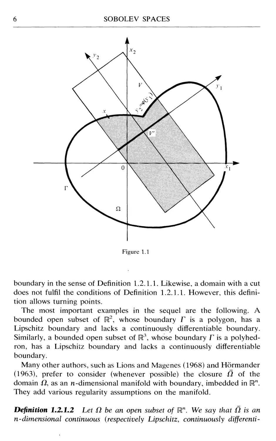
Definition 1.2.1.1 Let fl be an open subset of Un. We say that its
boundary F is continuous (respectively Lipschitz, continuously differenti-
able, of class CkA, m times continuously differentiated) if for every xeF
there exists a neighbourhood V of x in Un and new orthogonal coordinates
{yl5. .., yn} such that
(a) V is an hypercube in the new coordinates:
= {(y1,... ,yn)
(b) there exists a continuousi (resp. Lipschitz,§ continuously differentiate,
of class CkJ, m times continuously differentiate) function <p, defined
in
V = {(y,,..., yn _ i) | - a,- < y,- < a,-, 1 ^ j ^ n - 1}
and such that
W(y')\^aJ2 for every y' = (y, yn-i)eV,
A,2,1,1)
In other words, in a neighbourhood of x, fl is below the graph of <p and
consequently the boundary F is the graph of <p. We recall that saying that
<p belongs to the class CkA means that it is k times continuously
differentiate and its derivatives of order k are Lipschitz continuous.
If an open set fl has a continuous boundary F, then fl is not on both
sides of F at any point of F. For instance, [R* = (R\{()} has not a continuous
t m and k are integers 2=1, possibly equal to +°°.
t Observe that the word continuous may be omitted there. Indeed, if a function fulfils the
conditions A,2,1,1), it is easily proved that <p has to be continuous.
§ By Lipschitz condition, we always mean uniform Lipschitz condition.

SOBOLEV SPACES
Figure 1.1
boundary in the sense of Definition 1.2.1.1. Likewise, a domain with a cut
does not fulfil the conditions of Definition 1.2.1.1. However, this defini-
definition allows turning points.
The most important examples in the sequel are the following. A
bounded open subset of [R2, whose boundary F is a polygon, has a
Lipschitz boundary and lacks a continuously differentiate boundary.
Similarly, a bounded open subset of [R\ whose boundary F is a polyhed-
polyhedron, has a Lipschitz boundary and lacks a continuously differentiable
boundary.
Many other authors, such as Lions and Magenes A968) and Hormander
A963), prefer to consider (whenever possible) the closure Q of the
domain f2, as an n-dimensional manifold with boundary, imbedded in Un.
They add various regularity assumptions on the manifold.
Definition 1.2.1.2 Let Q be an open subset of Rn. We say that Q is an
n-dimensional continuous (respectively Lipschitz, continuously differenti-

1.2 BOUNDARIES
able, of class CkA, m times continuously differentiate) submanifold't with
boundary in Rn, if for every xeF there exists a neighbourhood V of x in Un
and a mapping ip from V into Rn such that
(a) ip is injective
(b) ip together with i/T1 (defined on ip(V)) is continuous (respectively
Lipschitz, continuously differentiate, of class CkA, m times continu-
continuously differentiate)
(c) fl H V = {y e fl | ipn(y) <0} where i//n(y) denotes the nth component of
As a consequence of condition (c), the boundary F of fl is defined
locally by the equation ipn(y) = O.
In the notations of Definition 1.2.1.1, define ip as follows:
*My) = {yi, • •., yn-\, yn-<p(y')} A,2,1,2)
It is easily seen that i// fulfils all the conditions in Definition 1.2.1.2 with
the same amount of differentiability for i// and i//1 as for <p. In other
words, Definition 1.2.1.1 implies Definition 1.2.1.2 and it is natural to ask
whether the converse is also true. Unfortunately the converse statement is
only partly true. It follows from the implicit functions theorem that
Definition 1.2.1.2 implies Definition 1.2.1.1 provided everything is at
least continuously differentiable. Indeed, we rebuild a function <p from a
given i//, by solving the equation
with respect to y, where j is chosen in such a way that D^ does not
vanish (locally). This is possible when ifj is continuously differentiate.
Then the chain rule shows that <p is continuously differentiate (resp. of
class CkA, m times continuously differentiate) when ip is continuously
differentiate (resp. of class CkA, m times continuously differentiate).
The implicit function theorem does not hold for Lipschitz functions and
the following counterexample will show that Definition 1.2.1.2 does not
imply Definition 1.2.1.1 under the single assumption that ip together with
ipl is Lipschitz. This counterexample was shown to me by Zerner. We
need some preliminary lemmas.
Lemma 1.2.1.3 The Definition 1.2.1.2 of n-dimensional Lipschitz sub-
manifolds with boundary in Rn is invariant under bi-Lipschitz
homeomorphisms.
A homeomorphism rj of QA onto f22 and of a neighbourhood W{ of
t A continuous manifold is more usually called a topological manifold.

8
SOBOLEV SPACES
onto a neighbourhood W2 of il2 will be called a bi-Lipschitz
homeomorphism of Qx onto £22 if r\ and tj are uniformly Lipschitz-
continuous. Lemma 1.2.1.3 is an easy consequence of the chain rule for
the Lipschitz functions due to Rademacher A919-20).
We now define a bi-Lipschitz homeomorphism from U2 onto U2 by
where
3 t\-
-3 t +
1
for
for
1
22k
1
The slope of <p is either 3 or -3. Consequently, <p is a uniformly Lipschitz
function (with Lipschitz constant equal to 3). This implies that rj together
with r| are uniformly Lipschitz mappings.
Let Q be defined as follows:
={(x,, x2)| 0<x, < 1, 0<x2<x,}.
It is clear that fl has a Lipschitz boundary according to Definition 1.2.1.1.
Figure 1.2

1.2 BOUNDARIES
Therefore, fl is a two-dimensional Lipschitz submanifold with boundary,
in [R2, according to Definition 1.2.1.2, since Definition 1.2.1.1 implies
Definition 1.2.1.2. Next, consider the new domain r\(Q). This is also a
two-dimensional Lipschitz submanifold with boundary in [R2, owing to
Lemma 1.2.1.3. Now we have the following result.
Lemma 1.2.1.4 r}({2) has not a continuous boundary according to Defin-
Definition 1.2.1.1.
Proof It is obvious from the geometry of r\({l) (see Fig. 1.3) that every
linear segment with origin at 0, which cuts F, actually cuts F at infinitely
many points. This property is true without any restriction on the length of
the segment under consideration. This prevents the existence of a neigh-
neighbourhood V of 0, together with the existence of new coordinates such
that rnV should be the graph of a function as in Definition 1.2.1.1.
Accordingly rj(/2) lacks a continuous boundary in the sense of Definition
1.2.1.1. ■
Summing up, the comparison between Definition 1.2.1.1 and Definition
1.2.1.2 is the following.
Figure 1.3

10 SOBOLEV SPACES
Theorem 1.2.1.5 A bounded open subset Q in Rn has a continuously
differentiate (respectively of class Ckl, m times continuously differenti-
able) boundary F if and only if Q is an n-dimensional continuously
differentiate (respectively of class CM, m times continuously differenti-
able) submanifold with boundary in Un. A bounded open subset Q in Rn
with continuous (respectively Lipschitz) boundary F has a closure Q which
is an n-dimensional continuous (respectively Lipschitz) submanifold with
boundary in Rn. The converse statement is not true.
In some special questions, for technical reasons, we shall need uni-
uniformly Lipschitz unbounded domains of the following kind.
Definition 1.2.1.6 An open subset ft of Un is said to be a uniform
Lipschitz epigraph if there exists new coordinates {yu ..., yn} and an
uniformly Lipschitz continuous function <p of n -1 variables, such that
A,2,1,3)
Examples of such domains are infinite cones or plane sectors.
1.2.2 Segment property and cone property
In the early stages of the theory of Sobolev spaces, many authors
preferred to describe the boundary properties of the possible domains fl
in a more straightforward fashion. Namely, they required that for each
point x of the boundary F of fl, there exists a linear segment C with
origin at x or a cone C with vertex at x, such that C\{x} is contained in fl.
Usually a local uniformity assumption is added (cf. below). This point of
view, adopted by Sobolev, has been followed by Agmon A965) and
Calderon A961).
Definition 1.2.2.1 Let fl be an open subset of Rn. We say that fl has the
uniform (or restricted) segment property (resp. cone property) if for every
xeF, there exists a neighbourhood V of x in Rn and new coordinates
,..., yn} such that
(a) V is a hypercube in the new coordinates:
(b) y — zeO whenever y e £2 n V and z e C, where C is the open
segment {@,. .., 0, zn) \ 0 < zn < h} (resp. C is the open cone
{z =(z', zn) | (cot 0) \z'\<zn <h} for some 0e]O, tt/2]) for some h>0.
It is obvious that if Q has a continuous boundary according to Defini-

1.2 BOUNDARIES
11
Figure 1.4
tion 1.2.1.1, then it has the uniform segment property (just choose h<
aJ2). The same way, if Q has a Lipschitz boundary, then it has the
uniform cone property. Indeed, this is seen by replacing all the a, by a,/2
in Definition 1.2.1.2 and by choosing h<anl2 together with
/ 1
6 ^ inf I arctan —; arctan
\ K
a
arctan
a
n
where K is the Lipschitz constant of <p.
The converse statement has been known to be true for a long time by
oral tradition. However, an actual proof has been published only recently
by Chenais A973). We shall give a transcript of the proof only for
domains having the uniform cone property, because it is slightly simpler
and it is the only one we need in the following sections.

12 SOBOLEV SPACES
Theorem 1.2.2.2 A bounded open subset Q of Rn has the uniform cone
property if and only if its boundary F is Lipschitz.
Proof We have already observed that the condition of having a Lipschitz
boundary is sufficient. Thus, let us consider x e F, assuming that Q has the
uniform cone property of Definition 1.2.2.1. We know that {x}— C<^fl,
but we can also observe that {x}+ C<= CX2, at least if the distance from x
to CV is greater than h/cos 6; this last condition can always be achieved
by choosing a smaller h. Indeed, if {x}+Cnf2 is not empty, let y be a
point in the intersection; then y eOHV since |yn —xn\ < h; consequently,
{y}-C<=: jl7 but this contradicts the fact that {y}-C3x.
From this remark it follows that if we translate the origin of the
coordinates {y^ . . ., yn} at x and define a cylinder K by
= {(y', yn) | -h < yn < K |y'| < h tan 0},
then we have
|yn| tan 0<|y'|<h tan 0};
This means that F cannot 'escape' through the top of K.
We conclude by defining <p in the following way
<p(y') = sup{yn | (y',yn)eFnK};
<p is defined only for |y'|<h tan 6. Clearly, (y', <p(y'))eF. Then the cone
property shows that all points (y',yn)eK with yn<<p(y') are in Q; by
contradiction, as we did previously for x, we show that all points (y\ yn)c
K with yn ><p(y') are in CO. Finally, if we consider two points (y', <p(y'))
and (z\ <p(z')) on the graph of <p, it follows from the cone property that
yn-zn>-|y'-z'|cot0;
this implies that <p is a uniformly Lipshitz function with constant K =
cot 6.
We conclude the proof by observing that all the conditions in Defini-
Definition 1.2.1.1 are fulfilled when we choose the ai small enough. ■
A useful consequence is the following:
Corollary 1.2.2.3 Let fl be a bounded open convex subset of [Rn, then Q
has a Lipschitz boundary.
Proof Let x0 be any point in fl and let r>0 be the radius of a ball B
with centre x0, contained in fl. Since fl is convex, all the points ty +
(l-r)z with ye A zeB, 0^f<l, are in fl. This shows already that fl
has some kind of a cone property but we still need uniformity.

1.2 BOUNDARIES
13
y
Figure 1.5
Now fix x e r and choose new coordinates {yi,..., yn} with, say, origin
at x and such that xox is parallel to Oyn. Denote by I the distance from x0
to x. Then to each y e Q at a distance less than r/2 from x, we associate a
ball B(y) centred at (y\ yn - 0 with radius r/2. Obviously B(y)c:B, and
therefore all the points fy + (l-f)z with zeB(y), O^r<1 are in fl. The
property in Definition 1.2.2.1 is verified by choosing the ai small enough,
h = / and sin 0 = r/2L ■
Remark 1.2.2.4 Unfortunately domains with cuts or with turning points
are not well classified by the various previous definitions. Let us consider,
for instance, the following domains in the plane:
-Kx1<l,-Kx2<-
1/2}
1/21
= {(x,,x2)|0<x1<2, -Kx2<-(x1/2I/2}.
The domain Ol is easily seen to have a continuous (and non-Lipschitz)
boundary according to Definition 1.2.1.1. On the other hand, O2 nas n°t
the segment property of Definition 1.2.2.1; consequently, it lacks a

14
SOBOLEV SPACES
t
Figure 1.6
continuous boundary. However, fl2 is the image of
mapping
(p :(x,, x2) >-> (x!+ x2, x2)
x through the
which is a diffeomorphism of class C°° of [R2 onto
1.3 Spaces
This section is just a list of the definitions of the Sobolev spaces. We
confine our attention strictly to those spaces which we really need in the
following chapters. Consequently we will not consider any of those
functional spaces such as Bes.ov spaces and Nikolski spaces that are very
closely related to Sobolev spaces and have better properties. The reader
interested in those spaces is referred to Triebel A978) for instance.
The Sobolev spaces are very easy to define on the whole Euclidean
space. Then a possible definition of Sobolev spaces on a subdomain Q of
Un with boundary uses restrictions to Q. This is why we treat the spaces
on Rn separately and first.
1.3.1 Euclidean space
In what follows, s is any real number and p is a real number such that
l<p<oo. We shall denote by m the integer part of s and by <j its
fractional part; consequently, s = m + cr and 0=^c
Definition 1.3.1.1 We denote by Wsp(Rn) the space of all distributions
(all functions and distributions are complex valued unless otherwise
specified) defined in Rn7 such that
(a) DaMGLp(!Rn), for
, when s = m is a nonnegative integer,

1.3 SPACES 15
(b) ueW™(Un) and
\Docu(x)-Docu(y)\p
JJ \x-y\n+(TP
[Rnx[Rn
dx dy
u
for \a\ = m, when s = m + o~ is nonnegative and is not an integer.
As usual, Lp((Rn) is the space of all measurable functions u such that
is integrable over Un. We define a Banach norm on Wsp(Rn) by
( c 1 l/p
IMIm.p*»=( I j[jDaUPdXj A,3,1,1)
in case (a), and by
\D<*u(x)-D<*u(y)\p j j V/P
ff
A,3,1,2)
in case (b).
The previous definition is extended to negative values of p by duality as
follows:
Definition 1.3.1.2 For s<0 we denote by WP(IRn) the dual space of
Wqs([Rn), where p-1+q~1 = l.
In the special case where p = 2, we shall use the more common notation
Hs(IRn) instead of W^((Rn). The norms defined in A,3,1,1) and A,3,1,2)
are Hilbert norms when p = 2.
In some special questions where the use of Fourier transform cannot be
avoided, it is useful to introduce a different kind of spaces as follows.
Definition 1.3.1.3 We denote by Hsp(Rn) the space of all distributions in
Un such that
Gs ^u
where Gs is the Bessel potential of order s defined by
As usual, F is the Fourier transform operator defined by
and the star * denotes the convolution product.

16 SOBOLEV SPACES
It is known that H2(Un) = Ws2(Un) (by Plancherel's theorem) for all real
s, and that H™(Mn) = W™(Un) (by Mikhlin's theorem) for all integer m
and 1 <p<oo. Furthermore, it is proved in Taibleson A964) that
Hsp(Rn) 3 Wsp([Rn), 1< p ^ 2,
while
for any real s.
It is also easily checked that WP([Rn) and HP(Mn) decrease when s
increases and finally Lions and Peetre A964) have proved that
Wsp(Un) c Hsp"(Un) c WP'\Un)
for any real numbers s', s", s'" such that
sf>s">sf".
1.3.2 Open subsets of the Euclidean space
We now deal with fl, an open subset of [Rn, possibly different from Rn
itself. Our purpose is to extend the definitions given in Section 1.3.1, in
order to define Sobolev spaces on fl. In doing that, we can follow
different schools. Here are the three main methods:
(a) We can reproduce Definition 1.3.1.1 by restricting the domain of
integration (replacing Rn by Q). This is the point of view in Lions
and Magenes A960-63) and Necas A967), for instance.
(b) We can define Wsp(fl) as being the set of restrictions to fl of all
functions in WP([Rn). This is the point of view in Hormander A963).
(c) Finally, following Agmon A965) and Miranda A970), we can con-
consider the completion of the space of smooth functions in O, with
respect to the norm in (a).
It turns out that each of these three methods has its advantages. All
three lead to the same spaces when fl is smooth enough (we shall give a
precise meaning to this sentence in the next sections). However, for
general domains they may produce three different spaces, which we shall
have to compare.
Definition 1.3.2.1 We denote by Wsp(fl) the space of all distributions u
defined in 17, such that
(a) D"mgLp(/2), for \a\^m, when s = m is a nonnegative integer,

1.3 SPACES 17
(b) u e W™(O) and
DOiu(x)-D<xu(y)\p
JJ \x-y\n+ov
nxn
dx dy <+oo
for \a\ = m, when s = m + (r is nonnegative and is not an integer.
We define a Banach norm on WSP(Q) by
MLp.n=( I f \D«u\Pdx\ " A,3,2,1)
in the case (a), and by
, .. fn i. v ff \Dau(x)-Dau(y)\p I
l"IUn=jMm,P,n+ L " [7T^ dx dy |
^ i«i=m jj x~y\ J
A,3,2,2)
in the case (b).
We cannot directly reproduce Definition 1.3.1.2 since in general 2>(/2),
the space of all C°° functions with compact support in Q, is not dense in
Wp(/2). Consequently, the dual space of WSP(O) cannot be identified to a
space of distributions in Q. This is the reason for introducing another
family of Sobolev spaces.
o
Definition 1.3.2.2 For s>0, we denote by WSP({1) the closure of' 3)({l) in
Equivalently, it is the closure in WP(/2) of all distributions with compact
support in Q which belong to WP(/2).
Then the extension of Definition 1.3.1.2 is the following:
Definition 1.3.2.3 For s<0, we denote by Wp(/2) the dual space of
Wq%T2), where p-l + q~l = l.
In the special case when p = 2, we shall also use the common notation,
namely Hs(fl) instead of Ws2(B) and Hs(fl) instead of W|(f2). These are
Hilbert spaces.
When s is a negative integer — m, Wp(/2) is also the space of all
distributions T in Q such that
T= I D7« A,3,2,3)
where /a eLp(/2). The proof can be found in Magenes and Stampacchia
A958), for instance. An extension of A,3,2,3) to non integer s is given in
Lions A961b).

18 SOBOLEV SPACES
For the sake of clarity in the following sections, it will be convenient to
have a specific notation for the space defined by restriction.
Defininions 1.3.2.4 For every s >0, we denote by WP(O) the space of all
distributions in Q which are restrictions of elements of Wsp(Mn).
In other words, WSP(O) is the space of all u \n where u e Wsp(Un) and
u\n is defined by (u \n; <p) = (u, <p) for all <pe3)(Q), where <p is the
continuation of cp by zero, outside fl. We define a Banach norm on
Wp(fl) by
IMUn = inf IIUlUji- A,3,2,4)
UeWps(K")
U\a = u
As obvious consequences of the definition, we have the following
inclusions:
pp A,3,2,5)
for every real s>0, and
W^O) c W™(/2) s W™(/2) A,3,2,6)
for every integer m>0.
Unfortunately we shall need one more kind of Sobolev space whose
technical interest will appear much later.
Definition 1.3.2.5 For every positive s, we denote by WP(Q), the space of
all u e WP(/2), where u e WP(Un).
WSP(O) is a Banach space for the norm
A,3,2,7)
The only obvious inclusions concerning Wp(/2) are the following
WP(f2) c= Wsp(/2) A,3,2,8)
for all s > 0 and
^ A,3,2,9)
for m integer >0.
The norm defined in A,3,2,7), although it is the natural one, is
somewhat tricky, because it is the norm induced by WSP(O) only when s is
an integer.
Lemma 1.3.2.6 Let u belong to Wsp({2); then
,p,n A,3,2,10)

1.3 SPACES 19
when s = m is an integer, while
f f
«ltp.n= IKP,n+ I \Dau(x)\'Pa,p(x)dx\
^ \<x\ = mJn J
A3 2
when s = m + cr is not an integer, where - v ' ' '
It is not easy to describe the weight p^p in general. However, when fl
is bounded and has a Lipschitz boundary, there exist two constants Cu C2
with 0 < d ^ C2, such that
C1d(x;r)"op^Pcr.pW^C2d(x;r)"op A,3,2,12)
where d(x, f) denotes the distance from x to the boundary F of /2. The
same inequalities hold when O is a uniform Lipschitz epigraph (Defini-
(Definition 1.2.1.6).
1.3.3 Manifolds
In the following sections, we shall need Sobolev spaces on manifolds
which are only (possibly part of) boundaries of open subsets of Rn
fulfilling the assumptions in Definition 1.2.1.1. In other words, they will
be (n — l)-dimensional hypersurfaces in IRn. Consequently, keeping the
same notations as in Definition 1.2.1.1, the boundary F of fl is such that
for every xeF, there exists a neighbourhood V of x in IRn, fulfilling the
condition (a) in Definition 1.2.1.1 and a function fulfilling the condition
(b) such that
Let us define 0 as follows:
A,3,3,1)
then (F C\ V, cf>) is a map of F around x, where we now view F as a
(n — l)-dimensional Lipschitz (respectively continuously diflerentiable, of
class CM, m times continuously differentiate) submanifold of IRn.
The following statement expresses in a precise way the stability of
Sobolev spaces under sufficiently smooth changes of variables. We assume
that i/> is at least a bi-Lipschitz mapping from OA onto O2 where O^ and O2
are bounded open subsets of Rn. This hypothesis ensures that Lebesgue
measure is mapped by ^ or i^ to an equivalent image measure.
Lemma 1.3.3.1 Let u e Wp(/22); assume that ifs and i/T1 are of class CM
where k is an integer s^s — 1; then m°i//g Wsp(Qi).

20 SOBOLEV SPACES
This property is easy to check with the help of the results in
Rademacher A919). It is a justification for the following definition.
Definition 1.3.3.2 Let Q be a bounded open subset of Un with a boundary
F of class Ckl, where k is a nonnegative integer. Let Fo be an open subset
of F. A distribution u on Fo belongs to WP(F0) with |s|^k + l if u°<P e
Wp( V C\<P~l(F0 n V)) for all possible V and cp fulfilling the assumptions in
Definition 1.2.1.1.
Usually distributions are defined only on C°° manifolds. When Fo is
only an open subset of a Ckl manifold we consider distributions whose
order is less than or equal to k + 1; those span the dual space of the space
of all Ckl functions with compact support in Fo. Functions are identified
with distributions by means of the usual injection u »-> Tu, defined by
I,
(Tu; v)= uv dcr
Jr
where dcr is the usual hypersurface measure on F (defined provided F is a
Lipschitz hypersurface).
One possible Banach norm on WP(F) is
w •-> Z l|wo^lls,p,v;n^>J-1(ronv;) A,3,3,2)
where (V,, <J> )/= x is any atlas of F such that each couple (V,, <p,) fulfils the
assumptions of Definition 1.3.3.1 (we recall that <£>• is defined from cp,- by
In the particular case when sg]0, l[, one can easily check that any of
the norms defined in A,3,3,2) is equivalent to
ff l,"(*)Tn-^
J J \x y\
n|'d<r+ ff l,"(*)Tn-^d<r(x)dG(y)y. A,3,3,3)
J J \ \ J
1.4 Basic properties
This section is only a list of the main properties of the spaces defined
above. We do not report any proof but just indicate easy references
where all the details can be found.
1.4.1 Multiplication and differentiation
The question here is to know sufficient conditions on a function cp defined
in Q, ensuring that u —»<pu is a continuous linear mapping in a given

1.4 BASIC PROPERTIES 21
Wp(/2). We state here a very simple answer, which is just a straightfor-
straightforward consequence of the definitions given in Section 1.3. A more com-
complete answer will be given in Section 1.4.4 as a consequence of the
imbedding theorems (see Theorem 1.4.4.2).
We denote by CcM(fl) (k a nonnegative integer and a e [0, 1]) the
space of all functions defined in O which are restrictions to O of functions
of class Ck'" defined on the whole of Rn which have a compact support.
Theorem 1.4.1.1 Let cp e C£'"(/2) with k + a^z\s\ when s is an integer
and k + a>\s\ when s is not an integer, then <pueWsp({2) for every
u s Wp(/2), and there exists a constant K = K(<p, s, p) such that
ll<P"IL,P,n=SK||u||s,p,fi. A,4,1,1)
An easy consequence is that under the same hypothesis on cp, u —» cpu is
a continuous linear mapping in Wp(il) and in Wp(/2). The following
result is also easy to check.
Theorem 1.4.1.2 Let cp e C£'"(/2) with k + a ^ \s\ when s is an integer and
ii ° °
k + a > \s\ when s is not an integer, then <pu e Wp(/2) for every u e WSP(O).
For a nonnegative integer m, the space W^ifl) is just the space of all
functions defined in O, which are m times differentiate in Lp(/2), so to
say. The definition of WP(O) for a noninteger s has been stated with the
underlying idea that WP(/2) should be the space of all functions in fl
which are s times differentiate in some sense. Consequently, one could
expect Da to be a continuous linear operator from WSP(O) into
Wp~|o£'(/2). The extension of the definition of WP(Q) to negative values of
s was devised with the hope that this rule should hold for every s.
Unfortunately, this is not always true, as we shall begin to show now.
Firstly, Da maps WP(fl) into Wsp"lo£l(/2) provided either \a\^s or s^O.
This follows from Definition 1.3.2.1 when |a|^s. Then, from Definition
1.3.2.2, we see that Da is also a continuous linear operator from WSJO)
Oil.. ^
into Wsp~{Oi\{2) when |a|^s. Transposing this result and remembering
Definition 1.3.2.3, we conclude that Da maps WP(fl) into WspHo£|(/2)
when s =^0.
Now it remains to understand how differentiation operates from spaces
with positive order to spaces with negative order. For this purpose it is
enough to consider an elementary differentiation operator Dy with respect
to xh with 1^/^n.
Lemma 1.4.1.3 D} is a continuous linear operator from WP0Rn) into

22
SOBOLEV SPACES
The only case we have to consider is when 0 < s < 1. When p = 2 and
consequently Wsp(Un) = Hs(Un) = Hs2(Un), the property is obvious from
Definition 1.3.1.3. Unfortunately, we need another method of proof
when p is not 2. We describe it now. Here 1? belongs to 2)(Rn) and has its
support in the unit ball and integral equal to one.
Lemma 1.4.1.4 Let u e WP(IRn) and set
,xn+1) = -7r- I R[—-)u(y)dy, xeOT, xn+1>0;
then x;~sr 1/pDkL/GLp(IRn+1), k = 1, 2,..., n + 1.
A,4,1,2)
Proof We follow the method used in Lemma 5.6, Chapter 2 in Necas
A967), just adding a weight. We first consider DkU where l^k^n. We
have
DkU(x,
n
n+1J
dy
-u(x)]dy
since obviously
dy = 0
It follows that
DkU(x,xn+1)= DkR(z)[u(x)-u(x
and consequently
dz
f (
I
T Mi |M(x)-M
= cf([ xnlM[
= c JJ \u{x)-u(y)\pU
u(x)~u(y)\p-^-\dx)dxn+l
-1-sp-n
•^n + 1
■}
sp + n
u(x)-u(y)|pJ
-yl1
where c is a constant depending on R.

1.4 BASIC PROPERTIES
23
Now let us consider Dn+lU; we have
Dn+1l/(x, xn+1)= —
n
n+l
R\
;^->
n+1
X
r J =
n
n+l
R
(B
-u(x)ldy
1
v-n+l
xn+l
since
4r
n+l
^<dv = O
by integration by parts. Then each integral in Dn+1U is estimated as we
did for Dk U. ■
Proof of Lemma 1.4.1.3 We consider the bilinear form
u, v »—>
dx
and we prove that it is defined and continuous on Wp(lRn)xWj s0Rn),
where (l/p) + (l/q) = 1. From u and v we construct U and V according to
identity A,4,1,2). We know from Lemma 1.4.1.4 that
Furthermore, in the topology of Lp(IRn) we have
lim U = u, lim U — 0
,,+
while in the topology of Lq(IRn) we have
lim V=v, lim V = 0.
xn+ I
►oo
This implies that
jUix, xn+l) V(x, xn+1)
/•
foo
[D,U(x, t)DB+1 V(x, t)-Dn+lU(x, t)D,V(.x, t)]dx d(

24 SOBOLEV SPACES
and consequently
j, xn+l) V(x, xn+1) dx
2-. WXn+\ ^k^llLpdR"^) ll^n+l^l Ml
where K is some constant produced by Lemma 1.4.1.4. Taking the limit
when xn+l-^0, one gets
This proves Lemma 1.4.1.3. ■
As a consequence of Lemma 1.4.1.3, it is clear that for u e Wsp({2), Dtu
is the restriction to fl of a distribution belonging to Wp^). Conse-
Consequently, a complete answer to the question of whether or not D, maps
Wp(fi) into Wsp~l(fl) will follow the study of continuation and restriction
properties.
1.4.2 Density results
Here we quote only one basic result proved in Agmon A959) and Necas
A967) for instance. We denote by C~(/2) the space of all functions
defined in ft which are restrictions to fl of C°° functions with compact
support in Un.
Theorem 1.4.2.1 Let fl be an open subset of Un with a continuous
boundary, then C~(/2) is dense in WP(Q) for all s>0.
It follows easily from Definition 1.3.2.3 that C°°(/2) is dense in WP(Q)
for all s<0, without any hypothesis on fl.
Moreover, S>0Rn) is dense in Wp(IRn) for all s and consequently C~(O)
is dense in WP(Q) without any assumption on fl.
Another result, closely related to Theorem 1.4.2.1, is the following:
Theorem 1.4.2.2 Let fl be an open subset of Un with a continuous
boundary, then Q)(fl) is dense in WSP(Q) for all s >0.
Together with the identity A,3,2,10), this shows that when s = m is an
integer and fl is a domain with a continuous boundary, then

1.4 BASIC PROPERTIES 25
An easy and useful consequence of Theorem 1.4.2.2 is the following:
Proposition 1.4.2.3 Let fl be an open subset of W with a continuous
boundary and let T belong to Wp(IRn) with s <0. Then the restriction of T to
fl belongs to the dual space of W~S(Q).
Finally we state an improvement of Theorem 1.4.2.1 in the particular
case when s ^ 1/p.
Theorem 1.4.2.4 Let fl be a bounded open subset of Un with a Lipschitz
boundary; then 2(fl) is dense in Wsp(fl) for
The same is true when fl is uniform Lipschitz epigraph (Definition
1.2.1.6).
In view of Theorem 1.4.2.1 we only have to approximate functions in
C°°(n) by functions in 3)(B) for the norm of WP(Q). This is easily
achieved by means of a sequence of cut-off functions.
A direct consequence is that under the assumptions of Theorem
1.4.2.4, Wsp(fl) is the same space as Wsp(/2), when
1.4.3 Continuation, compactness and convexity inequalities
Now we clarify partly the relation between Wsp(fl) and WSP(O). The
following result is proved in Agmon A965), Aronszajn and Smith A961),
Lions A957), Necas A967), Stein A970).
Theorem 1.4.3.1 Let fl be a bounded open subset of Un with a Lipschitz
boundary; then for every s > 0 there exists a continuous linear operator Ps
from WSP(Q) into WP(Un) such that
Psu \n = w. A,4,3,1)
The same results hold when fl is an uniform Lipschitz epigraph or an
infinite strip.
In other words each function u e Wsp(fl) is the restriction of a function
Psu e Wp(IRn). A counterexample in Lions A957) shows that the property
may not hold when fl has not a Lipschitz boundary. Consequently we
have Wp(/2) = WSP(Q) when fl is bounded and has a Lipschitz boundary.
In addition it has been shown in Seeley A964) and Aronszajn and
Smith A961) that Ps can be chosen independently of s.
The continuation theorems are powerful tools for extending several
results proved on IRn to similar results on a bounded domain with a
Lipschitz boundary. We list some of them now.

26 SOBOLEV SPACES
Theorem 1.4.3.2 Let sf>s"^0 and assume that Q is a bounded open
subset of Un with a Lipschitz boundary. Then the injection of Wp(fl) in
Wp\fl) is compact.
(For the sake of convenience here we define W£(/2) as being Lp(fl).)
This result originally due to Kondrasov A945) is proved in Necas
A961) for the case in which sf and s" are integers. The extension to
possibly non-integer values of s' and s" may be found in Lions and Peetre
A964).
The following inequality is closely related to the previous theorem,
through a lemma of Lions (cf. Lemma 2,7, Chapter 1 in Magenes and
Stampacchia A958)).
Theorem 1.4.3.3 Let sf>s">s"'^0 and assume that fl is a bounded
open subset of Un with a Lipschitz boundary. Then there exists a constant C
(depending on fl, s', s", s'" and p) such that
l,P, NL~.,ui A,4,3,2)
for all ugWsp\O).
Such an inequality is also true when fl = Un or fl is any subset of Un with
the continuation property of Theorem 1.4.3.1.
This is an interpolation inequality which follows from the similar
inequality on Un. See Lions and Magenes A960-63) for a proof. In the
case when s', s" and s'" are integers, this is a particular case of more
general inequalities by Gagliardo A958) and Nirenberg A959).
Let us also recall here a related inequality often referred to as Poin-
care's inequality (cf. Necas A967), for instance).
Theorem 1.4.3.4 Assume that fl is a bounded open subset of W1. Then
there exists a constant K(fl) which depends only on the diameter of fl such that
du
)
/p
for all u e WP(Q).
Closely related to the inequality in Theorem 1.4.3.3 is the interpolation
theorem (cf. Lions and Peetre A964)).
Theorem 1.4.3.5 Let U be a continuous linear operator in Wp(IRn),
\<p< +oo7 sgU. Assume that for some t>s the restriction of 77 to Wp(IRn)

1.4 BASIC PROPERTIES 27
is continuous in W[,(IRn). Then for every ue]s, t[, the restriction of II to
is continuous in
Due to the continuation property a similar statement holds concerning
the Sobolev spaces on Q a bounded open subset of Un with a Lipschitz
boundary.
1.4.4 Imbeddings
The most outstanding result about Sobolev spaces is the famous imbed-
imbedding theorem, derived first by Sobolev himself. The main statement is
this:
Theorem 1.4.4.1 The following inclusions hold:
Wsp(ffT)c=W<(ffr) ' A,4,4,1)
for t ^ s and q^p such that s - nip = t - n/qt and
Wsp(Un)^CKoc(Un) A,4,4,2)
for k<s — n/p<fc + 1, where a = s — k — nip, k a nonnegative integer.
It is possible to state a weaker result in the limit cases when s — nip is
an integer, as follows. We have
Wnp/p(Un) cz LQ(Un) A,4,4,3)
for all q^p, and
ku A,4,4,4)
for all a e[0, 1[, where k is an integer ^1.
The proof may be found in any of the references quoted before about
Sobolev spaces.
As a consequence we have the following inclusions
i^ A,4,4,5)
for f^s, q^p such that s-nlp = t-n/q and
5M^ A,4,4,6)
for k<s — nip<fc + 1, a = s — k — nip, k a non-negative integer. These
inclusions hold without any assumption on fl. As a consequence of
Theorem 1.4.3.1, similar inclusions hold for WSP(O), when fl is a
bounded open subset of Rn, with a Lipschitz boundary.
t Negative values of t are admitted and WjJ(Rn) means Lq(Un).

28 SOBOLEV SPACES
The main interest of these results, in the subsequent sections, is the
following. Assume we are able to build a solution to some given boundary
value problem, which belongs to WP(O), with s large enough; then we
know that it is differentiable in the usual sense up to an order (strictly
less) than s - nip.
A by-product of Theorem 1.4.4.1 is that Wp([Rn) is an algebra for
s > nip. The more general result which follows has been proved by
Zolesio A977).
Theorem 1.4.4.2 Let s1^s and s2^s be such that either
/I 1 1\ /I 1\
S] + s2 — s^n\—I 1^0, s, - s>n\ I, / = 1, 2
W\ Pi pl \Pt Pi
or
(i l i\ /i :
S\ + s2 — s > nl—I J^0> si~ s^n\
\pi p2 p) \pj p
then u, v ^> u - v is a continuous bilinear map from Wsp\(Un) x Wp22(IRn) into
Wsp(Un).
A similar statement holds for Sobolev spaces defined on a bounded
open subset of Un, with a Lipschitz boundary. It is a complement to
Theorem 1.4.1.1.
Imbedding results of a different sort deal with weighted spaces. They
are consequences of the well-known Hardy inequality (more precisely
Theorem 330 in Hardy et al. A952)). Let us recall a convenient statement
of the Hardy inequality. Here we denote by Lp(X(R+) the space of all
measurable functions u defined in IR. such that
Then, we define two linear operators H and L by
1 T
(Hu)(t) = - u(s)ds
1 T
t Jo
1 f°°
u)(f) = - u
t Jt
(Lu)(t) = - u(s)ds.
t Jt
It turns out that H is linear continuous in Lt,jtt(IR+) iff a + Up < 1, while L
is linear continuous in Lpa([R+) iff a + 1/p > 1. In both cases the norm of
the operator is bounded by \a + 1/p— 1|~\
Theorem 1.4.4.3 Let fl be a bounded open subset of Un with a Lipschitz

1.4 BASIC PROPERTIES 29
boundary F and denote by p(x) the distance from a point x to F. Then when
0<s<l/p, we have u/pseLp(Q) for all ue WP(Q) and when l/p<s=^l,
we have u/ps eLp(fl) for all u e WP(O).
The same result holds (with the same proof) when 11 is a uniform
Lipschitz epigraph (Definition 1.2.1.6).
This result is proved in Grisvard A963) for spaces defined on a half
space IR+. The result is extended to the case of a Lipschitz domain by
bi-Lipschitz changes of coordinates (use Theorem 1.4.1.1 and Lemma
1.3.3.1).
Iteration of Theorem 1.4.4.3 provides a more complete result concern-
ing the spaces Wp({2). Since this is not a result easy to find in the current
literature on Sobolev spaces, we give the statement together with a
detailed proof.
Theorem 1.4.4.4 Let Q be a bounded open subset of Un with a Lipschitz
boundary F, then for all ue Wp(/2) such that s-l/p is not an integer, the
following property holds:
p-s+|a|Dau€ 1^,A2) A,4,4,7)
for all \a\^s.
Proof We observe first that by replacing s by s — \a\ it is enough to prove
the result when |a| = 0.
Let us consider first the case when fl = R+ the nonnegative real axis
and s = m is an integer. Then, for ue3)(R+) we have
u(jc)=[ (* yJ v u(m)(y)dy
and consequently
l«(x)l
^-tt:- fVm)(y)|dy, A,4,4,8)
xm (m-
Hardy's inequality (mentioned above) implies that
By density, this implies the desired result for W™([R+).
Let us consider then the case when fl is still IR+ but s = m + cr is no
longer an integer. We consider now v = ir, which belongs to Wp(IR+).
We make use of the following strange identity:
A,4,4,9)
f
+o°

30 SOBOLEV SPACES
where
= -f [v(t)-v(x)]dt. A,4,4,10)
x J
We first show that x <twgLp([R+). Indeed, we have
J'°° /1 fx \p
X I I L^vU — V\X)]Gt\ QX
r OT ifx,, x
^ LJ_Z L_ii
I I I ^.1 l + op
Jq J0 \X l\
Then Hardy's inequality shows that, when cr < 1/p,
i
< oo
— cr
'x y
and consequently x <TveLp(U+). Unfortunately, when cr>l/p, using for-
formula A,4,4,9) is inconclusive; we therefore use
r
A,4,4,11)
b y
with the same w. Now, Hardy's inequality shows that
f
Jn
X
.—cr
h y
and consequently, again, x~<TveLp(U+). Now inequality A,4,4,8) and one
more application of Hardy's inequality implies that
o
This is the desired result in \Vp(IR+) provided s - 1/p is not an integer.
We conclude by extending this result to a general fl. Let us use the
same notation as in Definition 1.2.1.1 and consider a function u whose
support is contained in V. One can always reduce the general case to this
particular case, using a partition of unity. Now for y'e V let us set
uy.(f)=u(y',<p(y')-f).
o
For almost all y'eV, we have uy>eWsp(U+) and consequently t~suye
LP(U+) with
\\t~su llp < Kp IIii llp
II y \\i-*vy)HL+) || y ns,p,lNt

1.4 BASIC PROPERTIES 31
where K does not depend ony'. Integrating this inequality in y' leads to
Since <p is a Lipschitz function, the weight <p(y')- yn is equivalent to p(y),
the distance from y to F, throughout V. This completes the proof of
Theorem 1.4.4.4. ■
Corollary 1.4.4.5 Let Q be a bounded open subset of Un with a Lipschitz
boundary; then when s-l/p is not an integer we have
p^ A,4,4,12)
and furthermore, when 0<s<l/p we have
A,4,4,13)
Proof From Lemma 1.3.2.6 and Theorem 1.4.4.4, we know that the
norms of WSP(O) and of WSP(O) are equivalent at least on 2)(fl) when
s-l/p is not an integer. Then, from Definition 1.3.2.2 and Lemma
1.4.2.2 we know that 3)(O) is dense in both spaces Wsp(fl) and WD(fl).
Consequently, Wp(fl) and WSP(Q) are the completions on 2>(fl) for two
equivalent norms. This proves identity A,4,4,12).
We always have W;(/])c Wsp(fl). Then when s<l/p, it follows from
Theorem 1.4.4.3 and Lemma 1.3.2.6 that W*(fl)= \V*(fl). This proves
identity A,4,4,13). ■
Another useful consequence of Theorem 1.4.4.4 is the extension of
Lemma 1.4.1.3 to a bounded open domain fl with a Lipschitz boundary.
Theorem 1.4.4.6 Let fl be a bounded open subset of Un with a Lipschitz
boundary. Then Dy is a linear continuous operator from WP(fl) into
WP~\n) unless s = 1/p.
Proof We have already seen in Subsection 1.4.1 that Di maps WSP(O)
into Wsp~1(fl) when either s^lors^O. Let us assume that 0<s<l. We
know from Theorem 1.4.3.1 that Wsp(fl) = WSP({1). Consequently, for
ueWsp(O), D,w is the restriction to fl of a distribution Te Wp l(Un).
More precisely, we have
iM, v) = <T, v)
for every ve3)({2). Furthermore, we have
\(DjU, v)\ ^||T||s_liPfRn \\vl-s,qW = UTIU,^ ||V\\T-s,q,n
where (l/p) + (l/q)= 1. This shows that T belongs to the dual space of

32 SOBOLEV SPACES
Wl~s(fl). Due to Corollary 1.4.4.5, this last space coincides with Wlq~s(n)
provided 1-s^l/q; this means s^l/p. Therefore DyM belongs to
Wsp~\n) provided s^ 1/p. ■
Remark 1.4.4.7 The preceding proof shows that DyM belongs to the dual
space of Wq/q(O) when u belongs to Wlp/p(n). This result cannot be
improved as will be shown now. Here, for simplicity, we assume that
p = 2.
Proposition 1.4.4.8 The bilinear form (defined for u and v smooth)
i
u'vdx A,4,4,14)
f
has no continuous extension to H1/2(]0, l[)xH1/2(]0, 1[).
This obviously implies that for ueH1/2(]0, 1[), u' is not necessarily in
H~1/2(]0, 1[), the dual space of H1/2(]0, 1[), since H1/2(]0, 1[) = H1/2(]0, 1[)
(see Theorem 1.4.2.4).
Proof Let us assume that A,4,4,14) is continuous on H1/2(]0, l[)x
H1/2(]0, 1[); then there exists a constant K such that
J u'v dx^K ||m||1/2,2J(U[ ||u||i/2,2,to,i[
for all u, ve3)([0, 1]). Now let us assume that v = if/u, where $ is some
cut-off function (i|tg3([0, 1]), ifr(O) = 1 and i/r(l) = 0). We have
w't;djc= u'iljudx = -\u2(S))-\\ i{/fu2dx;
consequently, there exists a new constant C such that
for all mg^J([0, 1]). By translation we also have
max
x e[0,l/21
By density, this last inequality implies that all the functions in H1/2(]0, 1[)
are continuous near zero. However, the particular function
u(x) = \og
2
is an obvious counterexample to this property. Consequently, the form
A,4,4,14) cannot be continuous. ■

1.4 BASIC PROPERTIES 33
Remark 1.4.4.9 A by-product of the previous proof is that Sobolev's
theorem A.4.4.1) cannot be improved in the case where s = n/p (here
n = 1 and p = 2). Indeed, we have
H1/2(]o,
this is the negation of the inclusion A,4,4,1) in the limit case. The same
way, we have
°([O, 1])
and this is the negation of A,4,4,2) in the limit case.
As a last consequence of Theorem 1.4.4.4, we can investigate further
the relations between Wsp(fl) and WP(O) in the exceptional case when
s — 1/p is an integer.
Corollary 1.4.4.10 Let O be a bounded open subset of Un with a
Lipschitz boundary; then for all s>0, we have
\ A,4,4,15)
where p(x) is the distance from x to the boundary F of Q and s = m + cr, m
integer, cre[0, l[.
Proof Let us denote by Z{£1) the space on the right-hand side of
A,4,4,15). From Theorem 1.4.2.2 we know that 3)({1) is dense in WSP(O)
for the norm given by A,3,2,11). This implies the inclusion
To prove the converse inclusion, first we observe that
A,4,4,16)
for all u g W™(O). This identity is obvious for u e 3)(O); it is extended to
the whole of W™(Q) by density. Now let us start with ueZ(Q). From
A,4,4,16) we deduce that u e W™([Rn). To prove that u e WSP(O), we just
need to check that D"m g WP~m(Un), for |a| = m, according to Definitions
1.3.2.5 and 1.3.2.1. This means that
-m,p,fl
has to be finite, in view of A,3,2,11). This is obvious from the assumption
that ueZ(n). ■
1.4.5 Spaces defined on polygons
In most of the forthcoming sections, we shall deal with plane domains
whose boundaries are (possibly curvilinear) polygons. First we shall make

34 SOBOLEV SPACES
precise what we mean by curvilinear polygon. Then we shall review
briefly the consequences of the results of the preceding sections, in the
case when fl has such a polygonal boundary.
Roughly speaking a curvilinear polygon is a manifold with corners.
More precisely, let us state a definition similar in most respects to Defini-
Definition 1.2.1.2.
Definition 1.4.5.1 Let fl be a bounded open subset of U2. We say that the
boundary F is a curvilinear polygon of class Cm, m integer 2^1 (respectively
CK<X, k integer 2^1, CXa^l) if for every xeF there exists a neighbourhood
V of x in R2 and a mapping i/> from V in U2 such that
(a) i/> is injective,
(b) if/ together with i(/~l (defined on i(f(V)) belongs to the class C
(respectively CK<X),
(c) nnV is either
m
{y|fe(y)},{y|h(y) and
or
{ye{2
or
where i^-(y) denotes the /th component of
Any domain fl fulfilling the requirements in Definition 1.4.5.1 has a
Lipschitz boundary according to Definition 1.2.1.1. Consequently, the
Sobolev spaces on fl will have all the properties already listed for
Sobolev spaces on bounded domains with Lipschitz boundary. However,
the actual advantages of these domains will appear clearly in the next
section dedicated to the trace theorems.
Theorem 1.4.5.2 Let fl be a bounded open subset of U2 whose boundary
F is a curvilinear polygon. Then we have the following inclusions and
identities:
(a) Wsp(fl) c w;(fl) c Wsp(fl) = Wsp(fl) fors>0.
(b) Wsp(fl) = Wsp(fl) for s-llp non-integer,
(c) Wsp(fl) = Wsp(fl) for s < 1/p,
(d)
for s = m + cr, m a non-negative integer. Furthermore, C°°(il) is dense in
Wsp(fl) and Q)(fl) is dense in Wsp(fl) for all s>0. We also have
(e) Wp(fl)^WtQ(fl),s--=t--,t^s
P q

1.4 BASIC PROPERTIES 35
and
(f) WSJO) c
P
for s — 2/p > 0, not an integer.
In practice, we shall often have to check whether or not some concrete
functions belong to a given Sobolev space. For instance, we shall deal
with functions which have an isolated singularity. A criterion for such
functions is the following.
Theorem 1.4.5.3 Let Q be a bounded open subset of U2, whose boundary
F is a curvilinear polygon. Assume that OeF. Let V be a neighbourhood of
0 such that
V D ft c {(r cos 0, r sin 6)\ r **0, a *s= Q *s= b}
with b — a <2v. Finally let u be a function which is smooth in f2\{0} and
which coincides with
ra<p@)
in VHft, where <p e C°°([a, b]). Then
2
u g WSJQ) for Re a > s A,4,5,1)
P
while
u£ WSJ{1) for Re a ^s — A,4,5,2)
P
when Re a is not an integer.
It is very easy to check these inclusions when s is an integer. However,
when s is not an integer the double integrals which appear in the norm
A,3,2,2) are so complicated that it is almost impossible to estimate them
directly. The method of proof devised by Babuska consists in proving that
ueW™({l) for m integer >s and r<p and then using the Sobolev
imbeddings. We get thus all the desired results when p^2. The general
proof for p <2 makes use of weighted Sobolev spaces; we skip it since we
shall mostly need inclusion A,4,5,1) when p^
Proof A derivative of order m of u behaves as a finite sum of functions
ra~milfF), where if*e C°°([a, b]), in VHO (This is true unless a is an
integer where cancellations can occur.) Consequently its rth power is

36 SOBOLEV SPACES
integrable in fl iff Re a > m - 21 r. In other words
2
ueW?(n) ifRea>m —
r
2
w^ Wrm(/2) if Re a ^m—.
r
By Sobolev imbeddings it follows that
(a) ueWp(O)
provided there exists an integer m^s and an re]l,p] such that
Rea>m-2/r and m-2/r = s — 2lp. This last condition is always
fulfilled when p^2.
(b) utw*p(a)
when there exists an integer m^s and an r^p such that Re a ^
m—2/r and m-2/r= s-2/p. This last condition is always fulfilled
when
So far, we have proved A,4,5,1) when p^2 and A,4,5,2) when p=s
We shall not attempt to extend A,4,5,1) to all values of p<2 since this
requires the use of weighted spaces as we already mentioned it earlier.
However, the extension of A,4,5,2) to all p>2 is simple at least when
s — 2/p is not an integer. Indeed, a derivative of order m of u is clearly
Holder continuous with exponent Re a — m when m <Re a ^ m + 1, and
it is not Holder continuous with a larger exponent. Consequently, the
second Sobolev imbedding implies A,4,5,2) in the remaining cases when
Reo:<s-2/p. ■
Remark 1.4.5.4 Similar results hold for the functions r"(ln r)cp(d).
1.5 Traces
Among the many consequences of Sobolev's imbeddings is the continuity
of the functions belonging to WP(O) when s > nip. It is even continuity up
to the boundary, which allows one to consider the values on the bound-
boundary, of such functions. This is obviously of the utmost importance in the
study of boundary value problems. However, if we agree to consider
boundary values of functions in a weaker sense, we can relax the
condition on s. This is the purpose of the present section.
1.5.1 Hyperplanes
Here, for the sake of convenience, we denote by yn the operator defined
by
.-i,0)

1.5 TRACES 37
when u is a smooth function, continuous, say. In other words, we want to
consider the restriction of u on the hyperplane xn = 0. The basic fact
about yn is that ynu is well defined as soon as u e Wp(IRn) when s>l/p.
We observe that this condition is less restrictive than the condition s > nip
which is necessary for ensuring the continuity with respect to all variables.
The proof of the following result may be found in Agmon A965) when
p = 2, in Necas A967) when s is an integer and in Uspenskii A962) in the
general case
Theorem 1.5.1.1 Assume that s — 1/p is not an integer and that s — \/p =
+ cr, 0<cr<l, k an integer 5=0. Then the mapping
{ynu, ynDnu,..., ynDknu),
y^hich is defined for ueS)(lRn), has a unique continuous extension as an
operator from
k
Wsp(Un) onto II W*-J"-1/p(Rn-1).
j=0
This operator has a right continuous inverse which does not depend on p.
This result is easily extended to the case when Rn~A is replaced by an
(n -l)-dimensional submanifold of IRn, which is smooth enough. This
simply uses changes of variables. More precisely, when F is the Lipschitz
boundary of a bounded open subset of IRn, we define a normal vector field
as follows. Let us keep the same notation as in Definition 1.2.1.1; then a
unit outward normal vector v is defined a.e. (for the usual surface
measure on F) by
{-DMy'),-..,-Dn-My')A}
for y'eV. This vector field is easily extended to the whole of V by
defining it independently of x^. Finally, by a partition of unity, we define
an L°° vector field in a neighbourhood of ft, such that v is the unit
outward normal a.e. on F. Then we observe that when the boundary of fl
is of class Ck'\ the vector field v is only of class Ck~11. Now we denote
by 7 the operator defined by (yu) = u\r when u is a smooth function.
Theorem 1.5.1.2 Let fl be a bounded open subset of Un with a Ckl
boundary F. Assume that s — \/p is not an integer, s ^ fc + 1, s — 1/p = J + <x,
()<cr< 1, I an integer ^0. Then the mapping
f du dlu\
m-» Wu, 7— . . . , 7 71 f
I dv dv J

38 SOBOLEV SPACES
which is defined for u e CkA(O), has a unique continuous extension as an
operator from
Wp({2) onto II W'-'-1/p(r).
This operator has a right continuous inverse which does not depend on p.
The particular case when s = 1 and k = 0 was proved a long time ago by
Gagliardo A957).
Theorem 1.5.1.3 Let Q be a bounded open subset of W1 with a Lipschitz
boundary F. Then the mapping u—>yu which is defined for u e C01(/2),
has a unique continuous extension as an operator from Wl(O) onto
Wp/P(f). This operator has a right continuous inverse independent of p.
In the sequel we shall always denote by 7 the extended operator
defined on the whole of Wj(/2) and we shall call it the trace operator.
In addition it is also possible to characterize the kernel of the trace
operator 7 and even of the mapping
du d h
dv' ' dv1.
in several cases.
Theorem 1.5.1.4 Assume that s - 1/p is not an integer and that s - 1/p =
k + cr, (Xo-<1, k an integer 5=0. Then ueWJK) if and only if ue
Wsp(Un+) and
ynu = ynDnu = •>• = ynDknu = 0.
Here we denote by IR+, the half space defined by a^ >0. By changing
variables, we deduce the following result.
Theorem 1.5.1.5 Let Q be a bounded open subset of W1 with a Ckl
boundary F. Assume that s — 1/p is not an integer and that s — l/p = l + cr,
0<<t<1, I an integer 5=0. Then for s^k + 1, ueWsp(O) if and only if
u g Wsp({2) and
du dlu
YT Yrr 0.
dv dv
Remembering Corollary 1.4.4.5, we see that Theorem 1.5.1.5 implies
also the following result.

1.5 TRACES 39
Corollary 1.5.1.6 Let Q be a bounded open subset of W1 with a CM
boundary F. Assume that s^k + l and that s-l/p is not an integer. Let
o
s - 1/p = l + (T, 0 < cr < 1, I an integer 5=0. Then u e WSP(O) if and only if
u g Wsp({2) and
dU dlU
7 777 0.
dv dv
In some special problems related to the study of mixed boundary
conditions on a regular boundary, it will be convenient to split the
boundary F into pieces and correspondingly to split the trace operator 7.
The related trace theorems follow. We first consider functions defined on
Un and define 7+ and y_ by
-i, 0), Xn_^
Theorem 1.5.1.7 Assume that s — 1/p is not an integer and that s — 1/p =
k + cr, 0<cr<l, k an integer ^0. Then the mapping u •->f ^
defined by
defined on 3)(Un) has a continuous extension as an operator from Wp(IRn)
on the subspace of
t=Y\ w^'-^ORr1) x n
i=o i=o
defined by the conditions
(a) Tn-lDn-l/^Tn-lDn-l/i", l< S ~ j ~~
P
and
(b)
I I l^n-l/j \Xli • • • •> Xn-2? 0
-DUi/,- (*i, . . . ,xn_2,-r)|p d*! • • •dxn_1—<+oo
I'
for I = s — j — 2/p, when s — 21 p is an integer.
The notation is self explanatory: we denote by IR" the subset of Un~l
defined by xn_!^0 respectively, yn^1 is the trace operator on the hyper-
plane xn_1=0 defined in Theorem 1.5.1.1. This statement is a direct
consequence of Theorem 1.5.1.1 through the following lemma.

40 SOBOLEV SPACES
Lemma 1.5.1.8 Let /* e W^IRr1) and define f by
f(x) = /*(*) when xn_x ^ 0;
then fe Wrp(Un~A) if and only if
(a) Yn-l£>n-l/+ = Yn-l£>n-l.r
J(
+oo
\Dl f+(r x rt
, dr
• ' ' dxn_2 —
/or 1 = r — 1/p when r— 1/p is an integer.
The corresponding results for a domain whose boundary is not a
hyperplane will be detailed only in the case of a plane domain in the next
subsection.
All the results that we have mentioned so far about trace properties are
rather qualitative. It is often useful to have also quantitative results for
traces. Here is a very elementary result in that direction. Before stating it,
we need an auxiliary result about Lipschitz boundaries.
Lemma 1.5.1.9 Let Q be a bounded open subset of Un with a Lipschitz
boundary F. Then there exist 8>0 and jieC^ii)" such that
|jl • v^8 a.e. on T. A,5,1,1)
Inequality A,5,1,1) means that |jl is not very different from the normal
v on F. However, |x is much smoother than v.
Proof It is very easy to define |x locally. In the notation of Definition
1.2.1.1 we can choose |xv (in V) as the unit vector in the direction of yn.
Indeed, the component of v in the direction of yn is [l + l^<p(y')|2] 1/2 and
consequently we have
where Ly is the Lipschitz constant of <p in V.
Then we cover the boundary F of Q by the interiors of a finite number
of hypercubes Vk, l^k^K, each of which fulfils the conditions of
Definition 1.2.1.1. To each Vk corresponds a vector [lv by the construc-
construction described above. Then we can define |jl as follows:
K
k=l

1.5 TRACES
41
where 0k, \^k^K, is a partition of unity on F such that
0k 5=0 and 6k has its support in the interior of Vk.
Obviously |x is a smooth vector field, and on F we have
K
\lv
• v
K
inf
k = i
-1/2 _
Theorem 1.5.1.10 Let O be a bounded open subset of Un with a Lipschitz
boundary F. Then there exists a constant K such that
i
yu
|u|pdx
•In -I
A,5,1,2)
/or aH u € Wp(il) and e e ]0, 1[. In addition K depends only on the norm of
|x in C^ll) and on 8 (defined in Lemma 1.5.1.9).
Proof In view of Theorem 1.4.2.1 it is sufficient to prove inequality
A,5,1,2) for all ueCl(O). For such a function, we have
u
p .
V f d|up A f
L ~— j^y dx = 2*,P\
= 1 *Q OX: 1 = 1 "fl
-'I
ax,-
w|p 2u Vm
On the other hand, applying the Green theorem (see also Theorem 1.1,
Section 3.1 in Necas A967), or Theorem 1.5.3.1) we obtain
I
u
[jidx= |w|p |jl • vdo--
•T Jfi
w
p div ul dx.
It follows that
Ju\p |x • v dcr = p |w|p 2m Vu • |x dx + |w|p div |x dx
and consequently that
if \u
Jr
max ||jl| I
u
p-1
Vu dx + max div
•4
u
dx.
Then, applying Holder's inequality, we get
s{ |u|pdo-^|||a||cl
.(fi)fp(f |u|"dx) "(f |Vu|pdx) Vf |u|pdx)

42
SOBOLEV SPACES
where p 1 + q l = 1 and then
8\ \u
dx + s
[/p- \ \u
dx
L
u
dxj.
This inequality, clearly implies A,5,1,2) when ee]0, l[. ■
1.5.2 Polygons
The results stated in Theorem 1.5.1.2 and 1.5.1.3 are not sufficient for
studying the Neumann problem in a domain whose boundary is a
polygon. Indeed such a domain is never of class C1'1. However, those
theorems give us a hint of what happens.
First let us fix some notation. From now on, we consider a bounded
open subset fl of R2, whose boundary is a curvilinear polygon of class
CkA. We denote each of the Ckl curves which constitute the boundary by
Fj for some / ranging from 1 to N. The curve fj+1 follows fj according to
the positive orientation, on each connected component of F. We denote
by Sf the vertex which is the end point of fj. Following the same method
as in Section 1.5.1 we define a Ck~1'1 vector field v, on a neighbourhood
of /2, which is the unit outward normal a.e. on Fj. (We observe that v, = v
a.e. on f), but in general vi / v inside O.) Finally we denote by o)j the
measure of the angle at Si (toward the interior of fl). For a smooth
function ue^(/])we denote by jjU its restriction to Fj. (f) is the interior
of Fj, i.e., the set fj without its endpoints Sy_! and S,.)
Theorem 1.5.2.1 Let fl be a bounded open subset of U2, whose boundary
is a curvilinear polygon of class Ckl; then for each j, the mapping
dlu
]J
Ks—,
P
which is defined for ue2>(i2), has a unique continuous extension as an
operator from
W™(A) onto fl
m - 1 =££ k.
Lemma 1.5.2.2 Let fl be a bounded open subset of IR2 whose boundary is
a curvilinear polygon of class C1. Let fj = jjU; then we have
A,5,2,1)

1.5 TRACES 43
This is just a consequence of the finiteness of the norm of yu in
Wlp~Vp(F). From A,3,3,3), splitting the domain of integration TxT in
U,\k ri x rk, we get
N __
dcr(y)
1^—do-(x)
j=i JJ *-yl
ii
l/;(x)-/k(y)|'
— vP
Since we already knew from Theorem 1.5.2.1 that fj-g Wj/p(fj),
1^/^iV (and consequently /yeLp(f)), 1^/^N), the condition A,5,2,1)
is automatically fulfilled when the distance from Fj to Fk is strictly
positive. In other words, A,5,2,1) is an extra condition only when Ff and
Fk have a common end point. By possibly exchanging / and k, we can
assume that fc =/ + l. Then let <x be the distance along F, starting at SJ5
and let Xy(cr) be the point on F whose distance to S,- is cr. Consequently
for \a\ small enough, |o-|^6y, say, we have Xj(o-)e.r) when <r<0 and
xj((r)e^+1 when cr>0. With these notations, condition A,5,2,1) may be
rewritten as
Jo
since the angle at S, is not allowed to be 0 or 2tt (and therefore
Xj(o-) —Xj(—t)| and |ct + t| are equivalent functions). On the other hand,
the fact that jj-eWj-^-) and fi+1eWl~l/p(rj+l) implies the con-
convergence of the following integrals:
A,5,2,3,
From these inequalities, we shall deduce the following result, which is
nothing but a rephrasing of Gagliardo's theorem. For simplicity we
assume that F has only one connected component and agree that FN+l =
Fx; the extension of the forthcoming results to non-simply connected
domains is obvious and just leads to complications in the notation.
Theorem 1.5.2.3 Let Q be a bounded open subset of IR2 whose boundary
F is a curvilinear polygon of class C1. Then the mapping u »->{^}jli, where
j = jjU, is a linear continuous mapping from Wl(O) onto the subspace of

44
SOBOLEV SPACES
II" i
defined by
(a) no extra condition when Kp<2,
(b) f,(S,) = fh
Jr8. if Cy
0
cr
when p = 2.
We observe that condition (b) is meaningful since, for p > 2, it follows
from Sobolev's imbedding theorem that /j- and /j-+1 are continuous on f)
and fi+1 respectively. Furthermore, if for some particular ueHl(O), fi
and /i+1 are Holder continuous near Sr, then it is easily seen that
condition (c) reduces to condition (b). Unfortunately, condition (b) is not
always meaningful when p = 2, since functions in H1/2(FJ) are not always
continuous (see Remark 1.4.4.9). This is one of the few cases where
Sobolev spaces related to p = 2 are more complicated to handle than
Sobolev spaces related to
Proof We know from Theorem 1.5.2.1, that for u e Wlp({2),
N
Furthermore, when p>2, u is continuous up to the boundary F and
consequently we have fi = u \r for all /; in particular, we have
and this shows that condition (b) is necessary. Finally, in the limit case
p = 2, condition (c) will follow from A,5,2,2). Indeed, we have
rf • r-if- i(x-
rrs- rs'if
dcr dr
1/2
G+T
dcr dr
rrs, rs, \f.(x.
cr —t
dcr dr
1/2
1/2
and this is finite in view of A,5,2,2) and of the fact that f} belongs to
H1/2(FJ). We conclude by observing that
lim cr
dT
cr+r
1
= 1

1.5 TRACES
45
and consequently we have proved that
do-
<+oo.
cr
This is why condition (b) is necessary.
We now turn to prove that those conditions are sufficient.
First case Kp<2. We want to prove that the mapping is onto; in
other words, for every {/jljlierijii Wp/p(ri) we must show that there
exists a u e Wl(O) such that jjU =fr For that purpose, we take advantage
of Theorem 1.5.1.3 and it is enough to build up a function f on F from all
the given fi and to check that fe Wj/p(f). Thus we set
X G
Since fj is given in Wp (f)), we know that
and that
U
1 j L k
\fi(x)-fk(y)\l
x-y\*
do-(y)<+oo
is finite when / = k and when k / / - 1, /, / + 1 (so that the distance from Ff
to Fk is strictly positive). Remembering identity A,3,3,2), it remains to
check that
If =
|
J L J+l
x-y|'
d<x(x) d<r(y)
A,5,2,5)
Indeed, we have
L
1/P
I.
Since Fj+l is a C1 curve, the function
do-(x) "
do-(y)
Jr f^1
1 j -t 1 I
yl1
is equivalent to d(x,Fi+l) p+ and therefore
dcr(y)
i/p
K
1
A)
do-
i/p
where K and X' are some constants. The last two integrals are finite as is

46 SOBOLEV SPACES
shown in Theorem 1.4.4.3, since
P P
when p<2. Consequently, A,5,2,5) is proved and fe Wlp'Up(r).
Second case 2^p<o°. We follow the same method and eventually we
have to check the finiteness of lv This is equivalent to the finiteness of
This last integral is less than or equal to
——l j ^—- dcr dr
LJ0 Jo 0" + T
A,5,2,6)
where K is some constant. This is obviously finite when p = 2 as a
consequence of condition (c). Then when p>2 let us denote by h the
function
where i// is some smooth cut-off function, which is identically equal to 1
near zero and which is zero for cr^S,. We know that h belongs to
W^1/p(]0, §[) and that hFJ) = 0 by construction and that h@) = 0 in view
of condition (b). Consequently, we have he Wp~1/p(]0, Sy[) by Corollary
1.5.1.5. Finally, it follows from Theorem 1.4.4.3 that
cr
and this shows the finiteness of the integral which appears in A,5,2,6).
Consequently we have shown the convergence of Jj in all cases; this
means that /eWp~1/p(r) and the proof of Theorem 1.5.2.3 is
complete. ■
The remainder of this section is devoted to the extension of Theorem
1.5.2.3 to the spaces W^A7), when m>l. Essentially the method of
proof is the same; however, for the sake of clarity we shall consider

1.5 TRACES 47
successively the cases where Q is a quadrant, then a rectilinear polygon
and finally a curvilinear polygon. First let us denote by R+xR+ the first
quadrant defined by x>0 and y >0.
Theorem 1.5.2.4 The mapping u *-+{{fkYkIo, {gi}?=~o1} defined by
fk=Dkyu\y=0, gi = Dlxu\x=0 A,5,2,7)
for u e ®(R+x[R+), has a unique continuous extension as an operator from
W™(R+ x R+) onto the subspace of
m —1 m —1
t= n
k=0 1=0
defined by
(a) DlJk@) = Dkgt@), l + k<m-2lpfor all p, and
A,5,2,8)
(Here we shall denote by yx the trace operator on x = 0 and by y2 the
trace operator on y =0; accordingly fk = y2Dyu and gt =y1Dxu.)
The proof makes use of a simple continuation result which is proved by
applying twice Nikolski's continuation method (once with respect to each
variable). This method is explained in Section 3.6, §3, Chapter 2 of Necas
A967). See also Theorem 1.4.3.1 since R+xR+ is a uniform Lipschitz
epigraph.)
Lemma 1.5.2.5 We have W™(R+ x R+) = W™(R+ x U+).
Proof of Theorem 1.5.2.4 Let U be any function in W^(R2) such that u
is the restriction of U to R+ xR+. Applying Theorem 1.5.1.1, we see that
the traces of u must be in T. Then for each k and I such that k +1 ^
m — 1, we consider
ukl = DlxDkyu, on ]0, l[x]0, l[.
It is obvious that ukl belongs to Wp(]0, l[x]0, l[) and consequently
conditions (a) and (b) in Theorem 1.5.2.4 follow from Theorem 1.5.2.3.
Now we are left with the problem of showing that the trace mapping is
onto. We also need a continuation property on R+ for spaces of fractional
order.
Lemma 1.5.2.6 We have WSJU+) = Wi(R+) for all s>0.

48 SOBOLEV SPACES
Proof A short proof is the following. We can apply Theorem 1.4.3.1 to
ul5 the restriction of a given u e WSP(U+) to ]0, 1[. Let U = Psux and let <p
be a cut-off function such that <p(jc) = O for x^f and <p(x) = 1 for ^
then
is the desired continuation of u. ■
End of the proof of Theorem 1.5.2.4 Let {fk}kZo and {gJfLo1 fulfil all the
conditions in Theorem 1.5.2.4. We must find ue Wpm(i+x[R+) such that
A,5,2,7) holds. We first reduce our problem to the case when gt = 0 for
all /. For that purpose, let Gt be a continuation of gt with Gt e
W™-l~Up(R). From Theorem 1.5.1.1 we know that there exists Ue
W™(R2), such that y1DlxU= Gh 0 ^ I ^ m - 1, where ?a refers here to the
trace operator on the hyperplane x - 0.
Then, instead of looking for u, we shall look for v = u—U
W™(U+ x R+) such that
IR+xIR,
where hk = y2Dy(U \U^UJ. From the direct part of Theorem 1.5.2.4
which we have already proved, we know that
hke ^
and in addition
2
(c) Dlxhk @) = D^gt@), I + k < m — for all p and
P
(d) f \Dlxy^
for p = 2. Let us denote by <pk the difference fk — hk; then <pk e
k1/ and from (a)-(d) it follows that
<p(k°@) = 0, I < m - k -- for all p A,5,2,9)
P
and
I
\<Pk\t)\2— <+°°, ! = m-fc-lforp = 2. A,5,2,10)
) *
At this step our problem is the following. We are seeking v e

1.5 TRACES 49
such that
For the time being, let us accept the following result.
Lemma 1.5.2.7 Under assumptions A,5,2,9) and A,5,2,10), we have
This means that <pk e W™~k~1/p(R), and applying Theorem 1.5.2.1 we
know that there exists w e W™(R2) such that
72Dk w = <pk,
where y2 refers to the trace operator on the hyperplane y = 0. Then we
obtain v as follows:
m
v(x, y) = w(x, y)- £ \w(-/x, y), x>0, y>0
where the A,- are real numbers such that
m
It is obvious that ve W^(R+xR+). Then we have
m
for 0 ^ k ^ m — 1, since x > 0. We also have
m
"I
J
and consequently v is the desired function. The proof of Theorem 1.5.2.4
is complete provided we check Lemma 1.5.2.7. ■
Proof of Lemma 1.5.2.7 We just need to extend some of the previous
results valid on a finite open interval to the case of R+. We again use a
cut-off function \\f which is identically equal to 1 for x^\ and zero for
x 5»|. Then A - ip)<pk e W^~k~1/p(R+) and its support is far from zero; it is
readily seen from Definition 1.3.1.1 and Definition 1.3.2.5 that A - i\i)<pk e
Wpn~k~1/P(R+). On the other hand, we can consider if/(pk as belonging
to Wpn-k-1/p(]0, 1[). Applying Corollary 1.5.1.6 together with identity
A,4,4,12) when p^2 and Corollary 1.4.4.10 when p = 2, we see that

50 SOBOLEV SPACES
A,5,2,9) and A,5,2,10) imply that i/«pk e W^-k/p(]0, 1[) and conse-
consequently that i/«pk e W™~k~l/p(U+). The lemma is proved by addition,
writing <pk = $<pk + A - i//)<pk. ■
An extension of Theorem 1.5.2.4 to Wp(R+xR+) with a noninteger s
can be found in Grisvard A966). The method of proof followed here is
close to the method used in Nikolski A956a,b, 1956-58, 1961) for study-
studying the traces of some slightly different spaces.
The previous results are easily extended to an infinite sector with angle
co e ]0, tt[, by means of a linear change of coordinates. We also observe
that the same results hold for the complement of the first quadrant owing
to Lemma 1.5.2.5. Again, a linear change of coordinate allows one to
extend those results to any infinite sector with angle co e ]tt, 2tt[. Eventu-
Eventually using a partition of unity, we obtain the corresponding results on a
polygon; for simplicity we assume its boundary to be of class C°°.
Theorem 1.5.2.8 Let ft be a bounded open subset of U2 whose boundary
F is a curvilinear polygon of class C°°. Then the mapping u -^{y^uldv1^,
1 ^/ ^ N, 0 ^ I ^ m - 1 is linear continuous from W™(il) onto the subspace
of
N m-1
t=U
j = l 1 = 0
defined by the following condition: Let L be any linear differential operator
with coefficients of class C°° and of order d^m — 2/p. Denote by Pul the
differential operator tangential to JT)- such that L = Zt^0 Pj,i dVd^J; then
(a) I (P,J,.,)(S,) = I (Pl+iJi+1.i)(S,) ford<m--
f ' I (P,.IfM)(xj(-<r))- I (P,+i.ifl+i.d(M<r))
Jo IX) IX)
dcr
< + oo
(b)
IX) O"
/or d = m — 1 and p = 2.
Proof Using a partition of unity, we can restrict ourselves to the study of
one vertex. Then a change of variables of class C°° replaces the corres-
corresponding vertex by zero, the angle by tt/2 or 3tt/2 and the sides by the
coordinate axis. Now the only difference between Theorems 1.5.2.4 and
1.5.2.8 is that in the former we only consider the operators DlxDy, while
in the latter we consider all the operators with coefficients in C°°.
However, in the case of a right angle with straight sides, this is equivalent.
Indeed, let the fk and the gt fulfil condition (a) of Theorem 1.5.2.4 and

1.5 TRACES 51
let L be of order d<m— 2/p. We can write
d d
L= I P2,k(D3C)Dkv = I Pu(Dy)Dlx; A,5,2,11)
k=() 1=0
then
M A,5,2,12)
1=0
d-l
k
aM(x, y)Dyk. A,5,2,13)
k=0
Consequently we have
d d fd-k
d d fd-k -\
I [P2.k(Dx)/k]@)= I I 0^,@, 0)D&@)}
^=0 k=0 W = () J
I f I ak,@,0)D*g,@)} = I [PltI(Dy)a](O)
1=0 ^k=() J 1=0
and this is condition (a) in Theorem 1.5.2.8 (with the necessary change of
notation).
Then in the case p = 2, let us assume further that the gk and the f{ fulfil
condition (b) of Theorem 1.5.2.4. We want to check condition (b) of
Theorem 1.5.2.8. A preliminary remark is that we also have
1
DlJk(t)-Dkvgl(t)\2j<+™ A,5,2,14)
for I + k < m — 1. Indeed in that case we have
From Sobolev's imbedding theorem, we know that DlJk - D^gi is Holder
continuous of order a for every ae]0, l[. Since this function also
vanishes at zero by assumption, there exists a constant K such that
fe]0,l[.
This implies A,5,2,14). Then using the same identities A,5,2,11),
A,5,2,12) and A,5,2,13), it is easy to check condition (b) in Theorem
1.5.2.8. ■
Remark 1.5.2.9 In some questions related to the solution of mixed
boundary value problems, we have to admit the value it as possible value
for the measure of the angles of Q. In view of Theorem 1.5.1.7, the
conditions (a) and (b) in Theorem 1.5.2.8 have to be replaced by the

52 SOBOLEV SPACES
following, when the measure of the angle at Sy is tt:
(a) USj) = fi+ul(Si) for Km--
P
(b) f ' ifM-a))--!^, l(xi(a))\2 — <+™
J() cr
for l = m — \ and p = 2.
Remark 1.5.2.10 In the particular case when 11 is a rectilinear polygon,
it is enough to consider only those operators L which are homogeneous
and with constant coefficients in the corresponding statement of Theorem
1.5.2.8.
Remark 1.5.2.11 As in Corollary 1.5.1.6 we can characterize the kernel
of the mapping
as being W™(il).
1.5.3 Maximal domains of elliptic operators
So far, weehave defined the trace of a function belonging to some Sobolev
space Wp(il), under the assumption that s is larger than 1/p. However, it
was shown in Lions and Magenes A960-63) that when a function u is a
solution, in O, of an elliptic equation, u has traces on the boundary
provided it belongs to any Sobolev space, without any restriction on s and
p. The purpose of the present subsection is just to extend part of this
result to the case of a domain with a polygonal boundary. A different
approach to this kind of result is presented in Goulaouic and Grisvard
A970).
The method of proof devised by Lions and Magenes uses Green's
formula. First we recall that Green's formula is valid in any bounded
Lipschitz domain, as is shown in Necas A967) (Theorem 1.1, §1,
Chapter 3).
Theorem 1.5.3.1 Let fl be a bounded open subset of Rn with a Lipschitz
boundary F. Then for every u e Wj(il) and v e Wq(il), with 1/p + 1/q = 1,
we have
JDjUfdx+l uDtv dx =
uDtv dx = yuyvv1 dcr A,5,3,1)

1.5 TRACES 53
(V denotes the ith component of the vector field v which was defined in
Section 1.5.1.)
We shall apply this formula twice to derive the following, where A
denotes a second-order elliptic operator with coefficients smooth enough.
n n
Au — 2] Di(ai,kDku) + 2I aiDiU + aou
i = \
Precisely, we assume that aik and at are Lipschitz continuous and
a0GLx(fi). The adjoint operator will be denoted by A*, i.e.,
n n
A*v=
i,k = 1 i = 1
The corresponding 'conormal derivatives' are
a dv a
2- CL^kVlDkU, = 2- OiMV D-0.
i,k=i dv
Lemma 1.5.3.2 Let ft be a bounded open subset of Rn with a Lipschitz
boundary F. Then for every u e W^(fl) and v e W^(Q) with l/p + \/q — 1,
we have
J| Auvdx— uA*v dx
o Jo
f du f dv f / v \
= 7 yv da- yuy do-+ I > v'aAyuyu da. A,5,3,2)
Jr dvA Jr 8^A* Jr \i = \ /
When 12 is a plane bounded domain, whose boundary F is a CK1
curvilinear polygon, we can restate this lemma. Using the same notation
as in the previous subsection, we define, for each /, a Lipschitz vector field
Vj on 12, such that v, is the unit outward normal a.e. on F,. Accordingly,
we define several 'conormal derivatives'
dU ^ dV
For u e W^(fl), d e W^(I2), we have
civ
and e Wj(fl)
dvA^j
since ai-k and v\ are all Lipschitz functions. Consequently, Yr-(du/di>A.,) and
yj(dv/dvA* j) are well defined and coincide a.e. on Fr with ydu/dvA and
ydv/dvA* respectively, as defined previously.

54 SOBOLEV SPACES
Lemma 1.5.3.3 Let Q be a bounded open subset of U2 whose boundary is
a curvilinear polygon of class C11. Then for every u g Wp(fl) and ve
Wl((l) with l/p + l/q = l, we have
JAuvdx-\ uA*vdx
= 2j I I 7/ yjVacr— I JjUjj dcr+ I Vy • tuyjUjjV dcr
j = i \Jr dvAj Jp. ^^a*j rr
A,5,3,3)
where a denotes the vector with components aA and a2.
The first consequence of this Green formula concerns the domain of
the maximal extension of the operator A in Lp(il), which we denote by
D(A;LP(O)). In other wordst
This is a Banach space for the norm
Furthermore 2(Q) is dense in D(A; LP(Q)) when Q has a C11 boundary.
The same proof as in Lions and Magenes A960-63) works, although they
only deal with C°° boundaries. Then these authors show that the mapping
du
—
dv
\
has a continuous extension as an operator from D(A; Lp(fl)) into
Wp 1/P(D x Wp 11/p(r). Again, their method of proof allows one to handle
domains with a C1'1 boundary. However, the similar result for a domain
with a polygonal boundary deserves a proof.
Theorem 1.5.3.4 Let ft be a bounded open subset of U2, whose boundary
is a curvilinear polygon of class C11. Then the mapping
dU
which is defined for u e W^{fl) has a unique continuous extension as an
operator from D(A;LP(Q)) into
t We observe that for u e Lp(O), we have Djii e Wpl(O) and consequently a^DyM is well
defined and belongs to Wp {(O) too, since atj is Lipschitz continuous. Therefore, Au is well
defined as an element of Wn2(O).

1.5 TRACES 55
when pi=2 and into
for all e >0 when p = 2.
Actually when p = 2 we shall prove that the trace mapping defined
above, maps D(A, L2(O)) into the dual space of
H1/2(r,)xH3/2(r,)
It will also be clear from the proof that it is enough to assume that A is
nowhere characteristic on the boundary F of ft.
Finally, a different approach (as in Goulaouic and Grisvard A970))
allows one to show that the trace mapping in Theorem 1.5.3.4 is onto.
However, this is useless for the purpose of the next chapters.
Proof For u e W2(f2) and v e W2(f2), it follows from A,5,3,3) that
n r r ... r / dv
V f f du f (
2- 1 y\^ JiVda- yMy
i = 1 Ur| dvAti JF| \
where K is some constant depending on u. In particular, for a fixed /, we
consider those functions v which belong to
on Tk for
For v e V we also have Yk(du/d^A*,k) = 0 on Fk for k =fi j and consequently
%•- TjUdo-- 7,-wGj
A,5,3,4)
On the other hand, we know from Theorem 1.5.2.8 that the mapping
v
maps V onto the subspace of W^^r^x Wj^^) defined by the
following conditions, where Ty is the unit tangent vector to Fy (following
the positive orientation with respect to Q).
(a) /J,0(Sj) = /i,o(Sj_1) = OforaHq
(b) ^-fU)(Si) = ^-fifi(Si.i) = Q and
j OTj
,.,($) = /,.,($_,) = 0 for q>2

56
SOBOLEV SPACES
(c)
f
t
f8'
\fi
J()
r
d
O"
2 da
O"
do-
for q = 2.
These conditions show that fuoe W^7^^) and fiA e W^^m) through
Corollary 1.5.1.6, when q/2; however, when q = 2, these conditions
show that jj.0GH3/2(/;.) and ^eH1^) through Corollary 1.4.4.10. In
other words, u •->{^(); fiA} maps V onto
when q/2 (and consequently pj=2) and onto
H3/2(r;.)xHI/2(r;.)
when q = p = 2.
Now, since A is non-characteristic on Fy, we have
d
dv
where a is strictly positive on F,. Conversely, we have
dV 1 dl) 1
It follows that
v ■-»
maps V onto
dV
when qj=2, and onto
H3/2(r;.)xH1/2(r;-).
This result, together with inequality A,5,3,4), shows that
dU
7y
<p dcx —
I 7j
Jr
do"

1.5 TRACES 57
is a continuous bilinear form on
when q ^ 2, and on
when q = 2. This defines y] du/dvAj as an element of W~ 1~1/p(r/) and yjM
as an element of Wp1/p(ry) when p^ 2; while this defines yy du/dvAi as an
element of the dual space of H3/2(Fj) and ytu as an element of the dual
space of H112^) when p = 2. This proves Theorem 1.5.3.4. ■
Remark 1.5.3.5 Actually, since A is non characteristic on F, yi du/dv, is
also defined as an element of W^/^) (respectively the dual of
H3/2(ry)) when p^2 (respectively p = 2).
We shall also need a Green's formula, extending A,5,3,3) to we
D(A, Lp(f2)). When O is a bounded open subset of Un with a C°°
boundary F, it is shown that A,5,3,2) has a natural extension. Indeed,
Lions and Magenes A960-63) prove that
J Awdx-J
—
A,5,3,5)
for all mg D(A; Lp(f2)) and u g Wq(fl). Here the brackets denote the
duality pairing between W^-'^F) and W^+l/p(r) for the first and
between W~Vp(F) and W^F) for the second. The same result holds with
the same proof, if we only assume that Q has a CM boundary.
Unfortunately, the analogue of A,5,3,5) no longer holds, if we consider
a bounded plane open set O whose boundary F is a curvilinear polygon
which actually has corners. The reason is that, in general, for u e
D(A, Lp(f2)) and veW%(Q), the traces y}]duldvAi and y(o are in the
spaces Wp^Up(Fj) and Wq+1/p(ry) respectively and these spaces are not
in duality. (This is for p^2; the situation is even worse for p = 2.)
Consequently, we shall prove only the following statement.
Theorem 1.5.3.6 Let O be a bounded open subset of U2 whose boundary
is a curvilinear polygon of class C1'1. Then we have
J| Auv dx —
n Jn
Auv dx- I uA v dx
A,5,3,6)

58 SOBOLEV SPACES
for u g D(A, Lp(O)) and v g W^(f2), 1/p + 1/q = 1, such that
(a) u(SJ-) = 0, 7 = 1,2, ...,N when p>2
(b) u(SJ-) = 0, and Vu(SJ-) = 0, / = 1, 2,. . ., N when p<2
(c) v = Q in a neighbourhood of Sj7 j = 1, 2,. . ., N when p = 2.
Proof We already know from Lemma 1.5.3.2 that A,5,3,6) holds for
ueWl(n) and veW2q({2). We also know that Wp-(il) is dense in
D(A;Lp(f2)). So we just have to prove that the right-hand side of
A,5,3,6) is continuous in u for the norm of D(A;Lp(f2)) for those
particular v specified in the statement of Theorem 1.5.3.6.
Now, because of Theorem 1.5.3.4, we just have to check that
at least when p^2. It follows from Theorem 1.5.2.1 that
tv e Wi + l/p(r,.) and
Then from the extra hypotheses (a) and (b), we have
,) = v(Si) = 0, y,-u(S,-,) = v(SHl) = 0
for all p and
<
dv , dv
7,-(s)
for p<2. By Corollary 1.5.1.6 we therefore know that
Yj-u g Wq /P(F,) and 7
and this is enough to prove our Theorem for
In the particular case when p = 2, yp and yjdv/dvA*A have closed
supports inside F,. Consequently, it follows from Corollary 1.4.4.10 that
yjv e H^(rt) and
6vA*4
This shows that the right-hand side terms in A,5,3,6) depend continuously
on u g D(A, L2(O)) (in view of the first remark, just after the statement of
Theorem 1.5.3.4). ■

1.5 TRACES 59
In dealing with variational solutions of some boundary value problems,
we shall often need similar results concerning a 'half Green formula.
Indeed, the following is an easy consequence of Theorem 1.5.3.1. (We
restrict ourselves to the Laplace operator for simplicity, since we shall
only need this result in the coming sections.)
Lemma 1.5.3.7 let O be a bounded open subset of Un with a Lipschitz
boundary F. Then for every ueH2(f2) and veH](f2), we have
(Au)vdx = -\ Vu -Vvdx+\ 7—71; do-. A,5,3,7)
Jf2 «!n «r dv
The corresponding statement on polygons is (according to the notation
introduced previously in this subsection) the following:
Lemma 1.5.3.8 Let Q be a bounded open subset of U2 whose boundary is
a curvilinear polygon of class C1'1. Then for every ueH2(fl) and ve
H\fl), we have
I (Au)vdx = -\ Vu -Vvdx+Y, %—jjV da. A,5,3,8)
Again this can be extended to more functions u. Let us set
This is a Banach space for the obvious norm
As before, 3)(Q) is dense in E(A; Lp(f2)) when £2 has a Lipschitz
boundary, but this now requires a proof.
Lemma 1.5.3.9 Let Q be a bounded open subset of Un with a Lipschitz
boundary; then 3)(Q) is dense in E(A; Lp(f2)).
Proof Let P be any continuation operator defined on H\Q). In other
words, P is a continuous linear mapping from H\O) to H\Un) such that
Pu \n = w,
for every ueH\O) (see Theorem 1.4.3.1). With the help of P we can
view H\£l) as a closed subspace of H1^")- Thus for every continuous
linear form / on E(A, Lp(f2)) there exists feH~](Un) and geLq(O) such
that
l(u) = (f;Pu)+ I g Awdx

60 SOBOLEV SPACES
for all u e E(A* Lp(f2)). In addition, since / depends only on u and not on
Pu |cr2, the support of / is contained in H. (See also Theorem 2.3 in
Magenes and Stampacchia A958), Chapter 1.)
Now, in order to prove the claim of Lemma 1.5.3.9, we just need to
show that any / which vanishes on 3)(Q,) is actually zero everywhere.
Indeed for Ue3)(Rn), we have
since we have
where u= U \n, due to the properties of the support of /. It follows that
in the sense of distributions.
The ellipticity of A implies that geH\Rn) and consequently that
g e H\fl). Let us now consider a sequence gm, m = 1, 2,... of functions
belonging to 3)(O) and such that
in H](£l). For every u e H(A, Lp(f2)), we have
I(u)= lim |-<Agm, Pu> + gmAudx
= lim | - Agmw dx + gmAw dx
= 0.
Thus / is identically zero.
The inclusion
shows that % du/dv, is well defined and
when p 7^ 2 and
when p = 2. However, this result can be improved.

1.5 TRACES 61
Theorem 1.5.3.10 Let Q be a bounded open subset of U2, whose bound
ary is a curvilinear polygon of class C1J. Then the mapping
du
which is defined on 3)(Q), has a unique continuous extension as an
operator from E(A; Lp(O)) into
H1/2(r,)*.
Proof Consider veV, where
Then jjV gH1/2(Fj) (see Subsection 1.5.2). Furthermore, for ug3)(Q), we
have by Lemma 1.5.3.8
[ du f f
% — Jjv da = (Au)v dx + Vw • Vu dx.
Jr, dvi Jn Jn
It follows that
du
and consequently there exists a constant C such that
du
K u
'dV:
The result follows by density. ■
We can now extend the Green formula A,5,3,7) to ueE(A, Lp(/2)).
Theorem 1.5.3.11 Let O be a bounded open subset of U2, whose bound-
boundary is a curvilinear polygon of class C1'1. Then we have
I
n
Auvdx = -\ Vu -Vvdx+Y, \yi —; y,i;) A.5,3,9)
n Jn ,- = i > dvj I
for u e E(A; LP(O)) and v eW'(fl), r>2 such
u(S,-) = 0, 1^/^N.
Froo/ The identity A,5,3,9) holds by Lemma 1.5.3.8 for every u e
and ve W,!(I2), r>2 (since this last space is included in H\O)). Then
assuming that v is zero at the corners, implies that

62 SOBOLEV SPACES
Consequently, all the terms involved in identity A,5,3,9) are continuous
in u for the norm of E(A;Lp(f2)). Again, the result follows for
density. ■
Finally, let us recall for later reference, the corresponding result on
domains with smooth boundary, due to Lions and Magenes A960-63).
Here fl is a bounded open subset of Un with aCu boundary. Then 3)(Q)
is dense in JE(A; Lp(f2)), the trace operator
du
Y dv
is linear continuous from E(fl\LX)(fl)) to HU2(F) and the Green for-
formula
Auudx = -| Vu • Vudx + ty —; yv) A,5,3,10)
Jn Jn \ dv I
holds for every u e E(fl\ LJfl)) and veHl(£l).
1.6 Boundary conditions
So far, we have studied the traces on the boundary of a function w,
together with its derivatives in the direction of v up to a certain order.
For the purpose of studying boundary value problems, it is convenient to
replace the powers of d/dv by a more general set of differential operators.
This is the main goal of this section.
1.6.1 Normal systems
From now on, we consider a set of given differential operators
Bk(x,Dx)=
with C°° coefficients defined in fl. For convenience, we assume that these
operators are numbered according to the increasing orders of their
degrees; in other words, we assume that k —> dk is a nondecreasing
function of k.
Furthermore, we make the very restrictive assumption that the system
j^ is 'normal'. This means the following
Definition 1.6.1.1 Let fl be an open subset of Un with a Lipschitz
boundary F. The system {Bk}k==1 is said to be normal on a subset P of F if
(a) the degrees dk are all different

1.6 BOUNDARY CONDITIONS 63
(b) the Bk are all uniformly noncharacteristic on F: i.e. there exists m and
M such that 0 < m ^ M and
m
I oJxK
M
a.e. on F'. (As usual va means (v1) • • • (vn)an.)
This definition agrees with the usual one given for a bounded fl with
C°° boundary. We observe that k —> dk is now a strictly increasing
function.
We shall now investigate the mapping
when u varies in some Sobolev space. We first quote the classical results
of Lions and Magenes A960-63).
Theorem 1.6.1.2 Let {Bk}jf=1 be a system of homogeneous differential
operators with constant coefficients in [Rn, which is normal on the hyper-
plane xn = 0. Then for s — 1/p non-integer and >dK, the mapping
from Wsp(Un) into F[k = i Wsp-d*~Vp(Mn-]) is onto.
This is a consequence of Theorem 1.5.1.1. The following is a conse-
consequence of Theorem 1.5.1.2.
Theorem 1.6.1.3 Let O be a bounded open subset of Un with a boundary
of class Cu. Let also {Bk}k = l be a system of differential operators in Q
with coefficients belonging to C^iO), which is normal on the boundary F of
O. Then for s - 1/p non-integer, s-l/p>dK and s ^ I + 1, the mapping
from Wsp(n) into Ilk = i Wsp-d^Vp(F) is onto.
We now restrict our purpose to plane domains whose boundaries are
curvilinear polygons of class C°°, for simplicity. We also assume that s = m
is an integer. We use the same notation as in Section 1.5.2. With each of
the curves F, we consider a set of differential operators
BI-k(x,Dx)= £ aUcx(x)D^ fc = l,2,...,KJ,
|tt|*£d,,k
We assume that the coefficients aUot belong to C°°(/2) and that the set
{Bik}k = l is normal on Fi for each / = 1,2,. . ., N. It follows from

64 SOBOLEV SPACES
Theorem 1.5.2.1 that for ue W;i(O) we have
Then, let us consider for each /, all the possible sets of differential
operators PjJc(x, Dx), fc = 1, 2, . . ., K,- and Q, + i,k(*> Ac)* k =
1,2, ...,Ki+] such that Pik is tangential to T, for all k and Q|fUc is
tangential to F/M for all k. In addition, we assume that
lPukB,M= 1 Q/+i.fcBi+i.k A,6.1,1)
k = 1 k -= 1
at Sy and that the degree of Pjh is ^d-djk and the degree of Qj+i,k is
^d-d^y k. Consequently, the degree of the operator L in A,6,1,1) is
and for u e W™(Q) we have
Lue
Then, Theorem 1.5.2.8 shows that
I (nk/UXSj)= I (O,M.k/i+i.fcKSj) A,6,1,2)
lr — I Ir = 1
rV 1 rV 1
when d<m-2/p, while
'J V // J^ \ ^-^J 1-1,kJj+1,I
k = 1 k = 1
d" A,6,1,3)
cr
when d — m — \ and p = 2.
Conditions A,6,1,2) are obviously necessary conditions on the traces
fik. It turns out that they are also sufficient conditions.
Theorem 1.6.1.4 Let O be a bounded open subset of [R2, whose boundary
is a curvilinear polygon of class Cx. Let also {Bjk}kLi be, for each j, a
system of differential operators in Q, with coefficients belonging to C°°(/2),
which is normal on Fj. Then for p/2, the mapping
u >-> {fj,k = yjBuku}, j = 1,. .., N, k = 1,...,
maps W™(Q) onto the subspace of
N K,
n
/ - 1 k -
defined by the conditions A,6,1,2) for all possible systems of differential
operators {Pik}k>=i tangential to Fi and {O/+1,^=1 tangential to FJ+1, such
that identity A,6,1,1) holds.
Proof The conditions A,6,1,2) have a local character. This allows one,

1.6 BOUNDARY CONDITIONS 65
through partition of the unity and changes of variables, to reduce the
proof of the sufficiency of A,6,1,2) to the case when fl is replaced by
[R+x[R+ and the functions fik have bounded supports. (Indeed, when the
angle at S} is less than tt the problem is thus reduced to the case when fl
is replaced by [R+x[R+. On the other hand, when the angle at S, is more
than 7T, fl is replaced by the complement of U+ xU+. However, owing to
the continuation theorem, it is equivalent to prove sufficiency in U+ xU+.)
Since we consider a domain with only one corner, it will be convenient,
throughout the proof, to adopt some slightly different notation. We
replace Plk by Pk (setting K, = K'), Q+1,k by Qk (setting Ki+l = K"), B]k
by Bk (setting dik = m'k) and finally Bj+lk by Ck (setting dj+uk = mk).
Thus, we start from
<pk g
k ^ K' and 1^1^ K", such that
(Pk(Dy)cpk)@) = I (Q(Dx)«fo)@) A,6,1,4)
k=\ l=\
for all possible systems of operators Pk and Q{ such that
K' K."
X Pk(Dy)Bk(Dx, Dy) = I QtiDJQiD*, Dv) A,6,1,5)
k=l t=l
and this sum is an operator of degree d<m — 2/p. With this data, we look
for a function we W^([R+x[R+) such that
and y2Qu = <ft. A,6,1,6)
Instead of building directly a function w, we shall only look for those
functions fk and gt which, through the application of Theorem 1.5.2.4,
allow us to find a function u g W^([R+ xR+), such that
ylD[u = gl and y2Dkyu=fk
for /c, 1 = 1,2, ...,m — 1. In other words, we have to solve the following
problem: Find
fk g w;r "k/p([R+), a g w;rl-1/p([R+), fcJ = o,..., m -1
such that D^/k@) = D^gt@), l + k<m-2/p and that
1=0 A,6,1,7)
Q,k{Dx)fk =
m,

66 SOBOLEV SPACES
where the operators Bkl and Clk are defined by
ml
Bk(Dx,Dy) = £ BkJ(D,)Dlx
1=0
ff
Since we have assumed that the systems of operators {Bk}kL{ and {Q}fL"i
are normal on x = 0 and y=0 respectively, Bknik and C^m» are just
nonvanishing functions. Consequently A,6,1,7) may be rewritten as
^ml=- 1<Pk~ Z BkADy)&
mf'-l . A,6,1,8)
C,.k(Dx)/k
In other words, we know gmk and /m» as soon as we know gt for
and /k for k^m"—l. However, these identities do not define all the g{
and the fk since we never assumed that mk = k — 1 and that m" = I — 1.
As a first step in the construction of the missing gt and fk, we first look
for the numbers
akA = Dlxfk@) = Dkygl@), k + Km--.
P
These numbers are solution of the linear system of equations which we
obtain by differentiating the first equation in A,6,1,7) with respect to y
and the second with respect to x and then writing the corresponding equa-
equations at 0 when this makes sense. Namely, we have
mk
1 = 0
A,6,1,9)
k=0
We now adopt the following notation:
<
£>x<
^k,i
^i
-t,k
(A
(D,
) =
o
m{
c) =
I
£ =0
+ |X — 1
I
°k,l^y
c
B=0

1.6 BOUNDARY CONDITIONS 67
where b£;f and cff are functions. Then at 0, A,6,1,9) implies
mk mj,
Z Z k;J k £
1=0 a=0 P
m," m,"+*x-k A,6,1,10)
Z Z cfif@)ak,3=^)@), m';+|x<m—.
k=0 3 = 0 P
This is the system of linear equations in akl. This system is possibly
overdetermined. We must therefore check that it has a solution.
The simplest way to prove that A,6,1,10) has actually a solution is to
prove that the data are in the kernel of the transposed matrix. In other
words, the data have to annihilate all the linear forms which are zero after
composition with the matrix of the system. We must therefore check that
Ipk,x<P(kX)@)= Iqu^CO) A,6,1,11)
for all possible numbers pkx, l^fc^K', A = 0, 1,. . ., r — mk and qJ|X,
l^l^K", jul =0, 1,. . ., r —m'[ (r is the integral part of m-2/p), such
that
Z PfcA&tf @) = Z <^;/@) A,6,1,12)
k,X t,ix
for all possible values of a = k and |3 = /. For that purpose, let us consider
the operators
r~m'k
Pk(Dy)= L pk,xU,y)Dj, Q(DX) =
X=() M-=0
where the numbers pkx = pkx@, 0) and qlyL = ^,^@, 0) fulfil A,6,1,12).
We then have
" BKl(Dy)D'x
k = l X=() 1=0
K, r-m'k yn'k yn
= 1111 Pk,X?DlxD«.
k = \ X=() 1 = 0 a=0
As a consequence of A,6,1,12), this operator is also
K" r-ml' m'{ m("+ix- k K» r-m'/ m,"
ZV V V y-i /^M-,3r^3r|k _ V" V" r\|x V1 ^ / t-\ \p|k
t-1 ix =0 k=() 3=0 l=\ ix =0 k-0
K"
= I Qi(Dx)Q(Dx, Dy).

68 SOBOLEV SPACES
This is exactly identity A,6,1,5). It follows that A,6,1,4) holds and this
can be rewritten as
This proves identity A,6,1,11). Summing up, we have shown that the
linear system A,6,1,10) has a solution.
From now on, let us consider any solution of A,6,1,10). We must find
; A,6,1,13)
such that
/(k°@) = akb 0 ^ I < m - fc -- A,6,1,14)
P
Rik\0) = akM 0 ^ fc < m - i -- A,6,1,15)
and that A,6,1,8) holds. We obtain the functions fk such that fc^m"
(I = 1, 2,. . ., K") and the functions gt such that // m'k (k = 1, 2,. . ., K')
from the one-dimensional version of Theorem 1.5.1.1. Indeed this
theorem implies that the mapping
from W*(R) into Rk+\ is onto, when fc<s-l/p. We then obtain the
functions fm» A = 1,2,..., K") and gm, (fc = 1, 2,. . ., K') from A,6,1,8).
The functions which have been thus constructed satisfy A,6,1,13) and
A,6,1,8). They also satisfy A.6.1.14) for fc/m',' (I = 1, 2,..., K") and
A,6,1,15) for // m'k (fc = 1, 2,.. . , K'). The last step of the proof consists
in checking A,6,1,14) and A,6,1,15) for the remaining fc and /. We do
this by induction on m" and m'k separately.
Let us assume that we already know that
for fc^m'j'- 1 @^ fx <m -fc-2/p) and for fc = m" but only for 0^ /ui ^
fl - 1 (possibly with fl = 0; this means no information about fm>). We shall
then show that
Indeed we have A,6,1,8) which is equivalent to A,6,1,7). Thus
m," m," m,"+|l-k
Li Cl
f
lkTk
k=0 k=() 3=0
rt,3 f C) i V Y »l,3fC)
cu;7m("+ Z- Z- ciklk •
3-0 k=0 3=0

1.6 BOUNDARY CONDITIONS 69
At zero this implies
fx.
C-0 k=0 3=0
This is one of the equations of the system A,6,1,10) with am»^ replaced
by /m;'. Fortunately cfr£j'(O) is not zero because c££» is just the coefficient
of D™" in Q(DX, Dy) and the axis {y=0} is not characteristic for this
operator, by assumption. This shows that
Consequently we check A,6,1,14) by induction. We do the same for
A,6,1,15). The proof of Theorem 1.6.1.4 is now complete. ■
In the case when p = 2, which we have excluded so far, conditions
A,6,1,2) and A,6,1,3) turn out to be also sufficient conditions on the
traces fjk. However, this is really a result which is more easily proved by
using interpolation methods. For this reason we shall only prove the
sufficiency of A,6,1,2) and A,6,1,3) in some particular cases that we need
in the forthcoming chapters.
Theorem 1.6.1.5 Let Ci be a bounded open subset of R2, whose boundary
is a polygon. Let also {Bjk}kLA be for each j, a system of homogeneous
linear differential operators, with constant coefficients, which is normal on
Then the mapping
ik = yjBuku}, j = 1,. .., N, k = 1, 2,. . .,
maps Hm(D) onto the subspace of
j = 1 k = 1
defined by the conditions A,6,1,2) and A,6,1,3) for all possible systems of
homogeneous differential operators with constant coefficients {Pj,k}k'=i
tangential to Fj and {Q/+i,k}*-i such that A,6,1,1) holds.
Proof The beginning of the proof is quite similar to that of Theorem
1.6.1.4. Using a partition of unity and affine changes of coordinates, we
reduce the proof to the case when fl is replaced by [R+x|R+. After this
reduction, we still deal with homogeneous operators with constant coeffi-
coefficients.
Then we adopt the same simplified notation as in the previous proof.
Thus we are given
<pkeH
m

70
SOBOLEV SPACES
" such that
I (Pk(Dy)<pk)(())=£
k=l [ = 1
when d < m — 1, while
A,6,1,16)
Jrl K' K"
I (Pk(Dy)<pk)@- I (Q(D
0 k=l {=1
2dr
—
r
0,6,1,17)
when d = m - 1, for all possible systems of operators Pk and Q such that
K' K"
Pk(Dy)Bk(Dx,Dy)= I Q,(AJQ(Dx,Dy)
A,6,1,18)
and this sum is an operator of degree d^m — 1. We look for a function
ueH
m
xR+) such that
and
A,6,1,19)
Equivalently we look for functions fk and g{ such that
fk e Hm -k~U2(U+), gi e l1/2
for k, Z = l,2, ...,m — 1, with
k<m-l
r
and such that
m
1--0
m
A,6,1,20)
K"
where the numbers bk<1 and c{ k are defined by
m
1=0
m,"
k=()
The first step will be to find the numbers
akA = DlJk@) = Dfo@), k + / < m - 1

1.6 BOUNDARY CONDITIONS
71
together with those functions akl e HI/2(IR+) such that
' -
t
k + l = m — \.
The necessary conditions on the ak{ are obtained by differentiating
A,6,1,20) and then considering the behaviour of <pkx) and i//j^) near zero.
Namely, we have
I
1=0
I
and in addition
A,6,1,21)
1=0
r
2dr
—
r
A,6,1,22)
Now the interest of the assumption that all the involved operators are
homogeneous is that the systems A,6,1,21) and A,6,1,22) are not
coupled. In other words, the unknowns in A,6,1,21) are only the akl with
fc + f<m-l, while the unknowns in A,6,1,22) are only the akl with
k + l = m — \. This allows one to solve the two systems separately. The
system A,6,1,21) is the same as A,6,1,10) and it has a solution since we
assumed A,6,1,16) which is identical with A,6,1,4).
We are left with the problem of solving A,6,1,22). We can consider the
set of functions {ak,i}k+i = m-i as a vector valued function a in Um and
consequently A,6,1,22) can be rewritten as
A,6,1,23)
>N
where A is some matrix from Um into U and b is some given function of
class H1/2([RJ with values in UN. Here N = K' + K" and b is the function
whose components are the corresponding <p(km~1~m«') and {jJ(lm~^~mi\
shall use the following auxiliary result
Lemma 1.6.1.6 Let be H1/2([R+; UN); then there exists ae HV2(U+; Um)
which is a solution of A,6,1,23) if and only if Jo |<p(b(f))|2 dt/t <+°° for all
linear forms <p on UN such that <p°A = 0.

72
SOBOLEV SPACES
Applying this to A,6,1,22), we find a solution if and only if
1
(m-l-m.")
I
dr
— <+oo
t
A,6,1,24)
for all numbers pk and qt such that
K'
I
k-i
K"
[=1
A,6,1,25)
k I
for all k and / such that k + I = m — 1. Let us now introduce the operators
then we have
K'
Pfc(Dv)Bk(Dx;Dv) =
— i
= I IpA.^^-'d;.
k=l1=0
As a consequence of A,6,1,25), this operator is also
K"
I
K"
m
/,/. r^m-l-kpjk _ V jnvm-l-m," V lT)
(\lClkLJx Uy — Lt QlUx Lt Ck,iU
x
1=1k-0
K"
Dy).
This is exactly identity A,6,1,18), from which A,6,1,17) follows. This last
inequality is exactly inequality A,6,1,24), which we wanted to check.
Summing up, we have proved the existence of the numbers akl and the
functions akl which are solutions of A,6,1,21) and A,6,1,22).
Now we are left with the problem of finding the functions fk and g{. We
recall that A,6,1,20) implies identities similar to A,6,1,8), namely
1
l,m," I
m! - 1
k
-I
1=0
It 1
m, — 1
(m'-O
A,6,1,26)
k
We obtain the functions fk such that fc/ m7 for all / and the functions g{
such that l^mk for all k by applying the following lemma.
Lemma 1.6.1.7 Ler a0,. ..,
H1/2([R+); then there exists feHm~l/2
be given together with am_te
) such that
i.
'*(()- am-1(f)|2y<+cc-

1.6 BOUNDARY CONDITIONS
73
The remainder of the proof is similar to that of Theorem 1.6.1.4.
Indeed, so far, we have built fk e Hmkl/2(IR+) and g, e HmI1/2(R+) such
that A,6,1,20) holds and such that
/(k°@)=au,
(m-k-l)
(t)-ak,m_k_,(()|2 —
1/
for k± m" (I = 1, 2,..., K"), and such that
gik)@) = akJ,
A,6,1,27)
ll'
g
A,6,1,28)
for l=fi mi (k = \,. . ., K'). We still have to check the similar property for
the remaining indexes k = m" and l = mk. Proving that fk\0) = ak{ =
g{k)@) for k + l<m — l is exactly the last step of the proof of Theorem
1.6.1.4. Consequently, let us only check that
P
M- am,,m_m»_1(r)|4t<
for one / = / provided we already know that the property holds for
— l. Indeed we have
f
1
m['-1
m\
Clm['
(m-mr-l)
_ V _ f
Lt cUkT
(m-k-l)
I
I-
Near zero this implies that
~~ 2^ cf,k^k,m-k-l@
2dr
— <+oo
t
because of our induction hypothesis. On the other hand, it follows from
A,6,1,22) that
I,
mi'-l
li i'
2dr
— <+oo
and since cIm»^0, this shows that
-"*-"@-am.
r
2dr
— <+oo.
t
This is the desired result. Consequently A,6,1,27) is proved by induction
for k = m'l for all /; A,6,1,28) is proved the same way.
The existence of u solving our trace problem follows from that of fk
and gh through the application of Theorem 1.5.2.4. This completes the
proof of Theorem 1.6.1.5. ■

74 SOBOLEV SPACES
Proof of Lemma 1.6.1.6 We just write that
where M is any matrix such that AM = P and P is a projection operator
on the image of A. Fredholm's alternative theorem implies that the image
of A is the orthogonal of all linear forms <p such that <p°A = rAcp =0. ■
Proof of Lemma 1.6.1.7 We set
m-2 ,k ft /u. ^\m—2
rm-2 ,k ft
U=o fc! Jo
,v-v, • •'O Vm ~~
where £ is any smooth cut-off function which is zero for r^| and
identically equal to 1 for t<\. ■
Remark 1.6.1.8 Assume in Theorem 1.6.1.4 that fl has a (strictly)
polygonal boundary and the Bjk are homogeneous and have constant
coefficients (as in Theorem 1.6.1.5); then the necessary and sufficient
conditions A,6,1,2) in Theorem 1.6.1.4 involve only operators Pjk and
Oj + i,k homogeneous and with constant coefficients. This is easily checked
by inspecting the proof of Theorem 1.6.1.4.
1.7 A model domain with a cut
Domains with cuts sometimes occur in practice (in fracture mechanics for
instance). We shall not undertake here a comprehensive study of the
properties of Sobolev spaces on such domains. We shall only illustrate, on
the simplest possible example, the basic trick which reduces most of the
proofs for domains with cuts to the more classical proofs of the previous
sections. This relies on the trace theorems.
Our model domain is
O={(x, y)| x2+y2<l, x<0 when y=0}.
In other words fl is obtained by removing the right half x-axis from the
unit disc. Such a domain does not fulfil the assumptions of any of the
definitions in Section 1.2.
The space W™(Q) has been defined in Section 1.3, but no property has
been obtained in Sections 1.4-1.6 for this space. However, the trace
theorems in Section 1.5.2 imply many properties. The trick consists in
splitting fl into two pieces: let us denote by fl± the domains
Then fl± are plane open domains whose boundaries are curvilinear

1.7 A MODEL DOMAIN WITH A CUT
75
X
Figure 1.7
polygons of class C°°. For u e W™(Q) we set
u+ =
U- —
n.
It is obvious that u± e W™(O±) and consequently u± have well-defined
traces, up to the order m — 1, on {y = 0}. To make things more precise we
denote by y± the trace operators from Wj(fl±) onto Wp~1/p(]-l, +1[)
which are defined by
G±u)(jc) = u(x,
for ue@)({2±) respectively (see Theorem 1.5.2.1). We can reconstruct u
from u+ and u_ by the following result.
Theorem 1.7.1 Let u belong to LP(Q) and denote by u± its restrictions to
O± respectively; then ueW™({l) iff u±e W™(/2±) and
(y+Dkyu+)(x) = (y_Dkyu_)(x), 0 *ss k ^ m - 1, A,7,1)
for almost every xe]-l,0[.
Proof We prove the necessity of A,7,1) by approximating u by uve
, v = 1, 2,... in the norm of W™(/2R), where
Since O^ has a continuous boundary we can apply Theorem 1.4.2.1. Now,
on ]—1, 0[, we have
(y+Dkyuv)(x) = (y.Dkyuv)(x) = (DX)U 0).
By continuity the first identity is extended to u.

76 SOBOLEV SPACES
We prove the sufficiency as follows. We can approximate u+ by
uls3)(n+) and u_ by u^gS(I2_), i/=1,2, ... in the norm of
and W™(/2_) respectively. We define a distribution w" by setting
(uv;<p)= u+cpdxdy + u^cp dx dy
for all test functions <p e 2)(/2). It is a classical result that
^w1'; <p> = I D^M^cp dx dy + ( D^D^cp dx dy
-(D^D^-'u'Dix, 0)]D>(x, 0) dx.
By continuity, we obtain
(DkDlyu; <p> = ( D^D^M+cp dx dy + ( DkxDlyu_<p dx dy
- (D^-D^ u_)(x, 0)]DJy(p(x, 0) dx
provided fc + /^m —1. This, together with A,7,1), proves that
(DkxDlyu; <p> = ( D^w+cp dx dy + ( DkxDlyu_<p dx dy A,7,2)
kDl
for fc + /^m —1. Consequently DkDlyu is a function and belongs to
LP(I2). This completes the proof.
We shall now draw some conclusions from Theorem 1.7.1. First, in
general, there is no reason why y+u+ and y_m_ should coincide on ]0, 1[.
This implies that Coc(/2) is not dense in W™(B). Indeed O is the closed
unit disc. For all weC°°(i!) we have y+u+ = y_m_ on ]-l,+l[; by
continuity this identity is also valid for all u belonging to the closure of
in Wnp\n). It is also obvious that the norms of W™(/2) and of
i), where flx is the open unit disc, coincide on W™(fl^). Conse-
Consequently the closure of C°°(fl) in W™(O) is the space of the restrictions to
Q of all the functions in W™(OA). Since W^(Q1)= Wfinj, this shows
that W™(/2) + W™({1); in other words W^(/2) has no extension property
similar to that in Theorem 1.4.3.1.
In order to obtain some convenient density and imbedding results we
must introduce some other spaces.
Definition 1.1.2 We denote by Ck<x(f2) the space of all functions u

1.7 A MODEL DOMAIN WITH A CUT 77
defined in Q, which are uniformly continuous together with their derivatives
up to the order k and such that their derivatives of order k satisfy a uniform
Holder condition with exponent a, in Q.
It is easily seen that ueCK(X(Q) iff
and
Dlyu+(x, 0) = D;w_(x, 0), -1< x <0
for all I such that 0 ^ I ^ fc.
An easy consequence of Theorems 1.7.1 and 1.4.5.2 is that
;; d,7,3)
provided s - 2/p ^ t - 2/q, t ^ s and
provided k 4- a ^ s — 2/p and s — 2/p is not an integer.
The main consequence of Theorem 1.7.1 is a trace theorem for the
space W™(Q). We shall state it and derive it carefully since it is funda-
fundamental for studying boundary value problems in a domain like ft.
For this purpose, besides the trace operators y± already defined, we
introduce the trace operator yc on the unit circle. We consider the
subdomains flt defined by
ne = {(r cos 0; r sin 6) \ 0 < r < 1, e < 6 < 2tt - e}
for £ >0. Clearly £2 = (l0 = U*>o A and flt has a Lipschitz boundary. We
denote by CF the interior of the intersection of the unit circle with FF the
boundary of flH. The function
is well defined by Theorem 1.5.2.1 applied to fle. In addition it belongs to
Wp/p(Ce) when u belongs to Wj(fi). We define a function ycu a.e. on
Co by setting
7c" \c\ = 7"
c,
for every e>0. (This definition may seem artificial, but it saves the proof
of a density theorem which is not easy.)
From now on we set
7cTT=&> 1 = 0, 1,. .., m-1 A,7,5)
dr

78 SOBOLEV SPACES
and
y±Dlyu = f±M Z = 0, 1,. . ., m - 1
for ue W™(£2). We consider gt as a function of 6e]Q, 2tt[, and f±l as a
function of xe]0, l[.
Theorem 1.7.3 The mapping
is linear continuous from W™(Q) onto the subspace of
f1/, 2tt[)x W^-l-1/p(]0, l[)x W^-l/p(]0, ID
1 = 0
defined by the following conditions
(a) g{fc)@) = /£fc(l), g\k\2ir) = f(±\(l), /(^@) =/«>fc@)
for k + l<m- 21 p
(b) | |{fc)(O/^(lO|2
|
A)
/or fc + Z = m — 1, when p = 2.
Proo/ The necessity of the compatibility conditions between the gt and
the f+k follows from Theorem 1.5.2.8 on fl+. In the same way Theorem
1.5.2.8 on fl_ implies the compatibility conditions between the g{ and
the f_,k.
On the other hand the functions Dlyu± have traces y±Dyu± which
belong to
and which coincide for xg]-1,0[ by Definition 1.7.1. Consequently, we
have
The compatibility conditions between f+l and /_ t follow from Theorem
1.5.1.5 for k + Z < m — 2/p and from Lemma 1.3.2.6 for k + Z = m — 1 (and
In order to prove that the above conditions are sufficient, we start from
given functions gt and f± k fulfilling those conditions. Then instead of

1.7 A MODEL DOMAIN WITH A CUT 79
looking for u e W™(£2), having such traces, we first look for functions Fk,
fc =0, 1,. . ., m — 1, the traces of u on the segment {(x, y); -1 <x<0}.
We claim that there exists
such that
Fl°(O) = /^(O) A,7,6)
for k + Km— 2/p,
dt A,7,7)
for k + l = m — 1 (p = 2) and
for /c + i < m — 2/p
dr
1
A,7,9)
for k + I — m — 1 (p = 2).
The construction of such functions Fk is easy when p ^ 2, while their
existence follows from Lemma 1.6.1.7 when p = 2. Then we set
Fk(x) for-Kx<0
forO<x<l.
Clearly F±Jcg W^kl/P(]-1,+1[) and applying Theorem 1.5.2.8 to
and ft_ we check that there exists
such that
and that
on ]0, tt[ and ]tt, 2tt[ respectively.
Since we have obviously
on
for O^fc^m — 1, it follows that the function on 17 built up from u+ and
w_ belongs to W™(O). In addition it has the required traces. ■

80 SOBOLEV SPACES
Remark 1.7.4 It is easy to combine the results of Theorems 1.7.3 and
1.5.2.8 to obtain the description of the traces for more general domains
with cuts. It turns out that the statement of Theorem 1.5.2.8 remains
valid if we admit domains with cuts provided we consider both sides of
the cut as two different sides of Q. In the same way the Theorems 1.6.1.4
and 1.6.1.5 remain valid for domains with cuts. Also Theorem 1.4.5.3
holds for such domains.

2
Regular second-order elliptic
boundary value problems
2.1 Foreword
In the following chapters, we shall carry out the study of some elliptic
boundary value problems in domains whose boundaries are not smooth:
for example, domains with polygonal boundaries. Throughout this study,
we shall make an extensive use of results concerning the same kind of
boundary value problems in domains with regular boundaries. (We shall
call these problems 'regular'.) The theory of such boundary value prob-
problems can be found in Hormander A963) and Lions and Magenes A960-
63), for instance. These authors consider problems of arbitrary order in
domains with a Cx boundary. Less general boundary value problems are
solved in domains with less smooth boundaries by Agmon A965),
Miranda A970), Necas A967).
In spite of the great number of possible references on elliptic boundary
value problems, we shall devote this chapter to a self-contained study of
second-order strongly elliptic boundary value problems in regular do-
domains. Apart from the objective of making this book as self-contained
as possible, the purpose of this chapter is two-fold.
Three kinds of methods, at least, have proved to be quite successful in
solving regular elliptic boundary value problems. Namely,
(a) A priori estimates as in Agmon A965), Lions and Magenes A960-
63), Miranda A970) and Necas A967);
(b) parametrices as in Hormander A963);
(c) pseudo-differential operators as in Seeley A966).
These methods have long been known to allow one to solve elliptic
boundary value problems involving operators with coefficients only a few
times differentiable, in domains with boundaries also only a few times
differentiate. However, most of the available references deal only with
the C°° case. It is within the scope of this book to try to see to what
extent the assumptions on the coefficients and on the boundary can be
81

82 REGULAR SECOND-ORDER PROBLEMS
weakened when applying those methods. Actually we shall restrict our-
ourselves to the a priori estimates method, which seems to be more flexible in
this respect. It turns out that the most general domains that one is able to
handle with such methods, have a boundary of class C1'1. This assumption
clearly excludes polygonal boundaries.
The second purpose of this chapter is to give a brief account of the Lp
theory. The Lp theory of linear elliptic boundary value problems is of the
utmost importance in the study of nonlinear problems. The reason is that,
for a given m and a given domain 17, the Sobolev space Wpl(f}) is more
likely to be an algebra when p is large. The core of the Lp theory is the
celebrated Lp a priori estimate proved by Agmon et al. A959). These
authors deal with problems of great generality. Their proofs can hardly be
found, even in simpler particular cases, outside this original reference (but
see Freeman and Schechter A974)). We give here a simplified proof of
the Lp estimate in the case of second-order strongly elliptic boundary
value problems. This proof is closer to the L2 proof, since it uses the
partial Fourier transform, with the Plancherel theorem being replaced by
the famous Lp multiplier theorem of Mih'lin A956) (see also Hormander
(I960)). The proof makes use of a technical idea introduced for a
different purpose by Boutet de Monvel A971). The related existence and
uniqueness results will be worked out in domains whose boundary is only
of class C1'1. This does not seem to be standard material and will be
useful in the next chapters. (Here we attempt to work with the weakest
assumptions on the domain but not on the coefficients of the operators.
Indeed, in most practical cases one deals with simple operators—such as
operators with constant coefficients—in bad domains.)
Let us now introduce the following framework for the remainder of this
chapter. The domain fl will be a bounded open subset of Un. The
operator A is a second-order strongly elliptic real operator in /2, and B is
a real boundary operator of order d (d = 0 or 1). In most of the
forthcoming sections, we shall make the following assumptions:
(a) the boundary F of fl is of class C1*1 (see Definition 1.2.1.1)
(b) the operator A is in divergence form:
n
Au=
u =
with aLi = aUi e C (fl) and there exists a >0 such that
n
u^ B,1,1)
u --1
for all xefl and £ e Un.

2.1 FOREWORD 83
(c) B is either the identity operator (thus d =0) or
n
Bu= X biDiU B,1,2)
with bieC°A(n), i^i^n (then d = 1) and Ya = \ btvl^O everywhere
on F. (In other words, F is nowhere characteristic for B.)
For a given function / defined in 17 and a given function g defined on
we shall look for u defined in 17 such that
Au = f in 17
B,1,3)
Bu = g on F.
For some technical reasons, it will often be convenient to consider the
related problem with an extra real parameter A as follows.
Aw+ Am = f in 17 /
Bu = g oni.
Later on, we shall add lower order terms to A and B and get rid of A.
In the particular case where B = /, our problem is just a Dirichlet
problem for the equation Aw 4- Aw = /. Another particular case is when Bu
is the 'co-normal derivative' of u corresponding to A, i.e.
n
a, ;v] on
where v\ l^j^n are the components of the unit outer normal vector
field on F. Then, our problem is a Neumann problem for the equation
Aw 4- Am =/. In the general case when d = 1, we are solving the equation
Au + Au=/ with an 'oblique' boundary condition.
Actually, we shall pose the problem B,1,4) in the framework of
Sobolev spaces. Thus we shall look for conditions ensuring that
Tpk: u i-> {Aw 4- Aw, yBu}
is an isomorphism from W2p(fl) onto Lp(l7)x W^dl/p(r), \<p<™.
Let us conclude this introductory section with some examples of the
results which we will look for in this chapter. These examples are related
to the Laplace operator A. First, Theorem 2.4.2.5 implies that for every
fe Lp(l7) and every g e Wp 1/PCT), there exists a unique u e Wp(l7) which
is a solution of
Au = f in 17
yu = g on F
provided l<p<°° and 17 is a bounded open subset of Un with a C11

84 REGULAR SECOND-ORDER PROBLEMS
boundary. Then, Theorem 2.4.2.6 implies that for every feLp(Q) and
every g e Wj" 1/p(T) there exists a unique u e Wp(!7) which is a solution of
Au = f in Q
(du \
y\—+bou ) = g on T
provided boeC{)A(Q) and bo>0 everywhere on f, under the same
assumptions as above on p and fl. Similarly, Theorem 2.4.2.7 implies that
for every /g Lp(!7) and every geWp~ 1/p(T) there exists a unique ue
Wp(!7) which is a solution of
— Au + aou = f in Q,
du
y—-=g on r
dv
provided a()e LX(Q) and a()^|3 >0 a.e. in 17, under the same assumptions
as before on p and fl. Oblique boundary conditions are also considered in
those theorems.
Unless otherwise indicated, we only consider real-valued functions in
this chapter (with the exception of some proofs in Section 2.3.2 which
require the use of the Fourier transform).
2.2 Variational solution of special problems
The roots of almost all the forthcoming results lie in a basic existence and
uniqueness theorem for solutions in H\Q). This result is proved by the
variational method introduced first by Euler. A much more detailed
description of the extent of this powerful method can be found in
Magenes and Stampacchia A958), Lions A956), Necas A967) and
Agmon A959) for instance. We quote here the minimal material that we
will need in the following chapters. In particular, we restrict ourselves to
Dirichlet's and Neumann's problems although the variational approach
allows us to solve problems with an oblique boundary condition.
2.2.1 Existence and uniqueness
According to what is said above we are looking for u which is a solution
of
n
in ft B,2,1,1)
with either a Dirichlet boundary condition
u = () onf B,2,1,2)

2.2 VARIATIONAL SOLUTION OF SPECIAL PROBLEMS 85
or a Neumann boundary condition
v^ • c)U ,
= L ax\v—=% on r B,2,1,3)
Euler's variational approach to these problems consists of viewing them
as the equation of critical points for some functional (see Section 1.1).
However, we shall use a slightly different setting based on the famous
Lax-Milgram Lemma. This will allow us also to deal with oblique
boundary conditions later on.
Lemma 2.2.1.1 Let V be a Hilbert space and let a be a continuous
bilinear form on VxV. (a does not need to be symmetric.) Assume that a is
coercive, i.e. that there exists a constant a X) such that
l«llv
for all u e V. Then for every continuous linear form I on V, there exists a
unique u e V such that
a(u;v) = l(v) B,2,1,4)
for every v eV.
Now the problem is to convert equation B,2,1,1) and the boundary
condition into a problem of the form B,2,1,4). This is achieved by
performing integration by parts, using Theorem 1.5.3.1. Let us assume,
for instance, that ueH2(Q) is a solution of B,2,1,1), B,2,1,2) and that
o ..
veH (Q). Then we have
fv dx = Yj (D^Dj^v dx 4- A uv dx
Z ciijDjUDiV dx 4- A
U - 1 Jf2 -!f
dx 4- A uv dx. B,2,1,5)
°-l
It is therefore natural to define a and / on V=H(Q) as follows:
a(w, u) = — ]T a^D^uDiV dx + A uv dx
i,i i Jn Jn
l(v)= fv dx.
hi
With this choice of V, a and I, our u is a solution of problem B,2,1,4).
Conversely, it is easily seen that a is bilinear, continuous and coercive
on V for A^O, while / is continuous for feL2{Q). Applying Lemma
2.2.1.1, we obtain the basic existence and uniqueness result for Dirichlet's
problem.

86 REGULAR SECOND-ORDER PROBLEMS
Theorem 2.2.1.2 For every f e L2(fl) there exists a unique ueH\fl)
solution of equation B,2,1,1), with the boundary condition yu=0, pro-
provided A ^0.
Proof Identity B,2,1,4) with all v e 2d(Q), means that Au 4- ku = f in the
sense of distributions. This is all the information that we can get from
B,2,1,4) since 2>(/2) is dense in H[(Q). The fulfillment of the boundary
condition yu=0 follows from Corollary 1.5.1.6. ■
We turn now to the Neumann problem. Let us assume, as a starting
point, that u e H2(O) is a solution of B,2,1,1), B,2,1,3) and that we have
veH\Q). Then we have
fv dx = X (DidijDj^v dx + A uv dx
= — X (XijDjUDiV dx + I gfdcr + A uv dx. B,2,1,6)
U = i «!n «t «!f2
Accordingly, we define a as above and / as follows on V= H](Q):
l(v)= fvdx—l gv do-.
•Jo Jr
It follows again that u is a solution of problem B,2,1,4).
Conversely, it is easily seen that a is bilinear, continuous and coercive
on V for AX), while / is continuous provided f e L2(O) and geL2(F).
We again apply Lemma 2.2.1.1 for proving the basic existence and
uniqueness result for Neumann's problem:
Theorem 2.2.1.3 For every fe L2(O) and g e L2(F) there exists a unique
u e H](Q) such that
- X a^DjUDiV dx + A uv dx = I fv dx -I gu dcr B,2,1,7)
i,j — 1 Jf2 -!n Jf2 «T
/or a// t> e H](Q), provided A >0.
If we restrict identity B,2,1,7) to ue2>(/2) only, we check that
Aw + Aw=f in the sense of distributions. Consequently we have ue
E(A, L2(Q)) (a space defined in 1.5) and y du/dvA is defined as an
element of H 1/2(F). This allows one to prove that y du/dvA — g on F in
the sense of H~1/2(F) (see details in Lions A961a)), but we do not need
this in the sequel.

2.2 VARIATIONAL SOLUTION OF SPECIAL PROBLEMS 87
2.2.2 Smoothness
In this short section, we shall prove that the solutions to the Dirichlet and
Neumann problems that we obtained in 2.2.1 actually belong to H2(Q).
The main tool for proving this is the well-known method of tangential
differential quotients due to Nirenberg. We shall use this method only
near a flat boundary, taking advantage of the invariance of our set of
problems under cut offs and C1'1 changes of coordinates.
Let us begin with the Dirichlet problem. Thus, let u e H\Q) be a solu-
solution of
Z dx + A uv dx = fvdx B,2,2,1)
Z dijDjUDiV dx + A uv dx =
0 1
for all v e H (il). Let 6 be any function in <2>(il) and set ux = 6u. It is clear
that uxeH\Q) and that
— Z ciijDjUiDiV dx + A uxv dx = f^vdx
U = \ Jn -In -In
for all veH\fl) with
n
This function fx is again in L2(O) since ait eClA(Q) and ueH\Q).
Now let V be an open subset of Un and let $ be a C11 diffeomorphism
of V onto a neighbourhood of the support of 6. Assume that
<P~\nn<P(V))= u = utin
(We recall that we denote by [R? the half space defined by xn>0. In
addition, possibly, V does not cut the hyperplane {xn=0}.) Then we
consider u2= ux ° <P. Again we have u2£ H (U) and setting W = <£>~ , we
have
- Z a^(Dkw2D(i;dx + A |D^|w2i;dx= /2u dx B,2,2,2)
k,l=l Ju ^U ^LT
o .
for all ue H (LO, where
It is clear that f2eL2(U), af ,€ C°'(C7). In addition, it follows from B,1,1)

REGULAR SECOND-ORDER PROBLEMS
that
n
B,2,2,3)
kj ~
for all %eMn and yeU, with some
The first step is the following.
Lemma 2.2.2.1 Under the above hypotheses, we have u2e H2(U).
Proof We shall use identity B,2,2,2) with a special test function v
deduced from u2. We observe that the support of u2 is contained in the
inverse image of the support of 0, by <P. Consequently, the support of u2
is compact in V and cuts the boundary of U only on the hyperplane
xn=(). We extend u2 to w2, a function which is zero outside of V. It is
clear that u2eH\Ul).
We define v as follows:
v=
where rih is the operator defined by
M l^i^rc —1, heU,
e{ being the unit vector in the direction of xr We have veH\U) for h
small enough. Writing identity B,2,2,2) with this particular u, we get
n
I
dx
■i
A D0
'U
U2
h
This identity implies the following, which is obtained through a discrete
integration by parts, the adjoint of the operator rih being rL-h.
dx
h
u2
{y-MYLlLirlih
Then we observe that for any two functions a and <p we have
h
h
a

2.2 VARIATIONAL SOLUTION OF SPECIAL PROBLEMS
89
Therefore we find
,i = i Ju
n
dx
L J \ h Kl
,l = l JU L "
u2
dx
'U
X
n
I
u
Ti,h-
h
-\D<P\]
dx+ f2
h
u2 dx.
From this and inequality B,2,2,3) we deduce the following:
n
a
#
h
u2
2
I M\\Dku,
D,^
4-AN
+II/2II
2
\Nr\\a2
T»,h ~
h
h
U2
B,2,2,4)
Here we use the norm of L2(U), while M is a bound for all the Lipschitz
constants of the functions a^t, 1 ^ k, / ^ n, N is the maximum of |D<f>| and
finally N' is the Lipschitz constant of |D<f>|. We already know that
u2eH\U), therefore, from B,2,2,4) we deduce that there exist two
constants Cx and C2 such that
n
Dl
1
h
u2
Ti,h ~
h
h
1A
B,2,2,5)
owing to the following lemma (the proof is easy and left to the reader):
Lemma 2.2.2.2 For <p e H\Ul) we have
h -1
i ^ n - 1
11
Next we again apply Lemma 2.2.2.2 to <p = ((rih — l)/h)il2; we thus get
n
k=\
h


90 REGULAR SECOND-ORDER PROBLEMS
and consequently
n
I
Ac—;
h
2
2C, + C\ B,2,2,6)
for l^i^n-1.
To conclude, for each i, we consider any sequence fyNiO, such that
^ w 1 ^ k ^ w
J
converges weakly to some limit <pk, in L2(IR+). This is clearly possible, due
to the properties of bounded sequences in a Hilbert space. We have
obviously
in the sense of distributions, and consequently
DkDtu2 = cpM € L2(Ul) B,2,2,7)
for l^i^n — 1, l^fc^n. This shows that all second derivatives of u2
except D^w2 are square integrable in U. However, it follows from
B,2,2,2) that
n
in U. Furthermore, from B,2,2,3), we have a^n^-a#, so that we can
write
1 f
£w2 = —
/2-A |D4>| m2-
and this shows that D^u2e L2(U). The proof of Lemma 2.2.2.1 is
complete. ■
Now we prove the global result corresponding to Lemma 2.2.2.2.
Theorem 2.2.2.3 For every feL2(Q) there exists a unique ueH2(O)
solving equation B,2,1,1) with the boundary condition yu = 0, provided
Proof We recall that from the beginning we assume (a), (b) in Section
2.1. Thus O is bounded and has a C1J boundary, while au eC(U(fl) for
i, j=\,...,n. It is therefore possible to find a finite number of open
subsets Vk, l^k^K, of Un together with CM diffeomorphisms <Pk from

2.2 VARIATIONAL SOLUTION OF SPECIAL PROBLEMS 91
Vk onto <£k(Vk), 1^/e^K such that
(a) <Pk(Vk), l^k^K, is a covering of il
(b) \
We observe that Vk need not meet the hyperplane xn = 0, in order that
the <Pk(Vk) also cover fl. We used here Theorem 1.2.1.5 which allows us
to consider fl as a n-dimensional manifold with boundary, of class C11 in
Un.
With this covering of fl we associate a partition of the unity 6k,
l^k^K, such that
(c) 0ke2>(/2)
(d) the support of 6k is included in
(e) £U^ = 1 on O.
We apply Theorem 2.2.1.2 to prove the existence of a solution ue
o 1
H (fl) to equation B,2,1,1). Then Lemma 2.2.2.1 shows that for each k
Fku)°<£keH2(Uk).
We conclude by reconstructing u as follows
K
due to Lemma 1.3.3.1. ■
Corollary 2.2.2.4 The mapping
u i->{Au + Au; yu}
is invertible from H2(O) onto L2(O) x H3/2(r), /or A >0.
This is an obvious consequence of Theorem 2.2.2.3 using Theorem
1.5.1.2.
We shall now prove the same kind of results for the Neumann problem.
We start from ueH\Q) fulfilling the same identity B,2,2,1) for all
veHA(fl) (instead of H\O)). Such a solution u exists by Theorem
2.2.1.3 with g=0. Then exactly the same proof as in Lemma 2.2.2.1
shows that
Fu)o0eH2(U).
The corresponding global result is this:
Theorem 2.2.2.5 For every feL2(fl) there exists a unique ueH2(Q)
solving equation B,2,1,1) with the boundary condition y du/dvA ={), pro-
provided AX).

92 REGULAR SECOND-ORDER PROBLEMS
Proof The property that ue H2(Q) is proved exactly as in Theorem
2.2.2.3. Then identity B,2,2,1) shows that Au + \u=f in the sense of
distributions (this uses veQ)(fl)). This allows one to rewrite B,2,2,1) as
follows:
n r n r
- X ciijDjUDiV dx = £ I
Li-I 'n U-l «!f
(iijj^ dx
!f2
for all veH\Q). Finally due to Theorem 1.5.3.1, this identity is equival
ent to
v f
2, I y(aijviDiu)yvdor =
for all yv e Hv2(r). This shows that
= L y(aijviDju) = Q
in the space H1/2(F) (since u belongs to H2(Q)).
Corollary 2.2.2.6 The mapping
f
u *-> \Au + Aw; y
is invertible from H2(Q) onto L2({l)x Hl/2(n for A >0.
This follows from Theorems 2.2.2.5 and 1.5.1.2.
2.3 A priori estimates
We now consider the general operators A and B introduced in Section
2.1. We no longer restrict ourselves to Dirichlet or Neumann problems.
We shall prove the basic a priori estimate:
B,3,1,1)
for u e W2}({2). This estimate holds only for A large enough. This is
essentially the inequality in Agmon et al. A959); however, the proof given
here is slightly different.
2.3.1 An inequality based on the duality mapping
The duality mapping from LP(Q) into its dual Lq(Q) (with l/p + l/q = 1)
is the mapping u *-> u* defined by
p lsgnu(x) if k
) if u(x) = 0.

2.3 A PRIORI ESTIMATES 93
The reason for introducing u* is that it is the unique function in LX(Q),
such that
yn
uM*dx=||u||0,p,n||u*||0,q,n.
The strong ellipticity of A allows us to prove some very useful
estimates for ||w||() p n, just by multiplying the equation Au + ku =/, by u*
and integrating by parts. The boundary condition allows one to drop or to
estimate the boundary integrals that appear in the integration by parts.
This is the purpose of this subsection.
The differentiation of u* will be difficult at points where u vanishes,
since the sign of u will be undefined. So we shall approximate u* by uj
defined as follows for s >0:
? = (u(xJ + e)(p -2)nu(x). B,3,1,2)
Assuming that u<=C\O), we can differentiate u* as follows:
B,3,1,3)
Lemma 2.3.1.1 For u e CX(Q), we have
n
,, B,3,1,4)
for all x G A where a' = a inf {1, p — 1}.
Proof We have
u n
i,l-\
n
&-inf{l,P-l}(u2+e)(" 2)/2 X a
ij-l
Lemma 2.3.1.2 Let P be any first-order differential operator, with
Lipschitz coefficients, tangential to F, everywhere on F. Then there exists |3
such that
f (Au + ku)u;dx^\ ( — +PK)u* do--13 I (w
Jn Jr \dvA I Jn
[ M2 + e)(p-2)/2|n|2djc B,3,1,5)
for all u e C2(O).

94
REGULAR SECOND-ORDER PROBLEMS
Proof We have
Jo
" f
i i=1 ~£l
I kuu
»DJ-uDiu*dx
I
A
B,3,1,6)
Using Lemma 2.3.1.1 we deduce the following inequality:
1(AW
ku)u*
:'f (U
I
c)U
+e)
(p 2)/2
dx.
w;, do-
'B,3,1,7)
We then transform the boundary integral. We have
Jr
(-—+Pu)u*d(T-\ Puu*da
Jr \dvA / Jr
and
Puu* dcr =
{ (U2+E
| (u2+e
i r
P Jr
2)/2
(Pu)u dcr
-2)/HPu2 da
e)p/2]do-.
We use the following auxiliary lemma, which we shall prove later.
Lemma 2.3.1.3 For all <p e Cl(Q), we have
Pep da
C
f
B,3,1,8)
Setting <p = (w2 + e)p/2, we finally obtain
C
P
We now take advantage of inequality A,5,1,2). This leads to
CK
1
f (u
I
Puuf d<x
P
f \V(u
i 1(u

2.3 A PRIORI ESTIMATES
95
for all S>0. In other words, we have
l
Puu*da
p
4
1
f (u
£1
p/2
e)p/2dx
B,3,1,9)
We can choose 8 such that (CKp/4) V5 = a' and summing up from
B,3,1,7) we obtain
I (Au
ku)u;dx
K
du
f (M:
(p 2)/2
If we choose |3 large enough, this implies B,3,1,5). ■
Proof of Lemma 2.3.1.3 Using a partition of unity and local (CM)
coordinates, it is enough to prove B,3,1,8) when F is replaced by Un~\ P
is a first-order operator with Lipschitz coefficients on Un~l and <p has
compact support. Thus we have
n 1
k r-,
akDkip dx = —
n - 1
<P*
R
" '
_ j
}
and B,3,1,8) follows. We observe that the constant C depends only on
bounds for the coefficients of P and their first derivatives. ■
Lemma 2.3.1.4 Under the assumptions of Lemma 2.3.1.2, we have
1
I
u
u
p dx
du
p
y\
Pu)\ da
v\
(I i"
pdo-
B,3,1,10)
/or a// kg W2(il).
Proof We begin with ueC2(O) and let s -^ 0 in B,3,1,5). It is obvious
that wf-^u* pointwise everywhere and that u* remains uniformly
bounded in O when e —> 0, because w is continuous in O. Consequently,
by Lebesgue theorem we know that

96
REGULAR SECOND-ORDER PROBLEMS
strongly in Lq(Q) and in Lq(F). Thus from B,3,1,5) we deduce that
{Au
+ ku)u dx
f
Pu)u*d<r
I
uu dx.
Now applying Holder's inequality, we obtain
i
u
p dx
1
A-
+
i/p
l/q
p dx
u
dx
Jn
(I
dU
Pu
u
p da
This is exactly B,3,1,10) when u e C2(Q). However, this inequality does
not involve u*, so that it is easily extended to all ueWl(fl) by
density. ■
We are now able to prove
Theorem 2.3.1.5 Let A and B satisfy the assumptions in Section 2.1; then
there exists A() such that, for A > A():
1
for all ue
A-A()
i, such that yBu = 0.
B,3,1,11)
Proof We consider first the case when the order of B is one, i.e. d = \.
We observe that the boundary condition yBu = 0 may be rewritten as
y(duldvA + Pu) = 0, for some tangential operator P with Lipschitz coeffi-
coefficients. Indeed we have:
n
Z
b.D.u =
dU
bv
bT
where bv is the component of the vector b = (bx, . . . , bn) in the direction
of v and bT is the projection of b on the tangent hyperplane to F. We
denote by VT the tangential gradient on F. In the same way, we have
du
-—
dvA
du
dv
XTu
T
where cv = X"-1 aa^}-
We assumed that F is not characteristic for B and this means that b
does not vanish on F. Consequently we have
Bu = cT
v
a vA
T
v

2.3 A PRIORI ESTIMATES 97
We define P by
Pu = ^bT_CT),
and the boundary condition yBu = (T implies
We observe the cv, bv, bT, cT are all Lipschitz functions since au and bt
are so and F is of class C1J by assumption.
We now make use of inequality B,3,1,10) and get the following:
IMIS,p,n
Inequality B,3,1,11) follows easily.
So far we have left out the case of a Dirichlet problem (i.e. B = \ and
d = Q). In that case B,3,1,11) follows obviously from B,3,1,10), with
P = 0, say, because yu = 0 on F. Consequently B,3,1,11) holds. ■
2.3.2 An inequality in the half space
Here we consider a second-order, homogeneous, strongly elliptic
operator L, with constant real coefficients
n
together with a first-order, homogeneous differential operator M, with
constant real coefficients
M =
We assume that the hyperplane xn = 0 is not characteristic for M. This
means that mn^0. The strong ellipticity of —L means that there exists
(x X) such that
n
Z Uf,4^-^lf|2 B,3,2,1)
for all £e[Rn. The corresponding boundary value problem in M"
{xeUn | xn>()} is
{
ynMu = g on
where yn is the trace operator on xn = 0.
B,3,2,2)

98 REGULAR SECOND-ORDER PROBLEMS
The purpose of this subsection is to prove an estimate for auG WP([R+)
which is a solution of B,3,2,2). Namely, we shall prove that there exists
some constant C such that
HwlkpjRv ^C[||Lu||(),pJRr. +||7nMu||1_1/p,p,R»-i + ||u||1,p,R»]. B,3,2,3)
We shall also prove the corresponding estimate for the Dirichlet problem
(i.e. when M is replaced by /). This is the first step of the proof of Agmon
et a/.'s inequality. The proof presented here is different.
We shall use two auxiliary results, one of which is the powerful
Lp-multiplier theorem of Mih'lin A956) (see also Hormander (I960)).
Here, we denote by U% the set IR" \{0}. (In the rest of this section, we
allow our functions to be complex valued.)
Theorem 2.3.2.1 Let aeCn(U*) be such that there exists a constant C
with
B,3,2,4)
for all £eR% and \a\^n. Then the operator
F xaFg
is continuous in Lp(Un) and there exists a function n, p »-> K(n, p) such that
pn, p)C ||g||(),pjr B.3.2.5)
for all geLp(Un) and Kp<oc,
We emphasize the fact that Kin, p) blows up when p —> 1 and when
p —» oo. The case p = 2 is useless since B,3,2,5) holds with K(n, 2) = 1 and
C = maxjjn |a|, by PlanchereFs theorem.
Lemma 2.3.2.2 The mapping
yt • g -> g
where 8n denotes the Dirac measure in the variable xn, is continuous from
Wsp(Un-x) into Wsp+l/p~l(Un) provided s<0.
Proof This is a very simple consequence of Theorem 1.5.1.1 since 7* is
obviously the transposed operator of the trace operator yn. ■
We shall also use an elementary solution E for L+ 1, defined by
1
The assumption B,3,2,1) implies the existence of a constant C such that

2.3 A PRIORI ESTIMATES 99
a = D(iFE fulfils B,3,2,4) when |j3|^2. Consequently the convolution
operator by E maps Lp(Un) into W^([Rn).
We now use the elementary solution for reducing the boundary value
problem
+ u=f \nUn+ B 3 2 6)
ynMu = g ffT
to an equation on [Rn-1. For that purpose we set
v = u-E*f. B,3,2,1)
We then have
-v h4v = h
where h = g — ynME * /. We now denote by cp the partial Fourier trans-
transform of cp, in xx, . . . , xn_! (or Fourier transform on Un~ '), i.e.,
1
(n-D/2
where jc'= (jc^ . . ., jcn_j). We use the same notation for the Fourier
transform of a function defined on Un~l
nn 1
\irr~
It follows from B,3,2,8) that
n — 1 / n - 1
2i I UDBii + 11 - I /,,^,4 )t) = 0, xn >0
< nl B,3,2,9)
mi) -4- i 7 VYIr-1) = n X = \)
We now solve the differential equation in B,3,2,9). The corresponding
characteristic equation is
n-\ / n — 1 \
= 0. B,3,2,10)
If we set ^ = (^,,...,^ ,, r/i), this is equivalent to
n
1- I ',,
This equation has no real solution, due to the strong ellipticity of — L (see
B,3,2,1)). Furthermore, since the lik • s are real, the solutions are conju-

100 REGULAR SECOND-ORDER PROBLEMS
gates. It follows that B,3,2,10) has two symmetric, nonimaginary solu
tions in r, which are functions of £. We denote them by
with Re p+(£)>0 and Re p_(£)<0. It follows that v is, for almost every £,
a linear combination of the functions
exp xnp+(£), exp xnp
However, due to the assumption that v is a Fourier transform, the fast
increasing component has to be excluded.
Lemma 2.3.2.3 Let v e H2([R+)t be a solution of
\nUn+
then
#(£ xn) = y^v(^) exp xnp_(£), xn >0
for almost every \
Proof At first glance we have
xn) = a(£) exp xnp_(£) + /3(|) exp xnp + (£), xn X)
for almost every £, where a and |3 are some functions. From this, it
follows that
f a +13 = 7nu a.e.
I p_a + p+|3 = ynDnv a.e.
and this shows that a and |3 are measurable functions since ynv and
ynDnv are square integrable measurable functions.
Then, from the fact that v belongs to L2([R+) we deduce that v also
belongs to L2(U+) (in the variables (g, xn)) and consequently |3 = 0 a.e. It
follows that a = ynv. ■
An immediate consequence of B,3,2,10) is that
ynDnv = p_7^t) a.e.
and thus the boundary condition in B,3,2,8) may be rewritten as follows,
where k() = ynv:
n— 1 \
) B,3,2,11)
t It is enough to consider here the case p = 2, since later on we shall take advantage of the
density of W^)nH2K) in jJ

2.3 A PRIORI ESTIMATES 101
This is the equation on the boundary, which is equivalent to problem
B,3,2,9).
The equation B,3,2,11) is obviously uniquely solvable since the func-
function £|-^>(mnp +Zi=i1 imj£/) does not vanish on Un. Indeed the m, are all
real and Rep (£)<() everywhere. This leads to the representation for-
formula in Lemma 2.3.2.4.
Lemma 2.3.2.4 Let ue H2([R+) be the solution of problem B,3,2,6); then
we have
U =E */+/„,„*
(>
n \
8nl B,3,2,12)
- « .A .A
) h
.A - « .A .A ^
where fc0 = (wnp- + Zj"-1 ^mA\) h, k{ = p-k{) and h = g — ynME */.
Proof We first observe that we can apply Lemma 2.3.2.3 to v =
u-JE*/, since /eL2([R+) and consequently E */e H2([Rn).
Let us consider the equation of v (again u is the extension of u defined
by u =0 for xn <()):
n
Lv + v= X 'i,icD,Dki5 + v
j.k ■= 1
n — 1 n—\
j,k = 1
n-\
Since t) is a tempered distribution we check by Fourier transform that
V = E * (U[7nt> ® ^n+ 7nDnD ® 8n ] + 2 ^ knD^V ® sA
Then we derive fc0 = ynv from B,3,2,11) and substitute ynDnv by ki,
where k, = p_k{) by Lemma 2.3.2.3. ■
The representation formula B,3,2,12) is the key tool for proving the
estimate B,3,2,3). We need two more auxiliary lemmas.
Lemma 2.3.2.5 Let a fulfil the assumptions in Theorem 2.3.2.1. Then the
operator
is continuous in Wrs,(!R") for all s eU.

102 REGULAR SECOND-ORDER PROBLEMS
This result can be found in Triebel A978), however, we can also obtain
it as a consequence of Theorem 2.3.2.1.
Proof of Lemma 2.3.2.5 Applying Theorem 2.3.2.1 with a replaced by
and remembering Definition 1.3.1.3, we check that Ma is continuous in
H™(Un) for all meZ. Now, H™(Un) is the same space as W™(Un). The
result stated in Lemma 2.3.2.5 for a non-integer s, follows by the
interpolation Theorem 1.4.3.5. ■
Lemma 2.3.2.6 The functions
are bounded on Un ~l for all a.
Proof This is easily checked on the explicit formula for the roots of
B,3,2,10)
n-\
-I LA) -Ln(\-
n - \
1/2
It follows from B,3,2,1) that /n,n<0 and that the polynomial in the
bracket is always strictly positive. ■
We are now able to prove the basic estimate.
Theorem 2.3.2.7 Let —L be a homogeneous strongly elliptic second-order
operator with constant coefficients and let M be a homogeneous first-order
operator with constant coefficients. Assume that xn =0 is not characteristic
for M. Then there exists a constant C such that B,3,2,3) holds for all
ueW2p(Ull).
Proof It is enough to prove inequality B,3,2,3) for u e H2(Ul) n
since this is a dense subspace of Wp(R+). This allows one to use the
representation formula B,3,2,12) for u. We shall consider each term
separately.
We start from /eLp([JO and fiGW,!^). Since E maps Lp(Un)
into W2p(nn), we have
Then let us set
n-l

2.3 A PRIORI ESTIMATES
103
It follows from Lemma 2.3.2.6 that b, ^b,
B,3,2,4). Consequently the mappings
-1 and p_5, all fulfil
h
~
= F~%bFh,
are continuous operators in Wj
we have
owing to Lemma 2.3.2.5. Thus
B,3,2,14)
From this we deduce that
+2X ^fco
Then £e Wj'^") and Dy£e
2.3.2.2 implies that
£®8n^W-\Un) and
Consequently
i^n — \. Lemma
by Lemma 2.3.2.5. In other words, we have shown that
DpkE *
2^j + fc
UeLp(r),
We just need to check that D^E * (£ ® SJ g Lp([R") in order to prove that
E*({®8n)eWpK). This is achieved by using the fact that E is an
elementary solution for L + 1. This implies that in (R+ we have
1
I
n,n
E *
,,
*
«
„
Summing up, we have shown that
n-l
and in addition, we have
E *
I In.
n
/p,p,[Rtl
/p,piR"
B.3.2.15)
owing to the continuity of all the involved operators.

104
REGULAR SECOND-ORDER PROBLEMS
Finally, let us consider E*(fc0® 6^). We start from fc()e W2p-l/p(Un'1),
so that kneW-nl/p(Un-x), DikoeW-l/p(Un~]), l^j
p
=^/=^rc —1 and D^D^k^e
WpUp(Un~ '), l^j, k^n-1. From Lemmas 2.3.2.2 and 2.3.2.5 it follows
that
E*(ko®S,',)eLp(lR")
/, k^n-l.
Then we write that
DnE * (fe() (8) 8'n) = D2nE * (fe() (8) 8n)
1
n,n
ljMDiDkE*(kl>®8n)
since £ is an elementary solution for L + 1. It follows that in
1 r
", we have
/
n -1
2 X If,nE*(Difc,,®6;)
and that
m- 1
*
n-1
+ 2
Again applying Lemmas 2.3.2.2 and 2.3.2.5, we show that
n
DtDnE * (fe0 ® a^) g Lp(BK), 1 ^ i
The only derivative missing for proving that £*(lco®^)GWpK) is
D^E * (k()<£) 8'n). Using the property of the elementary solution E, we
derive this last fact as we did for D2rE * (£®6n). Summing up, we have
proved that
and in addition,
£ * (k0 ® 5,
B,3,2,16)

2.3 A PRIORI ESTIMATES 105
Putting together identity B,3,2,12) with inequalities B,3,2,13) to
B,3,2,16), we obtain the existence of a constant C such that
II "IkpjR? ^ C[||LU + u||0,pjR2 + hnMu\\i-1/PtPMn-y]
for all MGW2pK)nH2K). By density, the same is true for all ue
Wp(R+) and inequality B,3,2,3) follows obviously. This completes the
proof of Theorem 2.3.2.7. ■
Remark 2.3.2.8 Inspection shows that the constant C (deduced from Cx
to C4) is bounded by a continuous function of the ljk and the m,.
The similar statement concerning Dirichlet's problem is this.
Theorem 2.3.2.9 Let —L be a homogeneous strongly elliptic second-order
operator with constant coefficients. Then there exists a constant C such that
^,pj p,p, ,pJ^ B,3,2,17)
for all u e ^
Proof We use here the same representation formula B,3,2,12) but with
k0 = h = g - ynE * / and kl = p_/c(). The rest of the proof is exactly similar
to that of Theorem 2.3.2.7. ■
2.3.3 A general a priori estimate
We consider again the general operators A and B of Section 2.1, in a
general bounded domain fl with a C11 boundary. We shall now extend
inequality B,3,2,3) to this general case. Namely, we shall prove that there
exists a constant C such that
Bu\\2_d^ 1/p,p,r
+ ||u|kP>f2]. B,3,3,
Then we shall combine inequalities B,3,1,1) and B,3,3,1) to obtain the
basic inequality for the remaining sections of this chapter.
Inequality B,3,3,1) is very flexible because of the norm of u in Wp(/2)
that appears on the right-hand side. Indeed, it allows us to 'localize' the
inequality. This property is rigorously stated as follows.
Lemma 2.3.3.1 Assume that each point x e fl has a neighbourhood Vx
such that B,3,3,1) holds for all the functions u in W*(Q) which have their
support in Vx. Then B,3,3,1) holds for all u e WpCf2) (with possibly another
constant).
Proof The compactness of fi allows us to find a finite number of points
xA,... ,xN in il, such that ft is covered by the interiors of Vx, 1 =^/=

106 REGULAR SECOND-ORDER PROBLEMS
Then we choose a partition of unity corresponding to this covering.
Namely we assume that
N
= I e,
j = l
on fl, where di eS>(/2) and the support of 0y is contained in the interior of
V X,, X J ^ 1 y'
The assumption of Lemma 2.3.3.1 is that B,3,3,1) holds in particular
for all the djU. It follows that
N
N
N
C X [||[A; 0,-]w|kP,r2 + ll7[B; 0y]w||2-d-i/p,p,r]- B,3,3,2)
Here [A; 0y] is a first-order operator with continuous coefficients so that
there exists C2 such that
||[A; 0/]w|LP,r2^C2||w||1,p,r2, 1^/^N B,3,3,3)
for all ueWp(/2). The same way, [B;0j-] is either 0 when d = 0 (i.e.
B = I) or the multiplication by a Lipschitz-continuous function when
d = 1. In both cases there exists C3 such that
||7[B;0J]M||2_d_1/p^r^C3||w||1,p,f2, l^j^N B,3,3,4)
for all ueW2p({2). Inequality B,3,3,1) follows from B,3,3,2), B,3,3,3)
and B,3,3,4) by addition. ■
We shall now prove inequality B,3,3,1).
Theorem 2.33.2 Let A and B fulfil the assumptions in Section 2.1; then
there exists a constant C such that B,3,3,1) holds for all ue ^
Taking advantage of Lemma 2.3.3.1 we shall restrict ourselves to
proving inequality B,3,3,1) in those two particular cases.
Case (a) the support of u is compact in {I.
Case (b) the support of u is contained in 4>(V) where V is an open
neighbourhood of O and €> is a ClA diffeomorphism of V onto <P(V)
such that

2.3 A PRIORI ESTIMATES 107
We observe that the norms involved in B,3,3,1) are invariant under
C1'1 changes of coordinates. Furthermore the properties of A and B are
also invariant under C1'1 changes of coordinates. That is why we shall
consider u ° <P instead of u. This reduces the proof to the particular case
where the intersection of the support of u with F is contained in {xn = 0}.
The case (a) is solved with the help of this lemma.
Lemma 2.3.3.3 For all y e O, there exists a neighbourhood V of y in ft,
such that B,3,3,1) holds for all ue Wp(fl), whose support is contained in
V.
Proof We use the famous perturbation argument known as Korn's
procedure. Freezing the coefficients of A at y, we obtain an operator with
constant coefficients
n
L=
where lu = au(y), which satisfies the assumptions of Section 2.3.2.
We then observe that
n
2] D((atj — lij)DjU — u
i,/ = l
in (I. If we denote by au any Lipschitz functions defined everywhere,
such that au = aLj on il, we have
[n n
Z (ai i ~ h i)D:DjU + Z
i,j = 1 U = 1
Now we assume that the support of u is contained in V such that V<=j2.
Using the elementary solution E introduced in Section 2.3.2, we obtain
[n " -^ ^ n
Z («;;- L,-)D:D;U+ Z (A«i i)F>;U ~ U
Since E * is a linear continuous map from Lp(Un) into W^"), it follows
that
llAullo^flH- Z UK/ - ki)DiDiu\\o,P,n
u = 1
Let us now call 8 the diameter of V and K a bound for the Lipschitz
constants of all the aiA in O. We then have
\\u\\2,pm^ C[||Au||0,p,n + M2Xa ||u||2,p.n] + Q ||u||1>p^.
We conclude by choosing 5 small enough; indeed, if we assume that 8 is

108
REGULAR SECOND-ORDER PROBLEMS
less than or equal to l/2Oi2K, we have
l|M|kP,n^2C ||Au||0,p,n +20,1^11!,^.
This is exactly inequality B,3,3,1) for w, since the support of u is
contained in V <= fl and consequently yBu = 0. The proof of Lemma
2.3.3.3 is complete. ■
Let us now consider the case (b). It is solved with the help of this last
lemma.
Lemma 2.3.3.4 Let yef have a neighbourhood W in F, contained in the
hyperplane {xn = ()}. Then there exists a neighbourhood U of y in Q such
that B,3,3,/) holds for all ue W^ifl), whose support is contained in U.
Proof We shall use the same perturbation argument as in the proof of
the previous lemma. We freeze the coefficients of A and B at y and
obtain operators with constant coefficients:
n
L= I kAD,
M = either / or
where /M = au(y) and my = b,-(y) (when d — 1). These operators satisfy the
assumptions of Section 2.3.2.
We start with an open neighbourhood U of y in O such that L/nFcz
W, and we assume that the support of u is contained in U. We then have
Lu = Au —
in UHO and
X A(au - lu)DjU
yn
n
(br- - m
in W if d = l, while 7nw = ynBu if d = 0. We again denote by au
(respectively j3y) any Lipshitz functions defined everywhere, such that
oLij = a{] in Q (respectively j3, = bi in Q). We have
in R!J and
ynMu = ynBu - yn\

2.3 A PRIORI ESTIMATES 109
on {xn =0} if d = 1, while ynii = ynBu if d = 0. Since u e Wp(IR") we can
use estimate B,3,2,3) proved in Theorems 2.3.2.7 for d = \ and 2.3.2.9
for d = 0. It follows that
l|Au||(),p,
n
n
+ Z
7=1
when d = l (the additional boundary term £"=1 ||(b/-my)Dyu||2_d_1/p>p>r
does not appear when d = 0).
Let us again denote by 8 a bound for the diameter of U and by K a
bound for the Lipschitz constants of all the au and bf. It follows that
n
2KC
n2KC8||u||2,p,n+ Z QlK^-m^D^H,^ B,3,3,5)
by the trace theorem (Section 1.5.1). Let us consider separately the last
term of this inequality. We have
.pjt + Wib,
y ||u||ip,ft+C3||u||?,p,n. B,3,3,6)
From B,3,3,5) and B,3,3,6) we deduce that
+ {n2C+nC5}K8 ||u||2.p.n.
Choosing 8 small enough so that {m2C+ nC5}K8 ^^, we obtain finally
This is inequality B,3,3,1). ■
Proof of Theorem 2.3.3.2 We apply Lemma 2.3.3.1. The existence of Vx
follows from Lemma 2.3.3.3 when xeO while it follows from Lemma
2.3.3.4 after change of coordinates, when xeF. In this last case we
assume at once that Vxc:<2>(V), where (V, <P) is a map of the manifold O,
near x (see notation above). This allows us to 'flatten' the boundary F,
near x, by replacing u by u
Remark 2.3.3.5 Actually we have proved a little more than Theorem
2.3.3.2 and this will be useful in the next subsection. In the proof of
Lemma 2.3.3.1, it is enough to cover the support of u by the interiors of

110 REGULAR SECOND-ORDER PROBLEMS
Vx, 1^/^N. Consequently we can release the assumptions on fl. Let us
assume that fl is a (possibly unbounded) open subset of IR" with a C1*1
boundary. Then for each compact subset K of fl, there exists a constant C
(depending on K) such that inequality B,3,3,1) holds for all ue Wp(f2),
with support in K.
We are now able to perform the final step of our search for a priori
estimates.
Theorem 2.3.3.6 Let A and B fulfil the assumptions in Section 2.1, then
there exist C and Ao such that
IMkp.ri ^ CtllA" + Au||0.p.n + ||7Bu||2_d_1/p.p,r] B,3,3,7)
for all u e W%(Q) and A > Ao.
Proof We first improve inequality B,3,3,1), using Theorem 1.4.3.3. We
have
llwlli.p.n^e l|w|kP,f2 + —l|w||o,P.f2 B,3,3,8)
for all u e Wp(f2) and e >0. Choosing e >0 small enough and substituting
B,3,3,8) in B,3,3,1) we obtain:
B,3,3,9)
We now take advantage of B,3,1,11). We have
l|w|kP.f2 *£- — \\Au + Au|kP,n
A — Ao
for ue W2P(O) such that yBu = 0. From B,3,3,9) it follows that
IMkp.fi ^ C, A + -—-) \\Au + Au|kP,f2 = C2 \\Au + Au|kP,f2.
\ A — A()/
This is exactly B,3,3,7) in the particular case where yBu = 0.
Let us now consider the general case. From Theorem 1.6.1.3 we know
that there exists a linear continuous operator R from Wp~dl/p(r) into
W2P(O) such that
yBRg=g
for all g g W^"d~1/P(r). We set v = u - RyBu. It is clear that v e Wl(O)

2.4 EXISTENCE AND UNIQUENESS, THE GENERAL CASE 111
and that yBv = O so that B,3,3,7) holds for v. It follows that
^ C2 \\Av + Au||o.p.n+ C3 ||7Bu||2_d_1/p.p,r
^ C2{\\Au + Au||0.p.n + ||(A + \)RyBu\\0^a} + C2
^ C4{\\Au + Au||().p,f2 + ||7Bu||2_d_1/p,p>r}.
This is B,3,3,7). ■
2.4 Existence and uniqueness, the general case
In this section we derive a general existence and uniqueness result for
problem B,1,4) as a consequence of the a priori estimate of Section 2.3.
Then we remove the parameter A and attempt to solve problem B,1,3).
2.4.1 The basic result
We shall show that under the assumptions of Section 2.1, the mapping
Tpk: u >-> {Au + Aw; yBu}
is an isomorphism from W2P(O) onto Lp(il)x W^d/p(r), for A large
enough. For that purpose, we shall consider successively the three cases
(a) p = 2, (b) p<2, (c) p>2.
The starting point of the proof consists in observing that T2K is a
semi-Fredholm operator for A large enough. Indeed, from B,3,3,7), it
follows that T2,x is one to one and that the image of T2jX is closed in
L2(f2) x H3/2~d(r). This allows us to consider the index of T2A which is (in
this particular case):
where JR(T2A) is the image (range) of T2X and defK(T2x) is the
codimension (possibly infinite) of R(T2,k) i.e., the dimension of
{L2(/2)xH3/2-dCT)}/.R(T2,x).
It is well known that the index remains constant when one performs a
homotopy from an operator to another, remaining in the set of all
semi-Fredholm operators (see Kato A966), Chapter IV, §5). We shall
only use the following very simple form of this general principle:
Lemma 2.4.1.1 Let X, Y be a pair of Banach spaces and let t —> Tt be a
continuous mapping from \a, b] (a and b are any real numbers) into the
space L(X; Y) of all continuous linear operators from X into Y. Assume

112 REGULAR SECOND-ORDER PROBLEMS
that for each t, there exists Ct such that
IMIx^C||Ttx||Y, xgX B,4,1,1)
Assume Ta is an isomorphism; then Tb u; also an isomorphism.
A direct elementary proof, avoiding the general theory of semi-
Fredholm operators, can be built from the fact that isomorphisms define
an open subset of L(X; Y).
Many of the estimates that we have derived involve a parameter A
whose lower bound depends on the particular problem which is under
consideration. In performing homotopies from one problem to another,
this will cause problems. This is why we shall use the following technical
lemma.
Lemma 2.4.1.2 "Let X, Y be a pair of Banach spaces. Let t*->Tt be a
continuous mapping from [a, b] into L(X, Y). Let also S be a fixed element
of L(X; Y). Assume that for each t there exists Ct and At such that
Mix ^ Q ||Tfx+ASx||y, x g X B,4,1,2)
for all A ^ Af. Then there exists C and A such that
\\x\\x ^ C ||Tfx+ASx||y, x g X B,4,1,3)
for all A 55 A and t e [a, b].
Proof Consider any pair of numbers t and t1 in [a, b]. Then we have, for
Mix ^ c< HT<* + as*IIy ^ q \\rt - T<\\X^Y ||x||x + q \\t,x + asx||y.
If we assume that t and t' are close enough to one another, we have
since the mapping t >—> Tt is continuous. It follows that
for A 22 Af. This shows the existence of C and A locally. The desired result
follows, since [a, b] is compact. ■
We now prove our basic result
Theorem 2.4.1.3 Let A, B and Ct fulfil the assumptions in Section 2.1.
Then for 1 < p < oc? there exists Ap such that
T"P,\: u ^ \Au + Aw; yBu)
is an isomorphism from Wj(fl) onto Lp(il)x Wp"d"/P(r) for all A ^ Ap.

2.4 EXISTENCE AND UNIQUENESS, THE GENERAL CASE 113
Proof for p = 2 This is nothing but Corollary 2.2.2.4 when B = /, i.e.
when we are solving Dirichlet's problem. The same way, this is nothing
but Corollary 2.2.2.6 when B=d/dvA on F, i.e. when we are solving
Neumann's problem.
Let us consider now an oblique boundary condition (i.e. d = \). We
shall perform a homotopy from Neumann's problem to our problem. For
that purpose, we introduce the operators
dlA,
Btu = (\-t) +tBu, re[0,1].
dvA
We observe that F is not characteristic for Bf, for all te[0, 1], provided
K =Sr=i biVi<0'\ (if this is not the case we replace B by —B). Accord-
Accordingly, we can apply Theorem 2.3.3.6 to the mapping
Tt: u -^{Au; yBtu)
and there exists Ct and Af such that
for all ueH2(O) and A^Af.
Let us now set X = H2(O), Y = L2(O)x HV2(F) and
It is obvious that t >-> Tt is continuous from [0, 1] into L(X; V). Applying
Lemma 2.4.1.2, we find A and C such that
l|M||2,2,n^C[||Au + Au||0,2,n + ||7Btu||1/2>2,r] B,4,1,4)
for all ueH2(f2), A^A and te[0,1].
A first application of Lemma 2.4.1.1, using homotopy in A instead of f,
shows that T() + AS is an isomorphism for all A^A, since by Corollary
2.2.2.6 we already know that T() + AS is an isomorphism for A large
enough.
A second application of Lemma 2.4.1.1, using homotopy in t with a
fixed A 22= A^, shows that TA + AS is an isomorphism, since To +AS is so. This
proves Theorem 2.4.1.3 when p = 2.
Proof of Theorem 2.4.1.3 for all p <2 Inequality B,3,3,7) shows that TpK
is one to one and has a closed range for A large enough. On the other
hand, the result already proved for p = 2 shows that the range of TpX
contains L2(il) x H3/2(F), since H2(£2)^ WpCfl). Consequently, the range
of TpK is also dense; this proves that TpX is onto.
t We recall that bv does not vanish on F, since T is not characteristic for B.

114 REGULAR SECOND-ORDER PROBLEMS
Proof of Theorem 2.4.1.3 for all p > 2 We shall make use of this auxiliary
smoothness result which will be proved later on.
Lemma 2.4.1.4 Let A, B and fl fulfil the assumptions in Section 2.1. Let
u e W2(O) be a solution of
f Au = f in
[yBu = g on F
where fe Lp({2), g e Wp~d~1/p(T). Assume that p ^ ml{n ~ r) ifr<n. Then
Exactly as in all the preceding cases, it follows from inequality
B,3,3,7) that TpK is one to one and that its range is closed. To prove that
TpK is onto, we start from /gLp(/2) and g6Wp"d/p(f). We have
consequently /gL2D1) and g g H3/2~d(.T). Applying again the result al-
already proved for p = 2, we know that there exists u e H2((l) such that
Au + Aw = / in fl
yBu = g on F
for A large enough. A (possibly iterated) application of Lemma 2.4.1.4
shows that we Wp(fl). Consequently, TpK is onto. ■
Proof of Lemma 2.4.1.4 It uses methods very similar to those in Section
2.2.2. Accordingly, we shall first localize our problem with the aid of
cut-off functions. Then we shall use a CK1 change of coordinates to
flatten the boundary. Finally we shall use Friedrichs' mollifiers method
instead of Nirenberg's tangential differential quotients. This is to prove
smoothness in the case where the boundary is flat.
Thus, let 6 be any function in Q){Q) and set ul = Ou. It follows that
u,e W2((l) and that
/, = Aw, = 0/ + [A; 0]u e LP(O).
Indeed the assumption on p ensures that W]({2) is contained in Lp({2) by
Sobolev's imbedding theorem (see Section 1.4.4). Then we have
when d = 0 and
gl = yBu, = 0g + y[B; 0]u g ^
when d=\.
Now let V be an open subset of Rn and let <P be a C11 diffeomorphism
of V onto a neighbourhood of the support of 6. Assume that
<P~\nn<P(v))= u = mn v.

2.4 EXISTENCE AND UNIQUENESS, THE GENERAL CASE 115
(We do not exclude here the possibility that rn<P(V)=0.) Then we
consider u2 — ux° <P. Again we have u2e W^(U) and setting *& = <P~1, we
have
n
A#u2= £ Aa*A«2 = /2 'n U B,4,1,5)
where
n
Clearly we have f2eLp(U), a*ieCw(U) and in addition
n
for all ^elRn and all yeU, for some a#>0. We also have
yu2=g2=g,o^ in Vnjx^O} B,4,1,6)
when d — 0 and
in Vn{xn = O\, B,4,1,7)
where
n
if d = l. Clearly again, we have g2e W^/p(Vn{xn = 0}), bfeC°'\U)
and
n
does not vanish on {xn = 0} since v and the gradient of ^n are parallel.
A first technical step is:
Lemma 2.4.1.5 Under the above assumptions, we have u2e W*(U).
Then, since fl is bounded and has a CM boundary, it is possible to find
a finite number of open subsets Vk, 1^/c^N of Un, together with C11
diffeomorphisms from Vk onto <2\(Vk), 1^/c^N, such that
(a) {<Pk(Vk)}k^i is a covering of B
(b) 4>it-1(fln4>k(Vk))= 14=0^0 Vk, l^

116 REGULAR SECOND-ORDER PROBLEMS
With this covering of B, we associate a partition of unity 6k,
such that
(c) 0k
(d) the support of 6k is included in
(e) X£=i0k = l on
Now Lemma 2.4.1.5 shows that for each /c, we have
(eku)o<pkeW2p(Uk).
Consequently
N N
Here the symbol ~ means that the function has been continued by zero in
{l\<Pk(Vk). Lemma 2.4.1.4 is proved. ■
Before proving Lemma 2.4.1.5, let us quote and prove one particular
form of the famous mollifiers lemma due to Friedrichs. Here we denote by
pm, m = 1, 2, . .. a sequence of functions belonging to Q)(Rn~l) such that
') = mn p(mx')
where peQ)(Un~l) is such that JRn i p(x') dx'= 1. Therefore, the convolu-
convolution by pm is an approximation of the identity operator when m —> +o°.
Lemma 2.4.1.6 Let a be a uniformly Lipschitz function on U+; then
there exists a constant C such that
\\a(pm * At;)-pm * (aDfi;)!^; ^ C ||u||o,pjR5 B,4,1,8)
for all m and l^i^n — 1.
Proof Explicitly we have for v
(apm * Dtv - pm * aDtv)(x)
u
n 1
' - y')[a(x', xn) - a(y', xn)](Diu)(y', xn) dy
'- y')[«U', xn)- a(y', xn)]u(y', xn) dy'
IR
n-~ 1
:'-y')D,a(y',x,
Consequently we have the following estimate where K denotes the

2.4 EXISTENCE AND UNIQUENESS, THE GENERAL CASE 117
Lipschitz constant of a:
|(apm * Dtv - pm * aDtv)(x)\
K
R
n-l
Applying Young's inequality, we obtain
\\apm * Dtv - pm *
|Diftn(x')|]dx'
— 1
This is exactly B,4,1,8) when vs
density. ■
dx'.
+). The general case follows by
Proof of Lemma 2.4.1.5 The main idea is to apply inequality B,3,3,1) to
a sequence of smooth functions u™, m — 1, 2,. . . which approximates u2.
It is convenient to extend u2 in u2 defined, as usual by
u2
[u
in U
in Un+\U.
Since w2 has compact support in V, it is clear that w2e W;r([R+). We extend
f2 and g2 in a similar fashion. Then f2eLp(Un+) and g2e W^ "d/p(Rn-1).
We extend also the functions a^{ and bf to the whole of R+ in any way
that preserves all the properties of A# and B#. Accordingly, we have
in
on
n-1
We now set
= Pm *
 = Pm
We first show that u2e Wp(R+). Indeed, we know that w2e Wj
Sobolev imbedding. It follows that
+) by the
since the effect of pm * is to smooth up the functions in the directions of
xi5 l^i^n-1. It is a little more tricky to show that ^
Indeed, we observe that

118 REGULAR SECOND-ORDER PROBLEMS
Consequently, we have
if we agree to consider w2 as a vector-valued function of xn. Smoothing
with pm *, we obtain
We observe in addition that u™ remains bounded in WP([R+):
p^. B,4,1,9)
We now show that A^u™ = f™ remains bounded in LP([R+). We use
Lemma 2.4.1.6 to compare A^w™ with pm */2. First, since u2e ^)
jflRJ), we know that
* Dfii-Pm * a%iDkDlu2
remains bounded in LP(U+) for l^k^n — 1, 1^/^n. Then we write
-1
%Jl n,n K-
This shows that
n-l
,#
B,4,1,10)
where F and Gk, 1^/c^n-l, belong to LP([R+). Thus we have
atnPm * Dlu2-pm * a#nDl
n-l
m
and this is bounded in LP([R+), owing again to Lemma 2.4.1.6. Adding, we
obtain the boundedness in LP([R+) of
n n
m
- pm *
Clearly, it follows that there exists Cx such that
. B,4,1,11)
Finally we show that ynB^u^ = g^ remains bounded in
In the case where d = 0, we simply have ynB#M2n = ynuY2 = Pm * g2 and the
claim is obvious. In the case where d - 1, we again compare yJB^u™ with
Pm * g2- First, since u2£ WP([R+), it is clear that
bfPm * Diu2-Pm * ftf 0^2, 1^/^n

2.4 EXISTENCE AND UNIQUENESS, THE GENERAL CASE 119
remains bounded in LP(IR") and that
Dk(bfpm * Diu2-Pm * bf D,m2) = (Dkbf)Pm * Diu2-pm * (DJ^Dfe
Pm * Dpku2-pm * bfDpku2]
also remains bounded in LP(IR") provided 1 =s/ =sn — 1, 1 =£ fc =£ n, because
of Lemma 2.4.1.6. Then we write
nPm * Dnu2-pm * b#Dnu2)
= (Dkb#)(Pm * Dnu2) - Pm * (Dkb#)Dnu2
+ [b#pm * D2nu2-Pm * b#D2nu2]
= (Dkb#)(pm*Dnu2)-pm*(Dkb#)Dnu2+b#pm*F-Pm*b#F
n-1
- I [btPm * DkGk - Pm * b#DkGk]
owing to B,4,1,10). Using again Lemma 2.4.1.6 we show that there exists
C2 such that
Pm *
Taking the traces, we deduce that
. B,4,1,12)
The conclusion of the proof is now straightforward. The functions
have their support in a fixed compact set. This allows us to use inequality
B,3,3,1) (see Remark 2.3.3.5). Accordingly there exists C4 such that
HI <<^ i\\ A#,,™l| _i_IL, D#
The estimates B,4,1,9), B,4,1,11) and B,4,1,12) imply then that u?,
m = 1, 2,. .. is a bounded sequence in Wi(U+). On the other hand, we
have
m
in Wj(RJ). This implies that u2e W^(R!J). The proof of Lemma 2.4.1.5 is
now complete. ■
2.4.2 Applications of the Fredholm theory and the maximum
principle
So far, we have dealt with operators A and B respectively fulfilling the
assumptions (b) and (c) introduced in Section 2.1. We are now able to
widen our class of operators by adding lower-order terms. Thus we now

120 REGULAR SECOND-ORDER PROBLEMS
assume that
n n
U = 1 i = 1
where au = aUi g C0'1^) fulfil B,1,1) again and where at g L°°(>T2), 0 ^ i ^
n. In addition B is either the identity operator (d = 0) or
n
Bu= 2^ biDiU-\-bou
where ^GC01(il), O^i^n and ^v=Er=i^i^1 ^oes not vanish on F
(d = l). It will be convenient to assume that bv<0 on F (by possibly
changing B to —B).
Adding lower-order terms to A and B means adding a compact
operator to Tpk. Indeed, it follows from Theorem 1.4.3.2 that
Am; y(bou)
is a compact mapping from Wp(f2) into Lp(O)x Wlp~l/P(F). Adding this
to TpA, which is an isomorphism for A large, implies the following lemma:
Lemma 2.4.2.1 The mapping
Tp : m •-> {Am, yBu}
is a Fredholm operator of index zero from W^(fl) into Lp(O)x
i = l
In other words, this means that the operator under consideration has a
finite dimensional kernel and a range of finite codimension. In addition,
the codimension (a of its range is equal to the dimension of its kernel (see,
for instance, Theorem 5.26, §5, Chapter IV in Kato A966)).
The problem of showing that the mapping Tp is actually an isomorph-
isomorphism is now reduced to showing that /x = 0, i.e. that Tp is one to one. This
is a much simpler question since we have some strong smoothness results
for functions in the kernel of Tp.
Lemma 2.4.2.2 Let u e Wp(il) be a solution of
[ Au = 0 in O ,
In n r B,4,2,1)
lyBu = 0 on i;
then u g rii<q<oo W2q(fl) c C\O).
By the way, this shows that kerT does not depend on p.

2.4 EXISTENCE AND UNIQUENESS, THE GENERAL CASE 121
Proof of Lemma 2.4.2.2 The differentiability of u up to the boundary
follows from Lemma 2.4.1.4. This lemma does not apply directly to A
and B since we have weakened our assumptions on these operators.
However, it applies to Ao and Bo defined as follows:
n
Aou =
and BQu is either u (d = 0) or
n
Bou
Indeed it follows from B,4,2,1) that
and that yu = 0 when d = 0 and yBou g Wp~1/P(F) when d = 1. In all cases
Sobolev's imbedding theorem implies that
yBou g
where q^pn/(n — p) for p < n and q <<*> for p^n. Lemma 2.4.1.4 shows
that we Wl(O).
Iterating the previous procedure eventually shows that
ue n w2q(n).
l<q<oo
We conclude by using again Sobolev's imbedding theorem which implies
that u g C\O). M
Of course, the result of Lemma 2.4.2.2 is an invitation to use the
maximum principle for showing uniqueness. The proof of uniqueness
would be quite simple if we also knew that u g C2(O). However, this may
not be true under our assumptions on the coefficients ah l^i^n. Thus
we shall make use of the generalized form of the maximum principle for
weak solutions, due to Stampacchia A965). This author considers general
weak solutions in Hl(£l). Here we shall take advantage of the smoothness
proved in Lemma 2.4.2.2 to give a simpler proof.
Theorem 2.4.2.3 Let uef]1<Zp<oo Wp(f2) be a solution of Au = 0 in (I.
Assume that either at = 0, l^i^n and ao^0 or ao^/3>0, then
max w(x)^max @, max u(x) I. B,4,2,2)

122 REGULAR SECOND-ORDER PROBLEMS
The proof of this result will follow after some preliminaries. We set
k — max @, maxxer u(x)) and
uk (x) = max (m - k; 0) B,4,2,3)
Lemma 2.4.2.4 uk belongs to W\(il) for all p.
Proof We can redefine uk as being <pk ° w, where
(f- k; 0)
This is a uniformly Lipschitz function with Lipschitz constant equal to
one. Since u eCA(O), it follows that uk is also a Lipschitz function and
furthermore, applying a theorem of Rademacher A919), we see that
=(<pfk°u)Diu
almost everywhere. It follows that iDiU^l^lDjwl and consequently uk g
for all p. In addition, we have shown that
0 a.e. in {x | u(x) ^ k}
f
. ; Mxll B.4.2.4)
jM a.e. in {jc u(x)>k}.
Finally, to show that yuk = 0, we approximate <pk by means of a
sequence of functions <pk>m, m = 1, 2,. . . such that
(a) .
(b) <Pk,m is uniformly Lipschitz continuous, with Lipschitz constant equal
to one
(c) 0 ^ <pKm ^ <pk
m ~^ <Pk uniformly when m —» +°°.
Then we approximate wk by <pkm ° w. It is obvious that <pkm ° ue CA(fi)
and that cpk m ° w vanishes on F. Then we show that there exists an
increasing sequence mi? / = 1, 2,.. . such that <pkm ° u^ uk in
This implies that ywk = lim,-^ y(<pk>mj ° u) = 0, i.e., wk g Wp(vT2).
Actually we have
for all x and in addition
|(<Pk,m °
^|Am(x)|, 1 ^i ^n
for all x. Applying Lebesgue's dominated convergence theorem we find
an increasing sequence m, and functions vj7 0^/^n in Lp(£l) such that
E>i<Pk,m °u^vh 1 ^i^n

2.4 EXISTENCE AND UNIQUENESS, THE GENERAL CASE 123
in Lp(£l). Applying also Lebesgue's subsequence theorem we can achieve
the choice of the sequence m, in order that
<Pk,
m
almost everywhere. We conclude by observing that v0 = uk almost
everywhere on the one hand and that vt = Dtv0, 1 ^ i ^ n in the sense of
distributions on the other hand. Thus uk = voe W\(fl) and <pkm ° w —
in WpCO). This completes the proof of Lemma 2.4.2.4. ■
Now, as in Section 2.3.1, we shall consider the corresponding function
w* through the duality mapping from LP(O) into Lq(O), i.e.,
B,4,2,5)
Since we shall only use large values of p, we can view w* as i//p ° wk, where
il>p(t) = \t\p-2t B,4,2,6)
is a continuously differentiate function. Since function uk is uniformly
Lipschitz continuous, we can again apply Rademacher's theorem to
differentiate w*. This leads to the following identity
Dtut(x) = (p - 1)
r2 Dtuk(x)
B,4,2,7)
almost everywhere, 1 ^ i ^ n. This together with identity B,4,2,4), implies
the following:
l
O a.e. in {x
n|p.2 J
(p-l) uk{x)\p
m {x
u(x)>
B,4,2,8)
Proof of Theorem 2.4.2.3 We start from the identity
I
Auu* dx =
which is obvious, and then we integrate by parts. Since uk e Hl(O), we
obtain
X aiJ-DJ-uDiu*dx+J] aiDj
^n
This is equivalent to the following, where Ak denotes the set {jc
u(x)>fc}:
n
f
n f
rAfc
p 2
k) \uk\p 2 uk dx = 0.

124 REGULAR SECOND-ORDER PROBLEMS
We now denote by M an upper bound for \oi\, 1 ^ i ^ k in O. It follows
from B,1,1) that we have:
-l) \uk\p~2\Vuk\2dx-Mn \Vuk\ |uk|p-1 dx + ao\uk\p dx
<—k
JA
ao\uk\p~2 uk
Then using Cauchy-Schwarz inequality, we get the following inequality
for all e > 0
^]£ ^^]^ uk\pdx^0,

B,4,2,9)
where C^ao(x) a.e. We finally chose e small enough so that /3 -
(Mn/2)e^0. This is possible under the assumptions of Theorem 2.4.2.3,
which mean that either /3>0 or M = 0 if C=0. Once we have chosen e
we can find p large enough such that a(p — l)>Mn/2e. From B,4,2,9) we
conclude that
uk\p'2\Vuk\2 =
a.e. in Ak. Equivalently, we have
(u-k)Vu=0
everywhere in Ak (since u e C1 ((!)). In other words
in Ak and consequently u — k is constant in Ak. On the other hand, we
have u = k on the boundary of Ak; thus u = k everywhere in Ak. This
means that u^k. ■
It is now easy to deduce several uniqueness theorems corresponding to
various kinds of boundary conditions, from Theorem 2.4.2.3. First let us
consider the Dirichlet boundary condition.
Theorem 2.4.2.5 Let O be a bounded open subset of Un with a C11
boundary. Let au be uniformly Lipschitz functions and at be bounded
measurable functions such that aLi = au, 1 ^ i, j ^ n and that there exists
a > 0 with
n
Z au
for all £ e Un and for almost every xe£2. Assume in addition, that either

2.4 EXISTENCE AND UNIQUENESS, THE GENERAL CASE 125
at = 0, l^i ^n and ao^0 a.e. or ao^/3 >0 a.e. Then /or every
and et>ery ge Wp~1/P(T), there exists a unique ue W^(Cl) solution of
n n
Di(aiADiu) + X aiDjM + aow =/ mil
i,j = 1 i = 1
yw = g
on
Proof According to Lemma 2.4.2.1, we just have to prove that Tp is one
to one. Thus let wekerTp. From Lemma 2.4.2.2, we know that actually
MekerTp for all p. Then applying Theorem 2.4.2.3, we have
max u(x) = 0
since maxXGr u(x) = 0. The same holds for — w, so that w = 0. ■
Let us now consider the so-called third boundary value problem and
more generally an operator B of order d = 1, with a nonzero coefficient
b0.
Theorem 2.4.2.6 Let O be a bounded open subset of Un, with a C11
boundary. Let au and bt be uniformly Lipschitz functions and let at be
bounded measurable functions in Q. Assume that au = ajh 1 ^ i, / ^ n and
that there exists a > 0 with
n
for all £ g Un and almost every xeQ. Assume in addition, that either a{ = 0,
l^i^n and ao^0 a.e. or ao^/3>0 a.e. in O. Assume finally that
n
on F. Then for every fsLp({2) and every geWp l/p(r), there exists a
unique u e W^(Cl) which is a solution of
n n
DiiaijDjU) + 2, CLiDiU + aou = f in Q
i,i = 1 i = 1
n \
A b.D.w + bou I = g on F.
Proof Again, owing to Lemma 2.4.2.1, we just have to prove that Tp is
one to one. Thus let MEKerTp. We know from Lemma 2.4.2.2 that
u G rii<p<oc Wp(il). This allows us to apply Theorem 2.4.2.3. We want to

126 REGULAR SECOND-ORDER PROBLEMS
prove that
ma_xu(x)^0. B,4,2,10)
xefl
Assume the contrary; then necessarily, the maximum of u is attained
on the boundary F. Since the first derivatives of u are continuous up to
the boundary, the boundary condition is fulfilled in the classical sense. In
other words, we have
n
for all xeF.
At the particular point x0 where u reaches its maximum, the tangential
derivatives of u vanish and the derivative of u in the direction of v is
nonnegative. We can rewrite the boundary condition at x0 as follows:
du
K Uo) — Uo) + &o(*o) w (x0) = 0 •
dv
This is contradictory since we assumed that u(xo)>0 and that bv(xo) and
bQ(x0) are both nonzero numbers and have the same sign. This shows that
B,4,2,10) holds. The same holds for —w, so that u = 0. M
In the next statement we shall allow b0 to vanish so as to be able to
consider a Neumann boundary condition for instance. As a counterpart,
we have to assume that ao^/3>0 a.e.
Theorem 2.4.2.7 Let fl be a bounded open subset of Un, with a C11
boundary. Let au and bt be uniformly Lipschitz functions in fi and let at be
bounded measurable functions in fi. Assume that au = aih 1 ^ i, j ^ n and
that there exists a > 0 with
n
Z au
u
for all tjeMn and almost every xeO. Assume in addition that a0^/3 >0
a.e. in fi and that
n
on F. Then for every feLp(fl) and every g€Wj"l/p(f), there exists a
unique u e W^(fl), which is a solution of
n n
i
in
iiaijDjU) + Z ^iAM + aou — f
1 B 4 2
y[ h bjDjU + bou)= g on F.

2.4 EXISTENCE AND UNIQUENESS, THE GENERAL CASE 127
Proof We introduce a function p £ Cll(/2) such that p >0 in fl, p = 0 on
F and dp/dv<0 on JT.f Then we define u by setting
u = exp (—ep)v
and we show that u is a solution of problem B,4,2,11) if and only if v is a
solution of a problem which fulfils the assumptions of Theorem 2.4.2.6, at
least for e >0 small enough. The result will follow by applying Theorem
2.4.2.6 to v.
Indeed, we have
jV-e[Djp]v),
jU = exp
and consequently
n
Au =
n
Z
exP (-ep)(D,-t; - e[D,-p]t;)}
It follows that
exp (ep)Am =
n
n
-eoi>J-Dip(DJ-t;-e[Dip]t;)}+
and finally that
n
n
n
iOi,Pi» + Z
i,j = 1 J = 1
n
n
- 2e
n
«o~e Z aPiP~e Z A(au
t) = exp (ep)/.
On the other hand, we have
n
j exP
o exP
f It is easy to define p locally near the boundary. In the notations of Definition 1.2.1.1, we
can define pv as being (y', yn) •—»<p(y') — yn. Then covering F by a finite number of
hypercubes such as V, we build up a function p from the pv • s with the help of a partition of
unity.

128 REGULAR SECOND-ORDER PROBLEMS
and consequently
n
n
bo-S
V ) =
on F.
We now check that the problem of which v is a solution fulfils the
assumptions of Theorem 2.4.2.6. Indeed we have
n n n
D,(aijDlp)+e2 £ Oi/ApD.P>0/2>0
J = 1 i,j = 1 U = 1
a.e. in Q for e small enough, if ao^($>0 a.e. in il. Then we have
n
since 6^ does not vanish and dp/dv<0 everywhere on F.
2.5 Other kinds of solutions
2.5.1 More on smoothness
If we add the same amount of smoothness—so to speak—to the boundary
of 12, to the coefficients of the involved operators and to the data of our
problem, we obtain eventually the same amount of extra smoothness for
the solution. More precisely, let k be any positive integer and consider
the operators A and B introduced in Section 2.1. Assume that
(d) the boundary F of O is of class
(e) au = aUi e K\ti M
Then we have the following smoothness result.
Theorem 2.5.1.1 Let u e Wp(il) be such that
Au=feWkp({2)
then ueWkp+2({2).
Proof This follows very closely the proof of Lemma 2.4.1.4 to begin
with. That is why we use the same notation. In addition, it is clear that we
can prove by induction on m that u e Wp+m(jf2) implies that u e
Wp+m + 1(il) provided m^k — 1. Thus we have to prove that u2e
W;+m"l(U), knowing that u2e W2p+m(U).
Our additional smoothness hypotheses, imply that a^ieCkJ(U), bfe

2.5 OTHER KINDS OF SOLUTIONS 129
CkA(U), f2eW™*\U) and g2e W^ + ldl/p(L/). At this step, instead of
using Friedrichs' mollifier technique, it is possible to go back to Niren-
berg's tangential differential quotients as in the proof of Lemma 2.2.2.1.
However, for the sake of using the notation of Lemma 2.4.1 A, we
proceed with Friedrichs' technique.
With the help of Lemma 2.4.1.6, it is easy to check that
that u2 remains bounded in W?,+m(lR+) and that A^u2 is bounded in
W™+l(Ml), while yB^u? is bounded in W^+m+ld/p(lRrt-1). Then the
inequality B,3,3,1) shows that u2 is actually bounded in W2+m
Letting m-^»o°, this shows that u2<= W2+m+1(lR+) and consequently u2e
W2p+m(U).
The remaining steps of the proof are exactly similar to the correspond-
corresponding steps in the proof of Lemma 2.4.1.4. ■
Remark 2.5.1.2 To each of the existence and uniqueness results of
Section 2.4.2, corresponds a result with additional smoothness, proved
with the aid of Theorem 2.5.1.1. Briefly, those results are the following.
Under the assumptions of Theorem 2.4.2.5, plus the hypotheses (d) and
(e) above and if aiGClc'1(/i), O^i^n, the mapping (notation as in
Section 2.4.2)
u »-»{Aw; yu}
is an isomorphism from Wk+2(B) onto Wk(B)x Wp+2~l/p(F).
Under the assumptions of either Theorem 2.4.2.6 or Theorem 2.4.2.7,
plus the hypotheses (d) and (e) above, and if at e Ck~lA(O), bt e CkA(O),
the mapping (notations of Section 2.4.2)
u >->{Am; yBu}
is an isomorphism from Wk+2(O) onto Wk(O)x Wk + l~~l/
Remark 2.5.1.3 Under the hypotheses of this section we have
kerT 2
p
This makes the proof of Theorem 2.4.2.3 much simpler (see Hopf A927)
for instance).
2.5.2 Very weak solution
Here, for the sake of later reference, we prove a simple basic result which
is obtained from the results in Section 2.4.2, by applying the transposition
procedure of Lions and Magenes A960-63).

130 REGULAR SECOND-ORDER PROBLEMS
Let us begin with Dirichlet's problem.
Theorem 2.5.2.1 Let the assumptions of Theorem 2.4.2.5 be fulfilled.
Assume in addition that 0^=0, l^i^n. Then the mapping
u *-> {Aw, yu}
is an isomorphism from D(A; Lp({2)) onto Lp(Q)x Wpl/p(F).
Proof Let us consider the mapping
v >->{Au, yv}
which is an isomorphism from W*U2) onto Lq(O)x W^1/q(JT). The trans-
transposed operator T* is also an isomorphism. Assume that p "l +q l = 1 and
consider feLp(O) and ge W~1/p(JT). Define a continuous linear form on
W2q(fl) by
dv
\
Jn
'n * dvA
Here the brackets denote the duality pairing between Wq~1/q(F) and
Since T* is an isomorphism, there exists a unique ueL^ifl) and a
unique <p e Wpl'1/p(r) such that
l(v)= uAv dx + (<p; yv)
for all v e W*(Q). In other words, we have
fvdx-\ uAvdx^(ip\yv)-\g\y-—) B,5,2,1)
for all v e W2q({2).
If we use this identity with ve9)(Q) only, we check that Au=f.
Consequently u belongs to D(A, LP(Q)). This allows us to use Green's
formula (see identity A,5,3,5)): we have
/udx- uAv dx = (y-—;yv)-(yu;y-—) B,5,2,2)
Jn Jn \ dvA I \ dvAl
for all veWl(n). It follows from B,5,2,1) and B,5,2,2) that
du \ I dv\
))
<P,yv)=\yug;y)
dvA I \ dvA/
for all ve W^(jQ). By the trace theorem 1.5.1.2 this implies that
du
y- ^
dvA

2.5 OTHER KINDS OF SOLUTIONS 131
for all ifjoe W^1/q(f2) and all i^e Wj~1/q(r). Consequently we have
and
du
ip — y .
dvA
This proves the desired result. ■
Actually we shall only use this consequence of Theorem 2.5.2.1.
Corollary 2.5.2.2 Let the assumptions of Theorem 2.4.2.5 be fulfilled.
Assume in addition that at — 0, 1 ^ i ^ n. Let u e D(A, Lp(fl)) be a solu-
solution of
then ue Wp(f2).
This is a straightforward consequence of Theorems 2.4.2.5 and 2.5.2.1.
The corresponding result for Neumann's problem is this
Proposition 2.5.2.3 Let the assumptions of Theorem 2.4.2.5 be fulfilled.
Assume in addition that a^ = 0, 1 ^ i ^ n and that a0 ^ C > 0 a.e. in £2. Let
ueD(A; Lp({2)) be a solution of
Au=feLp({2)
dvA
then u e Wp(f2).
The proof of Proposition 2.5.2.3 is similar to the proof of Corollary
2.5.2.2. The corresponding statement for an oblique boundary condition
requires a little more smoothness on the coefficients.
Proposition 2.5.2.4 Let the assumptions of Theorem 2.4.2.7 be fulfilled.
Assume in addition that a^O, l^i^n and that bf eClA(O), l^j^n.
Let ueD(A; Lp({2)) be a solution of
f Au=feLp({2)
then u e Wl(fl).

3
Second-order elliptic
boundary value problems in
convex domains
3.1 A priori estimates and the curvature of the boundary
One of our basic tools throughout Chapter 2 has been the a priori
inequality B,3,3,7) proved in Theorem 2.3.3.6. In the present chapter we
propose an alternative proof of this inequality in the particular case when
p = 2 and when the function u e H2(O) under consideration fulfils the
homogeneous boundary condition
yBu = 0.
We shall mainly consider boundary value problems for the Laplace
operator (in order to avoid some extra technical difficulties). However, we
shall allow some nonlinear boundary conditions.
The main idea of the forthcoming alternative proof is to bypass the use
of local coordinates. These were used in Section 2.3 to reduce the
problem to the case when the boundary F of the domain fl is flat. Here
we shall perform straightforward integration by parts to prove the in-
inequality
ll2.2^^C(fl)||AM||o,2.n C,14)
for all u e H2({2) such that yBu - 0 on F. The constant C(fl) takes into
precise account the curvature of F.
This inequality has various applications, all of which are along the
following lines. We shall consider very rough domains fl, such as general
convex domains or domains whose boundary has turning points. We shall
approximate these domains by sequences of domains with a C2 boundary
for which the constant in inequality C,1,1) can easily be controlled.
Taking the limit will prove smoothness results for the solution of a
boundary value problem in fl, although fl is far from having a C
boundary.
132

3.1 CURVATURE OF THE BOUNDARY 133
3.1.1 An identity based on integration by parts
In this section we shall consider a bounded open subset fl of lRn with a
C2 boundary F together with its second fundamental quadratic form,
denoted by £ft. Let us recall briefly an elementary definition of £$. For that
purpose, let P be any point on F. It is possible to find n — \ curves of class
C2 in a neighbourhood of P, passing through P, and being orthogonal
there. Let us denote by c€1,. .., ^>n-i those curves, by t1? . .., Tn_x the
unit tangent vectors to c€1,..., ^n_x respectively, and by su ..., sn_i the
arc lengths along ^1?..., ^n_i respectively. We can assume that
{t1? . .., Tn_a} has the direct orientation at P.
Then, at P, £$P is the bilinear form (we shall often drop the subscript P
.and write £ft instead of £$P, whenever this does not lead to any misunder-
misunderstanding)
v dv
- 2- T"
s
where £ and it\ are the tangent vectors to F at P, whose components are
{£t,. .., 4i_t} and {t]1? ..., i)^}, respectively, in the basis {t1? ..., Tn_i}.
In other words, we have
dv
where d/d£ denotes differentiation in the direction of £. (Actually, we
could also extend the definition of £ft to sets fl with a C11 boundary with
just a little more extra work. All the subsequent results hold for domains
with a C1'1 boundary instead of C2.)
Another point of view is this. Let us consider a point P of F and
(according to Definition 1.2.1.1) related new coordinates {yl9. .., yn} with
origin at P as follows: there exists a hypercube
and a function cp of class C2 in V', where
such that
k(y')l ^ On/2 for every y'eV'
= {y = (y\yn)eV\yn«p(y')}
Let us assume further that Vcp@) = 0. This means that the new coordi-
coordinates have been chosen in such a way that the hyperplane yn = 0 is

134 SECOND-ORDER PROBLEMS IN CONVEX DOMAINS
tangent to F at P. Then, it is easily checked that the form 38 is
n — 1 ^2 ^
= I
where {£1?..., ^_i} and {t]!, ..., t^-i) are the components of £ and v\
respectively in the directions of {yl9. .., yn_i}. In particular, when jQ is
convex, the function —<p is also convex, and consequently the form 38 is
nonpositive.
Let us observe, finally, that in the general case of a domain Q with a
C2 boundary the form 38 is uniformly bounded on F. In other words,
there exists K such that
for all PeT, where | and ti are tangent vectors to F at P. Indeed, v is a
C1 vector field on F. This is why domains with a C2 boundary (or even
C1'1) are said to have a boundary with bounded curvature.
Now we introduce some more notation. Let v be any vector field on F;
we shall denote by vv the component of v in the direction of v, while we
shall denote by vT the projection of v on the tangent hyperplane to F. In
other words
vv=v*v and vT = v — vvv.
vvv and vT v vv
In the same way, we shall denote by VT the projection of the gradient
operator on the tangent hyperplane:
^ ^ du
\Tu = vu v.
bv
We can now state the following.
Theorem 3.1.1.1 Let Q be a bounded open subset of Un with a C2
boundary, and let \eHl(£2)n. Then, we have
f | ,. ,2 , V f dVidVi A
|divv|dx- 2- -dx
= -2<Gv)T; VT[7v • v]>- I {38(Gv)T; Gv)T)
+ (tr38)[Gv)-v]2}dcr. C,1,1,1)
Here tr 38 is the trace of the bilinear form 38, i.e.,
n — l
in the above notation.

3.1 CURVATURE OF THE BOUNDARY 135
Proof First, we apply repeatedly the Green formula of Theorem 1.5.3.1
which holds as soon as F is Lipschitz. We thus get, for yeC2(O)n,
|div v dx = > I d*
t i = 1 ~£l d-*i "A'i
= - L \ vt — dx + > vt —ivi
i i — 1 •'O OA, OA; ; ,• — i «/r OA;
A —L —L dx + > Ui—^
i,i = i Jr axi
In other words, we have
I(v)=\ |divv|2dx- t f -^^
Jn u = 1 Jn dXj dXt
= f ^divvdcr- [ {(v • V)v} • v da. C,1,1,2)
We shall now transform the integrand on the boundary. This can be
done locally. Let us consider any point P on F and choose an open
neighbourhood W of P in F small enough to allow the existence of (n — 1)
families of C2 curves on W with these properties: a curve of each family
passes through every piont of W and the unit tangent vectors to these
curves form an orthonormal system (which we assume to have the direct
orientation) at every point of W. The lengths sl9. .., sn_A along each
family of curves, respectively, are a possible system of coordinates in W.
We denote by t1? ...,Tri_1 the unit tangent vectors to each family of
curves, respectively.
With this notation, we have
y = yT-\-vvv, vT = 2^ vkik,
where vi = v • t,. We also have for any cp e Cl(fl):
acp Y*1 b<p
Vcp = VTcp H v, Vy<p = 2, ~ Ti
and consequently
dlV V = A. * T, H • V.
,-ri as,- ai/
Consider now the first integrand on F in the right-hand side of

136 SECOND-ORDER PROBLEMS IN CONVEX DOMAINS
C,1,1,2). We have
n-l
div v —
n-l
f J dv
dVk t dTk
i L- — 1 L
n-l
n-l
+
v+u
dt>.
and thus
n — l
—1
uv divv^uJ X ^+ Z
L--i oSi ,• i- —
n-l
—1
dSi
C,14,3)
since (dv/dv) • v = 0.
We then consider the second integrand on F in the right-hand side of
C,1,1,2). We have
n-l
= 2- uj
dv
V
= Z «ii
j,k = 1
3s,-/ i=1
dv
— v + vv— I,
dv dv J
and thus
n-l
= 2- w
n-l
n-l
J,k = 1
3 s,
k =
dTfc
3v
C,1,1,4)
because (dv/dSj) • v = 0.
Subtracting identities C,1,1,3) and C,1,1,4), we finally obtain
n-l
n-l
i V1
J+^ 2-
n-l
n-l
n-l
C,1,1,5)
On the other hand, using s1?. .., sn_1 as coordinates in W, we know

3.1 CURVATURE OF THE BOUNDARY 137
that £$ is defined by
n — 1 ~\ n — 1 •%
and consequently we have
V av
tr a = -
It follows that C,1,1,5) may be rewritten as:
vvdivv-{(v -V)v}-v = vv 2. — +v* 2-
m*. C,1,1,6)
Let us finally calculate
n —
dlVT (VVVT) = L —7— • Ty = 2. T,-.
Thus, we have
V1
C,1,1,7)
n — 1 »\
SflB(v;vJ X u
Then, from C,1,1,6) and C,1,1,7), we deduce
vv div v - {(v • V)v} • v
= divT (vv\T) - (tr 2ft)vI - ^(vT; vT) - 2
= divT(uvvT)-(trffl)u;-ffl(vT;vT)-2vT-VTu1,. C,1,1,8)
This expression of the integrand on F in C,1,1,2) no longer involves the
particular coordinates in W. Varying W, it is consequently true
everywhere on F, Thus, we have
19 V f dVi dV;
|divv|dx- A Ldx
f f
Jn Jr
. C,1,1,9)
Indeed, the integral of divT (vv\T) is zero since the vector field vv\T is
everywhere tangent to F.

138 SECOND-ORDER PROBLEMS IN CONVEX DOMAINS
We have proved C,1,1,9) assuming that ve C2(£2)n. However, since the
boundary of Q is of class C2, the space C2(/2) is dense in Hl(Q). From
C,1,1,9) we deduce C,1,1,1) by approximating yeHl(Q)n by a sequence
vm, m = 1, 2,... of elements of C2(Q)n for which C,1,1,9) holds. ■
Theorem 3.1.1.1 is thus completely proved. Most of the previous proof
can be carried out under weaker assumptions on ft. We shall say that a
bounded open subset of IRn with a Lipschitz boundary F has a piecewise
C2 boundary if F = FOUFU where
(a) Fo has zero measure (for the surface measure d<x).
(b) Fx is open in F, and each point x e Fx has the property of Definition
1.2.1.1 with a function <p of class C2.
Theorem 3.1.1.2 Let O be a bounded open subset of Un with a Lipschitz
boundary F. Assume, in addition, that F is piecewise C2. Then for all
\eH2({2)n we have
I |divv|2dx- £ — -^-dx=\ {divT(uvvT)-2vT-VTi;v}do-
- f {(tr^)u2 + ^(vT;vT)}do-.
C,1,1,10)
Proof This is quite similar to the proof of Theorem 3.1.1.1. Indeed,
C,1,1,2) holds since F is Lipschitz. Then identity C,1,1,8) holds at any
point of F1. Integrating C,1,1,8), we obtain C,1,1,10) since Fo has
measure zero. Finally, we extend C,1,1,10) from \eC2(Q)n to ve
H2(Q)n only, since it is now impossible to give a meaning to the bracket
of vT and VTvv when veH1^)" and F is only Lipschitz globally. ■
3.1.2 A priori inequalities for the Laplace operator revisited
We now take advantage of the results of Section 3.1.1 to prove inequality
C,1,1). Such an inequality has been proved by Caccioppoli A950-51) and
Ladyzhenskaia and Ural'ceva A968) in the case when fl has a C11
boundary. These latter authors call it 'the second fundamental a priori
estimate'. All of them make use of local coordinates in order to flatten
the boundary. The proof given below follows Grisvard and Iooss A975);
it allows better control of the constant C(Q). It also allows one to
consider some nonlinear boundary conditions. A slightly different point of
view is developed in Lewis A978) for two-dimensional domains.
For the sake of clarity, we shall first consider the particular case when
the operator A is the Laplace operator A, or the modified Laplace

3.1 CURVATURE OF THE BOUNDARY
139
operator A— A with A >0. The first inequality concerns a Dirichlet
boundary condition.
Theorem 3.1.2.1 Let ft be a convex, bounded open subset of Un with a C2
boundary F. Then there exists a constant C(O), which depends only on the
diameter of O, such that
,2n C,1,2,1)
for all ueH2(n)nH\{2).
Proof We first apply identity C,1,1,1) to v = Vw, observing that, since
yu = 0 on F, we also have (yv)T = yVTu = 0 on F. Thus, we have
f \Au\2dx- t f
dzu
-i
dx = —
Due to the convexity of U, we have tr £$ ^ 0 and consequently
n
l
dzu
dx
f \Au\
dx.
C,1,2,2)
So far, we have estimated the second derivatives of u. The estimate for
the first derivatives is well known to be obtainable by the straightforward
integration by parts which follows. We have
n f
i = l Jn
dU
f
= - Au - u dx^\\Au\\\\u
where the norm is the norm of L2(O). On the other hand, the Poincare
inequality implies that
2
n r
i = \ Jn
dU
dx
where K({2) depends only on the diameter of ft (see Theorem 1.4.3.4). It
follows that
n
and that
du
dx ^ K(ftJ \\Au\
C,1,2,3)
C,1,2,4)
Adding up inequalities C,1,2,2) to C,1,2,4), We obtain inequality
C,1,2,1) with
Remark 3.1.2.2 In the case when we assume Q to be only a bounded

140 SECOND-ORDER PROBLEMS IN CONVEX DOMAINS
open subset of Un with a C2 boundary without the assumption of convex-
convexity, we again obtain inequality C,1,2,1). This is achieved with the aid of
identity C,1,1,1), inequality A,5,1,2) and by using an upper bound for
tr £$. Consequently, the constant C(/2) depends not only on the diameter
of Q but also on an upper bound for tr £$. In other words, the constant
C(Q) depends on the curvature of F. This is nothing but an alternative
proof of the corresponding inequality in Section 2.3.
Let us now consider a Neumann boundary condition and even some
nonlinear boundary conditions closely related to the 'third boundary
problem'. Here we consider a real-valued, nondecreasing function /3
defined on the real line. In addition we assume /3@) = 0, and we assume /3
to be uniformly Lipschitz continuous. We now deal with the following
boundary problem for a function ueH2(Q):
-Au + Am =/ in O,
du C,1,2,5)
-y— = P(yu) on r.
dv
The corresponding estimate is the following:
2
Theorem 3.1.2.3 Let Q be a convex, bounded open subset of W1 with a C
boundary F, and let C be a uniformly Lipschitz, nondecreasing function
such that /3@) = 0. Then we have
C,1,2,6)
for all u g H2(O) such that —y du/dv = C(yu) on F and all A >0.
The particular case when the function /3 is identically zero is just a
Neumann problem. Obviously the interest of inequality C,1,2,6) is that
the constant depends neither on Q, nor on |3. This will allow us to extend
widely the possible Us and the possible /3s, in the following sections.
Proof We again apply identity C,1,1,1) to \ = Vu. The boundary condi-
condition now means that — (yv) • v = &(yu) on F. Thus we get
f \Au\2dx- t f
•In u = i -In
d2u
2
dx
- f
•T

3.1 CURVATURE OF THE BOUNDARY
141
Due to the convexity of ft, £ft is nonpositive. On the other hand,
yueH3/2(F), and since |3 is uniformly Lipschitz, we also have j3(yu)e
H1(F). This allows one to rewrite the bracket as an integral. Conse-
Consequently, we have
f \Au\2dx- t f
dzu
t
The integrand on F is
2VT(yu)VTC(yu) = 2C'(yu) \VT(yu)\2;
this is a nonnegative function since |3 is nondecreasing. We conclude that
n
u = i Jn
dzu
dx
f |4u
•to
dx.
C,1,2,7)
The estimate of the remaining terms in the H2(O) norm of u is
obtained, as usual, by integrating (-Am + Am)m. Indeed, we have
i
(—Au + Am)
n r
u dx - J]
i = i -fa
dx
f \u^dx- \
A I 8U A
dx —I 7 — 7M dcr.
Consequently, we have
I
n
du
dx^ll-
m||- |3GMOMdo-.
Since we assume |3 to be nondecreasing and |3@) = 0, it follows that
a.e.
on F. Then, we have
.[ |u|2dx+I f
du
and consequently
1
^A
and
C,1,2,8)
l
i = i Jn
du
2 I
A
C,1,2,9)
The conclusion follows from inequalities C,1,2,7) to C,1,2,9). ■
Remark 3.1.2.4 Again we can drop the convexity assumption on Q and
let fl be any bounded open subset of IRn with a C2 boundary. Then, we

142 SECOND-ORDER PROBLEMS IN CONVEX DOMAINS
deduce from A,5,1,2) and C,1,1,1) the inequality
An C,1,2,10)
for every u e H2(f2) such that -7 du/dv = @(yu) and every A > 0. Here the
constant C(A, fl) depends only on A and on the curvature of O (or more
precisely, on an upper bound for £$). It is important to observe that
C(A, £1) does not depend on |3.
Remark 3.1.2.5 A priori bounds in H2 for solutions of the Laplace
operator under oblique boundary conditions are also proved in Subsec-
Subsection 3.2.4 in the particular case n =2.
3.1.3 A priori inequalities for more general operators
The purpose of this subsection is to extend the results of the previous
subsection to the more general operators A that we introduced in
Chapter 2. Here we shall no longer consider nonlinear boundary condi-
conditions. This is to avoid some very cumbersome calculations which can be
found in Grisvard and Iooss A975).
Accordingly, we consider an operator A defined by
n
Au =
U = 1
with au = aUi e C01(/2). We assume again that -A is strongly elliptic; i.e.
there exists a > 0 such that
n
y^| C,1,3,1)
u = 1
for all xeO and
We only consider here Dirichlet and Neumann boundary conditions.
Theorem 3.1.3.1 Let Q be a convex, bounded open subset of Rn with a C2
boundary. Then there exists a constant C(O; A), which depends only on the
diameter of Q, and on the Lipschitz norms of the coefficients at], 1 ^ /, j ^ n,
such that
\u\\2,2,n *£ C(fl; A) \\Au\\0^n C,1,3,2)
for all ueH2(n)nH\n).
Proof We could again use identity C,1,1,1) with
where sd is the matrix of the au. However, the less natural method of

3.1 CURVATURE OF THE BOUNDARY 143
proof that we shall follow here is simpler. Namely, we shall deduce
inequality C,1,3,2) directly from inequality C,1,2,1) through the same
perturbation procedure that we already used in Section 2.3.3. The main
step is the following:
Lemma 3.13.2 Each point y eO has a neighbourhood Vy such that
|2.2.n ^Q{||Au||0.2.n + Mli.2.nll} C,1,3,3)
for all ueH2({l) HH^il) whose support is contained in Vy. Furthermore,
the constant Cy depends only on the diameter of O and on the Lipschitz
norm of the a^,. The neighbourhood Vy depends only on the Lipschitz norm
of the ciij.
Proof As in Lemma 2.3.3.3 we freeze the coefficients of A at y. Thus,
we set la = Ojj(y). This defines a strictly negative symmetric matrix L, and
consequently there exists a nonsingular matrix jR such that —RLR is the
identity matrix (jR is the inverse of the square root of — L.) If we set
then the equation
n
is equivalent to
-Av = g.
We can apply inequality C,1,2,1) to v.
Precisely, our assumptions on u imply that
On the other hand, RO is convex and has a C11 boundary. Consequently,
we have
Going back to the original variables, we also have
n
"l|2,2,n « K(R, li)
C,1,3,4)
o,2,n
where K is a continuous function of the matrix jR and of the diameter of
a
We compare the right-hand side in C,1,3,4) with the norm of Au in

144 SECOND-ORDER PROBLEMS IN CONVEX DOMAINS
L2(/2). Actually, we have
n n
lUiDiDiu-Au=
U = 1 i,j = 1
n n
= I
i,j = 1 i,j = 1
It follows that
jU -Au
C,1,3,5)
where M is a common bound for the Lipschitz norms of all the atj.
From C,1,3,4) and C,1,3,5), it follows that \\u\\2aM^K(R,{2)
max |x-
The inequality C,1,3,3) follows by choosing the neighbourhood Vy of y
small enough to ensure that
2K(R, Q)Mn2
for all x 6 Vy.
The proof of Lemma 3.1.3.2 is complete. The claim in Theorem 3.1.3.1
follows easily with the aid of a partition of the unity on H. ■
We turn now to the Neumann problem.
Theorem 3.1.3.3 Let O be a convex, bounded open subset of Un with a
C2 boundary. Then there exists a constant C(A, A), which depends only on
A, at and the C01 norm of the a^, such that
IMk2.n^ C(A, A) \\Au + Au||o.2.n C,1,3,6)
for all u 6 H2(£l) such that —y du/dvA — 0 on T and all A >0.
Proof We first apply identity C,1,1,1) to
where si is the matrix of the a{i. We observe that
Au = div v in ft
t We recall that a is the ellipticity constant which occurs in C,1,3,1).

3.1 CURVATURE OF THE BOUNDARY
145
and that
du A du
77—= L v^
on
Accordingly, we have
J^ ^ /* "~\ "~\ C
C,1,3,7)
since il is assumed to be convex.
We then use the following lemma, whose proof is postponed to the
completion of the proof of Theorem 3.1.3.3 (cf. also Lemma 7.1, p. 152
in Ladyzhenskaia and Ural'ceva A968)).
Lemma 3.1.3.4 The following inequality holds for all ueH2(Q):
n
«2I
u
n
Z aiMaU\
d2u
d2u
i dXi
a.e. in ft.
C,1,3,8)
From C,1,3,8) it follows that
n
dzu
n
L - .„ +2
a.e. in ft. Integrating, we have
n r
«2 I I
d2u
dx
2dx
U dCLj3i dU
j dX
| Z- a Z-
d2u
dx,
where M is a common bound for the C01 norms of all the atj. This,
together with inequality C,1,3,7), implies:
n r
«2I I
dzu
dx
|Au|
4M2
2n4M
f
Jn
I I
n i = i
du
n
d2u
dx
f |Au|2dx + ^ I f
dzu
dx + 2
n
dx.

146
SECOND-ORDER PROBLEMS IN CONVEX DOMAINS
Thus we get
n r
u = i Jn
dzu
f \Au\
Jn
dx+4
du
dx.
C,1,3,9)
The estimate of the remaining terms in the norm of u in H2(O) is the
classical one. Indeed, we have
J(Au + Au)udx = 2] %
n u = i Jn
du du
dx
i'-'
dx
and consequently
It follows that
^A
and that
C,1,3,10)
n
aA
Au||
C,1,3,11)
Adding inequalities C,1,3,9) to C,1,3,11), we obtain C,1,3,6). Indeed,
we have
n
n
"III,2,fi=ll«ll2+ZllAu||2+ I IIAA"
i = 1
U =
a
2M4
4n2M4 8
+
aA Aa
a
Proo/ 0/ Lemma 3.1.3.4 By density, it is enough to prove inequality
C,1,3,8) for u g C2(/2). At a particular fixed point x, let A1?. .., An be the
eigenvalues of the matrix whose entries are the a^. Also, let yl9..., yn be
a new system of orthogonal axes which diagonalize this matrix. The
inequality C,1,3,8) is equivalent to
d2u
dyt ayy
I A.A,
dyt ay,.
This is evident since all the eigenvalues are ^—a.

3.2 PROBLEMS IN CONVEX DOMAINS 147
3.2 Boundary value problems in convex domains
For some of the boundary value problems introduced at the beginning of
Chapter 2, we now have two kinds of results. First an existence and
uniqueness result for a solution in H2{fl) provided fl is bounded and has
a C1'1 boundary (see Section 2.4 mainly). On the other hand, we proved
(in Section 3.1) a priori bounds for solutions in H2(fl), where the
constants depend very weakly on fl provided it is convex and has a C2
boundary. In most of the inequalities the constants do not depend on the
curvature of T, i.e. on the fact that F is C11. This will allow us to take
limits with respect to fl, i.e. to let fl vary among convex domains. Thus
we shall extend our previous results to general bounded convex domains.
The first result of this kind is due to Kadlec A964) and concerns the
Dirichlet problem. The extension of this result to other boundary condi-
conditions has been achieved in Grisvard and Iooss A975).
3.2.1 Linear boundary conditions
The possibility of approximating a general convex domain by domains
with C2 boundaries follows easily from the results in Eggleston A958).
Lemma 3.2.1.1 Let fl be a convex, bounded and open subset of Un. Then
for every e >0, there exist two convex open subsets flx and fl2 in W1 such
that
(a) flx<=:flc:fl2
(b) !7y has a C2 boundary Fh j = 1, 2.
(c)
where d(FA, F2) denotes the distance from Fx to F2.
This lemma allows us to approximate a given fl either from the inside
or from the outside by a domain with a smoother boundary. The inside
approximation is more convenient for studying the Dirichlet boundary
condition while the outside approximation is more suitable for dealing
with boundary conditions of the Neumann type. By the way, we recall
that we already proved in Section 1.2 that a bounded convex open subset
of Un always has a Lipschitz boundary.
In the following results A denotes the same operator as in 3.1.3,
fulfilling the assumption C,1,3,1).
Theorem 3.2.1.2 Let fl be a convex, bounded and open subset of Un.
Then for each feL2(O), there exists a unique ueH2(Q), the solution of
in fl
r C,2,1,1)
on 1.

148 SECOND-ORDER PROBLEMS IN CONVEX DOMAINS
Proof We choose a sequence !7m, m = 1, 2,... of convex open subsets of
Un with C2 boundaries Fm such that !7m c 17 and d(rm, f) tends to zero
as m —»+oo. We consider the solution MmeH2(i7m) of the Dirichlet
problem in !7m, i.e.
Awm = / in
.ymum=0 on
where ym denotes the trace operator on Tm, m = 1, 2,. ... Such a solution
um exists by Theorem 2.2.2.3.
It follows from Theorem 1.5.1.5 that um sHx(flm)\ in other words, we
have um e H1^). Then from Theorem 3.1.3.1 we know that there exists
a constant C such that
llwmll2,2,nm — *>-— y-J")^"* LiJ)
This implies that um is a bounded sequence in HHlR11), and in addition
that
vmXj = (ADywm)~, m = 1, 2,...
are bounded sequences in L2([Rn) for 1 ^ i, /=^ m. Consequently there exist
U eHl(Un) and Vu s L2(Un) and a suitable increasing sequence of integers
mk, k = 1, 2,... such that
l
G weakly in H\Un),
weakly in L2((Rn), k-^>°°.
First, we shall check that the restriction u of U to fl is solution of the
Dirichlet problem in fl. Indeed we have u e Hl(Q). In addition, all the u^
have their support in il; it follows that U also has its support in il, i.e.
U=u. By Definition 1.3.2.5, this means that ueHl(£l) and finally
Corollary 1.5.1.5 implies that yu = 0 on F (here the Corollary is applied
with k—0, which is possible owing to Corollary 1.2.2.3). Finally, let
cpe3)({l); then there exists fc(cp) such that the support of cp is contained
in flmk for all k^k(cp). Thus for k^k(cp) we have
fcp dx = \ Aumkcp dx = - X
n r
= ~ Z OiPiUmP
M = l J«
Taking the limit in k, we obtain
ftp dx = - Z ciijDiUDjip dx.

3.2 PROBLEMS IN CONVEX DOMAINS 149
This identity is valid for all cp e2)(f2); it means that
Au = f in fl
in the sense of distributions.
So far we proved the existence of u <^Hx(fl), the solution of C,2,1,1).
The uniqueness of u is a classical result by the energy method (see for
instance Necas A967)). To complete the proof we have to check that the
second derivatives of u are square integrable. We again let cp belong to
. Then for Jc^Jc(cp), we have
MmkA£VP dx = umpiDl(pdx=\ DiDiumk(pdx= \ vm,ucp
Jn Jnmu Jnmk ->n
Taking the limit in k, we get
JuDiD:(p dx = I V; ,-cp dx.
n Jn
In other words, the distributional derivative DiDjU is the restriction of Vu
to fl; this is a square integrable function for all i, j = 1,. . ., n. ■
Theorem 3.2.1.3 Let fl be a convex, bounded and open subset of Un.
Then for each f e L2(O) and for each A > 0 there exists a unique u e H2(O)
which is the solution of
- £ OiPiUDjV dx + A uv dx = \ fv dx C,2,1,4)
U = i Jn Jn Jn
for all veH\n).
Identity C,2,1,4) is the weak form of the Neumann problem for the
equation
+ Au=/ in a C,2,1,5)
As we saw in the proof of Theorem 2.2.2.5, identity C,2,1,4) is equival-
equivalent to equation C,2,1,5) together with the boundary condition
n
viy(aiiDiu) = 0 a.e. on f. C,2,1,6)
This makes sense since F is Lipschitz and ailDlue
Proof This time, we choose a sequence !7m, m = 1, 2,. . ., of bounded
convex open subsets of Un with C2 boundaries Fm such that fl c flm and
d(Fm, F) tends to zero as m —»oo. We consider the solution um e H2(flm)

150 SECOND-ORDER PROBLEMS IN CONVEX DOMAINS
of the Neumann problem in ilm, i.e.
= f in
dum C.2.1.7)
ym -— = 0 on Fm.
Obviously feL2(Om) and um exists by Corollary 2.2.2.6.
From Theorem 3.1.3.3, we know that there exists a constant C such
that
um\\2,2,nm^ C C.2.1.8)
Consequently, restricting the iv to fl we obtain a bounded sequence in
H2(O) and then a weakly convergent subsequence. In other words, there
exists an increasing sequence of integers mk and a function u e H2(O)
such that
Umk\n ~^ u weakly in H2(i7), as k-+™.
We now complete the proof by checking that u is a solution of
C,2,1,4). Indeed let vsHx(fl). Since F is Lipschitz, we can apply
Theorem 1.4.3.1 to find a VsH\Un) such that V\n = v. It is clear that
V\nmsH\nm) and from C,2,1,7) we deduce that
-I f auDiU^DjVdx + kl umVdx= f fvdx. C,2,1,9)
We shall now consider the limit of C,2,1,9) when k-^^. We have first
JwmkVdx- uv dx = wmkVdx+ (umk-u)vdx
and consequently
wmkVdx-
dx
1/2
The right-hand side of this inequality converges to zero due to C,2,1,8)
and the compactness of the injection of H2(O) in L2(O) (see Theorem
1.4.3.2). In the same way, we prove that
aijDiumkDjV dx —» at jDiUDjV dx
owing to the compactness of the injection of H2(O) in Hx(^)- Summing
up we obtain identity C,2,1,4) as the limit of C,2,1,9) when k —> oo. ■

3.2 PROBLEMS IN CONVEX DOMAINS 151
Remark 3.2.1.4 One can prove results similar to those of Theorems
3.2.1.2 and 3.2.1.3 when fl is a plane bounded domain with Lipschitz and
piecewise C2 boundary whose angles are all convex.
3,2.2 Nonlinear boundary conditions (review)
In the next subsection we shall take advantage of inequality C,1,2,6),
which concerns the nonlinear boundary condition.
du
dv
on r
where |3 is a uniformly Lipschitz continuous and nondecreasing function
such that |3@) = 0. We shall take limits with respect to fl and |3. In this
subsection we review some known results about monotone operators.
Here we follow Brezis A971).
Let H be a Hilbert space and A a mapping from H into the family of all
subsets of H. In other words, A is a (possibly multivalued) mapping from
into H. A is said to be monotone if
u x2eD(A) and y^eAxu y2e Ax2. Then A is said to be maximal
monotone if it is maximal in the sense of inclusions of graphs; i.e., it
admits no proper monotone extension. For each A>0 we define an
inverse for the multivalued mapping (AA + J) as follows:
-(y-x)eAx\.
It turns out that (AA + J) a is univalued and is a contraction in H
provided A is monotone. It was shown by Minty A962) that A is
maximal if and only if (AA + J) is onto for A>0, or equivalently
(AA+J) is defined everywhere.
In what follows we shall only consider monotone operators which are in
some sense the gradient of a convex function. More precisely, let <p be a
convex lower semicontinuous function from H into ]—oo + oo]. We assume
that <p is proper, i.e. that cp^+o°. Let
For x e D(q>) the set
dcp(x) = {y g H | cp(z) - <p(x) ^ (y; z - x), Vz e D(cp)}
is called the subdifferential of cp at x. It was shown by Minty A964) that
the operator x*->dcp(x) is maximal monotone.

152 SECOND-ORDER PROBLEMS IN CONVEX DOMAINS
Following Moreau A965), such a convex function can be approximated
by smooth convex functions <px defined for A>0, by
(px(x) = min \— |x - z|2 + <p(z)
C,2,2,1)
It turns out that <px is convex and Frechet differentiate. Thus
for every xeH. In addition <px(x) is a decreasing function of A and
<Px(x) -»cp(x)
for every xeH as A —» 0. Finally
<px(x) = - {* - (A dcp +1) x}. C,2,2,2)
A
This is simply the so-called Yosida approximation of A = d<p, which is
monotone and Lipschitz continuous with Lipschitz constant I/A.
Not all maximal monotone operators are subdifferentials of convex
functions; however, in the particular case when H is just the real line R9
this does hold. Here are two typical examples of subdifferentials of
convex functions in R. First, if we assume that
then it is easy to check that
0 y
This is a maximal monotone operator in R. The Moreau approximation of
cp is
and accordingly the Yosida approximation of dtp is
On the other hand, let
x<0

3.2 PROBLEMS IN CONVEX DOMAINS 153
then it is easy to check that
0 x<0
dcp(x) =
[-oo, 0] X = 0
x>0
2A
0,
x
A'
0,
Turning back to the general case, an important existence result is the
following:
Lemma 3.2,2.1 Let cp be a convex, lower semi-continuous and proper
function on H. Assume that cp is coercive, i.e. that
cp(x)-^+o° when ||x||-»+oo. C,2,2,3)
Then cp has a minimum in H. The minimum is unique when cp is strictly
convex.
Accordingly, if x0 is such a minimum, we have
Oedcp(x0).
This is an existence result for the subdifferential of cp.
Proof of Lemma 3.2.2.1 We denote by m the g.l.b. of cp. There exists a
sequence xn, n = 1, 2,... of elements of H such that
when n —» +oo. Since cp is proper, we have m <+oo and condition C,2,2,3)
implies that the sequence xn, n =1, 2,... is bounded in H.
Consequently, by possibly replacing the original sequence by a suitable
subsequence, we can assume that xn, n = 1, 2,. .. is weakly convergent to
some limit xeH. By the very definition of m we have
On the other hand, since cp is lower semi-continuous (for either the strong

154 SECOND-ORDER PROBLEMS IN CONVEX DOMAINS
topology or the weak topology on H), we have
n—>oc
Summing up we have proved that cp(x) = m and x is the desired
minimum.
The uniqueness of the minimum, when <p is strictly convex is
obvious. ■
We shall use this existence result as follows. We consider a maximal
operator |3 in R and the corresponding convex function j on R such that
Then we build a new convex function on L2(fl) by setting
<p(v)
U \Vv\26x+ I j(yv)da
iive H\n) and j(yv) e Lx(r)
otherwise
C,2,2,4)
We are looking for solutions of the following boundary value problem
where c >0, feL2(Q) and fl is, say, a bounded open subset of Un with a
Lipschitz boundary F:
— Aw + cu = f in
-(yVu)-veC(yu) a.e. on
The function cp allows a weak formulation for problem C,2,2,5). Indeed
we have this lemma.
Lemma 3.2.2.2 Let u e H2(O) be a solution of C,2,2,5), then we have
dx C,2,2,6)
- f fvdx^cp(u) + ^\\u\\2- f fu
Jn 2 ia
for all v e L2(fl).
Proof The boundary condition in C,2,2,5) implies that for v e H1
such that j(yv)eLl(r) we have
j(yv) - j(yu) 2* -G Vu) ^G1; - yu)
and consequently that
J{j(Tu)~i(Tw)}dc7^:- I (v • 7 Vu)(yv-yu) da.
n Jn

3.2 PROBLEMS IN CONVEX DOMAINS 155
Then by the Green formula, we have
f
Jn
f(v — u)dx= (—Au + cu)(v — u) dx
= —\ (v ' y Vu)(yv — yu) dcr
Jr
+ Vu • V(v — u) dx + c\ u(v — u)dx
Jn Jn
and consequently
f(v-u)dx^\ {](yv) - j(yu)} da + Vw • V(u - u) dx
+ c\ u(v — u)dx.
Finally, observing that
2u(v — u)^v2— u2
and that
2VwV(v-u)^\Vv\2-\Vu\2
we conclude that
U \Vv\2dx+^ I \v\2dx+ ( j(yv)da- \ fv dx
Jn 2 Jn Jr Jn
^4 |Vw|2djc+^ |w|2djc+ /Gw)dc7- fu dx.
This is exactly inequality C,2,2,6) when v^Hx(fl) and j(yv)eL1(r). In
the other cases, we have <p(u) = +oo and inequality C,2,2,6) is
obvious. ■
In other words, we have reduced the problem of solving C,2,2,5) to
that of minimizing the function
$f-\ fvdx. C,2,2,7)
Jn
This is easily achieved, owing to the following lemma.
Lemma 3.2.2.3 For c>0 and fsL2(O) the function C,2,2,7) is convex,
lower semicontinuous, proper and coercive on L2(O), provided |3@)9 0.
Proof All but the coerciveness is obvious. To prove C,2,2,3), we ob-
observe that /(x)^O everywhere. Indeed, the condition that d/@)= |3@)9 0

156 SECOND-ORDER PROBLEMS IN CONVEX DOMAINS
means that the graph of / is contained in the upper half-plane. Then it
follows that
\2
--\ \f\
c Jn
\v\2dx--\ \f\2dx.
This lower bound obviously tends to +oo when ||u||—>oo. ■
3.2.3 Nonlinear boundary conditions (continued)
Let us first state the result which is the purpose of this subsection.
Theorem 3.2.3.1 Let Q be a bounded convex open subset of Un. Let C be a
maximal monotone operator on U such that |3@)9 0. Then for each
feL2(O) and for each c>0, there exists a unique ueH2(Q) which is the
solution of C,2,2,5).
Before proving this theorem, let us take a look at some examples. Let
us assume first that
i{x) = 'o * = o
Then obviously we have
if \Vv\2dx if veH\ft)
. + 00 otherwise.
Then, surprisingly enough, problem C,2,2,5) is just a Dirichlet problem.
Indeed, the boundary condition means that a.e. on F,
(yu, —v •
is a point of R2, which actually lies on the vertical axis. In other words,
yu = 0 a.e. on F With this special choice of /, Theorem 3.2.3.1 is just a
particular case of Theorem 3.2.1.2.
Let us assume now that
.0
Then we have
i f \Vv\2 dx if v e H\n) and yv s*0 a.e. on F
~n
+oo otherwise.

3.2 PROBLEMS IN CONVEX DOMAINS
157
The boundary condition in C,2,2,5) means that a.e. on F
(yu, —v • 7 Vu)e G
where G is the graph of |3 = dj, i.e.
G = {(x, y)eU2\x^0, y^O, x • y=0}.
Accordingly we have
C,2,3,1)
a.e. on F and this is the famous Signorini boundary condition.
Finally let us observe that if we assume that
.2
X
where
, then
<p(v) =
if |V.
[
. + 00
if vt
otherwise
Accordingly, we have ($(x) = j'(x) = bx and the boundary condition in
C,2,2,5) is just
—v • G Vu) = byu a.e. on F.
In particular, when b = 0, this is a Neumann boundary condition and we
have a particular case of Theorem 3.2.1.3.
Before proving Theorem 3.2.3.1, we need some preliminary results on
the approximation of fl.
Lemma 3.23.2 Let fl be a convex, bounded and open subset of Rn and
let flm, m = 1, 2,. .. be a sequence of convex, bounded and open subsets of
Rn such that fl c: jlm, flm has a C2 boundary Fm and
d(Fm,F)—>0 when m—>°°.
Then, for large enough m, there exists a finite number of open subsets Vk,
k = 1, 2,. .., K in Un with the following properties:
(a) For each k there exist new coordinates {yi,. .., y*} in which Vk is the
hypercube
Uyi> • • • > yn) I ~ai■• <yj <aJ? l^j^n}
(b) For each k there exist Lipschitz functions <pk and <p£ defined in
-af < yf < a\, 1 ^ j ^ n -

158 SECOND-ORDER PROBLEMS IN CONVEX DOMAINS
and such that
\<pk(zk)\, |<P*(zk)|^y for every zk e V'k
k = (z\yk)\yk<<pk(zk)}
= (zk, yk) I y* = <pkm(zk)}
(c) re u vk, rmc(j vk.
In addition -<pk and —<p^ are convex functions, <p^ is of class C2 for
all large enough m and
(d) <Pm converges uniformly to <pk on Vk and there exists L such that
|V<pk(zk)|, \V<pl(zk)\ ^L for every zk e V'k, l^k^K.
C,2,3,2)
Finally, V<p^^V<pk a.e. in V'k.
It follows from Corollary 1.2.2.3 that fl and all the ilm have Lipschitz
boundaries. Accordingly, properties (a) and (b) just refer to the corres-
corresponding properties in Definition 1.2.1.1. We actually just have to check
that property (d) holds.
Proof of property (d) in Lemma 3.2.3.2 Since the distance from F to Fm
converges to zero when m —»<», it follows that the distance from the
graph of <pk to the graph of <p^ converges to zero. This means that cp^
converges uniformly to <pk.
Inequality C,2,3,2) follows from the geometry. Indeed let us consider a
fixed k and a fixed m. Let yk = (zk, <pkn(zk)) be a point on Fm H Vk, with
-ak+ e <yk<ak-e, 1^/^n- 1
for a given e > 0. The set
5
is included in flm. So is the line segment from yk to any point of dS. The
slope of such a line has a modulus less than or equal to ak/s. This implies
that
We conclude by replacing all the ak, 1^/^n —1 by ak-e with an

3.2 PROBLEMS IN CONVEX DOMAINS
159
v,
Figure 3.1
e>0 small enough to preserve the condition Fez (J^=1 Vk. Since
d(Tm, F) -» 0 as m -» +00, the condition Fm cz (Jk = i ^k is also preserved
for m large enough. We can define L as follows:
L =max ak/e.
k = 1
Let us now complete the proof by looking at the convergence of V<p[^
to V<pk. Since <pk is Lipschitz continuous, it has a gradient a.e. in V'k. Let
us consider such a point zeV'k such that V<pk(z) exists. The tangent
hyperplane at (z^^iz)) to the graph of <p^ is above the graph of <pk,
since <pk and <pj^ are concave functions and <pkn^<pk. In other words, we
have
for all
that
£.. Since <pk has a gradient at z in the usual sense, it follows

160 SECOND-ORDER PROBLEMS IN CONVEX DOMAINS
for all f e V'k. Then for each j = 1, 2,. .., n — 1, we have
for r| small enough. If we denote by a, and jfy the limits
a, = lim inf D^^z), j3; = lim sup D^^iz),
we easily see that
This shows that
when m —» °° and completes the proof. ■
Proof o/ Theorem 3.2.3.1 We shall approximate il by a sequence of
convex open subsets Hm, m = 1, 2,... of [Rn as in Lemma 3.2.3.2. We
shall also approximate j by its Moreau approximation /x, or equivalently |3
by its Yosida approximation &k=j'K. Thus we start from uKmeL2(Om),
which minimizes the functional
[ -\ fv dx
\\ |Vu|2dx + ^ [ |i;|2dx+
if veH\nm)
otherwise.
We observe that since jrk is uniformly Lipschitz, its primitive jk does not
grow faster than a quadratic function. Accordingly, when v eHl(Om), we
have /xGmu)GL1(rm).
There are four main steps in the proof.
1st step We check that uXmeH2(ilm).
2nd step We prove that ||wx m||2,2,r2m remains bounded uniformly in m
and A.
3rd step We take the limit in m.
4th step We take the limit in A.
In the first step we use the fact that ukm is the solution of
in il,
m
7
m
Indeed, we first observe that since iAm>(wXm)<+oo? Ukm must belong to

3.2 PROBLEMS IN CONVEX DOMAINS 161
. Thus it is the minimum for i\jm K on Hl(ftm). It is easily checked
that i/>mA is Frechet differentiable on H1(ilm) and consequently we have
= 0.
In other words we have
Vwx,m • Vv dx + c ux,mt; dx +
fv dx = 0 C,2,3,3)
for all uGH1(ilm). Making use of C,2,3,3) with only v eHl(Om), we
readily see that
in
Then applying the Green formula A,5,3,10), we rewrite C,2,3,3) as
follows:
7
m
,m \ f
m / Jr
for all ymv eH1/2(rm). This implies the boundary condition on uXm, i.e.
~7m duKm/dvm = px(ymuKm) in the sense of H~1/2(rm).
Let us now consider j3xGMXm) as the Neumann data for uKm. Since
uXm e Hl(Om), we have ymuKm e H1/2(Fm). Then, taking advantage of the
fact that |3X is uniformly Lipschitz continuous, we conclude that
Now it follows from Corollary 2.2.2.6 that uKm eH2(ilm) since Fm is C2.
The second step is just an application of Theorem 3.1.2.3. This theorem
can be used here because ilm is convex and has a C2 boundary, while |3X
is uniformly Lipschitz, non-decreasing and fulfils the condition
Indeed, we have -j3x@) = (l/A)(Aj3 + /)0 and (Aj3 + I)~1O = O since
0 g (Aj3 + /)@). Thus, we have
11 \1/2
C,2,3,4)
H
m = 1, 2,... is consequently a bounded sequence in H2(il). By
possibly considering a suitable subsequence we can therefore assume that
there exists uK e H2(il) such that
weakly in H2(il) when m -> +o°.

162
SECOND-ORDER PROBLEMS IN CONVEX DOMAINS
In the third step we take the limit in m in the equation which expresses
that i/fmA has a minimum at uKm. Actually we have
2
-
*> Jn
Jr
dam -
\ u
Jn
mf dx
n
C-\ |V|2dx+f k(yrnV)darn-\ Vfdx
^ Jn Jr Jn
C,2,3,5)
for all VeHl(R"). It is easy to check that
^f |V|2dx.
Then obviously we have
liminf
m^°° Jn
i,m
dx 5? lim
m
lim inf
m^oo J
lim
m—>-°o
Jn
K
Jn
dx= VuA2dx
m
dx=
Jn
\u
Jn
x\2dx
since ilm ^ Q. Also, we have
/umA dx -> fu,
Jn Jn
dx.
Thus the only difficult point in taking the limit in C,2,3,5), is to prove
that
f k(ymV)
lim inf J
1 m
f
dcr
m
L(yu
) da.
C,2,3,6)
C,2,3,7)
For this purpose, we fix a partition of unity on F and Fm corresponding to
the covering Vk, l^k ^K, introduced in Lemma 3.2.3.2, i.e. we consider
0ke3)(Mn), l^k^K, such that 0k has its support in Vk and
K
1= I ek(x)
for all x e F and all x e Fm (for m large enough). We have to prove that
C,2,3,8)

3.2 PROBLEMS IN CONVEX DOMAINS 163
We drop the index k and set r\ = Ojk(V). It follows that
f ymV
Clearly we have
(YmTjXz, <PmB))[l + |V<Pm(z)|2]1/2 - GT,)(z, <pB))[l + |V<pB)|2]I/2
a.e. in V. In addition, we have
|GmT,)(z,<pm(z))|[l
'T2{\(vn)(z,
r ran/2 ~|1/21
|Dnr,(z,y)|2dy .
— I J_ I * >
OJ2
X
I I
"On/2
Thus we have a fixed square integrable bound, and applying Lebesgue's
dominated convergence theorem, we conclude that C,2,3,8) holds.
To prove C,2,3,7) we introduce UkeH2(Un) such that Uk\n = uk.
Then, we have
I-.
Jr
rri
{j\ Gm"X,m ) - h Gm Uk )} do*m
+ k(ymUk)dam - k(yuk)
Jr Jr
1 m
It follows from C,2,3,6) that
f x f • /
I ix Gm Ux) do*m —» I K G11
1 j a \ / nr a / r > 1 1 j a v 1
Then we observe that for x, y € IR we have
and thus
{/xGmMx,m)-/xGmlA)} d°*m ^ P
1 m ± m
C,2,3,9)
We shall show that the right-hand side of this inequality converges to
zero. Indeed, we have
f l/3xGraL/x)|2d(rm^^ f |7ml/J2do-m^ f [|Vl/J2+|l/J2]dx
Jr ^ Jr A Jo

164 SECOND-ORDER PROBLEMS IN CONVEX DOMAINS
with a constant K which does not depend on m, due to Lemma 3.2.3.3
below and Theorem 1.5.1.10.
Lemma 3.2.3.3 Under the assumptions of Lemma 3.2.3.2, there exists a
Lipschitz vector field |x defined on Un and a constant 5>0 such that
jjl • vm ^ 8 on fm for all m.
We postpone the proof of this lemma until the proof of Theorem
3.2.3.1 is completed.
This shows that ||j3x(ymL7x)||0>2,rm remains bounded when m -»oo. Then
let us set
Use local coordinates and drop k. We have
f \6{ymuKm-ymUk}\2dam=\ fom(z, <pm(z))\2 [1 + \V<pm(z)\2Yn dz
We write
J-<Pm(z)
Dnr\m(z, y)dy
<p(z)
and consequently
r)m(z,
Dny)m(z, y)|2dy .
Thus we have
v
1/2
r 2"|l/4 I I ~ '
'V
+ [l + L2]1/4rnax[<pm(z)-<p(z)]1/2
zeV
x\\ |DBT)m(z,y)|2dzdy
r r ftp (z)
(I L

3.2 PROBLEMS IN CONVEX DOMAINS 165
In other words
}l/2
* m
m2ix[(pm(z)-(p(z)]l/2\\e(uKm-UK)\\1^nr
zeV
This shows that
[
when m -^oo since uXm —» C/x in Hx{fl) and ||MXm||l52,r2m remains bounded.
Summing up we have proved that
•'r
0
and remembering C,3,2,9), this implies C,2,3,7).
Taking the infimum limit in m, of inequality C,2,3,5), we eventually
obtain
C,2,3,10)
for all veHl(O), where i/fx is defined by
v\2dx+\ L(yv)dcr-\ vfdx.
In addition, taking the limit in C,2,3,4) we also have
llllAfl- C,2,3,11)
We can now perform the last step of the proof. Due to C,2,3,11) we
can find a sequence Ay, / = 1, 2,. .. such that
A, -> 0, / -> oo
and there exists u e H2(O) such that
"a, -» k, / -» °°
weakly in H2(Q) and consequently strongly in H2~e(il) for e>0. In
addition, by the Lebesgue theorem on subsequences, we can also assume

166 SECOND-ORDER PROBLEMS IN CONVEX DOMAINS
that
yu, / -> oo
v • y Vuk] —» v • y Vw, / —» oo
a.e. on F.
On the other hand, as in the first step of the proof, inequality C,2,3,10)
implies that
in ft
C,2,3,12)
—v • y VuK = &K(yuK) a.e. on F.
It is easy to take the limit in this equation. We thus obviously obtain
—Au + cu=f in fl.
To take the limit in the boundary condition, we use the following trick.
Lemma 3.2.3A Let fi be a maximal monotone operator in U and let |3X be
its Yosida approximation. Let xm, ym, Am be three sequences of real numbers
such that
, y
m
Then
y e
We consequently obtain
-v • y Vu e fi(yu)
a.e. on F. Summing up, ueH2(O) is the solution of problem C,2,2,5).
The uniqueness of u follows from Lemma 3.2.2.2 since the functional
which is minimized there is strictly convex (see also Lemma 3.2.2.3). This
completes the proof of Theorem 3.2.3.1. ■
Proof of Lemma 3.2.3.3 We fix a point x0eO and a ball B of radius
p >0 and centre at x0 such that B c ft. Then we fix a function 0
such that 6 = 1 on all ilm for large enough m. Then we can define |x by
It is clear that the angle of |x with vm is less than or equal to
I
— — arcsin
2 |jc — jco|

3.2 PROBLEMS IN CONVEX DOMAINS 167
at x g rm. Consequently we have
c xo|
Thus a 8 > 0 obviously exists and on the other hand, it is easy to check
that |x is Lipschitz continuous. ■
Proof of Lemma 3.2.3.4 Using the definition of |3X it is easy to check
that
Since ym —> y and xm - Amym —> x, it follows that
y e POO
since the graph of |3 is closed (by maximality). ■
3.2.4 Oblique boundary conditions
Here, for the sake of simplicity, we shall restrict our purpose to boundary
value problems in a plane domain Q. Thus let us assume that ft is a
bounded convex open subset of [R2; its boundary is a closed Lipschitz
curve F along which the arc-length s is well defined. We assume, in
addition, that c is a given Lipschitz function in 11. We shall solve the
following problem: for a given feL2(O) and A >0, find u e H2(O) which
is a solution of
C,2,4,1)
-Au
+
7
Am
du
dv
= f
— c
a
as
yu
in
on
n
r
The main result below is due to Moussaoui A974).
Theorem 3.2.4.1 Let Q be a bounded convex open subset of R2 and let
c eCi)A(fi). Then there exists Ao such that for each A>A0 and for each
feL2(O) there exists a unique ueH2(O) which is a solution of
Ji Vu-Vudx + A uv dx =1 fvdx — \c—yu,yv) C,2,4,2)
for all veH\n).
Of course, identity C,2,4,2) is a weak form for problem C,2,4,1).
Indeed, applying the Green formula of Theorem 1.5.3.1, it is easy to
check that for ueH2(O), C,2,4,1) and C,2,4,2) are equivalent.

168
SECOND-ORDER PROBLEMS IN CONVEX DOMAINS
Exactly as we did in the proof of Theorem 3.2.3.1, we shall approxi-
approximate ft by a decreasing sequence of smoother convex domains ilm,
m = 1, 2,... (see Lemma 3.2.3.2). In each of these domains, we shall
solve a problem similar to C,2,4,1). Then it will be possible to take the
limit in m with the help of an a priori estimate. Let us first prove this
estimate.
Theorem 3,2,4,2 Let ft be a bounded convex open subset of U2 with a C2
boundary. Let ceC0A({2) and jjlgC01(^J be such that jjl-v^6>0
everywhere on F; then there exists Ao and k such that
IMI22n^k \\—Au + AmIIo2n C,2,4,3)
/or aH w g H2(Q), such that —y du/dv = c d(yu)/ds on F. Moreover, k and Ao
depend only on 8, the Lipschitz norm of |x and maxr \dc/ds\.
Note that the existence of |x follows from Lemma 1.5.1.9.
Proof We apply again identity C,1,1,1) to \ = Vu. The two-dimensional
version of this identity and the convexity of fl, imply thatt
2
livv|2dx- y I — — dx^-2l Gv)TdGv)v.
f |divv|2dx- £ f J^
In other words, we have
f |4u|2dx £ f
Jn u = i Jn
dzu
Jr
v
Due to the boundary condition, we have
du"
-A
ds
ds
yu
dc.
Denoting by M an upper bound for \dc/ds\ on F, we have
dzu
dx
f \Au\
Jn
dx + M
i,j = i Jn
Besides this, we have as usual
I
d
ds
yu
ds.
C,2,4,4)
(—Au + \u)
u dx =\
Jn
F |2j [ dU
u\ dx—\ y—yu dx.
'n Jp dv
It follows from the boundary condition that
-I
dU
y—yuds =
dv
Jr \d
d \ J dC
yu )yu ds = ~2t
dS
~ 2\
ds
t For any vector field a, av and aT are the normal and tangential components of a on F.

3.2 PROBLEMS IN CONVEX DOMAINS
169
and consequently
u\2dx
-L<-
Au + \u)
u dx + ^\
ds
\yu
1
Vu\2dx
i
u
dx
owing to inequality A,5,1,2) of Lemma 1.5.1.10. Choosing s small
enough (e.g. such that Mk Ve ^ and A0^(MK/Ve)+ 1, we finally obtain
C,2,4,5)
+ \u\\2.
On the other hand, we have
a
ds
yu
\yVu\
consequently it follows from inequality C,2,4,4) that
dzu
dx
dx + M
\yVu
Jr
ds
f |4u
Jn
dx + MK
2 f
1 f
dzu
A MK..
dx + —r- ||Vm112
V8
by a new application of Theorem 1.5.1.10. Then we have
2 f
i,/ = l Jf2
f |4u
C,2,4,6)
where L = MK/Ve, MK Ve = i
Combining inequalities C,2,4,5) and C,2,4,6), we plainly obtain the
desired result. ■
Remark 3.2.4.3 The same proof can be worked out, without the
convexity assumption on Q; of course in that case, the constants k and Ao
will also depend on the curvature of F.
Remark 3.2.4.4 We can combine the two kinds of computations that
we did in the proof of Theorems 3.1.2.3 and 3.2.4.2 to deal with the more
complicated boundary condition
du d
-y — = c—
dv ds

170 SECOND-ORDER PROBLEMS IN CONVEX DOMAINS
assuming that |3 is a nondecreasing Lipschitz function. Unfortunately, we
shall not be able to take advantage of such a result in what follows.
We now turn to the
Proof of Theorem 3.2.4.1 We use a sequence of plane convex domains
ilm, m = 1, 2,. .. , as in Lemma 3.2.3.2. We extend c to the whole plane
in such a fashion that
cgC0A(U2).
Consequently c is defined on Fm. Then, in each ilm, we consider um e
H2(Om), a solution of
—Aum + An
dUm
. mdVm
-m=f
a
7m "m
in
on
Qm
i m.
C,2,4,7)
The existence of such a function um follows from Theorem 2.4.2.7 for
A >0. We shall now use inequality C,2,4,3) to show that ||wm||2,2,n remains
bounded when m —> oo.
Here, we take advantage of Lemma 3.2.3.3 again. Obviously
maxFm \dc/dsm\ remains bounded uniformly in m. This implies the exis-
existence of constants k and Ao, both independent of m, such that
ll"Jk2A.'£fc||/llo.2A. C,2,4,8)
provided A ^Ao.
Now we proceed as in the proof of Theorem 3.2.3.1. We first observe
that C,2,4,7) implies this:
Vum-VVdx + A umVdx= /Vdx- c-—ymumymV dsm
Jnm Jo™ Jn Jrm s
C,2,4,9)
for all VeH\nm).
On the other hand by inequality C,2,4,8), there exists a subsequence of
the sequence um, m = 1,2,... which is weakly convergent in H2(Q) to
some u g H2(Q). Let us again denote this subsequence wm, m = 1, 2,. . .
for the sake of avoiding further complications in the notation. We shall
show that u is the desired solution of C,2,4,2); this will be achieved by
taking the limit in identity C,2,4,9).
First let VeC\R2) be fixed. We shall set v = V\n. Exactly as in the
proof of Theorem 3.2.1.3 we show that
I Vum • V V dx -» I VwVv dx C,2,4,10)

3.2 PROBLEMS IN CONVEX DOMAINS 171
and that
wmVdx-*
uvdx. C,2,4,11)
To complete the proof, we shall show that
c~— ymUmymV dsm =
Jr. dSm J
m
r
-» f c(y Vu)Tyv ds = (c^- yu; yv). C,2,4,12)
Jr \ dS I
This requires much more care. First we fix a partition of unity @k,
l^k^K) on F and Fm corresponding to the covering Vk, l^k^K in
Lemma 3.2.3.2. The limit in C,2,4,12) will follow by adding these limits:
I Okc(ymVum)TmVdsm-> f 6kc(yVu)Tvds. C,2,4,13)
We shall use the local coordinates of Lemma 3.2.3.2 in each Vk. Let us
first introduce some auxiliary notation:
From now on, we shall drop the subscript k to simplify the notation. In
addition, we consider a function UeH2(U2) such that U\a — u (see
Theorem 1.4.3.1) we shall consider separately
i
ds,
and
where W = V U.
According to the notation in Lemma 3.2.3.2, we have (after dropping
the k):
V [7m (wm - W)]Tm dsm ^ a |ym (wm - W)| dsm
Jrm Jrmnv
= a\ |7m(wm-W)(z,cpm(z))|

172
SECOND-ORDER PROBLEMS IN CONVEX DOMAINS
where a does not depend on m. Owing to C,2,3,2) we have
i
ds
m
V(l + L2){f |7(wm-W)(z,«p(z))|dz
\ _ |7m(wm-W)(z,<pm(z))-7(wm-W)(z,
dz]
b||7(Vum-Vu)||0,2,r+aV(l + L
J" f f *m<Z> "I
|Dy(wm-W)(z,y)|dy
V' CD ( 2 )
<pm(z)-<p(z)|b|l"m-
dz
zeV
This implies that
!
T,[7m(wm-W)]Tmcism-*0
C,2,4,14)
since wm —> w weakly in H2(O) and <pm —> <p uniformly in V.
Next we have
Jr
I
I
1
T]Tm '
cpm(z))[7mD1G(z, <pm(z))
C,2,4,15)
Obviously tj(z, <pm(z)) converges uniformly to tj(z, <p(z)) in V. On the
other hand, we have
1
|7mW(z, <pm(z)) - 7W(z, <p(z))\
|D2W(z, y)| dy
X
"On/2
}
and consequently 7mW(z, cpm(z)) converges to 7W(z, <p(z)) almost
everywhere in V. Summing up this shows that the integrand in C,2,4,15)
has a limit almost everywhere in V.

3.2 PROBLEMS IN CONVEX DOMAINS
173
In addition, we have
X
f CaJI ■) 1/2
|D2W(z,y)|2dy
lJ-on/2 J
Thus the integrand in C,2,4,15) is bounded by a fixed integrable function
on V. One of Lebesgue's theorems implies, therefore, that
f
T,GW)Tds.
C,2,4,16)
Now C,2,4,13) follows from C,2,4,14) and C,2,4,16). Accordingly, we
have shown that C,2,4,2) holds for all v e C1^). This identity is ex-
extended to all veH1^) by density. Finally, the uniqueness of u follows
from C,2,4,2) by substituting u for v and assuming A large enough. ■
Remark 3.2.4.5 We can make the lower bound Ao more precise in the
statement of Theorem 3.2.4.1. Indeed, let us set v = u in C,2,4,2); thus
we obtain
Jn
/udx + 5 — \yu\2 ds.
Then let K be the best possible constant in inequality A,5,1,2) and set
M = max — ;
r ds
it follows that
f |Vu
dx
I
u
dx
f fu
Jn
Jn
x
KM
2
Vef |Vw|2dx+— I
I Jn Ve J
u
dx
Choosing Ve = 2/KM, we obtain
u
dx
f fu
Jn
dx
accordingly we have
A
and this shows that (KM/2J is a possible value for Ao.

174 SECOND-ORDER PROBLEMS IN CONVEX DOMAINS
Remark 3.2.4.6 In all the previous results the convexity of ft can be
replaced by the weaker assumptions that there exists a sequence ilm,
m = 1, 2,... of bounded open subsets of Mn, with C2 boundaries Fm such
that d(Tm, F) —> 0 as u —> +oo? the sequence of the corresponding second
fundamental forms 38m, m = 1, 2,. . . is uniformly bounded from above
independently of m, and flm c: 11 to solve the Dirichlet problem or
ilm 3 fl to solve the other boundary value problems. This assumption is
obviously fulfilled when fl is a bounded open subset of IR whose
boundary is a curvilinear polygon of class C1'1, provided all the angles are
strictly convex.
3.3 Boundary value problems in domains with turning points
As we observed in Remark 3.2.4.6, the good domains fl for the regular-
regularity in H2(fl) are those which are piecewise C2 with convex corners. This
is an upper bound on the measure of the possible angles and this leads
naturally to the question whether turning points (i.e. angles with measure
zero) allow the solution of an elliptic boundary value problem to belong
to H2(fl). The answer is yes for several boundary conditions as it is shown
in Khelif A978).
We shall consider here only the simplest problem, namely the Dirichlet
problem for the Laplace equation in a plane domain ft with a boundary F
which is C2 everywhere except in one point, which is a turning point. To
be more precise we assume that this turning point is at O and that there
exists p>0 such that, denoting by V the disc with centre at zero and
radius p, we have
where cp1 and <p2 are a pair of C2 functions such that
0<x<p.
Thus, near the origin, the boundary of ft is a pair of C2 curves which
meet at zero and which are tangent there to the positive half x-axis.
We are going to prove the following result of Ibuki A974) applying the
method of Khelif A978) which is simpler and more general.
Theorem 3.3.1 Given feL2(fl) there exists a unique ueH2(fl)P\H1{fl)
such that
Au=f

3.3 DOMAINS WITH TURNING POINTS
175
in ft provided
lim sup
Figure 3.2
<2
(One can observe that those conditions are fulfilled in the following exam-
example: (Pi(x) = 0 and <p2(x) = xa, where a is any real number >1.)
Exactly as in the previous section the method consists in approximating
Q by a sequence ilm, m = 1, 2,..., of 'better' domains. For this purpose
we consider a decreasing sequence am, m = l,2,... of positive real
numbers and we set
nm ={in{(x,
Clearly, we have
oo
n= u
and each flm has a piece wise C2 boundary with two convex angles.

176 SECOND-ORDER PROBLEMS IN CONVEX DOMAINS
Consequently there exists a unique
which is a solution of
in flm We are going to show that the sequence
is bounded as m —
Lemma 3.3.2 Under the assumptions of Theorem 3.3.1 there exists a
constant K such that
2,n C,3,D
for every m and every feL2(O).
Proof Integration by parts of (Aum)um and the Poincare inequality
(Theorem 1.4.3.4) yield a constant Cx such that
,ixi- C3,2)
Then we apply Theorem 3.1.1.2 in order to bound the second deriva-
derivatives of um. For this purpose, we assume that m is fixed and we set
v = Dxum, w = Dyum. C,3,3)
The functions v and w only belong to Hl(Qm) and we approximate them
by functions belonging to H2(Qm).
We observe that v and w fulfil the following boundary conditions:
y) = 0, <Pi(O<y<<p2(am)
on Fn {(x, y) | x > am},
where A and /uc are the components of the unit tangent vector to F.
Accordingly, there exists a couple of sequences of functions uk, wk,
k = 1, 2,..., such that
vk -> u, wk -> w
in Hl(ilm) as k —> +oc and such that
, wk g
y) = 0, <Pi(am)<y<cp2(am)
= 0 on fn{(x, y) x>am}.
(We skip the proof of this density result due to its similarity to Lemma
4.3.1.3.)

3.3 DOMAINS WITH TURNING POINTS
177
Applying identity C,1,1,10) to the vector function {vk, wk}, we obtain
f |Dxi;k+Dywk|2dxdy = f
Jo Jo
dy
(tr 98) \vxyvk + v2ywk\2 da.
Jr
Then, taking the limit in k, we have
1.
Jo
dx dy
I
and consequently, using C,3,3)> we have
f |/|2 dx dy = f [|D2um|2 + \D2yUm|2 + 2 |DxDyUm|2] dx dy
(tr3B)
7
dor.
C,3,4)
Let us now consider the boundary integral in C,3,4). The second
fundamental form £$ vanishes on the segment
{(am, y), <px(x) < y < cp2(x)}
which is curvature free. On the other hand the form £$ is bounded on
each C2 curve; in addition ^ is bounded by |<p"(x)| at (x, <p,-(x)). Thus we
shall consider differently the points of the boundary fm according to their
distance to the origin. For this purpose let S>0 be small enough to
ensure that the points E, cptE)) and E, <p2E)) lie in V. Assuming that m
is large enough to ensure am < 5, there exists a constant M2 such that
(tr38)
dli
7
m
t
7
m
do-
1
!
dli
m
y
dv
<p2(x))
dx. C,3,5)
Since
, y):x>5}
has a Lipschitz boundary, Theorem 1.5.1.10 implies the existence of a

178
SECOND-ORDER PROBLEMS IN CONVEX DOMAINS
constant KR such that
1
7
dv
[\D2xum
+ 2|DxDyum|2]dxdy
+ 8
-1/2
f |VuJ2dxdy]
for every e >0.
Next on the graph of <pj (/ = 1, 2) we have
yum(x,<pi(x)) = 0
and consequently
7(Dxum)(x, <p/(x)) + <p;(xO(Dyum)(x, <p
for a.e. x. On the other hand we have
7
at (x, <p2(x)). It follows that
m
"m
7
and there exists a constant N8 such that
1
7
m
C,3,6)
C,3,7)
for am < x ^ 8 (and Ns —> 1 as 5-^0).
The boundary integral corresponding to the graph of <p2 in C,3,5) is
bounded by
l2 l<P2(x)|dx
f
Since we have
7Dxum(x,
by C,3,7), we can write
yDxum(x,
C,3,8)
= 0,
, cp2(x))

3.3 DOMAINS WITH TURNING POINTS
179
Hence
\yDxum(x,
um(x, cp2(x))|
1/2
(
]
1/2
[[
D2um |2dy
I
1/2
Finally this implies that
max
X
[{£ i
DyDxum\2 dxdy
1/2
+ max
f8 f<p2<*>
dx dy
C,3,9)
We have a similar inequality for the boundary integral corresponding to
<p{. Summing up, there exists a constant M2 such that
i
(tr98)
M,
+ 8
dli
7
m
do-
[|D2u
2.. 12
m I
2|DxDvum|2]dxdy
-1/2
f |Vum
dxdy
)
max
DvDxum |2 dxdy
;(x)|2
max[|cp;(x)|
<^8
2u|2
}
D2um|2dx dy
C,3,10)
for every tj >0.
Now we can make precise the choice of 8. We choose 8 small enough
so that
A= max

180
SECOND-ORDER PROBLEMS IN CONVEX DOMAINS
Then we choose rj in such a way that again
Then we can replace 8 by a smaller one to ensure that for this value of rj
we have
and
1+— I max
This is clearly possible since (p[@) = cp^O) = 0 and N8
Finally we choose e small enough so that
M2K881/2<1.
Then the inequality C,3,10) may be rewritten merely as
(tr98)
dli
7
m
do-
1 as
|Vum|2dxdy
C,3,11)
where a < 1 and neither a nor |3 depend on m.
Let us go back to the identity C,3,4). Together with C,3,11) it yields
•h
1
f Iff
dx dy +
f
dx dy
C,3,12)
This last inequality combined with C,3,2) implies C,3,1).
Proof of Theorem 3.3.1 This is very similar to the proof of Theorem
3.2.1.2. By the same technique we find an increasing sequence of integers
mk, k = 1, 2,. . . and a function u such that
u
mk
U
weakly in H\Q),

3.3 DOMAINS WITH TURNING POINTS 181
weakly in L2(fl) such that
Au=f
in fl.
Obviously u belongs to H2(fl) and we just have to check that u
belongs to H (fl). Here fl has no Lipschitz boundary and H (fl) must be
understood as the closure of Q)(fl) in Hx(fl) (according to Definition
1.3.2.2). Indeed umk belongs to the closure of ®(flmk) for the norm of
HA(Qmk). Therefore umk belongs to the closure of £D(fl) for the norm of
Hx(fl) since flmw is a subset of fl. By taking the limit in k it is clear that u
belongs to the closure of 2)(il) in HA(fl). ■
Remark 3.3.3 In the work of Khelif A978) conditions on <pA and <p2 are
given for the smoothness of the solution of the Laplace equation under
other boundary conditions. For instance the conditions corresponding to
the Neumann problem are
r KU)
hmsup—
Mixed boundary conditions are also considered.

4
Second-order elliptic
boundary value problems in
polygons
4.1 Foreword
The purpose of this chapter is to investigate the properties of the second
derivatives of the solutions of boundary value problems for the Laplace
operator in a plane domain with a polygonal boundary. Here, we just
consider classical polygons, i.e. the union of a finite number of linear
segments Fi? 1 ^/^N (it is convenient to assume that F, is an open linear
segment). We also fix a partition of {1, 2,. . ., N} into two subsets N and
f2). The union of the Ft with j e2) is going to be the part of the boundary
where we consider a Dirichlet boundary condition. We shall consider
first-order boundary conditions (either Neumann or oblique) on the other
sides. Accordingly, our main problem will be the following. Given fe
Lp(il), we look for ue Wp(il), a solution of
in fl
onT,, je3) D,1,1)
a d n
dv, dr,
J
where v, denotes the unit normal on Fh while t, denotes the unit tangent
vector on Fj (following the direct orientation; finally jS,, jeJf are given
real numbers).
The first step in solving D,1,1) is the proof of a priori bounds for
solutions in Wp(il). Actually, we shall prove the existence of a constant C
depending on Q, p, 3) and j3y (/ e N) such that
D,1,2)
for all ue Wp(il) fulfilling the boundary conditions in D,1,1).
Curiously enough the inequality D,1,2) always holds when p = 2, while
it does not hold for some exceptional values of the numbers j3y (jeJf)
when p 7^ 2 (a detailed investigation of some exceptional cases can be
182

4.1 FOREWORD 183
found in Fabes et al. A977)). Actually our methods of proof when p = 2
and when p^2 are quite different. Our proof for p = 2 starts from a
particular case of identity C,1,1,10) which we shall prove directly by
performing integration by parts. On the other hand, when p ^ 2, we shall
use a local method which, together with the same change of variables as
in Kondratiev A967), reduces our problem to a boundary value problem
in an infinite plane strip. The main advantage is that such a strip has a
smooth boundary. There, we essentially use the same techniques as in
Subsection 2.3.2. That is, we write the solution as a double layer potential
which is estimated by applying Mikhlin's multipliers theorem.
Inequalities like D,1,2) when p = 2 for the Dirichlet problem have been
proven in Aronszajn A951) and Hanna and Smith A967). General
boundary conditions are dealt with in Grisvard A972).
The second step in solving D,1,1) is the following. The a priori bound
D,1,2) implies that the Laplace operator A has a closed range in Lp(fl)
when we look at it, as an unbounded operator whose domain is the
subspace of Wp(il) defined by the boundary conditions in D,1,1). There-
Therefore, the annihilator of the range is a space of functions in Lq(fl) (where
p +q-1 = 1) which are, in some weak sense, solutions of the homogene-
homogeneous adjoint problem. Using separation of variables in polar coordinates,
we shall be able to derive precise expansions of those functions near the
corners. Then it will be easy to calculate the codimension of the range of
the Laplace operator in Lp(fl). This is carried out in Section 4.4.
Such results for pj=2 were first proven by Merigot A972), who makes
use of quite different methods. A comprehensive detailed study of prob-
problem D,1,1) has been carried out independently by Lorenzi A978) and
Moussaoui A977). Here is a simplified version of their work.
The reader interested only by the p = 2 case may skip Section 4.2 and
Subsection 4.3.2.
Here are some additional notation. We denote by to, the measure (we
allow co, = 7T in order to consider also mixed problems along a flat
boundary) of the angle at S, and we set
D,1,3)
Accordingly we have Y^du/dfx,) = 0 for all / when u fulfils the boundary
conditions in D,1,1). Finally, we define <Pl by
ft *',<,"' '•"- D'!'4)
1<P, = tt/2 ; e
thus 0j is the angle of the vectors vt and \Hj.
Finally, let us mention that all the results in this section hold for

184 SECOND-ORDER PROBLEMS IN POLYGONS
domains with holes. Considering domains with holes (or domains which
are not connected) just leads to more complicated notation.
4.2 A priori estimates for a problem in an infinite strip
This whole section is devoted to the proof of bounds for solutions of the
following boundary value problem in the infinite strip B=Rx]O, h[
(h>0). We shall denote by x and y the coordinates in U2 and thus we
have
B={(x, y)\xeU, 0<y<h}.
We shall deal with a boundary value problem for the operator L defined
by
Lu = D2u + D2u + aDxu + bu,
where a and b are real numbers. The boundary conditions involve the
operators
MjU = (XjDyU + PjDxu + AyU, / = 0, 1.
where aj9 jS, and A, are real numbers / = 0, 1. (Actually, we shall only
need, in the forthcoming sections, these two special cases: either a, = 1 or
a, = j3jf = 0 and A, = 1.) Precisely, we look at we W2(B), a solution of
Lu = f in B
on F, 7 = 0,1
where Fo = {(x, 0) | x eU}, Fl ={(x, h) \ x eR} and yi denotes the trace
operator on Fi9 j = 0, 1.
We shall look for conditions on the coefficients a, b, c, a,, jS,-, Ay, / = 0, 1,
ensuring the existence of a constant C such that
IImIL ^Pllfll D-2 7)
llMll2,p,B ^ ^ \\J llO,p,B* V^?^?^/
For that purpose we shall calculate explicitly a solution u of D,2,1) by a
Fourier transform in x. Then the explicit solution will be suitably esti-
estimated by using Mikhlin's theorem.
4.2.1 Explicit solution by Fourier transform and consequences
As in Subsection 2.3.2 we denote by u (respectively f) the partial Fourier
transform of u (respectively /) with respect to x, i.e.
1 i» +oo
n x e"ix^u(x, y) dx,
27r) J_oo
vB7r) J_

4.2 ESTIMATES IN AN INFINITE STRIP 185
for £eM and ye]0, h[. Actually, in order to deal only with Fourier
transforms which are functions, we shall always assume that u e H2(B).
Eventually, we shall take advantage of density theorems for extending
our results to the whole of W2(B).
After performing the Fourier transform, problem D,2,1) becomes a
two-point boundary value problem in the interval ]0, h[ depending on the
parameter £. Namely this problem is
in]0, h[
U 0L (ij30£ + A0)u(£ 0) = 0 D,2,1,1)
for all £e[R, where the superscript prime denotes differentiation with
respect to y.
As is well known for two-point boundary value problems, problem
D,2,1,1) is well posed if and only if the only solution of the corresponding
homogeneous boundary value problem is zero. This possibly leads to
exceptional values of £. More precisely we have the following.
Theorem 4.2.1.1 Assuming b>0, a^O, then the problem D,2,1,1) is
well posed unless
sin
- p cos pfi([a0Ai - cxiA0] + i[ao|3i- «ij30]€), D,2,1,2)
where p = (fc + ia£-£2I/2.t
The case when b > 0, a ^ 0 is the only one that we need in the sequel.
Proof A fundamental system of solutions for the differential equation in
D,2,1,1) is the couple of functions
v^y) = sin py, v2(y) = cos py
where p = (fr+ ia£-£2I/2, for £eM. Thus any solution of the homogene-
homogeneous equation
has the form
V — fXif i +
The boundary conditions in problem D,2,1,1) are fulfilled if and only if
f aoGiit; 1@) + W'M) + (i|3o£ + AoHjui!MO) + fi2u2@)) = 0
loc^juL,!; J(h) + jut2t;^(h)) + (i/3^ + AjXjut^^h) + juL2t;2(h)) = 0.
t We define the square root of a complex number by placing the cut on the negative real
axis.

186 SECOND-ORDER PROBLEMS IN POLYGONS
This is a linear system in (fx1? jjl2) whose only solution is zero, provided its
determinant d is different from zero. Actually we have
d = {aov[@) + (ij3og + AoKOmKt^h) + 0/3^ + A ,
i t;
= aop{~°^iP sin ph + (ijS^ + A^ cos ph}
— (i|30£ + A0){a!p cos ph + (ijS^ + A^ sin ph}
= -sin
+ p cos ph{aQ(i^ + A0 - c*i(i|30£ + Ao)}.
The condition that d = 0 is exactly D,2,1,2). It is the one that allows the
homogeneous problem corresponding to problem D,2,1,1) to admit non-
nonzero solutions. ■
We observe that condition D,2,1,2) involves only analytic functions of
£. Thus, it is fulfilled for countably many exceptional values of £. In
addition, due to the asymptotic behaviour, for large |£|, of both members
of equation D,2,1,2), there is only a finite number of exceptional values
on the real axis. From now on we shall assume that problem D,2,1,1) is
well posed for all £eR. In other words, we assume that equation D,2,1,2)
has no real root.
Theorem 4.2.1.2 Assuming fr>0, a/0 and that £ is not a root of
D,2,1,2), the solution of problem D,2,1,1) is
r
w(£, y) = K(£, y, z)/(£, z) dz,
Jq
where, for z^y,
IT ij30g + A0 . ]
j, y, z) - - a0 cos py sin py
o L p J
«! cos p(z — h) ^-sin p(z — h)
P J
and, for z^y,
x If , ,x i^ + Ax . , , "
^D y» 2:)= ~ I «icos p(y ~ ") sin p(y ~ n)
5 l p
D,2,1,3)
pog () .
x | a() cos pz sin pz
where p = (b + ia£;- £2I/2 and
5 = [a1(ij80^ + A()) —aoOjS^ + AOJcos ph
sin ph

4.2 ESTIMATES IN AN INFINITE STRIP 187
Although these formulas are consequences of general procedures for
solving two-point boundary value problems, it is simpler to check them
directly by verifying that D,2,1,3) actually gives the solution of problem
D,2,1,1). This is straightforward.
We shall now use identity D,2,1,3) to show the existence of a constant
Co such that
;>IMIo.p.b D,2,1,4)
for all u g Wl(B)nH2(B) which fulfils the boundary conditions in D,2,1),
assuming the problem is well posed. We shall need the following lemma.
Lemma 4.2.1.3 Let |, y, z »-> K(|, y, z) be a smooth function such that
max I max{|K(£ y, z)| + |£| |D€K(£ y, z)|}dz<+oo D,2,1,5)
and
(h
max max {|K(£ y, z)\ +|£| |D€K(£ y, z)\} dy < +oo; D,2,1,6)
then the mapping u*-^> f defined by
h
;, y, z)/D z) dz
is continuous in Lp(B) for p such that l<p<°°.
Proof Let us denote by M the function
M(y, z) = max {|K(|, y, z)\ +1|| |DsK(g, y,
Applying Mikhlin's theorem (see Theorem 2.3.2.1) we know that there
exists a constant C such that
a
+00 \ /-h / f+oc \1/p
j M(y,z)^ |/(x, z)|p dxj dz.
We conclude by applying a classical result on integral operators (see for
instance Widom A965). ■
Now we have to check the conditions in Lemma 4.2.1.3 on the kernel
defined in Theorem A.2A.2. It is easy to derive the following bounds for
K when the problem is well posed (i.e. when D,2,1,2) has no real root).
Indeed there exists a constant L such that
IpI
y, z)\^L exp \p\ (y+ z-2h),

188 SECOND-ORDER PROBLEMS IN POLYGONS
while the asymptotic behaviour of p is like ±i|, when |£|—*oo. It follows
that inequalities D,2,1,5) and D,2,1,6) hold and consequently we have
proved inequality D,2,1,4).
Summing up, we have proved the following result.
Theorem 4.2.1.4 Let us assume that b>0, a/0 and that equation
D,2,1,2) has no real root, then there exists a constant Co such that D,2,1,4)
holds for all u e Wp(B) n H2(B) fulfilling the boundary conditions in
D,2,1).
Actually, with a little more care, we should be able to bound the first
derivatives of u in LP(B), by using the same Lemma 4.2.1.3. Unfortu-
Unfortunately, this does not allow us to bound the second derivatives, which is
our real goal.
Finally in most cases, a simple density argument allows us to extend the
previous result to all u e W2(B) fulfilling the boundary conditions.
Corollary 4.2.1.5 Under the assumptions of Theorem 4.2.1.4, inequality
D,2,1,4) holds for all ueWp(B) fulfilling the boundary conditions in
D,2,1), provided either a, = 1 or a, = j3, = 0, A, = 1 for each j = 0, 1.
This is deduced from Theorem 4.2.1 A with the help of the following
lemma.
Lemma 4.2.1.6 Assuming a, = 1 or a, = j3, = 0, Ay = 1 for each j = 0, 1,
the subspace of Wp(B) n H2(B) defined by the boundary conditions
yjMjU = 0 on Fi is dense in the subspace of Wp(B) defined by the same
boundary conditions.
■2t
Proof Due to the trace theorems in Section 1.5 we can view WP(B) as
x n { w^1/pcf;.) x wp-1/pcf;)}
j=o
and H2(B) as
H2(B)xf\{H"/2(Fi)xH1/2(Fi)}.
1=0
Since H2(B)DWl(B) is dense in Wp(B), it will be enough to prove that
for each j the space Z2 H Zp is dense in Zp, where Zq is defined for all q
as follows:
Zq = {(/c, l)\ke W^CF;.), I e Wj" 1/q(^-), <4 + ftA* + A,-fc = 0}.
In the case when a/ = j3J-=0 and A, = 1, the space Zq reduces to
Ox Wq~l/q(Fi) and thus Z2C\ZP is obviously dense in Zp.

4.2 ESTIMATES IN AN INFINITE STRIP 189
In the case when a, = 1, the space Zq is nothing but
{(k, -ftDxfc - a,./c) | k g w2q- 1/q(p;.)},
which is isomorphic to Wq~1/q(Pj). Again Z2HZP is obviously dense in
Zp. ■
4.2.2 Lp bounds for the second derivatives of the solution
In order to be able to bound the second derivatives of u, the solution of
problem D,2,1), we replace it by a slightly different problem:
B D22
jU = 0 oni^y, j=0,l,
where
Lxu = D2u + D2u — u = (A — \)u.
The reason for doing this is that (I — A) has an elementary solution E
with good properties in the Sobolev spaces. This was not true for L.
We shall prove in this subsection that there exists a constant CY such
that
Dau||o.PfB ^ Cx 11A - 4)u||ofP,B D,2,2,2)
for all \a\ = 2 and u e Wp(B) DH2(B) which fulfils the boundary condi-
conditions in D,2,2,1). Then it will be very easy to deduce D,2,2) from
D,2,1,4) combined with D,2,2,2).
Now we proceed exactly as in Subsection 2.3.2. The elementary solu-
solution for A - 1, namely
is linear continuous from LP(U2) into Wp([R2) according to Theorem
2.3.2.1. Then let us denote by v the function
v = u-E*g; D,2,2,3)
we obviously have
Ul-A)v = 0 inB
jj j on Fl? j = 0, I
where
j = 0, I. D,2,2,5)
Thus, denoting by dj the order of M] = a,Dy + j8,Dx + AJ? we obviously
have
/ = o, l.

190 SECOND-ORDER PROBLEMS IN POLYGONS
We shall calculate explicitly the partial Fourier transform in x of v. It is
a solution of
in
0) + (i|30f + A0)t3(|, 0) = h0
for almost all £eR.
Consequently we
V(l + |2) and
1
d ° l
have v(i
[axr cosh
;,y)
rh-\
= a(^) cosh ry +
- (i/3!^ + AT) sinh
sinh ry where r =
= - {—(i/30^ + A0)^i + [air sinh rh + (ij3^ + Ax) cosh rh]h0}
a
d — r cosh rfi[ao(i|3i£ + A1)-a1(i|30| + Ao)]
+ sinh rh[r2a0«i - (i|3ol + A0)(ij81| + A,)]. D,2,2,6)
Of course these identities make sense only if we assume that d does not
vanish.
From these formulas, we shall deduce the traces
j = yp on Fi9 lj = yjDyv on Fj9 j = 0, 1.
Actually we have
cosh rh + j3(|) sinh rh
+ j3(|) r cosh
Lemma 4.2.2.1 Assume that d defined by D,2,2,6) does not vanish for
any tjeM, then there exists a constant C such that
1=0 1=0
Proof This is just a repeated application of Lemma 2.3.2.5. ■
Then we look at v, the continuation of v by zero outside B. It is a
solution of
A-4N = -k()®Si+k1®S^-Io®So+Ii®Sh, D,2,2,7)
where 50 (respectively 8h) is the Dirac measure at zero (respectively h).

4.2 ESTIMATES IN AN INFINITE STRIP 191
Consequently we have
From this representation of u we shall deduce the following basic result.
Theorem 4.2.2.2 Assume that d defined by D,2,2,6) does not vanish for
any real £, then there exists a constant Cx such that
kp.,p,B D,2,2,8)
for all ueW2t(B)C\H2(B) which are solutions of problem D,2,2,1).
Proof This is mainly the same proof as for Theorem 2.3.2.7'. Indeed we
know that there exists a constant C such that
Then, let us consider one typical term E*(fco®5o)- From D,2,2,5) and
Theorems 2.3.2.1 and 1.5.1.1, we know that there exists a constant C
such that
Then combining this inequality with Lemma 4.2.2.1 we have (with
possibly a larger constant)
Now Lemma 2.3.2.2 shows that
and depend continuously on fcoe Wp~1/p(F0). Then setting
and applying Lemma 2.3.2.5, we see that
u0, Dxu0, Dlu0eLp(R2)
and depend continuously on koe Wp~1/p(F0).
Then we write
in the half plane y>0. Thus
and

192 SECOND-ORDER PROBLEMS IN POLYGONS
Applying again Lemmas 2.3.2.2 and 2.3.2.5 we show that
Dyw0, DxDyuoeLp(B)
and depend continuously on koe Wp~1/p(F0).
Finally we write that
Dyu0= w0 — Dxu0 in B.
Consequently DyUoeLp(B) and depend continuously on koe Wp~1/P(FO).
Summing up we have proved that
),p,B
for some constant C. The other terms in D,2,2,7) are estimated by the
same techniques. ■
Again using the density result of Lemma 4.2.1.6, we can extend
inequality D,2,2,8) to all u e Wl(B) in most cases.
Corollary 4.2.2.3 Under the assumptions of Theorem 4.2.2.2, inequality
D,2,2,8) holds for all ue W^(B) which are solutions of problem D,2,2,1)
provided either a,- = 1 or a,- = |3jf = 0 and A, = 1 for each j = 0, 1.
Theorem 4.2.2.4 Assume that b > 0, a / 0 and that for each j = 0 or 1 we
have either a, = 1 or at = jS, = 0 and X}f = 1. Assume in addition that
equation D,2,1,2) has no real root. Then there exists a constant C such that
inequality D,2,2) holds for ue Wp(B) the solution of problem D,2,1).
In the proof, we shall need this auxiliary lemma which we will prove
later.
Lemma 4.2.2.5 Assume that b>0, a/0 and that for each j we have
either at = 1 or a, = j3,; = 0. Then it is possible to find jll,-, j = 0, 1, such that
r cosh rh[ao(ipAi; + m) - a^i^ol +
+ sinh
where r = V(l + |2) does not vanish for
Proof of Theorem 4.2.2.4 Due to the assumption that equation D,2,1,2)
has no real root, inequality D,2,1,4) holds. Next we shall use inequality
D,2,2,8) with A, replaced by jll,-. From Corollary 4.2.2.3 and the trace
theorems in Subsection 1.5, we deduce the existence of a constant Cx
such that
(i
11 ^A t/C I L<£ I \(~\ »-. "D I /
II IIV/,LJ, p a^^t
1=0

4.2 ESTIMATES IN AN INFINITE STRIP 193
for all ue Wp(B). In particular when u satisfies the boundary condition
D,2,2,9)
on Fi9 we have
" 2.o.B^Cii\\-Au + u\Lv*+ X |A/-fX/lll7/w||i-i/p,p,F.r- D,2,2,10)
d, =
We observe that we have no boundary terms in the case when d}• = 0,
since y(M = 0.
From D,2,2,10) it follows that
II m||2.p.b ^ Qi HLmIIo,p,b + \\aDxu + (b + 1) u||Ofpf
B
In other words, we have
Next we take advantage of the inequality
K
for all e <1. If we choose e to be 1/2C2, we obtain
M
2,p,B
Finally, using inequality D,2,1,4) we conclude that there exists a constant
C3 such that
Nl2,p,B ^ C3 IIMIo,p,B
for all u e Wp(B) which fulfils the boundary conditions D,2,3,9). ■
Proof of Lemma 4.2.2.5 Let us consider first the case when a, = j3, =0
for / = 0, 1. Then the requirement is that equation
should have no real root £ This is achieved provided jll^O, j =0, 1.
Next we consider the mixed case when a0 = |30 = 0 and a1 = 1. Then the
requirement is that equation
iLt0V(l +12) cosh V(l +12) h + juL0(ii31€ + fxi) sinh V(l +12) h = 0
should have no real root. The real part of the equation is
/ulo{VA +12) cosh V(l +12) h + jllx sinh V(l +12) h} = 0.

194 SECOND-ORDER PROBLEMS IN POLYGONS
The condition is achieved if we choose (Jio^O and /ul 2 = 0, for instance. Of
course in the case al = Cl = 0 and a0 = 1 we choose /uc0 = 0 and (jl1^O.
Finally, let us consider the case when ao = al = l. Then we require that
+e) cosh V(i+e) fcpo, - Co)*+o* i - io]
= 0
should have no real root. The real part of this equation is
, - /uto)V(i+e) cosh V(i+e) k
2 + /80/8 x} - /llo/llJ sinh V(l +|2) h - 0.
When 1 + j80/3! ^= 0, we can choose ^0 = ^ = 0; then the equation be-
becomes
[1 +12{1 + floPx}] sinh V(l +12) h = 0,
which has no real root. On the other hand, when 1 + C0p1<0, we can
choose (jlo = (jl1 =2; then the equation becomes
[-3 +12{1 + floPx}] sinh V(l +
which has no real root either. ■
4.3 Bounds in a polygon
4.3.1 The L2 case
We prove here inequality D,1,2) when p = 2. We follow word by word
the proof in Grisvard A972). The principle is the same as in Theorem
3A.1.2 plus an additional density result. Again here, it is technically more
convenient to work with
v = Dxu, w = Dyu.
The boundary conditions for v and w are the following.
Lemma 4.3.1.1 Let ueH2(£2) fulfil the boundary conditions in D,1,1);
then for all j there exist two real numbers A; and (jlj such that
AyYyU + JJlyYyW = 0 OH Ty D,3,1,1)
and A2+jLt2/O.
Proof The condition D,3,1,1) means that Vu is orthogonal to some
nonzero vector whose components are A; and j^. Indeed, in the notation
of Section 4.1, we assume that
j + (BjTj) = 0

4.3 BOUNDS IN A POLYGON 195
on Fj for / e JV, and that
7yVM • Tj = 0
on ry for / g 2>. ■
From now on, we denote by Gs(/2) the space
, w) e Hs (/2) x Hs (/2) | 7i (A,i; + ^w) = 0 on Fi9 1 ^ / ^ N}.
Lemma 4.3.1.2 The identity
DxuDywdxdy =
DxuDywdxdy = DyvDxw dx dy D,3,1,2)
/or aH (u, w)g G2(/2).
Proo/ Integrating by parts twice, we obtain
Jl DxvDyw dx dy - I DyvDxw dx dy = I yv dyw,
owing to the Green formula.
Next we split the boundary integral into pieces. We have
f N f
yv dyw = £ yp dy-w.
We assume that the Fi have been numbered according to the positive
orientation of the boundary. We denote by Sl the terminal point of /};
thus Sj_-i is the origin of Fi for j>1, while SN is the origin of Fx. (It is
obviously convenient to set SN = So, FN+1 = F1.)
When jLty/O, we write 7yw = — (\J{x^y-v, and consequently
f y.v d7]w - -^ f yjV dyjv
This identity is meaningful since v g H2(O) and consequently t) g C(/2) by
the Sobolev imbedding theorem.
When jLty =0 we just have yfv = 0 on F, and accordingly
I
y-v d7jw = 0.
Next we observe that Giu)(S]) = G]+1i;)(S]) due to Theorem 1.5.2.8. Thus,

196 SECOND-ORDER PROBLEMS IN POLYGONS
we have
l\ yvdyW=
We shall now check that GJ-u)(S/) = 0 for all / such that kj+lfjLj^ \j(jlj+1
and consequently that
I yv dyw = 0.
Indeed at S, the boundary conditions corresponding to Fy and FJ+1 hold
together by continuity. Thus, we have
This implies that 7J-u(SJ-) = 0 when kjfjij+1^ Xj+1fjii. This is the claim.
Summing up, we have proved that
JDxvDyw dx dy = DyuDxw dx dy
n Jn
for all (v, w)gG2(/2). ■
In order to extend the previous result to the whole of G1(/2), we need a
density lemma.
Lemma 4.3.1.3 G2(£2) is dense in G1(£2); consequently D,3,1,2) holds for
all {v,w} in G\O).
Proof The trace Theorem 1.5.1.3 allows us to consider H1^) as
the direct sum of Hl(O) with the space Hll2(F). Thus any continuous
linear form / on Gl(£2) may be represented as
= <S, v-pyv) + (T, w - pyw) + (g, yv) + (h, yw)
where S, TeH^iO) and g, heH/2(F) and where p is a right inverse
for the trace operator 7.
Let us assume that / vanishes on G2(/2). Then, in particular, it vanishes
on H2(O) x H2(O) and, therefore, we have
2
for all v, w g H2(£2). This implies that S = T = 0. We have thus shown that
any continuous linear form on G^(O) which vanishes on G2(Q) may be

4.3 BOUNDS IN A POLYGON 197
represented as
</; {v, w}> = (g; yv) + (h; y w>,
where g and heH-l/2(r).
Now, in order to prove that G2(O) is dense in G1(O), we have to check
that any such I is identically zero. In view of the above representation
formula, it is therefore enough to prove that the space Z2(F) of the traces
of the functions in G2(il) is dense in the space Zl(T) of the traces of the
functions in G1(O).
A first step is to describe these spaces, taking advantage of Theorem
1.6.1.5. Let us begin with Z\r). This is a subspace of ft[?=1 H1/2(ry)}2.
An element belonging to Zl(T) will be denoted
where g, stands for 7,1; and h, stands for y,w. According to this notation
ZX(T) is the subspace defined by
Aygy + jULyhy = 0 On T,, 1 ^ / ^ JV
dcr<oo 1^/^N D 3 13)
I
a
do-<oo,
Now we choose N pairs of real numbers (£,, tj,) with
and such that
(a) ^,^
(b) (§, tj,-) = (§+1, r\i+l) for all / such that A,/utJ+1 - Ay+1jULy = 0.
In other words, we require the vector vy = (§; T]y) to be linearly inde-
independent of the vector (Ay; ^) and in addition we require vy to be equal to
vy+1 whenever (Ay, ^ty) and (Ay+1, ixj+l) are linearly dependent. Such a
choice of vectors vy is obviously possible. Next, let us define
/§& A D,3,1,4)
It is easy to check that Zl(F) is isomorphic to the subspace of those
N
such that
D,3,1,5)
9 dcr
2 <oo
f
Jo

198 SECOND-ORDER PROBLEMS IN POLYGONS
when Ay|LLy+1 —AJ+1|LLy7^ 0 and such that
Jo
D,3,1,6)
when Ay/x)+1 — A)+]/x, = 0.
In the same way we describe the space Z2(F). It is the subspace of
{Tl/N=i H3*^,)}2 defined by
ffc + m-h, = 0 on r,, l=s/=£N
D,3,U)
Then introducing again <p, defined by D,3,1,4), we check that Z2(F) is
isomorphic to the subspace of those {<p,}fli e 11^=1 H3/2(J^) such that
ii ,i D,3,1,8)
when Ay|LLJ+1 — \i+lixj^ 0 and such that
D,3,1,9)
when Ay|LtJ+1 - AJ+1|LLy = 0.
Finally let us consider {(P/jfli e Z^F). Due to the density of ^(Fy) in
H112^) and of 3(ff) in H1^) (see Subsection 1.4.2), we can approxi-
approximate <py by <pjm GH3/2(fy), m = 1, 2,. .. such that, for each m, D,3,1,8)
and D,3,1,9) hold with <py replaced by <p/>m. This can be achieved in such a
way that
in the norm of H1/2(Fy) and, in addition, that
f s>,, ^ dcr
S
2 do-
when AijLLJ+1 — AJ+1|LLy / 0, while
l(<Py - <Py,m)Uy(-o-)) ~ (<Py + i ~ <Py + i,m)Uy(o-))|2 —-> 0
0 O"
when Ay|LLy+1 - Ai+1jULy = 0. This completes the proof of Lemma 4.3.1.3. ■
We are now able to prove our main result.
Theorem 4.3.1.4 Let ft be a bounded open subset of U2 with a (strictly)

4.3 BOUNDS IN A POLYGON 199
polygonal boundary F. Then there exists a constant C such that
ll"l|2,2,«^C{||/||o,2,fi + ||u||o>2,n} D,3,1,10)
for all ueH2(fl) which are solutions of problem D,1,1).
Proof This is proved via a very straightforward calculation. As in
Section 3.1.2 we calculate the following integral
[ |Au|2dxdy=[ |D2u + D2u|2dxdy
= | |D2u|2dxdy + |D2u|2dxdy + 2 D2uD2u dx dy
Jn Jn Jn
D,3,1,11)
Then applying Lemma 4.3.1.3 to v = Dxu, w = Dyu, we obtain
I {|D2u|2 + |D2u|2 + 2|DxDyu|2}dxdy= | |Au|2dxdy.
Consequently we have
and the result follows by inequality A,4,3,2). ■
Remark 4.3.1.5 Here we have a very precise control of the constant in
inequality D,3,1,10). Indeed it depends only on the best constant K in
inequality A,4,3,2); in this particular case this is
In most practical cases, given a plane domain ft with a polygonal
boundary, the constant K can be determined explicitly as a function of fl.
Remark 4.3.1.6 Let us observe for further reference that we have
proved identity D,3,1,11) for all functions ueH2(O) which fulfil the
boundary conditions in D,1,1).
Remark 4.3.1.7 So far we have excluded the domains fl with cuts.
However, the inequality D,3,1,10) remains valid if one allows fl to have
cuts. Indeed the only modification of the proof occurs in Lemma 4.3.1.3.
An application of Theorem 1.7.3 must be substituted for the application
of Theorem 1.6.1.5 at the appropriate corners.
4.3.2 The Lp case (p + 2)
p
We shall now derive inequality D,1,2) for pi=2. The method that we shall
use here is quite different from the method of Subsection 4.3.1. Curiously

200 SECOND-ORDER PROBLEMS IN POLYGONS
enough, the method used here does not work when p = 2. (See, however,
Section 4 in Kondratiev A967a) who deals with the case p = 2.) It relies
essentially on the estimates proved in Section 4.2.
We shall need some new weighted spaces similar to those introduced by
Kondratiev A967a) in the case when p = 2. We shall denote by p(x, y) the
distance from the point (x, y) to the vertices (S,, l^j^N) of fl.
Definition 4.3.2.1 We denote by P™(O) the space of all functions u
defined in fl such that
for all
a
Obviously we can define a Banach norm on P™(il) by setting
Mllo,p,n-
The inclusion of P™(O) into W™(Cl) is obvious. We shall actually need
a converse statement. Fortunately the converse inclusion holds, up to the
addition of a finite-diensional space, at least when pi=2.
Theorem 4.3.2.2 Let u e W™(fl) be such that
2
Dau(S.-) = 0 for \a\<m — t
P
P
j = 1, 2,. . ., N and pi=2; then ueP™(O).
Proof By induction on k, we shall prove that
PkD"ueLp(n) D,3,2,1)
for |a|^m — k. Thus we assume that inclusion D,3,2,1) holds for a given
k and we derive the same inclusion where k is replaced by k + 1.
Let |a| ^m — fc — 1 and set v = D^u. Thus we know that
In addition we know that v(Sj) = 0 when p>2 or when fc^l. We shall
show that this implies that
p-kt;eLp(fl).
Let us first look at the case where k = 0 and p <2. We observe that the
condition that p~k~lv belongs to LP(Q) is relevant only near the vertices.
f Let / be the greatest integer <m-2/p; it follows from Sobolev's imbedding theorem,
that ueCl(Q) and consequently the condition D^uiSj) = 0 is meaningful for \a\ < m —21 p.

4.3 BOUNDS IN A POLYGON 201
This allows us to localize the problem. Let tj,- e Q)(U2) be such that tj,- = 1
near S,- and tj, = 0 outside a small circle centred at S,- which contains no
other vertex of fl. Let us denote its radius by 5,. Now we only need to
show that
for all /. Using polar coordinates centred at S,-, we can write
Gjitj)(pei0)= f
Equivalently, we have
p(Tljt;)(pei6) = - f
P P
From the assumptions on v it follows that \(d/do-)(r}jV)\p is integrable with
respect to the measure <x dcr d0. By Hardy's inequality (see Subsection
1.4.4) it follows that |p~lTiiu|p is integrable with respect to the measure
p dp d0. This is the claim.
Let us now consider the case where either p >2 or k ^ 1. Then with the
same notation we write
p Jo "O"
and again the inequality mentioned above shows that \p lT)jV\p is integra-
integrable with respect to the measure p dp d0.
The basic result in this subsection is the following
Theorem 43.2.3 There exists a constant C such that
for all uePp(il) which are solutions of problem D,1,1), provided
is not an integer for any j, where <Pj = arc tan j3y for j e M and <£y = tt/2 for
Proof Again we can consider our problem locally. We fix a partition of
unity {j]}h j = 0,. .., N on il such that tj, e Q)(U2) for each / and
(a) the support of tj0 does not contain any vertex of fl,
(b) the support of rjy contains Sy and does not contain any other vertex;
in addition the support of tjj does not intersect Fk for k^j and

202
SECOND-ORDER PROBLEMS IN POLYGONS
(c) dr\jldvk+ pk(dr\jldTk) = 0 on Tk for k = j if jeJf and for k = j+\ if
It follows that there exists K, such that
u|
lfPfn
and
— 0
a
on Fk,
on Fk,
for / = 1, 2,. .., N.
The results in Subsection 2.3.3 imply that
D,3,2,2)
D,3,2,3)
since the support of tjom is at a strictly positive distance from the corners.
We are now left with estimating t\jU for / = 1,. .., N. For that purpose
we use local coordinates as follows.
We fix / once and for all and choose polar coordinates with origin at S,-,
and such that 0 = 0 on FJ+1, while 6 = coy on ry. We also denote by G the
Figure 4.1

4.3 BOUNDS IN A POLYGON 203
infinite sector defined by the half lines with origin at S, and which contain
Fj and FJ+1 respectively.
With this notation the function v = r^u is a solution of
Av = g in G
where
with the following boundary conditions. On the line 0 = 0we have
if j; + 1 e 3) and we have
1 dv dv _
rdO ' dr
if j + 1 e N. In the same way, on 0 = co, we have
if j e 3) and we have
1 dv dv
r dO 'dr ~
if ]GJi.
Finally we set
w(r, (9) = e-B/q)tu(et+ie), D,3,2,4)
where we make the following abuse of notation whose meaning is
obvious: we denote by v(et+1°) the value of v at the point whose polar
coordinates are er and 6. Then w is solution of a boundary value problem
in the strip
B=Rx]0,4
The equation is
4 _ 4
~2
Dfw + Dlw + - Dtw 4—5 w = k D,3,2,5)
q q
in B, where we have set
fc(f; e) = e-B/q)t{e2tg(et+ie)}. D,3,2,6)
The boundary condition at 0 = co^ is as follows:
w = 0 D,3,2,7a)

204 SECOND-ORDER PROBLEMS IN POLYGONS
if je3) and
2
Dew - &Dtw — ft w = 0 D,3,2,7b)
<\
if j e N. In the same way, the boundary condition at 0 = 0 is as follows
w = 0 D,3,2,8a)
if j + 1 e 2> and
2
Dew-pi+1Dtw — ft+1vv = 0 D,3,2,8b)
if y + i
The boundary value problem D,3,2,5) D,3,2,7) D,3,2,8) is one of those
that we have studied in Section 4.2. Applying Theorem 4.2.2.4, we know
that inequality D,2,2) holds provided the following equation has no real
root. When j and j + le^V the equation is
sin po>j(l + ftft+i) = cos pcoy(ft+1 — ft), D,3,2,9a)
where p = 2/q + i£, £gR. When jeN and j + leS the equation is
ft sin pcoy = cos pojj. D,3,2,9b)
When j g 2) and ]' + 1 e JV the equation is
ft+1 sin pcoy = —cos pojj. D,3,2,9c)
Finally, when j and j +1 g 2), the equation is just
sin pcoy = 0. D,3,2,9d)
Separating the real part and the imaginary part in equations D,3,2,9) we
obtain the following systems of equations:
2 2
A + ftft+i) sin - co, cosh &o, = (ft+1 - ft) cos — CO; cosh &x
2 2
A + ftft+i) cos — ojj sinh £<Oy = (ft — ft + 1) sin — coy sinh ^coy
when j and / +1 belong to JV and
ft sin - (Oj cosh ^coy = cos - coy cosh
2 2
ft cos — coy sinh £<oy = —sin — coy sinh ^coy

4.3 BOUNDS IN A POLYGON 205
when j g Jf and j + 1 g 2) and
2 2
3y+1 sin — coy cosh £coy = —cos — coy cosh £coy
3,-+1 cos - co. sinh £co? = sin — a); sinh £co,
q q
when / g 2) and j + 1 g *V and finally
sin — co. cosh £co, = 0
q
cos — coy sinh £coy = 0
q
when ] and j +1 belong to 2).
In each of the previous systems of equations, £ = 0 is a root of the
second equation, while the first equation can be divided by cosh £coy. It
follows that equation D,3,2,9) has no real root iff
2 2
A + |3yj3y+1) sin — coy / (|3y+1 — |3y) cos — coy
when y and j +1 belong to N and
• 2 , 2
3; sin — co. j1 cos — co.
q q
when j g *V and j + 1 g 2) and
2 2
6I + 1 sin — co. 7^ —cos — co,
q q
when j g 21 and y + 1 e JV and finally
sin - co; j= 0
q
when ] and j +1 belong to 2). If we define <2>y by the equation
tan <£> = j3,
when ] e JV and set ^y = tt/2 when j g 2), then all the previous conditions
can be summarized as
• D,3,2,10)
coy q
for all /cgZ (i.e. k an integer).
When condition D,3,2,10) is fulfilled then inequality D,2,2) holds for

206 SECOND-ORDER PROBLEMS IN POLYGONS
our problem and this means the existence of a constant Cy such that
|0,p,B.
Finally, performing the inverse change of variables in D,3,2,4) and
D,3,2,6), we see that there exists another constant CJ such that
and consequently
D,3,2,11)
These last inequalities together with inequality D,3,2,3) imply the claim
in Theorem 4.3.2.3. ■
An easy consequence of Theorems 4.3.2.2 and 4.3.2.3 is the following
theorem.
Theorem 4.3.2.4 Assume that p^2 and that
is not an integer for any j where <2>y = arctan j3y for jeN and <2>y = tt/2 for
j e 3). Then there exists a constant C such that
p,p, ,p, D,3,2,12)
for all ue Wp(il) which are solutions of the problem D,1,1).
Proof Let us denote by E the space of all ue Wp(il) which fulfil the
boundary conditions of problem D,1,1). Let us also denote by F the
subspace of E defined by the conditions
u(S,-) = 0,
(This is not an extra condition when / or / +1 belongs to S)) and
Vu(Sy) = 0, 1^/^N whenp>2.
(This is not an extra condition when / and / + 1 belong to Jf and vi + /3, Ty
and v,-+1 + Pj-mtj-+1 are linearly independent. It is not an extra condition
either when je3), / + leJV and t, and vj+1 + Pj + 1tj+1 are independent
(and, mutatis mutandis, when jeN and / + 1 e 3)).) The codimension of F
in E is finite and due to Theorem 4.3.2.2, F is a subspace of Pp(il). Thus
inequality D,3,2,12) holds for all ueF, by Theorem 4.3.2.3.
Now let us denote by FI any projection from E onto F. It is clear that
N
/7u = u-

4.3 BOUNDS IN A POLYGON 207
when p < 2 and
when p>2 where cpy, i/>y, § belong to Wp(il). This representation shows
that LI is also a linear continuous operator in the norm of WSP(Q)
provided
2
-<s^2 when p<2
P
and
2
l+-<s^2 when p>2. D,3,2,13)
P
We can now prove the desired inequality. Let u<=E, then we have
since we can apply Theorem 4.3.2.3 to IIu. It follows that
m -
Next, we observe that on the finite dimensional space A — FI)E, the
norms of W^(fl) and of WSP(Q) are equivalent for s<2. We choose s
such that condition D,3,2,13) is fulfilled so that II is continuous in the
WP(il) norm. Therefore we have
We conclude by taking advantage of inequality A,4,3,2) which implies
that
for every ee]0, l[. Choosing C3e =5, we conclude that
This is inequality D,3,2,12). ■
Remark 4.3.2.5 The inequality D,1,2) follows plainly from inequality

208 SECOND-ORDER PROBLEMS IN POLYGONS
D,3,2,12) by applying again inequality A,4,3,2):
\u\\2,Pmn +
for every e e]0, 1[.
Remark 4.3.2.6 Here we have very poor control of the constant in
inequality D,3,2,12) in particular because of the abstract functional
analysis procedure that we used for dealing with the equivalences of
norms on finite-dimensional spaces. In that respect we have much less
information in the case p ^ 2 in comparison with the case p = 2 (see
Remark 4.3.1.5).
Remark 4.3.2.7 The inequality D,3,2,12) remains valid for domains
with cuts (i.e. we allow a>y = 2rr for some /). Indeed the results in Section
4.2 have been derived without any limitation on the width h of the strip
B. Thus the only modification lies in the proof of Theorem 4.3.2.4. There
the imbedding A,7,4) has to replace the usual Sobolev imbedding
A,4,4,6) in the definition of the space E.
4.4 The Fredholm alternative
In this section we shall derive the consequences of the inequality D,1,2).
An immediate consequence is that our problem has the semi-Fredholm
property. Then in most cases we shall be able to prove the uniqueness of
the solution by very straightforward arguments. Studying the range of the
Laplace operator under the given boundary conditions will require much
more work. A careful study of the orthogonal of the range will allow us to
calculate exactly the index of our problem.
4.4.1 The semi-Fredholm properties
We first need a classical result of functional analysis.
Lemma 4,4,1,1 Let JEa and E2 be two Banach spaces such that Ex is
compactly imbedded in E2. Assume that A is a continuous linear operator
from Ex into E2 and that there exists a constant C such that
D,4,1,1)
for all xeE1. Then A has a finite-dimensional kernel and a closed range.
In other words, A is a semi-Fredholm operator. We now apply this

4.4 THE FREDHOLM ALTERNATIVE 209
result to A = A considered as an operator from
Ex = {u e Wl(n); jjU - 0 on rj9 j e 2 and
j) + Pjid/dr^yjU = 0 on rj9 j e
into E2 = Lp(il). Due to Theorem 1.4.3.2, Ex is compactly imbedded in
E2 and inequality D,1,2) is nothing but inequality D,4,1,1). Thus Lemma
4.4.1.1 shows that the space of the solutions ueWl(Q) of problem
D,1,1) for / = 0 is finite-dimensional. In addition, the subspace of all
fe LpCfi), for which problem D,1,1) has a solution u e Wp(il), is closed in
We shall now investigate the uniqueness of u. We shall state two kinds
of results corresponding to two different methods of proof. We first look
at problems for which uniqueness (possibly up to a constant) follows from
the consideration of
JAu u dx dy.
a
Theorem 4,4,1,2 Assume that |8y^j8y_i whenever /—1 and jeN. Then
problem D,1,1) has at most one solution u 6 Wj(fJ) defined up to an
additive constant. If in addition, 3) is non-empty, then problem D,1,1) has
at most one solution in
In other words the kernel of A, considered as an operator from Ex to
E2, is either one-dimensional (when 3) = 0) or zero (when 3)j= 0).
Proof Let us assume that u e Wp(il) is a solution of problem C,1,1) with
= 0. We use the classical identity
-I Au u dx dy =\ \Vu\2dxdy~Y, 7/—7,-u do\ D,4,1,2)
Jn Jn / = iJr, ty
Such an identity obviously holds for functions in W^(Q) n W%(Q) with
lip + IIq = 1 (see Lemma 1.5.3.3). We therefore consider a sequence
m = 1, 2,... of functions belonging to W^(il)n W^(il) and such that
in Wp(il) when m —* +00. We have
J* r ^ c
I Ai^i^dxdy- |Vwm|2dxdy-X
for all m, and we can take the limit in m, since by Sobolev's imbedding

210 SECOND-ORDER PROBLEMS IN POLYGONS
theorem (see Subsection 1.4.4), we have
in L2(il)
in
This proves identity D,4,1,2).
Then since Au = 0 and u fulfils the boundary conditions, we have
N
f £ f
0- |Vu|2dxdy+ 2- ft
Jn j? = 1 Jj
I ^f 9 -i ^^
= I v u n y H m 4- 7
Jo 1 = 1
This identity is meaningful since u is continuous up to the boundary of ft.
The assumption that j3y^|3J+i for all / implies
Jn
and therefore u is a constant (since il is connected). This constant is zero
if and only if 3) is nonempty. ■
Next we consider problems for which uniqueness follows from the
consideration of
Theorem 4.4.1.3 Assume that p^2 and that at least two of the vectors |xy
are linearly independent. Then problem D,1,1) has at most one solution
u e W2(il) defined up to the addition of a constant. If in addition, 3) is
nonempty, then problem D,1,1) has at most one solution in ^
In other words, the kernel of A as an operator from E± to E2 is either
one-dimensional (when 3) = 0) or zero (when 3)j=0.)
Proof Let ue W^{fl) be a solution of problem C,1,1) with / = 0. Then
since we assume that p ^ 2, we have
u e H2(fl).

4.4 THE FREDHOLM ALTERNATIVE 211
It follows that
by Remark 4.3.1.6. This shows that u is a polynomial of degree less than
or equal to 1.
Let us assume from now on that u = £x + rjy + a. The boundary condi-
condition on Fj means that the vector whose components are £ and rj, is
orthogonal to jut,. Since two of these vectors are linearly independent by
assumption, this implies that u = a, a constant. The constant a. is zero if
and only if 2) is nonempty. ■
The above investigation of the kernel of A as an operator from EA to
E2 is conclusive in most of the practical cases. We turn now to studying
the range of A. Taking advantage of the fact that it is closed, we shall
instead investigate its annihilator which is a subspace of Lq(Q) with
1/p + 1/q = 1. Naturally this is, in some sense, the space of the solutions of
a homogeneous adjoint problem. This will be stated in a precise way with
the aid of Theorem 1.5.3.6.
From now on we shall denote by JVq the subspace of all functions
v e Lq(Q) such that
Jfv dx dy = 0
n
for all feLp(Q) such that there exists u e W^{fl) satisfying D,1,1). This is
the annihilator of the image of A. Obviously Nq is a space of harmonic
functions. Indeed, for all ueQ){fl) we have
Jl Au v dx dy =0,
n
and consequently Av = 0 in the sense of distributions. This implies that
veD(A;LQ
a space defined in Subsection 1.5.3. Therefore by Theorem 1.5.3.4 the
traces of v and dv/dvj are well defined on each of the sides JTJ, l^s/^
Precisely, we have
yjv e W^CT,), 7/
when p 7^ 2 and
vi
when p = 2. Accordingly the following statement is meaningful.

212 SECOND-ORDER PROBLEMS IN POLYGONS
Lemma 4.4.1.4 Let veNQ; then v is solution of the following boundary
value problem
Av = 0 in fl,
onri9je2), D,4,1,3)
7i ft — 7.^ = 0 on r, / g
]dv JaT ' '
For convenience, in what follows, we shall denote by Mq the space of
the solutions of problem D,4,1,3) which belong to LQ(Q).
Proof Let us first look at the case when p/2. Given cp,-g W£~1/P(JT)),
/ e JV, and ^ e Wj/P(JT;), / g 3, there exists u e W$(O) such that
du
dU
This is a direct application of Theorem 1.5.2.8. Indeed all the conditions
(a) in this theorem are obviously fulfilled since both sides of the desired
identities vanish (see Corollary 1.5.1.6).
We observe that m(S,-) = 0 for all / and in addition that
Vu(Sy) = 0 for all /
when p>2. Consequently, we can apply Theorem 1.5.3.6 (the Green
formula) to this function u and v e NQ. We obtain
du \ I dv
i.e.
If we let cpy vary in W^1/P(ry) and ^ vary in W^1/P(r;), this identity
shows that
7/t> = 0, ]£ %
dv d
7,-~ ft — 7,^ = 0, jeJf.
We have thus checked that v is solution of problem D,4,1,3) when p^ 2.
To conclude we must look at the case where p = 2. We just observe

4.4 THE FREDHOLM ALTERNATIVE 213
that N2 ^ Nq for q < 2 and consequently v e N2 is also a solution of
problem D,4,1,3). ■
In the next subsection we shall show that Mq, the space of the solutions
of problem D,4,1,3), is a finite-dimensional subspace of Lq(Q). Further-
Furthermore we shall be able to calculate its dimension in most cases. This will
show that A is a Fredholm operator from Ex to E2- Actually, calculating
its index will require some additional work since in many cases Nq
happens to be a strict subspace of the space of the solutions of D,4,1,3) in
Lq(O). Indeed, let
be such that:
(a) The supports of cpy and i|iy do not meet jf| for I =/= j and / +1 (in
particular they do not contain S{ for l=£ j).
(b) cp,(Sy) = l, Dxi|iy(Sy) = (l,0), Dy*/,y(Sy) = @,l), V<py(Sy) = 0, i|>/(Sy) = 0.
With this notation we can state the following lemma:
Lemma 4.4*1*5 Let veNq\ then for all ue W^(Q), fulfilling the bound-
boundary conditions in D,1,1) and all j, we have
I {uiS
kJ
ill
,-}; ykv)
/
^{u(S()cp, +Vu(Si) • iji,}; ykj£-} D,4,1,4)
when p >2, and
"a a
M(SJ-L<p/t)dxdy=
w(Sy)cpy;
D,4,1,5)
when p <2.
Proof This is again an application of Theorem 1.5.3.6. Let us look at the
case when p>2 first. Let ue Wp(il) and set
N N
w = u— 2^ u(Sj)<pj — 2^ Vw(Sy) • i|iy.
J=l J=l
Then obviously w e Wp(il) and
w(Sy) = 0, Vw(Sy) = 0. D,4,1,6)

214
SECOND-ORDER PROBLEMS IN POLYGONS
for all j. Since veNQ is also in D(A; Lq(Q)), we can apply identity
A,5,3,6) to w and v.
Thus we have
Awv dx dy =
V \1
= 1 l\
dvk
since Av = 0. We then observe that D,4,1,6) implies that ykw e
Wp~1/p(Fk). On the other hand, we have proved in Lemma 4.4.1.4 that
dv d
when k e M. It follows that
dV
7k w; 7k
Thus we have
I
Awv dx dy =
Since
JAu v dx dy =0,
n
du
7k
and
ykv).
drh
= 0 onfk for /c e
= 0 on Fk for keQ),
it follows that
Jr n
| A]T MSjOcpj+Vi^Sy) -i|fy}t; dx dy
n i = i
k e JV / = 1 ^ L" "k u * k
N I
ZV /f /C\
2- \MS/)<P/
,.}; 7k
Now if we let u vary, the values of {w(Sy), Vw(Sy)} for different / are

4.4 THE FREDHOLM ALTERNATIVE 215
independent. Thus we have
dvk k
Due to the assumptions on the supports of cp, and tjjj the sum in k has to
be extended to k = j and fc =/+1 only. This proves D,4,1,4).
In the case when p < 2, we make the same calculations defining w as
N
= u-
The last sum
dv
,-; 7k
)
is always zero since when 2) n{/, / + 1} ^ 0 we must have M(Sy) = 0. ■
Remark 4.4.1.6 The meaning of these two lemmas is the following: In
addition to being a solution of problem D,4,1,3), every function veNq
must fulfil a finite number of linear conditions defined by D,4,1,4) or
D,4,1,5) (observe that it is not clear whether or not these conditions are
independent). By the way, this shows that the adjoint problem to D,1,1) is
not exactly the adjoint boundary value problem as is always the case
when the boundary of fl is smooth.
Remark 4.4.1.7 The conditions on v expressed by D,4,1,4) and
D,4,1,5) can be simplified in most cases. Let us first look at the case when
p<2; we have two possible cases:
(a) If / or j + 1 belongs to 2), we always have M(Sy) = 0 and D,4,1,5) is
not an additional condition on v.
(b) If / and / + 1 belong to N, then w(Sy) is any real number and
consequently condition D,4,1,5) is nothing but
J* j + l/r^ «\ "I \
A<pjo dx dy = X ( T- + &T- <P/; ykV)' D,4,
a k=j\ldvk drkA I
k=j
k drk
Then when p>2, there are many more cases,
(a) If / and / +1 belong to 2) and the angle a>y is not flat (the case of a

216 SECOND-ORDER PROBLEMS IN POLYGONS
flat angle with Dirichlet boundary conditions on both sides is irrelev-
irrelevant since flat angles are considered only when dealing with mixed
boundary conditions), then we always have w(Sy) and Vw(Sy) = 0.
Therefore, D,4,1,4) is not an additional condition on v.
(b) If / e 3 and j+leN and if we assume that Ty and |xJ+1 are linearly
independent, we also have u(Sj) = 0 and Vw(Sy) = 0 and thus no
additional condition on v.
(c) The same holds when jeN, j+le3 and if tj+1 and |Ay are linearly
independent.
(d) If j e 3 and j + leN and if Ty and |xJ + 1 are parallel, we have only
u(Sy) = 0 and Vu(Sy)-t,-=0.
Thus condition D,4,1,4) is equivalent to
JAi|iy • Vj v dx dy
n
l\ d d I \ / dv\ , A ^
= \h +ft+i^ *i •vi;%+i^)-\^i 'v,-;^— /• D,4,1,8)
(e) A similar result holds mutatis mutandis when jeN and / + 1 e
(f) When / and /+1 belong to M and |xy and |xJ + 1 are linearly indepen-
independent, then we have Vw(Sy) = 0 and condition D,4,1,4) reduces to
D,4,1,7) again.
(g) Finally, when / and / +1 belong to M and |xy is parallel to |xy+1, we
have only
while ^(Sj) and Vw(Sy) • Ty are any real numbers. Therefore, condition
D,4,1,4) is equivalent to condition D,4,1,7) and the following condition:
J*
k=j \ldvk drkA
D,4,1,9)
Summing up, we have proved the following theorem.
Theorem 4.4.1.8 Let pj= 2; then Nq is the space of all solutions v e Lq(Q)
of problem D,4,1,3) which in addition fulfil the following conditions:
(a) D,4,1,7) for all j such that both j and /+ 1 belong to Jf;
and, when p>2:
(b) D,4,1,8) for all j such that j e 3) and j+leN or such that jeN and
j + 1 e 3 and |xy is parallel to |xy+1;
(c) D,4,1,9) for all j such that both j and /+1 belong to M and |xy is
parallel to |xy+1.

4.4 THE FREDHOLM ALTERNATIVE 217
Unfortunately we are unable to prove such a precise result when p = 2.
The reason is that, for ueH2({}), it is not possible to apply the Green
formula of Theorem 1.5.3.6 to the function
N
w = u- X w(Sj)<P/.
Indeed, in general we have Yyw eH3/2(Ty), and in addition
but this is not enough to conclude that 7yw eH3/2(ry) (see Subsection
1.5.1).
4.4.2 The adjoint problem
In this subsection we shall show that the dimension of NQ is finite in most
cases. This will be achieved by studying thoroughly the behaviour of the
solutions of problem D,4,1,3) which belong to LQ(O). Sometimes, this
will also allow us to calculate exactly the dimension of NQ.
Lemma 4.4.2.1 Let veMQ, then v e C°°(/2\V), where V is any neigh-
neighbourhood of the vertices of ft.
Proof Actually v is a harmonic function in ft and it is well known that it
is smooth inside ft. We must prove the smoothness of v near any of the
ry. For that purpose we fix / and perform a change of coordinate axes
such that the segment Ty is on the axis {x2 = 0} and such that ft is above
r,. Then we introduce a cut-off function <pe2f(/2), whose support does
not intersect any of the sides fk with k^j (consequently it does not
contain any of the corners) and such that cp does not depend on x2 for
small values of x2. We shall now investigate the smoothness of cpv.
The function w = cpv belongs to Lq(IR+) where (R+ = {x2>0}. In addition,
w is solution of
in
d\V dw
=g on{x2 =
Y ft
dX2
jw - 0 on {x2 = 0} if j
where
and

218 SECOND-ORDER PROBLEMS IN POLYGONS
At first sight we have feWQ{(Ul) and geW~l/q(U). However, / is
actually a little better than this. Indeed, / is smooth for x2>0, while for
small values of x2, we have
f dip dv
f=\<pv-2 — - (A<p)v
due to the fact that <p does not depend on x2. It follows that
if we agree to view / as a vector-valued function of x2. This will allow us
to show that w e W^([R+) as a first step.
We replace w by Rw, where R is the inverse operator of A — DiI/2;
i.e.
where FA denotes the Fourier transform in xT. It follows from Lemma
2.3.2.5 that RweLQ(Ul) and that
ARw + Rw = Rf in (R+
\dRw dRw"
7irr-+ftrr-[ = «g on{x2 = 0} if/e
- 0 on {x2 - 0} if j e %
where Rfe LQ(Ul) and Rg e Wl~l/Q(R). We conclude by applying Proposi-
Proposition 2.5.2.4 when jeJf and Corollary 2.5.2.2 when je3), replacing ft by
any domain Qx with a smooth boundary containing the support of cp and
such that Fic:d{21. It follows that
and consequently we have Rw e W*(Rl) and we W^flR2-). If we vary <p
and /, we finally show that
veWlQ({l\V),
where V is any neighbourhood of the vertices of (I.
Now we retrace all the previous steps of the proof. Since we know that
v belongs to Wj(f2\V), we also know that feLq(U2+) and g e W^17^).
Thus, applying Corollary 2.5.2.2 and Proposition 2.5.2.4 to w in this case
(instead of Rw) shows that
w
n,

4.4 THE FREDHOLM ALTERNATIVE 219
and consequently
veW2q(O\V),
where V is any neighbourhood of the corners of (I.
Finally, repeated application of Theorem 2.5.1.1 with ft replaced by
O1 as above, shows that
ve
for every positive integer k. The Sobolev imbedding theorem (Subsection
1.4.4) implies that
The proof of Lemma 4.4.2.1 is complete. ■
Now we shall study the behaviour of v e MQ near the corners. For
simplicity we begin with those corners Sy which correspond to self-ad joint
conditions. In other words, we assume that |3y=0 if jeJf and that
|3i+i = 0 if /+ le X. For technical purposes, we shall need the eigenfunc-
tions of the operator
under various boundary conditions in the interval ]0, cd,[.
More precisely, let us define the unbounded operator Ay, in
L2(]0, o)j[) as follows:
Aycp - -<p",
where <p e D(Aj), the domain of Ay, given by
D(A,.) =
({cpe H2(]0, cuyD I <p@) = cp(^) - 0} if / and / + 1 e
if/ and j + l<=
if jeJf and /
{cp g H2(]0, coj-t) | cp'(O) = <p(co,.) = 0} if / g S and ]
This is a nonnegative self-adjoint operator with a discrete spectrum. We
shall denote by cpy m, m = 1, 2,. .. the normalized eigenfunctions and by
^Im, m = 1,2,... the corresponding eigenvalues in increasing order of
magnitude. We thus have
where <py m e D(Aj) for every m.

220
SECOND-ORDER PROBLEMS IN POLYGONS
Of course, we have
. rmrO
sin
mir
Ct);
when / and / 4-1 e
2\ (m-
— cos
.CO;
Ct);
0
(m — 1)tt
m >
Ct),
when / and / 4-1 e Jf
<P/,
m
CO,-
sin
CO;
when / e M and / 4-1 e
(m-£
Ct),
when je3) and / 4-1 e M.
Using the polar coordinates with origin at Si (introduced in Subsection
4.3.2), any v e Mq is a solution of
d2v
d2V 1 dv _ _ _
ar2 r dr r2 d62 ] P
D,4,2,1)
where p > 0 is small enough (chosen such that the disc whose centre is S,
and radius is p does not cut any side of fl except Ty and Fi+1. We set
Dp = fl n{0<ry <p}). In addition it fulfils the following boundary condi-
conditions: at 6 = 0
if /
and
di;
= 0 ifj
and at 0 = co,
v = 0 if /
and
= 0 if j
Since i; is smooth for r>0 by Lemma 4.4.2.1, we have
It follows that
i;(re10)eD(Ay)
for each re]0, p[.

4.4 THE FREDHOLM ALTERNATIVE 221
Consequently we have
d2V idV 1
0<r<p. D,4,2,2)
This implies that v can be expanded in series of the eigenfunctions of Ay,
in a very special fashion, which we describe now.
Proposition 4.4.2.2 Let v e C°°(]0, p]; D(Ak)) be a solution of Equation
D,4,2,2) and assume that v eLq(Dp). Then
where
and
U!(r) = «! 4- j3T log r i/ Au = 0,
and where am and |3m are real numbers such that
D,4,2,3)
where L is a constant which depends only on v.
m and |3m
Proof Since the sequence <py>m, m = 1, 2,... is a basis of 2^, we have
v(rz«)= £ t;m(r)cp,m@), D,4,2,4)
where
»m(r)=f u(reie)cpJ.m@)d0. D,4,2,5)
However, since v is differentiable in r with values in D(Aj), the differen-
differential equation D,4,2,2) implies that
% = 0, 0<r<p.
Accordingly, we have
m
when Xjm > 0, and
= am + |3m logr
when Aj[>m = 0.

222 SECOND-ORDER PROBLEMS IN POLYGONS
On the other hand, since v belongs to LQ(DP), it follows from identity
D,4,2,5) that
vm(r)\q ^y/ivwf*-*2 I \v(reie)\q
and consequently
r*
D,4,2,6)
This implies that j3m = 0 when A; m 3s21 q, and in addition that
for A/m^2/q. This completes the proof of Proposition 4.4.2.2.
We shall now show that v e MQ has an expansion near each corner
(which looks very much like the expansion in Proposition 4.4.2.2) in the
general case where j3y, j3J+1 are possibly nonzero. We shall use here the
eigenfunctions and eigenvalues of a different operator. Let us denote by
Aj the unbounded operator in 9^r = L2(]0, cdj[)xL2(]0, coy[) defined by
where {vu i;2}e D(Ay) and
cos 0J + 1i;2(O)-sin 0J + 1i;1(O) = 01
in (pjV^iOj) = 0 J
cos 0ri;2(cDy)-sin (pj
It is obvious that Ai is a self-adjoint operator and has a discrete
spectrum. The expansions in terms of eigenfunctions are as follows:
Lemma 4.4.2.3 Every {vu i;2}e $?y has an expansion of the following
form
+ oo
(Ae 4-
CL);
Z T
,„ sin (Aim0 4
— oo
where

4.4 THE FREDHOLM ALTERNATIVE 223
and
1 (■"-
0^=7— [vl
provided (<£y - <Pi+l)/7r is not an integer.
When (<2>y — <Pj+l)/7r is an integer I, the expansion is
V^ =
_i tan 0yv.
2-
where
tan20y)] Jo
am, m ^ ~l is as before.
Proof It is easy to check that the eigenvalues of Ai are the numbers Ay
—oo<m<+oo? rn integer and that the corresponding eigenvectors are
(cos (kUm0 4- 0y+1); sin (kUm6 + 4>j+
m.?
for Ay m 7^ 0 and
for A/m =0. ■
Using again the polar coordinates introduced in Subsection 4.3.2, we
see that each v e MQ has the following features. First, by Lemma 4.4.2.1,
v is a differentiate function of r with values in H2(]0, coy]) for re]0, p[,
where p>0 is suitably small. Then, we have again
d2v \dv 1 d2v
0, ()<0<<oy, 0<r<p, D,4,2,7
r 3r r 30
where v fulfils the boundary conditions
dv dv
[cos0, + 1—+ sin0y+1r—= 0 (and v = 0 if /4- le 3)),
0<r<p, 6 = 0
dv dv
Icos0? —4sin0?r—= 0 (and v=0 if jeS),
0 < r < p, 0 = o)y.

224 SECOND-ORDER PROBLEMS IN POLYGONS
Let us set
_ dv _ dv
1 dr' 2 d0'
then, obviously, w = {wr, w2} is a differentiable function of r with values in
DiAj) for 0<r^p and
, =A,-w. D,4,2,9)
dr
This implies the following:
Theorem 4.4.2.4 Let v e C°°(]0, p]; H2(]0, a>j[)) be a solution of equation
D,4,2,7) fulfilling the boundary conditions D,4,2,8). Assume, in addition,
that v eLq(Dp). Then
cos
m
where cm and k are rea/ numbers such that
^ D,4,2,10)
/or some constant L depending only on v, provided (<2> ~<Phi)/tt is not an
integer.
When (<2> - 4>i+l)/ir is an integer I, the expansion of v is
tan 0,
J 4-
)]
wir/x t/xe same growth condition on the sequence cm.
Proof The beginning of the proof is similar to that of Proposition
4.4.2.2. Indeed, the sequence tpUm is a basis of 9^-, and thus we have
+ OO
w(reie) = X wm(r)«pJ,m@) D,4,2,11)
— oc
where
= f w(reie). Vj.m@) d0. D,4,2,12)
J()
In other words, we have
(reie) = £ wm(r) ^— cos
or -oc
+00
'e) = ~X wm(r) -7— sin (Aj>m0
_oc

4.4 THE FREDHOLM ALTERNATIVE 225
where
dv
1 f"
dv
d6
with the obvious necessary modification when (<£y - <£y+1)/7r happens to be
an integer. Then the Equation D,4,2,9) implies that
and, accordingly
w (r*) = c r '-m
Thus it follows that
dv
Jtt'\
V CO, Jn I
dv
for every re]0, p] and therefore there exists a constant L(r) such that
for every r e ]0, p]. This implies the uniform convergence of the following
series:
+OO
dr
-oo
Cm r i-m sin
in the rectangles Qe = {(r, 6); e ^ r ^ p - e, 0 ^ 6 ^ coy} for e > 0.
Integrating, we obtain
-t— X cm-— cos (Ay,m0 4- 0y+1L- k.
Vcoy _00 Ay m
00 Ay m
This expansion is valid in Ue>o Oe, i.e. for re]0, p] and 0e[O, coy] (here,
for simplicity, we have assumed that none of the eigenvalues Ay m vanish;
the modifications for covering the general case are obvious). The condi-
condition that v belongs to LQ(DP) imply that cm = 0 when Aim ^—2/q. ■
Remark 4.4.2.5 The results in Theorem 4.4.2.4 clearly imply those of
Proposition 4.4.2.2.

226 SECOND-ORDER PROBLEMS IN POLYGONS
4.4.3 The Fredholm alternative for variational problems
In this subsection, we restrict our purpose to those problems D,1,1) which
are variational. That is why we assume that
|3, = 0 unless both / - 1 and / + 1 belong to 2). D,4,3,1)
Indeed we have the following statement
Lemma 4.4.3.1 Assume that D,4,3,1) holds. Then for every given fe
LP(O), problem D,1,1) has a unique solution ueH\O) when 2 is
nonempty. On the other hand, when 2 is empty, for every given
such that
f
the problem D,1,1) has a solution ueHl(O), which is unique up to an
additive constant.
Note that due to D,4,3,1) this is a pure Neumann problem when
Qs = OS
Proof As usual, we define a variational solution of problem D,1,1) as
being any function
ueV = {ueH\O)\ 7ju = 0, Vj e 2}
such that
a(u;v) = -\ fvdxdy D,4,3,2)
for every v e V, where
a(u; v) = Vu • Vv dx dy 4- £ ftx— 7,u; ytv V D,4,3,3)
We observe that the bilinear form a is continuous on V x V because
the only boundary terms that actually occur (with jS, i= 0) are such that
7yU and yp e H112^)
due to D,4,3,1) and Theorem 1.5.2.3. On the other hand, by Remark
1.4.4.7 we know that d/dr, maps H112^) into the dual of H1/2(ry).
Consequently all brackets in the right-hand side of D,4,3,3) are continu-
continuous on V x V.
Finally we observe that the form a is coercive (see Lemma 2.2.1.1)

4.4 THE FREDHOLM ALTERNATIVE 227
because we have
a(u;u)= |Vw|2dxdy. D,4,3,4)
Indeed, for every <pg3}(Fj) we have obviously
dip
drf
d<x = 0.
Then, since 2>(r)-) is dense in H1/2(ry), we have also
for every cpe^
From identity D,4,3,4), the coerciveness of a follows with the aid of
Poincare's inequality when 3} is not empty. When 3) is empty, we have
only shown that the form
a(u; v)
is coercive on V = Hl((l)IC, where C denotes the subspace of the
constant functions.
The existence and uniqueness of a solution u e V to problem D,4,3,2)
follows now by Lemma 2.2.1.1 when 3) is not empty. In the case when
is empty, we have existence and uniqueness in Hl(Q)IC, provided
\
fv dx dy
is a continuous linear form on Hl(Q)IC. This means that we have
existence in Hl({2) up to an additive constant, provided
We conclude by showing that our variational solution is actually a sol-
solution of problem D,1,1). Indeed, restricting identity D,4,3,2) to veQ)(Q)
shows that Au = f in Q in the sense of distributions. Accordingly, u
belongs to E(-A; Lp(£l)) (see Subsection 1.5.3) and y^u and yi duldv^ are
well defined on each ry by Theorem 1.5.3.10. Then the Green formula of
Theorem 1.5.3.11 shows that
du d
y( 1- ft — 7,-m = 0
on Fj for every jeJf.

228
SECOND-ORDER PROBLEMS IN POLYGONS
We shall now try to calculate the dimension of Mq. The first technical
step is the following. Here, again, rjy is any cut-oflf function which is 1 in a
neighborhood of Sy, whose support does not intersect Fk for k / j and
j; + 1 and such that
on Ft when
Lemma 4.4.3.2 For each j and each \jm e ] — 21 q, 0] there exists ajm g Mq
such that
where
cos
y,m
0
\,m
log rf - Qi tan <Py
if Km = 0
and j and j + 1 are
not both m ®.
Here, again, ry, 0y denote the polar coordinates with origin at Sy.
Proof It is obvious that
and that
onT,, /
= 0
on rt, / g
In addition J^ /y,m dx dy = 0 when 3) is empty.
We can therefore apply Lemma 4.4.3.1 to prove the existence of
v
jm
, a solution of
dv
],m
a
a;
m
= o
on
on
leJf
g 3).
The conclusion of this lemma follows by setting
We are now able to state the key result of this subsection.

4.4 THE FREDHOLM ALTERNATIVE
229
Theorem 4.4.3.3 Under the assumption D,4,3,1) and when
is not an integer for any /, the dimension of the space of all solutions
in LQ({2) of problem D,4,1,3) is
j
*■
cardjmeZ
Z
card
j or j + lGJV
when ® is not empty and
2 co,
l<mTr<0
2CO;
1 when 3) is empty.
Proof Let veLa(Q) be solution of problem D,4,1,3) and consider any
fixed corner Sy. We apply Theorem 4.4.2.4 and Lemma 4.4.3.2 in the
related disc D of radius p. It turns out that
V - 2- CUm^i,m ~ jL
COS
, +
D,4,3,5)
with cjm = 0 in the particular case when Ay m = 0 and j and j' + 1 belong to
We shall now show that the series in D,4,3,5) belong to H^iD^ for
every disc of radius Pi < p. Indeed, let us denote this series by w. We have
dw
x m>0
rid6i \,
and consequently
»X -1
Then due to inequality D,4,2,10), Vw is bounded in Dx; indeed we have
2
and this last series is convergent since
In other words, we have
v- Z chmaUmeH\Dx).
03*A,.m>-2/q

230 SECOND-ORDER PROBLEMS IN POLYGONS
Such a smoothness result holds near each of the corners S,-. Then, with
the help of Lemma 4.4.2.1, we conclude that
v- 1 chmahmeH\n) D,4,3,6)
where cim = 0 for A, m = 0, when both j and / +1 belong to 2).
To end the proof, let us denote by <p the function in D,4,3,6). It is a
solution of problem D,4,1,3) and in addition it belongs to H*((l). Thus
Lemma 4.4.3.1 shows that <p = 0, unless 3) is empty, where <p is a constant
K. In other words, we have
where K = 0 unless 2) is empty. The statement of Theorem 4.4.3.3 is an
easy consequence. ■
Then, with the help of Theorem 4.4.1.6, we can derive a bound for the
actual dimension of Nq.
Corollary 4.4.3.4 Assume that D,4,3,1) holds and that
is not an integer for any j. Then when p<2, the dimension of NQ is less
than or equal to
j+l + m>rr<0
if 3) is not empty and v((l)+ 1 if 3) is empty. When p>2 the dimension of
NQ is less than or equal to
—card {/ | |JLy is parallel to |ty+1
if 2 is not empty and v((l)+ 1 again if 3) is empty.
Observe that when 3) is empty, we are just dealing with a pure
Neumann problem, owing to D,4,3,1).
Proof So far, we have shown that the o"im, l^j' =^JV, —2/q<Ai>m <0 (if /
and j + 1 g 2J), — 2/q < Ai>m ^ 0 (if / or j'+ 1 e N) are a basis of Mq (possibly
up to the constant function).
We shall first show that any o~jm corresponding to Ai>m = 0 does not
belong to Nq. Due to assumption D,4,3,1) Aim can vanish iff j and
(and consequently 4>-= 4>i+1 =0). The corresponding ajm is

4.4 THE FREDHOLM ALTERNATIVE 231
eliminated by condition D,4,1,7) (see Theorem 4.4.1.8). Indeed we have
(in the polar coordinates related to Sy)
crUm = r] log ij
where v<=Hl(Q), tj(O)=1, tj depends only on ry, r)(rj)=l for r^Pi,
Tj(ry) = O for ry^pe where 0<Pi<pe are chosen in such a way that the
support of 7] does not meet Fk for fc// and /+1. Then, in condition
D,4,1,7), we can choose cpy = tj. Accordingly, this condition reduces to
Ar]aim dx dy = 0.
Jn
Actually we have
JAr)V dx dy = y\Av dx dy
n Jn
since both tj and t> belong to H1(f2), rj has a small support around Sy and
both 7] and u fulfil a Neumann boundary condition on Fy and Fy+1.
On the other hand, we have
J| Ar)(r) log ry) dx dy = Ar)(r) log ry) dx dy
a Jn'
where Q'= f2\{ry ^ft}, since Zkrj vanishes in O\(l'. We can apply again
Green's formula since both tj and tj log ry are smooth in fl'. We thus get
Ji
logry)dxdy
tL(t) logry)dxdy+ |—rj log ry - rj — (rj logry)[do-
Jn> Jy lav dv J
where y = dflf\dn. It follows that
Ar)(r) logr,)dxdy/Vcoy
Jo
f f" 1 f
= TjDor,-irn - Av) dx dy - I — p^ dO/J^ = - y\Av dx dy -
Jn Jo Pi Jf2
since <ry m is harmonic.
Finally, we have
Jo
Ar]aim dx dy = -V^y
and this contradicts the condition D,4,1,7). Accordingly, aim does not

232 SECOND-ORDER PROBLEMS IN POLYGONS
belong to Nq. Consequently, the dimension of Nq is less than or equal to
v{fl) when 3} is not empty and to v((l)+ 1 when 3) is empty.
To complete the proof of Corollary 4.4.3.4 we observe that any <jjm
corresponding to A, m = — 1 is eliminated from Nq by condition D,4,1,8) or
D,4,1,9) in Theorem 4.4.1.6 when p is greater than 2. The calculations
are very similar to the previous one, so that we do not need to repeat it.
The condition Aim = — 1 for one integer m is fulfilled iff |xy is parallel to
This result, together with Lemma 4.4.3.1, allows us to calculate the
index of A as an operator from Ex to E2 (these spaces have been defined
in Subsection 4.4.1). We shall also be able to conclude when p = 2, due to
the inclusion N2^Nq which holds for q<2.
For that purpose, let us again use the polar coordinates with origin at Si
and let us consider the functions
1
C°S (hmOi + <Pi + 1)Vi(rjee') D,4,3,7)
\,m
with A, m <0, not an integer. Here are some properties of these functions.
Lemma 4.4.3.5 SUm e H\n)\Wl(O) for
and in addition
ASUm
yiSim =0 on Ft if I e 3).
This is obvious. The following statement deserves a proof.
Lemma 4.4.3.6 Assuming that D,4,3,1) holds, ASjm is not orthogonal to
Q for
J,m, j, 7,
Proof This can be proved by contradiction. Thus, if we assume that Sjm
is orthogonal to Nq, then there exists wi>m e W%(A) fulfilling the boundary
conditions in D,1,1) such that
m = ASUm.

4.4 THE FREDHOLM ALTERNATIVE 233
Therefore wJ>n — Sjm is a solution of the homogeneous problem and
belongs to H1^). By the uniqueness result of Lemma 4.4.3.1, this
implies that Sjm belongs to Wp(il). This contradicts Lemma 4.4.3.5. ■
We are now able to conclude.
Theorem 4.4.3.7 We assume that D,4,3,1) holds and that
is not an integer for any /, that in addition |xy is never parallel to |xJ+1,
when p = 2. Then for each feLp(Q), there exist unique real numbers Cjm
and a unique u such that
"- I Q.Am e W£(/2) D,4,3,8)
-2/q<AJ>m<0
and u is solution of problem D,1,1) when 2 is not empty. Otherwise, when
is empty u is unique up to an additive constant and exists iff
I
/dxdy = 0.
Proof The functions ASjm corresponding to
2
are in LP(O) and are clearly linearly independent. Since they are not
orthogonal to Na, they do not belong to the image of E1 through A.
Moreover, their number is exactly the upper bound for the dimension of
Na (possibly minus one when 3) is empty) that we found in Corollary
4.4.3.4. Consequently, LP(O) is the span of the image of Ex through A
and of these functions AS]rn. The claim follows by Lemma 4.4.3.1. ■
One could ask why there is a gap in the index of the problem
corresponding to the eigenvalue A/m = —1. Actually, there is no longer
any gap when we consider nonhomogeneous boundary conditions:
Corollary 4.4.3.8 Under the assumptions of Theorem 4.4.3.7, let fe
LP(O) and g}-e W^~1/P(f;), /e®, g, g Wj1/P(ry), jetfbe given such that
ifjeQ) and j + 1 e J{, D,4,3,9)

234 SECOND-ORDER PROBLEMS IN POLYGONS
whenever |x;- is parallel to |xi+1, and p>2. Then assuming that 3) is not
empty, there exist unique real numbers Cjm and a unique u such that
D,4,3,8) holds and u is solution of
d
When 2 is empty the condition D,4,3,9) is void and u is unique up to the
addition of a constant and exists iff
e, dcr = 0.
This result follows from Theorem 4.4.3.7 and the trace theorems in
Subsection 1.5.2. We observe that the number of extra conditions that we
have added on the data in D,4,3,9) is exactly
N
j = l
4.4.4 The Fredholm alternative for nonvariational problems
Here, we try as far as possible, to deal with problem D,1,1) in most cases.
The existence and uniqueness result of Lemma 4.4.3.1 has been a basic
tool in the study that we carried out in Subsection 4A3. Unfortunately, if
we drop the assumption D,4,3,1), it may happen that problem D,1,1)
could not be solved uniquely in Ha(f2). This will make our analysis much
more complicated.
On the one hand, we still have an existence result in Hl(Q), which is an
application of a lemma in Lions A956). We recall this result with a
slightly different proof.
Lemma 4.4.4.1 Let W and V be a pair of Hilbert spaces with a continu-
continuous injection of W in V and let a be a continuous bilinear form on VxW.
Assume that there exists a constant a > 0 such that
a(v,v)^a \\v\\i D,4,4,1)
for all veW. Then for every continuous linear form I on V, there exists
ueV, possibly non-unique, such that
a(u;v)=l(v) D,4,4,2)
for every veW.

4.4 THE FREDHOLM ALTERNATIVE 235
This lemma is somewhat similar to Lemma 2.2.1.1 and is actually a
consequence of it.
Proof For e >0, we introduce the form
ae(u, v) = a(u; v) + e(u; t>)w, w, t> g W.
This is a continuous bilinear form on WxW, which, in addition, is
coercive (with coerciveness constant ^e). Consequently, by Lemma
2.2.1.1, there exists a unique ueeW such that
ae(ue, v) = l(v) D,4,4,3)
for every v eW.
Using the coerciveness assumption on a and setting v = ue in identity
D,4,4,3), we find bounds for ue:
Consequently, we have
. -i
-1/2
V
*.
Due to the famous property of bounded sequences in Hilbert spaces, we
can find a sequence e,-, j = 1, 2,. .. converging to zero, together with ueV
(clearly we cannot expect u to be unique in general) and w eW such that
ue —* u weakly in V
ie —* w weakly in W.
Going back to identity D,4,4,2), we have
a(uF, v) + Ve,- (Ve, wF ; t»)w = /(t>)
for every ueW. Taking the limit in j proves identity D,4,4,2). ■
Lemma 4.4.4.1 will be applied as follows. Again, as in Subsection
4.4.3, we set
v = {u e H\n) | 7,-m - o, vy e
Then we set
W = {uGH2(f2) 17^ = 0, V/g^ and w(Si) = 0, V/};
this is a Hilbert space for the norm of H2{ft). Finally the form a is
defined by
D,4,4,4)

236 SECOND-ORDER PROBLEMS IN POLYGONS
It is easy to check that a is well definedf and continuous on VxW, since
for ueV and ve W, we have
a
and
)) n h1^) c H1/2(ry), — yjv g H1/2(ry),
The coerciveness of a in the sense of D,4,4,1) follows obviously from
Poincare's inequality when 3) is not empty. When 3) is empty, we must
replace everywhere V by V/C, where C denotes the space of constant
functions in Q.
Consequently, given /eLp(f2), there exists at least one ueHx{Q) such
that
a(u;v) = -\ fvdxdy D,4,4,5)
for every v eW (provided $n f dx dy = 0 when 0) is empty).
We must now make it clear in what sense such a u is the solution of
problem D,1,1). Obviously, we show that
Au — f in Q,
by writing D,4,4,5) with ve3)((l). Therefore, u belongs to the space
E(A\ LP(Q)) defined in Subsection 1.5.3. Consequently, yi dujdv^ is well
defined as an element of H1/2(Fy)*. Then, applying the Green formula
A,5,3,9), we deduce from D,4,4,4) and D,4,4,5) that
v tan <fi f / a \ / a \\ v / du
for every dgW (which is a subspace of the space of possible test-
functions in Theorem 1.5.3.11). In other words, this identity holds for
every
f Observe that under assumption D,4,3,1) the forms defined by D,4,3,3) and D,4,4,4)
coincide, since
for every <p and i//eH1/2(FJ).

4.4 THE FREDHOLM ALTERNATIVE 237
This is enough to prove that
du d
7/ — + tan <Pj — yjU = 0, je
Summing up, we have proved the following statement.
Lemma 4.4.4.2 Assume that 2) is not empty, then for every given fe
Lp(/2), problem D,1,1) has a (possibly nonunique) solution ueHA(Q)
When 3) is empty, the same result holds provided
I
/dxdy =
Our main trouble now is that we have no uniqueness result in Hl(O).
However, we have results in some particular cases, if we assume in
addition that u is slightly more regular, namely ue Wp(/2) with p>2.
In the first particular case, we assume that 2 is empty and that
02^- * -^ft^ft+i^- • -^01, 2^/^N D,4,4,6)
Lemma 4.4.4.3 Let wg Wj(/2) with p>2 be the solution of problem
D,4,1) with / = 0. Assume that D,4,4,6) holds, then u is a constant.
This will be proved as usual, by calculating the integral of Au against u
on fl. Unfortunately, this cannot be done directly and we must approxi-
approximate u by a sequence of smoother functions. This is the purpose of the
following auxiliary lemma, whose proof is similar to that of Lemma
1.5.3.9 and Theorem 1.5.3.10.
Lemma 4.4.4.4 2J(/2) is dense in the space
equipped with the norm
In addition u »-> y, du/dvj has a continuous extension as an operator from
F(A',LP(O)) into Wp1/P(ry).
Proof of Lemma 4.4.4.3 We let wm, m = 1, 2,... be a sequence of
functions in Wp(il) such that
um -> u in Wj(fl)
Aum->Au in Lp(ft)
where m —» oo.

238 SECOND-ORDER PROBLEMS IN POLYGONS
For u™ e Wp(il) the usual Green formula holds. Thus we have
- Aumum dx dy
Jn
N
i nu...
do-
_ f f f du^
|Vwm| dxdy—2^ \7j '
J3r,- j
N
f 9 V f
+1 ^
J = l
We can take the limit in m of this identity, due to the fact that p is strictly
larger than 2. Thus we get
J| Au u dx dy = |Vw|2 dx dy
J = 1 \ di/y dry
D,4,4,7)
We observe that the bracket on Fy is meaningful since
and
for / = 1,. .., N.
Actually the same identity holds with u replaced by u - uiS^. Thus we
get
- Au(u - u(S^)) dx dy
f l~ ,9 £ / dU d , A
|Vu|2dxdy- 2, \7/ — +ft—7,-w; 7/"-"(Si))
J=2

4.4 THE FREDHOLM ALTERNATIVE 239
Since u is harmonic and fulfils the boundary conditions in D,4,1), we
finally conclude that
n
, lVul2dxdy+X
i=2
Since by assumption D,4,4,6) we have
for / = 2,..., N, it follows that u is a constant function. ■
Another useful particular case is this: We assume that 2) ={3,..., N}
and that
Pi ^fe. D,4,4,8)
Again we have a uniqueness result for solutions in Wj(/2) with p>2.
Lemma 4.4.4.5 Let ue Wp(/2), with p>2, be the solution of problem
D,4,1) with / = 0. Assume that D,4,4,8) holds, then u is zero.
Proof Again identity D,4,4,7) holds for u. Thus we have
and consequently u is zero. ■
We shall now study the space Mq. First we observe that the analogue of
Lemma 4.4.3.2 holds in the most general case.
Lemma 4.4.4.6 For each j and each Ai>m e ] - 2/q, 0] there exists ajytn e Mq
such that
kj,m < 0 or // Aj[ m = 0 and j and / + 1 do not both belong to
Proof This is quite similar to the proof of Lemma 4.4.3.2, since there we
only used the existence result in Lemma 4.4.3.1. The corresponding
existence result is now provided by Lemma 4.4.4.2. ■
However, we can improve this result due to the fact that 0 is not a limit
point of the set {Ai m | m
Lemma 4.4.4.7 There exists p > 2 such that
w
,m

240 SECOND-ORDER PROBLEMS IN POLYGONS
for each A, m e]-2/q, 0], provided (<Pk -<Pk+x + 2a)klq)l7r is not an integer
for any k.
Proof The function Wjf>m is one solution of the homogeneous problem
near each corner Sk. In addition it belongs to Lq(O) and it is smooth in
/2\{S1?. .., SN} by Lemma 4.4.2.1. Thus it follows from Theorem 4.4.2.4
that
Wum(rkeiOk)= Z
XM>-2/q
for rk small enough, provided (<Pk — <Pk+l + 2a)klq)l7r is not an integer.
Consequently, by Lemma 4.4.4.6, we have
D,4,4,9)
where D is il H{rk< p} for p small enough.
Now inequality D,4,2,10) implies that
is bounded as / —» +00. It follows that
Z ^^^(VA + ^.^W^) D,4,4,10)
for each D! = fl C\{rk <Pi}, where Pi<p. This implies, by difference
between D,4,4,9) and D,4,4,10), that
Consequently we have
cw=0 forAM
Summing up, we have
>k,i
— cos
^k.i>0
near Sk and by D,4,4,10) this shows that
wUm e
for inf {Aik I Aik >0}>l-2/p. This is true near each corner Sk and
consequently we have
w,m 6
for some p>2

4.4 THE FREDHOLM ALTERNATIVE 241
We are now able to calculate the dimension of Mq in two particular
cases 'adjoint' to the cases considered in Lemmas 4 A A3 and 4.4.4.5.
Theorem 4.4.4.8 Assume that 2 is empty, that (<P}f— <£,-+1 + 2co//q)/7r is
not an integer for any j and that
tan <P2^ • • • =ss tan <Pi =ss tan <£i+1 =ss • • • ^ tan <PN =ss tan
Then the dimension of Nq is less than or equal to
£ f
jm(il) = 2, card \meZ
q
Proof Let veMq. Then ueLq(/2) and is a solution of the problem
D,4,1,3). By Lemma 4.4.2.1, we know that v is smooth, far from the
corners. Then near each corner SJ? v has an expansion given by Theorem
4.4.2.4. In other words, we have
X,,m>-
in D = il n {ry < p} for some p > 0.
Again here, due to inequality D,4,2,10), the series
J,m
belongs to Wj(D). This, together with Lemma 4.4.4.7, implies that
v- Z ci>moi.mGWj(D).
Since aUm e Wj(f2\D), it follows that
w = u -
for some p > 2.
Now w is solution of the homogeneous problem D,4,1,3). Applying
Lemma 4.4.4.3 we see that w must be a constant. Finally, the function
o-j m corresponding (possibly) to Ai>m = 0 is eliminated from Nq by condi-
condition D,4,1,7) of Theorem 4.4.1.8 as in the proof of Corollary 4.4.3.4. ■
The same method of proof, with Lemma 4.4.4.3 replaced by Lemma
4.4.4.5, leads to the following statement.
Theorem 4.4.4.9 Assume that 21 = {3,4,. .., N}, that

242 SECOND-ORDER PROBLEMS IN POLYGONS
is not an integer for any j and that
tan cp^tan <£2.
Then the dimension of Nq is less than or equal to
1
<0 |.
j=i
q
Now, exactly as we did in Subsection 4A3, we shall derive existence
results in the space spanned by Wp(il) and the functions Sim correspond-
corresponding to -2/q<Ajm<0. Indeed, the result of Lemma 4.4.3.5 holds in the
most general case. The analogue of Lemma 4.4.3.6 is the following.
Lemma 4.4.4.10 ASi m is not orthogonal to Nq for -21 q =ss A, m < 0, 1 ^/
N, A,
Proof Actually, we shall prove that
f
4SJ,ma-J-mdxdy=T^-. D,4,4,11)
Indeed we have ajm = i/^ m + Wj m, where
COS
in the polar coordinates with origin at S,. In addition, both Sjm and wjm
belong to Wj(/2) for some p>2. This allows us to apply the classical
Green formula; thus we get
ASLmwLm dx dy - SUmAwUm dx dy
S
as,m \
N
= - X tan Oi(SUmwUm) ||;M = 0.
This is due to the boundary conditions
tan <Pi/-7«Sj.m = 0 on T,
dw- d
Ji -r1^ ~ tan <Pt — yiwUm =0 on

4.4 THE FREDHOLM ALTERNATIVE
243
to the properties of the support of Si>m and to the obvious fact that
Since Acrim = 0 we have
i
ASUmaUm dx dy =
1
Lm dx dy
-1
dx dy.
D,4,4,12)
Then, we cannot apply directly the Green formula to Sjm and \\ji
because \\jim is singular at Sy. Thus, we are led to introduce
rn
where p is chosen such that r\i(reie) = l for r<p. Since the support of
ASLm is contained in Q\ we have
Jn
dy
ASUm4/Um dx dy.
We can now apply the classical Green formula in IT, since both ajm and
m are smooth in il'.
Let us denote by F\ the intersection of F{ with dfl' and set
r^p, 0<6i<a)i}.
We have
ASUm^Um dx dy - SLm AifjLm dx dy
Jnr Jnr
^ f f^Sy m ^^jm
= L \ ~^~ Am ~ Sj,m —~
as,-
,m
do-
N
A,
due to the boundary conditions on Sjm and on i/^ m, i.e.
Ji
~ tan
^ =0
on F{.
Here we denote by A{ the origin of F[ and by B{ the endpoint of F'h
according to the positive orientation. We have also set
L dr,
i,m
-da.

244 SECOND-ORDER PROBLEMS IN POLYGONS
Due to the properties of the supports of SUm and i/^m, it turns out that
ASUmtlfUm dx dy - SUm AifjUm dx dy
cos2 <f>+1 cos2 &
= tan <Pi+l -^ tan <*>—^ + ^. D,4,4,13)
Finally, we calculate 3 explicitly. This is elementary, and we get
The identity D,4,4,11) follows plainly from identities D,4,4,12) to
D.4.4.14). ■
Corollary 4.4.4.11 Assume that the hypotheses of Theorem 4.4.4.8 are
fulfilled. Then for each /e 1^,A2) such that Jn/dx dy = 0, there exist real
numbers cUm and a function u such that
« - Z Cf.mSf.rn 6
f.mSf.rn
-2/q<X,.m<0
w is a solution of problem D,1,1).
Proof This is a simple consequence of the fact that LP(O) is the space
spanned by the annihilator of Nq, the constant functions and the functions
corresponding to the eigenvalues such that
j>m, J>
Clearly these functions are linearly independent (this follows from their
explicit definition in identity D,4,3,7)), do not belong to the annihilator of
Nq by Lemma 4.4.4.10 and span a subspace of Lp(il) whose dimension is
suitable by Theorem 4.4.4.8.
Replacing Theorem 4.4.4.8 by Theorem 4.4.4.9, we obtain the follow-
following statement.
Corollary 4.4.4.12 Assume that the hypotheses of Theorem 4.4.4.9 are
fulfilled. Then for each feLp(fl) there exist real numbers c/m and a
function u such that
-2/q<A,.m<0
and u is a solution of problem D,1,1).

4.4 THE FREDHOLM ALTERNATIVE 245
Now with the help of Theorems 4.4.3.7 and Corollaries 4.4.4.11 and
4.4.4.12, we reach our final goal.
Theorem 4.4.4.13 We assume that (<Pj — <Pj+l + 2co//q)/7r is not an integer
for any j. Then for each /eLp(il) (such that Jr2/dxdy=0 when 3) is
empty) there exist real numbers cjm and a function u (possibly non-unique)
such that
" " I cUmSUm e W2P(O)
-2/q<Ajm<0
and u is the solution of problem D,1,1).
Proof We start from one solution ueH1(O) to problem D,1,1); such a
solution exists by Lemma 4.4.4.2. Then we study locally the behaviour of
u. Since we have
it follows plainly that r]U e Wp(il) for every rj eS(fl). This describes the
smoothness of w inside Q.
Then let us look at the behaviour of u near the regular points of the
boundary. For that purpose we let rj eS(fl) have a support which does
not meet Ft for l^j. Since ue Hl(Q), we have
and
VO^ OTy/
r
Choosing a plane open subset flr with a C11 boundary such that
and such that Q' contains the support of rj, we see that
' + L2(O')
dv ] dr
Therefore, we have r/w gH2(/2)+ W^(il) by Theorem 2.4.1.3. Varying rj
this shows that u eH2(il\V)+ Wp(il\V), where V is any closed neigh-
neighbourhood of the corners of fl. Accordingly, it follows that
H3'2(dO')
dr I
Applying again Theorem 2.4.1.3, we see that i\u e W^(O). Varying rj this
shows that
ueWl(n\V).

246 SECOND-ORDER PROBLEMS IN POLYGONS
Finally, let us study the behaviour of u near one of the corners, say Sx.
We shall use one of the model problems studied before. For that purpose
we introduce new boundary conditions on Fy, 3^/^N, as follows:
First case leQ) or 2 e 2: we set
L,=I, j = 3,...,N.
Second case 1 and 2eN, tan <PA >tan <P2- we set
? J *^9 • • • 9 ^^
with tan <P2^tan cpj^tan <P'j+1^- • -^tan <Puj = 3,..., N.
Third case 1 and 2eN, tan cpj^tan <f>2: we set
In all cases, we have rjjWGH^il) and
on ,, /
on Ty, jeSn{l,2}
on
This is a problem that we have already solved in Theorem 4.4.3.7 in the
first case, Corollary 4.4.4.11 in the second case and in Corollary 4.4.4.12
in the third case. Accordingly, there exists v e H^il) and constants clrn
such that
v- Z cuSlt«eW;(flnV) D,4,4,15)
-2/q<Xlim<0
where V is a neighbourhood of St and v is the solution of the same
problem as tjjM. In other words, we have
in Q,
/e9n{l,2}
7, htan<P. — 7, (iliM —1>) = 0 on 1,, /€^n{l,2}.
< dl^y ^Ty /
The last step is to apply Theorem 4.4.2.4 to r^u-i;. This shows that
7]Au-v can be expanded as follows near zero:

m
4.4 THE FREDHOLM ALTERNATIVE 247
where
for some L and p. Consequently, we have
Thu-u- I cmSlimeW^nV). D,4,4,16)
-2/q<XKm<0
Adding D,4,4,15) and D,4,4,16) we see that
(cm + c1,m)s1,m g w^(fl n v).
A similar result holds for TjyU near Sy for each j and this completes the
proof of Theorem 4.4.4.13. ■
We conclude with a statement concerning the nonhomogeneous bound-
boundary value problem.
Corollary 4.4.4.14 Under the assumptions of Theorem 4.4.4.13, let
feLpiO) and gy e W^1/p(ry), j e 3) and gy e Wj/P(r;), jeJfbe given such
that
and i + 1 e 3)
or
or
if j e M and
whenever jjl, is parallel to jjlj+1 p>2, and g,-(Sy) = g,-+i(Sy) if je2) and
j + leQ). Then there exists a function u and numbers cjm (possibly non-
unique) such that
u —
-2/q<X,.m<0
K\.m
and u is solution of problem D,1,1).
Remark 4.4.4.15 In this whole chapter we have excluded the domains
with cuts (i.e. o)y = 2tt for some /) for simplicity. However, if we allow
cuts, the basic a priori ;nequality of Section 4.3 remains valid (see
Remarks 4.3.1.7 and 4.3.2.7). The main tool in Section 4.4 has been the

248 SECOND-ORDER PROBLEMS IN POLYGONS
Green formula in a Lipschitz domain. To handle domains with cuts
requires derivation of the corresponding Green formula. This can be
achieved by using the trick, described at the beginning of Section 1.7, of
considering separately the restrictions of the functions to fl+ and il_.
Accordingly the results of Theorem 4.4.4.13 and Corollary 4.4.4.14 hold
for domains with cuts (i.e. if we allow co, =2tt in the statements).
Remark 4.4.4.16 In the particular case of self-adjoint boundary condi-
conditions (i.e. either Dirichlet or Neumann) along a cut the results mentioned
above may be easily deduced from the Theorem 4.4.4.13. Indeed, to
make an example, let us assume that coj-=2tt and /, j + leQ). Then by
looking at the problem locally one can assume that fl is symmetric with
respect to rt. A rotation and a translation reduce the problem to the
particular case when Si = 0 and ry together with Fi+l lie on the positive
x-axis.
Now let us write u as the sum of an even function ue and an odd
function u0 with respect to y:
u(x, y) + u(x, -y) u(x, y)-u(x,-y)
, y) = , uo(x, y) = .
Assuming that /eLp(il), gj=O and gi+1 = 0 imply that u0 fulfils a
homogeneous Dirichlet on the axis y = 0 in a neighbourhood of O.
Therefore we have
u,,€W5(Vnfl), D,4,4,17)
where V is a suitable neighbourhood of O. In the same way ue fulfils a
homogeneous mixed boundary condition near O:
ue(x, 0) = 0,
X>yue(x,O) = O,
for some S>0. Accordingly, by Theorem 4.4.4.13 there exist constants
cim such that
I q.mrJ-m+1/2 sin (m -|N,. € W^(VHfl). D,4,4,18)
l/2-2/q<m<l/2
ue
By adding D,4,4,17) and D,4,4,18) we obtain the behaviour of u near 0.
This is an alternative proof of the results stated in Remark 4.4.4.15. The
same method allows one to handle the following cases:

5
More singular solutions
5.1 Behaviour of the derivatives of order higher than two
In this section, we look for ueW£+2(il), where k is a nonnegative
integer, which are solutions of the same boundary value problems as in
Chapter 4. However, we shall also consider non-homogeneous boundary
conditions. In other words, we shall try to find necessary and sufficient
conditions on the functions / and gy, 1^/^N, ensuring that the following
problem should have a solution u belonging to £2
Au=f in Q
y,u = gi onr, je®
du d _
7/ f~ ft — Jiu = & on 1,-, j e Js.
Here we keep the notation of Chapter 4.
Some necessary conditions are obvious. Indeed, if there exists u e
Wp+2(Q) which is a solution of E,1,1) we must have
and gj- €
In addition, we must have
(a) g/(S/) = g/+1(SJ-), if/and/ + l€3 E,1,2)
(b) —S-(SJ.) = g/+1(Sj) if j€3,j + l€^,ui/+1 is parallel to Tj
and k + 1 > B/p)
(c) gJ(SJ) = ^±1(SJ) if jeJTJ+le®,^ is parallel to tj+1
djUL;
and k +1 > B/p)
(d) gJ-(SJ.) = A-1g/+i(Si) if i andj + lG^ui^AuL^! and
249

250 MORE SINGULAR SOLUTIONS
(When p = 2 and fc + l = l, the pointwise conditions in (b)-(d) must be
replaced by the corresponding conditions with integrals.)
As we saw in Chapter 4 in the particular case when k = 0, some
additional orthogonality conditions occur. They were the orthogonality of
/ to the space Nq. Here we shall find many more orthogonality conditions
of the same nature when k is 2*1. However, for several special values of
the measure of the angles of H, we shall find additional conditions which
generalize E,1,2). This makes the study of higher derivatives of u a lot
more difficult than the study of the second derivatives that we carried out
in Chapter 4.
The technique that we shall use here is mainly based on the following
idea. We shall extensively use the trace theorems of Chapter 1 to reduce
the general problem E,1,1) to the particular case when g, =0 for every j
and fe Wp(il). In this particular case, the given function / fulfils a lot of
unnatural homogeneous boundary conditions. However, due to these
boundary conditions on /, it turns out that the derivatives up to the order
k of the corresponding solution u are solutions of boundary value
problems for the Laplace operator of the same kind as D,1,1). Accord-
Accordingly, we shall take advantage of the results proven in Chapter 4 to find
the behaviour of these derivatives of u near the corners.
5.1.1 Special data
Let us look in a first step, at ueWp(fl) which is a solution of E,1,1)
under the assumption that g, = 0 for every j and that fe Wp(H). In other
words we have
Au=f in ft
du d
7,- — + ft —
We already know that u is smoother far from the corners.
Lemma 5.1.1.1 Let u e Wp(il) be the solution of problem E,1,1,1) with f
given in WP(H); then we have
ueW3p({2\V)
for every closed neighbourhood V of the corners of fl.
Proof First let T]GSJ(il); we have
-A(ifu) + i)U = -T\f-[Afr\] u + ^ue W(R2
P

5.1 DERIVATIVES OF ORDER HIGHER THAN TWO 251
and j]U e Wp(R2). Accordingly
r\u =£*{—tj/—[A; t]]m + t]m}
where E is the elementary solution of -A +1 defined by
Then Theorem 2.3.2.1 shows that i)U e W3p(n).
Now let t] e2>(/2) be such that the support of i\ meets only the interior
of one side, F] say. Then let o> be any plane open set with smooth
boundary such that a> contains the support of tj and F Pi dco c: r,. With the
obvious modification when je2>, we have
7
+ft YnM l +ft
^ or \d^ dT
and it follows from Theorem 2.5.1.1 that
rju e p
The claim of Lemma 5.1.1.1 follows by partition of unity on O\V. ■
Now we consider any unit vector A.= (a;|3) and the corresponding
derivative of w, i.e.
v = — = aDxu + |3DyM.
This is obviously a function belonging to Wp(il) which is a solution of
The boundary conditions on v are the following.
Lemma 5.1.1.2 Assume that u e Wp(fl) is the solution of problem
E,1,1,1) wiffo / giuen in Wl(Q). Let Xj be the angle from t to X; then
+ tan @j-Xi) — JV = 0 on Fj E,1,1,2)
dVj or,
when (<Pj-Xi)/TT-l> is not an integer, and
yjv = 0 onF] E,1,1,2')
when (<&i — Xi)//rr~2 is an integer.
Proof By possibly performing a rotation of the coordinate axes, we can

252 MORE SINGULAR SOLUTIONS
assume that /")• is supported by the axis {y = 0} and that fl is 'above' T,.
Accordingly we have
vy=@,-l)
and the boundary condition for u on T, is
-(cos <£,)y,Dyu + (sin (pj)Dxyju = 0. E,1,1,3)
Differentiating with respect to x, we get
-(cos ^OD^-DyU + Csin ^OD^-u = 0. E,1,1,4)
On the other hand, the assumption that fe Wj(/2) implies that
yf = yiD2yu + D2xyjU = 0. E,1,1,5)
From the definition of Xj it follows that
v = (cos ^)Dxw + (sin
Accordingly, we have
dv
= -(cos xdDxypyu - (sin
dv
7/ — = (cos Xi)DljjU + (sin x
and finally
, dv
cos @,- - %.O,- — + sin
= - (cos (P^D^DyU -sin ^ cos
+ cos ^ sin (<£y - ^OD^^w.
Using E,1,1,5), we deduce that
cos @,- - %-O,- r- + sin @y - Xj)
= -(cos (P^D^DyU + (sin (P
this last expression is zero by E,1,1,4). This is the desired result when
(<&i~Xi)l'n'~2 is not an integer. Otherwise we have
cos Xj = £ sin <£,, sin X\ = ~£ cos <t>l
where e is either +1 or — 1. Accordingly, we have
7,-u = e{(sin (p^D^u -(cos ^O^-DyU
and this is zero due to E,1,1,3). ■

5.1 DERIVATIVES OF ORDER HIGHER THAN TWO 253
We are now able to apply the results of Chapter 4. However, a side
difficulty arises here. We shall not be able to apply Theorem 4.4.4.13
because of the possible non-uniqueness in that statement. Accordingly,
we shall try to make use of Theorem 4.4.3.7, which deals with variational
problems only. This is why we first have to localize our problem.
For this purpose, we introduce a cut-off function related to Sy as
follows: T]je£d(Q), J), is one near Sh the support of tjj does not meet ft
for / / /, / + 1 and
tan U+i0l
2
if (<Pj+l — <Pi] — <oi)l'jT is not an integer.
Then we look at
du
in other words, we choose A.= n/liiyl in order to study the behaviour
of u near Sy. By Lemma 5.1.1.2, we have (the boundary condition is
plainly 7,^1;,= 0 on Fi+l when (<Pi+1-<Pi-(oj)/7T is an integer)
7/U,- =0 on T,
dVj I 7T \ d
7j+i" + tan [(pj+l-(pi---o)j)- -yy+iu,- =0 on TJ+1.
dvj+1 \ 2 / dri+l
E,1,1,7)
The boundary conditions on the other sides will not matter, since we
finally introduce
By Lemma 5.1.1.1 we know that w,-e Wj(f2) and that
Z h 4]y e Lp(ft).
The boundary conditions on wy follow from E,1,1,6) and E,1,1,7).
Accordingly, we have (see the note preceding E,1,1,7))
y =0 on
+ tan@0co 7 lW. =0 on
E,1,1,8)
Assuming p^2 so that WjEH1(O), it follows from Theorem 4.4.3.7

254 MORE SINGULAR SOLUTIONS
that there exist numbers c'Um> such that
w- y c' >s' ,eW2(V) E 119)
where V, is a neighbourhood of Sy in fl and
_4>y-4>y+1+m'ir
A _ h i?
/ '
cos
This holds provided Aym'/ — 2/q for all m.
We can now easily derive the following result.
Proposition 5.1.1.3 Let ue Wp(fl) be the solution of problem E,1,1,1).
Assume that fe W{p({2) and p^2. Then there exist real numbers CUm such
that
"- I QA.eW^) E,1,1,10)
where V, is a neighbourhood of St and AJ-im=@J-+1-<l>/ + m7r)/ojJ- (m an
integer),
COS (Ay,m0J- +
provided kt m / — 1 — 2/q /or aM m.
Proof We merely integrate E,1,1,9). Indeed wy coincides with
near Sy. We can rewrite E,1,1,9) as follows:
E,1,1,11)
for some real numbers Cim. Then let us consider any vector £y orthogonal
to |jLj and having the same length I = ||Xy|. We shall show that
- I Cy,mSy,m)eW^(\/.). E,1,1,12)
Indeed, let us set
ilf=u- X Q,

5.1 DERIVATIVES OF ORDER HIGHER THAN TWO 255
We already know from E,1,1,11), that
E,1,1,13)
for a + /3^3, provided a 2*1. We just need to check that
since it is clear from the assumptions on u and the A/m that if/e Wp(Vy)
and accordingly i//, di/Vd£,-, d2i(//d^f eLp(Vy).
For this purpose we observe that
since SJ m is harmonic near Sy. It follows that
' 11/ 1 or o xb ,
—- = —pL (V)
-\s-3 7 2 -\r -v 7.-\i- P^ l'
due to E,1,1,13). The claim E,1,1,10) is an obvious consequence of
E,1,1,11) and E,1,1,12). ■
We are now able to reach the main purpose of this subsection.
Theorem 5.1.1.4 Let f be given in WP(H) with p^2 and jft/dxdy = 0
when 3) is empty. Assume that @y-0J + 1+coi+2co,/q)/7r is not an integer
for any j. Then there exists a function u (possibly non-unique) and numbers
m such that
and u is solution of problem E,1,1,1).
Proof We can choose Pi^p such that (<Pj~<Pj+l + 2(oi/ql)/7T is not an
integer for any j where qx is conjugate to p1. Since /eLPi(fi), we can
apply Theorem 4.4.4.13 with p replaced by px. Thus we know the
existence of a function u and of numbers Cy m such that
="- I CLmSLmeW2Pi({2)
2/q<A,,m<0
and w is solution of problem E,1,1,1). Since the functions Sy>m are all
solutions of the homogeneous problem corresponding to E,1,1,1), we can
apply Proposition 5.1.1.3 to ij/ near each of the corners Sf. The smooth-
smoothness of u far from the corners follows from Lemma 5.1.1.1. ■
Iterating the above procedure yields the following result.

256 MORE SINGULAR SOLUTIONS
Theorem 5.1.1.5 Let f be given in Wj(fl) with p^2. Assume that
)j + 2<ojq
7T
is not an integer for any j. Then there exists a function u (possibly
non-unique) and numbers Cjm such that
«- I C,mS,meW£+2(/2)
-k-2/q<X)m<0
and u is solution of problem E,1,1,1).
5.1.2 A trace theorem
We now want to solve the general non-homogeneous boundary value
problem E,1,1). This will be achieved by reducing the general case to the
particular case which we solved in Section 5.1.1. For this purpose we
need to find the necessary and sufficient conditions on the functions
feWj(fl) and gi e W^27^), jeS, & e W£M~1/p(r;), j e JV* which en-
ensure the existence of a function v e Wp+2(il) s.t.
gy on rh j e 3)
d . E,1,2,1)
7/ — + ft — 7/U = & on Ty, j e N
and
In other words, we are looking for a function v which fulfils the
boundary conditions E,1,2,1) and
onT,, O^l^k-1 E,1,2,2)
,,
(see Remark 1.5.2.11). This trace problem will be solved with the help of
Theorems 1.6.1.4 and 1.6.1.5 (and Remark 1.6.1.8).
In a first step let us define the operators Bjh which we shall need to
apply Theorem 1.6.1.4. The first operator BjA will be either J when j
or d/djui, when jeN, while
— I A, l = 2,...,fc
Accordingly, the order of Bitl is either zero or one, while the order of Bjt
is /, / = 2,. .., k + 1. In order to be able to apply Theorem 1.6.1.4 we
must find all the operators Pjt and OJ+i,i fulfilling condition A,6,1,1).

5.1 DERIVATIVES OF ORDER HIGHER THAN TWO
257
Since we are dealing with a polygon (in the strict sense) and the operators
Bji are homogeneous with constant coefficients, we can restrict ourselves
to looking for operators PLl and Q,+i,i, also homogeneous and with
constant coefficients.
We shall first look for the operators Pul and Q,+i,i. We must have (by
^^
E,1,2,3)
We observe that
1-2
1-2
and
p-
1=2
can be any homogeneous differential operators of order d — 2 when d is
the order of both sides of E,1,2,3). Indeed QJ + u and Phl are tangential
operators to Fi+1 and F} respectively. Accordingly, the identity E,1,2,3)
means that the symbol of
can be divided by the symbol of A.
Since P]X and O,+i,i are tangential to Fl_x and Fp respectively, it turns
out that
(d\
aA —
'\dT.J
= <
d-\
a,
if
if
E,1,2,4)
d
d-\
if y + 1 e
if 7
E,1,2,5)
Lemma 5.1.2.1 There exists real numbers a,- and b, s.t. Pj^Bj-^ —
Qj+1>1Bi+1>1 can be divided by A where PjA and OJ+i,i are defined by
E,1,2,4) and E,1,2,5) and such that
iff (^J + i — <Pj — d(x)f)/rr is an integer.
Proof Let us look for instance at the particular case when both / and

258 MORE SINGULAR SOLUTIONS
7 + 1 belong to X. Accordingly, we must be able to divide the symbol of
d-l ^ / -\ \ d-1
'/I
a y d
CLA b\
\dTjJ
by the symbol of A. Equivalently we must be able to divide the
polynomial
ai(—l)d~1(x cos <Dj + y sin co])d~1([-x sin co, + y cos <oy
-tan <Pj[x cos coi + y sin w,-]) —feixd~1(—y +tan <Pi+ix) = p(x, y)
by x2 + y2. This means that x = ±iy are roots of the polynomial p(x, y).
Writing p(±iy, y) = 0 leads to the following system of two equations in the
two unknowns ay and b,:
ai(-l)d~1(sin ajyiicos a>i)d~1([cos co, =Fisin (oj
-tan 0y[sin (oy±i cos o)J])-bJ(±i)d(-l±i tan
This system is equivalent to the following
Fitan^y+1] = O. E,1,2,6)
The determinant is proportional to
e~ito>-d(l -i tan 0y)(l + i tan <3>/+1)-eito-d(l + i tan 0,0A -i tan <Pi+l)
= e~itod(l + tan <£, tan 0i+1 + i[tan 0J+1-tan 0,])
-eltod(l +tan <£, tan <Pj+A -i[tan 0i+1 -tan <2>
= A +tan 0y tan <2>/+1){e~itod(l +i tan
= A +tan 0y tan <£y
= 2i(l+tan 0y tan <£y
Obviously this determinant is zero iff @]+1-0y - <oyd)/7r is an integer.
Similar calculations yield to the same result when / or / + 1 belong to 2>.
The system E,1,2,6) is replaced by
aI.(-Dd-1e=Fidw.[±i]-ft/[l=Fitan4>j+1] = 0 E,1,2,7)
when /e£d and j + le/,
a,-(-l)d~1e=Fidto>'[l=Fitan 0,]=Fibr =0 E,1,2,8)
when 7 g ^T and / + 1 g 2i and
ay(-l)deTld".-by=0 E,1,2,9)
when / and / + 1 e

5.1 DERIVATIVES OF ORDER HIGHER THAN TWO 259
Remark 5.1.2.2 When the determinant is zero, the space of the solu-
solutions of the systems E,1,2,6) to E,1,2,9) is one-dimensional. We shall
completely determine a, and bv by assuming in addition that b]f = 1.
Accordingly, we have (setting m = (<2>j+1 — (t>]f — d<or-)/7r):
cos<3>/+1
when / and / + 1 e N,
-i \d
a J. =
cos <Pi+l
when jgS) and ] + 1
a, = (-l)deld~. "' = (-l)d+m cos <*>,-
[1-itan <£,-] J
when jeJf and / + 1 e Si and
a. = (-
when / and / + 1 <=
Let us now introduce one more notation. We denote by Rjd the
differential operator (homogeneous and of order d-2: i.e., Rjd = 0 if
d<2) s.t.
d-i -\
~=RiA E,1,2,10)
'Vdr,-
when / and /
—) -I-— = R>,A E,1,2,11)
when jeS) and j + 1,
d'1 a / a \d
()
when / g ^T and / + 1 g S), and
E-1A13>
when / and /+ IgS). These identities are nothing but identity A,6,1,1) in
the particular case that we study here.
Accordingly, Theorem 1.6.1.4 implies the following result.
Theorem 5.1.2.3 Assume p^2 and let /eWj(fl) and g, e

260 MORE SINGULAR SOLUTIONS
Wk+2/P(rf), je% gGWk+1/p(rj), jeJfbe given. Then there exists a sol-
solution veWp+2(Q) of the boundary conditions E,1,2,1) and E,1,2,2) iff
the following equalities hold:
E,1,2,14)
when j and j
E,1,2,15)
j + 1
when j eQ) and j + 1 g .AT,
E,1,2,16)
when / e .AT and j + 1 g
W i^W E,1,2,17)
when / and / + 1 g 2i, /or all d g [0, fc + 2/q[ and j s.t. (<£, + ! - ^, - dco^/rr is
an integer, (d^l when j or j + l
Proof We just have rewritten the identity
Pug/(SJ)-Qi+,,,g,+1(S,)= t Qi+u^-riiS,)- I P/.|
|=2 OVj + i 1=2
as
for the corresponding value of d. ■
The similar result when p = 2 follows from Theorem 1.6.1.5.
Theorem 5.1.2.4 LetfeHk(O) and g, e Hk+3/2(ry), / e 3, g e Hk+1/2(ry),
/g>V be g/uen. Then there exists a solution v eHk+2(Q) of the boundary
conditions E,1,2,1) and E,1,2,2) iff equalities E,1,2,14) to E,1,2,17)
hold for all de[0, fc +1[ and j s.t. (<Pi+l-<Pi-d(oi)/Tr is an integer
and provided
77
is not an integer for any j.
This last provision is made to avoid possible identities E,1,2,10) to

5.1 DERIVATIVES OF ORDER HIGHER THAN TWO 261
E,1,2,13) corresponding to the order d = k + l. Such an identity would
yield a condition with an integral similar to A,6,1,3).
Remark 5.1.2.5 The identities E,1,2,10) to E,1,2,13) corresponding to
either d = 0 or d = 1 are just E,1,2).
5.1.3 More singular solutions
We first infer the consequences of Theorem 5.1.1.5 and Theorem 5.1.2.3
or 5.1.2.4.
Theorem 5.1.3.1 Let feWk(ft) and & g W^+2/P(r;), jg2>, gi g
Wp + 1~1/p(r)), /gjV, be g/uen. Assume that (<Pj+l-<P}f — fccojr —2o>i/q)/7r is
not an integer for any j and that the identities E,1,2,14) to E,1,2,17)
ho/d /or a// de[0, fc + l[ and all j such that (<J>i+1 — <2>f — doy^lir is an
integer. Then there exists a function u (possibly non-unique) and numbers
cjm such that
"- X cUmsUm g wkp+2(n)
-k-2/q<\jm<()
and u is solution of problem E,1,1,1).
Indeed, let v be given by Theorem 5.1.2.3 or Theorem 5.1.2.4; we just
have to apply Theorem 5.1.1.5 with / replaced by f—Av, since this
o .
function belongs to Wp(Q).
Remark 5.1.3.2 The number of extra conditions E,1,2,14) to E.1.2.17)
on the data of / and gJ5 l^j^N, is exactly the number of eigenvalues Ay m
which are excluded from the sum which describes the singular behaviour
of u, by the condition
For practical purposes, the identities E,1,2,14) to E,1,2,17) are not
easy to check on functions given explicitly. This is due, in particular, to
the fact that we did not attempt to find the operators Rjd. We shall rather
try to understand the particularly singular behaviour of the solution u
which occurs when one of these identities is not fulfilled. We need a
preliminary result.
Lemma 5.1.3.3 Let s be the function
s(r; 0) = r~x--4ln r cos (Ar- m0 + <3>,+1)+ 0 sin (A, m0 + <£\-+1)]
where A, m = (<Pi — 0J + i + mTr)/^), is assumed to be a negative integer. Then

262
MORE SINGULAR SOLUTIONS
s is harmonic for r>0 and 0e]0, a>y[. Furthermore, we have
1 ds
r dO
ds
I+1 —-0 /orr>0, 0 = 0
dr
s = 0 for r>0, 6 = 0 if cos <Pj+1 = 0
1 as , ds . ^.m A;mw, A
tan 0. — = (- l)m J r"x-
r dO l dr cos ^
-x -1
m
/orr>0,
= (-l)m(ojsin<Pjr
-K
J.m
/orr>0, 6 = 0I if cos <Pj=O.
This can be verified directly. Now let us consider a cut-off function ^
similar to the one we have used in Chapter 4. In other words, we have
7]j e 2>(/2), 7]j = 1 near S,; the support of tj, does not meet Ft for / ^ /, / + 1,
and
on
if j
= 0 on ri+1 ifj
Let us then set
n ry cos (Ait
sin (kUm6; +
This function has the following properties:
where fUm is zero near all the corners and
d©i m ^ 3
^- + tan 0k
dvk dyk
= gj- mtke C°°(rk)
for k eJf and
E,1,3,1)
for fceS). In addition gj>m,k is zero for all k, but k= j and /c = / + 1, and we
have
oj,m,j
COS CPy
j.m
if je
if/6

5.1 DERIVATIVES OF ORDER HIGHER THAN TWO 263
near Sy, while
near S,.
Accordingly, the necessary condition at S,- in Theorem 5.1.2.3 is not
fulfilled. On the other hand, it is easy to check that
iff s<-AJ-m+l, while ©J-m^H"x-+1(^).
The conclusion of these preliminaries is the following, where for
convenience, we introduce a new definition.
Definition 5.1.3.4 We define the function ©, m as follows
= r,-x- cos
when A, m is not an integer']' and
©,-,m(r,ei0-) = r7Mln rj cos (A^ + ^+O + fl,. sin (A,-
when A, m is an integer.
Theorem 5.1.3.5 Let fe Wp(O) and
given. Assume that (<£J + 1 - <£, — fc^ —2cOj/q)/Tr is not an integer for any j
and that gjiSj)^ gj+l(Sj) whenever j and y + leS>. Then there exists a
function u (possibly non-unique) and numbers fc, m, such that
«- I kuJ5UmeW$+2(.n)
-k-2/q<Xl.ni<0
and u is solution of problem E,1,1,1).
Proof We shall apply Theorem 5.1.3.1. For each j,m such that \Lm is an
integer belonging to the interval ~\ — k—2/q, 0[, let us define kjm as
follows:
[
*\d — 1
dT/+1
Observe that here (SJ<m is just a relabelling for

264 MORE SINGULAR SOLUTIONS
when / and / + 1 e Ji, d = (<£J+1 - <Pf - mir)/^. We define kUm in a similar
fashion (mutatis mutandis) when / or / +1 e 2).
It is clear that
f' = f— Y k f
J J Lmd rvj,mJj,m
-k-2/q<A,,m<0
A,m integer
and
-k-2/q<A,,m<0
^i.m integer
fulfil the assumptions of Theorem 5.1.3.1. Consequently, there exist a
function u' and numbers cUm such that
"'- I cLmSUmeWkp+2(fi)
-k-2/q<\,.m<0
^■l.m^ 1' 2,..., K.
and w' is a solution of
in n
7,-w'=g;- on r;, /e
7/ T—+ ft — 7,-u = g,- on r/5 y e
We conclude the proof by setting
k-2/q<A,,m<0
\, m integer
and fc^m = Cj.
Remark 5.1.3.6 The solution u in Theorem 5.1.3.5 is unique when
there is uniqueness in the space H^jQ) (see Section 4.4.3) or in the space
Wlr(n) with r>2 (see Section 4.4.4).
Remark 5.1.3.7 Again one can also handle the domains with cuts by
applying the same techniques (see Remark 1.7.4 in connection with the
trace results of Subsection 5.1.2). Therefore the results in Theorem
5.1.3.5 still hold if we allow coj = 2tt for some /. For instance in the case of
a Dirichlet problem on both sides of a cut (i.e. oji = 2tt and / e 2>, / + 1 e
the singular solutions are the following:
Um = rr2 sin (meil2)Vi(ri&ej)
when m is odd and
&um = C/2{\n r} sin (mfy/2) + 0, cos (m6il2)}T\i(ri&ej)
when m is even.

5.2 OPERATORS WITH VARIABLE COEFFICIENTS 265
5.2 Operators with variable coefficients
A natural continuation of the study carried out in the previous sections
would be to investigate boundary value problems with variable coeffi-
coefficients in a plane domain whose boundary is a curvilinear polygon. The
simplest idea is to apply the well-known perturbation method to reduce
such a problem to similar problems involving only homogeneous
operators with constant coefficients. This method will enable us to extend
only part of the preceding results to problems with variable coefficients.
Here just to illustrate such a method, we shall restrict ourselves to the
study of a Dirichlet problem. Thus we will also avoid a lot of side
difficulties which have nothing to do with the specific problem of singular
behaviour of solutions near the corners.
The data are the following. We consider a plane bounded open domain
fl whose boundary F is a curvilinear polygon of class C11 (see Definition
1.4.5.1). Thus F = UjN=i rh where Fi is an open arc of curve of class C11
and F, meets f J + 1 at S,. The measure of the angle of the tangent vectors
to f1, and Fi+l at S, (toward the interior of Q), will again by denoted by
co,-, 1^/^N. Next, we consider the elliptic operator A defined by
Au =
where aUi= aLie Ci)A(Q) (it is sufficient throughout this section to assume
that aMe Wlp(n) for some p >2) at e L°°(/2), 0^ / ^2. The ellipticity of A
means the existence of a > 0 such that
^-a\Z\2 E,2,1)
for all xe/2 and geR2.
Our first purpose is to calculate the index of the operator A from
Wp(/2)n Wlp(Q) into Lp(f2). For simplicity, we assume that the corres-
corresponding boundary value problem has a unique variational solution in
H\Q). This can be achieved by assuming for instance that
min ao(x)>~— max |ai(x)|2. E,2,2)
xefi 4a xefi
i = \,2
Consequently, applying Lemma 2.2.1.1, it is easily seen that for any given
/gLp(jT2), there exists a unique solution ueH (O) of the equation
Au=f in 0. E,2,3)
In addition it follows from the results in Subsection 2.5.1, that
ueW2M\V)

266 MORE SINGULAR SOLUTIONS
for every closed neighbourhood V of the corners. Thus we just have to
investigate the behaviour of u near the corners.
Before stating our main result, we need to introduce one more nota-
notation. We consider the operator A] obtained from A by freezing the
coefficients of its principal part at S,-:
Aju=
Then let us consider one matrix £fy such that
where sdj is the symmetrix matrix whose entries are the akti(Sj), 1 ^ fc,
2. We clearly have
where v
Definition 5.2.1 We denote by a^(A) the measure of the angle at ^S, of
We are now able to calculate the index of A.
Theorem 5.2.2 Assume that 2(oj(A)/Trq is not an integer for any /; then
the image of W^(fl) through the mapping
is a closed subspace of codimension
£ f 2 mU \
2, card \m —< /A <0\
in the space
This general result will be deduced from a sequence of lemmas of
technical character. In these we are going to deal with the particular case
when fl has only one corner. This is possible since we now consider
curvilinear polygons. One can think of the cross section of a wing, for
instance. We shall refer to this particular case as the case when N=l.
Lemma 5.2.3 Assume that N= 1; then there exists a constant C s.t.
>p,n E,2,4)
for all u e Wp(/2) n Whi}), provided 2(a1(A)liTq is not an integer.

5.2 OPERATORS WITH VARIABLE COEFFICIENTS
267
W
tfw
Figure 5.1
Proof This will be derived from inequalities B,3,3,1) and D,1,2), with
the help of the same technique that we have already used in Subsection
2.3.3.
First we select a neighbourhood W of Sl and a change of variable
°li : W —> %W with the following properties:
(a) °U is of class CM,
(b) the Frechet derivative of % at Sx is the linear operator defined by
the matrix ?f u
(c) °U(rr\ W) is the union of two straight segments with origin at %SX.
Then we choose a cut-off function r\ with support in W s.t. tj is
identically equal to one near SA. We shall look separately at r\u and
A —ti)m. Set
v(x) = G]u)(°U-'x), xe°UW
and select any plane open domain a> with a polygonal boundary such that
(a) oicW,
(b) co contains the support of v,
(c) day coincides with °ti SO near %St.
It is clear that t; e W^(co) n Wj(co) and that
- At;
LmU I I
in o>, where

268 MORE SINGULAR SOLUTIONS
and where bue C°'l(<b), b{ e L°°(co), 0^i ^2 and in addition:
We apply inequality D,1,2) to v. This is possible since the angle of <o at
X is (ox(A) and we have assumed that 2co1(A)/7rq is not an integer. It is
always possible to choose the other angles of <o so as to avoid the
exceptional cases for inequality D,1,2). Accordingly, we have
g
z. z.
biiDiDiv+ V b:DiV +
i,i = 1 i = 1
0,p,o>
It follows that
||g||0,p.o, + 4 max \bu(x)\
l2
XGSUpp
Now since biA vanishes at %Sl9 we can choose the support of r\ small
enough so that
max
U = 1,2
Accordingly, we have
INkp,^ 2C{||g||0,p,<o + lklli,p,
Going back to u, this implies that
||1>p>f2} E,2,5)
with possibly another value for C.
Then we can choose another plane open domain, Qr with a C1'1
boundary, such that the boundary of fl' coincides with the boundary of Q
out of the set {r\ — 1} where tj is equal to one. Accordingly, we have
ug Wl(nf)n Wl(nr) and applying inequality B,3,3,1), we have
||1,p^. E,2,6)
Adding inequalities E,2,5) and E,2,6), we obtain the estimate
E,2,7)
On the other hand, a direct integration by parts shows that
IMIi,2,«^ C ||Au||0,p,f2. E,2,8)
The inequality E,2,4) follows from E,2,7) and E,2,8) with the
help of inequality A,4,3,2). ■
The next step is the following.

5.2 OPERATORS WITH VARIABLE COEFFICIENTS 269
Lemma 5.2A Assume that N — 1 and that the boundary of ft is
rectilinear near Sx. Then the image of Wp(ft) Pi Wlp(O) through A is a
closed subspace of codimension \2oyxlr7rq]t in Lp(ft), provided lojjirq is
not an integer.
Proof Let /eLp(ft) be given and let ueH (Q) be the solution of
-Au = f in ft. E,2,9)
It is clear from the results in Chapter 2 that
u e W2P(O \ W)
where W is any closed neighbourhood of Sx. Again let r\ be a cut-off
function which is equal to 1 near Sx. We have
and if we choose the support of r\ small enough, r\u is solution of the
Dirichlet problem for the equation
-Ar]U = r]f- [A; 7]]u = fx
in a plane open domain co, whose boundary dco is a polygon which
coincides with dft near Sx. It is clear that f1eLp((o) and, applying
Theorem 4.4.3.7, we know that there exists numbers Cm such that
7]U— L Cmr{ * sin g
0<miT/a>1<2/q Wl
where W is a neighbourhood of Si in co.
Adding these results, we have
sin 7]1e
0<mir/a>1<2/q "^1
The numbers Cm are continuous linear functionals of fx and consequently
also of / through the Green operator
X :f -> u
defined by E,2,9). Accordingly, we have u e W2P(O) H Wp(ft) iff /
annihilates [Iwjjrq] linear functionals on Lp(ft). ■
Lemma 5.2.5 Assume that N = 1 and that the boundary of ft is
rectilinear near Sx. Then the image of Wp(ft)H WJ(fi) through A is a
closed subspace whose codimension is [2o>1(A)/irq] provided 2co1(A)/7rq is
not an integer.
t [S] denotes the integral part of S.

270 MORE SINGULAR SOLUTIONS
Proof Let us first look at the particular case when AA = —A or equival
ently
Then we shall derive the result by homotopy from -A to A. Let us set
te[0, 1].
Applying Lemma 5.2.3, we know that for each te[0, 1] there exists a
constant Ct such that
; ||A@u||(,,p,r2
for all we Wp(f2)n Wp(f2). Accordingly, A(t) is a semi-Fredholm
operator from Wp(f2) Pi Wp(f2) into LP(O) for every fe[0, 1].
The operator A(t) depends continuously on t. Thus by a theorem in
Kato A966), the index of A(t) does not depend on t. Consequently, the
index of AA) = A is equal to the index of A@) = — A, which is
— [2(oA/FIq], by Lemma 5.2.1.4. This completes the proof of Lemma
5.2.5 when Ax = — A, since A is one to one (inequality E,2,4)).
The general case is reduced to the particular case when Ar = — A by
composition with the matrix ?TX. ■
Proof of Theorem 5.2.2 Let us start from feLp(O). There exists a
solution ueHl(O) of
Au=f inO E,2,10)
and in addition we WP(/2\V), where V is any closed neighbourhood of
the corners. This was observed earlier. For further convenience we
° 1 /
denote by X the continuous linear operator from Lp(f2) into H (f2)
defined by E,2,10).
Let 7]j be a cut-off function whose support is small near Sy and such
that 7]j = 1 in a neighbourhood of S,-. Obviously, we have
A7]jU = 7]jf+ [A; y]j]Xf = fj e Lp(co,)
and rjjUe Wp(w,-) Pi Wp(ft>y), where co7 is an open plane domain whose
boundary is a curvilinear polygon of class C11 with only one corner at S,,
which contains the support of t], and such that the boundary of co,
coincides with the boundary of n near S,-.
Finally, we select a change of variable % defined in a neighbourhood
WA of S, such that
(a) % is of class C11
(b) the Frechet derivative of % at S, is the identity operator °tt
(c) %j(rn W|) is the union of two straight segments with origin at %,-Sy.
If the support of Tjy is small enough, we can also choose co, small enough

5.2 OPERATORS WITH VARIABLE COEFFICIENTS 271
to be contained in W,. Under these assumptions, we can apply Lemma
5.2.1.5 in the domain ^co,.
The conclusion is that t),mg Wp(co,) iff fi annihilates [2coy(A)/7rq] con-
continuous linear forms on Lp(coy), 1^/^N. Accordingly, ueWl(Q) iff /
annihilates
1 =
continuous linear forms on LAO), since
Thus we have shown that A is a one-to-one mapping from Wp(f2)n
Wl(fl) onto a closed subspace of Lp(f2), whose codimension is v. This,
together with a trace theorem (Subsection 1.6) implies the claim of
Theorem 5.2.2. ■
Remark 5.2.6 The general principle underlying Theorem 5.2.2 is
that we can easily extend the index property of our boundary value
problems from the case when all the operators have constant coefficients
to the general case. However, for practical purposes, one also needs to
know which singular functions must be added to Wp(f2) in order to get
surjectivity. The perturbation method used here will allow us to conclude
only in some particular cases when the singular functions remain the same
when passing from the constant coefficient case to the general case.
Theorem 5.2.7 Assume that 2(oj(A)/7rq is not an integer and that
p<<oi(A)l(<oi(A)~7r) E,2,11)
for all j s.t. (Oj(A)>tt. Then for every (/; gy, 1^/^N) given in Z, (as
defined in the statement of Theorem 5.2.2), there exists a unique function
u and unique numbers Cjm such that
«- I Ci.
0<m<2a>,(A)/7Tq
j=l,2,...,N
and
Au=f in ft
(Au=
\yiu =
yiu =
where
sin
f We identify x with r(e'°i in 3~}fl. where rr 0t are the polar coordinates of the corner 3~}S}
of <T./2; i.e., JiSi is the point r} = 0, while the lines tangent to 3f at ^S, correspond to
0, = 0 and 0. = co (A) respectively.

272 MORE SINGULAR SOLUTIONS
Proof Clearly the functions SUm belong to Hl(n)\Wl(O) when 0<
m7r/(oj(A)<2/q. We shall show that
provided condition E,2,11) is fulfilled.
Indeed, we have
where bwe C0'1^/}), bk eU^-fl), 0^/c ^2 and
From the above definition of Sim, it follows that
= o(rrMr/o>'(A))
near ^Sy, while ASitm is smooth in ^(ilvS,). This shows that
On the other hand, we have ykSjm e Wp~1/p(Fk) for all k, because
^i,m —0 for ki=j,j+l, while when k is j or j + 1 we can apply the
following Lemma which follows easily from the definition of the space
Lemma 5.2.8 Assume that <p e Cia([0, a]) with a>0 and that <p@) =
<p'@) = 0. Then rhe function u = <pOL belongs to Wp/p(]0, a[) provided
a > 1 - 1/p.
Here, choosing the coordinate axes suitably, we can assume that
is the graph of a function <p fulfilling the assumption of Lemma 5.2.8.
Then we have
i'ix, y) = V(x2 + cpOcJr^(A> sin (-^- arctan
\(A)
near the origin. Accordingly, yj+1SUm belongs to Wp~1/p(Ti+1) iff p<
^(AVCcoyCA)-^) when coy(A)>7r, m = 1, 2,
A similar proof shows that yjSUme W^~1/p(r))-
Summing up, we have shown that the mapping T (defined in the
statement of Theorem 5.2.2) maps the space E spanned by Wp(f2) and
the functions SLm A ^/ ^ N, 0 < m < 2coi(A)/7rq) into Z. The codimension
of Wp(f2) in £ is obviously
2a>,

5.2 OPERATORS WITH VARIABLE COEFFICIENTS 273
Consequenty if follows from Theorem 5.2.2 that T is an isomorphism
from E onto Z, since T is one to one on E^l
Remark 5.2.9 In the particular case when Q is a strict polygon (but A
still has variable coefficients), we can replace the condition E,2,11) by
the weaker one
Indeed we still have ASUmeLp(O), while ykSjm = 0 for all k.
Remark 5.2.10 Starting from the results explained in Remark
4.4.1.14, one can also apply the techniques of this section when o)j(A) =
2tt. This takes care of domains with turning points toward the interior of
Q (see Section 3.3 for the treatment of turning points toward the exterior
of n).
Remark 5.2.11 A technique for calculating singular solutions of other
boundary value problems has been worked out in Mghazli A983). This
technique allows one to handle second-order elliptic boundary value
problems for nonhomogeneous operators (i.e. including lower-order
terms).

6
Results in spaces of Holder
functions
6.1 Foreword
All the results in the previous chapters have been stated in the framework
of the Sobolev spaces described in Chapter 1. The basic reason for using
such spaces was explained in Section 1.1. However, one is mainly
interested in statements claiming that the solution of a given boundary
value problem has continuous derivatives up to a certain order. Such a
property cannot be derived directly due to the bad behaviour of the
kernels involved in the maximum norm (see Section 1.1 again). This is the
reason why the classical property of continuity of some derivatives of the
solution has been derived indirectly through the use of the Sobolev
imbedding theorem of Subsection 1.4.4.
Another approach to the continuous differentiability of the solution of
a boundary value problem consists in using spaces of functions with
derivatives up to a certain order (say m a nonnegative integer) which are
Holder continuous (with exponent <x a real number between zero and
one). Of course these spaces are closer to the classical spaces of continu-
continuously differentiable functions than the Sobolev spaces. However, they
have few nice properties besides the ones which are obvious from the
definition. Precise statements are given in Section 6.2. Fortunately a very
nice multiplier theorem, similar to Mikhlin's theorem (Theorem 2.3.2.1)
for the Lebesgue space Lp([Rn), holds for the Holder spaces. As it turned
out in Chapters 2 and 4, the multiplier theorem was the basic tool for
proving the a priori inequalities. Accordingly similar a priori inequalities
hold in the framework of Holder spaces. They will be proved in this
chapter and the corresponding regularity (or singularity) results will be
derived.
To conclude this introductory section, let us mention some references
about regularity in Holder spaces. A wide set of results is derived in the
classical book Miranda A970) which deals with second-order problems in
a domain with smooth boundary. Some of these results are extended to
274

6.2 A BRIEF REVIEW OF HOLDER SPACES 275
problems of higher order in Agmon et al. A959). Second-order problems
in domains with corners are studied in Volkoff A965a,b), Azzam
A979, 1981) and Moussaoui A971). The first two authors restrict their
purpose to the Dirichlet problem. Their results are included in the
present chapter.
6.2 A brief review of Holder spaces
In this section, after defining precisely the spaces under consideration, we
shall review their basic properties. In doing this, we shall follow the same
plan as in Chapter 1 for the Sobolev spaces. Here Q denotes any open
subset of Un.
Definition 6.2.1 Let m be a nonnegative integer and <j a real number such
that 0 < <T ^ 1. We denote by Cm'°"(il) the space of all functions u defined in
Q whose derivatives, up to the order m, are continuous and bounded in Q
and whose derivatives of order m are uniformly Holder continuous with
exponent cr.
We define a Banach norm on Cm'°"(il) by setting
Mlls,oo,fi — _ . _ x _
where s = m+cr. Observe that this definition includes the case when
n
In order to be able to describe the traces on the boundary F of Q of
such functions, we need a definition for similar spaces on F. This requires
some smoothness assumption on F. Precisely we assume that Q is
bounded and that its boundary is of class CM with k + \^s = m + <j. We
use the same notation as in Chapter 1; in particular <P is defined by the
identity A,3,3,1), where <p is described in the Definition 1.2.1.1.
Definition 6.2.2 Let fl be a bounded open subset of Rn with a boundary of
class Ckl, where k is a nonnegative integer. Let Fo be an open subset of F.
A function u defined in Fo belongs to Cm'°"(F0), m a nonnegative integer,
a e ]0, 1], s = m + a ^ k + 1, iffu ° <P e Cm'(T( V n <P~\F0 n V)) for all possi-
possible V and <p fulfilling the assumptions in Definition 1.2.1.1.
It follows plainly from this definition that u belongs to C^iF) iff u is
Holder continuous with exponent a in the usual sense. In addition, it is
clear that the trace u \r of a function u e Cm^(Q) is well defined and
belongs to Cm*<r(F). A converse statement will be derived later.

276 RESULTS IN SPACES OF HOLDER FUNCTIONS
Some of the properties of the Sobolev spaces have analogues which are
just obvious; among them are the following. First Cm*<r(Q) and Cm^(r)
are algebras for the usual multiplication. Next the differentiation operator
Di9\^i^n, is a continuous mapping_ from Cm'%f2) into Cml<r(/2).
Finally the natural imbedding of Cm'"(/2) into Cm'*T\(D (and of Cmi\r)
into Cml''°(F)) is compact provided m' + <r' < m + <r; this is a simple conse-
consequence of the well-known Ascoli theorem.
On the other hand some of the most useful properties of the Sobolev
spaces have no analogue at all for the Holder spaces. For instance, there
is no convenient density result. Indeed it is easy to check that any
function u in the closure of Q}(Un) for the norm of Cmcr(^n), has the
following extra properties:
(a) DfXu(x)-^0 when |x|—>+°°, for
(b) : l—>0 when |x-y —>0, for
x-y\
a
a
m
= m.
The main reason for introducing these Holder spaces is the following
multiplier theorem.
Theorem 6.2.3 Let a e Cn(Un) be such that there exists a constant C with
|a| F,2,2)
for all ^eRn and \a\^n. Then the operator
is continuous in Cm<T([Rn) for all m (a nonnegative integer) and ae]0, 1[.
A short outline of the proof may be found in Meyer A978) while a
detailed proof is given in Triebel A978).
Let us now focus our attention on the continuation property. The case
of a Lipschitz condition, i.e. the case when cr-1, is very peculiar. For
instance, if fl is bounded, any function u e Cml(il) is the restriction to O
of some function Ue CmA(Un). This very strong result may be found in
Schwarz A965) for instance. Unfortunately, since Theorem 6.2.3 ex-
excludes the case when cr= 1, we shall mainly use the spaces with 0<cr< 1
in studying boundary value problems. There exists a Holder version of
Theorem 1.4.3.1: under the same assumptions, Ps maps Cm'(T(Q) into
Cm^(Un), where s = m + cr. It is hard to give a precise reference for this
result. However, the proof is just the same as the corresponding proof for
the Sobolev spaces with Theorem 2.3.2.1 replaced by Theorem 6.2.3. The
following statements, whose proofs are easy, are sufficient for our pur-
purpose.

6.2 A BRIEF REVIEW OF HOLDER SPACES
277
Theorem 6.2.4 Let fl be a bounded open subset of Un with a boundary F
of class C"u. Then there exists a continuous linear operator Pm+i from
into Cm<T([Rn) for every <re]0, 1], such that
m + l
u
a
= u.
F,2,3)
Outline of proof This is quite similar to the proof of Theorem 3.9,
Section 3, Chapter 2, in Necas A967). The first step is a reduction to the
case when fl is replaced by a half space [R+ defined by xn>0. This is
achieved through the use of local coordinates near the boundary and a
partition of unity. The second step consists in defining U by
Xn) —
. . , Xn),
m + l
__i, lXn),
X
n
assuming that
m+ 1
1=1
a = 0,
F,2,4)
It is very easy to check that [/eCm'ff(r), when u is given in Cmcr([R:),
and that L/^» = u. ■
Theorem 6.2.5 Let fl be a bounded open subset of U2 whose boundary F
is a curvilinear polygon of class CmJ. There exists a continuous linear
operator Pm + 1 from Cm'%fi) into Cm^(IR2), for every ctg]0, 1], such that
/or every u e Cm'%f2).
m + l
Proof This is basically a repeat of the previous proof. Again we use a
partition of unity and local coordinates. According to Definition 1.4.5.1,
the problem is reduced to one of the following cases:
(a) fl is a half space and we proceed as in the proof of Theorem 6.2.4;
(b) fl is a quadrant, defined by xA>0, x2>0 and we define U as
follows:
U(xux2)=
V(x,,x2),
A,V(x,,
x2<0
where
m
-ix1, x2), xt<0,

m + l
278 RESULTS IN SPACES OF HOLDER FUNCTIONS
assuming again that F,2,4) holds. Clearly L/eCm'<r(!R2), when u is
given in Cm^(n) and U\n = u.
(c) Q is the complement of a quadrant, defined by x, ^0 or x2^0. Here
we proceed by steps. We start from u e Cm'°"(/2) and we denote by ux
the restriction of u to the half plane denned by jc^O. Then we
define V, by
Vr1(x1,x2)=
still assuming that F,2,4) holds. Clearly Vl belongs to Cm"([R2) and
V] = u for X! 5*0.
Next we set w = u — V, in the half plane defined by x2^0. We have
wg Cmcr([R+) and w = 0 in the first quadrant (x1 ^0 and x2^0). We finally
define a continuation W for w by
w(xl5 x2),
\iW(xx, — ix2), x2<0
again. The function W belongs to Cmcr([R2) and vanishes for x^O.
Consequently the function
U = Vl + W
is a suitable continuation for u. ■
As a consequence of the above continuation property, it is easy to
derive the following inequality. Assuming that s'> s"> s'">0 and that 17 is
a bounded open subset of Un with a Lipschitz boundary, there exists a
constant K (depending on s', s", s"' and ft) such that
for all e >0 and all u e Cmfr(il), s' = m + cr.
We shall conclude this section by a brief survey of trace results for the
Holder spaces. We shall obviously need them in the study of boundary
value problems. Their proofs are much easier than the corresponding
proofs for Sobolev spaces.
Theorem 6.2.6 Let fl be either a half space or a bounded open subset of
Un with a CkA boundary F. Then the mapping
f du dlu
u>->\yu, y—,. ..,77-7
I dv dv .
F,2,6)
maps Cm'r(n) onto nj=o Cm"j'cr(r), provided l^m and m + <r^k

6.2 A BRIEF REVIEW OF HOLDER SPACES 279
As in the previous chapters y denotes the mapping
Mi->u\r.
Here all the functions we consider the traces of are continuous and
accordingly no extension is needed to define y (compare with Subsection
1.5.1).
Theorem 6.2.6 is proved by reduction to the case when 17 is a half
space using local coordinates and a partition of unity. Assume that the
half-space is defined by xn>0, then the claim is that
u ■-* {ynu, ynDnu,..., ynDlnu}
maps Cm^(Un+) onto []/=(> Cm'U(T(Un'1). Indeed starting from u e Cmcr(^),
it is clear that DJnu|Xn=0 belongs to Cm'Lar(Un~1). Therefore the mapping
in F,2,6) is well defined. To show that it is onto one can follow the
method of proof of Theorem 5.8, Chapter 2 in Necas A967). (Observe
that the same kind of proof works when O is an infinite strip ]a, b[x|R
(with a, beU\ a<b). This will be useful later.)
We also need trace results for domains with corners. The model result
(corresponding to Theorem 1.5.2.4) is the following:
Theorem 6.2.7 The mapping u»-»({/k}£t=o;{gl}[Ilo) defined by
=0 F,2,7)
is a continuous mapping from Cm'cr([R+ x |R+) onto the subspace of
m m
T=
k=0 1=0
defined by
DlJk@) = D*gl@), I + k *£ m. F,2,8)
Proof The direct part of the statement is easy. Indeed when u is given in
Cmcr([R+x[R+), it is obvious from the definitions that
belongs to T and satisfies the compatibility conditions F,2,8). We just
have to prove the converse, i.e. that the mapping is onto.
For this purpose we start from fk e Cm~k'°"([R+), O^k^m and gt e
l^m, given such that the conditions F,2,8) are fulfilled.
We have to find ue Cm'°"([R+ xR+) such that F,2,7) holds. As we did in
the proof of Theorem 1.5.2.4, we first select functions G{ e Cm~lcr([R) such
that

280 RESULTS IN SPACES OF HOLDER FUNCTIONS
Then, by the trace theorem for Holder functions in a half space, there
exists Ug Cm'°"([R+) such that
DlxU\x=0=Gb
Next, instead of looking for w, we look for v = u — U, i.e. for a function
v g Cm'tT([R+ x U+) such that
In other words, we have reduced our problem to the particular case when
gi is replaced by zero for all I. It is clear from F,2,8) that
Dihk@) = 0, l + k^m
and consequently hk g Cmcr([R). (Again, ~ denotes the continuation by
zero out of the domain of definition of the function.)
Applying again the trace results concerning a half space, we can find
w g Cm^(Ul) such that
We obtain v as follows:
m + l
yw(-/x, y), x >0, y
assuming that
m + l
This theorem implies a similar result on curvilinear polygons whose
proof uses the same techniques as the proof of Theorem 1.5.2.8.
Corollary 6.2.8 Let fl be a bounded open subset of U2 whose boundary F
is a curvilinear polygon of class C°°. Then the mapping
dlu
is linear continuous from Cm'°"(i7) onto the subspace of
N m
1=0
defined by the following conditions: Let L be any linear differential operator
with coefficients of class C°° and order d^m. Denote by Pitl the differential

6.2 A BRIEF REVIEW OF HOLDER SPACES 281
operators tangential to Fj such that
then
I (PJ>I/M)(S,)= I (P, + ,.i/, + u)(S;)- F,2,9)
The notation is the same as in the previous chapters. Namely Fj is the
jth side of T, v,- the corresponding outward normal vector field and y, is
the corresponding trace operator, 1 ^ jf ^ N. Following the direct orientation,
Fj ends at S,-.
Another consequence of Theorem 6.2.7 through Corollary 6.2.8, is a
statement similar to Theorem 1.6.1.4. Here we keep the same notation.
Theorem 6.2.9 Let O be a bounded open subset of U2 whose boundary is
a curvilinear polygon of class C°°. Let {Bik}^=1 be for each j, a system of
differential operators in 17, with coefficients belonging to C°°(!7), which is
normal on Fj. Then the mapping
ui->{//,k=7/B/<ku},
maps Cmfr(i7) onto the subspace of
N K,
J.
n n
defined by the conditions A, 6, 1, 2) for d^m and all possible systems of
differential operators {Pj,u.}k'=\ tangential to Fj and {Qi+itk}k = i tangential to
Fi+U such that identity A,6,1,1) holds.
The proof is quite similar to that of Theorem 1.6.1.4.
Now we conclude this section with one technical result which is useful
in the remainder of this chapter. It is an extension of Theorem 1.4.5.3.
Theorem 6.2.10 Let O be a bounded open subset of [R2, whose boundary
F is a curvilinear polygon. Assume that Oef. Let V be a neighbourhood of
O such that
V H n c {(r cos 0, r sin 6); r ^ 0, a ^ 0 ^ b}
with b — a <2tt. Finally let u be a function which is smooth in il\{0} and
which is equal to
ra<pF)
in Vnf}, where cp e C°°([a : b]). Then
F,2,10)

282 RESULTS IN SPACES OF HOLDER FUNCTIONS
for a^m+cr, while
u^Cm^(n) F,2,11)
for a<m+cr, when a. is not an integer.
Observe that F,2,10) follows from A,4,5,1) with the help of the
Sobolev imbedding theorem, when a is strictly larger than m + cr. Other-
Otherwise it is a matter of direct elementary proof.
6.3 Regular second-order elliptic boundary value problems
revisited
6.3.1 The Schauder inequality
Here we shall derive a Holder version of the a priori estimate proved in
Section 2.3. Let us first briefly recall the notation (which we keep
consistent with that in Chapter 2). The domain 17 is a bounded open
subset of Un with a C21 boundary; —A is a strongly elliptic real second
order operator in O and B is a real boundary operator of order d (d = 0
or 1) which is nowhere characteristic on F. The reader is referred to
Section 2.1 for the detailed assumptions on the coefficients. Our aim is to
prove that there exists a constant C such that
l|w|U+2,oo,n^C[||Au|Uoo,n+ll7^w||cr+2-d,oo,r+llMllcr+i,oo,n] F,3,1,1)
for all u e C2'°"(il), 0<o-< 1.
Exactly as in Section 2.3 the first step is the proof of an inequality in
the half space. Here we make use of the notation of Subsection 2.3.2.
Namely, L is a strongly elliptic, real, homogeneous second-order operator
which has constant coefficients, while M is a real, homogeneous, first-
order operator with constant coefficients, noncharacteristic on the
hyperplane xn = 0. We now intend to prove that there exists a constant C
such that
u^ F,3,1,2)
for all u e C2'°"(IR+) whose support is bounded.
Observing that such a function u also belongs to H2([R+), we can use
the representation formula B,3,2,12). Thus we have
njjo]^) F,3,1,3)
Here F is a suitable continuation of / = Lu + u such that Fe C^OR") and
has compact support; E is the elementary solution for L + l defined in

6.3 REGULAR SECOND-ORDER PROBLEMS 283
Subsection 2.3.2. In addition we have
~ J = 1 F,3,1,4)
h = g — ynME * F
where g = ynMu.
Now it is very tempting to proceed with the same proofs as in
Subsection 2.3.2, just substituting Theorem 6.2.3 in MikhHn's multiplier
theorem 2.3.2.1. Unfortunately this method of proof requires using
spaces Wp corresponding to a negative order of differentiation s. This is
in particular necessary for Lemma 2.3.2.2. A theory of Holder spaces
with negative order of differentiation is not yet well established. We shall
not attempt to define such spaces and accordingly we shall not be able to
derive any property of the operator 7* in the framework of Holder
spaces. However, we shall be able to conclude by deriving directly the
properties of the Poisson operator
P:<p-*E*(<p<8>8'n). F,3,1,5)
Lemma 6.3.1.1 When u belongs to H2(M+) then
u=E*(F+<p®8'n), *n>0, F,3,1,6)
where
■^ if 1 1 It 1 1 ^^ ^L f t^v 7 1 / f ^^ "\ i*^ \
rn = -\-1 u A 1/ wA-//\liu^\ \(r\ \ \ i\
P- L ' /=1 ' J
In other words u is the solution of a Dirichlet problem
Lu + u= /, xn > 0
F,3,1,8)
y^u = cp, xM =0.
n
Proof This is a consequence of identity F,3,1,3), observing that
for xn>0.
From identities F,3,1,4) and F,3,1,7) and from the multiplier theorem
6.2.3, it follows that there exists a constant C such that
R? + Hglll+cr.oojir-i}. F,3,1,9)

284 RESULTS IN SPACES OF HOLDER FUNCTIONS
Next we focus our attention on problem F,3,1,8). A suitable linear
transformation of coordinates reduces L + l to —A + l, and accordingly
we can assume now that L is simply —A. The basic estimate is the
following.
Lemma 6.3.1.2 For 0<cr<l, there exists a constant C such that
N|2+CT,ocJR^C{||-4u+ u||criOO>R»+ ||7nW||2+cr,oc,[R" '} F,3,1,10)
for all MG2
Proof We first reduce the general case to the particular one when both
ynu and yj vanish. Indeed, by the trace theorem 6.2.6, we know that
ynue C^OfT) and yj e C^OfT),
and consequently there exists v e C2tT([R+) such that
>,- + Ijynu - yj.
In addition, v depends continuously on ynu and /, i.e. there exists C1 such
that
F,3,1,11)
Then we look at w = u — v; this function is a solution of a homogenous
Dirichlet problem:
ynw = 0, xn= 0,
where g = f-(-Av + v). Therefore gGC0>cr(R+) and yng = 0. We now
perform an odd reflection through the hyperplane xn = 0, i.e. we define W
as follows:
We define G in a similar fashion. Since yng — 0, ynw = 0 and ynD^w = 0,
it follows that GeCiUr(Un) and We C2<r([Rn). In addition we have
in Un.
Consequently the multiplier Theorem 6.2.3 shows that there exists a
constant C2 such that

6.3 REGULAR SECOND-ORDER PROBLEMS 285
By restriction to IR+ we derive the existence of another constant C3 such
that
.oJJi; ^ C3 UglUoo^^. F,3,1,12)
Finally inequality F,3,1,10) follows from F,3,1,11) and F,3,1,12). ■
With the help of inequality F,3,1,9) we conclude:
Theorem 6.3.1.3 Let —L be a homogeneous strongly elliptic second-order
operator with real constant coefficients and let M be either the identity
operator or a homogeneous first-order operator with constant coefficients for
which the hyperplane xn = 0 is not characteristic. Then for 0 < a < 1 there
exists a constant C such that
lU,+ 11 ,,11111^,^^ F,3,1,13)
for all ueC2'ar(U+) with bounded support @<cr<l).
This statement is quite similar to Theorem 2.3.2.7 in the framework of
Holder spaces. Then by applying exactly the same technique as in the
proof of Theorem 2.3.3.2, we derive a statement concerning operators
with variable coefficients:
Theorem 6.3.1.4 Let A, B and ft fulfil the assumptions in Section 2.1
Assume in addition that
(a) the boundary F of Q is of class C21
(b) a^^
(c) /
Then for 0<cr< 1 there exists a constant C such that F,3,1,1) holds for all
We first prove that it is enough that each xefi has a neighbourhood Vx
so that F,3,1,1) holds for all ueC2cr(il) whose support is contained in
Vx. This is a statement similar to Lemma 2.3.3.1. The proof is exactly the
same in the Holder norms due to the extra assumptions that are made on
the coefficients of A and B.
Then the existence of Vx is checked in the two particular cases (a) and
(b) similar to those in the proof of Theorem 2.3.3.2. Accordingly we have
two lemmas:
Lemma 6.3.1.5 For every y e 17, there exists a neighbourhood V of y in
such that F,3,1,1) holds for all ueC2'<r({2) whose support is contained in
V.

286 RESULTS IN SPACES OF HOLDER FUNCTIONS
Some minor modifications of the proof of Lemma 2.3.3.3 are neces-
necessary. This is why we shall detail the proof of Lemma 6.3.1.5.
Proof We freeze the coefficients of A at y and thus we obtain an
operator L with constant coefficients such that — L is strongly elliptic:
n
L =
where lM = aM(y).
Then if the support of u is contained in V and V c ft we have
^-. r n n
1 ij -4- fi "=■ An — I / ( rv — / ^ T~) T~) it -4- / ( T~) rv \ /") it — fi
Li./=i ' ' u=i
where au are functions belonging to CltT([Rn) such that aM= au in il. Let
£ be the elementary solution for L + l introduced in Section 2.3.2. It
follows that
[n ^_^^ n
u = i ' ' u = i
By Theorem 6.2.3, £* is a linear continuous mapping from COcr([Rn) into
C2oX(Rn) since the Fourier transform of any derivative of E up to order 2
fulfils the assumptions of that theorem. Therefore there exists a constant
Cx such that
Hwlb+cr.oo.n^C, HAulU.oo.n + llwlli+cr^n + Z IKau ~ kdDiD\uh,oo,n •
L i,/ = 1 J
F,3,1,14)
Handling the last term is slightly more tricky than in the case of the
Sobolev norms. Actually we have
au- lu
max
xeV
xeV
provided u has its support in V. If we assume that the diameter of V is
^5, then we have
max \au(x) - lu
xeV
since a^eC K<r(O) and we also have
max iDiDyuCx)! ^ 8° ||u||2+cr>oo,f2.
XG V
Accordingly there exists a constant C2 such that
IM|2+cr,oo,n ^ CzDlAulUoo.n + llwlln-cr.oc.n + ^ Iklb+o--,^]. F,3,1,15)

6.3 REGULAR SECOND-ORDER PROBLEMS 287
We conclude by choosing 8 small enough to ensure that C28(r is less
than 1. Then F,3,1,13) holds for all u g C2<T(i7) with support in V,
provided V is contained in O and the diameter of V is less than 8.
The technical lemma corresponding to Lemma 233 A is the following:
Lemma 63.1.6 Let y e F have a neighbourhood W in F, contained in the
hyperplane {xn = 0}. Then there exists a neighbourhood U of y in H such
that F,3,1,13) holds for all u e C2<T(i7), whose support is contained in U.
Translating the proof of Lemma 233.4 into the framework of Holder
spaces requires the same kind of modifications as for Lemma 6.3.1.5. It is
not worth detailing a theorem.
6.3.2 Smoothness
We shall now derive some regularity results similar to those in Section
2.5.1. We assume again that A and B fulfil the assumptions in Section
2.1. In addition we assume that
(d) the boundary F of £1 is of class C21
(e) oj,-e M u
These requirements are slightly more restrictive than those in Theorem
6.3.1.4 (about the a priori inequalities). These extra assumptions could
be avoided, but they will save many boring technicalities.
Theorem 6.3.2.1 Let u e W2(f3), with p>n, be such that
yBu = ge
with 0<<t<1; then u e C2or(/2).
Basically we shall approximate the data / and g by better ones to which
the regularity result of Theorem 2.5.1.1 may be applied. Then we shall be
able to take limits with the help of the a priori inequalities of Subsections
2.3.3 and 6.3.1. However, the lack of convenient density results in the
Holder spaces introduces an additional complication. The following state-
statement is a possible substitute for a density result.
Lemma 6.3.2.2 Let O be a bounded open subset of Un with a Lipschitz
boundary F. Then each u e Cm^(fl) can be approximated by a sequence
u,,, v — \,... such that
(a) uve2>(/2),

288 RESULTS IN SPACES OF HOLDER FUNCTIONS
(b) ll"Jlm+o-,oo,n *s bounded when v—
(c) \\uv — u\\m+(T>tOO^-*0 when v—>+<*> for every <j'<cr.
Proof This is straightforward. One can define uv as follows
where Ue Cmcr([Rn) is a continuation of u (i.e. U\n = u) and pVJv=\,
is an approximation of identity; in other words
f
pvdx =
and the support of pv converges to {0} when v—>°°. ■
Proof of Theorem 6.3.2.1 We first choose A large enough for inequality
B,3,3,7) to hold. Then we set h=/ + Au; it is clear that h e C0<r(/2).
Let hveCl(£}) and gveC3(r) be such that ||hX,oc,n and
remain bounded and
\\gu ~ \
for all & <cr. Such sequences can be found by Lemma 6.3.2.2. (In order
to approximate g, we can consider g as the trace of a function G
belonging to C^^iH) and apply Lemma 6.3.2.2 to G.) Finally let uv be
solution of
Auv + kuv = hv in
yBuv = gv on f.
We know that uv exists by Theorem 2.4.1.3. Then Theorem 2.5.1.1
shows that uv e Wp(il) for every p<+Qo. Consequently uv e C2<T(il).
In order to take the limit in v, we make use of the two a priori
inequalities B,3,3,7) and F,3,1,1). We first have
II", - "lkp,n ^ C\\\hv - h||0,p,n + \\gv~
and consequently uv—>u in Wp(il), when
On the other hand, we have
|U',oc,n + \\gv — gi/'|U'+2-d,oo,r
+ 11^ — M|1'||0.'4l>00j/2]
and since Wp(«f2) is continuously imbedded in C1<T(/2) for p large
enough, this shows that uv, i^=l,2,... is also a Cauchy sequence in
C2(r'(/2) for all cr'<cr. It follows that u e C2<T\n) and that
for all xeO, i, j = 1, 2,. .., n.

6.4 SECOND-ORDER PROBLEMS IN POLYGONS 289
Finally, applying again inequality F,3,1,1), we see that ||uj|2?o%n remains
bounded as i/—»+oo. Accordingly, there exists a constant K such that
for all i, / = 1, 2,. . ., n, v = 1, 2 . .., and x, y e Q. Taking the limit shows
that all the second derivatives of u are Holder continuous with exponent
Remark 6.3.2.3 A proof of the same result assuming that ati and bt
belong to C1>o"(/2) requires application of the same technique as in the
proof of Lemma 2.4.1.4 (i.e. locally flattening the boundary and mollify-
mollifying tangentially).
Remark 6.3.2.4 As a consequence of Theorem 6.3.2.1, we can restate
each of the Theorems 2.4.2.5-2.4.2.7 in the framework of the Holder
spaces. For instance the result corresponding to Theorem 2.4.2.5 reads as
follows. Assume that the hypotheses of Theorem 2.4.2.5 are fulfilled and
that in addition the boundary F of Q is of class C21 and that aue
C1<T(/2), 1 =ss i, j' ^ n; a{ e COcr(/2), 0 =ss i =ss n. Then, for every f_e C0<T(/2) and
every geC2^(F), there exists a unique solution u e C2j€T(Q) of
n n
Di(aijDju)+ £ aiDiu + aou=f in Q
yu = g on F.
6.4 Second-order elliptic problems in polygons revisited
6.4.1 The Schauder inequality in an infinite strip
We now look again at the boundary value problems of Section 4.2.
Keeping the same notation, we are going to find sufficient conditions on
the coefficients a, b, ay, j3,, AJ7 / = 0, 1 for the existence of a constant C
such that
IMk+er.oc.B ^ C ||Lu||<r,oo,B F,4,1,1)
for all u e C2(T(B) such that 7yM,u = 0 on JFj, j = 0, 1.
A first step will be the proof of the weaker inequality.
Uex.B. F,4,1,2)
B
The technique is quite similar to the one we used in Subsection 4.2.2, just
replacing the multiplier theorem 2.3.2.1 by Theorem 6.2.3. Then inequal-

290 RESULTS IN SPACES OF HOLDER FUNCTIONS
ity F,4,1,2) makes it possible to replace L by A -1 to estimate the
second derivatives of u in C°'°"(B).
Theorem 6.4.1.1 Assume that b>0, a^O and that for each j = 0 or 1,
we have either af = 1 or at = C}; = 0 and k}; = 1. Assume in addition that the
characteristic equation D,2,1,2) has no real root. Then for 0<cr<l there
exists a constant C such that inequality F,4,1,2) holds for u e C2yCr(B) such
that jjMjU = 0 on Ft, j = 0,1.
Proof We first consider the particular case when u e C2<T(B) and has a
bounded support. Thus u also belongs to H2(B) and we can apply
Theorem 4.2.1.2. In other words identity D,2,1,3) holds.
Then a Holder version of Lemma 4.2.1.3 is this one:
Lemma 6.4.1.2 Let £, y, z»->K(£, y, z) be a smooth function such that
fh
x
,hf J()
the mapping u>-*f defined by
max
ye]o,
«(|,y)= f
4)
y, z)/D z) dz
is continuous from COt<T(B) into the space of continuous bounded functions
in B.
Applying this lemma we obtain inequality F,4,1,2) but only for ue
C2<T(B) Pi H2(B) such that y^u = 0 on JFj, / = 0, 1.
We shall reduce the general case to the previous particular one with the
help of cut-off functions. Accordingly let 6 e 2>([R) be such that
6(x) = 0,
and let for e >0, 6e be defined by
6e(x) = 8(ex).
Clearly 0e(x)-> 1 when e->0. Thus let us start from u e C2<T(B) such that
yjMjU = 0 on Fj, / = 0, 1. We have
yjMjOeU = PjO^jjU on P), / = 0, 1.
By the trace theorem (Section 6.2) we know that there exists v

6.4 SECOND-ORDER PROBLEMS IN POLYGONS 291
such that
on jFj, j = 0, 1
on Fb j = 0, 1
and there exists a constant C, such that
J=O
If we replace ve by 62eve we can assume in addition that ve has a bounded
support. Consequently we have
6eu - ve e C2^(B) n H2(B)
and
yM^ -ve) = 0 on JF}, / = 0, 1.
Applying inequality F,4,1,2) to 6eu-ve, we get
max \6eu - vF| ^ C \\LFeu)
B
Therefore it follows that
B
Finally with the help of F,4,1,3) we get
max |0eu| ^ C{||0fLu|Uoo,b + IIOL.00.B +2
and taking the limit in e —> 0 yields plainly
max |u| ^||LuI^b;
B
this is the desired result. ■
Proof of Lemma 6.4.1.2 Again, as in the proof of Lemma 4.2.1.3, we
denote by M the function
M(y; z) = l.u.b. {\K& y,z)| + (l + |f |) |D€K(£ y,
£[R

292 RESULTS IN SPACES OF HOLDER FUNCTIONS
It follows from Theorem 6.2.3 that there exists C such that
ik ( M.iK l"Uy)-"(*'>y)|
l.u.b. u(x, y) +1.U.D.
xeR
x,x'e(R
x — x
fh f
C M(y,z) l.u.b. |/(x,z)|+l.u.b.
J^ I xeR x,x eR
dz.
Jo L xeR x,x'gr |x — jc J
It follows that
M(y,
J()
| ||||0.,00,B-
B J
z)dz
We are now able to prove the stronger inequality F,4,1,1).
Theorem 6.4.1.3 Under the assumptions of Theorem 6.4.1.1, there exists
a constant C such that inequality F,4,1,1) holds for u e C2^(B) such that
jjMjU = 0 on Fh j = 0, 1.
Proof Exactly as in the proof of Theorem 6.4.1.1, we begin with the
particular case when u has a bounded support and therefore belongs to
H2(B). We choose fXy, / = 0, 1 as in Lemma 4.2.2.5 and set
g = Au — u
1 = y,-(c*Am + ppxu + julju), j = 0, 1.
Clearly we have
= Lu-aDxu
4
Then we set v = u — E*G where G is a continuation of g from B (i.e.
G\b = g) such that Ge C°'°"([R2) has bounded support and
and where E is the elementary solution of (A — 1) defined by
By Theorem 6.2.3 the convolution by E maps continuously C0<T([R2) into
C2(r([R2). Consequently there exists a constant C2 such that
Now, we have to estimate v which is a solution of
'—Av + v = 0 in B
F,4,1,6)
i; + ftAcf + iJLjV) = hh ] = 0, 1,

6.4 SECOND-ORDER PROBLEMS IN POLYGONS 293
where h, is defined by
fy = *i - ?,-{(<* A + PA + ^)E * G}, / = 0, 1. F,4,1,7)
Since G has a bounded support, it belongs to L2(U2) and E * G belongs to
H2(U2). It follows that v also belongs to H2(B). This is why we can use
the calculations in Subsection 4.2.2.
This means that, setting fci = ytv and /, = jjDyv, j = 0, 1, we have:
k0 = a, lo= rC,
A = a cosh (rh) + |3 sinh (rh)
A = olx sinh (rh) + Cr cosh (rh),
where
1
a = — {aorhi - [axr cosh (rh) + (i/3^ + ju^) sinh (rh)]h0}
a
{(ij3()^ + iLLo)h1 + [a1r sinh (rh) + (i|31^+ ^0 cosh (rh)]h0}
a
d = r cosh (rh)[ao(i|3i£ + fXi) - ai(ij30^ + jll0)]
+ sinh 2
It is worth recalling here that due to Lemma 4.2.2.5 d does not vanish for
any real £. Applying Theorem 6.2.3 we get the following inequality:
1=0 1=0
Then F,4,1,4) and F,4,1,7) imply that
ll^l^w^ IIM^JIll^ lll^ F,4,1,8)
1=0
To conclude we write the equation of v:
(-A + 1M = -fco<g>5(,+ fci® 5'h-
Accordingly we have
And consequently (as in Lemma 6.3.1.11)
u = -E*{<po®5o + <P,®sa F,4,1,9)
t Here

294 RESULTS IN SPACES OF HOLDER FUNCTIONS
where
f f
F,4,1,10)
Thus, in B,v is the sum of two functions u0 and vA which are solutions of a
Dirichlet problem in the half planes x2>0 and x2<h respectively
= 0, x2>0
=
= 2<Pl-
Applying Lemma 6.3.1.2 twice, we get the inequality
i
IMl2+o\oo,B ^ C5
1=0
This implies, by F,4,1,10) and Theorem 6.2.3, that
j,,I i,,I F,4,1,11)
1=0
Summing up, from the inequalities F,4,1,5), F,4,1,8) and F,4,1,11) it
follows that
ll"ll2+^oc.B^C7{||Lu||CTiQO,B + ||u||1+<rtOO,B}. F,4,1,12)
Now we take advantage of the classical inequality F,2,5) in the case of
an infinite strip:
Lemma 6.4.1.4 There exists a constant K such that
max \u
B
for all e e]0, 1] and all u e C2(T(B).
Choosing e small enough, inequality F,4,1,1) follows from F,4,1,12)
and F,4,1,2).
So far we have always assumed that u had a compact support. In order
to remove this extra assumption, we approximate a general u by 6eu
exactly as in the proof of Theorem 6.4.1.1. ■
Proof of Lemma 6.4.1.4 One first extends the function u into a function

6.4 SECOND-ORDER PROBLEMS IN POLYGONS 295
U e C2<T([R2). Then the corresponding inequality on the whole plane, is an
easy consequence of the Taylor formula. ■
6.4.2 The Schauder inequality in a polygon and its consequences
The notation is now that of Section 4.4. Thus Q is a bounded open subset
of U2 whose boundary F is a polygon. To each side F, corresponds a
boundary condition which is either the Dirichlet condition or an oblique
condition (in the direction of ^ =vi + |3JTi). Given fe C0<T(/2), 0<cr< 1,
we look for a solution u e C2<T(/2) of
Au=f in
F,4,2,1)
yi—-+Pi — yiu = 0 onTj, jeJi
OVi OT;
I
We begin with the proof of an estimate of the Schauder type namely
for all u e C^iO) which fulfil the boundary conditions in F,4,2,1). Here
we shall use the same local method of proof as in Subsection 4.3.2, using
suitable weighted spaces (depending on p, the distance to the corners):
Definition 6.4.2.1 We denote by P™*r(Q) the space of all functions u
defined in Q, such that
(a) p^^^D^u is continuous and bounded in O for all a with |a
(b) Dau g C(K<T(/2) for \a
A Banach norm for this space
•""(«)-_ a
|D-u(x)-D"u(y)|
l.u.b.
The space P™*CT(fi) is a subspace of Cm'CT(O) while a converse inclusion is
given by the following result.
Theorem 6.4.2.2 Let ueCm^T(n) be such that
D"u(S,)-0 for
/ = 1, 2,. .., N; then u e

296 RESULTS IN SPACES OF HOLDER FUNCTIONS
This is an elementary application of Taylor's formula using polar
coordinates near each corner (see the proof of Theorem 4.3.2.2).
The basic estimate here is the following.
Theorem 6.4.2.3 For 0 < <x < 1 there exists a constant C such that
ll"l|p^(n) ^ C{||/IUc,n+1| w||i+<r,oc,n} F,4,2,2)
for all solutions ueP^ifl) of problem F,4,2,1), provided
j , - [2 + y
is not an integer for any /, where <£>,- = arctan j3y, j eN and c^ = tt/2, /
Sketch of the proof We just outline this proof since it is very similar to
the proof of Theorem 4.3.2.3. We consider the problem locally with the
help of a partition of unity {r\i}i=Ot N on 17 such that t], g Q)(U2) for each /
and such that
(a) the support of r\0 does not meet any vertex of 17.
(b) the support of tj,- contains Sy and none of the Sk with k =£ /, / =
(c) we have
onik
for fc = / if / g JV* and for fc = / + 1 if / + 1 g Ji.
Thus we have
o.n F,4,2,3)
and
yk(r\]u) = O on Tk, ke
7k (ViUj + Pk yk(r\iu) = 0 on
dvk drk
We can apply inequality F,3,1,1) to t]ou and this yields the following
inequality:
cr.o.n}. F,4,2,4)
We now consider the functions rjyU, 1^/^N.
Using the polar coordinates with origin at Sy and setting (for a given /)

6.4 SECOND-ORDER PROBLEMS IN POLYGONS 297
we obtain a function belonging to C2cr(B) where B =IRx]0, coy[. In
addition w is solution of a boundary value problem in B to which
inequality F,4,1,1) may be applied. This implies the following
\\vM\p^{n)^Cj ||4(i7J.u)||<r,oo,f2. F,4,2,5)
Finally inequality F,4,2,2) is a plain consequence of F,4,2,3), F,4,2,4)
and F,4,2,5). ■
Now Theorem 6.4.2.2 shows that P2cr(/2) contains a subspace of
C2cr(/2) whose codimension is finite in C2cr(/2). Therefore a proof similar
to that of Theorem 4.3.2.4 yields the following:
Theorem 6.4.2.4 Assume that 0<cr<l and that l/irD>j+l — <fij —
[2 + or]a)y) is not an integer for any j. Then there exists a constant C such
that
\M\ + oco^C{||4u|| oo a + IIuIIx+0-00/2} F,4,2,6)
for all ugC2ct(/2), a solution of the problem F,4,2,1).
We are now going to draw the consequences of Theorem 6.4.2.4. The
following existence result is closely related to the content of Subsection
5.1.3. Let us recall briefly some notation (taken from Definition 5.1.3.4):
/ = 1, 2, ...,N, me/,
COy
= rjA- cos (A,-m0y + <fc+1H-(r;.
where A,->m is not an integer and
ry cos (X^ +
+ 6i sin (A^e,- +
when kim is an integer. Here again r, and Oi are the polar coordinates
with origin at Sy.
The basic result is the following where, for the sake of simplicity, we
assume the uniqueness of the solution in H2(f2). Sufficient conditions for
this uniqueness have been found in Theorem 4.4.1.3.
Theorem 6.4.2.5 Assume that 2 is not empty and that at least two
of the vectors |x, are linearly independent. Assume in addition that
A/tt)(^)j+1 + ^)jf — [2 + cr]o>y) is not an integer for any /. Then for each
/GCOcr(/2), with 0<cr<l, there exists a function u and numbers cjm
such that
-(o-+2)<X,.m<0
and u is solution of the problem F,4,2,1)

298 RESULTS IN SPACES OF HOLDER FUNCTIONS
Proof We choose p^2 such that (<£i — <£i+1 + 2a>//q)/7r is not an integer
for any j and apply Theorem 4.4.4.11. Since /gLp(X2), there exists a
function u and numbers c,™ such that
w — u —
-2/q<XI>m<0
and u is a solution of the problem F,4,2,1)- Now we study w. Clearly we
have
Aw = f- Y CiJSiffl = e in X2
-2/q<XI>m<0
^w = 0 on rj, j
+ /3, — 7,w = 0 on i.-, i
because the functions ©i>m fulfil all the homogeneous boundary condi-
conditions in F,4,2,1). In addition we have ge COcr(/2) since ©i>m is harmonic
near S, and smooth far from S,-.
On the other hand A is one to one (Theorem 4.4.1.3) and has finite
index (Theorem 4.4.4.11) from
= 0 on ri9 je9), Yj —+ft— 7,-w -0 on
into LP(O). Let us denote by u1?. .., t>M a basis of the annihilator
(formerly denoted by Nq in Chapter 4) of AE. Necessarily we have
(g;uk) = 0, fc = l,2,...,M F,4,2,7)
We shall now approximate w by smoother solutions. For this purpose we
shall approximate g by smoother functions, trying to keep F,4,2,7).
We apply Lemma 6.3.2.2. This provides us with a sequence gv, v —
1, 2,... such that
(a) gve®(ti\
(b) llgi/ILoo,n, is bounded when v—>+oo?
(c) llgv-glUcx>,n->0 when i/-»oo for every or'<or.
Unfortunately there is no reason why gv should be orthogonal to
vk, k = 1, 2,. .., M. Thus we introduce <pk, k = 1, 2,. .., M belonging to
and such that
, <Pi) = 5k>i, k, / = 1, 2,..., M.
If we replace gv by g^-Xk^i (gv; uk)<Pk, we get a new sequence that we

6.4 SECOND-ORDER PROBLEMS IN POLYGONS 299
still denote by gv, v = 1, 2,. .., such that the properties (a)-(c) above still
hold and that in addition
Accordingly there exists for each v a unique wv e E such that Awv = gv.
In addition wv-^w in Wp(X2) when j/—>+oo.
Next Theorem 5.1.3.5 shows there exist real sequences Cjmv such that
-l-2/q1<X,.m<-2/q
where px has been chosen such that none of the [<£i+1 —<£, — co, — 2a>J/q1]7r
is an integer, l/pi+ l/ch= 1. If Pi is large enough the Sobolev imbedding
theorem implies that
Consequently we have
c & (= c2tCr(n)
-B+or)<X,.m<-2/q
In other words wv belongs to S, the space
dw d
W^ 0 on V i G Q) v- h R — ■v w = 0 on
augmented with the span of the functions ©iim corresponding to
—B + cr)<AJ m <—2/q, j = l,2,. .., N. If p is also large enough, the
Sobolev imbedding theorem implies that
and consequently we have S<= Clcr(f2). A natural Banach norm on S is
Ms = inf{|M|2+<r.o0,<i+
,m\
i.m<-2/q
where the infimum is taken over all the possible functions <p g2 and
numbers C; m such that
w = <p + Qj
-B+<T)<X,,m<-2/q
In addition, X has a finite codimension in S. It follows from Theorem
6.4.2.4 that there exists a new constant C such that
We apply this last inequality to wv. It shows that wv, v = 1, 2,. .., is a
bounded sequence in S. Remembering that wv—>w in Wp(X2) when
v—>+oo? it is now easy to conclude that w e S. Going back to u we see that

300 RESULTS IN SPACES OF HOLDER FUNCTIONS
it belongs to C2cr(/2) augmented with the span of all the functions ©i>m
corresponding (with the exception of Xjm = —1) to — B + cr)<Ai?m<0,
j = 1, 2,. .., N. M
Theorem 6.4.2.5 is a Holder version of Theorem 4.4.4.11. In Section
5.1, we proved a wide extension of Theorem 4.4.4.11, namely Theorem
5.1.3.5, where the behaviour of higher-order derivatives of the solution is
investigated. This was achieved by differentiating the original problem
D,1,1) and taking advantage of the very general trace theorem 1.6.1.4.
Replacing Theorem 1.6.1.4 by its Holder version, Theorem 6.2.9 yields
the following extension of Theorem 6.4.2.5.
Theorem 6.4.2.6 Assume that 3) is not empty and that at least two of the
vectors ix, are linearly independent. Assume in addition that
D>i+1 - <£,- - [fc + 2 + o-Jcoy)
is not an integer for any j. Then for each fe Ckcr(/2) and g,- e Ck+2cr(ri), / e
2, gJ-GCk+1'<T(fj) jeJf with 0<<t<1 such that gj(Sj)= gi+i(Sj) when j
and ]' + 1 e2>, there exists a solution u of
' Au =/ in ft
W = gj on ri5 j e
du d
and there exist real numbers Cjm such that
-(k+2+o-)<XIm<0
Remark 6.4.2.7 This statement is also valid when one allows
cuts in ft (i.e. co, = 2tt for some j).

7
A model fourth-order
problem
7.1 Introductory results
In this chapter we shall study the properties of the solutions of the first
boundary value problem for the biharmonic operator in a plane domain
with a polygonal boundary. All the notation concerning the domain fl
will be the same as in Chapter 4. Our main goal is this: Given fe Wp((l)
with Kp<+oo? k integer ^ —1, we look for a solution ue Wp+4(f2) of
A2u=f
on T, j = l,2,...,N G,1,1)
du
7, -— = 0 on T,, j = 1, 2,. .., N.
The reason why it is useful to consider / given in Wp (O) will appear
clearly in Section 7.4, which is devoted to the related Stokes problem.
We shall start from a variational solution u e H2(O) to problem G,1,1).
Then localizing the problem near one corner, we shall apply the method
introduced in Kondratiev A967a), to study the behaviour of u near the
corners. This is done in the framework of the weighted Sobolev spaces
which we defined in Subsection 4.3.2. Then the trace theorems of
Subsection 1.5.2 allow one to get rid of the weights in a very simple way.
Finally we shall extend all the results to the case p^2, by a technique
using a priori estimates, very similar to those of Subsection 4.3.2.
First let us recall briefly the classical variational approach to the
problem G,1,1). We apply the Lax-Milgram lemma (see Lemma 2.2.1.1)
with the following choice of V and a:
V = H\O) = \ue H2(Q) | 7/u = 7j — = 0 on T,, j = 1, 2,. .., N
and
a(u\ v) =
f f
u = i Jn
d2u d2v
dxt dXj dxt
301

302 A MODEL FOURTH-ORDER PROBLEM
It is obvious that
2
a(u\ u) =
dJC,
for a>0, due to Poincare's inequality. Therefore a is a continuous and
coercive bilinear form on V. Applying Lemma 2.2.1.1 we get the follow-
following result.
Lemma 7.1.1 For any fe W^) gwen, there exists a unique ueH2(Q)
solution of problem G,1,1).
Indeed we solve the variational problem:
a(u;
for all veH\Q). The Sobolev imbedding of H\ft) into W\(Q) for any
qe]l,o°[? implies that / is a continuous linear form on V.
In order to be able to study the behaviour of u only near the corners
we need a smoothness result away from the corners.
Theorem 7.1.2 Let ueH(O) be the solution of the problem G,1,1) with
fe Wp(O). Then u e Wp+4(f2\ V) for any neighbourhood V of the corners.
The smoothness of u inside Q is well known. Indeed we have
cpue Wp+4(f2) for every <pGS(fi). The corresponding smoothness result
near the sides ry of £1, deserves a proof. Here, we denote by IR+ the half
plane defined by x2>0; y is the trace operator on {x2-0}.
Lemma 7.1.3 Let v e Wp0R+), 1^2 be a solution with bounded support of
dv
= 0
Then veWlp+\U2+)
Proof We shall prove that yAv e Wj,^). The claim will follow from
the known results for the Dirichlet problem for the Laplace equation (see
Subsection 2.5.1) applied to i/j = Av and then to v.
First we shall prove a representation formula for v in terms of
(—A + lJv, yv and y dv/dx2. For this purpose, we approximate v by a
sequence of functions fm, m = 1, 2,. .., such that
vm e WlJUl) H

7.1 INTRODUCTORY RESULTS 303
and such that vm —> v in W[,([R2). Then we write
1") =■ \A) -4- r* $: l-« jk Pm
um vvtn i -is -is *■ 'lrn
where E is the elementary solution for —A + 1 introduced in Subsection 2,
P is a continuation operator form Wlp 30R+) into Wlp 3(U2) and from
L2(Ul) into L2(R2). Obviously we have
= yvm - yE * E * Phm e W^1/p([R) n H7f2(U)
yymp
dX2 dX2 dX2
Let us now perform a Fourier transform in x1. We get
a.e. in [R2
i, 0) = <po,m(£i) a.e. in R
, 0) = <p1>m(^i) a.e. in U,
where cpOm = ywm and <p1>m = yD2wm. It follows that
Accordingly we have
4wm(«l, 0) = "(I + .
In other words, if we denote by T the operator defined as follows
we have
yAwm = <po,m - 2T(plm - 2T2<p0,m.
Equivalently, we have
Taking the limit in m, we obtain finally
where h = (—A + lJv. Due to the assumptions on v, we conclude that
yAv = -(y - 2T7D2- 2T27 + 7^)E * E * P{g - 2 Av + u}.

304 A MODEL FOURTH-ORDER PROBLEM
The right-hand side of the identity belongs to Wlp~l~l/p(U) due to
Theorem 2.3.2.1. ■
Proof of Theorem 7.1.2 It is a step by step proof using Lemma 7.1.3 at
each step.
Assuming first that p is larger than two and that fe Wp (O) we show
that ue Wp(X2\V). Otherwise there is nothing to prove since H2(f2)c=
Wp(X2) when p^2. Let us consider one of the sides f). After translation
and rotation we can assume for convenience that F, lies in {x2 = 0}. Let us
consider tj e 3)(O) a cut-off function whose support is contained in
{x2 5= 0} and does not meet F( for I =£ j. Finally let us define v by
v =
Therefore v e H2([R2), 71; = 7 dv/dx2 = 0 and
A2v = 2 \l
Applying Lemma 7.1.3 shows that ueH3(IRj). Then varying <p and /
shows that u eH3(f2\V)c W2(f2\V).
Now we assume that we know that ueWlp((l\V), 2^l<k+3 for
every neighbourhood V of the corners and we show that this implies that
u e Wp+1(f2\ V). Indeed we go through the same steps as before. Setting
v =
we have v e WP([R+), yv = 7 dv/dx2 = 0 and
A2v = tf+ ([A2; <p]u)~ e W^3(R2).
Lemma 7.1.3 shows that ue Wp+1(R+) and therefore varying <p and j
shows that ue Wp+i(^\V).
We conclude by induction. ■
In order to study the behaviour of u the solution of the problem
G,1,1), near one of the corners, say Sj9 we use the related polar coordi-
coordinates (r-, dj) as in Subsection 4.3.2. We also use a cut-off function t],
which is equal to one near S, and has a bounded support which does not
intersect any of the F( but F, and FJ+i. Therefore u, = r\fu is the solution
of a boundary value problem in the infinite sector
G} = {r^ I r} > 0, 0 < 0,- < coj.
Precisely we have u, e H2(Gj) and
and in addition Uj has a bounded support. Dropping, for convenience, the
subscript j, we are left with the problem of investigating the behaviour of

7.2 SINGULAR SOLUTIONS, THE L2 CASE 305
u e H (G) a solution with bounded support of the problem
4 u = fe WP(G) G,1,2)
in an infinite plane sector G with angle o>.
7.2 Singular solutions, the L2 case
7.2.1 Kondratiev's method in weighted spaces
In this section we shall study the problem G,1,2) in the framework of the
spaces P\(G) defined in Subsection 4.3.2. Briefly, we recall that a
function u belongs to Pp(G) iff
Theorem 4.3.2.2 has been useful in comparing the weighted space
Pp(G) with the usual Sobolev space Wp(G); unfortunately it excluded the
case when p = 2. A corresponding weaker statement, when p = 2, is the
following:
Theorem 7.2.1.1 Let u e Hk(G), then u e P$(G).
The proof of this result is quite similar to the corresponding part of the
proof of Theorem 1A A A.
For technical reasons which will become obvious later, it is also
convenient to introduce a weighted space of order — 1:
Definition 7.2.1.2 We denote by P~l(G) the space of all the distributions
G,2,1,1)
where gjGLp(G),
A Banach norm on P~\G) is the following.
2
T->g.i.b.]T Ha-iio.p.G,
where the g.l.b. is taken with respect to all the functions gi?
belonging to LP(G) and such that G,2,1,1) holds.
Now let us go back to the problem G,1,2). Accordingly we consider
(remember Theorem 7.2.1.1) such that u has a bounded support and such

306 A MODEL FOURTH-ORDER PROBLEM
that
A2u=fePk2(G)
with fc^-1 and such that yu = y du/dv = 0. We shall denote by R a
number such that
u(r, 0) = O for r^ JR.
The Kondratiev method consists in performing the same change of
variable r = ef as in Subsection 4.3.2 and then solving the problem by
Fourier transform with respect to t. Thus we replace the equation A2u = f
in the infinite sector G by a similar equation in an infinite strip
B=Rx]0,o>[.
This change of variable also replaces the weighted Sobolev spaces by
ordinary Sobolev spaces. More precisely, the rule is the following.
Lemma 7.2.1.3 Assume that <p ePk(G) with k^ — \ and define i/j by
4t(U 0) = <p(ef cos 0, ef sin 0)e("k+2/p)t,
then ifjeWkp(B).
Proof This result is rather obvious when k is nonnegative. Consequently
we leave its proof to the reader. However the case when k is -1 is less
obvious and deserves a detailed proof.
From Definition 7.2.1.2 we know that
r
where gjeLp(G), 0^/^2. Using polar coordinates this means that
_k0 dkx 1 dk2
r dr r dd
where kf e LP(G), j = 0, 1, 2. Consequently we have
; 0) = eB/p)t(fco(e' cos 0, ef sin 0)— fc^e' cos 0, ef sin 0) |
I P J
+ Dt{eB/p)t/e1(et cos 0, ef sin 0)}
+ Dfl{eB/p)t/e2(ef cos 0, er sin 0)}.
Here, each function
t, e^^2lp)%(e cos 0, ef sin 0), j = 0, 1, 2
belongs to LSB). This clearly implies that ifj belongs to W~l(B)

7.2 SINGULAR SOLUTIONS, THE L2 CASE 307
Since u belongs to P\{G) by assumption, we set
v(t, 0) = e^e' cos 0; er sin 0) G,2,1,2)
in accordance with Lemma 7.2.1.3. Hence
veH2(B) G,2,1,3)
since, in addition, v and dv/dO have zero traces on Fo = [Rx{0} and
Fx = U x {a>}. The equation of v is
v = g G,2,1,4)
in B where
g(f, 0) = e3t/(er cos 0; e* sin 0). G,2,1,5)
We observe that the assumption that / belongs to P2(G) implies that
e-(k+2)tgeHk(B). G,2,1,6)
Finally, since u vanishes for r^R, it follows that v vanishes for t ^log R.
We recall that we define the partial Fourier transform of v with respect
to t by
2ir)l
i3(t, 0) = ^-^ J e-"V, 6) dr. G,2,1,7)
Here r is the dual variable of t and is possibly a complex number. From
G,2,1,3) and from the fact that v vanishes for t^log R, we derive that v
is defined for imr^O, analytic in ImrX) and that
+oo >| 1/2
2 <-+oo >|
I |Tl + iT2|4-2i||t5(T1+iT2,0)|g2,]o,u,[dT1
j=O J-oo J
G,2,1,8)
for every r2^0. Here we have applied the Paley-Wiener and Plancherel
theorems.
In addition the function 0^-^v(t, 0) is, for almost every tx(t = r1 + ir2,
r2^0), an element of the space H (]0, o>[). This implies four boundary
conditions on v (valid for every r with Imr>0 since v is analytic).
t3(r, 0) = t3(r, o) = D0t5(r, 0) = D0t5(r, <o) = 0. G,2,1,9)
From G,2,1,4), we derive the equation of v:
4 2 22 4v = g. G,2,1,10)
For each t G,2,1,10) and G,2,1,9) define a two-point boundary value
problem for a fourth-order differential equation in ]0, a>[. Solving such a
problem is easy. It is uniquely solvable away from a discrete set of
characteristic values for r. This will make v an analytic function of t in

308 A MODEL FOURTH-ORDER PROBLEM
any subset E of the complex plane where g is an analytic function of r,
away from the characteristic values. Eventually we take advantage of
G,2,1,6), from which we derive that g is defined for Im r^—(k + 2). This
will provide us with an analytic continuation for v which implies more
regularity for v.
Now we shall make all the previous outline more precise, step by step.
First we investigate how well posed the problem G,2,1,9), G,2,1,10) is.
The characteristic equation for the differential equation is
P4 + 2A-t2)P2+(t4 + 2t2+1) = 0
and its roots are p = ±r±i.t Accordingly, a fundamental system of
solutions for the fourth-order equation is
sin 6 sinh t0, sin 6 cosh t0, cos 6 sinh t0, cos 6 cosh tQ
when r is different from 0 and ±i. In the particular case when r = 0, a
fundamental system of solutions is
sin 0, cos 0, 6 sin 0, 6 cos 6
while in the particular case when r = ±i, a fundamental system of solu-
solutions is
1, 0, sin 20, cos 20.
For each r, a Fredholm alternative holds; namely, for a given g the
problem G,2,1,9) G,2,1,10) has a unique solution iff the corresponding
homogeneous problem has only the zero solution. In other words we are
reduced to checking whether the following problem has only the zero
solution:
(t4 + 2t2+ 1)^4- 2A -T2)*//'+*//IV) = 0 in
= o.
Later we shall call regular the values of r for which G,2,1,11) has only
the zero solution.
Lemma 7.2.1.4 The problem G,2,1,11) has only the zero solution in the
following cases
(a) r is not a root of the characteristic equation
sinh2 (to>) = t2 sin2 a> G,2,1,12)
(b) t = 0,
(c) t = ±i if o)^ tan a) and o) j= 2tt.
t When t = 0, p = ±i are double roots and when t = ±i, p = 0 is double root.

7.2 SINGULAR SOLUTIONS, THE L2 CASE 309
Consequently the characteristic values are the roots of G,2,1,12) except
0 and ±i in the general case and except 0 when tan a> = a>.
Proof When r is neither zero nor ±i, i// solution of the equation in
G,2,1,11) is of the following form
if/ = sin 0[a sinh t0 + |3 cosh t0] + cos 0[y sinh t0 + 8 cosh t0]
where a, |3, 7, 8 are complex numbers. Substituting ifj in the boundary
conditions, one finds an homogeneous system of four equations in the
four unknowns a, |3, 7, 8. The corresponding determinant is
sinh2 (to)) — t2 sin2 o).
When t = 0, i/r is of the particular form
*// = sin 6[a + 00] + cos 6[y + 60].
The determinant is now
sin2 a) — aJ,
which is not zero.
Finally when r = ±i, 1// is of the particular form
= a +130 + 7 sin 20 + 8 cos 20.
The corresponding determinant is proportional to
sin o) [sin co — co cos c
This is not zero unless oj = tan o) or 2tt.
In each case, a, |3, 7, 8 are all zero and thus ij/ vanishes unless the
determinant is zero. ■
Let us denote by D the set of all the regular values (i.e. the noncharac-
teristic values) for the problem G,2,1,10) G,2,1,9). D is the complement
of a discrete set in the complex plane. When reD the problem has a
unique solution
r2i
v e H2(]0, <
provided g is given in H~2(]0, o)[). In addition, let E be any open subset
of the complex plane such that
is analytic from E into H~2(]0, co[), then
is analytic from DDE into H (]0, oj[). Let us now find a subset

310 A MODEL FOURTH-ORDER PROBLEM
We recall that g, like u, vanishes for t>\ogR. Applying the Paley-
Wiener and Plancherel theorems, we derive from G,2,1,6) that, when k is
nonnegative g is defined for Imr^— (fe+2), analytic for Imr>— (fe+2)
and in addition that
(k r +oc n 1/2
I |T1 + i(T2 + /c+2)|2(k-'Mlg(T1 + iT2,0)||^,1o,O)[dT1
<z nxf((c+2) II -(k+2)t II
^K lle 8llk,2,B-
A similar result when fe = — 1 deserves a detailed proof.
Lemma 7.2.1.5 Assume that e^geH^) and that g vanishes for
t>R. Then g is defined in Imi^-1, analytic in Im r> —1 with values in
H~l(]09 o)[). Furthermore for each Rf>R, there exists gj and g2 such that
where gl5 respectively g2, is defined in Imi^-1, analytic in Imr> —1
with values in L2(]0, a>[), respectively H~1(]0, a)[). In addition there exists a
constant C such that
V-Jo
+oc
1/2
(^+1) G,2,1,14)
/or euery r2 ^ — 1.
Proof The assumption that e^geH'^B) implies that
G,2,1,15)
where jj- e L2(B), 0^/^2. Now we fix R'>R; then with the help of a
cut-off function we can modify the /y in order that they vanish for t^
Taking the Fourier transform in G,2,1,15) we derive that
g(r - i, 6) = /o(t, 6) + iTA(T, 6) + D0/2(t, 0),
where the fj are defined in Imr^O, analytic in Im t>0 and there exists a
constant C\ such that:
I.
for every t23=0. One obtains the desired result by setting
g2(T, 0) = fo(T + i, 0) + De/2(T + i, 6).
Observe that this method of proof lets gt and g2 depend on R'.

7.2 SINGULAR SOLUTIONS, THE L2 CASE 311
Going back to the problem G,2,1,9) G,2,1,10), we know that v is
analytic in Im r>0, while g is analytic in Im r>—(fc +2). Consequently v
has an analytic continuation to the domain
{-(fc + 2)<Imr}nD
where D is the set of the regular values defined above. We still denote
this continuation by v. Furthermore, from G,2,1,13), G,2,1,14) we shall
derive some growth condition on v.
Lemma 7.2.1.6 Assume that G,2,1,3), G,2,1,6), G,2,1,9) and
G,2,1,10) hold and that v vanishes for t^logR. Then there exists K such
that
l.u.b. {f i\r,\2(k+4-')\\v(rl + ir2,d)\\l2^loldT1}<cc.
+ 2^ '"•'It |s=K r=0 *
G,2,1,16)
Proof The main step is to find a bound for v in term of g at least for
large values of It^. This is straightforward for fc = — 1 and fc = 0. Indeed we
calculate (D^'u; g) for / = 0, 1, 2, where the brackets denote the pairing
between distributions and functions in ]0, co[. Integrating by parts, we find
a constant C and a number K such that
k+4
. |k f4-j
C UglUjcw G,2,1,17)
for fc = -2, -1, 0,
It is not possible to estimate further derivatives of v by mere integra-
integration by parts. We shall prove the corresponding inequality later.
Lemma 7.2.1.7 For every nonnegative integer fc, there exists a constant C
and a number K such that the solution v of G,2,1,9) G,2,1,10) verifies
k+4 k
G,2,1,18)
J=0
for
It is clear that G,2,1,16) follows from G,2,1,13) and G,2,1,18) when fc
is nonnegative. Now let us look at the case when fc is — 1. The inequality
G,2,1,17) implies in particular that the problem G,2,1,9) G,2,1,10) is
well posed for Ir^^K, -1^t2^0. Thus we can write
V = Vx + V2

312 A MODEL FOURTH-ORDER PROBLEM
where
(t4+2t2+ I)t5y + B-2t2)D^ + D4t3,. = g,-
j = 1,2, with g! and g2 given by Lemma 7.2.1.5 and vu v2 fulfilling the
boundary conditions G,2,1,9). The inequality G,2,1,16) follows by apply-
applying G,2,1,17) with fc =0 to #! and with fc =—1 to v2-
Proof of Lemma 7.2.1.7 First we consider an auxiliary problem on the
half-line U+ = ]0, oo[: w G H20R+) is a solution of
t?w - 2t2w" + w(iv) = h in R+. G,2,1,19)
It is clear that weHk+4([R+) when g is given in Hk(M+). In addition, for
= 1, there exists a constant Kk such that
,2>R+. G,2,1,20)
Then we observe that replacing 0 by 6/\ti\ reduces the equation
G,2,1,19) to a similar one where Tx = l. Performing this change of
variable in G,2,1,20) leads to
i^T1|k+4-'|IHIi.2iR+^KkI|Ti|k-M|h||/.2iR+ G,2,1,21)
j=0 j=0
for all r^eU.
Next it is easy to check that the same inequality holds for w e
H (]0, o)[) solution of the same equation in the interval ]0, oj[. (Use a
cut-ofT function and continuation by zero, then apply inequality
G,2,1,21)).
Finally we can consider v solution of G,2,1,9) G.2.1.10). We observe
that w = v is solution of
r4t3 -2r2t)"+ t)(iv) = h in
where
Consequently we can apply the previous inequality to v. We get
(c44
Z lk+4-/ 11-11 <
| l|U|lr^
||fi||y,2,]0,cu[+ kl| ||t3||J+2,2,]O,cu[}
since we assume that —(k-\-2)^r2^0. It is now clear that we can choose
K large enough such that G,2,1,18) holds. ■

7.2 SINGULAR SOLUTIONS, THE L2 CASE 313
Remark 7.2.1.8 The inequality G,2,1,18) is also a particular case of
some more general inequalities proved in Agranovitch and Visik A964).
We shall now consider the continuation v of the solution v of problem
G,2,1,9) G,2,1,10) on the horizontal line
T2 = -(fc + 2).
The function v is well defined almost everywhere on this line provided
there is no characteristic value (for the problem G,2,1,11)). In addition, it
follows from G,2,1,16) that
+ oo
f I kl2^4-" ||f5(Tl - i[fc + 2])|g2i]OiB>[ dTl < +00.
This inequality implies that
r1>->t3(T1-i[fc4-2])
is the Fourier transform of a function
which belongs to Hk+\B).
It is easy to compare v with w. Indeed from G,2,1,7) it follows that
T^ f
2tt) J
OJ-oo
and by Cauchy's formula that
t, 0) G,2,1,22)
-(k+2)<ImTm<0
where rm, m = 1, 2,. .. denotes the sequence of the characteristic values
and sm is the residue of
at t = rm.
We shall now calculate these residues. Some additional understanding
of the characteristic values is necessary for this purpose.
Lemma 7.2.1.9 Let rm be any characteristic value of the problem
G,2,1,11); then for r = rm the solutions of the problem G,2,1,11) span a
one-dimensional space. In addition let g be any analytic function in a
neighbourhood of rm, with values in H~2(]0, co[), then the corresponding
solution of the problem G,2,1,9) G,2,1,10) has the following Laurent

314 A MODEL FOURTH-ORDER PROBLEM
expansion near rm:
(a) v{T,0) = ^^- + wm{T,e) G,2,1,23)
T — T
1 'm
where if/m is a solution of G,2,1,11) with r = rm, and wm is an analytic
function near rm, with values in H2(]0, a>[), provided rm is a simple
root of G,2,1,12).
(b) u(t, 0) = - -5 + +wm(r, 0) G,2,1,24)
(r-rm) r-rm
with similar properties for ifjm and wm, whi/e cpm is a solution of
G,2,1,25)
in ]0, co[, with the boundary conditions G,2,1,9) provided rm is a
double root of G,2,1,12).
Finally, the equation G,2,1,12) has no root with a multiplicity
larger than two.
Proof It is readily seen that any solution of the equation is G,2,1,11)
which fulfils the boundary conditions at zero, is a linear combination of ux
and u2 defined below:
sin 0 sinh
ux(t96) =
T
1^@, 0)=0sin0
cos 0 sinh t0
. 1 f
", 6) = — ^
sin 0 cosh
0-sin0
sin
These functions are entire analytic functions of r. Then it follows from
the general results about the two-point boundary value problems that u,
the solution of G,2,1,9) G,2,1,10), is such that dv is analytic near rm,
where d is the determinant
d(r) =ux(t, o))Deu2(r, oj) -
1
sin2 a) —
sinh2 to)"
T2
The zeros of d are described in Lemma 7.2.1.4. They are either the

7.2 SINGULAR SOLUTIONS, THE L2 CASE 315
solutions of the equation G,2,1,12) with r^O, ±i or ±i in the particular
case when oj = tan oj or o) = 2tt. In addition the order of the zeros of d is
the multiplicity of the solutions of G,2,1,12) when r^ 0, ±i, while ±i is a
simple zero of d when tan oj = oj or o) = 2tt.
Differentiating the identity G,2,1,12) with respect to r shows that the
multiplicity of the solutions is at most two.
If we assume that d has a simple zero at rm, then v has a simple pole at
rm and consequently G,2,1,23) holds. Applying the differential operator
(t44-2t2+ 1) + B-2t2)D2 + D4e = L(t, D0)
to both sides of this identity multiplied by (t —rm) yields
(T-rm)g = L(r, D0)i//m + (r-Tm)L(T, D0)wm.
It follows obviously that L(rm, D0)i//m =0. The boundary conditions on
are obvious and thus i//m is a solution of the homogeneous problem
G,2,1,11) at r = rm.
Let us now assume that d has a double zero at rm, then v has a double
pole at rm and consequently G,2,1,24) holds. Applying the differential
operator L(r, D0) and multiplying by (r-rmJ, we obtain
- TmJg = L(t, D0)i//m + (t - rm)L(r, D0)cpm + (t - rmJL(r, D0)wm.
Again it is obvious that L(rm, D0)i//m = 0 and that i//m fulfils the boundary
conditions in G,2,1,11). Next we have
(T-Tm)g= +L(T;D0)(pm + (T-Tm)L(r, D0)w,
T — T
1 ' m
m->
and consequently
r I r-k \ ^(T? ^ye)^(Tm? ^0) . ./ xr/v r / r-k\-l
L(r; D0)cpm = i//m + (t- rm){g - L(t, D0)wm}
T — T
1 ' m
Taking the limit when r —> rm implies the equation for i//m, namely
L(Tm, D0)cpm = -4rm(T2n+ l)i//m + 4rmi//^.
Again, the boundary conditions on <pm are obvious. ■
Remark 7.2.1.10 The existence of <pm solution of G,2,1,25) with the
boundary conditions G,2,1,9) is not obvious since rm is a characteristic
value. Accordingly we must check that the right-hand side
-4rm(r2n+ l)^m +4rmi/C= -VT{rm\ De)^m
is orthogonal to the kernel of the transposed problem. In other words we
must check that this function is orthogonal to every function i\ which is a

316 A MODEL FOURTH-ORDER PROBLEM
solution of
L(Tm;D0)T)=O in
An auxiliary result for this verification, is the following.
Lemma 7.2.1.11 The double solutions of the equation G,2,1,12) are all
imaginary.
Proof All the solutions of G,2,1,12) are solutions of either
sinh (to)) = r sin oj G,2,1,26)
or
sinh (to)) = —r sin oo G,2,1,27)
Let us consider the first of these equations, for instance, and assume
that r™ is a double root. We have
m
sinh (rm(x}) = rm sin a),
together with the differentiated equation
o) cosh (rmo)) — sin oj.
If we denote by £m and y\m the real part and imaginary part of t,
respectively, we derive
sinh (£mo>) cos (r)ma)) = £m sin
cosh (£m<o) sin (Tjmco) = Tjm sin
a) cosh (^mco) cos (r)ma)) — sin c
sinh (£m<o) sin (Tjmco) = 0.
From the last equation, it follows that we have either £m = 0 or rjm =
/ctt/o), where fc is an integer. Assuming that £m ^ 0 and accordingly that
Tjm = /ctt/o), it follows from the second equation that k = 0, i.e. rjm = 0.
Then the first equation yields
sinh (£mo>) sin o)
This equation is impossible since we have |(sinh t)/t\^l for every t, while
we have |(sin a))l<o\< 1.
In conclusion, all the double roots are such that £m =0. ■
Since rm, a double root, is imaginary, we have rm = —rm and conse-

7.2 SINGULAR SOLUTIONS, THE L2 CASE 317
quently L(rm; De) = L(fm; De). Going back to the existence condition on
<pm we must check that L'T(rm, De)ipm is orthogonal to all the solutions of
the problem G,2,1,11) with t = rm.
Let m(t, 6) be the solution of
L(t;D0)m = O in]0,
u(t,0) = 0,
D0m(t,O) =
It is easily seen that u exists and is unique near each characteristic value
rm. The function i/>m@) is a scalar multiple of u(rm, 0), since the space of
the solutions of the problem G,2,1,11) is one-dimensional. Let us
differentiate with respect to r the identity
i
<JL>
This yields
l;(t; D0)m(t; 0)u(t; 6/) dO + L(t; D9)u;(t, 0)u(t, 0) dO = 0.
o •'o
At t = rm, we obtain
L;(rm, D0)w(rm, 0)m(t,
o
I T m9
; De)u(Tm; 0) d0 = 0.
Consequently LJ.(Tm, D0)w(Tm; 0) is orthogonal to w(rm, 0) and the same
way Z4(rm, De)i/fm@) is orthogonal to i//m in L2(]0, co[). This shows that
the solution <pm of equation of G,2,1,25) with the boundary conditions of
G,2,1,9) actually exists.
Now going back to identity G,2,1,22), we have
, 6)+
-(k+2)<ImT;<0
where we denote by t,'x the characteristic values which are simple and by
t^ the double ones.
Summing up, we have proved the following statement where we have
performed the change of variable r = el and used Lemma 7.2.1.3.

318 A MODEL FOURTH-ORDER PROBLEM
Theorem 7.2.1.12 We assume that u e P\(G) is a solution with bounded
support of
inG
with the boundary conditions
du n ^
yu = y — = 0 on dCr
dv
We assume in addition, that feP\(G) with k^ — 1 and that the problem
G,2,1,11) has no characteristic value on the line
T = -(fc+2).
Then u = ur + us, where ur e P\+4(G) and
us(n6)=
G,2,1,28)
where r^, m = 1, 2,. .. denotes the sequence of the simple roots of the
characteristic equation G,2,1,12) (augmented with ±i when tan a> = a>),
t^, m = 1, 2,. . . denotes the sequence of the double roots of equation
G,2,1,12), i//m is a solution of G,2,1,11) with r = r'm or r^ and finally
<pm is a solution of G,2,1,25) and G,2,1,9) wif/x t — t'^.
This result holds in particular when / is given in H (G) by Theorem
7.2.1.1. It implies that ur belongs to Hk+4(G).
In what follows it will be convenient to restate the expansion G,2,1,28)
in a slightly different way. We define the function sm by
in
sm@) = sm(w) = ^@) = s^(oj) = 0 G:2,1,29)
with the normalization condition
o
sm{e)\2de = i G,2,1,30)
and we define the function crm by
+ l)sm +4O:, in
= o-'m@) = <(<») = 0 G,2,1,31)

7.2 SINGULAR SOLUTIONS, THE L2 CASE 319
with the orthogonality condition
{
smF)<rm(e) d6 = 0. G,2,1,32)
The functions sm and <xm are uniquely determined and ifjm is a multiple
of sm, say,
= Amsm
for some complex number Am; then obviously iVB7r)<pm — Amcrm is a
multiple of sm, say,
iVB7r)(pm = Amo-m + fxmsm
for another complex number fxm. Accordingly we have
us(r,6)=
G,2,1,33)
Remark 7.2.1.13 When the assumption on the characteristic values of
the problem G,2,1,11) is not satisfied, one can prove some partial results.
Indeed if there is some characteristic value on the line Im A = —(fc + 2),
there exists e > 0 arbitrarily small such that there is no characteristic
value on the line Im A = —(fc + 2) + e. Again
is the Fourier transform of a function belonging to Hk+3(B). Conse-
Consequently we can replace G,2,1,22) by
X sm(t,6)
-(k+2) + F<IrtiTm<0
where peHk+3(B). Then the corresponding expansion in Theorem
7.2.1.12 implies that u = ur + us, where ur e P2+3(G) and us is given again
by G,2,1,28). This is not the best possible result but this will be techni-
technically convenient in Subsection 7.3.2.
Remark 7.2.1.14 It is easily checked that sm is proportional to the
function
— sinh rma>{sinh rm6 sin F — w)} + rm sin cojsinh rmF — oo) sin 6}
and that <x™ is a linear combination of the function above and its

320 A MODEL FOURTH-ORDER PROBLEM
derivative (with respect to rm), i.e. the function
- co cosh r^cojsinh r^6 sin F - w)} + sin tojsinh r^F - to) sin 6}
- sinh t^oj{6 cosh r^6 sin F - to)}
+ T^ sin <o{@ - <o) cosh r^@ - <o) sin 6}.
Remark 7.2.1.15 One can derive similar results for the boundary value
problem G,2,1,3) G,2,1,4) in a strip B whose width is co = 2tt. This takes
care of fracture problems. The characteristic values are the numbers
Tm = — im/2 with m an integer (m^O). The multiplicities are 2 unless
m\ = 2. It is readily seen that the solutions of the homogeneous problem
G,2,1,11) span the two-dimensional space generated by the functions
m + 2
gm@) = sin A + m/2N sin (-1 + m/2N
m —2
and
hmF) = cos A + m!2N-cos (-1 + m/2N.
This implies that the function i//m defined by G,2,1,23) is a linear
combination of gm and hm. On the other hand, when rm is a double root,
i//m defined by G,2,1,24) vanishes while <pm is again a linear combination
of gm and hm (this follows from the solvability condition for the problem
G,2,1,25)). Consequently the expansion G,2,1,28) is simply:
0<m<2(k+2)
where am and |3m are constants. Actually only the terms corresponding to
odd values of m are relevant in this expansion (since the other terms are
simply polynomial). Thus it will be convenient to relabel everything by
replacing m by 2m —1. The expansion G,2,1,33) now has the following
form:
us=
where
2m +1
s^F) = sin (m +4H-- -sin (m -\)Q
2m — 3
and
s(m@) = cos (m + \)Q - cos (m -1H.
Again we have u-usg?2+3(G) according to Remark 7.2.1.13

7.2 SINGULAR SOLUTIONS, THE L2 CASE 321
7.2.2 Getting rid of the weights
First we go back to the original problem G,1,1) in a polygon il. This will
be merely a matter of notation. Again we denote by Fy, 1^/^N, the
sides of il, Sj being the final point of Fy. We denote by co, the measure of
the angle at Sj and finally we use again the polar coordinates with origin
at Sj.
Now we define the singular functions corresponding to each corner.
The sequence Ay m, m = 1, 2,. . . denotes the set of all the roots of the
characteristic equation
sinh2 (Acoy) = A2 sin2 <o, G,2,2,1)
excluding 0 and +i when tan coy ^ co, and excluding only zero when
tan coy = (Oj. Then the sequence Ay m, m = 1, 2,. . . denotes the set of the
simple roots of G,2,2,1) including +i when tan co, = coy. Finally A-'m,
m = 1, 2,.. . denotes the set of the doifble roots of G,2,2,1). Accordingly
we have
lAj,mJm = l,2,... ~ lAj,mim = l,2,...ulAi,mJm = U...
and the numbers A/'m are all imaginary. Next we set
SrUm(.rt, 6,) = r,1+ix;.».Sj,m@J.)T1,.(rJ.eie.), G,2,2,2)
where rjy is a cut-off function which is equal to one near Sj and vanishes
near all the other corners and near all the sides but F; and Fi+1 and where
si>m is a solution of the equation.
J>t+ 2Ay,m+ \)\m + 2A - AjVn)sJ>l + s)^ = 0 G,2,2,3)
in ]0, o)j[ with the boundary conditions
s,-.m@) ^ sy,m(coy) = S;,m@) = S;,m(coy) = 0 G,2,2,4)
and the normalization condition
i
<JL>
We also set
STlm{rb 6,) = r,1+lx."»^m(ej)TiI-(rJeie.), G,2,2,5)
where tjm is a solution of the same problem as sjm with Ajm replaced by
Km and
%.m(.r,, Of) = r] +'<~{ulm@,.) + i(ln rJ)f/,m@,)}T?J.(rJeie.), G,2,2,6)
where u,-m is a solution of the equation
(A'/4m + 2\fm+ l)M,.m + 2A - A';2m)u^',m + uft>
G,2,2,7)
m

322 A MODEL FOURTH-ORDER PROBLEM
in ]0, Wj[ with the boundary conditions
w,-.m@) = u,-.m(a>,-) = u;,m@) = u'Um{^) = 0 G,2,2,8)
and the orthogonality condition
f ' uUm@)tLmF) dd = 0.
Our starting point in this section is the following statement.
Theorem 7.2.2.1 We assume that u e H2(il) is a solution of
A2u=f inQ
o o -
with /gH (il), k^ — 1. (Let us agree for convenience that H~ (il) =
H~l({!).) We assume in addition that the equations G,2,2,1) for j =
1, 2,. .., N, have no roots (other than —i) on the line
and we exclude the case k = — 1 when tan co, = co, /or at /east one value of j,
1^/^N. Then u belongs to the space spanned by Hk+4(il), the functions
if]rn which correspond to
+ 2)<ImA-m<0
and the functions 3~Um and °Uim which correspond to
+ 2)<ImA';,mo<0.
Proof It follows from Theorem 7.1.2 that ueHk+4({l\V) for any
neighbourhood V of the corners. Then we proceed as we did at the end
of the Subsection 7.1, considering u}} = ^u in the infinite sector Gi
corresponding to the corner S, (after a rotation and a translation, possi-
bly). The function uy belongs to H (Gy), has a bounded support and
42 ui=fl,
o ,
where f] e H (Gy) has a bounded support and coincides with / near S,. By
Theorem 7.2.1.1, this implies that
We can conclude by applying Theorem 7.2.1.12 to wy, 1^/^
The purpose of the remainder of this subsection is to eliminate the very
unnatural assumption that / belongs to Hk(il) instead of Hk(O) (this is
an actual assumption only when k^l). This will be achieved with the
help of a new trace theorem. Later in this chapter we shall also need a
similar result in the framework of the Sobolev spaces related to Lp with

7.2 SINGULAR SOLUTIONS, THE L2 CASE
323
2. This is the reason why we state and prove this trace theorem in the
general case, at once.
Theorem 7.2.2.2 Assume that fc^-1 and Kp <oo and let feWk(O)
and iPi e W
k+4-l/p
(ry), ^ e W
k+3-l/p
veWkp+4(O)
such that
dv
[A2v-feWkJn)
iff
dr.-
i(S() = -cosWj-^i(SJ)
sin
i + i
',- (S,-) = — sin Wj (Sj) — cos
for j = 1, 2,. . ., N, and iff in addition
—cos
when p>2 or /c^O and
r i
I COS (OA
Jo 'I
; then there exists
G,2,2,9)
G,2,2,10)
G,2,2,11)
G,2,2,12)
-sin ^ — (Sj) = -cos ^—2— wj) +sin ^y Wj)
G,2,2,13)
I 1 T J
+ sin wA
do-
<+00
O"
G,2,2,14)
/or / = 1, 2,.. ., N when p = 2 and fc = —1.
(We again identify N +1 with 1; the notation 8,, x, has been introduced
in Subsection 1.5.2.)
Proof First, we must view the property G,2,2,11) as a trace property.
Indeed A2v-f belongs to W%(il) iff
G,2,2,15)

324 A MODEL FOURTH-ORDER PROBLEM
for 0^/^/c —1, 1 ^/^N. Consequently we look for a function v which
satisfies G,2,2,9), G,2,2,10) and G,2,2,15).
We shall solve this problem by applying Theorems 1.6.1.4 and 1.6.1.5.
Accordingly, we have to define the operators Bul which are involved in
these statements. We set
3vi
G,2,2,16)
The degree of Bjt is clearly dLl = 1 — 1, when 1 = 1,2 and d]ui = 1 + 1 when
. The corresponding functions fjt are
/;,.=<Pi
G,2,2,17)
Next we have to find the operators Pjt and Qj+1j such that A,6,1,1)
holds. Due to Remark 1.6.1.8, we look for operators which are
homogeneous and have constant coefficients. Consequently we have
3
where for simplicity we do not make explicit the dependence of ax and bx
also on / and d. The corresponding identity A,6,1,1) reads as follows
(when
a\d / n \ d — \ 3 k + 2 / r\ \ d —1 —1 r\I~3
y/ dVj [=3
This implies the identity
/ J + 1 j + 1
G,2,2,18)
where R is a homogeneous differential operator of order d — 4. Consider-

7.2 SINGULAR SOLUTIONS, THE L2 CASE 325
ing the corresponding symbols, this identity implies that the polynomial
ax(-x cos co, - y sin co,)d + a2{-x cos co, - y sin o)i)d~1
x(y cos co, -x sin co,)-^^ + b2xd~1y = S(x, y)
can be divided by (*2+y2J.
Equivalently, this means that x = ±iy are double roots of S. This yields
the following system of equations for al5 a2, bu b2:
a!(-l)d(±i cos co, +sin co,)d + a2(-l)d~1(±i cos co, +sin co,)'*
x (cos co, =F i sin co,) - bx(±i)d + b2(±\)d~x = 0
and
axd{-\)d cos co,(±i cos co, +sin co,-)**
+ a2{(d — 1)(—l)dl cos co,(±i cos co, +sin co,)d~2(cos co, =F i sin co,)
+ (—l)d(±i cos co, +sin co,)dl sin co,}
- b1d(±i)d~1 + b2(d - l)(±i)d = 0.
An easy but lengthy calculation shows that the corresponding deter-
determinant is proportional to
d(d — 2) sin2 co, — sin (d — 2)co, sin dco,.
Consequently the determinant does not vanish and the only solution of
the system is the null solution.
Summing up, in the particular case under consideration here, there
exists no nonzero operators PLl and Q, + u such that A,6,1,1) holds with
d^4. Let us now consider the cases when 0^d<4.
First, when d = 0, we look for numbers ax and bx such that ax = bi\ the
corresponding relation A,6,1,2) is
ii ii G,2,2,19)
Then, when d = 1 we look for numbers au a2, bu b2 such that
+b
2
"^1 + 1
This can be any homogeneous first-order operator; the corresponding
relations A,6,1,2) are
(S,-) = -cos co,- —-— {Sj) + sin co,-
dip- x G,2,2,20)
i//,(S,) = -sin co, —— (Sj) - cos co,
since d/dr, and d/dvj generate ail the first-order operators.

326 A MODEL FOURTH-ORDER PROBLEM
Next, when d = 2 we look for numbers al5 a2, bu b2 such that
d\2 d2 / d V . a2
Equivalently, we look for numbers al5 a2, Pl5 j32 such that
2 a^ /_a_\2 a2
C^Tf + i WTf + i/ ^Ty 8T.- + 1
Obviously, we have at = pA = 0 and a2= C2. The corresponding relation
A,6,1,2) is
-cos coy—5^— (Syj + sin ot)j (Sj) = -cos
y5^(Syj + sin ot)j(Sj) = cos coy^(Sy)sin coy Oy).
G,2,2,21)
Finally, when d = 3 we look for numbers a,, a2, bi, i>2 such that
d\3 /n2a / a \3 / a \2 a
Obviously the only solution is ax = a2= bx = b2 = 0, and there is no
corresponding relation A,6,1,2).
In conclusion the image of Wp+4(il) by the mapping
is the subspace of
defined by the conditions G,2,2,19) G,2,2,20) and G,2,2,21), when
or when fc = —1 and p>2. When fc = —1 and p<2, only the conditions
G,2,2,19) and G,2,2,20) occur, while, in the limit case fc = —1 and p = 2
G,2,2,21) is replaced by the corresponding integral condition (the pattern
being that A,6,1,3) replaces A,6,1,2)). This implies the claim of Theorem
7.2.2.2. ■
Going back to the particular case when p = 2, we get the following
consequence of Theorems 7.2.2.1 and 7.2.2.2:
Theorem 7.2.2.3 Assume that u e H2(Q) is a solution of
A2u=f in fl
yiu = <Pi onTy, l^j^N G,2,2,22)
du

7.2 SINGULAR SOLUTIONS, THE L2 CASE 327
with /eHk(il), <pi^Hk+ll\ri\ ^Hk+5/2(rf), fc^-1 that G,2,2,12)
hoids and that G,2,2,13) holds when fc^O. In addition we assume that
G,2,2,14) holds when fc = —1. Finally we assume that the equations
G,2,2,1) /or / = 1,2, ...,N have no root (other than —i) on the ime
Im A = —(fc 4- 2) and we exclude the case fc = — 1, when tan co, = co, /or some
j. Then u belongs to the space spanned by Hk+4(il), the functions SfitVn
which correspond to Im Af>me] —(fc+2), 0[ and the functions 3~im and
°Ujm which correspond to Im A"m e ]—(fc 4- 2), 0[.
Proof We merely apply Theorem 7.2.2.1 to
w = u — v
where veHk+4({l) is a solution of G,2,2,9) to G,2,2,11) given by
Theorem 7.2.2.2.
Remark 7.2.2.4 When the condition that no root of the equations
G,2,2,1) lies on the line Im = — (fc + 2) is not fulfilled, then from Remark
7.2.1.13 we conclude that u belongs to span of Hk+3({2) and the
functions £fUm, 3~jtn and %im corresponding respectively to ImAjme
[-(fc + l),0[ and to Im A,"m e [-(fc + 1), 0[ (see also Theorem 1.4.5.3).
Remark 7.2.2.5 If we allow cuts i.e. co, = 2tt for some j, then the
assumptions G,2,2,12) to G,2,2,14) must be replaced by the following:
G,2,2,22)
2
for every p and by
r
r
2
cr
do-
— <+oo, l = k+2
a
G,2,2,23)
for p = 2. This result follows from Section 1.7.
Then we set Ai m = —i(m — 5) (m an integer) when co, = 2tt and
, Bt) = rr+1/2s«>(«,)T,,(rJeie.), i = 1, 2
where s(^, i = 1, 2 have been defined in the Remark 7.2.1.15.
The statement corresponding to the Theorem 7.2.2.3 is now that u, the

328 A MODEL FOURTH-ORDER PROBLEM
solution of the problem G,2,2,22), belongs to the span of Hk+3({1) and
the functions
,m and %m corresponding to Im Aj,m (or A,"m) e ] - (fc + 2), 0[
when a)l<2iT and the functions
Jm corresponding to m < fc +§
when <«>,■= 2tt. This holds provided feHk(O), (p^H^7^), ^ e
Hk+5/2(ry), G,2,2,12) and G,2,2,13) hold when w^tt, and G,2,2,22)
and G,2,2,23) hold when co, = 2tt.
7.3 Singular solutions, the Lp case
7.3.1 A priori inequalities
Assuming that l<p<+oo and p/2, we shall prove the existence of a
constant C such that
\\u\\k+4,PM^C{\\A2u\\k^n + \\u\\k+XpM} . G,3,1,1)
for all u e Wk+4({2) with jjU = 0 and yi du/dvj = 0 on Fh fc ^ — 1, provided
some conditions are satisfied by the angles. This inequality is similar to
inequality D,3,2,12) and we shall follow the same method of proof.
Consequently the first step is the proof of the corresponding inequality for
u belonging to the weighted space Pp+4(il) (see Definition 4.3.2.1). This
is done locally by considering first the equation A2u=f in an infinite
sector G.
Thus we consider
uePkp+4(G)
such that
A2u = fePkp(G)
with the boundary conditions yu = y du/dv = 0 on the boundary of G,
which is the infinite sector defined, in polar coordinates, by
= {(rcos 0, r sin 0); r>0, 0<0<a>}.
We use the change of variable r = e' in order to obtain an equation in the
strip B=Rx]0,a>[. Setting
u(r cos 0, r sin 0) = v(t, 0)
/(rcos 0, rsin 6) = g(r, 6)

7.3 SINGULAR SOLUTIONS, THE Lp CASE 329
we obtain the equation
(Df - 4D3 + AD2 + 2D2D2 - 4DtD2e + D4 + 4D2e)v = e4tg.
However, due to Lemma 7.2.1.3, it is more natural to consider
= e(-k-4+2/p)ti; g Wkp+4(B) H W2P(B)
and the corresponding equation is
[(Dt - pL - 4(Df - pK + f 4 + 2D2)(Df - pJ
G,3,1,2)
in B, where p = -fc-4 + 2/p (i.e. w = eptt>).
Now we use again the method of Section 4.2 We study the well
posedness of the problem by performing a partial Fourier transform in t.
Thus w(r, 0) is a solution of
IGt - pL - 4(ir - pK + 40t - pJ]w
+ [2(iT-pJ-4(ir-p) + 4]w" + w(iv) = h in ]0, <o[ G,3,1,3)
W(r, 0) = W(r, O)) = W'(r, 0) = w'(t, (o) = 0
for every tgIR, where the superscript ' denotes the differentiation in 0.
Here we assume in addition that w has a bounded support (in t) in order
to give a meaning to its Fourier transform everywhere in r.
In the particular case when p = 2 and fc = —1, the problem G,3,1,3)
coincides with the problem G,2,1,9) G,2,1,10). In the general case let us
set
then the equation in G,3,1,3) is just
Consequently the well posedness of the problem G,3,1,3) has been
investigated in Lemma 7.2.1.4.
Lemma 7.3.1.1 The problem G,3,1,3) has a unique solution for every
real r iff the characteristic equation
sinh2 (Aco) = A2 sin2 <o G,3,1,4)
has no solution on the line Im A = — (k + 1 + 2/q) (assuming p/2 and
fc^-1).
From now on, we assume that this condition is fulfilled. The solution of
the problem G,3,1,3) can be written down explicitly through the use of a

330 A MODEL FOURTH-ORDER PROBLEM
Green function:
I
CO
vv(t;<?) =
A)
where the kernel K is smooth in r and three times continuously diflferen-
tiable in 0 and 0'.
More precisely, let us set
= sin 0 sinh
j3@) = sinh £0 cos 0 - <£ cosh £0 sin 0
7@) = sinh <£0 cos 0 + <£ cosh <£0 sin 0
and
5 = ^2 sin2 o) - sinh2
then we have
for 0 ^ 0 ^ 0'
and
for
It is not hard to check that the kernels K, tK and DdK fulfil the
conditions of Lemma 4.2.1.3. This yields the following inequality.
Theorem 7.3.1.2 Assume that p/2, fc^-1 and that the characteristic
equation G,3,1,4) has no solution on the line Im A = —(fc + l + 2/q). Then
there exists a constant C such that
,p.B G,3,1,5)
for every w eW^4(B)nWl(B) such that G,3,1,2) holds.
Proof When fc^O, we apply directly Lemma 4.2.1.3 and actually show
that

7.3 SINGULAR SOLUTIONS, THE Lp CASE 331
In the particular case when fc = — 1, we write
with gjELpiB), 0=^/=^2. Consequently we have
/• co r co
;«)= K(T;0,0')go(T,0')d0'+ i
Jo Jo
1tK(t; 0, 0')gi(r,
f D9.K(t;0,0'
)g2(T,«')dfl'
since K(j\ 0, 0) = K(t\ 0, co) = 0. Then applying Lemma 4.2.1.3 three
times, we obtain
2
C
and consequently
for some other constant C.
Actually these estimates have been derived only for a w which has a
bounded support in t, but it is easy to deduce the general case by taking
limits. Indeed the functions with bounded support are dense in
Wkp ^4(B) PI W2P(B) (use cut-off functions). ■
Inequality G,3,1,5) is just the analogue of inequality D,2,1,4). Now we
must find bounds for the derivatives of order k + 4 of w. We proceed as in
Subsection 4.2.2, namely we will neglect some non leading terms in the
equation G,3,1,2). For this purpose we rewrite the equation as follows
, G,3,1,6)
where clearly there exists some constant such that
IIMk,p,B^IIMkp,B+ C ||w||k+3iPtB. G,3,1,7)
Lemma 7.3.1.3 There exists a constant C such that
for every w e Wkp+4(B) H W2P(B).
Before proving this lemma, let us take some preliminary steps. We shall
start from the inequality
I|m||2,p,b^Co{IMIo.p,b+II"IIi,p,b} G,3,1,8)
which follows from D,2,2) (see Theorem 4.2.2.4) for every u e
W2p(B)nWlp(B). It implies the following.

332 A MODEL FOURTH-ORDER PROBLEM
Lemma 7.3.1.4 For each integer k ^ 0 there exists a constant Ck such that
llMllk+2 ^CfllAulL +l|w|| I G,3,1,9)
for every u e Wk+2(B) d WP(B).
Proof Since we already know this result for k = 0, we can proceed by
induction. Thus we consider ueWp+2(B)dWl(B), assuming that Ck_a
exists. We have to estimate the Lp norm of the derivatives of order k + 2
of u. Applying G,3,1,9) to
we get the desired bound for all these derivatives but Dq+2u. We
conclude by writing
It follows that
\\Dke+2u\\0^B^\\Au\\Kp^
Now using the trace theorem it is easy to deduce the following result:
Corollary 7.3.1.5 For each integer fc ^=0 there exists a constant Lk such
that
G,3,1,10)
1=0
k+2.
for every ueW;+z(B).
We recall that Fo and Fx denote the two components of the boundary
of the strip B, i.e.
Fj=nx{j<o}9 j = 0, 1
We are now going to apply the inequality G,3,1,10) to Aw and then to
w. Clearly we have
l|w||k+4 b^L + {|l^Wllk+2 B + IIHIk+3 B}- G,3,1,11)
Then we have to estimate ||Aw||k+2,p,B- We will apply G,3,1,10) to w now.
We get
f
G,3,1,12)
The last step is the proof of an estimate for y,- 4w = yjD^w (since
jDfw = D*yjw = 0) for j = 0, 1.

7.3 SINGULAR SOLUTIONS, THE Lp CASE 333
Lemma 7.3.1.6 Let <peH3(B) be such that
(p=0 inB
then we have
GoD^)A(r) = P2Go<p)a(t) + 2p{sinh2 pco - p'co2}-1
x{p2co sinh pco(yi<p)a(t)
+ [sinh pco — pco cosh pco]G1D0(p)A(r)
-psinhpco(Y0<p)A(T)
+ [pco-sinh pco cosh pco](yoD0(p)a(t)}
where p = V(l + r2).
Proof It is a simple calculation: we write that <p, the Fourier transform of
cp in f, is solution of the differential equation
in]0,co[.
Consequently we have
<p(t, 6) = (a(r) + HtH) sinh pO + (c(t) + d(r)e) cosh
The explicit value of the functions a, b, c and d is obtained by substitut
ing the above expression for <p in yo<P, Yi<P, YoA*<P and
Obviously we have a similar formula (mutatis mutandis) for
Actually we need a consequence of Lemma 7.3.1.6:
Corollary 7.3.1.7 For every k ^ — 1, there exists a constant Kk such that
i ,p,B G,3,1,13)
j = 0, 1, for every w e W;+4(B) H W2V(B), p ^2.
Proof Let us set if/ = (—A + lJw and assume in addition that w has a
bounded support. Thus ifr e H~\B) H W*(B). Let I e H~\U2) H W*(U2) be
a continuation of i/> out of B such that
p.p,B G,3,1,14)
for some constant Cx.
Then consider the elementary solution E for -A +1 defined by
We write w = E * E * Z|B + (p. By the multiplier theorem 2.3.2.1, we know

334
A MODEL FOURTH-ORDER PROBLEM
that
||E*E*I||k+4,pJR2^C2
Then we have <p eH3(B)nW*+4(B) and in addition
in B.
G,3,1,15)
Therefore we can use the explicit formula for yi Acp given by Lemma
7.3.1.6. Applying again the multiplier theorem (or rather its corollary,
Lemma 2.3.2.5) we obtain
k+2-l/p,p,FJ
C3
k+4-l/p,p,F,
j=0
dcp
k+3-l/p,p,F,
}■
G,3,1,16)
On the other hand we have
Yj<P =
d
1 30 ld0
and accordingly
(E*E*l)
117,911
k+4-l/p,pF,
G,3,1,17)
k+3-l/p,p,F,
Summing up the inequalities G,3,1,14) to G,3,1,17) imply that
* J5 *
C«\\E*E*
k+4,p,B
k,P,n
lJw||k,p,B.
This is the desired result when w has a bounded support. The general
case follows by a density argument. ■
We are now able to derive the Lemma 7.3.1.3.
Proof of Lemma 7.3.1.3 From G,3,1,11) and G,3,1,12) we easily find a
constant C such that
w
k+4,p,B
1=0
Then applying inequality G,3,1,13) to estimate
desired result. ■
k+2-l/p,p,FJ
Aw, we obtain the
We conclude this subsection with a result which summarizes Theorem
7.3.1.2 and Lemma 7.3.1.3:

7.3 SINGULAR SOLUTIONS, THE LD CASE 335
'p
Theorem 7.3.1.8 Assume that 1 < p < +°° and p^ 2, k ^ — 1 and fhaf the
characteristic equation G,3,1,4) has no solution on the line Im A =
—(fc + 1 + 2/q). Then there exists a constant C such that
G,3,1,18)
for every w eW*;+4(B)nWl(B) such that G,3,1,2) holds.
Proof This is a direct consequence of the inequalities G,3,1,5) G,3,1,7)
A,4,3,2) and Lemma 7.3.1.3. ■
Going back to the original coordinates (r = In t) we have proved that
provided u e Pp+4(G) and yu = y du/dv = 0 on dG. Finally with the help
of Theorem 7.1.2 and a partition of unity we deduce the following:
Corollary 7.3.1.9 Assume that Kp<o°, p^2, k^-1 and that the
equations
sinh2 (Acoj) = A2 sin2 co.
have no solution on the line Im A = —(fc + 1 + 2/q) for any j = 1, 2,..., N.
Then there exists a constant C such that the inequality G,3,1,1) holds for
every
uewkp+4(n)nw2p(n).
Proof First we obtain directly the inequality
Then by Theorem 4.3.2.2 we know that Pp+4(il) has just a finite
codimension in Wp+4(il). This implies the inequality G,3,1,1) with,
possibly, another constant (see the method of proof of Theorem
4.3.2.4). ■
7.3.2 Smoothness
We extend now the results in Theorem 7.2.2.3 to the general case
Kp<+oo.
Theorem 7.3.2.1 Assume that u e H2(fl) is a solution of
A2u = f in £2
yiu = cpi onTh 1^/^N G,3,2,1)
dU
7i dVi "

336
A MODEL FOURTH-ORDER PROBLEM
with feWkp({l), ^e W^4^), ^ e W£+3/P(r;-), k^-1 such that
G,2,2,12) holds in any case and such that G,2,2,13) holds when either
fc^=0 or p>2 and G,2,2,14) holds when fc = — 1 and p = 2. Assume m
addition that the equations G,2,2,1) /or / = 1, 2,. . ., N haue no root (other
than —i) on the line
and exclude finally the case k = — 1 when tan co, = co, /or some j. Then
u belongs to the space spanned by W£+4(il), the functions SfitVn which
correspond to
-(fc
and the functions 9'i]tn and °Ujm which correspond to
G,3,2,2)
Im A-'me
G,3,2,3)
Proof First we approximate the data of the problem G,3,2,1) by better
ones. Indeed Theorem 7.2.2.2 shows that there exists ve Wp+4(il) such
that
dv
Then Theorem 1.4.2.1 implies that there exists a sequence vb 1 = 1,2,...
such that Dj e C°°(il) and vt—>v in WJ (il); the corresponding traces
(which are smooth)
7/
converge respectively to <py and ^ in W£+4~1/P(r;) and W^+3/P(ry). In
addition Theorem 7.2.2.2 implies that they fulfil the conditions G,2,2,12)
and G,2,2,13) G,2,2,14) when suitable. We also approximate / in Wk({2)
by a sequence / e C°°({2), 1 = 1,2,....
Clearly we have f{eHk+\n), (pMeHk+11/2(rf), feeHk+9/2(i;.) and all
the conditions for applying Theorem 7.2.2.3 with k replaced by k + 2 are
satisfied provided the equations G,2,2,1) have no root on the line

7.3 SINGULAR SOLUTIONS, THE Lp CASE 337
Im A = -(fc + 4). Let ut e H2(fl) be the solution of
A2ux =fx in fl
yjUx = <piti on
dux
on
Then ux belongs to the span of Hk+6({2) and the functions SfUm, 2TUm,
°UUm corresponding respectively to —(fc + 4)<Im Ajm <0 and —(fc + 4)<
ImA"m<0. When the conditions on the roots are not satisfied, one can
only claim that ux belongs to the span of Hk+5(O) and the same functions
,m» $~j,m and %j,m; this follows from Remark 7.2.2.4.
The Sobolev theorem and Theorem 1.4.5.2 imply in both cases that
where E is the span of Wk+4(O) and of the singular functions Sfim, 3~Um
and °U^m corresponding to the conditions G,3,2,2) and G,3,2,3).
To conclude we shall take advantage of the inequality in the following
lemma, of which we postpone the proof.
Lemma 7.3.2.2 There is a constant C such that
( N N II ()u 1
||u||E =sC ||/l2u||k,p,n+ I ||7,u||(c+4-i/p,p,r, + I h— \
^ i = i j = i II "Vj k+3-i/P,p,r,J
G,3,2,4)
for all ueE, where E is equipped with the natural norm
g.l.b.
-(k + l-2/q)<\"m<0
where
-(k + l-2/q)<\J.m<0
Let us apply this inequality to uv—ux; this yields
N
J=l
N >v
Z ll^j,r-^jJk+3-i/p,P,r, [
= i J
Consequently uh I = 1, 2,.. ., is a Cauchy sequence in E; its limit u is the
solution of problem G,3,2,1). This shows that ueE.

338 A MODEL FOURTH-ORDER PROBLEM
Proof of Lemma 7.3.2.2 First we observe that A1&)Urn, ysSfUm and
7s d^uJdVs are smooth functions. The functions 2Tim and °UUm have the
same property.
Consequently
Wkp(O) x [I {W^4'^) x
actually maps E into
N
rk{{2) x
J = l
Consequently the inequality G,3,2,4) is meaningful.
Now we proceed by steps starting from inequality G,3,1,1). Combined
with the obvious estimate
and Theorem 1.4.3.3, it yields the existence of C2 such that
for every u e Wp+4(il)n Wp(il), under the assumptions of Corollary
7.3.1.9.
Then the trace theorems imply the existence of C3 such that
C3]||42u||k,p,n + X llYiKllk+4-i/p.p.r, + Z
1 j=i j=
u"k+4,P,a
Jc+3-i/p,p,ry
for every ueWk+4(fl). Finally the inequality G,3,2,4) follows by aug-
augmenting Wp+4(il) with the finite-dimensional space spanned by the
functions £fUm, 3~im and GUlm corresponding to the conditions G,3,2,2)
and G,3,2,3) (see the method of proof of Theorem 4.3.2.4).
Remark 7.3.2.3 Theorem 7.3.2.1 does not express a regularity result in
general, since the solution does not belong to W£+4(/2). However, this is
a regularity result when the equations G,2,2,1) have no roots except — i in
the strip -(fc + 1 + 21 q) ^ Im A < 0. Then the solution u of problem
G,3,2,1) belongs to Wk+4({2). Therefore the behaviour of the solution of
the biharmonic equation is reduced just to the behaviour of the roots of
equation G,2,2,1). We now mention a very useful result in this direction.
Lemma 7.3.2.4 Assume that A = £ + irj is solution of
sinh2 (Aco) = A2 sin2 co
and assume that 0<co<tt; then |tj| is strictly larger than 1, unless | =
and \t)\ = 1.

7.3 SINGULAR SOLUTIONS, THE Lp CASE 339
Proof The equation is equivalent to
sinh (Aco) = ±A sin co.
Taking the imaginary part of this equation yields
cosh (|co) sin (tjco) = ±7] sin co. G,3,2,5)
Since the function
sin t
f->
t
is decreasing in [0, tt], it follows that
sin tjco
7]CO
sin co
co
for t]g[—1,+1]. Consequently, we have
sin tjco
7] sin co
and identity G,3,2,5) is impossible unless | = 0, since cosh(£co)>l for
This lemma together with Theorem 7.2.2.1 imply the following general
principle.
Corollary 7.3.2.5 Assume that fl is a convex plane polygon; then A2 is
an isomorphism from H3({l)nH2(fl) onto 1
Remark 7.3.2.6 The whole Subsection 7.3.1 is valid for a strip with
width co = 2tt. Taking advantage of the remarks 7.2.2.5 and 7.2.1.15, and
applying the techniques of the proof of Theorem 7.3.2.1, we derive the
following statement where, for simplicity, we assume that k ^0 and p/ 2.
The solution of the problem G,3,2,1) belongs to the span of Wp+4(il)
and the functions £fUm, 3~im and °llUm corresponding to ImAjm (or
A'/,m)e] -(fc + l + 2/q), 0[, coj<2t7 and ^, SffX corresponding to m <
2(k + l + 2/q) and coy=277. This holds provided feWkp(fl), cpJ g
W£+4/P(r;), ift e W^37^) and the conditions
G,2,2,12) and G,2,2,13) hold when co; <2tt,
G,2,2,22) hold when tOj = 2tt,
and the equations G,2,2,1) for coj<2t7 have no root (other than -i) on
the line
and p/4, 2, f.

340 A MODEL FOURTH-ORDER PROBLEM
When the conditions G,2,2,22) are not fulfilled the following additional
singular solutions must be introduced:
|
On ry sin W,- + 6i cos
together with
r('rt((r,ei0<){(ln r,- cos Jfy - 0, sin W,.) - (In r, cos (i - 2Ni - 0, sin (I - 2H,-)}
for l<k+4-2/p.
7.3.3 The related Stokes problem
We consider here a given vector function
in H \Qf and
the solution in H^ilJ of the system of equations
-A\+Vp=i
in il, where p is a scalar function in fl.
The existence and uniqueness of v is well known. One can apply the
variational method, i.e. Lemma 2.2.1.1, choosing H, V and a as follows:
V is the subspace of Hl(flJ spanned by the divergence-free vector
functions; H is the closure of V in L2(OJ and finally
2
a(u,\) =
£ I Vuj • Vuy dx.
the space H defined above is characterized in Teman A977). We are not
going to detail this proof of existence and uniqueness here but we rather
focus our attention on the regularity of u. Thus, assuming that / is given
in W|KjQJ, we ask whether v belongs to W£+2(jQJ or not.
We reduce this problem to the corresponding one for the biharmonic
equation by considering as usual the stream function u e H2(O) defined
by
G,3,3,
i , 2
dy dx
This function u is well defined since v is divergence-free and fl is simply

7.3 SINGULAR SOLUTIONS, THE Ln CASE 341
p
connected (an assumption). It follows that u is a solution of
in fl. G,3,3,3)
dy
This function g is given in Wp"^/]) and we can apply Theorem 7.3.2.1.
provided k is nonnegative. This shows why we have always included the
case fc = — 1 in previous subsections.
It follows that there exist a function ur and numbers aim, b]m and cjm
such that
U — Ur + ^ Clj m*J j m + ^ (,L>j m»J j m I Cy m
-(k+2/q)<Im\')m<0 -(k+2/q)<Im \"m
where wr e Wp+3(il), provided the equations G,2,2,1) have no root on the
line
ImA = -(
\ q
Consequently we have the following expansions for v1 and u2
vi = vlr + (-1)'
"•"
lm \",,,<0 -*
= 1, 2, where U(,r belongs to Wp+2(X2) and where we set
, 2
s = fc+ —.
If we go back to the identities defining 5^ m, Sfi_m and %,m, i.e. G,2,2,2),
G,2,2,5) and G,2,2,6), we obtain directly the singular solutions corres-
corresponding to the Stokes problem. We shall use the following notation:
;"
cos 6,. $,,,,@,) -sin 6, S{,m@,)}T,j(i}
sin e
T2J.m(rj, «,) = rj^{(iA;',m+ 1) cos %„(«,.) -sin
T,j.m(rf, 6,) = -r;x"-{(iA,",n+1) sin
xcos 0,-IXm@,.) + iln rf fU@,)]sin 0fH(r;«
x sin Oj + [M{,m@j) + i In r,- f{,m@j)] cos fylT^ryi
,3,3,4)

342 A MODEL FOURTH-ORDER PROBLEM
It is clear that {Su,m, S2tUm}, {ThUm, -T2^m} and {£/u,m, U2^J coincide
respectively with V5^m, V£TJ>n and
Theorem 1.33.1 Let \eH ((I) be the solution of the problem G,3,3,1)
with f given' in Wp(ilJ. Assume that the equations G,2,2,1) / =
1, 2,. .., N have no root (other than — i) on the line
ImA = -
and exclude the case k = 0 when tan co, = co, for some j. Then ul belongs to
the span of Wp+2({2), the functions SlUm which correspond to
-U+- ,0 , G,3,3,5)
\ qJ L
and the functions Tljm and Uljrn which correspond to
-(fc+-),o[, G,3,3,6)
Im A"me
Remark 7.3.3.2 This theorem implies that ve Wp+2(ilJ in the particu-
particular case when the equations G,2,2,1) have no root (except —i) in the strip
- ( k +- ) <Im A <0. G,3,3,7)
In particular, due to Lemma 7.3.2.4 (or the Corollary 7.3.2.5), if f is given
in L2(f2J and 11 is a convex plane polygon, then the solution veH1^J
of G,3,3,1) actually belongs to H2(flJ. This is the result proved by
Kellogg and Osborn A976). In Chapter 3 we proved a similar result for
many boundary value problems for a single Laplace equation in any
convex domain and in any dimension. It would be very tempting to try to
extend the previous result on the Stokes problem to a general plane
convex domain. The technique in Chapter 3 was to take limits with
respect to fl. However, here, we are unable to achieve such an extension
because we have no method of proof for an inequality similar to C,1,2,1)
providing good control of the constant C(Q) (as a function of fl).
Remark 7.3.3.3 Writing
and applying Theorem 7.3.3.1, yields that Vp belongs to the span of
Wkp(nJ and the functions (ASUUm9 4S2j-m), (ATtJ,m, AT2J,m) and

7.3 SINGULAR SOLUTIONS, THE Lp CASE 343
(AUltUm, AU2,j,m) corresponding to G,3,3,5) and G,3,3,6). By integrating,
one finds easily the singular part of p which does not belong to Wp+1(^)-
In particular peWp + 1(il) when there are no roots (except —i) of the
equations G,2,2,1) in the strip G,3,3,7). When ieL2(£lJ and ft is
convex, then peH1^).
We shall conclude this subsection with a few remarks concerning the
Navier-Stokes equations. Let us first recall a now classical result (see
Temam A977) for instance). Let f (a force) be given in L2(HJ; then there
exists a unique solution v (a velocity in Hl(QJ) of
„ G,3,3,8)
V- v = 0
in Q, where p (a pressure) belongs to L2(H) and is unique up to the
addition of some constant.
We shall derive some smoothness results for v, just by rewriting this
problem as a linear Stokes system
considering the components of f— (v • V)v as the data of our problem.
Theorem 7.3.3.4 Let veH1^J be the solution of the problem G,3,3,8)
with i given in L2(ilJ. Assume that the equations G,2,2,1), / = 1, 2,. . ., N
have no root (other than —i) on the line Im A = — 1, and assume that
co,/ tan (Oj for every j. Then ul belongs to the span of H2(O), the functions
SUm TUm and Ulti>m which correspond to — l<Im Ajm<0 and the functions
Ti,j,m and Uljm which correspond to -l<ImA"m<0, 1 = 1,2.
Proof Knowing that v belongs to H1^J implies that v e Lp(ilJ for every
p by Sobolev's imbedding theorem. Consequently
(v-V)veLrO2J
for every r<2, by Holder's inequality. We choose r>l, such that the
equations G,2,2,1) have no root on the line
2 1 1
ImA = , - + -=1
s r s
and we apply Theorem 7.3.3.1 with p — r. Thus vx belongs to the span of
W2(H) and the functions SUm, TUm and UlUm corresponding to
2
<ImA}.m<0

344 A MODEL FOURTH-ORDER PROBLEM
and
2
<Im Aim<0.
i3
Now we observe that the functions in W2(O) and SLLm, Tljm and UlUm
are all bounded functions. Thus v e LJ^flI and consequently
(v-V)veL2COJ.
We apply again Theorem 7.3.3.1 with p = 2 and get the desired
conclusion. ■
Corollary 7.3.3.5 Let veH1^J be the solution of problem G,3,3,8)
with i given in L2(OJ and assume that Q is a convex plane polygon. Then
\e H2(flJ {and consequently p e H](jQ)).
Now applying the same procedure as before, one can obtain further
results when il is convex.
Theorem 7.3.3.6 Let yeH1^J be the solution of the problem G,3,3,8)
with i given in Lp(flJ, 2<p<^. Assume that O is convex and that the
equations G,2,2,1), j = 1, 2,. .., N have no root on the line
2 1 1
ImA=~, - + -=1
q p q
Then vt belongs to the span of Wj(fl), the functions Sljm which correspond
to — B/q)<Im Ajm< — 1 and the functions Tljm and L/ljm which
correspond to -B/q)<Im A"m < —1.
Proof We already know that veH2(ilJ and consequently yeL
and Vut e Lp(ilJ, 1 = 1,2, by the imbedding theorem. Consequently we
have
and we can apply Theorem 7.3.3.1.

8
Miscellaneous
8.1 The Dirichlet problem for a strongly non-linear equation
Let fl be a plane domain with a strictly polygonal boundary as in the
previous chapters. We keep the same notation as in Section 4.4. We are
looking for a function u in fl which is the solution of
(8,1,1)
in 41, with the Dirichlet boundary condition i.e. u = 0 on JH. In practice the
equation —V • cp(|Vu|) Vu = f is more often found. The zero-order term in
equation (8,1,1) has been added just for technical convenience. See
Remark 8.1.8, however. Here / is given in fl and cp is a positive
nondecreasing real function defined on R+ = [0, oo[. Therefore we have
and the equation (8,1,1) is elliptic.
Such a problem has been solved by Caccioppoli A950-51) when fl is a
plane domain with a smooth boundary. This author does not make any
assumption on the rate of growth of cp at infinity. In more dimensions, a
similar equation has been solved by Ladyzhenskaia and Uralc'eva A968)
under the assumption that the growth of cp is of polynomial type at
infinity. This assumption allows one to use an optimization method.
Namely one minimizes a functional related to (8,1,1) in a suitable
Sobolev space WpD1). The exponent p is given by the rate of growth of cp
at infinity. This method provides a weak solution, while the more classical
method of Caccioppoli leads to strong smooth solutions.
Here we want to allow the domain fl to have corners. The correspond-
corresponding problem has been solved by Najmi A978) under the assumption that
fl is convex. The method is very close to Caccioppoli's and requires some
smoothness for the solution of the linearized problem. This is the reason
why it is assumed that fl is convex (see Chapters 4 and 5).
345

346 MISCELLANEOUS
For technical purposes it will be convenient to introduce the function
The function a is positive and nondecreasing. We shall assume in addition
that a is C2. Thus equation (8,1,1) is equivalent to
-V • a(\Vu\2) Vu+u=f (8,1,2)
and we shall prove the following result (due to Najmi A978)):
Theorem 8.1.1 Let O be a plane open and convex set with a strictly
polygonal boundary. Let a be any positive non decreasing C2 function. Then
for every f eC'^fl), there exists a unique
u e w2p(n) n wj(/2)
solution of equation (8,1,2) where 2<p <2/B — tt/w) and co is the measure
of the largest angle of fl.
Let us first outline the method of proof. Basically we want to globally
invert the non-linear mapping
-V- a(\Vu\2) Vu + u
between suitably chosen functional spaces. We observe that
F(u)=- X aKl(\Vu?)DkDlU + u, (8,1,3)
where
l + 2a'(\Vu\2)DkuDlu (8,1,4)
for k, 1=1,2, where 8kl is the Kronecker delta. Consequently F is a
well-defined mapping from
x=w2p(n)nwp(n) into Y=Lp(n\ (8,1,5)
provided Vu is continuous for every mgW2(jQ). This is achieved by
assuming p>2 (see Subsection 1.4.5).
A simple criterion for a non-linear mapping to be onto is the following
(see e.g. Ambrosetti and Prodi A973)):
(a) F is locally invertible (this can be proved by checking that the
Frechet derivative of F is invertible everywhere in X).
(b) F is proper i.e. the inverse image of every compact subset of Y is
relatively compact in X (this is usually obtained by proving an a
priori estimate).
In the particular case of F defined by (8,1,3) it will be easy to prove the

8.1 A STRONGLY NON-LINEAR EQUATION 347
property (a). Unfortunately we will not be able to prove the full a priori
estimate which implies the property (b). Thus the above principle will
only be a guideline.
Lemma 8.1.2 F is locally invertible from X into Y provided 2<p<
2/B-
Proof The Frechet derivative of F at u e X is the operator
2
F'(u)-v= X Dk[afc,((|Vu|2)D(t;] + i; (8,1,6)
k,l = l
where the functions akl are defined by (8,1,4). We shall apply Theorem
5.2.1.2 to this operator. Let us check the assumptions of this theorem.
(Setting A = -Fr(u)).
We have
t aM(|Vu|2)&fi - a(|Vu|2)|g|2 + 2a'(|Vu|2)(£ . VuJ^a@) |g|2.
Consequently inequality E,2,1,1) holds with a = a@).
It is also easy to check that the coefficients akl(\Vu\2) belong to Wp(/2).
Indeed we have
2
= Z
+ 2a'(|Vu|2)DiuDJDku + 2a'(|Vu|2)DkuDiDiu}.
Each of the terms here is the product of a second derivative of u (i.e. a
function belonging to LP(O)) and continuous function of the first deriva-
derivatives of u (i.e. a bounded function, by the Sobolev imbedding Theorem
1.4.5.2). Consequently we have
Finally inequality E,2,1,2) is obvious in the particular case under
consideration here (we have at =0, i ^ i ^2).
In order to apply Theorem 5.2.1.2, we must calculate d>,(A). Since
u g W2(/2) n Wp(/2), Vu is continuous up to the boundary and vanishes at
the corners Sr Accordingly, we have
= aM@) = a@)8M.
In the notation of Subsection 5.2.1, this implies that
A, = -a@L

348 MISCELLANEOUS
and STi is just the multiplication by a@) 1/2. This implies that
Theorem 5.2.1.2 shows that F(u) maps W2P(O) D WjCfl) onto Lp(/2),
provided
lZ
I
CardlmeZ
I q
This is achieved when 2/q<ir/a)j for every / when p <2/B—tt/co). ■
A first step toward the proof of an a-priori inequality is the follow-
following simple form of the maximum principle (see for instance Protter and
Weinberger A967)).
Lemma 8.1.3 Let u e C2(O) C\ C°(fJt) be a solution of the equation
2 2
- Z ak,i£>kDiU+ Z akDku + u=f in ft
k,l = \ k = l
where the ak[ and the ak are continuous functions such that
2
Z ak,
for every ^eU2 and xefl with a>0. Then we have
max
u
max
u
max|/|. (8,1,7)
n ' n
Proof Let xoeflt be a point where u reaches its maximum. There are
two possible cases: either xoeF, or xoefl. If xoeF we obviously have
u . (8,1,8)
max u ^ max
n r
On the other hand, if x0 e fl, the differential equation at x0 reduces to
2
- Z akA(xo)(DkDlu)(xo) + u(xo) =
k,i = \
The operator
2
Z a^ix
is nothing but the Laplace operator in different coordinates, thus we have
2
aM0co)(DfcD|U)(xo)=s;0.
k,l=l

8.1 A STRONGLY NON-LINEAR EQUATION 349
Consequently we have
max u = u (x0) ^ max |/|. (8,1,9)
n n
Inequalities similar to (8,1,8) (8,1,9) hold for the minimum of u on
and this implies (8,1,7). ■
Let us now go back to equation (8,1,2) i.e.
with u e W2p(n) Pi Wl(O) and fe C0'CT(/2). The classical interior regularity
results imply that u e C2'°"(/2) (see for instance Miranda A970); this can
also be easily deduced from results in Section 6.3). In particular, we have
Consequently Lemma 8.1.3 implies that
max|u|^max|/|. (8,1,10)
a n
Next we consider the equations obtained from (8,1,2) by differentiat-
differentiating. Let Vj = Dyu, / = 1,2; then we have
2
- Z a^dVu
2 2
- Z Ac A" Z [28Kla'(\Vu\2) + 4DkuDlua"(\Vu\2)]DiuDivi
-2a'(\Vu\2) X DkDtulDtuDtVj + DkuDtVj] + u, = £>,/ in A.
(8,1,11)
Assuming that feCu<T(Q) implies that
Applying again Lemma 8.1.3 yields that
max |D.u|^max |D.-u| + max I A/1. (8,1,12)
n r ' n
We want to find a bound for \Vu
is enough to find a bound for \Vu
in fl. The last inequality shows that it
= \du/dv\ on F. A classical tool is the
use of 'barrier functions' (see Oleinik and Radkievitz (T971) for instance).
Lemma 8.1.4 Let ueC\f})nC2(fl) be a solution of the equation
2
- Z akJDkDlu + u=f inO (8,1,13)

350
MISCELLANEOUS
with the boundary condition u = 0 on F. Assume that the ak[ are continu
ous in fl such that
2
I ak,,(x)&6>a|g
k,l=\
for every £,eM2 and xefl, with a>0. Then we have
max
r
du
dv
max |/|,
a n
(8,1,14)
where d is the diameter of fl.
Proof Let us consider one of the sides i~) of fl. We recall that Fi is a
linear segment and Q is convex. Let Fi be defined by the equation r = 0
where
for some real numbers a and b and assume that fl lies in r>0. We define
a barrier function w by
The function w is nonnegative in /2, provided C^O. In addition w =
on Fj. Consequently we have
onT
(8,1,15)
and
u-w =
(8,1,16)
On the other hand we have
2
~ Z aM
k,l=\
aklDkrD{r-w.
In addition, it follows from the assumptions on the akl that
2
Vr
2 =
We can assume that a2 + b2= 1; consequently we have
2
~ Z ^kA
where d is the diameter of Q. The right-hand side of this last inequality is

8.1 A STRONGLY NON-LINEAR EQUATION 351
nonpositive provided
ed
max|/|. (8,1,17)
a n
It follows that u — w cannot have a strictly positive maximum inside fl.
Together with inequality (8,1,15) this implies that
u — vv^O
everywhere in fl. Then from (8,1,16) it follows that
a
(u — w)^0 on Fj.
In the same way we show that
a
(— u — w)^0 on F,
just by replacing u by — u in the above considerations. This yields
du
aw
= C (8,1,18)
Summing up inequality (8,1,14) follows from (8,1,17) and (8,1,18).
The above result can be applied to u solution of F(u) = f, and with the
help of (8,1,10) and (8,1,12) we conclude that
(8,1,19)
max
n a in n
provided u e W2p(n) Pi Wlp(Q), /eClcr(il). Here K depends only on a
and d.
The above inequality will not be enough for our purpose. Actually we
shall need a bound for a Holder norm of the gradient of u. This will be
achieved with the help of a deep regularity result due to Caccioppoli
A950-51). This result concerns the smoothness of u inside /2; however,
it will be easy to extend it into a smoothness result up to the boundary,
when fl is a convex polygon.
Let us recall Caccioppoli's result. A reasonably simple proof can be
found in Talenti A966).
Lemma 8.1.5 Let fl be a bounded open subset of U2. Let

352 MISCELLANEOUS
be the solution of
2
~ X ak,iDkDtu + u = f in fl
k,i = \
where the ak{ are bounded measurable functions in fl such that
ak,i= ai,k a-e- in &
and such that there exists A,, A2 with O<A1^A2<+00 such that
kA = \
for every £e[R2 and a.e. in fl. Assume that feLp(fJt) with p>2. Then for
every compact subset K in fl there exists jut e]0, l[t which depends only on
A1? A2 and p, and there exists C such that
(8,1,20)
We shall improve this result as follows.
Corollary 8.1.6 Assume that fl is a convex plane polygon and assume all
the hypotheses of Lemma 8.1.5. Then VueC(hlx(Q) and
(8,1,21)
Proof We already know that VueC°^(fl). We must investigate the
behaviour of Vu near the boundary.
Let us consider one of the sides ry. After rotation and translation we
can assume that F, lies on the axis {x2 = 0} and that fl lies above the axis.
We perform a reflection with respect to x2 = 0 by setting
U{xu x2) =
[() x2<0
Then U is the solution of the equation
2
- Z AklDkDlU+U = F in co, (8,1,22)
where F is defined from / in the same way as U was defined from u and
where
akA(xux2),
,,(x, y) =
(-1) aktl(xl,-x2), x2<0.
(8,1,23)
^ l-2/p)[.

8.1 A STRONGLY NON-LINEAR EQUATION
353
Here co denotes the set
a) = n u ri u n
where
n = {(xu -x2) \ (xx, x2)
Now the main remark is that the Ak, are still bounded measurable and
that
for every ^eU2 and a.e. in eo. It is also clear that FgLp(co) and that
UeH2(o))nHl(o)). Consequently we can apply Lemma 8.1.5 to U. This
shows that Vu is Holder continuous up to the interior of Fj.
Finally let us consider one of the corners S,. An affine change of
coordinates reduces the general case to the case when S, = 0, Fj lies on
the x2-axis above zero and Fj+l lies on the x^axis on the right of zero.
(Here we have really used the convexity assumption.) Then we perform a
double reflection through {xl = 0} and {x2 = 0} by setting
fu(xl,x2)
U(xl9 x2) = <
u(-xu -x2)
x
I, x2<0.
In the same way, we define F from /. Then U is solution of (8,1,22) (there
is no point here in describing the corresponding Akl in full detail), where
co denotes now the set
{(*!, x2) | (±x1? ±x2)eflt UFj Ufi+1 U{0}}.
Again, we have FeLp(to), GgH2(co) HH^to) and we can define Af and
Af such that 0<Af ^Af <+oo and such that
for every ^g[R2 and a.e. in co. Applying Lemma 8.1.5 again shows that Vu
is Holder continuous near Sy. ■
Let us again consider u e X, a solution of F(u) = /; thus u is a solution
of (8,1,3). We shall apply Corollary 8.1.6 to u. First we have to find At
and A2 such that the assumptions hold. We have already shown that we
can set
Aj = a@).

354 MISCELLANEOUS
On the other hand inequality (8,1,19) provides a bound (K||/||loo^) for
|Vu|. Consequently, we have
This gives a value for A2.
Summing up, we have proved the following result.
Proposition 8.1.7 Let ueWp(/])flWj(/]) be a solution of equation
(8,1,2) where fl is a plane open and convex set with a strictly polygonal
boundary. Assume that f e ClCT(/2); then there exists fx e]0, 1[ (m- depends
on ||/||i,oo,n) such that VueC0^(O), and there exists a constant C (C
depends on ||/||i,oo,n) such that (8,1,21) holds.
Now we have all the preliminary material for proving Theorem 8.1.1.
Proof of Theorem 8.1.1 We introduce the subset Jf of [0, 1] defined by
the following condition (on re[0,1]): there exists uteX which is a
solution of
We shall prove that jV* is connected. Since JV obviously contains the
value t = 0, it will follow that JV also contains the value t = 1, which is the
claim of Theorem 8.1.1 (as far as existence is concerned).
Lemma 8.1.2 implies that jV is open. Then we have to show that JV is
closed. Let us consider a sequence th j = 1, 2,..., of numbers in jV which
converges to some limit t. We have to check that t ejV. Since f, ejV, there
exists a solution u.eX of
F(ut) = if.
From Proposition 8.1.7 the sequence ut, /=1,2,... is bounded in
Cl^(H) for some ju,e]0, l[. By Ascoli's theorem we know that we can
find a subsequence (which we will also denote by ut, /=1,2,... for
simplicity) which converges to some limit u in the topology of C\O). In
particular Vutj converges uniformly to Vu. Consequently
uniformly.
Since ut is a solution of
-V • a(|VutJ2) Vut + ut = tjf in
it follows that
-V • a(|Vu|2) Vu + u = tf in

8.1 A STRONGLY NON-LINEAR EQUATION 355
in the sense of distributions. By uniform convergence we also have
u = 0 on f.
On the other hand u e C1(X(/2) since the sequence uh is bounded in
C1>|X(/2). Thus the function a(|Vu|2) is also a Holder continuous. Conse-
Consequently Theorem 5.2.1.2 implies that u actually belongs to W2(/2)t since
we have assumed that 2<p<2/B—tt/co). In conclusion we have shown
that teN (setting ut = u).
Finally the uniqueness of the solution u in X of the equation (8,1,2) is
easily checked with the help of the usual monotonicity argument. Indeed
let us consider the functional
u)= i(/(\Vu
l)dx
on X, where i(/'(t) = a(t) for t^O. We have also
*"(u)= rj(|Vu|)dx
where rj(f) = i(/(t2). Thus rj is a nondecreasing and convex function.
@ = 2a(f2) + 4f2a'(f2) ^ 2a@).
This implies that ty is convex on X and that its Frechet derivative is
monotonous. Consequently let u' and u" be two solutions to the problem
(8,1,2); we have
0=f -V-{a(|Vu'|2)Vu'-a(|Vu"|2)Vu"}(u'-u")dx+ f |u'-u"|2dx
I
'u'f
u'-u'fdx.
Thus we have u' = u" and this proves the desired uniqueness. ■
Remark 8.1.8 As we have already mentioned at the beginning of this
section, one is more likely to find the equation
-V-<p(|Vu|)Vu=/ (8,1,24)
in practical problems. The equation (8,1,1) is obtained by adding a
zero-order term for technical convenience. Actually adding this zero-
order term has been an important simplification only for the proof of
t Here, we take advantage of the uniqueness of the solution w e Hl(O) of the equation
-V • a(|Vu|2) Vw + w = tf in 11.

356 MISCELLANEOUS
Lemma 8.1.3. A similar maximum principle for the equation without
zero-order term can be found in Stampacchia A965) (Remark 4,4, p.
119). This allows one to show that the result of Theorem 8.1.1 is also
valid for equation (8,1,24).
8.2 Some three-dimensional results (an outline)
In Chapters 2 and 3 we proved some smoothness for the solution of
an elliptic boundary value problem in a subset Q of Un without any
restriction on n. Then, in Chapters 4-7 we assumed that O was a
plane domain. There we obtained solutions which split into two parts: one
regular (in the sense of a suitable Sobolev norm) and the other singular
but very explicitly described. Very few similar results are known when O
is a three-dimensional domain. This subsection is an outline of them. For
the sake of simplicity, we shall restrict our purpose to self-adjoint
problems (in other words we exclude the oblique boundary conditions).
Let us start with a few remarks about the results proved in Chapter 3.
Now we consider Q a bounded open subset of U3 whose boundary is a
polyhedron. More precisely we assume that the boundary F of fl is the
union of a finite number of faces F,, 1 ^s/^sN, each of which is plane. We
assume that Q lies on one side of each of the ry. We denote by Ajk the
edge between i~J and Fk, wjk being the measure of the corresponding
angle (inside Q). Finally we denote by S the set of all the vertices and by
A the union of all the edges.
Next we split the set {1, 2,. . ., N} into two non-overlapping subsets S>
and X exactly as we did in Chapter 4. The boundary problem under
consideration is the following. Given / we look for u such that
Au= f in Q
7,« = 0 onF, je% {821)
7. — = 0 on F: j e.f{.
If we assume that / belongs to LP(Q), f ^p <o°, then the problem has a
unique variational solution u e Hl(Q). As in the two-dimensional case the
main question is to know what amount of smoothness for u can be
derived from the assumption that fe W^(/2) for some integer m ^0.
Theorem 3.1.1.2 implies the existence of a constant C (which does not
depend on Q) such that
Z
o,2,n-

8.2 SOME THREE-DIMENSIONAL RESULTS 357
Then if we allow C to depend only on the diameter of fl and if we
assume for simplicity that 2> is not empty, we have
,2,n (8,2,2)
for u satisfying (8,2,1). Indeed the curvature £$ is zero on each face ,
This is the basic a priori inequality.
Then if X is empty (a Dirichlet problem) or if 2) is empty (a Neumann
problem) we have a smoothness result when fl is convex. Indeed if /
belongs to L2(il), the corresponding solution u belongs to H2(fit).
These are the only results that follow easily from the general state-
statements in Chapter 3. On the other hand, when / is given in W™(/2), it
follows from Lemma 2.4.1.4 and Theorem 2.5.1.1 that ue W™+2 (il\V)
for any neighbourhood V of A. We shall now investigate the behaviour of
u near an edge and later a vertex (in this latter case we shall also consider
domains whose boundary has conical points).
8.2.1 Edges
The basic idea (to be stated rigorously later) is that an edge with measure
co leads to a smooth solution iff an angle with the same measure co leads
to a smooth solution (in the two-dimensional problems). Otherwise if co is
large enough to produce some singular solution in the two-dimensional
case, then an edge with the same measure will produce infinitely many
singular solutions.
Let us denote by x, y, z the three coordinates and use cylindrical
coordinates around the z-axis (i.e. we use polar coordinates in the xOy
plane: x + iy = reie). In addition let us consider a polyhedron fl such that
one of its edges is on the z-axis; in other words there exist / and k such
that
A,-fc = {@,0,z)| a<z<b} (8,2,1,1)
for some real numbers a and b with a<b. We also assume that the face
Fj is contained in the xOz plane.
We introduce two other real numbers a' and bf with a<a'<bf<b and
a cut-off function depending only on r such that rj(r) = 1 for r<p and
Tj(r) = O for r>2p, where p is chosen such that
, y, z)|0<r^2p, O<0<co/>k, a'
Lemma 8.2.1.1 Define the function u by
w(jc, y, z) = 7](r)rl7T/co^ sin —tp(z)

358 MISCELLANEOUS
where <peg>(]a',b'\). Then ueH\O), AueW™(O) and u<£W™+2({1) pro-
provided I is an integer such that
max {0,—— m — ></<—— m — + 2—^ . (8,2,1,2)
I 7T \ p/J 7T \ p/ 7T
The proof of this lemma is very easy. Indeed the support of u is
contained in K and one applies Theorem 1.4.5.3.
This lemma produces infinitely many singular solutions, provided the
condition (8.2.1.2) on / is not empty, since <p is allowed to span an
infinite-dimensional space.
The above functions u fulfil the Dirichlet boundary condition. Similar
singular solutions for other (self-adjoint) boundary conditions are easily
built: the function
IttO
u(x, y, z) = 7](r)rl7T/o)'k cos cp(z)
fulfils a Neumann boundary condition on Fl and Fk (and vanishes in a
neighbourhood of all the other faces) and the function
rrO
u(x, y, z) = T}(r)r(I-*Or/<°-< sin A -\) cp(z)
fulfils a Dirichlet condition on fj and a Neumann condition on Fk (and
vanishes near all the other faces).
In particular a nonconvex edge produces infinitely many variational
solutions u of the Dirichlet problem (or the Neumann problem) such that
AueL2(a), while u£H\n).
The above lemma has a negative character; let us now turn to a rather
obvious regularity result.
Theorem 8.2.1.2 Let ueH1{fl) be the solution of the problem (8,2,1)
with f given in C°°(£}). Then
u e W?(n \ V)
where V is any neighbourhood of S (the set of all the vertices) provided
(a) m -2/p<rr/ojjk when j and k e!2> or when j and
(b) m - 2/p < ir/2(oik when j e 2) and k^tf or when j eN and
Proof We look at the behaviour of u near A/k. After rotation and
translation we reduce the general case to the particular case when Ajk is
on the Oz axis (i.e. (8,2,1,1) holds and we keep the same notation as in
Lemma 8.2.1.1 assuming that F, is in the xOz plane).

8.2 SOME THREE-DIMENSIONAL RESULTS
359
It is easy to check that u is regular in the z \ ariable. For this purpose,
we replace u by
v(x, y, z) = Tj(r)<p(z)u(x, y, z),
with <p e2>(]a', b'[). We already know that u is regular inside Q; thus we
have
(8,2,1,3)
dz
Since we start from ueH^O), we have
In addition the support of u is contained in K and t> fulfils the same
boundary conditions as u.
Let rh be the translation operator in the direction of z, i.e.
rhw(x, y, z) = w(x, y, z + ft).
The function (rhv — v)/h is a solution of the same boundary conditions as
u when ft is small enough.
In addition, we have
ft
Integrating by parts the integral
{-A + 1)
~ V
V
h
h
^ A A
dx dy dz
yields the following inequality
ft
i,2,n
(-A +1)
ft
Taking the limit as ft\kO, we obtain
dz
\,2M
dz
and this shows that dv/dz eHA(O). Then letting <p be any function in
3)(]a', b'[), we derive that
for every

360 MISCELLANEOUS
Turning back to (8,2,1,3), we have now
and we apply again the same procedure as above to the function
t)v-
By iteration we eventually prove that
dku
dzk<E
for every integer fc^l and every i(/eS)(]a',l)'[). Thus rju is infinitely
differentiable function of z (in ]a', b'[) with values in H\G), where we
define G as follows:
G = {(x, y) | 0 < r < 2p, 0 < 0 < wuk}.
In particular rju is an infinitely differentiable function with values in
LP(G), for every p e ]1, o°[. Now let us denote by A' the Laplace operator
in the variables x and y. We have
A'(j]u) = A(r]u) - rjDlu. (8,2,1,4)
We already know that u is regular in fl\A; thus we have
and consequently A'(r)u) is infinitely differentiable with values in LP(G).
Applying Theorem 4.4.3.7 shows that rju is infinitely differentiable with
values in Wp(G) provided p is such that 2 — 2/p <Tr/a>jk when j and k
belong to the same set B) or ^V*) and 2-2/p <ir/2(oik otherwise.
Going back to (8,2,1,4), we see now that A'(y)u) is infinitely differenti-
differentiable with values in Wp(G). Then Theorem 5.1.3.5 shows that rju is
infinitely differentiable with values in Wp(G) provided p is such that
4-2/p<7r/coJuk when / and k belong to the same set B> or ^V*) and
4— 2/p < tt/2co/ k otherwise.
Iterating the above procedure yields the desired result. ■
Remark 8.2.1.3 When the condition (a) (respectively (b)) is violated, the
above proof shows that there exist functions kt e C^Qa', b'[) such that
u(x, y, z)- X kt(z)(Bi(x9 y)
-2+2/p<X,<0
is an infinitely differentiable function of z with values in Wp(G). (We
recall here that a and b' are any real numbers such that a<af<bf<b
and consequently k{ belongs to C^Qa, b[). In other words kt e CCO(A] k).)

8.2 SOME THREE-DIMENSIONAL RESULTS 361
Here the notation is the following:
Itt
Aj = when / and k both belong to 3) or
7T
Aj = (/ +1) otherwise.
In addition
» y) = ^~A'sin (Aj^), when / and k belongs to
> y) = r A' cos (^[^)» when / and k belong to
©i(x, y) = r A'sin (Aj^), when /e2> and
when Aj is not an integer (go back to Definition 5.1.3.4 for the modified
definition of ©[, when \t is an integer).
Remark 8.2.1.4 The assumption that /eC°°(/2) in Theorem 8.2.1.2 is
not necessary. Assuming only that / belongs to W™~2(/2) (with m^2)
leads to the same conclusion; however the proof is much more compli-
complicated. It can be found in Kondratiev A970) when p = 2 and in Grisvard
A975a) in the general case. Unfortunately we do not know the amount of
regularity of the functions k{ (cf. the previous remark) that follows from
the assumption that fe W^(/2).f
Additional results on the behaviour of kl when p = 2 are derived in
Grisvard A982).
Remark 8.2.1.5 As in Section 5.3, one can extend the result of
Theorem 8.2.1.2 to the case of an operator with variable coefficients in a
domain with a curvilinear edge (a precise definition is left to the taste of
the reader). The basic idea is still that the solution belongs to a given
Sobolev space iff the two dimensional angles with the same measure as
the edge (at any point of the edge) yield regularity (in the corresponding
Sobolev space in two variables of course).
8.2.2 Conical points and vertices
We proceed with our investigation of the behaviour of u, the solution of
problem (8,2,1), by considering u near one of the vertices. For conveni-
convenience, we translate this vertex to zero. Thus, in a neighbourhood of 0, ft
t The particular case when je2>, keJSf and <o^k = tt (mixed boundary condition along a
'flat' edge) has been investigated in Eskin A973). This author has given an explicit formula
for the functions kl involving the data /. Inspection of this formula easily shows that the
assumption that / belongs to HS(Q) implies that fc0 belongs to Hs+1/2(Af k). Related results
can be found in Nikishkin A979) and Maz'ya and PlamenevskiT A978).

362 MISCELLANEOUS
coincides with a cone C whose intersection with the unit sphere S2 is
denoted by G. Thus G is an open subset of the unit sphere whose
boundary is the union of a finite number of arcs of great circles.
Here, in order to include cones which have a regular basis, we shall
make a more general assumption on G. We shall only assume that 3G is a
curvilinear polygon (a definition similar to Definition 1.4.5.1 can be made
here; roughly speaking dG is the union of a finite number of curves which
cut at angles and G lies on one side of each of these curves only).
As it is natural we introduce the spherical coordinates (r, 0, <p). For the
sake of definiteness <p denotes the angle between OM (M the point
whose coordinates are x, y and z) and the z-axis; 6 denotes the angle
between Om (m the projection of M on the xOy plane) and the x-axis.
The basic idea here is that such a cone can produce two kinds of
singular solution:
(a) Solutions of the form
, y, z) = rKitjF,<p) (8,2,2,1)
where if/ is an eigenfunction of the Laplace-Beltrami operator A' in G
(with the suitable boundary conditions) and A is related to the eigenvalue.
These are singular functions similar to the singular functions © of the
two-dimensional case (cf. Chapter 4). Such singular functions will arise
even when the cone C has a regular basis (i.e. G is smooth). The amount
of singularity is related to A and only a finite number of such functions
will be generated outside a given Sobolev space.
(b) Solutions of the form
(8,2,2,2)
where if/ is a regular function of r, at least away from zero, while © is a
singular solution of A' on G (again fulfilling suitable boundary conditions
which will be made precise later). These are singular functions similar to
those produced by an edge (cf. Remark 8.2.1.3). Such singular functions
arise only when G has corners (or there is a mixed boundary condition).
In addition, i/> spans an infinite-dimensional space and accordingly there
are infinitely many such singular solutions.
In order to make the above outline more precise we shall first state a
result which shows how the singular solutions (8,2,2,1) arise. For this
purpose it is more convenient to consider a domain ilc=[R3 having only
conical points corresponding to a regular basis G <= S2. Exactly as in
Chapter 4 we shall start from an a priori inequality in H2(Q), which has
been derived in Hanna and Smith A967).
We consider here a bounded open subset fl of U3 such that 0 belongs
to its boundary F. We assume that F\{0} is of class C2; we assume in

8.2 SOME THREE-DIMENSIONAL RESULTS
363
Figure 8.1
addition that there exists a neighbourhood V of 0 such that, in V, ft
coincides with the infinite cone C whose intersection with the unit sphere
S2 is a subset G of S2 whose boundary dG is of class C2.
Given feL2(Q) we look for a solution ueH2(fit) of
Au = f in Q
with either a Dirichlet boundary condition
yu = 0 on F
or a Neumann boundary condition
(8,2,2,3)
(8,2,2,4)
y
du
—
on F\{0}.
(8,2,2,5)
We denote by A' the Laplace-Beltrami operator on G with the
corresponding boundary condition, i.e. its domain is either H2(G)C\
o
H (G) for a Dirichlet problem, or
<p e H2(G)
dcp
y — = 0 on 3G
dv
for a Neumann problem. In both cases this is a self-adjoint operator in
H = L2(G) whose spectrum is an infinite sequence of real numbers

364 MISCELLANEOUS
—A{, / = 1, 2,... where A{ ^0, with no limit point. We denote by \\/h I =
1, 2,... the orthonormalized sequence of the related eigenfunctions. Thus
we have
-4>i = Aiifo in G (8,2,2,6)
where i^eH2(G) and either i(/,gHJ(G) for a Dirichlet problem or
7 dij/i/dv = 0 on dG for a Neuman problem.
The basic a priori inequality for the equation (8,2,2,3) with one of the
boundary conditions (8,2,2,4) or (8,2,2,5), does not follow from (8,2,2)
since fl is not a polyhedron. We shall prove here the following statement.
Theorem 8.2.2.1 Assume that A^| for every /; then there exists a
constant C such that
.,.^ ,J (8,2,2,7)
for every u e H2(O) which fulfils either the boundary condition (8,2,2,4) or
the boundary condition (8,2,2,5).
(Of course one can drop the term ||w||0,2r2 in the case of a Dirichlet
problem.)
It is clearly seen with the help of a partition of unity that inequality
(8,2,2,7) follows from C,1,1) and a similar inequality in C for functions
with bounded support. (In addition, (8,2,2,7) is just C,1,1) when the cone
C is convex.)
Next the proof of the inequality in C relies on the use of weighted
spaces similar to those introduced in Subsection 4.3.2. Indeed we denote
by P2l(C) the space of all the functions u defined in C such that
for all \a\ ^ m.f It is obvious that a function u e P™(C) which has bounded
support also belongs to Hm(C). The converse statement is true up to the
addition of a finite-dimensional space. This will be stated in a precise
fashion below; however, we must observe at once that a similar statement
for the two-dimensional case does not hold (see Kondratiev A967),
Theorem 4.3.2.2, which excludes the case when p = 2 and the weaker
statement in Theorem 7.2.1.1 when p = 2).
Theorem 8.2.2.2 Let u e H2(C); then u e P\{C) iff u@) = 0.
The condition u@) = 0 is meaningful since every ueH2(C) is continu-
continuous in C (see inclusion A,4,4,6)). Conversely every ueP\{C) is locally in
H2 and therefore also continuous in C for the same reason.
t Pl2l(C) is equipped with the obvious norm (see Subsection 4.3.2).

8.2 SOME THRJEE-DIMENSIONAL RESULTS
365
Next the condition u@) — 0 is necessary for u to.belong to P\(C), since
this requires u/r2 to be square integrable near zero and u is continuous
there. We just have to prove that the above condition is sufficient. This
will be done in two steps.
Lemma 8.2.2.3 The inequality
1/2
1/2
(8,2,2,8)
holds for every u e Cl(C).
Proof For ueClc(C), we have
u(ro-)=-
f°° fd I
\ \— u(tcr)\dt= -
(fcr)df
for every creG.
It follows that
L^- |Vu(ro-)|dr.
r r Jr
Integrating, we obtain (8,2,2,8) by applying the second Hardy inequality
(see Subsection 1.4.4) with a = 1. H
Lemma 8.2.2.4 The inequality
{{.1
1/2
(8,2,2,9)
/or euery u e Cc(C) such that u@) = 0
Proof Here we have
! s—
Jo ldr
r v
for every creG.
It follows that
r2 L
dr.
Integrating, we obtain (8,2,2,9) by applying the first Hardy inequality (see
Subsection 1.4.4) with a =

366 MISCELLANEOUS
Proof of Theorem 8.2.2.2 We consider u e C2(C) a dense subspace in
H2(C) (by Theorem 1.4.2.1). We fix rj e2>(C) a cut-off function, such that
rj(O) = O, and we apply the previous lemmas to
u — u@)r)
and its first derivatives respectively. We obtain
u(x)-u@)-n(x)\2 , , f |V(u-m(O)t,)(x)|2
J bd4 J
Ivl2
\X\
dx
J3
X |ADi(ii-ii(O)r?)(x)|2dx
c u = i
for some constant K. By density (and Sobolev's imbedding theorem) the
same inequality holds for every ueH2(C). The conclusion follows when
Now a first step toward the proof of Theorem 8.2.2.1 is the following
preliminary result.
Lemma 8.2.2.5 There exists a constant K such that
,2,c (8,2,2,10)
for every u e P\(C) such that either yu = Q on dC or y du/dv — Q on dC,
provided A, / | for every I.
Proof In spherical coordinates, the equation
means
d2u 2du
dr2 r dr r2
As in Subsection 4.3.2, we perform the change of variable r = e1, setting
v(t, <r) = ui&
g(r, cr) = e2t/(
for every t e U and creG. We obtain the equation
4'« = g (8,2,2,11)
at
in the infinite cylinder B = (R x G.
If we assume that yw = 0 on dC, then we have 71; = 0 on dB, otherwise

8.2 SOME THREE-DIMENSIONAL RESULTS 367
we assume that 7 du/dv = 0 on dC and we have 7 dv/dv = 0 on dB. Finally
the assumption that u belongs to P|(C) implies that
e~t/2Dav e L2(B) = L2(U; H) (8,2,2,12)
for every |a
Expanding both sides of equation (8,2,2,11) on the eigenf unctions ifo,
one obtains
(8,2,2,13)
where
vt(t)=
&(*)=[
In addition the condition (8,2,2,12) reads as follows:
OO /• +OC
1 J-
The function gt is given such that e"t/2g{ gL2(IR); consequently the
equation (8,2,2,13) has a unique solution vx such that
+00
iff I is not a root of the characteristic equation (of the differential
equation)
This requirement means A
In addition it is easy to check that there exists a constant K such that
+00 ^ 1/2 is c f+00 ^ 1/2
dt
}
when l^>+™. Summing up, we have
00 i» 4 00 00 i» +00
I e-'[|f';@|2 + |A,|2|t;(@|2]dr«K'2X e-|ft(O|2dt
- 1 J_oo [ = 1 J_oo
for some K' and this implies
|e-'2D<*Hlo,o.B«K"l|e/2gllo,o,
B
by the Bessel identity.

368 MISCELLANEOUS
Performing the inverse change of variable t = In r, one obtains the
desired inequality (8,2,2,10). ■
Proof of Theorem 8.2.2.1 Let us assume that ueH2((l) and fulfils a
Dirichlet boundary condition, then we have u@) = 0 and consequently
by Theorem 8.2.2.2, where tj is a cut-off function such that tj<
tj(x) = 1 near zero and the support of r\ is contained in V (the neighbour-
neighbourhood of zero in which fl coincides with C). Therefore the inequality
(8,2,2,7) follows from (8,2,2,10) and from C,1,1).
When u e H2(O) and fulfils a Neumann boundary condition the same
procedure leads to the inequality (8,2,2,7) only for those functions
u e H2{fl) such that
on T\{0}
and such that in addition
u@) = 0.
This last condition defines a subspace of codimension one in the space
V=jueH2(il);*)
in which we want to prove the inequality.
The same technique as in the proof of Theorem 4.3.2.4 allows one to
derive the weaker inequality
This completes the proof. ■
From the inequality (8,2,2,7), we shall derive a Fredholm alternative
quite similar to the one in Subsection 4.4.1. Let us derive it briefly now.
We apply Lemma 4.4.1.1 to the operator A = A considered as an
operator from
E1 = \ueH2({2; yu =0 on T (respectively 7 — = 0 on r\{0}H
into E2= L2(O). Thus A has a finite-dimensional kernel and a closed
range.
The kernel of A is obviously {0} in the case of a Dirichlet problem and
the space of the constant functions in the case of a Neumann problem.

8.2 SOME THREE-DIMENSIONAL RESULTS 369
The closed range property is far more important. Let us denote by N the
orthogonal of the range of A in L2(O). As in Subsection 4.4.1, it is easily
seen that every v eN is harmonic in Q and such that 71; = 0 on
r\{0} (respectively dv/dv = 0 on r\{0}). Since F\{0} is of class C2 the
results in Chapter 2 imply that
v e Wl({2 \ W)
for every p<°° and every neighbourhood W of 0.
Then we look at the behaviour of v in V. In spherical coordinates, we
have
d2v 2dv 1
dr r dr r
Expanding v on the orthonormal system ift, / = 1, 2,..., we obtain
v(r,a)=
for r small enough (say ^r0), where
2, \v{(r)\ 2r2dr^\\v\\l2M. (8,2,2,14)
In addition, we have
2 _ A,
0<r<ro,
r r
since v is harmonic. Consequently
where ax and bx are arbitrary real numbers and
The condition (8,2,2,14) readily implies that b{ = 0 unless At<|. Thus
we have
u(r,cr)=
A,<3/4 l=s=l
It is clearly checked that the first sum (which is finite) does not belong to
H\fl n{r<r()}) while each term of the second sum belongs to this space.
More precisely, applying the method of Proposition 4.4.2.2, one shows
that this series actually converges in HX(Q n{r<r(')}) for every r(')<=]0, ro[.
Finally this implies that the dimension of N is the number jli of the

370 MISCELLANEOUS
eigenvalues At which are less than \ in the case of a Dirichlet problem and
jul +1 in the case of a Neumann problem (see the proof of Theorem
4.4.3.3).
Summing up, we have sketched the proof of the following result of
Kondratiev A967a).
Theorem 8.2.2.6 Assume that A{ ^ | for every I and denote by ix the
number of eigenvalues \t such that
then the space A(H2({2)nH\n)) (respectively A{u e H2(fl)\ y du/dv = 0
on r\{0}}) has codimension n {respectively n +1) in L2(O).
Consequently we must add ix singular functions to the space H2(Q) in
order to describe all the solutions of the equation (8,2,2,3) with / given in
L2(fl) under the boundary condition (8,2,2,4) (respectively (8,2,2,5)).
Applying the technique of Theorem 4.4.3.7, we set
for Aj<|. These functions are jli functions belonging to
H2(n)\H\n)
and such that
Ast e L\fl)
and they fulfil the boundary condition (8,2,2,4) (respectively (8,2,2,5)).
Accordingly, we have the following statement.
Corollary 8.2.2.7 Assume that A{/ \ for every /; then for every feL2(O)
there exist constants cx and a function u such that
A(<3/4
u is solution of the equation (8,2,2,3) and fulfils the boundary condition
(8,2,2,4) (respectively (8,2,2,5) provided Jr2/dx = 0); U *s unique (respec-
(respectively unique up to the addition of a constant).
This shows that a conical point produces singular solutions of the form
(8,2,2,1).
Let us now discuss the assumption At ^ |, which has been useful in
deriving the a priori inequality (8,2,2,7). It is easy to check that when G is
contained in a hemisphere then the first eigenvalue Ax corresponding to
the Dirichlet problem is greater than or equal to 1 (cf. for instance
Grisvard A975b)). Accordingly we have shown that u belongs to H2(f2),

8.2 SOME THREE-DIMENSIONAL RESULTS 371
when the cone C is convex; this was proved in Chapter 3. On the other
hand let us consider the particular case when G is a circular cone of angle
|3. It is shown in Hanna and Smith A967) that when C increases from rr
to 2tt, the first eigenvalue Ax decreases from 1 to 0. Consequently there is
one value (j3 = 1.45tt) for which the above method of proof is inconclu-
inconclusive (actually, the a priori inequality (8,2,2,7) does not hold either).
Curiously the inequality (8,2,2,7) always holds for polyhedral cones, i.e.
cones for which dG is the union of a finite number of arcs of great circles
(cf. inequality (8,2,2)). When the domain of A' is contained in H2(G),
the method of proof of Theorem 8.2.2.6 still works. This shows again the
regularity of u in H2(Q) when il is a convex polyhedron.
So far, we have shown precisely how the singular functions of the form
(8,2,2,1) arise. When fl is a polyhedron several edges meet at the same
vertex. Each edge is likely to produce the kind of singular solutions that
we have described in Subsection 8.2.1: the functions in Lemma 8.2.1.1
are of the form (8,2,2,2) near each vertex. Unfortunately the precise
behaviour of the function $ in (8,2,2,2) as r—>0 is not yet known.
To conclude this subsection, we give a statement which summarizes the
results in Theorem 8.2.1.2 when m=2 and an extension to p/2 of
Corollary 8.2.2.7 when Q is a polyhedron. The basic assumption is that
the angle of the edges are small enough not to produce edge singularities.
The proof is very technical and may be found in Grisvard A975a).
We need some auxiliary notation. We denote by St the vertices of 12,
1 ^ i ^ I, and by Gt the intersection of the unit sphere centred at St with
the cone Q corresponding to St. We denote by AM, { = 1,2,... the
sequence of the eigenvalues of — A' in Gt with the corresponding bound-
boundary conditions.
Theorem 8.2.2.8 We assume that
(a) 2- 2/p < Tr/(oj>k when j and ke2 or when j and keN.
(b) 2 - 2/p < ir/2(oj>k when j e 2 and keN or when j e Jf and k
We assume in addition that Ajj/ B —3/p)C —3/p) for every i and every I.
Then the space
, yju = 0 on r» j
has codimension (we assume that Q) is not empty for simplicity)
in LJA).

372 MISCELLANEOUS
Consequently the solution u of the problem (8,2,1) with / given in
is such that
i
i = l Xl.,<B-3/p)C-3/p)
where cM are real constants and
in an obvious notation; namely: r4 denotes the distance to Sh cr- a point of
G;, i/^j i is the normalized eigenfunction, corresponding to —Au, of A' with
suitable boundary conditions; finally rji is a cut-off function depending
only on rt such that r^eS^i!), ^ = 1 near S* and ^=0 outside some
neighbourhood of St.
Remark 8.2.2.9 An asymptotic expansion near the vertices of the
singular part of the solution corresponding to an edge is derived in
Grisvard A982) in the particular case p = 2 when the assumption (a) in
Theorem 8.2.2.8 is not fulfilled.
8.3 The heat equation
It is well known that one can derive several properties of the heat
equation by applying semigroup theory, provided one has a good know-
knowledge of the properties of the Laplace operator (and its resolvent
operator). This method has been applied successfully for solving the heat
equation with various mixed boundary conditions in regular cylinders. We
mean here a cylinder Q of the form
Q = ]0, T[x{}
where 17 is a domain with a smooth boundary in Un and ]0, T[ is an
interval in time. Possible references are Lions A956), Lions and Magenes
A960-63), Krein A967). One can apply the same kind of method when
Q is a plane polygon and consequently fl is a cylinder with edges.
However, we shall consider here a different problem. We shall solve a
mixed boundary value problem for the heat equation in a domain Q
which may not be the Cartesian product of an interval in time by a
domain in space. Here we follow work by Sadallah A976, 1977, 1978).
For simplicity, we consider a problem with only one space variable. To be
precise, we assume that
= {(t,x)\O<t<T,<p1(t)<x<<p2(t)},

8.3 THE HEAT EQUATION
373
Figure 8.2
where T is a finite positive number, while <px and <p2 are continuous
real-valued functions defined in [0, T] Lipschitz continuous in ]0, T[, such
that
for £e]0, T[. Given feL2(Q) we look for a solution w (as regular as
possible) of
tu — Dlu =f
u@,x) =
(8,3,D
in Q
<Pi@)<x<<p2@)
0 < t < T.
We emphasize that we shall allow <px to coincide with <p2 f°r * =
for t = T. Actually domains of the same kind under a weaker assumption
on <px and <p2 are considered in the works by Baderko A973, 1975, 1976).
This author assumes that <px and <p2 are only Holder continuous (with
exponent larger than or equal to ^) and solves the heat equation in Q by
the potential method introduced by Gevrey A913). However, in order to
apply this method, one must assume that <Pi(O)<<p2(O) and that <p1(T)<
<P2(T).
Actually the method of Sadallah, which we shall outline here, is a
straightforward extension of Chapter 3. We first prove an a priori esti-
estimate when Q is nice (in a sense to be defined later), and then we take
limits in Q in order to reach the kind of domains described above. The a
priori inequality is proved simply by integration by parts, and again we
have very accurate control of the constants involved, as functions of Q;
this is why we are able to take limits in Q.

374 MISCELLANEOUS
The result we are going to prove here is the following, for which we
need the technical assumption
(8,3,2)
if cpi(O) = <p2@) and
<P{W[<P2@-<Pi@]->0 ast^T, i = l,2 (8,3,3)
if (
Theorem 8.3.1 Assume that (8,3,2) and (8,3,3) hold and that f is given in
L2(Q); then there exists a unique function u which is a solution of
Dtu~D2xu=f inQ (8,3,4)
such that w, Dtu, Dxu and D\u belong to L2(Q) and
■yu(t,<pi(t)) = 0, 0<t<T, i =
(8,3,5)
yu@,x) = 0, <Pi@)<x«p2@).
We observe that u belongs to Hl(Q) and consequently the trace yu is
well defined on dQ away from the points @, <p£@)) and (T, <Pi(T)), i = 1, 2.
Indeed these are the only possible points in a neighbourhood of which the
boundary dQ may not be Lipschitz.
We emphasize that this is an existence result for a strong solution. The
existence and uniqueness of a weak solution with, say,
u and Dxu e L2(Q),
are easy to derive (see Oleinik and Radkievitz A971) for instance). Thus
Theorem 8.3.1 is mainly a smoothness result.
Let us now carry out some preliminaries. For the time being we
consider the simpler case which follows. We replace Q by
Qa = {(f, x) | a < t < T-a, (p^t) <x<<p2(f)}
with a>0. Thus we have
and <px and <p2 are uniformly Lipschitz continuous in [a, t — a]. In this case
it is very easy to prove the result corresponding to Theorem 8.3.1.
Indeed, we can easily find a change of variable if/ mapping Q* onto the
rectangle
= ]a, T-a[x]0,l[,

8.3 THE HEAT EQUATION 375
which leaves the t variable unchanged. We define tfj as follows
L *-<Pi@ 1
I <p2(t)-<p1(t))
x) = V'
I
Then we define the functions v and g in ,Ra by
v = u°i^~A and g = i
The equation
in Qa is equivalent to the following:
Dtv + a(r, x)Dxi; - b@£>xi> = g (8,3,6)
in R^, where a and b are defined by
1
[<p2(O-<Pi(O]
2 *
The mapping $ is bi-Lipschitz and therefore it preserves the space H1.
In other words w belongs to HHCU iff ueH1(JRa). The boundary
conditions on v which correspond to the boundary conditions on u are
the following:
yv(a,x) = 0, 0<x<l
(8,3,7)
yv(t, 0) = v(t, l) = 0, a<t<T-a.
In a first step we consider the simplified equation
Dtv - b(t)D2xv = g in Ra (8,3,8)
with the same boundary conditions on v.
Lemma 8.3.2 For every g e L2(ROI) there exists a unique v e Hi(ROi), with
D^vgL^R^), which is a solution of (8,3,8) and (8,3,7).
Proof A simple change of variable (in 0 reduces equation (8,3,6) to the
heat equation and we can apply some classical results.
Indeed we define the function |3 as follows:
|3(f)= b(s)ds.
This is an invertible C11 mapping from [a, T-a] onto [0, j3(T-a)]. It

376 MISCELLANEOUS
follows from Lions and Magenes A968), for instance, that there exists a
solution weHl(R'J of
Dtw-D2xw =
in R'a = ]0, |3(T-a)[x]0, 1[, with
fyw@, x) = 0, 0<x<l
L7w(f, 0) - 7w(f, 1) = 0, 0 < t < Z3(T- a)
and such that in addition D^w eL2(Rroc).
We obtain the desired function v by setting
v(t,x)=w(p(t),x). ■
Lemma 8.3.3 For every geL2(Ra) there exists a unique solution ve
H\Ra), with Dlve^RJ, of (8,3,6) and (8,3,7).
Proof We denote by A the operator Dt — b(t)D* defined from
V = {ve Hl(RJ | D2xv e L2(RJ, v fulfils (8,3,7)}
into L2(ROI). We have shown in Lemma 8.3.2 that A is an isomorphism.
Then it is known (cf. for instance Besov [1969]) that Dx is a compact
operator from V into L2(JRa).t Since a is a bounded function, the
operator aDx is also compact from V into L2(ROC). Consequently A + aDx
is a Fredholm operator (with index zero) from A into L2(JRa). Thus the
invertibility of A + aDx will follow from its injectivity.
Accordingly let us consider v e V, a solution of
Dtv + aDxv - bD2xv = 0,
in ,Ra. We perform the inverse change of variable of if/. Thus we set
u = v
It turns out that ueH1^^), DlueL2(Qa) and
Dtu-Dlu = 0 in Qa.
In addition u fulfils the homogeneous boundary condition (8,3,5). As
t Actually since JRa is a rectangle, it can easily be shown that there exists a continuous
extension operator from H12(JRa) into jHlp2(R2); here for a general plane domain Q,
12 is defined by
Hl'2(O) = {u\u, Dtu, Dxu, D2xu e L2(O)}.
Then the compactness of u^><pDxu from H12([R2) into L2(U2) is easily checked by Fourier
transform, provided <pe2>([R2).

8.3 THE HEAT EQUATION 377
usual we calculate the integral:
(Dtu-Dlu)u dt dx.
This yields
2 \yu\2 vxds- yDxuyuv2ds+ \Dxu\2 dt dx = 0.
All the boundary integrals vanish but
J«cp2(T-«)
| \yu(T-a,x)\2dx,
which is nonnegative. This yields the inequality
I
J
which implies that u vanishes; this is the desired injectivity. ■
So far we have proved the desired result in the better domains Qa. Now
we shall prove an a priori estimate which will allow us to take limits in a.
Lemma 8.3.4 Let ]a, b[ be a finite real interval. There exists a constant C
(independent of a and b) such that
b rb
v(x)\2dx^C(b-aJ\ \v'(x)\2dx
for every v e Hx(]a, b[) such that j£ v(x) dx = 0.
The proof of this inequality may be found in Necas A967) for instance
(it is elementary: actually the general case follows from the particular case
]a, b[ = ]0,1[ by an affine change of variable).
We shall apply this inequality later to the function Dxu, where u fulfils
the assumptions of Theorem 8.3.1. This yields the inequality
\DMU x)\2 dx ^ C[<p2(t) - <px(t)f \D2xu(U x)\2 dx. (8,3,9)
cp,(t) -WO
Since we have
CP
Dxu(U x) dx = yu(t, <p2(t)) - yu(t, <Px(t)) = 0.
Lemma 8.3.5 We assume that <px and <p2 fulfil the conditions (8,3,2) and

378 MISCELLANEOUS
(8,33)- We assume in addition that ueC2(Qa) and
u(<x, x) = 0, (p^a)^x ^<p2(a)
u(t, (fi(t)) = u(t, <p2@) = 0, a^t^T-a.
There exists a constant K which does not depend on a and u such that
\\u\\2 + \\D,u\\2 + \\Dxu\\2 + \\D2xuf ^ K \\D,u - D2xu\\2 (8,3,10)
in the norm of L2(QOL).
Proof There are two main steps. First we derive a bound for Dxu by
calculating
(Dtu - Dlu)u dt dx.
Second we derive a bound for JD\u and Dtu by calculating
(Dtu - Dluf dt dx
as we did in Chapter 3.
Setting / = Dtu - D^u, we have
Jfudtdx= \Dxu\2dtdx+^ \u\2v1ds- Dxuuv2ds
2* |Dxu|2dtdx.
o
It follows that
UXuMfllllul
in the norm of L2(O«).
On the other hand, Poincare's inequality implies that
\u\\^L\\Dxu\\,
where L = maxtG[OT][(p2(f)-(pi(f)]. It follows that
(8,3,11)
DmW^L" "
Then we have
I f2 dt dx = I |Dtw|2 dt dx + |Dxw|2 dt dx
f [\Dxu\2vl-2DtuDxuv2]ds. (8,3,12)

8.3 THE HEAT EQUATION
379
We shall rewrite the boundary integral making use of the boundary
conditions (8,3,5).
On the part of the boundary where t = a, we have v2 = 0, u = 0 and
consequently Dxu — 0. The corresponding boundary integral vanishes.
Then on the part of the boundary where t=T—a, we have again v2 = 0
and v1 = l. Accordingly the corresponding boundary integral is nonnega-
tive and we can forget it.
On the part of the boundary where x — q>t(t), i — 1, 2, we have
Differentiating with respect to t we obtain
Dtu = -<p[(t)Dxu.
Consequently the corresponding boundary integral is
J»T-ot /»T-cx
\Dxu(t,<Pi(t))\2<f>'i(t)dt+ I \Dxu(t, <P2(t))\2 <Pi(t) dt.
cc "'ex
(8,3,13)
We convert this boundary integral into a surface integral by setting
MU <Pi(t))f =
SQ
[Dxu(t, x)Y
f^0 a \ <p2(t)-x rrx 2
L(t, dx l<p2(O-<Pi(O
'vi(t)
1
1
<p2(t)-x
1
2Dxu(t, x)Dlu(t, x) dx
[Dxu(t, x)]2 dx
and consequently
+
l
dx
|Dxu(t,
A similar inequality holds for Dxu(t, <p2(t)) and this yields
i
W\(t)\ + W'2(t)\
<p2(O-<Pi(O
|Dxu|2 dt djc.

380 MISCELLANEOUS
It follows that
f
J
With inequality (8,3,9) this yields
W^||D2u||2 + Me ||Dxu||2+Ne ||D2u||2,
where
= ,u.b.
and
lub. r
te]0,e]U[T-e,T[
for every e >0.
Going back to (8,3,12) we have
with (8,3,11), this yields
Finally we take advantage of the assumptions (8,3,2) and (8,3,3). Thus
choosing e small enough, we have NF^^ and consequently
Summing up, we have
provided Ne «s|. ■
We shall need an extension of inequality (8,3,10) to functions with less
regularity. This requires a density lemma:
Lemma 8.3.6 Every ueHl(Qa) such that
D2xueL2(QJ
yu(f, (PiM) = yu(U <P2(O) = 0, a<t<T-a
yu(a, x) = 0, <P\(ol)< x < <p2(a)
can be approximated by a sequence un, n - 1, 2,. .. of functions belonging

8.3 THE HEAT EQUATION 381
to C (O«) such that
un(t (piit)) = wn(r, <p2(t)) = 0, a < r < T- a
.wn(a, x) = 0, <P
The convergence is such that
as n^
Proof One easily replaces Qa by R^ with the help of the change of
variable ip defined above. Then the proof in the case of R^ is just an
exercise. ■
This implies clearly that the inequality (8,3,10) holds for every ue
H^QcJ which fulfils the assumptions in Lemma 8.3.6. We are now able
to prove Theorem 8.3.1.
Proof of Theorem 8.3.1 By Lemma 8.3.3, there exists for each <x >0
(small enough), a unique
uaeH\Qa)
such that Dlu^ e L^Q^) and
Dtua-Dlua=f in Qa
<px(a) < x < <p2(a)
= 0, a<t<T-a.
In addition the inequality (8,3,10) holds for u^ and accordingly we have
llwJIl^C^+ll^xWjIo^Q^^ ||/||oj2,0-
We consider a sequence <xn^0, as rc^+o°. The related sequences of
functions
i2..
n = 1,2,..., are bounded in L2(Q). By replacing an by a suitable
subsequence (that we denote again by an,n = l,2,... for simplicity),
there exist functions
u, vu v2 and w
in L2(O) such that
weakly in L2(Q) as n—

382 MISCELLANEOUS
The remainder of the proof is similar to the proof of Theorem 3.2.1.2.
We have clearly
vl — Dtu, v2 = Dxu and w =
in the sense of distributions in Q and consequently we have
Dtu-D2xu=f in O.
Finally let <pe2)([R) be such that
= l for t^T-e
= O for f^T-
with e >0. We have clearly
o -•
and <pua remains bounded in H (Q). Thus, taking the limit, we have
This implies that
Gu)@,x) = 0, <Pi@)<x<<p2@)
(yu)(t, ip^t)) = (yu)(t, <p2(r)) = 0, 0 < r < T- 8.
Since the above boundary conditions hold for every e > 0 we have
proved the existence of a function u having the properties listed in
Theorem 8.3.1. As we have already observed the uniqueness of u is
classical. ■
Remark 8.3.7 Inspection of the identity (8,3,12) shows that the condi-
condition (8,3,2) is useless when <p2 is nondecreasing and <px is nonincreasing
near zero. In the same way, the condition (8,3,3) is useless when <p2 is
nondecreasing and <px is nonincreasing near T.
Remark 8.3.8 The works by Sadallah mentioned above include similar
results for the heat equation in more space variables and for the equation
m an arbitrary positive integer (such an equation is also studied in the
works by Baderko mentioned above).
The domains considered in Theorem 8.3.1 include all the convex
polygons but not all the polygons. However, it is very easy to derive a
similar result for any polygon.
Corollary 8.3.9 Let Q be a plane open domain with a polygonal bound-

8.3 THE HEAT EQUATION
383
Figure 8.3
ary. Then the operator Dt -T>\ is a one-to-one operator from
= {ueH\Q)-DxueL2(Q),yu = O on
into L2(Q), where Ff is the part of the boundary dQ where vx<l. In
addition the image of Dt — JD\ is closed and has finite codimension fx,
the number of corners Sy = (f,-, x,-), with the following property: There exists
a neighbourhood L/, of Si such that
for every point (f, x)e Ui C\dQ.
The proof consists in applying Theorem 8.3.1 in each polygon Q( of a
covering of Q such that
(a) Oi is a convex open subset of Q with a polygonal boundary
(b) QnQ = 0 for i
(c) ?
The details can be found in Sadallah A976).
Remark 8.3.10 Similar results for the operator Dt + (-l)mD^m are de-
derived in Sadallah A983).

384 MISCELLANEOUS
8.4 The numerical solution of elliptic problems with
singularities
In this section, we take for granted that the reader is familiar with the
finite element method for solving elliptic boundary problems in domains
with smooth boundaries (cf. for instance Ciarlet A978)). The analysis of
the finite element method usually relies on the assumption that the
solution of the given problem is regular enough. However, the implemen-
implementation of this method is very often done on problems in polygonal
domains which prevent the solution from being smooth everywhere.
As we saw in previous chapters, the presence of corners leads to
singular behaviour of the solution only near the corners. This singular be-
behaviour occurs even when the data of the problem are very smooth. It
strongly affects the accuracy of the finite element method throughout the
whole domain. We shall outline here the two main procedures which have
been proposed to overcome this difficulty. The first is based on mesh
refinements and has been analysed by several authors; see Babuska and
Kellogg A972), Babuska et al. A979), Raugel A978), Schatz and
Wahlbin A978-79), Thatcher A975) for instance. This method may be
applied to most of the practical problems since it requires only a qualita-
qualitative knowledge of the behaviour of the solution near the corners (see
details in Subsection 8.4.1). The second consists in augmenting the space
of trial functions in which one looks for the approximate solution. This is
done by adding some of the singular solutions of the problem to the usual
spaces of piecewise polynomial functions (cf., for instance, Fix et al.
A976), Babuska and Kellogg A972), Lelievre A976b), Djaoua A977)
and Ladeveze and Peyret A974)). This procedure requires a very accurate
knowledge of the singular solutions and consequently it can be applied
only to special problems (see details in Subsection 8.4.2).
Since the purpose of this section is only to illustrate the procedures
mentioned above, we shall consider only the simplest model problem;
namely we shall consider the Dirichlet problem for the Laplace equation
in a plane polygon with only one nonconvex corner. We shall approxi-
approximate its solution by means of a Galerkin method using trial functions
which are piecewise first-order polynomials for simplicity.
Some slightly different approaches to the singularity problems, using
integral equations, may be found in Wendland et al. A979).
8.4.1 Weighted spaces and mesh refinements
Let us again fix some notation which we keep consistent with that of
Chapter 4 (see Section 4.1). Accordingly Q is a plane domain with a
polygonal boundary F, the union of a finite number N of linear segments
Fy numbered according to the positive orientation. We denote by coi the

8.4 PROBLEMS WITH SINGULARITIES
385
Figure 8.4
angle between F, and FJ+1 and we assume that (Oj<rr for every j but
j = N. For simplicity we assume that SN, the corner point between FN and
Fu has been translated to the origin. In addition we assume that Fx is
included in the positive abscissa axis (Ox) while FN is supported by the
half line whose angle with Ox is coN (counted counterclockwise). For
further simplicity we set co = coN.
Given feL2(fl) we look for a solution ueH (fl) of
-Au=f
in fl.
(8,4,1,1)
We know (Chapter 4) that there exists a unique solution u and in addition
there exists a unique number A such that
770
u- -Ar^sin — eH2(ft).
(8,4,1,2)
(O
In theory this solution u is obtained by applying the variational method
of Lemma 2.2.1.1. We set

386 MISCELLANEOUS
and
J
a(u, v) = Vu • Vv dx, u,veV.
Then u is the unique element of V such that
a(u,v)= [ fvdx (8,4,1,3)
for every veV.
The Galerkin method for approximating u consists in replacing the
space V by a finite-dimensional subspace Vh of V in the above setting.
Thus we consider uh the unique element of Vh such that
a(uh,v)= fvdx (8,4,1,4)
for every v e Vh. This new problem is equivalent to a set of n linear
algebraic equations with n unknowns, n being the dimension of Vh. On
the one hand one expects to solve explicitly this set of equations with
the minimal amount of calculations. On the other hand one expects that uh
significantly approximates u; in other words one wants the error
\\u-uh\\
to be small for some suitable norm. Satisfying both requirements depends
strongly on the choice of Vh.
The basic tool for estimating the error is Cea's lemma (see Theorem
2.4.1 in Ciarlet A978)):
M
II || n || || /O A 1 C\
\\u — uh\\v^— inf ||m — v\\v, (8,4,1,5)
where a denotes the coerciveness constant (cf. Lemma 2.2.1.1) while M
is the constant such that
a(u,v)\^M\\u\\v\\v\\
V
for every u and v in V.
In the finite element method Vh is built with the help of a triangulation
£Th over 47; ZTh is a set of closed triangles (we assume that the triangles
are not 'degenerate' i.e. their interiors are not empty) such that
(a) {}= U K;
(b) for each distinct K^, K2e £Th, one has

8.4 PROBLEMS WITH SINGULARITIES 387
(c) any edge of any triangle KA is either a subset of the boundary F or
an edge of another triangle K2 in the triangulation.
The number h related to the triangulation ?Th is defined by
h — max hK,
where hK is the diameter of K. This number h is supposed to vary and
approach zero. While h varies we assume that the corresponding family
of triangulations is regular, i.e. that there exists a constant a such that
Pk
for every K in 3~h, where pK is the interior diameter of K. In other words,
pK is the diameter of the biggest disc included in K.
Once a family of such triangulations has been chosen the simplest
choice of a related family of spaces Vh is as follows: the functions
belonging to Vh are the continuous functions on 17 which vanish on F and
whose restrictions to each Ke?Th are 'linear' (i.e. affine).
In order to take advantage of Cea's lemma we need an estimate for
inf \\u-v\\v = dv(u;Vh).
The classical result is that there exists a constant C such that
dv(u; Vh)^Chk ||u||fc+1.2.n (8,4,1,6)
provided ueHk+\n), k = 1, 2 (see Section 3.2 in Ciarlet A978)). Ex-
Extrapolating this inequality to non-integral values of /c, 1 ^ k ^2, and taking
in account (8,4,1,2), one expects here the estimate
for every e>0. Indeed, by Theorem 1.4.5.3, we have
for every e >0, if A does not vanish. Even choosing higher-order finite
element spaces leads to the same limitation of the asymptotic rate of
convergence of the error as fi—>0. However, as we shall show now, the
above inequality (8,4,1,6) does not yield the best estimate of the asymp-
asymptotic rate of convergence provided some additional assumptions are made
on STh.
Indeed, the property (8,4,1,2) prevents u from belonging to H2(O)
when A does not vanish. Nevertheless it allows u to belong to a weighted
space corresponding to the second order of differentiation. For this
purpose let us set a new definition.

388 MISCELLANEOUS
Definition 8.4.1.1 For a a nonnegative real number, we denote by
the space of all functions ueHl(O) such that in addition
e L2(O)
for every C such that |j8| = 2.
We observe that for co g ]7t,27t[ we have u g H2oL(fl) for every a such
that
a > 1 — tt/o)
Some preliminary properties of those spaces will be useful.
Lemma 8.4.1.2 We equip H2'a(i}) with the norm
,2,n ^ zJ
131 = 2
T/ien r/ie natural imbedding of H2<x(fl) into Hl(fl) is compact for a < 1. In
addition H2<x(fl) is continuously imbedded in C°(il).
Proof A mere application of Holder's inequality shows that
H2iX(ft) e
for every p such that Kp<2/(a + l). Furthermore the corresponding
imbedding is continuous.
It follows that H2cL(Q) is continuously imbedded in C°(/2) by Theorem
1.4.5.2, provided a<l. The compactness of the imbedding of H2<x(fl)
into H{({2) is a consequence of Theorem 1.4.3.2. ■
Lemma 8.4.1.3 Let Pi(/2) be tfie space of the first-order polynomials
restricted to fl. Then there exists a constant C such that
inf \\u-p\\2H,..(n)^C2 £ ||r"Deu|gAn (8,4,1,8)
P^fi) ||3| = 2
/or euery w g H2'a(/2).
It is worth observing the similarity of this lemma with Theorem 3.1.1 in
Ciarlet A978).
Proof A first step is the proof of the following inequality
Z Ilr-D^lg.^ (8,4,1,9)
131 = 2
for every veP^HI- the orthogonal of P^O) in H2fX(O).

8.4 PROBLEMS WITH SINGULARITIES 389
Indeed if (8,4,1,9) does not hold, there exists a sequence vn, n =
1, 2,... of functions in P^OI- such that
(8,4,1,10)
for every n, while
|| (8,4,1,11)
in L2(Q) as n—
The compactness of the imbedding of H2<X(O) into Hl(O) (Lemma
8.4.1.2) implies that there exists a subsequence which is strongly con-
convergent in H\O). Again we denote this subsequence by vn9 n = 1, 2,...
and thus there exists veHl(O) such that
in Hl(O) as n—>+oo.
Next, by the very definition of the norm in H2'"(/2), vn9 n = 1, 2,. .. is a
Cauchy sequence in H2oL{fl). Indeed we have
131 = 2
and both terms on the right-hand side converge to zero as n and m
Accordingly we have
v e H2c\n)
and
in the norm of H2(\n). It follows that veP^OI- since vneP,(n)± for
every n, and furthermore (8,4,1,11) implies that
It follows that veP^ifynP^n^, i.e. u = 0. This contradicts (8,4,1,10),
which implies that
Now we complete the proof by observing that (8,4,1,8) follows from
(8,4,1,9) by setting
v = u—p,
where p is the orthogonal projection of u onto PA(O). ■
-A
From now on we denote by K the model triangle whose vertices are

390 MISCELLANEOUS
@,0), @, 1) and A,0). For any function ueHZa(K), we denote by flu
the first order interpolating polynomial i.e.
and
flu = u at @, 0), @, 1) and A, 0).
This makes sense since u is continuous by Lemma 8.4.1.2. Then for every
p ePx(K) we have
u — iiu = (i — n)(u — p).
Both the identity operator and II are continuous from H a(K) into
H (K). Consequently there exists a constant C such that
I1
III ~
and thus we have
II" ~ rt"ll,,2,K = 11A ~ A)(U - P)||i,2,K^ C \\U -
Taking the infimum in p it follows from (8,4,1,8) that
u~flu\\l2,K^C2 I Hr-D'ulB.^ (8,4,1,12)
131 = 2
for every ueH2^(K).
The above inequality is fundamental in the sequel. We shall need a
similar inequality on an arbitrary triangle. For this purpose let us consider
a triangle K whose vertices are a, b, c with
a — (a1? a2), b = (al + bl9 a2+b2), c =
The triangle K is the image of the model triangle K under the affine
mapping
<PK : x —> a + TKx,
where the matrix of TK is
c2J
We have already introduced above the numbers hK (diameter of K)
and pK (radius of the biggest circle contained in K). We can estimate TK
with the help of these numbers: obviously we have
\\TK\\^y/2 hK and HT^N—. (8,4,1,13)
Pk
For ueH2oi(K) we denote by HKu the first-order interpolating polyno-

8.4 PROBLEMS WITH SINGULARITIES 391
mial, i.e.
and
FIKu = u at the vertices of K.
We have the following estimate:
Lemma 8.4.1.4 There exists a constant C independent of the triangle K
such that
f
(8,4,1,14)
for every ueH2<x(K).
Proof We set u = u ° <PK. Obviously we have u eH2'a(K), and in addi-
addition
(JTKw) o (pK = flu.
Then we can apply inequality (8,4,1,12) to u: this yields
131 = 2
or equivalently
f \V[(u-nKu)o<PK](x)\2dx^C2 S f |r(x)aDB[uc*K](x)|2dJc.
Next applying the chain rule for differentiation we get
f |TKtV(u-J7Ku)]°4>K(x)|2dx
^K
^C2 J f |r(x)°T£D3u o ®k(x)\2 dx
Finally we perform the obvious change of variable, setting x = <PK(x).
Thus we obtain
f |V(u-/7KH)|2dx«C2M2llTKir X f |r@K1(x)rDBu(x)|2dx
The desired inequality follows since we have
KMI d(x, a).

392 MISCELLANEOUS
Remark 8.4.1.5 We shall use inequality (8,4,1,14) only in two particular
cases. First, when a = 0, we get the inequality (already proved in Ciarlet
A978)):
,2,K. (8,4,1,15)
Second when a < 1 and a = 0 (i.e. one of the vertices of K is the origin)
one gets the weighted inequality
r«D*u|E,2,K. (8,4,1,16)
The next statement is an easy consequence of these preliminaries. We
consider a triangulation over il as above and /7h, the interpolation
operator, defined as follows for every ueH2'a(fi):
(a) Uhu\K e PX(K) for every K e ?Th.
(b) llhu = u at any vertex of any K e £fh.
Theorem 8.4.1.6 We assume that the family of triangulations &'h satisfies
the following conditions as h^Q; there exists a such that
(a) maxKeTh hK/pK ^ cr for every h;
(b) hK ^crh 1/A~") for every Ke?Th such that one of the corners of K is at
0;
(c) hK ^crh infK ra for every Ke&~h with no corner at 0.
Then there exists a constant C such that
\\u-nhu\\u2,n^Ch ||u||H2«.(n) (8,4,1,17)
for every h>0 and every u e H2oc(ll), provided a < 1.
Proof We observe that for every k e^Th the restriction TIhu\K of Ilhu to
K is just IIk(w|k)> where u\K is the restriction of u to X. Thus we can
apply one of the inequalities (8,4,1,15), (8,4,1,16) to u\K.
If one of the vertices of K is 0 we make use of (8,4,1,16); this yields
|r«D*u|g.2,K.
131 = 2
On the other hand if no vertex of K is 0 we make use of (8,4,1,15). Thus
we get
131 = 2
Y' I |r-D*u|g.2,
.,K.
131 = 2

8.4 PROBLEMS WITH SINGULARITIES 393
In both cases the inequalities (8,4,1,13) and the assumptions (a)-(c) in
the statement of Theorem 8.4.1.6 imply the following inequality:
with possibly another value for the constant C (yet independent of K and
u). Inequality (8,4,1,17) follows by addition (over Ke$Th) and with the
help of Poincare's inequality (cf. Theorem 1.4.3.4). ■
Corollary 8.4.1.7 If the triangulation &'h fulfils the conditions in Theorem
8.4.1.6, then there exists a constant C which depends on neither u nor h
such that
W ~ "hlk2,n^ Ch \\u\\H^(n) (8,4,1,18)
(we recall that u and uh are defined by (8,4,1,1) and (8,4,1,4) respectively).
This follows obviously from inequality (8,4,1,17) and Cea's lemma
(inequality (8,4,1,5)).
This result shows that one can expect the same asymptotic rate of
convergence (as h —> 0) of the error (in the norm of Hl(il)) as in the
regular case provided the mesh is refined in a suitable way near 0. In
addition it is also shown in Babuska et al. A979) that this is the best
asymptotic rate of convergence that one can expect for spaces Vh such
that the dimension does not grow faster than Q(h~2) as fi—>0. This can
also be derived from the asymptotic estimates of diameters in El-Kolli
A971).
In practice one has to make sure that meshes refined in the above way
do exist. In Raugel A978), the following method is proposed:
First step: divide fl into 'big' triangles;
Second step: divide each of the big triangles which have no vertex at
zero in the usual uniform way (i.e. divide each side into n
subsegments of the same length and proceed).
Third step: divide each of the big triangles which have a vertex at zero,
according to the ratios
, 1 ^* ^n
along the sides which end at zero. Divide the third side in
the usual way (see figure) and proceed as usual.
With such a procedure the dimension of Vh is equivalent to n2 (as
n = h ! goes to infinity).

394 MISCELLANEOUS
Figure 8.5
Remark 8.4.1.8 It is important to emphasize that, once a refined mesh
has been chosen, the algebra of the approximate problem (8,4,1,4) is
unchanged with respect to the regular case. In other words the stiffness
matrix has the same structure as in the case when all the triangles have
the same order of magnitude.
Remark 8.4.1.9 We observe that all the previous analysis has been done
starting from the knowledge that u belongs to some weighted space
H2<X(O). We never used the explicit form of the singularity given by
(8,4,1,2). This is the reason why such an analysis may be carried out for
problems which are much more general than the model problem (8,4,1,1).
Remark 8.4.1.10 No attempt is made in the current literature about the
numerical treatment of singular problems to estimate the constant C in
inequality (8,4,1,18). In practice, the implementation is done with a
chosen h > 0 and the order of magnitude of C is as important as the
asymptotic rate of convergence in h for estimating the error.
8.4.2 Augmenting the space of trial functions
Another method for overcoming the polluting effect of the corners on the
finite element method has been proposed. Instead of refining the mesh
one keeps a regular mesh all over fl, i.e. we consider triangulations &'h
such that there exists cr1 and cr2 such that
<jx h ^ pk ^ h
K

8.4 PROBLEMS WITH SINGULARITIES 395
for every Ke^Th. However, we shall consider a bigger space Vh than before.
To be precise let us denote by Eh the space of the continuous functions
u on O whose restriction to each Ke?Th belongs to Pi(K) and which
vanish on F. We also introduce a cut-off function rj, of r, which is
identically 1 near zero and which vanishes near all the F, except Fj and
FN (notation of Subsection 8.4.1). Then we define Vh as the direct sum of
Eh and the one-dimensional space generated by the function
r, fl^rfWr^sin — = v(r)us(r, 0).
CO
In other words we set
Vh=JEh©R{r|Ms}.
With this new space Vh we consider the approximate problem (8,4,1,4).
Again we can apply Cea's lemma and we get
M
From (8,4,1,2) we know that
u — w + A.tjus,
where w eH2(O). Thus we have
inf ||u-u||1,2>n= inf
and from the results in Section 3.2 of Ciarlet A978), we conclude that
there exists a constant C such that
inf
<pe£,
Summing up we have
||t2.n (8,4,2,1)
with, possibly, another value for C With such a choice of Vh, we have
obtained the same asymptotic rate of convergence as in the regular case
(and again here the dimension of Vh is of the order h~2 as in Subsection
8.4.1).
Adding the one-dimensional space generated by r)us to Eh, the usual
space of trial functions, disturbs the sparseness of the matrix of problem
(8,4,1,4). Therefore it is advisable to choose the support of rj small
enough to be contained in those Ke^Th which have one corner at 0.
Accordingly an accurate study of the asymptotic error estimate might be
done with a cut-off function r\ depending also on h. Some details can be
found in Destuynder and Djaoua A979) and Lelievre A976b).

396 MISCELLANEOUS
8.4.3 Calculating the stress intensity factor
The coefficient A of the singular part of the solution in (8,4,1,2) is often
called the 'stress intensity factor'. Indeed in mechanical problems the
stresses are given by the gradient of the solution u. Here we have
u = \r"T/oi sin—+w,
CO
where weH2(O). Actually it was shown in Chapter 4 that there exists
po>2 such that we W^(fl) for every fe Lp({2) provided p<po.t Conse-
Consequently the gradient of w is bounded and the unbounded part of Vu is
AVr^sin—.
CO
In most practical problems one is mainly interested in calculating (ap-
(approximately) A rather than the whole solution u. When one works with the
method outlined in Subsection 8.4.2, one can show an error estimate of
the form
where Ah is defined by
uh - Xhr]us e Eh.
This is proved in Djaoua A983) in the particular case of a crack. This
shows poor convergence of AH toward A.
In addition it is not clear how to compute A when one uses only mesh
refinements as outlined in Subsection 8.4.1.
Several approaches have been proposed in Schatz and Wahlbin A978-
79), Destuynder and Djaoua A979) and finally in Destuynder et al.
A981, 1983) for the particular case of a crack. Here we shall rely on a
very simple method devised in Bellout and Moussaoui A981). We rely on
the results in Section 4.4. There we introduced (Subsection 4.4.1) the
space N2 of all functions v in L2(fl) which are orthogonal to the image of
H2(O) n H\fl) by A. We saw that every v belonging to N2 is harmonic in
fl and vanishes on the boundary F in the weak sense. In addition we have
proven (in Subsection 4.4.2) that N2 is one-dimensional and generated by
one function cr such that
cr-r^sin — eHl(O).
CO
f To be precise we have
IX \ / TV
— I ; min I 1 -
'JJNJ | = 1,2, ,N-1 \
co, >-it/2
—V'l
2<o, / J'

8.4 PROBLEMS WITH SINGULARITIES 397
This suggests that A is proportional to the scalar product
I
fa dx.
Unfortunately the function a is not known explicitly because fl is too
general a domain. Consequently we are unable to calculate the propor-
proportionality ratio above. To make this calculation feasible we replace A by
the simpler domain
Dp = {rei0; 0 < r < p, 0 < 6 < co},
where p is chosen small enough such that
p< min d@, f,).
j=2,...,IV-l
In addition we assume that r\ vanishes for r^p/2. We can now state the
basic preliminary result of this subsection.
Lemma 8.4.3.1 Assume that ueH (Q) and that
770
u-Ar^sin—eH2(/2);
then
= — A{j]u)r ^"sin — dx. (8,4,3,1)
Proof We use the same method as in Lemma 4.4.4.10.
We denote by w the difference
u — Ar77703 sin — = u — Aus.
(X)
First we shall calculate the integral
/j = A(r)\v)r '"""^sin — dx
by applying Theorem 1.5.3.6. For this purpose we introduce a second
cut-off function r]1 which is equal to one on the support of rj and which
vanishes for r^p. Thus we have
f
ttO
— dx.
(x)

398
MISCELLANEOUS
It is clear that r)\v e W^(O) for
and that the function
770
CO
= ^(r, 0)
belongs to D(A; Lp(/2)) for p<2co/ir. In addition we have
Tjw(Sy) = 0
for every /. Thus A,5,3,6) yields
H
tt6T
since the traces of all the involved functions are zero on the boundary and
the function r~'nloi sin ttO/w is harmonic on the support of r\.
In order to calculate
i
sin — )r"ir/to
CO /
sin — dx,
we apply the Green formula on the subdomain
and we take the limit as e—>0. This yields
I2 = lim I A
sin
sin — dx
= lim 6
J'{"
7T0 7T
O> CO
sin
ttO
(x) J
IT
(x)
i
77(9'
sin
co J
(x)
Summing up, we have proved that
1
A (rju)r-7rAu sin — dx = ]\ + A/2 =
Let us set
770
= r
sin

8.4 PROBLEMS WITH SINGULARITIES 399
Integrating by parts we derive from identity (8,4,3,1) that
= -f
= -\
uV - 2u div (V Vtj)] dx
[ (8,4,3,2)
77 J
due to the fact that Vtj vanishes for small r and for
This suggests that we define an approximate value for A by setting
| fVdI {*42VVy>}d (8,4,3,3)
where uh is the solution of (8,4,1,4). It is easy to estimate A-Ah.
Theorem 8.4.3.2 Let u be the solution of the problem (8,4,1,1), uh the
solution of the approximate problem (8,4,1,4) and A such that (8,4,1,2)
holds. Assume Ah is defined by (8,4,3,3) and that the triangulations &'h are
regular. Then there exists a constant C (which does not depend on h or f)
such that
Proof Clearly it follows from (8,4,3,2) and (8,4,3,3) that
|A-Ah|^K||u-uh||0.2.n (8,4,3,4)
for some constant K. Then as we have shown in Section 8.4.1 it follows
from (8,4,1,6) that
at least. In addition one has ueH3/2({l) at least (assuming <x)<2tt).
Therefore the Aubin-Nitsche trick (cf. Ciarlet A978)) implies that
||u-uh||0,2.fl=O(h). (8,4,3,5)
The result obviously follows from (8,4,3,4) and (8,4,3,5). ■
Remark 8.4.3.3 Let us emphasize that no mesh refinement is needed in
Theorem 8.4.3.2.

Bibliography
Adams, R. A975) Sobolev Spaces, Academic Press.
Agmon, S. A965) Lectures on Elliptic Boundary Value Problems, Van Nostrand
Mathematical Studies No. 2.
Agmon, S., Douglis, A. and Nirenberg, L. A959) Estimates near the boundary for
solutions of elliptic partial differential equations satisfying general boundary
conditions, 1, Commun. Pure Appl Math., 12, 623-727'.
Agranovitch, M. S. and Vichik, M. I. A964) Elliptic problems with parameters
and parabolic problems of general type, Uspeki Mat. Nauk, 19 C), 53-161 (and
Russian Mathematical Survey, 19, 53-157).
Akin, J. E. and Whiteman, J. R. A978) Finite Elements, Singularities and
Fracture, Technical report, Brunei University.
Ambrosetti, A. and Prodi, G. A973) Analisi Non Lineare, Scuola Normale
Superiore, Pisa, Quaderno I.
Aronszajn, N. A951) Green's functions and reproducing kernels, Proc. Sym-
Symposium on Spectral Theory and Differential Problems, Stillwater, Oklahoma,
355-412.
Aronszajn, N. and Smith, K. T. A961) Theory of Bessel potentials, 1, Ann. Inst.
Fourier, Grenoble, 11, 385-475.
Avantaggiati, A. A975) Due teoremi di isomorfismo per operatori associati a
sis ".mi ellittici di equazioni a derivate parziali a coefficienti costanti in spazi di
Sobolev con peso su U^., Rendiconti di Matematica, B) 8, Series 6, 509-517.
Avantaggiati, A. A976) Spazi di Sobolev con peso ed alcune applicazioni,
Bolletino U.M.I., E) 13-A, 1-52.
Avantaggiati, A. and Troisi, M. A973-74) Spazi di Sobolev con peso e problemi
ellittici in un angolo, Annali di Matematica pura ed applicata, Series. 95,
361-408 A973); 97, 207-252 A973); 99, 1-64 A974).
Avantaggiati, A. and Troisi, M. A974a) Ulteriori contributi alio studio dei
problemi ellittici in un angolo, Annali di Matematica pura ed applicata, Serie
4, 100, 153-168.
400

BIBLIOGRAPHY 401
Avantaggiati, A. and Troisi, M. A974b) Problemi al contorno di tipo ellittico in
un dominio piano limitato e dotato di punti angolosi, Am della Accademia
Nazionale dei Lincei (Memoria), Series 8, 12 D), 271-308.
Azzam, A. A979) On the first boundary value problem for elliptic equations in
regions with corners, Arabian J. Science and Engineering, 4, 2.
Azzam, A. A980) Smoothness properties of bounded solutions of Dirichlet's
problem for elliptic equations in regions with corners on the boundary, Canadian
Math. BulL 23 B), 213-226.
Azzam, A. and Kreyszig, E. A980) On parabolic equations in n space variables
and their solutions in regions with edges, Hokkaido Math. J., 9, 140-154.
Babuska, I. and Kellogg, R. B. A972) Numerical solution of the neutron diffusion
equation in the presence of corners and interfaces, Numerical Reactor Calcula-
Calculations, I.A.E.A., 473-486.
Babuska, I., Kellogg, R. B. and Pitkaranta, j. A979) Direct and inverse error
estimates for finite elements with mesh refinements, Numerical Math., 33,
447-471.
Baderko, E. A. A973) On smoothness in Holder spaces of potentials for 2p
parabolic equations, Dokl Akad Nauk S.S.S.R., 211 E) 1017-1020 (and Soviet
Math. Doklady, 14 D), 1128-1132).
Baderko, E. A A975) On the solution of boundary value problems for 2p-
parabolic equations in domains with curvilinear lateral boundaries, Dokl. Akad
Nauk S.S.S.R., 225 A), 21-23 (and Soviet Math. Doklady, 16 F), 1425-1427).
Baderko, E. A. A976) On the solution of boundary value problems for parabolic
equations of high order in domains with curvilinear lateral boundaries, Difj.
Urav., 12 A0), 1781-1792.
Bailet-Intissar, J. A978) Problemes aux limites non lineaires avec conditions
melees, Note C.R.A.S. Paris, 287, 1061-1063.
Bellout, H. and Moussaoui, M. A981) Quelques remarques sur 1'approximation
numerique du probleme de Dirichlet pour le Laplacien dans un ouvert avec coin,
Prepublications, Alger.
Besov, O. V. A967) The continuation of functions in Llp and W[p, Proc. Steklov
Inst. Math., 88 (and Translations A.M.S. A969)).
Boutet de Monvel, L. A971) Boundary problems for pseudo-differential
operators, Ada Mathematica, 126, 11-51.
Brezis, H. A971) Monotonicity Methods in Hilbert Spaces, Academic Press.
Caccioppoli, R. A950-51) Limitazioni integrali per le soluzioni di un'equazione
lineare ellittica a derivate parziali, Giornale di Battaglini, Series 4, 5, 80,
186-212.
Calderon, A. A961) Lebesgue spaces of differentiable functions and distributions,
Proc. Symposium in Pure Mathematics, A.M.S., 4, 33-49.
Chenais, D. A973) Un resultat de compacite d'un ensemble de parties de Un,
CR.A.S. Paris, 277, 905-907.

402 BIBLIOGRAPHY
Ciarlet, P. G. A978) The Finite Element Method for Elliptic Problems, North
Holland, Amsterdam.
Courant, R. and Hilbert, D. A953/1962) Methods of Mathematical Physics, Vols. 1
and 2, Interscience, New York.
Destuynder, P. and Djaoua, M. A979) Estimation de VErreur de la Singularity de
la Solution d'un Probleme Elliptique sur un Ouvert avec Coin, Centre de
Mathematiques Appliquees, Ecole Polytechnique, Palaiseau.
Destuynder, P., Djaoua, M. and Lescure, S. A981) Une nouvelle methode de calcul
de la singularite pour un probleme elliptique pose sur un ouvert avec fente,
C.R.A.S. Paris, 293, 343-346.
Destuynder, P., Djaoua, M. and Lescure, S. A983) Quelques remarques sur la
mecanique de la rupture elastique, J. Mecanique Theorique et Appliquee, 2 A),
113-135.
Djaoua, M. A977) Equations Integrales pour un Probleme Singulier dans le Plan,
These de Troisieme Cycle, Universite Pierre et Marie Curie, Paris.
Djaoua, M. A978) A Method of Calculation of Lifting Flows around 2-
Dimensional Corner Shaped Bodies, Centre de Mathematiques Appliquees,
Ecole Polytechnique, Palaiseau.
Djaoua, M. A983) Methodes Numeriques en Mecanique de la Rupture Elastique et
en Viscoplasticite, These, Ecole Polytechnique de Palaiseau.
Eggleston, H. G. A958) Convexity, Cambridge Tracts in Maths and Mathematical
Physics No. 47, Cambridge University Press.
El-Kolli, A. A971) n-ieme epaisseur dans les espaces de Sobolev avec poids, Note
C.R.A.S. Paris, 273, 450-453.
Eskin, G. I. A973) Boundary Value Problems for Elliptic Pseudo-differential
Equations, Nauka, Moscow.
Fabes, E. B., Jodeit, M. and Lewis, J. E. A977) Double layer potentials for
domains with corners and edges, Indiana University Math. J., 26A), 95-114.
Fabes, E. B., Jodeit, M. and Riviere, N. M. A978) Potential techniques for
boundary value problems on C1-domains, Acta Mathematica, 141, 165-186.
Fix, G. J., Gulati, S. and Wakoff, G. I. A976) On the use of singular functions
with finite elements approximations, /. Computational Physics, 13, 209-228.
Freeman, R. S. and Schechter, M. A974) On the existence and regularity of
solutions to general elliptic boundary value problems, J. Differential Equations,
1A5), 213-246.
Gagliardo, E. A957) Caratterizzazioni delle tracce sulla frontiera relative ad
alcune classi di funzioni in n variabili, Ren. Sem. Mat. Univ. Padova, 27,284-305.
Gagliardo, E. A958) Proprieta di alcune classi di funzioni in piu variabili, Ric. di
Mat., 1, 102-137.
Gevrey, M. A913) Sur les equations aux derivees partielles du type parabolique,
J. Math. Pures Appliquees, F) 9, 305-471.
Goulaouic, Ch. and Grisvard, P. A970) Existence de traces pour les elements

BIBLIOGRAPHY 403
d'espaces de distributions definis comme domaines d'operateurs differentials
maximaux, Inventiones Math., 9, 308-317.
Grisvard, P. A963) Espaces intermediaries entre espaces de Sobolev avec poids,
Annali della Scuola Normale Superiore di Pisa, Series 3, 17 C), 255-296.
Grisvard, P. A966) Commutativite de deux foncteurs d'interpolation et applica-
applications, J. Math. Pares Appliquees, 45, 143-290.
Grisvard, P. A972) Alternative de Fredholm relative au probleme de Dirichlet
dans un polygone ou un polyedre, Bollettino U.M.L, 132-164.
Grisvard, P. A975a) Behavior of the solutions of an elliptic boundary value
problem in a polygonal or polyhedral domain, Symposium on Numerical Solu-
Solutions of Partial Differential Equations, III, B. Hubbard, Ed., Academic Press,
207-274.
Grisvard, P. A975b) Alternative de Fredholm relative au probleme de Dirichlet
dans un polyedre, Annali S.N.S. Pisa, Series 4, 2 C), 359-388.
Grisvard, P. A984) Singular solutions of elliptic boundary value problems in
polyhedra, Portugaliae Mathematica, 41, 4.
Grisvard, P. and Iooss, G. A975) Problemes aux limites unilateraux dans des
domaines non reguliers, Publications des Seminaires de Mathematiques,
Universite de Rennes, expose 9, 1-26.
Hanna, M. and Smith, T. A967) Some remarks on the Dirichlet problem in
piecewise smooth domains, Comm. Pure and Applied Math., 20, 575-593.
Hardy, G., Littlewood, D. and Polya, G. A952) Inequalities, Cambridge Univer-
University Press.
Hopf, E. A927) Elementare Bemerkungen iiber die Losungen partieller Differen-
tialgleichungen zweiter Ordnung vom elliptischen Typus, S.-B Preussischen
Akad. Wiss, 19, 147-152.
Hormander, L. A960) Estimates for translation invariant operators in V spaces,
Ada Mathematica, 104, 1-140.
Hormander, L. A963) Linear Partial Differential Operators, Springer-Verlag.
Ibuki, K. A974) Dirichlet problem for elliptic equations of the second order in a
singular domain of U2, J. Math. Kyoto Univ., 14 A), 54-71.
Il'in, A. M. A976) A boundary value problem for the elliptic equation of second
order in a domain with a narrow slit. 1: The two-dimensional case, Mat.
Sbornik, 99 A41), 4 (and Math. U.S.S.R. Sbornik, 28 D), 459).
Kadlec, J. A964) On the regularity of the solution of the Poisson problem on a
domain with boundary locally similar to the boundary of a convex open set,
Czechoslovak Math. J., 14 (89), 386-393.
Kato, T. A966) Perturbation Theory for Linear Operators, Springer Verlag, New
York.
Kawohl, B. A980-81) On nonlinear mixed boundary value problems for second
order elliptic differential equations on domains with corners, Proc. Royal
Society of Edinburgh, Sect. A, 87 A-2), 35-51.

404 BIBLIOGRAPHY
Kellogg, R. B. A971) Singularities in interface problems, Symposium on Numeri-
Numerical Solutions of Partial Differential Equations, II, Academic Press, 351-400.
Kellogg, R. B. and Osborn, J. E. A976) A regularity result for the Stokes
problem in a convex polygon, J. Functional Analysis, 21 D), 397-431.
Khelif, A. A978) Problemes aux limites pour le Laplacien dans un domaine a
points cuspides, C.JR.A.S. Paris, 287, 1113-1116.
Kondrasov A945) Certain properties of functions in the spaces Lp, Dokl. Akad
Nauk, S.SS.R., 48, 535-538.
Kondratiev, V. A. A967a) Boundary value problems for elliptic equations in
domains with conical or angular points, Trudy Moskovkogo Mat. Obschetsva,
16, 209-292 (and Transactions Moscow Mat. Soc, 227-313).
Kondratiev, V. A. A967b) Asymptotic of the solution of the Navier-Stokes
equation near the angular part of the boundary, Prikl. Mat. Mech. 31, 119-123;
(and J. Appl. Math. Mech., 31, 125-129).
Kondratiev, V. A. A970) The smoothness of a solution of Dirichlet's problem for
2nd order elliptic equations in a region with a piecewise smooth boundary,
DifferentsiaVnye Uravneniya, 6 A0), 1831-1843 (and Differential Equations, 6,
1392-1401).
Krein, S. G. A967) Linear Differential Equations in Banach Spaces, Nauka,
Moscow (and A971) Providence, R.I., A.M.S.).
Ladeveze, J. and Peyret, R. A974) Calcul numerique d'une solution avec
singularite des equations de Navier-Stokes: ecoulement dans un canal avec
variation brusque de section, Journal de Mecanique, 13 C), 367-396.
Ladyzhenskaia, O. A. and Ural'ceva, N. N. A968) Equations a Derivees Partielles
de Type Elliptique, Dunod, Paris.
Lehmann, R. S. A959) Developments at an analytic corner of solutions of elliptic
partial differential equations, J. Mathematics and Mechanics, 8 E), 727-760.
Lelievre, J. A976a) Sur Putilisation de fonctions singulieres dans la methode des
elements finis, C.R.A.S. Paris, 283, 863-865.
Lelievre, J. A976b) Sur les elements finis singuliers, C.JR.A.S. Paris, 283, 1029-
1032.
Lemrabet, K. A977) Regularite de la solution d'un probleme de transmission, J.
Math. Pures et Appliquees, 56, 1-38.
Lemrabet, K. A978) An interface problem in a domain of U3, J. Mathematical
Analysis and its Applications, 63, 549-562.
Lewis, J. E. A978) Estimates for Poisson's equations when the curvature of the
boundary is in an Orlicz class, Boll. U.M.I., E) 15-A, 87-93.
Lions, J. L. A956) Sur les problemes aux limites du type derivee oblique, Annals
of Mathematics, 64 B).
Lions, J. L. A957) Lectures on Elliptic Partial Differential Equations, Tata
Institute of Fundamental Research, Bombay.

BIBLIOGRAPHY 405
Lions, J. L. A961a) Equations Differentielles Operationnelles et Problemes aux
Limites, Springer-Verlag.
Lions, J. L. A961b) Sur les espaces d'interpolation, dualite, Main. Scand., 9,
147-177.
Lions, J. L. A962) Problemes aux Limites dans les Equations aux Derivees
Partielles, Universite de Montreal.
Lions, J. L. and Magenes, E. A960-63) Problemes aux limiles non homogenes
(Problemi ai limiti non omogenei), 1, Annali S.N.S. Pisa, 14 C), 269-308
A960); 2, Annales de Vinstitut Fourier, 11, 137-178 A961); 3, Annali S.N.S.
Pisa, 15, 39-101 A961); 4, Annali S.N.S. Pisa, 15, 311-326 A961); 5, Annali
S.N.S. Pisa, 16, 1-44 A962); 6, J. d'Analyse Mathemaiique, Jerusalem, 11,
165-188 A963).
Lions, J. L. and Magenes, E. A968) Problemes aux Limites Non Homogenes et
Applications, Dunod, Paris.
Lions, J. L. and Peetre, J. A964) Sur une classe d'espaces d'interpolation,
Publications I.H.E.S., 19, 5-68.
Lorenzi, A. A975-76) A mixed boundary value problem for the Laplace equation
in an angle, 1, 2, Ren. Sem. Mat. Padova, 54, 147-183 A975); 55 A976).
Lorenzi, A. A978) Mixed boundary value problems for non-variational elliptic
equations on a polygon, Boll. U.M.I., E) 15-B, 401-435.
Lozi, R. A978) Resultats numeriques de regularite du probleme de Stokes et du
Laplacien itere dans un polygone, RAIRO, Analyse Numerique, 12 C), 267-
282.
Magenes, E. and Stampacchia, G. A958) I problemi al contorno per le equazioni
differenziali di tipo ellittico, Annali S. N. S. Pisa, Serie III, 12 (III), 247-357.
Maz'ya, V. G. and Plamenevskil, V. A. A978) Lp estimates of solutions of elliptic
boundary value problems in domains with edges, Trudy Moskov. Mat. Ob. 37
A978) (and Transactions of the Moscow Mathematical Society A980), Issue no.
1, 49-97).
Merigot, M. A971) Regularite des derivees de la solution du probleme de
Dirichlet dans un secteur plan, C.R.A.S. Paris, 273, 356-359.
Merigot, M. A972) Regularite des derivees de la solution du probleme de
Dirichlet dans un secteur plan, Le Matematiche, 28 B), 1-36.
Merigot, M. A974a) Etude de probleme Au = / dans un polygone plan. Inegalites a
priori, Boll. U.M.I., D) 10, 577-597.
Merigot, M. A974b) Potentiels et regularite Lp pour les problemes elliptiques
dans un secteur plan, C.R.A.S. Paris, 278, 1487-1489.
Meyer, I. A978) Nouvelles Estimations pour les Operateurs Pseudo-differentiels,
Seminaire Goulaouic-Schwartz, expose No. 10.
Mghazli, Z. A983) Une methode integrate pour un probleme mixte de Dirichlet-
Robin dans un polygone, These de Troisieme Cycle, Marseille.

406 BIBLIOGRAPHY
Mih'lin, S. A956) Sur les multiplicateurs des integrates de Fourier, Dokl. Akad.
Nauk. S.S.S.JR., A09) 4, 701-703.
Minty, G. A962) Monotone (non linear) operators in Hilbert spaces, Duke Math.
J., 29, 341-346.
Minty, G. A964) On the monotonicity of the gradient of a convex function, Pac.
J. Math., 14, 341-346.
Miranda, C. A970) Partial Differential Equations of Elliptic Type, Springer-
Verlag.
Moreau, J. A965) Proximite et dualite dans un espace hilbertien, Bull. Soc. Math.
France, 93, 273-299.
Moussaoui, M. A974) Regularite de la solution d'un probleme a derivee oblique,
C.R.A.S. Paris, 279, 869-872.
Moussaoui, M. A977) Etude, dans les Espaces de Holder, de Problemes Elliptiques
dans un Secteur Plan et, dans les Espaces de Sobolev, d'un Probleme a Derivee
Oblique dans un Polygone Plan, These a l'Universite de Nice.
Najmi, M. A978) Resolution d'un probleme de Dirichlet fortement non lineaire
dans un domaine non regulier, Note C.R.A.S. Paris, 287, 1109-1112.
Necas, J. A967) Les Methodes Directes en Theorie des Equations Elliptiques,
Masson, Paris.
Nikishkin, A. A979) Singularities of the solution to the Dirichlet problem for a
2nd order equation in a neighborhood of an edge, Vestnik Moskov. Univ. Mat,
34 B), 51-62 (and Moscow University Mathematics Bulletin, 34 B) 53-64).
NikoFskii, S. M. A956a) On Dirichlet's problem in a domain with corners, Dokl.
Akad. Nauk S.S.S.R., 109 A), 33-35.
Nikol'skii, S. M. A956b) Boundary properties of functions in domains with
corners, Dokl. Akad. Nauk. S.S.S.R., 3 A), 26-28.
Nikol'skii, S. M. A956-58) Boundary properties of functions defined in domains
with corners, 1-3, Mat. Sbornik., 40 (82) C), 303-318 A956); 44 (86) A),
127-144 A957); 45 (87) B), 181-194 A958).
Nikol'skii, S. M. A961) Imbedding continuation and approximation theorems for
differentiable functions of several variables, Uspeki Mat. Nauk, 16 E) A01),
63-114.
Nikol'skii, S. M. A975) Approximations of Functions of Several Variables and
Imbedding Theorems, Springer Verlag.
Nirenberg, L. A959) On elliptic partial differential equations, Annali S.N.S. Pisa,
13, 115-162.
Oleinik, O. A. and Radkievitz, E. V. A971) Second Order Equations with
Non-negative Characteristic Form, Moscow.
Osborn, J. A975) Regularity of solutions of the Stokes problem in a polygonal
domain, Symposium on Numerical Solutions of Partial Differential Equations,
III, B. Hubbard, Ed., Academic Press, 393-411.

BIBLIOGRAPHY 407
Protter, M. H. and Weinberger, H. F. A967) Maximum Principles in Differential
Equations, Prentice-Hall.
Rademacher A919) Uber partielle und totale Differenzierbarkeit, Math. Ann.,
79, 340-359 A919); Math. Ann., 81, 52-63 A920).
Raugel, G. A978) Resolution numerique par une methode d'elements finis du
probleme de Dirichlet pour le Laplacien dans un polygone, C.R.A.S. Paris, 286,
791-794.
Sadallah, B. K. A976) Regularite de la solution de l'equation de la chaleur dans
un domaine plan non rectangulaire, Bollettino U.M.I., E) 13-B, 32-54.
Sadallah, B.K. A977) Regularite de la solution de l'equation de la chaleur dans
un domaine plan sans condition de corne, Note C.R.A.S. Paris, 284, 599-602.
Sadallah, B. K. A978) Une equation 2m-parabolique dans un domaine plan
singulier, Note C.R.A.S. Paris, 287, 1025-1027.
Sadallah, B. K. A983) Etude d'un probleme 2m-parabolique dans des domaines
plans non rectangulaires, Bollettino U.M.I., F) 2-B, 51-112.
Schatz, A. and Wahlbin, L. A978-79) Maximum norm estimates in the finite
element method on plane polygonal domains, Part 1, Mathematics of Computa-
Computation, 32 A41), 73-109 A978); Part 2 (refinements), Mathematics of Computa-
Computation, 33 A46), 465-492 A979).
Schwarz, J. T. A965) Nonlinear Functional Analysis Lecture Notes, Courant
Institute, New York.
Seeley, S. A964) Extensions of C°° functions defined in a half-space, Proc. Amer.
Math. Soc, 15, 625-626.
Seeley, S. A966) Singular integrals and boundary value problems, American J.
Maths, 80, 781-809.
Seif, J. B. A973) On the Green's function for the biharmonic equation in an
infinite wedge, Transactions A.M.S., 182, 241-260.
Stampacchia, G. A965) Le probleme de Dirichlet pour les equations elliptiques
du second ordre a coefficients discontinus, Ann. Inst. Fourier, 15, 189-258.
Stein, E. M. A970) Singular Integrals and Differentiability Properties of Functions,
Princeton University Press.
Stephan, E. A979) Conform and mixed finite element schemes for the Dirichlet
problem for the BiLaplacian in plane domains with corners, Math. Methods in
Applied ScL, 1, 354-382.
Taibleson, M. A964) On the theory of Lipschitz spaces of distributions on
Euclidean n space, J. Mathematics and Mechanics, 13 C), 407-479.
Talenti, G. A966) Equazioni ellittiche in due variabili, Le Matematiche, Catania,
21, 1-38.
Temam, R. A977) Navier-Stokes Equations, North Holland, Amsterdam.
Thatcher, R. W. A975) Singularities in the solution of Laplace's equation in two
dimensions, J. Inst. Maths. Applies., 16, 303-319.

408 BIBLIOGRAPHY
Triebel, H. A978) Spaces of Besov-Hardy-Sobolev Type, Teubner Texte zur
Mathematik, Leipzig.
UspenskiT, S. V. A962) Theoremes d'immersion pour les classes Wrr, generalisees
de S. L. Sobolev, Sibirskii Mat. J., 3, 418-445.
Volkov A965a) On the differential properties of solutions of boundary value
problems for the Laplace and Poisson equations on a rectangle, Trudy Mat.
Instituta Steklova, 77, 89-112 A965) (and Proc. Steklov Institute of Maths,
101-126 A967)).
Volkov A965b) On the differential properties of solutions of boundary value
problems for the Laplace equations on a polygon, Trudy Mat. Instituta Steklova,
77, 113-142 A965) (and Proc. Steklov Institute of Maths, 127-159 A967)).
Wendland, W. L., Stephan, E. and Hsiao, G. C. A979) On the integral equation
method for the plane mixed boundary value problem of the Laplacian, Math.
Methods in Applied Sci., 1, 265-321.
Widom, H. A969) Lectures on Integral Equations, Van Nostrand Mathematical
Studies No. 17.
Yakovlev, G. N. A965) The Dirichlet problem for domains with non-Lipschitzian
boundaries, DifferentisiaVnye Uravneniya, 1 (8) 1085-1098.
Zolesio, J. L. A977) Multiplication dans les espaces de Besov, Proc. Royal Soc.
Edinburgh, 78A, 113-117.

Index
A priori estimates 92-111, 138-146, 184-
208, 328-335, 364-368
Adjoint operator 53
Algebra (Sobolev) 28
Barrier function 349-351
Bessel potential 15
Biharmonic equation 301-340
Bi-Lipschitz homeomorphism 7
Characteristic equation 308-322
Cone property 10
Conical points 361-372
Conormal derivatives 53
Continuation in Holder spaces 276-278
Continuation in Sobolev spaces 25
Continuous boundary 5
Continuous submanifold 7
Continuously difTerentiable boundary 5
Continuously difTerentiable submanifold 7
Curvilinear polygon 34, 42
Cuts 13, 74-80, 248, 320
Differential quotients 87-90
Differentiation in Sobolev spaces 21-24,
31-32
Dirichlet problem 83, 85-86, 91, 124-125,
131, 139, 142-144, 147-149, 174-181
Duality mapping 92
Edges 357-361
Elementary solution 98
Epigraph 10
Finite element method 384-399
Fourier transform 15, 99, 184, 307
Friedrichs method 114
Galerkin method 386
Green formula 52-62
Hardy inequality 28
Heat equation 372-383
Holder spaces 21, 275-282
Imbedding 27-31
Index (of an operator) 111
Korn procedure 107
Laplace-Beltrami operator 363
Laplace operator 83
Lax-Milgram lemma 85
Lipschitz boundary 5
Lipschitz epigraph 10
Lipschitz submanifold 7
Locally invertible mapping 346-347
Maximal extension (of an operator) 54-59
Maximum principle 121-124, 348-349
Mesh refinements 384-394
Monotone operator/Maximal monotone
operator 151
Multipliers 98, 276
Navier-Stokes problem 343-344
Neumann problem 83, 86, 91-92, 131,
140-142, 144-146, 149-151, 181
Noncharacteristic operators 63
Normal system of boundary conditions 62
Oblique boundary condition 167-174
Partition of the unity 91
Poincare inequality 26
Polygons 42
Proper mapping 346
Regular problems 81
409

410
INDEX
Schauder inequality 282
Segment property 10
Semi-Fredholm operator 111-208
Sobolev imbedding theorem 27, 34
Sobolev space 1, 14-20
Stokes problem 340-344
Stress intensity factor 396
Strongly elliptic operator 82
Subdifferential 151
Third boundary value problem 125
Traces of Holder spaces 278-281
Traces of Sobolev spaces 36-62
Transposition (a la Lions-Magenes) 129-
131
Triangulation 386
Turning points 174-181
Uniform cone property 10
Uniform segment property 10
Variational solution 84-86
Vertices 371-372
Weighted spaces 28-29, 200-206, 305-306,
364-368, 388
Yosida approximation 152
Index of non-customary symbols
2> 182
<2>, 183
^ 183
M 182
K 211
p;n 200
PTT 295
Th 359
T,h 88