/


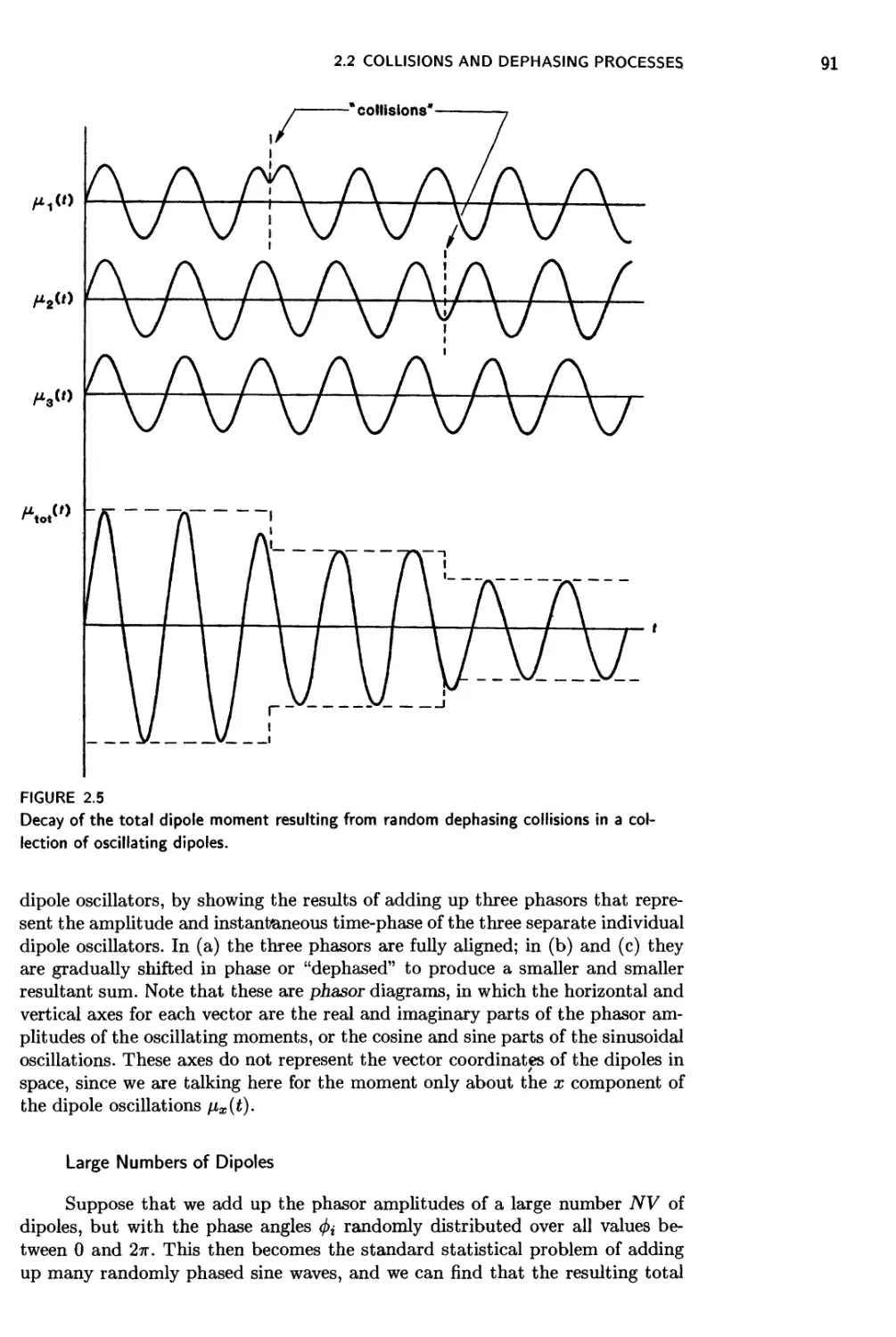


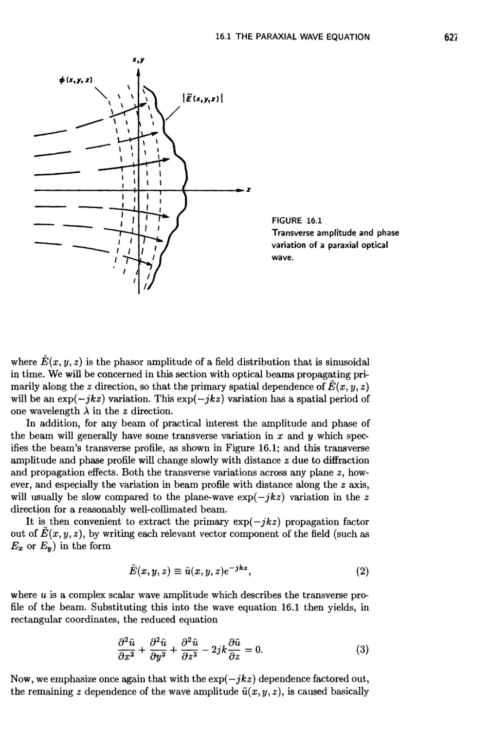


Текст
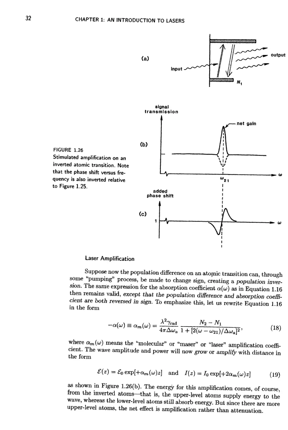
LASERS
Anthony E. Siegman
Professor of Electrical Engineering
Stanford University
University Science Books
Mill Valley, California
University Science Books
20 Edgehill Road
Mill Valley, CA 94941
Manuscript Editor: Aidan Kelly
Designer: Robert Ishi
Production: Miller/Scheier Associates, Palo Alto, CA
TfcjXpert: Laura Poplin
Printer and Binder: The Maple-Vail Book Manufacturing Group
Copyright © 1986 by University Science Books
Reproduction or translation of any part of this work
beyond that permitted by Sections 107 or 108 of the
1976 United States Copyright Act without the permission of
the copyright owner is unlawful. Requests for permission
or further information should be addressed to
the Permissions Department, University Science Books.
Library of Congress Catalog Card Number: 86-050346
ISBN 0-935702-11-5
Printed in the United States of America
This manuscript was prepared at Stanford University using the text
editing facilities of the Context and Sierra DEC-20 computers and
Professor Donald Knuth's T&& typesetting system. Camera-ready
copy was printed on an Autologic APS-^5 phototypesetter.
10 9 8 7 6 5 4
CONTENTS
Preface
Units and Notation
List of Symbols
xiu
xv
xvii
BASIC LASER PHYSICS
1. An Introduction to Lasers 1
2. Stimulated Transitions: The Classical Oscillator Model 80
3. Electric Dipole Transitions in Real Atoms 118
4. Atomic Rate Equations 176
5. The Rabi Frequency 221
6. Laser Pumping and Population Inversion 243
7. Laser Amplification 264
8. More On Laser Amplification 307
9. Linear Pulse Propagation 331
10. Nonlinear Optical Pulse Propagation 362
11. Laser Mirrors and Regenerative Feedback 398
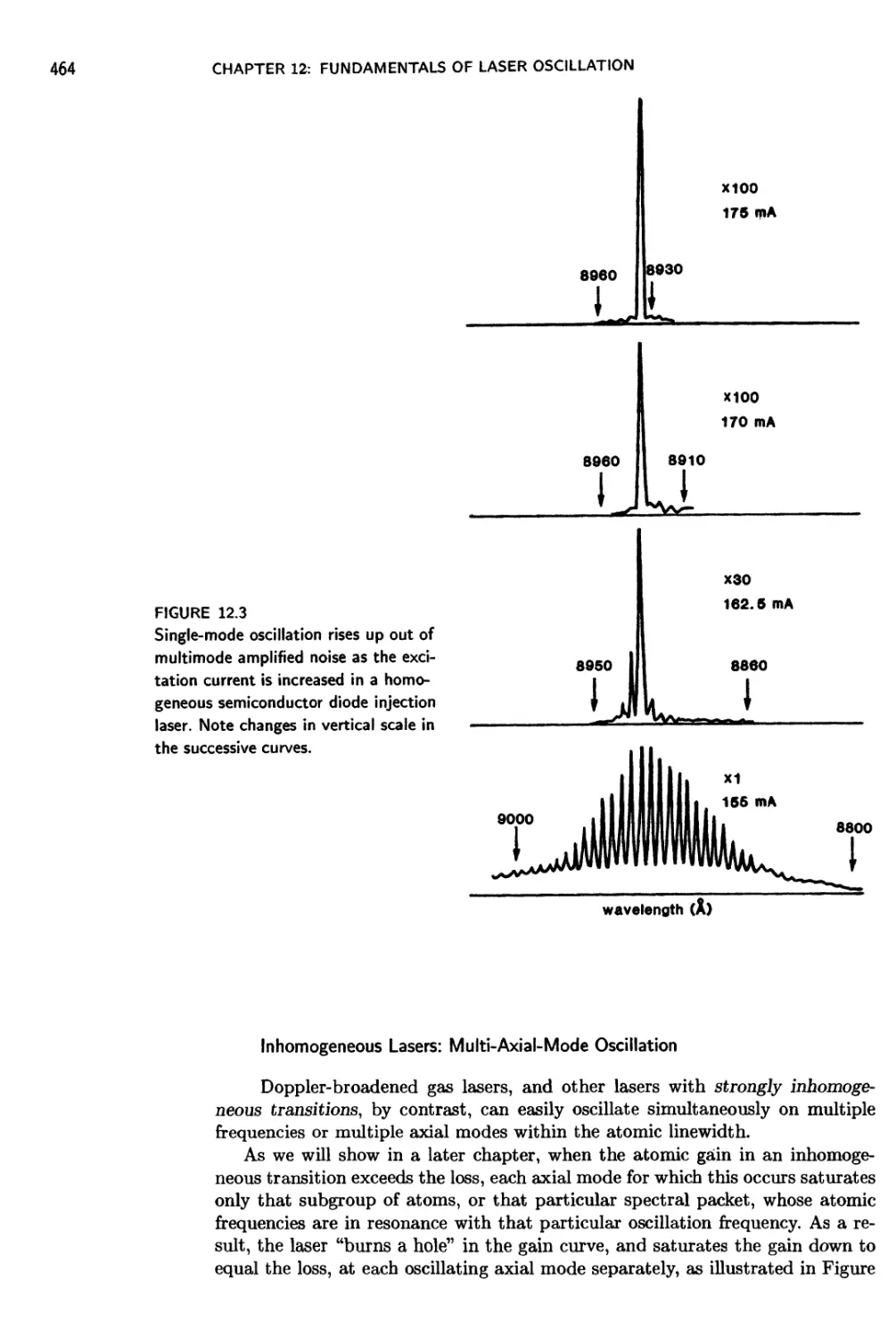
12. Fundamentals of Laser Oscillation 457
13. Oscillation Dynamics and Oscillation Threshold 491
OPTICAL BEAMS AND RESONATORS
14. Optical Beams and Resonators: An Introduction 558
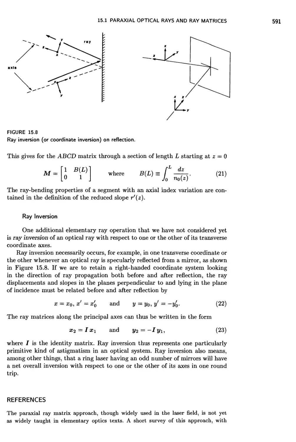
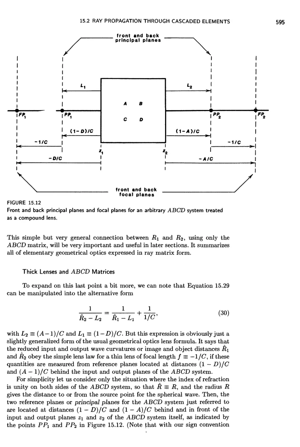
15. Ray Optics and Ray Matrices 581
16. Wave Optics and Gaussian Beams 626
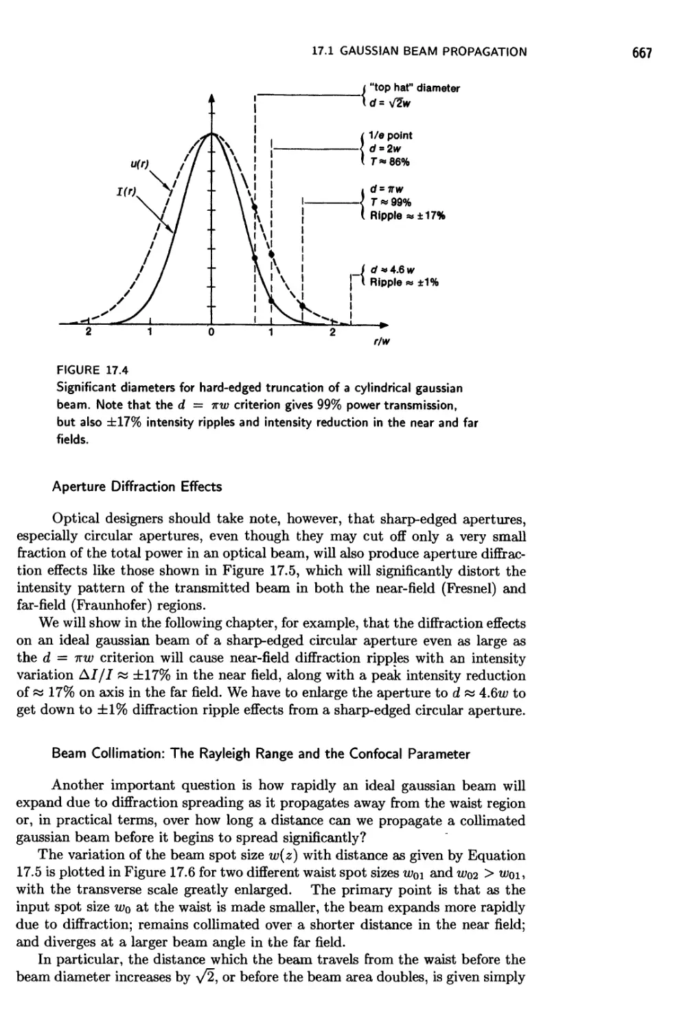
17. Physical Properties of Gaussian Beams 663
18. Beam Perturbation and Diffraction 698
19. Stable Two-Mirror Resonators 744
20. Complex Paraxial Wave Optics 777
21. Generalized Paraxial Resonator Theory 815
22. Unstable Optical Resonators 858
23. More on Unstable Resonators 891
LASER DYNAMICS AND ADVANCED TOPICS
24. Laser Dynamics: The Laser Cavity Equations
25. Laser Spiking and Mode Competition
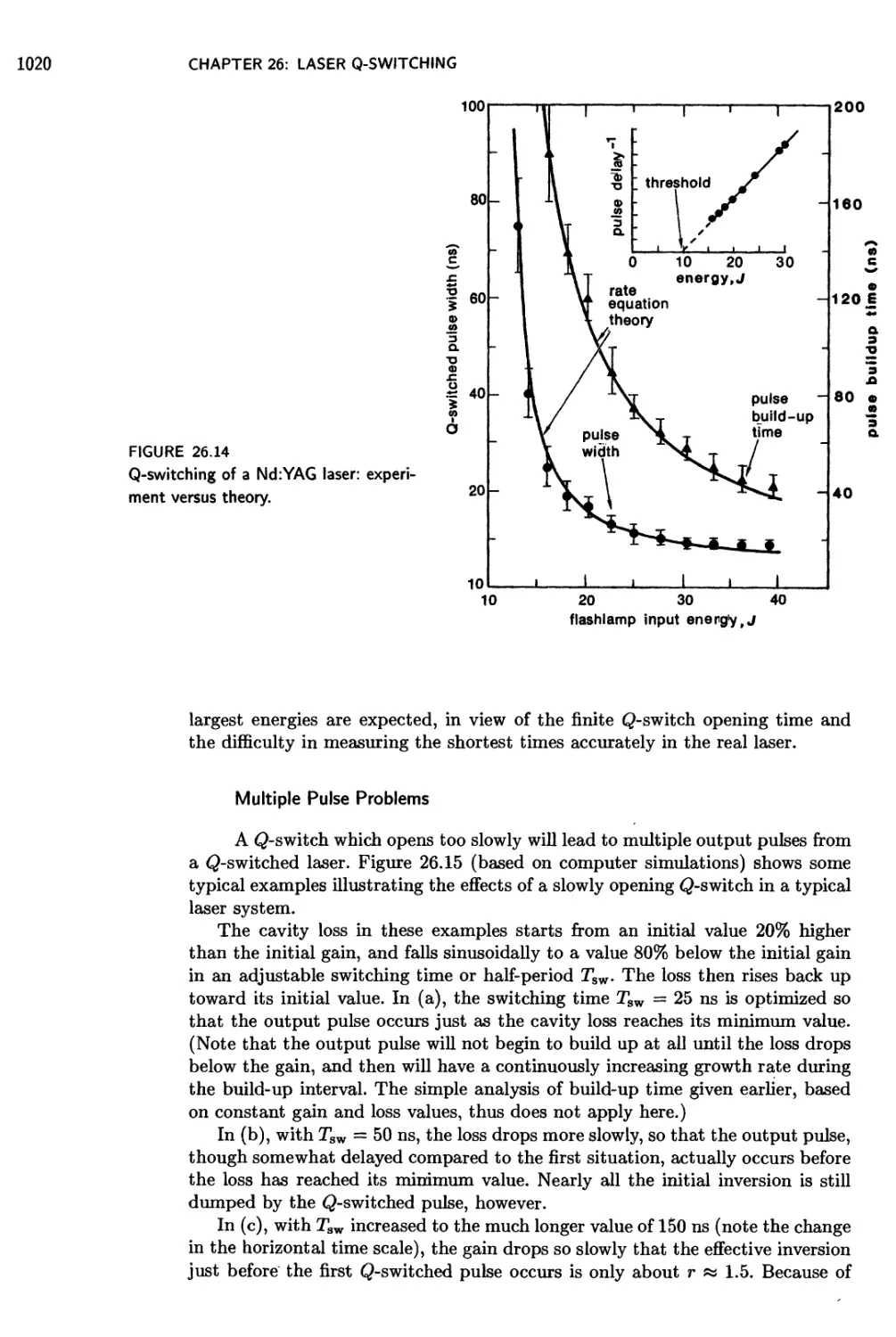
26. Laser Q-Switching
27. Active Laser Mode Coupling
28. Passive Mode Locking
29. Laser Injection Locking
30. Hole Burning and Saturation Spectroscopy
31. Magnetic-Dipole Transitions
923
954
1004
1041
1104
1129
1171
1213
LIST OF TOPICS
Preface xiii
Units and Notation xv
List of Symbols xvii
BASIC LASER PHYSICS
Chapter 1 An Introduction to Lasers
1.1 What Is a Laser? 2
1.2 Atomic Energy Levels and Spontaneous Emission 6
1.3 Stimulated Atomic Transitions 18
1.4 Laser Amplification 30
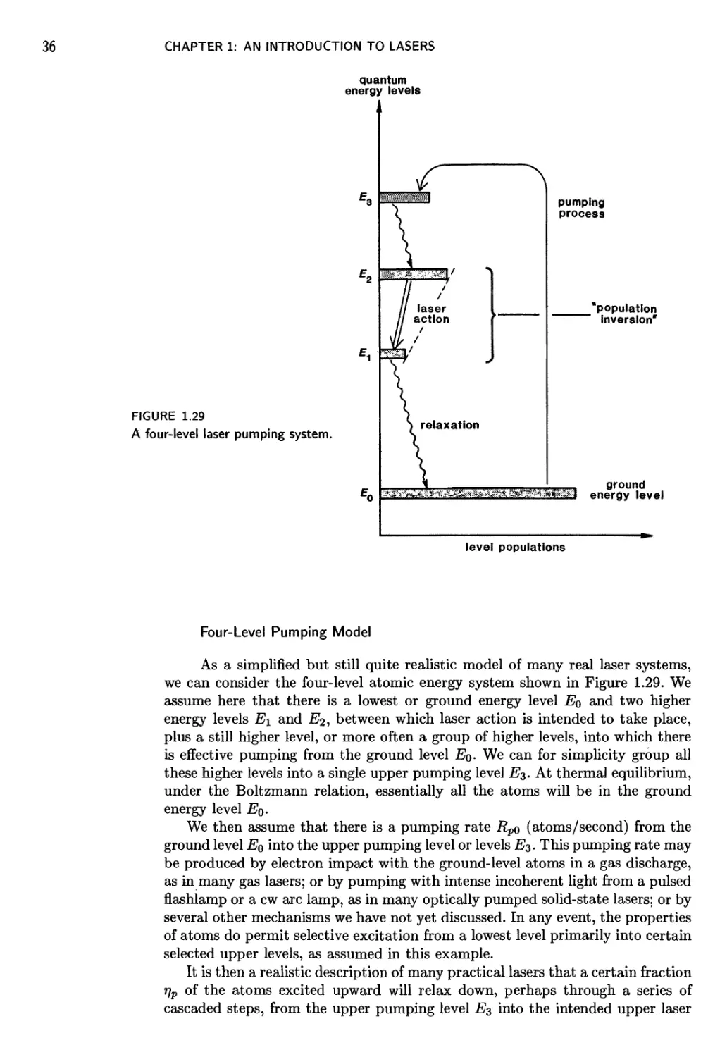
1.5 Laser Pumping and Population Inversion 35
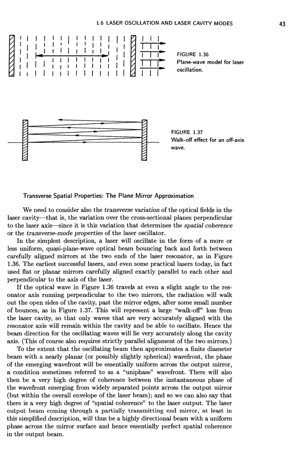
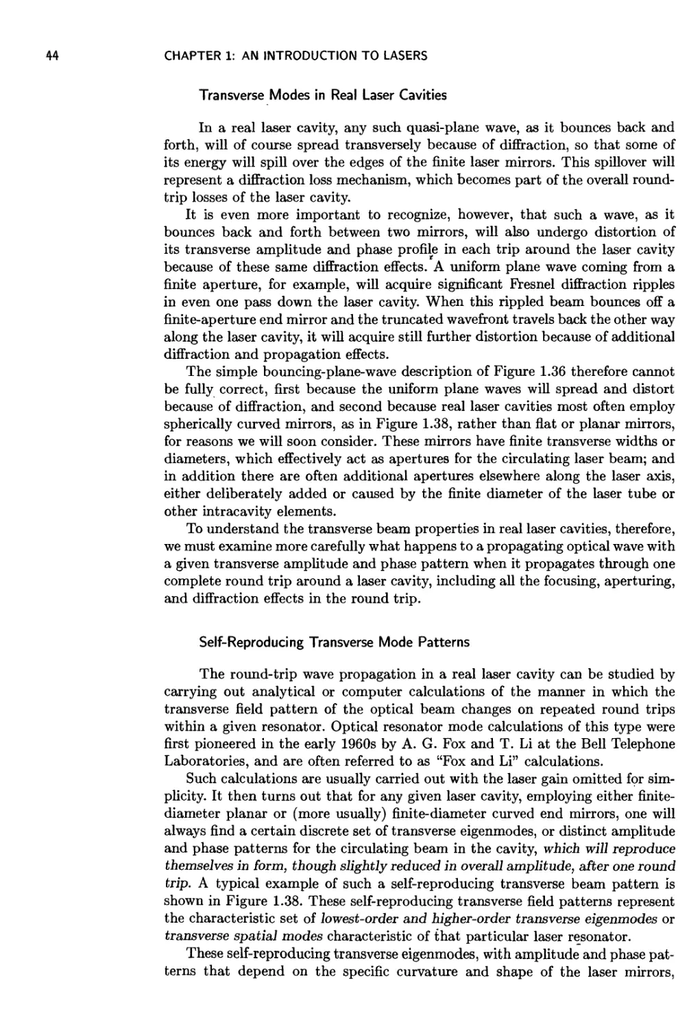
1.6 Laser Oscillation and Laser Cavity Modes 39
1.7 Laser Output-Beam Properties 49
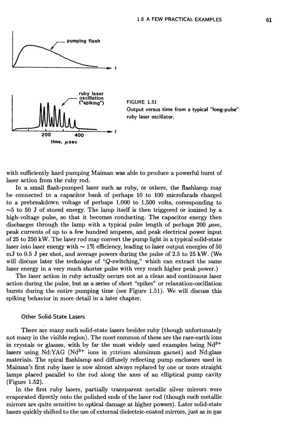
1.8 A Few Practical Examples 60
1.9 Other Properties of Real Lasers 66
1.10 Historical Background of the Laser 74
1.11 Additional Problems for Chapter 1 76
Chapter 2 Stimulated Transitions: The Classical Oscillator Model
2.1 The Classical Electron Oscillator 80
2.2 Collisions and Dephasing Processes 89
2.3 More on Atomic Dynamics and Dephasing 97
2.4 Steady-State Response: The Atomic Susceptibility 102
2.5 Conversion to Real Atomic Transitions 110
Chapter 3 Electric Dipole Transitions in Real Atoms
3.1 Decay Rates and Transition Strengths in Real Atoms 118
3.2 Line Broadening Mechanisms in Real Atoms 126
3.3 Polarization Properties of Atomic Transitions 135
3.4 Tensor Susceptibilities 143
3.5 The "Factor of Three" 150
3.6 Degenerate Energy Levels and Degeneracy Factors 153
3.7 Inhomogeneous Line Broadening 157
Chapter 4 Atomic Rate Equations
4.1 Power Transfer From Signals to Atoms 176
LIST OF TOPICS
4.2 Stimulated Transition Probability 181
4.3 Blackbody Radiation and Radiative Relaxation 187
4.4 Nonradiative Relaxation 195
4.5 Two-Level Rate Equations and Saturation 204
4.6 Multilevel Rate Equations 211
Chapter 5 The Rabi Frequency
5.1 Validity of the Rate Equation Model 221
5.2 Strong Signal Behavior: The Rabi Frequency 229
Chapter 6 Laser Pumping and Population Inversion
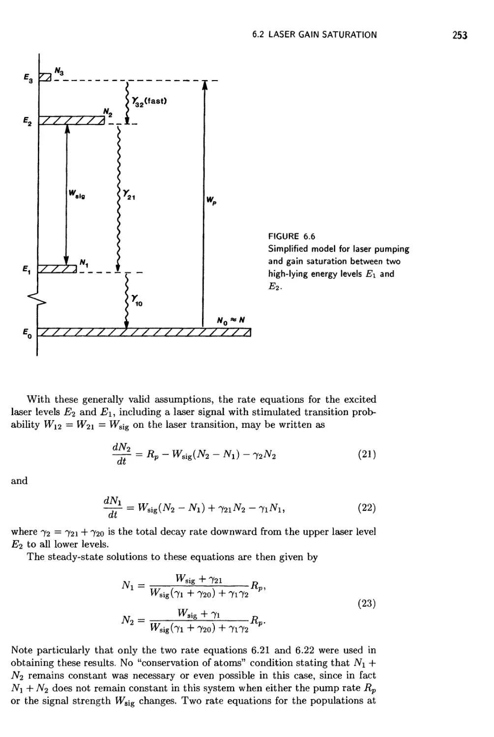
6.1 Steady-State Laser Pumping and Population Inversion 243
6.2 Laser Gain Saturation 252
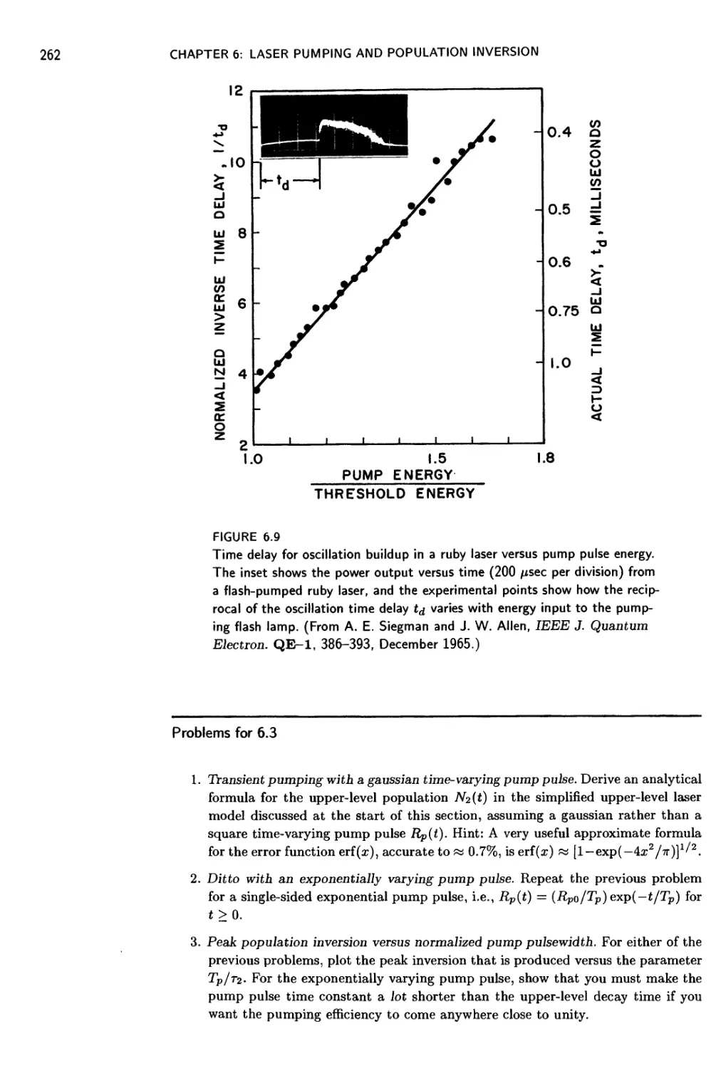
6.3 Transient Laser Pumping 257
Chapter 7 Laser Amplification
7.1 Practical Aspects of Laser Amplifiers 264
7.2 Wave Propagation in an Atomic Medium 266
7.3 The Paraxial Wave Equation 276
7.4 Single-Pass Laser Amplification 279
7.5 Stimulated Transition Cross Sections 286
7.6 Saturation Intensities in Laser Materials 292
7.7 Homogeneous Saturation in Laser Amplifiers 297
Chapter 8 More On Laser Amplification
8.1 Transient Response of Laser Amplifiers 307
8.2 Spatial Hole Burning, and Standing-Wave Grating Effects 316
8.3 More on Laser Amplifier Saturation 323
Chapter 9 Linear Pulse Propagation
9.1 Phase and Group Velocities 331
9.2 The Parabolic Equation 339
9.3 Group Velocity Dispersion and Pulse Compression 343
9.4 Phase and Group Velocities in Resonant Atomic Media 351
9.5 Pulse Broadening and Gain Dispersion 356
Chapter 10 Nonlinear Optical Pulse Propagation
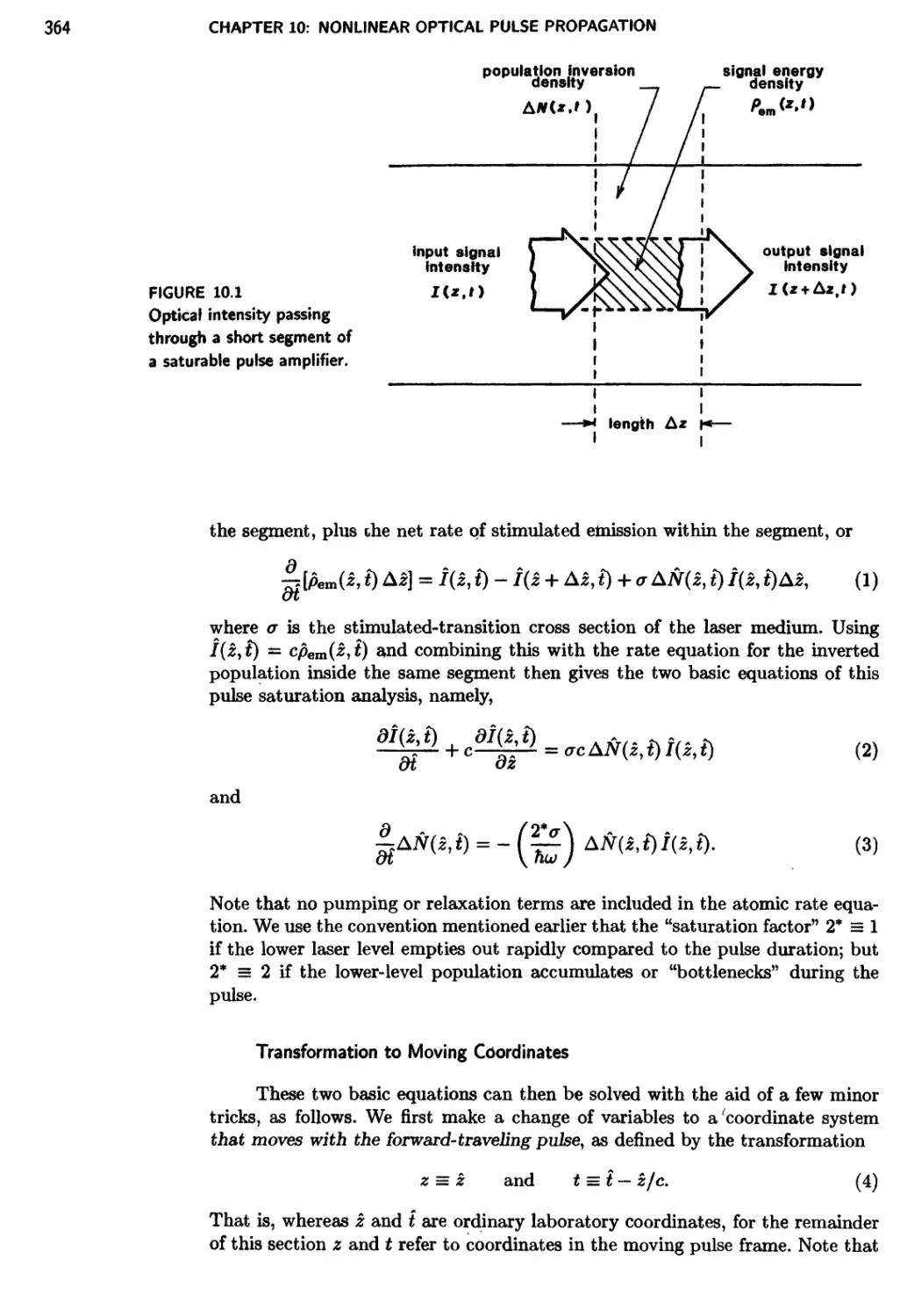
10.1 Pulse Amplification With Homogeneous Gain Saturation 362
10.2 Pulse Propagation in Nonlinear Dispersive Systems 375
10.3 The Nonlinear Schrodinger Equation 387
10.4 Nonlinear Pulse Broadening in Optical Fibers 388
10.5 Solitons in Optical Fibers 392
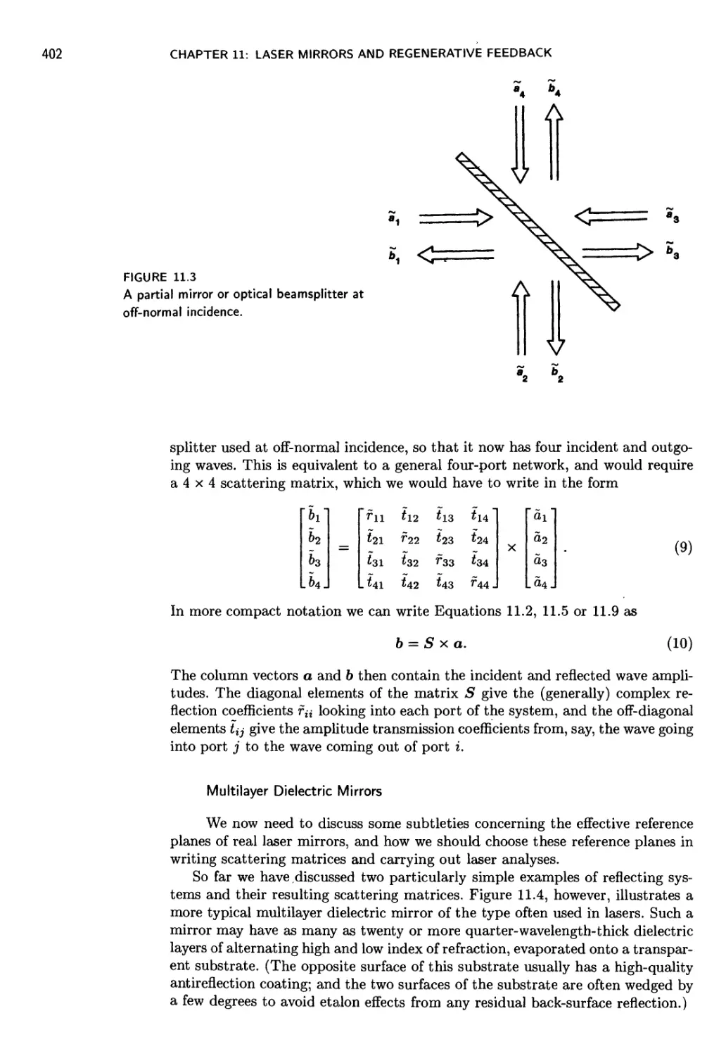
Chapter 11 Laser Mirrors and Regenerative Feedback
11.1 Laser Mirrors and Beam Splitters 398
11.2 Interferometers and Resonant Optical Cavities 408
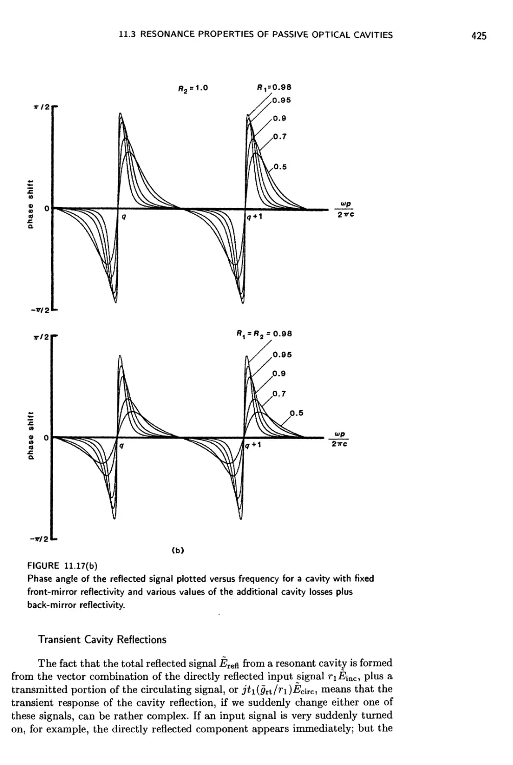
11.3 Resonance Properties of Passive Optical Cavities 413
LIST OF TOPICS
11.4 "Delta Notation" for Cavity Gains and Losses 428
11.5 Optical-Cavity Mode Frequencies 432
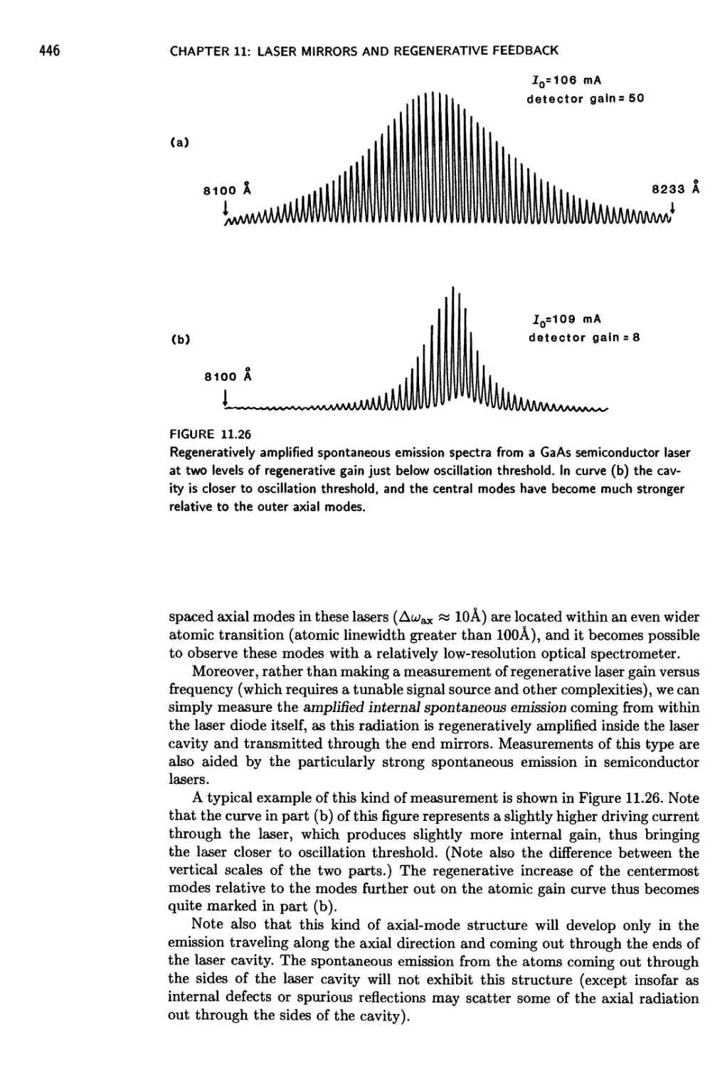
11.6 Regenerative Laser Amplification 440
11.7 Approaching Threshold: The Highly Regenerative Limit 447
Chapter 12 Fundamentals of Laser Oscillation
12.1 Oscillation Threshold Conditions 457
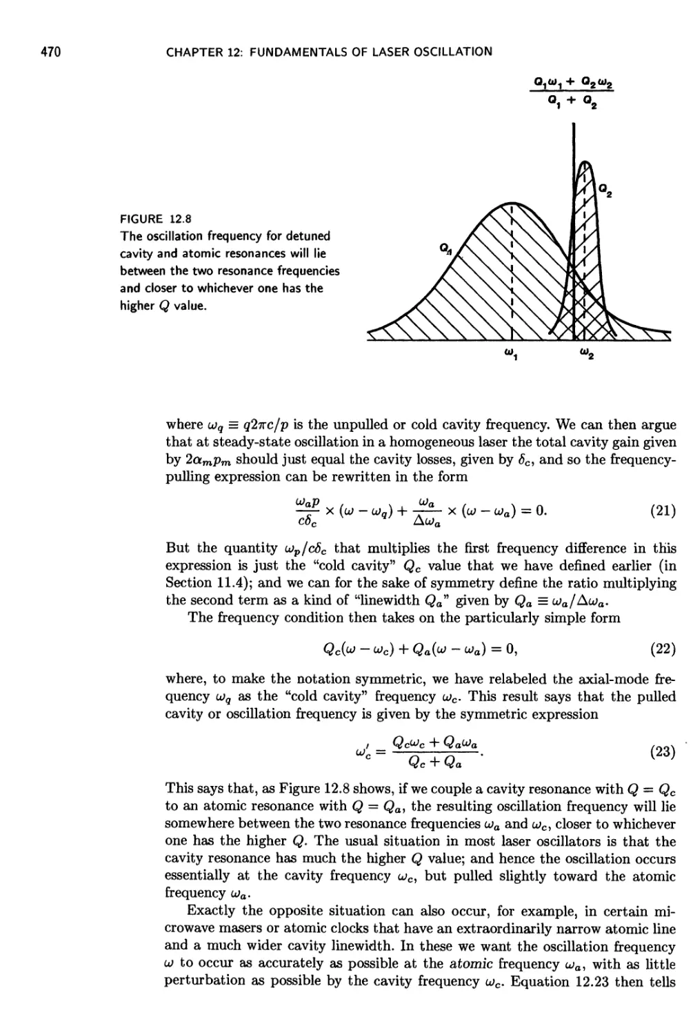
12.2 Oscillation Frequency and Frequency Pulling 462
12.3 Laser Output Power 473
12.4 The Large Output Coupling Case 485
Chapter 13 Oscillation Dynamics and Oscillation Threshold
13.1 Laser Oscillation Buildup 491
13.2 Derivation of the Cavity Rate Equation 497
13.3 Coupled Cavity and Atomic Rate Equations 505
13.4 The Laser Threshold Region 510
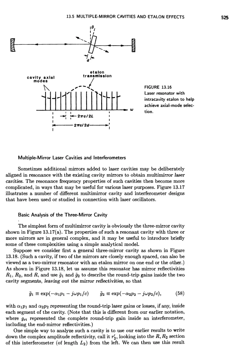
13.5 Multiple-Mirror Cavities and Etalon Effects 524
13.6 Unidirectional Ring-Laser Oscillators 532
13.7 Bistable Optical Systems 538
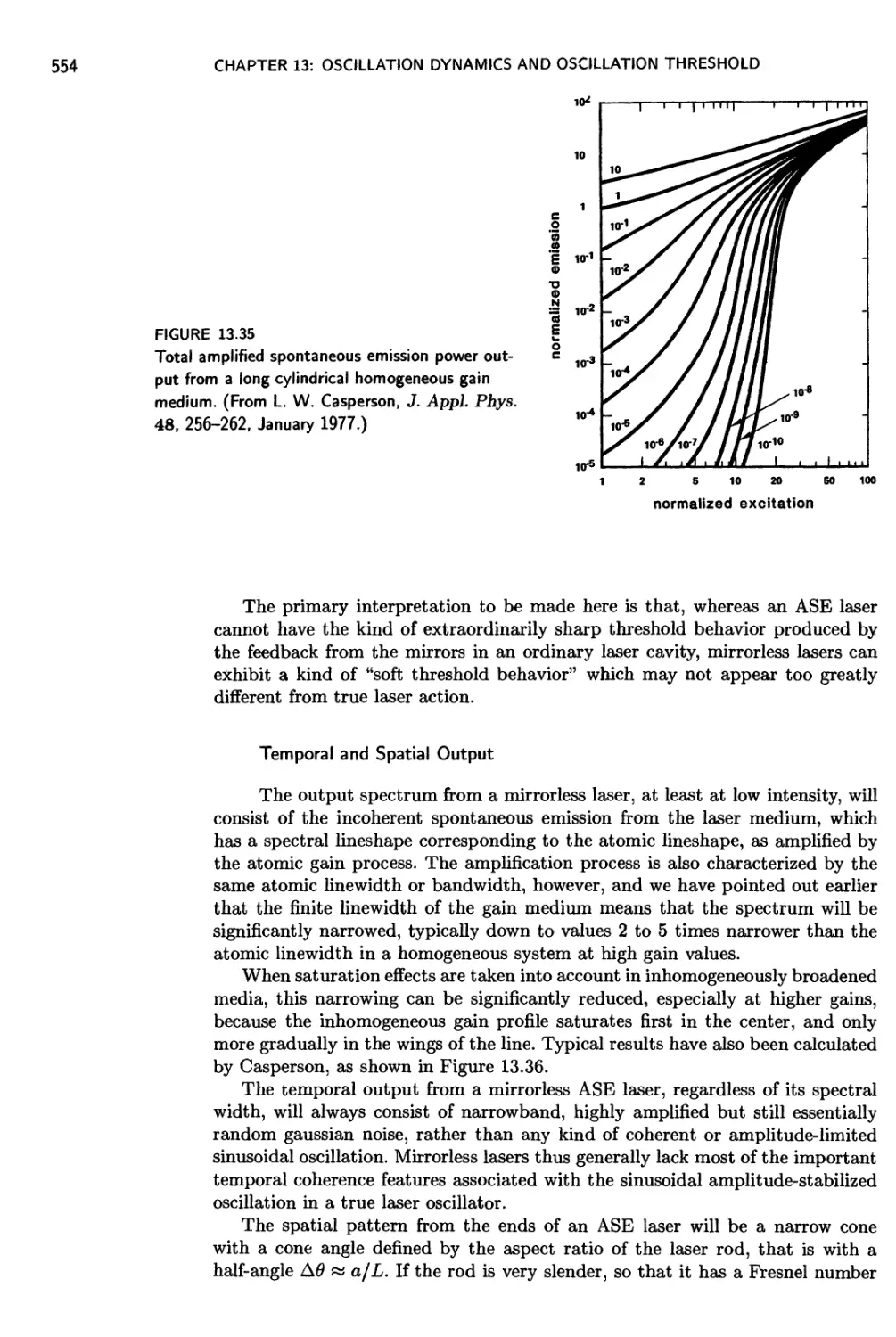
13.8 Amplified Spontaneous Emission and Mirrorless Lasers 547
OPTICAL BEAMS AND RESONATORS
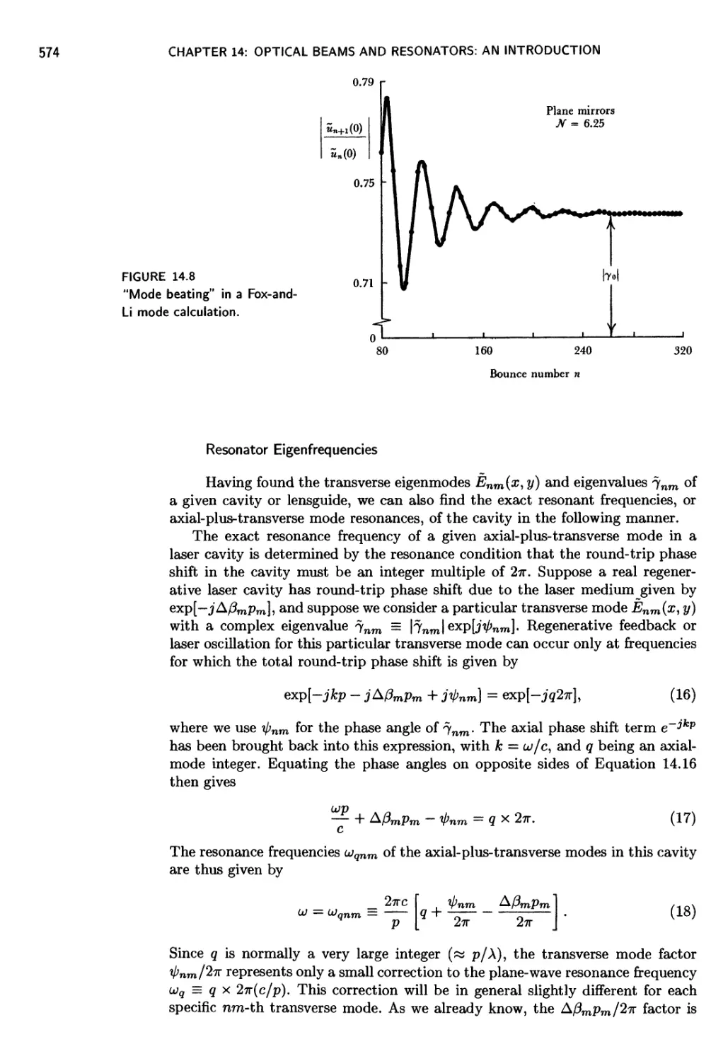
Chapter 14 Optical Beams and Resonators: An Introduction
14.1 Transverse Modes in Optical Resonators 559
14.2 The Mathematics of Optical Resonator Modes 565
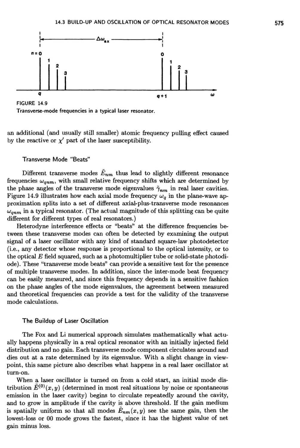
14.3 Build-Up and Oscillation of Optical Resonator Modes 569
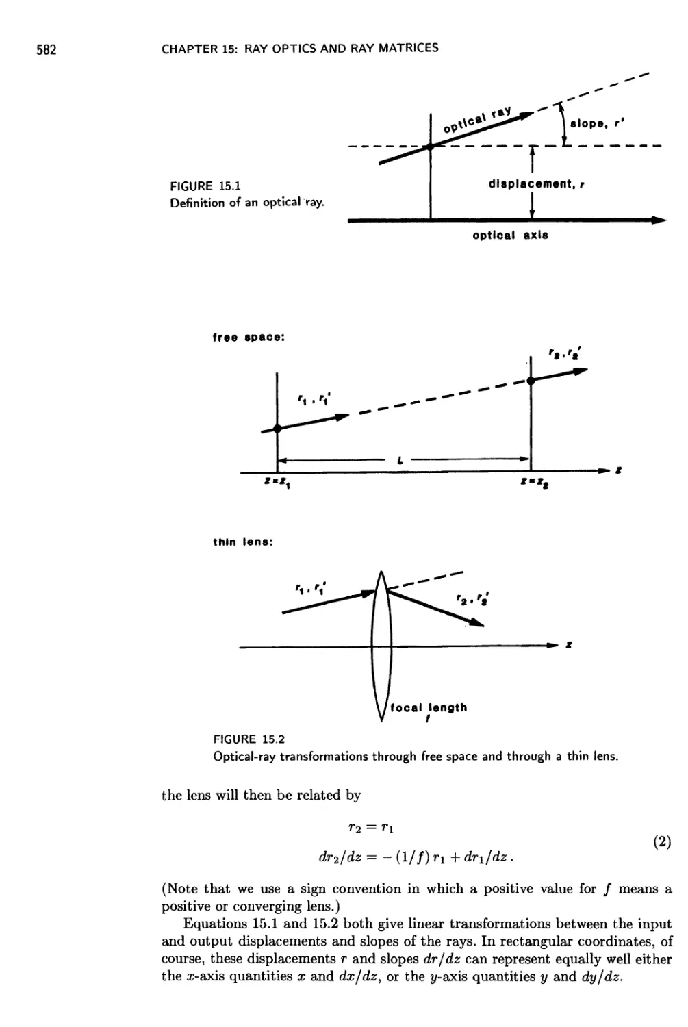
Chapter 15 Ray Optics and Ray Matrices
15.1 Paraxial Optical Rays and Ray Matrices 581
15.2 Ray Propagation Through Cascaded Elements 593
15.3 Rays in Periodic Focusing Systems 599
15.4 Ray Optics With Misaligned Elements 607
15.5 Ray Matrices in Curved Ducts 614
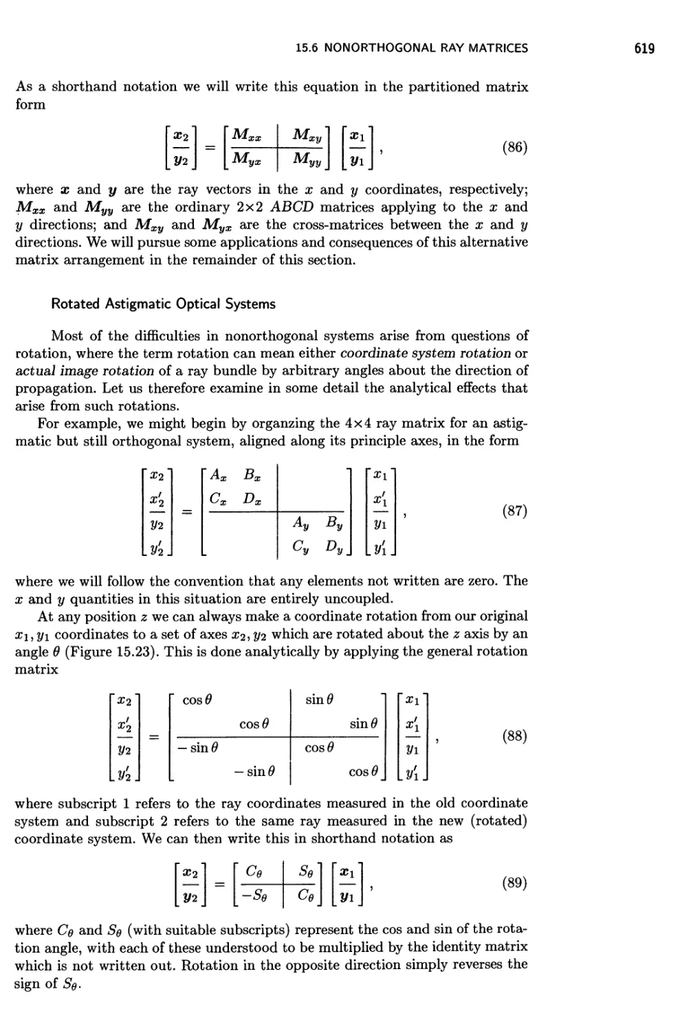
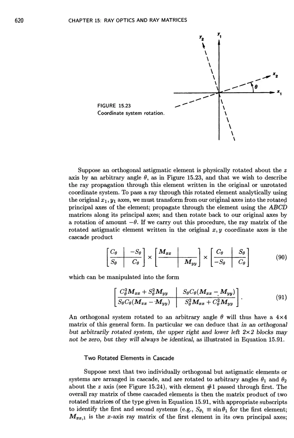
15.6 Nonorthogonal Ray Matrices 616
Chapter 16 Wave Optics and Gaussian Beams
16.1 The Paraxial Wave Equation 626
16.2 Huygens' Integral 630
16.3 Gaussian Spherical Waves 637
16.4 Higher-Order Gaussian Modes 642
16.5 Complex-Argument Gaussian Modes 649
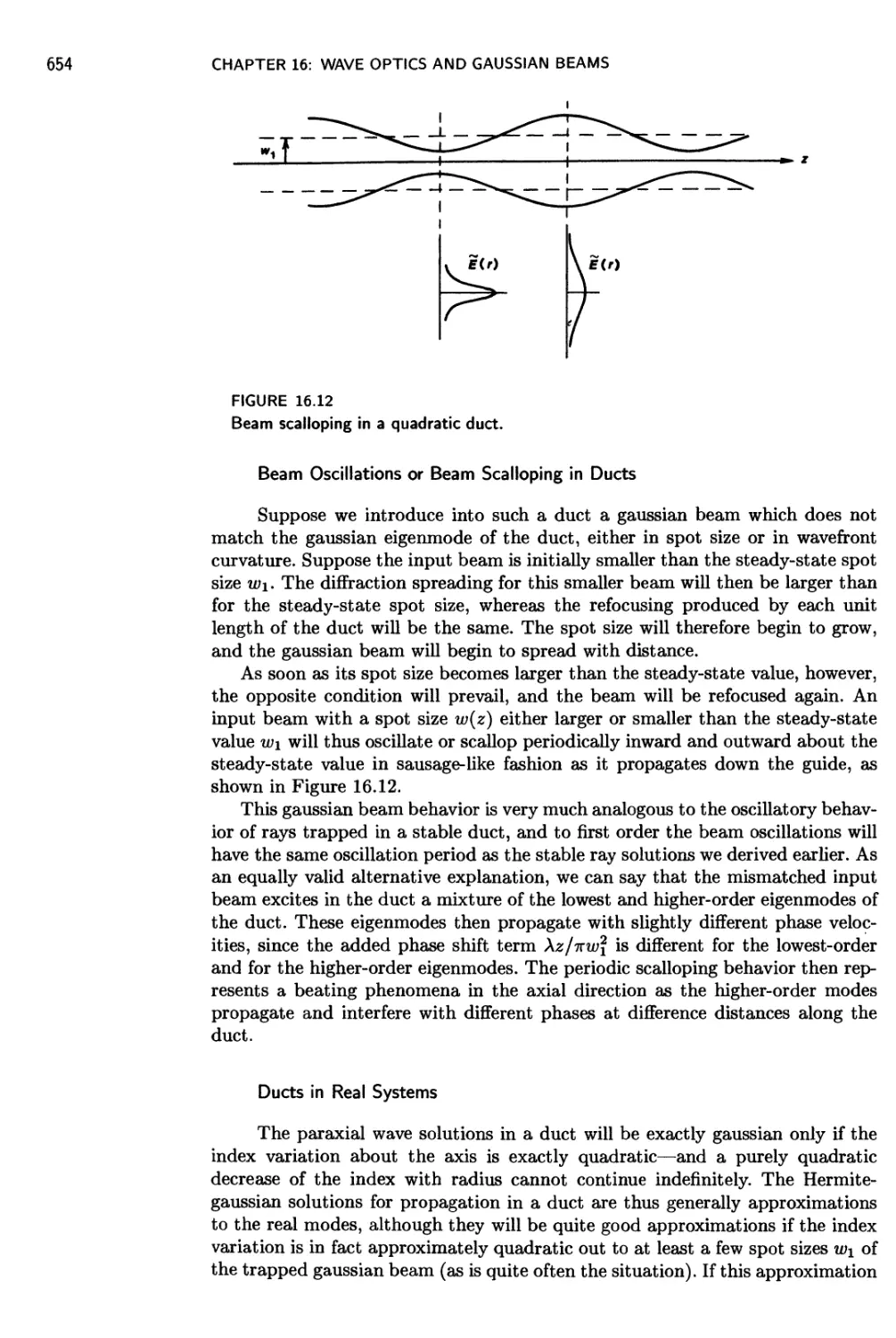
16.6 Gaussian Beam Propagation in Ducts 652
16.7 Numerical Beam Propagation Methods 656
LIST OF TOPICS
Chapter 17 Physical Properties of Gaussian Beams
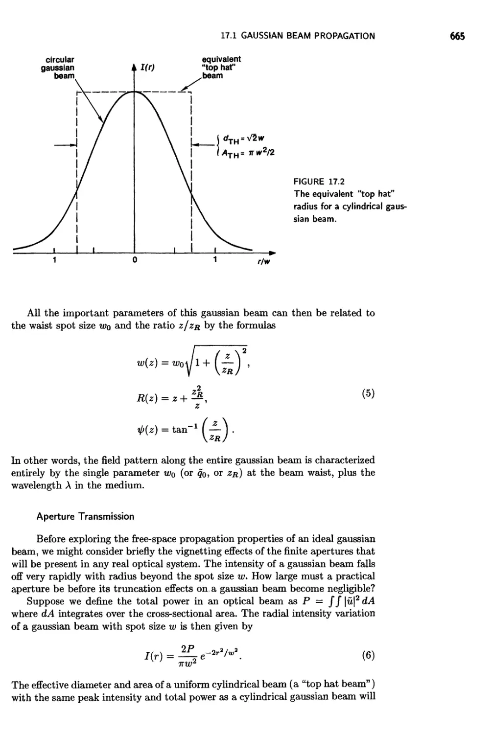
17.1 Gaussian Beam Propagation 663
17.2 Gaussian Beam Focusing 675
17.3 Lens Laws and Gaussian Mode Matching 680
17.4 Axial Phase Shift: The Guoy Effect 682
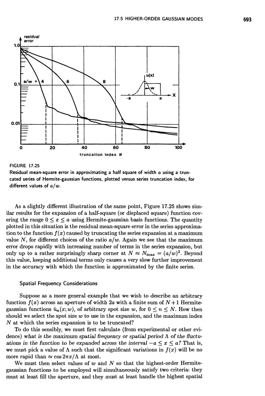
17.5 Higher-Order Gaussian Modes 685
17.6 Multimode Optical Beams 695
Chapter 18 Beam Perturbation and Diffraction
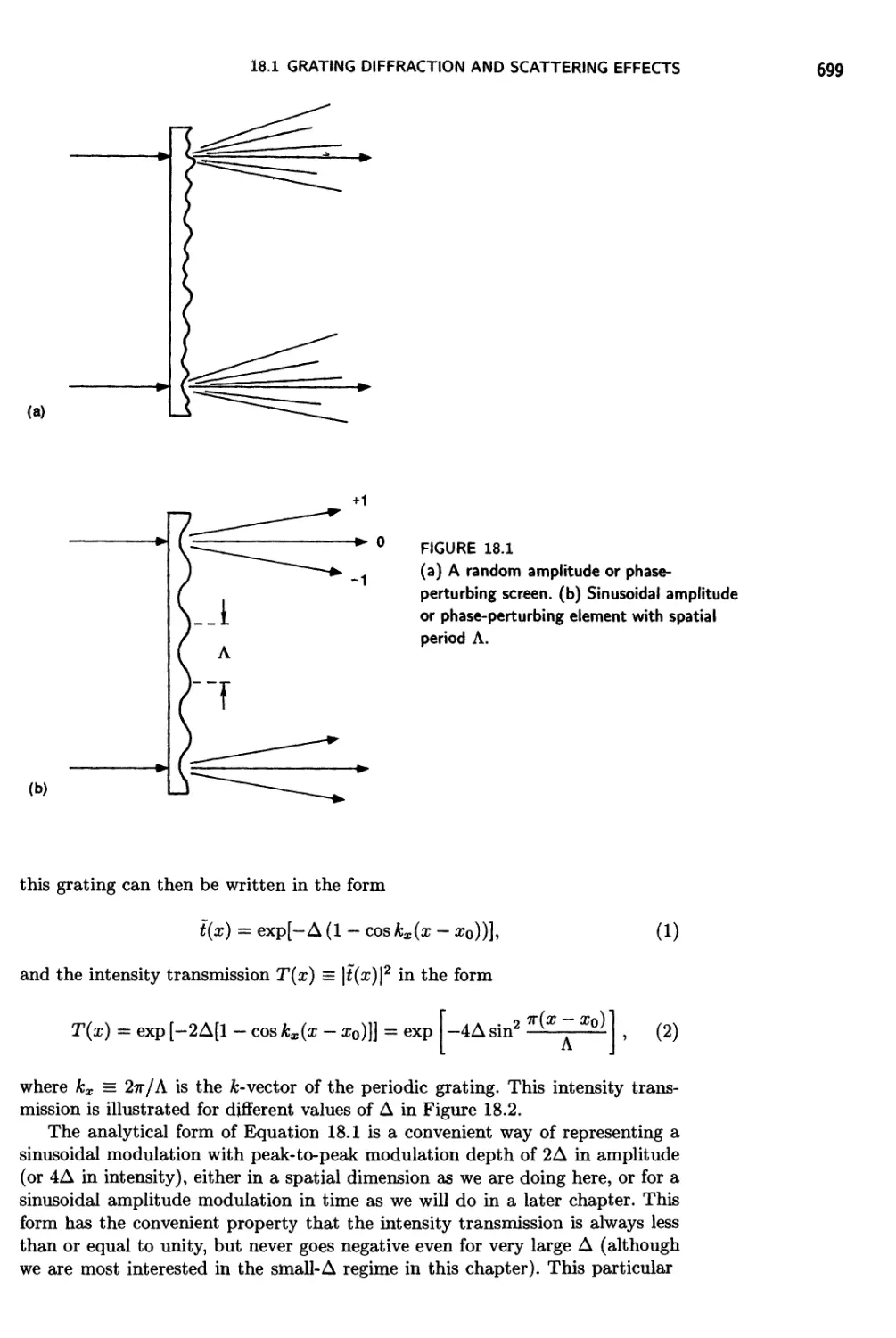
18.1 Grating Diffraction and Scattering Effects 698
18.2 Aberrated Laser Beams 706
18.3 Aperture Diffraction: Rectangular Apertures 712
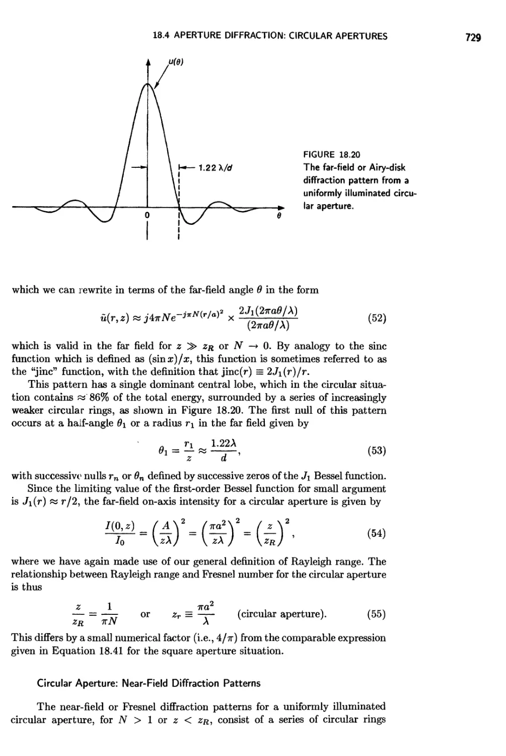
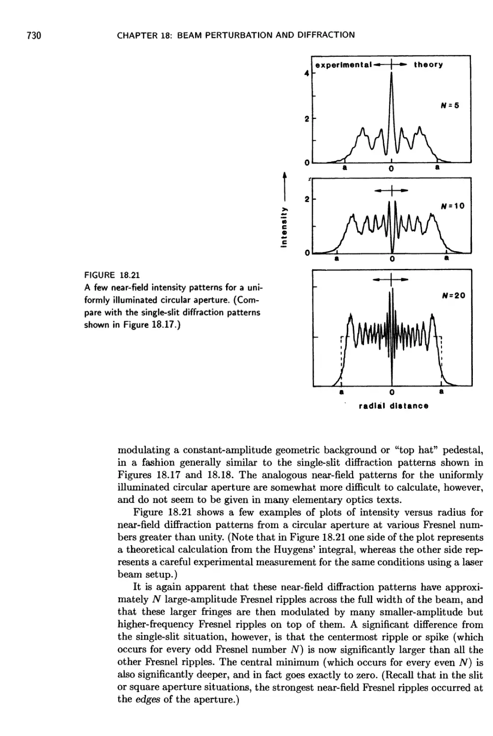
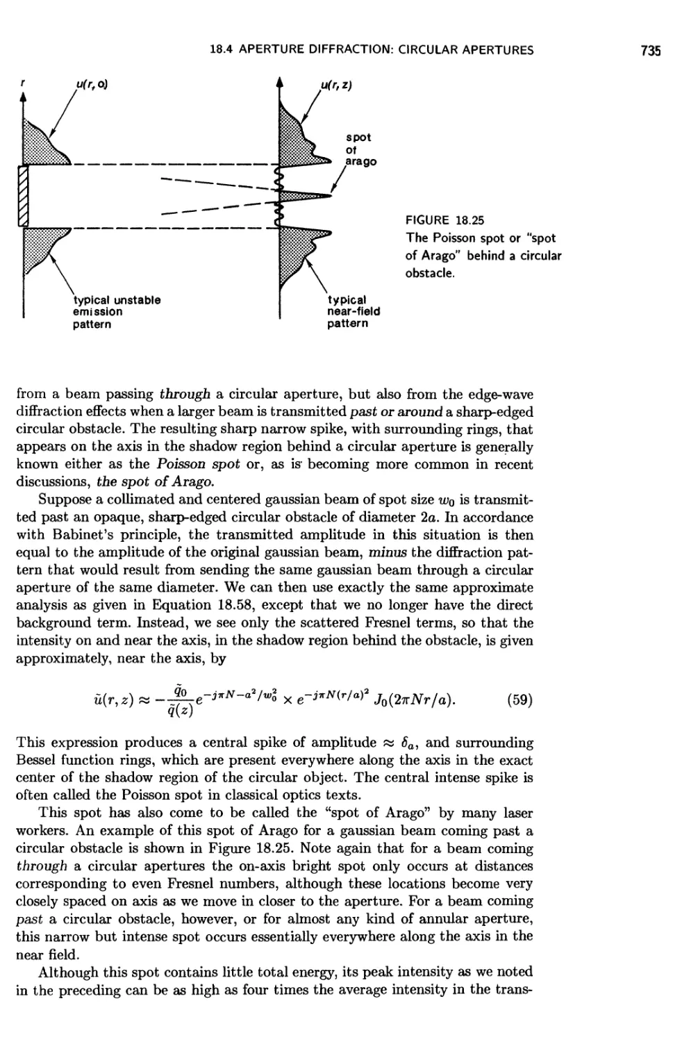
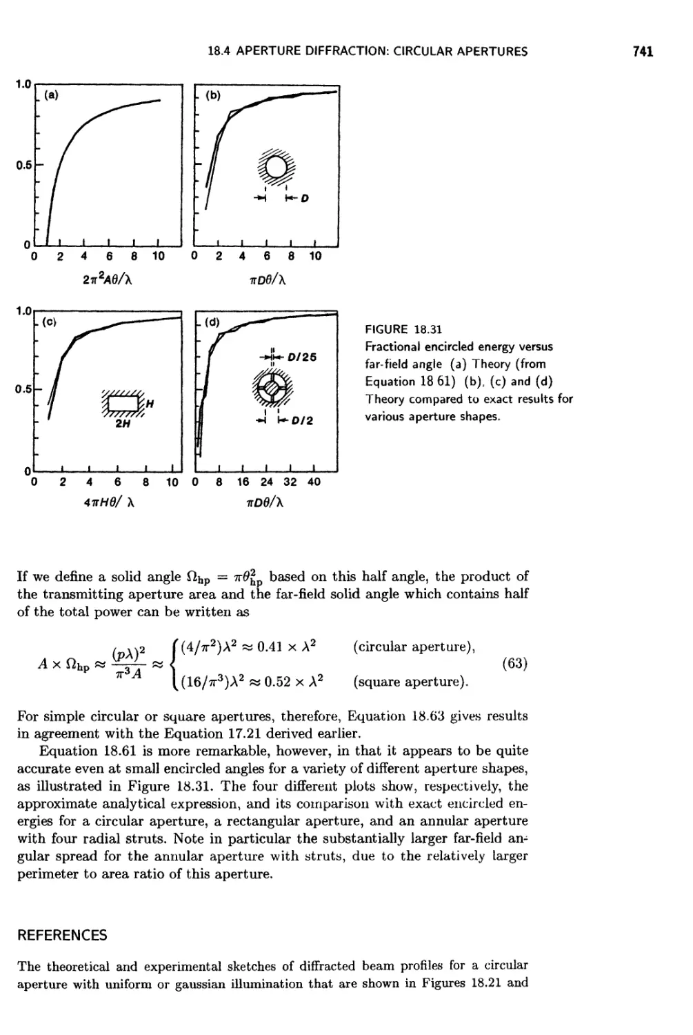
18.4 Aperture Diffraction: Circular Apertures 727
Chapter 19 Stable Two-Mirror Resonators
19.1 Stable Gaussian Resonator Modes 744
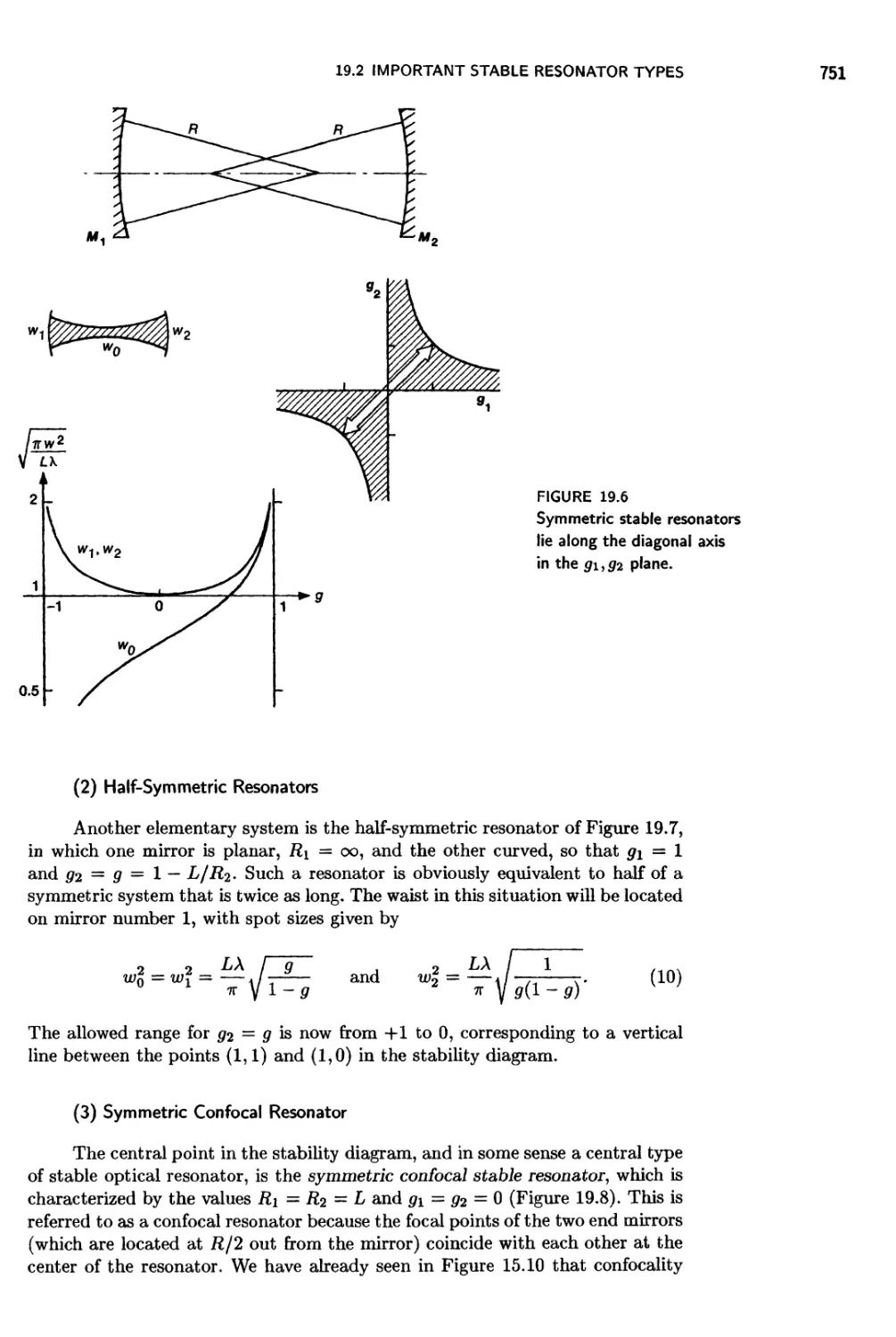
19.2 Important Stable Resonator Types 750
19.3 Gaussian Transverse Mode Frequencies 761
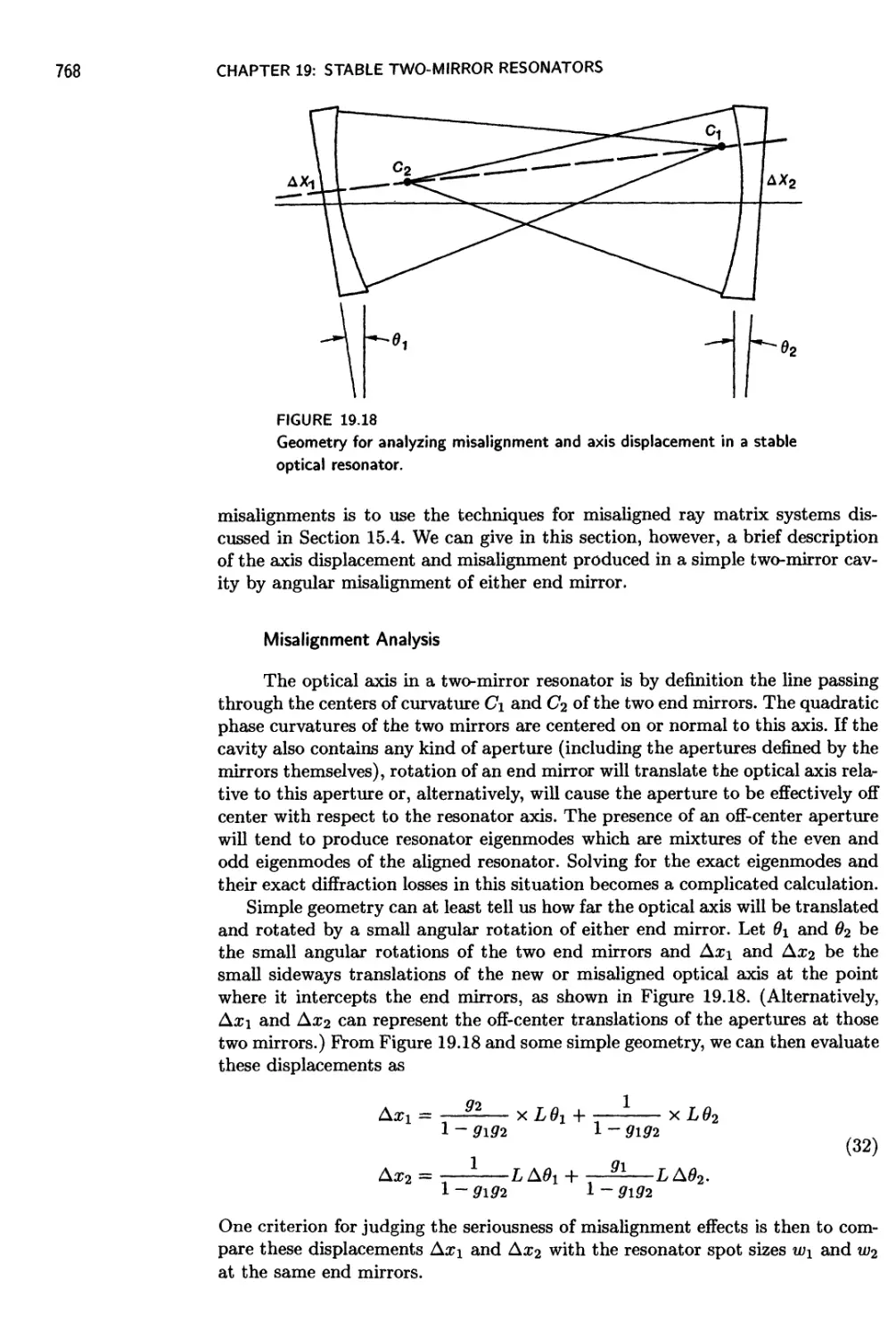
19.4 Misalignment Effects in Stable Resonators 767
19.5 Gaussian Resonator Mode Losses 769
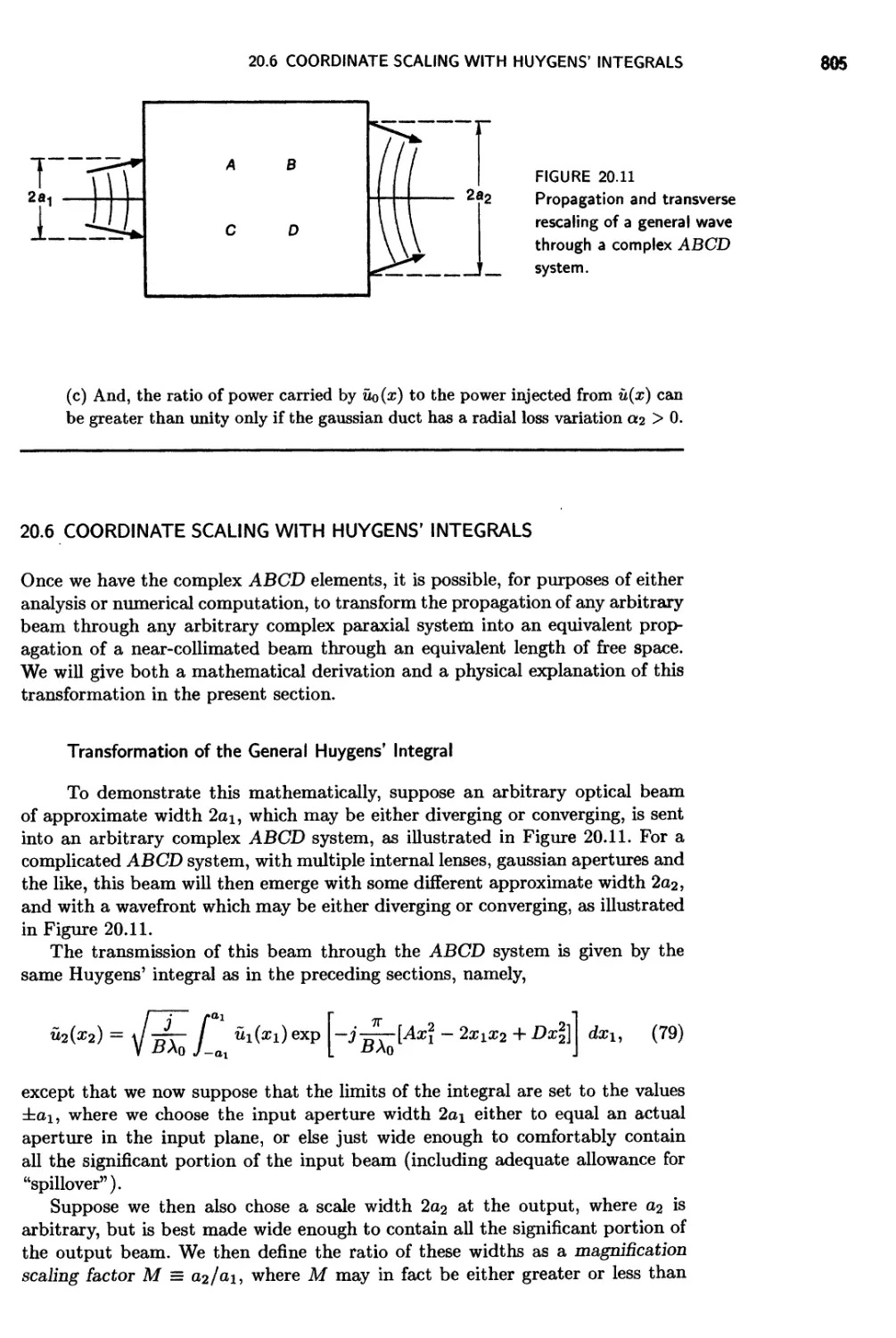
Chapter 20 Complex Paraxial Wave Optics
20.1 Huygens' Integral and ABCD Matrices 777
20.2 Gaussian Beams and ABCD Matrices 782
20.3 Gaussian Apertures and Complex ABCD Matrices 786
20.4 Complex Paraxial Optics 792
20.5 Complex Hermite-Gaussian Modes 798
20.6 Coordinate Scaling with Huygens' Integrals 805
20.7 Synthesis and Factorization of ABCD Matrices 811
Chapter 21 Generalized Paraxial Resonator Theory
21.1 Complex Paraxial Resonator Analysis 815
21.2 Real and Geometrically Stable Resonators 820
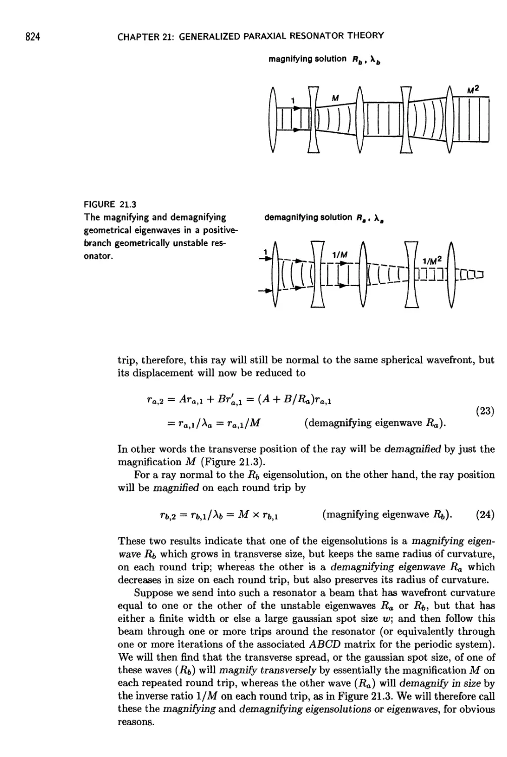
21.3 Real and Geometrically Unstable Resonators 822
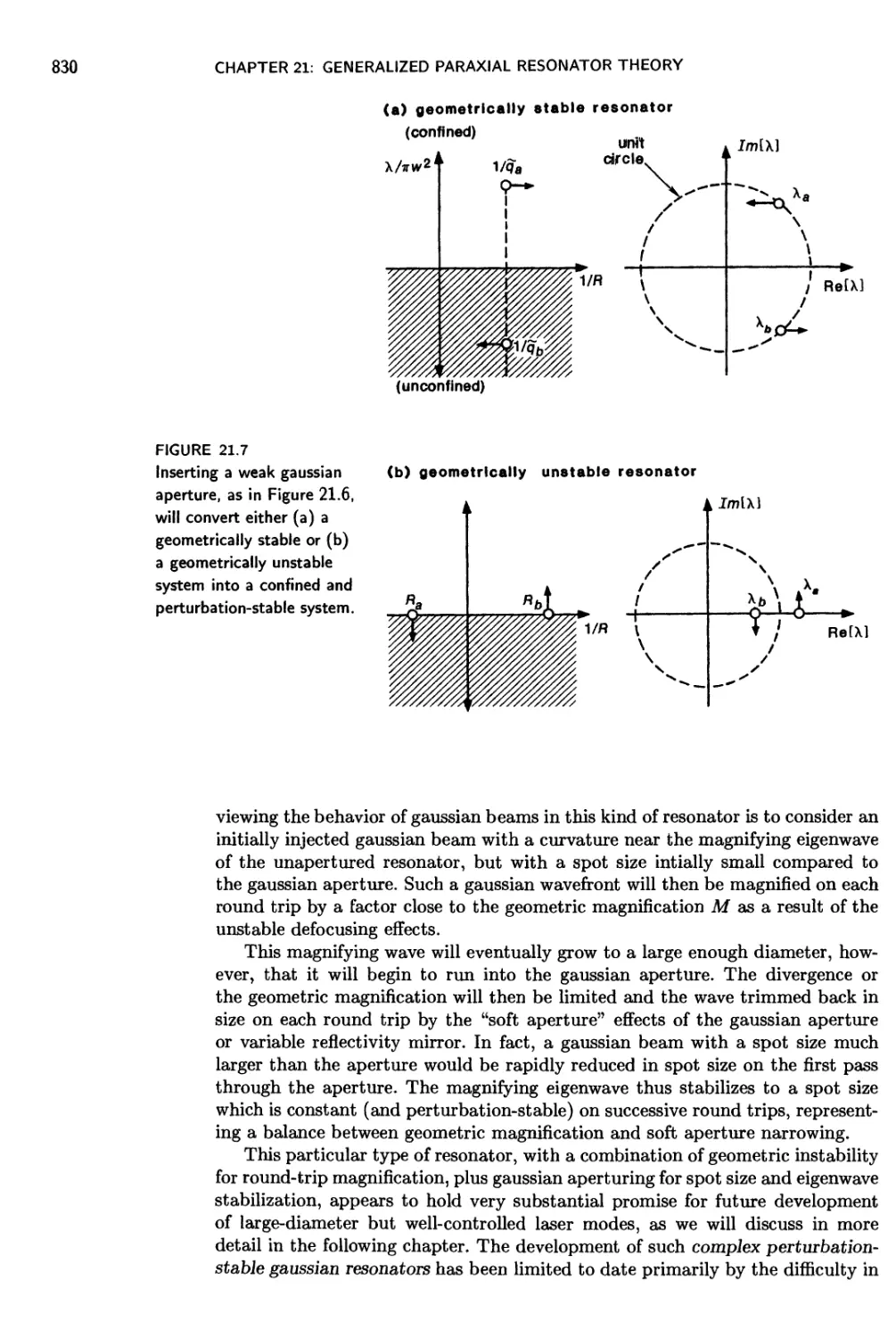
21.4 Complex Stable and Unstable Resonators 828
21.5 Other General Properties of Paraxial Resonators 835
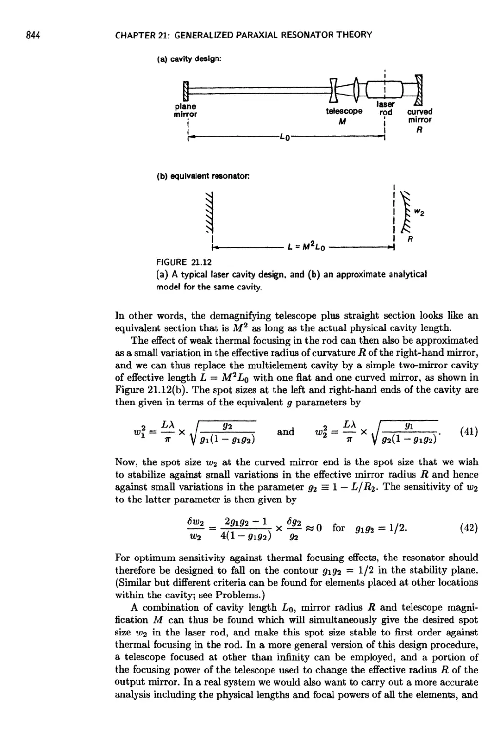
21.6 Multi-Element Stable Resonator Designs 841
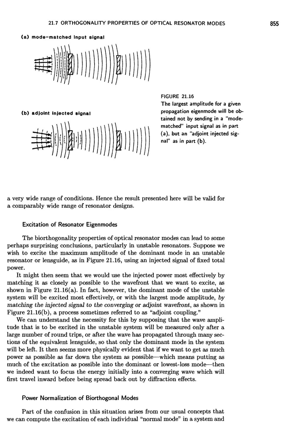
21.7 Orthogonality Properties of Optical Resonator Modes 847
Chapter 22 Unstable Optical Resonators
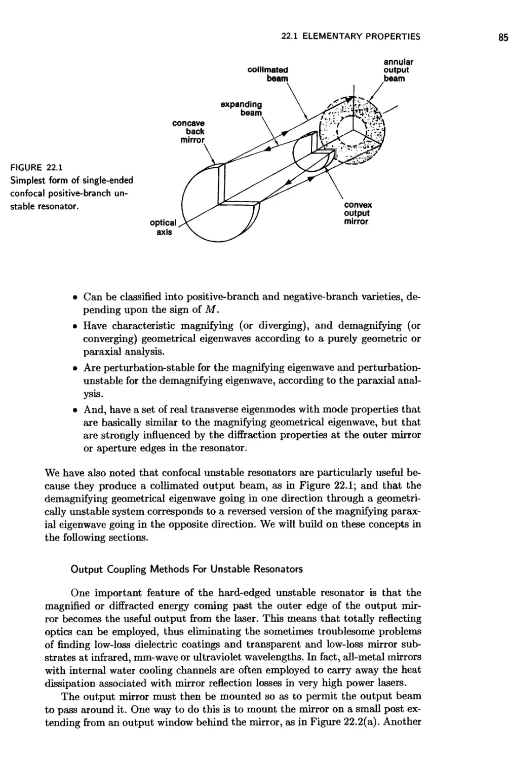
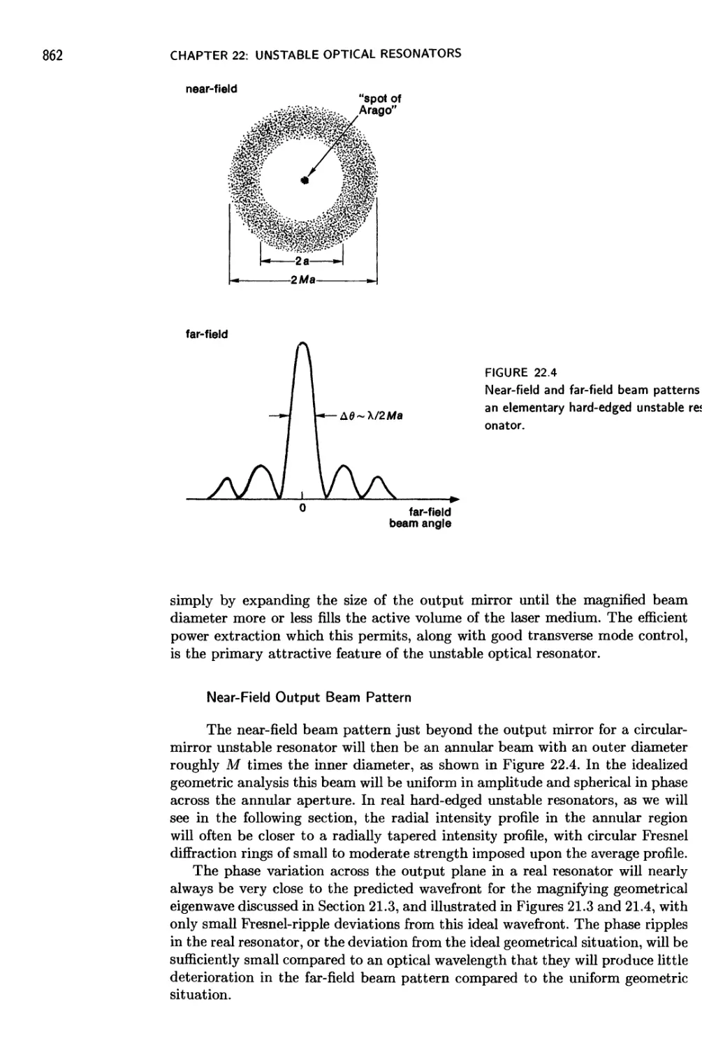
22.1 Elementary Properties 858
22.2 Canonical Analysis for Unstable Resonators 867
22.3 Hard-Edged Unstable Resonators 874
22.4 Unstable Resonators: Experimental Results 884
Chapter 23 More on Unstable Resonators
23.1 Advanced Analyses of Unstable Resonators 891
LIST OF TOPICS
23.2 Other Novel Unstable Resonator Designs 899
23.3 Variable-Reflectivity Unstable Resonators 913
LASER DYNAMICS AND ADVANCED TOPICS
Chapter 24 Laser Dynamics: The Laser Cavity Equations
24.1 Derivation of the Laser Cavity Equations 923
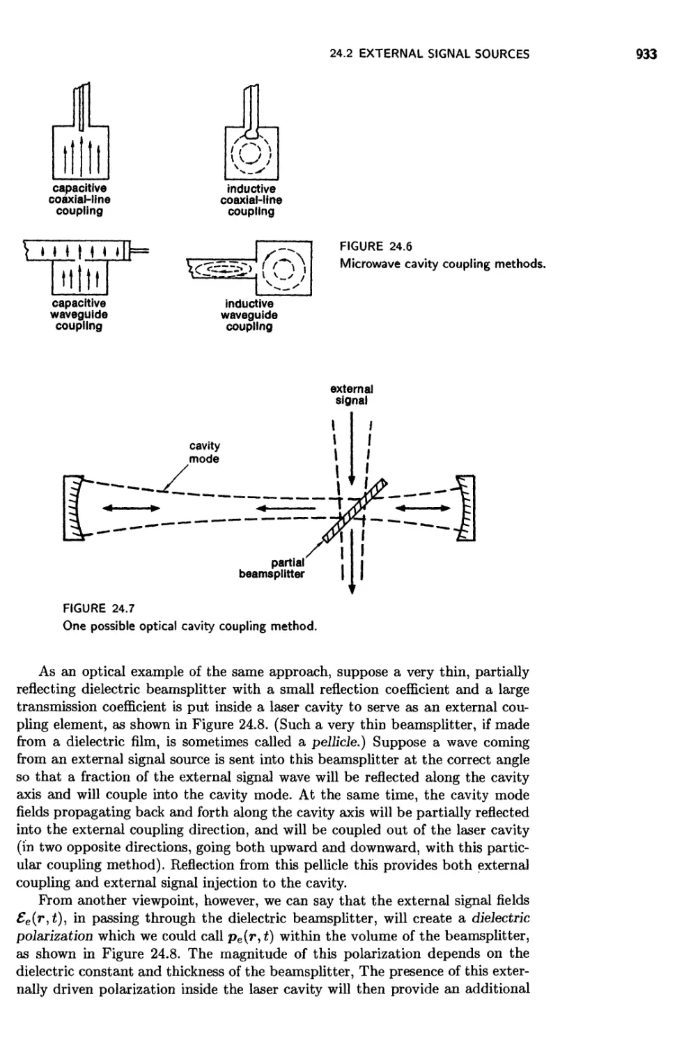
24.2 External Signal Sources 932
24.3 Coupled Cavity-Atom Equations 941
24.4 Alternative Formulations of the Laser Equations 944
24.5 Cavity and Atomic Rate Equations 949
Chapter 25 Laser Spiking and Mode Competition
25.1 Laser Spiking and Relaxation Oscillations 955
25.2 Laser Amplitude Modulation 971
25.3 Laser FYequency Modulation and Frequency Switching 980
25.4 Laser Mode Competition 992
Chapter 26 Laser Q-Switching
26.1 Laser Q-Switching: General Description 1004
26.2 Active Q-Switching: Rate-Equation Analysis 1008
26.3 Passive (Saturable Absorber) Q-Switching 1024
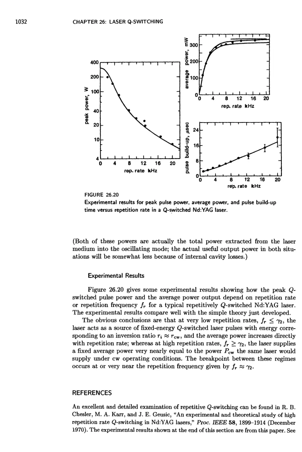
26.4 Repetitive Laser Q-Switching 1028
26.5 Mode Selection in Q-Switched Lasers 1034
26.6 Q-Switched Laser Applications 1039
Chapter 27 Active Laser Mode Coupling
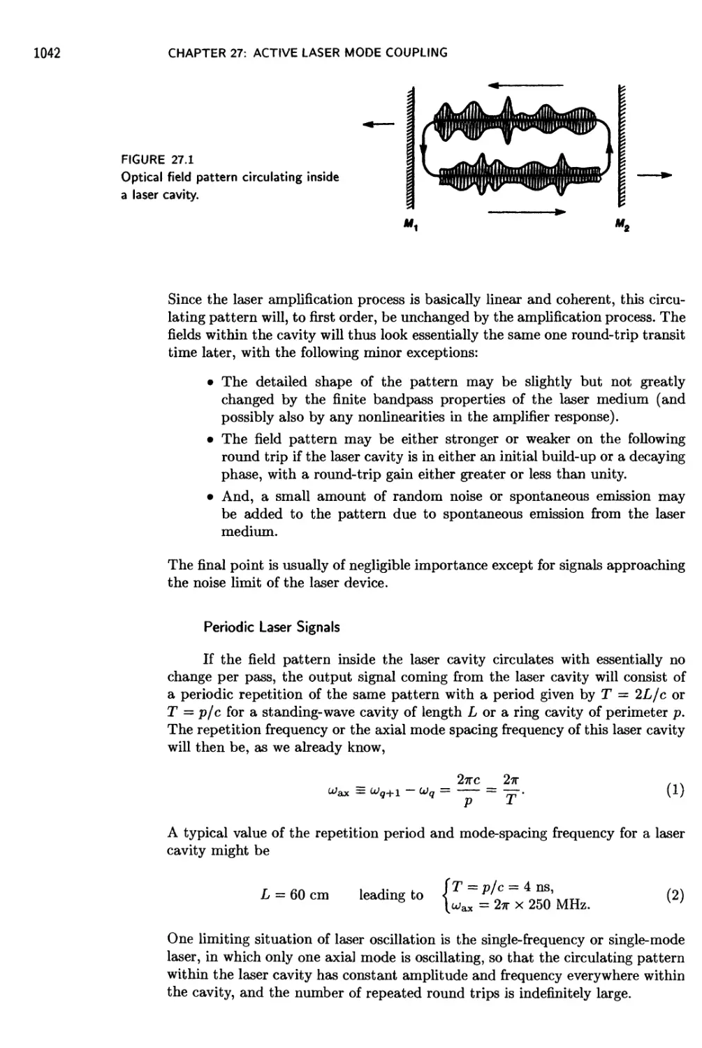
27.1 Optical Signals: Time and Frequency Descriptions 1041
27.2 Mode-Locked Lasers: An Overview 1056
27.3 Time-Domain Analysis: Homogeneous Mode Locking 1061
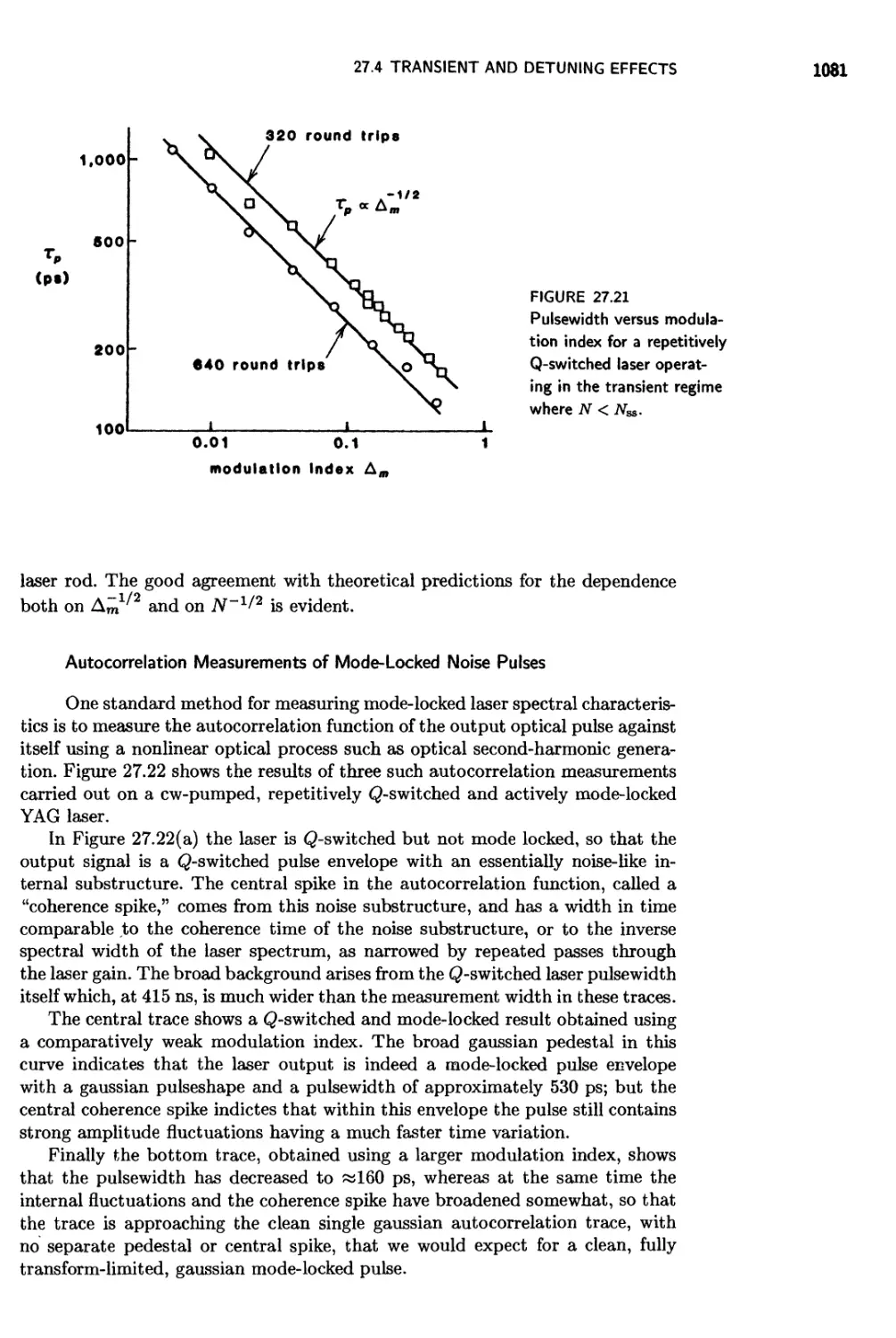
27.4 Transient and Detuning Effects 1075
27.5 Frequency-Domain Analysis: Coupled Mode Equations 1087
27.6 The Modulator Polarization Term 1092
27.7 FM Laser Operation 1095
Chapter 28 Passive Mode Locking
28.1 Pulse Shortening in Saturable Absorbers 1104
28.2 Passive Mode Locking in Pulsed Lasers 1109
28.3 Passive Mode Locking in CW Lasers 1117
Chapter 29 Laser Injection Locking
29.1 Injection Locking of Oscillators 1130
29.2 Basic Injection Locking Analysis 1138
29.3 The Locked Oscillator Regime 1142
29.4 Solutions Outside the Locking Range 1148
LIST OF TOPICS
29.5 Pulsed Injection Locking: A Phasor Description 1154
29.6 Applications: The Ring Laser Gyroscope 1162
Chapter 30 Hole Burning and Saturation Spectroscopy
30.1 Inhomogeneous Saturation and "Hole Burning" Effects 1171
30.2 Elementary Analysis of Inhomogeneous Hole Burning 1177
30.3 Saturation Absorption Spectroscopy 1184
30.4 Saturated Dispersion Effects 1192
30.5 Cross-Relaxation Effects 1195
30.6 Inhomogeneous Laser Oscillation: Lamb Dips 1199
Chapter 31 Magnetic-Dipole Transitions
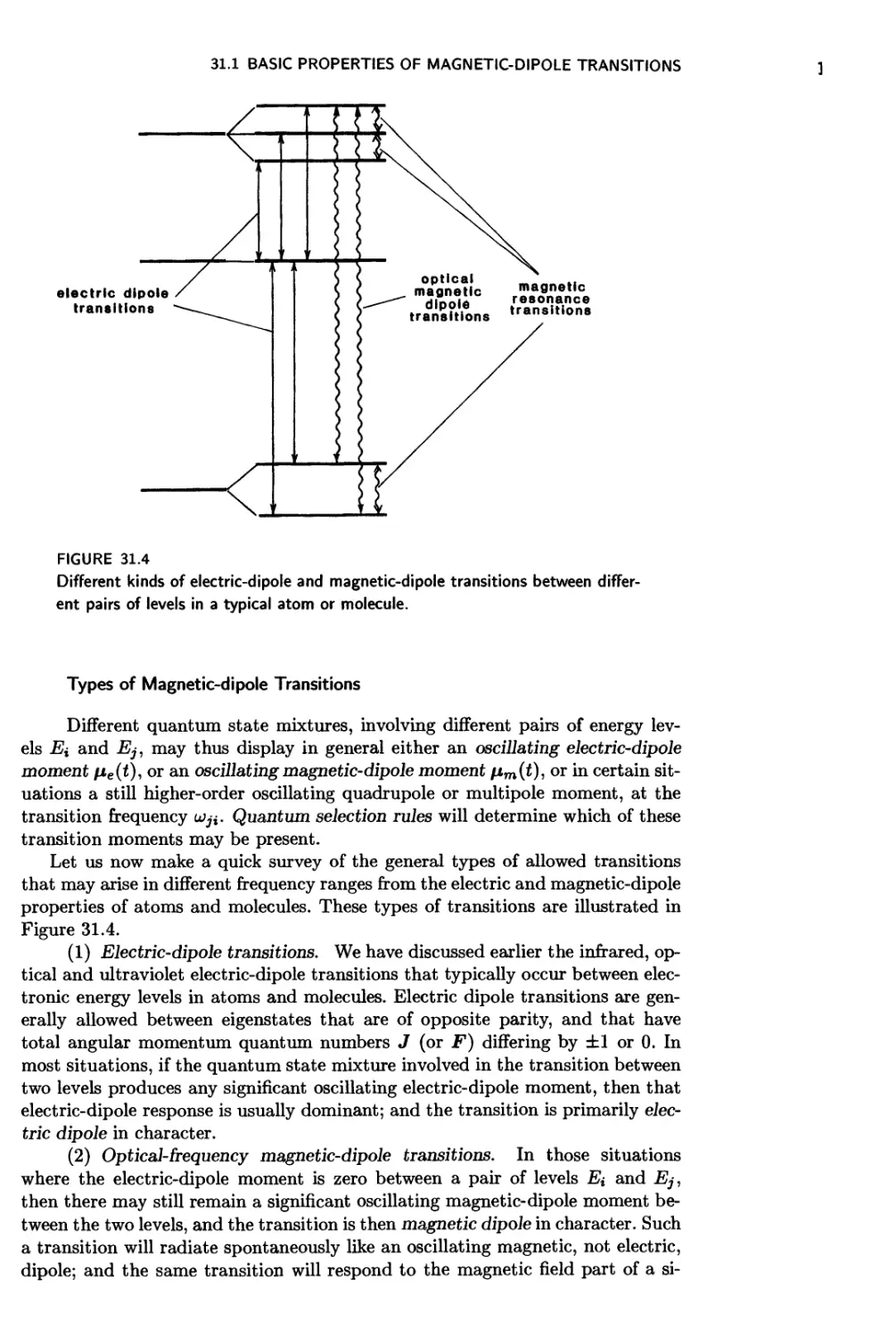
31.1 Basic Properties of Magnetic-Dipole Transitions 1213
31.2 The Iodine Laser: A Magnetic-Dipole Laser Transition 1223
31.3 The Classical Magnetic Top Model 1228
31.4 The Bloch Equations 1236
31.5 Transverse Response: The AC Susceptibility 1243
31.6 Longitudinal Response: Rate Equation 1249
31.7 Large-Signal and Coherent-Transient Effects 1256
Index 1267
PREFACE
This book presents a detailed and comprehensive treatment of laser physics and
laser theory which can serve a number of purposes for a number of different
groups. It can provide, first of all, a textbook for graduate students, or even
well-prepared seniors in science or engineering, describing in detail how lasers
work, and a bit about the applications for which lasers can be used. Problems,
references and illustrations are included throughout the book.
Second, it can also provide a solid and detailed description of laser physics
and the operational properties of lasers for the practicing engineer or scientist
who needs to learn about lasers in order to work on or with them.
Finally, the advanced sections of this text are sufficiently detailed that this
book will provide a useful one-volume reference for the experienced laser engineer
or laser researcher's bookshelf. The discussions of advanced laser topics, such as
optical resonators, Q-switching, mode locking, and injection locking, extend far
enough into the current state of the art to provide a working reference on these
and similar topics. References for further reading in the recent literature are
included in nearly every section.
One unique feature of this book is that it removes much of the quantum
mystique from "quantum electronics" (the generic label often applied to lasers
and laser applications). Many people think of lasers as quantum devices. In
fact, however, most of the basic concepts of laser physics, and virtually all the
practical details, are classical in nature. Lasers (and masers) of all types and in all
frequency ranges are simply electronic devices, of great interest and importance
to the electronics engineer.
In the analogous case of semiconductor electronics, for example, the transis-
transistor is not usually thought of as a quantum device. Mental images of holes and
electrons as classical charged particles which accelerate, drift, diffuse and re-
combine are used both by semiconductor device engineers to do practical device
engineering, and by solid-state physics researchers to understand sophisticated
physics experiments. These classical concepts serve to explain and make under-
understandable what is otherwise a complex quantum picture of energy bands, Bloch
wavefunctions, Fermi-Dirac distributions, and occupied or unoccupied quantum
states. The same simplification can be accomplished for lasers, and laser devices
can then be very well understood from a primarily classical viewpoint, with only
limited appeals to quantum terms or concepts.
The approach in this book is to build primarily upon the classical electron
oscillator model, appropriately extended with a descriptive picture of atomic en-
energy levels and level populations, in order to provide a fully accurate, detailed
and physically meaningful understanding of lasers. This can be accomplished
PREFACE
without requiring a previous formal background in quantum theory, and also
without attempting to teach an abbreviated and inadequate course in this sub-
subject on the spot. A thorough understanding of laser devices is readily available
through this book, in terms of classical and descriptively quantum-mechanical
concepts, without a prior course in quantum theory.
I have also attempted to review, at least briefly, relevant and necessary back-
background material for each successive topic in each section of this book. Students
will find the material most understandable, however, if they come to the book
with some background in electromagnetic theory, including Maxwell's equations;
some understanding of the concept of electromagnetic polarization in an atomic
medium; and some familiarity with the fundamentals of electromagnetic wave
propagation. An undergraduate-level background in optics and in Fourier trans-
transform concepts will certainly help; and although familiarity with quantum theory
is not required, the student must have at least enough introduction to atomic
physics to be prepared to accept that atoms do have quantum properties, espe-
especially quantum energy levels and transitions between these levels.
The discussions in this book begin with simple physical descriptions and
then go into considerable analytical detail on the stimulated transition process
in atoms and molecules; the basic amplification and oscillation processes in laser
devices; the analysis and design of laser beams and resonators; and the com-
complexities of laser dynamics (including spiking, Q-switching, mode locking, and
injection locking) common to all types of lasers'. We illustrate the general princi-
principles with specific examples from a number of important common laser systems,
although this book does not attempt to provide a detailed handbook of different
laser systems. Extensive references to the current literature will, however, guide
the reader to this kind of information.
There is obviously a large amount of material in this book. The author has
taught an introductory one-quarter "breadth" course on basic laser concepts for
engineering and applied physics students using most of the material from the
first part of the book on "Basic Laser Physics" (see the Table of Contents),
especially Chapters 1-4, 6-8 and 11-13. A second-quarter "depth" course then
adds more advanced material from Chapters 5, 9, 10, 30, 31 and selected sections
from Chapters 24-29. A complete course on optical beams and resonators can
be taught from Chapters 14 through 23.
I am very much indebted to many colleagues for help during the many years
while this book was being written. I wish it were possible to thank by name all the
students in my classes and my research group who lived through too many years
of drafts and class notes. Special thanks must go to Judy Clark, who became
a T]eX and computer expert and did so much of the editing and manuscript
preparation; to the Air Force Office of Scientific Research for supporting my
laser research activities over many years; to Stanford University, and especially
to Donald Knuth, for providing the environment, and the computerized text
preparation tools, in which this book could be written; and to the Alexander
von Humboldt Foundation and the Max Planck Institute for Quantum Optics in
Munich, who supplied the opportunity for the manuscript at last to be completed.
Finally, there are my wife Jeannie, and my family, who made it all worthwhile.
Anthony E. Siegman
UNITS AND NOTATION
The units and dimensions in this book are almost entirely mks, or SI, except for
a few concessions to long-established habits such as expressing atomic densities
N in atoms/cm3 and cross sections a in cm2. Such non-mks values should of
course always be converted to mks units before plugging them into formulas.
In general, lower-case symbols in bold-face type such as ?(r,t), b(r, t),
h(r, t), and so on refer to electromagnetic field quantities as real vector functions
of space and time, while ?(r,t), 6(r,?), h(r,t), etc., refer to the scalar counter-
counterparts of the same quantities. Bold-face capital letters E, В, Н, etc., refer to the
complex phasor amplitudes of the same vector quantities with e>wt variations,
while Ё, В, #, etc., are the complex phasor amplitudes of the corresponding
scalars. As illustrated here, complex quantities are sometimes, but not always,
identified by a superposed tilde.
In writing sinusoidal signals and waves, waves propagating toward positive z
are written in the "electrical engineer's form" of expj(wt — /3z) rather than the
"physicist's form" of expi(kz — vt). (This of course does not imply that i = —j!)
Linewidths А/, Ao>, AA and pulsewidths At, т or T, unless specifically noted,
always mean the full width at half maximum (FWHM).
In contrast to much of the published literature, an attenuation or gain co-
coefficient a in this book always refers to an amplitude or voltage growth rate,
such as for example ?(z) — ?@)exp ±az. Signal powers or intensities in this
book, therefore, always grow or attenuate with exponential growth coefficients
2a rather than a.
The notation in the book has a few other minor idiosyncrasies. First, we are
often concerned with signals and waves inside laser crystals, in which the host
crystal itself has a dielectric constant e and an index of refraction n even without
any atomic transition present. To take the dielectric properties of a possible host
medium into account, the symbols б, с and Л in formulas in this text always refer
to the dielectric permeability, velocity of light and wavelength of the radiation
in the dielectric medium if thereJs_one. We then use cq and Ao in the few cases
where it is necessary to refer to these same quantities specifically in vacuum.
The advantage of this choice is that all our formulas involving б, с and A remain
correct with or without a dielectric host medium, without needing to clutter
these formulas with different powers of the refractive index n.
The other special convention peculiar to this book is the nonstandard manner
in which we define the complex susceptibility Xat associated with a resonant
atomic transition. In brief, we define the linear relationship between the induced
polarization Pat on an atomic transition in a laser medium and the electric field
Ё that produces this polarization by the convention that Pat = Xat^E where e
is the dielectric permeability of the host laser crystal rather than the vacuum
value бо usually used in this definition. The merits of this nonstandard approach
are argued in Chapter 2.
LIST OF SYMBOLS
Throughout this text we attempt to follow a consistent notation for subscripts,
using the conventions that:
a = either atomic, as in atomic transition frequency ша or homogeneous
atomic linewidth Auja; or sometimes absorption, as in absorption coef-
coefficient аа.
с = cavity, as in cavity decay time rc or cavity energy decay rate 7C; also,
carrier, as in carrier frequency uc.
d = doppler, as in doppler broadening with linewidth Au>d, and by extension
any other kind of inhomogeneous broadening.
e = external, as in cavity external coupling factor 6e or external decay rate
7e; also, sometimes, effective, as in effective lifetime or pumping rate,
m = molecular or maser^ generally used to refer to atomic or maser or laser
quantities, e.g., laser gain coefficient am or laser growth rate 7m.
о = ohmic, referring generally to internal ohmic and/or scattering losses, as
in the ohmic loss coefficient ao or ohmic cavity decay rate 70. Also used
in several other ways, generally to indicate an initial value; a thermal
equilibrium value; a small-signal or unsaturated value; a midband value;
or a free-space (vacuum) values, as in cq, €q, and Ao-
p = pump, as in pumping rate Rp or pump transition probability Wp.
We also frequently use ax = axial; avail = available-, circ = circulating;
eff = effective; eq = equivalent; inc = incident; opt = optimum; out
= output; refl = reflected; rt = round-trip; sat = saturation; sp =
spontaneous or spiking; ss = small-signal or steady-state; and th =
threshold as compound subscripts.
A partial list of symbols used in the text then includes:
а = exponential gain or loss coefficient for amplitude (or voltage); also, am-
amplitude parameter for gaussian optical pulse
a" = second derivative of a(uj) with respect to и
an = complex amplitude of n-th order Hermite-gaussian mode
am = maser/laser/molecular gain (or loss) coefficient
chq = ohmic and/or scattering loss coefficient
/3 — propagation constant, including host dielectric effects, but usually not
loss or atomic transition effects; also, chirp parameter for gaussian
pulse; relaxation-time ratio in multilevel laser pumping systems; Bohr
magneton
/3i = Nuclear magneton
/3',/Зп = first and second derivatives of /3(uj) with respect to ш
A/3m = added propagation constant term due to reactive part of an atomic
transition xvii
LIST OF SYMBOLS
7 = in general, an energy or population decay rate
7c = decay rate for cavity stored energy (= l/rc)
7i = total downward population decay rate from energy level Ei
jij = population decay rate from upper level Ei to lower level Ej
7nr = nonradiative part of total decay rate for a classical oscillator or an
atomic transition
<yrad = radiative decay rate for classical electron oscillator or real atomic tran-
transition
7 = complex eigenvalue for optical resonator or lensguide
Imn = complex eigenvalue for ran-th order transverse eigenmode
Г = a + j/3 = complex propagation constant for an optical wave
Г = a — j/3 = complex gaussian pulse parameter
6 = coefficient of (logarithmic) fractional power gain or loss, per bounce or
per round trip
6C = total (round-trip) power loss coefficient due to cavity losses plus exter-
external coupling
8e = cavity loss coefficient due to external coupling only
Sm = power gain coefficient due to laser atoms
6q = cavity loss coefficient due to internal (ohmic) losses only
Дт = AM or FM modulation index
e = dielectric permeability of a medium
€o = dielectric permeability of free space (vacuum)
7] = efficiencies of various sorts; also, characteristic impedance у/ц/с of a
dielectric medium
rjo = characteristic impedance of free space (vacuum)
Л = optical wavelength (in a medium); also, eigenvalue for optical ray matrix
Ao = optical wavelength in vacuum
Aej Ль = eigenvalues of periodic lensguide or ABCD matrix
Л = spatial period of optical grating
/л = electric or magnetic dipole moment; also, magnetic permeability of a
magnetic medium
це = electric dipole moment
/лт = magnetic dipole moment
/iq = magnetic permeability of free space
p = amplitude reflection or transmission of optical mirror or beamsplitter;
also, distance between two points; p(uj) = cavity mode density
p = complex amplitude reflection or transmission of optical mirror or beam-
beamsplitter
<j — ohmic conductivity; also, transition cross section, standard deviation
(Tij = cross section for stimulated transition from level Ei to Ej
t = lifetime or decay time
rc = cavity decay time due to all internal losses plus external coupling
П = total lifetime (energy decay time) for energy level Ei
9,ф,ф = phase shifts and phase angles of various sorts
ф(г, t) = Schrodinger wave function
LIST OF SYMBOLS
фтп = Guoy phase shift for an mn-th order gaussian beam
X = susceptibility of a dielectric or magnetic medium = x! + jx"
x!, x" — rea-l and imaginary parts of x
Xat = susceptibility of a resonant atomic transition
Xe,Xm = electric (magnetic) dipole susceptibilities
ш — frequency (in radians/second)
сУ = in general, a frequency that has been shifted, pulled, or modified in
some small manner
uja = atomic transition frequency
ujb = a beat frequency (between two signals)
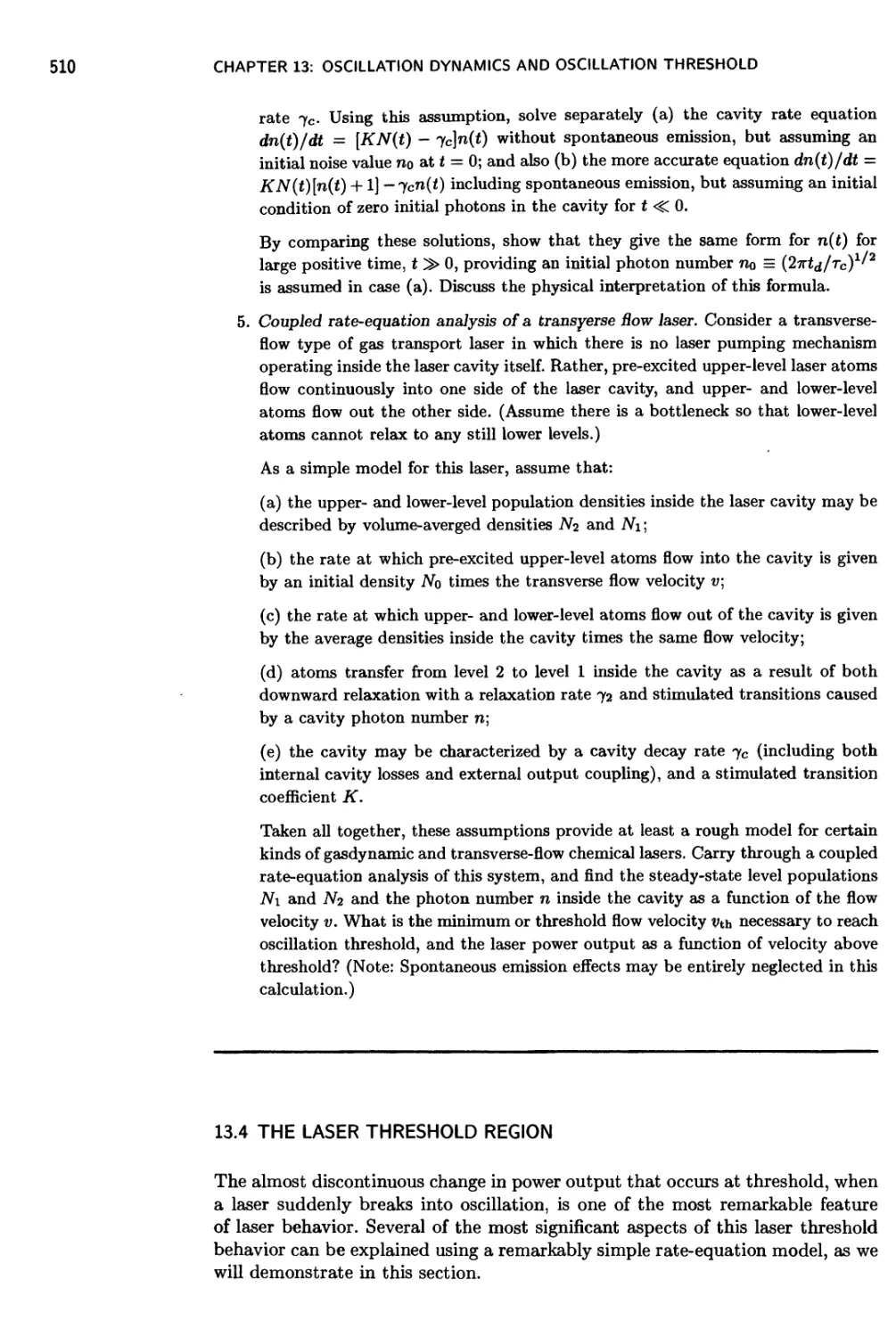
luc = cavity or circuit resonant frequency; also, carrier frequency
iVi(t) = instantaneous frequency of a phase-modulated signal
<^m = generally, a modulation frequency of some sort
ujq = resonant frequency of q-th axial mode
ujr = Rabi frequency on an atomic transition
u)sp = Spiking or relaxation-oscillation frequency
Sufq — frequency pulling of axial mode frequency uq
Аи = linewidth, or frequency tuning, in radians/sec
Аша = atomic linewidth (FWHM)nin radians/sec
Ашах — axial mode spacing between adjacent axial modes
п = solid angle; also, radian frequency or rotation rate
hi, bj '— normalized wave amplitudes
A = area
Aji = Einstein A coefficient on Ej —> Ei transition
ABCD = matrix elements for optical ray matrix or paraxial optical system
b = magnetic field as real function of space and time; also, confocal param-
parameter for gaussian beam
b = magnetic field as real vector function of space and time; also, confocal
parameter for gaussian beam
В = magnetic field; also, pressure-broadening coefficient or UB integral" for
nonlinear interaction
В = phasor amplitude of sinusoidal В field
с = velocity of light in a material medium
Co = velocity of light in vacuum
С = in general, an unspecified constant; also, electrical capacitance; coupling
coefficient in mode competition analysis
С С — complex conjugate (of preceding term)
CEO = classical electron oscillator model
d = electric displacement as real function of space and time; also, distance
or displacement
d = electric displacement as real vector function of space and time
D = dimensionless dispersion parameter
D = phasor amplitude of sinusoidal electric displacement
e = magnitude of electronic charge
S = electric field; usually, real field ?(#, t) as function of space and time
LIST OF SYMBOLS
E = phasor amplitude of sinusoidal E field
En (t) = amplitude of n-th mode in a normal mode expansion
/ = frequency in Hz (= cycles/sec); also, lens focal length
/# = lens /-number
Д/ = linewidth, or frequency detuning, in Hz
A/a = atomic transition linewidth (FWHM) in Hz
A/d = doppler or inhomogeneous linewidth (FWHM) in Hz
F = oscillator strength for an atomic transition; also, lens /-number
T — finesse, of interferometer or laser cavity
F(x) = Fresnel integral function
Fji = oscillator strength of Ej —> Ei atomic transition = 7rad,ji/37rad,ceo
g = amplitude (or voltage) gain, as a number; also, gaussian stable resonator
parameter; magnetic resonance g value
g(v),g(uj) = normalized lineshapes
g = complex amplitude (or voltage) gain, as a (complex) number
gugj — degeneracy factors for quantum energy levels Ei and Ej
gj = nuclear magnetic resonance g value
grt = round-trip voltage gain inside an optical cavity
G = power gain (as a number); also, electrical conductance
GdB — power gain in decibels
h = magnetic intensity as real function of space and time; also, Planck's
constant
h = h/2-к
h = magnetic H field as real vector function of space and time
hn = n-th order polynomial function
H = phasor amplitude of sinusoidal H field
Hn = n-th order hermite polynomial
/ = intensity (power/unit area) of an optical wave; also sometimes, loosely,
total power in the wave
Im = modified Bessel function of order m
J8at = amplifier (or absorber) saturation intensity
j — current density as real function of space and time; also, >/^T
j = current density as real vector function of space and time
J = phasor amplitude of sinusoidal current density
Jm = Bessel function of order m
k = propagation vector of optical wave = uj/c
К = scalar constant in various equations (especially coupled rate equations);
also, spring constant in classical oscillator model
L = length; electrical inductance
m = electron mass; also, magnetization (magnetic dipole moment per unit
volume) as real function of time
m — magnetization (magnetic dipole moment per unit volume) as real vector
function of space and time
m,m= half-trace parameter for ray or ABCD matrix
M = proton mass; molecular mass
LIST OF SYMBOLS xxi
M = phasor amplitude of sinusoidal magnetic dipole moment
M = optical ray matrix or ABCD matrix
n = refractive index; also, photon number n(t) (number of photons per cav-
cavity mode)
П2 = optical Kerr coefficient п^е or n<ii
N = atomic number or level population; usually interpreted as atoms per
unit volume, sometimes as total number of atoms
AN = population difference, or population difference density, on an atomic
transition (ATVy = Nt - Nj)
N = Fresnel number a2/LX for an optical beam or resonator
Nc = collimated Fresnel number for an unstable optical resonator
Neq = equivalent Fresnel number for an unstable optical resonator
JVj = population, or population density, in atomic energy level Ei
p = perimeter, period or round-trip path length, for cavities or periodic
lensguides; also, electric polarization (electric dipole moment per unit
volume) as real function of time, and laser mode density or mode num-
number
p = electric polarization (electric dipole moment per unit volume) as real
vector function of space and time
pm = path length (round-trip) through an atomic or laser gain medium
P = power, in watts; also, pressure, in torr
Pn(t) = polarization driving term for n-th order cavity mode in coupled-mode
expansion
P — phasor amplitude of sinusoidal electric polarization
q = axial mode index
q = complex gaussian beam parameter or complex radius of curvature
q = reduced gaussian beam parameter, q/n
r — amplitude reflectivity of mirror or beamsplitter; also, dimensionless or
normalized pumping rate; displacement off axis of optical ray
r' = reduced slope n dr/dz for optical ray
r = shorthand for spatial coordinates x, t/, z
f%j = complex scattering matrix element, or mirror or beamsplitter reflection
coefficient
rp = dimensionless pumping rate or inversion ratio, relative to threshold
pumping rate or threshold inversion density
dr = volume element, dV or dx dy dz
R = power reflectivity of mirror or beamsplitter (= |r|2); also, electrical
resistance; radius of curvature for mirror, dielectric interface, or optical
wave
R = reduced radius of curvature R/n
Rp = pumping rate in atoms per second and, usually, per unit volume
s = spatial frequency (cycles/unit length)
s = shorthand for transverse spatial coordinates #, у
ds = transverse area element dA or dx dy
S = multiport scattering matrix (matrix elements Sij)
LIST OF SYMBOLS
t = time; also, amplitude transmission through mirror, beamsplitter, or
light modulator
t = complex amplitude transmission coefficient through mirror, beamsplit-
beamsplitter or light modulator
iij = complex scattering matrix element, or mirror/beamsplitter transmis-
transmission coefficient
T = power transmission of mirror or beamsplitter (= |?|2); also, cavity
round-trip transit time, or temperature (K)
T = dimensionless susceptibility tensor
Ть = laser oscillation build-up time
Tnr = temperature of "nonradiative" surroundings
Trad = temperature of radiative surroundings
T\ = energy decay time, population recovery time, longitudinal relaxation
time
Т4 — dephasing time, collision time, transverse relaxation time
TV? = effective Ti or dephasing time for inhomogeneous (gaussian) transition
и = complex (and usually normalized) optical wave amplitude
U = energy or, more commonly, energy density (energy per unit volume)
Ua = energy density in a collection of atoms or atomic energy level popula-
populations
Ubbr — energy density of blackbody radiation
v = velocity of an atom, an electron, or a wave
v = complex spot size for Hermite-gaussian modes
vg = group velocity
Уф = phase velocity
V, Vc = volume (of a cavity mode-er field pattern)
w = gaussian spot size parameter A/e amplitude point)
Wij = total relaxation transition probability (per atom, per second) from level
Ei to level Ej
Wij = stimulated transition probability (per atom, per second) from level Ei
to level Ej
Wp = pumping transition probability (per atom, per second)
x(t) = displacement of electronic charge in classical electron oscillator model
zd = dispersion length for dispersive pulse broadening
zr = Rayleigh range for a gaussian or collimated optical beam
Z = atomic number
2* = dimensionless population saturation factor, with values between 2* = 1
(lower level empties out rapidly) and 2* = 2 (lower level bottlenecked)
3* = dimensionless polarization overlap factor for atomic interactions, with
numerical value between 0 and 3
LASERS
1
AN INTRODUCTION TO LASERS
Lasers are devices that generate or amplify coherent radiation at frequencies
in the infrared, visible, or ultraviolet regions of the electromagnetic spectrum.
Lasers operate by using a general principle that was originally invented at micro-
microwave frequencies, where it was called microwave amplification by stimulated
emission of radiation, or maser action. When extended to optical frequencies
this naturally becomes iight amplification by stimulated emission of radiation,
or laser action.
This basic laser or maser principle is now used in an enormous variety of
devices operating in many parts of the electromagnetic spectrum, from audio
to ultraviolet. Practical laser devices in particular employ an extraordinary va-
variety of materials, pumping methods, and design approaches, and find a great
variety of applications. The study of laser and maser devices and their scientific
applications is often referred to as the field of quantum electronics.
From an electronics-engineering viewpoint, the developments that followed
the operation of the first ruby laser in 1960 suddenly pushed the upper limit of
coherent electronics from the millimeter-wave range, using microwave tubes and
transistors, out to include the submillimeter, infrared, visible, and ultraviolet
spectral regions (and soft X-ray lasers are now on the horizon). All the familiar
functions of coherent signal generation, amplification, modulation, information
transmission, and detection are now possible at frequencies up to a million times
higher, or wavelengths down to a million times shorter, than previously. But
it has also become possible for engineers and scientists, in fields of technology
ranging from microbiology to auto manufacture, to perform an almost unlimited
variety of new and unexpected functions made possible by the short wavelengths,
high powers, ultrashort pulse widths, and other unique characteristics of these
laser devices.
In the twenty-odd years since the first appearance of coherent light, lasers
have become widespread and almost commonplace devices. The importance and
the excitement of the laser and its applications, however, still can hardly be
overestimated. The objective of this book is to explain in detail how lasers work,
what the performance characteristics of typical lasers are, and how lasers are
employed in a wide variety of applications. Our goal in this opening chapter is
CHAPTER 1: AN INTRODUCTION TO LASERS
feedback and mirror
mirror oscillation atoms (,aser medium) ./
pumping process
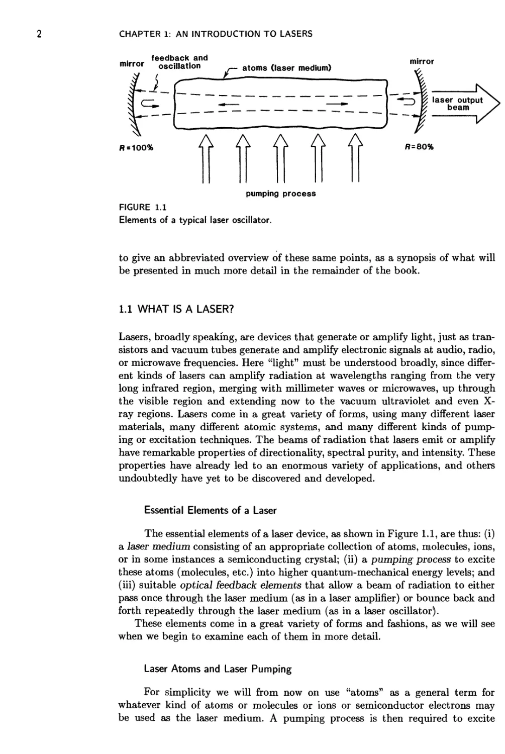
FIGURE 1.1
Elements of a typical laser oscillator.
to give an abbreviated overview of these same points, as a synopsis of what will
be presented in much more detail in the remainder of the book.
1.1 WHAT IS A LASER?
Lasers, broadly speaking, are devices that generate or amplify light, just as tran-
transistors and vacuum tubes generate and amplify electronic signals at audio, radio,
or microwave frequencies. Here "light" must be understood broadly, since differ-
different kinds of lasers can amplify radiation at wavelengths ranging from the very
long infrared region, merging with millimeter waves or microwaves, up through
the visible region and extending now to the vacuum ultraviolet and even X-
ray regions. Lasers come in a great variety of forms, using many different laser
materials, many different atomic systems, and many different kinds of pump-
pumping or excitation techniques. The beams of radiation that lasers emit or amplify
have remarkable properties of directionality, spectral purity, and intensity. These
properties have already led to an enormous variety of applications, and others
undoubtedly have yet to be discovered and developed.
Essential Elements of a Laser
The essential elements of a laser device, as shown in Figure LI, are thus: (i)
a laser medium consisting of an appropriate collection of atoms, molecules, ions,
or in some instances a semiconducting crystal; (ii) a pumping process to excite
these atoms (molecules, etc.) into higher quantum-mechanical energy levels; and
(iii) suitable optical feedback elements that allow a beam of radiation to either
pass once through the laser medium (as in a laser amplifier) or bounce back and
forth repeatedly through the laser medium (as in a laser oscillator).
These elements come in a great variety of forms and fashions, as we will see
when we begin to examine each of them in more detail.
Laser Atoms and Laser Pumping
For simplicity we will from now on use "atoms" as a general term for
whatever kind of atoms or molecules or ions or semiconductor electrons may
be used as the laser medium. A pumping process is then required to excite
1.1 WHAT IS A LASER?
energy
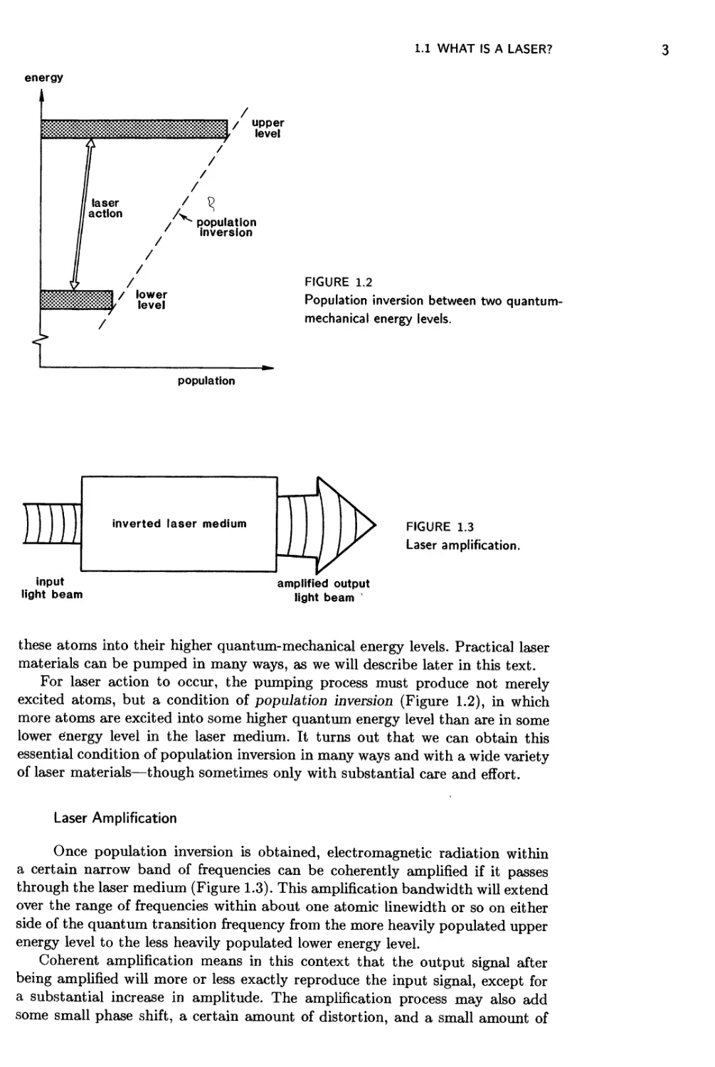
FIGURE 1.2
Population inversion between two quantum-
mechanical energy levels.
population
inverted
laser
medium
. i
\
I
FIGURE 1.3
Laser amplification.
input
light beam
amplified output
light beam
these atoms into their higher quantum-mechanical energy levels. Practical laser
materials can be pumped in many ways, as we will describe later in this text.
For laser action to occur, the pumping process must produce not merely
excited atoms, but a condition of population inversion (Figure 1.2), in which
more atoms are excited into some higher quantum energy level than are in some
lower energy level in the laser medium. It turns out that we can obtain this
essential condition of population inversion in many ways and with a wide variety
of laser materials—though sometimes only with substantial care and effort.
Laser Amplification
Once population inversion is obtained, electromagnetic radiation within
a certain narrow band of frequencies can be coherently amplified if it passes
through the laser medium (Figure 1.3). This amplification bandwidth will extend
over the range of frequencies within about one atomic linewidth or so on either
side of the quantum transition frequency from the more heavily populated upper
energy level to the less heavily populated lower energy level.
Coherent amplification means in this context that the output signal after
being amplified will more or less exactly reproduce the input signal, except for
a substantial increase in amplitude. The amplification process may also add
some small phase shift, a certain amount of distortion, and a small amount of
CHAPTER 1: AN INTRODUCTION TO LASERS
100% partially
reflecting transmitting
mirror mirror
FIGURE 1.4
Laser oscillation.
amplifier noise. Basically, however, the amplified output signal will be a coherent
reproduction of the input optical signal, just as in any other coherent electronic
amplification process.
Laser Oscillation
Coherent amplification combined with feedback is, of course, a formula for
producing oscillation, as is well known to anyone who has turned up the gain on
a public-address system and heard the loud squeal of oscillation produced by the
feedback from the loudspeaker output to the microphone input. The feedback in
a laser oscillator is usually supplied by mirrors at each end of the amplifying laser
medium, carefully aligned so that waves can bounce back and forth between these
mirrors with very small loss per bounce (Figure 1.4). If the net laser amplification
between mirrors, taking into account any scattering or other losses, exceeds the
net reflection loss at the mirrors themselves, then coherent optical oscillations
will build up in this system, just as in any other electronic feedback oscillator.
When such coherent oscillation does occur, an output beam that is both
highly directional and highly monochromatic can be coupled out of the laser
oscillator, either through a partially transmitting mirror on either end, or by some
other technique. This output in essentially all lasers will be both extremely bright
and highly coherent. The output beam may also in some cases be extremely
powerful. Just what we mean by "bright" and by "coherent" we will explain
later.
REFERENCES
The first stimulated emission devices, before lasers, were various kinds of masers, which
operated on essentially the same basic physical principles, but at much lower frequencies
and with much different experimental techniques. For an overview and unified approach
to all these devices, see my earlier texts Microwave Solid-State Masers (McGraw-Hill,
1964) and Ал Introduction to Lasers and Masers (McGraw-Hill, 1971).
Some other good books on lasers can be found. A more elementary introduction,
with good illustrations, is D. С O'Shea, W. R. Callen, and W. T. Rhodes, Introduction
to Lasers and Their Applications (Addison-Wesley, 1977). A good general coverage is
also given in O. Svelto, Principles of Lasers (Plenum Press, 1982). Two well-known texts
by A. Yariv are Introduction to Optical Electronics (Rinehart and Winston, 1971) and
the more advanced Quantum Electronics (Wiley, 1975).
1.1 WHAT IS A LASER?
For full quantum-mechanical treatments of lasers, two good choices are M. Sargent
III, M. O. Scully, and W. E. Lamb, Jr., Laser Physics (Addison-Wesley, 1977), and H.
Haken, Laser Theory (Springer-Verlag, 1983).
A useful short bibliographic survey of laser references, aimed particularly at the
college teacher, can be found in "Resource Letter L-l: Lasers," by D. C. O'Shea and
D. C. Peckham, Am. J. Phys. 49, 915-925 (October 1981).
For more advanced information on various laser topics, the four-volume Laser Hand-
Handbook, edited by F. T. Arecchi and E. O. Schulz-Dubois (North-Holland, Amsterdam,
1972), provides an encyclopedic source with detailed articles on nearly every topic in
laser physics, devices, and applications. If you'd like to look at some of the impor-
important original literature on lasers for yourself, well-chosen selections can be found in
F. S. Barnes, ed., Laser Theory (IEEE Press Reprint Series, IEEE Press, 1972), or
in D. O'Shea and D. C. Peckham, Lasers: Selected Reprints (American Association of
Physics Teachers, Stony Brook, N. Y., 1982).
If you would like to do experiments with a home-made laser or just see how one might
be constructed, a useful collection of articles from the "Amateur Scientist" section
of Scientific American has been reprinted under the title Light and Its Uses, with
introduction by Jearl Walker (W. H. Freeman and Company, 1980). Topics covered
include simple helium-neon, argon-ion, carbon-dioxide, semiconductor, tunable dye,
and nitrogen lasers, plus experiments on holography, interferometry, and spectroscopy.
Problems for 1.1
1. Diagramming the electromagnetic spectrum. On a large sheet of paper lay out a
logarithmic frequency scale extending from the audio range (say, / = 10 Hz) to
the far ultraviolet or soft X-ray region (say, Л = 100 A). Mark both frequency
and wavelength below the same scale in powers of 10 in appropriate units, e.g.,
Hz, kHz, MHz, and m, mm, /xm. (You might also mark a "wavenumber" scale
for 1/Л in units of cm, and an energy scale for %ш in units of eV.) Above the
scale indicate the following landmarks (plus any other significant ones that occur
to you):
• Audio frequency range (human ear) B0-15000 Hz)
• Standard AM and FM broadcast bands E35-1605 kHz, 88-108 MHz)
• Television channels 2-6 E4-88 MHz) and 7-13 A74-216 MHz)
• Microwave radar "S" and "X" bands B-4 and 8-12 GHz)
• Visible region (human eye)
• Important laser wavelengths, including:
HCN far-IR laser C11, 337, 545, 676, 744 /xm)
H2O far-IR laser B8, 48, 120 /xm)
CO2 laser (9.6-10.6 /xm)
CO laser E.1-6.5 /xm)
HF chemical laser B.7-3.0 /xm)
Nd:YAG laser A.06 /xm)
He-Ne lasers A.15 /xm, 633 nm)
GaAs semiconductor laser (870 nm)
Ruby laser F94 nm)
CHAPTER 1: AN INTRODUCTION TO LASERS
Red
Eye
ч He
I ^ discharge
f lamp
FIGURE 1.5
Helium discharge spectrum observed through an inexpensive replica transmission
grating.
Rhodamine 6G dye laser E60-640 nm)
Argon-ion laser D88-515 nm)
Pulsed N2 discharge laser C37 nm)
Pulsed H2 discharge laser A60 nm)
1.2 ATOMIC ENERGY LEVELS AND SPONTANEOUS EMISSION
Our objective in this section is to give a very brief introduction to the concepts
of atomic energy levels and of spontaneous emission between those levels. We
attempt to demonstrate heuristically that atoms (or ions, or molecules) have
quantum-mechanical energy levels; that atoms can be pumped or excited up
into higher energy levels by various methods; and that these atoms then make
spontaneous downward transitions to lower levels, emitting radiation at char-
characteristic transition frequencies in the process. (Readers already familiar with
these ideas may want to move on to Section 1.3.)
The Helium Spectrum
Figure 1.5 illustrates a simple experiment in which a small helium discharge
lamp (or lacking that, a neon sign) is viewed through an inexpensive transmission
diffraction grating of the type available at scientific hobby stores. (If you have
never done such an experiment, try to do this demonstration for yourself.)
1.2 ATOMIC ENERGY LEVELS AND SPONTANEOUS EMISSION
4000
5000 6000
wavelength, A
7000
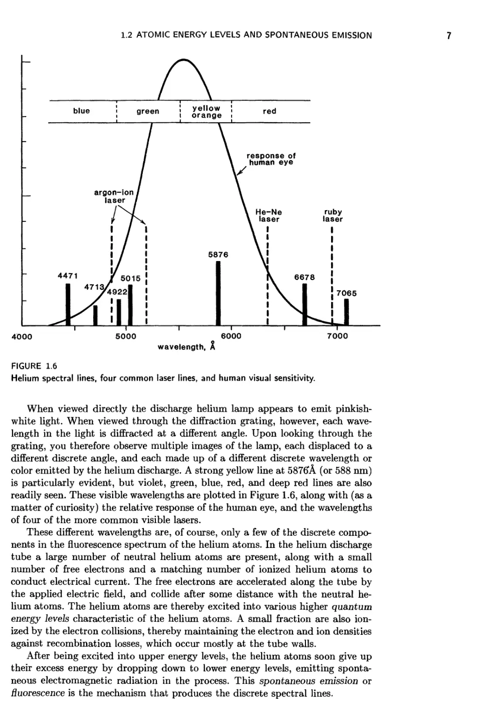
FIGURE 1.6
Helium spectral lines, four common laser lines, and human visual sensitivity.
When viewed directly the discharge helium lamp appears to emit pinkish-
white light. When viewed through the diffraction grating, however, each wave-
wavelength in the light is diffracted at a different angle. Upon looking through the
grating, you therefore observe multiple images of the lamp, each displaced to a
different discrete angle, and each made up of a different discrete wavelength or
color emitted by the helium discharge. A strong yellow line at 5876>A (or 588 nm)
is particularly evident, but violet, green, blue, red, and deep red lines are also
readily seen. These visible wavelengths are plotted in Figure 1.6, along with (as a
matter of curiosity) the relative response of the human eye, and the wavelengths
of four of the more common visible lasers.
These different wavelengths are, of course, only a few of the discrete compo-
components in the fluorescence spectrum of the helium atoms. In the helium discharge
tube a large number of neutral helium atoms are present, along with a small
number of free electrons and a matching number of ionized helium atoms to
conduct electrical current. The free electrons are accelerated along the tube by
the applied electric field, and collide after some distance with the neutral he-
helium atoms. The helium atoms are thereby excited into various higher quantum
energy levels characteristic of the helium atoms. A small fraction are also ion-
ionized by the electron collisions, thereby maintaining the electron and ion densities
against recombination losses, which occur mostly at the tube walls.
After being excited into upper energy levels, the helium atoms soon give up
their excess energy by dropping down to lower energy levels, emitting sponta-
spontaneous electromagnetic radiation in the process. This spontaneous emission or
fluorescence is the mechanism that produces the discrete spectral lines.
CHAPTER 1: AN INTRODUCTION TO LASERS.
The Discovery of Helium
Helium was first identified as a new element by its fluorescence spectrum in the solar
corona. During the solar eclipse of 1868 a bright yellow line was observed in the emission
spectrum of the Sun's prominences by at least six different observers. This line could be
explained in relation to the known spectral lines of already identified elements only by
postulating the existence of a new element, helium, named after the Greek word Helios,
the Sun. This same element was later, of course, identified and isolated on Earth.
Quantum Energy Levels
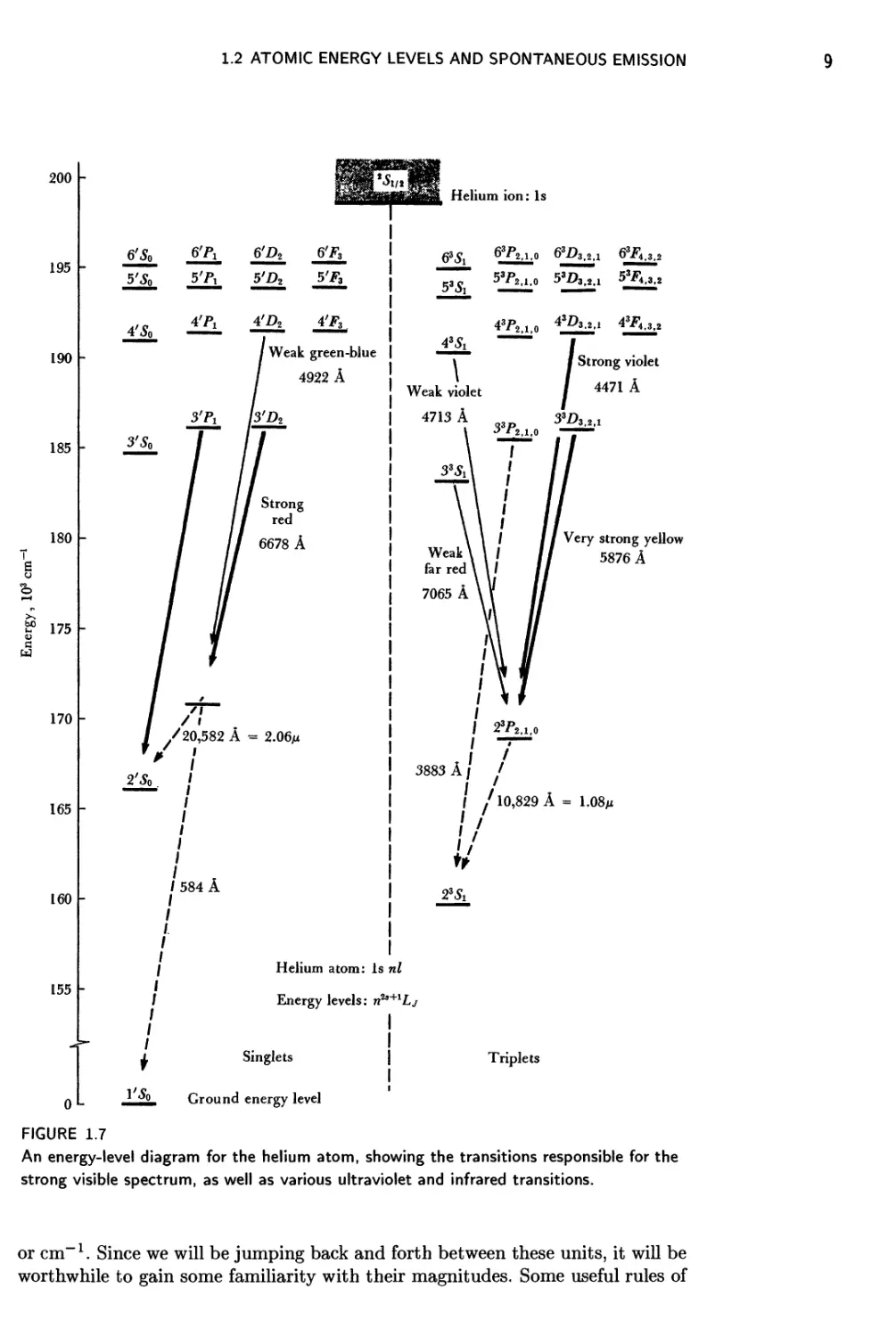
Figure 1.7 shows the rather complex set of quantum energy levels possessed
by even so simple an atom as the He atom. The solid arrows in this diagram
designate some of the spontaneous-emission transitions that are responsible for
the stronger lines in the visible spectrum of helium. The dashed arrows indicate
a few of the many additional transitions that produce spontaneous emission
at longer or shorter wavelengths in the infrared or ultraviolet portions of the
spectrum, lines which we can "see" only with the aid of suitable instruments.
Every atom in the periodic table, as well as every molecule or ion, has its
own similar characteristic set of quantum energy levels, and its own characteristic
spectrum of fluorescent emission lines, just as does the helium atom. Understand-
Understanding and explaining the exact values of these quantum energy levels for different
atoms and molecules, through experiment or through complex quantum analy-
analyses, is the task of the spectroscopist. The complex labels given to each energy
level in Figure 1.7 are part of the working jargon of the spectroscopist or atomic
physicist. In this text we will not be concerned with predicting the quantum
energy levels of laser atoms, or even with understanding their complex labeling
schemes, except in a few simple cases. Rather, we will accept the positions and
properties of these levels as part of the data given us by spectroscopists, and will
concentrate on understanding the dynamics and the interactions through which
laser action is obtained on these transitions.
Planck's Law
The relationship between the frequency U21 emitted on any of these tran-
transitions and the energies E2 and E\ of the upper and lower atomic levels is given
by Planck's Law
W21 = j- , A)
where % = h/2n, and Planck's constant h = 6.626 x 10~34 Joule-second.
In this text, as in real life, optical and infrared radiation will sometimes be
characterized by its frequency u, and sometimes by its wavelength Ao expressed
in units such as Angstroms (A), nanometers (nm), or microns (/mi). Quantum
transitions and the associated transition frequencies are also very often charac-
characterized by their transition energy or photon energy, measured in units of electron
volts (eV), or their inverse wavelength 1/Ao measured in units of "wavenumbers"
1.2 ATOMIC ENERGY LEVELS AND SPONTANEOUS EMISSION
6'Sq
6'Рг
5'Л
6'А> &F3
5'Рг BfF3
Weak green-blue
4922 A
I /20,582 A = 2j
*/ /
2'So !
2.06m
/584 A
/
Helium atom: Is
Energy levels: n2*
Singlets
Ground energy level
Helium ion: Is
63^ 63Р2л,р 63РЗЛЛ 63fl,3,2
~ 53/>2>1>0 53A.2.! 53F4,3,2
jJl
43D3,2,i 43tfM,
Weak violet
4713 A
I 23/>2,1,o
3883 A / /
v
nl
Strong violet
4471 A
33D3.2.i
Very strong yellow
5876 A
1.08/z
Triplets
FIGURE 1.7
An energy-level diagram for the helium atom, showing the transitions responsible for the
strong visible spectrum, as well as various ultraviolet and infrared transitions.
or cm. Since we will be jumping back and forth between these units, it will be
worthwhile to gain some familiarity with their magnitudes. Some useful rules of
10 CHAPTER 1: AN INTRODUCTION TO LASERS
thumb to remember are that
1 /im ("one micron") = 1,000 nm = lOOOOA B)
and that, in suitable energy units,
[transition energy E2 - #i in eV] « -T ——r-1:—: : =¦ C)
[wavelength Ло m microns]
Hence 10000A or 1 /яп matches up with 10,000 cm or ~ 1.24 eV. A visible
wavelength of 500 nm or 5000A or 0.5 /яп thus corresponds to a photon energy
of 20,000 cm or ~ 2.5 eV. Note that this also corresponds to a transition
frequency of o>2i/27r = 6 x 10¹⁴ Hz, expressed in the conventional units of cycles
per second, or Hertz.
Energy Levels in Solids: Ruby or Pink Sapphire
As another simple illustration of energy levels, try shining a small ultravio-
ultraviolet lamp (sometimes called a "mineral light") on any kind of fluorescent mineral,
such as a piece of pink ruby or a sample of glass doped with a rare-earth ion,
or on a fluorescent dye such as Rhodamine 6G. These and many other materials
will then glow or fluoresce brightly at certain discrete wavelengths under such ul-
ultraviolet excitation. A sample of ruby, for example, will fluoresce very efficiently
at Л « 694 nm in the deep red, a sample of crystal or glass doped with, say, the
rare-earth ion terbium, Tb3+, will fluoresce at Л « 540 nm (bright green), and
a liquid sample of Rhodamine 6G dye will fluoresce bright orange.
Since ruby was the very first laser material, and is still a useful and instructive
laser system, let us examine its fluorescence in more detail. Figure 1.8 shows a
more sophisticated version of such an experiment, in which a scanning monochro-
mator plus an optical detector are used to examine the ruby fluorescent emission
in more detail. The lower trace shows the two very sharp (for a solid) and very
closely spaced deep-red emission lines that will be observed from a good-quality
ruby sample cooled to liquid-helium temperature. (At higher temperatures these
lines will broaden and merge into what appears to be a single emission line.)
Figure 1.9 shows the crystal structure of ruby. Ruby consists essentially of
lightly doped sapphire, AI2O3, with the darker spheres in the figure indicating
the Al3+ ions. (The lattice planes shown in the figure are ~ 2.1бА apart.) Sap-
Sapphire is a very hard, colorless (when, pure), transparent crystal which can be
grown in large and optically very good samples by flame-fusion techniques. The
transparency of pure sapphire in the visible and infrared means that its Al3+
and O2~ atoms, when they are bound into the sapphire crystal lattice, have no
absorption lines from their ground energy levels to levels anywhere in the in-
infrared or visible regions. Indeed, no optical absorption appears in pure sapphire
below the insulating band gap of the crystal in the ultraviolet.
We can, however, replace a significant fraction (several percent) of the Al3+
ions in the lattice by chromium or Cr3+ ions. The sapphire lattice as a result
acquires a pink tint at low chromium concentrations, or a deeper red color at
higher concentrations, and becomes what is called "pink ruby." The individual
chromium ions, when they are bound into the sapphire lattice, have a set of
quantum energy levels that are associated with partially filled inner electron
shells in the Cr3+ ion. These energy levels are located as shown in Figure 1.10.
1.2 ATOMIC ENERGY LEVELS AND SPONTANEOUS EMISSION
11
Ruby
A, lines
X « 6934 A
Scanning
optical
monochromator
Optical
detector
i
Frequency
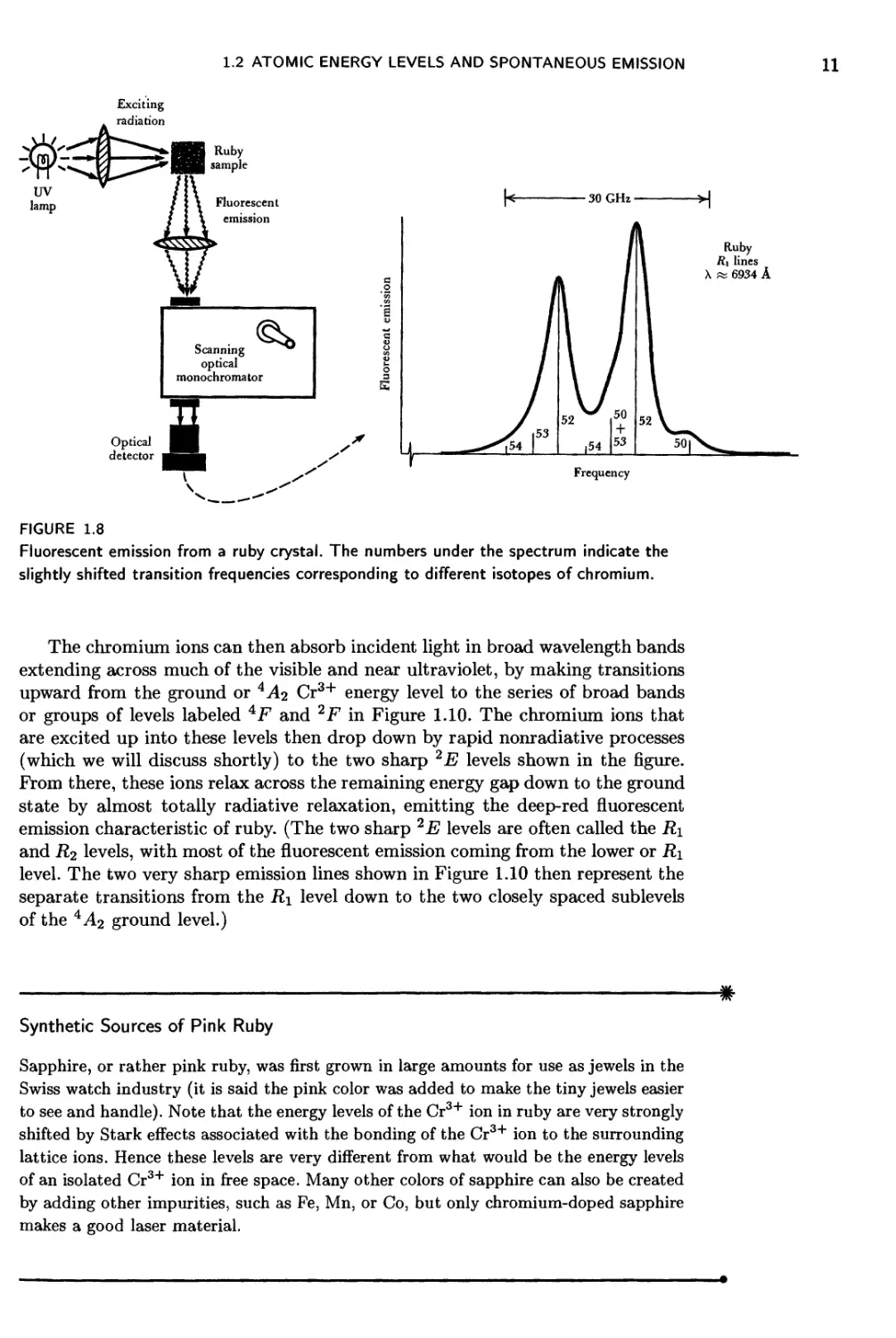
FIGURE 1.8
Fluorescent emission from a ruby crystal. The numbers under the spectrum indicate the
slightly shifted transition frequencies corresponding to different isotopes of chromium.
The chromium ions can then absorb incident light in broad wavelength bands
extending across much of the visible and near ultraviolet, by making transitions
upward from the ground or 4Л2 Cr3+ energy level to the series of broad bands
or groups of levels labeled 4F and 2F in Figure 1.10. The chromium ions that
are excited up into these levels then drop down by rapid nonradiative processes
(which we will discuss shortly) to the two sharp 2E levels shown in the figure.
From there, these ions relax across the remaining energy gap down to the ground
state by almost totally radiative relaxation, emitting the deep-red fluorescent
emission characteristic of ruby. (The two sharp 2E levels are often called the Ri
and R2 levels, with most of the fluorescent emission coming from the lower or Ri
level. The two very sharp emission lines shown in Figure 1.10 then represent the
separate transitions from the R\ level down to the two closely spaced sublevels
of the 4 A2 ground level.)
Synthetic Sources of Pink Ruby
Sapphire, or rather pink ruby, was first grown in large amounts for use as jewels in the
Swiss watch industry (it is said the pink color was added to make the tiny jewels easier
to see and handle). Note that the energy levels of the Cr3+ ion in ruby are very strongly
shifted by Stark effects associated with the bonding of the Cr3+ ion to the surrounding
lattice ions. Hence these levels are very different from what would be the energy levels
of an isolated Cr3+ ion in free space. Many other colors of sapphire can also be created
by adding other impurities, such as Fe, Mn, or Co, but only chromium-doped sapphire
makes a good laser material.
12
CHAPTER 1: AN INTRODUCTION TO LASERS
С axis
FIGURE 1.9
Sapphire crystal lattice.
Energy Levels in Solids: Rare Earth Ions
Figures 1.11 and 1.12 show how a typical rare-earth ion such as Nd3+ or
Tb3+ can be bonded into an irregular glassy lattice structure, together with the
quantum energy levels associated with a trivalent terbium Tb3+ ion when such
an ion is dispersed at low concentration, either in a glass or in a crystal structure
(for example, CaF2).
Note that the energy levels of rare-earth ions such as Tb3+ or Nd3+ are
associated with the electrons in the partially filled 4/ inner shell of the rare-earth
atom. In nearly all solid materials, these inner electrons are well shielded, by
surrounding outer filled electron shells, from the crystalline Stark effects caused
by the bonds to surrounding atoms in the crystal or glass material. Hence the
quantum energy levels of such rare-earth ions are almost unchanged in many
different crystalline or glass host materials.
Almost any material containing small amounts of Tb3+, for example, will
fluoresce with the same brilliant green color around 540 run, and materials con-
containing Nd3+ all fluoresce strongly around 1.06 ^m in the near infrared. There
are also several other such rare-earth ions, including Dy2+, Tm2+, Ho3+, Eu3+,
and Er3+, that make good to excellent laser materials.
1.2 ATOMIC ENERGY LEVELS AND SPONTANEOUS EMISSION 13
energy
A03 cm)
30 -
20
10
FIGURE 1.10
optical pumping jj Quantum-mechanical energy
strong red fluorescence ,eve|s of the Сгз+ ions jn a mby
crystal.
11.6 GHz
Optical Pumping of Atoms
All of these minerals illustrate another basic method for pumping or excit-
exciting atoms into upper energy levels, that is, through the absorption of light at an
appropriate pumping wavelength. The high-pressure mercury lamp used as the
excitation source in a "mineral light" emits a broad continuum of visible and
ultraviolet wavelengths. As shown in Figures 1.8 and 1.12, some of these wave-
wavelengths will coincide with the transition frequencies from the lowest or ground
levels of the chromium or terbium ions (nearly all the ions are located at ground
level when in thermal equilibrium) up to some of the higher energy levels of these
ions.
These ions can thus absorb radiation ("absorb photons") from the UV light
source at these particular frequencies, and as a result be lifted up to various of
the upper levels. This excitation is enhanced by the fact that in solids the higher
energy levels are often rather broad bands of levels. The absorption linewidths
of the ruby and terbium absorption lines are thus relatively broad, permitting
reasonably efficient absorption of the continuum radiation from the mercury
lamp.
Once they are lifted upward by this so-called "optical pumping," the ions in
each case then relax or fluoresce down to lower energy levels, as shown in Figure
1.12, emitting a relatively sharp fluorescence at two or three visible wavelengths
as they drop from upper to lower levels.
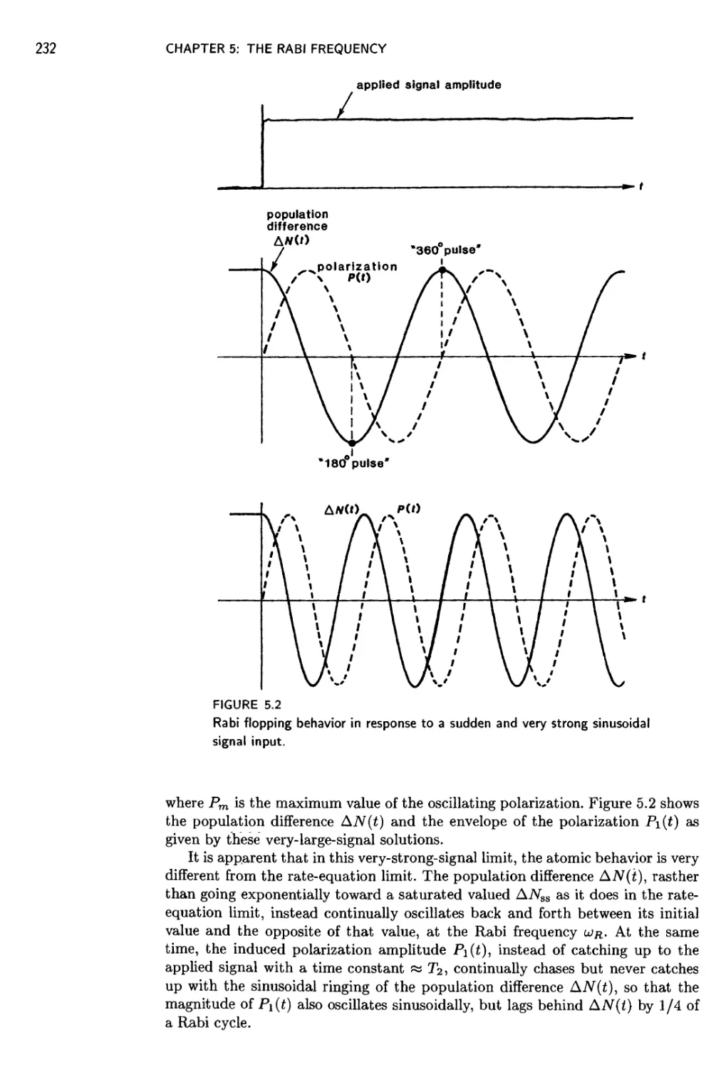
Spontaneous Energy Decay or Relaxation
Let us discuss a little more the spontaneous decay or relaxation process
we have introduced here. Suppose that a certain number Ni of such atoms have
been pumped into some upper energy level E2 of an atom or molecule, whether
14
CHAPTER 1: AN INTRODUCTION TO LASERS
FIGURE 1.11
A single rare-earth ion (largest sphere) imbedded in a BaF2 glass matrix. The
larger spheres in the matrix represent barium, the smaller fluorine.
by electron collision in a gas like helium, or by optical pumping in a solid like
ruby, or by some other mechanism. These atoms will then spontaneously drop
down or relax to lower energy levels, giving up their excess internal energy in
the process (Figure 1.13). (We will see where this energy goes in a moment.)
The rate at which atoms spontaneously decay or relax downward from any
upper level N2 is given by a spontaneous energy-decay rate, often called 72, times
the instantaneous number of atoms in the level, or
dN2
dt
= -72N2 = -N2/r2.
D)
If an initial number of atoms N20 are pumped into the level at t — 0, for example,
by a short intense pumping pulse, and the pumping process is then turned off,
the number of atoms in the upper level will decay exponentially in the form
E)
where r2 = I/72 is the lifetime of the upper level E2 for energy decay to all lower
levels.
1.2 ATOMIC ENERGY LEVELS AND SPONTANEOUS EMISSION
15
10 —
FIGURE 1.12
Optical pumping of the upper quantum-mechanical energy levels in the
rare-earth ion terbium, Tb3+.
The lifetime of the R levels in the ruby crystal happens to be long enough
(about 4 msec), and the visible fluorescence strong enough, that we can rather
easily demonstrate this kind of exponential decay by using the simple apparatus
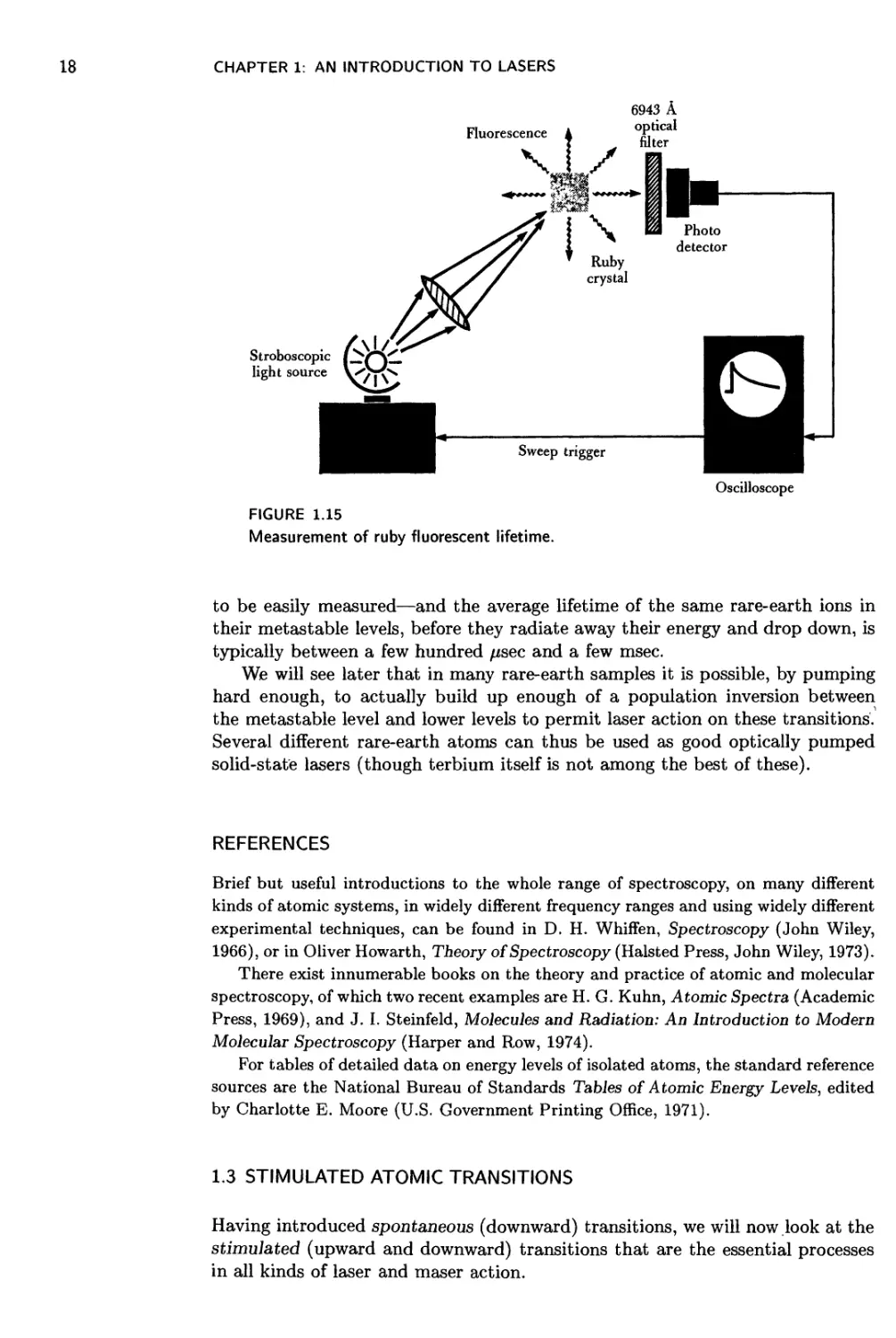
shown in Figure 1.15. The pulsed stroboscopic light source emits a broadband
flash of visible and ultraviolet light about 60 /xsec long. This flash of light optically
pumps the Cr3+ ions in the ruby sample up to upper levels, from which they
very rapidly decay to the metastable R levels. These levels then decay to the
ground level by emitting visible red fluorescence with a decay time r « 4.3 msec.
(Similar fluorescence lifetime measurements can also be made for any of the other
materials we have mentioned, but some of the lifetimes are much shorter, and
the fluorescent intensities much smaller, making the experiment more difficult.)
Radiative and Nonradiative Relaxation
There are actually two quite separate kinds of downward relaxation that
occur in these solid-state materials, as well as in most other atomic systems.
One mechanism is radiative relaxation, which is to say the spontaneous emission
of electromagnetic or fluorescent radiation, as we have already discussed. We
16 CHAPTER 1: AN INTRODUCTION TO LASERS
i relaxation by fluorescence
or nonradiative relaxation
/
I
excitation by
electron impact
or optical pumping
FIGURE 1.13 \ rams-
General concept of upper-level \
excitation by electron impact or \
optical pumping. *
} atomic energy levels
\
\
\
can usually measure this emitted radiation directly, with some suitable kind of
photodetector.
The other mechanism is what is commonly called nonradiative relaxation.
In terbium, for example, when the terbium ions relax from higher energy levels
shown in Figure 1.12 down into the 5D4 level, they get rid of the transition en-
energy not by radiating electromagnetic radiation somewhere in the infrared, but
by setting up mechanical vibrations of the surrounding crystal lattice. To put
this in another way, the excess energy is emitted as lattice phonons, or as heat-
heating of the surrounding crystal lattice, rather than as electromagnetic radiation
or photons—hence the term nonradiative relaxation. This kind of nonradiative
emission is usually difficult to measure directly, since it mostly goes into a very
small warming up of the surrounding medium. This same kind of nonradiative
relaxation process also allows excited ruby atoms to relax down into the 2E levels.
The total relaxation rate 7 on any given transition will thus be, in general, the
sum of a radiative or fluorescent or electromagnetic part, described by a purely
radiative decay rate that we often write as 7гаа; plus a nonradiative part, with a
nonradiative decay rate that we often write as 7nr. The total or measured decay
rate for atoms out of the upper level will then be the sum of these, or 7tot =
7rad +7nr- The actual numerical values for these rates, and the balance between
radiative and nonradiative parts, will in general be different for every different
atomic transition, and may depend greatly on the immediate surroundings of
the atoms, as we will discuss in much more detail later. The one certain thing is
that atoms placed in an upper level will decay downward, by some combination
of radiative and/or nonradiative decay processes.
Nonradiative relaxation can be a particularly rapid process for relaxation
across some of the smaller energy gaps for rare-earth ions and other absorbing
ions in solids, as we will see in more detail later. For example, in terbium as in
many other rare-earth ions, there may be many rather closely spaced levels or
bands at higher energies; but then the energy gap down from the lowest of these
energy
1.2 ATOMIC ENERGY LEVELS AND SPONTANEOUS EMISSION
population
17
N2(t)
4^20
т* —
У
^2
"""I
1 ^
FIGURE 1.14
Spontaneous energy decay rate.
upper levels (the 5D4 level in terbium) to the next lower group of levels may be
larger than the frequency huj of the highest phonon mode that the crystal lattice
can support.
As a result, the terbium ion cannot relax across this gap very readily by
nonradiative processes, i.e., by emitting lattice phonons, since the lattice cannot
accept or propagate phonons of this frequency. Instead the atoms relax across
this gap almost entirely by radiative emission, i.e., by spontaneous emission of
visible fluorescence. Across other, smaller gaps, however^ the nonradiative relax-
relaxation rate is so fast that any radiative decay on these transitions is completely
overshadowed by the nonradiative rate.
This behavior is typical for many other rare-earth ions in crystals and glasses.
Following optical excitation to high-lying levels, the atoms relax by rapid nonra-
nonradiative relaxation into some lower metastable level, from which further nonradia-
nonradiative relaxation is blocked by the size of the gap to the next lower level. Efficient
fluorescent emission from here to the lower levels then occurs, followed by fur-
further fast nonradiative relaxation across any remaining energy gaps to the ground
level. The nonradiative decay time of the atoms via phonon emission across the
smaller energy gaps may be in the subnanosecond to picosecond range—too fast
18
CHAPTER 1: AN INTRODUCTION TO LASERS
6943 A
Stroboscopic fe
light source
Oscilloscope
FIGURE 1.15
Measurement of ruby fluorescent lifetime.
to be easily measured—and the average lifetime of the same rare-earth ions in
their metastable levels, before they radiate away their energy and drop down, is
typically between a few hundred /xsec and a few msec.
We will see later that in many rare-earth samples it is possible, by pumping
hard enough, to actually build up enough of a population inversion between
the metastable level and lower levels to permit laser action on these transitions.
Several different rare-earth atoms can thus be used as good optically pumped
solid-state lasers (though terbium itself is not among the best of these).
REFERENCES
Brief but useful introductions to the whole range of spectroscopy, on many different
kinds of atomic systems, in widely different frequency ranges and using widely different
experimental techniques, can be found in D. H. Whiffen, Spectroscopy (John Wiley,
1966), or in Oliver Howarth, Theory of Spectroscopy (Halsted Press, John Wiley, 1973).
There exist innumerable books on the theory and practice of atomic and molecular
spectroscopy, of which two recent examples are H. G. Kuhn, Atomic Spectra (Academic
Press, 1969), and J. I. Steinfeld, Molecules and Radiation: An Introduction to Modern
Molecular Spectroscopy (Harper and Row, 1974).
For tables of detailed data on energy levels of isolated atoms, the standard reference
sources are the National Bureau of Standards Tables of Atomic Energy Levels, edited
by Charlotte E. Moore (U.S. Government Printing Office, 1971).
1.3 STIMULATED ATOMIC TRANSITIONS
Having introduced spontaneous (downward) transitions, we will now look at the
stimulated (upward and downward) transitions that are the essential processes
in all kinds of laser and maser action.
1.3 STIMULATED ATOMIC TRANSITIONS
19
absorption
sample
broadband W
light source ~~XJ.
FIGURE 1.16
An elementary grating spectrometer.
Atomic Absorption Lines
Suppose we now examine more carefully the absorption of radiation by a
collection of atoms as a function of the wavelength of the incident radiation.
Figure 1.16 shows a very elementary example of a grating spectrometer such as
might be used for such measurements. (A tunable laser would be a very useful
alternative, if one were conveniently available.)
In this spectrometer the radiation from a broadband continuum light source
is collected into a roughly parallel beam by a collimating mirror, and is then
reflected from a diffraction grating located on a rotatable mount. At any one
orientation of the grating, only one wavelength (rather, a finite but narrow band
of wavelengths) is reflected at the correct angle to be collected by another curved
mirror, focused down through a narrow slit, and passed through the experimen-
experimental sample onto a detector. By rotating the grating, we can tune the wavelength
of the radiation that passes through the sample and thereby measure the trans-
transmission through the sample as a function of frequency or wavelength. (Figure
1.17 shows a more compact in-line version of such an instrument.)
The result of such an experiment will often appear as shown schematically in
Figure 1.18. The atomic sample will have absorption transitions from the lowest
energy level to higher energy levels; so it will exhibit discrete absorption lines—
that is, narrow bands of frequency in which the sample exhibits more or less
strong absorption—at exactly those wavelengths. These wavelengths will corre-
correspond through Planck's law to the energy gaps between the lowest and higher
levels. If there happen to be some atoms already located in higher-lying levels,
then absorption lines from those levels to still higher levels may also be seen, as
illustrated by transition С in the figure. These excited-state absorptions, how-
20
CHAPTER 1: AN INTRODUCTION TO LASERS
FIGURE 1.17
A compact in-line grating monochromator.
A
С
В
transmitted
energy
-v
optical frequency
FIGURE 1.18
Absorption transitions (top) and absorption lines (bottom).
ever, will usually appear substantially weaker, simply because there will normally
be many fewer atoms in the higher energy levels.
As a specific illustration of atomic absorption, Figure 1.19 shows some of
the sharp absorption lines observed when radiation at wavelengths around 540
nm in the visible is transmitted through a crystal of lanthanum fluoride (LaF2)
1.3 STIMULATED ATOMIC TRANSITIONS
21
Er34" in LaF2
5340 5360 5380 5400 5420 5440
Wavelength, A
l0, high-pressure Hg-lamp spectrum
Вь T f Bj Gd3+ in SrF2
Total instrumental width, 50ju
3060 3055 3050 3045
Wavelength, A
FIGURE 1.19
Light transmission versus wavelength through crystals of lanthanum fluoride (LaF2) con-
containing a small amount of the rare-earth ion erbium Er34" (upper trace), and strontium
fluoride (SrF2) containing a small amount of the rare-earth ion gadolinium Gd3+ (lower
trace).
containing a small percentage of the rare-earth ion erbium, or when radiation
at wavelengths around 300 nm in the near ultraviolet is transmitted through a
crystal of strontium fluoride (SrF2) containing a small percentage of the rare-
earth ion gadolinium. These absorption lines all represent different transitions
from the lowest or ground levels of the Er3+ or Gd3+ ions to higher-lying levels,
exactly analogous to the terbium levels shown in Figure 1.13. Of course, if a
pure lanthanum or strontium fluoride crystal is grown without any erbium or
gadolinium present, no such absorption lines are observed.
22 CHAPTER 1: AN INTRODUCTION TO LASERS
Absorption Lines in Gases, and Molecular Spectroscopy
Absorption experiments of this sort are, of course, by no means limited
to solids or to rare earths. Isolated atoms or ions in gases will exhibit such
absorption lines in the visible, and especially the UV. Molecules in gases, liquids,
and solids will exhibit an extremely rich spectrum of absorption lines, notably
in the infrared as well as in the visible and ultraviolet. The absorption lines of
atoms and molecules in gases are typically sharper or narrower than those in
solids or liquids, since the energy levels in gases are not subject to some of the
perturbing influences that tend to broaden, or smear out the energy levels in
liquids or solids.
As just one more example to illustrate absorption spectroscopy, Figure 1.20
shows a few of the sharp absorption lines characteristic of the formaldehyde
molecule H2CO in a narrow range of wavelengths near 3.57 /mi. This particular
spectrum was taken by using a continuously tunable laser source (a cw injec-
injection diode laser using a lead/cadmium sulfide diode) rather than an incoherent
spectrometer. The dashed envelope in Figure 1.20(a) is the power output of the
tunable laser versus wavelength, over a tuning range that is extremely large in
absolute terms (~ 3 x 10¹⁰ Hz), yet extremely narrow (~ 0.04%) relative to the
center frequency. The solid line is the power transmitted through the vapor-filled
cell.
Many different molecules exhibit exactly such characteristic sharp lines, spe-
specific to the individual molecules, in rich profusion through the near and middle
infrared regions. These sharp lines are extremely useful not only as potential laser
lines, but as characteristic signatures of different molecules, for use in chemical
diagnostics or in identifying the presence of specific pollutant molecules or haz-
hazardous chemicals. Note that the sensitivity and the laser scanning rate in the
experiment allow a small portion of the formaldehyde absorption spectrum to
be displayed on an oscilloscope in real time.
Emission spectroscopy, using the spontaneous emission lines radiated from
an excited sample as in Figure 1.5, is thus one way of observing and learning
about the discrete transitions and the quantum' energy levels of atoms, ions,
and molecules. Absorption spectroscopy, as briefly described here, is another
and complementary method of obtaining the same kind of information. These
methods are in fact complementary in their utility, since emission spectroscopy
tends to give information about downward transitions emanating from high-lying
levels, whereas absorption spectroscopy tends to give information about upward
transitions from the ground level or low-lying atomic levels. The formaldehyde
example illustrates the possibilities for applying tunable lasers to spectroscopy,
to analytical chemistry, and to practical applications such as pollution detection.
Stimulated versus Spontaneous Atomic Transitions
We have now seen that there are two basically different kinds of transition
processes that can occur in atoms or molecules.
First, there are spontaneous emission or relaxation transitions, in which
atoms spontaneously drop from an upper to a lower level while emitting electro-
electromagnetic and/or acoustic radiation at the transition frequency. Fluorescence, en-
energy decay, and energy relaxation are other names for this process. When atoms
emit this kind of fluorescence or spontaneous electromagnetic radiation, each in-
individual atom acts almost exactly like a small randomly oscillating antenna—in
1.3 STIMULATED ATOMIC TRANSITIONS
23
5 Torr H2CO
X*« 2802.5cm
L s 10 cm
T « 295eK
0.0
0.2 0.4 0.6 0.8 1.0 1.2
FREQUENCY (cm)
FIGURE 1.20
Absorption spectroscopy of formaldehyde using a tunable laser source near A =
3.57/im.
most common cases, a small electric dipole antenna—internally driven at the
transition frequency. Each individual atom radiates independently, with a tem-
temporal phase angle that is independent of all the other radiating atoms. Thus, the
total fluorescent emission from a collection of spontaneously emitting atoms is
noise-like in character (Figure 1.21), even though it will be limited in spectral
width to the comparatively narrow linewidth of the atomic transition. Indeed,
such spontaneously emitted radiation has all the statistical properties of narrowly
bandlimited gaussian noise. We usually refer to it as incoherent emission.
Second, there are the stimulated responses or stimulated transitions—both
stimulated absorption and stimulated emission—that occur when an external
radiation signal is applied to an atom. In these transitions each individual atom
acts like a miniature passive resonant antenna (again, usually an electric dipole
antenna) that is set oscillating by the applied signal itself. That is, the internal
motion or oscillation in the atom is not random, but is driven by and coherent
with the applied signal.
24
CHAPTER 1: AN fNTRODUCTION TO LASERS
FIGURE 1.21
Spontaneous emission is incoherent or
noise-like, emerging randomly in atl di-
directions.
incoherent radiation
stimulated
transitions
FIGURE 1.22
An energy-level population
diagram, showing sponta-
spontaneous emission plus stimu-
stimulated transitions.
spontaneous
emission
Atomic Rate Equations
Suppose we have very many identical atoms, each of which has two just
energy levels, Ex and E2. (Real atoms will undoubtedly have many other energy
levels as well, but we will ignore other levels for the moment.) Suppose that
Ni(*) of the atoms present are in level Ег and N2(t) atoms are in level E2. This
situation can be illustrated by an energy-level population diagram, as in Figure
1.22.
We have already stated that the spontaneous-relaxation rate down from level
E2 to level E\ is directly proportional to the upper-level population N2(t) and is
not influenced at all by the lower-level population Ni(t). Hence the spontaneous-
emission rate out of level 2 and into level 1 is given by
dN2{t)
dt
spontaneous
dt
F)
spontaneous
1.3 STIMULATED ATOMIC TRANSITIONS 25
where 721 indicates the total spontaneous-transition rate or decay rate (radiative
plus nonradiative) from level 2 to level 1.
Suppose now an optical signal is applied to these atoms to cause stimulated
transitions, as in the optical pumping or absorption spectroscopy experiments
we have just discussed. This signal must, of course, be tuned in frequency close
to the transition frequency of interest, i.e., u; w ^21 ± Au;a, where Аша is the
linewidth of the atomic transition. We might then characterize the strength of
this signal by its intensity I (dimensions of power per unit area), or by the
strength of its E or H fields. In discussions of stimulated transitions, however,
the applied signal intensity or energy density is often expressed in units of the
number of signal photons n(t) per unit volume in the applied signal. This does
not necessarily imply anything about photons as being billiard-ball-like point
particles; it merely means that n(t) is the electromagnetic energy density of the
applied signal divided by the quantum energy unit Uuj.
Such an applied signal will cause atoms initially in the lower energy level
to begin making stimulated transitions or "jumps" upward to the upper energy
level, at a rate proportional to the applied signal intensity (or power density)
times the number of atoms in the starting level. The number of stimulated up-
upward transitions per unit time caused by the applied signal can then be written
as
dN2(t)
dt
stimulated
upward
= Kn(t)Nx{t). G)
That is, the stimulated upward transition rate is directly proportional to the
photon density n of the applied signal. Each such upward transition absorbs
one quantum of energy from the applied signal and—at least in an elementary
description—transfers it to one of the atoms which is lifted upward. This is the
process of stimulated absorption.
But the essential point is that the same applied signal will also cause any
atoms initially in the upper energy level to begin making similar stimulated
transitions or jumps downward in energy, at a rate which is again proportional
to the applied signal intensity times the number of atoms in the initial (i.e.,
upper) level. The number of stimulated downward transitions per unit time can
thus similarly be written as
dN2(t)
dt
stimulated
downward
= -Kn(t)N2(t). (8)
This is the process of stimulated emission. The atoms in this case jump down-
downward, giving up energy. This energy must go into the stimulating optical signal,
which is therefore strengthened or amplified.
The constant К in each of these equations is just a proportionality constant
that measures the absolute strength of the stimulated response on the particu-
particular atomic transition. A fundamental and essential point, however, is that this
proportionality constant necessarily has exactly the same value for transitions in
either direction. This constant К will also be largest for an applied signal tuned
exactly to the atomic transition frequency, and will rapidly become small to neg-
negligible as the signal frequency и is tuned away from the transition frequency w2\
by more than a linewidth or so.
26 CHAPTER 1: AN INTRODUCTION TO LASERS
The total rate equation for the atomic populations in this simple example,
including stimulated plus spontaneous transitions, is thus given by
dN2(t)
dt
dN2(t)
total
dt
dN2(t)
stimulated dt
upward
dN2(t)
stimulated dt
downward
spontaneous
= Kn(t) x [Nxit) - N2(t)\ - -¦ ы 'A ~ dNl^
dt total
(9)
where n(t) is directly proportional to the applied signal intensity or power den-
density.
Quantum Derivation of the Spontaneous Emission Process
In a quantum-mechanical analysis the constant К in the stimulated-transition rate
Kn(t)N(t) is usually derived by using a semiclassical quantum analysis, in which
the atoms are treated quantum-mechanically but the applied electromagnetic signal is
treated classically. The spontaneous emission processes described by the spontaneous-
relaxation probability 721 ^(t) can, however, only be derived from a fully quantum
electrodynamic analysis in which both the atoms and the electromagnetic field itself
are treated quantum-mechanically.
Some people note that there is a correspondence in quantum theory between the
spontaneous-emission rate, which corresponds to the downward stimulated-transition
rate that would be caused by one extra photon, and the presence of zero-point fluctua-
fluctuations in the quantum electromagnetic fields, with a magnitude equivalent to an energy
of one photon per mode; and deduce from this that zero-point fluctuations "cause" or
"stimulate" the spontaneous emission. This can be a convenient way to calculate the
spontaneous-emission rate or the quantum noise magnitude in a laser calculation, but
attributing a causal relation to the zero-point fluctuations is a more dubious proposi-
proposition. Zero-point fluctuations and spontaneous emission are both predicted, separately
and independently, by quantum field theory, but nothing in the theory says that either
one causes the other: they each arise independently of the other, from the commutation
properties of the quantum field operators.
Stimulated Transitions and Laser Amplification
The total rate at which atoms make signal-stimulated transitions between
two energy levels (i.e., "up" minus "down") is thus given by Kn(t) x [N\(t) —
N2(t)]. Each upward transition transfers Tiuj of energy from the signal to the
atoms; each downward transition does the reverse.
But this implies that the net rate at which energy per unit volume is absorbed
from the signal by the atoms is then given by this net flow rate times the energy
hu per jump. That is, the net energy transfer rate to the atoms is
^ = Kn(t) x [N.it) - N2(t)} x Пш, A0)
1.3 STIMULATED ATOMIC TRANSITIONS 27
where Ua is the energy density in the forced internal oscillation of the atoms.
This same energy must at the same time be coming out of the signal. Hence
the energy density USig(t) = n(t) x fiu) in the applied signal must be decreasing
with time according to the reverse expression
^P = -K[Nx{t) - N2(t)} x n(t) xhu> = -К[ЩЦ - N2(t)] x Uais(t) A1)
or, in terms of photon density,
^ t). A2)
The signal energy density USig(t), or the photon density n(t), may thus either
decay or grow with time, depending on the sign of the population difference
AN(t) = Ni(t) - N2(t) in the square brackets.
The signal growth rate described by Equation 1.12 leads to the essential
concept of laser amplification. This equation says that if an external signal is
applied to a collection of atoms where there are more atoms in the lower energy
level than in the upper, or, where N\(t) > N2(t), then the net transition rate
or net flow of atoms between the levels will be upward. In this case net energy
is being supplied to the atoms by the applied signal; so the applied signal must
become absorbed or attenuated.
If, however, we can somehow produce a condition of population inversion, in
which there are more atoms in the upper level than in the lower, or N2 > N\,
then both the quantity JVi - N2 and hence the net energy flow between signal and
atoms will change sign. The net stimulated-transition rate for the atoms will now
be in the downward direction. Net energy will then be given up by the atoms,
and taken up by the applied signal. This energy flow will in fact produce a net
amplification of that signal, at a rate proportional to the population difference
and to the strength of the external signal.
Boltzmann's Principle
One of the fundamental laws of thermodynamics, Boltzmann's Principle,
states that when a collection of atoms is in thermal equilibrium at a positive
temperature T, the relative populations of any two energy levels E\ and E2 are
given by
which of course means that
= Nl-N2=(l- e-h"/kT)} Nx. A4)
Thus for a collection of atoms in equilibrium at a normal positive temperature T,
an upper-level population is always smaller than a lower-level population (much
smaller if the energy gap E2 — E\ is an optical-frequency gap).
The total stimulated-transition rate on such an equilibrium transition is thus
always absorptive or attenuating rather than amplifying. To create laser ampli-
amplification, we must find some pumping process which will put more atoms into an
upper level than into a lower level, and thus create a nonequilibrium condition
28 CHAPTER 1: AN INTRODUCTION TO LASERS
FIGURE 1.23
Boltzmann population
factors.
¦
>»
0»
ф
с
Ф
E2
\
\
\
\
\
\
\
\
ч
population —»>
of population inversion. In Section 1.5 we give some information on how this can
be done in practice.
Coherence in Stimulated Transitions
If we want, we can think of the basic stimulated transition process as the
sum of two separate processes: in one, atoms initially in the lower energy level are
stimulated by the applied signal to make transitions upward; in the other, atoms
initially in the upper energy level are stimulated by the applied signal to make
transitions downward. It is vital to understand, however, that the stimulated-
transition probability produced by an applied signal (probability of transition
per atom and per second) is always exactly the same in both directions. The net
flow of atoms is thus always from whichever level has the larger population at
the moment, to whichever level has the smaller population.
There is also no conceivable way to "turn off" one or the other of the stim-
stimulated absorption or emission processes separately. If the lower level is more
heavily populated, the signal is attenuated. If the upper level is more heavily
populated, the signal is amplified. This is the essential amplification process in
all lasers and other stimulated-emission devices.
It is also essential to keep in mind that the stimulated transition process
we have been introducing here results from a resonant response of the atomic
wave function, or of the atomic charge cloud in each individual atom, to the
applied signal. That is, the internal induced oscillation or dipole response that is
produced in each atom is stimulated by and thus fully coherent with the applied
signal.
The net amplification (or attenuation) process is thus a fully coherent one,
in which the atomic oscillations follow the driving optical signal coherently in
amplitude and phase. The output signal from an amplifying laser medium is a
linear reproduction of the input signal, and of any amplitude modulation or phase
modulation that may be on the input signal, except that (i) the output signal is
amplified or increased in magnitude; (ii) the signal modulation may be decreased
somewhat in bandwidth because of the finite bandwidth of the atomic response;
and (iii) the signal in general has a small amount of spontaneous emission noise
added to it.
1.3 STIMULATED ATOMIC TRANSITION
29
FIGURE 1.24
Incoherent spontaneous emission and coherent stimulated amplification occur
simultaneously and in parallel in the laser medium.
Spontaneous Versus Stimulated Transitions
Note also that in a collection of laser atoms with a population inversion,
and with an applied signal present, both the spontaneous transitions and the
stimulated transitions will occur simultaneously and essentially independently.
The stimulated-transition rates and the spontaneous-relaxation rate can be sim-
simply added together. The spontaneous emission, however, will emerge in all di-
directions, as in Figure 1.24, and will have the spectral and statistical character
of narrowband random noise; whereas the stimulated emission (and absorption)
will all be in the same direction and at the same frequency as the applied signal.
In a laser amplifier the input signal will thus be amplified by the stimulated
transitions. At the same time, a small amount of the spontaneous emission (in
essence, that portion traveling exactly parallel to the applied signal) will be
added to the output signal by the spontaneous emission process. The spontaneous
emission in this situation thus acts essentially like a small additive amplifier noise
source insofar as the stimulated amplification process is concerned. Unless the
applied signal is very small, approaching the noise limit of the laser amplifier,
the added spontaneous-emission noise can normally be ignored in discussions of
the basic stimulated amplification process.
REFERENCES
The basic concepts of the stimulated emission process and the possibility of coher-
coherent "negative absorption" from atoms in the upper level of an atomic transition were
clearly outlined by A. Einstein in "On the quantum theory of radiation," Physikalische
Zeitschrifb 18, 121 A917), and again by R. C. Tolman, "Duration of molecules in upper
quantum states," Rev. Mod. Phys. 23, 693-709 (June 1924).
An interesting and instructive early study on purely spontaneous emission from
atoms is reported by E. Gaviola in "An experimental test of Schrodinger's theory,"
Nature 122, 772 A928). Gaviola observed the spontaneous emission lines from a.mer-
a.mercury discharge at 435.8 nm and 404.6 nm from a common 23Si upper level down to
the 23Pi and 23Po lower levels, under widely varying conditions of pressure and with
various added buffer gases. The relative populations of these levels could then be ex-
30 CHAPTER 1: AN INTRODUCTION TO LASERS
pected to vary widely under these different conditions. Although Gaviola had no way
to measure any of these populations, he could observe that the ratio of the intensities
on the 435.8 nm and 404.6 nm lines always remained fixed, even though their abso-
absolute intensities changed widely. This strongly implied that the emission rates on these
transitions depended only on their common upper-level population and not on either
of the lower-level populations.
The first successful demonstration of amplification and oscillation using stimulated
emission, employing an inverted population in ammonia at a microwave frequency,
was accomplished by J. P. Gordon, H. J. Zeiger, and С. Н. Townes, as reported in
"The maser—new type of microwave amplifier, frequency standard, and spectrometer,"
Phys. Rev. 18, 1264-1274 (August 15, 1955). Other references to the early history of
stimulated emission devices are given in Section 1.10.
1.4 LASER AMPLIFICATION
Using the principles of stimulated emission outlined in the preceding section as a
foundation, we next outline briefly how a laser material with an inverted atomic
population produces useful laser amplification.
Signal Absorption and Attenuation
Suppose first that we send a wave of tunable optical radiation through a
collection of absorbing atoms, as illustrated in Figure 1.25, with this radiation
tuned to a frequency ш near the transition frequency Ш21 between two energy
levels E\ and Ei of the atoms. Let the populations of these energy levels be N\
and N2 as shown earlier. (The symbols TVi and N2 nearly always in this book
mean population densities; i.e., they have dimensions of atoms per unit volume
inside the laser medium.)
For an absorbing population difference, we will find that this wave will be
absorbed or attenuated with distance in passing through the atoms, in the form
E(z) =?ox exp[-a(w)z]. A5)
For many atomic transitions the attenuation coefficient a(u) due to the atoms
will be given (as we will derive later) by an expression of the general form
, . A2 7rad JVi -N2 , .
а[Ш) " 4тг Аиа 1 + [2(w - U2i)lA^a]2' { }
This expression contains factors such as the transition wavelength Л (in the
laser material); the radiative decay rate 7rad of the transition; and the transition
linewidth Аша. Most important, it contains the population difference N\ — iV2,
and a lineshape factor (in the final term) giving the frequency lineshape of the
transition. This lineshape will in general be a sharp resonance curve, as illustrated
in Figure 1.25, with a finite linewidth or bandwidth Awe.
The particular lineshape given by Equation 1.16 is known as a lorentzian
linesh&pe, and is characteristic of many real atomic transitions. Other transi-
transitions, for various reasons, may have somewhat different lineshapes, for example,
a doppler-broadened or gaussian lineshape. The general dependence of the gain
coefficient on the important atomic parameters for any real atomic transition
1.4 LASER AMPLIFICATION
31
(a)
input
output
signal
transmission
(b)
FIGURE 1.25
Stimulated absorption on an
uninverted atomic transition.
will still be very much like Equation 1.16, even though the exact lineshape is
somewhat different.
The signal wave passing through such an absorbing laser medium will also
experience a small frequency-dependent phase shift due to the atoms, as shown
by Figure 1.25(c). This atomic phase shift can have practical implications (such
as laser frequency-pulling effects), which we will discuss in later chapters.
Attenuation Coefficients
Note that the power flow carried by the wave passing through the atoms,
or the wave intensity I(z) (in units of power per unit area), is given by
A7)
Hence the power or intensity attenuates with distance in the form dl(z)/dz =
—2a(uj)I(z). Thus in our notation the power-attenuation coefficient is given by
2a(u). We will consistently use a in this text to represent an amplitude or "volt-
"voltage" attenuation (or gain) coefficient, and 2a to represent a power or intensity
coefficient. In the journal literature, however, a by itself is often used to represent
a power-attenuation or power-gain coefficient.
32
CHAPTER 1: AN INTRODUCTION TO LASERS
(a)
input -
output
signal
transmission
(b)
FIGURE 1.26
Stimulated amplification on an
inverted atomic transition. Note
that the phase shift versus fre-
frequency is also inverted relative
to Figure 1.25.
net gain
added
phase shift
(c)
Laser Amplification
Suppose now the population difference on an atomic transition can, through
some "pumping" process, be made to change sign, creating a population inver-
inversion. The same expression for the absorption coefficient a(u) as in Equation 1.16
then remains valid, except that the population difference and absorption coeffi-
coefficient are both reversed in sign. To emphasize this, let us rewrite Equation 1.16
in the form
= am(u) -
A27rad
N2-Nx
а 1 + [2{a/ -
A8)
where am(a;) means the "molecular" or "maser" or "laser" amplification coeffi-
coefficient. The wave amplitude and power will now grow or amplify with distance in
the form
?{z) = So exp[+am(u)z] and I(z) = Io exp[+2am(u))z]
A9)
as shown in Figure 1.26(b). The energy for this amplification comes, of course,
from the inverted atoms—that is, the upper-level atoms supply energy to the
wave, whereas the lower-level atoms still absorb energy. But since there are more
upper-level atoms, the net effect is amplification rather than attenuation.
1.4 LASER AMPLIFICATION 33
photon
atom
FIGURE 1.27
Photon description of stimulated ab-
absorption (top) and stimulated emission
(bottom). (This viewpoint is not recom-
recommended!)
photon
atom
The laser amplification coefficient ат(ш) thus has exactly the same lineshape
and all other properties as the absorption coefficient a(w) for the same transition
without inversion. The only difference between stimulated absorption and stim-
stimulated emission is in the sign of the population difference. The net atomic phase
shift, in fact, also changes sign as the population difference goes from absorbing
to amplifying.
Coherence and "Photons"
We have hardly mentioned photons yet in this book. Many descriptions
of laser action use a photon picture like Figure 1.27, in which billiard-ball-like
photons travel through the laser medium. Each photon, if it strikes a lower-
level atom, is absorbed and causes the atom to make a "jump" upward. On the
other hand, a photon, when it strikes an upper-level atom, causes that atom
to drop down to the lower level, releasing another photon in the process. Laser
amplification then appears as a kind of photon avalanche process.
Although this picture is not exactly incorrect, we will avoid using it to de-
describe laser amplification and oscillation, in order to focus from the beginning
on the coherent nature of stimulated transition processes. The problem with the
simple photon description of Figure 1.27 is that it leaves out and even hides the
important wave aspects of the laser interaction process. A photon description
leads students to ask questions like, "How do we know that the photon emitted
in the stimulated emission process is coherent with the stimulating photon?" The
answer is that the whole stimulated transition process should be treated not as
a "photon process" but as a coherent or wave process. These coherence effects
are present, and must be considered, in at least two different ways.
First, when an electromagnetic signal wave passes through a collection of
atoms, a much more accurate description of the stimulated transition process is
that the electromagnetic fields in the wave cause the electronic charges inside the
atoms to begin vibrating or oscillating in a coherent relationship to the driving
signal fields. The atoms in fact both respond and reradiate like miniature atomic
antennas. The fields reradiated by the individual atoms combine coherently with
the incident signal fields to produce absorption or amplification (and also phase
34
CHAPTER 1: AN INTRODUCTION TO LASERS
(a)
do»
do»
do»)
(<o>)
Co»
do»)
do>)
do»
Co»
(lO!)
do»)
(Ю»)
input beam
amplified
output beam
(b)
input signal
-V
amplified I
output signal S I n atomic resonance
a ' \ curve
V
\
\
FIGURE 1.28
(a) The stimulated emission or reradiation from each laser atom is spatially co-
coherent or spatially in phase with the incident signal radiation, (b) The stimu-
stimulated emission is also temporally coherent with, and at the same frequency as,
the incident signal radiation.
shift) in a manner that is both spatially and spectrally coherent, as illustrated
in Figure 1.28.
Quantum mechanics tells us in fact that these atoms respond very much like
little classical electronic dipole oscillators (as we will discuss in great detail in a
later chapter), except that atoms initially in the lower energy level respond in a
way that tends to cancel or absorb the incident signal, whereas atoms initially
in the upper level respond in exactly opposite phase to the applied signal. The
waves reradiated by the upper-level atoms thus tend to add to the driving signal
wave, and amplify it, whereas the wavelets reradiated by lower-level atoms tend
to add out of phase to the driving signal and thus attenuate it. Other than this
phase difference, the stimulated absorption and emission processes are identical.
1.5 LASER PUMPING AND POPULATION INVERSION 35
Quantum Description of Stimulated Transitions
A second important aspect of stimulated transitions can also be obscured
by the photon picture. In a fully correct quantum description, most atoms are
not likely to be exactly "in" one quantum level or another at any given instant
of time. Rather, the instantaneous quantum state of any one individual atom
is usually a time-varying mixture of quantum states, for example, the upper
and lower states of a laser transition. The populations N\ and N2 do not really
represent discrete integer numbers of atoms in each level. Rather, each individual
atom is partly in the lower level and partly in the upper level (that is, its quantum
state is a mixture of the two eigenstates); and the numbers N1 and N2 represent
averages over all the atoms of the fractional amount that each atom is in the
lower or the upper quantum state in its individual state mixture-
Applying an external signal therefore does not cause an individual atom to
make a sudden discrete "jump" from one level to the other. Rather, it really
causes the quantum-state mixture of each atom to begin to evolve in a continuous
fashion. Quantum theory says that an atom initially more in the lower level tends
to evolve under the influence of an applied signal toward the upper level, and
vice versa. This changes the state mixture or level occupancy for each atom,
and hence the averaged values N1 and N2 over all the atoms. Individual atoms
do not make sudden jumps; rather, the quantum states of all the atoms change
somewhat, but each by a very small amount.
We should emphasize, finally, that laser materials nearly always contain a
very large number of atoms per unit volume. Densities of atoms in laser materials
typically range from ~ 1012 to ~ 1019 atoms/cm3. This density is sufficiently
high that laser amplification is an essentially smooth and continuous process,
with very little "graininess" or "shot noise" associated with the discrete nature
of the atoms involved.
Problems for 1.4
1. Numerical values for the Boltzmann ratio. The relative numbers of atoms N1
and N2 in two energy levels E\ and E2 separated by an energy gap E2 — E\ are
given at thermal equilibrium by the Boltzmann ratio. To gain some feeling for
real situations, evaluate the ratio N2/N1 for the following cases:
(a) an optical transition, Л = 500 nm, at room temperature, 300 K;
(b) a microwave transition, / = 3 GHz, at room temperature;
(c) а 10 GHz transition at liquid-helium temperature, 4.2 K.
For an optical transition at Л = 500 nm to have N2/N1 =0.1, what temperature
is required? What is the energy kT corresponding to room temperature, expressed
in wave numbers?
1.5 LASER PUMPING AND POPULATION INVERSION
Let us now examine in elementary terms the kind of pumping process that can
produce the population inversion needed for laser amplification.
36
CHAPTER 1: AN INTRODUCTION TO LASERS
quantum
energy levels
FIGURE 1.29
A four-level laser pumping system.
V
fco
// laser
// action
S relaxation
\
\
pumping
process
"population
inversion"
ground
^^^:1 energy level
level populations
Four-Level Pumping Model
As a simplified but still quite realistic model of many real laser systems,
we can consider the four-level atomic energy system shown in Figure 1.29. We
assume here that there is a lowest or ground energy level Eq and two higher
energy levels E\ and #2, between which laser action is intended to take place,
plus a still higher level, or more often a group of higher levels, into which there
is effective pumping from the ground level Eq. We can for simplicity group all
these higher levels into a single upper pumping level E$. At thermal equilibrium,
under the Boltzmann relation, essentially all the atoms will be in the ground
energy level Eq.
We then assume that there is a pumping rate Rpq (atoms/second) from the
ground level Eq into the upper pumping level or levels E3. This pumping rate may
be produced by electron impact with the ground-level atoms in a gas discharge,
as in many gas lasers; or by pumping with intense incoherent light from a pulsed
flashlamp or a cw arc lamp, as in many optically pumped solid-state lasers; or by
several other mechanisms we have not yet discussed. In any event, the properties
of atoms do permit selective excitation from a lowest level primarily into certain
selected upper levels, as assumed in this example.
It is then a realistic description of many practical lasers that a certain fraction
rjp of the atoms excited upward will relax down, perhaps through a series of
cascaded steps, from the upper pumping level E$ into the intended upper laser
1.5 LASER PUMPING AND POPULATION INVERSION
37
FIGURE 1.30
Rates of flow between atomic energy levels in an ideal four-
level laser system.
level Еч- We might call щ the pumping efficiency for the laser system, since
the effective pumping rate into the upper laser level (again in atoms/second) is
Rp = rjpRpo. This pumping efficiency can be close to unity in some solid-state
and organic dye lasers, and only parts per thousand or less in many gas laser
systems.
We can also assume in the simplest case that atoms relax from level Щ
down to level E\ with a relaxation rate 721 and from level E\ down to level Eq
with a relaxation rate 710. The relaxation processes between these levels may be
a combination of the radiative and nonradiative processes we have described in
preceding sections. In many practical lasers the fractional number of atoms lifted
up out of the ground level Eq into all the upper excited levels also remains small,
so that the ground-level population remains essentially unchanged whether the
pumping process is on or not.
The flow of atoms between energy levels under the influence of these pump-
pumping and relaxation processes (but not laser action for the minute) can then be
described by atomic rate equations which we will discuss in much more detail in
later chapters. For example, the rate equations describing the laser-level popu-
populations in the system shown in Figure 1.29 may be written as (Figure 1.30)
B0)
and
-?¦ «721ЛГ2
B1)
These equations include the upward pumping rate and the downward relaxation
rates into and out of levels E\ and E^-
If the pumping process is applied in a continuous fashion and the system
comes to a steady-state equilibrium in which dNi/dt = dN2/dt = 0, we can
solve these equations for the steady-state populations and population difference
on the laser transition, in the form
= Rp/721 and iVi,ss = G21/710) N2,a
B2)
38 CHAPTER 1: AN INTRODUCTION TO LASERS
and hence
(N2 - JVi)ss = ДрG1°~721) = RpT2i x A - t10/t21) , B3)
710721
where T21 = I/721 and тю = l/7io-
This formula shows that if the lower-level decay rate 710 is fast compared
to the upper-level decay rate 721, so that тю < r2i, then there will inevitably
be a population inversion on the 2 —> 1 laser transition produced by the pump-
pumping process. Whether this inversion will be large enough to permit continuous
laser amplification or oscillation on this trarfeition is another question, obviously
depending in part on the pumping efficiency and on how hard we can pump.
Conditions for Population Inversion
The basic physical requirement to obtain continuous population inversion
in this system is that atoms should relax out of the lower laser level E\ down
to still lower levels faster than atoms relax into this level from the upper laser
level E2. The absolute strength of the population inversion also depends on a
strong pumping rate Rp and a long upper-level lifetime T21 = I/721; but the
essential condition for population is still that the relative relaxation rates obey
the condition that 710 > 721-
The rate equations for real laser systems can become considerably more com-
complicated, and involve more energy levels and relaxation rates than this simplest
example; but the essential features will still be quite similar. The upper levels in
many real lasers, for example, are more or less metastable—that is, they have
comparatively long lifetimes. If we can pump efficiently into such a longer-lived
upper level, and if there is a lower energy level with a short lifetime or rapid
downward relaxation rate, then a population inversion is very likely to be estab-
established between these levels by the pumping process.
As we have mentioned, gas discharges and optical pumping are the two most
widely used laser pumping processes. The gas discharges may be continuous
(usually in lower-pressure gases) or pulsed (typically in higher-pressure gases).
Direct electron impact with atoms or ions, and transfer of energy by collisions
between different atoms, are the two main mechanisms involved in gas discharge
pumping.
Optical pumping techniques may also be continuous or pulsed. The sources
of the pumping light may be continuous-arc lamps, pulsed flashlamps, exploding
wires, another laser, or even focused sunlight. Other more exotic pumping mech-
mechanisms include chemical reactions in gases, especially in expanding supersonic
flows; high-voltage electron-beam pumping of gases or solids; and direct current
injection across the junction region in a semiconductor laser.
Problems for 1.5
1. Slightly more complicated laser pumping system. Add a third relaxation rate
directly from level 2 to level 0 in Figure 1.29, with a downward rate on this
transition given by 720 Afc. Write out and solve the new rate equations including
this term, and discuss the new conditions that are now necessary for population
inversion.
1.6 LASER OSCILLATION AND LASER CAVITY MODES 39
FIGURE 1.31
Round-trip amplification in a laser
cavity.
1.6 LASER OSCILLATION AND LASER CAVITY MODES
Adding laser mirrors and hence signal feedback, as we will do in this section, is
then the final step necessary to produce coherent laser oscillation and thus to
obtain a working laser oscillator.
Condition for Build-Up of Laser Oscillation
Suppose in fact that we have a laser rod or a laser tube containing atoms
that are properly pumped so as to produce population inversion and amplifi-
amplification on a certain laser transition. To make a coherent oscillator using this
medium, we must then add partially reflecting, carefully aligned end mirrors to
the laser medium, as shown in Figures 1.1 or 1.4.
Suppose that we do this, and that a small amount of spontaneous emission
at the laser transition frequency starts out along the axis of this device, being
amplified as it goes. This radiation will reflect off one end mirror and then be
reamplified as it passes back though the laser medium to the other end mirror,
where it will of course again be sent back though the laser medium (Figure 1.31).
If the round-trip laser gain minus mirror losses is less than unity, this radiation
will decrease in intensity on each pass, and will die away after a few bounces.
But, if the total round-trip gain, including laser gain and mirror losses, is greater
than unity, this noise radiation will build up in amplitude exponentially on each
successive round trip; and will eventually grow into a coherent self-sustained
oscillation inside the laser cavity formed by the two end mirrors. The threshold
condition for the build-up of laser oscillation is thus that the total round-trip
gain—that is, net laser gain minus net cavity and coupling losses—must have a
magnitude greater than unity.
Steady-State Oscillation Conditions
Net gain greater than net loss for a circulating wave thus leads to signal
build-up at the transition frequency within the laser cavity. This exponential
growth will continue until the signal amplitude becomes sufficiently large that
it begins to "burn up" some of the population inversion, and partially saturate
the laser gain.
Steady-state oscillation within a laser cavity, just as in any other steady-state
oscillator, then requires that net gain just exactly equal net losses, or that the
total round-trip gain exactly equal unity, so that the recirculating signal neither
grows nor decays on each round trip, but stays constant in amplitude.
In mathematical terms, using the more detailed model shown in Figure 1.32,
the steady-state oscillation condition for a linear laser cavity with spacing L
between the mirrors is that the total voltage gain and phase shift for a signal
40
CHAPTER 1: AN INTRODUCTION TO LASERS
С
laser medium
h l H
FIGURE 1.32
More detailed model of a linear or "standing-wave" laser oscillator.
FIGURE 1.33
Analytical model of a ring laser
oscillator.
round-trip
path length
wave at frequency и in one complete round trip must satisfy the condition that
?2/?i = rir2 exp BamLm - j2uL/c) = 1 at steady state, B4)
where the coefficients n and r2 (\r\ < 1) are the wave-amplitude or "voltage"
reflection coefficients of the end mirrors; expBamLm) is the round-trip voltage
amplification through the laser gain medium of length Lm\ and exp(-2jwL/c) is
the round-trip phase shift around the laser cavity of length L. (For simplicity we
have left out here any internal losses inside the laser cavity, and also any small
additional phase-shift effects caused by the laser atoms or the cavity mirrors.)
If the laser employs instead a ring cavity of the type shown in Figure 1.33—as
is becoming more common in laser systems—then this condition becomes instead
= Г1Г2Г3 exp (ampm - jwp/c) = 1 at steady state,
B5)
where now p is the perimeter or full distance around the ring, and pm is again
the single-pass distance through the laser medium.
Round-Trip Amplitude Condition
Either of these conditions on steady-state round-trip gain then leads to
two separate conditions, one on the amplitude and the other on the phase shift
of the round-trip signal transmission. For example, the magnitude part of the
steady-state oscillation condition expressed by Equation 1.24 requires simply
1.6 LASER OSCILLATION AND LASER CAVITY MODES 41
that
nr2 expBamLm) = 1 or am = —— In ( —— ) , B6)
4Lm \H\H2J
where R\ = \ri\2 and R2 = |гг|2 are the power reflectivities of the two end
mirrors.
This condition determines the net gain coefficient or the minimum population
inversion in the laser medium that is required to achieve oscillation in a given
laser system. Using Equation 1.18 for the laser gain coefficient, we can convert
this to the often-quoted threshold inversion density
^N2-N,> ANtb = T?=T7- In (-^ . B7)
This expression on the one hand gives the minimum or threshold population in-
inversion ANtb that must be created by the pumping process if oscillation build-up
toward sustained coherent oscillation is to be achieved. On the other hand, Equa-
Equations 1.26 and 1.27 also give the saturated gain coefficient am or the saturated
inversion density AN (atoms per unit volume) that must just be maintained to
have unity net gain at steady state.
A laser oscillator will always start out with inversion somewhat greater than
threshold. It will then build up to an oscillation level that just saturates the net
laser gain down to equal net loss. This saturation occurs (as we will show in more
detail later) when the laser oscillation begins to use up atoms from the upper
level at a rate which begins to match the net pumping rate into that level; and
it is just this gain saturation process which stabilizes the amplitude of a laser
oscillator at its steady-state oscillation level.
Equation 1.27 makes clear that reaching laser threshold will be easiest if the
laser has a narrow transition linewidth Aua, and low cavity losses, including
R\,R2 —*¦ 1. Note also that laser action generally gets more difficult to achieve
as the wavelength Л gets shorter—infrared lasers are often easy, ultraviolet lasers
are hard.
Round-Trip Phase or Frequency Condition
Equations 1.24 or 1.25 also express a round-trip phase shift condition which
says that the complex gain in these equations must actually be equal to unity
modulo some large factor of e~j27r; so for a linear cavity,
2uL
exp(—j2ujL/c) = exp(—jq2Tr) or =^2тг, q = integer. B8)
In other words, the round-trip phase shift 2uL/c inside the cavity must be some
(large) integer multiple of 2тг, or the round-trip path length must be an integer
number of wavelengths at the oscillation frequency.
In the linear cavity case this phase condition is met at a set of discrete and
equally spaced axial-mode frequencies given by
ш = uq = q x 2тг x (^r) . B9)
The phase shift condition thus leads to a resonance frequency condition for the
laser cavity, or equivalently to an oscillation frequency condition for the laser
oscillator. The set of frequencies tvq are called axial modes because they represent
42 CHAPTER 1: AN INTRODUCTION TO LASERS
FIGURE 1.34
Axial-mode resonance condi-
condition in a standing-wave laser
cavity.
-X/2
L=nX/2-
laser gain
curve ^
К J J I I I
cavity axial
modes
Я <7+1
q-2 q-1
I I
—H M-
FIGURE 1.35
Multiple axial-mode frequencies under the atomic gain profile in a typical
laser system.
the resonant frequencies at which there are exactly q half-wavelengths along the
resonator axis between the laser mirror in the linear or standing-wave case.
This same round-trip phase shift condition becomes шр/с — q2ir in the ring
cavity case, and the resonant frequencies uq = q x 2тг x (c/p) are then the
frequencies at which the ring perimeter p is an integer number of full wavelengths.
The axial-mode integer q is typically a very large number in any real laser; e.g.,
for the standing-wave case
9 = -±T = T- = T :
C0)
since L (or p) is always ^> Л for any except very unusual laser cavities.
The axial resonant modes of the laser cavity are thus equally spaced in fre-
frequency, with axial-mode separation Ди>ах given by
- u)q = 2тг x ^ = 2тг х ^
« 2тг x 300 MHz for L = 50 cm.
C1)
For many (though not all) practical lasers, this mode spacing is smaller than
the atomic linewidth Aua\ and hence there will be several axial-mode cavity
resonances within the atomic gain curve, as shown in Figure 1.35. The laser may
then oscillate, depending on more complex details, on just the centermost one of
these axial modes, or on several (or even many) axial modes simultaneously.
1.6 LASER OSCILLATION AND LASER CAVITY MODES
43
1
1
1
1
1
1 1
1
1
1
1
1 1
1 1
1 1
1 1
1 1
1 1
1! '
i i
i i
7
A l
FIGURE 1.36
Plane-wave model for laser
oscillation.
FIGURE 1.37
Walk-off effect for an off-axis
Transverse Spatial Properties: The Plane Mirror Approximation
We need to consider also the transverse variation of the optical fields in the
laser cavity—that is, the variation over the cross-sectional planes perpendicular
to the laser axis—since it is this variation that determines the spatial coherence
or the transverse-mode properties of the laser oscillator.
In the simplest description, a laser will oscillate in the form of a more or
less uniform, quasi-plane-wave optical beam bouncing back and forth between
carefully aligned mirrors at the two ends of the laser resonator, as in Figure
1.36. The earliest successful lasers, and even some practical lasers today, in fact
used flat or planar mirrors carefully aligned exactly parallel to each other and
perpendicular to the axis of the laser.
If the optical wave in Figure 1.36 travels at even a slight angle to the res-
resonator axis running perpendicular to the two mirrors, the radiation will walk
out the open sides of the cavity, past the mirror edges, after some small number
of bounces, as in Figure 1.37. This will represent a large "walk-off" loss from
the laser cavity, so that only waves that are very accurately aligned with the
resonator axis will remain within the cavity and be able to oscillate. Hence the
beam direction for the oscillating waves will lie very accurately along the cavity
axis. (This of course also requires strictly parallel alignment of the two mirrors.)
To the extent that the oscillating beam then approximates a finite diameter
beam with a nearly planar (or possibly slightly spherical) wavefront, the phase
of the emerging wavefront will be essentially uniform across the output mirror,
a condition sometimes referred to as a "uniphase" wavefront. There will also
then be a very high degree of coherence between the instantaneous phase of
the wavefront emerging from widely separated points across the output mirror
(but within the overall envelope of the laser beam); and so we can also say that
there is a very high degree of "spatial coherence" to the laser output. The laser
output beam coming through a partially transmitting end mirror,' at least in
this simplified description, will thus be a highly directional beam with a uniform
phase across the mirror surface and hence essentially perfect spatial coherence
in the output beam.
44 CHAPTER 1: AN INTRODUCTION TO LASERS
Transverse Modes in Real Laser Cavities
In a real laser cavity, any such quasi-plane wave, as it bounces back and
forth, will of course spread transversely because of diffraction, so that some of
its energy will spill over the edges of the finite laser mirrors. This spillover will
represent a diffraction loss mechanism, which becomes part of the overall round-
trip losses of the laser cavity.
It is even more important to recognize, however, that such a wave, as it
bounces back and forth between two mirrors, will also undergo distortion of
its transverse amplitude and phase profile in each trip around the laser cavity
because of these same diffraction effects. A uniform plane wave coming from a
finite aperture, for example, will acquire significant Presnel diffraction ripples
in even one pass down the laser cavity. When this rippled beam bounces off a
finite-aperture end mirror and the truncated wavefront travels back the other way
along the laser cavity, it will acquire still further distortion because of additional
diffraction and propagation effects.
The simple bouncing-plane-wave description of Figure 1.36 therefore cannot
be fully correct, first because the uniform plane waves will spread and distort
because of diffraction, and second because real laser cavities most often employ
spherically curved mirrors, as in Figure 1.38, rather than flat or planar mirrors,
for reasons we will soon consider. These mirrors have finite transverse widths or
diameters, which effectively act as apertures for the circulating laser beam; and
in addition there are often additional apertures elsewhere along the laser axis,
either deliberately added or caused by the finite diameter of the laser tube or
other intracavity elements.
To understand the transverse beam properties in real laser cavities, therefore,
we must examine more carefully what happens to a propagating optical wave with
a given transverse amplitude and phase pattern when it propagates through one
complete round trip around a laser cavity, including all the focusing, aperturing,
and diffraction effects in the round trip.
Self-Reproducing Transverse Mode Patterns
The round-trip wave propagation in a real laser cavity can be studied by
carrying out analytical or computer calculations of the manner in which the
transverse field pattern of the optical beam changes on repeated round trips
within a given resonator. Optical resonator mode calculations of this type were
first pioneered in the early 1960s by A. G. Fox and T. Li at the Bell Telephone
Laboratories, and are often referred to as "Fox and Li" calculations.
Such calculations are usually carried out with the laser gain omitted for sim-
simplicity. It then turns out that for any given laser cavity, employing either finite-
diameter planar or (more usually) finite-diameter curved end mirrors, one will
always find a certain discrete set of transverse eigenmodes, or distinct amplitude
and phase patterns for the circulating beam in the cavity, which will reproduce
themselves in form, though slightly reduced in overall amplitude, after one round
trip. A typical example of such a self-reproducing transverse beam pattern is
shown in Figure 1.38. These self-reproducing transverse field patterns represent
the characteristic set of lowest-order and higher-order transverse eigenmodes or
transverse spatial modes characteristic of that particular laser resonator.
These self-reproducing transverse eigenmodes, with amplitude and phase pat-
patterns that depend on the specific curvature and shape of the laser mirrors,
1.6 LASER OSCILLATION AND LASER CAVITY MODES
self-reproducing
transverse amplitude
and phase profile
45
diffraction "spillover"
past the mirror edges
FIGURE 1.38
Example of a self-reproducing transverse mode pattern with finite diffraction
losses in a typical real laser cavity.
are analogous to the transverse modes in a closed waveguide, or even more
closely analogous to the lowest-order and higher-order propagation modes in
a leaky optical lensguide. Indeed, we can view the repeated round trips in either
a standing-wave or a ring laser resonator as essentially equivalent to passage
through repeated sections of an iterated periodic lensguide, with reflection from
the finite-aperture cavity mirrors being replaced by transmission through equiv-
equivalent finite-aperture lenses having the same focal power.
These transverse eigenmodes can then provide self-consistent oscillation beam
patterns for an oscillating laser. The amplitude reduction on each pass—which is
generally different for each such transverse mode—simply represents the diffrac-
diffraction or spillover losses for that particular mode, caused by whatever finite aper-
apertures are present in the cavity. If the laser then begins oscillating in one of these
patterns, and if the laser medium can maintain sufficient round-trip gain to over-
overcome the diffraction losses of that particular transverse mode, along with all the
other losses in the cavity, this will be one possible steady-state beam pattern or
beam profile for the laser oscillation.
Planar Resonator Modes
In any reasonably well-designed laser cavity with finite-width or finite-
diameter end mirrors, we will normally find that there is one such lowest-order
transverse mode pattern, which is usually reasonably smooth in its transverse
amplitude and phase profile, and which has the lowest diffraction loss of all the
self-reproducing transverse mode patterns in that particular resonator.
In a properly aligned planar resonator, for example, the lowest-order trans-
transverse mode will generally have an amplitude profile which looks something like
the upper part of figure 1.39. That is, this mode will typically look something like
the central lobe of a Jo(r) Bessel function across the mirror for circular end mir-
mirrors, or like a single lobe of a cosine wave, that is ?(#, y) « cos(irx/a) cos(iry/b)
for rectangular mirrors of width 2a by 26. The exact amplitude pattern of this
lowest-order mode will, however, also have diffraction ripples, as in the upper
part of Figure 1.39, whose amplitude and spacing depend on the finite mirror
size; and the quasi-Bessel function or cosine variation will not drop quite to zero
46
CHAPTER 1: AN INTRODUCTION TO LASERS
amplitude profile I
\
diffraction ripples
diffraction losses
FIGURE 1.39 h
A typical lowest-order transverse
mode profile in a planar-mirror phase profile
cavity like Figure 1.36.
mirror edges -
at the mirror edges, in agreement with the inevitable diffraction losses in such
an open-sided resonator.
The phase variation of the lowest-order mode in a typical planar resonator
will also exhibit some small Fresnel diffraction ripples, along with some small
curvature of the wavefront along the outer edges of the resonator, as in the lower
part of Figure 1.39; but over the major portion of the mode the wavefront will in
fact be a very good approximation to a planar wavefront. A plane-mirror cavity
oscillating in this lowest-order transverse mode will thus in fact have output
beam properties very close to those of the simple plane wave described earlier.
The unwanted diffraction losses past the mirror edges for this lowest-order
transverse mode will also typically be very small, unless the mirror sizes are
made very small. The lower-order self-consistent transverse modes in almost any
type of resonator in fact exhibit an uncanny ability to shape their amplitude and
phase patterns in ways that minimize their diffraction losses on each round trip.
Higher-Order Modes
This same laser cavity will generally also have many higher-order transverse
modes. These will generally have larger diffraction losses and also more complex
transverse amplitude and phase variations, like the higher-order transverse modes
in waveguides. And they will generally have several transverse nulls and phase
reversals, with either even or odd symmetry in simple cases. Their transverse
spread inside the cavity is generally larger, which makes their diffraction losses
larger than those of the lowest-order transverse mode; and their diffraction spread
or beam spread outside the cavity is also generally larger than that for the lowest-
order transverse mode. For these reasons, laser oscillation in these higher-order
modes is generally considered undesirable. We will analyze the mode properties
of these transverse modes in great detail in Chapters 14 through 23.
1.6 LASER OSCILLATION AND LASER CAVITY MODES
47
л = О
n = 1
л = 2
FIGURE 1.40
Hermite-gaussian transverse-mode patterns in a stable laser resonator.
Stable and Unstable Laser Resonators
Practical laser cavities most often employ curved rather than planar end
mirrors, in order to shape the transverse modes of the cavity and control the
diffraction losses. There is one broad class of such curved-mirror resonator de-
designs, the so-called stable laser resonators, in which the diffraction losses are
generally very small, and the lowest-order and higher-order modes'have the form
(very nearly) of Hermite-gaussian functions, as in Figure 1.40, with the lowest-
order mode having a gaussian transverse profile of the form S(r) — exp(—r2/w2).
Such gaussian modes and the resulting gaussian output beams are particularly
easy to handle both analytically and in experiments, and practical lasers are very
often designed in this fashion.
On the other hand, these Hermite-gaussian modes in realistic laser cavities
do turn out to be very slender in diameter, so that they do not readily fill all the
volume of larger-diameter laser tubes or rods. The laser must then oscillate in a
mixture of lowest-order and higher-order modes (which tends to spoil the beam
collimation properties) in order to fill and extract all the available power from
the laser volume.
There is also a class of so-called unstable optical resonators, which make
use of deliberately diverging laser wavefronts as shown in Figure 1.41. These
resonators have transverse mode patterns that much more readily fill large laser
volumes, but still suppress higher-order transverse modes. These unstable optical
resonators necessarily have much larger output coupling or lower effective mirror
reflectivity than stable resonators, since the diffraction spread past the output
48
CHAPTER 1: AN INTRODUCTION TO LASERS
FIGURE 1.41
A typical unstable resonator
transverse-mode profile.
mode
" intensity
mirror edges is used as the output coupling mechanism. This property limits the
usefulness of unstable resonators for low-gain laser systems.
The mode properties of such unstable resonators are also rather more com-
complex and esoteric than the simple Hermite-gaussian stable modes. (Note that
the "stability" referred to in these resonator classifications is that of geometrical
rays bouncing back and forth in the cavity designs in question, and has nothing
directly to do with the stability or instability of the laser oscillation in the re-
resulting transverse eigenmodes.) Perhaps the most useful class of laser resonator
modes in the future will be the geometrically unstable but still Hermite-gaussian
modes that can be obtained in so-called "complex paraxial" resonators by using
variable reflectivity mirrors, as will be described in Chapter 23.
General Transverse-Mode Oscillation Properties
Each different optical-resonator design, whether planar, stable, unstable,
or still more complex, will thus possess some lowest-order transverse mode pat-
pattern which can circulate repeatedly around the laser cavity without changing
its amplitude or phase profile. The phase profile of this lowest-order transverse
mode will usually be comparatively smooth and regular across the output mirror
of the laser cavity (as well as at any other transverse plane within the cavity).
The phase front is often quasi spherical across the output plane of the laser, but
this spherical curvature can be removed by a simple lens to convert the output
beam into a fairly well-collimated plane wave.
A laser cavity which oscillates only in this lowest-order transverse mode will
thus generally produce an output beam with good transverse characteristics and
with a nearly Uniphase character across the output mirror. If the laser oscillates
simultaneously in several transverse modes, however, as can readily happen in
real lasers, the output wavefront will no longer be "uniphase," and the collimation
and focusing properties of the beam will generally deteriorate.
Forcing laser oscillation to occur only in the lowest-order transverse mode
is thus a practical design objective, which is achieved in some though not all
practical lasers. The primary obstacle to achieving single-transverse-mode os-
oscillation in higher-power (or higher-gain) lasers is that the diffraction losses of
the lowest- and higher-order modes in a large-diameter cavity are all small and
nearly identical; so there is little or no loss discrimination between the different
transverse modes. A designer must then add mode-control apertures, employ
unstable resonator designs, or use other tricks to suppress the unwanted higher-
order transverse modes.
1.7 LASER OUTPUT-BEAM PROPERTIES 49
Note also that the transverse mode properties we have just been discussing,
and the axial mode or resonant frequency properties we discussed earlier, are
almost independent of each other. There are some important secondary con-
connections between these properties, and we will discuss them in detail in later
chapters. In simplified terms, however, the round-trip propagation length de-
determines the resonant axial-mode frequencies of the laser, whereas the focusing
and diffraction effects associated with mirrors and apertures in the round-trip
propagation determine the transverse mode patterns.
REFERENCES
The original reference on the Fox and Li approach to optical resonator modes is A.
G. Fox and T. Li, "Resonant modes in a maser interferometer," Bell Sys. Tech. J. 40,
453-458 (March 1961); with later and more extensive results in "Modes in a maser
interferometer with curved and tilted mirrors," Proc. IEEE 51, 80-89 (January 1963).
A good review of standard stable resonator theory is given by H. Kogelnik and T. Li,
"Laser beams and resonators," Proc. IEEE 54, 1312 (October 1966) and Appl. Optics
5, 1550-1567 (October 1966). Unstable resonators are reviewed in A. E. Siegman,
"Unstable optical resonators," Appl Optics 13, 353 (February 1974).
1.7 LASER OUTPUT-BEAM PROPERTIES
The output beam from a laser oscillator thus basically consists of electromag-
electromagnetic radiation, or light, that is not fundamentally different in kind from the
radiation emitted by any other source of electromagnetic radiation. There are
several important and fundamental differences in detail, however, between the
"incoherent" light emitted by any thermal light source, such as the flashlight in
Figure 1.42, and the "coherent" light emitted by a laser oscillator.
The output beams produced by laser oscillators in fact have much more in
common with the outputs of conventional low-frequency electronic oscillators,
such as transistors or vacuum tubes, than they do with any kind of thermal
light sources. Laser beams are often described as being different from ordinary
light sources in being both spatially coherent and temporally or spectrally coher-
coherent. These rather vague phrases refer to some* characteristic laser output-beam
properties that we will review briefly in this section.
An important point to keep in mind is that all these coherence properties arise
primarily from the classical resonant-cavity properties of the laser resonator, as
we described in the preceding section, rather than from any of the quantum
transition properties of the laser atoms.
Ideal Laser Monochromaticity and Frequency Stability
The flashlight shown in Figure 1.42, like any other thermal light source,
emits a generally broadband continuum of light at many different wavelengths.
There are light sources, such as discharge lamps, that emit only comparatively
few spectral lines or narrow bands of wavelengths, but the spectral widths of the
light emitted by even the best such sources are still limited by the Unewidths of
the atomic transitions in the discharge atoms.
50
CHAPTER 1: AN INTRODUCTION TO LASERS
FIGURE 1.42
Incoherent light from a flashlight (top) and coherent light from a laser (bottom).
The output beams from most lasers can be, by contrast, highly monochro-
monochromatic, and in ideal lasers can consist almost entirely of a single frequency. That
is, the output signal from a near-ideal laser will be a nearly pure, constant-
amplitude, highly stable, single-frequency sine wave, exactly like the signal gen-
generated by a highly stable electronic oscillator in any other frequency range.
Atomic transitions typically have fractional atomic linewidths Аи>а/и> ranging
from 1 part in 100 (broadband dye or semiconductor materials) to narrower than
1 part in 106 (narrow-line atomic transitions in gases); and it is this linewidth
that characterizes the spontaneous or fluorescent emission from such atoms. In
absolute terms such linewidths range from a few GHz (as in typical doppler-
broadened gas lasers in the visible) to a few tens or hundreds of GHz (as in
typical solid-state lasers). The short-term spectral purity of a good-quality single-
frequency laser oscillator, by contrast, can range from a few tens of MHz (in a
moderately well-stabilized gas laser) down to only a few Hz in a very highly
stabilized system.
As we have said, it is the laser cavity and not the laser atomic transition that
is primarily responsible for these spectral properties. Continuous oscillations can
be sustained in a laser resonator only at those discrete axial-mode frequencies
where the round-trip phase shift inside the laser cavity is an integer q times
2тг. The laser atomic transition then serves primarily to provide gain at these
cavity resonance frequencies, not to determine the oscillation frequency (except
for small, second-order frequency-pulling effects that we have not yet discussed).
Spectral Purity in Practical Lasers
Both the short-term frequency jitter and the long-term frequency drift of
a laser oscillator usually result primarily from mechanical vibrations and noise,
thermal expansion, and other effects that tend to change the length L of the
1.7 LASER OUTPUT-BEAM PROPERTIES
51
amplitude-stabilized oscillation
narrowband gaussian noise signal
FIGURE 1.43
Sine wave from a coherent oscillator (top) and "noise wave" from a narrowband ther-
thermal source (bottom).
laser cavity. Very highly stabilized laser oscillators can nonetheless have long-
term absolute frequency stabilities better than 1 part in 1010, and short-term
spectral purities as high as 1 part in 1013, making them equal to or better than
the best atomic clocks available in any frequency range.
The ultimate limit on laser spectral purity is finally set by quantum noise fluc-
fluctuations caused by the spontaneous emission from the atoms inside the laser cav-
cavity. These quantum noise effects, which are described by the so-called "Schawlow-
Townes formula," can be observed with great difficulty only on the very best and
most highly stabilized laser oscillators.
Laser Statistical Characteristics
In addition to being highly frequency-stable, a good-quality laser oscillator
will generally have all the other statistical and amplitude-stabilization properties
associated with a coherent electronic oscillator in any frequency range.
The most basic of these properties is that the instantaneous optical field in
a single oscillating cavity mode will be essentially a pure optical-frequency sine
wave, whose amplitude remains closely stabilized to the steady-state value at
which the saturated laser gain just equals the net mode losses. This is usually a
self-stabilizing situation: if the gain increases slightly above the loss because of
some random fluctuation, the oscillation amplitude begins to grow slightly, and
the slightly increased signal amplitude pulls the gain back down. Conversely, if
the amplitude fluctuates slightly above its average value, this pushes the gain
down below the loss, and pulls the oscillation amplitude back down.
52
CHAPTER 1: AN INTRODUCTION TO LASERS
?(#)
(a) (b) (c)
FIGURE 1.44
(a) The complex phasor amplitude of a sinusoidal signal at any one instant of time,
and its statistical distributions for (b) a narrowband gaussian noise source, and (c) an
amplitude-stabilized oscillator.
A well-stabilized single-frequency laser can in fact have almost negligible am-
amplitude fluctuations, limited mostly by random fluctuations in the pumping rate
and the cavity parameters. The output signal from a well-stabilized high-quality
single-frequency laser can thus be best described as an optical sine wave with a
highly stabilized amplitude and frequency, whose amplitude changes very little,
but whose absolute phase drifts randomly and slowly through all possible values,
because of small random environmental fluctuations and ultimately because of
quantum noise.
Laser Signals Versus Narrowband Incoherent (Thermal) Signals
The output signal from such a high-quality laser will also differ in another
quite fundamental way from the spontaneous emission emitted by any thermal
or "incoherent" light source. Suppose that the output signal from some very
bright thermal light source could be first filtered through some extraordinarily
narrowband optical filter, and then amplified through some very high-gain linear
optical amplifier (perhaps a laser amplifier), so that the resulting signal was both
as narrowband and as powerful as a typical high-quality laser beam. (Though
this conceptual experiment would be extremely difficult in practice, there is no
fundamental barrier to it in principle.) This output will then also look like an
optical-frequency sine wave, but this sine wave will not have constant amplitude
or phase, no matter how narrowly filtered it may be. Rather, it will always look
something like the incoherent narrowband noise wave in the lower part of Figure
1.43.
Suppose that we write the instantaneous electric field for both the signals in
Figure 1.43 in the form S(t) — E(t) cosfcjo* + ФA)]ч wnere ^o is the midband or
carrier frequency, and E(t) and 4>(t) are the slowly varying amplitude and phase
of the signals. We can then represent each signal during any short interval of time
by its instantaneous phasor amplitude Е{$)е?№\ where this phasor amplitude
moves around in time in the complex plane as shown in Figure 1.44(a).
For a thermal noise source, the instantaneous phasor amplitude will then
move slowly but randomly through many different phase angles and amplitudes,
tracing out a two-dimensional random walk as shown in Figure 1.44(b). The
Pr[M
lm[?]
1.7 LASER OUTPUT-BEAM PROPERTIES
FIGURE 1.45
In three dimensions, the distribution in Figure
1.44(b) is a "gaussian molehill."
Re[fi]
53
bandwidth of the noise signal, no matter how narrow, will determine only how
rapidly the phasor moves around within this region—not how far it moves, or
with what probability distribution. This noise signal, though having the same
power and bandwidth (and hence the same power spectral density) as the laser,
will still have the statistical character of narrowband gaussian noise. That is, both
the phase and the amplitude of this thermal signal will fluctuate slowly with time,
at a rate given essentially by the inverse bandwidth of the signal. The probability
distribution for the instantaneous phasor amplitude of the thermal signal will be
a "gaussian molehill" (Figure 1.45), with the x and у axes corresponding to the
amplitudes of the sin(u;o?) and cos(coot) components of the signal, and the height
of the molehill corresponding to the probability of the signal having these sin
and cos components at any instant.
However, the laser oscillator signal, like any other conventional oscillator,
will fluctuate primarily only in phase, with only small fluctuations in amplitude
about its steady-state value. Its phase angle will wander slowly but randomly
through all possible phase angles, in a manner corresponding to its small residual
frequency uncertainty; but its amplitude will not. Its probability distribution will
thus be a "gaussian molerun" (Figure 1.46) rather than a molehill.
Amplitude Fluctuations in Semiconductor Diode Injection Lasers
The active volume in a semiconductor diode is very small; the passive cavity Q is com-
comparatively low; the atomic lifetimes are fairly short; and the atomic linewidth is very
wide compared to most other Lasers. As a result of all these characteristics, sponta-
spontaneous emission effects or fundamental quantum noise fluctuations are generally more
significant in semiconductor lasers than in many other types of lasers, and the result-
resulting amplitude and phase fluctuations are larger and more easily observed than in most
other lasers. A particularly clean illustration of amplitude-fluctuation effects in semi-
semiconductor injection Lasers is given, for example, by P.-I. Liu, et. ai., in "Amplitude
fluctuations and photon statistics of InGaAsP injection lasers," IEEE J. Quantum
Electron. QE-19, 1348-1351 (September 1983). One of the conclusions of this study
is that the output signal from a laser oscillator can be very accurately described as the
combination of a coherent (highly stabilized) sinusoidal oscillation, plus an additive
54
CHAPTER 1: AN INTRODUCTION TO LASERS
FIGURE 1.46
In three dimensions, the distribution in Figure 1.44(c) is a "gaussian
molerun."
gaussian noise component which represents the net effect of spontaneous emission from
the inverted laser medium inside the cavity.
Laser Temporal Coherence
The preceding descriptions make more precise what is generally meant by
the "temporal coherence" of a laser output signal. However, the term "coherence"
is often used carelessly, both in discussions of lasers and in other situations, and
this has led to some confusion. The term coherence necessarily refers not to one
property of a signal at a single point in space and time, but to a relationship, or
a family of relationships, between one signal at one point in space and time, and
the same or another signal at other points in space and time.
There are, for example, certain precise mathematical definitions of coher-
coherence functions as used in coherence theory. These functions give the degree of
correlation, described in a specific mathematical fashion, between two signals
observed at different points in space and/or time. More colloquially, a signal is
called "temporally coherent" if there is strong correlation in some sense between
the amplitude and/or phase of the signal at any one time and at earlier or later
times.
Both the amplitude and the phase of a good-quality laser oscillator will in
fact change only slowly with time, so that the amplitude and phase of the output
sine wave from the laser at any one time will be strongly correlated with the
amplitudes and phases at considerably earlier or later times. A good laser beam
might thus be said to be temporally coherent because of this strong correlation
between the amplitudes and phases of the signal at not very different points in
time. Much the same might be said, however, of the narrowband noise signal
described earlier, since there is considerable coherence between the signals at
any two times that are less than one reciprocal bandwidth apart. In fact, a high
degree of coherence in the formal mathematical sense does not by itself imply
1.7 LASER OUTPUT-BEAM PROPERTIES 55
that signals are the kind of "clean" and amplitude-stable sinusoidal oscillation
signal generated by a good laser oscillator. Two highly disorderly or irregular
signals can still have a very high degree of coherence between themselves.
Laser Spatial Coherence
We have already noted that a good-quality laser oscillator can also oscillate
in a single transverse-mode pattern, which has a definite and specific amplitude
and phase pattern across any transverse plane inside the laser, and particu-
particularly across the output mirror. In this situation there is a very high degree of
correlation between the instanteous amplitudes, and especially between the in-
instantaneous phase angles, of the wavefront at any two points across the output
beam. We can then also say that the output beam possesses a very high de-
degree of "spatial coherence" (in the transverse direction) as well as the temporal
coherence discussed above.
Often this lowest-order output-beam pattern will vary reasonably smoothly
in amplitude, and its phase variation will approximate reasonably closely either
a plane wave or a spherical wave (which can be converted into a plane wave with
a simple lens). In contrast, if there are badly distorted optical elements inside the
laser cavity, the amplitude and especially the phase profile across the beam may
be badly distorted. But if this pattern still represents a single transverse cavity
mode, however badly distorted, then there will still be a high degree of coherence
between the wavefront phasor at different transverse points; i.e., this beam will
still be "spatially coherent" in some sense. In principle, we could therefore design
a complex "deaberrating lens" or deaberrating spatial filter that can convert this
distorted but stationary wavefront into a smooth and Uniphase wavefront of the
type that is desirable in a laser output beam.
Laser Beam Collimation
Thermal light sources not only usually emit many wavelengths, but also
emit them quite randomly, in essentially all directions. Even if we capture some
fraction of this radiation and collimate it with a lens or mirror, as in a searchlight
or in the flashlight in Figure 1.42, the resulting degree of collimation, or the
amount of radiation emitted per unit solid angle^ is still much smaller than in
even a very poor quality laser oscillator.
A single-transverse-mode laser oscillator can produce (usually in practice, and
always in principle) an output beam that is more or less uniform in amplitude
and constant in phase ("uniphase") across its full output aperture of width or
diameter d. Such a beam can propagate for a sizable distance with very little
diffraction spread; will have a very small far-field angle at still larger distances;
and can be focused into a spot only a few wavelengths in diameter.
Elementary diffraction theory says, for example, that a uniphase plane wave
coming from an aperture of diameter d will have a minimum angular diffraction
spread Д0 in the far field (Figure 1.47) given by
Д0 » - (in radians). C2)
a
For a visible laser with Л = 0.5 /mi and an output aperture of, say, d = 0.5 cm,
this gives an angular spread of Д0 « 10~4 radians, which we might alternatively
express as 0.1 milliradians or 100 //rad.
56
CHAPTER 1: AN INTRODUCTION TO LASERS
"V
FIGURE 1.47
Laser beam collimation and diffraction spreading.
FIGURE 1.48 d
Beam-expanding telescope.
Mxd
The axial distance over which this same beam will stay approximately parallel
and collimated before diffraction spreading begins to significantly increase the
beam size—sometimes called the Rayleigh range—is then given (see Figure 1.47)
by d/zji « Л/d, or
d2/X.
C3)
:50
A visible beam with a diameter of 5 mm thus has a Rayleigh range of zr '•
meters.
Suppose this same Uniphase beam is magnified by a 20-power telescope at-
attached to the laser output and focused to infinity, as in Figure 1.48. Then the
source aperture diameter is increased to d = 10 cm, and these results change to
Д^«5 /irad and zr « 20 km. Uniphase laser beams can be propagated for very
large distances with very small diffraction spreads.
Laser Beam Focusing
Suppose this same uniphase laser beam with initial diameter d is focused
down to a spot of diameter do by means of a simple lens of focal length /. The
diameter do of the focused spot can then be calculated by applying the same
angular spread condition in reverse, to obtain
?«7
do f
C4)
dod ~ /Л, C5)
since the focal point will occur essentially one focal length / beyond the lens.
Suppose we follow the common practice in optics of defining the "/-шипЬег"
or "/-stop" of the focusing lens by /# = f/d, i.e., focal length over diameter. (We
1.7 LASER OUTPUT-BEAM PROPERTIES
т-Л
FIGURE 1.49
Laser-beam focusing.
57
are really defining this quantity in terms of the input beam diameter rather than
of the lens diameter, but this of course determines the minimum lens diameter
that can be employed.) The approximate diameter of the focused spot can then
be written as simply
d0 « /#Л.
C6)
Photography buffs will know that lenses with /# > 10 are fairly easy to ob-
obtain; lenses with /# less than about 2 become expensive; and lenses with /*
approaching unity become very expensive.
All the power in a truly Uniphase laser beam can thus be focused into a
spot a few laser wavelengths in diameter, if we use a powerful lens. (Microscope
objectives are usually used for this purpose, at least for laser beams that are not
too high in power. A focusing lens for single-wavelength laser radiation of course
requires no correction for chromatic aberration, which helps.)
Nonideal Laser Oscillators: Multimode and Multifrequency Oscillation
Many real lasers can produce output beams which come very close to the
ideal temporal and spatial behavior described in the preceding paragraphs. Other
lasers, however—especially including some of the higher-power laser systems—
are more likely to oscillate in both multiple axial and multiple transverse cavity
modes. The coherence properties, both temporal and spatial, of such lasers then
necessarily deteriorate relative to more ideal single-mode lasers; and the effort
to obtain both single-axial-mode (or single frequency) oscillation, and single-
transverse-mode (or "diffraction limited") beam quality, provides a continuing
struggle for those who design and construct lasers.
Forcing a practical laser to oscillate in only a single centermost axial mode
within the atomic linewidth is most easily accomplished if the laser cavity is
made short in order to increase the c/2L axial mode spacing, and if the atomic
linewidth is narrow. The laser transition should also preferably be "homoge-
"homogeneously" rather than "inhomogeneously" broadened (we will define these spe-
specialized terms later). Special mode-selection techniques employing intracavity
etalons and other special filters can also be used to reinforce one selected axial
mode and suppress others.
Many practical lasers, however, actually oscillate in several axial modes si-
simultaneously, usually in only a few, but perhaps in a few hundred in extreme
58 CHAPTER 1: AN INTRODUCTION TO LASERS
cases. The outputs from such lasers, though no longer single-frequency, can still
be quite narrowband compared to incoherent light sources; and multi-axial-mode
oscillation is not a serious defect for many practical laser applications.
In such multi-axial-mode lasers there are more likely to be large random
fluctuations of individual mode amplitudes, as individual mode frequencies drift
across the gain profile because of thermal cavity expansion, and as individual
modes compete with each other. The total intensity in all the axial modes is,
however, somewhat more likely to remain constant. Real laser devices can also be
operated in various internally modulated and pulsed forms, and may be subject
to various kinds of instabilities and relaxation oscillations, such as "spiking,"
which we will discuss in more detail in later chapters.
The output signals from such less-than-perfect lasers may thus usually be
described as the summation of several simultaneous and independent oscillation
frequencies, and may have substantial random variations in amplitude and fre-
frequency for each separate oscillation. Such a rather random multifrequency out-
output, though not really the same as a gaussian random noise signal, may appear
much like random noise according to various statistical and spectral measures.
Real Laser Oscillators: Multiple-Transverse-Mode Oscillation
Many real lasers produce output beams which also approach the desirable
single-transverse-mode character. A laser beam having the necessary single-mode
and uniphase character is often said to be "diffraction limited," since its far-field
diffraction angle and focal spot size will approach the ideal limits given just
above; whereas beams whose far-field angular spread or focused spot size are к
times larger than this are said to be к times diffraction-limited in performance.
More detailed diffraction calculations show that the far-field beam spread of
a nonideal beam from an aperture of diameter d is not greatly affected by the
exact amplitude pattern of the beam across the aperture; that is, it does not
matter greatly whether the amplitude pattern is uniform, gaussian, cosine, or
Bessel function, nor do moderate amplitude ripples on the beam lead to serious
far-field beam spreading. However, phase variations across the beam wavefront,
whether random or regular in character, do begin to substantially increase the
far-field beam spread or the focal spot size as soon as they approach the order of
90° phase shift—a distortion of more than a quarter of an optical wavelength—
anywhere across the beam width.
A rough argument for the deterioration in beam quality that results from
multiple-transverse-mode operation can be developed as follows. Let us call the
number of simultaneously oscillating transverse modes in some real laser Ntm.
Then the far-field angular spread of the output beam from that laser will usually
be ~ Ntm times larger than the ideal value for a uniphase beam coming from an
aperture of the same size, and the focused spot diameter will be ~ Ntm ^irnes
larger than for an ideal beam. (The spot area will, of course, be ~ Ntm times
larger.)
The ratio N^ is sometimes referred as the "times diffraction limited" or
"TDL" ratio of the real laser oscillator. This TDL ratio may range from about 1
up to a few factors of ten in real lasers. (In practice, a designer can often insert
some suitable aperture inside a real laser cavity to improve the transverse beam
quality, at the price of a corresponding reduction in total output power.)
1.7 LASER OUTPUT-BEAM PROPERTIES 59
REFERENCES
In using this text, you may wish to have an optics text handy as a reference. A list of
good optics books includes:
С L. Andrews, Optics of the Electromagnetic Spectrum (Prentice-Hall, 1960). Good
especially for simple descriptions of diffraction, interference, and optical wave phenom-
phenomena, using microwave demonstrations. Not very mathematical.
Max Born and Emil Wolf, Principles of Optics (Pergamon Press, 1959). The classic
advanced-level optics text, found on every laser worker's bookshelf.
Earle B. Brown, Modern Optics (Reinhold, 1965). Largely nonanalytical, giving
extensive detailed illustrations of practical optical instruments and devices as used in
practice.
R. W. Ditchburn, Light (Wiley, 1952/1963). Another classic optics text, not as
advanced as Born and Wolf, but very extensive and newly revised in 1962.
Grant R. Fowles, Introduction to Modern Optics (Holt, Rinehart, and Winston,
1968). Very good elementary optics text, modern and well illustrated.
Max Garbuny, Optical Physics (Academic Press, 1965). Not really an optics text;
concerned rather with topics in physics that involve optical radiation, including thermal
radiation, atomic spectra, and the interaction of optical radiation with matter.
Eugene Hecht and Alfred Zajac, Optics (Addison-Wesley, 1974). Another modern
basic optics text, including elementary introductions to lasers and holography.
Miles V. Klein, Optics (Wiley, 1970). Modern introductory text focused primarily
on interference and diffraction.
A. Nussbaum and R. A. Phillips, Contemporary Optics for Scientists and Engineers
(Prentice-Hall, 1976). Modern coverage of geometrical and physical optics, emphasizing
matrix optics and the Fourier analysis approach, plus holography, interferometry, and
nonlinear optics.
John M. Stone, Radiation and Optics (McGraw-Hill, 1963). More analytical, de-
detailed, and mathematically sophisticated, and with more emphasis on atomic phenom-
phenomena than the other basic texts in this list.
Robert W. Wood, Physical Optics (Dover Publications, 1967). Though many parts
of this classic book have become outdated by the passage of four decades since its last
revision, this Dover reprint is still valuable for clear descripions, physical and historical
insights, and ingeniously simple demonstrations of optical phenomena.
Problems for 1.7
1. Fraunhofer (far Held) aperture diffraction patterns. From an optics text find the
Fraunhofer diffraction patterns for (a) a square aperture of width rf, or (b) a
circular aperture of diameter d, when illuminated by a uniform plane wave. Let
the beam width of either of these diffraction patterns be defined arbitrarily as the
full width between the first mills in each pattern. Determine the angular width
(in radians) and the full solid angle (in steradians) of either far-field pattern as a
function of wavelength and aperture area. Compare with the X/d rule of thumb
developed in this chapter.
2. Huygens' integral and the on-axis intensity in the far Reid. Look up a mathemat-
mathematical statement of Huygens' principle in its simplest form. Then suppose a colli-
mated plane wave (i.e., uniform intensity and phase) emerges with total power
Po through a transmitting aperture of total area Aq. Using Huygen's integral,
show that optical intensity or power density (Watts per unit area) on the beam
60 CHAPTER 1: AN INTRODUCTION TO LASERS
FIGURE 1.50
Design of the first pulsed ruby laser.
axis at large distance z in tlie far field will be I = AqPq/(z\J independent of
the shape of the transmitting aperture. Verify that this is compatible with the
far-field angular spread A0 « \/d asserted in this section.
1.8 A FEW PRACTICAL EXAMPLES
Let us look at just a few practical examples of real lasers that illustrate some of
the points we have been discussing, notably the ruby solid-state laser, and the
helium-neon gas laser.
The Ruby Laser
The first laser of any type ever to be operated was in fact the flash-pumped
ruby laser demonstrated by Т. Н. Maiman at the Hughes Research Laboratory
in early 1960. We have already shown in Figure 1.10 the quantum energy levels
associated with the unfilled 3d inner shell of a Cr3+ ion when this ion replaces
one of the Al3+ ions in the sapphire or AI2O3 lattice. Up to ~ 1% of such
replacements can be made in the sapphire lattice to create pink ruby.
By placing such a ruby rod shaped roughly like a slightly overweight cigarette
inside a spiral flashlamp filled with a few hundred Torr of xenon (Figure 1.50),
and then discharging a high-voltage capacitor bank through this lamp, Maiman
was able to use the blue and green wavelengths from this lamp to optically pump
atoms from the 4Аг ground level of the Cr3+ ions in the lattice into the broad
4F2 and 4Fi bands of excited levels. In ruby, atoms excited into these levels will
relax very rapidly, and with close to 100% quantum efficiency, down into the
comparatively very sharp 2E levels, or Ri and #2 levels, lying ~ 14,400 cm or
694 nm (~1.8 eV) above the ground level.
The ruby laser is, however, a three-level laser system, in which the lower
laser level is also the ground energy level. By pumping hard enough, we can
nonetheless cycle more than half of the Cr3+ ions from the ground level up
through the pumping bands and into the highly metastable upper laser level,
with its fluorescent lifetime of г и 4.3 msec. Thus, even though ruby is a three-
level system rather than a four-level system, which is usually very unfavorable,
1.8 A FEW PRACTICAL EXAMPLES
61
pumping flash
ruby laser
oscillation
("spiking")
200 400
time, /xsec
FIGURE 1.51
Output versus time from a typical "long-pulse"
ruby laser oscillator.
with sufficiently hard pumping Maiman was able to produce a powerful burst of
laser action from the ruby rod.
In a small flash-pumped laser such as ruby, or others, the flashlamp may
be connected to a capacitor bank of perhaps 10 to 100 microfarads charged
to a prebreakdown voltage of perhaps 1,000 to 1,500 volts, corresponding to
~5 to 50 J of stored energy. The lamp itself is then triggered or ionized by a
high-voltage pulse, so that it becomes conducting. The capacitor energy then
discharges through the lamp with a typical pulse length of perhaps 200 /zsec,
peak currents of up to a few hundred amperes, and peak electrical power input
of 25 to 250 kW. The laser rod may convert the pump light in a typical solid-state
laser into laser energy with ~ 1% efficiency, leading to laser output energies of 50
mJ to 0.5 J per shot, and average powers during the pulse of 2.5 to 25 kW. (We
will discuss later the technique of "Q-switching," which can extract the same
laser energy in a very much shorter pulse with very much higher peak power.)
The laser action in ruby actually occurs not as a clean and continuous laser
action during the pulse, but as a series of short "spikes" or relaxation-oscillation
bursts during the entire pumping time (see Figure 1.51). We will discuss this
spiking behavior in more detail in a later chapter.
Other Solid-State Lasers
There are many such solid-state lasers besides ruby (though unfortunately
not many in the visible region). The most common of these are the rare-earth ions
in crystals or glasses, with by far the most widely used examples being Nd3+
lasers using Nd:YAG (Nd3+ ions in yttrium aluminum garnet) and Nd:glass
materials. The spiral flashlamp and diffusely reflecting pump enclosure used in
Maiman's first ruby laser is now almost always replaced by one or more straight
lamps placed parallel to the rod along the axes of an elliptical pump cavity
(Figure 1.52).
In the first ruby lasers, partially transparent metallic silver mirrors were
evaporated directly onto the polished ends of the laser rod (though such metallic
mirrors are quite sensitive to optical damage at higher powers). Later solid-state
lasers quickly shifted to the use of external dielectric-coated mirrors, just as in gas
62
CHAPTER 1: AN INTRODUCTION TO LASERS
laser rod
cooling water
jacket
FIGURE 1.52
Elliptical pump cavity used in
many optically pumped solid-
state lasers.
laser
axis
elliptical
pump cavity
linear flashlamp
or
cw arc lamp
lasers. The round-trip gains in ruby and other solid-state lasers are often much
higher than in gas lasers—up to round-trip power gains of 10X and higher—so
that mirrors with much lower reflectivity or higher transmission output can be
employed.
Pulsed solid-state lasers are used for a variety of smaller-scale laser cutting,
drilling, and marking applications; as military rangefinders and target designa-
designators; and in an enormous variety of scientific and technological experiments. By
taking advantage of improved lamp efficiencies and laser materials, as well as the
fact that most other materials are four-level lasers, we can also operate several
solid-state lasers continuously at cw power outputs in the 1-100 W range with
efficiencies of ~ 1% or slightly higher, using electrical inputs of 100 W to 10
kW into xenon or krypton-filled arc lamps. (Both laser rod and lamps must, of
course, be carefully water-cooled.) Even ruby can, with some difficulty, be made
to oscillate on a cw basis. We will discuss the very useful Nd3+ laser system in
detail in later chapters.
The Helium-Neon Laser
Another of the most common and familiar types of laser is the helium-
neon gas laser developed at the Bell Telephone Laboratories in 1960 and 1961.
The laser tube in a He-Ne laser consists of a few Torr of helium combined with
approximately one-tenth that pressure of neon inside a quartz plasma discharge
tube, which is usually provided with an aluminum cold cathode and an anode,
as in Figure 1.53. This discharge tube may be 10 to 50 cm long and a few mm in
diameter in a typical small laser. To avoid broadening of the laser transition by
isotope shifts (and for other more complex reasons), a mixture of single-isotope
He3 and Ne20 is usually employed; and it is found empirically that the optimum
pressure-diameter product pd in such a laser is a few Torr-mm and that the
optimum gain per unit length varies inversely with tube diameter d.
This tube is then excited with a dc discharge voltage typically of order 1,000
to 1,500 vdc, producing a dc current typically of order ~10 mA from a special
1.8 A FEW PRACTICAL EXAMPLES
FIGURE 1.53
Elementary design for a helium-
neon laser.
1500 -
75 kft
ballast
resistance
FIGURE 1.54
The glow discharge in a He-Ne laser tube has a
negative-resistance I-V curve.
4 6 8 10
I,mA
high-purity aluminum cold cathode. (Radio-frequency excitation through exter-
external electrodes was also employed in many early lasers, but has been found to
be generally less convenient.) Because a dc glow discharge in this pressure range
has a negative-resistance I-V curve (Figure 1.54), a ballast resistance in series
with the dc voltage supply is necessary to stabilize the discharge; and an initial
higher-voltage spike must be supplied to ionize the gas and break down the gas
discharge each time the tube is turned on.
The discharge tubes in many gas lasers (especially with longer lasers, or lasers
for research purposes) may be provided with Brewster-angle end windows which
transmit light of the proper linear polarization with essentially zero reflection
loss at either face. (Because of the very low gain in the He-Ne system, reflection
losses of several percent at each of the air-dielectric interfaces would be totally
intolerable.) In many small inexpensive internal-mirror He-Ne lasers, however,
54 CHAPTER 1: AN INTRODUCTION TO LASERS
glass envelope
cylindrical anode pin
aluminum cathode
FIGURE 1.55
An internal-mirror He-Ne laser design.
the end mirrors are sealed directly onto the discharge tube, as part of the laser
structure (Figure 1.55). Extreme cleanliness and purity of the laser gas fill is vital
in the inherently low-gain He-Ne system; the tube envelope must be very carefully
outgassed during fabrication, and a special aluminum cathode employed, at least
in long-lived sealed-off lasers. The end mirrors themselves are carefully polished
flat or curved mirrors with multilayer evaporated dielectric coatings, having as
many as 21 carefully designed and evaporated layers to give power reflectivities
in excess of 99.5% in some cases.
The pumping mechanism in the He-Ne laser is slightly more complex than
those we have discussed so far. The helium gas, as the majority component,
dominates the discharge properties of the He-Ne laser tube. Helium atoms have
in fact two very long-lived or metastable energy levels, generally referred to as
the 2lS (-singlet-S") and 235 (-triplet-S") metastable levels, located ~20
eV above the helium ground level. Free electrons that are accelerated by the
axial voltage in the laser tube and that collide with ground-state neutral helium
atoms in the laser tube then can excite helium atoms up into these metastable
levels, where they remain for long times.
There is then a fortuitous—and very fortunate—near coincidence in energy
between each of these helium metastable levels and certain sublevels within the
so-called 2s and 3s groups of excited levels of the neutral neon atoms, as shown in
Figure 1.56. (The atomic energy levels in neon, as in other gases, are commonly
labeled by means of several different forms of spectroscopic notation of various
degrees of obscurity.)
When an excited He atom in one of the metastable levels collides with a
ground-state Ne atom, the excited He atom may drop down and give up its
energy, while the Ne atom simultaneously takes up almost exactly the same
amount of energy and is thus excited upward to its near-coincident energy level.
This important type of collision and energy-exchange process between the He
and Ne atoms is commonly referred to as a "collision of the second kind." Any
small energy defect in the process is taken up by small changes in the kinetic
energy of motion of one or the other atom.
This process thus amounts to a selective pumping process, carried out via the
helium atoms, which efficiently pumps neon atoms into certain specified excited
energy levels. As Figure 1.56 shows, laser action is then potentially possible from
these levels into various lower energy levels in the so-called 2p and 3p groups.
1.8 A FEW PRACTICAL EXAMPLES
65
19.81 eV
FIGURE 1.56
Energy levels in the He-Ne laser.
The first successful laser action in any gas laser was in fact accomplished by
A. Javan and co-workers at Bell Labs in late 1960 on the 2s2 —> 2^4 transition
of helium-neon at 1.1523 microns in the near infrared. Shortly thereafter A. D.
White and J. D. Rigden discovered that the same system would lase on the
familiar and very useful 3s2 —¦ 2p4 visible red transition at 633 nm (or 6328A),
as well as on a much stronger and quite high-gain set of 3s —> 3p transitions near
3.39 microns. (A half-dozen or so different nearby transitions within each of these
groups can actually be made to lase, with the strongest transition in each group
being determined in part by the relative pumping efficiencies into each sublevel
and in part by the relative transition strengths of the different transitions.)
Characteristics of Gas Lasers
The laser gain in the He-Ne 633 nm system is quite low, with perhaps
2am « 0.02 to 0,1 cm (often expressed as % to 10% gain per meter");
and the typical power output from a small He-Ne laser may be 0.5 to 2.0 mW.
With a dc power input of ~10 W, this corresponds to an efficiency of ~0.01%.
Several manufacturers supply inexpensive self-contained laser tubes of this type
for about $100 retail and considerably less in volume production. Such lasers are
very useful as alignment tools in surveying, for industrial and scientific alignment
purposes, supermarket scanners, video disk players, laser printers, and the like.
(The dominance of the He-Ne laser in such applications may soon be ended by
even cheaper and simpler semiconductor injection lasers.) Larger He-Ne lasers
66 CHAPTER 1: AN INTRODUCTION TO LASERS
with lengths of 1 to 2 meters that can yield up to 100 mW output at comparable
efficiencies are also available.
There are also scores of other gas lasers that are excited by using electrical
glow discharges, higher-current arc discharges, hollow-cathode discharges, and
transverse arc discharges. One notable family of such lasers are the rare-gas ion
lasers, including argon, krypton, and xenon ion lasers, in which much larger
electron discharge currents passing through, for example, a He-Аг mixture can
directly excite very high-lying argon levels to produce laser action in both singly
ionized Ar+ and doubly ionized Ar++ ions. Such ion lasers are generally larger
than the He-Ne lasers, and even less efficien-t, but when heavily driven can pro-
produce from hundreds of milliwatts to watts of cw oscillation at various wavelengths
in the near infrared, visible, and near ultraviolet. Longer-wavelength molecular
lasers, such as the CO2 laser, and shorter-wavelength excimer lasers are other
examples of important gas laser systems.
REFERENCES
For a recent summary of practical laser systems and many of their applications, see,
for example W. W. Duley, Laser Processing and Analysis of Materials (Plenum Press,
1983).
1.9 OTHER PROPERTIES OF REAL LASERS
Practical lasers in fact come in a great variety of forms and types, using many
different kinds of atoms, molecules, and ions, in the form of gases, liquids, crys-
crystals, glasses, plastics, and semiconductors. These systems oscillate at a great
many different wavelengths, using many different pumping mechanisms. Nearly
all real lasers have, however, certain useful properties in common.
Temporal and Spatial Coherence
As we have discussed in some detail in earlier sections, nearly all lasers can
be:
(a) Very monochromatic. Real laser oscillators can in certain near-ideal
situations oscillate in a single, essentially discrete oscillation frequency, exactly
like a coherent single-frequency electronic oscillator in more-familiar frequency
ranges. This oscillation will, as with any other real oscillator, still have some very
small residual frequency or phase modulation and drift, because of mechanical
vibrations and thermal expansion of the laser structure and other noise effects,
as well as small amplitude fluctuations due to power supply ripple and the like.
Such a high-quality laser can still be, however, one of the most spectrally pure
oscillators available in any frequency range.
More typically, a real laser device will oscillate in some number of discrete
frequencies, ranging from perhaps 5 or 10 simultaneous discrete axial modes in
narrower-line lasers up to a few thousand discrete and closely spaced frequencies
in less well-behaved lasers with wider atomic linewidths.
1.9 OTHER PROPERTIES OF REAL LASERS 67
Real lasers will also in many cases jump more or less randomly from one
oscillation frequency to another, and the amplitudes and phases of individual
modes will fluctuate randomly, because of mode competition combined with the
kinds of unavoidable mechanical and electronic perturbations mentioned above.
Nonetheless, the degree of temporal coherence in even a rather bad laser will
generally be much higher than in any purely thermal or incoherent light source,
and especially in any thermal source providing anywhere near the same power
output as the laser's oscillation output power.
(b) Very directional. The output beam from a typical real laser will also
be very directional and spatially coherent. This occurs because, with properly
designed mirrors, many lasers can oscillate in a cavity resonance mode which is
essentially a single transverse mode; and this mode can approximate a more or
less ideal quasi-plane wave bouncing back and forth between carefully aligned
end mirrors.
As we discussed in the preceding section, the resulting output beam from the
laser can then be a highly collimated or highly directional beam, which can also
be focused to a very tiny spot. Such a beam can be projected for long distances
with the minimum amount of diffraction spreading allowed by electromagnetic
theory. It can also be focused to a spot only a few wavelengths in diameter,
permitting all the power in the laser beam to be focused onto an extremely
small area.
Even lasers with nonideal spatial properties (perhaps because of distorted
laser mirrors or, more commonly, because of optical aberrations and distortions
in the laser medium or in other elements inside the laser cavity) will typically
oscillate in only some moderate number of transverse modes, representing some
lowest-order transverse mode and a number of more complicated higher-order
transverse modes.
Note again that the longitudinal-mode or frequency properties and the trans-
transverse-mode or spatial properties of most laser oscillators are more or less inde-
independent, so that, for example, even wide-line or multifrequency lasers can very
often have well-controlled transverse mode properties and can oscillate in a nearly
ideal single transverse mode.
Other Real Laser Properties
Besides these two basic properties, specific individual lasers can be:
(c) Very powerful. Continuous powers of kilowatts or even hundreds of
kilowatts are obtained from some lasers, and peak pulse powers exceeding 1013
Watts are generated by other lasers. (It is interesting to note that this peak
power is an order of magnitude more than the total electrical power-generating
capacity of the United States—but of course for a very short time only.)
(d) Very frequency-stable. Both the spectral purity and the absolute fre-
frequency stability of certain lasers can equal or surpass that of any other electronic
oscillator; so these lasers can provide an absolute wavelength standard with an
accuracy exceeding that of any other presently known technique.
(e) Very widely tunable. Although most common lasers are limited to
fairly sharply defined discrete frequencies, those of the spectral lines of the spe-
specific atoms employed in certain lasers (e.g., organic dye lasers and to a lesser
extent semiconductor lasers) can be tuned over enormous wavelength ranges,
and so are extremely useful for spectroscopic and chemical applications.
68 CHAPTER 1: AN INTRODUCTION TO LASERS
(f) Very broadband. Many laser transitions, though very narrowband in
fractional terms, have extremely wide linewidths compared to those of conven-
conventional radio or microwave frequencies. Hence, such lasers can provide very broad-
broadband amplification and, more important, can generate and amplify extraordinar-
extraordinarily short optical pulses. Laser pulses as short as a few picoseconds in duration are
relatively commonplace, and some mode-locked lasers can generate light pulses
as short as 30 femtoseconds C0 x 10~15 seconds) in length.
(g) Very efficient. The efficiency of most common lasers is smaller than
designers would like, ranging from ~ 0.001 to 0.1% in many gas lasers, up to
typically 1 or 2% in optically pumped solid-state lasers. A few selected lasers,
such as the CO2 laser and the semiconductor injection lasers, can have efficien-
efficiencies as high as 50% to 70% in converting electrical power directly into coherent
radiation.
Examples of Practical Laser Systems
It is impossible to catalog all the laser devices that have been demonstrated
to date, especially since the variety of laser materials, laser pumping methods,
and laser experimental techniques is almost endless. The Laser Handbook (see
the References at the end of this section) gives a comprehensive list of most
current laser systems. Some laser systems that are particularly well-known, par-
particularly useful for practical applications, or particularly interesting for other
reasons will be discussed in more detail later in this text.
The overall situation at present is that at least 105, and up to 106, distinct
laser transitions that have been demonstrated, at wavelengths ranging from Л >
600 /«л @.6 mm) in the far infrared to the present short-wavelength record A983)
of Л = ИбОА from the pulsed-discharge H2 laser in the near ultraviolet. At
still longer wavelengths, besides more familiar vacuum tubes and semiconductor
devices, there are several varieties of millimeter-wave and microwave masers,
including molecular beam masers, solid-state electron paramagnetic resonance
masers, and nuclear magnetic resonance (NMR) masers. These last devices in
fact carry the stimulated-emission principle down to frequencies below 100 Hz.
Lasers operating in the X-ray region do not yet seem to have been successfully
demonstrated, though several candidates in the soft X-ray region A00-200A)
appear very promising.
A critical study by Bennett in 1979 identified a total of 1,329 distinct laser
wavelengths coming from 51 different elements, considering only neutral atoms
and ions in gases (no molecules). This data was culled from a source file of 30,000
(!) literature articles. There were, for example, 203 identified laser lines from
neutral neon alone, grouped into the clusters of transitions shown in Figure 1.57.
Another study identified 270 new lasing lines on various vibrational-rotational
transitions in a limited wavelength range for the CO molecule alone. When we
consider the enormous diversity of potential molecular species, and the very large
number of distinct rotational-vibrational transitions in any one such molecule,
it is not impossible that the number of potential distinct molecular laser lines
could exceed one million.
Laser action has been obtained thus far in atoms, molecules, and ions in vapor
(gas) phase; in atoms, ions, or molecules in crystals, glasses, and liquid solutions;
in organic dye molecules in liquids, vapors, gels, and plastics; in semiconductors
of several varieties; and in molecules and molecular radicals in planetary atmo-
atmospheres and in interstellar space.
1.9 OTHER PROPERTIES OF REAL LASERS
69
170
165
160
150
145
140
135 -
FIGURE 1.57
Groups of available laser transitions in the
energy-level spectrum of atomic neon.
Commercially Available Lasers
Of the laser systems mentioned so far, those that are now readily available
in routine commercial production include the He-Ne 633 nm laser; many differ-
different sizes of both cw and TEA CO2 lasers at 9 to 11 /zm; various argonjcryp-
ton, and other noble-gas ion lasers in the visible arnd UV; the pulsed N2 laser
at 377 nm; the blue cadmium ion laser; the Nd:YAG laser (including many Q-
switched, mode-locked, and wavelength-doubled versions); similar ruby, Ndrglass,
and alexandrite solid-state lasers; various KrF and other excimer lasers; several
varieties of flash-pumped, N2-laser-pumped, YAG-laser-pumped, and cw-argon-
laser-pumped tunable dye lasers; and of course many versions of the GaAs in-
injection laser.
In addition there is much development work in government, industrial, and
university laboratories on large Nd:glass laser systems and on the atomic iodine
laser for laser fusion systems, and on various chemical lasers (HF, DF, CO, CO2)
70 CHAPTER 1: AN INTRODUCTION TO LASERS
for military applications. There are also development efforts to a lesser extent
on the copper vapor laser, various hollow-cathode visible gas lasers, and a few
others. Most of the other known laser systems are available only as (expensive)
custom prototypes, or by constructing one's own "home-built" version. (Many
chemists, biologists, solid-state physicists, and spectroscopists have now become
expert amateur laser builders.)
Commercial development of many other lasers has been rather slow, because
the expensive engineering effort to develop a commercially engineered product
cannot be justified until a market has been clearly identified. At the same time,
commercially significant applications for certain lasers cannot be easily developed
if the lasers are not available in commercially developed form.
Laser-Pumping Methods
The list of successful laser-pumping methods that have been demonstrated
to date includes the following.
• Gas discharges, both dc, rf,.and pulsed, including glow discharges, hollow
cathodes, arc discharges, and many kinds of pulsed axial and transverse
discharges, and involving both direct electron excitation and two-stage
collision pumping.
• Optical pumping, using flashlamps, arc lamps (pulsed or dc), tung-
tungsten lamps, semiconductor LEDs, explosions and exploding wires, other
lasers, and even gas flames and direct sunlight.
• Chemical reactions, including chemical mixing, flash photolysis, and di-
direct laser action in flames. It is instructive to realize that the combustion
of one kg of fuel can produce enough excited molecules to yield several
hundred kilojoules of laser output. A chemical laser burning one kg per
second, especially if combined with a supersonic expansion nozzle, can
thus provide several hundred kW of cw laser output from what becomes
essentially a small "jet-engine laser."
• Direct electrical pumping, including high-voltage electron beams di-
directed into high-pressure gas cells, and direct current injection into semi-
semiconductor injection lasers.
• Nuclear pumping of gases by nuclear-fission fragments, when a gas laser
tube is placed in ciose proximity to a nuclear reactor.
• Supersonic expansion of gases, usually preheated by chemical reaction
or electrical discharge, through supersonic expansion nozzles, to create
the so-called gasdynamic lasers.
• Plasma pumping in hot dense plasmas, created by plasma pinches, fo-
focused high-power laser pulses, or electrical pulses. There are also widely
believed rumors that X-ray laser action has in fact been demonstrated in
a rod of some laser material pumped by the ultimate high-energy pump
source, the explosion of a nuclear bomb.
In general, any nonequilibrium situation that involves intense enough energy
deposition is reasonably likely to produce laser action, given the right conditions,
Schawlow's Law (attributed to A. L. Schawlow, but apparently thus far unpub-
unpublished) asserts in fact that anything will lase if you hit it hard enough. Schawlow
himself has attempted to illustrate this by building, and then consuming, the
1.9 OTHER PROPERTIES OF REAL LASERS 71
first edible laser— a fluorescein dye in Knox gelatine, "prepared in accordance
with the directions on the package" and then pumped with a pulsed N2 laser.
The fumes of Scotch whiskeys are also rumored to give molecular laser action
in the far infrared when pumped with CO2 radiation at 10.6 /um; and Israeli
ingenuity has demonstrated a gasoline-fueled chemical laser which is ignited by
an automobile spark plug (kilojoules per gallon and resulting pollution problems
not identified).
Lasers and Masers as Carnot-Cycle Heat Engines
A microwave laser or maser can be pumped in principle—and even in practice—by
connecting a very hot, purely thermal source to the pumping transition, and connecting
much colder thermal reservoirs to the other transitions (other than the laser transition)
on which efficient downward relaxation is required. In practice, connecting a thermal
source only to the pumping transition can mean either varying the emissivity versus
wavelength of the pumping source, or putting appropriate wavelength filters between
the pumping source and the laser medium, so that the laser medium "sees" the pumping
source only within the desired pumping bands.
The maser or laser then functions as a heat engine, extracting energy from the hot
pumping source, and converting it partly into coherent oscillation or work, and partly
into waste heat delivered to the cold thermal reservoirs with which the other transitions
must be in contact. The elementary thermodynamics of this have been discussed by H.
E. D. Scovil and E. O. Schulz-DuBois, "Three-level masers as heat engines," Phys. Rev.
Lett. 2, 262-263 (March 15, 1959), who show that the limiting efficiency of these engines
is exactly given by the Carnot-cycle efficiency between the hot pumping source and the
cold reservoirs. For an experimental example, see J. M. Sirota and W. H. Christiansen,
"basing in N2 О and CO2 isotope mixtures pumped by blackbody radiation," IEEE J.
Quantum Electron. QE-21, 1777-1781 (November 1985),
Scovil and Schulz-DuBois also point out that a multilevel atomic system can be
used as an atomic refrigerator, in which coherent radiation is applied to one of the
transitions in order to reduce the Boltzmann temperature appropriate to some other
transition in the same atomic system. Atomic refrigeration experiments of this sort
have in fact been demonstrated, using another laser or coherent oscillator as the pump.
Laser Performance Records
Much ingenuity as well as much sophisticated physics and engineering have
thus far gone into laser research and development. As a result of this, plus the
enormous flexibility of the stimulated-emission principle, in nearly every per-
performance characteristic that we can define, the world record for any type of
electronic device can be claimed by some laser device or laser system (generally
a different laser for each characteristic). Different lasers can claim the current
performance records in the following areas.
(a) Instantaneous peak power. A rather modest amplified mode-locked
solid-state laser system can generate a peak instantaneous power in excess of
72 CHAPTER 1: AN INTRODUCTION TO LASERS
~ 1013 W—or several times the total installed-electrical generating capacity of
the United States—though only for a few picoseconds.
(b) Continuous average power. The unclassified power outputs from cer-
certain infrared chemical lasers are in the range of several hundred kilowatts to one-
half megawatt of continuous power output. The classified figures for cw power
output are, at a guess, probably several megawatts cw or greater.
(c) Absolute frequency stability. The short-term spectral purity of a
highly stabilized cw laser oscillator can be at least as good as l:1013. The ab-
absolute reproducibility of, for example, a He-Ne 3.39 /ип laser stabilized against
a methane absorption line will exceed 1 part in 1010, and may become much
better. The absolute standard of time at present is already an atomic stimulated
absorption device, the cesium atomic clock. This may be replaced in the future
as an absolute standard for both frequency and time by a very stable laser,
stabilized against an IR or visible absorption line.
(d) Short pulsewidth. Mode-locked laser pulses shorter than 1 ps A0~12
sec) in duration are now fairly routine. The current record is in fact a mode-locked
and then compressed dye laser pulse with duration (full width at half maximum)
of rp и 12 femtoseconds, or 1.2xlO~~14 seconds. Since this corresponds to a burst
of light only ~6 optical cycles in duration, further sizeable improvements may
be difficult.
(e) Instantaneous bandwidth and tuning range. Most common lasers are
limited to sharply defined discrete frequencies of operation that depend on the
transitions of the specific atoms employed in the laser, and to fairly narrow
tuning ranges that depend on the linewidths of these atomic transitions. Both
organic dye lasers in the visible and semiconductor lasers in the near infrared
can offer, however, instantaneous amplification bandwidths of order АЛ « 200A.
This corresponds, for the former, to a frequency bandwidth A/ « 24 x 1012 Hz,
or 24,000 GHz, or about one telephone channel for every person on Earth.
(f) Antenna beamwidths. The diffraction-limited beamwidth of a visible
laser beam coming from a telescope 10 cm in diameter is considered easy to
obtain. In order to obtain such a beamwidth at even a high microwave frequency
of 30 GHz (Л = 1 cm), we would have to use diffraction-limited microwave
antenna two kilometers in diameter.
(g) Noise figure. Laser amplifiers actually do not offer particularly good
noise-figure performance in the usual sense of this term, because of the unavoid-
unavoidable added noise that comes from spontaneous emission in the laser medium. (It
is simply not possible to have an inverted laser population without also having
spontaneous emission from the upper level.)
This comparatively poor noise performance is, however, really an inherent
limitation of the optical-frequency range rather than of the laser principle. That
is, it can be shown that no coherent or linear phase-preserving amplifier of any
kind can be a highly sensitive receiver or detector at optical frequencies, because
"quantum noise" imposes a rather poor noise limitation, equivalent to an input
noise of one photon per inverse amplifier bandwidth, on any such optical ampli-
amplifier, no matter how it operates. Spontaneous emission is the putative source of
this noise in a laser device, but any other conceivable optical amplifier with the
same performance characteristics will have some equivalent noise source. (This
noise limitation can be viewed as representing, if you like, the quantum uncer-
uncertainty principle appearing in another guise.) Real lasers can, however, operate
very close to this quantum noise limit.
Maser amplifiers can, in any case, provide noise figures in the microwave and
radio-frequency ranges that are lower than those for any other electronic types of
1.9 OTHER PROPERTIES OF REAL LASERS 73
amplifiers at the same frequencies (though both cooled parametric amplifiers and
even microwave traveling-wave tubes can come very close to the same values).
Natural Masers and Lasers
It is also very challenging to realize that naturally occurring molecular
masers and lasers with truly enormous power outputs have been oscillating for
eons in interstellar space, on comets, and in planetary atmospheres in our own
solar system.
Naturally occurring maser action was first identified from observations that
certain discrete molecular lines in the radio emission coming from interstellar
clouds had enormously large intensities (equivalent to blackbody radiation tem-
temperatures of 1012 to 1015 K), but at the same time had very narrow doppler
linewidths, corresponding to kinetic temperatures below 100 K. The radiation
was also found to be sometimes strongly polarized, and to occur only on a very
few discrete lines in the complex spectra of these molecules.
The only reasonable explanation is that these emissions represent naturally
occurring microwave maser action on these particular molecular transitions. Such
astronomical maser amplification has been seen on certain discrete vibrational
and rotational transitions of molecules, such as the hydroxyl radical (OH~, 1,600
to 1,700 MHz), water vapor (H2O, ~ 22 GHz), silicon monoxide (SiO, mm wave
region), and a few others. The pumping mechanism responsible for producing
inversion is still uncertain, but may involve either radiative pumping by IR or
UV radiation from nearby stellar sources or collision pumping by energetic par-
particles. There is of course no feedback; so the observed radiation represents highly
amplified spontaneous emission or "ASE" rather than true coherent oscillation.
More recently, amplified spontaneous-emission lines corresponding to popula-
population inversion on known CO2 laser transitions near 10.4 and 9.4 ^m have similarly
been observed coming from the planetary atmospheres, or mesospheres, of the
planets Mars and Venus. The pumping mechanism is believed to be absorption
of sunlight by the CO2 molecules. The net gains through the atmospheric layers
are remarkably small (< 10%) but the total powers involved quite large, because
of the large volumes involved in these "natural lasers."
REFERENCES
The edible laser medium is reported by T. W. Hansch, M. Pernier, and A. L. Schawlow,
"Laser action of dyes in gelatine," IEEE J. Quantum Electron. QE-7, 45-46 (January
1971).
The list of atomic laser lines comes from W. R. Bennett, Jr., Atomic Gas Laser
Transition Data: A Critical Evaluation (Plenum Press, 1979). The reference to the
carbon-monoxide laser lines is from D. W. Gregg and S. J. Thomas, "Analysis of the
CS2-O2 chemical laser showing new lines and selective excitation," J. Appl. Phys. 39,
4399 (August 1968).
For other extensive listings of most known laser transitions, see the Chemical Rubber
Company Handbook of Laser Science and Technology, Vol. I: Lasers and Masers and
Vol. II: Gas Lasers, ed. by M. J. Weber (CRC Press, 1982); or B. Beck, W. Englisch,
and K. Giirs, Table of (> 6000J Laser Lines in Gases and Vapors (Springer-Verlag, 3d
ed., 1980).
74 CHAPTER 1: AN INTRODUCTION TO LASERS
A good review of the important basic atomic and plasma processes in gas discharge
lasers is given in C. S. Willett, Introduction to Gas Lasers: Population and Inversion
Mechanisms (Pergamon Press, 1974). For an introduction to gasdynamic laser pumping
see S. A. Losev, Gasdynamic Laser (Springer-Verlag, 1981).
Good reviews of naturally occurring masers are given by W. H. Kegel, "Natural
masers: Maser emission from cosmic objects," Appl. Phys. 9, 1-10 A976); by M. J.
Reid and J. M. Moran, "Masers," Ann. Rev. Astron. Astrophys. 19, 231-276 A981);
and by M. Elitzur, "Physical characteristics of astronomical masers," Rev. Mod. Phys.
54, 1225-1260 (October 1982).
Recent reports of natural laser action can be found in M. J. Mumma et. ai., "Dis-
"Discovery of natural gain amplification in the 10 цт CO2 laser bands on Mars: A natural
laser," Science 212 45-49 A981); and in D. Deming et. ah, "Observations of the 10-^m
natural laser emission from the mesospheres of Mars and Venus," Icarus 55, 347-355
A983).
1.10 HISTORICAL BACKGROUND OF THE LASER
Readers of H. G. Wells' novel The War of the Worlds might quite reasonably
conclude that the first laser device to be operated on Earth was in fact brought
here by Martian invaders a century ago, at least according to the description
that:
"In some way they (the Martians) are able to generate an intense heat
in a chamber of practically absolute nonconductivity This intense heat
they project in a parallel beam against any object they choose, by means
of a polished parabolic mirror of unknown composition... . However it
is done, it is certain that a beam of heat is the essence of the matter.
What is combustible flashes into flame at its touch, lead runs like water,
it softens iron, cracks and melts glass, and when it falls upon water, that
explodes into steam."
(From Pearson's Magazine, 1897.)
Those who have seen the effects produced by the beam from a modern multikilo-
watt CO2 laser will not be surprised at the recent discovery that the atmosphere
of Mars consists primarily of carbon dioxide, and that natural laser action occurs
in it!
Whether or not Martians operated CO2 lasers in 1897, the first man-made
stimulated-emission device on Earth came in early 1954, when Charles H. Townes
at Columbia University, assisted by J. P. Gordon and H. Zeiger, operated an am-
ammonia beam maser, a microwave-frequency device that oscillated (very weakly) at
approximately 24 GHz. This was closely followed by a similar development by N.
G. Basov and A. M. Prokhorov in the Soviet Union. The Columbia group coined
the name maser to represent microwave amplification by stimulated emission of
radiation.
There was then much discussion and some experimental work in subsequent
years on radio and microwave-frequency maser devices, using both molecular
beams and magnetic resonance in solids, and also on theoretical developments
toward an optical-frequency maser or laser. Perhaps the most important of these
developments was when Nicolaas Bloembergen of Harvard University in 1956
suggested a continuous three-level pumping scheme for obtaining a continuous
1.10 HISTORICAL BACKGROUND OF THE LASER 75
population inversion on one microwave resonance transition, by pumping with
continuous microwave radiation on another transition.
Bloembergen's ideas were quickly verified in other laboratories, leading to a
series of microwave paramagnetic solid-state masers. These microwave masers
were useful primarily as exceedingly low noise but rather complex and narrow-
narrowband microwave amplifiers. They are now largely obsolescent, except for a few
highly specialized radio-astronomy experiments or deep-space communications
receivers.
The extension of microwave maser concepts to obtain maser or laser action at
optical wavelengths was being considered by many scientific workers in the late
1950s. A widely cited and influential paper on the possibility of optical masers
was published by Charles Townes and A. L. Schawlow in 1958. Much recent
attention has been given to a series of patent claims based on notebook entries
recorded at about the same time by Gordon Gould, then a graduate student at
Columbia.
The first experimentally successful optical maser or laser device of any kind,
however, was the flashlamp-pumped ruby laser at 694 nm in the deep red op-
operated by Theodore H. Maiman at the Hughes Research Laboratories in I960.
The very important helium-neon gas discharge laser was also successfully oper-
operated later in the same year by АИ Javan and co-workers at the Bell Telephone
Laboratories. This laser operated initially at 1.15 /ип in the near infrared, but
was extended a year later to the familiar helium-neon laser transition oscillating
at 633 nm in the red.
An enormous number of other laser devices have of course since emerged,
not only in the first few years following the initial demonstration of laser action,
but steadily during the more than two decades since that time. The variety of
different types of lasers now available is enormous, with several hundred thou-
thousand different discrete wavelengths available, from perhaps close to a thousand
different laser systems. Commercially important and widely used practical lasers
are very much fewer, of course, but still numerous. Some of the more interesting
and/or useful laser systems have been described earlier in this chapter.
REFERENCES
A useful summary of the early history of masers and lasers is given by B. A. Lengyel,
"Evolution of lasers and masers," Am. J. Phys. 34, 903-913 (October 1966). Additional
details are in an excellent survey on laser work at IBM by P. P. Sorokin, "Contributions
of IBM to laser science—1960 to present," IBM J. Res. Develop. 23, 476-489 (September
1979); and a more personal account of work at General Electric by R. N. Hall, "Injection
lasers," IEEE Trans. Electron Devices ED-23, 700-704 (July 1976).
The widely cited early article by A. L. Schawlow and С. Н. Townes setting forth
some of the fundamental considerations for laser action is "Infrared and optical masers,"
Phys. Rev. 112,1940-1949 (December 15,1958). Related personal details are given in A.
L. Schawlow, "Masers and lasers," IEEE Trans. Electron Devices ED-23, 773-779 (July
1976); and in R. Kompfner, "Optics at Bell Laboratories—optical communications,"
Appl. Optics 11, 2412-2425 (November 1972).
The first successful laser operation was published (after a rather ludicrous series of
publication misadventures) by Т. Н. Maiman in Nature 187, 493 (August 6, 1960).
Two news stories on the emergence of Gordon Gould's early patent claims are by
Nicholas Wade, "Forgotten inventor emerges from epic patent battle with claim to
76 CHAPTER 1: AN INTRODUCTION TO LASERS
laser," Science 198, 379-381 (October 28, 1977), with a reply by A. J. Torsiglieri and
W. 0. Baker, "The origins of the laser," Science 199, 1022-1026 (March 10, 1978),
and by Eliot Marshall, "Gould advances inventor's claim on the laser," Science 216,
392-395 (April 23, 1982).
W. E. Lamb, Jr., has written a scholarly and detailed study of some of the ideas
behind the laser in "Physical Concepts in the Development of the Maser and Laser," in
Impact of Basic Research on Technology, edited by B. Kursunoglu and A. Perlmutter
(Plenum Publishing Corporation, 1972), pp. 59-111. Another book covering some of
the same material is M. Bertolotti's Masers and Lasers: An Historical Approach (Adam
Hilger, 1983).
Soviet views on the early laser contributions of V. A. Fabrikant are in an encomium
published on his 70th birthday by the editors of Optics and Spectroscopy (USSR) 43,
708 (December 1977).
Finally, an excellent series of historical reminiscences by pioneers in the laser and
maser field will be found in the "Centennial Papers" in a Centennial Issue of the IEEE
J. Quantum Electron. QE-20, 545-615 (June 1984).
1.11 Additional Problems for Chapter 1
1. Energy storage and Q-switching in a solid-state laser. Solid-state lasers (and some
gas lasers) can be operated in a useful fashion known as "Q-switching," in which
laser oscillation is prevented by blocking (or misaligning) one of the cavity end
mirrors, and building up a very large population inversion in the laser medium
using a long pump pulse. At the end of this pumping pulse, the mirrors are
suddenly unblocked, and the laser then oscillates in a short but very intense burst
that "dumps" most of the energy available in the inverted atomic population.
Pink ruby of the type used in ruby lasers contains ~ 2 x 10¹⁹ chromium Cr3+
ions/cm3. In a typical Q-switched ruby laser, almost all the ions in the laser
rod can be pumped into the upper laser level while the mirrors are blocked,
by a flashlamp pump pulse lasting ~1 ms. Since the resulting Q-switched pulse
when the mirrors are unblocked typically lasts only ~50 ns, there will be no
further pumping or repumping once the Q-switched pulse begins. What will be
the maximum possible energy output in such a single-shot Q-switched burst from
a cylindrical ruby rod 7.5 cm long by 1 cm diameter? What will be the peak laser
power output (approximately)?
2. Optical intensity in a focused laser-beam spot. If the laser pulse in the preceding
problem is focused onto a circular spot 1 mm in diameter, what will be the peak
power density (in W/cm2) in the spot? What will be the optical E field strength
in the spot?
3. Stimulated transition rate for molecules in a CO2 laser. A typical low-pressure
glow-discharge-pumped CO2 laser uses a mixture of He, N2, and CO2 with an
8:1:1 ratio of partial pressures for the three gases and a total gas pressure at
room temperature of 20 Torr (though this may vary somewhat depending on
tube diameter). The cw laser power output at Л = 10.6 /xm from an optimized
CO2 laser tube 1 cm in diameter by 1 meter long might be 50 W. At this power
output, how many times per second is an individual CO2 molecule being pumped
upward to the upper laser level and then stimulated downward to the lower laser
level by stimulated emission? Note that. the relation between pressure p and
density N in a gas is N(molecules/cm3) = 9.65 x 10¹⁸p(Torr)/T(K).
1.11 ADDITIONAL PROBLEMS FOR CHAPTER 1 77
4. Stored energy and energy output in a TEA COi laser. A CO2 laser at Ю.б^т
can be operated at low gas pressures, in the range of 20 to 50 Torr, as a low-
to medium-power cw gas laser pumped by a cw glow discharge. It can also be
operated at much higher gas pressures, in the range of 1 to 10 atmospheres A
atmosphere = 760 Torr) as a pulsed laser with much higher peak power out-
output. Since it is impossible to maintain a stable glow discharge at such high gas
pressures, and since the discharge voltage per unit length goes up rapidly with
increasing gas pressure, such a laser must be pumped with a very short high-
voltage discharge, lasting perhaps a few microseconds, which is usually applied
transversely across the laser tube rather than along the tube. A laser of this type
is thus referred to as a Transverse Electric Atmospheric, or TEA, type of laser.
Suppose every CO2 molecule in such a laser is lifted up to the upper laser level and
then drops down by laser action just once during a single laser pulse. Calculate
the resulting pulse energy output in Joules per 1,000 cm3 of gas volume per Torr
of CO2 gas pressure. Calculate also the total energy output per puke from a laser
1 meter long by 2 cm diameter operating with 760 Torr partial pressure of CO2•
Real TEA CO2 lasers more typically yield ~ 40 Joules of output per liter-
atmosphere of gas volume during a laser oscillation pulse lasting from a few
hundred nanoseconds to perhaps half a microsecond. How many times on aver-
average does each CO2 molecule circulate up through the upper laser level during the
pulse?
5. Heating effects due to focused laser beams. We wish to gain some feeling for the
heating effects of focused laser beams, by calculating these effects for some highly
idealized (and hence not fully realistic) examples, as follows.
(a) A 1-Joule, 100-nanosecond pulse from a Q-switched Nd:glass laser is focused
onto a metallic surface and totally absorbed in a volume of material 20 microns
in diameter by 10 nm A00A) deep. Neglecting surface losses and heat conduction
into the material, what will be the initial rate of rise of the temperature in the
absorbing volume?
(b) A 1-Watt laser beam (perhaps from a 1-Watt cw Nd:YAG laser) is focused by a
good-quality lens into the same spot. If both heat conduction and vaporization of
the material are ignored (which is clearly not realistic), what will be the predicted
steady-state temperature of the surface in the focused spot?
(c) Suppose a 100-Watt cw beam is used, and all the laser power goes into va-
vaporizing material in and near the spot, so that the laser beam tunnels a hole
with a constant 50 цт diameter into the medium. What is the drilling rate in
meters/second?
In each of (a) to (c), assume for simplicity a material density of 2 gms/cm3, a
material specific heat of 1 cal/gm-deg K, and in (c) a vaporization temperature
of 1,800 К .
6. Laser fusion: laser design and fundamental economics. Fusion researchers hope it
may be possible in the future to heat and compress tiny nuclear-fuel pellets with
short, intense laser pulses until nuclear fusion occurs inside the compressed pellet.
Such a process would release useful energy in the form of neutrons emitted from
a nuclear micro-explosion. This potentially unlimited energy source faces many
practical difficulties, however. Some estimates say laser pulses of ~ 105 Joules in
~ 100 psec may be needed even to reach "scientific break-even," i.e., the point
where nuclear energy released just equals laser energy incident.
78 CHAPTER 1: AN INTRODUCTION TO LASERS
Preliminary laser fusion experiments use a small mode-locked neodymium-YAG
laser oscillator to generate a 10 mJ input pulse at A = 1.06 /ли, followed by
a chain of successively larger Ndiglass amplifiers to amplify the pulse to the
required final energy. The amplifier material consists of a special glass doped
with ~ 5% by weight of Nd3O5 to give ~ 4.6 x 10²⁰ Nd3+ ions/cm3. The laser
transition is between two excited energy levels of the Nd ions. Some of the design
considerations for a Nd:glass fusion laser are as follows.
(a) As a reasonable estimate, perhaps 10% of the available Nd ions can be pumped
into the upper laser energy level, and tjien 1% of those excited ions can be
stimulated to make downward transitions by the ultrashort laser pulse as it passes
down the amplifier chain. What minimum total volume of laser glass will be
required in the amplifier chain?
(b) The laser glass when fully pumped has a power gain coefficient 2am «0.1
cm. What overall length of glass will be required in the amplifier chain?
(c) Laser glass may be permanently damaged if the optical power density in a
short optical pulse exceeds <~ 1010 W/cm2. What aperture size will be required
at the output of the final amplifier stage?
(d) The energy efficiency of this type of laser, from electrical energy initially
stored in the power supply to potential laser energy stored in the upper energy
level, is about 1% ; and then only <~ 1% of this is usefully extracted by a short
pulse. If energy-storage capacitors for laser power supplies cost about 10 cents
per Joule of energy stored, what will the capacitor bank for this system cost?
(e) Suppose things go well, and each pellet releases 106 Joules A MJ) of energy
when it is "zapped" by the laser. If the price of electricity is currently 10 cents per
kilowatt-hour, what is the retail value of the fusion energy produced per shot?
7. Thermal light sources versus coherent light sources. To gain some appreciation
for the differences between a thermal and a laser light source, we can compare
the visual brightness of a weak laser beam and of a powerful searchlight beam as
seen by a distant observer standing in the center of each beam and looking back
toward the source.
(a) Consider first a 10-mW 6328A Ne-Ne laser with a beam expansion telescope
attached. The beam from such a laser usually has a gaussian transverse intensity
profile; but let's assume for simplicity that the output beam has a uniform plane-
wave distribution across an output aperture 1 cm in diameter. What will be the
power density (W/m2) at the center of this beam as a function of distance in
the far field, i.e., at large distances from the source? Note that such a laser will
require an electrical power input of perhaps 100 Watts.
A human eye can, under optimum conditions, detect as little as 100 photons per
second entering a fully dark-adapted eye with an entrance pupil diameter of ~8
mm. From how far away could this laser be seen (assuming you are standing in
the center of the beam in the far field)?
(b) Consider next a simple searchlight consisting of a spherical hot spot (for
example, an electric arc) located at the focal point of a large lens or, more likely,
a large spherical mirror. Assume the hot spot can be modeled as a thermally
emitting ball-shaped blackbody radiator 1 cm in diameter with a temperature of
6,000 K. (Note: melting point of tungsten ~3,700 К and of carbon ~3,850 K.)
What is the total thermal radiation in Watts from the surface area of this ball
1.11 ADDITIONAL PROBLEMS FOR CHAPTER 1 79
at this temperature (which is also the minimum electrical input power required
to drive the searchlight)?
Assume that roughly 15% of this total radiated power falls within the 100-nm-
wide band of visible wavelengths. Let both the searchlight mirror diameter and
its focal length be 1 meter. What fraction of the total visible emitted radiation is
then collimated by the searchlight mirror, and what is the far-field beamspread
of this collimated radiation? When all factors are included, what is the far-field
visible power density as a function of distance in the searchlight beam? How do
the small milliwatt laser and the large kilowatt searchlight compare in far-field
brightness?
(c) How do these comparisons change (i) if another 10-power telescope expands
the laser beam initially to 10 cm in diameter? (ii) If the diameter of the searchlight
hot spot is increased to 2 cm? (iii) If the searchlight mirror is changed to 2 meters
diameter with the same focal length for the mirror? (iv) If the searchlight mirror
diameter and its focal length are both doubled, so that the /-number stays the
same?
Legal and illegal laser applications. How many methods (legal or illegal) can you
think of to measure the height of a tall building using a laser—without turning
on the laser?
STIMULATED TRANSITIONS: THE
CLASSICAL OSCILLATOR MODEL
Our first major objective in this text is to understand how optical signals act on
atoms (or ions, or molecules) to excite resonance responses and to cause tran-
transitions between the atomic energy levels. In later chapters we will examine how
the excited atoms or molecules react back on the optical signals to produce gain
and phase shift. Eventually we will combine these two parts of the problem into
a complete, self-consistent description of laser action. For the minute, however,
all we want to consider is what optical fields do to atoms.
The effect of a near-resonant applied signal on a collection of atoms can be
divided into two parts. First, there is a resonance excitation of some individual
transition in the atoms. This can be modeled by a resonant oscillator model,
which leads to a resonant atomic susceptibility, among other things. In this
chapter we will develop the classical electron oscillator model for an atomic
resonance, and show how this model can lead to equations that describe all the
essential features of a single atomic transition. In Chapter 3 we will show in more
detail how this purely classical model can in fact describe and explain even the
most complex quantum-mechanical aspects of real atomic transitions.
The second aspect of the atomic response in real atoms is that, under the in-
influence of an applied signal, atoms begin to make stimulated transitions between
the upper and lower levels involved in the transition, so that the atomic level
populations begin to change. These stimulated transition rates are described by
the atomic rate equations that we introduced in the opening chapter of this book.
We will discuss these rate equations in more detail in several later chapters.
2.1 THE CLASSICAL ELECTRON OSCILLATOR
Let us first review some of the important physical properties of real atoms.
Note that throughout this text, we will speak of "atoms" as a shorthand for
simple free atoms, ions, or molecules in gases; or for individual laser atoms,
ions, or molecules in solids or in liquids (such as the Cr3+ ions in ruby, or
80 the Rhodamine 6G dye molecules in a laser dye); or even for the valence and
2.1 THE CLASSICAL ELECTRON OSCILLATOR 81
conduction electrons responsible for optical transitions in semiconductors. Some
of the important background facts about real atoms are as follows.
• Atoms consist in simplified terms of a massive fixed nucleus plus a sur-
surrounding electron-charge distribution, whether we think of this distri-
distribution as a fuzzy charge cloud, or as a set of electronic orbits, as shown
in Figure 2.1 (a), or as a quantum wavefunction.
• Atoms exhibit sharp resonances both in their spontaneous-radiation
wavelengths and in their stimulated response to applied signals. .
• These resonances are usually simple harmonic resonances—that is, there
are usually no additional responses at exactly integer multiples of these
sharp resonant frequencies.
• Most (though not all) atoms respond to the electric field of an ap-
applied signal rather than the magnetic field. In more technical terms,
the strongest atomic transitions, and those most important for laser ac-
action, are usually of the type known as electric dipole transitions. (There
do exist other types of atomic transitions, including some laser transi-
transitions, that are classified as magnetic dipole, electric quadrupole, or even
higher order. Magnetic dipole transitions are described, using a different
classical model, in a later chapter of this text.)
All these properties lead us to use the classical electron oscillator (CEO) model
shown in Figure 2.1 as a classical model to represent a single electric-dipole
transition in a single atom. With some simple extensions, which we will describe
later, this CEO model will give a complete and accurate description of every
significant feature of a real atomic quantum transition.
Analysis of the Classical Electron Oscillator Model
The CEO model envisions that the electronic charge cloud in a real atom
may be displaced from its equilibrium position with an instantaneous displace-
displacement x(t), as shown in Figure 2.1(b). Because of the positive charge on the nu-
nucleus, this displacement causes the electronic charge cloud to experience a linear
restoring force — Kx(t). The electronic charge cloud is thus in many ways similar
to a point electron with mass m and charge —e that is located in a quadratic
potential well, with potential V = Kx2(t), or that is attached to a spring with
spring constant K. An externally applied signal with an electric field Sx(t) may
also be applied to this charge cloud.
The classical equation of motion for an electron trapped in such a potential
well, or suspended on such a spring, and subjected to an applied electric field
?x(t), is then
d2x(t)
m ———— = —Kx(t) — e?x(t), A)
which we may write in more abstract form as
d2x(t) 2 _ .
dtz
The frequency ша is then the classical oscillator's resonance frequency, given by
ufl = K/m. We will equate this resonance frequency for the CEO model with the
82
CHAPTER 2: STIMULATED TRANSITIONS: THE CLASSICAL OSCILLATOR MODEL
(a)
(b)
x(O
(
charge -e
mass m
Electron
FIGURE 2.1
(a) Electronic models for a real atom, (b) The classical electron oscillator model.
transition frequency (J21 = (E2~Ei)/h of a real atomic transition in a real atom.
More generally, we will identify any one single transition in an individual atom
with a corresponding classical electron oscillator, so that from here on we will
refer to real atoms or to individual classical oscillators almost interchangeably.
Damping and Oscillation Energy Decay
The oscillatory motion of the electron in the CEO model, or of the charge
cloud in a real atom, must be damped in some fashion, however, since it will
surely lose energy with time. Hence we must add a damping term to the equation
of motion in the form
_
e
C)
where 7 is a damping rate or damping coefficient for the oscillator. The electronic
motion x(t) without any applied signal will then oscillate and decay in the fashion
2.1 THE CLASSICAL ELECTRON OSCILLATOR
83
x(f)
FIGURE 2.2
Emission of electromagnetic
radiation by a sinusoidally
oscillating electronic charge.
x(t) = x(to) exp[-G/2)(t - t0)
where ш'а is the exact resonance frequency given by
¦ - to)}, D)
E)
The Q of an optical frequency transition in an atom will always be high enough
to allow us to simplify life from now on by ignoring the difference between ua
and u'a. The energy associated with the internal oscillation in the CEO model,
which we will write as Ua(t), thus decays as
Ua(t) = \Kx\t) + \mv2x(t) =
F)
The decay rate 7 is thus the energy decay rate, and the lifetime r = 7"l is the
energy decay time for the oscillator model.
Both classical electron oscillators and real atomic transitions will always lose
energy in part by radiating away electromagnetic radiation, in what we call spon-
spontaneous emission or fluorescence, at the transition frequency u)a. This radiation
of electromagnetic energy from the oscillating charge cloud, as shown in Figure
2.2, leads to a purely radiative part of the decay rate 7, which we will call 7rad.
Real atomic transitions in many cases, however, also lose additional oscilla-
oscillation energy by other "nonradiative" mechanisms, such as collisions with other
atoms, or the emission of heat vibrations into a surrounding crystal lattice. This
additional energy loss leads to an additional nonradiative part of the total decay
rate, which we will denote by 7nr. The total energy decay rate is then generally
84 CHAPTER 2: STIMULATED TRANSITIONS: THE CLASSICAL OSCILLATOR MODEL
given by
Note that the energy Ua we are talking about here is the energy associated with
the internal charge cloud oscillation within the atom. This energy is quite distinct
from other kinds of energy the atom may also possess, such as the kinetic energy
of motion the same atom may possess if the atom as a whole is moving rapidly
in a gas.
The energy decay rate for an atomic transition may thus include both ra-
radiative and nonradiative parts. Radiative decay, which is exactly the same thing
as spontaneous electromagnetic emission or fluorescent emission from the atom,
is always present, though sometimes very weak. Nonradiative decay can also be
present, sometimes much more strongly and sometimes much less strongly than
the radiative part of the total decay, depending on individual circumstances. The
causes of nonradiative decay can include inelastic collisions of atoms with each
other, or with the walls of a laser tube, so that the internal oscillating energy
of the atoms gets converted into kinetic energy of the gas atoms, or goes into
heating up the tube walls. Nonradiative decay in solids or liquids can also in-
involve the loss of energy from the electronic oscillation of the atoms into lattice
vibrations and hence into heat in the surrounding crystal lattice in a solid. The
general property of all nonradiative atomic relaxation or decay mechanisms is
that energy is lost from the internal oscillatory motion of the individual atomic
charge clouds, and that this energy goes into simple heating up of surrounding
gas atoms or tube walls or crystal lattices.
Radiative Decay Rates
The purely radiative decay rate or spontaneous emission rate for a classical
electron oscillator can be calculated from classical electromagnetic theory (see
Problems). The sinusoidally oscillating electron radiates energy outward exactly
like an oscillating dipole antenna or an oscillating current source; and this energy
is the spontaneous emission. The resulting decay rate for a classical electron
oscillator imbedded in an infinite medium of dielectric permittivity e is given by
7rad'ceo =
Note that according to the conventions used in this text, e and с are the dielectric
permeability and the velocity of light in any surrounding dielectric medium,
and not necessarily the free-space values eo and cq. (You might now review the
discussion of units and notation for this text given in the Introduction.) This
classical oscillator radiative decay rate has a value 7rad,ceo ~ Ю8 sec /or a
visible frequency oscillator, compared to an oscillation frequency of ша « 4 x 10¹⁵
sec. Hence, the decay rate is very small compared to the oscillation frequency.
Real atomic transitions have radiative decay rates that are determined by
quantum considerations. These rates for real atoms are different from the classical
expression just given, and are different for each different atomic transition. For
many transitions, however, the real atomic decay rates for so-called strongly
allowed transitions are of the same order of magnitude as the purely classical
radiative decay rate for a CEO with the same resonance frequency.
2.1 THE CLASSICAL ELECTRON OSCILLATOR 85
FIGURE 2.3
Microscopic electric-dipole mo-
moment in an atom with a displaced
electron-charge cloud.
More On Radiative Damping,
The radiative damping process for a classical oscillating electron has other, more com-
complex aspects that we have avoided discussing, here. These properties are discussed, for
example, in Chapter 25 of W. К. H. Panofsky and M. Phillips, Classical Electricity and
Magnetism (Addison-Wesley, 1955), or in Chapter 12 of J. M. Stone, Radiation and
Optics (McGraw-Hill, 1963). An advanced discussion is given by F. Rohrlich, Classical
Charged Particles (Addison-Wesley, 1965). Other interesting discussions can be found
in R. G. Newburgh, "Radiation and the classical electron," Am. J. Phys. 36, 399 (May
1968); in W. L. Burke, "Runaway solutions: Remarks on the asymptotic theory of radi-
radiation damping," Phys. Rev. A2, 1501 (October 1, 1970); and in G. N. Plass, "Classical
electrodynamic equations of motion with radiative reaction," Rev. Mod. Phys. 33, 37
(January 1961). A short summary can also be found, on pp. 70-71 of A. E. Siegman,
An Introduction to Lasers and Masers (McGraw-Hill, 1971).
Microscopic Dipole Moments and Macroscopic Polarization
The next important step we must take is to go from microscopic individual
atoms, represented by individual electron oscillators, to macroscopic electromag-
electromagnetic effects in real laser materials. We do this by adding up the microscopic
electric dipole moments from many individual atoms or classical oscillators to
produce a macroscopic electromagnetic polarization in the laser material.
We first note that displacement of the electronic charge cloud of an atom
away from its equilibrium position around the nucleus by an effective distance
x(t) means that there is a displacement of the center of the negative electronic
charge, with value —e, away from the matching positive charge +e of the heavy
and nearly immobile nucleus. This displacement creates a microscopic electric
dipole moment /ix(t) associated with that individual oscillator or atom, which is
given by
jj,x(t) = [charge] x [displacement] = — ex(t) (9)
as shown in Figure 2.3.
86
CHAPTER 2: STIMULATED TRANSITIONS: THE CLASSICAL OSCILLATOR MODEL
individual
dipole moments
FIGURE 2.4
Macroscopic electric polar-
polarization produced by a col-
collection of individual dipole
moments.
macroscopic
ation
Let us then recall that in electromagnetic theory Maxwell's equations are
written in the form
Vx
together with the definitions
A0)
(И)
in which p(r,t) and m(r,t) are the electric and magnetic polarizations, or dipole
moments per unit volume, at point r and time t.
The electric polarization p(r, i) at any point in an atomic medium is thus, by
definition, the net electric dipole moment per unit volume in a small differential
volume surrounding that point. In a laser medium in particular, this polarization
p must be calculated by adding up the vector sum of the individual dipole
moments jj,x of all the atoms in that unit volume.
Consider, for example, a tiny volume of a laser medium containing a very large
number of microscopic atoms or classical oscillators, as shown schematically in
Figure 2.4. (Note that in a typical laser medium the density of atoms may be
anywhere from 1012 to 1019 laser atoms/cm3; so there may be anywhere from
103 to 1010 atoms even in a tiny cube only 10 optical wavelengths on a side.)
Let each atom in this volume be labeled by an index i, and let each atom have
an instantaneous electric dipole momentj/a^^ = — exi(t).
This medium will then have a macroscopic electric polarization p around that
point r in the medium whose x component is given by
NV
A2)
2.1 THE CLASSICAL ELECTRON OSCILLATOR 87
The volume V here can represent any small unit volume (but still containing
many dipoles) surrounding the point r, and N is the density of individual dipoles
in that volume, so that NV is the total number of dipoles.
We could, to be more general, write both the microscopic dipole moments
and the macroscopic polarization in this formula as vector quantities, in which
case the macroscopic polarization p would be the vector sum over all individual
dipoles fa within that volume. However, for now we are focusing only on the
linearly polarized x components of p(r, t) and Hi(t)- Also, in real materials both
the applied field ?(r,t) and the polarization p(r,t) will in general be functions
of position r, though the changes in value will be very small compared to in-
interatomic spacings. We will not be worrying about the spatial variation of this
macroscopic polarization until later, however.
The step we have just taken, of going from individual microscopic atomic
dipole moments /ixi to a macroscopic electric polarization px, is a crucial step
in the theoretical analysis of laser action. To analyze the response of a laser
material, we use quantum theory—or as a substitute we use the CEO model—
to calculate the microscopic dipole moments of individual laser atoms. These
responses are then summed over large numbers of such atoms per unit volume in
a real laser medium to produce the macroscopic polarization. This polarization
then goes into Maxwell's equations to produce laser absorption, gain, and/or
phase shift (as we will see later). We measure in the laboratory, or employ in
laser devices, only the macroscopic effects of this atomic polarization. We seldom
if ever observe the minute microscopic effects produced by one tiny single atom
acting alone.
Discussion
The primary concept introduced in this section is that we can use the clas-
classical electron oscillator model, with resonance frequency u;a, as a substitute for
a single atomic transition with transition frequency ^21 in a single real quantum
atom. The very great utility of the CEO model for this purpose will become ap-
apparent in following sections. The essential accuracy of this simple classical model
can, however, be further illustrated by the following point.
Suppose a classical oscillating electric dipole antenna is placed close to a
reflecting metallic surface, or close to one or more dielectric layers or surfaces.
The spatial radiation pattern, the radiative decay rate, and even the resonance
frequency of the classical dipole will then all be changed by significant amounts.
This occurs, in classical terms, because the radiating dipole is influenced by
its own radiated fields reflected back from the nearby surfaces. These effects
are strongest, of course, when the oscillator is close to the surface, within one
wavelength or less.
Experimental studies of exactly these same effects have also been carried out
on real atomic transition dipoles, using real radiating atoms placed very close to
dielectric or metal surfaces, with exactly the same results being obtained for the
real atoms. Such experiments have been carried out, for example, by using thin
monomolecular layers of radiating dye molecules adsorbed onto dielectric films
one wavelength or less thick attached to a reflecting silver surface or to another
dielectric surface or layer. The observed changes in the radiative behavior of
these real atomic (or molecular) dipoles have been found to agree completely
with theoretical calculations using purely classical models for both the radiating
atoms and the electromagnetic fields.
CHAPTER 2: STIMULATED TRANSITIONS: THE CLASSICAL OSCILLATOR MODEL
REFERENCES
The CEO model, often referred to as the Lorentz model of an atom, has a long history
and has been widely used. An early reference, still worth reading, is the second edition of
H. A. Lorentz, The Theory of Electrons, (reprinted in paperback by Dover Publications,
1952), especially Chapter III, Sections 77-81. Other discussions can be found in, for
example, M. Garbuny, Optical Physics (Academic Press, 1965); in B. Rossi, Optics
(Addison-Wesley, 1957); and in J. M. Stone, Radiation and Optics (McGraw-Hill, 1963),
where a particularly extensive discussion is given. An interesting short discussion of
some fine points of the CEO model is given in L. Mandel, "Energy flow from an atomic
dipole in classical electrodynamics," J. Opt Soc. Am. 62, 1011-1012 (August 1972).
For further information on microscopic dipole moments and macroscopic polariza-
polarization, consult any good text on electromagnetic theory, such as W. К. Н. Panofsky and
M. Phillips, Classical Electricity and Magnetism (Addison-Wesley, 1955), pp. 20-35
and 117-118; D. T. Paris and F. K. Hurd, Basic Electromagnetic Theory (McGraw-
Hill, 1969), pp. 65-70; R. S. Elliott, Electromagnetics (McGraw-Hill, 1966), Chapter 6;
or S. Ramo, J. Whinnery, and Т. Н. Van Duzer, Fields and Waves in Communication
Electronics (Wiley, 1965), pp. 63-64 and 131-149. An extensive review of much the
same elementary ideas as in this chapter is given in R. W. Christy, "Classical theory
of optical dispersion," Am. J. Phys. 40, 1403 (October 1972).
For interesting references on oscillating atomic dipoles close to surfaces, see K.
H. Drexhage in Scientific American 222, March 1970, p. 108; and also in Progress in
Optics, Vol. XII, edited by E. Wolf (North Holland, Amsterdam, 1974). Other clever ex-
experiments done by W. Lukosz and R. E. Kunz are described in "Changes in fluorescence
lifetimes induced by variations of the radiating molecules' optical environment," Optics
Commun. 31, 42-46 (October 1979). See also R. R. Chance, A. Prock, and R. Silbey,
Phys. Rev. A 12, 1448 A975); J. P. Wittke, "Spontaneous-emission-rate alteration by
dielectric and other waveguiding structures," RCA Rev. 36, 655-665 (December 1975);
and P. W. Milonni and P. L. Knight, "Spontaneous emission between mirrors," Optics
Commun. 9, 119-122 (October 1973).
Problems for 2.1
1. More detailed classical electron oscillator model. A more detailed semiclassical
model of an atom might picture the electronic charge cloud as a rigid, uniform,
spherical distribution of negative charge with total charge -Ze, total mass Zm,
and diameter 2a, surrounding a point nucleus of mass ZM and charge +Ze,
where Z is the atomic number, m the electron mass, M the proton mass, and —e
the charge on an electron. Suppose this rigid electronic charge cloud is displaced
slightly from a concentric position about the nucleus (the charge cloud is assumed
to be "transparent" to the nucleus, so that they can easily move with respect to
each other).
Find the net restoring force on the displaced charge cloud (or, alternatively, find
the resulting change in total potential energy of the system) for small displace-
displacements of the charge cloud with respect to the nucleus; and then find the classical
resonance frequency at which the charge cloud will oscillate about the nucleus.
(It may be assumed that only the electronic charge cloud will move appreciably,
since M ^> m.)
In the simplified Bohr model of the hydrogen atom, the radius of the first electron
orbit is ao — 0.53A (lA = 100 m or 0.1 nm). Using twice this value as a first
2.2 COLLISIONS AND DEPHASING PROCESSES 89
guess for the outside radius of the charge cloud in a typical atom, compute a
numerical value for the resonance frequency derived above. To what wavelength
does this correspond?
2. Q-value for a classical electron oscillator. One way (though not the most gen-
general way) of defining the Q or "quality factor" of any resonant system is as the
ratio of its resonant frequency to its energy decay rate. At what frequency and
what wavelength will the Q of a classical electron oscillator be reduced to unity,
provided that purely radiative decay is the only energy decay mechanism that is
operative?
3. Classical derivation of the radiative decay rate. The time-aver aged rate (aver-
(averaged over a few cycles) at which power is radiated into the far field in all di-
directions by a dipole antenna or by a sinusoidally oscillating charge with an elec-
electric dipole moment fix(t) = fucoswt is, from classical electromagnetic theory,
Pav = a;4/Zi/127T6C3. Use this formula to verify Equation 2.8 for the radiative
decay rate 7rad of a classical electron oscillator.
2.2 COLLISIONS AND DEPHASING PROCESSES
The next important concept that we have to introduce—a particularly funda-
fundamental and important concept—is the effect of dephasing events, such as atomic
collisions, on the oscillation behavior of classical oscillators or of real atoms.
Coherent Dipole Oscillations
Any single microscopic electric dipole oscillator, when left by itself, obeys
the equation of motion
which is obtained by multiplying —e into both sides of Equation 2.3 and using
Equation 2.9. Hence the oscillating moment of a single atom with no applied
field Sx present has the exponentially decaying sinusoidal form
M*) = /**o exp[-G/2)(f - t0) +jua(t - to)+j<fro], A4)
where /^жо is the magnitude and фо the phase (at time to) of the initial oscillation
that has been set up in the dipole oscillator, perhaps by some pulsed applied
signal.
We have already pointed out that even a small volume of laser material may
contain a large number of laser atoms, or tiny oscillating dipoles. We might
therefore label each individual atom or dipole by an index г, and write the
oscillating dipole moment of the г-th atom as
/**,i(t) = I/W'o)| exp [-G/2)(f - t0) + 3"a(t - to) + зФг\ , A5)
where </>i is the phase angle of the г-th dipole oscillator at the starting time to.
Now suppose first that these dipoles are all oscillating together, all at the
same frequency, and more importantly all initially in phase—that is, all with the
90 CHAPTER 2: STIMULATED TRANSITIONS: THE CLASSICAL OSCILLATOR MODEL
same value of </>* at the same reference time to. Then the total dipole moment
due to the vector sum of all these moments in some small volume will be
nv rail dipoles
/**,tot@ = ]T /i*,*(t) = NViAx(t) I oscillating A6)
i=i lin phase,
where nx(t) is the moment of any one dipole; N is the density of dipoles (i.e.,
the number per unit volume); and NV is the total number of dipoles in a small
volume V. The macroscopic polarization, or the dipole moment per unit volume,
will then be given by px(t) = Hx,tot{t)/V, of
( all dipoles
px(t) = Nfj,x0 exp[[-G/2) + jwa\(t - to) + зФо] I oscillating A7)
У in phase.
The macroscopic polarization px(t) in the atomic medium will thus have the
same natural oscillation frequency ua and the same energy decay rate 7/2 as the
individual dipoles. In this example its magnitude will also be N times as large
as any one individual dipole—but if (and only if) the individual dipoles all keep
oscillating unperturbed and with the same phases.
This macroscopic polarization when all the dipoles are oscillating in time-
phase with each other may be rather large in real situations. The dipoles are
then said to be oscillating coherently, or fully aligned with each other.
Dephasing Effects: Random Collisions
This is not the usual situation with real atoms, however. There are almost
always perturbation effects, or dephasing effects, which scramble or randomize
the time-phases (j>i of individual dipole oscillators, and which thereby cause the
macroscopic polarization px(t) to become much smaller than the result given
by the two preceding equations. To understand this, let us look first at a very
simple example of how a particular type of dephasing process, namely, randomly
occurring and instantaneous dephasing events or "collisions," might operate to
destroy the macroscopic polarization or coherent dipolar oscillation in a collection
of atoms.
Figure 2.5 shows three assumed dipole moments, which we label /хжд(?),
?4ж,2№, and А1ж,з(?), all oscillating initially in phase and at the same oscilla-
oscillation frequency. The total moment /ix,tot(*)> as shown at the bottom of the figure,
is then initially three times as large as the moment of any one dipole. Sup-
Suppose, however, that after random time intervals first one and then another of the
dipoles suffers an instantaneous dephasing event or "collision," which does not
reduce the amplitude of the oscillating moment, but does shift it to a new phase
angle in time.
After each such collision the amplitude of the total moment is reduced, be-
because the individual moments no longer add in phase. (The individual dipole
oscillations will also slowly decay in amplitude themselves because of energy de-
decay, as discussed in the previous section; but we have not illustrated this point
here.) Random collisions thus gradually destroy the macroscopic polarization,
even without any energy decay.
Figure 2.6 illustrates in another manner this difference between dipole oscil-
oscillators that are "aligned" or oscillating coherently in phase, and randomly phased
2.2 COLLISIONS AND DEPHASING PROCESSES
•collisions"-
91
.y v i
FIGURE 2.5
Decay of the total dipole moment resulting from random dephasing collisions in a col-
collection of oscillating dipoles.
dipole oscillators, by showing the results of adding up three phasors that repre-
represent the amplitude and instantaneous time-phase of the three separate individual
dipole oscillators. In (a) the three phasors are fully aligned; in (b) and (c) they
are gradually shifted in phase or "dephased" to produce a smaller and smaller
resultant sum. Note that these are phasor diagrams, in which the horizontal and
vertical axes for each vector are the real and imaginary parts of the phasor am-
amplitudes of the oscillating moments, or the cosine and sine parts of the sinusoidal
oscillations. These axes do not represent the vector coordinates of the dipoles in
space, since we are talking here for the moment only about the x component of
the dipole oscillations fix(t).
Large Numbers of Dipoles
Suppose that we add up the phasor amplitudes of a large number NV of
dipoles, but with the phase angles ф{ randomly distributed over all values be-
between 0 and 2тг. This then becomes the standard statistical problem of adding
up many randomly phased sine waves, and we can find that the resulting total
92
CHAPTER 2: STIMULATED TRANSITIONS: THE CLASSICAL OSCILLATOR MODEL
Re|>]
И-3
(a) (b) (с)
FIGURE 2.6
Addition of phasors. (a) All three phasors in phase, (b) Partially ran-
randomized phases, (c) More completely randomized.
dipole moment /ix,tot№ in апУ small volume V will now be a random quantity;
i.e., its amplitude and phase will vary randomly from one small volume to an-
another. Moreover, the total dipole moment in any small volume will have a mean
value of zero, i.e.,
(/i*,tot(*)) = 0
(randomly phased dipoles),
but will have a root-mean-square value given by
(/4,tot№>1/2 = {NVI'2 \»x(t)\ (randomly phased dipoles),
A8)
A9)
where \fix\ refers to the value for any one single dipole by itself.
The quantity NV will be a very large number even for very small volumes
V. Hence the rms moment, or rms macroscopic polarization, for the randomly
phased case, which is proportional to (NVI/2\fj,x\, will be very much smaller
than the possible coherent polarization of order NV\/jlx\ that could be produced
by the same number of dipoles oscillating in phase. (The rms polarization in
the randomly phased case is in fact essentially random noise; and this noise
is essentially the same thing as the spontaneous emission from a collection of
quantum atoms, although we will not discuss this topic here.)
Dephasing Mechanisms
The crucial point, then, is that any effect which tends to randomize the os-
oscillation phases фг in a large collection of individual dipoles (such as are present
in even a small volume of laser material) will act to destroy any coherent macro-
macroscopic polarization that may be present in this collection of dipoie oscillators.
Such dephasing effects do exist in real atomic systems, and understanding these
additional dephasing effects is our primary task in this section.
These dephasing effects that cause the oscillation phases of individual atomic
oscillators to become randomized, even though each dipole continues to oscillate
2.2 COLLISIONS AND DEPHASING PROCESSED 93
with the same decaying amplitude and average frequency, are often referred to
for simplicity as collisions. However, the actual physical processes that can cause
dephasing of the individual internal atomic oscillations in a collection of atoms
can include the following.
• Atoms (or ions or molecules) in gases, moving with their normal ther-
thermal or Brownian motion, can in fact make random physical collisions
with each other, or with other gas atoms, or with the walls of the laser
tube. Even if these collisions are elastic—that is, even if they do not
take any energy away from the internal electronic oscillation energy of
the atoms—in general such collisions between atoms will scramble and
randomize the phases of the electronic oscillations inside the colliding
atoms.
• For laser atoms in solids, the quantum energy-level spacings and hence
the exact transition frequencies cja of the laser atoms are affected by
nearby host atoms, and hence depend on the exact distances to nearby
atoms in the host crystal lattice. Thermal vibrations of the crystal lattice
will modulate these distances slightly, and thus modulate the atomic
transition frequencies ша by small but random amounts with time. This
is called phonon broadening, and it produces in turn a random phase
modulation and hence a "phase smearing" of the dipole oscillations in
the laser atoms.
• In materials where the laser atoms are sufficiently dense, the local time-
varying electric (or magnetic) fields produced by any one oscillating
dipole may spread out to, and be felt by, other neighboring laser atoms.
The individual oscillating dipoles are then no longer totally independent,
but become weakly coupled to each other through what is called dipolar
coupling. This kind of weak coupling between individual resonant sys-
systems, "even if they are all identical, always tends to randomize and to
broaden the overall response of the collection. (This is true of weakly
coupled resonant electric circuits, as well as weakly coupled resonant
atoms.) This process of dipolar coupling is thus still another mechanism
for producing random phase smearing in the atomic dipoles. Moreover,
this dipolar coupling itself will be randomly modulated in atoms by the
thermal motion of the atoms, whether by gas kinetics in gases or lattice
vibrations in solids.
Whatever may be the physical cause, the net result of each of these physical
processes is to randomize or "dephase" the phases of individual atomic oscilla-
oscillators with respect to each other. The coherent dipole oscillations get converted
eventually into incoherent oscillations.
*
More on Collision Broadening.
In a more sophisticated description of collision broadening in gases, the discrete col-
collision between two atoms in the gas is not really instantaneous. Rather, when two
quantum atoms in a gas come very near each other, their quantum wavefunctions over-
overlap. The presence of each atom then causes a small but not insignificant shift in the
94 CHAPTER 2: STIMULATED TRANSITIONS: THE CLASSICAL OSCILLATOR MODEL
quantum energy levels of the other atom. (More precisely, we must calculate the shifted
quantum levels of the two atoms taken together as a single combined quantum system.)
The resonance frequency of each atom is thus shifted by a small, time-varying amount
as the atoms pass near each other. The collision interval during which the atoms are
close enough to influence each other is short enough (« 103 sec) to be "instanta-
"instantaneous" on a practical time-scale; yet it is long enough for the accumulated shifts in
optical frequency cycles to leave the final phases of the oscillators essentially random-
randomized relative to their initial phases. This brief interaction acts for all practical purposes,
then, like an instantaneous randomizing collision.
Exponential Decay: The Dephasing Time T2
A simple formula for the rate at which a macroscopic polarization px(t)
will be destroyed by random dephasing events can be developed as follows. Sup-
Suppose that not just a few dipoles, as in the preceding examples, but a very large
number of individual (but identical) oscillators are involved. Suppose also that
the dephasing events for individual dipoles happen randomly both in their times
of occurrence and in the phase changes they produce. Let there then be some
large number TVo of dipoles in a unit volume, all initially oscillating in phase, so
that the magnitude of the initial polarization at a starting time to is
Px(to) = NoiixO. B0)
At any later time t > to, we can then divide these Nq dipoles into (a) a decreasing
number of dipoles N(t) that have not yet suffered any collisions at all; and (b) an
increasing number TVo — N(t) of dipoles that have suffered at least one collision,
and perhaps more. The N(t) dipoles that have not yet undergone any collisions
or dephasing events will then continue to oscillate in phase and to produce a
macroscopic polarization
px(t) = N(t)fix(t) = N(t)fixocoscj^ B1)
Those dipoles that have suffered even one collision, however, will have phases that
are entirely random (assuming, as is normally done, that the phase of a dipole
oscillation is entirely randomized after each collision). Hence those dipoles will
add up to produce no coherent polarization at all, on the average.
The coherent polarization after any time t > to thus comes entirely from the
remaining uncollided dipoles. [A more precise statement is that the TV dipoles
oscillating coherently in phase will add up to produce a macroscopic polarization
proportional to TV/ixO, whereas the Nq—N dipoles oscillating with random phases
will add up to produce a macroscopic sum with a mean value of zero and an rms
value proportional to (No — TVI/2/^. Since the number of atoms involved in any
atomic system is always very large, the latter quantity is negligible compared to
the coherent part of the oscillation; and we can neglect the contribution from
the randomly phased dipoles in the latter group.]
The number of uncollided dipoles N(t) will of course decrease steadily with
time. How can we calculate the rate at which the number of uncollided atoms
N(t) decreases? Let us suppose that collisions occur at a random rate of I/T2
collisions per atom per second. Then, the total number of collisions dN that
2.2 COLLISIONS AND DEPHASING PROCESSES
95
FIGURE 2.7
Decay of the number of
uncollided dipoles.
t/To
members of this uncollided group will undergo in a little time interval dt about
time t, or the loss rate from the uncollided group N(t) in time dt, will be given
by
B2)
B3)
J-2
The size of the uncollided group will thus decay as
N(t) = N0e~(i-to^T2, t>t0.
The coherent macroscopic polarization produced by these still uncollided oscil-
oscillators will therefore also decay as
px(t) = N(t)»x(t)
= ЛГое-<*-*°>/Г2 x fix0 exp [-G/2)(< - t0) + juja(t - t0)
= px0 exp [-(т/2 + 1/T2)(t - t0) + jua(t - t0)
B4)
In other words, the amplitude decay rate 7/2 appropriate for the individual
dipoles must be replaced by ^7 + T^1 as the effective amplitude decay rate for
the coherent polarization px(t), or
/ 7 \ / single-dipole \ / 7 _1_ \
\2/ V decay rate ) \2 T2)
I macroscopic \
polarization . B5)
\ decay rate )
It may seem slightly odd that in this substitution the dephasing rate 1/Г2 gets
added to the quantity 7/2 = l/2r, which is half the energy decay rate. The
reason for this difference of a factor of two—which will continue to be with us—
is essentially that 1/T2 and l/2r are both decay rates for sinusoidal amplitudes
like fix(t) or px(t)] whereas 7 itself is an energy decay rate for the quantity
M*)l2-
96 CHAPTER 2: STIMULATED TRANSITIONS: THE CLASSICAL OSCILLATOR MODEL
Summary
The primary conclusion of this section, therefore, is that although the
macroscopic polarization px(t), has the same resonance frequency as the in-
individual microscopic dipole oscillations fix(t), it may have a faster decay rate
because of dephasing effects. Individual atomic dipole oscillations, in the inter-
intervals between dephasing events, can thus be described as obeying the equation of
motion
|^ (e>i)^ B6)
with an amplitude decay rate 7/2. But the coherent polarization px(t) must be
described as obeying the equation
^Ш ^ = (Ne*/m)?x(t), B7)
where there is an additional factor of I/T2 in the amplitude decay rate because
the dephasing processes cause the oscillations of individual atoms to become
randomized in phase at a rate I/T2. (Note again the difference of a factor of 2
between the 7 and 1/T2 terms.)
In the analysis we have presented here—which is in fact very similar to the
approach in much more sophisticated quantum treatments—the time constant Г2
thus has the physical significance of the mean time between dephasing events or
collisions for any one individual atom, so that I/T2 is the collision frequency for
any one individual atom. The time constant Г2 is thus often called the collision
time. This same time constant is often referred to more broadly as the dephasing
time, or even the dipolar interaction time for px(t). In quantum analyses or in
the Bloch equations for magnetic resonance, Г2 is also called the off-diagonal or
transverse relaxation time.
REFERENCES
The concepts of collisions and dephasing as presented here were apparently first intro-
introduced by H. A. Lorentz in the Proceedings of the Amsterdam Academy of Science 8,
591 A906). The number of discussions of collisions and line broadening in the literature
is now extremely large. We will give many references to these in Section 3.2, where we
discuss collision broadening and line broadening in real atoms in more detail.
Problems for 2.2
1. Collision broadening with a different kind of collision statistics. Consider a some-
somewhat unusual collection of atoms, in which each individual atom suffers its de-
phasing collisions at absolutely regular intervals, spaced by an intercollision time
Tc, so that the collisions for a given atom occur at instants t = <o, *o + Tc, to + 2TC,
and so forth, with the intercollision time Tc being the same for all the atoms.
(You might think of each individual atom as bouncing back and forth between
two walls at the same constant velocity, not hitting any other atoms, but being
dephased each time it hits the walls.) The reference time or "first-collision time"
to is different for each atom, however, with values uniformly distributed between
2.3 MORE ON ATOMIC DYNAMICS AND DEPHASING 97
0 and Tc (i.e., the atoms at any instant are uniformly distributed in the space
between the walls).
Suppose that a group of atoms with these oddball collision properties are all set
oscillating internally, with their internal oscillations initially in phase at t = 0.
Describe how the macroscopic polarization px(t) will decrease with time, includ-
including both energy decay and this oddball dephasing; and plot px(t) versus t/Tc for
values of the parameter jTc = 0.1, 1, and 10.
2.3 MORE ON ATOMIC DYNAMICS AND DEPHASING
Since dephasing effects are a particularly important aspect of atomic dynamics,
let us look a bit further at some of the additional consequences and varieties of
dephasing effects in real atomic systems.
Dephasing Effects Plus Applied Signals
One basic assumption in discussions of dephasing is that dephasing effects
and applied signal fields such as ?x(t) will act on individual dipoles simultane-
simultaneously and independently—that is, we can simply add up their effects in comput-
computing the total internal motion of individual atoms. What, then, are the relative
strengths of these two effects? To explore this, let us consider, for example, the
response of a single dipole oscillator subjected to an on-resonance sinusoidal,ap-
sinusoidal,applied field Sx(t) = Ei cosuat during the period just after this atom has suffered
a randomizing collision at t = to. How rapidly can the applied signal ?x{t) "pull"
the individual dipole moment iix{t) back into a coherent phase relationship with
the applied signal, following a dephasing collision?
The problem here is clearly to solve the single-dipole equation of motion
(Equation 2.26) with the specified applied signal and with an arbitrary initial
condition on the phase (i.e., the position and velocity) of the oscillator at time
t = 0. This can be done straightforwardly, although the exact solution is a
bit messy. We know, however, that an equation of this type has a transient or
homogeneous solution, independent of ?x(t), of the form
/*«№ = A**o exp [-G/2)(t - k) + jcja(t - t0) + зфо]. B8)
(There is a minor approximation in this expression, namely, the replacing of u'a
by ша.) We will also show in Section 2.4 that an on-resonance applied signal will
produce a steady-state or forced sinusoidal solution of the form
№,(*) = Re [-ji^Le***! = Re [?sse>">f], B9)
where jlss = j(e/mua/y)Ei is the steady-state phasor amplitude of the motion
produced by the field E\. Suppose we also define До = A*xO expj?<?@) as the
complex phasor amplitude (magnitude and phase) of the sinusoidal motion of
fix(t) immediately after the collision. (The phase 0@) will take on random values
for different dipoles after different collisions.)
The total solution for fix{t) following any given collision will then be a linear
combination of the forced plus transient solutions, with just enough transient
CHAPTER 2: STIMULATED TRANSITIONS: THE CLASSICAL OSCILLATOR MODEL
solution included to meet the initial boundary condition at t0, or
/ix(t) = Re [jl8S + (До - Me-^W-^] e^a(t-to) CQ)
This says, in effect, that we can write fj,x(t) in the form
fj,x(t) = Re [д(<)е>ш«(«-'°)] , C1)
where fi(t) is a slowly changing complex phasor amplitude given by
?@ = A» + [«»-A«]e-('-'o)/8T- C2)
In other words, following a collision the phasor amplitude p,(t) of the sinusoidal
motion "pulls in" from the initial random post-collision value До? toward the
forced or steady-state value fiss, with an exponential time constant 2r. Note
that this pull-in time constant does not depend at all on the strength of the
applied field.
Now, we will see later that for most real laser transitions the dephasing
time T2 is usually much shorter than the energy decay time r; so the dephasing
time constant T2 is also much shorter than the pull-in time constant r (or 2r).
Any individual atom is, therefore, very likely to be dephased again by another
collision, after a short time « T2, well before it gets pulled completely into phase
by the applied signal Sx(t). In real laser systems, therefore, even with applied
signals present, the motions of the individual dipoles are mostly dephased, or
randomly phased, by the dephasing processes. A coherent applied signal Sx(t)
can usually only struggle to impose a small amount of phase ordering on this
unruly bunch of oscillators.
Exceptions to this usual situation occur only for applied signals that are
strong enough to produce the kind of Rabi flopping behavior that we will dis-
discuss in Chapter 5. Most signals in common lasers are "weak signals" which do
not produce this kind of behavior; and the dipole motion in these system will
be mostly random, with a small fractional amount of signal-imposed coherent
ordering.
Dephasing by Random Frequency Modulation
Let us also look in a bit more detail at another type of dephasing that
occurs in many solid-state laser materials.
The most graphic way of picturing dephasing effects in any collection of atoms
is probably the kind of sudden, sharp, discrete, randomly occurring dephasing
events or "collisions" that we have described above. An important alternative
dephasing process for atoms, however, especially in crystals and other solids, is
phonon broadening, or phonon frequency modulation of the atomic transitions,
rather than genuine collisions between different atoms as in a gas.
In systems with phonon broadening (or with dipolar coupling as well) the
dephasing process results not from sudden collisions, but from a more continuous
but still random frequency modulation of each individual dipole's oscillation
frequency. The net result, however, is essentially the same: dipoles that begin
oscillating in phase gradually end up, after a time on the order of T2, with their
phases completely randomized.
2.3 MORE ON ATOMIC DYNAMICS AND DEPHASING 99
Consider, for example, the chromium Cr3+ ions in a ruby crystal or the
neodymium Nd3+ ions in a Nd:YAG crystal or glass lattice, such as we showed
in Chapter 1; and suppose the internal electronic charges of several such ions
have been set oscillating in an internal dipole oscillation with the same initial
phase. Now, the surrounding lattice itself will also be vibrating slightly at any
finite temperature, because of thermal agitation; so the spacing between each ion
and its nearest neighbors in the lattice will be changing slightly in a random way
that is different for each ion. But for ions in solids, small changes in the lattice
spacing will cause very small but finite shifts in the exact resonance frequency u>a
of the transition in each ion. The sinusoidal dipole oscillations of the various ions,
as a result, will proceed at slightly different and randomly changing frequencies;
and the dipole oscillations will thus drift slowly and randomly out of phase with
each other.
This same argument can hold for dipole oscillations in a crystal lattice, in a
glassy solid, in a liquid, or in any condensed atomic medium. Dipoles initially
oscillating in phase will eventually be converted to random phases. It is not
so evident here that this will lead to an exponential decrease in the coherent
polarization component. The fact is, however, that the same assumption of ex-
exponential decay that we made for the macroscopic polarization is just as good
an approximation for these situations also.
Note on Phonon Broadening.
The shifts in resonance frequencies of ionic transitions in solids due to changes in
the local lattice spacing can be demonstrated experimentally simply by squeezing the
crystals to compress the lattice spacing slightly, and noting that there are small but
finite pressure shifts for the transition frequencies of the ions in the crystals. These
pressure shifts may be viewed as small changes in the Stark shifts of the atomic energy
levels which are produced by the electric fields associated with the bonds between atoms
in the crystal lattice.
Some Typical Numbers for Dephasing Effects
The magnitudes of the dephasing effects and the values of the dephasing
time T2 exhibit very large variations in different kinds of atomic media. Recall
first that visible transitions have oscillation frequencies on the order of 6 x 10¹⁴
Hz and thus oscillation periods of the order of 10~15 sec.
The collision frequencies for atoms in real gases can vary over a wide range,
depending on gas pressure; but values in the range of 1/T2 » 108 to 109 sec, or
dephasing times of T2 « 10~8 to 10~9 sec at low pressures, are not uncommon.
Energy decay times in the range of r = 7 « 10~5 to 10~~7 sec for transitions of
interest are also reasonable. The general conclusion is thus that there are always
an enormous number of optical cycles between each collision or dephasing event.
The collision rate is usually an order of magnitude or more higher than the
energy decay rate; so the I/T2 term in the polarization decay often dominates
over the 7/2 part of the decay.
100 CHAPTER 2: STIMULATED TRANSITIONS: THE CLASSICAL OSCILLATOR MODEL
For atoms in solids, the lattice vibrational frequencies that are excited by
thermal agitation, and that cause the thermal frequency dephasing, range from
zero up to « 1013 Hz. The lattice modulation of the atomic transition frequencies
is thus in general very fast compared to any measurements we might try to make
on the atoms, but still slow compared to the actual transition frequencies ша.
We must then ask not only how rapidly the lattice atoms vibrate, but also
how strongly they modulate or shift the transition frequencies ua. The answer
in typical lasers (e.g., ruby or Nd:YAG) is that these frequencies are shifted
randomly by amounts on the order of 1011 to 1012 Hz.
Now, two dipoles having a random frequency difference of ua2 — uai will get
2тг out of time-phase with each other after an interval of 2тг/(иа2 — uai) seconds.
The effective T2 dephasing times for ionic transitions in solids are thus often
of the order of 10"n to 10~12 sec. The energy decay times in solids on good
laser transitions are sometimes as slow as 10~3 to 10~4 sec. Again, the I/T2
dephasing component dominates, generally by a very large amount, over the 7/2
energy decay rate.
Coherent Versus Incoherent Decay
Suppose, as a final mental exercise, that a large number of atoms No are
initially all oscillating and radiating together in phase, as we described earlier.
(Preparing a group of atoms in this coherently phased initial condition is not
always easy to accomplish, as we will see later. It generally requires very strong
applied signals, applied in very short pulses.)
Given this initial preparation, all these atoms or oscillators will then radiate
together as one giant coherent dipole. The initial value of this dipole will be
NoiiXQ, where /1жо is the dipole moment of one individual atom; and the rate
at which this collection of coherently oscillating atoms radiates energy will be
proportional to Nq \цхо\2- The essential point is that all the dipoles are radiating
coherently, that is, in time-phase with each other.
This coherence will, however, be destroyed by dephasing processes in a time
of order T2, which for real atomic transitions is often very short (from nanosec-
nanoseconds down to less than picoseconds). Once the coherent oscillation is destroyed,
after a few dephasing times T2, the individual dipoles will in general still be
oscillating and radiating energy, since their energy decay time r = 7-1 is gener-
generally longer (sometimes much longer) than the dephasing time T2- The individual
dipoles will continue, in fact, to radiate energy through the 7rad and 7nr pro-
processes, but they now radiate individually and incoherently, with random phase
relationships between the dipoles. The radiation that now comes out from the
sample is essentially narrowband noise, or spontaneous emission, or fluorescence
centered at the atomic transition frequency ша. It comes out in all directions,
and with a narrowband but essentially noise-like spectrum. The power radiated
is simply the sum of the individual powers radiated by the No individual dipoles,
and hence is now proportional to iVol/^ol2 rather than to No\fj,xo\2*
Suppose we perform an experiment in which we set a collection of atomic
dipoles oscillating coherently, perhaps using some kind of pulsed applied signal,
and then observe how the atoms radiate afterward. We can expect to see two
transients: first the coherent transient radiation, which may be strong but very
fast (time constant « T2); and then the incoherent transient radiation, generally
much weaker but longer-lived, corresponding to normal spontaneous emission
or fluorescence (time constant « 7\). So-called coherent pulse or coherent free-
2.4 STEADY-STATE RESPONSE: THE ATOMIC SUSCEPTIBILITY 101
induction decay experiments displaying the first type of behavior can be per-
performed on atoms at optical frequencies. These experiments are generally rather
difficult, however, requiring short but intense coherent laser pulses for excitation,
together with high-speed detectors for the coherently radiated signals.
Much more common are ordinary fluorescent lifetime experiments, such as
we will illustrate later. In these, a group of atoms are again set oscillating, but
the excitation mechanism is some form of incoherent excitation, such as a pulse
of broadband light from an incoherent flashlamp, or a short burst of current
through a collection of gas atoms. There is no initial phase coherence to the
excitation in these cases, and hence no coherent initial polarization to either
radiate coherently or decay at the T<i rate. The radiation in this case comes
entirely from incoherent spontaneous emission or fluorescence, and the measured
decay rate will be simply the energy decay rate 7 = 7rad+7nr- Understanding the
distinction between these coherent and incoherent types of processes is extremely
important in understanding the atomic phenomena involved in lasers.
Problems for 2.3
1. Dephasing by random frequency modulation. It is claimed in this section that
a continuous but random modulation of the resonance frequencies of a system
can lead to a net exponential result for dephasing behavior. To examine this
basic idea in more detail, consider a large number of individual dipole oscillators
all having the same natural oscillation frequency o;a, and all oscillating initially
in phase with each other in the general form cosujat. Suppose, however, that
each oscillator is randomly phase-modulated (or frequency-modulated) by some
external perturbation, so that after a time t any individual oscillator oscillates as
cos[ujat + </>i(<)], where <f>i{t) is a random phase angle for the г-th oscillator after
time t.
If the individual oscillators randomly diffuse in phase angle with increasing time,
the probability density distribution of oscillation phases for different oscillators af-
after a time t may take on the gaussian form Рг[ф^] = exp[—ф\/2<т2(г)\/yj2it<j2(t).
If, for example, the phases of different oscillators diffuse as a random-walk pro-
process, standard statistical arguments say that the random phases will have just
this kind of gaussian probability distribution, and that the variance a1 of this
distribution will increase linearly in time in the form <T2(t) = 2Dt, where D is a
diffusion coefficient for the phases.
Using this probabilistic model, evaluate how the macroscopic polarization p(t)
obtained by summing over a large number of microscopic dipoles fii(t) per unit
volume will decay in time, assuming all the dipoles start out oscillating in phase
(i.e., with фг@) = О). Hints: The expected value or average value for some func-
function f(y), where у is a random variable with probability distribution Pr[t/], is
given by < / >= J f(y) Рт[у] dy. A useful formula to remember is that
Г
J-o
This formula holds for A and В complex, provided only that Re[j4] > 0.
102 CHAPTER 2: STIMULATED TRANSITIONS: THE CLASSICAL OSCILLATOR MODEL
2.4 STEADY-STATE RESPONSE: THE ATOMIC SUSCEPTIBILITY
Our next task is to compute the steady-state response of a collection of oscillators
or atoms to a sinusoidal applied signal, and to express this response as a linear
resonant electric susceptibility.
Phasor Analysis
Suppose that the electric field Sx(t) applied to a collection of classical
oscillators, or electric dipole atoms, is a sinusoidal signal with frequency o>, which
we write in the form
?x(t) = ЩЕхе>ш*] = -[Ехедшг + Ele~ju}% C3)
In electrical engineering jargon the complex quantity Ex is a "phasor" whose
magnitude and phase angle give the amplitude and phase of the real quantity
?x(t). Suppose, for example, that the complex phasor Ex has the magnitude and
phase angle Ёх = \Ex\e?*'. Then the real field ?x(t) will be given by ?x(t) =
Ке[\Ёх\е^шг+ф)] = \Ex\cos(wt + </)), so that obviously \EX\ is the magnitude and
ф the phase angle (in time) of the cosinusoidal signal.
The steady-state response from a linear, atomic system will then have the
same sinusoidal form, i.e.,
px(t) = Re[Ae*"*] = i[Рхе^г + Р^ш% C4)
so that a similar description will obviously prevail for the magnitude and phase
angle of the real polarization px(t) and its complex phasor amplitude Px.
Both the eJwt and the е~*ш* terms in these phasor expansions are needed to
give the complete real fields; but in any linear system with a linear differential
equation, such as we are considering here, the Exe3u}t part of the applied field will
be connected only to the PxeJLOt part of the induced polarization, and similarly
for the E*e~juJi and P*e~juJt parts of these quantities^ Moreover, these separate
responses in any real physical system will be simply the complex conjugates
of each other, so that the complex-conjugate or e~3u)t terms really contain no
additional information over and above the e^1 terms.
Following the usual practice in phasor analyses, therefore, we will focus only
on the e3u)t terms from now on. Moreover, for simplicity we will generally leave
off the "Re" notation from now on and write the real fields in the form ?x(t) =
Exe3ivt, with the operation of taking the real part being understood.
If we put these sinusoidal phasor expansions into the equation of motion
for px(t), Equation 2.27, and separate out the e3u}t terms, we obtain a relation
between the complex phasor amplitudes:
[-a;2 + jwG + 2/710 + "a] Л = ^" Д*> C5)
which we will rearrange into the form
h = u± i (v*
Ёх то шг_ил j-A...I-. , 1/ФЛ- Ум>
2.4 STEADY-STATE RESPONSE: THE ATOMIC SUSCEPTIBILITY 103
This is the linear steady-state relationship between the phasor polarization Px
induced in the collection of oscillators or atoms and the field Ex applied to them.
In linear-system terms, it is the transfer function for the response of the atomic
medium.
Electric Polarization and Susceptibility: Standard Definitions
This transfer function is more commonly known as the electric susceptibil-
susceptibility of the atomic medium, as produced by the polarization response of the atoms
or oscillators. We can recall that the electric field Ё, the electric polarization P,
and the electric displacement D in any arbitrary dielectric medium are related
under all circumstances by the basic definition from electromagnetic theory
D = €0Ё + P. C7)
In the more restrictive case of a linear and isotropic dielectric medium, the
polarization P and the electric field E will also be related, by an expression
which is conventionally written in the form
P(u) = хМбоЯН, C8)
so that the quantity x(u;) defined by
X(u>) = -Ш- C9)
eE(v)
is the electric susceptibility of the medium, with €o being the dielectric perme-
permeability of free space. We will adopt a slightly modified version of this definition
a few paragraphs further on.
The relationship between the electric displacement D and the electric field Ё
in a linear medium can then be written, using the standard definition of Equation
2.39, as
ZE, D0)
which means that the complex dielectric constant ё(ш) is given by
e(w) = €o(l + x). D1)
For a completely general description, the field quantities D, Ё, and P really
should be treated as vector quantities in these relations; and in the more general
linear but anisotropic case the susceptibility x then becomes a tensor quantity.
For simplicity, however, let us stick with scalar notation at this point.
The electric susceptibility relating the applied signal Ex and the atomic po-
polarization Px in an atomic medium is very important in calculating laser gain,
phase shift, and many other properties, as we will see shortly. Before going fur-
further with this discussion, however, we must introduce a slightly nonstandard
definition of the electric susceptibility x, which is peculiar to this book, but
which will turn out to be very useful in simplying later formulas.
104 CHAPTER 2: STIMULATED TRANSITIONS: THE CLASSICAL OSCILLATOR MODEL
Atomic Susceptibility: A Modified Definition
In a sizable fraction of the laser materials of interest to us, the resonant
oscillators or the laser atoms that produce the resonant polarization Px are
not located in free space. Rather, these atoms are imbedded in a laser crystal,
or perhaps in a glass or a liquid host material. In the laser material ruby, for
example, the Cr3+ laser atoms that are responsible for the laser behavior are
dispersed (at « 1% density) in a host lattice of colorless AI2O3, or sapphire. In
dye laser solutions the dye molecules, for example, Rhodamine 6G, are dissolved
at perhaps 10~3 molar concentration in a liquid solvent such as water or ethanol.
In all these devices, the host materials in the absence of the laser atoms are
transparent dielectric materials that are nearly lossless at the laser wavelength,
but have a relative dielectric constant e/eo or an index of refraction n that is
significantly greater than unity. These materials will possess, therefore, a large
nonresonant linear electric polarization Phost that is associated with the host
material by itself, and that has no direct connection with the generally much
weaker resonant polarization Pat that comes from the resonant response of the
classical oscillators or from the resonant transitions in the laser atoms.
We can therefore write the total displacement vector in such a material in
more detail as
D = €0E + Pbast + P*. D2)
In this equation Phost refers to the large, broadband, linear nonresonant polariza-
polarization associated with the host material by itself; whereas Pat refers to the weak,
narrowband, linear resonant polarization produced by the classical oscillators or
atoms imbedded in the host material. Following conventional electromagnetic
notation, we can then define a nonresonant susceptibility Xhost and a dielectric
constant 6host for the host material according to the usual definitions, in the form
and 6host = €0(l + Xhost). D3)
The total polarization can therefore be written as
D = 60 [1 + Xhost] Ё + Pat = 6host? + Pat- D4)
Note that in typical laser crystals or liquids the host dielectric constant (at optical
frequencies) will have magnitude €h0stAo ~ 2 to 3, so that the dimensionless host
susceptibility will have magnitude Xhost « 1 to 2. To put this in another way, the
index of refraction of typical laser host materials, given by nhost = "sAhostAo?
will have values of nhost ~ 1.5 to 2.0 for typical liquids or crystals.
Suppose now that we were also to define a separate susceptibility xat for the
atomic or resonant oscillator part of the response in the laser medium, using the
same conventional definition as given earlier, namely,
л / ? /conventional^
X» = P«I*E ( definition )• D5)
Then we would end up with a result of the form
D = ehostE + х^оЁ = ehost[l + (eoAho3t)Xat]S f convent'onalN) . D6)
\ definition /
Now, there will be many times in later chapters when we will want to expand
the bracketed factor involving xat to various orders in (€o/€host)Xat, smce this
2.4 STEADY-STATE RESPONSE: THE ATOMIC SUSCEPTIBILITY 105
quantity is always small compared to unity. If we follow this conventional defini-
definition for Xat? using €o, we will end up carrying along perpetual factors of 60/6host
to various powers in all these expressions.
To avoid this, we will instead consistently use in this book an alternative
nonstandard definition for Xat which we obtain by writing
л fs /this book's\
P^X^^E (definitionJ, D7)
so that the atomic resonance part of the susceptibility is defined by the expression
~ fittM /this book's\
€hostEH V definition )' K }
Note that we are not rewriting any laws of electromagnetic theory by doing
this—we are merely introducing a slightly unconventional way of defining Xat
for an atomic transition, in which ehost is used as a normalizing constant in
the denominator, rather than eo as in the standard definition. If we use this
definition, as we will from here on, the total electric displacement in any laser
material is then given by the simpler form
~ ~ ~ . _ . _ /this book's\ ,. N
D = e^E + Pat = ebost [1 + xat] E ( defin.t.on j . D9)
This alternative form avoids the factor of eo/^host in Equation 2.46. For simplicity,
from here on we will also drop all the "host" subscripts and simply write
To keep all this straight, just remember: from here on e is the dielectric con-
constant of the host lattice or dielectric material without the laser atoms; whereas
Xat, defined according to the alternative definition of Equation 2.48, is the ad-
additional (weak) contribution due to the resonant atomic transition in the laser
atoms. Of course, if the laser material is a dilute gas with €hOst = to? there is no
difference anyway.
Resonant Susceptibility: The Resonance Approximation
With this definition we can write the general susceptibility Xat for the
resonant response in a collection of resonant oscillators or atoms by combining
Equations 2.36 and 2.48 to obtain
+;а,д«в E0)
We have introduced here the important quantity
Au;a ее 7+ 2/T2, E1)
which we will shortly identify as the atomic linewidth (FWHM) of the atomic
resonance. Since both 7 and 2/T2 are always small compared to optical frequen-
frequencies, this linewidth Au>a is very small compared to the center frequency ua for
essentially all transitions of interest in lasers—never more than 10% at absolute
most, and usually much, much narrower. (In fact, fractional linewidths greater
than a fraction of a percent occur in practice only in semiconductor injection
lasers and organic dye lasers.)
106 CHAPTER 2: STIMULATED TRANSITIONS: THE CLASSICAL OSCILLATOR MODEL
We are most often interested only in the response of the atoms to signal
frequencies ш that lie within a few linewidths of either side of the resonant
frequency ua. Within this region we can make what is called the resonance
approximation by writing
J1 — ш\ = (a; + a;a)(a; - ша) « 2иа(и - иа) « 2и(ш - ша), E2)
so that the frequency-dependent part of the susceptibility expression becomes
u2 - u>2 4- juAua ~ 2u(ua — u) + juAu^ 2ua(ua — u) 4- juAu^
By using this we can then convert Equation 2.50 into the simpler resonant form
-jNe2 1
XatM ~ тшаеАшп 1 + 2j(u - u;a)/Au;a ' E4)
It is evident that this response will decrease rapidly compared to its midband
value as soon as the frequency detuning ш — ша becomes more than a few times
the linewidth ±Aua; and hence it really does not matter at all whether we use
и or ua in the denominator in the first part of this expression, so long as we do
not tune away from ua by more than, say, ±10%.
The Lorentzian Lineshape
The right-hand part of Equation 2.54 exhibits a very common frequency
dependence known as a complex lorentzian lineshape. Since we will be seeing this
frequency dependence over and over in the remainder of this text, let us gain a
little familiarity with its properties.
Suppose that, for simplicity, we define a normalized frequency shift away from
line center by
so that Ax = 0 corresponds to midband and Ax = ±1 corresponds to a frequency
shift of half a linewidth away from line center on either side. Then the complex
lorentzian lineshape is given by
Ы) ^ ^W E6)
where
E7)
is the magnitude of the negative-imaginary value at midband.
Readers^ familiar with ^.urier_transforms will_ recognize that this complex
lorentzian lineshape is simply the Fourier' transform in frequency space of the
exponential time decay of the polarization px{t). (Whether the —j factor in
front of the 1/A + jAx) frequency dependence is to be considered part of the
complex iorentzian lineshape or not is entirely a matter of style.) Note once
again that in examining thev frequency dependence of lorentzian transitions—
for example, in solving some of the problems at the end of this section—the
frequency dependence of the constant x'o can be entirely ignored; i.e., it makes
2.4 STEADY-STATE RESPONSE: THE ATOMIC SUSCEPTIBILITY 107
no practical difference whether we use и or ua in the denominator of Equation
2.57. This constant in front can be treated as entirely independent of frequency
within the resonance approximation.
The real and imaginary parts of this complex lorentzian lineshape then have
the forms
Г л ™ 1 1
E8)
where x'(u) and x"iu) are the real and imaginary parts of this function, as
plotted in Figure 2.8. The imaginary part of this response, or x"(u;), has a
resonant response curve of the form
*» " -*°1 + [2(а
This lineshape is conventionally called the real lorentzian lineshape, with a re-
response centered at Ax = 0 or ш = иа, and with a full width between the
half-power points ш — иа = ±Аиа given by
Аша=1 + 2/Т2. F0)
The linewidth Aua is thus the full width at half maximum (FWHM) linewidth
of the atomic transition. We will shortly identify х"(ш) as tne absorbing (or
amplifying) part of the atomic response.
The real part of the lorentzian susceptibility, or x'(u;), has the frequency
dependence
// \ „ 2(o;-a;a)/Aa;a „Ax
X {U) = -Xol + [2(a; = "X ГТ^ (б1)
which has the antisymmetric or roughly first-derivative form shown in Figure
2.8. We will shortly identify this x'(u) part as the reactive, or phase-shift, or
dispersive part of the atomic response.
Note that the literature on atomic transitions and lasers uses many different
iinewidth definitions for Аи, А/, ДА, etc., which in different publications are
sometimes defined as the half widths of resonance lines; sometimes as the full
widths, as here; and sometimes even as rms linewidths, or 1/e2 linewidths, or
other exotic widths. We will be consistent in this text in always using a FWHM
definition for any linewidth Да;, A/, or ЛЛ, unless we explicitly say otherwise.
Magnitude of the Steady-State Atomic Response
Let us emphasize once more that the atomic response of a collection of
atoms to an applied signal is coherent, in the sense that the steady-state in-
induced polarization P(w) follows, in amplitude and time-phase, the driving signal
field i?(o;) in the manner described by the complex susceptibility or transfer
function х(ш). The susceptibility x(u) given by Equations 2.50, 2.54 or 2.56 is a
dimensionless quantity. We will see later that in essentially every case of inter-
interest to us, the numerical value of this quantity is very small compared to unity.
Only for very large atomic densities, very strongly allowed transitions, and very
narrow linewidths does the numerical magnitude of x approach unity; and these
conditions are not normally all present at once in laser materials.
108
CHAPTER 2: STIMULATED TRANSITIONS: THE CLASSICAL OSCILLATOR MODEL
FIGURE 2.8
Real and imaginary parts of the complex lorentzian lineshape.
We might also note that the magnitude of the atomic susceptibility at mid-
band is proportional to the inverse linewidth 1/До;а, where the linewidth Aua
for classical oscillators is given by
F2)
As the dephasing time T<i becomes smaller, this linewidth becomes larger, and
hence the relative strength of the induced atomic response decreases in direct
proportion to the dephasing processes as measured by 2/T2.
If there were no dephasing processes, so that Ti —> 00, then the applied signal
field E could drive all the individual atomic dipoles to oscillate completely in
phase, and would produce the largest possible induced response, limited only by
the dipole energy decay rate. The dephasing processes associated with any finite
T2 value, however, operate to "fight" the coherent phasing effects of the applied
signal, and to reduce the coherent polarization that can be developed. The usual
situation in most (though not all) laser materials is that the 2/T2 dephasing
term dominates over the energy decay rate 7; as a result, the applied signal
can produce only a small fractional coherent ordering of the dipole oscillation's
steady state, working against the randomizing effects of the dephasing processes.
2.4 STEADYrSTATE RESPONSE: THE ATOMIC SUSCEPTIBILITY 109
Problems for 2.4
1. Radiative decay rate at the He-Ne laser transition frequency. Evaluate the radia-
radiative decay rate and the radiative lifetime for a classical electron oscillator with
the same resonance frequency as the He-Ne 6328A laser line. Also evaluate the
atomic linewidth Aa>a that would apply if this were the only damping or line-
broadening effect present. (Note: The actual 6328A transition in neon is much
weaker, i.e., has a much slower radiative decay rate; and other broadening mech-
mechanisms, including both collision and doppler-broadening, are present in the real
He-Ne laser.)
2. Classical-mechanics description of power transfer from field to atoms. Describe,
using suitable plots, the magnitude and phase of the induced dipole response
/xa:@ of a classical electron oscillator to a sinusoidal applied field Sx(t) as a
function of the driving frequency u>, from well below to well above resonance.
Using the fact that the work done by a force fx(t) pushing on an object moving
with velocity vx(t) is given by dW/dt = fx(i)vx(t), explain in mechanical terms
the steady-state power transfer from the applied signal to the oscillating dipole,
both for frequencies near resonance and in the reactive regimes well away from
resonance.
3. Lorentzian lineshape for a resonant electrical circuit. Show that the electrical
impedance Z{uS) as a function of frequency for a resistance R, an inductance L,
and a capacitance С connected in parallel can also be approximated by a complex
lorentzian lineshape.
4. Lorentzian lineshape locus in the complex plane. The complex lorentzian suscep-
susceptibility x(t«;) can be plotted as a contour in the complex plane with x! and x"
as the horizontal and vertical axes, respectively, and u) as a parameter along this
contour. Plot a few points to trace the geometric form of this contour. Can you
give a simple analytic form for the contour (in the resonance approximation)?
5. Range of validity for the resonance approximation. The resonance approximation
leading to the lorentzian lineshape for a high-Q classical oscillator is said to be
valid "near resonance." How far from resonance on either side can you in fact vary
the frequency tuning lj - u)a before the magnitude of the difference between the
exact form and the approximate lorentzian form for the complex susceptibility of
a classical electron oscillator becomes as large as 10 percent?
6. Derivative spectroscopy. Some types of spectrometers used to study atomic res-
resonances give an output signal proportional not to the atomic absorption line
x"(u) itself as a function of u>, but rather to its first derivative dx"{w)/du) . This
first-derivative curve has two peaks of opposite sign centered about ша. Find the
spacing Awpfc between these two peaks in terms of the usual FWHM atomic
linewidth Aa>a for a high-Q lorentzian line.
7. Overlapping lineshapes: maximally Bat condition. Suppose an atomic medium
contains two groups of resonant oscillators with the same linewidth, density, and
other parameters, but with slightly different resonant frequencies u>ai and ша2-
Using the resonance approximation for each line, plot the total susceptibilities
Xf(w) and х"(ш) versus w due to both groups of atoms combined, for frequency
separations шп2 — ^ai of 0.2, 0.5, 1, 2, and 5 times the linewidth Acja- What
110 CHAPTER 2: STIMULATED TRANSITIONS: THE CLASSICAL OSCILLATOR MODEL
frequency separation will cause the first derivative d-x!(w)/du to be exactly zero
at the midpoint between the two lines?
2.5 CONVERSION TO REAL ATOMIC TRANSITIONS
The classical electron oscillator results derived in the preceding sections can be
converted into quantum-mechanically correct?formulas for real atomic transitions
in real atoms by making a few simple and almost obvious substitutions. These
substitutions are briefly introduced in this section, and then discussed in more
detail in the following chapter.
Substitution of Radiative Decay Rate
The first step in converting from the CEO model to real atomic transitions
is to notice a similarity between the constant in front of the classical oscillator
susceptibility expression of Equation 2.57 in the preceding section, which has the
form
Ne2
'? F3)
and the classical oscillator radiative decay rate that we introduced in Equation
2.8, which is given by
In fact, if we substitute the second of these into the first, we can write the
amplitude of the classical oscillator susceptibility at midband in the form
„ 3 NX 7rad,ceo /л_ч
Xo = 4^ Ao,tt • F5)
In this form all the atomic and electromagnetic constants appearing in the clas-
classical oscillator model (charge e, mass m, and the dielectric constant e) drop
out; and the resulting expression depends only on directly measurable proper-
properties of the classical oscillator, namely, the transition wavelength Л, the density,
of oscillators TV, the radiative decay rate 7rad,ceo, and the linewidth Aua of the
transition itself. This expression is a more fundamental and useful way of writing
the susceptibility, since it is now equally valid for either classical oscillators or
real atoms, provided only that we use the appropriate values of Л, 7га<ь and
in each case.
Introduction of Population Difference
The second and more fundamental step in converting from classical oscil-
oscillators to real atoms is to notice that the classical electron oscillator response we
have derived here is proportional to the number density TV of the classical oscilla-
oscillators. But we learned in Chapter 1 that the response on real quantum transitions
is proportional to the population difference density AAT12 = Ni - N2 between
2.5 CONVERSION TO REAL ATOMIC TRANSITIONS Ш
the populations (atoms per unit volume) in the lower and upper levels of the
atomic transition.
That is, a collection of classical oscillator "atoms" can only absorb energy, at
least in steady state. Both quantum theory and experiments show, however, that
when a signal is applied to a collection of real quantum atoms, the steady-state
response is always such that the lower-level atoms absorb energy through upward
transitions, but the upper-level atoms emit energy through downward transitions.
The lower-level atoms thus act essentially like conventional classical oscillators,
but the upper-level atoms act somehow like "inverted" classical oscillators.
The single most crucial step in converting our classical oscillator results to
accurate quantum formulas for real atomic transitions is thus to replace the clas-
classical oscillator density N by a quantum population difference АЛГ12 = Ni — ТУг,
where N\ and N2 are the number of atoms per unit volume, or the "level popu-
populations," in the lower and upper energy levels. This substitution is the primary
point where quantum theory enters the classical oscillator model.
Quantum Susceptibility Result
If we make both of these substitutions, and also for simplicity leave off
all the classical oscillator labels, then the resonant susceptibility expression for
either a collection of classical oscillators or a real atomic transition is given by
the same expression, namely,
.3
XatM = ~J^
It will often be convenient to write this expression for the complex lorentzian
susceptibility in the form
л F7)
1
2 J
+ [2(« - и;а)/Да,а]
where —jx'o ls the given midband susceptibility, with magnitude given by
3 AJVA7rad
Xo ~ 4^ Аша ¦ F8)
This expression then becomes an essentially quantum-mechanically correct ex-
expressions for the resonant susceptibility of any real electric-dipole atomic tran-
transition, provided simply that we use in these formulas the real (i.e., measured)
values of the parameters X, 7га<ъ Аиа, and AN for that particular atomic tran-
transition.
Discussion
The preceding results thus say that the linear response to an applied signal,
as expressed by x(o;), for a collection of classical oscillators or for a real atomic
transition, depends only on the following.
112 CHAPTER 2: STIMULATED TRANSITIONS: THE CLASSICAL OSCILLATOR MODEL
• For the classical case the number of oscillators ЛГЛ3, or for the quantum
case the net population difference ДЛГА3, contained in a volume of one
wavelength cubed, where A = Ao/n is the wavelength in the host crystal
medium.
• The radiative decay rate 7rati characteristic of that particular oscilla-
oscillator, or of that particular atomic transition. This is a very fundamental
and important point: different transitions in real atoms will have very
different strengths, as measured by their radiative decay rates. We see
here that the induced or stimulated response on each such transition will
be directly proportional to the spontaneous emission rate on that same
transition. Oscillators that radiate strongly also respond strongly;
• The inverse linewidth 1/Aua of that transition. This says in effect that
there is a characteristic area under each such resonance (with a mag-
magnitude proportional to AiVA37rad). Transitions that are broadened or
smeared out by dephasing effects, or by other line-broadening mecha-
mechanism, then have proportionately less response at line center.
• And finally, there is the complex lorentzian lineshape that gives the
frequency variation of the atomic response as a system is tuned on either
side of the resonance frequency.
Each of these points is fundamental, and will reoccur many times in discussions
of real atomic responses later on.
The Quantum Polarization Equation of Motion
We can also make the same substitutions in the differential equation of
motion for p(t) in the time domain, and rewrite Equation 2.27 in the form
% ^ (t) = ^gM AN(t)Sx(t), F9)
after which this also becomes an essentially quantum-mechanically correct equa-
equation for the induced polarization response p(t), or at least for its quantum ex-
expectation value, on a real atomic transition. We will make further use of this
quantum equation in later chapters.
Notice that after making this conversion to the quantum case, we now have
a situation in which the population difference AN(t) on the right-hand side of
the equation may itself be an explicit function of time, as a result of stimulated
transitions, pumping effects, and/or relaxation processes, rather than being a
constant value iV as in the classical case. This makes the quantum equation
essentially nonlinear, as contrasted with the essentially linear character of the
classical oscillator model.
We will see later that in most cases of interest in lasers, the rate of change of
the population difference AAT(t) is slowl compared to the inverse of the atomic
linewidth Au>a. This represents the so-called rate-equation limit, in which we can
validly solve the polarization differential equation of motion in a linear fashion,
just as we did in this chapter, and thereby obtain the linear resonant sinusoidal
susceptibility given above.
There are other situations, however, in which the applied signal becomes
strong enough (or the transition linewidth is narrow enough) that we move into
a large-signal regime where the time-variation of AN(t) does become important.
2.5 CONVERSION TO REAL ATOMIC TRANSITIONS U3
In this large-signal regime it is no longer possible to solve Equation 2.69 as a
simple linear differential equation; and hence the linear susceptibility x(u) is no
longer an adequate description of the atomic response. We must instead solve the
nonlinear polarization equation for p(i), Equation 2.69, together with a separate
rate equation for the time variation of AN(t) that we will derive in a later
chapter, in order to get the full large-signal atomic behavior. The result in the
large-signal limit is a more complex form of behavior, commonly referred to as
Rabi flopping behavior, which we will describe in more detail in a later chapter.
The polarization equation of motion is thus more general than the sinusoidal
susceptibility results, which are valid only within the so-called "rate-equation
limits." Most laser devices in fact operate in the rate-equation regime; but there
are also more complex large-signal phenomena, often referred to as "coherent
pulse phenomena," which occur only in the Rabi-frequency regime. Such coherent
pulse effects can be demonstrated experimentally using appropriate high-power
laser beams and narrow-line atomic transitions.
Additional Substitutions
Let us finally give a brief but complete list of all the other steps that are
necessary to convert the classical oscillator results derived in this chapter into the
completely correct quantum results for any real electric-dipole atomic transition.
Converting the classical oscillator formulas to apply to a real atomic transition
requires the following steps.
1. Transition frequency. Any single kind of atom will of course have nu-
numerous resonant transitions among its large number of quantum energy levels
Ei. The classical electron oscillator can model only one such transition between
two selected levels, say Ei and Ej > ^, at a time. To treat several different
signals applied to different transitions at different frequencies simultaneously, we
must in essence employ multiple CEO models, one for each transition. The level
populations Ni(t) in the different levels involved are then interconnected by rate
equations, as we will discuss in a later section.
The classical resonance frequency ша must be replaced by the actual transi-
transition frequency Uji in the real atom, i.e.,
и>а => Шц = EiZJk. G0)
The actual transition wavelength Л, measured in the laser host medium, must of
course also be used.
2. Atomic population difference. The population difference must be re-
replaced by the population difference on that particular transition, i.e.,
AN => АЩ = Ni- Nj, G1)
where Ni is the lower-level and Nj the upper-level population density.
3. Radiative decay rate. The radiative decay rate 7ra(j must be replaced
by a quantum radiative decay rate appropriate to the specific i —> j transition
under consideration, i.e.,
Trad => Tradji- G2)
114 CHAPTER 2: STIMULATED TRANSITIONS: THE CLASSICAL OSCILLATOR MODEL
Every real atomic transition between two energy levels E{ and Ej will have such a
characteristic spontaneous-emission rate, which is the same thing as the Einstein
A coefficient on that transition, i.e., 7rad,jz = Aj%-
4. Transition linewidth. The linewidth Aua must be replaced by a
linewidth &u)a,ij characteristic of the real transition in the real atoms, i.e.,
Aua => Ди;а^. G3)
This involves using real-atom values for the linewidth contributions of both the
energy decay rate, i.e., jij, and the dephasing time T2,ij on that particular tran-
transition, as well as any other broadening mechanisms that may be present. We
will say more later about what these real-atom values mean and how they are
obtained. Note also that different г —¦ j transitions in a given atom may have
quite different line widths Да;в>^.
5. Transition lineshape. More generally, the complex lineshape of Xat(^)
for a real atomic transition may not be exactly lorentzian, although many real
atomic transitions are. It may be necessary for some transitions to replace the
lorentzian frequency dependence with some alternative lineshape or frequency
dependence for x(u)- Whatever this lineshape may be, however, the real and
imaginary parts х'(ш) and x"{u) near resonance will almost always have line-
shapes much like those in Figure 2.8.
6. Tensor properties. We assumed in previous sections a classical oscillator
model that was linearly polarized along the x direction. We have thus derived
essentially only one tensor component of the linear susceptibility, that is, the
component defined by
P-(«) = х„(ы)еЁш(Ш). G4)
The response of a real atomic transition may involve a more complicated
and anisotropic (though still linear) response of all three vector components
P(u) = [Px,Py,Pz] to the vector field components E(u) = [ЁХ,ЁУ,ЁЖ]. The
susceptibility x{u) must then be replaced by a tensor susceptibility х(ш)^ i*e->
XH =* x(w). G5)
where x(u) is a 3 x 3 susceptibility tensor defined by
Р{ш) = хМеЩш). G6)
We discuss the resulting tensor properties of real transitions in more detail later.
7. Polarization properties. The magnitude of the response of an atomic
transition to an applied signal in the tensor case will also depend on how well
the applied field polarization E lines up or overlaps with the tensor polarization
needed for optimum response from the atoms. If the applied field is not properly
polarized or oriented with respect to the atoms, the observed response will be
reduced. We can account for this by replacing the numerical factor of 3 that
appears in the susceptibility expression with a factor we call "three star," i.e.,
where the numerical value of this 3* factor (to be explained in more detail in the
following chapter) is 0 < 3* < 3.
2.5 CONVERSION TO REAL ATOMIC TRANSITIONS Ш
8. Degeneracy effects. What appears to be a single quantum energy level
Ei may be in many real atomic systems some number gi of degenerate energy
levels, i.e., separate and quantum-mechanically distinct energy states all with the
same or very nearly the same energy eigenvalue E{. To express the net small-
signal response summed over all the distinct but overlapping transitions between
these degenerate sublevels, the population-difference term Ni — Nj for systems
with degeneracy must be replaced by
ДЛу = (Nt - Nj) *• ANi:i = (gj/gt)Nt - Njt G8)
where E{ is the lower and Ej the upper group of levels; Qi and gj are the statistical
weights or degeneracy factors of these lower and upper groups of levels; and Ni
and Nj are the total population densities in the degenerate groups of lower and
upper levels.
9. Inhomogeneous broadening. Finally, additional line-broadening and
line-shifting mechanisms, the so-called "inhomogeneous" broadening mecha-
mechanisms, will often broaden and change the lineshapes of real atomic resonances,
over and above the broadening due to energy decay and dephasing as expressed
in the linewidth formula Aua = 7 + 2/T2-'The homogeneous linewidth Aua then
gets replaced (at least for certain purposes) by an inhomogeneous linewidth Aud,
i.e.,
Aua => Aud. G9)
When this happens, the lineshape often gets changed also, from lorentzian to
something more like gaussian in shape; and the 3* /4тг2 numerical factor in front
of the susceptibility expression may be increased by « 50%. What is meant by
inhomogeneous broadening, and how these additional broadening mechanisms
affect real atomic resonances, is described in the final section of the following
chapter.
Further details on all the topics introduced in this section are given in
the next chapter. With these conversion factors included, the basic polariza-
polarization equation of motion and the resulting linear susceptibility formula for a real
homogeneously broadened atomic transition become quantum-mechanically and
quantitatively correct for real quantum atomic transitions.
REFERENCES
An interesting historical review of early attempts to develop purely classical theories
of atomic and molecular absorption of radiation, and of their connections to quantum
mechanics, including dipole moments, collision broadening, and sum rules, is given
by J. H. Van Vleck and D. L. Huber, "Absorption, emission, and linebreadths: A
semihistorical perspective," Rev. Mod. Phys. 49, 939-959 (October 1977).
Problems for 2.5
1. Classical oscillator model for the index of refraction in gases. Can the classical
oscillator model be used to explain not only the resonance behavior of atomic
116 CHAPTER 2: STIMULATED TRANSITIONS: THE CLASSICAL OSCILLATOR MODEL
transitions, but also the low-frequency dielectric properties of gases and solids?
For example, the CRC Handbook of Chemistry and Physics gives the values
shown in the following table for the low-frequency relative dielectric constant
e/eo for some simple gases at 0°C and atmospheric pressure G60 torr), measured
from dc through radio and microwave frequencies, as well as the optical index of
refraction n measured across the visible region.
Gas
He
Ar
H2
CO2
Air
(e/eo - 1) x Ю4
0.6
5.1-5.4
2.5
9.2
5.3
(n - 1) x 104
0.36
2.8
1.3-1.4
4.5
2.9
Can these values be explained, at least as to order of magnitude, using a simple
CEO model for the atoms involved?
To answer this question, we must realize that in simple gases such as He, the
strongest upward electric-dipole transition from the atomic ground state is usually
to some first excited level that is located well into the ultraviolet. Such an atom
can then be modeled for many purposes by a classical electron oscillator with a
resonance frequency a>a located somewhere in the ultraviolet. The low-frequency
dielectric constant, as well as the index of refraction through the visible region,
are then both caused primarily by the low-frequency "tail" of this first strong
ultraviolet transition, with both of these quantities being only very slightly larger
than unity in numerical value.
To demonstrate this analytically, suppose a dc electric field Eq is applied to a
collection of such classical oscillators with the same density N as a standard gas
at room temperature and atmospheric pressure (which implies a density N w
2.5 x 10¹⁹ atoms/cm3). Assume these oscillators have a resonance frequency ша
corresponding to Ла = 100 nm, which is in the vacuum ultraviolet. Using the
CEO model, what will be the induced dc polarization Po/Eo in this gas? What
will be its dc dielectric constant e compared to the value of eo for a vacuum, and
by how much will its index of refraction n = y/e/eo differ from unity? Why does
argon have a larger value than helium, and why do the molecular gases also have
significantly larger values?
2. Classical oscillator model for the index of refraction in solids. Let us now apply the
same argument as in Problem 2 to a solid material. The host crystal in a typical
solid-state laser material, for example, itself consists of atoms, and these atoms
(in the crystalline form) usually have their lowest atomic resonance frequency in
the near ultraviolet. Can the CEO model also give a reasonable explanation of
the dielectric polarization properties of the host laser material itself, independent
of any laser atoms that may be present in the material?
To test this, evaluate the dielectric polarization P and the relative dielectric con-
constant €host/eo at visible and near-infrared wavelengths for a medium consisting
of a collection of classical oscillators, if the classical oscillators have a resonance
2.5 CONVERSION TO REAL ATOMIC TRANSITIONS 117
frequency u)a in the near ultraviolet, say, at Л = 300 iim (which is not an unreal-
unrealistic value for the band edge or ultraviolet edge in typical solid materials). Find
the numerical value of this relative dielectric constant, assuming the oscillators
have a density N comparable to typical solid densities, e.g., 1022 atoms/cm3.
ELECTRIC-DIPOLE TRANSITIONS
IN REAL ATOMS
In the previous chapter we developed the classical electron oscillator model for an
atomic transition, and showed how it could lead to quantum-mechanically correct
expressions for the equation of motion and for the resonant susceptibility on a
single atomic transition in a real quantum atom. In this chapter we continue this
discussion to show how, with some simple extensions, this same purely classical
model can explain even the most complex quantum-mechanical aspects of real
atomic transitions. We also give some typical numerical values and experimental
examples of these properties in real laser transitions.
3.1 DECAY RATES AND TRANSITION STRENGTHS IN REAL ATOMS
This section discusses in more detail the energy decay rates and the transition
strengths of real atomic transitions, and their relationship to the purely classical
oscillator model introduced in Chapter 2.
Energy Decay Processes in Real Atoms
Real atoms of course have a large number of quantum energy levels, with
many transitions and decay rates among these levels. The atoms in an upper
energy level Ej in a collection of real atoms will relax to many different lower
levels Ei via both radiative and nonradiative decay mechanisms, as illustrated
in Figure 3.1. The total rate at which atoms will decay from an upper energy
level Ej through all downward relaxation paths may be expressed by a "rate
equation" of the form
^Г ? A)
Et<E,
where tj is the total lifetime of the excited state Ej, and jj is its total decay
113 rate. The total decay rate 7j is given by the sum over all the downward decay
3.1 DECAY RATES AND TRANSITION STRENGTHS IN REAL ATOMS
119
FIGURE 3.1
Downward relaxation of atoms from an upper
energy level.
7,,-
paths, i.e.,
—
N — \^ F -I- 1 @\
j&i<Ej Et<Ej
so that this sum includes both radiative and nonradiative rates to all lower levels
In the absence of any applied signals, the population Nj(t) of the upper level
will thus decay with time in the exponential form
The decay rate 7^ given by these equations is the quantum analog for level Ej
of the energy decay rate 7 in the classical oscillator model.
Fluorescent Lifetime Measurements
The lifetime tj of an upper energy level can.be measured by observing the
fluorescent emission from the upper level Ej to any other lower level Ei immedi-
immediately after a short pulse of pumping light applied to a solid-state laser material,
or a short current pulse sent through a gaseous atomic system, has lifted an
initial number of atoms up into the upper level. Figure 3.2 illustrates this kind
of fluorescent lifetime measurement on a ruby sample, using a stroboscopic light
source that produces repeated pumping pulses a few tens of /is long, and an op-
optical filter that blocks most of the excitation light, so that only the exponentially
decaying ruby fluorescence (г и 4.3 ms) reaches the detector.
The measured intensity of the fluorescent emission on some specific j —> г
transition will be proportional to the radiative decay rate 7rad,j* on that transi-
transition and to the upper-level population as a function of time, i.e.,
/flD) = COnst X 1/radJiNj(t).
D)
Since the upper-level population Nj(t) decays with an exponential decay rate
equal to the total decay rate 7^, the measured exponential behavior for the
fluorescent emission will be like
Iu(t) = const x Nj(t) = const x e~t/T>.
E)
120
CHAPTER 3: ELECTRIC-DIPOLE TRANSITIONS IN REAL ATOMS
Stroboscopic f.^
light source vVTV
Oscilloscope
FIGURE 3.2
Fluorescent lifetime measurement using a pulsed light source.
A fluorescence decay measurement thus measures only the total lifetime Tj of the
upper level Ej, not the radiative decay rate 7rad,ii on any individual transition
(even though it is this radiative decay rate that produces the observed fluorescent
emission).
Nonradiative Decay Rates
It is important to distinguish between the radiative and the nonradiative
parts of the total energy decay rate jji on each downward transition. The total
decay rate, just as for a classical oscillator, is the sum of both mechanisms; so
the total decay rate on the j —> i transition is
Iji = 7rad ,ji + 7nr,ji- F)
The radiative part of this decay represents spontaneous emission of electromag-
electromagnetic radiation, which is physically the same thing as fluorescence. Radiative
decay is always present (although sometimes very weak) on any real atomic
transition.
The nonradiative part of the decay represents loss of energy from the atomic
oscillations into heating up the immediate surroundings in all other possible
ways, such as into inelastic collisions, collisions with the laser tube walls, lattice
vibrations, and so forth. Nonradiative decay may or may not be significant on
any specific transition, and its magnitude may change greatly for different local
surroundings of the atoms (e.g., the nonradiative decay rate can be quite different
for the same solid-state laser ion in different host lattices).
Purely Radiative Decay in Real Atoms
The radiative part of the total decay rate on a real atomic transition has
a very close analogy to the radiative decay rate of a classical oscillator. An os-
oscillating atom, like an oscillating classical dipole, will radiate electromagnetic
3.1 DECAY RATES AND TRANSITION STRENGTHS IN REAL ATOMS 121
energy (photons) at its discrete oscillation frequencies; this radiation will de-
decrease or decay with time; and many real atomic transitions will radiate with an
eiectric-dipole-like radiation pattern.
The radiative decay rate for a real atomic transition is_e.xactly the same thing
as the Einstein A coefficient for that transition, i.e.^^dji s^Jj^where Ej is
the upper and Ei the lower energy level involved. Thenumincal value of Aji or
7rad,j« on any real atomic transition is given by the quantum-mechanical integral
G)
which involves the dipole moment operator er and the product of the quantum
wave functions of the two quantum states involved. Hence the quantum radiative
decay rate for a real atomic transition can in principle always be calculated
(though not always easily) if the quantum wave functions ^ and i/)j of the two
levels are known. Calculated values for simpler atoms and molecules can also be
found in handbooks and in the literature.
We pointed out earlier that the classical electron oscillator has a radiative
decay rate given by
2 2
* 2-47 x w~22 x nfl
where n is the index of refraction of the medium in which the oscillator is imbed-
imbedded, and the oscillation frequency is measured in Hz (=cycles/second). A useful
rule of thumb is that the purely radiative lifetime for a classical oscillator is
approximately given by
, ч 45 x [Ao(microns)]2
Trad,ceo(ns) « l-^ *Ц (9)
where n is again the index of refraction and Ao is the free-space wavelength in дт.
(These two equations are among the few formulas in this book where an index
of refraction term is explicitly needed.) For example, at the visible wavelength
Ao = 500 nm or 0.5 /xm, the classical oscillator lifetime is rraci,ceo ~ П ns,
or 7rad,ceo w Ю8 sec. Note also the wavelength-squared dependence of this
lifetime: infrared oscillators will have substantially longer lifetimes than UV or
especially X-ray oscillators.
Oscillator Strength
It is then a general rule that the radiative decay rate for any real atomic
or molecular transition will always be slower than, or at best comparable to,
the radiative decay rate for a classical oscillator at the same frequency, so that
7rad,ji < 7rad,ceo> or Trad,ji > Trad,ceo- We can also recall that the induced response
to an applied signal of either a real atomic transition or a classical electron
oscillator will be directly proportional to the radiative decay rate 7rad, with
essentially the same proportionality constant in each case.
Because of this, it has become conventional to define a dimensionless oscillator
strength as a measure of the strength of the response on a real atomic transition
relative to the response of a classical electron oscillator at the same frequency.
122
CHAPTER 3: ELECTRIC-DIPOLE TRANSITIONS IN REAL ATOMS
This oscillator strength is defined formally for a transition from level j down to
level г by
~~ _ 7rad,ji 7rad,ceo /10"!
"'7rad,ceo "^"rad^'i
A factor of 3 appears in this definition because of the polarization properties of
real atoms compared to classical oscillators, in a fashion which will emerge later.
TABLE 3.1
Typical Radiative Decay Rates
Transition Wavelength
Atomic sodium resonance lines:
3s —> 3p 589 nm
3s -» Ap 330 nm
He-Ne laser transitions:
3s2 —> 2p4 633 nm
2s2 -»• 2p4 1.153/лп
3s2 — 3p4 3.392/mi
Radiative
decay rate
6.3 x 10⁷ s
A.6 ns)
2.9 x 10⁶ s
C50 ns)
1.4 x 10⁶ s
@.7 (ia)
4.4 x 10⁶ s
@.23 fja)
9.6 x 10⁵ s
A.04 fia)
Selenium quasi forbidden laser lines:
YS0 -> 3Pi 489 nm
% -> !#2 777 nm
Neodymium YAG laser transition:
4F3/2 -» 4/з/2 1-064 /xm
Ruby laser transition:
2E -> 4A2 694 nm
Rhodamine 6G dye laser transition
Si -> 50 620 nm
7.7 s
A30 ms)
2.3 s
D30 ms)
820 s
A.22 ms)
230 s
D.3 ms)
i;
3 x 10⁸ s^1
C.3 ns)
Oscillator
strength
0.33
0.0047
0.0084
0.09
0.17
3 x 10~8
2 x 10~9
» 8 x 10~6
«10-
« 1.1
Comments
Strong sodium
D line
Weaker UV
transition
Red laser line
Near IR laser
Middle IR laser
Magnet ic-dipole
transition
Electric-
quadrupole
Measured r2 is
230 /is
Decay is almost
purely radiative
Decay is almost
purely radiative
3.1 DECAY RATES AND TRANSITION STRENGTHS IN REAL ATOMS 123
Some typical oscillator strengths for real atomic transitions are given in Table
3.1. Note that strongly allowed transitions starting from the ground level of a
simple atom in a gas to the first excited level of opposite parity—for example, the
35 —> 3p transition in Na, or the 2s —> 2p transition in a Li atom—have oscillator
strengths very close to unity, and hence radiative decay rates close to the classical
oscillator values. These transitions are sometimes called the resonance lines of the
atoms, since they show up very strongly in both the spontaneous emission and
the absorption spectra of these atoms. Other allowed electric-dipole transitions
in the same atoms may be from 10" 2 to 10 times weaker, and magnetic-dipole
and electric-quadrupole transitions may have oscillator strengths of T « 10~7 or
smaller. Laser transitions in solids or in gaseous molecules typically have similarly
weak oscillator strengths, whereas the strong visible singlet-to-singlet transitions
in organic dye molecules, such as the Rhodamine 6G dye laser molecule, may
have oscillator strengths near unity, and hence radiative decay rates close to the
classical oscillator value (e.g., radiative decay times of several nanoseconds).
A strongly allowed atomic transition with oscillator strength of the order
of unity will thus have a stimulated response to an applied signal of the same
magnitude as a classical electron oscillator at the same frequency. Very weakly
allowed atomic transitions, on the other hand, may have an oscillator strength
or response ratio as small as T и 10~6 to 10 times weaker. So-called "for-
"forbidden transitions," or atomic transitions on which virtually no response can be
obtained, will have 7rad,ji < 7rad,ceo and hence Tji —> 0 in principle, although
in fact the decay rate is never absolutely zero.
Sum Rules, and Oscillator Strengths for Degenerate Transitions
When the upper and lower energy levels are degenerate, with degeneracy
factors Qj and <# (to be explained in a later section), the upward and downward
oscillator strengths for a given transition are usually defined more precisely by
With these more precise definitions also go quantum-mechanical sum rules, which
say that the numerical sum of the oscillator strengths J2j& T$% (including sign)
from a given level Ej to all other levels above and below it in the same atom.has
some simple value, which is usually close to unity.
Example: The Nd:YAG Laser Transition
The 1.06 /im transition in the NdrYAG laser is not only of great practical
importance, but can provide a good illustration of many of the practical factors
that determine the radiative decay rate and the oscillator strength for a real
atomic transition.
The solid arrow in Figure 3.3 shows the strong laser transition at Ao = 1.0642
/mi on the 4F3/2 to 4/ц/2 group of transitions in Nd:YAG. (The dashed lines
on the left in this figure indicate other transitions near 1.35 /im and 880 nm on
which useful laser oscillation can also be obtained; the transitions from the 4F3/2
to 4/i5/2 levels, with wavelengths near 1.8 /mi, are very weak and oscillate only
with difficulty if at all.)
The measured fluorescent lifetime of the 4i*3/2 upper energy level (call this
level E2) in this material is т2 « 230 /is; so the total decay rate for this compound
124
CHAPTER 3: ELECTRIC-DIPOLE TRANSITIONS IN REAL ATOMS
16
7 12
8
11414
/13/2t
1.06/tin
laser
transition
9/2 f _ ground 4f
level 9
648
311
щ
FIGURE 3.3
Quantum-mechanical energy levels of the Nd3+ ion in a Nd:YAG laser crystal.
level or group of levels is 72 = 7rad + 7nr ~ 4350 s 1. The measured quantum
efficiency for this level, however, defined as the ratio of radiative decay (photons
emitted) to total decay (i.e., total atoms relaxing down) turns out to have an
experimental value
radiative decay rate _ 7rad
total decay rate 7rad + 7nr
0.56;
A2)
so the purely radiative decay rate is 7rad ~ 0.56x4350 « 2435 s *. (The quantum
efficiency is measured by shining a calibrated light source onto the crystal, and
making a difficult measurement of the total number of input photons absorbed
compared to total fluorescent photons emitted.)
The upper level E% in Nd:YAG really consists, however, of two distinct but
closely spaced and partially overlapping levels (call them E2a and Еъъ), which
are sometimes called the R\ and R2 levels, and which have an energy spacing
of «80 cm. The upper level Егь is the actual upper laser level. These two
levels at room temperature will have Boltzmann population ratios А^гь/А^ «0.4
and N2a/N2 w 0.6, and will be held to these ratios by fast relaxation processes
between the two levels. Both of these levels will then radiate spontaneously with
different strengths to six different lower levels; so there are actually 12 closely
3.1 DECAY RATES AND TRANSITION STRENGTHS IN REAL ATOMS 125
spaced fluorescent lines from the two upper levels to the six lower levels in the
1.06 /лп group, with the relative strengths of these lines varying by more than
an order of magnitude.
The branching ratio, or the amount of spontaneous radiation on the actual
1.0642 /im laser transition, relative to the total radiative emission from both
4F3/2 levels to all lower levels, has been measured to be
7radA.0642 //m laser line) x N2b q n „*
7rad(all 1.06 /яп lines) x N2 ~ [ }
Hence we can finally deduce that the purely radiative decay rate for the isolated
YAG laser transition by itself is
7rad( 1.0642 /im) « @.135/0.40) x 2.435 x 103 « 820 sec. A4)
This corresponds to a purely radiative lifetime of 1/820 sec « 1.22 ms (to be
compared to the measured fluorescent lifetime of 230 //s).
The numbers quoted here represent a current best estimate, at the time of
writing, for the value of 7rad,ji that should be used in formulas for the response
on this particular Nd: YAG laser transition. However, even in a system as heavily
studied as NdrYAG, these numbers are uncertain, largely because of the experi-
experimental difficulties of measuring accurately such quantities as the branching ratio
and the absolute fluorescent quantum efficiency. There is no observable physical
quantity anywhere in this system that actually decays with this radiative lifetime
of 1.22 ms.
REFERENCES
The concept of an effective oscillator strength for each real atomic transition traces
back at least to R. Ladenburg in Zeitschrift fur Physik 4, 451 A921). For early but still
interesting reviews of this subject, see S. A. Korff and G. Breit, "Optical dispersion,"
Rev. Mod. Phys. 4, 471-502 (July 1932); or R. Ladenburg, "Dispersion in electrically
excited gases," Rev. Mod. Phys. 5, 243-256 (October 1933).
Calculations of oscillator strengths or decay rates for real atomic transitions in
real environments are very complex. You may have to search a wide variety of scien-
scientific literature to find whatever numbers are available for any specific laser system. In
practice, these rates are either measured or simply estimated. Tabulations of oscillator
strengths and radiative decay rates for individual transitions in isolated atoms (at least
the simpler ones) are published in such references as the National Bureau of Standards'
volumes on Atomic Transition Probabilities, Volume I: Hydrogen Through Neon, by
W. L. Wiese, M. W. Smith, and В. М. Glennon, and Volume II: Sodium Through Cal-
Calcium, by Wiese, Smith, and В. М. Miles, available from the U. S. Government Printing
Office.
Atomic transitions in isolated atoms are also of great interest to plasma physicists
and astrophysicists, and the literature in these fields includes many useful references.
Two outstanding examples are H. R. Griem, Plasma Spectroscopy (McGraw-Hill, 1964);
and the extensive compilation of formulas and data in C. W. Allen, Astrophysical
Quantities (London: Athlone Press, 1973).
A good example of how oscillator strengths and transition probabilities are calcu-
calculated for a гаге-earth ion in various crystals is M. J. Weber et al., "Optical transition
probabilities for trivalent holmium in LaF2 and YAIO3," J. Chem. Phys. 57, 11-16
126 CHAPTER 3: ELECTRIC-DIPOLE TRANSITIONS IN REAL ATOMS
(July 1, 1972). The oscillator strengths for the various transitions of this ion all turn
out to have values of 10~~6 to 10~7, typical of such гаге-earth ions.
As we said, the numbers given in the literature for the basic properties of the
Nd:YAG laser transition are by no means all in agreement, despite the widespread
use of this laser material. The most extensive and detailed review of all aspects of
the NdrYAG laser is probably the chapter on "Progress in NdrYAG Lasers" by H. G.
Danielmeyer in Vol. 4 of Lasers: A Series of Advances, edited by A. K. Levine and A.
J. DeMaria (Marcel Dekker, 1976), pp. 1-71. The numbers given in this section come
primarily from the careful measurements and analysis by S. Singh, R. G. Smith, and L.
G. Van Uitert, "Stimulated-emission cross section and fluorescent quantum efficiency of
Nd3+ in yttrium aluminum garnet at room temperature," Phys. Rev. В 10, 2566-2572
(September 15, 1974).
As if to illustrate the difficulty of accurate optical measurements^ a more recent
publication by M. Birnbaum, A. W. Tucker, and C. L. Fincher, "Laser emission cross
section of NdrYAG at 1064 nm," J. AppL Phys. 52, 1212-1215 (March 1981), argues
that the stimulated transition cross section and the quantum efficiency for NdrYAG are
both about twice the values previously given by Singh et al.
Problems for 3.1
1. Quantum calculation: Hydrogen-atom oscillator strengths. The energy eigenstates
for the hydrogen atom, and the formula for calculating the transition strength
or the Einstein A coefficient of a transition given the upper and lower quantum
wave functions, can be found in any standard quantum-theory text. Using these,
calculate the oscillator strengths for the three allowed transitions from the n = 1,
/ = 0, m = 0 ground state of the hydrogen atom to the n = 2, I = 1, m = — 1,
0, and +1 levels (taken together, these transitions form the 1216A Lyman а
transition). Note: This calculation is straightforward, but becomes a bit messy.
3.2 LINE-BROADENING MECHANISMS IN REAL ATOMS
Let us now consider a few of the more important line-broadening mechanisms
responsible for the atomic linewidths Au>a in real atoms. All of these mecha-
mechanisms are, as we will see, basically extensions of those derived for the classical
electron oscillator. In this section we give more information on homogeneous
line-broadening mechanisms in real atoms, and on how these relate to the CEO
model.
Homogeneous Broadening
All the line-broadening mechanisms we have considered thus far produce
what is called homogeneous broadening. This means simply that all the energy-
decay and dephasing mechanisms we have discussed thus far act on all the dipoles
in a coflectibn in the same way, so that the response of each individual oscillator
or atom in the collection is broadened in the same fashion. The homogeneous
lorentzian linewidth (FWHM) that we derived for the stimulated response of a
3.2 LINE-BROADENING MECHANISMS IN REAL ATOMS 127
collection of classical oscillators is then
Aua =7 + 2/T2, A5)
where 7 is the energy decay rate and I/T2 the rate at which "dephasing events"
occur, whatever may be the cause of these dephasing events. There do exist ad-
additional and basically different types of broadening effects called inhomogeneous
broadening effects, which we will introduce in the last section of this chapter.
Doppler broadening is one primary example of such an inhomogeneous broaden-
broadening mechanism.
Lifetime Broadening in Real Atomic Transitions
That part of the homogeneous linewidth Aua caused by the total energy
decay rate 7 = 7rad + 7nr is called lifetime broadening. Lifetime broadening is
basically a Fourier-transform effect. An exponentially decaying signal of the form
?{t) — exp[—G/2 + ju}a)t] for t > 0 has a complex lorentzian Fourier transform
of the form E(w) = l/[l + 2j(w-wa)/'y], which has a FWHM linewidth Aua = 7.
If dephasing effects are absent, only this lifetime broadening will remain.
If in addition all nonradiative mechanisms are turned off, then only radiative
decay will be left, and the linewidth will take on its minimum possible value
Aua = 7rad- This is called purely radiative lifetime broadening. This purely
radiatively broadened condition may sometimes occur for real atoms in very
low-pressure gases, where the atoms are highly isolated, and where no collisions
or nonradiative effects can occur (although doppler broadening, to be discussed
later, will also be present and of great importance in such a gas).
In a collection of real atoms, the transition at frequency Wji between two en-
energy levels Ej and E% with total decay rates 7, and 7$, respectively, will generally
have a lifetime-broadening contribution that is given in a more exact analysis by
Аиа = Ъ+Ъ + 2/Т2,ц, A6)
where 2/T2,ij is the dephasing rate appropriate to that particular transition.
The main point here is that in most cases the 7 term in the classical oscillator
linewidth is replaced by the sum of the upper-state and lower-state energy decay
rates 7i + 7^, so far as lifetime-broadening effects are concerned.
We have noted previously that energy decay rates 7^- for real atomic tran-
transitions take on widely different values, depending on both radiative and nonra-
nonradiative processes. For strong visible-wavelength atomic transitions in gases, 7rad
may become as large as « 107 to 108 s, leading to a lifetime-broadening con-
contribution Ашаl'2тг ranging from a few MHz to a few tens of MHz. This can be
a significant source of homogeneous line broadening for a transition in a low-
pressure gas.
For the Nd:YAG laser on the other hand, the upper-level energy decay time is
Tj « 230 //s. This gives a lifetime-broadening contribution of only 700 Hz, which
is absolutely insignificant compared to the enormously larger phonon-broadening
dephasing contribution of Ди>а/2тг « 120 GHz.
Dephasing Collisions and Pressure Broadening in Gases
The primary dephasing events for atoms or molecules in gases are real colli-
collisions between the radiating atoms or molecules and various collision partners. In
128
CHAPTER 3: ELECTRIC-DIPOLE TRANSITIONS IN REAL ATOMS
10 20 30 40
total pressure (torr)
10 20 30 40
FIGURE 3.4
Pressure broadening of the CO2 laser transition in various gas mixtures. (Adapted from
R. L. Abrams, Appl. Phys. Lett. 25, 609-611, November 15, 1974.)
a typical gas mixture atoms may collide with other atoms of the same kind (called
"self-broadening"); with atoms of different kinds (called "foreign-gas broaden-
broadening"); or with the tube walls (generally not of importance at optical frequencies).
The total collision-broadening contribution to the homogeneous linewidth of a
given atomic transition will then be directly proportional to the density, or to
the partial pressure, of each species that is present. The homogeneous linewidth
will therefore increase linearly with total gas pressure (assuming a constant gas
mixture) in the general form
Aua = A + BP, A7)
where A and В are constants that are different for different atomic transitions
and gas mixtures. This behavior is naturally referred to as pressure broadening,
and Equation 3.17 is sometimes referred to as the Stern-Vollmer equation. (The
coefficients A and В used here have nothing at all to do with the Einsten A and
В coefficients).
Figure 3.4 illustrates some measured homogeneous pressure-broadening re-
results for the 10.6 fim laser transition in CO2 caused by CO2 molecules colliding
with other CO2 molecules and also with He atoms or N2 molecules in various
gas mixtures. Note that here (as in many other common gases) a few tens of torr
of total pressure gives a few hundreds of MHz of pressure broadening. Note also
that the lifetime-broadening contribution in these mixtures is apparently negli-
negligible, as indicated by the essentially zero intercept of the pressure-broadening
curves at zero pressure.
Typical Numerical Values
The amount of dephasing and line broadening that actually occurs in a
real collision between two atoms (or molecules, or ions) depends on how close
the two partners come to each other; how their quantum wave functions overlap
and interact with each other during the collision; and (to a slight extent) how
fast the atoms are traveling. The atomic wave functions that are involved are,
of course, different for different energy states Ei or Ej of the colliding partners.
Therefore the amount of pressure broadening, or the constant factor В in the
3.2 LINE-BROADENING MECHANISMS IN REAL ATOMS
129
Stern-Vollmer formula, can often be different for different transitions even in the
same atom.
TABLE 3.2
Typical pressure-broadening coefficients
Wavelength
Mercury resonance line:
2537A
Sodium resonance line:
589 nm
He-Ne laser transitions:
633 nm
3.39 fim
CO2 laser transition:
10.6 /лт
10.6 /лт
10.6 /лп
10.6 /mi
Collision
partners
Hg + Ar,N2,CO2
Na + Na
He+Ne
He+Ne
CO2 4- CO2
CO2 + N2
CO2 + He
CO2 + H2O
Pressure
broadening
10-20 MHz/torr
« 2000 MHz/torr
« 70 MHz/torr
50-80 MHz/torr
7.6 MHz/torr
E.8 GHz/atm)
5.5 MHz/torr
D.2 GHz/atm)
4.5 MHz/torr)
C.5 GHz/atm)
2.9 MHz/torr
B.2 GHz/atm)
Pressure-broadening coefficients are often expressed in practice in units
of MHz/torr or, in some cases, GHz/atmosphere, as in Table 3.2. Collision-
broadening coefficients are also sometimes given in the literature as frequency
broadening (in various units) versus gas density N rather than gas pressure P.
It is then convenient to remember that
iV(atoms/cm3) = 9.65 x
T(K)
A8)
for the relation between partial pressure and density of each species in a gas
mixture.
The results for the CO2 laser transition in Table 3.2 and in Figure 3.4 also
illustrate how the pressure-broadening coefficient, or the effective cross section
of a gas molecule for dephasing collisions, can be different for different collision
partners. In a typical He:N2:C02 laser gas mixture, the total pressure broadening
130 CHAPTER 3: ELECTRIC-DIPOLE TRANSITIONS IN REAL ATOMS
of the 10.6 micron CO2 laser transition must be written as an expression like
Au>a(CO2) = A + BHePHe + BN2PN2 + BCo2Pco2, A9)
where, each Px is the partial pressure of a different gas, and the pressure-
broadening coefficients Bx have different values for each different collision part-
partner.
#
Nonlorentzian Lineshapes in Collision Broadening.
It can be shown from various statistical arguments that dephasing collisions that have
zero duration and that completely randomize the oscillation phases after each collision
should in theory produce an exponential polarization decay, and hence an associated
exact lorentzian lineshape. It can also be shown that zero-duration collisions that shift
the oscillation phases by very small but randomly distributed amounts Fф < 2тг after
each collision) should also produce a lorentzian lineshape. Collisions that last for a
short but finite duration, however, may lead to small but observable deviations from
the ideal lorentzian lineshape.
The simplest form of extended theory for finite-duration collisions predicts a modi-
modified lorentzian lineshape, in which the linewidth Ao>o itself becomes frequency-depend-
frequency-dependent, with a midband value Au;ao plus an added term of the form — С х (и — ua) at
frequencies away from line center. Hence the lineshape deviates increasingly from an
exact lorentzian with increasing detuning from line center, with this deviation becom-
becoming most observable in the outer wings of the atomic line, many linewidths from line
center.
Clearcut measurements of this small deviation in the wings of the sodium D\ and
?>2 lines at «589 nm, caused by collisions with He, Ne, Аг, Кг, and Xe atoms, have
recently been made by observing the scattering of a tunable single-frequency laser beam
from a sodium cell. Results in good agreement with an extended theory are reported
by R. E. Walkup, A. Spielfiedel, and D. E. Pritchard, "Observation of non-lorentzian
spectral lineshapes in Na-noble-gas systems," Phys. Rev. Lett. 45, 986-989 (September
22, 1980).
Phonon Broadening (FM Broadening) of Real Atoms in Solids
Another kind of homogeneous line broadening that is important for many
solid-state laser transitions is phonon broadening. Phonon broadening refers to a
rapid and random frequency modulation of the instantaneous atomic-transition
frequency for an atom in a solid (or liquid) caused by high-frequency lattice
vibrations in the surrounding crystal lattice. This process is physically quite
different from a discrete collision-type process having a mean time T2 between
collisions, but the net result in terms of randomizing the phases and broadening
the response of a collection of oscillators is very much the same, and can in fact
be described by an effective dephasing time T2.
Phonon broadening does not depend directly on atomic density N as does
pressure broadening. It does, however, depend strongly on lattice temperature,
3.2 LINE-BROADENING MECHANISMS IN REAL ATOMS
131
100
Temperature, К
i °
*.
1
¦3 "
Nd:YAG
X = 1.0бм
Thermal
width
T
5
u
Л -10
100 200 300 400 500
Temperature, К
(a) (b)
FIGURE 3.5
Phonon broadening and resonance frequency shifting versus temperature in two solid-
state laser materials. (From D. E. McCumber and M. D. Sturge, J. Appl. Phys. 34,
1682, June 1963.)
100 1000
Temperature, К
(с)
since the lattice vibrations result from thermal excitation of the lattice modes.
Figure 3.5 shows, for example, the linewidths of two common solid-state laser
transitions plotted versus temperature. The 694 nm laser transition in ruby shows
a residual inhomogeneous strain broadening at lower temperature, changing
over to thermal FM or phonon broadening at higher temperatures, whereas the
linewidth of the 1.06 /лп laser transition in Nd:YAG shows strongly temperature-
dependent thermal phonon broadening over essentially the entire range plotted.
The phonon-broadening contribution will become very small for temperatures
below a few tens of degrees Kelvin. There may then be a residual linewidt'fi
contribution of inhomogeneous type, which arises from residual static strains
and imperfections in the solid-state material. This residual strain broadening
may be quite different from sample to sample, depending on the perfection of
individual crystal samples.
Note also that besides phonon broadening in these solids, there may also be a
significant thermal shift of the exact center frequencies of the transitions, which
can sometimes be useful (and sometimes not so useful).
Dipolar Broadening
A third important mechanism that produces homogeneous dephasing and
line broadening in certain materials at higher densities is dipolar broadening.
Dipolar broadening results from the random interaction and coupling between
nearby atoms through their overlapping dipolar electric or magnetic fields (Figure
3.6). The random perturbation of each dipole oscillator by the random fields from
its neighbors can cause a time-varying frequency shift in the exact resonance
frequency of each such dipole; and this in turn leads to an effective dephasing
and line broadening in a fashion somewhat similar to phonon broadening.
132
CHAPTER 3: ELECTRIC-DIPOLE TRANSITIONS IN REAL ATOMS
FIGURE 3.6
Dipole-dipole coupling between two nearby
electric or magnetic dipoles.
Dipolar broadening is not commonly of great importance in laser materials,
since they do not usually have the combination of high atomic density and strong
atomic dipoles needed to make dipolar broadening predominate over the colli-
collision or thermal phonon-broadening mechanisms. However, dipolar broadening
can be observed, for example, in rare-earth pentaphosphates and certain other
solid-state materials that can have a high intrinsic density of rare-earth atoms,
and that are sometimes used for miniature optically pumped solid-state lasers.
If these materials are carefully prepared and cooled to liquid-helium tempera-
temperatures, where thermal phonon broadening becomes negligible, dipolar-broadened
linewidths of a few kHz can be observed by various sophisticated experiments.
Transit-Time Broadening
There can be some experiments in which the atoms in a gas move across the
full width of the optical beam with which they are interacting in a transit time
Ttr which is small compared with either the energy decay lifetime r — 1/7 or the
dephasing time T2 of the atoms. In such a situation, it is this transit time which
limits the duration of the coherent interaction between the atoms and the applied
signals, and which thus determines a kind of effective lifetime broadening. This
is generally referred to as transit-time broadening, with an effective linewidth
contribution on the order of Atua « l/TtT.
Since the thermal velocity of an atom or molecule in a gas is typically on the
order of « 105 cm/s, transit-time broadening will produce only a few hundred
kHz of broadening for a beam width or interaction length even as small as a few
mm. Transit-time broadening thus becomes significant only in special situations,
for example, very high-resolution molecular-beam experiments involving tightly
focused optical beams and high-speed molecules. Transit-time broadening must
also sometimes be considered with larger gas cells in experiments using extraor-
extraordinarily high-resolution laser frequency standards, very low-pressure gases, and
very long-lived molecular absorption lines.
3.2 LINE-BROADENING MECHANISMS IN REAL ATOMS 133
Coherent Pulse Experiments: Dephasing Versus Energy Decay
As we have noted in earlier discussions, it is important, and somewhat
subtle, to distinguish clearly between those effects involved in energy decay and
those involved in line broadening and dephasing of real atoms.
We described earlier, for example, an excited-state lifetime measurement in
which atoms were excited into an upper energy level Ej, and the spontaneous
emission or fluorescence on a downward transition Ej —> Ei was then observed.
This fluorescent emission is purely spontaneous emission, that is, incoherent
random noise with a narrow spectrum (of width Аша) centered at the transition
frequency Uji. The excitation mechanism (pumping light or electric current) ex-
excites the atoms into level Ej in an incoherent fashion. The atoms then oscillate
spontaneously at frequencies like ил^, but with no phase coherence between in-
individual atoms. We add the radiated powers from each atom (not the voltages)
to get the total spontaneous emission. This emission comes out randomly in
all directions, and has the statistical and spectral characteristics of narrowband
random noise.
It is also possible, though usually much more difficult, to perform a more com-
complicated experiment to demonstrate coherent atomic emission and the effects of
dephasing on this coherent emission. Suppose some incoherent excitation mech-
mechanism, such as a flash of light or a current pulse in a gas, excites some of the
atoms in an atomic medium up into some excited level Ej or E^ or maybe even
into a mixture of both. Spontaneous emission will then start. But before the
populations Nj or N\ have decayed away, let us send a strong but short coherent
signal pulse at the transition frequency Uji through the atoms. This pulse will
then excite a coherent response p(t) in the atoms on the j —> г transition.
This induced polarization p(t) will be given by the transient solution of the
polarization equation of motion (Equation 2.69), taking into account the applied
signal pulse. The applied signal pulse may be too short for the steady-state
solution Р(ш) given by the linear susceptibility to be reached. But nonetheless,
after the signal pulse passes through the collection of atoms, they will be left
with a coherently oscillating macroscopic polarization p(t) in the medium. The
atoms have all been driven in phase by the same applied signal; and after it
passes they will continue to oscillate coherently and in phase at least for a brief
while.
In the jargon of quantum electronics, we say that the atoms have been "co-
"coherently prepared" or "transversely aligned" by the strong signal pulse. They
will then continue to radiate coherently and in the same direction as the applied
signal pulse. This radiation, like the applied signal, will be spatially and tem-
temporally coherent radiation, not noise. The atoms will have some memory of how
they were coherently excited by the signal pulse; and we must add vectorially
the radiated voltage, not power, from each oscillating atomic dipole.
The amplitude of this coherent oscillation and radiation will, however, decay
away at a total rate G/2+ I/T2) because of the dephasing plus lifetime processes.
This decay will be faster—often very much faster—than the energy decay rates
7» or 7j of the level populations. If the dephasing rate 1 /T2 is rapid compared
to 7i and 7j, the coherent radiation will rapidly disappear, leaving behind the
much weaker but longer-lasting incoherent spontaneous emission.
This kind of more sophisticated experiment is referred to generally as a "co-
"coherent pulse" experiment. The presence of a coherent initial signal pulse to set
up the transient coherent polarization p(t) is essential. The exponentially decay-
decaying coherent radiation after the coherent signal pulse is turned off is often called
134 CHAPTER 3: ELECTRIC-DIPOLE TRANSITIONS IN REAL ATOMS
"free induction decay." Note that a very narrow atomic transition in a gas might
have a linewidth Atua/2n « 1 MHz, so that T2 « 300 ns. Optical signal pulses
shorter than this can be generated, and lifetimes this short can be measured with
fast photodetectors; hence coherent-pulse measurements on such a transition are
feasible.
In Nd:YAG, the 1.06 /im laser transition has an upper-level energy-decay life-
lifetime of T2 « 230 [is. The transverse dephasing time of this transition (its inverse
phonon-broadened iinewidth) is, however, more like T2 ~ 1 psec at room temper-
temperature. This is simply too fast to be either excited or observed with conveniently
available optical tools.
REFERENCES
The descriptions of collisions, dephasing processes, and energy decay that we have
presented have been largely "phenomenological"—that is, we have added reasonable
terms to the equations of motion for atomic phenomena in order to make theoretical
predictions that agree reasonably well with the phenomena observed in real atoms.
Essentially the same phenomenological approach is also used, however, even in more
sophisticated and detailed quantum analyses of atomic behavior and atomic transitions.
See, for example, R. G. Breene, Jr., The Shift and Shape of Spectral Lines (Pergamon
Press, 1970), which uses this same approach to the theory of collision broadening. A
newer and more advanced book on this topic by the same author is Theories of Spectral
Line Shape (Wiley, 1981).
An early but very clear review of the same semiclassical theory of collision broad-
broadening may be found in H. Margenau and W. W. Watson, "Pressure effects on spectral
lines," Rev. Mod. Phys. 8, 22 (January 1936). A more recent review is given by A.
Ben-Reuven, "The meaning of collision broadening of spectral lines: the classical ana-
analog," in Advances in Atomic and Molecular Physics, Vol. 5, ed. by D. R. Bates and I.
Estermann (Academic Press, 1969).
In real gases, collisions between atoms can lead not only to broadening of the transi-
transition, but also to a somewhat smaller shifting of the atomic transition frequency, usually
to a lower frequency (a "red shift"). These pressure shifts often amount to as much as
» 30% to m 50% of the line broadening. A good discussion of the physics underlying
both collision broadening and shifting of atomic lines in gases is given in Chapter 4 of A.
C. G. Mitchell and M. W. Zemansky, Resonance Radiation and Excited Atoms (Cam-
(Cambridge University Press, 1961). Various theories and confirming experimental data for
gaseous transitions are reviewed in S. Y. Chen and M. Takeo, "Broadening and shifting
of spectral lines due to the presence of foreign gases," Rev. Mod. Phys. 29, 20 (January
1957).
More advanced reviews of collision broadening and shifting include an excellent
review by H. M. Foley, "The pressure broadening of spectral lines," Phys. Rev. 69,
616 A946); as well as W. R. Hindmarsh and Judith M. Farr, "Collision broadening
of spectral lines by neutral atoms," in Progress in Quantum Electronics, Vol. 2, ed.
by J. H. Sanders and S. Stenholm (Pergamon Press, 1974), pp. 141-214. A similar
reference is H. van Regemonter, "Spectral line broadening," in Atoms and Molecules
in Astrophysics, ed. by T. R. Carson and M. J. Roberts (Academic Press, 1972), pp.
85-119. The most recent and extensive review is perhaps that by N. Allard and J.
Kielkopf, "The effect of neutral nonresonant collisions on atomic spectral lines," Rev.
Mod. Phys. 54, 1103-1182 (October 1982).
3.3 POLARIZATION PROPERTIES OF ATOMIC TRANSITIONS 135
Problems for 3.2
1. Derivative spectroscopy on a variable-pressure gas sample. A spectrometer of the
type that measures dx"(u)/duj versus и is used to study an atomic transition
in a gas for different gas pressures in the sample cell of the spectrometer. The
atomic transition exhibits lifetime broadening plus pressure broadening of the
Stern-Vollmer type. When all pressure-dependent factors are included, what is
the optimum pressure for obtaining the strongest peak-derivative signal in the
spectrometer? Explain physically.
3.3 POLARIZATION PROPERTIES OF ATOMIC TRANSITIONS
The transitions between quantum energy levels in real atoms exhibit anisotropic
vector characteristics, or tensor characteristics, in both their spontaneous emis-
emission behavior and their stimulated response; and we need to understand the
tensor nature of this behavior in order to fully understand real atomic transi-
transitions. In the simplest case, the response of a real atomic transition may be either
linearly polarized or circularly polarized on different transitions. In the most gen-
general case, any single transition in an atom or molecule may have an elliptically
polarized response relative to some specific set of (#,y, z) axes. The induced re-
response in all these situations must then be described by a tensor susceptibility
connecting the vector signal field and the vector atomic polarization.
We can gain a great deal of insight into these tensor properties by examining
the transitions in a collection of single free atoms (not molecules) when these
atoms are placed in a dc magnetic field. The dc field then both provides a ref-
reference axis and also Zeeman-splits the energy levels to eliminate all degeneracy
in the system. In this section we will examine the behavior of such Zeeman-split
transitions; in the next section we will introduce the general tensor-analytical
method.
Zeeman-Split Atomic Transitions
The simplest example of a real atomic transition is probably the transi-
transition between a single lower energy level E\ that is an S state, having quantized
angular momentum J = O, and an upper level E2 that is a P state, having quan-
quantized total angular momentum J = 1. (Such states are characteristic of isolated
single atoms in gases.) An angular-momentum value greater than 0 means that
the upper level really consists of 2 J + 1 =3 distinct quantum levels, which are
degenerate in energy in zero magnetic field. These levels will, however, be split
apart by a dc magnetic field Bq into 3 distinct energy levels labeled by Mj =
1,0, and —1, as illustrated in Figure 3.7. (This splitting into separate energy
levels is, of course, known as Zeeman splitting.) There are then three separate
and distinct transitions from the upper levels to the lower level, at three slightly
different transition frequencies as illustrated in Figure 3.7. Figure 3.8 shows some
real spectral lines recorded on photographic plates in a high-resolution spectrom-
spectrometer for various spontaneous emission lines from excited zinc or sodium atoms,
136
CHAPTER 3: ELECTRIC-DIPOLE TRANSITIONS IN REAL ATOMS
P state
S state
FIGURE 3.7
Zeeman splitting of atomic energy levels in a simple case.
with and without dc magnetic fields, illustrating both the simplest and more
complicated types of Zeeman splitting.
Pi and Sigma Transitions
If we study the polarization behavior of the central transition (from Mj = 0
to Mj = 0) in the example shown in Figure 3.7, we will find that this transi-
transition behaves exactly like a dipole oscillator that is linearly polarized along the
direction of the dc magnetic field, both in its spontaneous radiation and in its
stimulated response to an applied signal. That is, on this particular transition the
atoms act just like our linearly polarized CEO model, with their linear axis along
the dc field. No spontaneous emission comes out in the direction directly along
the dc field axis, for example, since a linearly oscillating dipole does not radiate
along its polarization axis; and there will be no stimulated response to applied
E fields perpendicular to that direction. Such a linearly polarized AMj = 0
transition is often called а тг transition.
3.3 POLARIZATION PROPERTIES OF ATOMIC TRANSITIONS
zinc singlet sodium principal doublet
no field
weak field
FIGURE 3.8
Spectral lines emitted on certain tran-
transitions from excited zinc and sodium
no field atoms, with and without dc magnetic
fields applied, showing both normal and
weak field anomalous Zeeman splitting.
137
normal triplet anomalous patterns
zinc sharp triplet
anomalous patterns
The outer two lines in Figure 3.7 (connected to the Mj = +1 and —1 levels)
are then found to be circularly polarized with respect to the magnetic field
axis, with opposite senses of circularity in both their spontaneous emission and
their stimulated responses. These circularly polarized lines are called cr+ and o-
transitions.
We will need to use tensors to describe the susceptibility properties of these
transitions. Before we discuss this, however, a brief summary of some of the quan-
quantum properties of these atomic transitions may be very useful in understanding
both their polarization properties and the relationship between the quantum
theory and the classical models of these transitions. Readers with limited back-
backgrounds in quantum theory should skim the next few paragraphs, and not be
concerned if all the details are not clear to them.
Quantum Description of Atomic Transitions
In quantum theory, the quantum state of any real atom at time t is com-
completely specified by a quantum wave function tf>(r,t), where г indicates a general
position in space. The evolution of this wave function in space and time is gov-
governed, according to quantum theory, by Schrodinger's equation of motion. We
can, at least in principle, solve Schrodinger's equation to find ф(г, t) for a given
atom with given initial conditions and a given applied signal; and we will then
know everything there is to know physically about that atom.
Any isolated quantum system such as a single atom will also have a special set
of quantum energy eigenstates or "stationary states" with associated quantum
wave functions t/jj(r). These wave functions xpj(r) are time-independent solutions
of Schrodinger's equation with no applied signal present. Each such eigenstate
corresponds to one of the energy levels and energy eigenvalues Ej of the atom.
These stationary eigenstates then provide a basis set, or a set of normal modes,
for expanding any quantum state of the atom at any time.
A real atom at any instant of time will in general not be in a single energy
eigenstate or energy level. Rather, it will be in a time-varying quantum state
mixture of two or more such eigenstates. The wave function for a single atom at
138 CHAPTER 3. ELECTRIC-DIPOLE TRANSITIONS IN REAL ATOMS
any instant of time may then be written in general as
г)+--- , B0)
where Ei, E2, etc., are the energy eigenvalues. In the absence of an applied signal
or any other external perturbation, the complex-valued expansion coefficients
ai(t), a>2(t)j ... in this expansion will be constant in time, and there will be only
the exp(—iEjt/h) frequency factor associated with each eigenstate.
One key idea here is that an atom is generally not in just one energy level.
Rather, each atom is generally in a mixture of levels. An individual atom with
a quantum state like that in Equation 3.20 then has a probability |ai|2 of being
found in level E\\ a probability \a2\2 of being found in level E2\ and so forth.
Averaging these probabilities over many atoms gives the same net effect as if iVi
atoms were in level Ei, N2 atoms in level E2, and so on.
A second key point is that these state mixtures are "stationary," in the sense
that the uj's do not change with time unless there is an external signal or ex-
external perturbation applied to the atom. The time-varying phase rotation factor
exp(—jEjt/h) associated with each term in the expansion is necessary to make
ip(r,t) satisfy the Schrodinger equation in the absence of an applied signal; but
these phase factors do not, of course, change the magnitudes of the coefficients.
Physical Interpretation of the Quantum State
One physical interpretation for the wave function ip(r,t) of an electron
charge cloud surrounding a fixed nucleus is that \ip(r,t)\2 gives the probability
density for rinding an orbital electron at point r at time t. More generally, we
can say that p(r,t) = — e\ip(r,t)\2 gives the value (more precisely, the "quan-
"quantum expectation value") of the local charge density in the electron charge cloud
around the atom. If the wave function ip(r,t) is a mixture of, say, two energy
states, the charge density in the atom has the form
r) exp[-i(E2 - Ejt/h]
The key observation here is that the atomic charge density contains both two
static parts, proportional to the individual level occupancies |o;(?)|2 |^(г)|2>
and a sinusoidally oscillating component given by the mixed term or cross term
pac(rj) = Re [a1(t)aZ(tI>1(rI>Z(r)ei"nt] . B2)
This oscillating component inherently oscillates at the transition frequency w2i =
(E2 — Ei)/% between the two levels involved. There is in effect a natural quantum
oscillating dipole moment in the real quantum atom, which can be compared with
the oscillating moment /ix(t) of the CEO model. This is a quantum-mechanically
predicted oscillation in the atom, at the transition frequency between any two
occupied levels.
3.3 POLARIZATION PROPERTIES OF ATOMIC TRANSITIONS
139
is
FIGURE 3.9
Schematic representations of the electronic charge distributions for Zeeman-split quan-
quantum eigenstates.
The magnitude of this oscillating component is proportional to the cross term
ai(t)a,2(t) between the two level occupancies, and it obviously decays away as
the level occupancy coefficients a\(t) and &2M decay away, just as fix(t) decays
at rate 7 in the classical oscillator. The phase <j>i of the atomic oscillation in the
г-th atom depends on the phase-angle difference of the complex coefficients a\ —
|ai|e~^ and a2 = |o2|e~^2 in the combination сцЦ = \а\а2\е^ф2~ф1). This
phase can be randomized by dephasing processes that randomize the individual
phases of a\ and 0,4, without necessarily changing the occupancies |аг|2 or \a,2\2
of either level.
Zeeman Transitions: Linear and Circular Dipoles
As a specific example of such an oscillating charge pattern and oscillating
dipole moment in a real atom, let us examine the simple but realistic Zeeman-
split example described earlier. We will look in the following paragraphs at
simplified three-dimensional representations of the volume charge distributions
il)(r,t) that correspond to various eigenstates and state mixtures, keeping in
mind that i>(r,t) itself is a complex function with a sign or phase angle as well
as a magnitude at each point in space.
Figure 3.9 shows in schematic form, for example, the wave functions \ф(г, t)\2
for a J = О eigenstate or S state (a spherically symmetric charge cloud); for a
J = 1, Mj = 0 or Pq eigenstate (dumbbell shape); and for a J — 1, Mj — ±1
or P±i eigenstate (toroidal ring). Note that in the dumbbell the wave function
ф(г) has opposite sign in the upper and lower lobes, whereas in the Mj = ±1
states the wave function has an exp(±j6) phase variation around the torus.
Linearly Polarized (тт) Transition
Suppose, then, that the quantum state ip(r,t) of an atom is a mixture of,
say, the IS and the 2Po states of the hydrogen atom (the ball and the dumbbell
in Figure 3.9; the transition between these two levels in the hydrogen atom is,
in fact, the Lyman a line at 1216A). When the phases of the complex coeffi-
coefficients ai(t) and a2(t) are included, the complex-valued wave functions a\ij)i{r)
and 62^2(**) associated with these states may interfere constructively and/or
140
CHAPTER 3: ELECTRIC-DIPOLE TRANSITIONS IN REAL ATOMS
linear dipole: S(M=0) + P(Af=O) states
circular dipole: S{M=0) + P(M=±1) states
FIGURE 3.10
Upper part: Oscillating charge distribution in the coherent state mixture 15 + 2Po as
a function of time for a quantum atom. The atom acts as a linearly oscillating dipole.
Lower part: Corresponding probability density, or quantum charge distribution, for a
quantum state mixture of 15 + 2P\ states. This quantum state mixture acts like a ro-
rotating, circularly polarized electric dipole. (Adapted from G. R. Fowles, Introduction to
Modern Optics, Holt, Rinehart, and Winston, 1968.)
destructively at different points to create the total wavefunction i/)(r, t); and this
interference will, moreover, rotate through all possible phases at the transition
frequency lj2i because of the exp(-iEjt/h) terms.
The upper part of Figure 3.10 shows what the total wave function \ip(r,t)\2
produced by summing and squaring the 15 and the 2Po states will look like
at successive times during one oscillation cycle of the exp(jco2it) variation. The
center of charge of the total atomic charge cloud clearly oscillates back and
forth linearly along what is here labeled the z axis. The quantum atom with
this particular mixture of 15 + 2Pq states acts exactly like a linearly oscillating
dipole.
Circularly Polarized (a) Transitions
The lower part of Figure 3.10 shows the same type of result when the lower
state Ei is again a 15 state, but the upper level E2 is now а 2Рг state with
Mj = +1. Because of the exp(+j#) variation of the P\ state wave function
3.3 POLARIZATION PROPERTIES OF ATOMIC TRANSITIONS 141
o- transitions
FIGURE 3.11
Polarization properties and oscillation characteris-
E tics of simple Zeeman-split atomic transitions.
around the equatorial plane, the wave functions ip\ and гр2 corresponding to the
"ball" and the "torus" interfere constructively on one side and destructively on
the other side of the rotational axis, producing a cancellation on one side and a
"bulge" on the other side.
As the coefficients a\e~%Ext^h and п2е~гЕ2^п rqtate in time-phase, however,
the resulting bulge in the quantity |^i(r)+^2(F)l2 rotates about the z axis at the
transition frequency o^i- The atom radiates like an oscillator that is circularly
polarized in the x} у plane. The polarization of this rotation will be of opposite
sense (opposite circularity) depending on whether the magnetic quantum number
M3; = +1 or -1 in the upper level.
Figure 3.11 summarizes the polarization properties and the radiation charac-
characteristics into various directions of these simple Zeeman-split oscillating-electric-
dipole charge distributions. These results represent the quantum-mechanical po-
polarization properties of real atomic transitions. They obviously can be very well
represented, however, by the kinds of purely classical electron oscillator models
we have been developing.
These polarization properties of the quantum oscillations in the atomic wave
functions determine both the spontaneous and the stimulated properties of the
real atoms. That is, an atom whose charge distribution can oscillate only in a
certain direction on a given transition will obviously respond only to applied
fields that have the same direction or sense of polarization. Hence Figure 3.11 il-
illustrates equally well both the stimulated response and the spontaneous emission
properties of these transitions.
142 CHAPTER 3: ELECTRIC-DIPOLE TRANSITIONS IN REAL ATOMS
EHiptically Polarized Transitions
Many real atomic transitions, particularly the transitions of isolated single
atoms in gases, as well as many molecular transitions, will have either pure linear
or pure circular polarization properties exactly like those illustrated in Figures
3.10 and 3.11. Atomic transitions in crystals or in complex molecules may, how-
however, have more complex polarization properties. It turns out (though we will not
attempt to illustrate this in detail here) that the most general possible polariza-
polarization for either an electric-dipole or a magnetic-dipole type of atomic transition
is an elliptical polarization in an arbitrarily oriented plane of polarization, with
arbitrary ellipticity and arbitrary orientation of the elliptical axes in that plane.
Linear and circular polarization are then elementary limiting cases of this general
form.
REFERENCES
The sketches of oscillating atomic dipoles in this section are adapted from the excellent
text by G. R. Fowles, Introduction to Modern Optics (Holt, Rinehart and Winston,
1968), especially Chap. 7. See also G. R. Fowles, "Quantum dynamical description of
atoms and radiative processes," Am. J. Phys. 31, 407-409 (June 1963).
Problems for 3.3
1. Two-dimensional Zeeman-split classical oscillator model. Let us see if it is pos-
possible to develop a purely classical oscillator model that will reproduce in more
detail some of the circular polarization and Zeeman-splitting properties of the
real atomic transitions described in this section.
To do this, consider a two-dimensional classical electron oscillator, consisting of
a point electron that is free to move in two dimensions on an x,y plane. Assume
that there is a central restoring force such that the restoring force terms in the
two transverse directions are fx = —Kx and fy = —Ky. Assume that there is
also a dc magnetic field Bo normal to the x, у plane. Such a field will cause forces
-eB0(dy/dt) in the x direction and +eB0(dx/dt) in the у direction. Assume also
that there are equal damping factors 7 in both directions, in exact analogy to
the one-dimensional case.
Assuming then a sinusoidal Ex field applied (for simplicity) only in the x direc-
direction, find the resulting steady-state displacements Х(ш) and Y{w) of the oscillator
as a function of the applied frequency. Discuss the resonance behavior of the re-
response, and identify the resonance frequencies of the oscillator. (Note that you
will need to solve two coupled equations of motion, and that the resulting equa-
equation for the resonance frequencies will be quartic rather than quadratic as for the
simple one-dimensional classical electron oscillator.)
Discuss also, with appropriate sketches, the nature of the induced steady-state
electron motion x(t) and y(t) for signals tuned to one or the other of the Zeeman-
split resonance peaks. The behavior calculated should be similar to the Zeeman
splitting of real atomic resonances when a dc magnetic field is applied. Discuss
also the induced electron motion at wa, exactly halfway between the peaks.
3.4 TENSOR SUSCEPTIBILITIES 14;
Hints: It will be convenient to define a cyclotron frequency u/c = eBo/m, and to
make the assumptions that 7 <C шс <С Ua- (These assumptions imply that the
magnetic field splitting, or Zeeman splitting, of the resonance at u>a will be large
compared to the damping 7 but still small compared to the unperturbed center
frequency ua.) The algebra involved in this problem will also be easier if you use
a resonance approximation, as well as the other approximations noted above, as
early as possible in the calculations.
2. Computer plots of oscillating atomic charge distributions (research problem). Us-
Using whatever computer graphics facilities may be available to you, carry out
further computer investigations of the oscillating charge density distributions for
quantum state mixtures like those shown in this section. Try making, for example,
contour plots or three-dimensional display plots at different phases in the oscil-
oscillation cycle, to illustrate the dynamic motion of the charge density—and please
send me copies of any particularly good results! You might also investigate such
plots for simpler one-dimensional cases, such as an electron in a one-dimensional
quadratic or square well potential.
3.4 TENSOR SUSCEPTIBILITIES
Real atomic transitions thus have a tensor character that must be taken into
account to give a complete and accurate description of the stimulated response
on these transitions. In this section we summarize these tensor aspects of electric
(or for that matter magnetic) dipole transitions in real atoms.
Tensor Susceptibility: Linear Dipole Oscillators
Suppose that a sinusoidal signal with frequency w on or near a single atomic
transition is applied to a collection of real electric-dipole atoms. Then the steady-
state vector polarization P(u>) induced in the collection of atoms must be related
to the vector field Е(ш) by a tensor equation of the form
P(w) = x(w)cJ5?H, B3)
where x0*0 is a 3 x 3 tensor form of the susceptibility x(w), with components
Xxx(w), Xxy(w), and so forth. Let us first examine the tensor character of this
susceptibility for some simple examples, to get a feeling for the nature of these
tensor responses.
The most elementary example is the linear classical electron oscillator. For
the classical oscillator we calculated the x component of polarization Px induced
by an x-polarized field component Ex. In tensor notation this gives us only the
xx tensor component of x> or
Px(u) = Ххх(ы)еЕх(ы). B4)
It is physically evident that no Py or Pz polarization components will occur in
the linear oscillator model (since the electron is by definition not free to move
along those coordinates in the linear model); and also that no response will be
induced in the linear model by field components Ev or Ez. Hence we can write
144
CHAPTER 3: ELECTRIC-DIPOLE TRANSITIONS IN REAL ATOMS
this response in expanded tensor or matrix form as
0
.0
0
0
0
o-
0
0.
Еу{ш)
Ли.
B5)
Following a pattern that we will use repeatedly in this section, we have sepa-
separated the right-hand side of this equation into a dimensionless tensor part with a
trace of magnitude 3, plus a purely scalar (but still complex) susceptibility x(cj).
The scalar susceptibility part of this expression for a homogeneously broad-
broadened lorentzian transition will then have the usual form
Awa
B6)
in which the factor of 3 has been left with the dimensionless tensor for reasons
that will become apparent later. Subscripts ij might also be attached to each
factor in Equations 3.25 and 3.26 if necessary to identify the specific transition
in a real atom that is involved.
Note that the choice of the x axis for the direction of the linear response here
is entirely arbitrary. We might choose to label the linear response as being along
the у or the z axes, or along some more arbitrary linear axis. If we made this
last choice, the tensor would become more complicated in form, corresponding
to an arbitrary rotation of the coordinate axes with respect to the x, y, z axes.
It would still be, however, a purely real tensor.
Circularly Polarized (Gyrotropic) Responses
Let us next consider circularly polarized transitions, such as the a± transi-
transitions we saw in the previous section. For a transition that is circularly polarized
in the x,y plane (which is true of many simple transitions in free atoms), the
tensor susceptibility becomes
P =
Pz.
3
*2
о
1
0
0
0
0
B7)
where x(a;) is exactly the same as in Equation 3.26, and the factor of 3/2 is
attached to the tensor part of this circularly polarized expression, in order to
make its trace (i.e., its diagonal sum) have the same value of 3 as for the linearly
polarized expression.
Suppose that the applied signal in this case is linearly polarized along the x
axis, i.e.,
Ёх =
and
= Ez = 0.
B8)
Then the induced polarization components will be
P* = Cxe/2)?0 and Py = f jCxe/2)E0,
B9)
3.4 TENSOR SUSCEPTIBILITIES 145
where C/2)xe is in general a complex-valued quantity. Hence the real polariza-
polarization terms will be of the form
px(t) = Re [Pxe>wt] = |CXc/2)J5b| cosM + 0),
Г i C0)
py(t) = Re [Py^\ = ±|C*€/2)Я0| sin(w* + 0),
where 9 is the net phase angle of Cxe/2)f?0. Although the applied signal field
is linearly polarized, the induced polarization p(t) is circularly polarized in the
x, у plane, rotating from x to у for the -h sign or from x to — у for the - sign.
The circularly polarized tensor form given in Equation 3.27 inherently leads
to circularly polarized behavior of the induced polarization. This form is char-
characteristic of cr-type electric-dipole transitions and many simple magnetic-dipole
transitions, and is often referred to as a gyrotropic tensor response. As before,
rotation to a different coordinate orientation will make the tensor appear more
complicated, but the essential character will remain the same.
Elliptically Polarized Responses
Suppose a sinusoidal electric field E is applied to an arbitrary two-level'
nondegenerate electric-dipole transition in a real atom. Such a transition will
have a quantum dipole matrix element Д21 given by the integral
C1)
between the upper and lower levels of the transition. That is, Д21 may be inter-
interpreted as a column vector with elements given by the ж, у, z vector components
of the integral. The hermitian conjugate Д21 of this column vector is then a row
vector whose elements [ДJ, Д*, Д*] are the complex conjugates of the elements in
the column vector.
An exact quantum analysis then says that the expectation value for the pha-
sor amplitude Jjl of the dipole moment induced in the atom by the applied field
will be given by
ft = const x [jj,21.Ej x Д21
W r*»l C2)
= const x [ft Д* ft] .
where the dot product is taken in the usual matrix-multiplication fashion between
the row vector /4i and the column vector Ё with elements [Ex, Ey,Ez].
The induced macroscopic polarization p(lu) in a collection of atoms will then
be just the microscopic dipole moment jj, in each individual atom, as given by
Equation 3.32, summed over all the atoms in any small unit volume. Equation
3.32 contains a scalar constant, times a scalar dot product, times the column vec-
vector 7x21, which is the net vector quantity on the right-hand side of the equation.
Equation 3.32 says, therefore, that the induced response fi or p of the atoms will
always have exactly the same polarization properties as the transition's dipole
matrix element ?121, regardless of the polarization properties of the applied signal
146
CHAPTER 3: ELECTRIC-DIPOLE TRANSITIONS IN REAL ATOMS
Ё. That is, you can drive the atoms with any polarization Ё you want; but they
will always respond with their own fixed, characteristic form of polarization, as
given by Д21.
The magnitude of this induced response, however, will depend on the dot
product between the applied field E and the hermitian conjugate of the moment
/z2i; and this dot product is mathematically the same thing as matrix multipli-
multiplication between these two quantities. By invoking the associative properties of
matrix and vector multiplication, therefore, we can reorder Equation 3.32 into
the alternative form
fi = const x fi2\ x /4i x Ё = const x
La*
[к к д:]х
Ey\. C3)
ЁА
In this reorganized form, the middle product Д21 x M21 can now ^e interpreted
as the matrix product, computed, according to the usual rules, of the two vector
(or matrix) quantities /i2i and its hermitian conjugate. But the result of this
multiplication will be a 3 x 3 matrix or tensor T, often called a dyadic product,
which we will write as
T = const x /x2i x /xJjj = const x
where the constant is some suitable normalization constant. Note that the nm-th
element of the T matrix is obtained in the usual matrix-multiplication way, by
multiplying the n-th row of the p4i column vector (just one element) times the
m-th column of the Д21 row vector (also just one element).
Hence we can write the macroscopic polarization in a general tensor form as
P(lu) = const x /X21M21 x
x T x Ё(ш),
C5)
where the most general form of the susceptibility tensor T for a dipole transition
is given by the dyadic product
T = const x
C6)
Suppose the transition matrix element Д21 is a column vector with elements
[1, — j, 0] corresponding to RHCP motion in the x, у plane. The hermitian conju-
conjugate jj,\x is then a row vector with elements [1, +j, 0], and the tensor susceptibility
has the form
1 0
C7)
This is, of course, just the RHCP gyrotropic result given in Equation 3.27.
Most General Tensor Form
Simple linearly polarized and circularly polarized responses are the most
common and elementary forms for the tensor responses of electric-dipole and
magnetic-dipole atomic transitions. To obtain the most general possible form for
a dipole susceptibility tensor, we can note that the quantum transition moment
3.4 TENSOR SUSCEPTIBILITIES 147
Д21 can have at most three complex-valued vector components, namely, jj,x, fiy,
and /iz, or six independent real numbers. Using these values, we can then carry
out the matrix multiplication of the dyadic product as defined in Equation 3.34
to obtain the most general tensor .form T.
It can then be shown that for any such dipole transition the most general
allowed form of this dyadic-product response will be an elliptically polarized ten-
tensor response, with the resulting induced polarization Р(ш) having some arbitrary
(but fixed) degree of ellipticity and arbitrary orientation of the elliptical axes in
some reference plane which is itself arbitrarily oriented with respect to the x, ?/, z
axes. This behavior is inherent in the mathematical form itself, independent of
physical properties of the transitions.
There seems to be little point in writing out this general elliptical tensor form
in more detail here. If you wish to know what the resulting tensor looks like, first
add together the tensor responses for two independent linear responses along the
x and у axes, but with an arbitrary amplitude ratio and arbitrary phase angle
between them. This will produce the tensor form for an arbitrary elliptical re-
response in the x, у plane. Performing a conventional coordinate rotation from the
#, 2/, z axes to an arbitrarily oriented set of new x', 2/, z' axes will then generate
the most general possible form for the susceptibility tensor.
Note that the degree of ellipticity of the original ellipse, plus the orientation
of this ellipse in space, accounts for four real parameters. The normalization
condition that the trace of the resulting tensor should be normalized to three,
i.e., ixx + iyy + tzz — 3, then accounts for the remaining two of the six real num-
numbers mentioned above. (Alternatively, we could require only that the magnitude
of the trace be unity, leaving an arbitrary overall phase shift in all the tensor
elements.) There are thus really only four adjustable real parameters among the
nine complex elements of the normalized susceptibility tensor.
Tensor Axes
But what determines the direction of the relevant axes of polarization and
the degree of ellipticity for a real transition in a real atom? A simplified answer
is as follows.
Single atoms floating freely in a gas always have degenerate electronic energy
levels, for example, the Zeeman levels described earlier (except, of course, for
J = 0 or S states, which are not degenerate). In this situation we must apply
some static perturbation, such as a dc magnetic field (Zeeman splitting) or a dc
electric field (Stark splitting), to "break" this degeneracy and to separate the
individual transitions into distinct transition frequencies. Each of these separate
Zeeman-split transitions will then have a distinct type and direction of tensor
polarization.
The direction of the static perturbation in this situation will determine one
of the reference axes for the tensor susceptibility; this direction is often chosen
to be the z direction. The dc field direction will thus serve as the reference axis
for the tensor responses on these transitions. For free atoms in such a static field,
the response is then always either linear along this z axis (тг transitions) or else
circularly polarized about it (a transitions), so that no unique choice for the x
and у axes is either necessary or possible.
Atoms in a crystal will have a more complex environment, with more clearly
determined reference axes, but often with a lower order of symmetry. In a crystal,
each individual atom will be imbedded in some surrounding lattice structure
148 CHAPTER 3: ELECTRIC-DIPOLE TRANSITIONS IN REAL ATOMS
with a distinctive orientation in space. The orientation of this Lattice structure
gives the reference axes against which the polarization-tensor properties of the
atomic transitions can be uniquely evaluated. The most general possible result,
as already noted, is an elliptically polarized tensor response with respect to these
axes.
Finally, in molecules the structural axes of the molecular structure itself give
reference axes for the electronic transitions of the electron charge cloud of the
molecule. As the molecule rotates, these axes rotate with it. If a simple molecule
has only a single axis of symmetry (e.g., a diatomic molecule like N2), all its
electronic transitions are either linear along this axis or circular about it.
Isotropic Responses?
An. important observation is that it is not physically possible for the tensor
response of a single, nondegenerate atomic or molecular transition to be isotropic
(that is, to be linear and equal in all directions). That is, a single nondegenerate
transition cannot have a tensor response of the form
•y . C8)
LeA
A response that is effectively isotropic in this fashion can, however, be obtained
by averaging over a collection of atoms. There are two different ways in which
this can occur, as follows.
• The response of each individual atom in a collection may be anisotropic,
with one of the nondegenerate tensor forms given earlier; but the atoms
may have their reference axes randomly oriented in all directions. This
would be expected in a randomly oriented collection of gas molecules,
for example, or in a noncrystalline material, such as a liquid, a powder,
or a glass, in which the local surroundings for different atoms may be
randomly oriented. Averaging over all directions of the atomic axes leads
to an isotropic overall response as in Equation 3.38.
• The observed response may be the summation over a complete set of
degenerate atomic transitions that are not resolved in frequency, be-
because no external perturbation has been applied to break the degeneracy.
These degenerate transitions all coincide in frequency, and hence cannot
be separately excited. Adding up the small-signal tensor responses of
such a complete set of overlapping degenerate transitions then leads to
an isotropic response here also. (Or we could say that there is no way to
define any unique reference axes in the atoms; so the atoms are in effect
randomly oriented.)
In either situation the tensor response will have the apparently isotropic form
given in Equation 3.38, where the scalar x(o>) is again the same as in Equation
3.26, that is, without the factor of 3 in front.
To look at this in another way, suppose we have a collection of randomly
oriented atoms, so that NfZ of them will be in effect oriented along each axis.
The linear response due to these atoms will then be the value of x(u/) derived in
the previous chapter, including the initial factor of 3, but with a population (or
3.4 TENSOR SUSCEPTIBILITIES Ш
population difference) of only N/3 instead of N. Therefore, the response along
each axis will be given by the scalar x(w) formula in the form we have used
in this section without the initial factor of 3 that appeared in х(ш) in earlier
chapters.
The isotropic tensor form of Equation 3.38 is thus both mathematically simple
and characteristic of certain common physical situations. It also has a trace equal
to three—at least if we give the diagonal elements the simplest value of unity. It
is largely for this reason that we have adopted the convention that Tr[T ] = 3 in
writing all of the preceding normalized tensor susceptibilities. The significance
of this factor of 3 is discussed in more detail in the following section.
Problems for 3.4
1. Negative circular polarization response of a gyrotropic tensor. Using the gy-
rotropic form of tensor response, verify that if you apply a circularly polarized
E field which has one sense of circular polarization to an atom whose natural
response is the opposite sense of circular polarization, then this applied E field
will produce no atomic response at all.
2. Tensor response of an anisotropic two-dimensional classical oscillator. Suppose
that you have a two-dimensional classical electron oscillator in which the electron
moves in an anisotropic potential well in such a way that the restoring force in
the x direction is —Kxx, but in the у direction is Kyy, where K& and Ky differ
by an amount that is small compared to their average value, but large compared
to the fractional linewidth of the atomic transitions. The damping and collision-
broadening rates for motion, along both axes are the same, and no magnetic field is
present. Write the classical electron oscillator susceptibility, including the tensor
form, for a macroscopic collection of such oscillators.
3. Tensor response of a three-dimensional Zeeman-split classical oscillator. Consider
as a classical model for an electric-dipole atom an electron that can move in the
ж, у, and z directions about a nucleus with a linear central restoring force, where
a dc magnetic field Bo is also present in the z direction as in Problem 1 of Sec-
Section 3.3. Using the same notation and results as in that problem (except4that the
electron is now also free to move in the z direction), derive a general expression
for the tensor electric susceptibility of a collection of these classical atoms. As
in the earlier problem, work out the three separate resonance frequencies of this
system (corresponding to separate atomic transitions). Then, making the reason-
reasonable assumptions that ljq ^> ljc ^> Ли>а (i.e., small Zeeman splitting, but even
smaller atomic linewidths), discuss tlhe tensor character of x(u>).
4. Field patterns in a "twisted-mode" Istser cavity. Circularly polarized optical sig-
signals can be confusing but interesting. Consider, for example, a uniform optical
wave that is right-hand circularly polarized looking along its direction of propa-
propagation (that is, at any single transverse /plane, the field ? of this particular wave
rotates from x into у as time t increases). Suppose this wave passes through a
quarter-wave plate (QWP); bounces off a mirror at normal incidence; and passes
back out through the QWP along the sanae optical axis, but propagating in the
opposite direction.
[A quarter-wave plate is an optical element imade of an anistropic or birefringent
material, e.g., crystal quartz, that has two transverse axes; call them the x and у
150 CHAPTER 3: ELECTRIC-DIPOLE TRANSITIONS IN REAL ATOMS
or "fast" and "slow" axes. When an optical wave passes through such an element
in the z direction, the ?y component of the optical field vector S sees a slightly
higher index of refraction ny than the value nx seen by the ?x field component.
A quarter-wave plate has a thickness d such that (ny — nx)wd/co = (тг/2), i.e.,
the optical path length through the QWP is one quarter-wavelength longer for
one polarization component than the other.]
(a) Develop a "snapshot" of the vector field pattern S(z,t) in the standing-wave
region on the side of the QWP away from the mirror, showing how the S fields
appear at any single instant of time ?, ^with whatever amount of analysis or
explanation is needed to support this "snapshot." How does this resulting field
pattern differ from a RHCP propagating wave?
(b) In an ordinary standing-wave laser cavity with linearly polarized S fields,
there are nulls in the standing-wave field pattern every half-wavelength along the
cavity. Laser atoms located at or near these nulls are thus essentially unaffected
by the optical signal, and in particular deliver no power or gain to the optical
signal, leading to a phenomenon referred to as "spatial hole burning." Would the
vector field pattern analyzed above eliminate the problems caused by spatial hole
burning?
5. More on the twisted-mode cavity. A laser cavity with no Brewster angle surfaces,
with a quarter-wave plate at each end of the cavity, and with the principal axes
of the two quarter-wave plates rotated by 45° with respect to each other, was
invented once as a means of eliminating spatial inhomogeneity effects in lasers.
Analyze the axial modes in this cavity, and explain why it may be useful for this
purpose. (See my article, "Historical note on spatial hole burning and twisted-
mode laser resonators," Opt. Commun. 24, 365, March 1978).
3.5 THE "FACTOR OF THREE"
One of the more confusing and often-argued aspects of atomic transitions is the
"factor of three" that appeared in Equations 3.10 and 3.11, in the definition
of oscillator strength, as well as in the trace of the tensor susceptibility in the
preceding section. This section gives a brief but accurate explanation both of how
this factor arises and of how it must be included in the appropriate theoretical
formulas.
Tensor Power Transfer Rates
We showed in Section 3.4 that the tensor susceptibility for a real atomic
transition can be written in the form
Х(ш) = х(ш)Т = -Jx'oT (at midband), C9)
where x(u)i or its midband value — jx'o, is a scalar susceptilility formula (without
the numerical factor of 3); and T is a dimensionless tensor that we will always
normalize to make
Tr[T ] = 3. D0)
3.5 THE "FACTOR OF THREE"
Let us now do some energy-storage and power-transfer calculations. For exam-
example, the time-averaged rate of energy transfer per unit volume from an applied
field S(t) to a collection of atoms through the induced polarization p(t) may be
written as
For a steady-state sinusoidal response given by Р(ш) = х(ш)е^(ш)^ tms leads
at midband, и = ша, to the time-averaged result
dUa _ uaX'?t[E.TE + E.TE]
__ _ _ . D2)
The multiplications on the right-hand side of this equation must be carried out
using the standard rules for matrix multiplication, with vectors to the right of
the dots considered as column vectors and quantities to the left of the dots
considered as row vectors.
The time-averaged stored energy per unit volume in the same signal fields is,
however,
D3)
Hence a ratio of energy transfer rate (to the atoms) over energy stored (in the
signal fields) may be written as
dUa „ [E*.TE + E.T*E
-]¦
When the dimensionless ratio in the brackets on the right-hand side of this
equation is calculated for various forms of the susceptibility tensor T, as given
in the previous section, and for various signal field polarizations E, its value
always turns out to be somewhere between a maximum of 3 and a minimum of
0. (Some examples are shown in Table 3.3. Work a few of these out for practice,
using the tensor forms from Section 3.4.)
152
CHAPTER 3: ELECTRIC-DIPOLE TRANSITIONS IN REAL ATOMS
TABLE 3.3
Normalized tensor responses
Saturated
Tensor
Form
Circular, x —>
Circular, x —>
Circular, x —>
Circular, x —>
Circular, x —>
Linear (x)
Linear (x)
Linear (x)
L\inear
Litfiear (x)
Isotropic
±y
±y
±y
±2/
±2/
Gain
Applied Field
Polarization
Circular, x —» ± у
Circular, x —> =F2/
Linear (x от у)
Linear (x)
Random
Linear (x)
Linear (angle в from x)
Circular, x —* ± у
Random
Linear (y or x)
Arbitrary
Normalized
Response
3
0
1.5
0
1
3
3cos20
1.5
1
0
1
The Factor of "Three-Star"
The dimensionless factor that multiplies шаХо in Equation 3.44 thus always
ranges between 0 a\nd 3, depending on the nature of the signal polarization and
the normalized tens or response. In fact, for different situations this dimensionless
factor takes on valuers as follows.
• For aligned a\toms—that is, for any collection of atoms that have a non-
degenerate transition, and all of whose atomic axes are aligned in parallel
to give an identical tensor response—there is always some optimum sig-
signal field polariz ation that will give this dimensionless factor its maximum
value of 3, and thus make (l/Usig)(dUa/dt) = 3 x шахЦ.
• For such aligned atoms there is always also an "anti-optimum" signal
polarization, for which the corresponding value is identically zero. (Lin-
(Linear dipole transitions have, in fact, an entire plane in which the induced
response is identically zero.)
• Combining aligned atoms with any other signal polarization between the
optimum and anti-voptimum forms gives a value for the dimensionless
factor somewhere between 3 x шах'о and 0 x uaXo-
3.6 DEGENERATE ENERGY LEVELS AND DEGENERACY FACTORS 153
• For nonaligned (which is to say, randomly aligned) atoms, and hence
an isotropic tensor response, the dimensionless response always has the
value of unity, so that (l/USig)(dUa/dt) = 1 x шх%.
• In a similar manner, for randomly polarized signal fields combined with
any atomic alignment, the dimensionless response is also always unity.
In our discussions from here on, it would be nice if we did not have to keep
track of the explicit vector nature of the signals or the tensor nature of the
atomic responses. In order to do this, while allowing for the tensor nature of
the atomic response, we will give this dimensionless factor in Equation 3.44 a
name, and include it in the atomic susceptibility expression from now on. That
is, we will from now on in this book often write the susceptibility expression for
a homogeneous lorentzian atomic transition in the form
-, v -3* AATA37rad 1
Пи)~ J47r2 Aua l+2j(u-ua)/Aua> K0)
where the parameter 3* ("three-star") indicates what we will from now on call
the "factor of three." This parameter, depending on circumstances, may have
the numerical values:
• 3* = 3 for fully aligned atoms plus optimally polarized fields; or
• 3* = 1 either for randomly aligned atoms with arbitrarily polarized
fields, or for randomly polarized fields with any atomic alignment; or
• 3* = 0 for fully aligned atoms and "anti-optimum" fields; or
• 0 < 3* < 3 for any intermediate case.
This notation will prove very convenient, especially since, as we will see, this
same factor of 3* carries over into many other stimulated-transition and gain
formulas as well.
Problems for 3.5
1. Averaging cos2 0 over 4тг steradians. Show by direct integration that the average
value of cos2 в averaged over all directions—that is, the value of D7т) J J cos2
в du, where du is the integral over all solid angles—is 1/3.
3.6 DEGENERATE ENERGY LEVELS AND DEGENERACY FACTORS
In many real atomic systems, what appears to be a single atomic resonance
in a collection of atoms, with a single transition frequency иг\ between upper
and lower energy levels E<i and Ei, may in fact be the summation of a number
of overlapping transitions, with different strengths and polarization properties,
between distinct but degenerate sublevels of the upper and lower levels. It is still
possible in discussing the small-signal response of such a system to treat such a
154 CHAPTER 3: ELECTRIC-DIPOLE TRANSITIONS IN REAL ATOMS
set of degenerate transitions as a single transition with an isotropic susceptibility.
This section shows, however, that we must modify the definition of population
inversion on such a degenerate transition by adding certain lower-level and upper-
level degeneracy factors, in order to take into account the unresolved degeneracies
of both the upper and lower levels.
Degeneracy Factors
Suppose, to be specific, that two apparently discrete energy levels E\ and
E2 really each consist of g\ and g2 quanturrf-mechanically distinct sublevels, re-
respectively, as shown in Figure 3.12. The integers g\ and g2 are then called the
statistical weights or degeneracy factors of the levels. Let N\ and N2 be the
total populations in levels E± and E2. At thermal equilibrium the atoms in each
level will then be divided equally among the sublevels, with populations N\/g\
or N2/g2 in each of the respective sublevels. (There are, moreover, very rapid
relaxation processes that usually act to rapidly equalize the populations of de-
degenerate sublevels, even if they are somehow perturbated from equal populations,
for example, by a strong applied signal.)
Boltzmann's Law, which relates the relative populations of an upper and
lower energy level at thermal equilibrium, then applies rigorously to each distinct
energy sublevel. In other words, it says that for any pair of such sublevels the
population ratio at thermal equilibrium must be
N2/92 I ^ -n D6)
Hence for the total level populations the Boltzmann ratio really must be written
in the form
ug(*?S)
This is a more precise generalization of the Boltzmann Law. Note that as a
consequence of this, a highly degenerate upper level might possibly have, at
thermal equilibrium, a larger total population than a lower level that is less
degenerate (that is, if g2/g± > exp[(E2 — E\)/kT}). This is not a population
inversion in any sense, however—for example, it does not lead to net stimulated
emission or gain, as we will now show.
Net Susceptibility of a Degenerate Transition
To evaluate the overall stimulated response on a degenerate transition, we
must sum over all the individual subtransitions, as shown in Figure 3.12. Let us
label all the upper sublevels by an index m that runs from m = 1 to m = g2, and
all the lower sublevels by a similar index n. The total response on the transition
is then the sum over n and m of all transitions between all the sublevels E\n
and E2m.
The tensor susceptibility on any one such transition between level Ein and
level E2m may then be written in the form
(' N\ N2\
Xln,2mM = g(u) X 7rad,2m-+ln X * Tin,2m, D8)
3.6 DEGENERATE ENERGY LEVELS AND DEGENERACY FACTORS
2 3
155
FIGURE 3.12
Degenerate sublevels of two
quantum energy levels Ei
and ?*2- Each subleve! is a
separate and distinct quan-
quantum energy eigenstate, but
the degenerate sublevels
all have the same energy
eigenvalue.
#»=1
where T\n^rn is the tensor response on that particular transition; Ni/gi —N2/92
gives the population difference on that particular transition; 7rad,2m->in gives
the strength of that particular transition; and the lineshape function g(u) can
usually be assumed to be the same for all transitions, namely,
^ J 4тг2 Аша 1 + 2j(u - иа)/Аша'
D9)
(If different subtransitions have different linewidths, this will complicate the
following analysis, but probably not change the results.)
The total response on all the In —*¦ 2m transitions can then be written as
XtotM =
E0)
where Tav is some averaged tensor susceptibility over all the transitions involved.
This tensor will simply be isotropic if the average is over a complete set of
degenerate transitions.
At the same time, the total radiative decay rate downward out of the upper
level E2 will be given by
dN2
N2
E1)
That is, we must sum over all radiative decay rates from all upper sublevels to all
lower sublevels. This total downward rate may then be equated to an averaged
156 CHAPTER 3: ELECTRIC-DIPOLE TRANSITIONS IN REAL ATOMS
or measured radiative decay rate that we will call 7rad,2->i> denned by
^T = -7^,2-^2- E2)
This will be the measured radiative decay rate for level E2 viewed as a single
effective level without degeneracy taken into account. Since the level populations
can be taken outside the sums in all the preceding equations, this averaged decay
rate is given by
7rad,2->l = — У2 / 7rad,2m— In E3)
Combining Equations 3.48 to 3.53 then gives
XtotM = ~g(u) x 7rad,2-.i x ( ^iVi - N2 ) x Tav. E4)
\9i )
If we absorb the tensor properties into a factor 3* as in the previous section, this
may be written as a scalar susceptibility
<"> - -'? ^ E* - *) .+W.-.O
where Тау will normally be isotropic and 3* will be equal to unity.
This final result now looks exactly like the nondegenerate susceptibility ex-
expression in earlier sections, except that the population difference AN is replaced
by
AN => ^iVi - N2 . E6)
\9i /
A more precise condition for population inversion and gain on an atomic transi-
transition is thus
* > * E7)
92 9i
and not just N2 > N\. In physical terms, there must be true population inversion
on the individual sub levels, and not simply N2 > N\.
For degenerate transitions in gases, with randomly aligned atoms, the aver-
averaged tensor susceptibility Tav will in fact always be isotropic, leading to 3* = 1
in Equation 3.55. For degenerate transitions in solids the situation may be some-
somewhat more complex, and a degenerate transition may still have some anisotropic
character to its tensor response Tav.
Discussion
The main result of this section, then, is that the small-signal steady-state
response on a degenerate transition is exactly the same as for a nondegenerate
transition, except that the effective value of 7rad,2-»i must be employed, and the
effective population difference becomes AN = {g2l9i)Ni — N2 rather than just
N\ — N2. We will use this result where appropriate in future sections.
This result does assume that the various sublevels of each main level remain
equally populated, so that we can assign an equal fraction Nj /gj of the level pop-
population to each one of them. For very strong signals, and perhaps also for very
3.7 INHOMOGENEOUS LINE BROADENING 157
short pulses (short compared to T2), some of the transitions between sublevels
Ein and E2m will respond more strongly to an applied signal than will others,
because of substantially different values of 7rad,2m->in> as well as different po-
polarization properties. A strong applied signal will then cause atoms to flow from
certain sublevels E\n to other sublevels E2m at quite different rates; and this
difference will tend to unbalance the otherwise equal sublevel populations, es-
especially if for some reason the relaxation between the sublevels is slowed down.
This kind of selective pumping between lower and upper sublevels, especially
when the degeneracy has been slightly broken, is in fact an essential element of
a spectroscopic technique referred to as optical pumping.
Unless the degeneracy between sublevels is at least partially broken, however,
there will usually also be relaxation processes between sublevels that will tend
to rapidly return the sublevel populations to equality. These so-called "cross-
relaxation" processes can be especially fast, because no energy change is re-
required to relax an atom from one sublevel to another sublevel within the same
degenerate main level. Strong applied signals can thus override these relaxation
processes, but only temporarily.
The general warning to be taken is the following: In considering the effects
of very strong (or very short-pulse) signals, for example, in so-called "coherent
pulse" experiments, a degenerate transition can no longer be treated as a slightly
modified single transition. It must instead be treated in detail as a set of multiple,
independent, though still closely coupled transitions all at the same frequency.
REFERENCES
A good readable discussion of some of the limitations warned about in the last para-
paragraph is A. Dienes, "On the physical meaning of the 'two nondegenerate levels' atomic
model in nonlinear calculations," IEEE J. Quantum Electr. QE-4, 260-263 (May
1968). See also B. W. Shore, "Effects of magnetic sublevel degeneracy on Rabi os-
oscillations," Phys. Rev. A 17, 1739-1746 (May 1978).
Self-induced transparency is one of the large-signal situations in which the behavior
with degeneracy present is considerably different from that in the simple nondegenerate
case. This is discussed in detail by С. К. Rhodes, A. Szoke, and A. Javan, "The influence
of level degeneracy on the self-induced transparency effect," Phys. Rev. Lett. 21, 1151—
1155 (October 14, 1978).
Rather complex equations result if we take full account of the level degeneracies in
a gas laser, especially if we include the small Zeeman splitting of the nearly degenerate
transitions that results when either a longitudinal or a transverse dc magnetic field is
applied. One example from among the extensive literature on this topic is M. Sargent
III and W. E. Lamb, Jr., "Theory of a Zeeman laser. I and II," Phys. Rev. 164, 436-465
(December 10, 1967).
3.7 INHOMOGENEOUS LINE BROADENING
As the final step in describing the resonant response of real atomic transitions,
we must introduce an additional and important type of line broadening known as
inhomogeneous broadening, of which doppler broadening is the premier example.
158 CHAPTER 3: ELECTRIC-DIPOLE TRANSITIONS IN REAL ATOMS
Homogeneous Broadening
The steady-state response of a homogeneously broadened transition in a
collection of oscillators or atoms is given by the complex lorentzian formula
.3* A7VA37rad 1
We have attached a subscript h to indicate that this is the usual form for a
homogeneous transition; and we have added the second argument to Xh(u\u>a)
to indicate the explicit dependence on the resonance frequency ua along with
the applied frequency or signal frequency uj. This kind of broadening is called
homogeneous broadening because the response of each individual atom in the col-
collection is equally and homogeneously broadened. Many real atomic transitions,
under appropriate conditions, exhibit exactly this lineshape.
Inhomogeneous Broadening
In many other real atomic situations, however, different atoms in a collec-
collection of nominally identical atoms may, for various reasons, have slightly different
resonant frequencies ua, such that the uja values for different atoms are randomly
distributed about some central value uaQ. We must then think of the resonance
frequencies ша for different atoms as being randomly shifted by small but differ-
different amounts for each atom in the collection.
An applied signal passing through such a collection of atoms will then see
only a total response due to all the atoms—it will have no way to pick out
only those atoms with certain specific frequency shifts. If the random shifting
of the individual center frequencies is sizable compared to the linewidth Aua of
each individual response, any measurement of the overall response from all the
atoms in the collection will then give a smeared-out or broadened summation
of the randomly shifted responses of all the individual atoms (see Figure 3.13).
The overall response of the collection of atoms will be substantially broadened,
and the response at line center will be substantially reduced in amplitude. This
general type of behavior is referred to as inhomogeneous broadening.
Spectral Packets
That subgroup of atoms whose resonant frequencies ua all fall within a
range of roughly one homogeneous linewidth Aua about a given value of ua is
often referred to as a single spectral packet (or spin packet in magnetic-resonance
jargon). All the atoms in a single packet have essentially the same (homogeneous)
response to an applied signal. The total response of an inhomogeneousl'y broad-
broadened line is then the sum of the individual responses of all the spectral packets,
each at a different resonance frequency.
If the individual packets are spread out in frequency about uao by an amount
large compared to their individual homogeneous widths Auay as in Figure 3.13,
the line is said to be strongly inhomogeneous. If the inhomogeneous shifting is
small compared to the homogeneous packet widths, the line will remain essen-
essentially homogeneous, and the amount of inhomogeneous broadening that does
exist will be of little importance.
3.7 INHOMOGENEOUS LINE BROADENING 159
Individual atomic
responses
overall
FIGURE 3.13
Individual atomic responses, or "spec-
individual atomic tral packets," within an inhomoge-
overall X\u>) responses neously broadened atomic transition.
» ш
Causes of Inhomogeneous Broadening
There are several possible causes of random resonance-frequency shifting
and thus of inhomogeneous broadening in typical atomic systems.
• In gases, different atoms will have different kinetic velocities through
space. This kinetic motion produces a doppler shift in the frequency of
an applied signal as seen by the atom, or alternatively a doppler shift in
the apparent resonance frequency ua of the atom as seen by the applied
signal. This so-called doppler broadening is an important and widespread
source of inhomogeneous broadening for optical-frequency transitions in
atomic and molecular gases.
• In solids, laser atoms at different sites in a crystal may see slightly dif-
different local surroundings, or different local crystal structures, because of
defects, dislocations, or lattice impurities. This produces slightly differ-
different values for the exact energy levels of the atoms, and thus slight shifts
in transition frequencies. To the extent that the local lattice surround-
surroundings are similar for every atom but vibrate rapidly and randomly in
time, they produce a dynamic homogeneous phonon broadening. To the
extent that the surroundings are different from site to site but static in
time, they produce a static inhomogeneous lattice broadening or strain
broadening.
Other types of inhomogeneous broadening also exist (for example, inhomoge-
inhomogeneous dc magnetic fields in magnetic resonance experiments), but these are two
of the most important for optical transitions.
160 CHAPTER 3: ELECTRIC-DIPOLE TRANSITIONS IN REAL ATOMS
atom
velocity v
FIGURE 3.14
Doppler shift for an atom moving through an wave
, KK frequency w
electromagnetic wave. velocity с
Doppler Broadening
One of the most common examples of inhomogeneous broadening is doppler
broadening of the resonance transitions in gases. The atoms in an atomic or
molecular gas will have, in addition to their internal oscillations, thermal or
Brownian kinetic motion through space, with a maxwellian distribution of kinetic
velocities. When an atom moving with velocity vz as in Figure 3.14 interacts
with a wave of signal frequency uj traveling at velocity с along the z direction
(for example, a wave traveling down the axis of a laser tube), the frequency of
the wave as seen by the atom will be doppler-shifted to a new value uj' given by
a/ = A-vz/c)uj. E9)
Resonance of the applied signal with the atomic transition in that particular
atom will then occur when the doppler-shifted signal frequency uj1 = w{\ — vz/c)
seen by the moving atom equals the atom's internal resonance frequency ujuq.
Prom an alternative viewpoint, resonance will occur when the signal frequency
uj measured in the laboratory frame equals the shifted resonance value иаоA +
vz/c). In other words, as seen from the lab the resonance frequency of the atom
appears to be doppler-shifted to a new value,
Ua = (l + Vx/c)u>a0- F0)
For an atom or molecule of mass M in a gas at temperature Г, the kinetic
velocity vz has a mean-square value given by M (y\) « kT. Hence the average
doppler shift for a moving gas atom will be of order
Vq - uJqo _ / kT ^ l0_6 / for typical atomic \
ujao ~ V Me2 \ masses and temperatures/ '
The amount of doppler broadening in a real gas thus depends (but only rather
slowly) on the kinetic temperature T of the gas and on the molecular weight of
the atom or molecule involved.
Doppler Lineshape
To be more precise, the distribution of axial velocities vz m a gas at thermal
equilibrium will be a maxwellian, or gaussian, probability distribution given by
1/2
F2)
3.7 INHOMOGENEOUS LINE BROADENING
2
FIGURE 3.15
A gaussian inhomogeneous atomic
lineshape, such as is produced by
doppler broadening in atoms.
"•o
with an rms spread given by crj = kT/M. The inhomogeneous distribution of
shifted resonant frequencies, call it g(va), for a doppler-broadened atomic tran-
transition will then similarly have a gaussian form that can be written as
1/2
exp
_D1n2) [ ^—i^2 )
[ \ Aud J \
F3)
as illustrated in Figure 3.15. This expression has been written so that uao is
the center frequency; and following our standard convention, the linewidth Аид
has been defined to be the FWHM linewidth of the gaussian distribution, which
means it must take on the form
(8ln2)kT
Me2
-UJaQ.
F4)
It is useful to remember that in units of electron volts, kT at room temperature
is 1/40 of an electron volt or 25 meV; and Me2 is the rest-mass energy of the
atom, which for a single proton is « 109 eV. For an atom or molecule with an
atomic number of 20, the fractional doppler broadening is thus
Aud
V
5.5 x 25 x 10
20 x 109
2.6 x 10~
F5)
or typically a few parts per million. A visible laser transition will have a center
frequency on the order of иа/2ж w 6 x 10¹⁴ Hz, and a doppler broadening on the
order of Aud/27r w 2 x 10⁹ Hz « 2 GHz. The room-temperature doppler broaden-
broadening of the He-Ne laser transition at 633 nm, in fact, is just about Ди^/2тг w 1,500
MHz.
161
General Analysis of Inhomogeneous Broadening
As a more general approach to inhomogeneous broadening, suppose we con-
consider a large collection of nominally identical atoms, with the fractional number
of atoms whose exact resonant frequency is between some value ua and ua + dua
being given by
dN(u>a) = Ng(ua)duja
F6)
where N is the total number of atoms. (We really should use the population
difference AN here, but let's write N instead for simplicity.) The function g(ua)
is thus the probability density distribution over the resonant frequencies uja, with
162 CHAPTER 3: ELECTRICDIPOLE TRANSITIONS IN REAL ATOMS
the normalization that
N~l Г dN(ua) = f д(ша) duja = 1. F7)
JO J—oo
The function g(u>a) is always very narrowly clustered about the center frequency
wa0, so any portion of the analytic function g(u>a) extending below ua = 0 can
be ignored. It therefore makes negligible difference whether the lower limit in
this normalization integral is actually 0 or — oo.
To calculate the overall complex susceptibility of any such collection of atoms,
we must then multiply the homogeneous response Xh(w,ua) produced by any
one atom whose resonance frequency is ua by the fractional number of atoms
g(uja}du)a that have the same resonance frequency u>a, as illustrated in Figure
3.13, and then integrate that response over all values of ua in the form
xM = /
J—o
F8)
Suppose the distribution g(ua) is gaussian, as it often is. The full-blown equation
for the complex small-signal susceptibility of an inhomogeneously broadened
transition thus becomes a gaussian distribution of frequency-shifted lorentzian
lines. If we write this out in full, it takes the general form
F9)
This rather messy integral must be evaluated each time an accurate calculation is
needed of the susceptibility of an atomic transition in which doppler broadening
is important. (Even this integral still ignores certain large-signal saturation and
"hole-burning" effects that we will discuss in a later chapter.)
Inhomogeneous broadening in general, whether due to doppler broadening
or to other mechanisms, is usually caused by some kind of random distribution
of velocities, or defects, or whatever; and random distributions, whatever their
cause, are very often gaussian in form (as sometimes expressed in the Central
Limit Theorem). We will therefore interpret the gaussian expression for doppler
broadening in Equation 3.63 somewhat more broadly, and use it as a general
expression for g(u>a) in any kind of inhomogeneous broadening. Similarly, we will
use Au>d as a general notation for the inhomogeneous linewidth of an inhomoge-
neously broadened distribution, whether this is due to doppler broadening or to
some other cause.
Strongly Homogeneous Limit
The integral in Equation 3.69 cannot be evaluated analytically, at least not
for arbitrary ratios of inhomogeneous broadening Aud to homogeneous broad-
broadening Aua. The limiting cases of strongly homogeneous broadening and strongly
inhomogeneous broadening can, however, be handled, at least approximately, as
follows.
Let us suppose first that the inhomogeneous broadening effects are small,
which means either that the resonance frequencies of individual packets are
3.7 INHOMOGENEOUS LINE BROADENING 163
shifted by very little compared to the homogeneous linewidth Aua, or alter-
alternatively that the individual packets have a wide homogeneous linewidth Auja
compared to the inhomogeneous linewidth Au^. The inhomogeneous distribu-
distribution, whether gaussian or otherwise, is then essentially a delta function, i.e.,
g(ua) w 6(ua - ua0) if Aud < Aua. G0)
The integral in Equation 3.69 is now trivial, and physically obvious: the overall
response is simply the unperturbed homogeneous form Xh(u;u>ao). In effect there
is no inhomogeneous or doppler broadening. This is commonly known as the
strongly homogeneous limit.
As one practical example of this, consider the 10.6 fim TEA CO2 laser oper-
operating at atmospheric pressure. The inhomogeneous doppler broadening for this
long-wavelength transition is Aud/2-п « 60 MHz, whereas the homogeneous
pressure broadening at one atmosphere is До>а/2тг w 6 GHz or 6,000 MHz. The
individual packets are thus ~ 100 times wider than the doppler broadening, and
the line is essentially homogeneous.
Strongly Inhomogeneous Limit
Now suppose instead that the inhomogeneous linewidth Aud is large
enough to shift the spectral packets widely in frequency compared to their ho-
homogeneous linewidth Au>a, so that there are many packets within the overall
linewidth. It is then possible in this limit to obtain an analytic approximation
to Equation 3.69 that is reasonably accurate for the imaginary part х"(^) of the
overall inhomogeneous susceptibility, though not for the x'(u) Par*-
The approximation for the absorptive part of the overall susceptibility is ob-
obtained by expanding the complex lorentzian Xh{u\u)a) inside the general integral
into its real and imaginary parts. In the limit as Аша becomes small, the Xh part
of the homogeneous function becomes roughly like a delta function, i.e.,
2 1
6() ifA<A G1)
жАиа 1 + [2(о> - ы.)/Ды.]а v *'
This lorentzian curve is not a very good delta function, since its wings fall off
only as l/(u — uaJ far from line center, but it is adequate here. Putting this
into the general equation and integrating over the delta function then gives for
the x"(^) part of the susceptibility
G2)
in the strongly inhomogeneous limit where Аид > Aua.
This expression for a strongly inhomogeneous absorption line has the follow-
following interesting features in comparison with the usual homogeneous lorentzian
absorption line.
• It has a gaussian, not a lorentzian, lineshape for the absorption profile
of x"(v)> with a FWHM linewidth of Au>d, not Aua.
164
CHAPTER 3: ELECTRIC-DIPOLE TRANSITIONS IN REAL ATOMS
Gaussi
Half-power
linewidths
h^— Awa or Аса а
I
FIGURE 3.16
Comparison of gaussian and
lorentzian lineshapes having the
same half-power linewidth and
the same total area.
Lorentzian
-1
• It has essentially the same constant factors in front as does the homoge-
homogeneous lorentzian response for x"(w)i except that the response now varies
as l/Aud, instead of 1/Aua.
• But it has an extra numerical factor of \Лг1п2 и 1.48 in front of the
other factors that appear in the lorentzian expression.
In fact, these three simple modifications convert the x"{u) susceptibility expres-
expression for a homogeneous lorentzian transition into the corresponding expression
for a strongly inhomogeneous gaussian or doppler-broadened transition.
Figure 3.16 shows lorentzian and gaussian (i.e., strongly homogeneous and
strongly inhomogeneous) susceptibilities x"iu) normalized to the same FWHM
linewidth and the same area. Note that the gaussian absorption curve x"^) nas
a peak value that is « 50% higher, but that it drops off much faster in the wings
than does the lorentzian. The integrated area under each curve is the same, since
the smaller area in the wings of the gaussian profile is balanced by the 50% larger
peak intensity at the^center.
It is also interesting to note that the homogeneous packet linewidth Aua
actually does not appear at all in the strongly inhomogeneous expression given
in Equation 3.72. Measuring the x"{u) response of a strongly inhomogeneous
line tells you Au>d, but it does not give any information about the homogeneous
linewidth Aua of the packets buried within the line—at least not to first order.
Complex Susceptibility in the Strongly Inhomogeneous Limit
It is not possible to develop a similar approximation for the reactive part
of the susceptibility, х!{и), in the strongly inhomogeneous limit. The reason is
essentially that although x"{u) varies like 1/A + uJ) in frequency, which is a
weak delta function, the real part х'{ш) varies like u/(l+u2), which is not a delta
3J INHOMOGENEOUS LINE BROADENING
165
FIGURE 3.17
Exact plots of the real and
imaginary parts of the complex
susceptibility for a strongly in-
homogeneous gaussian transi-
transition.
function at all. There is thus no analytic approximation to the exact integral of
Equation 3.69 for x'(u) even m tne strongly inhomogeneous limit.
Figure 3.17 does show numerically computed plots of both x'(u) an<^ x!'{u)
for the strongly inhomogeneous gaussian limit, Ащ ^ Aua. The inhomogeneous
susceptibility x'C^)* though it cannot be analytically approximated, looks in
general very much like the lorentzian case; i.e., it is antisymmetric and looks
generally (though not exactly) like the first derivative of the х"(и) curve.
Intermediate Region: Voight Profiles and Their Uses
In the intermediate region where Aua « Ашд and neither of the limiting
approximations is valid, the general expression for x(u) m Equation 3.69 can
only be integrated numerically and then plotted for different ratios of Aua/Aud.
The lineshapes for the х"(и) curves that are obtained in this region are obvi-
obviously intermediate between lorentzian and gaussian lineshapes, and are generally
referred to as Voight profiles. The exact shape of the Voight profile depends on
both the homogeneous and the inhomogeneous linewidths, or, more precisely, on
the ratio of these two linewidths.
Figure 3.18 shows, for example, the measured absorption profile for a molec-
molecular transition in carbon monoxide (the v" = 0, J" = 11 to v' = 1, J' = 10
transition) at a wavelength of Л = 4.76 /лп or 1/Л = 2,099 cm, as measured
with a tunable laser in a 10:2:88 mixture of CCbiFhrAr at a temperature of 3,340
К and a pressure of 0.195 atm. (These rather unusual conditions were obtained
in a special shock-tube measuring apparatus.) This absorption profile is clearly
best matched by a Voight profile somewhere intermediate between a gaussian
and a lorentzian.
166
CHAPTER 3: ELECTRIC-DIPOLE TRANSITIONS IN REAL ATOMS
Gaussian
I
-0.04
0.04
FIGURE 3.18
Measured values of the absorption profile for carbon monoxide (circles) com-
compared with gaussian and Voight functions having the same half-power values.
If we have an experimental plot of х'Ч^) f°r a transition in this intermediate
region that has been measured with sufficient accuracy, we can in fact decon-
deconvolve the lorentzian and gaussian contributions by fitting the measured curve
to numerically a computed Voight profile with the proper ratio of Aua/Aud-
Since we can predict the doppler linewidth for a given transition in a gas fairly
accurately from the theoretical expression in Equation 3.64, we can then use the
ratio of AuJa/Aujd from this kind of Voight profile determinations to derive the
homogeneous linewidth Aua, provided it is not too small compared to Аид. Fig-
Figure 3.19 shows, for example, absorption data for various pressures of pure CO2
taken with a tunable CO2 laser and fitted to Voight profiles. (The absorption
measurement technique used here was actually a more effective way of measuring
weak absorptions, called photoacoustic spectroscopy.) The top trace shows the
laser tuning curve, and the middle traces show raw data, with frequency markers
every 30 MHz of frequency tuning. The lower plot shows this data normalized
and fitted to a series of Voight profiles with increasing amounts of lorentzian
pressure broadening.
3.7 INHOMOGENEOUS LINE BROADENING
167
linear ramp voltage-
normalized
absorption
CO2 pressure
° 10.4 Torr
A 20.3 Torr
о 33.9 Torr
— Volght lineshape
FIGURE 3.19
Top: The power output from a tun-
tunable CO2 laser versus frequency
tuning. Middle: Three absorption
profiles for pure CO2 at different
pressures measured using this laser.
Bottom: This same data fitted to
Voight profiles with different degrees
of inhomogeneous broadening.
-200 -100 0 100
frequency (MHz)
200
The Transition From Doppler to Pressure Broadening
If we gradually increase the gas pressure in an absorption cell, the measured
absorption profile of a transition in the gas atoms will change over from being
doppler-broadened at low pressures (Au>a «C Au>d) to being pressure broadened
at high pressures (Aua > A^d).
Figure 3.20(a) shows, as one example, an apparatus for making accurate
measurements of the absorption profiles of various CO2 gas mixtures at different
pressures using a tunable CO2 laser. In (b) we see direct midband absorption
data versus total gas pressure measured on a typical He:N2:CC>2 gas mixture,
and (c) shows the atomic linewidth deduced from this data. Both curves illus-
illustrate the changeover from inhomogeneous doppler broadening at low pressures to
homogenous pressure (collision) broadening at high pressures. Figure 3.21 which
CHAPTER 3: ELECTRIC-DIPOLE TRANSITIONS IN REAL ATOMS
CO2 laser
signal source
Hi
CO, He
Gas
(a)
10-2
^DOPPLER = ^COLLISION, P = 5.2 tOIT
10 100
Density, torr at 273°K Of
104
10"
1 10
CO2 pressure, torr
(c)
(b)
FIGURE 3.20
(a) Apparatus using a tunable CO2 laser to measure absorption versus frequency in a
variable-pressure CO2 cell, (b) Mid band (peak) absorption versus gas pressure; and (c)
linewidth versus pressure in a typical He:Ne:CO2 mixture, showing changeover from
doppler broadening at low pressures to pressure (collision) broadening above about 10
torr total pressure. (Data from E. T. Gerry and D. A. Leonard, Appl. Phys. Lett. 8, 227,
May 1, 1966.)
shows a very similar variation with pressure of the absorption coefficient on a
certain chemical laser transition in the mid-IR using deuterium fluoride (DF)
molecules (see Problems).
An Alternative Notation: T2 and T2*
The lorentzian and gaussian lineshapes that we have developed in this
section are often expressed in an alternative notation, which we can briefly sum-
summarize as follows.
3.7 INHOMOGENEOUS LINE BROADENING
169
deuterium fluoride (DF)
1 -> 0, P(8) transition
X = 3.67/i.m, 300 К
0.1
10
pressure (Torr)
100
FIGURE 3.21
Midband absorption coefficient versus pressure on a deuterium fluoride (DF) transition,
showing the transition from doppler broadening at low pressures to pressure broadening
at higher pressures.
In the scientific literature on magnetic resonance, where inhomogeneous
broadening was first studied, as well as in other areas of resonance physics, the
complex homogeneous lorentzian lineshape is often written in the alternative
notation
= -JXo-
G3)
and the real lorentzian lineshape for a homogeneous absorption line is then com-
commonly written in normalized form as
1
[2(UJ - Ua)
- UaJ
G4)
with the same normalization that J giOT(u) du = 1. In this notation the FWHM
homogeneous iinewidth is usually written in the simpler form
Aua = 2/T2
G5)
rather than as Aua = 7+2/T2. In essence, the 7 contribution to the homogeneous
Iinewidth has been absorbed into an expanded definition of 2/T2 that includes
both the dephasing and lifetime-broadening contributions. (We will occasionally
use this expanded definition of T<i later in this book.)
Then, in order to make the gaussian lineshape function pgauss(^) have the
same algebraic constants in front for the same normalization, the inhomogeneous
170 CHAPTER 3: ELECTRIC-DIPOLE TRANSITIONS IN REAL ATOMS
function is written in the analogous form
[^pl!] G6)
which satisfies the same normalization that / Pgauss^) dcj = 1- The parameter
T2 that has been introduced here is the inhomogeneous analog to the dephasing
time T2 in the homogeneous case. It is related to the gaussian inhomogeneous
linewidth Au)d by
G7)
The quantity T2 w 3/Aud is thus the inhomogeneous (or gaussian) analog to
the quantity T2 = 2/Aua for the homogeneous (or lorentzian) lineshape.
Physical Significance of T2 and T2*
If we leave out the complications involving the additional 7 contribution,
the time constant T2 is what we identified earlier as the homogeneous dephasing
time. It defines the average time duration within which the coherent oscillations
of two different atomic dipoles are likely to be permanently and irreversibly
randomized by collisions, or by other homogeneous dephasing events.
The time constant T2 can be given an analogous interpretation as the in-
homogeneous dephasing time due to inhomogeneous broadening mechanisms for
a group of oscillating atoms. Consider, for example, two atoms located in dif-
different spectral packets within a gaussian inhomogeneous line. The natural os-
oscillation frequencies uai and ua2 of these two atoms will differ by an amount
wa\ — <^a2 that will typically be of order и Aud- Even without any homoge-
homogeneous dephasing events, therefore, these two oscillating dipoles will get out of
phase by one half-cycle after a length of time St given by (ша\ — ua2) 6t = тг, or
6t = 7r/(cjai - cja2) « тг/Ди;^ и T2.
The time constant T2 is thus the time duration after which different packets
within an inhomogeneous line are likely to have become dephased because of their
different oscillation frequencies, even without any collisions or similar dephasing
events. The condition for a strongly inhomogeneous atomic line can be written
in either of the alternative forms
strongly inhomogeneous line: Auj > Aua or T2 < T2. G8)
Thus in a strongly inhomogeneous line the T^ dephasing of different packets
because of different oscillation frequencies will happen much more rapidly than
the homogeneous dephasing within each packet that is caused by T^.
In practical experiments, therefore, if all the different atoms or packets within
a strongly inhomogeneous line are initially set oscillating coherently and in phase
by means of some suitable initial preparation pulse, the coherent macroscopic
polarization p(t) in the collection will disappear after the shorter time T2*, not the
longer homogeneous dephasing time T2, because of the inhomogeneous frequency-
difference effects. In an inhomogeneous line under small-signal conditions, T2 and
not T2 is the significant dephasing time.
For example, in the He-Ne 633 nm laser transition the doppler linewidth
is Afd « 1,500 MHz, and the inhomogeneous dephasing time is thus T2* и
3/BтгA fd) « 320 psec. This must be compared with a homogeneous linewidth
3.7 INHOMOGENEOUS LINE BROADENING 171
for individual packets of more like A/a w 100 MHz, and hence a homogeneous
dephasing time of T<i « 1/Acja и 3.2 ns.
One vitally important difference between strongly homogeneous and strongly
inhomogeneous systems, however, is that the inhomogeneous dephasing after the
time T% is fundamentally reversible: the different oscillation phases cjai?, cja2^,
and so forth, that develop for different atoms after a time t can in principle be
"unwound" by certain sophisticated large-signal or coherent-pulse techniques. We
will discuss these later, in connection with coherent photon echo experiments.
Inhomogeneous Strain Broadening: Glass Laser Materials
Inhomogeneous broadening is also of considerable importance in certain
solid-state laser transitions. Random strains, defects, and other site-to-site vari-
variations in solid-state laser materials can significantly change the local crystal fields
seen by laser ions that are imbedded in these materials, and this in turn can ran-
randomly shift the exact resonance frequencies of laser atoms in those materials,
sometimes by quite large amounts.
This type of inhomogeneous broadening predominates in inhomogeneous ma-
materials such as laser glasses at room temperature, or in more organized crystalline
laser materials at very low temperatures (approaching liquid-helium tempera-
temperatures), where it is no longer masked by the much larger phonon-broadening
effects. Since this kind of broadening, often called strain broadening, is caused
basically by random defects in the laser material, its magnitude may depend
strongly on material growth and perfection, impurities, and annealing. It is thus
not possible to give any general formulas, since the amount of strain broadening
may vary from sample to sample of the same material.
If these random strains and defects have a gaussian distribution, the resulting
inhomogeneous broadening effects can look and act much like doppler broaden-
broadening, even though the underlying physical mechanism is totally different. The
ratio of homogeneous linewidth Acja to inhomogeneous linewidth Aud will still
be the crucial parameter in determining whether the transition will be strongly
homogeneous, strongly inhomogeneous, or somewhere in between.
For example, the widely used yttrium aluminum garnet (YAG) crystal can be
grown with high crystal quality. The linewidth of the Nd3+ ion in Nd:YAG laser
crystals therefore exhibits only a small amount of inhomogeneous strain broad-
broadening. The laser transition is primarily phonon broadened and thus homogeneous
at room temperature. Reducing the temperature to below liquid-nitrogen tem-
temperature G7 К) greatly reduces the phonon broadening and makes the residual
strain broadening observable.
On the other hand, the same Nd3+ ion placed in a Nd:glass laser material,
with its much larger amount of structural randomness, has a much larger in-
homogeneous strain-broadening component, which is significant even at room
temperature. This broadening is due to variations in the local crystal fields seen
by the laser ions at different sites within the glassy material. The ratio of inho-
inhomogeneous to homogeneous broadening in Nd:glass laser materials is not fully
understood and varies considerably (by at least a factor of three) from one glass
composition to another.
The inhomogeneous linewidths in different glasses at room temperature, for
example, vary over a linewidth range of from at least 40 to 120 cm. (Linewidths
this wide are more often expressed in units of cm or wavenumbers than in
172 CHAPTER 3: ELECTRIC-DIPOLE TRANSITIONS IN REAL ATOMS
more conventional units; remember that 1 cm = 30 GHz.) The homogeneous
linewidth in the same materials varies over a range from 20 to 75 cm"x, and is
strongly correlated (for reasons that are not well understood) with the velocity
of sound in the glass. This homogeneous linewidth reduces to <^C 1 cm at 4.2
K, where the lattice vibrations and hence the homogeneous phonon broadening
are reduced to nearly zero.
As a general rule, therefore, Nd:glasses are found to fall somewhere in the in-
intermediate or mixed category between homogeneous and inhomogeneous broad-
broadening, with ratios of Au}a/Aud ranging from 0.16 to 1.9 in different glasses.
Far Outside the Resonance Linewidth: All Lines Become Homogeneous
Suppose we go out into the far wings of any atomic resonance transition,
homogeneous or inhomogeneous, and measure the atomic response at 5 or 10
linewidths out from the line center. (Note that in any usual atomic transition we
can do this and still be well within the "resonance approximation" we introduced
earlier, so that the lorentzian and gaussian lineshapes will still apply.)
The gaussian response characteristic of an inhomogeneous transition—for ex-
example, a doppler-broadened transition—will then fall off as « exp [—(u — cjaJ],
whereas the lorentzian response characteristic of a homogeneous transition—or
of a homogeneous packet within an inhomogeneous transition—will fall off only
at the much slower rate of и 1/(cj - uaJ for the x" Part of the susceptibility,
or the even slower rate of « l/(u — ua) for the x! Part °f the susceptibility.
Figure 3.22 shows, for example, the x"{u) parts of the susceptibility plotted on
the same frequency scale for a gaussian transition with a given linewidth Аид
and for a lorentzian line—or a lorentzian packet within the gaussian line—whose
linewidth Aua is only 1/5 as large as the gaussian linewidth Au\j.
This example makes it clear that if we go far enough out from line center, the
lorentzian response, though it may be 20 or 30 dB down from the midband value,
will clearly dominate over the gaussian response. In other words, far enough
out in the wings, all transitions—even strongly inhomogeneous transitions—
once again appear to be homogeneous in character. If we tune away from an
inhomogeneous transition by a sufficient number of inhomogeneous lineshapes,
the atomic response will be very weak, though possibly still measurable; and
the lineshape of that response will look like a homogeneous lineshape charac-
characterized by the Аша of the individual spectral packets, rather than the Aud of
the inhomogeneous frequency spreading. For sufficiently strong transitions, this
homogeneous response far out in the wings of an inhomogeneous transition can
still be of interest, as we will see later on.
Summary
The differences between homogeneous and inhomogeneous broadening in
the central part of the atomic line play a very significant role in the performance
of a laser material, especially when saturation effects are taken into account.
Many practical laser materials, particularly gases, are strongly inhomogeneous,
but others are strongly homogeneous. We will return to the detailed "hole burn-
burning" properties of inhomogeneous laser systems in a later chapter.
3.7 INHOMOGENEOUS LINE BROADENING
173
FIGURE 3.22
Comparison of lorentzian and gaussian lineshapes in the wings far from
line center.
REFERENCES
The concepts of inhomogeneous broadening and of spectral packets (originally called
"spin packets") were first originated in magnetic resonance, notably in the pioneering
paper by A. M. Portis, "Electronic structure of F centers: saturation of the electron
spin resonance," Phys. Rev. 91, 1071 A953).
The exact integral for the inhomogeneous susceptibility in the Voight region, with
mixed homogeneous and inhomogeneous broadening, can be transformed mathemati-
mathematically into a closed expression involving an error function of complex argument (which
doesn't help much). One of many references on this is W. J. Surtrees, "Calculation of
combined doppler and collision broadening," J. Opt. Soc. Am. 55, 893 A965).
The experimental results in Figure 3.20 and nearby illustrations are from E. T.
Gerry and D. A. Leonard, "Measurement of 10.6 /xra CO2 laser transition probability
and optical broadening cross sections," Appl. Phys. Lett. 8, 227 (May 1, 1966); from R.
K. Hanson, "Shock tube spectroscopy: advanced instrumentation with a tunable diode
laser," Appl. Optics 16, 1479 A977); and from R. L. Abrams, "Broadening coefficients
for the PB0) CO2 laser transition," Appl. Phys. Lett. 25, 609-611 (November 15,
1974).
For an example of the use of Voight profiles in a solid—specifically in ruby at low
temperature, when the linewidth is a combination of homogeneous phonon broadening
174 CHAPTER 3: ELECTRIC-DIPOLE TRANSITIONS IN REAL ATOMS
and inhomogeneous strain broadening—see D. F. Nelson and M. D. Sturge, "Relation
between absorption and emission in the region of the R lines of ruby," Phys. Rev. 137,
A1117-A1130 (February 15, 1965).
Problems for 3.7
1. Inhomogeneous broadening with a lorentzian (rather than gaussian) inhomoge-
inhomogeneous distribution. Most inhomogeneous broadening mechanisms, such as doppler
broadening, lead to a gaussian probability distribution of resonance frequencies,
for reasons associated with the Central Limit Theorem of statistics. Suppose,
however, we could create a collection of atoms having a lorentzian rather than
gaussian inhomogeneous distribution of resonance frequencies, i.e., a distribution
given by
+ [2(wa ~ U)ao)/Au)d]2 '
The linewidth Au>d of this distribution is then exactly analogous to Au>d in the
doppler case. (The reason for considering such a distribution is primarily because
it will make the mathematics easier.)
Using such a lorentzian inhomogeneous distribution, calculate the inhomoge-
neously broadened small-signal susceptibility x(u>) of a collection of atoms or
oscillators, assuming the usual homogeneous complex lorentzian response for each
individual atom or spectral packet. (Hint: This calculation is easily done if you
know how to evaluate contour integrals in the complex plane using the residue
method; if you're not familiar with this, ask an acquaintance.) Discuss the re-
resulting general inhomogeneous lineshape, its real and imaginary parts, and their
overall linewidth for various values of the inhomogeneity parameter
2. Inhomogeneous broadening with a uniform inhomogeneous distribution. There
might exist an oddball laser crystal with a distribution of defects such that the
atomic frequency shifts produced by these defects were uniformly distributed
between some maximum positive and negative shift values about the unshifted
center frequency шао. (Or there might be an even more remarkable gas in which
the axial velocities, instead of having a maxwellian distribution, were uniformly
distributed between a minimum and a maximum value.) Either of these unusual
situations would lead to an inhomogeneously broadened transition with a rect-
rectangular inhomogeneous lineshape д(и)а), rather than the much more common
gaussian lineshape discussed in the text.
Let Ашд here mean the full width of this rectangular distribution. Find an exact
analytic expression for the complex susceptibility x(u>)> and plot x4w) and x"M
versus (uj — иа)/Аиа for different degrees of homogeneous versus inhomogeneous
broadening, for example, for Аша/Аша = 1/20, 1, and 20. Find also the midband
value x(u>0o) m ^ne limits of very large and very small inhomogeneous broadening.
(Hint: You may have to do some thinking about how to interpret the natural
logarithm of a complex argument.)
3. Ditto with a triangular distribution. Repeat the previous problem with a trian-
triangular inhomogeneous lineshape having FWHM linewidth Aw^ and base width
3.7 INHOMOGENEOUS LINE BROADENING 175
4. Midband absorption versus pressure in a gas. Why does the midband absorption
value shown in Figure 3.20 at first increase with increasing pressure and then
saturate in the form shown?
5. Chemical lasers, and absorption versus pressure in a deuterium fluoride gas
cell. By burning deuterium with fluorine to get chemically excited molecules of
deuterium fluoride (DF), and then letting the resulting molecules expand through
a supersonic nozzle, we can make a very powerful chemical laser (hundreds of kilo-
kilowatts cw) at wavelengths around A = 3.6 to 4.1 microns in the near infrared. Such
lasers have been considered as military weapons (if the laser beam doesn't get
you, the toxic chemicals will). The quantum transitions in deuterium fluoride
molecules are thus of some interest.
Figure 3.21 shows the measured signal-absorption coefficient 2a at midband
(и) — ша) versus pressure on a certain DF transition at A = 3.67 microns
starting from the ground state (lowest energy level) of the DF molecule. The
power absorption coefficient 2a is related to the transition susceptibility x" by
2a(u/) = Bir/\)x"(u) (as we will learn later). The midband absorption is plot-
plotted against gas pressure in a cell containing unexcited DF molecules at room
temperature. The DF transition is presumably pressure-broadened, lorentzian,
and homogeneous at high gas pressures; but doppler-broadened, gaussian, and
inhomogeneous at low gas pressures (pure lifetime broadening will be negligible
in all cases).
Explain the shape of this experimental curve, and use it to deduce as much as
you can about the properties and numerical coefficients of this particular DF
transition. Some useful numbers: molecular weight of a DF molecule = 21; mass
of a proton, M = 1.67 x 10~27 kg; Boltzmann constant к = 1.38 x 10~23 in
mks units; gas density N(molecules/cm3) = 9.65 x 10¹⁸P(torr)/T(K) ; room
temperature « 300 K; and 1 atmosphere = 760 torr.
6. Inhomogeneous Voight proEles far out in the wings. Using any suitable numerical
procedure, calculate the Voight profile for x"(w) versus u> for Acj^/Awa = 10,
extending the calculations out to several inhomogeneous linewidths from line
center. Plot the results on a log amplitude scale, and compare the exact Voight
profile to a gaussian curve that matches the Voight profile near line center. Are
there significant differences in the outer wings? Explain.
ATOMIC RATE EQUATIONS
Applying a sinusoidal signal to a collection of atoms, with the frequency и tuned
near one of the atomic transition frequencies o;a, will produce a coherent in-
induced polarization p(t) or P(u) in the collection of atoms, as we have described
in the preceding two chapters. The strength of this induced response will be
proportional to the instantaneous population difference AN on that particular
transition.
At the same time, however, this applied signal field will also cause the popula-
populations Ni(t) and N2(t) in the collection of atoms to begin changing slowly because
of stimulated transitions between the two levels E\ and E2, as we will discuss
in this chapter. The rates of change of the populations are given by atomic rate
equations, which contain both stimulated terms and relaxation or energy-decay
terms (and possibly also other kinds of pumping terms). Deriving the quantum
form for these stimulated and relaxation terms is the primary objective of this
chapter.
These atomic rate equations are of great value in analyzing pumping and
population inversion in laser systems. Solutions of the rate equations for strong
applied signals also lead to population saturation effects, which are of very great
importance in understanding the large-signal saturation behavior of laser ampli-
amplifiers and the power output of laser oscillators. Solving the atomic rate equations
and understanding these solutions for some simple cases will therefore be the
principal objective of Chapter 6.
4.1 POWER TRANSFER FROM SIGNALS TO ATOMS
We will derive the stimulated transition rates for an atomic transition in this
chapter by examining the power.flow or the energy transfer between an applied
optical signal and an atomic transition. To get started on this, let us learn some-
something about the rate at which power is transferred from an applied signal to any
176 material medium, including a collection of resonant oscillators or atoms.
4.1 POWER TRANSFER FROM SIGNALS TO ATOMS
177
/у////////////
?At)
FIGURE 4.1
Mechanical model for a classical electron oscillator with an
applied ? field.
Power Transfer to a Collection of Oscillators: Mechanical Derivation
When an electric field Sx(t) acts on a moving charge, it delivers power to (or
perhaps receives power from) that moving charge. In a single classical oscillator
(as in Figure 4.1), a purely mechanical argument says that the amount of work
dll done by a force fx acting on the electron, when the electron moves through
a distance dx is
dU = fxdx = -eSx dx.
A)
The instantaneous rate at which power is delivered by the field to the classical
oscillator is then
B)
where nx(t) is, of course, the dipole moment of the oscillator.
If we sum this power flow over all the oscillators or atoms in a small unit
volume У, this result says that the average power per unit volume, dUa/dt,
delivered by the field to the atoms or oscillators is
dUa
dt
= V
dt
dt
C)
This equation, although derived from a mechanical argument, is a very general
electromagnetic or even quantum-mechanical result. That is, this equation still
holds true whether px(t) represents the sum of a large number of classical oscilla-
oscillator dipoles with a number density N, or whether px(t) represents the effect of a
large number of quantum dipole expectation values proportional to a population
difference AN.
Time-Averaged Power Flow
To obtain the time-averaged power delivered to a collection of atoms by a
sinusoidal signal field, we can write the applied signal and the resulting polar-
polarization in phasor form as
Sx(t) = \[Ё(ы)<*"
D)
178 CHAPTER 4: ATOMIC RATE EQUATIONS
and
The steady-state sinusoidal polarization Р(ш) on an atomic transition will then
be related to the applied field by
(Remember that we use the host dielectric constant e and not eo in this relation,
for the reasons explained in the previous chapter.)
If we substitute these phasor forms into Equation 4.3 and take the time
average (by dropping the e±2^wt terms) we obtain a useful result for the average
power absorbed from the fields, by the atoms, per unit volume, namely,
= ^ (e*P - ЁР*) = -i«*x"M №)l2. G)
dt
The most important point here is that the power absorption (or emission) by
the atoms depends only on the x"(u) part of the complex susceptibility x(o;).
This is the "resistive" or lossy part of x(u)-> whereas x'{u) is the purely reactive
part.
The minus sign in the final term of Equation 4.7 merely means that if we
use the definition x = x! + Jx"i then the quantity x" f°r an absorbing medium
will turn out to be a negative number, as indeed we have already found for the
classical electron oscillator. (Some authors, attempting to avoid this minus sign,
use instead the definition that x = x! — 3X"•)
Poynting Derivation of Energy Transfer
The results for power transfer obtained above are in fact general electro-
electromagnetic results, having nothing directly to do with the particular atomic or
quantum process that creates the polarization px(t). To verify this, let us carry
through a standard electromagnetic derivation of this same result, starting by
writing Maxwell's equations
V x ? = -дЪ/dt, V xh=j + dd/dt,
d = e?+ b= - (8)
and then substituting them into the vector identity
h • (V x S) - S • (V x h) = V • (S x h). (9)
Note that all the vector quantities here, for example, 5(r, i), are general vector
functions of space and time at this point.
Equation 4.9 can then be integrated over an arbitrary volume V, bounded
by a closed surface S as in Figure 4.2, using the additional vector identity that
/ V(? xh)dV = - [(Sxh)- dS, A0)
Jv Js
4.1 POWER TRANSFER FROM SIGNALS TO ATOMS
179
FIGURE 4.2
Volume V with a surface S for the evaluation of electromagnetic
power flow.
surface S
where dS is an inward unit vector normal to the surface 5. Rearranging terms
then gives as a general formula
J
(?j)dV
(и)
We can give a physical interpretation to each term in this equation.
The surface integral on the left-hand side of this equation gives the integral
over the closed surface S of the inwardly directed instantaneous Poynting vector
? x h. According to the standard interpretation of electromagnetic theory, this
Poynting integral gives the total electromagnetic power being carried by fields ?
and h and flowing into the volume V at any instant.
The terms on the right-hand side of Equation 4.11 tell where this power is
going. The volume integral on the right-hand side of the first line is a purely
reactive or energy-storage term. It gives the instantaneous rate of increase or
decrease in the stored electromagnetic field energy terms \to?2 and |/io^2 in
the volume V. (These are vacuum energy density terms—that is, they do not
include any energy going into atomic polarizations p(t) or m(t) in the volume
v.)
The integral on the right-hand side of the second line gives the instantaneous
power per unit volume being delivered by the ? field to any currents j, whether
these currents come from ohmic losses (j = a?) or any other real currents j(r, t)
that may be present in the volume.
The integral on the right-hand side of the final line of Equation 4.11 then
accounts for the instantaneous powers per unit volume ?• (dp/dt) and fj^h-
(dm/dt) that are being delivered by these fields to any electric and magnetic
polarizations p(r,t) and m(r,t) that may be present, as a consequence of any
kind of atomic or material medium. The ? • (dp/dt) term represents in particular
the vector generalization of the simple mechanical derivation we gave at the
beginning of this section.
Reactive Versus Resistive Power Flow
Note that power transfer from the signal fields to these atomic polarization
terms does not necessarily mean this power is being dissipated in the atoms. If
180 CHAPTER 4: ATOMIC RATE EQUATIONS
the medium has a purely reactive susceptibility, with x" — 0> then there can be
no time-averaged power transfer, because S(t) and p(t) will be 90° out of time-
phase, and the time-averaged value of the S • dp/dt term will be zero: energy
will flow from the signal into the medium during one quarter cycle, and back out
during the following quarter cycle.
The energy transfer into the polarization in this situation is basically reactive
stored energy, which flows into the atoms during one half-cycle and back out
during the following half-cycle. This reactive energy flow could be combined
with the first integral on the right-hand side of Equation 4.1L If this were done,
the expanded first term would become the jtime derivative of the more familiar
expressions |e|?|2 and ^/i|h|2, which give the total electromagnetic energy stored
in a medium rather than in vacuum.
We can also see that the rate of change of polarization dp/dt in the S • dp/dt
term plays the same role as the current density j in the E-j term. It is sometimes
convenient to define a "polarization current density" jp by
jp = dp/dt, A2)
which can be added to the real current density j in Maxwell's equations. From
Chapter 3 we realize that this polarization current simply represents the sloshing
back and forth of the bound but oscillating atomic charge clouds that lead to the
oscillating dipole moments ix(t) in each atom and to the macroscopic polarization
p(t) in the collection of atoms. To the extent that this current is in phase with the
S(t) term [that is, comes from the x"(w). part of the susceptibility], it represents
additional resistive loss or dissipation in the medium; to the extent that it is 90°
out of phase [the x'(w) part], it represents reactive energy storage.
Quality Factor
The absorptive susceptibility x" ш an atomic medium can be interpreted
as a kind of inverse Q or quality factor for the ratio of signal energy stored in a
volume to signal power dissipated in that volume, in just the same fashion as the
Q factor is defined for a mechanical system or an electrical circuit. That is, the
time-averaged stored signal energy per unit volume associated with a sinusoidal
signal field in a host medium of dielectric constant e can be written as
Usig = \e\E\\ A3)
The inverse Q factor for this little volume can then be defined as
1 __ energy dissipated _ 1 dUa _ „ .
Q ~ lj x energy stored шG81& dt
The dimenpionless atomic susceptibility x", as we have defined it in this text,
is thus essentially an inverse Q factor describing the average power absorption
per unit volume, by the atoms, from the signal. Of course for an amplifying
transition, this Q becomes a negative number.
For real laser transitions this Q is always very high, since in all practical laser
situations \x"\ <C 1. We usually think of a high Q value in a system as being in
some sense "good". Here, however, a high Q means a weak susceptibility, and
hence a small gain in an amplifying laser medium, which is generally not what
we would like to have.
4.2 STIMULATED-TRANSITION PROBABILITY 181
Tensor Formulation of Power Flow
Real laser transitions may have a linear but anisotropic response, in which
the induced polarization must be described by a tensor susceptibility. To describe
the power transfer properly in this case we must employ a more sophisticated
form for the analysis in terms of the hermitian and antihermitian parts of this
susceptibility tensor.
To do this, we note that the full vector formula for instantaneous power
delivered per unit volume is
^ = e-dp/dt. (is)
The time-averaged power flow in an atomic medium with a tensor atomic sus-
susceptibility x is tnen given by
where г and j» are both summed over the three directions x, y, z. If x happens to
be an isotropic or even a diagonal tensor, then these sums reduce directly to our
previous scalar results. For a general anisotropic tensor susceptibility, however,
we must separate the complex tensor x n°t into its real and imaginary parts,
but into its hermitian and antihermitian parts, as given by
A7)
where Xh and \ah are defined by
Xh = A/2) (xf + x) and Xah = 0/2) (x+ - x) , A8)
with x} being the hermitian conjugate of x- Note that Xh and Xah are not
necessarily the same as the real and imaginary parts of x-> since y} and \ are in
general not simply the complex conjugates of each other.
It can then be shown that the time-averaged power transfer is given by
dt
= ~u€E*{u>)Xah(<o)E(b>). A9)
In the general tensor case it is the antihermitian part JXah of the susceptibil-
susceptibility tensor, and not just the imaginary part x"> that is the resistive or power-
absorbing part.
4.2 STIMULATED-TRANSITION PROBABILITY
We will next use these results to derive a stimulated-transition probability, which
gives the stimulated-transition rate at which atoms make transitions back and
forth between quantum energy levels under the influence of an applied signal.
We will do this by considering the rate at which an applied signal will deliver
energy to a collection of real quantum atoms, and the manner in which these
atoms can accept this energy.
182 CHAPTER 4: ATOMIC RATE EQUATIONS
energy
FIGURE 4.3 ?
Energy levels and level populations in an atomic system. 1
77771 "•<'>
(///////7Л
population
Energy Transfer From Signal To Atoms
We have learned that when a sinusoidal signal field Ё(ш) produces a steady-
state polarization P(w) on a transition in a collection of atoms, the time-averaged
power transfer per unit volume from the signal to the atoms must be given by
—?l — —ujy" (и))е\Ё\2, B0)
dt 2 v ' ' ' y J
where the susceptibility for a homogeneous lorentzian atomic transition is given
from the previous chapter by
_^ A*7radA» 1
X K } 4тг2 Awa 1 + [2(u - ша)/Аша}2 K '
(For an inhomogeneous gaussian transition exactly the same expression as Equa-
Equation 4.21 would apply, except that the homogeneous linewidth Aua would be
replaced by the inhomogeneous linewidth Дад the lorentzian frequency depen-
dependence would be replaced by a gaussian; and an additional factor of у/тг\п2 «1.48
would appear in front.)
The rate of energy transfer from the signal to the atoms can thus be written
in the general form
B2)
dt 8тг2 Aua 1 + [2{u - wa)/Aua]2
Note that this energy absorption is directly proportional to the population dif-
difference A N = Ni — iV2.
Energy Storage by the Atoms
Now, what will the atoms do with this energy, or how can they accept this
energy from the applied fields? From a quantum viewpoint, the total oscillation
energy stored in a collection of atoms is given by the number of atoms Nj in
each quantum energy level, times the energy eigenvalue Ej associated with that
level, summed over all the energy levels Ej, as in Figure 4.3. In a collection of
4.2 STIMULATED-TRANSITION PROBABILITY 183
identical two-level atoms, for example, the total oscillation energy density Ua
(energy per unit volume) is given by
Ua(t) = N1(t)E1+Na(t)E2, B3)
where Ni and N2 are the populations in levels E\ and E2. More generally, the
total energy in a collection of multilevel atoms is the sum over all levels
м
Since the energy eigenvalues Ej are fixed quantities, if the collection of atoms is
to accept energy the level populations Nj must change, with atoms flowing from
a lower energy level to a higher energy level.
In the classical oscillator model the energy of each oscillator was associated
with the internal oscillatory motion |#(?)|2- In a quantum description, however,
the internal energy of each atom must be calculated from the level populations
and energy eigenvalues as above. These two descriptions are not unrelated—for
example, we noted earlier that an atom in a mixture of populations at levels E\
and E2 has an internal oscillating dipole moment fj,(t) at the transition frequency
u>2i that is associated with that mixture of populations.
In any event, if energy is to be delivered from a signal to a collection of atoms,
the only way in which the atoms can accept this energy and change their total
internal energy Ua(t) is by changing the populations Nj(t) in the collection of
atoms. The signal field, as we have seen in the previous chapter, induces a dipole
moment in each atom, and thus produces a coherent macroscopic polarization
proportional to the population difference AN = N\ — N2. But, it must also cause
the quantum state of each individual atom to begin to change in such a way that
the populations Ni(t) and N2(t) in the collection of atoms also begin to change.
Stimulated Transition Probabilities
We can emphasize this point by rewriting Equation 4.22 in the alternative
form
—r- — Wi2N\huja — W2iN2hua, B5)
dt
where either of the quantities W\2huia = W2\hua corresponds to the collection of
factors inside the set of square brackets in Equation 4.22. By rewriting Equation
4.22 in this alternative form, however, we make the energy flow from the signal to
the atoms seem to be produced by two flows of atoms, one upward from level 1 to
level 2 at an upward stimulated-transition rate given by W\2N\ (units of atoms
per second), as shown by the upward arrow in Figure 4.4; plus an opposite flow
of atoms downward from level 2 to level 1 at a downward stimulated-transition
rate given by W21N2.
In other words, the energy transfer from the signal to the atoms, as given by
Equation 4.25, can be accounted for by a net flow rate of atoms across the gap,
upward minus downward, given by
dN2 _ «., =Wl2Nl-W21N2, ¦ B6)
dt
stim
stim
184
CHAPTER 4: ATOMIC RATE EQUATIONS
FIGURE 4.4
Upward and downward stimulated transi-
transitions between two energy levels.
////////Г77/7/777777Х
as illustrated in Figure 4.4. Both of these flow rates are expressed in units of
atoms per second. To get the net energy flow, each of these rates must be mul-
multiplied by the transition energy or photon energy Ttua, since each transit of one
atom across the energy gap represents a net absorption or emission of one quan-
quantum of energy by the atoms.
The quantities W\2 and W2\ are then referred to as the upward and downward
stimulated-transition probabilities, per atom and per unit time, produced by the
applied signal acting on the lower-level and upper-level atoms, respectively. By
equating Equations 4.22 and 4.25, we can see that these stimulated-transition
probabilities are given by
Wl2 =
7rad
e\E\2X3
8тг2 ПАша
B7)
With this interpretation we may say that the applied signal gives each atom in the
lower level E\ a probability W\2 per unit time of making a stimulated transition
to the upper level, absorbing a quantum of energy in the process; similarly, the
applied signal gives each atom in the upper level an equal probability W2\ per
unit time of making a transition downward to the lower level, giving up one
quantum of energy to the signal in the process.
Equations 4.25 through 4.27 provide an important and general result, some-
sometimes referred to as "Fermi's Golden Rule", which is usually derived only with
the aid of quantum theory. We have obtained the correct quantum answer, how-
however, from a simple energy argument, thus further illustrating the power of the
classical oscillator arguments used in this text. The reader might reasonably ask,
however, since W\2 = W2i, why didn't we describe them both by a single symbol?
The answer is, first of all, that later on in writing multilevel rate equations it may
help to keep various terms straight if we use Wij to mean a transition probability
from level i to level j, and Wji to mean the same transition probability in the
reverse direction. In addition, there are some slight additional complications for
the rate equations between degenerate energy levels, as we will see in a moment.
4.2 STIMULATED-TRANSITION PROBABILITY 185
Quantum Description of Stimulated Transitions.
These signal-stimulated transition rates for atoms between two energy lev-
levels are often described in simplified fashion as a process in which the applied
signal causes individual atoms to make discrete jumps back and forth between
the two levels under the influence of the applied signal, exchanging one photon
with each jump. This is the "billiard-ball" or photon model of laser amplification.
A much more correct description, however, even in quantum theory, is to
say that each individual atom in the collection of atoms, rather than making
a discrete "jump" or transition from one level to the other, in fact really only
changes its quantum state by a small amount in response to the applied signal.
We have pointed out earlier that the quantum state of an atom involved in a
transition between two levels E\ and E2 can be written in the general form
tl>{r,t) = uiWe-'^'tyiM + a2(t)e-iE^hi;2(r). B8)
where the expansion coefficients ai(t) and a2(t) are constant (stationary) in the
absence of an applied signal. The time evolution of this quantum state in each
individual atom in the presence of an applied signal must then be calculated in a
proper quantum analysis by solving the Schrodinger equation of motion for the
atom in the presence of the signal field.
The net result of such a calculation will be that, under the influence of an
applied signal, the expansion coefficients di(t) and a2(t) of each individual atom
will begin to change slowly but continuously with time. In other words, the
quantum state makeup of each individual atom will begin to shift by a small but
continuous amount from quantum state гр\ towards quantum state ф2 or vice
versa. The probability of finding each atom in one level or the other begins to
change by a small amount; and when these probabilities for individual atoms are
averaged over the entire collection, it appears as if the population in one level
has decreased and in the other has increased.
For many purposes, however, it is acceptable to summarize the results of this
calculation by simply saying that, in the presence of an applied signal, atoms
begin to make stimulated transitions or jumps back and forth between the two
levels E\ and E2, thus changing Ni(t) and N2(t). The final result averaged
over the collection of atoms is basically the same whether we think of each
individual atom changing its quantum state by a small amount (which is what
really happens), or whether we think of a small fraction of the atoms making
discrete "jumps" from one level to the other (which is how the situation is often
described).
General Atomic Transition With Degeneracy
To take care of the more general case in which we have transition rates
between two arbitrary energy levels E{ and E3 > Ei, where these levels may
have degeneracy factors pj and gj, we must note that the complex susceptibility
on such a transition is given by
186 CHAPTER 4: ATOMIC RATE EQUATIONS
Hence, the power transfer from signal to atoms can be written, first in electro-
electromagnetic form, and then in rate-equation form, as
dUa = [il Trad^i
dt 8тг2 Аша
(?iNi-N)
\9i V
C0)
By equating these two forms, we see that the*general expression for the stimulated
transition probabilities in this case becomes
3*
where 2^, is the electric field of the applied signal on the i — j transition.
Again the flow of atoms upward from level Ei to level Ej is given by the
number of atoms in the lower level Ni times an upward stimulated-transition
probability Wij, and the quantity Wji is similarly the probability of an upper
level atom being stimulated to make a downward transition. The stimulated-
transition probabilities W^ and Wji in the two directions are, however, related
in general by
9iWij=9jWji. C2)
A very fundamental point is that the stimulated-transition probabilities in the
two directions are still identical, except for the minor complication of the degen-
degeneracy factors Qi and Qj.
Fundamental Properties of the Stimulated-Transition Probabilities
From Equations 4.27 or 4.31, the important physical parameters involved
in these signal-stimulated transition probabilities Wij and Wji are evidently
• The applied signal strength, or the signal energy per wavelength cubed,
as measured by €|f?|2A3.
• The relative strength of the atomic transition, measured by its radiative
decay rate or Einstein A coefficient, 7rad-
• The inverse atomic linewidth, 1/Ao;a.
• The frequency of the applied signal uj relative to the atomic transi-
transition frequency ша, as measured by the atomic lineshape. Applied signals
tuned away from line center are less effective in producing stimulated
transitions.
• And, finally, the tensor alignment between the applied field and the
atoms, as measured by the factor 0 < 3* < 3.
For an inhomogeneous gaussian transition the formulas in Equations 4.27 or
4.31 must be modified by replacing 1/Ao;a by l/Дад replacing the lorentzian
frequency dependence by a gaussian; and adding a factor of \Лг1п2 « 1.48 in
front.
4.3 BLACKBODY RADIATION AND RADIATIVE RELAXATION 187
Note also that in the preceding analysis we speak of the upward and down-
downward stimulated rates W12N1 and W21N2 as if they were separate and dis-
distinct processes. It is, however, only the net transition rate between levels,
W12N1 - W21N2, that really counts. There is no way to "turn off" one of these
rates and produce only the other one. They are physically identical or at least
physically inseparable.
The transition rates discussed in this section are called stimulated transition
rates because they are caused by applied signals producing changes in the pop-
populations Ni(t) and N2(t). Populations of atomic levels also change with time
because of pumping effects, and because of energy decay or relaxation transi-
transitions between the levels. These relaxation processes produce additional terms in
the rate equations, which we must describe in subsequent sections. The stimu-
stimulated and relaxation terms must be added together in the total rate equations
to describe how the populations change with time.
REFERENCES
Nearly all the discussions in this book will speak of atoms being acted upon by optical
fields that are part of some traveling wave or beam of light. The atoms really respond,
however, to the local E field strength of the optical signal (at least in an electric-
dipole transition), without caring whether these fields are part of a propagating wave
or perhaps of an evanescent field distribution, as in frustrated total internal reflection,
or in the evanescent fields outside the core of an optical fiber. Experiments to show that
the stimulated-transition probability is in fact exactly the same either for propagating
photons or for evanescent fields have been carried out by C. K. Carniglia, L. Mandel,
and K. H. Drexhage, "Absorption and emission of evanescent photons," J. Opt. Soc.
Am. 62, 479-486 (April 1972).
4.3 BLACKBODY RADIATION AND RADIATIVE RELAXATION
The next objective in this chapter must be to understand how thermal fluctua-
fluctuations, or blackbody radiation fields, can also cause stimulated transitions between
atomic energy levels. We will then go on to show how these "noise-stimulated"
transitions are related to the spontaneous emission or radiative decay processes
we have discussed earlier, and how they provide a very important part of the
relaxation processes in an atomic system.
Blackbody Radiation Density
One of the most basic conclusions of thermodynamics is that any volume
of space that is in thermal equilibrium with its surroundings must contain a
blackbody radiation energy density, made up of noise-like blackbody radiation
fields. Furthermore, the magnitude of these fields depends only on the tempera-
temperature of the region and of its immediate surroundings and not at all on the shape
or construction of the volume (provided only that the volume is large compared
to a wavelength of the radiation involved). The electromagnetic fields that make
up this blackbody radiation energy are real, measurable, broadband, noise-like
E and H fields, with random amplitudes, phases, and polarization, which are
present everywhere in the volume.
188
CHAPTER 4: ATOMIC RATE EQUATIONS
random blackbody
noise waves
FIGURE 4.5
Measurement of the blackbody
radiation fields inside an arbitrary
enclosure.
antenna
low-noise
receiver
The amount of blackbody radiation energy per unit volume that is present
within a region at temperature Trad, at frequencies within a narrow frequency
range duj about a;, is given in fact by the blackbody radiation density
8тг
hdu>
A3 expGiu;/fcTrad)-l*
C3)
In more precise terms, dUbbr/du; is the spectral density of the blackbody radiation
energy, i.e., the amount of energy per unit volume and per unit frequency range
centered at frequency ш. We write the temperature as Trad in this expression
to indicate that it is the temperature of the "radiative surroundings" of this
region—that is, the temperature of the. nearest electromagnetically absorbing
walls or boundaries—that determines the blackbody radiation energy density in
the region.
The energy density dUbbr in.any narrow frequency range duj will have asso-
associated with it a mean-square electric field intensity d|?"bbr|2 given by
C4)
That is, there will be real measurable electric fields of noise-like character associ-
associated with the blackbody energy within the frequency range du, and these fields
will have a root-mean-square phasor amplitude Ёъъг given by
hdu
16тг
A3 exp(fto;/A;Trad)-l"
C5)
With a sensitive enough antenna or probe and a receiver with a low,enough
noise figure (Figure 4.5), these noise-like fields can be detected and measured as
a function of center frequency ш and temperature Tra(j inside the enclosure.
Blackbody-Stimulated Atomic Transitions
Any atoms that may be present in the region under consideration are then
exposed to these entirely real though noise-like ?"ььг fields. These E fields will in
fact act on the atoms just like signal fields, and will cause stimulated transitions
and power absorption at exactly the same rate as would be caused by any other
4.3 BLACKBODY RADIATION AND RADIATIVE RELAXATION
189
blackbody radiation
spectrum
atomic transition
FIGURE 4.6
Blackbody radiation spec-
spectrum, and the absorption
spectrum of a single narrow
atomic transition.
Ъш/кТ
applied signal fields with the same mean-square amplitude. We can calculate
the stimulated-transition rates that will be caused by these blackbody radiation
fields by means of the following argument.
Figure 4.6 illustrates how the broadband continuum spectral distribution of
the blackbody noise fields will overlap with the narrow atomic lineshape of a
typical atomic transition. The amount of stimulated-transition probability dW\2
that will be caused in a two-level atomic system by those blackbody radiation
components lying within a small frequency bandwidth du) centered at ш within
the atomic linewidth will then be given (for a lorentzian transition) by exactly the
same stimulated-transition probability expression as was derived in the previous
section, namely,
AW
«Wi2,bbr =
Trad
6rf|?bbrl2A3
го/
[2(и -
C6)
with d|?bbr|2 given by Equation 4.35. Because these blackbody Ё fields will be
randomly polarized, the 3* factor will have an averaged value of unity; so we will
drop it from here on.
The total transition rate on the 1 —» 2 transition due to blackbody radiation
fields at all frequencies is then easily calculated by integrating the contribution
from each narrow range du, as given by Equation 4.36, over all the blackbody
signals that are present at all frequencies, in the form
- - /
21,ЬЬг - J
LA
radiation density! [transition response! ,
x „ \ du.
at frequency и j [at frequency и J
C7)
For any reasonable atomic transition, the atomic linewidth will always be very
much narrower than the blackbody spectral distribution, as in Figure 4.6. It is
then an entirely valid approximation to give the blackbody distribution function
its value at the line center, и = c*;a, and take it outside the integral over du. The
190 CHAPTER 4: ATOMIC RATE EQUATIONS
integral of Equation 4.36 over the lineshape then reduces to the simple form
_ 7rad Г 2dw
12'bbr ~ 21lbbr " exp(ftWa/fcTtad) 1 ]_ж 7Г Awa 1 + [2(w - we)/ Aw
C8)
But the integral on the right-hand side of this equation has unity area indepen-
independent of its linewidth Ao>a; hence we obtain the very simple and fundamental
result that
Wi2,bbr = w21>bbr = — 7™t л 1- C9)
exp(/iu;a/fcTrad) - 1
These blackbody-stimulated transition rates turn out to be independent of any
properties of the atomic transition except its radiative decay rate 7rad.
The very basic result that we obtain here is thus that the stimulated transition
rate between any two atomic levels caused by blackbody fields depends only on
the radiative decay rate for that transition, and on the Boltzmann factor at the
temperature of the radiation, and on nothing else. In particular this result does
not depend at all on the linewidth, or even the lineshape, of the transition.
Power Absorption from the Surroundings?
This argument says that even without any externally applied signals,
thermal-noise-stimulated transitions or "jumps" will be continually taking place
in both directions between any two energy levels E\ and Еч, with stimulated-
transition probabilities W^bbr and W^i.bbr given by Equation 4.39. More pre-
precisely, for two energy levels E% and Ej > E\ having level degeneracies gi and g$,
respectively, these thermally stimulated transition rates will be given by
, л D0)
) - 1
These transitions are caused entirely by the unavoidable blackbody radiation
fields in which the atoms are always immersed (unless the electromagnetic sur-
surroundings can be cooled all the way to absolute zero).
But this in turn implies that there will necessarily be net power absorp-
absorption, proportional to the atomic population difference AN — N\ — N2, from
the blackbody fields to the atoms. In other words, the blackbody fields will be
continuously delivering energy, or heat, to the atoms through these stimulated
transitions. But this in turn raises serious questions about thermal equilibrium
between the atoms and the surroundings. How can a collection of atoms, which
are nominally in thermal equilibrium, remain in equilibrium if they are contin-
continually absorbing energy from their surroundings? Even more serious, how can a
collection of atoms which are supposedly at an atomic temperature Ta (defined
by the Boltzmann ratio) continually absorb energy from surroundings that might
be at a diflFerent thermodynamic temperature Trad—especially if the surrounding
temperature Trad might in some cases be colder than the atomic temperature Ta?
Power Emission to the Surroundings
The answer to these questions comes in remembering that there will also
be in any atomic system purely spontaneous and entirely downward transitions,
due to the spontaneous emission or radiative decay from the upper-level atoms;
4.3 BLACKBODY RADIATION AND RADIATIVE RELAXATION 191
and these spontaneous transitions or purely radiative decays will transfer power
from the atoms back to the electromagnetic surroundings, with a spontaneous
decay rate given by 7rad-
These spontaneous downward transitions in the atoms are to be viewed
as genuinely "spontaneous" and not as "noise-induced" transitions, at least in
the approach we are taking here, since they simply occur spontaneously in a
manner explainable only by quantum theory. However, we will see that these
spontaneous-emission transitions from the atoms to the surroundings can and
do exactly balance the noise-stimulated absorption from the surroundings to the
atoms, when the atoms are in thermal equilibrium with their electromagnetic
surroundings. (Some people find it helpful to describe the spontaneous down-
downward transitions as being "one-way stimulated transitions" which are stimulated
by quantum zero-point fluctuations in the electromagnetic field; but we will not
get involved in that argument here.)
Thermal Balance with the Electromagnetic Surroundings
Figure 4.7 shows schematically the overall transfer of energy that takes
place in both directions between a collection of atoms and their "electromag-
"electromagnetic surroundings," through stimulated absorption and emission of blackbody
radiation, plus spontaneous emission of energy from the atoms to the surround-
surroundings.
Each arrow in Figure 4.7 indicates the direction and magnitude of an energy
flow. The ratio of energy flow from the atoms into the surroundings caused by
blackbody-stimulated plus spontaneous emission, compared to energy flow in the
reverse direction due to blackbody-stimulated absorption, is given by
energy flow out of atoms _ (И^ььг + 7rad) №
energy flow into atoms W12 bbr-^i
D1)
_ ^21,bbr + 7rad -^2
Now, the population ratio in a collection of two-level atoms can be described at
any instant by an "atomic temperature" Ta, in the sense that the Boltzmann
ratio between the energy-level populations is given by
At the same time, by using Equation 4.39 the ratio of spontaneous and noise-
stimulated emission rates to noise-stimulated absorption rates is related to the
temperature Trad of the electromagnetic surroundings by
The ratio of the energy flow rates in the two directions is thus given, in terms of
the temperatures of the atoms and the surroundings, by
energy flow out of atoms / fiua htua\ ,,,4
= exp I I . D4)
energy flow into atoms \ fcjTrad kTa J
192
CHAPTER 4: ATOMIC RATE EQUATIONS
electromagnetic surroundings
spontaneous emission
blackbody
radiation
atoms
temperature Ta
blackbody
radiation
spontaneous emission
\l
temperature Tra(J
FIGURE 4.7
The blackbody radiation fields inside any volume whose surroundings are at
temperature Trad will produce stimulated transitions, and thus power absorp-
absorption, in a collection of atoms; the atoms in turn will radiate power back to
the surroundings through spontaneous emission.
These rates will be equal and opposite if and only if the atomic temperature Ta
exactly equals the surrounding electromagnetic temperature Trad-
The net energy received by the atoms from the blackbody fields will thus, at
thermal equilibrium, exactly equal the energy radiated back to the surroundings
by the atoms. There will be no net flow of atoms between levels E\ and E2, and
no net power transfer between atoms and surroundings—as should certainly be
the case at thermal equilibrium.
Discussion: Thermal Equilibrium
There are several very fundamental conclusions that can be drawn from
the preceding analytical results. First, the existence of a spontaneous, purely
downward emission in any collection of atoms appears to be essential, if for no
other reason than to maintain energy balance with the atomic surroundings at
thermal equilibrium. A collection of atoms in thermal equilibrium at any finite
temperature will always have a net power absorption on its atomic transitions;
and the volume containing these atoms will always have finite blackbody signals
4.3 BLACKBODY RADIATION AND RADIATIVE RELAXATION Ш
to be absorbed by the atoms (unless the surroundings are at absolute zero). The
atoms will therefore always absorb energy from the blackbody fields, producing
a net flow of atoms into the upper energy levels.
These upper-level atoms must then spontaneously drop down and radiate
away energy at a rate given by 7rad times the number of atoms in the upper level.
This energy reradiation will exactly equal the energy that the same atoms in-
inevitably absorb from the blackbody radiation fields in which they are immersed,
if the atoms and the surroundings are at the same temperature.
In the more general situation, the atomic temperature Ta of a collection of
atoms and the electromagnetic temperature Tra(j of their surroundings might be
different, at least on a temporary basis. That is, the atoms might be in inter-
internal thermal equilibrium at a temperature Ta, in the sense that all the phases
of individual atomic oscillations are fully dephased or randomized, and all level
populations satisfy the Boltzmann ratios with this temperature value. This tem-
temperature might, for example, be relatively hot because the atoms have been im-
immersed in a hot environment. These atoms might then be suddenly moved into
an enclosure which has walls at a substantially colder (or hotter) temperature
Tra,d-
The atoms will now form one thermal reservoir at temperature Га, and the
walls and the blackbody radiation will form another reservoir at Trad ^ Ta.
Whichever is hotter, energy will flow from the hotter system to the colder. The
total system will eventually come to a thermal equilibrium at some temperature
in between the initial temperatures, depending on the relative heat capacities
of the two systems. This kind of "atomic transition calorimetry" can in fact be
carried out experimentally, on nuclear magnetic transitions, for example.
Detailed Balance
Overall thermal equilibrium requires, in fact, that the blackbody absorption
and spontaneous emission rates be in exact equilibrium transition by transition,
for each one of the E{ —> Ej pairs in a collection of multilevel atoms. This neces-
necessity for the net absorption and spontaneous emission to be in balance on each
individual transition at thermal equilibrium is sometimes referred to as "detailed
balance." Detailed balance applies, in fact, not just transition by transition, but
also frequency component by frequency component within any single transition:
the net absorption rate by the atoms at any frequency и and the spontaneous
emission in a very narrow range du) about that same ш must also balance. An
atomic transition must, therefore, by fundamental thermodynamic arguments,
have exactly the same atomic lineshape for spontaneous emission as it does for
stimulated absorption, whether this lineshape be lorentzian, gaussian, or what-
whatever.
The simple relationship derived in Equation 4.39 between И^ьы and Tradj*
is therefore hardly accidental. This relation is rather a basic and necessary con-
condition for thermal equilibrium to ensue. The same relation between W^bbr and
7rad,ji must hold generally for any kind of stimulated transition, with any line-
shape or form of tensor response, and any order of electric or magnetic dipole
or multipole character. The direct proportionality we noted earlier between the
stimulated response х(ш) and tne spontaneous emission rate 7raa for an atomic
transition is also a necessary consequence of the balance between net blackbody
absorption and spontaneous emission that is required to reach thermal equilib-
194
CHAPTER 4: ATOMIC RATE EQUATIONS
FIGURE 4.8
Stimulated atomic transitions,
spontaneous emission, and
blackbody radiation are con-
connected by the right sort of circu-
circular argument: given any two of
them we can calculate the third.
The logical arguments we have developed here might be represented by Figure
4.8. The stimulated-transition circle indicates the processes of noise-stimulated
absorption and emission in a collection of atoms. These noise-stimulated pro-
processes can be derived by a semiclassica.1 derivation—that is, a derivation in which
the atoms are quantized but the electromagnetic fields are not. The blackbody-
radiation and spontaneous-emission circles then indicate the existence of these
two phenomena, either of which can be derived independently of the other, but
only by employing a full quantum electrodynamic calculation in which the elec-
electromagnetic field itself is quantized.
The connecting arrows then indicate that we can use the existence of any
two of these phenomena, plus the criterion of thermal equilibrium, to derive
the existence and magnitude of the third. It is a matter of choice, for example,
whether we begin with the existence of blackbody radiation, and then use this
to imply the necessity for spontaneous emission; or whether we take some other
direction around the circle. Any two of these processes imply the third.
REFERENCES
An early paper which develops almost exactly the same argument as in this section is
R. C. Tolman, "Duration of molecules in upper quantum states," Rev. Mod. Phys. 23,
693-709 (June 1924). This paper is interesting and instructive to read even now because
of how clearly Tolman understands (and presents) the fundamental ideas, despite the
confusion over the quantum theory which still prevailed in 1924; and also because he
mentions experimental evidence which confirms the theory. Tolman also clearly foresees
the possibility of coherent "negative absorption" and hence laser amplification.
Problems for 4.3
1. Thermal equilibration in a two-level atomic system: purely radiative case.
Suppose a collection of two-level atoms has a specified radiative decay rate 7raci,
4.4 NONRADIATIVE RELAXATION 195
and no nonradiative decay, 7nr = 0. The atoms are рге-cooled to absolute zero for long
enough to come into equilibrium with N2=0, and then are suddenly moved at t = 0
into an enclosure with walls held at a finite, temperature Trad. Find formulas for the
populations Ni(t) and iV2(<), and for the temperature Ta(t) of the collection of atoms
for t > 0.
4.4 NONRADIATIVE RELAXATION
The total energy-decay rates for quantum energy levels in atoms can involve both
radiative and nonradiative transfer of energy from atoms to their surroundings.
In a broader viewpoint, therefore, we must really be concerned with the total
atomic relaxation processes that result from interactions between the atoms and
their thermal surroundings, both through electromagnetic or "radiative" inter-
interactions and through nonelectromagnetic or "nonradiative" interactions. In this
section we will try to make clear how an atomic transition interacts with both
its electromagnetic and its nonelectromagnetic surroundings; how these interac-
interactions lead to both radiative and nonradiative decay; and how these in turn lead
to two different but similar kinds of relaxation transitions associated with these
two mechanisms.
Radiative Relaxation Rates and Transition Probabilities
In the preceding section we obtained the remarkable and very fundamental
result that blackbody radiation from the "electromagnetic surroundings" of a
nondegenerate two-level atom will cause "blackbody stimulated transitions" with
upward and downward transition probabilities given by
)-1' D5)
where Trad is the temperature of the electromagnetic surroundings. This is a very
fundamental relationship. We can view it as being imposed by the necessity for
thermal equilibrium between the rate at which an atom spontaneously radiates
energy and the rate at which it absorbs energy from blackbody fields.
The transition rates W^i2,bbr and W^i.bbr are thus from one viewpoint stim-
stimulated transitions caused by the real (if weak), random, omnipresent blackbody
radiation fields. The existence of these fields depends only on the temperature of
the surroundings, however, and on nothing else. There is nothing we can do in
practice to control or modify these blackbody fields (short of cooling everything
in the vicinity down toward absolute zero). Hence we may just as well think of
the blackbody-stimulated transition rates as being part of the relaxation mecha-
mechanisms which are always present among the atomic-level populations, independent
of anything that we ourselves do.
In earlier chapters we spoke for simplicity only of energy decay, i.e., only of
spontaneous downward relaxation from upper levels to lower levels. The possi-
possibility of "upward relaxation," caused by energy coming back from the thermal
surroundings to the atoms, was not mentioned. We are now seeing that, in a com-
complete and accurate description, when an atom is coupled to external surroundings
it can do more than just relax downward and give energy to those surroundings,
196 CHAPTER 4: ATOMIC RATE EQUATIONS
as we said earlier. It can also (but with inherently lower probability) receive
energy from its thermal surroundings and be lifted or relaxed upward in energy.
This is directly related to the fact that in thermal equilibrium there are always
some numbers of atoms, given by the Boltzmann ratios, in upper energy levels
(though these may be very small numbers). At any temperature greater than
absolute zero, the atoms never relax completely into the lowest energy level, as
would always happen if only downward relaxation occurred.
Of course, for optical-frequency transitions at room temperature, the Boltz-
Boltzmann ratio is enormously small (« 10~36). Both the upper-level populations and
the upward relaxation rates are truly negligible, and only downward relaxation
need be considered. For lower frequencies and more closely spaced levels, how-
however, Boltzmann ratios and upward relaxation rates do need to be taken into
account, and therefore we do need to understand the full situation described
here. For microwave and lower-frequency transitions, in fact, the Boltzmann ra-
ratio becomes nearly unity, and upward and downward relaxation rates become
very nearly equal.
Nonradiative Relaxation Rates and Transition Probabilities
Blackbody relaxation and energy-exchange mechanisms represent, however,
only the interactions of the atoms with their electromagnetic surroundings, acting
through the blackbody radiation and the radiative decay rate. These interactions
are shown in a schematic form in the top part of Figure 4.9.
We must recognize, however, that real atoms will usually also be in thermal
contact with what we will refer to, in general terms, as "other surroundings"
or "nonradiative surroundings," as shown schematically in Figure 4.9(b). These
nonradiative surroundings, to which the atoms can also be coupled, can include
a crystal lattice in which the laser atoms are imbedded; or a surrounding liquid
medium in which the laser molecules are dissolved; or other atoms or walls with
which the atoms of interest are colliding in a gas.
The atoms may then exchange energy with these "nonradiative surroundings"
by means of the nonradiative decay processes that are included in the nonradia-
nonradiative decay rate 7nr, in essentially the same way as the atoms exchange energy
with the "electromagnetic surroundings" through the purely radiative processes
that are involved in 7rad. But this necessarily implies, from the same kind of
thermodynamic reasoning we employed earlier, that these "nonradiative sur-
surroundings" must also be able to cause "nonradiatively stimulated transitions"
between the atomic levels, with stimulated-transition probabilities W^nr and
W^2i,nr, in a manner exactly analogous to the blackbody transitions Wi2,bbr and
W^2i,bbr described earlier.
These additional transitions we will refer to generally as nonradiative relax-
relaxation transitions. The basic physics involved in the nonradiative interaction of
a collection of atoms with their "nonradiative surroundings" will then be the
same in every important aspect as that of the radiative interaction of these same
atoms with their electromagnetic surroundings.
Example: Phonon Interactions in Crystal Lattices
As a specific example of this, let us consider the interaction between a
collection of laser or maser atoms and the lattice vibrations in a surrounding host
crystal lattice, since this is one important type of "nonradiative surroundings."
4.4 NONRADIATIVE RELAXATION
197
electromagnetic
surroundings
(bbr)
temperature Trad
atoms
temperature Ta
(a)
electromagnetic
surroundings
(bbr)
temperature 7"rad
atoms
temperature 7"a
nonradiative
surroundings
(nr)
temperature 7"nr
(b)
electromagnetic
surroundings
(bbr)
temperature T.ad
externally
applied signals
temperature Ta
nonradiative
surroundings
(nr)
temperature Tnr
(c)
FIGURE 4.9
(a) Interaction of a collection of atoms with the "electromagnetic surroundings" only.
(b) Interaction with both "electromagnetic" and "nonradiative" surroundings (which may
in general be at different temperatures), (c) Interaction with both of these types of sur-
surroundings, and with an externally applied signal.
198 CHAPTER 4: ATOMIC RATE EQUATIONS
A crystal lattice containing laser atoms can propagate acoustic waves, often
referred to as phonons, at many different frequencies and in many different di-
directions, just as a vacuum or dielectric medium can propagate electromagnetic
waves, or photons. Moreover, like electromagnetic waves, these acoustic waves
can interact with atomic transitions of atoms contained in the crystal lattice,
and can produce stimulated transitions and induced atomic responses.
That is, there will generally be some weak coupling or interaction between the
quantum wave function of an atom imbedded in a crystal lattice and the acoustic
vibrations in the surrounding crystal lattice. This coupling is very analogous to
the weak electric-dipole coupling between the atomic wave functions and the
electromagnetic vibrations (fields) in the surrounding electromagnetic "ether."
The basic physical principles that apply to electromagnetic interactions with
atoms therefore apply in almost exactly the same way to what we may call
generalized acoustic interactions with the atoms.
For example, a coherent acoustic signal in the form of a lattice vibrational
wave at a frequency w near an atomic transition frequency ua can be absorbed
or amplified through its interaction with the atoms, just like an electromagnetic
wave; and this absorption or amplification of the acoustic wave will depend on the
atomic population difference (and the atomic linewidth and lineshape) exactly
like an electromagnetic wave interaction. It is entirely possible to use an inverted
atomic population to amplify acoustic waves and to produce acoustic-wave os-
oscillation in a crystal at the atomic transition frequency. Such "acoustic lasers"
or "acoustic masers" have been experimentally demonstrated at microwave fre-
frequencies, using some of the same pumping methods and maser materials used to
produce electromagnetic maser oscillation at the same frequencies on the same
transitions.
Acoustic Transition Rates
Of more importance to us here is the fact that at any finite temperature
such a crystal lattice will have thermal lattice vibrations, or "blackbody acoustic
radiation," which is exactly analogous in character to blackbody electromagnetic
fields (although the appropriate energy density formulas are somewhat different).
These thermally induced vibrations represent the heat content of the crystal
lattice, and as such can be characterized by a lattice temperature which we
will label more generally as Tnr, with the subscripts standing for "nonradiative
surroundings". The lattice vibrations of course go to zero only if the lattice
temperature Tnr itself goes to absolute zero.
A critically important point is that the atoms will then be affected by these
thermal lattice vibrations in the surrounding crystal, in basically the same way
that they are affected by the blackbody radiation in the electromagnetic sur-
surroundings. To describe this interaction we must use exactly the same arguments
as for the electromagnetic surroundings, but now we refer to interactions with
the "nonradiative" or lattice surroundings rather than with the "electromagnetic
surroundings."
Generalized Nonradiative Interaction Processes
In fact, by invoking the necessity for detailed thermal balance in the energy
transfer processes between the atoms and the lattice acoustic modes, we can
argue that these acoustically stimulated transition rates H^i2,nr and W^i.nr must
4.4 NONRADIATIVE RELAXATION 199
be related to the nonradiative decay rate 7nr by exactly the same fundamental
relationship as Equation 4.45 for the radiative case, namely,
—. D6)
Only if these relations hold will the power delivered to the atoms by the sur-
surrounding lattice through the W\2,nr and W21,m transitions always be exactly
balanced, under thermal equilibrium conditions, by the power delivered from
the atoms back to the nonradiative lattice surroundings through 7nr. This equa-
equation applies, in fact, in a completely general fashion, not just to the interaction
of atoms with acoustic lattice surroundings in crystals, but also to the nonradia-
nonradiative interactions of a collection of quantum atoms with any kind of nonradiative
thermal surroundings.
That is, suppose the upper-level atoms in a collection of atoms do in fact
lose some of their excitation energy by transferring energy into any kind of
"nonradiative surroundings," whether to a surrounding crystal lattice or cell
walls, or by collisions with other atoms in a gas mixture. Suppose this energy
loss rate is described by a nonradiative decay rate 7nr times the upper-level
population, and that the surroundings which receive this energy are describable
by a temperature Tnr.
These other surroundings must then necessarily produce upward and down-
downward thermally stimulated transitions on the same transition in the collection
of atoms, with thermally stimulated transition probabilities Wi2,m and W2i,m
exactly as given by Equation 4.46. We use the notations WnT and Tnr in this
equation, and in Figure 4.9(b), to emphasize that the net interaction with any
"nonradiative thermal surroundings" is completely analogous to the interaction
of the same atoms with the blackbody radiation surroundings, even though elec-
electromagnetic radiation and blackbody radiation fields in the usual sense are not
involved.
Radiative Plus Nonradiative Surroundings
The nonradiative decay rate 7nr thus plays the same role in interacting
with any kind of "nonradiative surroundings" as the radiative decay rate 7rad
plays in interacting with the radiative or electromagnetic surroundings. The gen-
generalization of Equation 4.46 to degenerate transitions is also the same as for the
electromagnetic case, namely,
тяг 9i лтт Tnr,ji 1 лп\
The combined influence of radiative and nonradiative interactions for any col-
collection of atoms (actually for any single transition in a collection of atoms) can
then be illustrated by an expanded diagram like Figure 4.9(b), in which we
indicate separately the interactions and the relaxation transition rates for the
radiative and the nonradiative surroundings. The only significant parameters in
these interactions are the two relaxation rates 7rad and 7nr, and the associated
temperatures of the surroundings Trad and Tnr, respectively.
These two temperatures Traa and Tnr will usually have the same value; but
in special cases the temperature Tnr of the "nonradiative surroundings" could be
different from the temperature Trad of the electromagnetic surroundings. Suppose
the crystal lattice of an atomic medium is essentially lossless and transparent to
200 CHAPTER 4: ATOMIC RATE EQUATIONS
electromagnetic radiation at all frequencies of interest, so that the lattice itself is
not part of the electromagnetic surroundings. The temperature Tnr characteristic
of the lattice vibrations when the crystal is cooled, for example, in a liquid
helium bath, may be much colder than the temperature Tra(i of the warmer
electromagnetic surroundings seen by the atoms through the windows of the
helium dewar.
Another Nonradiative Example: Inelastic Collisions in Gases
As another example of nonradiative interactions, suppose that excited
atoms of type A in a mixture of two different gases can lose some of their exci-
excitation energy through inelastic collisions with atoms of type B, with this energy
going into heating up the kinetic motion of the type В atoms. This is a form of
nonradiative decay for the excited atoms of type A, which can be accounted for
by a nonradiative decay rate 7nr (which will probably be directly proportional
to the pressure or density of the atoms of type B).
Prom the same arguments.as before, these same collisions must then also
produced collision-stimulated transitions in both directions between the levels
of the type A atoms, with transition rates Wi2,nr and Wii.nr giyen by Equation
4.47, and with Tnr given by the kinetic temperature of the type В atoms. The
physical details of how the kinetic motion of the type В atoms can react back
to produce collision-stimulated upward and downward transitions in the type A
atoms may not be particularly obvious; and it is certainly not at all clear how
we might use a population inversion in the type A atoms to "amplify" the type
В kinetic motion.
The general rule is, however, that if a collection of excited atoms can de-
deliver energy in any fashion to some part of their nonradiative surroundings, then
they are in some way coupled to those surroundings. As a result, these "other
surroundings" are necessarily coupled back to the atoms, and thermal fluctua-
fluctuations in these "other surroundings" can cause upward and downward thermally
stimulated transition rates in the atomic system by acting through the same
nonradiative interaction^mechanisms.
Note in this instance that collisions between atoms in a gas may contribute
to the homogeneous line broadening of transitions in these atoms in either of
two distinct ways. Elastic collisions between atoms cause dephasing effects, and
thus give a homogeneous line-broadening contribution 2/T2 which is directly
proportional to the collision frequency and thus to the gas pressure. Inelastic
collisions may cause both additional dephasing and an additional nonradiative
energy decay term 7nr, which will in turn give an additional pressure-dependent
lifetime broadening contribution.
Total Relaxation Transition Rates
It is important to understand how there can be separate but essentially
similar relaxation effects produced by both the radiative and the nonradiative
surroundings, as illustrated in Figure 4.9(b). Once we understand the underlying
physics, however, it is then much simpler to combine these two effects (including
the spontaneous relaxation effects) into a single pair of thermally stimulated
relaxation transition probabilities, which we will henceforth denote by W12 and
W21, and which are defined as follows.
4.4 NONRADIATIVE RELAXATION 201
Let the transition rate or flow rate (in atoms/second) in the downward di-
direction due to all these interactions be written in the form
. = №l,bbr + Trad + W21,nr + 7nr) N2
downward /,л\
relaxation D8)
dN2
dt
and let the corresponding flow rate in the upward direction be written as
dt upward ' 'ПГ
relaxation D9)
Obviously we then have
W2l = W21,bbr + W2i,nr + Trad + 7nr E0)
in the downward direction, and
W12,nr E1)
in the upward direction. The downward relaxation transition probability w2i in-
includes both the thermally stimulated downward transitions and the spontaneous
emission transitions from both radiative and nonradiative mechanisms, whereas
the upward transition probability w\2 represents the thermally stimulated up-
upward transitions due to both mechanisms.
Figure 4.10 illustrates these net relaxation rates between any pair of atomic
levels. For an arbitrary pair of levels Ei and Ej > Ei, the downward relaxation
probability must be written as
Wji = Wji,bbr + Wjitnr + 7radji + 7nr,ji E2)
and the upward relaxation probability on the same transition is written as
r- E3)
We will from here on use these lowercase notations w\2 and W2i, or more gen-
generally Wij and Wji, as defined above, to indicate the total relaxation transition
probabilities (per atom and per unit time) in the upward and downward direc-
directions between any two levels i and j, due to all the purely thermal interactions
plus energy decay processes connecting the atoms to their surroundings.
Also, from now on we will restrict the uppercase symbols W12 and W21, or
more generally Wij and Wji, to indicate signal-stimulated transition probabilities
that are produced by external signals or pumping mechanisms that we either
deliberately apply to the atoms, or that we allow to build up in a laser cavity,
as shown schematically in Figure 4.9(c). That is, from here on the uppercase
Wij's signify deliberately induced transition probabilities that we can turn off or
suppress; the lowercase iu^'s are relaxation transition probabilities that we can
in essence do nothing about (except possibly by cooling the surroundings).
202
CHAPTER 4: ATOMIC RATE EQUATIONS
FIGURE 4.10
Total thermally stimulated plus spontaneous-emission transition rates between
two energy levels, including both blackbody or radiative relaxation rates and
nonradiative relaxation rates.
Boltzmann Relaxation Ratios
Note that if the surroundings of an atom, radiative and nonradiative, are
both at the same equilibrium temperature Tnr = Trad = T, then the preced-
preceding expressions show that the ratio between upward and downward relaxation
probabilities is always given by the Boltzmann ratio
or, more generally,
E4)
E5)
where T is the temperature of the thermal surroundings. The upward thermally
induced relaxation rate is always smaller (and on optical-frequency transitions
usually much smaller) than the combination of downward thermally induced
relaxation plus energy decay.
This Boltzmann relation does not depend on the nature or the strength of
the radiative and/or nonradiative relaxation mechanisms that may be present;
it will hold if they are all at the same temperature T. If the radiative and
nonradiative surroundings are somehow at different temperatures, however, each
interaction must be considered separately, and this ratio becomes somewhat more
complicated.
Optical Frequency Approximation
A convenient rule of thumb for visible frequencies is that the equivalent
temperature corresponding to hua/k is и 25,000 К. For any reasonable temper-
temperature T of the surroundings, therefore, the Boltzmann ratio at optical frequencies
is always very small, on the order of
ехр(-Пша/кТ) « exp (-25,000/300) « 10
-36
E6)
4.5 TWO-LEVEL RATE EQUATIONS AND SATURATION 203
The thermally stimulated terms in the relaxation rates, either upward or down-
downward, are then totally negligible compared to the spontaneous emission rates, and
the relaxation transition probabilities in the two directions can be approximated
by
wij(l) ~ 0 (upward direction) E7)
and
Wjdl) ~ Iji = 7rad,ji + 7nr,ji (downward direction). E8)
When we write out the rate equations for lower-frequency transitions, such as for
magnetic resonance or microwave maser experiments, where the photon energy .
hu is <C kT, then the relaxation terms in both upward and downward directions
must be included; and we must use the more complete formulation involving
the relaxation probabilities Wij and Wji in both upward and downward direc-
directions. The simplified notation using only 7^ terms and including relaxation or
energy decay in the downward direction only is more commonly employed in
optical-frequency and laser analyses, where the optical-frequency approximation
is almost always valid. Infrared and submillimeter laser transitions fall some-
somewhere in between, and may require use of the more complete formulation on at
least some of the transitions.
REFERENCES
We refer iD this section to the possibility of maser amplification of coherent acoustic sig-
signals rather than electromagnetic signals. Coherent amplification of microwave phonons
using an inverted atomic transition was first demonstrated by E. B. Tucker, "Amplifi-
"Amplification of 9.3-kMc/s ultrasonic pulses by maser action in ruby," Phys. Rev. Lett. 6, 547
A961). A more lengthy review of these kinds of experiments is given in E. B. Tucker,
"Interactions of phonons with iron-group ions," Proc. IEEE 53, 1547 (October 1965).
Problems for 4.4
1. Thermal equilibration: radiative and nonradiative contributions. A collection of
two-level atoms in a crystal is coupled both to the electromagnetic surroundings
with radiative decay rate 7rad and to the crystal-lattice surroundings with decay
rate 7nr- Suppose the electromagnetic surroundings are somehow held at a fixed
temperature Trad which is different from the fixed temperature Tnr of the crystal
lattice. Derive a formula for the steady-state equilibrium value of the Boltzmann
temperature Ta for the level populations of the two-level atoms in this case, as
a function of the two surrounding temperatures Trad and Tnr, the normalized
energy gap huj/k, and the ratio 7rad/7nr.
4.5 TWO-LEVEL RATE EQUATIONS AND SATURATION
The stimulated transition probabilities and relaxation transition probabilities
derived in the preceding sections of this chapter can now be used to write the
204
CHAPTER 4: ATOMIC RATE EQUATIONS
FIGURE 4.11
Total relaxation rates plus
signal-stimulated transition rates
between two energy levels.
"~ *"^, ^ J
general rate equations for any atomic system, taking into account both applied
signals and relaxation processes. In this section we will explore the rate-equation
solutions for an ideal two-level system. This will allow us to introduce a number
of useful concepts, particularly the idea of saturation of the population difference
AN at high enough applied signal levels.
Two-Level Rate Equation
In a simple two-level atomic system with an applied signal present, atoms
flow from level 1 to level 2 at a rate (W\2 + w\2) iVi, and from level 2 to level 1
at a rate (W2i + w2i) N2, as illustrated in Figure 4.11. The total rate equation
for the level populations N\ and N2 in this system is
dNijt)
dt
dN2(t)
dt
= -[W12 +
+ [W21 + w21]N2(t). E9)
If the energy levels have no degeneracy, the stimulated-transition rates are
related by W\2 = W2i, and the relaxation rates are related by w\2/w2\ =
exp(—hua/kT), where T is the temperature of the surroundings of the atoms.
For a two-level system, however, it is usually more convenient to work with the
total number of atoms Nx(t) + N2(t) = N and the population difference Ni(t)-
N2(t) = AN(t). Since the thermal equilibrium populations N10 and N20 with no
signal present are related by the Boltzmann ratio N20/N10 = ехр(-Тьша/кТ), the
population difference AJVo on a nondegenerate two-level transition at thermal
equilibrium, with no applied signal, can be written as
AN0 = Nl0 - N20 = W21~Wl2N = N tanh (Пша/2кТ). F0)
Wl2 + W21
For a simple system with just two levels and a fixed total population, only
one rate equation for the population difference AN(t) is then really needed.
The equations for dNi(t)/dt and dN2(t)/dt can be combined into a single rate
4.5 TWO-LEVEL RATE EQUATIONS AND SATURATION 205
equation in the form
-?ДЛГ(<) = - (Wn + W21) AN(t) - (w12 + w21) (^NA) - г1~г2
at \ w±2 + W21
Fi)
We can make this equation appear even simpler by using the fact that W12 = W21
for the signal-stimulated transition probability, and by defining a two-level energy
relaxation time or population recovery time T± by
W12 + W21 = 1/T1. F2)
If we also recognize that the final term in Equation 4.61 is just the thermal-
equilibrium population difference A7V0 for the atoms in equilibrium with the
surroundings at temperature Trad, then this two-level rate equation takes on the
particularly simple and yet very general form
AN{t) = 2W12AN{t)TAN°. F3)
This particularly simple form for the ideal two-level case with fixed total popu-
population turns out to be very useful and important for describing a great variety
of laser and maser phenomena.
Physical Interpretation: The Population Recovery Time T\
Understanding this two-level rate equation is important for understanding
many subsequent aspects of laser behavior. For example, the relaxation term on
the right-hand side of Equation 4.63, namely, ~[AN(t) - A7V0]/Ti, obviously
causes the population difference AN(t) to relax toward its thermal equilibrium
value ANo in the absence of an applied signal, with an exponential time constant
7i. This time constant T\ is therefore often called the population recovery time
or the energy relaxation time of the system.
Suppose the two-level transition is an optical-frequency transition with
Ь,ша > kT. The upward relaxation probability w12 is then essentially zero,
whereas the downward relaxation probability W21 is essentially the upper-level
energy decay rate 721 as, we discussed earlier. The definition of T\ therefore
becomes
1/Ti = w12 + w2i « 721 = I/T21. F4)
In the optical-frequency limit, the time constant Ii is thus the same thing as the
total lifetime or energy decay time T21 of the upper energy level.
Steady-State Atomic Response: Saturation
In contrast, the stimulated signal term — 2Wi2 AN(t) on the right-hand side
of Equation 4.63 obviously acts to drive the population difference AN(t) toward
zero, that is, to saturate the population difference. The stimulated-transition
probability W12 is, of course, proportional to the strength of the applied signal,
and so the rate at which AN(t) is driven toward zero is proportional to the ap-
applied signal intensity. Note that the factor of 2 appears in front of this stimulated
term because the transition of a single atom from level 1 to level 2 both reduces
206
CHAPTER 4: ATOMIC RATE EQUATIONS
FIGURE 4.12
Saturation of the population difference AN with increasing applied signal strength in a
two-level atomic transition.
Wi(t) by one and increases N2(t) by one, and thus changes ATV(?) by twice that
much.
The steady-state behavior of the population difference A7V in the presence of
an applied signal W±2 must be a balance between these competing population-
recovery and population-saturation effects. To obtain the steady-state solution,
we can set the total time derivative in the rate equation equal to zero, i.e.,
F5)
F6)
The ratio of the steady-state value AiVss with signal present to the thermal-
equilibrium value ATVo with no applied signal is plotted versus applied signal
strength W\2 in Figure 4.12.
We see that as the applied signal strength or stimulated-transition rate W±2
increases, the steady-state population difference AiVss is driven below the small-
signal or thermal-equilibrium value ATVo, and eventually is driven toward zero
at large enough applied signal levels. This steady-state value of the population
difference results from a balance between the stimulated-transition term, which
acts to transfer atoms from the more heavily populated level Ni toward the less
heavily populated level 7V2, and thus tends to equalize the populations, and the
dt '
and obtain from this the steady-state population difference
AN = ATVSS = AiV0 x l
4.5 TWO-LEVEL RATE EQUATIONS AND SATURATION 207
relaxation term, which tends to pull AN back toward its thermal-equilibrium
value ANo.
This reduction in the steady-state population difference with increasing signal
strength has the general form
AiVss 1 1F?)
= = F?)
AN0 1 + Wi2/Wsa.t 1 + const x signal power'
where Wsat = l/2Ti is the value of the stimulated-transition probability at which
the population difference is driven down to exactly half its initial or small-signal
value. This form of reduction in population difference with increasing signal
strength is generally referred to as homogeneous saturation of the population
difference on the two-level transition.
Saturation in Real Laser Systems
This general type of saturation behavior is extremely important in laser
theory. Gain coefficients and loss coefficients in laser materials are directly pro-
proportional to the population difference on the laser transition. We will see later
on that in a great many atomic systems the population difference on the atomic
transition will very often saturate with increasing signal strength in the form
given by Equation 4.67, even for initially inverted population differences pro-
produced by laser pumping.
As a result, either the attenuation coefficient or the gain coefficient am in an
atomic medium will very often saturate with increasing signal intensity / in the
general fashion given by
otm = otm(I) = am0 x — = am0 x — : , F8)
1 -f ///Sat 1 + const x signal power
where amo is the small-signal (unsaturated) attenuation or gain coefficient; / is
the applied signal intensity (usually expressed as power per unit area); and /sat
is a saturation intensity at which the gain or loss coefficient is saturated down
to half its initial value amo-
This form of saturation behavior is often referred to as homogeneous satu-
saturation, since it is characteristic of homogeneously broadened transitions. Inho-
mogeneously broadened transitions, such as doppler-broadened lines, exhibit a
more complex saturation behavior, including "hole burning" effects, which we
will describe in a later chapter.
Saturable Absorption and Saturable Gain
Materials specially chosen to operate as saturable absorbers are often used
in laser experiments for Q-switching, mode-locking, and isolation from low-level
leakage signals. On the other hand, saturation of the inverted population dif-
difference and hence the gain in an amplifying laser medium is what determines a
laser's power output. When a laser oscillator begins to oscillate, the oscillation
amplitude grows at first until the intensity inside the cavity is sufficient to sat-
saturate down the laser gain exactly as we have described. Steady-state oscillation
then occurs when the saturated laser gain becomes just equal to the total cavity
losses, so that the net round-trip gain is exactly unity. Gain saturation is thus
208 CHAPTER 4: ATOMIC RATE EQUATIONS
the primary mechanism that determines the power level at which a laser will
oscillate.
Note that the reactive susceptibility x'(<*>)> and hence the phase shift on an
atomic transition, is also directly proportional to the population difference AN.
An atomic transition will thus exhibit both saturable absorption or gain and
saturable phase shift as the applied signal strength is increased.
Transient Two-Level Solutions
Let us also look at the transient response of a two-level atomic system to an
applied signal. Suppose a two-level system has some initial population difference
AN (to) at time to (where this initial value may or may not be the same as
the thermal-equilibrium value AAT0); and assume that an applied signal with
constant amplitude W12 is then turned on at t = to- The transient solution to
the rate equation for t > to is then
AN(t) = AiVss + [AN(t0) - ANSS] exp [-BW12 + 1/T,)(t - t0)], F9)
where AiVss is the steady-state or saturated value of AN given earlier. This
transient response is plotted for a few typical cases in Figure 4.13.
With no applied signal present, so that 2W12T1 = 0, the population AN(t)
relaxes from the initial value AN (to) toward the thermal-equilibrium value AAT0
with exponential time constant T±. When a constant applied signal is present,
however, the population difference AN(t) relaxes—more accurately, is driven—
toward the saturated steady-state value ANSS < AN0. Increasing the signal
strength also speeds up the rate BW12 + I/T1) at which the population difference
approaches this saturated condition.
Two-Level Systems With Degeneracy
The same simple results derived above can also be obtained, though with
slightly more algebraic complexity, even if the two-level system has degeneracies
<7i and #2 in its lower and upper energy levels. To verify this we can recall that
if degeneracy factors g\ and #2 are present, the stimulated transition rates are
related by g{W\2 = #2^21, and the relaxation rates are related by w12/w2i =
(92/91) exp[— (E2 — E\)/kT]. For the degenerate case, it also makes the most
sense to define the population difference AN on the two-level transition in the
form
Wt) - N3(t), G0)
since this is the population difference that appears in the complex susceptibility
x(ct>), and hence in any absorption or gain expressions.
The population difference ANo at thermal equilibrium must also now be
written, using these definitions, in the slightly more complicated form
0 = ЛГ *7Xfftrfr' G1)
1 + (^i/^2)expl-?ict;a/A;TJ
Here we must also define the effective signal-stimulated transition probability
= \ (Wn + W21) G2)
4.5 TWO-LEVEL RATE EQUATIONS AND SATURATION
20
t/т,
FIGURE 4.13
Transient saturation behav-
behavior following sudden turn-on
of an applied signal.
t/T,
and the energy relaxation time Ti in the same fashion as above, namely, wu +
ш21 = 1/Ti. The two-level rate equation with degeneracy then takes on exactly
the same simple form as in Equation 4.63, namely,
at
G3)
A two-level system even with degeneracy thus behaves exactly like an ideal non-
degenerate two-level system, and all the results we have just derived remain
valid, provided that we use the special definitions of AN(t) and Weff that we
have just introduced.
210 CHAPTER 4: ATOMIC RATE EQUATIONS
Atomic Time Constants: T\,T2, and r
The notation T\ that we have introduced for the two-level rate equation in
this section is one example of several different notations for atomic time constants
that will appear frequently in the rest of this text, as well as in many analyses of
atomic behavior in the scientific literature. It is important to keep track of the
physical meanings of these time constants, as well as the distinctions between
them.
The symbol T\ is used rather widely in the scientific literature as we have
used it here, namely, to indicate in general the time constant with which a
population N(t) or a population difference AN(t) will return to its equilibrium
value or—what is essentially the same thing—the time constant with which an
atomic system will exchange energy with its surroundings. The time constant Ti
is thus generally equivalent to the population recovery or energy decay times r or
7 often used in other analyses. For a two-level optical-frequency transition in
particular, this time constant, is essentially the same as the upper-level lifetime
or energy-decay lifetime T21. This same time constant T\ is also, for reasons
that we will learn later, sometimes referred to as the longitudinal relaxation
time, especially in Bloch equation analyses, or the on-diagonal relaxation time
in quantum analyses of atomic systems.
This time constant 7\ stands in contrast to the quite different time constant
T2 we introduced in an earlier chapter to describe the elastic dephasing of the
coherent macroscopic polarization p(t). The time constant T2 is also widely used
in the scientific literature, and is sometimes called the atomic dephasing time,
the transverse relaxation time, or the off-diagonal relaxation time of the same
atomic transition. In most situations the energy decay or population recovery
time T\ is substantially longer than the dephasing time T2 (although for highly
isolated individual atoms, as in a very low-pressure gas cell, the usual dephasing
mechanisms may be nearly eliminated, and then, in the usual notation, T2 ^ T\).
The notations T\ and T2 are most commonly used to indicate these two
different time constants in magnetic resonance and Bloch equation analyses, and
for analyses on two-level atomic systems; the alternative notations r or 7 and
sometimes Act>a = 2/T2 are also commonly used, especially in optical-wavelength
and multilevel laser calculations. We will jump back and forth between these
alternative notations in different parts of this text, depending on what seems to
match up best with the usual scientific literature.
Problems for 4.5
1. Signal-power absorption by a collection of atoms: Where does the absorbed power
go? Consider the net steady-state power per unit volume that is absorbed by
the atoms, from the applied signal, in a simple two-level atomic system as a
function of the applied signal strength W12 = W21 (ignore degeneracy effects for
simplicity). Plot how this absorbed power varies with signal strength W12, and
discuss the behavior especially at very small and very large W12. Where does the
absorbed power go?—and how does it get there?
2. Effect of a sinusoidally modulated saturating signal: linearized analysis. Suppose
a time-varying signal is applied to a collection of nondegenerate absorbing two-
level atoms. Assume this signal is tuned exactly to the transition frequency uja
, but is weakly amplitude-modulated in time at a low frequency u>m, so that
4.6 MULTILEVEL RATE EQUATIONS 211
Wi2(t) = W21 (t) = Wa + Wb cosumt. Assume the modulation depth is small,
Wb < Wa, and the modulation frequency is low, um < ^21 or Aua- The modu-
modulation frequency ujm may, however, be of the same order as the inverse relaxation
rate 1/Ti = iui2 + IU2L
Try putting this time-modulated transition probability into the two-level rate
equation and solving for the time-varying population difference AN(t), including
saturation effects. Hints: Assume the population difference will vary like AN(t) =
AiVa + ANb(t), with ANb <^ AiVa, and then linearize the equation by neglecting
cross-products of the small terms Wb and ANb- Find out in particular how the
phase lag ф between the signal modulation W12W and the population modulation
AN(t) will change with the modulation frequency u>m.
The instantaneous population of the upper level iV^W in this experiment might be
monitored as a function of time by observing the spontaneous emission 7radAf2@
from the upper level with a suitable detector. By using a variable modulation
frequency Um and a phase meter to measure the phase lag ф versus u;m, could
someone use this technique to measure the lifetime Ti (or r ) of the two-level
system?
3. Effects of a square-wave modulated saturating signal. The power level of the signal
applied to a two-level atomic transition is modulated back and forth between
two steady levels, say, W{t) = Wa and Wb, in square-wave fashion, spending a
length of time T at each level before switching to the other level. Carry out an
analysis to find the population difference AN(t) as a function of time through
one complete cycle of this process, after many cycles have taken place. With the
aid of a calculator if necessary, calculate and plot the peak-to-peak variation of
AN(t) versus the quantity T/Ti for various values of the quantities 2WaTi and
Verify that your answers go to the correct limiting values in the limits of T/Ti <C 1
and T/Ti » 1.
4.6 MULTILEVEL RATE EQUATIONS
A real atomic system will, of course, have a very large number of energy levels Ei,
with different degeneracies gi and time-varying populations Ni(t). Signals may
then be applied to this atomic system simultaneously at frequencies near several
different transition frequencies Wji = (Ej —Ei)/h; and relaxation transitions will
occur in general between all possible pairs of levels in the system. We will now
show how to write the complete rate equations applicable to such a multilevel,
multisignal, multifrequency case.
Multilevel Atomic Systems
Figure 4.14 shows a typical multienergy-level atomic system to which sev-
several different signals tuned near different transition frequencies may be simul-
simultaneously applied. We assume for simplicity that all the transitions to which
signals are applied have resonance frequencies Uji that differ from each other
by at least a few atomic linewidths. This ensures that each applied signal is in
212
CHAPTER 4: ATOMIC RATE EQUATIONS
Wijf
FIGURE 4.14
Multienergy-level rate equations.
resonance with (and thus affects) only the one transition to which it is tuned. We
also assume that all the applied signals will be weak enough that a rate equation
approach is valid. This is a point that will be discussed in more detail in a later
chapter.
Consider first just the flow of atoms between some given level Ei and some
other higher-lying level Ej. If a signal is applied to this particular transition, the
flow rate in the upward direction out of level E{ will be (W%j -f Wij) N^ and the
flow rate in the downward direction into level E{ will be (Wji + Wji)Nj. The net
flow rate between these two levels will thus be expressed by the rate equation
terms
+
G4)
for any pair of i and j levels.
The stimulated transition rate produced by the applied signal on this partic-
particular transition will have the same general form as Equation 4.31, namely,
3*
8^
7rad,jt
G5)
where all the quantities have values appropriate to that particular i -» j tran-
transition. This expression assumes a lorentzian homogeneous transition. An ap-
appropriately modified version must be substituted if the transition is a gaussian
inhomogeneous transition. All atomic transition parameters such as 7rad,jt and
Awa,ij, as well as the applied signal field ?7^, will of course have different values
for each transition in the system.
4.6 MULTILEVEL RATE EQUATIONS
FIGURE 4.15
Example of multiple stimulated and relaxation transitions in a
multilevel atomic system.
213
The relaxation transition probabilities wij and w^ between an. arbitrary pair
of levels usually cannot be calculated in any simple fashion, and their numerical
values are most often either measured or just guessed at. These numerical values
may differ (widely!) for different transitions in any given system, and may depend
strongly on gas pressure, crystal-lattice temperature, or other properties of the
atomic surroundings. These probabilities on any given transition will, however,
be related, as always, by the Boltzmann ratios
G6)
for any pair of levels Ex and Ej.
Multilevel Rate Equations
When multiple signals are present simultaneously on several different tran-
transitions, each applied signal will produce stimulated transitions that affect only
the populations Ni and Nj of the two levels involved in that particular transi-
transition. The population changes produced by multiple signals are then taken into
account by simply summing the stimulated transition rates produced by each
applied signal on its particular transition, plus the relevant relaxation rates, as
given by the preceding equations. The signals on different transitions do not
(to first order) interfere with each other, even if they happen to terminate on
the same energy level. The relaxation transition rates between all the levels are
similarly taken into account simply by adding their independent effects on each
energy-level population.
Suppose as a general example that energy level Ex is acted on by several
applied signals each close to a different transition frequency \ujji\ = \Ej — Ei\/h
as illustrated in Figure 4.15. (The other levels Ej may be below or above level
Ei.) The general rate equation for the population Ni(t) on this particular level
is then
The first sum gives the stimulated transition rates to all other levels Ej for
which appropriate signals tuned at or near \ujji\ are present. Each such signal
will produce appropriate stimulated-transition probabilities related by gtWij =
gjWji. The second sum gives the relaxation rates to and from all the other levels
214 CHAPTER 4: ATOMIC RATE EQUATIONS
Ej of the atom, or at least all other levels Ej for which the relaxation terms
WijNi and WjiNj have any appreciable magnitude.
In general, then, for an M-level atomic system we can write M separate rate
equations of the form in Equation 4.77, one for each level population Ni(t) for
i = 1 to г = M. The three rate equations for a 3-level atomic system, for example,
have the form
dNjdt =¦ - (Wi2 + W13 + w12 + w13) Nx
+ (W21 + щи) N2 + (W31 + w31) 7V3,
dN2/dt = - {W2i + W
)
G8)
(W12 ) N № ) ЛГ
= - (W31 + W32 + ^31 + w32) N3
4- (Ж13 + w13) Nx + (W23 + w23) N2,
if we assume that applied signals may be present on all three possible transitions.
Note that we organized these equations by systematically writing the stimu-
stimulated plus relaxation terms in each equation, first for the level Ni itself, and then
for all the other levels Nj connected to this level. It would be equally possible to
organize the terms in each equation in a pair-wise fashion, for example, for level
dN2/dt = - (W2iN2 - W12N1) - (W23N2 - W32N3)
G9)
- (w21N2 - w12Ni) - (w23N2 - w32N3),
where we first write all the stimulated terms and then all the relaxation terms, for
each other level to which level E2 is connected. The important point is obviously
to include all the (necessary) terms, and then to organize them in a fashion which
makes their solution the easiest.
Conservation of Atoms
If the total number of atoms in all the energy levels is constant, however,
there will also be a "conservation of atoms" equation, namely,
м
Y^ N, (80)
where M is the total number of energy levels in the system. But if this condition
applies, then only M — 1 of the M rate equations will be linearly independent,
since any one of the M rate equations can be obtained as the negative sum of
the pther M — 1 equations.
We will really have, therefore, M — \ rate equations for individual level popu-
populations, plus the conservation of atoms equation, to give a total of M independent
equations in the M unknown populations A^(t), г = 1 to M.
4.6 MULTILEVEL RATE EQUATIONS
Multilevel Systems: Steady-State Behavior
We will employ general multilevel rate equations of the type described here
to analyze several different laser pumping and signal saturation processes in
future chapters. In the remainder of this chapter, however, let us look at some
general characteristics of these multilevel equations and their solutions, without
going into the details of any specific problems or specific examples.
Let us consider first the steady-state behavior of such a multilevel system
when one or more signals of constant amplitude are applied to different tran-
transitions in the system. In particular, how will the populations and population
differences in a multilevel system saturate or move away from their thermal-
equilibrium values in the presence of one or more strong applied signals, and
how will this compare to the simple two-level saturation result?
To find out how the steady-state level populations NijSS will vary in a multi-
multilevel system with a set of const ant-intensity applied signals Wij, we must solve
the appropriate set of M — 1 rate equations Like those just described, with the
time derivatives set equal to zero, plus the supplementary condition given by
conservation of the total number of atoms. This gives a set of M coupled linear
algebraic equations of the general form
= 0,
+W22N2,SS + ... +W2MNM^ = 0,
(81)
+ ... + ... + ... =0,
iVl,ss +JV2.88 +". +ArM,ss = N
where each of the W^ elements is a linear combination of (constant) Wy and w^
factors. The first M — 1 of these equations come from the M - 1 rate equations,
and the final one comes from the conservation of atoms. (These equations could,
of course, be rearranged into any arbitrary order.)
The available methods for solving such a set of M coupled algebraic equa-
equations in all their glory, in order to find the steady-state populations in an M-
level system, are merely those used for solving any set of M linear algebraic
equations—and the calculations that are required, especially for M > 3, become
just as messy. If you have not done this kind of calculation recently, try carrying
out an explicit solution of the full-blown coupled equations for the 3-level sys-
system (Equations 4.78). It will rapidly become obvious how intractably messy the
algebra becomes even for just three energy levels, let alone any case with M > 3.
Real laser problems do sometimes involve, however, atomic or molecular sys-
systems having anywhere from four to several dozen simultaneous coupled rate
equations of this type. Possible methods for attacking these M-level steady-state
problems then include the following.
• Adopt some standard algebraic algorithm, such as Cramer's Rule, and
keep tirelessly turning the crank until algebraic solutions emerge. (How-
(However, Cramer's Rule is well known to be a poor procedure for numerical
computer calculations, because of round-off error in the repeated addi-
additions and subtractions that are involved.)
• Use a computer with a good packaged linear-equation routine other than
Cramer's rule (such as gaussian elimination).
• Eliminate as many terms from the equations as possible by means of
physical arguments (for example, eliminate levels you know have negli-
216 CHAPTER 4: ATOMIC RATE EQUATIONS
gible populations or terms corresponding to negligible relaxation rates);
and then be clever in substituting the remaining equations into each
other.
• Give up and substitute some alternative attack.
The second of these methods is the only feasible one if you have a really big
multilevel problem and it really has to be solved. The third approach is the only
useful one for most other simple cases.
Saturation in Multilevel Systems
If we do solve one of these multilevel systems for the steady-state popula-
populations as a function of relaxation rates and applied signal strengths, what will the
saturation behavior on any particular transition look like? ^
We found in the previous section that the steady-state population difference
ДАГ12 in a two-level system saturates with increasing signal intensity W in a
simple homogeneous fashion. We will also find quite generally in any multilevel
system that increasing the signal strength Wij applied to any i —»• ,; transition
will cause the population difference on that transition to saturate in essentially
the same fashion, that is, in the form
(82)
where Wsax,ij is a saturation value or saturation intensity for that particular
transition under those particular circumstances.
The initial inversion AiVo,ij on this transition might be, for example, the
small-signal population inversion on the lasing transition in a system which is
being pumped on some other transition. Both the initial inversion ААГ0 ^ and
the saturation intensity WijjS3kt will then depend in a complicated way on the
relaxation rates of the system and the signals applied to any other transitions
in the system. So long as these are fixed in amplitude, however, turning on and
increasing the strength of a signal W^ applied to the j —> % transition will cause
the population difference AN3S,ij on that particular transition to saturate in ex-
exactly the same homogeneous fashion as for the two-level system. The saturation
behavior on the inverted i —> j transition will be formally identical to the satu-
saturation behavior of a two-level system, even though many other relaxation rates
or other applied (fixed-intensity) signals may be present in the system.
Proof of Saturation Behavior
The point that we have just made concerning saturation in a multilevel
system is best illustrated by solving the multilevel rate equations for a few simple
but still realistic practical cases, and examining the solutions, as we will do in
later chapters. This point can also be proven in a slightly messy but quite general
way, which we will outline here. Readers willing to accept this point may want
to move on to the next subheading.
We first note that if a signal W^ is applied to a certain г —> j transition, the
rate equation for either of the two levels N» or Nj involved in that transition
4.6 MULTILEVEL RATE EQUATIONS 217
may be rewritten at steady-state (d/dt = 0) in the form
^ = -WtiNt + WjiNj + fi(Nk, wik, Wik) = 0, (83)
where fi(Nk, Wik, Wik) is a complicated function of all the other level populations
Nk, relaxation rates wiki and applied signals Wik on all the other levels in the
system (but not Wij or Wji).
Now, if the signal intensity on this one transition is turned up to a very large
value, so that Wij and Wji approach oo, the function fi must approach a finite
limiting value, since all the factors in the /« expression remain finite. Hence, to
keep the first pair of terms in Equation 4.83 finite as Wij and Wji —> oo, the
population difference on the transition must decrease in the limiting form
ANij s (aNi _ N\ « ЩепА {WijyWji _ oo). (84)
\9i / wij
To examine this in more detail, we can note that since the rate equations are
a linear coupled set, their steady-state solutions (for dNi/dt = 0) for any of
the steady-state level populations iV*, expressed in terms of any one particular
transition probability Wij = {9j/9i)Wji, must be of the general form
where the constants a,kij, bkij, etc., will in general be complicated mixtures of
all the other relaxation probabilities wpq and transition probabilities Wr8 that
are present in the system for all the pq and rs transitions other than Wij and
Wji. (These coefficients might be found, for example, by expanding the steady-
state solution of the rate equations using Cramer's rule; and noting that all the
population expressions Nk will have the same denominator c^-\-dijWij.) As Wij
and Wji become arbitrarily large, each of the level populations will approach
some saturated steady-state value given by Nk —* bkij/dij as Wij —> oo.
Consider in particular the limit of the г —> j population difference ANij as
W^ —> oo. This can be gotten by subtracting two expressions like Equation 4.85
with к = i and к = j. But then the infinite signal limit implies that the factors
{9j19i)bujWij and bjijWij involved in these two expressions must exactly cancel.
Hence ANij must have the form (for all values of
Note again that all the constants in this expression, like cluj and Cjj, depend on
all the other wpq's and Wrs's, but not on Wij or Wji.
The conclusion of the derivation just given is that the saturated population
difference for a strong signal applied to any one single transition in a multilevel
system can be written in the general form
This is exactly like the saturation of a two-level system as derived in the preceding
section.
218 CHAPTER 4: ATOMIC RATE EQUATIONS
Transient Response of Multilevel Systems
We can also say some general things about the transient reponse of a mul-
multilevel atomic system, for example when an applied signal is suddenly, turned on
or turned off. The M—l coupled rate equations given earlier, plus the conser-
conservation of atoms equation, form a set of M coupled linear differential equations
for the level populations Ni(t) versus t (or at least these equations are linear
so long as the applied signals W^ have either zero or constant values). Linear
coupled differential equations lead in general either to exponentially decaying or
possibly to oscillating transient solutions. A*two-level system exhibits, for exam-
example, a single exponential recovery with decay rate 1/Ti for no applied signal or
(W12 + Wi\ + 1/Ti) for a constant applied signal (cf. Equation 4.69).
The transient solutions for an M-level atomic system will similarly exhibit
M — l transient terms with M — l exponential time constants, very much like the
transient response of a multiloop RC electrical circuit containing M — l indepen-
independent capacitances. Each time constant of the multilevel system will in general be
some complicated combination of all the wy's and Wij's in the system. These
time constants, or rather the corresponding decay rates, will be the multiple
roots of a polynomial equation formed from the secular determinant for the cou-
coupled set of linear equations. Standard techniques such as Laplace transforms can
be used to find these decay rates and transient solutions.
As a practical matter, however, in most multilevel systems one or two relax-
relaxation rates dominate in determining the transient behavior of any given level.
Experimental results for the time behavior of any one level population Ni (t) usu-
usually show either just one predominant time constant or perhaps in more complex
cases a double-exponential type of transient behavior.
Optical-Frequency Approximation
As we noted earlier, most laser systems at optical frequencies have
hu/kT » 1 for all the transitions involved. To express this in still another
way, the energy gap corresponding to visible-frequency radiation is hu « 2 eV,
as compared to kT « 25 meV at room temperature, so that hu/kT и 40.
In this limit, all upward relaxation probabilities w^ can be ignored, and all
downward relaxation probabilities can be written as energy decay rates in the
form Wji и jji. We can therefore use yji as an alternative notation for the
downward relaxation probability from any level Ej to any lower level Ei in the
rate equations, and there are no upward relaxation processes.
The relaxation terms for any given level Ei in the general rate equations can
then be simplified to the form
where the first sum represents relaxation out of level Ei into all lower levels
Ek, and the second sum represents relaxation down into level Ei from all higher
levels Ek- If we consider only the first term, the net energy-decay rate from level
Ei to all lower levels is
(89)
4.6 MULTILEVEL RATE EQUATIONS 21<
The total decay rate 7* and the net lifetime Tj for level Ei are thus given by
summing over all the radiative and nonradiative decay rates from level Ei to all
lower levels Ek, i.e.,
7< = ^=Хл«-*' (90)
In the absence of pumping effects or relaxation from upper levels, an initial
population Ni(to) in level Ei will decay as
Note again that multiple decay processes acting in parallel combine by summing
the decay rates, or summing the inverse lifetimes associated with each process.
REFERENCES
An early paper which discusses multilevel rate equations and the saturation behavior
of multilevel systems, without any optical-frequency approximations, is J. P. Lloyd and
G. E. Pake, "Spin relaxation in free radical solutions exhibiting hyperfine structure,"
Phys. Rev. 94, 579 (May 1, 1954). A systematic procedure for solving rate equations
and finding the transient populations Nj(t) in a sequence of cascading energy levels,
using the optical-frequency approximation, is given by L. J. Curtis, "A diagrammatic
mnemonic for calculation of cascading level populations," Am. J. Pbys. 36, 1123 (De-
(December 1968).
A general proof that the populations of an M-level system will return to equilibrium
in the form of a sum of M — 1 decaying exponentials is given in M. W. P. Strandberg
and J. R. Shaw, "General properties of thermal-relaxation rate equations," Pbys. Rev.
В 7, 4809 A973).
Problems for 4.6
1. Saturation of the lower transition in a general three-level atomic system^ Sup-
Suppose a signal that produces a stimulated transition probability W12 = W21 (no
degeneracy) is applied to the 1 —> 2 transition of a three-level system. Solve
the complete steady-state rate equations to obtain the saturation behavior of
the population difference AiVi2 without making any optical-frequency approxi-
approximation. In general terms, how does this saturation resemble or differ from the
saturation of a simple two-level system?
2. Ditto for saturation of the upper transition in a three-level system. Repeat the
previous problem for a signal W23 applied only to the 2 —> 3 transition. Compare
the saturation behavior in this case to the ideal two-level case.
3. Saturation of the 1-3 transition in a three-level system: no optical approxima-
approximation. Suppose a signal producing a stimulated transition probability W13 = W31
(no degeneracy) is applied to the 1 —> 3 transition of a 3-level system. Using
the full rate equations (no optical-frequency approximation), calculate how the
population difference ДАГ13 = N\- N3 on the signal transition will saturate with
increasing signal intensity W13. What does the general answer reduce to if all
220 CHAPTER 4: ATOMIC RATE EQUATIONS
relaxation rates have very nearly the same value wij « Wji w 1/2T for all г and
л
4. Ditto, using the optical approximation. Repeat the previous problem, assuming
that the optical approximation applies; i.e., all downward rates Wji are finite and
all upward rates Wij « 0.
5. Rate-equation analysis of a thermally pumped laser (research problem). We men-
mentioned in Chapter 1 that a laser or maser can be pumped by a purely thermal
or blackbody source, and that a laser oscillator of this sort is really a kind of
heat engine with a limiting efficiency that should be equal to the Carnot-cycle
efficiency between the pumping and relaxation temperature. Let us try to develop
this analysis further.
As an idealized model for this analysis, let us consider a collection of identi-
identical atoms having just three energy levels Eq, E\, and ?; and suppose that this
collection of atoms has very strong and primarily radiative decay on the 0-2 tran-
transition, and has very strong and primarily nonradiative decay on the 0-1 and 1-2
transitions. Suppose also that the effective temperature Trad of the electromag-
electromagnetic surroundings for the 0-2 radiative transition is very hot, but the effective
temperature Tnr for the nonradiative surroundings of the 0-1 and 1-2 transitions
is much colder. It may then be possible to achieve a thermally pumped laser
inversion on the 2-1 transition; in fact, this situation sounds very much like a
description of an idealized sun-pumped laser.
Suppose a laser signal that produces a stimulated transition probability W3 on
the 2-1 transition is also present. Solve the rate equations for this system to
evaluate the steady-state populations No, JVi, and N2, and evaluate under what
conditions a population inversion can in fact be produced on the 2-1 transition.
Then evaluate both the net rate at which energy is extracted from the laser
medium by the laser signal, as given by W8{N2 - N\)TujJ2\, and also the net
rate at which the thermal radiative pumping source delivers energy to the laser
medium on the 0-2 transition.
Considering this device as a kind of heat engine, which converts thermal energy
from the hot source at Trad into work in the form of coherent radiation, evaluate
the conversion efficiency in this device as a function of the applied signal level
Ws- Can the resulting efficiency be made to look anything like a Carnot-cycle
efficiency in any reasonable limit?
#-
THE RABI FREQUENCY
Both the linear susceptibility approach and the rate equation analysis we have
developed in the past several chapters are approximations—though usually very
good approximations—to the exact dynamics of an atomic system with an ex-
external signal applied.
If a very strong (or very fast) signal is applied to an atomic transition, how-
however, the exact nonlinear behavior of the atomic response becomes more com-
complicated, and the rate-equation approximation is no longer adequate to describe
the atomic response. In this chapter, therefore, we explore the conditions under
which the rate-equation approximation will remain valid, and some of the inter-
interesting new effects—particularly the very important Rabi flopping behavior—that
a resonant atomic transition will display in response to a strong enough applied
signal.
The material discussed in this chapter, though essential for understanding
large signals and so-called "coherent transient" effects, is not essential for most
straightforward laser amplification and oscillation effects. Readers who are pri-
primarily interested in the latter may therefore want to skip over this chapter.
5.1 VALIDITY OF THE RATE-EQUATION MODEL
Let us first do a quick review of the basic equations which lead to rate equations,
and of the approximations involved in writing the rate equation for a simple two-
level atomic system.
The Resonant-Dipole Equation
The classical electron oscillator model, with suitable quantum extensions,
led us in Chapter 2 to the "resonant-dipole equation"
+Аша
222 CHAPTER 5: THE RABI FREQUENCY
where the constant К is given by
We emphasize once more that this equation is a quantum-mechanically correct
equation for the expectation value of the polarization (p(t)) in a two-level quan-
quantum system.
To derive the linear susceptibility x(o>) f°r the atomic transition, we solved
this equation for sinusoidal steady-state signals, treating the population differ-
difference AN(t) as a constant. This susceptibility turns out to be, of course, directly
proportional to the population difference AN.
In Chapter 4 we then used these linearized sinusoidal results, based on as-
assuming that the level populations are constant, to derive the rate equations that
predict a time rate of change for the populations Ni(t), N2(t), and AN(t). To
do this, we made the assumption that both the linear susceptibility description
(based on constant AN) and the rate-equation results (which describe a time-
varying AN(t)) will remain valid provided that the time rate of change of the
population difference AN(t) is "slow" in some meaningful sense. The conditions
for this approximation to be valid are essentially the following.
Transient Response of the Resonant Dipole Equation
The resonant-dipole equation 5.1 is basically a linear second-order resonant
equation, with a linewidth Aua or response time 2/Acja (often written as T2).
To examine its transient behavior, let us suppose that the population difference
AN(t) is indeed constant, or nearly so, and that the applied signal ?(t) is a
cosinusoidal signal at cj = ua that is turned on at t = 0 in the form
C)
The induced response p(t) will then be given, very nearly, by
D)
as illustrated in Figure 5.1.
If the 2/T2 term dominates in the linewidth expression Aua = 7 + 2/T2, as
is often the case, or if we simply absorb the 7 contribution into a broadened
definition of 2/T2, this may be written as
1-е-"т>}со8Шаг. E)
The transient response is thus a forced cosinusoidal oscillation that builds up to
a steady-state value with a time constant 2/Acja, often written as just T<i for
simplicity.
The important conclusion to be drawn here is the following. We already know
that the forced response of the atomic polarization p(t) to a sinudoidal driving
signal ?(t) will in general be very small unless the driving signal frequency cj is
at or close to the resonance frequency ua of the system. We now see that this
forced sinusoidal response of p(t) will follow any amplitude (or phase) variations
in the envelope of the sinusoidal driving term ?{t) with a transient time delay
that is approximately 2/До>а « Гг.
5.1 VALIDITY OF THE RATE-EQUATION MODEL
22
sinusoidal signal input:
?(»
induced polarization response:
--^JUJJJJJJJ
FIGURE 5.1
Transient build-up of induced polarization in response to a weak sinusoidal signal input
which is suddenly turned on at t = 0.
It will therefore be a valid approximation to solve the resonant-dipole equa-
equation 5.1 and use it to find both the steady-state and transient responses of p(t),
making the approximation that AN(t) is a constant, provided that the transient
rate of change ofAN(t) itself is slow compared to the time constant 2/Ao;a « T2.
It is the slow variation of AN(t) that is essential—not necessarily the slow vari-
variation (or weak amplitude) of S(i).
Note also that within this approximation, variations in either the phase or
the amplitude of a signal field S(t) that are rapid compared to T2 will simply
not be "seen" or responded to by the atomic system. To put this in another
way, the atomic transition has a finite bandwidth Acja, and rapid variations in
phase or amplitude of S(t) represent frequency sidebands that are outside the
line width Аша of the atomic response. Hence these sidebands will induce little
or no response (in the small signal limit).
The Population Difference Equation
Let us now see what determines the time-variation of AN(t) itself, es-
especially under the influence of stronger applied signals. From an energy-
conservation argument, we showed in Chapter 4 that the population equation
224 CHAPTER 5: THE RABI FREQUENCY
for a simple two-level quantum system may be written in the form
dAN(t) AN(t) - ANq _ _ /_2
dt
F)
The population difference AN(t) is essentially a measure of the energy in the
atomic system; and the term on the right-hand side of this equation gives the
instantaneous power delivered by the field ?{t) to the atomic polarization p(t),
expressed in photon units. (The factor of 2 is present here for the same reason
given in Section 4.5.)
This equation, written in this form, is aQso a quantum-mechanically correct
equation for the expectation value of the energy, or the population difference
ДАТ, in a two-level quantum system. To make this be generally true even at
large signals, however, the right-hand side of this equation must be kept in the
more general and fundamental form given here, rather than in the stimulated
transition form — 2Wi2AiV, because we are now not limiting ourselves to the
usual steady-state amplitude and phase relationship between ?(t) and p(t) that
leads to the rate equations.
Quasi-sinusoidal Applied Signals
Suppose we write the applied signal ?(t) in a somewhat more general form,
namely
€(t) = Re E(t)ejuJat. G)
That is, we assume that S(t) is basically a sinusoidal signal somewhere near the
resonance frequency ua, but with a possible amplitude or phase modulation that
is contained in the time-varying complex amplitude E(t). Similarly, we can write
the resulting polarization in the same general form
p@=ReP(t)e*"**. (8)
Let us put these signals into the right-hand side of the population difference
equation 5.6. This right-hand side then becomes
Щ =
huj dt 2h \ / \ /
= -4 [ЕР* - E*P) - 4r (EPe2ju>i - E*P*e~2ju)t) .
2n \ / 2л V /
The driving term on the right-hand side of the population equation will thus
contain both quasi constant or dc terms proportional to the imaginary part of
ЁР* and second harmonic or ±2u terms proportional to the imaginary part of
ЁР.
Harmonic-Generation Terms
Let us first consider these ±2cj terms, which are essentially harmonic-
generation terms. The response of the population difference AN(t) in Equation
5.6 is fundamentally a sluggish response, because of the normally very long re-
relaxation time 7\ that appears on the left-hand side. We can expect therefore
that the response of this equation to the second harmonic or ±2u terms will be
5.1 VALIDITY OF THE RATE-EQUATION MODEL 225
very small, compared to the response to the quasi-dc terms on the right-hand
side.
To put this in another way, changes in AN(t) will result from the integration
over time of the terms on the right-hand side of Equation 5.6. But those terms
with a time-variation of the form e±2^u>t will tend to integrate to zero within a
few optical cycles, whereas quasi-dc terms will tend to integrate into a significant
change with time. The 2u terms on the right-hand side of Equation 5.6 can
therefore normally be dropped.
At high enough signal levels, the harmonic terms appearing in Equation 5.6,
which we are now discarding, will produce some small but nonzero modulation
at 2cj of the population difference AN(t). These small second-harmonic terms
in AN(t) will then carry back into the right-hand side of the resonant-dipole
equation 5.1 for p(t), where they will mix with the ±u> terms in E(t) to produce
both ±3cj driving terms, and small additional 2a; - cj = и terms. The ±3ш
driving terms will then produce third harmonic terms in the polarization jd(?),
and these terms may in turn radiate and generate third-harmonic optical signals.
This chain of harmonic effects can continue to higher orders as well, though the
effects grow rapidly weaker with increasing order.
Large enough driving signals will, therefore, potentially produce even-order
harmonic responses in AAT(f), which in turn will feed back to produce odd-order
harmonic responses in p(t), and vice versa. These various higher-order harmonic
responses can be observed as harmonic generation and intermodulation or mixing
effects that occur at large signal intensities in atomic systems. These harmonic-
generation effects are one part of the rich repertoire of large-signal nonlinear
effects that can be observed in atomic systems, and that form the basis of the
very useful field of nonlinear optics.
Conventional Rate-Equation Approximation
If we ignore these weak harmonic terms, however, the population difference
equation 5.6 simplifies to
dAN(t) + AN(t) - ANq = _J_ !E(t)p,{t) _ E(typ{t)] A0)
dt T\ 2% L J
Now, if the linear-susceptibility or rate-equation condition holds, we can relate
P and Ё to a good approximation by
P « xtE « (x' + jx") eE, A1)
where x itself is directly proportional to AN. The right-hand side of this equation
then simplifies still further to become
A2)
at 1\
But this is, of course, simply the standard two-level rate equation.
Conditions for Rate-Equation Validity
Having derived this rate equation for AN(t) on the assumption that any
changes in AN(t) will be slow, we can then solve it for the predicted variation
of AN(t) and see if the rate of change will in fact be slow. As we have seen
226 CHAPTER 5: THE RABI FREQUENCY
in earlier chapters, a typical transient solution to the rate equation, assuming a
constant-amplitude signal Wu suddenly turned on at t = to, is
AN(t) = AiVss + [ATV(io) - AATSS] x exp[-BW12 + 1/Ti)(* - <0)], A3)
where AiVss is the partially saturated, steady-state value of AN(t) as t —* oo.
The condition that the time rate of change of the population, or (d/cft)AJV(t),
be slow compared to the time constant 2/Auja in the resonant-dipole equation
reduces to the condition that
[2W12 + 1/Ti] « [Aa;a = 1/Ti + 2/Г2]. A4)
One general condition for this to be satisfied, and for a rate equation to be valid,
is that 1/Ti < I/T2, or that the energy relaxation time T\ be long compared
to the dephasing time T2. To put this another way, the atomic transition should
have a significant amount of broadening due to dephasing, as compared to the
purely lifetime broadening in the system. This condition is generally true for
most laser transitions.
Of more significance, once this condition is met, is that the signal strength
must be weak enough so that
W12 « Aua. A5)
In other words, the stimulated-transition rate W12 must be small compared to
the transition linewidth Au>a. For electric dipole transitions this can be converted
into a condition on the applied signal strength given by
« g^. (i6)
In a quantum analysis we can show that this condition is equivalent to requiring
that the quantum-mechanical perturbation of the energy of the atom caused
by the applied field strength Ё must be small compared to the homogeneous
linewidth hAcoa of the atom expressed in energy units. We will express this
condition in another and more meaningful way in the following section.
Rate-Equation Validity in Typical Laser Systems
The great majority of signals present in even high-power laser systems will
in fact satisfy the criteria expressed by Equations 5.14 through 5.16, and the
rate-equation approximation will thus be valid. Higher-power laser systems, in
fact, commonly use materials that have wider atomic linewidths, which helps to
preserve this condition.
For example, the atomic linewidths in gas lasers may range from a few hun-
hundred Mhz up to a few Ghz, and solid-state linewidths are typically 1011 to 1012
Hz. The corresponding transient response times T2 for the polarization equation
are in the range from 10~8 to 10~12 sec. The stimulated-transition rates in these
same lasers can be estimated by equating the actual laser power density extracted
per unit volume from the laser medium to the inverted population density AN
per unit volume, times hu, times a signal-stimulated-transition rate Wij. The
resulting stimulated-transition rates are typically in the range from 103 to 107
sec, and thus readily meet the criterion just given.
5.1 VALIDITY OF THE RATE-EQUATION MODEL 227
The level populations Nj(t) in an atomic system also change with time as a
result of relaxation and laser pumping. In practice, in useful laser materials pop-
population changes due to either relaxation or pumping are slow—in fact, most often
very slow—compared to the inverse linewidth. As an elementary example, the re-
relaxation and pumping time constants w^1 and W^1 in solid-state laser materials
commonly range from milliseconds (e.g., ruby) to a few hundred microseconds
(e.g., Nd:YAG or Nd:glass); whereas inverse linewidths in these materials are
in the range l/Aua « 10~~n seconds. In organic dye lasers the relaxation and
stimulated transition times can be much faster, e.g., a few nanoseconds A0~~9
sec) down to even a few picoseconds A0~~12 sec). However, the inverse linewidths
for these materials are even shorter, e.g., typically 1/Acja « 10~~13 sec.
Saturation Condition
We might also ask if we can obtain the saturation condition for a population
difference AN, as discussed in Chapter 4, while still remaining within the range
of validity of the rate equation approach. The signal intensity required to achieve
saturation in, for eample, a simple two-level atomic system is given by 2W12T1. >
1 or W12 > l/27i, and the condition for remaining within the rate-equation
regime is given in Equation 5.14. Combining these two equations then yields the
double condition
[l/2Ti] < W12 < [Aua = 1/Ti 4- 2/T2]. A7)
This says that a population difference can be saturated without violating the
rate-equation limitation only if the time constants T\ and T2 satisfy the con-
condition, 1/Ti <C Acja or T2 С Ti. This condition is met in virtually all useful
laser materials: the energy relaxation rates are nearly always slow compared to
the atomic linewidth, since the latter is determined primarily by dephasing (or
even inhomogeneous) mechanisms that are substantially larger than pure lifetime
broadening.
Large-Signal Effects in Multilevel Systems
The classical oscillator or resonant-dipole model and the associated linear
susceptibility, on the one hand, and the multilevel rate equations, on the other
hand, provide two complementary sets of equations for analyzing the complete
response not merely of a two-level system, but of a multilevel atomic system as
well.
In a multienergy-level system, a separate resonant-dipole model must be ap-
applied to each individual atomic transition, with the associated populations Nj(t)
and Ni(t) taken as quasi constants. The resulting polarization and susceptibility
on each transition can then be used directly in Maxwell's equations, and can
describe accurately the amplitude, phase, polarization, and even tensor char-
characteristics of the atomic response on that particular transition. Note that the
resonant-dipole equation for each transition is a second-order equation, as well
as potentially a vector equation. Hence it can give both amplitude and phase, as
well as tensor properties, of the response on that transition.
The rate equations, by contrast, treat only the energy flow, or the intensity
part of the atomic response, with no phase information being available. However,
they do provide a set of simple coupled first-order equations that can tie together
228 CHAPTER 5: THE RABI FREQUENCY
the populations of all the energy levels in an atomic system, including relaxation
and pumping mechanisms, as well as all the simultaneous signals applied to the
system.
As a general approach, then, given a multilevel system with multiple signals
applied, we can use the susceptibility and polarization results on each individual
transition to find phase shifts, gains, and reactions back on the applied signals,
and the rate equations to find the resulting populations on those transitions.
Combining these two approaches provides a more or less complete, accurate,
and self-consistent description of the atomic response.
There are, of course, situations in which applied signals may violate the rate-
equation conditions. We can then expect to find nonlinear effects, including non-
nonlinear mixing, intermodulation, harmonic signals, and the Rabi flopping behavior
we will describe in the following section. Detailed analysis of these effects in a
multilevel system requires more general analytical methods, of which the "den-
"density matrix" approach of quantum theory is among the most useful and widely
employed. The Bloch equations of magnetic-resonance theory are also very use-
useful for analyzing large-signal and nonlinear effects in simple two-level atomic
systems.
REFERENCES
An interesting discussion of when simple rate equations do and do not apply, including
the reaction of the atoms back on the signal field, is given by С L. Tang, "On maser
rate equations and transient oscillations," J. Appl. Phys. 34, 2935 (October 1963).
A few representative references on large-signal harmonic-generation and intermod-
intermodulation effects in atomic systems include J. R. Fontana, R. H. Pantell, and R. G. Smith,
"Parametric effects in a two-level electric dipole system," J. Appl. Phys. 33, 2085 (June
1962); C. L. Tang and H. Statz, "Nonlinear effects in the resonant absorption of several
oscillating fields by a gas," Phys. Rev. 128, 1013 A962); W. J. Tabor, F. S. Chen, and
E. O. Schulz-DuBois, "Measurement of intermodulation and a discussion of dynamic
range in a ruby traveling-wave maser," Proc. IEEE 52, 656 (June 1964); F. Bosch, H.
Rothe, and E. O. Schulz-DuBois, "Direct observation of difference frequency signal in
a traveling-wave maser," Proc. IEEE 54, 1243 (October 1964); A. Javan and A. Szoke,
"Theory of optical frequency mixing using resonant phenomena," Phys. Rev. 137, A536
A965); and D. H. Close, "Strong-field saturation effects in laser media," Phys. Rev.
153, 360 (January 10, 1967).
Problems for 5.1
1. Harmonic response of a two-level atomic system. To gain some feel for the non-
nonlinear harmonic response of an atomic system, retain the second-harmonic terms
on the right-hand side of the population equation for a two-level electric dipole
system, and evaluate the steady-state ±2cj component AN2 of the population
difference AN(t) that will be produced by these second-harmonic driving terms,
using the steady-state fundamental-frequency solutions for E and P. (Assume
for simplicity that the fundamental-frequency applied signal Ё is exactly on res-
resonance.)
Then put this second-harmonic component of AN(t) into the resonant-dipole
equation on the right-hand side, and evaluate how large a ±3cj component of
5.2 STRONG-SIGNAL BEHAVIOR: THE RABI FREQUENCY 229
polarization Pz will be produced at steady state by mixing between the ±2o>
components of AN(t) and the ±u components of the applied signal E. (This
analytical process of computing and matching up successively higher powers of
u) on both sides of a set of equations is sometimes referred to as "harmonic
balancing.")
Verify that at low signal levels the third-harmonic component of the polarization
will be weaker than the fundamental component by a ratio with a functional
dependence like P3/P1 oc (ojr/WJ, where u>r <C uja is the Rabi frequency
defined in the following section.
5.2 STRONG-SIGNAL BEHAVIOR: THE RABI FREQUENCY
What happens to the atomic behavior when an applied signal is strong enough
that the rate-equation approximation is no longer valid? Much additional insight
into the range of validity of the rate equations, and into the quantum behavior
of an atomic transition outside this range, can be obtained from a simplified
analysis we will present in this section to describe the large-signal response of
an elementary two-level electric dipole system. This analysis will introduce an
important new concept, the Rabi frequency for a stimulated atomic transition.
Students who read this section on the large-signal behavior of electric dipole
transitions may also want to read Chapter 31 on magnetic dipole transitions, es-
especially the final section of that chapter, which shows how these same large-signal
and Rabi-frequency effects can alternatively be described in magnetic dipole
terms.
Simplified Large-Signal Analysis: The Polarization Equation
To carry out a large signal analysis in a simplified and yet meaningful way,
we will make three simplifying, though really not very limiting, assumptions.
First, we will assume an on-resonance applied signal, which we will write as
?(t) = Ei(t)exp(juat), where E\{t) is the slowly varying amplitude of this
applied signal. Later on we will assume that this amplitude is constant, although
it may be very strong, and may be turned on suddenly at t = 0.
Second, we will allow for possible large-signal and transient effects in the
atomic response by writing the polarization p(t) in the form
p(t) = Re [Афе**1] = Re [-jP1(<)e**°t] . A8)
That is, the polarization amplitude P\(t) is itself assumed to be a time-varying
quantity, to account for the transient dynamics of the atomic response. Because
we know from experience that in the limiting case of an on-resonance applied
signal p(t) will turn out to be —90° out of time-phase with ?{t), we also write
this phasor quantity as a real (but time-varying) amplitude P\{t) with a constant
factor of —j in front, corresponding to a fixed 90° phase shift,
Substituting Equation 5.18 into the resonant-dipole equation 5.1, and sep-
separating the e+juJat and e~juJat terms leads us to an equation of motion for the
230 CHAPTER 5: THE RABI FREQUENCY
phasor amplitude Pi(t), namely,
<=jKE^t)AN{t). A9)
Now, it is certainly true that Aua <C ша; so we can probably drop the Ao;a
factor in front of the dPi(t)/dt term. In addition, we can reasonably assume
that the time-variation of P\{t) itself, though it may approach in magnitude the
quantity AujaPi(t), will surely be slow compared to ujaP\(t). In simple terms,
the phasor amplitude Pi (t) may change significantly within a time of the order
of one reciprocal linewidth, or 1/Auja, but not in one optical cycle, or l/ua.
As a result of this, we can drop the second-derivative term d2P\ (t)/dt2 relative
to the 2ujadPi(t)/dt term, and simplify the transient equation for P\{t) to
^ ^? B0)
This approximation is commonly referred to as the slowly varying envelope ap-
approximation (SVEA). Note that it is a much less restrictive approximation than
the rate-equation approximation—that it, it allows much faster time-variations
and much stronger signals than in the rate-equation limit.
The Population Difference Equation
Along with this slowly varying envelope approximation for the resonant-
dipole equation, we must also use the population equation of motion (Equation
5.6). We have already noted that the transient response of that equation will
be governed by the generally very slow relaxation time 7i. Therefore, as a third
approximation we will use on the right-hand side of Equation 5.6 the time-
averaged value of S • dp/dt, with the time average being taken over at least a few
cycles of the sinusoidal quantities ?(t) and p(t). This approximation then takes
out the second-harmonic factors, but still allows for relatively rapid envelope
variations in either the signal ?(t) or the polarization p(t).
With this further approximation the population equation becomes
B1)
All complex conjugates have been dropped, since we will find that P\(t) always
turns out to be purely real for the on-resonance case, ш = ша, which is all we are
considering here.
Large-Signal Solutions: The Rabi Frequency
These last two equations are the basis for our large-signal atomic analysis.
Suppose we now assume a constant signal amplitude E\ which is turned on sud-
suddenly at t = 0. The large-signal polarization and population equations 5.20 and
5.21 with Ei constant form a simple pair of linear coupled first-order differential
equations for the quantities Pi(t) and AJV(t) under the influence of the constant
signal field E\. By substituting one of these equations into the other, we can
combine the two first-order equations to obtain a single second-order equation
5.2 STRONG-SIGNAL BEHAVIOR: THE RABI FREQUENCY 231
for AN(t), namely,
Now, the quantity КЕЦ2Ь,ш appearing in the second set of brackets in this
equation has the dimensions of a frequency squared. Suppose we define this
frequency to be the Rabi frequency wr, given by
B3)
This Rabi frequency ujr is proportional to the applied signal field strength J5?i,
and also depends on the transition strength as measured by 7raj. It has a very im-
important physical significance, which we will develop in the following paragraphs.
Using this notation, we can rewrite the population difference equation in the
form
We can also write the P\(t) equation in exactly the same form
2 d
which has exactly the same form as the AN(t) equation, except for a constant
on the right-hand side.
Large-Signal Limit: Rabi-Frequency Oscillations
Let us consider first the limiting case in which either the applied signal
amplitude E\ is extremely strong or the relaxation times T\ and T<i are very
long and the linewidth Aua is very narrow. We can then make the large-signal
assumption that the Rabi frequency is large compared to all of these other rates,
i.e., ljr ^> Аиа and u)r ^> 1/Ti. The differential equations 5.24 and 5.25 for the
population difference AN(t) and the polarization amplitude Pi(t) then reduce
to the very much simplified forms
^0 B6)
and similarly
^ 4. B7)
The first of these equations has an elementary solution of the form
AN(t) = AN0cosujRt, B8)
and the polarization amplitude Pi(t) then has a matching solution of the form
Pi(t) = ^Kh/2ua AN0 smuRt = Pm sinwR*. B9)
232
CHAPTER 5: THE RABI FREQUENCY
applied signal amplitude
population
difference
ДЛКО
m360°pulse*
FIGURE 5.2
Rabi flopping behavior in response to a sudden and very strong sinusoidal
signal input.
where Pm is the maximum value of the oscillating polarization. Figure 5.2 shows
the population difference AN(t) and the envelope of the polarization Pi(t) as
given by these very-large-signal solutions.
It is apparent that in this very-strong-signal limit, the atomic behavior is very
different from the rate-equation limit. The population difference AiV(i), rasther
than going exponentially toward a saturated valued AiVss as it does in the rate-
equation limit, instead continually oscillates back and forth between its initial
value and the opposite of that value, at the Rabi frequency ujr. At the same
time, the induced polarization amplitude P\(t), instead of catching up to the
applied signal with a time constant « Т2, continually chases but never catches
up with the sinusoidal ringing of the population difference AN(t), so that the
magnitude of Px(t) also oscillates sinusoidally, but lags behind AN(t) by 1/4 of
a Rabi cycle.
5.2 STRONG-SIGNAL BEHAVIOR: THE RABI FREQUENCY 233
Discussion of the Rabi Flopping Behavior
This overall behavior of AN(t) and Pi(t) is generally referred to as Rabi
Hopping behavior. It is a common result of quantum as well as classical analyses
of large-signal atomic response.
The Rabi frequency ur in this very-large-signal limit is, by assumption, large
compared to either Аиа « 2/T2 or to 1/Ti. An essential feature of this regime
is therefore that the population difference AN(t) oscillates through many Rabi
cycles in a time interval short compared to either T\ or (more important) T^.
This Rabi oscillation frequency will still, however, be very small compared to the
optical carrier frequency wa, so that there will still be very many optical cycles
within each Rabi cycle. The slowly varying envelope approximation for AN(t)
and P\(t) compared to ua is therefore still entirely valid.
It is also important to note that the Rabi frequency ujr at which these os-
oscillations occur depends directly on the applied signal amplitude E\, and on the
square root of the transition strength as determined by the 7rad value. Turning
up the applied signal intensity will therefore give an even more rapid oscillation
of the atomic population. The two lower plots in Figure 5.2 show two different
applied signal strengths, with the stronger applied signal leading to a larger Rabi
frequency. We emphasize again that all this oscillatory behavior occurs during
a time interval short compared to either T\ or T2, and is entirely different from
the rate-equation behavior at much lower applied signal levels.
Note also that the polarization amplitude oscillates with a 90° time lag rel-
relative to AN(t), so that the maximum value of |/\| occurs when \AN\ = 0, in
sharp contrast to the usual rate-equation behavior, in which |P(u;)| is directly
proportional to AN(t). What this means physically is that the oscillating dipoles
are all fully aligned in phase in this situation (since the T<i dephasing mechanisms
are weak compared to the applied signal); in addition, the oscillatory quantum
component a\h% that we discussed earlier has its maximum value, subject to the
constraint that |ai|2 + |a2|2 = 1, at the midway point when |oi| = |аг| = y/lJZ-
This Rabi flopping behavior is thus, once again, totally different from the
usual rate-equation behavior. It represents the most fundamental type of tran-
transient large-signal behavior that can be produced in either an isolated atom or a
collection of atoms in which the applied signal is strong enough to override all
the relaxation and dephasing processes.
Large-Signal Case: Limiting Behavior at Long Times
To gain further insight into the distinction between small-signal and large-
signal atomic behavior, we can write down the exact solutions to the full dif-
differential equations for AN(t) and P\(t), assuming a signal E\ of arbitrary (but
constant) amplitude that is again turned on at t — 0.
Let us first look, however, at the long-term steady-state solution to these
equations. If we set all time derivatives to zero in the full differential equations
5.24 or 5.25, the eventual steady-state value of AN(t), when d/dt = 0, is given
by
C0)
234 CHAPTER 5: THE RABI FREQUENCY
But this is exactly the same as the rate-equation saturation result for a two-level
system, namely,
Comparing these two equations that the stimulated-transition probability W12
which is valid in the small-signal or rate-equation regime can be related to the
Rabi frequency ljr and the transition linewidth Aua by the very simple and
useful form
2
stimulated transition probability, W12 = A R . C2)
Aua
(The reader can verify this formula by making use of the exact formulas for ujr
and W\2 given earlier.) We will make more use of this interesting result a little
later.
Even in the very-large-signal or Rabi-flopping regime, so long as there is
any finite T\ and T2, no matter how small, the Rabi flopping behavior will
eventually die out. The population difference in our simple two-level mode will
eventually saturate (possibly after many Rabi cycles) to a steady-state (and
highly saturated) value given by
ANTs' C3)
where S is the "saturation factor" given by
S = 2WHT, = 1/1ш = ^- x «|. C4)
This factor is, of course, directly proportional to the applied signal power, and
will be very much greater than one for any signal falling in the very-large-signal
or Rabi-flopping regime.
Exact Solutions: Transient Response
The differential equations 5.20 and 5.21 (or 5.24 and 5.25) for AN(t) and
Pi(t) can, of course, be solved exactly, without approximations, for any level of
signal strength. As a practical hint, the algebra involved in doing this becomes
much easier if you convert the equations to a suitable set of normalized variables.
A convenient choice is to normalize the time scale to the dephasing time T2 by
writing t' = t/T2] to define a normalized signal amplitude by R — ujrT2 =
2u)R/Auja, and a time-constant ratio by D = T2/Ti (note that D will normally
be a small number); and then to use normalized quantities h = AN/ANo and
p = P1/P01 where Po = л/НК/2ша AN0. The two coupled equations then become
^ + D(h - 1) = -Rp,
Since these are linear coupled equations, the exact solutions will have a transient
behavior that will take on either overdamped or oscillatory forms, depending on
5.2 STRONG-SIGNAL BEHAVIOR: THE RABI FREQUENCY 235
the ratio of R to A — ?>)/2, which in real terms corresponds to the ratio of uR
to the quantity (Аша/А — l/2TiJ. Let us examine each of these limits in turn.
1. The overdamped or weak-signal regime. In the weak-signal regime the
applied signal strength is small enough that ur < (Aua/4— l/2Ti), which means
that the Rabi frequency is small compared to the atomic linewidth Aua (and so
the stimulated-transition probability W12 is small compared to Aua also). The
exact solution is then overdamped, and has two exponential decay components
given by
AuJa ¦ * l ¦ " ~~a A l ° C6)
so that 0 < a. This condition corresponds to the usual rate-equation limit, as
we will now see.
If we assume for simplicity that the atomic system is initially at rest, so that
P1 @) = 0 and AN@) = ANo when the signal is first turned on, then the solution
in this limit may written as
AN(t) = AiVsat [1 + Se~at (cosh/ft + (a/0) sinh/ft)] , C7)
where ДЛи and the saturation factor S are as defined earlier. For the limiting
case of a very weak signal, ujr <^C Awa, and also slow energy decay, \/T\ <C Aua,
the two time constants approach the limits
a + 0*i Aua/2 and a - 0» BWx2 + 1/Ti); C8)
so Equation 5.37 can be approximated by
AN(t) » ДЛи {1 + Sexp[-BW12 + l/Ti)t]} . C9)
But this is exactly the same as the transient two-level behavior developed in
Section 4.5 using rate equations. This result thus verifies that the Rabi-frequency
behavior blends smoothly into rate-equation behavior in the appropriate weak-
signal limit.
2. The oscillatory or strong-signal regime. For signals strong enough that
ur > (Аша/4 — l/2Ti), the equations become underdamped, and we must use
instead a pair of complex conjugate time constants given by
1"(^Г"йт) ' D0)
The imaginary part 0 in particular now corresponds to a kind of modified Rabi
frequency lj'r given by
— - — D1)
4 2Tj V ;
when the effects of damping and dephasing are included.
In terms of these quantities, the exact solution for the same initial conditions
then becomes
AN(t) = ДЛи {1 + Se~at [cos/ft + (a/0) sin/ft]} . D2)
236 CHAPTER 5: THE RABI FREQUENCY
This result is a more exact form of the large-signal Rabi flopping limit given
earlier, with the effects of weak relaxation terms Aua and T\ included.
To illustrate how the transient response of the atomic system changes as the
applied signal amplitude increases from the weak-signal or rate-equation regime
to the large-signal or Rabi-flopping regime, Figure 5.3 shows the calculated be-
behavior of AN(t) and Pi{t) from these exact solutions plotted versus t/T\ in a
two-level system, assuming that the dephasing time T4 is 1/5 of the energy decay
rate 1/Xi and that the Rabi frequency ranges from 0.15 to 2.2 times the atomic
linewidth Aua. This obviously covers a range from the weak-signal regime, ex-
exhibiting essentially rate-equation behavior, into the lower end of the strong-signal
regime, exhibiting a significant amount of Rabi flopping behavior.
In the intermediate regime between weak and very strong applied signals,
the population clearly oscillates back and forth at a modified Rabi frequency
p-=u'R that is somewhat lower than ljr. This Rabi flopping behavior eventually
dies out, however, as the dephasing effects described by Aua gradually destroy
the coherently driven transient behavior.
Summary
There are two points concerning the results derived in this chapter that we
should especially emphasize here.
• All the results we have developed in this section are quantum-
mechamcally correct (at least for an ideal two-level quantum system),
since the initial polarization and population difference equations from
which we started were quantum-mechanically correct. The Rabi flop-
flopping behavior is a very general andcharacteristic quantum phenomenon,
readily predicted from Schrodinger's equation for any strongly perturbed
two-level system.
• Even in the weak-signal regime where no Rabi flopping behavior is oc-
occurring, the Rabi frequency ujr still provides a natural measure of the
strength of the applied signal field, relative to the transition frequency
ua. In quantum-mechanical terms, Tiujr is a measure of the perturba-
perturbation hamiltonian caused by the applied field acting on the atom, just
as hAuja is a measure of the random perturbation hamiltonian caused
by the relaxation mechanisms and the dephasing or phonon-broadening
mechanisms acting on the atoms, and hua is a measure of the static or
unperturbed hamiltonian of the atom.
This point is especially illustrated by the fact that the stimulated-transit ion
probability W12 in any two-level system (electric dipole or any other kind) can
always be written in terms of the Rabi frequency ur for that transition, in the
form
w» = A- D3)
where Aa;a is the homogeneous linewidth for that transition. The condition for
rate-equation behavior, which we said earlier was W12 < Aua, translates into
the condition that
uR < Aua. D4)
5.2 STRONG-SIGNAL BEHAVIOR: THE RABI FREQUENCY
237
az 0.16
AN(t)
rate-equation limit
1/Г,
= 5
i/r
FIGURE 5.3
Exact solutions for the induced polarization Pi(t) and the population differ-
difference N(t) in a two-level system produced by sinusoidal applied signals of vary-
varying strengths that are suddenly turned on at t = 0. The parameters for the vari-
various curves are Au;aTi = 10 (or TA = 5Тг) and шц/Аиа ranging from 0.15 up
to 2.2. The behavior changes over from weak-signal or rate-equation behavior for
ujr < Au)a to strong-signal or Rabi flopping behavior for ur > Аиа-
In other words, in order to be in the rate-equation regime, the Rabi flopping
frequency u)r itself must be much less than the linewidth Aua.
In physical terms, rate-equation behavior results when the signal strength
and hence the Rabi frequency are small enough that a dephasing event or a
relaxation event is sure to occur, and to break up the Rabi flopping behavior,
before even a fraction of a Rabi cycle is completed. So-called coherent or large-
signal Rabi-flopping effects occur, on the other hand, when the atoms can be
238 CHAPTER 5: THE RABI FREQUENCY
driven through one or several Rabi cycles in a time short compared to either of
the relaxation times T\ or Ti-
Coherent Pulse Effects
Rabi flopping behavior, and other strong-signal effects and departures from
elementary rate-equation behavior, are most easily observed by using pulsed sig-
signals and transient detection methods. This is both a practical matter, in that
strong applied signals are more easily obtained in pulsed form, and a conse-
consequence of the fact that the nonlinear Rabi-frequency kind of behavior shows up
most clearly in transient rather than steady-state behavior of the atoms. Hence
a number of different pulsed large-signal experiments have been developed to
demonstrate such coherent transient behavior; these are commonly referred to
as "coherent pulse" experiments.
As one example, the Rabi flopping behavior predicts that if we apply a suffi-
sufficiently strong signal pulse with a duration Tp such that ujrTp = тг to an initially
uninverted and absorbing two-level atomic transition, this pulse can flip the ini-
initially absorbing population difference AiVo over into a completely inverted and
hence amplifying condition -AN0 at the end of the pulse. We simply turn off
the applied signal in the Rabi flopping behavior at the point where the initial
population inversion has been completely inverted, and then let this inverted
population slowly decay back to equilibrium with time constant T\.
This is commonly known as а "тг pulse" or 80° pulse" experiment. It pro-
provides one way (though in practice not a very useful way) to obtain pulsed in-
inversion in a two-level system. Note that there is an inverse relationship between
the signal amplitude E\ and the pulse duration Tp needed to produce an exactly
180° pulse.
Similarly, a pulse with an "area" (that is, an ujrTp product) such that ujrTp =
2тг will first invert the atomic population difference, and then flip it exactly
back to its initial condition, as illustrated in Figure 5.4. As a result such а тг
pulse" or 60° pulse" will deliver no energy at all to the atoms (at least, not to
first order). This means that a sufficiently strong pulse with this area can travel
essentially unattenuated through an absorbing atomic medium which is otherwise
opaque for lower-intensity signals. This phenomenon is known as "self-induced
transparency" and has been demonstrated experimentally.
Self-Consistent Coherent Pulse Analyses
More rigorous analysis of these coherent pulse experiments requires us to
take into consideration not only the effect of the signal on the atoms, but also the
reaction of the resulting induced atomic polarization p(t) back on the signal. For
instance, in self-induced transparency the first half of the signal pulse delivers
energy from the signal to the atoms, but in the second half of the pulse the
atoms radiate energy back to the signal. As a consequence the signal pulse soon
distorts from a square pulse, or whatever its initial shape may be, into a unique
self-consistent pulse shape. Also, the pulse velocity is reduced much below the
free propagation velocity of the electromagnetic wave, in essence because the
pulse energy spends a significant fraction of the time stored in the atoms rather
than in the wave.
A detailed calculation of pulse propagation through a simple two-level ab-
absorbing medium has been carried out by Davis and Lin, using essentially the
5.2 STRONG-SIGNAL BEHAVIOR: THE RABI FREQUENCY
FIGURE 5.4
Large-signal V and тг"
pulses applied to an atomic
system.
applied signal pulse
\
%w pulse"
ir pulse'
J
\
27Г
UtRt
atomic equations presented in this section, combined with Maxwell's equations
for the propagation of the signal pulse itself. Figure 5.5 illustrates some typical
results from their calculations.
The left-hand plots show the initial smooth pulse sent into the absorbing
medium (plotted as E field amplitude, not intensity), and also the resulting
modified pulseshapes at two different distances into the absorbing medium. The
time scale for the modified pulses has been delayed in each case by the propaga-
propagation time from the input plane to the observation plane, so that the two pulses
will line up. The input pulse duration (« 5 ps) is much shorter than the assumed
value of T2 for the atomic medium, and the pulse intensity is large enough that
the Rabi frequency at the peak is large compared to both the atomic linewidth
and the inverse pulse duration. The right-hand plots show the time-variation of
the population difference AN(t) at these same two observation planes, on the
same delayed time scale, as the pulse sweeps past each plane.
In the top pair of plots, corresponding to the first observation plane, the early
portion of the pulse (up to about 1.5 ps) has been strongly absorbed by the
medium; but beyond that time the accumulated pulse energy has been enough
to strongly saturate the absorber, so that the trailing edge of the pulse is nearly
unattenuated. The right-hand plot also shows that the pulse intensity near the
peak is more than adequate to produce significant Rabi flopping behavior in
the atomic system. Note also that the population difference begins to recover
toward its unsaturated value (plotted downward) with time constant T\ as the
pulse intensity dies away.
By the time the pulse reaches the second observation plane, which is five
times further into the absorbing medium, the oscillatory Rabi behavior of the
240
CHAPTER 5: THE RABI FREQUENCY
signal pulse:
population difference:
xio2
0.16 cm
-ДЛКО
0 2 4
0 2 4
X10
\C(O\
0.80 cm
time (ps) time (ps)
FIGURE 5.5
Results of numerical calculations for propagation of an intense optical
pulse through a two-1 eve I absorbing medium, including both the non-
nonlinear response of the atoms, and the reaction of the medium back on
the intensity and phase of the pulse. The left-hand plots show the input
pulseshape, and the partially absorbed and reshaped pulses at two dif-
different distances into the medium. The right-hand curves show the time-
variation of the population difference at the same reference planes inside
the medium as the pulse passes by in each case. From L. W. Davis and
Y. S. Lin, IEEE J. Quant. Electr. QE-9, 1135-1138 (December 1973).
atomic polarization has begun to react back on the propagating pulse; and the
pulse itself has acquired a strong oscillatory behavior as well. The first full cycle
in the pulse oscillation has become, in fact, almost a full 2тг pulse, sufficient to
flip the population difference more than 60% of the way to complete inversion to
the opposite sign. If this pulse were to propagate further, it would it fact break
up into one or several such 2тг pulses.
There exist a great many such transient, large-signal, coherent-pulse effects
which can be demonstrated on atomic transitions using appropriate pulsed sig-
signals. These transient responses can be described analytically using either an
electric-dipole model for the atomic transition, or a magnetic-dipole model, which
often provides more insight into the transient behavior even for what are really
electric-dipole transitions. We will therefore consider these transient responses
in more extensive detail in Chapter 31, after we have introduced the magnetic-
dipole model for atomic transitions.
5.2 STRONG-SIGNAL BEHAVIOR: THE RABI FREQUENCY 241
Multilevel Systems: Mixing and Intermodulation
Strong cw or long-pulse signals can also produce significant harmonic gen-
generation and intermodulation effects in a real atomic system, as we mentioned
in the previous section. Suppose, for example, that two cw signals are simulta-
simultaneously applied to the same atomic transition, with at least one of the signals
being strong enough to violate the rate approximation conditions and produce
significant Rabi flopping effects. Alternatively, suppose that this strong signal is
applied to one transition, say, the г —> j transition, and a weak signal is simulta-
simultaneously applied to another transition which shares a common energy level, say,
the j —> к transition.
Then in either case, to give a somewhat simplified description, the strong
signal will modulate the populations Ni(t) or Nj(t) in time according to the
modified Rabi frequency. This modulation of the populations will then modulate
the net absorption or emission seen by other, weaker signals on the same or on
connecting transitions. In general, we can expect to see intermodulation and dis-
distortion products appearing in any strong-signal multiple-frequency experiment,
with the weaker signals being modulated at something like the Rabi frequency
produced by the stronger signal.
These mixing and intermodulation effects rapidly become very complicated
when several energy levels or several applied frequencies are involved. Proper
analysis of these effects usually requires carrying out what is called a multi-
multilevel quantum-mechanical density-matrix analysis. Fortunately, intermodulation
effects of this type are usually small in most practical laser systems, although
they can sometimes be observed. The general criterion for observing them is
applying unusually strong signals to an atomic system that has unusually nar-
narrow linewidths and strong transitions, so that the Rabi frequencies involved can
become larger than the linewidths. Some references on effects of this type are
given below.
REFERENCES
Discussions of the Rabi frequency will be found in many quantum-mechanics texts
and books on atomic transitions and resonance physics. One example (although the
discussion happens to be framed in magnetic-dipole or В loch- vector terminology) is L.
Allen and J. H. Eberly, Optical Resonance and Two-Level Atoms (Wiley-Interscience,
1975), pp. 52-60. Another is M. Sargent III, M. O. Scully, and W. E. Lamb, Jr. Laser
Physics (Addison-Wesley, 1974).
Problems for 5.2
1. The slowly varying envelope approximation. When you apply the slowly vary-
varying envelope approximation to the second-order resonance equation, why isn't it
possible to simply drop the d2p/dt2 derivative term right from the beginning?
2. Analysis of off-resonance Rabi flopping behavior. Carry through the same deriva-
derivation of large-signal atomic response as in the text for a constant but large-
amplitude Ei field applied to a two-level system, but assume that the applied
signal frequency и may be tuned well off the resonance frequency ша, by an
amount (lj — uja) « ur or greater. Describe in particular how the effective Rabi
242 CHAPTER 5: THE RABI FREQUENCY
flopping frequency changes as the signal frequency is tuned away from ua- [Hint:
You will need to treat P(t) as a complex quantity, and to make a resonance
approximation along with the slowly varying envelope approximation.]
3. Coherent transients: The 90° pulse. In addition to 180° and 360° pulses, coher-
coherent transient experimenters often make use of 90° pulses. What sort of atomic
behavior would occur in an atomic system following a 90° applied signal pulse,
and what sort of experimental uses might this behavior have?
4. Large-signal atomic response: Two-frequency mixing and intermodulation ef-
effects. Suppose that an applied signal with*two steady-state sinusoidal frequency
components, ?{i) — E\e^xi + Ё2^Ш2Ь, where u\ and a>2 are both near ша, is
applied to a two-level atomic system. Try expanding both AN(t) and p(t) in the
form, for example,
AN(t) = ^^ ANnm expj(nui + muj2)t,
n,m
and then substituting these into the exact atomic equations and applying har-
harmonic balance to find the coefficients ANnm and Pnm-
Find in particular the magnitudes of the n = 1, m = 1 (sum frequency) and n =
— 1, m = —1 (difference frequency) components in AN(t), and the n + m = ±3
components in p(t), as nonlinear functions of the signal amplitudes E\ and E2.
5. Quantum transition matrix element for an electric-dipole atom. In quantum the-
theory, applying an electric field ? to an atom produces a perturbation hamilto-
nian 7if = —fiOp? where //Op is a quantum-mechanical electric-dipole operator.
In terms of this operator, an electric-dipole transition matrix element //12 be-
between any two atomic levels can then be calculated from an overlap integral
//12 = f ipi(r)fj,opip2(r)dr; where Vi and ^2 are the quantum eigenstates for
the two energy levels involved. This transition matrix element gives a quantum
measure of the strength of the electric dipole response on that transition. One
can show, for example, that the Rabi frequency produced by a sinusoidal field
Ei acting on that transition is given by
This is the form in which the Rabi frequency is most often written in the scientific
literature.
(a) By equating this form to the expressions for шд derived in this section, show
that under strong Rabi-flopping conditions the maximum induced polarization
Pm of Equation 5.29 has the value Pm = AN0f?12. In physical terms, this means
that at the maximum points of Pi(?), the applied field Ei has set the quantum
state of every single atom in the population difference AA/o oscillating in exactly
the same phase, with an induced dipole moment per atom just equal to the
quantum transition dipole matrix element //12.
(b) Find the analytical connection between the radiative decay rate 7racj and
the electric-dipole matrix element \i\2 as two alternative ways of expressing the
strength of any allowed electric-dipole transition; and again, if possible, give a
physical interpretation of this.
LASER PUMPING
AND POPULATION INVERSION
The atomic rate equations introduced in the two previous chapters are of great
value in analyzing laser pumping, population inversion, and gain saturation in
laser systems. The primary objective of this chapter is to illustrate this point by
solving the atomic rate equations and examining these solutions for some simple
but important atomic systems.
6.1 STEADY-STATE LASER PUMPING AND POPULATION INVERSION
One of the most common applications for rate equations is in analyzing laser
pumping. In this section, therefore, we will develop and solve the rate equations
to analyze steady-state laser pumping in simplified four-level and three-level laser
systems.
Elementary Four-Level Laser System
Figure 6.1 shows a complicated multienergy-level system typical of many
real laser systems; this one is for a solid-state laser system using the Nd3+ ion
in Nd:YAG or Nd:glass. The upward arrows indicate upward pumping rates to
various higher levels produced by flashlamp pumping on strong absorption lines
from the ground state; the downward arrow indicates the widely used 1.064 /ли
laser transition from the 4F3/2 level to the 4/ц/2 level. (There are actually at
least eight different laser transitions of widely varying strengths between these
two clusters of closely spaced levels, with wavelengths extending from 1.0520 to
1.1226 /im. In addition, generally weaker laser action is possible from the same
4F3/2 levels to the cluster of 4/э/2 levels at four wavelengths between 0.89 and
0.9462 /xm; to the 4/i3/2 levels at four wavelengths between 1.319 and 1.358 /лп;
and—very weakly—at 1.833 /лп to one of the 4/i5/2 levels slightly above the
lowest or ground level in this cluster.)
Figure 6.1 does not show the numerous downward radiative and nonradiative
relaxation paths among all these levels. As in many other rare-earth and other
solid-state laser systems, however, atoms excited into the higher excited levels in
this material will nearly all relax, primarily by fast nonradiative relaxation, into
the sharp and long-lived 4F3/2 metastable level that provides the upper laser 243
244
CHAPTER 6: LASER PUMPING AND POPULATION INVERSION
30000
20000
FIGURE 6.1
Important pump bands and
the dominant 1.06 //m laser
transition in the NdiYAG or
Ndtglass laser medium.
10000
1.064^m laser
*1б/2
13/2
J11/2
К*
IR/visible pump bands
level in this system. A sizable population density can thus build up in this upper
laser level.
For purposes of analysis this complicated set of levels can then be simplified
into the idealized four-level laser system shown in Figure 6.2. This four-level
model will in fact provide a simple but surprisingly accurate analytical model
for many real laser systems. In this model level 4 represents the combination of
all the levels lying above the upper laser level in the real atomic system. It is
desirable that many of these levels be in fact broad absorption bands, so that
the optical pumping into these levels by a broadband pump lamp can be very
efficient.
Level 3 represents the upper laser level, usually a fairly sharp and long-lived
level, with a large gap below it. Level 2 then represents the lower laser level, and
level 1 the lowest or ground level. Other low-lying levels that may be present in
the material, both above and below the lower laser level, are ignored in the model
because they play no real role in the laser action. They act only as temporary
way stations through which atoms may pass in relaxing from the other levels to
the ground level E\.
6.1 STEADY-STATE LASER PUMPING AND POPULATION INVERSION
245
Pump
excitation
(a)
FIGURE 6.2
An idealized four-level pumping system which replaces the more complex
scheme of Figure 6.1.
Four-Level Pumping Analysis
To analyze this system we will write down the relevant rate equations one
after another, using the model shown in Figure 6.3, and then solve for their
steady-state solutions, making reasonable approximations as we go along. Since
the condition Hu/kT ^> 1 is usually very well satisfied for all transitions in a
visible laser system, we will write all of the following rate equations using the
"optical approximation" introduced in Section 4.4.
We begin by assuming that the laser pumping process, whatever its physical
cause, produces a stimulated pump transition probability Wu = W41 = Wv
between levels 1 and 4. The rate equation for level 4 in the optical approximation
is then
dN4
dt
= WP(NX -N4)- G43 + 742 + 74i)NA
= Wp(Ni-N4)-N4/r4,
where the lifetime r4 given by
1
— = 74 = 743 + 742 + 741
A)
B)
is the total lifetime for decay of level 4 to all lower levels. The steady-state
population of level 4, when dN4/dt = 0, is then given by
ЛГ4 =
¦Wprt
« WprAN, if Wpta < 1.
C)
The normalized pumping rate Wpt4, which will appear in many of the following
expressions, will in fact have a value much less than unity in many (though not
all) practical laser systems.
Direct pumping up from the ground level into the upper laser level 3 in this
model can very often be assumed negligible, either because the 1 —» 3 transition
246
CHAPTER 6: LASER PUMPING AND POPULATION INVERSION
FIGURE 6.3
The idealized four-level
pumping scheme of Figure ?
6.2 shown in more detail.
pumping
'///////////////////Л
will have a weaker absorption cross section than the collected 1 —> 4 transitions,
or because this transition will be much narrower than the strong absorption
bands from the ground level to the groups of levels that make up level 4. The
rate equations for the two levels 7V3 and N2 are then
T43 T3
D)
and
T42 T32
The first of these then gives at steady state (d/dt = 0)
W = N
T21
F)
In a good laser system the 4 —> 3 relaxation rate will be very fast, but the upper
laser level 3 will have a long lifetime by comparison, so that r3 > T43 and hence
ЛГ3 > N4.
6.1 STEADY-STATE LASER PUMPING AND POPULATION INVERSION 247
Combining Equation 6.5 and 6.6 then gives the result
N2=(T2L + 111
\r32 Т42Г3
where the parameter C is defined to be
T32
This parameter C thus depends only on relaxation-time ratios, not absolute val-
values. If this quantity is less than unity, the steady-state result will be N2 < N3,
which means there will be the desired population inversion on the 3 —> 2 transi-
transition .
In a good laser system the upper levels E4 will relax primarily into the upper
laser level ?3, so that 742 « 0 or r42 « 00. In this case /3 и t2i/t32, and the
condition for population inversion becomes simply
0=%«?<1. (9)
In other words, to have good inversion on the 3 —> 2 transition, atoms should
relax out of the lower laser level E2 down into lower levels much faster than
atoms relax into E2 from above. Even if level 4 does not relax only into level 3,
if the upper laser level has a long lifetime (both T32 and T3 long) and the lower
laser level has a short lifetime (T21 short), then population inversion on the 3 —> 2
transition is virtually certain.
Whether this population inversion will be large enough to give sufficient gain
to achieve laser action in a practical cavity is another matter. Nonetheless, these
conditions are met and laser action can be produced on many transitions in many
real atomic systems.
Fluorescent Quantum Efficiency
Another dimensionless parameter often used in evaluating laser materials
is the fluorescent quantum efficiency 77, defined as the number of fluorescent
photons spontaneously emitted on the laser transition divided by the number of
pump photons absorbed on the pump transition(s) when the laser material is
below threshold. For the four-level system this quantum efficiency is given by
= 743 x Trad = T^ x ъ_
74 73 T43 Trad
where 7rad = 7radC —> 2) is the radiative decay rate on the 3 —> 2 transition.
The first ratio in this expression tells what fraction of the total atoms excited
to level 4 relax directly into the upper laser level 3, rather than bypassing 3 and
dropping to lower levels, and the second ratio tells what fraction of the total
decay out of level 3 is purely radiative decay to level 2.
Four-Level Population Inversion
With the aid of the parameters C and 77, plus the conservation of atoms
condition that N\ + N2 + N3 + N4 = AT, we can solve for the population inversion
248
CHAPTER 6: LASER PUMPING AND POPULATION INVERSION
FIGURE 6.4
Laser population inversion
versus normalized pumping
rate for idealized four-level
and three-level laser
systems.
Four-level Three-level
system system
Laser threshold
inversion
1 2 3
Normalized pump rate, Wpt
N3 — N2 versus pumping strength on the four-level system. After some algebra
we can obtain
N3-N2
N
A -
1 + [1 4- /3 4-
(П)
where тгаа = rradC —> 2) is the radiative decay rate on the laser transition itself.
In a good laser material the lifetime T43 from the upper pump level into the
upper laser level will be short compared to this radiative decay time, and this
expression can then be simplified into
N3 - N2
N
1 4-
if
A2)
The optimum situation is obviously /3 « t2i/t32 —> 0.
Figure 6.4 shows a plot of the inversion N3 — N2 on the four-level laser
transition versus the normalized pumping rate Wpt, assuming /3 = 0. For a four-
level system, the population inversion on the 3 —> 2 transition increases linearly
with the pumping intensity Wp at lower pump levels, but then approaches a
limiting value for Wpr > 1 as the ground state i?i is depleted and a large
fraction of the atoms are lifted into the upper laser level.
This four-level pumping model provides a surprisingly good analytical model
for understanding the behavior of a large number of real laser systems, as we
will show in later sections.
Three-Level Laser System
Figure 6.5 illustrates how a three-level laser system can be similarly em-
employed as a model for the real energy levels of the familiar ruby laser, just as the
four-level system provided a model for the Nd:YAG and many similar solid-state
and dye lasers.
A three-level laser differs from the four-level system in that the lower laser
level is the ground level E\. This is a serious disadvantage, since more than
half the atoms initially in the ground state must be pumped through the upper
pumping level E3 into the upper laser level E2 before any inversion at all is
obtained on the 2 —> 1 transition. Three-level lasers are, therefore, usually not
as efficient as four-level lasers. One reason for analyzing the three-level system,
6.1 STEADY-STATE LASER PUMPING AND POPULATION INVERSION
249
FIGURE 6.5
The relevant quantum energy levels in the laser material ruby, and an
idealized three-level model for this system.
nonetheless, in addition to general background knowledge, is that the 694 run
ruby laser—the first laser ever to be operated and still a useful solid-state laser—
is a nearly ideal three-level laser system.
Suppose the pumping process in a three-level system produces a stimulated
transition probability W\$ = W31 = Wp. Then the rate equations for the two
upper levels are
N3
dt
and
dN2
dt
N2
T32
A3)
A4)
There is also the usual conservation equation N1 + N2 4- N3 = TV, and it is again
useful to define a fluorescence quantum efficiency given by
' r32 rradB-»l)-
The important relaxation-time ratio in this model is given by
A5)
N3
N2
T32
T21'
The steady-state population difference on the 2 ¦
to be
N
1 transition can then be found
A7)
Inversion in the three-level system can be obtained only if/3 < 1, and even then
inversion can occur only when the pumping rate exceeds a threshold value given
250 CHAPTER 6: LASER PUMPING AND POPULATION INVERSION
by
The optimum situation obviously occurs when the relaxation from the upper
pumping level 3 into the upper laser level 2 is very fast, so that /3 —> 0, and when
the relaxation from the upper laser level 1 down to the ground level 1 is purely
radiative, so that 77 —»> 1. The inversion versus normalized pumping strength then
reduces to
The significant differences in inversion versus pumping for a three-level and a
four-level system are illustrated in Figure 6.4. Other things being equal, a four-
level laser system should have a much lower pumping threshold than a three-level
laser system.
More on the Ruby Laser
The well-known ruby laser is a special case that overcomes the inherent
disadvantages of the three-level laser, since the ruby laser can in fact have a
moderately low pulsed laser threshold, and can even (with some difficulty) be
operated as a cw laser. The ruby laser works as well as it does because of an
unusually favorable combination of other factors, including:
• Unusually broad and well-located pump absorption bands that make
very efficient use of the broadband radiation from standard flashlamps.
• A fluorescent quantum efficiency 77 very close to unity.
• An unusually narrow atomic linewidth for the laser transition.
• An unusually long and almost purely radiative lifetime r2i « 4.3 ms for
the upper laser level.
• The availability of ruby synthetic crystals with very good optical quality,
good thermal conductivity, and high optical power handling capability.
The ruby laser has been particularly useful because it has an oscillation wave-
wavelength located in (or at least on the edge of) the visible region, where more
sensitive photodetectors are generally available, in contrast to the infrared wave-
wavelengths of most of the solid-state rare-earth lasers. On the other hand, modern
flashlamp-pumped dye lasers also give good laser action all across the visible
region.
Problems for 6.1
1. Three-level system with two pumping signals applied. Consider a three-level
atomic system with no degeneracies (gi — 92 = 93 = 1) and with two separate
pumping signals applied to give W12 = W21 = Wa and W\z = W31 = №5. Using
the optical-frequency approximation, find the population difference N2 — N3 as
a function of pumping and relaxation rates. Suppose that Wa and Wb can have
variable amplitudes but always with a fixed ratio of Wa/Wb. Describe and plot
the variation of (JV2 - N3) with pumping strength for some illustrative cases.
6.2 LASER GAIN SATURATION 251
2. Population inversion versus pumping in an "upper-ievei" three-level laser sys-
system. It is possible (though not likely in practice) to have a three-level laser
system which is pumped on the 1 —> 3 transition and in which cw laser action
takes place on the 3 —> 2 rather then the 2 —> 1 transition (no such real system
is known). Suppose that level 3 in such a system is long-lived with lifetime тз;
level 2 has a short relaxation time to the ground state; and the system is pumped
with transition probability Wp on the 1 —> 3 transition.
Carry through the rate-equation analysis (in the optical approximation) necessary
to find the population inversion on the 3 —> 2 transition as a function of pumping
power Wp. Compare the AN versus Wp curve for this system to to those for the
four-level and three-level models shown in Figure 6.4.
3. Cascade pumping of a four-level laser system. Suppose a four-level system is
"cascade pumped" with two separate pumping transition probabilities W13 = W&
and W34 = Wb- The optical approximation fiu > kT applies for all transitions,
and there are significant downward relaxation rates 7^ between all levels.
Solve for the population difference Д.Л/42 = N4 — N2 in this system as a function
of the two pumping powers Wa and Wb » using the 7^ and 7ji notations for the
downward relaxation rates. Discuss what conditions are needed for an inversion
on the 4 —> 2 transition, and how this inversion depends on the two pumping
powers.
4. Analysis of a Rve-level laser system. Consider a five-level atomic system in which
the optical approximation applies between all levels. Assume that this system
is pumped on the 1—+5 transition with a pumping transition probability W\$ =
Wbi + Wp, and that each upper level in the system relaxes only into the level
immediately beneath it. Evaluate the population difference on the 3—+2 transition
as a function of Wp, and discuss the dependence of this population difference on
various interlevel relaxation rates.
5. Laser refrigeration? In an earlier chapter we considered an analysis of the popula-
population inversion and energy transfer in a thermally pumped laser or maser system.
The reverse of this, which is also physically possible, is an optically pumped "laser
refrigerator."
To see how such a refrigerator might operate, consider applying a strong coherent
signal to the 1—+2 transition in a three-level system. With the right ratios of
relaxation times, we can then achieve a steady-state population difference on the
2—>3 transition which is considerably "colder" than the Boltzmann ratio on the
same transition before the signal was turned on. The atoms now look significantly
colder to the thermal surroundings, at least in the frequency band at and around
the 2—>3 transition frequency. In other words, this becomes a refrigerator, which
uses coherent work (the applied signal on the 1 —>2 transition) to achieve cooling
of the atoms, and maybe even the atomic surroundings, at and near the 2—»3
transition frequency.
Assume again that, with the use of suitable filters, the atoms can see quite differ-
different physical surroundings at different frequency bands (this is a perfectly reason-
reasonable assumption). What sort of refrigeration efficiencies might we achieve? What
relaxation time ratios and other conditions do we need to achieve high efficiency?
Can we ever approach the thermodynamic limit?
252 CHAPTER 6: LASER PUMPING AND POPULATION INVERSION
6.2 LASER GAIN SATURATION
In many real laser systems laser action takes place between two excited levels
that are located high above the ground level, and the population density in
these excited laser levels always remains small compared to the total density of
atoms in the lowest energy level Eo (as we will label the ground level in this
section). This is particularly true in gas lasers, where linewidths are narrow,
transitions are relatively strong, and only small inversion densities are necessary
to give significant gain. It may be less true in solid-state lasers, such as the
ruby example of the preceding section, where large fractions of the total atomic
density may sometimes be pumped into the upper laser levels.
In any event, in this section we will use this as a simplified model to develop
some further rate equation analyses, showing in particular how the laser gain
itself saturates with increasing signal power in typical laser systems.
Laser Gain Saturation Analysis
Figure 6.6 gives a simplified but yet realistic model for many laser systems
of this type. Atoms are pumped by some pumping mechanism from the ground
level Eo into some upper level E3. They then relax down (perhaps by cascade
processes) into the upper laser level ?, from where they relax or make stimulated
laser transitions down to the lower laser level ?1, and thence back to ground.
Note that we have specifically included a laser signal, corresponding to laser
amplification or laser oscillation, and represented by the stimulated transition
probability WSig in this diagram.
Suppose the upper-level populations all remain small compared to the initial
ground-state population. Then the pumping rate from the ground level Eo into
the upper atomic level E3 caused by a pumping transition probability W03 =
W30 = Wp may be written as
dN3
dt
= WP{NO - N3) « WPNO, B0)
pump
where No ~ N is very nearly the total density of laser atoms in the system.
In this situation there is essentially no "back-pumping" from E3 to Eo, since
very few atoms accumulate in the upper levels and hence N3 <^ A/"o. It is then
common and convenient practice to speak not of a pumping transition probability
Wp (probability per atom per second), but of a net pumping rate (atoms per
second, per unit volume) being lifted up out of the ground level, as given by
WPNO « WpN.
This pumping rate WpNq in a real laser system will be more or less directly
proportional to the pump light intensity (in an optically pumped laser), or to
the discharge current density (in a discharge-pumped gas laser), or to a chemical
reaction rate (in a chemically pumped laser). Moreover, in many real lasers some
fixed fraction щ of the atoms pumped into an upper energy level will decay,
often through some cascade process, down into the longer-lived upper laser level
E<i- The number of atoms per second reaching the upper laser level is then given
by an effective pumping rate Rp = rjpWpN0, where r\v represents the quantum
efficiency for pump excitation into this upper laser level. (This pumping efficiency
may be quite high, even approaching unity, for many solid-state and organic dye
lasers, and may be very small for many typical discharge-pumped gas lasers.)
6.2 LASER GAIN SATURATION
253
X / 7/ 7Л 1_
FIGURE 6.6
Simplified model for laser pumping
and gain saturation between two
high-lying energy levels E\ and
E2.
With these generally valid assumptions, the rate equations for the excited
laser levels E2 and E\, including a laser signal with stimulated transition prob-
probability W\2 = W21 = ^sig on the laser transition, may be written as
^ = Rp - Wsig(N2 -
and
~
721iV2 -
B1)
B2)
where 72 = 721 + 720 is the total decay rate downward from the upper laser level
E2 to all lower levels.
The steady-state solutions to these equations are then given by
Wsig + 721
N2 =
+720)
»g + 7i
B3)
Др.
Note particularly that only the two rate equations 6.21 and 6.22 were used in
obtaining these results. No "conservation of atoms" condition stating that N1 +
N2 remains constant was necessary or even possible in this case, since in fact
N-[ -f N2 does not remain constant in this system when either the pump rate Rp
or the signal strength WSig changes. Two rate equations for the populations at
254 CHAPTER 6: LASER PUMPING AND POPULATION INVERSION
the two levels are thus both necessary and also sufficient in this particular type
of rate-equation calculation.
Gain Saturation Behavior
The steady-state population difference AA^i = N2— Ni on the laser tran-
transition is then given by
• B4)
The inverted population difference in this simple example varies with both pump-
pumping rate and signal intensity in the simple form
1 B5)
where ANq is a small-signal or unsaturated population inversion given by
ANo = 7121Др = A - п/т21) х RpT2 B6)
7i72
and Teff is an effective recovery time or lifetime for the signal gain given by
1 _ 7172 or reff = r2(l + ri/r2o), B7)
Teff 71 + 720
If the upper laser level E2 relaxes primarily into the lower laser level E\ and
not directly down to any lower levels Eq, then the expression for the population
inversion reduces to simply
AiV21 « RP(T2 - ri) x ——~ B8)
J- т Ws\gT2
where we have used the approximation that 72 ~ 721 and 720 ~ 0.
Discussion
The analytical results in Equations 6.24 through 6.28 illustrate several typ-
typical aspects of laser behavior, including:
• The crucial requirement for obtaining inversion on this transition is that
the time-constant ratio T2\JT\ should be > 1, or that the condition
7i > 721 be satisfied. In physical terms, this means that inversion is
obtained only if atoms relax downward out of the lower level E\ at rate
71 faster than they relax in at rate 721 from the upper level.
• If this condition is met, the srnall-signal or unsaturated population dif-
difference AiV0 between the two laser levels is then directly proportional to
the pump rate Rp times an effective "population integration time," which
is basically the upper-level lifetime r2 reduced by the factor A -ri/r2i).
• The effective recovery time reff, which determines the signal saturation
behavior in Equation 6.25, is in general a combination of the various
inter-level relaxation rates or lifetimes in the system. If the lower-level
lifetime becomes short enough, r\ —> 0, so that little or no population
6.2 LASER GAIN SATURATION 255
can accumulate in the lower level E\, then reff becomes just the upper-
level lifetime, reff « r2.
• Finally, in this system as in many real lasers, the saturation intensity of
the inverted population depends only on the relaxation lifetimes between
the atomic levels, and does not depend directly on the pumping intensity
Up. That is, the signal intensity Ws\g needed to reduce the population
inversion or laser gain to half its initial value does not depend at all (at
least in this example) on how hard the atoms are being pumped.
The final point implies in particular that turning up the pump intensity will not
increase the saturation intensity of the material, or the signal level required to
reduce the gain to half its small-signal value. Turning up the pump intensity does
increase the unsaturated population inversion A7V0 and hence the unsaturated
gain, so that the laser must oscillate harder to bring the saturated gain down to
match the losses; but the value of Wsa.\, or /sat is basically independent of how
hard the system is pumped. This same behavior is characteristic of most real
laser systems.
The Factor of 2*
We showed earlier that in a simple two-level system with a constant total
population, or JVi + JV2 = N, the rate equation for the absorbing population
difference AiV = N\ — 7V2 takes the general form
AN B9)
at T\
and so the saturation behavior takes the form
C0)
where T\ is the recovery time for the population difference.
Suppose instead that we have a pumped and possibly inverted two-level sys-
system like that just discussed, in which the total population is no longer necessarily
constant; and let us suppose in addition that the relaxation rate 710 out of the
lower level is extremely rapid, so that essentially no atoms ever collect in level
1, and that N\ ~ 0 under all circumstances. According to the preceding results,
the rate equation for the inverted population difference AN = JV2 — JVi « 7V2
the becomes
^AJVAiVo C1)
AJV^^igA7V
at r2
and so the saturation behavior is
C2)
where r^ is the upper-level lifetime; Wsig = W12; and AiVo = #pr2. These two
situations thus lead to exactly the same basic equations except that there is an
additional factor of 2 in the stimulated-transition term in one case and not the
other. This factor occurs in the simple two-level absorbing system because the
transition of one atom between levels reduces the population difference AN by
two.
256 CHAPTER 6: LASER PUMPING AND POPULATION INVERSION
Now, there are also many inverted laser systems in which an atom that is
stimulated to make a downward transition from level 2 to level 1 remains for
some considerable lifetime in level 1 before relaxing down to still lower levels. If
the lifetime in level 1 is particularly long, we sometimes say that the atoms are
more or less "bottlenecked" in level 1. The stimulated transition of one atom from
N2 to N1 thus again reduces the population difference AN = N2 — N± by two,
and we must write the stimulated-transition term as (d/dt)AN « — 2WSigAN
here also. If level 1 is not bottlenecked, however, and its population empties out
very rapidly, so that N1 « 0 at all times, we can write the stimulated term as
(d/dt)AN « -И^ДЛГ, where AN « JV2 as* above.
To handle both of these situations in a single notation, and also to take
account of the fact that the population difference most often recovers to some
small-signal or unsaturated value ANo with an effective time constant reff, we
can write the saturation equation for the inverted population in many different
practical laser systems (and also the absorbing population difference in many
absorbing systems) in the general form
™®-™; C3)
where 2* is a numerical factor with a value somewhere between 2* = 2 (for
strongly bottlenecked systems) and 2* = 1 (for systems with no bottlenecking).
We will use this simple form several times later on to analyze the gain saturation
and atomic dynamics in many laser problems, although a more complex rate-
equation analysis may be needed to evaluate the actual values of 2* and reff. The
effective value of 2* will turn out to make a significant difference in the energy
and power outputs of laser devices. (In general, the absence of bottlenecking, or
2* « 1, is good; and the presence of bottlenecking, or 2* « 2, is not so good.)
Problems for 6.2
1. Transient response in the simplified laser-pumping model Find the transient
(time-varying) solutions for the laser populations Ni(t) and .№(*) in the same
simplified atomic model discussed in this section, assuming that both the pump
rate Rp and the signal intensity WSig are turned on to constant values at t = 0.
Discuss: (a) the transient build-up of AN(t) when Rp is first turned on, assuming
Wsig = 0; (b) the transient decay when Rp is turned off, again assuming W8ig = 0;
and (c) the transient behavior of ДАТ(t) if Wsig is suddenly turned on or changed,
assuming Rp is constant.
2. Laser inversion and saturation including degeneracies. Repeat the pumping and
saturation calculations of this section assuming the same pumping rate Rp and
relaxation rates 7^ as in the text, but taking into account the existence of de-
degeneracies #i and #2 of the lower and upper energy levels and their effects on the
definitions of W12, W21, and ДЛГ21
3. Optically pumped laser absorber. In a three-level atomic system with levels E\,
Ei and #3, for which the optical-frequency approximation is valid, pumping
radiation producing a stimulated-transition rate W12 = W21 = Wp is applied to
the 1—>2 transition, and signal radiation with W23 = Wz2 = Wsig is applied to the
2—+3 transition. The pump thus lifts atoms from level 1 to level 2, and creates a
6.3 TRANSIENT LASER PUMPING 257
kind of optically pumped laser absorption rather than laser amplification for the
signal on the 2-»3 transition. (Who knows?—it might be good for something.)
Find the population difference ДЛГ23 as a function of the pumping intensity Wp,
the signal intensity Wsig, and the various downward relaxation rates in this sys-
system. Discuss in particular the signal saturation behavior of A-/V~23 as a function
of signal intensity Ws\g at fixed pump intensity Wp.
4. Simultaneous pumping into both the upper and the lower laser levels. Consider a
laser transition between two upper energy levels E\ and Ei in an atomic system
similar to that discussed in this section. Assume, however, that there is pumping
up from the ground level into both the laser levels E\ and E2, at pumping rates Ri
and R2, respectively. (Note: these are pumping rates, not transition probabilities.)
Assume there is also a laser signal WSig on the 2—>1 transition, as in this section.
Solve the steady-state equations for the population difference AN21 = N2 - N\
in this system, and put the answer into a form that illustrates the dependence on
pumping rates and on signal saturation. Discuss briefly (a) the pumping-rate and
relaxation-time conditions for obtaining an inversion at all in this system; and
(b) the form of the signal saturation behavior, and how it compares to simpler
systems.
5. Signal saturation behavior in the ideal three-level laser system. Consider a three-
level laser system like the ruby laser analyzed in a preceding section, assuming
for simplicity that the only relaxation processes present are 732, which is very
fast, and .721, which is slow and purely radiative. In addition to a pump transition
probability on the 1^3 transition, add a signal transition probability WSig on
the 2 —> 1 transition. Analyze the steady-state population inversion on the 2 —> 1
transition as a function of Wp and WSig. In particular, is the signal-saturation
behavior produced by WSig, for a fixed value of Wp, homogeneous in form? Does
the saturation value for WSig depend on how hard the system is being pumped?
If so, is there a physical explanation why this is different from the gain saturation
behavior analyzed in this section?
6.3 TRANSIENT LASER PUMPING
The full transient solution to a set of multilevel rate equations can become very
complicated, as we noted in Chapter 4, since there will be in general M — 1
transient decay terms for an M-level atomic system. The transient solution for
the build-up of inversion in a multilevel pulse-pumped laser can, therefore, also
become a complicated problem. We will illustrate one or two such transient
situations in this section, however, using very simplified models, in order to give
some idea of the kind of behavior to be expected.
Transient Rate-Equation Example: Upper-Level Laser
As a first example, let us consider the "upper-level" laser model shown in
Figure 6.6 and described in Equations 6.20 through 6.23. To simplify this still
further, assume that no signal is present on the E2 to E\ transition, and that the
relaxation rate out of the lower Ei level is sufficiently fast that N\ w 0 under all
258 CHAPTER 6: LASER PUMPING AND POPULATION INVERSION
conditions. The transient pumping equation for the upper laser level population
N2(t) is then
«) C4)
=Др(*)
where Rp{t) is the (possibly) time-varying pump rate (in atoms lifted up per
second) applied to the atomic system. A formal solution to this equation is
= f
J — C
N2{t)= / Лр@«~72( '<&' C5)
This equation says, of course, that of the number of atoms Rp(t')dt' lifted up
during a little time interval dtf, only a fraction e~7 **"*) will remain in the upper
level at a time t — t' later. Suppose we put in a square pump pulse with constant
amplitude Rpo and duration Tp, i.e., Rp(t) = Rpo,0 < t < Tp. The maximum
upper-level population, reached just at the end of the pumping pulse, is then
given by
N2(TP) = Rp0r2 [l - e-T»/T2] C6)
where r2 = I/72 is the lifetime of the upper laser level. This tells us that in
a pulse-pumped laser of the type in which one first pumps up the upper-level
population, and then "dumps" this population by Q-switching, it is of very little
use to continue the pump pulse for longer than about two upper-level lifetimes or
so, since beyond that point the upper-level population no longer increases much
with further pumping. Alternatively, we might define a pumping efficiency r)p for
this case as the ratio of the maximum number of atoms stored in the upper level,
just at the end of the pumping pulse, to the total number of pump photons sent
in or atoms lifted up during the pump pulse. Since the total number of atoms
lifted up during the pump pulse is RpoTp, this pumping efficiency is given by
Tp/r2
C7)
In other words, this efficiency depends only on the ratio of pump pulsewidth
Tp to upper-level time constant, r2. A little work with your pocket calculator
will show that if these time constants are equal, i.e., Tp = r2, then the pumping
efficiency is only about r\p « 63%. For the pumping efficiency to reach 90%
requires Tpjr2 « 0.2, i.e., the total pump energy must be delivered in a pulse
whose width Tp is only about 1/5 of the upper-level time constant r2.
Transient Rate-Equation Example: Pulsed Ruby Laser
A transient solution for the simplified three-level ruby laser model given
earlier in this chapter can also rather easily be obtained and used to demonstrate
both the techniques of rate-equation analysis and the good agreement with ex-
experiment that can be provided by even a simple rate-equation description.
In ruby the 732 relaxation rate is so fast (> 1010 sec) that atoms pumped
into level 3 may be assumed to relax instantaneously into level 2. Hence we may
assume that N3 « 0 at all times, even with the strongest practical pump powers
that we can apply. The three-level rate equations for a ruby laser, including
6.3 TRANSIENT LASER PUMPING 259
pumping but not signal terms, can then be reduced to the single rate equation
combined with the conservation of atoms condition that Ni(t) -f N2A) « N.
Here the lifetime r is the total (and, in ruby, mostly radiative) decay time of
approximately 4.3 ms for relaxation downward from level 2 to level 1.
These two equations can then be combined into a single rate equation for the
inverted population difference AN(t) = JV^W ~ Ni(t) in the form
jfbN{t) = -[Wp(t) + l/r]AN(t) + [Wp(t) - l/r]N. C9)
For the special case of constant pump intensity, this can be written in the even
sh :pler form
jtAN = -(Wp + l/T)x[AN(t)-ANss]. D0)
This equation has exactly the same form as the relaxation of an elementary two-
level system toward thermal equilibrium, except that the population difference
AN(t) here relaxes toward a nonthermal steady-state equilibrium value AiVss
given by
W т — 1
д"-ай?+т* D1)
and the relaxation rate toward this value is (Wp + 1/t) rather than simply 1/r. If
the pumping rate is above threshold, or Wpr > 1, then AN(t) of course actually
relaxes toward an inverted value of A7VSS.
Pulsed Inversion
Suppose a square pump pulse with constant pump intensity Wp is turned
on at t = 0 in this particular system. (Some sort of pulse-forming network rather
than just a single charged capacitor will be required to produce such a square
pulse with a standard flashlamp.) The population inversion as a function of time
during the pump flash is then given by the transient solution to the preceding
equations with the initial condition that AN(t = 0) = -TV. This solution is
AN(t) _ (Wpt - 1) - 2Wp
D2)
Suppose that this pumping rate is left on for a pump pulse time Tp which is
short compared to the atomic decay time r; and that the pumping rate Wpr is
> 1, which says that if the pump rate were left on for a full atomic lifetime r, it
would create a very strong inversion. The inversion just at the end of the pump
pulse, or t = Tp, is then given to a good approximation by
N^T) 1 - 2e~w>>T'> (Tp « т and Wpr » 1). D3)
This then says that (a) the inversion at the end of the pump pulse depends only
on the total energy WpTp in the pulse, and not on its duration (or even shape);
260
CHAPTER 6: LASER PUMPING AND POPULATION INVERSION
Flashlamp
FIGURE 6.7
Pulsed laser gain measurement system.
and (b) the pulsed pump can produce complete inversion of the system, if the
pumping energy is large enough (WpTp ^> 1).
Figure 6.7 illustrates a ruby-laser amplifier experiment in which a square
pump pulse of length Tp short compared to the atomic decay time r was used
to pump a ruby amplifier rod without end mirrors. (Practical values for the
pumping circuit might be a flashlamp pulse length Tp « 200 /zs, compared to
a ruby fluorescent decay time of r = 4.3 ms.) A separate probe ruby laser was
then used to measure the single-pass gain through the ruby rod just at the end
of this pump pulse.
We will learn later that the gain or loss through a laser amplifier measured in
dB is directly proportional to the laser population difference A7V. For Tp <C r as
in these experiments, the ratio of gain G^b just after the pump pulse to initial
loss LdB just before the pump pulse is predicted from the preceding equation to
be
LdB{t =
AN(t = Tp)
AN(t = 0)
D4)
Figure 6.8 shows experimental data for this ratio for different values of the to-
total flashlamp pump pulse energy, which is in turn directly proportional to the
normalized pump quantity WPTP. The experimental results are in excellent agree-
agreement with the simple theoretical formula. Note in particular that a sufficiently
powerful and rapid pump pulse can come very close to complete inversion of the
ruby transition; i.e., it can pump essentially all of the Cr3+ atoms into the upper
laser level.
Laser Oscillation Time Delay
Figure 6.9 shows another simple experimental examination of the transient
behavior of populations in a pumped laser system. The small insert in this figure
shows the oscillation output from a typical flash-pumped ruby laser, including
the time delay tj between the start of the pump flash and the onset of laser
oscillation. The pumping pulse Wp(t) requires a certain amount of time, or a
certain amount of integrated pumping energy, before it can pump enough atoms
up to the upper laser level to create a population inversion, especially in a three-
level system such as ruby. Once a net population inversion is created, however,
the laser oscillation then builds up extremely rapidly, as illustrated by the sharp
6.3 TRANSIENT LASER PUMPING
261
Theoretical
curve
1.0 2.0 3.0 4.0
Pump energy (arb. units)
A Experimental points
for 3-in. ruby
• Experimental points
for 1-in. ruby
FIGURE 6.8
Experimental data for ruby laser gain versus
pumping energy, obtained by using the experi-
experimental setup of Figure 6.7. (From J. E. Geusic
and H. E. D. Scovil, Bell. Sys. Tech. J. 41,
1371, July 1962.)
-1.0
leading edge of the laser oscillation. (Note also the strong characteristic spiking
behavior in the oscillation output.) The smoothly rising curve before the oscil-
oscillation starts represents pump light leakage and preoscillation fluorescence from
the laser rod.
This figure also shows how the reciprocal of the oscillation time delay varies
with the total energy in a long flashlamp pulse. For a long square-topped pump
pulse, the time delay td to the onset of oscillation can be estimated from the
transient solution for AN(t) by finding the time t = td at which AN(t) passes
through zero (assuming that the oscillation signal will build up very rapidly once
inversion is obtained). This time delay to inversion is given for constant pumping
by
r\n[2Wpr/(WpT-l)]
Wpt+1
D5)
There is a minimum value of pumping intensity Wp below which the laser will
not reach oscillation threshold at all. If the pumping pulse has a pulse length
Tp several times longer than the upper laser level lifetime r, then this thresh-
threshold pump intensity is given by WP)th и 1/r for Tp » т. For pump intensities
below this value, inversion is never reached no matter how long the pump pulse
continues.
The reciprocal oscillation time delay td normalized to the upper-level lifetime
r can then be written as
D6)
where the parameter r represents the normalized pumping energy above thresh-
threshold, i.e., r = Wp/WPith- This simple expression gives a moderately good fit to
the experimental data in Figure 6.9.
262
CHAPTER 6: LASER PUMPING AND POPULATION INVERSION
1.5
PUMP ENERGY
THRESHOLD ENERGY
FIGURE 6.9
Time delay for oscillation buildup in a ruby laser versus pump pulse energy.
The inset shows the power output versus time B00 /xsec per division) from
a flash-pumped ruby laser, and the experimental points show how the recip-
reciprocal of the oscillation time delay td varies with energy input to the pump-
pumping flash lamp. (From A. E. Siegman and J. W. Allen, IEEE J. Quantum
Electron. QE-1, 386-393, December 1965.)
Problems for 6.3
1. Transient pumping with a gaussian time-varying pump pulse. Derive an analytical
formula for the upper-level population N2{t) in the simplified upper-level laser
model discussed at the start of this section, assuming a gaussian rather than a
square time-varying pump pulse Rp(t). Hint: A very useful approximate formula
for the error function erf (ж), accurate to и 0.7%, is erf (x) « [1-ехр(-4ж2/тг)]1/2.
2. Ditto with an exponentially varying pump pulse. Repeat the previous problem
for a single-sided exponential pump pulse, i.e., Rp(t) = (Rp0/Tp)exp(-t/Tp) for
t>0.
3. Peak population inversion versus normalized pump pulsewidth. For either of the
previous problems, plot the peak inversion that is produced versus the parameter
Tp/t2. For the exponentially varying pump pulse, show that you must make the
pump pulse time constant a lot shorter than the upper-level decay time if you
want the pumping efficiency to come anywhere close to unity.
6.3 TRANSIENT LASER PUMPING 263
4. Ruby laser gain analysis including degeneracy and R1-R2 level splitting. In a
more exact model of the ruby laser than given in the text, the ground-energy
level Ei is found to have a total degeneracy of pi =4. The upper laser level E2
is split into two so-called Ri and R2 levels, separated by AE — Е2ъ - -#2a = 39
cm with separate degeneracies дга = 9гь — 2. The relaxation between these
two levels is extremely rapid, and so we can always assume that the relative pop-
populations of the two levels will remain fixed in the appropriate Boltzmann ratio
exp(—AE/kT) corresponding to room temperature, even during laser pumping
and laser oscillation. Since this Boltzmann ratio is not negligible, the Я2 popula-
population will be smaller than the lower-lying R\ population by a significant amount,
and the Я1 rather than the R2 transition always oscillates unless special steps
are taken.
Taking these splittings and degeneracy factors into account, but otherwise making
the same idealized three-level assumptions as in the text, calculate the effective
population difference from the Я1 level to the ground level as a function of pump-
pumping power. Also, develop an expression for inverted gain after a pumping pulse
compared to absorption before the pumping pulse analogous to the expression
given in the text, but with the degeneracy and Boltzmann effects taken into
account.
7
LASER AMPLIFICATION
In this chapter we begin examining the other side of the laser problem—that
is, what laser atoms do to applied signals, rather than what applied signals do
to atoms. This chapter and the following chapter are concerned primarily with
continuous-wave or "cw" laser amplification: how inverted atomic transitions
amplify optical signals; what determines the magnitude and bandwidth of this
gain; how it saturates; and what phase shifts are associated with it. In Chapters
9 and 10 we will consider pulse propagation and pulsed laser amplification; and
then in Chapters 11 and 12 we will add the laser mirrors to these amplifying
atoms, and (finally!) be able to discuss laser oscillation and the generation of
coherent laser radiation.
7.1 PRACTICAL ASPECTS OF LASER AMPLIFIERS
Let us begin with a few words about the practical interest in lasers as optical
amplifiers, rather than as oscillators. Single-pass (and sometimes double-pass)
laser amplifiers are used in many practical situations, primarily as power ampli-
amplifiers, and seldom if ever as weak-signal preamplifiers. The reasons for this are
generally the following.
Laser Power Amplifiers
Large laser devices very often face severe stability problems associated with
large electrical power inputs, optical damage problems, mechanical vibrations,
cooling and heat-dissipation problems, acoustic noise, and other sources of what
in the Soviet literature is called "technical noise." One common way to obtain
high laser power output, simultaneously with good beam quality, short pulse
length, excellent frequency stability, and good beam control, is to generate a
stable input laser signal from a small but well-controlled laser oscillator. This
signal can then be amplified through a chain of laser amplifiers, in what is com-
commonly known as a master-oscillator-power-amplifier or MOPA system. Figure 7.1
shows, as one rather extreme example, the sequence of parallel cascaded Nd:glass
laser amplifiers used in a giant laser fusion system, in which a four-story-high
264 "space frame" supports some twenty parallel Nd:glass laser amplifier chains. Very
7.1 PRACTICAL ASPECTS OF LASER AMPLIFIERS
265
-Pulsed oscillator
Folding mirror-
Beam splitter -
— Laser space frame
- Target chamber
FIGURE 7.1
Laser space frame used with very large laser fusion system at Lawrence Livermore
National Laboratory. The four-story-high space frame supports twenty parallel chains of
cascaded Nd:glass laser amplifiers.
large high-power CO2 laser amplifiers are also used in laser fusion experiments;
and much smaller but very high-gain pulsed dye laser amplifiers and pulsed solid-
state laser amplifiers are used to amplify tunable dye laser pulses or mode-locked
solid-state laser pulses in many laboratory experiments.
The output signals in these devices will probably be much more stable than
if the same laser amplifiers were converted into a single very high power laser
oscillator. The primary defect in the MO PA approach, as we will see later, is
that it is generally much less effective in extracting the available power in the
large amplifier devices than if the large amplifiers were themselves converted into
powerful but hard-to-control large oscillators.
Lasers as Weak Signal Amplifiers
Laser amplifiers are in fact almost always used as power amplifiers, espe-
especially for pulsed input signals, almost never as preamplifiers to amplify weak
signals in optical receivers, for reasons related primarily to noise figure, and
secondarily to the narrow bandwidth of most laser amplifiers.
There exists, as a result of fundamental quantum considerations, an unavoid-
unavoidable quantum noise level in any type of coherent or linear amplifier, at any fre-
frequency, whether it be laser, maser, transistor, or vacuum tube. (By a coherent
amplifier we mean one which preserves all the phase and amplitude information
in the amplified signal; this includes any kind of linear coherent heterodyne de-
detection.) This quantum noise level is roughly equivalent to one noise photon per
second per unit bandwidth at the input to the amplifier.
The physical source of this quantum noise in a laser amplifier is the unavoid-
unavoidable spontaneous emission in the laser system, from the upper energy level of
the laser transition, into the signal to be amplified. There is, however, some
equivalent source of spontaneous-emission-like noise in every other linear ampli-
266 CHAPTER 7: LASER AMPLIFICATION
fication mechanism, no matter what its physical nature. (If there were not, it
would be possible to use such an amplifier to make physical measurements that
would violate the quantum uncertainty principle.) This "quantum noise" source
is normally negligible at ordinary radio or microwave frequencies, but becomes
much more significant at optical frequencies. As a result, any coherent optical
amplifier, including a laser amplifier, is generally unsuitable for detecting very
weak optical signals. An incoherent detection mechanism, such as a photomulti-
plier tube, can detect much weaker optical signals, though of course at the cost
of losing all phase information contained in the signal.
As we will see in this and following chapters, laser amplifiers also generally
have a quite narrow bandwidth, especially if any regenerative feedback is added
to increase the laser gain. As a consequence of both noise and bandwidth con-
considerations, therefore, laser amplifiers are not used to any significant extent in
optical communications receivers or other weak-signal-detection applications.
REFERENCES
A useful survey of the state of the art for designing and building Ndrglass laser amplifiers
for pulsed laser fusion systems will be found in David C. Brown, The Physics of High
Peak Power Nd:Glass Laser Systems (Springer-Verlag, 1980).
A good illustration of the noise properties of laser amplifiers is given by R. A.
Paananen et ai., "Noise measurement in an He-Ne laser amplifier," Appl. Phys. Lett.
4, 149-151 (April 15, 1964). More extensive discussions of spontaneous emission and
noise in laser amplifiers and electrical systems generally are given in my earlier books
Introduction to Lasers and Masers (McGraw-Hill, 1971), Chap. 10; and Microwave
Solid-State Masers (McGraw-Hill, 1964).
7.2 WAVE PROPAGATION IN AN ATOMIC MEDIUM
Our first formal step toward understanding laser amplification will be to ana-
analyze the propagation of an ideal plane electromagnetic wave through an atomic
medium which may contain laser gain or loss, as well as atomic phase-shift terms
and possibly ohmic losses or scattering losses.
The Wave Equation in a Laser Medium
We begin with Maxwell's equations for a sinusoidal electromagnetic field
at frequency cj. The two basic Maxwell equations are
VxE= -juB, V x H = J + ju>D, A)
where the real vector field ?(r, t) as a function of space and time is given by
±['] B)
and similarly for all the other quantities. If these fields are in a linear dielec-
dielectric host medium which has dielectric constant e, and which possibly contains
laser atoms as well as ohmic losses, these quantities will also be connected by
7.2 WAVE PROPAGATION IN AN ATOMIC MEDIUM 267
"constitutive relations" which may be written as
В = imH, J = crE, and D = eE + Pat = e[l + xat]#, C)
where Pat and Xat represent the contribution of the laser atoms imbedded in the
host dielectric medium. The material parameters appearing in these equations
include:
• The optical-frequency dielectric permeability e of the host medium, not
counting any atomic transitions due to laser atoms that may be present.
• The magnetic permeability // of the host medium (which will be very
close to the free-space value /^ for essentially all common laser materials
at optical frequencies).
• The conductivity <r, which is included to account for any ohmic losses
in the host material.
• The resonant susceptibility Xat(^) associated with the transitions in
any laser atoms that may be present, where this Xat(^) is defined in the
slightly unconventional fashion we introduced in Section 2.4.
We will assume here that the atomic transition in these atoms is an electric-dipole
transition, and thus contributes an electric polarization Pat in the medium. A
magnetic-dipole atomic transition would contribute instead an atomic magnetic
polarization Afat and thus a magnetic susceptibility Xm in the В = рьН expres-
expression. The net result in the following expressions would be essentially the same,
however, as you can verify for yourself.
Substituting Equations 7.1-7.3 into a vector identity for V x V x E, and then
assuming that V • E = 0, gives
Vx V xE = V(V-JE?)-V2JE?
= —juz/zV x H
D)
= -jufi [<r + jue(l + Xat)l E
= uj2fi€ [1 + Xat ~ jv/we] E.
We can assume that V • E = 0 provided only that the properties of the medium
are spatially uniform (see Problems); and for simplicity we can drop the tensor
or vector notation for x and E- This vector equation then reduces to the scalar
wave equation
[V2 + a/V A + Xat - jo/ujt)} Ё(х, у, z) = 0, E)
where Ё(хуу, z) is the phasor amplitude of any one of the vector components of
E.
This equation will be the fundamental starting point for the analyses in
this chapter. We can immediately note as one important point that the atomic
susceptibility term Xat = x' + jx" and the ohmic loss term —ja/cue appear in
exactly similar fashion in this expression.
268
CHAPTER 7: LASER AMPLIFICATION
amplitude profile
phase fronts
FIGURE 7.2
A propagating optical wave with a reasonably smooth transverse amplitude
and phase profile.
Plane-Wave Approximation
Let us consider now either an infinite plane wave propagating in the z
direction, so that the transverse derivatives are identically zero, i.e., д/дх —
д/ду = 0, or a finite-width laser beam traveling in the same direction (see Figure
7.2). For a laser beam of any reasonable transverse width (more than a few tens of
wavelengths) the transverse derivations will be small enough, and the transverse
second derivatives even smaller, so that we can make the approximation
д2Ё
Ьх2
д2Ё
ду2
д2Ё
dz2
F)
(we will justify this in more detail in the following section).
With this approximation, Equation 7.5 will reduce to the one-dimensional
scalar wave equation
d2
^2 + u; V A + Xat - Эо
E{z) = 0.
We will also for simplicity drop the subscripts on the atomic susceptibility ?at
from here on.
Lossless Free-Space Propagation
Let us now consider the traveling-wave solutions to this equation, first of all
without any ohmic losses or laser atoms. We will generally refer to this as "free-
7.2 WAVE PROPAGATION IN AN ATOMIC MEDIUM 269
space" propagation, although we are in fact including the electric and magnetic
permeabilities € and fi of the host dielectric medium if there is one.
for Xat = cr = 0 the one-dimensional wave equation reduces to
[<P/dz2+u>2iie]E(z) = O. (8)
If we assume traveling-wave solutions to this equation of the form
E(z) = const x e~Vz, (9)
where Г is a complex-valued propagation constant, then the wave equation re-
reduces to
[Г2 + ш V] E = 0. A0)
The allowed values for the complex propagation factor Г are thus given by
Г2 = -u>V or Г = ±ju)y/iH = ±jp, A1)
where the quantity C = Шу/Щ is the plane-wave propagation constant in the host
medium.
The complete solution for the S field in the medium may thus be written as
S(z,t) =- \Ё+еЯш*-^ + Ele-j{u)t-Pz)]
A2)
i
In this expansion the first line on the right-hand side represents a wave traveling
to the right (i.e., in the +z direction) with a complex phasor amplitude E+, and
the second line represents a wave traveling to the left with phasor amplitude E_.
The student should be sure that the distinction between these two waves is clear
and well-understood.
The "free-space" propagation constant /3 for these waves may then be written
in any of the various alternative forms:
p = fj
с со
A3)
_ 2тг _ 2тгп
where the refractive index n of the host crystal is given by
n = v//WMo6o ~ у/фо if /i « /xo- A4)
Note again that in the notation used in this text, Co and Ao are the velocity
of light and the wavelength of the radiation in vacuum, whereas с = cq/п and
Л = Xq/п always indicate the corresponding values in the dielectric medium.
When we identify particular laser transitions we normally give the value of the
wavelength in air, e.g., Ao = 1.064 //m for the Nd:YAG laser. (Note also that in
very precise calculations there will even be a slight difference, typically on the
order of ~ 0.03%, between the exact vacuum wavelength of a transition and the
commonly measured value of the wavelength in air.)
270 CHAPTER 7: LASER AMPLIFICATION
Propagation With Laser Action and Loss
Let us now include laser action (i.e., an atomic transition) and also ohmic
losses in the wave propagation calculation. The one-dimensional wave equation
then becomes
— + p2 A + xat - j*/™)'\ E{z) = 0 A5)
If we assume a ^-directed propagation factor Г in the same form as before, this
propagation factor now becomes
Г2 = -иJце [1 + Xat - ja/we] = -02 [1 + Xat - 3*1 we] {Щ
Г = J0 y/l + Xat - jcr/ujt = J0 y/l + X'M + 3X"H ~ 3<r/u>e. A7)
We include the specific dependence of ~x!{uj) and x"(u) on frequency to emphasize
that, at least for atomic transitions, this quantity will normally be complex and
will have a resonant lineshape, with frequency-dependent real and imaginary
parts.
Under almost all practical conditions, both the susceptibility Xat(^) and the
loss factor а/ше will have magnitudes that are <C 1. Hence the square root in
Equation 7.17 can, with negligible error, be expanded in the form \/l + 6 «
1 + 6/2 to give
Г « j/3 x [l + ix'H + j\x"H ~ jcr/2uje^ . A8)
From here on we will separate this into the four individual terms
cr/2ec
A9)
+ a0,
where each of the factors on the first line matches up with the corresponding
factor on the second line. The propagation of a +z traveling wave thus takes on
the form
S(z, t) = Re Eo exp {jut - j[C + А0т{ш)]г + [ат{ш) - ao]z} B0)
when the effects of ohmic losses and an atomic transition are included.
Propagation Factors
The significant factors in this complex wave propagation behavior are the
following.
1. The basic plane wave propagation constant. This is the basic wave
propagation coefficient j3 in the host medium, which is given by
C = P(u) = LJy/JR = U/C B1)
This propagation constant leads to a fundamental phase variation <t>(z,u>) =
/3z = wz/c = 2ttz/X, This phase shift with distance is large (many complete
7.2 WAVE PROPAGATION IN AN ATOMIC MEDIUM
271
.Jl
"free-space"
contribution
27Г
T
// atomic phase-shift contribution А0т(ш)г
(greatly exaggerated)
1
J1^
4-
<". \
\ ^--
atomic gain
FIGURE 7.3
Phase shift and gain versus frequency in a resonant atomic medium. The atomic phase
shift contribution is greatly exaggerated.
cycles) for any propagation length z » Л, and increases linearly (and rapidly)
with frequency as shown by the dashed straight line in Figure 7.3.
2. The additional atomic phase shift. There is an added phase-shift factor
Аф(г,ш) = Aj3m(u>)z due to the atomic transition, where А(Зт(ш) is given by
Д/Зт = ДД..И = (/?/2)Х'И-
B2)
This phase shift is caused by and has essentially the same iineshape as the
reactive part of the atomic susceptibility, хЧ^)? ^ illustrated by the additional
asymmetric contribution to the total phase shift in Figure 7.3.
Note that the sign of this term depends on the sign of the population differ-
difference AN, just as does the atomic gain or loss coefficient am. We have drawn
the phase shift in Figure 7.3 assuming an inverted or amplifying population
difference.
272 CHAPTER 7: LASER AMPLIFICATION
3. The atomic gain or loss coefficient. There is an atomic gain (or loss)
coefficient am(uj) due to the atomic transition, given by
ат = ат(и) = (C/2)Х"(")- B3)
This gain (or loss) has the lineshape of х"(^) as illustrated in the bottom curve
of Figure 7.3.
We noted in an earlier chapter that if we followed the definition %at = x'+Jx'\
an absorbing transition produced a negative value of x" - We see here also that
an amplifying transition will imply positive yalues for both x" and am, but an
absorbing atomic transition will imply negative values for both these quantities.
Of course, we can always associate a suitable ± sign with am(uj) to give it the
proper sign for either absorbing or amplifying media.
4. The ohmic or background loss coefficient. Finally, there is an ohmic or
background loss coefficient ao due to the host medium itself. For pure ohmic
conductivity in the host medium, this loss term is given by
oo=f- = f. B4)
2 u>6 2ec
We will extend the interpretation of the coefficient «o in later equations, however,
to represent any kind of broadband, background absorption or loss that may be
present for the signal in the laser medium, whether this loss is due to ohmic
conductivity in the host crystal, or to other loss mechanisms such as scattering
or diffraction losses. This loss usually has no significant variation with frequency
across the range of interest for a single laser transition.
The preceding four expressions summarize the laser amplification or atomic
absorption properties, as well as the phase-shift properties, of any real atomic
medium. Recall that in cases of interest to us Xat(^) is virtually always caused
by a very narrow resonant transition, with bandwidth Cl%. Hence the linear
frequency dependence of C(uj) across the narrow linewidth of Xat(^) can be
neglected in the (C/2)x'(u) and (C/2)x"(u) products, and only the midband
value of j3 need be used. Each of these terms will show up in more detail in later
sections.
Experimental Example
A set of measurements of absorption and phase shift made by Bean and
Izatt on the 694 nm laser transition in ruby, without pumping or laser inversion,
will give a particularly clean and striking experimental confirmation of the results
we have just derived.
Let us recall that the laser transition in the ruby energy-level system termi-
terminates on the ground level, so that this transition will have a strongly absorptive
population difference in the absence of any laser pumping. We have also noted
earlier that the 4Аг ground state of the Cr3+ ion in ruby is actually two en-
energy levels which are split, even in zero magnetic field, into two closely spaced
sublevels separated by AE = 0.38 cm = 11.4 GHz, as illustrated in Figure
7.4. (Each of these two sublevels is in fact also a doublet, which can be further
split into two Zeeman levels using a dc magnetic field of a few hundred to a few
thousand gauss.)
At liquid-nitrogen temperature the phonon broadening in a good sample of
ruby becomes small enough (Auja < 2тг х 6 GHz) that the separate absorption
lines from the two ground levels can be clearly resolved in the optical absorption
7.2 WAVE PROPAGATION 1141 AN ATOMIC MEDIUM
273
-694 nm
11.4 GHz
FIGURE 7.4
Absorption transitions near 694 nm from the two ground-
state sublevels in ruby to the first excited level.
spectrum of ruby. Bean and Izatt have in fact made careful measurements of
the transitions from this split ground state to the first excited or Ri level in a
ruby sample, measuring both the absorption coefficient ат(ш) versus frequency,
which is directly proportional to х!'{ш), and the change in index of refraction
Ап(ш) relative to the background index no, which is directly proportional to
x'{w). Typical results of their experiments are shown in Figure 7.5.
These independent measurements of х"{^) and x'M can then be fitted very
closely by simply summing two partially overlapping complex lorentzian line-
shapes, as illustrated both in Figure 7.5 and in the double-lorentzian curves in
Figure 7.6. These latter curves represent the sum of two elementary lorentzian
lines with a relative peak amplitude of 1.29 to 1, a resonance frequency spacing
^a2 - u>ai = 2тг x 11.5 GHz, and equal linewidths Auua = 2тг х 5.88 Ghz.
The close agreement between theory and experiment that is obtained here
demonstrates both the validity of the lorentzian lineshape analysis and the close
relationship between the х'(^) and x"^) parts of the atomic response.
Larger Atomic Gain or Absorption Effects
The analytical results in this section (and indeed in most of the rest of this
book) are based on the approximation that |xat — ja/cjc\ <C 1. There are in fact
only a few optical situations where this approximation is not valid, and where
the related Taylor approximation for the complex propagation constant Г will
no longer be valid. These include:
1. Absorption in metals and semiconductors. For propagation into a semi-
semiconductor or a metal (or reflection from their surfaces) at wavelengths shorter
than the band edge, or frequencies huj greater than the bandgap energy Eg,
the effective conductivity a and the —jcr/ue term can become very large. Exact
expressions for both the propagation factor Г and the wave impedance must
274
CHAPTER 7: LASER AMPLIFICATION
-0.20 0 0.20
relative wavelength (X)
0.1X
-0.500
-0.250 0.0 0.250
relative wavelength (X)
0.500
FIGURE 7.5
Measured absorption coefficient and index change for the ground-state absorption line in
a ruby crystal at 95 K. (Adapted from B. L. Bean and J. R. Izatt, J. Opt. Soc. Am. 63,
832-839, July 1973.)
then be employed to calculate absorption coefficients and phase shifts (as well
as surface reflectivities).
2. Absorption on strong resonance lines in metal vapors. Another and
more interesting situation where the atomic susceptibility term \ can become
quite large compared to unity is ground-state absorption on the very strong
visible or near-UV resonance lines of alkali metal vapors, such as sodium or
rubidium, or other metal vapors such as Hg or Cd, at vapor pressures of a
few torr or even lower. One particularly common example of this is the pair
of sodium D lines at 589.0 and 589.6 nm in the green portion of the visible
spectrum. The special features in these situations are that the transitions are
very strongly allowed (with oscillator strengths approaching unity); they are
relatively narrow, being broadened by doppler broadening only; and they are all
ground-state absorption lines, so that all the atoms are in the lower level of the
absorbing transition.
As a result, the absorption per unit length at line center on one of these
transitions can be extremely large. For example, at the inside surface of a window
in a cell containing a moderate vapor pressure of Na or Rb or Hg, the vapor will
be so highly absorbing that it will appear essentially metallic and very highly
reflecting. This will hold true, however, only within the very narrow range of
frequencies within the atomic linewidth (typically a few GHz).
Interesting experiments on optical propagation and atomic transition phe-
phenomena can often be done in such vapors, using tunable dye lasers to tune at
or very close to these transitions. The practical applications of these phenomena
are somewhat limited, however, by the narrow bandwidths, and also by the vo-
voracious appetite of the alkali metal vapors for consuming and destroying almost
7.2 WAVE PROPAGATION IN AN ATOMIC MEDIUM
275
X M
FIGURE 7.6
The summation of two complex lorentzian lines with slightly shifted center fre-
frequencies closely matches the experimental data of Figure 7.5.
any conveniently available transparent window materials (not to mention seals
and even the metal walls of the vapor cells).
Problems for 7.2
1. Lineshapes for absorption and phase shift in ruby. Reproduce the theoretical
double-lorentzian absorption and phase-shift curves shown for the ruby example
in this section.
2. The V -E = 0 approximation in deriving the wave equation. Disputatious students
always question the wave-equation approximation that V • E = 0, since the
rigorous form of Gauss's law is actually V • D = p, where p is the free charge
276 CHAPTER 7: LASER AMPLIFICATION
that may be present. The free charge p and convection current J are, however,
also connected by an equation of continuity which says that V • J + др/dt = 0.
Using these two equations plus the assumption of an ohmic conductivity, i.e.,
J = aE, show that V • E = 0 is indeed strictly valid provided only that the
quantity (x — jir/vje) is spatially uniform within the medium.
3. Extending the Taylor approximation to higher-order terms in high-loss materi-
materials. Consider a lossy medium having a finite conductivity a but, for purposes of
this problem, no laser susceptibility x&t{u). First-order expressions for the prop-
propagation coefficient ft and the attenuation coefficient a for this case are derived in
the text by a Taylor-series approximation in ет/W. Extend this approximation to
get the next higher-order corrections to both C and a. How large will the power
attenuation have to become (in the first-order approximation) before either of
these higher-order corrections amounts to 10% of the first-order expressions? Ex-
Express your answer in units of dB of power attenuation per wavelength of distance
traveled.
7.3 THE PARAXIAL WAVE EQUATION
The next step in accuracy beyond the plane-wave approximation of Section 7.2
is the paraxial wave equation. This equation, which we will derive in this section,
in fact leads to exactly the same results for axial propagation as in Section 7.2,
but also makes it possible to handle transverse variations and diffraction effects
of the optical beam profile.
The paraxial wave equation is, in fact, complete enough to describe essentially
all laser amplification and laser propagation problems of practical interest in
lasers; so it is used in a wide variety of laser and nonlinear optical calculations.
It seems worthwhile therefore to derive the paraxial equation at this point, even
though we will not need to use it until later in this book.
Paraxial Wave Derivation
The full vector form of the wave equation from Section 7.2 is
[V2 + /?2A + x ~ W] E(*> 2/, z) = 0, B5)
where /3 is the plane-wave propagation constant in the host medium, disregard-
disregarding losses and/or atomic transitions. Suppose we now write any given vector
component of this complex E vector in the form
E{x,y,z) = u{x,y,z)e-jPz. B6)
This says that the field E(x,y,z) is basically a traveling wave of the form
exp(-j/3z) in the -\-z direction. (We would, of course, write this as e+^z if the
wave were traveling instead in the —z direction; so reversing the wave direction
is the same thing as reversing the sign of j3 in all the following equations.)
This traveling wave may, however, have a transverse amplitude and phase
variation, i.e., a dependence on x and у as contained in й(х, у, z); and this trans-
transverse profile u(x,y,z) will in general change slowly with propagation distance
z as the wave grows, spreads, and/or changes in shape because of absorption
7.3 THE PARAXIAL WAVE EQUATION
277
and/or diffraction effects, as illustrated for a typical case in Figure 7.2. The very
rapid phase variation exp(-j/3z) = exp(-j2nz/X) due to the traveling-wave part
of the propagation has, however, been factored out of u(x,y, z).
Putting the above form into the wave equation then yields
V2E =
дЧ
дх2
дЧ
ду2
дЧ
дп
¦ /32
B7)
Now, we know in advance (or at least we can verify shortly) that the trans-
transverse beam profile u(x, y, z) for any reasonably well-collimated optical beam will
change only rather slowly with distance z along the beam. That is, the effects
of both diffraction and atomic gain or loss on the beam profile u(x,y,z) will
be fairly slow, at least compared with the variation of one complete cycle in
phase that occurs in one optical wavelength A because of the exp(— j2nz/X)
term. Hence we will make the paraxial approximation that the z dependence of
ii(x, y,z) is particularly slow, especially in its second derivative, so that
дЧ
dz2
_ 4тг
= T
дп
!Tz
and also that
дЧ
dz2
<
дЧ
дх2
>
дЧ
ду2
B8)
B9)
We will show shortly that these approximations can in fact be very well justified
for beams of interest in lasers.
Making these approximations then allows us to drop the d2u/dz2 term in the
preceding equation, and thus reduce the wave equation to the so-called paraxial
form
V2u - 2j?-^ + /?2(xat - j<r/u€)u = 0, C0)
where the laplacian operator in the transverse plane is denoted by
This paraxial form is the desired and widely used paraxial wave equation.
Diffraction Effects Versus Propagation Effects
The paraxial wave equation may also be turned around into the equivalent
form
Х?Я) = - ^ V?u(*, y, z) - [oo - ara + jД/Зт] й(х, y,z), C2)
where the loss term qq and the atomic susceptibility terms am(uj) and jA/3m(u))
are defined exactly as in Section 7.2. Equation 7.32 neatly separates the axial
rate of change of the complex wave amplitude u(x, y, z) into two terms: the V2u
term, which represents diffraction effects; and the a0, am and jAPm terms, which
represent ohmic and atomic gain, loss, and phase shift effects caused by a and
Xat-
278
CHAPTER 7: LASER AMPLIFICATION
Since these diffraction and gain or phase-shift effects appear in the differential
equation as separate and independent terms for the z variation of the beam
profile, we can conclude that the atomic gain and phase-shift effects for a finite
laser beam are to first order unaffected by diffraction effects, and are the same
as for an infinite plane wave; and also that the diffraction effects on such a
beam are to first order unaffected by spatially uniform atomic gain or phase-
shift effects. Note also that the paraxial results for the gain and phase shift am
and A/?m are exactly the same as the plane-wave results derived by expanding
the square-root function for Г to first order in Xat and in a/ue. The paraxial
approximation invokes essentially the same physical approximation concerning
z-axis propagation as does the Taylor expansion of the square root in Equation
7.18.
Validity of the Paraxial Approximation
A simple analytical example may give somewhat more insight into the
validity of the paraxial approximation. Many real laser beams have a gaussian
transverse profile of the form
C3)
I = щ ехр -
«;»(*)
where the gaussian spot size w = w(z) is a slowly varying function of axial
distance z. (The complex field will have some similar transverse phase variation
or phase curvature as well, but for simplicity let us leave this out of the following
discussion.) The transverse derivatives of this beam profile at any fixed plane z
are then given by
и дх
2x
and
1 д2и
Ax2
C4)
where the final approximation is valid both on the optic axis and over most of
the main part of the gaussian beam profile.
Suppose now that the gaussian spot size w equals 1 mm (which is a fairly
slender beam), at a visible wavelength of Л = 500 nm. The term that represents
diffraction effects in the paraxial wave equation will then have an approximate
numerical magnitude
1. дп
li~dz
1 д2й
Зй дх2
C5)
In other words, this small but rather smooth beam will propagate about 10
meters or so before diffraction effects cause any major change in the beam profile
й(х,у,г).
Suppose also that the amplitude gain or loss in the axial direction due to
the am or ckq terms has an e-folding length somewhere between 10 cm and 1 m
(which implies a rather large power gain or attenuation, of between 10 and 100
dB/meter). The gain term in the paraxial equation then has a magnitude
i 1 to 10 m
C6)
7.4 SINGLE-PASS LASER AMPLIFICATION 279
In this example at least, diffraction spreading occurs somewhat more slowly than
amplification.
The normalized first axial derivative (l/u)(du/dz) that results from either
gain or diffraction effects thus occurs at a rate somewhere between 10"! and 101
m. The second derivative (l/u)(d2u/dz2) in the axial direction will then have
a magnitude corresponding to (at most) this rate squared, say,
д2й
: 10 to 102 m. C7)
Therefore the axial derivative contribution produced by this second derivative
term, which we dropped in deriving the paraxial equation, if expressed in the
same fashion as Equation 7.37, would be about
1 д2й
2f3u dz2
1 д2й
udz2
C8)
The normalized second derivative given in Equation 7.38 is thus many orders
of magnitude smaller than the other derivative terms given in Equations 7.35
through 7.37. The basic paraxial approximation is clearly very well-justified in
this example, even for a wide range of different axial growth rates.
Problems for 7.3
1. Applying the paraxial-wave approximation to gaussian beam propagation. A more
accurate form for the gaussian transverse profile in real laser beams is E(x, y, z) =
A(z) exp[—jk(x2 + y2)/2q(z)] exp(-jfiz), where A(z) and q(z) are functions of z
only, not of a; or y. (We will see later that the parameter q(z) is a kind of complex
gaussian radius of curvature plus spot size.) Using the paraxial wave equation,
including atomic susceptibility and loss terms, find differential equations for A{z)
and q{z), and discuss their meaning.
For example, will ?(x,y,z) remain gaussian as the wave propagates? How do
A(z) and q(z) change with distance, and why? Note that the factor A(z) might
be replaced by A(z) = expa(^), or a(z) = lnA(z), and one could then get a
differential equation for a(z) instead.
7.4 SINGLE-PASS LASER AMPLIFICATION
Let us look next at some of the practicalities of single-pass., small-signal ampli-
amplification for a wave passing through an inverted laser medium
Laser Gain Formulas
If a quasi-plane wave propagates through a length L of laser material, as
in Figure 7.7, the complex amplitude gain or "voltage gain" in an inverted laser
280
CHAPTER 7: LASER AMPLIFICATION
E(O)
I I
I I
I I
I I
laser medium
FIGURE 7.7
An elementary single-pass laser amplifier.
I I
medium will be
д(ш) =
= exp{-
xexp{[am(w)-a0]L}. C9)
The first exponent on the right-hand side represents the total phase shift through
the amplifier, and the second is the amplitude gain or loss.
Because signal power or intensity I(z) is proportional to \E(z)\2, the single-
pass power or intensity gain going through the laser medium is
Щ
- 2a0L].
D0)
(Note again that in this text symbols like am and c*o will always denote gain
coefficients or loss coefficients for the field amplitude or "voltage" of a wave; and
hence we will always write 2a for a power gain coefficient. In other books and
papers in the literature, the symbol a by itself often means the power gain or
loss coefficient.)
In most useful laser materials the ohmic insertion loss coefficient ao will be
small compared to the laser gain coefficient am; so for simplicity we will leave
out the 2aoL loss factor in most of the following equations. Also, for many
transitions the laser lineshape will be lorentzian, so that the imaginary part of
the susceptibility is given by
X» =
+ [2(w-u>a)/Auja]21
D1)
where Xo IS the midband value. The power gain G{lj) then has the frequency
lineshape
D2)
where с is the velocity of light in the laser medium. Note that in this gain
expression, the lorentzian atomic lineshape appears in the exponent. If the atomic
lineshape were inhomogeneous and gaussian, then the gaussian lineshape would
similarly appear in the exponent.
The quantity G(w) is power gain expressed as a number. To convert this to
power gain in decibels, or dB, as often used in engineering discussions, we must
use the definition that
GdB(u) = 10
= 4.34 logeG(u;) =
D3)
Therefore the power gain measured in dB has the same lineshape as the atomic
susceptibility х"(ш)^ whether this lineshape is lorentzian, gaussian, or whatever.
7.4 SINGLE-PASS LASER AMPLIFICATION
281
laser gain
G(u>)
-2-10 1
2(ш-ша)/Дсо8
FIGURE 7.8
Gain narrowing in a single-pass laser amplifier.
Amplification Bandwidth and Gain Narrowing
Because the frequency dependence of х"(ш) appears in the exponent of the
gain expression, the exponential gain falls off much more rapidly with detuning
than the atomic lineshape itself. The bandwidth of a single-pass laser amplifier
is thus generally narrower than the atomic linewidth (see Figure 7.8); and this
bandwidth narrowing increases (that is, the bandwidth decreases still further)
with increasing amplifier gain.
The conventional definition for the bandwidth of any amplifier is the full
distance between frequency points at which the amplifier power gain has fallen
to half the peak value. This corresponds to dB down" from the peak gain
value in dB, if we recall that 10 Iog100.5 = —3.01. For a lorentzian atomic line
the amplifier 3 dB points are thus defined as those frequencies и for which
D4)
> - п}а)/Аша}2
(uJ-ujaKdB =±—^
2 VGdBK)-3'
D5)
282
CHAPTER 7: LASER AMPLIFICATION
1.0
0.5
Lorentzian line
0 10 20 30
midband gain GdB (dB)
FIGURE 7.9
Reduction of amplifier bandwidth compared to atomic linewidth for single-pass amplifiers
using gaussian and lorentzian atomic lines.
The full 3-dB amplifier bandwidth between these points is then twice this value
or
D6)
Figure 7.9 plots this amplifier bandwidth, normalized to the atomic linewidth, as
a function of the midband gain GdsW for both lorentzian and gaussian atomic
lineshapes.
The 3-dB amplification bandwidth is substantially smaller than the atomic
linewidth, dropping to only 30% to 40% of the atomic linewidth at higher gains.
This so-called gain narrowing at higher gains is significant in reducing the useful
bandwidth of a high-gain laser amplifier.
Amplifier Phase Shift
The total phase shift for a single pass through a laser amplifier can be
written as exp[-j(/3 + A/3m)L] = exp[-j</>tot(u>)], where the total phase shift
0totM is given by
фш(и>) =
D7)
The first term gives the basic "free-space" phase shift C{uj)L = ojL/c = 2nL/X
through the laser medium. This term is large and increases linearly with increas-
increasing frequency. The second term is then the small added shift A/3m(u;)L due to
the atomic transition, as illustrated earlier in Figure 7.3.
7.4 SINGLE-PASS LASER AMPLIFICATION 283
Note that the magnitude of the added phase shift through a laser amplifier
or absorber is directly proportional to the net gain or attenuation through the
same atomic medium. For a lorentzian atomic transition we can in fact relate
the added phase shift in radians to the amplitude gain (or loss) factor amL (the
value of which is often said to be measured in units of nepers) by the relation
A/3m(uj)L = (^^)
D8)
201og10e 1 + [2(ш-ша)/Аша}2'
In practical terms, the peak value of the added phase shift Aj3mL occurs at half
a linewidth, or ±До;а/2, off line center on each side; and the added phase shift
in radians at these peaks is related to the midband gain in dB by (A/3mL)max =
GdB/401og10e«GdB/17.4.
Absorbing Media
The results just discussed are for an amplifying laser medium. The same
formulas and physical ideas apply equally well to an absorbing (uninverted)
atomic transition, however, if we simply reverse the sign of Xat(^) and hence of
both ат(ш) and А/Зт(ш). Figure 7.10 plots, for example, the power transmission
Т(ш) = exp[—2am(uj)L} versus frequency through a material with a lorentzian
absorbing atomic transition. [In this terminology the power transmission T(u)
is the same as the power gain G(u>), but with a magnitude less than unity,
not greater than unity.] Note that for very strong absorption the transmission
curve "touches bottom" and then broadens with increased absorption strength.
An absorbing transition thus has "absorber broadening" rather than the "gain
narrowing" discussed earlier (see Problems).
REFERENCES
A very useful even if rather early work is E. U. Condon and G. H. Shortley, The Theory
of Atomic Spectra (Cambridge University Press, 1935; reprinted 1963).
An early but still quite clear and detailed discussion of a laser amplifier experiment
(using a ruby laser rod) is given by J. E. Geusic and E. O. Schulz-DuBois, "A unidi-
unidirectional traveling-wave optical maser," Bell Sys. Tech. J. 41, 1371-1397 (July 1962).
An early analysis of bandwidth narrowing in a doppler-broadened laser, including sat-
saturation effects, is D. F. Hotz, "Gain narrowing in a laser amplifier," Appl. Opt. 34,
527-530 (May 1965).
An interesting experimental verification of strong phase-shift effects in a high-gain,
narrow-line laser amplifier can be found in С S. Liu, B. E. Cherrington, and J. T.
Verdeyen, "Dispersion effects in a high-gain 3.39 /im He-Ne laser," J. Appl. Phys. 40,
3556 (August 1969).
284
CHAPTER 7: LASER AMPLIFICATION
FIGURE 7.10
Power transmission versus frequency through an absorbing medium with a iorentzian
atomic lineshape, for increasing degrees of midband absorption. (Adapted from E. U.
Condon and G. H. Shortley, The Theory of Atomic Spectra, Cambridge Univ. Press,
1935, p. 111.)
Problems for 7.4
1. Amplification bandwidth for a gaussian atomic transition. Derive an analytic
expression for the 3-dB bandwidth Au^dB of a single-pass laser amplifier which
has a gaussian rather than a Iorentzian linewidth, as plotted in this section.
2. Absorption linewidth for an absorbing atomic transition. Consider the curves of
power transmission Т{ш) = exp[—2am(uj)L] through an atomic medium with
a Iorentzian resonant transition, plotted versus normalized frequency detuning
(и) — Ыо)/Ао;о for various values of the midband absorption factor 2ат(ша)Ь, as
shown in this section. Suppose an "absorption linewidth" Au>abs is defined as the
full width of the power transmission profile T(lu) at a level halfway down into
the dip, i.e., halfway between the midband value T(uja) and the far-off-resonance
value T = 1. Derive an expression for this linewidth Au>abs as a function of the
midband absorption 2am(ua)L, and examine its limiting values for very small
and very large absorptions.
3. An alternative bandwidth definition for low-gain amplifiers. The conventional
definition of the 3-dB linewidth as discussed in the text ceases to have meaning
for a laser amplifier whose peak gain is less than 3 dB, i.e., when G(wfl) < 2.
Extend the linewidth calculation of the previous problem to the amplifying case
(i.e., change the sign of 2amL), and compare the amplifier linewidth calculated
in this way to the definition of 3 dB given in the text, assuming the atomic line
has a Iorentzian lineshape.
7.5 STIMULATED-TRANSITION CROSS SECTIONS 285
4. Testing for a gaussian atomic lineshape. How might you plot experimental data
on the single-pass gain G(u>) of a laser amplifier versus frequency detuning ш — oja
to see immediately if the atomic lineshape of the amplifying medium is gaussian?
5. Gain versus frequency for a cascaded amplifier plus absorber. A tunable optical
signal is passed through a linear single-pass laser amplifier having midband gain
coefficient a\L and lorentzian atomic linewidth Au;ai, followed by a linear single-
pass laser absorber—that is, a collection of absorbing atoms—having midband
absorption coefficient oliL and atomic linewidth Au;a2-, with both transitions
centered at the same resonance frequency and with ol\ > «2- What condition
on the relative atomic linewidths Au>ai and Au>a2 will just lead to a double-
humped rather than single-humped curve of overall power gain versus frequency
for the two atomic systems in cascade? (Hint: You can solve this problem by
differentiating the power-transmission expression a couple of times, but there's
an easier approach also.)
6. Continuation of the previous problem: general evaluation ofpassband broadening
in a laser amplifier. Consider the approach outlined in Problem 5 in more detail,
as a possible method of broadening the amplification bandwidth of a single-pass
laser amplifier. Give a short analysis and summary of the passband broadening
that might be obtained, what this costs in midband gain reduction and in gain
variation across the passband, and what conditions on the absorber are required
in some typical cases. Note: The allowable gain variation between the two peaks
and the midband value in a practical amplifier depends on the application for
which the amplifier is to be used; but usually cannot exceed somewhere between
1 dB and 3 dB of peak-to-peak ripple.
7. Continuation of the previous problem: relationship between midband gain and
phase shift derivatives? In Problem 6, what relationship if any is there between
having a maximally flat gain profile at line center and the slope of the phase vari-
variation ACm{u)L versus и at line center (where A/3m includes both the amplifier
and absorber phase-shift contributions)?
8. "Linewidth modulation spectroscopy"': a new experimental technique. A low-
frequency pressure modulation or mechanical squeezing, when applied to certain
organic host crystals, will modulate the atomic linewidth Аша of an absorbing
transition in the organic crystal by a small amount about its average value, with-
without changing any other parameters of the transition. Suppose we modulate the
linewidth Auja in this fashion by a very small amount at some low modulation
frequency, perhaps in the audio range, and then measure the resulting ac mod-
modulation of the transmitted intensity of an optical signal transmitted through the
absorbing medium, while we slowly scan the optical frequency и of the signal
across the absorption line. The resulting ac signal in the detector will be propor-
proportional to the first derivative dx" /dAu)a at each frequency и across the absorption
profile. (This general type of technique, in which we slowly scan the optical mea-
measuring frequency и across a line, while modulating some parameter of the line
at a low modulation frequency and measuring the resulting ac output, is often
called modulation spectroscopy.)
Derive and plot the lineshape that we will see for the magnitude and phase of
this low-frequency modulation signal versus the optical frequency u>, and give a
brief physical explanation for its form.
286
CHAPTER 7: LASER AMPLIFICATION
area, A
density N of
atoms/unit vol.
cross section area
a per atom
thickness Az
FIGURE 7.11
A collection of atoms with small but finite absorption cross sections distributed
throughout a thin slab.
7.5 STIMULATED-TRANSITION CROSS SECTIONS
A very useful concept which we will next introduce for describing both stimu-
stimulated transitions in absorbing atoms and laser amplification in laser media is the
stimulated-transition cross section of a laser atom. If you have encountered the
idea of a cross section previously in some other connection, you will find this
concept straightforward; if not, you may have to pay close attention at first.
Absorption and Emission Cross Sections
Suppose a small black (i.e., totally absorbing) particle with a capture area
or "cross section" a is illuminated by an optical wave having intensity or power
per unit area / = P/A. The net power APabs absorbed by this object from the
wave will then be its capture area or cross section a times the incident power
per unit area in the wave, or
(P/A) = <Tl.
D9)
(In this text we attempt to always use P to represent total power in watts, and
/ to represent intensity in watts per unit area. When given in conversation or
in texts, values for laser beam intensities are almost universally expressed in
dimensions of watts/cm2, although the correct mks unit for substitution into
formulas is watts/m2.)
Consider next a thin slab of thickness Az and transverse area A, as in Figure
7.11, containing densities N\ and N2 of atoms in the lower and upper energy
levels of some atomic transition. Suppose we say that each lower-level atom has
an effective area or cross section o\2 for power absorption from the wave, and
similarly each upper-level atom has an effective cross section o^i for "negative
absorption" or emission back to the wave (since upper-level atoms must emit
power rather than absorb it).
The total number of lower-level atoms in this slab will then be NyAAz,
and the total absorbing area that results from all the lower-level atoms will be
the total number of atoms times the cross section per atom, or Nia^AAz. (We
7.5 STIMULATED-TRANSITION CROSS SECTIONS 287
assume the slab is thin enough and the atoms small enough that shadowing of any
one atom by other atoms is negligible.) Similarly, the total effective "emitting
area" that results from all the upper-level atoms will be N2a2iAAz. The net
power absorbed by the atoms in the slab from an incident wave carrying a total
power P distributed over the area A will then be
AFabs = {Nia12 - N2<r21) x P Az. E0)
Note that the area factors in the slab volume AAz and in the power density
PjA just cancel.
The quantities o\2 and a2i that we have introduced here are the stimulated-
transition cross sections of the atoms on the 1 —» 2 transition, with a±2 being
the stimulated-absorption cross section and 021 the stimulated emission cross
section. These cross sections, which have dimensions of area per atom, provide
a very useful way of expressing the strength of an atomic transition, or the size
of the atomic response to an applied signal.
Cross Sections and Amplification Coefficients
The net growth or decay with distance caused by an atomic transition for
a wave carrying power P or intensity / through an atomic medium can then be
written as
^ = - lim (^) = - (JVi<7ia - N2a21) x P. E1)
dz Az—>o \ &Z J
The relationship between upward and downward cross sections on a possibly
degenerate transition is in fact given by g\<J\2 — #2021, and so the preceding
equation, if converted into units of intensity I(z) and population difference AN,
can be written as
j-^ = -AN12a21 = ~[(92/gi)Ni - N2]a2U E2)
where AN\2 = (g2/gi)Ni — N2 as usual.
But the growth or decay rate for a wave passing through an absorbing or am-
amplifying atomic medium may also be written as I(z) = I(zo) exp [—2am(z — zq)],
which corresponds to the differential relation
2{) E3)
Hence we obtain the simple but very useful expression for the absorption (or am-
amplification) coefficient am on the 1 -+ 2 transition in terms of only the population
difference and cross section, namely,
2<хт(ш) = AN12ff21(u). E4)
288 CHAPTER 7: LASER AMPLIFICATION
To specify the loss or gain per unit length on an atomic transition, all we need
to know is the atomic density and the transition cross section. Note that the
absorption coefficient am{u)) and the cross section 0210*0 must necessarily have
the same dependence on the atomic lineshape; i.e., there is an atomic lineshape
contained in 021(^M although usually only the numerical value at midband is
stated as so many cm2.
In practice the gain coefficient 2am is commonly expressed in cm, the
density N in atoms/cm3, and the cross section a in cm2/atom, which makes
Equation 7.54 dimensionally consistent even without use of mks units. Both AN
and am will, of course, change sign on an inyerted laser transition.
Formula for the Cross Section
One way to obtain a theoretical expression for the cross section a of a
transition is to combine Equation 7.54 with the gain formula 7.23 to obtain
E5)
3*
2тгЛ Aua 1 + [2{u - иа)/Аиа]2'
The population difference AN can then be canceled from both sides to give the
midband result
E6)
The more general form of the cross-section expression for an arbitrary i
transition, including degeneracy, is
E7)
These expressions give the midband value of the stimulated-emission cross section
for a lorentzian atomic transition. For a gaussian transition, we must replace
Ди;а by Ди;^ and put an additional numerical factor of \Лг1п2 « 1.48 in front.
Note again that the degeneracy factors appear in such a way that the expression
Ni<Jij—Nj<jji converts neatly into the form ANij<jji, where we use the degenerate
form of the population difference ANij = (gi/9j)Ni — Nj as defined earlier, and
where &ji is the cross section in the downward direction»
The effective cross section 021@;) then decreases off line center with precisely
the same lineshape as the absorption susceptibility х"(и) ог *ne stimulated-
transition probability W2i(w). That is, we may have either the lorentzian ex-
expression
Q* ^ ,\2 1
cr(lorentzian) = — -^ — i———- E8)
v ' 2тг Aua 1 + [2(ш - а;а)/Да;а]2 v ;
7.5 STIMULATED-TRANSITION CROSS SECTIONS 289
or the gaussian expression
%- ^^ exp |-DIn2) ('^^
2тг Аид I \ AtJd
cr(gaussian) = ч/тг In 2 ~ -^~ exp -D In 2) f ^-^ J | E9)
L _
corresponding to the homogeneous or inhomogeneous limiting cases.
Maximum Value of the Transition Cross Section
The stimulated-emission (or absorption) cross section provides a convenient
and useful way to express the apparent "size" of an atom for interacting with an
optical wave, as well as a convenient way to calculate the expected gain in laser
systems. Let us look first at the maximum possible value that any such cross
section can have. The cross section will be maximal for a transition that has
purely radiative lifetime broadening only, and no other line-broadening effects,
so that Aua = 7ra<j. If the atoms all have their transition axes aligned and the
incident fields are optimally polarized, so that 3* = 3, the cross section is then
*— l-r« у- F°)
This says that the maximum cross section is roughly one wavelength square. For
a visible transition this means
(jmax и 0.5 x E000AJ * 10"9 cm2. F1)
Now, the actual physical size of an atom, as measured, say, by the radius of its
outermost Bohr orbit, is only a few Angstroms; yet its effective cross section for
capturing radiation can be thousands of Angstroms in diameter. The physical
explanation for this is essentially that the atom has an internal resonance which
makes it act like a miniature dipole radio antenna, whose effective cross section
for receiving radio or optical waves can be very much larger than the physical
dimensions of the antenna, or the atom, by itself.
Real Atomic Cross Sections
For more realistic atoms with realistic line-broadening effects and random
orientations C* = 1), the effective cross section at midband is given by values
more like
ч 2
cr(lorentzian) « — -^- F2)
v 2тг Аиа к }
or by
(j(gaussian) « — -J^ . F3)
Note that the wavelength Л in these expressions is, as always, the wavelength in
the laser medium. Table 7.1 gives some typical cross-section values for a few of
the more useful laser transitions.
290 CHAPTER 7: LASER AMPLIFICATION
TABLE 7.1
Typical Laser Transition Cross Sections
Laser system Transition cross section а
Gas lasers in the visible and near IR 10" u to 10~13cm2
Low-pressure CO2 laser A0.6/xm) 3 x 10~18cm2
Organic dye laser (Rhodamine 6G) 1 to 2 x 10~16cm2
Nd3+ ion in Nd:YAG 4.6 x 1(Г19ст2
Nd3+ ion in Nd:glass 3 x 10-20cm2
Cr3+ ion in ruby 2 x 10~20cm2
For example, on a strong but doppler-broadened visible laser transition in a
gas with oscillator strength T « 1, a radiative decay rate 7rad « Ю8 s, and a
doppler linewidth Да^/2тг « 2 x 10⁹ Hz, the cross section will be а « 5 x 10~12
cm2. Experimentally this would be regarded as a very large cross section; the
oscillator strengths and cross sections for transitions in real single atoms in gases
are typically one to three orders of magnitude smaller.
Visible and near IR laser transitions in solid-state laser materials have much
smaller cross sections, in the range а = 10~18 to 10~20 cm2. For a typical rare-
earth laser transition in a solid, the wavelength might be Л = Xq/п « 0.6 /xm; the
radiative decay rate might be 500 sec; and the linewidth might be 4 cm or
Aua « 2?r x 4 x 30 GHz. The resulting cross section will be a « 4 x 109 cm2.
Visible transitions in the organic molecules used as laser dyes have very wide
linewidths, but also very strong radiative decay rates, with oscillator strengths
close to unity. This leads to considerably larger cross sections, in the range of
a « 1 to 5 x 10~16 cm2.
Transition Strength
The cross section a is a measure of the strength of an atomic transition, as
modified by the line-broadening effects of whichever linewidth mechanism Aua
or Aud is dominant in determining the linewidth of the atomic response. If the
cross section as a function of frequency is integrated across the entire linewidth,
however, we obtain a so-called transition strength given by
F4)
which is the direct measure of the strength of the transition and is entirely
independent of the lineshape of <t(u>), whether it be lorentzian, gaussian, or
7.5 STIMULATED-TRANSITION CROSS SECTIONS 291
otherwise. With degeneracy factors included this expression becomes
J J% 9j J tJs 4 '
where j is the upper and i the lower level. Measuring (carefully) the integrated
absorption or cross section across the full linewidth of an atomic transition is
thus one practical way of determining the radiative decay rate or Einstein A
coefficient for that transition. Calculated or measured values of the integrated
line strengths for different transitions are often given in handbooks and tables
of atomic properties.
Problems for 7.5
1. Practical expression for atomic oscillator strength. Develop a general formula
for the cross section of a gaussian atomic transition in the form а — KT/Ai/,
where К is a numerical constant (which you should evaluate); T is the oscillator
strength of the atomic transition; and Av is the doppler linewidth of the transition
expressed in units of wavenumbers or cm.
2. Design considerations for a high-energy-storage laser medium. Laser designers
often face the following problem. Suppose you want to build a large high-energy
single-pass amplifier for laser pulses. To accomplish this you must pump the laser
medium up to an inverted condition, which takes a substantial pumping time;
and then "dump" this inversion into the amplified pulse in a very short time. In
the inverted condition you want to have the gain coefficient fairly low, to avoid
parasitic oscillations in the large inverted volume; and yet you must have a large
stored energy density in the laser medium to get large energy output. If you were
evaluating different laser media for this application, what specific characteristics
(cross section, lifetime, etc.) of the laser atomic transition would you look for?
Outline briefly the reasoning behind your choice of specifications.
3. Measuring an inverted laser transition cross section. Measuring the cross section
a of an inverted laser transition by simply measuring the small-signal power gain
G = exp(NcrL) is not straightforward, because of the difficulty of measuring in
any direct way the inverted population difference N. One practical way of bypass-
bypassing this problem is to measure the gain for a weak signal pulse of total energy U
passing through the amplifier, while monitoring the sidelight fluorescence inten-
intensity / from the inverted laser atoms. The signal pulse is made powerful enough
to cause a small but observable change A/ in the fluorescence intensity from
just before to just after the pulse passes; i.e., the pulse causes a small change
in the inverted population N, but not enough to represent any significant gain
saturation.
We then measure the pulse energy gain G in the amplifier; the net energy AU
acquired by the laser pulse; and the fractional change AI/I in the sidelight flu-
fluorescence (which does not require any absolute calibration of the fluorescent
intensity). Show that the cross section for the laser transition is then given by
а — (hv/AU)(AI/1) lnG, and discuss why this can be a practical method for a
real measurement using available apparatus. (See B. S. Guba et ai., "Measure-
"Measurement of cross section for induced transitions in neodymium glasses," Opt. and
Spectrosc. 47, 67-69, July 1979.)
292 CHAPTER 7: LASER AMPLIFICATION
4. Energy storage in a Nd:YAG rod. A Nd:YAG laser rod 6.4 mm diameter by 75
mm long is to be pumped to have a maximum one-way power gain of 20. How
many joules of laser energy can this rod potentially deliver in a single short pulse
(no repumping during the pulse)? [Hint: You know the transition cross section
for this material].
5. Gain through a thin atomic layer near, a mirror. A very thin layer of inverted
laser atoms is located half an optical wavelength in front of a perfectly conducting
metal mirror1. The layer has N atoms per unit cross-sectional area, and each atom
has a stimulated-emission cross section a. A signal wave is incident perpendicular
to the atoms and the mirror. What will be the net gain of the wave after double-
passing the thin layer?
7.6 SATURATION INTENSITIES IN LASER MATERIALS
The amplification coefficient for a signal wave passing through a laser amplifier
is proportional to the population difference on the amplifying transition. At the
same time, however, for a strong enough input signal the stimulated transition
rate may become large enough to saturate the population difference, and thus
reduce the gain coefficient seen by the signal. This process is commonly referred
to as saturation of the gain (or absorption) coefficient by the applied signal.
Saturation behavior in a laser amplifier (or for that matter an atomic ab-
absorber) can be expected therefore whenever the signal strength becomes strong
enough for the signal itself to reduce the signal growth or attenuation rate. Under-
Understanding this kind of saturation behavior, which is very important in determining
the performance of practical laser systems, is our objective here.
Saturation of the Population Difference
A wave traveling through an atomic medium will grow or decay in intensity
with distance through the medium according to the differential formula
~ = ±2am/ = ±ANaI, F6)
where a is the stimulated-transition cross section and the ± signs apply to in-
inverted or absorbing population differences. We have also shown that the pop-
population difference AN, whether emitting or absorbing, will often saturate with
increasing signal strength in the homogeneous form
кк F7)
where ANo is an unsaturated or small-signal inversion value; ге# is an effective
lifetime or recovery time for the transition; and /sat is the saturation intensity, or
the value of signal intensity passing through the laser medium that will saturate
the gain (or loss) coefficient down to half its small-signal or unsaturated value.
The saturation intensity is thus a parameter of great importance in practical
laser materials; and our first task in this section is to derive a simple formula and
some typical values for this quantity. (Note also that in writing the Wre$ term
7.6 SATURATION INTENSITIES IN LASER MATERIALS 293
we have omitted the factor of 2 that appears in the 1 + 2WT\ denominator for
the ideal two-level case, because the condition that N± + N2 = constant does not
apply on most laser transitions as it does for a simple ideal two-level system.)
The Stimulated-Transition Probability
Obviously, the stimulated-transition probability W must be directly pro-
proportional to the signal intensity (power per unit area) / inside the laser medium,
with a proportionality factor that can be obtained by the following argument.
The net power absorbed by the atoms in a thin slab of thickness Az from an
incident wave carrying total power P uniformly distributed over a transverse
area A will be
AP&hs = (-^1^12 — N20-21) P Az. F8)
(Note that N1 and N2 are, as usual, atoms per unit volume, and that the area
factors in the slab volume A Az and the power density P/A just cancel.) But
from a rate-equation analysis the net power absorption by the atoms in the same
slab can also be written as
AFabs = (W12N1 - W2iN2) A Az hua, F9)
where the energy per photon fiu must be included to convert the net stimulated
transition rate in atoms/second into a net power-absorption rate.
Equating these two expressions, including possible degeneracy factors, then
gives the relation
02 Тъш А Ьи)
or in simple terms
W=?. G1)
аи
This is a very useful and general relation which connects the cross section a,
intensity /, and stimulated transition probability W. For degenerate transitions
the upward and downward stimulated transition cross sections must obey the
same relationship Q\O\2 = 02^21 as do the stimulated-transition probabilities
Saturation Intensity Derivation
The gain or absorption coefficient 2am for a homogeneous atomic transition
will thus commonly saturate with increasing signal intensity in the form
2am0 ANq*
The saturation intensity that reduces the small-signal absorption coefficient
2amo = ANoa down to half its small-signal value is thus given by
T = I^=*0L.. G3)
CTff
>94 CHAPTER 7: LASER AMPLIFICATION
From this formula, the saturation intensity is inversely proportional to the tran-
transition cross section <j; that is, the larger the cross section, the easier the transition
is to saturate. The saturation intensity is also inversely proportional to the re-
recovery time reff, because the longer the recovery time (the slower the recovery
rate), the easier the transition is to saturate. In fact, an intensity / = /sat ba-
basically means one photon incident on each atom, within its cross section <r, per
recovery time reff.
Of course, if the signal being applied to either an amplifying or an absorbing
atomic transition is tuned off line center, the stimulated transition rate and hence
the degree of saturation produced by that signal will decrease in proportion
to the atomic lineshape, since for a given intensity /the applied signal will
be less effective in inducing transitions and thus causing saturation. Suppose
the transition has a homogeneous lorentzian lineshape, and suppose we use the
normalized variable у — 2(uj—ua)/Auj as a shorthand for the frequency detuning.
The effective saturation of the atomic gain or loss coefficient am by a signal of
intensity / applied off line center will then be given by
1 + (///sat) X
G4)
1+2/2
where J^t is the saturation intensity appropriate to a signal at midband. (Note
that amo here indicates the unsaturated or small-signal gain, not the midband
gain.)
We must then take this frequency dependence into account either by retain-
retaining the explicit frequency dependence 1/A + y2) in this formula in all further
calculations, or by assuming that the saturation intensity itself becomes fre-
frequency dependent, with the effective saturation intensity for an off-resonance
signal increasing by the amount
G5)
The effective saturation intensity goes up off line center, because the applied
signal fields are less effective in inducing transitions; so a larger signal intensity is
needed to produce a given amount of saturation. The most common procedure is
to give a number for the midband-saturation intensity value, and then to include
the frequency dependence explicitly in Equation 7.74.
Saturation Broadening or Power Broadening
Suppose we tune a signal of fixed intensity / across an absorption line or a
gain profile, and measure the saturated loss or gain coefficient am(u), /) versus-o;
using this fixed-intensity signal. Then the complete frequency dependence for the
gain coefficient (or the absorption coefficient) on a homogeneous atomic transi-
transition will include both the real lorentzian lineshape or frequency dependence of
the atomic response itself, which will have the form 1/A +г/2), and the frequency
dependence of the saturation behavior, which we have given in Equation 7.74.
Suppose we include both of these frequency dependences explicitly in the gain
coefficient am(a>, /). We can then rewrite Equation 7.74 in terms of the midband
7.6 SATURATION INTENSITIES IN LASER MATERIALS 295
gain coefficient and saturation intensity, with the explicit frequency dependences
G6)
This can then be further rewritten in the equivalent form
G7)
where Аиь is a power-broadened or saturation-broadened linewidth given by
G8)
That is, the measured lineshape for ат(и,1) will still be lorentzian, but it will
now appear to have a broadened linewidth given by Auji rather than Аша. Note
that the homogeneous linewidth of the transition has not really been broad-
broadened in any fundamentally new way; but the absorption lineshape measured by
means of a tunable signal of fixed intensity / appears to be broadened because
of stronger saturation and hence flattening down of the gain or loss coefficient
at the middle of the line. This type of power broadening of the atomic response
appears in other laser situations as well.
Numerical Values for Saturation Intensities
This saturation intensity, measured in watts per unit area, is very impor-
important in determining the large-signal saturation behavior of laser amplifiers and
oscillators, as well as saturable absorbers. A laser amplifier will become saturated
and give little or no additional gain when the signal intensity passing through
the laser material becomes of the order of the saturation intensity. Similarly, the
power level in a laser oscillator, at least under steady-state conditions, is going
to build up to at most a few times the saturation intensity, at which point the
gain in the laser medium will be saturated down to equal the losses in the laser
cavity. The saturation intensity is thus a very important measure of the amount
of power per unit cross-sectional area that can be extracted from a practical laser
device.
In practical terms a visible gas-laser transition might have, very approxi-
approximately, %u « 10~19 J, а « 103 cm2, Teff « Ю s, and hence /sat « 1 W/cm2.
The oscillation power outputs from visible cw gas lasers do typically range from
milliwatts to perhaps a few watts at most. A solid-state laser, on the other hand,
might have а « 109 cm2, тед « 10~3 sec, and hence /sat « 1 kW/cm2. A
good cw Nd:YAG laser oscillator with an area A « 0.3 cm2 can have a cw power
output of a few hundred watts. Note that a typical liquid-dye laser might have
а « 10~16 cm2, and reff « 10~9 sec, giving /sat « 1 MW/cm2.
Note also that the saturation-intensity value in general does not depend on
the pumping intensity applied to the laser medium, since neither the cross section
a nor the effective recovery time (in most materials) depends directly on the
pumping rate. Pumping a laser medium harder generally creates more small-
signal gain, which has to be saturated down further; but it does not change the
saturation intensity involved in the saturation expression.
296 CHAPTER 7: LASER AMPLIFICATION
Problems for 7.6
1. Saturation intensity for a three-level atomic absorber. A system with three energy
levels has transition frequencies CJ32, ^21, and CJ31; total decay rates 732, 721, and
731; and stimulated-transitions probabilities G32 = 0"гз, °i = 0"i2, and G31 =
Gi3 between its levels. The "optical frequency approximation" is valid for all
transitions. What will be the saturation intensity /sat for a signal passing through
this collection of atoms with frequency ш tuned to the transition frequency CJ31?
2. Saturation lineshape for the reactive part of a homogeneous two-level atomic
transition. How will the atomic phase shift A/3mL, as contrasted to the atomic
gain or absorption coefficient amL, saturate in a homogeneous atomic medium?
To examine this, suppose that a signal wave having fixed intensity / but variable
frequency ш is transmitted through a thin slab of lorentzian, homogeneously
saturable absorbing medium of thickness L; and the added phase shift Apm(uj)L
caused by the atoms is measured as a function of a;. Let the absorption in the cell
be fairly small, say, 1aL — 0.1, so that the intensity T(z) is essentially constant
throughout the cell. Plot the variation of A/3m {u)L versus ш for selected values
of ///sat both < 1 and > 1. How does the spacing between the peaks of А/Зт(ш)Ь
change with increasing intensity?
3. Saturation behavior in a two-level absorber including excited-state absorption. A
certain molecule has two lowest energy levels E\ and E2 with stimulated-
transition cross section G12 = 0i between them. The energy decay time from
level E2 back to level Ei is 7\.
These same molecules also absorb at the same wavelength, with a stimulated-
transition cross section сг2з = сгзг, from level E2 up to a higher level (or group of
levels) E3. (This would be referred to as an excited-state absorption transition.)
One can assume, however, that the relaxation rate from the upper levels E3 back
to E2 is so fast as to be essentially instantaneous, so that the approximation
JV3 ~ 0 prevails under all conditions.
Evaluate the absorption through a thin slab of this medium as a function of
the incident signal intensity / and find its saturation behavior with increasing
intensity.
If you could measure the intensity transmission T(I) through a thin slab of this
material over a wide range of incident intensities /, what information could you
gain (from this data alone) about the relative cross sections <7i2 and G23?
4. Power balance versus intensity in a two-level saturable absorber. This problem
combines the saturation-intensity concepts of this section with the fundamental
rate equation discussed in earlier chapters. Suppose an optical signal with ad-
adjustable intensity / is applied to a collection of elementary two-level atoms in
an optically thin slab (net attenuation through the slab is small). The slab has
total volume V, and the atoms have cross section <7, relaxation time T\, and total
density of TV atoms per unit volume. The optical approximation does not apply.
Evaluate the steady-state power balance in this slab by evaluating (a) the net
power absorbed by the atoms, from the signal, (b) the net power absorbed by the
atoms from their "thermal surroundings," and (c) the net power spontaneously
7.7 HOMOGENEOUS SATURATION IN LASER AMPLIFIERS 297
radiated by the atoms to their surroundings, all as a function of signal intensity
7.7 HOMOGENEOUS SATURATION IN LASER AMPLIFIERS
As an optical signal passes through a laser amplifier, the signal intensity I(z)
grows more or less exponentially with distance along the length of the amplifier.
However, when the signal intensity begins to approach the saturation intensity
for the laser medium, the population difference and hence the gain coefficient in
the laser material begin to be saturated; the rate of signal growth with distance
begins to decrease; and the signal intensity thus grows more slowly with distance.
In a single-pass laser amplifier such saturation effects begin first at the output
end of the amplifier (see Figure 7.12), but only when the input signal is large
enough that the amplified signal level at the output end has approached the
saturation intensity of the laser medium. This saturation at the output end then
causes the growth rate to decrease near the output end, and this in turn reduces
the overall saturated gain from input to output as compared to the small-signal
or unsaturated gain of the amplifier.
As we increase the input intensity to a laser amplifier, the intensity I(z) will
reach the saturating range at an earlier point along the amplifier: the saturation
region moves toward the input end as the input power is increased. The net result
of this saturation behavior is that large-signal output is not a linear function
of large-signal input. In this section we will analyze this behavior in a simple
lossless single-pass amplifier, assuming cw signals and homogeneous saturation
of the laser gain coefficient.
Homogeneous Saturation Analysis
Suppose the laser gain coefficient in a single-pass laser amplifier saturates
homogeneously, with unsaturated gain coefficient 2am0, saturation intensity /sat
and, for simplicity, no linear losses, so that c*o = 0- The basic differential equa-
equation governing the growth rate for the signal intensity along the amplifier thus
becomes
1 dI(z) "- '»- 2am07^, G9)
I(z) dz -2a™(/)-
where amo is the unsaturated gain coefficient and /sat the saturation intensity
of the laser medium. Obviously we can not simply integrate this equation to
obtain an overall gain G = expBamL), since the gain coefficient am varies with
intensity / and hence with distance z along the amplifier length.
If, however, we assume an input intensity /in at the input end z = 0 and
an output intensity /out at the output end z — L, then this equation can be
rearranged into the form
1 + J_ U = 2am0/ dz. (80)
-=Лп L-/ 'satj Jz=0
298
CHAPTER 7: LASER AMPLIFICATION
saturated gain
coefficient
(log scale)
exponential growth /
(no saturation) /
reduced growth
with saturation
axial distance z
input
FIGURE 7.12
Gain saturation as a function of distance along a single-pass laser amplifier.
Both sides of this equation can then be integrated to obtain the expression
, / -«out \
In ( —— I
Л
-«in
= In Go,
(81)
where Go = expBamOb) is the small-signal or unsaturated power gain through
the amplifier.
As it stands this result gives us an implicit relationship between the input
and output intensities, the saturation intensity, and the unsaturated power gain
Go for the amplifier. We can then obtain useful numbers from this equation in
the following fashion. Suppose we define the actual power gain of the amplifier
as the ratio of output over input, or G = /outAn, under arbitrary saturation
conditions. This gain cannot be written as expBamL), and its value in fact
depends on the intensities /in or /out. We can, however, use Equation 7.81 to
write this overall power gain in the form
G_ -*out
= —— =
I
exp
L
-tout -tin
(82)
7.7 HOMOGENEOUS SATURATION IN LASER AMPLIFIERS 299
which says that the value of the saturated gain G at a given value of Jin (or /out)
is reduced below the unsaturated value Go by a factor that depends exponentially
on the extracted intensity /out — -Лп relative to the saturation intensity /sat.
These results can then be manipulated into a variety of forms that can be
used in different ways. For example, Equation 7.82 can be rewritten in the forms
G = -pi = Go x exp — = Go x exp —-— out . (83)
hn L isat J L **-«sat J
The first of these forms can then be turned around to give the relationship
which gives the input intensity in terms of the unsaturated gain Go and saturated
gain G. But using the second form (or just multiplying both sides of Equation
7.84 by G) also gives the result
^) (85)
which gives the output intensity as a function of the same quantities. For any
given value of unsaturated gain Go we can then plug different values of saturated
gain in the range 1 < G < Go into Equations 7.84 and 7.85 to obtain paired
values of normalized input intensity /in//Sat and output intensity IOut/ha.t-
Figure 7.13 illustrates the resulting amplifier input-output intensity curves
for two different small-signal gain values. Note that for each value, the actual
gain G begins to be saturated below its small-signal value Go even at output
intensities well below the saturation intensity. At high enough input intensities
the gain always saturates down toward the limiting value G = 1, or 0 dB. For
high intensities the amplifier transmission saturates down, not toward zero trans-
transmission, but toward unity transmission—that is, the amplifier (which is assumed
to have zero ohmic losses) becomes essentially transparent at high enough input
intensities.
Power Extraction and Available Power
We might next ask how much intensity, or how much power per unit cross-
section area, can be extracted from such an amplifier at different input-signal
levels? By manipulating the preceding equations we can find that the power
per unit area extracted from the amplifier—that is, the output power minus the
input power, or the power really supplied to the wave by the amplifier—is given
by
~G I
(86)
The values of this quantity are illustrated by the dashed lines in Figures 7.13
and 7.14.
Note that for low input intensity and high gain (G & Go), the output power
and the extracted power are essentially the same—that is, we are putting in very
little power at the input end compared to what we are getting out at the output
end. As the amplifier begins to saturate, however, the extracted power approaches
a limiting value, which is the maximum power available to be extracted from the
300
CHAPTER 7: LASER AMPLIFICATION
100
-Tout
'sat
10
0=30 dB 20 dB 10 dB 0 dB
i I
10 100
/ t
/ /
Jin
FIGURE 7.13
Amplifier output versus input curves for two difFerent values of small-signal gain.
FIGURE 7.14
Power input, power output, and power extraction from a saturating laser amplifier.
7.7 HOMOGENEOUS SATURATION IN LASER AMPLIFIERS 301
amplifying medium. This maximum available power from the amplifier (per unit
area) is given by the limiting value
/avail = lim In -^ X /sat = (In G0) /sat- (87)
This is the maximum power per unit area that is available in the laser medium
to be given up to the amplified signal.
This expression for the available intensity in the laser medium has a simple
physical interpretation. It can be rewritten, using earlier formulas, as
/avail = 2am0L x /sat = {ANoaL) x (—) . (88)
Since intensity is already power per unit area, we can reduce this to available
power per unit volume by writing it as
/avail /\vail _ ANphu
L - V - reff •
This says that the maximum power output per unit volume that we can obtain
from the laser medium is given by the initial or small-signal inversion energy
stored in the medium, or ANqHu, times an effective recovery rate l/reff- In
other words, we can obtain the initial inversion energy ANqHu once in every
effective relaxation or gain recovery time reg, which makes good physical sense.
Power-Extraction Efficiency
A major practical problem, however, is that this available power can be
fully extracted only by heavily saturating the amplifier, in essence, by saturating
the amplifier gain down until its saturated gain is reduced close to G = 1.
Suppose we calculate the input and output power, and the associated gain and
extracted power, for a hypothetical single-pass amplifier having an unsaturated
gain Go = 1,000 = 30 dB and an available power Pavaii = (lnG0)A/sat = 1
kW/cm2. With this amplifier we might hope to put in an input of 1 W and
obtain an amplified output of 1,000 times larger, or close to 1 kW. The actual
numbers for this case are, however, those shown in Table 7.2. Note in particular
that by the time the device is putting out 800 W, the actual gain has already been
reduced from a small-signal gain of 1,000 or 30 dB down to 9 dB or approximately
8. Hence, to obtain this output of 800 W, we must drive the amplifier with an
input not of 0.8 W but of 100 W. To get an actual output power equal to the
nominally available 1,000 W, we must provide 220 W of inputs that is, we already
need a fairly high-power preamplifier, just to extract the available power from
this power amplifier.
302
CHAPTER 7: LASER AMPLIFICATION
100%
50%
Oo(dB)
saturated power gain, О (dB)
FIGURE 7.15
Power-extraction efficiency versus saturated power gain in a homogeneously
saturating laser amplifier.
TABLE 7.2
Actual gain versus input power in a CO2 amplifier0
Pin
~0
0.1
1
10
100
220
~ 00
-Pout
~0
64
220
457
800
1,000
~ 00
Pextr
~0
64
219
447
700
780
1,000
Saturated
gain G
1,000
643
220
46
8
4.5
1
Gain
G in dB
30 dB
28 dB
23 dB
17 dB
9dB
7dB
OdB
aG0 = 30 dB,
= (In G0) Psat = 1,000 W.
An instructive way to demonstrate this same point is to define an energy-
extraction efficiency as the ratio of actually extracted power to available power,
or
lnGp-lnG
7
J avail
(90)
This energy-extraction efficiency, if plotted versus actual or saturated gain G
in dB, is thus a straight line (see Figure 7.15). To extract even half the power
potentially available in a cw amplifier, one must give up half the small-signal dB
gain of the amplifier.
7.7 HOMOGENEOUS SATURATION IN LASER AMPLIFIERS 30:
Driving a single-pass amplifier hard enough to extract most of the energy
potentially available in the laser medium is thus a difficult problem, and this
difficulty in obtaining full energy extraction is the principle defect in MOPA
applications. One way around this difficulty is to use multipass amplification,
with the same beam sent through the amplifier medium several times, possibly
from slightly different directions. Another solution (with its own difficulties) is
to convert the amplifier into an oscillator, since oscillators are generally more
efficient at extracting the available energy from a laser medium, as we will see
in a later chapter.
Saturable Amplifier Phase Shift
If the intensity I(z) at any plane in an amplifier is sufficient to cause satu-
saturation of the population difference and thus the gain coefficient am, then it will
also cause a similar saturation of the atomic phase-shift coefficient Aj3m. The
total phase shift through a linear amplifier may thus also change under satura-
saturation conditions. To analyze this, we can note that the differential equation for
the net phase shift <j>{z) for a signal of frequency a; as a function of distance z
along the amplifier can be written as
Щи, z) = ^-+ Д/Ы", z) dz. (91)
The atomic phase-shift term A/3m will depend on the degree of saturation or on
the intensity i(z), and thus will vary with distance z along the amplifier. For
a homogeneous lorentzian atomic transition, by using the relationship between
saturated gain and the saturated value of Aj3m we can integrate this equation
and show that the overall phase shift is related to the input and output intensities
in the form
^^(^) (92)
where /in and /out are the actual (saturated) values of input and output intensity
at frequency u. There is, of course, no atomic phase-shift contribution exactly
at line center.
REFERENCES
All the results presented in this section, plus more detailed analyses taking into account
finite-bandwidth applied signals, are discussed by A. Y. Cabezas and R. P. Treat,
"Effects of spectral hole-burning and cross relaxation on the gain saturation of laser
amplifiers," J. Appl. Phys. 37, 3556-3563 (August 1966).
More detailed analyses of saturation effects can also be found in W. W. Rigrod,
"Gain saturation and output power of optical masers," J. Appl. Phys. 34, 2602-2609
(September 1963), and "Saturation effects in high-gain lasers," J. Appl. Phys. 36,
2487-2490 (August 1965).
A representative example of the measurement of saturation intensity in a laser
material is T. S. Lomheim and L. G. DeShazer, "Determination of optical cross sections
by the measurement of saturation flux using laser-pumped laser oscillators," J. Opt.
Soc. Am. 68, 1575-1579 (November 1978).
304 CHAPTER 7: LASER AMPLIFICATION
A good source on saturable absorption effects, including experimental results, is A.
Zunger and K. Bar-Eli, "Nonlinear behavior of solutions illuminated by a ruby laser.
II," IEEE J. Quantum Electron. QE-10, 29-36 (January 1974).
Suppose two independent signals are sent through an amplifier separately but simul-
simultaneously. Then the saturation effects due to one signal can change the gain seen by the
other signal, and vice versa. This can lead to interesting and potentially useful cross-
modulation or cross-saturation effects, some of which are discussed and analyzed by R.
W. Gray and L. W. Casperson in "Optooptic modulation based on gain saturation,"
IEEE J. Quantum Electron. QE-14, 893-900 (November 1978).
Problems for 7.7
1. Input-output intensity curves for a saturable amplifier offline center. The typical
curves of output intensity versus input intensity for a homogeneous single-pass
laser amplifier given in this section assume a signal tuned to the atomic line
center. Explain clearly (with sketches) exactly how these curves will change, for
the same amplifier and the same plot, as the signal frequency is tuned off line
center. How will the plot of energy extraction efficiency ц versus net power gain
G change with the same detuning?
2. Input versus output intensities for a saturable atomic absorber. All the equa-
equations in this section should apply equally well, with an appropriate change of
sign, to saturable atomic absorbers. Consider a single-pass, saturable, traveling-
wave atomic attenuator (rather than amplifier) using a homogeneously saturating
atomic system. Analyze the output intensity versus input intensity for this de-
device, and plot intensity out versus intensity in on log scales for several different
unsaturated loss values, say 10 dB, 20 dB, and 30 dB.
3. Signal penetration and saturation depth versus signal intensity in a homogeneous
saturable absorber. A weak cw laser beam injected into one end of a very long cell
containing a homogeneously saturable absorbing medium will be almost totally
attenuated within a few absorption lengths. A strong enough input signal, with
/in > /sat, on the other hand, will saturate the absorption and "burn" its way
some longer distance into the absorbing cell before being absorbed. Calculate
and plot the signal intensity I(z) on a log scale, and the saturated population
difference AN(z)/ANq on a linear scale, both versus distance z through the cell,
for input signals that are 1, 10, 100, and 1,000 times the saturation intensity. Can
you give an approximate rule of thumb for how far into the cell a strong beam
will "burn" its way if Гт > /sat ?
4. Obtaining an amplifier output intensity just equal to the available intensity of
the laser medium. A single-pass, homogeneously saturable laser amplifier has an
available intensity /aVaii = 1 kW/cm2. Suppose you want to obtain an actual
output intensity equal to the same value, i.e., /out = 1 kW/cm2, with an actual
(saturated) power gain of G — 10 = 10 dB. What must be the unsaturated
gain Go of the amplifier (either as a number, or in dB)? /itemln general, if you
want to obtain an actual output /out from an amplifier which is just equal to the
available intensity /avail, with a specified actual gain G, what is a relationship for
the required unsaturated gain C?o?
7.7 HOMOGENEOUS SATURATION IN LASER AMPLIFIERS 305
5. Power output stabilization factor in a partially saturated laser amplifier. It is
sometimes desirable that the output power /out from a laser amplifier remain as
nearly constant as possible when the input power lm fluctuates by a small amount
A/in. A useful measure of this output-power stabilization is the stabilization
factor S, defined as АГт/1-1П divided by A/out//out evaluated in the limit as
A/in —> 0. Evaluate this stabilization factor as a function of operating conditions
for a single-pass homogeneously saturating laser amplifier. Suppose you want to
achieve a specified output level /Out//Sat, a specified saturated gain G, and a
specified stabilization factor 5 in a practical laser system. Discuss the design
procedure you would follow.
6. Cross-saturation of a transversely double-pass laser amplifier. A laser beam with
input power /i is sent through a single-pass laser amplifier going in the z direc-
direction; and the output beam h is then transversely expanded in one direction and
brought around to pass through the amplifier sideways in, say, the x direction.
Assume the rectangular laser medium has length L in the z direction and width
d in the x direction, and the length-width (L/d) ratio of the amplifier is such that
it will have a high unsaturated gain Go in the z direction, but only small net gain
in the transverse direction. Develop an expression relating the input and output
intensities /i, and /2 in this system, taking saturation into account. Indicate how
you could calculate and plot a curve of /2 versus /1 for the system.
7. Amplifier input-output curves for other forms of laser saturation. Suppose that
certain unusual laser media saturate with the intensity dependences either 1/[1 +
(///satJ] or l/[l + (///sat)]2 instead of the usual l/[l + ///sat]. Evaluate and plot
the output versus input intensities (on log scales) for single-pass amplifiers using
these media, and compare to a standard homogeneous laser system for Go = 30
dB.
8. Signal transmission through two intermingled saturable absorber transitions. Sup-
Suppose a saturable absorber system contains a mixture of two independent homoge-
homogeneously saturating atomic absorbers, with absorption coefficients ami and am2
and saturation intensities hi and /52, respectively. Show that the power trans-
transmission G through a length L of this dual absorber (where G < 1) is related to
the input intensity I\n by the implicit relation ln(G/Go) = C\ ln[(l + C2/in)/(l 4-
C2GIin] + СзA - G)/in, where Go = expBamiL + 2<xm2L) is the unsaturated
transmission through the absorber cell. (The algebra involved in this calculation
is undeniably a bit messy. The problem is also treated by L. Huff and L. G.-DeS-
hazer, "Saturation of optical transitions in organic compounds by laser flux," J.
Opt. Soc. Am. 60, 157-165, February 1970.) "
9. Saturation effects on transverse beam profiles. Suppose a collimated laser beam
with a smooth transverse amplitude profile (for example, a gaussian transverse
amplitude profile) is passed through a thin layer of a rather highly absorbing, ho-
homogeneously saturable atomic absorbing medium. Let us consider what happens
not to the power level but to the shape and the angular spreading (or focusing)
of the beam.
In experiments like this, we find that in fact both the shape and the focusing
properties of the beam coming out of the absorbing slab depend on both the
intensity of the incident beam and its frequency ш relative to the resonance
frequency ua of the absorbing atoms.
306 CHAPTER 7: LASER AMPLIFICATION
List the significant physical effects or processes that might be responsible for
these sorts of effects; and predict in general terms the sort of behavior (e.g.,
additional beam spreading, or beam focusing) that might be expected under
various experimental conditions.
8
MORE ON LASER AMPLIFICATION
We extend the discussion of laser amplification in this chapter to examine a few
more advanced aspects of cw laser amplification, including the transient response
of laser amplifiers; spatial hole-burning or standing-wave grating effects in laser
amplifiers; and some more details on saturation in laser amplifiers.
8.1 TRANSIENT RESPONSE OF LASER AMPLIFIERS
Let us look first at the very interesting topic of the linear transient response of a
laser amplifier, for example, to a step-function or a delta-function type of signal
input.
To understand what a laser amplifier does on a transient basis, we have to
recall what the atoms in the laser amplifier do on ^transient basis. The induced
polarization on an atomic transition is linear in the applied signal field, at least
within the rate-equation approximation. A laser amplifier is thus a linear system
in its response to an applied signal, at least at low enough signal levels that
no saturation effects occur. The impulse response of a laser amplifier to a delta-
function-like input pulse should therefore be the Fourier transform of the transfer
function, or the complex voltage gain function g{u>), of this linear system; and
the response to a fast-rising step-function input should be the integral of this
impulse response. In this section we will illustrate what this means for both
passive absorbers and laser amplifiers.
Step Response of an Atomic Absorption Cell
We can obtain a very instructive picture of the transient response both of an
atomic cell and of the atoms themselves, by examining an ingenious optical-pulse
generation experiment carried out by Eli Yablonovitch at Harvard University,
using a CO2 laser and an atomic absorption cell filled with absorbing (that is,
unpumped) hot CO2 vapor.
Imagine first that a step-function optical signal with carrier frequency tuned
to the resonance frequency ша is sent into an absorption cell having a large
total attenuation 2amL, where am is the midband absorption coefficient for the
atomic transition in the cell. Suppose that the rise time for the leading edge of 307
308
CHAPTER 8: MORE ON LASER AMPLIFICATION
*~ f
FIGURE 8.1
The step response of an atomic absorber to an input signal which is sud-
suddenly turned on, and just as suddenly turned off.
this optical signal is fast compared to the inverse linewidth Г2 = 1/Au;a of the
atomic transition (but not compared to the optical carrier frequency ша of the
signal). As the leading edge of the signal pulse sweeps past each point in the
cell, there will then be a time delay of order и Т2 before the absorbing atoms at
that cross section can begin to respond to the applied signal, that is, before the
induced sinusoidal polarization P(u) can build up to its steady-state value.
As a result, the leading edge of the pulse will sweep through the full length
of the cell with essentially no attenuation. Only after the atoms have begun to
respond can the cell begin to function as an absorber, and begin to attenuate
the applied signal. The output response of an absorbing cell to a step input with
fast enough rise time will thus be a short pulse as shown in Figure 8.1, with
essentially the same peak amplitude as the leading edge of the input signal, and
with a duration that corresponds roughly to the time constant T2 before the
atomic response and hence the attenuation of the cell can develop.
Transient Response to Signal Turn-Off
An even more interesting observation is that an essentially similar pulse,
again of duration « T2 but now of opposite sign, will also emerge from the cell
just after the termination of the input signal, if we can suddenly turn off the
input signal with a similarly fast fall time. The physical interpretation of this
trailing-edge pulse is particularly instructive.
As one way of understanding it, consider the total signal that will be seen by
an optical detector looking at the total transmitted output from the absorption
cell. This detector in our example will see essentially no signal under steady-state
conditions, during the main part of the input pulse, since we assume that the
attenuation through the absorber cell is large.
One instructive (and correct) way of describing this situation is to say that
the detector is actually seeing the superposition of the full original signal field
8.1 TRANSIENT RESPONSE OF LASER AMPLIFIERS 309
that would be generated at the detector location by the input signal source
without the absorber cell present, plus the additional fields that are produced at
the detector by radiation from the induced polarization p(r,t) in the absorber
cell itself. This induced polarization is coherently related to the applied signal;
and because we assume an absorbing medium or an absorbing transition, the
induced polarization reradiates in a way that will cancel (or nearly cancel) the
original applied signal at the detector. (For a strongly absorbing cell this induced
polarization exists, with steadily decreasing amplitude, only in the first few ab-
absorption lengths at the input end of the cell, after which the total field, applied
plus reradiated, becomes small to negligible for the rest of the cell length.)
Suppose we suddenly turn off the applied signal, with a very fast fall time.
After an appropriate time delay, corresponding to the travel time at the velocity
of light from the applied signal source to the detector, the component of the ap-
applied signal field due to the applied signal source itself will thus suddenly vanish.
The atomic dipoles, however, will at that instant still be oscillating and radiating
in coherent fashion; and, as we have described earlier, they will continue to os-
oscillate and reradiate until the coherent polarization dies out with time constant
T2 because of an appropriate combination of dephasing and energy decay.
Just before the applied signal is turned off, the net signal reaching the detector
is essentially zero, since the applied signal field is almost totally canceled by
the fields radiated by the absorber-induced polarization (for high insertion loss).
Just after the signal turnoff the applied signal component is gone; but the atomic
polarization p(t) and its dipole radiation contribution remains, at least for a time
of order Тч- The net signal at the detector, or at the absorber output, will thus
suddenly jump up to an amplitude essentially equal to the unattenuated input
signal, but with a phase 180° out of phase with the applied signal, as shown in
Figure 8.1. In other words, suddenly turning off the input will also produce a
short transient pulse at the output.
Experimental Results
Turning an optical signal on or off with a rise time short compared to an
atomic response time T2 requires an unusually fast electrooptic modulator and/or
a very narrow atomic absorption line; so experiments of the type described here
are not in general easy. Yablonovitch developed an ingeniously simple and also
useful way to carry out such a demonstration, using the experimental system
shown in Figure 8.2.
In this experiment the output from a pulsed TEA CO2 laser, which generates
a 10.6 /itm laser pulse with a pulsewidth of about 100 ns and a peak power of about
100 MW, was passed first through a lens pair which focused the incident beam
down to a focal spot less than two wavelengths in diameter. The beam diverging
from this focal spot was then recollimated by the second lens, and transmitted
through an absorption cell several meters long and containing hot CO2 vapor,
which automatically absorbs at the CO2 laser wavelength. The absorbing cell
was heated in order to thermally populate the lower level of the CO2 absorption
line, and the pressure could be changed in order to vary the pressure-broadened
linewidth and hence the response time T<^.
When this type of TEA laser is fired, the input intensity to the absorbing cell
rises quite slowly, following the build-up time of the TEA laser itself, which has
a rise time much too slow («100 ns) to produce any of the transient pulse effects
we have discussed here. At a certain power level, however, the optical intensity
310
CHAPTER 8: MORE ON LASER AMPLIFICATION
(a)
discharge/^
gas flow
25-100 Torr CO2
at 500°C
(b)
—H (-*— 1 ns
FIGURE 8.2
(a) Apparatus employed to demonstrate fast signal truncation with a gas
breakdown cell, followed by short pulse generation in a linear absorber cell.
(b) Short pulse generated in the CO2 absorber cell (rise time of the pulse
is limited by the oscilloscope response time). (From E. Yablonovitch and J.
Goldhar, Appl. Phys. Lett. 25, 580-582, November 15, 1974.)
in the focal spot can become sufficient to produce very rapid gas breakdown
in air, leading to the almost instantaneous creation of a high-density plasma or
"laser spark" (accompanied by a very loud sound wave). The electron density
in this plasma almost immediately becomes so high that its index of refraction
drops almost instantaneously to zero. This plasma spark then acts like a tiny
but highly reflecting ball, which scatters essentially all the laser energy out of
the beam. The gas breakdown thus provides in essence a self-actuated optical
switch, which can completely shut off the transmitted laser beam with a fall time
of less than 30 psec in practice.
Shutting off the incident signal using this technique produced the transient
output pulse from the CO2 absorber cell shown in Figure 8.2(b). This pulse not
only is interesting as a demonstration of laser dynamics, but can also be useful
for subsequent experiments, since it has a peak power nearly equal to the incident
TEA laser signal, and a pulsewidth which can be varied simply by changing the
gas pressure in the absorber cell in order to change the time constant T^.
8.1 TRANSIENT RESPONSE OF LASER AMPLIFIERS 311
Mathematical Analysis: The Step-Function Spectrum
To obtain a simple mathematical description of this pulse-generation pro-
process, consider a sinsuoidal signal of the form ?\(t) = E8(t) exp(juat), where Es(t)
is a unit step-function, so that the carrier signal is suddenly turned on (or off)
with zero rise time at t = 0. Such a signal has an optical spectrum, or Fourier
transform, of the form
E
M = Г e-*w-w->« dt = —- r. A)
When this spectrum passes through an absorber cell with a lorentzian lineshape,
the output spectrum is this input spectrum multiplied by the transfer function
of the absorber cell or
B)
where we use the simplified formula that Aw = 2/T2 to define T2. The output
signal is then given by the inverse Fourier transform
1 r°° . .ш1
"К J—oo
C)
ju,at f°° exp \j2-Kst - amL/(l + j2irT2s)] ^
J—oo
If we write this as S2(t) = E2(t)exp(jwat), where E2(t) is the output envelope
for a step-function input, then Yablonovitch and Goldhar have noted that this
integral can be evaluated in terms of Bessel functions Jm in the form
*>0, D)
for the boundary conditions corresponding to the fast turn-off case.
(In doing this analysis we have left out the е~^шЬ phase shift through the
amplifier length L, since this would merely produce a propagation time delay
t = L/c in the output pulse; i.e., the output signal given in Equation 8.21 should
really occur starting at t > L/c and not t > 0.)
Step-Function Spectrum
This Fourier analysis says in physical terms that turning a monochromatic
signal on or off very rapidly will give the signal a spectrum with frequency
components extending far into the wings on both the high-frequency and the
low-frequency side of the carrier frequency u>a. This spectral broadening following
the breakdown point was confirmed in the Yablonovitch experiments by using
an infrared spectrometer to show that the sharply truncated signal following the
breakdown point had a much wider power spectrum than the input TEA laser
signal. Figure 8.3 illustrates the resulting long and approximately 1/w2 tails in
the measured spectral density on both high-frequency and low-frequency sides
of the CO2 laser wavelength.
312
CHAPTER 8: MORE ON LASER AMPLIFICATION
100
100
с
* 100
0.01
(a) nitrogen 1 atm.
(b) nitrogen 40 atm.
(c) helium 1 atm.
100
1
о.от
100
1
0.01
1
At (d) helium 50 atm.
/ \
(e)
/\ theory
10.6/АГП "--
-25
25
frequency (cm)
50
-25 0 25 50
frequency (cm)
FIGURE 8.3
Spectral broadening of an initially monochromatic CO2 laser signal that is suddenly trun-
truncated by plasma breakdown in various gases. (From E. Yablonovitch, Phys. Rev. Lett.
32, 1102-1104, May 20, 1974.)
An alternative physical approach to understanding the pulse-formation pro-
process on either the leading or trailing edges is thus the following. When the spec-
spectrally broadened signal shown in Figure 8.3 is transmitted through the absorber
cell, the comparatively narrowband CO2 absorption cuts out only the narrow
central portion of the spectrum, within about one linewidth Аша about the car-
carrier frequency. In frequency terms, it is the unattenuated spectral wings that are
transmitted through the absorber cell, with a hole cut out of the center, that
produce the leading and/or trailing edge pulses.
It is also important to realize that this pulse behavior results entirely from
the linear or small-signal transient behavior of the absorber cell—no nonlinear or
large-signal or Rabi flopping phenomena are involved in these particular results.
The trailing-edge pulse in particular is a classic example of what is generally
referred to as free induction decay—that is, after the signal turnoff the oscillat-
oscillating dipoles are still freely oscillating, initially in phase but with decaying total
macroscopic polarization, and in the process are inducing a matching pulse of
decaying radiation out the end of the absorption cell. The Yablonovitch experi-
experiment thus gives a highly instructive illustration of the linear response behavior of
an atomic transition, and of how this behavior can be variously interpreted using
8.1 TRANSIENT RESPONSE OF LASER AMPLIFIERS 313
a transient time-domain viewpoint, a Fourier or frequency-domain viewpoint, or
an interpretation based on the reradiation from an induced atomic polarization.
Impulse and Step Responses of Laser Amplifiers
Essentially the same transient effects can also be produced in an inverted
laser amplifier using an input signal that is either a short enough pulse (quasi
delta function) or a step-function having fast enough rise or fall times. For the
amplifier it is perhaps more instructive, in fact, to begin with the impulse re-
response of the amplifier to a very short input pulse.
If the input signal to a laser amplifier has the form ?\(t) = Ei^e^*1, where
the envelope Ei(t) « S(t) is a very short delta-function-like pulse, then the
Fourier spectrum of this input signal will be essentially flat. The output signal,
or the impulse response of the laser amplifier, will then be essentially the Fourier
transform of the amplifier's complex voltage gain function, or
E2(u) = exp - E)
[1+jT{uj ш)\
(assuming that the amplifier has a lorentzian iineshape). An analysis by Bridges,
Haus, and Hopf then shows that the inverse transform of this spectrum is given
by ?г(?) = E2{t)e^at, where the output envelope E2(t) is given by
E2(t) = S(t) + yj^-h [W<*mLt/T2] e~4T\ t > 0, F)
with /i being the modified Bessel function of first order. (Changing the sign of
the atomic absorption from -am to +am in the л/aL t/T2 argument changes
the Bessel function from the oscillatory Jm's given In Equation 8.4 to a growing
Л-type modified Bessel function.)
The physical interpretation of the first term in this analytical result, as shown
in Figure 8.4, is that the impulse function itself will travel through the ampli-
amplifier essentially unchanged—that is, neither attenuated nor amplified—since the
atoms simply do not have time to respond or to build up oscillation and begin
reradiating in steady-state fashion as the impulse rushes past. The sinusoidal
fields during the impulse do, however, give a finite impulse or "kick" to the
atomic dipoles even during the brief passage of the pulse, so that the atoms
are left with some induced oscillation or polarization p(t) following the passage
of the pulse. The atomic dipoles then continue radiating, and thus produce the
decaying free-induction tail which follows the impulse, as shown in Figure 8.4.
Because the atoms are inverted or amplifying, this induced tail is in phase with
the impulse function, rather than 180° out of phase like the absorber turn-off
tail. (In a certain sense, all the gain experienced by the input impulse occurs
after the impulse itself has swept past.)
Amplifier Step Response
The step response of a laser amplifier to a fast-rising input signal will be
given by the integral of the impulse response. In other words, if E2(t) as given
in Equation 8.6 is the impulse response, then the output response produced by
314
CHAPTER 8: MORE ON LASER AMPLIFICATION
input
impulse
FIGURE 8.4
Linear impulse response of a laser
amplifier. The free-induction "tail"
on the output pulse actually con-
contains all the energy or power gain
which the amplifier gives to the in-
input pulse.
output
impulse
free Induction "tail"
a step input will be given by
step
JO
G)
Integrating over the delta-function part of the impulse response will cause the
output step response to jump instantaneously from 0 to the input value at t = 0,
as shown in Figure 8.5. This obviously represents the fast-rising leading edge
sweeping through the amplifier with neither gain nor attenuation, just as in the
absorber.
Integrating over the free-induction "tail" will then cause the output signal
to continue to grow up to the steady-state amplified output value of eamL, also
as shown in Figure 8.5. Again, obviously the net gain of the amplifier comes in
integrating over the area of the tail; and in fact the net voltage gain is just the
total area in the impulse plus the tail, compared to the area in the impulse only.
Experimental Results
Careful measurements of the step response of a laser amplifier have been
made and compared with a similar but more detailed analysis in work done by
Bridges, Haus, and Hopf. These measurements were made using a low-pressure
CO2 laser amplifier having a pressure-broadened homogeneous atomic linewidth
of around 120 MHz or a T2 of « 2.6 ns. A fast-rising input pulse with less
than 1 nanosecond rise time was obtained by passing a low-power cw laser beam
through an electrooptic light modulator, and this signal was then reflected back
and forth for five passes through the amplifier in order to obtain a net gain of
greater than 20 dB. Since the gain-narrowed 3 dB bandwidth of the low-pressure
CO2 amplifier was reduced to about 50 MHz, the 1 ns pulse rise time was short
enough to approximate a step-function input, and the w 15 ns rise time of the
8.1 TRANSIENT RESPONSE OF LASER AMPLIFIERS
315
FIGURE 8.5
Linear step response of a laser amplifier. It requires a time
signal to build up to the full amplified input value.
Тг for the output
(a)
(b)
Г2= 2.7 ns
Go=23 dB
I (ns)
FIGURE 8.6
(a) Measured step response of a CO2 laser amplifier (input signal, lower trace; output
signal, upper trace), (b) Comparison of measured output with theory for two different
assumed values of T2. (From T. J. Bridges, H. A. Haus, and P. W. Hoff, IEEE J. Quan-
Quantum Electron. QE-4, 777-782, November 1968.)
amplifier's output signal could then be observed with a fast infrared detector
and oscilloscope, as illustrated in Figure 8.6.
The results in this experiment are closely fit by a more exact version of the
theory outlined above, as illustrated by the theoretical plot in Figure 8.6(b).
In fact, several measurements of this type using different amplifier gas pressures
yielded both the pressure-broadening coefficient for the CO2 laser transition, and
the zero-pressure Doppler-broadened intercept of «59 MHz.
316 CHAPTER 8: MORE ON LASER AMPLIFICATION
REFERENCES
The transient turn-off experiments for the CO2 absorber cell described in this section
come from E. Yablonovitch and J. Goldhar, "Short CO2 laser pulse generation by
optical free induction decay," Appl. Phys. Lett. 25, 580-582 (November 15, 1974). The
background physics of gas breakdown and the resultant spectral broadening with a
CO2 laser are described in E. Yablonovitch, "Self-phase modulation of light in a laser-
breakdown plasma," Phys. Rev. Lett. 32, 1101-1104 (May 20, 1974); and "Self-phase
modulation and short-pulse generation from laser-breakdown plasma," Phys. Rev. A
10, 1888-1895 (November 1974).
Further measurements on the same system are in H. S. Kwok and E. Yablonovitch,
0-psec CO2 laser pulses generated by optical free induction decay," Appl. Phys.
Lett. 30,158-160 (February 1,1977), and "CO2 oscillator-pulse shaper-amplifier system
producing 0.1 J in a 500 psec laser pulse," Rev. Sci. Instrum. 46, 814-816 (July 1975).
The same scheme is applied to the 1.315 /xm iodine laser by E. Fill, K. Hohla, G.
T. Schappert, and R. Volk, 00-ps pulse generation and amplification in the iodine
laser,"' Appl. Phys. Lett. 29, 805-807 (December 15, 1976).
The earlier work on amplifier step-response measurements discussed in this section
comes from T. J. Bridges, H. A. Haus, and P. W. Hoff, "Small-signal step response of
laser amplifiers and measurement of CO2 laser linewidth," IEEE J. Quantum Electron.
QE-4, 777-782 (November 1968), and "CO2 laser linewidth by measurement of step
response," Appl. Phys. Lett. 13, 316-318 (November 1, 1968).
Interesting extensions to the impulse response of a laser amplifier, including double-
pulse inputs and nonlinear large-signal responses, are discussed and illustrated in S. M.
Hamadani, N. A. Kurnit, and A. Javan, "Coherent optical pulse evolution in a CO2
amplifier," Opt. Commun. 17, 32-37 (April 1976).
Problems for 8.1
1. The leading-edge pulse in a Yablonovitch-type experiment. Find the analytical ex-
expression for the leading-edge pulse in a Yablonovitch-type experiment, assuming
an infinitely fast signal turn-on. Hint: Use superposition.
2. Asymptotic expressions for amplifier or absorber transient responses. Using the
asymptotic expressions for Bessel functions for very small or very large arguments,
show that the Yablonovitch and Goldhar analytical result checks out for (a) a
weakly absorbing cell, ашЬ <С 1; and (b) a very strongly absorbing cell, amL ^>
1, for the limit as t —» 00.
8.2 SPATIAL HOLE BURNING, AND STANDING-WAVE GRATING EFFECTS
When two waves traveling in different directions are simultaneously present in a
laser medium, interference between these two waves will produce both frequency
beating effects and standing-wave patterns in the optical intensity. These in-
interference effects in turn may produce both temporal modulation and spatial
variations in the amount of saturation in the laser medium.
Interference between two waves at the same frequency but traveling in differ-
different directions in particular can produce spatial hole burning effects, which can
8.2 SPATIAL HOLE BURNING, AND STANDING-WAVE GRATING EFFECTS 317
modify the saturation behavior of each wave independently, as well as induced
grating effects, which can couple the two initially independent waves to each
other. Nonlinear coupling between waves can in turn significantly modify the
behavior of certain laser systems. In this section we will therefore introduce the
fundamentals of spatial hole burning, and analyze the first-order coupling effects
that spatial hole burning can produce in elementary two-wave situations.
Wave Interference Effects
Consider a general situation in which two propagating waves with complex
amplitudes E\ and E2, frequencies u\ and ш2, and propagation vectors 0\ and
02 are simultaneously present in an atomic medium. The total S field intensity
at any point in the atomic medium must then be written as
= Re |?i(*) expj(u!t - 0xz) + E2(z) ex
and so the total optical intensity I(z, t), at any point z and any instant of time
t, must then in general be written in the form
(9)
+ El(z)E2(z)ej^2-u)l)t-^-^)z^ + c.c.
We see that the local intensity will contain, in addition to the average intensities
\Ei\2 and \Ё2\2 associated with the two waves separately, an interference term
proportional to the dot product EiE2- This interference term contains both a
time-variation, at the "beat frequency" or difference frequency u;beat = ^2 — ^1
between the two signals, and a spatial variation, with a spatial periodicity given
by 02 - 0i-
Temporal Interference Terms
The interference between two signals with different frequencies ui and u2
will thus produce a time-varying intensity at each point in the atomic medium,
with a sinusoidal frequency equal to the beat frequency u;beat- What this time-
varying intensity does to the atomic medium, and particularly to the local popu-
population difference AN(t), depends on the difference frequency u;beat and especially
on its value relative to the atomic time constants T\ and T2.
Often this sinusoidal modulation can be neglected, for several reasons. Sup-
Suppose the difference frequency ш2 — ui between the two modes is large compared
to any of the population recovery times r or 7\, as it often is. (This difference
frequency may, for example, represent an axial-mode beat frequency of several
hundred megahertz or larger.) Then the time-varying part of this modulation
will be so rapid that the atomic population difference will simply not respond
to this frequency; and hence all the terms oscillating sinusoidally in time can be
ignored.
In other situations the two waves E\ and E2 may have orthogonal polar-
polarizations, so that the vector dot product between them is zero. The interference
terms that vary in time and space will then all be identically zero.
318 CHAPTER 8: MORE ON LASER AMPLIFICATION
Finally, sometimes there may be not just two such ideal sine waves but in
fact many such waves, with a significant spread in frequency. If this spread in
frequency is sufficiently large—in other words, if the overall temporal coherence
of the optical signal is not large—then the temporal interference effects between
the multiple signals will tend to be washed out on the average, and only the total
time-averaged intensity of the signals will be important.
Cross-Modulation Effects
Note, however, that if any of the atomic properties, such as the gain or
loss or phase shift in the atomic medium, do become significantly modulated
at the difference frequency Wbeat = ^2 — <^i, either by time-varying saturation
effects or by other nonlinear mixing effects in the atomic medium, then the
resulting modulation effects will produce frequency sidebands on both of the
applied signals. In fact, the modulation of the o^ optical signal by the time-
variations at Wbeat will produce both an upper sideband at u>2 +<^beat = 2^2 — c*>i
and a lower sideband at u>2 — c^beat = <^i; while the u)\ signal will similarly acquire
an upper sideband at u)\ 4- t^beat = ^2 and a lower sideband at u)\ — шъеах —
In other words, any type of nonlinear modulation or cross-saturation effects
in the atomic response produced by the two signals will react back to couple or
cross-modulate the two signals to each other (as well as to produce new nonlinear
mixing frequencies in the system). These nonlinear mixing or cross-modulation
effects can become extremely complex, and also quite important in coupling
together different frequency signals either in a laser medium or in other kinds of
nonlinear optical materials.
Standing-Wave Interference Effects
Even if the two optical waves are at the same frequency, they will still pro-
produce spatial (though not temporal) cross-modulation and cross-coupling effects.
That is, even if w\ = u>2 the intensity / in Equation 8.26 will have a spatial
variation of the form
I(z) = h(z) + I2(z) + 2y/hh cos[(/32 - A)* + ф], A0)
where /1 and /2 are the intensities of the two waves separately, and the sinusoidal
standing-wave portion has a spatial phase angle ф related to the relative phases
of the two E fields.
If an intensity pattern of this form is present in a homogeneously saturable
atomic medium, it will presumably produce a spatially varying saturation of the
form
as illustrated in Figure 8.7. This spatial variation can then considerably compli-
complicate the analysis of gain saturation, as well as introduce complex wave-coupling
effects in laser problems. The spatial variation of the gain (or loss) saturation in
an atomic medium, as illustrated in Figure 8.7(b), is commonly referred taas
spatial hole burning in the medium.
8.2 SPATIAL HOLE BURNING, AND STANDING-WAVE GRATING EFFECTS
319
(a)
(b)
ANB)
FIGURE 8.7
(a) Spatial intensity pattern produced by interference between two op-
oppositely traveling waves having the same optical frequency, (b) Resulting
spatial hole burning or saturation grating pattern of the population differ-
difference AN(z).
There are many ways in which the spatial interference effects between two or
more waves can be washed out, however, so that we can merely add intensities—
that is, merely write I(z) = I\ +/2, without the cross term—in order to calculate
the total atomic saturation, as we will do in a number of later analyses.
First of all, if the waves are in fact at different frequencies, then the inter-
interference fringes or standing-wave patterns produced by the two beams will move,
or sweep through the material, because of the temporal part of the interference
effect. If the beat frequency is large and the material response is slow—that
is, if Wbeat ^ 1/^i» as ^ often is—then the spatial saturation effects tend to
be washed out. Crossed polarizations will also eliminate interference effects—in
isotropic though not in anisotropic materials.
Finally, if not just two ideal plane waves are present, but instead many compo-
components with different к vectors, then the standing-wave patterns between different
waves can become sufficiently complex that many of the cross-coupling effects
tend to be washed out on the average, and again only the average intensity in
all the waves is significant.
320 CHAPTER 8: MORE ON LASER AMPLIFICATION
Two-Wave Coupling Effects
There are many situations, however, in which spatial coupling effects, or
"induced grating effects," between signals can be quite important. Let us look
somewhat further at an analysis of the most elementary form of this coupling.
The situation we will analyze here is the elementary case of two coherently
related uniform plane waves at the same optical frequency passing in opposite
directions through a homogeneously saturable atomic medium. The superposi-
superposition of these two oppositely traveling waves in the medium produces a standing
wave with intensity fringes whose period is equal to half the optical wavelength
of either wave, as shown in Figure 8.7. If this intensity pattern occurs inside a
saturable amplifying or absorbing medium, the net result is to create a greater
degree of saturation at the peaks of the intensity profile and a lesser degree of
saturation at the nulls.
The saturable medium thus develops a stratified character, and becomes in
effect a volume interference grating or a volume hologram. (Such a grating pro-
produced by two waves traveling in more or less exactly opposite directions is some-
sometimes referred to as a Lippman grating.) A simple analysis of this case will both
demonstrate how to analyze nonlinear wave-interaction problems, and lead to
some useful and not entirely obvious conclusions concerning the interaction be-
between these two waves.
The general one-dimensional wave equation that applies in this situation can
be written as
^1+^Ё(г) = -ш^Р(г), A2)
where E(z) is the total electric field and P(z) is the polarization in the atomic
medium. The two waves traveling in the +z and —z directions are then written
in the form
?(z, t) = Re [Eiiz)^»*-™ + Ё2(г)е>(шг+Ы] , A3)
where we allow the possibility that each complex wave amplitude E(z) may
change with distance. Note that the plus sign in front of the propagation constant
P in the second term means that this wave is traveling to the left or toward —z.
We also assume that the atomic medium is a homogeneously saturable gain
medium (or absorption medium) in which the signal is exactly on resonance.
Hence the sinusoidal polarization P(z) at any position z can be written as
P(z) = x(cj«, z)eE(z) = Jx"K, z)eE(z), A4)
where the susceptibility x" (<*><* i z) at any point will be the saturated value given
by the expression
*'^z) = TinWU A5)
Note that I(z), the total intensity at position z, will contain a sinusoidal
standing-wave variation of the type we have written above.
Small-Saturation Approximation
To proceed further at this point, we must make the approximation that the
degree of saturation produced in the atomic medium is comparatively weak, so
8.2 SPATIAL HOLE BURNING, AND STANDING-WAVE GRATING EFFECTS
321
that we can use the mathematical approximation 1/A +///sat) « 1 — ///sat for
///sat ^ 1- We can then write the saturated susceptibility as
X"K, z) « xo x [1 - /(*)//«*], ///sat < 0.2.
A6)
We make this approximation partly because it is often physically reasonable, but
also because it would be much more difficult to proceed if we did not make it.
Putting the exact form for the intensity as given in Equation 8.9 into the
wave equation 8.12 then expands this equation into the form
1-
A7)
We can drop both of the second-derivative terms on the left-hand side of this
equation, on the basis of the slowly varying envelope approximation, and then
multiply out and match up the e~^z and e+^z traveling-wave terms on each
side of this equation.
When we do this, we note that there is a product term between the
Ё\Ё2е~2з^г interference term in the saturation expression for x"^2) and the
left going wave term E2e+^z, and that this product term leads to an additional
right going term E\E2E\e~^z on the right-hand side of the equation. Similarly,
there is a product of ElE2e+2^z times E\e~^zr, which leads to an additional
E*EiE2e+3^z term on the right-hand side. When all these cross-coupling and
saturation terms are sorted out, the result is the pair of coupled equations
dE1 I
—— » ±am0 I
dz
l?i|2+2|?2|:
/sat
A8)
and
dE2
——
dz
=Fam0 1
/sat
A9)
where we have used (l/2)/3xo = am0i and where the upper or lower signs apply
depending on whether the atomic medium is an amplifying or absorbing medium.
These equations are sometimes referred to as a third-order expansion for
the atomic response, since the derivative terms for, say, the wave amplitude Ei
contain not only a linear or first-order term proportional to Ei, but also third-
order nonlinear terms of the form EiE*Ei and E2E\E\. If we want to keep track
of intensities only, we can also use these equations to obtain
322
CHAPTER 8: MORE ON LASER AMPLIFICATION
FIGURE 8.8
Two waves traveling in opposite di-
directions through a nonlinear medium
can create ah induced grating (as in
Figure 8.7) which can scatter each
wave into the direction of the other
wave, as shown in this figure.
— «±2aw0 1
dz [
B0)
and
B1)
The most interesting thing to note here is the extra factor of 2 that appears
in each of the cross-saturation terms, as compared to the self-saturation terms,
in the preceding equations. These terms represent an important (and perhaps
unexpected) result that emerges from this analysis. For some reason the cross-
saturation between waves—that is, for example, the degree of gain saturation
for wave #1 produced by the intensity of wave #2—is exactly twice the self-
saturation of each wave by its own intensity.
Grating Backscattering Effects
It is evident, in fact, both physically and from the way in which these terms
arise in the equations, that the excess part of this cross-saturation effect is not
additional "saturation" caused by the other wave, but results from a grating
backscattering effect. That is, in physical terms the oppositely traveling waves
Ei and E2 combine to produce a standing wave, which in turn produces a set of
stratified layers or a thick grating in the partially saturated medium. This grating
has exactly the correct spacing so that a portion of wave #1 gets backscattered
into wave #2 and vice versa (see Figure 8.8).
This physical picture of backscattering from a standing-wave grating also
makes it physically reasonable that the excess cross-saturation effect should wash
out if waves E\ and Ei are sufficiently incoherent. If waves E\ and E<i contain
different frequency components, or have a partially incoherent spatial pattern,
the clean standing-wave grating pattern will tend to wash out or average out,
and the associated backscattering or wave-coupling effects will be reduced or
eliminated.
Standing-wave grating effects can play a significant role in saturable absorber
mode locking of lasers, and especially in the mode competition between simulta-
simultaneously oscillating modes traveling in opposite directions in a ring laser cavity,
as well as in other laser experiments.
8.3 MORE ON LASER AMPLIFIER SATURATION 323
REFERENCES
For a typical discussion of spatial hole burning and its effects, see T. Kimura, K.
Otsuka, and M. Saruwatari, "Spatial hole-burning effects in a Nd3+:YAG laser," IEEE
J. Quantum Electron. QE-7, 225-230 (June 1971).
Problems for 8.2
1. Effects of drift or spatial offset in a grating or wave-coupling experiment. Suppose
for purposes of analysis that in a certain atomic medium the saturation effects are
basically homogeneous, except that the saturation effect produced by the local
signal intensity I(z) at point z tends to drift in space by a small amount e, so that
the saturation produced by I(z) actually occurs at point z + e. (Something like
this might happen in a real system if the atomic medium is moving or flowing,
so that the atoms move by a distance « e before they decay; or if the medium
is, for example, a semiconductor with strong internal fields that cause carriers to
move in a certain direction.)
For the coherent standing-wave grating discussed in this section, this would mean
a spatial displacement by distance e between the intensity standing wave I(z) and
the resulting spatial grating of x(u), z). Analyze what this would do to the cou-
coupling between the two oppositely traveling waves, and discuss any new or inter-
interesting effects that may arise from this. (Note: certain so-called photo-refractive
materials have refractive index gratings that are spatially displaced from the
light intensity which produces them, and can as a result produce very interesting
wave-coupling and wave-interaction effects.)
8.3 MORE ON LASER AMPLIFIER SATURATION
This section will present some additional details on laser amplifier saturation,
including the effects of nonsaturable amplifier losses, saturation behavior in inho-
mogeneously broadened amplifiers, and transversely varying saturation effects.
Amplifiers With Saturable Gain and Loss
Many practical laser amplifier systems will have both a homogeneously
saturable gain coefficient am and a smaller but nonsaturating "ohmic" loss co-
coefficient ao due to host-crystal absorption, impurities, scattering losses, excited-
state absorption, and other effects. The differential equation for signal growth
along the amplifier then becomes
dl 2Qm0/ 2/ B2)
dz 1 + I/I,
sat
If this equation is integrated through an amplifier of length L, as we did for the
lossless amplifier of Section 7.7, the more complicated relation connecting input
324 CHAPTER 8: MORE ON LASER AMPLIFICATION
and output signal intensities becomes
, f^outl o T о г . famo\ ! [«mO ~ QqA + /Out//sat)] ,о„ч
In -— = 2amOb - 2a0L + I 1 In B3)
L /in J \ «0 / L OLmO ~ OL0(l + /in/Jsat) J
or, in an alternative form,
In \2l] _
1I
at) J '
1? In [
)l L«mO " aO(l + /out//sat
where B = /out //in is the saturated gain at a given input intensity and
Go = expBamoZ/ — 2aoX) is the net unsaturated gain minus loss. Either of
these equations must be solved implicitly to find the input-output intensity rela-
relationship for an amplifier With given small-signal gain coefficient 2amoL and loss
coefficient 2aoL.
Maximum Effective Amplifier Length
The deleterious effects of even relatively small amounts of loss in a laser am-
amplifier can be appreciated, however, without making detailed input-output plots,
by noting that if we make an arbitrarily long amplifier using such a medium, the
effective gain coefficient given by
will eventually saturate down to give zero further growth, i.e., a'm —> 0, as the
intensity flux in the amplifier approaches a maximum value /max given by
/max = (amo/«O - 1) /sat- B6)
In other words, for a given small-signal gain amo and loss a0, there is a maximum
possible signal flux which can build up in the amplifier. Alternatively, there is a
maximum useful amplifier length given approximately by
l in [2=!Z?! x Щ . B7)
I a /i J
2(am0 - a0)
Beyond this length the signal intensity never increases, because all the additional
energy given to the signal by the inverted medium through stimulated emission
is immediately absorbed and dissipated by the ohmic loss mechanisms.
Ohmic loss considerations can become important in solid state amplifiers
when we wish to obtain particularly high gains and high pulsed flux densities.
Losses due to scattering from materials imperfections, or to absorption by either
weak ground-state or excited-state absorptions, can then limit the available gain
and power output. Similar considerations apply also to dye laser amplifiers, and
to high-power visible and ultraviolet gas laser devices, such as excimer lasers, in
which both high power and high efficiency are very desirable.
High-power gas lasers in particular often employ moderately high-pressure
mixtures of several different gases which are very highly excited by intense
transverse arc discharges or electron-beam pumping. There may well be pre-
previously unknown or unexpected excited-state absorption lines in these mixtures
that unfortunately overlap the desired laser transition; more than one originally
8.3 MORE ON LASER AMPLIFIER SATURATION 325
promising high-power gas laser system has been eliminated by such unpleasant
discoveries.
In homogeneously Saturating Amplifiers
Although many high-power lasers do have the kind of homogeneous broad-
broadening that we have assumed in the discussion of saturation thus far, other useful
laser materials (including most low-pressure doppler-broadened gas lasers) can be
inhomogeneously broadened. We will learn in Chapter 30 that when a strongly
inhomogeneous transition is subjected to a strong monochromatic signal, the
gain (or loss) for that signal saturates in the inhomogeneous form
? - (i+2/XV <*>
The square root in the denominator comes about (as we will show in Chapter
30) because in an inhomogeneous line the applied signal saturates not only the
spectral packet with which it is in exact resonance, but also other adjoining
packets with which it has weaker interactions, thus "burning a hole" in the
inhomogeneous line.
The analog to the input-output relationship for the homogeneous amplifier
that we derived in the previous section then becomes
/-'='out / i 1 \ I/2 fz=L
/ 72 + Ц— dI^) = / 2<*rnodz. B9)
Jl-I\n \J /7sat/ Jz=0
Performing the complicated integration in this case leads to the result
y/1 + /out//sat + 1 V1 + W^sat + 1
x exp [2am0L - 2л/1 + /out//sat + 2\/l + /in//sat]
C0)
This expression provides an implicit (and somewhat complex) way of computing
/out versus /in for specified values of Сто and /sat in the inhomogeneous case.
Transversely Varying Saturation
The discussions of amplifier saturation thus far have also all been phrased
in terms of the intensity (power per unit area) of the amplifying beam. If a beam
has a flat transverse intensity profile, then we can simply multiply the intensity
I(z) by the cross-sectional area A of the beam to get the total power P(z) at
any plane.
Real laser beams, however, typically have nonuniform transverse intensity
profiles, with the gaussian transverse intensity profile being a common example.
When a nonuniform beam passes through a saturable amplifier, the more intense
parts of the beam saturate more rapidly than the weaker portions. The beam
profile can thus be distorted, with in general the higher-intensity peaks being
flattened out relative to the weaker parts.
The transverse profile of the amplifying beam may also change with distance
because of diffraction effects as the beam propagates through the amplifier. Usu-
326 CHAPTER 8: MORE ON LASER AMPLIFICATION
ally, however, amplifiers will be short enough and/or the beam diameters large
enough that the beam will not have significant diffraction spreading; so diffrac-
diffraction effects will be far less important than spatially nonuniform saturation effects
in the amplifier. To gain some insight into the latter, let us consider a few simple
points about such saturation effects, using an elementary gaussian beam profile.
Gaussian Beam Saturation
The transverse intensity distribution in a cylindrically symmetric gaussian
beam with spot size w may be written as
(The factor of 2 appears in the exponent because w is conventionally defined as
the 1/e radius for the E field amplitude.) The peak intensity of the gaussian is
thus the same as if the total power P were uniformly distributed over an area
A = тли2/2; and indeed we can show that if we consider a uniform-intensity beam
having the same total power and the same intensity as the central peak intensity
of the gaussian, then the effective area for this equivalent uniform beam appears
to be Aes = ttw2/2. This may not, however, be the best choice of effective area
for a gaussian beam when we want to calculate saturation and power extraction
effects.
Let us assume, as is often reasonable, that the amplifying beam is colli-
mated and that diffraction effects are small. Then in essence each elemental
cross-sectional area of the beam amplifies and saturates according to its own
Local intensity /(r, jz), independently of all other points in the cross section. The
equation for local intensity in a homogeneously saturating amplifier will be
2am0I(r,z)
dz
and the relation between input and output intensity profiles will be the same as
in Equation 7.81, namely,
C3)
Given an input beam profile lin(r), we must in general solve this equation numer-
numerically for /out (t), and then integrate to find the total input and output powers
Pin and Pout-
Suppose, however, that an amplifier with a gaussian input profile is either
short enough or heavily saturated enough that its overall saturated gain is small.
Then the beam profile will not change greatly with distance, and we may assume
that the beam remains gaussian at every plane z through the amplifier. This
differential gain equation may then be integrated over the amplifier cross section
8.3 MORE ON LASER AMPLIFIER SATURATION 327
to give the result
dP(z) f°°dl(r,z)c
C4)
1 + {2P(z)/Trw4M]exP(-2ryW2)
= irw2amolsax In 1+ —?р- .
Consider first the short and weakly saturated case, where the gaussian beam
power P is small compared to the quantity Trw2Is&i/2. Then by expanding the
logarithm to second order, we can calculate that the power extraction in a short
length Az will vary with incident power P in the form
ЛР « 2am0P[l - P/™2/8at] Az {S™ Prfle' C5)
I weak saturation.
The analogous result for power extraction by a uniform beam having area A and
total power P, in the small-saturation limit, would be
ДР = ^f.f * 2am0P [1 - P/AIM] Az (uniform profile,
1 + P/AI I weak saturation.
By comparing these two equations, we may conclude that in the weak-saturation
limit the effective area of a gaussian beam for power extraction is not тгш2/2 but
Aett ~ ttw2. In physical terms, the outer wings of the gaussian beam (where
much of the power is carried) are at low intensity, and thus do not saturate the
laser medium. The gaussian beam therefore acts as if its area were larger than
we might expect.
Consider next the heavily saturated (and hence still low-gain) gaussian am-
amplifier when P(z) ^> (irw2/2)Isa.t. The power extracted from the laser medium
in an incremental length Az may then be written as
. _ о , Г 2Pi 1 Г gaussian profile, /п„.
[ 7rw2JsatJ \ strong saturation. v ;
The corresponding expression for a uniform beam in the high-saturation limit
will be
Г uniform profile, . ч
{J^ C8)
By comparing these we can get a rough idea of how the effective saturation
area of the gaussian beam increases at high intensities, as more and more of the
gaussian beam profile rises above the saturation-intensity level.
328 CHAPTER 8: MORE ON LASER AMPLIFICATION
REFERENCES
The effects of amplifier losses and the concept of maximum useful amplifier length
are discussed in A. Y. Cabezas, G. L. McAllister, and W. K. Ng, "Gain saturation in
neodymiumrglass laser amplifiers," J. Appl Phys. 38, 3487-3491 (August 1967).
An extensive analysis plus experimental results for the combination of saturable gain
plus nonsaturating loss will be found in S. M. Curry, R. Cubeddu, and T. W. Hansch,
"Intensity stabilization of dye laser radiation by saturated amplification,1' Appl. Phys.
1, 153-159 A973).
Another reference on amplifier saturation, including inhomogeneous systems with
hole broadening, is Kazantsev, Rautian, and SUrdutovich, "Theory of a gas laser with
nonlinear saturation," Sov. Phys. JETP 27, 756 A968).
Problems for 8.3
1. Maximum available power in an inhomogeneously broadened laser amplifier. Eval-
Evaluate the available power that can be extracted from an inhomogeneously broad-
broadened single-pass laser amplifier in the limit of very large signals when /,n and
/out ^> /sat< Comment on differences between this case and the homogeneous
case, and give a physical explanation of the difference. (You may need to refer
to the discussions of hole burning and inhomogeneous saturation given in later
chapters.)
2. Power output versus power input for a gaussian beam profile in a homogeneously
saturable ampliuer. Consider a collimated laser beam with a gaussian transverse
profile passing through a homogeneously saturable single-pass laser amplifier.
Assume that diffraction effects in passing through the amplifier length are small,
so that each element of the beam cross section saturates essentially independently
based on its local intensity. Set up a computer program to integrate the output
intensity IOnt{f) across the output beam cross section to get the total output
power P2 for general values of unsaturated gain Gq and normalized input power
Pi/7rit/2/sat. Evaluate in particular the extracted power /extracted = P2—P1 versus
Pi, and discuss the variation of the effective cross section of the gaussian beam
for extracting energy as a function of the input power for some typical values of
Go.
3. Behavior of a combined saturable amplifier and saturable absorber system. Sup-
Suppose an atomic medium contains both a saturable atomic gain with small-signal
gain coefficient am and saturation intensity Im ; and a saturable atomic loss with
small-signal loss coefficient ao and saturation intensity /0. Describe with the aid of
appropriate sketches the behavior of the intensity J(z) of a wave passing through
such a medium (especially the behavior at large z) for all possible relative values
of a-m and ao, and /m and /0, and for an arbitrary initial input intensity /@).
(A quantitative and graphic description, rather than any mathematical analysis,
is what is wanted here.)
4. Improving laser amplifier energy extraction by reshaping the laser medium: con-
continuous. Suppose a single-pass homogeneous cw laser amplifier is to be operated
with a fixed input-signal power that falls in the saturating range for the laser
amplifier. For such a situation the unsaturated input end of the amplifier gives
full gain but inefficient energy extraction, whereas the more heavily saturated
output end of the amplifier gives efficient energy extraction but not much gain.
8.3 MORE ON LASER AMPLIFIER SATURATION 329
It might seem that we could improve the overall performance of an amplifier using
the same total volume of laser material by arranging to have a constant degree
of gain saturation and energy extraction all through the amplifier. This might be
done by tapering the cross-sectional area of the signal beam and the amplifier in
such a way that, as the signal grows in power, it also grows in area, so that the
intensity I(z) just stays constant.
Suppose appropriate optics are provided to let us continuously expand the diam-
diameter of both the laser beam and the laser medium along the amplifier, in such
a way that the laser intensity I(z) (i.e., the power per unit area) stays constant
with distance along the amplifier. Analyze this case to find the necessary change
in amplifier cross section with distance and the resulting saturated power input-
output relationship for the amplifier.
Compare the performance of this variable-cross-section amplifier to a constant-
cross-section amplifier, assuming the same laser material with the same unsatu-
rated gain coefficient amo and saturation intensity /Sat, the same overall amplifier
length L, the same total volume V of laser material, and the same signal power
input Pi.
[For a related reference, see J. H. Jacob, et ai., "Expanding beam concept for
building very large excimer laser amplifiers," Appl. Phys. Lett. 48, 318-320 C
February 1986).]
5. Improving laser amplifier energy extraction by reshaping the laser medium: in two
steps. Repeat the previous problem, but use only two fixed-diameter amplifier
stages rather than a continuous variation.
That is, suppose a single-pass, homogeneous, cw, saturating amplifier of length L
is divided into two sections each of length L/2, with the same basic gain medium
and hence the same total unsaturated gain through the two sections, but with
different cross-sectional areas for the two sections. Assume the output beam from
the first stage is appropriately magnified or demagnified by a suitable telescope
between stages to match the change in area between the two stages. Since the
cost of the power supplies and pumping hardware for a laser is likely to be more
or less directly proportional to the volume of laser material that must be pumped,
assume that the total volume of the two stages remains constant and equal to
the original single-stage amplifier, but that the relative areas of the two stages
may be changed.
Develop an analysis for the power output versus power input of this two-stage
amplifier in the presence of saturation, allowing for different distributions of area
between the two stages. Suppose the original single-stage amplifier is intended
to operate with a certain specified power input sufficient to produce significant
saturation in the single-stage device. Is it possible by going to two stages to
increase the saturated gain and power output, as compared to the single-stage
values, for the same specified power input?
6. General analysis of output-power improvement by amplifier reshaping (research
problem). As an extension of the preceding problems, consider the more general
question: Can we redistribute a given volume of laser material to obtain better
overall performance than we get from a constant-cross-section amplifier, and how
much better a performance can be obtained in this way? As design constraints for
this question, assume: (a) a homogeneously saturating laser material with fixed
gain coefficient a and saturation intensity /sat; (b) a fixed overall amplifier length
330 CHAPTER 8: MORE ON LASER AMPLIFICATION
L (and hence fixed total small-signal gain); (c) fixed total amplifier volume V (and
hence fixed total materials cost and pumping-power requirements); and (d) fixed
signal input power Pi. Assume, however, that optics can be provided to achieve
any desired change in beam cross section along the amplifier. Consider then what
sorts of tapered or axially varying amplifier cross sections might improve amplifier
performance, especially for situations you can analyze either numerically or in
closed form. What progress can you make in obtaining improved performance
(at least in theory), either by increasing the saturated gain for a given energy
extraction, or by increasing the energy extraction for a given saturated gain?
(Note: this question leads to some interestihg and not entirely expected answers.)
LINEAR PULSE PROPAGATION
Extraordinarily short optical pulses can be generated in mode-locked lasers, and
these pulses can then be amplified to very large energies in subsequent laser
amplifiers. Such pulses can be used for laser ranging (laser radar, or lidar); for
pulse-modulated optical communications, both in free space and especially along
optical fibers; and as measurement probes for studying a very wide variety of
ultrafast physical, chemical, and biological processes, in what has come to be
known as picosecond spectroscopy.
Pulse propagation both in passive optical propagation systems and in laser
amplifiers is therefore a subject of considerable practical interest. Understanding
the propagation of optical pulses through bofch linear and nonlinear systems is
also important in mode-locked lasers, in optical fibers and other propagation
systems, and in picosecond spectroscopic applications.
In this chapter we first introduce some of the fundamental ideas of pulse
propagation in linear systems, including the concepts of group and phase veloci-
velocities, and pulse compression and broadening in linear dispersive systems and laser
amplifiers. In the following chapter we will discuss some elementary concepts in
the amplification and distortion of optical pulses caused by saturation in laser
amplifiers, and also some of the interesting and useful effects, such as nonlinear
pulse compression and soliton propagation, that occur in nonlinear dispersive
fibers and other propagation systems.
9.1 PHASE AND GROUP VELOCITIES
In this section we will analyze some of the fundamental effects that can arise in
pulse propagation through linear systems, especially systems with either group
velocity or gain dispersion. Fundamental concepts we will examine include pulse
deiay, group velocity, and pulse compression or group velocity dispersion effects.
Gaussian Pulses
The concepts we will introduce in this section occur for pulses of any shape.
The analysis of these effects becomes particularly simple, however, with little if
any of the physics being lost, if we analyze these effects using primarily gaussian 331
332 CHAPTER 9: LINEAR PULSE PROPAGATION
pulses. Such pulses are simple, mathematically tractable, and clearly exhibit all
the essential physical features. Many real systems such as actively mode-locked
lasers generate pulses that are very close to complex gaussian pulses.
We consider as our basic model, therefore, an optical pulse with a carrier
frequency uo and a complex gaussian envelope written in the form
?(t) = exp(-at2) expj(ujot + bt2) = ехр(-Г*2) exp juot. A)
The complex gaussian parameter describing this pulse is thus
Vsa-jb. B)
(This Г has nothing to do with the axial wave propagation constant Г we used in
an earlier chapter.) The instantaneous intensity I(t) associated with this pulse
can be written as
I(t) = \?(t)\2 = exp(-2at2) = exp[-D1n2)(t/rpJ], C)
so that the pulsewidth rp, defined in the usual FWHM fashion, is related to the
parameter a by
D)
Note that this is the FWHM pulsewidth for the intensity /(?), and not for the
signal amplitude E{t).
Instantaneous Frequency
The time-vary ing phase shift or phase rotation of the sinusoidal signal
within this gaussian pulse is given by
?{t) oc exp j(u)Ot + bt2) = ехрЦфилф], E)
so that the total instantaneous phase of the signal is
2 F)
What then is the "instantaneous frequency" u>i(t) of this sinusoidal signal?
The total phase variation in this case can obviously be written in the form
0totM = k>o* + bt2 — (cjo + bt)t. We might therefore be led to say that the
instantaneous frequency of the pulse at time t should be written as u^(?) = u)o+bt.
This is not, however, a correct interpretation.
The instantaneous radian frequency of an oscillating signal, in the way this
term is usually interpreted, should instead be the rate at which the total phase
of the sinusoidal signal rotates forward, or alternatively 2тг times the number of
cycles completed per unit time, as measured in any small time interval. In other
words, the instantaneous frequency in radians per second is properly defined as
„,(«)» *Й|Ф. G)
9.1 PHASE AND GROUP VELOCITIES
333
FIGURE 9.1
A chirped gaussian signal pulse.
In the complex gaussian case this gives
Ui{t) = —(uot + bt2) = uo + 2bt.
at
(8)
The factor of 2 in the time-varying part of this expression is important.
A gaussian pulse with a nonzero imaginary part b thus has a linearly time-
varying instantaneous frequency. Such a signal is often said to be chirped, with
the parameter b being a measure of this chirp. Figure 9.1 shows a rather strongly
chirped gaussian pulse with a sizable variation of the instantaneous frequency
within the pulse.
Gaussian Pulse Spectrum
One of the major virtues of the gaussian pulse approach is that a gaus-
gaussian pulse in time immediately Fourier-transforms into a gaussian spectrum in
frequency, in the form
?(t) = ехр(-П2 + juot)
E(u>) = exp -
(a; —
(9)
334 CHAPTER 9: LINEAR PULSE PROPAGATION
The exponent in the Fourier transform thus has a complex-quadratic dependence
on frequency of the form
*И- exp [-1 (^) (« - »0? -i\ (^) (« - «*)»] . A0)
A signal with a linear frequency chirp (or quadratic phase chirp) in time auto-
automatically also has a quadratic imaginary component or quadratic phase shift of
its Fourier spectrum in frequency, as given by the b/(a2 + b2) factor.
The power spectrum, or power spectral density, of this pulse is then given by
12 i / п. \ 2
exp
= exp
«"—>
]
-D In 2)
(И)
where Aup is the FWHM spectral width (in radians/second) of the pulse. We
can convert this into a pulse bandwidth measured in Hz by writing
For a given pulsewidth in time as determined by the real parameter a, the pres-
presence of a frequency chirp as determined by the imaginary parameter jb increases
the spectral bandwidth Aup by a ratio y/l + (b/aJ, as compared to an unchirped
pulse with the same pulsewidth in time.
Time-Bandwidth Products, and Transform-Li mi ted Pulses
Combining the preceding equations shows in fact that the gaussian pulse
has a time-bandwidth product given by
А/ртр = (^*\ x y/\ + (b/аJ « 0.44 x y/l + {b/aJ. A3)
The minimum or unchirped value of time-bandwidth product for a gaussian
pulse is thus Afprp « 0.44. The presence of chirp increases this time-bandwidth
product to a value given, in the limit of large chirp, by « b/a times the minimum
value.
This particular time-bandwidth product is the gaussian-pulse, FWHM ver-
version of a general Fourier theorem which says the time-bandwidth product of
any pulsed signal is constrained by the uncertainty principle AfTmsAtTm& > 1/2,
where A/rms and AtTms are the root-mean-square widths of the signal in fre-
frequency and in time. If one uses the rms definitions of A/ and At, the time-
bandwidth product for a chirped gaussian pulse is in fact the same as Equation
9.13, except that the 0.44 factor is replaced by exactly 0.5. More generally, the
exact value of time-bandwidth product A/At for an arbitrary pulse shape de-
depends on:
9.1 PHASE AND GROUP VELOCITIES 335
the exact shape of the pulse (gaussian, square, exponential, etc.);
how A/ and At are denned (rms, FWHM, etc.); and
especially on the amount of chirp or other amplitude or phase substruc-
substructure within the pulse.
Pulses with little chirp or other internal substructure will have a time-
bandwidth product close to the value of « 0.5. Such pulses are often referred to
as transform-limited pulses. If separate measurements of pulse width and spectral
width on a pulsed signal give a time-bandwidth product close to this limit, the
pulsed signal must have little or no amplitude or phase substructure within the
pulse duration. (See Problem 9.1-1 for some other examples of time-bandwidth
products.)
Dispersive Systems and "Omega-Beta Curves"
Consider now a dispersive atomic medium, or any other kind of disper-
dispersive wave-propagating system, such as a transmission line, waveguide, or optical
fiber. By "dispersive" in this context we mean any linear system in which the
propagation constant /3(u) as a function of frequency has any form other than a
straight line through the origin, i.e., /3 = w/c.
We have shown plots in earlier chapters of the propagation constant /3(u),
or the total phase shift ф(ш) — /3(w)L, plotted versus frequency w for various
atomic systems. In discussing dispersive systems, however, it is convenient to plot
и versus /3, rather than /3 versus u, as shown in Figure 9.2. Such an "omega-
beta plot" may represent the dispersive effect of an atomic transition or of the
background index in a host medium, in which case it is called material dispersion.
Alternatively, it may represent the propagation characteristics of a guided mode
in some waveguiding system such as a microwave waveguide, an optical fiber, or
a general filter network, in which case the dispersion is commonly referred to as
waveguide dispersion or modal dispersion.
Suppose we are concerned with narrowband signals having frequency compo-
components primarily near some center frequency uo. Then the propagation constant
of a dispersive system can be conveniently expanded about its value at uq in the
form
х(ш- wo) + ±0" x (ш - u,oJ, A4)
where the derivatives ff = d/3/du and /3" = d2/3/du2 are both evaluated at
Besides the frequency-dependent propagation constant /3(u), we might at the
same time consider the effects of a frequency-dependent gain or loss coefficient
а = a (a;) = а(шо) + a' x (ш — шо) + \а" x (и — uqJ in the same system. Both
of these frequency variations will distort or modify a pulse propagating through
the system. We wish to focus at this point, however, on pulse propagation and
pulse-compression phenomena due only to velocity dispersion. We will therefore
ignore for now any frequency-dependent gain coefficient, and assume that any
gains or losses are either zero or at least independent of frequency.
336
CHAPTER 9: LINEAR PULSE PROPAGATION
FIGURE 9.2
An "omega-beta" dia-
diagram for a dispersive wave-
propagating system.
Gaussian Pulse Propagation Through a Dispersive System
Suppose then that we put a gaussian pulse of the form
S0(t) = exp(-IV2 + jwot)9 Ё0(ш) = exp - 7„ ,
L 4Го J
A5)
into such a dispersive system, where Го = по — jbo is the initial pulse parameter
at the input to the system. The output pulse spectrum E(z,u) after propagating
a distance z through such a system will be the input spectrum Ёо(ш) of Equation
9.9, multiplied by the frequency-dependent propagation through the system, or
E(z,w) = E0(u) x exp[-jp(w)z]
= exp -j/3(uo)z - iffz x(w-wo)-(— + 3—^- J x (ш - uof
A6)
The output pulse in time from this system will be4he inverse Fourier transform
of the output spectrum, or
= f
J—
E(z,w)ejuJtdu. A7)
With some minor manipulations, this integral can be put into the form
J
A8)
where 1/Г(^) = 1/ГоЧ- Zjfl'- In this form, the carrier-frequency time and space
dependence have been moved out in front, so that the integral part of this ex-
expression gives the time and space dependence of the output pulse envelope. The
9.1 PHASE AMD GROUP VELOOTtES 337
output pulse is still a gaussian pulse, but with an altered gaussian pulse param-
parameter Г(z) at the output of the system.
To interpret this mathematical result, we can carry out the integration ex-
explicitly using "Siegman's lemma,1' namely,
Re[A] > 0 A9)
or we can simply note that the integral in Equation 9.18 is obviously the Fourier
transform of a gaussian pulse of the form exp(—Г*2), with a shift in time by
t — fi'z included. From either approach, the output pulse after traveling any
arbitrary distance z through the system is given by
E(z, t) = expi?' {wot - 0{wo)z)} x ехр[-Г(г) x (t - p'zJ)
Г ( z W Г / z \21 B°)
= exp \jujQ I t —- I x exp -V{z) x It —- I ,
L \ 5 / / J
where V{z) is the modified gaussian pulse parameter after traveling a distance
z, and where Уф(шо) = u>o//3(ujo) and i^(u>o) = l/^'^o)-
Phase Velocity
The first exponent in each line of Equation 9.20 says that in propagating
through the distance z, the phase of the sinusoidal carrier frequency ljq is delayed
by a midband phase shift C(wq)z, or by a midband phase delay гф (in time) given
by
phase delay, Ц = * . = E^°lz. B1)
Уф(шо) u;o
This says that the carrier-frequency cycles, or the sinusoidal waves within the
pulse envelope, will appear to move forward with a midband phase velocity
уф(и>0) given by
phase velocity, уф(ш0) = ~ = -=?^r. B2)
tф 0{ujo)
The midband phase velocity is thus determined by the propagation constant
/3(uo) at the carrier frequency u>o.
Group Velocity
The second exponent in each line of Equation 9.20 says, however, that the
pulse envelope, which remains gaussian but with a modified pulse parameter
T{z), is delayed by the group delay time t9 given by
group delay, tg = Z = 0z. B3)
That is, the pulse envelope appears to move forward with a midband group
velocity vg(u>o) given by
group velocity, vg(wo) =
(d/3/du>)
338 CHAPTER 9: LINEAR PULSE PROPAGATION
If we could take instantaneous "snapshots" of the pulse fields ?{z,t) from Figure
9.1 as the pulse propagated through the system, we would see the (invisible)
pulse envelope moving forward at the group velocity vg(u0), while the individual
cycles within the pulse envelope moved forward at the phase velocity v<p(tJo) =
ио/Р(ио). For vg(uo) < Уф(и0), for example, we would appear to see cycles
of the carrier frequency walking into the pulse envelope from the back edge and
disappearing out through the front edge of the pulse envelope, while the envelope
itself moved forward at a slower velocity.
Pulse Compression
Finally, the gaussian pulse parameter T(z) at distance z, relative to the
value Го at the input, is given from Equations 9.16 and 9.18 by
wrk+2^'z- B5)
The change in T(z) is determined by /?", the second derivative of the propaga-
propagation constant at line center. We will discuss the meaning of this formula, which
includes pulse compression in particular, in much more detail in the following
section.
Summary
The successive coefficients in the power series expansion of j3(u) thus have
the meanings
Ли/_и>0 Уф(и0) phase velocity'
dp _ 1
du>
1 _ 1
v9(uo) ~ group velocity' B6)
_ d ( 1 \ _ "gr
du \vg(u)))~ di
:group velocity
dispersion."
The physical interpretation of these coefficients in terms of group and phase ve-
velocities, although derived here using gaussian pulses, is very general, and applies
to any sort of pulse signal. If a pulsed signal has a carrier frequency cjo within a
pulse envelope of any shape, and this pulse propagates through any lossless linear
system that has a midband propagation constant /3(uq) and a first-order linear
variation /3' x (u> - uq) across the pulse spectrum, then the carrier-frequency
cycles within the pulse will move forward at the phase velocity Уф, while the
pulse envelope itself will move forward at the group velocity vg evaluated at the
center of the pulse spectrum. The pulse envelope itself may also change in shape
with distance because of the /3" term, as we will discuss in the following section.
REFERENCES
For an excellent survey of ultrashort optical pulses and the various ways of gener-
generating, artificially compressing, and applying them, see the various chapters included
9.2 THE PARABOLIC EQUATION 339
in Ultrashort Light Pulses, ed. by S. L. Shapiro (Topics in Applied Physics, Vol. 18,
Springer-Verlag, 1977).
There are many discussions in the literature of dispersive wave propagation, group
and phase velocities, and pulse velocity and pulse distortion. A collection of classic early
papers by A. Sommerfeld and L. Brillouin is given in L. Brillouin, Wave Propagation
and Group Velocity (Academic Press, 1960).
For a list of more recent references, work backward starting from S. C. Bloch,
"Eighth velocity of light," Am. J. Phys. 45, 538-549 (June 1977).
Problems for 9.1
1. Time-bandwidth products for various optical pulseshapes. Evaluate the time-
bandwidth products, using both rms and FWHM definitions of pulsewidth and
bandwidth, for (a) a square pulse of width T in time; (b) a double-sided ex-
exponential pulse ?(t) = exp(-|*/T|); (c) a single-sided exponential pulse ?{t) =
exp(-?/T) for t > 0 and ?{t) = 0 for t < 0; and (d) a secant-squared pulse
S(t) = seen2(t/тр). (Note: There are some unanticipated difficulties in this prob-
problem.)
9.2 THE PARABOLIC EQUATION
There is an alternative and somewhat more general way to derive the linear
pulse propagation results we are presenting in this chapter, by using the so-
called "parabolic wave equation." This parabolic equation is widely used in the
professional literature, and it also brings out an interesting analogy between dis-
dispersive pulse spreading and diffractive optical beam spreading. We will therefore
give a brief derivation of the parabolic equation in this section, although we will
not make any further direct use of it here. Readers in a hurry for results may
therefore want to skip over this short section.
Derivation of the Parabolic Equation
The basic wave equation for a one-dimensional signal in a dispersive
medium, or on a dispersive transmission line, may be written as
d4{z,t) d4{z,t) dP{z,t) ,07,
where p(z, t) is the potentially dispersive but linear polarization of the medium
or transmission line. (In more sophisticated problems, a nonlinear polarization
may be included here also.) Suppose we write this field ?(z,t) in the form
?(z,t) = ReE(z,t)ej[u;ot-PMz\ B8)
where uo is again a carrier or midband frequency for the signal, with propagation
constant /?(cjo) at this midband frequency, and E(z, t) is taken to be the complex
envelope of the pulsed signal.
340 CHAPTER 9: LINEAR PULSE PROPAGATION
We can write the polarization p(z, t) in terms of its Fourier transform P(z, ш)
in the form
P(M) = ^- Г Р(г^)е^Ыш. B9)
to J-oo
Assume this polarization arises from a linear but possibly dispersive response in
the medium or transmission line. Then, we may write it in terms of the electric
field in the form
P(z,tj) = x(u)eoS(z,u), C0)
where E(z,u) is the Fourier transform of ?(z,t) given by
*,w) = Г ?{z,t)tT*-*A
J-oo
= f E(z,t)ej{u)°-U))t dt
J — oo
C1)
and where х(ш) ls the dispersive susceptibility of the propagation system.
By using these definitions, plus standard Fourier transform theorems, we can
write the polarization term on the right-hand side of Equation 9.27 as
C2)
= -12. Г uj2x f°°
The derivation of the parabolic equation then proceeds by expanding the quantity
и2х(и) in Equation 9.32 about its midband value in the form
-г- [u2x(u)} x{u- u0)
C3)
+ 2 i2H] ( J +
with all derivatives evaluated at и = ljq. This is of course exactly the same
approximation as in the expansion of j3(u) in the previous section. It is then
possible to evaluate the polarization integral of Equation 9.32 by making use of
the convenient identities
JL f°° е*(«-и*)(<-О duJ = 6(t - t') = 6(t' - t) C4)
to J-oo
~ Г (lj- ио)е^-^^-^ du = j6il)(t - t') = -j6M(t' - t) C5)
^ J-oo
— Г (и - иоJе^-ш^~^ du = -8&\t - t') = -6W(t' - t). C6)
to J-oo
as well as
and
9.2 THE PARABOLIC EQUATION 341
In these relations, 6^n\t) indicates an n-th order derivative of the Dirac delta
function, with the useful property that
J-oo
C7)
when applied to any reasonable function f(t). We will also use the various iden-
identities that
P2(u) = LJ2n0e0 + 1л0е0ш2х{и) C8)
as well as
2/3 ее 2cju6 + /хб [u2xH]
[uxH] C9)
аи J
and
where [dj3(uj)/'с1и]ш=Шо = v9(u)q) is the midband group velocity in the system; and
we will use the slowly varying envelope approximation to drop second derivatives
of the pulse envelope E(z, t) with respect to distance z.
When all these approximations are inserted and all the algebra is cleared
away, the basic wave equation for ?(z, t) given in Equation 9.27 reduces to the
parabolic equation for the pulse envelope E(z,t) given by
dE(z,t) , 1 dE(z,t) .fi"d2E{z,t) n
~ЪГ~+ vg dt J 2 дР ~ ( '
where vg and /3" are both evaluated at midband, и = uq. This equation is called
the parabolic equation both because of the parabolic expansion of u>2x(v) used
in deriving it, and because of the second-derivative term in t which appears as a
consequence of this approximation.
Group Velocity and Group Velocity Dispersion
We can note first that if the second-derivative term /3" = 0, then this
equation is obviously satisfied by any solution of the form E(z, t) = E(z — vgt),
where vg is the midband value at и = uo as defined in Equations 9.23 and
9.24. This shows that the group velocity concept for propagation of the pulse
envelope E(z, t) applies to much more than just the gaussian pulses discussed
in the preceding section. For any reasonably narrowband pulsed or modulated
signal, the pulse or modulation envelope moves forward at velocity vg, whereas
the individual optical cycles move forward at velocity v<j>.
If the d2j3/du2 term is nonzero, however, the propagation system will have a
"group velocity dispersion," or a variation of group velocity with frequency, as
we will discuss in the following sections. The j(/3"/2) d2E/dt2 term in Equation
9.41 then acts like a kind of generalized complex diffusion term for the pulse
envelope E(z,t) in the time coordinate. This "complex-valued diffusion" leads
to pulse broadening, pulse compression, and pulse reshaping effects that we will
discuss in more detail in the following sections.
342 CHAPTER 9: LINEAR PULSE PROPAGATION
Alternative Form
There is also an alternative form for the parabolic equation, in which we
begin with a pulseshape defined as
D2)
= Re E(z, t - z/vg)ej{uJot-0Mz\
so that r) = t — z/vg is a displaced time coordinate whose origin r\ = 0 is centered
at the time of arrival of the pulse at each plane z. The parabolic equation (9.41)
then simplifies to the form
9E(z,V) j (d20\ d2E(z,V) _
D3)
Obviously if the dispersion term d2/dco2 = 0, then the pulse shape E(z,r)) be-
becomes independent of z, or E(z, r/) = Eo(r)) = Eo(t — z/vg), as we have discussed.
This form offers a slightly simpler way to express the same ideas.
Space-Time Analogy
The parabolic equation derived in this section has exactly the same math-
mathematical form as the paraxial wave equation used in optical beam propagation
analyses (Chapter 16), if we identify the delayed time coordinate t — z/vg (or rj)
in the parabolic equation with either of the transverse spatial coordinates x or
у in the paraxial equation. The dispersive or second-derivative term that leads
to broadening (or compression) of a pulse's time envelope with distance z in the
parabolic equation then plays exactly the same role as the diffractive term that
leads to transverse spreading of a laser beam's transverse profile with distance z
in the paraxial equation. There is thus a very close analogy between signal pulse
distortion with propagation distance in the dispersive equation, and changes in
transverse beam profile with propagation distance due to diffraction effects in
the paraxial situation. An optical wavefront with positive or negative wavefront
curvature (imaginary quadratic dependence on x or у in the exponent) is di-
directly analogous to an optical signal with positive or negative chirp (imaginary
quadratic dependence on t in the exponent); and this wavefront curvature may
lead to a converging or diverging optical-beam profile, just as chirp may lead to
pulse compression or expansion with distance.
As another example, an initially square signal pulse propagating on a disper-
dispersive transmission line will broaden into a (sin?)/? pulseshape after a long enough
distance, exactly as a uniform plane wave coming through a rectangular slit in the
near field will broaden into a (sin x)/x beam pattern in the far field. This general
approach can give useful insights into the relationship between pulse-distortion
effects on dispersive lines and beam-spreading effects in diffractive propagation.
REFERENCES
The space-time analogy between dispersive pulse compression in time and optical-beam
focusing in space is clearly illustrated in E. B. Treacy, "Optical pulse compression with
diffraction gratings," IEEE J. Quantum Electron. QE-5, 454-458 (September 1969).
9.3 GROUP VELOCITY DISPERSION AND PULSE COMPRESSION
This same analogy is also developed in more detail, and applied to both linear
and nonlinear examples, by S. A. Akhmanov, A. P. Sukhomkov, and A. S. Chirkin,
"Stationary phenomena and space-time analogy in nonlinear optics," Sov. Phys. JETP
28, 748-757 (April 1969). Another paper by the same group is "Nonstationary nonlinear
optical effects and ultrashort light pulse formation," IEEE J. Quantum Electron. QE-
4, 598-605 (October 1968).
Problems for 9.2
1. Parabolic equation derivation. Carry through the detailed steps leading from
Equation 9.27 to 9.41 in this section.
9.3 GROUP VELOCITY DISPERSION AND PULSE COMPRESSION
If a pulse propagates through a system in which the group-velocity dispersion
term C" x (u — ljoJ has a significant amplitude, then we must consider not only
the phase and group velocities as discussed in the preceding sections, but also
the fact that the pulseshape itself will be significantly changed in propagating
through the system. Interesting and useful effects, such as pulse compression,
pulse spreading, and pulse reshaping, can result from such second-order disper-
dispersion effects. Once again it is very convenient to derive and illustrate such effects
using a chirped gaussian pulse model, as we will show щ this section.
Gaussian Pulse Propagation
From the analysis of the preceding section, if we put a pulse with initial
pulse parameter Tq = ao — jbo through a dispersive propagation system whose
propagation constant has nonzero second derivative C" at the carrier frequency
of the pulse, then the change in the complex pulseshape parameter Y{z) with
propagation distance z through the system will be given by
D4)
a(z) +j b(z)
a(z) - jb(z) a2(z) + b2(z) J a2(z) + b2(z)'
This result can be interpreted graphically by noting that the quantity l/T(z)
moves along a vertical straight-line trajectory in the complex 1/Г plane with
increasing propagation distance 2/3" z, starting from an initial point l/Го, as
indicated in Figure 9.3.
Since the real part of l/T(z) determines the pulse bandwidth, it is evident
from the left-hand part of Figure 9.3 that the pulse bandwidth stays constant,
as it obviously should do in the absence of gain narrowing. This trajectory in
the 1/Г plane can then be converted to a trajectory in the a — jb plane (or more
conveniently in the a + jb = Г* plane) by simply inverting each complex point
through the origin. An inversion of this form always converts a straight line in
344
CHAPTER ft LINEAR PU1SE PROPAGATION
imft/rl
* i 1/F trajectory
V
1/ГСО
Г trajectory
Re [1/r]
1 - До^/Ьр
ГЧО
'от "о
FIGURE 9.3
Trajectories for dispersive pulse propagation and pulse compression m the Г and 1/Г
planes.
the 1/Г plane to a circle in the Г or Г* plane. Propagation through a distance
2/3"z now represents propagation about an arc of this circle, as illustrated on the
right-hand side of Figure 9.3.
Differential Approach
These sahie results can also be derived using a differential approach. If we
differentiate the complex beam parameter T(z) with respect to distance along
the system, we obtain the differential equation
= -2j/3" x T2(z)
dz
and this in turn separates into the two equations
D5)
D6)
The solutions to these equations are a family of circular trajectories, such as the
trajectory indicated in Figure 9.3.
Pulse Compression
The pulse parameters at the output of a length z of the dispersive line are
a(z) =
a0
and
b( , =
D7)
D8)
9.У GROUP VELOCITY DISPERSION AND PULSE COMPRESSION 345
The point where the trajectory of T(z) crosses the positive real axis in either
the Г or 1/Г plots obviously corresponds to the maximum value of the output
parameter a(z), and hence to the minimum value of the output pulsewidth tp(z).
As the pulse propagates from the initial value Го to this point, the pulse is being
compressed in width, or shortened in time, at least with the choice of parameters
we have used in Figure 9.3. Beyond this point, the pulse broadens again in
time. This pulse compression for a chirped pulse passing through a dispersive
propagation system can be very useful in a wide variety of not only optical but
also microwave and radio frequency applications, as we will see later.
Optimum Compression Length
Suppose we can adjust the total dispersion 20"z, by changing either the
group velocity dispersion 0" or the distance z that is traveled. The size of this
parameter is related to the distance traveled along the straight-line trajectory
or, in a more complicated way, to the arc length traveled along the circle in
Figure 9.3. What dispersion length 20" z is then needed to reach the minimum
pulsewidth point, starting with a given input pulse parameter Го? Differentiating
the quantity a(z) with respect to the parameter 20"'z shows that the maximum
value of a(z) occurs for an optimum propagation distance related to the input
pulse parameters by
^ bo» ao. D9)
The output pulse parameters at this optimum distance are given by
«opt = a0 [l + (&o/aoJ] w bl/ao and bopt = 0. E0)
After propagating an optimum distance through the system, the output pulse is
compressed in time down to a minimum pulsewidth тр,т\п which is related to its
input pulsewidth rpo and to its initial pulse parameters uq and 6q by
Fo/aoJ
if b0 > a0. E1)
A large initial chirp compared to the pulsewidth, or &o ^ Go—which is the
same thing as a large initial time-bandwidth product—leads to the possibility
of large pulsewidth compression (Figure 9.4); whereas an initial condition such
that b0 < a0 permits only a negligible pulse compression. It is also evident that
at the optimum compression point 6opt = 0, meaning that all the chirp has been
removed. A gaussian pulse will be compressed all the way down to its minimum
time-bandwidth product A/prP)min = 0.44 at the optimum point.
Again these results, although derived for a gaussian pulse, are in fact quite
general conclusions, which by no means apply only to gaussian pulses. All signals
with large initial time-bandwidth products are potentially compressible; signals
with near-transform-limited initial time-bandwidth products are not.
346
CHAPTER 9: LINEAR PULSE PROPAGATION
b
small compression
I
large compression
FIGURE 9.4
Optimum pulse compression with the same
initial pulsewidths but smaller and larger
initial time-bandwidth products.
Physical Interpretation
We can give a physical interpretation of the preceding results as follows. A
quadratic variation in /3(lj) means that the group velocity, which is related to the
linear variation of /3(cj), must itself vary significantly across the pulse spectrum.
The dispersion parameter /3" is related in fact to the so-called group-velocity
dispersion dvg(w)/du> by
du>
E2)
Hence the group velocity vg(u)) as a function of the frequency deviation of a
signal away from uq will be given by
vg(u) « vg(u>o) -
E3)
i.e., the group velocity itself is frequency dependent.
Consider then a strongly chirped pulse whose instantaneous frequency varies
with time in the form Ui(t) = u0 + 2bt at the input plane to a linear system.
Instead of thinking of this as a single pulse with carrier frequency c^o, let us
mentally break this pulse up into a number of segments or subpulses, each with
a slightly different carrier frequency, and hence a slightly different group velocity.
9.3 GROUP VELOCITY DISPERSION AND PULSE COMPRESSION 347
Suppose in particular that the center portion of the pulse, which has the
central frequency ljq, leaves z = 0 at to = 0, and travels a distance z with
a group delay given by tdo = z/vg(uo). Any other part of the pulse starting
at some slightly earlier or later time ti has an instantaneous carrier frequency
lji и u>o + 26(^i - to). Hence we can, in a crude way, say that this other portion
of the pulse will travel with slightly different group velocity уд(ш\).
Let us assume that the chirp bo is > 0, so that the instantaneous frequency
u>i is greater than ujq for t\ > to (ье., the part of the pulse that starts late).
Then we can say that this part of the pulse travels at a velocity
vgi « vg(uo) - 2/3"v2g(uo)bo(t1 - to). E4)
Hence it travels the distance z in a time
Z- Z
In order for the reduction in travel time for this portion of the pulse to just
match the amount t\ — to by which it started late, so that it will exactly catch
up with the center of the pulse, we should have
tdo ~~ tdi = ti — to E6)
Substituting the above equations into this leads to the condition
E7)
which is the same as the optimum result for large chirp given above.
We can thus view the pulse-compression process as one in which different
parts of a chirped pulse, which start out down the line at slightly earlier or later
times, also have slightly different frequencies. They can then travel slightly more
slowly or rapidly down the line because of group-velocity dispersion, in such a
way that they just exactly catch up with the central portion of the pulse.
Pulse Compression With Other Pulseshapes: Chirp Radars
We have discussed pulse compression for the analytically tractable case of
a gaussian pulse. In other cases, however, it may be necessary to work with other
pulseshapes.
In certain radar systems, for example, it is easy to generate rectangular pulses
which have constant output amplitude during a long time duration, thus com-
combining low peak power with large total energy per pulse. Suppose we then give
these same pulses a linear frequency chirp within the pulse as shown in Figure
9.5. A pulse like this, after propagating through a properly designed dispersive
system, can also be substantially compressed in time (by roughly its initial time-
bandwidth product). However it will also be distorted in shape> and generally
will acquire side-lobes something like a sine function, as illustrated in Figure 9.5.
Pulses much like this are often used in microwave chirped radar systems, since
they can combine a comparatively long low-intensity pulse, easily obtainable
from a microwave transmitter, with the much sharper range resolution achieved
by using substantial pulse compression in the microwave receiver. Such systems
are commonly referred to as chirped radar systems. The name dates back to an
early classified memo during World War II which described such systems under
348
CHAPTER 9: LINEAR PULSE PROPAGATION
chirped input pulse
compressed output pulse
FIGURE 9.5
Pulse compression and reshaping with a square input pulse envelope.
the title "Not With a Bang But a Chirp." The echo-locating properties of bats
are also related to a form of sonic chirped radar.
Other Dispersive Optical Systems
In addition to dispersive atomic media, and to dispersive propagation ef-
effects in waveguiding systems such as optical fibers, various other dispersive op-
optical systems have been invented and used, particularly to compress naturally or
deliberately chirped laser pulses.
One such system is the Gires-Tournois interferometer (Figure 9.6). This de-
device is simply a lossless etalon with a partially reflecting front surface and a
100% reflecting back surface, so that there is regenerative interference between
the front and back surfaces. If the back surface is truly 100% reflecting, and the
material between the surfaces is sufficiently lossless, then this device must have a
reflectivity magnitude equal to unity at all frequencies. The interference between
the front and back surfaces leads, however, to a periodic phase-versus-frequency
curve for the complex reflectivity, which varies periodically with the axial mode
spacing of the etalon. Portions of this phase-versus-frequency curve can then
exhibit the correct dispersion to be used as a pulse-compression method. It is
9.3 GROUP VELOCITY DISPERSION AND PULSE COMPRESSION
349
FIGURE 9.6
A Gires-Tournois interferometer has 100% amplitude reflectiv-
reflectivity, but a frequency-dependent phase variation.
r.jt
Я=1ОО%
FIGURE 9.7
A pair of diffraction gratings used as a dis-
dispersive optical element.
physically obvious, however, that the interferometer itself must be physically
very thin compared to the physical length of the laser pulse, or it will obviously
break a single laser pulse into two or more multiply reflected pulses, rather than
compressing it.
Another and much more useful dispersive system consists of a pair of grat-
gratings arranged as shown in Figure 9.7. Different frequencies or wavelengths have
a different geometrical propagation distance through this system because they
diffract from the gratings at slightly different angles. Such grating pairs have
been used very successfuly to compress short chirped optical pulses in several
different experiments, as will be discussed later.
Still another kind of dispersive system is a sequence of prisms as shown in
Figure 9.8. Since the angular dispersion from a prism is generally smaller than
from a diffraction grating, prism systems generally produce considerably smaller
dispersion effects than grating pairs. On the other hand the insertion losses are
also much smaller with prisms. Systems such as Figure 9.8 can thus be placed
inside laser cavities to provide small corrections to the round-trip group velocity
dispersion which are important in controlling the mode-locking behavior in very
short-pulse lasers.
Sign of the Group-Velocity Dispersion
The second derivative of the dispersion parameter /3 with respect to fre-
frequency can be related to other frequency or wavelength derivatives in the forms
=
da;2
о c/2n(A0)
d\%
dvg(uj)
du '
E8)
where cq and Ao are the velocity of light and the optical wavelength in free space,
and n(Ao) is the index versus wavelength in a dispersive medium.
350 CHAPTER 9: LINEAR PULSE PROPAGATION
FIGURE 9.8
A sequence of prisms which can be adjusted to give a negative value of group
velocity dispersion.
The usual practice in optics texts has been to plot index of refraction n(Ao)
of a dispersive medium versus free-space wavelength До, and then to speak of
regions where this plot is concave upward (positive cPn/dXl) as regions of positive
dispersion, and regions of opposite sign as regions of negative dispersion. Positive
dispersion in this sense thus means positive values for both /3" and (Pti/cLXq, but
a negative derivative for dvg/du, i.e., for group velocity versus frequency. Most
common optical materials exhibit positive dispersion in the visible region, turning
to negative dispersion somewhere in the near infrared.
With the recent advent of extremely short (femtosecond-time-scale) pulses,
as well as growing realization of the role that self-chirping and pulse compres-
compression play in the mode-locked lasers that generate these pulses, there is growing
interest in low-loss dispersive systems which can generate dispersion of either
sign. The prism configuration in Figure 9.8 can be designed to give either nega-
negative or positive dispersion, with the additional advantages that the beams enter
and leave the prisms at Brewster's angle, and there is neither displacement nor
deviation of the input and output beam paths.
REFERENCES
A detailed survey of microwave chirped radar concepts is given by J. R. Klauder, A. C.
Price, S. Darlington, and W. J. Albersheim, "The theory and design of chirp radars,"
Bell Sys. Tech. J. 39, 745-808 (July 1960). See also С. Е. Cook, "Pulse compression-
key to more efficient radar transmission," Proc. IRE 48, 310-316 A960); M. L. Skolnik,
Introduction to Radar Systems (McGraw-Hill, 1962), pp. 493-500; and S. C. Bloch,
9.4 PHASE AND GROUP VELOCITIES IN RESONANT ATOMIC MEDIA 351
"Introduction to chirp concepts with a cheap chirp radar," Am. J. Phys. 41, 857-864
(July 1973).
The first suggestions for the chirping of optical pulses and then their subsequent
compression seem to have come from F. Gires and P. Tournois, "Interferometre util-
isable pour la compression d'impulsions lumineuses modulees en frequence," Compt.
Rend. Acad. Sci. (Paris) 258, 6112-6115 (June 1964); and J. A. Giordmaine, M. A.
Duguay, and J. W. Hansen, "Compression of optical pulses," IEEE J. Quantum Elec-
Electron. QE-4, 252-255 (May 1968).
One of the earliest experiments was by M. A. Duguay and J. W. Hansen, "Compres-
"Compression of pulses from a mode-locked He-Ne laser," AppL Phys. Lett. 14, 14-16 (January
1969).
For a description of optical pulse compression using diffraction grating pairs, see
E. B. Treacy, "Optical pulse compression with diffraction gratings," IEEE J. Quantum
Electron. QE-5, 454-458 (September 1969); or J. Desbois, F. Gires, and P. Tournois,
"A new approach to picosecond laser pulse analysis, shaping and coding," IEEE J.
Quantum Electron. QE-9, 213-218 (February 1973).
The prism configuration shown in Figure 9.8, and other related designs, are outlined
in R. L. Fork, О. Е. Martinez, and J. P. Gordon, "Negative dispersion using pairs of
prisms," Opt. Lett. 9, 150-152 (May 1984), and J. P. Gordon and R. L. Fork, "Optical
(ring) resonator with negative dispersion," Opt. Lett. 9, 153-155 (May 1984).
Problems for 9.3
1. Phase shift versus frequency analysis for the Gires-Tournois interferometer. As-
Assuming that the voltage reflection coefficient of a Gires-Tournois interferometer
can be written as prefl(^) = exp[—j<f>(uj)], calculate and plot a few curves of
ф"(ш) = d2ф(ш)Idu2 versus ш over one full free spectral range for two or three
different values of the front mirror power reflectivity R = r2. Derive approxi-
approximate analytical formulas for the maximum value of ф"(ш), and the value of шТ
at which this occurs, where T = 2L/c is the round-trip transit time inside the
interferometer.
2. Usefulness of the Gires-Tournois interferometer? Extend the results of the pre-
previous problem to show that the Gires-Tournois interferometer is in fact a fairly
lousy pulse-compression device in practical terms.
9.4 PHASE AND GROUP VELOCITIES IN RESONANT ATOMIC MEDIA
Particularly strong and interesting dispersion effects can occur when signals are
tuned close to the transition frequency of a narrow atomic resonance in an ab-
absorbing or amplifying atomic medium. In this section we give a brief description
of these atomic dispersive effects, showing how they confirm both the absorption
and especially the phase-shift properties of a resonant atomic transition.
352 CHAPTER 9: LINEAR PULSE PROPAGATION
Phase and Group Velocities Near Atomic Transitions
The total phase shift for a wave making a single pass through a laser
amplifier (or an absorbing atomic medium) can be written as exp[—i^tot(^)] =
[_j(^ 4. Д/Зто)?], where the total phase shift consists of
]Х = ^ 4- ^х'И, E9)
с z
The first term gives the basic "free-space" phase shift ujL/c through the laser
medram, a phase shift which is large and linear in frequency; the second term is
the small added shift A/3m(uj)L due to the atomic transition. The phase velocity
Уф(ш) of the wave in the medium is then given by
F0)
and the group velocity vg(uj) by
The phase velocity in a medium with an atomic transition is thus given by
Уф(ш) = -,— = , F2)
and the group velocity is given by
F3)
Figure 9.9 shows these quantities for a wave passing through a resonant amplify-
amplifying laser medium, with the atomic or х'(сь') contributions very much exaggerated.
The group velocity over the central portion of the amplifying bandwidth in
a laser medium is slightly slower than the free-wave velocity in the medium. A
physical explanation for this is that as a pulse travels through the medium, the
leading edge of the pulse must first build up a coherent induced polarization in
the inverted atomic transition, before this polarization can begin radiating back
into the input pulse to amplify it. This build-up, however, Tequires a short but
finite build-up time, on the order of T2, as described in the preceding chapter.
The leading edge of the pulse thus gets slightly "under-amplified" compared to
the steady-state gain of the medium, and by similar arguments the continuing
reradiation of the oscillating atoms slightly "over-amplifies" the trailing edge of
the pulse. The net pulse envelope in an amplifying medium thus appears to travel
slightly more slowly than the free-space wave velocity.
Group Velocities Faster Than the Velocity of Light?
The phase and group velocities in Figure 9.9 are associated with an ampli-
amplifying atomic medium. Going from an amplifying to an absorbing medium will
reverse the signs of both x" and Xfi aild thus reverse the sign of all the atomic
phase-shift contributions in this figure.
The careful reader may then note that for a strongly absorbing atomic tran-
transition the group velocity at the center of the transition can apparently become
9.4 PHASE AND GROUP VELOCITIES IN RESONANT ATOMIC MEDIA
353
?Ф
(w)
FIGURE 9.9
Phase shift, phase velocity, and group
velocity versus frequency for propagation
through an inverted atomic transition.
faster than the velocity of light с in the host medium, and also the group velocity
off line center can become negative for strong enough absorbing transitions. In
fact, for a strong enough transition in a gas, г^ might even become greater than
the velocity of light cq in vacuum. But this would seem to be in serious conflict
with a fundamental axiom of relativity, that no signal or information can ever
be transmitted at a velocity greater than cq.
The resolution to this apparent paradox lies in the fact that the group veloc-
velocity г>0, as defined here, can significantly exceed c0 only at the center of a very
strongly absorbing transition. But this is also a situation in which any incident
signal will be both strongly attenuated and distorted by this attenuation. Both
detailed calculations and experimental measurements for a pulsed signal sent into
a strongly absorbing atomic medium, with a carrier frequency anywhere within
the absorption line, have been carried out in recent years (see References). These
results have shown that when a smooth pulse is sent into a strongly absorbing
medium, the observed signal-pulse envelope will indeed appear to travel at very
close to the group velocity vg = duj/d/S in almost all cases, with very little dis-
distortion of the pulse shape, even when vg has values that are greater than Co, or
even negative (i.e., the peak of the pulse appears to come out of the absorbing
sample before it goes in.
This is not a violation of special relativity, however, nor does it mean that
the signal is transmitted at greater than the (vacuum) speed of light. The pulses
used for all such calculations (and measurements) necessarily always have long
354 CHAPTER 9. LINEAR PULSE PROPAGATION
tails that are weak but finite. In passing through the lossy medium, different
portions of the pulse spectrum are attenuated and phase-shifted very differently,
in such a way that the peak of pulse envelope appears to move faster than c. In
reality, however, the pulse is being severely modified under the envelope; and no
part of it is actually moving faster than light.
When such calculations are done for an input signal with a sharp discrete
leading edge, it is always found that no output ever emerges at the output face
at a time earlier than the transit time L/cq through the system at the vacuum
velocity of light. (For more discussion of this point, see some of the references at
the end of this section.)
Group Velocities Much Slower Than Light
The dispersion in the wings of a strongly absorbing transition can produce
a group velocity much less than the phase velocity с in the medium (and also
obviously less than Co in free space); and if the entire signal spectrum of a pulse
is sufficiently far out in the wings, the net absorption for the pulse may simul-
simultaneously be made very small. With a sufficiently strong and narrow transition,
one can thus obtain a very large slowing of the group velocity of a pulse, even
while there is very small net absorption of the pulse energy.
As an example of this, cells filled with alkali vapor (such as rubidium or
sodium) have been used to produce some rather large (though comparatively
narrowband) dispersive effects at wavelengths on the sides of the strong resonance
absorption lines in these atoms. In experiments done at the IBM Laboratories,
Yorktown Heights, N.Y., the pulse-envelope group delay was measured when
short pulses from a tunable dye laser were sent through a gas absorption cell one
meter long. By using pulses whose center frequencies were located far out on the
wings of a very strongly absorbing transition (i.e., by operating at \ш - ша\ »
Au)a), the experimenters were able to obtain a power absorption loss of only
« 20% per pass, and yet have a group velocity as slow as 1/10 to 1/15 the
velocity of light.
REFERENCES
A detailed analysis of pulse propagation and apparent group velocity in strongly ab-
absorbing or amplifying media is given by C. G. B. Garrett and D. E. McCumber, "Prop-
"Propagation of a gaussian light pulse through an anomalous dispersion medium," Phys. Rev.
A 1, 305-313 (February 1970).
The series of striking experiments demonstrating group velocities much less than
the velocity of light, obtained by operating far from line center on very strongly ab-
absorbing atomic transitions in sodium and rubidium vapor cells, are described by D.
Grischkowsky in "Adiabatic following and slow optical pulse propagation in rubidium
vapor," Phys. Rev. A 7, 2096-2102 (June 1973). See also ibid., "Compression of low-
intensity, phase modulated light pulses," IEEE J. Quantum Electron. QE-10, 723
(September 1974), and "Optical pulse compression," Appl. Phys. Lett. 25, 566-568
(November 15, 1974); and J. K. Wigmore and D. Grischkowsky, "Temporal compres-
compression of light," IEEE J. Quantum Electron. QE-14, 310-315 (April 1978).
Similarly striking experiments showing greatly modified and even negative pulse
velocities produced by a strong exciton absorption line in a semiconductor (nitrogen-
9.5 PULSE BROADENING AND GAIN DISPERSION 35*
doped GaP) are reported by S. Chu and S. Wong, "Linear pulse propagation in an
absorbing medium," Phys. Rev. Lett. 48, 738-741 (March 15, 1982).
The strong dispersion in the refractive index of a semiconductor near the band gap
is also demonstrated in J. P. van der Ziel and R. A. Logan, "Dispersion of the group
velocity refractive index in GaAs double heterostructure lasers," IEEE J. Quantum
Electron. QE-19, 164-169 (February 1983).
Problems for 9.4
1. Analysis of group-velocity slowing in the wings of a strong atomic transition. An-
Analyze the type of experiment discussed in the text, in which the group delay of a
gaussian pulse is measured when the pulse is sent through a strongly absorbing
atomic transition with the pulse carrier frequency tuned quite far out on the
wings of the absorption line. What conditions are necessary (i.e., what values of
midband absorption, atomic linewidth, and detuning off line center) to obtain
a absorption loss of only about 20% per pass, and yet have a group velocity as
slow as 1/10 or 1/15 the velocity of light? Note: You may want to refer back to
the discussion in Section 3.7 which pointed out that far enough from line cen-
center, even inhomogeneous doppler-broadened transitions appear to be essentially
homogeneous or lorentzian in their lineshapes.
2. Phase and group velocity versus frequency in a mixed laser amplifier and atomic
absorber medium. In an earlier chapter we considered a linear single-pass laser
amplifier with midband gain coefficient ol\L and lorentzian atomic linewidth
Au;tti, followed by a linear single-pass laser absorber—that is, a collection of ab-
absorbing atoms—having midband absorption coefficient агЬ and atomic linewidth
Acjtt2, with both transitions centered at the same resonance frequency; and we
asked what relative gain coefficients ot\ and 012 and relative atomic linewidths
Au)ai and Ao>o2 would just lead to a double-humped rather than single-humped
curve of overall power transmission versus frequency for the two atomic systems
in cascade.
Suppose that these two atomic media are mixed together to produce a medium
with both an amplifying and an absorbing transition at the same frequency.
Consider the variation in phase and group velocity versus frequency across this
compound transition, and especially the derivatives of phase shift and group
velocity versus frequency at line center. Does there seem to be any fundamental
connection between having a maximally flat gain profile at line center and having
either the group velocity or phase velocity derivatives be zero at line center?
3. Sensitivity of pulse compression to disperser length. A chirped gaussian pulse
whose initial time-bandwidth product is N times the transform-limited value,
where N > 1, is to be compressed by passage through an optimum length of
some dispersive system. Evaluate the sensitivity of the pulse-compression process
to the length L of the dispersive system by finding the length tolerance about
the optimum value Lopt that will cause the output pulse length to increase by
y/2 from the optimum value.
356 CHAPTER 9: LINEAR PULSE PROPAGATION
9.5 PULSE BROADENING AND GAIN DISPERSION
Pulses can be broadened as well as compressed in a propagation system having
significant group-velocity dispersion, and this broadening can be very impor-
important both in measurement applications of picosecond optical pulses and in the
transmission of such pulses through optical fibers. In this section, therefore, we
extend the discussion of the previous sections to cover pulse broadening in such
dispersive systems.
In addition, pulses will also be broadened—and more rarely narrowed—in
passing through systems with gain dispersidn, that is, in passing through am-
amplifiers with a finite bandwidth. In this section therefore we also consider the
complementary effects of gain or absorption dispersion in a propagating system.
Dispersive Pulse Broadening
Gaussian pulses starting out in the lower half-plane in Figure 9.3 will be
initially compressed as they propagate through the dispersive system. On the
other hand, pulses starting out—or moving into—the upper half-plane will be
broadened (unless, of course, the sign of /3" is reversed, in which case the ar-
arrowheads on the trajectories must be reversed). Group-velocity dispersion can
thus either compress a pulse with the right initial chirp, or broaden a pulse with
the wrong initial chirp. In particular, a pulse with no initial chirp will begin to
acquire a growing amount of chirp and then be broadened in any such system.
Consider for example an initially unchirped pulse, with bo = 0. Its gaussian
pulse parameter after propagating a distance z through a dispersive medium
becomes
Reduction in a(z) means that the pulsewidth rp(z) has broadened, as given by
the expression
^+ ( J j t1 + WJ] V F5)
The initial unchirped pulsewidth rpo will increase by a factor of y/2 after a
propagation distance zd given by
F6)
This "dispersion length" zjy is a kind of Rayleigh length for pulse broadening
in time, analogous to, the Rayleigh range for transverse beam spreading we will
meet in a later chapter.
It is convenient to rewrite this dispersion length in the form
where the quantity
9.5 PULSE BROADENING AND GAIN DISPERSION 357
is a dimensionless group-velocity dispersion parameter for a propagating system
or an atomic medium. The first factor in the z& expression depends only on pulse
parameters—it is essentially the number of optical cycles in the pulse squared—
and the second factor is the wavelength in the medium, Л = Ao/n, divided by
the dimensionless dispersion parameter D.
Dispersive Broadening in Real Materials
We might want to evaluate this dispersion parameter, for example, for an
ultrashort optical pulse propagating through a typical optical material with a
frequency-dependent index of refraction, so that the propagation constant is
given by
/J(«) = =^. F9)
CO
A common form for the variation of the index of the refraction across the visible
region in transparent optical materials is the Sellmeier equation
For typical optical glasses and crystals A has a value between 1 and 2, and uie
corresponds to an effective resonant frequency or absorption band edge for the
material, often located in the ultraviolet at a wavelength Ae somewhere between
1000 and 2000 A. (For semiconductors this wavelength generally corresponds to
the band-gap wavelength, and the Sellmeier equation then gives the index of
refraction for the semiconductor in the transparent region at wavelengths longer
than the band-gap wavelength.)
We can then find that for many typical transparent materials the magnitude
of the dimensionless dispersion parameter is given by
D = ^-r « 0.10 to 0.20. G1)
тРо
zd
100
~ 1
fs
cm
lps
~ 100 cm
10 ps
~ 100 m
100 ps
~ 10 km
If we assume a value of D « 0.10 and an index of refraction n — 1.5, the
approximate y/2 broadening lengths for initially unchirped pulses of different
initial pulsewidths tpq are given by
G2)
This type of dispersive pulse broadening becomes very important in the use of
picosecond and femtosecond optical pulses from mode-locked lasers. Pulses < 20
femtoseconds long have already been generated in mode-locked dye lasers. Such
a pulse obviously cannot propagate more than a few mm through a typically
dispersive medium before it will be significantly broadened by the self-broadening
effect.
Dispersive Broadening in Optical Fibers
The pulse-broadening effects caused by group-velocity dispersion in optical
fibers are also of great importance in determining the maximum distance that a
358 CHAPTER 9: LINEAR PULSE PROPAGATION
pulse of given width can be propagated through an optical-fiber communications
systems before being significantly broadened. A 100 ps visible-wavelength pulse,
for example, can propagate only a few km in a typical single-mode fiber before
being significantly broadened (the situation in multimode fibers is much worse,
because of mode-mixing effects). Dispersive pulse broadening can become the
primary factor limiting the potential data rate for long-distance communication
in low-loss high-capacity optical fibers.
The dispersive behavior of an optical fiber is usually a combination of mate-
materials dispersion, associated with the index variation of the glass in the fiber, and
waveguide or modal dispersion associated with the propagating normal mode
patterns in the fiber. In typical fibers this net dispersion passes through zero
at a wavelength around 1.3 /im, so that in principle very short pulses tuned to
this wavelength could be propagated for very long distances without dispersive
spreading.
It can be difficult to match the transmitted wavelength exactly to the zero
dispersion point, however, and in addition the lowest-loss wavelength for optical
fibers is typically closer to Л = 1.5 /im (at which wavelength the absorption
and scattering losses in real fibers can have values as extraordinarily small as
« 0.2 dB/km). To transmit a pulse with the minimum possible input and output
pulsewidth through a given length of such a fiber, we should launch a pulse with
an input pulsewidth тр = \/2тр0 and just the right amount of initial compressive
chirp into the fiber, where the fiber length is given by z = 2zd, and tpq and zd
are connected by the analytical relations given in Equations 9.65 and 9.66. This
pulse will then compress down to tpq at the middle of the fiber and broaden back
to тр at the output end. For a small enough value of normalized dispersion—
perhaps D и 0.005, which might be typical of a single-mode quartz fiber at
Ao = 1.5 дт—the relationship between fiber length and minimum input-output
pulsewidth will have typical values given by
z = 2zD
10 20 50 100 km
11 16 23 33 53 74 ps
G3)
Note that a data transmission rate of 10 Gbits per second, such as optical-fiber
communications designers hope to achieve, requires a pulsewidth at least as short
as 100 ps, and preferably somewhat less.
(One very interesting alternative approach for accomplishing the propagation
of very much shorter optical pulses in fiber communications systems is the use of
nonlinear solitons in optical fibers, as described briefly in the following chapter.)
Pulse-Broadening Effects of Gain Dispersion
Velocity or phase-shift dispersion, which is produced by a frequency-
dependent propagation constant C(u>), causes one set of pulse distortion effects.
.Gain dispersion, by which we mean a frequency-dependent gain coefficient a(u>),
produces a different set of effects. The primary effects that result when a pulse
passes through a linear but frequency-dependent gain medium (now leaving out
dispersion effects) are pulse-broadening in time, due to finite bandwidth of the
gain medium, and possibly more complex frequency-shifting and time-shifting
effects that can occur if the gain medium has a linear variation of gain with
frequency across the pulse spectrum.
9.5 PULSE BROADENING AND GAIN DISPERSION 359
In this section we will consider only quadratic or pulse-broadening effects,
since they are the most fundamentally important, leaving the more complex
effects of linear frequency dependence to an exercise. We therefore consider again
a gaussian pulse with carrier frequency u>0 and initial pulse parameter Го, which
now passes through a linear gain medium whose gain coefficient has the quadratic
frequency dependence
ат(ш) = am0 - -ajjj(wu) x (w - w0J, G4)
where a^ = -d2am(uj)/du>2 evaluated at midband. The first term in this ex-
expansion gives a uniform amplitude gain which applies equally to all frequency
components and hence simply increases the pulse amplitude uniformly without
changing its shape. The a^ term, however, leads to a change in the gaussian
pulse parameter given by
-kp ? + *?(„),. G5)
The trajectory of F(z) now moves horizontally in the 1/Г plane, rather than
vertically as in Figure 9.3. For a!^ > 0 (that is, a gain peak at line center) this
increases the real part of 1/Г and hence, as is physically obvious, decreases the
spectral bandwidth of the pulse. The result is commonly, though not universally,
to broaden the pulse in time as it propagates through the amplifier.
Pulse Broadening in Amplifiers
Consider as a particular example a lorentzian atomic transition with
linewidth Awa and a spectrum centered at u>q = ша* The gain variation around
line center may be written to a first approximation as
A length z of such an amplifier then produces an output pulse parameter given
by
J_ _ 1 16am0z
Г« ~ Го + ^Г G7)
Laser amplifiers with finite band widths will then usually broaden pulses in time,
just as occurs in any other finite bandpass system.
Consider, for example, an input pulse with no initial chirp, i.e., with Го =
a0 and b0 = 0. Equations 9.75-9.77 then convert into the simple pulsewidth
broadening result
(H!gp G8)
where Go = expBamOz). In a Nd:YAG laser amplifier with Да>а/2тг « 120 GHz
and the very high (possibly multipass) gain Go = Ю5, this gives approximately
^2«^0 + (~15psJ. G9)
Such an amplifier will convert an ideal delta-function input pulse into an ~15
ps output pulse, and will broaden a 50 ps input pulse to ~52 ps at its output.
360 CHAPTER 9: LINEAR PULSE PROPAGATION
Also, the initially unchirped pulse develops an added chirp in passing through the
amplifier. These kinds of results are important in understanding the amplification
of short pulses in a laser amplifier, and, as we will see in a later chapter, in
understanding mode-locking in laser oscillators.
Pulse Narrowing in a Chirped Laser Amplifier
Laser amplifiers with finite bandwidths can also, under certain special cir-
circumstances, shorten chirped pulses in time. Suppose the input pulse also has a
significant initial chirp bo. The general resiflt for the pulsewidth parameter a(z)
after an amplification distance z is then
where К = Id^z — 8 In Go/ Ao^. Suppose for simplicity that the bandwidth-
broadening factor К is small compared to l/Го or 1/Г. Equation 9.80 expanded
to first order in К then becomes
a(z) « a0 [l - Ka0 + КЬЦао] . (81)
This shows the first-order pulsewidth-broadening effect due to the —Kuq term,
but also a pulsewidth-narrowing term in the КЬ%/ао term.
The physical interpretation of this effect is the following. If the pulse has a
sizable chirp during its time duration (i.e., bo >• ao), we may think approximately
of the pulse frequency sweeping across the gain profile of the amplifying transi-
transition. The center section of the pulse (in time) is at line center and hence gets
maximum amplification, whereas the frequencies in both the leading and trailing
edges of the pulse are somewhat off line center and get less amplification; hence
the pulseshape gets somewhat narrowed in time.
This last explanation mingles time and frequency descriptions in a way that is
not rigorously correct, but which still gives a reasonably correct physical picture
of the result for bo >• ao. Note that the pulse narrowing or compression here is
independent of the sign of the chirp, as is compatible with our physical reasoning.
Problems for 9.5
1. Pulse broadening on passing through a Fabry-Perot etalon. A paper by Albrecht
and Mourou [IEEE 3. Quantum Electron. QE-17, 1709-1712 (September 1981)]
describes a laser pulse that circulates around repeatedly inside a laser cavity
containing an intracavity Fabry-Perot etalon, and gives the formula
r«L. = 4ы + 16(ln2) Г » + (™)*1 x N
| AU V ГС / J
for the FWHM pulsewidth after TV round trips. (The - rather than + sign that
appears inside the brackets in the original reference must be incorrect.) In this
formula the etalon is characterized by its finesse F and thickness d, and the laser
gain medium by its gain coefficient per pass д and bandwidth Ди>р.
Derive this same formula; interpret what the authors must mean by the symbols
employed; and also explain the next equation in the paper, which says that the
9.5 PULSE BROADENING himc/ v^.,
final pulsewidth after many round trips will be given by Tfinai » 3-5 x 10" n Fd>/N,
which depends only on the etalon and not on the laser medium.
2. Pulse propagation through mixed group-velocity dispersion and gain disper-
dispersion. Consider in more detail the propagation of a complex gaussian pulse with
an arbitrary input pulse parameter Го through a long transmission line (or an ex-
extended laser medium) that has both finite group-velocity dispersion /?" and also
finite gain dispersion ot"'. Illustrate this by plotting contours of pulse propagation
in the 1/Г (or 1/Г*) plane for various ratios of a" to /?".
Under which conditions can a system that produces bandwidth narrowing in the
frequency domain (i.e., a system with a" > 0) still produce pulsewidth narrowing
in the time domain?
3. Pulse propagation and distortion tuned on the side of an amplifying atomic tran-
transition. The carrier frequency uja of a gaussian pulse might be tuned off to the side
of an amplifier's passband (that is, ljq ф &а), so that the gain dispersion across
the pulse spectrum would need to be written as
Gt(uj) = «o + ot * (w — wo) — —ol" x (cj — woJ
with ol = da/dw at ш — u>o, and «o being the gain value at w = wo (not the
midband value at ш = wa). Analyze and describe the resulting pulse-propagation
effects in this situation, including trajectories in the Г and 1/Г planes, and phys-
physical effects on the pulse parameters.
10
*-——
NONLINEAR OPTICAL PULSE
PROPAGATION
All the propagation phenomena described in Chapter 9 are linear propagation ef-
effects, produced by the linear response of the propagating systems. In this chapter
we will give a brief survey of a few of the most important nonlinear propagation
phenomena that occur with optical pulses. These effects include in particular:
gain saturation in pulsed amplifiers (which is a relatively weak form of nonlinear-
ity); optical pulse propagation through nonlinear dispersive systems in general;
and the especially interesting topic of nonlinear pulse propagation in optical
fibers, including the fascinating topic of soliton propagation in optical fibers.
10.1 PULSE AMPLIFICATION WITH HOMOGENEOUS GAIN SATURATION
As we mentioned earlier, laser amplifiers are much more commonly used for am-
amplifying optical pulses than for amplifying cw optical signals. Common examples
of pulsed laser amplification include flash-pumped Nd:YAG and Ndiglass ampli-
amplifiers at 1.06 /zm; electron-beam-pumped TEA CO2 laser amplifers at 10.6 fan;
excimer lasers in the visible; and pulsed dye laser amplifiers, which are them-
themselves often pumped by another pulsed laser, and which can amplify across broad
bandwidths in the visible and near infrared.
Short pulses passing through laser amplifiers will be broadened and distorted
by the effects we discussed in Chapter 9. These effects are, however, entirely
linear effects, and generally require quite short pulses and sizable dispersions to
be significant. Let us now consider an entirely separate form of weakly nonlinear
pulse distortion that can arise with much longer pulses, as a result of time-
varying gain saturation effects when a higher energy pulse is amplified in a
homogeneously saturable laser amplifier.
Pulse Energy Saturation in Amplifiers and Absorbers
In order to obtain efficient energy extraction from a laser amplifier, an
amplified pulse must be intense enough to cause significant saturation of the
population inversion during its passage through the amplifier. But this means
that the amplifier gain must necessarily be reduced from a large initial value to
362 a small residual value during the passage of the pulse; hence this time-dependent
10.1 PULSE AMPLIFICATION WITH HOMOGENEOUS GAIN SATURATION 363
saturation during the passage of the pulse must also lead to time-varying gain
reduction and pulseshape distortion.
In the same fashion, when a strong enough pulse is sent through a saturable
absorber medium, the signal energy in the pulse may partially or completely sat-
saturate the atomic absorption and thus increase the energy transmission, leading
to an analogous though oppositely directed pulse distortion. Such pulse propaga-
propagation through saturable absorbers is widely used to shorten mode-locked pulses in
passively mode-locked lasers. Again, the pulse itself must change the transmis-
transmission of the saturable absorber during the passage of the pulse. The fundamental
physics is the same as it is for the saturable amplifier, except for a change of sign
in going from saturable amplification to saturable absorption.
In order to explain both of these effects, this section presents an analysis
of the population saturation and the pulseshape distortion that results when a
sufficiently intense pulse passes through a homogeneously saturable, single-pass
laser amplifier, or saturable absorber. The physical approximations made in this
section are thus significantly different from the linear pulse propagation analysis
of Chapter 9. The pulsewidths we are concerned with here are generally long
enough, and the propagation lengths short enough, that pulse compression or
expansion effects due to finite amplification bandwidths or to group velocity or
gain dispersion effects are generally of minor importance. Our emphasis is thus
entirely on the time-varying saturation effects in the atomic material.
Homogeneous Saturation Approximations
Two physical approximations help to simplify this analysis. First, although
pulse amplification often involves short pulses with fast time-variation and high
intensities, usually the rate-equation approximations are still valid, and a purely
rate-equation analysis can be employed. Second, in most situations of interest for
laser pulse amplification, the amplified pulse durations are short enough that we
can neglect both any pumping effects and any upper-level relaxation during the
transit time of the amplified pulse. Hence in this section we will analyze a short
pulse propagating through a prepumped and inverted laser medium, without
including any pumping or relaxation effects during the pulse interval.
Analysis of Homogeneous Pulse Amplification
We consider therefore a short pulse with signal intensity I(z,i) traveling
in the +z direction through a laser medium with inverted population difference
AN(z, ?), where z and i are the usual laboratory coordinates. (The reason for the
"hats" on all these quantities will become apparent in a moment.) We neglect
any transverse intensity variations to simplify the analysis.
The basic differential equations for this situation can then be developed as
follows. Let us denote the electromagnetic energy density in the optical signal
pulse, measured in J/m3, by pem(z, i). The instantaneous intensity I(z,i) in
W/m2 being carried by the pulse through any plane z at time i is then given by
/(?, i) = pem(zj) x vg, where vg is the group velocity in the laser medium. This
velocity is normally very close to the phase velocity с in most laser media; so for
simplicity we will write vg — с in the following analysis.
Consider then a short segment of length Az in the laser medium, as shown
in Figure 10.1. The rate of change of stored signal energy in the length Az is
given by the energy flux into one end minus the energy flux out the other end of
364
CHAPTER 10: NONLINEAR OPTICAL PULSE PROPAGATION
population inversion
AJVU.O
FIGURE 10.1
Optical intensity passing
through a short segment of
a saturable pulse amplifier.
the segment, plus the net rate of stimulated emission within the segment, or
at
where a is the stimulated-transition cross section of the laser medium. Using
/(?,?) = cpem(z,i) and combining this with the rate equation for the inverted
population inside the same segment then gives the two basic equations of this
pulse saturation analysis, namely,
and
B)
C)
Note that no pumping or relaxation terms are included in the atomic rate equa-
equation. We use the convention mentioned earlier that the "saturation factor" 2* = 1
if the lower laser level empties out rapidly compared to the pulse duration; but
2* = 2 if the lower-level population accumulates or "bottlenecks" during the
pulse.
Transformation to Moving Coordinates
These two basic equations can then be solved with the aid of a few minor
tricks, as follows. We first make a change of variables to a coordinate system
that moves with the forward-traveling pulse, as defined by the transformation
z = z
and
D)
That is, whereas z and i are ordinary laboratory coordinates, for the remainder
of this section z and t refer to coordinates in the moving pulse frame. Note that
10.1 PULSE AMPLIFICATION WITH HOMOGENEOUS GAIN SATURATION 365
the delayed time coordinate t is essentially centered on the pulse's arrival time
at each plane z. For example, if the pulse starts out at an input plane z = 0
centered at time i = 0, and arrives at some plane z centered about time i = z/c,
then the pulse written in the delayed time coordinate t is centered on t = 0 at
every plane along the amplifier.
We also rewrite the pulse intensity and the population difference in the new
coordinate system in the modified forms
I(zyt)==I(z,t) and N(z,t) = bN(zj), E)
where we use N(z,t) instead of AN(z>t) from here on merely to simplify the
formulas. The basic equations for the pulse intensity and the population inversion
are then transformed into the significantly simpler forms
F)
dz
and
dN(z,t)
at
where these equations are now expressed in the transformed or moving coordinate
system.
Solution of the Pulse Equations
The first of these equations can then be rearranged and integrated over the
length of the amplifier in the form
I out dI=(TfZ N{z^t)dZi (8)
where Lm(t) is the input pulse intensity at the input plane to the amplifier, and
¦JoutM is correspondingly the signal intensity at the output plane, both measured
in the delayed time coordinate t. It will then be convenient to define the integral
on the right-hand side of this equation as a kind of "total number of atoms"
Ntot(t) in the amplifier, in the form
Ntot(t)= Г N{z,t)dz. (9)
Л=о
The first of the basic equations can then be expressed in the simple form
T +(t\ — T- /'/^<rJvtot(*) — n(t\ T- (t\ Aft)
where G(t) = exp[<r7Vtot@]1S the time-varying or partially saturated gain at any
instant within the pulse.
The second of the basic pulse equations can also be integrated over the am-
amplifier length and then rewritten, using the first equation, in the form
366 CHAPTER 10: NONLINEAR OPTICAL PULSE PROPAGATION
FIGURE 10.2
Thin-slab model for a homogeneously saturating laser
pulse amplifier.
which simplifies to
dt
~hL [ Ottt( ] " in
The two basic equations thus reduce to two coupled equations in the delayed
time coordinate t only. These will be the fundamental working equations from
this point on.
Physical Interpretation
With this change of coordinates the equations take on the same form as if
the total number of atoms Ntot(t) were condensed into an arbitrarily thin slab,
as in Figure 10.2. Equation 10.10 is then a standard exponential gain equation,
showing that the input signal Iin(t) is exponentially amplified by iVtot(*) to
become the output signal JOut№; and Equation 10.12 is essentially a conservation
of energy equation, showing how iVtot(*) is burned up by the amplification of
Im(t) to produce IOut{t)-
Note that the output pulse /Out@ is actually delayed in real time i with
respect to the input pulse Iin(t) by the transit time through the amplifier, since
a particular point t in the output pulse occurs Ljc later than the same point t in
the input pulse. Also, the "number of atoms" iVtot(*) is actually not a physical
number of atoms that exists at any instant of time i, or that could be seen by
some snapshot of the amplifier at any single time i. It is rather a measure of the
total space-integrated (or time-integrated) population difference / N(z> t) dz seen
by any one small segment of the pulse centered at time i, as that segment passes
through each successive plane z = z of the amplifier at the local time t. The
net result, however, still reduces to an equivalent thin slab in which everything
seems to happen simultaneously in the delayed time coordinate t.
Analytic Solutions
Several useful explicit solutions to these equations can be obtained as fol-
follows. We start by substituting Equation 10.10 into Equation 10.12 to obtain
10.1 PULSE AMPLIFICATION WITH HOMOGENEOUS GAIN SATURATION 3$
either of the alternative forms
- 1} x
Suppose the total initial inversion No in the laser medium, at a time to prior to
the arrival of any input pulse energy, is given by
r
=
No= N{z,to)dz. A4)
Jz-0
The initial single-pass power gain of the amplifier is then Go = ехр[ЛГосг].
We will also write the accumulated signal energies per unit area Uin(t) and
?^out(*) in the input and output pulses, from starting time to up to normalized
time t as
0in(t) = / hn{t)dt and C/outW = f Iom(t)dt A5)
These pulse energies per unit area are sometimes referred to as energy uuences.
It is also convenient to define a saturation energy per unit area C/sat (sometimes
called a saturation пиепсе) for the atomic medium by
Uux s |?. A6)
This quantity is clearly the pulsed analog to the saturation intensity Jsat =
hw/сгт we saw for continuous amplification. If a signal energy fluence Usa,t flows
by an atom in a time much less than the atom's recovery time r, the atom has
essentially a 50% chance of making a stimulated transition from one level to
the other during the pulse. (As an example, a Nd:YAG laser, with cross section
(j«5x 1019 cm2, has a saturation fluence of « 0.4 Joules per cm2.)
The first of the differential forms in Equation 10.13 can then be integrated
in the form
JNo exp(<rNtot) - 1 Пш Jto %w
to give the useful relation
i / 1
where again G(t) = exp[criVtot(*)] = Iout(t)/Iin(t) is the time-varying partially
saturated gain within the pulse interval. This expression thus connects the cu-
cumulative input energy Uin(t) to the net remaining inversion Ntot(t) or the time-
varying power gain G(t) at any instant of (normalized) time t within the pulse.
The second differential relation in Equation 10.13 can be similarly integrated
to give the complementary relation
In { Tjffi' - l 1 1 = Um x in f^lll , A9)
( exp[aiVtot (t)j - 1 J L ^@ 1J
368 CHAPTER 10: NONLINEAR OPTICAL PULSE PROPAGATION
where Uout(t) is similarly the cumulative energy in the output pulse up to time
t (in delayed time coordinates).
Gain Saturation
Either one of these results can then be inverted to express the instantaneous
inversion and gain within the pulse in terms of either of the input or output
pulseshapes, Um(i) or Uont(t). For example, Equation 10.18'can be rewritten in
the form
<rNtot(t) = In [Go_(go,1)^>[_yfa|(t)/cuJ > B°)
which gives
G(t) = exp[criVtot(t)] = — j- ° . B1)
For a given input pulseshape Im(t) and a given initial gain Go we can use this
to calculate the output pulseshape /out(t) = O(t) x Im(t).
Alternatively, if we want to specify a desired output pulseshape /out(*) in the
presence of saturation, we can calculate the necessary gain versus time from the
output pulseshape, using
G(t) = 1 + (Go - 1) exp[-Uout(t)/U^t], B2)
and then find the required input pulseshape from Jfn(t) = Iout(t)/G(t). How to
synthesize the required input pulseshape—which will be different for different
output pulse energy levels or degrees of saturation—is, of course, a separate
problem.
Pulseshape Distortion
Figure 10.3 illustrates the kind of output pulse distortion that is produced
by amplifier gain saturation assuming typical input pulseshapes. In Figure 10.3,
where we assume a square input pulse with a perfectly sharp leading edge, the
initial gain right at the leading edge of the pulse is the unsaturated value Go.
This gain immediately begins to saturate, however, falling rather slowly for a
weak input pulse and thus producing only a certain amount of "droop" in the
output pulse, as in (a), but dropping much more strongly for a strong input
pulse, as in (b). The result is then a rapid decrease in the output signal, leaving
a large spike on the leading edge of the amplified pulse.
This short pulse formation might seem potentially useful as a means of pulse
sharpening, in order to obtain a shortened output pulse from a much longer input
pulse. Its practicality is limited, however, because in order to obtain strong pulse
sharpening the leading edge of the input pulse must have a rise time substantially
shorter than the desired output pulse length. If a practical modulator is unable
to create the desired short pulse to begin with, it may be no more capable of
generating an input pulse with the required rise time on the leading edge.
A gaussian pulseshape, or any other shape with rounded leading and trailing
edges, is generally a more realistic model for saturable pulse amplification. Figure
10.4 illustrates how the gaussian pulseshape (plotted on a log scale) changes as
we increase the input energy level to an amplifier with an initial gain Go = 10,000
10.1 PULSE AMPLIFICATION WITH HOMOGENEOUS GAIN SATURATION
369
input pulse
output pulse
input pulse
(a)
(b)
FIGURE 10.3
Output pulseshape distortion for square input pulses with small and large input energy.
(= 40 dB), keeping the input gaussian pulseshape constant. Significant saturation
effects begin to occur when the amplified output energy disregarding saturation,
or GoU'in, begins to approach the saturation energy t/sat. Even for input energies
well above this value, however, the output pulsewidth appears to be very little
changed from the input pulsewidth, even with quite strong saturation, although
the pulse does seem to move forward slightly in time.
The output pulse is substantially changed, nonetheless, since there clearly is
substantial gain saturation during the pulse. This saturation shows up primarily
as an apparent advance in time of the peak of the output pulse. The pulse is not
really advanced in time, but merely appears so because the leading edge receives
essentially full amplification, whereas the gain is substantially reduced during
the peak and trailing-edge portions of the pulse.
Figure 10.5 also plots the total pulse output energy ?/Out integrated over
the full pulsewidth versus total pulse input energy U\n for the particular case
of a homogeneously saturable amplifier with Go = 1,000 = 30 dB. This plot
clearly shows how the pulse energy gain saturates down as the output pulse
energy increases much above t/sat- (Note that these results are independent of
the actual shape of the pulses.)
Pulse Energy Extraction and Energy Gain
The efficiency with which a signal pulse extracts the available energy from a
laser pulse amplifier can be calculated in a simple fashion as follows. Subtracting
the two earlier expressions for Uin(t) and Uout(t) gives
= lnpU
G{t)\
B3)
370
CHAPTER 10: NONLINEAR OPTICAL PULSE PROPAGATION
FIGURE 10.4
Pulseshape distortion for
gaussian input pulses with
different input energies
into a high-gain amplifier.
The FWHM pulsewidth is
very little changed, but the
pulses appear to move for-
forward in time at higher input
energies.
FIGURE 10.5
Pulse output energy versus pulse input energy for a homogeneously saturable am-
amplifier with initial gain Go = 1,000 = 30 dB.
Let Uin and Uont without a specific time-dependence henceforth denote the total
energies in the complete input and output pulses, i.e., the limits of Uin(t) and
UOnt(t) as t -> +oo; and similarly let G/ denote the final value of G(t) after the
pulse has passed, i.e., the limit of G(t) as t —> oo. The total energy extracted
60
20
10.1 PULSE AMPLIFICATION WITH HOMOGENEOUS GAIN SATURATION
(a) (b)
37
simple theory
modified theory
— full theory
a so
--- simple theory
—— full theory
о experimental data Xs 595 nm
a experimental data \s610nm
9.5
13.5
8
10
12
Io9i
log of photons/cm2 input
FIGURE 10.6
Pulse energy gain (integrated over the full pulse) versus input pulse energy: (a) theoreti-
theoretical curves for an initial gain Go = 50 dB; (b) experimental results and theoretical curves
for two somewhat lower initial gains in a dye-laser pulse amplifier (from T. L. Koch, L. C.
Chiu, and A. Yariv, Opt. Comrnun. 40, 364-368, February 1982).
from the gain medium by the complete pulse is then given by
<7extr S <7out - Uto = <7sat X In ^j .
B4)
The maximum available energy from the amplifier is obviously obtained when the
residual gain is saturated all the way down to G/ —> 1. The maximum available
energy that can be extracted from the amplifier, assuming an input pulse strong
enough to completely saturate the initial inversion, is thus given by
^
B5)
The right-hand expression confirms the physically obvious result that the avail-
available energy from the amplifier is either the total initial inversion energy, Nohu>>
or half that value, depending on whether the lower level does or does not empty
out rapidly during the pulse.
We might also define an overall or pulse-averaged "pulse energy gain" Gpe as
the ratio of the total pulse energy output Uout to the total pulse energy input
CAn, or
uin
B6)
Figure 10.6 shows (theoretical and experimental examples for the reduction in
laser pulse energy gain with increasing input pulse energy for one particular
experiment using a picosecond-pulse dye laser amplifier.
372
CHAPTER 10: NONLINEAR OPTICAL PULSE PROPAGATION
1OOO
ioo
FIGURE 10.7 a
Integrated pulse energy gain versus energy-
extraction efficiency for pulse amplifiers with
different initial gains Go.
=1000
0 50 100
energy extraction efficiency (%)
Pulse Energy Extraction Efficiency
Equations 10.23 through. 10.26 can also be manipulated in various other
ways that may be useful. For example, we might define an energy extraction
efficiency rj as the ratio of the energy actually extracted from the laser medium
to the maximum energy available in the medium, or
In Go
B7)
Inverting this tells us that the final gain G/ can be related to the initial gain Go
and the energy extraction efficiency r/ in a simple fashion by
Uf — Ctq . \№)
Obviously, if the energy extraction efficiency approaches anywhere near 100%,
the final saturated gain G/ at the end of the pulse will be much less than the
unsaturated gain Go at the beginning of the pulse.
Putting this result into Equation 10.26 then gives a general relationship be-
between the initial or unsaturated power gain Go, the time-averaged pulse energy
gain Gpe, and the energy extraction efficiency 77, entirely independent of input or
output pulseshapes. Figure 10.7 illustrates how the pulse energy gain is rapidly
saturated downward as we attempt to obtain increased energy extraction from
an amplifier (i.e., by putting in stronger and stronger input pulses).
Summary
This section has presented the simplest possible rate-equation analysis of
pulsed amplifier saturation (often referred to as the Frantz-Nodvik analysis; see
the References). More complicated analyses can, of course, be developed to
10.1 PULSE AMPLIFICATION WITH HOMOGENEOUS GAIN SATURATION 373
take into account transverse intensity variations, finite pumping and relaxation
times, large-signal and Rabi-flopping effects in the atoms, dispersive wave prop-
propagation effects, and other complications; some of these effects are treated in the
references.
All of these results for pulse amplification are obviously similar in character
to the power extraction and efficiency results we obtained for continuous ampli-
amplification in Chapter 7. As usual, efficient energy extraction is obtained only at
the cost of substantial reduction in effective energy gain integrated over the full
pulse. Except for relatively smooth pulses, like gaussian pulses, efficient energy
extraction can also mean severe distortion of the output pulseshape.
All the results given in this section also apply directly to pulse propagation
through a saturable absorber, if we simply invert the signs of No and Ntot(t)
in all the expressions. We will apply these results to passive saturable absorber
mode locking in a later chapter.
REFERENCES
An extensive and detailed discussion of the behavior of a pulse sent into a strongly
absorbing or amplifying medium, including "negative group delay effects," is given
in a lengthy paper by E. O. Schulz-DuBois, "Pulse sharpening and gain saturation
in traveling-wave masers," Bell Sys. Tech. J. 43, 625-658 A964). One of the most
complete and detailed reviews of nearly all aspects of laser pulse amplification and
saturation, using both rate-equation and resonant-dipole approaches, and covering both
simple saturable-absorption aspects and more complex coherent-pulse and self-induced-
transparency aspects, is given in P. G. Kryukov and V. S. Letokhov, "Propagation of
a light pulse in a resonantly amplifying (absorbing) medium," Sov. Phys. Uspekhi 12,
641-672 (March-April 1970).
There are numerous other analyses of optical pulse amplification and propagation
in the published literature. Some of the more useful articles include the following.
R. Bellman, G. Birnbaum, and W. G. Wagner, "Transmission of monochromatic
radiation in a two-level material," J. Appl. Phys. 34, 780-783 (April 1963). A compact
rate-equation analysis of pulse absorption and/or amplification in saturable two-level
absorbers and/or amplifiers.
L. W. Davis and Y. S. Lin, "Propagation of optical pulses in a saturable absorber,"
IEEE J. Quantum Electron. QE-9, 1135-1138 (December 1973). A resonant-dipole
calculation of pulse propagation and attenuation in a saturable absorber, going beyond
the rate-equation limits, and showing how coherent ringing and optical-nutation effects
also occur at large enough input pulse intensities.
E. Fill and W. Schmid, "Amplification of short pulses in CO2 laser amplifiers," Phys.
Lett. 45A, 145-146 (September 10, 1973). A resonant-dipole calculation of short pulse
amplification including both coherent-pulse effects and effects of rotational relaxation
in CO2. Shows how the pulse leading edge steepens and then breaks up into optical
nutations at large enough intensity.
L. M. Frantz and J. S. Nodvik, "Theory of pulse propagation in a laser amplifier," J.
Appl. Phys. 34, 2346-2349 (August 1963). A detailed rate-equation analysis of energy
amplification and pulse sharpening in saturable two-level amplifiers, similar to the
discussions in this section.
A. Icsevgi and W. E. Lamb, Jr., "Propagation of light pulses in a laser amplifier,"
Phys. Rev. 185, 517-545 (September 10, 1969). Extensive and detailed analysis of
374 CHAPTER 10: NONLINEAR OPTICAL PULSE PROPAGATION
pulse propagation using density matrix atomic equations and including inhomogeneous
(doppler) broadening effects, with extensive numerically calculated solutions.
A. E. Siegman, "Design considerations for laser pulse amplifiers," J. Appl. Phys. 35,
460-461 (February 1964). A simplified rate-equation derivation of the energy extraction
efficiency results for pulse amplification.
J. P. Wittke and P. J. Warter, "Pulse propagation in a laser amplifier," J. Appl.
Phys. 35, 1668-1672 (June 1964). Analysis of pulse propagation in homogeneously
saturable laser amplifiers with a nonsaturable loss also present, using the Bloch form
for the atomic equations. Shows that with loss included a steady-state pulseshape
develops at large enough gain or long enough propagation distance.
One practical application of pulsed saturable absorbers is in stabilizing very high-
gain pulsed amplifier systems against parasitic oscillations. A good example ofithe
practical complexities this entails in a real application can be found, for example, in
R. F. Haglund, Jr., A. V. Nowak, and S. J. Czuchlewski, "Gaseous saturable absorbers
for the Helios CO2 laser system," IEEE J. Quantum Electron. QE-17, 1799-1808
(September 1981). Another practical application of pulsed saturable absorbers is in
nonlinear pulse compression, with a good practical example being a paper by Д. Е.
Murray, 'Temporal compression of mode-locked laser pulses for laser-fusion diagnos-
diagnostics," IEEE J. Quantum Electron. QE-17, 1713-1723 (September 1981).
Problems for 10.1
1. Pulse input energy to saturate the pulse energy gain down to just half the initial
unsaturated gain. A laser amplifier with large initial power gain, Go ^ 1, is to
be used to amplify a pulse having just enough energy so that the final gain after
the pulse has passed is half the initial (numerical) gain. Show that the required
input energy is Um ~ C/Sat/Go, the resulting output energy is C/Out ~ (In2)?/sat,
and hence the pulse energy gain is Gpe « (ln2)Go.
2. Leading-edge spike width for an infinitely sharp square input pulse. A square
input pulse with an infinitely sharp leading edge when sent into a high-gain
saturable pulse amplifier produces a sharp spike on the leading edge of the output
pulse. Develop an expression for the width of this spike (FWHM) as a function of
the unsaturated amplifier gain, amplifier initial stored energy or available energy,
and the power level of the input pulse step.
3. Calculating input-output pulse profiles for gaussian input pulses of varying pulse
energy. A pulse with total energy Ulu and gaussian pulse width rp (FWHM)
is sent through a homogeneous saturable laser amplifier with small-signal gain
Go = expBao?). Plot the input and output pulseshapes Im(t) and /out@ on log
scales versus t for gains Go = 3,10> and 100, and for various values of input energy,
such as Uin/Us&t = 0.001, 0.01, 0.1, and 1.0. Repeat for a saturable absorber with
small-signal transmission To = ехр(-2«оЬ) = 0.1 and 0.01. Try square instead
of gaussian pulse with the same parameters.
4. Pulse energy transmission through a saturable atomic absorber. A pulse of input
energy tAn is sent through a homogeneous saturable absorber having a small-
signal transmission To = exp(-2aoL). Plot the net energy transmission T =
10.2 PULSE PROPAGATION IN NONLINEAR DISPERSIVE SYSTEMS 37
C/out/f/in through the absorber versus input pulse energy Uin for To = 0.1, 0.01,
and 0.001.
5. Measuring pube saturation energies using photoacoustic spectroscopy. If a short
pulse of laser energy is passed through a very weakly absorbing gas 'mixture
BamL <Cl), then a technique called photoacoustic or optoacoustic spectroscopy
can be used to measure accurately, at least on a relative scale, the very small
amount of energy At/ absorbed by the gas. This technique works in essence by
measuring the sound impulse that this sudden heat input produces, using an
ordinary microphone inside the atomic cell.
Suppose we plot the measured I/At/ (in arbitrary units) versus the reciprocal
input pulse energy 1/t/m in the range U-m < Usdkt- Show that the results of these
measurements should be a straight line, which we can extrapolate to find the
saturation energy U3&t without needing to know either aoL or the absolute cal-
calibration factor on the measurement of At/. (See E. A. Ryabov, "Method for
measuring the saturation energy of weakly absorbing gases," Sov. J. Quantum
Electron. 5, 81-82, July 1975.)
6. Penetration depth versus energy for pubes traveling into a saturable absorber. A
short laser pulse is injected into one end of a long cell containing a homogeneously
saturable absorbing medium. Make plots of the saturation absorption coefficient
versus depth into the cell just after the pulse has gone past, for different amounts
of input pulse energy, from well below to well above the saturation energy density
of the absorbing medium. What is an approximate 4trule of thumb" for how far
into the cell a strong pulse will penetrate?
7. Pulse input-output and pulse energy extraction for a partially bottlenecked lower
energy level (research problem). Consider a saturable pulse amplifier of the type
analyzed in this section, but assume that the relaxation rate 71 out of the lower
laser level may be on the same time scale as the pulsewidth (although the pulse
is still assumed very short compared to the upper-level relaxation or pumping
times). Develop the necessary set of three coupled rate equations (cavity, upper
laser level, lower laser level) to describe this situation, and see if you can make
any progress on solving these equations in order to predict, for example, pulse
output versus pulse input.
10.2 PULSE PROPAGATION IN NONLINEAR DISPERSIVE SYSTEMS
When an optical pulse propagates through any kind of nonlinear system, we can
expect to see at least some nonlinear distortion of the pulseshape with prop-
propagation distance, with stronger effects for larger amplitude pulses. When such
nonlinear distortion is combined, however, with linear dispersive pulse distortion
effects such as those discussed in the Chapter 9, even more complex and inter-
interesting effects can be expected to occur—especially since the nonlinear distortion
effects may in general tend either to combine with or to cancel out the linear
dispersive effects. In this section we will introduce several such nonlinear and
dispersive effects that are of particular importance in real laser systems.
376 CHAPTER 10: NONLINEAR OPTICAL PULSE PROPAGATION
Nonlinear Pulse Propagation in Atomic Systems
Let us first make some general observations about the large-signal propa-
propagation of an optical pulse through an atomic medium which contains a resonant
atomic transition, such as a typical laser medium.
When a pulsed signal with an electric field variation S(z,t) propagates
through any kind of atomic medium, the electromagnetic aspects of the pulse
behavior are governed by the electromagnetic wave equation. This equation is a
fundamentally linear equation for the electric field ?(z, t) in terms of the polar-
polarization p(z, t) in the atomic medium. If t?e polarization term on the right-hand
side of this wave equation in turn represents an induced polarization which is also
linear in the applied signal Geld, then the overall response of this system will be
entirely linear; and the pulse propagation and distortion behavior in the system
can be completely described by the dispersion curve for the atomic medium, or
the Ш-Р curve for the wave-propagating system.
Suppose however that the polarization p(z, t) arises from a resonant atomic
transition, and also that the applied signal fields are strong enough to produce
significant nonlinear or "Rabi flopping" behavior (as described in Chapter 5).
The polarization response p(z, t) is then more complicated and no longer linear
in the applied signal. The polarization response must be described instead by (at
least in simple cases) a resonant dipole equation for the polarization response,
together with an additional equation for the population difference AN(z, t) on
the relevant transition as a function of space and time. Both of these equations
are basically nonlinear equations, at least at larger signal levels.
To find the complete pulse propagation behavior for a large-amplitude wave
passing through a resonant atomic system, all three of these equations must then
be solved simultaneously and in a self-consistent fashion, taking full account of
both the effects of the pulse fields on the atoms and the effects of the atomic
polarization back on the pulses. For larger signals where these equations become
more strongly nonlinear, the resulting solutions wiD generally be quite compli-
complicated, in themselves and in how they depend on the pulse intensity. As a result
there are many complicated analyses of such phenomena in the scientific litera-
literature. (Only the atomic equations are nonlinear; Maxwell's equations and hence
the electromagnetic wave equation are entirely linear in S and p.)
The results that come out of these analyses (and experiments) include purely
linear behavior, such as free induction decay, and other types of pulse prop-
propagation and distortion behavior, such as Rabi flopping behavior, "self-induced
transparency," and "тг and 2тг pulse propagation." We will not attempt to review
any of these resonant-atom pulse phenomena in detail here, since such discus-
discussions are unavoidably lengthy and complex, and since the resulting large-signal
phenomena, though sometimes experimentally interesting, do not seem to have
major practical applications. (We have given a brief description of large-signal
pulse propagation in Chapter 5, where we introduced the concept of Rabi flop-
flopping behavior).
Nonlinear Optical Polarization: The Optical Kerr Effect
There is, however, another fundamental type of nonlinear polarization re-
response that occurs in essentially all transparent optical materials, not just on
resonant atomic transitions, and that can be of considerable practical importance
in many laser situations. This is a nonlinear change in the dielectric constant or
10.2 PULSE PROPAGATION IN NONLINEAR DISPERSIVE SYSTEMS 377
index of refraction of almost any optical material with increasing optical inten-
intensity, often referred to as an optical Kerr effect. In the rest of this section we will
examine several of the important propagation effects produced by this optical
Kerr effect.
When an electric field 8 is applied to a transparent dielectric medium, the
force associated with this field produces a distortion of the electron-charge clouds
in that medium, and also a possible reorientation of the molecular axes of
molecules in a liquid medium, since such molecules generally like to line up
with an applied field. Both effects in turn lead to a macroscopic polarization
p in the medium that in first order will be linear in the applied S field. This
linear response in a low-loss or transparent dielectric is, of course, just the linear
dielectric constant or index of refraction of the medium.
If the applied field is strong enough, however, the polarization response
of the medium may become nonlinear in the applied field. (The distortion of
the electron-charge clouds, or the realignment of the molecular axes, becomes
nonlinear—usually weakly nonlinear—in the applied field strength.) This is very
often expressed in a somewhat simplified but still fairly general fashion.by writing
the polarization as a series expansion in the applied field in the form
P = Xd)€o? + XB)?2 + Х(з)?3 + • • •, B9)
where Xw 1S the linear susceptibility, and Xw and Xo) (which have quite different
dimensions) represent weak higher-order nonlinearities in the dielectric response
of the medium. (In a more accurate picture, all three of the x quantities should be
tensor quantities, and all three should have frequency dependences that become
increasingly complex for the higher-order terms.)
Second-Order Susceptibility: Harmonic Generation and Modulation
The X{2)?2 term—sometimes written in an alternative notation as d^E2—
represents a second-order nonlinearity, which can be responsible for second-
harmonic generation, optical rectification, optical parametric amplification, and
other useful nonlinear effects. By symmetry arguments, however, this effect must
be identically zero in any material that has a centrosymmetric arrangement of
atoms. Effects of this type are found therefore primarily in certain special crys-
crystals having a noncentrosymmetric crystal structure—in essence, only in those
materials that are also piezoelectric.
This includes, for example,.barium titanate or ВаТЮз, crystal quartz, potas-
potassium dihydrogen phosphate (KDP), ammonium dihydrogen phosphate (ADP),
cesium dihydrogen arsenate (CDA), and lithium niobate (ЫМЮз); these are
some of the nonlinear optical crystals most widely used in optical modulators
and harmonic generators.
The Third-Order Susceptibility
The third-order susceptibility term Х(з>?3 can be present, however, with
varying strength, in essentially all optical materials of any crystal structure or
class, including liquids and gases. If we include this term in the polarization
p, the total electric displacement d in the medium can then be related to the
applied field S in the form
d = €0[l + XW]S + XC)?3 = €0[l + X(x) + 6o ^(з)*2] S. C0)
378
CHAPTER 10: NONLINEAR OPTICAL PULSE PROPAGATION
polarizer analyzer
FIGURE 10.8
A Kerr cell light modulator.
Hence the dielectric constant e is now a nonlinearly varying quantity given by
e = Cl + e2?2, C1)
in which €\ = eoA + X(i)) 1S tne linear or first-order dielectric constant, and
e2?2 = Х(з)?2 is tne nonlinear change in the dielectric constant, produced by the
applied field.
Since the optical index of refraction n is related to the optical-frequency value
of € by n = л/е/соу we can also view this as a nonlinear dependence of the index
of refraction on applied signal strength, as given by
where no = х/еГДо
index of refraction.
n = no •+¦ ti2e? » C2)
is the linear value and п2е?2 the nonlinear variation of the
Kerr Cell Light Modulators
Suppose we construct a liquid cell containing CS2 or nitrobenzene or some
similar liquid, as in Figure 10.8, to which we apply both a strong low-frequency
modulation field Eo (by using suitable electrodes) and a much weaker optical-
frequency field ? (in the form of a traveling optical wave). A strong enough
modulation field will then change the index of refraction seen by the optical
wave according to the relationship
П = По -f Tb2E^0» C3)
and this provides a way of phase modulating the light beam.
To be slightly more accurate, the modulation field Eo usually causes an in-
increase in index of refraction for optical ? fields polarized parallel to the dc field,
and a decrease in index of refraction for fields polarized perpendicular to Eo. This
then creates an induced birefringence in the modulation cell, with a magnitude
proportional to the modulating voltage squared. This birefringence can in turn
be converted into amplitude modulation by placing the modulation cell between
suitable crossed polarizers. This physical effect is known as the Kerr effect, and
the resulting device is a Kerr cell modulator.
10.2 PULSE PROPAGATION IN NONLINEAR DISPERSIVE SYSTEMS
379
transverse modulation
voltage
light beam
electrooptic
crystal
axial modulation
voltage
FIGURE 10.9
Alternative ways of constructing a Pockels cell light modulator.
Pockels Cell Light Modulators
Practical Kerr cells, when they are used at all, usually employ one of the
molecular liquids mentioned earlier, since the reorientation of the molecules in
these liquids under the influence of the applied field Eo produces the strongest
available Kerr coefficient, or change of index with voltage. Even with these liq-
liquids, however, voltages on the order of 25,000 volts are necessary to produce
sizable amplitude-modulation effects.
Most of the electrooptic modulators used with lasers, therefore, are instead
Pockels cell modulators, which use one of the noncentrosymmetric crystals men-
mentioned earlier, and produce the index change or birefringence through the second-
order nonlinearity term x^Eq. The induced birefringence is then linear rather
than quadratic in the modulation field Eo, and adequate modulation can be
obtained in practice with modulation voltages of a few thousand volts, or even
less in some especially favorable cases. Figure 10.9 shows two examples of simple
Pockels cell modulator designs.
Optical Kerr Effect
Suppose, however, we consider an optical signal with a sufficiently strong
optical field strength that we can have a significant Xo)?3 ог п2е?2 term pro-
produced by the optical beam itself. If ?(t) is in fact an optical-frequency signal, at
frequency cj, then this term will produce two effects. On the one hand the Х(з)?3
term will produce a third-harmonic polarization p(t) at frequency 3cj; this may
radiate—typically very weakly—at the third harmonic of the applied optical fre-
frequency w. We will neglect this third-harmonic generation process here, since it is
usually very weak; is not of direct interest at this point; and will not be properly
phase-matched in most situations.
On the other hand, this same uie^1 effect will also produce a zero-frequency
or time-averaged signal-induced change in the refractive index for the signal field,
380 CHAPTER 10: NONLINEAR OPTICAL PULSE PROPAGATION
which can be written as
П = По + T12E \? ) = ^0 "Ь ^21'1» C4)
where (?2) represents the time-averaged value of the field squared, and / =
y/ejjj, (S2) represents the optical intensity. This change in the average value of
the optical refractive index produced by the optical signal itself is commonly
referred to as the optical Kerr effect.
Such an optical Kerr effect will be present, with a positive sign (n2/ > 0), in
nearly all optical materials. A representative value for the optical Kerr coefficient
in a typical glass (such as might be used in an optical fiber) might be n^E «
10~22 m2/V2 or nil » 10~16 cm2/W. Certain strongly polarizable molecular
liquids, such as CS2 or certain long-chain organics, can have values 10 to 20 times
larger than this. (Essentially all condensed materials have an electronic optical
Kerr effect of roughly comparable magnitude; the strongly enhanced response in
molecular liquids comes from an orientational Kerr effect similar to that produced
by low-frequency electric fields).
We will review several nonlinear phenomena produced by this optical Kerr
effect in subsequent paragraphs. We can estimate, however, that this optical Kerr
effect might produce significant effects if it produces an additional path length
AnL of half a wavelength, or an additional half cycle of phase shift, in a path
length of, say, L = 1 cm, or 2тгп2//Ь/Л = тг. If we use L = 1 cm and Л = 0.6 nm,
then a significant nonlinear effect will occur for an optical intensity of I « 1 to 10
GW/cm2', depending on the value of n2/. It is in fact in this range of intensities
that significant optical Kerr effects do occur in optical systems like high-power
laser rods, focusing lenses, and other optical elements.
Note, however, that intensities in this range will occur for a total input power
of less than 1 watt in a 4 /im-diameter optical fiber; moreover, in an optical fiber it
may take kilometers rather than centimeters for the resulting phase-modulation
effects to accumulate. This can make possible very strong and useful nonlinear
optical effects in optical fibers, as we will see in more detail in the following
section.
Whole-Beam Self-Focusing Effects
As a first illustration of an important effect produced by the optical Kerr
effect, we can consider so-called self-focusing of an optical beam. Suppose an
optical beam with a moderate intensity / and a smooth transverse profile passes
through a medium having a finite and positive optical Kerr coefficient п<ц, as in
Figure 10.10. The higher intensity in the center of the beam will then cause an
increase in the index of refraction seen by the center of the beam, as compared
to the wings; in other words, the optical medium will be given a focusing power,
or converted into a weak positive lens.
If this self-focusing effect in propagating through a given length of the medium
exceeds the diffraction spreading of the optical beam in the same length, the
optical beam profile will begin to be focused inward as the beam propagates.
But, inward focusing then increases the intensity in the center of the beam,
and makes the sides of the beam profile steeper; and this in turn increases the
strength of the self-induced lens. The beam will then continue to be focused ever
more strongly inward, in an essentially runaway fashion.
10.2 PULSE PROPAGATION IN NONLINEAR DISPERSIVE SYSTEMS
381
input-beam
profile
optical kerr
medium
FIGURE 10.10
Whole-beam self-focusing
in an optical Kerr medium.
The light beam itself in-
induces a weak focusing lens
in the optical medium.
output-beam
profile
This type of self-focusing of the entire beam profile is known as whole-
beam self-focusing. A more detailed analysis shows that, when the effects of
self-focusing and diffraction spreading axe both taken into account, runaway
whole-beam self-focusing will begin to occur when the total power in a beam
with a smooth transverse profile exceeds a certain critical power PCrit* indepen-
independent of the diameter of the beam. Typical values of Pcrit range from a few tens
of kilowatts in strong Kerr liquids to a few megawatts in materials with typical
weak Kerr coefficients.
Small-Scale Self-Focusing Effects
There is a similar phenomenon known as smaJlrscale self-focusing, in which
any small-amplitude variations or ripples on a transverse beam profile will begin
to grow in amplitude exponentially with distance because of the optical Kerr
effect. In essence the transverse spatial variation of the optical beam intensity
produces a transverse spatial variation in refractive index, or a refractive index
grating. This grating diffracts some of the optical beam energy into small-angle
scattering, and this diffracted light interferes with the original beam in exactly
such a way as to make the initial intensity ripples on the beam profile grow in
amplitude with distance.
Figure 10.11 shows the dramatic results of an experiment in which initially
small-amplitude ripples were put on the transverse amplitude profile of an optical
beam, and the beam then sent through a strong optical Kerr medium with an
intensity sufficient to cause significant growth in these ripples after a few tens of
cm. The runaway growth of the periodic amplitude variations is evident.
In general, if either whole-beam or small-scale self-focusing becomes signifi-
significant, this self-focusing will continue in a runaway fashion. The optical beam may
then rapidly collapse with distance into one or several very small filaments or self-
focused focal spots. Once this happens, not only does the beam become badly
distorted in its transverse profile, but the power density also usually becomes
large enough to cause optical damage, optical breakdown, or other undesirable
nonlinear effects to ensue.
382
CHAPTER 10: NONLINEAR OPTICAL PULSE PROPAGATION
input beam
2=0
FIGURE 10.11
An experimental demonstration of small-scale self-focusing, or the exponential growth
with distance of small periodic intensity ripples on the transverse profile of an optical
beam.
The type of nonlinear self-focusing produced by the optical Kerr effect can
thus be a major problem in many high-power lasers, especially pulsed lasers, as
well as in scientific experiments using focused high-power laser beams.
Self-Phase Modulation
The optical Kerr effect can also produce a very similar self-phase-
modulation effect, which occurs for pulsed or modulated signals in the time
rather than the spatial domain. To demonstrate this, we can next suppose that
an optical pulse with some given intensity variation I(t) in time propagates
through a certain length I of a medium with a finite optical Kerr coefficient
П21, and that the pulse amplitude is large enough to produce a significant in-
index change An(t) = n(t) - n0 = n2il(t) and a significant change in optical
path length An{t)L, at least near the peak of the pulse. (Assume for now that
the transverse beam profile is uniform, or that we somehow otherwise avoid the
self-focusing effects just discussed.)
The pulse fields will then experience a time-varying phase shift or phase mod-
modulation expfo" Д#(*)] = exp[-j2-n;An(t)L/\] = ехр^^тгпг/J(t)L/A] produced by
the intensity variation of the pulse itself. If the optical Kerr coefficient is positive
(ri2i > 0), as it usually is, this self-phase modulation will represent in effect a
lowering of the optical frequency of the pulse during the rising or leading edge
of the pulse, since dn/dt > 0 and hence Awi(t) = (d/dt) A<j>(t) < 0. (In physical
terms, the medium is getting optically longer; so the arrival of optical cycles is
delayed or slowed down.) Similarly there will be an increase in the instantaneous
frequency of the pulse signal during the trailing or falling edge of the pulse. The
maximum frequency shift will occur at the points of maximum slope or maximum
dl(t)/dt.
A pulse with a smooth time envelope, as in Figure 10.12, will thus acquire
a more or less linear frequency chirp across the central region of the pulse, as
10.2 PULSE PROPAGATION IN NONLINEAR DISPERSIVE SYSTEMS
383
pulse envelope
1@
frequency chirp
FIGURE 10.12
The initial effect of intensity-dependent self-
phase modulation is to lower the frequency on
the leading edge and raise the frequency on the
trailing edge of a pulse, thus producing a chirp.
shown in the lower plot. The magnitude of this chirp will increase more or less
linearly with distance through the medium, at least as long as the pulse intensity
profile remains unchanged.
In most, practical situations, however, the optical medium will also have a
certain value of group-velocity dispersion dvg(u)/dcj. The different portions of
the pulse, with their slightly different optical frequencies, will thus begin to
travel at slightly different group velocities; and as a result the pulseshape will
begin to change by an increasing amount with increasing distance. Depending on
circumstances, this effect can lead to at least three different types of behavior:
severe pulse distortion and breakup, soliton formation and propagation, or pulse
broadening and enhanced frequency chirping. We can discuss each of these in
turn.
Approximate Analysis of Self-Phase Modulation
We can develop an approximate analysis to indicate the magnitude of these
self-phase modulation effects as follows. Suppose an initially unchirped gaussian
input pulse has the time-variation
C(t) = ?0e~a'2 or I{t) = ,
C5)
The net phase shift for this pulse in passing through a length L of nonlinear
medium will then be
4>(t) =
2ir(n0 + n21I)L
C6)
384 CHAPTER 10: NONLINEAR OPTICAL PULSE PROPAGATION
and hence the phase-shift derivative will be
d(f> 2irn2iL dl(t) Airan2ILIo 2at2
dt A at A
where we assume for simplicity that to first order the pulseshape I(t) is not
changed in passing through the length L.
But this phase modulation corresponds to giving the pulse a frequency chirp
at the center of the pulse which is given (in our earlier gaussian pulse notation)
by
d4^an'U C8)
4=2U^t.
at A
This means that the pulse will acquire a chirp parameter b = a, and thus increase
its time-bandwidth product by a factor of \[2, after passing through a length of
nonlinear medium given by
^fM l. C9)
That is, the pulse will acquire a significant amount of self-phase modulation in
length L if its peak intensity exceeds a value given by
If we take nil = 3 x 10~16 cm2/W, L = 10 cm, and A = 0.5 /im, this gives
a threshold intensity for significant self-phase modulation of Jo « 3 GW/cm2,
which is close to the damage threshold in most optical materials. Suppose, how-
however, we consider a single-mode optical fiber with a diameter of 4 frni and a
length of L = 10 m. Its threshold intensity of 30 MW/cm2 is reached with a
total power in the fiber of « 3 W.
Pulse Distortion and Breakup Effects
We can recall that the group velocity in a dispersive medium is given by
l/vg(uj) = dC{u)ldu) = P'(u). Hence the variation of group velocity with fre-
frequency is given by
where /3" = d2f3/du2 is commonly referred to as the group-velocity dispersion of
the medium. A negative value of /?", which corresponds to negative dispersion
according to this conventional definition, thus means that the group velocity
increases with increasing frequency*
Suppose that an optical Kerr medium in fact has such a negative dispersion,
so that v9 increases with increasing w. This means physically that the leading
edge of the chirped pulse in Figure 10.12 will begin to travel more slowly, and to
fall back against the main part of the pulse, while the trailing edge of the pulse
will begin to travel faster and to catch up with the main part of the pulse. In
other words, the pulse will generally become compressed as it propagates, as a
consequence of the self-phase-modulation process.
10.2 PULSE PROPAGATION IN NONLINEAR DISPERSIVE SYSTEMS 385
As the pulse becomes more compressed, however, its peak intensity will in-
increase, on the one hand, and its rise and fall times will become shorter, on the
other hand. Both effects will then combine to greatly increase the self-chirping
effects on the leading and trailing edges of the pulse, and this in turn will increase
the pulse compression, in another runaway type of process.
If the dispersion in the medium is of opposite sign, an initially smooth pulse
will become broadened in time rather than compressed (as we will discuss in
more detail in a later section). Even in this situation, however, the pulse will
also acquire a growing amount of chirp, and its spectrum will be continuously
broadened by the combination of nonlinear effects plus dispersion. (Note also that
the analog to dispersion for pulse distortion in time is diffraction for pulse distor-
distortion in space—i.e., in the transverse coordinates—and this diffractive dispersion
always has a sign corresponding to pulse compression in space for positive П2/.
Self-focusing thus always leads to beam compression in the transverse direction.)
In either situation, if the time envelope of either a pulsed or a cw signal con-
contains any significant amount of initial amplitude (or phase) modulation or pulse
substructure—that is, if either the phasor amplitude or the phase angle of the
signal field has significant time modulation within the overall pulse envelope—
this will increase these nonlinear distortion effects. The phase substructure will
represent additional chirp, and the amplitude structure will reinforce the self-
phase-modulation effect. The result will often be that the envelope of a high-
power laser beam will not retain a smooth shape, if indeed it initially has one,
but will begin to break up into increasingly complex subpulses within the main
pulse envelope. This increasingly strong phase and amplitude modulation will
also broaden the frequency spectrum of the pulse (but not the overall time en-
envelope) by an amount that can increase rapidly with increasing distance.
Pulse Breakup in Practical Laser Systems: The В Integral
These pulse-breakup and spectral-broadening effects, especially when ac-
accompanied and intensified by self-focusing effects, can be a source of consider-
considerable difficulty in many high-power lasers, and particularly in mode-locked lasers,
where the peak power can be very high even though the total energy or the
average power may be quite low. As we have said, the effects of nonlinear mod-
modulation and dispersion will grow exponentially as a laser signal begins to break
up, because the time-variation becomes faster across the substructure within the
pulse, and because the pulse energy gets compressed into shorter subpulses with
higher peak intensities.
Self-phase-modulation and self-focusing effects are thus especially strong
"runaway" effects in such devices as multistage Ndrglass laser amplifier chains
and mode-locked Nd:glass laser oscillators. In both the pulse is continually being
further amplified, and the laser medium has a broad enough atomic linewidth
to continue amplifying the pulse even after its spectrum has been substantially
broadened by the nonlinear effects. When a mode-locked Ndiglass laser is pumped
too strongly, for example, the early pulses in the mode-locked and Q-switched
burst may be reasonably clean and well-formed, but the pulses near and after
the peak of the Q-switched burst often become severely distorted and spectrally
broadened.
Self-phase modulation of this type is often accompanied by, and reinforced by,
self-focusing effects in the same system. It is also a common characteristic of such
self-phase modulation that the pulse spectrum gets greatly broadened, generally
386 CHAPTER 10: NONLINEAR OPTICAL PULSE PROPAGATION
in a one-sided fashion, to the low-frequency side of the original carrier frequency;
and catastrophic optical damage may occur, often in small self-focused spots, if
the peak intensity is not limited.
As a generalization of the self-phase-modulation criterion we developed a
few paragraphs back, it has become conventional to define the UB integral" for
a multipass laser system as a cumulative measure of the nonlinear interaction,
where this integral is given by
n2I(z)I(z)dzy D2)
taking into account the changes in diameter and power level of the laser beam
through the complete system. A generally accepted criterion for high-power laser
systems is that the cumulative В integral must be kept somewhere below the
value В < 3 to 5 to avoid serious nonlinear damage and distortion effects due to
either self-phase modulation or self-focusing.
REFERENCES
The literature on self-focusing and self-phase-modulation effects is very extensive.
A review article covering many aspects of the subject is S. A. Ahkmanov, R. V.
Khokhlov, and A. P. Sukhorukov, "Self-focusing, self-defocusing and self-modulation
of laser beams," in Laser Handbook, edited by F. T. Arecchi and E. O. Schulz-Dubois
(North-Holland, 1972), pp. 1151-1228.
An early paper on the concept of whole-beam self-focusing is P. L. Kelley, "Self-
focusing of optical beams," Phys. Rev. Lett. 15 1005-1008 (December 27, 1965). For a
recent and rather clean experimental example of whole-beam self-focusing effects, see
J. E. Bjorkholm and A. Ashkin, "CW self-focusing and self-trapping of light in sodium
vapor," Pbys. Rev. Lett. 32, 129-132 (January 28, 1974).
The earliest discussion of small-scale self-focusing effects seems to be by V. I. Be-
spalov and V. I. Talanov, "Filamentary structure of light beams in nonlinear liquids,"
Sov. Pbys.—JETP 3, 307-310 A966), and the associated analysis is often referred to
as the "Bespalov-Talanov analysis." See also V. I. Talanov, "Focusing of light in cubic
media," Sov. Phys.—JETP 11, 199-201 A970).
An extended version of this theory is given by B. R. Suydam, "Self-focusing of very
high power laser beams: II," IEEE J. Qu&ntum Electron. QE-10, 837-843 (November
1974); and the deleterious effects of both whole-beam and small-scale self-focusing are
discussed in B. R. Suydam, "Effect of refractive-index nonlinearity on the optical quality
of high-power laser beams," IEEE J. Quantum Electron. QE-11, 225-230 (June 1975).
Definitive experimental demonstrations of small-scale self-focusing are given by A.
J. Campillo, S. L. Shapiro, and B. R. Suydam, "Periodic breakup of optical beams due
to self-focusing," Appl. Phys. Lett. 23, 628-630 (December 1, 1973); and "Relationship
of self-focusing to spatial instability modes," Appl. Pbys. Lett. 24, 178-180 (February
15, 1974).
One of the first experiments to combine nonlinear chirping via self-phase modulation
with subsequent pulse recompression is R. A. Fisher, P. L. Kelley, and Т. К. Gustafson,
"Subpicosecond pulse generation using the optical Kerr effect," Appl. Phys. Lett. 14,
140-143 (February 15, 1969).
An extensive discussion of the В integral and its application in multistage amplifier
design is given in D. C. Brown, The Physics of High Peak Power Nd:Glass Laser Systems
(Springer- Verlag, 1980).
10.3 THE NONLINEAR SCHRODINGER EQUATION 387
10.3 THE NONLINEAR SCHRODINGER EQUATION
The basic equation of motion for analyzing signal propagation through a weakly
nonlinear optical medium, or along a nonlinear transmission line (such as an
optical fiber with an optical Kerr coefficient), is a nonlinear extension of the
parabolic equation we derived in Chapter 9. We can derive this nonlinear form
in a simplified manner as follows.
Derivation of the Nonlinear Schrodinger Equation
Consider an optical signal of the form ?{z,t) = E(z, t) exp j[u}Ot - P(uo)z]
traveling in the +z direction, where E(z, t) is the slowly varying amplitude of this
signal. If we Fourier-transform this signal E(z, t)e>Wot into its frequency spectrum
E(z,lj) at any arbitrarily chosen plane zy propagate each frequency component
forward by a small distance dz using the frequency-dependent and intensity-
dependent propagation constant /9(o;), and then Fourier-transform these compo-
components back into the time domain, we can find that the signal envelope E(z, t) at
the plane z = z + dz is given by
E(z + dz, t) = -!- f°° dАш Г dt' E(z,t') e**^*-*') e"^pdz , D3)
where Аш = ш — uq and A/3 = /3(uj) —
The partial derivatives of the signal E(z,t) with respect to time can be calcu-
calculated by multiplying the integrand in Equation 10.43 by д/dt = j Acj, and with
respect to distance by either expanding in powers of dz or by multiplying the
integrand by д/dz = —jA/3. We can also suppose that the propagation constant
/3(u>) has the weakly nonlinear and dispersive form
P(u>) = P(u0) + fa (S2) + /3'M x (ш - uq) + ^"Ы x (ш - ш0J, D4)
where /9' and /3" are the first and second derivatives of ft with respect to a>, and
where
gives the (small) change in midband propagation constant due to the optical
Kerr effect. We can then show, after some algebra, that the integral form for
E(z, t) in Equation 10.43 is equivalent to the differential equation
<->
where we have used (?2) = ^\E\2 for a sinusoidal signal.
388 CHAPTER 10: NONLINEAR OPTICAL PULSE PROPAGATION
Discussion
Equation 10.46 is a generalization of the parabolic equation 9.41 derived in
Chapter 9, with a nonlinear optical Kerr effect term added. (This approach to its
derivation also illustrates another way of arriving at Equation 9.41.) Equation
10.46 has the form of a nonlinear Schrodinger equation, with a nonlinear potential
function, except that z and t are interchanged from the roles they usually play
in the conventional Schrodinger equation.
This same equation arises in other physical situations, including deep-water
wave propagation, ion-acoustic waves in plasma physics, superconductivity, and
vortex motions; so many techniques for its solution have been developed. Note
again that the group-velocity dispersion term /3" in the propagation constant
translates into what is essentially a complex diffusion term jf3"d2/dt2 in the
differential equation. Since this diffusion coefficient can have either sign, it can
correspond to either pulse spreading or pulse compression in different situations.
Its effects must, however, be balanced against the nonlinear propagation effects,
as we will see further in the following section.
REFERENCES
For references on the solutions to this equation, see the works by Akhmanov and
coworkers cited at the end of Section 9.2, and the works on the analysis of solitons
cited in the final sections of this chapter.
10.4 NONLINEAR PULSE BROADENING IN OPTICAL FIBERS
To illustrate the importance of self-phase-modulation effects in fiber optics, we
can consider what happens when a low- to moderate-power optical pulse (e.g., a
few hundred milliwatts to a few watts peak power) of very short time duration
(picoseconds to femtoseconds) is injected into a very low-loss single-mode optical
fiber, typically a few microns in diameter.
Self-focusing effects will then be effectively eliminated by the strong waveg-
uiding properties of the optical fiber; at the same time, the low losses and small
area of the fiber will permit strong self-phase-modulation and dispersion effects
to accumulate over very long distances in the fiber, at energy and power levels
well below those that will produce optical damage. This permits the demonstra-
demonstration of some very interesting and useful nonlinear propagation effects, including
in particular pulse self-chirping and subsequent compression, and optical soliton
propagation.
Dispersive Effects in Optical Fibers
We need first to describe the dispersion effects versus wavelength in an
optical fiber, especially a single-mode optical fiber. Figure 10.13 shows the typical
variation of the index of refraction versus wavelength or frequency across the
visible and near-infrared regions, and the resulting variations of /3' and /3" across
the same regions, for typical transparent optical materials such as quartz or
glass. The group-velocity dispersion parameter /3" changes from being positive
at shorter wavelengths or higher frequencies to negative at longer wavelengths.
10.4 NONLINEAR PULSE BROADENING IN OPTICAL FIBERS
389
n(\)
(л) ».
positive
disperson
negative
disperson
FIGURE 10.13
Optical dispersion versus fre-
frequency or wavelength in a typi-
typical optical fiber. The dispersion
parameter j3" is usually positive
in the visible region, becoming
negative somewhere in the near
infrared.
There is some confusion in the literature over how dispersive properties should
be labeled; but the situation where /3" > 0, which is equivalent to dvg/dw < 0
or dvg/dX > 0, is usually referred to as positive or normal dispersion, and the
opposite case is referred to as negative or anomalous dispersion.
The effective dispersion values for a propagating wave in a single-mode optical
fiber will differ somewhat from the purely material dispersion properties, because
of modal dispersion effects, or waveguide propagation effects, which depend in
essence on the mode shape, and on how the fields of the propagating mode are
distributed between the core and the cladding of the optical fiber. The general
rule for quartz optical fibers, however, is that the group-velocity dispersion is
positive (according to the preceding definition) across the visible region, goes
through zero in the vicinity of 1.3 /im, and becomes increasingly negative at
longer wavelengths. Note that the lowest-loss region for such optical fibers occurs,
however, in the vicinity of 1.5 /zm, where the dispersion has become significantly
negative.
390
CHAPTER 10: NONLINEAR OPTICAL PULSE PROPAGATION
FIGURE 10.14
Pulse broadening produced
by self-phase modulation plus
positive dispersion for a 5.5
ps, 10 W input pulse at Ao
= 590 nm traveling through
increasing lengths of single-
mode fiber.
-20
time (psec)
Nonlinear Pulse Broadening and Self-Chirping
Let us first consider the propagation properties of an optical fiber in the
visible region, where the group-velocity dispersion is positive. From the argu-
arguments given two sections back, this means that the frequency chirp produced by
the optical Kerr effect across the center of an optical pulse with a smooth time
envelope will lead to broadening of the pulse envelope in time. It also turns out
that such a pulse, as it propagates, will not only broaden, but acquire a growing
amount of frequency chirp.
Suppose a short optical pulse propagates through an optical fiber at a wave-
wavelength in the visible region where the group-velocity dispersion in glass fibers
is positive. Propagation of this pulse can then be calculated by the nonlinear
Schrodinger equation derived in the preceding section, with an appropriate sign
for the group-velocity-dispersion parameter. It is found that an initially smooth
input pulse gradually broadens out to acquire an essentially rectangular shape,
with increasing width and increasingly sharp rising and falling edges at increasing
distances. Figure 10.14 shows predicted pulseshapes if we transmit a 5.5-ps pulse
with 10 W peak power at 590 nm through increasing lengths ranging from 0 to 70
meters of a typical 4 //m-diameter single-mode optical fiber. The self-broadening
effect on the pulse profile is evident.
10.4 NONLINEAR PULSE BROADENING IN OPTICAL FIBERS
391
-10 0 10 20 -Ю -5 0
time (ps) time (ps)
FIGURE 10.15
Self-broadening of an initial 6-ps 100-W pulse after propagation through 30 m of single-
mode fiber, (a) Output pulse intensity versus time, (b) Output frequency chirp, (c) Out-
Output pulse spectrum, (d) Result of linear dispersive compression of this chirped pulse.
10
Figure 10.15 shows more details from a similarly calculated result for an
initially 6-ps 100-W pulse propagated through 30 m of single-mode fiber. The
pulse has broadened from a initial smooth hyperbolic secant pulse with initial
pulsewidth of 6 ps to a rectangular pulse « 24 ps in duration as shown in
(a). This pulse has also acquired a nearly linear frequency chirp over the full
pulse duration as shown in (b). In agreement with this, the pulse spectrum
has broadened from the initial transform limit of « 2.5 cm to a characteristic
phase-modulation spectrum nearly 50 cm wide, as shown in (c). Plot (d) shows
the greatly shortened pulse that could result from taking the self-chirped pulse
in this particular theoretical example and compressing it externally using an
optimum linear dispersion element.
Chirped Pulse Recompression
It was in fact realized and demonstrated by Grischkowsky and co-workers
at the IBM Research Laboratories that this kind of strongly self-chirped pulse
is an essentially ideal input signal for subsequent pulse recompression using any
type of auxiliary dispersive medium following the fiber, such as the diffraction
grating pair shown earlier.
Figure 10.16 illustrates an experiment in which an initial pulse from a mode-
locked laser is first self-chirped and broadened using a length of optical fiber,
and then compressed to less than a tenth of its initial pulsewidth by using a
simple grating pair of the type described in an earlier section as the auxiliary
linear dispersive element. (Note that Grischkowsky and colleagues in fact used a
retroreflective prism to achieve the desired dispersion with only a single grating.)
By cascading two stages of this type of self-broadening and linear recompres-
recompression, this group has in fact converted initial 5.9-ps pulses into 0.09-ps (or 90-fs)
pulses, as illustrated in Figure 10.17. In other experiments, Shank and co-workers
392 CHAPTER 10: NONLINEAR OPTICAL PULSE PROPAGATION
-J W- 5.4 ps 25 ps -
Input pulse 30m optical fiber output pulse
compressed
pulse
FIGURE 10.16
Experimental system for first broadening a pulse using an optical fiber, and
then compressing it with a diffraction grating system.
have used a single stage to convert initial 90-fs pulses from a colliding-pulse
mode-locked dye laser into 30-fs optical pulses. These pulses are approximately
14 optical cycles long, and are the shortest pukes known to date.
REFERENCES
One of the earliest articles on pulse self-broadening and compression in optical fibers is
H. Nakatsuka, D. Grischkowsky, and A. C. Balant, "Nonlinear picosecond-pulse propa-
propagation through optical fibers with positive group-velocity dispersion," Phys. Rev. Lett.
47, 910-913 (September 28, 1981).
Other recent articles from this same group include D. Grischkowsky and A. C. Bal-
Balant, "Optical pulse compression based on enhanced frequency chirping," AppL Phys.
Lett. 41, 1-3 (July 1, 1982); B. Nikolaus and D. Grischkowsky, 2x pulse compression
using optical fibers," Appl. Phys. Lett 42, 1-3 (January 1, 1983); and B. Nikolaus and
D. Grischkowsky, "90 fsec tunable optical pulses obtained by two-stage pulse compres-
compression," AppL Phys. Lett. 43, 228-230 (August 1, 1983).
Application of the same technique to femtosecond dye laser pulses is also described
by C. V. Shank et ai., "Compression of femtosecond optical pulses," AppL Phys. Lett.
40, 761-763 (May 1, 1982).
10.5 SOLITONS IN OPTICAL FIBERS
In 1834 John Scott Russell, then a young Scottish university scientist and later
to become a famous Victorian engineer and shipbuilder, recorded the following
observations from the banks of the Glasgow-Edinburgh canal, where he first
developed many of the fundamental principles of hydrodynamics and of ship's
hull design: "I was observing the motion of a boat which was rapidly drawn along
a narrow channel by a pair of horses, when the boat suddenly stopped—not so the
mass of water in the channel which it had put in motion; it accumulated round
the prow of the vessel in a state of violent agitation, then suddenly leaving it
behind, rolled forward with great velocity, assuming the form of a large solitary
elevation, a rounded, smooth and well-defined heap of water, which continued
its course along the channel apparently without change of form or diminution of
speed. I followed it on horseback, and overtook it still rolling on at a rate of some
10.5 SOLITONS IN OPTICAL FIBERS
393
diffraction
grating
compressed pulse +2
prism
(b)
5.9 ps
pulsewidth
(c)
input pulse
200 fs
pulsewidth
compressed pulse ФЛ
(d)
90 fs
-pulsewidth
compressed pulse +2
FIGURE 10.17
(a) Two-stage pulse compression system, (b) Autocorrelation trace of 5.9-ps ini-
initial input pulse, (c) Output of first compression stage D50 fs). (d) Output of sec-
second stage (90 ps).
394 CHAPTER 10: NONLINEAR OPTICAL PULSE PROPAGATION
eight or nine miles an hour, preserving its original figure some thirty feet long
and a foot to a foot and a half in height. Its height gradually diminished, and
after a chase of one or two miles I lost it in the windings of the channel. Such,
in the month of August 1834, was my first chance interview with that singular
and beautiful phenomenon ..."
This represented one of the first detailed observations of a solitary wave, or soli-
ton, a special large-signal solution to some nonlinear dispersive propagation equa-
equation, which either propagates with a certain fixed and unchanging steady-state
pulseshape over very long distances, or else displays a slow periodic oscillation
with distance between a certain set of similar characteristic pulseshapes.
Solitons having these properties represent a very interesting and useful phys-
physical phenomenon, with applications in many fundamental areas of physics. It has
very recently been realized that very short optical pulses in optical fibers can
also propagate as solitons, at very modest power levels; and that these soliton
pulses may be very important for carrying pulsed optical communications signals
through such fibers over very long distances and at very high data rates. In this
section therefore we will briefly review some of the basic concepts of solitons,
and particularly of their properties in single-mode optical fibers.
Solitons in General
A soliton is in general any member of a class of solutions to some nonlin-
nonlinear equation or nonlinear propagation problem, in which each such solution is
characterized by a certain amplitude or power level and a certain pulseshape,
with these two usually being interrelated; and in which these solutions can ei-
either propagate with an unchanging pulseshape over an indefinite distance, or
else display a slow periodic oscillation with distance through a set of recurring
characteristic pulseshapes. Depending on the particular nonlinear equation, the
soliton pulses may have different shapes; and the velocities of propagation and
the distances for periodic recurrence generally depend on both the nonlinear
equation and the pulse amplitude.
(According to a more precise classification, any solution to a nonlinear equa-
equation which will propagate with unchanged shape, or will repeat its shape period-
periodically in distance, is known as a solitary wave; but only those classes of solitary
waves which can collide or pass through each other and then resume their solitary
propagation without change of shape after such a collision are called solitons.
Hence not all solitary-wave solutions are solitons.)
Three nonlinear equations which are known to have soliton solutions are
the Korteweg-deVries equation, the Sine-Gordon equation, and the nonlinear
Schrodinger equation already introduced in this chapter. Equations like these
arise in many physical situations, including shallow- and deep-water wave prop-
propagation, waves in plasmas, lattice waves in solids, superconductivity, vortex mo-
motions in liquids, and propagation in optical fibers.
Solitons in Optical Fibers
At wavelengths longer than Ao « 1.35 /zm, the group-velocity dispersion
in quartz single-mode optical fibers has the appropriate sign (namely, j3tf < 0)
such that the chirp produced by self-phase modulation through the optical Kerr
effect will lead, at least at first, to time-compression of the central part of the
optical pulse, rather than to pulse broadening as described in a preceding section.
10.5 SOLITONS IN OPTICAL FIBERS 395
A smooth pulse of sufficient amplitude will thus be steadily compressed, and
also progressively distorted in shape, at least until it becomes sufficiently short
that higher-order nonlinear effects begin to compete with the dispersive pulse
compression.
It is found, in fact, that such a pulse can approach a limiting pulseshape
which does not change further with distance, and which represents in fact the
lowest-order soliton solution to the nonlinear Schrodinger equation that governs
the nonlinear wave propagation in the fiber. This solution has a sech dependence
of the pulse amplitude on time, in the form
S(z, t) = So sech (lzhZltk\ expb-(m - **)], D7)
\ To /
where the peak amplitude So, the pulsewidth To, the modified group velocity v'g,
the (small) frequency shift ft, and the wavenumber shift к are all interrelated.
Different values for these parameters thus describe a continuous family of solu-
solutions that have the same basic shape but different amplitudes and pulsewidths,
that carry different amounts of energy per pulse, and that travel at very slightly
different group velocities.
For example, such a pulse in a single-mode fiber might have a width of 3 ps
and a peak power of 100 mW, and thus carry a total energy of « 0.3 pJ. Lower
peak powers mean longer pulsewidths, and the converse.
Higher-Order Soliton Solutions
There also turn out to be higher-order soliton solutions, characterized by
an index N > 1, which do not propagate with constant shape, but which instead,
if launched with a proper initial shape and amplitude will return to that same
initial shape at periodic distances along the fiber. Analytical solutions for these
periodically recurring solitons are difficult to obtain, and they are often studied
by means of large-scale numerical simulations.
These higher-order solutions generally require higher amplitudes and energies
than the lowest-order soliton, and the soliton period generally decreases with
increasing pulse amplitude. They have also now been seen experimentally (see
References).
Fermi-Pasta-Ulam Recurrence
One of the counterintuitive properties of these higher-order periodic soliton
solutions in certain systems—including optical fibers—is that the frequency spec-
spectrum of the nonlinear pulse signal, starting from a narrow and even transform-
limited initial pulse, can first broaden out substantially with distance (or with
time), but then can later condense back again to the same narrow initial spec-
spectrum. This seems quite counter to what might be an initial expectation, that
nonlinear and intermodulation effects should generally always act to continually
broaden a signal spectrum.
This spectral broadening and subsequent recondensation is sometimes re-
referred to as "Fermi-Pasta-Ulam recurrence"; these three men carried out an
early set of calculations on the first large-scale computers at Los Alamos in or-
order to trace the long-term dynamics of a computer model of nonlinear springs
and discrete masses having many nonlinearly coupled resonant modes. Instead
396 CHAPTER 10: NONLINEAR OPTICAL PULSE PROPAGATION
of displaying a long-term trend from initial order toward eventual quasi random
thermalization, as had been expected, these computer simulations frequently re-
revealed a mysterious periodic recurrence behavior, which was not understood,
and which is now sometimes explained as the excitation of periodically recurring
solitons in the nonlinear system.
The Soliton Laser
The circulating pulses in some of the narrowest-pulse mode-locked lasers
are in fact probably solitons, in the sense that nonlinear chirping and dispersion
in the various laser elements begins to play a significant role in the reshaping
of the pulses. This reshaping can be beneficial, if it leads to narrower pulses,
or deleterious, as in the pulse break-up effects discussed earlier. There is an
even more interesting way of using solitons in a mode-locked laser, which is
accomplished as follows.
Suppose a length of fiber is connected to one end of a laser cavity in such
a fashion that a pulse can come out the end of the laser, propagate down the
fiber and reflect at the far end, and come back and enter the laser cavity again;
and suppose the fiber length corresponds to the periodic recurrence or reshap-
reshaping distance for a certain optical soliton. If the laser operates at a wavelength
where the fiber supports soliton propagation, and if the laser energy is prop-
properly adjusted, it is possible for the pulse to travel through the laser medium as
a comparatively wide pulse in time, with a correspondingly narrow bandwidth
that remains within the amplification bandwidth of the laser medium; but then
it enters the fiber to propagate as a higher-order soliton (N > 1). As the pulse
travels down the fiber and back, it can thus narrow in time and broaden in band-
bandwidth, and then reverse this process as it returns back to the laser. This makes
it possible to generate mode-locked pulses which are much narrower than can
normally be supported by the finite amplification bandwidth of the mode-locked
laser medium. This important (and very recent) development is referred to as
the "soliton laser."
REFERENCES
The quotation from John Scott Russell which opens this section comes from his "Report
on Waves," Proceedings of the Royal Society of Edinburgh, 319 A844). It is reprinted
in a recent and extensive review paper with many references on "The soliton: A new
concept in applied science," by A. C. Scott, F. Y. F. Chu, and D. W. McLaughlin,
Proc. IEEE 61, 1443-1483 (October 1973).
The initial suggestion for soliton propagation in optical fibers was made by A.
Hasegawa and F. Tappert, "Transmission of stationary nonlinear optical pulses in dis-
dispersive optical fibers: I, Anomalous dispersion; II, Normal dispersion," Appl. Phys.
Lett 23, 142-144 and 171-172 (August 1 and 15, 1973). More detailed theoretical
discussions are given in A. Hasegawa and Y. Kodama, "Signal transmission by optical
solitons in monomode fiber," Proc. IEEE 69, 1145-1150 (September 1981).
The first experimental confirmation of their prediction was L. F. Mollenauer, R.
H. Stolen, and J. P. Gordon, "Experimental observation of picosecond pulse narrowing
and solitons in optical fibers," Phys. Rev. Lett. 45, 1095-1098 (September 29, 1980).
More recent experimental observations include R. H. Stolen, L. F. Mollenauer, and
W. J. Tomlinson, "Observation of pulse restoration at the soliton period in optical
10.5 SOLITONS IN OPTICAL FIBERS 397
fibers," Opt Lett 8, 186-188 (March 1983); and L. F. Mollenauer, R. H. Stolen, J.
P. Gordon, and W. J. Tomlinson, "Extreme picosecond pulse narrowing by means of
soliton effect in single-mode optical fibers," Opt. Lett. 8, 289-291 (May 1983). See also
L. F. Mollenauer and R. H. Stolen, "The soliton laser," Opt. Lett. 9, 13-15 (January
1984).
The literature on solitons in other physical systems unfortunately seems to be far
more mathematical than physical in approach. For further general discussions of nonlin-
nonlinear waves and solitons, see, for example, G. B. Whitham, Linear and Nonlinear Waves
(Wiley, 1974), Solitons in Action, edited by K. Lonngren and A. Scott (Academic Press,
1978), or G. L. Lamb, Jr., Elements of Soliton Theory (Wiley, 1980).
The original Fermi-Past a-Ulam recurrence phenomena can be found in The Col-
Collected Papers of Enrico Fermi (University of Chicago Press, 1962), II, 978-988.
11
LASER MIRRORS AND
REGENERATIVE FEEDBACK
In previous chapters we have described what optical signals do to laser atoms,
including resonant atomic response, laser pumping, and population inversion;
and what laser atoms do back to optical signals, including the amplification of
signals in a single pass through a laser medium. In this and the following two
chapters we will bring in the laser mirrors and resonant cavities needed to provide
regenerative feedback and eventually oscillation in laser devices.
Because the mirrors are the critical new elements, and regenerative feedback
is the critical new physical process, we will first examine in this chapter some
basic physical properties of mirrors and optical beam splitters, as well as the
resonant properties of optical cavities, or etalons, or interferometers. We then
explore the regenerative feedback and amplification effects that occur in a reso-
resonant laser cavity below threshold. Besides introducing some useful new concepts
and devices, this will give us an understanding of cavity resonant frequencies and
axial modes, and show us how lasers behave just below the oscillation threshold
that we will (finally!) reach in the following chapter.
11.1 LASER MIRRORS AND BEAM SPLITTERS
Laser mirrors and beam splitters have certain fundamental properties that are
important to understand. Before discussing the use of mirrors in laser cavities,
let us therefore review the more important of these properties.
Single Dielectric Interface
The simplest example of a partial mirror or beam splitter is the interface
between two dielectric media, as shown in Figure 11.1. Suppose we write the
normalized fields for the incident and reflected waves on the two sides of this
interface (labeled by subscripts г = 1, 2) in the form
Si(z,t) = Re [en exptfM =F &*)] + k exp\j(ut ± ft*)]} , i = 1,2, A)
where fa is the propagation constant in the dielectric medium on the left side
398 of the interface, hi is the normalized wave amplitude of the incident wave and
11.1 LASER MIRRORS AND BEAM SPLITTERS
399
FIGURE 11.1
Reflection and transmission of optical waves
at a dielectric interface.
b\ is the normalized wave amplitude of the reflected wave on that side of the
interface, and the same expressions with subscript г = 2 apply on the right-hand
side of the interface. The field amplitudes Si are normalized so that \?i\2 gives
the intensity or power flow in the medium on either side of the interface.
Note that the upper signs in front of the ft terms in the exponents apply on
the left-hand side of the interface, so that d\ represents the complex amplitude
of the incident wave traveling to the right (toward +z), and &i represents the
reflected or left-traveling wave. The lower signs apply on the right-hand side of
the interface, so that a^ is again the incident but now left-traveling wave and 62
the right-traveling wave.
The amplitude reflection and transmission properties for a simple dielectric
interface at normal incidence can then be written as
61 =
62 =
+ ta,2,
or in matrix notation
-r
o2
B)
C)
where the reflection and transmission coefficients r and t are given for this par-
particular interface by
+ n2
and
t =
+n2
D)
and the lossless nature of the interface is expressed by r2 +12 = 1. Note that in
writing these relations we are implicitly locating the z = 0 plane, or the reference
plane for the fields given in Equation 11.1, exactly at the dielectric interface. The
аг and bi coefficients thus express the complex wave amplitudes exactly at the
interface between the two dielectrics.
400
CHAPTER 11: LASER MIRRORS AND REGENERATIVE FEEDBACK
FIGURE 11.2
Reflection and transmission of optical
waves from a thin dielectric slab.
C> **
For this particular interface, and this particular choice of reference plane, the
coefficients r and t are purely real numbers. The reflection coefficients have oppo-
opposite signs, however, depending on the direction from which the wave approaches
the interface. This change of sign can be understood in physical terms because
a medium with a very high index of refraction acts essentially like a metallic
surface or like a very large shunt capacitance across a transmission line. Going
from a low-index to a high-index medium G12 > ^1) is thus like the reflection
from the end of a short-circuited transmission line, with a 180° phase shift on
reflection or r < 0, whereas reflection from a low index medium acts like an
open-circuited transmission line, with a reflection coefficient r > 0.
Thin Dielectric Slab
As a more realistic model for a real laser mirror, we might consider next the
reflection and transmission properties of a thin lossless dielectric slab of thickness
L and index n as shown in Figure 11.2, assuming, for simplicity, air or vacuum
on both sides of this slab.
We will again write the fields on both sides of the slab as in Equation 11.1,
using hi and bi coefficients for the incident and reflected waves, except that we
will now measure the incident waves and the reflected waves using separate z = 0
planes that are located at the outer surfaces of the slab on each side, so that the
reference planes on opposite sides of the slab are offset by the thickness of the
slab.
With a little calculation we can find that the general relationship between
incident and reflected waves in this case can be written in the general complex
matrix form
hi ?12
?21 ^22
E)
11Л LASER MIRRORS AND BEAM SPLITTERS 401
where the complex reflection coefficients are now given by
and the complex transmission coefficients by
In these expressions в = пшЬ/сц is the optical thickness of the slab, and tq —
A — n)/(l 4- n) is the single-surface reflection coefficient at either surface of the
slab. The scattering matrix is now complex but symmetric, and the coefficients
now obey the complex condition \r\2 4- |f|2 = 1 representing zero losses in the
slab.
Purely Real Reflectivity
As one particularly simple example of this type of mirror, we might adjust
the optical thickness nL of the slab to be an odd number of quarter wavelengths,
so that в = tiwL/cq is an odd integer multiple of тг/2. The reflection and trans-
transmission coefficients for the mirror then take on the particularly simple form
ItH; :']*[:;]•
where r and t are again purely real and subject to r2 4-12 — 1.
The reflection coefficients from the two sides of this slab are now symmetric
and purely real. In writing down the reflection equations we no longer have
to worry about whether we are approaching this mirror or beamsplitter from
its "high index side" or its "low index side." The transmission factors in this
example, however, now have an additional factor of j, or a phase shift of 90°,
associated with them. This phase shift arises essentially from the fact that we
measure the waves at two different reference planes, on opposite sides of the slab
and separated by the (small) thickness of the slab.
Note that we can, at least in principle, always adjust the index n and the
thickness L of such a slab separately to obtain any desired values of в and tq,
and hence any desired values for the magnitudes of r or t. This thin-slab model
might therefore be a particularly simple and symmetric model for any real lossless
dielectric mirror.
Scattering Matrix Formalism
The formalism we have been using here is obviously a scattering matrix
formalism of the kind used in circuit theory or in describing waveguide or
transmission-line junctions- From this viewpoint a partially transmitting mir-
mirror is simply a two-port network connected between two waveguides or trans-
transmission lines; and the matrices we have written represent simple examples of
the 2x2 scattering matrix S that might describe such a two-port network in
transmission-line theory.
This scattering matrix approach is of course not limited to two-port cases.
Figure 11,3 shows, for example, a partially transmitting mirror or optical beam
402
CHAPTER 11: LASER MIRRORS AND REGENERATIVE FEEDBACK
FIGURE 11.3
A partial mirror or optical beamsplitter at
off-normal incidence.
splitter used at off-normal incidence, so that it now has four incident and outgo-
outgoing waves. This is equivalent to a general four-port network, and would require
a 4 x 4 scattering matrix, which we would have to write in the form
h~ Гц «12 «13 «14
&2 _ «21 ^22 «23 «24 _ «2
Ьз «31 «32 ^33 «34
&4J L«41 «42 «43 ^44-
In more compact notation we can write Equations 11.2, 11.5 or 11.9 as
b = S x a.
(9)
A0)
The column vectors a and b then contain the incident and reflected wave ampli-
amplitudes. The diagonal elements of the matrix S give the (generally) complex re-
reflection coefficients f ц looking into each port of the system, and the off-diagonal
elements Uj give the amplitude transmission coefficients from, say, the wave going
into port j to the wave coming out of port г.
Multilayer Dielectric Mirrors
We now need to discuss some subtleties concerning the effective reference
planes of real laser mirrors, and how we should choose these reference planes in
writing scattering matrices and carrying out laser analyses.
So far we have discussed two particularly simple examples of reflecting sys-
systems and their resulting scattering matrices. Figure 11.4, however, illustrates a
more typical multilayer dielectric mirror of the type often used in lasers. Such a
mirror may have as many as twenty or more quarter-wavelength-thick dielectric
layers of alternating high and low index of refraction, evaporated onto a transpar-
transparent substrate. (The opposite surface of this substrate usually has a high-quality
antireflection coating; and the two surfaces of the substrate are often wedged by
a few degrees to avoid etalon effects from any residual back-surface reflection.)
11.1 LASER MIRRORS AND BEAM SPLITTERS
403
A-R coating
dielectric layers substrate
FIGURE 11.4
Reflection and transmission of optical waves from a multilayer
dielectric mirror.
In the simple examples we have discussed so far, it may have seemed phys-
physically obvious that the reflecting surfaces are located at the physical surfaces
of the dielectrics. But where should the effective mirror surface, or the effective
reflecting plane z = 0, be located in a thick multilayer mirror like Figure 11.4
that is several optical wavelengths thick?
Mirror Reference Planes
In fact, there really is no unique plane which we can (or need to) identify as
the exact reflecting surface, or the unique reference plane, for such a multilayer
mirror. The total reflection of the mirror, as seen from outside the coating layers
on either side, builds up gradually through the series of layers, which can be sev-
several wavelengths thick overall. The choice of where to locate the reference plane
in this (or any other) mirror is entirely arbitrary. We can pick any reasonable
reference plane within (or even outside) the multilayer mirror as the reference
plane for defining the scattering matrix coefficients. In physical terms, picking
such a reference plane simply means choosing the z = 0 origin for measuring the
electric fields ?{z,t) well outside the mirror, assuming the fields are expanded as
in the opening equation of this section.
Even with the single dielectric interface, it is not essential that the mirror
reference surface be chosen right at the physical surface between the dielectrics—
especially since we very seldom if ever can position any mirror or optical element
with an absolute position accuracy of better than a few optical wavelengths. So
long as we are concerned only with the amplitudes and phases of the waves ?(z, t)
at larger distances — say, more than a few wavelengths—away from the reflect-
reflecting surface, we can choose the reference surface anywhere near the physically
reflecting structure. Shifting the choice of reference plane from one axial posi-
position to another location a distance Az away then merely rotates the phase angles
of the complex wave amplitudes hi and b{ by phase shifts exp(±jft Дя), without
changing their amplitudes. This rotation of the phase angles of щ and bi in turn
merely attaches different phase angles to each of the scattering coefficients Si3.
404
CHAPTER 11: LASER MIRRORS AND REGENERATIVE FEEDBACK
FIGURE 11.5
The reference planes for incident and reflected waves
need not be at the same positions.
We can in fact even choose different reference planes at which to measure
the complex incoming and outgoing waves in each of the arms, as illustrated
in Figure 11.5 (although why this would be a useful choice may be open to
question). Regardless of the choice of reference plane(s) and the associated phase
shifts, however, the scattering matrix elements still have certain fundamental
properties, which we must next consider.
Hermitian Matrix Notation
To understand a bit more about the basic properties of mirrors and beam
splitters and their scattering matrices, it will be useful to introduce some hermi-
hermitian matrix notation.
We are using the notation 6, for example, to denote a column vector with
complex elements b\, b<i, 63, ... running from the top down. We can then define
the hermitian adjoint or hermitian conjugate to this vector, denoted by 6*, as the
row vector with complex conjugate elements 6J, 1%, Щ, ... running horizontally.
Hermitian conjugation converts a column vector into a row vector, or vice versa,
and takes the complex conjugate of each individual element.
More generally, suppose we have an m x n matrix S with complex elements
Sij as given above. Then, the hermitian adjoint or hermitian conjugate 5* of this
matrix will be an n x m matrix with complex elements given by (S^)ij = (S)^.
The hermitian adjoint or hermitian conjugate is a kind of matrix generalization of
the complex conjugate of an ordinary quantity. To calculate the hermitian adjoint
of a complex matrix or vector, interchange subscripts and take the complex
conjugate. Just as with ordinary complex conjugation, applying this operation
twice restores the original matrix or vector, i.e., S^ = S.
Power Flow Into and Out of a Scattering Matrix System
Matrix notation can then be used to write the total power flowing into or
out of a multiport scattering system in a particularly compressed form. We have
assumed that the wave amplitudes in our examples are normalized, so that the
time-averaged power flowing into or out of any single port can be written as \di\2
or as \bi\2, respectively. Assuming we pick the right units for сц and hi, the total
power flowing out of an optical element, or out of all the ports in an ЛГ-port
11.1 LASER MIRRORS AND BEAM SPLITTERS 405
network, can then be written in the simplified form
N
Pout =
Ьз -Ь xb, A1)
where the final term implies matrix multiplication of 6* times b, carried out, as
in all hermitian adjoint formulas, using the usual rules for matrix multiplication.
By using this notation, plus the usual rules for matrix multiplication, we can
then relate the total power flowing out of any scattering system—for example,
any optical mirror or beam splitter—to the input waves and the scattering matrix
in the form
Pout = tfb = (Sa)] (Sa)
A2)
(Sa) = f (*
In going from the third to fourth and fourth to fifth terms, we have made use
of the basic rules that (i) matrix multiplication is associative, i.e., A(BC) =
(AB)C, and (ii) the hermitian adjoint of any product is the product of the
individual adjoints taken in reverse order, i.e., (ABCI1 = C^B^AK
Scattering Matrices for Lossless Systems
But, if a mirror or other scattering element is to be lossless, then the output
power in Equation 11.12 must equal the input power, which is just Р[п = at a.
The only way this can be true in general, for arbitrary input signals a, is for the
product S^S in Equation 11.12 to equal the identity matrix; i.e.,
S*S = I or S^S'1 A3)
In this equation / is the identity matrix (unity elements on the diagonal and all
other elements zero), and S denotes the matrix inverse of the S matrix. In
matrix terms, this says that the scattering matrix S for a lossless network must
be a unitary matrix, since Equation 11.13 is the definition of unitarity.
Matrix Forms for Lossless and Reciprocal Twoport Networks
It is also a general theorem that the scattering coefficients of a reciprocal
system must obey \Sij\ = \Sji\. This result comes from the symmetrical behavior
of Maxwell's equations if we reverse either the E or the H fields and also reverse
the sign of the time t. Most common optical elements are in fact reciprocal; only
elements such as optical isolators containing Faraday rotators or similar elements
containing a dc magnetic field can be nonreciprocal.
If all these constraints are applied to a lossless reciprocal two-port network,
the result is the set of conditions
Ы = fell, |fii| = Ы,
f lltj2 + ?i2f52 = 0
406 CHAPTER 11: LASER MIRRORS AND REGENERATIVE FEEDBACK
These are general conditions that must be obeyed by the complex reflection and
transmission coefficients of any lossless two-port mirror or beam splitter.
The purely real and the complex symmetric examples we derived earlier in
this section, namely,
a=[t :r\ -d s=[jt q («)
with г and ? real, are two of the possible ways in which the four conditions of
Equation 11.14 can be satisfied for a two-port system. One the other hand, the
real and symmetric matrix
is not an allowable scattering matrix for a lossless optical mirror or beam splitter.
The conditions of unitarity plus reciprocity will always lead to a set of rela-
relationships like Equations 11.14 between the coefficients §i3 of any lossless TV x TV
scattering matrix. We can always rotate the complex phase angles of the differ-
different matrix elements for a given physical system by choosing different reference
planes in the various input and output arms. The magnitudes of the scattering
coefficients of course will not change in this process, since the power transfer from
any one arm to any other arm is not changed by a different choice of reference
planes. No matter how the reference planes are chosen, however, certain phase
relationships between the different coefficients must be maintained, at least for
lossless systems.
The exact form of the scattering matrix S for a real mirror or beamsplitter
thus depends on where we pick the reference planes; and there is in general no
unique or preferred place to pick the reference plane in a real mirror. For all
future analyses of laser cavities and interferometers in this book, however, we
will arbitrarily choose the complex symmetric form S = [r>jt,jt,r], with r and
t purely real, as the scattering matrix form to describe all mirrors and beam
splitters. This arbitrary choice will make no difference in any of the physical
conclusions we reach about laser devices. It seems easier, however, to remember
that transmission coefficients always have a factor of j associated with them than
to remember which side of each mirror in a laser system is the +r and which is
the — r side.
Polarization Effects and Transverse Mode Effects
In all the examples discussed so far, we have implicitly assumed a single
sense of polarization in each of the input and output directions. Optical waves
can, however, have two orthogonal senses of polarization for the wave in each
direction. These may be, for example, two orthogonal linear polarizations, or
positive and negative circular polarization, or whatever. If two orthogonal po-
polarizations are present, each is in essence a separately measurable wave, with a
separate wave amplitude. If both polarizations are considered separately, there-
therefore, the total number of ports in the scattering matrix must be doubled; i.e., a
system with TV input and output directions will require a 27V x 27V scattering
matrix.
In addition, if we go to more realistic optical beams (or fibers), in which there
may be both a lowest-order transverse mode and various higher-order transverse
modes, then in essence each such transverse mode is a separate port or beam;
11.1 LASER MIRRORS AND BEAM SPLITTERS 407
and the dimensionality of the scattering matrix must be expanded to include a
separate port for each different transverse mode (with possible coupling between
transverse modes inside the scattering system).
Further Discussion
All the analysis in this section may seem an overly complicated approach
to the scattering properties of a simple mirror or beam splitter. If we failed to
include the unitary properties of beam splitters when we analyze more complex
configurations, such as Michelson interferometers or ring-laser cavities, however,
it would be easy to invent cavities or optical devices that do not conserve energy,
or have other useful properties. (It is by no means unknown for such inventions
to be suggested, and even to appear in research proposals.)
The dielectric mirrors and beam splitters used in most laser applications are
in fact almost perfectly lossless (though the partially transmitting metal films
which were often used as output mirrors for early solid-state lasers were by
contrast quite lossy). Higher-power lasers require nearly lossless mirrors if the
mirrors are not to be destroyed by the power they absorb; and low-gain lasers
need high reflectivity and low mirror losses for good efficiency. Even a lossy
mirror can usually be described as a lossless mirror which obeys the preceding
restrictions, sandwiched between two thin absorbing layers.
Finally, we might also emphasize that once we choose a specific reference
plane in a multilayer mirror, the phase shifts associated with the scattering
matrix for that mirror are fixed at any one frequency, but may have different
values at different frequencies. The different phase shifts in reflecting from a
mirror at two different optical wavelengths can be quite significant when we
intercompare two optical frequency standards using interferometric methods,
since the exact optical length of an interferometer cavity (between the reference
planes of the two end mirrors) need not be the same for two different wavelengths.
Mirror phase shifts can also be significant in nonlinear optics experiments,
such as double-pass harmonic-generation experiments. Suppose a fundamen-
fundamental wave passes through a phase-matched nonlinear crystal, generating second-
harmonic radiation; and both the fundamental and the harmonic then reflect off
a mirror and back through the crystal again. This is not necessarily equivalent
to a nonlinear crystal twice as long, if the relative phases of the fundamental and
the harmonic are shifted in bouncing off the mirror.
REFERENCES
Multilayer dielectric mirrors have been produced with accurately measured power re-
reflectivities as high as R = 99.975% in the visible. Measuring a mirror reflectivity to
this accuracy is far from an easy task, as discussed, for example, by J. M. Herbelin
and J. A. McKay, "Development of laser mirrors of very high reflectivity using the
cavity-attenuated phase-shift method," Appl Optics 20, 3341-3344 (October 1, 1981).
Problems for 11.1
1. Scattering matrix for a general dielectric slab. Derive the general scattering matrix
results for a thin dielectric slab, as given in the text.
408 CHAPTER 11: LASER MIRRORS AND REGENERATIVE FEEDBACK
2. Changes in the scattering matrix for different reference planes. Show in detail how
the scattering matrix for a planar interface between two different dielectric media
can be converted to complex symmetric form by choosing a different reference
plane or planes. Indicate specifically where the new reference plane(s) should be
located.
3. Derivation of the necessary matrix element relationships for a lossless reciprocal
two-port. Write out the hermitian adjoint and inverse matrices S* and S~* in
full for the general two-port S matrix given in the text, using the гц and гц
notations, and show that reciprocity and unitarity lead to the conditions that are
stated there.
4. Scattering matrix for a transmission line junction. Work out the scattering matrix
for a transmission line of characteristic impedance Zoi connected to a second
transmission line of characteristic impedance Z02, using the connection point as
the reference plane; and show that it takes the purely real form given in the text.
5. Transmission-line junction with a lumped shunt capacitance. Repeat this calcula-
calculation assuming a lumped capacitance of value С is connected across the two lines
in shunt right at the connection point. Is the scattering matrix still unitary?
6. Three-port and five-port optical scattering systems? Invent and sketch some real,
physical 3-port and 5-port optical beam splitters.
7. Impossibility of a completely matched three-port network. When a wave is sent
into any one of the ports of the four-port beam splitter shown in this section,
there is no reflected wave directly back out the same port, so that Гц = 0 for all
i. In transmission line jargon this system is said to be matched looking into each
of the four ports. Show that it is impossible in principle to devise any kind of
lossless three-port network in which all three ports are similarly matched.
8. Conditions for an N-port equal-amplitude beam splitter. An iV-port optical ele-
element is to function as a lossless equal-amplitude beam splitter, dividing the beam
coming into any port into two equal beams coming out the next two adjacent
ports moving clockwise around the network. All inputs are to be matched, i.e.,
there is no reflection of the input beam looking into any of the ports. Can you
develop an all-real and symmetric form of the scattering matrix for such a system
with N = 4 ports?
9. Synthesizing an arbitrary complex optical two-port (research problem). Suppose
you are given the values of all four elements of an arbitrary complex 2x2 scatter-
scattering matrix, which may be in general neither lossless nor reciprocal. Synthesizing
a lumped electrical circuit which will produce this scattering matrix is a classic
electric-circuit design problem. How about the optical analog? If you wanted to
synthesize an arbitrary 2x2 optical scattering matrix, which elementary "build-
"building blocks" might you employ, and how could you synthesize a given arbitrary
scattering matrix S from them?
11.2 INTERFEROMETERS AND RESONANT OPTICAL CAVITIES
In this section, we will introduce some of the key ideas concerning the resonance
behavior of passive optical cavities, without laser gain. We will use a plane-wave
11.2 INTERFEROMETERS AND RESONANT OPTICAL CAVITIES
409
reflected
Incident
, transmitted
FIGURE 11.6
A Fabry-Perot interferometer (old
style) with a slightly off-axis inci-
incident wave.
or transmission-line model for the resonators, and discuss both standing-wave
and ring optical resonators on an equal footing. In later sections we will then
introduce laser gain to produce regenerative amplification and, eventually, laser
oscillation in such structures.
Fabry-Perot Interferometers and Eta Ions
A common optical element, widely used since long before the advent of
lasers is the Fabry-Perot interferometer or Fabry-Perot etalon sketched in Figure
11.6. In its original form, a Fabry-Perot interferometer consisted of two closely
spaced and highly reflecting mirrors, with mirror surfaces adjusted to be as flat
and parallel to each other as possible. An alternative but conceptually equiv-
equivalent element is a solid etalon made from some very low-loss material such as
fused quartz or sapphire, with its two faces polished flat and parallel and perhaps
coated with a metal or dielectric mirror coating. As we will see, such Fabry-Perot
interferometers or etalons can have sharp resonances or transmission passbands
at discrete optical frequencies. Fabry-Perot interferometers or etalons have thus
long been used as narrowband optical filters for measuring the frequency spec-
spectrum of particularly narrow optical lines, especially lines whose width was below
the resolving power of prism or grating spectrometers.
In their original form, such interferometers used only flat or planar reflecting
surfaces, and the spacings between the mirrors were usually smaller than, or at
most on the same scale as, the transverse diameters of the mirrors. Moreover,
it was usual to illuminate such an interferometer with a converging or diverging
beam having a spread of angular directions, and then look at the "Fabry-Perot
rings" transmitted through the interferometer in certain discrete angular direc-
directions.
Interferometers used in this manner were generally analyzed using an infinite
plane-wave model, with the plane waves assumed to be arriving either at normal
incidence or at some specified angle to the normal, as in Figure 11.6. The stan-
standard formulas in optics texts, as a result, consider the resonant frequencies and
the transmission properties of Fabry-Perot etalons as a function of the mirror
spacing, the optical wavelength or frequency, and the angle of incidence. The
transverse width or shape of the two mirrors is generally not taken into account,
and transverse field variations are neglected.
410 CHAPTER 11: LASER MIRRORS AND REGENERATIVE FEEDBACK
mode-matching
optics
mirrors
QDDD clcl a mi] a Ц Q
resonant cavity mode
FIGURE 11.7
A typical optical resonator or passive interferometer cavity (new style) with an
on-axis resonant cavity mode.
Optical Resonators
As the fundamental ideas of laser devices began to emerge, however, re-
researchers began to consider the properties of interferometers formed by setting
up rather small mirrors, spaced by distances large compared to the mirror sizes,
as in Figure 11.7. The waves in such long, narrow optical cavities must travel
at very small angles to the optical axis of the cavity, or else the waves will very
rapidly "walk off" past the edges of the mirrors; hence the off-axis angular prop-
properties of such structures are of little interest. It was soon realized, in fact, that
such structures are better thought of as optical resonators or optical cavities,
with properties related as much to microwave waveguide resonators as to optical
interferometers. The ideas of transverse as well as longitudinal modes in such
structures, and of using curved as well as planar mirror surfaces, then began to
be developed.
Modes in Planar and Curved-Mirror Cavities
Figure 11.8(a) shows, for example, a typical optical cavity formed by two
partially transmitting mirrors set up facing each other, such as might be used in
a regenerative laser amplifier or oscillator, or in a modern optical interferometer,
along with two lenses being used to focus a collimated external optical beam into
and out of this cavity. The one slightly unrealistic aspect of this drawing is that
real laser cavities are often even longer and relatively more slender than shown
here.
Most modern optical resonators and laser cavities are also designed using
mirrors which are slightly curved rather than planar, as illustrated in Figures
11.7 and 11.8. The use of such curved mirrors generally leads (as we will study
in much more detail in later chapters) to the existence of very well-defined and
well-behaved, low-loss transverse-mode patterns in such cavities. (By loss we
mean here the leakage or diffraction losses caused by the loss of energy out
the open sides of the cavity or past the edges of the finite-diameter mirrors.)
The transverse-mode patterns in many, though not all, curved-mirror optical
resonators take the form of quite smooth and regular transverse patterns that
resemble Hermite-gaussian or Laguerre-gaussian cross sections, and that depend
to first order only on the curvature and spacing, and not on the transverse size,
of the end mirrors.
Optical resonators formed by finite flat or planar mirrors have definite trans-
transverse modes also. These modes are generally more irregular than in curved-mirror
cavities, and not gaussian in profile; they also typically have somewhat larger
11.2 INTERFEROMETERS AND RESONANT OPTICAL CAVITIES
cavity mode pattern
пмп
пхпШЩП
trans
(a)
411
refl
cavity mode pattern
trans
(b)
FIGURE 11.8
Simple examples of (a) a linear or standing-wave optical cavity, and (b) a ring or
traveling-wave optical cavity.
diffraction losses or power leakage. The details of the transverse mode profiles in
planar-mirror cavities also depend rather more critically on the exact size and
transverse shape of the mirrors (e.g., circular, square, or whatever).
There also exist so-called unstable optical resonators, whose mirrors have
a negative or divergent curvature so that the optical waves tend to be spread
outward as they bounce back and forth between the end mirrors. These unstable
resonators still have definite transverse mode patterns, and in fact are very useful
for high-gain lasers, though their mode properties are more complicated and their
diffraction losses much higher than in planar or convergent-mirror resonators.
The basic idea that it is possible set up two aligned mirrors to create a
resonant optical cavity with clearcut resonant modes may seem straightforward
and obvious now, but was in fact one of the key ideas in the development of
the laser. The antecedents to this idea were the passive resonant etalons and
interferometers used in classical optics; and there are many useful devices in
optics today which involve passive optical cavities, or resonant mirror structures
without optical gain.
412 CHAPTER 11: LASER MIRRORS AND REGENERATIVE FEEDBACK
Ring Cavities and Standing-Wave Cavities
The majority of early laser cavities, as well as passive resonant interferom-
interferometers and etalons, employed just two mirrors set up facing each other to form a
resonant structure, as in Figure 11.8(a). Such a cavity is often referred to as a
standing-wave cavity, since the two waves traveling in the forward and reverse
directions in such a cavity form an optical standing wave. In such a standing-
wave system, the signal E and H fields will have periodic spatial variations along
the axis, with a period equal to one-half the optical wavelength.
(This is strictly true, of course, only if the signal inside the cavity is at a single
frequency. If multiple frequencies are present, the standing waves associated with
different frequency components will have different periods and spatial locations,
and the summation of these will tend to wash out some of the standing-wave
character.)
In more recent years, however, many laser cavities, as well as passive optical
interferometers, have been designed as ring resonators, such as that in Figure
11.8(b). Traveling-wave or ring cavities are not really different in principle from
linear or standing-wave cavities, since the round-trip optical path in going once
down a standing-wave cavity and back is essentially equivalent to going once
around a ring cavity of the same overall path length. Ring resonators do have the
special property, however, of having separate and independent resonances in the
two opposite directions around the ring. Despite their slightly greater complexity,
ring cavities offer several practical advantages in different applications, and are
being increasingly used in practical devices (see Section 13.5).
One of these major advantages is that when a ring resonator is driven by
an external signal, the cavity is excited with signals going in only one direction
around the ring, and there is no reflection directly back into the external sig-
signal source. This can be important because many laser devices do not function
well when looking directly into a back reflection. Ring laser oscillators can also,
with proper design, be made to oscillate in one direction only, so that there
is no standing-wave character to the fields inside the cavity; and this can give
advantages in power output and in mode stability.
Mode-Matching Optics
To excite any such optical cavity in just one of its transverse modes, it is
necessary to shape and focus the input beam using lenses and other so-called
mode-matching optics in order to couple properly into the desired transverse
mode of the cavity. The desired mode is usually the lowest-order transverse mode
of the cavity, since this is (by definition) the transverse mode with the most highly
confined transverse field pattern and the lowest leakage or diffraction losses.
If the input beam is not properly aligned and mode-matched to the trans-
transverse pattern of the lowest-order mode, the input wave will excite some mix-
mixture of lowest-order and higher-order transverse modes in the cavity. Since these
higher-order transverse modes usually have slightly different resonance frequen-
frequencies, tuning the input signal may excite a number of separate and frequency-
shifted resonances in different transverse modes as the frequency is varied; but
since the higher-order modes often have larger diffraction losses and thus lower
Q values, the cavity response in the higher-order modes is often weaker than in
the lowest-order transverse mode.
11.3 RESONANCE PROPERTIES OF PASSIVE OPTICAL CAVITIES 413
Uniform Plane-Wave (Transmission-Line) Approximation
The transverse field patterns inside most practical laser resonators and
interferometer cavities, even when excited in a single transverse mode, are still
very close to ideal plane waves. The fields propagate along the axial direction of
the resonator essentially like uniform plane waves, with only minor or second-
order effects due to the finite transverse width and transverse mode profile of
the fields.
We will, therefore, in this and several following chapters, disregard all these
transverse-mode complications and analyze the resonant properties of the signals
inside and outside such cavities or interferometers using only a simple on-axis
plane-wave approach. That is, we will consider the variations of the fields only
in the axial or z direction, and ignore any variations in the transverse or x and
у directions. This is equivalent to using essentially a transmission-line model to
describe all the cavity resonance effects.
REFERENCES
For much more detailed information on the transverse modes and mode properties
of optical resonators and interferometers, see Chapters 14-23 of this text, and the
references in those chapters.
11.3 RESONANCE PROPERTIES OF PASSIVE OPTICAL CAVITIES
Let us develop therefore an elementary analysis for the resonance properties of
either a linear (standing-wave) or a ring (traveling-wave) optical cavity, using
the plane-wave or transmission-line analytical models shown in Figure 11.9.
Basic Cavity Analysis: The Circulating Intensity
To do this, we will suppose that a steady-state sinusoidal optical signal
is incident on one of the cavity mirrors, call it mirror Mi, using the notations
Einc and Eref[ to denote the incident and reflected complex signal amplitudes,
respectively, as measured just outside this mirror. We will also use -ECjrc to denote
the circulating signal amplitude inside the cavity, as measured just inside the
same mirror.
The circulating signal just inside the input mirror then consists of the vector
sum of that portion of the incident signal which is transmitted through the
input mirror, and thus has the value jt\Einc; plus a contribution representing
the circulating signal Ecirc which left this same point one round-trip time earlier,
traveled once around the cavity, and has returned to the same point after passing
through all the elements (twice, in the standing-wave model) and bouncing off
mirror Mi as well as all the other mirrors in the cavity. The total circulating
signal just inside mirror M\ can thus be written in the form
?circ = jtiEinc + дп(из) Ecirc, A7)
414
CHAPTER 11: LASER MIRRORS AND REGENERATIVE FEEDBACK
inc
refl
circ
trans
FIGURE 11.9
Elementary models for the
incident, reflected, and cir-
circulating waves in resonant
optical cavities or interfer-
interferometers.
w refl
<nc J\jp clrc
trans
where grt(uj) is the net complex round-trip gain for a wave making one com-
complete transit around the interior of the resonant cavity, whether it be a standing-
wave or a ring-type cavity. Equation 11.17 is the key equation for calculating
the resonance properties of any resonant optical cavity optical interferometer,
or oscillating laser system.
Passive Lossy Optical Cavities
In analyzing optical cavities we will consistently use L for the one-way
length of a standing-wave cavity, and p (= 2L) for the perimeter or the round-
trip path length in either the ring or the standing-wave cavities. By using this
notation, and by always considering round-trip gains, losses, and phase shifts,
we can develop a unified analysis that treats standing-wave or ring cavities on
an equal footing.
Suppose then that the round-trip optical path in either type of cavity contains
material with voltage absorption coefficient ao (or possibly other kinds of internal
losses), so that the attenuation of the signal amplitude or signal voltage in one
round trip is exp(—aop) = exp(—2aol/), and the round-trip power reduction is
exp(-2aop) = exp(-4a0L).
We are, of course, considering here sinusoidal optical signals with frequency
u) and propagation constant j3 = P(u) = u/c, where с is the velocity of light in
the material inside the cavity. Hence there is also a phase shift or propagation
factor exp(—jup/c) associated with the round trip. (Let's leave out any atomic
phase shifts A/3m for the moment.)
The circulating signal after one complete round trip in either type of cavity
will then return to the reference plane just inside mirror Mi with a net round-
trip transmission factor, or complex round-trip gain, which is given for a passive
11.3 RESONANCE PROPERTIES OF PASSIVE OPTICAL CAVITIES 415
lossy cavity by
дтЬ(и) = rxr2(r3 ...) x exp [-aop - jup/c]. A8)
In writing this expression we put the (r3 ...) factor inside brackets because there
may or may not be a third or fourth mirror in the cavity, depending on whether
we are considering a simple two-mirror standing-wave resonator or some kind
of multimirror ring (or folded linear) cavity. We refer to prt as the "complex
round-trip gain" inside the cavity, even though of course in any passive optical
cavity (or even in any laser cavity below oscillation threshold) the magnitude of
this round-trip gain will be less than unity, i.e., \grt\ < 1.
We can then write Equation 11.17 as
?circ = jhEinc + rir2(r3 • • •) exp[-aop - jup/c] Ecitc. A9)
This expression then applies equally well to either a ring or a standing-wave
cavity, if we simply replace p by 2L for the standing wave.
Cavity Resonances
This derivation says we can relate the circulating signal inside the cavity
to the incident signal outside the cavity by
...) exp[-aop - jup/c]'
What does this equation tell us? To help answer this question, Figure 11.10(a)
shows several examples of how the circulating intensity /Circ = |-^circ|2 inside
such an optical resonator varies with frequency и or round-trip phase shift up/c,
assuming unit incident intensity, a round-trip internal power loss of 2a^p = 2%,
and symmetric mirror reflectivities R\ — R2 = R which vary from R = 70% to
R = 98%.
It is obvious from these plots, as well as from Equation 11.20, that the signal
inside the optical resonator exhibits a strong resonance behavior each time the
round-trip phase shift up/с equals an integer multiple of 2тг, i.e., each time
и = uq = q x 2тг x (c/p), with q being an integer. In fact, the circulating
intensity inside the cavity at these resonances becomes many times larger than
the intensity incident on the cavity from outside. As we will discuss in more
detail in the following sections, these resonant frequencies are known as cavity
axial modes, and the frequency interval between resonances is known as the axial
mode spacing or the free spectral range of the cavity.
Rotating Vector Interpretation
The resonance behavior that is evident in these plots can perhaps be most
easily understood from the following graphical analysis. The denominator in the
ratio of circulating to incident signal amplitudes in Equation 11.20 is given by the
complex factor l-gvi(u) = 1-г1г2{гз ...) exp[-aop-jup/c]. The quantity grt(u)
is a complex vector with a magnitude that is less—but perhaps not much less—
than unity. This complex gain has a phase angle up/с such that grt{u) rotates
through one complete revolution in the complex plane every time up/с increases
by 2тг. Since the cavity perimeter p is many optical wavelengths in length, the
416
CHAPTER 11: LASER MIRRORS AND REGENERATIVE FEEDBACK
(a)
I
100
10
0.1
0.01
L iclrc
line
I
A
I
N. 0.95 У N.
Д = 0.98
(b)
«9
I
1
0.1
0.01
0.001
•^Iran*
J.nc
j
У
Т^уУ J
/
я
i\
^0.98
G + 1
/ \
1 ж
cue
2irp
^—
FIGURE 11.10
Circulating (a) and transmitted (b) power in an optical resonator plot-
plotted versus frequency or round-trip phase shift u^p/c and mirror reflectivity
Rx = R2 — R, assuming a fixed internal power loss of 2% per round trip.
rotation of up/с through many complete cycles with increasing frequency is quite
rapid.
Suppose we plot this denominator in a complex plane. The complex vector
representing gTt(u) then rotates about the point 1+ jO as shown in Figure 11.11.
Every time the tip of the rotating 1 - gTt(u) vector sweeps close to the origin
in this sketch, the denominator 1 — <7rt(^) of the Ecixc/Einc ratio becomes very
small, and the value of the circulating field becomes correspondingly large. This
occurs, of course, every time up/с passes through another integer multiple of 2тг.
Circulating Intensity Magnification
Let us examine how large the circulating signal inside the cavity can become
at one of these peaks. Consider as a simple example a symmetric linear cavity
with equal end-mirror reflectivities r\ = v<l = r, and assume negligible internal
losses, or aop « 0. The peak value of the circulating field at resonance is then
11.3 RESONANCE PROPERTIES OF PASSIVE OPTICAL CAVITIES
417
Im
Re
FIGURE 11.11
Graphical diagram to help explain the behavior of an interferometer
cavity near resonance.
given by
it
1-r2
B1)
where we have used t\ = t?, = sf\ — r2 for lossless mirrors. (Note that the 90°
phase shift between the incident and circulating fields is inherent in our choice
of matrix representation for the partially transmitting mirror.)
The ratio of circulating intensity to incident intensity for a symmetric cavity
with negligible internal losses is thus given by
-*cir<
/inc
1
r
B2)
where T = t2 is the power transmission of either end mirror. If we assume, for
example, end mirrors which are 99% reflecting and 1% transmitting, so that
T = 1% = 0.01 (note that mirrors are usually characterized by their power
reflection and transmission values), then this gives
hire « 100 X /inc for
{'
\ = R2 = 0.99,
aop < 0.01.
B3)
418 CHAPTER 11: LASER MIRRORS AND REGENERATIVE FEEDBACK
FIGURE 11.12
Magnification of the circulating
signal level in a lossless optical cavity
at resonance.
1
1
watt
*»
¦ ¦ в _
watt?
К
100
100
watts
watts
J 1 watt
/
7_1%
T_1%
In other words, 1 watt of laser power incident on this cavity from outside will
build up a circulating power of «100 watts traveling in each direction inside the
laser cavity, as illustrated in Figure 11.12.
The circulating power inside a passive cavity resonator can thus be much
larger than the power incident on the cavity end mirror from outside. There is, of
course, no way that this magnified circulating power can be usefully extracted (at
least not continuously), since energy conservation still must be obeyed! This form
of power magnification can be used, however, in testing the damage thresholds
of low-loss optical elements placed inside such a cavity. This circulating stored
energy can also be switched out of the cavity on a transient basis, using a fast
switch, to give a short pulse of energy at the magnified intensity level. The latter
technique is sometimes referred to as "cavity dumping".
The intensity magnification in this symmetric and lossless example has a
maximum value of 1/t2 = 1/A — Д), where R is the mirror reflectivity at each
end. Finite internal losses or increased mirror transmission will in general reduce
this resonance enhancement, the circulating intensity at resonance being given
more generally by
-*cir<
-МПС
B4)
If, for example, г\Гъ = 0.99 (and Г3 = 1), so that the round-trip power loss
through the end mirrors is 1%, then giving the internal losses the same value of
1% by making aop = 0.01 will cut the circulating field amplitude in half, and
decrease the circulating intensity by four times, or a reduction of approximately
6dB.
Transmitted Cavity Fields
When the 100 watts of power circulating inside the cavity in Figure 11.12
impinge on the 1% transmitting output mirror, this means that a net transmitted
power of 1 watt—equal to the incident signal—must be transmitted out through
the output mirror at the opposite end of the cavity, as shown in Figure 11.12. In
other words, this particular cavity, at resonance, has a resonant transmission from
input to output of essentially unity. As the frequency ш is tuned off resonance,
however, both the circulating and the transmitted signal intensities will drop
rapidly, as illustrated in Figure 11.10.
To develop a more general formula for the transmitted field ^trans coming
out the other end or through the other mirror M2, in either the ring or the
linear example, we can suppose that a portion pi of the cavity path is in the leg
between mirrors Мг and M2 (pi = L in the linear example). The transmitted
11.3 RESONANCE PROPERTIES OF PASSIVE OPTICAL CAVITIES 419
signal intensity coming out through mirror M<i will then be given by
^trans = 3h exp[-a0Pi - jwpi/c] x EciTC. B5)
Hence the net transmission through the cavity or interferometer, from input to
output, is given by
- jwpi/c] _
Дпс ~ 1 - пЫ^з ...) exp[-aop - jwp/c\ ~ 1 - 9гь(ш)
B6)
for the ring example, or by the essentially equivalent formula
^trans _ -tit2exp[-a0L- jwL/c] = M2 у/9п(ш) .
for the standing-wave cavity. The minus sign in front of either expression is a
basically irrelevant additional phase shift of тг that arises because we insist on
making a certain choice of reference planes at each mirror, as discussed in the
preceding section.
Both Figure 11.10(b) and Figure 11.13(a) plot the transmitted intensity ver-
versus frequency for various choices of mirror reflectivities and losses. It is evident
that the resonant cavity acts as a narrowband transmission filter, with a peri-
periodically spaced set of transmission passbands whose bandwidth and peak trans-
transmission depend on the cavity losses and the balance between input and output
coupling to the cavity. Figure 11.13(b) also shows the transmission phase angle
versus frequency for a typical case.
Dielectric Etalons
The resonant transmission properties of optical interferometers or Fabry-
Perot etalons have long been used as passive optical filters for incoherent light
sources. In the laser field, thin dielectric etalons, with or without additional
reflective coatings, are also often used as filters inside laser cavities, in order
to tune the laser, to obtain wavelength or frequency selection, or to reduce the
gain bandwidth and thus limit the number of oscillating axial modes inside a
laser cavity. The intracavity application of such an etalon is illustrated in Figure
11.14.
In this application the etalon is usually tilted to an angle large enough that
the external reflected beams from the etalon are deflected away from the cavity
axis, so that they do not set up any unwanted resonances with the other mirrors
in the resonator. At the same time the angle is made small enough that the waves
bouncing back and forth inside the etalon are shifted transversely by only a very
small amount compared to the beam diameter on each bounce, thus keeping the
"walk-off losses" of the etalon interferometer small.
The resonant transmission peaks of the etalon can then be tuned by small
changes in the etalon angle. (Warning: the peaks tune "the wrong way" with
change in angle; see Problem 11.3-2.) By using several etalons of different thick-
thickness in cascade, it is possible to combine the narrow linewidth but small free
spectral range obtained from a longer etalon, with the wider linewidth but also
wider free spectral range of a thinner etalon, as shown in Figure 11.14(b).
420
CHAPTER 11: LASER MIRRORS AND REGENERATIVE FEEDBACK
1
flf+1
ОФ/27ГС
FIGURE 11.13
Transmitted intensity (top curve)
and phase shift (bottom curve)
versus frequency through a typical
interferometer or eta Ion.
qw
Reflected Cavity Fields
Let us examine finally the reflected wave that comes back from a reso-
resonant cavity or etalon at the cavity input mirror, as illustrated in Figure 11.15.
Note that in in a standing-wave cavity (Figure 11.15(a)) the reflected wave goes
straight back along the same direction as the incident wave, and hence presum-
presumably straight back into whatever source generated the incident wave; whereas in
the ring cavity (Figure 11.15(b)) this reflected wave goes off in a different direc-
direction, like a specular reflection from mirror M\. This can be a major advantage
of a ring as compared to a standing-wave cavity, since many laser devices do not
function well when looking into even a relatively weak back-reflection.
Suppose we look first at the reflected wave from the symmetric cavity example
with the 100 watts of circulating power in Figure 11.12. Since the input mirror
Mi in this example also has a 1% power transmission, it might appear that at
resonance another 1 watt of power must be transmitted back out of the cavity in
the reverse direction, because of transmission from the 100 watts of circulating
power back through the 1% mirror at the input end. This seems to say that with
1 watt of incident power, 1 watt of power can appear in the reflected wave as
well as in the transmitted wave coming out of the cavity. Obtaining 2 watts of
total output power in the transmitted plus reflected waves from the cavity, with
only 1 watt of input power, does pose some conceptual difficulties, however; and
11.3 RESONANCE PROPERTIES OF PASSIVE OPTICAL CAVITIES
angfe tuning
421
(a)
thinnest
etalons
FIGURE 11.14
(a) Tilted Fabry-Perot etalons as intracavity filters or tuning elements, and
(b)jthe sequential transmission curves for etalons of different thicknesses,
adjusted so that their transmission peaks coincide at one frequency.
it would seem that « 0 watts in the reflected wave would be a more reasonable
result for this example.
Reflected Signal Formulas
The significant point here is, of course, that for both the traveling-wave
and standing-wave cases the total "reflected" wave Ётец coming from mirror Mt
must consist of a component r\Emc that is due to straightforward reflection
from the outer surface of mirror M\, plus a second component that represents
the circulating signal Ecirc inside the cavity that is transmitted out through the
mirror Mi into the same direction, as illustrated graphically in Figures 11.15(a)
and (b). The latter component comes from the circulating signal Z?Circ that left
the reference plane one round-trip time earlier; traveled once around the cavity
except for bouncing off mirror Mi; and then is transmitted out through the input
mirror. The value of this component is thus given by jti(gTt/ri) x ЕС'1ТС. (The
round-trip gain must be divided by ri because the wave does not bounce off
mirror Mi, it goes through it.)
The total reflected wave thus consists of
(gTt/ri)Ecirc
B8)
422
CHAPTER 11: LASER MIRRORS AND REGENERATIVE FEEDBACK
(a)
(b)
FIGURE 11.15
Externally reflected waves from (a) standing-wave and (b) ring-laser
cavities.
Using our earlier expressions for Ecirc, we can then write the total reflection
coefficient from mirror Mi as
— ?™1 — I —— —: j~ I — T\ — — —~.—-.
B9)
These expressions, with their two separate terms, are useful in emphasizing that
the reflected signal does consist of the directly reflected component, plus a trans-
transmitted component coming from the circulating signal inside the cavity, as shown
in Figure 11.15. By using the lossless mirror expression that r2 +t\ — 1, however,
we can also convert these expressions into the slightly simpler forms
~ rir2e-°«>P-J4>p/c ri
C0)
The second form of this expression makes it evident that the reflectivity from
mirror Mi of the cavity depends only on the amplitude reflectivity r^ of that
mirror and the round-trip gain ^rt(^), and that the reflectivity can go to zero if
these become exactly equal at resonance.
Figures 11.16 and 11.17 show several curves of the power reflectivity /гейДтс
from a resonant cavity or interferometer versus frequency, assuming a fixed re-
reflectivity Ri for the front mirror and varying values of the additional losses due
to #2e~2aoP. Note that only the product R2e~2aoP counts; it makes no difference
to the total reflectivity at mirror Mi how the additional losses in the rest of the
cavity are divided between the second mirror reflectivity R2 and the internal
losses e~2otoP.
In plotting Figure 11.17, we have plotted the intensity-reflection curves for
#i > R2e~2aoP above the axis and the curves for RY < R2e~2aoP below the
11.3 RESONANCE PROPERTIES OF PASSIVE OPTICAL CAVITIES
423
0.5
(matched)
q <7+1 q gr+1
о>р/2тгс
FIGURE 11.16
Reflected intensity versus frequency from one mirror of an interferometer cavity, for dif-
different values of the internal cavity loss or the reflectivity of the other mirror.
axis, to indicate that there is indeed a 180° phase shift in the total reflectivity
at resonance as the interferometer goes from one situation to the other. We have
also shown some examples of the rather complex phase-angle variations with
frequency exhibited by the reflected wave.
Matched Input Conditions
The special situation when the input mirror reflectivity Ri exactly equals
the additional loss terms given by R2e~2a°p causes the two terms in the reflection
expression to exactly cancel, and the net reflection coefficient to become exactly
zero at resonance. This is often called the impedance-matched situation, since
it corresponds to looking into an impedance-matched resonant circuit or cavity
(i.e., load impedance = characteristic impedance) on an ordinary transmission
line. The numerical example that we considered in Figure 11.12, with the 100
watts of circulating power, was an input-matched situation, as is any symmetric
interferometer (i.e., n = r2) with very small internal losses.
Eta Ion Mirrors
Even when the reflectivities from each individual mirror surface are com-
comparatively low, i.e., Ri and R2 < 1, the combined reflectivity in the backward
424
CHAPTER 11: LASER MIRRORS AND REGENERATIVE FEEDBACK
0.5
-0.5
R =0.5
2irc
(a)
FIGURE 11.17(a)
Intensity of the reflected signal plotted versus frequency for a cavity with fixed front-
mirror reflectivity and various values of the additional cavity losses plus back-mirror re-
reflectivity.
direction from an interferometer cavity over the off-resonance part of the reflec-
reflection curve can be considerably larger than the individual reflections from either
surface alone, as illustrated in Figure 11.18.
As one application of this, polished etalons made from dielectric materials
such as quartz (n w 1.46) or clear sapphire (n « 1.76) with highly parallel faces
are often used as the output mirrors for pulsed high-power solid-state lasers—
that is, the lasers are operated with a 100% mirror on one end and a polished
etalon a few mm or a cm thick, generally with no additional reflective coatings,
as the output mirror on the other end. Since these lasers typically have large
round-trip gains, they operate best with low-reflectivity output mirrors, and
the uncoated dielectric etalon provides a simple way of achieving the necessary
output mirror reflectivity. These uncoated etalons are also simple to fabricate,
can have very high optical-damage thresholds, and the reflectivity peaks can
serve a useful purpose in narrowing the oscillation bandwidth of a wide-line
laser medium, such as a Nd:glass or dye laser. Note that the reflectivity peaks in
these mirrors occur not at resonance, but rather half-way between the axial-mode
resonances of the etalon itself.
11.3 RESONANCE PROPERTIES OF PASSIVE OPTICAL CAVITIES
425
тг/2
FIGURE U.17(b)
Phase angle of the reflected signal plotted versus frequency for a cavity with fixed
front-mirror reflectivity and various values of the additional cavity losses plus
back-mirror reflectivity.
Transient Cavity Reflections
The fact that the total reflected signal Ётец from a resonant cavity is formed
from the vector combination of the directly reflected input signal r\ Дпс, plus a
transmitted portion of the circulating signal, or jti(gTt/ri)Ecirc, means that the
transient response of the cavity reflection, if we suddenly change either one of
these signals, can be rather complex. If an input signal is very suddenly turned
on, for example, the directly reflected component appears immediately; but the
426
CHAPTER 11: LASER MIRRORS AND REGENERATIVE FEEDBACK
inc_
0.2
27ГС
FIGURE 11.18
The back-reflection from a dielectric etalon at frequencies midway between the
transmission resonances can be substantially larger than the reflection from either
of the etalon surfaces alone.
circulating component only appears more gradually, after the circulating field
inside the cavity has time to build up.
This makes it possible to devise various clever schemes for modulating the
reflected signal on a transient or pulsed basis. Suppose, for example, that a
matched steady-state on-resonance situation with these two terms essentially
canceling each other has been established, and that the incident signal is then
suddenly turned off by means of some kind of fast electro-optic modulator. The
net reflected signal will then suddenly jump from near zero to a value equal
to —n times the originally incident signal, with a step-function leading edge;
and will then gradually die away, with the cavity decay rate u)/Qc as the stored
energy drains out of the resonant cavity.
If we can instead suddenly shift the phase of the incident signal by 180°, the
total reflected signal will suddenly jump up to a value Ётеа w -2r\Emc, or a
reflected power equal to four times the incident power, at least in the leading
edge of the resulting transient response.
11.3 RESONANCE PROPERTIES OF PASSIVE OPTICAL CAVITIES 427
Problems for 11.3
1. Design specifications for a transmission etalon. A Fabry-Perot etalon is to be
used as a transmission filter inside an oscillating laser cavity, as mentioned in
this section. A very high peak transmission (> 99.0%) is required in order to
avoid excessive losses inside the laser, and a finesse > 30 is also needed. What
specifications must be given for the etalon mirror reflectivities Ri and Яг, and
for the internal round-trip power loss 6q = 2«op in the etalon?
2. Angle tuning of a. transmission etalon. Analyze (or look up in an optics text) the
transmission function of a resonant etalon as a function of angle; and discuss how
the transmission peak of an intracavity etalon will tune with angle.
At larger angles the apparent thickness or path length through the etalon in-
increases; therefore the etalon should tune to lower frequencies or longer wave-
wavelengths with increasing angle—right?
3. Calculating cavity parameters from measured transmission-reflection curves. Sup-
Suppose that by using a tunable laser you can measure fairly accurately the mag-
magnitudes of both the transmission coefficient and the reflection coefficient versus
frequency for a passive interferometer cavity (i.e., internal losses but no gain
medium) across one full axial-mode resonance. Develop formulas by which you
can work backward to calculate the reflectivities r\ and гг of the two end mir-
mirrors, and also the internal cavity loss аор of the cavity, in terms of the measured
midband transmission and reflection factors and their measured bandwidths.
4. Reflection properties of uncoated dielectric etalon mirrors. Carry out an analysis
of the dielectric-etalon mirrors mentioned in this section, assuming a simple di-
dielectric slab a few mm to a cm thick with polished and parallel front and back
surfaces, negligible internal losses, and no additional mirror coatings. Analyze
the reflectivity properties versus frequency of these dielectric etalons, and find
typical values of peak reflectivity for such etalons both on resonance and mid-
midway between resonances. (Note: typical values of index of refraction range from
n « 1.45 for simple typical glasses ton» 1.54 for quartz, n « 1.76 for sapphire
or n « 3.3 for GaAs.) Does the maximum reflectivity occur at resonance, or
midway between resonances, and how large is this reflectivity compared to the
single-surface reflectivities of the same etalons? Discuss in physical terms how
the reflection versus frequency behavior can be explained.
5. Linewidth of a power reflectivity dip. Suppose we define the 0% linewidth"
Au>50 for the power reflection curve from a Fabry-Perot interferometer or lossy
regenerative cavity as the full frequency width between the points halfway down
into the resonance dip. Find an expression for this linewidth versus the midband
loss of the interferometer in dB.
6. Reflection phase angle versus frequency. Compute and plot the phase angle versus
frequency for the complex interferometer reflectivity Ётеъ/Ё\пс for some typical
choices of Ri, Я2 and 6q. Consider in particular the case of the Gires-Tournois
interferometer, which has Ri finite, Л2 = 100%, and 60 = 0, so that the magni-
magnitude of the overall reflectivity is constant and equal to 1 at all frequencies, but
the phase angle of the reflection changes sharply with frequency. (Hint: Consider
the phase angles versus frequency for the numerator and denominator separately,
and then combine.)
428 CHAPTER 11: LASER MIRRORS AND REGENERATIVE FEEDBACK
7. Field magnification inside a resonant cavity. How much larger is the electric field
strength inside the resonant cavity of Figure 11.11, compared to the field strength
at any point in the incident laser beam outside the cavity?
11.4 "DELTA NOTATION" FOR CAVITY GAINS AND LOSSES
Before we continue our general discussion *bf cavity resonance properties, let us
introduce in this section a unified notation for describing cavity gain and loss
factors that will be useful throughout the rest of this book. We can also then use
this notation to simplify some of the formulas from the preceding section.
Mirror Reflectivities: The Delta Notation
The usual practice in optics is to describe mirrors by their power reflection
and transmission values; "95% reflectivity," for example, means a mirror with
Ri = 0.95 and hence, for a lossless mirror, Ti = 1 - Ri — 0.05.
In the early days of lasers, the available gains in most laser systems were
very small, and oscillation could be obtained only with very high-reflectivity
mirrors. It then became conventional to describe the small difference between
the mirror power reflectivity and unity by the symbol <5, so that a mirror with
95% reflectivity would be described by Rx = 1 - <5i = 0.95, or <5i = Ti = 0.05.
As a more convenient and general definition, however, one useful for both
high- and low-reflectivity mirrors, and hence for either small or large output
coupling, we will in the remainder of this text relate the reflectivity R\ of any
mirror to a "mirror coupling coefficient" <$i by means of the definition
\= e 6l (exact definition, arbitrary <$i),
C1)
« 1 — <5i (approximate definition, 6\ <^C 1).
Thus, if we have a laser cavity with two end mirrors having reflectivities R\ and
J?2, we will write these as R\ = r\ = e~Sl and R2 = r\ = e~62. The general
definition of 8{ is thus
(з2)
for mirrors with arbitrarily low reflectivity and thus arbitrarily large output
coupling.
In the high-reflectivity, low-coupling limit we can still write the mirror trans-
transmission as T = 1 — i?, with the approximation that T « 6 and hence t и \fd
for 6 < 1. For a mirror having, say, R = 80% reflectivity and T = 20% power
transmission, the exact value of 8 is given by 6 — lnA.25) = 0.223, not far dis-
distant from the approximate value of 1 - R = 0.20. Hence the approximation that
6 « 1 — R = T remains reasonably accurate even for mirror reflectivities as low
as R и 80% and T » 20%.
11.4 "DELTA NOTATION" FOR CAVITY GAINS AND LOSSES 429
Internal Cavity Gain and Loss Factors
If we use this notation for the end-mirror coupling factors 6\ and 62, the
round-trip power gain inside any cavity or interferometer with a perimeter p,
internal loss coefficient a0, and internal gain coefficient am, can be conveniently
condensed into the form
|prt|2 = RlR2e2<XmPm-2a^ = etm-бо-бг-б^ C3)
That is, we сал make a natural extension of the "<5 notation" by also writing
the total round-trip power gain and loss in the cavity due to the internal loss
coefficient ao and the laser gain medium in the forms
<50 = 2aop and 6m = 2ampm. C4)
As a further extension we can include within the internal loss coefficient 60 not
only the round-trip power reduction arising from any distributed attenuation
aop, but also any additional discrete losses that may occur inside the cavity
because of lossy interfaces, imperfect Brewster windows, internal scattering ele-
elements, or whatever. The significant quantity is thus not ao or p separately, but
the total internal power loss in one complete round trip, as expressed by e~6°.
From here on we will thus generally express any kind of round-trip power
gain or power loss in an optical cavity by the notation
6X = lnfpower gain, or power loss, ratio per round trip]. C5)
In the small gain or loss limit, 6X is essentially the fractional power gain or loss
per round trip due to mechanism x, and we will often speak loosely of 6X in those
terms, e.g., 6X = 0.20 means и 20% power gain or loss per round trip.
Total Cavity Gains and Losses
As one final bit of notation, it will often be convenient to combine all the
round-trip losses contained in the factor <$o—which we will call internal cavity
losses—with all the loss factors <5i and 62 due to the cavity mirrors—which we
will call external coupling losses—to give a total cavity-loss factor 6C defined by
6C = 60 + 61 + 62 = 2aop + In ( —— ) C6)
\K1K2J
(plus additional mirror reflectivities R3 if needed). With this notation the round-
trip power gain inside any cavity also containing a laser gain medium can then
be written in the simple form
Ы2=е6"-бс «l+<5m-<5c if \бт-6с\<&1. C7)
The net growth (or decay) rate for a signal circulating around inside the laser
cavity (with no injected signal) is thus simply the difference between the total
(saturated) laser gain factor 6m and the total cavity loss factor 6C.
With all of these gain and loss factors 6X defined in terms of a round trip,
most of our formulas will apply equally well to either standing-wave or ring-type
laser cavities. Note that similar notation is used in much of the laser literature,
but published papers are not always consistent about whether 6X means power
430 CHAPTER 11: LASER MIRRORS AND REGENERATIVE FEEDBACK
gain or loss per one-way pass or per round trip. In consulting the literature,
watch out for possible factors of two, depending on which definition is employed.
Cavity Q Values
It can also be useful in some situations to relate cavity gain or loss factors
to cavity Q factors, defined in the following manner.
Suppose some initially injected energy is circulating around inside a laser
cavity, with no further injected signal being applied. If we consider only a "cold"
laser cavity (no gain present), this circulating energy will decrease after a number
N of round trips in the exponential fashion
Icirc(t) = Лйгс(*о) x exp[-NSc] = Idrc(to) x exp — ^г" (* ~ *o) » C8)
where Trt = р/с is the round-trip transit time in the laser cavity, and N =
(t — to)/TIt is the number of round trips in time t — to- Another way of expressing
this exponential decay that is commonly used in many engineering fields is to
write it in the form
.[-?(*-4
= Icirdto) x exp -т? (t - to) , C9)
where Qc is sometimes called the "cold cavity Q" of the laser cavity due to
internal losses plus external coupling. This Q value plays the same role in an
optical cavity as does, for example, the familiar Q = uL/R value characteristic
of a series RLC electrical circuit.
The Q factor (sometimes called the "quality factor") of an optical cavity
due to its internal losses plus external coupling through the mirrors can thus be
calculated from
u;arrt 2тгр 1
Qc = -7— = -г- Т-. D0)
oc A oc
(We could also define a negative Qm value representing the laser gain, by replac-
replacing the loss factor Sc by 6m in this expression.) Real laser cavities typically have
very large Qc values, even in very lossy optical cavities.
Suppose for example that an optical cavity is very lossy, with 90% power
loss per round trip, corresponding to 6C = ln(l/0.1) « 2.3. The Qc value will
then still be very large, even though 90% of the circulating energy is lost out of
the cavity on every round trip, because the cavity perimeter p will (except in
very special cases) be larger than the optical wavelength Л by a factor typically
somewhere between 104 and 106. In physical terms, the power loss per round
trip is large, but the fractional power loss per cycle (which determines the Qc
value) is very small.
Field Values in Low-Loss Cavities
By using the delta notation, plus the low-loss approximations, we can write
some useful simplified forms of the analytical results given earlier in this chap-
chapter. The on-resonance value of the denominator 1 — gTt that appears in all the
11.4 "DELTA NOTATION" FOR CAVITY GAINS AND LOSSES 431
resonant-cavity expressions can first be simplified to the form
1 - 9n ss 1 - r1raee"*"'-eo* « hiZJhlL. D1)
The peak value for the circulating intensity in a purely passive cavity (<5m = 0)
at resonance can then be written as
icirc
/inc
4<5, f4/*i if «52 + <50 < <5i and
<52 + <5оГ 1 l/6i if E2 + 60 = (
The power increase of the signals inside the cavity at resonance is thus of order
4<5i/<5;? « 1/<5C, where again <5C = <5i + ?2 + <5o- For maximum enhancement, the
only loss mechanism in the cavity should be the external mirror transmission or
coupling <5i through which the external signal is injected.
Similarly the peak signal transmission through a passive low-loss interferom-
interferometer or cavity at resonance can be written in the form
Дга
line
46162
+62
D3)
A little examination shows that this gives itrans/Лпс « 1 if <5i « ?2 and <5o <?
<$i,<52. The peak transmission through a Fabry-Perot etalon can thus approach
100%, provided that (a) the end-mirror reflectivities are closely enough matched,
and (b) the internal loss 60 is small compared to the end-mirror couplings. The
actual mirror-transmission values <5i and <52 are not important for high peak
transmission (though of course they have a critical effect on the bandwidth of
the transmission peak).
Reflected Waves For Low-Loss Cavities
The somewhat more complex behavior of the reflected waves for a passive
cavity or interferometer can be emphasized for the low-loss situation, where all
the <5's are <C 1, by writing the on-resonance voltage reflectivity in the form
ifall<5's<l. D4)
This gives the limiting values
if tf2 ¦
if<52 + <50 = <5b D5)
if <52 -+- <5o <C 6\.
These three Limiting cases may be described as follows.
1. If the internal cavity losses plus output mirror coupling are significantly
larger than the input mirror coupling, i.e:, <52 + <5o > 6i, then this represents an
undercoupled cavity. The circulating intensity inside the cavity does not build
up to a large value, and the net reflectivity for the external signal is essentially
just the normal reflectivity ri « +1 due to the input mirror alone.
2. If the input coupling is exactly equal to all the other cavity losses, i.e.,
if <5i = <52 + <5o, then this is the impedance-matched situation, in which the
432 CHAPTER 11: LASER MIRRORS AND REGENERATIVE FEEDBACK
normal reflection component of +гг from the mirror itself is just matched by a
net component of -rx from the circulating energy inside the cavity. The input
reflectivity is zero, and all the power delivered by the external source onto mirror
Mi goes into either the internal cavity losses or the transmitted output through
mirror M4.
3. Finally, in the overcoupled situation, all the other losses and coupling are
small compared to the coupling at mirror Mi, i.e., 62+So <C 6\. The on-resonance
circulating intensity builds up to its largest possible value (Ecirc/Einc « Aj/бЛ;
and the out-coupled portion of this circulating intensity completely reverses the
П & +1 term to give a total reflectivity of и — 1 instead.
Obviously, all these reflected and transmitted cavity field expressions can be
generalized to active laser cavities if we use 6C - 6m rather than simply 6C in the
denominator; but we leave the examination of these formulas as an exercise for
the reader.
11.5 OPTICAL-CAVITY MODE FREQUENCIES
Since the resonance frequencies of optical cavities and interferometers are of
particular interest, let us also examine in somewhat more detail the frequency
properties of passive optical resonators, including the axial-mode spacing, the
resonance bandwidths, and the frequency tuning or scanning possibilities in op-
optical resonators.
Axial-Mode Spacing
The axial modes in a passive optical resonator (without laser gain) occur,
as we have already seen, at those frequencies и which satisfy the round-trip
phase condition ф(и) = up/с — q x 2тг in a ring cavity of perimeter p, or ф(и) =
2uL/c — q x 2тг in a standing-wave cavity of length L, with q being a (large)
integer. (We have left out any atomic pulling effects at this point, but will include
them in the next section.)
The resonant frequencies of the optical cavity are thus given by
с с
u=LJq=qx27rx- = qx27rx —, q — integer. D6)
These axial modes form an equally spaced comb of resonant frequencies labeled
by index q, as in Figure 11.19, with each mode separated by the axial-mode
spacing or axial-mode interval
Auax = Ua+i - uQ = 2тг x - = 2тг x —. D7)
p 2L
The frequency spacing between the axial modes of a standing-wave cavity, ex-
expressed in Hz or cycles/second, is thus A/ax = Acjax/27r = c/p or c/2L. (Since
most cavities in the earlier days of lasers were standing-wave cavities, many laser
workers routinely speak of the "c/2L mode spacing" in a laser cavity.) These
quantities must be written as co/np or co/2nL if it is necessary to take explicitly
into account the index of refraction of any dielectric material inside the cavity.
11.5 OPTICAL-CAVITY MODE FREQUENCIES
433
(a)
axial mode spacing
(free spectral range)
J V
У \
У V
(b)
FIGURE 11.19
(a) Axial-mode resonances
in an interferometer or laser
cavity, and (b) the corre-
corresponding electric field dis-
distributions along the axis of
the cavity.
For typical cavities in laser oscillators, this axial mode spacing will have
values in the range
! 150 MHz ifL=lm,
500 MHz if L = 30 cm,
2,000 MHz if L = 5 cm and n = 1.5.
D8)
The axial-mode intervals for laser cavities are thus typically a hundred Mhz or
less for a one- or two-meter-long argon-ion or CO2 laser cavity; rising to 500 MHz
for a shorter, 30-cm-lpng He-Ne or Nd:YAG laser; and increasing to several GHz
for a very short laser a few cm long. An example of the latter category might be
a very simple solid-state laser with the mirror coatings evaporated directly on
the ends of the rod.
Note also that semiconductor injection lasers (and also certain very short
dye-laser cavities) can have cavity lengths L of only a few tens to a few hundreds
of microns. These axial modes become so widely spaced that it may make more
sense to specify their axial-mode spacing as a wavelength spacing in A than as a
frequency spacing in MHz. A typical GaAs semiconductor diode laser with length
L = 100 (im and index of refraction n = 3.6 has an axial-mode spacing of Д/ах ~
4.2 x 10¹¹ Hz, corresponding to a wavelength interval АЛ « 10 A at a center
wavelength of Л « 8600 A. Figure 11.20 shows, as a similar example, the amplified
spontaneous emission spectrum from a thin film of optically pumped organic dye
434
CHAPTER 11: LASER MIRRORS AND REGENERATIVE FEEDBACK
(a)
electron beam
sapphire substrate
(b)
axial-mode spectrum
520
540
580
600
560
wavelength (nm)
FIGURE 11.20
(a) A "Dagwood sandwich" laser, in which an electron beam pumps a
thin CdS semiconductor laser, which in turn pumps a very thin film of
dye laser material, (b) Amplified spontaneous emission spectrum from
the dye laser segment below oscillation threshhold, showing the very
widely spaced axial mode resonances. (Adapted from J. R. Onstatt,
AppL Phys. Lett. 31, 818-820, December 15, 1977.)
medium filling the space between two very closely spaced high-reflectivity mirrors
(see Problems).
Interferometers and Free Spectral Range
In the jargon of optical interferometry, the c/p or c/2L frequency spacing
is commonly called the free spectral range, since it represents the frequency
interval between transmission peaks of a resonant interferometer. Fabry-Perot
etalons, which are often used in laser experiments as resonant mirrors, filters, or
bandwidth narrowing elements, typically have lengths ranging from L = 1 cm
down to 100 /im, and are often made of materials like fused quartz, with an index
of refraction n « 1.46, or sapphire, with n « 1.76. Their axial-mode spacings or
11.5 OPTICAL-CAVITY MODE FREQUENCIES 435
free spectral ranges therefore typically have values more like
!0.33 cm и 10 GHz if L = 1 cm,
3.3 cm * 100 GHz if L =* 1 mm, D9)
33 cm « 1012 Hz if L = 100 /mi.
assuming n = 1.5 in each case. When mode spacings become this large, it is more
convenient to express them in wavenumber units, or
A convenient rule of thumb to remember is that 1 wavenumber or 1 cm equals
30 GHz.
Axial-Mode Number
The axial mode index q in an optical cavity or interferometer is given by
E1)
Since the perimeter p of an optical cavity is typically much longer than the
optical wavelength Л, the value of q is typically a very large integer, on the
order of 106 to 107 for typical laser cavity lengths. In a ring cavity the index
q represents simply the number of optical wavelengths or optical cycles around
the cavity perimeter, and in a standing-wave cavity it represents the number of
half-optical-wavelengths along the cavity axis as illustrated in Figure 11.19(b).
The values of the mode integer q in very short cavities or thin etalons become
more like 103 to 105.
Going from mode q to mode q -f1 thus corresponds to increasing the optical
frequency or decreasing the optical wavelength Л just enough to squeeze one
more half-wavelength into the standing-wave cavity length, as shown in Figure
11.19(b). Note that the standing-wave patterns of two adjacent axial modes in
a linear cavity are spatially in phase at the ends of the cavity, but exactly out
of phase at the center of the cavity. The spatial offset of the fields can have
important implications for axial-mode competition in various kinds of lasers.
Bandwidth, Resolving Power, and Finesse
Let us next look at the resonance bandwidths of optical cavities or inter-
interferometers. The dominant frequency dependence for both the circulating and
the transmitted signals in a resonant cavity is obviously contained in the reso-
resonance denominator 1 - дл{ш) = 1 - г1г2(гз .. .)e-a^-J^c. The magnitudes of
Ec\tclE\nc and -etrans/^inc will be decreased by \/2, or the corresponding inten-
intensities reduced to half their maximum values, at those frequencies for which the
quantity |1 — gtt(u)\2 doubles compared to its value at a resonance peak. With
436 CHAPTER 11: LASER MIRRORS AND REGENERATIVE FEEDBACK
a little algebra, this gives a FWHM bandwidth for the resonance peaks of
Aa; sin \\
J
E2)
]
~ p
where the assumption in the second line is that the magnitude of the round-trip
gain, gTt = \gTt(w)\4 is not too much less than unity. The resonance bandwidth
in general is obviously only a fraction of the axial-mode spacing or free spectral
range, and becomes narrower the closer the round-trip gain gTt comes to unity.
In classical optics the power transmission through an etalon or interferometer
is often written in the form
luansM ^ E3)
where Tmax is the peak transmission through the etalon; Au>ax = 2тгс/р is the
free spectral range or axial-mode interval between resonances; and T is the so-
called finesse of the interferometer. By comparing this with Equation 11.27 for
^trans/^ino we can see that the finesse is in fact just the ratio of the free spectral
range to the cavity bandwidth, as given by
fineSSe, r^^Lv^L. E4)
The finesse thus gives the resolving power of the etalon used as a transmission
filter. This resolving power obviously becomes largest in the limit of mirror reflec-
reflectivities approaching unity (ri,r2 —> 1) and very small internal losses (aop —> 0).
As a practical matter, a finesse of T « 100 for a passive interferometer or optical
cavity in the visible is considered extremely good; and a finesse this large clearly
requires 1 - prt < 0.03, or less than 3% round-trip voltage loss.
If we use the delta factors defined in the preceding section, and include gain
as well as cavity losses, the finesse can be written as
E5)
where бс = 61+62 + 60 is the total fractional power loss per one round trip in the
cavity due to all the cavity-loss mechanisms—mirror reflectivities plus internal
losses. The laser gain, if any is present, then appears as a kind of ''negative loss"
term. The resonance bandwidth for the circulating signals then becomes
Obviously by adding laser gain 6m to a passive cavity with total losses 6C we can
make the finesse T approach infinity, and the resonance bandwidth approach
zero.
11.5 OPTICAL-CAVITY MODE FREQUENCIES 43?
Axial Modes in Dispersive Optical Cavities
The resonance frequency formulas given in Equation 11.46 above become
slightly more complicated for dispersive optical cavities—cavities in which the
velocity of light с or the index of refraction n are themselves functions of fre-
frequency. The round-trip phase-shift condition for the q-th axial mode in this case
(again with atomic pulling or A/?n effects neglected) becomes
Co Co
where cq is the velocity of light in free space and n{w) the frequency-dependent
refractive index.
Since the fractional spacing between axial modes is normally very small, and
the index variation with frequency is also small, we can almost always expand
the index of refraction about its value at some central mode wq in the form
п(щ+1) « п{шч)+пг{шч) x Дс^ах, where nf = dn{w)lduj. The axial-mode spacing
is then given, to first order of approximation in n(w), by
2тгсо 1 с ,
Дс^ « = 2тг x —. ч/ , . ч х -, E8)
l + (w/n)(dn/dw) p
Дс^ах « = 2тг x. ч/ , . ч х ,
(n + n'w)p l + (w/n)(dn/dw) p
where n and n' = dn/dw are midband values.
The correction term (w/n)(dn/dw) for transparent dielectrics is usually pos-
positive, so that the effective axial-mode spacing is slightly reduced by this term.
The resulting correction factor can become as large as a 10-percent reduction in
axial-mode spacing over the 2тгс/р value for the special case of GaAs injection
lasers, in which the GaAs crystal fills the entire cavity and has an unusually large
dispersion at the lasing wavelength. For most other lasers, even solid dielectric
etalons, this correction is very small and is usually neglected.
Optical Cavity Tuning
Very small changes in the length of an optical cavity can be used to tune
the resonant frequencies of the cavity by sizable amounts. From the resonant-
frequency expressions given earlier, we can see that changing the cavity perimeter
by a small amount 6p at fixed q tunes each of the axial-mode resonant frequencies
by an amount
^, E9)
L
which can be rewritten as
6v 6L
6шя « -у x Л"ах * --щ х АШах. F0)
In other words, changing the ring-cavity perimeter by one optical wavelength,
or the standing-wave cavity length by one half-wavelength, shifts each of the
axial modes over by an amount just equal to the spacing between axial modes.
A round-trip length change of Л causes mode q to be tuned over to the frequency
previously occupied by mode g±l, depending on whether the cavity is shortened
or lengthened.
438 CHAPTER 11: LASER MIRRORS AND REGENERATIVE FEEDBACK
Cavity Tuning Methods
Interferometer cavities and laser oscillators are commonly tuned (or sta-
stabilized) in absolute frequency by a combination of temperature tuning (to be
described below), plus the use of a piezoelectric mounting on one cavity mirror
to move the mirror back and forth by a few optical wavelengths, thus scanning
the absolute frequency of each axial mode by a few axial-mode intervals.
With typical piezoelectric "stacks," a few hundred volts applied to the piezo-
piezoelectric element is usually sufficient to tune each resonance through one axial-
mode interval. (Note that moving one of the mirrors in a ring cavity by a distance
Az actually increases the ring perimeter by an amount « 2Az, depending on how
the ring is laid out; so a mirror motion of Az accomplishes approximately the
same frequency tuning in either the ring or the standing-wave cavity.) The abso-
absolute amount of frequency tuning for an increase of one wavelength in the cavity
perimeter, namely, Ди>ах, is itself inversely proportional to the cavity length; so
the absolute amount of frequency tuning can become very large for very short
interferometer cavities.
Magnetic drivers—in the simplest case, converted loudspeaker coils—can also
be used to obtain larger mirror motions, for example, for long-wavelength infrared
lasers. To first order the spacing Auqx between adjacent axial modes is hardly
changed by adding a few half-wavelengths A/2 to the cavity length L or perimeter
p. Hence, to first order, changing the cavity length by a few wavelengths simply
tunes the entire comb of axial modes back and forth underneath the atomic line,
without noticeably changing the axial-mode spacing.
Temperature Tuning and Thermal Drifts
Note also that in a typical optical cavity or laser structure a temperature
change 6T of a few degrees or less will produce enough thermal expansion of the
cavity to give a dp of one half-wavelength or more. Optical cavities thus generally
have a large thermal tuning or thermal drift rate, unless carefully stabilized in
temperature.
Highly stable laser cavities are often made with the mirror spacing controlled
by a rod of Invar, a steel alloy having small or even zero expansion coefficient
at room temperature. Rods of quartz, carbon fiber, or zero-expansion ceramics
can also be used for the same purpose. Unwanted tuning and frequency jitter of
lasers caused by mechanical vibrations and acoustic noise is another very serious
issue in any laser where high-frequency stability is required, and careful shock
mounting and acoustic isolation may be required for highest stability.
Scanning Optical Interferometers
Tunable interferometer cavities are often used as passive tunable filters, or
as so-called scanning interferometers, for measuring laser output spectra or other
optical signals.
To measure a laser signal in this fashion, we can send the signal through a
passive optical cavity or scanning interferometer as illustrated in Figure 11.21,
and then scan the axial modes of the interferometer back and forth in frequency
across the laser spectrum by changing the passive cavity length (typically at an
audio frequency rate or slower). A strong optical signal is transmitted through
the passive cavity each time one of its axial-mode resonances coincides with an
11.5 OPTICAL-CAVITY MOPE FREQUENCIES
439
piezo
mount photodetector
scanning
Fabry-Perot
interferometer
interferometer
modes
scanning
voltage
oscilloscope display
laser frequencies
FIGURE 11.21
A scanning Fabry-Perot interferometer used as a tunable filter for observing the frequency
output of a multifrequency laser. The laser oscillator has axial modes q - 1, q, and q + 1,
and the interferometer cavity has axial modes q' and q' + 1.
input laser signal. This transmitted signal is then detected and displayed on an
oscilloscope as illustrated in Figure 11.21.
Note that if the scanning interferometer is scanned by more than one of its
free spectral ranges, another transmission resonance will be observed each time
another axial mode of the scanning interferometer cavity scans across any one
of the incident laser frequencies. Hence to prevent confusion or ambiguity in
the results, the axial-mode spacing or free spectral range of the interferometer
should be wider than the full oscillation range of the laser signal being mea-
measured, as illustrated in Figure 11.21. This requires that the interferometer cavity
be shorter than the cavity of the laser generating the signals—and often consid-
considerably shorter. The shorter the scanning cavity, however, the wider its resonance
linewidth and the poorer its frequency resolution for a given amount of loss.
Scanning interferometer design is thus a tradeoff between free spectral range
and resolving power, with a high premium given to minimizing the losses in the
scanning cavity.
Confocal Fabry-Perot Interferometers
With a conventional Fabry-Perot interferometer using planar or only
slightly curved mirrors, the incident laser beam must be very precisely aligned
with the axis of the interferometer in order not to excite many higher-order trans-
transverse modes of the interferometer cavity, and thus obtain very confused resonance
signals. For interferometer cavities which are exactly confocal (meaning that the
center of curvature of each mirror lies exactly on the other mirror) this difficulty
does not occur, for reasons we will explain in a later chapter. Hence confocal op-
440 CHAPTER 11: LASER MIRRORS AND REGENERATIVE FEEDBACK
tical cavities, because of their relative freedom from alignment restrictions, are
widely used for scanning interferometers, including several commercially avail-
available instruments of this type.
REFERENCES
Very strong second-order dispersion effects on the mode spacing in semiconductor in-
injection lasers are demonstrated, for example, by L. F. Johnson, "Mode locking a diode
laser," J. Appl. Phys. 51, 6413-6414 (December 1980); or by J. P. van der Ziel and
R. A. Logan, "Dispersion of the group velocity refractive index in GaAs double het-
erostructure lasers," IEEE J. Quantum Electron. QE-19, 164-169 (February 1983).
Problems for 11.5
1. Axial-mode spectrum for an optical cavity with an internal dielectric sec-
section. Evaluate the axial-mode spectrum of a standing-wave cavity of total length
L — L\ + Li assuming that length L\ of the cavity is filled with a medium having
index of refraction n\ and length L2 is filled with medium of index П2. Neglect
any dispersion effects in the two dielectics, and also any reflections at the interface
between the two dielectrics.
2. Axial-mode spectrum including dispersion. Repeat the previous problem assum-
assuming that dispersion effects in both dielectrics are in fact significant.
3. Resonance properties of an equilateral triangular dielectric prism. Suppose a
prism in the shape of an equilateral triangle is used as a three-mirror reflec-
reflective ring-type solid etalon, in which an optical beam enters at the midpoint of
one face, bounces around inside the prism, reflecting at the midpoint of each
of the three faces with an internal angle of incidence 30° of the normal to sur-
surface, and emerges at the same point it entered. What will be the finesse of this
interferometer (a) if it is made of quartz (n = 1.46) and depends only on the
air-dielectric reflection at each of the three faces; and (b) if the two faces other
than the input-output face are silvered to give « 100% reflectivity?
4. Mirror spacing in an optically pumped thin dye laser. Figure 11.20 shows the flu-
fluorescence emission spectrum from a thin "sandwich" of optically pumped organic
dye molecules filling the space between two high-reflectivity mirrors, as observed
normal to the mirror surfaces. When optically pumped by another laser beam,
the dye molecules become inverted and regeneratively amplify their own sponta-
spontaneous emission. What is the spacing L between the mirrors in this experiment?
Assume the dye solution has index of refraction n « 1.5.
11.6 REGENERATIVE LASER AMPLIFICATION
In this section we will finally add laser gain as well as mirrors to a laser cavity,
and thus finally achieve true regenerative feedback and regenerative amplification
in a laser amplifier. Doing this will bring us closer to the threshold of laser
oscillation—a threshold we will finally cross in the following chapter.
11.6 REGENERATIVE LASER AMPLIFICATION 441
Regenerative Gain Formula
Suppose that we add a laser gain medium with gain coefficient аш(и)рш
and added phase shift —j&f3m{uj)pm to the interferometer model we have already
analyzed. Then the formulas we have already developed will all remain valid,
except that the round-trip gain gTt{u) inside the laser cavity will be modified to
<7rt(w) = rir2(r3...) x exp[ampm - aop - jup/c - jА/Зт(и)рт]. F1)
The length pm here is the total length of the active laser medium in a ring laser
cavity, or twice the length of the laser medium (i.e., pm = 2Lm) in a standing-
wave laser cavity.
The circulating power in the laser cavity will then still be given by Equa-
Equation 11.20, except that gTt{v) will now be given by Equation 11.61. The overall
regenerative gain through the cavity, or the transmission from input to output,
will thus be given by
^trans = *i*2 exp[(ampm - aop - jup/c - jA/3mpm)/2]
exp[ampw - aop - jup/c - jA/3mpm]
t F2)
/()
This is the formula for transmission gain through the regenerative amplifier.
We could write another, slightly more complex formula for the reflection gain
Е1ец/Е'тс coming back out the input end of the amplifier (and this reflection gain
would in fact be a more useful way to employ a regenerative ring-laser amplifier);
but we leave this task as an exercise for the reader (see Problems).
Gain Properties of Regenerative Amplifiers
We are now going to demonstrate that as we turn up the magnitude of the
round-trip gain inside the interferometer or laser cavity toward a limiting value
of unity, the peak value of the transmission (and also the reflection) gain through
the laser cavity will shoot upward toward infinity, as a result of regeneration in
the laser cavity.
Figure 11.22 plots the log of the transmitted power gain |i?trans/-??inc|2 versus
frequency, as given by Equation 11.62, assuming a fixed gain medium with the
rather largish midband gain value exp[ampm — aopo] — 2, and with increasing
end-mirror reflectivities ranging from R\ = R2 = 0 (i.e., no mirrors) to R\ =
R2 « 35%.
Two aspects of the amplification behavior in this system are immediately
apparent. First, when mirrors with even rather small reflectivity are added, the
overall power gain |^(o/)|2 at certain frequencies within the atomic-gain curve
can become larger, and eventually very much larger, than the single-pass gain
of the laser medium itself; and second, these high-gain frequencies occur only in
very narrow bands located at the regularly spaced axial-mode resonances of the
cavity.
The round-trip cavity length p for these particular calculations has been
chosen so that one of the axial-mode resonances lies exactly at the line-center
frequency ша, and several adjoining axial modes are nearby within the atomic
linewidth. The regenerative amplification of these off-line-center axial modes
442
CHAPTER 11: LASER MIRRORS AND REGENERATIVE FEEDBACK
transmitted ,
power gain 5
atomic gain
profile v 2
10
R= 0
-0.2 -0.1
0
(a)
5-
0.1 0.2
0) — (Oa
/\ЛУ\Л/\
I
6.2%
R = 30.4%
Я =35.6%
(с)
FIGURE 11.22
Regenerative power gain (on log scales) through a regenerative laser cavity versus fre-
frequency detuning from atomic line center. Plot (a) shows the single-pass gain through the
laser medium alone, without mirrors. Plots (b) through (d) show the overall transmission
gain for increasing values of end-mirror reflectivity.
is clearly reduced relative to the centermost mode, especially at higher mirror
reflectivities, because of the decreasing atomic gain away from line center. We
have used a fairly high atomic-gain value in order to make all the regenerative
gain peaks broader and thus easier to plot; and we have used log scales in order
to exhibit the large increases that the overall gain can acquire.
Figure 11.23 plots a similar set of transmission gain curves versus fre-
frequency, but this time on a linear scale and assuming fixed mirror reflectivities of
Ri = R2 = 40%, with increasing amounts of internal laser gain. Figure 11.23(a)
shows the overall power gain or intensity transmission through the cavity with
no internal laser gain and 4% internal round-trip power losses, demonstrating
the typical resonance behavior of a passive interferometer cavity or etalon. The
peak overall transmission is slightly less than unity, and the transmission peaks
are spaced in frequency by the usual free spectral range of the interferometer.
Adding small amounts of internal gain then rapidly converts these resonance
peaks into overall regenerative gain peaks, with peak gain substantially larger
than unity, as shown in Figure 11.23(b).
11.6 REGENERATIVE LASER AMPLIFICATION
443
"cold cavity'
(no gain)
(a)
-0.2 -0.1
0 0.1 0.2
central axial mode
cavity with gain
off-center axial modes
(b)
(ш-ша)/Аша
FIGURE 11.23
Plots of regenerative power gain similar to Figure 11.22, but on a linear scale and with
fixed mirror reflectivities of Ri = R2 = 40%. (a) Transmission through the "cold cavity"
or passive interferometer without laser gain, (b) Transmission through the amplifier cavity
with increasing amounts of intracavity laser gain.
Regenerative Feedback Model
To readers familiar with regenerative feedback systems, the reasons for the
behavior shown in Figures 11.22 and 11.23 will seem obvious. The laser cavity can
be modeled by a typical control-system or feedback-system block diagram, as in
CHAPTER 11: LASER MIRRORS AND REGENERATIVE FEEDBACK
input mirror output mirror
FIGURE 11.24
Feedback diagram describing a regenerative laser cavity.
Figure 11.24. Near the axial-mode resonances the system has a round-trip phase
shift which passes through an integer multiple of 2тг, thus producing positive or
regenerative feedback. This condition reoccurs at each axial mode; and because
the round-trip path length in a laser is very long in units of wavelengths, these
axial modes are very closely spaced in frequency.
As the magnitude of the round-trip gain in this feedback loop approaches
unity, the overall gain from input to output of the feedback system approaches
infinity; and the system in fact becomes unstable and breaks into self-oscillation
when the round-trip gain just becomes unity.
This same kind of regenerative feedback can always be used to obtain large
overall gain in any kind of amplifying system, using a single-pass amplifier with
comparatively small gain, but applying positive feedback to obtain a very large
overall gain. This feedback mechanism is effective, however, only over a very
limited bandwidth, where the feedback signal has the correct phase. For exam-
example, at frequencies halfway between the axial modes, the round-trip phase shift
changes so that the feedback produces instead negative feedback or degeneration.
This in turn actually reduces the overall gain below what would otherwise be
the net transmission through the two mirrors and the gain medium. (Note the
demonstration of this in Figure 11.22.)
Physical Interpretation: The Approach to Threshold
Another physical interpretation of the large regenerative gain observed at
resonance can be given as follows. Suppose as an extreme example that the input
mirror to a regenerative amplifier has a large reflectivity, say, R = 98%. It may
then appear that 98% of an input signal is immediately reflected back from the
laser input and wasted, with only 2% entering the amplifier to be amplified.
The high-reflectivity mirrors plus the internal gain inside the cavity, however,
permit any energy inside the cavity to recirculate or reverberate inside the cavity
many times, extracting energy from the laser medium on each bounce, so that
the recirculating wave also builds up to very large amplitudes inside the cavity,
relative to the incident wave amplitude outside the cavity. This build-up plus
coherent reinforcement leads to a very large increase of the internal circulating
energy relative to the incident energy striking the mirror from outside. On each
11.6 REGENERATIVE LASER AMPLIFICATION
successive axial modes
445
one axial mode peak
Im
Re
FIGURE 11.25
Geometric interpretation of axial-mode gain peaks.
end-mirror reflection, a portion of this very large circulating energy is also trans-
transmitted back out through both the input and the output mirrors, leading to the
large overall transmission and reflections gains that occur at resonance.
Geometric Interpretation
Looking again at the vector or geometric interpretation given in Figure
11.11 may also be helpful in explaining the high overall gain obtained at res-
resonance. The crucial aspect of the overall gain expression is again the feedback
denominator 1 — <7rt(^)- The round-trip gain gTt(u) has a-magnitude just less than
unity (for cavities below threshold), and a phase angle which rotates rapidly with
frequency in the complex plane. The length of this vector may also change slowly
as it rotates because of the change in laser gain as the frequency is tuned off line
center.
Figure 11.25 shows again how this vector is pivoted at the point 1+jO in the
complex plane, and rotates rapidly about that point. The cavity transmission
gain is inversely proportional to the distance from the origin to the tip of this
vector. Hence each time the tip of 1 — prt(o;) sweeps close to the origin the gain
becomes very high—but over only a brief section of the rotation cycle—and
another axial-mode resonance is generated.
Experimental Illustration
The existence of axial cavity modes, and especially the regenerative am-
amplification which occurs at axial-mode peaks in a laser cavity below threshold,
shows up most dramatically perhaps in semiconductor diode lasers. The widely
446
CHAPTER 11: LASER MIRRORS AND REGENERATIVE FEEDBACK
I0=106 mA
detector gain= 50
(a)
I0=109 mA
detector gain = 8
(b)
FIGURE 11.26
Regeneratively amplified spontaneous emission spectra from a GaAs semiconductor laser
at two levels of regenerative gain just below oscillation threshold. In curve (b) the cav-
cavity is closer to oscillation threshold, and the central modes have become much stronger
relative to the outer axial modes.
spaced axial modes in these lasers (Au^ и ЮА) are located within an even wider
atomic transition (atomic linewidth greater than lOOA), and it becomes possible
to observe these modes with a relatively low-resolution optical spectrometer.
Moreover, rather than making a measurement of regenerative laser gain versus
frequency (which requires a tunable signal source and other complexities), we can
simply measure the amplified internal spontaneous emission coming from within
the laser diode itself, as this radiation is regeneratively amplified inside the laser
cavity and transmitted through the end mirrors. Measurements of this type are
also aided by the particularly strong spontaneous emission in semiconductor
lasers.
A typical example of this kind of measurement is shown in Figure 11.26. Note
that the curve in part (b) of this figure represents a slightly higher driving current
through the laser, which produces slightly more internal gain, thus bringing
the laser closer to oscillation threshold. (Note also the difference between the
vertical scales of the two parts.) The regenerative increase of the centermost
modes relative to the modes further out on the atomic gain curve thus becomes
quite marked in part (b).
Note also that this kind of axial-mode structure will develop only in the
emission traveling along the axial direction and coming out through the ends of
the laser cavity. The spontaneous emission from the atoms coming out through
the sides of the laser cavity will not exhibit this structure (except insofar as
internal defects or spurious reflections may scatter some of the axial radiation
out through the sides of the cavity).
11.7 APPROACHING THRESHOLD: THE HIGHLY REGENERATIVE LIMIT 447
Problems for 11.6
1. Reflection gain of a regenerative iaser amplifier. The "reflection gain" looking
into the input end of a regenerative laser amplifier may be defined as дтеп(и>) =
Ёгеп/Einc, using the same notation as in the text. Derive a general expression
for this reflection gain дГеп(и) as a function of the mirror parameters and the
round-trip gain of the laser medium, and discuss its behavior as compared to the
transmission gain derived in this section.
2. Phase angle versus frequency for a regenerative laser cavity amplifier. The vari-
variation of the magnitude of the overall transmission gain |i?trans/j?inc| versus fre-
frequency over several axial modes has been plotted and discussed in this section.
Give a similar analysis and description of how the phase angle of this transmission
gain versus frequency varies across a similar range spanning two or three axial
modes. You may ignore any small frequency pulling effects due to the Abetam
term in doing this. (Hints: To understand the phase variation with frequency,
consider the rotating-vector picture of regenerative feedback, and evaluate the
total phase shift by evaluating the phase shifts of numerator and denominator
separately and then subtracting them.)
3. Enhanced feedback diagram. Extend and complete the feedback diagram of Figure
11.24 to include reflection gain from the interferometer cavity, and possible input
signals that might be sent into the "output" as well as "input" ends of the
interferometer cavity.
11.7 APPROACHING THRESHOLD: THE HIGHLY REGENERATIVE LIMIT
As the laser gain is turned up (or the cavity losses are turned down) in a
regenerative laser cavity, and the laser cavity approaches oscillation threshold,
we can observe that:
• the regenerative gain peaks become very high (especially the centermost
one);
• these regenerative gain peaks also become very narrow; and
• each regenerative gain peak approaches (as we will now show) a fixed
gain-bandwidth product.
This section analyzes this limiting situation when an optical cavity is highly
regenerative and just below threshold.
The Approach to Threshold
Let us note once again that the quantity 1 — gtt (u) appearing in the de-
denominator of Equation 11.62 is one minus the round-trip voltage gain for a wave
circulating around inside the laser cavity, including bouncing off the mirrors at
each end. If this round-trip gain has magnitude less than unity, then the laser
cavity is below threshold. This means that unless new energy is continually in-
448 CHAPTER 11: LASER MIRRORS AND REGENERATIVE FEEDBACK
jected into the cavity by an external injected signal, the recirculating signal
energy inside the cavity will decay in amplitude on successive round trips, so
that any signals in the cavity will gradually die out. The cavity can thus not
oscillate so long as gT% < 1. It can, however, function as a regenerative amplifier,
with potentially very high transmission or reflection gain.
If the magnitude of the internal round-trip gain approaches and then ex-
exceeds unity, however, then any circulating signals inside the cavity will grow in
amplitude on each successive round trip, eventually building up to unlimited am-
amplitudes. Of course when the signal amplitude inside the cavity grows to a large
enough value, the signal fields will begin to saturate the population inversion
and reduce the atomic gain. The round-trip'gain will then be driven back down
toward the value of exactly unity, at which point the circulating signals inside
the cavity neither grow nor decay on successive round trips. The laser can then
maintain a steady-state self-sustained oscillation, without any externally injected
signal. The condition for the build-up of such a steady-state self-sustained oscil-
oscillation in a laser cavity (starting from an injected signal, or just from spontaneous
emission noise) is thus \gx\\ > 1.
The line where the round-trip gain magnitude |^rt| becomes just equal to
unity, as shown in Figure 11.27, thus marks a boundary line between the sta-
stable, below-threshold, finite regenerative-gain region, and the unstable, above-
threshold region where no steady-state operation is possible. This boundary line
thus represents both oscillation threshold (where oscillation can just start) and
the steady-state oscillation condition for an oscillating laser.
The High-Gain Near-Threshold Limit
Some interesting calculations can then be made as the round-trip gain in
the cavity approaches the threshold limit from below. To show this, suppose we
write the round-trip gain inside a regenerative cavity in the phase-amplitude
form
F3)
Then we can generally assume that the round-trip gain magnitude gTt(w) will
be essentially constant across any one axial-mode peak at и = uq, although
the value of gTt,q = <?rt(^g) will change from one axial mode peak to the next,
depending on where each individual peak is located within the atomic linewidth.
This is equivalent to saying that the laser gain coefficient ат{и)) within any
one axial-mode peak may be approximated by its value at the center of that
peak; i.e., ат{ш) « otm(uq) = атд for ш « uq for the g-th axial mode. We
must, however, keep track of the slightly different gain values amq at different
axial modes #, because very small differences in expBamqpm) between different
axial modes can lead to large differences in the height of the overall gain peaks,
especially as the centermost mode approaches threshold.
Near any single high-gain axial-mode peak located at ш = uq, we can also
approximate the round-trip phase shift inside the cavity by
¦=дх2* + 6ф(ш), F4)
11.7 APPROACHING THRESHOLD: THE HIGHLY REGENERATIVE LIMIT
regenerative gain region unstable rtgion
449
regenerative overall gain
FIGURE 11.27
Regenerative gain versus in-
internal round-trip gain, show-
showing the approach to oscillation
threshold.
internal round-trip gain, |grt|
where q x 2тг is the phase shift exactly at the axial-mode peak, and the additional
phase shift дф(ш) given by
6ф(п) = ¦
-p « 2тг x
F5)
is the small phase deviation as we tune away from resonance. In writing these
expressions, we have supposed that any small atomic pulling effects due to the
A/?mpm term are incorporated into a slightly pulled value for the axial-mode
frequency uq.
Gain and Bandwidth Near Any One Axial-Mode Peak
Suppose we consider only those frequencies within a narrow bandwidth
about one such axial mode, so that ш « uq and \u — uq\ <C Au^. We may then
make the approximation that
F6)
The transmission gain given by Equation 11.62 near this one axial-mode peak
(assuming for simplicity that the round-trip path length is evenly divided be-
between the forward and reverse paths, as in a standing-wave cavity) can then be
450 CHAPTER 11: LASER MIRRORS AND REGENERATIVE FEEDBACK
put into the form
-^trans ^1^2 ffrt \u)e
Дпс
F7)
\/Г1Г2 1 - 0rt,g + j I
The overall gain profile for this one axial mode can evidently be well approxi-
approximated by a complex lorentzian resonance lineshape, so that we can rewrite this
expression in the form
The minus sign in front of this expression comes from our convention for mirror
transmissions, and the е~*Мы)/* term is simply a phase shift term representing
the net optical path length шЬ/с from mirror Mi to mirror M2. The significant
part of this expression is the remaining portion, which is a complex lorentzian
lineshape with a peak voltage gain from input to output of po,<j for the g-th
axial-mode gain peak, and a FWHM bandwidth of До;3(ш)<г for that same gain
peak.
By comparing Equations 11.67 and 11.68, we see that in the highly regenera-
regenerative limit any single axial-mode peak thus has a midband voltage gain magnitude
given by
1/2
(e9)
and a 3 dB amplification bandwidth given by
Au3dBq^Lz?lhlx^i, G0)
9tt,q К
As the round-trip gain magnitude gn,q inside the cavity approaches unity, the
corresponding regenerative transmission gain through the cavity obviously be-
becomes very high, so that po,g —* oo, and the bandwidth of that gain peak becomes
very narrow, so that Ао;зав,д —* 0.
Gain-Bandwidth Product
But more than this, as the peak gain becomes very large and the bandwidth
very small, their product approaches a fixed gain-bandwidth product given by
G1)
But since in the high-gain limit <7rt>9 —> 1, we can further simplify this to
Щ ^. G2)
11.7 APPROACHING THRESHOLD: THE HIGHLY REGENERATIVE LIMIT 451
In this final result, therefore, the dependence on the atomic gain and cavity
losses, and even on the axial-mode coefficient g, drops out entirely, leaving only
the cavity external-coupling parameters п,Г2 and i1? t2 in the formula.
We conclude that there is a fixed gadn-bandwidth product in the high-gain
limit for each axial-mode peak. Moreover, this gain-bandwidth product is the
same for all axial modes, and depends only on the cavity coupling parameters,
i.e., on n, Г2, tit and t^ and not on either the laser gain or the internal cavity
losses.
Note that the peak transmission gain values po,g for the different axial modes
across an atomic-gain curve will have significantly different values, because of the
slightly different values of amq or gtttQ in the resonance denominators. The cen-
termost mode will rapidly outstrip the off-center modes as its value of roundstrip
gain gTt,q comes closest to unity. Earlier figures have illustrated how the peak gain
of the most favored mode races up to infinity, and the bandwidth heads toward
zero, as the mode approaches threshold. The off-center axial modes will not come
quite as close to the threshold limit, but all will have the same gain-bandwidth
product.
Numerical Example
Does this kind of regenerative gain enhancement have practical applications
in laser devices? The answer is generally no, first because the practical gain-
bandwidth products are too small to be useful, and second because the necessary
adjustments of the round-trip gain to achieve high overall gain are too delicate
to be controlled in practical applications. Unless a laser medium has enough
single-pass gain to be used without regeneration, it is probably not useful as a
laser amplifier. On the other hand, the theory of regenerative laser amplification
is very useful in understanding laser physics and particularly in understanding
the manner in which laser oscillators approach oscillation threshold.
As a representative numerical example for gain-bandwidth product, we might
consider a typical low-loss laser cavity with the parameters
rir2 = R = 0.97
txt2 = Г = 0.03
ЯоМыв « 5 MHz. G3)
L = 30 cm
Д^ах = 2тг x 500 MHz
Suppose we want to place a 30-cm-long He-Ne laser tube, which might be able to
produce somewhere between 5% and 10% power gain per one-way pass, inside this
cavity, and then magnify this up by regeneration to obtain a peak-transmission
gain for the centermost axial mode of g0 — 10 or gl = 100 = 20 dB. Since this
cavity has about 6% power loss through the end mirrors per round trip, and
perhaps a few percent more of internal losses, the He-Ne laser tube will easily be
able to bring the cavity arbitrarily close to threshold, and produce the desired
20 dB of overall gain from input to output on the centermost axial mode.
The amplification bandwidth of this axial mode will then, however, turn out
to be only А/зав « 500 kHz! The usefulness of a bandwidth of a few hundred
kHz, even though it may be at an optical carrier frequency, seems dubious. In
fact, even to measure this bandpass will require a frequency stability of A///o «
5 x 10⁵/5 x 1014 «lx 10~9 between the signal source and the laser amplifier.
452 CHAPTER 11: LASER MIRRORS AND REGENERATIVE FEEDBACK
Regenerative optical amplifiers are thus useful as a source of insight into the
physics of laser oscillation, but seem not to have practical applications.
The concept of a fixed gain-bandwidth product which we have derived here
applies, of course, not only to laser amplifiers, but also to any type of regenerative
amplifier in any frequency range. Given any kind of electronic or acoustic or
mechanical amplification process, no matter how weak its gain, we can always
employ positive feedback to increase the overall gain by any desired amount.
If the feedback loop has a long time delay, however, as is inherent in a laser
merely from the propagation time around the cavity, the total phase shift in
the feedback loop will be large and will change rapidly with frequency. This in
turn will inherently limit the bandwidth or, more precisely, the gain-bandwidth
product of the regeneratively magnified amplification.
Regenerative Noise Amplification in a Laser
The fixed gain-bandwidth product for a regenerative laser amplifier oper-
operating just below threshold can be used to derive, at least in a heuristic fashion,
one of the most famous formulas in laser theory, the so-called Schawlow-Townes
formula for the spectral linewidth caused by quantum noise of a laser oscillator
operating above threshold.
To derive this, we must first note that a regenerative laser amplifier—or
indeed any other kind of coherent optical amplifier—will have a certain finite
amount of noise because of spontaneous emission from the upper-laser-level
atoms inside the amplifier. For a laser amplifier of any kind, regenerative or
single pass, this finite amount can be represented by an equivalent input noise
power, which we view as coming into the input of the amplifier, with an input
noise power spectral density given by
dPn N2 % ,_..
-3— = — — x Пи. G4)
du N2 - N1
In other words, the equivalent input noise power to the amplifier is equivalent
to one input photon per second per cycle of bandwidth, multiplied by an excess
noise factor N2/(N2 — N1). This excess noise factor is unity if the lower laser
level is empty, so that N2 - N1 = N2. It becomes larger than unity if N1 is finite,
because then more upper-level atoms and hence more spontaneous emission will
be present for the same net inversion and gain.
Consider now a regenerative laser amplifier pumped right up to the oscillation
threshold point, with no coherent input signal applied. Even with no input signal
present, this laser will still amplify the equivalent input noise within its 3 dB
amplification bandwidth Доодв- (Really, of course, it is regeneratively amplifying
its own spontaneous emission generated within the laser cavity.) The effective
rectangular bandwidth of a lorentzian amplifier with FWHM bandwidth Ао;3ав
is in fact (тг/2) х А^зав- Hence the total amplified noise output power from the
amplifier very close to threshold will be given by
i:Au3dB dPn
^out - Go X X —
G5)
N2 GAh
= N2 - N1 X 2 '
where Go = g% is the midband overall transmission gain through the laser cavity.
11.7 APPROACHING THRESHOLD: THE HIGHLY REGENERATIVE LIMIT
453
free-running
osclll
power
oscillator
r level
regeneratively
amplified
noise power
Schawlow-Townes
oscillation point*
FIGURE 11.28
Schawlow-Townes model of a laser
oscillator as a very high-gain, very nar-
narrowband regenerative noise amplifier
operating just below the threshold
point.
Internal round-trip gain
As we bring the cavity closer and closer to threshold, the overall gain Go
will become very large; the bandwidth До^ав will become very narrow; and the
noise output from the laser will become an increasingly powerful but increasingly
narrowband amplified noise signal. Suppose we bring the cavity extremely close
to oscillation threshold, as shown in Figure 11.28. One partially correct, but
incomplete, way of describing what happens as the laser comes very close to the
threshold point is the following: When the amplified noise output power comes
close to the available power that can be extracted from the laser gain medium,
then the laser gain medium begins to saturate. As a result of this gain saturation,
the overall power gain Go will no longer increase beyond the point where the
(very) narrowband amplified noise output equals the potential output oscillation
power from the laser.
The Schawlow-Townes Formula
Prom this (partially correct) viewpoint, the laser oscillator is simply a very
high-gain, very narrow bandwidth, amplified spontaneous emission noise source
operating just the slightest bit below the exact threshold point, with an overall
power output given by Equation 11.75, with Pout = Paaa where Posc is the free-
running power output that the laser oscillator can deliver. But we also have a
constant gain-bandwidth expression connecting go = G\' and До^в • For sim-
454 CHAPTER 11: LASER MIRRORS AND REGENERATIVE FEEDBACK
plicity let us assume a laser cavity with very small internal losses and reasonably
small external coupling, so that we can write г\Гъ « 1 and t\t2 « 6C, where 6C
is the cavity loss factor derived earlier. By using the cavity Qc definition from
Equation 11.40, we can then rewrite the gain-bandwidth product in the form
Gj/2Aa;3<iB « tt = 2Awc, G6)
where Aljc =w/Qc is the "cold cavity" bandwidth of any one axial mode in the
laser cavity due to its external coupling.
Combining Equations 11.75 and 11.76 then gives the interesting result that
B) x -* x =»?*?, G7)
iV2 — i>i /
where Да;О8С is to be interpreted as the spectral width of the highly amplified
noise coming out of the laser operating at or above threshold. This formula for the
"noise bandwidth" of the laser output is commonly referred to as the "Schawlow-
Townes formula" for a laser oscillator. Note that this linewidth depends only on
the cold-cavity bandwidth Awc of the laser cavity, and on the power level Posc
at which the laser oscillates above threshold.
More Correct Description
We have put the factor of 2 in Equation 11.77 in brackets to emphasize the
way in which this formula is partially correct and partially incorrect. When a laser
reaches its oscillation threshold, there is, as we noted in Chapter 1, a qualitative
change in the character of the laser output spectrum. The laser changes over
just at threshold from being a very narrowband but still essentially incoherent
gaussian noise source, with large (but slow) fluctuations in both amplitude and
phase, to being a coherent sinusoidal oscillator, with a highly stabilized phasor
amplitude, but still with random noise-like but very slow fluctuations or drifts
in the oscillation phase.
If we simply delete the bracketed factor of 2 in Equation 11.77, this equation
still correctly predicts the spectral bandwidth of the coherent laser oscillation
above threshold, as caused by random phase fluctuations in the laser output.
In other words, the Schawlow-Townes result, reduced by a factor of two, is still
correct in the nonlinear region above threshold, even though it is derived by
using a linear below-threshold model.
The phase fluctuations and the consequent oscillation spectral broadening
caused by spontaneous emission in a laser oscillator above threshold (along
with some small but still observable residual amplitude fluctuations) are com-
commonly referred to as quantum noise fluctuations in the laser. These quantum
amplitude and frequency fluctuations in ordinary lasers are usually completely
masked by much larger fluctuations due to mechanical vibrations, acoustic noise,
thermal drift, and other "technical noise sources." Quantum amplitude and fre-
frequency fluctuations have been measured, however, in excellent agreement with
the Schawlow-Townes formula, by careful measurements both on highly stabi-
stabilized gas lasers, and on semiconductor injection lasers, where these fluctuations
can be substantially more noticeable.
11.7 APPROACHING THRESHOLD: THE HIGHLY REGENERATIVE LIMIT 455
REFERENCES
Despite the technical difficulties in dealing with such high gains and narrow linewidths,
painstaking measurements demonstrating in detail the fixed gain-bandwidth product
in a He-Ne laser with a gain-bandwidth product of «1 MHz were once carried out by G.
Herziger, G. Makosch, and J. Weber, "Verstarkung, Bandbreite und Photonendichte
beim He-He-Laserverstarker fur die Wellenlaenge Л = 6328A,"Z. Physik 228, 89-98
A969). Peak gain in the experiment was varied from G = 1 up to G = 40,000, and the
corresponding bandwidth varied from 1 MHz down to 5 kHz.
Problems for 11.7
1. Power transmission through a laser cavity hatfway between axial modes. Suppose
one sets up two high-reflectivity mirrors in series, but with the mirrors misaligned
in angle by enough to destroy any regenerative or resonance effects. The total
power transmission through these two mirrors in cascade is then simply T1T2.
Examination of the results given in this chapter will show that the power trans-
transmission through a highly regenerative traveling-wave amplifier at a frequency
halfway between two axial-mode resonances turns out to be approximately 6
dB lower than this value for the end mirrors by themselves with no regenera-
regenerative effects—in other words, regeneration with the wrong phase actually reduces
the power transmission from input to output. Verify this, and explain why the
reduction factor is roughly 6 dB.
2. Gain sensitivity of a regenerative laser amplifier. The gain sensitivity of a laser
amplifier to small changes in the active laser medium may be defined as the frac-
fractional change 6G/G in the overall midband power gain divided by the fractional
change 6ат/ат in the laser-medium gain coefficient, for small changes 6am and
6G. (The change in am might be caused, for example, by a small change in the
laser's pumping rate.) Calculate and compare the overall gain sensitivities for a
round-trip laser amplifier and for a highly regenerative laser amplifier, as a func-
function of the overall midband power gain in each case. (Disregard saturation effects
in both cases.)
3. Skirt selectivity of a regenerative laser amplifier. In some applications it can be
important to know not only the 3 dB bandwidth of an amplifier, but also how fast
the amplifier gain falls off outside this bandwidth (for example, in order to find
out how much a strong interfering signal outside the amplifier passband will be
suppressed). Analyze and discuss this so-called "skirt selectivity" performance for
a highly regenerative laser amplifier, considering the maximum rejection halfway
between axial modes, and the linewidths for the gain to drop 10, 15, 20 dB, etc.,
below the peak gain.
4. Output versus input for a regenerative laser amplifier with saturable internal
gain. The following problem is slightly tricky, but also instructive.
Suppose a highly regenerative ring interferometer cavity has an input mirror
reflectivity jRi = 95%, an internal round-trip voltage attenuation amp = -4% =
—0.04 due to an absorbing atomic transition, and no other internal losses (i.e.,
«o = 0). The output mirror reflectivity is R2 = 100%. The internal atomic
absorption am saturates in homogeneous fashion with a saturation intensity /sat.
456 CHAPTER 11: LASER MIRRORS AND REGENERATIVE FEEDBACK
An input signal with intensity /me tuned to the resonant frequency of the resonant
cavity is sent against the input mirror (mirror Mi) of the cavity from outside.
The problem is to plot the reflected intensity /гея that is reflected back from the
input mirror as a function of the input intensity /inc of the input signal.
Hints: A) You clearly need to establish a relationship between the input intensity
/inc and the intensity /Circ inside the cavity, since it is the latter intensity that
saturates the atomic absorption. B) Since the round-trip gain inside the cavity
is always close to unity, you can assume that the intensity inside the cavity has
essentially the same value all around the cavity. C) The system may exhibit
bistable or bivalued behavior in its output-versus-input relationship.
5. Regenerative gain peaks for off-line-center axial modes. In a certain laser the
axial-mode spacing 2wc/2L is exactly one-fifth the lorentzian atomic linewidth
Ao;a, and the centermost axial mode (the g-th axial mode, say) is located exactly
at line center. The mirror reflectivity at each end of the laser is Ri = Яг = 0.95,
and there are no internal cavity losses. Find and plot the overall power gains at
the peaks of the three closest off-line-center axial modes (i.e., the q + 1, q + 2,
and q + 3 modes) versus the peak power gain of the centermost axial mode, as
the round-trip gain inside the laser cavity is slowly turned up to unity.
You should discover that the peak gains of the off-center modes go to finite values
as the gain of the centermost mode goes to infinity (i.e., to oscillation threshold).
What gain values in dB do the off-center modes approach as the gain of the
central mode approaches infinity?
6. Transient reflection from a resonant cavity. Suppose a sinusoidal signal with a
step-function turnon (that is, Sinc(t) = 0 for t < 0 and Sinc(t) — sm{u)ot) for
t > 0) is incident on a highly regenerative optical cavity or interferometer, with
the signal carrier frequency шо tuned to one of the axial mode resonances of the
cavity. Use the highly regenerative approximation to find the complex voltage
reflection coefficient of the cavity as a function of frequency for ш near wo; and
then use Fourier transform or Laplace transform methods to find the reflected
signal Srefi{t) from the cavity as a function of time for t > 0. Discuss the physical
significance of your result, and compare the descriptions of the reflected signal in
the time and frequency domains.
(Hint: A signal with a sharp step-function leading edge will have a frequency
spectrum which actually spreads out over several axial modes. Using the highly
regenerative approximation and considering only the one axial mode with which
the signal is in resonance, as in this problem, will in essence filter out the discrete
step-wise variation of the reflected signal as the circulating signal travels around
and builds up on successive round trips.)
7. Approach to threshold in the Schawlow-Townes model. For a typical set of param-
parameters, how close is the round-trip gain magnitude gjn to unity at the operating
point implied by the Schawlow-Townes laser model illustrated in Figure 11.28.
What is the fractional deviation of дт from unity?
12
FUNDAMENTALS OF LASER OSCILLATION
This chapter brings us finally to the complete laser oscillator: atoms, plus pump-
pumping and population inversion, plus signals and amplification, plus mirrors to
provide feedback and oscillation.
In this chapter we will develop formulas for some of the simpler aspects of
laser operation, including the population inversion required to reach oscillation
threshold; the pumping power density required to produce this inversion; the
laser power output, and its dependence on output coupling and pumping power in
simple cases; the difference between homogeneously and inhomogeneously broad-
broadened lasers; and the atomic-frequency pulling effects in a laser oscillator.
In Chapter 13 we will then develop a set of coupled rate equations which link
cavity photons to laser atoms, and laser atoms to cavity photons. Using these
equations we will explore laser oscillation buildup and the remarkable threshold
properties characteristic of the laser oscillator.
12.1 OSCILLATION THRESHOLD CONDITIONS
The basic requirement either for just reaching laser oscillation threshold, or for
maintaining steady-state laser oscillation, is that the round-trip gain inside the
laser cavity, including mirror reflectionsy must be exactly unity, modulo an in-
integer number of multiples of e~j27r. Only if the round-trip gain is exactly unity
can the system maintain steady-state oscillation, in which the circulating signal
inside the cavity neither grows nor decays on successive round trips. (This asser-
assertion does leave out some extremely minute effects due to spontaneous emission
or noise in the laser cavity, which are totally negligible in any of the following
discussions.)
In the notation developed in Chapter 11, unity round-trip gain requires that
r3...) x exp \аш(ш)рт - а0р - j— - j
L с
where q is an integer. This can in turn be separated into an amplitude or mag-
magnitude condition, which says that at steady-state the round-trip gain must have 457
458 CHAPTER 12: FUNDAMENTALS OF LASER OSCILLATION
magnitude unity, or
ггг2(гз • •.) x exp[am(o;)pm - aop] = 1, B)
and a phase or frequency condition, which says that at steady state the round-
trip phase shift must be an integer multiple of 2тг, or
^ + Apm(u)pm = qx27r. C)
The first of these conditions determines the population inversion density, and
hence the pumping rate, needed to reach oscillation threshold. The second con-
condition determines primarily the frequency w at which the laser must oscillate.
Threshold Inversion Density
Suppose we rewrite the amplitude condition in terms of the round-trip
power gains and losses, since we usually speak of power gains and mirror power
reflectivities Ri rather than voltage reflectivities r* in practical discussions. The
gain coefficient required to just reach threshold in the laser cavity is then given
by
2ат(и)рт = 2аоР + In [ / г I , D)
or, in terms of the "delta notation" we introduced in the previous chapter,
2am(w)prn] = 6т(ш) = 60 + <5i + 62 + •••] = 6C. E)
Now, we can recall from earlier chapters that the laser gain coefficient for a
lorentzian atomic transition is given by
,v _ 3* TradA2 AN
or by a very similar expression for a gaussian atomic transition. The inversion
density required either to reach threshold, or to maintain steady-state oscillation,
in a cavity mode located at midband (a; = uo) on a lorentzian atomic transition,
is thus given by
AN = AiVth = — x i x — x —. G)
3* 7rad A2 pm
In order to have achieve oscillation with the lowest possible inversion density we
want to have a laser system with the following characteristics:
• A narrow atomic linewidth Аша.
• A strong radiative decay rate 7rad.
• A long wavelength Л.
• Low cavity losses and output coupling, 6C.
• A long gain medium pm.
The dependence on wavelength in particular agrees with the general observation
that infrared lasers are usually fairly easy to obtain, whereas visible and UV
lasers become progressively more difficult.
12.1 OSCILLATION THRESHOLD CONDITIONS
459
FIGURE 12.1
A general model for calculating
pumping power density required
in a typical four-level laser oscil-
oscillator.
Not all of these criteria are essential; some are not even always desirable. For
example, many useful laser materials have wide linewidths and small radiative
decay rates, and many lasers work best with very large output couplings. They
do, however, at least indicate which properties will make achieving laser action
more or less difficult.
This same threshold condition can also be expressed much more simply in
terms of the transition cross section a given by 2am = AiVcr, which leads to the
particularly simple result
(8)
A large transition cross section and a small threshold inversion obviously go
together.
Threshold Pump Power Density
Although the threshold inversion density is important, of more practical
importance is the pump power density required to achieve this threshold inversion
in a practical laser. We can express this threshold pump power density in a fairly
general form, more or less independent of the particular pumping mechanism that
is employed, using the general laser pumping model shown in Figure 12.1.
First of all, obtaining the threshold inversion density given by Equation 12.7
will require achieving an upper-laser-level population density iV2,th that is greater
than this threshold inversion AiVth by some ratio that depends, as shown in
Figure 12.1, on how much population accumulates in the lower laser level, which
depends in turn on how rapidly the lower laser level empties out.
460 CHAPTER 12: FUNDAMENTALS OF LASER OSCILLATION
Suppose that in order to achieve inversion atoms are pumped upward by a
pumping power density (power per unit volume) Pp/V into one or more upper
pump levels ?3, from which some fraction of these atoms fall down into the
upper laser level #2, w^h a net pumping rate of Rp atoms per unit volume
per second into this upper laser level. Let the effective energy gap across which
atoms must be lifted by the pumping mechanism be given by hu)p, where шр is
the "pumping frequency" (whether or not the pumping is actually done optically
using photons of energy hup or by some other mechanism); and let the fraction
of excited atoms that actually end up falling into the upper laser level be given
by a pumping efficiency r\p. (The remainder of the pumping power is wasted,
either in lifting up atoms which drop back down through other paths, or simply
in added heat dissipation in the medium.)
The effective pumping rate Rp and the upper level population density N2
which is created by this pumping rate are then given by
N2 = & =
72
where Pp/V is the total pumping power density (power per unit volume) going
into the laser medium, and.72 is interpreted as the total downward decay rate
out of level 2 due to all decay mechanisms.
By combining this expression with the threshold inversion expression 12.7,
we can find that a quite general expression for threshold pump power density is
xx?x^x. A0)
ша 7rad 3* A3 pm
This is a very important expression for calculating—or at least estimating—the
performance characteristics and pumping requirements of a given laser system.
Practical Laser Pumping Requirements
The first four factors in this expression are all dimensionless ratios with
values which may vary greatly from laser system to laser system, but which are
never smaller than unity. Each factor can thus provide a criterion for searching
for good laser systems. Each ratio does in fact come close to unity in certain
particularly favored laser systems, though each of them is also more commonly
much worse than unity in other systems.
If we look at each of these factors in turn, we can see that the criteria for a
good laser medium—or at least one with low pump-power requirements—include,
first, a good pumping efficiency rjp in terms of atoms lifted up per unit pump
power applied to the medium. Systems which show up well on this criterion
include optically pumped dye lasers, solid state lasers, semiconductor lasers, and
some gas lasers such as chemical lasers and the CO2 laser. Systems not favored
by this criterion include many common gas-discharge lasers, such as the He-Ne
or ion lasers, where only a small part of the pumping energy goes into lifting
atoms into the desired upper laser levels.
In a He-Ne or Argon-ion gas laser, for example, the number of atoms actually
pumped into the upper laser level is very small compared to photon units of
electrical energy dissipated in the gas discharge medium, so that rjp < 1. In
these lasers most of the electrical energy input into the laser gas goes either into
exciting unwanted atomic levels or just into heating up the gas atoms and the
12.1 OSCILLATION THRESHOLD CONDITIONS 461
electrons. In a laser-pumped dye laser, by contrast, the ratio of dye molecules
pumped up to the upper laser level to laser pumping photons absorbed can be
almost unity. Of course, these laser-generated pumping photons are themselves
rather expensive photons to obtain.
A good laser system should also have a lower laser level that empties out
rapidly, so that Ni « 0 and AN « N2 (which, of course, works against three-
level lasers like ruby). A good laser system should also have its upper pumping
level not far above the upper laser level, and its lower laser level close to (but not
right at) the ground level, so that the pump photons can be as small as possible.
Again this favors dye lasers, most solid-state lasers, and some gas lasers, and
works strongly against other gas lasers like He-Ne and argon lasers, where we
must lift the atoms up to levels that are « 20 eV or more above ground level, in
order to get out « 2 eV photons across the laser transition.
Finally, we want a laser transition which is as close to purely radiative on
the laser transition as possible, with no other radiative or nonradiative decay
rates to leak off atoms, so that 72 « 7rad- This favors the ruby laser, organic dye
lasers, and to a lesser extent other solid-state and gas lasers.
Note in particular that if the condition 72 « 7rad is satisfied, then the actual
value of the transition strength 7rad drops out of the pump power density expres-
expression. A strong transition with a large 7rad needs a smaller population inversion,
according to our above results; but at the same time the faster decay makes this
inversion harder to maintain continuously. Hence ruby and Rhodamine 6G are
both very good visible laser systems, even though their values of 7rad differ by
some 6 orders of magnitude.
After all these factors are taken into account, the remaining factors in ob-
obtaining laser inversion are the final two terms in Equation 12.10. Laser action
is always harder to obtain the wider the atomic linewidth (though at the same
time wide linewidth is essential if we want to have tunable laser action). We also
see once again that the difficulty in obtaining laser action goes up very rapidly
as the laser wavelength gets shorter, with the pump power density rising, other
factors being equal, at least proportional to I/A3. In fact, in doppler-broadened
gas lasers the doppler linewidth itself tends to increase as 1/Л, and hence the
wavelength dependence of FP)th will be more like I/A4. A genuine X-ray laser
will be very difficult to obtain, both or this reason and because of other factors
as well, not the least of these being the lack of good X-ray mirrors.
Finally, the last term in the threshold pumping condition contains the cavity
factors, i.e., to reach oscillation in a weak laser system we want the lowest possible
cavity losses, and the longest possible gain medium.
Problems for 12.1
1. Off-resonance regenerative amplification through an oscillating laser? A standing-
wave laser cavity with mirror reflectivities R\ = R2 = R is oscillating in steady
state at its centermost axial mode. A separate signal tuned off by one-half of
an axial-mode spacing is sent into one end of this cavity. What is the overall
transmission gain for this signal out the opposite end of the cavity? (The laser
medium is homogeneous, and its atomic linewidth is wide compared to the axial
mode spacing.) What happens to this transmission gain if the mirror reflectivity
R is small? Explain physically.
462 CHAPTER 12: FUNDAMENTALS OF LASER OSCILLATION
12.2 OSCILLATION FREQUENCY AND FREQUENCY PULLING
Let us next look at the frequency characteristics of laser oscillators: whether a
laser will oscillate only in a single mode and at a single frequency, or in many
modes at once, and also what the exact frequencies of these oscillations will be
if atomic pulling effects are included.
The axial cavity mode whose frequency is located closest to the center of
an atomic transition will of course normally see the highest gain, and will thus
normally reach oscillation threshold first, before other modes located further
from the atomic line center. Suppose, however, that we turn up the gain or
the pump power still further, beyond the point where the first cavity mode
reaches threshold. Will additional axial (or transverse) modes then also begin
oscillating? The answer to this question is that there are in general two idealized
or limiting types of laser oscillation behavior for the remaining cavity modes,
depending on whether the laser transition is homogeneously or inhomogeneously
broadened. We will first consider these two general classes of laser oscillation,
before discussing the atomic pulling effects that occur for either class.
Ideal Homogeneous Lasers: Single Frequency Oscillation
In an ideally homogeneous laser transition, the atomic lineshape is fixed
and identical for all the atoms in the laser medium. The magnitude of the gain
and phase shift measured at any given frequency will move up and down as the
population inversion AN varies; but the lineshapes of х"(ш) and x'{u) versus
frequency will remain unchanged—in essence the whole lineshape moves up and
down together.
Suppose the midband gain in such a homogeneous laser medium is increased
until the axial mode closest to line center just reaches threshold (i.e., gain just
equals losses), as illustrated in Figure 12.2(a). This mode q can then begin to
oscillate, whereas all the other modes (q - 1, q + 1, and q + 2) are still below
threshold and cannot oscillate. (Note that the gain actually exceeds the losses in
the center portion of the atomic line, but there is no cavity mode located there
to build up to oscillation.)
Even if we pump this laser harder, we cannot push the gain profile further
up so as to cause the q + 1 mode to oscillate, as illustrated by the dashed gain
profile in Figure 12.2(a). Such oscillation is not possible, at any rate, on a cw or
steady-state basis, because then gain would exceed loss for the q-th mode, and
the amplitude of this mode would grow continuously on successive round trips.
It may of course be possible to push the gain for several modes above the
steady-state or threshold value on a transient basis, during initial turn-on or
pulsed operation of the laser. Note also that the centermost axial mode may not
be the first or preferred mode to oscillate, if special mode-control methods are
used to increase the losses of this mode relative to another axial mode further
out on the atomic gain profile.
An ideally homogeneous laser, therefore, should oscillate under steady-state
conditions in only one preferred mode, the first mode to reach threshold; and the
gain in the laser medium will be clamped at the level that just causes that mode
to reach threshold. Pumping harder will make that preferred mode oscillate more
strongly, as we will see very shortly, but will not increase the gain or start new
modes oscillating.
12.2 OSCILLATION FREQUENCY AND FREQUENCY PULLING
463
(a)
single oscillating
cavity mode
losses
steady-state gain
transient only
gain
q-1 q q+1
q+2
multiple oscillating cavity modes
(b)
•holes-
losses
gain
FIGURE 12.2
(a) In an ideal homoge-
homogeneously broadened laser,
the gain profile cannot be
pushed above the threshold
point for the first oscillating
mode—at least not on a
steady-state basis—because
the first mode would then
have a permanently positive
growth rate, (b) Multiple
axial modes can, however,
oscillate with each mode,
burning a separate and in-
independent "hole" in the
gain profile to make gain
equal loss for each mode.
q-1
q+1 q+2
Several practical factors, such as spatial hole burning (Section 8.2), tend to
weaken this conclusion in real lasers. In an ideal system, however, and to a
sizable extent in many real lasers, a homogeneously broadened laser will tend to
oscillate at only a single frequency, on its centermost (or most preferred) axial
and transverse mode.
The experimental spectra in Figure 12.3, taken on a semiconductor injection
laser, give an excellent illustration of how a single oscillating mode can emerge
just above threshold from a cluster of regeneratively amplified axial-mode noise
peaks just below threshold. Note the sharp change in the character and intensity
of the output spectrum as the diode injection current is increased from Io = 155
mA, just below threshold, to Io — 162.5 mA, just above threshold. The special
characteristics of semiconductor diode lasers, including their very small cavity
volume, high gain, strong spontaneous emission, broad linewidth, and wide axial-
mode spacing, make it comparatively easy to obtain this type of experimental
result. In most other types of lasers the below-threshold output is relatively
much weaker, and the threshold transition very much sharper, so that similar
experiments become very much more difficult.
464
CHAPTER 12: FUNDAMENTALS OF LASER OSCILLATION
8960
хюо
176 mA
8930
X100
170 mA
8960
8910
FIGURE 12.3
Single-mode oscillation rises up out of
multimode amplified noise as the exci-
excitation current is increased in a homo-
homogeneous semiconductor diode injection
laser. Note changes in vertical scale in
the successive curves.
8950
X30
162.6 mA
8860
9000
8800
wavelength (X)
Inhomogeneous Lasers: Multi-Axial-Mode Oscillation
Doppler-broadened gas lasers, and other lasers with strongly inhomoge-
inhomogeneous transitions, by contrast, can easily oscillate simultaneously on multiple
frequencies or multiple axial modes within the atomic linewidth.
As we will show in a later chapter, when the atomic gain in an inhomoge-
inhomogeneous transition exceeds the loss, each axial mode for which this occurs saturates
only that subgroup of atoms, or that particular spectral packet, whose atomic
frequencies are in resonance with that particular oscillation frequency. As a re-
result, the laser "burns a hole" in the gain curve, and saturates the gain down to
equal the loss, at each oscillating axial mode separately, as illustrated in Figure
12.2 OSCILLATION FREQUENCY AND FREQUENCY PULLING
465
mm
Л
—
L500 MHz
1
л
J\J
—
i
1
1
—>
л
д
«fete
Frequency Frequency
FIGURE 12.4
Multiple simultaneously oscillating axial modes in a He-Ne laser oscillator.
12.2(b). Inhomogeneous lasers can thus oscillate simultaneously in many axial
modes, with each mode oscillating almost independent of all the other modes.
For many common laser systems, there can be a substantial number of axial
cavity modes within the atomic gain profile of the laser. Helium-neon lasers, for
example, with a doppler linewidth A/d « 1,500 MHz and axial-mode spacings
A/ax « 150 to 500 MHz, will typically have three to ten axial modes within
the atomic linewidth; and because the line is strongly inhomogeneous, the laser
can oscillate in all of these modes at once. Figure 12.4 shows, for example, five
simultaneous axial-mode oscillation frequencies from a typical cw He-Ne laser.
A low-pressure CO2 laser, on the other hand, with only 60 to 100 MHz of com-
combined doppler and pressure broadening, may have only one axial mode within
its atomic linewidth. Far-infrared and submillimeter molecular gas lasers also
generally have very narrow atomic lines (because they operate at low gas pres-
pressures and because the doppler broadening decreases as the transition frequency
decreases); and so they usually have one (or even fewer) axial modes within their
atomic linewidth.
A neodymium-YAG laser with an atomic linewidth of Д/а « 4 cm « 120
GHz will typically have hundreds of axial modes within the atomic gain curve. As
a result this type of laser will often exhibit highly multimode oscillation under the
transient conditions associated with short-pulse operation. At the same time this
laser can oscillate in only one mode or more often a few simultaneous axial modes
under continuous-wave or cw conditions, because of the strongly homogeneous
character of the atomic transition.
Spatial Hole Burning
The most significant effect leading to multimode operation even in spec-
spectrally homogeneous lasers is spatial inhomogeneity, and especially spatial hole
burning, as described previously in Section 8.2, and illustrated in Figure 12.5.
Suppose a linear or standing-wave laser is initially oscillating in the q-th
axial mode. This leads to a standing-wave pattern for the field amplitude or
optical intensity along the z axis, with peaks and nulls spaced by one-half optical
wavelength (between each null). The inverted population in this laser will then
be saturated in a similar spatially periodic fashion, as illustrated in Figure 12.5.
One of the effects of this saturation will be to produce a spatial inverted-
population grating or gain grating, which will introduce cross-coupling between
the forward and backward-traveling wave components of the q-th axial mode. Of
more importance at this point, however, is the fact that, at least near the center
466
CHAPTER 12: FUNDAMENTALS OF LASER OSCILLATION
q +1 mode
FIGURE 12.5
Spatial hole burning.
of the cavity, the standing-wave pattern of the (q + l)-th mode—which squeezes
one more half optical wavelength into the cavity length—will have its maximum
intensity located just at the points that are left unsaturated by the q-ih mode.
[The same point is, of course, equally true for the (q - l)-th axial mode.]
As a result of this, the gain competition between the two adjacent axial
modes is much reduced; and both axial modes may well be able to oscillate
simultaneously, even with a strongly homogeneous laser medium, by using in
essence different groups of atoms. Oscillation with any two adjacent axial modes
at equal amplitudes will then saturate the population uniformly, at least in the
center of the cavity, possibly discouraging the oscillation of any further axial
modes. This behavior is sometimes seen, for example, in solid-state lasers, such
as the Nd:YAG laser, which often seem to prefer to oscillate at steady state in
just two axial modes.
Unidirectional oscillation in a ring-laser cavity is one way of eliminating this
kind of hole burning, thus giving a better chance of obtaining single-frequency
operation. Placing a comparatively short section of active laser medium close to
one of the end mirrors is another way to reduce the effectiveness of the spatial
hole-burning process.
Exact Oscillation Frequencies, and Frequency Pulling Effects
Laser oscillation normally occurs in only a few preferred longitudinal and
transverse modes of a laser cavity. The exact oscillation frequency of a laser will,
however, be shifted away by a small amount from the resonance frequency of
the corresponding "cold cavity" mode—that is, the resonance frequency of the
cavity mode without laser material—because of small frequency pulling effects
associated with the x' Paft of the atomic susceptibility. Let us next look at how
these pulling effects can be calculated.
The round-trip phase shift ф(ы) in a laser cavity, with the gain medium
present, must satisfy the phase shift condition
С
(И)
12.2 OSCILLATION FREQUENCY AND FREQUENCY PULLING
467
total phase shift ф (ш)
(including atomic pulling effects)
<«+2Jтг -
empty cavity
phase shift
pulling effect
(Q-D27T
FIGURE 12.6
Atomic frequency pulling effects. (An inverted transition always "pulls"
the cavity resonance frequencies toward the atomic line center.)
where the atomic phase shift term is normally given by
We thus obtain a general condition on the laser frequency given by
A2)
A3)
Figure 12.6 shows, in greatly exaggerated form, how the A/?m(u>) or x'{u) con-
contribution appropriate to an amplifying transition causes a shift in the exact
frequency at which the ф(ш) curve intersects the q 2тг resonance values.
Frequency-Pulling Expression
The magnitude of the х'(ш) term in Equation 12.13 is usually small com-
compared to unity; and the size of the pulling effect will be still further reduced
if the length of the atomic medium pm is small compared to the overall cavity
perimeter p. Given this assumption, we can invert Equation 12.13 and solve for
the pulled laser oscillation frequency—let's call it u)'q—in the form
q2irc/p
l + (pm/2p)x'K)
p L p
A4)
2 J
468 CHAPTER 12: FUNDAMENTALS OF LASER OSCILLATION
where wq = q2nc/p is the unpulled or "cold cavity" resonance frequency, and
6шя is the pulling of the resonance frequency by the atomic phase-shift effects.
We can then write this (usually) small pulling effect as
Swq «-—*,* (шд) » -J—. A5)
But since the axial-mode spacing in the cavity is given by Aw^ = 2тгс/р, we
may rewrite this as
_ pulling amount ^ A/3mpm ,-gv
axial mode spacing ~ 2тг
Since the atomic phase-shift term A/3mpm will usually be small compared to
2тг, the pulling of each mode will usually be small compared to an axial-mode
interval. If this pulling term is also small compared to the atomic linewidth, then
we can evaluate the pulling contribution x'(u) at the unpulled frequency w = wq
(which is much simpler to do) rather than at the pulled frequency и = u'q.
The magnitude of the reactive susceptibility У (u>) in an oscillating laser will,
of course, depend on the degree of saturation of the atomic transition, and thus
on how strongly the laser is oscillating, as well as on where the oscillating mode
(or modes) are located within the atomic linewidth. The phase-shift expressions
12.13 to 12.16 serve primarily, however, to determine the exact frequency at
which the laser must oscillate, rather than its power level or other characteristics.
Linear Dispersion Region
Figure 12.6 shows how the x'(u) term for an amplifying transition tends to
shift each axial mode in toward the atomic transition frequency wa by an amount
duq that depends on distance from the line center. Amplifying transitions always
tend to "pull" cavity frequencies toward line center; absorbing transitions have
X1 values of opposite sign, and thus tend to "push" the cavity resonances away
from line center.
For axial modes within the central part of an atomic line, where the value of
Xf{w) increases essentially linearly with the mode offset, modes that are further
from line center tend to be pulled proportionately more strongly, in such a way
that the axial-mode spacing between successive modes remains nearly constant,
though decreased by the mode-pulling effect. This is sometimes referred to as
the linear dispersion region of the atomic transition (Figure 12.7), in contrast
to the nonlinear dispersion region further out on the atomic gain profile, where
the value of х'(ш) begins to bend over and no longer increases linearly with
frequency.
Frequency Pulling for Lorentzian Atomic Transitions
The frequency-pulling term for a lorentzian atomic transition can be rewrit-
rewritten in a particularly simple form by noting that for a lorentzian transition the
atomic gain coefficient am(u) and the atomic phase shift A{3m(w) are related by
= 2^Г-^ x «mM- (IT)
12.2 OSCILLATION FREQUENCY AND FREQUENCY PULLING
469
Q-2 Q-1
Q+1 q+2
FIGURE 12.7
The pulling effects increase linearly with distance away from line center in
the central linear-dispersion region of the atomic line.
Hence the frequency-pulling correction can be written as
A8)
In most lasers the round-trip power gain coefficient 2ampm will be considerably
smaller than 2тг; and for those axial modes near line center the quantity шд — u>a
will be only a few axial-mode intervals, and hence usually small compared to the
atomic linewidth Аша. Hence the frequency pulling of each mode will be only a
small fraction of the axial-mode spacing.
As a numerical example, we might consider a He-Ne laser with 10% power
gain per round trip Bampm = 0.1) and ten axial modes within the atomic
linewidth (Аш^/Аша = 0.1). The fractional pulling for the first axial mode on
either side of line center will then be
0.1 1 л n лп о
— x — « -1.6 x 10~3.
27Г 10
A9)
This corresponds to «100 kHz pulling out of a 150 MHz axial-mode spacing.
It is also possible, however, for pulling effects to become much larger in lasers
that have both very high gain and very narrow atomic linewidth. One example
of this is the very high gain 3.39 fim transition in narrow-bore He-Ne laser tubes.
Still Another Frequency-Pulling Formulation
Still another version of the frequency-pulling formula is worth presenting
briefly, because of the additional insight it gives into frequency-pulling effects.
For the lorentzian case we have discussed, we can also rewrite the round-trip
phase-shift condition into the form
B0)
470
CHAPTER 12: FUNDAMENTALS OF LASER OSCILLATION
FIGURE 12.8
The oscillation frequency for detuned
cavity and atomic resonances will lie
between the two resonance frequencies
and closer to whichever one has the
higher Q value.
where wq = q2irc/p is the unpulled or cold cavity frequency. We can then argue
that at steady-state oscillation in a homogeneous laser the total cavity gain given
by 2ampm should just equal the cavity losses, given by Sc, and so the frequency-
pulling expression can be rewritten in the form
But the quantity up/c6c that multiplies the first frequency difference in this
expression is just the "cold cavity" Qc value that we have defined earlier (in
Section 11.4); and we can for the sake of symmetry define the ratio multiplying
the second term as a kind of "linewidth Qa" given by Qa = ша/Аша.
The frequency condition then takes on the particularly simple form
Qc(w - wc)
(w - ша) = О,
B2)
where, to make the notation symmetric, we have relabeled the axial-mode fre-
frequency wq as the "cold cavity" frequency wc. This result says that the pulled
cavity or oscillation frequency is given by the symmetric expression
Qc + Qa
B3)
This says that, as Figure 12.8 shows, if we couple a cavity resonance with Q = Qc
to an atomic resonance with Q = Qa, the resulting oscillation frequency will lie
somewhere between the two resonance frequencies wa and cjc, closer to whichever
one has the higher Q. The usual situation in most laser oscillators is that the
cavity resonance has much the higher Q value; and hence the oscillation occurs
essentially at the cavity frequency cjc, but pulled slightly toward the atomic
frequency ша.
Exactly the opposite situation can also occur, for example, in certain mi-
microwave masers or atomic clocks that have an extraordinarily narrow atomic line
and a much wider cavity linewidth. In these we want the oscillation frequency
и to occur as accurately as possible at the atomic frequency cja, with as little
perturbation as possible by the cavity frequency uc. Equation 12.23 then tells
12.2 OSCILLATION FREQUENCY AND FREQUENCY PULLING
471
radio-frequency
spectrum analyzer
FIGURE 12.9
Measurement system for observing heterodyne beats between axial modes in a laser.
how much error may result if the cavity frequency wc is unavoidably detuned by
some amount from ua.
Frequency Beating Measurements
Laser frequency-pulling effects, although typically very small, can be ob-
observed in the laboratory in a number of ways. In practice it can be quite difficult
to measure the absolute frequencies of laser oscillators to very high precision
(although the frequencies of highly engineered laser frequency standards can at
present be measured to an absolute accuracy exceeding 1 part in 1010, and can
be stabilized with relative accuracies several orders of magnitude higher). Laser
frequency pulling is therefore seldom if ever measured on an absolute basis.
It is much easier, however, to measure relative laser frequencies by observing
the difference or beat frequency between two different laser signals, assuming
these frequencies are close enough together and stable enough with respect to
each other to give a clean beat note, as is true in particular of different axial-mode
resonances in the same laser cavity. Difference frequency measurements between
two laser oscillations can be accomplished most easily by simply allowing the
two laser beams, carefully aligned to be parallel to each other, to fall on any
conventional optical detector, such as a photodiode or photomultiplier, and then
looking at the photodetector output for signals at the heterodyne or "beat"
frequencies between the optical frequencies, as illustrated in Figure 12.9.
Since the optical detector is a square-law device—that is, its signal current
is proportional to optical intensity, or to optical E field squared—the detector'
responds to two optical signals at, say, fq and fq+i in proportion not only to
the dc intensities Iq and Iq+i at these two frequencies, but also to a sinusoidal
heterodyne beat note of intensity y/IqIq+ \ at the difference frequency /g+i — fq.
(Do not allow the heterodyne jargon here to obscure the elementary fact that
the instantaneous amplitude of any signal consisting of the sum of two sinusoidal
472 CHAPTER 12: FUNDAMENTALS OF LASER OSCILLATION
carriers at fq and fq+i is automatically modulated at the difference frequency
l/g+i " /glO
If we make such a measurement on the output beam from, say, a typical
30-cm long He-Ne laser, using a reasonably fast photodetector and a radio re-
receiver or spectrum analyzer, we can easily detect the 500 MHz beats between
several simultaneous axial modes in the laser, as illustrated in Figure 12.9. If the
experiment is done using a suitable radio-frequency spectrum analyzer, we can
usually see two or three closely spaced beat notes between different pairs of axial
modes, with the frequencies of the different axial-mode beats spread out by a
few hundred kHz about the expected Acjax value of the laser.
These multiple axial-mode beats result from the slightly different pulling
effects that occur for different axial modes in the laser cavity, plus more com-
complicated inhomogeneous cross-pulling effects we have not discussed yet. The ob-
observed beat spectral components will in fact jump about in frequency by small
amounts as the axial modes shift together across the atomic gain profile be-
because of thermal drift of the laser cavity, and as different modes suddenly turn
on or off at the outer edges of the oscillation range. Mode-beating experiments
are thus an effective way of observing mode-pulling effects and any other small
frequency-shifting effects in laser oscillators.
Frequency Beating Between Two Independent Lasers
Heterodyne beats can be observed between beams from two separate lasers
as well, but with somewhat more difficulty. The spatial overlap and especially the
angular alignment of the two laser beams must first be adjusted to a very high
degree of precision to observe any beats. (In a single laser the angular alignment
of different frequency modes is automatic.) The two lasers must then be tuned
close enough together in frequency, and the frequency jitter of each laser must be
kept small enough, so the beat frequency is within the range of the photodetector
and receiver; and we must then scan either the receiver or the lasers until we
find where this initially unknown beat frequency is located. Optical heterodyne
measurements using sufficiently stable lasers are nonetheless commonly carried
out, often with the assistance of automatic frequency control (AFC) loops to
stabilize the difference frequency between the two lasers.
REFERENCES
An early but good discussion of spatial hole-burning effects can be found in C. L. Tang,
H. Statz, and G. deMars, "Spectral output and spiking behavior of solid-state lasers,"
J. Appl. Phys. 34, 2289-2295 (August 1963).
For an illustration of mode-pulling and mode-beating effects, see U. P. Oppenheim
and M. Naftaly, "Observation of mode pulling in a CO2 laser," Appl. Opt. 23, 661-664
(March 1 1984).
Problems for 12.2
1. Number of modes in a doppler-broadened laser. A doppler-broadened He-Ne lasers
(Au^ = 2тг x 1,500 MHz) has a midband unsaturated gain coefficient 2o;mo
12.3 LASER OUTPUT POWER 473
of 3% per meter. Assuming the intracavity power losses are 0.5% per one-way
pass because of imperfect Brewster windows and the output mirror is to have
R = 99%, with R = 100% for the other mirror, make a plot of the number of
modes oscillating versus the length L of the laser. Assume the laser material fills
the laser cavity except for 10 cm for the Brewster angle sections at each end, and
that the centermost axial mode is located exactly at the atomic line center.
2. Laser cavity design for at least one and not more than three simultaneous axial
modes. A certain laser system has a midband unsaturated gain coefficient 2amo,
output coupling 6e, internal cavity losses ?o, and an inhomogeneous gaussian
atomic lineshape with linewidth Alo^. You want to be sure that this laser will
always oscillate in at least one axial mode, no matter how the centermost axial
mode drifts back and forth with respect to the atomic line center. How long must
you make the cavity, at a minimum? What is the maximum length if you want
the laser never to reach threshold for three or more modes at once?
3. Length considerations for He-Ne laser design. If a He-Ne laser is made too short,
not only is the round-trip gain reduced, but there may be situations in which no
axial mode is present within the net positive-gain region of the laser. Suppose a
typical He-Ne laser has a doppler-broadened gain profile with linewidths A/j =
1,500 MHz and a midband gain coefficient 2amo = 2.5 x 10~4 cm. Suppose the
laser is to use mirrors with 100% and 98% reflectivity at the two ends, and that
internal cavity power losses are 0.5% per one-way pass. For mechanical reasons
the laser mirrors must be 3 cm beyond the end of the discharge at each end.
While the laser is running, its axial-mode frequencies will slowly drift across the
atomic-gain profile because of thermal expansion. Find the allowable range of
cavity lengths which will ensure that during such drifts the laser will always
oscillate in one or two axial modes, but never in three or more axial modes.
4. Mode pulling of the axial-mode spacing in different types of lasers. Calculate by
how much the beat frequency between two adjacent axial modes will differ from
the "cold cavity" c/2L value as a result of atomic frequency pulling in the linear
dispersion regime for the cases: (a) He-Ne 6328 A laser, L = 10 cm, T = 3% for
the output mirror, R = 100% for the other mirror; (b) Ruby laser at 77K, L = 5
cm, one end fully silvered (R = 100%), output end completely unsilvered (air-
dielectric reflection only). Hints: The index of refraction for sapphire is n « 1.76,
and data on the atomic linewidth versus temperature for the ruby laser transition
is given in Figure 3.5.
12.3 LASER OUTPUT POWER
We will next calculate the power output that can be obtained from an oscillating
laser, as a function of the output coupling and the pumping power, using a simple
laser model. In this section we will limit the derivation to a lightly coupled laser
oscillator—that is, a laser in which the reflectivities of the laser end mirrors are
not too much less than unity.
474
CHAPTER 12: FUNDAMENTALS OF LASER OSCILLATION
circulating Intensity
FIGURE 12.10
Left and right-traveling intensities in
a laser oscillator with small output
coupling.
power output
С
Steady-State Homogeneous Saturation Equations
We emphasized earlier that the round-trip power gain for the signal inten-
intensity inside a laser cavity must be exactly equal to unity under cw steady-state
conditions. If we assume, for example, a standing-wave laser cavity with a simple
homogeneously saturable gain medium, the growth of the two oppositely travel-
traveling waves I+(z) and I-(z) inside this cavity will be given by the two equations
dz
for the forward or +z wave, and
¦ = [2am(z)-2ao]/+(*)
dl-(z)
dz
= -[2am(z)-2ao)J-(z)
B4)
B5)
for the reverse wave as illustrated schematically in Figure 12.10. (We will carry
out all the calculations in this section for a linear or standing-wave cavity, leaving
it to the reader to carry out the essentially similar calculations of power output
and optimum output coupling for a ring-laser cavity.)
For a homogeneously saturable gain medium, which saturates at each trans-
transverse plane z according to the sum of the intensities I+{z) and I-(z) at that
plane, the saturated gain coefficient as a function of position along the axis will
be
0 / ч
2am{z) ~
B6)
where amo is the unsaturated gain coefficient. This assumption neglects in-
12.3 LASER OUTPUT POWER 475
terference or standing-wave effects between the right- and left-traveling waves,
as discussed earlier in Section 8.2. Nonetheless, it serves as an excellent first
approximation, and gives results that agree very well with experiment.
Small Output Coupling Approximation
Suppose now that the end-mirror reflectivities R± and Ri are both close to
unity, so that the intensities /+ and /_ remain nearly constant along the length
of the cavity, as in Figure 12.10. (The unsaturated gain per pass through the
laser medium need not be small; but the net saturated gain per pass must be
not much greater than unity.) We can then make the approximation that
/+(*)«/-(*)« .Uc, B7)
where /circ, the one-way circulating intensity inside the laser cavity, is to first
order independent of position inside the cavity. The saturated gain coefficient is
then similarly independent of position along the cavity, and can be written as
°Я • B8)
/^ sat
The factor of 2 in the denominator arises, of course, because the laser medium
sees equal intensities /circ traveling in both directions along the cavity.
Steady-State Oscillation Condition
The threshold and/or the steady-state gain condition for the laser oscillator
is then given by
2/circ//sat
+ S2. B9)
The circulating intensity inside the cavity that must build up in order to saturate
the gain factor 2amopm down to where it just equals the total cavity losses
So + #i + <b ls thus given by
[ X\ 2 • C0)
It is often convenient to define a threshold ratio r given by
_ 2amopm _ unsaturated round-trip laser gain
~ So + Si 4- S2 total round-trip cavity losses
The condition r = 1 then corresponds to threshold; and the value of r > 1 tells
by how much the laser gain is pumped above threshold. The circulating intensity
inside a standing-wave cavity can then be written as
/ci,c = (r-l)x^. C2)
This expression, of course, has meaning only so long as the laser is above thresh-
threshold, so that r > 1 or 2amopm > So 4- Si 4- S2.
476
CHAPTER 12: FUNDAMENTALS OF LASER OSCILLATION
output coupling 8e
FIGURE 12.11 g
Useful output intensity and internal circulating с
intensity versus output coupling for a weakly »
coupled laser. «jj
output coupling 8
Laser Power Output
Now, for a lightly coupled laser cavity, the end-mirror transmissions are
given by T\ = 1 - R\ « 6± and T2 = 1 - R2 « ?2, so long as both <5i and S2
are reasonably small compared to unity. Normally in a laser we take the power
output from one end of the cavity only. The total potentially useful output
intensity (power per unit area) is really the power from both ends of the laser
cavity, however, or
/out = (<$l + 62) X /circ = 6e X /ci
C3)
where we have defined one additional delta factor 6e (with "e" standing for
"external") by the definition
6e = 61 4- 62 — external cavity coupling.
C4)
The value of Se thus represents the total external coupling, or output coupling,
through both ends of the laser cavity. At least for small coupling, 6e represents the
total fractional power coupled out per round trip through the external mirrors
(or whatever other output coupling mechanism might be employed).
12.3 LASER OUTPUT POWER
477
He-Ne laser
argon-pumped
cw dye laser
X=590 nm
Pp=1.2 W
He-Ne laser
1 2
mirror transmission (%)
(a)
(b)
FIGURE 12.12
(a) Typical experimental results for laser power output versus coupling in two low-gain
He-Ne lasers, (b) Similar results for a higher-gain cw dye laser. (Adapted from P. Laures,
Phys. Lett. 10, 61r May 15r 1964; and from C. V. Shank et al, Opt. Commun. 7, 176-
177r March 1973.)
The total output intensity, as a function of the unsaturated gain 2amo, the
internal cavity losses 6q, and this external coupling factor 6e, then becomes
/out = 6e a™° m - 1 -2*.
I do 4- oe J 2
C5)
Figure 12.11 shows a typical example of how both the circulating power and the
output power vary with external coupling.
Experimental Verification
Some representative experimental results for power output versus output
mirror transmission are shown in Figure 12.12, both for two very low-gain He-
Ne lasers, and for a considerably higher-gain argon-laser-pumped Rhodamine
6G dye laser. Note that the results for the dye laser agree very well with the
predicted form derived earlier, even though the maximum output coupling of
« 20% is becoming significant compared to unity.
Mirrors or output couplers with continuously variable transmission or output
coupling are not readily available, especially for small values of output coupling;
and performing experiments like those shown in Figure 12.12 with a series of
different transmission mirrors on a low-gain, low-coupling laser can be difficult,
478
CHAPTER 12: FUNDAMENTALS OF LASER OSCILLATION
FIGURE 12.13
Device for small variable insertion loss or output coupling. The plates are
operated near Brewster's angle, where all the reflections vanish.
FIGURE 12.14
Circulating power versus coupling
loss in a weakly coupled Nd:YAG
laser.
2 4
coupling loss (%)
because the laser must be readjusted and realigned with each change of mirrors,
and because you can never be certain that all the mirrors are equally lossless
and defect-free.
Figure 12.13 shows a device that uses two contra-rotating dielectric plates
tilted near Brewster's angle, where the output reflectivity from each surface of
the plates passes through zero, in order to produce a variable output coupling or
insertion loss in a laser cavity. (The same device is also very useful as a separate
external optical attenuator; the use of two plates means that the optical axis of
the laser beam suffers no net transverse displacement as the plates are rotated in
opposite directions.) Figure 12.14 then shows a careful measurement, made using
one of these devices, of the circulating power inside a cw NdrYAG laser, with
results in excellent agreement with theory. Note that though the output power
from this laser is only a few hundred milliwatts, the circulating power inside the
cavity is several tens of Watts.
12.3 LASER OUTPUT POWER
47C
optimum coupling
internal cavity
losses
0%
20%
10% 15%
output coupling Se
FIGURE 12.15
Laser output intensity versus output coupling 6e assuming an unsaturated
gain coefficient 2amoPm — 20% and different values of the internal cavity
loss factor 2«oP-
Optimum Output Coupling Factor
For any of the lasers shown in Figures 12.11 or 12.12 there is obviously a
maximum allowable output coupling, given by ?e,max = 2amOpm - 2aop = Ьто -
8q, beyond which the cavity is overloaded, so that total cavity losses exceed the
available gain, and no oscillation is possible. As the cavity coupling or end-mirror
transmission is reduced below this value, both the circulating intensity and the
output intensity increase with decreasing coupling. Below a certain optimum
coupling factor ?e,opt> however, the mirror tranmission decreases faster than /circ
increases, and the power output decreases, eventually becoming zero at zero
transmission through the end mirrors. The laser at this point is, of course, still
oscillating—in fact, oscillating the strongest of all—but with all its available
power being uselessly dissipated in the internal cavity losses.
Figure 12.15 illustrates in more detail how the laser output intensity for a
typical laser depends on the cavity output coupling, assuming a fixed value of
20% power gain per round trip, and varying amounts of internal cavity loss. It
is evident that for each different value of internal cavity loss there is a different
optimum output coupling which maximizes the output power. It is also appar-
apparent that the optimum output coupling is always considerably smaller than the
available gain, and that even very small internal losses have a very serious effect
on the maximum useful output power available from the laser.
It is a straightforward calculation to evaluate the optimum output coupling
for given values of unsaturated gain and internal cavity losses. Differentiation of
the expression for output intensity given in Equation 12.35 with respect to the
output coupling 6e gives for this optimum coupling
<5e,opt =
- 60 =
C6)
480 CHAPTER 12: FUNDAMENTALS OF LASER OSCILLATION
where 6m0 = 2amOpm- The dashed line in Figure 12.15 indicates the locus of
these optimum coupling values.
One slightly unusual aspect evident from Figure 12.15 is that the optimum
coupling value apparently goes to zero as the internal cavity losses go to zero,
i-e., 6ejOpt -» 0 as #o -» 0. In the limiting case of zero internal losses, we would
apparently get maximum output by using end mirrors with 100% reflectivity and
zero transmission!
The explanation of this minor paradox is, of course, that as both So and 6e go
to zero, the internal circulating power /circ goes to oo; and the product of zero
coupling times infinite circulating power leads to a finite power output. Real
laser cavities will, of course, always have some small but finite losses, and so will
always require an equally small but finite output coupling.
Optimum Output Power and Power Extraction Efficiency
If one adjusts a standing-wave laser oscillator for optimum output coupling,
the output intensity with this optimum coupling is then given by
C7)
2
x [2amobm/sat],
where we have used pm.= 2Lm. But the second term in the second line of this
expression can be recognized as the same maximum available intensity from the
laser medium that we obtained in our earlier discussion of laser amplification
(Section 7.7), that is, /avaii = 2am0Lm/sat.
We can then identify the remaining factors in the output intensity formula
as defining the power extraction efficiency r) with which the laser oscillator ex-
extracts energy from the laser medium and converts it into useful power output. In
particular, for a standing-wave laser cavity with arbitrary gain, loss, and output,
coupling, the extraction efficiency will be given in general by
Tl{6o,6e) = = - — • C8)
-«avail lOo + Oe ^OPJ
The maximum value of this extraction efficiency with optimum output coupling,
or Se = ?e,opt» then becomes
C9)
which depends only on the ratio of internal losses to unsaturated gain.
The most significant aspect of these results is the extremely serious effect
that even very small internal losses ( So <C 2amopm ) will have on the useful
power output. Figure 12.16 shows how this optimum extraction efficiency rapidly
decreases as the ratio of internal losses to unsaturated gain increases.
Note, for example, that internal losses only one-tenth as large as the unsat-
unsaturated gain will reduce the optimized output intensity to less than 50% of its
maximum value; and internal cavity losses equal to half the unsaturated gain will
reduce the energy extraction efficiency to 7?opt « 9%. To put this another way, in
12.3 LASER OUTPUT POWER
481
100% -
power extraction
efficiency
50% -
0.01 0.1 1
internal cavity losses, ^o'2amo^m
FIGURE 12.16
Even very small internal losses, relative to the laser gain, will cause a
large reduction in power extraction efficiency in a low-gain laser oscilla-
a laser with 5% power gain per pass, to extract even 50% of the potentially avail-
available power output we must cut the internal cavity losses to < 0.3%—something
which can be very difficult to do in a real laser cavity.
If the internal losses can be made sufficiently small, however, then the extrac-
extraction efficiency of a laser oscillator—in contrast to our earlier results for single-
pass laser amplifiers—can approach 100% with optimum coupling. A properly
coupled low-loss oscillator can extract nearly all the power that is available in a
laser material, something that is much more difficult to do if the same medium
is used as a single-pass laser amplifier.
Power Output Versus Pumping
We showed in earlier chapters that in many real laser systems the unsatu-
rated gain coefficient 2amo increases linearly with the pumping power applied to
the laser, whereas the magnitude of the saturation intensity /sat is most often in-
independent of the pumping power. If this is so, then we can view the dimensionless
gain factor r that we defined earlier as also representing a dimensionless pump-
pumping ratio, which gives the amount that the laser is pumped above its oscillation
threshold, i.e.,
_ Rp _ pumping power
#o + f>e Rp,th threshold pump power'
D0)
482
CHAPTER 12: FUNDAMENTALS OF LASER OSCILLATION
Г
5 зо
a
i10
CaFe:lTT laser
f
I
Nd:YAG laser
200 400 600 800
pump power (W)
зо
о 20
о.
I
Ю
GaAs diode laser
$120
о
3
I 40
g
WOO 2000
pump power (W)
R6G dye lasers
0 0.4 0.8 0 0.2 0.4 0.6
dc current (A) 5145 X pump power (W)
FIGURE 12.17
Laser power outputs versus pumping input for two cw arc-lamp-pumped solid-state
lasers, a direct-current-pumped semiconductor diode laser, and a laser-pumped cw dye
laser oscillator, all illustrating a similar linear output variation above threshold.
Equation 12.35 laser output intensity then becomes
Rp,th
D1)
The power output versus pumping power or pumping rate, at fixed coupling, for
a great many lasers will therefore be zero up to a certain threshold pumping level
corresponding to r = 1, and will then rise more or less linearly with pumping
rate above this threshold.
To illustrate this point, Figure 12.17 shows the oscillation power outputs
versus pump power input for some very different lasers, including two cw lamp-
pumped solid-state lasers; a dc-current-pumped semiconductor diode laser; and
a laser-pumped cw dye laser, operating with three different end-mirror trans-
transmissions on the laser. These results are typical of many different experimental
results for many different types of laser devices, all showing more or less linear
variation of laser output with pump input for substantial distances above their
pump thresholds.
A particularly pretty illustration of several fundamental aspects of laser
physics is also shown by the experimental results for two similar narrow-strip
12.3 LASER OUTPUT POWER
483
I
Ф
I
150
100
50
0
device 128-2
Г=80К
5/z stripe
/ /
1 /
1 /
X0.05
f
X0.05
X1.0 л
1=73 mA
^
70 mA
49.7 mA
48.4 mA
1 1
150
I
%
a
100
50
device 153-5
T= 80 К
2fi stripe
1=112 mA
X0.04 л
50 100
current (mA)
9.3 8.9
wavelength (f±)
50 100
current (mA)
9.6 9.4
wavelength (д)
FIGURE 12.18
Power outputs and output spectra versus pumping current for two similar narrow-stripe
PbSnTe buried heterostructure laser diodes oscillating near 9.5 /xm. (Adapted from D.
Kasemset and С. С Fonstad, Appl. Phys. LetU, 39, 8720-874, December 1, 1981.)
buried heterostructure injection diode lasers shown in Figure 12.18. These lasers
are both PbSnTe diodes, fabricated using liquid-phase epitaxy, with active re-
regions 1 to 1.5 /mi thick, 2 to 5 /mi wide, and 250 to 450 цт long, oscillating in
a single transverse mode at wavelengths near 9.5 /mi. The experimental spectra
clearly show (i) the regeneratively amplified spontaneous emission at the axial-
mode peaks just at or below threshold; (ii) the sudden changeover to essentially
a single oscillating axial mode produced by a very small change in current just
at threshold (note the changes in vertical magnification between adjacent spec-
spectra); and (Hi) the extreme linearity of the power output versus pumping current
above threshold. The laser transition is clearly very homogeneous in its spectral
behavior.
REFERENCES
Two early laser analyses which include and extend the results of this section, and of
the preceding section, are P. A. Miles and I. Goldstein, "Effects of output coupling on
optical masers," IEEE Trans, on Electron Devices ED-10, 314-318 (September 1963);
and A. Yariv, "Energy and power considerations in injection and optically pumped
lasers," Proc. IEEE 51, 1723-1731 (December 1963).
The YAG circulating power measurements in this section are from R. R. Rice, J. R.
Teague, and J. E. Jackson, "Dynamic coupling characteristics of ТЕМ Nd:YAG lasers,"
J. Appl Phys. 46, 2716-2720 (June 1975).
Problems for 12.3
1. Optimum coupling analysis for a unidirectional ring-cavity laser. Repeat the
small-coupling analysis of this section for a unidirectional ring-cavity laser (i.e.,
one that oscillates in only one direction around the ring). Find the power out-
484 CHAPTER 12: FUNDAMENTALS OF LASER OSCILLATION
put versus coupling, the optimum output coupling, and the power-extraction
efficiency.
Suppose that exactly the same laser medium, with a fixed length Lm, fixed gain
coefficient amo, and fixed loss coefficient ao (assume all the losses are in the laser
medium itself), is to be used in either a standing-wave or a unidirectional ring
cavity. Plot the power output versus coupling for each, assuming a 10% one-way
unsaturated power gain and a 2% one-way power loss through the laser medium.
2. Internal losses and optimum coupling in real lasers. For the various experimental
curves of power output versus coupling illustrated in Figure 12.12 can you deduce
what the internal losses must have been in each situation, and hence what the
power extraction efficiencies at optimum coupling must have been?
3. Laser power output versus tuning. Suppose that the frequency of a single axial
mode can be tuned across the full gain profile of a homogeneous laser transition
at fixed pump power, with all other axial modes suppressed or spaced far outside
the gain profile. Show that the power output versus frequency curve for this mode
can be written as
and that the full tuning range over which this mode will oscillate is given by
Ao>osc = Ao>o x у/т - 1, where r measures how far above threshold the laser is
pumped at line center.
4. Laser oscillator with both saturable gain and saturable loss. A laser cavity con-
contains both a saturable gain medium with low-level gain coefficient amo and satu-
saturation intensity /sat,m; and a saturable absorbing medium with low-level absorp-
absorption coefficient aao and saturation intensity /sat,a ; and also some nonsaturating
losses (such as scattering losses or output coupling losses) represented by a non-
saturating absorption coefficient ao- Find the steady-state internal intensity /Circ
at which this laser will oscillate (or possibly will not oscillate) for different rel-
relative ratios of amo, aao, and ao? and also of /Sat,m and /Sat,a- Hint: there are
several physically different situations that have to be considered here.
5. Cross coupling between oscillation power and a separately injected signal. A low-
gain cavity laser with a homogeneously saturable laser medium is oscillating on
an axial mode located exactly at line center. A separate laser signal of intensity h
tuned exactly to line center is also sent through the same laser medium at a very
slight angle so that this external signal misses the laser mirrors but illuminates
exactly the same volume of atoms as the oscillation signal inside the laser cavity.
Develop an expression for the oscillation power output through the end mirrors
of the laser cavity as a function of the externally injected signal level and the
usual laser parameters.
6. Second-harmonic output coupling. When a laser beam passes through certain non-
nonlinear optical crystals, such as lithium niobate (LiNbOa) or potassium dihydrogen
phosphate (KH2PO4), a portion of the incident intensity at the laser frequency
uj can be converted into second-harmonic radiation at the doubled frequency 2u>.
For small conversion efficiency, the second-harmonic power generated is given by
I{2u) = K.2l2(b)), where Кг is the harmonic-generation coefficient. The power
converted into second harmonic is of course taken away from the fundamental
intensity.
12.4 LARGE OUTPUT COUPLING ANALYSIS 485
The conversion efficiency from I(lj) to 7Bcj) with low-power cw laser beams is
usually very small (a few percent or less), because the nonlinearity coefficient K2
in real crystals is typically small. The amount of second-harmonic power obtained
from a low-power laser can be increased by placing the nonlinear crystal inside the
laser cavity, where the circulating intensity is much larger than outside the cavity.
(Special mirrors are used to let the harmonic radiation escape while reflecting
the fundamental-frequency laser radiation.) The second harmonic radiation then
becomes the useful output coupling from the laser.
Analyze this type of second-harmonic output coupling by considering a ring-laser
cavity which contains a homogeneously saturable gain medium; some small inter-
internal cavity losses at the fundamental frequency; and a square-law second-harmonic
generation crystal whose conversion coefficient K2 can be adjusted, for example,
by changing the nonlinear crystal length or the degree of fundamental beam fo-
focusing inside the crystal. Assume the fundamental frequency output coupling is
zero, i.e., 100% reflecting mirrors at u> are employed. Find the value of the non-
linearity coefficient Кг that will maximize the second-harmonic power output
from this laser, and discuss in general how the harmonic power output can be
optimized, and how the power output at 2u> can compare with the optimum fun-
fundamental power that could be obtained from the same laser medium. Will the
optimum nonlinearity K2 change if the laser pumping rate is changed?
For literature references on this subject, see R. G. Smith, "Theory of intracavity
optical second-harmonic generation," IEEE J. Quantum Electron. QE-6, 215-
223 (April 1970); D. Frolich, L. Stein, H. W. Schroder, and H. Welling, "Efficient
frequency doubling of cw dye laser radiation," Appl. Phys. 11, 97-101 A976);
and A. I. Ferguson and M. H. Dunn, "Intracavity second-harmonic generation
in continuous-wave dye lasers," IEEE J. Quantum Electron. QE-13, 751-756
(September 1977).
12.4 LARGE OUTPUT COUPLING ANALYSIS
The power-output analysis of the previous section was based on a weak-coupling
approximation. A more accurate analysis of the power output from a homo-
homogeneous laser with arbitrarily large round-trip gain and output coupling was
originally developed by W. W. Rigrod at Bell Telephone Laboratories, and is
often referred to as the "Rigrod analysis."
As we will demonstrate in this section, for a laser with large unsaturated
atomic gain the power output remains fairly constant over a very wide range
of output coupling, so that critical adjustment of the output coupling is not as
essential for reasonably good energy extraction as it is for a low-gain laser.
Analytical Formulation: The Rigrod Analysis
The analysis we will repeat here assumes a homogeneously saturable gain
medium as in Section 12.3, but no distributed losses, so that 2ctop = 0. Following
Rigrod's original notation, as shown in Figure 12.19, we use I+{z) and I-{z) to
indicate the intensities traveling toward +z and -z, respectively, in the cavity.
486
CHAPTER 12: FUNDAMENTALS OF LASER OSCILLATION
circulating
intensity
FIGURE 12.19
Left and right-traveling intensities in a laser oscillator with large output
coupling.
These intensities then grow with distance according to the equations
dz
dl-(z)
dz
D2)
= -2am(z)I-(z).
(The sign changes in the second equation because the waves is traveling in the
-z direction.) For simplicity, let us assume that /+ and /_ are normalized to
the saturation intensity 7sat of the medium. The gain coefficient am(z) at any
plane z then saturates according to the total intensity at that plane in the form
l + I+(z) + I-(zY
D3)
Writing the gain in this form takes into account the spatial variation of both the
forward- and the backward-traveling waves in a high-gain cavity, but neglects
any spatial hole burning or induced-grating coupling effects caused by standing
waves or by interference between the forward- and the backward-traveling waves
inside the laser cavity.
By combining the two derivatives in Equation 12.42, we can see that the
product of the intensities in the two directions at any plane is constant, i.e.,
ь
= -2am/+/_ + 2amI+I- = 0,
D4)
so that we can write at any plane
12.4 LARGE OUTPUT COUPLING ANALYSIS 487
I+(z)I-(z) = constant = С D5)
The differential equation for, say, the I+(z) wave can then be written as
2amol+(z)
dz 1 + 1+ (;
and this can be integrated over the length of the laser medium in the form
л/2 / I (~ч \ /•?
Jli \ ¦* + /+/ J0
Carrying out the same procedure for the I-(z) wave, and using the boundary
conditions shown in Figure 12.19, then leads to the pair of expressions
—-Gb-^G-*)-
D8)
In addition we have the mirror power reflection coefficients I\ — R\I± and /3 =
Л2/2, and the two product relations at the end surfaces, namely, /1I4 = I2I3 = С
By combining all these relations, together with some minor manipulation,
we can eliminate the constant С and obtain the result that, for example, the
normalized intensity striking the right-hand mirror is
D9)
where r\ = R± 2 and r2 = Л2 2 are the voltage reflection coefficients of the
mirror.
Power Output and Power-Extraction Efficiency
Let us now assume that mirror M2 is the output mirror of the laser, with
output coupling T2 and reflection coefficient Д2, and that any finite reflectivity
Ri of the other mirror Mi represents unwanted or unavoidable losses in that mir-
mirror. Then the useful output intensity from the laser (with all intensities measured
now in real intensity units) will be
/out = T2/2 = - f2^ T fin Go - In (—)] . E0)
(l+r2/ri)(l-rir2) L Vrir2/J
We know from previous sections that the maximum intensity that can be ex-
extracted from such a laser medium is
4vail = 2am0Lm /sat = (In Go)/sat, E1)
and hence the power-extraction efficiency, or the normalized output intensity, of
the laser can be written as
_ -Tout T2 Г-, ,
V [ +
/avail " A + ra/nXl - Г1Г2) [ + \nG0 J
488
CHAPTER 12: FUNDAMENTALS OF LASER OSCILLATION
1
0.5 -
FIGURE 12.20
Normalized power output versus
output mirror transmission T2 for
homogeneous high-gain laser oscil-
oscillators with unsaturated single-pass
gains of Go = 3 and Go = 30, for
varying values of the mirror reflec-
reflectivity jRi at the opposite (nonout-
put) end, according to the Rigrod
analysis.
0.5-
100
output mirror transmission, r (%)
There are no small-amplitude restrictions on the unsaturated gain Go or the
output coupling level in this formula.
Typical Results
Examples of power output versus coupling as given by this formula for two
comparatively large values of one-way unsaturated power gain Go are shown
in Figure 12.20. For large values of Go and for reflectivity R\ on the left-hand
mirror not too much less than unity, the power output is roughly constant over
a very wide range of output couplings. The exact output coupling level applied
to a high-gain laser is thus not nearly as critical a factor as it is for a low-gain
laser.
At the same time it is evident that even fairly small losses caused by the
finite reflectivity R\ < 1 at the left-hand mirror do have a significant effect on
the useful power output from the other end. Obtaining the maximum available
power output clearly requires minimum internal losses {R\ —* 100%), and power
output is generally maximized by smaller rather than larger coupling (T2 < 50%).
We could obviously differentiate Equation 12.50 or 12.52 to find the optimum
output coupling T2,opt and the associated optimum output power. This yields,
however, a transcendental equation for T2,Opt does not seem useful to discuss
in more detail here. Internal cavity losses an internal absorption coefficient 2ao
12.4 LARGE OUTPUT COUPLING ANALYSIS 489
FIGURE 12.21
Measured output energy versus coupling in an atomic io-
iodine photodissociation laser at different buffer gas pres-
could also be added to the differential equations for the laser, but these equa-
equations then become much more difficult to integrate. The general effects of small
distributed losses in the laser cavity are best assessed by assuming them to be
incorporated as part of the left-hand mirror reflectivity Ri.
Many experimental examples of measured power output versus coupling in
confirmation of the Rigrod analysis can be found in the literature. Figure 12.21
shows, for example, the power output versus output mirror reflectivity for a large
atomic iodine photodissociation laser, intended as an amplifier (with a one-way
power gain of 200 to 300 times), but used in these tests as an oscillator.
REFERENCES
The analysis in this section is from W. W. Rigrod, "Saturation effects in high-gain
lasers," J. Appl. Phys. 36, 2487-2490 (August 1965). A complementary discussion,
including inhomogeneous transitions, is W.W. Rigrod, "Gain saturation and output
power of optical masers," J. Appl. Phys. 34, 2602-2609 (September 1963); and a more
general discussion including distributed internal loss is W. W. Rigrod, "Homogeneously
broadened CW lasers with uniform distributed loss," IEEE J. Quantum Electron. QE-
14, 377-381 (May 1978). See also G. M. Schindler, "Optimum output efficiency of ho^
mogeneously broadened lasers with constant loss," IEEE J. Quantum Electron. QE—16,
546-549 (May 1980). A rather opaque Rigrod-type analysis for ring-laser oscillators is
A. C. Eckbreth, "Coupling considerations for ring lasers," IEEE J. Quantum Electron.
QE-11, 796-798 (September 1965).
The various simplifying approximations usually made in laser power analyses are
examined and estimates of their validity given by L. W. Casperson, "Laser power
calculations: sources of error," Appl Opt, 19, 422-434 (February 1 1980).
Problems for 12.4
Optimum output coupling for a large-gain Rigrod-type laser. Consider a homo-
homogeneous high-gain laser which obeys the Rigrod analysis. Suppose there are no
internal losses; the round-trip unsaturated power gain is 5; the non-output mirror
has a power reflectivity of 95%; and the output mirror has adjustable coupling
with R+T = 1 (i.e., no loss in this mirror). What is the optimum output coupling
490 CHAPTER 12: FUNDAMENTALS OF LASER OSCILLATION
from this laser, and the power-extraction efficiency at that coupling? (Only the
power coming through the output mirror is counted as useful power.)
2. Total power output from a high-gain laser oscillator. Develop an analysis for
the total power output from both ends of a high-gain Rigrod-type laser, and
plot some examples of the total power output versus mirror transmission T2 for
various choices of the opposite reflectivity R\. How much difference in efficiency
does it make to include the power output from both ends?
3. Dual output coupling values for a high-gain laser oscillator. The Rigrod analysis
shows that a standing-wave oscillator cap have the same power output through
mirror M2 for two very different values of output coupling T2. For example, with
Go = 10 and R\ = 0.95 the power output will have the same value for either
R2 « 0.11 (i.e., very heavy output coupling) or for R2 « 0.949 (i.e., very light
output coupling). Examine the difference in internal behavior of the laser for
these two couplings, and explain in physical terms how these two very different
couplings can lead to the same useful power output.
4. Rigrod analysis of a one-way ring-laser oscillator. Develop a large-output-coupling
analysis of laser output power versus output coupling for a ring-cavity laser os-
oscillator. Assume a three-mirror (triangular) ring cavity with the output mirror
having power reflection R2. The laser medium is located between the other two
mirrors, both of which have power reflection #1. Only the power transmitted
through the output mirror is useful. Plot power out versus coupling for Go =
10 and jRi = 0.99, 0.95 and 0.90, and compare with results for a standing-wave
cavity using the same gain medium.
5. Two-segment ring-laser oscillator. Extend the preceding problem to a ring laser in
which the gain medium is broken into two segments of equal length with a finite
reflectivity mirror having reflection coefficient Ri between the two segments.
Assume the output mirror has reflection and transmission coefficients R2 and T2.
Compare your results to those for a standing-wave laser, assuming the same total
gain medium and same value of R\ in both.
6. Gain saturation in a high-gain, double-pass laser amplifier. A single-pass laser
amplifier can be converted to double-pass operation (with twice the dB gain) by
sending the input signal through the amplifier once in one direction and then
reflecting it back through the same volume of the amplifier in the opposite di-
direction. Two polarizers and a quarter-wave plate can be used to separate the
incident and return beams, or the reflected beam can simply be tilted slightly
so that the incident and reflected beams overlap within the medium but can be
separated externally.
Using the Rigrod formalism, develop a relationship between input and output
intensities from a homogeneous cw amplifier operated in this fashion. Evaluate
the maximum available power and the power-extraction efficiency, and compare
to the same laser medium operated as a single-pass amplifier.
13
*
OSCILLATION DYNAMICS
AND OSCILLATION THRESHOLD
In this chapter we discuss a number of additional topics related to the elementary
properties of laser oscillation. We consider first the oscillation build-up time with
which coherent oscillation develops from noise in a laser cavity. From this we
develop a set of simple coupled rate equations which link cavity photons to laser
atoms, and laser atoms to cavity photons. Using these equations we explore
further the laser oscillation buildup and the remarkable threshold properties
characteristic of the laser oscillator.
We then examine briefly some of the more complex laser cavities that are
useful in practice, including multimirror laser cavities, ring-cavity lasers, bistable
laser systems, and "lasers" with no cavity at all.
13.1 LASER OSCILLATION BUILDUP
The primary question to be addressed in this section is: How fast does the co-
coherent oscillation in a laser cavity build up from noise, when the laser is first
turned on?
Oscillation Buildup Analysis
To answer this question, consider a laser cavity in which the laser gain
exceeds the cavity losses, at least temporarily; and follow any small packet of
signal energy through one complete round trip within the cavity, with a round-
trip time T — р/с, as shown in Figure 13.1. The growth in circulating intensity
in one round trip, starting with intensity Jo at time t = 0, is then
I(T) = /0 x R1R2(R3 • • •) exp [2ampm - 2aop] = Jo exp [6m - 6C], A)
where all the notation has been defined in the preceding chapters. The net growth
after N round trips will be given by
I(NT) = Jo x [ДхR2(R3 • • .)e20*»*»-204"]N = IQ exp[N(Sm - 6C)] B)
491
492
CHAPTER 13: OSCILLATION DYNAMICS AND OSCILLATION THRESHOLD
FIGURE 13.1
Round-trip intensity gain and
travel time in a laser cavity.
С
which we can rewrite more generally as
C)
since the circulating intensity will make N round trips in a time t = NT. It can
also be convenient to write this as
D)
E)
where we define the cavity growth and decay rates by
Утл *~ rp
and
7c = тр =
where #tot = i?ii?2(^3 • • •)• The cavity lifetime or exponential decay time rc for
optical signals in the cavity in the absence of laser gain is then given by
T
Tc=7: Ь F)
Since the round-trip time T for a typical laser cavity is 1 to 10 ns, and the
round-trip cavity losses may range from 1% FC = 0.01) to, say, 70% FC w 1),
typical "cold cavity" decay times (with no laser gain) will range from the order
of 1 ns to the order of 1 us.
Oscillation Buildup
The signal in a laser cavity following a sudden initial turn-on of the laser
gain will thus build up exponentially with time much as shown in Figure 13.2,
starting from an initial noise level Iq which is usually very small, typically cor-
corresponding to only a few spontaneous-emission noise photons in the cavity. This
buildup will continue until the circulating intensity reaches a steady-state level
Jss with a very large number of photons in the cavity. This steady-state level cor-
corresponds to the oscillation level at which the laser gain is saturated down enough
to just equal the total cavity losses (internal losses plus output coupling).
Figure 13.2 does assume either that the laser gain is very suddenly turned on
to its full value at the start of the buildup interval, or else that some added cavity
losses are suddenly turned off at this point, with a switching time short compared
to the growth rate of the laser intensity. This may not be true in many real lasers.
In an He-Ne laser, for example, the turn-on time for the plasma discharge and
thus the laser gain will be much slower than the oscillation buildup time. In many
other lasers, however, including E-beam-pumped excimer lasers, certain optically
pumped lasers, and Q-switched lasers of all types, the gain can be switched on
13.1 LASER OSCILLATION BUILDUP
493
possible transient
overshoot ("spiking")
initial unsaturated value
/
final saturated value
FIGURE 13.2
Exponential buildup of the signal intensity inside a laser cavity fol-
following sudden turn-on of the laser gain. The signal intensity starts
from an initial noise level which is typically a few initial spontaneous-
emission-noise photons, and grows to a very much larger steady-state
oscillation level, with an approximate buildup time T^ Certain lasers
may approach the steady-state oscillation level with a transient over-
overshoot or "spiking."
(or added losses switched off) in times short compared to the oscillation buildup
time.
Typical Oscillation Buildup Times
It is very convenient in discussions such as these to define a normalized
inversion ratio r as the ratio of the initial unsaturated gain coefficient <$mo to the
cold-cavity loss coefficient 6Ci or
7mo
G)
494 CHAPTER 13: OSCILLATION DYNAMICS AND OSCILLATION THRESHOLD
The oscillation buildup rate of Equations 13.3 or 13.4 can then be written in the
form
(8)
The total intensity buildup from the initial noise level Iq to the final steady-state
oscillation level /ss is then given, to a good approximation, by
j^] (9)
or the buildup time T& is given by
The ratio of final oscillation level to initial noise level in real lasers may range
from /ss//o « Ю8 to /ss/io « Ю12, depending on the type of laser. Since this ratio
appears only logarithmically in the buildup-time expression of Equation 13.10,
however, and since its logarithm varies only from ln(/Ss До) « 18 to ln(/ss//o) «
28, an exact knowledge of this ratio is not essential.
The general conclusion, in fact, is that the oscillation buildup time Tb may
range from «10 to «30 cavity decay times rc, depending on how far the laser is
pumped above threshold. Thus, for a rather long, low-loss He-Ne laser operated
not far above threshold, with L — 1 m, T = 6 ns, Sc = 3%, and r = 1.1, the
buildup time will be Тъ « 50 ^s. For a short, high-gain Nd:YAG laser pumped
well above threshold, on the other hand, with L = 30 cm, T = 2 ns, Sc = 0.5,
and r = 3, the buildup time shortens to Тъ « 50 ns.
More Exact Buildup Analysis
In some but by no means all lasers the laser gain will saturate more or
less immediately with increasing light intensity I(t). Let us assume this, and
also assume that the unsaturated growth rate 7mo is not much greater than the
cold-cavity decay rate 7C, or that the initial inversion ratio r is not much greater
than 1, so that the degree of saturation at steady state will remain small.
We can then write the instantaneous growth rate in a standing-wave laser
oscillator cavity in the approximate form
+ 21{t)/lsax
« 7m0 [1 - 2/(t)//sat] , (И)
where 7mo = vyc is the unsaturated laser growth rate. A more exact equation
for the oscillation buildup, including gain saturation, can then be written in the
form
|=7/-/?Л A2)
where we have followed the notation commonly used in the literature, with 7 =
7mo — 7c being the unsaturated growth rate and /3 = 27mo//sat the saturation
coefficient. The solution to this more exact equation is
13.1 LASER OSCILLATION BUILDUP 495
where. Jo is the initial intensity at turn-on, corresponding usually to a few noise
photons inside the laser cavity; and Ias = 7//? = A - 7c/7mo) x /sat/2 is the
steady-state oscillation level at the end of the buildup period. The time delay
following gain turn-on needed to reach, say, half the final intensity is then given
from this expression
which is essentially the same result we obtained earlier.
Experimental Results
Figure 13.3 shows two examples of experimental results for oscillation
buildup times in gas lasers. In Figure 13.3(a) a helium-neon laser which is ini-
initially oscillating at steady state is suddenly quenched by illuminating the He-Ne
laser tube with a short but intense pulse of ultraviolet radiation from a xenon
flashlamp. This UV radiation efficiently pumps neon atoms from a lower-lying
Is5 metastable level up into the lower level of the laser transition, thus destroy-
destroying the laser gain and suddenly quenching the laser action, without significantly
disturbing either the laser cavity or the laser discharge. The gain then recovers
rapidly as these atoms relax back out of the lower laser level, and the laser oscil-
oscillation builds back up again, with varying time delays for different steady-state
intensities, as shown. Note that the numerical time delays agree generally with
the numerical estimate of » 50^s given earlier.
Figure 13.3(b) shows the buildup of oscillation in an optically pumped far-
infrared laser that employs formic acid vapor as the laser medium for oscillation
at a wavelength of 743 /im. The pumping power coming from the 9 /zm CO2 laser
that excites this laser is turned on very rapidly in step-function fashion, using an
acousto-optic modulator that has a 70-ns rise time, much faster than the buildup
time for the far-infrared oscillation. The experimental results shown can then be
fitted very accurately into Equation 13.13 using only a single intensity-scaling
parameter and a laser gain coefficient am that is directly proportional to the
optical pumping power.
Spiking Behavior
In many solid-state lasers, as well as other types of lasers, the excess gain
that is present during the oscillation buildup period does not saturate immedi-
immediately with increasing laser intensity, but decreases only after a certain time delay
required for the circulating laser intensity I(t) to "burn up" the excess popula-
population inversion. Analysis of this situation requires a more exact set of equations,
to describe the dynamics of the atomic populations as well as the cavity fields.
The oscillation buildup in this situation may not converge smoothly to the
final steady-state value, but may instead exhibit a strong transient overshoot,
followed by quasi periodic "spiking" or relation oscillation behavior, as illustrated
in Figure 13.2. We will carry out a more detailed examination of this interesting
but rather useless spiking behavior in a later chapter.
496
CHAPTER 13: OSCILLATION DYNAMICS AND OSCILLATION THRESHOLD
(a) He-Ne
X=633 nm
20
A)
200
Г </i8>
(b) formic acid
= 743 ji
FIGURE 133
Laser oscillation buildup
times: (a) in a helium-neon
laser; (b) in a far-infrared
laser.
400
0.9 W
10
16
20
REFERENCES
The experimental results for laser oscillation buildup shown in this section come from
B. Pariser and Т. С Marshall, "Time development of a laser signal," J. Appl. Phys.
6, 232-234 (June 15 1965); and from J. Wascat, D. Dangoisse, P. Glorieux, and M.
Lefebvre, "Growth of emission in a far infrared laser," IEEE J. Quantum Electron.
QE-19, 92-95 (January 1983).
For another careful and detailed set of experiments, see F. T. Arecchi and V. De
Giorgio, "Statistical properties of laser radiation during a transient buildup," Phys.
Rev. A3, 1108-1124 (March 1971).
For still another typical illustration of laser oscillation buildup, but with a time-
varying inversion and gain, see B. K. Garside, E. A. Ballik, and J. Reid, "Pulse delays
in TEA CO2 lasers," J. Appl. Phys. 43, 2387-2390 (May 1972).
Problems for 13.1
1. Discrete step behavior of laser oscillation buildup. Suppose a very short optical
pulse, like a little "bullet" of light, circulates around inside a laser cavity. The laser
cavity is 120 cm long and has end mirrors with power reflectivities Ri = 0.35 and
R2 = 0.8. In the exact center of the cavity is a very short laser rod with one-way
13.2 DERIVATION OF THE CAVITY RATE EQUATION 497
power gain of 3 times (G = 3). Plot the instantaneous energy in the circulating
pulse as a function of time for 3 full round trips around the cavity, starting with
unity initial energy. Also evaluate and plot the net exponential growth rate in the
cavity, on the same plot. Compare this exponential growth line with the exact
energy versus time plot for the circulating pulse.
2. More complicated discrete buildup calculation. Repeat the previous problem as-
assuming the end mirrors have reflectivities jRi = R2 — 0.5, the one-way power
gain is 4 times, and there is a uniformly distributed loss inside the laser cavity
such that 2aop - 0.4.
3. Cavity lifetime in a semiconductor diode laser. A typical GaAs injection diode
laser cavity may be 200 цт long, with an index of refraction n « 3.8 and an end-
mirror reflectivity R и 0.36 because of the air-dielectric interface. If the internal
absorption losses in the cavity are assumed to be small (which may not in fact
be true in real injection lasers), what is the cavity lifetime rc in such a cavity?
4. Exact buildup solution for a typical laser. Calculate and plot the exact oscillation
buildup behavior using the fast-saturation formula (Equation 13.13) given in this
section, assuming a steady-state intensity Jss that is 108 times the initial noise
intensity /0 and an unsaturated growth rate jmo that is 1.2 times the cavity
decay rate yc • Plot both the normalized intensity I(t)/Iss on a log scale, and the
instantaneous growth rate ym(t)/jc - 1 on a linear scale, versus the normalized
time t/rc.
13.2 DERIVATION OF THE CAVITY RATE EQUATION
In this section we will extend the cavity growth-rate calculation developed in the
preceding section to derive a "photon rate equation" for the signal intensity or
the number of photons in each laser cavity mode, including—for the first time—
the effects of spontaneous emission. In the following section we will then combine
these cavity rate equations with the atomic rate equations we have developed
earlier to obtain a set of coupled cavity plus atomic rate equations which are
simple, and yet extremely useful in analyzing many fundamental aspects of laser
theory.
Derivation of the Cavity Rate Equation
The exponential growth rate for the signal intensity inside a laser cavity
derived in the previous section had the general form
/@ = /oexp[Gm-7c)*], A5)
If either of the coefficients 7m or 7C is time-varying, however—as they well may be
in real cases—then we must convert this equation to the more general differential
form
A6)
498 CHAPTER 13: OSCILLATION DYNAMICS AND OSCILLATION THRESHOLD
The parameters 7m or 7C might become time-varying, for example, because the
gain coefficient saturates, or because we deliberately modulate the cavity losses
or cavity output coupling with time. Equation 13.15 is then a correct solution
to the more general Equation 13.16 only when the two gain and loss rates are
constant. In particular, the gain coefficient 7m will be directly proportional to
the inverted population difference AN(t) = N2(t)-Ni(t) on the laser transition;
and this population difference will very likely change with time in a real laser.
We can take this dependence of 7m on AiV into account by writing
A7)
where all the other geometrical and atomic parameters of the system are absorbed
into the constant K.
At the same time that we do this, we can also conveniently express the total
signal energy inside the laser cavity in dimensionless units by defining a "number
of photons" n(t) in the cavity by
n(t) = "number of photons in the cavity"
_ ftotal signal energy in the cavity 1
~~ [ quantum of energy, Тьш J
= COnst X /circu-
/circuit should be emphasized that we are not focusing any special attention on the
photon nature of light by writing this equation—the emphasis in laser analyses
should almost always be on the wave rather than the particle nature of light.
Rather, we are simply expressing the total signal energy in the laser cavity in
the convenient units of htj. Also, we will not really need any explicit formula
for the constant appearing in the last line of Equation 13.18, although if such a
formula is wanted, the photon number n(t) in a low-gain standing-wave cavity of
length L, cross-sectional area A and circulating intensity /Circ can be calculated
to a good first approximation from
where Vc = AL is the volume of the cavity mode.
Equations 13.16, 13.17, and 13.18 can then be combined to give the cavity
rate equation
^ -1c]xn(t) B0)
^ = К [N2(t) - N,A)} n(t) - 7en(i), B1)
where Ni(t) and А^(^) are the total number of atoms in the lower and upper
levels of the laser transition. The first two terms on the right-hand side of Equa-
Equation 13.21 then represent stimulated emission and absorption between the cavity
mode and the atoms, while the third term represents the cavity losses plus output
coupling.
Note that in earlier chapters we have consistently used N\(t) and N2H) to
indicate atomic densities, or numbers of atoms per unit volume. In writing the
13.2 DERIVATION OF THE CAVITY RATE EQUATION 499
frequency,
FIGURE 13.4
The lowest and higher-order resonant mode frequencies in a typical closed and
lossless resonant cvity.
cavity and atomic rate equations in this and following chapters, however, it
will be more convenient to let the symbols N(t) and AN(t) represent the total
numbers of atoms inside the laser cavity. The student will have to be a little
cautious in interpreting these symbols, therefore, in any formulas from now on
in this book.
Value of the Coupling Constant К
By using the formulas derived in earlier chapters for the gain coefficient
am, we can rewrite the constant К appearing in Equations 13.17, 13.20, and
13.21 in the form (for a lorentzian transition)
_ 2ampm _ 3*
TAN " 4*2 Au>aVc ' [ZZ)
where Vc is the volume of the cavity or, more precisely, of the cavity mode with
which the atoms are interacting. Note again that we are now using N\ and N2
to indicate the total numbers of atoms in the laser levels, so that AN(t)/Vc
is the volume-averaged inversion density with which the cavity mode interacts.
Equation 13.22 can be reduced to the particularly simple and useful form
К = ^^ B3)
V
if we define a parameter p, called the cavity mode number (no relation to the
laser cavity perimeter p), given by
This parameter has a very important physical significance, as we will now show.
Frequency Distribution of Resonant Cavity Modes
Suppose we consider some arbitrarily shaped enclosure or cavity having
closed and completely reflecting walls. Let us then calculate all the theoretically
possible lowest and higher-order electromagnetic modes in this cavity; and plot
the resonant frequencies of these modes as tic marks on a frequency scale, as
shown in Figure 13.4. Then, at some low frequency, corresponding to a wave-
wavelength on the order of the cavity dimensions, we will see the lowest-order resonant
mode of the cavity, followed by a succession of higher-order resonant modes with
successively higher resonant frequencies, as shown in Figure 13.4.
500
CHAPTER 13: OSCILLATION DYNAMICS AND OSCILLATION THRESHOLD
equal-area rectangle
atomic lineshape
%P modes within
atomic lineshape
FIGURE 13.5
Physical interpretation of the cavity mode number p. Note that the areas under
the lorentzian lineshape with linewidth Aua and the rectangular box of width
(л-/2) x Дуа are the same.
As we go to much higher frequencies, where the cavity dimensions become
large compared to the resonance wavelengths, these resonant modes will become
more and more closely spaced along the frequency axis, so that the mode dis-
distribution in frequency space will become very dense. In fact, it can be shown
that in any such enclosure or cavity, regardless of its exact shape, the number of
resonant modes falling within a unit (radian) frequency interval, or the resonant
mode density p{uj) along the frequency axis, will be given by
dp(u) _ ["number of cavity modes, с
du ~ i frequency range, du
]_ SttVc du
B5)
This formula will hold for any cavity shape, whenever the frequencies are high
enough that the cavity dimensions become large compared to the resonant wave-
wavelengths.
This distribution function can be given another interpretation that does not
even require the concept of resonant modes. Suppose we wish to describe an
arbitrary electromagnetic field distribution in some large rectangular volume. We
can always expand such a field distribution using a Fourier-series expansion in all
three spatial coordinates or, to put this in another way, we can expand the fields
in a set of waves traveling in all possible directions through the volume. (This
process is sometimes referred to as "box normalization" in electromagnetic theory
or in quantum mechanics.) The number of independent Fourier components,
or of traveling-wave terms, call this number dp(u), needed to give a complete
description of an arbitrary electromagnetic field within a large rectangular region
of volume Vc, assuming this field distribution is made up of frequency components
lying within a frequency range du, is then given by exactly the same formula
dp(u) = p(u) du given in Equation 13.25.
The Cavity Mode Number p
The mode number p appearing in the stimulated transition constant for-
formula (Equations 13.23 or 13.24) can then be understood as the effective number
of laser cavity modes lying within the atomic transition linewidth Aua, as shown
13.2 DERIVATION OF THE CAVITY RATE EQUATION 501
in Figure 13.5. That is, this number is given by the formula
psp{u)x — = -——. B6)
The effective frequency bandwidth multiplying the mode-density function p(w)
in this equation is (тг/2) times the atomic linewidth Aua rather than just Aua,
because this is the width of an equivalent rectangular distribution having the
same peak height and the same area as a lorentzian lineshape, as shown in
Figure 13.5.
The linewidth Аша of any laser transition is always small compared to the
transition frequency uai but the cavity volume Vc of a normal laser cavity is
always very much larger than a single cubic wavelength. The mode number p is
thus normally an extremely large number for ordinary laser cavities, with values
typically on the order of p « 107 to p « 1010. We will learn more about the
significance of this parameter very shortly.
Frequency Dependence of the Coupling Coefficient К
Before going on to introduce the concept of spontaneous emission into a
cavity mode, we should note that the value of the rate-equation coupling constant
К given in Equations 13.22 and 13.23 is obviously the midband value, appropri-
appropriate to a cavity mode tuned to the center of the atomic transition. If we consider
instead a cavity mode whose resonant frequency uji is tuned off the atomic line
center, then the response of the atoms to the cavity fields will be reduced by the
atomic lineshape, and hence the coupling coefficient K{u)i) for that off-resonance
mode will be reduced with a frequency dependence K(ui) = 2arn(ui)pm/T that
is given for a lorentzian transition by
B7)
or for a gaussian transition by
K(ui) = V^2 xKox exp -4to2 (Ш*ГШЛ . B8)
[ V A^ / J
where Ko = K(ua) = 3*7rad/p-
Suppose we sum the coupling coefficients K{oji) over all the cavity modes ui
underneath an atomic transition, weighted by their frequency dependences, while
also averaging the polarization factor 3* over all field or atomic polarizations.
This sum over all modes is, in essence, an integration over the mode density
shown in Figure 13.5, weighted by the atomic transition lineshape shown in that
figure, as given in Equations 13.27 or 13.28. Using either of these lineshapes, we
can obtain the very fundamental result that
V К(щ) - Г K(w) x p(u>) dw = 7tad. B9)
modes
This fundamental result, which says that the sum of K(ui) over all cavity modes
under an atomic linewidth is just equal to the 7ra(j value for that transition, is in
fact a very general result, completely independent of the atomic lineshape, the
502 CHAPTER 13: OSCILLATION DYNAMICS AND OSCILLATION THRESHOLD
details of the laser cavity, or any other factors except the radiative decay rate
7rad of the atomic transition.
Introduction of Spontaneous Emission
We have thus far written the cavity rate equation for a single cavity mode
in the form
^=K[N2-N^n-lcn, C0)
where this form includes stimulated transitions (that is, stimulated-emission
and stimulated-absorption terms), and also cavity loss terms, but not yet
spontaneous-emission terms.
We must now take into account the process of spontaneous emission from the
upper-level atoms into this cavity mode (as well as into every other cavity mode
within the laser cavity volume). That is, the atoms are spontaneously emitting
in a noise-like fashion, at a rate directly proportional to the number of upper-
level (but not lower-level) atoms, and independent of the number of photons n
already in each cavity mode; and a small fraction of this spontaneous emission
will have the right direction, polarization and frequency to feed directly into the
cavity mode we are considering. The rate equation for each individual cavity
mode must thus be extended to the more complete form
It
— = K[N2 - Njn + KspN2 - 7cn, C1)
where Ksp is a spontaneous-emission constant governing the rate of emission
from the upper-level atoms into that particular cavity mode.
But, there is a fundamental result of quantum theory—one of the most
fundamental principles of quantum electronics, in fact—which says that the
spontaneous-emission rate from any given set of atoms into any one individ-
individual cavity mode is exactly equal to the stimulated-emission rate that would be
produced from those same atoms by one photon of coherent signal energy present
in the same mode. For each cavity mode with resonance frequency и*, therefore,
the stimulated and spontaneous transition constants involved in the interaction
with a given set of atoms must necessarily be related by
Ksp(LOi) = К{ш{) C2)
for each and every cavity mode. Therefore, the cavity rate equation for each
separate cavity mode, including spontaneous emission, can also be rearranged
into the form
^ - KN2[n + 1] - KNxn - lcn. C3)
Written in this form the equation seems to say that, whereas the net atomic
absorption rate is proportional to the instantaneous number of cavity photons
n(t), the net emission rate is proportional to n(t) + 1, i.e., the number of cavity
photons plus one.
13.2 DERIVATION OF THE CAVITY RATE EQUATION 50
Spontaneous Emission: The "Extra Photon"
This "plus one" factor caused by the spontaneous emission sometimes leads
laser workers to speak of an "extra photon" in the cavity mode—a photon that
somehow causes only downward transitions.
It is important to understand, however, that this additional spontaneous-
emission term in the cavity rate equation is much more accurately viewed as
an incoherent or noise-like driving term which excites the cavity mode in a ran-
random or noise-like fashion, completely uncorrelated with the coherent stimulated-
emission terms or with any cavity signal that may already be present. This
spontaneous-emission term thus acts as a fundamental quantum noise source in
the cavity equations. It is this quantum noise source which is responsible for the
ultimate noise figure of laser amplifiers, for example, and also for the quantum
noise fluctuations in phase and amplitude that are present in even the most
ideally stabilized laser oscillators or frequency standards.
One of the practical conclusions stemming from this is that it is impossible
to make a laser amplifier—or, in fact, any other kind of amplifier—with an
equivalent input noise power less than one noise photon per Hz of bandwidth.
Derivation of the Spontaneous-Emission Coefficient
Let us now verify that this spontaneous emission rate for noise photons
into each cavity mode corresponds exactly to the spontaneous atomic emission
process that we have already discussed in earlier chapters. We can recall first
that the total relaxation rate out of any upper atomic level will normally include
two different relaxation processes. First of all, there will normally always be a
purely radiative relaxation rate, or a spontaneous emission rate, 7rad№ on the
2 —> 1 transition we are considering. In addition, there may be (and usually will
be) both nonradiative relaxation rates from level 2 down to various lower levels
and possibly other purely radiative decay rates from level 2 down to lower levels
other than level 1.
The purely radiative or spontaneous emission part of this relaxation on the
2 —> 1 transition can then be described in two different but physically equivalent
fashions. From a "free-space" viewpoint, each upper-level atom in the cavity
volume has a certain probability per unit time 7rad of radiating spontaneously
at some frequency within the atomic lineshape, and into some random emission
direction. If we look into the open sides of the cavity from any external point, we
will see this spontaneous emission coming out from all sides of the cavity, with
a lineshape corresponding to the atomic transition lineshape, and with a total
emission rate (in photons/second) into all directions given by 7rad№- Essentially
all this spontaneous emission is emitted out through the open sides of a normal
laser cavity, although a very minute portion of it is radiated into the low-loss
direction exactly along the cavity axis.
From an alternative "cavity mode" viewpoint, however, the atoms can be
thought of as spontaneously radiating this same energy, not out into free space,
but rather directly into each of the very large number of resonant cavity modes
(mostly very lossy modes) whose frequencies lie within the atomic Hnewidth. The
total spontaneous-emission fields coming out of the cavity in all directions can
then be viewed as the result of the very rapid leakage or diffraction loss from all
of these cavity modes out the sides of the cavity.
504 CHAPTER 13: OSCILLATION DYNAMICS AND OSCILLATION THRESHOLD
In considering the total number of modes within a resonant cavity, we must
keep in mind that all of the reasonably low-loss cavity modes—that is, those
lowest and slightly higher-order axial-transverse modes that we have described
elsewhere in this text—really represent only a very minute fraction of the total
number of cavity modes associated with the cavity volume. There will typically
be within an atomic linewidth only a few, or at most a few hundred, low-order
axial-plus-transverse modes which describe the radiation traveling in the low-
loss directions very close to the cavity axis. There are, however, some p = 107 to
1010 other potential cavity modes, most of them having enormously high losses
out the cavity sides, which are needed in principle to describe all possible field
configurations traveling in all directions within the cavity volume and within the
atomic linewidth.
From the second viewpoint, therefore, each of these laser cavity modes within
the atomic linewidth should receive spontaneous emission at a rate given by
Equation 13.33, with а К value K((Ji) appropriate to that particular cavity
mode. But, nearly all of these modes have extremely fast decay rates out the
side of the cavity, and hence this energy radiated from the atoms into all these
modes is immediately radiated on out of the cavity in all directions.
Prom this viewpoint we must equate the total spontaneous-emission power
coming from the atoms to the total spontaneous-emission power emitted into all
these cavity modes. That is, suppose we label each cavity mode by its resonance
frequency Ui> Then we can write for the total spontaneous rate on the 2 —> 1
transition
J2 KsP("i)N2 = ? K(ut)N2 = JtadN2 C4)
But, we have already shown in Equation 13.29 that the summation in the middle
term of this equation just adds up to the radiative decay rate 7rad> so that this
"conservation of total spontaneous emission" is indeed verified.
We can now understand better, as well, why the midband interaction con-
constant K, or Ksp, must have the value 3*7rad/p given in Equation 13.23. If we
assume, as is reasonable, that the geometrical and atomic factors determining the
spontaneous-emission rate into each mode within the atomic iineshape are likely
to be essentially the same, except for polarization factors and for the atomic
Iineshape itself, then we can approximate the total spontaneous rate into all of
the « p modes within the main part of the atomic linewidth by
7rad = ?) Ksp(U*) « P * #0, C5)
where Kq = К(ша) = Кар(ша) refers to the on-resonance value for some preferred
lowest-loss cavity mode located near the center of the atomic line. If we put in a
polarization factor 3*, the Ко value for this preferred mode located close to the
line center becomes
Ко = Ksp(wa) = K{wa) = 5^1, C6)
where 3* has a value appropriate to that particular mode. But this is just what
we started with in Equation 13.23. The p in the denominator simply represents
the fact that 1/p of the total spontaneous emission from the upper level atoms
goes into that one particular cavity mode.
13.3 COUPLED CAVITY AND ATOMIC RATE EQUATIONS 505
REFERENCES
The spontaneous-emission intensity per mode, or the fraction ps 1/p of the total spon-
spontaneous emission coupled into each individual laser cavity mode, is a particularly im-
important parameter in semiconductor lasers, where the mode number p is comparatively
small and the spontaneous emission comparatively strong. For an example of this, see
W. Streifer, D.R. Scifres, and R.D. Burnham, "Analysis of diode laser properties,"
IEEE J. Quantum Electron. QE-18, 1918-1929 (November 1982).
The mode-density arguments, and especially the "extra photon" explanations of
spontaneous emission in this section, depend in a fundamental way on the modes in
question being a set of power-orthogonal electromagnetic modes. The low-order ax-
axial plus transverse cavity modes that are commonly used to describe open-sided laser
cavities are, however, not power-orthogonal; and as a result the effective spontaneous-
emission rate into these modes can appear to be greater than the amount corresponding
to one added photon, by a so-called "excess spontaneous-emission factor," which in-
increases the increasing diffraction loss in the cavity.
The existence of such an excess spontaneous-emission factor was first predicted
for gain-guided semiconductor diode lasers by K. Petermann, "Calculated spontaneous
emission factor for double-heterostructure injection lasers with gain-induced waveguid-
ing," IEEE J. Quantum Electron. QE-15, 566-570 (July 1979). A good explanation
of how this excess emission factor depends on the non-power-orthogonality of the laser
modes, and how it can be reconciled with the fundamental arguments given in this
section, can be found in H.A. Haus and S. Kawakami, "On the "excess spontaneous
emission factor" in gain-guided laser amplifers," IEEE J. Quantum Electron. QE—21,
63-69 (January 1985).
Problems for 13.2
1. Cavity photon number in a real laser. A certain Nd:YAG laser is 1 meter long, has
internal power losses of 5% per one-way pass, and end mirrors with reflectivities
R\ = 100% and i?2 = 95%. The cw power output through mirror Mi is 1 watt.
What is the total number of photons nss in the laser cavity when it is oscillating?
2. Effective width of a lorentzian transition. Verify that the effective width of a
lorentzian lineshape—that is, the width of a rectangular lineshape having the
same peak height and the same total area—is in fact given by (тг/2) х Аша.
3. Examples of the cavity-mode density formula. Derive the cavity-mode density
expression p(uj) given in this section for one or more specific simple cavity shapes,
such as rectangular or cylindrical cavities, by starting with the standard resonant-
mode formulas for microwave cavities and then taking the limit as the wavelength
becomes very small compared to the cavity dimensions.
13.3 COUPLED CAVITY AND ATOMIC RATE EQUATIONS
We must now proceed to join the cavity rate equations developed in the preceding
section to the atomic rate equations developed in earlier chapters. The result
will be a set of coupled cavity plus atomic rate equations that are very useful
506 CHAPTER 13: OSCILLATION DYNAMICS AND OSCILLATION THRESHOLD
in describing laser threshold behavior, laser amplitude modulation, laser spiking
and Q-switching, and a wide range of other laser phenomena.
Atomic Rate Equations
The signal and noise photons in the cavity mode discussed in Section 13.2
were assumed to be interacting with a two-level atomic system having total
populations N\(t) and N2(t) m the lower and upper levels, respectively. Drawing
on our results from earlier chapters, we can then write a pair of atomic rate
equations for these level populations in the* same form as in earlier chapters,
that is
dN\ ___ __ _„ __ [pumping! [relaxation]
dt I terms J [ terms J
C7)
^ = WuNl _ WnN2 + fPW8] + [relaxation!
dt [ terms J [ terms J
The WnNi(t) and W2iN2(t) terms are the stimulated-transition terms caused
by the cavity fields. The exact form of the pumping and relaxation terms in each
equation will depend on the details of the particular atomic system and how it
is being pumped or excited.
But, we know that the stimulated-transition probabilities W\2 and W2\ that
appear in these atomic rate equations are themselves directly proportional to
the signal energy, or to the cavity photon number ra(?), in the resonant cavity
mode. We can thus write these stimulated-transition probabilities (leaving out
degeneracy effects for simplicity) as being directly proportional to n(t) in the
form
W12 = W21 = K'n(t), C8)
where Kr is again a proportionality constant which contains all the other geo-
geometrical and atomic parameters. The stimulated transition terms in the atomic
rate equations can thus be written as
W21N2 - W12N! = K' [N2(t) - Nx (t)} n(t). C9)
But every time an atom makes a signal-stimulated transition downward in the
atomic rate equations, giving up an energy of Ни, this energy must be delivered
into one of the cavity modes, so that the cavity photon number must simul-
simultaneously go up by one unit of huj in the cavity rate equation for that mode.
The reverse argument must of course apply equally well to stimulated absorp-
absorption transitions going in the opposite direction. The stimulated-transition rates
K(Ni - N2)n and K'(Ni - N2)n in the cavity and in the atomic rate equations
must therefore be numerically identical; and hence the constants К and K' in
front of these terms must be the same, so that in fact К' = К (see the Problems
at the end of this section for another way of deriving this same result.)
The form of the pumping and relaxation terms in Equations 13.37 will depend
on the exact atomic system being considered. Suppose we now consider, as a
simple but specific example, two upper atomic levels E\ and E2 such as we have
considered in earlier chapters, with a pumping rate Rp into the upper level, and
with the usual relaxation rates (in the optical-frequency approximation) from
the upper and lower levels downward. The complete atomic rate equations for
13.3 COUPLED CAVITY AND ATOMIC RATE EQUATIONS 507
this system will then take on the form
^ = Rj, - Kn[N2 - Nx] -
D0)
= Kn[N2 - JVx] + 7l2iV2 -
where the coupling coefficient К = K{uJi) is exactly the same as in the corre-
corresponding cavity rate equation.
Complete Coupled Cavity and Atomic Equations
We have shown in Section 13.32 how to write the cavity rate equation for
any one individual cavity mode, including spontaneous emission, and have also
pointed out that a real laser system will have « p cavity modes, each one of
which is, at least in principle, able to interact with the atoms contained within
the cavity volume. The final result of this discussion is then that to describe
properly, even within the rate-equation approximation, a laser cavity having a
large number of resonant modes, each labeled by index г, plus a set of atoms with
populations JVi and N2, we must, at least in principle, write down a separate
rate equation for each cavity mode individually, in the form
^ - Jcim(t), D1)
where щ is the cavity photon number, Ki the coupling constant, and jd the
cavity decay rate for the г-th cavity mode. We must then also write a pair of
rate equations for the atomic populations in the general form developed in this
section, namely,
¦
. e [] []
D2)
? [] []
The two atomic levels are, in other words, potentially coupled to the total set of
p near-resonant cavity modes, as illustrated in Figure 13.6, as well as to whatever
pumping and relaxation processes may be present.
Note that in these equations the stimulated-transition terms for the atoms
must be summed over the total stimulated-transition effects produced by the
signal fields in all the cavity modes acting on the atoms (or at least all those
cavity modes that contain any significant number of photons). Note also that
no additional spontaneous-emission terms need be added to the atomic rate
equations, because the transition rate due to spontaneous emission into all the
cavity modes is already included in the purely radiative part of the relaxation
terms.
Idealized Single-Mode, Single-Level Rate Equations
Writing out the complete set of cavity rate equations for p « 108 cavity
modes would be a daunting task, with or without the assistance of a computer.
508
CHAPTER 13: OSCILLATION DYNAMICS AND OSCILLATION THRESHOLD
Cavity mode #1
«,(<)
Cavity mode #2
11 j j j 1
Cavity mode § i
nf(t)
Ш
' ¦'/
Atomic level
populations
if/till J\~2(t)
pumping and
atomic
relaxation
processes
FIGURE 13.6
One set of atoms coupled to many cavity modes within the atomic linewidth.
Fortunately, in most real lasers we only need to write out explicitly the cavity
rate equations for one or a few of the most favored or lowest-loss cavity modes,
and not for the whole set of p such modes. In fact, one of the most remarkable
features of laser action is that a typical laser cavity having perhaps p « 108
individual and distinct cavity resonance modes can still oscillate in just one or
a few of these cavity modes. So long as only one or a few cavity modes are
excited with any significant number of photons п*, we need write down the rate
equations for only those few modes.
In fact, the simplest possible laser model—but one that still contains all the
essential physics—is to assume that there is just one lowest-loss (or highest-gain)
preferred cavity mode that builds up any significant photon number n(i), so that
we need write only one cavity rate equation. The atomic rate equations can also
be put into their simplest form by assuming that the relaxation rate downward
out of level 1 is sufficiently fast that Ni « 0 under all circumstances, and that
the pumping into level iV2 can be described by a simple pumping rate Rp.
The coupled cavity and atomic rate equations 13.41 and 13.42 will then reduce
to their simplest possible combined form, namely,
D3)
This simple pair of equations is still surprisingly general, and we will use these two
equations extensively to analyze several fundamental aspects of laser behavior
in succeeding chapters.
We might also just mention some of the limitations of the coupled cavity
plus atomic rate equations for analysing laser behavior, even in the case where
we might write a larger number of cavity mode equations. In particular, this
approach is necessarily limited to the small-signal or rate-equation atomic regime,
as described in earlier chapters. No coherent-pulse effects can be included. More
important, this rate-equation approach completely ignores, or hides, all the phase
information associated with the signal fields in each resonant cavity mode. It also
completely leaves out any spatial interference effects between modes, and thus
any spatially inhomogeneous saturation effects or "spatial hole burning" that
13.3 COUPLED CAVITY AND ATOMIC RATE EQUATIONS 509
this may produce in the atomic level populations Ni and ЛГг- Nonetheless, this
rate-equation approach can be very useful in laser theory, as we will see.
Problems for 13.3
1. Alternative derivation of the К coefficient. Give an alternative derivation of the
coefficient К appearing in the coupled cavity and atomic rate equations by start-
starting from the atomic rate equation; writing the stimulated-emission term in the
form K[N2(t) -N1 (t)]n(t) = Wn[N2(t) - Ni(t)\; and using the formulas we have
developed earlier for the stimulated-transition probability W12 • Demonstrate that
the final result is the same as given in this section.
2. Thermodynamic implications of the "extra photon." Suppose a laser cavity has no
other losses or output coupling, so that 7C = 0, but suppose it does contain a set
of absorbing atoms whose upper-level population N2 and lower-level population
N1 are held in thermal equilibrium at a positive temperature T. These atoms
then provide in effect a cavity loss, and the electromagnetic fields in the cavity
should come to thermal equilibrium with the atoms at this same temperature T\
It is also a basic result of quantum thermodynamics that the average number
of photons in each resonant mode in a system at thermal equlibrium should be
given by (n) = [exp(hw/kT) - I].
Write down the cavity rate equation for any one cavity mode in such a cavity,
and show that it predicts exactly this result, but only if (i) the "extra photon"
is included, and (ii) the spontaneous and stimulated transition coefficients are in
fact equal, or Ksp = K, for each mode individually.
3. More cavity-mode thermodynamics. Suppose a cavity like that in the previous
problem contains two different sets of atoms, both with the same transition fre-
frequency, but with their level populations held at two different temperatures. How
would we calculate the effective temperature of the blackbody radiation within
the cavity to which these groups of atoms are both coupled?
4. Initial noise value for laser oscillation buildup (research problem). We have as-
asserted in an earlier section that oscillation in a laser cavity builds up from a
small number of "initial noise photons" present in the cavity when the gain is
first turned on. In fact, however, the amount of noise energy initially present in
an optical cavity at ordinary temperatures, with no inverted population present,
is very much less than one photon; and a more accurate picture is to say that the
oscillation builds up from the effects of the spontaneous emission that always ac-
accompanies an inverted population, as described in this section. The spontaneous
emission that occurs during a short time just before and just after the laser gain
is first turned on, before the cavity signal builds up to more than a few stimuated
photons, is particularly important in setting the effective initial noise level for
the laser oscillator.
To demonstrate this, consider a laser cavity in which the laser gain increases
linearly with time in the form 7m(*) - 7c = KN(t) - yc = 7c x t/td- This means
that the net growth rate passes upward through zero just at t = 0, with t<i being
the time it takes the laser gain to rise from zero to just equal the cavity decay
510 CHAPTER 13: OSCILLATION DYNAMICS AND OSCILLATION THRESHOLD
rate 7c- Using this assumption, solve separately (a) the cavity rate equation
dn(i)/dt = [KN(t) - Jc]n(t) without spontaneous emission, but assuming an
initial noise value no at t = 0; and also (b) the more accurate equation dn(i)/dt =
KN(t)[n(t) +1] -7cw@ including spontaneous emission, but assuming an initial
condition of zero initial photons in the cavity for t <C 0.
By comparing these solutions, show that they give the same form for n(t) for
large positive time, t ^> 0, providing an initial photon number no = Bтгtd/тсI'2
is assumed in case (a). Discuss the physical interpretation of this formula.
5. Coupled rate-equation analysis of a transyerse uow laser. Consider a transverse-
flow type of gas transport laser in which there is no laser pumping mechanism
operating inside the laser cavity itself. Rather, pre-excited upper-level laser atoms
flow continuously into one side of the laser cavity, and upper- and lower-level
atoms flow out the other side. (Assume there is a bottleneck so that lower-level
atoms cannot relax to any still lower levels.)
As a simple model for this laser, assume that:
(a) the upper- and lower-level population densities inside the laser cavity may be
described by volume-averged densities N2 and JVi;
(b) the rate at which pre-excited upper-level atoms flow into the cavity is given
by an initial density No times the transverse flow velocity v;
(c) the rate at which upper- and lower-level atoms flow out of the cavity is given
by the average densities inside the cavity times the same flow velocity;
(d) atoms transfer from level 2 to level 1 inside the cavity as a result of both
downward relaxation with a relaxation rate 72 and stimulated transitions caused
by a cavity photon number n;
(e) the cavity may be characterized by a cavity decay rate jc (including both
internal cavity losses and external output coupling), and a stimulated transition
coefficient K.
Taken all together, these assumptions provide at least a rough model for certain
kinds of gasdynamic and transverse-flow chemical lasers. Carry through a coupled
rate-equation analysis of this system, and find the steady-state level populations
N\ and N2 and the photon number n inside the cavity as a function of the flow
velocity v. What is the minimum or threshold flow velocity Уьъ necessary to reach
oscillation threshold, and the laser power output as a function of velocity above
threshold? (Note: Spontaneous emission effects may be entirely neglected in this
calculation.)
13.4 THE LASER THRESHOLD REGION
The almost discontinuous change in power output that occurs at threshold, when
a laser suddenly breaks into oscillation, is one of the most remarkable feature
of laser behavior. Several of the most significant aspects of this laser threshold
behavior can be explained using a remarkably simple rate-equation model, as we
will demonstrate in this section.
13.4 THE LASER THRESHOLD REGION 511
Idealized Rate-Equation Analysis
To analyze laser threshold behavior we can use the highly idealized, and
yet very realistic, laser model developed in Section 13.3, consisting of a single
preferred or lowest-loss cavity mode with photon number n(t), plus an ideal
two-level laser transition with upper-level population N2{t). This upper level
is assumed to be pumped at a steady (but adjustable) pumping rate of Rp
atoms/second, and to have a population decay rate 72. Downward relaxation
out of the lower laser level is assumed to be arbitrarily fast, so that N\ w 0
under all circumstances.
The coupled rate equations for this system, as developed in Section 13.3, are
then
D4)
where jc is the cavity decay rate, and the coupling constant К is given, as in the
preceding sections, by К = 3*7raa/p. As usual, 7raa is the radiative decay rate
on the laser transition, and the important quantity p is the (very large) number
of resonant cavity modes within the cavity volume and transition linewidth. To
simplify the results slightly, we will set 3* = 1 from here on.
Steady-State Solutions Below Threshold
The steady-state solutions to Equations 13.44, when d/dt = 0 in both
equations, can then be manipulated in several different ways. For example, the
form that is most useful for understanding below-threshold behavior is to write
the steady-state solution to the first of these equations in the form
D5)
ss--yc/K-NBS- Ntb-Nss'
and the solution to the second in the form
M = ?2 = R ^ v 1
+(W72) x ым- D6)
Equation 13.45 then says that the number of steady-state photons nss in the cav-
cavity mode will remain small, somewhere between zero and perhaps a few hundred,
until the upper-level population Nss is raised to within a fraction of a percent of
a threshold inversion value JVth» where this threshold inversion value is given by
**¦?-?* D7)
This value is the threshold inversion we calculated earlier, at which (or very near
which) laser oscillation begins.
Equation 13.46 then says that in this same region, so long as the photon num-
number ns8 remains very much less than p, the upper-level population increases es-
essentially in direct proportion to the pumping rate; i.e., N2 « RpT2. The threshold
pumping rate, at which the population inversion 7VSS will just reach the threshold
512
CHAPTER 13: OSCILLATION DYNAMICS AND OSCILLATION THRESHOLD
1
pumping rate r
FIGURE 13.7
Laser behavior below threshold.
pumping rate r
inversion iVth if this continues, is given by
7г7с
Rp,th = 72-Nth = p
7rad
D8)
It is convenient to define a normalized pumping rate relative to this threshold
value by
~ Rp,th
D9)
The below-threshold region (r < 1) is then described by the approximate results
E0)
88 1 - r
Nss « r x Nth
below threshold, r < 1.
as plotted versus r in Figure 13.7. It is evident that until the pumping rate r
becomes very close to the threshold value r = 1, the photon number in the cavity
will be of order unity or a few orders of magnitude larger. Because the photon
number nsa will remain < p for r < 1, the saturation term 1/A + nss/p) in the
13.4 THE LASER THRESHOLD REGION 513
denominator of the pumping Equation 13.47 will be negligible, and so Nss will
increase linearly with pumping rate Rp below threshold, as shown in Figure 13.7.
Steady-State Behavior Above Threshold
We can also, however, rearrange the steady-state solutions to the same two
rate equations 13.44 in the reversed forms
NS8 = — * — = x Nth, E1)
К n8s + 1 n88 + 1
and
7radP
\
nss — — TTr
KNaa 72 [Nss
From Equation 13.51 we can see that above threshold, or as soon as the photon
number becomes very much greater than unity, the population inversion Nss
"clamps" at the threshold value Nss « N^ (or, more precisely, at just a miniscule
amount below iVth). At the same time, if Nss is clamped at iVth then Equation
13.52 says that for r > 1 the cavity photon number is given by
nss « (r - 1) x 22Ё. x p. E3)
72
For any reasonable ratio of 7rad/72 and any pumping rate r above threshold,
this says that (i) the photon number nss will increase linearly with pumping
power above threshold, and (ii) the photon number will be of the same order of
magnitude as the mode number jo, which we have noted is a very large number
(order of 108 to 1010) in most laser cavities.
The approximate formulas for the laser behavior above threshold are thus
Nss « Nth )
above threshold, r > 1, E4)
as illustrated in Figure 13.8. Note that the cavity photon number nss in the
below-threshold region in Figure 13.8 is orders of magnitude smaller than the
value above threshold, and does not even show up on the scale of the above-
threshold photon number.
Energy Transfer Rates Below and Above Threshold
Below threshold, all of the pumping power used in lifting atoms into the
upper laser level is reemitted by the atoms as incoherent energy, in the form of
radiative relaxation processes (spontaneous emission, or fluorescence), plus non-
radiative relaxation processes (lattice phonons, wall collisions, and the like), with
a combined relaxation rate of 72АГ2 = 7rad№ +7Пг^2- The radiative part of this
relaxation in particular can be pictured as a process in which the atoms spon-
spontaneously emit into all of the « p resonant modes within the cavity linewidth,
and then the energy spontaneously emitted into these cavity modes immediately
leaks ,out of the cavity into all directions as incoherent spontaneous emission.
As soon as the laser goes above threshold, however, the upper-level population
Naa clamps at the threshold value, and hence the incoherent relaxation out of
this level (radiative plus nonradiative) also clamps just at the value it had at
514
CHAPTER 13: OSCILLATION DYNAMICS AND OSCILLATION THRESHOLD
„"clamping"
pumping rate rp
FIGURE 13.8
Laser behavior above
threshold.
P/2
pumping rate г
threshold. All of the additional pumping power fed into the upper laser level
above threshold then goes into, or is stolen by, the coherently oscillating cavity
mode. The laser thus provides a kind of optical illustration of the maxim that
"the rich get richer" (or perhaps "the coherent get more coherent").
To illustrate this point, let us assume for simplicity that the upper-level
relaxation is purely radiative, so that 72 = 7га<ь and let us define Pth = Rp,th^a
to be the total pumping power that is fed into the upper laser level just at
threshold. The total incoherent or spontaneous emission power Pfluor coming
out of the atoms as they fluorescence into all directions, and the total coherent
oscillation power Posc coming out of the cavity in the one coherently oscillating
cavity mode, will then be given, both below and above threshold, by the simple
expressions
and
pfluor =
Pose = 7c^s
f rPth r:
l Аь г;
0 r < 1,
(r-l)Pth r>l.
E5)
E6)
13.4 THE LASER THRESHOLD REGION
515
coherent
laser oscillation
(one mode)
Incoherent
spontaneous emission
(many modes)
"p.th
pumping rate, RP
FIGURE 13.9
Coherent and incoherent power outputs.
As illustrated in Figure 13.9, below threshold all the input power goes into
incoherent emission; above threshold all the additional pumping power goes into
the coherent oscillation output.
Of course, in any real laser system most of the pump power input is not
used directly for exciting atoms to the upper laser level, but rather is wasted
in pumping atoms up into unwanted levels or in heating up the laser medium.
Nonetheless, all of what does go into the upper laser level is then converted into
laser oscillation above threshold.
Exact Results for the Threshold Region
The approximate results derived above are very useful for insight into the
behavior of laser oscillation below and above threshold. We can, however, also
obtain an exact expression for the cavity photon number nss versus pumping
rate r that is valid for all values of r (within the very mild approximations of the
rate-equation approach) by eliminating ЛГ2 between the two basic rate equations
13.44 and solving for nss versus r.
Suppose for simplicity we assume again that 3* = 1 and in addition that
72 = 7га<ь i-e., that the upper level relaxes entirely by radiative relaxation into
level 1. Then the exact steady-state solution to the two rate equations 13.44 at
the start of this section is the rather innocuous-looking expression
nas = (r -
E7)
Figure 13.10 is a plot of this expression over a range of pumping power centered
about r = 1, showing how the cavity photon number jumps almost discontinu-
ously from its below-threshold value of order unity, or slightly larger, to numbers
516
CHAPTER 13: OSCILLATION DYNAMICS AND OSCILLATION THRESHOLD
Cavity
photon
number
0.2 0.5 1 2
Normalized pump rate r = Rp/Rp
FIGURE 13.10
Cavity photon number nss versus normalized pumping rate r as given by the
exact solution to the single-cavity-mode rate equations.
of order p, as the pumping rate increases by a very small amount, with a change
of order l/p1//2, at threshold. Note the widely different logarithmic scales on the
two axes of this figure.
It is virtually impossible to control the pumping rate Rp in a real laser to a
precision of order 1/p1/2; and it is equally difficult, for that matter, to measure
the cavity photon number accurately over a dynamic range covering 8 or 10
orders of magnitude. Hence it is not surprising that when we gradually turn up
the pump-power knob in a real laser, the onset of oscillation at the oscillation
threshold point, where r passes through one, usually appears as an essentially
discontinuous event.
Oscillation Mode Discrimination
The sharpness of the photon number curve versus r, combined with the
sudden clamping of the population inversion N2 at the threshold value (really
just below the threshold value), also helps to explain how a laser cavity having
some p « 108 or 1010 potentially oscillating modes can actually oscillate and
extract all the additional pumping input in just one preferred oscillating mode.
Suppose, for example, a laser cavity has a resonant mode #1 which is the
"most preferred" mode, because it has the lowest losses and/or the best coupling
to the laser atoms; plus a second cavity mode #2 which is slightly less preferred
because it has higher losses or weaker coupling to the atoms or both. Then,
as Figure 13.11 shows, when the population inversion clamps at the threshold
inversion for mode #1, the less preferred mode #2 will still be slightly below
threshold (at least, in an ideal picture). Hence this second mode will never be
able to develop a sizable number of photons. The extraordinary sharpness of
the threshold behavior and the large value of p help to explain how the photon
number in mode #2 can always remain <C p, no matter how hard the laser is
13.4 THE LASER THRESHOLD REGION
Wth (mode +2)
517
FIGURE 13.11
"Clamping" of the population
inversion due to a slightly
preferred mode #1, leading
to suppression of oscillation
for mode #2.
pumping rate, Йр
pumped, unless the difference in losses between the two modes is of order 1/p1/2
or smaller.
The preceding description is, of course, highly idealized. In particular it ne-
neglects the spatial and spectral inhomogeneity effects that we discuss elsewhere
in this text. Only the population inversion in those atoms that are fully "seen"
by mode #1 will be clamped at threshold. If there are other atoms not fully seen
and saturated by mode #1, but seen by mode #2, the population inversion on
these other atoms can increase with increased pumping, and can pull mode #2
above threshold.
Most practical lasers will in fact oscillate in several, or even many, cavity
modes at pumping levels well above threshold; and controlling or eliminating
multimode oscillation is a continuing design problem in lasers. Nonetheless, there
are also real lasers which are sufficiently well controlled that they can generate
large laser output powers in exactly one single laser cavity mode, in full agree-
agreement with our idealized model.
Experimental Threshold Measurements on Injection Diode Lasers
Experimental measurements on lasers just at or below threshold are very
difficult, both because of the sharpness of the threshold, and hence the extraor-
extraordinary stability required in such experiments, and also because of the very weak
signals emitted from a cavity containing only a few noise photons below thresh-
threshold.4 Semiconductor diode lasers, however, because of their very small cavity
volume, can have a smaller than average mode density (p « 105 - 106), giv-
giving them a comparatively "soft" threshold. Their very efficient direct-current
pumping mechanism can also make threshold experiments somewhat simpler.
We have already seen in earlier chapters how a single preferred axial mode
can spring into oscillation, rising out of a cluster of amplified axial-mode noise
peaks in an injection laser. Figure 13.12 shows a more detailed measurement
of how the output power in the dominant axial mode from an injection laser
suddenly rises by a large amount as the laser current is increased by a very small
amount just at threshold. The light output below threshold in this situation
may not represent a fully accurate measure of the photon number in this single
518
ю
I °-1
a
©
то
о
E
0.01
0.001
CHAPTER 13: OSCILLATION DYNAMICS AND OSCILLATION THRESHOLD
current (mA)
27
28
29
30
31
32 35 40
~
Hitachi HLP 3400U pulse drive
const. Xg-gth)
0.04
-0.12 -0.08 -0.04 0
overdrive x = (g/gth)-i
FIGURE 13.12
Output power in the dominant axial mode from a GaAs injection laser as the pumping
current is increased through the threshold value (from Sommers).
0.08
preferred cavity mode, since the measurement apparatus may detect some of
the below-threshold noise emission from other axial or near-axial cavity modes.
Nonetheless, the general trend is clear.
Figure 13.13 also shows for two other injection laser diodes the sharp clamp-
clamping of the upper-level population at threshold, as observed by measuring the
spontaneous emission out the side or top of the diode as the diode current passes
through threshold. Figure 13.13(b) shows that if the face of the diode is scratched
or damaged to prevent laser oscillation, the sharp "knee" at the threshold point
disappears and the sidelight fluorescence continues to increase with increasing
current.
The energy-level system in a semiconductor injection laser is both very broad
and much more complicated than just a simple two-level system. Hence, for ex-
example, the fluorescent emission at longer wavelengths than the laser wavelength
does not clamp as sharply. This emission presumably comes from electronic lev-
levels slightly below the laser levels, whose population is not depleted or controlled
as sharply by the laser action.
13.4 THE LASER THRESHOLD REGION
519
1000
>
RELATIVE INTENSI1
8
10
XL=8725A
I|hr 980 mA
p-TYPE ACTIVE REGION
d«0.2/iM
/
1
'1 , , , 1
1—1
4r..rJ.x.01Mt"
ъ,** Х-9000А
(a)
t t
0.I 0.5 I.0 2.0 3.0
NORMALIZED CURRENT {^-)
X-8500 A
XL* 8790 Д
lth" 450 mA
p-TYPE ACTIVE REGION
0.5 1.0
NORMALIZED CURRENT (
Ith'
FIGURE 13.13
(a) Sidelight fluorescent emission from an injection diode laser as seen through the top
and sides of the lasing region, versus pumping current below and above threshold. The
different curves represent spontaneous emission at different wavelengths within the very
broad transition characteristic of GaAs injection lasers, (b) Sidelight fluorescent emission
from the same laser under lasing and nonlasing conditions (achieved by damaging the
cleaved end mirror surfaces).
Other Laser Threshold Measurements
It is also possible, with care, to make threshold measurements in other
lasers, for example, in highly stabilized He-Ne lasers. One preferred technique is
to stabilize the laser pumping rate at a value well above threshold at the middle
of the atomic gain profile; and then tune the cavity-mode frequency out to the
point on the side of the atomic-gain curve where gain just equals loss. By tuning
the cavity resonance through a very small frequency range centered on this point,
using piezoelectric-length tuning, we can pass smoothly and repeatedly from just
below to just above threshold.
Figure 13.14 shows the normalized power output from a highly stabilized
He-Ne laser (measured by photon counting techniques) as the normalized un-
saturated gain or effective pumping rate г is varied about the threshold by ±2
parts in 103. It is possible to deduce from this data that the mode number for
this cavity is p « 5 x 10⁷ (see Problems).
Finally, as another demonstration of the "clamping" phenomenon, Figure
13.15 shows the fluorescent emission below threshold and the laser emission
above threshold (with greatly reduced detector sensitivity) for a group of closely
adjacent transitions with a common upper level in an HgCl excimer laser.
The molecules in this laser are created in a v' = 0 excited state by a high-
voltage electron beam passing through a high-pressure cell containing rare-gas
mixtures with small traces of Hg and ССЦ. The left-hand diagram shows a
520
CHAPTER 13: OSCILLATION DYNAMICS AND OSCILLATION THRESHOLD
-10
10
FIGURE 13.14
Output intensity from a very carefully stabilized small He-
Ne laser as the effective pumping rate r is varied through a
range 6r — ±0.002 about the threshold value г = 1. Note
that even the highest points shown on this curve are still
very close to threshold, and far below what would be the
normal operating level in this laser (from Corti and Digeor-
gio.)
He-Ne laser
threshold region
-2 -1
(r-
0 1
1>X1O*
23
- 22
21
20
19
D
С
В
A
spontaneous
emission
(c)
H.C."
HgC."
1
4800
@,
@,
••% i
v } 14
V } 14
5000
i
i
5200
x (X)
1 . 1
18
18
5400
22
22
i
5600
FIGURE 13.15
Spontaneous emission and laser oscillation from HgCI molecules excited by electron-beam
pumping in an excimer laser. Curve (a): Spontaneous emission, measured with a sensitive
detector below threshold, on several different vibrational-rotational transitions indicated
in the adjoining partial energy diagram. Curves (b) and (c): Laser action at increased
pumping rates, well above threshold.
small part of the energy-level structure of the HgCI molecule, with several of
the spontaneous emission lines identified (note that these are different rotational
quantum transitions or lines, not just different axial modes). The v' = 0 to
13.4 THE LASER THRESHOLD REGION 521
v" = 22 transition is the strongest of these lines in fluorescence (strongest value
of 7rad)> and it also reaches laser threshold first.
Once this transition oscillates, the population of the upper v' — 0 level is then
clamped. (The populations of the lower v" < 22 levels may also be increased
once oscillations begin by cascading from the v" = 22 level.) The significant
point is that, even with very much higher pumping, none of the other lines can
be brought to threshold, except possibly for very weak transient oscillation of
the next adjoining line at the highest pump level.
Threshold Characteristics
A summary of the changes occurring in the cavity fields and in the output
beam as a laser passes through threshold for a single mode thus includes the
following.
• A sudden very large rise in power output in the oscillating mode.
• Clamping, more or less completely, of the upper-level population and
hence of the sidelight fluorescence.
• A sudden sharp spectral narrowing, in which the frequency width of the
signal radiation suddenly changes from broadband spontaneous emission
(with essentially the bandwidth of the atomic transition) to emission of
all the additional energy in one or a few essentially monochromatic axial
modes.
• A sudden sharp spatial or output beam narrowing, in which instead of
spontaneous fluorescent emission coming out randomly in all directions,
the additional energy emerges as a more or less collimated, spatially
coherent beam which is describable by (depending on the cavity) only
one or a few transverse cavity modes.
• A hidden but important change in the statistical character of the laser ra-
radiation, from essentially gaussian random noise to a coherent amplitude-
stabilized oscillation.
None of these last three items emerges directly from the rate-equation model
used in this section. However, the fact is that the signal energy in the laser
cavity below threshold is essentially random noise, with random phase and with
random amplitude that varies about its mean value from instant to instant. We
refer to this as gaussian noise, because the instantaneous amplitudes of the cosine
and sine frequency components of this noise are random variables with gaussian
probability-density distributions and with no correlation between cosine and sine
components. (This means that the phase of the instantaneous phasor amplitude
has a uniform distribution between 0 and 2тг, whereas the magnitude of the
phasor amplitude has a Rayleigh distribution.)
Above threshold, on the other hand, the laser oscillates (ideally) in a single
mode with a coherent purely sinusoidal oscillation of the instantaneous E field,
just like any coherent electronic oscillator at any frequency. The amplitude of the
oscillating E field is highly stabilized (by the gain saturation feedback mecha-
mechanism that stabilizes any laser oscillator), with only very small residual amplitude
fluctuations about the mean value. The phase of the optical oscillation is ran-
random, in the sense that there is no absolute phase or absolute clock to which a
free-running oscillator will be stabilized. However, the phase of a good laser os-
oscillator will stay essentially fixed for long periods of time (an enormous number
522 CHAPTER 13: OSCILLATION DYNAMICS AND OSCILLATION THRESHOLD
of optical cycles), changing only through a slow random walk in absolute phase
caused by small residual noise effects in the laser.
REFERENCES
The experimental results for semiconductor injection lasers in this section are from T.
Paoli, "Saturation behavior of the spontaneous emission from double-heterostructure
junction lasers operating high above threshold," IEEE J. Quantum Electron. QE-
9, 267-272 (February 1973); and H. S. Sommets, Jr., "Spontaneous power and the
coherent state of injection lasers," J. Appl. Phys. 45, 1787-1793 (January 1974).
A slightly different theoretical expression for semiconductor laser power output
versus pumping, which is experimentally indistinguishable from Equation 13.57 in this
section, is given and tested in H. S. Sommers, Jr., "Spectral characteristics of single-
mode injection lasers: The power-gain curve from weak stimulation to full output,"
J. Appl. Phys. 53, 156-160 (January 1982). Sommers has also written a review of
this subject in "Threshold and oscillation of injection lasers: A critical review of laser
theory," Solid-State Electron. 25, 25-44 A982).
The He-Ne laser results of Figure 13.14 come from M. Corti and V. Degiorgio,
"Analogy between the laser and second-order phase transitions," Phys. Rev. Lett. 36,
1173-1176 (May 17 1976).
The excimer laser results of Figure 13.15 are from J. H. Parks, "Laser action on the
В 2E+/2 — X 2E+/2. band of HgCl at 5576 A," Appl Phys. Lett. 31, 192-194 (August
1977).
The next step beyond the idealized single-mode analysis in this section would obvi-
obviously be to include more than one cavity mode (perhaps many more than one) in the
analysis. An expanded rate-equation analysis which includes a large number of modes
has been developed by L. W. Casperson, "Threshold characteristics of multimode laser
oscillators," J. Appl. Phys. 46, 5194-5201 (December 1975). Casperson shows that in a
cavity with a large number of very nearly equal-loss modes the laser threshold becomes
"softer" and less abrupt (as might be expected).
The very next case beyond one cavity mode is, of course, two cavity modes; and
one convenient way to experiment with two cavity modes is to use the two oppositely
directed modes in a ring-laser cavity. Experimental results illustrating the mode compe-
competition in such a system are given by M. M. Tehrani and L. Mandel, "Mode competition
in a ring laser at line center," Opt. Lett. 1, 196-198 (December 1977).
The transition or change of state that a laser undergoes at threshold has many
physical and theoretical similarities to the phase transitions that occur in ferromagnets,
superfluids, and superconductors. A brief but readable discussion of this identification is
given in R. Salomaa and S. Stenholm, "Observable manifestations of phase transitions
in lasers," Appl. Phys. 14, 355-360 A977).
Other references on this analogy include M. O. Scully, "The laser-phase transition
analogy — recent developments," in Coherence and Quantum Optics, ed. by L. Mandel
and E. Wolf (Plenum Publishing Corp.); and R. Graham, "The phase transition concept
and coherence in atomic emission," in Progress in Optics, Vol. XII, ed. by E. Wolf
(North-Holland, 1974), pp. 235-288.
See also G. Marowsky and W. Heudorfer, "Second- and first-order phase transi-
transition analogy in the operation of an organic dye laser," Opt. Commun. 26, 381-383
(September 1978); and A. R. Bulsara and W. C. Schieve, "First-passage time analysis
of metastable states in laser phase transitions," Opt. Commun. 26, 384-388 (September
1978).
13.4 THE LASER THRESHOLD REGION 523
Problems for 13.4
1. Exact solution for the inverted population. Complete the discussion in the text
by analyzing the exact variation of the upper-level population JVSS versus Rp or
r. Use the simplifying conditions that 3* = 1 and y2 = Trad- Develop in addition
approximate expressions for NSs/Nth to the first order in \jp for r both below
and above threshold. How close to threshold can r come (from either side) before
these approximate expressions fail?
2. Cavity mode number in a He-Ne laser. Using the data in Figure 13.14, deduce
that the mode number p in the He-Ne laser cavity used in these experiments
must be approximately p « 5 x 10⁷ modes within the doppler-broadened atomic
linewidth. The laser employed was a Spectra-Physics Model 119 frequency-stable
laser with an unusually short cavity length of 9.5 cm , bore diameter of around
1 mm, and doppler linewidth of 1,500 MHz. Does the theoretical value for p in
this laser check with the value estimated in the preceding (even though the laser
is inhomogeneous whereas our analytical model is homogeneous)?
3. Alternative expression for output-power variation through threshold. A paper by
Huang and Mandel, Opt. Commun. 32, 345-349 (February 1980), gives a more
sophisticated formula for the variation of photon number with pumping power
both below and above theshold
i=«0 О
2exp(-a2/4)
where a is some constant times r — 1. Relate this formula to the below and
above-threshold results derived in this section, and compare its behavior in the
threshold region near r = 1 with the "exact" formula (Equation 13.57) for the
threshold region derived in this section.
4. Threshold analysis with a partially bottlenecked lower level. Repeat the deriva-
derivations in the text for cavity photon number n, populations N\ and N2, and pop-
population inversion N2 — N1 versus pumping rate for pumping levels both below
and above threshold, but use a more complicated rate-equation model in which
the upper level is pumped at rate Rp and both upper and lower levels have finite
relaxation rates 72 and 71, with level 2 relaxing partly into level 1 (rate 721) and
partly down to still lower levels (rate 7).
5. Threshold behavior in a two-mode laser (research problem). Extend the threshold
discussion in the text by considering an idealized laser system in which just two
preferred laser cavity modes, with very nearly the same losses, share the same
single-level atomic system. Write the necessary rate equations, using the simpli-
simplifying single-level assumption, and attempt to find exact or approximate solutions
for the two cavity photon numbers versus pumping rate. Consider particularly
the population in the second (more lossy) mode as the first mode goes through
and above threshold. Note also whether there are any significant changes in the
general behavior when the difference in mode losses becomes very small. If so,
how small, in terms of p? Compare your results to those given by Tehrani and
Mandel cited in the preceding.
6. Threshold behavior in a partially inhomogeneous two-mode laser (research prob-
problem). As another approach to gain some insight into multimode oscillations in a
524 CHAPTER 13: OSCILLATION DYNAMICS AND OSCILLATION THRESHOLD
laser, consider a cavity having two preferred cavity modes, whose losses differ by
some moderate amount, say, 10 percent. As a rough way of modeling for either
spatial inhomogeneity or partially overlapping hole burning in the laser transi-
transition, assume that the laser atoms are divided into three groups: those seen only
by one cavity mode, those seen only by the other mode, and those seen equally
by both modes. All the atoms are pumped equally.
Devise a set of laser rate equations for this system, and attempt to solve these
to find the oscillation levels of the two modes as the pump level is raised so
that first one and then the other mode comes above threshold (assume that
each mode is either well above or well below threshold at any given pumping
level, and ignore the photon density in either mode when it is below threshold).
Explore the resulting behavior for various values of the cavity loss ratio and of the
population distribution between the modes (i.e., for different degrees of sharing
of atoms between the two modes). Note: It may be possible to solve this problem
analytically by assuming at various pumping levels that both, one, or neither of
the modes oscillates; or numerical solutions with the aid of a computer may be
needed.
13.5 MULTIPLE-MIRROR CAVITIES AND ETALON EFFECTS
In this and the following section we consider a number of more complicated
multiple-mirror cavity designs which can be used in practical lasers to help ob-
obtain various desirable laser properties such as bandwidth narrowing, axial-mode
selection, or single-frequency laser operation.
Intracavity Etalons for Frequency Tuning and Mode Control
We have already noted that in many kinds of lasers, including doppler-
broadened gas lasers, most solid-state lasers, and organic dye lasers, the atomic
gain profile can be much wider than the axial-mode spacing of the laser cavity;
and the laser can then oscillate simultaneously over a broad spectrum of multiple
axial modes, especially if the gain medium is at all inhomogeneously broadened.
It is then common practice, provided the laser gain is not too small, to insert
a short, tilted intracavity etalon, or even several such etalons, inside the laser
cavity, as shown in Figure 13.16, so that the narrowband frequency transmission
of these etalons near resonance can provide frequency tuning and axial mode
selection in the laser.
We have analyzed the transmission properties of such simple passive etalons
in an earlier section. In this particular situation, the tilt of the intracavity etalon
must be kept small enough that it does not seriously reduce the transmission
finesse of the etalon through transverse walk-off, yet large enough that the re-
reflected waves from each side of the etalon pass out of the cavity and do not set
up additional resonances with the other mirrors of the laser cavity. The center
frequency of such an etalon for transmission along the axial direction of the laser
can then be varied by angle tuning, temperature tuning, piezoelectric tuning, or
sometimes gas-pressure tuning.
13.5 MULTIPLE-MIRROR CAVITIES AND ETALON EFFECTS
525
cavity axial
modes
etalon
transmission
FIGURE 13.16
Laser resonator with
intr a cavity etalon to help
achieve axial-mode selec-
selection.
Multiple-Mirror Laser Cavities and Interferometers
Sometimes additional mirrors added to laser cavities may be deliberately
aligned in resonance with the existing cavity mirrors to obtain multimirror laser
cavities. The resonance frequency properties of such cavities then become more
complicated, in ways that may be useful for various laser purposes. Figure 13.17
illustrates a number of different multimirror cavity and interferometer designs
that have been used or studied in connection with laser oscillators.
Basic Analysis of the Three-Mirror Cavity
The simplest form of multimirror cavity is obviously the three-mirror cavity
shown in Figure 13.17(a). The properties of such a resonant cavity with three or
more mirrors are in general complex, and it may be useful to introduce briefly
some of these complexities using a simple analytical model.
Suppose we consider first a general three-mirror cavity as shown in Figure
13.18. (Such a cavity, if two of the mirrors are closely enough spaced, can also be
viewed as a two-mirror resonator with an etalon mirror on one end or the other.)
As shown in Figure 13.18, let us assume this resonator has mirror reflectivities
#i, #2, and R, and use <h and g2 to describe the round-trip gains inside the two
cavity segments, leaving out the mirror reflectivities, so that
g2 = ехр(-а2р2 -
E8)
with aiipi and oliVi representing the round-trip laser gains or losses, if any, inside
each segment of the cavity. (Note that this is different from our earlier notation,
where prt represented the complete round-trip gain inside an interferometer,
including the end-mirror reflectivities.)
One simple way to analyze such a cavity is to use our earlier results to write
down the complex amplitude reflectivity, call it r2, looking into the R, й2 section
of this interferometer (of length L2) from the left. We can then use this result
526
CHAPTER 13: OSCILLATION DYNAMICS AND OSCILLATION THRESHOLD
(a) general three-mirror cavity
h
+
<e) alternative Fox-Smith cavity
H I /
(b) etalon mirror cavity
I t
-H
(c) Michelson-mlrror cavity
I ?=7-
(d) Fox-Smith interferometer
(f) Safgnac interferometer (antlresonant ring)
I / 7-
Cg) Vernier Michelson cavity
I ?=7-7^4
FIGURE 13.17
Examples of multiple-mirror laser cavities and interferometers used for resonance-
frequency tuning and axial-mode control in lasers.
FIGURE 13.18
Analytical model for general three-mirror
laser cavity.
( *.
CJD
for r2 as the effective end reflectivity to write down the total reflectivity, call it
r[, looking into the RUR cavity segment (of length Li) again from the left.
The end result of this is that the total reflectivity looking into the three-
section cavity from outside the Ri mirror can be written as
r/ =
- ГГ292) - 9i(r ~ Г292)
- rr2g2 + Г1Г29192'
E9)
If we then consider the denominator D{u) of this expression as a function of
frequency, the complex values of w that give the roots of this denominator, i.e.,
that make
+ 1=0,
F0)
13.5 MULTIPLE-MIRROR CAVITIES AND ETALON EFFECTS 521
will define the resonance frequencies and the decay rates for the resonant modes
of this cavity.
Basic Properties of Three-Mirror Laser Cavities
Depending on the relative reflectivities and spacings of the cavity mirrors,
one might view a three-mirror cavity of this type either as two semi-independent
resonant cavities of lengths L\ and L2 coupled together by transmission through
the central mirror R\ or alternatively one might consider this as a single long
cavity of total length L\ + L2 with an internal perturbation produced by the
mirror R; or as a single cavity of length L\ with an etalon mirror of length
Li on one end. Various different analytical approximations can then be used to
calculate the cavity resonant frequencies and losses from Equation 13.60.
As a general rule, however, the resonance properties of the three-mirror cavity
are sufficiently complex that the use of numerical solutions and computer display
techniques can be very helpful, if not essential, in finding and understanding the
resulting cavity modes. We will show here only one or two examples of such
solutions, to illustrate the type of behavior that can result.
Figure 13.19, for example, shows how the resonant frequencies of a three-
mirror cavity shift and how the mode losses change in a typical situation if we
vary the reflectivity R of the central mirror, with fixed reflectivities JRi and R2
for the end mirrors. The cavity segments are assumed to be lossless in these
particular plots, except for the finite mirror reflectivities, and the height of each
spectral component is proportional to the energy decay rate for that resonance
component.
The longer cavity segment L\ in this particular situation is assumed to be
three times as long as the shorter cavity segment L^ on a macroscopic length
scale, so that the overall axial mode spectrum will repeat periodically with a
period corresponding to the axial mode spacing 2тг х cjiLi of the shorter cavity.
The spectral behavior will also depend strongly, however, on how the axial modes
of the two individual cavities are "micro-tuned" with respect to each other. Parts
(a) and (b) of Figure 13.19 illustrate the variation in cavity spectrum with central
mirror reflectivity R when the two individual cavities are adjusted so that an
axial mode characteristic of the short cavity by itself falls either exactly on top
of, or halfway in between, the axial modes of the longer cavity. The dashed
horizontal lines indicate the mode losses that would occur for the overall cavity
L\ -h ?2 with no central mirror.
Some examination of Figure 13.19 is worthwhile. There are, of course, four
axial modes per repetition period, since the overall cavity length is four times Li>
It is then evident that the coupling between the two cavity segments produces
both large variations in loss, and also strong frequency pulling effects on the
modes, and both of these effects depend strongly on how the two cavity segments
are tuned relative to each other.
Figure 13.20 similarly shows the variation in mode losses and resonant fre-
frequencies for a cavity with fixed mirror reflectivities and macroscopic lengths
Li и 4Z/2 as the shorter cavity is tuned through one of its separate axial mode
intervals. This example corresponds in essence to an etalon-mirror cavity in which
the etalon mirror (length L2) is continuously scanned in frequency through one
of its axial mode intervals.
Note that the location of the low-loss region in this spectrum tunes more or
less continuously across one full mode interval of the etalon mirror as the etalon
528 CHAPTER 13: OSCILLATION DYNAMICS AND OSCILLATION THRESHOLD
г
1
1.
1
1
—
-j
r
t
2L
.____
| ,
2
|
"Г"
._._
1
1
Tt
1 i
"IT
"I;-
-|-,7
0.3
0.5
|--r--i-r-1
0.9
I I I
(a) (b)
FIGURE 13.19
An illustration of how the mode frequencies and mode losses for a typical three-mirror
cavity change as the reflectivity of the central mirror is varied. The two segments of the
cavity in this situation have a 3:1 ratio of lengths (L\ = 3L2), with the two cavities
being microtuned so that an axial mode of the shorter cavity is located either (a) exactly
coincident with or (b) halfway in between the axial modes of the longer cavity.
is tuned. No single axial mode of the combined cavity tunes in this fashion,
however, and there is clearly a discontinuous "mode jump" in the lowest-loss
mode in the middle of the tuning range. If we wish to select and tune a single
axial mode across the full tuning range in an etalon cavity, it is obvious that
simply tuning the etalon mirror is not enough. We must instead somehow tune
the lengths of both cavity segments simultaneously, so that the lowest loss mode
of the overall cavity tracks the high-reflectivity region of the etalon mirror.
Applications of Three-Mirror Laser Cavities
Simple three-mirror cavities as discussed in the preceding have found some
direct applications in lasers. If, for example, we cleave a short semiconductor
diode laser into two segments somewhere near the center, carefully maintaining
the alignment of the two sections, and then attach separate current leads to
the two sections, the result has been called the "cleaved coupled cavity" or C3
type of injection laser. Both the gain and the optical length of each segment can
be individually controlled in this situation; and this design has been found to
have potential advantages in maintaining a,single axial mode, without "mode
hopping" effects, over a wide range of injection currents.
Three-mirror or etalon-mirror cavities of this type do not usually provide the
optimum design for achieving single-axial-mode operation in low-gain inhomo-
geneously broadened gas lasers, however, although etalon mirrors are often used
in high-gain pulsed solid-state lasers. One reason for this is that, as Figure 13.22
13.5 MULTIPLE-MIRROR CAVITIES AND ETALON EFFECTS
529
losses
A1 =0.99
Я2 = 0.25
Я - 0.25
Ё
micro tuning
of cavity
1 of cavity
J L
2wc/2L2
FIGURE 13.20
Another example showing the variations in mode losses and frequencies for a three-mirror
cavity with power reflectivities Ri = 0.99, R2 = 0.25, R = 0.25, and Li = 4L2 as the
shorter cavity is tuned through one of its axial mode intervals.
laser Junction
FIGURE 13.21
C3 (cleaved-coupled-cavity) injection
diode laser.
shows, a high-reflectivity or low-loss etalon normally provides a narrow trans-
transmission peak and thus a broad reflection band, whereas what is wanted for axial
mode control is a narrow reflection peak. For this same reason, the Michelson-
mirror cavity design shown in Figure 13.17(c), which has a sinusoidally varying
reflectivity versus frequency, is also usually a less than optimum design.
Fox-Smith Interferometers, and Other Multimirror Designs
More complex but preferred cavity designs for axial mode selection are then
provided by one or another of the alternative forms of the Fox-Smith interfer-
interferometer shown in Figures 13.17 (d) and (e). Note that in both forms most of the
signal energy circulating in the primary cavity will be reflected out of this cavity
530
CHAPTER 13: OSCILLATION DYNAMICS AND OSCILLATION THRESHOLD
(a) reflectivity for etalon mirror
cavity axial
modes
optical frequency
(b) reflectivity for Fox-Smith interferometer
I I
optical frequency w
FIGURE 13.22
Reflection coefficients versus frequency for (a) etalon mirror; (b) Fox-Smith
interferometer. The arrows indicate how the reflection profile scans as the
etalon or interferometer is tuned.
at most frequencies, except at those frequencies where the secondary cavity be-
becomes resonant and builds up a large internal amplitude. This design thus does
provide the desired narrow reflection peak as shown in Figure 13.22(b).
Reasonably good mode selection can also be obtained in low-gain lasers us-
using the "vernier Michelson" cavity design shown in Figure 13.17(g). Here, high
selectivity is obtained by placing a laser tube in each arm of the Michelson in-
interferometer; and the vernier action results from interference effects between the
two long arms, which are made very nearly but not exactly the same length.
Cavity Back-Reflection Effects
We might also note once again that laser cavities are often very sensitive (in
power output, frequency tuning, and oscillation stability) to any back-reflection
of the laser signal from external optical components directly back into the laser
cavity. These back-reflection effects can of course be understood as multimirror
cavity effects of the type described in this section, with the external cavity usually
being both long and mechanically unstable. If the external back-reflectivity is
small, this means that the external cavity segment is very lossy, or has low
effective reflectivity; but the very high Q of the oscillating laser cavity segment
can still mean that the effects of even weak backscattered signals can be very
significant.
13.6 UNIDIRECTIONAL RING-LASER OSCILLATORS 531
REFERENCES
An excellent comprehensive review of multimirror laser cavities and other resonator
mode control methods is given in P. W. Smith, "Mode selection in lasers," Proc. IEEE
60, 422-440 (April 1972).
The C3 semiconductor laser concept and some of its advantages are discussed in
W. T. Tsang, N. A. Olsson, and R. A. Logan, "High-speed direct single-frequency
modulation with large tuning rate and frequency excursion in cleaved-coupled-cavity
semiconductor lasers," AppL Phys. Lett. 42, 650-652 (April 15 1983).
For a recent example of three-mirror cavity-mode calculations, see M. J. Adams
and J. Buus, "Two segment cavity theory for mode selection in semiconductor lasers,"
IEEE J. Quantum Electron. QE-20, 99-103 (February 1984).
The Sagnac interferometer cavity design is described in A. E. Siegman, "An an-
tiresonant ring interferometer for coupled laser cavities, laser output coupling, mode
locking, and cavity dumping," IEEE J. Quantum Electron. QE-9, 247-250 (February
1973).
As one example from the many papers on the effects of back-reflected signals on
lasers, see J. H. Osmundsen and N. Gade, "Influence of optical feedback on laser fre-
frequency spectrum and threshold conditions," IEEE J. Quantum Electron. QE—19, 465-
469 (March 1983).
Problems for 13.5
1. Three-mirror cavity frequency expression. If we take the limit as the reflectivity
R of the internal mirror goes to zero and its transmission goes to 100%, then the
expression (Equation 13.60) given in this section for the resonant denominator
of a three-mirror cavity goes to D(uj) = 1 + г\Ггд\дъ rather than to D(u) =
1 — т 1Г29192 as we might expect. How come?
2. Energy distribution in a multimirror cavity. The different loss rates for differ-
different resonant modes in a multimirror cavity, as illustrated in this section, must
mean that the relative distribution of stored energy between the individual cavity
segments is different from one resonance to another. Carry out a more detailed
analysis of the three-mirror (or two-segment) cavity discussed in this section, in
order to calculate the relative wave amplitudes of the circulating waves in the two
sections of the cavity when the cavity is excited at one or another of its resonant
frequencies.
3. Analysis of the Fox-Smith interferometer. Carry out a suitable analysis of the
Fox-Smith interferometer in either of its forms and discuss the resulting mode
selection properties. Consider in particular the requirements on the beam splitter
reflection and transmission, and on the losses in the secondary cavity, if the peak
reflectivity back into the primary cavity is to be very close to unity. How might we
tune either of these cavity designs to obtain tunable single-frequency operation
across the full axial mode spacing of the shorter secondary cavity?
532
CHAPTER 13: OSCILLATION DYNAMICS AND OSCILLATION THRESHOLD
ION LASER PUMP BEAM
UNIDIRECTIONAL THIN SCANNING BIREFRINGENT
DEVICE ETALON ETALON FILTER LCOLLIMATED ARM
BEAM
SPLITTER
FIGURE 13.23
Example of a ring-laser cavity design with intracavity etalons, filters, and unidirectional
devices, as used to provide single-frequency, continuously tunable, high-efficiency opera-
operation in a commercially available cw dye laser.
13.6 UNIDIRECTIONAL RING-LASER OSCILLATORS
Ring-laser cavities were understood and demonstrated very early on, and have
since been extensively developed for application in ring-laser gyroscopes. Ring-
laser cavities possess one unique capability as compared to standing-wave cavi-
cavities, namely they have the ability to oscillate, simultaneously or independently,
in either of two distinct counter-propagating directions.
Ring resonators also possess a number of other attributes which can be very
useful in several different laser and passive interferometer applications. Full ap-
appreciation of the advantages of ring resonators in optical applications has only
emerged more recently, and it seems useful therefore to give a brief summary in
this section of the special properties of ring-laser resonators.
Example of a Unidirectional Ring-laser Cavity
Figure 13.23 shows, by way of example, a typical folded ring resonator de-
design as used in a commercially produced cw dye laser. The ring cavity in this
example contains not only the dye-jet gain medium, several frequency control
etalons and filters, and an astigmatism compensating element, but also a unidi-
unidirectional device ("optical diode") which allows oscillation to occur in only one
direction around the ring. This figure also illustrates the array of diagnostic ele-
elements which are used, in conjunction with electronic feedback loops, to control
the etalon elements, the piezo mirror control, a double galvoplate, and the bire-
fringent optical filter, all needed to give single-frequency laser operation tunable
over a wide tuning range.
The primary advantage to unidirectional oscillation in a ring laser such as this
is that the purely traveling-wave rather than standing-wave operation eliminates
spatial hole-burning effects, making the laser medium in effect much more ho-
homogeneous. This in turn substantially increases the mode competition between
adjacent axial modes, making it possible to pump the laser considerably further
above threshold while maintaining single-frequency operation. In addition, be-
because the traveling-wave mode saturates the gain medium uniformly, with no
13.6 UNIDIRECTIONAL RING-LASER OSCILLATORS
533
v///mm
FIGURE 13.24
Prism-type ring resonator. (Adapted from Schafer and Miiller.)
spatial nodes along the axial direction, this mode can extract more power than
would otherwise be obtained.
The combined effect can be an increase in single-frequency power output by
more than an order of magnitude compared to what can be obtained using a
standing-wave cavity in a typical dye laser example. Similar advantages can be
obtained in other lasers, for example, pulsed solid-state lasers, as well.
Other Attributes of Ring Resonators
Other potentially useful attributes of ring optical resonators include:
A) Increased cavity design flexibility and alignment insensitivity We will
point out later on, in the resonator chapters of this text, that a ring optical cavity
provides increased flexibility in resonator design as compared to a standing-
wave cavity, especially for unstable resonator designs. In particular, a ring cavity
can easily employ a comparatively short beam expansion section, using readily
available short-focal-length optical elements, and then a long collimated beam
section at large beam diameter, for obtaining full power extraction from large
diameter laser gain media. (Figure 13.23 shows, by contrast, the way in which
very small focal spots, for use with intracavity dye jets or modulation elements,
can equally easily be obtained inside a ring-laser resonator.)
Ring resonators also offer the possibility of using prisms of various sorts in
place of mirrors in forming the ring; and this aspect has been used in ring-laser
designs such as Figure 13.24. A planar ring resonator also has the interesting
attribute of being first order insensitive to misalignments in the plane of the
ring. That is, when any element is misaligned by a small amount in the plane
of the ring, the resonator mode can always respond by making small changes in
534 CHAPTER 13: OSCILLATION DYNAMICS AND OSCILLATION THRESHOLD
beam position and direction to find a new closed and aligned path in the plane
of the ring.
B) Elimination of input feedback, and reduced sensitivity to back reflec-
reflection. We have noted earlier that when an external signal is injected into a ring
resonator or ring interferometer, the reflected-plus-transmitted signal from the
input mirror goes off in a different direction, with no optical feedback directly
back into the external signal source. This can be very useful for laser injection
locking experiments, where feedback from a high-power locked oscillator back
into the much lower-power injection source can be a major experimental prob-
problem. A unidirectional ring oscillator can alsp be less sensitive to feedback from
external reflections placed in its output beam, since these reflections go into a
non-oscillating direction in the ring.
Similar considerations apply when a passive ring resonator is used as a scan-
scanning interferometer or frequency filter for laser diagnostics or frequency stabi-
stabilization. Elimination of feedback from the passive cavity in this situation can
minimize instability effects in the laser being studied.
C) Singte-pass operation of intracavity elements. Intracavity elements,
such as modulators, harmonic generation crystals, and the like, are excited in
only one direction in a unidirectional ring-laser oscillator. While this may in many
situations reduce the modulation efficiency or harmonic generation efficiency of
the element, it can also simplify certain experiments and permit more accurate
measurements on intracavity experimental cells or samples.
The order in which optical elements are encountered is also inherently dif-
different going in the two directions around a ring. Going in one direction, for
example, a wave may see first the laser-gain medium, then a saturable absorber,
and then the output coupler, whereas the order is obviously reversed in the
opposite direction. This can be used to control power levels and saturation in-
intensities in different elements, and can be a source of directional nonreciprocity
in a ring-laser oscillator.
Rmg-laser Disadvantages
The primary disadvantage of the ring resonator for laser applications, leav-
leaving aside the additional complexity and structural requirements, is probably that
the gain medium is traversed only once. A low-gain laser will thus operate con-
considerably closer to threshold, and have more stringent requirements on reducing
the output coupling, and especially the internal losses, if good efficiency is to be
maintained. (Of course, other lossy intracavity elements other than mirrors are
also encountered only once rather than twice per round trip.)
The astigmatism produced by off-axis reflection from cavity mirrors must
also be taken into account in the resonator design. This astigmatism can even
be an advantage in some situations, however, and can usually be compensated
for when it is not.
Techniques for Obtaining Unidirectional Oscillation
The mode competition between two potentially oscillating modes in a ring
laser (or in any other multimode laser situation) is in general a complex prob-
problem. As we will show in later sections, depending on mode losses, mode cross-
coupling, and mode self-saturation and cross-saturation properties, competition
between two modes may lead to stable single-mode operation; to simultaneous
13.6 UNIDIRECTIONAL RING-LASER OSCILLATORS 535
cw
FIGURE 13.25
Use of an external mirror to augment one-way oscillation in a ring laser.
dual-mode operation; or to random jumping back and forth between the two
potential modes. This applies especially to the oppositely traveling waves in a
ring resonator, and several different techniques for obtaining or improving uni-
unidirectional operation in ring resonators have been demonstrated.
One of the simplest of these is to employ an auxiliary external mirror, having
partial or complete reflectivity, to reflect part of, say the CCW circulating output
back into the CW direction, as illustrated in Figure 13.25. If this cavity attempts
to oscillate in the CW direction, the resulting back-reflected signal will serve as
an injected signal for the CCW direction, leading to a much stronger oscillation
in the CCW direction.
This technique does work as intended, at least crudely and in some situations.
If the laser medium is otherwise homogeneous, the preferred CW oscillation does
grow at the expense of the CCW oscillation. The CCW oscillation is not fully
extinguished, however, but remains as a low-amplitude injection signal to drive
the CW oscillation. Intensity ratios between the two directions in the range of
10:1 to 50:1 have been reported in typical situations.
For inhomogeneously broadened materials the technique may not work at
all, especially when the centermost axial mode of the ring cavity is not at line
center. In this situation the ring may oscillate with equal intensity in both direc-
directions, and may also oscillate in several axial modes at once. This scheme is also
sensitive to internal backscattering inside the ring, which can interact interfero-
metrically with the external mirror. These interactions make the basic technique
fundamentally unsound when finite backscattering is taken into account.
Nonreciprocal Optical Diodes
A much preferable solution is to place a nonreciprocal optical isolator,
sometimes referred to as an "optical diode," inside the ring cavity to introduce
nonreciprocal losses in the two directions. Figure 13.26 shows the basic elements
of such an optical diode.
The primary component is a Faraday rotation device using a transparent ma-
material with a finite Verdet constant placed in a dc magnetic field. When a linearly
polarized optical wave passes through such an element, its plane of polarization
is rotated about the optical axis, with a direction of rotation which depends- on
the dc magnetic field direction but not on the direction of travel of the wave. To
536 CHAPTER 13: OSCILLATION DYNAMICS AND OSCILLATION THRESHOLD
magnets
Brewster
plate
Faraday
rotator
FIGURE 13.26
Nonreciprocal "optical diode" using a Faraday rotator.
make an optical isolator, a second purely reciprocal rotation element is added to
cancel out the Faraday rotation going in one direction through the system. This
reciprocal element may be an optically active crystal or liquid (e.g., quartz, or a
sugar solution), or a birefringent crystal used as a partial wave plate.
The reciprocity properties of this system then mean that the total polariza-
polarization effects due to the two elements going in the forward direction through the
system can cancel each other, giving no net polarization change, whereas the
effects of the two elements going in the opposite direction will add to give a
finite modification of the wave polarization. A linearly polarized wave going in
the forward direction through the system can then pass unattenuated through
a Brewster angle plate (or some other type of polarization-sensitive element) on
successive round trips, whereas a wave going in the opposite direction, because
of the net polarization rotation, will experience added loss on each round trip.
(It should be noted that this additional loss is in general not given simply by
calculating first the polarization rotation of a linearly polarized wave in the opti-
optically active elements and then the transmission of the resulting wave through the
Brewster plate. We must instead use some form of polarization calculus to cal-
calculate the total propagation of two orthogonal polarization components around
the ring, as well as the cross coupling between these polarization components
in each optical element; and the use these results to find the two polarization
eigenmodes and associated eigenvalues for the cavity. A cavity which contains
birefringent or polarizing elements will in general have two such mixed polariza-
polarization eigenmodes, neither of which will generally be as lossy as predicted by the
simple approach given in the preceding.)
Useful Faraday rotators for optical wavelengths are difficult to obtain in prac-
practice, primarily because the physical basis of Faraday rotation is the anisotropic
tensor response x'fa) on the side of some very strong, and Zeeman split, atomic
transition. Materials with large Verdet constants (i.e., large polarization rotation
per unit of dc magnetic field) are thus most often also highly absorbing, whereas
highly transparent materials typically have very small Verdet constants. In prac-
practice the optical diodes used in ring lasers typically have Faraday rotations of a
few degrees, and differential losses between the two directions of a percent or
so. This additional insertion loss in the reverse direction is, however, enough to
strongly suppress oscillation in the reverse direction, and produce highly selective
oscillation in the forward direction only.
13.6 UNIDIRECTIONAL RING-LASER OSCILLATORS
537
FIGURE 13.27
Unidirectional nonplanar solid-state ring laser. (From Byer et al.)
Nonplanar Ring Resonators
We will also point out later in this text that nonplanar ring resonators can
provide unique image rotation and also polarization rotation properties. These
properties have been employed recently to develop a unique monolithic solid-
state laser with inherent unidirectional properties, as illustrated in Figure 13.27.
The material used here is Nd:YAG, which has both laser gain and a finite
Verdet constant. A small crystal cut as shown in this figure then provides a
nonplanar ring resonator which employs total internal reflection at all but one
of its surfaces. The polarization rotation inherent in the nonplanar ring path is
then compensated in one direction, but not in the other, by the Faraday rotation
produced by a dc magnetic field. The crystal thus oscillates inherently in only
one direction around the ring, and as a consequence also achieves high-quality
single-frequency operation.
REFERENCES
The use of a traveling-wave ring resonator with a Faraday rotator to eliminate standing
waves and thereby obtain single-frequency oscillation was demonstrated at an early
date in a ruby laser by C. L. Tang, H. Statz, and G. deMars, Jr., "Spectral output and
spiking behavior or solid-state lasers," J. AppL Phys. 34, 2289-2295 (August 1963).
The use of back reflection from an auxiliary mirror to improve unidirectional op-
operation was also demonstrated not long after by M. Hercher, M. Young, and С. В.
Smoyer, "Traveling-wave ruby laser with a passive optical isolator," J. AppL Phys. 36,
3351 (October 1965). The fundamental properties of this auxiliary mirror concept are
538 CHAPTER 13: OSCILLATION DYNAMICS AND OSCILLATION THRESHOLD
also discussed in F. R. Faxvog, "Modes of a unidirectional ring laser," Opt. Lett. 5,
285-287 (July 1980).
Application of the unidirectional ring resonator concept to dye lasers was first
demonstrated by F. P. Schafer and H. Miiller, "Tunable dye ring-laser," Opt. Com-
mun. 2, 407-409 (January 1971); and by J. M. Green, J. P. Hohimer, and F. K. Tittel,
"Traveling-wave operation of a tunable cw dye laser," Opt. Commun. 7, 349-350 (April
1973).
For more recent developments in unidirectional ring lasers and Faraday rotators,
see, for example, S. M. Jarrett and J. F. Young, "High-efficiency single-frequency cw
ring dye laser," Opt. Lett. 4, 176-178 (June 1J79); or T. F. Johnston, Jr., and W.
Proffitt, "Design and performance of a broad-band optical diode to enforce one-direction
traveling-wave operation of a ring laser," IEEE J. Quantum Electron. QE—16, 483-488
(April 1980).
The monolithic solid-state ring laser is described by T. J. Kane and R. L. Byer,
"Monolithic, unidirectional single-mode Nd:YAG ring laser," Opt. Lett. 10, 65-67
(February 1985).
13.7 BISTABLE OPTICAL SYSTEMS
The equations of motion for a laser oscillator, or more generally for any system
of coupled fields and atoms, are intrinsically nonlinear (although we often make
linear approximations to these equations). It has been increasingly realized in
recent years that one can often obtain in such nonlinear systems interesting
and fundamental types of bistable, multistable, self-pulsing, and even chaotic
behavior.
In this section, therefore, we briefly introduce some of the interesting bista-
bility properties of lasers and also of passive optical cavities. These bistability
properties may someday find practical applications in optical computers, "op-
"optical transistors," or other optical signal-processing devices, although the real
practicality of any such all-optical computer systems remains at present still in
considerable doubt.
Bistable Laser Oscillation
As the simplest example of a bistable laser oscillator, we can consider a
laser cavity containing both a homogeneously saturable gain medium and a ho-
homogeneously saturable atomic absorber. Suppose that at small signal levels the
combined saturable and nonsaturable losses in this cavity exceed the unsatu-
rated gain, so that the cavity cannot begin oscillating spontaneously starting
from noise. The laser thus has one stable operating point in the totally quiescent
condition, with no signal present.
Suppose, however, that the cavity losses saturate much more easily with in-
increasing signal intensity than does the laser gain—that is, the absorbing atoms
have a lower saturation intensity than do the amplifying atoms. At high- enough
signal intensities the saturated round-trip losses can then drop below the sat-
saturated round-trip gain, as shown in Figure 13.28. If this laser can ever start
oscillating, therefore—perhaps with assistance from some externally injected
signal—it will build up to a large circulating intensity and remain oscillating
until it is turned off.
13.7 BISTABLE OPTICAL SYSTEMS
53S
stable saturable loss
^V unstable
V
v ^
saturable gain
stable
FIGURE 13.28
Gain and loss saturation
versus intensity in a bistable
laser oscillator.
laser intensity
150 -
50
theory
¦
(x
12
FIGURE 13.29
Hysteresis and bistable operation in the output of a CO2 laser oscillator
plotted versus excitation current. (Adapted from E. Aromondo and В. М.
Dinelli, Opt. Commun., 44, 277-282, January 15, 1983.)
This simple system thus exhibits bistable behavior, with two stable steady-
state operating points, as shown in Figure 13.29. There is also a third potential
steady-state operating point where gain also equals loss, at the first crossing of
the saturable loss and saturable gain curves. However, it can readily be shown
(see Problems) that this is not a stable operating point for the laser.
540 CHAPTER 13: OSCILLATION DYNAMICS AND OSCILLATION THRESHOLD
A laser of this type can also exhibit a strong hysteresis in the variation of
output power with pumping power, as illustrated in Figure 13.29. The results
shown there are for a cw CO2 laser with an mtracavity cell containing 25 mm
of gaseous SFe as a saturable absorbing medium. When the pumping current
7o is turned up from zero, laser action cannot start until the laser gain exceeds
the laser cavity losses plus the unsaturated losses of the SFe cell. Once the laser
starts oscillating, however, the SFe absorber cell is saturated, and we can then
reduce the pumping current to a considerably lower value before the laser will
suddenly drop out of oscillation.
Analysis of a Nonlinearly Absorbing Cavity
As an even simpler example of a bistable optical system, we can consider
a passive Fabry-Perot interferometer, of either the standing-wave or the ring-
cavity type, containing only a simple passive saturable absorber, and driven by
an externally applied optical signal.
Suppose such a passive Fabry-Perot cavity has input and output mirrors with
reflectivities Ri = r\ = exp(—8\) and R2 = r\ — exp(—<52), and a round-trip
power attenuation coefficient due to a saturable atomic absorber of 6m = 2ampm.
If this cavity is driven by an externally incident signal IlQC which is tuned to
the cavity resonant frequency, then the internal circulating signal /circ and the
transmitted signal field /trans from the cavity will be given by the elementary in-
interferometer relations derived in earlier sections. In particular, if we assume that
all of the loss factors are small compared to unity, then the incident, circulating,
and transmitted intensities from this cavity will be related by the expressions
1 ГХ _i_ А ¦ Л /ГМ2
and
line ~[«l+fc+«m(J)P~ «1 ' ^ '
where T(I) = /trans/Zinc is the intensity-dependent power transmission through
the cavity. Let us assume that the internal atomic absorption saturates in the
homogeneous fashion
F3)
with 2* = 1 for a ring cavity and 2* = 2 for a standing-wave cavity, and where
/ = 2*/circ//sat. Then by picking successively increasing values of the circulating
intensity i"Circ, we can calculate first the intensity-dependent transmission gain
TG), and then calculate and plot the transmitted intensity /trans versus the
incident intensity /inc for the interferometer.
If we assume for simplicity that the input and output couplings are the same,
61 =621 then the power transmission T(I) through the interferometer can be
written as
R + I
F4)
13.7 BISTABLE OPTICAL SYSTEMS
541
j
О 1 2
input ?,
FIGURE 13.30
Nonlinear amplitude transmission through a Fabry-Perot interferometer contain-
containing a homogeneous saturable absorber.
where R is the ratio of unsaturated gain to total coupling, as defined by
F5)
It is further convenient to define normalized input and output signal intensities
for the cavity by
and
_ тр2 — ^ Arans
= Ь = —-
F6)
and then to eliminate the internal circulating intensity / = 2*/circ//sat between
the preceding equations. The input-output field relationship then takes the sim-
simple form
г d i
F7)
Figure 13.30 shows the nonlinear input-output relationship that is produced by
this type of saturable interferometer transmission. A multivalued input-output
relation occurs in this simple situation only if the ratio of unsaturated losses to
total cavity coupling has a value R > 8.
Absorptive Bistability
A saturable-absorber cavity of this type will, as a consequence, exhibit
the general type of bistable input-output hysteresis behavior shown in Figure
13.31. That is, if we turn up the input intensity to this cavity, starting from
low values, the circulating intensity inside the cavity will at first not be greatly
enhanced, because of the sizable absorption losses and hence low finesse of the
interferometer. When the incident signal level reaches a certain value marked
542
CHAPTER 13: OSCILLATION DYNAMICS AND OSCILLATION THRESHOLD
FIGURE 13.31
Hysteresis behavior in a non-
nonlinear system such as Figure
13.30.
input intensity
by the first turning point in Figure 13.31, however, the circulating intensity will
become large enough to begin to saturate the absorption.
The cavity finesse will then begin to increase, which means the circulating
intensity inside the cavity will also begin to increase for the same incident power
level, thus causing a further increase in cavity finesse and in circulating intensity.
The cavity operating point will then suddenly jump upward in a discontinuous
fashion to the upper branch, where the cavity losses are essentially saturated and
the cavity finesse, circulating intensity, and transmitted intensity are all much
larger than on the lower branch.
If the incident intensity is then reduced, the much higher finesse of the cavity
on the upper branch makes it possible for the internal circulating intensity to
remain above the saturation level even with much smaller input intensity. The
cavity will thus move back down along the upper branch, until at a certain point it
drops discontinuously back to the lower branch. The portion of the input-output
curve between these two discontinuities, marked by a dashed line, is unstable
and cannot be a steady-state solution.
Dispersive Optical Bistability
An analogous but physically different (and generally more useful) type of
bistability can also occur in a passive interferometer cavity containing a nonlin-
early dispersive rather than absorptive medium.
Consider, for example, a simple ring or standing-wave interferometer cavity
containing an optical Kerr type of material in which the optical refractive index
n changes as the optical intensity is increased, in the form for example n(I) =
no -f n2/, where / is the circulating intensity inside the cavity. As the circulating
intensity changes, therefore, the resonant frequency of the cavity will change,
and this will in turn change the relationship between the input, circulating, and
output intensities in a manner which can lead to a variety of complex bistable
and multistable behavior.
The incident signal in this situation need not be tuned to the small-signal
resonant frequency of the cavity. The nonlinear behavior in this system can
instead be examined using the following simple graphical analysis. If we again
13.7 BISTABLE OPTICAL SYSTEMS
543
increasing
input intensity
circulating intensity Jcirc
FIGURE 13.32
Graphical interpretation of dispersive cavity testability.
make use of results from earlier chapters, the power transmission T(I) through
the cavity can be written as
= 7trans =
F8)
where F is the finesse of the cavity and фA) is the round-trip phase shift. For a
cavity filled with an optical Kerr material and excited at a free-space wavelength
Ao this phase shift will be given by
К + n2
F9)
where p is the round-trip length in the cavity.
Figure 13.32 plots this transmission gain T(I) through an optical cavity con-
containing a lossless optical Kerr material, assuming that the cavity resonance is
tuned well away from the applied signal frequency at small signal levels, and
that the intensity is varied over a wide enough range to shift several axial modes
of the cavity through the applied signal frequency. This curve will be shifted
transversely, depending upon how the incident signal is tuned.
But, in addition the input, circulating, and output intensities are also related
by the expressions /trans = Wine = TIinCi or T(I) = «ЬЛлгсДтс, which corre-
corresponds to a set of straight lines in the T(I) versus /circ plot, with slopes which
decrease with increasing input intensity Лпс-
Figure 13.32 then shows, for example, how for a low incident intensity Imc =
/i there is only one operating point at which these two formulas intersect. The
cavity frequency in this situation is essentially unshifted from its low-intensity
value, and the cavity is operating at low transmission, well off resonance.
At a larger incident intensity /inc = I2, however, there are three potential
operating points, one at low transmission well off resonance, and two others
544 CHAPTER 13: OSCILLATION DYNAMICS AND OSCILLATION THRESHOLD
within the high-transmission resonance peak. Only two of these points, however,
indicated by the solid circles, represent stable operating points.
At the outermost operating point, for example, the cavity is operating close
to one of its axial mode resonances, but with the intensity-shifted cavity reso-
resonance frequency slightly below the input signal frequency. If the incident power
level increases slightly, then the circulating intensity increases, and this in turn
drives the cavity resonance frequency slightly lower (by increasing the value of
the intracavity index n). But, this moves the cavity resonance frequency slightly
further away from the applied signal frequency, causing the circulating power to
decrease and thus partially canceling the effect of the increased incident power.
Operating points on the upper sides of the cavity resonances are thus stable,
whereas operating points on the lower sides, by a similar argument, are pertur-
perturbation unstable.
This same plot also shows that if the incident intensity is still further in-
increased to the value /inc = I3, multistable behavior with three or more potential
operating points also becomes possible.
Fluctuations and Self-Pulsing Phenomena
These two examples illustrate the elementary properties of purely absorp-
absorptive and purely dispersive optical bistability or optical multistability. More gen-
generally, if one considers an optical cavity containing a general two-level resonant
atomic system, then we will have an even more complex situation, with a mix-
mixture of absorptive and dispersive nonlinear properties, depending upon how the
atoms and the cavity are tuned. The atomic system may also exhibit either ho-
homogeneous or inhomogeneous saturation behavior, depending upon its type; and
at larger signal levels we may have to take into account Rabi flopping effects in
addition to the nonlinear saturation behavior of the atoms.
The net result of all this is a very rich and complex variety of nonlinear behav-
behavior in passively excited optical cavities containing saturable atoms. In addition
to the simple bistability and hysteresis behavior illustrated in the preceding,
at larger input intensities many of these nonlinear optical systems will exhibit
spontaneous periodic fluctuations, in which the cavity intensity jumps back and
forth at a regular rate between two branches of the input-output curve, thus
converting a steady-state input beam into a pulsed output beam.
These jumps have a close conceptual relationship to phase transitions in
atomic systems, and to limit cycle behavior in other nonlinear systems. In fact,
it has been realized in recent years that many different nonlinear systems, rang-
ranging from optical cavities to mechanical systems and fluid-flow problems, can all
exhibit broadly similar nonlinear properties. As we turn up the excitation inten-
intensity, or some other kind of gain parameter in a nonlinear system, we often see at
first some kind of bistable or hysteresis behavior, as illustrated in the preceding.
This may be followed by a periodic pulsing behavior, and this periodic behavior
may at higher intensities show a discontinuous jump in the pulsation frequency,
often to half the previous frequency (referred to as period doubling).
At each of these discontinuities if we suddenly switch the incident intensity to
a value well above or well below the discontinuity point, then the transition from
one form of behavior to another occurs very rapidly. If the incident intensity is
only moved a very small amount beyond the transition point, however, then the
transition from one branch to the other occurs only very slowly, a phenomenon
referred to as critical slowing down.
13.7 BISTABLE OPTICAL SYSTEMS 545
The Transition to Chaos
Finally, such nonlinear systems may often, as the excitation parameter is
varied, suddenly jump to a very distinctive new form of behavior referred to, with
good reason, as chaos. In the chaotic region, even though the equations of motion
for the system are entirely deterministic and may contain only a few parameters,
and the system input is constant, still the resulting system behavior (e.g., the
cavity oiltput intensity) fluctuates wildly with time, in what seems to be a totally
random fashion. The power spectrum for the cavity amplitude fluctuations, for
example, will apparently have a continuous distribution in frequency, with no
observable discrete frequency components.
A passive optical cavity containing an ideal optical Kerr material, for exam-
example, with an externally applied cw signal, can pass through discrete regions of
bistable behavior, then periodic fluctuations, then various sorts of period dou-
doublings, and then various sharply defined regions of chaotic behavior, as the inci-
incident signal intensity is slowly increased. The turbulence which invariably devel-
develops in a fluid flow above a sharply defined Reynolds number is another elementary
illustration of chaos. These chaotic phenomena do not seem to depend on any
fundamental noise sources in the system, and exhibit striking similarities across
widely different physical systems.
Experimental Results
All of the preceding-mentioned nonlinear phenomena, including bistability,
multistability, periodic fluctuations, period doubling, and chaos, have in recent
years been both predicted and experimentally observed, although often only with
some difficulty, in optical cavities. In general, nonlinear dispersive and mixed-
dispersive effects are more easily obtained (as well as more interesting) than
purely absorptive effects.
For example, by combining tunable dye lasers with the very strong but narrow
resonance transitions in metal vapors, such as sodium or rubidium cells, one can
demonstrate many atomic nonlinear phenomena using reasonable input powers
and detection speeds. It is difficult to envision practical optical signal-processing
devices using this approach, however.
Optical Kerr effects are also often observed using molecular liquids such as
CS2, although only with comparatively high optical powers and fast pulses. Cer-
Certain semiconductors, such as GaAs and InSb, and also semiconductor quantum
well structures, can also exhibit strong optical nonlinearities at wavelengths near
or just beyond their optical absorption edges; and there is much interest in these
materials for possibly practical bistable optical systems.
REFERENCES
For some more recent and complex results in laser bistability, see, for example, L. W.
Hillman, J. Krasinski, R. W. Boyd, and C. R. Stroud, Jr., "Observations of higher order
dynamical states of a homogeneously broadened laser," Phys. Rev. Lett. 52, 1605-1608
(April 30 1984).
For an excellent introductory review of passive optical bistability, see E. Abraham
and S. D. Smith, "Optical bistability and related devices," Rep. Prog. Phys. 45, 815-
885 (August 1982).
546 CHAPTER 13: OSCILLATION DYNAMICS AND OSCILLATION THRESHOLD
More recent but more theoretical surveys of bistability in driven optical cavities,
with numerous references, are given by L. A. Lugiato, "Theory of Optical Bistability,"
and by J. C. Englund, R. P. Snapp, and W. C. Shieve, "Fluctuations, Instabilities and
Chaos in the Laser-Driven Nonlinear Ring Cavity," in Progress in Optics, Vol. XXI,
ed. by E. Wolf (Elsevier, 1984); pp. 69-216 and 355-428.
For an excellent introduction to the fundamental ideas of nonlinear instabilities and
chaos, the student should see "Metamagical Themas," by D. R. Hofstadter in Scientific
American 245E), 16-29 (November 1981). A more formal discussion of the same ideas
is given by E. Ott, "Strange attractors and chaotic motions of dynamical systems,"
Kev. Mod. Phys. 53, 655-671 (October 1981).
A few recent research results on optical bist&bility and chaos include E. Abraham,
W. J. Firth, and J. Carr, "Self-oscillation and chaos in nonlinear Fabry-Perot resonators
with finite response time," Phys. Lett. 91A, 47-51 (August 23 1982); M. Maeda and N.
B. Abrahamson, "Measurements of mode-splitting self-pulsing in a single-mode Fabry-
Perot laser," Phys. Rev. A 26, 3395-3403 (December 1982); and H. Nakatsuka et. aJ.,
"Observation of bifurcation to chaos in an all-optical bistable system," Phys. Rev. Lett.
50, 109-111 A0 January 1983).
Problems for 13.7
1. Bistable laser oscillator. Using a homogeneous rate-equation model, find the po-
potential steady-state operating points for the bistable laser oscillator discussed at
the beginning of this section, and show that the first intersection between the
loss and gain curves in this model is indeed unstable.
2. Critical condition for absorptive bistability. Show that for the simple absorptive
bistable example analyzed in this section, the critical point for the onset of bista-
bistability occurs at the operating conditions R = 8, /Circ = 3/sat, /inc = 275i/sat, and
/trans =
3. Absorptive bistability at large nonlinearity Show further that for strong absorp-
absorptive nonlinearity in an interferometer cavity—that is, for R ^ 8—the turning
points in the bistability curve of /trans versus /me are given by /Circ = /sat,
/inc = /?2<5iISat/4 and /trans = ^l/sat for the first root, and by /Circ = f/sat,
/inC = 4/?#i/sat/4 and /trans = /fcSi/sat for the second root.
4. Bistable ring absorber cavity Consider a ring-laser cavity which has only a single
input-output mirror with reflectivity Ri = exp(—6i), all other mirrors having
100% reflectivity. Evaluate the reflected intensity /гея versus incident intensity
/inc from this mirror, assuming the ring cavity contains a homogeneously sat-
urable absorber, and no other losses.
5. Inhomogeneous absorptive bistability Calculate and plot the input-output inten-
intensity relationship for a purely absorptive interferometer tuned to resonance, assum-
assuming that the absorber saturates inhomogeneously—that is, as 1/A + ///satI//2—
rather than homogeneously.
13.8 AMPLIFIED SPONTANEOUS EMISSION AND MIRRORLESS LASERS 547
13.8 AMPLIFIED SPONTANEOUS EMISSION AND MIRRORLESS LASERS
Some laser systems have such extremely high gain that they need no mirrors—
they can emit very bright and more or less quasi coherent beams out each end
of the laser medium simply as a result of very high-gain amplification of their
own internal spontaneous emission traveling along the length of the laser-gain
medium. Interstellar masers and x-ray lasers must also of necessity operate with-
without mirrors, since no mirrors are available.
Interesting concepts that have been developed in connection with this kind
of behavior include such terms as superradiance, superUuorescence, coherence
brightening, and amplified spontaneous emission (ASE). In this section we will
attempt to give a brief classification and explanation of each of these terms,
together with a brief summary of the useful properties of mirrorless laser systems.
Coherently Oscillating Dipoles and Free Induction Decay
In developing this topic it may be easiest to begin wih the more exotic and
strongly coherent forms of behavior, and work down toward the simplest and
most common kinds of mirrorless or ASE lasers. The first part of the following
discussion will thus be closely related to the coherent-pulse and coherent-dipole
types of behavior that we also discuss in other sections of this text.
We have pointed out elsewhere, for example, that if a collection of two-level
atoms is prepared such that the individual atomic dipoles are oscillating or pre-
cessing at least partly in phase with each other, then the associated macroscopic
polarization p(t) in the collection of atoms will emit electromagnetic radiation in
a coherent fashion—that is, the emitted radiation will be coherent or sinusoidal
in time, with a time-phase determined by the initial preparation of the atoms.
This radiation will also have directional or spatially coherent properties deter-
determined by the relative phases with which the radiating atoms at different points
are initially set oscillating.
Such a coherently prepared atomic system may occupy a volume that is large
in terms of optical wavelengths. If the initial atomic oscillations are then prepared
using, for example, a traveling optical pulse of sufficiently large intensity, the
resulting coherent emission will emerge in the same direction of travel as the
preparing pulse.
If the degree of initial coherence imposed on the individual oscillators is com-
comparatively small, and if the atomic populations are initially either not inverted, or
at most have small gain, then this coherent radiation, although brighter and more
directional than the usual spontaneous emission, will be relatively weak; and the
coherently radiated signal will decay in time with the appropriate dephasing time
Т4 in homogeneous systems, or 7? in inhomogeneous systems, until it disappears
into the incoherent spontaneous emission background from the same atoms.
This particular kind of coherent atomic radiation is often referred to as sim-
simple free-induction decay. Free-induction decay can be demonstrated experimen-
experimentally both in low-frequency magnetic resonance systems and in optical-frequency
atomic systems using pulsed laser excitation, as we describe elsewhere in this
text.
548 CHAPTER 13: OSCILLATION DYNAMICS AND OSCILLATION THRESHOLD
Dicke Superradiance
At a time well before the invention of the laser, R. H. Dicke also considered
analytically the situation in which a sizable number of atoms contained in a small
volume V may all be oscillating with a very high degree of coherence between the
individual dipole oscillations. If such a volume contains N coherently oscillating
atomic depoles, the macroscopic dipole moment within the volume will have
magnitude iV/^i, where \i\ is the oscillating moment of a single atom. The rate
of coherent radiative power emission from this volume will then be proportional
to (iV/^iJ, in contrast to the usual incoherent form of spontaneous emission,
where the emission rate is proportional only to the number of atoms N. The
coherent emission from this small but coherently excited volume will emerge as
a short burst or pulse of radiation with a duration proportional to 1/ЛГ, rather
than as an exponential decay with a lifetime r independent of the number of
atoms.
This specific type of small-volume, coherently prepared emission, with strong
initial coherence, has come to be known as Dicke superradiance. The atoms here
are locked together, not only by their initial preparation all in phase with each
other, but also by the strong coupling of all the atoms to each other through their
common radiation fields. Dicke superradiance of this type has been observed in
specially prepared low-frequency magnetic resonance systems, but not, at least
in its simplest form, in optical-frequency systems.
Incoherently Prepared Dicke Superradiance
Suppose next that a two-level system having N atoms is initially prepared
with a completely inverted population, i.e., iVi = 0 and N2 = N, so that each
of the atoms is completely in its upper energy level to start with. The atomic
system will then initially possess no coherent macroscopic polarization p(t), since
the quantum expectation value for the dipole oscillation of each individual atom
is zero if the atom is entirely in its upper (or for that matter, its lower) quan-
quantum state. (As an alternative, the atoms may be prepared in an only partially
inverted state, but with an incoherent preparation method, such that all the
atomic dipoles are randomly phased and no coherent macroscopic polarization
is initially present.)
Each upper-level in this situation will then begin to radiate spontaneously
and incoherently through the purely quantum spontaneous emission processes
that are represented by the radiative decay rate 7rad. Note that this spontaneous
emission process, although it can be modeled by a gaussian quantum noise source,
can only be derived from a completely quantum analysis, in which the atoms and
the electromagnetic field are both quantized.
Dicke then pointed out in his original paper that if the N atoms prepared in
this inverted but incoherent fashion were all contained in a volume small com-
compared to the emission wavelength cubed, the atoms would all be coupled together
through their overlapping radiation fields. As a consequence the individual atoms
will not in fact continue to radiate independently and incoherently. Rather the
initial spontaneous emission from any one atom (or, if you like, a small initial
fraction of the spontaneous emission from all of the atoms) will tend to "cap-
"capture" or entrain the oscillations in all the other atoms, in such a way that the
inverted system can develop a very large and almost totally coherent macroscopic
polarization.
13.8 AMPLIFIED SPONTANEOUS EMISSION AND MIRRORLESS LASERS 549
As a result, this system, although initially incoherent, can still evolve into a
coherent superposition, and can emit, after a certain time delay, almost exactly
the same sort of (N^iJ superradiant burst described in the preceding. Because
the coherent emission builds up initially from spontaneous emission noise, the
phase angle of the radiation will be entirely random from shot to shot, and
there will also be small random fluctuations in the delay time between initial
preparation of the atoms and emergence of the superradiant burst.
(In terms of the Bloch vector picture developed in a later chapter in this text,
the "super Bloch vector" describing the sum of all the dipoles in the small volume
is initially oriented essentially antiparallel to the effective dc magnetic field, in the
highest-energy, but metastable, orientation. The effect of spontaneous emission
is then to give a small initial disturbance, or effectively a small initial tilt angle
to this vector. If suitable conditions are met, this Bloch vector will then precess
outward, maintaining constant length, so that its tip stays on the surface of a
sphere, and will eventually radiate all of its energy into a superradiant burst as
the precessing vector passes from the inverted orientation through the equaorial
plane and on to the lowest-energy orientation parallel to the effective dc magnetic
field.)
Optical Extensions of Dicke Superradiance
In the simplest situation, the emergence of this type of superradiant emis-
emission from an initially inverted but incoherently prepared atomic system depends
on the atoms being contained within a volume V < A3, so that there will be very
strong coupling between all the atoms through their common radiation field.
(Note that this coupling occurs only through the radiation fields; the quantum
wavefunctions of the individual atoms need not be overlapping.) This particular
type of small-volume incoherently prepared superradiant emission has not yet
been demonstrated in any optical system, largely because there seems to be no
available atomic medium in which a sufficient number of suitable atoms can be
assembled within a volume of the order of A3.
Considerable attention has been given, however, to the more general situation
in which a large number of inverted atoms, with strong initial population inver-
inversion but with no initial coherent polarization, are prepared in an extended region
of space, most often in the form of a long cylindrical region, or pencil, having a
Presnel number on the order of unity. This larger volume may then, depending
on the size of the inversion, emit either simple amplified spontaneous emission
(ASE), as we will describe below, or a kind of extended Dicke superradiance
which has come to be referred to as superuuorescence.
Pure Superfluorescence Behavior
Ideal or pure superfluorescence behavior, as described by a number of the-
theories and experiments (see References), will occur in such systems only under
rather specialized conditions in which the atomic transition is strong and narrow
enough, and the inversion density large enough, so that the radiative coupling
between atoms becomes very strong, in the same sense as in the superradiant
experiments described in the preceding, even though the atoms are spread over a
volume large compared to the radiation wavelength. The necessary conditions for
pure superfluorescent behavior are quite complex, but a key condition seems to be
that the atomic gain coefficient must be large and the sample length small com-
550 CHAPTER 13: OSCILLATION DYNAMICS AND OSCILLATION THRESHOLD
pared to the distance that radiation can travel in one inverse atomic linewidth,
or one atomic dephasing time T2. If all the atoms are to emit cooperatively, they
must be able to communicate with each other strongly in a time short compared
to their dephasing time. To accomplish this, radiation coming from any one atom
must be strongly amplified and transmitted to another atom, and the reverse,
before either of these atoms has either radiated spontaneously or been dephased.
The principal experimental features of pure superfluorescence will then be an
intense simultaneous burst of quasi coherent radiation coming out in a narrow
cone from each end of the inverted pencil of atoms. This pulse will have an
intensity proportional to the initial number pf atoms squared, and an angular
spread which is roughly the aspect ratio of the inverted pencil of atoms. The pulse
duration will be inversely proportional to the number of atoms, and the pulse
will have a definite time delay following the initial preparation of the inverted
atoms. Since this emission will be initiated by random spontaneous emission in
the atoms, there will again be small random variations in the time delay of the
pulse from one experimental shot to another.
The essential features of pure superfluorescence are thus a delayed emission
pulse, with intensity proportional to iV2, emerging from a large-volume atomic
collection that is prepared with no initial coherent polarization or oscillating
dipole moment.
Superfluorescence Experiments
The conditions needed to demonstrate ideal superfluorescence are fairly
hard to obtain, and only a few experiments have displayed this effect in a clear
and definite fashion thus far. Perhaps the clearest experiment demonstrating pure
superfluorescence was carried out on an upper-level atomic transition having a
wavelength of 2.9 /лп in low-pressure cesium vapor. The upper level of this
transition could be selectively populated at a high density by optical pumping
from the cesium ground state using a tunable pulsed dye laser at 455 nm. By
using a low-pressure cesium cell it was possible to obtain a vapor with minimal
collision broadening and long lifetime; and by using Zeeman splitting in a dc
magnetic field together with selective pumping it was possible to populate the
upper level of only a single strong transition corresponding to a near-ideal two-
level atomic system. The results obtained in these experiments were then in
excellent agreement with the theoretical concepts outlined preceding.
Amplified Spontaneous Emission (ASE) Lasers
We come finally to the most common form of mirrorless laser behavior,
namely, "ordinary" amplified spontaneous emission or ASE, as illustrated in
Figure 13.33.
Amplified spontaneous emission as used here refers to any situation in which
the spontaneous emission coming from a distribution of inverted laser atoms is
linearly amplified by the same group of atoms, with a gain which is sizable in
at least one direction through the atoms, but the more complex features of su-
superfluorescence are not present. If the amplification along a long thin cylinder
of inverted atoms is sufficiently large, for example, this can produce an output
beam from each end of the laser medium which can be quite bright, powerful,
and moderately directional, with a fair amount of spatial (but usually not tempo-
temporal) coherence. This radiation may become strong enough to produce significant
13.8 AMPLIFIED SPONTANEOUS EMISSION AND MIRRORLESS LASERS 551
FIGURE 13.33
An amplified-spontaneous-emission or ASE laser.
saturation along the gain medium, and to extract the major portion of the in-
inversion energy into the directional beams. The inverted medium thus acts as a
"mirrorless laser," with output characteristics that are intermediate between a
truly coherent laser oscillator and a completely incoherent thermal source.
Examples of such mirrorless lasers can include many pulsed excimer lasers
and visible and ultraviolet molecular lasers, such as the N2 laser at 337 nm or the
H2 laser at 120 nm, especially when pumped by fast transverse discharges or by
electron beam pumping. Mirrorless laser action also occurs in certain very high-
gain infrared gas laser lines, such as the 3.39 /mi line in He-Ne or the 3.51 /лп line
in He-Xe; in very high-gain dye laser amplifiers; and in high-gain semiconductor
diode lasers in which the mirror reflection at the end of the laser is deliberately
spoiled. The enormously large and powerful natural masers and lasers which
occur in interstellar space are also primary examples of mirrorless or ASE laser
systems.
Questions of Terminology
There has in the past been considerable inconsistency in the laser literature
in the use of the various terms superradiance, superfluorescence, and amplified
spontaneous emission; and many articles still refer to the type of mirrorless laser
we are discussing here as "superradiant emission" or as a "superradiant laser
system."
In most of the mirrorless lasers of practical interest, however, the laser
medium can still be assumed to remain entirely in the rate-equation regime
(with population saturation taken into account); and the emerging radiation
can be accurately described merely as narrowband amplified gaussian noise. The
kinds of pulse delays and large coherent polarizations that are characteristic of
superradiance or superfluorescence, and the dependence of peak pulse intensity
on iV2 as described in the preceding, do not appear in simple ASE lasers. It
seems preferable, therefore, to refer to these simpler systems in general either as
amplified spontaneous emission systems or as mirrorless lasers1 and to reserve the
terms superradiance and superfluorescence for the more specialized phenomena
described in the preceding.
Practical Characteristics of Mirrorless ASE Lasers
Consider a long slender rod of inverted laser medium with length L and
diameter 2a, as illustrated in Figure 13.33, and assume for simplicity that the
laser transition is completely inverted with inversion population density N. The
spontaneous emission power going out into all directions from any small unit
volume of this medium will then be given by
552 CHAPTER 13: OSCILLATION DYNAMICS AND OSCILLATION THRESHOLD
If we neglect for the minute any gain saturation effects and assume a long
slender rod with L ^ a, the contribution to the amplified spontaneous intensity
dl arriving at the output end of the rod from any small length dz near the input
end of the rod can then be written as
**«-) dz, G0)
4ttL
where 2am = Na is the power amplification coefficient in the rod. If we integrate
the total spontaneous emission contribution coming from the entire length of the
rod, this yields for the total ASE intensity &t the output end
4L2 Jo
G1)
In writing this we have assumed that the total gain e2<XmL along the rod is
large, .so that we can replace the upper limit of the integral in Equation 13.71 by
infinity. Most of the ASE intensity at each end of the rod then comes from just
the first gain length Bam)~1 at the other end of the rod, and the solid angle of
this emitting volume as seen from the other end of the rod is essentially constant
at ira2/L2.
We have shown earlier that the stimulated transition rate Wu produced by
a wave of intensity / is given by Wn = crl/huj. Thus, the ratio of the stimulated
transition rate caused by the ASE to the spontaneous emission rate in the same
atoms at the output end of the rod (in other words, at either end) can be written
in the simple form
ТТЛ _ г г. ч 2
,2«m?) G2)
which depends only on the aspect ratio a/L of the rod, and the overall gain
coefficient 2amL.
Although the radius to length ratio a/L of a typical laser medium is nor-
normally small, the exponential gain factor in Equation 13.72 means that as soon
as the gain coefficient 2amL becomes larger than a few times unity, the stim-
stimulated emission rate from the atoms at each end of the laser medium due to
amplified spontaneous emission from the other end will begin to exceed the
purely spontaneous emission rate by a large ratio. In other words, as soon as
2amL ~^> 21nBL/a), the presence of ASE will begin to speed up the net emis-
emission rate, and thus to shorten the effective inversion lifetime of the laser medium,
by a significant amount. Obviously, this lifetime shortening due to ASE will be-
become even more serious if the amplification length is large in more than one
direction, for example, across the width of a flat gain slab, or across all three
dimensions of a spherical or rectangular gain volume.
Since the saturation intensity in a simple homogeneous gain medium can
be written at /sat = Ьш/сгтъ, where T2 is the effective lifetime or repumping
time for the upper laser level, then we can also write the ratio of the amplified
spontaneous emission intensity to the saturation intensity at either end of the
rod in the form
— ~(
¦'sat 4-<
13.8 AMPLIFIED SPONTANEOUS EMISSION AND MIRRORLESS LASERS
553
10
*¦« 10
10"*
10"
1 s
0.1 -o
FIGURE 13.34
Gain saturation and traveling-
wave intensities in a typical
ASE laser.
Again, as soon as the net gain coefficient 2amL becomes more than a few times
unity, the ASE will surely become large enough to produce significant gain sat-
saturation and significant power extraction from the inverted gain medium.
Saturation and Power Extraction
Calculating the total power extraction and the exact end-fire emission pat-
pattern from such a mirrorless laser system becomes a more complicated problem
when gain saturation is taken into account, since we must take into account both
the effects of the ASE on the atomic inversion and the effects of gain saturation
back on the growth rate for the ASE. Several numerical calculations for prob-
problems of this type are listed in the References, and Figure 13.34 illustrates the
general type of behavior that occurs in a long narrow high-gain ASE laser when
saturation is taken into account.
The basic result illustrated here is that under high-gain conditions, ASE
coming from each end of the gain medium tends to heavily saturate the inversion
over a sizable region at the opposite end of the medium, leaving a relatively
narrow region or band of unsaturated gain only in the central region of the
rod. As we increase the pumping level or the initial unsaturated gain value in a
system of this type, this central unsaturated gain region becomes narrower and
narrower. The growth of the intensities in opposite directions along the rod is
also, of course, no longer a simple exponential with distance, although there is
still large gain from one end of the system to the other.
Casperson has further calculated the manner in which the total spontaneous
emission flux from the ends of an ASE laser increases as we turn up the pumping
power, or alternatively the gain length in the laser medium. Typical results
for a homogeneously broadened laser medium are shown in Figure 13.35, and
generally similar results are obtained for inhomogeneously broadened lasers. The
parameter labeling the different curves in this figure is a dimensionless measure
of the spontaneous emission rate, related to the value of 1/p from our earlier
rate-equation analysis. This parameter thus has a value much less than unity for
most typical laser systems.
554
CHAPTER 13: OSCILLATION DYNAMICS AND OSCILLATION THRESHOLD
1—i i | i и
FIGURE 13.35
Total amplified spontaneous emission power out-
output from a long cylindrical homogeneous gain
medium. (From L. W. Casperson, J. Appl Phys.
48, 256-262, January 1977.)
2 S 10 20
normalized excitation
The primary interpretation to be made here is that, whereas an ASE laser
cannot have the kind of extraordinarily sharp threshold behavior produced by
the feedback from the mirrors in an ordinary laser cavity, mirrorless lasers can
exhibit a kind of "soft threshold behavior" which may not appear too greatly
different from true laser action.
Temporal and Spatial Output
The output spectrum from a mirrorless laser, at least at low intensity, will
consist of the incoherent spontaneous emission from the laser medium, which
has a spectral lineshape corresponding to the atomic lineshape, as amplified by
the atomic gain process. The amplification process is also characterized by the
same atomic linewidth or bandwidth, however, and we have pointed out earlier
that the finite linewidth of the gain medium means that the spectrum will be
significantly narrowed, typically down to values 2 to 5 times narrower than the
atomic linewidth in a homogeneous system at high gain values.
When saturation effects are taken into account in inhomogeneously broadened
media, this narrowing can be significantly reduced, especially at higher gains,
because the inhomogeneous gain profile saturates first in the center, and only
more gradually in the wings of the line. Typical results have also been calculated
by Casperson, as shown in Figure 13.36.
The temporal output from a mirrorless ASE laser, regardless of its spectral
width, will always consist of narrowband, highly amplified but still essentially
random gaussian noise, rather than any kind of coherent or amplitude-limited
sinusoidal oscillation. Mirrorless lasers thus generally lack most of the important
temporal coherence features associated with the sinusoidal amplitude-stabilized
oscillation in a true laser oscillator.
The spatial pattern from the ends of an ASE laser will be a narrow cone
with a cone angle defined by the aspect ratio of the laser rod, that is with a
half-angle Д0 « a/L. If the rod is very slender, so that it has a Fresnel number
13.8 AMPLIFIED SPONTANEOUS EMISSION AND MIRRORLESS LASERS
555
FIGURE 13.36
Normalized amplified spontaneous emission
spectral width for an inhomogeneous trans-
transmission. (From Casperson, loc. cit.)
S 10 20
normalized length
Nf = a2/LX « 1, then all of the end-fire emission will emerge in essentially a
single transverse mode. The output beam from a sufficiently slender mirrorless
laser can thus have a large degree of spatial coherence (although perhaps not so
much total power because of the small rod diameter).
A larger diameter rod, with Nf > 1, will emit its radiation into a random
superposition of essentially -кЩ transverse modes, as we will discuss in later
chapters, and will thus have considerably less ideal spatial coherence (although
such a system may still compare not unfavorably with a cavity-type laser having
poor mode selection and thus also a large number of transverse modes).
Coherence Brightening and Swept-Gain Operation
This combination of significant spatial coherence with some spectral nar-
narrowing is sometimes referred to as coherence brightening in the mirrorless laser
output. Coherence brightening is not a very precisely defined term, however,
and much the same kind of coherence brightening is equally well observed in
long slender superradiant or superfluorescent systems.
We can also note that in some laser systems with large spontaneous emission,
high gain, and short upper-state lifetimes, the pumping process in the laser
medium is carried out using some form of traveling-wave excitation which travels
down the laser medium in one direction, at a velocity close to the velocity of light.
If the total gain is large enough, the traveling excitation pulse soon becomes
accompanied by a pulse of amplified spontaneous emission, which travels just
behind the excitation pulse, and extracts or "dumps" the inversion energy as
fast as it is created.
This type of swept-gain laser action, which produces a beam coming out of
only one end of the laser, is likely to be characteristic of many X-ray lasers,
as well as many fast pulse UV lasers, since the inversion lifetime for the laser
medium in these situations may be comparable to or shorter than the transit
time for a light pulse down the length of the laser medium.
Parasitic Laser Oscillation and ASE
Amplified spontaneous emission can also play a very much unwanted role
in many large high-gain laser systems. In cascaded multisection laser amplifiers,
556 CHAPTER 13: OSCILLATION DYNAMICS AND OSCILLATION THRESHOLD
for example, such as are often used in laser fusion systems, spontaneous emission
from the input end of the amplifier chain may, after amplification through the
chain, become large enough to deplete the laser inversion, damage the target
pellet, or even cause optical damage to components, before the desired optical
signal can be sent through the amplifier chain. Saturable absorbers, which absorb
the weak spontaneous emission but pass the larger signal pulses, must often be
placed between the sections in such amplifier chains in order to avoid severe ASE
problems.
Parasitic oscillations which arise from a combination of amplified spontaneous
emission and weak unintentional reflections from various internal surfaces can
also be a serious problem in any large high-gain laser system. In large glass
disk amplifiers, for example, parasitic oscillations and ASE in directions running
across the face of the disk, or around the rim of the disk, can be a serious
problem; and in general the total energy storage volume of any large high-power
laser device is often limited by a combination of parasitic oscillations and ASE.
We might note finally that the emission improvement and lifetime shortening
that occurs in an inverted atomic system is the exact opposite of the emission
reduction and lifetime extension that has long been known due to radiation
trapping in strongly absorbing atomic systems. The spectral narrowing in an
ASE system is thus the reverse of the line reversal that is well known in such
radiation trapped systems.
REFERENCES
The basic concept of superradiance was first developed in the article by R. H. Dicke,
"Coherence in spontaneous radiation processes," Phys. Rev. 93, 99—110 (January 1
1954).
A more detailed analysis for the optical situation is given by R. Bonifacio, P.
Schwendimann, and F. Haake, "Quantum statistical theory of superradiance. I and II,"
Phys. Rev. A 4, 302-313 and 854-864 (July and September 1971). Other extensions
of this concept to optical systems are also reviewed in J. H. Eberly, "Superradiance
revisited," Am. J. Phys. 40, 1374-1383 (October 1972).
Some comments on the distinction between Dicke superradiance and mirrorless
lasers are also given by L. Allen and G. I. Peters, "Superradiance, coherence brightening
and amplified spontaneous emission," Phys. Lett. 31 A, 95-100 (9 February 1970).
The theory of optical superfluorescence is developed by R. Bonifacio and L. A.
Lugato, "Cooperative radiation processes in two-level systems: superfluorescence. I and
II," Phys. Rev. All, 1507-1521 (May 1975) and 12, 587-598 (August 1975).
Representative experiments demonstrating superfluorescence are described by N.
Skribanowitz, I. P. Herman, J. С MacGillivray, and M. S. Field, "Observation of Dicke
superradiance in optically pumped HF gas," Phys. Rev. Lett. 30, 309-311 (February
19 1973); and by H. M. Gibbs, Q. H. F. Vrehen, and H. M. J. Hikspoors, "Single-
pulse superfluorescence in cesium," Phys. Rev. Lett. 39, 547-550 (August 29 1977).
For an extensive review of this subject, see also Q. H. F. Vrehen and H. M. Gibbs,
"Superfluorescence experiments," in Dissipative Systems in Quantum Optics, ed. by R.
Bonifacio (Springer-Verlag, 1982).
For a general discussion of lasers based on amplified spontaneous emission, see L. W.
Casperson, "Threshold characteristics of mirrorless lasers," J. Appl. Phys. 48, 256-262
(January 1977), and references therein.
13.8 AMPLIFIED SPONTANEOUS EMISSION AND MIRRORLESS LASERS 557
Other typical calculations on the properties of ASE systems are given by L. W.
Casperson and A. Yariv, "Spectral narrowing in high-gain lasers," IEEE J. Quantum
Electron. QE-8, 80-85 (February 1972); by H. Maeda and A. Yariv, "Narrowing and
rebroadening of amplified spontaneous emission in high-gain laser media," Phys. Lett.
43A, 383-385 (March 26 1973); and by U. Ganiel, A. Hardy, G. Neumann, and D.
Treves, "Amplified spontaneous emission and signal amplification in dye-laser systems,"
IEEE J. Quantum Electron. QE-11, 881-892 (November 1975).
For one recent experimental example of a mirrorless ASE semiconductor laser, see C.
S. Wang, et. al., "High-power low-divergence superradiance diode," Appl. Phys. Lett.
41, 587-589 (October 1 1982).
14
*
OPTICAL BEAMS AND RESONATORS:
AN INTRODUCTION
This chapter and the following several chapters describe the transverse mode
properties of laser resonators, and the propagation properties of the optical
beams generated by lasers. These are very extensive subjects, and the reader
will need to pick and choose with some care, passing over those sections which
treat more detailed topics than are of immediate interest. It seems a good idea
therefore to give an outline at this point of the contents of these chapters.
Chapter 14: Optical Beams and Resonators: An Introduction. In this chapter
we first give a brief overview of what we mean by the transverse modes in an
optical resonator, and how these modes should be analyzed. We also summarize
briefly some of the most general properties of these modes, to set the stage for
the more detailed discussions to follow.
Chapter 15: Ray Optics and Ray Matrices. The basic concepts of ray optics,
especially paraxial ray optics and the so-called ray matrices or "ABCD matrices,"
prove to be very useful in understanding both the stability properties of optical
resonators and the propagation properties of optical beams. In fact the ray matrix
approach—which at first seems to be limited to geometrical optics only—turns
out later to provide the foundation for a sophisticated and powerful treatment
of paraxial wave optics and paraxial diffraction theory in general. Chapter 15,
therefore, presents a detailed review of ray optics and ray matrices.
Chapter 16: Free-Space Wave Optics. We then follow the ray analysis with
another review of the fundamentals of wave propagation and diffraction in free
space, including the paraxial wave equation and Huygens integral. We note in
particular that Hermite-gaussian (or Laguerre-gaussian) beams are the "eigen-
modes of free-space propagation."
Chapter 17: Gaussian Beams in Free Space. Because of the widespread im-
importance of gaussian beams in lasers, Chapter 17 reviews the practical properties
of these free-space gaussian optical beams in some detail.
Chapter 18: Beam Perturbation and Diffraction Effects. The propagation of
gaussian beams or of any other beam profiles in free space will be perturbed by
558 the diffraction effects associated either with any kind of hard-edged apertures
14.1 TRANSVERSE MODES IN OPTICAL RESONATORS 559
or with any kind of scattering or grating elements through which the beam may
pass. Since these effects are very important in determining the properties of real
optical beams and resonators, we give a brief review of their basic properties
here.
Chapter 19: Stable Two-Mirror Gaussian Resonators. Many practical laser
resonators consist essentially of two end mirrors with only free space in between.
When such a resonator is also "stable" in a certain sense, the resulting resonator
modes are very close to free-space gaussian modes. A substantial body of analysis
and terminology for such gaussian resonator modes has become part of the basic
lore of the laser field. Chapter 19 therefore reviews the basic properties of simple
two-mirror stable gaussian resonators.
Chapter 20: Generalized Paraxial Wave Optics. In recent years, on the other
hand, a much more general and powerful approach to paraxial wave optics and to
optical resonators has been developed, which includes "soft" gaussian apertures
and quadratic transverse amplitude variations as part of the formalism. This
generalized approach to paraxial wave optics can be expressed in a very powerful
fashion using a generalized ABCD matrix approach, which includes complex ray
matrices and complex Hermite-gaussian modes. Chapter 20 therefore develops
the full complex ABCD matrix formalism, of which the free-space gaussian beam
results are a simple limiting case.
Chapter 21: Generalized Paraxial Resonator Analysis. Applying this complex
paraxial formalism to optical resonators then enables us to develop a very general
analysis of such resonators, and in particular to see how optical resonators can be
classified into "real" and "complex" resonators, into "geometrically stable" and
"unstable" resonators, and into "perturbation-stable" and "unstable" resonators
(which is not the same thing). Chapter 21 therefore develops this more general
resonator analysis, and shows how it can be applied to important practical res-
resonators, including multielement stable resonators and the important new class
of complex-stable resonators with variable reflectivity mirrors.
Chapter 22: Unstable Optical Resonators, and Chapter 23: More on Unsta-
Unstable Resonators. Finally, the so-called "unstable optical resonators" that we just
mentioned are, in fact, a quite different class of resonators which have emerged
in recent years to provide very useful resonator designs for a wide variety of high-
power and high-gain lasers. Chapters 22 and 23 therefore present an extensive
review of the properties of this very useful class of resonators.
14.1 TRANSVERSE MODES IN OPTICAL RESONATORS
Laser cavities differ in several significant ways from the closed microwave cav-
cavities that are commonly treated in electromagnetic theory textbooks. Optical
resonators first of all usually have open sides, and hence always have diffraction
losses because of energy leaking out the sides of the resonator to infinity. Optical
resonators are also usually described in scalar or quasi plane-wave terms, with
emphasis on the diffraction effects at apertures and mirror edges, rather than in
vector terms with emphasis on matching boundary conditions. The distinction
between "longitudinal" and "transverse" modes in the resonator is also much
sharper in optical than in microwave resonators.
560
CHAPTER 14: OPTICAL BEAMS AND RESONATORS: AN INTRODUCTION
x,y x,y
radiation pulse
\4>ix,y)
\e(xty)\
\€\
FIGURE 14.1
A traveling pulse or "slab" of optical radiation, propagating in the z
direction.
Before beginning any detailed analysis of optical resonators, therefore, it may
be useful to introduce some of the fundamental concepts we will use to describe
optical resonator modes in rather broad and general terms.
The "Recirculating Pulse" Approach
In earlier chapters we have often emphasized how the optical radiation
inside an optical cavity circulates repeatedly around the cavity, bouncing back
and forth between the end mirrors (or circulating around the ring in a ring-laser
cavity). In these earlier discussions we used only a plane-wave approximation,
ignoring the transverse spatial variation of the waves.
To bring transverse variations into the discussion, let us next consider only
that portion of the optical energy traveling in the +z direction and contained
within some short axial segment of length Az within the cavity. We can think
of the radiation in this segment as forming a short pulse or a thin "slab" of
radiation (see Figure 14.1), whose axial thickness Az is small compared to the
length L of a typical laser cavity but still very large compared to an optical
wavelength Л.
The time and space variation of the S fields within such a circulating pulse
or slab as it travels through the resonator, including transverse variations, can
then be written in the form
A)
?(x,y,z) =
= Re \E(x,y,z)\ eJ("t-kz)+j<i>(x,y,z)^
By writing the fields in this fashion, we separate out the plane-wave aspects of the
wave propagation as given by the е?ш1~^кг factor, where lj is the optical carrier
frequency and к = ш/с = 2тг/Л the associated plane-wave propagation constant,
from the complex phasor amplitude E(x,y,z) which describes the transverse
amplitude and phase variation of the beam. The transverse intensity profile of the
beam within this particular pulse or slab is then given by I(x, y, z) = \Ё(х, у, z)|2,
whereas the transverse phase profile, or the shape of the optical wavefront is given
by the transverse phase variation (j>(x,y,z).
14.1 TRANSVERSE MODES IN OPTICAL RESONATORS
561
•table resonator
\e\
unstable resonator
FIGURE 14.2
Circulating pulses ("slabs") in sta-
stable and unstable optical
resonators.
Although we write the phasor amplitude function E(x,y,z) as a function
of x, у and also z, we will see later that the variation of this transverse beam
profile with the axial or z coordinate is generally very slow compared to the
e~Jkz variation that we have separated out. The latter function goes through a
complete e±:*2iT variation in just one optical wavelength. By contrast, the complex
amplitude profile E(x, y, z) will not change much if at all through the thickness of
one "slab"; and it will also change only very slowly with distance as a particular
slab propagates down the resonator, or through free space outside a resonator.
Pulse Propagation in Stable and Unstable Resonators
If, however, we follow the transverse profile E(x,y,z) of any one such slab
as it travels (at the velocity of light) through one complete round trip around a
laser cavity, we will definitely see the transverse field pattern in the slab change
with distance as the slab propagates, diffracts, bounces off mirrors, and passes
through rods, lenses and finite apertures. These changes in the transverse pat-
pattern E(x,y,z) of the slab caused by propagation and diffraction are the primary
effects that determine the transverse mode properties of optical beams and res-
resonators.
We will see later that optical resonators can usually be divided into either
ugeometrically stable" or "geometrically unstable" categories (where these terms
refer to ray stability within the resonators, and have nothing to do with whether
or not the laser is or is not stable against laser oscillation). In such resonators, the
recirculating slabs themselves may also acquire a certain macroscopic curvature
caused by the focusing effects of the laser mirrors, as shown for either a typical
"stable" resonator or an "unstable" resonator in Figure 14.2.
Each such pulse or slab of radiation as it travels around may thus be rather
inelegantly described as a "recirculating pancake" of radiation within the res-
resonator. An important point is that the propagation of each such slab is essentially
562
CHAPTER 14: OPTICAL BEAMS AND RESONATORS: AN INTRODUCTION
stable lensguide
unstable lonsQutde
FIGURE 14.3
Propagation through repeated round trips in an optical resonator is physically equivalent
to propagation through repeated sections of an iterated periodic lensguide. This lensguide
may be, as in Figure 14.2, geometrically stable or unstable.
unaffected by the radiation in the slabs immediately in front of or behind it—the
optical radiation in each axial segment or "pancake" is more or less independent
of the other pancakes ahead of or behind it in the resonator.
Optical Resonators and Equivalent Periodic Lensguides
Rather than thinking of repeated round trips within a resonator, it can
be helpful to think of the pulse or "pancake" as propagating instead through
repeated sections of an iterated periodic optical system as in Figure 14.3. In
setting up such an iterated periodic lensguide, curved mirrors in the original
resonator are replaced by thin lenses of equal focusing power, and all other
elements encountered in the lensguide are made the same as those encountered
in the original resonator (except that in a standing-wave cavity each element
must be included twice to model a complete round trip in both directions).
The diffraction and aperturing effects that the pulse sees in a series of re-
repeated round trips around the original laser cavity will then be the same as in
propagating through an equivalent number of segments in the periodic lensguide;
and the lensguide itself may be either "stable" or "unstable" in the sense dis-
discussed in the preceding. This lensguide approach obviously adds no new physics
to the problem, but it does convert the resonator problem into an equivalent
waveguide problem, and it can sometimes be helpful in visualizing the behavior
in an optical resonator, as we shall see.
Optical Resonator Eigenmodes and Eigenvalues
Let us now look at how this recirculating or traveling pulse approach leads
to the concept of transverse cavity modes or eigenmodes in an optical resonator.
Suppose such a pulse or slab of radiation makes one complete round trip
around an optical cavity, or travels through one complete period of the equivalent
14.1 TRANSVERSE MODES IN OPTICAL RESONATORS
lensguide. After one complete round trip, the transverse field pattern
within a given slab as it arrives back at its starting plane will in general be
different from its starting pattern Ё^(х,у) before the round trip, because of
diffraction, reflection and aperturing effects; and after a second round trip the
pattern EW{x,y) may again be still different. (Note that we have dropped the z
dependence in writing these patterns, because we are only considering the trans-
transverse variation as observed at one arbitrarily chosen reference plane somewhere
within the resonator, or at a set of such planes spaced one period apart in the
equivalent lensguide.)
We can then ask if, to put the question in physical terms, there exist any
transverse patterns, call them Ёпт(х,у), such that if a pulse or pancake starts
off with one of these transverse patterns, it will return one round trip later with
exactly the same pattern? More precisely, we require that the pulse of radiation
must return with exactly the same transverse form, but possibly with a reduced
amplitude because of diffraction and other losses during the round trip. The
wave may in general also return with an arbitrary absolute phase shift, because
of the propagation distance p around the resonator at the optical frequency ш of
the pancake.
If we can find any such self-reproducing transverse patterns, it certainly seems
reasonable to call them transverse modes of the resonator, or of the equiv-
equivalent lensguide. That is, a pulse which is launched with an initial transverse
profile matching one of these transverse modes can then propagate repeatedly
around the resonator, or propagate indefinitely down the lensguide, always get-
getting weaker in amplitude, but always maintaining the same transverse profile at
the same reference plane in the resonator or the lensguide.
In fact, if we add enough laser gain within the resonator to just cancel the
diffraction losses, it would seem that the resonator can oscillate indefinitely in
any one of these transverse modes. (We will see shortly that this is indeed true,
though with some slight complications.)
Examples of Optical Resonator Eigenmodes
Do such lossy but self-reproducing transverse eigenmodes then really ex-
exist for open-sided and finite-diameter optical cavities—especially the very long
slender cavities often used in practical lasers? The answer is that they do indeed
exist, and that moreover the lowest-order transverse modes in properly designed
(and aligned) laser cavities can have remarkably low diffraction losses, as well as
remarkably good propagation properties.
The simplest transverse mode patterns, and the ones that are easiest to ana-
analyze, occur in the so-called geometrically stable optical resonators or lensguides
using properly curved mirrors, such as those we have illustrated earlier. The
lowest-order and higher-order modes in stable optical resonators, if expanded in
rectangular transverse coordinates, are given almost (but not quite) exactly by
Hermite-gaussian functions, such as those exhibited in the top part of Figure
14.4. We will discuss these gaussian modes in much greater detail in subsequent
sections.
These modes, like the modes in most other optical resonators, are essentially
plane waves, or slightly curved spherical waves, multiplied by the transverse
amplitude and phase profiles given by the transverse mode functions Enm(x,y).
Although the exact vector expressions for the associated optical beams must
then necessarily have some small axial E and H field components, the primary
564
CHAPTER 14: OPTICAL BEAMS AND RESONATORS. AN INTRODUCTION
(a) stable cavity transverse modes
л=0 л=1
n=2
TEM00 TEM01
Ф II
TEM,0 TEMt1
4* #%
(b) planar cavity modes
TEMft
TEM20
ТЕМ.
(с) unstable cavity modes
-Ma
Ma
FIGURE 14.4
Examples of the lowest-order and higher-order transverse-mode intensity pro-
profiles in some typical (a) geometrically stable, (b) planar (flat mirror), and (c)
geometrically unstable optical resonators.
field components in these beams are polarized transverse to the direction of
propagation, just as in ideal uniform plane or spherical waves. These waves are
very often referred to, therefore, as TEMnm optical waves, and we have used this
notation in Figure 14.4. (Note, however, that a truly pure ТЕМ electromagnetic
wave can only exist in a transmission line having at least two conductors; and
that these TEMnm optical waves must therefore always have some small axial E
and H field components.)
14.2 THE MATHEMATICS OF OPTICAL RESONATOR MODES 565
Planar and Unstable Resonator Modes
If we set up an optical resonator with two perfectly aligned flat mirrors—
for example, two flat circular mirrors—the transverse mode patterns become
more difficult to express analytically, but they nonetheless still exist. The first
four azimuthally symmetric, or / = 0, modes of a typical circular plane-mirror
resonator will have radial variations something like those shown in Figure 14.4(b).
There also exist a large number of azimuthally varying or I > 0 transverse modes
which we have not shown here.
Again these are essentially ТЕМ modes, with radial amplitude patterns that
in this situation look approximately like lowest and higher-order Bessel functions,
with a small amount of irregular diffraction ripple added. Note, however, that
these transverse mode patterns, which are viewed in this figure at the end mirror
surface, do not quite go to zero at the mirror edges. The amount of energy that
is lost past the mirror edges represents the diffraction loss or diffraction spillover
from the ends of the resonator.
Finally, there are the even more complicated geometrically unstable res-
resonators, which we will discuss in more detail in Chapter 22. These resonators
have modes in which a large amount of energy is lost on each round trip past the
edges of the smaller output mirror, as illustrated for a typical situation in the
bottom part of Figure 14.4. This energy in fact forms the useful output beam in
unstable-resonator lasers, which must typically have large laser gain in order to
operate with such large output coupling.
Unstable resonator lasers can on the other hand have important advan-
advantages for higher-power lasers, including large mode volume, good discrimination
against higher-order transverse modes, all-reflective optics (which can be, for ex-
example, water-cooled in very high-power lasers), and good output beam quality.
Unstable resonators do have higher-order transverse modes, as well as the lowest-
order type of mode pattern illustrated in Figure 14.4(c), but all of these modes
are very difficult to express analytically and show large variations in shape with
changes in the resonator length and diameter. We have therefore shown only one
representative lowest-order example in Figure 14.4.
14.2 THE MATHEMATICS OF OPTICAL RESONATOR MODES
Let us now restate the basic problem outlined in the previous section in math-
mathematical terms, and ask how we can calculate the propagation effects for an
optical pulse through one round trip in a resonator, or one period of the pe-
periodic lensguide, and how we can find these transverse mode patterns that are
self-reproducing after each such round trip or periodic step.
The Round-Trip Propagation Integral
For essentially all the optical cavities of interest to us, the total propagation
through one round trip in an optical resonator, or through one period in the
equivalent lensguide, can be described mathematically by a propagation integral
which will have the general form
f L
J ''p
L ы K(x,y,Xo,yo)EHxo,yo)dx0dyo, B)
plane
566 CHAPTER 14: OPTICAL BEAMS AND RESONATORS: AN INTRODUCTION
where к is the propagation constant at the carrier frequency of the optical signal;
p is the length of one period or round trip; and the integral is over the transverse
coordinates at the reference or input plane. The function К appearing in this
integral is commonly called the propagation kernel, since the field E^ (ж, у) after
one propagation step can be obtained from the initial field Ё^(хо,уо) through
the operation of the linear kernel or "propagator" K(x,y,xo,yo).
Any arbitrary reference plane within the resonator, or within one period of
the equivalent lensguide, may be chosen as the starting plane or reference plane
for writing the preceding integral. The exact form of the kernel К will depeiid on
the reference plane that is chosen. If for example, the reference plane is chosen at
an aperture, and the only intervening element before the next aperture is simply
free space, this propagator will be simply Huygens' integral for free space, with
the integral being evaluated over the aperture at the input end of each period.
More generally the propagation kernel will contain additional factors caused
by intervening lenses, apertures, and other optical elements. Evaluating the form
of the kernel in Equation 14.2 will be one of our major interests in the following
chapters.
In doing resonator analyses, we will usually separate out from the propagation
kernel the on-axis phase shift term e~jfcp, as has been done in Equation 14.2,
since all the necessary information for evaluating transverse field patterns is
contained in the remaining kernel K(x, у, Жо, 2/о)> with the exponential term only
furnishing a constant phase shift in front. We will look at propagation kernels of
various types in much more detail for specific situations later on. For the present
all we need understand is that there is (almost always) a linear relationship like
Equation 14.2 between the input field E^(xo, yo) and the output field ЁA\х, у)
after one step.
The Eigenequation for Optical Resonator Modes
In mathematical terms the propagation integral in Equationl4.2 is a linear
operator equation: that is, the linear propagation operator К acts on the optical
field E^ (#, y) at a reference plane on one round trip to produce a new optical
field Ё(х\х,у) one round trip or one period later. Given an operator equation
such as this, we may then ask whether this equation has a set of eigensolutions.
That is, for a given resonator or kernel, does there exist a set of mathematical
eigenmodes Ёпт (х, у) and a corresponding set of eigenvalues 7nm such that each
one of these eigenmodes after one round trip satisfies the round-trip propagation
expression
, у) s j J K(x, y, x0, yo) ??» (*o, lib) dx0 dy0 = 1птЁ^1{х, у), C)
or simply
E / / K(x, y, aro, 2/o) Enm(xo,yo)dxodyo, D)
= / /
where we can drop the superscript indices.
If eigensolutions that satisfy Equation 14.4 do exist, then these eigensolutions
will provide exactly the self-reproducing transverse eigenmodes we seek, for either
the optical resonator or the corresponding periodic lensguide. That is, if we
launch a "recirculating pancake" in the form of any single one of these eigenmodes
ЕПт(х,у) in the proper direction at the selected reference plane, then after one
14.2 THE MATHEMATICS OF OPTICAL RESONATOR MODES 56/
round trip the field at that same plane will be
Ё?1(х, у) = w-^BjW (X, y). E)
The field after one period will have exactly the same transverse form, both in its
phase variation фпт{х,у) and in its amplitude variation \Enm(x,y)\, although if
we do not include any laser gain, the transverse mode pattern will be reduced
in amplitude and shifted in absolute phase by the complex eigenvalue 7nm. This
self-reproducing behavior is the mathematical definition of a "transverse mode"
of the optical resonator or the periodic lensguide.
Note that these transverse mode patterns Ёпт(х, у) (if any exist) will have
in general a different field pattern Ёпт(х, у, z) at each transverse z plane within
the resonator, i.e., the shape of each transverse mode will change (slowly) with
distance as it propagates along the resonator (or returns going in the opposite
direction at the same plane in a standing-wave cavity). To put this in another
way, the exact form of the kernel K(x,y,xo,yo) and hence of the eigenmodes
ЁПт{х,у) will be different if the kernel and the eigenmodes are evaluated at
different reference planes, although the round-trip eigenvalues jnm will be the
same.
Resonator Eigenvalues and Diffraction Losses
A transverse wave pattern that is bounded within a finite width will always
spread out due to diffraction as it propagates. In an open-sided resonator with
finite-diameter mirrors, therefore, some of the radiation will spread out past
the mirror edges after each round trip, and the magnitudes of the transverse
eigenvalues (again neglecting gain) will therefore always be less than unity, i.e.,
l7»ml < 1-
Hence even with perfectly lossless mirrors the rnn-th eigenmode of an optical
resonator will always have a power loss per round trip given by
fractional power loss per round trip = 1 — |7nm|2. F)
These losses result from diffraction losses at the mirror edges or at apertures
within the cavity, and will continue to occur on all subsequent round trips.
If no laser gain is present the amplitude of a given transverse mode will decay
exponentially with successive round trips in the form
EiSL() _ k
-7nm- КЧ
MO), x
&пт\Х, У)
If we add a laser medium with transversely uniform round-trip voltage gain
eocmpm inside the optical cavity, the total round-trip amplitude gain and phase
shift become
х, у) = inm в"-*»-"» |й»(«, у). (8)
(If the gain itself has a transverse #, у variation, this must become part of the
propagation kernel determining the eigenmodes.) The amplitude condition for
laser threshold or for steady-state laser oscillation, as in Chapter 5, then becomes
568 CHAPTER 14: OPTICAL BEAMS AND RESONATORS: AN INTRODUCTION
The lowest-loss eigenmode, i.e., the one with the largest value of |7nm| and
smallest value of 6nm, will have the lowest threshold for oscillation and hence
will (normally) be the dominant mode in the cavity.
Existence of Resonator Eigenmodes
Many readers of this text may be familiar with the electromagnetic theory
of microwave cavities or microwave waveguides, where resonant eigenmodes al-
always do exist. That is, for closed cavities with lossless walls, such as are usually
treated in electromagnetic theory texts, thfc wave equation describing the cavity
fields is a hermitian mathematical operator; and the existence of a complete set
of normal modes can therefore be rigorously proven. The completeness prop-
property then means that any arbitrary field pattern inside the cavity can always be
expanded using this set of eigenmodes as the basis set.
There is a serious mathematical difficulty for open-sided optical resonators,
however, in that the round-trip propagation kernel К(х,у,хо,Уо) for such res-
resonators is generally found not to be a hermitian operator. This in turn means
that the existence of a complete and orthogonal set of eigensolutions to Equa-
Equation 14.4 is not automatically guaranteed, whereas it would be for a hermitian
kernel. Such eigenmodes may exist, but we cannot guarantee in advance either
their existence or, if they do exist, their completeness.
In the early days of lasers, the physical reality as well as the mathematical
existence of transverse modes in open resonators was a matter of considerable
debate. Even now, in fact, except for a few special situations, rigorous mathe-
mathematical existence and completeness proofs for optical resonator modes do not
exist. Real lasers have never had any difficulty in finding such modes in which
to oscillate, however; and from a combination of empirical and experimental evi-
evidence, it is now entirely accepted that transverse eigenmodes as we have defined
them in the preceding paragraphs do exist, and do provide a physically realistic
and meaningful basis for describing laser oscillation in real laser resonators.
Transverse Mode Orthogonality
A related mathematical peculiarity of optical resonator eigenmodes is that
they are generally not "normal modes" in the usual sense of this term. That
is, because of the nonhermitian kernel the eigenmodes Ёпт(х,у) of an optical
resonator calculated at any plane z are generally not power orthogonal in the
usual fashion, i.e., for any two modes we may in general not write
II'
(x,y)E*q(x,y)dxdy = 6np6mq (wrong), A0)
where Snp is the Kronecker delta function. Rather the set of modes Enm(x,y)
are generally biorthogonal (without complex conjugation) to an adjoint set of
modes, let's call them E^q(x,y), in the form
J J Enm(x,y)Elq(x,y)dxdy = 6np6mq (right), A1)
These adjoint functions E\m(x,y) usually represent the transverse modes trav-
traveling in the opposite direction in the same cavity. The biorthogonality properties
of general optical resonator modes are summarized at the end of Chapter 20.
14.3 BUILD-UP AND OSCILLATION OF OPTICAL RESONATOR MODES 569
It is also not in general possible to prove that the transverse eigenmodes of
an optical resonator form a complete set. That is, it cannot be rigorously proven
in advance that any field pattern within a given resonator can be written in the
form
Ё(х, у)±^2 сптпЁпт(х, у) (not guaranteed). A2)
However, the Hermite-gaussian or Laguerre-gaussian functions that approximate
the eigenmodes in ideal stable resonators certainly do form a complete basis
set; and in most practical situations people simply proceed as if the resonator
eigenmodes always do form a complete set.
Axial Versus Transverse Resonator Modes
It is important to understand that, once the axial phase shift term e~ikp
has been factored out, the propagation kernel K(x,y,xo,yo) in a typical optical
resonator or lens waveguide depends only very slightly on the exact frequency
и or the exact wavelength Л of the radiation in the recirculating pancake. In
physical terms, the diffraction effects experienced by a transverse mode function
Enm(x,y) in a round trip will be essentially the same for any carrier frequency
(or any axial mode frequency) within the linewidth of a single atomic transition
or the oscillation bandwidth of a single laser oscillator. Hence, the transverse
mode properties and the axial frequency properties of a given optical resonator
can be treated almost completely separately from each other.
The transverse eigenmodes for any given laser can then be calculated based
only on the mean laser wavelength; and all of the axial modes within a given
laser line will then have the same set of transverse eigenmodes and eigenvalues.
The transverse eigensolutions, in fact, might rather be viewed as the transverse
propagation modes of the equivalent lensguide, for which axial resonance fre-
frequencies have no meaning. If we shift to a different laser line which is, say, 20%
different in frequency, then the diffraction effects in one round trip may change
somewhat, and we can expect the form of the transverse eigenmodes to change
by a noticeable amount.
By launching a continuous stream of "pancakes" one after another, nose to
tail so to speak, we can fill an entire laser cavity with radiation all in one given
transverse eigenmode, and all at one carrier frequency. To satisfy the round-
trip phase-shift condition, or to make the axial variation of the fields continuous
completely around the resonator, the carrier frequency of these pancakes would
have to be one of the axial mode frequencies of the resonator; and having done
this we would have filled the cavity with radiation in a single axial and single
transverse mode.
14.3 BUILD-UP AND OSCILLATION OF OPTICAL RESONATOR MODES
Without going into details of the exact modes for any specific resonator, we can
now say some additional things about how resonator transverse modes can be
calculated numerically; about their exact resonance frequencies; and about how
these modes build up, compete, and decay in real lasers.
570 CHAPTER 14: OPTICAL BEAMS AND RESONATORS: AN INTRODUCTION
Calculating The Lowest-Loss Eigenmode
Suppose one of our pulses or "pancakes" with an arbitrary initial field dis-
distribution E{0)(x,y) is launched inside a resonator with no laser gain. We will
assume, without worrying about rigorous justification, that this initial distribu-
distribution can be written as a sum of the transverse eigenmodes for that particular
resonator, i.e.,
?@)(*,2/) = ?<wSnm(z,y), A3)
nm
(and we will not worry about the axial variation of the pulse, since we do not
need it to calculate the round-trip propagation.)
Then, on each round trip inside the resonator each transverse mode compo-
component will be multiplied by its eigenvalue 7nw; and hence the field at the same
reference plane к round trips later will be given by
E^(x,y) = J2cnmltmEnm(x,y). A4)
nm
The relative amplitude of each transverse mode will thus have attenuated after
к successive round trips as |7nw|fc.
Suppose we index the transverse eigenmodes so that nm — 00 labels the trans-
transverse mode with the largest eigenvalue or the smallest loss per round trip. All
other nm combinations will then have smaller eigenvalues and hence larger mode
losses. Suppose we run the field distribution E(x,y) through many repeated
round trips, letting к in Equation 14.14 become large.
Then the amplitudes of the various eigenmodes will attenuate or die out
with different rates on repeated round trips (see Figure 14.5). It is apparent
that, whatever may be the initial mode distribution, after a sufficient number
of round trips the lowest-loss or 00 mode will become dominant compared to
all the other transverse modes. There is a chance that two modes will have
exactly the same magnitude, and hence both will persist, but we can handle this
as an unusual special situation. We can also dismiss as extremely unlikely the
chance of any real initial distribution containing no initial component of the 00
mode whatsoever. Starting with any arbitrary initial transverse field pattern and
following it through enough round trips in the resonator is thus a prescription
for finding the lowest-order transverse mode of an optical resonator or lensguide.
The Fox and Li Approach
This conceptual approach to finding the lowest-order resonator transverse
modes is often called the "Fox and Li" approach, since it describes not only
the real physical situation in an optical cavity, but also the numerical mode-
calculation procedure pioneered by A. G. Fox and T. Li at Bell Telephone Lab-
Laboratories around 1960, in the earliest days of the laser.
Fox and Li simulated the iterative round trips of a wavefront E(x,y) in a
resonator by using numerical computation on a digital computer. In these com-
computations they repeatedly integrated the propagation equation A4.2) using the
Huygens' integral kernels for plane-mirror resonators and other simple situations.
Figure 14.6 shows some typical results from this kind of calculation.
Fox and Li's first calculations were made assuming, for simplicity, a "strip
resonator," that is, a resonator with end mirrors in the form of two parallel flat
14.3 BUILD-UP AND OSCILLATION OF OPTICAL RESONATOR MODES
FIGURE 14.5
Attenuation of lowest-order
and higher-order transverse
modes on successive round
trips.
Лч\ lowest-order
\\x
\ V
\\
\ number
mode
2
\
of round trips
strips having transverse variations in the x direction only (strip width = 2a),
spaced by a distance L in the z direction, and with no variations in the у direction
along the strips. The starting field on one end mirror was simply a uniform field
pattern Ё(°\х,у) = 1 across the mirror, as in Figure 14.6(a).
The two curves in Figure 14.6(b) then show the resulting field pattern or
diffraction pattern E^(x,y) after the first propagation step from one end of
the laser cavity to the other. (Fox and Li's initial calculations involved axially
symmetrical laser cavities, and were phrased in terms of propagation steps from
one end to the other, rather than complete round trips; but the essential ideas
remain unchanged.) A beam propagating away from an aperture with sharp edges
can be expected to exhibit Fresnel diffraction ripples in its near-field pattern, and
the conventional Fresnel diffraction ripples in the field pattern after this first step
are very evident.
Convergence to the Lowest-Order Mode
Initially we do not know the eigenmodes Enm(x) of the resonator and we
thus have no way of separating an arbitrary starting function Ё(°\х,у) into
eigenmodes. After a sufficient number of bounces, however, the wavefunction
Ё^к\х, у) in the computer should converge in form to the lowest-order eigenmode
(#, у), for the reasons given in the preceding; and the eigenvalue for this mode
572
CHAPTER 14: OPTICAL BEAMS AND RESONATORS: AN INTRODUCTION
(a) starting distribution (b) after 1 bounce (c) after 300 bounces
FIGURE 14.6
Typical results from Fox and Li's early numerical mode calculations, showing amplitude
and phase variation of the wavefront E(x) across one end mirror of the optical cavity, (a)
Uniform initial distribution, (b) Field pattern after one bounce, showing Fresnel diffrac-
diffraction ripples, (c) Steady-state field pattern (=lowest-order mode) after 300 bounces.
should be given from the computer iterations by
A5)
The field distribution Ё№(х,у) in the computer of course decreases steadily in
overall amplitude with each successive bounce because of diffraction losses, but
this is handled in the calculations simply by rescaling the overall signal level
back upward by a constant amount after each iteration, or each few iterations.
Figure 14.6(c) then shows the steady-state, unchanging amplitude and phase
pattern that the resonator mode in this particular example settles into after
к « 250 to 300 round trips. (This is a comparatively low-loss resonator, and
the higher-order modes only die out quite slowly.) The finite value of the steady-
state mode pattern just at the mirror edge indicates that the mode does still have
some diffraction losses past the edges of the end mirror. The smoothed shape
and tapered profile of the steady-state pattern also indicate, however, that higher
spatial frequency components are rapidly lost past the edges of the resonator,
and that this lowest-loss transverse mode pattern has a very typical ability to
"pull in its edges" and minimize its diffraction losses due to diffraction spreading.
The exact shape of this mode pattern changes, and the mode losses decrease or
increase, as the width of the planar end mirrors is changed, or the cavity length
L is changed.
The primary conclusion from this numerical simulation or "computer exper-
experiment" is that even a simple optical resonator consisting only of two flat end
mirrors, with completely open sides, still has a lowest-order transverse mode
J
14.3 BUILD-UP AND OSCILLATION OF OPTICAL RESONATOR MODES 573
1
-l
1
FIGURE 14.7
The field pattern in Figure 14.6 can also be interpreted as the lowest-order transverse
mode in a "lensless lensguide" defined only by periodically spaced apertures.
which will reproduce itself on repeated round trips. This mode is in fact almost
like a half-cosine in appearance, rather similar to more familiar waveguide cavity
modes. The effects of the finite mirror edges and diffraction losses do show up,
however, in the small diffraction ripples on the mode wavefront and on the mode
amplitude pattern, and in the finite diffraction losses characteristic of the mode.
Note that this same analysis also means that a lens waveguide consisting
simply of a series of slit apertures, without any lenses (see Figure 14.7), will also
propagate exactly the same transverse mode pattern as a traveling mode pattern
in the lensguide. The diffraction effects of the aperture edges in this lensguide
are exactly equivalent to the cutting off of the transverse mode pattern on each
bounce by the finite mirror width in the Fox and Li resonator calculation.
Fox and Li, and many others since them, have done many more such cal-
calculations for resonators with curved mirrors, mirrors of more complex shape,
mirrors with central holes, planar but tilted mirrors, and so forth. In every situ-
situation a lowest-order mode with some sort of self-reproducing mode pattern and
associated eigenvalue has resulted from this sort of calculation.
Finding the Higher-Order Transverse Modes
More sophisticated numerical procedures then allow us to obtain higher-
order eigenmodes from the Fox and Li iterative procedure as well. For example,
even in the simple Fox and Li procedure if we reach a stage in the iterative
calculation where only two dominant modes are left, then there will be only two
terms left in Equation 14.14. The field amplitude at any fixed point on the mirror
surface will then display a periodic beating between the two modes (see Figure
14.8).
This periodic interference occurs because the fields of the two modes combine
with different phases on successive round trips, since the different eigenmodes
have eigenvalues 7nw with different phase angles t/w- The eigenvalue of the
next-highest eigenmode can then be deduced from the rate and period with
which this "mode beating" between the two modes dies out.
A more sophisticated procedure known as the Prony method is one among
several numerical techniques that allow us to start with an initial distribution
containing a mixture of many eigenmodes, and after N iterations to deduce the
TV lowest-loss eigenvalues 7nm and eigenmodes Enm(xyy).
574
CHAPTER 14: OPTICAL BEAMS AND RESONATORS: AN INTRODUCTION
0.79 I
FIGURE 14.8
"Mode beating" in a Fox-and-
Li mode calculation.
160 240
Bounce number n
320
Resonator Eigenfrequencies
Having found the transverse eigenmodes Ёпт(х, у) and eigenvalues 7nm of
a given cavity or lensguide, we can also find the exact resonant frequencies, or
axial-plus-transverse mode resonances, of the cavity in the following manner.
The exact resonance frequency of a given axial-plus-transverse mode in a
laser cavity is determined by the resonance condition that the round-trip phase
shift in the cavity must be an integer multiple of 2тг. Suppose a real regener-
regenerative laser cavity has round-trip phase shift due to the laser medium given by
exp[—jД/?трт], and suppose we consider a particular transverse mode Ёпт{х, y)
with a complex eigenvalue 7nm = |7nm|exp[j4/>nw]. Regenerative feedback or
laser oscillation for this particular transverse mode can occur only at frequencies
for which the total round-trip phase shift is given by
exp[-jkp -
+ jipnm] =
A6)
where we use ipnm for the phase angle of 7nm. The axial phase shift term e jfcp
has been brought back into this expression, with к = cj/c, and q being an axial-
mode integer. Equating the phase angles on opposite sides of Equation 14.16
then gives
up
— + Af3mpm -
A7)
The resonance frequencies шдпт of the axial-plus-transverse modes in this cavity
are thus given by
27ГС
—
1pnm
—
J.
A8)
Since q is normally a very large integer (« p/A), the transverse mode factor
^пш/2тг represents only a small correction to the plane-wave resonance frequency
шд = q x 2тг(с/р). This correction will be in general slightly different for each
specific nm-th transverse mode. As we already know, the Д/Зшрт/2тг factor is
14.3 BUILD-UP AND OSCILLATION OF OPTICAL RESONATOR MODES 575
-До*
2
3
1
2
3
q t
FIGURE 14.9
Transverse-mode frequencies in a typical laser resonator.
an additional (and usually still smaller) atomic frequency pulling effect caused
by the reactive or \' Par* of the laser susceptibility.
Transverse Mode "Beats"
Different transverse modes Enm thus lead to slightly different resonance
frequencies ujqnmi with small relative frequency shifts which are determined by
the phase angles of the transverse mode eigenvalues 7nw in real laser cavities.
Figure 14.9 illustrates how each axial mode frequency uq in the plane-wave ap-
approximation splits into a set of different axial-plus-transverse mode resonances
Uqnm in a typical resonator. (The actual magnitude of this splitting can be quite
different for different types of real resonators.)
Heterodyne interference effects or "beats" at the difference frequencies be-
between these transverse modes can often be detected by examining the output
signal of a laser oscillator with any kind of standard square-law photodetector
(i.e., any detector whose response is proportional to the optical intensity, or to
the optical E field squared, such as a photomultiplier tube or solid-state photodi-
ode). These "transverse mode beats" can provide a sensitive test for the presence
of multiple transverse modes. In addition, since the inter-mode beat frequency
can be easily measured, and since this frequency depends in a sensitive fashion
on the phase angles of the mode eigenvalues, the agreement between measured
and theoretical frequencies can provide a test for the validity of the transverse
mode calculations.
The Buildup of Laser Oscillation
The Fox and Li numerical approach simulates mathematically what actu-
actually happens physically in a real optical resonator with an initially injected field
distribution and no gain. Each transverse mode component circulates around and
dies out at a rate determined by its eigenvalue. With a slight change in view-
viewpoint, this same picture also describes what happens in a real laser oscillator at
turn-on.
When a laser oscillator is turned on from a cold start, an initial mode dis-
distribution Ё(°Цх,у) (determined in most real situations by noise or spontaneous
emission in the laser cavity) begins to circulate repeatedly around the cavity,
and to grow in amplitude if the cavity is above threshold. If the gain medium
is spatially uniform so that all modes Enm(x,y) see the same gain, then the
lowest-loss or 00 mode grows the fastest, since it has the highest value of net
gain minus loss.
576
CHAPTER 14: OPTICAL BEAMS AND RESONATORS: AN INTRODUCTION
steady-state
oscillation level
.A
transverse mode
amplitudes
\/
number of bounces
gain
saturation
point
FIGURE 14.10
Buildup of laser transverse modes at laser turn-on.
In simple situations the dominant or 00 mode will eventually grow to a level
where it saturates the gain down until the gain for this particular mode just
equals the loss. This mode will then stay at a steady-state level, whereas all the
higher-loss transverse modes die out, in the same way as sketched earlier. This
initial growth and eventual stabilization process is illustrated in Figure 14.10.
Transverse Mode Competition Effects
There are many factors that complicate this picture in real lasers. In a
more realistic picture, for example, the n = 0, m = 0 mode may still build up
most rapidly; but this mode will then saturate the gain medium strongly only
in those regions of the transverse plane where the field amplitude \Ёоо(х,у)\2 is
large. This may leave unsaturated gain at other transverse positions x,y, and
this may allow other higher-order transverse modes to oscillate simultaneously.
In very high-gain but short-pulse lasers the entire laser pulse may be over in
so few round trips that the 00 mode has insufficient time to grow to where it
dominates over higher-order modes. The transverse mode selection may thus be
less effective in a Q-switched laser than in a cw steady-state laser.
14.3 BUILD-UP AND OSCILLATION OF OPTICAL RESONATOR MODES 577
Even in a cw laser, the differences in loss and in growth rate for different
eigenmodes Enm may be very small, so that the competition between modes
is very weak. The gain may not be uniform across the laser, so that different
eigenmodes Ёпт(х, у) actually see different gains. If the atomic linewidth is par-
particularly narrow, and the laser is tuned so that the lowest-order qOO resonant
frequency is off line center, whereas some other higher-order qnm transverse
mode is tuned closer to line center, the laser may then also see higher net gain in
the higher-order mode even though it has higher diffraction losses. Interference
effects between the fields of different transverse modes may also modulate the
gain differently at different transverse positions and thus cross-couple the differ-
different transverse modes. In all these different situations, several transverse modes
may then oscillate simultaneously, or the laser may jump back and forth between
transverse modes.
Single Transverse Mode Operation
All in all, it is often a considerable struggle to force a large or high-gain
laser oscillator to oscillate only in a single lowest-loss transverse mode. One of
the main considerations in the design of a practical laser resonator is to have si-
simultaneously both minimum unwanted loss for the lowest-order transverse eigen-
mode, and also high mode discrimination—that is, a large increase in diffraction
losses—for all the higher-order transverse modes. This is often accomplished by
putting an adjustable aperture inside the laser cavity and reducing its size until
it attenuates and if possible kills the higher-order modes, but still has negligi-
negligible effect on the desired lowest-order modes. The unstable resonator provides
another and somewhat different method for accomplishing the same goal.
Despite these complexities, which we will discuss in more detail in later sec-
sections, there are many lasers which do operate in a single lowest-order transverse
mode according to the description presented above. Even in more complex sit-
situations the transverse eigenmode picture generally provides a solid and useful
basis for describing the more complex multimode and coupled-mode phenomena
that may occur in real lasers.
Conclusions
Evaluating the round-trip wave propagation in an optical resonator, using
the appropriate round-trip kernel or mathematical transformation, is obviously
the primary step in evaluating and understanding the transverse modes, their
losses, and their resonant frequencies, in any real laser resonator. In the following
two chapters we introduce two primary tools for accomplishing this: ray matrix
methods for treating ray propagation without diffraction, and paraxial wave
optics for treating wave propagation including diffraction in most real laser beams
and cavities.
REFERENCES
The original (and still very instructive) reference on the Fox and Li approach to optical
resonator modes is A. G. Fox and T. Li, "Resonant modes in a maser interferometer,"
Bell Sys. Tech. J. 40, 453-458 (March 1961). Later and more extensive results are in
578 CHAPTER 14: OPTICAL BEAMS AND RESONATORS: AN INTRODUCTION
"Modes in a maser interferometer with curved and tilted mirrors," Proc. IEEE 51,
80-89 (January 1963).
For an extension of this work which makes clear many of the basic properties of
transverse modes in laser resonators, see also A. G. Fox and T. Li, "Computation of
optical resonator modes by the method of resonance excitation," IEEE J. Quantum
Electron. QE-4, 460-465 (July 1968).
Many of the concepts and mathematical solutions of transverse modes for periodic
beam waveguides or lensguides were also developed quite independently of lasers, in
the context of millimeter wave systems, especially in work by G. Gobau as reviewed
in a chapter on "Beam Waveguides," in Advances in Microwaves, Vol. 3, edited by L.
Young (Academic Press, 1968); pp. 67-126.
For further examples of Gobau's important early contributions to propagation in
periodic optical and millimeter-wave systems, see, for example, G. Gobau, "On the
guided propagation of electromagnetic wave beams," IEEE Trans. AP-9, 248-255
(May 1961); and G. Gobau and J. R. Christian, "Some aspects of beam waveguides
for long distance transmission at optical frequencies," IEEE Trans. MTT-12, 212-220
(March 1964).
An excellent review of standard stable resonator theory as it developed in the early
years of the laser era is given by H. Kogelnik and T. Li, "Laser beams and resonators,"
appearing both in Proc. IEEE 54, 1312 (October 1966) and Appl. Opt. 5, 1550-1567
(October 1966); see also H. Kogelnik, "Modes in Optical Resonators," in Lasers: A
Series of Advances, Vol. I, ed. by A. K. Levine (Marcel Dekker, New York, 1966), p.
295. A historical survey of Bell Laboratories work in all aspects of laser optics, with
many references, is given by R. Kompfner in, "Optics at Bell Laboratories—optical
communications," Appl. Opt. 11, 2412-2425 (November 1972).
A survey of newer types of resonators for high-power lasers is given by A. E. Siegman
in, "Unstable optical resonators," Appl. Opt. 13, 353 (February 1974). A somewhat
inaccessible reference to Soviet work in resonator theory is L. A. Weinstein, Open
Resonators and Open Waveguides (Golem Press, Boulder, Colorado, 1969).
Another Soviet reference on laser resonators is Y. Ananiev (or Anan'ev),
Resonateurs Optiques et Probleme de Divergence du Rayonnement Laser (Editions
Mir, Moscow, Russian original 1979, French translation 1982).
Some early references on the mathematical questions involved in nonhermitian res-
resonator integral equations include S. P. Morgan, "On the integral equations of laser
theory," IEEE Trans. MTT-11, 191-193 (May 1963); W. Streifer and H. Gamo, "On
the Schmidt expansion for optical resonator modes," in Quasi Optics, ed., by J. Fox
(Polytechnic Press, Polytechnic Institute of Brooklyn, 1964), pp. 351-365; D. J. New-
Newman and S. P. Morgan, "Existence of eigenvalues of a class of integral equations arising
in laser theory," Bell Sys. Tech. J. 43 113-126 (January 1964); J. A. Cochran, "The
existence of eigenvalues for the integral equations of resonator theory," Bell Sys. Tech.
J. 44, 77-88 (January 1965); and H. Hochstadt, "On the eigenvalue of a class of integral
equations arising in resonator theory," SI AM Rev. 8 62 (January 1966).
More recent references include J. A. Arnaud, Beam and Fiber Optics (Academic
Press, 1976), pp. 122-123 and 175; I. F. Balashov and V. A. Berenberg, "Nonstationary
modes of an open resonator," Sov. J. Quantum Electron. 5, 159-161 (August 1975);
and A. E. Siegman, "Orthogonality properties of optical resonator eigenmodes," Optics
Comm. 31, 369-373 (December 1979).
The problem of finding optical resonator eigenmodes is very closely related to the
earlier mathematical problem of shaping a transmitted beam to obtain maximum power
transmission between two apertures. Various aspects of this topic are often referred to
as "Luneberg apodization problems," since they were posed, and also converted into
14.3 BUILD-UP AND OSCILLATION OF OPTICAL RESONATOR MODES 579
mathematical eigenvalue problems, in R. K. Luneberg, Mathematical Theory of Optics
(University of California Press, Berkeley, 1964).
Other and more recent references include A. F. Kay, "Near-field gain of aperture
antennas," IEEE Trans. AP-8, 586-593 (November 1960); G. V. Borgiotti, "Maximum
power transfer between two planar apertures in the Presnel zone," IEEE Trans. AP—14,
158-163 (March 1966); H. N. Rexroad and B. J. Henderson, "Maximum power-transfer
coefficient between two confocal apertures," J. Opt. Soc. Am. 59,1415-1421 (November
1969); and T. Ueno and T. Asakura, "Apodization for maximum encircled energy with
specified over-all transmittance," J. Optics (Paris) 8, 15-31 A981).
Problems for 14.3
1. Higher-order mode suppression during laser turn-on. A certain laser cavity has
a lowest-loss eigenmode Eqq with eigenvalue |700| = 0.9 and a next-lowest-loss
eigenmode Eqi with eigenvalue |7011 = 0.8 (as well as numerous higher-loss eigen-
eigenmodes). When this laser is first turned on, the unsaturated gain during the ini-
initial build-up period is 40% power gain per one-way pass down the laser cavity
(Gi = \gi\2 = 1.4). How many round trips will it take before the circulating
power in the laser cavity has become 99% lowest-order transverse mode, assum-
assuming for simplicity that the lowest and next-lowest eigenmodes have equal initial
noise amplitudes and that this all takes place during the initial build-up period
before gain saturation begins to occur?
2. Finding the next higher-order transverse mode. Develop the necessary mathe-
mathematical formulas and then, using the data from Figure 14.6, find the eigenvalue
magnitude |7j | for the next higher-order transverse mode in this resonator, and
its phase angle relative to the lowest-order eigenvalue %. (Note: The index in
this figure is the number of one-way "bounces" in the resonator, rather than the
number of two-way round trips.) Hint: Assume that only the 70 and ;y1 modes
are left, and that the complex amplitude of the jx mode component has become
small compared to the 70 mode component.
3. Higher-order transverse mode beats. In the previous problem, what will be the
beat frequency between the lowest and next lowest-order transverse modes in the
resonator of Figure 14.6, assuming that the laser cavity is 1 meter long?
4. Spectral content of a circulating pulse. Suppose a "circulating slab" of axial length
Az inside a laser cavity of length L has an axial field variation cos(wpt — kpz)
[or, if you like exp\j(ujpt — kpz)] within the slab, where kp = wp/c, and where u)p
(the carrier frequency of the "pancake") is not equal to any of the axial mode
frequencies u)q = ц2/к(с/2Ь) of the laser cavity. Suppose gain just equals loss,
so that this pulse circulates repeatedly inside the cavity, emitting a short pulse
of carrier frequency u)p and duration At = Az/c through the end mirror every
T = 2L/c seconds.
It may then seem that this laser is producing output primarily at frequency o»p,
when lasers are supposed to oscillate only at their axial mode frequencies u>q.
Resolve this apparent paradox by a suitable spectral argument. Hint: Consider
the frequency spectrum of a single pulse of carrier frequency wp; of two such
pulses separated in time by T = 2L/c; of three such pulses; and so forth. Use
some simple pulse shape (e.g., square or gaussian); assume u>p is, say, one-third
580 CHAPTER 14: OPTICAL BEAMS AND RESONATORS: AN INTRODUCTION
of the way between two axial modes; let Az equal, say, L/10; and actually plot
the spectral amplitude versus frequency for increasing numbers of pulses.
5. Output beam characteristics of a multi-transverse-mode laser. Suppose a laser is
oscillating simultaneously in a lowest-order transverse mode that has, say, even
symmetry in the transverse x direction and a higher-order transverse mode that
has odd symmetry in the same transverse direction. How will the center of gravity
of the beam emerging from this laser behave, in the near field and in the far field?
Suppose the output beam is detected by a photodetector large enough to capture
all of the energy emerging through the end of this laser. Will this photodetec-
photodetector sense a transverse mode beat? What sort of arrangement will maximize the
sensitivity for measuring such beats?
6. Transverse modes that setf-reproduce after several round trips? The question is
sometimes raised: Why does an optical resonator eigenmode ЁПт have to repro-
reproduce itself after only one round trip? Could we not have a transverse eigenmode
that was self-reproducing in form only after two, or three, or even к round trips?
Discuss this question, explaining why such a "multipass transverse eigenmode"
could not be associated with a single axial mode integer, and why such a "mul-
"multipass eigenmode" would really consist of a mixture of the "true" single-pass
transverse eigenmodes. Hint: Consider not only the transverse and longitudinal
field expansion inside the laser cavity, but also the space and time dependence
of the beam that would come out the output end of a laser cavity oscillating in
such a "multipass eigenmode."
15
RAY OPTICS AND RAY MATRICES
Ray optics—by which we mean the geometrical laws for optical ray propagation,
without including diffraction—is a topic that is not only important in its own
right, but also very useful in understanding the full diffractive propagation of
light waves in optical resonators and beams. This chapter, therefore, gives a fairly
extensive introduction to ray optics in paraxial optical systems. The following
chapter will then give a similar introduction to wave optics in the same systems.
15.1 PARAXIAL OPTICAL RAYS AND RAY MATRICES
Ray matrices or "ABCD matrices" are widely used to describe the propagation
of geometrical optical rays through paraxial optical elements, such as lenses,
curved mirrors, and "ducts." These ray matrices also turn out to be very useful
for describing a large number of other optical beam and resonator problems,
including even problems that involve the diffractive nature of light. Therefore,
we begin the discussion of optical beams and resonators with a detailed review
of paraxial ray theory and ray matrices.
Optical Rays and Ray Transformations
Consider a ray of light—or equally well a particle, such as an electron—that
is traveling approximately in the z direction, but with a transverse displacement
r(z) from the axis and also a small slope dr/dz, as in Figure 15.1. If such a ray
propagates in free space from a plane at z\ to a later plane at z-i = z\ + L,
as in Figure 15.2, its input and output ray coordinates will be related by the
transformation
г 2 = T\ + Ldri/dz
(i)
dr2/dz = dri/dz.
Suppose the same ray passes through a thin lens of focal length / as in the lower
part of Figure 15.2. The input and output ray coordinates just before and after 581
582
CHAPTER 15: RAY OPTICS AND RAY MATRICES
FIGURE 15.1
Definition of an optical ray.
l slope, г'
displacement, r
i
optical axis
free space:
thin lens:
W ocal length
FIGURE 15.2
Optical-ray transformations through free space and through a thin lens.
the lens will then be related by
dr2/dz= -
+dn/dz.
B)
(Note that we use a sign convention in which a positive value for / means a
positive or converging lens.)
Equations 15.1 and 15.2 both give linear transformations between the input
and output displacements and slopes of the rays. In rectangular coordinates, of
course, these displacements r and slopes dr/dz can represent equally well either
the ж-axis quantities x and dx/dz, or the y-a,xis quantities у and dy/dz.
15.1 PARAXIAL OPTICAL RAYS AND RAY MATRICES
583
FIGURE 15.3
Example of an overall ray
matrix.
Optical Ray Matrices, or ABCD Matrices
In fact, the change in displacement and slope of an optical ray upon passing
through a wide variety of simple optical elements can be written in the same
general form as Equations 15.1 and 15.2. One slight additional complexity should
be added, however. In writing ray transformations like these, we will simplify
many later results if we define the ray slope variable to be, not the actual slope
dr/dz of the ray, but rather this actual slope multiplied by the local index of
refraction at the ray position. Hence, we will define in the most general situation
dr(z)
dz
C)
and similarly for x'{z) = n(z)dx(z)/dz and y'{z) = n(z)dy(z)/dz. With these
definitions we can connect input and output displacments and slopes in a wide
variety of paraxial optical elements by the general form
r2 = Ari -f Br[
r'2 = Oi+ Dr[.
D)
where we use r[ and r'2 to denote the modified ray slopes at the input and
output planes, and where the coefficients А, В, С, and D characterize the paraxial
focusing properties of this element. If we need to, we can refer to the derivatives
dr(z)/dz and so forth as the real slopes and to the quantities r'(z) and so forth
as the reduced slopes, in situations where we need to be precise.
It is then natural to write Equation 15.4 in matrix form as
E)
where M is the ray matrix for the optical element. Table 15.1 lists the ray ma-
matrices for a large number of basic paraxial optical elements, using the actual
584 CHAPTER 15: RAY OPTICS AND RAY MATRICES
displacement and reduced slope variables. Note in particular that if we use the
generalized definition for the reduced ray slopes, then the bending of a ray trajec-
trajectory that occurs at a dielectric interface because of Snell's law is automatically
taken into account, and the ABCD matrix for a planar dielectric interface is
simply the identity matrix.
With the generalized slope definition of Equation 15.3, it is a general property
of all the basic elements in Table 15.1 that the ray matrix determinant is given
by
AD - ВС = 1. F)
(If we do not use the reduced slopes, then we have the more cumbersome relation
that AD — ВС = П\/п2 where rt\ and пч are the refractive indices at the input
and output planes.) Since the determinant of a matrix product is the product of
the determinants, Equation 15.6 holds equally well for an arbitrary cascade of
optical elements.
Interfaces and Ducts
The fundamental building blocks for all the paraxial systems of Table 15.1
are curved dielectric interfaces and quadratically varying dielectric media or
"ducts". The general ABCD matrix for a curved interface between two dielectric
media can be derived from Snell's law and elementary geometry, and is given in
Table 15.1. The corresponding ABCD matrix for a quadratically varying medium
can be developed as follows.
First of all, by a "duct" we mean any dielectric medium which has a quadratic
transverse variation in its index of refraction, with either a maximum or mini-
minimum on axis, as shown in Figure 15.4. We will also extend this concept in later
sections to include "complex ducts" in which there may be a quadratic transverse
variation of the loss or gain coefficient as well as the real index of refraction.
To analyze ray propagation in a duct, we can consider a ray, or better a light
beam of small but finite width, traveling as in Figure 15.5. The inner edge of
this beam is at radius r, and the outer edge at radius г-1-Аг. Suppose the index
of refraction n(r) decreases going radially outward from the system axis, so that
the inner edge of this light beam is in a region of slightly higher index. The
inner edge of the beam then travels more slowly, whereas the outer edge sees a
lower index value and travels faster. As a result the beam tends to be continually
turned or bent inward toward the axis.
Suppose that the index of refraction in this medium can be written, or at
least approximated, in the quadratic form
n(r, z) - no(z) - -n2(z) r2, G)
L
where По (г) is the variation along the axis, and the parameter
(8)
dr2
is the downward curvature of the index at the axis. Then, within the paraxial
approximation a ray traveling through this medium will follow a trajectory given
15.1 PARAXIAL OPTICAL RAYS AND RAY MATRICES
585
TABLE 15.1
Ray Matrices for Paraxial Optical Elements
(a) "Free space" region, index no, length L
1 L/nc
0 1
(b) Thin lens, focal length /
/ > 0 for converging lens
V
1 0
-1// 1
(c) Curved mirror, radius R, normal incidence
R > 0 for concave mirror
1 0
-2/R 1
(d) Curved mirror, arbitrary incidence
Re = R cos в in the plane of incidence ("tangential")
Re = R/cosd ± to plane of incidence ("sagittal")
-2/Я.
586
CHAPTER 15: RAY OPTICS AND RAY MATRICES
(e) Curved dielectric interface, normal incidence
R > 0 for concave surface
(f) Curved interface, arbitrary incidence, tangential plane
R > 0 for concave surface; m sin вг = т sin 02
Ane — (n2 cos $2 - rii cos вг)/ cos 0\ cos 62
cos $2
Ane/R
COS 0o
(g) Curved interface, arbitrary incidence, sagittal plane
R > 0 for concave surface; щ sin #i = П2 sin #2
Ane = П2 cos 02 - n\ cos 0i
1 '
nel R lj
(h) "Duct" (radially varying index and gain)
n(x) = no — |n2#2; 72 = пг/по
:- S; >fe?vvV/4v?".v*":'>/:Л^-":"л '-ЪЧ-'^'-^г^1!*---
cos 7:2;
(^07) ~ X sin 7:2; 1
J
15.1 PARAXIAL OPTICAL RAYS AND RAY MATRICES
587
r(z)
FIGURE 15.4
Ray propagation in a "duct."
r+Ar
Д/'
Аг
FIGURE 15.5
Ray bending in an index gradient.
by the ray propagation equation
(9)
Suppose we define the reduced slope for this ray at any plane, as already discussed
in the preceding, by
r'(z)=no(z)
dr(z)
dz
A0)
Then we can separate the ray propagation equation A5.9) into the pair of equa-
equations
dr{z) r'(z) , dr'{z)
v ' ~ ---'- and —r-^- = -n2{z)r(z), A1)
dz no{z)
dz
where the first equation is true by definition, and the second accounts for refrac-
refractive bending in the radially inhomogeneous duct.
Stable Quadratic Ducts
Ray propagation in real quadratic ducts separates naturally into geomet-
geometrically stable and unstable ducts. To show this, let us suppose that the on-axis
CHAPTER 15: RAY OPTICS AND RAY MATRICES
stable duct
FIGURE 15.6
Ray trajectories in geometrically stable
and unstable quadratic ducts.
unstable duct
index value no and the transverse derivative 712 in Equations 15.11 are both con-
constant with distance. The two ray equations can then be combined to give the
single trajectory equation
A2)
dz2 ' щ v ' dz2
where 7 is given (for positive values of П2) by
' = — or
7= W—.
A3)
The general solution for ray propagation in this kind of paraxial (quadratic) duct
becomes
/ ч 1 dr0 .
r(z) = r0 cos yz H — sin72
^ dz
A4)
= r0cos72 + (nO7) 1r'osin<yz,
where r$ and r0 are the initial displacement and (reduced) slope of the ray at
From Equation 15.14 and its derivative, we can see that the general ray matrix
for a duct of length z is
C0S7Z
— no7sin7^
sin 7^1
cos 72 J '
A5)
A duct with an index maximum on axis and a quadratic variation near the axis
will trap optical rays so that they will oscillate periodically back and forth across
the centerline of the duct, as shown in the top part of Figure 15.6. We will refer
to this as a stable quadratic duct.
15.1 PARAXIAL OPTICAL RAYS AND RAY MATRICES 589
Unstable Quadratic Ducts
The same analysis in Equations 15.12 to 15.15 will apply equally well to a
medium in which the index of refraction increases quadratically going outward
from the axis, so that n2 < 0 or cfn/dr2 > 0. In this situation, however, the
value of 72 becomes a negative quantity, and 7 must be replaced by
V2 —
n2
7 = - ~
The general solution analogous to Equation 15.14 then becomes
r(z) ¦= ro cosh 72: + (no7)~1rQsinh72r, A7)
and the ABCD matrix becomes
— no7sinh72r cosh 72 J ' '
Such an "anti-duct," with an index minimum on axis, will diverge (as well as
defocus) optical rays. It acts in general in the same way as a thick diverging lens,
as shown in the lower part of Figure 15.6.
Ducts thus provide our first illustration of the distinction between stable ray-
propagating systems, in which rays oscillate periodically back and forth about
the ray axis but with bounded excursions; and unstable ray-propagating systems,
in which rays diverge exponentially outward with distance. We will see many
examples of this for more complex types of paraxial focusing systems in later
sections.
Examples of Ducts: Optical Fibers and GRIN Rods
The focusing and ray-trapping properties of stable quadratic ducts are of
great practical importance. They provide first of all an idealized model for light
propagation in the graded-index optical fibers that are now becoming widely used
for long distance optical communications. The simplest type of optical fibers
are made up of a uniform core surrounded by a lower-index cladding, as in
Figure 15.7, so that the radial index variation is a step-function rather than a
smooth quadratic variation. A more detailed waveguide type of analysis is then
required to give an accurate description of the modes in fibers having this type
of discontinuous index variation.
Many fibers are now being made, however, with a smoothly varying radial
profile which more or less approximates a quadratic index variation (Figure 15.7,
lower part). The simple results given in the preceding equations will then pro-
provide a good first-order approximation to the ray behavior in this kind of fiber,
regardless of the actual index variation n(r), provided that the index variation
has a quadratic leading term near the axis and provided that the ray trajectories
are confined close enough to the axis so that higher-order terms in the radial in-
index variation do not become important. More accurate solutions for other index
variations—notably the square-topped or stepped index variations in cladded
fibers—are also available but rapidly become more complex.
Optical elements that are of poor optical quality, such as imperfect laser
rods and nonlinear optical crystals, may also have unintentional ducts, either
stable or unstable, built into them due to local variations in optical index. Laser
590
CHAPTER 15: RAY OPTICS AND RAY MATRICES
cladding
V
core
\
step index fiber
. /////////////////////
V//////////////////////
graded index (GRIN) fiber
FIGURE 15.7
Examples of step-index and graded-index optical fibers.
oscillations can then be trapped along the stable ducts, and rejected by any
unstable "anti-ducts," in such rods. Early laser rods, particularly ruby rods,
often exhibited large random index variations and thus random ducting effects
across their transverse cross section, leading to poor optical beam quality and
possibly to damage at high optical powers. Modern optical rods are generally
much better in this regard.
The intense pumping light in solid-state lasers can also cause a temperature
rise on the rod axis, which usually produces an increase in index of refraction
on axis. The rod as a whole then becomes a duct which acts like a weak positive
focusing lens with a pump-power-dependent focal length. Such thermal focusing
effects are usually not desirable, and usually limit the oscillation power available
from the rod.
Finally, glass rods and fibers with built-in quadratic ducting properties are
now commercially manufactured under such trade names as SEL-FOC ("self-
focusing") or GRIN ("graded refraction index") rods, and are used as self-
focusing laser systems and as specialized lenses for many optical applications.
Axial Index Variations
We can also consider the situation where there is no transverse variation,
or 7i2 =0, but there is an axial variation of the index in the medium given by
щ = no(z). The relevant ray equation in this situation is
*-гк^1-
with the solution
f* 1
r(z) = r0 + r'o / —
dz.
A9)
B0)
15.1 PARAXIAL OPTICAL RAYS AND RAY MATRICES
591
FIGURE 15.8
Ray inversion (or coordinate inversion) on reflection.
This gives for the ABCD matrix through a section of length L starting at z = 0
м =
o
1 J
where
B(L) = /
Jo
dz
no(z)'
B1)
The ray-bending properties of a segment with an axial index variation are con-
contained in the definition of the reduced slope r'{z).
Ray Inversion
One additional elementary ray operation that we have not considered yet
is ray inversion of an optical ray with respect to one or the other of its transverse
coordinate axes-
Ray inversion necessarily occurs, for example, in one transverse coordinate or
the other whenever an optical ray is specularly reflected from a mirror, as shown
in Figure 15.8. If we are to retain a right-handed coordinate system looking
in the direction of ray propagation both before and after reflection, the ray
displacements and slopes in the planes perpendicular to and lying in the plane
of incidence must be related before and after reflection by
x = x0, x =x0
and
B2)
The ray matrices along the principal axes can thus be written in the form
x2 = I xi and y2 = -Iyi, B3)
where / is the identity matrix. Ray inversion thus represents one particularly
primitive kind of astigmatism in an optical system. Ray inversion also means,
among other things, that a ring laser having an odd number of mirrors will have
a net overall inversion with respect to one or the other of its axes in one round
trip.
REFERENCES
The paraxial ray matrix approach, though widely used in the laser field, is not yet
as widely taught in elementary optics texts. A short survey of this approach, with
592 CHAPTER 15: RAY OPTICS AND RAY MATRICES
many useful references, is given by Allen Nussbaum in "Teaching of advanced geometric
opics," AppL Opt. 17, 2128-2129 (July 15 1978). One useful recent book not referenced
there is A. Garrard and J.M. Burch, Introduction to Matrix Methods in Optics (Wiley,
1975).
The detailed mathematical description of ray propagation and ray bending in an
inhomogeneous optical medium with arbitrary spatial variation of the index of refrac-
refraction is a fairly subtle and complex topic, involving such concepts as eikonal functions,
hamiltonian characteristic functions, variational principles, and Euler equations. The
classic reference book on the subject is R. K. Luneburg, Mathematical Theory of Optics
(University of California Press, 1964). Other lengthy discussions can be found in M.
Born and E. Wolf, Principles of Optics (Pergamon Press, 1959); and in J. A. Arnaud,
Beam and Fiber Optics (Academic Press, 1976).
A more complex and generalized analysis of ray propagation in ducts with both
axial and radial index variations is given in K. Tanaka, "Paraxial theory of rotationally
distributed-index media by means of Gaussian Constants," Appl. Opt. 23, 1700-1706
(June 1 1984).
The ray matrices for curved dielectric interfaces at oblique incidence are derived by
G. A. Massey and A. E. Siegman, "Reflection and refraction of gaussian light beams at
tilted ellipsoidal surfaces," AppL Opt. 8, 975-978 (May 1969).
Graded-index rods or ducts as discussed in this section are of course essentially
equivalent to thick optical lenses. Such graded-index or GRIN rods are now used as
lenses in a number of commercially important applications, either singly as fiber optical
connectors and medical imaging devices, or in large arrays as imaging systems for pho-
photocopying machines. A good series of papers reviewing the technology and applications
of graded-index optics can be found in AppL Opt. 21 (March 15 1982), 22 (February
1 1983) and 23 (June 1 1984).
Problems for 15.1
1. Ray matrix for a curved dielectric interface. Using SnelPs law, derive the ray
matrix for a curved interface between two dielectrics.
2. Ray matrix elements for a curved diffraction grating. Curved diffraction gratings
are occasionally employed as end mirrors for laser cavities, as well as in beam-
expanding systems and grating spectrometers. Suppose a curved diffraction grat-
grating with radius of curvature R has rulings running in the у direction with grating
spacing d in the x direction. An incident beam striking this grating at an angle
0i from the normal in the x, z plane will then be diffracted in ДГ-th order into
angle 02 in the same plane given by the grating equation sin#i -I- sin 02 = N/d.
Show that the ray matrix for, reflection from this grating has matrix elements
A = 1/D = M, В — 0, and С — -2/Rt in the tangential or xtz plane, where
M = cos02/cos0i is a transverse magnification or beamwidth expansion, and
the effective radius of the grating is Rt = Rcosflicos^Acosfli + cos #2)- Show
also that the matrix elements in the perpendicular or sagittal direction are given
by A = D = 1, В = 0, and С = -2/Rs where Rs = 2#/(cos0i + cos02).
3. Limiting case. Show that the limiting case for a short but very strongly focusing
duct is a simple thin lens, and give the focal power of the lens in terms of the
duct parameters.
15.2 RAY PROPAGATION THROUGH CASCADED ELEMENTS
593
FIGURE 15.9
Ray matrix systems in cascade.
15.2 RAY PROPAGATION THROUGH CASCADED ELEMENTS
Let us next look at how rays propagate through cascade optical systems con-
consisting of several different paraxial elements connected together in cascade. It is
one of the most important properties of ray matrices that such cascaded parax-
paraxial optical elements can be handled simply by matrix multiplying the individual
ABCD matrices for the individual optical elements, arranged in reverse order.
Cascaded Ray Matrices
Suppose several optical elements with ray matrices Mi, ..., Mn—for ex-
example, a free-space section, a thin lens, another free-space section, a dielectric
interface, and so on—are arranged in cascade as shown in Figure 15.9. The total
ray transformation through this cascaded series of elements can then be calcu-
calculated from the chain multiplication process
ri = Mi r0
r2 = M2 n = M2 Mi r0
Г3 = Mz r2 =
B4)
and so on up to the general result
rn = [МпМп-г • • • M2Ml) r0 = Aftot r0. B5)
The overall or total ray matrix Mtot for this system is thus given by
Mtot = MnMn-X • • • М2МХ. B6)
A single 4-element ray matrix equal to the ordinary matrix product of the in-
individual ray matrices can thus describe the total or overall ray propagation
through a complicated sequence of cascaded optical elements. Note, however,
that the matrices must be arranged in inverse order from the order in which the
ray physically encounters the corresponding elements.
Ray Matrices and Spherical Wave Propagation
Ray matrices and paraxial ray optics provide a general way of expressing
the elementary lens laws of geometrical optics, or of spherical-wave optics, leaving
out higher-order aberrations, in a form that many people find clearer and more
convenient. Ray optics and geometrical optics in fact contain exactly the same
physical content, expressed in different fashion.
To demonstrate this we can first note that an ideal spherical wave with radius
of curvature R can also be viewed as a collection of rays all diverging from a
common point, the wavefront's center of curvature С (Figure 15.10). The slope
594
CHAPTER 15: RAY OPTICS AND RAY MATRICES
FIGURE 15.10
Spherical wave as a fan of
rays.
FIGURE 15.11
Spherical wave transformation through an arbitrary paraxial system.
and displacement of each of these rays at the plane z where the radius of cur-
curvature is R(z)—that is, at a distance R from the source point—are then related
by
r'(z) = n(z)
dr(z) n(z)r(z)
dz
R(z)
B7)
Equation 15.27 implies a sign convention in which positive R indicates a diverging
spherical wave, as drawn, whereas a negative value of R implies a converging
spherical wave.
Suppose such a spherical wavefront with radius Ri passes through a paraxial
system with ray matrix ABCD as in Figure 15.11. Then the emerging wavefront
at the other end of the ABCD system will also be a spherical wavefront with
radius R2, which can be calculated from any one of the output rays by writing
#2 = ^2 _ Ari + Br[ _ A{Ri/m) + B
n2=V2~ Cn + Dr[ ~ C{Ri/m)+Dm
B8)
(Note that Figure 15.11 shows a converging output wave, which means its radius
of curvature R2 would be a negative number according to our sign conventions.)
More generally, if we define a "reduced radius of curvature" by R(z) = R(z)/n(z),
then Equation 15.28 in terms of the reduced radii becomes simply
B9)
15.2 RAY PROPAGATION THROUGH CASCADED ELEMENTS
595
front and back
' principal planes
-1/C
-D/C
А В
С D
-1/C
-A 1С
front and back
focal planes
FIGURE 15.12
Front and back principal planes and focal planes for an arbitrary ABCD system treated
as a compound lens.
This simple but very general connection between Ri and R2, using only the
ABCD matrix, will be very important and useful in later sections. It summarizes
all of elementary geometrical optics expressed in ray matrix form.
Thick Lenses and ABCD Matrices
To expand on this last point a bit more, we can note that Equation 15.29
can be manipulated into the alternative form
1
R2-L2
1/C"
C0)
with L2 = (A —I)IС and L\ = A-D)/C. But this expression is obviously just a
slightly generalized form of the usual geometrical optics lens formula. It says that
the reduced input and output wave curvatures or image and object distances Ri
and R2 obey the simple lens law for a thin lens of focal length / = — 1/C, if these
quantities are measured from reference planes located at distances A - D)/C
and (A — I)/C behind the input and output planes of the ABCD system.
For simplicity let us consider only the situation where the index of refraction
is unity on both sides of the ABCD system, so that R = R, and the radius R
gives the distance to or from the source point for the spherical wave. Then, the
two reference planes or principal planes for the ABCD system just referred to
are located at distances A - D)/C and A - A)/C behind and in front of the
input and output planes Z\ and z^ of the ABCD system itself, as indicated by
the points PPi and PP2 in Figure 15.12. (Note fhat with our sign convention
596 CHAPTER 15: RAY OPTICS AND RAY MATRICES
for radii of curvature, the output principal plane is located a distance L2 behind
the output plane z2, or a distance -L2 = A — А)/С in front of it.)
If the input and output rays, or spherical waves, are referenced to these
principal planes rather than the original reference planes z\ and z2, the overall
ABCD system from input to output principal planes then acts exactly like a thin
lens with a focal length / = — 1/C, as given in Equation 15.30. This lens then
also has front and back focal points FP\ and FP2 located a distance / outside
the principal planes, as indicated in Figure 15.12. Any arbitrary ABCD system
with n\ = П2 is thus equivalent to a thick lens, which can be fully characterized
by its two principal planes and its focal length /. If щ Ф n2 this conclusion still
remains true, but the thick lens must be characterized in a slightly more complex
fashion by its principal, focai, and nodal planes; see the Problems at the end of
this section for details.
Imaging Properties of ABCD Systems
For the simpler situation of ni = ra2 = 1, the overall ABCD matrix in
Figure 15.12 going from the input to output principal planes is then given by
м = Г 1 0] / principal plane \
[C lj \to principal plane/
This is the ray matrix for a thin lens with / = —1/C In other words, as we
noted in the preceding, the overall ABCD matrix between these planes appears
to have an effective length В — 0 and a focal power С equivalent to the ABCD
matrix itself.
By contrast, the overall ABCD matrix from the input to output focal planes
is given by
ГО С-Ч I focal plane \
[C 0 J Vto focal planej 4
This is the general form of the ray matrix going from focal point to focal point.
Note that the apparent length associated with this propagation is C~l = —/,
even though the actual physical length (for a positive thin lens) is actually 2/.
More generally, for arbitrary indices, consider an input spherical wave which
diverges from an arbitrary object plane located at a point OP on the z axis, and
is then focused by an arbitrary ABCD system back down to a (real or virtual)
image plane located at a point IP on the z axis. We can then show that the
overall ABCD matrix going from the object plane at OP to the image plane at
IP has the general form
M 0 1 / object plane \
С 1/M\ \to image plane/ '
Once again the effective length from object plane to image plane is zero, but in
the most general situation there will be an image magnification M (given in gen-
general by (CRi + D)~l) from any point r\ in the image plane to the corresponding
point r2 in the output plane. (Note that because the effective length В = 0, all
the rays leaving from any input point r% will pass through the same output point
A ray-angle demagnification given by the D element value of \/M is then
necessarily associated with this image magnification M. This conclusion repre-
15.2 RAY PROPAGATION THROUGH CASCADED ELEMENTS 597
ray' .,¦
FIGURE 15.13
optic axle 1""/ j "^ *" x Ray propagation in two transverse
coordinates.
sents, in fact, a paraxial approximation to the more general sine condition of
optics which says that if a ray leaves a point гг in an object plane with angle
#i and arrives at a point Г2 in an image plane with an angle 62, these quantities
must be related by 7ii7*isin0i = n2r2sin02-
This condition in turn can be given a thermodynamic interpretation: If we
collect the blackbody radiation leaving a small area of diameter r\ and tempera-
temperature T within a cone angle 6\ and image it, with lateral magnification M, so that
it is incident within cone angle 62 onto another small area of diameter Г2 = Mrx,
then this incident radiation must just match the blackbody radiation which the
second surface area at the same temperature T would emit back into the same
cone angle 62, If we take properly into account the difference in blackbody en-
energy densities and velocities in two media with different refractive indices, we
can then use the necessity for thermodynamic balance to derive either the more
general sine condition, or the ray matrix condition that AD — ВС = 1.
Ray Matrices in Astigmatic Systems
When cartesian coordinates are used in an optical system, with propagation
primarily in the z direction, then a general ray must be described by its transverse
displacements in both the x and у directions (Figure 15.13). For simple optical
elements the ray matrix formalism just described then applies separately and
independently to both the x,xf and у, у' coordinates. If an overall optical system
is rotationally symmetric the same ABCD matrices apply equally to both x, x'
and to у, у'. If the system contains astigmatic elements, then different ABCD
matrices must be used for these elements in the x and у directions, as we will
discuss in more detail in a later section.
Other Ray Matrix Properties
Ray matrices have many other interesting and useful properties and ap-
applications which we will introduce in this and later chapters. The properties of
real ray matrices in periodic systems, in misaligned ray matrix systems, and
in nonorthogonal ray matrix systems (systems with "twist") are discussed in
later sections of this chapter. In later chapters we will also show how Huygens'
diffraction integral can be written entirely in terms of ray matrix elements; how
ray matrix concepts can be extended and all of paraxial optics explained by
generalized or complex ray matrices; and how arbitrary ray matrices can be
symmetrized, decomposed and/or synthesized by appropriate transformations.
598 CHAPTER 15: RAY OPTICS AND RAY MATRICES
Problems for 15.2
1. Evaluating the focal length of a thin lens. A thin lens may be regarded as two
curved dielectric interfaces with vanishingly small distance between them. Using
this viewpoint and the ray matrices for a dielectric interface, find the focal length
/ of a thin lens in terms of the radii of curvature of the two lens surfaces and the
index of refraction n of the lens material.
2. Replacing an arbitrary "black box" ray matrix with a single lens. An optical black
box has various optical elements inside it, producing a given real ABCD matrix
from its input plane to its output plane. We want to replace this black box with
a box of physical length L containing only a single lens of focal length /. Can
this be done? What length L, focal length /, and lens location within L will be
required?
3. Ray matrix of cascaded elements going in the reverse direction. A collection of
optical elements in series has an overall ABCD matrix going in one direction. Find
the ABCD matrix going through the same elements in the reverse direction, i.e.,
assume the direction of the z axis going through these elements is reversed (or
equivalently, assume that the whole system is picked up, turned around, and set
back down on the same z axis with all the elements now in reverse order).
4. Evaluating the total ray matrix for a reflection problem. A ray passes through a
collection of optical elements in series having an overall ABCD matrix; bounces
off a mirror of radius R; and passes back out through the same collection of
elements in the reverse direction. What is the total ABCD matrix for the entire
round trip?
5. Replacing an arbitrary ray matrix system with a single mirror. A certain optical
black box has a front entrance plane and various lenses and mirrors inside it,
such that a ray entering the entrance plane eventually comes back out through
the same plane with a total ray transformation given by a known ABCD ray
matrix. Suppose this black box is to be replaced by a single curved mirror of
radius R located an appropriate distance L behind (or, if necessary, in front of)
the entrance plane of the box. Find the required radius R and position L of the
single curved mirror.
6. Focusing properties of thick-lens ABCD matrices. Verify the ABCD matrix equa-
equations A5.31-15.33) given in the text for transfer between input and output prin-
principal planes and between input and output focal planes (for nT — 1), and more
generally between object and image planes (for arbitrary nr).
7. General formulas for an arbitrary thick lens or ABCD system The focal, principal
and nodal planes for an arbitrary thick lens or ABCD system having input and
output reference planes z\ and 22 and input and output indices of refraction щ
and П2 are defined by the conditions that:
A) An input spherical wave emanating from the input focal point FP\ and passing
through the ABCD system will emerge as an output plane wave; whereas an
input plane wave will emerge as a spherical wave which converges to (or appears
to diverge from) the output focal point FP2.
B) If an input ray Г\ which comes from the input focal point FP\, and the output
ray Г2 parallel to the output axis which it produces, are extended forward or
15.3 RAYS IN PERIODIC FOCUSING SYSTEMS
599
м
л-1
м
'л
М
FIGURE 15.14
Analytical model for a peri-
periodic focusing system.
backward until they intersect, their intersection point defines the input principal
plane PP\. Similarly, the intersection of a parallel input ray Г\ and the output
ray ri which it produces defines the output principal plane PPi.
C) If an input ray with coordinates ri,r[ produces a parallel output ray, i.e., r'2 = r\,
then the line connecting the input and output points T\,z\ and гг,22 crosses the
optical axis at the optical center ОС of the lens. If extensions of the same entering
and exit rays are constructed, these rays then intersect the optical axis at the
front and back nodal planes NPi and NP2 of the lens.
(To put this in another way, Ditchburn speaks of any pair of planes which are
imaged onto each other as conjugate planes, and then says, "The plane conjugate
to a plane at an infinitely great distance from the system in a positive direction is
called the first focal plane ... In a similar way the second focal plane is conjugate
to a plane infinitely distant in the negative direction." Also, "Any ray which
before entering the system is directed toward the first nodal point will emerge
with its final direction parallel to the original direction and passing through (or
coming from) the second nodal point," and finally, the principal planes of a thick
lens ".. .are conjugate planes of unit positive magnification," i.e., any input ray
which, when projected, intersects the first principal plane at n = a and any
slope r'\ will produce an output ray which intersects the second plane at the
same distance Г2 = a).
From these definitions, find general formulas for the locations of all these points
or planes for an arbitrary ABCD system with щ ф пг, and then illustrate by
calculating the actual locations for some representative systems, such as a thick
lens with curved front and back faces, or a section of a quadratic duct.
15.3 RAYS IN PERIODIC FOCUSING SYSTEMS
Perhaps the most interesting and important application of ray matrices comes
in the analysis of periodic focusing systems, i.e., systems in which the same
sequence of elements is repeated many times down a cascaded chain or optical
lensguide. An optical resonator can be modeled, as we have already shown in
Figure 14.3, by such an iterated periodic focusing system. The eigenvalues and
"eigenrays" for such periodic focusing systems play an important role in optical
resonator theory, particularly in explaining the stable and unstable properties
of optical resonators and lensguides. The stability analysis for periodic optical
focusing that we will present here will also apply equally well to periodic particle
focusing systems, such as electron beams in periodically focused traveling-wave
tubes or in linear accelerators.
600 CHAPTER 15: RAY OPTICS AND RAY MATRICES
Eigenvalues and Eigenrays
Let the ray matrix for propagation through one period in such a system,
from an arbitrary reference plane in one period to the corresponding plane one
period later (see Figure 15.14), be denoted by M. The ray vectors rn and rn+i
at the n-th and n + 1-th reference planes are then related by
rn+1 = M rn = Mn+1 r0, C4)
where ro is the initial ray at the input plane p = 0, and Mn+1 is the matrix for
one period raised to the n -f- 1-th power.
Any cascaded matrix problem such as this can best be analyzed by finding
the eigenvalues and eigensolutions of the matrix M. That is, we look for a set
of "eigenrays" r and corresponding eigenvalues Л (no connection with optical
wavelength Л) which each individually satisfy the eigenequation
Mr=Ar. C5)
For a 2x2 ray matrix M this is equivalent to the equation
[М-АЦг-O or [A~X /A][;]=0, C6)
where I is the identity matrix.
Nonzero solutions to Equation 15.36 are possible if and only if the determi-
determinant of the matrix in this equation satisfies the relation
= 0, C7)
where we have used the fact that AD — ВС = 1. It is convenient to define an
"m parameter" for the system, equal to half the trace of the ABCD matrix, or
C8)
The ray matrix eigenvalues are then given by the two values
\а,\ь = т±л/т2 -1 C9)
which obey the general relationship that
AaAb = 1. D0)
There are also two matching eigenrays ra and r&, which the reader can calculate
for herself, such that
Mra = Aara and Мгь = Аьп,. D1)
The properties of these eigenvalues and eigenrays are fundamental to the theory
of stable and unstable optical resonators, as we shall now see.
15.3 RAYS IN PERIODIC FOCUSING SYSTEMS 601
Eigenray Expansions
It is a fundamental property of these matrix eigensolutions that any arbi-
arbitrary ray 7*0 at the input to the periodic system (or for that matter at any other
plane) can always be expanded as a sum of the two eigenrays of the system in
the form
ro = cara + cbrb, D2)
where ca and cb are suitable expansion coefficients. The ray vector after any
number of sections n will then be given by
rn = Mnr0 = Mn x (cara + cbrb)
= cax A?ra + cb x \%r
The propagation of each eigenray is thus specified simply by multiplying it by
the corresponding eigenvalue raised to the appropriate power. The eigenrays and
their matching eigenvalues therefore contain all the information that is needed
to fully describe the propagation of any arbitrary ray in the periodic system.
Stable Periodic Focusing Systems
All such periodic focusing systems (with purely real ray matrices) can in
fact be neatly divided into either stable or unstable periodic systems, depending
only on the properties of the matrix eigenvalues.
Suppose first that the ray matrix for one period has A and D coefficients
such that
<1. D4)
<i.
In this situation we may write the m parameter as
A + D
m = = cos0, D5)
A
where 0 is the angle defined by this expression. The eigenvalues of the system
can then be written as
Ae,h = m±j\/l-m2 = cos(9 ± jsinO = e±j6'. D6)
The matrix eigenvalues are thus complex and have magnitude unity. The prop-
propagation of any ray in the periodic system then takes the form
rn = сага x ejnd + cbrb x e~jne = r0 cos On + s0 sin On, D7)
where ro = сага +cbrb is the input ray vector, and so = j(cara — cbrb) is a kind
of "input slope vector."
Any periodic focusing system with |ra| < 1 thus represents a stable periodic
focusing system, analogous to a stable duct. Rays in the system will oscillate back
and forth about the axis, as in Figure 15.15, with a maximum excursion deter-
determined entirely by the initial ray parameters ro and so- The displacement rn of
any ray at successive reference planes down the system will oscillate periodically
about the axis in the form
rn — ro cos On + so sin On, D8)
602
CHAPTER 15: RAY OPTICS AND RAY MATRICES
л-1 л л-Н л+2
FIGURE 15.15
Ray trajectory in a stable periodic system.
<SS^^>SsS^^
FIGURE 15.16
A simple demonstration of a stable periodic focusing system or optical delay line,
using a pair of silvered mirrors and a He-Ne laser beam.
where т*о and so are the ray initial conditions. Note that it is the index n, and not
the angle 0, that is the variable which increases with distance down the chain.
Note also that Equations 15.47 and 15.48 only give the displacement rn as
measured at the successive reference planes—they do not say anything about
what happens to the ray inside the periodic section between those reference
planes. Viewed only at the successive reference planes, however, the ray appears
to oscillate about the axis of the periodic focusing system as in Figure 15.15,
with an oscillation period equal to 2тг/0 periods of the periodic focusing system
itself.
Periodic Focusing Demonstration
Any reader who has the opportunity should set up a simple demonstration
of such a stable periodic focusing system, using a pair of silvered mirrors perhaps
10 to 15 cm in diameter with a 50 cm to 1 m focal length, as illustrated in Figure
15.16. (Suitable inexpensive mirrors and simple mirror mounts are available from
hobby stores or amateur astronomy supply houses.) The beam from a He-Ne laser
can be injected at one edge of the resonator, using a small adjustable injection
mirror just inside the edge of one of the larger mirrors.
Thoughtful adjustment of the beam injection direction and the mirror spacing
and alignment will then lead to various kinds of periodically repeating spot
patterns on the end mirrors. A little chalk dust or smoke can make the interlaced
beam patterns inside the resonator dramatically visible in a darkened room,
although a more effective way to make the beams visible without fouling the
mirrors is to attach a few strands of white cord or thin wire to the shaft of a
15.3 RAYS IN PERIODIC FOCUSING SYSTEMS 603
Ф FIGURE 15.17
Depending upon the spacing and
ф alignment of the mirrors, and the
injection conditions for the laser
ф ф beam, the system shown in Figure
# ф 15.16 will produce spot patterns on
the end mirrors like those illustrated
in this figure.
small electric motor so that they sweep transversely across the resonator like a
soft buzzsaw.
Note that the periodic solutions derived in Equation 15.47 and 15.48 will
apply equally well to both of the transverse displacements xn and yn, with
appropriate (and in general different) initial conditions in each transverse co-
coordinate. The beam in a stable periodic focusing system should thus oscillate
sinusoidally about the axis with the same period in both x and у (assuming no
astigmatism in the optical system). The oscillations will however in general have
different amplitudes and phases in the two directions, depending upon the initial
conditions.
But this is just the necessary condition for producing Lissajou figures, except
that the Lissajou figures in this situation will be discrete spot patterns at integer
values of n rather than continuous line patterns. In the demonstration apparatus,
therefore, the successive spots at which the ray strikes either of the end mirrors
will trace out a Lissajou pattern with the same frequency or period in the x
and у directions. By adjusting the initial beam conditions to vary the phase and
amplitude between the x and у oscillations, we can obtain arbitrary circular,
elliptical or linear spot patterns (for examples, see Figure 15.17).
Inspection will also show (and we will later verify analytically) that the gaus-
sian laser beam in such a periodic focusing system does not spread due to diffrac-
diffraction as we might expect, even after a large number of round-trip bounces. The
604 CHAPTER 15: RAY OPTICS AND RAY MATRICES
same stability conditions that make the ray trajectory stable but oscillatory in-
inside the resonator also make the laser beam spot size be periodically refocused
at each mirror. The beam spot size at different points may then oscillate peri-
periodically, but it also remains bounded and stable over an indefinite number of
round trips.
With proper adjustment we can also catch the laser beam and extract it
from the cavity with an extraction mirror (or even with the injection mirror)
after any integral number of one-way bounces. The optical delay time in such a
cavity is ~6 nsec per round trip for a 1 m long cavity, and with more expensive
high-quality mirrors the power loss per bounce can be quite small. Reentrant
optical cavities of this type can thus function as optical delay lines. Such delay
lines were once seriously considered as potential high-capacity optical memories
(with the cavity filled with coded information in the form of very short optical
pulses); and they have also been used a number of times as optical delay lines
in various scientific experiments.
Unstable Periodic Focusing Systems
Let us now turn to the opposite example, that of an unstable periodic
focusing system, in which the ray matrix for one period has instead the property
that
2
> 1 or \m\ > 1. D9)
The eigenvalues of the system will then have the values
Ae,\b = m± \/m2 -1 = M, 1/Af, E0)
where M is a "transverse magnification per period," with the property that
\M\ > 1. The ray displacement in this situation will obey the formula
rn = Mn x сага + M~n x сьгь = r0 cosh On + s sinh On, E1)
where 0 = In M and ro and so again represent initial conditions at the start of
the periodic system.
The ray displacement rn in this situation will diverge exponentially with
distance down the chain, as shown in Figure 15.18, with the displacements and
slopes magnifying by a magnification M in each period. There will also be at first
a demagnifying component to the trajectories, decreasing as 1/M per section, but
this will die out after a few sections. Note that the ray position may also oscillate
back and forth across the ray axis in alternate periods, depending on whether the
magnification has a value M < — 1 or M > -f-1. Such unstable periodic focusing
systems have an important practical application in the unstable laser resonators
we will describe later.
REFERENCES
Periodic lens waveguides were once of great interest because of what seemed to be their
potential for long-distance communications through underground pipes (optical fibers
now seem to have made this concept obsolete). Gas lenses and other interesting concepts
were invented for use in these optical lensguides. Records of some of these experiments
15.3 RAYS IN PERIODIC FOCUSING SYSTEMS
605
positive branch
л-1 п n+1 n+2
negative branch
M <-
л-1 о n+1 n+2
FIGURE 15.18
Unstable periodic focusing systems of the "positive-branch" and "negative-
branch" types.
can be found in D. Gloge, "Experiment with an underground lens waveguide," Bell Sys.
Tech. J. 46, 721-735 (April 1967); and in D. Gloge and W. H Steier, "Pulse shuttling
in a half-mile optical lens guide," Bell Sys. Tech. J. 47, 767-782 (May-June 1968).
Problems for 15.3
1. Properties of the eigenrays in a periodic system. Calculate the two eigenrays r*a
and rj, for a periodic focusing system in terms of the ABCD matrix elements. Note
that any physically meaningful ray in the periodic system must be purely real,
i.e., must have purely real displacement and slope, yet the eigenvectors ra and
r& for a stable periodic system are in general complex quantities. How can this
be true? Under what conditions (if any) can individual eigenrays be individually
or separately excited in the periodic system?
2. Ray properties of an elementary periodic lensguide. Calculate the ray eigenvalues
and eigenrays for the simplest type of lens waveguide, namely repeated identical
convergent lenses of focal length / spaced a distance L apart, using the midpoint
between lenses as the reference plane. Use the notation L = 4/ A — Д), and discuss
the mathematical behavior and the physical significance of the eigenvalues and
eigenrays as the lens spacing is increased toward the value L —> 4/ or Д —> 0.
What would be the optical resonator analog to this limit?
606 CHAPTER 15: RAY OPTICS AND RAY MATRICES
Try repeating this problem working from reference planes located at the mid-
planes of the lenses (i.e., half the lens focusing power is placed on each side of
the reference plane); and compare the eigenvalues at this reference plane to the
eigenvalues at the previous reference plane.
3. Computer plotting of periodic ray positions. Write a simple computer program
to compute and plot (on some suitable plotter or printer) the x,y positions on
one end mirror on successive bounces for a ray bouncing through repeated round
trips inside a resonator of length L with two identical end mirrors having radii
of curvature R. Allow for arbitrary initial ray injection conditions and also for
astigmatic mirrors, i.e., mirrors having different curvatures Rx and Ry in the x
and у transverse directions.
Experiment with different spacings, curvatures, and injection conditions to find
the kinds of trajectories the spot will follow around the transverse plane on
one end mirror, noting particularly how the spot moves around the mirror from
bounce to bounce. (You might also plot side or top views of how the rays bounce
in the resonator, or examine the spot patterns at planes inside the resonator other
than the end mirror.)
4. Periodic systems with integer numbers of spots. Suppose you have set up either
the computer simulation outlined in the previous problem, or a working optical
delay line model using a He-Ne laser and two identical mirrors with variable
spacing. Then you can discover that as you change the spacing between mirrors
(with fixed mirror radii R), there are certain spacings L for which the beam
produces an exactly integral number of spots on each mirror before returning
back to the same point where it is injected, (a) Find an expression for the mirror
spacings Ln at which there are exactly n spots produced on each mirror, in terms
of the radius of curvature R of the two identical mirrors, (b) If the input beam is
injected properly the spots on the end mirrors walk around a circular orbit. At
any transverse plane in between the mirrors the spots then lie on a circle also,
but of smaller diameter than on the end mirrors (the rays lie on a hyperboloid of
revolution). Find the ratio between the diameters of the spot circles at the center
of the resonator and on the end mirrors.
5. Alignment procedure for the periodic delay line demonstration. There is a simple
sequence of steps one can follow, using the injected laser beam, to get the optical
delay line demonstration initially aligned, with the two mirrors properly aligned
to each other, and with the injected beam properly aligned to the resonator. Can
you describe how this should be done?
6. Eigenray solutions for a near-spherical optical resonator. Find the ray matrix
eigenvalues and eigenvectors for a near-spherical resonator (i.e., Ri = R2 «
2L), using the midplane of the resonator as the reference plane. Discuss the
physical significance of the results in the limiting situation of an exactly spherical
resonator.
7. Perturbation stability of periodic focusing eigenrays. Suppose that a ray starts
out in a periodic focusing system as primarily one of the eigenrays, say, the ra
eigenray, but with a small perturbation or a small amount of the other eigenray r&
mixed in, so that Г\ — а\Га + /3irj,, with /3i <C «i- Show that on each successive
round trip the relative amount of the r& component in the ray mixture will grow
as AJJ. In other words, show that any small perturbation about either one of the
eigensolutions will grow (or decay) with a "perturbation eigenvalue" that is equal
to the ray eigenvalue of the other eigensolution squared.
15.4 RAY OPTICS WITH MISALIGNED ELEMENTS
607
FIGURE 15.19
Notation for analyzing a misaligned paraxial optical element.
8. Ray intersections inside an optical resonator. In a multiple-pass optical delay line
as described in this section, optical rays on different bounces will intersect each
other (at least in one transverse dimension) at certain locations inside the cell.
Analyze the locations of these intersections, and find the total number of such
intersections within a cell as a function of the multiple-pass cell design. Note that
beam intersections within such a cell can be significant where nonlinear optical
interactions are important, for example, in the multiple-pass Raman gain cells
described by B. Perry, et ai., "Controllable pulse compression in a multiple-pass-
cell Raman laser," Optics Lett. 5, 288-290 (July 1980).
15.4 RAY OPTICS WITH MISALIGNED ELEMENTS
The ray matrix formalism we have used thus far assumes that all the paraxial
elements are properly aligned and centered with respect to the optical reference
axis. What effects will misalignment or transverse misplacement of individual
optical elements have on the overall ray matrix performance?
Analysis of Misaligned Elements
To answer this question let us first consider the effects of misalignment
on a single optical element, or perhaps a collection of elements forming a single
internally aligned ABCD system. In order to analyze this situation, we must from
here on distinguish between the real physical axis (the "true optical axis") of any
individual paraxial element or ABCD system, which we will call its element axis,
and the reference optical axis we use for analyzing the rays in this optical system,
which may be arbitrarily chosen, and which we will call the reference optical axis
or just the optical axis, as in Figure 15.19.
Suppose then that the element axis of some arbitrary ABCD system, with
overall length L, is displaced from the reference optical axis by displacements
Ai and A2 at the input and output ends, as in Figure 15.19. The element axis
is thus also misaligned in slope with respect to the reference axis by the (small)
608 CHAPTER 15: RAY OPTICS AND RAY MATRICES
angle
E2)
The misalignment of an individual element or collection of ABCD elements with
respect to the reference axis can thus be characterized by any two of the three
parameters Ai, A2, A'. (Note that A' is a real, not a reduced slope.)
We can also express this misalignment of the paraxial system by two "mis-
"misalignment vectors" at its input and output ends, as given by
Ai = дМ and A2 = д ? ¦ E3)
where Ai = п\Ы and A2 = П2А' are the reduced values of the element axis
slope at each end. The two misalignment vectors will then be connected by
where M& is shorthand for the 2x2 matrix in this equation.
The coordinates of any general ray vector as measured with respect to the
arbitrary reference optical axis we will then continue to denote by r, r1 as before,
whereas the same ray vector measured with respect to the element axis we will
denote by s,sf. These quantities are then related at the input plane by
ri = *i + Ai and r[ = s[ + A;, E5)
and similarly for r2 and r2. Hence, in vector notation,
r2 = $2 + A2 and v\ — s\ + ^1. E6)
(We assume small angles, so that we can simply add the slopes.)
Now, the ray vectors measured with respect to the element axis will transform
through the ABCD element in the usual fashion, namely
where M is the ABCD matrix for the aligned element(s). However, the input and
output displacements and slopes measured with respect to the reference optical
axis will now be given, in matrix terms, by
r2 = s2 + A2 = Mai + Мд4 = Mri + [Мд - M\AX E8)
which we will rewrite in general terms as
r2 = Mrx + E. E9)
The primary effect of misalignment on a paraxial system is to add to the usual
ray matrix transformation what we might call an "error vector" E which is given
by
E= \l |=[Мд-М]Д1=Г~" "~^МлМ F0)
in terms of the usual ABCD matrix elements and the misalignment quantities
Д1 and Д'.
15.4 RAY OPTICS WITH MISALIGNED ELEMENTS
609
Three-by-Three Matrix Formalism for Misaligned Systems
These results for a general misaligned paraxial system can be put into a
convenient 3x3 matrix form by adding a third dummy element of value unity to
each of the ray vectors, and then writing a 3x3 UABCDEF1 matrix relation in
the form
Г2\
г'Л =
1
А
С
0
В
D
0
Е
F
1
F1)
1
where the two additional ray matrix quantities E and F are given by the results
derived in Equation 15.60, namely,
E={\- A)A! + {L-nx B)Af and F = -СДi + (n2 - niD)A', F2)
These 3x3 matrices can then be cascaded, perhaps with the aid of a simple com-
computer program, to handle several such misaligned paraxial elements connected
in series.
Cascaded Misaligned Elements
Suppose several successive optical elements or groups of elements are ar-
arranged in cascade, with each element or group of elements having a different
degree of (small) misalignment, and hence different Ei and Fi elements, as well
as the usual Aj, 1%, Q, Di elements. (These individual misalignments are all
measured relative to a common reference optical axis passing, in a straight line,
through the whole collection.) We can then cascade these 3x3 ray vectors and
ray matrices (in reverse order, as usual) to propagate rays through any sequence
of cascaded, and individually misaligned, paraxial systems, each with its own
ABCD elements and its own distinct EF misalignment elements.
Rather than multiplying and manipulating 3x3 matrices, however, we can
analyze the same situation in a more convenient fashion by rewriting Equation
15.61 on the partitioned matrix form
E
1
F3)
where M is the usual 2x2 ABCD matrix; rb r2 and E are 2x1 column ma-
matrices; О is a 1x2 row matrix with both elements 0; and 1 is a single "lxl"
element. Partitioned matrices of this sort can then be multiplied out analytically
by applying the usual rules of matrix multiplication treating each individual
submatrix within the partitioned matrix as a fixed element.
Suppose we wish to cascade just two individually misaligned ABCD systems
in sequence. The overall 3x3 matrix for the cascaded system can then be calcu-
calculated from
о
Еил
1
м2
о
[М2Л
^2
1
Mi
О
Ех
1
М2ЕХ +-Е2 1
1
F4)
610 CHAPTER 15: RAY OPTICS AND RAY MATRICES
As a check the reader may want to multiply out the full 3x3 matrices in non-
partitioned form to verify that the final result is indeed
Et<
О
B2C\ A2B\ 4- B2D\ A2E\ -f" B2F\ H- E2
C2A\ + TJC\ C2B\ -f" D2D\ C2E\ -\- D2F\ -I- F2
0 0 1
F5)
or the same as given by the partitioned form.
We see first of all that the 2x2 or ABCD part of the overall cascaded, mis-
misaligned system has exactly the same form as the product of the two matrices
would have without misalignment, since this part of the product does not depend
at all on the misalignment values E\,F\ or E2, F2 of the individual elements. To
phrase this more generally, the basic ray matrix properties and paraxial focusing
properties of a cascaded system are entirely unchanged by small misalignments
of individual elements within the system.
Overall Misaligned Systems
These same conclusions obviously remain true even if we cascade an arbi-
arbitrary number of arbitrarily misaligned paraxial elements. Suppose we propagate
an initial ray vq through N such elements or subsystems, each with an individ-
individual misalignment described by an error vector Ek = [Ek, Fk] as referenced to a
single straight-line optical axis through the overall system.
The overall transformation through the cascaded system can then be written
as
rN = Mtotr-o + ^tot, F6)
where the overall ABCD matrix is given as usual by the matrix product
Mtot = Mn •• • M2M\i and where the cumulative "error vector" through the
entire system is given in terms of the error vectors of the individual elements by
Etot = [Afjv ' *' M2]Ei + [MN • • • M3]E2 + ¦ • • + MNEN-! + EN. F7)
The overall misalignment elements Etot and and jPtot for the cascaded system
obviously involve the misalignments Ek, Fk of each individual element in the sys-
system, as "pr0Pagated" through the ABCD matrices of all the subsequent elements
in the system. In a cascaded ABCD system with misaligned individual elements,
the overall system will thus appear to have a total misalignment .Etot?-Plot that
depends in a complicated way both on the misalignment of individual elements
and on the transmission of each of these individual misalignments through the
individual ABCD matrices of all later elements.
System Alignment, and the Overall Element Axis
Suppose we do the kind of calculation just outlined, and find the overall
misalignment parameters #tot and Ftoi for some particular cascaded system,
using some particular arbitrarily chosen reference optical axis that passes in a
straight line through the entire system. The preceding results then imply that
the overall system acts as if it is a single properly aligned overall system, but
one whose overall element axis has end-plane displacements До and Ддг at its
15.4 RAY OPTICS WITH MISALIGNED ELEMENTS 611
input and output ends like those in Figure 15.20, measured with respect to the
reference optical axis that we used in doing all the calculations.
Any system with misaligned individual elements can thus obviously be con-
converted into an effectively aligned overall system, having #tot = -Ftot = 0, either
by a physical translation and rotation of the overall system to bring its overall
element axis into coincidence with the reference optical axis, or equivalently by
a redefinition of the reference optical axis to bring it into coincidence with the
system's element axis. That is, any overall values of E = Etot and F = Ftot
for the overall system can be canceled out by physically translating the entire
system as a unit downward an amount Ao given by
A-D)E-(L-B)F
A F8)
(L-B)C
and then physically rotating it toward the system axis, with center of rotation
at the input plane, by the angle
where all the quantities A, J5, C, D, E, F and L in these expression are the
overall values for the cascaded system. Once this is done the overall system will
look perfectly well aligned, despite the individual misalignments of its various
internal elements.
Misaligned Resonators or Periodic Systems
A slightly different viewpoint and approach can also be useful in discussing
the ray matrix properties of an optical resonator, or its equivalent iterated pe-
periodic focusing system, in the situation where individual optical elements inside
the resonator may be misaligned.
Suppose we unfold an optical resonator having one or more misaligned inter-
internal elements into an equivalent periodic system. Each individual period of the
resulting lensguide, corresponding to one round trip in the resonator, will then
have an overall element axis, with respect to which that individual period or
round trip will look like an ideal aligned system. This element axis, however, in
general will not come back on itself after one round trip—that is, the element
axis in each individual period may be tilted with respect to the reference optical
axis running through the repeated sections of the lensguide, so that the element
axes in successive periods do not connect to each other.
Is there then some better or alternative way to define an effective axis in a
misaligned resonator or periodic system? To answer this question we might recall
that the distinguishing characteristic of the axis in an aligned paraxial system is
that a ray vector which starts out exactly aligned along the axis always remains
exactly on the axis. We might ask therefore if, starting from any given reference
plane within a misaligned resonator or periodic system, there will be some unique
"axis ray," let us label it by ro, whose displacement and slope (measured with
respect to the reference optical axis) will exactly repeat themselves after one
period or one round trip through this ABCDEF system?
Such a ray, which self-reproduces after one round trip, is given by the condi-
conditions that
Mro + E = ro or ro = (/ - M) E, G0)
612
CHAPTER 15: RAY OPTICS AND RAY MATRICES
reference
optical axis
FIGURE 15.20
A misaligned periodic focusing system, in which each period of the system has its ele-
element axis misaligned with respect to the reference optical axis of the overall system.
where I is the identity matrix, and the -1 superscript means the inverse of the
matrix within the parentheses. If we carry out the algebra, we can find that
the displacement and slope of this "axis ray" are given (at this one particular
reference plane) by
_
Го=
2-A-D
and
, _ CE + A - A)F
ro~ 2-A-D '
G1)
It is then easy to show that the transformation of any other input ray r\ through
the misaligned system is given by
r0) = M x (r1 - r0),
G2)
where the ABCD elements are the round-trip elements starting from and coming
back to some particular reference plane inside the resonator. This particular ray
ro then represents a kind of misaligned "natural optical axis" for the misaligned
periodic system, as observed at this particular reference plane.
The resonator or periodic system becomes in effect a well-aligned ABCD
system if the input and output ray coordinates are measured relative to the axis
ray ro = [ro, r0] at the particular reference plane zq used to define the ABCDEF
matrix elements. If a ray starts around the resonator with input displacement
and slope given by ro, it will return to this same position on every successive
round trip. Any other ray, however, starting off with different initial values, will
oscillate about this ray (or possibly diverge from it) in exactly the stable or
unstable periodic fashion described earlier for aligned periodic systems.
Differences Between the Axis Ray and the Overall Element Axis
We note again that the axis ray for a misaligned resonator or periodic
system is not the same in general as the "overall element axis" we discussed
a few paragraphs back. The overall element axis through a given collection of
misaligned elements is a straight line through these elements, as in Figure 15.20,
such that if the ray displacements and slopes are measured relative to this axis,
the overall system will act like an aligned 2x2 matrix from input to output.
The axis ray through the same collection of elements, by contrast, will consist
in general of a series of bent or even curving segments, with respect to which
15.4 RAY OPTICS WITH MISALIGNED ELEMENTS 613
the system again acts like an aligned 2x2 matrix. The axis ray has the property
that it comes out parallel to itself after one pass through the system. However,
although the axis rays at the input and output planes have the same displacement
and slope, and thus are parallel to each other, they do not in general define a
single straight line through the system, whereas does the overall element axis
does.
In fact, in an optical resonator or periodic system with several individually
misaligned elements the axis ray, which acts as the effective optical axis for
the periodic system, will trace out a zig-zag course within the ABCD system,
shifting or bending from plane to plane within the period or round trip. Moreover,
the axis rays going in the forward and reverse directions through a standing-
wave resonator may not lie on top of each other (though they must intersect in
position, but not necessarily in slope, at the end mirrors); and also the axis ray
in a misaligned system may or may not coincide with the element axis of any
individual element at the point where it intersects that element. Such an axis
ray nonetheless always exists.
Summary
The overall conclusion of this section is clearly that (small) displacements
or misalignments of individual paraxial elements are usually not a serious prob-
problem. They can be handled with the extended matrix technique of this section if
desired, but in general they do not change the basic focusing or stability problems
of a paraxial ABCD system. If we are designing an extended beam transmission
system and perhaps wish to know the sensitivity of the overall system alignment
to misalignments of individual elements, then the techniques of this section can
be very useful. If the problem is merely to design and evaluate the stability
and spot size properties of a closed resonator, then misalignment effects can be
ignored.
REFERENCES
The 3x3 matrix technique we have introduced for handling misaligned systems is also
briefly described in Appendix В of the book by A. Garrard and J.M. Burch, Introduc-
Introduction to Matrix Methods in Optics (Wiley, 1975).
Problems for 15.4
1. Error vector for a tilted flat mirror. What is the error vector E for a flat mirror
which is misaligned (i.e., tilted) by a small angle 9 relative to its aligned position
(assuming its aligned position is perpendicular to the reference optical axis of the
system).
2. Misaligned optical resonator. Consider an optical resonator consisting of an
aligned flat mirror at the left-hand end; a collection of aligned optical elements
having an overal ABCD matrix going in the +z direction from the left-hand mir-
mirror to the right-hand mirror; and another planar mirror at the right-hand end
which is misaligned by a small tilt angle в. Find formula for the overall element
614 CHAPTER 15: RAY OPTICS AND RAY MATRICES
AC*)
FIGURE 15.21
A curved optical fiber or duct.
optic axis
axis and axis ray for one round trip in this resonator, or in its equivalent periodic
lensguide.
Calculate and sketch the locations of these rays for the specific situation of a
resonator of length L with a thin lens of focal length / located at the center of
the cavity, for both a stable resonator (L/4 < / < oo) and a positive-branch
unstable resonator (/ < 0).
3. More misaligned resonators. Repeat the previous problem assuming the thin lens
of focal length / is located just in front of the left-hand mirror, and then just in
front of the right-hand mirror. (The stability conditions are different in each of
these situations.)
4. Finding the axis ray in another optical resonator with misaligned elements. A
laser resonator of total length L consists of two intracavity lenses of focal length
f = 2L equally spaced between two flat end mirrors. One lens is displaced above
the optic axis of the resonator by a small distance Д = e; the other is displaced
downward by Д = —2e. Trace the "axis ray" through this resonator.
15.5 RAY MATRICES IN CURVED DUCTS
As still another example of an interesting ray matrix system, consider a quadratic
duct as defined previously, in which the transverse index variation n = n{r) is
constant with distance, but assume now that this duct is twisted or bent, so that
the axis of the duct at any plane z is displaced from a straight reference axis
by a small amount A(z) as in Figure 15.21. (This could represent a curved or
twisted optical fiber.) What is the ABCD matrix for this curved duct?
Differential Matrix Analysis
Following the combined approach of the preceding two sections, we can
suppose that M(z) represents the 3x3 ABCDEF matrix for such a system from
an input plane zq up to plane z, with elements A(z) through F(z). Then from
the cascading properties of ray matrices we can write that
M(z + dz) = M(dz) x M{z), G3)
where M(dz) is the ray matrix for the short distance dz from z to z + dz.
15.5 RAY MATRICES IN CURVED DUCTS 615
Now, for a thin segment of transversely displaced duct, as in Figure 15.21,
this matrix has the form, in the limit as dz —* 0, of
M(dz) =
1 Uq1 dz 0
-nO72 dz 1 nO72 A(z) dz
0 0 1
G4)
Multiplying the matrices M(dz) and M(z) together and comparing them term-
by-term with the matrix M(z + dz), then gives the differential relations
dA(z) _j_, . dB(z) . . ч
G5)
plus the two additional equations
^l = n^F(z) and ^ = -по72№)-ДB)]. G6)
Solving the first four equations, starting from zq, gives the overall ABCD matrix
as a function of distance in the form
A{z) = D(z) = cos-y(z-zo), no-yB(z) = -(nO7)C(^) = sin7(^-2:o) G7)
which agrees with what we already know from Equation 15.15. The overall ABCD
matrix is again unchanged by curvature or misalignment of the duct.
Effects of Duct Misalignment
The final two equations, which are independent of ABCD, however, yield
the formal solutions
E(z) = 7 Г Д0О sin7B - z') dz'
Jzo
F(z) = П072 Г A(z') cosT(* - z1) dz1.
J Zq
G8)
There is one particular situation where these solutions can be quite important.
Suppose the axis displacement A(z) in the duct has a natural periodic component
with a spatial variation A(z) = cos 71 z or sin71 z, and suppose that 71 equals or
closely matches the natural ray oscillations at cos yz or sin 72. The integrands in
Equation 15.78 will then contain cos2 72: or sin2 72 factors which will integrate
cumulatively with distance z. This then implies that the displacement parameters
E(z) and F{z), or in essence the cumulative amount of misalignment in the duct,
will grow more or less linearly with distance.
Problems will thus result if the physical curvature or waviness of a duct has
a periodic variation that resonates with the natural oscillation period for optical
rays about the axis of the duct. The system axis of the duct then seems to
diverge by an increasing amount from the physical axis (or element axis) of the
duct as we go further down the duct. In more physical terms this means that the
periodic oscillations of rays in the duct will appear to grow linearly in amplitude
616 CHAPTER 15: RAY OPTICS AND RAY MATRICES
FIGURE 15.22
An astigmatic optical element (cylindrical lens).
with distance, until these rays encounter the edges of the duct, or some other
nonlinearity occurs to limit their growth.
If the duct has instead a randomly wavy axis, i.e., with random variations
in A(z) along the length of the guide, then the oscillations in off-axis rays will
grow as the square root of distance along the guide rather than linearly with the
distance z. The growth rate for this process will be proportional to the amplitude
of the spatial frequency components of A(z) in the immediate vicinity of the
natural wave number 7.
REFERENCES
The basic differential analysis presented in this section comes from A. Hardy, "Beam
propagation through parabolic-index waveguides with distorted optical axis," Appl.
Phys. 18, 223-226 A979).
Though the analysis in this section refers to a continuous parabolic duct with a
curved or wavy axis, very similar results will apply to an iterated periodic lensguide
having perturbations A(z) in the location of the optic elements from section to sec-
section along the guide. Understanding of the growth rate for random perturbations in
such periodic systems was of considerable importance in pre-fiber-optics times, when
periodic optical lensguides were under serious consideration for long-distance optical
communications.
An early analysis of this for the periodic lensguide situation was given by J. Hirano
and Y. Fukatsu, "Stability of a light beam in a beam waveguide," Proc. IEEE 52,1284-
1292 (November 1964). A later study was D. W. Berreman, "Growth of oscillations of
a ray about the irregularly wavy axis of a lens light guide," Bell Sys. Tech. J. 41,
2117-2132 (November 1965). Another interesting analysis is D. Marcuse, "Physical
limitations on ray oscillation suppressors," Bell Sys. Tech. J. 45, 743-751 (May-June
1966).
15.6 NONORTHOGONAL RAY MATRICES
We have noted earlier that in optical systems with rotational symmetry the
same ray matrices apply equally but separately to the ж, х' and the y,y' ray
coordinates. In the slightly more complicated situation of optical elements hav-
having simple astigmatism, the ray matrices will be different along the x and у
coordinates. A thin cylindrical lens having its cylinder axis aligned along the
x axis (Figure 15.22), for example, will act as a thin lens with the appropriate
ABCD matrix so far as the у transverse coordinate is concerned, but will have
no focusing or bending effect on the x displacement of the ray.
15.6 NONORTHOGONAL RAY MATRICES
617
Suppose that an overall optical system contains several such astigmatic ele-
elements, but these elements all have their principal axes aligned along the same
x and у axes. We can then still analyze the ray behavior in each transverse co-
coordinate separately and independently, using separate ABCD matrices for the
x and the у directions. Such an astigmatic system, for example, might even be
stable in one coordinate and unstable in the other. Systems having only simple
astigmatism, and thus describable by separate and independent ray matrices in
two principle planes that are 90° apart, are commonly referred to as orthogonal
systems.
Systems not having this property are said to be nonorthogonal. Nonorthogo-
Nonorthogonal systems in general exhibit one or another kind of "twist" or image rotation,
which is more complicated than simple astigmatism, and which in general does
not permit the ray matrices to be separated into two separate ray matrices along
two orthogonal axes. The ray analysis of nonorthogonal paraxial optical systems
has not yet been extensively developed, and we can therefore summarize in this
section only a few results concerning such systems.
General Analysis of Nonorthogonal Ray Optical Systems
It would be useful, for example, to establish the most general forms that
the ray matrices of both orthognal and nonorthogonal optical systems can as-
assume if we include such operations as arbitrary astigmatism, image rotation,
and image inversion. These questions will not be fully answered in this section,
although we will derive some of the general properties of nonorthogonal systems
by building up from combinations of elementary ray operations and matrices. We
are particularly interested in establishing the conditions under which an optical
system will remain orthogonal, so that the system can be described by separate
and independent ray matrices along two orthogonal transverse directions.
There are first of all two basically different ways in which we might write
the 4x4 matrices needed to describe the ray coordinates in both the x and у
transverse coordinates. One way is to organize the ray coordinates in the form
of displacements and then slopes, e.g.,
or in shorthand notation
ЪуХ
&хх Оху
^ух ^уу
Bvx Ви
Dxx Dxy
Dyx Dyyj
G9)
7*2
A
С
В
D
(80)
where we use the notation in these paragraphs that r and r' are column vectors
with elements r = [x,y] and r' = [nx dx/dz, ny dy/dz], and A, J3, С and D are
all 2x2 matrices.
For an astigmatic but orthogonal system with its principal axes oriented
along the x and у directions, all four of these matrices will then be diagonal, i.e.,
the xy and yx elements that couple between the x and у axes will all be zero.
Any rotation of the coordinate system will make these off-diagonal elements
618
CHAPTER 15: RAY OPTICS AND RAY MATRICES
nonzero, although for orthogonal systems there will be constraints among the
diagonal and off-diagonal elements. A general nonorthogonal system will have
off-diagonal elements between the x and у directions that cannot be removed by
any coordinate rotation.
Expressing the 4x4 problem in the form of Equation 15.79 has a number of
advantages, as discussed for example by Nazarathy (see References). If a super-
superscript T indicates the matrix transpose, then it can be shown (see References)
that even in the most general nonorthogonal system these 2x2 matrices must
satisfy the constraints
ABT = BAT, BTD = DTB
DCT = CDT, CTA = ATC
(81)
as well as
ADT - BCT = ATD - BTC =
(82)
where I is the identity matrix. The last two relations are obviously the
nonorthogonal generalizations of the AD — ВС = 1 relation for orthogonal 2x2
ray matrices. There are potentially sixteen elements in the general 4x4 ray ma-
matrix, but as a result of these six relations there are only ten independent elements
(as also pointed out by Arnaud).
We can also show, following Nazarathy, that with this form for the 4x4
matrices the general form of the Huygens-Fresnel integral that we will introduce
in a later chapter can be put into the very beautiful form
= |В|1/2Л J K{r2iri)ui(n)dru
(83)
where |В|Х/2 is the square root of the determinant of the В matrix, and К is
the exponential part of the Huygens' kernel given by
= exp [-jj
• B~lA • n - 2n • B~l <r2+r2- DB~l • r2)] ,
(84)
with В x being the inverse of the В matrix. This form of Huygens' integral is
then equally valid for orthogonal or nonorthogonal systems.
Alternative Matrix Notation
An alternative notation to Equation 15.79 for ray systems in two transverse
dimensions is to organize the coordinates and matrix elements in the form
x2
У2
У2.
Ахх
Схх
Аух
Сух
вхх
Dxx
Вух
Пух
Аху
Сху
Ауу
Суу
Вху
Dxy
Вуу
Dyy
Х\
х\
2/1
У\
(85)
15.6 NONORTHOGONAL RAY MATRICES
619
As a shorthand notation we will write this equation in the partitioned matrix
form
MXi
Myx
MXI
(86)
where x and у are the ray vectors in the x and у coordinates, respectively;
Mxx and Myy are the ordinary 2x2 ABCD matrices applying to the x and
у directions; and Mxy and Myx are the cross-matrices between the x and у
directions. We will pursue some applications and consequences of this alternative
matrix arrangement in the remainder of this section.
Rotated Astigmatic Optical Systems
Most of the difficulties in nonorthogonal systems arise from questions of
rotation, where the term rotation can mean either coordinate system rotation or
actual image rotation of a ray bundle by arbitrary angles about the direction of
propagation. Let us therefore examine in some detail the analytical effects that
arise from such rotations.
For example, we might begin by organzing the 4x4 ray matrix for an astig-
astigmatic but still orthogonal system, aligned along its principle axes, in the form
2/2
2/2 J
Ax Bx
Cx Dx
Ay By
Vi
(87)
where we will follow the convention that any elements not written are zero. The
x and у quantities in this situation are entirely uncoupled.
At any position z we can always make a coordinate rotation from our original
x\, 2/i coordinates to a set of axes #2,2/2 which are rotated about the z axis by an
angle 9 (Figure 15.23). This is done analytically by applying the general rotation
matrix
X2
4
cos 9
cos 9
-sin 9
— sin 9
cos#
cos0
2/1
2/ij
(88)
where subscript 1 refers to the ray coordinates measured in the old coordinate
system and subscript 2 refers to the same ray measured in the new (rotated)
coordinate system. We can then write this in shorthand notation as
-So
Se
Ce
(89)
where Ce and So (with suitable subscripts) represent the cos and sin of the rota-
rotation angle, with each of these understood to be multiplied by the identity matrix
which is not written out. Rotation in the opposite direction simply reverses the
sign of S$.
620
CHAPTER 15: RAY OPTICS AND RAY MATRICES
FIGURE 15.23
Coordinate system rotation.
У *
V
\
\
\
\
\
\
\
—
г
1
\
\
\
\
\
\
\
Suppose an orthogonal astigmatic element is physically rotated about the z
axis by an arbitrary angle 0, as in Figure 15.23, and that we wish to describe
the ray propagation through this element written in the original or unrotated
coordinate system. To pass a ray through this rotated element analytically using
the original xi, y\ axes, we must transform from our original axes into the rotated
principal axes of the element; propagate through the element using the ABCD
matrices along its principal axes; and then rotate back to our original axes by
a rotation of amount —в. If we carry out this procedure, the ray matrix of the
rotated astigmatic element written in the original x,y coordinate axes is the
cascade product
Ce
Se
Ce
м„
Ce
-Se
Se
Ce
which can be manipulated into the form
\
[SeCe(Mxx-'Myy)
SeC0(Mxx-Myy)
(90)
(91)
An orthogonal system rotated to an arbitrary angle 9 will thus have a 4x4
matrix of this general form. In particular we can deduce that in an orthogonal
but arbitrarily rotated system, the upper right and lower left 2x 2 blocks may
not be zero, but they will always be identical, as illustrated in Equation 15.91.
Two Rotated Elements in Cascade
Suppose next that two individually orthogonal but astigmatic elements or
systems are arranged in cascade, and are rotated to arbitrary angles в\ and $2
about the z axis (see Figure 15.24), with element #1 passed through first. The
overall ray matrix of these cascaded elements is then the matrix product of two
rotated matrices of the type given in Equation 15.91, with appropriate subscripts
to identify the first and second systems (e.g., Se, = sin0i for the first element;
Mxx,i is the a;-axis ray matrix of the first element in its own principal axes;
15.6 NONORTHOGONAL RAY MATRICES
621
FIGURE 15.24
Rotated astigmatic optical
elements.
MyVj2 is the 2/-axis ray matrix of the second element in its own principal axes;
and so forth).
The overall matrix product that results from carrying out this multiplication
is lengthy and not particularly transparent. But suppose this overall product is
written in the shorthand form
MVi
Г overall 4x4 1
[matrix product]
(92)
In this situation the 2x2 Mxx and Myy matrices are no longer necessarily correct
ABCD matrices by themselves, but are merely the upper left and lower right
blocks of the overall 4x4 matrix, whereas the Mxy and Myx are cross matrices
between the x and у coordinates.
Now, if this overall cascaded system is to be an orthogonal system, then the
upper right and lower left blocks must be identical, i.e., Mxy — Myx, in the same
way as in the rotated orthogonal system of Equation 15.91. All of these blocks are
complicated functions of the rotations 6\, #2 and the individual system matrices.
It can be shown, however, after some algebra, that the upper right and lower left
blocks of the cascade product of Equation 15.91 will differ by the amount
). (93)
Mxy - Myx = sin@2 - 0i) cos(<92 - fliXM^,! - МууЛ)(Мхх,2 -
We can deduce from this that a cascaded system of two rotated astigmatic ele-
elements will in general be orthogonal only if (i) 02 — 9\ = 0° or 90°, which means
the two elements have relative rotations such that their principal planes coincide;
or else if (ii) Mxx,\ = Myy,i, or Mxx^ — ^lyy^.i which means that one or the
other of the cascaded systems is not astigmatic (e.g., is rotationally symmetric).
To phrase this in the opposite sense, we can conclude that, except for these
very special situations, an optical system having cascaded astigmatic elements
rotated at arbitrary angles will in general not be orthogonal. Such a system will
not have any pair of transverse coordinates separated by 90° with respect to
which a ray can be analyzed* by separate and independent ABCD matrices.
622 CHAPTER 15: RAY OPTICS AND RAY MATRICES
FIGURE 15.25
Image inversion in a Dove
prism.
Image Rotation
Paraxial optical systems of the most general form can also exhibit image
rotation in addition to inversion and astigmatism. Image rotation means that
the displacement and slope of a ray on passing through an element are actually
rotated in the x,y plane in the manner given analytically by the general 4x4
rotation matrix given in Equation 15.88.
We introduced the coordinate rotation notation given above at first to rep-
represent simply a purely mathematical transformation of coordinates. In simple
situations we may rotate the x, у coordinate system by an angle 0, perhaps in
order to line up the coordinate system with the principal axes of an astigmatic
element. We may then rotate the coordinate system back by — 9 to the original
axes further along the z axis, after passing through the astigmatic element.
However, there are also optical systems which accomplish genuine physical
rotation of the ray position even with respect to fixed coordinate axes. This image
rotation is also given analytically by the same rotation matrix using Ce and S$ as
given in Equation 15.88, but with the rotation operation now viewed as operating
on the rays with respect to fixed coordinate axes. Such image rotation systems
often also contain one or more image inversions. A beam passing a partially
rotated Dove prism is one simple example of this type. In such a system the
rotation matrix only operates once—there is no "reverse rotation" later on.
Nonplanar Ring Resonators
The concepts of coordinate rotation versus image rotation become partic-
particularly indistinguishable for a twisted or nonplanar ring resonator (see Figure
15.26). When rays bounce off a mirror at other than normal incidence, as in any
ring resonator, it is most natural to use transverse coordinate axes that lie in
the plane and perpendicular to the plane of incidence defined by the ray axes
just before and after reflection. This is particularly desirable when reflecting off
spherical mirrors at other than normal incidence, since the effective radius of
curvature of the mirror becomes R cos во for rays in the plane of incidence and
Л/cos^o for rays perpendicular to the plane of incidence, where #o is the angle
between the incident direction and the normal to the mirror.
Analyzing the ray propagation in going around a twisted or nonplanar ring
then requires repeated coordinate rotations just before each mirror, in order to
bring the transverse x, у axes into agreement with the plane of incidence and
reflection of the optical rays on that particular mirror. For a twisted ring, these
rotations at each mirror may or in general may not sum to zero net rotation
after a complete round trip.
We can then view this situation either as a set of sequential coordinate trans-
transformations which do not bring the final coordinate axes back in alignment with
the initial axes after one round trip; or alternatively we may view this as a phys-
15.6 NONORTHOGONAL RAY MATRICES
623
FIGURE 15.26
Nonplanar ring resonators.
ical rotation of the image or of the ray vectors as seen in the original transverse
coordinates after one round trip. The result either way is a net nonzero rotation
of the ray coordinates in one round trip. An image rotation plus an orthogonal
system in cascade will have a net 4x4 matrix in one of the two forms
CeMxx
SeMx:
vv
CeMx:
SeMx
(94)
depending on whether the rotation or the astigmatic element comes first. Systems
with image rotation are clearly not orthogonal.
Summary
The analysis of general nonorthogonal systems, i.e., those having image
rotation, inversion, and/or cascaded and rotated astigmatic elements, thus be-
becomes significantly more complicated than for the simple 2x2 ray matrix. Ar-
naud and others have shown, for example, that the most general 4x4 ray matrix
has just ten independent elements out of the sixteen total elements. A general
nonorthogonal system can also be separated into independent x and у coordi-
coordinates in a particular nonorthogonal set of x and у axes, i.e., a set of transverse
coordinates that are not at 90° to each other. Systems with image rotation gen-
generally also rotate the electric field polarization of a real optical wave, leading to
added complexities for the polarization eigenmodes of such a resonator.
We will not explore any of these properties of nonorthogonal optical systems
further in this text, and the remainder of our discussions in the following chapters
will apply only to orthogonal astigmatic systems, with separable and orthogonal
x and у axes.
REFERENCES
The theory of ray propagation, paraxial optical propagation, and gaussian beam prop-
propagation in nonorthogonal systems has been treated by a number of authors using ray
matrix, eikonal, Huygens' integral, and differential operator methods. An important
624 CHAPTER 15: RAY OPTICS AND RAY MATRICES
early reference is S. A. Collins, Jr., "Lens-system diffraction integral written in terms
of matrix optics," J. Opt. Soc. Am. 60, 1168-1177 (September 1970).
Other references from this same period include E. E. Bergmann, "Optical resonators
with paraxial modes," Appl. Opt. 11, 113-119 (January 1972); and Y. Suematsu and
H. Fukinuki, "Matrix theory of light beam waveguides," Bull Tokyo Inst. Technol. 88,
33-47 A968).
Extensive discussions have also been given by J. A. Arnaud in a series of papers,
including "Degenerate optical cavities," Appl. Opt. 8, 189-195 (January 1969); "Degen-
"Degenerate optical cavities. II: Effects of misalignments," Appl. Opt. 8, 1909-1917 (Septem-
(September 1969); "Gaussian light beams with general astigmatism," (with H. Kogelnik) Appl.
Opt. 8, 1687-1693 (August 1969); "Nonorthogonal optical waveguides and resonators,"
Bell Sys. Tech. J. 49, 2311-2347 (November 1970); and "Mode coupling in first-order
optics," J. Opt. Soc. Am. 61, 751-758 (June 1971).
The matrix results using the first of the two formalisms outlined in this chapter
come from M. Nazarathy, Operator Methods in Ftst Order Optics, D. Sc. Dissertation,
Technion, Israel Institute of Technology A982).
Other relevant references, particularly on nonplanar ring resonators, include S. I.
Zavgorodnava, V. I. Kuprenyuk, and V. I. Sherstobitov, "Unstable resonator with field
rotation," Sov. J. Quantum Electron. 7, 787-788 (June 1977); G. B. Al'tshuler, efc ai.,
"Analysis of misalignment sensitivity of ring-laser resonators," Sov. J. Quantum Elec-
Electron. 7, 857-859 (July 1977); and F. Biraben, "Efficacite des systemes unidirectionnels
utilisables dans les lasers en anneau," Optics Comm. 29, 353-356 (June 1979), which
proposes the use of a nonplanar ring to rotate the plane of polarization for an optical
isolator.
Russian theorists have published extensively on field rotation in resonators and
nonplanar rings, including papers by V. I. Kuprenyuk and V. E. Sherstobitov, "Cal-
"Calculations on the mirror system of an unstable resonator with field rotation," Sov. J.
Quantum Electron. 10, 449-453 (April 1980); M. M. Popov, "Resonators for lasers with
unfolded directions of principal curvatures," Optics and Spectrosc. 25, 213-217 A968);
and "Resonators for lasers with rotated directions of principal curvatures," Optics and
Spectrosc. 25, 170-171 A968).
See also E. F. Ishchenko and E. F. Reshetin, "Sensitivity to misalignment of an opti-
optical ring resonator with a focusing element," Optics and Spectrosc. 46, 202-207 (Febru-
(February 1979); and Yu. A. Anan'ev, V. I. Kuprenyuk, and V. E. Sherstobitov, "Properties
of unstable resonators with field rotation. I. Theoretical principles," Sov. J. Quantum
Electron. 9, 1105-1110 (September 1979), and D. A. Goryachkin efc ai., "II. Experi-
Experimental results," Sov. J. Quantum Electron. 9, 1110-1114 (September 1979).
Recent Soviet work on nonplanar rings is reported by Yu. ID. Golyaev, efc ai., in
"Spatial and polarization characteristics...," and "Temporal and spectral character-
characteristics of radiation from a cw neodymium-doped garnet laser with a nonplanar ring
resonator," Sov. J. Quantum Electron. 11, 1421-1426 and 1427-1432 (November 1981).
Fundamental formulas for the rotation of an image upon reflection from a plane
mirror are given in D. A. Berkowitz, "Design of plane mirror systems," J. Opt. Soc.
Am. 55, 1464-1467 (November 1965).
15.6 NONORTHOGONAL RAY MATRICES 625
Problems for 15.6
1. Image rotation in a Dove prism. Using ray matrices, show that when you physi-
physically rotate the Dove prism of Figure 15.25, the image transmitted through the
prism rotates twice as fast as the prism itself.
16
WAVE OPTICS AND GAUS$IAN BEAMS
A more accurate treatment of optical beams and laser resonators must take into
account diffraction and the wave nature of light. Practical laser beams are almost
always well enough collimated even under worst conditions, however, that we can
describe their diffraction properties using a scalar wave theory, and working in
the paraxial wave approximation.
In this chapter, therefore, we introduce the paraxial wave analysis and the
equivalent Huygens-Fresnel integral approach for optical beams in free space.
We also introduce the lowest and higher-order gaussian mode solutions of these
equations as a widely useful set of "normal modes of free space."
The Hermite-gaussian or Laguerre-gaussian modes which we introduce in this
chapter are exact and yet mathematically convenient solutions to the paraxial
wave equation in free space. They also provide very close (though not quite
exact) approximations for the transverse eigenmodes of stable laser resonators
with finite diameter mirrors. Gaussian beams are therefore very widely used in
analyzing laser beams and related optical systems. Our approach in this chapter
is to focus primarily on the mathematical derivation of these modes, whereas in
the following chapter we summarize most of the important practical properties
of gaussian beams in considerable detail.
16.1 THE PARAXIAL WAVE EQUATION
One fundamental way of analyzing free-space wave propagation, using a differen-
differential approach, is through the paraxial wave equation, which we can derive once
again here in the following fashion.
Derivation of the Paraxial Wave Equation
Electromagnetic fields in free space (or in any uniform and isotropic
medium) are governed in general by the scalar wave equation
626 [V2 + k2]E(x,y,z) = 0, A)
16.1 THE PARAXIAL WAVE EQUATION
627
FIGURE 16.1
Transverse amplitude and phase
variation of a paraxial optical
wave.
where Ё(х, у, z) is the phasor amplitude of a field distribution that is sinusoidal
in time. We will be concerned in this section with optical beams propagating pri-
primarily along the z direction, so that the primary spatial dependence of Ё(х, у, z)
will be an exp(—jfcz) variation. This exp(— jkz) variation has a spatial period of
one wavelength Л in the z direction.
In addition, for any beam of practical interest the amplitude and phase of
the beam will generally have some transverse variation in x and у which spec-
specifies the beam's transverse profile, as shown in Figure 16.1; and this transverse
amplitude and phase profile will change slowly with distance z due to diffraction
and propagation effects. Both the transverse variations across any plane 2, how-
however, and especially the variation in beam profile with distance along the z axis,
will usually be slow compared to the plane-wave exp(—jkz) variation in the z
direction for a reasonably well-collimated beam.
It is then convenient to extract the primary exp(— jkz) propagation factor
out of E(x, ?/, z), by writing each relevant vector component of the field (such as
Ex or Ey) in the form
E(x,y,z) =u{x,y,z)e
B)
where и is a complex scalar wave amplitude which describes the transverse pro-
profile of the beam. Substituting this into the wave equation 16.1 then yields, in
rectangular coordinates, the reduced equation
д2п д2й д2й ,дй
О)
Now, we emphasize once again that with the exp(— jkz) dependence factored out,
the remaining z dependence of the wave amplitude u(x,y, z), is caused basically
дЧ
dz>
<
а,дй
2kd~z
or
дЧ
дх2
or
дЧ
ду2
628 CHAPTER 16: WAVE OPTICS AND GAUSSIAN BEAMS
by diffraction effects, and this z dependence will in general be slow compared
not only to one optical wavelength, as in exp(— jkz), but also to the transverse
variations due to the finite width of the beam. This slowly varying dependence of
u(x, 2/, z) on z can be expressed mathematically by the paraxial approximation
D)
By dropping the second partial derivative in z, we thus reduce the exact wave
equation 16.3 to the paraxial wave equation *
More generally we may write this paraxial wave equation as
vja(e,*)-2ifc2fel = o, F)
where s refers to the transverse coordinates s = (x,y) or s = (r, 0), depending
on what coordinate system (rectangular or cylindrical) we elect to use, and V?
means the laplacian operator operating on these coordinates in the transverse
plane. This equation will be the primary governing equation for all the analysis
of this and the following several chapters.
Paraxial Wave Propagation: Finite Difference Approach
The paraxial wave equation can also be turned around and written in the
G)
form
du(s,z) _ j 2 \
dz ~~2fc *M'e'^'
This equation can then be integrated forward in the z direction in order to com-
compute the forward propagation and diffraction spreading of an arbitrary paraxial
optical beam. That is, we can employ any suitable numerical differentiation and
integration algorithms, first to evaluate the transverse derivative V?w(s, z) at a
given plane z, and then to step forward to a new plane z + Az. We can thus
accomplish numerical forward propagation of an arbitrary optical wavefront,
making sure to use adequate numbers of sampling points in both the transverse
and longitudinal directions.
This numerical approach, sometimes referred to as the "finite difference ap-
approach," has been applied to practical beam propagation problems by several
workers. For almost any free-space beam propagation problem that we may con-
consider, however, the integral formulation that we will consider in the next section is
probably a better choice for numerical calculations, because of the much greater
computational efficiency of fast Fourier transforms that can be employed.
Validity of the Paraxial Approximation
The paraxial wave equation in either of the above forms is fully adequate
for describing nearly all optical resonator and beam propagation problems that
arise with real lasers. As perhaps the simplest but most effective way to confirm
16.1 THE PARAXIAL WAVE EQUATION 629
FIGURE 16.2
A plane wave traveling at a
small angle 0 to the optic
this, and also to illustrate the physical limitations of the paraxial approximation,
we can consider the following argument.
Any optical beam can always be viewed as being made up of a superposition
of plane wave components traveling at various angles to the z axis. (We will
discuss this kind of plane wave expansion more rigorously in a later section.)
Consider, for example, a plane wave component E(x, z) traveling at angle в to
the z axis in the x, z plane, as shown in Figure 16.2. (For simplicity we consider
only one transverse coordinate.) The axial and transverse variations of this plane
wave component are then given by
E(x, z) = exp[-jkx sin 9 - jkz cos 9] = u(ar, z)e~jkz. (8)
The exact form for the reduced wave amplitude й(ж, 2/, г), and its approximate
form within the paraxial approximation, then become
п(х, z) = exp[—jkx sin 9 — jkz(l — cos 9)] « exp —jk9x + jk—— . (9)
The normalized first and second derivatives of u(x, z) in the transverse direction
then take on the values
-;~ = +2fc2(l - cos0)
и oz
A0)
However, the second derivative in the z direction takes on the form
1д2й l2/, ..2 k294
630 CHAPTER 16: WAVE OPTICS AND GAUSSIAN BEAMS
This particular derivative is smaller than either of the preceding terms by the
ratio 02/4 (with 9 measured in radians)—a ratio which will be «C 1 so long as 9
is < 1/2 radian.
We can conclude that so long as all (or at least most) of the plane wave
components making up any optical beam are traveling at angles 9 < 0.5 rad, or
9 less than about 3(f, the d2u/dz2 terms will be at least an order of magnitude
smaller than either of the other two terms, in agreement with the basic parax-
ial approximation. Paraxial optical beams can thus be focused or can diverge
at cone angles up to « 30° before significant corrections to the paraxial wave
approximation become necessary.
REFERENCES
Corrections to the paraxial optical theory derived in this section do become significant
when beams are focused so tightly, or diverged so rapidly, that local wavefronts become
tilted by more than about 30° to the beam axis. The next higher-order extensions that
are then required are discussed in M. Lax, W.H. Louisell, and W.B. McKnight, "From
Maxwell to paraxial optics," Phys. Rev. All, 1365-1370 A975).
Their approach is extended and simplified by L.W. Davis, "Theory of electromag-
electromagnetic beams," Phys. Rev. A 19, 1177-1179 (March, 1979); and the resulting next-order
correction term for gaussian optical beams is discussed by G.P. Agrawal and D.N. Pat-
tanayak, "Gaussian beam propagation beyond the paraxial approximation," J. Opt.
Soc. Am. 69, 575-578 (April 1979).
16.2 HUYGENS' INTEGRAL
Another equally valid and effective way of analyzing paraxial wave propagation,
but now using an integral approach, is to employ Huygens' principle, expressed
in the Fresnel approximation. We can derive this alternative approach to paraxial
beam propagation as follows.
Spherical Waves, and the Fresnel Approximation
Let us first note that one very general solution to the exact wave equation,
which corresponds physically to a uniform spherical wave diverging from a source
point ro (Figure 16.3) may be written in the form
where E(r; 7*o) means the field at point r due to a source at paint ro, and where
the distance p(r,ro) from the source point sq^zq to the observation point s,z is
given by
p(r, r0) = V(x - x0J + (y - 2/oJ + (z - z0J. A3)
We emphasize that a spherical wavefunction in this form is an exact solution to
the full scalar wave equation of the previous section.
Consider, however, a situation in which the source point #o> Уо,*о for this
wave is located somewhere not too far off the z axis; and suppose we only wish
16.2 HUYGENS' INTEGRAL
631
FIGURE 16.3
A general spherical wave.
х,У
FIGURE 16.4
Fresnel approximation to the spherical wave of Figure 16.3.
to write the resulting field distribution Ё(х, у, z) or й(х, у, z) of this spherical
wave on some transverse plane #, у that is farther along the z axis, for values
of x and у that are also not too far off the axis, as in Figure 16.4. The Fresnel
approximation to diffraction theory says that if we expand the distance p(r, ro)
in Equation 16.13 in a power series in the form
P(r,ro) = z-
(X - X0J + (y - j/pJ
2(z-z0)
A4)
then we can drop all terms higher than quadratic in this expression, at least in
writing the phase shift factor exp[—jkp(r, ro)]. (We will examine the validity
of this assumption in more detail a bit further on.) In the 1/p denominator of
Equation 16.12, on the other hand, we will drop even the quadratic terms, and
replace p(r, r0) by simply z - z0.
The spherical wave of Equation 16.12 is then converted, in this Fresnel ap-
approximation, into what we might call a "paraxial-spherical wave" given by
-exp
\-jk(z-zo)-j
jk
(x - spJ + (y - j/o);
2B - ZQ)
A5)
632 CHAPTER 16: WAVE OPTICS AND GAUSSIAN BEAMS
FIGURE 16.5
Huygens' principle.
Huygene'
wavelets
u{x, 2/, z) = -—- exp -jk± ——K— . A6)
z - zo I 2(z — zo) J
These expressions approximate the spherical wave by a quadratic phase variation
as observed on a transverse plane ж, у located at a distance z — zq away from the
source point along the z axis, as shown in Figure 16.4. The "paraxial-spherical
wave" given by this Presnel approximation is, as the reader can verify, an exact
analytical solution to the paraxiai wave equation rather than to the exact wave
equation.
Huygens' Integral
We can next connect these spherical-wave and paraxial-spherical-wave ideas
to Huygens' integral.
Huygens' integral originated as an intuitive physical principle, which was only
later put into more rigorous mathematical terms. This principle says in physical
terms that if we are given an incident field distribution -Ёо(#о>2Ль2о) over some
closed surface So, we may regard the field at each point on that surface as the
source for a uniform spherical wave or "Huygens' wavelet" which radiates from
that point on the surface, as illustrated in Figure 16.5. The total field at any
other point s,z inside, or beyond, the surface So can then be calculated by
summing the fields of all these Huygens' wavelets coming from all the points on
the surface So.
Huygens' intuitive ideas concerning this principle were put into more formal
mathematical form, first by Fresnel and Kirchoff, and later by Rayleigh and
Sommerfeld. The general idea is that each of the Huygens' wavelets should be
viewed as a spherical wave with a form like Equation 16.12, leading to Huygens'
integral equation in the form
E(s,z) = { 11 Eo(8o,zo) еХР[7МГ;Г0I cos0(r,ro)dSo, A7)
where p(r, ro) is the distance between source and observation points as defined
earlier. In this formulation dSo is an incremental element of surface area at point
so> zo on the surface So, and the factor cos 0(r, ro) is an "obliquity factor" which
depends on the angle 0(r,r*o) between the line element p(r,ro) and the normal
to the surface element dSo.
16.2 HUYGENS1 INTEGRAL
633
FIGURE 16.6
Geometry for evaluating Huygens' integral in the Fresnel approximation.
Slightly different forms for the obliquity factor in Equation 16.17 are predicted
by the Kirchoff-Fresnel or the Rayleigh-Sommerfeld approaches to diffraction
theory, although in either situation this factor goes to unity if the angle в is
limited to small values. The j/X factor in front of Huygens' integral is a nor-
normalization factor which comes out of a more detailed approach to the theory,
and which is necessary in order to get the correct near-field and far-field depen-
dependence from Huygens' integral. (We will also see another physically meaningful
explanation for this factor in the following chapter.)
Fresnel Approximation to Huygens' Integral
Suppose now that we are given the input field distribution or beam profile
¦Eo(#o»2/o»2o) of a paraxial optical beam across an input transverse plane at z —
zo, as in Figure 16.6, and we wish to calculate the output beam profile E(x,y, z)
across another plane at distance z = Zq + L, accurate to within the paraxial
degree of approximation. We can then make this calculation by using Huygens'
principle in the form just given, except that we can replace the exact spherical
wave exp[—jkp]/p from Equation 16.12 with a "paraxial-spherical wave" in the
form derived in Equation 16.15.
If we do this, we obtain Huygens' integral in the Fresnel approximation, as
given by
je-Mz-z0)
(z - zo)X
fh
2B - Zo) J
A8)
We have assumed here that the distance z — zq between input and output planes
in Figure 16.6 is large enough so that the angle of the line element connecting
source and observation points is always < 0.5 rad. Hence we can approximate
the obliquity factor cos# in Equation 16.17 by unity, as well as using the Fresnel
approximation in the exponent.
634 CHAPTER 16: WAVE OPTICS AND GAUSSIAN BEAMS
This formulation of Huygens' integral can equally well be written for the
reduced wavefunction й(х, у, z) in the form
dxodyo,
A9)
where L = z — zq is again the distance from input to output plane, and the
integrations are over the transverse input plane located at z — zq. We will most
often use Huygens' integral in this second form, with the on-axis or plane-wave
phase shift exp(— jkL) or exp[—jk(z — Zo)] omitted, since it is the transverse
variation of u{x,y) that is usually of primary interest. The plane-wave phase
factor must be brought back into the calculation if resonant frequencies or total
phase shifts are to be calculated.
Validity of the Fresnel Approximation
The reader can verify that the "paraxial spherical wave" given in Equations
16.15 or 16.16 satisfies exactly the paraxial wave equation, just as the exact spher-
spherical wave in Equation 16.12 satisfies the exact wave equation. Any field expression
for u(x, 2/, z) given by Huygens' integral in the Fresnel approximation, as given
in Equation 16.19 with L — z — zq, will therefore satisfy the paraxial wave equa-
equation exactly, and vice versa. Huygens' integral and the paraxial wave equation
represent exactly the same mathematical (and physical) approximations.
There are, however, some subtleties in the physical interpretation of the Fres-
Fresnel approximation which it is useful to understand. Suppose we wish to calcu-
calculate the forward propagation of a paraxial beam through a distance L, from an
input wave ui (#1,2/1) at plane z = z\ to an output wave U2 (#2*2/2) at plane
z — Z2 = z\ + L. Suppose also that this beam is confined to a width « 2a, i.e.,
й\ and U2 have negligible values outside of —a < ж, у < а.
Now the Fresnel approximation of Equations 16.14 to 16.19 assumes that
the quartic and higher-order terms in the expansion of the exponent e~j/sp can
be dropped, because their contribution to the complex exponent will be small
compared to, say, 7r/2. If we consider either of the transverse coordinates x or 2/,
this condition on the next higher-order terms seems to require that
к(х2-хгL
4L3
2тг BаL
Л 4L3
7Г
< §, B0)
since by assumption \x2 — x\\ < 2a. This condition can be rewritten in the
alternative form
In any normal situation, where the beam width is large compared to a wave-
wavelength, or 2a ^> Л, this condition apparently says that Huygens' integral in the
Fresnel approximation can only be applied to calculate forward beam propa-
propagation over lengths that are significantly greater than the beam diameter, or
L » 2a. There seems to be an inconsistency in this limitation, however, in that
the paraxial wave equation 16.7 of the previous section can obviously be applied
over arbitrarily short forward steps in z, and the paraxial wave equation and the
16.2 HUYGENS' INTEGRAL 635
Huygens-Fresnel integral are supposed to be mathematically equivalent. Is the
condition in Equation 16.21 really a limitation on the use of Huygens' integral
in the Presnel approximation?
This question can be answered (in the negative) as follows. Suppose the opti-
optical wavefront u{x\,y\,z\) at the input plane Z\ is a freely propagating paraxial
beam, without any sharp discontinuities or aperturing at or near that particular
plane. Then, the effective sources for this beam are really located at source points
#o> ЗЛь^о that are located far behind (or, for a converging beam, far ahead) of
either of the planes z\ or z^. We can then clearly apply the Huygens-Fresnel
integral to calculate the wave propagation from plane zq to plane z\, and we can
equally well apply this integral to calculate the propagation from plane Zq to
plane 22 • But the inherent cascading properties of the Huygens-Fresnel integral
(which the reader may want to verify; see the Problems) then imply that the
Huygens-Fresnel integral in exactly the same form must also be valid over the
distance zi — Z\ = L, even if this distance is too small to satisfy Equation 16.21,
and in fact even if L —* 0.
The essential physical point here is that the paraxial or Fresnel approxima-
approximation is a physical property of the optical beam, not a mathematical property of
the Huygens-Fresnel formulation. The paraxial wave equation 16.7 and also the
Huygens-Fresnel integral 16.19 can be applied over arbitrarily short distances L
if the optical beam itself is truly paraxial.
Sharp-Edged Aperture Effects
We can give a more physical interpretation to this assertion about paraxial
beams—which may seem somewhat confusing at first—by the following illustra-
illustration.
Suppose for example that an input wave u\(x\,yi) does have some sharp
discontinuity in its wavefunction at the input plane z\, either in amplitude or
phase, such as would be caused by a hard-edged aperture or by a discontinuous
phase step in the input plane Z\, say, at radius x — a. We will see later that such
discontinuities appear to act in effect as sources for quasi spherical diffraction
waves or "edge waves" which appear to radiate from the discontinuous edges of
the aperture. The criterion of Equation 16.21 must then be applied, not only to
the kernel of Huygens' integral, but also to these "edge waves" as seen at any
plane a distance L away from the aperture plane. Huygens' integral in the Fresnel
approximation can thus not be used for distances closer than L/2a « Ba/AI/3
beyond such an aperture.
But in fact, neither Huygens' integral in the Fresnel approximation nor the
paraxial wave equation can be applied to this sort of sharp-edged diffraction
situation over distances L shorter than given by the preceding condition. The
Huygens-Fresnel integral cannot be used because this would violate the Fresnel
approximation for those diffracted wavelets which appear to be scattered from
the edges of the aperture. The paraxial wave equation cannot be applied accu-
accurately in this region, because the rapid changes in u(x, z) with both x and z near
the sharp aperture edges violate the approximations inherent in the paraxial
wave equation.
The fundamental point, then, is that paraxial methods, however they may be
formulated, can only be applied to paraxial beams, and a beam diffracted by a
sharp-edged aperture does not again become paraxial until we move far enough
past the aperture to satisfy Equation 16.21.
636 CHAPTER 16: WAVE OPTICS AND GAUSSIAN BEAMS
Huygens1 Integral in One Dimension
Huygens' integral may be rewritten in the general form
t*(«, z) = j j K(r, r0) «o(*o, zo) ds0, B2)
where Vq and r indicate points on the input and output transverse planes;
K(r,ro) is shorthand for the Huygens kernel of Equation 16.19; and dso in-
indicates an element of area on the input plane. In rectangular coordinates the
Huygens-Fresnel kernel separates into a product kernel in the form
K(r,ro) = Ki(x-xo)xK1(y-yo), B3)
where the one-dimensional kernel K\ has the form
B4)
If the wavefunction w(s, z) is also separable in #, у coordinates, the entire integral
can be separated into two one-dimensional integrals of the form
dx0 B5)
and the same for u(y, z) and U0B/o, го)- We will frequently write such integrals in
only one transverse dimension, in order to simplify the mathematical expressions.
Note that the j/LX factor in front of the three-dimensional Huygens' integral
16.19 reduces to y/j/LX if there is only one transverse dimension. If only one
transverse coordinate is included, the Huygens' wavelet is in essence a cylindrical
wave rather than a spherical wave. Hence its amplitude decreases with distance
as 1/y/p or l/\/bi rather than as 1/p. The phase shift of 7r/2 due to the j
factor in two dimensions also reduces to 7r/4 in one dimension. This phase factor
represents in essence an initial phase shift of the Huygens' wavelet compared to
the actual field value at the input point. We will see later that this corresponds
to a well-known "Guoy phase shift" associated with any wave passing through a
focus, or coming from a small enough source point.
REFERENCES
For an excellent introduction to scalar diffraction theory, with earlier references, see
Chapter 3 of J. W. Goodman, Introduction to Fourier Optics (McGraw-Hill, 1968).
Much more extensive discussions will also be found in M. Born and E. Wolf, Principles
of Optics (Pergamon Press, 1959).
Problems for 16.2
1. Solid angular spread from a uniformly illuminated aperture. A transmitting aper-
aperture of total area Ao transmits a collimated wavefront with total power Po having
(ideally) a uniform intensity distribution over the aperture. Using Huygens' in-
integral, show that the transmitted intensity on axis in the far-field (as z —> oo)
16.3 GAUSSIAN SPHERICAL WAVES 637
FIGURE 16.7
~*~ ""** ¦*¦* *J 7 717 Spherical waveform coming
from a real point source.
will be given in all cases by Iz — Po/(z\J, entirely independent of the shape of
the aperture. What does this say about the approximate spread in solid angle of
the far-field beam diverging from an aperture having total area Ao but arbitrary
shape? Can you give a simple argument why a uniform intensity distribution is
optimum?
2. Cascade properties of the Huygens-Fresnel integral. Suppose we use the operator
notation u(xi,zi) = K(xi — xo', z\ - zo)*u(xo, zo) as shorthand to indicate the
operation of propagating an optical field u(x, z) from plane zo to plane z\ using
the one-dimensional Huygens-Fresnel integral 16.19. Verify that the cascade of
two such steps over successive distances zo to z\ and then z\ to Z2 is the same
as a single step over the combined distance zo to 22, independent of the length
of the individual steps. That is, verify that K(x2 — Xo]Z2 — zo)*u(xo,zo) =
K(x2 - x\\Z2 - z\)*K(x\ — xo; z\ - zo)-кй(хо, zo) independent of the spacings
between zo, z\ and z<i.
16.3 GAUSSIAN SPHERICAL WAVES
Our next important step is to derive the analytical form for a gaussian spherical
wave, or a so-called "gaussian beam" in free space; and then to show that this
gaussian beam is a very useful exact solution to the paraxial wave equation, or
to Huygens' integral in the Fresnel approximation.
Paraxial Spherical Waves
Consider a uniform spherical wave diverging from a source point located at
#o> Уо, 2(b and observed at an observation point x, y, z, as in Figure 16.7. If the
axial distance z—zq between the source and observation points is sufficiently large
compared to the transverse coordinates x0, y0 and x, y, then the field distribution
produced by this wave at point ж, у on the plane located at distance z can be
638 CHAPTER 16: WAVE OPTICS AND GAUSSIAN BEAMS
written, using the paraxial approximation, in the form
u(x,y,z) = exp \-jk
2(z-zo)
B6)
гйехрГ *Щ*Г
where R(z) = z—Zq gives the radius of curvature of the spherical wave at plane z.
The phase variation exp[—j<j>{x, y, z)] across^a transverse plane at fixed z for such
a paraxial spherical wave with radius of curvature R(z) thus has the quadratic
form
The radius of curvature R(z) of the wave at plane z can be written in a more
general form as
R(z) = R0 + z-z0, B8)
with Rq being the value at the earlier plane z0 (and with Rq — 0 if the earlier
plane is the source plane, as in the present situation). As such a spherical wave
propagates forward to any other plane z, the radius of curvature of the wave
thus increases linearly with distance.
Note that with our sign convention, a value of R > 0 indicates a diverging
or expanding wave, whereas R < 0 indicates a converging wave moving inward
toward the source point. Note also that if the wave is propagating in some di-
dielectric medium, к and Л are the values in that medium, not in free space. This
quadratic phase variation of course represents only a paraxial or Fresnel approxi-
approximation to the true surface of a sphere, so that this form will have a sizable phase
error if we move far enough out from the optic axis.
Introducing Complex Source Point Coordinates
A paraxial spherical wave in the form given in Equation 16.26 cannot by
itself be a very useful analytical form for a real physical beam, however, because
the amplitude of the spherical wave does not fall off with transverse distance
from the axis. Such a wave instead extends out to infinity in the transverse
direction, and carries infinite energy and power across the transverse plane (as
well as having large deviation from a true sphere far off the axis).
A very simple way to overcome these difficulties can be developed, however,
as follows. Let us first note that the spherical wave expressions in Equations
16.26-16.28 satisfy the paraxial wave equation, or the Huygens-Fresnel integral,
exactly for any arbitrary choice of the source point coordinates xo, Vq^zq. That is,
these coordinates are simply constant parameters, which cancel out identically
when the spherical wave expression is put into the paraxial wave equation or the
Huygens-Fresnel integral. What then will happen if we explore the possibility of
employing complex values for these source point coordinates?
In particular, suppose that for simplicity we set xq and yo to zero, but that
we convert the axial location z0 of the source point into a complex number, by
subtracting from it an arbitrary complex quantity which we will call %. That
is, we replace the purely real value zq in the spherical wave expression by the
16.3 GAUSSIAN SPHERICAL WAVES
639
FIGURE 16.8
Gaussian-spherical wave from a complex point source.
complex value zq - qo- This amounts to the same thing as replacing the radius
of curvature R(z) = Ro + z — zq by the complex quantity q(z) — z — {zq — qo) =
q0 -h z — zq. [We introduce a new notation q(z) in place of R(z) because this
quantity will turn out to be a complex generalization of the purely real spherical-
wave radius of curvature R{z)]. Note that the value of this new "complex radius"
at the source plane z = zq is just q(z0) = #o-
The spherical wave diverging from this complex source point is now written,
following the same form as Equation 16.26, as
— exp \-jk
1
2(z-
B9)
C0)
in direct analogy to the expression 16.28 for R(z).
But if q(z) is complex, then we can separate the exponent in Equation 16.29
into real and imaginary parts, by first separating the quantity l/q(z) into real
and imaginary parts in the form
where the complex radius q(z) is given by
q(z) =
1
q(z)~ qr(z) J qi(zY
and then writing the spherical wave expression in the form
C1)
C2)
(Note that qr and qt as defined here are not in general the real and imaginary
parts of q(z), but rather are defined by Equation 16.31.)
640 CHAPTER 16: WAVE OPTICS AND GAUSSIAN BEAMS
The resulting exponent for this complex-source-point beam now has both an
imaginary quadratic transverse variation, corresponding to a quadratic phase
front, or a spherical wave with a real radius of curvature; and also a purely
real quadratic transverse variation, which gives a gaussian transverse amplitude
profile or amplitude variation, with a transverse fall-off determined by the imag-
imaginary part of \/q. Both of these variations are contained in the complex radius
of curvature q through Equation 16.31.
Gaussian-Spherical Beams
At this point let us convert this result into the standard notation which is
very widely used in the laser field, by rewriting it in the form
C3)
exp \-jk-
~ q(z)
where R(z) is now the radius of curvature and w(z) the so-called "gaussian spot
size" of this solution. Equation 16.33 gives the lowest-order spherical-gaussian
beam solution in free space. We can view this solution if we like as being simply a
paraxial-spherical wave diverging from a complex source point, which is located
a complex distance z — zq -f qo rather than a real distance z — zq behind the
observation plane z.
It is very important to note here that, although we use the same notation for
R(z) as before, this radius of curvature can no longer be calculated by the formula
R(z) = R(zo) + z — zo from Equation 16.28. Rather, the radius of curvature R(z)
and the spot size w(z) of the wave at any plane z are derived from the complex
radius q(z) by the definition that
_L = JL _ • Л /<мч
q(z)-R(z) J7rw>(z)' W
The variation of the complex radius of curvature q(z) with distance is then
determined by the formula
q(z) = qo + z-zo. C5)
The fundamental propagation law for all such gaussian beams in free space is
entirely contained in this simple relation for q(z).
Summary
The primary result of this section, then, is that replacing the purely real
radius of curvature R(z) for a spherical wave coming from a real source point zq
with a complex radius of curvature q^z), or a complex source point (zo—qo), con-
converts the paraxial-spherical wave solution given in the opening paragraphs of this
section into the gaussian-spherical wave solution given by Equations 16.29-16.35.
This gaussian-spherical wave solution is still an exact mathematical solution to
either the paraxial wave equation or the Huygens-Fresnel integral. Now, however,
it has in addition the physically desirable properties that its amplitude falls off
smoothly and rapidly with distances from the z axis; it carries finite total power
16.3 GAUSSIAN SPHERICAL WAVES 641
across the beam cross section; and it also remains complex gaussian in profile at
all later planes z.
This gaussian-spherical solution, together with various higher-order Hermite-
gaussian or Laguerre-gaussian extensions, will prove to be extraordinarily useful
in the analysis of optical resonators and beams. This gaussian-spherical wave
solution and its higher-order extensions for paraxial beams in free space can in
fact be derived in at least four different ways, by using;
(i) The complex source point derivation used in the present sec-
section; or
(ii) A differential equation approach based on the paraxial wave
equation, which we will use in the following two sections; or
(iii) Direct substitution of the spherical-gaussian solution into
the Huygens-Fresnel integral; or
(iv) A plane-wave expansion approach, which we will introduce
in several later sections.
The complex-source-point approach we have used here is, despite its simplicity,
both subtle and entirely rigorous. We will explore the physical properties of this
gaussian mode solution, and its higher-order extensions, in great detail in the
following chapter.
REFERENCES
A very good summary of much of the early work on gaussian beams and resonator
modes is given by H. Kogelnik and T. Li, "Laser beams and resonators," AppL Optics
5, 1150-1567 (October 1966).
The concept of a gaussian beam as a spherical wave emanating from a complex-
valued source point has been developed in numerous places in the literature. See, for
example, G. A. Deschamps, "Gaussian beam as a bundle of complex rays," Electron.
Lett. 7, 684-685 A971); or M. Couture and P-A. Belanger, "From gaussian beam to
complex-source-point spherical wave," Phys. Rev. A 24, 355-359 (July 1981).
Problems for 16.3
1. Changes in wavefront curvature on reflection from a curved mirror. The phase
variation across a. transverse plane (i.e., at constant z) for a diverging spherical
wave with radius of curvature |Д| traveling in the +z direction has the form
exp[—jkx2/2\R\]. What will be the transverse variation of this same wave (a) after
- reflecting off a planar mirror set up normal to the z axis? (b) After reflecting off a
concave spherical mirror with radius of curvature Rm = |#|? (с) After reflecting
off a concave spherical mirror with the same radius?
2. Using a reversed coordinate system. In the previous problem, suppose that in
writing the fields of the reflected wave we decide to use a coordinate system in
which the z direction is reversed, i.e., we write the reflected fields as E(x,zf)
where z' = —z. What will be the answers to the same questions?
3. Spherical waves and circular interference rings. When we work with coherent
light sources it is commonplace to observe circular interference rings or "bulls-
eye patterns" in the beam coming from a laser resonator or from some subsequent
642 CHAPTER 16: WAVE OPTICS AND GAUSSIAN BEAMS
optical system. Suppose that a set of such concentric rings with maxima at radii
rn are observed in the output beam pattern from an optical system, and the
hypothesis is that these rings must result from interference between two spherical
waves coming from different source points within the system. Analyze what the
radial spacing of such interference rings would be and discuss how, if you were
able to measure a set of such radii rn in the output beam, you might be able to
determine where one or both of the source points were located within the system.
Complex transverse source point coordinates. Demonstrate that if we introduce
complex values for one or both of the transverse source point coordinates—say,
a small imaginary value for the transverse coordinate xq—as well as a complex
value for zq, the result is to produce a tilted (and possibly transversely displaced)
gaussian-spherical beam which travels at a small angle to the z axis in the re, z
plane.
16.4 HIGHER-ORDER GAUSSIAN MODES
The gaussian beam expression we introduced in the previous section is really
only the lowest-order solution in an infinite family of higher-order solutions to
the same Huygens' integral, or the same free-space paraxial wave equation. The
higher-order solutions to the same equations can take the form either of Hermite-
gaussian functions in rectangular coordinates, or of Laguerre-gaussian functions
in cylindrical coordinates. These higher-order gaussian modes are of considerable
importance both in practical lasers and in optical beam analyses. Hence we
reproduce their mathematical derivation in some detail in this section.
Lowest-Order Mode: The Differential Approach
A slightly more formal way of deriving the expressions we have just given
for a lowest-order gaussian beam is to assume a trial solution to the paraxial
wave equation of the form
u(x,y,z) = A(z) x exp [-jfc^g-j , C6)
where A(z) and q(z) are initially assumed to be unknown. If we substitute this
trial solution into the paraxial wave equation, we obtain
iNJow, the only way in which this equation can be satisfied for all x and у is to
set both of the differential expressions inside the large square brackets to zero.
We then have the two differential equations
m,x and "w
dz dz
16.4 HIGHER-ORDER GAUSSIAN MODES 643
whose solutions are given by
q(z) = qo + z-zo and ^ = ^fV C9)
Aq q{z)
These correspond exactly to the complex-source-point expressions derived in the
preceding section.
Higher-Order Solutions in Rectangular Coordinates
We will now show how this same trial solution approach can be extended
to find higher-order Hermite-gaussian eigensolutions unm(x, y,z) or Laguerre-
gaussian eigensolutions wpm(r, 6,z) to the paraxial wave equation.
We will derive first the higher-order Hermite-gaussian solutions to the wave
equation in rectangular coordinates. In rectangular coordinates the elementary
solutions can be separated into products of identical solutions in the x and у
directions, i.e.,
unm(x,y,z) =un{x,z) x um(y,z), D0)
where un(x, z) and um(y, z) have the same mathematical form. We can therefore
find the solutions in only one rectangular coordinate and bring in the other
coordinate by analogy.
The paraxial wave equation in one transverse coordinate reduces to
*L = 0. D1)
As one way of looking for higher-order solutions, let us now write a more general
trial solution for the wave amplitude й(ж, z) in the form
un{x,z) = A(q(z)) x hn (щ) x exp ["^^у] > D2)
where q = q(z) is the same as in the preceding; A(q) and hn(x/p) are initially
unknown functions; and p — p(z) is a distance-dependent scaling factor in the
argument of hn. Diode '
Substituting this form into the paraxial wave equation, and assuming that
q(z) will continue to obey the propagation rule dq/dz = 1, then converts the
paraxial wave equation into a differential relation for hn(x/p), namely
D3)
where h'n and h'^ mean the first and second derivatives of hn with respect to its
total argument, e.g., h'n(y) = dhn(y)/dy, andjo' = dp(z)jdz. But, Equation 16.43
is very similar to the standard differential equation for the Hermite polynomials
Hn(x/p), which has the form
Hi - 2(x/p)Hfn + 2nHn = 0. D4)
644 CHAPTER 16: WAVE OPTICS AND GAUSSIAN BEAMS
The two equations for hn and Hn will in fact become the same if we can find
solutions for p(z) and A(q) which satisfy simultaneously the two conditions
and
A dq\ A dq q
Now, there are at least two, and probably «nany different ways in which Equa-
Equations 16.45 and 16.46 can be solved, with each solution leading to a different fam-
family of higher-order Hermite-gaussian solutions. We will describe in this section
one family of such solutions, which we will refer to as the "standard" Hermite-
gaussian solutions. In the following section we will describe another alternative
set of solutions which we will refer to as the "elegant" solutions.
The "Standard" Hermite Polynomial Solutions
The set of Hermite-gaussian solutions that we will derive in this section
are by far the most widely used set of such solutions, as well as being the clos-
closest to simple physical solutions in ordinary stable lasers. However, this set is
also perhaps the most complicated and inelegant approach from a mathematical
viewpoint. This standard approach to Hermite polynomial solutions is obtained
by assuming that the scale factor p(z) in the function hn(x/p) will be purely
real, and in fact will be related to the gaussian spot size w(z) in the form
As motivation for this approach we can note that if this is valid then the higher-
order solutions of Equation 16.42, namely
йп(х,z) = h J Щ I exp y^ - ^j , D8)
will have the same normalized shape at every transverse plane z. That is, these
functions will change in transverse scale like w(z), and will acquire spherical
curvature R(z), but their amplitude profiles will remain unchanged in shape at
any plane z.
We must first verify that this form for p(z) will satisfy the differential equation
16.45. Since the spot size w(z) is related to q(z) by
q(z) R(z) 3HW*(Z) D9)
we can use this to obtain
J_ = jk Г J 1_] = jk
?{z) 4 [q(z) q*(z)\ 4
q(z)q*(z) ¦ ^
We can also note that the formulas for q(z) imply the useful relations that
dq*/dz = dq/dz = 1 and hence q* - q — qfc - q0. E1)
16.4 HIGHER-ORDER GAUSSIAN MODES 645
The reader can then verify that the form for p(z) given in Equation 16.47 does
indeed satisfy Equation 16.45.
The simplest way to satisfy the equation for A(q) is then perhaps to use the
definition of 1/q, and the fact that dq* = dq to rewrite Equation 16.46 as
(?f)
Integrating this equation then yields
A complete set of properly normalized higher-order Hermite-gaussian mode func-
functions for a beam propagating in free-space are thus given, in one transverse
dimension, by
1/2 p~ -*/ \-in/2
E4)
where the #n's are the Hermite polynomials of order n, and q{z) and гу(г) are
exactly the same as for the lowest-order gaussian mode.
The Guoy Phase Shift
The most compact and efficient way of writing the higher-order Hermite-
gaussian eigenmodes is as in Equation 16.54, using the ratios of q(z) and q*(z)
raised to appropriate powers. This form can also be converted, however, to a
more commonly used form involving the real spot size w(z) and a phase angle
ip(z), as follows.
Let us associate a magnitude and especially a phase angle ip(z) with the
complex q parameter at any plane z by writing
1&*- E5)
so that the phase angle ф = ij){z) is given at any plane z by
= =$? E6)
We have included the factor of j in Equation 16.55 because it will be convenient
later on to have ф(г) = О at the "waist" of a gaussian beam, where the spot size
w is finite but the radius of curvature R becomes infinite.
If we use this definition, we can then show (after some algebra) that the first
part of the qo/woq(z) normalization factor in Equation 16.54 can be written as
1 go
wo q(z) w(z)
646 CHAPTER 16: WAVE OPTICS AND GAUSSIAN BEAMS
where фо = ф^о) is the initial value ofip(z) at z — zq. The lowest-order gaussian-
spherical wave (Equation 16.33) may then be written in the alternative form
In other words, the factor A/wo) x (qo/q(z)) contains the necessary l/w(z)
normalization factor in front of the gaussian beam expression, along with an
added phase shift term given by ф(z) - ф0.
For all higher-order Hermite-gaussian modes we must also include the addi-
additional factors given by the term
"/2 V(*)-Vo]] E9)
appearing on the right-hand side of Equation 16.54. This factor gives rise to a
pure phase shift. With this factor included, the higher-order Hermite-gaussian
mode functions of Equation 16.54 can be written in the alternative form
йп(х)
-07
2nn\w(z)
exp -j
'2R(z) w*(z)\-
We will discuss the physical significance of the so-called "Guoy phase shift term"
ф(г) in the following chapter.
Hermite-Gaussian Mode Expansions
The Hermite-gaussian functions un(x,z) we have derived here provide a
complete basis set of orthogonal functions characterized by a single complex
parameter, the complex qo parameter at any arbitrary reference plane zq. (We
will discuss the physical significance of this parameter in the following chapter.)
These functions obey the orthonormality condition
<(z, z) пш{х, z) dx = <5nm, F1)
—oo
independent of either z or of q0. They can thus be used as a basis set to expand
any arbitrary paraxial optical beam Ё(х, у, z) in the form
)e~ikz. F2)
If we multiply both sides of this by it* (ж, z)it^(?/, z) and integrate across the full
cross section, we can find that the expansion coefficients cnm are given by
/»OO /»OO
Cnm= / E(xiy,z)u*n(x,z)u*m(y,z)dxdy. F3)
The coefficients cnrn will depend upon the arbitrary choice of ^o at zq. There is
thus in general no unique or necessary way of choosing the waist size wq or waist
16.4 HIGHER-ORDER GAUSSIAN MODES 647
location zq for the basis set to expand a given beam pattern E(x,y). We may
attempt to choose these parameters to given an expansion which best fits some
other physical constraint in the problem, or which gives an expansion that best
fits the actual field Ё(х, 2/, z) with the smallest number of terms.
Astigmatic Mode Functions
As we noted earlier, the Hermite-gaussian function un(x,z) in one dimen-
dimension corresponds essentially to a cylindrical wave, and hence has a normalization
factor of l/q^2(z) or l/w1/2^) rather than l/q(z) or l/w(z). The overall nor-
normalization factor for the field function unm(x,y,z) is then the product of the
individual normalization functions for пп(х,z) and um(y,z).
There is no fundamental reason in fact why the complex beam parameters qox,
wOx and zOx associated with the functions un(x, z) in the x transverse coordinate
cannot have entirely different values from the corresponding parameters qoy, woy
and zoy associated with the functions um(y, z) in the у direction. The gaussian
beam solutions can thus be converted, where it seems necessary or useful, into
a set of somewhat more general astigmatic gaussian beam modes by replacing
q(z), and the related quantities w(z) and ^(г), by separate values for the x and у
coordinates wherever these quantities appear in the Hermite-gaussian solutions.
Note in particular that only half of the fundamental Guoy phase comes from
each transverse coordinate. The Guoy phase shift for a uniform cylindrical wave
through a focus is only 90° rather than 180°, and the phase factor in Huygens'
integral in one transverse dimension is yf] rather than j.
Cylindrical Coordinates: Laguerre-Gaussian Modes
An alternative but equally valid family of solutions to the paraxial wave
equation can be written in cylindrical rather than rectangular coordinates. These
solutions are in general the Laguerre-gaussian solutions of the form
2p!
(l + 6om)*(m+p)\ w(z)
F4)
In these solutions the integer p > 0 is the radial index and the integer m is the
azimuthal mode index; the Llp functions are the generalized Laguerre polyno-
polynomials; and all the other quantities g, w and ф are exactly the same as in the
Hermite-gaussian situation.
These solutions are written using the "standard" transverse scaling r/p(z) =
y/2r/w(z) that we used for the Hermite-gaussian solutions in Equation 16.47 of
this section. An alternative set of complex Laguerre-gaussian cylindrical solutions
using the complex scaling r/p(z) = y/jkr2/2q(z) which we will introduce in the
following section could equally well be developed. In either situation these modes
have cylindrical symmetry, with modes having circles of constant intensity in the
radial direction and an егтв variation in the azimuthal direction. Alternatively
linear combinations of the ±m terms can be formed to give cos mO and/or sin mO
variations, leading to 2m nodal lines running radial outward from the mode axis.
Laguerre-gaussian exhibit the same Guoy phase shift as the rectangular modes.
648 CHAPTER 16: WAVE OPTICS AND GAUSSIAN BEAMS
The Laguerre-gaussian solutions provide an equally general but alternative
basis set to the Hermite-gaussian solutions for expanding an arbitrary optical
beam u(r,0,z) in free space (provided we are knowledgeable about generalized
Laguerre polynomials). Since both the Hermite-gaussian and Laguerre-gaussian
functions form complete sets, we must be able to expand any Hermite solution
in terms of the Laguerre functions and vice versa.
The Laguerre-gaussian functions will perhaps be more convenient for prob-
problems having a large amount of cylindrical symmetry, and will probably not
provide the most convenient set for expanding any real optical beam having
substantial astigmatism between x and у axes. In real lasers the Brewster win-
windows and any other tilted surfaces or distorted elements usually provide a small
but inherent rectangular symmetry to the laser cavity. Real lasers, therefore,
overwhelmingly elect to oscillate in near-Hermite-gaussian rather than near-
Laguerre-gaussian modes. Experiments with very carefully aligned gas lasers
having internal mirrors and no Brewster windows have, however, clearly demon-
demonstrated oscillations in Laguerre-gaussian modes with higher-order radial and az-
imuthal symmetry.
REFERENCES
A summary of the standard Hermite-gaussian mode functions and some of their prop-
properties is given in A. E. Siegman and E. A Sziklas, "Mode calculations in unstable
resonators with flowing saturable gain. I: Hermite-gaussian expansion," Appl. Optics
13, 2775-2792 (December 1974).
More detailed discussions of the vector properties of free-space beam modes can be
found in, for example, L. W. Davis and G. Patsakos, "TM and ТЕ electromagnetic
beams in free space," Optics Lett. 6, 22-23 (January 1981) and "Comment on 'Repre-
'Representation of vector electromagnetic beams'," Phys. Rev. A 26, 3702-3703 (December
1982), and the references cited therein.
A very useful reference source for orthogonal polynomials and almost all other spe-
special functions is M. Abramowitz and I. A. Stegun, Handbook of Mathematical Functions
(Dover Publications, Inc., New York, 1965).
Problems for 16.4
1. Intensity contours for a higher-order Hermite-gaussian mode. Consider as an
example the «22C, у) higher-order gaussian mode in rectangular coordinates.
Develop a formula and write a computer program to trace out the constant-
amplitude contours in the xy plane for this mode, and make an isoamplitude
contour map or model.
2. Finding the mode content of an arbitrary optical beam (research problem). Sup-
Suppose you have an optical beam made up of an arbitrary, unknown combination of
lowest and higher-order Hermite-gaussian modes. How could you experimentally
separate this beam into its individual Hermite-gaussian components, with each
component being directed into a separate single-mode optical fiber?
So far asl know, no good solution to this problem has yet been given. The problem
of identifying and measuring the mode content of an arbitrary optical beam
is addressed, however, in M. A. Golub, efc ai., "Synthesis of spatial filters for
16.5 COMPLEX-ARGUMENT GAUSSIAN MODES 649
investigation of the transverse mode composition of coherent radiation," Sov. J.
Quantum Electron. 12, 1208-1209 (September 1982).
3. Recursion relation for Hermite-gaussian modes A standard recursion relation for
the Hermite polynomials Hn(x) is Hn+i(x) = 2xHn(x) - 2nHn-i(x). Using this
relation derive a similar recursion relation for the normalized Hermite-gaussian
functions un(x) introduced in this section.
16.5 COMPLEX-ARGUMENT GAUSSIAN MODES
The "standard" Hermite-gaussian solutions developed in the preceding section
are the most commonly used form for the Hermite-gaussian eigenmodes, and
the form most often given in the laser literature. They represent, among other
things, the set of Hermite-gaussian modes that are the closest approximation to
the actual higher-order modes of finite-mirror stable resonators. These modes
are perhaps somewhat inelegant mathematically, however, in that we have a
complex scaling factor in the gaussian function but only a real scaling factor in
the Hermite polynomials. As a result, Equation 16.54 is somewhat messy, since
the inelegant combinations of q and q* values must be carried along in all the
normalization factors.
There are, however, many other alternative choices for p(z) and A(q) that
will satisfy the differential equations 16.45 and 16.46 for these quantities derived
in the preceding section. To illustrate this we will develop one of these alternative
families of solutions in this section. The motivation behind this particular solu-
tion is to use the same complex scaling factor, that is, the quantity y/jkx2/2q,
as the argument both in the gaussian exponent and in the Hermite polynomial
functions.
The "Elegant" Hermite Polynomial Solutions
To do this we will define the complex scale factor p in the functions hn(x/p)
of the previous section not by 1/p = y/2/w as in Equation 16.47, but by
F5)
The reader can verify that this choice will also satisfy the differential equation
16.45, and that the differential condition 16.46 for A(q) then takes on the signif-
significantly simpler form
If we solve this, the Hermite-gaussian eigenfunctions then take on the alternative
form
F7)
650
CHAPTER 16: WAVE OPTICS AND GAUSSIAN BEAMS
x/w
FIGURE 16.9
The "standard" (real-argument) Hermite-gaussian function un(x) for n = 2.
This alternative solution puts the same complex argument y/jkx2/2q(z) into
both the Hermite polynomial and the gaussian exponent, and is much simpler
than the "standard" solutions given in Equation 16.54.
This alternative set of Hermite-gaussian solutions represents an equally valid
complete set of solutions to the paraxial wave equation in free space. This alterna-
alternative set is more compact and elegant, with some interesting analytical properties,
but it is also perhaps less directly useful physically. For example, whereas these
alternative functions un(x, z) still form a mathematically complete set, they are
no longer orthogonal to each other in the usual sense. Rather the alternative
functions un are biorthogonal to a set of adjoint functions vn given by
F8)
(no gaussian factor) with the orthogonality relation now being
/ un(x, z) v*n{x, z) dx = cn6nm, F9)
J-oo
where cn is an appropriate normalization constant.
Properties of the "Elegant" Solutions
The lowest-order or n = 0 and n — 1 members of the "standard" and the
alternative or "elegant" sets of Hermite-gaussian functions given in Equations
16.54 and 16.67 are indistinguishable from each other, since they consist only
of the gaussian exponential, or of this exponential multiplied by x. There are,
however, significant differences between the higher-order modes in the two sets.
The next higher-order function n = 2, for example, uses the Hermite polyno-
polynomial H2(x) = Ax2 - 2, so that the "standard" solution u2(x) has the form
Ax2
u2(x, z) = const x I —- - 11 exp I -j—
lq
.kx2
G0)
16.5 COMPLEX-ARGUMENT GAUSSIAN MODES
651
180
90-
FIGURE 16.10
The "elegant" (complex-argument) Hermite-gaussian function un(x) for
n = 2 and for different values of the parameter a = -kw2/RX.
whereas the "elegant" solution xi^ix) becomes
\jkx2 I Г кх2Л
u2(x) = const x I -j- - 11 exp I -J-^z-1
= const x [
G1)
where a = irw2/R\. The two functions are different, though somewhat simi-
similar, even for a = 0; and for nonzero values of a the complex argument in the
polynomial causes the usual nulls in the function to be filled in, as illustrated in
Figure 16.10, and also produces an additional phase variation across the beam
which is not purely spherical in form, as Figure 16.10 also shows. For n > 2 the
amplitude and phase patterns of the higher-order alternative modes also change
in shape with propagation distance z (unlike the "standard" modes) because of
the change in q(z) with distance.
Either family of Hermite-gaussian solutions, 16.54 or 16.67, is equally valid as
a general basis set for analytic expansions of arbitrary optical beams. Stable laser
resonators with spherical mirrors and neligible beam aperturing will generally
have real eigenmodes that are much closer to the "standard" or yflxjw family of
Hermite-gaussian modes, and hence this form for the Hermite-gaussian solutions
652 CHAPTER 16: WAVE OPTICS AND GAUSSIAN BEAMS
is much more widely used in the laser literature. More general complex paraxial
systems including soft gaussian apertures, such as we will discuss later, do lead
to Hermite modes with complex arguments, like the "elegant'* or y/jkx2/2q
family, and this type of solution is now being more extensively considered. In all
situations we can develop astigmatic mode solutions with different fundamental
parameters in the x and у coordinates if this seems useful.
REFERENCES
The complex Hermite solutions described in this section were introduced in A. E.
Siegman, "Hermite-gaussian functions of complex argument as optical-beam eigenfunc-
tions," 3. Opt. Soc. Am. 61, 1093-1094 (September 1973).
More general complex free-space solutions are also given by R. Pratesi and L.
Ronchi, "Generalized gaussian beams in free space," J. Opt. Soc. Am. 67, 1274-1276
(September 1977).
16.6 GAUSSIAN BEAM PROPAGATION IN DUCTS
Gaussian beams in free space always remain gaussian, but do of course spread
outward due to diffraction effects as they propagate. In a medium with a
quadratic transverse variation of index of refraction, however, it becomes pos-
possible to trap and propagate a particular confined gaussian beam which neither
spreads nor contracts with distance. We have already discussed the ray-trapping
properties of graded-index optical waveguides or ducts. Such ducts are also of
substantial practical and analytical interest in gaussian beam optics as well as
in ray optics. The two topics are, in fact, essentially identical in concept and in
results.
Gaussian Beam Propagation in Ducts
Suppose again that the index of refraction n(r) in a duct has a radial (or
transverse) variation given by
n(r) = n0 - -n2r2. G2)
The wave equation 16.1 in a medium with a quadratic transverse variation such
as this must then be expanded to the form
[V2 4- и2це[1 - n2(x2 + у2)]] Ё{х, у, z) = 0. G3)
Converting this to the paraxial approximation in the same form as used in de-
deriving Equation 16.5 then gives
- k2n2(x2 + y2) - 2jfc?l й(х, у, z) = 0. G4)
16.6 GAUSSIAN BEAM PROPAGATION IN DUCTS 653
FIGURE 16.11
A short section of a duct.
The reader can verify that a stable solution to this equation is given by the
confined or trapped gaussian beam
[X2 _^_у2 д^
—^Г"+j^r G5)
where the spot size W\ is given by
• =
This solution thus represents a stable trapped gaussian eigenmode of fixed di-
diameter in the waveguide or duct Note that the quadratic exponent for this wave
is purely real, i.e., the wavefronts in this guided beam are exactly plane waves.
Higher-order modes with Hermite-gaussian or Laguerre-gaussian form can also
propagate in the same duct.
Physical Interpretation
One way of understanding this confined mode is the following. In a duct
with an index variation like Equation 16.72, each axial segment of length Az
is like a thin lens with focal length / = 1/П2Д2, as illustrated in Figure 16.11.
For a gaussian beam with spot size w\ as given in the preceding, the effects of
diffraction spreading in each unit length are just canceled by this focusing effect,
so that the beam size remains constant.
Note again that the steady-state gaussian spot size w\ varies inversely as
the strength П2 of the transverse index variation—the stronger the focusing the
smaller the steady-state beam profile that will be propagated in the duct. This
gaussian eigenmode also acquires a small added phase shift per unit length,
over and above the e~~*kz factor, that is expressed by the +j\z/irwi term. This
indicates that the ^-directed propagation constant in the duct, call it kd, is not
the on-axis value of к in the medium but rather a guided-wave value given by
kd = к - X/ttwI G7)
The added phase shift ip(z) associated with the —\zj-kw\ per unit length in the
duct is just given by di\)[z)jdz = X/ttwI = 1/zr where zr would be the Rayleigh
range for the guided beam without the ducting effects. This is in fact exactly the
same as the derivative dip(z)/dz exactly at the waist for the Guoy effect which
we will discuss in the following chapter.
654
CHAPTER 16: WAVE OPTICS AND GAUSSIAN BEAMS
FIGURE 16.12
Beam scalloping in a quadratic duct.
Beam Oscillations or Beam Scalloping in Ducts
Suppose we introduce into such a duct a gaussian beam which does not
match the gaussian eigenmode of the duct, either in spot size or in wavefront
curvature. Suppose the input beam is initially smaller than the steady-state spot
size wi. The diffraction spreading for this smaller beam will then be larger than
for the steady-state spot size, whereas the refocusing produced by each unit
length of the duct will be the same. The spot size will therefore begin to grow,
and the gaussian beam will begin to spread with distance.
As soon as its spot size becomes larger than the steady-state value, however,
the opposite condition will prevail, and the beam will be refocused again. An
input beam with a spot size w(z) either larger or smaller than the steady-state
value w\ will thus oscillate or scallop periodically inward and outward about the
steady-state value in sausage-like fashion as it propagates down the guide, as
shown in Figure 16.12.
This gaussian beam behavior is very much analogous to the oscillatory behav-
behavior of rays trapped in a stable duct, and to first order the beam oscillations will
have the same oscillation period as the stable ray solutions we derived earlier. As
an equally valid alternative explanation, we can say that the mismatched input
beam excites in the duct a mixture of the lowest and higher-order eigenmodes of
the duct. These eigenmodes then propagate with slightly different phase veloc-
velocities, since the added phase shift term Xz/ttw^ is different for the lowest-order
and for the higher-order eigenmodes. The periodic scalloping behavior then rep-
represents a beating phenomena in the axial direction as the higher-order modes
propagate and interfere with different phases at difference distances along the
duct.
Ducts in Real Systems
The paraxial wave solutions in a duct will be exactly gaussian only if the
index variation about the axis is exactly quadratic—and a purely quadratic
decrease of the index with radius cannot continue indefinitely. The Hermite-
gaussian solutions for propagation in a duct are thus generally approximations
to the real modes, although they will be quite good approximations if the index
variation is in fact approximately quadratic out to at least a few spot sizes Wx of
the trapped gaussian beam (as is quite often the situation). If this approximation
16.6 GAUSSIAN BEAM PROPAGATION IN DUCTS 655
fails, or if the index variation is other than quadratic, then other mathematical
forms for the trapped modes must be sought; and there is a very large published
literature on such trapped modes, especially of course for the modes in simple
optical fibers which have step variations rather than continuous variations in
index of refraction.
Transverse index variations leading to duct-like effects occur naturally on a
random basis in many situations—for example, in laser rods, in inhomogeneous
optical materials, in optical (or radio-wave) propagation through the atmosphere,
or in sound-wave propagation through the oceans. Poor quality laser rods in the
early days of lasers, in fact, often exhibited highly irregular transverse beam
patterns, with many small spots across the face of the rod, due to strong ducting
effects at random locations across the rod cross-section. More controlled ducting
effects are also now deliberately produced to create waveguiding effects in optical
fibers or in laser rods manufactured under such trade names as GRIN (graded
refractive index) or SEL-FOC rods. Note that the spot size W\ of the trapped
beam in a duct will almost always be much smaller than the half-width l/n^
of the duct itself, unless the duct is extremely small. Hence it will only be the
quadratic or пъ = —д2п/дг2 variation of the index close to the axis that will
usually be important, even if the index profile no longer remains purely quadratic
at larger radii.
Larger ducts can also trap an entire family of higher-order Hermite-gaussian
or Laguerre-gaussian modes such as we have analyzed in the previous chapter. We
will develop a more general theorem of gaussian ducts in Chapter 20, including
both quadratic index and loss variations, by using a complex ABCD matrix
approach
REFERENCES
Two examples of more general treatments of optical ducting and guided waves with
arbitrary index profiles are C. N. Kurtz and W. Streifer, "Guided waves in inhomoge-
inhomogeneous focusing media, Part I and Part II," IEEE Trans. MTT-17, 11-15 and 250-253
(January 1969 and May 1969); and W. J. Firth, "Propagation of laser beams through
inhomogeneous media," Optics Commun. 22, 226-230 (August 1977).
Many of the optical properties and applications of graded-index or GRIN laser rods
and lenses are surveyed in a Special Issue of Appi Optics 21 (March 15 1982).
Problems for 16.6
1. Practical criteria for trapping a gaussian beam in a duct. To express the criterion
for trapping of a gaussian beam in an index duct in a more visible form, suppose
that the index variation across a duct in given by the formula n(x) = na +
Anexp[—(ж/оJ] where na is the background value in the duct; An is the (small)
peak value of the transversely varying part of the index; and a is the 1/e spot
size for this index variation. Show that the spot size w of the gaussian beam that
will be trapped in this duct is then given by
(Л±Л
\2An/
656 CHAPTER 16: WAVE OPTICS AND GAUSSIAN BEAMS
with the obvious condition that w must be somewhat smaller than a for the
gaussian beam theory to be a reasonable approximation.
2. Leasing or ducting effects in a saturated laser amplifier. In an experiment carried
out at the Bell Telephone Laboratories, a powerful gaussian laser beam was passed
through a laser amplifier, and certain interesting power-dependent focusing effects
were observed. The incident laser beam was powerful enough to cause at least
partial saturation of the amplifying transition in the laser amplifier, and because
the signal fields are strongest at the center of a gaussian incident beam, the
degree of saturation was largest on the axis of the amplifier tube, decreasing
radially outward. When the saturation tdfok place, it was found that the amplifier
tube began to act as a (weak) lens, with the sign of this lens effect (convergent or
divergent) depending on whether a weak probing beam used to observe lens effect
had a frequency slightly above or slightly below the atomic center frequency.
Explain the physical causes of this effect, and in particular whether the lens
should be convergent or divergent above and below the laser center frequency.
(For simplicity, assume that the gain profile is uniform across the amplifier-tube
cross section before saturation, and that the atomic transition is homogeneously
broadened.)
3. Higher-order eigenmodes in ducts. Find the higher-order Hermite-gaussian modes
in a quadratic duct—that is, find the higher-order solutions to the paraxial wave
equation given in this section. (Hint: The standard analysis given in quantum-
mechanics texts for the quantum wavefunctions of a harmonic oscillator in a
quadratic potential well may be useful.)
16.7 NUMERICAL BEAM PROPAGATION METHODS
Hermite-gaussian modes, particularly the lowest-order gaussian beams, provide
extremely useful tools for analyzing optical beam propagation in simple situ-
situations, especially in low-loss stable optical resonators, and in other situations
where the physical modes of the problem are close to Hermite-gaussian in char-
character, and where the effects of diffraction by hard-edged apertures are negligible
or entirely absent. We can even, if necessary, expand any arbitrary optical beam
as a summation of Hermite-gaussian modes; and then calculate the propagation
of the arbitrary beam by calculating the propagation of the individual Hermite-
gaussian modes.
There are many situations in real optical systems, however—such as unsta-
unstable resonator problems, for example—where aperture diffraction effects play a
major role. We must then treat the effects of edge diffraction, and analyze the
propagation of beams with rather arbitrary and irregular amplitude and phase
profiles. Numerical calculation methods play a large role in such analyses. The
most efficient numerical methods then generally center around the use of Huy-
gens' integral together with various "fast transform" numerical methods. In this
section we will review briefly some of the analytical and numerical tools that be-
become important in handling these more messy situations that arise in real-world
problems.
16.7 NUMERICAL BEAM PROPAGATION METHODS 657
Paraxial Wave Propagation: The Finite Difference Approach
We have already mentioned the possibility of calculating the forward prop-
propagation of an arbitrary optical beam by writing the paraxial wave equation in
the form
--?"•<•¦•>• т
and then integrating this equation forward numerically using so-called finite dif-
difference methods, first to calculate the transverse derivative of the known wave-
function at one plane, and then to step forward in z to the next plane.
This finite-difference approach to paraxial wave propagation can be of some
practical usefulness for calculating beam propagation through inhomogeneous
regions, such as perturbed atmospheres or problems involving thermal blooming
or an inhomogeneous laser medium. Even in such inhomogeneous situations,
however, fast transform methods, properly applied, are probably still superior.
Huygens' Integral: Fourier Transform Interpretation
Huygens' integral provides another straightforward way to propagate an
arbitrary optical wavefront from an input plane at zq to any later plane z. In
doing this, it is particularly useful to note that the one-dimensional Huygens'
integral written in rectangular coordinates has exactly the form of a convolution
integral.
That is, Huygens' integral as given in Equation 16.25 has exactly the form of
a convolution (in x) of the input field uq(xq,Zq) with a spherical wavefunction
exp[—jirx2/(z — zq)X] in the form
u(x, z) = щ(хо) * exp[-jirxl/(z - 20)A], G9)
where the symbol * indicates the convolution operation. (We leave out the jcon-
stant in front for simplicity.)
The convolution of two functions, as in Equation 16.79, can be accomplished,
however, according to Fourier transform theory, by (i) calculating the Fourier
transform of each function individually; (ii) multiplying together the two Fourier
transforms point by point to get a product transform; and then (Ш) inverse
Fourier transforming this product transform to get the desired convolution.
Efficient fast Fourier transform algorithms then provide a very practical way
of doing the required transforms in order to numerically convolve two arbitrary
functions such as Equation 16.79 on a digital computer. (In doing Huygens'
integral calculations in this fashion, the spherical function corresponding to the
kernel in Huygens' integral must be transformed only once and then stored.)
This approach is generally by far the most efficient way to evaluate the Huygens-
Fresnel integral numerically, in order to calculate the propagation and diffraction
spreading of an arbitrary optical beam in a numerical calculation, if the work is
to be done in rectangular coordinates.
658 CHAPTER 16: WAVE OPTICS AND GAUSSIAN BEAMS
Alternative Fourier Transform Approach
As a slightly different approach, we can also rewrite Huygens' integral for
one transverse dimension in the form
('—7тга:2\ / j f°°
TX \/tt / u'0(x0,z0) x exp\jBir/LX)xxo}dxOy (80)
LA J V ЬЛ J_oo
where L = z — zOi and ufQ{xo^ zq) is a modified input function given by
v!q(xq, zq) = щ(хо, zb) e~J7rx°' . (81)
But Equation 16.80 simply has the mathematical form of a Fourier transform
between the variables x and x0. In this form, therefore, the Huygens-Fresnel
propagation integral appears as a single (scaled) Fourier transform between the
input and output functions щ and п. This transform is applied, however, to the
modified function uo(xo,zo)exp(— jttxq/LX), and is followed by multiplication
by another factor of exp(— jtvx2/LX).
Applying a fast Fourier transform algorithm directly to the evaluation of
Equation 16.80 provides another related but different way to do the same propa-
propagation calculation, using now a single Fourier transform. However, this transform
is now applied to a more complex input function, because of the additional spher-
spherical wave factor exp(— jttXq/LX). The total amount of numerical work seems to
come out about the same for either approach in most practical situations.
Fourier Transforms and Gaussian Beams
Huygen's integral in the Fresnel approximation thus has the mathematical
form either of a convolution of the input wavefront against a spherical wavefunc-
tion, or of a Fourier transform of the input wavefront multiplied by a spherical
wavefront. Suppose we put a gaussian-spherical beam as the input into either of
these mathematical forms. The reader should then know, or learn, that the con-
convolution of a gaussian function with another (possibly complex) gaussian always
gives still another gaussian. A gaussian beam passing through the convolution
process of Equation 16.79 will thus always come out again gaussian, as we already
know.
To express this same point in an alternative form, the Fourier transform
of a gaussian function is always another gaussian transform (and in fact the
Fourier transform of a Hermite-gaussian function is always another Hermite-
gaussian function of the same order). All of the gaussian beam properties we
have derived earlier and will discuss later are thus deeply imbedded in the self-
transforming properties of generalized complex gaussian functions, and their
higher-order Hermite-gaussian extensions.
Paraxial Plane Waves and Transverse Spatial Frequencies
The mathematical procedures that are employed in evaluating the Huygens-
Fresnel integral by Fourier transform methods can be given a simple and graphic
physical interpretation in terms of an expansion of the optical beam in a set of
infinite plane waves traveling in slightly different directions. The Fourier trans-
transforms that are calculated in the convolution procedure correspond, in fact, to the
transformation of the beam profile into a "spatial frequency" domain, or into a
16.7 NUMERICAL BEAM PROPAGATION METHODS 659
FIGURE 16.13
Off-axis propagation vector.
Jrcoe0
"fc-vector space" of plane waves traveling at different directions with respect to
the z axis, as illustrated earlier in Figure 16.2.
Because this spatial-frequency or fc-vector viewpoint is very graphic and be-
because it may give useful physical insights into the nature of beam propagation,
we will rederive this plane wave description in some detail in the following para-
paragraphs, even though the final results we obtain will be entirely identical to what
we have already obtained merely by applying Fourier theorems to the Huygens-
Fresnel integral.
To carry out this derivation, we consider as fundamental building blocks a
set of infinite plane waves of the form
upw(x, y, z) = exp[-jk - r] = exp [-j(kxx + kyy + kzz)\. (82)
The propagation vector к = (кх, ky, kz) for any such plane wave traveling at an-
angles 6X and By with respect to the z axis in the re, z and y, z planes has transverse
components which we can write (see Figure 16.13) as
kx = fcsin&E = 2ksx and ky = ksmOy = 2тг5у. (83)
The quantities sx = (к/2ж) sinOx « 0x/X and sy = (к/2ж) smOy « 0y/X are then
the transverse spatial frequencies along the x or у axes for a plane wave traveling
at a small angle @x,0y) away from the z axis toward the x or у directions.
The longitudinal к-vector component for a given plane-wave component can
then be written, using the paraxial or Fresnel approximation, in the form
hz = ^fc2 - fcl - к\ ък-(к2х + к2у)/2к
у)/
Each individual plane wave component, characterized by its angles Bx and 9y, or
by its spatial frequencies sx and syy will then have a z propagation given by
upw(x, y, z) = upw(x, y, 0) x exp[-jfc2 + j-kX(sx + s2y)z\. (85)
Each plane-wave component thus travels with a slightly different propagation
constant in the z direction, given (within the paraxial approximation) by the
ivX(sl + s2)z factor.
660 CHAPTER 16: WAVE OPTICS AND GAUSSIAN BEAMS
Expansion as a Distribution of Plane Waves
We then assume that an arbitrary paraxial optical beam й(х, y, z) can be
expanded into a plane-wave or spatial-frequency expansion in the form
-//[ft.
-11°"
xupw(x,y,z)dsxdsy
>x, fy, z) x e J'2'r(»';E+sv!') ^S;E <foy,
(86)
where Upw(sx,sy,O) gives the complex amplitude at plane z = 0 of each plane-
wave component in the beam having spatial frequencies sx,sy, or traveling at
angles 0x « Xsx and 0y « Xsy. In writing the second and third lines we have
made use of the fact that each such plane-wave component propagates forward
in z with a differential propagation constant given by
Upw(sx,sv, z) = Upw(sx, sv,0) x 6-^+^D+4)^ (g7)
so that each component of this spatial-frequency distribution rotates in phase
by a slightly different amount as the beam propagates forward.
At any arbitrary input plane z = zq the beam intensity pattern can thus be
written as
й(х, у, z0) = j j Uyvisx, sy, z0) x e-'2*<«**+s»»> dsx dsy. (88)
But this expression is exactly a two-dimensional Fourier transform between the
transverse spatial coordinates x,y and the spatial frequencies sx,sy. If we know
the input field distribution й(х, у, zq) at plane zo, therefore, we can evaluate the
spatial frequency distribution Upw(sx, sy,zo) by carrying out the inverse Fourier
transformation given by
Upw(sx,sy,z0) = f fu(x,y,z0) x e+j2*C*x+8yridxdy. (89)
Having transformed u(x,y, zq) into the spatial-frequency domain, we can then
propagate this spatial-frequency distribution forward (or for that matter back-
backward) to any other plane z by multiplying it by the phase shift factor
Upw(sx, sy, z) = Upw(sx, sy, z0) x e-ife(—о)+^л(.2я+4)(,-го)> (90)
The field distribution й(х, у, z) at the second plane can then be evaluated from
the second Fourier transformation
u(x, y,z)= f f Upw(sx, sy,z)x e-i2^****^ dsx dsy. (91)
Propagating any arbitrary paraxial wavefunction from plane zq to plane z in
free space is thus carried out using two Fourier transformations plus one simple
multiplication step. Note also that the e~jk(z~z°) term is just the on-axis or
plane-wave phase shift, whereas the e^irX^8x+8y^z~Zo^ factor gives the differential
phase rotation of each individual spatial frequency component.
16.7 NUMERICAL BEAM PROPAGATION METHODS 661
This whole approach, from Equation 16.86 to Equation 16.91, is nothing more
than a physical reinterpretation of the convolution or double-Fourier-transform
approach to the evaluation of Huy gens' integral which we discussed in connection
with Equation 16.79. Looking at it in spatial-frequency terms, however, empha-
emphasizes again the importance of the small-angle or Fresnel approximation and the
quadratic spatial-frequency dependence which this produces in all the exponents.
Huygens' Integral in Cylindrical Coordinates
Huy gens' integral 16.19 for free space can also be written in cylindrical
coordinates (г, 0, z), leading to the result
u{r,e)=f- rodro
LX Jo Jo (92)
exp{~
Suppose the wavefunction has m-th order azimuthal symmetry, so that we can
separate the radial and azimuthal variables in the form
(93)
for both и and u0. Huygens' integral then reduces to the simpler form
um(r) = ^^ Г rouo(ro)e-^LXHr2+rVjmBirrro/L\) drOi (94)
where Jm is the m-th order Bessel function.
Huygens' integral in this situation takes the form of a Fourier-Bessel trans-
transform, more commonly called a Hankel transform. A quasi "fast Hankel trans-
transform" is then available for the carrying out of numerical propagation and diffrac-
diffraction calculations on optical beams in cylindrical coordinates.
REFERENCES
One representative example of the finite-difference method for numerical beam calcu-
calculations can be found in P.B. Ulrich and J. Wallace, "Propagation of collimated pulsed
laser beams through an absorbing atmosphere," J. Opt. Soc. Am. 63, 8 A973).
The plane-wave or spatial-frequency approach to beam propagation has been dis-
discussed, among many other references, in L. M. V. Camargo and I. Palocz, "A new
Fraunhofer zone and some of its applications," Proc. IEEE 60, 149 (January 1972).
The fast Fourier transform was first extensively applied to optical beam and res-
resonator calculations by E. A. Sziklas and A. E. Siegman, "Diffraction calculations using
fast Fourier transform methods," Proc. IEEE 62, 410 (March 1974), and "Mode cal-
calculations in unstable resonator with flowing saturable gain. II. Fast Fourier transform
method," Appl. Opt. 14, 1873-1889 (August 1975). See also M. M. Johnson, "Direct
application of the fast Fourier transform to open resonator calculations," Appl. Opt.
13, 2326-2328 (October 1974): and A. E. Siegman, "How to compute two complex even
Fourier transforms with one transform step," Proc. IEEE 63, 544 (March 1975).
Optical resonator and beam propagation calculations using the standard fast Fourier
transform algorithm (sometimes called the Cooley-Tukey algorithm) can be speeded
662 CHAPTER 16: WAVE OPTICS AND GAUSSIAN BEAMS
up still further by a newer and even faster FFT algorithm developed by S. Winograd,
"On computing the discrete Fourier transform," Math, of Сотр. 32, 175-199 (January
1978). This approach is followed, for example, by D. Heshmaty-Manesh and S. C. Tarn,
"Optical transfer function calculation by Winograd's fast Fourier transform," Appl.
Opt 21, 3273-3277 (September 15 1982).
A "fast Hankel transform" algorithm for carrying out beam calculations in cylindri-
cylindrical coordinates is outlined (in a primitive form) in A. E. Siegman, "Quasi fast Hankel
transform," Optics Lett. 1, 13-15 (March 1977); and applied in a more sophisticated
form in S-C. Sheng and A.E. Siegman, "Nonlinear optical calculations using fast trans-
transform methods: Second harmonic generation witl| depletion and diffraction," Phys. Rev.
A 21, 599-606 (February 1980).
For other ways of calculating Hankel transforms, see A. V. Oppenheim, G. V. Frisk,
and D. R. Martinez, "Computation of the Hankel transform using projections," «7.
Acoust. Soc. Am. 68, 523-529 A980); S. M. Candel, "Dual algorithms for fast cal-
calculation of the Fourier-Bessel transform," IEEE Trans. ASSP-29, 963-972 (October
1981); S. M. Candel, "An algorithm for the Fourier-Bessel transform," Сотр. Phys.
Commun. 23, 343-353 A981); and P. K. Murphy and N. C. Gallagher, "Fast algo-
algorithm for the computation of the zero-order Hankel transform," J. Opt. Soc. Am. 73,
1130-1137 (September 1983).
Problems for 16.7
1. Center of gravity of a paraxial optical beam. Given an arbitrary paraxial optical
beam u(x, z) in free space, prove that the "center of gravity" x(z) of this beam
as defined by
travels in a straight line in the x, z plane. (Hints: Use the wave equation and
differential identities; or a plane wave expansion and Fourier transform theorems;
or Huygens' integral; or a Hermite-gaussian expansion and the Hermite-gaussian
recursion relation.)
What physical interpretation can you give to the formula for the slope of this
line? (Each of the preceding techniques in fact gives different and interesting
insights into this question.)
2. Second moment of a paraxial optical beam. Extend the calculations of the previ-
previous problem, using a plane wave expansion, to calculate the second moment and
the standard deviation {(x - xJ) of an arbitrary paraxial beam as a function of
propagation distance. Again, give physical interpretations of the quantities in-
involved, and see if you can develop an uncertainty relation between the standard
deviations of the beam in real (x) space and in spatial frequency space.
17
PHYSICAL PROPERTIES OF GAUSSIAN BEAMS
The previous chapter developed the analytical tools needed for calculating
optical-beam propagation in free space. We also need to have, however, a phys-
physical and intuitive understanding of the propagation of real optical beams—an
understanding which the next two chapters attempt to develop.
In particular, the Hermite-gaussian or Laguerre-gaussian modes which we
introduced in the previous chapter are both mathematically convenient, and
also provide very good (though not quite exact) approximations to the transverse
modes of stable laser resonators with finite diameter mirrors. Gaussian or quasi
gaussian beams are therefore very widely used in analyzing laser problems and
related optical systems. A good physical as well as mathematical understanding
of gaussian beam properties is particularly important. In this chapter we thus
review most of the important physical properties of ideal gaussian optical beams
in free space.
17.1 GAUSSIAN BEAM PROPAGATION
We first look in this section at what the analytic expressions for a lowest-order
gaussian beam imply physically in terms of aperture transmission, collimated
beam distances, far-field angular beam spread, and other practical aspects of
gaussian beam propagation.
Analytical Expressions
Let us assume a lowest-order gaussian beam characterized by a spot size
Wo and a planar wavefront Rq = oo in the transverse dimension, at a reference
plane which for simplicity we take to be z = 0. This plane will henceforth be
known for obvious reasons as the beam waist, as in Figure 17.1. 663
CHAPTER 17: PHYSICAL PROPERTIES OF GAUSSIAN BEAMS
Waist
(z=0)
FIGURE 17.1
Notation for a lowest-order gaussian beam diverging away from its
waist.
The normalized field pattern of this gaussian beam at any other plane z will
then be given by
1/2
w(z)
х2 + г/2]
Jk 2R(z) J '
A)
where the complex radius of curvature q(z) is related to the spot size w(z) and
the radius of curvature R(z) at any plane z by the definition
1 1 . A
q(z)~R(z) J*w*(zy
In free space this parameter obeys the propagation law
Qiz) = 9o + z =
with the initial value
B)
C)
D)
Note that the value of Л in these formulas is always the wavelength of the radi-
radiation in the medium in which the beam is propagating.
17.1 GAUSSIAN BEAM PROPAGATION
665
circular
gaussian i
beam
^
У
1
\
equivalent
"top hat"
beam
j dJH = y/2w
FIGURE 17.2
The equivalent "top hat"
radius for a cylindrical gaus-
gaussian beam.
r/w
All the important parameters of this gaussian beam can then be related to
the waist spot size Wq and the ratio z/zr by the formulas
w(z) = wq
ip(z) = tan'
(=)•
E)
¦¦(=)•
In other words, the field pattern along the entire gaussian beam is characterized
entirely by the single parameter wq (or #o> or zr) at the beam waist, plus the
wavelength Л in the medium.
Aperture Transmission
Before exploring the free-space propagation properties of an ideal gaussian
beam, we might consider briefly the vignetting effects of the finite apertures that
will be present in any real optical system. The intensity of a gaussian beam falls
off very rapidly with radius beyond the spot size w* How large must a practical
aperture be before its truncation effects on. a gaussian beam become negligible?
Suppose we define the total power in an optical beam as P = ff \u\2 dA
where dA integrates over the cross-sectional area. The radial intensity variation
of a gaussian beam with spot size w is then given by
F)
The effective diameter and area of a uniform cylindrical beam (a "top hat beam")
with the same peak intensity and total power as a cylindrical gaussian beam will
666
CHAPTER 17: PHYSICAL PROPERTIES OF GAUSSIAN BEAMS
FIGURE 17.3
Power transmission of a cylindrical
gaussian beam through a circular aper-
aperture.
then be
<2TH =
and
—z-
G)
as shown in Figure 17.2.
An aperture significantly larger than this will be needed, however, to pass a
real gaussian beam of spot size w without serious clipping of the beam skirts.
The fractional power transfer, for example, for a gaussian beam of spot size w
passing through a centered circular aperture of diameter 2a, as in Figure 17.3,
will be given by
power transmission =
(8)
This figure plots this transmission versus aperture radius a normalized to spot
size w. An aperture with radius a = w transmits « 86% of the total power in
the gaussian beam. We will refer to this as the 1/e or 86% criterion for aperture
size.
A more useful rule of thumb to remember, however, is that an aperture with
radius a — (tt/2)w, or diameter d = ww, will pass just over 99% of the gaussian
beam power. We will often use this as a practical design criterion for laser beam
apertures, and will refer to it as the "d = irw" or 99% criterion. (A criterion
of d = 3w which gives w 98.9% transmission would obviously serve equally
well.) Figure 17.4 illustrates just where some of these significant diameters for a
gaussian beam will fall on the gaussian beam profile.
17.1 GAUSSIAN BEAM PROPAGATION
i "top hat" diameter
667
FIGURE 17.4
Significant diameters for hard-edged truncation of a cylindrical gaussian
beam. Note that the d = nw criterion gives 99% power transmission,
but also ±17% intensity ripples and intensity reduction in the near and far
fields.
Aperture Diffraction Effects
Optical designers should take note, however, that sharp-edged apertures,
especially circular apertures, even though they may cut off only a very small
fraction of the total power in an optical beam, will also produce aperture diffrac-
diffraction effects like those shown in Figure 17.5, which will significantly distort the
intensity pattern of the transmitted beam in both the near-field (Fresnel) and
far-field (Fraunhofer) regions.
We will show in the following chapter, for example, that the diffraction effects
on an ideal gaussian beam of a sharp-edged circular aperture even as large as
the d = irw criterion will cause near-field diffraction ripples with an intensity
variation AI/I и ±17% in the near field, along with a peak intensity reduction
of « 17% on axis in the far field. We have to enlarge the aperture to d « 4.6w to
get down to ±1% diffraction ripple effects from a sharp-edged circular aperture.
Beam Collimation: The Rayleigh Range and the Confocal Parameter
Another important question is how rapidly an ideal gaussian beam will
expand due to diffraction spreading as it propagates away from the waist region
or, in practical terms, over how long a distance can we propagate a collimated
gaussian beam before it begins to spread significantly?
The variation of the beam spot size w(z) with distance as given by Equation
17.5 is plotted in Figure 17.6 for two different waist spot sizes woi and W02 > woi,
with the transverse scale greatly enlarged. The primary point is that as the
input spot size w0 at the waist is made smaller, the beam expands more rapidly
due to diffraction; remains collimated over a shorter distance in the near field;
and diverges at a larger beam angle in the far field.
In particular, the distance which the beam travels from the waist before the
beam diameter increases by >/2, or before the beam area doubles, is given simply
668
CHAPTER 17: PHYSICAL PROPERTIES OF GAUSSIAN BEAMS
odd Fresnel
number
r/w
FIGURE 17.5
Near-field Fresnel-diffraction
ripples produced by truncation
of a gaussian beam.
even Fresnel
number
r/w
FIGURE 17.6
Diffraction spreading of two gaus-
gaussian beams with different spot
sizes at the waist.
by the parameter
z = zR = —- = "Rayleigh range."
(9)
The term Rayleigh range is sometimes used in antenna theory to describe the dis-
distance z « d2 /A that a collimated beam travels from an antenna of aperture diam-
diameter d (assuming d > Л) before the beam begins to diverge significantly. We have
17.1 GAUSSIAN BEAM PROPAGATION 669
confocal parameter
waist
FIGURE 17.7
The collimated waist region of a gaussian beam.
therefore adopted the same term here as a name for the quantity zr = kWq/\.
The Rayleigh range marks the approximate dividing line between the "near-field"
or Fresnel and the "far-field" or Fraunhofer regions for a beam propagating out
from a gaussian waist.
To express this same point in another way, if a gaussian beam is focused from
an aperture down to a waist and then expands again, the full distance between
the y/2wo spot size points is the quantity b given by
b — 2zr = —r-2- = confocal parameter. A0)
A
This confocal parameter was widely used in earlier writings to characterize gaus-
gaussian beams. Using the Rayleigh range zr = 6/2, as shown in Figure 17.7, seems,
however, to give simpler results in most gaussian beam formulas.
Collimated Gaussian Beam Propagation
Over what distance can the collimated waist region of an optical beam
then extend, in practical terms? To gain some insight into this question, we
might suppose that a gaussian optical beam is to be transmitted from a source
aperture of diameter D with a slight initial inward convergence, as shown in
Figure 17.8, so that the beam focuses slightly to a waist with spot size wq at one
Rayleigh range out, and then reexpands to the same diameter D two Rayleigh
ranges (or one confocal parameter) out. We will choose the aperture diameter
according to the irw or 99% criterion, i.e., we will use D = тг х y/2wo at each
end.
The relation between the collimated beam distance and the transmitting
aperture size using this criterion is then
collimated range = 2zr = ——- « —. A1)
А 7ГЛ
Some representative numbers for this collimated beam range at two different
laser wavelengths are illustrated in Figure 17.8 and in Table 17.1. A visible laser
with a 1 cm diameter aperture can project a beam having an effective diameter
of a few mm with no significant diffraction spreading over a length of 50 meters
or more. Such a beam can be used, for example, as a "weightless string" for
alignment on a construction project. With the aid of a simple photocell array,
670
CHAPTER 17: PHYSICAL PROPERTIES OF GAUSSIAN BEAMS
FIGURE 17.8
Collimated gaussian beam
ranges versus transmitting
aperture diameter D, using
the d = тгш criterion.
103km
100 km
10 km
1 km
100 m
10 m
collimated
beam range
-
-
/
//
/ /
//
633nm/ /
</
D s ttV^Wq
1 1 1 >
1 mm 1 cm 10 cm 1m
aperture diameter D
TABLE 17.1
Collimated Laser Beam Ranges
Aperture
diameter
D
Waist
spot size
wo
Collimated
range, 2zr
A0.6 цт)
Collimated
range, 2tr
F33 run)
1 cm
10 cm
1 m
2.25 mm
2.25 cm
22.5 cm
3 m
300 m
30 km
45 m
5 km
500 km
the center of such a beam can easily be found to an accuracy of better than
ги/20, or a small fraction of a mm, over the entire distance.
Far-Field Beam Angle: The "Top Hat" Criterion
Suppose we next move out into the far field, where the beam size expands
linearly with distance, as in Figure 17.9. At what angle does a gaussian beam
spread in the far field, that is, for z > zr?
From the gaussian beam equations A7.1-17.5), the 1/e spot size w(z) for the
field amplitude in the far field for a gaussian beam coming from a waist with
spot size wq is given by
, N WqZ Xz , x
W(z) « = (Z > Zr),
zr ttwo
A2)
17.1 GAUSSIAN BEAM PROPAGATION
671
FIGURE 17.9
A gaussian beam spreads with a con-
constant diffraction angle in the far field.
which gives the simple relation
wo x w(z) и —
7Г
A3)
connecting the spot sizes at the waist and in the far field. The far-field angular
beam spread for a gaussian beam can then related to the near-field beam size or
aperture area in several different ways, depending on how conservative we want
to be.
The on-axis beam intensity in the far field, for example, is given by
¦kw2(z)
A4)
Hence, the on-axis intensity is the same as if the total power P were uniformly
distributed over an area nw2(z)/2 = \2z2/2nwQ. The solid angle for an equiva-
equivalent "top hat" angular distribution in the far field, call it Птн(г), is thus given
by
fcneg"
A5)
At the same time, the "equivalent top hat" definition of the source area at the
waist is given from Equation 17.7 by Атп = ttwq/2. The product of these two
quantities is thus given by
ATH
The source aperture size (at the waist) and the far-field solid angular spread thus
have a product on the order of the wavelength Л squared, although the exact
numerical factor will depend on the definitions we choose for the area and the
solid angle, as we will see in more detail later.
Far-Field Beam Angle: The 1/e Criterion
Another and perhaps more reasonable definition for the far-field beam angle
is to use the 1/e or 86% criterion for the beam diameter, so that the far field
half-angular spread is defined by the width corresponding to the 1/e point for
the E field amplitude at large z.
672 CHAPTER 17: PHYSICAL PROPERTIES OF GAUSSIAN BEAMS
With this definition, the half-angle 9x/e out to the 1/e amplitude points in
the far-field beam is given, as shown in Figure 17.9, by
*,. = lun =<*> = -*-. A7)
Twice this angle then gives a full angular spread of
2Л
2(? <">
which can be interpreted as a more precise formulation, valid for gaussian beams,
of the approximate relation Д0 « X/d that we gave in Chapter 1. We can then
define the gaussian beam solid angle ?1\/е on this same basis as the circular cone
defined by this angular spread, or
This cone will, as noted in the preceding, contain 86% of the total beam power
in the far field.
Suppose we use the same 1/e criterion to define the effective radius of the
input beam at the beam waist (ignoring the fact that an aperture of radius
a — wo at the waist would actually produce some very substantial diffraction
effects on the far-field beam pattern). Then the product of the effective source
aperture area A\/e = ttwq/2 and the effective far-field solid angle кб\,е using
these 1/e definitions becomes
„ **»!/. = ¦*'• B0)
This is a precise formulation for gaussian beams of a very general antenna the-
theorem which states that
г г
A2 B1)
This theorem says in physical terms that if we measure the effective capture area
A(O) of an antenna for plane-wave radiation arriving from a direction specified
by the vector angle П = (9,0), and then integrate these measured areas over all
possible arrival angles as specified by б?П, the result (for a lossless antenna of any
form) is always just the measurement wavelength Л. This result is valid for any
kind of antenna, at radio, microwave or optical wavelengths.
Far-Field Beam Angle: Conservative Criterion
Finally, as a still more conservative way of expressing the same points, we
might use the d = ttw or 99% criterion instead of the 1/e criterion to define both
the effective source aperture size and the effective far field solid angle. We might
then say that a source aperture of diameter d = тггио transmitting a beam of
initial spot size ги0 will produce a far-field beam with 99% of its energy within
a cone of full angular spread 29Ж = ttw(z)/z. On this basis the source aperture
area, call it Av is 7tg?2/4 and the beam far-field solid angle is ft* = tt0J; and
these are related by the more conservative criterion
AA= m A2«6A2. B2)
17.1 GAUSSIAN BEAM PROPAGATION
673
+22*
/
FIGURE 17.10
Radius of curvature for the
wavefront *of a gaussian beam,
versus distance from the
waist.
None of the criteria we have introduced here for defining effective aperture size
and effective solid angle are divinely ordained, and which of them we use should
depend largely on what objective we have in mind.
Wavefront Radius of Curvature
We can next look at how the wavefront curvature of a gaussian beam varies
with distance. The radius of curvature R(z) of a gaussian beam has a variation
with distance given analytically by
oo for z < zr
R(z) = z + ^ » I 2zR for z = zR
Z for Z > Zr
B3)
This is plotted against normalized distance in Figure 17.10(a).
The wavefront is flat or planar right at the waist, corresponding to an infinite
radius of curvature or R@) = схз. As the beam propagates outward, however,
the wavefront gradually becomes curved, and the radius of curvature R(z) drops
rather rapidly down to finite values (see Figure 17.10). For distances well beyond1
the Rayleigh range zr the radius then increases again as R(z) « z, i.e., the
gaussian beam becomes essentially like a spherical wave centered at the beam
waist. What this means in physical terms is that the center of curvature of the
wavefront starts out at —oo for a wavefront right at the beam waist, and then
moves monotonically inward toward the waist, as the wavefront itself moves
outward toward z —> +oo.
674 CHAPTER 17: PHYSICAL PROPERTIES OF GAUSSIAN BEAMS
Confocal Curvatures
The minimum radius of curvature occurs for the wavefront at a distance
from the waist given by z = zR, with the radius value R = b = 2zr. This means
that at this point the center of curvature for the wavefront at z = +zr is located
at z = —zr, and vice versa, as illustrated in Figure 17.10.
This particular spacing has a special significance in stable resonator theory.
Suppose the curved wavefronts R(z) at ±zr are matched exactly by two curved
mirrors of radius R and separation L — R = b = 2zr. Since the focal point of a
curved mirror of radius R is located at / = i2/2, the focal points of these two
mirrors then coincide exactly at the center of the resonator. The two mirrors are
said to form a symmetric confocal resonator, thus giving rise to the confocal pa-
parameter b = 2zr = 2/jtWq/X. Such a resonator has certain particularly interesting
mode properties which we will explore later.
REFERENCES
Further discussion of the concept of the "Rayleigh range" can be found in J. F. Ramsay,
"Tubular beams from radiating apertures," in Advances in Microwaves, Vol. 3, ed. by
L. F. Young (Academic Press, New York, 1968), p. 127.
Earlier considerations of the same ideas by Lord Rayleigh (J. W. Strutt) himself
can be found in his papers "On images formed with or without reflection or refraction,"
Phil Mag. 11, 214-218 A881), and "On pinhole photography," Phil. Mag. 31, 87-89
A891).
Problems for 17.1
1. Gaussian beam transmission through a square aperture. Find the power trans-
transmission for a gaussian beam through a square aperture with sides of length 2a,
in analogy to the circular aperture results given in the text.
2. Criteria for centering accuracy of a circular aperture. Suppose a gaussian beam
is transmitted through a circular aperture of diameter d = тгги. How critical
is the centering of the laser beam axis with respect to the aperture position
(or vice versa)? Attempt to evaluate the decrease in beam transmission versus
the displacement between beam and aperture centers, using either approximate
mathematical methods or computer evaluation.
3. Setting tolerances on beam collimation and far-field beam angle. A laser oscillator
is designed to give a collimated beam at its output plane with a specified spot
size wo and a collimated wavefront with radius of curvature Rq = oo. Due to
manufacturing tolerances, however, the actual output wavefront may come out
slightly spherical. Suppose we establish as a practical tolerance for good collima-
collimation that the far-field beam angle of the laser output beam should not vary by
more than 10% from its design value. What is the resulting tolerance on Ro (or
1/Ro) at the laser's output plane for a fixed value of wo? How much wavefront
distortion does this represent, expressed in terms of fractional wavelengths of
wavefront distortion at the 1/e radius of the output beam?
4. Simulating an annular beam with positive and negative gaussians. A circularly
symmetric beam with a hole in the center can be simulated by superposing
17.2 GAUSSIAN BEAM FOCUSING 675
two collimated gaussian beams to give an initial field distribution uo(r) =
exp(-r2/wi) ~ exp(-r2/w2) with W2 = Cwi and 0 < /3 < 1. Calculate and
plot the profile u(r, z) of this beam at different distances z in the near and far
fields for different values of /?, with distance measured in the normalized coordi-
coordinate s = zX/ttwI = z/zrx . How rapidly does the hole in the center of the beam
fill in as a function of distance for different values of /??
5. Locating the center of curvature of a gaussian beam. The text describes how the
radius of curvature R(z) changes as we move out along the z axis away from
a gaussian waist at z — 0. Give an analytic expression for how the center of
curvature of the same wavefront moves.
6. Beam spot size at long distances. Suppose a frequency-doubled Nd:YAG laser
(A = 532 nm) is transmitted through a 1 meter diameter diffraction-limited
telescope, using the d = тг criterion, to illuminate a spot on the face of the moon
(z w 384,000 km). What will be the 1/e diameter of the spot?
As a practical matter, because of beam distortions through the atmosphere, ex-
except under very exceptional "seeing conditions" the largest aperture that can be
diffraction-limited through the Earth's atmosphere has a diameter more like 10
cm. What will be the spot size for this aperture?
17.2 GAUSSIAN BEAM FOCUSING
Besides propagating collimated gaussian beams over long distances, we are often
interested in focusing such beams to very small spots, whether for recording
data on optical videodisks or tapes, drilling holes in razor blades, or counting
cell nuclei in a laser microscope. (Since the standard demonstration of ruby laser
intensity in early days was to zap a hole in one or more razor blades with a
single laser shot, pulsed laser energies were occasionally quoted in "Gillettes.")
What sort of focused spot sizes and intensities can be achieved with a gaussian
beam—or for that matter with any reasonably well-formed optical beam?
Focused Spot Sizes
The usual situation where a collimated gaussian beam is strongly focused
by a lens of focal length /, as shown in Figure 17.11, can be viewed as simply the
far-field beam problem of Figure 17.9 in reverse. The waist region now becomes
the focal spot of spot size wq, whereas the focusing lens can be viewed as being
in the far field at z « ±/. If w(f) is the gaussian spot size at the lens, we then
have the same relationship as Equation 17.13 but with a reverse interpretation,
namely,
wo x w(f) « ^. B4)
7Г
What does this expression imply in practical terms?
It seems obvious that in a practical focusing problem, the incident gaussian
beam should fill the aperture of the focusing lens to the largest extent possible
without a severe loss of power due to the finite aperture of the lens (and also
without serious edge diffraction effects). As one reasonable criterion for practical
676
CHAPTER 17: PHYSICAL PROPERTIES OF GAUSSIAN BEAMS
FIGURE 17.11
Focusing of a gaussian beam to a small
spot size.
w0
designs, we might' adopt the D — тггу(/) or 99% criterion for the diameter d of
the focusing lens, so that we lose < 1% of the incident energy in this lens. At the
same time we might adopt the 1/e or d0 = 2w0 criterion for defining the effective
diameter do of the focused spot, since this is a diameter which contains 86% of
the focused energy, and at the edges of which the focused intensity is already
down to 1/e2 и 14% of its peak value. Combining these criteria then gives
B5)
for the effective diameter of the focused gaussian spot.
The f-number of a focusing lens (also called the relative aperture or the speed
of the lens) is defined by
D
B6)
The focal spot diameter, using the rather arbitrary criteria we have just selected,
will then be given by
d0 « 2/#A.
B7)
As an alternative way of reaching essentially this same conclusion, we can cal-
calculate that if a gaussian beam carries total power P and we focus it using a lens
of focal length / with the same D = ttw criterion for the lens diameter, then the
peak intensity at the center of the focused spot will be given by
2P
B8)
The peak intensity is thus the same as if all the energy were focused into a circle
with an area of 2(/#AJ, or a diameter of (8/тгI/2/#Л « 1.6/#A.
Influence of the Lens f Number and the Lens Fresnel Number
Whatever the choice of definitions, it is evident that an ideal gaussian beam
can be focused down to a spot that is roughly one to two optical wavelengths in
diameter, multiplied by the /-number of the focusing lens. Note that a long focal
length lens, say, an //10 lens, will generally be simple, inexpensive and easy to
17.2 GAUSSIAN BEAM FOCUSING 677
obtain, with quite small aberration coefficients. Lenses with /-numbers less than
2, and especially with /# < 1, on the other hand, generally require complex and
expensive multielement designs, and can become very expensive.
Some optics workers also like to characterize a simple lens of diameter D — 2a
and focal length / by its lens Fresnel number iV/, given by
N, = j-y B9)
In terms of this quantity plus our arbitrary criteria for beam and spot diameters,
the focal spot diameter and the lens diameter are then related by
Whereas the /-number of a given lens is independent of wavelength, the Fresnel
number depends on wavelength. The limitation expressed by Equation 17.30 can
become significant particularly for longer wavelengths,, for example, in focusing
infrared beams using IR lenses. Strong focusing, down to a spot size much less
than the lens diameter, requires a lens with an adequately large Fresnel number
A crucial condition for accomplishing strong focusing, regardless of defini-
definitions, is that the incident gaussian beam properly fill the focusing lens aperture,
since it is the gaussian beam diameter and not the lens diameter that is the
critical dimension in determining the focal spot size of the gaussian beam.
Depth of Focus
The depth of focus of a gaussian beam is obviously given by the Rayleigh
range zr of the gaussian waist, or perhaps by 2zr, depending upon just how we
want to define the depth of focus. If we use the latter definition, along with the
lens diameter criterion D = тгги(/), then the depth of focus can be written as
-^ ) A.
C1)
If the beam is focused down to a spot N wavelengths in diameter, the depth of
focus will be « iV2 wavelengths in length.
All these expressions for focused spot size and depth of focus do of course
assume (a) that the gaussian beam entering the lens is more or less collimated,
with a planar wavefront, so that the beam focuses approximately at the focal
point /; and (b) that the beam is in fact "strongly focused," in the sense that
wq <C w(f), or zr <C /, or Nf » 1. This latter point is equivalent to saying
that the lens is in the far field, as seen looking backward from the waist or
the focal point. If either of these assumptions is not entirely valid, corrections
must be applied in calculating the exact location and size of the focused spot,
as illustrated in several of the Problems following this section.
Focal Spot Deviation
When a collimated beam is focused by an ideal lens, the actual focal spot,
meaning the position of minimum spot size and maximum energy density, does
678
CHAPTER 17: PHYSICAL PROPERTIES OF GAUSSIAN BEAMS
FIGURE 17.12
There is a very small (in practice,
negligible) shift in position be-
between the geometrical focus of the
lens and the actual waist of the
focused gaussian beam.
waist I I _ geometric
focus
I
i
not in fact occur exactly at the geometrical focus of the lens; but rather is
located just slightly inside the lens focal length. The amount of this focal spot
deviation—which is typically very small—can be easily calculated for a focused
gaussian beam from Figure 17.12.
Using the notation of Figure 17.12, we can let the distance from the lens to
the beam waist, or the actual focal spot, be z, whereas the focal length of the lens
is /. A collimated beam passing through a thin lens of focal length / acquires (by
definition) a wavefront radius of curvature equal to /. The wavefront curvature
just beyond the thin lens must therefore be given, from the combination of
gaussian beam theory and lens theory, by
R(z) — z + z2 /z = f C2)
The difference between the focal length / and the actual distance z to the waist
can then be written as
д/ = / -, = 4/z» 4//.
C3)
Since the Rayleigh range zr of the focused beam is normally much less than the
focal length /, the focal deviation is generally much less than the depth of focus
(which means that in fact it is really quite negligible). One way of expressing
this criterion is
A/
т
C4)
As a practical matter, when adjusting an optical setup one very seldom knows the
exact value of the lens focal length, or the exact location of the lens focal point,
or the exact degree of collimation of the input beam to sufficiently high accuracy
that this focal spot deviation is of any practical significance. We usually find the
best focal adjustment in any optical system by small experimental adjustments
over a small adjustment range, after the system is assembled.
Summary
Essentially all of the results we have given in this section, for collimated
beam length, far-field beam angle, focal spot size, depth of focus, and focal
spot deviation, although derived here for a gaussian beam, will apply equally
17.2 GAUSSIAN BEAM FOCUSING 679
well in fact to any optical beam having a reasonably well-collimated or uniform
phase front and a reasonably uniform amplitude profile across the beam. The
gaussian beam simply provides a particularly convenient example in which the
mathematical expressions for spot size and wavefront curvature are particularly
simple. The gaussian beam also has the special characteristic, as distinguished
from most other beams, that its transverse profile remains gaussian at every
transverse cross section.
Suppose a uniform plane wave is focused to a spot by an ideal thin lens with
a circular aperture. The focused spot will then have the form of an Airy disk
pattern at the focal plane of the lens; but the spot size and depth of focus of this
focused spot will still have essentially the same dependence on lens /-number or
Presnel number as given by Equations 17.24 to 17.31. More detailed calculations
will even show that the on-axis intensity will be very slightly higher, and the
average beam diameter very slightly smaller, at a transverse cross section just
slightly inside the exact focal length; and the position of this plane of tighter
focus will be given by the same Equations 17.33 or 17.34 we have just derived
for focal spot deviation.
REFERENCES
Some interesting practical methods for measuring small gaussian beam waists can be
found in M. B. Schneider and W. W. Webb, "Measurement of submicron laser beam
radii," Appl. Optics 20, 1382-1388 (April 15 1981); and in D. K. Cohen, B. Little, and
F. S. Luecke, "Techniques for measuring l-/im diam gaussian beams," Appl. Opt. 23,
637-640 (February 15 1984).
If a gaussian beam is focused strongly enough to begin violating the paraxial ap-
approximation, we expect deviations from gaussian beam theory to appear particularly
strongly in the focal spot region. Some of these deviations have been calculated and
plotted in detail by W. H. Carter, "Anomalies in the field of a gaussian beam near
focus,'* Optics Commun. 7, 211-218 (March 1973).
Problems for 17.2
1. Focusing for absolute minimum spot size. A collimated gaussian beam of fixed
spot size w is to be focused to the absolute minimum possible spot size (not
necessarily a beam waist) on a work piece, using a single lens located a fixed
distance L from the work piece. What should be the exact focal length / of this
lens, and what will be the exact spot size of the focused spot? What is the waist
size and location of the same focused beam?
2. Focusing a gaussian beam with an astigmatic lens. A circular gaussian beam
with an initially large spot size w\ is focused using an astigmatic lens which has
different focal lengths fx and fy in the x and у transverse coordinates. Develop
an analysis for the shape and location of the two different waists in the two
transverse directions. Discuss in particular how the axial distance between the
two waists will relate to the Rayleigh length for each individual waist if the two
focal lengths are similar but differ by, say, 10% to 20% in magnitude.
3. Focusing into a dielectric medium. A focusing lens of focal length / is located
outside a dielectric sample with a flat front surface, at a distance from the sur-
680 CHAPTER 17: PHYSICAL PROPERTIES OF GAUSSIAN BEAMS
face that is less than the focal length /, so that the focal spot or gaussian beam
waist occurs inside the dielectric sample. What is the spot size at this resulting
waist; how does it compare to the spot size that would occur without the di-
dielectric present; and where does it occur with respect to the lens position and
the dielectric surface? (Warning! You will have to think through rather carefully
what happens to a gaussian beam in passing through a planar dielectric surface.)
17.3 LENS LAWS AND GAUSSIAN MODE MATCHING
A common requirement in laser optical systems is to propagate a gaussian beam
through a cascaded sequence of lenses, free-space regions, and other optical el-
elements, as shown in Figure 17.14, perhaps in order to match a gaussian beam
coming from a waist with specified spot size W\ at location z\ into another laser
cavity or interferometer requiring waist spot size w2 at location z2. The design
steps necessary to accomplish this are usually referred to as gaussian beam mode
matching.
Such problems if they become at all complicated are probably best handled
by the general ABCD methods we will introduce later. A quick introduction to
elementary gaussian mode matching techniques at this point may, however, be
useful.
Lens Laws and Collins Charts
The lens law for purely spherical waves passing through an ideal thin lens
of focal length / (Figure 17.13) is
5-Я-7-
We follow the standard convention in this book of using positive R for diverging
waves going in the +z direction, and positive / for converging or positive lenses.
A gaussian spherical beam passing through such a thin lens then has its radius
of curvature R changed in exactly the same way, whereas its spot size w is
unchanged. The lens law for gaussian beams is therefore the direct analog, that
is,
where q is the complex curvature parameter defined in Equation 17.2.
By applying this lens law, plus the propagation rule q2 = <ji + z2 — z\ for a
free-space section, we can then propagate a gaussian beam forward or backward
through any sequence of thin lenses and spaces. It can be helpful to plot this
propagation as a trajectory in the complex 1/q plane or, more conveniently, in
the complex j/q plane with rectangular coordinates x and у corresponding to
x = X/ttw2(z) and у = l/R(z), respectively. From Equation 17.36 the effect of
a thin lens is to cause a vertical jump of magnitude -1/f in the j/q plane.
To those familiar with bilateral transformations as used in electrical circuit
theory and elsewhere, it will be obvious that the transformation law through
a free-space section, as given by q(z) = q0 + z = z + jzr, corresponds to a
17.3 LENS LAWS AND GAUSSIAN MODE MATCHING
681
^1 - W2
J_ _ j i_
R2 Я., f
JL = J L.
FIGURE 17.13
Gaussian beam transmitted through an ideal
thin lens.
FIGURE 17.14
Gaussian beam propagation through a se-
sequence of optical elements, as diagrammed
on a gaussian-beam chart or Collins chart.
transformation around a circular arc in the complex j/q plane, as shown in
Figure 17.14. In these so-called gaussian beam charts or Collins charts—which
are very similar in form to the Smith charts of transmission line theory—different
gaussian beam waists correspond to different points x = 1/zr, у = 0 on the x
axis. Free space propagation then corresponds to circular arcs passing through
these points and the origin (which corresponds to the far field at z —> oo);
whereas lines of constant z/zr for different zr are also circles passing through
the origin. Thin lenses are then vertical transitions on the same chart as shown.
Charts of this type may be of some use for visualizing gaussian beam propa-
propagation problems or for diagramming solutions. With widespread access to com-
computers, however, their practical uses as calculational tools are negligible.
682 CHAPTER 17: PHYSICAL PROPERTIES OF GAUSSIAN BEAMS
REFERENCES
The gaussian beam chart or Collins chart is described in S. A. Collins, Jr., "Analysis of
optical resonators involving focusing elements," Appl. Optics 3, 1263-1275 (November
1964); and in T. Li, "Dual forms of the gaussian beam chart," AppL Optics 3, 1315-
1317 (November 1964).
Other references on the same topic include J. P. Gordon, "A circle diagram for
optical resonators," Bell Sys. Tech. J. 43, 1826-1827 (November 1964); and T. S. Chu,
"Geometrical representation of gaussian beam propagation," Bell. Sys. Tech. J. 45,
287-299 (February 1966).
Another graphical approach to gaussian beam propagation and mode matching is
given by P. Laures, "Geometrical approach to gaussian beam propagation," AppL Opt.
6, 747-755 (April 1967).
Problems for 17.3
1. Thin-lens imaging formulas for gaussian beams. A gaussian waist with spot size
wi, located a distance L\ to the left of a thin lens with focal length /, is imaged
by that lens into a waist with spot W2 located a distance L2 to the right of
the lens. Evaluate for this situation (a) the relationship between the "object
distance" Li, the "image distance" Z,2, and the focal length /; and (b) the linear
magnification M = W2/W1 between object and image, again in terms of Li,
1/2 and /. Discuss any differences between these gaussian-beam results and the
corresponding formulas for purely geometrical optics.
17.4 AXIAL PHASE SHIFTS: THE GUOY EFFECT
The propagation of a gaussian beam also involves a subtle but sometimes impor-
important added phase shift through the waist region, which we will briefly describe
in this section.
Axial Phase Shift
The propagation equation A7.3 or 17.5) for a lowest-order gaussian beam
includes both a spot size variation and a cumulative phase shift variation with
axial distance z which are given on the optical axis (x = у = 0) by the factors
1-jz/zr w(z)
In addition to the free-space or plane-wave phase shift given by the e~ikz term,
there is also an added axially-varying phase shift ip(z) given by
ф(г) = tan (—) C8)
assuming we measure this added phase shift with respect to the beam waist
location.
17.4 AXIAL PHASE SHIFTS: THE GUOY EFFECT
683
kHz)
7Г/2
-7Г/2
FIGURE 17.15
Guoy phase shift through
the waist region of a gaus-
gaussian beam.
The net effect of this added phase shift ip(z) for the lowest-order gaussian
mode, as plotted in Figure 17.15, is to give an additional cumulative phase shift
of ±90° on either side of the waist, or a total added phase shift of 180° in passing
through the waist, with most of this additional phase shift occurring within one
or two Rayleigh ranges on either side of the waist.
This added phase shift means in physical terms that the effective axial prop-
propagation constant in the waist region is slightly smaller, i.e., keq(z) — к — Д&, or
that the phase velocity and the spacing between phase fronts are slightly larger,
i.e., v<j,(z) = c+Av, than for an ideal plane wave. The phase fronts for a gaussian
beam passing through a waist will thus shift forward by a total amount of half
a wavelength compared to an ideal plane wave, as illustrated in Figure 17.16.
A mathematical understanding of this additional phase shift can be obtained
by rewriting the paraxial wave equation A6.7) in the form
C9)
where Vjy is the Laplacian in x, у coordinates. The transverse second derivatives
of the wave amplitude и thus lead, through the wave equation, to a small but
significant additional phase shift per unit length in the axial direction. The re-
resulting increased phase velocity in the axial direction is exactly like the increased
phase velocity in a closed waveguide. The transverse derivatives are the largest,
and hence the added phase shift term is most significant, within one or two focal
depths on either side of a focus, more or less independent of the exact transverse
amplitude profile of the focused beam.
The Guoy Effect
This result is in fact simply the gaussian beam version of the Guoy effect,
which is valid for any kind of optical (or microwave) beam passing through a
focal region. This-effect, which was first discovered experimentally by Guoy in
684
CHAPTER 17: PHYSICAL PROPERTIES OF GAUSSIAN BEAMS
ч\\
i I !//,,'/s'ZZr^
f // // / / ,- ^v N N \\ \\ \\ *
gaussian beam Г
spherical wave
FIGURE 17.16
Alternative picture of the Guoy phase shift through the waist region, as compared
to an ideal spherical wave.
FIGURE 17.17
Experimental apparatus used by
Guoy to demonstrate the extra
180° phase shift for an optical
beam passing through a focus.
interference
fringe region
1890, says that a beam with any reasonably simple cross section will acquire an
extra half-cycle of phase shift in passing through a focal region.
Figure 17.17 shows the simple apparatus employed by Guoy to demonstrate
this effect. In the original experiment the light diverging from a small pinhole
was reflected into two overlapping beams reflected from both a planar and a
curved mirror. Interference effects between the two beams then produced a set
of circular interference fringes between the two beams which could be observed
at transverse planes near the first image of the pinhole. Guoy noticed that the
centermost fringe in this "bulls-eye pattern" changed sign from dark to light (or
vice versa) if he observed the fringes at observation planes just before or just
after the focal point. This change of sign implied that the focused beam had
somehow picked up an extra тг phase shift in passing through the focus.
We will see shortly that higher-order transverse modes, because they have
more complicated transverse second derivatives in Equation 17.39, have larger
17.5 HIGHER-ORDER GAUSSIAN MODES 685
Guoy phase shifts in passing through the waist region. In fact, if the lowest-order
gaussian mode has Guoy phase shift xp(zz) at any plane z, measured relative to
the focal point, then an nm-th order Hermite-gaussian mode with the same q
parameter will have a Guoy phase shift of (ra+m+1) xip(z). These differing phase
shifts are directly responsible for the slightly different resonance frequencies and
mode beats of different nm-th order transverse modes in stable laser cavities.
The Guoy phase shift also explains the possibly somewhat puzzling 90° phase
shift associated with the factor of j in the j/LX constant that occurs as part
of the kernel in Huygens' integral (Equations 16.17 or 16.19). The physical in-
interpretation of Huygens' integral considers the Huygens' wavelets as being ideal
spherical wavelets diverging from each source point on the wavefront in the in-
input plane, except that there is apparently a 90° phase shift between the incident
wavefront and the diverging wavelet. The Guoy effect says that this occurs be-
because each wavelet will acquire exactly 90° of extra phase shift in diverging from
its point source or focus to the far field, thus accounting exactly for the j factor
in the j/L\ term.
REFERENCES
The original references on the Guoy effect can be found in G. Guoy, Compt. Rendue
Acad. ScL Paris 110,1251-1253 A890) and Ann. de Chim. et Phys. 24,145-213 A981);
cf. also F. Reiche, Ann. Physik 29, 65 and 401 A909).
The Guoy effect occurs equally well with focused microwave or radio-wave beams
as well as with optical beams. A useful discussion and illustration of all these situations
can be found in C. L. Andrew, Optics of the Electromagnetic Spectrum (Prentice-Hall,
1960), pp. 114-118.
Another useful discussion along lines similar to the present section, and with an
extensive summary of earlier references, can be found in R. W. Boyd, "Intuitive expla-
explanation of the phase anomaly of focused light beams," J. Opt. Soc. Am. 70, 877-880
(July 1980).
For a clear theoretical discussion and graphical illustrations of the Guoy effect near
the focal region of a nongaussian (uniform) beam, see E. H. Linfoot and E. Wolf, "Phase
distribution near focus in an aberration-free diffraction image," Proc. Phys. Soc. В 69,
823-832 A956). For theoretical results in the focal region of a gaussian beam, see W.
H. Carter, "Anomalies in the field of a gaussian beam near focus," Optics. Commun.
7, 211-218 (March 1983).
For experimental results, see G. W. Farnell, "Measured phase distribution in the
image space of a microwave lens," Canadian J. Phys. 36, 935 A958).
17.5 HIGHER-ORDER GAUSSIAN MODES
Let us now look in somewhat more detail at the higher-order Hermite-gaussian
modes we derived in the previous chapter. In doing this we will consider only
the "standard" set of higher-order Hermite-gaussians discussed in Section 16.4,
since they usually match up most closely with the actual higher-order modes in
simple optical resonators (at least in optical resonators which do not have "soft"
apertures or radially varying gains or losses).
686 CHAPTER 17: PHYSICAL PROPERTIES OF GAUSSIAN BEAMS
Higher-Order Hermite-Gaussian Mode Functions
The free-space Hermite-gaussian TEMnm solutions derived in the preceding
chapter can be written, in either the x от у transverse dimensions, and with the
plane-wave e~ikz phase shift factor included for completeness, in the normalized
form
2Nl/4 / л \1/2 / ~л Ч1/2 ГЛл
where the ifn's are the Hermite polynomials of order n, and the parameters
q(z)> w(z) and ip(z) are exactly the same as for the lowest-order gaussian mode
as given in Equation 17.5. These same functions can be written in alternative
form, emphasing the spot size w(z) and Guoy phase shift il>(z), in the form
2nn\w(z) )
D1)
~~3KZ ~ 3 лг>/~\ ~~ ...2/~\ '
where ip(z) is still given by ф(г) = ta,n~1(z/zR).
Note the important point that the higher-order modes, because of their more
rapid transverse variation, have a net Guoy phase shift of (n + l/2)^(z) in
traveling from the waist to any other plane z, as compared to only ip(z) for
the lowest-order mode. This differential phase shift between Hermite-gaussian
modes of different orders is of fundamental importance in explaining, for example,
why higher-order transverse modes in a stable laser cavity will have different
oscillation frequencies; or how the Hermite-gaussian components that add up to
make a uniform rectangular or strip beam in one transverse dimension at an
input plane located in the near field (at a beam waist) can add up to give a
(sinx)/j; transverse variation for the same beam in the far field.
Hermite-Gaussian Mode Patterns
Figure 17.18 illustrates the transverse amplitude variations for the first six
even and odd Hermite-gaussian modes. Note that the first few (unnormalized)
Hermite polynomials are given by
H0 = l Нг(х) = 2х
H2(x)=4x2-2 H3(x) = Sx3 - 12*.
These polynomials obey the recursion relation
Hn+1(x) = 2xHn(x) - 2nHn-.1(x) D3)
which can provide a useful way of calculating the higher-order polynomials in
numerical computations.
The Hermite-gaussian beam functions alternate between even and odd sym-
symmetry with alternating index n. The ra-th order function has n nulls and n + 1
17.5 HIGHER-ORDER GAUSSIAN MODES
687
FIGURE 17.18
Amplitude profiles for low-order Hermite-
gaussian modes.
FIGURE 17.19
Intensity profile for the Hermite-
gaussian mode pattern with n =
10.
x/w
peaks. These same Hermite-gaussian functions are also the quantum mechanical
eigenfunctions for the linear quantum harmonic oscillator. Figure 17.19 illus-
illustrates the intensity variation, or the wave amplitude squared, for the n = 10
eigenmode, showing how the wave distribution approaches the classical proba-
688
CHAPTER 17: PHYSICAL PROPERTIES OF GAUSSIAN BEAMS
2,0
1,1
Ж *
1,3
0f2
2,6
FIGURE 17.20
Transverse mode patterns for Hermite-gaussian
modes of various orders.
1,4
2,2
0,5
7.6
bility density for a linear harmonic oscillator. It can also be seen that for larger
values of n the outermost peaks become noticeably more intense than the inner
peaks.
The complete set of Hermite-gaussian transverse modes for a beam in two
transverse dimensions can then be written as йпт(х, у, z) = йп{х, z) x um(y^ z),
where in the most general situation a different q{z) parameter, and even a differ-
different waist location, may apply to the x and the у variations. Figure 17.20 shows
how the intensity patterns of various higher-order modes appear if the output
beam from a laser oscillating in one of these higher-order modes is projected onto
a screen. Note that the Hermite-gaussian functions are everywhere scaled to the
spot size w through the arguments x/w and y/w. Hence, the intensity pattern
of any given TEMnm mode changes size but not shape as it propagates forward
in z—a given TEMnm mode looks exactly the same, except for scaling, at every
point along the z axis.
The higher-order Laguerre-gaussian mode patterns also described in Section
16.4 (cf. Equation 16.64) are characterized by azimuthal and radial symmetry,
rather than by the rectangular symmetry of the Hermite-gaussian modes, as
illustrated in Figure 17.21. As explained earlier, most real lasers prefer to oscillate
in modes of rectangular rather than cylindrical symmetry, although with very
17.5 HIGHER-ORDER GAUSSIAN MODES
689
pi = 0,0
0,3
FIGURE 17.21
Transverse mode pat-
patterns for Laguerre-gaussian
modes of various orders.
0,4
FIGURE 17.22
The "donut" mode is a linear superposition of 10 and 01
Hermite-gaussian modes.
careful adjustment, certain internal-mirror lasers can be made to oscillate in the
cylindrical Hermite-gaussian modes.
The "Donut Mode"
In many laser experiments with stable laser resonators, the experimental
procedure is to stop down an adjustable circular aperture inside the laser cavity
until higher-order mode oscillation is completely suppressed and the laser oscil-
oscillates only in the desired TEMoo mode. For aperture diameters slightly larger
than this value, lasers are often observed to produce an output beam in the form
of a circularly symmetric ring with a dark spot on axis, as illustrated in Figure
17.22.
This mode, often referred to as the "donut mode," cannot be an m = 0 mode,
since an m = 0 Laguerre-gaussian mode can never have a null on axis. It might be
interpreted as a higher-order upm(r, в) Laguerre-gaussian mode with p = 1 and
an azimuthal variation like ejmd with m > p. In most practical lasers, however,
690
CHAPTER 17: PHYSICAL PROPERTIES OF GAUSSIAN BEAMS
30
mode index n
FIGURE 17.23
The outermost peak of an n-th order Hermite-gaussian mode occurs at xn w
yfn x ш. The inset shows the n = 20 mode as an example.
this "mode" is more likely to represent a linear combination of the ТЕМю and
TEMoi Hermite-gaussian modes oscillating separately and independently, with
slightly different oscillation frequencies because of the astigmatism introduced
by the Brewster windows in the laser. The time-averaged total power output is
then still circularly symmetric about the axis.
Higher-Order Mode Sizes
It is obvious from inspection as well as from analytical approximations that
higher-order Hermite-gaussian or Laguerre-gaussian modes spread out further in
diameter as the mode index n (or p) increases. The mode pattern of the n = 10
mode function shown in Figure 17.23, for example, spreads out considerably
farther than the lowest-order or n = 0 gaussian mode. This increase in mode
diameter with increasing index n can be put on a quantitative footing as follows.
Let us use the peak of the outermost ripple in the Hermite-gaussian pattern,
call its location xn, as a convenient and fairly realistic measure of the spread or
half-width of the Hermite-gaussian function. Numerically calculating and plot-
plotting the location of this outmost peak versus the mode index n, as in Figure
17.23—or alternatively, exploring more advanced descriptions of the mathemat-
mathematical properties of the Hermite-gaussian functions—then shows that this width
17.5 HIGHER-ORDER GAUSSIAN MODES 691
increases with n in approximately the form
mode half-width, xn « y/n x w. D4)
In addition, since these higher-order modes have n/2 full ripples or periods of
approximately equal width across the full width 2y/n w of an n-th order Hermite-
gaussian function, the spatial period Лп of the quasi-sinusoidal ripples associated
with, or describable by, a Hermite-gaussjan function of order n and spot size w
is given by
4iy
spatial period, Лп « —=. D5)
y/n
Both of these criteria are very reasonable approximations to the mathematical
properties of the Hermite-gaussian functions, especially for larger n.
Higher-Order Transverse Mode Aperturing
To illustrate the use of these quantities, suppose that we have an aperture
of width or diameter 2a, corresponding perhaps to a mode control aperture
or an end mirror inside a laser cavity; and that we are considering expanding
the amplitude distribution across that aperture using a set of Hermite-gaussian
modes of spot size w at the plane of the aperture. It is then obvious that only
those Hermite-gaussian modes of orders low enough so that xn < a, or with
indices n less than the value given by
(^J D6)
will pass through this aperture, or oscillate inside this cavity with relatively
negligible mode losses. Modes with higher mode indices will spill over past the
edges of the aperture; and we can expect a rapid increase in energy losses caused
by the aperture for all modes with indices larger than this value. (Obviously
this criteria is the most accurate for apertures at least several times larger than
it>, since the sharpness of the outer edge transition becomes increasingly appar-
apparent at higher mode numbers.) Larger-diameter lasers often choose to oscillate
in multiple transverse modes extending up to and including the highest-order
transverse modes that will "fit" inside the laser tube or the laser mirrors accord-
according to this criterion, since all of these transverse modes will have comparatively
low diffraction losses at the laser tube walls or mirror edges.
Transverse mode-control apertures are often placed inside stable laser cav-
cavities in order to attenuate or block higher-order modes from oscillating while
producing minimal loss for the lowest-order TEMoo modes. A common rule of
thumb for the necessary aperture size in low-gain lasers, such as for example
He-Ne lasers, is that the mode control aperture should have an aperture size of
diameter 2a « 3.5 to 4.0xw, or slightly larger than the 2a = nw or 99% criterion
we introduced at the beginning of this section.
Numerical Hermite-Gaussian Mode Expansions
Suppose we wish to carry out a numerical expansion of some given (or
perhaps unknown) function f(x) across an aperture or strip of width 2a using a
692
CHAPTER 17: PHYSICAL PROPERTIES OF GAUSSIAN BEAMS
.01
20
40 60
mode index n
100
FIGURE 17.24
Expansion coefficient magnitudes \cn\ versus mode index n for expanding a uniform
square function of width 2a using a Hermite-gaussian basis set, for different choices of
the parameter a/w.
Hermite-gaussian basis set in the form
N
n=0
—a<x<a,
D7)
where un(x;w) refers to an n-th order Hermite-gaussian function characterized
by spot size w, and N is the maximum index value to be kept in a finite expansion.
Let us explore some of the numerical considerations involved in this expansion,
such as the optimum choice of the gaussian spot size w (assuming this to be a
free parameter), and the number of terms N that we will need to keep in the
summation.
The expansion coefficients for a given function f(x) will be given by the
overlap integrals
D8)
= I f(x)u*n(x)dx.
J
Figure 17.24 shows, for example, how the expansion coefficient magnitudes |en|
will decrease in amplitude with increasing mode index n if we expand a simple
rectangular function of width 2a using Hermite-gaussian basis sets of different
fundamental spot size w. The dashed lines represent the values ATmax = (a/wJ in
each situation. It is obvious from these plots that the amplitude of the expansion
coefficients drops off rapidly in each situation as soon as n increases slightly
beyond this value. This fall-off obviously occurs because the Hermite-gaussian
modes of order higher than this extend past the edges of the aperture, or the
square input function, and hence less and less of the Hermite-gaussian function
falls within the overlap integral given in the preceding.
17.5 HIGHER-ORDER GAUSSIAN MODES
693
O.O1
40 60
truncation index N
100
FIGURE 17.25
Residual mean-square error in approximating a half square of width a using a trun-
truncated series of Hermite-gaussian functions, plotted versus series truncation index, for
different values of a/w.
As a slightly different illustration of the same point, Figure 17.25 shows sim-
similar results for the expansion of a half-square (or displaced square) function cov-
covering the range 0 < x < a using Hermite-gaussian basis functions. The quantity
plotted in this situation is the residual mean-square error in the series approxima-
approximation to the function f(x) caused by truncating the series expansion at a maximum
value JV, for different choices of the ratio a/w. Again we see that the maximum
error drops rapidly with increasing number of terms in the series expansion, but
only up to a rather surprisingly sharp corner at N « Nmax = (а/wJ. Beyond
this value, keeping additional terms only causes a very slow further improvement
in the accuracy with which the function is approximated by the finite series.
Spatial Frequency Considerations
Suppose as a more general example that we wish to describe an arbitrary
function f(x) across an aperture of width 2a with a finite sum of ЛГ +1 Hermite-
gaussian functions un(x;w), of arbitrary spot size w, for 0 < n < N. How then
should we select the spot size w to use in the expansion, and the maximum index
N at which the series expansion is to be truncated?
To do this sensibly, we must first calculate (from experimental or other evi-
evidence) what is the maximum spatial frequency or spatial period A of the fluctu-
fluctuations in the function to be expanded across the interval —а<х<а? That is,
we must pick a value of Л such that the significant variations in f(x) will be no
more rapid than « cos2?r:c/A at most.
We must then select values of w and N so that the highest-order Hermite-
gaussian functions to be employed will simultaneously satisfy two criteria: they
must at least fill the aperture, and they must at least handle the highest spatial
694 CHAPTER 17: PHYSICAL PROPERTIES OF GAUSSIAN BEAMS
variations in the signal. But these are equivalent to the two conditions
N>Nmax= (^J and Л*«^=<Л. D9)
Satisfying these conditions simultaneously then leads to the spot-size and
maximum-index criteria
r
4
The second of these criteria is obviously a Hermite-gaussian version of the famil-
familiar sampling theorem of Fourier transform theory, which says that to describe an
arbitrary function which is bandlimited to a spatial frequency 2тг/Л, we need at
least two sample points per spatial period A. In the Hermite-gaussian analog we
need N = 4а/Л samples in space across a width of 2a, or equivalently N = 4а/Л
coefficients in a Hermite-gaussian expansion.
REFERENCES
The width and divergence properties of higher-order Hermite-gaussian modes have also
been analyzed by W. B. Bridges, "Divergence of high order gaussian modes," Appl.
Optics 14, 2346-2347 (October 1975). Similar properties for Laguerre-gaussian modes
are treated by R. L. Phillips and L. C. Andrews, "Spot size and divergence for Laguerre
gaussian beams of any order," Appl. Optics 22, 643-644 (March 1 1983).
Some interesting properties of Laguerre-gaussian modes with zero radial order and
high azimuthal orders are given by A. H. Paxton, "Propagation of high-order azimuthal
Fourier terms of the amplitude distribution of a light beam: a useful feature," J. Opt.
Soc. Am. A 1, 319-321 (March 1984).
Experimental studies of multimode beam divergence are given by H. M. Lamberton
and V. G. Roper, "Beam divergence of a highly multimode CO2 laser," J. Phys. E:
ScL Instrum. 11. 1102-1103 A978); and J. T. Luxon and D. E. Parker, "Higher-order
CO2 laser beam spot size and depth of focus determined," Appl. Optics 20, 1933-1935
(June 1 1981).
More details on astigmatic higher-order modes and their aberrations are given in S.
L. Chao and J. M. Forsyth, "Properties of high-order transverse modes in astigmatic
laser cavities," J. Opt. Soc. Am. 65, 867-875 (August 1975).
An experimental method for analyzing the transverse mode content of laser beams
is outlined in M. A. Golub, A. M. Prokhorov, I. N. Sisakyan, and V. A. Soffer, "Syn-
"Synthesis of spatial filters for investigation of the transverse mode composition of coherent
radiation," Sov. J. Quantum Electron. 12, 1208-1209 (September 1982).
Problems for 17.5
1. Instantaneous beam profile for the "donut mode." Suppose you can take a series
of instantaneous snapshots of the output beam intensity profile from a laser
oscillating in the donut mode, in a situation where there is a finite frequency
difference or beat frequency between the TEM01 and ТЕМю modes (perhaps
because some Brewster windows make the laser cavity slightly astigmatic and
17.6 MULTIMODE OPTICAL BEAMS 69i
slightly different in length for ж-varying and y-varying modes). What will the
time variation of the instantaneous intensity profile look like?
2. Near-Reid beam with a central hole. Consider a near-field beam pattern at the
beam waist location which has a central hole in it (in one transverse direction),
produced by combining щ(х) and йг(ж) modes with correct amplitude ratio to
produce a null value on axis (i.e., at x — 0). What will the far field pattern of
this beam look like? Will there still be a hole on axis? Explain.
3. Recursion relation for expanding a half-rectangle in Hermite-gaussian functions. If
you expand an off-center half-square function of width a into Hermite-gaussian
functions, the first two expansion coefficients are
Co = B7r)l/4(ty/4a)l/2erf(a/u/)
Cl = B7ГI/V/aI'2 [l - exp(-a2/«;2)] .
Using the recursion and differential relations for Hermite-gaussian polynomials,
show that all the higher-order expansion coefficients can be obtained from the
recursion relation
) Cn-2 ^—\un-\(a\w) -un_i@;u;)],
n I CL
= (- )
where the un(x;w) are the properly normalized Hermite-gaussian functions of
spot size w.
17.6 MULTIMODE OPTICAL BEAMS
Lasers that oscillate in multiple higher-order transverse modes are almost always
considered as "bad" lasers, since they will have a far-field beam spread cosider-
ably larger than a well-behaved lowest-order single-transverse-mode laser. The
quasi analytic results that we have just obtained for Hermite-gaussian mode
expansions can also be applied to give a useful description of multimode or non-
diffraction-limited laser beams, in the following fashion.
Description of a Multimode or Non-Diffraction-Limited Beam
Suppose that an oscillating laser emits a reasonably well-collimated but
obviously multimode optical beam which occupies a width or diameter 2a in
the transverse direction at the output from the laser. (By "collimated" we mean
simply that any overall spherical curvature of the wavefronts emitted from the
laser has been corrected by a suitable collimating lens.)
The far-field angular spread of the multimode beam coming from this laser
will then be substantially larger than the value Д0 « A/2a that would be char-
characteristic of a more or less diffraction-limited optical beam. From another view-
viewpoint, if the output beam from this laser consists of a mixture of a sizable number
of different transverse modes, the wavefront at the laser output is likely to be
quite random in character, with considerable spatial incoherence or variation in
local amplitude and phase from point to point across the aperture.
696 CHAPTER 17: PHYSICAL PROPERTIES OF GAUSSIAN BEAMS
How can such a strongly non-diffraction-limited laser beam then be described
analytically—especially in situations where little information may be available
concerning the detailed mode characteristics of the laser, and where all that is
known for certain may be the near-field aperture width and the far-field angular
spread of this beam?
Hermite-Gaussian Analysis of Multimode Optical Beams
One useful approach can be to analyze this beam as if the output fields in
the beam are made up of, or can be anaryzed as, a superposition of Hermite-
gaussian modes having a characteristic spot size wo* This assumption might
apply quite well, for example, to the output beam from a laser with a stable
gaussian resonator, such as we will describe in the following chapter, in which the
natural resonator spot size is wo, but the laser tube diameter or mirror diameter
2a is substantially larger than wo- This laser may then oscillate simultaneously
in multiple transverse modes which fill the entire diameter 2a.
More generally, consider an arbitrary, irregular, multimode beam coming from
any kind of laser cavity, stable or not; and assume that this beam has sizable
fluctuations in amplitude and especially in phase across its diameter 2a. Re-
Regardless of whether the underlying mode structure in this beam is gaussian, we
can still use a set of Hermite-gaussian modes to expand the fields. Following the
procedure outlined in the previous section, we can first ask what spot size wq
and number of modes N we would need to choose so that the spatial frequen-
frequencies and the spatial resolution of the set of Hermite-gaussian modes would be
just adequate to describe the most rapid spatial variations across the aperture
of that particular beam. We can then use these values to calculate the basis set
of Hermite-gaussian functions which we can employ to describe that particular
beam with adequate accuracy.
For an aperture of width 2a, where a is at least a few times larger than
wo, the maximum number of Hermite-gaussian modes that will "fit" within the
aperture, or the number of modes that will be needed to describe the fields in
the aperture, will then be given by
N « Nmax = (a/w0J. E1)
The corresponding maximum half-angle spread of the overall beam in the far
field, using a near-field spot size of wo and modes of index running up to n = AT,
will then be
^?г E2)
If we consider for simplicity a circular aperture of diameter 2a, then the far
field beam will also have a circular cross section of angular diameter 20max. The
product of the source aperture area A = na2 and the far-field solid angular
spread Ct = кв^^ will then be given by
Ахп = (па2) x (тг^) « (JVAJ. E3)
This product for the multimode or non-diffraction-limited beam is then N2 times
the diffraction-limited value A x Q = A2 we derived earlier for an ideal lowest-
order gaussian beam.
17.6 MULTIMODE OPTICAL BEAMS 697
"Times Diffraction Limited" (TDL)
An irregular or multimode laser beam which can be described in the fashion
leading up to Equation 17.53 is often said to be UN times diffraction limited."
That is, its far-field angular spread is « N times as large in one dimension (or
N2 times in solid angle) as the diffraction-limited angular spread that would be
obtained from a uniphase beam with a reasonably regular amplitude variation
filling the same aperture. The quantity N is sometimes referred to as the "times
diffraction limited" or "TDL" of the beam. Note that if this same beam is focused
to a spot with a suitable lens, the diameter of the focused spot will also be « N
times the spot size that would be obtained with an ideal diffraction-limited beam.
This argument can also be applied in the reverse direction. That is, given a
beam known to be N times diffraction limited (based on experimental data on
its initial aperture size and its far-field beam spread), we can treat this beam
analytically as if it were made up of a mixture of N2 Hermite-gaussian modes,
with spot size given by wq « a/N1/2, and with mode amplitude coefficients as-
assumed to be approximately equal or perhaps randomly distributed in amplitude.
The relatively simple mathematical properties of the Hermite-gaussian modes
then make it possible to calculate or at least estimate other properties of this
beam that might be of interest (for example, perhaps the amount of harmonic
generation it would produce in a given crystal).
It may seem somewhat inconsistent here to employ the Hermite-gaussian
modes, which are characteristic of rectangular coordinates, and then compute
areas and solid angles assuming circular beams, which might more accurately
be described using cylindrical coordinates and Laguerre-gaussian functions. The
only excuse is that the Hermite-gaussian properties are perhaps simpler and
more familiar than the Laguerre-gaussians, and the right answer comes out by
using formulas based on a circular aperture.
REFERENCES
For more discussion of these topics see the following chapter, and also the references
at the end of the previous section. See also Z. Karny, S. Lavi, and O. Kafri, "Direct
determination of the number of transverse modes of a light beam," Optics Lett. 8,
409-411 (July 1983).
For a somewhat different approach to other types of laser beam aberration, see
C. B. Hogge, R. R. Butts, and M. Burlakoff, "Characteristics of phase-aberrated
nondiffraction-limited laser beams," AppL Optics 13, 1065-1070 (May 1984).
Problems for 17.6
1. Beam expansion criteria using Laguerre-gaussian functions. Look up sufficient
information concerning the asymptotic properties of Laguerre polynomials and
Laguerre-gaussian functions to calculate the number of Laguerre-gaussian func-
functions of given wo that will fit within a circular aperture of radius a, and the
number of azimuthal orders that will be involved; and then repeat the "TDL"
argument of this section working in cylindrical coordinates.
18
m—
BEAM PERTURBATION AND DIFFRACTION
In this chapter we consider what happens to the transverse profile of an optical
beam in free space when the beam is perturbed by a weak disturbance such as a
phase or amplitude perturbing screen, or by a hard-edged diffracting aperture,
such as a uniform slit or a square or circular aperture. The primary objective
in presenting these examples is to gain insight into the effects that can occur
when a free-space beam is perturbed in various elementary ways, as well as some
familiarity with the common analytical techniques for describing these effects.
18.1 GRATING DIFFRACTION AND SCATTERING EFFECTS
Optical elements in real life are often of good but not perfect quality. Optical
beams may then be perturbed by various kinds of weak amplitude or phase
perturbations, such as scratches, dust particles or blemishes on lenses or mirror
surfaces, or bubbles and defects inside optical components. Optical imperfections
of this kind may be modeled in many situations either as a collection of point
scatterers, or as weak and more or less random amplitude or phase-perturbing
screens or gratings. We will look briefly at both of these descriptions in this
section, taking up the grating diffraction approach first.
Consider, for example, a perturbing screen with a random transverse ampli-
amplitude or phase profile like Figure 18.1. The amplitude and phase variations this
element will impose on a uniform beam passing through it can be described by
a perturbation transmission function; and the phase and amplitude parts of this
transmission function can in turn be expressed as a superposition of sinusoidal
components or spatial-frequency components of the form sin 2тгж/Л or cos 2тгж/Л
in the transverse direction. We can analyze the scattering produced by each such
spatial component separately, and then for weak gratings add their effects to de-
describe the total scattering produced by the complete perturbation.
Amplitude Gratings
Let us consider first a weak sinusoidal amplitude grating oriented perpen-
perpendicular to the z axis and having a sinusoidal periodicity of period Л in the x
698 direction, as in Figure 18.1 (b). The amplitude (i.e., field) transmission through
18.1 GRATING DIFFRACTION AND SCATTERING EFFECTS
699
(a)
+1
(b)
л
л
FIGURE 18.1
(a) A random amplitude or phase-
perturbing screen, (b) Sinusoidal amplitude
or phase-perturbing element with spatial
period Л.
this grating can then be written in the form
i(x) == exp[-Д A - cos kx(x -
A)
and the intensity transmission T(x) = |?(#)|2 in the form
T(x) = exp [-2Д[1 - cos kx(x - xo)l] = exp |-4Д sin2 ^"^Ч , B)
where kx = 2тг/Л is the fc-vector of the periodic grating. This intensity trans-
transmission is illustrated for different values of Д in Figure 18.2.
The analytical form of Equation 18.1 is a convenient way of representing a
sinusoidal modulation with peak-to-peak modulation depth of 2Д in amplitude
(or 4Д in intensity), either in a spatial dimension as we are doing here, or for a
sinusoidal amplitude modulation in time as we will do in a later chapter. This
form has the convenient property that the intensity transmission is always less
than or equal to unity, but never goes negative even for very large Д (although
we are most interested in the small-Д regime in this chapter). This particular
700
CHAPTER 18: BEAM PERTURBATION AND DIFFRACTION
FIGURE 18.2
Intensity transmission versus po-
position for various modulation
depths A.
Д = 0.05
FIGURE 18.3
Relative phase angles of the +1
and -1 sidebands for different
transverse positions of a pure
amplitude grating.
kyxo = 0
Д/2
J/
1-Д
У-2ж/А О
Д/2
7+kx
Зя/2
/r
form also corresponds rather closely to the actual amplitude transmission versus
time or space in many practical acoustooptic and electrooptic light modulators.
18.1 GRATING DIFFRACTION AND SCATTERING EFFECTS 701
A uniform plane wave passing through this grating will retain a planar wave-
front, but will acquire a transverse intensity profile which we can write as
u(x) = exp [-A[l - cos kx(x - x0)]]
» 1 - A + — exp[-jkx(x - x0)] + — exp[+jkx(x - x0)] C)
& z
= 60 + 6ie-jk*x + 6-ie+ik*x, for A < 1.
The second and third lines of this expression show that the primary effect of
a weak sinusoidal amplitude grating is to scatter a small part of the original
plane wave amplitude into two diffracted components or diffraction orders with
transverse к vector components given by ±kx, where
kx = к sin вх = 2тг/Лх « 2жвх/\. D)
The amplitudes of these sidebands are given by 6 о = 1 — A for the original wave
vector component (the "carrier"), and by
Sx = j x e*"*-*° and Li = ^x e~ik*XQ E)
for the amplitudes scattered into the +1 and -1 diffraction orders, respectively.
Note that the transverse position of the amplitude grating with respect to the
z axis, as contained in the xq parameter, shows up as a relative phase shift
exp(±jkxxo) in the phases of these two sidebands. The various possible relative
phase angles for the amplitude grating sidebands caused by different transverse
shifts of the grating are sometimes represented graphically by the kind of three-
dimensional phasor diagram shown in Figure 18.3.
Phase Grating
Suppose we have instead a weak sinusoidal phase grating, with complex
amplitude transmission given by
i(x) = exp[?Д coskx(x - x0)]. F)
(Note that there is no need to add a constant term in front of the cosine in
this situation, since the phase shift can equally well go positive or negative.) An
initially uniform plane wave passing through this grating will again be diffracted
into/the components
« 1 + j* x [е-'М*-*о) _|_ e+jM*-*0)] G)
= 1 + 6ie-jk*x + 6-ie+ik'x, for A < 1,
where A is again the depth of modulation, but now in phase rather than in
magnitude.
The transmitted intensity is now constant across the aperture. The same
amount of energy has, however, again been scattered (for the same modulation
702
CHAPTER 18: BEAM PERTURBATION AND DIFFRACTION
\y
FIGURE 18.4
Relative phase angles of the +1
and -1 sidebands for different
transverse positions of a pure
phase grating.
-2*/Л
/Г
,'-1 О
7V
depth A) into two diffracted orders with the same transverse к vector compo-
components, but now with complex amplitudes given by
and
p-jkxx0
(8)
Again the relative phase angles of these two sidebands for different transverse
shifts of the phase grating can be represented by different vector diagrams as
shown in Figure 18.4. Note, however, the distinguishing phase differences between
the amplitude and phase grating results shown in Figures 18.3 and 18.4. If the
grating is a pure amplitude grating the two wave amplitudes will be related by
the condition
Si =S!i (amplitude grating),
whereas we have instead the condition that
= —611 (phase grating)
(9)
A0)
for a pure phase grating.
General Two-Diffracted-Wave Situation
Suppose a uniform plane wave passes through some general combination of
a weak amplitude grating plus a weak phase grating, with both gratings having
the same transverse period Л (though not necessarily the same modulation depth
A or offset xq). The transmitted wave just beyond the grating can then still be
18.1 GRATING DIFFRACTION AND SCATTERING EFFECTS 703
written in the general form
u(x) « 6Q + 6ie~jkxX + 6-ie+jkxX, A1)
where $i and 6-\ represent the complex amplitudes of the waves scattered or
diffracted into the +1 and -1 orders. Any arbitrary relative amplitudes and phases
for the two sidebands can then always be generated by the proper combination
of a weak amplitude grating plus a weak phase grating, with the resulting total
wave amplitudes given by
h = <5i,am + <5l,fm and 6-! = <^am - <5?,fm- A2)
(Because of the obvious connection between these grating sidebands and the
modulation sidebands associated with the time modulation of signals as in AM
and FM radio, we use the initials AM and FM as shorthand to represent ampli-
amplitude and phase gratings, respectively.)
Single-Sideband Gratings
An optical grating may in fact even act like a single- sideband modulator,
i.e., it may produce only a single diffracted sideband which may be written in
the form
A\X) r^ 1 -f- G^e . V-'-'-'/
It is evident from the preceding results that such a single sideband represents
an equal combination of amplitude and phase gratings, with transverse displace-
displacements xq between them adjusted to just cancel the total sideband on one side,
but reinforce the sidebands on the opposite side. The intensity variation across
this beam is then
/(яг) = \u{x)\2 « 1 + \26X\ cos(kxx + 0i). A4)
The intensity variation in this situation always has a periodic ripple with peak
magnitude 2o\ and period corresponding to the grating spacing, independent of
the phase angle 9\ of the single sideband.
Beam Transformations With Distance
From our earlier discussion of plane-wave expansions of optical beams, we
know that for a plane wave with transverse fc-vector components given by
kx — к sin 9X « k9x and ky = ksin9y » кву, A5)
the propagation vector component in the z direction will be given by
If a grating produces two diffracted components traveling at angles ±9 in the
ж, z plane, these components will both propagate or rotate in relative phase as
they travel outward from the grating in the form
«±iM = «±i@) x exp[j(k92/2)z]. A7)
704
CHAPTER 18: BEAM PERTURBATION AND DIFFRACTION
FIGURE 18.5
Propagation through distance
z rotates both the +1 and -1
sidebands of Figures 18.3 and
18.4 in the same direction.
У О
rotation
with
distance Z
Note that both sidebands rotate in the same direction relative to the carrier, as
illustrated in Figure 18.5.
But this rotation will gradually shift the relative phases so as to convert am-
amplitude modulation sidebands into phase modulation sidebands, and vice versa.
In fact, the primary result that emerges from this is that after a distance d given
by exp\jk02d/2] = exp[;7r/2], or
— = — = —
кв2 2в2 2Л
A8)
the sideband components corresponding to a pure phase grating wavefront will
have rotated into a phase angle relationship corresponding to a pure amplitude
grating wavefront, and vice versa. In other words, a Geld distribution that starts
out as, for example, a pure phase grating or phase-modulated wavefront will be
converted after a certain distance into the form of a pure amplitude-modulated
wavefront, and vice versa. In addition, after twice this distance the components
of either type of grating will return to the same type of grating but exactly
reversed in sign.
These conversion distances depend on the square of the angle 9 or of the
period Л of the grating components. If we have a more complex grating with
several spatial frequency components, each of these components will convert back
and forth between amplitude and phase gratings with a different axial period.
The general amplitude profile of the beam in the space beyond the multiple
grating will thus be quite complicated. If the conversion distances for the different
spatial components are incommensurate, then the original beam profile will never
be recovered completely at any distance.
Point Scatterers and Spherical Waves
An alternative model to the grating approach for a random scatterer or
perturbation in an optical beam—one that can be a better representation for
point defects like dust particles or other very small scatterers—is a single point
scatterer that reradiates a weak scattered spherical wave. Such a wave then
generally interferes with the primary wave to create patterns of interference
rings, such as we will analyze in this section.
Consider, for example, a weak spherical wave scattered by a point source
and interfering with a primary plane wave, as in Figure 18.6. The total field
amplitude at radius r, centered on the transverse location of the point defect,
18.1 GRATING DIFFRACTION AND SCATTERING EFFECTS
705
—+>
—>
(
N
) |
N
\
\
1
\
\
1
1
\
V
\
\
\
\
j
\
\
/
/
(a)
(b)
FIGURE 18.6
(a) Quasi spherical wave scattered from a point defect, (b) Concentric ring interfer-
interference pattern between primary and scattered waves.
can then be written as
u{x) =
exp[-jkr2/2R(z)] with \6\ < 1.
The intensity across the transverse plane will be given by
I(x) « 1 + \2SX | cos[kr2/2R(z) + 0i],
A9)
B0)
where 6\ is the initial phase angle of the scattered wave referred back to the
scattering point. The amplitude of the scattered wave (assumed to be <^C 1) will
obviously decrease as l/R, but we can include this implicitly in the value of 6i.
The intensity profile in this situation will obviously consist of a "bulls-eye
pattern" or series of concentric rings, with the radii rn of the successive bright
rings given by
(krl/2R) + 0i = п2тг or
- -f x 2ДА.
B1)
Whether the center of the pattern will be a bright ring, a dark ring, or somewhere
in between depends on the absolute value of the initial phase angle d\, but not
on the distance R = z — zq along the axis. As we move farther away from the
point-source origin of the rings, however, the diameter of the rings will steadily
increase in proportion to 21/2, until all the rings walk out of a finite-sized beam,
leaving only the central bright, or dim, spot filling the entire beam.
REFERENCES
The elementary analysis presented in this section is valid only for optically thin gratings.
For optically thick amplitude or phase gratings we must use one of the many advanced
analyses of grating diffraction in the literature, of which a widely referenced example
is H. Kogelnik, "Coupled wave theory for thick hologram gratings," Bell Sys. Tech. J.
48, 2909-2947 (November 1969).
706 CHAPTER 18: BEAM PERTURBATION AND DIFFRACTION
Problems for 18.1
1. Doppler shift from a moving grating. Suppose that the weak amplitude or phase
gratings discussed at the beginning of this section are not stationary in time but
are moving transversely in space (in the x direction) at velocity vx (as is the
situation in, for example, a traveling-wave acoustooptic phase modulator). This
transverse motion will then give a linear time dependence to the exp(±jkxxo)
phase shifts, which will represent in tmp. an upward or downward frequency shift
for the first-order diffracted sidebands.
Calculate this frequency shift for the two sidebands, and show also that it is
essentially equivalent to a doppler shift of the scattered radiation as it "bounces"
off the moving fringes of the grating.
18.2 ABERRATED LASER BEAMS
Let us now look briefly at what these properties of diffracted or scattered radi-
radiation imply for the overall properties of weakly perturbed or weakly aberrated
laser beams.
Scattered Wave Amplitude and Ripple Amplitude
We can first note that in all of these situations, a very small amount of
intensity scattered into a diffracted wave will produce a much larger relative
variation or ripple amplitude in the total beam intensity. That is, if we have, for
example, a scattered wave with a relative field amplitude of 6\ =0.1, the various
relative quantities then become
• amplitude of scattered wave = 6i =0.1,
• intensity of scattered wave = 8\ = 0.01 = 1%,
• intensity ripple in total wave « ±26\ = ±20%.
Only 1% power scattered into a diffracted sideband thus leads to ±20% ripple
in the total intensity across the beam profile.
Note that for 6i < 1 the intensity in the minima of the interference fringes
or in the "dark" rings is not actually zero. The response of the human eye is
such, however, that even a fringe pattern or ring pattern with relatively limited
visibility, or relatively limited difference between "bright" and "dark" rings, will
still appear visually to have a quite high contrast between these two levels.
Unless we take great pains, the near-field beam profiles associated with a coherent
laser beam in almost any optical system are apt to contain a rich assortment of
perturbation or dust-induced fringe patterns and ring patterns. On the other
hand, because of this enhanced visibility of interference fringes, what appears
to be a terribly rippled and distorted beam profile may really represent only
very small power losses into scattered waves diffracted out of the primary beam
profile.
18.2 ABERRATED LASER BEAMS
70
wedge
thin lens
FIGURE 18.7
A wedge, and a thin lens, are the two lowest-
order "slow" phase perturbations across an
optical beam.
Low-Spatial-Frequency Beam Perturbations
The aberrations, especially phase aberrations, that occur in real laser cavi-
cavities or laser optical systems can often be separated into two broad classifications.
One category consists of those phase aberrations that have only a very slow vari-
variation across the beam profile. If these aberrations are sufficiently slow, their
effect is relatively trivial and easily corrected.
A linearly varying phase profile across a beam, for example, simply represents
a wedge, which bends the beam direction without distorting the beam profile as
in the upper part of Figure 18.7. A quadratic phase variation represents a lens
which causes focusing, or defocusing, of the beam. This can be corrected by
inserting an appropriate compensating lens (possibly an astigmatic lens, if the
quadratic aberration is different along two transverse directions).
From another viewpoint a thin lens imposes a quadratic phase "chirp" on
the spatial profile of an optical beam. This spatial chirp has many analogies
to the temporal phase chirp that we discussed in Chapter 9. In fact the spatial
compression and then expansion of a focused beam following a lens (Figure 18.8),
is an exact analog in the spatial domain to the pulse compression and expansion
in the time domain caused by propagation through a dispersive waveguiding
system.
Slow aberrations of order higher than quadratic are then true aberrations—
that is, they are not easily analyzed by paraxial techniques, nor corrected by
simple lenses or spherical surfaces. These higher-order aberrations are extensively
discussed in standard optics texts, and we will not attempt to cover these topics
here, except to say that such aberrations with magnitudes much greater than a
fraction of a wavelength across a beam profile will have serious distortion effects
on a good-quality laser beam profile.
708
CHAPTER 18: BEAM PERTURBATION AND DIFFRACTION
FIGURE 18.8
Free-space propagation converts
a quadratically chirped wavefront
into a focused, or spatially com-
compressed, beam at the focal point.
uniform
input
profile
quadratically
"chirped"
wavefront
4
~ 1
К
spatially
compressed
profile
High-Spatial-Frequency Beam Perturbations
The opposite limiting situation then consists of those phase or amplitude
aberrations that have at least several cycles of variation across the laser beam.
Suppose a laser beam which has reasonably good beam quality, or which is
reasonably close to diffraction-limited in its transverse profile, is perturbed by
phase or amplitude variations whose spatial frequencies are large compared to the
inverse of the beam diameter d, so that the spatial periods of these aberrations
are given by Л < d/N, where N is some number (not necessarily an integer) at
least several times unity.
If the original laser beam is of reasonably good beam quality, this means that
essentially all its energy is contained within a narrow distribution of plane waves,
with a spread in к space or in angle 0 limited to roughly AS « A/d, where d is
the width or diameter of the laser beam. The effect of higher-spatial-frequency
aberrations, according to the analysis of Section 18.1, will then be to scatter
energy from these plane-wave components into diffracted angles given by
Л
Л
B2)
These angles are large compared to the original angular spread of the laser beam.
The primary effect of high-spatial-frequency perturbations is thus a scattering
of some amount of the original beam energy into a range of angles considerably
larger than the diffraction limit for the original beam, leaving the main or central
portion of the beam's angular spectrum weakened in amplitude, but otherwise
unchanged in shape. Such aberrations are thus likely to weaken the central por-
portion of the far-field profile of a laser beam, but to leave it more or less unchanged
in shape. The missing energy will then be found in a broader and more or less
random pedestal of scattered energy spread over a much wider angle around the
central portion of the beam, as shown schematically in Figure 18.9. The general
18.2 ABERRATED LASER BEAMS
709
weakly perturbed beam
original
profile
reduced central
beam lobe
angularly
scattered
pedestal"
FIGURE 18.9
Far-field beam profile of a
weakly perturbed laser beam.
axis
far-field
beam angle
shape and width of this background pedestal will depend on the exact shape and
nature of the aberrations.
Note the difference in viewpoint between this discussion and the discussion
of strongly distorted or highly multimode beams in Section 17.6. That discussion
was concerned with strongly aberrated or highly multimode beams. The present
viewpoint can be used as a model for the analytical treatment of weakly aberrated
or weakly non-diffraction-limited laser beams.
The Intermediate situation: Serious Beam Distortion
The most difficult situation clearly arises for those aberrations whose spa-
spatial variation is roughly comparable to the laser beam diameter. These aberra-
aberrations are generally too complicated to be corrected by simple lenses or wedges;
and at the same time the diffraction angles produced by these aberrations are
small enough that the scattered waves remain within the main beam angle, se-
seriously distorting the main beam profile, rather than merely being scattered in
a large-angle background surrounding the main laser spot.
The designers of large-aperture laser amplifiers in laser fusion systems, where
the beam profile must be very good to permit focusing onto a very small tar-
target pellet, have actually made careful point-by-point measurements of the phase
aberrations across the entire laser profile, and then added special elements to
correct these distortions. Experimenters working with other kinds of high-power
laser oscillators have used real-time measurement and correction of beam aber-
aberrations by adaptive optical techniques within the laser resonator, for example by
servo-controlled deformable laser mirrors.
Amplitude Versus Phase Perturbations
The discussions at the beginning of this chapter demonstrate that weak
or small-amplitude perturbations with high spatial frequencies do about the
same amount of damage to an optical beam—that is, about the same amount of
energy is scattered out into larger angles—for either amplitude or phase gratings
having the same peak-to-peak modulation index A. As beam profile variations or
beam perturbing effects become stronger, however, particularly for beam profile
variations with slow to intermediate spatial frequencies, a general principle is
that phase perturbations are generally more serious, and cause more reduction
in far-ueld beam intensity, than do amplitude variations.
710 CHAPTER 18: BEAM PERTURBATION AND DIFFRACTION
If an optical beam with fixed total power is transmitted through an aperture
having an arbitrary transverse shape, the highest on-axis intensity in the far field
will be obtained if the transmitted power is distributed as a collimated plane
wave with uniform intensity over the entire transmitting aperture, regardless of
its shape. Suppose, however, that the phase and amplitude distribution in the
transmitting aperture is to be modified (keeping the total transmitted power
fixed), perhaps in order to obtain other advantages, such as reduced intensity
in certain side lobes, or perhaps simply because a uniform intensity distribution
is not available from the beam source. In the jargon used by some workers,
modification of the amplitude or intensity distribution within the aperture is
referred to as apodization, whereas modification of the phase profile or wavefront
shape is referred to as (phase) aberration.
The general rule then is that large but slow amplitude variations or apodiza-
tion will not greatly reduce the far-field brightness; whereas large but slow phase
variations or aberration will quite strongly reduce the on-axis brightness in the
far field. To demonstrate this, we can calculate the on-axis far-field intensity
for a slit or circular aperture using various transverse or radial amplitude vari-
variations, such as 1 — (x/d)n or cosn(-jrx/2a) (at fixed total power), and see that
the brightess is generally reduced by factors of the order of 50% or less. Large
phase variations across the beam, however, represent strong lenses or prisms,
which either strongly defocus the beam in the far field, or bend the direction of
different parts of the beam to different positions in the far field. It is also pos-
possible to show using fundamental mathematical inequalities (see the References)
that applying phase aberration to an already apodized beam always makes the
far-field brightness become still lower, whereas in the reverse situation, applying
apodization to an already phase-aberrated beam can sometimes make the far-
field brightness get (somewhat) better. Phase aberrations always make things
worse; apodization sometimes can make them even a little better.
Nonlinear Wavefront Perturbations: Small-Scale Self-Focusing
The grating description introduced in this section is particularly relevant
to the nonlinear type of self-induced perturbation known as "small-scale self-
focusing" which occurs in higher-power laser beams passing through almost any
optical material (and which we have also mentioned in an earlier section).
In almost any transparent optical material, the local index of refraction of the
material will increase slightly with increasing optical intensity at high enough
optical field strengths, in the form n = n0 + n2\E\2. This is referred to as the
optical Kerr effect, since it represents a kind of Kerr effect induced in the medium
by the optical fields themselves. The coefficient n^ is present, though typically
very weak, and has a positive sign in nearly all optical materials. (The optical
intensities needed to produce a noticeable index change are typically in the range
of 1 to 10 Gw/cm2.)
Suppose a high-power laser beam has an amplitude profile with some ini-
initial weak amplitude ripples, produced by any sort of initial perturbation. These
ripples in the optical intensity will then cause a periodic variation in the local
index of refraction, thus producing a weak phase grating having the same period,
through the n2\E|2 effect. But this phase grating will then diffract additional en-
energy from the main beam into phase-grating sidebands; and these sidebands will,
after a certain distance as discussed in the preceding, convert into an additional
18.3 APERTURE DIFFRACTION: RECTANGULAR APERTURES 711
amplitude grating, which can produce additional index changes and additional
scattering.
Analysis of this effect shows that in fact the feedback in this process is posi-
positive: the strength of the amplitude ripples on the beam and of the index perturba-
perturbation in the material will grow exponentially with distance as the beam propagates
forward through the medium. The growth rate itself depends on the intensity of
the laser beam. For beams with intensity levels in the range > 1 Gw/cm2—which
are not uncommon in high-power Nd:glass lasers, for example—this exponential
growth can cause initially very small ripples to grow to a level sufficient to destroy
the material within a very short distance. Elimination of these small-scale self-
focusing effects, both by carefully filtering out the initial ripples and by selecting
low Kerr coefficient materials, is one of the primary objectives in designing a
high-power and high-intensity laser system.
REFERENCES
A viewpoint on weakly aberrated laser beams very similar to that presented in this
section is also expressed in more detail by C. B. Hogge, R. R. Butts, and M. Burlakoff,
"Characteristics of phase-aberrated nondiffraction-limited laser beams," Appl. Optics
13, 1065-1070 (May 1974).
This viewpoint is also used to get a rough estimate of aberration effects on laser
oscillator power output and beam quality in А. Б. Siegman, "Effects of small-scale
phase perturbations on laser oscillator beam quality,"IEEE J. Quant. Elect. QE-13,
334-337 (May 1977).
A quite different way of describing aberrated laser beams in circular apertures, which
is much more closely related to classical lens aberrations, but much less suited to beam
propagation calculations, is to express the beam wavefront in Zernike polynomials. A
recent discussion of this approach is given by J. Y. Wang and D. E. Silva, "Wave-front
interpretation with Zernike polynomials," Appl. Opt. 19, 1510-1518 (May 1, 1980).
Adaptive optical techniques for correcting optical wavefronts in laser beams and
imaging systems are surveyed in a Special Issue of the J. Opt. Soc. Am. 63 (March
1977) and in a review paper by J. W. Hardy, "Active optics: A new technology for the
control of light," Proc. IEEE 66, 651-697 (June 1978).
For an application of these techniques inside laser resonators see К. Е. Oughstun,
"Intracavity adaptive optic compensation of phase aberrations. I: Analysis," J. Opt.
Soc. Am. 71, 862-872 (July 1981).
A starting point for discussions of apodization and the effects of different aperture
distributions is V. N. Mahajan, "Luneberg apodization problem I," Opt. Lett. 5, 267-
269 (June 1980).
The original recognition and analysis of small-scale self-focusing traces back to a
paper by V.I. Bespalov and V. I. Talanov, "Filamentary structure of light beams in
nonlinear liquids," JETP Lett. 3, 307-310 (June 15, 1966).
Interesting experimental demonstrations of the effect are given by A. J. Campillo,
S. L. Shapiro, and B. R. Suydam in "Periodic breakup of optical beams due to self-
focusing," Appl Phys. Lett. 23, 628-630 (December 1, 1973), and "Relationship of
self-focusing to spatial instability modes," Appl. Phys. Lett. 24, 178-180 (February 15,
1974).
712
CHAPTER 18: BEAM PERTURBATION AND DIFFRACTION
2
FIGURE 18.10
Geometry for evaluating the Fresnel zones surrounding a projected obser-
observation point r.
18.3 APERTURE DIFFRACTION: RECTANGULAR APERTURES
All real optical systems will have finite apertures, with some sort of boundaries
or edges. In this section, therefore, we will consider the near-field and far-field
diffraction patterns that are produced when paraxial optical beams pass through
simple apertures having sharp edges, with emphasis on slits and square or rect-
rectangular apertures. (Circular apertures will be taken up in the following section.)
The primary objective in presenting these examples is again to gain insight into
the kinds of physical diffraction effects that can occur in simple situations, as
well as some familiarity with the common analytical techniques for describing
these diffraction effects.
Fresnel Diffraction Effects
Much of the material in this section will be a replay of the optics section
from the freshman physics curriculum. Let us remind ourselves therefore (at least
for those who need reminding) of the elementary physics of Fresnel diffraction
and Fresnel zones.
The Huygens-Fresnel integral says, as we have already noted, that the wave
amplitude at an observation point r = (s, z) as in Figure 18.10 is produced by
the vector sum of wavelets coming from source points r0 = (so,zo) with a net
phase delay, over and above the on-axis phase shift term, given by
B3)
Wavelets coming from different source points r0 thus add with different relative
phases depending on the magnitude of this additional phase shift.
One way to visualize this is to drop a perpendicular from the observation
point r back to the source plane, as shown in Figure 18.10, and then to imagine
the intercept of this line as surrounded by circles of constant s — so, or constant
additional phase shift, as shown in Figure 18.10. AH those source points lying
within the central circle for which kp < ет, or \s — sq\2 < (z - zQ)\, will then
18.3 APERTURE DIFFRACTION: RECTANGULAR APERTURES
713
phasor
contributions,
FIGURE 18.11
The phasor contributions from successive
Fresnel zones first add and then cancel.
Fresnel
zone
produce phasor contributions that add up at the observation point with phasor
angles that are more or less in phase, or at least in the same half-plane, as shown
in the phasor diagram in Figure 18.11. However, all those points lying in the
next annular region for which n < kp < 2тг, or (z — zq)A < \s — sq\2 < 2{z — zq)\,
will add with phasor angles that tend to cancel the contributions coming from
wavelets in the inner circle.
Suppose the wave passing through the source plane is a uniform plane wave
with constant phase, and that we gradually open up a circular aperture of in-
increasing diameter 2a in the source plane surrounding the projected observation
point (s,zq). Examination of the phasor diagram in Figure 18.11, or a more
formal integration of Huygens' integral, will then show that the intensity at the
observation point s, z increases steadily with increasing source aperture diam-
diameter, up to a maximum value when the aperture just contains the entire inner
disk for which kp < n. The intensity at the observation point will then decrease
as the source aperture is opened further, and in fact will drop entirely to zero
when the diameter 2a is such that kp = 2ж. (A dramatic demonstration of this
effect using a microwave source and detector can be found in the optics text by
Andrews.)
Fresnel Zones and the Fresnel Number
The intensity at the observation point in fact will oscillate periodically from
zero to maximum and back again as successive additional annular rings or Fresnel
zones are contained within the aperture. The radii sn that define the boundaries
of these successive rings or so-called Fresnel zones about the projected source
point s, zq are thus given by
e2 _
^ — nLX,
L = z —
B4)
An important point here is that each successive Fresnel zone has, equal area, so
that each contributes an equal positive or negative contribution (assuming the
entire circular aperture is uniformly illuminated).
To look at the consequences of this in another way, suppose we consider an
observation point situated on the z axis a distance L out from the center of an
aperture of width or diameter 2a. The number of Fresnel zones contained within
the aperture, as seen from the observation point, is then given by the Fresnel
714 CHAPTER 18: BEAM PERTURBATION AND DIFFRACTION
number defined by
The importance of this Fresnel number parameter both for beam propagation
problems and for optical resonators will become apparent in this section and in
later chapters.
Far-Field Intensity and the Rayleigh Range
A second useful parameter in characterizing the diffraction properties of an
aperture is the Rayleigh range of a collimated beam emerging from that aperture.
Let us consider a definition of this parameter for an aperture of arbitrary cross-
sectional shape.
Suppose an aperture of any arbitrary cross-sectional shape is illuminated by
a collimated and uniform-intensity plane wave. We can then show quite generally
from Huygens' integral that the peak intensity in the far field occurs exactly on
the beam axis, and that this on-axis intensity I(z) at distance z is related to the
uniform intensity /q in the transmitting aperture itself by
zxj • <26>
where A is the total area of the input aperture.
For a gaussian beam, on the other hand, the peak or on-axis intensities at
the beam waist and in the far field (z » zr) are related by
-(?)'¦
<»)
where zr is the Rayleigh range for a gaussian beam, given by zr = ttwq/X where
Wo is the gaussian spot size at the beam waist.
Now, there does not seem to be any universally accepted way of defining a
similar Rayleigh range zr for other beam profiles or aperture shapes, although
it is generally accepted that the Rayleigh range should mark in some sense the
boundary between the "near-field" and "far field" diffraction regions for the
beam emerging from the aperture. As a convenient and simple definition, we will
adopt the convention that the Rayleigh range for a transmitting aperture of any
shape is given by equating the two preceding equations for I(z)/Iq. That is, for
a transmitting aperture of area A, the Rayleigh range is given by
zR = — (arbitrary aperture shape). B8)
A
This definition will lead to slightly different expressions for the relationship be-
between the aperture diameter or width and the Rayieigh range, or between the
aperture Fresnel number and Rayleigh range, depending on the exact shape of
the aperture, as we will see in later sections. It does, however, seem to be a
convenient and meaningful way of defining a Rayleigh range for any shape of
aperture.
18.3 APERTURE DIFFRACTION: RECTANGULAR APERTURES
715
FIGURE 18.12
In the Sommerfeld diffrac-
diffraction theory, a sharp edge
appears to be the source
point of a cylindrical scat-
scattered wave.
Apertures and Scalar Diffraction Theory
Let us now turn to the diffraction properties of sharp-edged apertures. The
primary mathematical foundation for this discussion is an analytical solution
published by Sommerfeld around 1896 for the diffraction of an infinite plane
wave incident at an arbitrary angle on a perfectly conducting half plane. Notable
aspects of this Sommerfeld solution (which we will not examine in detail here)
are that it is a vector solution to the full electromagnetic problem; it assumes
as boundary condition an infinitely thin and perfectly conducting sheet covering
half of the transverse plane; part of the diffracted signal appears as a nonuniform
cylindrical wave radiating from the discontinuous edge of this half plane; and the
results are expressed in terms of Fresnel integral functions of the coordinates.
This Sommerfeld solution (along with earlier work by Huygens, Rayleigh, Presnel,
and Kirchoff) provides the mathematical underpinnings for the scalar Huygens-
Presnel integral theory we will use to describe diffraction effects in a variety of
situations.
We might note that the Fresnel-Kirchoff and the Rayleigh-Sommerfeld for-
formulations of diffraction theory predict slightly different forms for the obliquity
factor as a function of angle in Huygens' integral. These two forms, however,
both go to the same limit of unity in the paraxial limit which is of interest to us.
We might also note again that Sommerfeld's theory is based on a diffracting
surface which is perfectly conducting and infinitely thin. The diffracting aper-
apertures that we encounter in most real diffraction problems, on the other hand, are
made from materials that have a finite thickness and are certainly not perfectly
conducting. The Huygens-Fresnel integral, however, is calculated using only the
incident field values in the open part of the aperture. We normally do not even
consider what are the electromagnetic properties of the surrounding material,
therefore, and in practice the nature of the aperture does not seem to make any
significant difference either in the theory or in the experimental results that are
obtained under conditions typical of paraxial optical beams.
716
CHAPTER 18: BEAM PERTURBATION AND DIFFRACTION
-!ГТ!Г'Г
1 I !
\ \
I I !
FIGURE 18.13
Single-slit diffraction involves the
interplay between two scattered
"edge waves."
zaR
Edge Waves or Boundary-Wave Diffraction Theory
One important concept that emerges both in the Sommerfeld theory and
in the discussions further on in this section is that diffraction from a sharp-
edged aperture creates a series of nonuniform spherical waves (or more precisely,
cylindrical waves) that appear to be scattered from line sources exactly along
the edges of the aperture, as sketched in Figure 18.12. This concept in fact traces
back to suggestions by Young and observations by Newton more than a century
earlier, noting that if we observe the diffracted light from an aperture, we can
indeed see that the edge of the aperture appears to be a brightly illuminated line
source.
The edge-wave interpretation of the Sommerfeld diffraction results was also
extended around 1957 by Keller into a more general formulation of diffraction
theory entirely in terms of edges waves scattered from aperture boundaries (see
References). This interpretation is sometimes referred to as the "Keller edge-
wave theory," or the "boundary diffraction wave theory" of optics. We must use
this edge-wave theory with some caution, however, as the simple boundary-wave
picture applies rigorously only to edges or apertures that are illuminated with
uniform-intensity plane or spherical waves, and not to other more general types
of illumination.
Single-Slit Diffraction Formula
One classic problem in diffraction theory is the diffraction of a uniform
collimated plane wave by a single slit of width 2a, as illustrated in Figure 18.13.
The Huygens-Fresnel integral in one dimension that applies to this problem is
u(x,z) = J — / uo(xOtzo)exp\-j-—^-tt(#-#oJ dx0.
V ZA J_a I [Z — Z0)A J
B9)
18.3 APERTURE DIFFRACTION: RECTANGULAR APERTURES 717
Suppose we assume a uniform incident plane wave, and define the normalized
variables
x a2
у = - and TV = — = Fresnel number, C0)
a [z — zq)a
where N is the number of circular Fresnel zones that will be visible in the slit, as
seen from a distance z — zq beyond the slit. The Huygens-Fresnel integral then
takes on the normalized form
<У) = VW / e-Wb-v*) dyQ% C1)
J-i
This expression makes it apparent that the normalized diffraction pattern de-
depends on distance z only through the dimensionless Fresnel number N and no
other parameters.
The Complex Fresnel Integral
It is convenient to interpret this single-slit result using the complex Fresnel
integral function F(x) defined by
F(x) = C(x) + jS(ar) = Г е?**12 dt. C2)
Jo
The real and imaginary parts of this are the well-known Fresnel cosine and sine
integrals, which are conventionally defined as
C(x) = / cos I — ] «ft and S(x) = sin ( —- I dt. C3)
Jo \ 2 / Jo V 2 /
If we plot the values of these integrals as real and imaginary parts of a contour
in the complex plane, with the argument a? as a parameter along the contour, we
produce the well-known Cornu spiral shown in many optics texts and in Figure
18.14. Note that this curve spirals inward in a decreasing circle to the asymptotic
points ±(l+j)/2 in the complex plane for large positive or negative arguments.
The complex Fresnel integral has the mathematical property that F(—x) =
—F(x)y and the asymptotic formulas given by
for \x\ < 1,
C4)
for |ж| » 1.
The large argument form is particularly useful, and is in fact a quite reasonably
good approximation even for arguments only slightly greater than unity.
Delta Function Property of the Fresnel Kernel
The integrand in the Fresnel integral function or in the sine and cosine
integrals is obviously a normalized version of the Huygens' integral kernel, and
it can be useful to examine briefly the form of this integrand. The functions
cosGr/2)x2 and sinGr/2)a?2, if plotted versus x, appear as in Figure 18.15. We
718
CHAPTER 18: BEAM PERTURBATION AND DIFFRACTION
S(x)
1.0
FIGURE 18.14
The Cornu spiral is a map
of the complex Fresnel inte-
in the (C, S) plane.
-1.0
C(x)
can note that the total area under either of these functions is finite and also
equal, as evidenced by the result that
J-oo J-
dx
a=-jir/2
C5)
(We obviously have to add a very small positive real part to the constant a, or
perhaps to the value of 7Г, to make the integral converge properly.)
This complex Fresnel integrand, moreover, despite the fact that it neither
goes to infinity at x — 0 nor goes to small values as x —> oo, still operates
something like a rather crude Dirac delta function. If we multiply the curves
shown in Figure 18.15 by any slowly varying function f(x) and integrate from
—oo to oo, the integral will pick out primarily the value of f(x) within the central
lobes of the kernel around x = 0. At larger values of x the cos(tt#2/2) and
sin (тле2/2) functions oscillate so furiously between positive and negative values
that they average out to 0 over any slow variations of the function f(x). We must
emphasize, however, that the Fresnel kernel really is a quite poor delta function,
with a considerable response to values of f(x)—and especially to discontinuous
changes in f(x)—at values of x well away from zero.
Rational Approximation to the Fresnel Integral
The Fresnel integral function is essentially identical to an error function of
complex argument. Analytical expressions and numerical results related to the
error function can thus be very useful in working with the Fresnel integral.
Abramowitz and Stegun also give a rational approximation—that is, a purely
emperical polynomial approximation—to the Fresnel integral function which can
be very useful for numerical calculations. The complex Fresnel integral can first
cos(ttx2/2)
18.3 APERTURE DIFFRACTION: RECTANGULAR APERTURES
719
sin(*rx2/2)
FIGURE 18.15
The cosine and sine func-
functions in the Fresnel integral
look like this.
be written as
and the two functions f(x) and g(x) can then be approximated by
., ч 1-f 0.962a:
C6)
C7)
2 + 4.142a; + 3.492a;2 4- 6.670a;3'
The resulting error in the calculation of F(x) is < 2 x 10~3 for all values of
0 < x < oo. (Similar polynomial approximations exist for Bessel functions and
many of the other higher transcendental functions.)
Single-Slit Diffraction Results
The diffraction pattern predicted by Huygens' integral for a uniformly il-
illuminated slit then becomes, in terms of the Presnel integral function,
C8)
u{y) = yl [F* [VWA - y)] - F* [-V2NA + y)]] .
Prom the analytical results for the Presnel integral function, we can deduce the
following characteristics of the single-slit diffraction patterns in the near and
far-field regions:
720
CHAPTER 18: BEAM PERTURBATION AND DIFFRACTION
rectangular aperture
far-field diffraction pattern
FIGURE 18.16
The far-field diffraction pattern of a uni-
uniformly illuminated hard-edged rectangular
aperture.
A) Far-Geld diffraction pattern. In the far-field region, where z >> a2/A
or N -C 1, the analytical form for the beam pattern becomes
for z >> a2/A or N <?C 1. [We use the definition that sinc(ar) = (sin #)/#.] The
diffraction-pattern thus stabilizes into a single central peak, plus substantially
weaker sidelobes, as shown for a rectangular aperture (equivalent to two crossed
slits) in Figure 18.16. The width of the central peak is inversely proportional to
the slit width, and eventually diverges linearly with increasing distance from the
source aperture, yet remains essentially constant in shape.
B) Fresnel number and Rayleigh range. The on-axis field amplitude in
the far field can thus be written in the form
«o
D0)
18.3 APERTURE DIFFRACTION: RECTANGULAR APERTURES
721
FIGURE 18.17
Near-field intensity profiles
from a uniformly illuminated
single-sfit aperture, plotted
versus the Fresnel number
N. Note that larger values of
N mean that one is moving
closer to the source aperture.
where the first equality comes from Huygens' integral and the second from our
convention for defining zr for an aperture. We thus have the relation
z 1 4я
— = —rr or zr = -— (single-slit aperture)
Zr 4iV A
D1)
between the Fresnel number and the Rayleigh range for a slit or a square aper-
aperture. (Other aperture shapes will give a slightly different numerical constant in
this relation, as we will see later.)
C) Near-ueld diffraction ripples. The near-field diffraction patterns closer
in to a uniformly illuminated slit are much more complex and variable than the
far-field pattern, which has a constant shape, and merely expands linearly in size
with increasing distance.
Figure 18.17, for example, along with Figure 18.18, shows plots of the nor-
normalized beam intensity profile |й(у)]2 across the normalized slit width у — х/а
at various Fresnel numbers N or normalized distances z/zr from the input slit.
(These results were plotted using the rational approximations given in Equation
18.37; note that the distance z goes inversely with the Fresnel number N.)
The diffraction behavior clearly separates into a far-field region where N <C 1
and z >• zr, and a near-field region for which N > 1 and z < zr. For N = 0.5, for
example, which is roughly the boundary region between near and far fields, the
beam has essentially only one smooth central lobe, similar to the far field, with
weak ripples or side lobes in the outer tails. From Figure 18.17 is may seem that
in the boundary region around N « 0.5, the central lobe of the beam appears
to be considerably narrower than the slit from which it came, even though no
focusing is present, and only diffraction spreading is taking place. A substantially
fraction of the beam energy, however, has actually diverged out into the strong
tails of the beam, extending well beyond the projected slit width, so that the rms
width of the beam continually increases. Figure 18.18 shows that beyond this
722
CHAPTER 18: BEAM PERTURBATION AND DIFFRACTION
FIGURE 18.18
Intensity patterns for a uniform plane wave coming through a slit of width 2a, at fixed
increments of normalized distance z/zr beyond the slit. (Note the slight change in axial
step size between the left and right plots.)
distance the beam does diverge into a linearly spreading beam with an essentially
constant profile.
In the near-field region, on the other hand, as we move closer to the aperture
and the Fresnel number N increases, the diffraction patterns acquire an increas-
increasingly complex structure, with increasing number of diffraction ripples, or "Fresnel
ripples." The pattern becomes increasing rectangular in shape as we move closer
to the aperture, especially for JV > 3 or 4, but the Fresnel ripples remain strong
and increase rapidly in frequency as we move in toward the aperture.
D) Ripple interpretation. The strong Fresnel ripples observed on the
beam in the near field can be interpreted using the asymptotic form of the
Fresnel integral function, as follows. Consider the two terms in the Huygens' in-
integral solution, using the large-argument approximation for the complex Fresnel
integral given in Equations 18.34 or 18.36. The two exp(jirx2/2) terms, when
evaluated for x — \/2N(l ±y), then have the forms
й(у)
± IJ] = exp [-j
D2)
But we can recognize these as exactly the analytical forms for two spherical
(or, more precisely, cylindrical) waves emanating from the edges of the slit, as
in Figure 18.13. That is, Equation 18.43 corresponds to two cylindrical waves
coming from source points xq = ±a, and observed at an observation point (x, z)
beyond the slit.
18.3 APERTURE DIFFRACTION: RECTANGULAR APERTURES 723
The Fresnel ripples seen in Figure 18.17 and 18.18 result from the presence of
two Sommerfeld edge waves. These waves interfere with the primary geometric
part of the transmitted wave (which is represented by the constant term in the
asymptotic expansion), producing the large-scale or large-amplitude ripples; and
also interfere with each other, thus leading to a complex pattern of finer ripples
on top of the coarser ripples.
E) Number of ripples. Inspection will show in fact that for N > 1, the
diffraction patterns in Figure 18.17 have essentially N large-scale ripples across
the aperture width. These ripples come, more or less, from each edge wave inter-
interfering with the geometric plane wave coming through the aperture on the same
side. These larger ripples are then modified by smaller-amplitude but higher-
frequency ripples, especially near the outer edges of the aperture. These higher-
frequency ripples are clearly produced primarily by interference with the spher-
spherical wave that comes from the opposite side of the aperture, so that we are on
the 4/V-th Fresnel zone from that source point or, rather, that source line. (Why
is this 4ЛГ and not 2iV?)
F) Geometric shadow terms. We can also note that if we are inside the
projected slit aperture, so that \x\ < a and hence \y\ < 1, and also in the near-
field region where N > 1 or z < &zr, then both of the arguments in the complex
Fresnel integral of Equation 18.38 will be positive. Hence, the two constant terms
in the large-argument expansion will add in phase. These two terms combine in
fact to give a value just equal to unity, i.e., they give the constant geometric
projection of the incident beam through the aperture.
As soon as we move outside the geometric shadow, however, on either side
of the beam, one or the other of these arguments changes sign and becomes
negative. The two constant terms then cancel, and give the expected value of
zero for the geometric value of the amplitude outside of x = ±a or у = ±1.
Conclusions: Single-Slit Diffraction Behavior
All in all, the complex diffraction ripples in the near field can thus be
viewed as resulting from a complicated interference between the simple geometric
transmission of the aperture, and the spherical edge waves scattered from the
two edges. As we move in ever closer to the aperture (yet still remain within the
underlying paraxial approximation), the beam profile in Figure 18.17 becomes
more and more "square" and the Fresnel ripples become higher and higher in
frequency, although they never disappear.
The Fresnel ripple behavior near the aperture, in fact, is very analogous to
the Gibbs phenomena that occur in the Fourier analysis of a square pulse as we
take an increasing number of Fourier components. We can show that for large
N the outermost ripple, just inside the beam boundary, is always the largest,
and that this ripple has a peak overshoot of « 18% in amplitude or twice this in
intensity.
Numerical Beam Calculations: Number of Sample Points
In practical beam or resonator problems, we often want to calculate the
exact diffraction pattern produced by some source wave uo(xo) which is more
complicated than a simple plane wave, after that wave has passed through a
724 CHAPTER 18: BEAM PERTURBATION AND DIFFRACTION
hard-edged aperture such as a slit of width 2a. We must then evaluate Huygens'
integral (Equation 18.29) with the appropriate source function щ(х0) included;
and the resulting calculations must usually be done numerically.
The Sommerfeld edge waves from the aperture edges will still play a role in
the diffraction patterns with apertures other than simple slits, and with source
functions other than a simple plane wave. The exact diffraction patterns will be
more complex, however, than just a geometric projection of the incident source
function, plus edge waves proportional to the amplitude of the source function at
the aperture edges. (The Sommerfeld edge waves in some sense have a physical
reality as cylindrical waves diverging, or appearing to diverge, from the slit edges;
but in a more accurate picture they represent a mathematical effect of sharply
truncating a uniform plane wavefunction at the aperture edges.)
From the uniform plane wave solutions discussed in this section, we can at
least draw the insight that the diffraction patterns for reasonably smooth source
functions passing through apertures of width 2a are likely to exhibit on the order
of N large-scale ripples across the beam aperture, plus smaller-amplitude ripples
with spatial periods ranging down to approximately 2a/4JV. (Again, why 4iV?)
Prom the sampling theorems of transform theory, we then know that to describe
the diffracted wave pattern accurately we will need at least 2 sample points per
ripple period.
Depending upon the accuracy that is required, we will therefore need some-
somewhere between 2JV and &N total sample points in each transverse direction across
the aperture—or a comparable number of terms in any kind of series expansion—
in order to do numerical calculations of the diffraction patterns with adequate
accuracy. (We can derive this same criterion by asking how many points we will
need to evaluate the kernal in Huygens' integral accurately for all pairs of points
across the aperture.)
As we move inward toward a source aperture, the Fresnel number N goes up:
it takes more mathematical work to propagate a beam a short distance beyond
an aperture than a long distance! (assuming that we want to describe the detailed
near-field function accurately).
Beam Spillover and Guard Bands
In doing numerical calculations of beam propagation beyond a slit or other
hard-edged aperture, we must also realize that the diffracted wave function even
in the near-field region spreads out for a sizeable distance into the shadow region
outside the aperture width, i.e., into the region x > a or у > 1. (Look again at
Figure 18.17 to confirm this.) Although the field amplitude obviously dies out
as we move transversely outward, a significant amount of energy can reside out-
outside the geometric beam boundary, and this region must be taken into account,
particularly if we are making a series of forward propagation step» beyond the
aperture.
It is thus necessary to include in the numerical calculations the field values in
a "guard band" that extends into the shadow-region, out to a distance of perhaps
« 1.2 to « 1.5 times the half-width of the aperture itself. Additional guard-band
space may also be required by whatever numerical technique is being employed, in
order to avoid spurious results due to aliasing effects in the numerical procedure.
This additional requirement will increase still further the total number of sample
points required in a numerical calculation procedure.
18.3 APERTURE DIFFRACTION: RECTANGULAR APERTURES 725
On-Axis Intensity: Square Aperture
It is also often of interest to calculate the field amplitude or the intensity
as a function of distance z exactly on the aperture axis in both the near and
far fields for a wave diffracted by apertures of various shapes. For a uniformly
illuminated single slit, the diffracted amplitude on axis is given in the near and
far fields by
u@,z) = y/2jE*{y/2N)
iy/4jN
The diffraction pattern for a rectangular aperture is then simply the product of
diffraction patterns for two slits at right angles with Fresnel numbers Nx — a2/z\
and Ny = b2/z\ in the two transverse directions, as illustrated in Figure 18.16.
The intensity on axis for a square aperture is thus equal to the amplitude
for a slit aperture raised to the fourth power. Figure 18.19 shows this on-axis
intensity versus normalized distance z/zr = DJV)~l for both square and circular
apertures of width or diameter 2a. For both apertures the intensity (by definition)
asymptotically approaches the value (zr/zJ at large z.
For a square aperture (upper plot) the intensity oscillates periodically with
period 2JV as we move inward toward the source aperture, i.e., peaks occur
roughly near N — 1, 3, 5, ... and minima occur near N — 2, 4, 6, The
phase factors in the second term of the large-argument expansion for the Fresnel
integral show, however, that the extrema will not occur exactly at integer values
of Ny though the periodicity goes as Nn. Note that in contrast to the circular
aperture (which we will discuss shortly), the amplitude of the on-axis variation
for the square aperture fades out as we move closer in to the source aperture.
REFERENCES
In addition to the list of optics books given in Chapter 1 of this text, some addi-
additional texts on diffraction problems and their analysis by transform methods include
J. D. Gaskill, Linear Systems, Transforms, and Optics (Wiley, 1978); J. W. Goodman,
Introduction to Fourier Optics (McGraw-Hill, 1968); and A. Papoulis, Systems and
Transforms With Applications in Optics (McGraw-Hill, 1968).
An interesting collection of pictures and plots of far-field diffraction patterns from
many different sources is given in G. Harburn, C. A. Taylor, and T. R. Welberry, Atlas
of Optical Transforms (Cornell University Press, 1975).
The Keller edge-wave theory of diffraction is introduced in J. B. Keller, "Diffraction
by an aperture," J. Appl Phys. 28, 426-444 A957); and J. B. Keller, R. M. Lewis, and
B. D. Seckler, "Diffraction by an aperture. II," J. Appl. Phys. 28, 570-579 A957).
Analytic expressions for another gaussian-beam sharp-edged diffraction problem
will be found in T. Takenaka and O. Fukumitsu, "Asymptotic representation of the
boundary-diffraction wave for a three-dimensional gaussian beam incident upon a Kir-
choff half-screen," J. Opt. Soc, Am. 72, 331-336 (March 1982).
A rather over-detailed discussion of collimated beam patterns from various forms of
apertures, with emphasis on the Rayleigh range concept, can be found in J. F. Ramsey,
726
CHAPTER 18: BEAM PERTURBATION AND DIFFRACTION
FIGURE 18.19
Variation of the central or on-
axis intensity with distance
z beyond the aperture for a
square aperture (upper plot)
and a circular aperture (lower
plot), both illuminated with uni-
uniform intensity plane waves.
"Tubular beams from radiating apertures," in Advances in Microwaves, Vol. 3, edited
by L. Young (Academic Press, 1968); pp. 127-221.
Historical references relevant to the "Rayleigh range" include J. W. Strutt (Lord
Rayleigh), "On images formed with or without reflection or refraction," Phil Mag. 11,
214-218 A881); and "On pinhole photography," Phil Mag. 31, 87-99 A891).
Problems for 18.3
1. Single-slit diffraction pattern exactly at the shadow edge. Using the complex
Presnel integral properties, find an expression for the field amplitude in a uni-
uniformly illuminated single-slit diffraction pattern exactly at the shadow edge, i.e.,
at у = 1, as a function of distance z along the beam, and discuss its behavior for
large and small distances.
2. Far-ueld slit diffraction pattern. Missing from our analysis of the single slit results
in this section is any formal analysis of the far-field amplitude pattern, i.e., the
variation of field amplitude off the axis in the far field (although most readers
will probably know that the Fraunhofer diffraction pattern of a single slit has a
sine я = (sinz)/:r variation with distance off axis, or with angular deviation from
the z axis, in the far field).
18.4 APERTURE DIFFRACTION: CIRCULAR APERTURES 727
Using the Presnel integral function results, fill in this missing discussion of the
far-field diffraction pattern for the single-slit situation. Hint: Although the point
exactly on axis in the far field falls in the small-argument range of the Fresnel
integrals, as soon as you move any significant distance off axis in the far field,
or move out to any significant angle from the axis, you are again back in the
large-argument range of approximation.
3. Single slit with gaussian illumination. Develop an analysis of a single-slit aper-
aperture of width 2a illuminated by a centered gaussian plane-wave source field with
central amplitude uo and spot size wq at the source plane. Show that the results
can be expressed as Presnel integral functions of complex argument. Discuss in
particular the intensity variation u(z)/uo along the axis as a function of distance
z in the near-field region, with different ratios of wo/а as a parameter.
4. Single slit with variable-size gaussian illumination. Consider the same situation
as in the preceding problem, but suppose that the slit has a fixed width 2a, and
the incident gaussian beam has a fixed total power Po per unit slit length, but
a variable spot size wo. (This would correspond to the situation where a given
gaussian beam was passed through a coilimating telescope of variable magnifying
or deinagaiiyiiig power just beibre striking the slit.) What value of wo/а would
give the largest far-field on-axis intensity in this situation?
18.4 APERTURE DIFFRACTION: CIRCULAR APERTURES
Another classic diffraction problem is the diffraction of a uniform plane wave
by a circular aperture of diameter 2a. We will explore some of the practical
implications of this problem for laser-beam behavior in this section.
Circular Aperture With Cylindrical Symmetry
Suppose a circular aperture of diameter 2a located at plane zq is illuminated
by an arbitrary but cylindically symmetric source function щ(го). The general
Huygens' integral giving the field amplitude u(r) at plane z can then be written
in radial coordinates in the form
fj^) ,BЛ D4)
where the Presnel number N for the circular case is denned by
N = TT^Tu- D5)
{z z)A
Note that this again depends only on the normalized variable r/a and the Fresnel
number N.
Circular Aperture, Noncylindrical Symmetry
If the input function щ(го, во) is not cylindrically symmetric, we must first
expand this input function into a set of functions uomC^o) of increasing azimuthal
728 CHAPTER 18: BEAM PERTURBATION AND DIFFRACTION
order m in the form
uo(roA)= ? Щт{г0)е?т(>. D6)
m=—oo
The functions uom(fo) can be found by Fourier-transforming the source function
uo(ro, 0o) ш the azimuthal variable 0o in the form
/.27Г
U0m(r0) = B7Г) / fio(r0,0o)e-JW0° <*0O. D7)
Each individual azimuthal component um(r) can then be propagated to distance
z — zq by a generalized form of Equation 18,44, namely
um(r) - Г«2,г*е-*« Г г™М*Ж) jm (™p) d ГЛ
Jo a \ a* ) \ a
D8)
where Jm is Bessel function of order m. The final output function is obtained by
reassembling the azimuthal components in the same series, i.e.,
u(r,0)= f; йт(г)е?тв. D9)
The integral transforms involved in these calculations are referred to as the
Fourier-Bessel or Hankel transforms.
No analytical solutions as convenient as the Fresnel integral function exist for
these circular aperture situations, even for uniform plane wave excitation. The
circular analogs of the Presnel integral function are the Lommel functions, which
are not much discussed in standard references. The general features of the near
and far-field diffraction patterns for a circular aperture are, however, generally
similar to the slit or square aperture situations, although there are also some
very significant differences, as we will now discuss.
Circular Aperture: Far-Field Diffraction Pattern
The properties of circular-aperture mode functions become successively
more complex as we go to higher azimuthal orders; and in practice the first
effort we make with any laser having cylindrical symmetry is to obtain at least
an azimuthally symmetric beam. In the remainder of this section, therefore, we
will limit our discussion almost entirely to the lowest-order m = 0 or azimuthally
uniform beams.
The far-field diffraction pattern for a uniformly illuminated circular aperture,
i.e., the solution to Equation 18.44 for N < 1, can be obtained using the Bessel
function relation
^ . E0)
The result is the well-known Airy disk pattern given by
18.4 APERTURE DIFFRACTION: CIRCULAR APERTURES
729
FIGURE 18.20
The far-field or Airy-disk
diffraction pattern from a
uniformly illuminated circu-
circular aperture.
which we can rewrite in terms of the far-field angle в in the form
E2)
which is valid in the far field for z ^> zr or N —> 0. By analogy to the sine
function which is defined as (sin x) /ж, this function is sometimes referred to as
the "jinc" function, with the definition that jinc(r) = 2J1(r)/r.
This pattern has a single dominant central lobe, which in the circular situa-
situation contains « 86% of the total energy, surrounded by a series of increasingly
weaker circular rings, as shown in Figure 18.20. The first null of this pattern
occurs at a half-angle 0\ or a radius r\ in the far field given by
d
E3)
with successive nulls rn or 9n defined by successive zeros of the J\ Bessel function.
Since the limiting value of the first-order Bessel function for small argument
is J\(r) « r/2, the far-field on-axis intensity for a circular aperture is given by
\z\) \zx) \zR) '
E4)
where we have again made use of our general definition of Rayleigh range. The
relationship between Rayleigh range and Fresnel number for the circular aperture
is thus
(circular aperture).
E5)
z 1 тга2
= —- ОГ Zr = -r-
zr ttN A
This differs by a small numerical factor (i.e., 4/тг) from the comparable expression
given in Equation 18.41 for the square aperture situation.
Circular Aperture: Near-Field Diffraction Patterns
The near-field or Fresnel diffraction patterns for a uniformly illuminated
circular aperture, for N > 1 or z < zr, consist of a series of circular rings
730
CHAPTER 18: BEAM PERTURBATION AND DIFFRACTION
experimental——r—»• theory
W = 10
FIGURE 18.21
A few near-field intensity patterns for a uni-
uniformly illuminated circular aperture. (Com-
(Compare with the single-slit diffraction patterns
shown in Figure 18.17.)
N = 20
radial distance
modulating a constant-amplitude geometric background or "top hat" pedestal,
in a fashion generally similar to the single-slit diffraction patterns shown in
Figures 18.17 and 18.18. The analogous near-field patterns for the uniformly
illuminated circular aperture are somewhat more difficult to calculate, however,
and do not seem to be given in many elementary optics texts.
Figure 18.21 shows a few examples of plots of intensity versus radius for
near-field diffraction patterns from a circular aperture at various Fresnel num-
numbers greater than unity. (Note that in Figure 18.21 one side of the plot represents
a theoretical calculation from the Huygens' integral, whereas the other side rep-
represents a careful experimental measurement for the same conditions using a laser
beam setup.)
It is again apparent that these near-field diffraction patterns have approxi-
approximately N large-amplitude Fresnel ripples across the full width of the beam, and
that these larger fringes are then modulated by many smaller-amplitude but
higher-frequency Fresnel ripples on top of them. A significant difference from
the single-slit situation, however, is that the centermost ripple or spike (which
occurs for every odd Fresnel number N) is now significantly larger than all the
other Fresnel ripples. The central minimum (which occurs for every even N) is
also significantly deeper, and in fact goes exactly to zero. (Recall that in the slit
or square aperture situations, the strongest near-field Fresnel ripples occurred at
the edges of the aperture.)
18.4 APERTURE DIFFRACTION: CIRCULAR APERTURES 73
FIGURE 18.22
A circular aperture with gaussian plane-wave illumi-
illumination.
Circular Aperture: On-Axis Intensity
This difference between rectangular and circular apertures also shows up
in the behavior of the intensity on axis, which has already been plotted for
both square and circular apertures in Figure 18.19. As we move in toward the
uniformly illuminated circular aperture, the on-axis intensity oscillates with in-
increasing frequency between limiting values of zero and of four times the intensity
in the transmitting aperture. These peaks and nulls occur exactly at integer val-
values of the Fresnel number TV, and the magnitude of these oscillations does not
decrease as we get closer in to the aperture, in distinct contrast to the slit or
square aperture case. This magnification of the intensity on axis can sometimes
cause significant damage problems in higher-power lasers, and we will explore it
further below.
General Formula: Circular Aperture With Gaussian Illumination
Before carrying this discussion further, it will be convenient to generalize
the azimuthally uniform circular-aperture situation slightly by supposing that
the source field in the aperture is a centered gaussian plane-wavefunction with a
radial amplitude function given by
E6)
as shown in Figure 18.22.
It is then possible, after some manipulation, to expand the general Huygens'
integral given in Equation 18.44 into an infinite series of terms containing suc-
successively higher-order Bessel functions (see References). The two leading terms
732 CHAPTER 18: BEAM PERTURBATION AND DIFFRACTION
in this series expansion are given by
« Qoe'</) x U _ e-^Ne-a^wl j^Nr/a)} , E7)
q(z) I J
where qo = J^^o/A, and <l{z) — Qo + z ls given by the usual gaussian-beam
propagation expressions. This approximation is valid only for values of r near
the optical axis, i.e., for r/a < 1, but it is valid on axis, i.e., at r = 0, for any
arbitrary distance z in the near or far fields beyond the aperture.
To make Equation 18.57 more transparent, we can define the amplitude 6a =
e~a /wo to represent the wave amplitude of the input gaussian beam at the point
where it is cut off at the edge of the circular aperture, as in Figure 18.22. The
magnitude of the wave on and near the z axis in the near and far fields then has
the form
x |i _ 6ae-j*N J0B<jrNr/a)\2 (r < a), E8)
where 6a < 1, with 6a = 1 corresponding to a uniform plane-wave input.
Near-Axis Fresnel Ripples: Uniform Illumination
Equation 18.58 says that for either gaussian or uniform plane wave illumina-
illumination, the wave amplitude on and near the axis consists in essence of the amplitude
corresponding to the unperturbed gaussian beam, with a relative magnitude of
unity times qo/q(z), plus a Bessel function contribution of the form JoBirNr/a)
which has relative magnitude 6a < 1, and which adds to the unperturbed beam
with relative phase given by e~^N.
Consider first the uniform plane-wave situation, with wq —¦ oo and Sa —> 1.
The centermost ripples in the uniform circular-aperture diffraction patterns given
in the preceding have the form of a Jo(r) Bessel function centered on the axis
whose central lobe has magnitude of unity. This Bessel function subtracts from
the background value for even TV values, thus giving an exact null on axis, but
adds to the background value for odd N values, thus giving twice the ampli-
amplitude. The central spikes occurring at even Fresnel numbers should thus have
an intensity equal to four times the peak intensity in the transmitting aperture
itself.
The surrounding rings are substantially weaker than the central spike, be-
because the higher-order maxima of the Jo function become successively smaller
compared to unity. The central spikes continue to reoccur at more and more
closely spaced axial distances as we move toward the source aperture, as seen
in the near-field patterns in Figure 18.21, and also in the on-axis intensity re-
results for the uniformly illuminated circular aperture given in Figure 18.19. They
also become much narrower or sharper as we move in to larger Fresnel numbers,
because the JoBTrNr/a) function becomes much narrower as N increases.
Near-Axis Fresnel Ripples: Truncated Gaussian Illumination
We can easily extend this discussion to the circularly truncated gaussian
beam situation. The Jo(r) function responsible for the central spike is simply
reduced in amplitude in this situation by exactly the relative field strength 6a —
exp(-a2/wl) at tne edge of the circular aperture. For 6a < 1 this smooths out
18.4 APERTURE DIFFRACTION: CIRCULAR APERTURES
733
radial distance
-
i
^A I
N = 71
FIGURE 18.23
Near-field intensity patterns
for a circular aperture with
gaussian plane-wave illumina-
illumination.
redlel distance
the ripple variation along the z axis in the near field, filling in the nulls and
trimming down the peaks.
Figure 18.23 shows a few experimental and theoretical near-field diffraction
patterns for the intensity versus radius when a gaussian beam is truncated by
a circular aperture at the 1/e intensity points (i.e., at a = wo/y/2). The central
null at even TV and central peak at odd N are still apparent, but the null no
longer touches bottom, and the peak is now substantially reduced in intensity.
We clearly have here an example of the general point discussed in the pre-
previous section: Truncating the gaussian beam at a fractional amplitude given
by 6a, and hence at a much smaller fractional intensity given by E^, produces
central diffraction ripples in the near-field intensity pattern whose peak-to-peak
amplitude variation is given by 1 ± 6a. The ripples in the near field thus have
an intensity variation given by « ±26a. Truncating the gaussian beam even as
far out as its 1% intensity point, for example, corresponding to Si = 0.01 or
6a — 0.1, will still cause an intensity ripple of magnitude « ±0.2 or ±20% in the
near field.
Far-field Intensity For a Truncated Gaussian
It is worth noting that in the truncated gaussian situation, the change
in on-axis intensity caused by the central diffraction fringe or intensity ripple
persists out to arbitrary distance in the far field; and this ripple is a negative
ripple, or an intensity reduction, as z —> oo. Truncating a gaussian beam with
a circular aperture at the 6% intensity radius will reduce the on-axis far-field
intensity—and in fact the whole central far-field lobe intensity—by a fractional
amount A - 8aJ « 1 - 26a.
734
CHAPTER 18: BEAM PERTURBATION AND DIFFRACTION
I
1.0
0.8-
0.6 -
0.4 -
FIGURE 18.24
Optimum truncation of a gaus-
sian beam through a fixed-
diameter circular aperture. Q 2
0.0
Suppose we wish to reduce the intensity ripples in the near field, or the bright-
brightness reducton in the far field to < 1%. This then requires Sa = exp(—a2 /wq) <
1/200, which in turn requires an aperture with diameter d = 2a > 4.6гУо- This
is substantially larger than the d = ттгуо criterion we have introduced earlier on
the basis of > 99% power transmission through the aperture itself.
Optimum Aperture for a Gaussian Beam
As an extension of this point, suppose we have a gaussian beam of fixed
total power Pq whose spot size wo we can adjust to any desired value by passing
this beam through a magnifying or demagnifying telescope. We wish to transmit
this beam through a circular aperture whose diameter 2a is fixed by practical
considerations, such as available lens or mirror sizes, in such a way as to maximize
the on-axis intensity in the far-field beam from the aperture. Increasing the beam
spot size wo to better fill the aperture will thus decrease the far-field angular
spread in this situation, but beyond a certain point will also cause increasing
power loss as the gaussian beam is truncated by the finite-diameter aperture.
Figure 18.24 illustrates the optimum choice of the ratio wo/a for optimum far-
field intensity in this situation. The maximum far-field intensity is « 81% of what
could be obtained if the same total power could be uniformly distributed over the
circular aperture; and this condition occurs for wo/a « 0.89, or for an aperture
diameter d « 2.26wo. Note that the amplitude reduction at the aperture edge in
this situation has a value of only 6a « 0.28, so that this particular situation will
lead to quite substantial near-field ripples.
The Poisson Spot, or the Spot of Arago
Exactly the same kind of intense but narrow on-axis Fresnel structure in
the near field that we have discussed in the preceding can also be seen, not only
18.4 APERTURE DIFFRACTION: CIRCULAR APERTURES
735
u(rfo)
typical unstable
emission
pattern
typical
near-field
pattern
FIGURE 18.25
The Poisson spot or "spot
of Arago" behind a circular
obstacle.
from a beam passing through a circular aperture, but also from the edge-wave
diffraction effects when a larger beam is transmitted past or around a sharp-edged
circular obstacle. The resulting sharp narrow spike, with surrounding rings, that
appears on the axis in the shadow region behind a circular aperture is generally
known either as the Poisson spot or, as is1 becoming more common in recent
discussions, the spot of Arago.
Suppose a collimated and centered gaussian beam of spot size wq is transmit-
transmitted past an opaque, sharp-edged circular obstacle of diameter 2a. In accordance
with Babinet's principle, the transmitted amplitude in this situation is then
equal to the amplitude of the original gaussian beam, minus the diffraction pat-
pattern that would result from sending the same gaussian beam through a circular
aperture of the same diameter. We can then use exactly the same approximate
analysis as given in Equation 18.58, except that we no longer have the direct
background term. Instead, we see only the scattered Fresnel terms, so that the
intensity on and near the axis, in the shadow region behind the obstacle, is given
approximately, near the axis, by
r, z) « —JkLe
E9)
This expression produces a central spike of amplitude « 6a, and surrounding
Bessel function rings, which are present everywhere along the axis in the exact
center of the shadow region of the circular object. The central intense spike is
often called the Poisson spot in classical optics texts.
This spot has also come to be called the "spot of Arago" by many laser
workers. An example of this spot of Arago for a gaussian beam coming past a
circular obstacle is shown in Figure 18.25. Note again that for a beam coming
through a circular apertures the on-axis bright spot only occurs at distances
corresponding to even Fresnel numbers, although these locations become very
closely spaced on axis as we move in closer to the aperture. For a beam coming
past a circular obstacle, however, or for almost any kind of annular aperture,
this narrow but intense spot occurs essentially everywhere along the axis in the
near field.
Although this spot contains little total energy, its peak intensity as we noted
in the preceding can be as high as four times the average intensity in the trans-
736 CHAPTER 18: BEAM PERTURBATION AND DIFFRACTION
mitting aperture. Such spots of Arago have in fact been responsible for many
small damage spots and even holes drilled in the center of lenses or optical win-
windows placed in the near-field output region in front of unstable-resonator lasers.
Note also that analogous very bright on-axis spots or Fresnel diffraction peaks
may occur at certain points along the axis inside a laser resonator, where the
large circulating intensity may do similar unexpected (and unwanted!) optical
damage.
Diffraction Patterns for Annular Apertures
By applying Babinet's principle—that is, by combining i he approximate
analytic formulas for one or more truncated or untruncated gaussian beams—
we can then compute the on-axis and near-axis intensities for a wide variety of
annular apertures which have either uniform or radially tapered Llumination, and
which may be truncated on both their inner and outer edges. Because this type
of illumination provides a reasonably good model for the outpat beam coming
from a circular unstable resonator, these results can be of somo, interest in the
design and evaluation of unstable optical resonators.
The kind of annular output beam that comes from a simple, hard-edged un-
unstable resonator in fact generally produces both a strong spot of Arago in the
near field, and a far-field beam spread which is proportional more to the ra-
radial width of the annulus than to the overall beam diameter. Proposals are often
made, therefore, to find some way of combining the standard diffraction coupling
past the edge of the unstable resonator with partial transmission through the
central part of the output mirror. One difficulty with this idea, however, lies in
controlling the absolute phase angle which the centrally transmitted wavefront
will have relative to the wavefront transmitted past the output mirror edge.
To illustrate the kind of behavior we can expect in these situations, Figure
18.26 shows a few examples of the axial intensity variation we v*an expect from
apertures of this type with different intensities and relative phase angles for
the wavefront coming throught the central and annular regions of the output
aperture.
The Distinction Between Circular and Other Apertures
The intense but narrow on-axis spikes, rings and nulls that we have seen
in Figures 18.21, 18.23, and 18.25 are very commonly seen whenever a coherent
optical wavefront passes through an aperture having circular symmetry, but are
much attenuated for essentially any other aperture shape. A physical explanation
for the large increase in sharpness and in peak intensity of these central spike
phenomena seen with a circular aperture as compared to to other shapes might
be argued as follows.
We can note, for example, that in a square aperture the effective Fresnel
number or Fresnel phase shift, as seen from an on-axis point, is different in
different radial directions, as illustrated in Figure 18.27. For the square aperture,
the effective Fresnel number is equal to a2 /zX only exactly along the z or у axes;
and the Fresnel phase shift changes as we consider scattered waves coming from
points near the corners of the aperture. In other words, the edge waves from
various points along the perimeter of a rectangular aperture (or a slit) will arrive
at the observation point with somewhat different phase shifts, so that they will
not all add in phase.
18.4 APERTURE DIFFRACTION: CIRCULAR APERTURES
737
10
1
0 1
! i
20
100%
4 Z
Ш
\
200
г (km)
\
2000
FIGURE 18.26
On-axis intensity versus distance in the near and far fields for a gaussian
beam with various types of inner and outer truncation, (a) Gaussian beam
truncated only on the outer edge, (b) Annular beam (gaussian beam trun-
truncated on inner and outer edges) similar to unstable resonator output with
magnification M = 2. (c) Same annular beam with central portion partially
filled in to various percentage intensity levels, (d) Annular beam with cen-
central region filled in to 20% of full amplitude, but with varying phase shifts
between central section and annulus.
FIGURE 18.27
With a rectangular aperture, the effective Fresnel number
is different along different radial directions.
In the circular situation, by contrast—and in fact only in this situation—the
Presnel phase shifts between a point on axis and the scattered wavelets coming
from the aperture edge are the same fur every point around the perimeter of
the aperture, since the Fresnel number is independent of azimuth. In a circular
aperture, therefore, all of the edge-wave contributions from the entire perimeter
can arrive afc an on-axis point exactly in phase, and thus they can add up to
produce the maximum possible Presnel ripple fluctuation.
The smearing or averaging out of the Fresnel number in other situations seems
to be the obvious physical reason for the substantial softening or smoothing
out of the on-axis peaks as compared to the circular situation, expecially at
larger Fresnel numbers. (This smearing out of the Fresnel number along different
738
CHAPTER 18: BEAM PERTURBATION AND DIFFRACTION
. HO
FIGURE 18.28
Supergaussian beam pro-
profiles.
azimuthal directions is also responsible for the extrema of the square-aperture
on-axis intensity not occurring exactly at integer values of the Presnel number
N.)
Anything that tends to reduce the in-phase vector addition characteristic of
the circular aperture will tend to damp out the peak amplitude of the Fresnel
ripple effects. Techniques for reducing Fresnel ripple effects can include tapering
the aperture transmission at the aperture edge ("soft" versus "hard" apertures);
or using any aperture shape other than a perfect circle (rippled or serrated
apertures, ellipses, etc.). Several of these approaches have in fact been used in
laser beam applications.
"Supergaussians" and Other Smoothed Beam Shapes
As an extension of this idea, we can note that the simple gaussian beam
profile, though it may be attractive to the mathematical analyst, is generally
not attractive to the designer of laser fusion amplifiers, or other high-power laser
systems, for two related reasons. If the gaussian spot size is made relatively small
compared to the amplifier aperture, in order to avoid edge diffraction effects,
then the energy extraction from the laser medium is poor—the outer part of the
beam does not saturate and extract energy from the laser medium, which has
been pumped or excited at great trouble and expense. If the gaussian beam is
expanded to more effectively fill the aperture, however, this will produce strong
edge diffraction ripples, which are not only unsightly but will produce serious
self-focusing effects at high powers, thus causing even more troublesome and
expensive damage effects.
To get around this, laser designers have explored a variety of other potential
transverse beam profiles, which may be more difficult to generate, but which
will on the one hand more uniformly fill the aperture, and on the other hand
taper smoothly to zero or near-zero at the aperture edge, on the principle that
the way to avoid edge waves is to set the optical amplitude 6a to zero at the
aperture edge. (This principle is approximately but not exactly valid.) One set
of transverse functions that have been proposed are the "supergaussians," with
18.4 APERTURE DIFFRACTION: CIRCULAR APERTURES
739
1 -
initial beam profile ~«
— -- orofiie at N = 10
I —-w
radial distance
FIGURE 18.29
A smoothed circular beam profile (left side) and its near-field diffraction pattern at
Fresnel number N = 10 (right side).
the analytical form
u(r) = exp[-cnrn], n > 2.
F0)
Intensity profiles for some of these supergaussians are shown in Figure 18.28.
Profiles of this type with indices ranging from n = 5 to 10 have been analyzed in
various laser fusion programs. We can show, for example, that a TEMOo gaussian
beam profile only fills w 22% of the volume of a laser rod or tube with diameter
d = Зги, whereas a supergaussian with n = 8 will fill « 86% of the rod volume
at the same diameter.
Figure 18.29 shows, on one side, another smoothed intensity profile, in this
situation one obtained by passing a gaussian beam through a strongly saturating
amplifier so that the center of the gaussian is much reduced compared to the
outer edges. The other side of Figure 18.29 then shows the calculated near-field
diffraction pattern for this input intensity for a particular outer edge truncation,
at a distance corresponding to a Fresnel number of N = 10. Diffraction ripples
still exist, but the elimination of the central spike and general smoothing of the
near-field pattern is very evident.
Relay Imaging of Apertured Laser Beams
As an extension of this topic, we can note that multistage laser amplifiers
often use beam expanding telescopes between successively higher-power stages,
combined with spatial filters consisting of small apertures at the telescope fo-
focus which remove the amplitude components scattered or diffracted into larger
angles by imperfections, ripples, edges, or small-scale self-focusing in each succes-
successive amplifier stage. A concept found very useful in the design of these systems
is the use of image relaying, as illustrated in Figure 18.30. In this technique, the
740
CHAPTER 18: BEAM PERTURBATION AND DIFFRACTION
input
mode-
suppressing
spatial
filter
output
FIGURE 18.30
Combination of image magnification* spatial filtering, and image
relaying.
locations and focal lengths of the relay lenses are chosen so that they simultane-
simultaneously achieve the desired beam magnification, namely, M = /г/Л, and achieve
direct imaging from an object plane located at — d\ to an image plane located
at +d,2 as shown in Figure 18.30.
This means that, except for the (we hope) small diffraction effects of inter-
intervening apertures, the beam profile at the aperture plane or midplane of one
amplifier can be imaged as an essentially identical but magnified beam profile
at the midplane or image plane of the next amplifier. The intensity cutoff at
one aperture is thus automatically converted into an (almost) zero amplitude at
the edge of the next aperture. By thus successively relaying the aperture images
from amplifier to amplifier through the system, we can hope to fill the diameter
of each stage, and yet simultaneously reduce or mimimize the edge diffraction
effects produced by the finite aperture of each stage.
Far-Field Angular Beam Spread: Arbitrary Aperture Shapes
Finally, for use in predicting the far-field diffraction effects of beams coming
from more imperfect or irregular apertures, we can present a rather remarkable
expression for the far-field angular beam spread from uniformly illuminated aper-
apertures of arbitrary transverse cross section which has recently been published by
Clark, Howard, and Freniere (see References). The derivation of this formula,
which is rather subtle, makes use of the concepts that the normalized intensity
near the beam axis in the far field from a uniformly illuminated aperture will be
directly proportional to the aperture area A (as we have already shown); but be-
because of edge diffraction effects, the amount of intensity scattered out into larger
angles away from the axis should be directly proportional to the total perimeter
length p of the aperture.
Using this approach, these authors obtain an approximate expression for the
fractional encircled power P(#)/Ptot contained within a far-field cone of half-
angle fl, in the form
P(8)
pX 1 1 0hp
F1)
The half-angle #hp which contains (approximately) half of the total power in the
far-field beam will thus be given by
тгМ'
F2)
18.4 APERTURE DIFFRACTION: CIRCULAR APERTURES
741
02468 10 02468 10
2тг2А0/Х 7TD0/X
1.0
0.5-
.(с) ^
2H
j i i i 1
• I -*ir O/25
| -И ^0/2
i i I I i
FIGURE 18.31
Fractional encircled energy versus
far-field angle (a) Theory (from
Equation 18 61) (b), (c) and (d)
Theory compared to exact results for
various aperture shapes.
0 2 4 6 8 10 0 8 16 24 32 40
4ттНв/ X 7Г00/Х
If we define a solid angle Ohp = я"#ьр based on this half angle, the product of
the transmitting aperture area and the far-field solid angle which contains half
of the total power can be written as
ГD/тг2)Л2 w 0.41 x A2 (circular aperture),
{A6/тг3)Л2 « 0.52 x Л2 (square aperture).
F3)
For simple circular or square apertures, therefore, Equation 18.63 gives results
in agreement with the Equation 17.21 derived earlier.
Equation 18.61 is more remarkable, however, in that it appears to be quite
accurate even at small encircled angles for a variety of different aperture shapes,
as illustrated in Figure 18.31. The four different plots show, respectively, the
approximate analytical expression, and its comparison with exact encircled en-
energies for a circular aperture, a rectangular aperture, and an annular aperture
with four radial struts. Note in particular the substantially larger far-field an-
angular spread for the annular aperture with struts, due to the relatively larger
perimeter to area ratio of this aperture.
REFERENCES
The theoretical and experimental sketches of diffracted beam profiles for a circular
aperture with uniform or gaussian illumination that are shown in Figures 18.21 and
742 CHAPTER 18: BEAM PERTURBATION AND DIFFRACTION
18.23 come from a very useful paper by A. J. Campillo et aJ., "Fresnel diffraction effects
in the design of high-power laser systems," J. Appl Phys. 23, 85-85 (July 15, 1973).
See also A. I. Mahon, C. V. Bitterli, and S. M. Cannon, "Far-field diffraction patterns
of single and multiple apertures bounded by arcs and radii of concentric circles," J.
Opt. Soc. Am. 54, 721-732 (June 1964).
The full Bessel-function series expansions for diffraction of a gaussian beam by a
circular aperture ean be found in G. O. Olaofe, "Diffraction by gaussian apertures,"
J. Opt. Soc. Am. 60, 1654-1657 (December 1970); and in R. G. Schell and G. Tyras,
"Irradiance from an aperture with a truncated-gaussian field distribution," J. Opt. Soc.
Am. 61, 31-35 (January 1971).
Conclusions on gaussian-beam circular-aperture diffraction effects similar to those
in this section will be found in J. P. Campbell and L. G. DeShazer, "Near fields of
truncated-gaussian apertures," J. Opt. Soc. Am. 59, 1427-1429 (November 1969); and
in P. Belland and J. P. Crenn, "Changes in the characteristics of a gaussian beam weakly
diffracted by a circular aperture," Appl. Optics 21, 522-527 (February 1, 1982).
A discussion and experimental demonstration of relay imaging in a large amplifier
chain is given in J. T. Hunt, P. A. Renard, and W. W. Simmons, "Improved performance
of fusion lasers using the imaging properties of multiple spatial filters," Appl. Opt. 16,
779-782 (April 1977).
An excellent survey is given by J. E. Harvey and J. L. Forgham of "The spot of
Arago: New relevance for an old phenomena," Am. J. Phys. 52, 243-247 (March 1984).
The approximate formula for arbitrary apertures comes from P. P. Clark, J. W.
Howard, and E. R. Freniere, "Asymptotic approximation to the encircled energy func-
function for arbitrary aperture shapes," Appl. Opt. 23, 353-357 (January 15, 1984).
Problems for 18.4
1. Diffraction pattern of circular aperture at the shadow edge. Show that for a
uniformly illuminated circular aperture the diffracted field amplitude exactly at
the geometric shadow edge, i.e., at r = o, is given analytically as a function of
distance z by u(a, z) = (j/2) [jQB'nN)e-j2'KN - l] where N = a2/z\.
2. More on diffraction ripples near the shadow edge. As the Fresnel number N
becomes significantly larger than unity—that is, as we move closer and closer in
toward the aperture—the outer Fresnel ripples just inside the shadow edge for
a circular aperture begin to look more and more like the same ripples near the
shadow edge for a slit or rectangular near-field diffraction pattern. (For example,
the peak vershoot of the outermost ripple begins to look about the same in both
situations.)
Indeed, we might suppose that if we look at the first few diffraction fringes in
the near vicinity to an aperture edge, it would not make much difference whether
the edge was straight (corresponding to a slit or half-plane) or had some slight
curvature (corresponding to a large circular aperture). Attempt to justify this
similarity by comparing the diffraction formulas for a slit and a circular aperture
in the limits of N ^> 1 and x or г approaching a from inside.
3. Central spike for a truncated circular gaussian. Figure 18.23 shows the near-field
diffraction pattern for a gaussian beam truncated at the 1/e intensity point and
observed at N — 71. Explain the numerical value of the observed peak intensity
in the central spike.
18.4 APERTURE DIFFRACTION: CIRCULAR APERTURES 743
4. Simple numerical method for calculating uniform circular aperture diffraction
patterns. One quite simple (if perhaps not very efficient) way to compute the far-
field (or even the near-field) diffraction pattern of a circular aperture, without
getting involved in Bessel functions, is to break the circular aperture up into a
moderate number of narrow rectangular strips and then add up the easier-to-
calculate diffraction patterns from each individual strip. Program this on a small
personal computer and try a few simple situations.
5. Optimum gaussian spot size through an aperture. Verify the result given in the
text for the optimum spot size of a gaussian beam if this beam is to be transmitted
through a circular aperture of radius a so as to produce the maximum on-axis
intensity in the far-field.
6. Diffraction patterns for partially filled annular apertures. Set up the necessary
analysis to handle the kinds of problems illustrated in Figure 18.26, and reproduce
the results shown there, or other similar situations that you find of interest.
7. Imaging analysis for the relay imaging system. Set up an ABCD matrix analysis
of the relay imaging system shown in this section, and explain how we can si-
simultaneously achieve arbitrary transverse magnification M (for collimated input
and output beams) and a zero effective length (i.e., В — 0) from input to output
planes.
8. Diffraction pattern for an "inverted" truncated gaussian (research prob-
problem). There seems to be no reason why the approximate result for a gaussian-
illuminated circular aperture given in the text cannot also model an inverted or
radially growing gaussian beam which is sharply truncated at radius a, but which
has Wo < 0 and thus 6a > 1. If so, this could serve as a model for a beam with a
sharply truncated quasi annular ring pattern.
Examine whether the approximate formula seems to be valid in this situation,
and if so discuss the nature of the near and far-field patterns that would be
produced by this kind of illumination.
19
STABLE TWO-MIRROR RESONATORS
The simplest kind of optical resonator consists of just two curved mirrors set up
facing each other. If the curvatures of these two mirrors correspond to a stable
periodic focusing system, and if their transverse dimensions are large enough so
that we can neglect edge-diffraction effects, then these mirrors can in essence
trap a set of lowest-order and higher-order gaussian modes or beams that will
bounce back and forth between the two mirrors. These trapped Hermite-gaussian
modes form, to a first approximation, a set of resonant modes for the two-mirror
cavity.
Simple two-mirror cavities such as this are widely used in practical lasers,
and the properties of these stable gaussian resonator modes form part of the
basic lore of laser physics. In this chapter, therefore, we give a fairly detailed
account of these properties and of how they are derived from gaussian beam
theory. In addition we give a brief survey of the (usually) small deviations from
ideal gaussian beam behavior that occur because of finite mirror sizes, including
in particular the finite diffraction losses in finite-diameter resonators.
In later chapters we will discuss the additional complexities that arise in an-
analyzing multielement resonators which contain, for example, intracavity lenses
or gaussian apertures, as well as the quite different and nongaussian modes as-
associated with unstable optical resonators. Even in these situations, however, the
stable two-mirror gaussian concepts introduced in this section will prove very
useful in understanding and explaining the behavior of these more complex res-
resonators.
19.1 STABLE GAUSSIAN RESONATOR MODES
Suppose we have a gaussian beam with a certain waist size and waist location,
as in Figure 19.1, and suppose that we then fit a pair of curved mirrors to this
beam at any two points along the beam, as also illustrated in Figure 19.1. If the
radii of curvature of the mirrors are exactly matched to the wavefront radii of
the gaussian beam at those two points, and if the transverse size of the mirrors
is substantially larger than the gaussian spot size of the beam, each of these
mirrors will in essence reflect the gaussian beam exactly back on itself, with
744 exactly reversed wavefront curvature and direction.
19.1 STABLE GAUSSIAN RESONATOR MODES
745
FIGURE 19.1
A gaussian beam can be
trapped by two mirrors of the
proper curvature and spacing.
waist
u-'—L'
---^
Z = 0
FIGURE 19.2
Notation and analytical model for analyzing a simple stable two-
mirror cavity.
These two mirrors can thus trap the gaussian beam as a standing wave be-
between the two mirrors, with, if the mirrors are large enough in size, negligible
diffraction or "spillover" losses past the edges of the mirrors. The two mirrors
thus form an optical resonator which can support both the lowest-order gaussian
mode, and also higher-order Hermite-gaussian or Laguerre-gaussian modes, as
resonant modes of the cavity. We will see in this section that this simple de-
description is, in essence, exactly what happens in elementary stable two-mirror
gaussian resonators.
Stable Two-Mirror Resonator Analysis
In practice, instead of being given a gaussian beam and asked to fit mirrors
to it, we are much more likely to be given two curved mirrors Mi and Mi
with radii of curvature R\ and Щ, and spacing L, and asked to find the right
gaussian beam that will just fit properly between these two mirrors. To analyze
this situation we can use the model in Figure 19.2, assuming that the gaussian
beam will have an (initially unknown) spot size wq or Rayleigh range zr =
ttWo/A, and that the mirrors will be located at distances z\ and z<i from the
(initially unknown) location of the beam waist.
The essential conditions are then that the wavefront curvature R(z) of the
gaussian beam, as given by gaussian beam theory, must match the mirror cur-
curvature at each mirror, taking into account the specified mirror spacing L. This
746
CHAPTER 19: STABLE TWO-MIRROR RESONATORS
g1 = 1-L/R1
g2=1-L/R2
FIGURE 19.3
The resonator g parameters.
provides us with three equations, namely,
R(Z2) = Z2 + z2R/z2 =
A)
and
L = z2 -
B)
The minus sign in the first of these equations arises because of a difference in the
sign conventions that we use in in describing beam wavefronts or in describing
resonator mirrors. The gaussian wavefront curvature R(z) is usually taken as
positive for a diverging beam, or negative for a converging beam, traveling to
the right; whereas the mirror curvatures R\ and R2 are usually taken as positive
numbers for mirrors that are concave inward, i.e., as seen looking out from within
the resonator, and as negative numbers for mirrors that are convex as seen from
inside the resonator.
The g Parameters
We must then invert these three equations in order to find the gaussian
beam parameters zr, z\ and z2 in terms of the specified mirror curvatures and
spacing ill, Ri and L. Before doing this, however, it is customary to define a
pair of "resonator g parameters," gi and g2, which were introduced in the early
days of laser theory to describe laser resonators, and have since become standard
notation in the field. These parameters are given by
= 1 — —- and
C)
We will see more of their physical significance later.
In terms of these parameters we can then find that the trapped gaussian
beam in Figure 19.2 will have a unique Rayleigh range given by
4 =
@1 +92- 29ШJ
D)
19.1 STABLE GAUSSIAN RESONATOR MODES 747
and that the locations of the two mirrors relative to the gaussian beam waist
will be given by
92A-9i) T , 9 9i(l92) T ...
Z\ = L ana z% — L. E)
9i + 92 ~ 2#i02 9\ + 92 ~ 2^102
(Note that if mirror Mi is located to the left of the beam waist, so that the waist
is inside the resonator as in Figure 19.2, then z\ as measured from the waist will
be a negative number.)
It is also useful to write out the waist spot size Wq, which is given by
LX / 0102A-0102)
and the spot sizes W\ and w<i at the ends of the resonator, which are given by
and wl = ~J ,/' G)
7Г V ^A ~ 0102)
These quantities depend only on the resonator g parameters defined in the pre-
preceding, and on the quantity y/LX/тг which we will discuss in the following.
Resonator Stability Diagram
It is immediately obvious from Equations 19.4 to 19.7 that real and finite
solutions for the gaussian beam parameters and spot sizes can exist only if the
01 > 02 parameters are confined to a stability range defined by
0 < 0102 < 1. (8)
We refer to this as a stability range because this is also exactly the condition
required for two mirrors with radii R\ and #2 and spacing L to form a stable
periodic focusing system for rays, as analyzed earlier in Chapter 15.
In the early days of gaussian resonator theory this stability criterion was
immediately translated into the resonator stability diagram shown in Figure 19.4.
Every two-mirror optical resonator can then be characterized by the parameters
0i = 1 — L/ R\ and 02 = 1 — L/R21 and hence represented by a point in the
0i > 02 plane. If this point falls in the shaded stable region, shown in Figure 19.4,
the mirrors correspond to a stable periodic focusing system, and the resonator
(if the mirrors are large enough transversely) will trap a family of lowest and
higher-order gaussian modes with gaussian beam parameters given by Equations
19.4 through 19.7. Such a stable resonator will thus have a unique set of gaussian
transverse resonator modes.
If the point 01,02 instead falls in any of the unstable regions outside the
shaded area, the mirrors will correspond to an unstable periodic focusing system,
and no gaussian beam that will fit properly between the mirrors can be found.
These mirror configurations correspond to the very different (but also very useful)
unstable optical resonators that we will discuss in a later chapter.
Optical ray theory and gaussian mode theory thus have a close connection,
which we will study in more detail later on, even though the diffraction effects
that are an integral part of gaussian beam theory are entirely neglected in the
748
CHAPTER 19: STABLE TWO-MIRROR RESONATORS
9,92 =
FIGURE 19.4
The stability diagram for a two-mirror optical resonator.
optical ray theory. Note also that these distinctions between stability and insta-
instability depend only on the g parameters, and are (to first order) entirely indepen-
independent of either the optical wavelength or the transverse size or dimensions of the
resonator. In the following section we will examine in more detail the various
types of resonators that occur in various regions of the stability diagram, and
the various practical properties of these resonators.
Resonator Circle Diagrams
An alternative and less commonly used graphical method for interpreting
the gaussian beam parameters in stable two-mirror resonators is the circle dia-
diagram of Deschamps. Suppose again that two mirrors of radii R\ and ife are set
up with spacing L. If we then draw circles with diameters R\ and R2 tangent to
the concave side of each of these mirrors, as shown in Figure 19.5, the intersec-
intersection of these two circles is a necessary and sufficient condition for the existence
of a stable gaussian mode in the resonator; and moreover the waist location and
its relative size in the resonator is determined by the line joining the intersection
of these two circles.
REFERENCES
The standard review article in the journal literature on gaussian resonator modes is H.
Kogelnik and T. Li, "Laser beams and resonators," AppL Optics 5, 1550-1567 (October
1966). See also the many other references cited therein.
Many of the same ideas cm gaussian beams as eigenmodes of stable periodic fo-
focusing systems developed quite independently of laser resonator theory, and somewhat
19.1 STABLE GAUSSIAN RESONATOR MODES
/мг,я2
749
waist outside:
FIGURE 19.5
Circle diagrams for stable optical
resonators.
earlier, in the work of Gobau and colleagues on periodic beam waveguides intended as
millimeter-wave rather than optical transmission systems. A good review of this work
is given in the article by G. Gobau, "Beam waveguides," in Advances in Microwaves,
Vol. 3, ed. by L. F. Young (Academic Press, 1968), p. 67.
The connections between ray theory and gaussian resonator theory are explored in
more detail by I. A. Ramsay and J. J. Degnan, "A ray analysis of optical resonators
formed by two spherical mirrors," Appl. Optics 9, 385-398 (February 1970).
The circle diagram described in this section was introduced by G. A. Deschamps
and P. E. Mast in Proceedings of the Symposium on Quasi-Optics, edited by J. Fox
(Brooklyn Polytechnic Press, New York, 1964), p. 379; and has been extended by P.
Laures in "Geometrical approach to gaussian beam propagation," Appl. Optics 6, 747-
755 (April 1967).
Problems for 19.1
Another graphical representation for resonator mode stability. Make a series of
sketches showing two mirrors facing each other, with the mirror spacing fixed.
Assuming that the center of curvature Сг of the right-hand mirror is located
in the following positions, indicate by cross hatching those sections of the axis
within which the center of curvature C\ of the left-hand mirror must be located
in order to have a stable resonator:
(а) Сг located between the two mirrors.
750 CHAPTER 19: STABLE TWO-MIRROR RESONATORS
(b) C2 located to the left of the left-hand mirror.
(c) С2 located to the right of the right-hand mirror (i.e., a divergent right-hand
mirror).
2. Symmetric cavity with central thin lens. A stable optical cavity of length L is
to be formed by two symmetric mirrors with radius of curvature Л, plus a thin
lens of focal length / placed exactly in in the center of the cavity. Calculate how
to fit a stable gaussian beam within this cavity, and then describe the stability
limits of the cavity and the profile of the gaussian beam within the cavity for
different choices of /, R, and L. Describe in particlar where the waist (or waists)
will occur in the cavity under different conditions. Hint: Split the central thin
lens into two lenses with half the focal power each, and then put a reference right
in the middle between these two thin lenses.
3. Standing-wave cavity Gelds. The standing-wave field й(ж, t/, z) for a single lowest-
order gaussian made inside an ideal stable laser cavity is the sum of two identical
but oppositely traveling gaussian beams. Write down this field expression, in
terms of the waist spot size wq characteristic of the resonator and the coordinates
ж, у, z. Do the standing-wave fields oscillate in the same time-phase everywhere
inside the laser cavity?
19.2 IMPORTANT STABLE RESONATOR TYPES
To gain more insight into the general properties of stable gaussian resonators, let
us now survey some of the characteristics associated with resonators at various
different points of interest in the stability diagram introduced in the previous
section.
A) Symmetric Resonators
Perhaps the simplest resonator configurations to analyze are symmetric
resonators, which have mirror curvatures R\ — R2 = R, and hence g parameters
9\ — 92 = 9 = 1 — LjR. The waist of the gaussian resonant mode is then
obviously in the center of the resonator, with waist and end mirror spot sizes
given by
and
All these symmetric resonators obviously lie along the +45° diagonal through
the origin in the g plane, with an allowed range from g = 1 (planar mirror case),
through g = 0 (symmetric confocal case), to g = — 1 (concentric or spherical
case).
Figure 19.6 shows how the resonator spot sizes change as the g value is varied
along this range, for example, by steadily increasing the mirror curvatures while
keeping the mirror spacing fixed.
19.2 IMPORTANT STABLE RESONATOR TYPES
751
L\
2 -
0.5
FIGURE 19.6
Symmetric stable resonators
lie along the diagonal axis
in the 0i,02 plane.
B) Half-Symmetric Resonators
Another elementary system is the half-symmetric resonator of Figure 19.7,
in which one mirror is planar, Ri = 00, and the other curved, so that g± = 1
and 02 = 9 = 1 — L/R2. Such a resonator is obviously equivalent to half of a
symmetric system that is twice as long. The waist in this situation will be located
on mirror number 1, with spot sizes given by
2 2
and
A0)
The allowed range for gi = g is now from +1 to 0, corresponding to a vertical
line between the points A,1) and A,0) in the stability diagram.
C) Symmetric Confocal Resonator
The central point in the stability diagram, and in some sense a central type
of stable optical resonator, is the symmetric confocal stable resonator, which is
characterized by the values Ri = R2 = L and gx = g2 = 0 (Figure 19.8). This is
referred to as a confocal resonator because the focal points of the two end mirrors
(which are located at Я/2 out from the mirror) coincide with each other at the
center of the resonator. We have already seen in Figure 15.10 that confocality
752
CHAPTER 19: STABLE TWO-MIRROR RESONATORS
FIGURE 19.7
Half-symmetric resonators
have their waist at the
plane-mirror end of the cav-
cavity.
corresponds to the condition for a gaussian beam in which the center of curvature
of each mirror is located exactly on the opposite mirror. The two mirrors are thus
spaced from each other by exactly two Rayleigh ranges or by exactly the waist
length of the trapped gaussian beam.
The spot sizes at the center and at the end mirrors of a confocal resonator
are then given by
2 L\
0=^
and
-W\ — W% = .
7Г
(ii)
The spot sizes on the end mirrors thus correspond exactly to the scale factor
y/LX/ж that arises in all types of stable resonators, whereas the spot size at the
central waist is smaller by \j\[2.
Table 19.1 gives some typical values of this spot size for resonators of different
lengths at the typical wavelengths of 633 nm for the He-Ne laser and at 10.6 /im
for the CO2 lasers. The Table also shows the laser tube diameter that might be
associated with this length of resonator, using the rule of thumb that aperture
diameter d = irw.
19.2 IMPORTANT STABLE RESONATOR TYPES
753
FIGURE 19.8
The symmetric confocal
resonator is a special case,
located exactly at the origin
of the stability diagram.
TABLE 19.1
Confocal Resonator Spot Sizes
Cavity length, L
Spot size, w\ = y/LX/тг:
A = 633 nm
Л = 10.6 /mi
Tube diameter, irwi:
Л = 633 nm
Л = 10.6 /mi
10 cm
150 цт
600 цт
0.4 mm
1.7 mm
1 m
0.4 mm
1.7 mm
1.2 mm
5 mm
JOm
1.5 mm
6 mm
4 mm
1.7 cm
These mode diameters are significantly smaller than the diameters of the laser
rods or tubes that we might want to use to obtain reasonable laser power out-
outputs at these wavelengths. Finding ways to increase the diameter of the stable
gaussian modes (or finding new resonator designs which inherently have larger
mode volumes) is one of the primary design objectives in most laser designs.
The confocal resonator in fact has overall the smallest average spot diam-
diameter along its length of any stable resonator, although we will see that other
resonators may have a smaller waist size at one spot within the resonator. The
confocal resonator is also highly insensitive to misalignment of either mirror.
Tilting of either mirror still leaves the center of curvature located on the other
mirror surface, and merely displaces the optic axis of the resonator by a small
amount. The confocal resonator can thus be very useful, for example, as a trial
resonator design when we are first attempting to obtain laser oscillation from a
laser medium whose gain is small or uncertain. The small mode size then means
very small diffraction losses, and the alignment insensitivity means that critical
mirror alignment should not be necessary to get the laser to oscillate.
The confocal resonator is also useful for power or energy measurements, in
which we simply want to know how much power or energy is available in some
laser medium, without consideration of mode control requirements. A confocal
754
CHAPTER 19: STABLE TWO-MIRROR RESONATORS
FIGURE 19.9
The long-radius or near-planar
resonator can have larger
mode volume, but is very sen-
sensitive to mirror misalignment.
resonator is then likely to oscillate in a combination of lowest and higher-order
modes that will fill the entire volume of the laser medium and extract essentially
all the stimulated emission available from the laser medium.
The small average size of the confocal modes, on the other hand, means that
the lowest-order or TEMoo confocal mode will not be very effective in extracting
power from larger-diameter gain media. Multimode oscillation, as in the power
measurement situation, will mean large far-field diffraction spreading of the laser
output beam.
D) Long-Radius (Near-Planar) Resonators
Another elementary resonator configuration, and one that was used in many
of the earliest laser devices, is the near-planar or long-radius stable resonator of
Figure 19.9. A planar or flat-mirror resonator can be regarded as the limiting
situation of a long-radius stable resonator as the radii of curvature of the two
mirrors go to infinity. The resonator parameters then become Ri « R2 « 00 and
gx « g2 « 1. If we let Ri = R2 — Л, the spot sizes in this situation all become
large and essentially equal, in the form
« w\ « w2 i
— for R > L.
ZLi
A2)
In gaussian beam terms the long-radius resonator has a very long and large waist,
of which the resonator encompasses only a very short central part. As the mirror
radii become infinite the spot sizes become infinite also, though only very slowly,
with the radius increasing as (R/2LI/4. The exactly planar resonator occurs
right on the stability boundary, at g\ = g2 = 1, and so the gaussian theory fails
at and beyond that point.
Long-radius resonators, although they can have larger mode volumes, are
generally avoided in practical laser designs because of their very great alignment
difficulties. Since the centers of curvature of the mirrors are cantilevered far
out beyond the ends of the resonator, at distances ±Я, very delicate angular
19.2 IMPORTANT STABLE RESONATOR TYPES
755
0.2
0.01
0.02
FIGURE 19.10
The near-concentric res-
resonator can have large spot
sizes at the ends, but is also
very sensitive to misalign-
misalignment.
alignment of the mirrors becomes necessary if the optical axis of the resonator
(which passes through these two centers of curvature) is to be kept aligned within
the center of the laser medium itself. Long-radius mirrors are also difficult to
manufacture and to test. Note, for example, that for a 2.5 cm diameter mirror
with a 50-m radius of curvature, the total sag at the center of the mirror relative
to the edges is only «1.5 //ra. At the same time the spot size enhancement factor
for a laser resonator that is L = 50 cm long is only (R/2LI/4 » 2.7.
E) Near-Concentric Resonators
The near-concentric stable resonator is another design which is on the
boundary of the stability region, and which can give large spot sizes at the
end mirrors, but now with a vanishingly small spot size in the center of the
resonator, as illustrated in Figure 19.10.
For a near-concentric resonator, in which the cavity length L is less than the
sum of the two radii R\ + R2 by the small amount AL, the resonator parameters
are given by R\ « Я2 « R = L/2 + AL and g\ « дг = -1 + AL/R. The spot
size at the central waist is then given by
for AL
A3)
756
CHAPTER 19: STABLE TWO-MIRROR RESONATORS
A#i ^
FIGURE 19.11
The near-hemispherical res-
resonator is widely used in
practical laser oscillators.
0.2
0.002
0.004
and the end-mirror spot sizes by
for AL < L.
A4)
The mirror radii are now physically reasonable, and the spot sizes can be adjusted
in operation by using translatable end-mirror mounts. The mirrors can then be
pulled slowly apart in order to bring the resonator closer to or even across the
stability boundary, by making the incremental length AL small or even negative.
The central portion of the resonator, where the spot size becomes very small,
is then not very useful, at least for laser power extraction. More seriously, the
mirror centers of curvature now become very close to each other at the center of
the cavity, as illustrated in Figure 19.10. Hence this resonator again becomes very
sensitive to large axis misalignments caused by very small mirror misalignments.
F) Hemispherical Resonators
The resonator design that is by far the most commonly used in practical
stable-resonator lasers, such as, for example, most medium and low-power gas
lasers, is the near-hemispherical or half-concentric stable resonator, of Figure
19.11, for which the resonator parameters are R\ = oo and R^ = L + AX, and
hence g\ = 1 and #2 = AL/L « 0. This resonator is like half of a near-concentric
19.2 IMPORTANT STABLE RESONATOR TYPES
757
laser medium
FIGURE 19.12
The active mode volume in a
near-hemispherical resonator is
essentially cone-shaped.
resonator, with the very small spot size at the plane-mirror end given by
and the large spot size at the curved mirror end given by
A5)
A6)
Again by making small adjustments in the resonator length the spot size W2 at
the curved mirror end can be made as large as desired, whereas the spot size
wi = wo at the flat mirror end becomes corresponding tiny.
The mode volume in a near-hemispherical resonator is then essentially in the
shape of a cone, as in Figure 19.12. Lasers with near-hemispherical resonators are
usually designed with the cavity somewhat longer than the active laser volume,
and with the laser tube or rod placed near the large-diameter end of the cavity.
Readers may note in typical small internal-mirror He-Ne lasers, for example, that
the discharge region is usually stopped well short of the flat-mirror end of the
laser; and in some situations a tapered laser bore is even employed.
Hemispherical Laser Construction
The great advantage of the hemispherical design, however, is that the mode
alignment difficulties in this design are largely if not completely eliminated. Con-
Consider, for example, the construction of an internal-mirror laser structure in which
the mirrors are to be attached directly to the laser tube bore, as in Figure 19.13.
The mechanical requirements are then first that the bore itself be fabricated
with a sufficiently accurate length L compared to the mirror radius R to give
the desired AL and hence the desired spot size. This is not, in general, a se-
severe requirement. The second requirement is that the flat-mirror end of the bore
be sufficiently perpendicular to the bore axis that the mirror normal will travel
down the bore, which is again typically not a severe mechanical tolerance.
The curved mirror can thus be brought into alignment with the perpendicular
axis through the bore either by angular adjustments, or alternatively by sideways
translation of the curved mirror relative to the bore. Gas lasers can thus be
aligned on production lines purely by translation of the curved mirror, if this
proves simpler than providing an angular adjustment.
For all these reasons hemispherical resonator designs, or slightly more compli-
complicated variations, are used in many practical lasers. Lasers with external mirrors
usually provide for angular adjustments in both mirror mounts, and possibly a
small length adjustment in one of the mounts; whereas many small gas lasers
have completely fixed or internally mounted mirrors.
758
CHAPTER 19: STABLE TWO-MIRROR RESONATORS
mirror
axis
FIGURE 19.13
Alignment of a hemispheri-
hemispherical resonator can be accom-
accomplished by mirror translation
instead of mirror tilt.
laser
axis
sideways
alignment
motion
FIGURE 19.14
Convex-concave stable res-
onators can also provide
large mode volumes, but
are seldom used in practice.
G) Concave-Convex Resonators
Even with a hemispherical design, the spot size of the TEMoo mode in a
stable gaussian resonator is often much smaller than we would like in order to
extract energy efficiently from a larger-diameter laser medium. Any design in
fact which operates close to the stability boundary can give larger mode sizes,
but only at the expense of high sensitivity to small fluctuations in the mirror
curvature or spacing. Such resonators are also likely to be highly sensitive to
effects such as pump-power dependent thermal focusing effects in solid-state
laser rods.
19.2 IMPORTANT STABLE RESONATOR TYPES 759
By moving out into the regions of the stability diagram beyond pi = 1 or
g2 = 1, it is possible to have so-called concave-convex stable resonators such
as are illustrated in Figure 19.15. In these resonators the waist lies outside the
resonator, and the mode volume is comparatively large everywhere inside the
resonator. Resonators such as these have found some practical use, but gen-
generally tend to require inconveniently long mirror radii and sensitive alignment
procedures.
(8) Unstable Confocal Resonators
Finally, it is also possible to have resonators that are confocal but asym-
asymmetric, i.e., resonators in which the two mirrors have different radii of curvature
#i and R2 but their focal points still coincide, as in Figure 19.15. The spacing
for a general asymmetric confocal resonator is
2 = L, A7)
which can be translated into the condition
9i + 92 = 2#i02. A8)
Examination of the stability diagram will show that this condition corresponds
to a contour or locus which is unstable everywhere in the g\, g2 plane, except at
the symmetric confocal point g\ = g2 — 0, and at the planar symmetric point
gx — g2 = 1. (The mirror focal points in the latter situation are coincident at
infinity.)
All asymmetric confocal resonators are thus unstable, as is also evident from
the gaussian beam parameters in the previous section. In fact, we will see later
that such confocal unstable resonators are of particular interest because one of
the circulating beams in such a resonator is always a collimated beam, which can
be particularly useful as the collimated output beam from the unstable resonator.
The inset in Figure 19.15 shows how a typical ray diverges outward on successive
bounces in such a resonator.
The symmetric confocal resonator shown in Figure 19.8 is thus obviously
located at a kind of singular point or saddle point in the stability diagram, since
small deviations from this point in different directions can take we either into
stable or unstable regions of the plane.
REFERENCES
For references on concave-convex resonators, see R. B. Chesler and D. May dan,
"Convex-concave resonators for TEMoo operation of solid-state ion lasers," J. Appl.
Phys. 43, 2254-2257 (May 1972); and J. Steffen, J-P. Lortscher, and G. Herziger, "Fun-
"Fundamental mode radiation with solid-state lasers," IEEE J. Quantum Electron. QE—8,
239-245 (February 1972).
Problems for 19.2
1. The "stop band" in near-confocal resonators. When a low-gain laser with two
curved mirrors of the same nominal radius R (in reality the two mirrors are
760
CHAPTER 19: STABLE TWO-MIRROR RESONATORS
R
FIGURE 19.15
All asymmetric confocal
resonators lie outside the
shaded region and are thus
unstable.
positive
branch
confocal
locus
negative
branch
confocal
locus
never exactly identical) and with variable spacing L is set up as a nominally
confocal resonator, it is sometimes found that in the region near confocal spacing
(L « R) there is a narrow range of L over which the laser wiO not oscillate,
although it will oscillate quite well at either slightly larger or slightly smaller
values of the spacing L. What might be the reason for this somewhat mysterious
(but frequently observed) behavior?
2. Mode matching from one stable resonator into another, (a) The output beam
from a He-Ne laser whose two mirrors have 2 m radii of curvature and are 1
m apart is to be re-focused by a single lens so as to match into the resonant
mode of an interferometer cavity having 10 cm radius of curvature mirrors 5 cm
apart. The only lens available has / = 1 m. Find the necessary spacings between
the laser output mirror, the lens, and the interferometer input mirror. (Hint:
Some trial-and-error numerical calculations may be faster than trying to obtain
a closed-form analytic solution).
(b) Suppose instead the laser output mirror and the interferometer input mirror must
be exactly 50 cm apart, but a single lens is still to be used. What lens focal length
is required and where must this lens be located?
19.3 GAUSSIAN TRANSVERSE MODE FREQUENCIES 761
3. Spot size adjustments in a near-hemispherical resonator. An He-Ne 6328A gas
laser nominally 1 m long is to be designed with a hemispherical cavity, i.e., one
flat mirror and one curved mirror with R = 1 m. A micrometer screw is to be
used to vary the exact cavity length over a small range, so that the cavity length
will be L = R — AL, where AX «C L. In this way the spot size W2 at the curved-
mirror end can be varied to fill the 5 mm radius of an aperture at the spherical
mirror end of the laser.
(a) Making use of the fact that AL < L and R, write down the simple expression
for w<i as a function of AL.
(b) Over what range of AL must the micrometer screw move the curved mirror if wi
is to vary from 5 mm to all larger values? Plot W2 versus AL over this range.
(c) When W2 = 5 mm, what will be the value of w\ at the flat mirror end of the
laser?
19.3 GAUSSIAN TRANSVERSE MODE FREQUENCIES
Because of the Guoy phase shift and its dependence on Hermite-gaussian mode
number, the different transverse modes in a stable gaussian resonator have dif-
different resonance frequencies and transverse mode frequency shifts that are some-
sometimes of practical interest. In this section, therefore, we derive and summarize
the analytic formulas for these transverse modes.
Transverse Mode Phase Shifts
The total phase shift from one end of the cavity to the other, including
the k(z2 — Z\) = kL term and the Guoy phase shift terms, for an nra-th order
Hermite-gaussian mode is given by
A9)
where the Guoy phase shifts ф are related to the gaussian beam parameters by
\ B0)
If we use Equations 19.5 and 19.6 for Z\ and z2 in terms of G1 and 02 from the
first section of this chapter, it is possible to show (after a fair amount of algebra)
that the total Guoy phase shift along the resonator length is given in terms only
of the g parameters by the formula
ф(г2) - ipfa) = cos ±у/дп}2~ B1)
where the + sign applies in the upper right quadrant @1,02 > 0) an^ the —
sign applies in the lower left quadrant. (Note that in the lower left quadrant,
for example, near the concentric situation g\ = 02 = — 1, the resonator becomes
substantially longer than the gaussian beam waist. The beam then picks up
essentially the full 180° Guoy phase shift, which means that the cosine of this
phase shift must approach — 1.)
762 CHAPTER 19: STABLE TWO-MIRROR RESONATORS
Transverse Mode Frequencies
The resonance condition for a standing-wave cavity says that this one-way
phase shift must be an integer number of half cycles, or the total round-trip
phase shift must be an integer multiple of 2тг, so that we must satisfy
(n + m + 1) cos ±y/g\92 = qn, q — integer. B2)
The resonance frequencies of the axial-plus-transverse modes in the cavity must
thus be given by
g + (n + m + l)""" ~v*"" x—, B3)
7Г ] P
where p = 2L is the round-trip distance or perimeter of the cavity. A little
inspection will show that the Guoy phase shift factor appearing in this equation
takes on the limiting values
{0 for the near-planar situation, 01,02 —> 1,
1/2 for the near-confocal situation, 01,02—> 0, B4)
1 for the near-concentric situation, 01,02 —* —1 •
Let us examine these results in a bit more detail.
Near-Planar (Long-Radius) situation
For the near-planar situation the transverse mode frequencies usqnm asso-
associated with a given axial mode q are all clustered on the high-frequency side
of the associated axial mode frequency cj^oo, as shown in the top line of Figure
19.16, with equal spacings that are small compared to the axial mode spacing.
The mode spot size is large in this situation, and the resonator length is short
compared to the Rayleigh range for the gaussian beam. The transverse modes
therefore pick up very little additional Guoy phase shift. What phase shift they
do pick up subtracts from the plane-wave u>L/C term, and therefore a higher
frequency is required to make up the qn total phase shift—in other words, the
higher-order transverse mode frequencies are always on the high-frequency side
of the associated axial mode.
The axial-plus-transverse mode spectrum in the near-planar situation thus
appears as the usual axial mode frequencies spaced by q x 2тгс/р, with higher-
order transverse modes clustered as satellite modes on the high-frequency side of
each axial mode. If we think, for example, of fixing the resonator length L and
gradually increasing the mirror curvatures R to bring the resonator gradually
inward from the near-planar situation to the near-confocal situation, then the
mode spot size gradually gets smaller; the transverse derivatives get larger; the
Guoy phase shift contributions become larger; and the transverse mode spacings
gradually broaden out, as illustrated in Figure 19.16. The higher-order transverse
modes wqnm associated with a given axial mode q move out toward, and in fact
pass above, the frequencies of the higher-frequency axial modes, e.g., the q +1,00
and q + 2,00 and higher axial modes.
19.3 GAUSSIAN TRANSVERSE MODE FREQUENCIES
763
near
planar
confocal
q-1 q q+1
FIGURE 19.16
Transverse mode frequencies in various stable gaussian resonators.
Confocal Resonators
The confocal resonator represents the situation, in fact, where the 01 and
10 transverse modes associated with the q-th. axial mode move out to fall exactly
halfway between the q and q + 1 axial modes; the qll, qO2 and #20 modes of
the q-th axial mode move out to coincide with the q + 2,00 mode; and so forth.
The confocal resonator thus represents a situation where all the even-symmetry
transverse modes of the cavity are exactly degenerate at the axial mode frequen-
frequencies of the laser; and all the odd-symmetry modes are exactly degenerate at the
"half-axial" positions midway between the axial mode locations.
Scanning Fabry-Perot Interferometers
This degeneracy in confocal transverse mode frequencies is of consider-
considerable practical importance for scanning Fabry-Perot interferometers or optical
frequency tunable filters. A scanning Fabry-Perot interferometer is a passive op-
optical cavity whose length L can be scanned over a few optical half-wavelengths,
usually by means of a piezoelectric crystal or piezoelectric stack mounted be-
behind one of the end mirrors. The resonant frequencies of the cavity can thus be
scanned over a few axial modes or free spectral ranges of the cavity.
If the output signal from a laser is sent through such a cavity while it is being
scanned, and the optical signal transmitted through the scanning interferometer
is displayed on an oscilloscope, then a large detected signal will be seen every
time the scanning cavity frequency equals one of the oscillation frequencies in the
laser output. The scanning interferometer thus provides an electrically tunable
filter for examining and displaying the frequency components in the laser signal.
One practical difficulty with such interferometers, however, is the existence of
higher-order transverse modes in the scanning interferometer. Suppose the laser
input signal has only a single frequency component, but that the input laser beam
764
CHAPTER 19: STABLE TWO-MIRROR RESONATORS
FIGURE 19.17
Operation of a scanning
Fabry-Perot interferometer.
resonant
cavity
input
signals
photo
detector
scanning
interferometer
modes
is misaligned or improperly mode matched to the scanning interferometer cavity.
Then as the interferometer cavity is scanned, the laser signal will successively
come into resonance with and excite different higher-order transverse modes
of the interferometer (Figure 19.17); and these in turn will produce transmitted
signals in the interferometer output. The single laser input frequency will produce
multiple spurious, or at least unwanted, apparent frequency components in the
scanning interferometer display.
One way to eliminate these spurious transmission signals is to carefully align
and mode-match the laser signal into the interferometer cavity—generally a del-
delicate and difficult task. An alternative and much more practical solution is to
make the scanning Fabry-Perot interferometer be an exactly confocal cavity, so
that all the higher-order transverse modes are exactly degenerate in frequency.
This then means that the input beam to such an interferometer need not be
mode-matched into the interferometer in order to excite only a single transmis-
transmission resonance. Rather the input beam can be misaligned and mismatched to
a significant extent, and yet it will still excite resonance transmission at only a
single frequency.
Commercial scanning Fabry-Perot interferometers are thus very often de-
designed as confocal resonators. A mismatched input beam to a confocal cavity
still excites a mixture of lowest and higher-order transverse modes in the inter-
interferometer; but in the confocal situation their resonance frequencies are all exactly
degenerate. More precisely, the even-order transverse modes are all degenerate at
the axial mode frequencies, whereas the odd-order modes are degenerate halfway
in between.
One disadvantage of a confocal scanning interferometer is that the free spec-
spectral range of the interferometer is now only half the axial mode spacing, or c/iL
in hertzian frequency. The odd-order modes can be eliminated or at least greatly
attenuated, however, by at least centering and aligning a spatially coherent in-
input beam to the interferometer, even if proper mode matching is not obtained.
Observing how the scanning interferometer signal sharpens up for very small
adjustments of the interferometer length about the confocal condition is also an
interesting experimental demonstration.
19.3 GAUSSIAN TRANSVERSE MODE FREQUENCIES 765
Concentric Resonator situation
If we continue to sharpen the mirror curvature so that the resonator ap-
approaches the concentric condition, the qOl mode in Figure 19.16 as an example
will move out until it approaches the q + 1,00 mode from the low-frequency
side; and so forth. In the concentric limit, therefore, the axial-transverse mode
spectrum will come again to look like a set of axial modes with closely spaced
transverse mode satellites, but with these now clustered on the low-frequency
side. It is important to realize, however, that these clusters of modes, although
they are closely grouped in frequency, in this limit actually represent different
axial as well as transverse mode numbers.
Transverse Mode Beats
One of the best ways to observe experimentally the presence of transverse
mode oscillations, in any resonator configuration, is to look for the transverse
mode beats between whatever axial-transverse modes may be ocillating in a given
laser, using a suitable photodetector and radio-frequency receiver or spectrum
analyzer.
Suppose a laser is oscillating simultaneously in two such modes with indices
q\n\m\ and q2n2m2. The output signal from this laser impinging on a suitable
photodetector may then be written in the form
?(x,y,t) = ицж,?/)eJ 2 И- М2(ж,?/)eJ 2 , B5)
where ui(#, y) and йг^с, 2/) are the transverse patterns of these two modes on
the photodetector. The total photocurrent or photosignal that this optical field
will produce from a typical square-law optical detector is then given by
<(*) = JJ\S(x,y,t)\2 dxdy
\ui(x,y)eiu>lt +й2(х,у)е>"**\2 dxdy №
-//I*
= /01 + '02 + 112ея^~Ш1)г + c.c. ,
where the dc currents /01 and /02 are given by
I01 = JJ\щ(х,у)\2 dA and /02 = jj\u2{x,y)\2 dA, B7)
and the complex phasor amplitude 1\2 is given by
/12 = / I u\(x,y) x u2(x,y)dA. B8)
The integrals are taken over the active surface area of the photodevice; and it is
assumed that the photodetector response averages over a few optical cycles, so
that sum-frequency cross products at u>\ Н- и>2 can be ignored.
The total output signal from the photodetector thus consists of dc currents
ioi and 7o2 due to each beam separately, plus a cross product or beat frequency
term /12 between the two signals, in the form
i(t) = /01 + 7o2 + /12 cos [(W2 - ал )i 4- ^12], B9)
766 CHAPTER 19: STABLE TWO-MIRROR RESONATORS
where u>2 - u>i is the difference frequency or beat frequency between the two
oscillating modes. If several such modes are oscillating, similar beat frequencies
between any pair of the oscillating modes may be observed. For a stable gaussian
resonator these difference frequencies will be given in general by
= (Я2 ~ Ql) + (n2 — П\ + 7П2 — 1
= Aq x At^ax + A(n + m) x Aa;trans,
where Aq = #2 — </ъ An = 712 — гн, and so on. The beat signal will thus contain
components at various integral multiples of the axial mode spacing До/ах and
the transverse mode spacing Acjtrans-
Overlap Integrals and Orthogonality
Note that the magnitude of each beat signal will be given by the overlap
integral between the transverse modes on the photodetector surface, or
/12 =
/ / ul(x,y) xu2(x,y)dxdy
C1)
For ideal Hermite-gaussian modes (and to a lesser extent for real resonator
modes), this overlap integral between different transverse modes will integrate
out to zero because of the transverse orthogonality or near-orthogonality be-
between different transverse modes. This is only true, however, if the integral is
taken over the full transverse cross section of the modes. This overlap integral
will in general not vanish if the integration is taken only over part of the beam
cross section. The area of integration may be limited either because the photode-
photodetector itself has a limited area, or because of an aperture inserted in the beam
in front of the detector. Inserting such a partial aperture is, in fact, a standard
technique for making visible transverse mode beats that are otherwise not seen.
Transverse mode beat frequencies (which are typically in the range from a
few MHz to a few hundred MHz) can be measured with great accuracy, since
any absolute frequency shifts in the laser oscillation due to mechanical vibrations
or thermal expansion are essentially the same for both modes, and cancel out
of the difference frequency. Such mode beats thus provide both a convenient
diagnostic for the presence of higher-order transverse-mode oscillations, and also
a particularly good test for resonator mode theory.
Note that the transverse beat frequencies are directly tied to the Guoy phase
shifts of the different modes, which are in turn directly tied to the transverse
spatial derivatives and hence the transverse mode patterns of the modes. Ex-
Experiments that have been done on transverse mode beats in stable gaussian
resonators have always yielded results in excellent agreement with theory, and
thus have served as at least a strong indirect confirmation of the validity of the
gaussian resonator mode theory.
19.4 MISALIGNMENT EFFECTS IN STABLE RESONATORS 767
REFERENCES
An excellent and detailed set of measurements on transverse mode frequencies are
reported in J. P. Goldsborough, "Beat frequencies between modes of a concave-mirror
optical resonator," AppL Optics 3, 267-275 (February 1964).
For any given set of mirror radii in a stable gaussian resonator there are certain
mirror spacings at which there will be exactly an integer number n of transverse modes
between each axial mode. In certain multimode doppler broadened gas lasers this can
lead to a slight reduction in oscillation power output at these spacings, since the differ-
different transverse modes no longer burn holes more or less uniformly across the frequency
profile of the gain line, but instead cluster in groups separated by Ашах/п between
each axial mode. This weak but definite effect is neatly confirmed by G. O. Harding
and T. Li in "Effect of mode degeneracy on output of gaseous optical masers," J. AppL
Phys. 35, 475-478 (March 1964).
Problems for 19.3
1. Relationship between spot size and transverse mode frequency. Consider a near-
hemispherical optical resonator of length L with one plane mirror and one curved
mirror of radius Д, where L = R — AL and AL «C L. In such a resonator both the
output spot size W2 and the transverse-mode frequency spacing will depend rather
strongly on the small length adjustment A?, and so we can use measurements
of either or both of these quantities to check on the predictions of the gaussian
mode theory.
Assume such a laser is allowed to oscillate in several axial and transverse modes,
and that /beat is the lowest intermode beat frequency that is observed in the
laser output (i.e., it is the beat between some (/00 mode and the nearest adjacent
q + k,mn mode). Verify that W2 and /beat will then satisfy the fixed product
гу| x /beat fc* сЛ/тг2, independent of L or Я, as AL is varied with AX <C L.
2. Conditions for transverse mode degeneracy. Under certain conditions there can
be a kind of transverse mode degeneracy in a stable gaussian resonator in which
exactly an integer number of transverse mode frequencies lie between each axial
mode interval, so that transverse modes of different orders from different axial
modes all coincide at a discrete set of frequencies. Tuning a laser cavity to this
condition can then lead to a small reduction in total power output in certain
inhomogeneously broadened lasers.
For an optical resonator of length L with one flat mirror and one curved mirror
of radius Д, evaluate the length to mirror-curvature ratios L/R at which there
will be exactly 2,3,4,... transverse-mode spacings in each axial-mode frequency
interval.
19.4 MISALIGNMENT EFFECTS IN STABLE RESONATORS
The effects of mirror misalignments on stable two-mirror resonators can be rel-
relatively complicated, since misalignment or misadjustment of either mirror both
rotates and translates the optical axis of the resonator. One way to handle such
768
CHAPTER 19: STABLE TWO-MIRROR RESONATORS
FIGURE 19.18
Geometry for analyzing misalignment and axis displacement in a stable
optical resonator.
misalignments is to use the techniques for misaligned ray matrix systems dis-
discussed in Section 15.4. We can give in this section, however, a brief description
of the axis displacement and misalignment produced in a simple two-mirror cav-
cavity by angular misalignment of either end mirror.
Misalignment Analysis
The optical axis in a two-mirror resonator is by definition the line passing
through the centers of curvature C\ and Ci of the two end mirrors. The quadratic
phase curvatures of the two mirrors are centered on or normal to this axis. If the
cavity also contains any kind of aperture (including the apertures defined by the
mirrors themselves), rotation of an end mirror will translate the optical axis rela-
relative to this aperture or, alternatively, will cause the aperture to be effectively off
center with respect to the resonator axis. The presence of an off-center aperture
will tend to produce resonator eigenmodes which are mixtures of the even and
odd eigenmodes of the aligned resonator. Solving for the exact eigenmodes and
their exact diffraction losses in this situation becomes a complicated calculation.
Simple geometry can at least tell us how far the optical axis will be translated
and rotated by a small angular rotation of either end mirror. Let 0\ and $2 be
the small angular rotations of the two end mirrors and Ax\ and Лхг be the
small sideways translations of the new or misaligned optical axis at the point
where it intercepts the end mirrors, as shown in Figure 19.18. (Alternatively,
Ax\ and Ax2 can represent the off-center translations of the apertures at those
two mirrors.) Prom Figure 19.18 and some simple geometry, we can then evaluate
these displacements as
92
Ax2 =
- ~ 9\92
1
- — 9\92
1 - 9\92
хЬв2
9\
C2)
~ 9\92
-LA62
One criterion for judging the seriousness of misalignment effects is then to com-
compare these displacements Ax\ and Ax2 with the resonator spot sizes w\ and W2
at the same end mirrors.
19.5 GAUSSIAN RESONATOR MODE LOSSES 769
The angular displacement of the resonator axis (which can be important in
evaluating far-field pointing accuracy, for example) can also be evaluated from
Д0 C3)
L 1-9192
Note that the sensitivity of all these measures to angular misalignment blows
up as <7i<72 —*¦ 1> i-e., as the resonator design approaches the stability boundary
on either the planar (long-radius) or the near-concentric sides of the stability
region.
REFERENCES
Misalignment effects in stable resonators are treated in more detail, and with sup-
supporting experimental results, by R. Hauck, H. P. Kortz, and H. Weber, "Misalignment
sensitivity of optical resonators," Appl. Optics 19, 598-601 (February 15, 1980).
Exact calculations of the effects of mirror tilt on resonator losses for planar res-
resonators, with both strip and circular mirrors, are given by J. L. Remo, "Diffraction
losses for symmetrically tilted plane reflectors in open resonators," Appl. Optics 19,
774-777 (March 1, 1980).
19.5 GAUSSIAN RESONATOR MODE LOSSES
The gaussian beam results developed in this chapter thus far are based on the
assumption that the resonator end mirrors are infinitely wide in the transverse
direction, or at least extend out so far compared to the gaussian spot size of the
gaussian modes that any aperture diffraction effects are entirely negligible.
Introduction of a finite aperture into a stable gaussian resonator then modifies
these results, though generally by a small amount if the aperture diameter is
large compared to the gaussian spot size. In this section we will review briefly
the mode distortions and diffraction losses that result from introduction of finite
apertures or mirror sizes.
Resonator Fresnel Number
A very important parameter for discussing aperture effects in finite-
diameter stable (or for that matter unstable) optical resonators is the resonator
Fresnel number JV/, which is commonly defined as follows. Let 2a represent the
transverse width of the resonator end mirrors in the x or у directions in a one-
dimensional strip mirror situation, or alternatively the diameter of the circular
end mirrors in a circularly symmetric situation. The resonator Fresnel number
Nf is then defined, just as in the previous chapter, by
a2
resonator Fresnel number, Nf = —. C4)
LjA
This parameter is obviously the number of Fresnel zones across one end mirror,
as seen from the center of the opposite mirror. There are also, however, a number
of other significant interpretations of this parameter.
770 CHAPTER 19: STABLE TWO-MIRROR RESONATORS
We note first that the spot size on the end mirror of a symmetric confocal res-
resonator of length L is given by w\ = LA/тг, and that other stable resonators have
spot sizes which differ from this only by some numerical factor which depends
on the g values. We can therefore write the simple expression
resonator mirror surface area _ ж a2 _ .
confocal TEMoo mode area ttw2 ''
In other words, the ratio of the resonator mirror area to the area of the lowest-
order confocal mode, with the mode area defined for this purpose by irw2, is
given by the resonator Fresnel number multiplied by тг.
We can express much the same point in a slightly different way by recalling
from an earlier chapter that the outer radius of an n-th order Hermite-gaussian
mode (for n > 1) is given to a good approximation by
sn « y/nwi « \fnLXfH. C6)
We might ask therefore what is the largest-order Hermite-gaussian or Laguerre-
gaussian mode (indicated by index Nmax) that will still fit within the aperture
of width or diameter 2a? The answer is again
Nmax = a2/w2=7rNf. C7)
The resonator Fresnel number Nf is thus essentially an indicator of how large
the resonator aperture is compared to the confocal mode size in that resonator,
or alternatively a measure of the order of transverse modes we can go to before
these higher-order modes begin to be significantly perturbed by the aperture
Finite-Diameter Resonator Mode Losses
The exact transverse eigenmodes and eigenvalues of stable gaussian res-
resonators with finite apertures must be calculated by finding the eigensolutions
to the resonator integral equation using the appropriate Huygens' kernel with
finite limits of integration, as described in earlier chapters. Analytical solutions
to these equations with finite mirror diameters are generally not available (with
a few limited exceptions), and so the eigensolutions must usually be found nu-
numerically. This is most commonly done using some variation of the Fox and Li
iterative technique described earlier. The results of some of these calculations
will be summarized briefly here, and in the References at the end of this section.
Figure 19.19 shows, for example, the power losses per bounce (that is, per
one-way transit) in both confocal and planar resonators having circular finite-
diameter mirrors, for the first few azimuthally symmetric and radially varying
modes in each situation. (Similar curves could be calculated and plotted for
modes of higher azimuthal index m; they would in general have similar shapes,
and show significantly higher losses.)
In the confocal situation, for example, which we already know to be a very
small mode diameter or low loss situation, we see that as soon as the resonator
Fresnel number becomes greater than about unity, the diffraction losses for the
TEMoo mode become very small, on the order of 1% per bounce or less. The
higher-order ТЁМю and TEM2o modes, which have higher-order radial vari-
variations, have larger losses at any given Fresnel number, but all of these losses
19.5 GAUSSIAN RESONATOR MODE LOSSES
771
100Г
plane
circular
mirrors
0.1
10 1.4 .01 ' 1
Fresnel number N =
10
FIGURE 19.19
Exact one-way mode losses due to finite-diameter mirrors in plane-
circular and confocal-circular laser cavities.
decrease very rapidly and become very small as the Fresnel number increases
much above unity.
For the planar (flat) mirror resonator, by contrast, the losses are significantly
larger, although again these losses decrease with increasing Fresnel number. The
right-hand plot shows, in fact, that when N becomes greater than about 10, the
losses become less than «1% per bounce and continue decreasing rapidly with
increasing Fresnel number.
Finite-Diameter Mode Patterns
The exact mode calculations for the confocal resonator situation will also
show that when the Fresnel number becomes greater than about unity, the exact
mode pattern over the central portion of the resonator becomes very similar to
the gaussian beam pattern predicted by the infinite-mirror gaussian mode theory
presented in the preceding sections of this chapter. The exact mode losses in this
limit will, however, actually be considerably smaller than the spillover losses
that we might calculate by using the gaussian mode patterns and calculating the
amount of energy going past the mirror edges on each bounce. In other words,
the exact mode patterns will distort near the mirror edges in such a way as to
reduce the mode amplitude and the power losses at the mirror edges below even
the (small) value predicted by the gaussian beam theory.
The planar resonator mode patterns can not approach such a gaussian limit,
since the planar resonator is on the boundary of the stability region, where
the gaussian spot size blows up to infinity. The planar resonator mode will,
however, have a relatively smooth radial mode pattern, something similar to a
Jn(r) Bessel-function pattern with the first (or ra-th) null of the Bessel function
occurring at the mirror edges. There will also be small Fresnel ripples on top of
this pattern and a small but finite value at the mirror edges, with the amplitudes
of both the Fresnel ripples and the mirror-edge value becoming increasingly small
as the Fresnel number (i.e., the mirror diameter) of the resonator increases.
772
CHAPTER 19: STABLE TWO-MIRROR RESONATORS
100
10 100 0.1
Fresnel number e2/LX
10
100
FIGURE 19.20
Power losses per bounce (measured in dB) and additional phase shifts per
transit versus Fresnel number for both the TEMoo and TEMoi modes in
two-mirror resonators with g values ranging from g = 0 (confocal res-
resonator) to g = 1 (planar resonator). The intermediate g values in each
plot are g = 0.5, 0.8, 0.9, 0.95, 0.97, and 0.99.
Mode Losses and Phase Shifts
Figure 19.20 shows further results from a large number of additional exact
mode calculations for finite-diameter circular-mirror resonators with different g
values ranging from g = 0 (confocal resonators) to g = 1 (planar resonators).
Plotted in this situation are both the loss per bounce (expressed in dB) and the
phase angle of the one-way resonator eigenvalue, for both the TEMoo and TEMoi
modes, i.e., the lowest-order radial modes for the azimuthal indices m = 0 and
m= 1.
Of particular interest here are the phase shifts of the eigenvalue 7, where 7
is the resonator eigenvalue for a one-way pass. These phase shifts are the exact
versions of the Guoy phase shifts ф^) — ip{z\) given in the ideal gaussian limit
by Equation 19.21. They thus determine the exact transverse mode spacing in
the finite-diameter mirrors. We see, for example, that the phase shift for the
g = 0 confocal TEMoo mode is exactly 90°, corresponding to the phase shift
through the waist region (from —zr to zr) in the confocal situation; whereas
the same phase shift for the TEMoi situation is 180°, corresponding to Am = 1.
More generally, we can see that in both the losses and the phase shifts, as N
increases for a given g value, there is a shoulder or break point—admittedly,
a rather soft shoulder—above which the mode losses decrease more rapidly,
whereas the added phase shift becomes essentially constant at the value pred-
ited by the cos yfgvgi formula for the ideal gaussian situation. This break point
19.5 GAUSSIAN RESONATOR MODE LOSSES 773
represents the value of N at which the truncation of the gaussian mode fields by
the finite-diameter mirrors becomes sufficiently weak that the gaussian approx-
approximation for the mode shape is exceedingly good. This diameter increases with
increasing g value, and never occurs at all for the plane mirror situation where
Approximate Formulas for Resonator Losses
A number of approximate or emperical formulas for finite-diameter res-
resonator losses have been developed by various researchers. In general these are
formulas for the one-way power loss per pass 6 = 1—17|2 where 7 is the single-pass
eigenvalue. Examples of these formulas include:
A) for confocal square mirrors,
6 » $irV2N ехр(-4тгЛГ) for N ><0.b,
6 w 1 - UN2 ехр[-2BтгЛГ/3J] for N -> 0;
B) for confocal circular mirrors,
<5«7r224JVexp(-47rJV) for TV > 1, f3g.
6 « 1 - (ttNJ for N -> 0;
C) for planar strip mirrors,
6 « 0.12JV-3/2 for N > 1;
D) for planar circular mirrors,
6 « О.ЗЗЛГ3/2 for N>1.
More complicated formulas are given in various publications by the Soviet re-
researcher Vainshtein (or Weinstein in some English translations).
Experimental Verification
The numerical results shown in Figure 19.20 may be regarded in a sense
as "computer experiments" which serve both to verify the ideal gaussian mode
theory and to define its limits. Moreover, numerous measurements that have been
made of resonator spot sizes and of transverse mode beat frequencies serve to
verify the gaussian mode theory in quite exact detail. (Note that the transverse
mode beats in particular represent a subtle but very significant confirmation of
the theory.)
Detailed experimental tests of the mode losses predicted by the exact theory
have been quite limited, however. Such experiments are difficult because the
losses are generally small, and thus easily obscured by other mirror and scattering
losses, Brewster window losses, effects of cavity misalignment, and the like.
Figure 19.21 shows the very good comparison between experiment and theory
for the TEMoo mode losses that was obtained in a near-hemispherical resonator
with one flat mirror and curved mirror of radius 60 cm, as the mirror spacing
was pulled apart toward the stability boundary at L = 60 cm. Note that the
exact mirror spacing at which the losses reach some particular loss level as L
is increased depends on the diameter or Fresnel number of the resonator, with
774
CHAPTER 19: STABLE TWO-MIRROR RESONATORS
FIGURE 19.21
Experimental tests of mode losses in a
near-hemispherical laser cavity.
540
560 580
mirror spacing d(mm)
600
this value moving out toward the limiting value of L — 600 mm as the mirror
diameter increases.
We might say, in fact, that the stability diagram of Figure 19.4 has infinitely
sharp edges between stable and unstable regions only if the mirror diameter is
infinite. For finite-diameter mirrors the boundary line between stable and unsta-
unstable regions is more like a fuzzy boundary region, where the resonator behavior
changes over from ideal gaussian behavior, uninfluenced by the mirror edges,
to a region where the mode pattern and mode losses are strongly influenced by
the mirror or aperture edges. This boundary region has a width that decreases
toward zero as the mirror diameter becomes very large.
Hole-Coupled Resonators
A number of calculations and experiments have also been done on the
modes of hole-coupled resonators, that is, stable gaussian resonators with cou-
coupling holes in the center of the end mirror. Such mirrors can be comparatively
simple to fabricate (for example by drilling a central hole in a polished copper or
molybdenum mirror), and the use of hole coupling might seem attractive as one
way of bypassing the difficulties of finding low-loss transparent mirror substrates
and low-loss reflective coatings for high-power IR or UV lasers.
The general conclusion from exact Fox and Li calculations of such resonators,
however, is that this is not an effective method for obtaining significant output
coupling while simultaneously maintaining good transverse mode performance.
As soon as the diameter of a central coupling hole is made large enough to cou-
19.5 GAUSSIAN RESONATOR MODE LOSSES 775
pie significant power out of the lowest-order gaussian mode in such a resonator,
theory and experiment show that the resonator will convert to oscillation in a
distorted lowest-order eigenmode—basically, a mixture of higher-order Hermite-
gaussian modes—which avoids the central hole and concentrates the modal en-
energy in an annular ring around the hole.
Resonators quite generally, in fact, show a remarkable ability to distort their
eigenmodes and, so to speak, "pull in their skirts" to minimize diffraction losses
for whatever aperture or distortion may be placed in the resonator. The one
form of hole coupling that may be effective is a large number of coupling holes,
each individually small compared to the y/LX/тг dimension for the resonator,
distributed more or less uniformly over the entire surface of the end mirror.
REFERENCES
Numerical results and asymptotic formulas for losses in real finite stable resonators are
reviewed at some length in the review article by Kogelnik and Li referenced in the first
section of this chapter. For a typical example of the important early calculations of
exact resonator modes from the Bell Laboratories (by other than Fox and Li), see, for
example, G. D. Boyd and J. P. Gordon, "Confocal multimode resonator for millimeter
through optical-wavelength masers," Bell Sys. Tech. J. 40, 489-508 (March 1961).
For a review and discussion of losses in strip resonators, see L. Ronchi, "The asymp-
asymptotic expression for the resonant modes losses of a Fabry-Perot open resonator," Appl.
Optics 9, 733-736 (March 1970).
The experimental results in this section are from J. P. Tache, "Experimental de-
determination of diffraction losses in a near-hemispherical resonator," Opt. Quantum
Electron. 16, 71-76 A984).
Some of the theoretical calculations on hole-coupled resonators are by D.E. Mc-
Cumber, "Eigenmodes of a symmetric cylindrical confocal laser resonator and their
perturbation by output coupling apertures," Bell Sys. Tech. J. 44, 333—363 (February
1965); and "Eigenmodes of an asymmetric cylindrical confocal laser resonator with a
single output-coupling aperture," Bell Sys. Tech. J. 48, 1919 (July-August 1969).
Other references on this topic include T. Li and H. Zucker, "Modes of a Fabry-
Perot laser resonator with output-coupling apertures," J. Opt. Soc. Am. 57, 984—986
(August 1967); G.T. McNice and V.E. Derr, "Analysis of the cylindrical confocal laser
resonator having a single circular coupling hole," IEEE J. Quantum Electron. QE-
5, 569—575 (December 1969); and J. M. Moran, "Coupling of power from a circular
confocal laser with an output aperture," IEEE J. Quantum Electron. QE-6, 93—96
(February 1970).
Further references on this topic include G. Shennagel, "Eigenmodes of a laser res-
resonator with concave mirror and a hole for beam extraction," Soviet Physics—Technical
Physics 14, 1553—1559 (May 1970); Y. Yoshida, H. Ogura, and J-I. Ikenoue, "Fabry-
Perot resonator with circular apertures," Japan. J. Appl. Phys. 10, 754-757 (June
1971); and M. Tsuji, H. Shigesawa, and K. Takiyama, "Eigenvalues of a nonconfocal
laser resonator with an output-coupling aperture," Appl. Optics 18, 1334—1340 (May
1979).
776 CHAPTER 19: STABLE TWO-MIRROR RESONATORS
Problems for 19.5
1. "Spillover losses" for a gaussian resonator mode. As a rough first estimate for the
power losses in stable optical resonators having circular mirrors of finite diameter
a, use the standard gaussian field expressions and calculate the fraction of the
energy in the assumed gaussian patterns that will be lost by spillover past the
edges of the mirrors, as a function of the Fresnel number N and the resonator д
parameters.
Note: The losses predicted by this procedure, although small, will still be con-
considerably larger than the real losses. In stable resonators with mirror diameters
larger than a spot size or two, the real modes follow the predicted gaussian mode
patterns quite accurately over most of the central region of the mirror where the
mode amplitude is large, but the exact mode pattern close to the edge of the mir-
mirror, where the gaussian is small, deviate from the gaussian patterns and become
even smaller, so that the exact mode losses are reduced considerably below the
simple gaussian spillover predictions.
2. Criterion for the "shoulder" in unite-diameter resonator loss curves. Using the
formulas given in this chapter for resonator spot size, plus the Fresnel number
criterion, attempt to develop an approximate criterion for the Fresnel numbers
at which the break points in Figure 19.20 occur, as a function of the д values of
the resonators.
20
COMPLEX PARAXIAL WAVE OPTICS
A very useful generalized form of paraxial optics has been developed in recent
years. This generalized form can handle paraxial wave propagation not only in
free space, and in simple lenses and ducts, but also in more general types of
paraxial optical systems, including cascaded multielement optical systems (cas-
(cascaded sequences of paraxial optical elements), and also systems having "soft
apertures" or quadratic amplitude as well as phase variations about the axis.
This more general type of paraxial wave theory can be expressed in sev-
several mathematically equivalent forms. The approach that seems most convenient
describes paraxial wave propagation entirely in terms of complex ray matrices
or complex ABCD matrices. This approach is very useful for handling compli-
complicated multielement optical resonators, as well as resonators with the very useful
variable-reflectivity mirrors that are now being developed.
In the present chapter, therefore, we develop the basic theory for this ex-
extended form of paraxial optics using complex ABCD matrices. Topics covered
include soft or gaussian apertures; complex ABCD matrices; the expansion of
Huygens' integral in complex ABCD matrices; and the complex Hermite-gaussian
modes that appear as the eigensolutions for generalized paraxial optical systems.
In the following chapter we will apply this approach to develop a generalized
analysis of paraxial optical resonators, which will treat in one formalism not
only conventional stable and unstable optical resonators, but also two new and
useful classes of complex stable and unstable resonators.
The author appreciates many helpful contributions that have been made
to the development of these chapters, first by Professor Amos Hardy of the
Weizmann Institute of Science and by Dr. Shinan-Chur Sheng, and more recently
by Dr. Moshe Nazarathy as a visitor at Stanford University.
20.1 HUYGENS1 INTEGRAL AND ABCD MATRICES
The first step in deriving a generalized form of paraxial wave optics is to show
how Huygens' integral for propagation through a cascaded series of conventional
optical elements can be accomplished in one step, using nothing more than the
overall ABCD matrix elements for that system. We will give a tutorial derivation
in this section which applies initially only to real ABCD matrices. The general- 777
778
CHAPTER 20: COMPLEX PARAXIAL WAVE OPTICS
щ(хл)
FIGURE 20.1
Huygens' integral in free space.
ized Huygens formula that we will derive will, however, in fact be valid for both
real and complex ABCD matrices, as we will show later.
Huygens' Integral in Free Space
Huygens' integral in one transverse dimension for propagation through a
distance L in free space can be written in the form
й2{х2) = e~ikL f K(x2,x1)u1(x1)dx1
(i)
where the path length p(xi,x2) for an optical ray in free space traveling from
position x\ at plane z\ to position x2 at plane z2 = z\ +L is given in the paraxial
approximation by
p(xux2) =
!«L + -
2L
B)
Huygens' integral always involves this kind of optical path length p(r\, Г2), some-
sometimes called the eikonal function, from an optical source point at ri to an ob-
observation or field measurement point at r2. The Huygens-Fresnel kernel for wave
propagation in free space thus takes on the form
( free space \
\ propagation J
C)
in one transverse dimension, or a product of two such kernels in two transverse
dimensions.
Huygens' Integral Through a General Paraxial System
Suppose we consider instead an input wavefunction ui(xi) traveling not
through free space, but through a cascaded optical system containing an arbi-
arbitrary collection of real paraxial optical elements (lenses, ducts, etc.) between the
20.1 HUYGENS' INTEGRAL AND ABCD MATRICES
X2
779
xz,x2
paraxial
ABCD
system
FIGURE 20.2
Huygens' integral through an arbitrary paraxial ABCD system.
two planes Z\ and 22, as illustrated in Figure 20.2. These cascaded optical ele-
elements can be characterized by an overall ABCD matrix or ray matrix. We will
now show (or at least give a pretty good argument) that the eikonal function
and the total Huygens' integral through this complete system can be written in
one step, using only the overall ABCD matrix elements for the cascaded paraxial
system.
To do this, we will again invoke Huygens' principle of viewing the wave func-
function u\(xi) at each point on the input plane 21 as a source of Huygens' wavelets,
and evaluating the total amplitude ?2(^2) at each point on the output plane 22
by adding up the contributions at #2 from all the input points x\, taking account
of the path length or phase delay from each input point x\ to each output point
#2- We must therefore be able to calculate the overall path length, or the eikonal
function p{x\,X2), from each point x\ on plane z\ in Figure 20.2 to each point
#2 on plane 22, going through the complex paraxial system.
To do this, we can try to find the net path length p(xi, #2) for that particular
optical ray which, starting out from transverse displacement X\ at plane zi, will
emerge with transverse displacement #2 at plane Z2, as in Figure 20.3. This ray
will, in general, not travel along a straight line path inside the system between
the two end points, but will instead follow some more complicated trajectory
within the optical elements making up the ABCD system. What will be the
optical path length p{x\^X2)-t or the eikonal function, for this ray between the
input and output points, analogous to the free-space value used in the Huygens''
integral in Equation 20.2?
Optical Path Lengths, and Fermat's Principle
We note first that if a ray is to enter at a specified point x\ and exit at
a specified point X2, then from the ray relationship X2 — Ax\ + Bx'x the input
slope of this particular ray must be given by
X2 — Ax\
В '
D)
and the exit slope must be
Dx2 -
E)
780
CHAPTER 20: COMPLEX PARAXIAL WAVE OPTICS
FIGURE 20.3
Fermat's principle says the total path length from object point Pi to.image point P2
must be the same along the axis or along the ray path indicated by the dashed lines.
The input ray may then be viewed as coming from an on-axis source point Pi
located a distance Ri behind the input plane, as shown io Figure 20.3. Hence,
Ri is given by
Bxx
x\
X2 —
F)
Upon passing through the cascaded paraxial optical system, this input ray is
converted into an output ray which can again be associated with a spherical
wave having an output radius of curvature R2 given by
n2
\2 _ x2 _ Bx2
DX2 —
G)
This output ray thus intersects the axis at point P2 located a distance R2 behind
(or — R2 in front of) the plane z2; and we now have both Ri and R2 given in
terms only of x\ and x2 and the ABCD matrix elements.
Now in optical terms, the points Pi and P2 in Figure 20.3 are conjugate
points, or object-image points, in the sense that all rays leaving the axis from
Pi will be focused back to the axis at P2, or vice versa. But Fermat's principle
then says that "all rays connecting two conjugate points must have the same
optical path length between these two points." Applied to our system, Fermat's
principle requires that
ray path from Pi to P2
through X\ and X2
ray path from P\ to P2
along the optical axis
(8)
where we use Xi and X2 to denote the points on planes z\ and z2 where the
off-axis rays intersect and leave the ABCD system.
Suppose the total optical path length through the paraxial system, from plane
z\ to plane 221 for a ray traveling exactly on the axis is denoted by Lq. In general
this length will be given by a summation like
Lq = У UjLj,
(9)
where each individual element inside the system has physical thickness Li and
index of refraction щ. If we also assume for complete generality that there are
20.1 HUYGENS' INTEGRAL AND ABCD MATRICES 781
different indices of refraction щ in the region before z\ and П2 in the region after
22, then the total optical path length along the optical axis from point P\ to P2
is given by
P1P2 = niRi + Lo - n2i*2. A0)
(Again, the minus sign is associated with the sign convention for R2.)
On the other hand the total distance going along the off-axis ray trajectory
through points X\ and X2 is given, in the par axial approximation, by
P1X1X2P2 = PA + XiX2 + X2P2
x?I/2 + p{xux2) - n2(R22
where p(x\,X2) is the path length inside the ABCD system. Fermat's principle
then requires that the total path length from point Pi to conjugate point P2
going along either path be the same, i.e., P1P2 = P1X1X2P2.
Equating 20.10 and 20.11 and using the paraxial approximations, along with
20.6 and 20.7 for R\ and #2, then gives for the desired eikonal function
p{xux2) =Lo-^ + ^ = bo + ^ {Ax\ - 2xxx2 + Dx%) . A2)
The optical path length р{х\,Х2) through the ABCD system from point x\ to
point X2 is thus equal to the on-axis distance Lo, plus an added optical length
which is, within the paraxial approximation, quadratic in the displacements x\
and X2, and otherwise involves only the overall ABCD matrix elements for the
system. This added length is the generalized eikonal function, or a generalized
analog to the added optical distance (X2 —x\J/2L that appears in the free-space
Huygens' kernel between a source point at (x 1,21) and an observation point at
(x2, Z2) when Z2 — z\ — L.
Huygens1 Integral Through the General ABCD System
We can make therefore a (correct) guess that the Huygens' integral for
wave propagation all the way through the entire paraxial system, from plane
Z\ to plane Z2-, can be written in one step in the same general form as for the
free-space situation of Equation 20.1, namely
U2(x2) = «.-'«• j J K(x2,x1)u1(x1)dx1, A3)
but now with the Huygens kernel in one transverse dimension given by
)
A4)
with Ao being the optical wavelength in free space. The scale factor ^/j/BXo in
front of the kernel is inserted out of necessity to conserve power, and to make the
general Huygens kernel agree with the free space result when the ABCD system
782 CHAPTER 20: COMPLEX PARAXIAL WAVE OPTICS
consists only of free space. The matrix element В plays the same role in this
kernel as the length L = z2 - zi in the simple free-space Huygens' integral.
This form for Huygens' integral says that, within the paraxial approximation,
an arbitrary optical wave can be propagated through a complete paraxial opti-
optical system, including all diffraction effects, using knowledge only of the overall
ABCD coefficients of the system. (This is assuming no significant apertures or
stops within the optical system, between the input and output planes.) A more
rigorous derivation to be given later will verify that this is in fact true even for
more general paraxial systems having complex-valued ABCD matrices. A still
more general version, applying to nonorthbgonal systems as well, has been stated
without proof in Equation 15.83 of the earlier chapter on ray optics.
If there are apertures within the system, it is necessary to apply Huygens'
integral in separate steps from the input up to the first aperture, from that
aperture on to the next aperture, and so on. Note also that the on-axis optical
length I/o of the system is not contained in the generalized Huygens' integral,
and in fact is not given by the ABCD coefficients. This length represents a
separate and independent parameter, outside of the ABCD coefficients. Also, if
the paraxial system is astigmatic, we will use different ABCD matrices in the x
and у directions.
REFERENCES
The formula for Huygens' integral given at the end of this section can be found in
several places in the literature, although it is perhaps not as widely understood as
it ought to be. Two important early references are P. Baues, "Huygens' principle in
inhomogeneous isotropic media and a general integral equation applicable to optical
resonators," Opto-Electronics 1, 37-44 A969); and S. A. Collins, Jr., "Lens-system
diffraction integral written in terms of matrix optics," J. Opt. Soc. Am. 60, 1168
(September 1970).
Several other relevant references by J. A. Arnaud include "Mode coupling in first-
order optics," J. Opt. Soc. Am. 61, 751-758 (June 1971); "Hamiltonian theory of
beam mode propagation," in Progress in Optics, Vol. 11, ed. by E. Wolf (American
Elsevier Publishing Co., New York, 1973); and "Nonorthogonal optical waveguides and
resonators," Bell Sys. Tech. J. 49, 2311-2348 (November 1970).
For discussions of Fermat's Principle, see any standard optics text, such as, for
example, B. Rossi, Optics (Addison-Wesley, 1957), p. 100; or R. W. Ditchburn, Light
(Wiley Interscience, 1963), Sect. 6.58, p. 217.
20.2 GAUSSIAN BEAMS AND ABCD MATRICES
Gaussian beams are the "eigenfunctions of free space", as we have pointed out
in Chapter 16, and they may be the eigenfunctions of general complex paraxial
wave systems also—especially since the Huygens-Fresnel integrals for free space
and for a general paraxial ABCD system are so similar in form.
To explore this point, let us therefore consider next what happens if we
transmit a gaussian (or Hermite-gaussian) optical beam through a multielement
paraxial optical system that is described only by its real (or possibly complex)
ABCD matrix, and see if a Hermite-gaussian beam in produces a Hermite-
gaussian beam out.
20.2 GAUSSIAN BEAMS AND ABCD MATRICES 783
Gaussian Beam Propagation Formula
For this purpose consider an input beam of the form
ui(a?0 = exp( — j-r—г-) where — = 7: j—K- A5)
(Note that the A used in writing q is always, by our definition, the wavelength
in the medium where the beam is currently located.) If we put such a gaussian
beam into the generalized one-dimensional Huygens' integral given in Equation
20.14, we obtain the integral
exp \~j?4- ~
I qX
where Ao in this formula is the vacuum or free-space wavelength.
This integral contains only linear and quadratic powers of xi, and thus is
easily evaluated using the lemma ("Siegman's lemma")
r
A7)
where a and b may in general be complex, the only requirement being that о
have a slightly positive real part. The result of this integration is that the beam
at the output plane will still be a gaussian beam, but now in the form
n exp (~j
q \ q
a
A
where its complex q parameter will have been transformed according to the
relationship
&_ Afa/nJ+B ,
n2 Cfa/m) + D K }
with П2А2 = П1А1. But this is exactly the same as the ray-matrix equation 15.28.
In other words, the complex q parameter for a gaussian beam can be transformed
through an arbitrary real or complex paraxial system by exactly the same rule as
applies to the radius of curvature R for a spherical wave using purely geometric
optics.
Discussion
Equation 20.19 is extremely useful. It permits a gaussian beam to be prop-
propagated through multiple paraxial elements in sequence, using only the cascaded
ABCD matrices for those elements. One can either step the q value through in-
individual elements in sequence, one by one, using the individual ABCD matrices;
or alternatively we can cascade-multiply all the ABCD matrices first, and then
propagate the gaussian beam through the entire system in one step using the
overall ABCD matrix.
784 CHAPTER 20: COMPLEX PARAXIAL WAVE OPTICS
We noted earlier that if we defined the reduced radius of curvature R for a
purely spherical wave at any plane by
*(Z),?g, B0)
where R(z) is the real radius of curvature at that plane, then the fundamental
law of geometric optics can be simplified to
R2 = —~ (georrfetric ray optics only). B1)
CR\ + D
Note again that this formula is strictly valid only for purely spherical waves,
that is, only in the geometric optics limit. Equation 20.21 does not give correct
results for the radius Л of a gaussian beam, except in the limit as the spot size
w approaches infinity.
Obviously we can also define a reduced q parameter, q, at any plane z by the
corresponding definition
1 n n . nX 1 . Ao /ллЧ
? = д-^ = ]Г^' B2)
where R(z) is the real radius of curvature; w(z) is the real spot size; X(z) =
Xo/n(z) is the wavelength in the medium at that plane; and Ao is the optical
wavelength in vacuum. The paraxial wave transformation rule using the ABCD
matrix elements and the q gaussian beam parameters then becomes
<b = 77^ ft (fuU paraxial wave optics). B3)
Cqi + D
By using the reduced q values we can carry out all calculations using only the
ABCD matrix elements and the vacuum wavelength, with the local index of
refraction n(z) coming into the calculations only when we go from reduced to
real variables. Obviously the radius R and the "complex radius" q scale by the
index n in going from real to reduced variables, whereas the spot size w remains
unchanged.
We will make extensive use of this gaussian beam transformation rule in
future sections. It remains valid even for complex-valued ABCD matrices, to be
introduced shortly.
Gaussian Beam Amplitude Transformation
Note also that the complex amplitude coefficient in front of the gaussian
beam is transformed in propagating through the ABCD system in the form (for
one transverse dimension)
ui(x1=0)
With some algebraic manipulation this can be converted for purely real-valued
ABCD elements into the form (again, for one transverse dimension)
W2 <25)
20.2 GAUSSJAN BEAMS AND ABCD MATRICES 785
where ф is now the phase angle denned by the complex quantity
This phase shift is a generalization of the Guoy phase shift introduced earlier. The
ratio \fw\jw2 is just the amplitude scaling for a one-dimensional or cylindrical
wave.
For a beam that has gaussian variations in both transverse dimensions, the
ratio U2@)/ui @) given in Equation 20.25 must be squared, taking account also of
any astigmatism in the beam parameters (i.e., <jila., qly) or in the optical system
(Ax, Ay, etc.). The phase shift t/>/2, or (грх -f- ipy)/2 for the two-transverse-
dimension situation, must then be added to the e~ikL° term which is normally
left out of these calculations.
REFERENCES
For an early discussion of the use of the generalized Huygens' integral with gaussian
beams, see P. Baues, "The connection of geometric optics with the propagation of
gaussian beams and the theory of optical resonators," Opto-Electronics 1, 103-118
A969).
Relationships between gaussian beams, rays and ABCD matrices are also developed
in R. Herloski, S. Marshall and R. Antos, "Gaussian beam ray-equivalent modeling and
optical design," Appl. Opt. 5, 1168-1174 (April 15, 1983).
Problems for 20.2
1. Bilinear transforms for gaussian beams in ABCD matrix systems. The input to
an arbitrary real paraxial optical system is a collimated gaussian beam, with a
planar wavefront (R\ = oo) at the input plane, but with a variable input spot
size w\. Show that the gaussian beam parameter q? at the output plane moves
around a complete semicircle in the complex 1/q plane as the input spot size
varies from w\ —> 0 to wq —> oo. (The mathematical jargon relevant to this is
"bilinear transform.")
2. Mirror design specification for a small He-Ne laser—ABCD analysis. You are
asked to specify the output mirror design for a small commercial He-Ne laser
which is to have one flat high reflectivity mirror and one curved output mirror
spaced by exactly L = 30.0 cm. The output mirror is actually a cylindrical plug
of thickness t = 0.5 cm made of quartz (index n — 1.457), with the mirror coating
on its inner surface. The outer surface of the mirror will be AR (anti-reflection)
coated and ground to serve as a collimating lens. The output beam is to have a
gaussian spot size w = 1.0 mm at the inside mirror surface, and is to be collimated
outside the laser. Find the necessary radii of curvature R\ and Яг for the inside
and outside surfaces of the collimating mirror.
3. Tolerances on the mirror design specification. Suppose in the previous problem
that the tolerance on the output spot size is actually w = 1 ± 0.05 mm, and the
tolerance on the output beam collimation is stated as "the far-field beam angle
shall not differ from the collimated-beam value by more than ±10%." Establish
the manufacturing tolerances that are allowable for the mirror spacing L and
786 CHAPTER 20: COMPLEX PARAXIAL WAVE OPTICS
for the two radii of curvature. Note: For simplicity, in solving this problem you
may treat the output mirror as a thin lens, i.e., disregard the finite thickness t
(although in fact it should probably not be disregarded).
4. Focusing into a dielectric sample—ABCD analysis. A focusing lens of focal length
/ is located a distance L\ < f outside a dielectric sample having a flat front
surface, so that this lens focuses a collimated gaussian beam with initial waist
size u/i (before the lens) to a waist with spot size wo located inside the dielectric
sample. Using an ABCD analysis, calculate the spot size wo at this waist, and
where this waist is located inside the dielectric medium. Compare with the waist
spot size and distance that would be produced by the same lens focusing the
same input beam without the dielectric present.
20.3 GAUSSIAN APERTURES AND COMPLEX ABCD MATRICES
In this section we introduce the very important new concepts of gaussian or "soft"
apertures and gaussian ducts, and their description as generalized or complex
paraxial elements, described by complex- valued ABCD matrices.
Gaussian Apertures
We might first recall that a thin convergent lens of focal length /, gives an
optical wave an added quadratic phase shift of the form
m>
and is represented by an ABCD matrix of the form
A B}_\ 1 0] /ABCD matrix\
С D\ " [-1// lj ^ for thin lens )'
Let us consider instead a thin optical element consisting of a "soft aperture"
(Figure 20.4) which has a quadratic transversely varying wave-amplitude trans-
transmission of the form
This might be the transmission function through a thin apodized filter element,
as in Figure 20.4, or the amplitude reflection function from a planar mirror with
a radially varying reflectivity, often referred to as a variable-reflectivity mirror
or VRM.
We will commonly refer to an optical element with this sort of radially vary-
varying transmission or reflection function as a "gaussian aperture" or a "gaussian
variable-reflectivity mirror." Note that the intensity transmission through this
element will be T(x) = |?(x)|2, and that a two-transverse-dimensional version
will have i(x,y) — ix(x)iy(y) along its transverse principal axes.
20.3 GAUSSIAN APERTURES AND COMPLEX ABCD MATRICES
= exp(-1/2a2x2)
787
FIGURE 20.4
A gaussian aperture with transversely varying
amplitude transmission.
The transmisson of a centered gaussian beam through this element is then
given (in one transverse dimension) by
= exp (-,_j = t(x) x щ(х) = exp (- — -,—J .
C0)
Assuming that a2 is a positive quantity, the gaussian spot size is reduced, and
the complex gaussian beam parameter q is transformed in passing through a
gaussian aperture according to
C1)
C2)
т~ — ~ 3"
q2 q\ 2тг
We can put this into a more systematic form by rewriting it as
7i + 0 Aqx + B
42 =
-1-1 Cqi + D'
A gaussian aperture thus seems to' act, at least so far as the q parameter of a
gaussian beam is concerned, like a complex par axial element, with a complex-
valued ABCD matrix given by
[A B~\ _ Г 1 0] /
[С D\~[-j\0a2/2тг 1J V"
ABCD matrix for
gaussian aperture
:¦)•
C3)
The gaussian aperture (with quadratic variation in the real part of the exponent)
is thus very much like a thin lens or curved mirror (with quadratic variation in
the imaginary part of the exponent), except that its focal length appears to be
a purely imaginary quantity.
Gaussian Aperture Plus Thin Lens
As a slightly more general case, we might suppose that the element un-
under consideration combines a thin lens having focal length / with a quadratic
transmission variation a2x2/2 as io Equation 20.27. (This could equally well be
a curved variable-reflectivity mirror, with a radius of curvature R = 2f and the
CHAPTER 20: COMPLEX PARAXIAL WAVE OPTICS
Ux)i
FIGURE 20.5
Either radially increasing loss
or radially decreasing gain can
lead to effectively the same
gaussian aperture.
radially
decreasing
gain
radially
increasing
loss
same amplitude variation.) The complex ABCD matrix then becomes
B}_\ 1
/ thin lens plus \
\ gaussian aperture/ "
C4)
The complex-valued matrix element shows up only in the lower left corner of
this particular matrix. One can easily see, however, that if this ABCD matrix is
cascaded with other purely real matrices, the complex values can easily spread
to all four elements of the overall ABCD matrix.
Complex ABCD Matrices
So far we have only shown that a complex ABCD matrix like that in Equa-
Equation 20.34 provides one way to interpret the propagation law for q through a
gaussian aperture. In the following sections we will prove more generally, how-
however, one of the fundamental principles of generalized or complex paraxial optics
— namely, that any paraxiai optical system which includes a gaussia,n (that is,
a quadratic-exponent) variation in amplitude transmission across the axis may
be considered as a complex paraxial system, and described by a complex-valued
ABCD matrix or ray matrix.
It may not be clear what it means physically to have a ray passing through a
complex-valued ray matrix—at least, not in a purely geometric ray-optic analysis.
We will see shortly, however, that essentially every formula developed for real
paraxial systems and ABCD matrices will hold equally well for complex paraxial
systems described by complex ABCD matrices.
A transverse variation in transmission (or reflection) amplitude, as described
in Equation 20.29, is the basic condition for a complex paraxial system. Such a
transverse variation may arise physically from a transverse variation in loss or
absorption, or it may equally well represent a transverse variation in laser gain,
as illustrated in Figure 20.5. The gaussian aperture described in Equation 20.29,
for example, may equally well have the more general form
i(x) =
[2"| Г п T2l
-ao - -~- = to exp —y-
C5)
The on-axis transmission may then either be t0 < 1 and hence do > 0, represent-
representing an on-axis loss which increases radially; or it may be to > 1 and ao < 0, i-e.,
an on-axis gain which decreases radially. The complex ABCD matrix remains
20.3 GAUSSIAN APERTURES AND COMPLEX ABCD MATRICES
789
T(x)
FIGURE 20.6
A "negative gaussian aperture" with ra-
radially increasing amplitude transmission.
the same, since it involves only the quadratic part of the transverse variation in
either situation.
Other Forms of Aperture Transmission
The complex paraxial analysis developed in this chapter will be mathemat-
mathematically exact (within the limits of the overall paraxial approximation) for systems
having only linear or quadratic transverse variations in the exponent, as given
in Equation 20.35. (Linear variations in phase or amplitude across the beam
represent tilt, misalignment, or a displacement of the center of the beam.) This
analysis can also be extended, however, at least as a first approximation, to any
transversely varying system whose transmission has a quadratic variation to first
order near the optical axis.
That is, consider any "soft" aperture whose transmission varies with trans-
transverse coordinate, at least near the axis, in the approximate form
t(x) « to * A - a2x2/2) ,
C6)
where the coefficient a,2 is now defined by the transverse second derivative, i.e.,
0.2 = -7-
dH{x)
dx2
C7)
x=0
evaluated at the axis. This aperture may be approximated to first order by a
gaussian aperture, and by a complex ABCD matrix with the same value of a,2.
The complex paraxial analysis will then remain a good approximation so long
as the resulting mode solutions remain confined sufficiently close to the axis so
that |^a2#2| ^ 1 across the main portion of the wave.
The transverse coefficient a<i may even be a negative number, representing a
radially increasing transmission, i.e.
C8)
as in Figure 20.6, and the basic analysis will still apply equally well, with ap-
appropriate changes of sign. Questions arise, of course, as to how one realizes a
radially increasing transmission function in practice, at least over any very large
radius; and we will also see shortly that serious mode instability problems arise
790
CHAPTER 20: COMPLEX PARAXIAL WAVE OPTICS
n(r) = nQ-n2r2/2
///////////////a/////////////\
i У////////////////////////////, j
| V////////////////////////////[
a(r) =
FIGURE 20.7
A complex gaussian duct, with transversely varying refractive index and/or
absorption coefficient.
in systems with radially increasing transmisson functions. The basic analysis,
however, still remains valid regardless of the sign of a2.
Gaussian Ducts
As a generalization of the gaussian aperture, or gaussian aperture plus lens,
we next introduce the concept of a complex gaussian duct. We mean by this an
arbitrary length of a dielectric medium which may have in general gaussian
transverse variations of either the index of refraction n(x) and/or the loss (or
gain) coefficient a(x) about the optical axis. Such a gaussian duct will also lead
to a complex ABCD matrix which is a direct extension of the ray matrix for
purely real gaussian ducts.
A gaussian duct is thus a transversely inhomogeneous medium in which the
refractive index and the absorption coefficient may both vary transversely, in the
forms
1 2
n(x) = n0- -n2x
and a(x) =
C9)
Note that the coefficients a, c*o and a2 in this situation are loss coefficients or
loss factors per unit length, rather than total loss factors ao and a2 through
a discrete aperture as in the previous section. Such a medium is obviously a
complex extension of the graded-index ducts that we have considered earlier.
The complex propagation constant к in such a duct varies near the axis in the
form
k2(x) = hi - k0k2x2 or k(x) w k0 - -k2x2,
where the coefficient k2 corresponds to the transverse second derivative
d2k(x)
dx2
2тг /п2 .\ct2\
» 2тг J
D0)
D1)
measured on the axis of the duct. The presence of a small uniform background
loss or gain ao will also give the on-axis propagation constant a (normally very
small) imaginary part, so that k0 is expanded to k0 - jao. Note again that k0
in this section means the к value on axis, at x = 0, and not necessarily the
free-space or vacuum value.
20.3 GAUSSIAN APERTURES AND COMPLEX ABCD MATRICES
791
M(dz)-
-M(z)-
Illl
111
FIGURE 20.8
A short segment of a complex gaussian duct.
-M(z+dz)-
Differential Analysis
Consider a small axial segment dz of such a duct, as in Figure 20.8. The
results of the preceding section say that this small segment can be considered as
a gaussian aperture plus a thin lens, with a complex ABCD matrix given by
M(dz) =
[1 dz/n0] Г 1 0] Г 1
= л Iх ~2j -, \ — \ ~r<
[0 1 J [-noYdz 1J [-noY
dz
dz/n01
Г
D2)
That is, the segment is essentially the combination of a small increment of free
space having length В ==¦ dz/щ, plus a thin lens-gaussian aperture combination
with a complex focal power given by
—По72 dz = — ( П2 -h j
*)
dz
D3)
for the incremental length dz.
Now let M{z) be the ABCD matrix for a complex (but axially uniform) duct
from some arbitrary initial plane zq up the the plane 2, and let M(z + dz) be
the same matrix from zq to z 4- dz. Prom the rules for cascading matrices we can
then write
M(z + dz) = M(dz) x M{z),
D4)
where M(z) has matrix elements A(z), B(z), etc., and M(z + dz) has matrix
elements A(z + dz), B(z + dz), and so on. If we multiply out this matrix product
and take the limit as dz —* 0, we will obtain the same four differential equations
as we obtained in Section 15.1, except now with a complex argument 7. Hence
the complex overall ABCD matrix is given by the same result we derived in
Equations 15.15 and 15.18, namely,
А В
С D
cosj(z-zq)
(nO7) 1sm7(z-2to)
cos 7B-20)
D5)
except that the 7 parameters are now all complex. This is the general complex
ABCD matrix for a general gaussian dust.
792 CHAPTER 20: COMPLEX PARAXIAL WAVE OPTICS
Discussion
The matrix solution in Equation 20.45 is obviously the complex general-
generalization of the purely real ray matrix results derived earlier for a quadratic-index
duct. Since 7 will in general now be complex (except for the limiting situation of
a2 = 0 and 712 > 0), the cosines and sines will now have complex arguments, and
must be interpreted as combinations of trigonometric and hyperbolic functions
according to the usual rules.
As one limiting situation, suppose the length Az = (z — zq) of such a duct
goes to zero, but the strength 7 of the transverse variation increases in such a
way that *y2Az remains finite. The ABCD matrix then simplifies to
lj '
This becomes just the combination of a thin converging lens (for 712 > 0) and a
thin gaussian aperture with quadratic coefficient c*2, as discussed earlier.
We have chosen the definitions for 712 and a2 in this section such that n2 > 0
represents an index maximum on axis, whereas a2 > 0 represents a transmission
maximum (i.e., a loss minimum, or a gain maximum) on axis. These are the
conditions which usually lead to confined and stable resonator or waveguide
modes, and hence they are usually the conditions of most interest. Either n^ or
a2 could change sign, and all of Equations 20.27 to 20.45 would remain valid,
provided that we keep proper track of signs and complex phase angles in the
various complex-valued formulas.
In an orthogonal but astigmatic system a separate matrix like this can obvi-
obviously be written for each of the transverse principal axes, with the appropriate
and possible different values of 7 for the x or у transverse axes.
20.4 COMPLEX PARAXIAL OPTICS
We have argued, though not rigorously proved, in the previous two sections
that any general paraxial optical element can be described by a complex-valued
ABCD matrix. The most general cascaded, orthogonal, paraxial optical system
can then be described by its overall ABCD matrix, which will be the matrix
product of the complex matrices of the individual elements. Imaginary parts
of the ABCD matrix elements will appear in such systems in general whenever
there are components that have a quadratic transverse variation of gain or loss,
such as quadratic apertures or ducts.
The primary objectives in this section are to extend this complex ray matrix
picture to Huygens' integral, and then to prove in a general way that this picture
is indeed a valid representation for any complex-valued quadratic or paraxial
system.
Complex Huygens' Integral
We developed in the first section of this chapter a generalized form of
Huygens' integral for arbitrary real ABCD systems, namely, (in one transverse
20.4 COMPLEX PARAXIAL OPTICS 793
dimension)
u2(x2) = J-Jr- / ui(ari) exp -j^r- [Ax\ - 2хгх2 + Dxfj dxx D7)
in which й\(х\) is the complex input wave at plane Z\\ u2(x2) is the output wave
at plane z2\ and the ABCD elements are the overall complex ray matrix elements
from z\ to z2.
This equation does not include the on-axis phase shift factor e~^Z2~Zx\ This
total phase shift factor will be given in general by a sum of individual terms like
D8)
where ki(zi — ^_i) is the on-axis optical path length through the г-th element.
This axial phase shift factor is not uniquely determined by the ABCD matrix
elements, and must be separately evaluated if its exact value is required.
For simplicity we are writing Huygens' integral and all of the corresponding
equations throughout this section in one transverse coordinate only, assuming
an orthogonal optical system. It is also assumed throughout that there are no
hard apertures that will cause significant diffraction effects anywhere inside the
optical system beyond the input plane, other than the soft gaussian apertures
represented by the complex parts of the ABCD matrices.
General Proof For Complex Paraxial Systems
We now want to prove in general that the complex form 20.47 for Huygens'
integral, and all of the other results given so far in this chapter, will apply to
any arbitrary complex paraxial system.
In order to do this, we first note that any complex paraxial optical system can
be made up of only two basic elements, namely, complex gaussian propagation
segments, or "ducts," such as we have previously described; and curved dielectric
interfaces, having a spherical radius of curvature R, between such gaussian prop-
propagation segments. All other paraxial elements can be formed from combinations
and/or limiting situations of these two basic elements. (Note that if we were to
use the reduced ray matrix notation discussed in an earlier chapter, even the
planar dielectric interfaces would drop out, and we could formulate everything
from ducts alone.) The general validity of complex paraxial optics can then be
established by
(a) Showing that the generalized Huygens' integral in the form given in Equa-
Equation 20.47 is valid for both of these two basic elements individually; and
(b) Showing that Huygens' integral in this form can be cascaded through mul-
multiple elements in sequence simply by using ABCD matrix multiplication.
If Huygens' integral is valid for complex elements, then all the other results
that we have established using the general Huygens' integral must also be valid
in general for complex ABCD elements.
794 CHAPTER 20: COMPLEX PARAXIAL WAVE OPTICS
Huygens' Integral for Complex Ducts
Let us now proceed with these steps. First of all, the general definition of
a quadratic propagation medium or duct is any region in which the complex
propagation constant к has the quadratic transverse variation
k2(x) = kl-kok2x2. D9)
Although the constants fc0 and k2 are in general complex when gain or loss are
present, the imaginary part of ко is usually neglected in the ABCD formulation;
and the restriction that \k2x2\ <C |fco| over the volume of interest is generally
assumed.
If we combine this with the usual paraxial approximation that \d2u/dz2\ <C
\k du/dz\, the paraxial wave equation for propagation in this quadratic duct then
becomes
[ш ~ 2jkoi ~ kok2x2\й{х'z) = °' E0)
Any valid solution for wave propagation in a gaussian duct must satisfy this wave
equation.
Suppose we now take Huygens' integral in the form given in Equation 20.47,
together with the complex ABCD matrix in the form
A(z) B(z)]
C(z) D(z)\ [-nO7sin7(*-2o) cosj(z-z0)
where
~2 ^2 n2 , .\a2
E2)
and substitute all of this into the extended paraxial wave equation 20.50 for the
duct. We can then show—after a considerable amount of algebraic labor—that
this combination indeed satisfies Equation 20.50 exactly in any gaussian duct.
The kernel of the complex Huygens' integral also reduces to the usual Huygens-
Fresnel kernel—that is, to simple spherical wavelets emanating from each source
point x\—in the limit as |7| <g. 1, so that the whole solution is also valid in the
free-space limit.
Huygen's integral as given at the beginning of this section, plus the general
ABCD matrix as given in Equation 20.51, thus provide general solutions within
any gaussian duct. It remains only to prove that these results can be extended
to dielectric interfaces, and that they cascade properly.
Huygens1 Integral for Dielectric Interfaces
A spherically curved boundary or interface between any two optical ele-
elements, and in particular between any two sections of complex gaussian duct, is
the other basic paraxial optical element. Such an interface will have a basically
real ABCD matrix that is given in general by
where n\ and n2 are the on-axis propagation constants on the input and output
sides of the interface, and R is the radius of curvature of the interface. The sign
20.4 COMPLEX PARAXIAL OPTICS
795
FIGURE 20.9
A curved interface between two dielectric
media.
convention for this curvature says that R is positive for a surface concave toward
the input medium or medium #1.
The ABCD matrix for an interface is basically purely real, because nx and
n2 are essentially real quantities. Any'small imaginary part to these on-axis
propagation constants, due to an average gain or loss coefficient ao, can normally
be neglected.
We must now verify that the combination of Huygens' integral plus this in-
interface ABCD matrix reproduces what actually happens at a dielectric interface.
If we insert the matrix elements given in Equation 20.51 directly into Huygens'
integral, this will lead to a singular integral, because В = 0 for a discontinuous
interface. We can avoid this difficulty, however, by cascading a short length Az
of the appropriate dielectric medium on each side of the interface, so that the
integral then becomes finite.
When we then evaluate Huygens' integral across an interface in the limit as
the length Az of each attached segment goes to zero, we find that the kernel
of Huygens' integral acquires a Dirac delta function character; and the effect on
the incident wavefront ui(x) predicted by Huygens' integral becomes in the limit
simply
u2(x) =
J .
E4)
But this is exactly the expected physical result for a curved interface.
In carrying out beam calculations with cascaded optical elements, it is thus
important to remember that even though the optical fields themselves will be
continuous across an interface between two different media, the interface still
has an ABCD matrix as given in Equation 20.53, which must be included in the
calculations. The q value of a gaussian beam changes discontinuously in going
through such an interface, for example, because the wavelength in the medium
changes, even though the spot size of the beam is continuous. The radius of
curvature changes because of Snell's law.
Cascading Huygens1 Integral
To complete our proof, we must verify that we can cascade Huygens' in-
integral in the ABCD matrix form off Equation 20.47 using matrix multiplication
of the complex ABCD elements. Propagating through any sequence of complex
ducts and interfaces can then be done by first multiplying out their cascaded
ABCD matrices, and then applying Huygens' integral using the product matrix
for the system.
Suppose we want to transform an arbitrary input wavefunction щ(хо) from
an input plane zq to an intermediate wavefunction ui(xi) through one paraxial
796
CHAPTER 20: COMPLEX PARAXIAL WAVE OPTICS
FIGURE 20.10
Cascaded complex ABCD
matrix systems.
element, using Huygens' integral with some set of complex matrix elements Mi —
(A\, BiyCiyDi); and then (without any intervening aperture) transform from the
intermediate wavefunction ui(xi) to an output wavefunction u2(x2) as in Figure
20.10, again using Huygens' integral through a second set of matrix elements
M2 = (A2,B2,C2,D2).
Suppose we do this in straightforward fashion, by writing the cascaded Huy-
Huygens' integrals
п2(х2) = / K2(x2,x1)u1{x1)dx1
J—00
= / K2{x2,xi) < / K1(xiixo)uo{xo)dxo\ dxi E5)
J-oo W-oo J
= / < K2(x2,x1)Ki(x1,x0)dx1\ uo(xo)dxo,
J-oo KJ-00 J
where the transition from the second to the third lines requires interchanging the
order of integration between dx$ and dx\. Doing this calculation then involves
quadratic terms and products in #o, #1 and x2 that arise from the exponents of
the Huygens' kernels. It therefore requires some algebraic exercise in completing
squares and using "Siegman's lemma."
But we will find that the final result is exactly the same as we would have
gotten by first multiplying together the two matrices to get a product matrix
M20 = M2 x Mi using standard matrix multiplication; writing a Huygens'
kernel if2o(#2>#o) in the usual fashion using these matrix elements; and then
evaluating Huygens' integral in one step in the form
-Г
J—
K2o(x2,xo) uo(xo) dx0.
E6)
(Note as usual that the matrices must be multiplied together in reverse order.)
Huygens' integral in the generalized ABCD matrix form can thus always be
cascaded through multiple sections simply by multiplying together the individual
complex ABCD matrices in the appropriate (i.e., reversed) order.
There is one weak mathematical constraint on this proof. Convergence of the
intermediate integration over x2 in Equation 20.55 does require a weak condition
on the matrix elements involved, to ensure that the fields do not blow up radially
at the intermediate plane if any negative gaussian apertures are present. However,
20.4 COMPLEX PARAXIAL OPTICS 797
this does not appear to present a significant limitation for actual physical optical
systems.
Conclusions
All the expressions for the ABCD matrices, Huygens' integral, the trans-
transformation rule for the gaussian q parameter, and in fact all of the other results
we have derived in earlier sections and chapters for real ABCD matrices, thus
apply equally well to complex paraxial systems and complex ABCD matrices.
The reader will note that the fundamental formula AD — ВС = 1 also applies
to all the basic building blocks of complex paraxial analysis, and hence to any
complex cascaded system as well. This general approach, employing complex
ABCD matrices in the x and у directions separately, seems to provide the most
general form for analyzing propagation of any generalized paraxial wave through
any generalized or complex paraxial optical system.
There are several other more sophisticated mathematical approaches, besides
the complex ABCD matrix approach, through which these same generalized
paraxial optical results can derived and expressed (see References). Some of these
alternative approaches express generalized paraxial optics in terms of generalized
operators, whereas others employ complex ray functions, eikonal functions, or
Green's functions. The generalized ABCD approach of this section seems to the
author be the simplest approach, both to learn and to apply, as we will attempt
to demonstrate in the following sections and chapters.
REFERENCES
One of the alternative approaches to complex paraxial optics, using differential raising
and lower operators, is introduced in partial form by E. E. Bergmann, "Optical res-
resonators with paraxial modes," Appl. Optics 11, 113-119 (January 1972). An extended
and generalized version of this approach, with numerous other references, is developed
by D. Stoler, "Operator methods in physical optics," J. Opt. Soc. Am. 71, 334-341
(March 1981).
Another very powerful canonical operator approach is outlined by M. Nazarathy and
J. Shamir in "First-order optics—a canonical operator representing lossless systems," J.
Opt. Soc. Am. 72, 356-364 (March 1982); and in "First-order optics: operator represen-
representation for systems with loss or gain," J. Opt. Soc. Am. 72, 1398-1408 (October 1982).
See also M. Nazarathy, "Operator Methods in First Order Optics," D. Sc. Dissertation,
Technion, Israel Institute of Technology A982).
Complex ray and complex eikonal approaches are reviewed by J. A. Arnaud in
"Nonorthogonal optical waveguides and resonators," Bell Sys. Tech. J. 49, 2311-2348
(November 1970); "Mode coupling in first-order optics," J. Opt. Soc. Am. 61, 751-
758 (June 1971); and "Hamiltonian theory of beam mode propagation," in Progress in
Optics, Vol. 11, ed. by E. Wolf (American Elsevier, 1973). See also M. J. Bastiaans,
"The Wigner distribution function and Hamilton's characteristics of a geometrical-
optical system," Optics Commun. 30, 321-326 (September 1979).
Complex ray techniques for analyzing general paraxial wave systems (though with-
without including transverse amplitude variations) have also been extensively discussed
by G. A. Deschamps, "Ray techniques in electromagnetics," Proc. IEEE 60, 1022-1035
(September 1972); and J. B. Keller and W. Streifer, "Complex rays with an application
to gaussian beams," J. Opt. Soc. Am. 61, 40-43 (January 1971).
798 CHAPTER 20: COMPLEX PARAXIAL WAVE OPTICS
Problems for 20.4
1. Square root of an ABCD matrix. Show that the square root of an arbitrary
ABCD matrix has matrix elements Аг/2 - (A + 1)/(A + D + 2I/2, Bx/2 =
B/(A + D + 2I/2, and Dl/2 = (D + 1)/(Л + D + 2I/2.
20.5 COMPLEX HERMITE-GAUSSIAN MODES
The ordinary Hermite-gaussian modes derived in Chapter 16 form a set of "nor-
"normal modes of free space." Any such Hermite-gaussian (or Laguerre-gaussian)
mode will propagate through free space retaining its Hermite-gaussian form and
changing only in its radius of curvature R(z) and its scale factor or spot size
w{z). The propagation of such Hermite-gaussian modes is entirely governed by
the free-space propagation law q(z) = q(z0) + z - z0.
As a very general extension of this free-space gaussian beam theory, a family
of generalized or complex Hermite-gaussian modes will be identified in this sec-
section as normal modes for any arbitrary complex paraxial optical system. In this
section we will develop the formalism and the propagation laws for these complex
Hermite-gaussian modes of any order propagating through any complex paraxial
ABCD system. The propagation of these complex Hermite-gaussian modes can
be completely described, in fact, by simple transformation rules very much like
the transformation rules for free space, using only the complex ABCD elements
of the system.
Complex Hermite-Gaussian Waves
An n-th order complex Hermite-gaussian mode of the type we wish to
consider may be written in its most general form, in one transverse coordinate,
as
(^j exp (-j^pj , E7)
where the three parameters an, v and q all become complex quantities in the
most general situation. The complex radius of curvature q is still defined, just as
in the free-space situation, by
hsr-d?' E8)
where R and w are the purely real radius of curvature and gaussian spot size. The
Hermite polynomial part of Equation 20.57 contains, however, a new complex
Hermite scale factor or "complex spot size" v which appears in the argument of
the Hermite polynomials. This parameter is basically a new independent complex
parameter, representing a generalization on the real gaussian spot size w.
We will henceforth refer to waves of the form in which v is purely real and
equal to м as "real" or "ordinary" Hermite-gaussian waves. The same functions
20.5 COMPLEX HERMITE-GAUSSIAN MODES 799
with v complex, or even with v real but different from tu, we will refer to as
"complex" or "generalized" Hermite-gaussian waves. The distinction between
these "ordinary" and "complex" Hermite-gaussians is the primary topic of this
section.
We have pointed out in Chapter 16 that there is no meaningful difference be-
between the ordinary and the complex Hermite-gaussian waves for the two lowest-
order modes n = 0 and n = 1, since the factor v drops out of both of these.
For modes with n > 1, however, a complex argument in the Hermite polyno-
polynomial produces a transverse phase as well as amplitude variation in the Hermite
polynomial part of the function. As a result, the phase front of the mode is no
longer purely spherical, but has additional phase distortion or wrinkling due to
the complex Hermite factor as well. The transverse mode pattern also changes
shape with distance for complex Hermite-gaussians with n > 2.
Propagation of Complex Hermites Through Complex Systems
Suppose a complex Hermite-gaussian mode function uin(xi) in the general
form given in Equation 20.57, with subscripts 1 on the quantities ain, k\, q\
and v\, is sent into a general paraxial optical system characterized by a complex
ABCD matrix. (Remember that q\ is the reduced value of the q parameter, as
denned earlier.) Propagation of this wave through the complete paraxial system
can then be calculated in one step by using the complex Huygens' integral of
Equation 20.47 in terms of the complex ABCD elements. Use of the generating
function for the Hermite polynomials, namely,
expB*t-t2)=f;^g^, E9)
n=0
allows this Huygens' integral to be evaluated analytically. The output function for
a complex Hermite-gaussian input mode function uin(xi) propagating through
a complex ABCD system is found to be still a complex Hermite-gaussian mode
function of exactly the same order as the input, but with in general new and
different values for the parameters агп, #2 and v-i.
The output value for the q parameter after passing through the complex
paraxial system is related to the input value by exactly the same transformation
rule as for real ABCD systems, namely,
л Адг+В
q2=C4^D' F0)
In addition, the input and output mode amplitudes are related by the simple
rule
Finally, the input and output values of the complex v parameter are related by
a new, third rule, namely,
v\ = (A + BlqxJ x vj+j^A + B/q!). F2)
This is a new basic rule governing the propagation of the complex spot size
parameter v through a general complex ABCD system.
800 CHAPTER 20: COMPLEX PARAXIAL WAVE OPTICS
Discussion
The three transformation laws 20.60 to 20.62 are the most general form
of the propagation rules for a complex Hermite-gaussian function through a
complex paraxial optical system. They involve the complex (reduced) radius of
curvature q, the complex spot size parameter v, and the complex amplitude (and
phase) parameter an. In terms of these parameters any input Hermite-gaussian
of order n transforms into another Hermite-gaussian of the same order after
passing through any complex paraxial system. The on-axis phase shift factor
exp[—jk(z2 — z\)] is not included in this transformation, but will be the same
for all modes of any order n.
We can then show algebraically that each of the transformation rules in Equa-
Equations 20.60 to 20.62 cascades properly through multiple ABCD systems if we use
as the matrix elements for the cascaded system the matrix product of the ma-
matrices of the individual cascaded elements. Thus, the cascading property of the
complex ABCD matrices holds here as it does in all other situations.
In carrying out the evaluation of Huygens' integral with a general Hermite-
gaussian input, there is one mathematical condition that arises, namely, it is
necessary for convergence to assume that the imaginary part of the input quantity
ЦА/B+l/qx) is negative. For real к and real ABCD elements this means that the
input and output spot sizes must both be positive and finite. For the complex
situation, especially in systems that might have both radially decreasing and
radially increasing loss at different points along the system, the physical meaning
of this restriction is somewhat obscure. A reasonable hypothesis is that this
mathematical restriction may mean that the input wave must be limited to values
that keep the output spot size bounded and the beam energy finite everywhere
within the overall system.
Applications of the Complex Hermite-Gaussian Functions
The complex-argument Hermite-gaussian functions of Equation 20.57 have
not yet found wide application, in optics or elsewhere, and the properties of these
functions have not yet become as familiar as the conventional real-argument
Hermite-gaussians. It may be helpful, therefore, to present a few examples to
illustrate the application of these general propagation rules and their connection
with various earlier analyses.
A) The Complex Hermite-Gaussian Scale Factor
The complex scale factor v appearing in the generalized Hermite-gaussian
functions in Equation 20.57 is a complex generalization of the usual gaussian
spot size w. The physical relationship between w and v in the general situation
is not entirely clear. In fact, it may be that some other way of parameterizing
these functions would lead to a clearer separation between w and v. In any case,
the transformation rule given in Equation 20.62 for the parameter v may perhaps
be made to appear somewhat more plausible as follows.
The usual propagation law for the real gaussian spot size w through a purely
real ABCD system may be written, using earlier gaussian beam formulas, as
w\ = (A + ?/#iJ x^2 + B?/fciJ(l/w2), F3)
20.5 COMPLEX HERMITE-GAUSS1AN MODES 801
where w\ and R\ are the real gaussian parameters at the input to the system and
the ABCD elements are assumed purely real. With some algebraic manipulation,
this result may also be recast in the form (again, for real matrices only)
u? = {A + B/qiJ xw2 + {AjB/hKA + В/п). F4)
This involves the complex factor q\ but gives a real answer. The transforma-
transformation rule 20.62 for v then appears to be a fully complex generalization of these
expressions, applicable to the fully complex situation.
B) Propagation Eigenmodes of a Complex Quadratic Medium
As one example of the use of the general propagation rules, we can search
for the propagation eigenmodes of a complex quadratic medium, i.e., a gaussian
duct. That is, we can look for a set of complex Hermite-gaussian eigenmodes
Unix, z) for which the transverse field distribution will be independent of the
axial distance z. Formally this means we must look for input values of q\ and
v\ such that the transformed values of these quantities remain unchanged, or
q(z) = qi and v(z) = V\t through an arbitrary length of complex gaussian duct.
From the transformation rules for q and v plus the matrix elements of a
gaussian duct, we can find that the complex Hermite-gaussian parameter values
for these eigenmodes are
#(*) = 9? = -T\ F5)
and
v2(z) = v\ = 2/fcO7, F6)
where ко is the on-axis propagation constant, 7 is the complex parameter char-
characterizing the duct as defined in Equation 20.43, and a\n is an arbitrary initial
constant. The phase shift and attenuation factor for one of these eigenmodes
traveling a distance z down the duct is then given by
2^ +1/2O*]. F7)
OL\n
These results are identical with results obtained previously by Marcuse, who
solved the inhomogeneous wave equation directly. However, we will also show in
a later section that modes with m > 2 may be unstable in this system, so that
only the two lowest eigenmodes may be physically useful.
C) Complex Gaussian Beams in Purely Real ABCD Systems
A general complex beam with a complex scale factor v can be launched
into a purely real ray matrix system. In working with the complex v parameter,
it is sometimes useful to define a parameter V as the ratio of the complex to real
spot sizes, i.e.,
V = -, F8)
w
802 CHAPTER 20: COMPLEX PARAXIAL WAVE OPTICS
so that the generalized Hermite-gaussian beam has the form
йп(х) = &n[VW]nHn Щ?) exp (-j^) . F9)
When V = ±1 the complex Hermite-gaussian reduces to a conventional real
Hermite-gaussian.
We can then show that for a purely real ABCD system the propagation rule
for v reduces to
?1 А+В/яг
V?-l A
which can be converted to
V? - 1 = (V? - 1) x exp[2jl(A + В/дг)], G1)
where L{A + B/q\) means the phase angle of that quantity. This shows that any
optical system with real matrix elements will have an output wave with Vz = =Ы
if and only if the input wave has V\ — ±1. Therefore if we start with a purely
real gaussian beam there is no optical system with purely real matrix elements
that will transform it into a complex gaussian beam.
Conversely, once we have a generalized complex gaussian beam with V? Ф 1,
there is no optical system with real matrix elements that can transform it back
into a purely real gaussian beam. This can be done only by a complex ABCD
system. These conclusions are meaningful only for mode indices n > 2, since, as
we have noted before, there is no meaningful distinction between real or complex
modes for n — 0 or n = 1.
As one specific example, consider the propagation of a complex Hermite-
gaussian beam in free space. Suppose that the input plane of the optical system,
z\, coincides with the waist of the beam. The matrix elements of the system out
to any plane z are then A = D = ltB = z and G = 0, and we then find
V2(z) - 1 = l~J(z-z1)/zR
This result is essentially identical to that of Pratesi and Ronchi, who obtained
it by solving the wave equation directly.
Beam Expansions In Complex Hermite-Gaussians
Any field distribution u(x) that satisfies the wave equation in a paraxial op-
optical system can be expanded using as a basis set the complex Hermite-gaussian
functions
йп(х) = &nv"Hn l^-x) exp (-i^) - G3)
where ctn is an appropriate normalization constant, and where v and q may be
arbitrarily chosen. The series expansion has the usual form
oo
^. G4)
20.5 COMPLEX HERMITE-GAUSSIAN MODES
The general orthogonality relation for Hermite polynomials is
/ Hn
J-oo
Hm (sfcx) exp (-ex2) dx = J^2nn\ 6nm Re[c] > 0. G5)
V c
Using this we can show that the complex Hermite-gaussian functions un(x) are
biorthogonal to a set of functions фп(х) given by
Щ G6)
with the normalization constant given by
1/2
=* (ГГ)
in the sense that j^ фп(х)йт(х) dx = 6nm. The coefficients in the expansion
are then given by
cn= Г<t>n{x)u(x)dx G8)
J-oo
as in the usual expansion fashion.
If the input wave щ(х) to a complex ABCD system is expanded in this
fashion, then the output wave U2(x) from the system can be found by propagating
each Hermite-gaussian wave йп(х) through the system using the transformation
rules of the previous section, and then reexpanding U2(x) at the output using
the same Cn coefficients. In other words the coefficients Cn in the expansion do
not change as the wave passes through a general paraxial system. The Hermite-
gaussian basis functions themselves change, as given by the transformation rules.
This invariance is one of the useful properties of the complex Hermite-gaussian
expansion.
REFERENCES
The results presented in this section seem to have been first derived in their most
general form in unpublished work by Amos A. Hardy, Shinan-Chur Sheng, and A. E.
Siegman at Stanford University. They are also derived, using the "first-order optics"
approach, in M. Nazarathy, A. Hardy, and J. Shamir, "Generalized mode propagation in
first-order optical systems with loss or gain," J. Opt. Soc. Am. 72, 1409-1420 (October
1982).
Earlier references on the same topic include A. E. Siegman, "Hermite-gaussian func-
functions of complex argument as optical beam eigenfunctions," J. Opt. Soc. Am. 63, 1093-
1094 (September 1973); L. W. Casperson, "Beam modes in complex lenslike media and
resonators," J. Opt. Soc. Am. 66, 1373-1379 (December 1976); and R. Pratesi and L.
Ronchi, "Generalized gaussian beams in free space," J. Opt. Soc. Am. 67, 1274-1276
(September 1977)/
The propagation formulas for linear propagation of gaussian beams through com-
complex paraxial media, as developed in these sections, can also be extended to nonlinear
media. Nonlinear effects such as thermal defocusing or Kerr effect self-focusing can then
be analyzed, at least to a first order of approximation, via the following approach. We
first solve for small-signal or unperturbed gaussian-beam propagation in the medium;
804 CHAPTER 20: COMPLEX PARAXIAL WAVE OPTICS
then calculate the resulting nonlinear effects and their modifications to the medium;
take these modifications into account as modifications to the paraxial elements; recal-
recalculate the new propagation behavior; and then iterate this procedure. The resulting
calculations represent reasonable approximations so long as the modified beam stays
gaussian, i.e., so long as the nonlinear effects are not so strong as to produce severe
beam focusing, spherical aberration, or other nonparaxial effects. One example of this
type of calculation is presented in A. Yariv and P. Yeh, "The application of gaus-
gaussian beam formalism to optical propagation in nonlinear media," Optics Commun. 27,
295-298 (November 1978).
More exact solutions for wave propagation in ducts with gaussian (as contrasted
to quadratic) transverse gain variations are described by B. N. Perry, P. Rabinowitz
and M. Newstein, "Wave propagation in media with focused gain," Phys. Rev. A 27,
1989-2002 (April 1983).
Problems for 20.5
1. Verifying the cascading properties of complex ABCD matrices. Verify that each of
the transformation rules in Equations 20.60 through 20.62 does cascade properly
through two complex ABCD systems in succession, using the matrix product for
the two ABCD systems.
2. Complex gaussian eigenmode of a complex gaussian duct. More detailed exami-
examination shows that a gaussian duct will have a confined and stable lowest-order
complex-gaussian eigenmode only when either (a) the transverse loss variation
has a value of «2 > 0 (i.e., radially increasing loss), with the radial index vari-
variation П2 being arbitrary, or (b) the transverse loss profile has a2 = 0 and the
transverse index variation has 712 > 0 (i.e., a radially decreasing index). Verify
that as a result of this, the physically meaningful gaussian eigenmode in any such
duct is given by 1/qi = — jj and not by the opposite sign.
3. Biorthogonal modes in gaussian ducts. Using the result from the previous prob-
problem, show that if the complex functions пп(х) are the propagation eigenmodes of
a complex gaussian duct, then the biorthogonal set of modes фп(х) have exactly
the same form of gaussian exponent as the пп{х). [In fact, the modes фп(х) in
this situation are really just the same modes пп(х) propagating in the opposite
direction along the gaussian duct.]
4. Initial excitation of a complex gaussian duct. Suppose a complex gaussian duct
with gaussian eigenvalue 1/q = — jy is excited at an input plane by a lowest-
order gaussian input function п(х) = B/тгги?I'4 exp[—jkx2/2щ] where the щ
value for this input wave can be experimentally varied. Evaluate the resulting
expansion coefficient со for the lowest-order eigenmode uq{x) in this situation
as a function of the input gaussian parameter qi (keeping the total input power
constant). Show in particular that:
(a) The magnitude of the lowest-order expansion coefficient cq is maximized if
the input wave has (ц = —q*, that is, if wi = w and Я4 = —R (which means that
maximum excitation of a positively curved eigenwave is accomplished by sending
in a negatively curved input wave).
(b) The power excited into the lowest-order uq{x) by itself (disregarding the
excitation into higher-order modes пп(х) with n > 0) can actually be greater
than the incident power in the input wave п(х).
20.6 COORDINATE SCALING WITH HUYGENS' INTEGRALS
805
1
FIGURE 20.11
Propagation and transverse
reseating of a general wave
through a complex ABCD
system.
(c) And, the ratio of power carried by по (ж) to the power injected from u(x) can
be greater than unity only if the gaussian duct has a radial loss variation ai > 0.
20.6 COORDINATE SCALING WITH HUYGENS' INTEGRALS
Once we have the complex ABCD elements, it is possible, for purposes of either
analysis or numerical computation, to transform the propagation of any arbitrary
beam through any arbitrary complex paraxial system into an equivalent prop-
propagation of a near-collimated beam through an equivalent length of free space.
We will give both a mathematical derivation and a physical explanation of this
transformation in the present section.
Transformation of the General Huygens' Integral
To demonstrate this mathematically, suppose an arbitrary optical beam
of approximate width 2ai, which may be either diverging or converging, is sent
into an arbitrary complex ABCD system, as illustrated in Figure 20.11. For a
complicated ABCD system, with multiple internal lenses, gaussian apertures and
the like, this beam will then emerge with some different approximate width 2a2i
and with a wavefront which may be either diverging or converging, as illustrated
in Figure 20.11.
The transmission of this beam through the ABCD system is given by the
same Huygens' integral as in the preceding sections, namely,
-j-^r-iAxl - 2Xlx2 + Dx%\\ dxu G9)
BXQ J
Ij г0-*
u2{x2) = J— j
V BXq J_ai
except that we now suppose that the limits of the integral are set to the values
±oi, where we choose the input aperture width 2a\ either to equal an actual
aperture in the input plane, or else just wide enough to comfortably contain
all the significant portion of the input beam (including adequate allowance for
"spillover").
Suppose we then also chose a scale width 2a2 at the output, where a2 is
arbitrary, but is best made wide enough to contain all the significant portion of
the output beam. We then define the ratio of these widths as a magnification
scaling factor M = a2/ai, where M may in fact be either greater or less than
806 CHAPTER 20: COMPLEX PARAXIAL WAVE OPTICS
unity, depending upon what actually happens to the particular beam in going
through the paraxial system.
Let us next define normalized transverse coordinates y\ and y2 at the input
and output planes by
„s?i and й = ^=* (80)
a\ п2 Mai
and also define transformed input and output wavefunctions by
МЫ н а{'*щ(Х1) ехр [rJ*{A-B™)xl] (81)
and
a\'2 щ(х2) ехр [+/[D~AM]a:i] . (82)
Obviously, these transformations—which depend in part upon the choice of the
magnification M—amount to multiplying the input and output wavefronts by
a quadratic phase transformation, as in passing through a thin lens, plus also
possibly multiplying them by a gaussian aperture transmission if the А, В or D
elements are complex.
The physical effect of these transformations, as we will see in the following,
is essentially to convert the input beam, whether diverging or converging, into a
quasi collimated input beam, and then to convert the output from the analysis
back into the appropriate diverging or converging beam. We will also sometimes
refer to this transformation as "extracting out the spherical portion of the input
or output wavefront."
If we make these analytical transformations and plug them into the general
Huygens' integral 20.79, this integral is then transformed into the very simple
form
?2B/2) = \/jN~c I v\{y\) exp [-J7r/Vc(t/i - y2J] dyx. (83)
J-i
But this is exactly the normalized form of Huygens' integral for transmission
through a free-space region with a Fresnel number given by
0102 _ Mof
"c ~ BX " BX ' W
where Nc is a new kind of "collimated Fresnel number" for this propagation
calculation.
The Collimated Fresnel Number
The formal transformation from the original Huygens' integral to the nor-
normalized free-space form in Equation 20.83 is mathematically valid independent
of the choice we make for the output scale factor a2 or the magnification M,
so that the values assigned to these quantities are quite arbitrary so far as the
mathematical analysis is concerned. The most meaningful choice, however, will
be for us to select the value of a\ so that a\ either matches the actual input
aperture, if there is one, or else is just large enough to match the full width of
the input beam. We should then choose M so that a2 is similarly large enough
to just include all the significant portions of the output beam.
20.6 COORDINATE SCALING WITH HUYGENS1 INTEGRALS
807
2a2
FIGURE 20.12
A more detailed propagation model to represent the general parax-
paraxial propagation of Figure 20.11.
If we do this, the normalized functions vi(t/i) and #2B/2) will then both more
or less fill up the range ±1 in the input or y± and output or г/2 coordinates, i.e., the
optical beam will look more or less like a collimated beam confined to the range
« ±1 in the dimensionless у coordinate. After the quadratic phase (and possibly
quadratic amplitude) variations are extracted out by the transformations given
in Equations 20.80 through 20.82, therefore, the diffraction effects of propagating
through a complex ABCD system are exactly the same as propagating a quasi
collimated beam through an equivalent length B/M of free space, as expressed
by the Presnel number iVc. We therefore refer to this Fresnel number Nc as the
"collimated Fresnel number" for the system.
This collimated Fresnel number is a primary measure of the amount of nu-
numerical work needed to evaluate the wave propagation integral 20.79 or 20.83
using any of the numerical techniques discussed in Section 16.7 (see also Section
18.3). It depends on the paraxial optical system through the parameter B\ on
the width 2a\ of the input beam; and also on the divergence or convergence of
the input beam, through the magnification M that is needed to match the input
and output beam widths.
Physical Interpretation
The preceding mathematical analysis can be given a more physical inter-
interpretation as follows. Consider again the wave propagation through an arbitrary
ABCD system as in Figure 20.11. This propagation can always be modeled by the
collection of elements shown in Figure 20.12, consisting of a (possibly complex)
lens with (possibly complex) focal length /i at the input end, which converts the
input beam into a quasi collimated beam; a "magnifier" (i.e., a relay imaging
system of zero effective length) which magnifies this collimated beam pattern
transversely by a magnification Mi; a free space section of (as yet unknown)
length L; a second "magnifier" of power M2\ and an output lens of (possibly
complex) focal length /2, which gives the output beam the correct output cur-
curvature.
The total transformation through the equivalent model of Figure 20.12 can
then be equated to the ABCD matrix of the actual paraxial system in Figure
808 CHAPTER 20: COMPLEX PARAXIAL WAVE OPTICS
20.11 by evaluating the matrix products
\A В] _ Г 1 0] Г M2 0] [1 L]\ Мг 0] Г 1 0]
[С D\-[-\lh lj L1/M2 0j [0 lj [l/M! Oj [-1/Л lj'
(85)
where the ABCD coefficients on the left side are those of the actual paraxial
system. If we multiply this out, we get the relationships
(86)
where Leq = L/M^ and where M is now set equal to the total magnification
Mi x M2 through the model system, which we will presumably adjust to match
the actual transverse magnification from input to output beams.
We can then see that for any given choice of M, the three independent el-
elements А, В and D of the actual system can be matched by three adjustable
parameters /i, /2 and an "equivalent length" Leq = Ь/М* which always appears
in combination in Equations 20.86. If we invert these relations, we find that the
equivalent free space length and the input and output focal lengths in the model
of Figure 20.12 are given in terms of the M value and the parameters of Figure
20.11 by
L В l М-A J 1 1/M-D , ч
l°* = m! = m' ТГ-в- and ЗГ *— (87)
Moreover, the collimated free-space region in the center of Figure 20.12—which
is the only region where Huygens' integral need be evaluated—has a width M\a\
and a length L = M^B/M. Hence the Fresnel number in this free-space portion
of the model is given by
_ (Miaif _ aj _Ma\_
Nc ~ ^ПГ ~ (L/Ml)\ -~b\~Nc- (88)
In other words, the Fresnel number in the collimated region of the model is
exactly the same as the result in the purely mathematical analysis in Equation
20.84, independent of how we divide the total magnification M between the
input magnification Mi and the output magnification M2. The collimated Fresnel
number Nc—which determines the computational difficulty of the propagation
task—is indifferent to this choice.
More On the Optimum Magnification
Suppose further that in the system of Figure 20.11 the ABCD matrix el-
elements are purely real, or nearly so, so that we may with reasonable accuracy
think about real rays going through the system. In addition, suppose further that
the beam coming into the system is more or less similar to a bounded spherical
wave with an input width 2ai and an approximate radius of curvature Ri. The
outer edge of this beam can then be delineated by an input ray with displacement
x\ = a\ and slope x[ = a\/R\.
20.6 COORDINATE SCALING WITH HUYGENS' INTEGRALS 809
The corresponding output ray, which will delineate the approximate outer
edge of the output beam, will than have a displacement i2 й «2 = Ax\ +
Bx[ = (A + B/Ri)ai. Hence, the approximate or geometric magnification of the
transverse width for this beam going through the system will be given by
M=^*iA + B/R1. (89)
But if we plug this magnification into Equations 20.87, the resulting focal lengths
for the input and output lenses will be
1
л
1
h
М-А
В
1/M-D
В
1
R
1
1
(90)
In other words, with the commonsense geometric choice for M, the input and
output lenses do just convert from the external diverging or converging beam
profiles to an essentially collimated profile internal to the model.
Simple Example
As the simplest possible example of this beam transformation process, let us
consider a uniform-amplitude spherical wave of imtial radius Ro diverging away
from a hard-edged input aperture of width 2a\ and traveling forward through a
real distance L, as in Figure 20.13. The ABCD matrix for the paraxial "system"
in this situation will just be the free-space matrix
[c d\ ~ [o
and the magnification from input to output will be
^^. (92)
ito
This diverging beam problem will then be formally equivalent to a collimated
beam problem with a collimated Presnel number given by
LX
BX RqLX LeqX
In other words, propagation of the uniform diverging beam through distance L
will be formally equivalent to propagation of a uniform collimated beam of the
same width a\ through an equivalent (shorter) length Leq given by
as in Figure 20.13.
In physical terms, the Fresnel diffraction profile of the diverging beam at
distance L will be exactly the same as the Fresnel profile of the collimated beam
at the shorter distance Leq, except for transverse scaling and an underlying
wavefront curvature in the former. We might crudely say that the diverging
beam in the upper part of the figure suffers less Fresnel diffraction because it
810
CHAPTER 20: COMPLEX PARAXIAL WAVE OPTICS
FIGURE 20.13
The two propagation problems shown
here are formally equivalent, and the
output beam profiles will have the same
shape except for a transverse scaling and
an underlying wavefront curvature.
keeps getting wider transversely, and thus diffraction effects act more slowly.
If the beam is converging, and has a negative value for Яо, then exactly the
opposite is true. In fact, as we know, following a converging beam down to its
focus or caustic point is equivalent to following the equivalent collimated beam
all the way out to Leq —> oo.
Conclusion
Use of the coordinate transformation developed in this section makes it
evident that propagation and aperture diffraction calculations for diverging and
converging beams traveling different physical distances are entirely equivalent,
if they are described by the same collimated Presnel number JVC. In fact, Nc is
the only parameter that is relevant for any situation in which a uniform inten-
intensity plane or spherical wave, of any curvature, comes through a slit or circular
aperture of width or diameter 2a.
The use of this transformation also makes it possible to handle the diffrac-
diffraction calculations for any paraxial propagation problem, through any paraxial
system, with a single computer program which solves the propagation problem
only through free space. Such a program is generally best written, as we have
said several times, using some sort of fast Fourier or Hankel transform algorithm.
20.7 SYNTHESIS AND FACTORIZATION OF ABCD MATRICES
811
FIGURE 20.14
Self-cancelling thin-lens pair, with equal and opposite fo-
focal lengths.
-f
REFERENCES
The coordinate transformation described in this section is a generalization of an earlier
version described by E. A. Sziklas and A. E. Siegman, "Diffraction calculations using
fast Fourier transform methods," Proc. IEEE 62, 410-412 (March 1974), which in turn
was based on a coordinate transformation described by L. C. Bradley and J. Hermann,
"Numerical calculations of light propagation in a nonlinear medium," (abstract only)
J. Opt. Soc. Am. 61, 668 (May 1971).
Some of the relevant ideas were also developed in A. E. Siegman, "A canonical for-
formulation for analyzing multielement unstable resonators," IEEE J. Quantum Electron.
QE-12, 35-40 (January 1976).
Very similar ideas on transformation and factorization of the overall ABCD system
have also been expressed in an unpublished memo by D. A. Copeland and D. L. Bul-
Bullock, "A canonical formalism for wave propagation through a series of paraxial optical
elements," Optical Physics Department, TRW, Inc., Redondo Beach, California.
20.7 SYNTHESIS AND FACTORIZATION OF ABCD MATRICES
The previous section briefly introduced the concepts of extracting out a quadratic
phase and amplitude profile from an arbitrary wavefront, and of synthesizing a
given complex ABCD system out of elementary paraxial elements. These are
very useful analytical techniques, and in this section we add a few additional
notes on how they might be generalized and employed.
Curved Reference Planes and Self-Canceling Lens Pairs
One technique for simplifying ABCD matrix problems and paraxial prop-
propagation calculations is to extract out a quadratic phase front from the actual
optical beam by multiplying the actual beam by a given spherical wave function,
as we did in the previous section. In general we do this so as to convert a quasi
spherical beam that is diverging or converging into a quasi collimated beam.
From another viewpoint, this is exactly the same as measuring or observing the
optical beam not on a transverse reference plane but on a spherical reference
surface intersecting the optical axis at the given location z.
Another way of describing this same technique physically is to think of in-
introducing into the ABCD system at any point of interest a self-canceling lens
812
CHAPTER 20: COMPLEX PARAXIAL WAVE OPTICS
FIGURE 20.15
Introducing self-cancelling lens pairs
before and after an arbitrary ABCD
system can transform the matrix
elements for that system.
А В
С D
pair—that is, a pair of thin lenses of equal but opposite focal power, as shown
in Figure 20.14. The overall ABCD matrix through these two lenses is just the
identity matrix, and so introducing this lens pair will do nothing to the overall
performance of the ABCD system. Choosing a reference plane located between
the two lenses, however, is equivalent to observing the optical beam at that
location on a spherically curved reference surface.
The generalization of these ideas is to extract out both a quadratic or spher-
spherical phase and a quadratic or gaussian amplitude variation from the optical
wavefront, by multiplying the actual wave by an arbitrary complex-quadratic
exponential, which is to say, by an arbitrary gaussian aperture. This is equiva-
equivalent to observing the optical wave on some kind of "complex-spherical" reference
surface. Physically it corresponds, of course, to inserting into the ABCD system
a self-canceling thin lens plus gaussian aperture pair, with one aperture hav-
having a positive and the other a negative gaussian transmission; and then again
observing the optical beam at the reference plane between these two elements.
Transforming the ABCD Matrix
As one example of this technique, let us show how we can transform the
elements of an arbitrary ABCD matrix in various ways by putting in such self-
canceling pairs before and after the ABCD system. To do this, we visualize
an optical element consisting of a thin lens plus possibly a gaussian aperture,
so that this element has a total complex focal power, call it p, given by p =
A// + jXa2/2ir) in the notation of the previous sections. We then introduce a
self-canceling pair of such elements both before and after the arbitrary ABCD
system, as in Figure 20.15. Introducing these elements will obviously not change
the physical performance of this ABCD system as a periodic focusing or round-
trip resonator matrix; and we can go through one period or one round trip from
the reference planes between the self-canceling elements.
Multiplying out the ray matrices will then give a transformed or primed ray
matrix in the form
B]\l 01 \A ВЛ Г 1 0
D\ ~ [p lj [C D\ [-P i
Г
A - Bp
Ap-Bp2 + C
В
D + Bp
(95)
The ray matrix ABCD is then the ray matrix going from one reference plane
between the self-canceling elements to the next such reference plane.
20.7 SYNTHESIS AND FACTORIZATION OF ABCD MATRICES 813
Symmetric Matrix Form
Provided that the В element of the original ABCD matrix is not zero, we
can convert the "hat" form of the ABCD matrix into a symmetrized form with
A = D by choosing the complex curvature p to be
With this choice of reference plane, the ABCD matrix will take on the sym-
symmetrized form
m J5i / symmetric \ ,
(m2 - 1)/B m\ \matrix form/
Making the A and D elements equal will complete the square in the exponent
of the Huygens' kernel of the previous section, and it will also simplify some of
the resonator results of the following chapter. Note also that for any choice of
p, the value of the В element of the matrix—which is essentially the "length" of
the paraxial system—remains unchanged.
Canonical Matrix Form
As another example, if we choose 1/p to be equal to either of the eigen-g-
values of the system, as discussed in the following chapter, namely,
i \a-d. \(a + d\2 i
= "r ~T~~± \ T~ ~1\=T
В \ 2 у V 2 / qa
i
or F>
q
then the ABCD matrix will be cast into a canonical form in which С = 0 and
A x D = 1. The A and D elements will in fact become equal to the eigenvalues
Aa and Ль of the system (see the following chapter), and the ABCD matrix can
be converted into the simplified form
\A B]f
[C D\ ~ [
Xa B] ( canonical \
0 A6] Vmatrix form;
or else the reverse of this with a and b interchanged.
Once it is in canonical form, the ABCD matrix can then easily be raised to
the n-th power by writing
о aj"=[Ao" $]• A00)
К в
ь
where Bn is given by
—. k=n k=n k=n
n — \~* \n~k \k~1 — \^ \n+l-2fc _ V^ \n+l~2k ПГШ
k=l fc=l k=l
These various kinds of transformation can prove useful in the following chapter.
814 CHAPTER 20: COMPLEX PARAXIAL WAVE OPTICS
fIGURE 20.16 I H 4~tt 1 I
The system shown here is a factorized W| Wj W[ W|
version of the identity matrix. I ' ' '
L/3 L/3 L/3 L/3
Telescopic Ray Matrices
A ray matrix with С — 0 is sometimes called a telescopic ray matrix, since
any ray coming into such a system parallel to the axis (x[ = 0) will emerge
parallel to the axis (x'2 = 0), which is the property of a telescope focused to
infinity. Since the eigenwaves and eigenvalues of any real but geometrically un-
unstable ray matrix system will be purely real, this canonical transformation shows
that all such geometrically unstable ABCD systems are telescopic going from one
properly chosen real (curved) reference plane to another. Real but geometrically
stable systems, by contrast, are telescopic only in a complex ray sense, i.e., only
if we extract out a complex gaussian wave from the input and output beams, or
go from one "complex-curved reference plane" to another.
Factorization of Arbitrary ABCD Matrices
Other related questions in this same area involve how we might break
down or factorize an arbitrary complex ABCD matrix into various subelements,
for example, in order to synthesize an arbitrary system from a minimum number
of subelements, or to find the n-th root of an arbitrary complex matrix. These
questions are closely associated with the basic mathematical properties of matrix
theory; and paraxial optical matrices can provide interesting practical examples
to illustrate these more general mathematical properties. Some preliminary work
on this topic has been done.
Casperson has shown, for example, as an illustration of the possibilities of
these techniques, that the triple-cascaded combination of lenses and free spaces
in Figure 20.16 has the interesting property that
i.e., each individual section consisting of free space of length L and a thin lens
of focal length L/3 has an ABCD matrix corresponding to the cube root of the
identity matrix. More work on this topic remains to be done.
REFERENCES
Some of the fundamental concepts in the factorization and synthesis of ABCD matrices,
including the cube root example in this section, are summarized by L. W. Casperson,
"Synthesis of gaussian beam optical systems," Appl Optics 20, 2243-2249 (July 1,
1981).
21
GENERALIZED
PARAXIAL RESONATOR THEORY
In this chapter we will use the generalized paraxial-wave concepts of the pre-
preceding chapter to analyze the Hermite-gaussian modes of generalized paraxial
optical resonators. The resulting analysis will show how all such resonators can
be classified into four categories of resonators whose modes are either real or
complex gaussian in character, and either stable or unstable in behavior. It will
also show how complicated multielement paraxial resonators can be analyzed
based on knowledge only of their round-trip ABCD matrices, whether real or
complex.
The results of this analysis will provide nearly exact descriptions of the
Hermite-gaussian resonator eigenmodes for real and complex stable resonators,
and will provide at least a great deal of insight .into the mode properties of real
and complex unstable resonators. We will also examine some of the special fea-
features of multielement real stable resonators, and give an analysis of the general
orthogonality properties of optical resonator eigenmodes.
21.1 COMPLEX PARAXIAL RESONATOR ANALYSIS
As a general analytical model for this chapter, we consider either a standing-wave
cavity or a ring-laser cavity in which all the optical elements can be described
as generalized complex paraxial elements. Any hard-edged stops or apertures
in the resonator are thus ignored, or at least their effects are deferred for later
consideration. A complete round trip around such a resonator, including any
end mirrors or internal soft apertures, can then be completely described by a
complex total ABCD matrix.
Self-Consistent Lowest-Order Gaussian Solutions
The analysis of such a resonator then proceeds as follows. We must select
some specific reference plane inside the resonator—perhaps just before the output
mirror—and then evaluate the total ABCD matrix for one complete round trip
inside the cavity, starting from and returning to this reference plane, as illustrated
in Figure 21.1. We then ask: is there a complex Hermite-gaussian beam whose q 815
816
CHAPTER 21: GENERALIZED PARAXIAL RESONATOR THEORY
»rence
plane
(a)
FIGURE 21.1
Analytical models for one complete
round trip inside a generalized parax-
ial optical resonator.
„reference
plane
and v values will be self-consistent, that is to say, self-reproducing after one trip
around this resonator?
Let us focus initially on the lowest-order Hermite-gaussian mode, so that the
parameter v is not involved. Also, let us assume in all situations from now on
that q means the reduced value of q, if it necessary to make the distinction. We
then ask specifically if there is a self-consistent value of q = q± = $2 such that
after one complete round trip this value will return to its initial value, as given
by
Aqi + В
(i)
To find this self-consistent q value, or better the corresponding 1/q value, we
rewrite this as
A-D
. -AD
= 0,
B)
using the relationship AD — ВС = 1. The solution to this quadratic equation
then gives the two self-consistent solutions
1 1 D-A 1
qa'qb- 2B *B
C)
These are the self-consistent q values or "eigen-*/-values" of the resonator, which
we will label from now on by the subscripts a and b.
21.1 COMPLEX PARAXIAL RESONATOR ANALYSIS 817
Confined Gaussian Solutions
A second important question is then whether at least one of these solutions
represents a confined gaussian beam solution. That is, we recall that the exponent
in the Hermite-gaussian functions is given by
.тгя2 х2 1 1 . Л
E-JlA"S °Г ~Г R ~3^' D)
If the fields of the beam are to die off at large radius, one or the other of l/qa
or 1/qb in Equation 21.3 must have a negative imaginary part, corresponding
to the —x2/w2 term with w2 being a real and positive quantity. If this is not
the situation, then the wave fields will not fall off as exp(—x2/w2) at large
distances from the axis, and this wave obviously cannot represent a physical
solution carrying finite power.
Deciding which if either of the solutions in Equation 21.3 corresponds to
a confined solution can become somewhat difficult in the completely general
situation where А, В and D may all be arbitrary complex quantities.
Pertur bat ion-Stable Gaussian Solutions
Self-consistency after each round trip, together with a confined mode pat-
pattern, might seem to be enough to characterize a Hermite-gaussian wave and to
determine whether it provides a physically meaningful eigensolution for an opti-
optical resonator or a periodic complex paraxial system. But, as Casperson showed,
we must ask still another question, namely, are these confined and self-consistent
eigensolutions stable against perturbations? That is, if we start a wave around
the cavity with an initial q value close to one of these eigensolutions, qa or %,
but differing by a small amount Aq, will this deviation Aq increase or decrease
after one round trip?
To analyze this, we can put an input beam with an initial value of either
q\ — qa + A?l or q\ = % + Aqi into the round-trip propagation formula in
Equation 21.1, and evaluate the output q% to first order in A^i, in the form
В
where we consider only small perturbations about either of the self-consistent
solutions qa or <jb, so that Agi, A^ ^C qa or %.
The unperturbed portions of <?i and q2 cancel out for either of the self-
consistent eigensolutions qa or qy, and so the input and output perturbations
are related by
818 CHAPTER 21: GENERALIZED PARAXIAL RESONATOR THEORY
But if we plug in the self-consistent values for qa or &, this then leads to per-
perturbation growth ratios that are given for the qa eigensolution by
А* Г 1 V_.\A + D , J(A + D\* t
and for the % eigensolution by
_ 2
1 I _ \A + Dt f A + D\ _ 2 /8\
A + B/<k\ -\~Т~~\\ГТ~) - "' ()
where the quantities Aa and Хь are in fact just the eigenvalues of the ABCD
matrix. We will often speak of Aa and A& as the perturbation eigenvalues corre-
corresponding to the self-consistent solutions qa and зд, respectively, although in fact
the respective perturbations actually grow as A2 rather than as A. Note that the
± signs in the two Equations 21.7 and 21.8 for Aa and Хь are exactly reversed
from the =F signs in the corresponding self-consistent Equation 21.3 for qa and
Qb-
The Perturbation Eigenvalues
It will again be a convenient shorthand to define a "complex m value" for
a general complex paraxial resonator as
- A + D fn\
ros—• (9)
Note that this m value is half the trace of the ray matrix. As such it is invariant
under many transformations—particularly the choice of reference plane within
the cavity. The perturbation eigenvalues then take on the simple forms
Aa, Xb = m± Vra2 - 1, A0)
and we can also see that for all values of m
XaXb = 1. A1)
These eigenvalues have the same form as the ray matrix eigenvalues for stable or
unstable periodic focusing systems that we developed from a purely geometric ray
analysis in an earlier chapter (Equation 15.39), except that they now represent
the perturbation-stability eigenvalues, or the eigenvalues for growth and/or decay
of small perturbations about the self-consistent waves, in a general complex
paraxial optical system. (The reader might also refer back to Problem 7 in Section
15.3.)
Conclusions
The essential requirements for a physically meaningful gaussian mode in a
generalized paraxial resonator are thus that:
• The q parameter (and if relevant the v parameter) of the mode must be
self-consistent in one complete round trip;
21.1 COMPLEX PARAXIAL RESONATOR ANALYSIS 819
• One or the other of the two self-consistent solutions must be confined
(that is, must have finite spot size) in the transverse direction;
• And, of particular importance, this confined and self-consistent mode
must be perturbation-stable in the sense developed in the preceding
paragraphs.
The general category of paraxial optical resonators (or generalized periodic
paraxial waveguides) that we have analyzed here can then be conveniently sep-
separated into four distinct physical categories, namely,
• Purely real and geometrically stable resonators (m2 real and < 1);
• Purely real and geometrically unstable resonators (m2 real and > 1);
• Complex and perturbation-stable resonators (m complex); and
• Complex and perturbation-unstable resonators (fh also complex).
In the following sections we will give a brief review of the differing properties of
each of these four fundamental types of resonators.
REFERENCES
The complex ABCD matrix and perturbation-stability concepts described in this sec-
section were introduced by L. W. Casperson in "Mode stability of lasers and periodic op-
optical systems," IEEE J. Quantum Electron. QE-10, 629-634 (September 1974). The
same analysis has been formulated in canonical operator form by M. Nazarathy, A.
Hardy, and J. Shamir, "Generalized mode theory of conventional and phase-conjugate
resonators," J. Opt. Soc. Am. 73, 576-586 (May 1983).
Many of the ideas in these chapters are also contained, although in a rather con-
confusing presentation, in the papers by P. Baues, "Huygens' principle in inhomogeneous
isotropic media and a general integral equation applicable to optical resonators," Opto-
Electronics 1, 37-44 A969) and "The connection of geometrical optics with the prop-
propagation of gaussian beams and the theory of optical resonators," Opto-Electronics 1,
103-118 A969).
A nonlinear expansion of the general ABCD technique has been developed, in which
gaussian modes for a resonator with uniform gain are calculated; these modes are used
to calculate a transversely nonuniform gain saturation; the modes are recalulated with
the gain nonuniformity included; and the process is iterated to convergence. See A.
Hardy, "Gaussian modes of resonators containing saturable gain medium," Appl Optics
19, 3830-3836 (November 15, 1980).
Problems for 21.1
1. Resonator analysis using symmetrized matrices. The derivations of the present
section could equally well be done after using the matrix symmetrization tech-
techniques introduced in Section 20.7 of the previous chapter to reduce the round-trip
ABCD matrix for the resonator to symmetric form. Carry out such an analysis,
and find the somewhat simpler algebraic expressions that result for the confine-
confinement and stability conditions.
820 CHAPTER 21: GENERALIZED PARAXIAL RESONATOR THEORY
dye jet
FIGURE 21.2
Example of a stable multielement gaussian resonator.
21.2 REAL AND GEOMETRICALLY STABLE RESONATORS
Let us consider first the situation where the ABCD elements within a resonator
are all purely real, i.e., there are no transversely varying gains or losses, and the
purely real half-trace or m value of this matrix falls within the range
-1 < тп < 1 (geometrically stable situation). A2)
This situation represents a straightforward generalization of the stable two-
mirror gaussian optical resonators discussed in an earlier chapter.
Confined Mode in a Real and Stable Resonator
The self-consistent gaussian q values derived in the previous section can be
written for this situation as
1 1 D-A
where (D — A)/2B is real, but the second term is in all situations imaginary. De-
Depending upon the sign of f?, which can be either a positive or a negative quantity,
one or the other of these two solutions then corresponds to a confined gaussian
beam solution with a positive real spot size w. In other words, for any multiele-
multielement optical resonator with a purely real ABCD matrix and m2 < 1, there will
be a confined and self-consistent gaussian beam which can be fitted within the
multielement paraxial resonator, in exactly the same way that a gaussian beam
was fitted between the mirrors of the simple two-mirror resonator. An example of
such a gaussian mode for a stable multielement resonator is illustrated in Figure
21.2. The other eigensolution then corresponds to a nonphysical gaussian beam
with a transversely increasing intensity, and hence can be ignored.
The radius of curvature of the confined solution (actually, of either the con-
confined or unconfined solutions) at the chosen reference plane is then
IB
whereas the spot size is
IRI\ I i
A5)
21.2 REAL AND GEOMETRICALLY STABLE RESONATORS 821
We see that the \B\ parameter for the generalized ABCD situation plays some-
something like the same role as the cavity length L in the simple two-mirror resonators
of Chapter 19, whereas m (or m2) plays something like the role of g±g2 in the
two-mirror resonator.
Eigenvalues for the Real and Geometrically Stable Resonator
Since \m\ < 1, the perturbation eigenvalues of Equation 21.10 can be writ-
written in the form
Aa, \b = m± jy/l-m2 = cos в ± j sin0 = exp (±j0), A6)
where we introduce an angle в defined by
ra = cos0 or в = cos m = cos f—-—J. A7)
The eigenvalue for the confined eigensolution is thus either e^e or e~jd, with the
choice of sign depending on the sign of B. This notation is exactly the same
as the ray eigenvalues in Equations 15.45 and 15.46. Small perturbations to the
mode thus do not decrease on successive round trips, but neither do they grow,
so that the system is considered stable.
Discussion
We thus have the general conclusion that any paraxial resonator with m
real and \m\ < 1 will have a confined and stable gaussian mode solution, such as
that illustrated for a typical situation in Figure 21.2. Such resonators are both
geometrically stable (in the periodic focusing sense) and perturbation-stable (in
the sense introduced in the previous section). This class of resonators represents
a straightforward generalization of the ordinary two-mirror stable resonators
considered in Chapter 18.
Note that in a folded but planar multielement resonator (e.g., that in Figure
21.2), there may be some astigmatism; that is, the round-trip ABCD matrices
may be different for rays in the plane of the paper and for rays perpendicular
to this plane. We must then evaluate the ABCD matrices, eigensolutions and
eigenvalues separately and independently in the x and у transverse directions.
(As a practical matter, resonators of this particular type are often used in dye
lasers and other mode-locked lasers to get tightly focused waists between the
two curved mirrors; and the resulting astigmatism in the off-axis mirrors and in
various other Brewster angle plates is traded off to obtain near-zero astigmatism
in the overall round trip.)
Higher-Order Hermite-Gaussian Modes
These real and geometrically stable resonators will also support a com-
complete family of higher-order real Hermite-gaussian modes of the type described
in Chapters 16, 17, and 18, provided that the mirror diameters in the real system
are sufficiently large so that the diffraction losses are small. Using the ABCD
procedure described here thus makes it easy to find the gaussian mode parame-
parameters for multiple-element stable resonators, with any kind of real elements such
822 CHAPTER 21: GENERALIZED PARAXIAL RESONATOR THEORY
as lenses, graded-index ducts, and so forth within the laser cavity. Note that
the eigenvalues of the resonator are independent of the choice of reference plane
within the cavity, but the eigen-q-values depend upon the reference plane se-
selected.
Modal Oscillations in Real Stable Gaussian Resonators
The fact that the perturbation eigenvalues in this class of resonators have
magnitude unity actually means that perturbations in the stable gaussian mode
will oscillate on successive round trips, neitner growing nor dying out (at least,
not in the ideal gaussian situation). This means physically that if we launch a
gaussian beam into such a resonator with a q value close to, but not exactly
equal to, the confined self-consistent value, then on successive round trips the
beam will "scallop" or oscillate about the self-consistent value in the quasi-
sinusoidal fashion already shown in Figure 16.12. The angle в gives the fraction
of this oscillation that will be completed in one round trip, so that one complete
oscillation of the beam will require essentially 2тг/0 round trips.
This same behavior can also be described in another basically equivalent
fashion. Suppose again that a perturbed input wave near but not equal to the
confined perturbation-stable eigenmode is sent into the resonator. Such a per-
perturbed eigenwave can be expanded as a superposition of the correct lowest-order
gaussian eigenmode plus a small amount of higher-order Hermite-gaussian or
Laguerre-gaussian mode components mixed in.
These various higher-order mode components will then propagate around the
resonator with slightly different total phase shifts per round trip, because of the
Guoy phase shifts we have discussed earlier. These individual mode phase shifts
will in fact differ by integer multiples of the angle 0, and hence the total field,
produced by the superposition of these modes, will appear to oscillate or change
in shape with a period equal to 0.
As a practical matter, any real stable resonator will have small but finite
diffraction losses due to an outer aperture or finite mirror size; and these diffrac-
diffraction losses will be in general larger the higher the mode number. In a real res-
resonator, therefore, the higher-order mode components with m > 1 will gradually
be filtered out, eventually reducing the fields in the resonator to the m = 0 com-
component only. The scalloping in a real resonator will thus appear to damp out due
to this diffraction filtering after a sufficient number of round trips.
21.3 REAL AND GEOMETRICALLY UNSTABLE RESONATORS
We consider next an equally important but very different class of resonators—
that is, those resonators in which the ABCD elements are still all real, but the
resonator is geometrically unstable in the periodic focusing sense, so that
A ¦+¦ D
> 1 (geometrically unstable). A8)
This means the half-trace of the matrix is either m greater than -1-1 (positive
branch resonator) or m negative and less than -1 (negative branch resonator).
21.3 REAL AND GEOMETRICALLY UNSTABLE RESONATORS 823
Unstable Resonator Eigenwaves
The self-consistent eigenwaves in this situation are both purely real, and
may be written in the form
1 1 D-A Vm2 -1 _ 1 1
ТаЧь~^В~Т В ~Wa °r Rb' {Щ
The formal solutions in this situation correspond to two purely spherical waves
with radii of curvature Ra and Rb and with infinite width, i.e., with no gaussian
transverse amplitude variation. These waves obviously violate the confinement
condition of our analysis. They are still of considerable practical importance,
however. As we will see in a later chapter they have a meaningful interpretation
as zero-order solutions for the general class of hard-edged geometrically unstable
resonators.
The matching perturbation eigenvalues for these two spherical waves are now
also purely real quantities, i.e.,
Aa, A6 = m ± \/™2-l = M or 1/M, B0)
where the geometric magnification M is a real number with magnitude \M\
greater than unity. The eigenvalues and eigenwaves for either of these waves can
also be rewritten in the alternative forms
1 1 D-Xq D-Xb f .
Ra Rb В В
and these can sometimes be useful expressions.
Positive Branch Unstable Resonators
The labeling of these geometrically unstable solutions then becomes some-
somewhat complicated, because geometrically unstable resonators must first be di-
divided into positive-branch and negative-branch unstable resonators, depending
upon whether M is greater than +1 or less than —1; and the two geometrical
eigensolutions for either of these classes must then be separated into a magnifying
and a demagnifying eigensolution. Which of these waves corresponds to eigen-
eigensolution qa or eigensolution % then depends upon which branch the resonator
corresponds to.
Consider first the situation of m positive and greater than +1. The two
eigenvalues are then
Aa = m + Vm2 - 1 = M \ /positive branch\
\ /~2—7 i 1кж I V m > +1 j ' '
Хь = m — у ш — 1 = 1/M ) '
where the geometric magnification M itself is also positive and greater than +1.
The two corresponding eigenwaves then have radii of curvature Ra and Rb as
given in Equation 21.19 or 21.21.
Consider next a ray ra which is perpendicular to the surface of the eigenwave
Ra. The displacement and slope of this ray crossing the reference plane at the
start of any one round trip will then be related by r'al = ruii/Ra- After one round
824
CHAPTER 21: GENERALIZED PARAXIAL RESONATOR THEORY
magnifying solution Rb, \b
1
A
м
л
V
FIGURE 21.3
The magnifying and demagnifying
geometrical eigenwayes in a positive-
branch geometrically unstable res-
resonator.
demagnifying solution Ra, Xa
ГШ
MM
:qt
1/M2
Г03
trip, therefore, this ray will still be normal to the same spherical wavefront, but
its displacement will now be reduced to
Вг'а>1 = (A + B/Ra)rati
= гаД/М (demagnifying eigenwave Ra).
B3)
In other words the transverse position of the ray will be demagniGed by just the
magnification M (Figure 21.3).
For a ray normal to the Rb eigensolution, on the other hand, the ray position
will be magnified on each round trip by
гь,2 = rb,i/h = M x rb,i
(magnifying eigenwave Щ). B4)
These two results indicate that one of the eigensolutions is a magnifying eigen-
eigenwave Rb which grows in transverse size, but keeps the same radius of curvature,
on each round trip; whereas the other is a demagnifying eigenwave Ra which
decreases in size on each round trip, but also preserves its radius of curvature.
Suppose we send into such a resonator a beam that has wavefront curvature
equal to one or the other of the unstable eigenwaves Ra or Rb, but that has
either a finite width or else a large gaussian spot size w; and then follow this
beam through one or more trips around the resonator (or equivalently through
one or more iterations of the associated ABCD matrix for the periodic system).
We will then find that the transverse spread, or the gaussian spot size, of one of
these waves (Rb) will magnify transversely by essentially the magnification M on
each repeated round trip, whereas the other wave (Ra) will demagnify in size by
the inverse ratio 1/M on each round trip, as in Figure 21.3. We will therefore call
these the magnifying and demagnifying eigensolutions or eigenwaves, for obvious
21.3 REAL AND GEOMETRICALLY UNSTABLE RESONATORS
825
magnifying solution Ra, Xa
demagnifying solution Rb, Xb
1
1
/
у
Л
V
x
\
f ^
/
/ ^
f-i/M \
V Д
/
I V
1/M2
FIGURE 21.4
Magnifying and demagnifying geo-
geometrical eigenwaves in a negative-
branch unstable resonator.
Negative Branch Unstable Resonators
Suppose on the other hand that we consider a negative-branch resonator
(Figure 21.4) for which m is negative and less than — 1. In this situation we will
find that the two eigenvalues are
/negative branch\
V m<-l )'
B5)
where M is now also a negative number in the range M < — 1. If we again
trace the eigenwaves or eigenrays through this system, we will find that in this
situation it is the Ra wave that magnifies in size (but inverts in sign) on each
round trip, whereas the Rb wave also inverts but demagnifies in sign, as in Figure
21.4.
For both the positive and the negative branch, therefore, one of the two
eigenwaves magnifies and the other demagnifies in transverse width on each
round trip, as illustrated in Figure 21.4. This is what we mean when we say
that the system is geometrically unstable. The negative branch differs from the
positive branch only in different ordering of the a or b solutions, and in the fact
that the wave inverts about the system axis, as well as becoming magnified after
each pass, corresponding to the fact that M < — 1.
This inversion about the axis on each pass for a negative branch resonator
implies that there must be at least one (or in general, an odd number) of focal
points inside the cavity, whereas positive branch resonators must have an even
number (including zero) of such internal foci. Negative-branch resonators, even
though attractive in other ways, must usually be avoided in high-power lasers
because of problems with optically induced breakdown at these focal points.
Note also that the magnifying wave going in the forward direction through
the equivalent periodic lensguide is precisely equivalent to the demagnifying wave
826 CHAPTER 21: GENERALIZED PARAXIAL RESONATOR THEORY
going in the reverse direction, and vice versa. This point will become important
in understanding asymmetric ring unstable resonators in later sections.
Perturbations in Real Unstable Resonators
Further examination of the wave solutions in the real unstable resonator
situation will then reveal that in every case it is the magnifying wave solution that
is associated with the perturbation-stable eigenvalue, and the demagnifying wave
solution that is associated with the perturbation-unstable eigenvalue, whether
these are the waves labeled by Ra or Rb.
That is, if we send into the system a spherical wavefront with a curvature
close to the magnifying wavefront radius, but with some slight perturbation in
curvature, that wavefront will grow in size transversely by the magnification M
on each successive pass; but the deviation in curvature from the exact eigenwave
will decrease on each successive pass by the ratio A/MJ.
Conversely, if the wavefront is initially close to the demagnifying solution
but with some slight initial error, this error in the wavefront curvature will grow
as M2 on each successive bounce, until the converging wave essentially "runs
away," and eventually converts over into the diverging or magnifying wavefront.
(This conversion generally occurs after only a rather small number of round trips
in typical situations.) If we follow the labeling conventions used in the preced-
preceding, in the positive-branch situation it is the a eigenwave that is demagnifying
but perturbation unstable and the b eigenwave that is magnifying but perturba-
perturbation stable; whereas for the negative-branch situation these subscripts must be
reversed.
This general behavior clearly illustrates how the eigenvalues Aa and A& are
associated as much with the perturbation stability of the eigenwaves, as with
the transverse magnification or demagnification of the waves on successive round
trips.
Practical Properties of Real Unstable Resonators
These unbounded spherical-wave solutions for the real but geometrically
unstable situation are clearly nonphysical as they stand. They do represent,
however, a useful "zeroth-order" approximation to the real nongaussian modes
of the so-called hard-edged unstable optical resonators (Figure 21.5) that are
used in many higher-power lasers. We will discuss this class of resonators in
more detail in a later chapter, but for the present we can say the following.
If the magnifying wave expands on each round trip in a geometrically unstable
resonator, it must eventually run into the mirror edges or the laser tube walls.
These edges will then obviously have major effects on the wave, both in cutting
off further transverse growth, and also in producing strong diffraction effects in
the wavefront on the next round trip. The resonator edges thus obviously play
a very important role in real unstable resonators, and the diffraction effects due
to these effects cannot be ignored, even in an approximate theory. A correct
analysis of real unstable resonators can thus be carried out in full detail only by
doing a full diffraction or Huygens-integral analysis of the unstable resonator.
As we will see in a later chapter, however, experience shows that the magnify-
magnifying eigenwave predicted by the simple ABCD analysis does give a very good first
approximation for the basic wavefront radius of curvature (either R^ or Rb) and
for the round-trip magnification M in a real hard-edged unstable resonator, even
21.3 REAL AND GEOMETRICALLY UNSTABLE RESONATORS
negative branch confocal
827
positive branch confocal
FIGURE 21.5
The geometric modes in real hard-
edged unstable resonators correspond
to the magnifying eigenwaves shown in
Figures 21.3 and 21.4.
when the strong edge-diffraction effects are taken into account. The exact trans-
transverse mode shape in such a resonator will look like the geometrically magnifying
phase front, with an amplitude profile that has large Fresnel diffraction ripples
and that expands by an amount M on each round trip, before being cut off by
the finite aperture edges. The detailed amplitude ripples can only be predicted
from a full diffraction calculation taking into account the mirror edges, and the
exact form of these ripples will depend very strongly on the exact aperture size.
These hard-edged unstable resonators can be very useful, and we will describe
them in much more detail in the following chapter.
REFERENCES
Geometrically unstable resonators were first analyzed by A. E. Siegman, "Unstable
optical resonators for laser applications," Proc. IEEE 53, 277-287 (March 1965). A
longer review article is in A. E. Siegman, "Unstable optical resonators," Appl. Opt.
13, 353-367 (February 1974).
The distinction between positive and negative branch unstable resonators was
pointed out by W. F. Krupke and W. R. Sooy, "Properties of an unstable confocal
resonator CO2 laser system," IEEE J. Quantum Electron. QE-5, 575-586 (December
1969).
Problems for 21.3
1. Convergence and divergence of a gaussian beam in a geometrically unstable sys-
system. Suppose that a gaussian beam with an initially large spot size wq and an
initial radius of curvature До equal to that of the demagnifying eigensolution is
launched into a real unstable ABCD system. Using the positive branch situation
828 CHAPTER 21: GENERALIZED PARAXIAL RESONATOR THEORY
for simplicity, analyze the changes in spot size wn and radius of curvature Rn
for this injected gaussian beam on successive round trips around the resonator
(or at successive reference planes along the equivalent lensguide). In particular,
show that:
(a) The spot size will initially demagnify by wn+i » wn/M on each successive round
trip.
(b) The minimum spot size that wn can reach is then given by w^in « ВХ/тг, and
the number of round trips to reach this minimum is given by the (small) number
N « \n(wo/wmin)/\nM. (Hint: Use the normalized variables xn = А/тггу^, у =
l/Дп, and zn = Xn +jyn = j/
(c) Beyond this point the gaussian beam then converts over into a magnifying wave
with a limiting behavior that ttfn+i ~ M x wn.
Suggestion: Try both some analysis and some purely numerical simulations of
specific situations, and see how they compare.
21.4 COMPLEX STABLE AND UNSTABLE RESONATORS
Putting gaussian apertures or similar transverse amplitude variations into an
optical resonator will lead in general to complex ABCD systems. The general so-
solutions that we developed in the first section of this chapter for the self-consistent
eigenwaves and perturbation eigenvalues in a general complex paraxial resonator
will then be given, once again, by
la' %
and
B7)
where A, B, and D may all be complex quantities. The conditions for a well-
behaved and physically real resonator eigenmode are again that at least one
of these eigenwaves should be confined, and that the perturbation eigenvalue
associated with that particular wave should have a magnitude |A| < 1.
When the individual matrix elements in Equations 21.26 and 21.27 may all
potentially be complex numbers, it is not usually at all obvious by inspection
which of the two eigenwaves is the confined solution; nor is it then obvious
by inspection whether the eigenvalue associated with that confined wave has a
magnitude less than or greater than unity. In fact, the only way to answer these
questions for a completely general complex paraxial resonator seems to be to
calculate the complex ABCD elements and then examine the 1/q and Л values
for a specific system in close detail, to see whether or not they meet the necessary
criteria.
21.4 COMPLEX STABLE AND UNSTABLE RESONATORS
= exp(-a2x2/2)
829
<=>!-—
А В
С D
-one round trip-
FIGURE 21.6
Inserting a weak gaussian
aperture into a purely real
ABCD system.
Complex Perturbation-Stable Gaussian Resonators
We can, however, gain considerable insight into complex paraxial resonator
systems in the following fashion. It is possible to show quite generally (see the
Problems) that if an arbitrarily small amount of transversely increasing loss (or
transversely decreasing gain) is added anywhere inside any purely real ABCD
system, whether geometrically stable or unstable, then one of the eigenwaves
for that system will always be modified so as to become both a confined and
perturbation-stable gaussian wave.
In other words, an arbitrarily weak gaussian aperture, as in Figure 21.6, will
act to convert any purely real resonator—whether it is geometrically stable or
unstable to start with—into a complex perturbation-stable resonator. Note that
geometric stability and perturbation stability are thus quite separate and distinct
concepts in the complex resonator.
Consider first the results for a geometrically stable resonator to which a weak
gaussian aperture is added. An initially stable resonator will have one confined
and one unconfined eigensolution, which we have indicated by points labeled
l/qa and 11% in Figure 21.7(a), together with matching eigenvalues Aa and \b,
both of which lie on the unit circle in the complex Л plane. Adding a weak
positive gaussian aperture will then cause the eigenwaves and eigenvalues for
this situation to move in the directions indicated by the arrows in the plots. In
particular, for an initially stable resonator the confined eigensolution will always
move so as to remain confined and become perturbation stable.
If, on the other hand, we consider a geometrically unstable system, we initially
have two unconfined eigenwaves Ra and Rb and two purely real eigenvalues Aa
and Ль, with Л& being the perturbation-stable (and thus magnifying) solution
in this example. Adding the weak gaussian aperture will then always cause the
perturbation-stable solution to remain perturbation-stable and become confined,
as illustrated by the arrows in Figure 21.7(b).
Physical Example
Figure 21.8 shows an example of the kind of complex gaussian eigenmode
that results for a resonator where the mirror curvatures by themselves lead to
strongly unstable behavior in the geometric sense, but where the complex gaus-
gaussian modes are perturbation-stabilized by a weak gaussian aperture. One way of
830
CHAPTER 21: GENERALIZED PARAXIAL RESONATOR THEORY
(a) geometrically stable resonator
unit
circle.
(confined)
I
Ж
I
1/Qa
Г
1
1
1
i
1тШ
1 ReM
(unconfined)
FIGURE 21.7
Inserting a weak gaussian
aperture, as in Figure 21.6,
will convert either (a) a
geometrically stable or (b)
a geometrically unstable
system into a confined and
perturbation-stable system.
(b) geometrically unstable resonator
JmlXl
RetX]
viewing the behavior of gaussian beams in this kind of resonator is to consider an
initially injected gaussian beam with a curvature near the magnifying eigenwave
of the unapertured resonator, but with a spot size intially small compared to
the gaussian aperture. Such a gaussian wavefront will then be magnified on each
round trip by a factor close to the geometric magnification M as a result of the
unstable defocusing effects.
This magnifying wave will eventually grow to a large enough diameter, how-
however, that it will begin to run into the gaussian aperture. The divergence or
the geometric magnification will then be limited and the wave trimmed back in
size on each round trip by the "soft aperture" effects of the gaussian aperture
or variable reflectivity mirror. In fact, a gaussian beam with a spot size much
larger than the aperture would be rapidly reduced in spot size on the first pass
through the aperture. The magnifying eigenwave thus stabilizes to a spot size
which is constant (and perturbation-stable) on successive round trips, represent-
representing a balance between geometric magnification and soft aperture narrowing.
This particular type of resonator, with a combination of geometric instability
for round-trip magnification, plus gaussian aperturing for spot size and eigenwave
stabilization, appears to hold very substantial promise for future development
of large-diameter but well-controlled laser modes, as we will discuss in more
detail in the following chapter. The development of such complex perturbation-
stable gaussian resonators has been limited to date primarily by the difficulty in
21.4 COMPLEX STABLE AND UNSTABLE RESONATORS
831
gaussian
aperture
FIGURE 21.8
General behavior of the lowest-
order gaussian mode in a ge-
geometrically unstable resonator
which is stabilized by a weak
gaussian aperture.
KWWWWI
obtaining practical gaussian apertures, but this is a problem which now seems
to be finding practical solutions.
Complex Perturbation-Unstable Resonators
There is also the opposite situation, namely, a resonator with a trans-
transversely increasing transmission caused either by transversely decreasing loss or
transversely increasing gain. The opposite of the previous generalization then
applies, namely, adding even a small amount of transversely increasing transmis-
transmission will convert any purely real resonator, geometrically stable or unstable, into
a complex and perturbation-unstable resonator.
Even in this situation there will be one eigenwave which is transversely con-
confined, and which might therefore seem to be a physically useful solution. If trans-
transversely increasing gain is present, however, this confined eigenwave will always
turn out to be perturbation unstable: if it is disturbed even slightly, it will begin
to grow in diameter. The other wave which is perturbation stable, by contrast,
will always turn out to be unconfined in the transverse direction. Hence, neither
of these waves appears to be physically useful as a real resonator mode, and
so such complex perturbation-unstable resonator modes appear to be of little
interest for practical laser devices—at least not in their ideal form.
A brief summary of the properties of each of the general types of complex
par axial resonators is presented in Table 21.1.
Practical Considerations for Systems With Radially Increasing Gain
There can be some practical situations in which transversely increasing
gain will be present in a resonator, at least over some finite range of diameter.
In large-bore CO2 lasers, for example, increased heating of the laser gas at the
center of the laser tube can lead to decreased gain on axis and increasing gain
near the tube walls. Gain saturation of almost any gain medium by a gaussian
laser beam will also appear to reduce the gain more at the center than at the
edges, even in an initially uniform gain medium.
According to the complex resonator theory, even small effects of this type
should then, at least in principle, cause even strongly stable real resonators to
832
CHAPTER 21: GENERALIZED PARAXIAL RESONATOR THEORY
TABLE 21.1
Complex Paraxial Resonator
Type of
resonator:
ABCD elements:
Half-trace, m2:
Gain vs. radius:
Nature of
eigenwaves:
Modes confined?
Perturbation stable?
Edge effects important?
Types
Real
stable
Real
m2 < 1
Flat
Stable
gaussian
Yes/No
Yes/Yes
No
Real
unstable
Real
m2> 1
/Flat
Unstable
spherical
No/No
Yes/No
Yes!!
Complex
stable
Complex
Complex
Decreasing
Complex
gaussian
Yes/No
Yes/No
No
Complex
unstable
Complex
Complex
Increasing
Complex
gaussian
Yes/No
No/Yes
Yes
become perturbation unstable. As a practical matter, however, it appears that
the focusing effects of the lenses and mirrors in a real stable resonator are of sub-
substantially larger magnitude than the defocusing or destabilizing effects of weak
radial gain increases. What is probably of even more importance is that even
weak diffraction effects from mirror edges or mode control apertures appear to
have a stabilizing effect, though this is obviously not directly covered by the ideal
ABCD theory. The practical implication, therefore, is that weak and transversely
bounded radial increases in gain do not appear to cause serious perturbations
in otherwise stable laser resonators. This entire subject has, however, not as yet
been much investigated.
Multiaperture Complex Resonators
We might finally, in the most general situation, even encounter resonators
containing transversely decreasing transmission elements at some locations in the
resonator, and transversely increasing or destabilizing elements at other places,
so that both positive and negative apertures are encountered in a complete round
trip. Will such a resonator then be overall complex-stable or complex-unstable?
It appears to be difficult to give any general answers regarding the resulting
resonator behavior, other than by computing the total complex ABCD matrices
for the resonator of interest, and then finding out by direct inspection into which
class the overall system falls.
An additional complication for resonators having both positive and negative
gaussian apertures at different points around the resonator is the following. It is
possible for such a resonator to have a mode which appears to be self-reproducing,
confined and perturbation-stable when calculations are made starting from one
reference plane within the resonator—for example, a reference plane just after
a transversely decreasing aperture—but for the same eigenwave to appear as
perturbation-stable but unconfined when the same resonator is analyzed starting
from a different reference plane;—for example, a reference plane just after one
21.4 COMPLEX STABLE AND UNSTABLE RESONATORS
833
positive
gaussian
aperture
space
1/Я
negative
(divergent)
gaussian
aperture
FIGURE 21.9
Round-trip trajectory for a gaus-
gaussian beam in a multiaperture
resonator which is perturbation-
stable around the full trajectory
but transversely unconfined in
part of the resonator.
unconfined
of the transversely increasing apertures. The trajectory in the 1/q plane for one
example of such a resonator is shown in Figure 21.9.
One primary point here is that beam power is in general not conserved in
going through a gaussian aperture of either sign. In particular, it is possible for a
confined gaussian beam having finite power, after passing through a transversely
increasing aperture, to be converted into an unconfined beam carrying infinite
power. All that is required is that the transverse gain increase more rapidly than
the bounded input wave amplitude decreases. Thus, a confined and perturbation-
stable gaussian beam, in passing through a transversely increasing aperture, can
under some conditions be transformed into an unconfined wave; and then later
transformed back into a confined wave by a transversely decreasing aperture.
The conclusion is that in those rare situations where transversely decreasing
and increasing apertures are both present in a single resonator, we cannot find out
whether the wave is confined at every plane merely by examining the solutions for
the eigenwaves and perturbation eigenvalues at one reference plane. The round-
trip ABCD matrix from only one reference plane does not contain sufficient
information to determine this. We must instead follow the selected eigenwave
completely round the resonator, step by step, and verify its confinement at every
plane.
834 CHAPTER 21: GENERALIZED PARAXIAL RESONATOR THEORY
REFERENCES
The earliest discussion of modes in resonators with gaussian reflectivity mirrors—
though done without introducing any ABCD matrix concepts—is by H. Zucker, "Op-
"Optical resonators with variable reflectivity mirrors," Bell Sys. Tech. J. 49, 2349-2376
(November 1970).
Additional discussions of this situation are presented in A. Yariv and P. Yeh, "Con-
"Confinement and stability in optical resonators employing mirrors with gaussian reflectivity
tapers," Optics Commun. 13, 370-374 (April 1975); L. W. Casperson and S. D. Lun-
nam, "Gaussian modes in high loss laser resonators," Appl. Optics 14, 1193-1199 (May
1975); and U. Ganiel, A. Hardy, and Y. Silberberg, "Stability of optical laser resonators
with mirrors of gaussian reflectivity profiles, which contain an active medium," Optics
Commun. 14, 290-293 (July 1975).
Problems for 21.4
1. Inserting a weak gaussian aperture into an arbitrary ring resonator. A multiele-
multielement paraxial ring optical resonator with all real ABCD elements is "cut open" at
some point and an arbitrarily weak gaussian aperture is inserted. Verify the asser-
assertions made in the section that this will always produce a self-consistent, confined,
perturbation-stable mode, regardless of whether the initial all-real resonator was
geometrically stable or unstable.
2. Practical design of a large-mode-volume resonator. A common objective in laser
resonator design is to produce a resonator having a large gaussian mode size, in
order to efficiently fill a large diameter laser rod or laser tube, and at the same
time to have a sizable difference in loss per round trip between the lowest and
next higher-order modes, in order to suppress higher-order mode oscillation.
Suppose you are setting out to achieve these objectives, starting from a purely
real paraxial optical resonator and adding a weak gaussian aperture. In terms
of the resonator parameters introduced in this section, what criteria would you
specify? For example, would you start with a resonator that was geometrically
stable or unstable? Large or small values of В, т or Ml What value of aperture
size relative to other parameters?
3. Convergence to the final stable mode in a gaussian-aperture-stabih'zed res-
resonator. Consider a general complex paraxial resonator with round-trip matrix
elements A = M(l - ja), В = L, С = -ja and D = 1/M with M > +1. (This
corresponds more or less to a geometrically unstable resonator with round-trip
magnification M to which has been added a gaussian aperture with strength
proportional to a.)
Plot trajectories in the \/q (or 1/g*) plane which show how the q value of a beam
with an initial complex radius qo will evolve on successive round trips, starting
with initial values in all different parts of the physically realizable complex half-
plane. Discuss the physical interpretation of significant regions in this plane. Use,
for example, the values M = 2 and aL — 1/10.
4. Same problem, but for a negative branch resonator. Repeat the previous problem,
but with M < -1.
5. Mode parameters in a gaussian-aperture-stabilized two-mirror standing-wave res-
resonator. Consider a symmetric two-mirror optical resonator of length L having
21.5 OTHER GENERAL PROPERTIES OF PARAXIAL RESONATORS 835
mirrors with radius of curvature R and transverse amplitude reflectivity varia-
variation |p(a:)|2 = ехр(-а2ж2/2) at each end. Assuming there is enough single-pass
gain in the resonator to make up the losses at the mirrors, find the steady-state
self-consistent lowest-order mode in which the resonator will oscillate. Consider
both stable and unstable curvatures R, noting in particular the spot sizes and
wavefront curvatures at the center and at the end of the resonator, as functions
of R,L and u2.
6. Gaussian aperture stabilization in a plane-mirror resonator. A complex paraxiai
resonator is set up with two plane mirrors spaced by a distance L. Both mirrors
are variable-reflectivity mirrors (VRM), one with a transversely decreasing trans-
transmission (positive value of аг), and one with a transversely increasing transmission
(negative value of аг). Assuming that both of these gaussian apertures are very
weak (small values of аг for each), evaluate the perturbation stability and the
confinement properties of the perturbation-stable mode, for the situations where
the two аг values are both different and exactly equal in magnitude. Note: This
problem may be a bit more subtle than it looks, and the situations of equal or
different аг magnitudes require slightly different treatment.
21.5 OTHER GENERAL PROPERTIES OF PARAXIAL RESONATORS
We can next analyze some further properties of complex paraxiai resonators, in-
including round-trip amplitude and phase changes; general properties of standing-
wave and traveling-wave (ring) resonators; and the stability properties of higher-
order modes in such resonators.
Round-Trip Amplitude Changes and Phase Shifts
We consider next what happens to the complex amplitude coefficients in
front of the Hermite-gaussian eigenmodes of a generalized paraxiai resonator on
each round trip. We showed in the previous chapter that when a generalized
Hermite-gaussian mode passes through an arbitrary complex ABCD system, the
amplitude coefficient for the wave changes by the complex ratio
n+l/2
• B8)
But if <ji corresponds to either of the self-consistent eigenvalues qa or %, as it
does for a resonator mode, this result says that the round-trip change in wave
amplitude and phase for the mode in the resonator is given by the same factor
as the perturbation eigenvalue. If we work in only one transverse dimension, this
factor is
/ i \ n+l/2
a2,n i \
836 CHAPTER 21: GENERALIZED PARAXIAL RESONATOR THEORY
whereas if we consider a complete TEMnm higher-order Hermite-gaussian mode
in two transverse dimensions, then we have
«2,71171
,-G
n+m+l
\n+m+l
дп+т-ы ш C0)
(For Laguerre-gaussian modes n + m + l can be replaced byp + m+1.) A
perturbation-stable mode decreases (or at least stays constant) in amplitude on
each round trip, whereas a perturbation-unstable mode increases in amplitude.
Guoy Phase Shifts and Transverse Mode Frequencies
The magnitudes of the eigenvalues Aa and Хь thus determine the round-
trip losses for the resonator eigenmodes (to be made up by the laser gain in
an oscillating laser), whereas the phase angles of the eigenvalues give the phase
shifts for the mn-th order Hermite-gaussian modes. For example, in a real stable
gaussian resonator the round-trip eigenvalue becomes simply
в], C1)
Ql=Qa,Qb
where cos# = m. The angle в thus represents the multielement or real-ABCD
generalization of the Guoy phase shift %p for gaussian beams and two-mirror
resonators that we discussed in Section 19.3. Higher-order modes once again have
this phase shift increased by the factor n + ra +1. A real gaussian resonator with
no soft apertures has no diffraction losses. Hence, the magnitude of the amplitude
coefficient remains unchanged, or the net round-trip amplitude gain is unity, for
modes of all orders m or n. There is thus no transverse mode discrimination—at
least not until some finite aperture is inserted into the cavity.
For a complex stable resonator, i.e., one which contains soft apertures, the
round-trip amplitude and phase shift will be given by the formulas developed in
this section, where the applicable eigenvalue will be the perturbation eigenvalue
for the confined and perturbation-stable mode. Since this eigenvalue by definition
has magnitude |A| < 1, each higher-order mode is attenuated relative to lower-
order modes by this eigenvalue raised to the appropriate power. So long as no
hard apertures are present, the perturbation eigenvalues are all that are needed
to characterize completely the losses, the phase shifts, and the perturbation
stability of Hermite-gaussian modes of all orders.
Higher-Order Hermite-Gaussian Modes
We have considered up to this point only the transformation and the
perturbation-stability properties of the gaussian q parameter and of the mode
amplitude coefficient anm. For higher-order modes, however, we also have to ex-
examine what happens to the complex spot size paramter v on successive round
trips.
The general transformation rule for the v parameter on one round trip is, as
derived in the previous chapter,
v\ = (A + B/<jiJ xvl+j^-(A + B/qt). C2)
21.5 OTHER GENERAL PROPERTIES OF PARAXIAL RESONATORS 837
If gi has the values qa or ф>, then the self-consistent values of щ = #i = v are
given by
where га = (A + D)/2, and where the upper and lower^igns are consistent with
the upper and lower signs in Equations 21.3 and 21.10 for the eigen-g-values and
eigenvalues.
If we then look at the perturbation stability of va and щ, we can find that
whereas the perturbation stability for the qa and % values is expressed by
= A» or \2b C4)
the perturbation stability analysis for the v values leads to exactly inverse results,
namely,
i or i = A^ or A». C5)
ла ЛЬ
In other words, any mode which is perturbation-stable in q is perturbation-
unstable in v. This would seem to imply that no higher-order modes above n = 2
can exist and be simultaneously perturbation-stable in both q and v in a general
complex paraxial resonator.
Physical Interpretation
The physical meaning of this result is the following. For purely real and
stable systems, the eigenvalues Aa and A& all have unity magnitude in any event.
Both lowest and higher-order modes can then propagate with (marginal) stability
in both q and v on repeated round trips, although we can expect that as soon
as any finite aperture, soft or hard, is added to the resonator, the higher-order
modes will begin to be filtered out, since they always spread out further.
In complex but perturbation-stable systems, however, soft apertures are al-
already present; and higher-order Hermite-gaussian or Laguerre-gaussian modes,
because they spread farther out, will have higher losses. Consider then the prop-
propagation of some higher-order mode un(x) with n > 2, so that both q and v
are relevant. Any slight perturbation of this mode can then be described as a
coupling of some of the power from this particular n-th order mode into other
Hermite-gaussian modes of both higher and lower index nf.
But any lower-order modes that are excited by the perturbation will have
lower net losses than the original n-th order mode. Hence, as the beam goes
around on successive round trips, the original n-th order mode will gradually
die out relative to the lower-order modes; and in the long run only the lowest
symmetric (n = 0) and antisymmetric (n = 1) modes will remain.
The higher-order Hermite-gaussian or Laguerre-gaussian modes are thus a
mathematical possibility; but unless we put in specially shaped apertures (wires,
point scatters, etc.), they do not represent long-term perturbation-stable solu-
solutions in competition with the lowest-order modes. This higher-order mode sup-
suppression tendency of the complex stable resonators is, in fact, one of the most
attractive features of this class of resonators.
838 CHAPTER 21: GENERALIZED PARAXIAL RESONATOR THEORY
Standing-Wave Resonators Versus Travel ing-Wave Resonators
We can point out finally some significant distinctions that can be drawn
between the eigenwaves in standing-wave and traveling-wave optical resonators.
These distinctions will supplement, but in no way replace, the various consid-
considerations concerning confinement and stability that we have introduced in the
previous section.
Consider, for example, standing-wave resonators that are either geometrically
stable or unstable. The unit cell for the equivalent lensguide in either situation is
then necessarily symmetric about the two reference planes corresponding to the
two end mirror surfaces of the standing-wave resonator. If either of these mirror
surfaces is taken as the reference plane for the ABCD calculation, the round-trip
ABCD matrix necessarily has the symmetry property that A = D.
Prom the analytical results derived earlier, we can see that for a real stable
standing-wave resonator the two eigen-g-values are both purely imaginary on the
end mirror surfaces, since D — A = 0. This means in turn that the phase front of
the eigenwaves is always exactly matched in curvature to the end mirror surfaces,
and this implies in turn that the forward and reverse traveling waves in the stable
standing-wave cavity are matched in curvature everywhere. The standing wave
is, in fact, a true standing wave (leaving out the possibility of different amplitudes
for the forward and reverse waves due to finite mirror amplitude reflectivity or
laser gain).
For real but unstable standing-wave resonators, on the other hand, the condi-
condition that A = D on the end mirror reference planes implies that the magnifying
and demagnifying waves Ra and Rb (or vice versa) (a) have equal and opposite
curvatures at the end mirror surface, and (b) neither of these curvatures matches
the end mirror surface. This is in fact a general characteristic of geometrically
unstable resonators. We can also see, from a little further examination, that the
geometrically demagnirying wave in the standing-wave situation is just the mag-
magnifying wave traveling in the reverse direction around the resonator, or in the
reverse direction down the equivalent lensguide. The magnifying and demagni-
demagnifying waves are connected in essence simply by time reversal.
Traveling-Wave Resonators and Eigenmodes
Consider now ring-type or traveling-wave real stable and unstable res-
resonators and their equivalent lensguides. For a ring laser there is in general no
necessary requirement that the equivalent lensguides have any symmetry be-
between forward and reverse directions, and hence there need not be any reference
plane within the rings or the lensguides where the ABCD matrix will have equal
diagonal elements, i.e., in general А ф D at any plane.
In fact, if we use the same reference plane going in either direction around
the ring, the inversion rules for ABCD matrices say that the ABCD matrix
elements in the two directions are related by AR = Dp, Dr = Ap, Bp = Br
and Cf = Cr, where the subscripts refer to forward and reverse directions,
respectively. We will see later that the general propagation operators in the
two directions, including finite aperture effects, are in general the mathematical
transposes of each other. This does not mean that the ABCD matrices in the
two directions are the matrix transposes of each other; but rather that when
these matrices are inserted into the generalized Huygens' integral operator, this
21.5 OTHER GENERAL PROPERTIES OF PARAXIAL RESONATORS
FIGURE 21.10
In an asymmetric geomet-
geometrically unstable system the
forward and reverse eigen-
eigenvalues are the same, but
the forward and reverse
eigenvalues are not.
839
operator in the reverse direction becomes the transpose of the integral operator
in the reverse direction.
General Properties of Travel ing-Wave (Ring) Resonators
Several general properties of the paraxial eigenmodes going in the two
opposite directions around a ring can then be deduced from this. First, since the
traces of the ABCD matrices going in the two directions are always identical,
we can deduce that for either stable or unstable, real or complex resonators, the
eigenvalues in the two opposite directions are always identical. The losses and
phase shifts in either direction around a ring laser cavity are always the same,
even though the shapes of the eigenwaves in the two directions may be different.
Second, for real stable resonators the perturbation-stable eigenwaves in the
two directions are also the same, i.e., the eigenwave in one direction is just the
reversed eigenwave in the other direction. On the other hand, for real unstable
resonators the magnifying and perturbation-stable eigenwave going in one direc-
direction is just the time-reversed demagnifying wave going in the other direction.
In the asymmetric unstable lensguide shown in Figure 21.10, for example,
the wave Ep corresponds to the magnifying and perturbation-stable wave going
in the forward direction. The wave Er then corresponds both to the demagni-
demagnifying and perturbation-unstable wave going in the forward direction and also
to the magnifying and perturbation-stable wave going in the reverse direction.
Note that although the wavefronts and beam profiles of these two waves are
significantly different, the geometric magnifications are in fact the same.
The resonator parameters in Figure 21.10 have been chosen so that the mag-
magnifying wave in the forward direction has a collimated wavefront in the magnified
section. This is not in general true of all or even most unstable resonators. It oc-
occurs here only because the particular wave shown in Figure 21.10 corresponds to
a confocal unstable resonator going in the forward direction. The same resonator
is then obviously not confocal going in the reverse direction. Note that this kind
of directional asymmetry can only be accomplished in a ring resonator. There is
no way in which this same situation could be accomplished in a standing-wave
resonator.
840 CHAPTER 21: GENERALIZED PARAXIAL RESONATOR THEORY
Resonator Properties With Nonparaxial Apertures
Essentially all of the properties introduced in this section, although derived
here only for ideal paraxial resonators with infinite mirrors and at most only
soft apertures, remain either partially or completely true even for the exact
eigenmodes of much more general resonators with finite mirror diameters or
hard-edged apertures.
If, for example, the underlying real paraxial elements in a resonator cor-
correspond to a geometrically stable system, then the exact eigenmodes in any
standing-wave resonator will still have phase fronts that nearly coincide with the
end mirror surfaces, and nearly correspond to pure standing-wave fields, even if
the resonator contains finite apertures which produce small but finite diffraction
losses. Increasing amounts of diffraction loss will cause progressively increasing
departures from these properties.
The exact eigenmodes in geometrically unstable resonators with finite aper-
apertures will also, as we have mentioned earlier, still have wavefront curvatures close
to the magnifying spherical eigenwave, even for rather large diffraction losses. The
forward and reverse eigenmodes in the unstable traveling-wave situation will also
continue to correspond to the magnifying and demagnifying forward solutions as
described in the preceding, even for large diffraction losses.
The exact eigenmodes in the forward and reverse direction for any traveling-
wave resonator, whether geometrically stable or unstable, will also continue to
have exactly the same eigenvalues (and hence the same diffraction losses) in
both directions even under very general conditions of finite apertures and large
diffraction losses. Several of these concepts will be discussed further, for more
general resonator models, when we discuss the orthogonality properties of res-
resonator modes in a later section.
REFERENCES
The relation between forward and reverse, and magnifying and demagnifying waves in
an asymmetric ring resonator is clearly outlined in P. del Pozzo, R. Polloni, O. Svelto,
and F. Zaraga, "An unstable ring resonator," IEEE J. Quantum Electron. QE-9, 1061
(November 1973).
Problems for 21.5
1. Magnifying and demagnifying eigenwaves in an unsymmetric ring unstable res-
resonator. Consider an unstable resonator or lensguide similar to Figure 21.10, con-
consisting of a diverging lens of focal length —/i, free space of length l\ =¦ /2 — /1,
a converging lens of focal length /2 = Mfi, and a second free space segment of
length I2 = /Wi, where M is the geometric magnification, and /3 is a symmetry
parameter which must have the value /3 = 1 for a standing-wave cavity, but can
have arbitrary values in a traveling-wave or ring cavity.
Solve for and sketch the magnifying and demagnifying eigenwaves in this res-
resonator going in the forward direction, or equivalently the magnifying waves going
in the forward and reverse directions, for the situation M = 2 and for values of
j3 = 0.6, 0.8, 1, 2 and 3.
21.6 MULTIELEMENT STABLE RESONATOR DESIGNS 841
21.6 MULTIELEMENT STABLE RESONATOR DESIGNS
Many practical laser devices (such as, for example, mode-locked ion lasers, pulsed
solid-state lasers, and tunable dye lasers) make use of multielement stable laser
resonators which may contain a sizable number of lenses, curved and off-axis
mirrors, ducts, Brewster-angle plates, and the like. As we have already noted
several times, the stable gaussian modes in these multielement cavities can be
analyzed in one pass by multiplying out their round-trip ABCD matrices and
then solving for their confined and perturbation-stable gaussian eigenwaves. A
simple interactive computer program can be of great assistance both in entering
the various elements into such an analysis and then in calculating and displaying
the results—especially since this procedure may often have to be done separately
but simultaneously in two transverse dimensions.
In complicated resonators of this type, changing the values of different ele-
elements can have effects on the stable mode parameters that interact in a complex
and sometimes sensitive fashion; so that even with computer assistance the design
procedure for synthesizing an optimized laser resonator can be time-consuming
and unclear. Some general guidance in approaching the desired design values
may then be of help; and this section will briefly review a few general principles
for stable multielement resonator design.
Mode Sizes in Real Stable Resonators
In many situations we may wish to obtain a large spot size w at a certain
plane inside a laser resonator, in order, for example, to extract maximum energy
from a laser rod or tube; whereas in other situations a very small spot size may
be needed to obtain maximum energy density in a saturable absorber or a dye
laser cell or jet. How can we control in general terms the spot size at selected
planes in a multielement optical resonator?
We might first recall that the gaussian spot size w for the stable eigenmode
at the selected reference plane in a stable cavity is given by
, = \в\х
C6)
where we use the abbreviation w% = |В|Л/7г. We can then observe that the
"effective length" |B| for a multielement resonator will depend on the reference
plane that is employed, whereas the half-trace m will be the same for all choices
of reference plane. In many situations, moreover, the effective round-trip length
| В| will be of the same order as the physical cavity length, or shorter, so that
wq will be comparable to the (small) confocal spot size in a simple two-mirror
resonator of comparable length.
To achieve a larger spot size w ^> wo, for example in order to fill a large-
diameter laser tube, we must then adjust m2 fairly close to unity, or close to the
stability boundary for the cavity. But we can then show that the sensitivity of
this adjustment—that is, the sensitivity 6w of the spot size w to small errors 8m
in the adjustment of the m parameter—will be given by
Sw m2 fw\A6m lfw\4 6m 2 , *
— = — — — w - — x — for mz -+ 1. C7)
w 2 \woj m 2 \wqJ m
Г А В] \М ML1+L2/M + /2-I/1I]
I (~* 7") I I О 1 /А/Г I '
842 CHAPTER 21: GENERALIZED PARAXIAL RESONATOR THEORY
If we want to achieve, for example, a spot size w that is 10 times the "confocal
value" гуо, then the adjustment tolerance for whatever resonator parameter is
being adjusted to vary m becomes « 5,000 times more sensitive than the allow-
allowable tolerance in the spot size w itself. It is thus in general a difficult and tricky
process to achieve a large spot size with a stable gaussian resonator, unless we
can somehow obtain a large В parameter.
To meet the opposite design objective, that is, to obtain an unusually small
spot size, it is evident that adjustments of the m2 parameter offer little room for
improvement; and we must find instead an overall resonator design that yields a
sufficiently small В parameter at the desire^ reference plane. We will show how
to accomplish either of these objectives shortly.
Intracavity Telescopes
One technique that can be useful for obtaining both small and large spot
sizes is the use of an intracavity telescope or magnifier, usually with the focus set
to infinity or not too far from there. Consider, for example, a galilean telescope
focused at infinity plus two adjoining free-space sections L\ and L2 as in the
top part of Figure 21.11. The ABCD matrix going in the magnifying direction
through this telescope is then
C8)
where M = /2/I/1I is the transverse magnification of the telescope. Note that
the effective length on the smaller side of this telescope is equal to the actual
physical length L\ multiplied by the telescope magnification M, whereas the
effective length on the larger side is the physical length divided by M.
If we use instead a newtonian telescope, as in the lower part of Figure 21.11,
then the ABCD matrix going in the forward direction through the telescope
becomes
\A B]_\-M (h + f2)-(ML1 + L2/M)]
[c d\ - [ 0 -l/M j' C9)
where in this situation — M = — /2//1 is the (negative) magnification through the
telescope. One significant point here is that if we pick L\ and L^ to correspond
to conjugate image points we can make the net value of the effective length В
through the telescope be zero, or arbitrarily close to zero. This condition obvi-
obviously corresponds to the image relaying system, with transverse magnification
M, that we mentioned in an earlier section.
More generally, an inverting or newtonian telescope can be used to insert a
negative value of effective length into a resonator, in order to cancel out positive
В contributions from other parts of the resonator. For a resonator to be geo-
geometrically stable, the net round-trip magnification must be unity. This can be
accomplished more or less automatically in a standing-wave cavity since the tele-
telescope will be traversed twice, going in opposite directions, so that the telescope
magnification M will be canceled out.
Mode Spot Size Stability Against Internal Perturbations
One common cause of spot size instability in solid-state lasers can be the
weak thermal focusing that occurs in solid laser rods when they are heavily
21.6 MULTIELEMENT STABLE RESONATOR DESIGNS
84:
galilean:
FIGURE 21.11
Galilean and newtonian tele-
telescopes, both focused at infinity.
pumped. The combination of temperature rise and thermal expansion at the
center of a cylindrical rod will produce an index increase due both to the thermal
variation of the index of refraction and to thermally induced stress-optic effects
The rod will then act like a weak index duct, with a sufficiently long focal length
that it can usually be approximated as a weak thin lens. For typical Nd:YAG
rods, for example, the focal length of this thin lens decreases inversely with
pumping power, and has a typical focal length of и 1 m for a few kW of input
electrical power to the pumping lamps.
The effect of this pump-power-dependent thermal focusing on mode spot size
can then be eliminated to first order, while achieving the desired spot size in
the rod, by the use of an intracavity telescope as illustrated in Figure 21.12 (see
References). In this cavity design the rod is placed close to a curved mirror of
radius of curvature i?, with a telescope of magnification M placed close to the
rod on the other side, spaced by a larger distance Lo from a flat mirror at the
opposite end of the cavity.
In a typical cavity of this type the rod and telescope will be sufficiently short
compared to the remainder of the cavity that we can lump their contribution
to the cavity length into the rest of the cavity, and treat them as zero-length
elements in a preliminary analysis. The net ray matrix starting from a reference
plane at the curved mirror end, going out through the demagnifying telescope
to the flat mirror, and back again (but leaving out the curved mirror), will then
have an ABCD matrix given by
A
\c
в]
D\
]-\1/M 0 1 [1 2LO1[M 0 l_
2M2L0]
1 J
D0)
CHAPTER 21: GENERALIZED PARAXIAL RESONATOR THEORY
(a) cavity design:
plane
mirror
4-0-
laser
telescope rod curved
M 1 mirror
I Я
(b) equivalent resonator
M2L0
FIGURE 21.12
(a) A typical laser cavity design, and (b) an approximate analytical
model for the same cavity.
In other words, the demagnifying telescope plus straight section looks like an
equivalent section that is M2 as long as the actual physical cavity length.
The effect of weak thermal focusing in the rod can then also be approximated
as a small variation in the effective radius of curvature R of the right-hand mirror,
and we can thus replace the multielement cavity by a simple two-mirror cavity
of effective length L = M2L0 with one flat and one curved mirror, as shown in
Figure 21.12(b). The spot sizes at the left and right-hand ends of the cavity are
then given in terms of the equivalent g parameters by
w{ — —
~ 0102)
and
w2
2 Л-1Л.
»o = X
02A-0102)'
D1)
Now, the spot size w2 at the curved mirror end is the spot size that we wish
to stabilize against small variations in the effective mirror radius R and hence
against small variations in the parameter g2 = 1 — L/R2. The sensitivity of w2
to the latter parameter is then given by
w2
l to,
Ч1-9192) 92
D2)
For optimum sensitivity against thermal focusing effects, the resonator should
therefore be designed to fall on the contour 0102 = 1/2 in the stability plane.
(Similar but different criteria can be found for elements placed at other locations
within the cavity; see Problems.)
A combination of cavity length Lo, mirror radius R and telescope magni-
magnification M can thus be found which will simultaneously give the desired spot
size w2 in the laser rod, and make this spot size stable to first order against
thermal focusing in the rod. In a more general version of this design procedure,
a telescope focused at other than infinity can be employed, and a portion of
the focusing power of the telescope used to change the effective radius R of the
output mirror. In a real system we would also want to carry out a more accurate
analysis including the physical lengths and focal powers of all the elements, and
21.6 MULTIELEMENT STABLE RESONATOR DESIGNS 845
examining the sensitivity of the system to, for example, slight changes in focal
adjustment of the telescope. The general criterion given here can be used, how-
however, as the starting point for a fundamentally sound solution to this particular
design problem.
Other Fundamental Cavity Designs
Various other concepts that are sometimes used in describing or synthe-
synthesizing multielement cavities (or cavity subsections) with real ABCD matrices
include the following:
A) A real ABCD system with С = 0 is often called a telescopic system,
since any rays coming into the system parallel to the axis (х'г = О) will emerge
parallel to the axis (x'2 = 0), as in a telescope focused to infinity. We pointed
out in the previous chapter that all real and geometrically unstable systems
(with \m\ > 1) will be telescopic going from one properly chosen real (curved)
reference plane to another. Geometrically stable systems (\m\ < 1), by contrast,
are telescopic only in a complex ray sense, i.e., only if we extract out a complex
gaussian wave from the input and output beams, or go from one "complex-curved
reference plane" to another.
B) Real ABCD systems with В = 0 can be referred to as self imaging
or image relaying systems, since they transfer or image all the rays leaving a
point x\ at the input to a point x% = Ax\ after one round trip. (Such systems
might also be called "round-trip confocal systems," since they transfer a focal
point of the system back to the same focal point after one round trip.) All real
self-imaging or round-trip confocal systems are geometrically unstable (\m\ > 1)
except for the marginally stable situation where A = D — m = ±1.
C) Cavities having the special limiting values of A = D = 1 and В = С — 0
are classified by some authors as degenerate cavities. They have the general
properties that any arbitrary ray returns to its initial value after one round trip;
and hence that any input beam pattern or image reproduces itself exactly after
one round trip. Systems with A — D = — 1 and В = С — 0 are then half
degenerate: They repeat after two round trips, and convert into a degenerate
cavity if we shift to an arbitrary off-axis ray as the optical axis.
Because such degenerate and half-degenerate cavities can support more or
less arbitrary multimode transverse beam patterns, they are useful for applica-
applications in active imaging; in "Scan Lasers" whose direction of oscillation can be
scanned within the laser cavity; in the regenerative amplification of distorted
beam patterns; and in scanning interferometers or filters which do not require
transverse mode matching.
D) Finally, any system that has A — D = 0 (and hence m = 0) will
convert Huygens' integral into a simple Fourier transformation from the input
wave to the output plane, going in either direction through the system. Such
systems might thus be referred to as Fourier transform systems. Systems with
only A = 0 or only D — 0 accomplish a modified kind of Fourier transform in one
direction only, and might thus be called "one-way Fourier transform systems."
The trace of m value of a system is, of course, invariant to changes in either
the curvature or location of the reference plane, but the ABCD values themselves
can be modified in various ways by changing either the curvature of the reference
plane, as discussed in the previous chapter, or by moving to another reference
plane within the system.
846 CHAPTER 21: GENERALIZED PARAXIAL RESONATOR THEORY
REFERENCES
Techniques for designing perturbation-insensitive stable resonators in the manner out-
outlined in this section are discussed in more detail by J. Steffen, J-P. Lortscher, and
G. Herziger, "Fundamental mode radiation with solid-state lasers," IEEE J. Quantum
Electron. QE-8, 239-245 (February 1972); J-P. Lortscher, J. Steffen and G. Herziger,
"Dynamic stable resonators: a design procedure," Opt. Quant. Electr. 7, 505 A975);
and D. С Hanna, C. G. Sawyers, and M. A. Yuratich, "Telescopic resonators for large-
volume TEMoo-mode operation," Opt. Quant. Electr. 13 493-507 A981).
A related analysis is given by A. Le Floch, J. M. Lenormand, R. Le Naour, and J. P.
Tache, "A critical geometry for lasers with internal lenslike effects," J. Physique-Lettres
43, L493-L497 (July 15, 1982).
A general discussion of cavities in which an arbitrary ray retraces its path after a
single round trip is given by J. A. Arnaud, "Degenerate optical cavities," Appl. Opt.
8, 189-195 (January 1969).
Self-imaging unstable resonators were first discussed by A. H. Paxton and Т. С
Salvi, "Unstable optical resonator with self-imaging aperture," Opt. Commun. 26,
305-308 (September 1978). The properties of a marginally stable self-imaging cav-
cavity (inaccurately referred to as a "Fourier-transform" cavity) are also described by E.
Sklar, "Fourier-transform ring laser," J. Opt. Soc. Am. A 1, 537-540 (May 1984).
Problems for 21.6
1. Longitudinal magnification of a telescope. A simple newtonian telescope used
as an image relaying system magnifies the transverse size of an image by the
magnification — M and also demagnifies beam angles by the ratio — 1/M. Show
that the longitudinal magnification of an image, however, is either M2 or 1/M2,
depending upon which direction one goes through the telescope.
2. Contours of constant m in the stability diagram. Calculate the contours of con-
constant half-trace m in the д\, дг plane for a simple two-mirror laser cavity.
3. Perturbation-insensitive cavity design. Show that the perturbation-insensitive
cavity design discussed in this section (spot size at a certain plane insensitive
to small focusing perturbations at that same plane) corresponds in general to the
condition that A — — Z) or m = 0.
4. Planar resonator with a single intracavity lens. A stable optical cavity is to be
formed by two flat mirrors spaced by distance L plus a single lens of focal length
/ placed at an arbitrary location within the cavity. Develop a formula for the spot
size at the lens in this cavity, as a function of lens position and focal length, and
discuss the stability range and the stable gaussian mode patterns in this cavity.
5. Mode profile in a stable multielement resonator. A ring resonator or periodic
lensguide consists of alternating lenses of focal lengths /i and /2 separated by
distances of L\ (going from /i to /2) and L2 (going from /2 to /1). Find the
stable gaussian beam solution in this system, and sketch the beam profile though
one section for various values of the focal lengths and spacings.
6. Spot size stability against focusing at a different plane. Suppose we want the out-
output spot size W2 in a laser cavity to be insensitive to first order to small amounts
of thermal focusing for a laser rod placed at the center of a half-symmetric laser
cavity consisting of a flat mirror Mi and a curved mirror M2 with radius of cur-
21.7 ORTHOGONALITY PROPERTIES OF OPTICAL RESONATOR MODES 84
vature R2. What should be the length of the cavity, and on what contour should
it be located in the pi, g2 plane, assuming the rod is always at the center of the
cavity?
7. Characteristics of various types of ray systems. Verify that (a) an even number of
Fourier transform systems (not necessarily all identical) in cascade corresponds
to an overall self-imaging system; and (b) an odd number of such systems gives
an overall Fourier transform system.
21.7 ORTHOGONALITY PROPERTIES OF OPTICAL RESONATOR MODES
To finish our discussion of general paraxial resonators, in this section we will
consider the orthogonality properties of optical resonator eigenmodes. Our anal-
analysis will include not only the ideal complex paraxial resonator model introduced
at the beginning of this chapter, but also a more general class of resonators
having hard-edged apertures and other quite general nonparaxial apertures and
elements. In the derivation as we will carry it out in this section, these nonparax-
nonparaxial elements are all lumped at a single plane within the resonator, and described
by a complex aperture transmission function p(s). The results we will obtain
probably apply, however, to a considerably more general class of resonators than
just this single-aperture situation.
"Normal Modes" in Transmission Lines and Resonators
The propagating modes in ordinary waveguides or transmission lines are
commonly referred to as "normal modes" of these systems. The usual meaning
of this phrase is that these eigenmodes are power-orthogonal to each other across
the waveguide cross section, in the sense that
D3)
where un and um are two different eigensolutions in the transverse direction.
These modes also generally provide a complete set of basis functions for expand-
expanding any propagating fields in the waveguide or in a resonant cavity having the
same cross-section.
Optical resonator modes, however, are generally not orthogonal in this fash-
fashion, nor do they necessarily comprise a complete set. Optical modes lack these
desirable properties because the fundamental operator of which the optical modes
are eigensolutions is not in general a hermitian operator; and nonhermitian op-
operators are not necessarily guaranteed to have a complete and orthonormal set
of eigensolutions.
Transverse eigenmodes in open-sided optical resonators and lensguides in-
instead usually obey a biorthogonality relationship between the eigenmodes and a
related set of transposed or adjoint modes. We will show in this section that these
adjoint modes represent in physical terms the transverse eigenmodes traveling
in the opposite direction inside the same resonator or lensguide.
848 CHAPTER 21: GENERALIZED PARAXIAL RESONATOR THEORY
TABLE 21.2
Linear Operators and Their Adjoints
Type of Operator Transpose Hermitian
operator L Lj< adjoint Ljj
Matrix: Mij (Мт)у = Mjf (MH)is = Mji
Integral: K(x,xo) Kt(x,xq) — K(xo:x) Kh(x,xq) = K*(xo,x)
Differential: pn(x)?ru(x) (-1)" ?гЫ*) »(*)] Ы)п ?гШФ* (*)]
Linear Operator Notation: Adjoints and Transposes
By way of introduction, let us first review some general properties of linear
but not necessarily hermitian operators. Let L indicate a general linear operator,
whether this means a differential, integral, or matrix operator. Such an operator
then acts on a function и (or in the matrix situation on a vector u) to produce
some new function u', in the fashion
Lu = u'. D4)
Associated with any such linear operator L will then also be an adjoint or trans-
transposed operator Lt-, and an hermitian conjugate or hermitian adjoint operator
The procedures for converting an operator to its transpose or its hermitian
conjugate are illustrated in Table 21.2. For example, if L is a matrix operator,
then its transposed operator is obtained simply by interchanging the order of
subscripts. For an integral operator the transpose is obtained by interchanging
coordinates in the operator kernel. For a differential operator the transpose is
obtained by modifying each тг-th order derivative term in the manner illustrated
in the table. The hermitian conjugate or hermitian adjoint operator for each of
these situations is then simply the complex conjugate of the transpose operator.
A hermitian operator is then by definition an operator which is equal to its
hermitian conjugate, so that Lu = Lj. = L.
Operator Eigenfunctions and Eigenvalues
Most of the linear operators with which we work, whether hermitian or
not, possess some set of eigenfunctions un and eigenvalues 7n satisfying the
eigenequation
Lun = 7nt2n. D5)
If a linear operator is hermitian, then it can be rigorously proven that its eigen-
eigenvalues 7n will all be purely real, and its eigenfunctions un will form a set that is
complete and also orthonormal in the sense given earlier, namely,
= <W D6)
The integration here is over the full range of the complete set of coordinates s
that characterise the eigenfunctions.
21.7 ORTHOGONALITY PROPERTIES OF OPTICAL RESONATOR MODES 849
If linear operator is not hermitian, however, then these properties cannot be
proven in general, and may or not be true in individual specific situations. In
this situation, the transposed operator LT and the hermitian adjoint operator
Lh will have separate and different sets of eigensolutions, call them фп and wn
respectively, which satisfy the separate eigenequations
LT Фп = &пФп and LH wn = ?nwn. D7)
Since the two operators LT and Lh are simply complex conjugates of each other,
however, their eigensolutions are essentially the same set, with the relations
фп = К and kn=C. D8)
It can also be shown that even for a nonhermitian operator, the eigenvalues of
all three operators are related by
С = «» = 7n- D9)
That is, L and its transpose Lt always have the same eigenvalues even for
nonhermitian operators. Their eigenfunctions un and фп will not in general be
complex conjugates, however, nor will they have any other simple relationship
for a nonhermitian operator.
Biorthogonality
Instead of being power-orthogonal in the sense of Equation 21.43, the eigen-
eigenfunctions un of a nonhermitian operator L will be biorthogonal to the eigenfunc-
eigenfunctions фп of the corresponding transpose operator, in the form
J um{s) фп{8) ds = J um{s) wn{s) ds = 6nm. E0)
(It is a matter of convenience whether we choose to employ the hermitian adjoint
eigenfunctions wn or the transpose eigenfunctions фп in this relationship.) A
further useful relation between these eigenfunctions is that
) = ]T wn(s) un(sQ) = 6{x - ж0), E1)
where the sum is over the full set of eigenfunctions. Prom this relation, we can
show that for either a matrix operator or an integral operator, the sum of the
eigenvalues will be
E2)
where Tr means the trace of the matrix operator. This can be very useful for
checking numerical calculations of optical resonator eigenmodes.
850
CHAPTER 21: GENERALIZED PARAXIAL RESONATOR THEORY
FIGURE 21.13
Models for an optical res-
resonator or lensguide con-
containing arbitrary paraxial
elements, plus an output
mirror or aperture which
has an arbitrary nonparaxial
reflection or transmission
function p(s) (including
hard-edged diffraction ef-
effects).
reference-
plane
aperture or
output coupler
transmission = p(x)
Optical Resonator Model
To apply these orthogonality or biorthogonality concepts to optical res-
resonators, we will use the slightly idealized model for an optical resonator shown
in Figure 21.13.
In this model we consider either a standing-wave cavity, or a ring cavity, or
an equivalent periodic lensguide, which may contain an arbitrary collection of
complex paraxial elements; but in which all finite mirrors, or hard-edged aper-
apertures, or other nonparaxial apertures or output coupling elements are lumped at
a single transverse plane. The transmission of the circulating wave through this
plane is then described by a transverse transmission or reflection function p(s).
That is, for a standing-wave resonator with some kind of finite output mir-
mirror, this function describes the transverse reflectivity variation p(s) of the output
mirror. For a ring resonator or a periodic lensguide with some kind of internal
aperture or spatial filter, on the other hand, p(s) is the transmission factor of the
aperture between successive sections. For a finite mirror or hard-edged aperture
this function then has the value \p\ = 0 outside the finite mirror or aperture
edges. The remainder of the resonator is assumed to contain only an arbitrary
sequence of complex paraxial optical elements. For simplicity, we write the Huy-
gens' integrals in one transverse dimension only, but this is easily generalized.
21.7 ORTHOGONALITY PROPERTIES OF OPTICAL RESONATOR MODES 85]
Forward and Reverse Propagation Operators
Let us first note that the propagation through the paraxial portions of
the resonator, starting just after the aperture, traveling in the forward direction
around the resonator, and ending just before the aperture, can be expressed by
the standard complex paraxial Huygens' kernel
K{x, x0) = \[^~exp \-j-?- {Ax2 - 2xx0 + Dx2)] , E3)
where А, В and С are the complex matrix elements going around the resonator
or along the lensguide in the forward direction. Note that this is not in general
a hermitian integral kernel.
Suppose we reverse the direction of travel, however, and propagate the field in
the reverse direction between these same two planes. The ABCD matrix elements
going in the reverse direction through the same system are then given by Ar = D,
Br = B, Cr = C, and Dr = A; and the Huygens' kernel in the reverse direction
is thus given by
^ [ ] E4)
But this is just the transpose of the kernel in the forward direction; so we can
write (in two transverse directions)
Kr{s, so) = K(s0, s) - Kt(s, sq). E5)
We see that (a) the Huygens' integral kernel is not a hermitian operator; and
(b) propagating in the reverse direction through a given paraxial system is the
transpose of propagating through the same system in the forward direction.
Handling the Nonparaxial Aperture
We can now include the nonparaxial aperture in this same analysis by
the following trick, namely, as shown in Figure 21.14, we will use as our initial
reference plane a hypothetical plane located "halfway through" the transmitting
aperture or reflecting mirror that is characterized by the aperture function p(s).
That is, we assume that to propagate once around the resonator the initial field
Sq(so) at this reference plane must be multiplied by half the mirror reflection
function, or Д1//2($о); propagated on around the remainder of the cavity using
Huygens' integral; and finally again multiplied by half the mirror reflection, or
px/2(s), before becoming the resulting field ?(s) one full round trip later. (For a
real curved mirror this is in fact equivalent to taking the reference plane on the
mirror surface.)
The propagation operator for one complete trip around the resonator in the
forward direction, starting out from and coming back to this reference plane, is
then
) J K(a, s0) P1/2(so) ?o(so) ds0, E6)
where K(s, sq) is the forward Huygens' integral kernel as given in Equation 21.54,
and where the integral is evaluated over the aperture midplane. This integral is
852
CHAPTER 21: GENERALIZED PARAXIAL RESONATOR THEORY
reference
plane.
FIGURE 21.14
The reference plane is taken at the midplane of
the aperture p(s).
aperture
transmission
P(x)
obviously over all regions of the aperture or mirror midplane where the optical
field is not zero, that is to say, all regions where \p{s)\ Ф 0.
The resonator eigenmode equation going in the forward direction is then
E7)
E8)
KF(s, so) ?Z(so) ds0 = ^S^(s),
where the overall kernel Kp(s, sq) in the forward direction is
KF(s, so) = p1/2(s) x K(s, so) x fV2(s0).
This is clearly not in general a hermitian integral operator, and the transverse
modes of optical resonators are thus in general not guaranteed to be normal
modes in the usual sense.
If we go around the ring resonator or travel along the lensguide in the reverse
direction, however, then we have potentially a different, transposed round-trip
operator, such that the eigensolutions for the resonator or lensguide going in the
reverse direction, call them ??(s), will be given by the eigenmode equation
E9)
F0)
In other words, even with the aperture included, these propagation operators are
in general not hermitian, and the integral operator Kr for propagation through
the lensguide or resonator in the reverse direction is just the transpose of the
operator Kp for propagation in the forward direction.
Kr(s, s0) ??(so) ds0 = 7^?*(s),
where the reverse-direction kernel Kr(s,8o) is given by
s,s0) = P1/2(so) x K(so,s) x
21.7 ORTHOGONALITY PROPERTIES OF OPTICAL RESONATOR MODES 853
Biorthogonality of Resonator Eigenmodes
We can conclude therefore that the forward eigenmodes ??{s) of an optical
resonator will in general not be orthogonal among themselves in the usual com-
complex conjugate fashion. Rather, the forward-going transverse modes ??(s) will
be biorthogonal to the transverse modes ?*(s) of the wave going in the reverse
direction in the same resonator, as expressed mathematically by
*(s)?Zl(s)ds = 6nm. F1)
Note that no complex conjugation is involved in the integrand.
This biorthogonality integral is derived thus far only for the special "mid-
aperture" reference plane described by p(s). Since the two sets of waves are
traveling in opposite directions through the system, however, it is evident that
we can shift to a reference plane immediately outside the aperture, on either
side, by multiplying one set of modes by the partial reflection factor pl^2{s)
and dividing the other set by the same factor. The net effect of this leaves the
biorthogonality integral unchanged. The integral in Equation 21.61 thus holds
immediately outside the aperture also.
In addition, given that the two sets of functions represent propagating waves
traveling in opposite directions through a paraxial system, it is then not difficult
to use the propagation properties of a general paraxial system to prove that
biorthogonality at one transverse plane implies biorthogonality at all other planes
within the resonator. The integral in Equation 21.61 thus holds generally, at any
plane within the resonator.
Physical Interpretation
This biorthogonality relation between forward and reverse directions has
the following physical interpretations for standing-wave and traveling-wave op-
optical resonators. First of all, in a standing-wave optical resonator with a 100%
reflecting mirror at one end and the finite output mirror at the other end, the
aperture midplane is actually on the surface of the output mirror. The forward
and reverse propagation paths around the resonator, starting from this mirror
surface, are then equivalent and identical; and the equivalent lensguide is inher-
inherently symmetrical in the forward and reverse directions.
A little consideration then shows that in such a standing-wave resonator
the biorthogonality property means simply that the fields of the right-traveling
wave component of any standing-wave eigenmode ?n(x,z) are biorthogonal to
the fields of the left-traveling wave components of all the other eigenmodes at
the same transverse plane z.
In a ring cavity, on the other hand, the forward and reverse (or clockwise and
anticlockwise) directions are physically distinguishable, and can correspond to
a directionally asymmetric lensguide. The forward and reverse waves can then
have quite separate and distinct sets of eigenfunctions traveling in the two op-
opposite directions around the ring or along the lensguide. Characteristic profiles
for the oppositely traveling modes in an asymmetric ring unstable resonator are
illustrated in Figure 21.15. The geometric profiles of these modes are signifi-
significantly different, as shown, with the forward mode in this particular asymmetric
situation being confocal and the reverse mode nonconfocal. The actual unstable
resonator eigenmodes, which will be Fresnel-distorted variations on these zero-
854
CHAPTER 21: GENERALIZED PARAXIAL RESONATOR THEORY
forward wave
FIGURE 21.15
The forward and reverse eigenmodes
in an asymmetric unstable resonator
have the same eigenvalues, but dis-
distinctly different transverse mode
profiles.
reverse wave
order geometric solutions, will have similar variations in the two directions. The
eigenvalues will, however, be the same, as illustrated by the fact that the net
magnification is M = 2 in both directions in Figure 21.15. These two sets of
eigenfunctions are then biorthogonal to each other in exactly the fashion given
in the preceding.
Discussion
The nonhermitian character of the Huygens' integral operator may seem
surprising, especially since Huygens' integral is derived from the wave equation
operator [V2 — це(д2/dt2)] u, which is clearly hermitian. Suppose we consider,
however, an asymmetric unstable lensguide with its forward and reverse modes
as shown in Figures 21.10 or 21.15. The significant point is that the forward
and reverse eigenmodes deliver power to opposite sides of the aperture. More
generally, in any real open-sided resonator there will be radiation leakage or
output coupling fields that represent power flow out to infinity.
In terms of the complete wave equation in space and time, therefore, the
operator is hermitian but the boundary conditions are not. This difficulty does
not arise in simple waveguide problems where all the boundaries are closed and
perfectly conducting, or else the fields all die away rapidly enough at infinity.
When the optical resonator problem is separated into exp(±jut) terms, however,
the individual operator applied only to the exp(jut) part of the fields turns out
to be nonhermitian.
The derivation presented here has also been limited to the paraxial form of
the Huygens integral. All that is really necessary, however, is that the appro-
appropriate kernel or Green's function for propagation around the resonator obey the
reciprocity property KR(s, so) = KF(s0, s); and this will be generally true under
21.7 ORTHOGONALITY PROPERTIES OF OPTICAL RESONATOR MODES
855
(a) mode-matched Input signal
(b) adjoint injected signal
FIGURE 21.16
The largest amplitude for a given
propagation eigenmode will be ob-
obtained not by sending in a "mode-
matched" input signal as in part
(a), but an "adjoint injected sig-
signal" as in part (b).
a very wide range of conditions. Hence the result presented here will be valid for
a comparably wide range of resonator designs.
Excitation of Resonator Eigenmodes
The biorthogonality properties of optical resonator modes can lead to some
perhaps surprising conclusions, particularly in unstable resonators. Suppose we
wish to excite the maximum amplitude of the dominant mode in an unstable
resonator or lensguide, as in Figure 21.16, using an injected signal of fixed total
power.
It might then seem that we would use the injected power most effectively by
matching it as closely as possible to the wavefront that we want to excite, as
shown in Figure 21.16(a). In fact, however, the dominant mode of the unstable
system will be excited most effectively, or with the largest mode amplitude, by
matching the injected signal to the converging or adjoint wavefront, as shown in
Figure 21.16(b), a process sometimes referred to as "adjoint coupling."
We can understand the necessity for this by supposing that the wave ampli-
amplitude that is to be excited in the unstable system will be measured only after a
large number of round trips, or after the wave has propagated through many sec-
sections of the equivalent lensguide, so that only the dominant mode in the system
will be left. It then seems more physically evident that if we want to get as much
power as possible as far down the system as possible—which means putting as
much of the excitation as possible into the dominant or lowest-loss mode—then
we indeed want to focus the energy initially into a converging wave which will
first travel inward before being spread back out by diffraction effects.
Power Normalization of Biorthogonal Modes
Part of the confusion in this situation arises from our usual concepts that
we can compute the excitation of each individual "normal mode" in a system and
856 CHAPTER 21: GENERALIZED PARAXIAL RESONATOR THEORY
then add up the powers given to each normal mode to get the total power carried
by the system. In a biorthogonal system, however, we cannot do this because the
eigenmodes are not in general power-orthogonal to each other—in fact, they are
in general not orthogonal to each other at all, either with or without complex
conjugation involved. Hence one cannot compute the total power traveling along
a nonhermitian lensguide as simply the sum of the powers in the individual
eigenmodes.
We can normalize the individual forward or reverse eigenmodes ?? and ?? in
various ways. However, we can also show that if these eigenmodes are biorthogo-
biorthogonal in the form given in Equation 21.61, the^ it is in general not possible to also
power-normalize both ?? and ?* sucn *па* the integral of |?|2 is unity for both
of these sets of functions separately.
We should perhaps note again that the Hermite-gaussian modes, which pro-
provide very close approximations for the real eigenmodes in stable gaussian res-
resonators, are a complete set of normal modes in the usual sense, and hence we can
apply all the usual orthonormality properties to these functions. The diffraction
losses in stable resonators are usually very small, and as a consequence the real
modes in stable gaussian resonators are very nearly "normal modes" in the usual
REFERENCES
The material in this section is an extension of the discussion presented by J. A. Arnaud
in Beam and Fiber Optics (Academic Press, New York, 1976), pp. 122-123 and 174.
Some related ideas on the completeness of optical resonator modes are discussed in I.
F. Balashov and V. A. Berenberg, "Nonstationary modes of an open resonator," Sov.
J. Quantum Electron. 5, 151-161 (August 1975).
An abbreviated version of the material in this section, using a rather awkward
notation, has been published in A. E. Siegman, "Orthogonality properties of optical
resonator eigenmodes," Optics Commun. 31, 369-373 (December 1979); and also ap-
applied to laser calculations in A.E. Siegman, "Exact cavity equations for lasers with
large output coupling," Appl. Phys. Lett. 36, 412-414 (March 15, 1980).
Much more general (though sometimes confusing) discussions of hermitian and non-
nonhermitian operators, adjoints, conjugates, and biorthogonality will be found in P. M.
Morse and H. Feshbach, Methods of Theoretical Physics, Vol. 1 (McGraw-Hill, 1953).
There has been some controversy over whether the biorthogonality relation pre-
presented in this section also applies to optical resonators with several apertures in the
cavity, especially if the apertures are asymmetrically spaced [see K. E. Oughstun,
"Transverse mode structure properties in multiaperture optical cavities," Opt. Comm.
43, 41-46 (September 1, 1982); and K. E. Oughstun, P. A. Slaymaker, and K. A. Bush,
"Intracavity spatial filtering in unstable ring resonator geometries: Part I - Passive
cavity mode theory," IEEE J. Quantum Electron. QE-19, 1558-1576 A983)].
The consensus appears to be that the biorthogonality property as referenced in the
preceding applies equally well to multiaperture resonators under a very broad range
of conditions: cf. E. M. Wright and W. J. Firth, "Orthogonality properties of general
optical resonator eigenmodes," Opt. Comm. 40, 410-412 (February 15, 1982); E. M.
Wright, D. P. O'Brien, and W. J. Firth, "Reciprocity and orthogonality relations for
ring resonators," IEEE J. Quantum Electron. QE-20, 1307-1310 A984); and M. Piche
and P. A. Belanger, "On the losses of the counterpropagating modes of ring cavities,"
IEEE J. Quantum Electron. QE-20, 1303-1307 A984).
21.7 ORTHOGONALITY PROPERTIES OF OPTICAL RESONATOR MODES 857
Problems for 21.7
1. Demonstrating the transpose relationship for propagation in opposite directions
through a multiaperture resonator. Suppose a second aperture with an arbitrary
wave-amplitude transmission factor p'(x) is placed at some arbitrary plane inside
an optical resonator, in addition to the "end mirror" aperture p{x). Arbitrary
complex paraxial elements occupy both spaces between apertures. Demonstrate
that the total propagation kernels from end to end of the resonator in forward and
reverse directions still obey the transpose relationship Kp(x,xo) = Kr(xo,x).
2. Symmetrizing the optical resonator eigenproblem. Show that if we extract out
an appropriate spherical-gaussian wave from both the forward and reverse-
traveling waves at the aperture midplane by multiplying each of them by one
or the other of the functions expl^j(w(D - A)/2BX)x% then the round-trip
propagation in either direction (including the aperture) can be represented
by the same symmetrized kernel, namely, Кз(х,хо) = \/jp(x)p(xo)/BX x
exp{-jGr/2BX) x [(A + D)(x2 4- x%) - 2xxo]}, and hence these reduced mode
functions in the two directions will become identical.
*-
22
UNSTABLE OPTICAL RESONATORS
Unstable optical resonators, of both the "hard-edged" and "soft-edged" varieties,
have been found very useful as resonant cavities for laser oscillators, particularly
whenever any combination of high gain, large mode volume, high energy or high
power is present. In this and the following chapter, therefore, we apply many of
the concepts developed in the preceding chapters to a more detailed examination
of the somewhat complex properties of unstable optical resonators.
Before reading these chapters, readers may wish to review the fundamental
ideas about ray matrices and ray matrix stability, generalized paraxial resonator
theory, resonator Presnel numbers, and aperture diffraction effects that have been
discussed in earlier chapters, especially Section 21.3, because these concepts turn
out to be fundamental to understanding the sometimes complex and mysterious
behavior of unstable optical resonators.
Readers should also be sure to persevere (or if necessary skip) to the final
section of the following chapter, which is concerned with soft-edged or variable-
reflectivity unstable resonators. Resonators of this type seem likely in the long
run to provide the optimum resonator designs for almost any variety of low or
high-gain laser systems.
22.1 ELEMENTARY PROPERTIES
Before developing a more detailed analysis of unstable resonator eigenmodes,
as we will do in following sections, let us look in this section at some of the
elementary practical aspects of unstable resonators, including practical coupling
methods, and the general structure of the near-field and far-field beam patterns
of unstable resonator lasers, using a purely geometric approach.
Figure 22.1 illustrates the general characteristics of the simplest form of hard-
edged, single-ended, positive-branch, standing-wave confocal unstable resonator.
We have already pointed out that unstable resonators in general:
• Are derived from unstable periodic focusing systems.
• Are characterized by a geometric magnification parameter M, which
may be either a positive or negative number with magnitude greater
858 than unity.
22.1 ELEMENTARY PROPERTIES
FIGURE 22.1
Simplest form of single-ended
confocal positive-branch un-
unstable resonator. I J^~ ff convex
\/^ I output
optical Xi JJ mirror
axis
• Can be classified into positive-branch and negative-branch varieties, de-
depending upon the sign of M.
• Have characteristic magnifying (or diverging), and demagnifying (or
converging) geometrical eigenwaves according to a purely geometric or
paraxial analysis.
• Are perturbation-stable for the magnifying eigenwave and perturbation-
unstable for the demagnifying eigenwave, according to the paraxial anal-
analysis.
• And, have a set of real transverse eigenmodes with mode properties that
are basically similar to the magnifying geometrical eigenwave, but that
are strongly influenced by the diffraction properties at the outer mirror
or aperture edges in the resonator.
We have also noted that confocal unstable resonators are particularly useful be-
because they produce a collimated output beam, as in Figure 22.1; and that the
demagnifying geometrical eigenwave going in one direction through a geometri-
geometrically unstable system corresponds to a reversed version of the magnifying parax-
paraxial eigenwave going in the opposite direction. We will build on these concepts in
the following sections.
Output Coupling Methods For Unstable Resonators
One important feature of the hard-edged unstable resonator is that the
magnified or diffracted energy coining past the outer edge of the output mir-
mirror becomes the useful output from the laser. This means that totally reflecting
optics can be employed, thus eliminating the sometimes troublesome problems
of finding low-loss dielectric coatings and transparent and low-loss mirror sub-
substrates at infrared, mm-wave or ultraviolet wavelengths. In fact, all-metal mirrors
with internal water cooling channels are often employed to carry away the heat
dissipation associated with mirror reflection losses in very high power lasers.
The output mirror must then be mounted so as to permit the output beam
to pass around it. One way to do this is to mount the mirror on a small post ex-
extending from an output window behind the mirror, as in Figure 22.2(a). Another
860
CHAPTER 22: UNSTABLE OPTICAL RESONATORS
(a) post mounting
Brewster
plate^
i-— mounting
J post
(b) spicier mounting
output
mirror
output
beam
FIGURE 22.2
Practical mirror mounting methods 1
unstable resonators.
technique is to use a "spider" or arrangement of transverse wires or struts, as in
figure 22.2(b). These struts should have as small an area as possible to minimize
power losses and unwanted far-field diffraction effects.
A third technique, widely used in higher-power lasers, is to employ a diagonal
"scraper mirror" to provide the output coupling, as shown in Figure 22.3. This
has the advantages that no struts or posts are required; the output coupling
element can be mounted entirely separately from the cavity end mirrors; there
are no obstructions in the output aperture; and the output beam direction can
even be steered to some extent, without upsetting the cavity alignment. The
major practical problems with this approach are the difficulties in cutting an
aperture with clean and optically smooth edges in the scraper mirror, and some
small difficulties in standing-wave cavities because the circulating beam in the
cavity actually strikes the scraper mirror twice, coming from opposite sides.
Geometrical Output Coupling Value
Note that the output coupling from an unstable resonator depends, in the
zero-order or geometric approximation, only on the magnification M, and not at
all on the transverse mirror diameters or the Fresnel numbers of the resonator.
(We will see some more exact corrections to this statement in the following
sections, but it is still basically a good approximation.)
22.1 ELEMENTARY PROPERTIES
*~~2-~~?^ output
ч С -> jbeam
diverging
beam
scraper
mirror
FIGURE 22.3
Output coupling with a "scraper
mirror."
negative-branch confocal resonator
with scraper mirror
In a one-dimensional or strip-mirror resonator, according to the purely ge-
geometric picture, the field expands transversely in one dimension by the fac-
factor M, and thus decreases in field amplitude by the geometric eigenvalue
7geom = 1/I-M11/2 on each round trip. The fractional power loss per round trip
is thus given by
power loss per round trip = 1 — |7geOm|2 = 1 ~ T7 (strip resonator). A)
For a two-transverse-dimensional mirror, the area expansion becomes M2, so
that the geometric eigenvalue is 7geom = \jM and the fractional power loss per
round trip becomes
power loss per round trip = 1 - |7geoml2 = 1 - ttj (circular resonator). B)
The reader can verify from geometric arguments, in fact, that even in a double-
ended unstable resonator (with output from both ends) the total geometric out-
output coupling per round trip is entirely independent of the transverse shape or
alignment of the end mirrors (provided the resonator axis passes through both
mirrors), and also of how the total magnification and total coupling may be
divided between the two end mirrors.
Since the output coupling, in the geometric approximation, depends only
on the magnification and not on the mirror diameters, we can therefore always
expand the diameter of the geometric mode in an unstable resonator so as to fill
a laser rod or tube of almost any size, at fixed magnification or output coupling,
862
CHAPTER 22: UNSTABLE OPTICAL RESONATORS
near-field
"spot of
Arago"
far-field
Д0~А/2Ма
FIGURE 22.4
Near-field and far-field beam patterns
an elementary hard-edged unstable re«
onator.
far-field
beam angle
simply by expanding the size of the output mirror until the magnified beam
diameter more or less fills the active volume of the laser medium. The efficient
power extraction which this permits, along with good transverse mode control,
is the primary attractive feature of the unstable optical resonator.
Near-Field Output Beam Pattern
The near-field beam pattern just beyond the output mirror for a circular-
mirror unstable resonator will then be an annular beam with an outer diameter
roughly M times the inner diameter, as shown in Figure 22.4. In the idealized
geometric analysis this beam will be uniform in amplitude and spherical in phase
across the annular aperture. In real hard-edged unstable resonators, as we will
see in the following section, the radial intensity profile in the annular region
will often be closer to a radially tapered intensity profile, with circular Fresnel
diffraction rings of small to moderate strength imposed upon the average profile.
The phase variation across the output plane in a real resonator will nearly
always be very close to the predicted wavefront for the magnifying geometrical
eigenwave discussed in Section 21.3, and illustrated in Figures 21.3 and 21.4, with
only small Fresnel-ripple deviations from this ideal wavefront. The phase ripples
in the real resonator, or the deviation from the ideal geometrical situation, will be
sufficiently small compared to an optical wavelength that they will produce little
deterioration in the far-field beam pattern compared to the uniform geometric
situation.
/\A/
22.1 ELEMENTARY PROPERTIES
theory
86
\A/\
-1 0 1
0, m rad
-1 0 1
в, mrad
CO2 laser burn patterns
(Thermofax paper)
exposure time
4 sees
exposure time
2 sees
FIGURE 22.5
Experimental results for far-field
burn patterns on thermofax paper
for a low-power CO2 laser with two
different sets of mirrors.
exposure time
1 sec
Np * 3.7
Np = 6.1
The near-field pattern will also develop, within a very short distance from the
output mirror, a strong but small "spot of Arago" which can, as we have men-
mentioned earlier, cause optical damage or other difficulties if not properly blocked
in higher power lasers.
Far-Field Output Beam Pattern
The far-field pattern from an unstable resonator laser, like the far-field
pattern from a Casegrainian telescope, will no longer have a hole on axis as in
the near field, but will have a central lobe on axis, surrounded by side lobes or
diffraction rings of decreasing amplitude, as shown in Figures 22.4 and 22.5. The
angular width of this central lobe will correspond more or less to the diffraction-
limited far-field pattern for a slit or circular aperture corresponding to the outer
width or diameter of the near-field pattern.
864
CHAPTER 22: UNSTABLE OPTICAL RESONATORS
near-field
far-field
FIGURE 22.6
Reproductions of the burn patterns in a Iucite block produced by a very
high power CO2 laser beam, both in the near field (approximately one
meter from the output mirror) and in the far field (at the focus of a long
focal-length lens). The near-field pattern shows a distinct spot of Arago
on axis. The far-field pattern, which is heavily overexposed, shows the
narrow central lobe, with a series of surrounding rings similar to an Airy
disk pattern.
Because of the finite annular nature of the near-field pattern, however, the
surrounding side lobes or rings will spread out over an angular width correspond-
corresponding roughly to the width of the annulus itself. A laser having low magnification
and thus a narrow annulus will have a correspondingly broad distribution of side
lobes or rings, with only a limited fraction of the total energy contained in the
central lobe. To obtain the narrowest overall far-field distribution for a given
near-field aperture diameter, we thus want to use the largest possible magnifica-
magnification, so that the largest possible fraction of the near-field aperture is filled with
radiation.
Some examples of the far-field beam patterns from an low-power unstable-
resonator CO2 laser, as observed using burn patterns on thermofax paper, are
shown in Figure 22.5. Note that in the far-field patterns, the different patterns
represent different exposure times, in order to bring out first the narrow central
peak and then the surrounding circular ring patterns. Figure 22.6 illustrates
burn patterns in lucite blocks from a somewhat higher-power CO2 laser, again
illustrating the annular near field, including a central spot of Arago, and the
(much overexposed) far-field pattern.
Advantages of Unstable Laser Resonators
The desire to operate at large magnification, in order to obtain a good far-
field beam pattern, means that unstable resonators operate best at large output
couplings. The simple hard-edged unstable resonator is thus best suited to laser
oscillators that are characterized by large mode volume (in technical terms, large
Fresnel number), and large round-trip gain, so that the oscillator can operate
efficiently at large output coupling. Unstable resonators are frequently employed
on very high power or high energy lasers as well; but high gain is the primary
criterion to make efficient use of the unstable resonator's useful characteristics.
For laser devices that may have large mode volume or large Fresnel number,
but only low gain—for example, cw CO2 lasers—the situation is more difficult.
The potential solutions in this situation seem to be to use a low-magnification
unstable resonator and live with the output beam problem; or to use a folded
22.1 ELEMENTARY PROPERTIES 865
multipass configuration through the gain medium in order to get the effective
Fresnel number down and the gain up; or to use either a very long stable cavity or
one adjusted perilously close to the stability boundary, in order to get increased
stable gaussian spot size; or best of all, if possible, to use the variable-reflectivity-
mirror techniques described in the final section of Chapter 23.
The advantages of the unstable resonator concept, when the necessary con-
conditions are met, then include:
• Large, and controllable, mode volume.
• Controllable diffractive output coupling.
• Good transverse mode discrimination.
• Single-ended, all-reflective optics.
• Automatically collimated output beams
• Ease of alignment and adjustment.
• Efficient power extraction.
• Good far-field beam patterns.
Unstable resonators have to date found useful application in flash-pumped solid-
state lasers, such as ruby and Nd:YAG lasers; in flash-pumped and nitrogen-
pumped dye lasers; in pulsed and cw CO2 lasers; in optically pumped sub-mm
and far infrared lasers; in many very high power chemical and gasdynamic lasers;
in many excimer lasers such as KrF and XeF lasers; in pulsed metal vapor lasers
such as the Cu vapor laser; in optically pumped Raman lasers; and in semicon-
semiconductor injection diode lasers.
Additional Discussion
The intuitive feeling of some laser researchers seems to be that an unsta-
unstable resonator laser, perhaps because it is called "unstable," or because of its
use of diffractive rather than transmissive coupling, is in some way special and
fundamentally different from a more conventional laser using output coupling
through a partially transmitting mirror. It has sometimes been argued, for ex-
example, that an unstable resonator laser, especially one with large magnification,
"cannot have axial modes." It may be worthwhile asserting, therefore, that an
unstable resonator laser cavity having a certain percentage output coupling will
not differ in any fundamental aspect of its behavior from any other kind of laser
cavity having the same effective output coupling (except in the details of their
respective mode shapes and volumes).
It is clear in principle—and has many times been verified experimentally—
that applying either a stable or an unstable cavity resonator with the same
percentage output coupling to the same laser medium will produce essentially
the same total power output. Unstable resonator lasers can be and have been
internally modulated, Q-switched, mode locked, injection locked, and generally
made to demonstrate the same properties as any other type of laser. The unstable
resonator, however, because of its much better transverse mode discrimination,
will almost always produce a better far field beam profile and higher on-axis
brightness in the far field than any other cavity design for those high-gain and
large Fresnel number resonators to which it is best suited.
866 CHAPTER 22: UNSTABLE OPTICAL RESONATORS
REFERENCES
The unstable resonator concept was first discussed in A. E. Siegman, "Unstable optical
resonators for laser applications," Proc. IEEE 53, 277-287 (March 1965), with further
analysis in A. E. Siegman and R. Arrathoon, "Modes in unstable optical resonators
and lens waveguides," IEEE J. Quantum Electron. QE-3, 156-163 (April 1967). See
also A. E. Siegman and H. Y. Miller, "Unstable optical resonator loss calculations using
the Prony method," Appl. Opt. 9, 2729-2736 (December 1970); and A. E. Siegman,
"Stabilizing output with unstable resonators," Laser Focus, 42-47 (May 1971). An early
analysis in terms of ray matrices was also giyen by W. K. Kahn, "Unstable optical
resonators," Appl Opt. 5, 407-413 (March 1966).
More recent review articles include A. E. Siegman, "Unstable optical resonators,"
Appl. Opt. 13, 353-367 (February 1974); A. Anan'ev, "Unstable resonators and their
applications ," Sov. J. Quantum Electron. 1, 565-586 (May-June 1972); and R. A.
Chodzko and A. N. Chester, "Optical Aspects of Chemical Lasers," Chapter 3 in Hand-
Handbook of Chemical Lasers, edited by R. W. F. Gross and J. F. Bott (Wiley, 1976).
Books reporting on the extensive Soviet contributions to stable and unstable res-
resonator theory include L. A. Weinstein, Open Resonators and Open Waveguides (in
English translation from Golem Press, Boulder, Colorado, A969); and Y. Ananiev (or
Anan'ev), Resonateurs Optiques et Probleme de Divergence du Rayonnement Laser
(Editions Mir, Moscow, Russian original 1979, French translation 1982).
A simple post-mounted end mirror for an unstable resonator is illustrated in R. L.
Herbst, H. Komine, and R. L. Byer, "A 200 mJ unstable resonator Nd:YAG oscillator,"
Optics Commun. 21, 5-7 (April 1977).
Spider mountings that employ curved spokes will produce smaller far-field diffrac-
diffraction effects than similar mountings with straight radial spokes; see, for example, J. L.
Richter, "Spider diffraction: a comparison of curved and straight legs," Appl. Opt. 23,
1907-1913 (June 15 1984).
When a scraper mirror is used in a standing-wave cavity, additional diffraction
effects can occur because the wave encounters the aperture twice in each round trip.
Although these effects are usually small if the coupling aperture is located close to one
end of the cavity, some of their possible consequences are explored in W. P. Latham, Jr.,
and M. E. Smithers, "Diffractive effect of a scraper mirror in an unstable resonator,"
J. Opt. Soc. Am. 72, 1321-1327 (October 1982).
Techniques for aligning unstable resonators usually involve sending a collimated
visible beam back into the unstable cavity in the reverse direction and observing the
resulting behavior of the beam spot on successive bounces. Various techniques are dis-
discussed in L. V. Koval-chuk and N. A. Sventsitskaya, "Methods of alignment of lasers
with unstable resonators," Sov. J. Quantum Electron. 2, 450 (March-April 1973); J.
Hanlon and S. Aiken, "Alignment technique for unstable resonators," Appl. Opt. 13,
2461 (November 1974); and S. L. Chao and A. D. Schnurr, "Unstable resonator align-
alignment using off-axis gaussian beam propagation," Appl. Opt. 23, 2115-2121 (July 1,
1984).
Problems for 22.1
1. Geometrical output coupling for double-ended unstable resonators. Verify that
even if an unstable optical resonator of overall round-trip magnification M has
diffraction-coupled outputs past the edges of both end mirrors, the total round-
22.2 CANONICAL ANALYSIS FOR UNSTABLE RESONATORS 867
trip power loss is still given by the same formula which depends on the overall
magnification M only.
22.2 CANONICAL ANALYSIS FOR UNSTABLE RESONATORS
Our next important steps are to calculate the significant parameters and to
calculate and examine some of the exact mode properties of unstable optical res-
resonators, taking into account the strong diffraction effects that occur at the mirror
edges. Before examining any of these exact results, however, we will develop a
simple but very general canonical formulation for analyzing almost all standard
unstable resonator designs of interest. We do this by transforming the round-trip
Huygens' integral for a general unstable resonator into an equivalent collimated
free-space form, and then examining the important physical parameters of this
canonical model.
Huygens' Integral for Unstable Resonators
The objective here is to obtain a basic analytical formalism that will cover
all but the most exotic forms of real unstable resonators, by considering a general
unstable resonator with either a single output coupling mirror in the standing-
wave situation, or a single output coupling plane or mirror in the ring situation.
Given the ABCD matrix for the full round trip around the cavity (see Figure
22.7), we can then define as usual the half-trace parameter m = (A + ?>)/2, with
\m\ > 1 for unstable resonators. This then leads to the round-trip geometric
magnification M given by
{ra-f y/m2 — 1
—m — \/m2 — 1
. ... , y ..„ _ positive branch, m > -f 1
negative branch, m < — 1,
where \M\ is also > 1 for unstable resonators.
For purposes of analysis, let us choose a reference plane zq that is located
just inside the output mirror or just before the coupling aperture, going in the
outward direction; and then consider the propagation to a reference plane z2 at
the same location one period or round-trip later, as shown in the bottom plot
of Figure 22.7. If we assume that the output mirror or coupling aperture has a
finite width of 2a in one transverse dimension, we can then write the round-trip
Huygens* integral for the resonator in that one transverse direction in the form
Г я 1
exp -j-=-r- {Ax% - 2x2x0 + Dx\) dx0.
L **0 J
1
)
J
D)
If the output mirror or coupler, rather than being a simple hard-edged aperture,
has some form of variable reflection or transmission, we can take this into account
by including the transmission function p(xo) which multiplies the input function
uo(xo) inside the integral, as in the orthogonality discussion in the previous
chapter.
In a real circular or other two-transverse-dimension resonator we will have
to write the Huygens' integral in both transverse dimensions, and take proper
868
CHAPTER 22: UNSTABLE OPTICAL RESONATORS
typical unstable resonator
unfolded lensguide model
2a
L
ABCD matrix model
FIGURE 22.7
Evolution of a general analytical model for
any unstable resonator with a single output
coupling plane.
account of the actual transverse shape of the output mirror or coupler, whether
it is square, rectangular, circular, or some more complex shape. To simplify the
notation, however, let us write out the expressions here in only one transverse
dimension, assuming a simple aperture of half-width (or, if it is circular, of radius)
equal to a.
Canonical Formulation
We can now convert the Huygens' integral of Equation 22.4 into a general
canonical form by a simple transformation which begins by writing the input
and output waves in the forms
and
x exp
u2(x2) s v2(x2) x exp \-j
BXo
BXn
J*
E)
F)
These transformations are physically equivalent to extracting out the spherical
curvature of the unstable resonator modes, thereby converting the magnifying
wavefronts into coUimated wavefronts at both the input and output ends of the
22.2 CANONICAL ANALYSIS FOR UNSTABLE RESONATORS
869
FIGURE 22.8
Canonical formulation for an
arbitrary single-aperture geo-
geometrically unstable resonator.
transverse
magnification
M
cavity. The Huygens' integral given in Equation 22.4 then becomes
exp [-i^? (Mxo - 2*2*о + 4/МЦ dx0.
But this form for Huygens' integral corresponds to propagation through a simple
collimated telescopic system with a ray matrix of the form
М В 1 = [1 MB]
о i/mJ - [о 1 J
M
0
0
\jM
(8)
The overall system, with the spherical curvatures extracted out, can thus be
factored into the matrix product of a zero-length telescope of magnification Af,
plus a free-space section of length MB, as indicated by the matrix product in
Equation 22.8 and by the drawing in Figure 22.8.
To express this same point in another way, we can move the input reference
plane from the location z0 just before the telescope to a magnified input plane zx
just after the zero-length magnification step, by making the change of variables
xi = Mxq and dxi = M dxQ. The Huygens' integral of Equation 22.7 can then
be converted to the form
ЛР/2
ехр -
The general Huygens' integral for traveling completely around an arbitrary un-
unstable resonator has thus been converted into the form of a purely tee space
Huygens' integral, which operates through a distance MB and across a full
width of 2Ma, and which is applied to a transversely magnified version of the
input wavefunction p(xo)vq(xq).
We can use this integral as a canonical form for making calculations on any
type of unstable resonator, with any number of intracavity paraxial elements,
which falls within the above assumptions.
870
CHAPTER 22: UNSTABLE OPTICAL RESONATORS
(a) magnifying wave
\
\
\
\
(b) demagnifying wave
radius Ro h radius Я-j
FIGURE 22.9
A purely geometrical analysis predicts both a magnifying and a demag-
demagnifying eigenwave in the canonical unstable system.
Collimated Fresnel Number
The effective Presnel number, call it iVc, which characterizes the effective
free-space propagation distance in this canonical model is then obviously given
by
(Ma):
Ma2
MBXq BXq
= collimated Fresnel number.
A0)
This so-called collimated Fresnel number Nc will determine the amount of nu-
numerical work it takes to propagate a wave once around the resonator. It will also
determine the number of Presnel diffraction ripples that we can expect to see in
the output wave across the output aperture of the unstable resonator. It is thus a
second primary parameter which, along with the magnification M, characterizes
any real hard-edged unstable resonator.
Low-Fresnel-number resonators (Nc < 5 or 10, say) can generally be handled
numerically with reasonable computer programs, whereas iarge-Presnel-number
resonators (Nc > 100, say) are very difficult to handle in any sort of exact
numerical analysis. Unfortunately, many unstable resonator lasers of practical
interest have collimated Presnel numbers Nc that are as large as this, or even
much larger.
The Converging (Demagnifying) Geometrical Wave Solution
The magnifying geometrical eigenwave solution for an unstable resonator,
viewed in the canonical formulation, is clearly just a collimated plane wave which
passes through the aperture (or equivalently bounces off the finite output mirror);
is expanded transversely by the magnification M, remaining planar; and then
22.2 CANONICAL ANALYSIS FOR UNSTABLE RESONATORS
FIGURE 22.10
Transverse magnification by a
factor M increases the radius
of curvature by M2.
propagates through distance MB back to the same reference plane, as shown in
the top sketch in Figure 22.9.
This same canonical system also has, however, a demagnifying geometrical
eigenwave (or equivalently a magnifying eigenwave going in the opposite direc-
direction), which in general is not collimated, but instead has the general form shown
in the lower part of Figure 22.9. We can obtain the parameters of this demagni-
demagnifying solution from a simple geometric analysis as follows.
Consider a spherical wave of radius Rq viewed at the input reference plane
zq in the canonical model. When we magnify or stretch such a spherical wave
in the transverse direction by a magnification factor M, its radius of curvature
is multiplied by M2, since the phase lag Аф(х) at the outer edge of the beam
lag should stay the same before and after magnification (Figure 22.10). If we use
R\ for the radius of curvature of the wave at the reference plane z\ after the
magnification step, then we can write this phase lag at the beam edge in each
case as
тг(МаJ
(И)
so that obviously R\ = M2Rq.
But after this spherical wave propagates on through the free-space distance
MB in Figure 22.8, it should then come back to the same reference plane z<i
with radius R<i = Rq, as given by
R2 = Ri + MB = M2Rq +
A2)
Hence the radius of the demagnifying eigenwave in Figure 22.9(b) must be given
by
MB
A3)
where this is evaluated at the reference plane just before striking the output
mirror or aperture. (The radius is negative because the wave is a converging
wave.)
872 CHAPTER 22: UNSTABLE OPTICAL RESONATORS
Aperture Coupling Between the Geometrical Eigenwaves
The reader should keep in mind that the magnifying and demagnifying ge-
geometrical eigenwaves shown in Figure 22.9 are, strictly speaking, eigensolutions
only for an unbounded or purely geometrical unstable system—not for a real,
hard-edged resonator in which finite beam diameters and edge diffraction effects
must be included. The dominant mode pattern in a real unstable resonator is,
however, generally quite similar in its basic properties to the magnifying geo-
geometrical eigenwave.
Now, when this kind of magnifying wav? strikes the edges of the output aper-
aperture, we can expect that spherical (or cylindrical) edge waves will be scattered
from the aperture edges into all directions, as we have discussed in Chapter 18.
Some of this edge-wave energy, in particular, will be scattered into a direction
which matches up with the demagnifying eigenwave traveling on beyond the
aperture (or if you like, some rays are scattered from the aperture edge into a
direction which feeds directly into the demagnifying eigensolution).
We might hypothesize then that the wave energy scattered by the aperture
edges from the magnifying eigenwave into the demagnifying eigenwave direction
will at first demagnify down toward the "core" of the unstable system, coming
closer to the axis on each pass around the system. After a relatively few round
trips, however, this energy will have demagnified down into such a small diam-
diameter beam that diffraction spreading effects will become very important. After
a relatively few round trips, therefore, this "demagnified energy" will be turned
back outward by diffraction effects, and in fact will be converted back into the
magnifying eigenwave direction. If this simple edge-wave description has any
validity, we might then guess that the relative phase angle with which the de-
magnifying wave is excited by the aperture edges and fed back into the primary
magnifying wave may be quite significant in determining the mode behavior of
a real unstable resonator.
Equivalent Fresnel Number
It turns out, in fact, that this relative phase shift between the magnifying
and demagnifying geometrical eigenwaves at the aperture edge is very significant
in real unstable resonators. Suppose we calculate this relative phase shift, as
shown in Figure 22.11, and then express it in terms of what has become known
as the equivalent Fresnel number Neq for an unstable resonator, through the
definition
2
^eq X 2тГ, A4)
M2-1 a2 _ M2-l
~ШГ юГо " ~2hP~ x Nc' A5)
This equivalent Fresnel number ATeq turns out to be a very important alternative
parameter for the behavior of hard-edged unstable resonators—perhaps more
important than the collimated Fresnel number Nc to which it is related.
Equation 22.15, although derived using the canonical model, is quite general.
Exactly the same expression for 7Veq can also be derived, for example, in any
22.2 CANONICAL ANALYSIS FOR UNSTABLE RESONATORS
(a) canonical formulation
87
demagnifying
FIGURE 22.11
Geometrical interpretation of the equivalent
Fresnel number JVeq.
(b) standing-wave cavity
specific resonator by using
= ( д~ """ Д~ )
-ка*
A6)
A physical interpretation of this formula at the outer edge of the output mirror
for a standing-wave unstable resonator is also shown in Figure 22.1 l(b).
Confocal Unstable Resonators
Design formulas for various kinds of unstable resonators in terms of the
three parameters 7Veq, Nc and M are presented in Table 22.1. In particular, for
any confocal unstable resonator (of either positive or negative branch) we can
show that the matrix В parameter is given by В = (M + l)L/M. Because of
the collimated output beam in this situation, it is also convenient to define an
"outer Fresnel number" Nq for a confocal resonator based on the actual length
L and the actual outer diameter 2Ma of the resonator, by
= —rr—
.LA
= outer Fresnel number,
A7)
where 2a is the width or diameter of the output mirror, or of the hole in the
output coupler. This outer Fresnel number is the quantity most directly related
874 CHAPTER 22: UNSTABLE OPTICAL RESONATORS
to the diameter and length of the real laser device. The relations between this
outer Fresnel number and Neq and Nc are then given in Table 22.1.
REFERENCES
The concepts of positive and negative branch unstable resonators, and the virtues of
the confocal unstable resonator design, were first pointed out by W. F. Krupke and
W. R. Sooy, "Properties of an unstable confocal resonator CO2 laser system," IEEE J.
Quantum Electron. QE-5, 575-586 (December 1969).
The canonical formulation presented in this section was first outlined in A. E.
Siegman, "A canonical formulation for analyzing multielement unstable resonators,"
IEEE J. Quantum Electron. QE-12, 35-40 (January 1976).
The equivalent Fresnel number was first introduced in the paper by Siegman and
Arrathoon referenced in the previous section. Its physical interpretation seems to have
been first explained clearly by A. Anan'ev and V. E. Sherstobitov, "Influence of the edge
effects on the properties of unstable resonators," Sov. J. Quantum Electron. 1, 263-267
(November-December 1971). See also C. R. Bisio, L. Ronchi, and V. Tognetti, "Some
considerations about the diffraction loss of open resonators," IEEE Trans. MTT-19,
490-491 (May 1971).
A concept similar to the collimated Fresnel number can also be found in W. H.
Steier and G. L. McAllister, "A simplified method for predicting unstable resonator
mode profiles," IEEE J. Quantum Electron. QE-11, 725-728 (September 1975).
22.3 HARD-EDGED UNSTABLE RESONATORS
To find the exact eigenvalues and eigenmodes for a hard-edged unstable res-
resonator, we must solve the exact resonator integral equation (preferably after
converting it into canonical form). This can be done either by using a Fox-and-
Li type numerical procedure or by one of several complicated analytical methods
(most of which end up requiring extensive numerical calculations in any case).
We will describe in this section a few results of such calculations for typical
hard-edged unstable resonators.
Exact Mode Losses
There are only a limited number of published results for unstable optical
resonator modes in the literature, partly because, as we will see, the results are
complex and somewhat difficult to present, and partly because successful unsta-
unstable resonator design can usually proceed using only a general understanding of
unstable resonator properties, without the need for detailed design curves. Un-
Unstable resonator calculations are most often carried out either for one-transverse-
dimension "strip" resonators, or for two-transverse-dimension circular-mirror res-
resonators. Strip resonator calculations are considerably more common, probably
because the Huygens-integral or Fourier-transform calculations that are involved
seem simpler (though it is arguable whether they are really any simpler than the
circular situation done right). Square or rectangular-mirror unstable resonators
can then be treated as the product of two crossed strip resonators of appropriate
widths.
22.3 HARD-EDGED UNSTABLE RESONATORS 8<
TABLE 22.1
Unstable Resonator Formulas
Each of these cases refers to a two-mirror standing-wave cavity of length L,
with mirror radii of curvature R± and R2 taken positive for mirrors concave
inward toward the resonator, and with 2ец and 2a2 being the mirror widths
for strip resonators, or the mirror diameters for circular mirrors. The reference
plane is just before the output mirror M2, and the basic Fresnel number N is
defined by N = a2/LA where 2a = 2a2 is the width or diameter of M2.
a. Symmetric double-ended resonator, one-way pass
Mirror radii Ri = R2 = R; mirror half-widths a\ = a2 = а
Half-trace parameter m = g — 1 - L/R
Positive branch: Я < 0, m > +1, M — m + \/m2 - 1
Negative branch: 0 < R < L/2, m < -1, M = m - \/m2 - 1
One-way ray matrix:
\A B] _\l-
[C D\ ~ [ -
_\l-2L/R L]__\ 2m-l
[ 2L/R J[
Fresnel numbers Nc = MN, Neq = \/m2 - IN = [(M2 - l)/2M]N
b. Single-ended resonator, full round trip, output mirror Mi
Mirror radii R\, R2 arbitrary; mirror half-widths 01 = 00, аг = Q>
Parameters pi = 1 - L/R\, g2 = 1 - L/R2; m = 2pip2 - 1
Positive branch: gig2 >l,m>+l, M = m + y/m2 — 1
Negative branch: gig2 <0,m<— l,M = m — y/m2 — 1
Round-trip ray matrix:
\A B]_\ Agig2-2g2-l 2g2L 1
[C D\ [(±gig2-2gx-2g2)lL 2g2~l\
Fresnel numbers Nc = [M/2g2\N, Neq = [(M2 - l)/2p2M2]iV
с Confocal unstable resonator, positive or negative branches
Radius condition Ri + R2 — 2L\ mirror half-widths a\ = 00, а2 = а
Magnification M = -R2/R1; half-trace m = (M2 + 1)/2M
Radii Ri = -2L/(M - 1), R2 = 2ML/(M - 1), M > 1 or < -1
Round-trip ray matrix:
Га в] _ Гм (m + i)l/m1
[С D\ ~ [ 0 1/Af J
Outer Fresnel number ЛГ0 = (MaJ/L\
Fresnel number iVc = [M2/(M + l)]iV = [1/(M + l)]iV0
Fresnel number Neq = [(M - l)/2]N = [(M - 1)/2М2)ЛГ0
876
CHAPTER 22: UNSTABLE OPTICAL RESONATORS
0.1 0.2
80
60-
40-
20-
(b)
-
1.1С^
~ 1.05
1.01
i I
"mode
crossings"
i4 »
1 1
к
к
T
i
1,
s2\
»=o)
У
1 1
geometrical
value
/ /
FIGURE 22.12
(a) Early resonator loss calcula-
calculations carried out by Fox and Li for
a symmetric strip unstable res-
resonator, showing the power loss
per one-way bounce versus Fresnel
number a2/LA for a set of both
stable and unstable resonators.
(b) Similar calculations with the
results plotted against the equiv-
equivalent Fresnel number iVeq, show-
showing the mode-crossing behavior.
The horizontal straight lines in
both situations indicate the losses
predicted by a purely geometric
analysis.
1.0 2.0 3.0 4.0 5.0
equivalent Fresnel number, A/eq
6.0
The earliest unstable resonator calculations were published by Fox and Li in
a somewhat obscure conference proceedings (see References), at a time before
the general properties of the unstable class of resonators were recognized. As
shown in Figure 22.12(a), Fox and Li found that as soon as the parameter g =
1 ~ L/R for a simple symmetric strip resonator was moved outside the stable
region -1 < g < 1, the behavior of the resonator diffraction losses with Fresnel
number N = a2/LA changed dramatically. The round-trip diffraction losses,
rather than decreasing rapidly with increasing N, approached a roughly constant
value, with a periodic ripple about this value.
Repeating these calculations, but plotting them against the equivalent Fresnel
number Neq rather than the elementary Fresnel number N, as in Figure 22.12(b),
later made it clear that iVeq rather than N is indeed the significant parameter
in accounting for this periodic loss behavior. Adding lines corresponding to the
geometric round-trip loss values 1 - |7geom|2 = 1 - 1/Af (for the strip situation),
as we have done in these figures, also makes clear that the real unstable resonator
diffraction losses are similar but by no means exactly equal to the geometrically
predicted values.
22.3 HARD-EDGED UNSTABLE RESONATORS 8Л
Mode-Crossing Behavior
In addition, it soon became clear that what appeared to be cusps in the
early Fox and Li loss curves were in fact "mode crossings," or values of M and
JVeq at which two different modes had exactly the same diffraction losses. The
loss curves at these points, when plotted versus Neq, passed through each other,
so that what was previously the lowest-order or lowest-loss mode gave up that
priority to a separate and distinguishably different mode.
These crossing points are sometimes referred to as "mode degeneracies." Only
the magnitudes and not the phase angles of the eigenvalues are equal at these
crossing points, however. More detailed examination shows that the two com-
complex eigenvalues are always far apart in the complex plane, so that whereas the
eigenvalue magnitudes may "cross," the complex eigenvalues do not "intersect"
or become degenerate in any true sense.
This behavior creates some difficulties in devising a sensible labeling scheme
for the different eigenvalues, since the lowest-order mode at one value of iVeq is
generally not the lowest-loss or dominant mode at other values. This is usually
resolved by switching indices so that the lowest-loss mode at any given value of
JVeq is by definition the ra = 0 mode.
Eigenvalues For Circular-Mirror Resonators
Figures 22.13 and 22.14 show some of the results from an extensive series
of eigenvalue calculations carried out by the author and H. Y. Miller on circular
mirror hard-edged unstable resonators for a wide range of magnifications and
Fresnel numbers. (Note that these calculations plot the eigenvalue magnitude J7|
versus Neq whereas the previous figures plotted the loss per bounce 1 — |7|2.)
These calculations were carried out for modes with both zero and first-order
azimuthal variations, i.e., assuming fields of the form upi(r,9) = йр(г) х e*w
with I = 0 and I = 1.
These results demonstrate that the periodic crossing of the eigenvalues near
integer values of iVeq continues indefinitely, up to the largest values of M and JVeq
that could be handled with the available computational resources. At low Fresnel
numbers, which correspond to smaller mirror diameters, only a very few radial
modes fit within the unstable resonator, or at least the computations indicate
that all higher-order modes have such high losses that their eigenvalues cannot
be seen numerically. As the Frespiel number increases, additional modes come up
out of the high-loss region, with each such mode eventually becoming the lowest-
loss mode and then oscillating and perhaps recurring as the dominant mode at
irregular repetition periods.
The phase angles of the eigenvalues obviously rotate continuously through in-
increasing negative multiples of 2тг as the Fresnel number increases. This indicates
that if we follow the trajectory of any one eigenvalue in the complex plane, each
eigenvalue rotates continuously about the origin in a roughly circular orbit with
increasing Fresnel number. The dominant eigenvalues, however many of them
there are, are always spaced by roughly equal angles in the complex plane.
The Half-Integer "Anti-Crossing Points"
Those values of Neq halfway between the mode crossings, that is, near half-
integer values of equivalent Fresnel number in Figures 22.13 and 22.14, might
378
CHAPTER 22: UNSTABLE OPTICAL RESONATORS
FIGURE 22.13
Plots of the eigenvalue magnitude j-^y| versus equivalent Fresnel number for
the I = 0 and 1 = 1 azimuthally varying eigenmodes in a circular-mirror
unstable resonator with magnification M = 2. In this and the following figure
the losses of any higher-order eigenmodes are so large that the eigenvalues
cannot be distinguished from the baseline.
0.32
0.28
0.24
0.20
0.16
0.08
0.04
0
120
L-120
-i|iiiii|i|i\i|i|i|i|i|i|iiii
^geom
f-j .m i м \ i4 м i >i ,\i fti ,\i i\i ,\ i -. ,\ i
6 8 10 12 14 16 18 20 22 24 26 28 30
FIGURE 22.14
Magnitude and phase angle of the complex eigenvalue 7 versus Fresnel num-
number for the / = 0 eigenmodes of a circular-mirror unstable resonator with
larger magnification (M — 5).
seem to be the optimum operating points for an unstable resonator laser, since
they combine the largest discrimination between lowest and higher-order modes
with the lowest diffraction losses for a given magnification M (which permits op-
operating at a larger magnification for a specified coupling value). This observation
is largely true, but has some qualifications, as will be pointed out later.
The general observation is that for circular-mirror unstable resonators the
mode crossings and the intervening maximum separation points occur very near
22.3 HARD-EDGED UNSTABLE RESONATORS
100
50
FIGURE 22.15
Geometrical output coupling, and
approximate output coupling near
half-integer equivalent Fresnel num-
number peaks, yersus magnification M
for a circular-mirror unstable res-
resonator.
10
1 I ' I ' I I I II I I
geometrical
output couping
output coupling
near the
half-Integer
Fresnel number
peaks
I ,1,1 I I I I I I
1,1,
1.2 1.4 2.0
magnification, M
5.0
to values of JVeq « к and к + 1/2, with к integer, whereas for strip resonators
these points occur nearer to i\Teq « к + 7/8 and к + 3/8. This difference is
almost surely due to the fact that a strip resonator actually has different Fresnel
numbers along different azimuthal directions, as pointed out in Chapter 18 in
connection with slit diffraction effects.
Output Coupling Approximations
The previous results and many similar calculations all show that the res-
resonator diffraction losses or output coupling values at the eigenvalue peaks near
the half-integer Fresnel numbers are substantially smaller than predicted by the
simple geometric theory; and in fact the diffraction losses for the lowest-order
mode at any value of iVeq are almost always less than or at most equal to the
geometric value. This represents, as we have noted earlier, the strong ability of
optical resonator modes to "pull in their skirts" or to shape their eigenmode
profiles so as to minimize diffraction losses out the sides of the resonator.
We have already noted that the geometric eigenvalue for a circular resonator
is given by 7geom = l/M. A purely emperical formula says that the eigenvalue
magnitude near the larger half-integer peaks in the same situation is given ap-
approximately by
7peak '
A8)
as shown in Figure 22.15. The peak near the lowest value iVeq « 1/2 generally
has a value even slightly larger, or losses even slightly smaller, than this.
880
CHAPTER 22: UNSTABLE OPTICAL RESONATORS
M= 1.42
ЛМ2.5
?,= 0.52
Me = 2.07
30
3.12
12.4
60
6.25
24.8
5
0.60
1.43
60
7.2
17.14
!
14.929
20.204
-0.6
0.6 -0.6 0 0.6 -0.6 0 0.6
1,0-
0
t
2
0
-2
J \ 4.05 |^V
~. i . i i . . i i
( ,!... 1.. \
-
• i . . i . . i .
-0.6
0.6
-0.6 0 0.6
2 1.0
0
1.0
6.629
.A.
14.929
A
-20.204
jnffllnL
-6
1.0
0
1.0
-6
6
-8.4
8.4
" 4'05 к
A
-11.061
.A..
-50
42
50 -42
0/СХ/2*,)
FIGURE 22.16
Transverse variation of the lowest-order ei gen mode intensity and phase inside the cav-
cavity, and of the far-field beam pattern and cumulative power versus beam angle, for strip
unstable resonators with various values of magnification and Fresnel number.
Exact Mode Patterns
Figures 22.16 and 22.17 illustrate some of the complicated forms taken on
by the lowest-order transverse eigemnodes in a one-dimensional strip resonator
for different values of the magnification M and equivalent Fresnel number Neq.
The corresponding mode patterns for circular-mirror resonators would be equally
if not more interesting, but few detailed calculations for circular-mirror patterns
can be found in the literature. The general features will always be very much the
same for either the strip or the circular mirror.
The results shown in Figures 22.16 and 22.17 come from early calculations,
and may contain some minor inaccuracies, but they correctly illustrate the gen-
general features of the unstable resonator lowest-order modes. For each case shown,
the top figure illustrates the intensity profile across the strip resonator just inside
the output mirror, with the vertical lines indicating the edges of the mirror. The
next plot down then shows the phase angle of the same wavefront versus the
transverse coordinate.
The complex field amplitude falling outside the vertical bars or mirror edges
in these figures determines the near-field pattern that will be coupled out of
the resonator past the mirror edges. The third plot indicates the far-field beam
pattern versus beam angle that will be produced (in one transverse dimension) by
М=б
22.3 HARD-EDGED UNSTABLE RESONATORS
M = 10
881
Nc
= 5
= 0.4
= 0.833
60
4.80
10
6
0.225
0.455
60
2.7
5.45
?1.0-
¦o 2
w 0
I
•/\2.346
-
"А 6'79:7 А
'. . . i . ! . Л
-
• i. • i.. i.
-0.6 0 0.6 -0.6 0 0.6
Д 2.346
ГУТ
1.0
0
-2
~/f\
-
. i . . ¦ . . i ,
2.325
-
". i . . i . . . .
1.0-
0
1.0
0.6 0 0.6 -0.6 0 0.6
x/a.
-2.8 0 2.8 -2.7 О 2.7
[IT.
-3.0 0 3.0 -2.7 О 2.7
9/{\12шл)
FIGURE 22.17
Transverse variation of the lowest-order eigenmode intensity and phase inside the cav-
cavity, and of the far-field beam pattern and cumulative power versus beam angle, for strip
unstable resonators with various values of magnification and Fresnel number.
the out-coupled beam pattern. This pattern is essentially the Fourier transform of
the out-coupled near-field pattern. Finally, the bottom plot shows the cumulative
or integrated power ("power in the bucket") within a given far-field angle.
These plots taken all together illustrate most of the primary features of un-
unstable resonator modes:
A) The overall shape of the mode inside the resonator is somewhere
between roughly triangular and roughly gaussian for low Fresnel numbers
(Neq < 1), changing over to a generally squarish shape for large Fresnel numbers
(Neq ^> 1), with the intensity pattern extending out to roughly M times the
mirror diameter in each case.
B) Superimposed on this basic shape are complex patterns of Fresnel rip-
ripples, which become increasingly complex and contain increasingly high spatial
frequencies with increasing values of the collimated Fresnel number Nc. In many
cases, especially for iVc ^> 1, one can see that there are just about iVc large-scale
ripples across the full magnified width of the resonator, together with significant
amounts of much higher-frequency but small-amplitude ripples superimposed on
this.
C) The near-Geld transverse phase variation shown in the second plot in
each group is the transverse phase variation as calculated for a confocal resonator,
or equivalently for the canonical formulation. This phase variation represents
882
CHAPTER 22: UNSTABLE OPTICAL RESONATORS
FIGURE 22.18
Amplitude profiles of the three lowest-order
eigenmodes for a strip unstable resonator witl
Й = 2.5 and iVeq = 0.60.
0.00
therefore the phasefront difference between the exact unstable eigenmode and
the spherical wavefront of the diverging geometrical eigenwave. It is evident that
this deviation is small in all situations; i.e., the actual lowest-order wavefront
is very close to the purely geometric eigenwave. The finite average value of the
phase angle in certain situations simply represents the finite phase angle of the
resonator eigenvalue 7, which has not been subtracted out of these plots.
D) The far-Geld plots make clear the primary weakness of low-magnification
unstable resonators: when the near-field output beam is a comparatively narrow
annulus, or two comparatively narrow slits as it is here, the far-field pattern con-
contains a large number of side lobes, with only a small fraction of the total beam
energy in the centermost lobe. Note that in all the far-field plots the beam angle
is normalized to the diffraction angle X/2Ma characteristic of the full magnified
outer width of the near-field pattern; and the first zero of the centermost lobe
always occurs at roughly в « А/2Мо. The first break point or change in slope in
the integrated power curve indicates the fractional amount of the total output
power that is contained in the central lobe. Note that, for example, this central
lobe only contains « 15% of the total power for M = 1.42, rising to > 70% for
M = 10.
Also note how little the far-field patterns actually depend on the equiva-
equivalent or collimated Fresnel numbers—for any given magnification M the far-field
patterns, and especially the "power in the bucket" curves, are essentially inde-
independent of iVeq or Nc.
Higher-Order Modes
Calculations of higher-order unstable resonator modes are also very sparse
in the literature. Figure 22.18 shows one example of the three lowest-order sym-
symmetric and antisymmetric modes for a very low Fresnel number strip resonator,
as calculated using in this case an expansion of the one-dimensional Huygens
kernel in linear prolate functions.
We can readily see in Figure 22.18 how the lowest-order or n = 0 mode
has pulled in its fields so that its diffraction losses are substantially less than
would be predicted by the geometric theory. The higher-order modes, by contrast,
have substantially larger diffraction spread, and thus greatly increased diffraction
; for the n — 1 and n = 2 modes.
22.3 HARD-EDGED UNSTABLE RESONATORS
FIGURE 22.19
Calculated near-field and far-
field patterns for the steady-
state oscillation patterns in
two unstable resonators, as-
assuming that a uniform sat-
urable gain sheet with an un-
saturated gain equal to ten
times the laser threshold value
is pasted on the back mir-
mirror. Compare with the bare-
resonator mode calculations
shown in Figures 22.13 and
22.14.
/
a* =
f\
\
2
1
I
Л
У
I
.5
43
и
/Л
"Л
1 1
Af = 1.42
Wc=24.8
-1.0
-5.0
0 5.0
0/(Х/2а1)
(a)
1.2
0.8
0.4
0
r
1 1 1 I 1 I I
-1.0
-1.0
Loaded Resonator Calculations
The question repeatedly arises as to how the modes of a laser cavity will be
modified by the effects of a spatially varying gain within the resonator, as well
as the effects of gain saturation in the laser medium. To explore this question,
Figure 22.19 shows the oscillation mode patterns calculated for two of the same
unstable resonators as in Figure 22.13 and 22.14, assuming that a thin saturable
"gain sheet" is pasted on the surface of mirror #1 (the back mirror) in the
unstable resonator.
In the Fox and Li procedure used for these calculations, the circulating field
is multiplied by this gain sheet on each round trip; and then the gain itself is
saturated in a homogeneous fashion by the local intensity at each point across
the mirror before calculating the next round trip. The resonator fields are then
found to converge, after only a very few round trips in most unstable situations,
to a self-consistent transverse field and transverse gain pattern which presumably
represents the actual oscillating mode that would develop in such a laser.
By comparing these "loaded resonator" results with the corresponding "bare
resonator" modes in Figures 22.13 and 22.14, we can see that the general char-
character of the mode is very little changed, the primary difference being that some
884 CHAPTER 22: UNSTABLE OPTICAL RESONATORS
of the higher peaks are pushed down in amplitude by the local gain saturation
that they produce in the loaded resonator. This seems to be true in most loaded
resonator calculations: transverse gain variations and gain saturation have only
minor effects on the mode patterns, although any kind of local transverse phase
variations will have large effect on the mode patterns and on the far-field beam
spread in particular.
REFERENCES
The earliest unstable resonator results shown in this section are from A. G. Fox and T.
Li, "Modes in a maser interferometer with curved mirrors," in Quantum Electronics III,
edited by P. Grivet and N. Bloembergen (Columbia University Press, 1964), p. 1263.;
and from A. E. Siegman and R. Arrathoon, "Modes in unstable optical resonators and
lens waveguides," IEEE J. Quantum Electron. QE-3, 156-163 (April 1967).
Other early numerical calculations of mode losses and mode patterns for unstable
resonators with strip or rectangular mirrors are given in R. L. Sanderson and W.
Streifer, "Unstable laser resonator modes," Appl. Opt. 8, 2129-2136 (October 1969),
and "Laser resonators with tilted reflectors," Appl. Opt. 8, 2241-2248 (November 1969).
Extensive tabulations of eigenvalues (but not eigenmodes) for circular-mirror unsta-
unstable resonators are given in A. E. Siegman and H. Y. Miller, "Unstable optical resonator
loss calculations using the Prony method," Appl. Opt. 9, 2729-2736 (December 1970).
See also D. B. Rensch, "Three-dimensional unstable resonator calculations with laser
medium," Appl. Opt. 13, 2546-2561 (November 1974).
The mode patterns for strip resonators given in this chapter come from D. B. Rensch
and A. N. Chester, "Iterative diffraction calculations of transverse mode distributions
in confocal unstable laser resonators," Appl. Opt. 12, 997-1010 (May 1973). See also
The higher-order eigenfunctions come from M. E. Rogers and J. H. Erkkila, "Res-
"Resonator mode analysis using linear prolate functions," Appl. Opt. 22, 1992-1995 (July
1, 1983).
For further comments on the use of the Prony method in resonator calculations, see
W. D. Murphy and M. L. Bernabe, "Numerical procedures for solving nonsymmetric
eigenvalue problems associated with optical resonators," Appl. Opt. 17, 2358-2365
(August 1978). (Has axicon results),
22.4 UNSTABLE RESONATORS: EXPERIMENTAL RESULTS
Detailed experimental studies and comparisons with theory are also surprisingly
sparse for unstable resonators, probably due to several reasons. First, many of
the development efforts on unstable resonators were focused on very large high-
power chemical and gasdynamic lasers in the infrared, where careful diagnostics
are technically difficult; and because of the nature of these development projects
emphasis was focused on meeting project specifications rather than on detailed
exploration of the unstable resonator itself. In addition, there does not seem to
be available any convenient, large-bore, high-gain, continuously operating visible
laser which could serve as a test bed for careful unstable resonator studies.
The general observation nonetheless is that the experimental performance
of unstable resonators agrees very well with theoretical calculations, with no
significant disagreements between theory and experiment being found. We will
22.4 UNSTABLE RESONATORS: EXPERIMENTAL RESULTS
(a)
(b)
gas
inlet
и
gas
outlet
A beam /
I splitter У
annular
coupling
mirror
anode cathode anode
^>
Ge lens
fv
.A
ЛА
scanning"
Ir camera
0.8
0.6
0.4
5 0.2
Af=1.29
theory x
uniform y^*0.
distribution y^/theory
^ tapered
distribution
= 1.36
experiment
f = 2.26
conventional Fresnel number
0 8 16
о
- 20
theory
Af=2
I . . . .
0 2 4
far-field beam angle (mrad)
0 1 2
equivalent Fresnel number, NbQ
(c)
(d)
FIGURE 22.20
Measurement system and experimental results for unstable resonator modes on a low-
power cw CO2 laser studied by Freiberg, Chenausky and Buczek (see References).
review briefly in this section a few of the more significant experimental studies
that have been performed on unstable resonators.
Low-Power Unstable Resonator Experiments
Perhaps the most careful and detailed such experimental study was that
performed by Freiberg, Chenausky and Buczek at the United Technologies Re-
Research Center on a low-power 10.6 /xm CO2 laser, with results as shown in Figure
22.20.
As shown in part (a) of Figure 22.20, a thin beam splitter was placed inside
the laser cavity so that it reflected out a few percent of the circulating intensity
just before the output scraper mirror. Insertion of this beam splitter, together
with appropriate imaging optics and a scanning IR camera, made it possible to
study the circulating mode pattern inside the laser cavity, as well as the near-field
and far-field beam patterns coupled out of the cavity.
Figure 22.20(b) shows two typical examples of the internal circulating mode
pattern and the near-field beam pattern coming from the scraper mirror, for two
different magnifications and (small) values of equivalent Fresnel number. The
CHAPTER 22: UNSTABLE OPTICAL RESONATORS
FIGURE 22.21
Theory versus experiment for the far-field beam
pattern from a large, pulsed, square-mirror CO2
laser.
2.5 5.0 7.5 10.0 12.5
far-field beam angle
general similarity between these results and the low-Fresnel-number calculations
of the previous section is evident.
A typical measurement of integrated far-field energy versus far-field beam
angle is shown in Figure 22.20(c). The design value for this resonator was a radial
magnification of M — 1.29. Both exact calculations and near-field experiments
showed, however, that the near-field pattern was closer to a linearly tapered
annular radial variation falling to zero at approximately 1.36 rather than 1.29
times the coupling hole diameter. The far-field experimental results have been
compared, therefore, to the theoretical far-field patterns for both a uniformly
illuminated annular aperture corresponding to M = 1.29, and a linearly tapered
(but uniphase) annular aperture with M = 1.36. It is evident that the far-
field beam pattern is not greatly sensitive to the difference between these two
distributions, with the actual experimental values falling neatly in between.
Finally, by measuring carefully with an optical power meter both the cir-
circulating power inside the cavity just before the coupling mirror and the ac-
actual out-coupled power, it was possible to measure experimentally the actual
diffraction coupling from the unstable resonator laser under varying experimen-
experimental conditions. Part (d) of this figure demonstrates the extent to which these
measurements agree with the periodic loss variation expected for the unstable
resonator near iVeq = 1.
Measurements on Higher-Power Lasers
Experimental measurements on higher-power unstable resonator lasers
have usually been limited to near-field intensity profiles or burn patterns, which
are generally rather uninformative; to measurements of total power or energy
output, which generally yield the expected power output for the laser in ques-
question; and to observations of the far-field beam patterns, which almost always
give something very close to the expected pattern of an intense near-diffraction-
limited central spot with surrounding diffraction rings or lines.
Figure 22.21 shows, for example, the variation along one transverse direction
of the far-field burn pattern of a very large («500 J/shot) electron-beam-ionized
CO2 TEA laser having a rectangular laser medium «1 m long and 15 by 20 cm in
cross section, using an unstable resonator with a square output mirror of width
22.4 UNSTABLE RESONATORS: EXPERIMENTAL RESULTS 88"
2a = 9.5 cm and a magnification M = 1.58. The agreement between theory and
experiment for the width of the central lobe and the spacing of the diffraction side
lobes is very good, considering the nature of this type of experiment. Many other
generally similar experimental results for other unstable resonator lasers can be
found in the literature, with some of them listed in the following References.
Large-Scale Unstable Resonator Simulations
We might also describe briefly here some of the very large-scale numerical
simulations or "computer experiments" that have been carried out for unstable
resonator lasers. These calculations are in essence extended versions of the Fox
and Li method, in which an optical signal is propagated through repeated round
trips inside an unstable resonator, taking into account both the optical beam
propagation, as modified by the resonator mirrors, the laser gain medium, in-
internal phase perturbations, and other effects, and also the effects of the optical
signals back on the laser medium and the resonator parameters, including gain
saturation and repumping, heating and distortion of the laser medium, possible
mirror distortions, and other nonlinear effects.
These simulations thus require both large-scale optical codes which propagate
the circulating optical field from plane to plane within the unstable resonator,
and also atomic, molecular and possibly chemical codes which calculate the non-
nonlinear responses of the gain and phase media inside the resonator. The usual
procedure is to divide the laser resonator into several sections in the axial di-
direction and to lump the net laser gain and phase distortion occurring in each
section into a thin discrete "gain and phase sheet." The optical wave is propa-
propagated through a free-space length equal to one section, and then multiplied by
the lumped gain and phase shift associated with that section, through one com-
complete round trip; after which the gain and phase for each section is recalculated
based on the optical intensities in the previous round trip.
Figure 22.22 illustrates the kind of results that can be obtained from such
a simulation. The plots in part (a) show the normalized intensity and phase
profiles just inside the output coupler for the lowest-order eigenmode in an empty
circular-mirror unstable resonator with iVeq = 1.5 and M = 2.5. The circular
beam pattern and flat phase front of the mode are evident. The successive plots
then show the results of adding a transversely flowing saturable gain medium;
flowing gain plus internal phase perturbations from two intra-cavity shock waves;
and flowing gain plus a small mirror tilt.
Including the saturable gain clearly produces a large change in the mode
intensity profile but only minor changes in the phase profile. Adding to this the
phase perturbation due to the weak shock waves causes further severe amplitude
distortion, but still only relatively minor phase distortion. Indeed, the far-field
beam patterns for all three of these situations are essentially identical, despite
the large differences in the near-field intensity patterns.
The primary effect of mirror misalignment is to tilt the output wavefront
while leaving it still essentially planar. The far-field beam spot in this situation
is steered to one side, but otherwise is essentially unchanged.
We have pointed out earlier that it may take a large number of sample points
(perhaps on the order of 8iVc points in each transverse direction) to handle ade-
adequately even the undistorted bare-resonator modes of an optical resonator. This
number can be substantially increased by higher-spatial-frequency distortions
within the resonator, and by the necessity to provide adequate "guard bands"
CHAPTER 22: UNSTABLE OPTICAL RESONATORS
1.00
0.12
-1.21
TRANSVERSE DISTANCE - cm
%
0 1.21 2.42
TRANSVERSE DISTANCE • cm
i resonator: flowing gain only
-1.21
1.21
2.42
DISTANCE ACROSS FLOW - cm
-2.42 -1.21 0 1.21 2.42
DISTANCE ACROSS FLOW - cm
FIGURE 22.22
Near-field intensity and phase profiles from a large-scale computer simulation of a gas-
dynamic CO2 laser, (a) Bare resonator, lowest-order eigenmode. (b) Loaded resonator
including transversely flowing saturable gasdynamic gain medium.
outside the resonator edges. The numerical work required in these simulations
can thus become very substantial. Fast transform algorithms (fast Fourier or
Hankel transforms) seem clearly the optimum way to handle the optical prop-
propagation steps. On the fortunate side, the general experience is that large-scale
simulations of this type appear to converge in only a small number (e.g., 5 or
22.4 UNSTABLE RESONATORS: EXPERIMENTAL RESULTS
889
(c) loaded resonator: flowing gain, weak shock waves
1.0 i
0 1.21 2.42
DISTANCE ACROSS FLOW - cm
-2.42 -1.21 0 1.21 2.42
DISTANCE ACROSS FLOW - cm
(d) loaded resonator: flowing gain» 50/x.rad mirror tilt
-2.42 -1.21 0 1.21 2.42
^ DISTANCE ACROSS FLOW - cm
1.21 2.42
DISTANCE ACROSS FLOW - cm
FIGURE 22.22, continued
Near-field intensity and phase profiles from a large-scale computer simulation of a gasdy-
namic CO2 laser, (c) Loaded resonator with flowing gain and index perturbations due to
two weak shock waves crossing the optical beam inside the cavity, (d) Loaded resonator
with flowing gain and no shock waves, but 50 /irad of mirror tilt.
10) of round trips for most unstable resonators, presumably because of the large
transverse mode discrimination associated with unstable resonators.
890 CHAPTER 22: UNSTABLE OPTICAL RESONATORS
REFERENCES
Many of the earliest published experimental results for unstable resonators are in the
Soviet literature, for example, in Yu. A. Anan'ev, N. A. Sventsitskaya, and V. E. Sher-
stobitov, "Transverse mode selection in a laser with convex mirrors," Sov. Phys.—
Doklady 13, 351-352 (October 1968); Yu. A. Anan'ev, N. A. Sventsitskaya, and V. E.
Sherstobitov, "Properties of a laser with an unstable resonator," Sov. Phys. JETP 28,
69-74 (October 1969); and Yu. A. Anan'ev, et. ai, "Telescopic-resonator laser," Sov.
Phys. JETP 31, 420-424 (September 1970).
The low-power CO2 results cited in this section are from R. J. Freiberg, P.P.
Chenausky, and C. J. Buczek, "An experimental study of unstable confocal CO2 res-
resonators," IEEE J. Quantum Electron. QE-8, 882-892 (December 1972); and the high-
power pulsed result is from H. Granek and A. J. Morency, "Large effective Fresnel
number confocal unstable resonators: an experimental study," Appl. Opt. 13, 368-373
(February 1974).
A representative sample of early references which contain experimental studies of
unstable resonator properties in various lasers include W. F. Krupke and W. R. Sooy,
"Properties of an unstable confocal resonator CO2 laser system," IEEE J. Quantum
Electron. QE-5, 575-586 (December 1969); E. V. Locke, R. Hella, and L. Westra,
"Performance of an unstable oscillator on a 30-kW CW gas dynamic laser," IEEE
J. Quantum Electron. QE-7, 581-583 (December 1971); J. P. Reilly, "Single-mode
operation of a high-power pulsed N2/CO2 laser," ГЕЕЕ J. Quantum Electron. QE-
8, 136-139 (February 1972); P. E. Dyer, D. J. James and S. A. Ramsden, "Single
transverse mode operation of a pulsed volume excited atmospheric pressure CO2 laser
using an unstable resonator," Opt. Commun. 5, 236-238 (July 1972); J. Davit and
C. Charles, "Performance of an unstable repetitive pulsed 02 laser oscillator," Appl.
Phys. Lett. 22, 248-250 (March 1, 1973); R. A. Chodzko, H. Mirels, F. S. Roehrs, and
R. J. Pedersen, "Application of a single-frequency unstable cavity to a CW HF laser,"
IEEE J. Quantum Electron. QE-9, 523-530 (May 1973); and V. N Grebenyuk, V. M.
Izgorodin, S. B. Kormer, and К. В. Yushko, "Infrared Raman laser with an unstable
resonator," Sov. J. Quantum Electron. 8, 779-781 (June 1978).
The first extensive numerical simulations of a loaded unstable resonator laser, in-
including saturable gain and index perturbations, were reported in A. E. Siegman and
E. A. Sziklas, "Mode calculations in unstable resonators with flowing saturable gain.
1: Hermite-gaussian expansion," Appl. Opt. 13, 2775-2792 (December 1974). These
calculations were extended to use the FFT approach in E. A. Sziklas and A. E. Sieg-
Siegman, "Mode calculations in unstable resonators with flowing saturable gain. 2: Fast
Fourier transform method," Appl. Opt. 14, 1874-1889 (August 1975). Another such
calculation is D. B. Rensch, "Three-dimensional unstable resonator calculations with
laser medium," Appl Opt. 13, 2546-2561 (November 1974).
Examples of loaded-resonator calculations from the Soviet literature include L. A.
Vasil'ev, V. K. Demkin, Yu. A. Kalinin, and Yu. I. Kruzhilin, "Calculation of the
angular distribution of the radiation emitted by a laser with an inhomogeneous active
medium and a telescopic resonator," Sov. J. Quantum Electron. 5, 27-29 (July 1975);
and Yu. N. Karamzin and Yu. B. Konev, "Numerical investigation of the operation
of unstable telescopic resonators allowing fro diffraction and saturation in the active
medium," Sov. J. Quantum Electron. 5, 144-148 (August 1975).
23
*
MORE ON UNSTABLE RESONATORS
Unstable resonators, as a consequence of both their practical utility and their
complex analytical properties, have stimulated many clever extensions as well
as detailed mathematical analyses. In this chapter we review briefly some of
these more advanced analytical techniques and inventions, and then introduce
what may eventually become the most useful form of unstable resonator, namely,
the "soft-edged" or gaussian variable reflectivity type of geometrically unstable
resonator.
23.1 ADVANCED ANALYSES OF UNSTABLE RESONATORS
We first introduce in this section several of the more advanced analytical tech-
techniques for treating unstable resonators, along with some more advanced concepts
and design ideas related to unstable resonator modes.
Advanced Analytical Techniques for Unstable Resonators
The purely geometric analysis of the unstable resonator, leaving out diffrac-
diffraction or wave-optical aspects, is very simple and provides an excellent zero-order
approximation to the wavefronts and mode patterns of the unstable resonator.
Numerical solution of the exact integral equation, by contrast, provides an ef-
effective but somewhat expensive method for predicting the exact eigenvalues and
eigenmode properties of unstable resonators.
We might then attempt to develop some sort of approximate analytical exten-
extension to the geometric analysis, putting in diffraction effects to a first-order level
of approximation, so as to obtain more accurate answers than in the geometric
limit, but in a simpler and more general fashion than purely numerical calcula-
calculations. We might expect that such a first-order solution would become increasingly
valid for larger values of equivalent Presnel number JVeq, or for vanishing values
of the optical wavelength Л.
Success in finding any such approximation technique which is simultaneously
simple and reasonably accurate has been limited, however. The wave-optical
properties of the unstable resonator seem to be inherently complex, so that, for
example, the complicated ripple structure of the eigenmodes and the crossing 891
892
CHAPTER 23: MORE ON UNSTABLE RESONATORS
FIGURE 23.1
An optical resonator, with wave
propagation in the z direction, can
also be viewed as a waveguide, with
very-high-order propagation in the x
direction.
(a) waveguide propagation in
an open-ended waveguide
-2a-
waveguide
propagation
(b) optical resonator modes in
a planar optical resonator
H
у component
к vectors
Л
V
optical
beam
propagation
transverse
leakage
(c) unstable resonator as an
open-ended transverse waveguide
iJzzz
-2a-
1—ГТ77Т//////////////77ТТП
transverse
waveguide
models
behavior of the circular-mirror eigenvalues persist even to very large Fresnel
numbers iVeq, in much the same way that the Gibbs phenomenon in a square-
wave Fourier series approximation persists no matter how many terms are kept
in the Fourier expansion.
There are, however, a few analytical techniques developed for unstable res-
resonators which we can review briefly, in part because they can be used to obtain
useful results, and in part because of the insight they can yield into unstable res-
resonator behavior. These techniques include the so-called coupled-mode analysis
and several versions of the asymptotic or virtual-source analysis.
The Coupled Mode or Transverse Waveguide Approach
To introduce this interesting and quite different form of unstable resonator
analysis, we can consider the wave propagation in both directions along a finite
open-ended length of a conventional microwave waveguide, as shown in Figure
23.1 (a). For simplicity let us consider only a two-dimensional strip waveguide
formed by two flat metallic planes parallel to the x, у plane, as in Figure 23.1 (a).
We view this waveguide as having finite length 2a in the x or propagation direc-
23.1 ADVANCED ANALYSES OF UNSTABLE RESONATORS 893
tion, height L in the transverse or z direction, and (in the simplest situation) no
variations in the у direction.
From the conventional waveguide viewpoint the propagation direction in this
waveguide is the x direction; and we can view the internal energy as being re-
reflected back and forth between the open ends of the waveguide, which have a
finite but not 100% reflectivity. The waveguide section is thus a kind of leaky
waveguide cavity, with energy loss out of both ends.
Suppose this waveguide is operated in an extremely high-order transverse
mode, at a frequency very close to the cutoff frequency for that mode. It is well
known in waveguide theory that the fields in the guide will then be made up
essentially of plane wave components that are traveling at nearly 90° to the
nominal propagation direction or x axis, with their individual к vectors nearly
parallel to the z rather than the x axis. These nearly transverse plane waves will
combine in such a fashion as to satisfy the transverse boundary conditions at
the two metallic planes. In this limit the electromagnetic energy is essentially
bouncing back and forth between the two planes and only traveling very slowly
in the z direction, in agreement with the weO-known fact that the axial group
velocity in a waveguide goes to zero at cutoff.
But from an optical-resonator viewpoint, this same truncated waveguide sec-
section then looks very much like a very short, very wide optical resonator with its
width in the x direction and its length or axial direction in the z direction, as
in Figure 23.1(b). This same structure as seen from the usual optical-resonator
viewpoint has propagating waves which bounce back and forth between the two
planes in the z direction, with some leakage out the open sides in the x direction.
In fact, the same identical electromagnetic fields can equally well be described
either from the waveguide viewpoint as made up of very high-order modes travel-
traveling (with very low group velocity) in the ±x directions, with leakage out the open
ends of the structure; or from the optical-resonator viewpoint as optical waves
traveling in the ±z direction with leakage out the open sides of the structure.
Coupled Mode Analysis of Unstable Resonators
A planar optical resonator can thus be analyzed by treating it as a waveg-
waveguide problem with propagation in the transverse direction; expanding the fields
in very high-order ж-directed waveguide modes; and then properly evaluating
the mode reflectivity, mode conversion, and leakage output which takes place
at the truncated open ends of the waveguide. This approach is known as the
coupled mode approach to optical-resonator theory. Evaluating the complex end
reflectivity for an open-ended waveguide is one of the more complicated aspects
of this approach.
Conversion from a planar to an unstable (or stable) resonator is accomplished
simply by curving the transverse planes as shown in Figure 23.1(c), and then
analyzing this situation as a variable-height waveguide. If the waveguide height
increases going toward the ends, as shown, this models an unstable resonator; if
the height decreases it models a stable resonator. If such a structure is viewed as
a pair of curved strips with finite width 2a in the x direction and finite average
separation L in the z direction, then it obviously corresponds to a strip optical
resonator. If the curved surfaces are viewed instead as circular disks with radius
a in the y, z plane and spacing L in the z direction, then this is a circular-mirror
resonator, in which the waveguide modes must be radial waveguide modes, but
such modes are also well-known in waveguide theory.
894 CHAPTER 23: MORE ON UNSTABLE RESONATORS
This coupled-mode waveguide approach to optical resonators has been suc-
successfully applied to planar, stable and unstable resonators by several groups in
both the U.S. and USSR. It may seem bizarre to analyze the propagating modes
in a "waveguide" where the waveguide structure is, say, 5 mm long, 1 meter wide,
and operates at a frequency of 5 x 10⁵ GHz; but there is no formal objection to
doing so, and in fact the approach does work. The one difficulty is perhaps that
the analysis is fairly complicated; and in the end we must do nearly as much
numerical work to obtain numerical answers as if we simply did a brute-force
Fox and Li calculation.
Asymptotic Analysis of Unstable Resonators
A second analytical approach to unstable resonators, commonly called the
asymptotic approach, is closer in spirit to the opening paragraphs of this section.
It involves expanding the Huygens' kernel in the resonator integral equation in
inverse powers of the Fresnel number N, or the equivalent Presnel number iVeq,
and then evaluating the Huygens' integral using techniques from the method
of stationary phase. The resonator eigenequation is then converted into a poly-
polynomial equation whose order depends on the number of terms retained in the
expansion. Solving this polynomial leads, after some further algebra, to results
for both the eigenvalues and eigenfunctions of the unstable resonator.
The asymptotic approach was developed first in rectangular coordinates, for
application to strip resonators. It has since been extended to circular resonators
using Bessel function terms in the expansion. It provides a convenient if some-
somewhat tricky way of obtaining solutions at larger Fresnel numbers, with a domain
of validity that in fact seems to extend down to Fresnel numbers even as small
as unity.
Virtual Source Theory for Unstable Resonators
The most recent, and perhaps most useful, analytical approximation for the
unstable resonator is the virtual source theory, which is a modified version of
the asymptotic approach. In this analysis, one envisions standing, say, just inside
the output coupler of an unstable resonator (or just before the aperture plane in
an equivalent unstable lensguide), looking back into the resonator or lensguide.
One then sees a series of repeated images of the output aperture, with different
sizes and at different distances, corresponding to the real output aperture seen
after multiple internal reflections in the resonator or multiple periods back down
the lensguide.
The field across the output aperture in this model is then approximated by the
sum of the geometric field of a plane wave coming from a distant aperture located
JV* round trips earlier, where Af is some moderately large integer, plus the Af
individual edge waves coming from that aperture and all the closer apertures, as
seen looking backwards down the equivalent lensguide from the output aperture.
Since each of these apertures is seen looking back through a different number of
round trips, each such aperture seems to be located at a different distance and
with a different transverse magnification.
If the number of terms Af is made large enough, this combination of the plane-
wave plus aperture-edge terms becomes a very good analytical approximation
for the real field in the resonator, and one can then manipulate this function to
obtain a polynomial equation of order jV, which then gives the actual eigenvalues
23.1 ADVANCED ANALYSES OF UNSTABLE RESONATORS
895
100
/у mode
mode
ation
40
Л moae separation
- —— /
5 mode
geometrical
value
I I I , I , I I I I I I 1
6
FIGURE 23.2
In rectangular (but not circular) unstable resonators, the lowest-loss eigenvalue
will often separate from the remaining intertwined eigenvalues above a certain
magnification-dependent value of iVeq.
and eigenmodes. A suitable number of terms seems to be
lnAf
A)
where К is a constant on the order of a few hundred, and perhaps smaller.
The virtual source technique has been demonstrated first for strip resonators,
where the Fresnel-integral edge-waveftmctions can be calculated with relative
ease, and more recently for circular-mirror resonators as well. Although the vir-
virtual source technique is similar in many ways to the asymptotic approach, it
has the considerable advantage that we can attach direct physical significance to
each individual term in the mathematical formulation.
Mode Separation Behavior
One striking property of rectangular (but not circular) unstable resonators,
which was observed in early numerical calculations and has been confirmed in
more recent analyses, is that above some fairly large magnification-dependent
value of JVeq the eigenvalue for the lowest-loss eigenmode separates off from
the other eigenvalues, and no longer continues to exhibit the mode crossing
behavior at larger Fresnel numbers, as shown for a typical example in Figure
23.2. The diffraction loss for the lowest-loss mode does continue to exhibit a
periodic dependence on iVeq, however, leading to what is often referred to as
"cusping behavior," as illustrated in Figure 23.2.
Development of the asymptotic analysis for unstable resonators made it pos-
possible to explore this mode separation behavior at large Fresnel numbers in more
detail. An approximate expression for the critical value of ЛГеч above which mode
896 CHAPTER 23: MORE ON UNSTABLE RESONATORS
separation will occur in strip resonators has been found to be
^(it)
Even above this value of iVeq, however, it is observed that the lowest eigenmode
may separate off and remain separated for only 6 or 7 cusping points, after
which this mode may drop down in eigenvalue magnitude, and a new lowest-
order eigenmode may emerge at a single isolated crossing point. For still larger
iVeq values there will be a further series of'regular cusping points; and so on.
No evidence of any similar mode separation behavior has ever been seen,
however, for circular-mirror hard-edged unstable resonators at any values of M
or Neq) and the asymptotic analysis for circular-mirror resonators indicates that
the periodic crossing of the eigenvalue magnitudes should apparently continue
forever in them. It seems clear that this infinite oscillation is unique to circular-
mirror resonators, and is closely related to our earlier discussions in Section
18.4 regarding the unique diffraction properties of circular apertures. Only for
a perfectly circular mirror or aperture is the Fresnel number independent of
azimuth, so that the edge wave contributions from the entire aperture edge will
always add in phase on the system axis or resonator axis.
Eigenmode Behavior at Mode Crossing Points
Another odd aspect of unstable resonator mode behavior brought out by
more detailed mode studies is that the eigenmode patterns of the two lowest-
loss symmetric eigenmodes in a strip resonator appear to become nearly if not
exactly identical at the mode crossing points. At a Fresnel number slightly below
a crossing point, for example, the lowest-loss (n = 0) mode pattern will generally
have more of its intensity concentrated toward the center of the resonator and
less in the outer wings, so that the diffraction loss is indeed smaller than the
geometric value; whereas the next higher-order (n = 2) symmetric mode will
have smaller intensity near the center and increasing intensity toward the edges.
As the Fresnel number is adjusted toward a crossing point, however, both
mode patterns will change so that at the crossing point they become virtually
identical, even to fine details of the Fresnel diffraction structure. On the other
side of the crossing point the two mode patterns diverge again, more or less
exchanging shapes. This same behavior is also observed at Fresnel numbers above
the mode separation limit, where mode crossing no longer occurs. The mode
patterns again become very similar at the "cusping points" where the two lowest-
mode loss values approach each other, even if they no longer intersect.
Several examples of this behavior are shown in Figure 23.3, which illustrates
the n = 0 and n = 2 lowest-order mode patterns for a strip resonator as calcu-
calculated using the asymptotic analysis introduced by Horwitz. The mode intensity
patterns are plotted from the center to the mirror edges for a magnification
M — 2.9 and various equivalent Fresnel numbers corresponding to a maximum
separation point, a mode crossing point, and a cusping point.
If the two lowest-order mode patterns at a mode crossing point are generally
similar (and if both have reasonbly good beam quality), then this result implies
that it may not be all that essential in unstable resonator design to aim for a half-
integer equivalent Fresnel number so as to obtain maximum loss discrimination
between modes. Even if the resonator operates at a crossing point, and oscillates
23.1 ADVANCED ANALYSES OF UNSTABLE RESONATORS
897
maximum separation point
M = 2.9, /V©q= 16.4
0 0.2 0.4 0.6 0.8 1.00 0.2 0.4 0.6 0.8 1.0
x x
I
crossing point
M = 2.9, Neq=t5.863
0 0.2 0.4 0.6 0.8 1.00 0.2 0.4 0.6 0.8 1.0
x x
"cusping point"
M = 2.9, Neqs 16.874
FIGURE 23.3
Whenever the two lowest-order modes
in a strip unstable resonator come near
a "crossing" (or "cusping") point, the
mode patterns of the two eigenmodes
become nearly identical.
0 0.2 0.4 0.6 0.8 1.00 0.2 0.4 0.6 0.8 1.0
x x
simultaneously in two modes, the far-field beam quality may not be significantly
deteriorated by the multi-transverse-mode operation.
Oscillation Build-Up in Pulsed Unstable Resonators
Unstable resonators can be particularly useful for very high-gain, large-
volume pulsed lasers, in some of which (such as the pulsed Cu vapor and other
metal vapor lasers) the full duration of laser action may only include a few
round trips (< 10) within the laser cavity. It is then important to understand
how rapidly a good transverse mode pattern can be built up within an unstable
optical resonator.
The difference in round-trip diffraction losses between the lowest-order mode
(or modes) and all the higher-order modes in an unstable resonator is, fortu-
fortunately, usually quite large. As a result, when laser oscillation begins to build up
898 CHAPTER 23: MORE ON UNSTABLE RESONATORS
from noise in a high-gain unstable resonator, the lowest-order mode, or possible
a few lowest-order modes, will rapidly outstrip all the higher-order and higher-
loss transverse modes; and the desired lowest-order mode pattern will be fully
established typically within only a few round trips.
An approximate formula for the number of round trips A/*rt needed to establish
a predominantly lowest-order mode distribution in a high-gain unstable resonator
of mirror half-width a and length L is given by Anan'ev as
The reader may recognize this from our earlier discussions as essentially the num-
number of round trips that would be required for spontaneous emission coming into
the resonator with wavefront equal to the converging eigenwave to be focused
down and then converted by diffraction back out into the diverging or magnifying
eigenwave. Experiments and numerical simulations by Jones and Perkins demon-
demonstrate the general validity of this approximate expression in Equation 23.3. It
can thus be used as an estimate for the magnification M needed to ensure that
reasonable mode discrimination will be established within the number of round
trips n that will be possible in a very short pulse unstable resonator laser.
REFERENCES
The coupled mode or "waveguide near cutoff" technique described in this section is
employed in the book by Weinstein cited in Section 22.1, and has been extensively de-
developed by L-W. Chen and L. B. Felsen, "Coupled-mode theory of unstable resonators,"
IEEE J. Quantum Electron. QE-9, 1102-1113 (November 1973).
The asymptotic approach for strip unstable resonators was first developed by P.
Horwitz, "Asymptotic theory of unstable resonator modes," J. Opt. Soc. Am. 63, 1528-
1543 (December 1974). See also P. Horwitz, "Modes in misaligned unstable resonators,"
Appl. Opt. 15, 167-178 (January 1976).
This approach was later extended to circular mirrors by R. R. Butts and P. V.
Avizonis, "Asymptotic analysis of unstable laser resonators with circular mirrors," J.
Opt. Soc. Am. 68, 1072-1078 (August 1978).
The virtual source theory for strip resonators is very clearly outlined in W. H.
Southwell, "Virtual-source theory of unstable resonator modes," Opt. Lett. 6, 487-489
(October 1981). An extension to circular resonators by the same author is in press as
of mid-1986.
Another typical technique for expanding the Huygens' integral in a set of orthogonal
functions is demonstrated in M. E. Rogers and J. H. Erkkila, "Resonator mode analysis
using linear prolate functions," Appl. Opt. 22, 1992-1995 (July 1, 1983).
A fully quantum-mechanical analysis has even been applied to unstable resonators
by D. F. Walls and K. J. McNeil, "A quantum multimode approach to unstable laser
resonators," Opt. Commun. 18, 471-475 (September 1976).
Both the mode separation behavior and the similarity of the mode functions near
a crossing point were first noted in the early results for strip mirrors given by R. L.
Sanderson and W. Streifer, "Unstable laser resonator modes," Appl. Opt. 8, 2129-2136
(October 1969). Further discussion of mode separation behavior is given in the paper by
Horwitz cited in the preceding, and the analysis by M. J. Smith, "Simplified calculation
of mode degeneracy in unstable strip resonators," Appl. Opt. 20, 4148-4149 (December
15, 1981).
23.2 OTHER NOVEL UNSTABLE RESONATOR DESIGNS 899
The primary theoretical discussion of oscillation build-up in unstable resonators
is by Yu. A. Anen'ev, "Establishment of oscillations in unstable resonators," Sov. J.
Quantum Electron. 5, 615-617 (June 1975), with extensions and experimental results
by R. W. Jones and J. F. Perkins, "Transverse mode formation in low-magnification
positive-branch unstable resonators," Appl Opt. 23, 1361-1368 (May 1, 1984).
Other papers in the Soviet literature include A. A. Isaev, M. A. Kazaryan, G. G.
Petrash, and S. G. Rautian, "Converging beams in unstable telescopic resonators," Sov.
J. Quantum Electron. 4, 761-766 (December 1974); N. S. Golubeva, L. F. Krinitsyna,
L. S. Orbachevskii, and V. I. Rozhdestvin, "Transient processes in Q-switched lasers
with unstable resonators," Sov. J. Quantum Electron. 7, 25-29 (January 1977); and A.
A. Isaev, M. A. Kazaryan, G. G. Petrash, S. G. Rautian, and A. M. Shalagin, "Shaping
of the output beam in a pulsed gas laser with an unstable resonator," Sov. J. Quantum
Electron. 7, 746-752 (June 1977).
23.2 OTHER NOVEL UNSTABLE RESONATOR DESIGNS
Unstable resonator designs have been modified in many clever ways in various
attempts to expand their usefulness. In this section we discuss briefly some of
the novel approaches that have been suggested and tried.
Ring Unstable Resonators
Ring unstable resonators, as contrasted to linear unstable resonators, pro-
provide much increased design flexibility and a number of design possibilities over
and above the advantages possessed by ring resonators for laser applications
generally. Several of these aspects are illustrated by Figure 23.4.
A ring unstable resonator can be designed, for example, to have a short tele-
telescopic magnification section using conveniently available optical elements with
short radii of curvature, and then to have much longer collimated regions which
can fill large diameter laser tubes. Negative-branch ring resonators can also be
built with internal spatial filters, which can clean up the mode patterns and filter
out some of the phase distortion effects caused by inhomogeneous elements in
the resonator.
Ring resonators also offer the possibility of unidirectional oscillation, which
can eliminate spatial hole burning effects and make injection locking easier. As we
have previously pointed out, the bare cavity modes going in opposite directions
around a ring resonator will always have exactly the same inherent diffraction
losses. The transverse spatial profiles for the modes going in opposite directions
can be quite different, however, and this can make a substantial difference in
how the mode fills a given gain medium or saturable absorber medium in the
two directions. The effects that this will have on the mode competition between
the two directions in an oscillating laser can be fairly subtle; but this does offer
one approach toward achieving unidirectional oscillation in a ring laser.
Ring lasers are often designed using various sorts of folded or "Z" shapes
in order to hit at least some of the mirrors at close to normal incidence, since
this minimizes astigmatism from curved mirrors and permits standard mirror
coatings to be used. Figure 23.4(d) shows one typical example of a folded ring-
laser cavity, here for a nitrogen-pumped pulsed dye laser. Folded rings of this
sort also minimize the amount of real estate needed for a given cavity length.
900
CHAPTER 23: MORE ON UNSTABLE RESONATORS
/ Ц—telescope j
I | section /
/ I collimated-
/ i sections
(a)
spatial
filter
(b)
(c)
FIGURE 23.4
Examples of ring unstable resonator designs, (a) Unstable ring laser with
short telescope section and long expanded regions, (b) Negative-branch un-
unstable resonator with internal spatial filter, (c) Ring cavity with different in-
interaction mode volumes in opposite directions, (d) Example of a ring dye
laser design including an intr a cavity diffraction grating.
Self-Imaging Unstable Resonators
It is possible to design a negative-branch ring unstable resonator (and only
a ring resonator) such that each round trip corresponds to an image relay system,
which images a magnified version of the coupling aperture back onto itself after
each round trip. In the negative-branch confocal ring resonator shown in Figure
23.5, for example, the round-trip ABCD matrix can be written as
A B]_\-\M\
С D\~\ 0
/i + Л - \M\LX - L2/\M\
-l/\M\
D)
23.2 OTHER NOVEL UNSTABLE RESONATOR DESIGNS
901
FIGURE 23.5
Self-imaging ring unstable resonator.
where the (negative) value of magnification is given by M = —/2//1. If the
element spacings in this resonator satisfy the self-imaging condition /1 + /2 =
|M|Li + I/2/|M|, then the canonical form of this resonator has В = 0 (see also
Figure 21.11). Each round trip in this self-imaging unstable resonator then has
an effective propagation length that is identically zero, and hence the resonator
has infinite Presnel numbers, i.e., Nc = iVeq = 00.
The exact eigenmodes of this kind of "self-imaging resonator" are difficult
to predict, since it is not clear at present how we should handle the limiting
situation of iV"eq —> 00 in a mathematical analysis. There is considerable doubt,
for example, whether the limiting behavior of the Huygens' integral problem
for Neq —> 00 really connects smoothly to the geometric limit, particularly in
the circular-mirror situation. It is generally believed, however, that the self-
imaging situation should give a particularly smooth and uniform lowest-order
mode pattern in an unstable resonator.
Off-Axis Unstable Resonators
Another useful if somewhat inelegant variation in unstable resonator de-
design is to use any one of a variety of off-axis unstable resonator conugurationsi
as illustrated in Figure 23.6. The primary motivation for any of these off-axis
unstable resonator designs is a more uniformly illuminated near-field pattern,
so as to increase the intensity in the central lobe and reduce the intensity in
the diffraction side lobes in the far field. This objective can in fact generally be
achieved, at least to some extent, despite the irregular far-field patterns that we
can expect from the kinds of near-field patterns shown.
Off-Axis Mirror Positioning Equals Misalignment
The general properties of these off-axis unstable resonators can be under-
understood from the following argument. Shifting the output mirror of an unstable
resonator off axis in ^either transverse dimension is in fact exactly equivalent to
902
CHAPTER 23: MORE ON UNSTABLE RESONATORS
(a) square mirror, off-axis (b) square mirror, corner
(c) astigmatic rectangular (d) circular mirror, off-axis
FIGURE 23.6
Unstable resonators with off-axis
output mirrors.
FIGURE 23.7
An off-axis unstable
resonator is the same as a mis-
misaligned unstable resonator.
ТШС
misaligning the resonator mirrors (or the resonator optical axis), as shown in
Figure 23.7. A misaligned resonator of this type, so long as the optical axis still
intercepts the output mirror, can then be viewed, at least approximately, as con-
consisting of two half-resonators on opposite sides of the optical axis, with the two
sides having the same magnification but different Fresnel numbers.
Since the mode properties and the output coupling of an unstable resonator
depend primarily on the magnification M, and only secondarily on the Fresnel
number iVeq, we can expect that the near-field pattern for a misaligned unstable
resonator will still consist of a roughly uniform (or perhaps tapered) near-field
distribution which is magnified outward from the optical axis by the same mag-
magnification M on all sides of the output mirror, as illustrated in Figure 23.6. The
Fresnel ripple structures within these geometrically predicted patterns, and the
exact eigenmodes and mode losses, will certainly depend on the amount of mis-
misalignment; but the zero-order near-field and far-field patterns will still be very
much as illustrated.
These predictions turn out to be entirely correct. Misalignment of an un-
unstable resonator modifies the exact eigenvalues, and changes the mode crossing
behavior, in a complicated but essentially minor fashion. As we might expect,
moreover, the nature of these changes is closely related to the equivalent Fresnel
numbers of the individual half resonators, e.g., whether the two halves of the res-
23.2 OTHER NOVEL UNSTABLE RESONATOR DESIGNS
903
(a) off-axis toroidal resonator
optical axis
(b) stable-unstable slab resonator
FIGURE 23.8
Two examples of rectangular stable-
unstable resonator design.
onator are both at (different) half-integer ATeq values, or whether one side is at a
half-integer and the other at an integer value. To quote from one of the references
at the end of this section (Horwitz, 1976): "The basic conclusion is that rectan-
rectangular aperture unstable resonators are quite insensitive to misalignment, in the
sense that the lowest-loss mode continues to be essentially diffraction limited as
long as the feedback mirror remains well within the output beam."
The optimum form of this approach, for a low-gain laser system with rectan-
rectangular symmetry, might be to use an astigmatic rectangular unstable resonator as
shown in Figure 23.6(c), with the magnification in one transverse dimension, say,
Mx, made just enough greater than unity to give good mode discrimination and
good filling of the mode volume, but very small output coupling. The magnifi-
magnification My in the other transverse direction could then be made large enough to
give good output coupling, with the resonator misaligned in this direction until
the relative amount of power coming past one edge was negligible. The small
fractional amount of power coming past three sides of the mirror could then be
discarded, and the output power extracted from the fourth side as a completely
unobstructed and essentially rectangular output beam.
904
CHAPTER 23: MORE ON UNSTABLE RESONATORS
u, 46 cm
24 cm
FIGURE 23.9
A large one-sided stable-
unstable glass slab laser.
A0*2O/irad
N * 56,000
7,000
Stable-Unstable Resonators
In a further extension of this concept, there are certain laser systems in
which the active medium occurs in the form of a thin slab or gain sheet, which
may have a very small equivalent Presnel number in one transverse direction, and
a substantially larger width or equivalent Presnel number in the other transverse
direction. Examples include slab glass or other solid-state lasers; certain flowing
chemical lasers where the excited states relax very rapidly after leaving a flat
array of supersonic nozzles; certain dye lasers where we might pump a thin
flowing sheet of dye with a flashlamp; and various transverse discharge-pumped
and e-beam pumped molecular and excimer lasers.
A very effective technique—at the cost of some complexity in optical
components—can then be to employ a laser cavity which is stable and supports
a lowest-order TEMo gaussian mode in one direction, but which is unstable
(and probably misaligned in one-sided fashion) in the other dimension. Figure
23.8 shows some examples of how this concept can be applied to various lasers.
The Soviet researchers who carried out early experiments using the large glass
slab shown in Figure 23.9 reported, for example, diffraction-limited performance
(Д0 w 20 ^rad) in the unstable transverse dimension, for a laser resonator with
an equivalent Fresnel number of iVeq « 7,000!
Unstable Resonators in Semiconductor Diode Lasers
Another prime candidate for this type of stable-unstable resonator design
would seem to be the semiconductor diode laser or injection laser, in which the
gain region is inherently a very thin slab, with stable mode guiding perpendicular
to the junction region, and no mode confinement in the plane of the junction
(at least in the simplest form of injection diode structure). Use of a curved back
mirror to spread out the fields into an unstable mode in the plane of the junction
should give simultaneously good transverse mode control and much more power
output from a much larger junction area.
Only one Soviet experiment on this type of unstable semiconductor laser
action has been published to date, although other efforts may be in progress.
There can be some practical difficulties in obtaining a cleaved (or polished) back
mirror surface with the necessary unstable curvature on a typically very small
injection diode laser.
23.2 OTHER NOVEL UNSTABLE RESONATOR DESIGNS
905
(a) grating expanded
(b) grating coupled
(c) corner reflector
FIGURE 23.10
Design concepts for unstable resonators using diffraction gratings and corner reflectors.
oval
serrated
stepped
О
FIGURE 23.11
Shaped mirror edges intended to cancel the edge-wave interference and reduce the near-
field diffraction effects.
Grating Expanded Unstable Resonators
Designers of tunable dye lasers realized some years ago that spatially dis-
dispersive elements, such as prisms and gratings, could also be used as spatial beam
expanders, functioning in essence as one-dimensional psuedo telescopes. Figure
23.10 shows a few of the more exotic proposals for applying this concept to un-
unstable resonators, using the beam-expanding and also output-coupling properties
either of diffraction gratings or of dihedral prisms or corner retroreflectors.
Few if any experiments with this type of resonator design seem to have been
attempted to date.
Minimizing Edge Wave Effects: Aperture Shaping
We have discussed in earlier sections how the near-field diffraction effects
from hard-edged apertures can be minimized by changing the aperture shape
so as to more or less cancel the edge waves from different parts of the aper-
aperture edges. In our discussion of aperture diffraction, for example, we noted that
changing the shape of a hard-edged aperture to anything other than perfectly
circular greatly reduces the peak value of the on-axis ripple in the near-field
diffraction pattern. Similarly, tapering the actual reflectivity of the edge itself,
so that the amplitude or phase of the edge reflectivity varies significantly over a
distance corresponding to one full Fresnel zone or more, will greatly reduce the
net amplitude of the diffracted edge wave, and thus reduce the Fresnel ripples in
the near-field diffraction pattern.
Understanding of these principles has led to various attempts to improve the
mode performance of hard-edged unstable resonators by shaping or smoothing
906
CHAPTER 23: MORE ON UNSTABLE RESONATORS
rounded-edge unstable mirrors rimmed and stepped-edge mirrors
FIGURE 23.12
Unstable resonators with stepped or rounded mirror edges.
the edges of the output mirror or output coupler. Figure 23.11 shows some of
the modified circular aperture shapes that have been considered for unstable
resonators. The difficulties in fabricating such special mirror shapes, however,
as well as the analytical complexities they introduce into any exact mode cal-
calculations, make this concept seem relatively unattractive for practical unstable
resonator <
Unstable Mirrors With Tapered Phase Values
A somewhat more attractive approach to edge-wave cancellation might be
to modify or taper the phase angle of the mirror reflection coefficient over a
narrow region near the mirror edges, but still retain completely reflective optics.
Techniques that have been suggested for this purpose include mirrors with rims
or steps near the mirror edges and rolled-over mirror edges, as illustrated in
Figure 23.12.
The basic design principle here is to vary the reflection phase through one or
more multiples of 2тг over a transverse or radial distance which includes at least
one or more Fresnel zones as measured by the collimated Fresnel number in the
resonator. In general it has been found that this kind of edge modulation applied
to one or more of the end mirrors does cause the eigenvalue for the lowest-loss
eigenmode in an unstable resonator to separate from the higher-order modes at
a lower value of equivalent Fresnel number JVeq, as well as reducing the periodic
rippling of the eigenvalue or the cavity coupling with increasing Neq, as illustrated
for a typical situation in Figure 23.13.
Retroreflected Unstable Resonators
Still another in the list of more unsuccessful attempts to extend the un-
unstable resonator concept is what might be called the "retroreflected unstable
resonator," as illustrated in Figure 23.14.
The general idea here is to use an additional plane mirror to reflect a portion
of the emerging beam from an unstable resonator back into the resonator, where
it will excite a converging wave that will demagnify down into the center of the
resonator and then eventually emerge again as an addition to the magnifying
wave. Figure 23.14 shows a design where the inner portion of the annular output
beam is retroreflected; an alternative design retroreflects the outer portion of the
annulus and lets the inner portion escape.
23.2 OTHER NOVEL UNSTABLE RESONATOR DESIGNS
907
(a) hard-edged circular
unstable resonator
I
100
90
80
> power loss
per bounce, %
- 1
. i . . i . .
M = 3.3
(\JV/V/ geometrical
limit
10
(b) rounded-edge circular
unstable resonator
power loss
per bounce, %
100
95
90 -
M0
geometrical
limit
FIGURE 23.13
Rounding the mirror edges, as
in Figure 23.12, can lead to a
clear separation of the lowest-loss
eigenvalue from all the higher-
order modes. (From Santana and
Felsen.)
retroreflected
region
~— -V
FIGURE 23.14
Retroreflected unstable resonator
concept.
*?a nrimorw retro
back
mirror
primary
mirror
retro
mirror
Advantages that might be hoped for from this design concept include reduced
output coupling for the same magnification, for use with low-gain lasers; and the
development of an extended annular region with partially standing-wave fields,
which could be useful in coupling to certain kinds of annularly shaped active
gain media. This general concept also faces a number of fundamental difficulties,
however, including:
908 CHAPTER 23: MORE ON UNSTABLE RESONATORS
• The detailed transverse mode behavior turns out to be (as we might
expect) very sensitive to the exact phase with which the retroreflected
energy is fed back into the converging paraxial eigenwave. Hence, the
resonator performance is sensitive to changes in the relative mirror spac-
ings L\ and L^ on the order of a small fraction of an optical wavelength.
The cavity is also very sensitive to small changes in the relative angular
alignments of the three mirrors.
• Under a wide range of conditions the flat annular mirror and the larger
curved mirror at the opposite end of the cavity can form a stable two-
mirror resonator, which can suppfort a number of high-order Laguerre-
gaussian modes with large radial and azimuthal indices in the annular
region outside the normal output mirror.
• In contrast to the simplified geometric picture in Figure 23.14, the beams
will inherently experience diffraction spreading in traveling down to the
annular mirror and back to the normal output mirror. This, along with
the increased number of edges and apertures in the resonator, greatly
complicates the exact mode behavior (and mode calculations) in the
resonator.
AH these difficulties have generally made the retroreflection concept seem
unattractive after further examination, although we will see even more complex
continuations of this idea a few paragraphs further on.
Back-Reflection Effects in Unstable Resonators
The substantial influence on unstable resonator performance of any energy
that is fed back into the converging or demagnifying eigenwave has also led other
authors to note that unstable resonators can be A) unusually sensitive to any
internal apertures or partially reflecting surfaces (imperfect AR coatings, etc.)
which may reflect energy directly back along the laser axis with the correct
curvature and direction to go into the converging wave, and also B) unusually
sensitive to external surfaces or optical elements that retroreflect the collimated
output beam directly back into an unstable oscillator cavity.
Axicons, Split-Mode Resonators, HSURIAs, and Other Exotica
Many higher-power laser systems, including especially chemical and gasdy-
namic lasers, tend naturally to generate a thin annularly shaped gain medium,
produced perhaps by radial flow of combusting gases coming out from the outer
surface of a cylindrical burner shaped rather like a large oil drum. It is then a
particularly difficult challenge to find a resonator structure, perhaps some vari-
variant of the unstable resonator, which can extract the energy from a large annular
gain region, yet retain good transverse mode control and beam quality. This
problem may, in fact, be essentially unsolvable.
Attempts to meet this challenge have led first to the idea of splitting an
unstable resonator in half at some point along its optical axis, leading to the
concept of the "split-mode unstable resonator"; and then folding these halves
back on themselves to create various varieties of coupled half-symmetric unstable
resonators. If we accomplish this splitting using an axicon structure with its
(a) radial axicon
23.2 OTHER NOVEL UNSTABLE RESONATOR DESIGNS
(b) toroidal axicon
909
(c) waxicon HSURIA
w axicon
I
(d) reflaxicon HSURIA
reflaxicon4
FIGURE 23.15
(a) and (b), Radial and toroidal split-mode resonators with internal axicons.
(c) HSURIA structure using a waxicon. (d) HSURIA structure with reflaxicon.
point located on the optical axis, we can create an increasingly complicated set
of exotic radial or annular resonator configurations, a few of which are illustrated
in Figure 23.15.
Even the nomenclature for these structures becomes exotic. As an example,
the "half-symmetric unstable resonator with internal axicon" becomes known,
obviously, as the HSURIA. (The test for whether a laser engineer has received
an adequate liberal education is whether this is referred to as "a HSURIA" or
"an HSURIA.") In the jargon that has developed, an axicon that reverses the
beam direction (and thereby inverts inner and outer edges) is a "W-axicon" or
"waxicon," whereas a reflective axicon that expands or contracts a beam while
sending it on in the same direction is a "reflaxicon." The region where the beam
is brought back together again at reduced diameter, and where most of the
transverse mode control presumably takes place, is the "compacted region."
Axicon structures of any type exhibit extremely high sensitivity not only to
angular misalignment, but to transverse displacements of even a fraction of a
wavelength with respect to the optical axis of the resonator system. If the axicon
is to function simultaneously as a telescopic or focusing element, the axicon may
also require a surface that is parabolic, toroidal, or some more complex combina-
combination. The construction and alignment of any type of practical large high-power
laser employing an axicon or other complex resonator design is thus extremely
difficulty, and may be essentially impossible.
910 CHAPTER 23: MORE ON UNSTABLE RESONATORS
REFERENCES
Design concepts for positive and negative branch ring unstable resonators were first
outlined in A. Anan'ev, N. A. Sventsitskaya, and V. E. Sherstobitov, "Properties of
a laser with an unstable resonator," Sov. Phys. JETP 28, 69-74 (October 1969). See
also A. Anan'ev, N. I. Grishmanova, L. V. KovaPchuk, N. A. Sventsitskaya, and V.
E. Sherstobitov, " Possibilities of control of radiation emitted by lasers with telescopic
resonators," Sov. J. Quantum Electron. 2, 157-159 (September-October 1972).
The distinctions between forward and reverse and magnifying and demagnifying
waves in an asymmetric ring resonator are clearly outlined in P. del Pozzo, R. Polloni,
O. Svelto, and F. Zaraga, "An unstable ring'resonator," IEEE J. Quantum Electron.
QE-9, 1061 (November 1973), and also "A doubly-confocal unstable ring resonator,"
Opt. Commun. 11, 115-117 (June 1974).
The virtues of ring resonators are demonstrated experimentally by R. J. Freiberg,
P. P. Chenausky, and C. J. Buczek, "Unidirectional unstable ring lasers," Appl. Opt.
12, 1140-1144 (June 1973).
Another interesting example of a ring unstable resonator design is O. Teschke and S.
Ribeiro Teixeira, "Unstable ring resonator nitrogen pumped dye laser," Opt. Commun.
32, 287-290 (February 1980).
Self-imaging unstable resonators were first discussed by A. H. Paxton and Т. С
Salvi, "Unstable optical resonator with self-imaging aperture," Opt. Commun. 26, 305-
308 (September 1978).
The properties of a marginally stable self-imaging cavity (inaccurately referred to
as a "Fourier-transform" cavity) are also described by E. Sklar, "Fourier-transform ring
laser," J. Opt. Soc. Am. A 1, 537-540 (May 1984).
The analytical questions involved in understanding the limiting values of resonator
eigenvalues and eigenmodes at very large Fresnel numbers, as in a self-imaging res-
resonator, and also in understanding the differences between resonators with rectangular
and circular mirrors, FLAG remain fairly obscure. One attempt to deal with some
of the mathematical issues involved can be found in H. J. Landau, "Loss in unstable
resonators," J. Opt. Soc. Am. 66, 525-529 (June 1976).
An excellent experimental demonstration of the virtues of the off-axis unstable
resonator approach for a large laser can be found in E. A. Phillips, J. P. Reilly, and D.
B. Northam, "Off-axis unstable laser resonator: operation," Appl. Opt. 15, 2159-2166
(September 1976).
The interplay between the equivalent Fresnel numbers for the half-resonators on
either side of the optical axis in an off-axis unstable resonator is demonstrated in J. F.
Perkins and R. W. Jones, "Effects of unstable resonator misalignment in the cusping
domain," Appl. Opt. 23, 358-360 (January 15, 1984).
The far-field pattern from an off-axis unstable resonator will be similar to the far-
field diffraction pattern from an aperture with an off-center obstruction. One useful
paper on this topic is G. W. Sutton, M. M. Weiner, and S. A. Mani, "Fraunhofer
diffraction patterns from uniformly illuminated square output apertures with noncen-
tered square obscurations," Appl. Opt. 15, 2228-2232 (September 1976).
Other related references include M. M. Weiner, "Far-field energy, in the geometric
mode limit, of loaded unstable resonators with centered or corner obscurations," Appl.
Opt. 16, 1790-1791 (July 1977); and V. N. Mahajan, "Imaging with noncentrally ob-
obscured circular pupils," J. Opt. Soc. Am. 68, 742-749 (June 1978).
An early example of an off-axis stable-unstable resonator applied to a very large
flat glass slab laser is A. Anan'ev, V. N. Chernov, and V. E. Sherstobitov, "Solid laser
with a high spatial coherence of radiation," Sov. J. Quantum Electron. 1, 403-404
(January-February 1972).
23.2 OTHER NOVEL UNSTABLE RESONATOR DESIGNS 911
The stable-unstable concept is applied to a KrF excimer laser in O. L. Bourne and P.
E. Dyer, "A novel stable-unstable resonator for beam control of rare-gas halide lasers,"
Opt. Commun. 31, 193-196 (November 1979).
A combination of an off-axis unstable resonator in one direction, and a stable gaus-
sian resonator in the other direction is applied to a high-power CO2 laser in A. Borgh-
ese, R. Canevari, V. Donati, and L. Garito, "Unstable-stable resonators with toroidal
mirrors," Appl. Opt. 20, 3547-3552 (October 15, 1981).
Some thoughts on the geometric analysis of unstable resonators in which the geo-
geometric magnification may vary across the resonator (i.e., using nonspherical mirrors)
are given in T. R. Ferguson and M. E. Smithers, "Optical resonators with nonuniform
magnification," J. Opt. Soc. Am. A 1, 653-662 (June 1984).
The only published paper in which the unstable resonator concept is applied to a
semiconductor diode laser seems to be A. P. Bogatov, P. G. Eliseev, M. A. Man'ko, G.
T. Mikaelyan, and Yu. M. Popov, "Injection laser with an unstable resonator," Sov. J.
Quantum Electron. 10, 620-622 (May 1980).
The idea may be spreading, however. See, for example, R. R. Craig, L. W. Casper-
son, G. A. Evans, and J. J. J. Yang, "High loss resonators for semiconductor diode
lasers," Postdeadline Paper ThR4-l, Conference on Lasers and Electro-Optics (CLEO
'84), Anaheim, Calif., June 1984.
The use of prisms and corner reflectors in unstable resonators was introduced by
Yu. A. Anan'ev, "Unstable prism resonators," Sov. J. Quantum Electron. 3, 58-59
(July-August 1973). See also Yu. A. Anan'ev et. ai., "Investigations of the properties
of an unstable resonator using a dihedral corner reflector in a continuous-flow CO2
laser," Sov. J. Quantum Electron. 7, 822-824 (July 1977).
The manner in which tapering of the mirror edges could smooth unstable resonator
mode performance was first illustrated by A. Anan'ev and V. E. Sherstobitov, "In-
"Influence of the edge effects on the properties of unstable resonators," Sov. J. Quantum
Electron. 1, 263-267 (November-December 1971). See also V. E. Sherstobitov and G. N.
Vinokurov, "Properties of unstable resonators with large equivalent Fresnel numbers,"
Sov. J. Quantum Electron. 2, 224-229 (November-December 1972).
Further illustrations can be found in G. L. McAllister, W. H. Steier, and W. B.
Lacina, "Improved mode properties of unstable resonators with tapered reflectivity
mirrors and shaped apertures," IEEE J. Quantum Electron. QE-10, 346-355 (March
3, 1974); and E. A. Maunders, G. L. McAllister, and W. H. Steier, "Experiments on
improved unstable mode profiles by aperture shaping," IEEE J. Quantum Electron.
QE-10, 821-822 (October 1974).
Resonator mode control using various kinds of mirrors with rimmed edges is dis-
discussed in M. Lax, W. H. Louisell, C. E. Greninger, and W. B. McKnight, "Transverse
mode suppression using rimmed unstable resonators (abstract only)," IEEE J. Quan-
Quantum Electron. QE-8, 554 A972); and in M. Lax, C. E. Greninger, W. H. Louisell,
and W. B. McKnight, "Large-mode-volume stable resonators," J. Opt. Soc. Am. 65,
642-648 (June 1975).
Other theoretical calculations of mirror-edge tapering can be found in V. V. Lyu-
bimov and I. B. Orlova, "Effect of mirror-edge shape on the selective properties of
unstable cavities," Opt. Spectrosc. 41, 166-168 (August 1976); С Santana and L. B.
Felsen, "Mode losses in unstable resonators with rounded edges," Appl. Opt. 17, 2239-
2243 (July 15, 1978); and С Santana, "Ray-optical calculations of eigenmode behavior
of unstable laser resonators with rounded edges," Appl. Opt. 20, 2852-2855 (August
15, 1981).
For still another example of strong mode separation effects produced by a mirror
with a stepped edge, see M. E. Smithers, Т. С Salvi, and G. C. Dente, "Unstable
resonator with canceling edge waves," Appl. Opt. 21, 729-732 (February 15, 1982);
912 CHAPTER 23: MORE ON UNSTABLE RESONATORS
and M. E. Smithers and G. C. Dente, "Unstable resonator with canceling edge waves:
asymptotic analysis," J. Opt. Soc. Am. 73, 76-79 (January 1983).
See also the additional references cited in P. F. Checcacci, A. Consortini, and A. M
Scheggi, "Unstable optical resonators: Comment," AppL Opt. 13, 1993-1994 (Septem-
(September 1974).
The fundamental ideas of retroreflected unstable resonators are explored in R. A.
Chodzko, S. B. Mason, and E. F. Cross, "Annular converging wave cavity," AppL Opt.
15, 2137-2144 (September 1976).
See also A. H. Paxton and J. H. Erkkila, "Annular converging wave resonator:
new insights," Opt. Lett. 1, 166-168 (November 1977); and Yu. A. Anan'ev, D. A.
Goryachkin, N. A. Sventsitskaya, and I. M. P§trova, "Investigation of the properties of
a laser with an unstable resonator and additional feedback," Sov. J. Quantum Electron.
9, 1043-1044 (August 1979).
The negative effects of retroreflective feedback into an unstable laser oscillator are
explored in Yu. A. Anan'ev, N. I. Grishmanova, I. M. Petrova, and N. A. Sventsitskaya,
"Internal reflecting surfaces in unstable resonators," Sov. J. Quantum Electron. 5,
1060-1062 (September 1975); and in P. B. Corkum and H. A. Baldis, "Extra-cavity
feedback into unstable resonators," AppL Opt. 18, 1346-1349 (May 1, 1979).
The concept of using an axicon or similar element to split an unstable resonator
beam along its axis is introduced and demonstrated by R. J. Freiberg, D. W. Fradin,
and P. P. Chenausky, "Split-mode unstable resonator," AppL Opt. 16, 1192-1196 (May
1977).
Further useful discussions and experimental investigations are given in P. B. Mu-
mola, H. J. Robertson, G. N. Steinberg, J. L. Kreuzer, and A. W. McCullough, "Un-
"Unstable resonators for annular gain volume lasers," AppL Opt. 17, 936-943 (March 15,
1978).
Numerical simulations of the HSURIA concept are also given in W. D. Murphy and
M. L. Bernabe, "Numerical procedures for solving nonsymmetric eigenvalue problems
associated with optical resonators," AppL Opt. 17, 2358-2365 (August 1978).
Polarization rotation effects caused by the off-axis reflections from the surfaces of
the axicons in HSURIA resonators produce complicated effects in which the electric
field polarization varies with azimuth around the resonator, rather than having the
simple linear polarization characteristic of more elementary resonators. These effects are
discussed, for example, in W. P. Latham, Jr., "Polarization effects in a half-symmetric
unstable resonator with a coated rear cone," AppL Opt. 19,1222-1223 (April 15, 1980).
Other papers on this topic include J. K. Guha, J. L. Martin, R. A. Mickish, and
E. E. Pape, "Performance of a coated cone in an annular resonator," AppL Opt. 20,
3089-3090 (September 15, 1981); and T. R. Ferguson, "Vector modes in cylindrical
resonators," J. Opt. Soc. Am. 72, 1328-1334 (October 1982).
See also R. A. Chodzko, S. B. Mason, E. B. Turner, and W. W. Plummer, Jr., "An-
"Annular (HSURIA) resonators: some experimental studies including polarization effects,"
AppL Opt. 19, 778-789 (March 1980).
Adaptive optical techniques (i.e., deformable mirrors with feedback control) have
also been explored to solve the mode control difficulties in HSURIA resonators, as
described, for example, in J. B. Shellan, D. A. Holmes, M. L. Bernabe, and A. M.
Simonoff, "Adaptive mirror effects on the performance of annular resonators," AppL
Opt. 19, 610-615 (February 15, 1980); and J. M. Spinhirne, D. Anafi, and R. H. Free-
Freeman, "Intracavity adaptive optics. 3: Hsuria performance," AppL Opt. 21, 3969-3982
(November 1, 1982).
23.3 VARIABLE-REFLECTIVITY UNSTABLE RESONATORS
linear taper
-a 0
rounded edge
gausslan taper
FIGURE 23.16
Various forms of tapered reflectivity for laser
resonator mirrors.
913
23.3 VARIABLE-REFLECTIVITY UNSTABLE RESONATORS
We have saved until last what seems to be the best unstable resonator concept
of all—the use of geometrically unstable resonator optics, in order to achieve in-
increased mode volume and good transverse mode discrimination, combined with
gaussian variable-reflectivity mirrors (or variable-transmission output couplers)
to control both the mode performance of the unstable resonator and the trans-
transverse beam profile of the output beam as well.
Unstable Resonators With Variable Reflectivity Mirrors
An obvious extension of the tapered-edge mirror concepts introduced in
the previous section is to taper the magnitude of the mirror reflectivity from its
maximum value down to zero over some annular region at the outer edge of the
output coupling mirror, as shown in Figure 23.16, in order to smear out the edge
diffraction effects. Once again it is found both theoretically and experimentally,
as shown in Figure 23.17, that this kind of amplitude tapering can lead to sub-
substantially improved mode discrimination as well as substantial reduction of the
periodic cusping behavior with the equivalent Fresnel number Neq.
Again, however, the primary problem with both phase and amplitude taper-
tapering is finding practical methods for tapering the mirror reflectivity which can be
fabricated to adequate optical tolerances at reasonable cost, and which will also
stand high output powers if necessary. In addition, unwanted phase perturbations
associated with an amplitude taper may distort the phase front of the lowest-
order mode, so that this mode, although it may have excellent mode separation
and mode discrimination against higher-order modes, will have a nonplanar or
nonspherical wavefront which cannot easily be converted into a well-collimated
output beam.
914
CHAPTER 23: MORE ON UNSTABLE RESONATORS
(a) hard-edged strip resonator
(no smoothing
100
(b) tapered-edge or partially
smoothed mirror reflectivity
100
FIGURE 23.17
Typical difference in behavior between (a) a conventional hard-edged unstable resonator,
and (b) the same resonator with tapered-reflectivity mirrors. (From Anan'ev and Shersto-
bitov.)
reference
plane.
gaussian aperture
transmission p(x)
magnification, M
FIGURE 23.18
Canonical formulation for a ge-
geometrically unstable resonator
with gaussian aperture or gaus-
gaussian variable-reflectivity mirror.
length
MB
Gaussian Variable Reflectivity Mirrors (VRM)
If we are going to taper the output-mirror reflectivity, however, then the
simplest solution, at least analytically, would seem to be a gaussian reflectiv-
reflectivity taper—that is, converting the output mirror into effectively a soft gaussian
aperture, so that the resonator will become identically a complex gaussian or
paraxial resonator of the type already discussed in Section 21.4.
Such a resonator will then have well-understood Hermite-gaussian or
Laguerre-gaussian modes, which can be analyzed more or less exactly using the
complex ABCD methods described in Chapter 21. In the remainder of this chap-
chapter we will summarize some of the useful design features of such complex geo-
geometrically unstable gaussian resonators, as well as some of the practical methods
by which such resonators might be obtained.
23.3 VARIABLE-REFLECTIVITY UNSTABLE RESONATORS 915
Analysis of an Unstable Gaussian-Reflectivity Resonator
To analyze an unstable resonator with a gaussian variable-reflectivity mir-
mirror, we can simply replace the hard-edged aperture in the canonical model of
Section 22.2 by an aperture with the appropriate amplitude transmission coef-
coefficient p(r). [The mirror reflection coefficient p(r) in the real laser becomes the
aperture transmission coefficient in the equivalent lensguide model.] For the ideal
gaussian situation we assume this reflection or transmission coefficient is given
by
so that
The radius wa is then the 1/e radius for amplitude transmission, or the 1/e2
radius for intensity transmission, through the aperture. (For simplicity, we will
consider cylindrically symmetric resonators through the rest of this section.)
The round-trip complex ray matrix for this system is then given by
B] _ ( MB] \M 0 1 Г 1 0]
D\ ~ [0 1 J X [ 0 1/Mj X [-jXa2/27r l]
_ \M-j\a2B/2тг
~ [ -j\a2/27rM
Although the gaussian aperture does not have a discrete sharp edge, it is conve-
convenient to define an effective Fresnel number for the gaussian aperture, based on
the radius wa and the resonator's effective length ?, by the definition
w2
iVga = —y = gaussian resonator Fresnel number. (8)
In practice we will usually be interested in resonators with comparatively large
mode diameters, or large values of this Fresnel number JVga.
With this notation the ABCD matrix can be written as
\ A B]_\M-j/*Ng& В 1
[С D\ ~ [-jI-kN^MB 1/Mj
1/Mj' iy
and we can then write the complex m value associated with this resonator as
The quantity mr is then the real, geometrically unstable m value that would
be associated with this resonator in the absence of the gaussian aperture. It is
related to the geometric magnification M by the same formulas used in ordinary
unstable resonators, namely,
M = mr 4- x/m2. -1 or mr = , A1)
ZJM
assuming for simplicity that we consider only the positive branch from here on.
916 CHAPTER 23: MORE ON UNSTABLE RESONATORS
Eigenvalues and Eigenmodes
We will also assume for the remainder of this section that the gaussian
aperture's Fresnel number Nga will be large enough compared to unity so that
the imaginary part j/2irNga of the complex rh expression can be considered as
a small first-order perturbation relative to the real mr part. In practical terms,
this means we assume a comparatively weak gaussian aperture. But since in
most practical situations we want a comparatively large-diameter mode, this
assumption matches the desired design objective.
The complex eigenvalue for the confined, magnifying, perturbation-stable so-
solution in this gaussian resonator can then be approximated by
= mr - /g ^/g
( ^) fc for ^-
whereas the corresponding complex gaussian eigensolution is given by a gaussian
beam with q parameter
A3)
for "*
We see that to first order in l/7rNga.B, adding the gaussian aperture to this
unstable resonator leaves the round-trip eigenvalue at 7 « 1/M, plus a small
imaginary part; whereas it changes the magnifying paraxial eigenwave from an
unbounded plane wave (as seen in this canonical formulation) to a gaussian beam
which is still collimated, with infinite radius of curvature, but with a finite spot
size. This modal spot size w is in fact given by
w2 « (M2 - 1) x w2a for mT » l/27rJVga. A4)
The amplitude discrimination between the lowest and higher-order TEMmn
modes will thus be roughly Щт+п « (l/M)m+n on each round trip, and the
lowest-order TEMoo mode will be a clean, collimated gaussian beam inside the
laser cavity.
Output Coupling and Output Beam Profiles
Although the transverse profile of the lowest eigenmode will be gaussian
inside the laser cavity, the output beam will have this gaussian profile multiplied
by the radially varying mirror transmission T(r) = 1 — R(r) outside the cavity.
(We will certainly want to use a lossless variable reflection technique, so that
R 4- T = 1 everywhere.) The end-mirror reflectivity R(r) will have the general
form
Д(г) = |p(r)|2 = До ехр[-2г7ш*], A5)
23.3 VARIABLE-REFLECTIVITY UNSTABLE RESONATORS
917
> r
output beam
profiles
FIGURE 23.19
Output beam profiles from a
VRM resonator with different
output mirror transmission
factors.
where RQ is the the central value of reflection coefficient and To = 1 - Ro is the
power transmission at the center of the mirror.
Multiplying the radially decreasing gaussian beam profile inside the resonator
by the radially increasing mirror transmission then gives for the output beam
profile
A6)
where w2 « (M2 - l)wl is the beam spot size in the large-Fresnel-number limit.
Figure 23.19 shows plots of the output mirror transmission profile 1 — R(r);
the gaussian beam profile I{r) = |n(r)|2 just inside the output mirror; and the
output intensity profiles /out(?*) = [1 — R{r)]I(r) (normalized to the same peak
values) for a magnification M = \/2 and for several different choices of the
central mirror reflectivity Rq. If we want to have an output beam profile without
a significant dip in the center, we must use an output mirror or output coupler
whose reflectivity at the center is less than unity, so that there is some finite
transmission out of the cavity even at the center of the beam.
918
CHAPTER 23: MORE ON UNSTABLE RESONATORS
FIGURE 23.20
Maximally flat output beam
profiles from VRM lasers with
different geometric magnifica-
magnifications.
Radially Averaged Output Coupling
The power output of a laser oscillator depends strongly on the output cou-
coupling. The effective output coupling from a gaussian variable-reflectivity-mirror
cavity depends upon the effective or average power reflectivity of the end mirror,
integrated across the entire mode pattern, as given by
до
M2'
A7)
(as we could already have deduced from the fact that the eigenvalue for the res-
resonator is 7 « \/M and 1 - Щ2 = R.) The essential point here is that the average
reflectivity of the end mirror, or one minus the output coupling, is given by the
central reflectivity value Rq of the output mirror, divided by the magnification
M squared. This output coupling value must be adjusted to fall in the optimum
output coupling range for the particular type of laser under consideration.
Maximally Flat Output Beam Profiles
The primary tradeoff in designing a gaussian VRM laser is then that if
the central reflectivity Rq is too small the laser oscillator will be overcoupled;
whereas if Rq is greater than a certain value, the mirror transmission will increase
with radius faster than the gaussian intensity of the eigenmode itself decreases,
so that the output beam will acquire a dip or hole in the center.
For the smoothest and most uniform output beam profile, we might wish to
design a gaussian-reflectivity unstable resonator laser so that it operates just at
the reflectivity Ro where the central dip is about to appear. It is then easy to
show that the "maximally flat" condition at which the central dip just begins to
occur is given by
Ro{maximally flat) = —r,
A8)
23.3 VARIABLE-REFLECTIVITY UNSTABLE RESONATORS 91
whereas the effective or average reflectivity of the end mirror under maximally
flat conditions is given by
^(maximally flat) = -^. A9)
Figure 23.20 shows examples of these maximally flat output profiles for different
values of M.
Gaussian Reflectivity Design Criteria
The design procedure for a gaussian-variable-reflectivity unstable resonator
can then be outlined as follows:
• Select a value of geometric magnification M which will achieve an ade-
adequate mode intensity discrimination ratio 1/M2 per round trip between
the lowest-order and next higher-order mode on each round trip.
• At the same time select a value of mirror-center reflectivity Ro which
will, if possible, satisfy the maximally flat criterion Ro < 1/M2 yet stiD
keep the average reflectivity R = Ro/M2 high enough for good power
extraction from the laser medium.
• Finally, choose the width parameter wa or the Fresnel number iVga =
w2/BX of the gaussian aperture large enough so that the spot size w2 —
(M2 — l)w% inside the resonator adequately fills the gain medium.
In low gain lasers, the combination of M and Ro required to achieve both good
mode discrimination and a maximally flat output beam profile may over-couple
the laser. In this situation, it may be necessary to increase the central reflectivity
Ro and accept some amount of intensity reduction in the center of the beam. It
can then be shown that the intensity reduction at the center of the beam relative
to that at the peak of the annular ring (at radius rp) is given by
= 0) = M2(\ - До)(МДо)
=
/out(r = rp) M2-l
for values of Ro > 1/M2.
Practical Variable-Reflectivity Mirrors and Couplers
Any practical form of gaussian aperture or gaussian variable-reflectivity
mirror (VRM) which can be employed in this kind of resonator will thus be a
very useful optical element. Components of this type which have been proposed
or demonstrated to date include:
A) Absorbing gaussian apertures. These can made using evaporated
metal or absorptive coatings, exposed and developed photographic films, or ab-
absorptive filters with radially tapered density. Aside from the difficulty of fabri-
fabricating such apertures, they have the practical problem that they absorb power
and hence reduce laser efficiency, and they are likely to be damage-prone in high
power lasers.
B) Tapered-reflectivity dielectric mirrors. These can be made by prepar-
preparing some kind of tapered-reflectivity and hence tapered-transmission, lossless
dielectric coating on one end mirror of the laser. Such mirrors, if they became
920 CHAPTER 23: MORE ON UNSTABLE RESONATORS
radially
varying
groove
depth
FIGURE 23.21
A diffraction grating with radially varying groove
depth can function as a VRM coupler capable of
handling large laser powers.
readily available, would be very useful and effective. The principal problem here
is that such coatings appear at present to be difficult and expensive to make.
There may also be unwanted phase distortions in the transmitted wave due to
the tapered coatings.
C) Tapered-groove-depth diffraction gratings. A complex but effective
type of variable-reflectivity mirror or coupler can be obtained by etching a diffrac-
diffraction grating into an otherwise 100% reflecting mirror. This grating should be
fabricated with a constant grating period and hence diffraction angle, but with a
groove depth and hence a diffraction efficiency which varies from center to edge.
We can then use this type of element in either of two ways, with the diffracted
beam either providing the mirror feedback and the specular beam the output
coupling, or vice versa, as illustrated in Figure 23.10 An element of this kind is
obviously difficult to fabriate initially, but once fabricated should be efficient and
effective. At least one successful grating-mirror of this type has been prepared
by ion beam milling techniques and used with success in a high-power CO2 laser.
Radially Varying Birefringent Couplers
One of the most promising and effective recent solutions to the variable-
reflectivity mirror or coupler problem is the radially varying birefringent coupling
technique illustrated in Figure 23.22.
In this technique a birefringent element (or, in a ring resonator, an optically
active element) with a radially increasing strength or thickness is placed inside a
laser cavity. The wave passing through the element will then have its polarization
rotated, or converted from linear to elliptical, by an amount which increases with
radius from the center of the element. A polarization-sensitive coupling element,
such as a dielectric-coated beam splitter, a polarizing crystal, or a Brewster-angle.
plate, is then used to extract the rotated polarization component with a strength
which increases radially at the desired rate.
In more advanced versions of this technique, two polarizing elements of op-
opposite sign, shaped like positive and negative lenses, can be used in cascade to
produce the radially varying birefringence yet cancel out any focusing effects due
to either element alone. If ordinary birefringent crystals are used, a variety of
both radial profiles and central reflection values can be obtained by rotating one
birefringent output
coupled laser
23.3 VARIABLE-REFLECTIVITY UNSTABLE RESONATORS
polarizing
im splitter
radially varying
field polarization
radially varying
birefringent
element
optical axis
/
FIGURE 23.22
Radially varying birefringent cou-
coupling technique.
-^/,11
921
or both of these crystals about the resonator axis, as demonstrated by Byer and
his co-workers.
This particular technique appears to have great potential, at least for low
to medium power lasers in the visible and near IR. The necessary elements can
be relatively simple to fabricate and adjust, and can have low insertion losses
and relatively high optical-damage thresholds at least in the visible region where
suitable optical materials are available. Finding suitable birefringent elements
and polarizers does, however, become much more difficult for high average power
lasers, especially in the infrared; and alternative solutions to the general variable-
reflectivity coupler problem with similarly useful properties would be well worth
inventing.
REFERENCES
The earliest discussion of modes in resonators with gaussian variable reflectivity
mirrors—though done without introducing any ABCD matrix concepts—is by H.
Zucker, "Optical resonators with variable reflectivity mirrors," Bell Sys. Tech. J. 49,
2349-2376 (November 1970).
Another early discussion of unstable resonators with gaussian reflectivity mirrors is
given in A. N. Chester, "Mode selectivity and mirror misalignment effects in unstable
laser resonators," AppL Opt. 11, 2584-2590 (November 1972).
The complex ABCD matrix and perturbation-stability formalism for resonators
with tapered reflectivity mirrors was first introduced by L. W. Casperson in "Mode
922 CHAPTER 23: MORE ON UNSTABLE RESONATORS
stability of lasers and periodic optical systems," IEEE J. Quantum Electron. QE-10,
629-634 (September 1974).
Additional discussions of this topic are presented in A. Yariv and P. Yeh, "Confine-
"Confinement and stability in optical resonators employing mirrors with gaussian reflectivity
tapers," Optics Commun. 13, 370-374 (April 1975); L. W. Casperson and S. D. Lun-
nam, "Gaussian modes in high loss laser resonators," Appl. Optics 14, 1193-1199 (May
1975); and U. Ganiel, A. Hardy, and Y. Silberberg, "Stability of optical laser resonators
with mirrors of gaussian reflectivity profiles, which contain an active medium," Optics
Commun. 14, 290-293 (July 1975).
The radial birefringent element described yn this section is introduced in two papers
by G. Giuliani, Y. K. Park, and R. L. Byer, "Radial birefringent element and its
application to laser resonator design," Opt. Lett. 5, 491-493 (November 1980); and
J. M. Eggleston, G. Giuliani, and R. L. Byer, "Radial intensity filters using radial
birefringent elements," J. Opt. Soc. Am. 71, 1264-1272 (October 1981).
Three excellent recent papers on this topic are by N. McCarthy and P. Lavigne,
"Optical resonators with gaussian reflectivity mirrors: misalignment sensitivity," Appl
Opt. 22, 2704-2708 A September 1983) and (with experimental results) 'Large-size
gaussian mode in unstable resonators using gaussian mirrors," Opt. Lett. 10, 553-
555 (November 1985); as well as P. Lavigne, N. McCarthy, and J-G. Demers, "Design
and characterization of complementary gaussian reflectivity mirrors," Appl. Opt. 24,
2581-2586 A5 August 1985).
24
LASER DYNAMICS:
THE LASER CAVITY EQUATIONS
In earlier chapters we analyzed the steady-state behavior of laser cavities using
simplified interferometer models, with a few extensions into transient behavior,
as in the cavity build-up equations. The objective in this chapter is to give a more
complete and systematic derivation of the combined cavity and atomic equations
of motion for a real multimode laser. We will then use these equations of motion
in later chapters to analyze dynamic phenomena such as spiking,. Q-switching,
mode locking, and injection locking in lasers.
The laser equations of motion used in the scientific and engineering litera-
literature come in several slightly different forms and degrees of approximation. This
chapter shows how the basic equations of motion transform into these different
versions, and how they relate to each other.
24.1 DERIVATION OF THE LASER CAVITY EQUATIONS
In this opening section we derive the basic laser-cavity equation of motion, using
a so-called "Slater normal mode approach" (see References). This approach is
independent of the specific form or details of the actual laser cavity. Like essen-
essentially every other derivation of the laser-cavity equations in the literature or in
other textbooks, this analysis will make certain assumptions about the lossless
and orthonormal character of the cavity modes—assumptions which are not, in
fact, valid for real laser cavities.
Despite this fundamental weakness in the starting approximations, the ap-
approach presented here is the standard approach used in the laser field. We re-
reproduce this standard derivation here partly because it will permit students to
compare results with the standard laser literature; partly because this deriva-
derivation also gives many useful insights; but mostly because the final results of this
derivation are still essentially correct despite the weakness of the initial assump-
assumptions. (For the beginnings of a more rigorously correct approach to the cavity
equations, see the references at the end of this section.) 923
924 CHAPTER 24: LASER DYNAMICS: THE LASER CAVITY EQUATIONS
The Vector Wave Equation
We begin the analysis as usual with Maxwell's equations for the real vector
electromagnetic fields in the cavity, namely,
and VxMM)=i(r,() + ^. A)
We add to these the "constitutive relations"
b(r,t) = МММ) + me(r,t)], d(r,t) = eS(r,t) + pe(r,*), B)
and also an assumed ohmic loss relation
j(r,*) = <r?(r,t). C)
The field quantities €(r,t),b(r,t),j(r,t), and so on, are all real functions of
space and time at this point. The dielectric constant € includes the dielectric
permeability of the host crystal lattice or any other dielectric material inside the
laser cavity, but does not include the resonant laser transition itself. The polariza-
polarizations Pa(r,t) and rna(r,t) then represent any electric-dipole or magnetic-dipole
atomic transitions (e.g., laser transitions) that may be present. The conductivity
a represents ohmic losses inside the laser cavity, extended to include scattering
and coupling losses as well.
We then proceed by taking the curl of the first Maxwell equation and com-
combining it with the other equations, plus the vector identity V x V x S =
V(V • S). - V2?. We also assume that V • S = 0 inside a closed cavity with
no free charges present. The result, after some rearrangement, is the full vector
wave equation
4 № ¦ ?'«-H ¦
D)
This is the basic equation for calculating how the cavity fields ?(r, t) on the left-
hand side of Equation 24.4 will be driven or excited by any electric and magnetic
atomic polarizations pa(r,t) and ma(r,t) appearing on the right-hand side.
Normal Mode Expansion
We now make the crucial assumption that we can write the fields inside
any laser cavity as an expansion in a set of normal modes or eigenmodes un(r)
in the form
?(r,t) = 5>n(t)un(r), E)
П
where the expansion coefficients En(t) are scalar functions of time only. The
normal modes un(r) in this expansion are assumed to be solutions of Laplace's
equation
[V2 + k2n]un(r) = 0 F)
which satisfy the boundary conditions of the particular cavity being analyzed,
without the atoms being present. These cavity modes are therefore the eigen-
eigenmodes of the cavity, which can exist—that is, which can satisfy both the wave
24.1 DERIVATION OF THE LASER CAVITY EQUATIONS
b
FIGURE 24.1
Resonant eigenmodes of a closed
rectangular cavity.
925
equation and the boundary conditions—only for certain discrete values of the
separation constant or eigenvalue kn. This eigenvalue can in turn be written as
К = un
G)
where the un's are the resonance frequencies of the cavity (without laser atoms).
The modes un and frequencies un are thus the resonant eigenmodes and eigenfre-
quencies of the empty cavity, leaving out any effects of the atomic polarizations
pa or ma.
We will also assume that these modes are orthogonal, and that their ampli-
amplitudes un(r) can always be normalized so that they satisfy the orthonormality
relation
IIL
cavity
un(r) - um(r) dr = Vcx 6nn
(8)
where the integral dr = dx dy dz is over the entire cavity volume. An arbitrary
normalization factor Vc is included on the right-hand side of this equation. The
value of this normalization factor can be arbitrarily chosen, since it merely de-
determines a scale factor for the amplitudes of the cavity modes un. The most
elementary choice, for example, would be simply to set Vc = 1. If, however,
this arbitrary normalization factor Vc is chosen to be more or less equal to the
volume of the cavity—or, more precisely, to the mode volume occupied by elec-
electromagnetic fields in the laser cavity—then the normal mode functions un(r)
themselves will be dimensionless and will have magnitudes of order unity, i.e.,
if Vc « actual cavity volume.
(9)
With this choice the mode amplitude coefficients En(t) will have the dimensions
of electric field and magnitudes more or less equal to the actual field €(r,t)
inside the laser cavity.
Eigenmode Example: Closed Rectangular Cavity
Let us take a moment to look at some elementary examples of cavity eigen-
eigenmodes wn(r), since this may help to understand the nature of typical cavity
eigenmodes.
First of all, it is well-known from microwave theory that closed cavities with
lossless boundary conditions will always possess just such a complete set of loss-
lossless and orthogonal normal modes for the electromagnetic fields within the cavity.
926
CHAPTER 24: LASER DYNAMICS: THE LASER CAVITY EQUATIONS
FIGURE 24.2
Hermite-gaussian eigenmodes of an open-sided, stable optical resonator.
For example, in a closed rectangular cavity with perfectly conducting waDs (Fig-
(Figure 24.1) there is a set of a; polarized transverse-electric (ТЕ) modes which can
be written as
/тпх\ /niry\ /qnz\ ,
= V8 COS {—^-) Sin {-y-) Sln (V"
where ж is a unit vector in the x direction, and we have made the arbitrary
choice that Vc = abd, the cavity volume. The associated eigenvalues are given by
_ fUmnq\2 _
\ a ) +\b ) +
(?)¦
(и)
(We will use multiple mode indices, like mnq, where they are useful to identify
separate spatial coordinates or axes; but will condense this back to just a single
overall index n when we are talking about a general mode expansion or about a
single mode in a general expansion.)
The field pattern for a typical mode of this type is shown in Figure 24.1.
These яг-polarized ТЕ modes, plus a similar set of ^/-polarized ТЕ modes and
a set of TM modes, can be shown to provide a complete set for expanding any
electromagnetic field distribution within such a rectangular cavity.
Second Example: Stable Optical Cavity Eigenmodes
As one example of the eigenmodes in an optical or laser cavity, we might
consider the transverse and longitudinal eigenmodes in a stable two-mirror opti-
optical resonator of length L with mirrors large enough to have negligible diffraction
losses, as illustrated in Figure 24.2. These eigenmodes will be given, to a very
good approximation, by
НП
with eigenvalues given by
A2)
+Dcos~1(rI/2] • из)
The index q (typically a very large integer) identifies the axial or longitudinal
mode number, whereas the indices m and n (typically small integers) identify
different transverse mode patterns associated with each longitudinal mode. The
gaussian beam parameters gi, g2, w(z), R(z) and ф(г) in Equations 24.12 and
24.13 are given by stable gaussian mode formulas that are discussed elsewhere
24.1 DERIVATION OF THE LASER CAVITY EQUATIONS 92'
in this text, and the normalization constant in front of the eigenmode expression
has been left out for simplicity.
The fundamental weakness mentioned at the beginning of this section is,
however, that real laser cavities like Figure 24.2 are in fact neither closed nor
lossless. Real laser cavities usually have a significant power loss out of the cavity
through (or past the edges of) at least one end mirror. In addition they normally
have open sides, which unavoidably allow some energy to leak out to infinity.
The transverse and axial eigenmodes of conventional laser cavities, therefore,
as normally calculated in optical-resonator theory (cf. Chapter 14), are not loss-
lossless (against diffraction and coupling losses). In addition, they generally do not
satisfy the orthogonality relation given in Equation 24.8 (they obey instead a
more general biorthogonality relation derived in Section 21.7). Finally, there are
some fundamental mathematical difficulties in even proving that such modes can
exist in an open-sided laser cavity, much less that they will form a complete set.
The ideal Hermite-gaussian functions written in Equation 24.12 are in fact
lossless and do obey the orthogonality property given in Equation 24.8. The
functions in Equation 24.12 are, however, only approximations, though usually
very good approximations, to the exact modes of such an open-sided laser cavity.
The exact eigenmodes in a stable laser cavity with finite diameter mirrors wiD
differ slightly from these Hermite-gaussian modes, primarily out near the mirror
edges, because of the diffraction effects associated with these edges. The Hermite-
gaussian modes will be an excellent approximation over most of the resonator
volume, so long as the "spillover" losses at the mirror edges are small.
All these mathematical difficulties with real laser cavity modes are generally
ignored in conventional laser analyses, and we will ignore them in the present
section also. This is not as criminal an act as it might seem—-the general form
of the derivation, and the final equations resulting from it, are still essentially
correct, despite these formal weaknesses in the analytical approach.
Cavity Mode Equation of Motion
The next important step in our derivation is to substitute the normal mode
expansion given in Equation 24.5 into the vector wave equation 24.4. From this
point on let us also keep only the electric polarization pa and drop the magnetic
polarization raa, since we are most often interested in electric-dipole atomic
transitions. Equation 24.4 then reduces to the form
Suppose the atomic polarization term pa on the right-hand side of this equation
happens to be zero. Each term of the left-hand summation can then be inde-
independently set to zero, and the free decay of each cavity mode will be given by
independent solutions of the form
En(t) = ReEoexp [-|;* + ^n*] = Re?oexp [-?yt + ju>nt] . A5)
We introduce the notation 7on to represent the decay rate for the cavity-mode
energy due to internal losses. The exact resonant frequency of the cavity mode
is then given by
Cjn = v4 - Go«/2J. A6)
928 CHAPTER 24: LASER DYNAMICS: THE LASER CAVITY EQUATIONS
Since the cavity loss rate 70w is normally many orders of magnitude smaller than
the oscillation frequency, we will ignore the very small distinction between шп
and un from here on.
In the general situation the driving polarization pa on the right-hand side
will not be zero. We can then multiply both sides of Equation 24.14 by any one
particular mode function un(r); integrate over the cavity volume; and make use
of the orthonormality relation 24.5 for the cavity modes. If we do this, we obtain
a separate equation of motion for the amplitude of that one particular cavity
mode, namely,
dEn(t) 2 1 d*Pn(t)
T"+ Al)" ! dt2 ' A7j
The amplitude of this eigenmode is driven or excited by a polarization term
Pn{t) which is given by the overlap integral
Pa(r,t).Un(r)dr. A8)
cavity
A separate cavity-mode equation, with a separate polarization driving term like
this, can then be written for each separate normal mode of the cavity. Each such
equation has the form of a second-order differential equation, with a character-
characteristic decay rate 7on, resonance frequency u)ny and driving polarization Pn(t).
In many practical lasers, multiple cavity modes will oscillate simultaneously.
We must then write a separate cavity equation like Equation 24.17 for each such
mode. When we include inhomogeneous transitions, saturation, and similar ef-
effects, different cavity modes En may become coupled to each other, as we shall
see later. In mathematical terms this coupling occurs through the polarization
terms Pn, i.e., the polarization term Pn for the rc-th mode may include contri-
contributions proportional to the amplitudes of other modes Em, as well as the mode
En itself.
In the simplest situation, however, a laser may operate in only one oscillation
mode; and only one cavity equation need then be written. In this situation we
will often use the notation шс rather than шп for the cavity resonant frequency;
and we will also drop the subscript n on all other quantities in the equations.
The Polarization Driving Term
The polarization driving term Pn(t) on the right-hand side of Equation
24.17 corresponds to the expansion coefficient for the ra-th eigenmode un{r) in
an eigenmode expansion of pa(r, t). That is, if we write pa(?% t) as
n
then Pn(t) as defined in Equation 24.18 is just the expansion coefficient in this
expansion. In many situations the atomic polarization pa(r,t) will itself be co-
coherently produced by the cavity-mode field ?(r, t) acting on the atoms in a laser
medium. In this situation the polarization pa(r>t) will have more or less the
same spatial pattern as the cavity field un(r), at least within the laser medium.
Suppose for example that a laser medium with linear susceptibility x fills part
of the laser cavity, as in Figure 24.3. We can then write the polarization in this
laser medium as pa(r,t) « xc?(r>*) ~ XeEn{t)un(r). (Writing the polarization
24.1 DERIVATION OF THE LASER CAVITY EQUATIONS
929
.cavity fields
FIGURE 24.3
Overlap integral between cavity fields
and laser atoms.
atoms
cavity
mode
Un(r)
FIGURE 24.4
A situation where the cavity fields and the
atomic polarization have nearly zero overlap.
atomic
polarization
in this form leaves out the phase shift associated with a complex susceptibility
X, which we cannot handle properly until we convert to sinusoidal signals.) The
driving polarization then becomes
Pn(t)
7/1
un(r) • un{r) dr
where цс is a filling factor < 1 given by
4c = tt if tin(r) • un(r) dr.
'C J J J atoms
B0)
B1)
Because the volume of integration in these integrals extends only over the atoms,
and not the full cavity volume, the filling factor has a value rjc < 1 which reduces
the effective value of x on tne right-hand side of Equation 24.20.
There can even be situations, as illustrated in Figure 24.4, where the laser
atoms or the driving polarization may be located at a node of the electric field.
The field then produces no polarization in the material; but even if it did, because
of the lack of spatial overlap between the polarization pair, t) and the cavity-
mode pattern u(r, t), this polarization would not couple back into the cavity.
Cavity Lumped Equivalent Circuits
Some people find it helpful to interpret each of the separate resonant modes
in a microwave or optical cavity as represented by a lumped resonant electrical
circuit, as shown in Figure 24.5. The circuit equation for this lumped resonant
circuit is
+ Gov(t) + jj v(t) dt,
B2)
930
CHAPTER 24: LASER DYNAMICS: THE LASER CAVITY EQUATIONS
v(t)
FIGURE 24.5 *¦ (
A lumped-element resonant circuit
corresponding to a single resonant
cavity mode.
cavity
X
-о—«*-
atoms
which we can differentiate once more and rewrite as
dv(t) , idia(t)
B3)
Then this equation obviously has the same basic form as the cavity equation
24.17 for a single cavity mode.
Noticing the identity in form between the cavity equation 24.17 and the
circuit equations 24.23 is the important point here, rather than making an exact
connection between the two systems. We can set up at least two relations between
the lumped circuit and the real cavity parameters, however, by writing
Ton = Go/C and ь?п = w\ = 1/LC.
B4)
Specifying the actual decay rate 7on and the actual cavity frequency uc thus
determines any two of the lumped circuit elements Go, L and С in terms of the
third. The value of the third element is still arbitrary.
We can go further if we wish, however, and relate the cavity-mode amplitude
En(t) and the equivalent circuit voltage v(t) in a convenient way as follows. The
stored electrical energy in the cavity electric fields can be written as
^cavity = | (И \S(r, t)\2 dT = pVcEl(t) B5)
1 J J ./cavity Z
while the stored electrical energy in the lumped circuit can be written as
t/circuit = \Cv\t). B6)
We will make these two energies numerically equal if we make the identification
that
*>¦-(*)
1/2
B7)
The minus sign in this relation is arbitrary; we insert it merely because the
conventional relation between a field E and the voltage v across a distance d is
E = -v/d.
If we put this into the circuit equation 24.23, then the circuit equation be-
becomes
1/2
dt
B8)
24.1 DERIVATION OF THE LASER CAVITY EQUATIONS 93
But this has exactly the same form as the cavity equation 24.17 provided we
make the final identification
/Cy\ 1/2 dp ,.ч
ia(t) = \—Z) -^l. B9)
If Vc has dimensions of volume (which we have said is a convenient choice for
this parameter) then Pn(t) will have the dimensions of electric polarization, or
electric dipole moment per unit volume. The first time derivative of Pn(t) will
have dimensions of polarization current density, or current per unit area. Since
the square-root factor in Equation 24.29 has the dimensions (in inks) of area,
the quantity ia(t) has exactly the proper dimensions of a current.
Conclusion
The net result of all this is that a single cavity mode containing a driv-
driving polarization pa{v^t) can be made formally identical to a simple lumped
shunt resonant circuit, with the atomic polarization term Pn(t) represented by
an equivalent shunt current generator ia(t). There are five parameters describing
the lumped circuit (Go, ?, C, v, and ia), but only four connecting relations be-
between the lumped circuit and the real cavity. Hence, there is an arbitrary scale
factor in this relationship, which can be thought of as an arbitrary choice of
impedance level for the lumped equivalent circuit. That is, given specified values
of the parameters of the real optical cavity, we can arbitrarily choose С = 1 fd,
say, or perhaps I/Go = 50ft, or any other convenient choice for the lumped cir-
circuit. All the other lumped circuit parameters will then be uniquely determined.
Equivalent resonant circuits such as these can be extremely useful, both for
purposes of visualization and for understanding the resonance and transient be-
behavior of cavities, and the coupled-mode effects in multimode cavities.
REFERENCES
The type of normal mode expansion developed in this section is sometimes called a
"Slater mode expansion" because its use for microwave problems was widely intro-
introduced by J. C. Slater in Microwave Electronics (Van Nostrand, 1950). It is now the
standard approach for microwave electromagnetic problems, as illustrated in R. E.
Collin, Foundations for Microwave Engineering (McGraw-Hill, 1966), pp. 183-191 and
344-359; or С. С. Johnson, Field and Wave Electrodynamics (McGraw-Hill, 1965), esp.
Chap. 6, pp. 213-227.
The classic example of applying this approach to laser problems is W. F. Lamb, Jr.,
"Theory of an optical maser," Phys. Rev. 134A, 1429—1450 (June 15 1964). Another
typical example is E. T. Jaynes and F. W. Cummings, "Comparison of quantum and
semiclassical radiation theories with application to the beam maser," Proc. IEEE 51,
89 (January 1963).
A more rigorous and exact approach to laser-cavity equations, which takes into
account external coupling and the real cavity eigenmodes, has been outlined in A. E.
Siegman, "Exact cavity equations for lasers with large output coupling," AppL Phys.
Lett. 36, 412-414 (March 15, 1980).
932 CHAPTER 24: LASER DYNAMICS: THE LASER CAVITY EQUATIONS
Problems for 24.1
1. Cavity equations with a magnetic-dipole driving polarization. The resonant
cavity-mode equation B4.17) derived in this section is a second-order differential
equation for En(t). As an alternative, show that by using the two expansions
?(**, *) = E En(t)un(r) and h(r, 0 = E M*)V x un(r)t we can obtain cavity
equations in the form of two coupled first-order differential equations for En(t)
and hn(t). Include a magnetic dipole polarization ma{r,t) as well as an electric
dipole polarization pa(f, t) in your analysis for completeness.
Note: The vector identity V • (A x В) = В - (V x A) - A > (V x B) may be
useful; and we can assume the cavity is a closed cavity, with the integral of the
Poynting vector over the cavity's outside surface being identically zero.
2. Equivalent lumped circuit equations. Identify the two equations derived in the
preceding problem with the corresponding equations in an equivalent lumped
circuit model.
24.2 EXTERNAL SIGNAL SOURCES
A real resonant cavity will normally have some form of coupling to the external
world, whether through a partially transmitting end mirror, a coupling hole, or
perhaps a partially reflecting beam splitter inside the laser cavity. The cavity
modes may then be driven or excited by external signals sent into the cavity
through one of these output coupling ports. In this section we develop an analysis
of external coupling and external signal injection, using the lumped circuit model
as an analytical approach.
Wave Analysis of External Coupling and External Signal Injection
Analyzing the external coupling or external signal injection into a resonant
cavity is not always simple or straightforward in a full vector field analysis or in
a normal-mode formulation. Figure 24.6 shows, for example, some of the typical
cavity coupling methods used for microwave resonant cavities.
One analytical approach often used in microwave problems like these is to
treat the coupling hole in a waveguide cavity, or the coupling loop or coupling
probe from a coaxial line, as a lumped delta-function polarization. That is, one
writes the induced polarization due to the coupling element in the form pe(r, t) =
Pe(tN(r - re) or me(r,t) = Me(tN(r - re), where re is the point at which the
coupling occurs, and the amplitudes Pe{t) or Me(t) are related to the amplitude
of the external driving signal.
This polarization due to the external coupling is then added to the right-
hand side of the wave equation 24.4 as an additional driving term for the cavity
fields. Additional analysis is required to connect the amplitude of the driving
polarization terms Pe(t) or Me(t) to the amplitude of the externally applied
signal.
JL
ii
и
capacitive
coaxial-line
coupling
capacitive
waveguide
coupling
inductive
coaxial-line
coupling
inductive
waveguide
coupling
24.2 EXTERNAL SIGNAL SOURCES
933
FIGURE 24.6
Microwave cavity coupling methods.
external
signal
FIGURE 24.7
One possible optical cavity coupling method.
As an optical example of the same approach, suppose a very thin, partially
reflecting dielectric beamsplitter with a small reflection coefficient and a large
transmission coefficient is put inside a laser cavity to serve as an external cou-
coupling element, as shown in Figure 24.8. (Such a very thin beamsplitter, if made
from a dielectric film, is sometimes called a pellicle.) Suppose a wave coming
from an external signal source is sent into this beamsplitter at the correct angle
so that a fraction of the external signal wave will be reflected along the cavity
axis and will couple into the cavity mode. At the same time, the cavity mode
fields propagating back and forth along the cavity axis will be partially reflected
into the external coupling direction, and will be coupled out of the laser cavity
(in two opposite directions, going both upward and downward, with this partic-
particular coupling method). Reflection from this pellicle this provides both external
coupling and external signal injection to the cavity.
Prom another viewpoint, however, we can say that the external signal fields
?e(/*,?), in passing through the dielectric beamsplitter, will create a dielectric
polarization which we could call pe(?,t) within the volume of the beamsplitter,
as shown in Figure 24.8. The magnitude of this polarization depends on the
dielectric constant and thickness of the beamsplitter, The presence of this exter-
externally driven polarization inside the laser cavity will then provide an additional
934
CHAPTER 24: LASER DYNAMICS: THE LASER CAVITY EQUATIONS
external
signal
FIGURE 24.8
Detailed view of the optical coupling method.
ee(r,t)
polarization driving term on the right-hand side of the wave equation 24.4, or of
the cavity equation, which will excite or drive the cavity mode amplitude.
Tilting the pellicle to the proper angle to reflect the external wave exactly
along the cavity axis ensures that the polarization pe(r, t) in the pellicle volume
will have exactly the optimum overlap integral with the cavity mode un(r). Note
also that the incident wave should have a transverse mode pattern and wavefront
curvature which just matches the cavity transverse mode we want to excite.
At the same time, the fields ?{r,t) of the cavity mode, in passing through the
same pellicle, will induce a similar dielectric polarization in the pellicle volume
which will, in part, radiate out of the laser cavity, giving the external coupling
out of the cavity illustrated in Figure 24.7. The same pellicle necessarily acts
both to couple the external signal into the cavity and to couple internal energy
from the cavity mode out of the cavity. Hence, there is a fundamental connection
between the decay rate for external coupling or loss out of the cavity, and the
coupling strength for coupling of an external signal into the cavity.
How to Calculate External Cavity Coupling and Signal Injection
Given a specific cavity geometry and pellicle geometry, we could calculate
both the external coupling and the signal injection for a cavity model like Figure
24.7. This calculation would be somewhat subtle, however, and would require us
to assume a specific cavity and coupling geometry (although the results would
in fact turn out to be independent of the specific geometry). To analyze external
cavity coupling in a manner which does not depend on the specific cavity geom-
geometry, we will follow instead a (possibly) simpler approach, in which we use the
lumped equivalent circuit developed in the previous section as an analog model
for analyzing an eternally coupled cavity.
That is, we will derive a general formula for external coupling and external
signal injection effects in a resonant system using the lumped circuit model with
an external signal source; and we will then assume that this same formula will
apply equally well to a resonant optical cavity mode (as indeed it does). The
24.2 EXTERNAL SIGNAL SOURCES
935
optical cavity
Г7
ao,pa
lumped equivalent circuit
external
coupling
FIGURE 24.9
Circuit model to represent external
cavity coupling.
atoms
resulting equation will be correct for essentially all types of optical cavities and
coupling methods, even though it has been derived from a low-frequency lumped-
circuit model.
Lumped Circuit Analysis of External Coupling
In order to follow this line of attack, we first recall that in a real optical
cavity with round-trip internal power losses 2ccop and with one partially trans-
transmitting end mirror having power reflectivity R = r2, the circulating energy in
the cavity will decay in each round trip with a total energy decay rate 7C given
by
7c = 70 + 7e = 2a0c + - ln(l/R).
C0)
where T is the round-trip transit time in the cavity. We are following the same
convention as in earlier chapters by using the subscript о (for "ohmic") to refer
to internal cavity losses such as absorption or scattering losses; the subscript e
to refer to external coupling effects] and the subscript с to refer to total cavity
losses including both of these.
Now, an analogous external coupling can be added to the lumped circuit
model of Figure 24.5 by adding an "external" conductance Ge across the lumped
circuit, as in Figure 24.9, so that the total decay rate in the lumped circuit
becomes
7c = 70 + 7e = '
C1)
For the decay rates in the lumped circuit and the real cavity to remain matched,
the additional or external conductance should have a value given by
Ge =
C2)
just as Go was given by 70C. The conductance Ge then represents the external
loading or the external coupling to the real optical cavity.
936
CHAPTER 24: LASER DYNAMICS: THE LASER CAVITY EQUATIONS
ееМ^Пт-*
aO>Pa
r, It
FIGURE 24.10
Circuit model to represent external
coupling plus an external signal source.
i
cavity
atoms
External Signal Source in the Optical Cavity
Next suppose an externally generated signal wave of amplitude Se(t) is sent
into the laser cavity from some outside signal source (perhaps another laser), as
shown in Figure 24Л0, using ?e(t) to indicate the amplitude of the impinging
wave outside the cavity mirror. We do not know, yet, how much of this wave
will be reflected at the input and how much will be coupled into the cavity. We
also assume that Se(t) represents only that part of this signal that is properly
transverse mode-matched so as to couple into the cavity mode under consider-
consideration. (Any remaining part of the incident signal that is not transversely mode
matched to the cavity mode in question will have no effect on that mode, but
will presumably couple into other transverse modes of the cavity.)
A lumped-circuit analog to such an external signal can then be obtained by
adding an external current source ie(t) in parallel with the external conductance
<7e, as shown in the lower part of Figure 24.10. We can relate the amplitude of
this external current source ie(t) in the lumped circuit to the amplitude of the
external wave Se(t) in the real laser cavity by the following argument.
Suppose we normalize the external wave amplitude Se(t) of this incident wave
such that the instantaneous incident optical power being carried by this incident
optical wave (in the mode-matched portion) is given by
P(t) = 2S2e(t).
C3)
We include the factor of 2 in this equation because Se(t) will normally represent
a quasi-sinusoidal wave, which we will write in the form Se{t) = КеЕе(Ь)е^ь;
and we can then write the time-averaged power being carried by the external
wave in the particularly simple form
~ 2
C4)
In electrical circuit jargon, Fav represents the available power from the exter-
external source, i.e., the maximum power that this wave could deliver to a totally
absorbing and reflectionless surface.
The particular normalization used in Equations 24.33 and 24.34 is quite ar-
arbitrary, and could be chosen differently. Obviously this particular normalization
24.2 EXTERNAL SIGNAL SOURCES 937
means that Se(t) must be interpreted as an instantaneous normalized wave am-
amplitude, rather than an optical E field. In particular, En(t) and Se{t) will have
different dimensions, because we have chosen to relate them in different ways to
the real optical E fields inside and outside the cavity.
External Signal Source in the Lumped Circuit
Now, in the lumped circuit analog of Figure 24.10, the available power
from the source current generator ie(t) in parallel with the source conductance
or external conductance Ge is the power which this external source could deliver
to an optimum load conductance C?iOad = Ge. (This corresponds to a signal
generator delivering power to a matched or nonreflecting load.) This available
power from the parallel combination of ie(t) and Ge can be written as
P(*) = §? or Р^ = ~\1е\\ C5)
4Ge 8Ge I I
where we again assume that ie(t) will probably be a quasi-sinusoidal signal in
the form ie(t) = Re/e(*)e^*.
If we want the external signal source in the real cavity and the external signal
source in the lumped circuit model to have the the same available power, so that
the lumped-circuit model will continue to be a good representation for the cavity,
then we must match up Equations 24.33, 24.34, and 24.35 such that the lumped
current source ie(t) will be related to the normalized external wave amplitude
Se(t) by
ie(t) = -(8GeI/2?e(t). C6)
The minus sign is entirely arbitrary and is inserted only for later convenience.
General Equation for an Externally Excited Cavity
When the external coupling and external signal source are added, Equation
24.23 for the lumped equivalent circuit is expanded to
*v (G0+GAdv / 1\ _1 Tdia{t) die(t
dt* + \ С ) dt + \LC) C[ dt + dt
If we convert this lumped circuit equation to optical-cavity quantities by using
all the definitions that we have developed above, then the final result for the
lumped circuit is
cPEn ,^dE 1 cPP /87e\1/2 d?e
This was derived as a lumped-circuit equation, but it is now expressed entirely
in terms of optical-resonator quantities. That is. all of the factors like L, G and
С that are specific to the lumped circuit model have canceled out, and only
parameters like 7e, 7C, uc and Vc that apply equally well to the optical cavity
are left. We can therefore take Equation 24.38 as representing the general form
of the equation of motion for an arbitrary optical cavity mode having internal
losses, resonant atoms, external coupling, and an externally injected signal.
938
CHAPTER 24: LASER DYNAMICS: THE LASER CAVITY EQUATIONS
ao,Pa
cavity
FIGURE 24.11
Circuit model to represent an optical cavity with multiple external coupling
ports.
This equation, applied to any arbitrary form of external coupling into an
optical or laser cavity, is the primary result of this section.
Discussion
A real optical cavity may have output coupling at several different points,
the simplest example being two partially transmitting mirrors with power reflec-
reflectivities Ri and R2 at the two ends of a laser cavity, as illustrated in Figure 24.11.
Each such output coupling port must then be represented by a separate external
conductance Ge\ and Ge<i, as illustrated in the lumped equivalent circuit. If nec-
necessary separate current sources ie\(t) and ie2(t) must also be added to represent
external signals coming into both of these ports. The complete equation for the
cavity mode in the two-port case then takes on the form
d*E« dE^
^F + 7c dt
where 7C = 7o +7ei +7e2*> the magnitude of each external conductance is related
to the contribution of that output coupling port to the total external-coupling
decay rate in the form 7e>i = Ge%%jC\ and the external current sources are related
to the incident external wave amplitudes by ieii(t) = — (вбге,»I^2^,*^)*
We emphasize again that the lumped circuit model and the cavity equation of
motion that we have developed here represent only one cavity resonant mode—
that is, if multiple cavity modes are active, each separate transverse and axial
laser cavity mode needs a separate mode equation and a separate lumped-circuit
model. If several modes are being excited or are oscillating in a real laser, a
separate lumped circuit and a separate equation is required for each such mode.
Each mode will then have separate mode amplitudes En and will in general have
different values of internal loss 7on, external coupling 7en, resonance frequency
шп, and so forth.
An external signal Se(t) must generally have a sinusoidal frequency close
to some one cavity frequency uc in order to excite a significant response in
that mode. In a general multimode analysis, the various frequency components
24.2 EXTERNAL SIGNAL SOURCES 939
contained in a possibly broadband external signal ?e{t) will in general excite
separately each of the different laser-cavity modes with which different frequency
components are in resonance. To see just how an external signal will excite the
cavity mode, and where the input power will go, the reader may want to consider
the problems at the end of this section.
REFERENCES
The easiest way to obtain a simple yet general theory of external coupling to resonator
modes is through a lumped equivalent circuit approach, as we have just done in this sec-
section. A more formal approach which treats coupling loops or holes between microwave
cavities as delta-function polarization terms is outlined in standard books on electro-
electromagnetic theory. Two basic papers on this subject are H. A. Wheeler, "Coupling holes
between resonant cavities or waveguides evaluated in terms of volume ratios," ШЕЕ
Trans. MTT-12, 231 (March 1964); and H. A. Bethe, "Theory of diffraction by small
holes," Phys. Rev. 66, 163 (October 1966). A similar approach to external coupling in
lasers, using a quasi transmission line approach, is developed by M. B. Spencer and
W. E. Lamb, "Laser with a transmitting window," Phys. Rev. A 5, 884-892 (February
1972).
Developing a proper quantum theory of the fields in a laser cavity with finite output
coupling is even more difficult, since the usual approach to quantization of electromag-
electromagnetic fields relies on normal modes which are lossless as well as orthogonal. One ap-
approach is a one-dimensional cavity model with one 100% reflecting mirror, one lossless
but partially transmitting mirror, and then another 100% mirror located a large dis-
distance outside the partially transmitting mirror. If this distance is sufficiently large, this
system is something like a cavity coupling into free space, and yet we can expand the
fields in the closely spaced resonant modes of the lossless region between the two 100%
mirrors. This approach has been used, for example, in a series of papers by K. Ujihara,
"Theory of a one-dimensional laser with output coupling—linear theory," Japan. J.
Appl. Phys. 15, 1529-1541 (August 1976); and "Quantum theory of a one-dimensional
laser with output coupling. I. through IV.," Phys. Rev. A 12, 148-158 A975) through
Phys. Rev. A 20, 1096-1104 A979). The same approach is also used by R. Lang, M.
O. Scully, and W. E. Lamb, Jr., in "Why is the laser line so narrow? A theory of
single-quasi-mode operation," Phys. Rev. A 7, 1788-1797 (May 1973).
Problems for 24.2
1. Power dissipation in an externally excited cavity. Suppose a sinusoidal external
signal of form 8(t) = Re Eee>wt with ш equal to the cavity frequency шс is applied
to a single-ended optical cavity like that discussed in the text, with the cavity
having internal losses but, for simplicity, no atomic polarization pa. Using the
laser-cavity equation of motion developed in this section, solve for the steady-
state amplitude of the cavity mode, and show that the time-average power P
delivered to the internal cavity losses is
* — 7 ; T^-* avail*
G0 + 7eJ
Verify that this is exactly the same as the power that would be delivered to the
conductance Go in the equivalent circuit.
940 CHAPTER 24: LASER DYNAMICS: THE LASER CAVITY EQUATIONS
Note that when 70 = 7e the power dissipated inside the cavity becomes equal to
the total available power in the external wave, which means that the optical cavity
must have a "matched" input, i.e., it must have zero input reflection coefficient.
Verify that a single-ended plane-wave interferometer with 7e = 70 does indeed
have a zero reflection coefficient looking into the partially transmitting mirror
end from outside.
2. Calculating regenerative cavity gain from the lumped equivalent circuit model. In-
Insert a negative conductance —Gm connected across a lumped equivalent circuit
like Figure 24.11, in parallel with the internal loss conductance Go, as a way
of representing' a laser gain medium inside a laser cavity. Then use this lumped
equivalent circuit with external coupling at both ends, plus the internal gain and
loss, as a circuit model to calculate the overall regenerative gain (below the os-
oscillation threshold) for a signal coming in one coupling port and going out the
other coupling port. Compare the result you obtain from this circuit model with
the result obtained using a regenerative plane-wave amplifier model in earlier
chapters, and identify the corresponding quantities in the lumped circuit and the
regenerative laser cavity.
3. Alternative derivation of the external coupling term. Here is an alternative way
of deriving the cavity equation of motion, including an external signal, by using
another fairly general model. To do this, represent the laser cavity by a sim-
simple plane-wave interferometer of the type discussed in Chapter 11. Suppose for
simplicity that no atomic polarization pa is present; but suppose that an exter-
external signal wave at a carrier frequency close to one of the axial modes u>q of the
interferometer is incident on the partially transmitting mirror.
We can then say that the wave amplitude traveling to the right just inside the
partial mirror, call it E(t), at any instant of time is the sum of the incident wave
jtEe(t) being transmitted through the mirror at that same instant, plus the wave
amplitude 9mE(t — T) which left that point one cavity transit time T earlier,
traveled around inside the cavity with net round-trip gain and phase shift ?, and
is being reflected from the partial mirror at time t.
Using the slowly varying envelope approximation plus the approximation that
E(t + T) « E(t) + (dE(t)/df) x T, show that you can obtain the SVEA form
of the cavity equation using this plane-wave or transmission-line type of model
rather than the lumped-circuit model used in this chapter.
4. Another alternative derivation of the external coupling term. As still another al-
alternative approach to the previous problem, use the plane-wave or interferometer
model employed in earlier chapters to calculate the plane-wave amplitude Ё(ш)
that will be produced inside an interferometer cavity by an external signal JE?e(u>).
This gives you the frequency domain transfer function between E(u>) and Ee(uj)
at any frequency ш. Using this transfer function with suitable approximations,
such as ш ~ u>q, together with the standard Fourier transform theorems for the
first and second time derivatives of a function, show how you can transform the
frequency domain results into the full second-order cavity equation of motion for
En(t) and 8e(t) derived in this section.
24.3 COUPLED CAVITY-ATOM EQUATIONS 941
24.3 COUPLED CAVITY-ATOM EQUATIONS
The analysis developed in the preceding two sections, combined with the analy-
analyses in earlier chapters, has now given us a full set of coupled cavity and atomic
equations that can be used to solve almost any practical laser problem. The pur-
purpose of this section and the following section is to combine these equations into
a single set, using a unified and consistent notation, and then to show how the
resulting set of equations can be simplified and approximated in various useful
ways. These simplifications will include the slowly varying envelope approxima-
approximation (SVEA) and the phase-amplitude form of the equations, as first introduced
by Lamb, and a simplified set of coupled cavity and atomic rate equations.
Atomic Polarization Equation
The atomic polarization pa{r,t) at any point inside a laser cavity will
depend on the signal field ?(r, t) at that point and perhaps also, as we will see
later, on various nonlinear and/or modulation effects occurring inside the cavity.
In the simplest situation, for a two-level electric-dipole model as derived in earlier
chapters, the atomic polarization at every point r is coupled to the signal field
by the resonant dipole equation of motion
with the constant к given by
r, t) = к ДАГ(г, t) *(г, *), D0)
~- 4„2 • w
For simplicity we will ignore the tensor nature of the atomic response from here
on, since the tensor properties complicate the algebra with little or no gain in
physical significance.
Suppose we dot-multiply both sides of Equation 24.40 by one particular mode
function un(r) and integrate, using the orthonormality properties. The result is
a scalar time-varying equation of motion
fj2p t±\ jp U\ К, С С С
7 '+Aua "v }+u2aPn{t) = — AN(r, t) 6(r, t)-un{r) rfr, D2)
dt at Vc J J Jatoms
where Pn(t) is the same polarization driving term as introduced in the cavity
equations 24.17 and 24.18.
Equation 24.42 is still quite general, since it involves the total field S(r,t)
on the right-hand side. Note also that we must allow for the possibility that the
population difference AN(r, t) as well as the field ?(r, t) may both be functions
of both space and time inside the laser cavity. Suppose, however, that only a
single cavity mode S(r,t) = En(t)un(r) is excited, or is oscillating. The right-
hand side of Equation 24.42 can then be written as
KEn{t) x±rJJJAN(r,t)un(r)-un(r)dr = VnAM(t)En(t), D3)
942 CHAPTER 24: LASER DYNAMICS: THE LASER CAVITY EQUATIONS
where AAf(t) is an average population difference density given by
t)dr. D4)
= V- Ш
*c J J ,/at
This quantity is evaluated as if the total number of atoms JJJ AN(r, t) dr were
uniformly distributed over the cavity volume Vc with a uniform density AW(?);
but then this average density must be multiplied by a filling factor rjn for the
n-th mode given by
_ JJJ AN(r,t)\un(r)\4r
""= JJlAN(r,t)dr ¦ D5)
This dimensionless filling factor is always < 1 and, together with ДЛ/*(?), takes
account of the fact that the atoms may not be uniformly distributed inside the
laser cavity.
In terms of these quantities the polarization equation B4.42) for any one
resonant mode simplifies to
M
D6)
where кп = rjnK. This equation represents the simplest but yet still fairly general
form of the atomic polarization equation for the n-th cavity mode. The filling
factor rjn describes how well the field pattern un(r) overlaps the distribution
AN(r, t) of atoms inside the cavity—for example, rjn —> 0 if atoms are located
only where the fields are not, and j]n —> 1 if the atoms are located optimally
where the fields are. The numerical value of r}n can in fact most conveniently be
absorbed into the definition of the constant кп = щк, as we will do from now
on.
Atomic Population Equation
Besides the polarization equation for -Pn@> we a^so need an equation of
motion for the population difference AAf(t). To derive this, suppose we define
the zero level of energy for a two-level atomic system halfway between the lower
and upper energy levels E\ and E^, as we can always do. Then the energy density
Ua(r,t) (per unit volume) associated with the energy level populations in the
collection of atoms is
Ua(r,t) = [N2(r,t) - N^t)} x hu>/2 = -±AN(r,t)tiu. D7)
The rate of change of this energy density due to stimulated transitions caused by
the cavity fields must be just the power density delivered by the signal fields to
the atoms. But the power per unit volume delivered to the atoms at any point r
by the field ?(r, t) acting on the atomic polarization pa(r, t) is S-dpa/dt. Hence
in the vicinity of any point r the equation of motion, or rate equation, for the
atomic population difference AN, with relaxation included, may be written as
It + т, -~\п1)е(-гЛ)'~дГ~' D8)
where T\ is the effective population relaxation time for the two levels involved;
and the factor 2* depends upon whether the population "bottlenecks" in the
24.3 COUPLED CAVITY-ATOM EQUATIONS 943
lower level (if so, 2* = 2), or whether atoms relax very rapidly out of the lower
level to still lower levels (if so, 2* = 1).
Suppose we now expand both S(r,t) and pa(r,t) in the cavity eigenmodes,
and then integrate both sides of Equation 24.48 over the cavity volume. After
using the orthogonality properties of the eigenmodes un(r), plus the definition
of cavity-averaged atomic density AJ\f(t) just given in Equation 24.44, we find
that Equation 24.48 reduces to
where the right-hand side is the sum over all cavity modes that are significantly
excited. This is the simplest general form of the atomic population equation.
Final Result: The "Neoclassical Equations"
Suppose finally that only a single cavity mode is significantly excited, as
can often happen in real laser systems. The complete cavity-plus-atom equations
of motion for the laser can then be reduced to just three coupled differential
equations connecting the cavity mode amplitude E(t), the atomic polarization
amplitude P(t), and the population difference AJ\f(t) relevant to that particular
cavity mode. (We can drop the subscripts n for simplicity).
These equations consist of the cavity equation, the atomic polarization equa-
equation, and the population difference equation, or
dP ' IC dt l ~c~w t dt* l \eVcJ dt
E0)
dAM(t) AM(t)-AAf0 = Г dP(t)
dt 2\ Пш u dt '
These three equations are used as the starting point for a great many laser
analyses in the literature. They are sometimes called the "neoclassical formu-
formulation of laser theory" based on a series of theoretical papers by Jaynes, since
they represent the simplest form of semiclassical quantum theory (i.e., the atoms
are quantized, but the electromagnetic field is not) as applied to a single cav-
cavity mode and a two-level atomic system. They can in principle be solved with
any given initial conditions, taking into account an external driving field Se{t).
Self-consistent solutions to Equations 24.50 can bring out nearly every signifi-
significant classical and quantum feature of laser dynamics and of quantum electronic
phenomena (except for noise phenomena), at both small and large signal levels.
Note that all the variables in Equations 24.50 are functions of time only, since
all spatial variations have been eliminated by using the normal mode formulation.
The essential parameters in Equations 24.50 are then the cavity decay rate jCi
the atomic homogeneous linewidth Ao;a, the population recovery time 7i, and
the coupling coefficient к between the cavity signal and the atoms. Note also
that the arbitrary normalization constant Vc disappears from Equations 24.50,
except for its role in establishing the amplitude of the externally injected signal
term.
944 CHAPTER 24: LASER DYNAMICS: THE LASER CAVITY EQUATIONS
Equations 24.50 can be extended to multi-cavity-mode problems by writing
separate cavity and polarization equations for the amplitudes En and Pn of each
significant cavity mode; and then restoring the summation over these modes on
the right-hand side of Equation 24.49. This still does not include, however, one
potentially important aspect of multimode behavior, namely, the cross-coupling
or cross-saturation effects between modes. If multiple modes are excited, interfer-
interference effects between modes can cause the degree of saturation of AJV(r, t) to be
significantly different at peaks or nulls of the multimode field pattern. This effect
can be difficult to include in the preceding analysis, since it shows up primarily
as a complicated intensity-dependent change in the filling factor -qn for each dif-
different normal mode, caused by changes in the spatial distribution of AN(r,t).
More complicated analytical approaches must be adopted when spatially varying
saturation effects become important.
REFERENCES
A typical example of the use of the neoclassical equations is L. W. Davis, "Semiclas-
sical treatment of the optical maser," Proc. IEEE 51, 76-88 (January 1963). A more
involved discussion of the same topic appears in the article by E. T. Jaynes and F.
W. Cummings, "Comparison of quantum and semiclassical radiation theories with ap-
application to the beam maser," Proc. IEEE 51, 89 (January 1963). In this article and
other later publications, Jaynes argued that the neoclassical or semiclassical equations
of motion, if solved properly in a fully self-consistent manner, could potentially pre-
predict spontaneous emission, Lamb shifts, and other phenomena commonly thought to
require a full quantized electromagnetic field analysis. This argument is not now widely
accepted, but for a time was heavily debated in the laser field. An article which refer-
references many earlier papers on the subject is H. M. Gibbs, "Test of neoclassical radiation
theory: incoherent resonance fluorescence from a coherently excited state," Phys. Rev.
A 8, 456 (July 1973).
24.4 ALTERNATIVE FORMULATIONS OF THE LASER EQUATIONS
The three coupled cavity-plus-atomic equations in Equation 24.50 can be manip-
manipulated and simplified into several other useful forms. Two of these forms involve
the slowly varying envelope approximation, and the phase-amplitude form of the
coupled equations, both of which are developed in this section.
Slowly Varying Envelope Approximation
Suppose we consider a single-mode laser, and assume, as is almost always
reasonable, that the field amplitude E(t) and the polarization P(t) will both be
quasi-sinusoidal quantities, with slowly varying amplitudes and phases referenced
to some carrier frequency ш. We can then write the ac signal quantities in the
slowly varying sinusoidal forms
E(t) = \{E(t)ef"* + c.c], and 4(<) = ^[4(t)eJU"+c.c], E1)
24.4 ALTERNATIVE FORMULATIONS OF THE LASER EQUATIONS 945
and also write the atomic polarization in the same form
i E2)
The quantities E(t), P(t) and Ee(t) are thus the slowly time-varying complex
phasor amplitudes of these nearly sinusoidal quantities.
Suppose we introduce these expressions into the second-order differential
equations for E(t) and P(t), and pick out only the ejwt terms on each side
of the equations. The equation for E(t), for example, with the external signal
term left off for simplicity, then takes on the expanded form
E3)
We can eliminate or simplify a number of the terms in this equation, and in
the corresponding equation for P(?), by making the slowly varying envelope
approximation or SVEA.
This approximation assumes that the time variations of the phasor ampli-
amplitudes E(t), Ee(t) and P(t) will all be slow compared to the optical carrier fre-
frequency ш, and that the cavity decay rate 7C and the atomic linewidth Аша will
also be small compared to о;, ша or u)c. In taking derivatives of the complex
phasor amplitudes, therefore, as in Equation 24.53, we can order all of the terms
according to the magnitudes
E4)
where и in the middle term means either о;, шс or ша. We then drop all the
terms of second-order smallness (i.e., d2/dt2 or ^cd/dt) with respect to terms
of first-order or zero-order time variation. We also make the same resonance
approximation as in earlier chapters, namely,
и2 — u>a = (u; 4- ша)(и - u>a) « 2u(u) - ша). E5)
Finally, we can argue that the whole polarization term on the right-hand side
of Equation 24.53 is inherently of first-order smallness, since this term basically
represents a comparatively small gain and/or frequency pulling effect on the cav-
cavity due to the atoms. We can therefore drop both the d2P/dt2 and the 2ju dP/dt
terms on the right-hand side as being of second or even third-order smallness,
and keep only the u2P term on this side.
If we put all these approximations — which are in fact quite mild approxima-
approximations — into Equations 24.50, the result is a pair of first-order but now complex
equations for the phasor amplitudes E(t) and P(t), plus a modified population
946 CHAPTER 24: LASER DYNAMICS: THE LASER CAVITY EQUATIONS
equation for ДЛ/*@> m *ne form
'ЩР- + [7c/2 + j(« - «e)] E(t) = -j^P(t) + f %?) Ee(t)
¦[Ao;a/2+i(a;-a;e)]P(*) = -i^-
= _ . |
These three equations are essentially as accurate as the second-order real-
amplitude equations 24.50, but they are considerably easier to work with. Hence
these simplified SVEA equations are also very widely used.
Discussion of the Slowly Varying Envelope Approximation
Despite its name, the "slowly varying" envelope approximation actually
allows for quite fast variations in the complex phasor amplitudes E(t) and P(t).
These quantities may have, for example, rapid rates of change compared to the
atomic linewidth Aua or to any of the various decay rates 7. The SVEA merely
says that the amplitudes and phases of all quantities vary slowly with respect
to the optical carrier frequency и itself— and this is virtually always true. This
means that the SVEA equations can still accurately describe coherent tran-
transients, Rabi frequency behavior, and other large-signal or fast-pulse effects (see
Problems). They cannot, however, in their ordinary form, describe harmonic
generation or similar effects occurring at totally different optical frequencies.
The reader should also note that in setting up the SVEA equations, the
choice of the reference frequency or carrier frequency ш to use in expanding
E(t) and P(t), as in Equations 24.51 and 24.52, is essentially arbitrary. As an
elementary example to demonstrate this, suppose we use some arbitrary value
of ш in writing these quantities, and then solve for the free decay of the cavity
fields and the atomic polarization, ignoring the coupling terms on the right-hand
sides of Equations 24.56. The solution for the cavity signal phasor will be
E(t) = Ё@) exp [-Gc/2)i - j(w - we)t]. E7)
This says that the real cavity-mode amplitude will then oscillate and decay in
the form
= E(t)exp[jut]
= E@) exp[-(-yc/2)t - j(u - uc)t + jut] E8)
In other words, the final solution for E(t) will turn out to oscillate at the correct
frequency шс regardless of the choice of the reference frequency ш used in the
initial SVEA expansions. The reader can similarly demonstrate that the free
oscillation of P(t) will end up at the correct frequency o;a, independent of the
initial choice of uj.
In the more general situation where we are solving some real laser problem,
we can choose any arbitrary value of u> anywhere near шс (or ша) to set up the
SVEA expansion in Equations 24.51 and 24.52; and the SVEA equations will
24.4 ALTERNATIVE FORMULATIONS OF THE LASER EQUATIONS 94
automatically take this arbitrary choice of uj into account through the ш — ша
and и - uc terms in Equations 24.56. Suppose an external signal with some
definite frequency ше is being applied to a laser. Then it will probably make the
most sense to choose the reference frequency ш to be equal to the applied signal
ue. Suppose on the other hand that the cavity is oscillating as a free-running laser
oscillator with no injected signal, and the cavity frequency uc and the atomic
transition frequency ua are not tuned to be equal to each other. Then, the actual
oscillation frequency will lie somewhere between these two frequencies and will be
initially unknown. The correct procedure in this case is to write all the equations
using an initially unknown value of uj, and then solve these equations to calculate
what the proper value of ш = u)osc should be (see Problems).
Phase-Amplitude Equations of Motion
It can be useful in certain situations to break the complex SVEA equations
of motion for E(t) and P(t) into separate equations of motion for the amplitudes
and the phases of these quantities. A particularly useful way of doing this was
introduced in an important early laser analysis by Willis Lamb, Jr., and this
form has since been widely copied.
In this modification the complex signal phasors in the SVEA equations are
separated into their magnitudes and phases in the forms
E(t) = Ec(t)ej*c{t) and Ee(t) == Ee(t)ej<t>e^K E9)
The atomic polarization P(t) is then written in the slightly more subtle form
<!*•<«>, F0)
The C(t) and S(t) functions in this equation evidently give the in-phase and
quadrature components—that is, the "cosine" and "sine" parts—of the sinu-
sinusoidal polarization P(t). These in-phase and quadrature components are mea-
measured, however, not with respect to some absolute sine wave, but with respect
to the instantaneous phase angle фсA) of the sinusoidal cavity field E(t) (which
may itself be varying substantially with time). The C(t) and -jS(t) parts thus
correspond, at least in the linear steady state, to the x' or reactive and the x"
or dissipative parts of the atomic susceptibility, respectively.
The SVEA equations from 24.56 now break up into five coupled purely real
equations. These consist of the cavity phase and amplitude equations, namely,
~S(t) + (b?j 2Se@cos[<6c@ - *,(*)] F1)
and
948 CHAPTER 24: LASER DYNAMICS: THE LASER CAVITY EQUATIONS
plus two equations for the real and imaginary parts of the atomic polarization,
namely,
F3)
and finally the population equation
AW-ЛЛ/Ь
Щ %i F4)
These five equations, though somewhat complicated in appearance, contain a
large amount of useful information.
Discussion of the Phase-Amplitude Equations
We can see immediately, for example, that the cavity signal amplitude
Ec(t) is driven only by the S(t) or quadrature component of the polarization
P(t)—which is the part proportional to x"» Similarly, the time-vary ing phase or
frequency expression d(j>c(t)/dt + uj is affected only by the in-phase polarization
component C(?), or the part proportional to x'- The final or population equa-
equation also makes clear that power transfer from field to atoms involves only the
field amplitude Ec(t) times the quadrature component S(t) and not the reactive
component C(t) of the polarization.
We can also see that the quantity d<j)c(t)/dt + и always appears in combi-
combination in these equations. This is another manifestation of the arbitrary nature
for the choice of the reference frequency и used in making the slowly varying
envelope approximation in Equations 24.51 and 24.52. Choosing an incorrect (or
inappropriate) value of и for the initial expansion simply shows up as a com-
compensating linear phase variation of <pc(t) with time, which is the same thing as
a frequency correction d<j)c(t)/dt added to ш. (Note also that when we speak
of steady-state solutions to a laser problem, we generally mean that the time
derivatives d/dt = 0 for all amplitude quantities; but steady state can still mean
d<fic(t)/dt = const, or 4>c(t) = const x t for the phase variation in a steady-state
solution.)
The phase-amplitude equations in the form given in Equations 24.61 to 24.64
were extensively used by Lamb and other authors in laser analyses and in mode-
locking calculations in earlier years. They seem to have become less popular
in recent years, as compared to the complex SVEA equations. We will use the
cavity phase-amplitude equations later on, however, in the study of laser injection
locking.
REFERENCES
The original reference on the phase-amplitude form of the laser equations is W. E.
Lamb, Jr., "Theory of an optical maser," Phys. Rev. 134A, 1429-1450 (June 15,1964).
Another extensive discussion and summary of the coupled cavity and atomic equa-
equations, including external coupling, and the various ways these equations can be manip-
24.5 CAVITY AND ATOMIC RATE EQUATIONS 949
ulated is given in J. H. Shirley, "Dynamics of a simple maser model," Am. J. Phys. 36,
949-963 (November 1968).
A quite different approach to the problem of a single resonant cavity mode coupled
to a single resonant atom is presented in W. L. Lama and L. Mandel, "Source-field
approach to the two-level atom in a closed cavity," Phys. Rev. A 6, 2247 A972).
The slowly varying envelope approximation raises the more general issue of the best
way to chose the carrier frequency u> and the complex phasor amplitude E(t) if we want
to write a known quasi-sinusoidal signal E(t) in complex phasor form, since specifying
a definite real quasi-sinusoidal function does not by itself uniquely determine either
the time-varying amplitude or phase for the phasor representation of that function.
An analytical procedure which will accomplish this in an optimum manner, according
to certain reasonable criteria, is the analytical signal approach, first introduced by D.
Gabor in "Theory of Communication," Proc. IEE (London) Ser. 3 93, 429-457 A956).
This approach has since been widely adopted in communication theory, in coher-
coherence theory, and in optics, for example, in A. Papoulis, Systems and Transforms With
Applications to Optics (McGraw-Hill, 1968), p. 83. A recent comment on its use versus
alternative formulations is given in L. Mandel, "Carrier frequency and envelope of an
electromagnetic wave," J. Opt Soc. Am. 71, 362-363 (March 1981).
Problems for 24.4
1. Obtaining previous results using the SVEA equations. Verify that you can obtain
the same results as derived in Chapters 2 and 5 for (a) the complex atomic
susceptibility x(w) and (b) the Rabi frequency шц, starting from the SVEA form
of the atomic equations.
2. Obtaining previous results using the phase-amplitude equations. Obtain the same
results as in the previous problem, including the lorentzian lineshape response
for an atomic transition, by using the phase-amplitude form of the cavity-atomic
equations, (b) Obtain the Rabi frequency for the same transition from the same
equations.
3. Calculating atomic response bom the phase-amplitude equations. Assume a
strong signal field of amplitude Eo tuned to the atomic transition frequency
(i.e., и = Lja) is suddenly turned on and applied to an atomic transition starting
at t = 0. Using Lamb's phase-amplitude, but neglecting the reaction of the atoms
back on the field (that is, ignoring the cavity equations of motion), calculate the
induced response of the atoms in the most general situation (including finite T\
and T2) and discuss the form of the resulting atomic motion in small and large-
signal situations. (Your solutions will then represent an extension to a slightly
higher degree of approximation of the Rabi frequency solutions presented in an
earlier chapter.)
24.5 CAVITY AND ATOMIC RATE EQUATIONS
In the simplest limit of all, the coupled cavity-plus-atomic equations derived in
the preceding sections can be reduced to a pair of coupled cavity and atomic rate
equations which we will now derive. These rate equations, although valid only
950 CHAPTER 24: LASER DYNAMICS: THE LASER CAVITY EQUATIONS
within certain approximations, provide a simple and very useful way of analyzing
many significant laser phenomena with more than adequate accuracy, including
spiking, Q-switching, mode locking (in most situations), laser power output, and
laser threshold behavior.
Cavity Photon Number and Cavity Energy Equation
As a first step %e express the electromagnetic signal energy contained in
a laser-cavity mode in units of Tiu, which is to say, we consider the number of
photons n(t) in the cavity as defined by
Note that in discussing the number of photons here, we are not implicitly assign-
assigning any "billiard-ball" particle properties to photons. We are merely expressing
the signal energy in the cavity in the convenient units of Ьш.
For a single cavity mode with electric field given by ?(r,t) = En(t)un{r)
and E{i) = \[Ё{г)е^шг + с.с. ], the cavity energy oscillates at frequency 2u
back and forth between the electric and magnetic fields. To obtain the total
or time-averaged energy in the cavity, therefore, we must evaluate the integral
in Equation 24.65 using either the peak value of En{t) (corresponding to those
instants in the cycle when all the energy in the cavity is in electric form), or else
use twice the time-averaged value of the E-field integral (to account for electric
power plus magnetic stored energies).
Prom either argument the cavity photon number in a given cavity mode is
given by
If we differentiate Equation 24.66 with respect to time and use the SVEA cavity
equation B4.56) for the cavity field E(t), we can show that the rate of change
of n(t) is given by
(t)=j%r \E{t)P*(t) -Ё*(t)P(tj\ . F7)
The 7C term obviously represents photon decay due to cavity losses plus output
coupling, whereas the term on the right-hand side gives the time-averaged energy
flow (in photon units) delivered by the atomic polarization to the cavity fields.
The external signal term has been dropped because external driving signals to
a cavity cannot in general be properly accounted for in a purely rate equation
analysis.
Atomic Population Equation
If we multiply the average population density AJ\f(t) by the cavity volume
Vc, we get the total number of atoms AN(t) = VcAAf(t) in the cavity. The
atomic population equation for this quantity then becomes
- ANo] = -y^- [E(t)P*(t) - E*(t)P(tj\ . F8)
dt
24.5 CAVITY AND ATOMIC RATE EQUATIONS 95
The right-hand side of this equation has exactly the same form as in the cavity
rate equation 24.67, as it must, since the right-hand side of each equation repre-
represents energy flow from the atoms to the fields, or vice versa. The only difference
is the factor of 2*, which we have explained earlier. Note also that the cavity
equation for n(t) is not really an independent addition to our earlier set of three
coupled Equations 24.56, since it contains no new information over and above
the cavity equation for En(t) or E(t).
Conversion to Coupled Rate Equations
In many real situations the atomic linewidth Ao;a, which gives the dephas-
ing rate or decay rate for any coherent atomic polarization Ptilda(t), is much
faster than the decay rate for the cavity fields, i.e., Aua >> 7C. Even if this is
not true, it may still be true that the linewidth Aua is large compared to the
rate of change \dE/dt\ of the cavity field phasor E. If either of these conditions
holds true, this means physically that the transient response time T<i = 1/Ao;a
with which the polarization P(t) will follow any variation in AN(t)E(t) will
be much faster than the rate of variation of the quantity E(t) itself. In other
words, the complex polarization P(t) will follow the complex cavity field E(t)
with negligible delay on the time scale of variations in E(i).
Within this approximation, which is essentially the linear-susceptibility or
rate-equation approximation, we can assume that P(t) will be related to E(t)
by the steady-state solution to the SVEA polarization equations, or
If we put this result into the right-hand sides of the two rate equations 24.67
and 24.68, we will find that both right-hand sides have the form
Л [E(t)P*(t) - E*(t)P(t)] = -JT° л lo,AN(t\/A ,»lW G0)
4л L J 2ПАша 1 + [2(u - иа)/Аиа]
+ [2(u - иа)/Аиа
Given the connection between the photon number n(t) and \E(t)\2, we can sim-
simplify this further into the form
i§ [E(t)P*(t) - E*(t)P(t)] = -KAN(t)n(t), G1)
where the constant К appearing in Equation 24.71 is the same rate-equation К
value derived in earlier chapters (note that this constant includes a lorentzian
lineshape dependence on the frequency ш).
Hence we obtain, finally, the pair of particularly simple coupled first-order
differential equations, namely,
= _2. G2)
These are the coupled rate equations connecting the cavity photon number
n(t) and the effective number of absorbing atoms AN(t) in the cavity. These
equations state the physically reasonable fact that—within the rate-equation
952 CHAPTER 24: LASER DYNAMICS: THE LASER CAVITY EQUATIONS
approximation—the rates of change of n(t) and AN(t) will be proportional to
their respective relaxation terms, plus a stimulated transition term which is pro-
proportional to the product of the number of photons n(t) acting on the population
difference AN(t). These rate equations are very widely useful for a broad range of
laser problems, including spiking, Q-switching, laser amplitude modulation, and
laser mode-locking, where the underlying rate-equation approximation remains
valid.
Note that these rate equations discard all knowledge of the phase angles of
either the atomic polarization or the cavity field, except for the implicit assump-
assumption that P(t) remains coherently driven by E(t). The benefit gained, on the
other hand, is simplification to a pair of real, first-order, only slightly nonlin-
nonlinear equations to be solved. We will make extensive use of these equations in
subsequent sections.
An Alternative Formulation: Radiative Damping
There is also an opposite limiting situation, considered by Tang and others,
in which the cavity mode has a very rapid energy-decay rate and hence a wide
bandwidth, whereas the atomic resonance transition is very sharp or narrow, so
that the relevant condition is 7C >> Aua. In this limit we can assume that the
cavity field E(t) follows the polarization P(i) on a nearly instantaneous basis,
rather than the opposite condition as assumed in the preceding paragraphs. In
physical terms, the atomic polarization serves as a kind of flywheel, dragging the
cavity field along with it, rather than the cavity fields predominantly forcing the
atomic oscillations to follow as in the usual rate-equation limit.
In this limit we can solve the SVEA cavity equation of motion in steady-state
form, with an atomic polarization present but with no externally applied signal,
to get the on-resonance relationship
E(t) « ~i^P(t). G3)
This is equivalent to assuming that the cavity fields are generated by radiation
from the atomic polarization and not by anything else, particularly not by any
externally applied signal.
Putting this result into the SVEA polarization equation 24.56 then yields the
modified equation
a [**=? ]-a
For the noninverted population situation, AN > 0, this says that the usual decay
or dephasing rate Acua/2 for the polarization P(t) is increased by an additional
term proportional to AN and to the coupling factor к between the polarization
and the cavity. This additional term represents essentially a speeded-up decay of
the polarization because P(t) radiates energy into the cavity fields, from where
this energy decays more or less instantaneously into the cavity losses. Hence
this effect, which occurs only in this special limiting case, is commonly called
radiation damping from the atoms into the cavity.
This special form of radiation damping represents an increased or extended
form of the free-space radiative decay rate 7rad associated with radiating atoms
that we discussed in an early chapter of this book. That is, we can recall that
for atoms in free space, 7rad is the physical mechanism by which the atoms
24.5 CAVITY AND ATOMIC RATE EQUATIONS 953
radiate away energy to their surroundings. When such atoms are placed inside a
sufficiently high-Q cavity, the polarization p(r, t) associated with the oscillating
atomic dipoles sees a significantly different radiation impedance, because the
cavity in effect responds to the radiated fields and reflects them back at the
atoms. The radiative decay rate can then be increased because the dipoles are
radiating into a cavity impedance which is better matched than simply radiating
into free space.
This kind of increased radiative damping is not usually of significance in prac-
practical lasers, and we will not have occasion to solve any practical laser problems
using this alternative approximation. Significant increased radiative damping
can occur in special situations, however, both in certain optical spectroscopy
experiments and in low-frequency magnetic resonance experiments (where the
concept of radiation damping first originated). Frequency standards and atomic
clocks are another example where an atomic transition with a very narrow reso-
resonance line may interact with a resonant cavity with a substantially wider cavity
linewidth, so that cavity-increased radiative damping can be significant.
REFERENCES
The two limiting situations discussed in this section, of rapid polarization response
(rate-equation limit) and of rapid cavity response (radiative damping limit), are also
derived and discussed in some detail by С L. Tang, "On maser rate equations and
transient oscillations," J. Appl. Phys. 34, 2935-2940 (October 1963).
The concept of radiation damping of oscillating atoms in cavities was introduced by
N. Bloemberge and R. V. Pound, "Radiation damping in magnetic resonance experi-
experiments," Phys. Rev. 95, 8-12 (July 1 1954). Other early papers on the same topic include
S. Bloom, "Molecular ringing," J. Appl. Phys. 27, 785-788 (July 1956); S. Bloom, "Ef-
"Effects of radiation damping on spin dynamics," J. AppL Phys. 28, 800-805 (July 1957);
and C. Greifinger and G. Birnbaum, "Super-radiation and super-regeneration," IRE
Trans, on Electron Devices ED-6, 288-293 (July 1959).
More recent references, and an experimental confirmation of radiation damping
effects on the spontaneous emission rate of a single atom in a cavity are given in
P. Goy, J. M. Raimond, M. Gross, and S. Haroche, "Observation of cavity-enhanced
single-atom spontaneous emission," Phys. Rev. Lett. 50, 1903-1906 (June 13, 1983).
A somewhat different approach to describing how the electromagnetic fields pro-
produced by a radiating atom will react back on the same atom is given by P. W. Ander-
Anderson, "The reaction field and its use in some solid-state amplifiers," J. AppL Phys. 28,
1049-1053 (September 1957).
Problems for 24.5
1. Deriving the rate equations from the phase-amplitude equations. Derive the cou-
coupled cavity-atom rate equations developed in this section starting from the Lamb
phase-amplitude equations developed in Section 24.5.
25
*
LASER SPIKING AND MODE COMPETITION
In this and the following several chapters we will discuss the transient or dynamic
behavior of laser oscillators, especially in response to different kinds of internal
modulation. Lasers exhibit several different kinds of characteristic transient or
modulation behavior, with some of the most important being:
(a) Spiking, relaxation oscillations, and gain switching. These terms all
refer to similar kinds of comparatively slow but often large-amplitude relaxation
oscillations that are exhibited by many (though not all) kinds of lasers, either
when the laser is first turned on, or when the laser is suddenly perturbed by any
kind of small fluctuation in gain, cavity loss, or cavity alignment. We will discuss
these spiking effects and some related modulation effects in the present chapter.
(b) Internal Amplitude and Phase Modulation. This refers usually to in-
internal amplitude or phase modulation applied inside the laser cavity, in such
a way as to modulate the oscillation amplitude or frequency of the laser, most
commonly at modulation rates which fall within the cavity bandwidth of a single
cavity axial mode, so that the resulting modulation spectrum is narrow compared
to the spacing between axial modes in the laser.
(c) Laser Frequency Switching. This is a very useful technique, which we
will describe later in this chapter, in which the instantaneous frequency of a laser
can be switched, within one cavity round-trip time, to a completely new value
which can be a large distance—even several times the axial mode spacing—away
from the initial oscillation frequency.
(d) Q-Switching. Q-Switching is a very useful technique employed in
many lasers to obtain relatively short and very high-power output pulses. In
order to Q-switch a laser, the losses in the cavity are initially held at a very high
level, for example, by rotating one end mirror out of alignment, or by inserting
a high-loss modulator into the cavity. This prevents the laser from oscillating
as the laser pumping process pumps the inversion up to a very high value. The
cavity Q in this situation is said to be "spoiled."
After the population inversion and laser gain have been built up to a high
value, the cavity Q is suddenly switched or restored to a low loss value. The laser
oscillation in the cavity then builds up very rapidly, and the laser delivers nearly
all its energy in a single short, high-intensity burst. This Q-switched mode of
operation can be extremely useful, and we will analyze it at some length in the
954 following chapter.
25.1 LASER SPIKING AND RELAXATION OSCILLATIONS
flashlamp
pumping
intensity
955
ruby laser
oscillation
intensity
FIGURE 25.1
Spiking behavior in the first ruby laser.
Inns
(e) Laser Cavity Dumping. This is a technique (sometimes applied in
conjunction with either Q-switching or mode locking) in which an intracavity
light modulator is used to suddenly "open up" the output coupling from the
laser cavity, thereby suddenly "dumping" out most or all of the stored optical
energy in the cavity, rather than letting this energy come out gradually through
a partially transmitting output mirror.
(f) Mode locking. Mode locking is another very useful technique in which
many simultaneously oscillating axial modes in a laser cavity are locked or cou-
coupled together, using an intracavity modulator driven at the axial mode spacing
frequency, in order to produce very rapid modulation of the laser output. This
mode-locked output usually takes the form of extremely short optical pulses,
which circulate around inside the cavity and emerge through one end mirror at
a repetition rate corresponding to the round-trip transit time inside the laser
cavity. There also exist other less common forms of mode coupling which lead to
fast frequency modulation rather than pulsed behavior of the laser oscillation.
Laser mode locking will also be discussed at length in later chapters.
In this chapter we will analyze the first three of the above laser modulation
techniques; also, because it seems to fit naturally here, we will discuss the com-
competition that may occur between two simultaneously oscillating modes in a laser
cavity. In later chapters we will then discuss the remaining topics of Q-switching
and mode locking in considerable detail, and also analyze the additional and
very useful technique of injection locking as applied to laser oscillators.
25.1 LASER SPIKING AND RELAXATION OSCILLATIONS
As soon as the first ruby laser was operated, it was immediately evident that this
laser did not wish to oscillate smoothly or continuously during the 1 millisecond
or so duration of the pumping flash. Figure 25.1 shows in fact the pumping
flash, and the extremely irregular and unstable laser oscillation that resulted,
as reported in one of the publications by Т. Н. Maiman on the first successful
operation of the ruby laser. (The initial transient in the laser output trace is
electrical leakage from the flashlamp trigger circuitry.)
More careful examination of this laser output intensity on an expanded time
scale, using a faster photodetector and oscilloscope, showed that the ruby laser
output typically consisted of an irregular sequence of sharp narrow pulses or
956
CHAPTER 25: LASER SPIKING AND MODE COMPETITION
laser
oscillation
level
ill
mode
.1.
ц||||||||||
Ш
l
jump'
у
»
III
Щ
/№
ill
Щ
1,
щ
i ¦
JJ
FIGURE 25.2
Ruby laser spiking on an
expanded time-scale.
-—m>"—-
1 1
II
Ull
III
Ш
III
1Ш
111
Ш
LA.
FIGURE 25.3
Attenuated spiking behavior in a
low-temperature cw ruby laser.
\S14nm argon
laser pump beam
quasi-CW 694nm
ruby laser oscillation
H К so
"spikes," each a fraction of a microsecond wide and a few microseconds apart,
as illustrated in Figure 25.2. Sometimes the spiking behavior jumped erratically
and discontinuously as in the upper trace, due presumably to fluctuations or
mode jumps in the laser itself; whereas under more stable conditions the spiking
behavior appeared to gradually damp out as in the lower trace (which is taken
in the trailing edge of the pumping flash).
The ruby laser, for a variety of reasons—primarily because it is a three-level
solid-state laser—almost always tends to spike in this very strong and irregular
fashion, although under special conditions even ruby laser spiking can be con-
controlled. Figure 25.3 shows, for example, the pumping pulse (upper trace) and
the output intensity (lower trace) from a very small ruby laser which is operated
under very well-controlled quasi-cw conditions at liquid nitrogen temperature
G7 K) and end-pumped by a 514.5 nm beam from a cw argon laser. The laser
exhibits a strong spiking response when it first comes on, but this spiking be-
behavior rapidly damps out (with only one visible "glitch") into an essentially cw
oscillation.
It was soon found that other and better disciplined four-level solid-state lasers
also exhibited a similar spiking behavior when they were first turned on. The
initial spiking in these other lasers, however, almost always damps down fairly
quickly into a decaying quasi-sinusoidal relaxation oscillation in the laser power
25.1 LASER SPIKING AND RELAXATION OSCILLATIONS
957
—•>| 10/is (-•— -4 50
FIGURE 25.4
Spiking turn-on behavior in three typical Nd:YAG lasers.
output. This behavior is well-illustrated in Figure 25.4, which shows typical
transient turn-on behavior for three different Nd:YAG lasers.
Large-Amplitude Spiking Versus Relaxation Oscillations
Most lasers that exhibit such spiking, in fact, if they are operated with
stable power supplies and in a quiet and stable environment, will eventually
settle down to a fairly constant output intensity. Even in this limit, however,
any small perturbation, such as a sudden change in pumping rate or cavity loss,
will trigger a transient relaxation oscillation of the same general character, which
will again die away exponentially in the same oscillatory fashion.
The terminology used to describe this kind of transient laser behavior is not
entirely uniform in the laser literature. We will generally use the term "spiking"
to refer to the discrete, sharp, large-amplitude pulses that typically occur during
the initial turn-on phase of many lasers. We will then use "relaxation oscilla-
oscillations" to describe the small-amplitude, quasi-sinusoidal, exponentially damped
oscillations about the steady-state amplitude which occur when a continuously
operating laser is slightly disturbed, or into which the initial spiking behavior
generally evolves.
Spiking and relaxation oscillations are phenomena that are characteristic of
most solid-state lasers, semiconductor lasers, and certain other laser systems in
which the recovery time of the excited state population inversion is substan-
substantially longer than the laser cavity decay time. Most gas lasers do not satisfy this
necessary condition, and as a result spiking and relaxation oscillations are not
generally observed in most gas lasers.
958 CHAPTER 25: LASER SPIKING AND MODE COMPETITION
Laser Rate Equations
Spiking is an example of laser behavior that can be accurately described
using a very simple set of single-mode, single-atomic-level rate equations for the
laser. Let us write these equations once again as an equation for the cavity photon
number
^ t)-ycn(t), A)
and an equation for the population inversion
dN(t)
dt
= Rp-<y2N(t)-KN{t)n(t). B)
We are as usual describing the oscillation amplitude in the laser cavity by the
photon number n(t) in the oscillating mode, and the instantaneous population
inversion by the upper level population or population inversion N(t). The pump-
pumping rate for the laser inversion is then Rp and the atomic decay rate is 72.
These two coupled equations are nonlinear because of the product term
KN(t)n(t) in each equation; and it is therefore not surprising that they may
under certain conditions exhibit relaxation oscillations in their evolution toward
a steady-state. In fact, these two equations will describe both spiking and re-
relaxation oscillations with more than adequate accuracy in nearly all four-level
laser systems. There do not seem to be, however, any simple analytic solutions
to Equations 25.1 and 25.2 that apply during the period of strong spiking, when
both the population N(t) and particularly the cavity photon number n(t) are
changing in a rapid and quite nonlinear fashion.
Elementary Description of Laser Spiking
A reasonably accurate description of the spiking process when a solid-state
laser is first turned on can be given by following the graphical argument illus-
illustrated in Figure 25.5, which shows the time evolution of a single laser spike. In
Figure 25.5 we suppose that the pumping intensity has been turned on somewhat
earlier, so that the population inversion N(t) is passing up through the thresh-
threshold value Nth at the starting time t\ shown in this diagram, whereas the photon
number in the laser cavity is still essentially zero at this time. (Note that the
buildup time for the population inversion to first reach threshold in solid-state
lasers is typically on the order of several hundred microseconds or longer.)
So long as the population inversion N(t) is below the threshold value ATth
(which represents also the steady-state oscillation value), the photon density
in the laser cavity remains essentially at zero (or more accurately at roughly
one noise photon per cavity mode). As soon as the population inversion passes
through the threshold value iVth, however, at time U in the figure, the laser gain
then exceeds the loss and the photon number in the cavity begins to build up
exponentially from noise.
The exponential growth rate for this build-up is [iV(?)/iVth — 1]7C, where 7C is
the cavity decay rate as defined earlier, and N(t)/Nth is the instantaneous ratio
of laser gain to cavity loss. This ratio is continually increasing, , as the pump
pushes the population inversion further above threshold. The e-folding time for
build-up of the photon number n(t) is thus on the order of the cavity decay time
rc or thereabouts, which might be several tens of nanoseconds in a typical laser
cavity. The cumulative time for the cavity photon number to build up from the
25.1 LASER SPIKING AND RELAXATION OSCILLATIONS
959
FIGURE 25.5
Chronology of a single laser spike.
'1 '2 'з
*> f
initial noise level to an observable output signal corresponding to perhaps 108
to 1010 photons in the cavity is 20 to 30 times longer than this, in the range of
hundreds of nanoseconds to perhaps a few microseconds in typical lasers. The
buildup rate for n(t) due to stimulated emission may thus be hundreds of times
faster than the buildup rate for N(t) produced by the pumping process.
As soon as the cavity photon number n(t) passes through the steady-state
oscillation level nss—that is, the level which would correspond to continuous
steady-state operation in that laser at that pumping rate—the signal intensity
in the cavity is large enough to begin burning up excited state atoms at a faster
rate than the pump supplies them. Beyond time t2 in Figure 25.5, therefore, the
population inversion N(t) no longer continues to rise, but rather begins to be
pulled rather rapidly downward. The population inversion N(t) still exceeds the
steady-state value iVth, however; so the net gain in the cavity continues to be
greater than unity. The cavity photon number therefore continues to rise rapidly.
In fact, it is only the last portion of this rise over many orders of magnitude that
will be visible on a linear plot, or on a linear oscilloscope display.
The point at which the population inversion N(t) comes back just to the
threshold or steady-state value JVth, so that gain just equals loss, is also the point
at which the photon density n(t) reaches its peak value (time t3 in the figure)
and then begins to fall back downward. There is still a large signal intensity
circulating around inside the laser cavity and burning up excited state atoms,
960
CHAPTER 25: LASER SPIKING AND MODE COMPETITION
10
FIGURE 25.6
Computer simulation of laser 2
spiking.
0
6 8 10 12 14 16
microseconds
however, so that the population inversion N(t) continues to be driven downward
below the steady-state level. The laser gain is now less than the cavity losses,
however, so that there is a net loss in the laser cavity. The photon number n(t)
therefore drops back down precipitously.
The point where n(t) again reaches the steady-state oscillation level (point
?4 in the figure) is also the point at which the population inversion reaches a
minimum, after which the pump can again begin to build up the population
inversion toward threshold. The photon number n(t) continues to decrease down
to negligible values, however, so the pumping back up of the population inversion
by the pump source occurs essentially independently of the photon number in
the cavity.
The laser spikes are thus steep and narrow, because of the rapid rates of rise
and fall of the photon number n(t) in the cavity, with these rates being related
to the cavity decay rate 7C. The spacing between pulses is somewhat longer,
because it is determined by the more lethargic manner in which the pumping
source is able to replenish the net population inversion N(t).
This kind of large-signal spiking behavior eventually damps down in most
lasers toward a quasi-sinusoidal relaxation oscillation type of behavior. The spik-
spiking tends to damp down because neither the cavity photon number n(t) nor
especially the population inversion N(t) drops all the way to zero following a
spike. Hence each successive spike starts from initial conditions that come closer
and closer to the steady-state behavior of the laser.
More accurate and detailed calculations of laser spiking behavior using the
rate equations given in Equations 25.1 and 25.2 can only be made by solving
these equations with the aid of an analog or digital computer. Figure 25.6 shows
calculated results using the rate equations for a hypothetical laser with atomic
lifetime t<i = 5 ms, cavity lifetime rc — 16 ns, and a pumping rate r « 2600,
i.e., the laser is pumped very far above threshold. Note that the interval between
the early, large-amplitude spikes changes slightly from spike to spike, but is not
greatly different from the period of the damped quasi-sinusoidal behavior toward
which the laser system evolves.
Anyone who might undertake these kinds of numerical or computer solutions
of the rate equations should note that they involve large and rapid changes of am-
amplitude, particularly in the cavity photon number. Therefore solving Equations
25.1 and 25.2 to obtain accurate predictions on a numerical computer requires
25.1 LASER SPIKING AND RELAXATION OSCILLATIONS
961
FIGURE 25.7
Phase-plane description of laser
spiking.
population inversion, /V//Vth
careful attention to the numerical algorithm and the equation solving procedures
that are followed.
Phase Plane Description
Another way to describe spiking behavior analytically is to plot values of
the photon number n(t) and the population inversion N(t) as points in a phase
plane which has N(t) as, say, the x axis and n(t) as the у axis, as in Figure
25.7. Dividing the two rate equations 25.1 and 25.2 into each other then gives
the equation
dn
dN
C)
which gives the slope of the trajectory of n(t) versus N(t) passing through any
point in the N, n plane.
Figure 25.7 shows the typical convergence toward a steady-state limit point
for a moderately "spiky" laser. Starting from any initial point No, no in this
plane, we can thus follow the spiking trajectory as it circles in toward the final
convergence point at ATth,nss.
962 CHAPTER 25: LASER SPIKING AND MODE COMPETITION
Relaxation Oscillations: Linearized Analysis
Once the spiking behavior in a laser oscillator has damped down to what are
essentially small-amplitude fluctuations about the steady-state oscillation condi-
conditions in the laser, we can carry out a linearized small-signal analysis which gives
simple analytic solutions for the relaxation-oscillation frequency and damping
rate.
To carry out this analysis we begin with the same rate equations as in Equa-
Equations 25.1 and 25.2, and recall that the steady-state or dc solutions to these
equations above threshold are given by
Ntb = -yc/K and nsa = Rr/KNtb--r2/K = (r-l)l2/K. D)
Suppose that in the relaxation-oscillation regime the instantaneous photon num-
number and population inversion in the laser will be not too distant from the steady-
state values, so that we can write these quantities in the form
n(t)=nss+n1{t), ()
E)
If we substitute Equations 25.5 into the rate equations, the dc or steady-state
terms will automatically cancel out of both equations. In addition, we can drop
the KNi(t)ni(t) terms on the right side of both equations, on the grounds that
these cross products of the small fluctuations will be small compared to the
products of steady-state values times the small fluctuations.
By using the steady-state solutions, the rate equations can then be reduced
to the linearized small-signal form
F)
If we assume that the small quantities n\(t) and N\(t) vary as esi, then this
leads to the secular determinant
= 0 G)
s -(r-lO
7c s + Г72
and hence to the secular equation
s2 + n2s + (r - lO27c = 0. (8)
The natural roots of the system, or the exponential decay rates and oscillation
frequencies for the relaxation oscillation behavior, are therefore given by
(9)
*There are two different situations to discuss, depending on the sign of the quan-
quantity inside the square root.
(a) Nonspiking Lasers : In most gas lasers, to take care of the nonspiking
situation first, the atomic lifetime 72 and the cavity decay rate jc may be of
25.1 LASER SPIKING AND RELAXATION OSCILLATIONS
963
FIGURE 25.8
Relaxation oscillations ("ringing")
in a slightly perturbed Nd.YAG laser
oscillator.
the same order of magnitude. Let us suppose in fact that the cavity decay rate
7c is somewhat slower, or that the laser is not too far above threshold, so that
(r — lO27c is smaller than (r72/2J. The two natural roots of this equation are
then
-Г72
A0)
The transient response of the oscillating laser to any kind of perturbation in this
limit has two exponentially decaying roots, one of which corresponds essentially
to a net population repumping rate Г72, whereas the other corresponds to a
net cavity build-up rate of [(r - l)/r]7c. The system is overdamped, so that
any fluctuations die out in a double exponential form rather than an oscillatory
fashion, with time constants corresponding roughly to the atomic and cavity
lifetimes.
When a laser in this category is suddenly turned on, the laser oscillation
will generally build up and converge toward the steady-state level with little
or no overshoot, or at least without the kind of extreme relaxation oscillations
associated with spiking types of lasers
(b) Strongly Spiking Lasers : The alternative situation, which is charac-
characteristic of most solid-state and certain other lasers (for example, the iodine pho-
todissociation laser), occurs whenever the atomic decay rate 72 is very much
slower (with a time constant of perhaps hundreds of microseconds) compared to
the cavity decay rate 7C (which is perhaps hundreds of nanoseconds). In this sit-
situation the natural roots for the transient response of the system may be written
in the form
Г72
" 2
= -7sP
The system clearly has an exponentially damped sinusoidal response of the form
n{t) = ns
' COS 07^*,
A2)
in which 7Sp = Г72/2 gives the decay rate with which the relaxation-oscillation
behavior dies out. The small-signal relaxation-oscillation frequency for the laser is
then cjgp = J^gp - 7|p « o7sp, where usp = y/{r — 1O27c- (We use the subscript
sp for these quantities because usp is very often referred to as the "spiking
frequency," although we are being more precise and calling it the "relaxation-
oscillation frequency.") The population inversion N(t) will have similar damped
sinusoidal fluctuations about its steady-state value.
964 CHAPTER 25: LASER SPIKING AND MODE COMPETITION
If we take typical values for, say, a Nd:YAG laser pumped to 50% above
threshold (r = 1.5), and assume r<i « 230 /xsec for the atomic lifetime and rc « 30
nsec for the cavity lifetime, we find a typical relaxation-oscillation frequency of
b>sp = y/(r - lO27c « 2тг x 40 kHz. A3)
Figure 25.8 is an oscilloscope trace that shows a classic example of this type of
ringing, or transient relaxation oscillation, in a Nd:YAG laser. The dependence
of the relaxation-oscillation frequency u;sp on y/(r — 1O27C has been checked ex-
experimentally in a number of lasers; indeed, measurements of usp have sometimes
been used as a way to find values for the parameters r, 72 or 7C.
We can also define a Q factor for the relaxation oscillations, given by
again in reasonable agreement with observations.
This analysis thus gives the resonant frequency O7sp and the damping rate
7sP in the small-signal relaxation-oscillation regime for an ideal four-level laser
system. Note that if we identify the relaxation time or recovery time for the
atomic population by 7*2 = 1/72» and an effective build-up time or recovery time
for the cavity fields by (r — l)/rc, then the relaxation-oscillation frequency is just
the geometric mean of these, i.e.,
A5)
The repetition rate for the large-amplitude spikes in the strong spiking regime
will generally be somewhat different (usually slower) than the small-amplitude
relaxation-oscillation frequency O7sp, but not usually by more than a factor of
2 or 3. The damping rate for the large-amplitude spikes will also be different,
but o;sp and 7sp at least give a general indication of the resonant frequency and
damping rate of the laser even for large-amplitude perturbations.
Ruby Laser Spiking
The ruby laser, since it is a three-level system, has a somewhat more com-
complex set of rate equations than those used in this section. A linearized fluctuation
analysis of the ruby laser must thus be carried out using the same approach as
in this section but applied to the appropriate equations for the ruby system (see
Problems).
Such an analysis shows that the oscillatory behavior in ruby has a quite
similar relaxation-oscillation frequency o>sp, but is much less damped than in
four-level lasers, as illustrated experimentally by the weak damping observed
in the typical ruby laser results shown at the beginning of this section. The
sudden random jumps that are typically observed in the ruby spiking behavior
can be attributed to various sudden transient fluctuations in the laser, caused by
such disturbances as pump fluctuations, acoustic vibrations, thermal expansion
of the ruby rod, or the sudden turning on or off of one or more transverse or
axial modes within the ruby laser. Special ruby lasers built with very careful
transverse mode control, and with unusually long laser cavities to increase the
25.1 LASER SPIKING AND RELAXATION OSCILLATIONS
965
FIGURE 25.9
Transient spiking behavior in pulsed semiconductor diode
lasers.
D.C. bias = 0.94 x threshold
cavity lifetime relative to the upper level lifetime, have been found to give much
more regular and smoothly damped spiking behavior.
Spiking in Semiconductor Injection Diode Lasers
Semiconductor injection diode lasers also exhibit essentially the same kind
of spiking behavior as ruby and Nd:YAG lasers, but in a very different time or
frequency domain, as illustrated by the curves in Figure 25.9. In each of these
curves the upper trace shows the driving current pulse through a GaAs injection
diode laser, whereas the lower trace shows the laser oscillation output on the
same time scale. Note, however, that this time scale is 2 nsec per division, or
several orders of magnitude faster than in the previous illustrations.
The physical processes in a typical semiconductor laser are somewhat more
complex than, for example, in a NdrYAG laser, since a typical semiconductor
laser will have a large distributed optical loss along the junction; a low mirror
reflectivity at each end of the lasers; and a large lower-level absorption as well as
a large current-pumped upper level amplification. The spiking behavior in semi-
semiconductor lasers can nonetheless be at least roughly described by essentially the
same rate equations as in Equations 25.1 and 25.2, but with very different values
for the time constants and hence the eventual relaxation-oscillation frequency.
A typical GasAs injection laser may have a cavity which is L — 300 /im long,
with an index of refraction n = 3.35, and a distributed ohmic loss coefficient
along the optical waveguide of 2<*o ~ 60 cm. The end mirror reflectivities due
to dielectric reflection at the cleaved ends will then be Ri — R2 « 0.3; the round-
trip transit time in the cavity will be T = 2nL/co «6.7 psec; and the cavity
lifetime will be rc = T/[Aa0L + \n(l/R1R2)] « 1.1 psec. The upper level lifetime
for the inverted population in the p-n junction might be т% = 7^x « 3 nsec. It
is then clear that rc <^C Г2, which is the condition for relaxation oscillations and
spiking. The relaxation-oscillation frequency for a GaAs pumped to 1.5 times
966 CHAPTER 25: LASER SPIKING AND MODE COMPETITION
threshold will then be very roughly given by
This calculated result is in reasonable agreement with typical experimental re-
results for such lasers.
Suppression of Spiking
Various attempts have been made to control or suppress spiking behavior,
either by adding some kind of loss mechanism within the laser cavity whose
loss increases with increasing photon number n(t)—an optical limiting element,
so to speak—or by adding an external feedback loop with a photodetector and
loss modulator within the cavity. It can be shown analytically that adding even a
small amount of fast-acting limiting effect or saturable gain in a spiking laser will
strongly damp the spikes and relaxation oscillations. This approach is limited,
however, by the inability to find any good, fast-acting, low-threshold optical
limiter which will be effective at the power levels present in typical spiking lasers,
and which will not add large amounts of unwanted loss at the normal operating
point. (The laser gain medium itself provides a kind of slow-acting optical gain
control or AGC; but it is the time delay of this AGC that makes the relaxation
oscillations possible.)
The external feedback approach is quite feasible, but generally too compli-
complicated and expensive to be worth implementing, given the minor seriousness of
the spiking phenomena. Stable mechanical design, acoustic isolation, and power
supply stabilization are the keys to avoiding recurrent small-amplitude relaxation
oscillations in a practical laser, such as the cw Nd:YAG laser.
Discussion and Summary
Spiking is thus in general more of a nuisance than a useful phenomenon.
It does, however, provide a convenient illustration of the validity of the rate-
equation theory for laser oscillators. Measurements of the relaxation-oscillation
frequency have also been used on occasion to calculate or verify the cavity life-
lifetime rc and the atomic lifetime r^ in laser oscillators. The spiking behavior in
semiconductor injection lasers has also been used to generate a single short puke
(«100 psec or less) from an injection diode laser, by turning on the driving cur-
current very rapidly to create a strong initial spike and then turning the current
off equally rapidly before the second and later spikes can form. This makes it
possible to generate a single optical pulse significantly shorter than the width of
the driving current pulse itself.
Gain Switching
Gain switching is another initial-buildup phenomenon in lasers which is
generally very similar to spiking. In certain pulsed gas lasers, for example, pulsed
or TEA CO2 lasers, it is possible to turn on the laser gain quite rapidly using a
fast pulse of pumping current through the laser tube. (Fast gain turn-on is also
accomplished in TEA or electron-beam pumped excimer lasers in the visible or
near ultraviolet, and in other laser systems as well.) This fast pumping may cause
25.1 LASER SPIKING AND RELAXATION OSCILLATIONS
967
II
pump ra<
ntensity (K
§f
33 fc
«5 °
1|
о»?
81
О c
°-&
v^
^2
roui
6
4
2
-
1 1
8
6
4
2
0
0.4
0.2
л А
1
- i
-
-
1
- \
:/l
. /
/
-/
/,
0 400
time,
pumping
power
oscillation
output
i
round-trip
gain
t 1 i
800
ns
FIGURE 25.10
Calculated gain-switching behavior in a pulsed CO2 laser
at 10.6 /xm.
the population inversion and gain to go considerably above threshold before the
laser oscillation has time to build up from the initial noise level in the cavity.
The oscillation output of these lasers can then also exhibit a single, rather
large initial output spike, possibly followed by a few additional weaker spikes,
during the initial turn-on transient. This behavior, which is usually called "gain
switching," is similar in character to spiking, and can be described by essentially
the same rate equations.
Figure 25.10 illustrates the kind of gain switching behavior that can be ob-
observed, for example, in pulsed CO2 lasers at Л = 10.6 /xm. The plots show the
results of theoretical calculations for gain switching in a particular high-pressure
CO2 laser. (These calculations happen to be a laser system in which the pumping
power is supplied by a separate pulsed deuterium fluoride or DF laser; the DF
laser radiation in the near infrared is absorbed by DF molecules contained in
the CO2 laser gas mixture, and this pumping energy is then transferred to the
CO2 molecules by collisional energy transfer.) The three traces show, from top to
bottom, the assumed DF laser pump variation; the calculated CO2 laser output;
and the time-vary ing average gain in the CO2 laser. Experimental results on this
laser are in general agreement with these theoretical curves.
Figure 25.11 shows experimental results for two different discharge-pumped
CO2 lasers. The left-hand plot shows the 500 nanosecond long current pulse in
a typical transversely excited, atmospheric pressure (TEA) CO2 laser, together
with the resulting laser output. In this laser the output more or less follows the
fast pumping current pulse, except for a turn-on transient or gain spike on the
leading edge.
968
CHAPTER 25: LASER SPIKING AND MODE COMPETITION
I discharge
current
| pulse
20/tsec
pulsed
low-pressure
CO* laser
1 laser
output
FIGURE 25.11
Examples of "gain switching" in two different pulsed CO2 lasers.
The right-hand trace shows a somewhat unusual low-pressure CO2 laser re-
result, in which the longitudinal discharge current is a very short but very intense
current pulse only w 50 nsec long. This current pulse produces, however, a sizable
population inversion which develops and persists in the low-pressure medium for
a long time following the current pulse. The laser thus begins oscillation with a
sizable gain-switched pulse that occurs some 70 /zsec after the end of the current
pulse, and continues to oscillate for a sizable time after that. (The inversion in
this particular laser system is maintained primarily by long-lived vibrationally
excited N2 molecules, which are created in large numbers by the initial current
pulse, and which gradually transfer their energy into pumping up the laser CO2
molecules.)
Because the population lifetimes 72 are shorter and closer to the cavity de-
decay times 7c in these situations than in solid-state lasers, these gain-switched
relaxation oscillations are much more heavily damped than the spikes in typical
solid-state lasers, and so the spiking behavior typically damps out after one or
a very few spikes.
REFERENCES
An inordinate number of experiments and especially of analyses on laser spiking were
published in the first few years following the discovery of the laser. Many of these fol-
followed on an earlier analysis by H. Statz and G. deMars, "Transients and oscillation
pulses in masers," in Quantum Electronics, edited by C.H. Townes, (Columbia Uni-
University Press, 1960), pp. 530-537. The two coupled rate equations used in the present
section are thus often referred to as the Statz-deMars equations (though their original
paper actually dealt with spiking in microwave ruby masers).
Some of the better subsequent theoretical analyses include papers by R. Dunsmuir,
"Theory of relaxation oscillations in optical masers," J. Electron. Control 10, 453-458
A961); by D. M. Sinnett, "An analysis of the maser oscillator equations," J. Appl
Phys. 33, 1578-1581, and by D. A. Kleinman, "The maser rate equation and spiking,"
Bell Sys. Tech. J. 43, 1505-1532 (July 1964). A good analysis of small-amplitude re-
relaxation oscillations is D. E. McCumber, "Intensity fluctuations in the output of cw
laser oscillators," Phys. Rev. 141, 306-322 A966).
The experimental result in this section showing cleanly damped spiking from an
argon-laser-pumped ruby laser is from M. Birnbaum, P. H. Wendzikowski, and С L.
25.1 LASER SPIKING AND RELAXATION OSCILLATIONS 969
Fincher, "Continuous-wave nonspiking single-mode ruby laser," Appl. Phys. Lett. 16,
436-438 (June 1, 1970).
Some interesting early experiments showing how to control or simplify ruby laser
behavior with various exotic schemes include D. Roess, "Ruby laser with mode-selective
etalon reflector," Proc. IEEE 52, 196-197 A964), and J. Free and A. Korpel, "Laser
emission from a moving ruby rod," Proc. IEEE 52, 90 A964).
Methods for eliminating spiking by external feedback control are illustrated in H.
Statz, et ai, "Problem of spike elimination in lasers," J. Appl. Phys. 36, 1510-1514
(May 1965); and the effects of multimode oscillation and mode jumping on ruby laser
spiking are treated in C. L. Tang, H. Statz and G. deMars, "Regular spiking and single-
mode operation of ruby laser," Appl. Phys. Lett. 2, 222-224 (June 1963), and in H.
Statz and C.L. Tang, "Multimode oscillations in solid-state masers," J. Appl. Phys.
35, 1377-1383 (May 1964).
Two selections from the many references in the literature on spiking in semiconduc-
semiconductor lasers include V. D. Kurnosov et ai., "Self-modulation of emission from an injection
semiconductor laser," JETP Lett. 4, 303-305 A966) (first published observation); and
R. Roldan, "Spikes in the light output of room-temperature GaAs injection lasers,"
Appl. Phys. Lett. 11, 346-348 (December 1967).
Some particularly clean illustrations of predicted multimode spiking behavior in
semiconductor diode lasers, including competition between and the gradual suppression
of all but one dominant axial mode, are shown in D. Marcuse and T. P. Lee, "On
approximate analytical solutions of rate equations for studying transient spectra of
injection lasers," IEEE J. Quantum Electron. QE-19, 1397-1406 (September 1983).
The DF/СОг gain switching calculations shown in this section are from K. Sten-
ersen and G. Wang, "Continuously tunable optically pumped high-pressure DF—^СОг
transfer laser," IEEE J. Quantum Electron. QE-19, 1414-1426 (September 1983).
Other detailed calculations and illustrations for gain switching in gas lasers can
be found in L. W. Casperson, "Analytic modeling of gain-switched lasers. I. Laser
oscillators," J. Appl. Phys. 47, 4555-4562 (October 1976).
A quite different regime of instability which may also cause lasers to "spike," but in a
continuous and undamped fashion, has also been predicted for certain inhomogeneously
broadened gas lasers in which the product of homogeneous linewidth and cavity lifetime
is less than unity. See, for example, L. W. Casperson, "Stability criterion for high-
intensity lasers," Phys. Rev. A 21, 911-923 (March 1980).
Relaxation oscillations are a common phenomenon, r in many other physical systems
besides lasers. For an illustration of rate equations, population depletion, saturation,
and "spiking" that involves wolves and moose, rather than photons and atoms, try the
article by D. C. Gazis, E. W. Montroll, and J. E. Ryniker, "Age-specific, deterministic
model of predator-prey populations: application to Isle Royal," IBM J. Res. Develop.
17, 47-53 (January 1973).
Problems for 25.1
1. Phase plane description of spiking. Without actually solving Equations 25.1 and
25.2 for n(t) and N(t) versus t, carry out a graphical analysis of how the spiking
trajectories must look in the N, n phase plane by looking for particularly signif-
significant loci in the phase plane, such as the lines along which the slope dn/dN is
either 0 or 00. Use the idealized single-mode four-level laser model, and use nu-
numerical values 3* = 1, 72 = 7rad, 7c/7rad = 5 and r = 2 for purposes of plotting
in the phase plane.
970 CHAPTER 25: LASER SPIKING AND MODE COMPETITION
2. Dimensionless form for the spiking equations. Before carrying out any numer-
numerical calculations with the spiking Equations 25.1 and 25.2, it is convenient to
reduce them to dimensionless form, for example, by letting p — п/п<& be the
dimensionless photon number or oscillation level; N/Nth be the dimensionless
population inversion; and 72 ? = tf/тг be the dimensionless time. Show that the
spiking equations then reduce to
q' = г - q - (r - \)pq,
p =c(qrl)p,
where p' and q[ are the derivatives with respect to the dimensionless time coor-
coordinate, and с = 7c/72 is a large number in a spiky laser.
Since the value of p changes very rapidly and has a wide range of variation, it
can also be convenient in numerical calculations to transform from p to the new
variable у = In p. Rewrite these equations in terms of q and у rather than q and
P-
3. Spiking analysis for the ruby laser. Because the ruby laser is a three-level rather
than a four-level laser, it is considerably more difficult to make it oscillate contin-
continuously; and its spiking and relaxation-oscillation behavior also differ somewhat in
detail from the four-level model analyzed in this section. Carry out the necessary
rate-equation analysis to derive the cw oscillation values and also the linearized
small-signal relaxation oscillations about that level for the ruby laser. Find the
relaxation-oscillation frequency o>sp and spiking decay rate 7sp as functions of the
ruby parameters and the pumping rate r above threshold. (Note: It is a valid ap-
approximation to treat the relaxation from level E3 to level Ei in the ruby system
as essentially instantaneous, so that we can assume N3 « 0 under all conditions.)
4. Step response of a "spiky" laser. The pump power in an operating Nd:YAG laser is
suddenly increased from its previous steady-state value of Rp by a small amount
ARp at t = to, with ARp <C Rp. Evaluate the resulting transient and steady-
state changes in the laser power level n(i) and in the upper-laser-level population
N(t) for t > t0.
5. Controlling spiking by an external feedback loop? Suppose a fast-acting feed-
feedback loop is to be added to a strongly spiking laser in an attempt to damp out
the relaxation oscillations and stabilize the output power. The proposal is that
whenever the instantaneous photon number n(t) in the laser deviates from its
steady-state value nss by any small amount 6n(t), as sensed by a photodetector
monitoring the laser's output, the feedback loop shall change the instantaneous
pumping rate away from its steady-state value Rp by an amount 6Rp(t) given by
SRpjt) = Sn(t)
Rp nss '
where /3 is a feedback gain coefficient. Evaluate the resulting transient character-
characteristics of this system for small deviations about steady-state, using an elementary
laser rate-equation model. Express your answers as a function of 72, 7c, /5 and
the steady-state pumping rate normalized to threshold, i.e., r = Rp/Rtb- What
value (and sign) should the feedback parameter /5 have for critical damping (and
hence zero overshoot) in the spiking behavior? Are there likely to be any stability
problems in this system?
25.2 LASER AMPLITUDE MODULATION 971
6. Proof that spiking will always die out in a simple laser system. The spiking
analysis by Sinnett listed in the References [J. Appl. Phys. 33, 1578 A962)]
contains a general proof that the Statz-deMars rate equations cannot have any
undamped large-amplitude limit cycles in the n-versus-ЛГ phase plane, and hence
that even large-amplitude spiking behavior will always die out eventually. Sinnett
also presents a procedure for calculating the damping rate of the large-amplitude
spikes, without actually solving the nonlinear rate equations for large amplitudes.
Review these analyses and convert them into the notation of this section; and
compare the decay rate for large-amplitude spikes from Sinnett's analysis with
the damping rate 7sp for small-signal relaxation oscillations from our linearized
7. Extended spiking analysis for a semiconductor laser. A slightly more accurate set
of rate equations for an injection diode or semiconductor laser is given by
and
— = J K(N - No)n,
at Г2
where J is the dc pumping current through the injection diode, measured in
appropriately modified units, and the KNq terms represent additional loss due
to absorption by atoms in the lower laser level. Analyze the dc behavior of these
equations, and then carry out a small-signal relaxation oscillation analysis about
the steady state, similar to that in the present section. Using the same numbers
as given in the text for 7C and гг, and assuming that the lower-level loss term
К No corresponds to an additional loss coefficient of 300 cm in the optical
waveguide, find a modified prediction for the relaxation-oscillation frequency at
a pumping level of J/Jth = 1.25.
25.2 LASER AMPLITUDE MODULATION
In this section we consider amplitude modulation of laser oscillators produced
by modulating either the pumping rate or the cavity losses, for the most part at
frequencies small compared to the axial mode spacing of the laser. Other more
sophisticated amplitude modulation techniques, such as Q-switching and mode
locking, will be considered in later chapters.
Small-Amplitude Pump Modulation
If a laser oscillator is inherently "spiky"—that is, if it has only a weakly
damped relaxation oscillation behavior—we can expect that the response of the
oscillator to weak modulation of any of the laser parameters will also exhibit a
rather strongly resonant response at the natural relaxation-oscillation frequency
of the laser. To demonstrate this, suppose we assume the pumping rate applied
to the laser is modulated sinusoidally at some low modulation frequency шт in
the form
Rp(t) = Rpo + Rpi cos wmt. A6)
972
CHAPTER 25: LASER SPIKING AND MODE COMPETITION
FIGURE 25.12
Theoretical response of a laser
to small-amplitude pump modu-
modulation at modulation frequencies
around the relaxation-oscillation
frequency.
We can then also expand the cavity photon number and population inversion in
the forms
n(t) = ns
N(t) = 7Vth
nss
< 7Vth.
A7)
By using the same rate equations as in the spiking analysis, and again lineariz-
linearizing by dropping all products of the small sinusoidal terms i?pi, hi and Ni, we
can obtain a linear transfer function between pump modulation and oscillation
amplitude response, namely,
Rpi
"sp/
A8)
where o;sp = y/(r — lO27c and 7sp = Г72/2 are the relaxation-oscillation reso-
resonant frequency and decay rate defined in the previous section.
Figure 25.12 shows the theoretical variation of the amplitude and phase of the
pump modulation response for such a laser in which the relaxation oscillations
are relatively undamped (usp/isp = 10). The general form of this response is
exactly like the response of any similar underdamped resonant linear system,
i.e.,
25.2 LASER AMPLITUDE MODULATION
973
270
180
output modulation index
phase angle
\
360-
FIGURE 25.13
Measured small-signal pump modulation response in a
diode-pumped NdrYAG laser.
1 10 100
frequency, KHz
A9)
That is, there is a quasi-dc response well below resonance; a resonance peak with
a 90° shift at resonance; and a rapidly decreasing response with a 180° phase
shift at frequencies above resonance.
Figure 25.13 shows experimental results for the pump modulation response
in a small 1 mW Nd:YAG laser pumped by an array of 64 semiconductor light
emitting diodes. (Semiconductor LEDs, excited with a few hundred mA of direct
current and emitting efficiently at around 840 nm, can provide an efffective
pump source for a small Nd:YAG laser oscillating at 1064 nm. Although there
are practical problems in obtaining sufficiently powerful and long-lived LEDs
and coupling their emission into the Nd:YAG rod; this kind of pumping can
provide an efficient, small, portable and rugged YAG laser, which can be directly
modulated by modulating the current through the LEDs.)
The results in Figure 25.13 indicate that a modulation index of only 0.48%
in the diode pumping current produced a modulation index of и 30% in the
laser output near the laser relaxation oscillation frequency of и 12 kHz. Similar
experiments on this laser at different dc drive levels also confirm (as has also
been done on many other lasers) the \/(r — lO27c formula for the resonance
frequency of the relaxation oscillations.
We can expect that the laser oscillation level will be similarly affected by
sinusoidal modulation of any other laser parameter, such as cavity loss, output
coupling, or mirror alignment. Random noise fluctuations in the laser structure or
surroundings or pumping system can thus produce large unwanted resonant fluc-
fluctuations in the laser oscillation level at frequencies near the natural relaxation-
oscillation frequency. In general, if we examine carefully the output spectrum of
any naturally spiky laser, we can expect to find enhanced noise sidebands on the
output signal at or near the resonance frequency usp.
The increased modulation response near the spiking frequency can also
become a source of signal distortion in semiconductor diode lasers used in
amplitude-modulation communication systems, as we will discuss a little later
in this section.
974
CHAPTER 25:^ LASER SPIKING AND MODE COMPETITION
pump
modulation
synchronized
spiking
FIGURE 25.14
Synchronized spiking behavior in a Nd:YAG laser
with large-amplitude pump modulation.
\ Г
\
-300 fis-
Large-Amplitude Pump Modulation
The response of a "spiky" laser to cavity modulation or pump modula-
modulation will be linear at very small modulation depths, but will become nonlinear
for larger modulation depths. For example, by increasing the pump modulation
index in the diode-pumped YAG laser of Figure 25.13 to a larger level, and
then tuning the modulation frequency anywhere in the range below or up to
the resonance frequency a;sp, we can obtain the alternative kind of controlled
or entrained spiking behavior shown in Figure 25.14. In this case the current
through the pumping diodes is being modulated at a frequency around half the
natural resonance frequency cjsp, with a modulation amplitude of ±70% around
the threshold level for the laser (shown by the dashed line in the figure). The
strong laser spike occurring near the end of each pumping cycle is evident.
In general it is a common characteristic of resonant but nonlinear systems, like
spiky lasers, to exhibit complex nonlinear relaxation oscillations, especially when
driven with larger excitation amplitudes. Figure 25.15 shows additional forced
spiking behavior caused by sinusoidal pump modulation, here in a small diode-
laser-pumped LiNdP4Oi2 laser. The average pumping rate in this situation is set
at twice the laser threshold, with a peak sinusoidal modulation Rpi — 0.55 x RpQ
about that level.
The upper left figure shows a locked single-spike behavior at a modulation
frequency slightly less than the natural spiking rate in this laser (the sweep rate in
all three parts of Figure 25.15 is 20 /is per division). In the lower left illustration
the modulation frequency has been raised somewhat above the natural spiking
frequency, and the laser responds by emitting a spike only every other modulation
cycle. In the right-hand trace, at an intermediate frequency, the laser spikes on
every cycle, but with an amplitude and timing that shifts every alternate cycle.
Other more complex harmonic and subharmonic entrained spiking patterns can
be obtained at other modulation frequencies and modulation depths.
Injection Diode Lasers
These types of resonant response and locked spiking behavior become of
very direct interest in semiconductor diode lasers, whose natural spiking fre-
frequency lies in the GHz rather than kHz range, as we showed in the preceding
section. This is especially true when such lasers are operated as directly modu-
modulated light sources for optical communication links, with modulation frequencies
25.2 LASER AMPLITUDE MODULATION
97
\ААЛЛД
гтттт
/wwvww
out*
FIGURE 25.15
Examples of synchronized spike trains in a diode-pumped Nd:pentaphosphate laser at
different modulation frequencies.
in the same range. The resonance enhancement of the small-signal modulation
response near um « tJsp can then distort sinusoidal communication signals; while
the transient response to pulsed current injection becomes of great importance
in pulsed binary modulation devices.
In a pulsed binary system we need to know, for example, how much the laser
response to one modulation pulse will depend on closely preceding pulses, or
whether the laser will respond to a string of several successive closely spaced
pulses in a manner different from isolated individual pulses. We can thus find
numerous papers in the literature reporting both rate-equation simulations and
experimental tests of the effects of spiking and relaxation-oscillation response to
current modulation in injection diode lasers.
We illustrated in the previous section the kind of strong initial turn-on spikes
that can be produced in an injection diode by a pumping current pulse with a
fast-rising leading edge. As an extension of this, if we drive a particularly spiky
injection diode laser with a very intense and fast-rise current pulse, and then turn
off this current pulse equally rapidly after the first spike, it becomes possible to
generate a laser pulse substantially shorter than the driving current pulse (e.g.,
an optical pulse of duration j50 ps for a current pulse of duration ?500 ps).
This provides a convenient and inexpensive low-power ultrashort optical pulse
source for calibrating the response of optical-fiber systems, photodetectors, or
fast oscilloscopes, or for measuring other ultrafast physical phenomena.
Cavity Loss and Coupling Modulation
Small-amplitude modulation of the cavity loss rate, i.e., making 7C = jc W>
should lead to much the same kind of resonance response near the relaxation
oscillation frequency as happens for pump power modulation (see Problems);
and this type of response has been experimentally demonstated as well. Large-
amplitude modulation of the cavity loss or cavity coupling should also simi-
similarly lead to controlled nonlinear spiking behavior under appropriate conditions.
976
CHAPTER 25: LASER SPIKING AND MODE COMPETITION
cavity-
dumped
output
laser rod
FIGURE 25.16
Electrooptic cavity dumping.
polarizing
beamsplitter
Two of the most common forms of large-amplitude cavity modulation are cavity
dumping, which we will discuss further in this section, and Q-switching, which
we will discuss in more detail in the following chapter.
Cavity dumping is a technique in which the output coupling from the laser
cavity is suddenly increased to a very large value—essentially as if one of the
end laser mirrors had been removed—so that all the circulating energy inside
the cavity is "dumped" into an output pulse which, for perfect dumping will be
exactly one cavity round-trip time T in length, and contain all the signal energy
in the cavity. Figure 25.16 shows one common technique by which this can be
accomplished.
This laser cavity contains a polarizing beam splitter which makes the cav-
cavity oscillate normally with a vertically oriented linear polarization. In order to
dump the cavity energy, the voltage across the electrooptic Pockels modulator
is suddenly switched (in a time short compared to T, or typically a few ns) to a
value which makes this transparent crystal become birefringent, with a magni-
magnitude corresponding to a quarter-wave plate for single pass, or a half-wave plate
for double pass. The linearly polarized energy circulating in the cavity, as it
passes through this plate going to the right and then coming back to the left,
has its polarization converted into circular polarization striking the right-hand
mirror, and then on into horizontal polarization coming back out of the Pockels
crystal. All the energy in this polarization coming back to the polarizing beam-
beamsplitter (which can either be an especially coated dielectric plate, as shown, or
a polarizing prism, such as a Glan-Thompson prism) is then dumped out of the
cavity as shown.
(As a practical matter, a fixed quarter-wave plate is often added to the Pockels
modulator, and the Pockels modulator is then initially biased to the fixed voltage,
typically several thousand volts, needed to cancel the fixed quarter-wave plate.
Cavity dumping is then accomplished by suddenly switching off the voltage across
the Pockels cell, leaving only the fixed quarter-wave plate, since it is often easier
to short out or "crowbar" the Pockels cell voltage from a high initial value down
to zero in a few ns than it is to switch the same voltage from zero up to the
necessary high value in the same length of time.)
Figure 25.17 is an oscilloscope trace that shows the effect of cavity dumping
on a laser cavity. This is a low-pressure CO2 laser pumped by a long current
pulse starting at the left end of the trace. The laser oscillation then shows a par-
particularly strong initial gain spike, followed after « 80 /isec by a cavity dumping
transient. The detector in this experiment was observing the energy circulat-
25.2 LASER AMPLITUDE MODULATION
977
circulating
cavity
power
gain spike
at laser
turn-on
20jus
г cavity
v dumping
time
FIGURE 25.17
Cavity dumping of a pulsed CO2 laser.
ing inside the cavity (via leakage through one of the end mirrors), rather than
the energy dumped into the output direction. Hence, the circulating energy is
observed to drop nearly to zero, representing nearly complete cavity dumping.
The recirculating energy then rapidly recovers with a second gain-switched spike.
(The noise on the trace following this point probably represents a combination
of electrical pickup noise from the spark gap needed to provide the w 25 kV, 2 ns
pulse applied to the CdTe electrooptic modulator crystal, plus acoustic ringing
in the CdTe crytal caused by application of the electrical pulse.)
This kind of cavity dumping has the disadvantages of requiring high volt-
voltages with fast rise times, applied to a crystal which is typically expensive, often
optically lossy, and subject to optical damage at high powers. It can, however,
provide fairly complete dumping, with moderately accurate electronic timing,
and the ability to handle higher optical powers than most other cavity dumping
schemes.
Repetitive Cavity Dumping
If a cw laser oscillator is running in steady-state with a 5% output coupling
mirror (R = 95%), the circulating intensity inside the laser cavity is then 20 times
as large as the cw output intensity from the laser. If this circulating intensity
is suddenly cavity dumped, the peak power output during the dumped pulse
can be 20 times as large as the average or cw power output from the laser. (In
fact, by reducing the output coupling below its optimum value for maximum
average output power, we can make both the circulating intensity and thus the
"dumpable" peak power still larger.)
If we further allow the intensity inside the cavity to build back up again,
and then again dump the cavity, using repetitive cavity dumping, we can obtain
most of the available power output from the laser medium in the form of repeated
pulses which have substantially higher peak power than the average power from
the laser. With proper choice of repetition frequency, the average power in the
dumped output can approach the full average power available with optimum
coupling in cw operation; but the higher peak powers can make this energy
much more effective in cutting, welding, and other nonlinear laser processes.
Cavity dumping in lower power cw lasers, including cw Nd: YAG lasers and gas
lasers such as argon-ion lasers, is often accomplished using the kind of acoustoop-
tic modulation arrangement shown (somewhat foreshortened) in Figure 25.18.
The acoustooptic modulator consists of a bar of quartz or some other optically
low-loss material with a piezoelectric acoustic transducer attached to one end,
978 CHAPTER 25: LASER SPIKING AND MODE COMPETITION
FIGURE 25.18
Acoustooptic cavity dumping.
inserted in the laser cavity at Brewster's angle to minimize optical reflection
losses. A radiofrequency pulse with a power level of perhaps 10 to 20 watts, at a
frequency typically in the range of 20 to 50 MHz, sends a strong acoustic wave
at the same frequency down the bar.
The density and index of refraction variations associated with this acoustic
wave then act as a Bragg diffraction grating, deflecting from 50 to 95% of the
circulating optical intensity at a small angle, as shown by the dashed lines in the
drawing. In the optical arrangement shown in Figure 25.18, the diffracted signals
in both directions are recombined to produce the output beam. (By having the
acoustic signal normally present and suddenly turning it off, the same arrange-
arrangement can also function as an acoustooptic Q-switching system, as we will discuss
in the following chapter.)
In practice, the rise time for the cavity dumping process when the acoustic
signal is turned on is limited by the transit time with which the leading edge
of the acoustic signal can travel across the width of the laser beam, moving at
the speed of sound. To reduce this rise time (which is about 15 nsec per 100
/Ш1 of laser beam width), the laser beam is often brought to a focus inside the
cavity using the folded arrangement of curved mirrors shown in Figure 25.18.
Acoustooptic cavity dumping is thus best suited to relatively long laser cavities.
The recovery time for the intracavity intensity to build back up following a
single cavity dumping pulse depends on the laser, but may typically range from a
fraction of a microsecond to several microseconds. Repetitive cavity dumping can
thus provide a way to get trains of pulses with increased peak power compared
to the cw laser output, at repetition rates ranging from kHz to potentially a
few MHz. Cavity dumping is also often used in mode-locked lasers to select out
a single ultrashort pulse. If a single mode-locked pulse is circulating inside the
laser cavity, as is characteristic of mode-locked operation, turning on the cavity
dumping modulator can dump that single pulse into the output port of the laser.
REFERENCES
The illustrations of controlled spiking using pump modulation in this section are taken
from H. G. Danielmeyer and F. W. Ostermeyer, Jr., "Diode-pump-modulated NdrYAG
laser," J. AppL Phys. 43, 2911-2913 (June 1972); and К Kubodera and K. Otsuka,
"Spike-mode oscillations in laser-diode pumped LiNdPC>4 lasers," IEEE J. Quantum
Electron. QE-17, 1139-1144 (June 1981).
25.3 LASER FREQUENCY MODULATION AND FREQUENCY SWITCHING 979
A few of the many references in the literature concerning the modulation response
of injection lasers to injection current modulation include T. Ikegami and Y. Suematsu,
"Carrier lifetime measurement of a junction laser using direct modulation," IEEE 3.
Quantum Electron. QE-4, 148-151 A968); G. Arnold and P. Russer, "Modulation
behavior of semiconductor injection lasers," Appl. Phys. 14, 255-268 A977); M. Ito
et ai., "Dynamic properties of semiconductor lasers," J. Appl. Phys. 50, 6168-6174
A979); and K. Y. Lau and A. Yariv, "Effect of superluminescence on the modulation
response of semiconductor lasers," Appl. Phys. Lett. 40, 452-454 (March 15, 1982).
Good examples of experiment and theory for small-signal cavity loss modulation in-
inside a laser are given by T. Kimura and K. Otsuka, "Response of a CW Nd3+ :YAG laser
to sinusoidal cavity perturbations," IEEE J. Quantum Electron. QE-6, 764 (December
1970).
The CO2 laser cavity dumping example in the text, which uses a slightly different
electrooptic dumping method, comes from R. Trutna and A. E. Siegman, "Laser cavity
dumping using an antiresonant ring," IEEE J. Quantum Electron. QE-13, 955-962
(December 1977).
The standard literature references on repetitive laser cavity dumping are by R. B.
Chesler and D. Maydan, "Calculation of Nd:YAlG cavity dumping," and "Q-Switching
and cavity dumping of Nd:YAlG lasers," J. Appl. Phys. 42, 1028-1034 and 1031-1034
(March 1, 1971). See also R. B. Chesler, M. A. Karp, and J. E. Geusic, "Repetitively
Q-switched Nd:YAG-LiIO3 0.53-д harmonic source," J. Appl. Phys. 41, 4125-4127
(September 1978).
The transition zone between controlled spiking and repetitive cavity dumping is
discussed in more detail by H. A. Kruegle and L. Klein, "High peak power output, high
PRF by cavity dumping a Nd:YAG laser," Appl. Optics 15, 466-471 (February 1976);
and J. M. Moran, "Calculation of the minimum repetition rate of a cavity-dumped
four-level laser," IEEE J. Quantum Electron. QE-12, 639-644 (October 1976).
The standard literature reference describing high-repetition-rate laser Q-switching
is R, B. Chesler, M. A. Karr, and J. E. Geusic, "An experimental and theoretical
study of high repetition rate Q-switched Nd:YAlG lasers," Proc. IEEE 58, 1899-1914
(December 1970).
For a general survey of optical modulation techniques, see R. T. Denton, "Modula-
"Modulation Techniques," Chapter C6 in Laser Handbook, edited by T. F. Arecchi and E. O.
Schulz-DuBois (North-Holland, 1972), I, 703-724.
Problems for 25.2
1. Linearized small-signal response to laser cavity loss modulation. The resonance
behavior of the cavity photon number for small-amplitude sinusoidal modulation
of the pumping rate Rp is analyzed in the text. Carry out a similar analysis to
describe small-amplitude sinusoidal modulation of the cavity decay rate 7C, in
the form jc(t) — 7co + jci coswmtf. Discuss the resulting behavior of the cavity
oscillation amplitude versus modulation frequency um in a laser with strongly
resonant relaxation oscillation behavior.
2. Linearized small-signal response of the laser population difference. Calculate and
describe the transfer function between sinusoidal pump modulation Rp\ and the
population response N\ in a strongly resonant laser oscillator.
980 CHAPTER 25: LASER SPIKING AND MODE COMPETITION
electrode
FIGURE 25.19
electro-optic Pockels-cell phase modulator,
crystal
25.3 LASER FREQUENCY MODULATION AND FREQUENCY SWITCHING
Suppose that instead of an amplitude modulator, a phase modulator is placed
inside a laser cavity. By a phase modulator we mean any device which can add a
time-varying phase shift <f>m(t) to the signal wave passing through it. Such mod-,
ulators are generally referred to, more or less interchangeably, either as phase
modulators or as frequency (FM) modulators, since the effects of such a mod-
modulator can be described as producing either frequency modulation sidebands on
the laser oscillation signal or as causing a phase shift or frequency jump of the
laser oscillation frequency.
We will describe in this section the kinds of frequency modulation and fre-
frequency switching behavior that can be produced in a laser oscillator by a phase
modulator which is driven either with sinusoidal modulation signals at frequen-
frequencies that are generally low compared to the axial mode spacing frequency of the
laser cavity, or with step-function modulation signals that may be considerably
faster. Discontinuous frequency switching of the laser oscillation will then turn
out to be one of the more useful forms of such modulation.
There are also more complex types of mode coupling or mode locking behavior
that can occur when the phase modulation фт{г) is driven with signals at or near
the axial mode frequency interval. These mode-coupling effects will be considered
separately in a later chapter devoted to mode locking in general.
Optical Phase and Frequency Modulators
The most common form for an electrooptic phase modulator, as illustrated
in Figure 25.19, is a so-called Pockels cell, consisting of a crystal of an electrooptic
material such as potassium dihydrogen phosphate (KDP), ammonium dihydro-
gen phosphate (ADP), or lithium niobate Aл№Юз), with electrodes located so
as to apply a transverse voltage across the crystal. (If the material is described
as KD*P or AD*P, this means the crystal is deuterated, i.e., the dihydrogen is
replaced by dideuterium.) Electrooptic materials such as these have the property
that applying a transverse or (sometimes) a longitudinal electric field (depending
upon the particular crystal) causes a small but significant change in the optical
index of refraction and hence in the optical phase shift through the crystal.
Usually applying a voltage causes the index of refraction to increase for opti-
optical E fields polarized along one transverse axis, and to decrease for fields polar-
polarized along the orthogonal transverse axis, so that the crystal in general acquires
25.3 LASER FREQUENCY MODULATION AND FREQUENCY SWITCHING
6L
981
FIGURE 25.20
Optical phase modulation via mirror motion.
ЬФт = 4tt5L/X
an electrically induced birefringence. If this electrically induced birefringence is
combined with an optical beam that is polarized, for example, between these two
axes, then the applied voltage can produce polarization rotation of the optical
signal. This rotation, combined with optical polarizers, can then produce ampli-
amplitude modulation and switching, such as we discussed in the previous section.
Alternatively, with proper orientation of the electrooptic crystal, so that the
optical signal is polarized along one or the other of the induced axes in the
crystal, the net effect on the optical signal can be pure phase modulation, with
no polarization rotation or amplitude modulation. In Pockels devices this change
in the index of refraction, and hence in the optical phase shift through the
crystal, is linearly proportional to the voltage applied across or along the crystal.
Other useful electrooptic crystals, all of which must lack inversion symmetry in
their crystal structure, include gallium arsenide (GaAs) and cadmium telluride
(CdTe), both of which are useful for infrared applications.
There also exist optical Kerr cells in which an applied voltage produces an
optical index change in a transparent but polarizable liquid placed between the
electrodes. The index change in such liquid Kerr cells is generally much smaller,
but rises as the applied modulation voltage squared.
Cavity Mirror Motions
The simplest way to change the phase of an optical signal at some given
point is to change the optical path length the signal must travel to reach that
point. One elementary way to accomplish this for a signal which bounces off an
optical mirror is to move the mirror forward or backward in some mechanical
fashion. A movable mirror is thus the simplest kind of phase modulator. One
way to move a mirror electrically is to use either a piezoelectric, magnetostric-
tive, or magneto-inductive mirror mount (i.e., a solenoid or loudspeaker cone).
These electromechanical methods are simple and inexpensive, but are generally
limited to low-modulation frequencies (in the audio range), and at least with the
piezoelectric mount to very small motions (a few microns at the most).
The simplest form of phase or frequency modulation inside a laser cavity is
thus simpiy to move a cavity end mirror back and forth by an amount 6L, as in
982 CHAPTER 25: LASER SPIKING AND MODE COMPETITION
Figure 25.20, thereby producing a double-pass phase modulation 6фт given by
c, 2uo6L 2ir6p
Офт = = —Г B0)
с Л
where ш0 is the unmodulated laser oscillation frequency and Sp = 26L is the
change in the cavity perimeter p. In the static limit this leads to a shift of the
oscillation frequency given by
«wo(l - 6p/p), B1)
0 = g
which can be rewritten as
6ш0 = -6фт _ 6p _ 2 6L
AtJax 27Г ~ Л ~ Л
This emphasizes that a net mirror motion of one-half wavelength in the standing-
wave cavity, or an added phase shift of 6фт — 2тг in either type of cavity, will
shift the laser's oscillation frequency by exactly one axial mode spacing Ao;^.
Phase-Modulated Laser Cavity Model
What effects are produced if a more general phase modulator of any of
the preceding types is placed inside an oscillating laser cavity? To answer this
question, we will use a simplified but still generally realistic model of the laser
cavity as shown in Figure 25.21. To make the analysis apply equally well to
standing-wave or ring resonators, let us define the quantity фт{г) to be the
double-pass phase modulation going through the modulator and back again in
a standing-wave cavity, or the single-pass phase modulation going once through
the modulator in a ring laser. The net round-trip effects in the ring or standing-
wave cavities will then be essentially the same, provided that the modulator for
the standing-wave is placed immediately adjacent to an end mirror, as is usually
done.
Consider then a general time-vary ing phase modulation </>mM> but suppose
for simplicity that the modulation frequencies applied to the phase modulator
are on the order of an axial mode spacing or smaller, whereas the laser gain
curve is perhaps several axial modes wide. The frequency-modulation sidebands
produced by the intracavity modulator acting on the circulating light within the
laser cavity will then all fall well within the atomic gain profile. The effect of the
finite bandwidth of the laser medium on the modulation sidebands can then be
ignored to first order, along with any other dispersion effects in the laser cavity.
Suppose we then consider the time-varying laser oscillation signal at some
arbitrary plane inside the laser cavity, for example, the plane just at the output
side of the phase modulator, as illustrated in the cavity diagrams. The signal
?2B) leaving the phase modulator at time t is then just equal to the signal
?\(t) incident on the modulator at the same time, multiplied by the modulator
transfer function ej<f>m^K (We lump all the phase modulation into a plane of
zero thickness for simplicity.) But if we assume that the net round-trip gain
for the radiation in the remainder of the laser cavity is exactly unity—which is
equivalent to our assumption that atomic bandwidth and dispersion effects can
be neglected—then the signal ?x(t) arriving at the modulator at time t is equal
to the signal ?г(* — T) which left the modulator one round-trip transit time T
earlier.
25.3 LASER FREQUENCY MODULATION AND FREQUENCY SWITCHING
983
linear laser cavity
Фт(*)
ring laser cavity
FIGURE 25.21
Cavity models for the analysis of intracavity phase modulation.
Hence we may write the fundamental relationship for phase modulation inside
a laser cavity (at least for signals within the atomic linewidth) as
S2(t) = ?i(t) x jb»M « S2(t - Г) х ej<f>mW. B3)
Let us assume that the optical signal inside the laser cavity has the general form
?2(t) « Eo exvj[uot + феф], B4)
where Eo is the (approximately constant) signal amplitude; ljq is the unmod-
unmodulated oscillation frequency or carrier frequency; and </>c(t) is the time-vary ing
phase modulation of the laser cavity signal produced by the phase modulator.
Equation 25.23 then translates to the self-consistency condition
Eo exp j[uot + <t>c(t)} = Eo exp j[uo(t -
фс{1 - T) + фт(г)]. B5)
But upon using the fact that (by definition) the frequency ш0 is an axial mode
for which ujqT = q2ir, this reduces to the phase modulation condition
Ф&) = 4>c(t - T) 4- фт(г).
B6)
This is the basic equation for analyzing low-frequency phase modulation effects
in the laser cavity.
Sinusoidal Phase or Frequency Modulation
Let's consider first pure sinusoidal modulation of the intracavity phase
modulator. Suppose the phase modulation is driven sinusoidally at a modulation
984 CHAPTER 25: LASER SPIKING AND MODE COMPETITION
frequency шт with a peak phase deviation Фт in the form
фт(г) = Фтсоаштг. B7)
The oscillation signal in the laser cavity will then acquire a similar phase mod-
modulation of the form
This result may make more physical sense if rwe interpret it as a sinusoidal mod-
modulation of the instantaneous frequency Ui(t) of the laser, where we define instan-
instantaneous frequency in the manner introduced in an earlier chapter, namely,
Ui{t) =
It
Ф B9)
= u0 + |=L x . W7 r x cosa;m(* + Г/2).
2тг smGro;m/Aa;ax)
It is clear that an applied phase modulation with peak amplitude Фт inside the
Jaser cavity produces a frequency modulation of the laser signal itself.
This frequency modulation reduces in the low-modulation-frequency limit to
2тг
T/2) if wm < До;^. C0)
The peak frequency deviation of the laser signal is thus given by the quasi static
frequency-tuning result w» и о;0 + (Фт/2тг)о;ах, so long as the modulation fre-
frequency o;m is fairly small compared to the axial mode spacing u&x.
If, however, the modulation frequency um approaches the axial mode fre-
frequency ш^—which means that the modulation sidebands produced on any one
axial mode come close to the adjoining axial mode cavity resonances—then the
modulation index and the peak frequency deviation diverge toward very large
values, as shown in Figure 25.22. At some point in this limit, the simplified anal-
analysis of this section will no longer apply, and we must use instead the kind of
axial-mode-coupling analysis that we will develop to describe laser mode locking
in a later chapter.
Linear Phase Shift and Instantaneous Frequency Switching
Let us next consider the interesting effects that can be produced by a sud-
sudden or fast-rising step-function phase shift applied inside a laser cavity. Suddenly
and rapidly moving one end mirror of a laser cavity to a new position is, at least
in principle, the simplest way of producing such a fast-rising phase shift. Apply-
Applying an additional round-trip phase shift of magnitude Фт inside a laser cavity
will shift the resonance frequency of the cavity, and hence eventually the laser
oscillation frequency, over by an amount (Фт/2тг)о;ах. There are interesting ex-
experiments in which we might wish to shift the oscillation frequency of a cw laser
quite suddenly, by some small or large amount. How fast (and how far) can we
actually jump the oscillation frequency inside an oscillating laser cavity?
To understand how we can do this in an ideal fashion, suppose that the
intracavity phase modulator фт{Ь) is changed linearly during one cavity round-
trip transit time T from an initial value фт{0) = 0 at time t = 0, to a final
25.3 LASER FREQUENCY MODULATION AND FREQUENCY SWITCHING
985
5 -
FIGURE 25.22
Modulation response of laser oscillation
frequency to sinusoidal cavity phase modu-
modulation.
FIGURE 25.23
Ideal linearly ramped cavity
phase modulation.
t = Г
(constant) value фт(Т) = Фт exactly one round-trip time later, as illustrated
in Figure 25.23. We thus have the phase modulation input
4>m(t) =
Г
U
t <0
0<t<T
t>0.
C1)
A little examination will then show that the phase (j>c(t) of the cavity oscillation
signal itself will rise linearly with a time slope d<j>c(t)/dt — Фт/Т, beginning at
t = 0 and continuing indefinitely.
986 CHAPTER 25: LASER SPIKING AND MODE COMPETITION
8L(t)
wwwwi
/wvwvwwwv
? p FIGURE 25.24
Doppler frequency shift f»
a linearly inward-moving
cavity end mirror.
But this is the same as saying that the oscillation frequency Ui(t) of the laser
changes essentially instantaneously at t = 0 from its original value wo to a new
quasi static value, as given by
t<0
12ж)ш^ t > 0.
With this particular phase modulation input, therefore, we can instantaneously
shift the oscillation frequency by any desired amount (even by several axial mode
spacings if Фт >> 2тг), provided only that (a) the new phase shift is inserted
linearly in time over exactly one round-trip time, and (b) the resulting signal
remains within the central part of the atomic gain profile of the laser medium.
Physical Interpretation: Linear Doppler Shift
This conclusion seems to run contrary to the intuition of some laser stu-
students. Some people argue, for example, that changing the oscillation frequency
of a laser cavity ought to take at least several laser cavity lifetimes rc, since "it
should take time for the photons at the old frequency to die out, and the new
oscillation photons at the new frequency to build up." Setting aside the intro-
introduction into this argument of particle-like photons (which is almost always a
mistake in any laser analysis), we can understand this instantaneous frequency
shift as follows.
First, consider those portions of the recirculating cavity signal which pass
through the phase modulator during the linear ramp interval. These waves receive
a linear phase modulation as given by the middle line of Equation 25.31 for фт{г).
Suppose we think of this phase modulation as being provided, for example,
by a linearly moving end mirror in a standing-wave cavity (though it would be
difficult in practice to move a real mirror this rapidly). Then, the reader can
easily determine that the frequency shift of Equation 25.32 is exactly equivalent
to a doppler shift off this moving mirror. This linear phase modulation or doppler
shift, in fact, frequency shifts the reflected wave by exactly the desired frequency
jump between the new and old values.
Figure 25.24 then shows (in greatly exaggerated form) how the optical cycles
in the cavity might appear shortly after the end mirror has started moving inward
(i.e., shortly after the ramp of phase modulation has begun). That portion of the
circulating signal reflected from the mirror has been doppler-shifted upward in
frequency by the inward-moving mirror. If the duration of the linear ramp lasts,
as in our ideal situation, exactly long enough for all the circulating waves within
the laser cavity to come around and be doppler-shifted by the requisite amount
25.3 LASER FREQUENCY MODULATION AND FREQUENCY SWITCHING 987
vwwwvx
\ЛЛЛ/1ЩЩЛЛЛ
Pulsed frequency shifting in-
inside a laser cavity for a non-
ideal linear ramp.
exactly once, then all of the circulating radiation within the cavity will be shifted
to the new frequency. The moving mirror then stops, having just exactly done
its job.
The new oscillation frequency need not be an axial mode of the old cavity.
It will, however, be automatically an axial mode of the new cavity, with its new
cavity length changed by the effective amount 6L — —ФтЛ/4тг.
Note that the results given here only apply to the instantaneous S(t) field at
one particular plane in the cavity, namely, just after the phase modulator. The
same frequency shift only arrives at any other planes within the laser cavity after
an appropriate transit time delay.
Exact Results: General Analysis
Modulation signals that do not exactly match the ideal ramp waveform
of Figure 25.23 will produce more complex frequency shifting effects. Suppose
the mirror moves the same total distance in a shorter time (i.e., shorter than
the cavity round-trip time). The recirculating signal shortly after the mirror
moves will then look something like the drawing in Figure 25.25 (again with
the modulation effects greatly exaggerated). We will then need to consider the
Fourier transform of the signal circulating inside the cavity, as expanded in axial
cavity modes of the new cavity length; and consider how these new axial mode
amplitudes will grow or decay in the cavity following the switching time.
An exact analysis of intracavity phase modulation with any waveform <t>m(t)
(still assuming a perfectly flat atomic gain profile) can be obtained as follows.
Suppose we define the Fourier transforms of the modulator phase фт(г) and of
the resulting cavity signal phase фс{%) in the form
¦«(P) = Г ФтЬ)*-'** dt, C3)
J—oo
with the inverse transform
<Ы<)= Г Фх(р)е>2«* dp. C4)
J—oo
where x can be either m for the modulator or с for the cavity signal. From
a standard theorem for Fourier transforms we can write the transform of the
time-delayed cavity phase as
Г фс(г - T)e-j2*pidt = е-^ТФс(р). C5)
J-oo
988
CHAPTER 25: LASER SPIKING AND MODE COMPETITION
frequency-switched
laser oscillator
FIGURE 25.26
Spectroscopy system using a
frequency-switched laser osci
tor.
atomic
absorption
cell
Hence the basic relationship between Фс(р) and Фш(р) becomes, in the transform
domain,
¦e(p) =
2j sin кТр
C6)
We can then invert this transform to find the phase modulation <j)c(t) of the laser
cavity signal produced by any arbitrary phase modulation фт(г).
We may also define fii(p) to be the Fourier transform of the instantaneous
frequency deviation Ui(t)— Uq = <fyc(t)/dt. Another Fourier theorem then tells us
that the instantaneous frequency modulation of the laser is given by the inverse
transform of
C7)
sin тгТр
Our earlier results are specific examples of what can be produced by specific
phase modulations фт(г).
Laser Frequency Switching Spectroscopy
Laser frequency switching, using exactly the electrooptic ramp technique
described in Figure 25.23 and Figure 25.24, has become the basis of a very
useful form of time-resolved spectroscopy, in which coherent optical transients
are excited by fast frequency-switched laser signals. One elementary form for
such an experiment is illustrated in Figure 25.26.
The example illustrated here uses a cw dye laser, which has a very wide
atomic line, so that it can potentially be frequency switched over a large range.
The output from this laser is sent through an atomic absorption cell, with the
laser initially tuned at or near the center of the moderately narrow atomic tran-
transition in the cell. Hence this signal, during an initial preparation phase, excites a
steady-state coherent polarization in the atoms on this transition. (This induced
atomic polarization may involve all the atoms in a homogeneously broadened
25.3 LASER FREQUENCY MODULATION AND FREQUENCY SWITCHING
wnew
989
time
FIGURE 25.27
Frequency-switched laser spec-
troscopy using the experimental
system of Figure 25.26. (The
old and new laser frequencies
see entirely different spectral
packets.)
transition, or just those atoms in a single spectral packet with which the signal
is in resonance in an inhomogeneously broadened transition.)
The laser frequency is then suddenly switched to a new value that is either
entirely outside the atomic absorption profile, though still within the much wider
linewidth of the dye laser itself, or at least that is tuned to a completely different
spectral packet in the inhomogeneously broadened absorption cell, as shown in
Figure 25.27.
So far as the initially excited atoms in the absorption cell are concerned, the
effect of this frequency jump is the' same as if the laser signal is suddenly turned
off—the laser signal is now shifted so far off resonance as to be irrelevant. The
oscillating dipole polarization of these atoms will then continue to oscillate and
to radiate at the natural oscillation frequency of the atoms, but this polarization
will die out with the decay time T^ associated with the atomic transition.
A very important aspect of this experiment is that these oscillating atoms
were initially excited by the spatially coherent forward-traveling laser beam.
Hence they oscillate and continue to radiate in the same forward direction and
with the same collimated beam pattern as the exciting laser beam. This spatial
as well as temporal coherence of the radiation persists—though its amplitude
dies away with time constant Ti—even after the laser frequency is switched.
Following the switching time the photodetector in this experiment thus sees
a linear combination of the frequency-shifted, constant-amplitude laser beam,
plus the exponentially decaying radiation from the excited atoms at the origi-
original excitation frequency. These two signals mix or heterodyne in the square-law
photodetector, with the frequency-shifted laser acting as a frequency offset local
oscillator, and the atomic radiation as the signal. The result is a beat frequency
output from the photodetector at the difference frequency c*>oid — t*>newi as de-
determined by the laser frequency jump, with an amplitude that decays away in
proportion to the decaying radiation from the originally excited spectral packet.
990
CHAPTER 25: LASER SPIKING AND MODE COMPETITION
(a)
1.5K
5f = 14.3 MHz
400
800ns
12 vapor
54MHz
100
200
300
(с)ГТ
12 vapor
higher laser
intensity
0.2 0.4 0.6
time (msec)
FIGURE 25.28
Some typical experimental results from
frequency-switched spectroscopic experiment
Experimental Results
Figure 25.28 illustrates exactly this kind of result. The top trace shows an
essentially ideal free induction decay signal obtained from a very narrow line
produced by Pr3+ ions in LaF3 crystals at liquid helium temperature. The beat
note between the frequency-shifted laser signal and the initially excited and still
radiating atoms is obvious. The laser frequency jump from inside to outside the
atomic line is 14.3 MHz in this instance.
In the second and third traces, a cw dye laser signal with a few mW of
power at 589.75 nm is passed through a cell containing 30-m torr of I2 vapor,
which has strong narrow atomic lines in the visible. In the second trace the
laser frequency has been suddenly frequency shifted by approximately 54 MHz,
starting and ending within the doppler-broadened linewidth of one of the discrete
optical-frequency rotational-vibrational absorption lines of the I2 molecule. The
decaying oscillation signal is the beat note at 54 MHz between the free-induction
25.4 LASER MODE COMPETITION 99
decay radiation from the originally excited molecules and the laser signal at its
new frequency.
The third trace is a similar result but with a somewhat higher laser power
and a longer time scale. The broader, heavily damped, negative-going oscillation
after the free-induction signal has died out represents the "optical nutation"
response of the new group of iodine molecules that are being driven into forced
oscillation in the spectral packet at the new laser frequency after switching.
The combination of the spatial coherence of the free-induction-decay signal
from the originally excited atoms, plus the sensitivity advantage of coherent opti-
optical heterodyne detection, plus the relative simplicity of laser frequency switching,
all combine to make this a very attractive and important technique for observing
coherent transients and measuring various relaxation times in atomic systems.
Similar experiments with much faster switching, and switching over much larger
frequency jumps, have also been demonstrated.
Other variations on this technique include switching the laser frequency into
rather than out of the atomic line, in order to observe the turn-on transient for the
atomic response; switching from one packet to another within an inhomogeneous
atomic line; and switching away from and then back to a single spectral packet, to
observe more complicated atomic dynamics. Detailed observation of the resulting
decay profiles can bring out information about hyperfine degeneracies within
atomic lines; about the widths and shapes of the holes burnt in inhomogeneous
lines; and about many other details of great interest to atomic and molecular
spectroscopists.
REFERENCES
An excellent introduction to laser frequency switching and some of its spectroscopic
applications is in A. Z. Genack and R. G. Brewer, "Optical coherent transients by laser
frequency switching," Phys. Rev. A 17, 1463-1473 (April 1978).
The practicalities of rapid frequency switching in a CO2 laser are demonstrated in
R. L. Shoemaker, et. a/, "Frequency-switchable CO2 laser: design and performance,"
Appl. Optics 21, 961-966 (March 1, 1982).
Problems for 25.3
1. Verifying the step-function frequency-shift analysis. Verify that applying the exact
form of frequency-domain or Fourier transform analysis developed at the end of
this section to the ideal ramp phase shift described earlier in the section will
produce exactly the same instantaneous step-function frequency shift as described
in the text.
2. Frequency shift analysis for a nonideal phase ramp. Repeat the previous problem
for a ramp that takes twice as long (i.e., two round-trip times) to rise to its final
value
992 CHAPTER 25: LASER SPIKING AND MODE COMPETITION
25.4 LASER MODE COMPETITION
We now turn to a rather different but also important kind of laser dynamic
behavior, namely, the mode competition between simultaneously oscillating (or
potentially oscillating) modes in a laser oscillator.
Most laser cavities have the potential of oscillating in a large number of dif-
different modes, including different axial and transverse cavity modes; different
directions in ring-laser cavities; and even different senses of polarization in cav-
cavities with internal mirrors and no Brewster windows. Different modes will in
general have different gains, losses and saturation parameters, and will compete
for the available population inversion in the laser. Oscillation in one mode will
generally reduce the gain available for another mode, and in some situations
may suppress the other mode entirely. The purpose of this section is to intro-
introduce some of the elementary concepts and analytical techniques that arise in
discussing competition between laser modes.
Mode Competition Effects
Competition between modes in a laser cavity is in general a very complex
problem. We may need to take into account among other things:
• Self-saturation and cross-saturation effects between modes, both in the
gain medium and in any saturable absorbing media that may be present.
• Possible injection locking and frequency pulling effects between modes
caused by scattering effects or by intracavity modulators (as we will
discuss in more detail in a later chapter).
• The degree of spatial overlap between modes. Two different transverse
or axial modes will in general be partially overlapping and partially
separated in space, and thus will have some shared and some separate
regions of population inversion.
• The degree of spectral overlap between modes, including whether the
competing modes are at the same or different frequencies, and whether
the atomic line is homogeneous or inhomogeneous.
In addition we may sometimes need to consider the beating effects between
modes at different frequencies, and the population pulsations that this can pro-
produce. If two modes of different frequencies are present, the total optical intensity
at any point includes both a dc component due to each mode, plus an oscillating
component at the difference frequency between modes. The saturation effects
due to this time-varying part will be different depending on whether the differ-
difference frequency is large or small compared to the atomic relaxation rates for the
population inversion.
Self-Saturation and Cross-Saturation Coefficients
To illustrate some of the elementary features of mode competition we will
review in the remainder of this section the simplest form of pure intensity or gain
competition between just two potentially oscillating modes. We will consider in
this discussion only the self-saturation and cross-saturation effects on the respec-
respective gains for these two modes, ignoring any back-scattering or cross-scattering
25.4 LASER MODE COMPETITION 993
effects that may couple one mode into the other. As in so many other aspects
of laser behavior, the fundamental concepts involved in the discussion are much
older than the laser, but are particularly well-illustrated by the laser example.
Let us note first that the self-saturation and cross-saturation effects between
any two simultaneously oscillating modes in a laser will depend very much both
on the spatial overlap of the two modes, and also their spectral overlap and on
whether the atomic transition involved is homogeneous or inhomogeneous. For
example, in the simplest situation, a completely homogeneous atomic transition
being saturated by two incoherently related signals /i and I2 at different fre-
frequencies w\ and Ш2, we can in general write the gain saturation for mode #1 in
the form
C8)
1 + «nil + K12J2
and for mode #2 in the form
1 + «22^2 +«21il
_ ат0(ш2) x [1 - k22I2 - «21/1]. C9)
The coefficients /сц and «22 then represent self-saturation of the gains of modes
#1 and #2 by their own intensities in each situation, whereas the coefficients «12
and «21 represent the cross-saturation of the gain of mode #1 by the intensity
of mode #2, and vice versa. The values of these four factors will depend on the
inverse of the saturation intensity in the laser medium, but they will also depend
on spatial overlaps of the modes with the gain medium and with each other, and
on lineshape factors that must be included to take account of how far each of
the signals is off the resonance line center. The simplifying approximation in the
second term in each equation will then be valid provided the gain coefficient is
not too strongly saturated by either signal.
Suppose the two signals are incoherently related (i.e., their intensities can
simply be added to get the total intensity in the medium); that both of their
frequencies are near the center of a strongly homogeneous atomic gain profile;
and that their spatial patterns are essentially identical in the gain medium. We
would then expect to find that the four coefficients all have approximately equal
values, i.e., кц « «22 « «12 « «21-
Suppose the atomic transition is strongly inhomogeneous, on the other hand,
so that the two signals lie within quite different spectral packets or velocity
groups. We would then expect to find only very weak cross-saturation effects, so
that «12, «21 ^ ^1Ъ^22- In the more general situation of mixed homogeneous
and inhomogeneous broadening, the evaluation of the relative self-saturation and
cross-saturation effects will require a complicated integration over the partial
saturation effects of all the spectral packets, such as we will carry out in a later
chapter.
The self-saturation and cross-saturation effects between two modes can thus
have quite different relative magnitudes in different situations. We might fur-
further recall that for two coherently related signals at the same frequency passing
in opposite directions though a completely homogeneous transition, and thus
producing significant hole burning and grating backscattering, we have earlier
derived the results that the net gain (or absorption) for signal #1 depends on
994 CHAPTER 25: LASER SPIKING AND MODE COMPETITION
the two signal intensities (in the small-saturation approximation) in the form
« *mo("i) x [l - ^±2^1 . D0)
L isat J
That is, here the cross-saturation coefficients «12 and «21 are actually larger than
the self-saturation coefficients кц and «22 effects by a factor of 2.
Two-Mode Competition Analysis
To describe the competition between two potentially oscillating modes in a
fairly general fashion, therefore, we might write the rate equations, or intensity
growth equations, for the two assumed modes in the generalized form
dli/dt « 7mi Ji x [1 - «ц/i - «12/2] - icih
D1)
d!2/dt « 7m2/2 X [1 ~ «22-^2 - /] ^
This says that the two modes each have unsaturated growth rates 7mi and 7m2
and cavity decay rates jci and 7C2, respectively. The saturation effects on the
growth rate for each mode caused by itself and by the opposite mode are then
expressed in terms of the same self-saturation and cross-saturation parameters
Kij, which are inversely proportional to the saturation intensity in the laser
medium.
To be consistent with much of the published literature, however, we will
instead rewrite Equations 25.41 in a notation used originally by Willis Lamb,
and repeated later in the book by Sargent, Scully and Lamb, namely,
dh/dt = [ai - A/j - 012I2] x h
D2)
dI2/dt = [a2 - C2I2 ~ OI] /
The coefficients a\ and a2 are then obviously the small-signal or unsaturated
gains minus losses for each mode, whereas the coefficients /% and вц represent
the self- and cross-saturation coefficients. We will now explore the transient and
steady-state solutions to Equations 25.42 in some detail.
Steady-State Solutions
Steady-state solutions to Equations 25.42 obviously require either that the
saturated gain factor ai-flili—OijIj = 0, or else that the corresponding intensity
Ii = 0, in each of Equations 25.42. The condition for zero saturated gain for each
mode is given by one of the linear relations
h = (ai/A) - @i2/A)J2 and I2 = (a2/C2) - (в21/{32Iи D3)
and each of these relations can in turn be represented by a straight line in the
/1, /2 plane, as illustrated in Figure 25.29. These two lines then may or may not
intersect in the first quadrant of the /1, /2 plane, as shown in Figures 25.30 and
25.31.
To develop this analysis further, let us indicate the origin of each of these
lines on its own axis by the points Ox = ai/ft and O2 = a2/C2; and the tip or
termination of each vector, where it intercepts the opposite axis, by T\ = ai/^12
and T2 = a2j02\. Then, whether or not the two lines intersect, the two points
25.4 LASER MODE COMPETITION
995
unstable
^solution
stable
iolution
FIGURE 25.29
Single-mode coupled-oscillator
conditions.
O\ and O2 clearly represent at least potential single-mode steady-state operating
points for the two-mode laser, corresponding to the operating conditions
Ji,ss = O\ =
and
= 0
on one hand, and to
= O2 = OL2IP2 and /ljSS = 0
D4)
D5)
in the other.
If the two vectors also have an intersection point in the first quadrant of the
Ji,/2 plane, as illustrated in Figures 25.30 and 25.31, then that intersection also
represents a third potential two-mode steady-state operating point, which we
can call O3. Both modes can potentially oscillate simultaneously at this point,
with steady-state intensities given by
h,ss =
and
where С is a dimensionless coupling factor given by
С = в12°21
D7)
The question now is, under what conditions will these three potential steady-
state solutions be stable against small perturbations?
Perturbation Stability Analysis
To evaluate this we can follow the usual approach of expanding the inten-
intensities Ii(t) and /2B) about the steady-state intensities in the form
= /i,ss
and I2(t) = /2,ss
D8)
996 CHAPTER 25: LASER SPIKING AND MODE COMPETITION
and then look for the linearized growth or decay rates of the small perturbations
ei(t) and e2(t) about each potential steady-state operating point.
Let us treat first the single-mode operating point at Oi, where mode #1 is
oscillating alone with intensity h = ai/A- The linearized differential equations
for the small-signal perturbations about this point then become
^^ D9)
and
^f4f H
The requirement that mode #2 remain stable at zero amplitude at this operating
point is clearly determined by the stability criterion that
l. E1)
In geometric terms, this condition says that
Ox
«2/021
> 1. E2)
That is, for single-mode stability the origin O\ of the zero-gain line for mode #1
must be farther out on the I\ intensity axis than the tip T^ of the zero-gain line
for mode #2.
The stability criterion for the single-mode solution at O2 is obviously the
same as Equation 25.52, except that the indices are reversed, i.e.,
In geometric terms, it is clear that if the two zero-gain lines do not intersect, as
in Figure 25.29, the origin of the outermost of the two vectors (vector O\ —> T\
in this illustration) is the stable solution. The laser oscillates only in mode #1,
and this mode completely suppresses the less favored mode #2.
Dual-Mode Stability Analysis
When the two zero-gain vectors do intersect, as in Figures 25.30 and 25.31,
two quite different situations can occur. First of all, if the origins Oi of both
vectors lie inside the tips Tj of the opposite vectors on the /j axes, as in Figure
25.30, then by the criteria just developed neither of the single-mode solutions O\
or O2 can be stable. Hence, the dual-mode solution O3 must be the only stable
solution. The mathematical criterion for this is that both O1/T2 and O2/T1 must
be < 1, which we can write in the combined form,
This is generally referred to as weak coupling between the two oscillating modes.
Both modes can oscillate simultaneously, sharing the same gain medium.
25.4 LASER MODE COMPETITION
997
simultaneous
oscillation
stable
solution
FIGURE 25.30
Weakly coupled oscillator modes (C < 1).
bistable
oscillation
FIGURE 25.31
Strongly coupled oscillator modes
(C > 1).
For strong coupling, on the other hand, we have the opposite condition,
namely,
_ &12021
= 1~
O2
(strong coupling),
E5)
and in fact both Ог/Т2 and O2/Ti individually > 1, as illustrated in Figure 25.31.
For strong coupling, both of the single-mode solutions O\ or O2 are stable, and
hence presumably the dual-mode solution Оз is not.
To verify these conclusions mathematically, we must apply the perturbation
expansion about the dual-mode solution at point O3. The linearized perturbation
equations then become, after some algebra,
de2/dt — -
E6)
998
CHAPTER 25: LASER SPIKING AND MODE COMPETITION
To see if these equations are stable, we assume potential variations in e\ (t) and
€2A) of the form est, and then evaluate the resulting secular determinant given
by
= 0.
This reduces, after some further algebra, to the secular equation
1-C
= 0,
E7)
E8)
where a\ and a2 are reduced gains given by a[ = a\ ~ (#12//#2H:2 and ot!2 =
&2 — (#2i/A.W- (These gains represent physically the net gains for mode #1
when mode #2 is oscillating by itself at its full single-mode strength, and vice
versa.)
The roots of the secular equation are then given by
1-е ;
-4
l-C
E9)
The weak-coupling situation corresponds to С < 1 and a[, a'2 > 0, which makes
both of the roots in this equation negative. The intersection point O3 in the
weak-coupling situation is therefore a stable dual-mode operating point, as we
surmised in the preceding.
The strong-coupling situation, with С > 1 and a[, a2 < 0, by contrast causes
one of the roots to take on the positive value
a[+a2
C-l
4
a'j + a2
C-l
C-l'
F0)
The dual-mode solution at point O3 is unstable in this situation. Even if the two
modes somehow start oscillating with intensities appropriate to this point, the
effect of any small perturbation will cause the laser to move to a condition where
only one of the modes (either one) is oscillating by itself. A two-mode laser with
strong coupling between modes is, in other words, a bistable system.
Phase-Plane Trajectory Plots
To illustrate the physical behavior of the mode competition in these various
situations in a bit more detail, we can follow the lead of Lamb's original paper
and plot trajectories for the coupled oscillators in the /ь/2 plane. Suppose the
two modes are initially set oscillating with initial intensities corresponding to
various points in the IUI2 plane (ignoring the practical question of how this
might be done).
We can then integrate the basic differential equations of motion for dli/dt
and dltjdt forward in time and follow the trajectory of I\ and I2 as these inten-
intensities converge to a final steady-state solution in the Д, /2 plane. The three plots
in Figure 25.32" illustrate the general nature of this behavior for single-mode os-
oscillation, weakly coupled dual-mode oscillation, and strongly coupled or bistable
single-mode oscillation. Note how the various trajectories converge toward the
stable point or points indicated by the stability analysis given in the preceding.
25.4 LASER MODE COMPETITION
999
Intensity, 11 (t)
FIGURE 25.32
Oscillator trajectories in the h,h plane corresponding to (a) single-mode, (b) weakly
coupled dual-mode, and (c) strongly coupled bistable single-mode operation of a pair of
competing oscillators.
FIGURE 25.33
Competition between oppositely directed waves in
a ring laser oscillator.
Examples
A few practical examples may be useful to illustrate the application of these
fundamental concepts of mode competition to real lasers:
A) Homogeneously Broadened Ring Lasers: One elementary example of
mode competition occurs in ring lasers, where there are two potential modes
having the same resonance frequency but traveling in opposite directions around
the ring (Figure 25.33). Consider in particular a ring laser in which the gain
medium saturates homogeneously, and in which coupling between the two direc-
directions produced by backscattering effects inside the ring cavity is negligible.
If the two oppositely traveling waves in such a cavity are at the same fre-
frequency, the cross-saturation effect between the two oppositely traveling waves
will be larger by a factor of two than the self-saturation effect due to either wave
alone, because of the self-induced grating effects we have described in an earlier
chapter. A homogeneously broadened ring laser, at least under ideal conditions,
will thus correspond to a very strongly coupled situation with С = 4. Such a
ring should therefore oscillate, at least under ideal conditions, in only one di-
direction at a time. This can be observed experimentally in a number of lasers,
although backscattering effects, deviations of the laser medium from ideal ho-
homogeneity, and other effects may either partially or completely overcome these
strong coupling effects.
1000 CHAPTER 25: LASER SPIKING AND MODE COMPETITION
Note also that a ring laser with a homogeneous saturable absorber should
presumably want to run in both directions simultaneously. This corresponds in
fact to the very important situation of colliding-pulse saturable-absorber mode
locking, which will be discussed in more detail in a later section.
B) Mode competition in inhomogeneously broadened atomic systems: In
an inhomogeneous atomic transition, a strong signal saturates or "burns a hole"
in only a single spectral packet, or a small group of atoms with which the signal
is nearly or completely in resonance. Another competing mode may interact pri-
primarily with atoms in a different, unsaturated spectral packet. Mode competition
effects in simple inhomogeneous atomic transitions thus depend very much on
whether the two mode frequencies do or do not fall within the same hole, i.e.,
within roughly one homogeneous linewidth of each other.
If this is not so, and the two modes burn totally separate holes, the coupling
can be expected to be weak (С «C 1), in agreement with the common observation
of simultaneous multimode oscillation in inhomogeneous lasers. If the two modes
come within less than a homogeneous linewidth of each other, the coupling can be
expected to approach С « 1 or neutral coupling. If the two waves are at the same
frequency but traveling in opposite directions (as in a ring laser) the coupling in
the inhomogeneous situation can potentially become somewhat stronger, and can
approach С « 2 (rather than С = 4 as in the analogous homogeneous situation).
C) Doppler-broadened lasers, and ring-laser gyroscopes: Inhomogeneous
mode competition effects can become considerably more complex with either
standing-wave or ring lasers that employ doppler-broadened inhomogeneous
atomic transitions. In the ring laser, for example, if there are two cavity modes
with frequencies ш\ and U2, each mode can burn a single hole at some velocity
class in the doppler profile determined by both the frequency detuning w — o»o of
the mode and the direction in which the mode travels around the ring. We must
then average the self-saturation and cross-saturation effects over all the velocity
classes in the doppler-broadened atomic transition.
Suppose that in a ring-laser gyroscope only a single axial mode falls within the
doppler-broadened atomic gain profile, as in Figure 25.34. If the ring-laser gyro is
rotated sufficiently rapidly, then this axial mode is split into two frequencies a»cw
and o»ccw? corresponding to clockwise and counter-clockwise traveling modes, so
long as |o»ccw — u)cw\ is larger than the locking range of the laser gyroscope caused
by backscatter within the ring.
If this axial mode, which is split into two simultaneously oscillating modes
in opposite directions, is tuned off the center of the doppler gain profile on
either side, then the two counter-propagating waves will burn separate and in-
independent holes on opposite sides of the maxwellian velocity distribution. The
coupling between the two modes is then weak (C < 1), and both modes can
oscillate simultaneously, although with a slight intensity preference toward the
mode nearest line center, as in the lower part of Figure 25.34.
If the axial mode is tuned near or through the atomic line center, however,
the two holes merge. The coupling then moves toward neutral or even toward
strong coupling (C > 1). The result is that one or the other of the oppositely
traveling modes goes out just at line center, as shown in Figure 25.34. Note that
this is purely an intensity competition effect, quite separate from the injection
locking effects in laser gyroscopes, which are also troublesome and which we will
discuss in a later chapter.
In practical ring-laser gyroscopes we want to avoid this mode competition.
To accomplish this, most practical helium-neon ring-laser gyroscopes use a laser
tube filled with an isotopic mixture of Ne20 and Ne22. These two transitions, have
25.4 LASER MODE COMPETITION
1001
gain
profile
\
FIGURE 25.34
Mode-competition effects in an
in homogeneous single-frequency
ring-laser gyroscope. The lower
curve shows the intensity in
each direction as a function of
where the pair of modes are lo-
located underneath the atomic
gain profile.
cavity mode tuning
gain curves that overlap, but with center frequencies that are slightly displaced
in frequency by an isotopic shift. Thus, a single axial mode can never be at the
center of both lines simultaneously. The combined effect of these two transitions
is sufficient to avoid the cross-mode suppression since the two modes are never
simultaneously at the center of both lines.
D) Zeeman lasers: Some interesting and complicated experiments have
also been done to study mode competition in what are called "Zeeman lasers."
These are in general gas lasers which use a inhomogeneous doppler-broadened
line and a standing-wave cavity, but with no polarization selecting elements.
The experiments are normally done using internal mirror lasers, in which there
are no Brewster windows, with the mirror surfaces and the mirrors inside the
laser carefully selected to avoid even small polarization anisotropies in the mirror
reflectivity. A constant dc magnetic field is also applied either across or along
the laser tube.
A laser of this type can then oscillate in two different modes representing
standing-wave resonances with two different senses of polarization—usually two
different senses of circular polarization /+ and /_—at the same axial mode fre-
frequency. These experimental results also depend on the fact that gas laser tran-
transitions will normally have an angular momentum degeneracy, with an angular
momentum quantum number J' and hence 2 J' + 1 degenerate transitions for the
upper laser level, and 2 J" 4- 1 transitions for the lower laser level.
1002 CHAPTER 25: LASER SPIKING AND MODE COMPETITION
The calculations of the self-saturation and cross-saturation effects in these
lasers then become quite complicated since we must include such effects as the
superposition of the multiple transitions between each of the degenerate upper
and lower levels; the polarization-dependent selection rules for each of these
subtransitions; the Zeeman splitting of the upper and lower levels produced by
the constant magnetic field; and the doppler velocity distribution for each of
these transitions. The resulting calculations, while lengthy, are straightforward,
and one can make experimental and theoretical comparisons for a variety of
conditions. The results can provide a detailed test of spectroscopic theory, laser
theory, and mode competition theory, all*within a single experiment.
REFERENCES
The competition between oscillating modes in doppler-broadened lasers is discussed
in considerable detail in an important early paper by W. E. Lamb, Jr., "Theory of
an optical maser," Phys. Rev. 134, A1429-A1450 (June 15, 1964). Additional results
concerning mode competition in doppler-broadened gas lasers and Zeeman lasers are
discussed in Chapters 9 through 12 of Laser Physics by M. Sargent III, M. O. Scully,
and W. E. Lamb, Jr. (Addison-Wesley, 1974).
The competition effects between laser modes can be complicated by noise effects if
the amplitudes of the modes involved become very weak. Suppose the pump intensity
in a homogeneously broadened ring laser is reduced down very close to threshold, so
that both of the two stable single-mode oscillation amplitudes become very weak. At
low enough signal levels, quantum fluctuations due to spontaneous emission can then
cause the laser to jump randomly between the two stable operating points. Exactly this
behavior has in fact been observed in very careful experiments on a cw dye ring laser
by P. Lett et al., "Macroscopic quantum fluctuations and first-order phase transition
in a laser," Phys. Rev. Lett. 47, 1892-1894 (December 28 1981).
Problems for 25.4
1. Mode competition with partial spatial overlap. As a simplified description of mode
competition between different transverse cavity modes, suppose that two differ-
different laser modes (such as two different transverse modes) share a common laser
medium, except that one mode only illuminates a fraction r\ < 1 of the transverse
cross section of the gain medium, whereas the other illuminates the entire cross
section. For simplicity, assume that each mode has a uniform transverse intensity
profile in the region that it illuminates; that the gain medium is homogeneous
with both modes tuned to line center; and that standing-wave effects and other
similar complexities can be ignored.
Develop an analysis for the mode competition in this situation, and discuss the
circumstances (i.e., relative values of mode losses) under which such a laser is
likely to run single or multiple transverse mode.
2. Mode competition analysis including coupling or scattering between modes (re-
(research problem). Suppose that a laser cavity or other oscillator has two potentially
oscillating modes with field amplitudes (phasor amplitudes) Ei(t) and 23г(?); that
the gains or growth rates for these two modes have self-saturation and cross-
saturation terms of the forms Ki\Ei\2 and kij\Ej\2\ and that in addition there
25.4 LASER MODE COMPETITION
are linear coupling terms between the two modes such as might be caused by
weak backscattering effects from one direction into the other in a ring laser. To
handle these linear cross-coupling effects, one will have to write the differential
equations for the field amplitudes dEi/dt rather than the intensities dli/dt, and
then include a weak coupling term like сцЩ in the dEi/dt equation and vice
versa.
Set up the necessary equations for this problem—perhaps in phase-amplitude
form?—and then attempt to explore how the combined effects of mode competi-
competition and mode coupling will interact. Note: This rapidly becomes a very messy
situation, especially if the cavity frequencies шг and Ш2 of the two original modes
are different.
Gain saturation with time delay (research problem). Note that the mode competi-
competition analysis presented in this section implicitly assumes that the gain saturation
is instantaneous, i.e., that the saturation effects follow the intensities /1 and I2
with no time delays. We know that in real lasers, however, the population or
gain saturation has a time delay, described by appropriate rate equations for the
atomic population inversion; and that if the population response is slow enough
(i.e., 72 -C 7c) then the laser will exhibit the kind of spiking behavior described
in the first section of this chapter.
Attempt to extend the analysis of this section by writing three coupled rate equa-
equations (or should it be four?) which will describe the intensities of two competing
laser cavity modes and the population difference in the gain medium which sup-
supplies the gain for both modes; and then try to find extended solutions analogous
to the mode competition discussion in this section. As part of this, you might, for
example, attempt to make plots like the trajectories in the ii, I2 plane shown in
this section, in the situation where there is enough time delay in the saturation
so that the intensities approach their steady-state values in a "spiky" rather than
smooth fashion.
26
LASER Q-SWITCHING
Q-switching is a widely used laser technique in which we allow a laser pumping
process to build up a much larger than usual population inversion inside a laser
cavity, while keeping the cavity itself from oscillating by removing the cavity
feedback or greatly increasing the cavity losses—in effect by blocking or removing
one of the end mirrors. Then, after a large inversion has been developed, we
restore the cavity feedback, or "switch" the cavity Q back to its usual large
value, using some suitably rapid modulation method. The result in general is
a very short, intense burst of laser output which dumps all the accumulated
population inversion in a single short laser pulse, typically only a few tens of
nanoseconds long.
There are many practical applications, including laser ranging, laser cutting
and drilling, and nonlinear optical studies, where such a short but intense laser
pulse is much more useful and effective than the same amount of laser energy
distributed over a longer time. The Q-switching approach is therefore a technique
of great practical importance in many different laser systems. In the present
chapter we examine the general characteristics of laser Q-switching, and some
of the lasers and modulation techniques that are useful for Q-switching; and
then review some of the fundamental analytical concepts that apply to laser
Q-switching in actively, passively, and repetitively Q-switched lasers.
26.1 LASER Q-SWITCHING: GENERAL DESCRIPTION
The fundamental dynamics of laser Q-switching, or giant pulsing, are shown
schematically in Figure 26.1. As illustrated there, we assume that the cavity loss
in the laser cavity is initially set at some artifically high value—that is, at an
artificially low value of the laser cavity Qc—while the inversion, and hence the
gain and the stored energy, in the laser medium are pumped up to a value much
larger than normally present in the oscillating laser. In essence, we block one of
the laser mirrors to prevent the build-up of oscillation, while the laser pumping
process builds up the population inversion over some period of time to a larger
than normal value.
The cavity loss is then suddenly lowered to a more normal value—in other
1004 words the cavity Qc is suddenly "switched" to a higher value—with the result
26.1 LASER Q-SWITCHING: GENERAL DESCRIPTION
1005
loss
-> t
loss
high initial
cavity loss
pumping process
builds up a
large inversion
loss
gaii
laser i
output /
cavity loss
is suddenly
"switched"
to low value
FIGURE 26.1
Laser Q-switching, step-by-step.
that the round-trip gain after switching is much larger than the cavity loss. The
initial spontaneous emission or noise level in the laser cavity then immediately
begins to build up at an unusually rapid rate, soon developing into a rapidly
rising and intense burst, or "giant pulse," of laser oscillation. This oscillation
burst rapidly becomes sufficiently powerful that it begins to saturate or deplete
the inverted atomic population—in essence to "burn up" the inverted atoms—
in a very short time. The oscillation signal in fact rapidly drives the inversion
down well below the new cavity loss level, after which the oscillation signal in
the cavity dies out nearly as rapidly as it rose. The entire process is somewhat
similar to an unusually rapid and intense "spike" of the type we described in the
preceding chapter.
The oscillation build-up interval, and particularly the output pulse duration,
are generally much shorter than the pumping time during which the population
inversion was created. The inversion built up during a long pumping time is thus
dumped during a very short pulse duration. The peak power in the Q-switched
giant pulse can be three to four orders of magnitude more intense than the cw
long-pulse oscillation level that would be created in the same laser using the
same pumping rate.
1006 CHAPTER 26: LASER Q-SWITCHING
rotating mirror
electrooptic
acoustooptic
f
-/ 7—-i\y--i
saturable absorber
FIGURE 26.2
Laser Q-switching techniques. A / /
Q-Switching Methods
Figure 26.2 illustrates some of the more common Q-switching methods
that are employed in practical laser systems, including the following standard
techniques:
A) Rotating Mirror Q-Switching: The most direct and one of the earliest
Q-switching methods is simply to mount one end mirror of the laser on a rapidly
spinning motor shaft, so that the laser can oscillate only during the brief inter-
interval when the mirror rotates through an aligned orientation with respect to the
opposite mirror.
This method, although cheap and simple, has numerous practical disadvan-
disadvantages. Even with the highest-speed motors (Waring Blendor motors were reputed
to be extremely good!) this approach suffers from uncertain timing, slow switch-
switching speed, lack of reliability, and vibration and mechanical noise which lead to
alignment difficulties in the direction perpendicular to the plane of rotation. To
avoid the latter, a rotating 90° prism rather than a rotating mirror was often
employed.
This method is now used if at all only on very long laser cavities at very long
laser wavelengths—e.g., long CO2 or far infrared molecular lasers—where mirror
alignment is less critical and other modulation techniques may be more difficult.
B) Electrooptic Q-Switching: An electrooptic modulator, as we described
in the previous chapter, consists in general of an electrooptic crystal which be-
becomes birefringent under the influence of an applied electrical voltage, plus one
or more prisms or other polarizing elements inside the laser cavity. In one form
26.1 LASER Q-SWITCHING: GENERAL DESCRIPTION 10
of electrooptic Q-switch, an applied voltage sufficient to make the Pockels crys-
crystal into a quarter-wave plate is initially applied. Energy circulating once around
the laser cavity then has its polarization rotated by 90° about the cavity axis,
so that all the circulating energy is coupled out of the cavity by the polarizing
element after just one round trip.
Switching the cavity to a low-loss condition is then accomplished by suddenly
turning this voltage off (referred to as "crowbarring" the voltage across the
modulator). As an alternative, a fixed quarter-wave element can create the high-
loss condition with no voltage applied, and the Pockels cell can then be switched
on to cancel this birefringence; but this approach requires an additional element
inside the laser cavity.
Electrooptic Q-switching provides the fastest form of Q-switching (switch-
(switching time < 10 ns), with precise timing, good stability and repeatability, and a
large hold-off ratio (i.e., large insertion loss in the low-Q state). This approach
requires, however, both a fairly expensive electrooptic crystal and a very fast-
rising high-voltage pulse source (at least several kV in a few tens of nanoseconds).
Nanosecond rise-time pulses at this voltage level are difficult to obtain, and can
produce severe electrical interference in nearby electronic equipment. In addition,
this approach needs several elements inside the laser cavity, and these elements
(particularly the Pockels crystal) may be both optically lossy and subject to
optical damage at the high intensities inside the Q-switched laser.
C) Acoustooptic Q-Switching: We also have described in the previous
chapter the use of an acoustooptic modulator, in which the index grating pro-
produced by an rf acoustic wave Bragg-diffracts light out of the laser cavity. Acous-
Acoustooptic modulators have the advantages of very low optical insertion loss, rel-
relatively simple rf drive circuitry, and ease of use for repetitive Q-switching at
kHz repetition rates. They have only relatively slow opening times, however, as
well as low hold-off ratios. Hence they are primarily employed for lower-gain cw-
pumped or repetitively Q-switched lasers (as we will describe in more detail in
a later section of this chapter).
D) Passive Saturable-Absorber Q-Switching: Passive Q switching (also
described in more detail in a coming section) uses some form of easily saturable
absorbing medium inside the laser cavity. Laser inversion is built up by the
pumping process until the gain inside the cavity exceeds this absorption, and
laser oscillation begins to develop inside the cavity. This oscillation at some rela-
relatively low level then rapidly saturates the absorber and thus opens up the cavity,
leading to the development of a rapid and intense oscillation pulse. Saturable ab-
absorption using an organic dye solution in an intracavity cell is the most common
form of passive Q-switching, although there are other systems as well.
Passive ©-switching is generally simple, convenient, and requires a minimum
of optical elements inside the laser and no external driving circuitry. It is subject
to some shot-to-shot amplitude fluctuations and timing jitter, however, and ex-
external apparatus must be synchronized to the timing of the laser pulse rather than
vice versa. In addition, the absorbing dyes may need careful initial adjustment
and may be subject to chemical or photochemical degradation in use. Passive
Q-switching is nonetheless quite widely used in practical Q-switched lasers.
E) Thin-Film Q-Switching: A somewhat unusual form of saturable ab-
absorber Q-switching is the use of a thin absorbing or metallic layer on a glass
or mylar substrate, with the laser energy focused to a small spot on this layer.
When laser oscillation first begins to build up in this cavity, the thin absorbing
coating very rapidly burns away and is vaporized as the laser oscillation builds
up from noise. This makes a particularly simple and fast-opening Q-switch which
1008
CHAPTER 26: LASER Q-SWITCHING
FIGURE 26.3
Schematic illustration of the
Q-switching process in a
pulse-pumped and Q-switched
laser oscillator. In a real laser
the pumping interval will typi-
typically be much longer than the
pulse output interval
may have applications in low-cost "throwaway" lasers; or it may be practical to
obtain repeated shots by moving the absorbing film by a small amount between
shots.
26.2 ACTIVE Q-SWITCHING: RATE-EQUATION ANALYSIS
Even though Q-switched lasers involve high intensities and moderately short
pulses, a simple rate-equation analysis is still virtually always adequate for de-
describing Q-switched laser behavior. In this section we derive therefore some sim-
simple and yet quite useful results for each of the important stages of laser Q-
switching, using a simple rate-equation formulation.
Basic Rate Equations
The elementary rate equations for the cavity photon number n(t) and the
inverted population difference N(t) in a Q-switched laser are, once again,
at
and ^=Rp-l2N-2*KnN, A)
at
where 7C = l/rc is the total cavity decay rate; Rp is the pumping rate and 72 is
the decay rate or recovery rate for the inverted population difference; and К is
the coupling coefficient between photons and atoms as given in earlier sections.
There are two limiting situations for the saturation behavior of the population
difference N(t) = N2(t) — Ni(t) in a Q-switched laser. In many Q-switched lasers
the relaxation out of the lower state will be sufficiently fast that the lower-level
population Ni(t) will remain « 0 at all times, even during the Q-switched pulse,
in which case the parameter 2* = 1. In a few situations the lower laser level
may be "bottlenecked" so that it cannot empty out during the laser pulse (for
example, in Q-switched ruby lasers, where the lower laser level is in fact the
ground level). The "bottlenecking parameter" then becomes 2* = 2 in order to
take into account the filling up of the lower level by stimulated transitions from
the upper level.
26.2 ACTIVE Q-SWITCHING: RATE-EQUATION ANALYSIS 1009
N(t)
FIGURE 26.4
Energy storage during the
pumping interval for a fixed
pumping rate.
r2 2
pump pulse duration, T/p
Figure 26.3 shows in somewhat more detail the various stages in the usual
pulse-pumped active Q-switching process. As shown in this figure, we can divide
the Q-switching process into a pumping interval and a pulse output interval,
with the latter being subdivided more or less into a pulse build-up interval,
and a pulse emission interval. We will now look in more detail at each of these
intervals, and give a simplified solution and interpretation of the rate equations
for each regime.
Pumping Interval, and Population Build-Up
To model the simplest form of pulsed pumping in a Q-switched laser, let
us suppose that the cavity feedback is completely blocked during the pumping
interval, so that no oscillation occurs and n(t) = 0; and that a pump pulse with
constant intensity Rp is turned on at t = 0. The population rate equation during
this interval then reduces to the simplified form
!««*-*(«)/*, B)
with the solution
N(t) = Rpt2 [1 - exp(-*/r2)]. C)
The inversion thus builds up toward a maximum inversion value RpT2> as il-
illustrated in Figure 26.4. This inversion may or may not be above the thresh-
threshold inversion with the cavity blocked; but it preferably will be much above the
threshold inversion after the cavity Q is switched.
Figure 26.4 makes it clear that there is not much point in supplying pumping
power to a Q-switched laser for longer than about one or two population decay
times T2 before the Q-switching takes place, since the inverted population no
longer continues to grow after this length of time. In fact, at any instant of time,
any atoms pumped up more than 1 or 2 lifetimes earlier will already have decayed
and no longer be available.
1010
CHAPTER 26: LASER Q-SWITCHING
FIGURE 26.5
Pumping efficiency versus pump pulse duration
for a fixed total pump energy.
0.6 1 1.5 2
pump pulse duration, Tp
Pumping Efficiency
We can make this same point in a more practical fashion by assuming
a pumping pulse with constant pumping energy and variable pulse duration.
Suppose the laser pumping energy (e.g., the energy input to a laser flashlamp)
is supplied by a square pump pulse of fixed total energy, although the duration
Tp and peak height Rp of this pump pulse may be changed. We can then say
that this pumping energy lifts up a total number of inverted atoms given by
Np = RpTp during the pumping pulse. The inversion ATt- that still remains at the
end of the pump pulse, and hence at the initiation of the Q-switching buildup,
is given, however, by
Ni = N(TP) =
1-ехр(-Тр/т2)
D)
The normalized inversion Ni/Np produced by a pump pulse of fixed total energy
or fixed Np = RpTp is plotted versus normalized pump pulse duration Тр/т2 in
Figure 26.5. To get better than 75% efficiency from the pumping pulse, we need
to restrict its duration to less than about half of the excited-state lifetime r2.
For typical solid-state lasers with r2 « 200 /is to 1 ms, this means we should
use pumping pulses with durations not longer than a few hundred microseconds
at most. Such pulses can be obtained from typical laser flashlamps, though careful
circuit design is required to minimize the inductance in the flashlamp circuitry.
The tendency of flashlamps to explode also increases substantially as the pulse
duration is decreased below a few hundred /is.
Note also that for most visible gas lasers, as well as organic dye lasers, the
population lifetimes r2 are typically a few nanoseconds to a few tens of nanosec-
nanoseconds. The time over which population inversion can be built up and stored is
then in general less than the time required for a Q-switched pulse to develop.
Q-switching of these lasers is thus not a useful or realistic concept, because the
storage time for inverted atoms is just too short.
26.2 ACTIVE Q-SWITCHING: RATE-EQUATION ANALYSIS
10
r = Л///Л/
th
FIGURE 26.6
Inversion values and inversion ratio just after the
Q-switch is opened.
Pulse Build-Up Time
At some point near the end of the pumping interval the Q-switch will be
opened, dropping the cavity losses to a low value; and the Q-switched oscillation
pulse will then begin to build up. There will be, however, a finite delay time or
pulse build-up time, typically of a few tens to hundreds of nanoseconds duration,
between the time when the cavity Q-switch is opened and when the Q-switched
pulse appears.
This pulse build-up time is not precisely defined, since the Q-switch itself
may have a finite opening time, and the resulting pulse has a finite risetime and
duration. To make an estimate of the build-up time for a simple situation, how-
however, we can assume that after an initial population inversion has been pumped
up, the losses in the laser cavity are switched essentially instantaneously at t = 0
(somewhere near the end of the pumping interval) to some much lower value.
The laser will at that point have an inversion Ni which is some ratio r times
larger than the threshold inversion iVth just after switching. That is, this initial
inversion ratio r is defined by
Ni _ population inversion just after switching
Nth ~~ threshold inversion just after switching
E)
as illustrated in Figure 26.6. This initial inversion ratio, plus the cavity lifetime
rc, are the primary factors controlling the performance of a Q-switched laser.
At this point the photon density in the cavity is extremely small, although
it will begin to grow rapidly; and so we can neglect the rate at which inverted
atoms are burned up by the cavity photons. If the pulse build-up time (a few
hundred nanoseconds typically) is also short compared to the upper-level lifetime
T2, as it usually will be, then we can neglect relaxation and pumping effects also,
and assume that the population inversion N(t) stays approximately equal to its
initial value Ni all through the pulse build-up time. The photon rate equation
then becomes to a good approximation
F)
1012 CHAPTER 26: LASER Q-SWITCHING
with the solution
п(*) = гцехр[(г-1)*/тс]. G)
Unless some artificially injected external signal is present in the laser cavity (as
we will discuss in a later chapter on injection locking), the initial noise value in
the cavity will be equivalent to щ и 1 or a few photons, representing the initial
spontaneous-emission noise excitation of the cavity mode.
Let us arbitrarily define the end of the pulse build-up interval as that point
on the leading edge of the Q-switched pulse where the photon number n(t) just
becomes equal to the steady-state photon'number naa that would be present in
the laser cavity if the laser could be continuously pumped at a pumping rate r
times above its threshold after Q-switching. We pick this point because it marks
the point where the stimulated emission term KN(t)n(t) first begins to burn
up inverted population density at a significant rate. Note that this point is still
quite early in the leading edge of the Q-switched pulse, since the photon number
rip at the peak of the Q-switched pulse will be np ^> nss.
The build-up time Тъ from the initial photon density щ to a photon density
nsg is then given, from Equation 26.7, by
or, if we invert this,
The ratio of initial to final photon numbers in this expression may vary over the
range from nss/nj » 108 to 1012. Even a difference of four orders of magnitude
in this ratio, however, only makes a difference of ±20% in the logarithm of this
ratio. Hence, we may rewrite this result, using an earlier formula for the cavity
decay time rc, in the form
where T = 2L/c is the round-trip time inside the laser cavity and 6C is the
fractional power loss per round trip due to cavity losses and output coupling.
As one practical example, we might consider a flash-pumped Nd:YAG laser
with a cavity 60 cm long, so that T = 4 ns, and an output mirror transmission
\-R = 65%, or 6C = 1пA/Д) = 1.05. If this laser is initially pumped to three
times threshold (r = 3), the build-up time will be Тъ « 50 ns.
By contrast, a longer cw-pumped Nd:YAG laser or a low-gain CO2 laser
might have a 2 m long cavity with T — 12 ns, and only 20% output coupling or
6C = ln(l/0.8) « 0.22, and be pumped to only 50% above threshold (r = 1.5).
The build-up time in this situation will be Тъ « 3 /is.
Pulse Output Interval
We can now in fact develop a quite accurate analytical solution that will
describe not only the pulse build-up time, but the entire interval during which
the Q-switched pulse is generated and the inverted population is "dumped."
This entire period, including pulse build-up and decay, is almost always much
26.2 ACTIVE Q-SWITCHING: RATE-EQUATION ANALYSIS 101 •
too short for either any significant pumping or relaxation of the inverted atoms
to occur. We can therefore leave out the pumping and relaxation terms in the
population equation, and approximate the rate equations in this pulse-output
interval by
= К \N(t) - Nth] n(t) * and ^P- к -2*Kn(t)N(t), A1)
at
with the initial conditions that N = N» = rNth and n = щ « 1 at the switching
time t — t%. Dividing these two equations into each other then gives the single
relation
dn_ _ Nth-N
dN~ 2*N ' K >
This relation can then be integrated, starting from the time when the cavity Q
is switched and going to any arbitrary time t, in the form
N(t)
The initial photon number щ « 1 is negligible compared to the very much larger
values of n(t) anytime during the laser output pulse. Hence we can set the lower
limit on the left-hand integral to zero, and then solve both integrals to obtain
the implicit relation
2'n(t)^Ni-N(t)-^]n^^j where r = A. A4)
The only parameters in this expression are the initial inversion TV», and the ratio
r = Ni/Ntb by which this initial inversion exceeds threshold. This expression
can then be manipulated to yield a large number of useful results concerning the
Q-switched pulse.
Q-Switched Pulse Energy
For example, the total energy in the Q-switched pulse is a very important
parameter for many applications, such as laser ranging or drilling or cutting.
To calculate this, suppose we let the time t in Equation 26.13 run until some
final time well after the Q-switched pulse is over, when the pulse energy is well
down in the tail of the pulse, so that the photon number approaches a final value
n/ w 0. (This time would be at the far right-hand edge of Figure 26.3, or Figure
26.7.) The pulse inversion N(t) must then also approach a final value Afy, which
is given from Equation 26.14 by
' 0, A5)
' \ 1 V / /
which can be rewritten as
AT. 1 / \T.\
). A6)
This formula implicitly gives the ratio of final to initial inversions, 7V//Ni, as a
function only of the initial inversion ratio r = Ni/Ntb, and nothing else.
1014 CHAPTER 26: LASER Q-SWITCHING
FIGURE 26.7
Variations of n(t) and N(t) during the pulse
output interval.
The initial energy stored in the atoms in the upper laser level just at the
end of the pumping pulse, and potentially convertible into laser photons, can be
written as t/mitiai = Nihua (we assume iV2» ~ Ni and Nu « 0 at the start);
whereas the same energy remaining in the upper energy level at the end of the
Q-switched burst will be given by C/finai = (Ni+Nf)huJa/2* (note that if 2* = 2,
at most half of the initial energy can be dumped). Since atomic relaxation during
the Q-switching interval is negligible, there is no other place that the difference
between these initial and final energies can have gone except into Q-switched
laser output. The total energy delivered to the Q-switched pulse will thus be
just the difference between the initial and final stored energies in the upper laser
level, or
Q-switched output pulse energy, Uoxlt = ^initial — t^fmai = * 9»—- Ъма. A7)
This energy is not necessarily all delivered to useful output from the Q-switched
laser, since some of it may be dissipated in internal cavity losses. In practice,
however, the useful output coupling will typically be substantially larger than
the internal cavity losses in most Q-switched lasers, and so most of this energy
does come out in the output beam.
Suppose we thus define an energy extraction efficiency r/ for the conversion
of initial stored energy into Q-switched pulse energy, as given by
_ Q-switched output energy _ Uoxlt _ Ni — Nf . .
~~ initial inversion energy initial 2*ЛГ»
Equations 26.16 and 26.18 then combine to give a single implicit relation between
the initial inversion ratio r and the energy extraction efficiency r/, namely,
A9)
The solution to this implicit equation is plotted in Figure 26.8.
The efficiency with which a Q-switched laser extracts energy from the initial
inverted population depends only on the initial inversion ratio r, the bottleneck-
ing parameter 2*, and nothing else. Note that 2*r/(r) rapidly approaches 100%
for r > 2. So long as the condition r ^> 1 is satisfied, the output energy from
a Q-switched laser is largely independent of the exact cavity output coupling or
almost any other design parameters, providing the coupling is not so large as to
reduce r too close to unity. A Q-switched laser which is only a small amount
above threshold (r —> 1) will, on the other hand, leave a large fraction of the
initial inversion still in the upper-level atomic population, i.e., it will waste a
good deal of the initial inversion.
26.2 ACTIVE Q-SWITCHING: RATE-EQUATION ANALYSIS
10
100%
FIGURE 26.8
Energy-extraction efficiency in a
Q-switched laser as a function
of the initial inversion ratio.
1.2
1.5 2 3
initial inversion ratio r
Peak Pulse Power
The power output at the peak of a Q-switched laser pulse is also of practical
interest. The cavity photon number n(t) obviously reaches its peak value np
(and the slope dn/dt becomes 0) at the instant when the inversion N(t) passes
through the threshold value -Vth on its way downward in Figure 26.7. If we put
these values into Equation 26.14, we can rewrite this equation in either of the
forms
r - 1 -lhr
r-l-lnr
B0)
The first of these equations says that at the peak of the Q-switched pulse the
photon number np in the cavity is equal to the initial inversion Ni multiplied by
a factor which approaches unity for r > 1 (and 2* = 1), as illustrated in Figure
26.9.
In other words, if the initial inversion is very much above threshold, so that
there is a very large initial gain and initial signal growth rate, then the Q-
switched laser in essence first converts virtually all of the initially inverted atoms
into photons bouncing around inside the laser cavity. These photons then "leak"
out of the cavity, at something like the cavity decay rate 7C, to produce the
Q-switched output pulse.
The second form in Equation 26.20 relates the peak power or peak photon
number np in the cavity to the threshold inversion ATth after switching, which
is usually a fixed quantity for a fixed cavity output coupling, and also to the
initial inversion ratio r, which usually depends linearly on the pumping power
or energy applied to the laser. The peak power output from a Q-switched laser
can be written, using this form, as
1 —lnr
B1)
1016
CHAPTER 26: LASER Q-SWITCHING
1.0
FIGURE 26.9
Peak photon density in a
Q-switched laser.
2 5
initial inversion r
FIGURE 26.10
Experimental results for peak pulse amplitude versus
pump rate.
80
60
40
20
16 20 24
lamp current (A)
This form is thus convenient for comparison with experimental results of peak
pulse output versus input pump energy Wp or pump rate Rp, such as in Figure
26.10.
The peak pulse powers are actually plotted here versus the pumping lamp
current in two similar Nd:YAG lasers pumped by a rather long-pulse low-current
flashlamp. The general conclusion is clearly that increasing the initial excitation
r increases the peak intensity inside the laser—up to the point, that is, where
26.2 ACTIVE Q-SWITCHING: RATE-EQUATION ANALYSIS
1017
FIGURE 26.11
Q-switched pulsewidth versus
initial inversion ratio.
3 5 7
initial inversion ratio г
some component inside the cavity suffers optical damage and terminates the
experiment.
Q-Switched Pulsewidth
A good approximation to the pulsewidth rp for a Q-switched laser pulse
can be obtained by dividing the total pulse energy by the peak pulse power to
obtain
п?(г)
r-l-lnr
B2)
where rc is the cavity decay time. The result will not be exactly equal to the
FWHM pulsewidth of the pulse, but it will be close enough for most purposes.
Figure 26.11 plots this pulsewidth (which is about 20% smaller than the true
FWHM pulsewidth) versus the initial inversion ratio r. The pulsewidth comes
down toward a limiting value equal to the cavity lifetime rc as the initial inversion
r is raised sufficiently far above threshold.
Figure 26.12 shows experimental measurements of the Q-switched pulsewidth
versus lamp current in the same two NdrYAG lasers shown in Figure 26.10. It
is evident, as predicted, that the pulsewidth decreases rapidly with increasing
pump power or initial inversion r. Moreover, since the two laser cavities use the
same laser rod and the same mirror reflectivities, the shorter cavity should have
a correspondingly shorter cavity lifetime rc and hence a shorter pulsewidth rp,
exactly as illustrated by the data.
1018
CHAPTER 26: LASER Q-SWITCHING
FIGURE 26.12
Pulse width versus pumping rate in two typical Q-switcfied
Nd:YAG lasers.
16 20 24
lamp current (A)
Exact Solutions for the Q-Switched Pulseshape
If we really wish to calculate exact solutions for the Q-switched pulse enve-
envelope n(t) and the population variation N(t) (exact, at least, within the approxi-
approximations made earlier in this section), we can substitute Equation 26.14 for n(t)
versus N(t) into the rate equation dN/dt « —KNn to obtain a single differential
expression for N(t) versus t. This equation can then be integrated, starting with
N = Ni at the switching time t = 0, in the form
which can be converted if desired into the dimensionless integral form
dy
B3)
B4)
where Я = N{t)/Ni.
No analytical solution for this integral seems to be available. The integral
can be evaluated numerically without much trouble, however, to give N(t)/Ni
versus tjrc\ and these values can then be substituted into Equation 26.14 to
give an exact solution for n(t) versus t/rc. Figure 26.13 illustrates typical Q-
switched pulseshapes for different degrees of initial inversion plotted versus t/rc
(and normalized to the same peak power in each case). The pulseshapes clearly
become somewhat asymmetric for larger initial inversions, with a very fast rise
time and a slower decay, time.
With a very large initial inversion r ^> 1, in fact, the leading edge builds
up with a growth rate (r — l)jc which is substantially faster than the cavity
decay rate 7C during most of the leading edge. Once the pulse reaches its peak,
however, the most it can do is to saturate the laser gain down to zero. In the
trailing edge, therefore, the pulse intensity dies out with a decay rate which is
at most the empty cavity decay rate jc. The pulses thus acquire a fast leading
edge and a slower trailing edge.
26.2 ACTIVE Q-SWITCHING: RATE-EQUATION ANALYSIS
1019
1.6
г = 2.7
t/rc
t/Tn
r - 4.5
r - 7.4
FIGURE 26.13
Exact Q-switched pulse shapes.
Experimental Results
Let's now compare all this analysis with some experimental results. Figure
26.14 reproduces measured data on the pulse delay, or pulse build-up time after
Q-switching, ?nd also on the Q-switched pulse width, for a Nd:YAG laser built
at Stanford University by Professor Robert L. Byer. These quantities are plotted
versus the electrical pumping energy applied to the flashlamp in the laser, which
will be more or less directly proportional to the initial inversion in the rod before
the Q-switch is opened.
To compare this data with theory, we need to know the exact threshold
pumping energy of the laser, in order to calculate the initial inversion ratio r
accurately; and it is difficult to obtain this number with precision from the data
in its initial form. Since we know from Equation 26.10, however, that the pulse
build-up rate scales linearly with inversion ratio, a useful tactic is to invert the
measured build-up times and replot them in the form of l/Ть versus pumping
energy, as shown in the inset to Figure 26.14. Doing this makes it clear that the
threshold pumping energy in this situation (corresponding to r = 1) is almost
exactly 10 J input to the flashlamp.
The solid lines in Figure 26.14 then represent a simultaneous fit to the theory
for both the build-up time and pulsewidth, assuming that r is proportional to
the lamp energy relative to 10 J, and using the known cavity lifetime rc for this
laser. It appears that the simple theory developed in this section does give a very
reasonable description for real Q-switched lasers. The slight discrepancies at the
1020
CHAPTER 26: LASER Q-SWITCHING
200
FIGURE 26.14
Q-switching of a Nd:YAG laser: experi-
experiment versus theory.
10
10
20 30 40
flashlamp input energV.J
largest energies are expected, in view of the finite Q-switch opening time and
the difficulty in measuring the shortest times accurately in the real laser.
Multiple Pulse Problems
A Q-switch which opens too slowly will lead to multiple output pulses from
a Q-switched laser. Figure 26.15 (based on computer simulations) shows some
typical examples illustrating the effects of a slowly opening Q-switch in a typical
laser system.
The cavity loss in these examples starts from an initial value 20% higher
than the initial gain, and falls sinusoidally to a value 80% below the initial gain
in an adjustable switching time or half-period Tsvr. The loss then rises back up
toward its initial value. In (a), the switching time Tsw = 25 ns is optimized so
that the output pulse occurs just as the cavity loss reaches its minimum value.
(Note that the output pulse will not begin to build up at all until the loss drops
below the gain, and then will have a continuously increasing growth rate during
the build-up interval. The simple analysis of build-up time given earlier, based
on constant gain and loss values, thus does not apply here.)
In (b), with Tsw = 50 ns, the loss drops more slowly, so that the output pulse,
though somewhat delayed compared to the first situation, actually occurs before
the loss has reached its minimum value. Nearly all the initial inversion is still
dumped by the Q-switched pulse, however.
In (c), with Tsw increased to the much longer value of 150 ns (note the change
in the horizontal time scale), the gain drops so slowly that the effective inversion
just before the first Q-switched pulse occurs is only about г « 1.5. Because of
26.2 ACTIVE Q-SWITCHING: RATE-EQUATION ANALYSIS
1021
20
40ns
1 1
N.
1
^ gain
(d)
250ns
л
50 100
150
200
1 -
50
100
150 200 ns
FIGURE 26.15
Multiple pulsing with a slowly opening Q-switch.
this, the initial inversion is only slightly more than half dumped by the first
Q-switched pulse, leaving a sizable amount of upper-level population and gain
remaining after this pulse. The loss then continues to drop, soon falling below the
residual gain value remaining in the cavity. The result is a weak but observable
second Q-switched pulse, which actually occurs after the loss has reached its
minimum value and is beginning to rise again.
Finally, (d) shows the same sort of behavior with an even slower Q-switch,
Tsw = 250 ns. This situation leads to two clearly defined sequential Q-switched
pulses, each of which dumps half or less of the initial inversion.
The behavior shown in these examples, though calculated for one partic-
particular sinusoidal switching profile, is quite general—a slowly opening Q-switch,
whether the loss falls linearly, sinusoidally, or in some other fashion with time,
will eventually cause the generation of multiple Q-switched pulses. The existence
of these secondary pulses can, of course, cause timing errors in optical radars,
measurement errors in scientific experiments, and a variety of other difficulties in
practical applications. A good Q-switching device, whatever its nature, should
open in a time significantly shorter than the build-up time for the desired output
pulse. The opening time required in practical lasers is thus typically a few tens
of nanoseconds or faster.
REFERENCES
Early references on Q-switching analysis include W. G. Wagner and B. A. Lengyel,
"Evolution of the giant pulse in a laser," J. AppL Phys. 34, 2040 (July 1963); and C.
С Wang, "Optical giant pulses from a Q-switched laser," Proc. IEEE 51, 1767 A963).
Further analyses, especially for slowly opening switches, include A. A. Vuylsteke,
"Theory of laser regeneration switching," J. AppL Phys. 34, 1615 (June 1963); J. E.
Midwinter, "The theory of Q-switching applied to slow switching and pulse shaping
for solid state lasers," Brit. J. AppL Phys. 16, 1125 A965); and R. B. Kay and G. S.
Waldman, "Complete solutions to the rate equations describing Q-spoiled and PTM
laser operation," J. AppL Phys. 36, 1319 (April 1965).
1022 CHAPTER 26: LASER Q-SWITCHING
In certain applications we would like to slow down the pulse generation process in
a Q-switched laser, so as to obtain the same output energy in a longer pulse (perhaps
5 or 10 times longer) with lower peak power. One way to accomplish this is to control
the opening rate of the Q-switch on a dynamic basis, although this approach requires
very fast high-voltage electronics, as described by W. E. Schmid, "Pulse stretching in a
Q-switched Nd:YAG laser," IEEE J. Quantum Electron. QE-16, 790-794 (July 1980).
Another method is to place a second-harmonic-generation crystal inside the laser
cavity, so that the laser output is coupled out at the second harmonic. Because the har-
harmonic conversion efficiency increases as the fundamental signal intensity squared, this
process acts like a coupling mechanism whiclj increases with increasing signal intensity,
thereby slowing the growth rate at higher intensities and flattening off the pulse peak.
Obtaining sufficient harmonic conversion for pulse stretching is difficult, however, as
discussed by J. E. Murray and S. E. Harris, "Pulse lengthening via overcoupled internal
second-harmonic generation," J. Appl. Phys. 41, 609-613 (February 1970).
One way of obtaining very large amplification of a weak, short optical pulse (shorter
than a cavity round-trip time) in a relatively low-gain laser medium is to place the laser
medium between two mirrors to form a closed (and potentially oscillating) laser cavity.
The pulse is then injected into this cavity (by means of a fast electrooptic Pockels cell),
and allowed to bounce back and forth perhaps 20 to 100 times between the mirrors,
being amplified and burning up the inverted laser medium, before being dumped out
of the cavity by the same Pockels switch. (This switch also keeps the cavity from self-
oscillating before and after the pulse is present.)
The dynamics of this multipass amplifier concept are essentially identical to those
of a Q-switched laser, except that n(t) now represents the number of photons in the
short recirculating pulse. This is illustrated, for example, in W. H. Lowdermilk and J.
E. Murray, "The multipass amplifier: Theory and numerical analysis," J. Appl. Phys.
51, 2436-2444 (May 1980). Pulse energy gains as high as 1012 are obtained in practice.
Problems for 26.2
1. Calculating the Q-switched energy efficiency. Derive and test a simple computer
routine which uses Newton's method to find the Q-switched energy efficiency rf(r)
given r. (It's not as simple as it first seems.)
2. Two-step, two-pulse Q-switching. Suppose you have a very flexible Q-switch which
you can open in two successive discontinuous steps to get two independent Q-
switched pulses. Assume the initial inversion in the atomic system before the first
pulse, call it JVj, and the final cavity threshold value after the second pulse, call
it Nth, are both fixed, with a ratio between them of r = Ni/Nth\ and you want to
obtain two Q-switched pulses with exactly the same energy (but not necessarily
the same peak power or pulsewidth). To what intermediate value (let's call it
Mnt) should you switch the cavity threshold value on the first pulse in order to
accomplish this?
Express your answer as a threshold ratio rmt = Nint/Nth between the intermedi-
intermediate threshold that produces the first pulse and the final threshold that produces
the second pulse. Plot the effective inversion ratios n and r2 and the energy effi-
efficiencies 771 and 772 on the first and second pulses, as well as the necessary threshold
ratio nnt, all versus the initial inversion ratio r; and discuss their limiting values
for large r.
26.2 ACTIVE Q-SWITCHING: RATE-EQUATION ANALYSIS 1023
3. Minimizing the Q-switched pulsewidth. Figure 26.11 shows the ratio Тр/тс going
down toward unity with increasing initial inversion ratio r; hence for a fixed
cavity coupling or cavity lifetime rc, the Q-switched pulsewidth rp will go down
toward tp « tc as the initial population inversion Ni or the pumping energy to
the laser is increased.
Suppose instead you are given a fixed initial inversion value Ni just before the
cavity Q is switched, but you can adjust the cavity coupling 6C and hence the cav-
cavity lifetime rc or the threshold inversion Ntb that applies after the Q is switched.
Show that in this situation the shortest possible Q-switched pulsewidth rp is ob-
obtained by adjusting the initial inversion ratio to be r « 3 and that this minimum
pulsewidth is given by rp « 3.1rc or тр « 9.4тто? where rmo is the exponential
build-up time that energy in the cavity would have if the cavity were switched
to have zero total losses just after switching.
4. Q-switching performance versus tuning off line center. The NdrYAG laser tran-
transition may be described as a homogeneous lorentzian line with a linewidth До>а
corresponding to «4 cm or «120 GHz. A certain Q-switched NdrYAG laser
with a cavity length of 60 cm and an output coupling of 80% (i.e., power reflec-
reflectivity R = 0.2 for the output mirror) is pumped sufficiently hard to be r = 5
times above threshold at line center. Suppose a tunable mode selector is added
to this laser cavity which can force the oscillation to build up at an adjustable
frequency other than the exact line center. Plot how the Q-switched pulsewidth,
peak power, and pulse energy will vary with frequency tuning of this laser, as-
assuming the pumping power or energy remains fixed as the oscillation frequency
is tuned.
5. Linearly opening slow Q-switch. Suppose the threshold inversion Nth(t) in a
slowly opening Q-switched laser cavity switches linearly (rather than discontin-
uously) from an initial high-loss value No at t = 0 and earlier, to a final low-loss
value iVmin at t — Tsw and after, so that Tsw is the Q-switch opening time. The
initial inversion in the laser medium at t = 0 is Ni. Develop a computer simulation
to analyze and plot the pulse build-up time and pulse output energy for the first
Q-switched output pulse from this laser as functions of the normalized switching
time Tsw/tc, where rc is the cavity lifetime corresponding to the final low-loss
threshold value 7Vmin. Calculate also the values of Tsw for which secondary output
pulses will first appear.
Use as parameters in your analysis the inversion ratio r = 7Vj/7Vmin (i.e., the usual
ratio of initial inversion to final threshold value) and also the loss modulation ratio
r0 = No/Nmin- Plot results (including second-pulse thresholds) for r = 5, ro = 6
and for r = 1.5, r0 = 2 assuming ln(nss/nj) = 20.
6. Sinusoidally opening slow Q-switch. Repeat the previous problem assuming the
cavity loss is sinusoidally modulated so that the cavity threshold varies as
JVth(t) = No - {No - A/min)sin27rt/2Tsw for t > 0. Ignore very short switch-
switching times Tsw less than the build-up time, for which the output pulse will occur
after the loss begins to rise back up again.
7. Double pulsing in a slowly opening Q-switched laser. Suppose that the threshold
inversion for a slowly opening Q-switched laser cavity decreases with time as
Nth(t) = Ni — (Ni — iVmin)sin2 7r?/2Tsw for t > 0, where Nmin is the minimum
or lowest-loss cavity threshold, which the cavity reaches after time Tsw, and Ni
is both the initial high-loss threshold value and the initial inversion of the laser
medium at t = 0. (That is, the cavity Q begins to be switched sinusoidally
024 CHAPTER 26: LASER Q-SWITCHING
downward just at the instant when the initial inversion equals the initial losses
before switching.) What is the earliest time (as a function of the switching time
Tsw and the inversion ratio г = Ni/NmiQ) at which a first Q-switched output
pulse can occur, if the laser is not to generate a second (unwanted) output pulse?
26.3 PASSIVE (SATURABLE ABSORBER) Q-SWITCHING
Passive Q-switching, making use of a saturable absorber inside the laser cav-
cavity, is another basic approach for generating Q-switched pulses. This approach
can be one of the simplest forms of Q switching in practice, since it requires a
minimum of elements inside the laser cavity, and no external pulse sources or
control circuitry. The Q-switching behavior depends critically, however, on the
saturation properties of the gain medium and the saturable absorber, and these
can deteriorate with time or with repeated laser shots. In addition, there is no
direct control over the timing of the Q-switched pulse—one must synchronize
external apparatus to the laser output pulse, rather than the reverse.
The most common examples of saturable-absorber Q-switching are various
solid-state lasers Q-switched by organic saturable-absorber dye solutions, such
as Nd:YAG or Ndtglass lasers mode-locked with various commercially available
dyes having names like Eastman Kodak 9860 or 9740. The possibilities of thin-
film single-shot Q-switches for such lasers have also been mentioned. Certain
infrared CO2 lasers are also passively Q-switched using the saturable absorption
properties of SFe vapor, or hot unpumped CO2 vapor, or thin p-type Ge slabs.
Rate Equations For Passive Q-Switching
The simplest model for a passively Q-switched laser consists of a laser
cavity mode with cavity photon number n(t); a saturable gain medium with
population difference and coupling coefficient which we might call Ng(t) and
Kg\ and a saturable absorbing medium with population difference Na(t) and
coupling coefficient Ka. The elementary rate equations describing this system
are then the cavity photon number equation, which becomes
^ = \KgNg(t) - KaNa(t) - 7c] n(t), B5)
plus the usual rate equation for the gain medium, which can be written as
^№ )-KgNg(t)n(t), B6)
dt
plus a similar rate equation for the saturable absorber, which we write as
dNa(t)
dt
¦ -72a \Na(t) - Na0] - KaNa(t)n(t). B7)
Obviously 720 and 72a now mean the population recovery rates for the gain and
the saturable absorber, respectively. The saturable absorber is assumed to relax
back toward an unsaturated value Nao with a time constant ra = l/72a-
26.3 PASSIVE (SATURABLE ABSORBER) Q-SWITCHING 1025
Approximate Solution
The solutions to these equations for the passively Q-switched laser are
even more strongly nonlinear than for an actively Q-switched laser, since the
Q-switching process itself is controlled by the signal buildup in the laser. Simple
analytic results like those we derived for active Q switching in an earlier section
are thus difficult if not impossible to find. Passive Q-switching is thus more often
approached by numerical or experimental methods than by analytical methods.
There is, however, one relatively simple analytical criterion for good passive
Q-switching behavior that can be derived from these equations, as follows. Sup-
Suppose the laser pump power is turned on and begins to pump up the laser gain
medium, until the laser gain exceeds the cavity loss plus the unsaturated ab-
absorber losses. The photon density n(t) in the cavity will then start to build up
from noise, and after a certain time the photon density n(t) will become large
enough that it begins to saturate the saturable absorber. Let the point where
the saturable absorber just begins to saturate, and the Q-switched pulse just
starts to develop, be called t = 0 and let the laser inversion just at this point be
represented by Ngo.
Now, in most Q-switched lasers the pumping and relaxation times for the
gain medium are long compared to the Q-switching buildup and decay time (as
we have already noted in an earlier section), so that the gain medium equation
during the Q-switching interval can be simplified to
^M± « -KgNa(t)u(t), B8)
which has as a formal solution
Ng(t) = Ng0 exp \-Kgf n(t') dA . B9)
The physical significance of this approximation is that the gain is depleted by
the integrated or cumulative effect of the photon flux n(t) which passes through
the gain medium, rather than by the instantaneous intensity in the cavity (at
least in the initial stages).
The recovery times ra for saturable absorbers are, on the other hand, usu-
usually short (in the range of nanoseconds to picoseconds) compared to the Q-
switched pulsewidths rp in practical lasers (which are typically tens to hundreds
of nanoseconds). The absorber's population difference will then be given to a
good approximation by the steady-state solution of the absorber rate equation,
C0)
meaning that the saturable absorber saturates in an essentially instantaneous
fashion during the Q-switched pulse.
The initial growth rate for the cavity photon number, just before saturation
of either absorber or amplifier occurs, is then given by
[K9Ng0 - KaNa0 - 7c] n(t) = <ygOn(t), C1)
where jg0 = KgNgo - KaNao - 7c is the initial growth rate for the photon
number, before any Q-switching has occurred. The photon number n(t) thus
1026 CHAPTER 26: LASER Q-SWITCHING
grows initially from a (very small) starting value щ in the form
n(t) « щ ехр G30*) • C2)
The population inversion Ng{t) can then be written, using the approximation of
Equation 26.29, in the form
Ng(t) и Ng0 exp[-Kgn(t)/jgo], C3)
where this approximation should be valid at least the very early stages of Q-
switching.
If the above results for Na(t) and Ng(t) are used in the rate equation for the
cavity photon number n(t), the growth rate of the cavity signal for very early
times in the Q-switching period then can be written approximately as
n(t) dt
( '
If we expand each of the terms on the right-hand side of this equation to first
order in n(t), we can write this to a first approximation as
- C5)
The photon number at first grows as 7^0; but as n(t) begins to increase, the
growth rate changes as determined by the second term on the right-hand side of
the equation.
The "Second Threshold" Condition
The criterion that controls the Q-switching behavior is whether the second
term on the right-hand side of Equation 26.35 has a positive or a negative sign,
so that slope of the growth curve for the signal intensity will turn increasingly
upward or downward as the photon number n(t) increases. In physical terms,
the question is whether the saturable absorber term will saturate first, thereby
allowing the net growth rate to turn upward in an expanding or Q-switching
fashion, as shown in Figure 26.16; or whether the gain will begin to saturate
first, so that the intensity in the laser will never turn upward, but will only turn
downward with increasing n(t), so that a true giant pulse never develops.
An approximate analytical criterion for good Q-switching is thus that the
coefficient of the n(t) term on the right-hand side of the preceding equation
must be positive. This criterion will be satisfied if
lg0- C6)
This is a fundamental condition, sometimes called the "second threshold condi-
condition," that must be satisfied for good passive Q-switching. (The "first threshold"
is the earlier point in the pumping pulse where the gain first exceeds the unsatu-
rated loss, so that the intensity in the cavity can begin to grow at all; the second
threshold is the break point where the growth curve for n(t) turns upward.)
To put this criterion into more readily understandable terms, we can note
that the ratio of the initial growth and decay rates KgNg0 and KaNa0 is just the
26.3 PASSIVE (SATURABLE ABSORBER) Q-SWITCHING
1027
log n(t) -
FIGURE 26.16
Good passive or saturable-absorber
Q-switching is dependent on the exis-
existence of a "second threshold."
ratio of the initial or unsaturated gain and loss factors 2agoLg and 2aaoLa in the
laser medium and in the saturable absorber cell. These are both experimentally
measurable quantities. Also, from the two rate equations we can see that the
ratio of the saturation intensities in the two media will be given by
C7)
This tells us the rather obvious fact that the gain and loss coupling coefficients
are related by Ka/Kg = oajog^ since stimulated transition coefficients К are
directly proportional to the stimulated emission or absorption cross sections a
in the two media.
With these interpretations, the criterion for good passive Q-switching reduces
to
72a
C8)
To put this in still more practical terms, we can note that the saturable absorber's
decay rate and lifetime are related by 72a = 1/та. Suppose in addition that the
net exponential gain coefficient (power gain coefficient) for one complete round
trip around the laser cavity in the initial stage, before any saturation takes place,
is denoted by 6g0. That is, we write the initial photon growth rate as
I —
n dt
= 7<?0 =
T*
6g0
C9)
1028 CHAPTER 26: LASER Q-SWITCHING
where T is the round-trip transit time. The criterion then becomes, finally,
2aQ0LQ <ja
The ratio of cross sections cra/ag in this expression can be quite large (for exam-
example, aa « 10~16 cm2 for a dye absorber versus crg « 10~19 cm2 for a solid-state
laser). The ratio of time constants, on the other hand, is apt to be small (ra < 0.1
ns, perhaps, whereas T « 5 ns). The ratio of laser gain to saturable absorber loss,
or 2agoLg/2aaoLa, must be greater than unity, but perhaps not by any large
factor. Finally, the net initial growth coefficient 6go in a passively Q-switched
laser may be fairly small, as the pump slowly pushes the laser above threshold.
Fast pumping, to push 6go upward rapidly, is thus desirable.
Some readers may wonder why the net growth coefficient 6go just at the
start of the Q-switching process appears in this formula. The answer is that
the saturable absorber saturates, in our approximation, on an instantaneous
intensity basis, whereas the laser gain medium saturates on a cumulative or
integrated intensity basis. We want the laser intensity to grow very rapidly in
the initial stages, so that the cavity signal reaches the absorber saturation level
before very much of the laser inversion has been burned up.
REFERENCES
The second threshold concept is discussed in a paper by G. H. C. New and Т. В.
O'Hare, "A simple criterion for passive Q-switching of lasers," Phys. Lett. 68A, 27-28
(September 18, 1978).
An earlier theoretical paper on passive Q-switching is by A. Szabo and R. A. Stein,
"Theory of laser giant pulsing by a saturable absorber," J. AppL Phys. 36, 1562-1566
(May 1965).
26.4 REPETITIVE LASER Q-SWITCHING
Another useful way to operate some lasers is to pump the laser medium on a con-
continuous rather than pulsed basis, and then to repeatedly Q switch the laser cavity
at a repetition rate which may range from a few hundred to several thousand
pulses per second. Practical examples of repetitively Q-switched lasers include
the CO2 laser, using either a rotating mirror or a GaAs or Ge acoustooptic cell,
and the Nd:YAG laser, using a quartz acoustooptic Q-switch. The lower power
but higher repetition rate pulses from such lasers can be useful, for example, in
micromachining, surgical applications, or scientific experiments.
Characteristics of Repetitively Q-Switched Lasers
Because of practical limitations on the average pump power that can be
applied to a laser under cw conditions, the round-trip gain in a cw-pumped and
Q-switched laser just before the Q-switch opens is usually rather modest (perhaps
20-40% round-trip power gain in a cw Nd:YAG or CO2 laser); and the inversion
ratio just after the Q-switch opens is similarly modest (perhaps r « 1.2 to 1.4).
As a result the pulse peak powers tend to be much smaller in repetitively Q-
26.4 REPETITIVE LASER Q-SWITCHING
1029
radio
frequency
acoustic
modulation
laser
output
pulse
FIGURE 26.17
Repetitive acoustooptic
Q-switching.
switched operation than in flash-pumped and Q-switched operation of the same
laser, and the pulse build-up times and pulse durations substantially longer (from
perhaps several hundred nanoseconds up to a few microseconds).
These lower-intensity pulses can still be very useful, for example, in materials
processing applications, where the cutting or drilling effect of even a weak Q-
switched pulse tends to be much more efficient than the same energy delivered in
a cw beam. Repetitively Q-switched Nd: YAG lasers can thus be useful for resistor
trimming, or for scribing or cutting thin films or integrated circuits. Experiments
on nonlinear effects, such as second harmonic generation or stimulated Raman
scattering, which depend much more on peak laser power than on average power,
are also much more effectively performed with the same total energy delivered
as a series of pulses than as a cw beam.
The lower gain and the slower dynamics in the cw-pumped situation make it
possible to use Q-switching modulators which have smaller hold-off and slower
opening times than in the flashpumped situation. The premier example of this
type of modulator is the acoustooptic Q-switch illustrated in Figure 26.2 of
this chapter. Figure 26.17 shows how the radio-frequency signal applied to an
acoustooptic modulator can be turned off to "open" the Q switch (upper trace),
and the resulting Q-switched pulse from a low-power Nd:YAG laser (lower trace).
The long time delay between the Q-switch opening and the output pulse is partly
build-up time, but largely acoustic wave propagation time from the acoustic
transducer to the laser beam position.
The requirements of repetitively Q-switched lasers thus match very well with
the capabilities of acoustooptic modulators. In addition the cw-pumped and
repetitively Q-switched laser tends to retain much the same power stability and
good transverse and longitudinal mode stability as characterizes the underlying
cw-pumped laser.
Elementary Analysis of Repetitive Q-Switching
To analyze this mode of operation in the simplest situation, we can first note
that the time interval needed for the build-up and emission of a Q-switched pulse
after the Q-switch opens will typically be a few microseconds or less, whereas the
repumping interval between pulses will almost always be > 100 fis (sometimes
considerably longer). Therefore we can divide the periodic repetitive operation
into a Q-switching interval which is essentially of zero length, plus a repumping
1030
CHAPTER 26: LASER Q-SWITCHING
rr = t:
¦*> t
FIGURE 26.18
One period of a repetitive Q-switching cycle.
interval of duration rr = l//r where /r is the Q-switching repetition rate, as
illustrated in Figure 26.18.
If we take the simplest possible laser model (single cavity mode, ideal upper
laser level, fast-emptying lower level, and fixed cw pumping rate which is rcw
times above the cw laser threshold for the low-loss condition), then the laser
inversions iVj and Nf just before and just after the k-th Q-switched pulse will
be given by the Q-switching energy relation
D1)
But the final inversion Nf just after the k-th pulse and the initial inversion
N$ + 1' just before the fc+l-th pulse are also connected by the repumping relation
Njk+1) = rcwiVth +
D2)
where rcw is the normalized cw pumping rate and 72 is the population decay
rate for the upper laser level. These quantities are illustrated in Figure 26.18.
If we normalize both these inversions to the threshold inversion iVth, we can
write both of these equations in the dimensionless forms
= ln(r<*
and
— ' cw v' cw '
'', D3)
where r^ = Ni/Nth is the actual inversion ratio just before each Q-switched pulse
(fi < rcw), as defined in an earlier section; and 77 = Nf/Nth < 1 is the residual
inversion ratio G7 < 1) just after each pulse.
Steady-State Solutions
Under steady-state operating conditions, these initial and final inversions
will each remain the same on successive pulses, so that we can drop the к and
к + 1 superscripts. Suppose we also define the normalized energy wout dumped
26.4 REPETITIVE LASER Q-SWITCHING
10
1 -
0.1 -
-
!
- 1.5
1.2
у
energy
per pulse
5 \
, ;>
/ xs
average
/ power
-
2
1.5
N 1-2
\
FIGURE 26.19
Variation of pulse energy and
average power output with
repetition rate in a repeti-
repetitively Q-switched laser.
0.1 1 10
repetition frequency г>/7г
in each pulse by
Ntb
= П-г;.
D4)
In physical terms, this normalized energy wout is the ratio of the population
dumped during a single Q-switched pulse to either the population stored in the
rod under cw oscillation conditions, or the population pumped up in one lifetime
T2 when the pump is exactly at threshold. (It is also the same thing as rir)(ri)
where r\ is the energy extraction efficiency defined in an earlier section.)
This equation can then be recast into the form
wout = r{(l - e~uo*t), D5)
after which Equations 26.41 through 26.45 can be combined to obtain the nor-
normalized pulse energy wout for a given pumping rate rcw and normalized repetition
frequency /r/72- The resulting values of r*, together with 7C, will then determine
the pulsewidth and the build-up time of the Q-switched pulse, using the formu-
formulas from Section 26.2. Typical results from this calculation are shown in Figure
26.19.
The total energy Uout extracted from the laser medium on each Q-switched
pulse is then given by
out = {Ni - Nf)hva = wout(rcvf,fr) x Ntbhua.
D6)
The average laser power output is this energy per pulse Uout times the repetition
rate /r, or Pav = /r/7out- The average power output from the same laser under
cw conditions, on the other hand, would be Pcw = (rcw — l^iVthfo*;. The ratio
of average power under Q-switching conditions to the potential cw power output
is then
Pav = fr_ Wout(rcw,/r)
-*cw 72 rcvr ~ 1
D7)
1032
CHAPTER 26: LASER Q-SW1TCHING
4 8 12 16 20
rep. rate kHz
8 12 16
rep. rate kHz
FIGURE 26.20
Experimental results for peak pulse power, average power, and pulse build-up
time versus repetition rate in a Q-switched Nd:YAG laser.
20
(Both of these powers are actually the total power extracted from the laser
medium into the oscillating mode; the actual useful output power in both situ-
situations will be somewhat less because of internal cavity losses.)
Experimental Results
Figure 26.20 gives some experimental results showing how the peak Q-
switched pulse power and the average power output depend on repetition rate
or repetition frequency /r for a typical repetitively Q-switched Nd:YAG laser.
The experimental results compare well with the simple theory just developed.
The obvious conclusions are that at very low repetition rates, fr < 72, the
laser acts as a source of fixed-energy Q-switched laser pulses with energy corre-
corresponding to an inversion ratio r * « rcw, and the average power increases directly
with repetition rate; whereas at high repetition rates, /r > 72, the laser supplies
a fixed average power very nearly equal to the power Pcw the same laser would
supply under cw operating conditions. The breakpoint between these regimes
occurs at or very near the repetition frequency given by fr «72.
REFERENCES
An excellent and detailed examination of repetitive Q-switching can be found in R. B.
Chester, M. A. Karr, and J. E. Geusic, "An experimental and theoretical study of high
repetition rate Q-switching in Nd.YAG lasers," Proc. IEEE 58, 1899-1914 (December
1970). The experimental results shown at the end of this section are from this paper. See
26.4 REPETITIVE LASER Q-SWITCHING 1033
also R. B. Chester, M. A. Karp, and J. E. Geusic, "Repetitively Q-switched Nd:YAG-
L1IO3 0.53-// harmonic source," J. Appl. Phys. 41, 4125-4127 (September 1970).
Repetitive passive Q-switching is also possible in a cw-pumped laser with a suitable
saturable absorber placed inside the cavity. (The laser dynamics in this situation are
in fact much like a sustained spiking behavior which does not damp out with time,
because of the destabilizing effect of the saturable absorber.) An illustrative example
can be found in H. T. Powell and G. J. Wolga, "Repetitive passive Q-switching of
single-frequency lasers," IEEE J. Quantum Electron. QE-7, 213-219 (June 1971).
If a cw-pumped laser is repetitively Q-switched at a rate slow compared to the
upper-level lifetime, a large fraction of the pumping power is wasted in the intervals
between Q-switched pulses. It would be more efficient in this situation to build a more
complex power supply, which supplies the same average pump power (or perhaps less
average power) in repetitive short pump pulses just before the Q-switching takes place.
A discussion of the resulting behavior can be found in D. G. Carlson, "Dynamics of a
repetitively pump-pulsed Nd:YAG laser," J. Appl. Phys. 39, 4369-4374 (August 1968).
See also G. A. Badal'yan, V. A. Berenberg, and B. A. Ermakov, "Optimal operating
regime for pulsed garnet lasers with a pulse repetition frequency around 1 kHz," Sov.
J. Quantum Electron. 9, 1134-1136 (September 1979).
Problems for 26.4
1. Plotting theoretical curves for repetitively switched lasers. Use the formulas in
this section and in the earlier Q-switching analyses to derive and plot theoretical
curves for pulse energy, peak pulse power, and average power versus normalized
pumping rate rcw in a repetitively Q-switched laser operating at steady state.
2. Transient start-up of a repetitively switched lasers. If the repetitive Q-switching
process in a cw-pumped laser is suddenly turned on from an initially nonlasing
state, assuming that the pump has been on for some time and has brought the
atomic inversion to its full value, but that lasing has been blocked, the first few
Q-switched pulses from the laser will have higher amplitudes than after the laser
settles down to steady-state Q-switched operation.
To analyze this, suppose that an ideal single-mode repetitively Q-switched laser
is being continuously pumped at a pumping rate which is rcw times threshold for
the cavity in its low-loss cavity condition. At time t = 0 (after the pump power
has been on for some time) the cavity then begins to be repetitively Q-switched
at a repetition frequency fr. Develop an analysis to show how the energy per
pulse varies during the first few Q-switched pulses, as the repetitively Q-switched
laser approaches its steady-state operating conditions. Illustrate the resulting
pulse energies versus pulse number for the situations rcw = 1.5 and 2.0 and for
repetition rates fr = 0.5, 1 and 2 times the upper-level decay rate 72.
3. Optimizing the cavity coupling in a repetitively switched laser. The cavity decay
rate 7c in a repetitively Q-switched laser after switching (i.e., after the acous-
tooptic modulator is turned off) is usually set by the output coupling through the
cavity end mirror. The output coupling which is optimum for cw output power
from a given laser with a given pumping rate may not be optimum for Q-switched
operation of the same laser with the same pumping.
Carry out an analysis which predicts the peak Q-switched pulse power in a repet-
repetitively Q-switched laser versus cavity coupling 7c, keeping all other physical pa-
1034
CHAPTER 26: LASER Q-SWITCHING
single
axial
mode
two
axtel
modes
I I I
I I
I I
J
FIGURE 26.21
Axial-mode beating in the output from a Q-switched laser running in two
axial modes.
rameters (i.e., real pumping rate rcw, repetition rate /r, and so forth) constant.
Illustrate your conclusions for a typical situation, and compare the coupling for
peak pulse power to the optimum coupling for maximum cw oscillation power.
Analytic result for repetition rate equals atomic decay rate. If the repetition
frequency fr in a repetitively Q-switched laser is set equal to the upper-level decay
rate 72, the ratio of average power in the Q-switched situation to unswitched cw
power from the same laser approaches a limiting value P&v/Pcw = 0.9242343...
at vanishingly small pumping above threshold, i.e., as rcw -»> 1. What analytic
expression accounts for this number?
26.5 MODE SELECTION IN Q-SWITCHED LASERS
Transverse and axial mode selection processes are generally less effective in Q-
switched lasers than in continuous-wave (cw) or long-pulse types of lasers; and Q-
switched lasers are therefore more likely than cw lasers to oscillate in several axial
and/or transverse modes. Control of these modes can be a significant practical
problem in Q-switched lasers used for certain applications.
Axial Mode Discrimination and Axial Mode Beating
When a laser, whether Q-switched or cw, oscillates in two modes simulta-
simultaneously, the output exhibits "mode beats" at the difference frequency between
the two modes. Mode beats of this type are illustrated for a Q-switched solid-
state laser in the oscilloscope traces in Figure 26.21. The upper trace shows a
clean, smooth Q-switched oscillation pulse corresponding to oscillation in only a
single axial mode. The lower trace shows the same output with two axial modes
oscillating simultaneously. The two modes in this situation are two adjacent axial
modes separated by the observed beat frequency of 150 MHz.
26.5 MODE SELECTION IN Q-SWITCHED LASERS 103>
eta Ion mode selector
/7 \
V
narrowband gain cell
externa. injected signal FIGURE Ж22
Mode control methods for Q-switched
M „ ч lasers.
This observed output simply represents the fact that the sum of two sinusoids
at closely adjacent frequencies f\ and /2 appears to be a single sinusoid at the
average frequency (/i -f- /2)/2, whose amplitude is modulated at the difference
frequency fd = |/i — /u|. If three or more equally spaced modes are present,
the output will still be periodic at the intermode frequency, but with a more
complicated periodic waveform.
Note that in Q-switched lasers with shorter cavities and/or with wider atomic
lines, the mode beats between axial modes may be at very high frequencies, which
are outside the passband of the photodetector/amplifier/oscilloscope combina-
combination used to observe the laser output. A smooth laser output pulse does not
therefore guarantee single-mode operation, unless the photodetection system em-
employed is fast enough to resolve the mode beats within the pulse.
Axial Mode Control
Axial mode beats may be undesirable in some applications, and various
techniques are therefore employed to promote single-axial-mode oscillation in
Q-switched (as also in cw) lasers.
As shown in Figure 26.22, one common technique is to employ one or more
resonant etalons within the laser cavity, so as to modulate the cavity losses and
provide additional loss for all but the centermost mode, as discussed in an earlier
chapter. Another technique, often employed in CO2 lasers among others, is to
place a low-pressure, narrowband gain cell within the same cavity as the high-
pressure broadband TEA gain cell that furnishes the primary laser power. The
1036
CHAPTER 26: LASER Q-SWITCHING
10
,10
FIGURE 26.23
Mode build-up and mode
competition in a Q-switched
laser.
Q-switched peak
preferred
lowest loss
mode
next
higher loss
mode
- Q-switch opens
time, t
low-pressure cell is then operated either in a long-pulse or possibly even cw mode,
so as to furnish either a preferential narrowband gain region containing only a
single axial mode, or possibly even to produce weak "pre-lasing" before the main
Q-switch pulse occurs.
More sophisticated single-mode techniques include injecting a weak signal
from a separate single-frequency laser into the Q-switched laser cavity so that
one single cavity mode is given a large preferential initial excitation; or employing
various complex feedback systems on the cavity length to ensure that one single
axial mode is located exactly at the central gain maximum of the laser medium.
Mode Discrimination in Q-Switched Lasers
A characteristic feature of actively Q-switched lasers is that there is little or
no gain saturation during the major portion of the oscillation build-up. During
the build-up of the oscillation pulse the laser gain is usually large compared to
the cavity losses for both the preferred or lowest-loss cavity mode and for some
number of higher-loss axial and transverse modes; and so all of these modes tend
to grow at comparably rapid rates for most of the pulse build-up time. Only
very near the peak of the Q-switched pulse is the gain saturated down to near
or below the cavity losses.
Figure 26.23 thus illustrates schematically how the preferred or lowest-loss
mode (sometimes called the dominant mode) and also the next higher-loss mode
may grow to nearly the same amplitude on a log scale during the Q-switched
burst. As the inversion becomes saturated down by the dominant mode, near
the peak of the Q-switching process, the gain of the next higher-loss mode also
decreases; and this mode will typically pass through its peak value slightly earlier,
26.5 MODE SELECTION IN Q-SWITCHED LASERS
1037
FIGURE 26.24
Ratio of intensities in two com-
competing modes versus number of
round trips, for different values
of the discrimination parameter
6.
number of round trips, N
and begin to decay slightly faster than the dominant mode. If the inversion is
large, however, and the losses of the two modes nearly the same, the next higher-
loss mode may reach nearly the same peak amplitude as the dominant mode.
The axial and transverse mode selection in a Q-switched laser may, therefore,
not be as good as in cw or long-pulse lasers, where the mode discrimination
process has a longer time to operate. Furthermore, there may be a noticeable
improvement in mode discrimination even during the Q-switched pulse itself.
Mode Discrimination Analysis
The conditions necessary to achieve good mode discrimination by the time
the peak of the giant pulse occurs can be developed from a simple argument
which applies in essentially the same way to mode.discrimination between either
multiple axial or transverse modes in the laser. To show this, let two different
modes in a Q-switched laser cavity be denoted by indices a and /3. The ratio of
the intensities of these two modes after N round trips during the build-up phase,
starting from the same noise level, will then be given by an expression like
[RiR2 expBampm - 2аор)]а
[RiR-г expBaTOpm - 2aop)}0
D8)
The numerator and denominator of the middle term represent the net round-
trip gain minus loss values for the two individual modes; and we then assume
that these two net gain minus loss values stand in the ratio e6, where 6 = 0.01,
for example, represents a 1% difference in the two net round-trip gains. This
difference may result in practice from either a difference in actual laser gain, as
for example with two different axial modes, one of which is farther from line
center; or from a difference in cavity losses, as for example with two different
transverse modes.
1038 CHAPTER 26: LASER Q-SWITCHING
The number of round in a typical Q-switched laser during the build-up phase
will typically be on the order of N « 20 to 30. Figure 26.24 plots the ratio
of intensities I^/Ip tnat; will have developed after a number N of round trips,
starting from the same initial noise intensities, for different values of the gain
ratio parameter 8. The general conclusion is that if two different modes have
only a few percent difference in gain, the mode discrimination between them
after even 20 or 30 round trips will be very poor. For good mode discrimination
in a Q-switched laser, at least a 10% to 15% difference in mode losses or gains
is required.
Transverse Mode Control and Mode Distortions
The suppression of unwanted higher-order transverse modes in Q-switched
lasers is much like transverse mode control in cw lasers. That is, the general
approach is to use suitable resonator designs and intracavity apertures so that
the lowest-order transverse mode has significantly lower diffraction losses than
the next higher-order transverse mode. This condition must, however, be more
stringently enforced in a Q-switched laser than in a cw laser, for the reasons
discussed above.
Transverse mode control may in some situations be more effective in passively
rather than actively Q-switched lasers, because the dominant transverse mode
which builds up first will preferentially saturate the saturable absorber cell in
the transverse region which its fields are most intense. The saturable absorber
then becomes a kind of dynamic spatial filter, which lets the lowest-order mode
build up while continuing to suppress higher-order modes.
The transverse mode dynamics can also be complicated in a Q-switched laser,
however, by dynamic changes in the resonator parameters occurring during the
Q-switched pulse, caused by dynamic gain saturation produced by the pulse. The
gain medium saturates first in those portions of the transverse cross section where
the laser field is most intense. This may cause the high-gain laser medium to act
like a rapidly changing aperture, which may modify and distort the transverse
profile of the circulating energy on successive round trips. We may then expect
dynamic changes in the output beam profile during the pulse itself, produced
by both (a) continued filtering out of higher-order transverse modes, and (b)
dynamic distortion of all the modes.
REFERENCES
A mode discriminating analysis very similar to that in this section is presented by W.
R. Sooy, "The natural selection of modes in a passive Q-switched laser," Appl Phys.
Lett. 7, 36-37 (July 15, 1965).
Dynamic mode distortions are discussed by G. L. McAllister, M. M. Mann, and L. G.
DeShazer, "Transverse-mode distortions in giant-pulse amplifiers," IEEE J. Quantum
Electron. QE-6, 44-48 (January 1970).
Problems for 26.5
1. Gain discrimination requirement for good mode discrimination. Plot the required
gain discrimination in percent needed to obtain a ten to one discrimination in
26.6 Q-SWITCHED LASER APPLICATIONS 1039
mode intensities after N round trips versus the number of round trips, for N = 10
to 30.
26.6 Q-SWITCHED LASER APPLICATIONS
We can review briefly in this section some typical performance figures for Q-
switched lasers, and some of the practical applications for these lasers.
Typical Performance Results
As a practical example of laser Q-switching, we might consider a typical
small-to-medium size solid-state laser, such as a Q-switched ruby, Nd:YAG or
Nd:glass laser oscillator. The pump power input from the capacitor bank to the
flashlamp (or lamps) in such a laser might be 20 to 200 J delivered in a pulse
100 //s long, corresponding to an electrical power input of 1 to 2 MW to the
flashlamps.
This electrical input might be converted to laser output in a typical laser
with an efficiency between 0.1% (typical) and 1% (absolute best), so that the
laser output energy will be between 20 mJ and perhaps 2 J in a single laser shot.
If the laser oscillates in "long pulse mode" (no Q-switching), this corresponds to
an average power output between 200 W and 20 kW during the 100 //s pumping
period (although spiking effects may produce peak powers 10 to 20x as large).
Suppose the same energy is extracted in a Q-switched pulse which is only
100 ns long. The peak optical output power during this pulse then has a value
somewhere in the range from 2 to 200 MW peak, or more than 104 larger than
the power level from the same laser in long pulse mode (although this may be
reduced somewhat by the fact that in general a laser will oscillate more efficiently
in long-pulse than in Q-switched operation).
These numbers are quite typical for Q-switched solid-state lasers. If more
energy per pulse is needed, either larger diameter rods and flashlamps can be
employed or, more commonly, the initial Q-switched laser is followed by one
or more stages of laser amplification. Extraction of too much energy from a
single oscillator is usually avoided because of self-focusing and optical-damage
problems that occur in the laser mirrors, laser rods, and Q-switching elements if
the Q-switched energy or peak pulse power is increased much further.
Q-Switched Laser Applications
Important applications for the short pulses and high peak powers provided
by Q-switched lasers include:
(a) Laser radars, or lidars: The short intense pulses generated by Q-
switched lasers are ideal for optical ranging, optical radar, or "lidar" applica-
applications, as for example in tank or artillery range-finders. Q-switched solid-state
lasers along with the associated detection electronics can be packaged into re-
remarkably small and rugged units, not much bigger than a large pair of binoculars,
for military field applications. The pulses from larger Q-switched lasers can be
transmitted though large telescopes to permit ranging off corner-cube retrore-
flector targets in orbiting satellites, or on the surface of the moon. By integrating
1040 CHAPTER 26: LASER Q-SWITCHING
over many Q-switched shots, the distance to the moon can in fact be measured
with relative accuracy of 10 cm or less, permitting precise calculations of the
lunar orbit and of "moon-quakes." By conducting accurately timed ranging ex-
experiments on an orbiting satellite from observing stations in different continents,
we can calculate the satellite orbit to very high accuracy; we can detect perturba-
perturbations in the orbit caused by mass perturbations in the Earth itself; and distances
between the observing stations can be established with sufficient precision to
potentially measure continental drifts. FLAG
(b) Tunable laser radars: Laser ranging systems using tunable lasers,
whose wavelengths can be tuned to specific atomic or molecular transitions,
can be used for for pollution detection, aerosol measurement, ranging on clouds
and measurement of optical visibility, and similar applications. Similar measure-
measurements from orbiting space stations may eventually become possible, leading to
world-wide pollution detection and weather forecasting applications.
(c) Cutting and drilling applications: The intense pulses from even rather
modest sized Q-switched lasers are also extremely effective for optical cutting,
welding, and scribing applications. Q-switched lasers can be used for drilling
diamonds for wire dies and instrument jewels; scribing semiconductor wafers so
that they can be separated into individual chips; welding shut nuclear fuel rods,
and trimming resistors and integrated circuits while simultaneously monitoring
the electrical properties of these circuits. Unique applications include drilling
holes in small rubber baby bottle nipples or in plastic pipes used for trickle
irrigation systems.
(d) Basic scientific experiments, especially nonlinear optics: Finally, Q-
switched lasers have found great many applications in basic physics experiments,
particularly where we need to have high-peak power to produce some nonlinear
or optical breakdown effect, while still having only relatively small total energy
so as to avoid damage effects. Examples of such physical phenomena include
optical harmonic generation, stimulated Raman and Brillouin scattering, gas
breakdown, and the shock heating of gases and other samples.
27
0
ACTIVE LASER MODE COUPLING
Mode locking and related forms of mode coupling in lasers provide important
techniques for generating ultrashort light pulses and other useful forms of period-
periodically modulated laser signals, including frequency-swept or so-called "FM-laser"
signals.
In this chapter we first introduce some of the general concepts of mode cou-
coupling in lasers, and then discuss in particular the kinds of active mode locking or
active mode coupling that can be produced using intracavity amplitude (AM) or
phase (FM) modulators. In the following chapter we will describe the ultrashort
optical pulses that can be produced using passive mode locking, with a saturable
absorber element inside the laser cavity.
27.1 OPTICAL SIGNALS: TIME AND FREQUENCY DESCRIPTION
The circulating signal inside an oscillating laser cavity can be described either in
the time domain, using recirculating pulse concepts, or in the frequency domain,
using multiple axial-mode concepts. Before introducing any of the mode-coupling
techniques that are used in real lasers, therefore, let us describe each of these
approaches in turn, and illustrate how they lead to important ideas that are
fundamental to mode-locked lasers.
Time Description of Laser Signals
Suppose first of all that we can take a kind of instantaneous "snapshot"
of the optical fields circulating inside a laser cavity. As we have pointed out
previously, such a snapshot might look something like Figure 27.1.
The fields inside the laser cavity in this example obviously have an irregular
structure which does not represent a single oscillation frequency or a single-
mode laser. A field pattern such as the one shown would correspond to a laser
oscillating in several axial modes with irregular phases, as in a multimode laser
or a laser building up from an initial noise pattern.
One point to be emphasized here is that this same circulating field pattern,
after being weakened by reflection from the output coupling mirror, will circulate
once more around inside the laser cavity and be re-amplified by the laser medium. 1041
1042
CHAPTER 27: ACTIVE LASER MODE COUPLING
FIGURE 27.1
Optical field pattern circulating inside
a laser cavity.
Since the laser amplification process is basically linear and coherent, this circu-
circulating pattern will, to first order, be unchanged by the amplification process. The
fields within the cavity will thus look essentially the same one round-trip transit
time later, with the following minor exceptions:
• The detailed shape of the pattern may be slightly but not greatly
changed by the finite bandpass properties of the laser medium (and
possibly also by any nonlinearities in the amplifier response).
• The field pattern may be either stronger or weaker on the following
round trip if the laser cavity is in either an initial build-up or a decaying
phase, with a round-trip gain either greater or less than unity.
• And, a small amount of random noise or spontaneous emission may
be added to the pattern due to spontaneous emission from the laser
medium.
The final point is usually of negligible importance except for signals approaching
the noise limit of the laser device.
Periodic Laser Signals
If the field pattern inside the laser cavity circulates with essentially no
change per pass, the output signal coming from the laser cavity will consist of
a periodic repetition of the same pattern with a period given by T = 2L/c or
T = р/с for a standing-wave cavity of length L or a ring cavity of perimeter p.
The repetition frequency or the axial mode spacing frequency of this laser cavity
will then be, as we already know,
2тгс 2тг
A)
A typical value of the repetition period and mode-spacing frequency for a laser
cavity might be
L = 60 cm leading to
1 = р/с — 4 ns,
ах = 2тг х 250 MHz.
B)
One limiting situation of laser oscillation is the single-frequency or single-mode
laser, in which only one axial mode is oscillating, so that the circulating pattern
within the laser cavity has constant amplitude and frequency everywhere within
the cavity, and the number of repeated round trips is indefinitely large.
27.1 OPTICAL SIGNALS: TIME AND FREQUENCY DESCRIPTION 10<
Another limiting situation is a very high-gain, short pulse type of laser—
for example, certain kinds of pulsed excimer lasers or dye lasers—in which the
entire laser oscillation burst only lasts for perhaps two or three round trips, and
the circulating energy within the cavity may be largely random noise with a
bandwidth approaching the atomic linewidth of the laser medium. In certain
very high-gain pulsed lasers, for example, the cavity round-trip time may be
perhaps 5 or 6 ns, and yet the burst of laser oscillation may last for only 10 or
20 ns.
Periodically Repeated Signal Spectra
The time-domain approach consists in essence of specifying the real laser
signal ?(t) that circulates inside the cavity, or that comes out of the cavity output
mirror, during one round trip; and then examining what happens to this signal
on successive round trips. We need in particular to have a clear understanding
of the extent to which steady-state concepts such as cavity axial modes apply,
or have any useful meaning, in transient situations such as Q-switched lasers, or
in the type of very short pulse lasers we have just mentioned.
To develop this understanding, let us consider the real optical signal ?(t)
which may come out of a laser cavity (or transit any reference plane within the
laser cavity) during one single round-trip transit time, that is, during the time
interval 0 < t < Г, as shown in Figure 27.2(a), with ?(t) = 0 outside that range.
Let E(u>) then be the Fourier transform of this particular time-limited signal
?(t), as shown in the right-hand part of Figure 27.2(a).
The signal ?(t) in this situation may have almost any form—it may consist,
for example, of a short pulse, or burst, of sinusoidal signal, with pulsewidth
rp «C T, having a carrier frequency, let us call it uc, which may not match up
with any of the axial modes u>q of the laser cavity itself. Suppose that ?{t) has
time fluctuations in either amplitude or phase that are rapid compared to the
round-trip time T. This implies that its spectrum E(u) will have a spread in
radian frequency that is wide compared to 2тг/Т, and hence compared to the
axial-mode interval o;^. In other words, even if the underlying sine wave in ?(t)
looks like a "clean" sine wave with a definite carrier frequency cjc, the frequency
of this signal will not be sharply defined compared to the axial-mode spacing.
Consider now a signal ?B\t) that consists of the same signal ?(t) repeated
for two round trips, i.e., ?B)@ = ?{i)+?{t-T) as shown in Figure 27.2(b). The
Fourier transform of a signal ?{t — T) which is delayed by an amount T in the
time domain is given by exp(—jTu) x E(u) in the frequency domain; and hence
the Fourier transform of the two-section signal ?^2\t) (normalized to unity peak
value) is given by
= | [1 + e~jTuJ] x E(w) = E(u) cos(Tuj/2) exp(-jTu/2). C)
The corresponding intensity or power spectrum is
IB){u) = \EB){u) 2 = § [1+ cosTu;] x I(u) = I(w) cos2 ^. D)
This two-segment spectrum exactly equals the one-segment spectrum—except for
being twice as large in amplitude—at those frequencies where и = uq = #2тг/Т;
but it drops to zero halfway in between.
Figure 27.2(c) then shows the same result for a signal ?^\i) and its spectrum
\и)) obtained by combining three successive copies of the original signal ?(t).
1044
CHAPTER 27. ACTIVE LASER MODE COUPLING
(a) one period: signal С (f)
\*шт % %tl *
<2>
(b) two periods: signal € <#)
spectrum E
ЛШЖ*
C)
(c) three periods: signal Б (О
spectrum E
FIGURE 27.2
Examples of a time signal E{t) and its power spectrum for the same signal repeated one,
two, or three times in succession. (Note that the carrier frequency u)c of the sine-wave
signal does not coincide with any of the axial modes u)q.)
It is evident that even after two or three round trips—or after combining only two
or three copies of the individual round trip—we have a signal that has already
developed a rather broadly defined but clearcut axial-mode spectrum.
The ЛГ-Period Spectrum
Suppose in fact we combine N round trips or N identically delayed copies
of the time function S(t) such that
n=0
The Fourier transform of this function is then
1 _ „-
n=0
_ _j
and hence the power spectral intensity is given by
2 l-cosA/To;
1-cos Га;
An illustration of this formula is shown in Figure 27.3 for the case N = 10.
E)
F)
G)
27.1 OPTICAL SIGNALS: TIME AND FREQUENCY DESCRIPTION 1045
spectral density
for one round trip
X(Ol)
n round trips
A/-v . ^-^/\7 I V/\
FIGURE 27.3
Power spectral density for the same optical signal repeated 10 times in succession.
Discussion
The interpretation of these results seems clear. It is the fixed time delay or
time shift T between successive round trips that gives the axial mode character to
a laser output signal, independent of the detailed waveform S(t) or of the carrier
frequency u>c that may characterize the optical sine waves under the output signal
envelope.
If a Q-switched or short-pulse laser, for example, puts out a signal that lasts
only a few round trips (perhaps N = 4 or 5 round trips), then the spectrum of this
output will have strong peaks exactly at the steady state axial-mode frequencies
wq of the cavity. These peaks will not be infinitely sharp, however, but will have a
frequency width of order 8uq « c^ax/iV. The total number of axial modes within
the spectrum will be essentially the spectral width of the single-pass signal S(t)
divided by the axial-mode spacing u^, and will not depend at all on the total
number of round trips N. The number of axial modes for a short circulating
pulse of width тр, or for any circulating signal that has large amplitude or phase
fluctuations occurring with time constant rp, will be A/modes ~ Т/тр.
Frequency Domain Description
Let us look again at these laser signals, focusing now on the frequency
domain, in which we speak primarily of the axial modes within a laser cavity.
The simplest situation to consider is that of a laser oscillating in a single
axial mode, which means that the signal amplitude, phase and frequency are all
constant in time. (Real lasers will always have some random amplitude and phase
fluctuations even in a single- mode laser, because of power-supply fluctuations,
quantum noise sources, and so forth, but we can ignore these here.)
The next most complicated situation is obviously two oscillating axial modes,
for which the output field as a function of time can be written as
S(t) = RefJ^e^1*4-^ + E2ej^t+^)], (8)
1046 CHAPTER 27: ACTIVE LASER MODE COUPLING
FIGURE 27.4
Mode beating in a Q-switched laser oscillat- 5
ing in two axial modes.
J
a >»
Is
is
J2
20 ns
iftll i
|Щп11|.
tJuiMilluillnlli
1111A11111
time
where taking the real part of the right-hand side is understood. The output
intensity from the laser as a function of time then becomes
J(t) = \S(t)f = #? + ??2 + 2#iE2 cos [(u;2 - ^i)< + ф2 - фг], (9)
where ф\ and <fo are the phase angles of the two phasor amplitudes E\ and E2i
respectively.
The output intensity from a laser with two axial modes obviously varies
sinusoidally with a beat frequency equal to the difference frequency u2 — u)\
between the two sidebands. This kind of sinusoidal mode beating, as illustrated
for a Q-switched laser in Figure 27.4, can be seen in the time output of many
lasers, and serves as a clear indicator that at least two axial modes are present
in the laser spectrum.
The depth of modulation, or visibility, of this sinusoidal beating is 100% if
the amplitudes of the two sidebands are equal, and decreases if they are unequal.
Note also that changes in the relative phases ф\ and ф2 of the two sidebands will
change the time origin for the peak of the mode beating, but will not otherwise
change the appearance of the mode beats. As a result, the concept of "mode
locking," in the sense of locking together the phases of sinusoidal signals, is not
a very meaningful concept for two axial modes only—or perhaps we should say
instead that any two sinusoidal signals are always mode-locked, since changes in
the relative phases between the two modes can only change the time origin, but
not the shape of the resulting signal.
Three Axial Modes
The situation becomes more interesting when we have three or more equally
spaced axial modes or sidebands within a laser, as illustrated in Figure 27.5. We
show here three sine waves with equally spaced frequencies шч, u>q+i, and u>q+2.
Suppose that we pick some instant of time when the first two of these sine waves
are exactly in phase, and shift the time origin so that this instant corresponds
to t = 0. Suppose that we then adjust the phase of the third sine wave so that
it is exactly in phase with the other two sine waves at this same instant.
The S field amplitude of the total signal (that is, the sum of the three fre-
frequency components) will then appear as in the middle part of Figure 27.5. Note
that the peak field amplitude in this situation is 3 times the amplitude of each
individual sideband, and hence the peak intensity /peak is nine times the inten-
intensity in any single sideband. The average intensity with three equal-amplitude
modes will be just three times the intensity in any one mode, so we also have
^peak = 3/av. We have plotted both the field amplitude ?{t) in this situation,
f=0
27.1 OPTICAL SIGNALS: TIME AND FREQUENCY DESCRIPTION
f = 7
10
?<»)
FIGURE 27.5
Superposition of three equally spaced
frequency components which are all
exactly in phase at t = 0.
f*0
including its sign, in order to make the weaker central lobe stand out, and to
emphasize the 180° phase shift in the center lobe; and also the intensity I(t)
versus time to emphasize that even with only three modes we already have a
reasonable good "mode-locked" pulse, provided that all three modes are indeed
in phase.
Phasor Description
A useful alternative way of describing this same behavior is to represent
the complex amplitude and phase of each frequency component in the signal by
a complex vector or phasor in the complex plane. Suppose we choose a coordi-
coordinate system in which the centermost spectral component is stationary, i.e., the
coordinate system rotates in real time at the frequency of the centermost spec-
spectral component. Higher-frequency or lower-frequency sidebands will then rotate
1048 CHAPTER 27: ACTIVE LASER MODE COUPLING
f=O
-1 q
ill
f>0
¦>
f=1/3 Г
f =1/2 Г ¦
;ed sine wave signals
in Figure 27.5.
FIGURE 27.6
Rotating-phasor description of the —«—*—f— Г*4^ Г
three mode-locked sine wave signals I I >^ \
t= T
111 ¦>
either forward or backward in this coordinate system, at successively faster rates
for more distant sidebands.
The instantaneous amplitude and phase of the total electric field or optical
signal at any instant t will then be given by the vector sum of these rotating
sideband vectors. Figure 27.6 shows, for example, how three vectors can start out
initially all in phase, giving the largest possible signal amplitude. One vector then
rotates forward in phase with increasing time, whereas the other vector rotates
backward, so that after, say, 1/3 of a beat-frequency period (and also after 2/3 of
a period) the three phasors will have rotated to be 120° out of phase, giving zero
output amplitude in the particular situation of three equal-amplitude phasors.
After one complete period of the fundamental beat frequency, however, the
three phasors will all add up in phase again, giving another mode-locked pulse;
whereas halfway between these pulses the phasors will be arranged with one
phasor up and two down, giving an intermediate subpulse as shown in Figure
27.5, in which the phase of the sinusoidal carrier is shifted by 180° relative to
the main pulses.
We can also consider situations where the three phasors in Figure 27.6 may
have different amplitudes, or different relative phases between themselves. In any
27.1 OPTICAL SIGNALS. TIME AND FREQUENCY DESCRIPTION 10ф
such situation there will always be periodically repeated instants of time spaced
by t = to + nT at which any two of the three sidebands will be in phase. We
can always pick one of those instants to be t = 0 and then measure the phase of
the third sideband relative to that origin. Hence, there is really only one relative
phase difference among the three sidebands in any three-frequency situation like
this (or N — 2 significant relative phases in an ЛГ-sideband spectrum).
The overall time waveform produced by adding up three sine waves will
change significantly, however, for other relative phases between the sidebands.
The ideally "mode-locked" or "all-in-phase" situation we have described here is
only one possible situation. This situation gives the highest-possible peak pulse
amplitude, at the periodically recurring instants when all three vectors are in
phase. Varying the relative phase of any one of the sidebands will then lead
to a continuous family of other waveforms having significantly different time-
variations, as we will illustrate later on.
Multiple Axial Modes: Short-Pulsed Mode Locking
The obvious next step is to go to some larger number N of sidebands or
equally spaced axial-mode frequencies, where for simplicity we will first assume
these sidebands all have the same amplitude. Suppose that we again assume that
all these sidebands are lined up exactly in phase at some instant which we define
to be t = 0. We can then extend the phasor description given in Figure 27.6 to
have N phasors rotating in the complex plane at various integral multiples of the
axial-mode spacing frequency ш^, corresponding to N equally spaced sidebands
in the signal spectrum.
If there are just N sidebands or axial modes, all in phase, and all of equal
amplitude, then we can write the total wave amplitude associated with this signal
in the form
N~1 pjNwaxt _ 1
E(t) = У en»o+™&x)t = ±_— -ePWo\ A0)
n=0
so that the intensity is given by
The first four plots in Figure 27.7 show the periodic time envelopes that result
from Equation 27.11 for the cases N = 4, 5, 6, and 8. There is a complete
duality between the time variation that results from adding up N equal frequency
sidebands in this situation, and the axial-mode spectral modulation that results
from adding up N time periods in the time-description approach introduced in
the preceding.
From the phasor viewpoint we can easily see how these short-pulse signals
arise. Adding together N equal-amplitude sine waves or complex phasors, all in
phase at t = 0, produces a peak at t = 0, and also again at t = ±T, ±2T, and
so forth. The E field amplitude at this peak is N times the amplitude of any one
component, or its peak intensity is N times the total time-averaged intensity
in all the sidebands together. After a time At = ±T/N on either side of these
peaks, however, the phasor amplitudes rotate by enough relative to each other
to become uniformly distributed in angle, so that the total field amplitude and
intensity fall to exactly zero (in the situation of equal phasor amplitudes).
1050 CHAPTER 27: ACTIVE LASER MODE COUPLING
The result is a short intense "mode-locked" pulse, with a full width at the
base of 2T/iV, or a FWHM pulsewidth given approximately by rp w T/N. In
between these peaks come N -2 much weaker subsidiary peaks whose width at
the baseline is only T/N rather than 2T/N as for the main peaks.
Experimental Illustration: Short Pulse Synthesis
The frequency sidebands that make up a mode-locked laser pulse normally
come from multiple axial modes within a single laser cavity. Figure 27.8 shows an
instructive experiment, however, in which* several independent monochromatic
signals, derived from independent lasers, were combined to produce artifically
synthesized mode-locked pulses.
This experiment made use of a number of small CO2 waveguide lasers, a type
of laser which can provide relatively stable and tunable single-frequency oscilla-
oscillations on the PB0) CO2 laser transition near 10.6 /лп. As shown in Figure 27.8,
a portion of the output signal from each of these independently tunable single-
frequency lasers was tapped off and independently heterodyned against a master
reference laser. By monitoring the rf beat frequency between each oscillator and
the reference laser, comparing this to a master radio frequency oscillator, and
then using a separate feedback control loop to the piezoelectric mirror adjust-
adjustment on each laser, it was possible to stabilize each laser's oscillation frequency
to a different fixed offset from the reference laser, with each offset being an inte-
integer multiple of the same master radio frequency oscillator. (The reference laser
itself may then still retain considerable frequency jitter; but if the feedback loops
are sufficiently fast and high gain, all the other lasers can be tightly locked at
fixed offsets to the reference laser and to each other.)
The lower traces show the pulsed time outputs produced by the combined
outputs of three, four, or five such lasers, when the frequency spacings between
the lasers were made exactly equal and the phases properly adjusted. Note that
the number of secondary maxima between pulses is exactly as expected from the
preceding analysis.
This particular experiment represents more a feasibility demonstration than
a useful way of generating short optical pulses. It does indicate, however, that
at the cost of some complexity we can combine the outputs from N independent
lasers to obtain peak power powers iV2 times the output of just one laser. The
pulse intervals can also be adjusted to any arbitrary value, entirely independent
of the laser lengths. We might, for example, make the frequency offsets small, and
thus obtain (rather wide) pulses separated by much more than the round-trip
time in the individual lasers.
Other Mode-Coupled Waveforms
The results we have shown so far have all been for the limiting situation
of equal-amplitude sidebands, with all sidebands exactly in phase. There are
obviously many other periodic waveforms that can result from adding up equally
spaced sidebands with other relative amplitudes and phase angles; and it is
important to understand what other kinds of results can also result from other
multimode laser signals. Figure 27.8 shows, by way of example, some of the
other kinds of periodic signal amplitudes and phases that can be produced if we
consider other arrangements of the sidebands.
27.1 OPTICAL SIGNALS: TIME AND FREQUENCY DESCRIPTION
(a)N=4 modes, all in phase (f)N=8, In phase, random
amplitudes
105
(b)N=5 modes, all in phase
Mill
(c)N=6 modes, all in phase
HIM
(d)N=8 modes, all in phase
(e) Gaussian spectrum,
all In phase
(g) N=8, In phase, random
amplitudes
.....ll»
(h)N=8, equal amplitudes,
random phases
<D*«8, equal amplitudes,
random phases
..illlHi.."""
(J)W«5, equal amplitudes,
*FM phases',
J(O
W)
HIM
Wl/Wl
f=7
f=0
FIGURE 27.7
Examples of the different intensity patterns in time that can be synthesized
using N equally spaced frequency components with different relative ampli-
amplitudes and phase angles.
A) Uniform-amplitude sidebands, all in phase. Figures 27.7(a) through
27.7(d) show the more or less ideal mode-locked pulses that result from a square
or uniform-amplitude spectrum having N equal-amplitude modes all in phase,
for various values of N. In each situation there is one primary mode-locked pulse
per period, with a FWHM pulsewidth given, roughly, by rp « T/N; plus N — 2
much weaker subsidiary peaks. (Note that these subsidiary peaks, which are not
1052
CHAPTER 27: ACTIVE LASER MODE COUPLING
reference
laser
phase
coherent
offset
frequency
generator
1 waveguide
laser 1
phase
detector
and ,
servo filter
phase
detector
and
servo filter
detector
beam splitter
at 45*
У
10/im
detector
10am
pulse
detector
high-speed
oscilloscope
three lasers:
four lasers:
five lasers:
ЛЛЛ
FIGURE 27.8
Short mode-locked 10.6 micron pulses produced by combining and locking together
the monochromatic outputs from three, four, or five independent CO2 laser oscillators.
(From Hayes and Laughman, Appl. Opt. 16, 263-264, February 1977.)
that far down when measured in decibels, may cause difficulties in, for example,
pulsed digital optical communications systems.)
B) Gaussian-amplitude sidebands, all in phase. Figure 27.7(e) shows the
time output assuming a gaussian frequency spectrum (gaussian sideband am-
amplitude distribution), with a spectral FWHM corresponding to 4 axial-mode
spacings, again with all modes in phase at t = 0. Again the result is a train of
periodically spaced short pulse, but the pulses now have gaussian shapes in time,
with essentially no subsidiary peaks. This illustrates that the Fourier transform
of a gaussian spectrum is a gaussian pulse in time, and also that amplitude shap-
shaping of the axial-mode spectrum can reduce or eliminate the subsidiary peaks.
C) Random-amplitude sidebands, all in phase. Figures 27.7(f) and (g)
then show two examples of the pulses obtained from a spectrum which still has all
modes in phase, but which now has random amplitudes over the set of N modes.
(Since the sideband amplitudes are random numbers, one obtains a different
intensity output profile each time one calculates a case like this.) Periodic pulses
are still obtained in this case, but there is an irregular background of sub-pulses
27.1 OPTICAL SIGNALS: TIME AND FREQUENCY DESCRIPTION 1053
between the main pulses, with the shape of this background varying from case
to case.
D) Uniform-amplitude sidebands, random phases. Figures 27.7(h) and
(i) show by contrast typical results for a square or uniform-amplitude spectrum,
but with random phases among the sidebands. The signal now consists not of
single clean pulses, but of a random set of much weaker impulses—essentially,
a noise-like signal—with the impulses distributed throughout the entire round-
trip period. The signal is still strictly periodic in time, however, that is, it will
repeat exactly after one period T. Note also that the "noise spikes" within each
period have a width which is approximately the same as the ideally mode-locked
situation, i.e., rv « T/N where N is the number of sidebands in the spectrum.
We could also plot other examples of the output waveforms for situations in
which both the phases and amplitudes of the sidebands are completely random.
Such signals would accurately represent in particular the kind of initial noise
distribution present in a cavity when it first begins to build up toward oscillation.
These results, however, would appear generally very similar to the random-phase
but uniform amplitude results shown in Figures 27.7(i) and (j), except that the
intensity tends to touch the baseline somewhat more often when both phases
and amplitudes are random. The conclusion is that random sideband phases will
always lead to noise-like signals, independent of whether the sideband amplitude
distribution is random or more orderly.
E) Rectangular quasi-FM spectral distribution. Finally, Figure 27.7(j)
shows the output intensity versus time for a rectangular spectrum with N = 5
in which the sideband amplitudes are uniform but the sideband phases have
been empirically adjusted to give an intensity profile which has reduced peak to
peak variation, and which does not go to zero anywhere within the period. This
particular result thus represents something close to a quasi-phase modulation
or frequency modulation (FM) signal, with only a minimal amplitude variation
during the round-trip period.
"Mode Coupling" Versus "Mode Locking"
Any arrangement of a set of frequency sidebands or axial modes in which
the sidebands are exactly equally spaced in frequency, regardless of the relative
amplitudes and phases of these sidebands, will thus produce an output signal
envelope which is periodic in time, with a fundamental period equal to the in-
inverse spacing between adjacent sidebands. Any such situation, regardless of the
signal variation within one period, might thus be referred to in general as a
mode-coupled situation, since the modes are, in some sense, all coupled together
with fixed (even if irregular) amplitudes and phases. As a somewhat arbitrary
distinction, we might then reserve the term mode-locked for only those situations
in which the sidebands are arrayed all in phase, or nearly so, regardless of their
amplitudes; since only these situations lead to the kind of short-pulse output
that has become associated with the term "mode locking" in lasers. This at least
is the sense in which we will interpret these two terms in the remainder of this
chapter.
Summary
An understanding of the points illustrated by each of the preceding ex-
examples is very useful for understanding the complex behavior that can occur in
1054 CHAPTER 27: ACTIVE LASER MODE COUPLING
different types of mode-coupled lasers. The essential points that we wish to make
in this section include:
• Any laser signal whose time envelope contains variations in amplitude or
phase that are rapid compared to the cavity round-trip time—including,
but by no means limited to short pulses—will have a frequency spectrum
that is wide compared to a single-cavity axial-mode interval.
• The continuous spectrum that corresponds to the time-limited signal
during just one round trip then becomes the envelope for a spectrum
which begins to exhibit an increasingly sharp axial-mode structure, if
the laser signal is repeated any reasonable number of times.
• In fact, any laser signal which continues or repeats for as many as two or
three round trips, and which does not change by "too much" from round
trip to round trip, will have an axial-mode structure simply due to this
repetition. The axial modes will be narrowed by « 1/iV compared to the
axial mode spacing, if the laser action continues for « N round trips.
• Any laser signal that has a wide frequency spectrum containing nu-
numerous axial modes will necessarily have rapid time-variations in either
amplitude or phase or both during one round trip, with the time rate of
change for either amplitude, or phase, or both, approximately matching
the inverse of the full width of the axial-mode spectrum.
• Any spectrum with the sidebands all in phase, even if the amplitude
distribution over the sidebands is quite irregular, will generally lead to an
output signal in the form of one dominant short pulse per period, usually
with weaker side pulses. Random phasing of the frequency sidebands
will generally produce large and irregular time-variations in both the
instantaneous amplitude and phase of the output signal, more or less
independent of the amplitude distribution over the sidebands.
In subsequent sections we will see how these concepts play important roles in
the performance of different kinds of mode-locked laser systems.
REFERENCES
The synthesized optical-pulse results shown in this section come from C. L. Hayes and
L. M. Laughman, "Generation of coherent optical pulses," Appl. Opt. 16, 263-264
(February 1977). See also C. L. Hayes and W. C. Davis, "High-power-laser adaptive
phased arrays," Appl Opt. 18, 4106-4111 (December 15, 1979).
Problems for 27.1
1. Two-pulse laser spectrum. Suppose the signal inside a laser cavity consists of
two short optical pulses separated by one third of the cavity round-trip length
(as if there were originally three equally spaced pulses, of which one got lost).
For simplicity assume each pulse has a gaussian shape with the same FWHM
pulsewdith rp and carrier frequency шс (no chirp), but let the phases фр\ and фР2
27.2 MODE-LOCKED LASERS: AN OVERVIEW 105
of the optical carrier within each pulse be different. Evaluate the Fourier trans-
transform spectrum for an indefinitely repeated set of such pulses, and comment on
their relative forms, especially for different values of the optical phase difference
Фр2 — Фр1 between the sinusoidal carriers under each pulse envelope.
2. Three-mode signal example. An optical signal has three equal-amplitude side-
sidebands, equally spaced in frequency, whose absolute phases at t = 0 are -тг, О
and 0. Plot the amplitude and the instantaneous frequency Wi(t) of the resulting
total optical signal versus time over one full period of the difference frequency or
mode spacing between adjacent sidebands.
3. General three-mode signal spectrum. Write the total intensity T(t) for an optical
signal consisting of three equal-amplitude, equally spaced axial modes having
arbitrary phases 0i, (fa and фз, putting the result into a form which illustrates
the dependence of the mode beats on the phase differences between these three
axial modes. Discuss the various forms of output which can be obtained.
4. Another three-mode example. Calculate and plot the output intensity I(t) versus
t for a laser oscillating in three axial modes which are all of equal amplitude and
all in phase at t = 0, but let these three modes correspond to the axial mode fre-
frequencies o\j, Wq+i and u>q+3 (rather than ujq+2). Compare with the corresponding
results for three adjacent axial modes q, q + 1 and q + 2.
5. Phasor model with N sidebands. Write a computer program which will plot or
display N complex phasors and their vector sum in a complex plane, and then
examine how the total vector amplitude and phase angle will vary with time
during one beat period if these phasors correspond to the amplitudes of equally
spaced sidebands or axial modes, as described in the text.
6. Mode-locked spectrum with random amplitudes. Suppose a mode-locked signal
has N sidebands all exactly in phase, but that the amplitudes of the individual
sidebands are randomly and uniformly distributed between zero and a maximum
value Eo. What will be the expectation values for (a) the average power in the
JV-mode signal, and (b) the peak power of the dominant mode-locked pulse in
each period. What also will be the standard deviation of this peak mode-locked
amplitude?
7. Quasi-FM signal with a square signal spectrum (research problem). It is well-
known that the sideband amplitudes and phases in the spectrum of the pure
sinusoidally phase-modulated or frequency-modulated (FM) signal given by
?{t) = Reexpj(uot + Amcoso>m?), with no amplitude variation, are given by
the Bessel functions Jn(A).
Suppose, however, that we must use a rectangular amplitude spectrum, that is, a
set of N equal-amplitude and equally spaced sidebands or axial modes; but wish
to arrange the phases of these axial modes to obtain the closest possible approx-
approximation to a quasi-FM signal, i.e., one which has the smallest possible amplitude
variations in some reasonable sense. How should we arrange the phase angles of
these N axial modes? What can be said about the significant characteristics of
the resulting spectrum, and the associated time signal?
1056 CHAPTER 27: ACTIVE LASER MODE COUPLING
standing-wave cavity: mode-locked time behavior:
¦J*& ., modulation
jd-^- K function
mode-locked frequency behavior:
sideband
coupling
g-1 q g+1 qr+2 ш
FIGURE 27.9
Active AM mode-locking of a standing-wave or
ring-type laser cavity, and its description in the
time and frequency domains.
27.2 MODE-LOCKED LASERS: AN OVERVIEW
As an introduction to the more detailed analyses to be given in the remainder of
this chapter and in the following chapter, let us first look in a very introductory
way at how practical mode-coupling techniques can be applied in practice in
various types of mode-locked lasers.
Active Mode Locking
Suppose first that an amplitude (AM) modulator is placed inside either a
traveling-wave or a ring-type laser cavity, as shown in the left-hand part of fig-
figure 27.9, with this modulator driven at a modulation frequency um that exactly
matches the round-trip frequency of the laser cavity (or possibly one of its har-
harmonics). From a time-domain viewpoint it is then reasonable to think that the
laser may begin to oscillate in the form of a short pulse which circulates around
inside the laser cavity, passing through the modulator on each round trip just at
the instant when the modulator transmission is at its maximum, as illustrated
in the upper right-hand part of Figure 27.9.
From a frequency-domain viewpoint, by contrast, we can say that each of the
oscillating axial modes present in the laser cavity at frequency uq will acquire
modulation sidebands at frequencies uq ±n x um as a result of the active modula-
modulator. The modulator will normally be driven at a modulation frequency шт equal
or very close to the axial-mode spacing, or one of its integer multiples. Hence
the modulation sidebands from each axial mode will fall on top of, or very close
to, one of the other axial modes in the cavity, as shown in the lower right-hand
part of Figure 27Л0. Each of these sidebands will then tend to "injection lock"
the axial mode with which it is in resonance; and so the intracavity modulator
will tend to couple together, or "mode-lock," each axial mode to one or more of
its neighboring modes.
/ laser medium
27.2 MODE-LOCKED LASERS: AN OVERVIEW 1057
eaturable
FIGURE 27.10
Saturable-absorber mode locking.
This kind of intracavity modulation, whether viewed in the time or the fre-
frequency domain, thus represents the most common form of active mode locking,
in which the pulse formation process is controlled and synchronized by the ap-
applied modulation frequency (which must, however, be tuned very close to the
natural round-trip frequency ш^ in the laser cavity). Active mode locking, using
a variety of intracavity electrooptic or acoustooptic modulators, can be accom-
accomplished in a wide variety of continuous-wave gas lasers and solid-state lasers, and
in some pulsed or Q-switched lasers as well.
The shorter the circulating pulse becomes in such an actively mode-locked
laser, the less loss it experiences in passing through the modulator—at least until
the pulse becomes quite short compared to the modulator period. At the same
time, however, the pulse spectrum necessarily becomes wider, and encompasses
more axial modes. Since laser media often have very wide atomic linewidths, the
laser medium can still continue to provide gain as the pulse becomes narrower,
but this gain will decrease as the spectral width of the pulse begins to approach
the amplification bandwidth of the laser medium. The limiting pulsewidth for an
actively mode-locked laser therefore usually results from a compromise between
the pulsewidth narrowing effects of the intracavity modulator and the spectral
narrowing (or pulsewidth-broadening) effects of the laser gain medium.
AM and FM Mode Locking, and "FM Laser" Operation
We will see shortly that this kind of mode locking can in fact be produced
using either an amplitude or a phase (or frequency) modulator inside the cavity,
so that we can have what is referred to as either "AM mode locking" or "FM
mode locking," with the output being short pulses in either situation. With
an FM modulator, however, it turns out that we can obtain, depending upon
details of how the modulator is tuned, either a pulsed mode of operation such
as we have just described; or a quite different form of constant-amplitude but
frequency-swept type of operation usually referred to as "FM-laser operation."
We will discuss both of these types of operation in later sections of this chapter.
Passive (Saturable-Absorber) Mode Locking
The second primary method that is widely used to obtain short-pulse mode-
locked operation is to place a purely passive saturable-absorber element or cell
inside the laser cavity, as shown in Figure 27.10. Such an saturable element
can be any material—a solid, a liquid solution or a gas—which has an optical
absorption that is constant at low intensities, but that saturates and decreases
to lower values as the laser intensity rises.
1058 CHAPTER 27: ACTIVE LASER MODE COUPLING
When the laser pumping process is first turned on, this absorption may even
be larger than the laser gain, so that no signal can build up in the laser cav-
cavity. As the laser gain continues to increase because of continued laser pumping,
however, the round-trip gain eventually begins to exceed the total saturable and
non-saturable losses in the laser cavity, and an initially weak laser oscillation
gradually begins to build up from noise. We can expect that the initial noise
distribution in the laser may contain one particular noise spike that has larger
intensity than all the other noise spikes within the round-trip time. As the laser
oscillation level continues to build up, this particular noise spike can grow to an
intensity level where it begins to saturate the loss it encounters in the saturable
absorber.
When this begins to happen, this particular noise spike will begin to expe-
experience less loss per round trip than other weaker noise spikes which have not
yet reached the absorber's saturation level; and hence this particular noise spike
will begin to grow preferentially relative to the other noise spikes (which helps it
even more in "burning" its way through the saturable absorber). Under proper
conditions—which can be in fact rather tricky to obtain—this type of passive
mode locking process using a saturable absorber can select a single noise pulse,
and cause the laser oscillation to build up in the form of a single very short
pulse circulating around inside the laser cavity and burning its way through the
saturable absorber on each round trip.
Practical Passive Mode-Locked Lasers
Such passive mode locking using many different forms of saturable ab-
absorbers is widely used in many different kinds of both pulsed and continuous-
wave lasers. In a passively mode-locked laser the modulation effect is produced
by the mode-locked laser pulse itself, which means both that the modulation
always remains in perfect synchronism with the circulating pulse, and that the
modulation effect can become both stronger and faster as the pulse itself be-
becomes shorter. As a result, pasive mode locking generally leads to significantly
shorter pulses than does active mode locking.
We have emphasized the way in which such a passively mode-locked pulse
initially builds up from noise; and indeed there is, unfortunately, a good deal of
statistical selection and randomness in the shot-to-shot mode locking behavior of
pulsed mode-locked lasers. In certain continuous-wave lasers, however, saturable-
absorber mode locking can cause the laser to develop a steady-state mode-locked
behavior in which only a single ultrashort pulse circulates repeatedly around the
laser cavity, with very high stability. Such a circulating pulse represents the
most stable mode of operation for the laser in essence because the round trip
loss is significantly less for an intense short pulse, which can saturate its way
through the absorber, than for a continuous signal with lower average intensity,
which cannot. Continuously operating mode-locked dye lasers of this type have
produced the shortest optical (or electrical) pulses yet to be generated, with
durations shorter than 30 femtoseconds, corresponding to an optical pulse only
a few tens of optical cycles in duration.
Synchronously Pumped Mode Locking
Still another alternative type of modulation that can be used in some lasers
is to modulate the laser gain itself at a frequency equal to the cavity-mode
27.2 MODE-LOCKED LASERS: AN OVERVIEW 105
spacing or one of its harmonics, by modulating the pump power applied to the
gain medium. This so-called synchronous pumping process can be very effectively
done in laser-pumped lasers, such as cw dye lasers, by mode-locking the pumping
laser at the same repetition frequency. It can also be accomplished very easily and
efficiently in semiconductor injection lasers, simply by modulating the pumping
current through the injection laser diode.
Homogeneous Versus Inhomogeneous Atomic Transitions
The detailed behavior of either active or of passive mode locking will also
be significantly different depending upon whether the laser transition involved
is homogeneously or inhomogeneously broadened.
In an inhomogeneously broadened laser, of which typical examples are any
of the visible cw gas lasers such as the He-Ne or argon-ion lasers, the laser will
normally oscillate spontaneously in some large number No of free-running axial
modes, with mode amplitudes determined primarily by the inhomogeneous sat-
saturation and hole-burning properties of the laser transition itself. The primary
task of the active modulator in an inhomogeneous laser is then only to pull into
synchronism, or lock into phase, these already oscillating modes. If the modu-
modulation frequency is tuned close enough to the axial-mode interval, so that the
modulation sidebands fall directly on the adjoining axial modes, the modulation
sidebands can easily pull the adjoining modes into the necessary phase and fre-
frequency synchronism, and the modulation strength required to injection-lock an
already oscillating axial mode to its neighbors is quite small.
The oscillation range in, an inhomogeneous laser is typically close to the
doppler-broadened atomic lmewidth Ашд, so that the number of oscillating
modes is given by iVo « Aud/wm- From Fourier-transform arguments, there-
therefore, the mode-locked pulsewidth in an inhomogeneous mode-locked laser will
typically be given by
Tp(inhomogeneous) » -^— w лг л f , A2)
where Afd and fm are the atomic linewidth and modulation frequency measured
in Hz. The value of the mode-locked pulsewidth is thus determined primarily by
the atomic linewidth. The modulation index or the modulator drive power is
unimportant above a certain minimum (and usually quite small) value needed
to pull the modes into synchronism. (A more detailed analysis of the inhomoge-
inhomogeneous situation, for example, in a doppler-broadened and mode-locked gas laser,
requires a more complicated analysis, including the hole-burning and disper-
dispersion properties of the laser transition, as well as the modulator effects. Such an
analysis is probably best carried out using the coupled-mode frequency domain
approach to be introduced later in this chapter.)
With a strongly homogeneous line, by contrast, the laser prefers to oscillate
naturally in only one or a few axial modes located just at line center. The active
modulator must then play a stronger role in generating additional modulation
sidebands and in causing the laser spectrum to broaden and spread out across
more of the atomic linewidth. This leads in general to a quite different depen-
dependence of the mode-locked pulsewidth on the modulation strength and the atomic
linewidth, which we will describe in detail in Section 27.4.
1060 CHAPTER 27: ACTIVE LASER MODE COUPLING
Transient Versus Steady-State Mode Locking
In any of the mode-locked situations described in the preceding, there is
also a finite build-up time, after the modulator or the laser has been turned
on, before the active or passive modulator can cause the short pulse to form or
can synchronize the axial modes. With practical active modulators this transient
build-up time for the mode-locking process is usually many round trip times, and
is often longer than the oscillation duration in Q-switched or pulsed lasers. The
transient characteristics of active mode locking are therefore of considerable im-
importance, and the mode-locking behavior of practical lasers may be significantly
different in transient situations than in cw steady-state situations.
Time Versus Frequency Descriptions
The distinction between the time-domain and frequency-domain descrip-
descriptions of optical signals, as outlined in Section 27.1, translates into two com-
complementary methods of analysis: a differential-equation type of analysis that is
carried out primarily in the time domain (with occasional Fourier transforms
into the frequency domain); and a coupled-mode type of analysis that is carried
out primarily in the frequency domain. Both types of analysis are widely used,
and we will give examples of both methods applied to useful laser problems in
the following sections.
Harmonic Mode Locking
The modulator in a mode-locked laser is usually driven at or very near the
fundamental axial-mode frequency ujm « u^ = 2тг/Т, where T is the round-
trip cavity time; and this then leads to a single circulating short pulse within
the laser cavity. It is entirely possible, however, to drive the modulator at some
multiple of this frequency, or шт и Nlu^ = 2ttN/T, in what is referred to
as harmonic mode locking. Harmonic mode locking couples together sidebands
which are spaced by N axial-mode intervals apart, and this can lead, depending
upon circumstances, to the production of up to N individual pulses following
each other around within the laser cavity, separated by equal time intervals of
T/N.
Passively mode-locked lasers can also, again depending upon circumstances,
oscillate with several distinct pulses circulating within the cavity; and the pulses
in this situation need not even be equally spaced, since each pulse can burn its
way, more or less independently, through the saturable absorber cell.
Harmonic mode locking is occasionally used in actively mode-locked lasers,
either to shorten the mode-locked pulses or to raise the pulse repetition frequency.
Multiple-pulse behavior in passively mode-locked lasers is generally unstable and
is usually regarded as an undesirable form of behavior.
Summary
If we make a short summary of the major types of physical situations and
analytical methods that we have mentioned in this section, we see that we must
potentially consider the different properties of:
27.3 TIME-DOMAIN ANALYSIS: HOMOGENEOUS MODE LOCKING 1061
• Active versus passive mode coupling.
• Amplitude (AM) versus phase or frequency (FM) modulation (or versus
synchronous pump modulation).
• Short-pulse versus frequency-swept operation.
• Homogeneous versus inhomogeneous laser transitions.
• Pulsed or transient versus cw or steady-state operation
• Time-domain versus frequency-domain descriptions.
Even leaving out harmonic mode locking and the various subcategories of passive
mode coupling, this gives us something like 26 or 64 different possible examples
to consider. Obviously, in the following sections we will be able to consider only a
few of these, perhaps four or five typical examples illustrating each of the major
points that have been mentioned. (The wary student may note that this leaves
more than fifty additional examples for homework exercises.)
REFERENCES
An excellent survey volume on the basic principles of mode-locked laser pulses and
their applications is Ultrashort Light Pulses: Picosecond Techniques and Applications,
ed. by S. L. Shapiro (Springer-Verlag, 1977).
For more recent advances in this field there is a continuing series of conference
proceedings in book form, including Picosecond Phenomena, ed. by C. V. Shank, E.
P. Ippen and S. L. Shapiro (Springer-Verlag, 1978); Picosecond Phenomena II, ed. by
R. M. Hochstrasser, W. Kaiser and C. V. Shank (Springer-Verlag, 1980); and Picosec-
Picosecond Phenomena III, ed. by K. B. Eisenthal, R. M. Hochstrasser, W. Kaiser and A.
Laubereau (Springer-Verlag, 1982).
Other useful review articles and surveys in the laser literature that cover various
aspects of mode locking include A. J. DeMaria, D. A. Stetser, and W. H. Glenn, Jr.,
"Ultrashort light pulses," Science 156, 1557-1568 (June 23, 1967); A. J. DeMaria,
W. H. Glenn, Jr., M. J. Brienza, and M. E. Mack, "Picosecond laser pulses," Proc.
IEEE 57, 2-25 (January 1969); P. W. Smith, "Mode-locking of lasers," Proc. IEEE
58, 1342-1359 (September 1970); L. Allen and D. G. C. Jones, "Mode locking in gas
lasers," Progress in Optics, Vol. IX, edited by E. Wolf (North-Holland, 1971); pp.
179-234; A. E. Siegman and D. J. Kuizenga, "Active mode-coupling phenomena in
pulsed and continuous lasers," Opto-electronics 6, 43-66 A974); and W. H. Lowdermilk,
"Technology of Bandwidth-Limited Ultrashort Pulse Generation," in Laser Handbook,
Vol. 3, edited by M. L. Stitch (North-Holland, 1979); Chap. Bl, pp. 361-420.
27.3 TIME-DOMAIN ANALYSIS: HOMOGENEOUS MODE LOCKING
In the time-domain approach to laser mode locking, we follow the signal field
?(t) inside a laser cavity through one complete round trip, examining how this
signal is changed as it passes through the laser medium, the active or passive
modulator, and any other elements inside the cavity, we can then analyze either
the transient build-up of a mode-locked signal, or the steady-state form that this
recirculating signal must take if it is to remain unchanged from one complete
round trip to another.
L062 CHAPTER 27: ACTIVE LASER MODE COUPLING
In this section we will apply this approach to one of the simplest and yet
quite important types of mode locking, namely, the active mode locking of a
homogeneously broadened laser, using either an intracavity amplitude (AM) or
phase (FM) modulator. This particular type of mode locking is of great practical
significance in the important Nd:YAG laser, as well as in actively mode-locked
CO2 TEA lasers, and a number of other useful laser systems.
Circulating Gaussian Pulse Analysis
The great convenience of this class of mode-locked lasers is that we can
assume quite accurately from the beginning that the pulse circulating inside the
laser will be described by a gaussian pulse envelope, which we can write in the
general form
S(t) = exp [-П2 + juot] , Г = a - jp, A3)
where Г = a — j/3 is the complex gaussian pulse parameter. This pulse then also
has a gaussian frequency spectrum given by
A4)
We have already described the propagation properties of such gaussian pulses in
considerable detail in Chapter 9. The results obtained there are very directly rel-
relevant to the propagation of a gaussian mode-locked laser pulse through repeated
round trips in a laser cavity; and the reader may want to review the discussion
given in Chapter 9 before proceeding with this chapter.
To analyze the round-trip propagation of such a pulse, let us first transform
this pulse into the frequency domain and then pass its Fourier transform through
the laser gain function for one complete round trip around the laser cavity by
writing
Ё'(ш) = д(ш)Ё(и). A5)
The transfer function or complex voltage gain д(ш) for one round trip, including
everything except the intracavity modulation function, can then be written in
the form
amPm
)/Aua с I
(i6)
where атрт is the round-trip voltage gain coefficient and шр/с the round-trip
phase shift in the empty cavity. We will see later that in essentially all situations
of practical interest the frequency spectrum E(u) of the mode-locked pulse will
remain narrow compared to the full atomic linewidth Аша of the laser gain
medium, so that the Taylor series expansion used in the second line of Equation
27.16 will be a valid approximation.
27.3 TIME-DOMAIN ANALYSIS: HOMOGENEOUS MODE LOCKING 1063
Round Trip Transit Time
We have included in this gain expression the phase shift term up/c which
accounts for the total phase shift versus frequency of the signal as it propagates
once around the laser cavity, taking into consideration everything except the
laser transition itself. This means that the length p represents the total optical
length taking into account the refractive indices of all the elements, including if
necessary the laser host medium, but not including the x' or x" effects of the
laser atoms themselves. Let us consider this linear phase shift term in more detail
for a moment, before exploring the quadratic pulse shaping effects of the laser
medium.
The total linear (in u) portion of the round-trip phase shift includes the terms
шр 2aTnpmu up Г
с Аша с [
A7)
ua p\
Шр\ U^OrnPrn]
с [ Au;a 7Г J
where c^ax = 2тгр/с is the axial-mode spacing. If we recall that a linear phase
shift е~^Тш versus frequency for a signal in frequency space is directly related to
a time delay t — T in the time domain, then Equation 27.16 says that the effective
time T' for a pulse to make one round trip is increased over the "cold-cavity"
transit time T = р/с, or the effective round-trip length p' is increased over the
cold-cavity perimeter p, by a small fractional amount 6 given by
T'-T _ p1 -p _ u;ax ampm
T p &Ша 7Г
Alternatively, we can say that the effective group velocity vg of the pulse is
slightly reduced by the atomic dispersion effects, as compared to the phase ve-
velocity c, or that the pulled axial-mode frequency interval Ыах is similarly reduced
by essentially the same ratio, as expressed by
A9)
The significant factors here are the ratio of axial-mode spacing ш^ to the atomic
linewidth Дша, and the ratio of the round-trip gain factor ampm to тг.
In a Nd:YAG laser cavity, for example, there may be from 500 to 1,000 axial
mode intervals within the atomic linewidth, and the round-trip voltage gain
factor under operating conditions may have a value ampm « 0.2. The fractional
change in round-trip cavity length or in modulation frequency thus amounts
to approximately 1 part in 10,000, or a frequency shift of «25 kHz out of a
modulation frequency of «250 MHz.
As a practical matter, we are unlikely to know the exact cavity length or
round-trip transit time to this order of precision. The exact synchronism neces-
necessary between modulation frequency and laser cavity length is achieved in prac-
practice by using a stable modulation signal generator, and then adjusting either the
modulation frequency or the cavity length empirically for best mode locking.
We will assume from here on that the modulation frequency um applied to
the mode-locking modulator is tuned very precisely to the perturbed or effective
round-trip transit frequency u'^ for the laser pulses—or possibly to an inte-
integer multiple of this frequency—taking into account the dispersive effects of the
1064 CHAPTER 27: ACTIVE LASER MODE COUPLING
atomic transition. A circulating laser pulse will thus return to exactly the same
position in the modulation cycle on each successive round trip, a condition which
is essential for good mode-locking behavior. For simplicity we will usually drop
the primes on T' or pf or u'Ay. from here on, but the reader should keep in mind
that this exact mode-locking modulation frequency um is shifted by this small
fractional amount, which is in turn itself somewhat dependent on the round-trip
gain in the laser cavity.
Pulse Propagation Through the Laser Gain Medium
The great virtue of the gaussian pulse approximation, combined with the
quadratic approximation for the gain medium, is that when we multiply the
gaussian pulse spectrum with pulse parameter Г by the atomic gain function
д(ш) using the quadratic expansion, we simply obtain a new gaussian pulse with
a modified pulse parameter Г" given by
exp [_ (^] x exp [_^(w . „).] = exp p^*)!] , B0)
assuming that uq = wa, i.e., that the pulse spectrum is centered on the atomic
gain profile. The net change in the gaussian pulse parameter due to passing
through the gain medium is thus given by
1 ¦ 1 ЫатРт ( v
Since the gain factor ampm is commonly small compared to unity, and the pulse
spectrum is also usually narrow compared to the atomic linewidth Auai the
fractional change in the gaussian parameter on one pass will normally be small,
and Equation 27.21 can be replaced to a very good approximation by
Г' - Г » -16д"Г"г2- B2)
This expression summarizes the spectral narrowing of the pulse envelope in the
frequency domain, or the pulse broadening of the pulse envelope in the time
domain, produced by one round-trip transit through the laser medium gain.
Pulse Propagation Through an Amplitude (AM) Modulator
We must next consider the effect of either an amplitude or a phase modu-
modulator on the same gaussian pulse parameter. For a simple optical modulator, the
net amplitude or voltage transmission as a function of time for a signal passing
through the modulator can be written as
?"(t) = im{t)S'(t), B3)
where im(t) is the time-varying transmission function. The modulator transmis-
transmission function for a simple amplitude or AM modulator can be written in the
form
U = exp [-Am(l - cosumt)], B4)
27.3 TIME-DOMAIN ANALYSIS: HOMOGENEOUS MODE LOCKING
106!
modulator amplitude
transmission
2Дт FIGURE 27.11
Pulse transmission through an AM (amplitude)
modulator.
f=O
where um is some integer multiple of u;ax, and where the quantity 2Am gives the
peak-to-peak voltage modulation index, as shown in Figure 27.10. Another form
for the AM transmission function sometimes used in the literature is tam(t) =
соз@ш sin cumt), in which case 0^ = Am will give the same transmission function
near the transmission peaks.
The usual condition is that the gaussian optical pulse will be short compared
to the modulation period, and its passage through the modulator will be centered
on the peak of the modulator transmission function, as shown in Figure 27.11.
Either of these transmission functions can then be approximated by its quadratic
variation about the peak transmission point, as given by
tam(t)
\t\ < T.
B5)
This says that the change in the gaussian pulse parameter Г" in passing through
the modulator will be given by
exp[-rt2] x exp [-
= ехр[-Г"*2],
or in simpler form
1 —
B6)
B7)
This expresses the pulse narrowing (and hence the spectral broadening) of the
pulse produced by passing through the amplitude modulator.
Pulse Propagation Through a Phase (FM) Modulator
For an ideal phase or frequency modulator, we can write a formally very
similar expression in which the phase modulation effects of the FM modulator
are expressed by the complex transmission function
= exp [jAm cos umt].
B8)
The modulation index 2АШ in this situation corresponds to the peak-to-peak
phase deviation in passing through the modulator, so that 2Аши;ш will be the
peak-to-peak frequency deviation imposed on a cw signal in a single round trip
through the^ modulator.
It turns out, as we will confirm shortly, that the circulating pulse in an FM
mode-locked laser always passes through the modulator very near one or the
1066
CHAPTER 27: ACTIVE LASER MODE COUPLING
mirror motion
лг<0 ф
alternative
phase states
FIGURE 27.12
Pulse transmission through an FM (phase) modulator.
other of the two peaks of the phase modulation cycle, as shown in Figure 27.12.
Hence we can again make the quadratic approximation, this time in the form
tfm(t) a exp [±jAm(l
B9)
The static part of this phase shift can be absorbed into a very small net change in
the total effective length of the laser cavity, whereas the quadratic part imposes
a small chirp on the pulse on each round trip.
The net change in the gaussian pulse parameter on passing through a phase
modulator can thus be written in the same fashion as Equation 27.27 for an
amplitude modulator, namely,
Г" - Г' « ±j
C0)
The only difference is that the change in Г is purely real for AM, but purely
imaginary for FM modulation.
Steady-State Round Trip Solutions
We can thus find that the total change Г" — Г in the gaussian pulse pa-
parameter in one complete round trip around the laser cavity is given by
C1)
= 0 for steady-state mode locking.
The symbol in front of the modulation term on the right-hand side has the value
1 or ±j depending on whether the intracavity modulator is an AM or an FM
modulator.
The net change in Г in one round trip must be identically zero for a steady-
state mode-locked laser, as expressed by the second line of Equation 27.31. The
steady-state gaussian pulse parameter in an actively mode-locked homogeneous
27.3 TIME-DOMAIN ANALYSIS: HOMOGENEOUS MODE LOCKING Щ
laser is thus given by the simple result
~^) ^Jf" = «ss - iAs. C2)
It is evident that for AM the steady-state gaussian parameter is purely real with
a pulsewidth parameter given by
and with /3sa = 0, which means no frequency chirp in the AM mode-locked
situation. In the FM modulation situation, on the other hand, Г88 is proportional
to the square root of ±j, which has a phase angle of ±45° and a magnitude of
1/\/2. The FM situation thus has ass>fm = A,s,fm = aSs,am/\/2.
Steady-State AM Mode Locking
The FWHM pulsewidth for the pulse intensity I(t) in an AM mode-locked
homogeneous laser is then given by the useful expression
2y/21n2y/2 (атРту ( 1 y'2
C4)
whereas the pulsewidth in the FM mode-locked situation is given by the same
expression except increased by a factor of 21/4. (This factor could equally well
be absorbed into a modified definition of the modulation index Аш between the
AM and FM situations.)
Several useful conclusions can be drawn from this result. First of all, the
round-trip gain coefficient ampm in a typical actively mode-locked laser may
have a value ranging from 0.1 to perhaps 1 (note that this must be the saturated
value of ampm under steady-state operating conditions). The modulation depth
Am will typically have a similar range. The ratio of these quantities, reduced
to one-quarter power, will then have a value not far from unity in almost all
situations; and so the pulsewidth will depend primarily on 1/(/шД/аI/2.
The modulation index Am in a typical optical modulator varies with the rf
power applied to the modulator in one or the other of the forms
¦4
Pni for electrooptic FM modulators,
C5)
for acoustooptic AM modulators.
The mode-locked pulsewidth will thus decrease with increasing modulation power
with a variation somewhere between 1/Pm and l/Pj, • This says that the
pulsewidth does get shorter, but not very rapidly, as we increase the modulator
power.
1068
CHAPTER 27: ACTIVE LASER MODE COUPLING
gainXose
cavity
1088
laser ,
gain
FIGURE 27.13
Energy flow outward in fre-
frequency in an actively mode-
locked, homogeneously
broadened laser.
it
t
i
i
energy flow
Comparison With Inhomogeneously Mode-Locked Lasers
The results of this analysis also predict that an actively mode-locked ho-
homogeneous laser will behave quite differently from an actively mode-locked in-
homogeneously broadened laser.
We argued in Equation 27.12 that in an inhomogeneous laser, oscillating
more or less across its full inhomogeneous linewidth, the mode-locked pulsewidth
should have a value of тр « 0.5/A/d « 0.5/(AT0A/m) where iVo is the number
of axial modes within the atomic linewidth. In the homogeneous mode-locked
situation, by contrast, the mode-locked pulsewidth given by Equation 27.34 is
related to both the atomic linewidth 2тгА/а and also to the applied modulation
frequency fm by the dependence
0.5
0.5
C6)
Since No is typically a large number—for example, on the order of No w 500
in a Nd:YAG laser—the mode-locked pulsewidth rp is broadened compared to
the "linewidth-limited" value of 0.5/Д/а, and the mode-locked spectral width is
correspondingly narrowed compared to the atomic linewidth, by the square root
of this large number.
The mode-locking behavior in the homogeneous situation obviously repre-
represents a balance between spectral narrowing produced by the laser gain medium,
which tries to push the laser toward cw single-mode operation, and spectral
broadening produced by the active modulator, which in effect attempts to push
the sideband distribution outwards in frequency. One consequence of this is that
in a fully homogeneous mode-locked laser the centermost group of axial modes
will actually have round-trip gains slightly greater than unity, whereas those
modes out in the wings of the mode-locked spectrum will have net round-trip
losses. A steady-state energy balance is then maintained by the action of the
active modulator in transferring or diffusing energy from the stronger central
modes to the weaker modes in the wings, as shown in Figure 27.13.
27.3 TIME-DOMAIN ANALYSIS: HOMOGENEOUS MODE LOCKING 1069
Higher-Order Mode-Locked Pulses.
The gaussian pulse approximation that makes possible the simple analysis presented
in this section rests upon the quadratic approximations that can be made for the laser
gain as a function of frequency and for the active modulators as functions of time. Any
gaussian pulse will then always remain gaussian upon passing through such a system.
But there also exists a complete set of higher-order mode-locked pulseshapes that are
also self-reproducing under the same quadratic approximations. These higher-order
Hermite-gaussian mode shapes all have higher round-trip losses, however, or to express
this in a different way, they are all mathematically unstable against small perturbations
in shape. The properties of these higher-order mode-locked solutions are discussed by
D. M. Kim, S. Marathe, and T. A. Rabson, "Eigenfunction analysis of the mode-locking
process," J. Appl Phys. 44, 1673-1675 (April 1973); and by H. A. Haus, "A theory of
forced mode locking," IEEE J. Quantum Electron. QE-11, 323-330 (July 1975).
FM Mode-Locking Behavior
Prom the preceding analysis, the steady-state mode-locking performance of
a homogeneous laser with an intracavity FM modulator is essentially the same
as with an AM modulator, except that the FM mode-locked pulse also acquires
a small frequency chirp equal in magnitude to the pulsewidth modulation, i.e.,
As,fm = i^ss.fm- This implies among other things that the time-bandwidth
product for the FM mode-locked pulse will be increased by л/2, i.e., Вртр » 0.626
for the FM mode-locked situation, as compared to the ideal gaussian-pulse value
of BPTP « 0.442 (cf. Chapter 9) for the AM situation.
It may seem surprising that an intracavity phase or frequency modulator
should lead to a strongly amplitude-modulated or short-pulse type of behavior.
A simple physical explanation for this can be given as follows. A phase modulator
with peak modulation index Am located near one end of, say, a standing-wave
cavity can be viewed in effect as a modulation of the cavity length or of the
end mirror position back and forth, with a sinusoidal motion given by x(t) =
xm cos cvmt = (АшЛ/4тг) cos Ljmt. Any optical signal which circulates around
inside the cavity and strikes this moving end mirror at the same point in its
cycle once per round trip, will then in most situations experience a doppler shift
on reflection from the moving mirror; and these doppler shifts will accumulate
rapidly on successive round trips so as to push the spectrum of the signal entirely
outside the atomic gain curve.
A short circulating pulse which strikes the end mirror just at either of the
turning points where the mirror reverses direction, however, as shown in Figure
27.12, will not receive such a doppler shift, but only a small quadratic phase
modulation or frequency chirp which will tend to broaden its spectrum slightly.
Steady-state FM mode locking then represents a condition in which this chirp
coming from the FM modulator is just canceled, and in addition a steady-state
pulsewidth is just maintained, by the subsequent propagation of the complex or
chirped gaussian pulse through the gain medium on each round trip.
One difficulty with the FM mode-locked situation is that the pulses can occur
equally well at either of two phase positions that are 180° apart relative to the
1070
CHAPTER 27: ACTIVE LASER MODE COUPLING
2.0 GHz/div
7OOpS/div
(o)
Am= 0.046
2.0 GHz/div
700pS/div
(b) Am=0.25
FIGURE 27.14
Experimental results for an actively FM mode-locked Nd:YAG laser, showing
both the axial-mode spectrum as observed using a scanning Fabry-Perot inter-
interferometer (left column), and the output pulses in time as observed using a fast
photodetector (right column), for two different modulation depths Дт. The
sine wave corresponds to the modulation signal applied to the FM modulator.
modulation signal. In practice FM mode-locked lasers tend to jump back and
forth randomly between these two "phase states," or (less often) even to oscillate
in both states simultaneously.
Experimental Results
The analytical results given in the preceding paragraphs have all been
closely confirmed by repeated experiments on a variety of different homoge-
homogeneously broadened lasers. Figure 27.14 shows, for example, the results of early
experiments on an actively mode-locked Nd:YAG laser using a lithium niobate
FM modulator inside the laser cavity. The upper and lower plots show how
the axial-mode spectrum broadens, and the pulsewidth narrows in time, as the
modulation depth or the rf power applied to the modulator is increased.
The time profiles of the mode-locked pulses in this figure are considerably
distorted by the finite response time of the photodetector and oscilloscope; but
the frequency profile of the mode-locked spectrum, as measured with a scanning
27.3 TIME-DOMAIN ANALYSIS: HOMOGENEOUS MODE LOCKING
107
10 -
. .... I
So
bandwidth
flp а Дт
. i i . . t
T
pulsewidth
Tp
c>«
1
m
v^ /
Nd:YAQ User
experiment
i i i i i i i
— 100
a
10
0.1 1
FIGURE 27.15
Experimental results for the pulse width and mode-locked spectral
bandwidth of an actively mode-locked Nd:YAG laser, confirming the
expected dependence on the modulation depth Am of the active mod-
modulator.
Fabry-Perot interferometer, is indeed very accurately gaussian, confirming the
basic approximation of this section.
If we measure separately the FWHM pulsewidth of the time output and the
FWHM bandwidth of the spectral output from a series of experiments such as
this, we can also verify quite accurately the expected dependence of both of
these quantities on the modulation depth Aw, as illustrated in Figure 27.15.
Experiments of this type have been done on both AM and FM mode-locked
lasers of several different types, with very similar results.
We can also plot bandwidth versus pulsewidth with modulation index as
a parameter, and obtain results for a typical FM mode-locked laser such as
those shown in Figure 27.16. The agreement with the expected time-bandwidth
product of 0.626 then confirms, at least indirectly, the existence of the expected
chirp in the FM mode-locked pulse.
Etalon Effects
One important practical consideration in any actively mode-locked laser is
that all of the intracavity elements—laser rod, modulator crystal, and so forth—
should either use Brewster's angle surfaces, or else be tilted sufficiently with
respect to the cavity axis that no unwanted etalon effects can occur in trans-
transmission through any of these elements. Such etalon effects if present will cause
a periodic variation in transmission, or effectively a periodic variation in the
round-trip gain inside the laser cavity, as illustrated in Figure 27.17. An etalon
effect of this type which has a spectral period or free spectral range smaller than
1072
CHAPTER 27: ACTIVE LASER MODE COUPLING
FIGURE 27.16
Confirmation of the time-
bandwidth product for an FM-
mode-locked Nd:YAG laser.
In
Z
•*
IPI*
¦о
e
4
3
2
1
0
t v
\ ov
\ V5»
\ \
N \
\ N
\ bo
s
N
0.442
i
1.626
1 1
200 400
pulsewfdth, T0 (pe)
600
the atomic linewidth and a transmission peak near line center can then act in
effect like a modified gain profile with a much narrower linewidth, even though
the peak-to-peak transmission modulation of the etalon may be quite small (see
the upper sketch in Figure 27.17).
The spectrum of the mode-locked signal may then be, in effect, trapped in
this central quadratic well. The mode-locked laser will still obey the theory of
this section, except that the effective linewidth of the atomic gain curve will
appear to be drastically reduced, and the mode-locked pulsewidth will be as a
result much wider than expected. Such behavior was in fact often observed in
early active mode-locking experiments. Ordinary antireflection coatings on the
intracavity elements may not be adequate to eliminate these effects; and it may
also be necessary in some situations to have the outer surfaces of any output
mirrors tilted by a small wedge angle to eliminate etalon effects in the mirror
reflectivity.
The experimental trace at the bottom of Figure 27.17 shows a different out-
outcome, for a situation in which the etalon effects were sufficiently weak, and the
active modulation sufficiently strong, to push the mode-locked spectrum out of
the central well and spread the mode-locked spectral bandwidth over several pe-
periods of the etalon effect. The individual axial modes are not well resolved in
this photograph, but there are approximately 36 axial modes, or a free spectral
range of 36 x 250 MHz «9 Ghz between the etalon peaks. The very strong effect
of even weak etalon gain modulation on the mode-locked spectrum is evident.
A few experiments have also used a thin etalon deliberately tuned with a
transmission minimum at line center, in an attempt to cancel part of the laser
linewidth curvature and effectively broaden the atomic linewidth, thus obtaining
shorter mode-locked pulses. Such experiments, while requiring careful adjust-
adjustment, have obtained some success.
27.3 TIME-DOMAIN ANALYSIS: HOMOGENEOUS MODE LOCKING
1073
atomic
gain profile
effective
gain profile
FIGURE 27.17
Etalon effects on the spectral pro-
profile of an actively mode-locked
laser.
frequency
Harmonic Mode Locking
Note that the mode-locked pulsewidth predicted by the preceding analysis
varies inversely with the square root of the modulation frequency um, rather
than the axial-mode interval c^ax- Going to a harmonic modulation frequency
cum = 7Vu;ax, with TV > 1, can thus produce somewhat shorter mode-locked pulses
if other parameters are held constant, and this has been observed in practice.
The detailed behavior of such harmonic mode locking is rather complex,
however. The sidebands produced by the modulator couple a given axial mode
only to its neighbors N axial-mode intervals away on each side. As a result the
axial modes become organized into N more or less independent "supermodes"
or sets of coupled axial modes, each set consisting only of frequencies spaced N
axial-mode intervals apart, with each set shifted by one axial mode interval with
respect to the next adjacent set.
These "supermodes" may then oscillate separately and more or less inde-
independently, with the competition among them depending upon how the active
elements are located in the cavity, and upon spatial and spectral hole burning
in the laser gain medium. If only a single supermode oscillates, the result is
necessarily N equally spaced pulses circulating inside the laser cavity, and N
output pulses per round-trip period. If several of the supermodes oscillate simul-
simultaneously, however, the result can be anything ranging from N pulses down to
only one pulse per period, depending upon the relative amplitudes and especially
phases between the supermodes.
1074 CHAPTER 27: ACTIVE LASER MODE COUPLING
The optimum form of harmonic mode-locking would perhaps be to use a
double intracavity modulation system, with one modulator having TV = 1 to
ensure only one pulse per round trip, and a second phase-synchronized modulator
with N >> 1 to produce the maximum quadratic curvature about the modulator
peak, and thus the shortest possible mode-locked pulses.
REFERENCES
The analytical approach presented in this section comes largely from D. J. Kuizenga
and A. E. Siegman, "FM and AM mode locking of the homogeneous laser—Part I:
Theory. Part II: Experimental results," IEEE J. Quantum Electron. QE-6, 694-715
(November 1970). A summary of these and related results, with additional references,
is given in A. E. Siegman and D. J. Kuizenga, "Active mode-coupling phenomena in
pulsed and continuous lasers," Opto-electronics 6, 43-66 A974).
Properties of the two possible states in an FM mode-locked laser are discussed by
G. W. Hong and J. R. Whinnery, "Switching of phase-locked states in the intracac-
ity phase-modulated He-Ne laser," IEEE J. Quantum Electron. QE-5, 367-376 (July
1969); and by K. Otsuka and T. Kimura, "Higher order mode-locking and separation of
mode-locked states," Hev. Electr. Commun. Labor. (Japan) 20, 682-689 (July-August
1972).
The properties of harmonic mode locking are discussed by M. F. Becker, D. J.
Kuizenga, and A. E. Siegman, "Harmonic mode locking of the Nd: YAG laser," IEEE
J. Quantum Electron. QE-8, 687-693 (August 1972).
FM laser mode locking by mechanical modulation of the laser cavity length, using
a very long cavity and a high-frequency piezoelectric mirror mount, has in fact been
demonstrated experimentally. See, for example, A. L. Pardue, Jr., and G. J. Dezenberg,
"CO2 laser mode locking produced by sinusoidal cavity-length modulation," IEEE J.
Quantum Electron. QE-7, 95-97 (February 1971); and H. J. Schulte, "Optical pulses
produced by (He-Ne) laser length modulation," J. Appl. Phys. 37, 2189 (April 1966).
Problems for 27.3
1. Steady-state gain condition in an actively mode-locked laser. A more detailed
treatment of the actively mode-locked laser requires calculation of the net changes
in the constant, linear in a;, and quadratic in ш terms in the exponent of the
gaussian pulse spectrum (or alternatively the changes in the constant, linear
and quadratic parts of the pulse exponent in time) in one round trip. Each of
these changes must then be separately set equal to zero to find the steady-state
operating conditions.
Carry out this type of calculation focusing on the constant factors in the ex-
exponent, i.e., on the net change in overall amplitude in the pulse in one round
trip. Add a round-trip loss coefficient аор to account for internal cavity losses
and output coupling, and explain the physical meaning of any small differences
that may be required between this loss coefficient and the steady-state value of
the saturated gain coefficient ampm, in either the AM or the FM mode-locked
situations.
2. Physical basis ofFM mode locking. A complex gaussian pulse with a sizable chirp
can actually be narrowed in time, rather than broadened, upon passing through
27.4 TRANSIENT AND DETUNING EFFECTS 107
a homogeneous laser gain medium. Explain this both analytically and in physical
terms.
3. Evaluation ofetalon line narrowing effects. Suppose that a thin lossless dielectric
etalon located within a mode-locked laser cavity has an amplitude reflection coef-
coefficient pe or a power reflection coefficient Re — pi at each air-dielectric interface;
and a free spectral range determined by its thickness d. Evaluate the transmis-
transmission factor for this etalon versus frequency, and then compare the quadratic line-
narrowing effect that transmission through this etalon will have on a gaussian
mode-locked spectrum to the quadratic line-narrowing effects of a homogeneous
gain medium, as calculated in this section. Under what sort of conditions will the
etalon narrowing dominate over the laser gain medium narrowing?
4. Changes in pulseshape produced by etalon effects. Figure 27.17 shows a mode-
locked pulse spectrum which has been strongly modulated by periodic etalon
transmission effects. What will be the corresponding effects on the envelope puls-
pulseshape for the same mode-locked pulses in time?
5. uSupermodes" in harmonically mode-locked lasers. Suppose a laser is harmoni-
harmonically mode locked with N = 2 or N = 3. Discuss in more detail how the su-
superposition of two or three supermodes with different relative phases can lead
to different oscillation outputs having either one, two or three output pulses per
cavity round-trip time.
6. Research problem: Mode competition among "supermodes" in a harmonically
mode-locked laser.
Using arguments based upon mode competition and spatial hole burning effects,
discuss in general terms the types of mode competition and pulse behavior that
might be expected in a harmonically AM mode-locked laser with N = 2 for
different locations of either the active modulator or the laser gain medium within
a standing-wave laser cavity.
27.4 TRANSIENT AND DETUNING EFFECTS
As an extension to the previous section, let us look at the transient build-up of
mode locking when, for example, the active modulator is suddenly turned on in
a homogeneous actively mode-locked laser. We can then ask: how long will it
take for the mode-locking condition to develop, and for the actively mode-locked
pulse to come to its steady-state solutions? This question is an important one,
first of all because it applies directly to specific lasers such as the repetitively
Q-switched and actively mode-locked Nd:YAG laser, which is a very useful laser
in many practical applications; and second because it answers (negatively) the
broader question of how useful active mode-locking (as contrasted to passive or
saturable-absorber mode-locking) can be in higher-power pulsed lasers, such as
flash-pumped or Q-switched solid-state or organic dye lasers.
We will approach this problem first with a physical discussion, and then with
a simplified gaussian pulse analysis. As an extension we will also consider the
experimentally important question of just how precisely a mode-locking modula-
modulator must be tuned to the cavity round-trip time for good mode-locking behavior
to result.
1076
CHAPTER 27: ACTIVE LASER MODE COUPLING
uniform Initial distribution:
after 1 round trip:
2 round tripe:
_.. . . A
\ . J
-Т/2 О Т/2 -2 0 2
t w
4 round trips:
7VA
6 round tripe:
J V A
10 round tripe:
exact j \ app°n
oaueelan
approximation
. У V Vik
-Г/2 О Т/2 -2 0 2
f u>
FIGURE 27.18
Evolution of a gaussian pulse shape and pulse spectrum during the first few passes
through an amplitude modulator.
Time Development of Active Mode Locking
The time development of active mode locking in a laser will depend to
some extent on just how homogeneous or inhomogeneous the laser transition is,
and also on just how the laser is turned on—for example, whether the active
mode locker is turned on first, before the laser begins oscillating, or whether the
laser is already oscillating in a cw steady-state condition when the mode-locking
modulator is energized.
Let us consider first an idealized situation in which a strongly homogeneous
laser is initially oscillating in only a single axial mode at the time an AM modu-
modulator is first turned on. The circulating field ?(t) inside the cavity is then initially
constant in time, and the spectrum has only one central axial mode, as shown
in the top curve of Figure 27.18.
After just one round trip following modulator turn-on, however, the circu-
circulating signal will have been modified to the form ?(t) — iam(t) = exp[—Am(l —
cosu;w?)]; and after N round trips it will have become ?{t) « i^m(t) «
exp[—NAm(l — cosu7m?)]. Figure 27.18 shows how the resulting pulse envelope
will evolve, and also how the corresponding axial-mode spectrum will change
during these first few round trips, assuming a peak to peak amplitude modu-
modulation index of 2Дт = 0.2. (These plots also assume, somewhat unrealistically,
that the AM modulator itself can be turned on instantaneously, within less than
one cavity round-trip time.)
The primary observation here is that within just a few round trips the circu-
circulating pulse becomes essentially gaussian in shape, with a pulse envelope given by
S(t) « exp[— (NAmivll/2)t2]; and along with this the axial-mode spectrum also
becomes essentially gaussian. The gaussian pulsewidth after the first N round
27.4 TRANSIENT AND DETUNING EFFECTS 107
trips is in fact given by
41n2 V/2 1
) C7)
The spectral width is the gaussian transform of this, and thus increases initially
as Bp oc iV1/2. Note also that the time-bandwidth product in this situation
becomes transform limited and fixed at Вртр « B1п2)/тг « 0.44 after just the
first few round trips.
Circulating Gaussian Pulse Analysis
The easiest way to handle this same situation analytically is then to assume
that, after a very few round trips, the circulating signal in the cavity—or at
least, the time envelope of any circulating noise energy in the cavity—acquires a
gaussian envelope shape, and also a gaussian spectrum, as illustrated in Figure
27.18, with a gaussian pulse parameter Г which changes on each successive round
trip. The net change in the gaussian pulse parameter in each round trip, as
derived in the preceding section, can then be written in the form
ДГ = Г" - Г к -16 дв"Рт(Г2 - rs2s), C8)
where Fss is the steady-state gaussian pulse parameter derived in the preceding
section. But in most practical situations, for reasonable modulation depths and
laser bandwidths, the fractional change in Г in one round trip will be small, and
so Equation 27.38 can be converted to the differential equation
dF~ т ~ rssrss ' (i9}
where,% is the cavity round-trip time, and Tss is a (potentially complex) time
constant defined by Tss = Aua2T/16ampmTss.
The simplest approach is then to suppose that the laser starts off on its first
round trip, at't = 0, from a pulse very much wider than its final steady-state
value; so we can take F@) « 0. This differential equation can then be integrated
in the form
which has the formal solution
r(t) = rsstanh(*/rss). D1)
This solution is formally correct for either the AM or the FM mode-locked sit-
situations. Its interpretation is more complicated for the FM situation, however,
because the quantities Fss and Tss both have complex values for FM. Let us
consider therefore only the simpler situation of AM modulation, for which both
Tss and Fss are purely real.
1078
CHAPTER 27: ACTIVE LASER MODE COUPLING
i
100 ~
10
non-gaussian
i i i i 1
AM mode-locked
Nd.YAG laser
^4^ modulation
^4. Index
<чч. ^\1 ^Vs^^ ^^^^
gausslan
i . . 1 > • • i 1 i iii
10
10е
10
100
number of round trips
FIGURE 27.19
Mode-locked puisewidth versus number of round trips after modulator turn-on for dif-
different AM modulation indices Am in a typical Nd.YAG laser, starting from uniform
single-axial-mode oscillation. The points near the left-hand end of each curve indi-
indicate the exact pulsewidth during the early evolution from constant amplitude toward
gaussian-shaped pulses.
Time Evolution of AM Mode Locking
It may be more useful to express the time constant Tss
the form of a number of round trips Nss defined by
N H?k = f
ss T \8ampmA
in this solution in
D2)
The time evolution of the AM mode-locked pulsewidth following modulator turn-
on can then be written as
'P,SS
tanhl/2(JV/7Vss)
Г(У\Г88/ЛО1/2,
I 1»
N<NSS,
N»7VSS,
D3)
with rP)Ss being the steady-state AM pulsewidth derived in the preceding section.
The AM mode-locked pulsewidth therefore converges toward steady-state in the
fashion illustrated for a typical laser with different AM modulation indices in
Figure 27.19.
The calculations in this figure have actually been carried out assuming a uni-
uniform single-axial-mode field pattern within the cavity just before the first round
trip. The individual dots in the left-hand portion of the figure illustrate how the
exact pulsewidth (and pulseshape) converge toward the gaussian approximation
within a very few round trips for larger modulation indices, and after a somewhat
larger number for small modulation index values.
The pulsewidth rp in each situation converges to within approximately 20%
of its final steady-state value after N ~ Nss round trips (or to within 5% of
Initial axial-mode amplitudes
27.4 TRANSIENT AND DETUNING EFFECTS
Initial signal amplitude. |c<J>|
10
initial axial-mode phases
•fir
r=o
Initial signal phase, Ze(O
FIGURE 27.20
Initial signal inside a laser cavity having a random distribution of axial-mode ampli-
amplitudes and phases.
the final value after N и 1.52JVSS round trips). For typical values in practical
lasers, the (l/8ampmI/2 factor in Equation 27.42 for Nss will have a value not
too far from unity. The significant factor determining Nss is then once again
the atomic linewidth Awa divided by the modulation frequency um. As we have
already pointed out, in a typical Nd:YAG laser this ratio may be on the order
of Nss « 500, with much larger values being characteristic of the much broader
Nd:glass or organic dye lasers.
The overall conclusion is that it will take somewhere between several hun-
hundreds and many thousands of round trips in an actively mode-locked laser for
even a rather effective active modulator to pull the mode-locked pulsewidth down
to its final steady-state value. Active mode locking by itself is thus not in gen-
general an effective mode-locking technique for short-pulse high-gain lasers,.such as
flash-pumped solid-state or organic dye lasers. (The combination of weak active
mode locking, for initiating and synchronizing the initial pulse build-up, plus a
saturable absorber for strong pulse shaping later in the laser burst, can, however,
be very effective in so-called active-passive mode-locked lasers.)
Evolution From an Initial Noise Signal
A slightly more complex but not really different situation occurs when
active AM mode locking builds up, not from single-frequency oscillations, but
from an initial noise-like or multimode situation in a laser cavity. An excellent
illustration of this is the widely used cw-pumped, repetitively Q-switched, and
actively mode-locked Nd:YAG laser. In this situation, as well as in any kind of
flash-pumped and actively mode-locked laser, the active modulator may already
be running when the signal in the laser cavity begins to build up; and the sig-
signal may then start from noise-like initial conditions produced by, for example,
spontaneous emission into multiple axial modes.
Figure 27.20 shows, for example, a typical illustration of the noise-like am-
amplitude and phase distribution that is produced within a laser cavity by a set of
1080 CHAPTER 27: ACTIVE LASER MODE COUPLING
axial modes having randomly distributed amplitudes and phases, such as may be
produced by spontaneous emission when the laser oscillation begins to build up.
The spectral bandwidth of this spontaneous emission will be approximately the
gain linewidth or atomic linewidth Аша- Hence, the signal within the cavity will
contain rapid amplitude and phase variations, or random pulses in time, having
time constants, comparable to the inverse bandwidth of the gain medium.
When the amplitude modulator is turned on in this situation, its first effect
will be to begin to impose a periodic modulation envelope like that shown in
Figure 27.18, on top of the noise-modulated signal already within the cavity.
This modulation envelope will then rapidly become gaussian-pulse-like, and will
narrow initially as the number of round trips iV/2, in identically the same fash-
fashion as described for a cw initial signal in Figure 27.18. The resulting gaussian
pulse envelope will contain considerable higher-frequency noise-like internal sub-
substructure, however; and thus might be more accurately described as a steadily
narrowing noise burst rather than as a clean pulse.
Evolution of the Signal Spectrum
At the same time, the spectral bandwidth of the circulating signal, which
is initially comparable to the laser atomic linewidth, will begin to be narrowed
on successive round trips by successive passes through the laser amplification
process. Indeed, if we make a gaussian approximation for the spectral profile of
the laser signal, we can also write a difference or differential equation for the
signal bandwidth on successive round trips, and show that it initially decreases
as JV/2, just as the envelope width in time decreases initially as TV/2. The
signal is, however, nowhere near transform-limited during this build-up stage;
and in fact has a time-bandwidth product large compared to unity.
The net result, if this goes on long enough, however, is that the gaussian time
envelope of the pulse or noise burst will steadily shorten toward the steady-state
mode-locked value; whereas at the same time the noise substructure underneath
this pulse envelope will begin to broaden in time because of the spectral nar-
narrowing due to the gain medium. Eventually these two trends will meet, and the
pulse will evolve into a clean, single, highly gaussian, Fourier-transform-limited
pulse, with no remaining internal amplitude or phase substructure.
Experimental Illustrations
In the actively mode-locked and repetitively Q-switched YAG laser that we
have mentioned previously, the build-up time for the Q-switched output burst to
develop and to dump the laser inversion (typically a few /xs) is generally shorter
than the number of round-trips needed to obtain full steady-state mode locking.
The output burst of mode-locked pulses from this type of laser thus typically
occurs in the sloping portion of the curves in Figure 27.19 where N < Nss. As
a result the mode-locked pulsewidth for fixed build-up time, or for a fixed value
of N, decreases with increasing modulation index as rv ос Am , rather than
having the rv ос ДШ variation characteristic of the steady state solutions for
N » iVS8.
Figure 27.21 shows experimental results for pulsewidth versus modulation
index in such a situation, for two different numbers of round trips. The number
of round trips needed for the Q-switched burst to build up is controlled in these
experiments by varying the cavity losses and the pumping power applied to the
27.4 TRANSIENT AND DETUNING EFFECTS
1081
(pt)
1,000
eoo
200
100
\
640
t
320 round
\>
round trips
i
trips
-1/2
«Am
FIGURE 27.21
Pulsewidth versus modula-
modulation index for a repetitively
Q-switched laser operat-
operating in the transient regime
where N <NSS>.
0.01 0.1
modulation Index Am
laser rod. The good agreement with theoretical predictions for the dependence
both on ДШ and on JV/2 is evident.
Autocorrelation Measurements of Mode-Locked Noise Pulses
One standard method for measuring mode-locked laser spectral characteris-
characteristics is to measure the autocorrelation function of the output optical pulse against
itself using a nonlinear optical process such as optical second-harmonic genera-
generation. Figure 27.22 shows the results of three such autocorrelation measurements
carried out on a cw-pumped, repetitively Q-switched and actively mode-locked
YAG laser.
In Figure 27.22(a) the laser is Q-switched but not mode locked, so that the
output signal is a Q-switched pulse envelope with an essentially noise-like in-
internal substructure. The central spike in the autocorrelation function, called a
"coherence spike," comes from this noise substructure, and has a width in time
comparable to the coherence time of the noise substructure, or to the inverse
spectral width of the laser spectrum, as narrowed by repeated passes through
the laser gain. The broad background arises from the Q-switched laser pulsewidth
itself which, at 415 ns, is much wider than the measurement width in these traces.
The central trace shows a Q-switched and mode-locked result obtained using
a comparatively weak modulation index. The broad gaussian pedestal in this
curve indicates that the laser output is indeed a mode-locked pulse envelope
with a gaussian pulseshape and a pulsewidth of approximately 530 ps; but the
central coherence spike indictes that within this envelope the pulse still contains
strong amplitude fluctuations having a much faster time variation.
Finally the bottom trace, obtained using a larger modulation index, shows
that the pulsewidth has decreased to «160 ps, whereas at the same time the
internal fluctuations and the coherence spike have broadened somewhat, so that
the trace is approaching the clean single gaussian autocorrelation trace, with
no separate pedestal or central spike, that we would expect for a clean, fully
transform-limited, gaussian mode-locked pulse.
1082 CHAPTER 27: ACTIVE LASER MODE COUPLING
(a) Q-ewltchlng with no mode locking: (b) partial mode locking:
2.0
«f1O
CO
20"
т= 0.2
10 б 0 б 10
630 ptec
10 б 0 б 10
(с) nearly complete mode locking:
20
•? 10
So
Дт=0.2б
}160 р8вС
w 10 б О б 10
corner cube displacement, cm
FIGURE 27.22
Autocorrelation traces for a cw pumped, actively mode-locked, and repetitively
Q-switched Nd:YAG laser, (a) Q-switched laser alone, without mode locking, (b) Laser
mode-locked but with a relatively weak modulation depth, so that the output pulse is not
yet fully transform-limited, (c) Mode-locked pulses have nearly reached a fully transform-
limited gaussian pulse, without internal substructure. The Q-switching build-up time is
Ть « 3 //sec in each situation.
Results similar to this have been obtained also for other mode-locked lasers,
with a similar interpretation in terms of partial versus complete or transform-
limited mode locking.
"Pre-Lasing"
Improved mode-locking in situations of this type can be obtained using
the technique of "pre-lasing", in which the opening of the Q-switch is carefully
controlled so that the laser can first oscillate weakly, at a low level and without
drawing much energy from the laser medium, for a long period before the Q-
switch is opened and the Q-switched pulse begins to develop. (The simplest
way to do this is to set the loss of the Q-switch in the "off" position at a level
where the laser can just oscillate continuously, but very weakly, with the given
cw pump power.) The AM modulator is fully energized during this pre-lasing
period, however, so that the signal circulating in the cavity has enough time to
develop into a fully mode-locked pulse, even though the amplitude of this pulse
may be very weak.
When the Q-switch opens, this already well-formed pulse then provides the
starting signal that grows into the large-amplitude Q-switched burst. Figure
27.4 TRANSIENT AND DETUNING EFFECTS
10
<ps)
600
200
100
SO
-
i i
\
FIGURE 27.23
Results for the laser shown in
Figure 27.21, but with pre-
lasing.
0.01 0.1
modulation Index A_
27.23 illustrates the results if the same laser illustrated previously is converted
to pre-lasing operation. The mode-locked pulsewidth is again proportional to
Am1^4, just as in the cw mode-locked situation, and does not depend on the
Q-switching build-up time.
Pulse Evolution in the FM Mode-Locked Laser
Let us now turn to the rather different pulse build-up behavior characteris-
characteristic of a phase-modulated or FM mode-locked laser cavity. The transient evolution
of mode locking in an FM mode-locked laser is more complex, and generally much
less useful, than for AM.
If an FM modulator is suddenly turned on in an already oscillating laser,
whether starting from a single-mode or multimode initial condition, its first effect
can only be to produce a phase or frequency modulation on that signal, essentially
an increasing sinusoidal chirp on successive round trips, but no pulse-amplitude
narrowing of the circulating signal at least within the first few round trips. In fact,
only after a much larger number of round trips, when the spectral broadening
produced by this phase modulation has become large, will the circulating signal's
amplitude profile begin to be changed by the effect of the gain medium acting
on this spectrally broadened signal.
If we plot the formal solution for Г versus number of round trips TV in a
complex a,/? plane for both the FM and AM situations, then the,results of
Equation 27.41 appear as in Figure 27.24, where the points along each curve
give the number of round trips in units of N/Nss. For AM the pulse steadily
narrows as the gaussian pulse parameter a moves outward toward the steady-
state value ass. In the FM situation, by contrast, the circulating signal at first
acquires only a frequency chirp /3. Only after the spectral broadening associated
with this chirp has become large enough to interact significantly with the finite
bandwidth of the laser gain medium does the pulse begin to narrow and to
converge into the steady-state values of ass and /3SS.
1084
CHAPTER 27: ACTIVE LASER MODE COUPLING
1.6 -
FM mode locking
1.26
1.76
FIGURE 27.24
Transient evolution of the complex
gaussian pulse parameter for FM
and AM mode locking.
0.6
0.5
a/a.
FM mode locking can thus work well enough in a steady-state situation, but
appears to have little value for any kind of pulsed or transient mode-locking
situation.
Modulation Frequency Detuning Effects
Initial misadjustments in the tuning of the modulation frequency um to
equal the axial mode spacing u^x» or subsequent slow frequency drifts in the
modulation signal generator or thermal changes in the laser cavity length, may
cause the round-trip time in a mode-locked laser cavity to be no longer exactly
equal to the modulation period of the active modulator, or to a submultiple
of this. Such detuning effects will then generally cause substantial deterioration
in the mode-locking behavior, especially in cw lasers having particularly short
mode-locked pulses.
If the modulation frequency in a mode-locked laser is detuned from exact
synchronism by a small amount 6fm, then the mode-locked pulse, instead of
arriving back at the modulator at exactly the same point in the modulation
cycle after each round trip, will instead arrive with a small time lag or lead 6T
given for just one round trip by
D4)
This time error will accumulate linearly on successive round trips. The circulating
pulse in a typical mode-locked laser makes > 108 round trips per second. An error
of even 1 Hz in the modulation frequency synchronism will cause the pulse to
walk off synchronism at a rate of one complete modulator period within one
second, unless this drift is in some way compensated.
27.4 TRANSIENT AND DETUNING EFFECTS 1085
The analysis of such detuning or pulse-walkoff effects is in general complex
and somewhat different for the AM and FM mode-locked situations. For example,
we can see that as the pulse moves out away from the modulator peak value in
the AM modulation situation, the pulse will begin to see an increased average
loss, as well as a linear plus quadratic variation in the modulator transmission
across the pulse peak. The linear variation of the loss across the pulse envelope
will cause a slight distortion in the time envelope of the pulse, which will tend
in a very weak fashion to put the pulse center of gravity in time back toward the
peak of the modulation function.
The increased average loss will also cause the amplitude of the pulses to
decrease, and this, after a time delay will reduce the amount of gain saturation
and thus cause the saturated gain to increase. But this in turn will change the
amount of atomic dispersion produced by the x' Part of the atomic susceptibility,
thereby causing a change in the effective round-trip time T', which may tend to
either cancel or reinforce the initial detuning.
For FM mode locking, as the pulse moves away from exact synchronism it will
begin to pick up a linear as well as quadratic phase shift on each pass through
the modulator. This will then produce a doppler shift which eventually causes
the center of gravity of the mode-locked spectrum to shift sideways out into the
wings of the atomic gain curve. This in turn will cause further changes in gain,
power output, saturation, and pulse reshaping in the laser medium.
The net result of all these effects is that the mode-locking performance in •
an actively mode-locked laser is extremely sensitive to very small detuning of
the modulation frequency from its exact synchronized value. Both a very well-
stabilized laser cavity and a highly stable signal generator are thus required for
well-controlled mode locking.
Crude Estimation of Frequency Detuning Effects
No completely satisfactory analysis of mode-locked detuning effects, ac-
accompanied by experimental confirmation, seems yet to be available. As a very
crude estimate, we might argue that since the active mode-locker requires « Nss
round trips to shape a mode-locked pulse and pull it into synchronism, one pos-
possible criterion is that the pulse should not walk off from its centered position in
the modulator by more than some fraction of the steady-state pulsewidth rP)SS
within Nss round trips, since it may take approximately that many round trips
for the modulator to correct the error and pull the pulse back into synchronism.
The synchronism requirement on the pulse round-trip time will then be given,
according to this crude argument, by
\ST\ = %i « ^-. D5)
As a practical matter, this says that the modulation frequency must be stable to
within a few hundred Hz, or perhaps at absolute most a few kHz, in an actively
mode-locked system such as the Nd:YAG laser with its typical pulsewidth of
100 ps or so; and similarly the mode-locked cavity length must be stabilized to
within a few /im or better.
These criteria seem to be in agreement with the empirical requirements de-
developed from various experiments. If we attempt to do active mode locking of an
even wider line laser, such as a cw dye laser with a potential pulsewidth of 1 ps
1086 CHAPTER 27: ACTIVE LASER MODE COUPLING
or less, the stabilization requirements become more like a frequency stabilization
of 1 Hz or better, and a cavity length of a fraction of a /xm.
REFERENCES
Theory and experimental results for the transient behavior of AM mode locking are
given in D. J. Kuizenga, D. W. Phillion, T. Lund, and A. E. Siegman, "Simultaneous
Q-switching and mode-locking in the cw NdrYAG laser," Opt. Commun. 9, 221-226
(November 1973). See also the more recent experimental results by D. J. Kuizenga,
"Generation of short pulses for laser fusion in an actively mode-locked Nd:YAG laser,"
Opt. Commun. 22,156-160 (August 1977); and a review by I. V. Tomov, R. Fedosejevs,
and M. C. Richardson, "Ultrashort pulse generation in lasers with active mode locking,"
Sov. J. Quantum Electron. 10, 797-807 (July 1980).
For some instructive numerical simulations showing the detailed transient build-
buildup of active mode locking from noise, see T. W. Chong and P. A. Lindsay, "The
generation of picosecond pulses in actively mode-locked c.w. solid-state lasers. IV. The
pulse formation," Int. J. Electron. 45, 573-608 A978).
Some of the complexities of mode-locking detuning analyses are illustrated in A.
E. Siegman and D. J. Kuizenga, "Modulator frequency detuning effects in the FM
mode-locked laser," IEEE J. Quantum Electron. QE-6, 803-808 (December 1970);
and in W. J. Witteman and A. H. M. Olbertz, "Detuning effects of FM mode-locking
in atmospheric CO2 lasers," Opt. and Quantum Electron. 12, 259 (May 1980).
One way of automatically stabilizing the modulation frequency in an actively mode-
locked laser is to detect the axial-mode beat frequency in the laser output with a fast
photodetector, and then feed this frequency, properly amplified, back to the active
modulator. The practicalities of this self-stabilization approach are well summarized
in T. S. Kinsel, "A stabilized mode-locked NdrYAG laser using electronic feedback,"
IEEE J. Quantum Electron. QE-9, 3-8 (January 1973). In particular, proper attention
to the radio-frequency phase shift of the feedback signal in this system is essential.
Problems for 27.4
1. Evolution of FM mode-locked pulses. Using the analytical solution for the tran-
transient build-up in an FM mode-locked laser, verify the transient behavior of Г
versus number of round trips, as illustrated in Figure 27.24.
2. Spectral narrowing in a mode-locked laser. Suppose an actively mode-locked laser
starts out with an initial broadband noise spectrum in the laser cavity, as de-
described at one point in this section. Develop an analysis for how the spectral
bandwidth is reduced with increasing numbers of passes through the laser gain
medium. Using this, describe how the gain-bandwidth product for the mode-
locked laser signal will behave as a function of number of round trips in the laser
cavity.
27.5 FREQUENCY-DOMAIN ANALYSIS. COUPLED-MODE EQUATIONS
later signal
sidebands
cavity
axial modes
-2 -1 q=o 1 2
-2 -1 n-0 i 2
FIGURE 27.25
Cavity resonance frequencies and signal sideband frequencies for use in
the coupled-mode analysis.
108
27.5 FREQUENCY-DOMAIN ANALYSIS: COUPLED-MODE EQUATIONS
The time-domain method of analysis, in which we follow the changes in the laser
signal on repeated round trips around the laser cavity, provides one primary
way of analyzing laser mode locking. A second primary method, introduced in
this section, is the discrete coupled-mode type of analysis, in which we analyze
the coupling between the multiple axial modes or mode-locked sidebands in a
mode-locked laser.
This approach is slightly more formal and complex. However, it also provides
a general method for handling more complex situations in a systematic manner.
The coupled-mode formalism that we will develop in this system is in fact widely
used in the laser literature to analyze not only laser mode locking, but a wide
variety of other mode-coupled and multimode laser phenomena.
Coupled-Mode Formulation: Signal and Cavity Frequencies
This analysis begins by recalling that the signal field inside a laser cavity
oscillating in multiple axial modes can be written in an axial-mode expansion of
the type introduced in earlier sections, namely,
D6)
where En(t) is the complex phasor amplitude of the ra-th sideband or axial mode
in the slowly varying envelope approximation, and it is understood that we take
the real part of the right-hand side. The mode frequencies un must be carefully
defined as follows. First, the axial-mode cavity resonances in a laser cavity are
given by
= VqQ + дШ
D7)
where uq is the centermost axial mode, and the adjacent axial modes are num-
numbered, for simplicity, starting with q = 0 at the line center. The axial-mode
spacing is u^ = 2жс/р without any pulling corrections. (These will be added
later.)
1088 CHAPTER 27: ACTIVE LASER MODE COUPLING
On the other hand, in an actively mode-coupled laser with a modulator driven
at frequency cjm, the laser will be oscillating with some central carrier frequency
wo plus sidebands produced by the intracavity modulation. The mode-locked
signal sidebands actually present in the cavity will then be
u)n=uH + пшт. D8)
Note that these sidebands will be spaced at the modulation frequency шт, even if
this modulation frequency is not quite equal to the axial mode spacing frequency
cJax, since it is the active modulator inside,the cavity that creates these sidebands
on the signal carrier frequency w0.
The actual signal frequencies present will thus be the u>n's, whereas the cavity
resonances will be the u>g's. Each sideband шп will, however, generally be very
close to a corresponding axial-mode resonance frequency ujq with q = n, so that
the n-th order signal sideband will fall within the resonance of the <j-th order
axial mode, and so forth, as in Figure 27.25. The carrier frequency u>o will also be
close to but perhaps not exactly identical with the centermost axial resonance u)qo
(especially if large detuning or pulling effects are present). It is also convenient
to define the detuning ша bet-ween the (pulled) axial-mode spacing ш^* and the
modulation frequency u)m by
U)d = U)m - U>ax. D9)
This detuning is generally small (e.g., a few kHz to at most a few MHz), but still
very important in mode-locked laser performance.
Cavity Equation and Driving Polarization
The cavity equation for the n-th sideband can then be written, from the
slowly varying envelope analysis of Chapter 24, as
п = -,-gД, E0)
where 7С)П is the total cavity decay rate for the n-th mode (which may be different
for different axial modes); and Pn is that component of the driving polarization
in the laser cavity which matches up in spatial variation and in frequency with
the n-th cavity mode. It is often convenient to separate the polarization term Pn
on the right-hand side into three parts in the form
Pn — Linear polarization due to the laser medium
+ Nonlinear polarization due to any nonlinear elements E1)
+ Modulator polarization due to any intracavity modulator.
The linear part of the polarization term, which is due to the linear response of
the laser medium in the cavity, can then be written as
Pn = г]пх{и>п)еЁп = (Xn + JXn)tEn, E2)
where x{wn) is the linear susceptibility of the laser medium evaluated at the mode
frequency ш — u)n, and 7)n is a filling factor < 1 that takes into account the overlap
integral between the cavity fields and the laser atoms, as discussed in an earlier
27.5 FREQUENCY-DOMAIN ANALYSIS: COUPLED-MODE EQUATIONS 1089
section. The atomic susceptibility x(u>n) will in general be the partially saturated
value of x(^)> so that the magnitude of \ таУ depend on the total intensity
X)|i?n|2 inside the cavity. The form of x(u)) versus u>, or of x'n an<^ Xn versus
n, will also depend very much on whether the laser medium is homogeneous or
inhomogeneous.
The nonlinear part of Pn depends on the exact problem being considered. If,
for example, a nonlinear optical medium is present in the cavity, we may have
a response in which p(t) oc ?2(t) for a second harmonic generation medium, or
p(t) oc ?3(t) for a medium with a so-called cubic nonlinearity. These situations
will produce polarization terms at higher harmonics of the signal frequencies
u)ni but they may also cause a sideband at u)n to mix or "beat" in nonlinear
fashion with other sidebands n', n", etc., to produce a nonlinear polarization
term Pn at frequency u)n. These kinds of effects can be important in nonlinear
laser calculations, and can be handled using the coupled mode formalism being
developed in this section.
Finally, an active modulator present in the cavity at frequency u)m will act
on the cavity fields of the mode at any one sideband, say, Eni to produce new
polarization components at the frequencies of the adjoining modes En+i and
En-i, and vice versa. The essential function of an intracavity modulator is in
fact to mix with or modulate each optical signal component so as to produce
sidebands at ±u)m. These modulation sidebands from modes n +1 and n — 1 will
appear as nonlinear polarization terms Pn at frequency u)n in the rc-th cavity
mode equation. Our next task is to calculate the modulation terms Pn in the
cavity coupled mode equations.
Modulator Polarization Term
There is a rigorous way to calculate the polarization terms Pn due to an
intracavity modulator from a rigorous field theory, which we will develop in the
following section. For simplicity, however, we will give a heuristic (but still quite
accurate) derivation of the modulator-induced polarization terms here, and then
confirm this with the more rigorous derivation in the following section. (Readers
of this section might also review the detailed discussion of grating or spatial-
modulation sidebands in Section 18.1.)
A) Amplitude (AM) modulation sidebands : Consider first an amplitude
modulator placed inside the laser cavity with a time-varying amplitude trans-
transmission given by
iam(t) = exp[-Am A - cosu>mt)} » 1 - Am + Amcosu)mt, Am < 1. E3)
The amplitude transmission thus has a peak-to-peak variation of 2Am, or a
peak-to-peak intensity variation of 4Am, as illustrated in Figure 27.26. We will
interpret Am to mean the single-pass modulation for a modulator inside a ring
cavity, or the double-pass modulation for a standing-wave cavity, since a traveling
wave passes through the modulator twice per round trip in the latter situation.
Suppose an optical sine wave of frequency u)n and complex amplitude En
passes through this modulator. The output wave, assuming Am <C 1, is then
T(t) x Enej"nt » A - Ьт)Ёпе>ш«* + ^y^- [e*(w»+ta;"'>t + e^»-""^] . E4)
1090
CHAPTER 27: ACTIVE LASER MODE COUPLING
e<#)
FIGURE 27.26
Modulation sidebands produced when a wave
pases through an amplitude (AM) modulator.
FIGURE 27.27
Modulation sidebands produced when a wave
pases through a phase (FM) modulator.
In other words the amplitude modulator attenuates the input sine wave by a
factor A - Am), and creates two adjoining sidebands with amplitudes given by
<5Kn+i = ЬЁп-х = {Ат/2)Ёп, as shown in Figure 27-26.
B) Phase or frequency (FM) modulation sidebands : Consider on the other
hand a phase or FM modulator with transmission given by
t(t) = exp [jAm cosu>mt] » 1 + j-^
+ e
'jufmt
!ь
E5)
where Am is now the peak phase deviation, or phase modulation index, again for
single or double pass in a ring or standing-wave cavity. The sideband generation
analogous to the AM situation is now 6En+i = 6En-i — j(Am/2)En.
27.5 FREQUENCY-DOMAIN ANALYSIS: COUPLED-MODE EQUATIONS 109
The sideband generation with either type of modulator can thus be written
in the unified form
SEn+l =«?„_! = { ]]^~, E6)
with 1 for the AM and j for the FM situation.
Modulator Coupled Mode Equations
As an initially sinusoidal signal makes multiple round trips through either
type of modulator it will acquire increasingly strong sideband components, and
these new sidebands will eventually acquire their own sidebands, and so on.
As a simple approximation, however, we can say that the amount of sideband
amplitude 6En added or generated per round-trip time T is given by Equation
27.56. Therefore the modulator part of Pn on the right-hand side of Equation
27.50 can be replaced by a dEn/dt term of the form
Ь итиЫмГ + ?М EГ)
mod
since both of the adjoining mode amplitudes En+i and En-\ will feed sideband
energy into the Ёп mode. The final coupled-mode equations will then be the set
of equations, one for each sideband Ёп, of the form
E8)
The bracketed terms on the left-hand side give the loss, the laser gain, the de-
detuning, and the atomic frequency pulling effects for each mode. The terms on
the right-hand side give the mode coupling by the AM or FM modulator from
the adjacent n -f1 and n — 1 modes into the n-th mode.
Note that the cavity frequency pulling effects have appeared in Equation
27.58 in the form of the wXn/% term on the left-hand side. That is, we can write
this term instead as uj'q = u)q[l - }dn(u)q)/2] where u)'q is the pulled axial-mode
resonance frequency.
Equations 27.58 are the fundamental coupled-mode equations used as the
starting point for a great many mode locking and other laser calculations.
It might seem that in the AM case we should also add a term of the form
—(Am/T)En to each dEn/dt equation to account for the signal conversion out
of En and into its neighbors En+i and En-\ by the modulator. Strictly speaking,
this is correct. However, the net effect is exactly the same as if the correspond-
corresponding factor Am/T were added to the cavity loss factor 7c,n/2; and it is usually
assumed that this is what is done. We will show a simple but useful application
of these coupled-mode equations in Section 27.7.
1092 CHAPTER 27: ACTIVE LASER MODE COUPLING
REFERENCES
A useful earlier review of mode locking, with emphasis on gas lasers and the coupled-
mode approach, is "Mode Locking in Gas Lasers" by L. Allen and D. G. C. Jones, in
Progress in Optics, Vol. IX, ed. by E. Wolf (North-Holland, 1971).
Two representative examples of the detailed application of coupled-mode theory to
mode-locked papers are S. E. Harris, "Stabilization and modulation of laser oscillators
by internal time-varying perturbation," AppL Optics 5, 1639-1651 (October 1966);
and O. P. McDuff and S. E. Harris, "Nonlinear theory of the internally loss-modulated
laser," IEEE J. Quantum Electron. QE-3, 10^-111 (March 1967).
See also M. DiDomenico, Jr., "Small-signal analysis of internal (coupling type)
modulation of lasers," J. AppL Phys. 35, 2870-2876 (October 1954); and H. Haken
and M. Pauthier, "Nonlinear theory of multimode action in loss modulated lasers,"
IEEE J. Quantum Electron. QE-4, 454 (July 1968).
27.6 THE MODULATOR POLARIZATION TERM
In this section we will give a more rigorous derivation of the modulation polar-
polarization term Pn that appears on the right-hand side of the cavity equation 27.50
in the previous section, to replace the approximate derivation given in Equa-
Equations 27.53 through 27.58. Those readers who are willing to accept that simple
but essentially correct derivation may want to skip over the more complicated
discussion in this section, and go directly to the discussion of the FM laser in
Section 27.7.
Modal Analysis
The cavity fields inside a laser cavity are given in the slowly varying enve-
envelope approximation (SVEA) by the mode expansion
S(r, t) = Y. En(t)^Wntun(r), E9)
П
where the un(r) are the eigenmodes (axial plus transverse modes) of the laser
cavity. The driving polarization term for the n-th cavity-mode equation in the
SVEA approach is then given by
'p(r,t).Un(r)dr, F0)
where p(r,t) is the total time- and space-varying electric polarization inside the
laser cavity. The cavity eigenmodes are normalized to
« = vc<w, Fi)
where the integral is over the full cavity volume.
The part of the driving polarization Pn(t) caused by an intracavity phase or
amplitude modulator can be calculated as follows. The modulator can be viewed
as an intracavity element (see Figure 27.28) whose instantaneous susceptibility
is modulated by an externally applied signal such that
X{r,t) = xo{r) + xi(r) cos u}mt. F2)
Si',»
27.6 THE MODULATOR POLARIZATION TERM 1093
FIGURE 27.28
Time-varying modulation ele-
element inside a laser cavity.
where xo(r) and Xi(r) же nonzero only inside the modulator element. Strictly
speaking, a time-varying linear susceptibility is not a valid concept; but in the
present situation the modulation frequency u>m is so low compared to the optical
frequencies of S(t) and p(t) that the modulation effects in the modulator may be
legitimately approximated by a simple time-variation of x(t) in the modulator
medium.
The electric polarization in the modulator volume may then be written as
The xo part of this expression is simply a linear susceptibility term. We may
drop it out of this expression by supposing that it has already been included in
the "empty cavity" calculations used to establish the empty cavity eigenmodes
un(r) and eigenfrequencies u>q.
The time-varying part of Equation 27.63 then contains two components at
the particular sideband frequency un, namely,
P(r,t) = \b(r) [En+l(t)un+1(r) + Sn_,(i)un-i(r)] e**>*. F4)
The two components are the only terms which, when put into the overlap integral
for Pn{t), will produce terms at the frequency шп corresponding to the n-th
eigenmode. The overlap integral in fact becomes
Pn{t) = щЁп+1(г) J J J xi(r)un+i(r)un(r)dr, F5)
plus an exactly identical term involving En-\ and un-\. Note that the integral
is effectively only over the modulator volume, since only inside the modulator
volume is the time-varying polarization xi nonzero.
Evaluation of the Overlap Integral
The overlap integral in Equation 27.65 involves the overlap between the
driven polarization p(r,t), which varies as xi(r)un+i(r), since it is driven by
the n + 1-th cavity mode, and the un(r) mode appropriate to the S field of the
гг-th cavity mode. These two modes are actually orthogonal over the full cavity
volume. However, in the most common situation the modulator fills only a short
length Lm located near one end of a cavity of total length L, and the modulated
susceptibility Xi(r) ls essentially constant inside the modulator, i.e., it is not a
1094 CHAPTER 27: ACTIVE LASER MODE COUPLING
function of r. The axial and transverse mode patterns of un(r) and un+i{r) are
then essentially identical inside the modulator, if the two modes represent the
same transverse mode, and if the modulator is located close to the end of the
cavity.
In this limit the overlap integral is reduced below the mode orthogonality
integral by essentially the ratio
к 11 jLWn+i(r)Ure(r) dr ~ ir> F6)
and the modulator polarization term is given by
] F7)
In the more general situation, however, the two modes will have spatial variations
which for two adjacent axial modes in a standing-wave cavity will typically look
like
uq(r) oc smqnz/L,
uq+i(r) oc sin(q + l)irz/L,
The electric field patterns corresponding to two adjacent axial modes will gen-
generally be in phase at a reflecting mirror surface; will gradually slip out of phase
in their spatial variations as we move toward the cavity center; and will slip in
phase by one complete half cycle over the full cavity length. (We might in some
situations use a modulation frequency шт which was several times, say, к times,
the axial-mode spacing w^. The two modes un and un+k would then slip by к
complete half cycles over the full cavity length.)
The implication of this is that to obtain the most effective coupling of adjacent
axial modes in a standing-wave cavity, the modulator must be placed at or near
the ends of the cavity. A modulator placed in the center of a standing-wave cavity
(or for that matter one filling the entire cavity) will have zero effectiveness in
coupling adjacent axial modes.
Connection With Previous Results
Suppose now that a plane wave with carrier frequency passes in one di-
direction through the modulator just described. For a short modulator (Lm «C
2тгс/шт) the one-way wave propagation through the modulator may be described
simply by a time-varying propagation factor
F9)
where the time-varying propagation constant is given by
G0)
Ignoring for the same reasons as before the purely linear portion of this, we can
write the modulated output signal from modulator as
S(t) » exp[jo;o* - j(u>xiLm/2c) coso/TO*]. G1)
27.7 FM LASER OPERATION 1095
If xi is purely real, corresponding to index modulation or phase modulation,
then this has the same form as a standard phase modulator with peak phase
deviation (in radians) given by
G2)
which exactly matches our earlier result. (The sign is immaterial.) If xi is imag-
imaginary, xi = ij'Xi» *hen the result in Equation 27.72 corresponds in essence to a
sinusoidal amplitude modulator with an amplitude modulation index Am given
by the same expression (give or take arbitrary factors of two in the definition of
modulation index).
The final result in the usual situation is thus the same as given earlier, namely,
that the mode-coupling terms in the SVEA equations have the basic form
dEn _^p
dt K J2e n
where the 1 or j apply for AM or FM modulation, respectively.
Problems for 27.6
1. Cross-coupling between adjacent modes due to gain saturation. The saturation of
the laser gain (or, alternatively, of a saturable absorber) at any point z inside a
laser cavity can be expressed to a first approximation by writing the induced po-
polarization p(z,t) at each point as p(z,t) w -jx" [l - {S2(t))/Jsat] ?(z,t) where
(?2(z)) refers to the time-average value of the total field ?(z,t) at point z. [In
other words, for not too strong saturation we can write the homogeneous satura-
saturation factor as (l + J/Jsat) « 1 - J/Jeat]. Suppose that S(z, t) in a standing-wave
laser cavity contains just two nearby axial modes En and En+k at frequencies
un and un+k-> where к is some small integer; and suppose the saturable gain (or
absorption) cell has length Lm such that on the one hand Lm is long compared
to a wavelength Л, but on the other hand Lm is short compared to the cavity
length L. Let this cell be located a fraction / of the total cavity length L away
from one end mirror where 0 < / < 0.5.
What will be the cross-coupling terms between En and En+k appearing in the
nonlinear polarization terms Pn and Pn+k on the right-hand side of the coupled-
mode equations in this situation?
27.7 FM LASER OPERATION
We showed in a previous section that an intracavity phase or FM modulator
which is tuned exactly to the round-trip transit time of a laser cavity can lead
to a pulsed kind of mode locking in the laser, even though it is the laser cavity
phase or frequency, not its amplitude, that is being modulated. This is generally
called "FM mode-locked" laser operation.
A laser containing an intracavity phase or FM modulator can, however, also
exhibit an interesting frequency-swept mode of operation which represents a
1096 CHAPTER 27: ACTIVE LASER MODE COUPLING
Г= 3.8
FIGURE 27.29 ^^^ВМНННИ^^^Н Г = 5'2
Axial mode spectra of a He-Ne laser in the
FM-laser mode of operation. The individ- ^^^^^ш^^^^^^шш^^^^
ual axial modes are «150 MHz apart. ^^^ИИШ^ИИи^^И Г = 6.5
different type of mode-coupled operation, quite distinct from the short-pulse
operation described earlier. This frequency-swept mode of operation, usually
called "FM laser operation", occurs when the FM modulation frequency шт is
detuned by a modest amount (e.g., 1% or so) from the exact axial mode spacing
0;^. We analyze this FM laser mode of operation in this section, both for its own
interest and as a simple but instructive example of the use of the coupled mode
equations for a laser.
Analysis of FM Laser Operation
Suppose a typical cw Nd:YAG laser is operated with an intracavity elec-
trooptic phase modulator (which might use a crystal of LiNbOe or KDP), but
with the radio-frequency signal um applied to the modulator detuned by « 1
MHz from the axial mode spacing u;^.. Examination of the laser output with a
fast photodiode will then show that the output is not "mode-locked" in the usual
short-pulse sense. The laser output amplitude instead appears to be essentially
constant, as if the laser were running in a single axial mode.
A photograph of the axial-mode spectrum of the laser, taken using a scanning
Fabry-Perot interferometer, may, however, look something like the Figure 27.29,
which shows traces taken on the output of a He-Ne laser driven with an internal
phase modulator at a modulation frequency near 150 MHz (which happens in
this situation to be very nearly twice the axial mode interval).
These spectra should be, and in fact are, very much like the spectral distri-
distribution of a pure phase or frequency-modulated (FM) signal, but with a phase
modulation index Г that is very much larger than the single-pass modulation
index Am of the intracavity modulation. This index Г also depends sensitively
on the detuning of the modulation frequency шт from the axial-mode spacing,
or one of its harmonics, as we will now demonstrate.
FM Coupled-Mode Analysis
To show this analytically, we must first note that the basic coupled-mode
equations for an FM-modulated laser cavity are
dEn(t)
dt
n = j^ (Ёп+1 + Д^), G4)
27.7 FM LASER OPERATION 1097
where the dispersive term x'n nas been absorbed into the definition of the axial
mode frequency uq. Let us assume steady-state operation, so that dEn/dt = 0,
and also assume a significant amount of detuning ш& between the modulation
frequency ujm and the axial-mode spacing lj^. We also assume (as is generally
correct) that this laser will run with the centermost sideband u)q aligned with
the centermost axial mode wqo. We can then write:
-u)g = (u>0 + nu)m) - (uH
= nx(u)m- 0;^) G5)
Typical values for these frequencies in an FM YAG laser might be шт « w^ «
27Г x 200 MHz and ujd = (шт — w^) « 2тг х 1 MHz.
FM laser operation can occur in either homogeneous or inhomogeneously
broadened lasers. We know that in any kind of steady-state laser oscillator the
net gain per pass must equal the total losses per pass. For an inhomogeneously
broadened laser with spectral hole burning (as in most visible gas lasers) this
condition is satisfied essentially mode by mode, i.e., 7Cj7l « cj^il f°r eacn n
individually. We can then drop the Gc,n - и)\п) factor in Equation 27.74.
For a homogeneous transition, by contrast, gain equals loss only averaged
over all modes. The net loss minus gain, 7Cjn — u>xj[, is not zero for individual
modes; and the net gain or loss for any one individual mode En must be balanced
by energy transfer between modes produced by the intracavity modulator. For a
sufficiently wide homogeneous linewidth, however, such as in NdrYAG lasers, the
gain is very nearly flat with frequency at line center. The net gain versus loss can
then be nearly zero even on a mode by mode basis. For either inhomogeneous
lines or reasonably wide homogeneous lines, therefore, it becomes possible to
make the approximation
bcn-^Xn\<riuJd, G6)
even for rather small values of the detuning frequency ujd*
Bessel Function Solutions
With this approximation, the coupled-mode equations B7.74) reduce to
the steady-state relationship
jnu>dEn « j^r (?»+i + Ёп-i) , (T7)
I д ч I bn « bn+i + bn-i. G8)
But this relation is exactly the same as a standard recursion relationship for
Bessel functions Jn(T) of argument Г, namely,
^Л(Г) = Л+1(Г) + Jn-i(r). G9)
1098 CHAPTER 27: ACTIVE LASER MODE COUPLING
A steady-state mode-coupled solution for the "FM laser" with detuning u<t is
thus given by
?(t)=E0 X) Jn(T)exp\j(uo + num)t), (80)
n=—oo
where the factor Г is given by
with a>ax the axial-mode spacing and ид the (small) detuning of um from u^.
But there is another standard Bessel function identity which says that
(82)
Hence the laser oscillation signal at any arbitrary reference plane inside the laser
cavity—at the end mirror, say—will have the general form
oo
nuJ™1 = Eoexp[ju;ot + jTsinu>mt\. (83)
This "FM laser" signal thus has the form of a constant-amplitude oscillation (no
pulse), but with a very large amount of sinusoidal modulation of the oscillation
phase, at modulation frequency o>m, and with a modulation index or peak phase
deviation Г.
Instantaneous Frequency Sweep
The behavior of a frequency-modulated or phase-modulated signal of this
type can be described either from a spectral viewpoint, leading to Bessel-function
sidebands as given in Equation 27.82, or from a temporal viewpoint in which we
speak of a sinusoidal frequency sweep of the instantaneous signal frequency. That
is, since the instantaneous phase </>tot of the laser output signal is given by
0tot№ = uot + T sin umt, (84)
where Г is the modulation index or the peak phase deviation in radians of the
output signal, then the "instantaneous frequency" of this signal is given, accord-
according to the usual definition, by
^ Шо + Тшт cosa,m«. (85)
The instantaneous frequency of the laser output signal, from this viewpoint,
appears to swing back and forth in sinusoidal fashion at the modulation frequency
a>m, but over a frequency range of ±Гшт, so that the quantity Тшт is the peak
upward or downward frequency deviation of the laser signal.
The modulation index Г for the actual FM laser output signal is then in-
increased over the single-round-trip modulation index Дт of the intracavity mod-
modulator by the large ratio
27.7 FM LASER OPERATION
105
(a)
(b)
0
}
+Ж-
VWv
ю с
-Hfh
5Hz
¦Ж+
-4
+Ж-
FREQUENCY C3GHz/div)
АпГ0-41
Г*38
-150 0 150
MODE NUMBER
@.477 GHz/MODE)
' ' 2.S GHi/div
FIGURE 27.30
Axial-mode spectra from two lasers operating in the FM laser mode, (a) Nd:YAG laser
with different values of modulation index and modulation frequency detuning, (b)
Neodymium-pentaphosphate FM laser with a very large value of Г.
Г
1
2tt
27Г U/m -
where
(86)
This multiplication factor can range up to «100 or more as the detuning fre-
frequency is made small. The frequency sweep of the FM laser output can thus be
very much larger than the intracavity modulation frequency.
Experimental Results
Figure 27.30 shows some further experimental results for FM laser opera-
operation as observed both in a cw Nd:YAG laser and in a small cw Ndtpentaphosphate
laser. In both of these experiments, as in Figure 27.29, we observe the spectral
output of the laser using a scanning Fabry-Perot interferometer, so that we mea-
measure directly the discrete axial-mode spectrum of the laser.
In the experimental results of Figure 27.30(a) the intracavity modulation
index is comparatively small, but by using a small detuning value the phase
modulation index of the actual laser output is made much larger. We can then
directly observe that the individual axial-mode amplitudes Figure 27.30(a) do
have the Bessel-function amplitudes expected for a purely frequency-modulated
signal. The sidebands must have the phases characteristic of a phase-modulated
rather than an amplitude-modulated or pulsed signal also, since we see no ob-
1100 CHAPTER 27: ACTIVE LASER MODE COUPLING
servable amplitude modulation if the laser output is observed directly with a
photodetector and oscilloscope.
Figure 27.30(b) shows additional FM laser results for a small cw neodymium-
pentaphosphate laser pumped by a cw dye laser. The atomic linewidth in this
laser medium is Аиа/2тг « 25 cm « 750 GHz, or very much wider than the
4 cm linewidth characteristic of Nd:YAG, so that a much wider oscillation
spectrum can be obtained. For the results shown here the intracavity round-trip
modulation index is «0.8 radians, the axial-mode interval is 480 MHz, and the
modulator detuning ranges down to as small as «400 kHz, giving a maximum
output modulation index of Г « 156. The top curve then shows the measured
spectrum (with individual axial modes not resolved) and the bottom curve a
computer simulation.
For such very large modulation indices it is a property of the Bessel func-
functions Jn(T) that the spectral range over which the Bessel-function sidebands
have significant amplitude extends out to approximately u)q ±Fcjm, and thus the
spread of the sidebands in frequency space corresponds more or less directly to
the instantaneous frequency variation in the time description. For large modula-
modulation index, moreover, the rather irregular Bessel-function spectrum, if sufficiently
smoothed, comes to look much like the probability distribution for a sinusoidal
oscillator, with most of the spectral energy concentrated in a group of outmost
sidebands near the classical turning points of the sinusoidally oscillating instan-
instantaneous frequency.
These FM laser spectra thus beautifully illustrate the Bessel-function proper-
properties of frequency-modulated signals. (What we have here are perhaps the world's
most expensive Bessel function computers!) Note that in the pentaphosphate
case the total number of FM sidebands is approximately 2Г « 310 axial modes.
Note also that the axial modes in these FM lasers are fully "mode-coupled" in
the sense of being fully locked together in relative amplitude and phase by the
intracavity modulator. In fact, the spectral range over which axial modes can be
tightly locked or coupled is typically much larger in an FM laser than in an AM
or FM mode-locked (i.e., pulsing) laser for the same modulation index.
Transition From FM Laser Operation to FM Mode Locking
There is necessarily a transition from FM laser operation to FM mode-
locked or pulsed behavior as the detuning uj is decreased towards zero from
either side. To understand this, we can note that when Ud becomes very small,
the ratio umlud and hence the modulation index Г become very large, and the
FM laser spectrum becomes very wide. As the FM laser sidebands illustrated in
figures 27.29 and 27.30 are pushed farther out in frequency from line center, the
laser gain decreases (because much of the laser energy moves out to the wings of
the gain profile). The laser then becomes unstable, and will eventually cease to
oscillate in the FM laser mode.
At very small detunings (typically < 1-10 kHz) FM mode-locked or pulsed
operation then begins, as illustrated in Figure 27.31. The intermediate detuning
region between the two regimes may produce multiple FM laser oscillations with
several carriers present simultaneously, or other varieties of noisy or unstable
operation.
FM laser operation, despite its interesting features and ease of operation, and
despite having been observed in gas, solid-state and dye lasers, has unfortunately
yet to find any widespread practical application in lasers.
27.7 FM LASER OPERATION
1101
llnewldth I
-modulation detuning-
FM laser regime %
(frequency sweep)
User
power
output
FM mode-locked
regime (pulses)
FIGURE 27.31
The transition from FM-
laser or frequency-swept
operation to FM-mode-
locked or pulsed operation.
REFERENCES
Two early papers giving the theory and experimental verification of FM laser operation
are by S. E. Harris and O. P. McDuff, "Theory of FM laser oscillation," IEEE J.
Quantum Electron. QE-1, 245-262 A965); and E. O. Ammann, B. J. McMurtry, and
M. K. Oshman, "Detailed experiments on helium-neon FM lasers," IEEE J. Quantum
Electron. QE-1, 263-272 A965). See also S. E. Harris, "Stabilization and modulation
of laser oscillators by internal time-varying perturbation," Appl. Optics 5, 1639-1651
(October 1966).
For examples of FM laser oscillation in wider-linewidth lasers, see D. J. Kuizenga
and A. E. Siegman, "FM-laser operation of the Nd:YAG lasers," IEEE J. Quantum
Electron. QE-6, 673-677 (November 1970); or S. R. Chirm and W. K. Zwicker, "FM
mode-locked Ndo.sLao.sPsOu laser," Appl Phys. Lett. 34, 647-649 (June 15, 1979).
The temporal and spectral approaches to FM laser signals, as well as to other
mode-locked laser signals, can be unified by using a kind of "frequency-plus-time"
analytical approach called the Wigner distribution (see Problems). A useful discus-
discussion of the Wigner distribution and its properties can be found in a tutorial series
by T.A.C.M. Claasen and W.F.G. Mecklenbraeker, "The Wigner distribution—a tool
for time-frequency signal analysis," Philips J. Res. 35, 217-300 and 372-389 A980).
The origin of the Wigner distribution is in E. Wigner, "On the quantum correction for
thermodynamic equilibrium," Phys. Rev. 40, 749-759 A932).
See also M. J. Bastiaans, "The Wigner distribution function applied to optical signals
and systems," Optics Comm. 25, 26-30 A978); and "Wigner distribution function and
its application to first order optics," J. Opt. Soc. Am. 69, 1710-1716 A979).
1102 CHAPTER 27: ACTIVE LASER MODE COUPLING
Problems for 27.7
1. Time-domain derivation ofFM laser operations. Show that the same analytic re-
results for FM-laser oscillation obtained in this section using a coupled-mode analy-
analysis can also be derived from a time-domain round-trip analysis. Hints: A) Assume
the circulating laser signal has constant amplitude but time-varying phase; B)
include the finite detuning between the intracavity phase modulation frequency
and the cavity round-trip transit time*eC) require self-consistency of phase after
one complete round trip; and D) recognize that your results may appear slightly
different depending just where in the cavity you evaluate the circulating field.
2. Research problem: Single-sideband mode-coupled lasers? Suppose a single-
sideband modulator which produces only a single sideband, say, 6En+i, to each
existing frequency component En is placed inside a multimode laser cavity. Can
you then predict any interesting mode-coupled type of behavior for the laser,
considering either homogeneous or inhomogeneous laser transitions, and either
an in-phase or quadrature phase shift for the sideband component. [Note: Single-
sideband optical modulators do exist, but the answer to this general mode-
coupling question—if there is one—does not seem to have been worked out in
the literature].
3. Wigner distributions for mode-coupled lasers. The Fourier transform E(u) for
a time signal ?(t) is a familiar, rigorously defined, and physically meaningful
concept.
The Fourier transform E(u) for a given signal is a fixed quantity, however, in-
independent of time; whereas physically we may know that the instantaneous fre-
frequency of some signal is modulated and changing in some way with time during
the signal. An analytical tool that can be useful in situations like this is the sym-
symmetrized Wigner distribution function W(u, t), which can be defined for a signal
?(t) by
f°°
W(lj, t)= ?*(t- r/2)?(t + т/2)е-зи)Т dr,
J -oo
where ?(t) is the analytical form of the signal given by
?(t) = E{t)ej[uJ°t+<t>(t)],
[i.e., without the "Re" operation being performed]. The Wigner distribution func-
function is then a two-dimensional function of frequency and time, which can be
mapped onto the w, t plane with contours of constant magnitude. Note that if
you take an average over all t along any fixed value of u> you have
= П
J -O
where R(t) is the autocorrelation function of ?(t). Hence, averaging W{u),t) over
t gives you the usual power spectral density \Ё(и)\2. On the other hand, looking at
W(u, t) versus ш for some fixed t may give you a kind of "quasi power-spectrum"
for the signal ?(t) near that particular instant.
27.7 FM LASER OPERATION Hi
The Wigner distribution would seem to be a useful tool for useful tool for ana-
analyzing laser mode locking, especially where a frequency sweep or strong chirp is
present. As a start on this, try the following:
(a) Compute the Wigner function W(u,t) for a complex gaussian pulse with
Г = a — j>/?, and discuss the form of this function in the u>, t plane. (Only the
form of the distribution is important, not the constants in front.)
(b) Describe briefly what happens to W(w,t) as a gaussian pulse goes through
an AM modulator; an FM modulator; a dispersive delay line (with /?"); and a
lorentzian gain medium.
(c) What does the Wigner distribution for a pure FM signal look like?
4. Transient build-up of FM laser oscillation. Try developing an analysis of the
transient build-up of FM laser oscillation, starting with the laser oscillating in a
single axial mode at the time the intracavity phase modulator is turned on. (No
such analysis exists in the laser literature, to the author's knowledge.) Assume
first an infinitely wide atomic line, i.e., ignore any effects of the finite bandwidth
of the laser medium; and then try adding a wide but finite atomic linewidth.
Hint: A computer simulation involving a time integration of the coupled mode
equations for dEn/dt for some suitable set of modes En may be instructive.
5. Coupled-mode analysis of AM and FM mode locking. Show that the Kuizenga-
Siegman gaussian-pulse results for homogeneous AM or FM mode locking which
were derived in Section 27.3 and 27.4 using a time-domain analysis can equally
well be obtained using the coupled-mode analysis developed in this and the pre-
preceding two sections. Some hints:
(a) If the spectrum of a laser signal is not too wide compared to the atomic
linewidth (that is, if \ujn — &а\ < Aa>a/2 for all significant sidebands usn), then
the susceptibility xi^n) can be expanded to only second order in шп — Ua about
line center.
(b) Obviously you will want to do something that matches up powers of a;, or more
precisely powers of n, on both sides of the coupled-mode equation B7.58 or 27.74).
Now, a gaussian distribution of the form En = exp(—an2) cannot be represented
accurately over its full significant range in n by a Taylor series containing only
the first one or two powers of n. However, the function En+j(. = exp[—a(n + кJ]
can be expanded in the first one or two powers of к about En or about к = 0,
in order to relate Ёп+к to En, and this expansion in к will be accurate for any
value of n over the entire spectrum.
6. Research problem: Coupled mode analysis of detuning effects in mode-locked
lasers. Try extending the previous problem to include constant and linear, as
well as quadratic, powers of n; and then using the results to analyze detuning
effects in the AM-mode-locked laser, i.e., try to predict the changes in AM-mode-
locked performance that will occur as the modulator frequency is slightly detuned
from the exact round-trip repetition rate.
*-
28
PASSIVE MODE LOCKING
Passive mode locking provides an alternative approach to generating ultrashort
pulses which is more effective and of more practical importance than active mode
locking for use in high-power flash-pumped lasers, and for generating the shortest
possible pulses in certain cw mode-locked lasers. This type of mode locking is,
however, also generally more difficult fco control, particularly if we wish to obtain
stable and reliable mode-locked operation.
Passive mode locking, as an inherently nonliner process, is also rather more
complex to describe and less amenable to simple analytical treatments than is ac-
active mode coupling. In this chapter, therefore, we will primarily give an overview
of the most important forms of passive mode locking, without attempting to
carry through the detailed analyses that are necessary to give a complete and
accurate picture of passive mode locking.
28.1 PULSE SHORTENING IN SATURABLE ABSORBERS
Since the basic mechanism in nearly all passively mode-locked lasers is pulse
shortening during transmission through a saturable absorber element, let us first
examine briefly the basic capabilities of this kind of pulse shortening in simple
types of saturable absorbers.
Signal Transmission Through Saturable Absorbers
In nearly all situations of practical interest in mode-locked lasers, the time-
variation of the mode-locked pulse will still be slow compared to the dephasing
time T2 in the saturable absorbing medium; and the saturation behavior of the
absorption will be essentially that of a simple homogeneous atomic transition.
Hence we can describe the nonlinear transmission of an optical pulse through such
a saturable absorber with sufficient accuracy using only a simple rate-equation
approach, without going into more complex resonant-dipole or Rabi-flopping
analyses.
The change in pulseshape on passing through the absorber will then still
depend quite strongly, however, on whether the absorbing medium is a fast sat-
1104 urable absorber, that is, one in which the absorption recovery time T\ is much
28.1 PULSE SHORTENING IN SATURABLE ABSORBERS
1105
1.0
FIGURE 28.1
Pulse shortening in a fast sat-
saturable absorber with initial in-
intensity transmission To = 0.01
and a gaussian input pulse.
1 10
peak Input Intensity, .
10
10
shorter than the pulsewidth rp, so that the absorber saturates in essence on
the instantaneous intensity I(t) of the optical pulse; or by contrast whether
the absorber is a slow saturable absorber, in which rp is much longer than the
pulsewidth rp, and the absorption saturates primarily on the integrated intensity
or energy in the optical pulse. Let us first consider therefore the pulse shortening
in the simplest form of fast saturable absorber, and then follow this with the
slow-absorber situation.
Pulse Shortening in Fast Saturable Absorbers
For the simplest case of a fast, homogeneously saturable, two-level absorber,
illuminated by a beam with a uniform transverse intensity profile, the instanta-
instantaneous input and output intensities can be related by the cw saturable amplifier
equation derived in Section 7.7, namely,
шШ + -
= inTo,
A)
where To = exp(—2ctoL) is the small-signal or unsaturated intensity transmission
through the absorbing medium. For any given input pulseshape Ii(t) that we
send into this medium—for example, an input pulse that is gaussian in time—
we can solve Equation 28.1 implicitly for the output pulseshape h{t), and then
evaluate both the intensity transmission at the pulse peak, and also the FWHM
pulsewidth of this output pulse compared to the input pulse.
Figure 28.1 illustrates the resulting peak pulse intensity transmission and
pulsewidth reduction for a gaussian input pulse after a single transit through
a fast saturable absorber with a small-signal intensity transmission To = 10~2,
plotted versus the peak input intensity of the input pulse. Obviously for peak
input intensities near or a few times larger than the saturation intensity /sat?
1106
CHAPTER 28: PASSIVE MODE LOCKING
1.0
0.6
FIGURE 28.2
Pulse shortening as in
Figure 28.1 for a range of
different initial intensity
transmission values.
0.2
gaussltn
Input pulses
10* Ю 1 10 Ю
peak input intensity, I1/2sat
10
the pulse transmission rises fairly rapidly from To up toward unity; while at the
same time the pulsewidth of the transmitted pulse is reduced by a maximum
ratio of «0.6 per transit. Note that this reduction factor is independent of the
input pulsewidth, within the fast-absorber approximation that Ti <rp.
This pulsewidth reduction obviously occurs because the stronger central part
of the pulse partially "burns through" the saturable absorber and is transmitted
with less absorption, whereas the weaker leading and trailing edges of the pulse
are more strongly absorbed. This reduction occurs, however, only over a limited
range of input intensities: If the input pulse is too weak, no saturation and hence
no pulse shortening occurs; whereas if the pulse is too strong, essentially all of
the pulse burns through the absorber and again no shortening occurs.
Figure 28.2 shows this same fast-absorber gaussian-pulse reduction factor
plotted versus input intensity for saturable absorber cells with different small-
signal tranmissions ranging from To = 10 down to To = 10~7. The pulsewidth
reduction factor obviously increases from a reduction ratio of only «0.8 per pass
for the 10% transmission cell to a reduction ratio approaching «0.3 per pass
(but occurring at a somewhat higher peak input intensity) for the cell with 10~7
small-signal transmission.
These pulsewidth reduction factors, though calculated for the specific situa-
situation of a gaussian input pulse, remain nearly the same for almost any reasonable
input pulseshape (other than square; cf. Problems). Figure 28.3 illustrates, for
example, the very minor differences in pulse shortening versus peak input in-
intensity between a gaussian pulse and a lorentzian pulse with the same input
intensity and input FWHM pulsewidth, despite the broader peak and wider tails
characteristic of the lorentzian situation.
The results just shown will be modified to some extent in practical situations.
The transmission through the saturable absorbing medium may not saturate all
the way up to unity at large input intensities, due to the effects of excited-state
absorption, triplet formation, and similar factors; and the absorbing medium
28.1 PULSE SHORTENING IN SATURABLE ABSORBERS
1107
1.0
Iz*.
o.e
0.2
FIGURE 28.3
Pulse shortening versus in-
input intensity in a fast sat-
saturable absorber for two dif-
different input pulse shapes.
10
10
10
peak input Intensity, 1 /Jsat
may as a result need to be modeled by a three-level or even more complex rate-
equation model. The optical pulses in real lasers will also have some form of
finite transverse beam profile, so that the degree of saturation will vary across
the transverse beam profile; and this will both modify the pulse shortening and
also produce intensity-dependent changes in the beam profile, which will need to
be taken into account along the remainder of the optical chain. And in many sit-
situations the pulsewidth rp may eventually become comparable to, or even shorter
than, the population recovery time T\ of the saturable absorber, as we mentioned
in the preceding.
Pulse Shortening in Slow Saturable Absorbers
The opposite limiting situation, that of a very slow or energy-integrating
saturable absorber with T\ > rp, is then the exact analog in absorption to the
short-pulse saturable amplification we analyzed in Section 10.1; and we can use
the same input-output relation we derived there, namely,
B)
where To is again the small-signal or unsaturated transmission; ?/sat = /satTi is
the saturation energy; and Ui(t) = J^I^dt is the integrated energy up to
time t in the input pulse. It is comparatively simple in this situation also, there-
therefore, to pick an arbitrary input pulseshape and again evaluate the output pulse
profile, the peak output pulse intensity transmission, and the output pulsewidth
reduction ratio, all as functions of the small-signal transmission To, the input
pulseshape, and the input pulse intensity.
Typical results from such calculations are not shown here, primarily because
in nearly all situations they turn out to be very similar to the fast absorber results
1108 CHAPTER 28: PASSIVE MODE LOCKING
already shown in Figures 28.1 to 28.3 that is, the pulsewidth reduction factors
versus To are very nearly the same, the weak dependence on input pulseshape
is very similar, and the only major difference is that in general the pulsewidth
reduction occurs at somewhat higher input intensities relative to the saturation
intensity. (The significant factor in fact is the input pulse energy, and not the
instantaneous input pulse intensity.)
The actual pulsewidth reduction mechanism for the slow absorber is, nonethe-
nonetheless, significantly different from the fast absorber. The primary mechanism in the
slow-absorber situation is that the saturable medium absorbs or "eats away" the
leading edge of the input pulse; but then, if there is sufficient energy in the input
pulse, the medium becomes bleached part way through the pulse, so that the
trailing edge of the pulse is transmitted more or less unchanged. We thus expect
the output pulse in this situation to acquire an asymmetry in time, with a faster
leading edge, and a more or less unchanged trailing edge.
It is also possible—though more difficult—to carry through similar input-
output calculations for an arbitrary ratio of input pulsewidth rp to absorber
lifetime T\. The general result of such calculations is that the amount of pulse
shortening obtained at the optimum input intensity remains roughly the same,
within a factor of 20% or 30%, as we go from a very fast absorber, with T\ «C rp,
to a very slow absorber with T\ ^> rp. The optimum input intensity, measured
relative to /sat, increases by a sizable amount, however, as the absorber changes
from a fast instantaneous absorber to a slow integrating-type absorber.
Regenerative and External Single-Pass Pulse Shortening
The most important characteristic of saturable-absorber pulse shortening
for use in passively mode-locked lasers is thus that a suitable saturable absorber
can continue to shorten an optical pulse by more or less a fixed ratio on each
successive pass, even when the pulse becomes very short; but this will occur
only if the pulse energy can be reset to somewhere near the optimum energy
on each successive pass. The pulse-shortening effects of an active modulator by
contrast are most effective when the pulse is wide, and become much less effective
as soon as the pulse becomes narrow compared to the sinusoidal period of the
modulator. A saturable absorber cell is, in effect, a kind of nonlinear modulator
whose modulation depth, or transmission curvature near the peak, is controlled
by the optical pulse itself.
The saturable absorber pulse shortening effects described in this section,
though most often employed inside passively mode-locked lasers, can also be
used—at considerable cost in pulse energy—to shorten available mode-locked
pulses still further in external single-pass operation. A single-pass absorber cell
with To < 10~5 can, for example, reduce the width of a pulse to less than half
its initial value in one pass, though at the cost of having only a few percent
of the initial energy remaining in the output pulse. This technique also has the
sometimes useful feature that it strips away any background energy or weak
subsidiary pulses that may precede or follow the primary input pulse.
A more interesting approach, if suitable fast electro-optic switches are avail-
available, is to use a regenerative pulse-shortening system. In this approach the input
pulse is switched into a laser cavity containing both a roughly balanced sat-
saturable absorber cell and a slowly saturating laser gain medium, and then, after
a controlled number of round trips, is switched out again. The effective pulse
compression obtained in this type of system can be both large and stable, and
28.2 PASSIVE MODE LOCKING IN PULSED LASERS 110$
the final output pulsewidth can be controlled by varying the number of round
trips in the regenerative cavity (cf. References).
REFERENCES
There are a great many publications in* the laser literature on the general problem
of pulse shortening in passing through saturable absorbers of different kinds, in long-
pulse, Q-switched, and mode-locked lasers. For an early set of experiments studying
this process in the picosecond time range, see A. Penzkofer, D. von der Linde, A.
Laubereau, and W. Kaiser, "Generation of single picosecond and subpicbsecond light
pulses," Appl. Phys. Lett. 20, 351-354 (May 1, 1972), along with the more detailed
analysis by A. Penzkofer, "Generation of picosecond and subpicosecond light pulses
with saturable absorbers," Opto-electron. 6, 87-98 (January 1974).
For a more recent analysis which includes finite absorber lifetimes and also finite
transverse spatial variations, see, for example, W. Rudolph and H. Weber, "Analysis
of saturable absorbers, interacting with gaussian pulses," Opt. Commun. 34, 491-496
(September 1980).
Another recent publication with good references to earlier work is W. Krause, "A
pulse compression analysis for the fast saturable absorber of arbitrary small-signal
transmittance," Opt. Commun. 48, 47-52 (November 1, 1983).
Repetitive pulse compression and reamplification inside a regenerature laser cavity
is well-demonstrated in J. E. Murray and D. J. Kuizenga, "Regnerative compression of
laser pulses," Appl. Phys. Lett. 37, 27-30 (July 1, 1980).
Problems for 28.1
1. Pulse shortening in fast saturable absorbers. Set up an analysis and computer pro-
program to reproduce the results given in this section for the shortening of gaussian
input pulses passing through a fast saturable absorber; and explore in particular
the pulse energy loss versus pulse time compression that we obtain operating
at the input intensity for optimum pulse shortening in absorbers with different
small signal transmissions To.
2. Pulse shortening in slow saturable absorbers. Repeat the previous problem con-
considering instead the situation of a slow saturable absorber, i.e., an absorber which
saturates on the integral of the input intensity rather than on the instantaneous
input intensity.
3. Shortening of square input pulses. An ideally square input pulse, with arbitrarily
sharp leading and trailing edges, will be shortened about as well as any other
pulseshape in a slow saturable absorber; but will not be shortened at all in a fast
saturable absorber. Explain.
28.2 PASSIVE MODE LOCKING IN PULSED LASERS
In this section we will briefly review the passive mode-locking process as it occurs
in high-power (and usually also high-gain) pulsed or uash-pumped or Q-switched
1110 CHAPTER 28: PASSIVE MODE LOCKING
lasers, with the premier examples of this type of laser being flash-pumped solid-
state lasers such as Nd:YAG, Ndrglass or ruby lasers, or flash-pumped organic
dye lasers.
This type of laser is usually made up of the laser mirrors, the laser medium,
and a thin saturable absorber cell which is normally placed in close contact
with one of the cavity mirrors, although ring-cavity designs employing a thin
Brewster angle cell somewhere within the ring are also becoming common. The
saturable-absorbing medium in visible and near-infrared lasers is usually some
kind of absorbing organic dye with a very short recovery time 7\. Other kinds
of saturable absorbers, including semiconducting materials and molecular gases,
are also used in other lasers, especially at longer wavelengths.
This saturable absorbing material usually functions simultaneously as both
the passive Q-switch and mode-locking material for the laser, although a separate
electro-optic Q-switch may be used along with the passive saturable absorber in
some situations.
Development of Pulsed Passive Mode Locking
The growth of laser oscillation and mode locking in this type of laser then
generally develops in something like the following five stages:
A) When the pumping pulse is first turned on, the population inversion
builds up at a comparatively slow rate (typically tens to hundreds of microsec-
microseconds), until the laser passes through a so-called "first threshold" at which the
laser gain first equals the total losses due to the unsaturated absorber, the cavity
output coupling, and all other internal cavity losses.
B) At this point the circulating signal energy in the laser cavity begins
to build up from a very weak initial noise or spontaneous-emission distribution
such as we have described earlier, composed of a large number of axial modes
with random initial amplitudes and phases. This kind of initial noise distribution
is illustrated in the upper left plot in the computer simulation of Figure 28.4
This initial distribution can equally well be viewed as a random assortment
of initial narrow spikes or noise pulses, of randomly varying heights and widths.
Since the initial noise emission will have an effective bandwidth essentially the
same as the atomic gain profile, the shortest of these initial noise spikes will have
a pulsewidth roughly given by the inverse of the atomic linewidth Ao;a.
C) For some time this initial noise distribution will continue to build up
from its very low initial intensity level, while at the same time the individual
noise spikes will begin to broaden and to smooth out because of the spectral
narrowing produced by repeated round trips through the finite bandpass of the
gain medium. This is illustrated in the left-hand column of Figure 28.4. The pop-
population inversion and gain may also continue to increase, usually rather slowly,
during this initial build-up period.
D) At some point, under suitable conditions, the laser will reach a "sec-
"second threshold," similar to the Q-switched situation of Section 26.3, beyond which
some one single preferred noise spike within the round trip becomes powerful
enough to begin burning its way through the saturable absorber on succeeding
round trips. This pulse will then begin to grow more rapidly than its less for-
fortunate surrounding comrades, so that it begins to grow up out of the general
noise background, as illustrated by the right-hand three plots in the computer
simulation of Figure 28.4.
28.2 PASSIVE MODE LOCKING IN PULSED LASERS
11:
round-trip
number
240 241 242 24Э
linear
growth
and
spectral
narrowing
85 86 87 88 B8.6
П5 116 117 118
time <ns)
pulse
shortening,
pulse
selection,
and
power
extraction
280 281 282 283 284
time (ns)
FIGURE 28.4
Computer simulation of the evolution of a single mode-locked pulse from the initial noise
spikes in a passively mode-locked laser. Each plot shows the laser output intensity versus
time during one round-trip cavity period; successive plots correspond to the output dиг-
ring successively later round trips. Note changes in the vertical intensity scale. (From J.
A. Fleck, Jr., Phys. Rev. В 1, 84-100, January 1970.)
The steak camera measurements of Figure 28.5, showing the output from
a passively mode-locked and Q-switched solid-state laser over several 100-
nanosecond-duration time intervals before and during the Q-switched peak, give
some experimental confirmation of these same effects.
E) Finally, this one preferred pulse will continue to build up in intensity
on succeeding round trips, until it reaches a power level such that it extracts
all the energy still stored in the laser gain medium in what is essentially a Q-
switched burst of mode-locked pulses, lasting typically some 10 to 20 or 30 round
trips, depending on the exact type of laser. Such a typical (^-switched and mode-
locked output burst is shown in Figure 28.6. In this experiment, one output pulse
near the peak has been selected and switched out using an external single-pulse
selector, and this pulse has then been sent into the same photodetector through
a different delay path.
1112
CHAPTER 28: PASSIVE MODE LOCKING
20
(a) 7 = -1.200 ns
200
(c) -600 ns
100
100
о
a
10
0
-
I
T
0
(b)
1
Щ
-900
Щ
П8
iAii
A
ч
1
100
3,000
(d) -300 ne
100
time (ns)
FIGURE 28.5
Streak camera measurements showing transient build-up of mode locking in a
Nd:glass ring laser using #3995 dye in nitrobenzene, over intervals several round trips
long at various measurement times Tm before the peak of the Q-switched output
burst, (a) and (b): Noise-like signal in the cavity during early linear build-up period,
(c) and (d): Emergence and evolution of a single short pulse. (From Chekalin et al.)
switched-out and
delayed peak pulse
FIGURE 28.6
Output pulse train from a passively mode-locked and
Q-switched laser, with one pulse switched out using a
single-pulse selector.
шшш
40 ns
Conditions for Good Quality Pulsed Mode Locking
The above is an idealized description of how passive mode locking should
work. One desirable condition for good mode locking and pulse generation is
28.2 PASSIVE MODE LOCKING IN PULSED LASERS 1113
clearly that the saturable absorber should have a short enough lifetime to re-
recover its absorption between individual noise bursts, so that the preferred pulse
does not bring several closely following noise spikes up along with it. Another
important and somewhat complex condition is that just about the time the pre-
preferred pulse begins to burn its way through the saturable absorber, the laser
gain should also begin to become at least partly saturated, so that whereas the
preferred pulse can continue to grow, all the other weaker pulses will not only
grow more slowly, but in fact will begin to decrease on subsequent round trips,
leaving only the one strongest pulse. This condition is generally similar to the
"second threshold" condition discussed in Section 26.3 in connection with pas-
passively Q-switched lasers, but with the more complicated interpretation that only
one preferred noise spike should reach this second threshold condition and all
the other spikes should not.
Note also that from our discussion in the previous section, a pulse passing
through a saturable absorber will be significantly shortened only if it falls in an
intensity range roughly a decade or so wide where the pulse compression effects
are strongest. We can expect, therefore, that the preferred pulse will be shortened
by some ratio in the range from perhaps 0.3 to 0.8 on each round trip during that
group of round trips when it builds up through the saturation intensity range of
the absorber; but that once the pulse intensity rises beyond this intensity range,
it will not be much further shortened on subsequent round trips. (In fact it may
be somewhat broadened by the finite bandpass of the laser amplification.) We
would thus like the preferred pulse to make as many round trips as possible with
its intensity remaining in this pulse-shortening intensity range.
Predicting the Passively Mode-Locked Pulsewidth
The final output pulsewidth will thus depend in a complex way on the width
of the initial noise spikes as determined by the atomic linewidth; on the degree of
pulsewidth broadening that occurs during the initial growth stage following the
first threshold; and on the degree of saturable-absorber narrowing that occurs
during the laser stages around and following the second threshold.
The duration and nature of both of these growth periods will depend in turn
in a complex fashion on the pumping rate, the cavity losses, the nature and
strength of the saturable absorber, the saturation characteristics of the laser
gain, and so forth. In most situations good mode-locked performance, or indeed
any mode locking at all, can be obtained only by careful adjustment of all of the
laser parameters, including limiting the laser pumping to only a small fractional
region above oscillation threshold. Passive mode locking is thus generally a more
difficult subject than active mode locking, both experimentally and theoretically;
and no simple analytical expressions for passively mode-locked pulsewidth are
generally to be had.
Statistical Theories of Passive Mode Locking
Another important point is that mode-locking behavior in the pulsed
saturable-absorber case is essentially statistical in nature. There are unavoid-
unavoidable statistical variations in the initial noise distribution in the laser cavity, and
hence there will be statistical variations in the output pulsewidth and pulse in-
intensity from shot to shot of the same laser. Fortunately, due to the nonlinear
limiting characteristics of the laser system, the fluctuations in the output pulse
1114 CHAPTER 28: PASSIVE MODE LOCKING
parameters will generally be less than the completely random nature of the initial
conditions.
However, there will inevitably be a certain fraction of shots in any simple
passively mode-locked laser in which two (or more) of the initial noise spikes
have nearly the same initial advantage, so that the resulting output pulse is
either accompanied by one or more somewhat weaker secondary pulses with
random time locations ("satellite pulses"); or there are two pulses of essentially
equal amplitude and random spacing ("double pulsing"); or in a few situations
the laser simply fails to mode-lock at all, and all of the energy comes out in a
longer and weaker noise burst ("mis-firing").
The practical experience is that even a well-engineered passively mode-locked
solid-state laser may generate a good mode-locked output pulse on only perhaps
«80% of the laser shots. The majority of applications which employ such lasers
thus incorporate circuitry which can detect the unsatisfactory shots and reject
the experimental data produced by those shots.
Active-passive mode locking, in which we combine the synchronizing and ini-
initial pulse-organizing capabilities of an active modulator with the powerful pulse-
shortening capabilities of a saturable absorber cell, is one effective method for
greatly improving the statistical characteristics of such lasers. Another effective
approach is the use of a stable regenerative laser amplifier, essentially a passively
mode-locked oscillator in which the saturable absorber loss is large enough to
keep the laser from achieving self-initiated oscillation under normal pumping. A
weak but reasonably well-formed pulse from a second laser is then injected into
this laser, with enough intensity to burn partly through the strong saturable
absorber on its initial round trip. This pulse will then continue to circulate and
build up in intensity so as to dump the energy in the regenerative laser medium.
At the same time, because the absorber in this situation can be considerably
stronger than is usual in passively mode-locked lasers, a much greater degree of
pulse shortening can be achieved.
"Experimental" Results
Given the very short time scales combined with very wide dynamic ranges
that are involved in passively mode-locked lasers, experimental studies of the
detailed working of such lasers are difficult. Figure 28.7 shows instead a few
examples from some very illuminating computer "experiments" closely simulat-
simulating a passively mode-locked solid-state laser that have been carried out at the
University of Graz in Austria.
In these figures, each horizontal slice running from upper left to lower right
represents the laser intensity, plotted on a highly compressed logarithmic vertical
scale, versus time during one round trip lasting a few ns in the laser cavity. Suc-
Successive slices from front to back then represent regularly spaced samples from the
some 1,000 or more successive round trips during a single mode-locked laser shot.
To obtain these plots, laser parameters matching a typical real laser, including
a suitable time-varying pump rate, were assumed; and the detailed equations of
motion for the cavity fields and the gain medium were solved by an extensive
computer simulation. In particular, randomly generated signals corresponding
to spontaneous emission were fed into the simulation, not only at the beginning,
but continually through the calculations, so that each shot was an independent
statistical event.
28.2 PASSIVE MODE LOCKING IN PULSED LASERS
1115
Q-switched and
mode-locked output pulse
FIGURE 28.7
Detailed numerical simulations of pulse evolution in a passively mode-locked NdrYAG
laser. In each plot, each transverse "slice" from left to right represents one round-trip
time; successive slices from front to back represent successive round trips; and the ver-
vertical scale represents laser output intensity on a highly compressed logarithmic scale. A
realistic time-varying pump intensity, spontaneous emission noise, saturable absorber,
cavity characteristics, and saturable gain have all been included in the simulation, (a)
Typical result showing good single-pulse mode-locked performance, (b) Another good
mode-locked example, (c) Example showing random occurrence of double pulsing. Illus-
Illustrations courtesy of Professor F. R. Aussenegg, Universitat Graz, Austria.
We can clearly see in these calculations the long initial region consisting
essentially of noise, while the gain builds up; then the amplitude growth and
substantial smoothing of this noise by bandwidth narrowing in the gain medium;
then, in a good situation, the sudden emergence of a single mode-locked pulse
which is much narrower and has much greater peak intensity than all the rest of
the background; and then the very rapid drop in intensity back to noise following
the Q-switched output burst. Figure 28.7(c) also shows, however, a randomly
occurring "double-pulse" event, in which two nearly equal-amplitude pulses both
grow and come out during the output period.
Nonlinear and Dispersive Effects
The instantaneous optical intensities inside typical flash-pumped and pas-
passively mode-locked lasers at the peak of the mode-locked pulse can easily exceed
the intensity level of 1 to 10 GW/cm2 at which nonlinear optical Kerr effects
become significant in nearly all common optical materials, as described in an
earlier chapter on nonlinear pulse propagation. As a result, in many such pas-
passively mode-locked lasers the recirculating mode-locked pulse acquires a large and
growing self-phase modulation during the several tens of round trips it makes at
the peak of the Q-switched burst.
1116 CHAPTER 28: PASSIVE MODE LOCKING
This self-phase modulation will not at first change the intensity profile of the
pulse in time; but it will produce a very large spectral broadening in frequency,
which will increase rapidly on each successive round trip during the output burst.
This nonlinear spectral broadening, or self-induced frequency chirp, will then in-
interact with the dispersive propagation characteristics of the media inside the
laser cavity to produce a large and growing amount of irregular amplitude sub-
substructure within the mode-locked pulse envelope.
The net result is that although a mode-locked pulse selected from one of the
low-intensity round trips early in the output burst may be a relatively clean and
near transform-limited pulse, a pulse selected near or after the peak of the burst
may have developed a much larger spectral width and also a much larger time-
bandwidth product, indicating that a large amount of phase and also amplitude
substructure has developed within the pulse. These effects, if strong enough, may
even distort the envelope profile of the output burst itself, in those situations
where the pulse spectrum becomes wide enough that it can no longer be fully
amplified by the finite bandwidth of the laser medium.
At about the same intensity level where self-phase modulation begins, there
may also simultaneously appear self-focusing effects, which can interact with the
focusing properties of the laser cavity to distort the transverse width and beam
profile of the recirculating pulse. These self-focusing effects may intensify the
self-phase modulation effects. There appears to be no simple way to avoid these
problems in high peak power mode-locked lasers, other than keeping the instan-
instantaneous intensity level inside the laser just below the (rather sharply defined)
level at which these effects become significant.
REFERENCES
The basic concepts involved in saturable absorber mode locking also appear in essen-
essentially the same form in much earlier electronic devices, though expressed in different jar-
jargon. See, for example, С. С Cutler, "The regenerative pulse generator," Proc. IRE 43,
140 (February 1955); W. A. Edson, "Nonlinear effects in broadband delay type feedback
systems," Proceedings of the Symposium on Nonlinear Circuit Analysis (Polytechnic
Press, Brooklyn, 1956), pp. 41-53; and V. Met, "On the regenerative pulse generator,"
Proc. IRE 48, 363 (March I960).
For detailed descriptions of the pulsed mode-locking process in much the same spirit
as in this section, see, for example, P. G. Kryukov and V. S. Letokhov, "Fluctuation
mechanism of ultrashort pulse generation by laser with saturable absorber," IEEE J.
Quantum Electron. QE-8, 766-782 (October 1972); or S. V. Chekalin, P. G. Kriukov,
Yu. A. Matveetz, and О. В. Shatberashvili, "The process of formation of ultrashort
laser pulses," Opto-electron. 6, 249-261 (April 15, 1981), from which Figure 28.6 is
taken.
Instructive computer simulations of pulsed passively mode-locked lasers have been
carried out by J. A. Fleck, Jr., in "Mode-locked pulse generation in passively switched
lasers," Appl. Phys. Lett. 12, 178-181 (March 1, 1968); and in "Ultrashort-pulse gen-
generation by Q-switched lasers," Phys. Rev. В 1, 84-100 (January 1, 1970), from which
Figure 28.4 is taken.
The statistical approach to passive mode locking is also explored by R. Wilbrandt
and H. Weber, "Fluctuations in mode-locking threshold due to statistics of spontaneous
emission," IEEE J. Quantum Electron. QE-11, 186-190 (May 1975).
28.3 PASSIVE MODE LOCKING IN CW LASERS 1117
For a practical description of a representative well-engineered solid-state mode-
locked laser, see L. S. Goldberg, P. E. Schoen, and M. J. Maronne, "Repetitively
pulsed mode-locked Ndrphosphate glass laser oscillator-amplifier system," Appl. Opt.
21, 1474-1477 (April 15 1982).
Some observations seem to show that the statistical probability of obtaining good
single-pulse operation in a passively mode-locked laser can be considerably deteriorated
by reflection of even a very small fraction (< 10~4) of the laser output back into the
laser cavity, e.g., from external measuring apparatus. See, for example, F. R. Aussenegg,
A. Leitner, and M. E. Lippitsch, "Observation of the influence of external feedback on
passive mode-locking,1' Opt Commun. 31, 231-232 (November 1979).
A further extension of the idea of stable regenerative pulse compression is described
in C. H. Brito Cruz, E. De Martini, H. L. Fragnito, and E. Palance, "Picosecond pulse
generation by intracavity nonlinear compression in self-injected Nd:YAG laser," Opt.
Commun. 40, 298-301 (January 15, 1982).
Successful use of an intracavity "anti-etalon" (an etalon with its transmission mini-
minimum tuned to line center) to broaden the effective linewidth in a passively mode-locked
laser is described by H. Graener and A. Laubereau, "Shorter and bandwidth-limited
Nd:YAG laser pulses," Opt. Commun. 37, 138-142 (April 15 1981).
Active-passive mode locking is described by W. Seka and J. Bunkenburg, "Active-
passive mode-locked oscillators at 1.054 //m," J. Appl. Phys. 49, 2277-2280 (April
1978).
28.3 PASSIVE MODE LOCKING IN CW LASERS
Passive mode locking in pulsed lasers is an important and widely used technique.
A second and equally important application of passive mode locking occurs in a
rather small set of continuous-wave or cw lasers, particularly cw mode-locked or-
organic dye lasers and cw mode-locked semiconductor lasers, in which it is possible
to generate the shortest optical pulses yet known.
Figure 28.8 shows, for example, a typical layout for a cw mode-locked linear-
cavity dye laser pumped by an argon-ion laser. The cavity mode is designed to
produce a sharp focal spot or waist with typical diameter «20 /xm at both the
saturable absorber and the gain medium, in order to produce the high intensities
required for saturation in typical organic dyes. The Rhodamine 6G laser medium
and the DODCI saturable absorber dye are both contained in thin flowing dye
cells, or more commonly in high-speed free-flow jet sheets, in order to prevent
the dye from being instantly destroyed by the high optical-power densities at
the two focal spots. In other variants of this type of laser the gain medium and
the saturable absorber may be combined into a single stream; or the pump laser
may be some other form of cw or mode-locked ion laser or a cw mode-locked and
frequency-doubled Nd:YAG laser; or the dye laser cavity may be a ring rather
than standing-wave cavity, as illustrated in an earlier section on ring lasers.
The theory of passive mode locking in this kind of cw laser system is again
rather complex, and we will give in this section only a brief overview of the
principal mechanisms involved, and the analytical approach that can be used to
describe them.
1118 CHAPTER 28: PASSIVE MODE LOCKING
Rhodamlne 6G
dye cell
Internal dye laser beam
B=oo
output
FIGURE 28.8
Typical layout for a cw passively mode-locked linear-cavity dye laser
pumped by a cw argon-ton laser.
Description of CW Passive Mode Locking
The mode-locked pulsewidths in these cw passively mode-locked lasers can
become shorter than 100 femtoseconds (= 0.1 ps), or much shorter than the
recovery time of the saturable absorber medium, so that the theory of slow
saturable absorbers is relevant. At the same time, good cw mode locking seems
to be limited to those lasers in which the repumping or recovery time for the
gain medium is comparable to, or not too much longer than, the round-trip time
in the laser cavity, so that at least some gain saturation can also occur during
the passage of a single pulse.
Passive cw mode locking has been obtained, for example, in cw organic dye
lasers, semiconductor injection diode Jasers, and cw CO2 lasers, all of which
meet this condition; but not in cw Nd:YAG lasers, where gain saturation occurs
only through the integrated effect of a large number of pulse round trips. The
cw mode-locked pulsewidths are then still very short compared to the recovery
time for the gain medium; and so the usual conditions for good cw saturable-
absorber mode locking correspond to both a slow saturable absorber and also a
slow saturable gain medium.
A simple picture of cw passive mode locking can then be outlined as follows.
For simplicity think of the saturable absorber and the gain medium as being
combined at a single plane in the laser cavity, and consider the net change in
transmission and in pulseshape as the circulating pulse passes through this plane.
For good cw mode locking, at the instant just before the circulating pulse passes
through this plane the initial loss value in the saturable absorber, plus the linear
cavity losses, must be greater than the initial gain value, so that the leading edge
of the pulse sees a net loss and is attenuated, as shown in Figure 28.9. (Note
that the initial gain and loss values just before the pulse passage will in general
not be the small-signal or totally unsaturated gain and loss values; rather they
will be partially saturated values that are present as a result of the action of the
Initial aaturabla 1о»»,*(О
28.3 PASSIVE MODE LOCKING IN CW LASERS
galn>0
1119
Initial saturabU gain, *<O
FIGURE 28.9
Gain and absorber saturation on each pass in a cw mode-locked laser.
last preceding pulse, combined with whatever recovery has occurred since the
last preceding pulse.)
The optical pulse must then have sufficient energy to saturate the saturable
absorption down so that it drops below the initial gain level at some time during
the leading edge of the pulse, as shown in Figure 28.9. It is equally essential,
however, that the pulse also be able, at a slightly later time during the pulse, to
saturate the gain medium also so that the gain again falls below the absorption
value during the trailing edge of the pulse.
Only the central portion of the pulse will then see a net energy gain, as
shown in Figure 28.9. Net attenuation on both edges of the pulse, leading and
trailing, produced by partial saturation of both absorption and gain, seems to
be essential (or at least very highly desirable) for the development of stable cw
steady-state mode-locking, and for continued compression of the pulsewidth on
successive round trips.
To obtain steady-state mode locking, both the partially saturated absorption
and gain must then recover back up to their initial values during the round-trip
time before the same pulse comes around again. Passive mode locking in a cw
laser thus depends on a delicate interplay between the pulse energy, the pump-
pumping rate, the cavity losses, the initial values and saturation energies of both the
saturable absorption and the gain, and the recovery times for both of these quan-
quantities relative to the mode-locked pulse interval. The general observation seems
to be that the necessary conditions for good cw mode locking can be met in only
a few laser systems, and then only with careful adjustment of the experimental
parameters, and usually only for small ranges above the laser threshold pumping
value.
1120 CHAPTER 28: PASSIVE MODE LOCKING
Analytical Formulation for CW Mode Locking
A simplified analytical formulation for this type of mode locking has been
developed in a series of papers by H. A. Haus (see References). Without re-
reproducing this entire analysis we can develop some useful concepts from it as
follows.
Suppose the circulating pulse inside the cavity is described by a signal am-
amplitude ?{t) = ReE(t)eju>ot with a Fourier transform E(w), so that E(t) is the
complex envelope of the pulse with the carrier frequency usq extracted out. We
can also normalize these quantities so that I(t) = |?(?)|2 1S tne instantaneous
intensity in the circulating pulse.
We then suppose that in any reasonable cavity the frequency-dependent
round-trip transfer function can be approximated by the form
Ё'(ш) = Ё(ш) x exp \-ao - j—{u - u0) Аш -o'oJ ,
l шс ш? J
C)
where uq represents the linear round-trip loss coefficient (i.e., ao = otop)\
the — jai(u — uq)/ujc term represents any linear dispersion or time-delay ef-
effects present in the cavity, over and above the simple round-trip time T; and
the —{u — uqJ/(^c term is the quadratic approximation about line center for
whichever bandwidth-limiting effect is most important in the laser cavity.
If the finite linewidth of the laser gain medium itself is the most significant
bandwidth-limiting quantity, then this — (a> — uqJ /u2 term will be simply the
—Dатрт/Аш%) x (ш — шаJ term that we introduced in the previous chapter. In
most cw mode-locked dye lasers, however, the atomic linewidth Ao>a is extremely
wide; and the —(u) — u)qJ/u)* term may represent instead the quadratic variation
about the peak transmission for some sort of intracavity etalon inside the mode-
locked laser.
Whatever may be the cause of these dispersive and bandwidth-limiting ef-
effects, if we assume that their net effect on the pulse in one round trip—that
is, the net attenuation, net time-delay, and net bandwidth narrowing—are all
small, then we can simplify Equation 28.3 to
Ё'{ш) « E{u) x \l-ao- j—(v - wq) = (w - woJ .
D)
But from Fourier transform theory we can replace multiplication by ju in the fre-
frequency domain by differentiation by d/dt in the time domain, and similarly mul-
multiplication by —u2 in frequency becomes d2/dt2 in time. Hence, the net change
in the pulse envelope E(t) due to the cavity loss and the linear and quadratic
terms can be written as
We see once again, as also in earlier chapters on pulse propagation, that band-
bandwidth limiting, which narrows the spectrum in the frequency domain, appears
as a second-derivative or diffusion term which inherently broadens the pulse in
the time domain.
We then assume that the cavity will also contain saturable (and thus time-
varying) gain and loss coefficients, which we write as g(t) = am(t)pm for the
saturable gain medium, and as q(t) = aa (t)pa for the saturable absorber. If we
also assume that the net effect of these factors on the pulse in one round trip is
28.3 PASSIVE MODE LOCKING IN CW LASERS 1121
small (e.g., not more than 20% change per round trip), then we can simply add
these time-varying gain and loss effects to the linear loss term uq in Equation
28.5 to obtain
F)
for the net change in one round trip.
Cavity Differential Equation
If we then seek a steady-state or self-consistent solution for the cw mode-
locked pulse, we can argue that the net change in the pulse envelope E(t) in
one round trip can be at most a smaD time shift, by an amount № < rp. The
physical interpretation of this time shift is that the round-trip time of flight
for the steady-state mode-locked pulse may be slightly different than the cavity
round-trip time, by an amount small compared to pulsewidth itself, as a result
of the time-varying gain and loss effects g(t) and q(t).
The self-consistency condition for a steady-state pulse mode-locked pulse can
then be written as E'(t) w E(t) + {dE/dt) x 6T; and so, from the. arguments
given in the preceding, the steady-state pulseshape must be a solution of the
differential equation
1 j2 ip / \ j u1
-2 —г - ( -1 + <*T ) 7 + Ь№ - 0W - ао]Щ) = 0 G)
w ox V u)r> I dt
with suitably self-consistent forms for the saturable gain g(t) and loss q(t).
Saturable Gain and Loss Terms
We then assume that both g(t) for the gain medium and q(i) for the sat-
saturable absorber are produced by appropriate population differences ANm(t) and
ANa(t), which are in turn governed by simple rate equations of the general form
dq(t) _ 1 \I(t)^ г„^ л1| (g)
dt
and similarly for g(i), where in each situation /sat is the saturation intensity and
7i the recovery time for the respective medium back to its small-signal or totally
unsaturated value of qo or go.
We can then analyze either the fast or slow limiting situations within the
same analytical framework. If we assume a fast saturable absorber, and also a
small degree of saturation, then we can write the saturable loss q(t) to first order
in the form
q(t) «qo[l - J(*)//sat], ///sat<l, (9)
with a similar expression for g(t). Alternatively, we can assume a slow saturable
absorber, for which the saturation behavior will be given by
ГЛ—Trf 'ю* = -^
Jqo q dt 7i/sat y.oo Usat
1122 CHAPTER 28: PASSIVE MODE LOCKING
and this can then be expanded to second order in the pulse energy U(t), in order
to obtain
q(t) = flb
Again there will also be an exactly analogous solution for the gain g(t).
It then turns out that a formal solution to the basic cavity differential equa-
equation B8.7), using either the slow or fast saturation forms as approximated here,
can be written as a hyperbolic secant function in the form
A2)
I(t) = /0sech2(*/rp) = J° . A3)
coslr (t/Tp)
(This kind of hyberbolic secant, or sech, function turns out to be a useful function
in several other areas of laser theory as well.) Note that the parameter rp in this
function is not the FWHM pulsewidth, but is related to the FWHM pulsewidth
for the hyperbolic secant squared or sech2(?/rp) function by r(FWHM) « 1.76 x
This sech(t/rp) solution, although it can satisfy the relations in Equation
28.7 through 28.11 for E(t), g(t) and q(t), does not immediately yield a unique
expression for the pulsewidth parameter rp. Instead, we obtain a set of algebraic
relations which interrelate the pulsewidth parameter тр, the peak pulse intensity
Jo, and the pulse time-delay ST in terms of the various parameters of the cavity,
the saturable absorber, and the gain medium. In addition, we must use the usual
rate-equation solutions, in conjunction with the laser pumping rate, to solve for
the recovery behavior of the gain and loss between each successive pulse passage.
All of these relations taken in conjunction then give one or in some cases
several different self-consistent solutions in the sech form. We must then inves-
investigate further to find out if each (or any) of these solutions: (a) is a stable,
self-consistent, and steady-state solution, as outlined in the preceding; (b) is fur-
further stable against slow, large-scale relaxation oscillations in the laser output;
and (c) is also capable of self-starting (from noise or initial fluctuations) when
the laser is first turned on in some physically reasonable manner. We will not
attempt to explore the details of any of these solutions in this section; but will
simply say that the usual outcome seems to be that all of these conditions can be
satisfied simultaneously only within a rather limited range of laser parameters,
which seem to be available in only a limited set of lasers. This set, however, fortu-
fortunately includes the very important cw mode-locked dye laser; the semiconductor
diode laser; and a few other less widely used examples.
Experimental Results
Figure 28.10 shows one example of a measured autocorrelation function
which provides partial information about the pulseshape for a cw mode-locked
28.3 PASSIVE MODE LOCKING IN CW LASERS
1123
2.0
о
§1.0
measured
autocorrelation
function
theoretical fit
for tech2
putee shape
1
0.5
0
/
¦ / /
\
\
1
log
scale
\
\
\
\
\
\
- 1
- 0.1
-30
30
-4
0.01
time delay (psec)
FIGURE 28.10
Measured autocorrelation function for a cw mode-locked dye laser operating both well
above threshold (left-hand trace) and very close to threshold (right-hand trace).
laser operating both some distance above oscillation threshold, and also very
close to threshold.
The left-hand autocorrelation trace, for operation well above threshold, can
obviously be fit very accurately by an assumed hyperbolic secant pulseshape with
a pulsewidth parameter rp — 9.8 ps, corresponding to a FWHM pulsewidth of
17.6 ps, together with a central correlation spike which indicates the presence of
very much faster amplitude substructure within the sech2 pulse. This substruc-
substructure may indicate that the dye laser is in reality generating several more or less
independent but overlapping hyperbolic secant pulses, with each pulse having a
different center frequency located at some different point across the very broad
amplification bandwidth of the dye laser.
The right-hand trace in Figure 28.10 shows a significantly sharper pulse that
is generated by the same laser operating much closer to threshold. The pulse
shape in this situation is clearly no longer hyperbolic secant. It can be tentatively
matched, however, by an assymmetric two-sided exponential function; and such
a function can in turn be matched against various extensions of the preceding
analysis which include higher-order terms in the saturation expansions for q(t)
and g(t).
Synchronously Pumped Mode Locking
The round-trip transit time in a cw mode-locked dye laser will typically
be in the range from 5 to 12 ns, whereas the upper-state lifetime for the dye
gain medium may be more like 3 to 5 ns. Pumping this type of passively mode-
locked laser with a cw pump source is then relatively inefficient, since many of
the upper-level atoms pumped up during the early part of each round-trip period
relax back down and are lost before the next mode-locked pulse comes around.
1124 CHAPTER 28: PASSIVE MODE LOCKING
A reasonably simple solution to this problem can be obtained by actively
mode-locking the pumping source, using exactly the same repetition rate as the
passively mode-locked laser, so that a short but intense pulse of pumping light
arrives at the dye cell immediately before, or just as, the mode-locked pulse
arrives to use up the inversion which this pumping pulse will provide. (The
circulating pulse in the passively mode-locked laser will synchronize itself more
or less automatically to the arriving pump pulses.)
This type of synchronously pumped mode locking can in fact be used in many
situations to obtain shortened pulses even without any saturable absorber in the
pumped laser cavity. Pump pulses with pulsewidths in the 40 to 300 ps range,
for example, can produce synchronously mode-locked pulses with widths in the
1 to 30 ps range from a considerable variety of dye lasers. As a practical matter,
the average power obtained from a cw ion laser is typically reduced by 50% or
more when the laser is actively mode-locked; but the increased efficiency with
which is power can be used means that better mode-locked dye laser operation
can still be obtained.
Synchronously pumped dye laser operation can be obtained, at least at
present, from a wider range of dyes, and hence of visible and near-infrared wave-
wavelengths, than can cw-pumped saturable-absorber mode locking, for which only
a few good dye laser and absorber combinations have been found. (The best
saturable-absorber mode-locked lasers still give, however, significantly shorter
pulses than the best purely synch-pumped situations.)
Synchronous Pumping with Nd:YAG Lasers
If a mode-locked Nd:YAG laser is used instead of an ion laser as the syn-
synchronous pump source, the mode-locked pumping pulses will be shorter; and the
increase in peak power output produced by mode-locking the YAG laser makes it
much easier to frequency double the 1.064 дт YAG output with good efficiency
into the green at A = 532 run, a wavelength which is ideally suited for pump-
pumping many laser dyes. Figure 28.11 shows the measured autocorrelation functions
of the accurately gaussian mode-locked and frequency-doubled 532 nm pulses
with pulsewidth of 39 ps that are obtained from a well-engineered cw-pumped
Nd:YAG laser; the sech2 pulses at A = 575 nm with pulsewidth «1.1 ps that are
obtained by using these YAG pulses for pure synchronous pumping of a Rho-
damine 6G dye laser; and the still shorter pulses, with pulsewidths of «240 and
«150 fs, that are obtained at A = 620 nm by combined synchronous pumping
and saturable absorber mode locking of this same system, using standing-wave
and ring cavities, respectively.
Mode-locked Nd:YAG lasers, which have greater simplicity, durability and
power efficiency, as well as shorter mode-locked pulsewidth, can thus replace
ion lasers in many cw synch-pumped dye laser applications. (Flash-pumped
and mode-locked YAG lasers can also be used as pump sources for transient
synchronously pumped dye lasers, thereby producing higher energies and wider
tuning ranges but also generally wider pulses.)
The primary practical difficulty with cw synchronously pumped lasers is the
necessity for extremely precise synchronization between the round-trip times or
pulse repetition rates in the two lasers if the shortest pulses are to be obtained.
Length changes in either cavity of a few microns or less around the optimum
synchronization point are found to produce rapid deterioration in the short-
pulse characteristics. The theoretical treatment of synchronous pumping, with
28.3 PASSIVE MODE LOCKING IN CW LASERS
(a) Nd:YAG laser pump pulses (b) synchronously pumped dye laser
1125
A=532 nm
Rhodamlne 6G
\=675 nm
tp = 39 ps
60 40 20 0 20 40 60
TIME (PS)
6 4 2 0 2 4 6
TIME (PS)
(c) synchronous pumping plus saturable absorber
R6G+DODCI
\ =620 nm
linear
cavity
ring
cavity
-— tp = 0.15 PS
1 0 1
TIME (PS)
1 0 1
TIME (PS)
FIGURE 28.11
Autocorrelation traces of (a) cw mode-locked Nd:YAG laser pump source; (b) cw dye
laser synchronously pumped with these pulses; and (c) same dye laser with saturable ab-
absorber added.
or without a combined saturable absorber, also has much the same complexity
and difficulty as for cw passive mode locking in general; and there seem to be
some discrepancies in the conclusions of published analyses (see References) even
as to the direction in which the pulse characteristics should change as one tunes
away from the optimum synchronization point.
Colliding Pulse Mode Locking
It has also been discovered in recent years that in cw mode-locked dye
lasers, and perhaps in pulsed lasers as well, significantly shorter pulses can be
obtained if the mode-locked cavity is arranged as a ring cavity, with pulses trav-
traveling in both directions around the ring, rather than as a linear or standing-wave
cavity. If such a cavity is arranged as shown in Figure 28.12, with the dye jets
for the gain medium and the saturable absorber separated by one-quarter of
the round-trip path length, the stable mode of operation consists of two equal-
amplitude pulses circulating in opposite directions around the ring such that
these pulses collide in the saturable absorber cell and "anti-collide" in the ac-
1126
CHAPTER 28: PASSIVE MODE LOCKING
counter-
propagating
pulses
gain medium
FIGURE 28.12
Layout of a colliding-pulse mode-locked laser.
tive gain medium. This type of colliding pulse mode locking in cw-pumped dye
lasers has produced the shortest mode-locked laser output pulses to date, with
pulsewidths (before farther external compression) in the range of 50 fe or shorter.
It is clear that in this type of CPML laser, coherent interference between the
two colliding pulses will produce a standing-wave grating pattern in the saturable
absorber. These grating effects can then both couple the two pulses together (as
we have discussed in an earlier section on spatial hole burning effects), and also
double the effective saturation efficiency for the colliding pulses as compared to
the two pulses passing through the absorber independently. These grating effects
may thus play a significant role in the apparently greater effectiveness of CPML
for obtaining the shortest possible pulses.
Essentially the same sort of grating effects also occur, however, for a standing-
wave cavity having a contacted saturable-absorber dye cell placed directly against
one end mirror. It does not yet seem to be entirely clear, therefore, either theoret-
theoretically or experimentally, whether the improved performance from colliding-pulse
mode-locked lasers results from some special attributes of the colliding pulse
interaction, or simply from the improved design flexibility and more efficient
saturation that the ring cavity can provide.
An alternative cavity form which also permits colliding pulse mode locking
without requiring a complete two-way ring is the antiresonant ring (or Sagnac
interferometer) cavity shown in Figure 28.13. This cavity design has also been
used with good success for passive mode-locking of both cw dye lasers and flash-
pumped solid-state lasers.
REFERENCES
The necessity for both absorber and amplifier saturation in cw mode-locked lasers is
discussed in more detail in G.H.C. New, "Pulse evolution in mode-locked quasi con-
continuous lasers," J. Quantum Electron. QE-10, 115-124 (February 1974). See also the
further computer simulations of G.H.C. New and D.H. Rea, "Rate-equation dynamics
28.3 PASSIVE MODE LOCKING IN CW LASERS 112
FIGURE 28.13
Antiresonant ring cavity for obtaining colliding-pulse mode locking in a
linear laser cavity.
of passively mode-locked quasi continuous lasers: Perturbation theory of a ring laser," J.
Appl. Phys. 47, 3107-3115 (July 1976), and in G.H.C. New, K.E. Orkney, and M.J.W.
Nock, "Rate equations dynamics of passively mode-locked quasi continuous lasers: Pulse
stability and dynamic pulse compression," Optical and Quantum Electron. 8, 425-431
A976).
The theoretical discussions of cw mode locking by H.A. Haus include "Theory of
mode locking with a fast saturable absorber," J. Appl. Phys. 46, 3049-3058 (July 1975);
"Theory of mode locking with a slow saturable absorber," J. Quantum Electron. QE-
11, 736-746 (September 1975); and "Parameter ranges for cw passive mode locking," J.
Quantum Electron. QE-12, 16&-176 (March 1976). See also H.A. Haus, C.V. Shank,
and Б.Р. Ippen, "Shape of passively mode-locked laser pulses," Opt. Commun. 15, 29-
31 (September 1975). A recent extension to this theory is given by O.E. Martinez, R.L.
Fork, ;and J.P. Gordon, "Theory of passively mode-locked lasers including self-phase
modulation and group-velocity dispersion," Opt. Lett. 9, 156-158 (May 1984).
For a recent theoretical discussion of synch-pumped laser mode locking, with ref-
references to earlier work, see L.M. Davis, J.D. Harvey, and J.M. Pearl, "Rate equation
simulation of a synchronously pumped dye laser," Opt. Commun. 50, 4&-55 (May 1
1984).
The synchronously pumped results shown in this section come from A.M. Johnson
and W.M. Simpson, "Continuous-wave mode-locked Nd:YAG-pumped subpicosecond
dye lasers," Opt. Lett. 8, 554-556 (November 1983).
The basic references on colliding pulse mode locking include R.L. Fork, B.I. Greene,
and C.V. Shank, "Generation of optical pulses shorter than 0.1 psec by colliding pulse
mode locking," Appl. Phys. Lett. 38, 671-672 (May 1, 1981); C.V. Shank et afe, "Com-
"Compression of femtosecond optical pulses," Appl. Phys. Lett. 40, 761-763 (May 1, 1982);
R.L. Fork, C.V. Shank, and R.T. Yen, "Amplification of 70-fe optical pulses to gigawatt
powers," Appl. Phys. Lett. 41, 223-225 (August 1,. 1982); and R.L. Fork, C.V. Shank,
C. Hirlimann, and R. Yen, "Femtosecond white-light continuum pulses," Opt. Lett. 8,
1-3 (January 1983). See also C.V. Shank, "Measurement of ultrafast phenomena in the
femtosecond time domain," Science 219, 1027-1031 (March 1983).
For theoretical studies of CPML, see D. Kiihlke, W. Rudolph, and B. Wilhelmi,
"Influence of transient absorber gratings on the pulse parameters of passively mode-
locked cw ring dye lasers," Appl. Phys. Lett. 42, 325-327 (February 15, 1983); or M.
Yoshzawa and T. Kobayashi, "Experimental and theoretical studies on colliding pulse
mode locking," IEEE J. Quantum Electron. QE-20, 797-803 (July 1984).
1128 CHAPTER 28: PASSIVE MODE LOCKING
The antiresonant ring configuration is described in H. Vanherzeele, J.L. Van Eck,
and A.E. Siegman, "Colliding pulse mode locking of a Nd:YAG laser with an antireso-
antiresonant ring structure," AppL Opt. 20, 3483-3486 (October 15, 1981); and applied to cw
dye lasers in H. Vanherzeele, J-C. Diels, and R. Torti, "Tunable passive colliding pulse
mode-locking in a linear dye laser," Opt. Lett. 9, 549-551 (December 1984).
The autocorrelation methods used to measure mode-locked pulsewidths bnecome
particularly important for the ultrashort pulses from cw mode-locked lasers. For an ex-
excellent review of these techniques, see the chapter by E.P. Ippen and C.V. Shank, "Tech-
"Techniques for measurement," in Ultrashort Light Pulses, ed. by S.L. Shapiro (Springer-
Verlag, 1977), pp. 83-122.
For some recent extensions of these methods, see also L.C. Diels, E.W. Van Stryland,
and D. Gold, "Investigation of the parameters affecting subpicosecond pulse durations
in passively mode-locked dye lasers," in Picosecond Phenomena, ed. by C.V. Shank,
E.P. Ippen, and S.L. Shapiro (Springer-Verlag, 1978), pp. 117-120; and also T. Mindl, P.
Hefferle, S. Schneider, and F. Dorr, "Characterization of a train of subpicosecond laser
pulses by fringe resolved autocorrelation measurements," AppL Phys. В 31, 201-207
A983).
29
LASER INJECTION LOCKING
In 1865 Christiaan Huygens (later to become known for the Huygens' integral),
while confined to bed by illness, noticed that the pendulums of two clocks in his
room invariably locked into synchronism if the clocks were hung close to each
other, but became free-running when hung farther apart. He eventually traced
the coupling mechanism to mechanical vibrations transmitted through the wall,
thus providing one of the first observations of the coupling of two oscillators by
injection locking.
Injecting a weak signal into a more powerful free-running oscillator can pro-
produce an interesting and useful set of injection locking effects, not only in clocks,
but also in lasers and almost any other kind of self-sustained periodic oscillator.
These injection-locking effects, besides having important practical applications,
provide an excellent illustration both of laser theory and of the fundamental
principles of oscillator dynamics.
There are actually two quite different types of behavior that are both (unfor-
(unfortunately) often referred to as injection locking. In one of these, which we might
call true injection locking, a weak monochromatic signal is injected into the res-
resonant circuit of another self-sustained oscillator, at a frequency within a narrow
locking range around the free-running frequency of that oscillator. The injected
signal can then capture or "lock" the subsequent oscillation behavior, so that
the oscillator is more or less completely controlled by the injected signal. This
kind of injection-locking behavior, which can be produced in almost any kind of
coherent oscillator, is analyzed in detail in the first four sections of this chapter.
There are other situations in which a weak external signal is injected into a
higher-power pulsed oscillator during the turn-on period when this oscillator is
building up from noise. The injected signal in this situation is often too weak or
too far off resonance to "lock" the oscillator as described above. It can, however,
establish the initial conditions from which the oscillation will build up, and thus
exert at least some control over the signal that will develop in the laser. An
approach for discussing this kind of pulsed injection locking—which might more
accurately be called "injection seeding" or some similar term—is given in a later
section of this chapter.
Finally, at the end of the chapter we discuss some practical applications of
laser injection locking, including the laser gyroscope, in which injection locking
plays an unavoidable but very much unwanted role. 1129
изо
CHAPTER 29: LASER INJECTION LOCKING
master oscillator
"¦
linear cavity laser
ring cavity laser
FIGURE 29.1
Laser injection locking techniques.
29.1 INJECTION LOCKING OF OSCILLATORS
As a simple example of "true injection locking," let us suppose that a self-
sustained oscillator of almost any sort—for example, a laser oscillator—is initially
oscillating at a free-running oscillation frequency o>o and producing a coherent
output intensity /0 at that frequency. This output intensity is presumably the
maximum intensity that can be extracted from the amplifying medium inside
that oscillator under the given conditions of output coupling, internal gain, and
internal losses with which the laser is operating.
Suppose now that a very weak or low-power external signal is injected into
this laser oscillator via some suitable coupling method, at a frequency w\ which
is close to but not exactly coincident with the free-running oscillation frequency
(jJq of the laser. As illustrated in Figure 29.1, the signal from the external master
oscillator may be injected either into a linear-cavity laser, with the resulting
problem that the injected oscillator also fires its output beam straight back into
the master oscillator; or the injected laser may be a ring laser, with the advantage
that input and output beams are clearly separated. In either situation, what will
happen to this injected signal, and what effects will it have on the original free-
running oscillation?
29.1 INJECTION LOCKING OF OSCILLATORS
11
regeneratlvely
amplified
input signal
FIGURE 29.2
Regenerative gain versus in-
input frequency ш\ for a laser
cavity oscillating at frequency
UJQ.
Regenerative Amplifier Description of Injection Locking
To answer this question in a simple fashion, we can refer back to the sim-
simple model of a laser as a regeneratively amplifying interferometer cavity with
partially transmitting end mirrors which we have analyzed in Chapter 11.
We pointed out in those chapters that a laser oscillator below threshold is
essentially a regenerative amplifier, with an amplitude gain from input to output
which can be written (leaving out a trivial minus sign) in the form
l-R
1-Я
) cos ф(ш)
A)
where R is the input-output mirror reflectivity, and Grt{u) = Q(cu)e~^^ is the
complex round-trip gain inside the laser cavity, with G(u>) being the round-trip
gain magnitude including laser gain, internal losses, and finite mirror reflectivi-
reflectivities, and ф(ш) = up/с the round-trip phase shift (neglecting small pulling effects).
In the highly regenerative limit where G(w) —> 1, this regenerative gain near any
one axial-mode frequency uq simplifies to the form
д(ш) и
l-R
- Q + jQT{y> -
B)
where T = р/с is the transit time for one round trip inside the cavity.
Oscillation threshold then occurs when the net round-trip gain magnitude
G inside the laser cavity rises to be exactly unity at the oscillation frequency;
and in fact the internal round-trip gain Q clamps at this same value of unity in
the steady-state oscillation condition above threshold. Oscillation threshold thus
corresponds to the point where the overall regenerative gain goes to infinity for
an externally applied signal tuned exactly to the oscillation frequency ljq of the
laser.
But the fact that Q is clamped at a value of unity also means that the overall
regenerative gain for an externally applied signal at any other frequency away
from the exact resonance frequency remains finite and limited, as shown in Figure
29.2, even when the laser begins oscillating at its oscillation frequency. In fact
1132 CHAPTER 29: LASER INJECTION LOCKING
W1
FIGURE 29.3
Simultaneous injected and free-
running signals in a ring laser
oscillator.
from the gain formula in Equation 29.2, the power amplification from input to
output for a signal at w ф u>o, under oscillating conditions at o>o, is given by
something very close to
|9(a,)|2 « 7e' , C)
where 7e is the energy decay rate (and hence also the frequency bandwidth) of
the laser cavity due to external coupling. In writing this we have made use of the
definition from earlier chapters that the energy decay rate je for a laser cavity
due to external coupling through an output mirror of reflectivity R is given by
I due to external couplmg J
The decay rate je and the external cavity Qe are thus given, at least for small
coupling, by
external decay rate, je = — « ———. E)
Qe T
This regenerative power gain blows up to infinity at w —> o>o, as illustrated in
Figure 29.2.
Suppose that a ring-laser cavity is already oscillating at its cavity-resonance
frequency o>o with an oscillation output level /o, as illustrated in Figure 29.3,
when a very weak signal of amplitude I\ at a frequency uj\ tuned a small amount
away from exact resonance is injected into the cavity through one of the end
mirrors. If this signal at u\ is weak enough, it can circulate around inside the
cavity, and be regeneratively amplified by the laser medium, even in the presence
of the much stronger oscillation already present at ш$.
The injected signal at w\ can thus be regeneratively amplified and can pro-
produce an amplified power output at this injected signal frequency, essentially inde-
independent of the much larger free-running oscillation signal also present inside the
cavity. With sufficiently narrowband filters and sensitive detection equipment we
could therefore, at least in theory, measure the regenerative amplification of an
injected signal at w\ ф а>о, entirely independent of the simultaneous oscillation
at ujq.
29.1 INJECTION LOCKING OF OSCILLATORS
113-
locking range
free-running
oelliatlon output
Jo at *"o
complex behavior
near locking point
FIGURE 29.4
When an injected signal is tuned outside the locking range on either side, the
output from the laser consists of both the amplified and the free-running oscil-
oscillation signal. When the injected signal is tuned inside the locking range, only a
single output wave with the injected frequency is present.
(If the signal at w\ is tuned very close to u>o, within less than the reciprocal
of the population recovery time of the laser gain medium, interference or beat-
beating effects between the two signals may drive or excite population fluctuations
and even spiking effects in the primary laser oscillation, thus complicating the
situation. The detuning range over which this occurs in most atomic systems is
extremely narrow, however; and in most situations we can simply assume that
both signals, at u)\ and u>o, will be independently amplified by the laser medium
inside the cavity, with little or no interference between them so long as the signal
at ш\ is weak enough not to cause additional gain saturation and thus interfere
with the laser oscillation at ujq.)
Suppression of the Free-Running Oscillation
Suppose now that we fix the incident intensity of the externally injected
signal at some small value—call it Д—but vary the frequency W\ so that it
moves continuously closer to the free-running frequency w0 from either side.
The amplified output intensity |^(cji)|2/i that is extracted from the regenerative
cavity, and hence from the laser medium, by this signal then rises up sharply
as u)\ approaches o>o, as illustrated by the rising heavy lines in Figures 29.2 and
29.4. The second heavy line in Figure 29.4 is then intended to show that in this
region the laser is simultaneously producing a free-running output intensity Iq
at the oscillation frequency o>o-
There will come a point, in fact, where the injected signal is tuned close
enough to w0 that the amplified intensity |<7(ui)|2/i begins to approach the free-
running oscillation intensity Jo- We will see in later sections that more or less
exactly at this point, on either side of the free-running frequency o>o, the amplified
signal begins to steal enough gain from the laser medium, or begins to saturate
1134 CHAPTER 29: LASER INJECTION LOCKING
the laser gain down by just enough, that the free-running laser oscillation at w0
is turned off or goes out, leaving only the injected signal at w\.
The amplified power output at the injected frequency ш\ will, however, no
longer continue to rise as w\ is tuned further inside this range, because the
amplifying medium inside the oscillator simply does not have this much power
to supply. Instead, the amplified output at u)\ will be limited to the free-running
oscillation intensity /o, or slightly above this to account for the additional signal
power that is being injected.
For an injected signal tuned outside this locking point, therefore, the laser
output consists of the strong free-running oscillation with intensity /o> plus the
weaker amplified intensity at the injected signal frequency u)\. Inside the locking
range, however, the output of the oscillator will consist entirely of the regenera-
tively amplified but amplitude-limited signal at w\.
Injection Locking Range
We can now ask: for an incident signal of a given intensity /i and variable
frequency o/i, how close to ujq can we in fact tune w\ before the amplified output
|p(a>i)|2Ji a^ *na* frequency will equal the free-running oscillation output, call it
Jo, of this laser. The answer to this is given, at least for small coupling, by
The amplified injected signal will thus take over from the free-running oscillation
somewhere near the detuning points given by
We will confirm in the following sections that exactly at this point the free-
running oscillation, depending on your viewpoint, either goes out and is replaced
by the amplified injected signal; or else is completely captured or "locked" by
the injected signal.
The full locking range for the oscillator is thus twice Equation 29.7, or
Note that this result does not contain any parameters of the specific oscillator
device, except for the energy decay rate 7e, or the "external bandwidth" u>o/Qe
(sometimes called the "cold cavity bandwidth") of the resonant circuit used
in the oscillator, and the ratio of injected input power to free-running output
power (both measured outside the oscillator). It can be shown in fact that this
same simple equation applies universally to virtually any kind of injection-locked
oscillator, whether laser, electronic, mechanical, or whatever.
Experimental Results
The first clear demonstration of this kind of injection locking of one laser
by another, in excellent agreement with the preceding description, was carried
29.1 INJECTION LOCKING OF OSCILLATORS
(a)
(b)
FIGURE 29.5
First experimental demon-
demonstration of laser injection
locking, by Stover and
Steier, Appl. Phys. Lett.
8, 91 A966).
strong
locking
out by Stover and Steier at the Bell Telephone Laboratories, using two single-
frequency helium-neon lasers as shown in Figure 29.5.
In these experiments, as outlined in Figure 29.5(a), a portion of the output
from one laser was injected back into the other laser through an optical isola-
isolator (a one-way Faraday rotation device) which was employed in order to avoid
simultaneous feedback from the second laser into the first. Portions of the out-
output beam from each laser were also combined and carefully aligned through a
beamsplitter and allowed to fall on a photodetector, so that the beat note or in-
interference signal between the two lasers could be detected electronically. Either
laser could then be tuned in frequency over a few tens of MHz by changing its
cavity length using the piezoelectric mirror mounts on each laser that are shown
in Figure 29.5.
To demonstrate injection locking, the frequency of the first laser was scanned
through the frequency of the second laser using a linear piezoelectric scan, and
the radio-frequency beat note between the two lasers as detected by the pho-
photodetector was displayed on an oscilloscope screen versus the horizontal scanning
voltage, with results as shown in the two following oscilloscope traces.
Inr the first of these, the injecting beam path is blocked, so that no injection
locking occurs. The beat frequency signal between the two lasers then sweeps
from a large difference frequency (perhaps a few tens of MHz) at the left-hand
end of the trace down to zero frequency at the middle and back up to a high value
at the right-hand end of the trace. Although the individual cycles of the beat
signal can not be resolved in the oscilloscope display (except in a very narrow
region at the center of the trace), the vertical displacement on the oscilloscope
1136
CHAPTER 29: LASER INJECTION LOCKING
FIGURE 29.6
Measured locking range in
MHz versus injected signal
level for the experiment of
Stover and Steier (Figure
29.5).
12 16 20 24
0.1 -
screen in effect maps out the audio and radio frequency response versus frequency
of the photodetector and oscilloscope combination that was employed.
When the injection path is unblocked, however, as in the lower oscilloscope
trace, the beat frequency completely disappears and only a dc response is ob-
observed as the two lasers lock together over a significant frequency range in the
center of the frequency sweep. (The irregular value of the detected signal within
the locking range is an artifact of the dc and low-frequency response in the
oscilloscope and photodetector.)
The width of this locking band about zero frequency can then be observed to
broaden and narrow as the strength of the injected signal from one laser into the
other is increased or decreased. Figure 29.6 shows how the width of this locking
range varies as a function of the (inverse) injected signal level in several different
experiments. The agreement in functional form between theory and experiment is
obviously excellent; and the differences in absolute level can readily be accounted
for by uncertainties in the cavity parameters of the two lasers, and by difficulties
in obtaining complete alignment and mode matching of the injected beam into
the locked laser cavity.
Figure 29.7 shows, finally, a stationary optical interference fringe pattern
between the two laser beams which could be observed whenever the two lasers
were properly locked (and only then). The interference pattern is circular because
the beams from the two lasers had spherical wavefronts with slightly different
radii of curvature. Such a stationary interference pattern between two optical
wavefronts can be achieved only if the two beams that are being combined to
form the interference pattern have exactly the same optical frequency. Shifting
the absolute phase of either beam by half a cycle will in fact cause the fringes
to shift by half the fringe spacing, so that the center of the pattern will become
dark rather than bright.
A frequency difference between the two beams even as small as, say, 1 kHz
would then mean that the phase difference between them would increase by 1,000
cycles per second, so that the fringes in the photograph, instead of being sta-
29.1 INJECTION LOCKING OF OSCILLATORS Ц37
FIGURE 29.7
Stationary interference pattern between two indepen-
independent but locked laser oscillators, as in Figure 29.5.
tionary, would sweep inward or outward (depending on which laser was higher in
frequency) at a rate of 1,000 cycles or fringes per second. In fact, this 1,000 Hz
variation, as observed by a photodetector looking only at the center spot in the
pattern, would represent precisely the photodetector beat note or optical het-
heterodyne signal described in the preceding. The ability to produce a completely
stationary interference pattern of this type thus provides a remarkable confirma-
confirmation that the two lasers are not merely closely tuned in frequency, but that they
are totally locked in both frequency and phase, on a cycle by cycle basis.
Discussion
Across the frequency locking range as derived in this section, therefore, we
can view a locked oscillator's power output as being simply the regeneratively
amplified but amplitude-limited reproduction of the input signal at frequency шг,
with the free-running oscillation at wq having been completely suppressed. Alter-
Alternatively, we can describe this situation by saying that inside the locking range
the free-running oscillation at wq has been completely captured or "injection-
locked" by the injected signal at frequency u)\. There is no operational difference
between the two descriptions, which are simply different ways of looking at the
same phenomena.
This brief description using the regenerative amplifier approach contains the
essential physics of cw steady-state injection locking in almost any kind of os-
oscillator. There are, however, some more subtle nonlinear effects that can occur
very near the edge of the locking range, or in the transient response of an os-
oscillator to an injected signal; and these more subtle effects require a much more
complex and detailed analysis, which we will present in the following sections of
this chapter.
REFERENCES
The anecdote concerning Huygens' observations of clock synchronization is based on
Huygens' letters to his father, cited on p. 52 of Laser Physics by M. Sargent III, M. O.
Scully, and W. E. Lamb, Jr. (Addison-Wesley, 1974). Later observations by Rayleigh in
1907 of the coupling between two tuning forks on a table top are also described there.
1138 CHAPTER 29: LASER INJECTION LOCKING
Other striking natural examples of oscillator synchronization, besides the wide range of
conventional electronic oscillators and phase-locked loops, include the locking of human
circadian rhythms to the length of the day; the synchronized flashing of entire trees
full of tropical fireflies; and the synchronization of female menstrual cycles through
pheremonal communication.
Two of the earliest discussions of injection locking in an electronic circuit (and still
very readable papers even now) are B. Van der Pol, "Forced oscillations in a circuit
with a negative resistance," Phil. Mag. Series 73, 65 A927), and "The nonlinear theory
of electric oscillations," Proc. IRE 22, 1051 A934).
A useful series of survey papers on injection locking in different kinds of oscillators,
including laser applications, can be found in the October 1973 issue of Proc. IEEE.
Two particularly good reviews from this issue are K. Kurokawa, "Injection locking
of microwave solid-state oscillators," Proc. IEEE 61, 1386 (October 1973); and C. J.
Buczek, R. J. Freiberg, and M. L. Skolnick, "Laser injection locking," Proc. IEEE 61,
1411 (October 1973).
The experimental results on the injection locking of one He-Ne laser oscillator by
another that are summarized in this section come from H. L. Stover and W. H. Steier,
"Locking of laser oscillators by light injection," Appl. Phys. Lett. 8, 91 A966). Two
other papers giving more detailed theory and experimental results on laser injection
locking are С J. Buczek, R. J. Freiberg, and M. L. Skolnick, "CO2 regenerative ring
power amplifiers," J. Appl. Phys. 42, 3133 A971); and R. J. Freiberg and C. J. Buczek,
"The saturated gain-bandwidth of CO2 regenerative ring amplifiers," Optics Commun.
4, 139 A971).
For more recent results see С. О. Weiss et. aJ, "Injection locking of an optically
pumped FIR laser," IEEE J. Quantum Electron. QE-16, 498-499 (May 1980); or T.
Urisu et ai., "Stabilized injection locking light amplification of a 1.15-/xm He-Ne laser,"
J. Appl. Phys. 5, 3154-3158 (May 1981).
29.2 BASIC INJECTION-LOCKING ANALYSIS
Let us now develop a more rigorous analysis for the injection locking of a laser
oscillator, based on the laser equations of motion developed in previous chapters.
Injection-Locking Equations
We will consider in this analysis a single-mode laser oscillator with an
external signal applied as discussed in previous sections. It is convenient, though
not at all necessary, to think of this as a ring-laser cavity as in Figure 29.3, one
advantage being that we then need to keep track of only a single input-output
coupling mirror. It is also then easier both analytically and experimentally to
separate the injected and the output signals.
Following the same approach as in the derivation of the laser-cavity equations
(Chapter 24), let us write the externally generated wave that is incident on the
cavity mirror in the phase-amplitude form
incident wave amplitude, Ex(t) = Ег (t)ei[uJlt+<pl^. (9)
(From here on we will use subscripts 1 instead of e to denote the externally
injected signal quantities.) Similarly, the mode amplitude inside the laser cavity
29.2 BASIC INJECTION-LOCKING ANALYSIS 1]
is written as
cavity-mode amplitude, E(t) = J57c(t)ertWl*+*(*M. A0)
Note that both of these are expanded using the incident or injected frequency ш\
as the carrier frequency. If the cavity field E(t) is actually oscillating primarily at
the free-running cavity frequency uo, this will have to show up as an appropriate
time variation in the cavity phase <f>(t).
Note also that as written these two signal amplitudes have different dimen-
dimensions and slightly different physical significance. It will be more convenient, as
well as simplifying comparisons with experiment, if we can express both of these
quantities in the same units of normalized wave amplitudes measured outside the
laser cavity, as we can do using the following approach. We can first recall that
in the normalization used in the derivation of the cavity equations (Sections 24.1
and 24.2), the injected signal is already normalized so that the incident intensity
coming toward the cavity from outside is given by
injected signal intensity, I\ = E\(t). A1)
On the other hand, the cavity-mode amplitude is normalized so that the stored
signal energy inside the laser cavity is given by
eV
stored signal energy, Usig = -^-El(t). A2)
The output intensity emerging from the cavity in the output arm is then given by
Io = 7e x C/sig = jeeVcEc/2. If we define a cavity-wave amplitude E(t) measured
just outside the cavity output coupler by
E(t) = y^SeW A3)
then the emerging or emitted intensity coming out the output coupling port of
the cavity can be written in the same format as the incident or injected power,
namely,
emerging signal intensity, I(t) = E2(t). A4)
We are now measuring both the incident and output wave amplitudes E\(t) and
E(t) in the same units, and at the same location, just outside the coupling mirror
of the laser cavity.
We also assume that the laser oscillator will be operating in the usual linear-
susceptibility or rate-equation regime, so that the atomic polarization in the
inverted laser medium inside the laser cavity can be related to the cavity field
amplitude by
P(t) ее C(t) - jS(t) = (x' + Jx")tEc(t), A5)
where x' and x" are the saturated values of the atomic susceptibility on the
laser transition, taking into account the filling factor, and whatever degree of
saturation of the laser transition may be present. We can further eliminate the
reactive term x' from the phase-amplitude equations (Section 24.4) by assuming
that it will at most produce a small pulling of the cavity frequency, which we
can absorb into the definition of the pulled free-running oscillation frequency wQ.
1140
CHAPTER 29: LASER INJECTION LOCKING
Iniected
signal
oscillator
circuit
FIGURE 29.8
Lumped equivalent circuit for an injection-locked oscillator.
With these definitions and approximations, the phase-amplitude equations
24.61 and 24.62 give us one equation for the time-varying amplitude E(i) of the
cavity signal, namely,
T
= leEl{t) oos[m '
A6)
where we use fm as a shorthand for the growth rate wx", plus another equation
for the time-varying phase <f>{t), namely,
1еж
A7)
These are the fundamental injection-locking equations for use in all our further
discussion.
Electrical Circuit Analog
We can also show, for whatever insight it may provide, that exactly these
same equations can be derived from the simple lumped resonant circuit shown
in Figure 29.8. We include in this circuit a negative conductance — <7m, which
can represent a transistor, vacuum tube, or other active electronic element in an
electronic oscillator.
The basic differential equation for this circuit is
+ [G - Gm]v(t) + i
»(<) A = h(t).
A8)
Suppose we write the injected signal from the current generator connected to
this circuit in the form n(t) — l\{f)expj[ojit + фг(г)], whereas the voltage that
is developed across the circuit has the similar form v(t) = V(t)exp j[u\t 4- <?(*)].
The integral term associated with the inductance L can then be manipulated
via the following widely useful trick. We first replace v(t) with the complex form
^*+^(*>J = ReVr(t)e^lt, and then integrate this term by parts twice
29.2 BASIC INJECTION-LOCKING ANALYSIS 1141
in succession to obtain the result
f
f
dV(t)
dt*
A9)
We can see that if this process were continued, successive terms in the expansion
would become smaller by successively higher derivatives of the slowly varying
envelope, divided by successively higher powers of the carrier frequency u)\. In
fact, only the first two terms in the second line need be kept, whereas the third
and higher-order terms can all be dropped in the SVEA approximation.
Putting the slowly varying envelope expansions for i\(t) and v(t) into the
circuit equation, using approximation along with the usual resonance approxi-
approximation, and separating out the real and imaginary parts of Equation 29.18 then
leads directly to the amplitude and phase equations for the resonant circuit,
namely,
dV(V ^ G-Gm_VM = 1 h D) cos[<j){t) _ ^(t)]) B0)
dt ' 2C " 2C
and
where usq = 1/LC. These two equations have exactly the same form as the laser
equations 29.16 and 29.17.
Steady-State Solutions Below Threshold
In order to illustrate the validity of these laser equations, let us consider the
solution to Equations 29.16 and 29.17 under the assumptions of (i) a constant
sinusoidal input signal so that E\ and ф\ are constants; (ii) a laser cavity below
threshold so that the total cavity loss rate 7C is greater than the laser growth
rate 7W = u)x"\ anc* (iii) steady-state output conditions so that all derivatives
satisfy dE(t)/dt = d(/>(t)/dt = 0. Squaring and adding the two equations 29.16
and 29.17 then gives ""
[Gc - 7mJ + 4K - woJ] E2 = 47e2S12. B2)
But this reduces immediately to the power gain versus frequency expression in
the large-regeneration limit, namely,
B3)
where g0 = 2^e/{^c — 7m) and Ас^зав = 7c - 7m, just as we derived earlier
for a ring-type regenerative laser cavity. As we showed earlier, any regenerative
amplifier of this type will have a fixed voltage gain-bandwidth product which
1142 CHAPTER 29: LASER INJECTION LOCKING
is given in this situation by go x Ao>3dB = 27e. This gain-bandwidth product,
like the injection-locking range, is independent of everything except the external
coupling rate 7e = vo/Qe for the cold laser cavity.
We can also note that the phase equation under these assumptions reduces
to
В 2 с^о
This demonstrates once again that the phase angle ф — ф\ between the input
and output waves in the below-threshold regenerative-amplifier regime swings
through approximately 180°, from 4-90° to —90°, as the injected signal frequency
u)\ is tuned through a narrow range of approximately ± До^в /2 about the res-1
onance frequency. As the amplifier comes closer to threshold, the bandwidth
becomes narrower, and this phase swing becomes sharper, becoming essentially
a phase discontinuity at oscillation threshold.
REFERENCES
In addition to the survey papers referenced in the previous section, further analyses of
injection locking for lasers have been given by R. H. Pantell, "The laser oscillator with
an external signal," Proc. IEEE 53, 474 A965); H. deLang, "Derivation of the relation
between two weakly coupled nonlinear optical oscillators," Appl. Phys. Lett. 9, 205
A966); C. L. Tang and H. Statz, "Phase-locking of laser oscillators by injected signal,"
J. Appl. Phys. 38, 323 A967); R. F. Boikova and E. F. Fradkin, "Laser subject to an
external signal," Optics and Spectrosc, 452 (May 1967); and С. С Wang, "Frequency
locking of laser oscillators by injected signal," Appl. Phys. Lett. 43, 158 A972).
For a more complex analysis starting with quantum theory (but in the end coming
to exactly the same clasical results) see M. B. Spencer and W. E. Lamb, Jr., "Laser
with a transmitting window," Phys. Rev. A 5, 884 A972), and "Theory of two coupled
lasers," Phys. Rev. A 5, 893 A972).
29.3 THE LOCKED-OSCILLATOR REGIME
Let us now examine the solutions to the injection-locking equations B9.16 and
29.70) in the locked oscillator regime, where the oscillator output is completely
controlled or locked by the injected signal.
Steady-State Amplitude Solution
Let us first look for solutions to these equations under steady-state condi-
conditions with a steady-state injected signal for which E\ = constant and ф\ = 0 for
simplicity. We also assume that the injected signal E\ is very weak compared to
the oscillator's free running output level.
The amplitude equation B9.16) then turns out to play a very minor role
in determining the injection-locking behavior. We can simply assume that the
oscillator will always be delivering an output amplitude E « Eq where Eq is the
oscillator's normal free-running output level. This is the oscillation level at which
the amplitude growth rate 7m = o>x" is saturated down to approximately equal
the total cavity decay rate 7C (which includes internal losses 70 and external
29.3 THE LOCKED-OSCILLATOR REGIME 1143
output coupling 7e), so that the signal level in the resonant circuit neither grows
nor decays with time.
With the time derivative set equal to zero, the amplitude equation B9.16)
therefore reduces to
E\cos ф , ч
7c-7w«27e * y, B5)
E0
This equation is more or less automatically balanced to approximately zero on
both sides by the fact that 7c - 7w « 0 on the left-hand side, whereas E\ is very
small (l?i < Eo) on the right-hand side. The laser gain 7m will actually be very
slightly less than the cavity loss 7c because of the fact that a small amount of
external signal energy is being continuously injected into the cavity.
Steady-State Phase Solution: The Adler Equation
With this approximation, the primary equation that describes the injection-
locking behavior is the phase equation, 26.17, which can be written in the form
- Uo = -?¦ |i sm*(t) = -Wmeintft), B6)
Q Eq
at Q q
where wm = (wo/Qe)(Ei/Eo). The equation in this form is often referred to as the
Adler equation (see References). It is this equation that is primarily responsible
for explaining the steady-state, and in fact also the transient, injection-locking
behavior of an oscillator with an external signal.
According to the Adler equation the requirement for a steady-state locked
oscillation, or йф/йЬ = О, is equivalent to the condition that
u\-uq + wm sin 0 = 0. B7)
But this reduces to the condition on sin ф that
B8)
This condition can be satisfied for real ф only if the injected signal frequency u\
remains within the range
-шт < (wi - u>0) < Wm, B9)
where um is given, as defined in Equation 29.26, by
The quantity шт is thus the maximum excursion that the injected frequency u\
can make about the resonance frequency uq within which the magnitude of sin ф
can remain less than unity. The full locking range is then twice this or
C1)
Outside this range a steady-state single-frequency solution is no longer possible,
and we must look for more complex solutions. This is exactly the same result
we derived in Equation 29.8 using the regenerative viewpoint. We have now,
1144 CHAPTER 29: LASER INJECTION LOCKING
however, derived it from the more general injection-locking equations, which are
valid under any conditions whether the laser is oscillating or not.
Practical Locking Ranges
As a practical example, we might consider a laser cavity 1 m long (round-
trip transit time T = 6 ns) with an output coupling of 6e = 10%. The cavity
decay rate will then be je « 6e/T « 1.7 x 10⁷ sec, and the full locking range
in hertzian frequency units will be
/? C2)
2тг
We have already shown experimental results for the injection-locking range in
MHz versus the ratio of free-running oscillator power to injected signal power, as
measured by Stover and Steier using He-Ne lasers, which fall exactly in this range.
The differences in absolute level between theory and the various experimental
results in Figure 29.5 represent primarily uncertainties in knowing the losses and
coupling coefficients in the lasers, as well as in measuring how accurately the
injected signal is aligned and gaussian-mode-matched into the laser cavity.
The general conclusion is that the true locking ranges in laser problems will
always be very narrow, in the range from a few MHz down to a few hundred kHz.
This imposes severe tolerances in practice, either in tuning the injected signal
to within the oscillator's locking range or, in more practical terms, in stabilizing
the cavity frequency uo of the injected laser to remain within the locking range
about the injected signal u\.
Locked-Oscillation Phase Shift
The solution just given also points out the important fact that the phase
angle ф = ф(ш\) of the output signal Eq with respect to the injected signal E\
will shift though 180° as the injected signal is tuned across the locking range, as
given by the formula
C3)
This behavior is illustrated in Figure 29.9.
As we tune the injected signal across the locking range, in other words, the
laser output follows at the same frequency wi, and keeps an essentially constant
amplitude E as Eo; but the phase angle between the injected and output signals
continuously shifts as shown. This dependence of phase shift on frequency can
have useful applications in the use of locked oscillators or phase-locked loops
as frequency demodulators and in other situations, as we will discuss in a later
section.
Locked-Oscillation Signal Amplitude
Let us now return to the amplitude equation B9.16) to find a slightly
more exact expression for the output power from the locked oscillator within the
injection-locked regime. If we have a homogeneous laser medium and not too
large output coupling, we can assume that the laser growth rate inside the laser
29.3 THE LOCKED-OSCILLATOR REGIME
1145
¦-*,
7Г/2
FIGURE 29.9
Relative phase angle versus
frequency within the injection-
locking range.
-1Г/2 -
cavity will saturate in the homogeneous form
7m =
7mO
C4)
The saturation factor E2&t in this expression is directly proportional to the sat-
saturation intensity of the laser medium, but also contains some other geometric
factors, especially since the field amplitude E2 in this formula is measured out-
outside rather than inside the laser cavity.
Under conditions of free-running oscillation with no injected signal (jm = jc
and Ei = 0) the laser output intensity Eq can be written in the usual form
^o = (lmo/lc — 1) #sat = (r ~~ !)^sat (free-running oscillator), C5)
where r = 7mo/7c is the amount by which the unsaturated laser gain exceeds the
losses in the cavity. If we then use Equation 29.34 to relate the unknown quantity
J?8at to the free-running oscillation output Eo, we can rewrite the amplitude
equation B9.25) under steady-state injection-locked conditions in the more exact
form
7c - 7m =
(locked oscillator). C6)
This equation is cubic in the output amplitude E, and hence somewhat difficult
to solve. If we assume, however, that E is not greatly different from Eq, an
approximate first order solution for the power output versus input frequency
1146
CHAPTER 29: LASER INJECTION LOCKING
d±
dt
FIGURE 29.10
Graphical illustration of phase pull-in in the injection-locked regime.
tuning is easily found to be
C7)
So long as the injected signal is small, E\/Eq «< 1, and the laser pumping ratio
not too close to threshold, this solution will be valid. Figure 29.4 shows the slight
increase in the power output over and above the free-running oscillation level E$
that is produced across the injection-locking range by the effects of the injected
Transient Pull-In of the Oscillation Phase
Suppose now that an injected signal with constant amplitude E\, frequency
o>i, and phase фх is suddenly turned on at time ti, when the laser is already
oscillating at frequency uq. The transient response with which the signal in
the locked oscillator will pull into phase (and frequency) synchronism with the
injected signal is again given by the Adler equation B9.26), which must now be
written in transient form as
C8)
dt
Figure 29.10 is a plot of the right-hand side of Equation 29.38, showing the
sign of йф1&Ь versus ф{Ь), with the arrows indicating the direction in which the
instantaneous phase </>(?) will move, starting from any arbitrary initial value.
The phase will obviously always pull in to the steady-state phase angle given
by sin</> = (uq — ш\Iшт (modulo 2тг), so long as \шх — uo\ < wm. Changing the
ratio of w\ — ujq to u)m obviously moves the sine wave in Figure 29.10 up and
down with respect to the horizontal axis, making4it graphically obvious how the
locking range is determined, and how the steady-state phase value changes with
A closed analytic solution to the Adler equation B9.26) can also be found.
For a frequency detuning \ш\ -шо\ <шт, that is, for ш\ within the locking range,
29.3 THE LOCKED-OSCILLATOR REGIME
1147
3ir/2
ir/2
-тг/2
.8
0.8
.2
-2 0 2 4 6 8
"m < ' ~ 'o >
FIGURE 29.11
Transient pull-in behavior in the locked-oscillator regime for two different
values of detuning.
this solution is given by the expression
tan
tanh
[ 2 J w,-c
C9)
where шь = \Л>т ~~ (^1 ~~ ^oJ and to is an adjustable constant needed to match
the initial boundary condition on <j>(t). The behavior of this rather complex
expression is best illustrated by plotting its solution for various detunings (u>i —
Шо)/ъ>т, as shown for two typical situations in Figure 29.11. Various initial phase
values correspond to different starting points in time along these curves.
We can find from such plots, as well as from Figure 29.10, that for injected
signals within the locking range, the phase ф{Ь) will always pull in smoothly
to the steady-state value given by sin~1(o;o — k>i)/o>m. The time required for
the phase to converge close to this value is on the order of a few times the
reciprocal locking width a;. In fact for the limiting situation of zero detuning,
u)\ —uq = 0, and a small enough initial phase error, the Adler equation B9.26)
reduces to simply
dt
: ф(г).
D0)
with the solution
4>(t)
- t0)].
D1)
1148 CHAPTER 29: LASER INJECTION LOCKING
The transient convergence to the locked condition in this situation is exponential
with a convergence rate exactly equal to wm. This convergence becomes some-
somewhat slower but is still reasonably rapid for larger values of Ui —Uo, approaching
the maximum detuning wm.
REFERENCES
The Adler equation, with its various analytic solutions, comes from a classic paper by
R. Adler, "A study of locking phenomena in oscillators," Proc. IRE 34, 351-357 A946),
reprinted in Proc. IEEE 61, 1380 (October 1973). (Trivia buffs may want to note that
this same Robert Adler invented the first "Space Command" remote control for Zenith
television sets.)
Problems for 29.3
1. Can the change in instantaneous frequency during the frequency lock-up transient
be measured? A laser is oscillating at its free-running frequency uq when a cw
injected signal whose frequency w\ is within the locking range is turned on at
t - 0. Derive an expression for the instantaneous frequency Wi(t) of the oscillator
signal for t > 0, and plot its variation for a few typical situations. Would it be
possible to verify this frequency variation experimentally? Why not? [Hint: You
may want to read Section 29.5 on the phasor picture of injection locking to help
in understanding the solution to this problem.]
29.4 SOLUTIONS OUTSIDE THE LOCKING RANGE
Analytical solutions to the Adler equation B9.26) are also available outside the
locking range, where both the injected signal and a "free-running" oscillation
signal are present. In fact, some particularly complex and interesting phenomena
can occur in this range, especially when the injected signal frequency is tuned
close to but still just outside the steady-state locking range.
Adler Equation Solutions Outside the Locking Range
Outside the locking range we can still assume that the total laser amplitude
E(t) is very close to the free-running oscillation amplitude Eo, so that the am-
amplitude equation B9-16) is still of minor importance. The important equation is
still Adler's equation B9.26), whose exact solution, assuming a constant injected
signal amplitude and fixed phase ф\, is given by a modified form of the solution
from the previous section, namely,
tanMZ*L = __J*L_ tan Ь(««оI ^l_. D2)
2 w\ - wo I 2 J Ui - w0
Because the argument of the square root has changed sign for \wi -wo\ > wm, the
hyperbolic tangent on the right-hand side of Equation 29.39 has now become a
29.4 SOLUTIONS OUTSIDE THE LOCKING RANGE
1149
(a)
(b)
FIGURE 29.12
Plots of <1ф/<И versus 0 just
outside the locking range (upper
plot) and well outside this range
(lower plot).
trigonometric tangent; and there has also been a change of sign in the definition
of the periodic frequency or beat frequency и>ь, which is now given by
UJb =
- Wo)
2 -
D3)
(Note that Equation 29.42 has a fundamental periodic frequency given by u;&,
despite the factor of two in the denominators, because of the doubly periodic
nature of the tangent functions.)
To understand the phase variation given by this rather complex expression,
we can plot once again the phase derivative д.ф(гI(И versus ф. Figure 29.12 shows
this derivative plotted for conditions in which the injected frequency o>i is tuned
either just outside the locking range or well outside this range. It is assumed in
both situations that the injected frequency u>i is tuned on the high side of the
locking range, i.e., w\ > u>o + шт.
Two things are evident from the direction and magnitude of the arrows in
Figure 29.12. First, the phase фA) will have a continuously increasing or cumula-
cumulative variation with time, toward negative values in these particular examples, and
the magnitude of this cumulative variation will increase with increasing values of
1150 CHAPTER 29: LASER INJECTION LOCKING
the detuning uj\ — u>o compared to the locking width wm. Second, superimposed
on this cumulative variation, especially for values of ш\ — щ closer to u;m, will
be a periodic modulation of (f>(t) at the beat frequency uv
In fact, it can be shown analytically that the continously increasing part of
the phase variation with time is just given by the linear expression (f>(t) = — u>bt,
where шь is the beat frequency denned in Equation 29.43. As a result, the total
variation of ф(г) as given by Equation 29.42 can be written in the general form
<p(t) = — c 2^
D4)
where фр(г) is a bounded periodic variation of the phase containing the fun-
fundamental and various harmonics of the frequency a>&. The beat frequency шь is
obviously very important in this phase behavior, as we will now demonstrate.
Physical Interpretation of the Phase Variation
In order to understand this phase variation, we should first recall that we
began our analysis with an expansion in which the phase ф(Ь) was referenced
to the injected signal frequency u)\ and not the free-running oscillator frequency
u>0. That is, we originally expressed the injected signal as
injected signal, S\(t) = E\ exp\jw\t ¦+¦ j</>i(?)], D5)
and hence the oscillator's output signal was also written as
oscillator output signal, ?(t) = E(t) exp \jw\ t + j<t>(t)}. D6)
But in the unlocked situation, although the injected signal is still at w\, the
dominant portion of the laser-cavity signal is likely to be at or close to the
free-running oscillation frequency u>o.
To see that this is in fact what the analysis predicts, we can rewrite the
oscillation signal ?(t) with the linear portion of the time-varying phase ф(Ь)
attached to the frequency u>o, i.e., we rewrite it as
= E(t)exp\ju>1t+j<l>(i)]
D7)
where фр(Ь) is the bounded and periodic portion of the instantaneous phase
variation given by Equation 29.44. The expansion coefficients an and bn in this
sum can be found by suitable analytical expansions of the Adler equation or of
the exact solution to 29.42.
Expressing the cavity signal in this fashion makes it clear that the oscilla-
oscillation signal in the cavity consists of a new primary or carrier component with
a frequency which we will write from now on as ljosc = w\ - o^, plus a set of
phase modulation components—one of which actually happens to be the injected
signal frequency uj\—that arise analytically from the periodic phase modulation
фр(г) and that are located at integer multiples of ±шь about this new carrier
frequency.
29.4 SOLUTIONS OUTSIDE THE LOCKING RANGE 11»
Behavior Well Outside the Locking Range
Let us look more closely at the situation where the injected signal frequency
wi is well outside the locking range, i.e., ш\ — wo >• шт. The beat frequency шь
is then given to good accuracy by the approximation
- oj0J -
oj0J - w^ « wi - щ 2L_? • D8)
i.e., the beat frequency is very close to, but still slightly smaller than, the injected
frequency offset w\ —uq. We will also see shortly that in this limit the periodic
phase modulation фр{г) is relatively small. The primary oscillation signal in the
cavity is then very nearly a pure sine wave at the slightly shifted or pulled
frequency шо&с given by
^osc = wi - wb « wo + ш^/2(ш1 - ш0). D9)
This is essentially the free-running frequency ljo of the laser oscillator, as we
would expect, except that it is shifted or pulled by a small amount of frequency
pulling of order — lj^/2(ui — o;o). In the way we have formulated our analysis,
this free-running oscillation signal, which is dominant in the laser for an injected
signal well outside the locking range, shows up in the mathematics as a phase
modulation sideband, produced by the time-variation of </>(t), on the injected
signal component uj\.
In fact, if we Fourier-analyze the total laser-cavity signal S(t) in the presence
of an injected signal well outside the locking range, the resulting Fourier spectrum
will contain a weak sideband at the injected frequency w\; a much stronger
sideband at the slightly pulled "free-running" oscillation frequency шо5с = w\ —
шь ~ k>o; and also other, generally very weak sidebands at all the other possible
frequencies cji+аъ, wi+2wb, u>i —2шъ, and so on. The relative amplitudes of these
various spectral components will depend on the exact form of ф(г), although we
already know from physical reasoning that if w\ is far outside the locking range,
the regeneratively amplified component at u>\ will be small, and the primary
"sideband" near ujq will be much larger, approaching the free-running oscillation
amplitude .Eo-
This analysis based on the Adler equation thus tells us two interesting pieces
of information. First, there will be additional (but probably very weak) sidebands
at several other frequencies ш±пшь. Secondly, and of more practical importance,
the free-running oscillation component at a>i — и>ъ will not be located right at
o>o, but will in fact be shifted or pulled slightly away from the frequency a>o, by
the amount a^/2(a>i — o;o). The injected signal, even well outside the locking
range, causes a pulling of the free-running oscillation away from u>q and toward
the injected signal frequency. Figure 29.13 illustrates this pulling effect, and also
the manner in which the additional spectral components shift and change in
amplitude as the injected frequency u)\ is tuned closer to the edge of the locking
range from outside.
The latter point is particularly important in many practical applications.
Laser frequency measurements can in many situations be made with great pre-
precision. We now see that even a weak injected signal going into a laser oscillator
well outside its locking range can become a source of frequency error through
this pulling effect.
1152
CHAPTER 29: LASER INJECTION LOCKING
injected signal
FIGURE 29.13
Frequency components in an oscillator with an injected signal outside the
locking range.
Behavior Close to the Locking Edge
Suppose the injected signal frequency шх is tuned closer to the edge of the
locking range from outside , so that |u>i — wq\ —* wm. The dominant oscillation
signal at wO3C then gets more and more strongly pulled away from its free-running
value wo and toward the edge of the locking range from inside, as w\ approaches
this locking range from outside, as illustrated in Figure 29.13.
In fact, if the injected signal is tuned to be just outside the locking range by
a small amount ?, so that we have
= u>o + u>m + f, with f < wTO,
E0)
then the oscillation signal is pulled over to be just inside the locking band, at
the frequency
. = u>i — шъ « wo +
E1)
As wi approaches the band edge w0 ¦+¦ wm from outside, the oscillation signal
approaches it from the inside, until the two merge at wq + o;m.
When the injected signal frequency ш\ is tuned very near the locking band
edge coming from the outside, it can be shown that the periodic variation фр(г) in
29.4 SOLUTIONS OUTSIDE THE LOCKING RANGE
1153
pulled
oscillation
locking-band
•age
\
= -2
Injected
signal
distortion sidebands
л=2
I
FIGURE 29.14
Additional sidebands appearing as u>\ come very close to u>m from the out-
outside.
the total phase <j>(t) becomes larger and more distorted. As a consequence of this
large phase variation, the Fourier spectrum of the cavity signal ?(t) (not just the
phase modulation <j>p(t)) acquires a growing number of additional sidebands or
Fourier components at the other frequencies ±паъ? as the injected signal is tuned
closer to the edge of the locking range. In physical terms, the oscillation signal
?(t) inside the cavity no longer consists simply of the weak injected component
at w\ plus a stronger pulled-oscillation component at wosc = u)\ — шъ- Additional
Fourier components or distortion sidebands at the frequencies шх + пшъ for n <
—2 and n > +1 also become significant in the oscillation spectrum, as illustrated
in Figure 29.14. The interference component between these sidebands at the
fundamental frequency шь is no longer purely sinusoidal but acquires distortion
at higher harmonics.
REFERENCES
The basic expressions for injection locking both inside and outside the locking range
are very clearly presented in the paper by R. Adler, "A study of locking phenomena
in oscillators,'7 Proc. IRE 34, 351-357 A946), reprinted in Proc. IEEE 61, 1380 (Oc-
(October 1973). Some useful additional formulas for injection-locking behavior outside the
locking region are given in M. Armand, "On the output spectrum of unlocked driven
oscillators," Proc. IEEE 57, 798 A969).
Problems for 29.4
1. Fourier signal components near the edge of the locking range. Try substituting
the expression ф{1) ~ -u)bt + ^[an cosnu^ + bn sin nutf) into the Adler solution
for cf)(t) outside the locking range; assuming the higher-order coefficients an and
bn are small (< 1); and then matching up corresponding harmonic components
to solve for the magnitudes of at least the first few of these coefficients. (The
trigonometric identities tan я/2 = A - cos z)/ sin z = sin2/(l 4- cos 2) may be
1154 CHAPTER 29: LASER INJECTION LOCKING
useful in doing this). Having obtained some of the lower-order an's and 6n's, can
you then find the amplitudes of the larger spectral components of the output
signal ?(*)?
29.5 PULSED INJECTION LOCKING: A PHASOR DESCRIPTION
Injection locking of the type described in the preceding sections is often thought
of as a promising way to control the temporal and spatial characteristics not
only of cw lasers, but also of high-power pulsed lasers, which are often noisy
and unstable, using injected signals from much weaker but much better-behaved
cw master oscillators. Much attention has been devoted to the possible use of
injection locking for pulsed TEA CO2 lasers, Q-switched Nd:YAG lasers, and
pulsed excimer lasers using cw or long-pulse master oscillators of the same type.
The behavior of a high-gain or high-power pulsed oscillator with an external
signal is, however, quite different from the classical description of cw injection
locking that we have given in previous sections. The injected signal in the pulsed
situation is typically so weak or so far off resonance in relation to the free-running
pulsed oscillator that the pulsed oscillator is not really "locked" by the injected
signal at all. Rather the injected signal can more accurately be viewed as provid-
providing an initial condition on the spatial and spectral modes of the pulsed oscillator,
from which these modes then grow and develop in the usual fashion, with little
continuing influence or control by the injected signal beyond its setting of the
initial conditions. We might more accurately refer to this as "injection seeding"
of the pulsed oscillator. The term "injection locking" nonetheless continues to
be applied, rather inappropriately, to the pulsed situation as well.
The conventional analysis of injection locking given in the previous four sec-
sections is thus of little direct relevance to the high-power pulsed situation. In this
section we will develop instead some alternative ways of describing and analyzing
pulsed laser injection locking. Discussions of this topic very often become very
confused, because we must consider highly transient situations, while trying to
apply concepts like sinusoidal signals and cavity modes which are basically cw
steady-state concepts. It is hoped the discussions in this section will clarify rather
than further confuse the situation.
Transient Phasor Analysis of Injected Signals
The injection-locking behavior of a laser cavity with an external signal can
perhaps best be understood from a simple phasor picture such as that shown in
Figure 29.15.
As shown in this model, let ECirc (or Ec in Figure 29.15) be the total phasor
amplitude of the circulating optical wave traveling around the cavity, measured
at a plane just inside and traveling inward from the output mirror. Let Етеъ
be the portion of that circulating wave that comes from the outward-traveling
internal wave reflecting off the output mirror, whereas Ёт} is the injected signal
coming in through the mirror, measured just inside the mirror. (For brevity these
waves are labelled as Ec, Er and Ei in Figures 29.15 through 29.19.) Note that
in this discussion all the waves are measured just inside the cavity end mirror.
29.5 PULSED INJECTION LOCKING: A PHASOR DESCRIPTION 1155
FIGURE 29.15
Analytical model for ring-laser oscillator.
These waves are most easily visualized in a ring cavity as shown, but the analysis
we will develop applies equally well to a standing-wave cavity.
These waves must then satisfy two separate physical conditions. First, at
every instant of time these complex phasor amplitudes must by definition satisfy
the condition that
Eciic(t) = &Teu(t) + Ёф). E2)
Remember that these phasor amplitudes are all defined with respect to the in-
injected signal frequency a>i, so that for each of them the real field Sx{t) at that
plane has the form
?.(t) = Re ^.(Oe**] • E3)
All three complex phasor amplitudes EC\IC, Eiea and Ещ may in general be
time-varying, within the slowly varying envelope approximation. However, we
will normally think of the injected signal ЕХщ as constant, so that it can be
represented by a constant phasor at a fixed phase angle in the complex plane.
The second physical condition is that the reflected phasor amplitude Ётеъ (t)
coming off the mirror at any time t is derived from the total circulating field
EcitC{t — T) that left that same plane one transit time T earlier, multiplied by
the net gain, loss and phase shift for one round trip inside the cavity. To a good
approximation this can be written as
Ecbc(t -T)x е*~-бе-тш1-и*)9 E4)
where T is the round-trip transit time, and u)\ — шо is the amount by which
the injection frequency Wi is detuned from the cavity resonance frequency u>q.
(Recall that by definition u>0T = wop/c is an exact multiple of 2тг.)
Equation 29.54 is strictly true only if the gain and loss factors 6m and 6C do
not change (at least, not by much) during one round-trip time T. However, even
in a rapidly changing situation something close to Equation 29.54 using averaged
values of 6m and 6C will be valid.
Below-Threshold Cavity Excitation
We can now describe both the steady state and the transient behavior of an
mjectionjocked laser cavity using Equations 29,52 and 29.54 to connect the three
1156
CHAPTER 29: LASER INJECTION LOCKING
FIGURE 29.16
Phasor diagrams for in-
injected, circulating and
(internally) reflected sig-
signals in steady-state below-
threshold operation.
phasors. As a starting exercise, let us first use this model to analyze steady-state
passive-cavity behavior below threshold, primarily to gain some understanding
and experience with the model.
In this situation the circulating wave Ec{xc will return after one round-trip
as a vector Ёте& which is smaller than Ёс\хс, and which is rotated in phase by
a net angle per round trip of (u>\ — u>o)T if the injected frequency is off cavity
resonance. To have steady-state behavior, the injected phasor Em^ must then add
vectorially to Егед so as to make up the original -ECirc- The vectorial implications
of this are illustrated in Figure 29.16 for injected signals below, at, and above
resonance.
Exactly on resonance all three vectors are in phase as shown by the middle
sketch in Figure 29.16. The reflected or returned phasor after one round trip,
Д-ей, is in phase with the circulating phasor Ес\тс, but is reduced in magnitude
by the amount that the round-trip gain is below unity. The circulating phasor
.ecirc must then adjust its length so that Ё{щ just makes up for the net round-trip
loss in .Ecirc- (This is how the net signal level inside the cavity is determined.)
Above or below resonance, however, as illustrated by the two vector diagrams
on each side, ETea returns after each round trip both attenuated and rotated in
phase by some positive or negative phase shift (u>i — u>o)T = (u>i — щ)р/с where
p is the round-trip distance. Both ETea and EdIC must then be rotated in phase
relative to the injected signal Ё1П$, so that E-mj can just make up the gap between
.Erefl and i?circ> as illustrated by these two diagrams. This demands in general
that j&circ and Ётей must both become smaller and also rotate in absolute phase
with respect to the injected phasor E\ny
The two basic Equations 29.52 and 29.54 can be combined in this situation
to give the steady-state circulating field .Ecirc produced by an injected field Е\щ,
namely,
1
- exp[-(<5c - 8m) - j
E5)
) cosT(o;i - u>0)]
. - wo)"
where 6C — 8m is the net round-trip loss minus gain due to cavity losses, mir-
mirror reflections, laser gain and whatever else is present. This equation, with the
differences in notation taken into account, has exactly the same form as the gen-
general analytic results derived in earlier chapters for regenerative interferometers
29.5 PULSED INJECTION LOCKING: A PHASOR DESCRIPTION
1157
FIGURE 29.17
Phasor diagrams for the
injection-locked oscillator, on
resonance and at the edges of
the locking range.
or below-threshold laser cavities with an external signal. The vector diagrams in
Figure 29.16 illustrate graphically how the intracavity signal .ECirc decreases in
amplitude and rotates in phase relative to the external signal Ё{щ as we go off
resonance on either side.
Steady-State Injection Locking
Consider now the situation of an above-threshold, cw oscillating and
injection-locked laser, as illustrated in Figure 29.17.
In an oscillating laser both i?circ and Ётец will increase in amplitude to es-
essentially the free-running oscillation level Eq of the laser oscillator. This is the
intensity level at which the laser gain 6m is saturated down to essentially equal
the loss 6C1 so that the difference 6m — 6C is nearly zero. This free-running level
Eo will normally be very much larger than the injected signal level Ё\щ, espe-
especially since these phasors are both measured inside the laser mirror, after the
injected signal vector is reduced by the mirror transmission, and before the laser
circulating field is reduced by the same amount.
Although the round-trip gain in an oscillating laser is reduced to very close
to exactly unity in magnitude, the phase shift {w\ — cuq)T will still apply on each
round trip. We can see graphically from these diagrams that if the detuning
w\ — u>o deviates from zero by even a very small amount, the very small phasor
.Einj must rotate by a rapidly increasing angle with respect to the circulating
phasor i?circ> in order to close the gap between the two much longer vectors Ecirc
and i?rea, which both have magnitudes « Eq. (To save space we have drawn
the two outer diagrams in Figure 29.17 as if the injected phasor Emj rotated
in absolute angle, while the longer vectors Ecirc and Ётеъ stayed vertical, rather
than keeping Ё\щ vertical as in Figure 29.16; but obviously it is the relative angle
between Einj and 2?circ that is of importance.)
In fact, the maximum allowable tuning range for the injected signal, ±u;m,
out to, the point where the injected signal E^ and the oscillation vector Eq will
be ±90° out of phase, will obviously be given by
Eo
E6)
1158
CHAPTER 29: LASER INJECTION LOCKING
(a)
FIGURE 29.18
Stable and unstable solutions to the
injection locking equations.
(b)
If we translate the phasor amplitudes outside the cavity, where the injected
intensity is I± = \Ещ\2/6е whereas the oscillator output intensity is Jo = 6e\E0\2,
where 8e is the external coupling factor for the cavity, then we obtain for the
half-locking range
Se fh
E7)
which is exactly the same cw result as derived earlier. It indicates graphically
that the injection-locking range terminates when the injected signal Ёщ, even
when turned at ±90° to the returning phasor Д.ея, is no longer able to bridge
the gap caused by the phase rotation (u>i - uH)T and pull Ётей back into phase
with .Ecirc- The narrowness of the cw locking range can be traced in essence to
the smallness of the injected signal vector \Einj\ = (WiI//2 compared to the
free-running oscillation vector \Eq\ = (W^eI//2-
The net round-trip gain (i.e., laser gain minus cavity loss) in an oscillating
laser is very close to unity, and there seems to be no reason in principle why
this gain might not be slightly greater than unity rather then slightly less. It
might seem therefore that there could actually be two different possible phase
arrangements between the incident, reflected and circulating waves in an oscil-
oscillating laser at steady state, as illustrated in Figure 29.18. In fact, however, only
one of these two situations is stable against perturbations, as the reader may
want to demonstrate (see Problems).
29.5 PULSED INJECTION LOCKING: A PHASOR DESCRIPTION
1159
starting
condition
after one
round trip
f = 0
I = Г
FIGURE 29.19
Phasor evolution on successive round trips during buildup of laser oscillation.
Pulsed Injection Locking
The phasor model thus gives useful new insights into cw injection locking.
This same general model is even more useful for pulsed laser injection locking,
although the physics and the conclusions are quite different.
The simplest situation to consider here is an ideally Q-switched or gain-
switched laser cavity which for t < 0 is well below threshold, and is passively
excited by an external signal in the manner just described. If this external signal
has been turned on for at least two or three cavity lifetimes prior to t = 0, the
cavity will be at essentially its steady-state, passively excited condition at t = 0.
The initial condition at t = 0 for an injected signal u)\ well outside a cavity
resonance uH—that is, with u>i detuned from iv0 by, say, 20% of the axial-mode
spacing—will be a vector diagram with Ecirc, Erea and E^ making large angles
with each other, as shown in earlier diagrams.
Suppose the cavity loss is then suddenly decreased by rapid Q-switching, or
the gain is suddenly and greatly increased by gain switching. The description is
simplest if we consider such switching as occurring instantaneously, in less than
one round-trip time; but the following description will change only in detail for
the more realistic situation of slower cavity turn-on.
The circulating vector ЁС1ТС will then begin to grow and to change rapidly in
amplitude and phase on successive round trips, beginning with the first round
trip following t — 0, as shown in Figure 29.19. Adding the injected phasor E^t)
to the returned phasor Erea(t) no longer restores the original Ec\iC(t—T) from one
round trip earlier, since the cavity is now in a transient and growing situation.
The phasor amplitude inside the cavity thus begins to rotate in phase by an
amount (u)\ — шо)Т per round trip, as well as growing rapidly, on each successive
round trip. In fact the magnitudes of Ёгей and i^circ will grow exponentially with
successive round-trips, so that within just a few round-trips they will become
much larger than the injected phasor Ё{щ. The injected phasor Emj thus becomes
of negligible significance after a few round trips.
The Cavity Signal Frequency
It is particularly important to note that the phasors Ётей and EciTC, once
they become large compared to the injected signal Еьц, not only continue to
grow in amplitude but—in the description given here—they continue to rotate
in phase in the complex plane by the factor exp[—j^i - u)q)T] per round-trip.
1160 CHAPTER 29: LASER INJECTION LOCKING
We must remember also that the reference plane in this situation is itself in
essence rotating at frequency — ш\, so that the real field then rotates at frequency
This means in effect that the actual frequency of the circulating cavity signals
is no longer the injected signal u)\, with respect to which the complex plane was
defined. Rather, the phasors now have a linearly increasing phase factor
4>(t) « -(wi - u>0)T x (t/T) = -(wi - w0)*, E8)
and hence the actual frequency of the signal inside the cavity is
^ « u>0. E9)
In other words, as soon as the phasors inside the cavity become significantly
larger than the injected phasor E{n^ the signal in the cavity automatically and
unavoidably changes over to the natural cavity frequency ljq rather than the
injected signal frequency or seeding frequency w\.
Injection Seeding and Oscillation Mode Control
The essential feature of pulsed injection locking, therefore, is that the initial
passive excitation Ёсис in the cavity before turn-on grows and is very rapidly
converted into an essentially free-running normal oscillation in the cavity after
turn-on. The signal in any given cavity mode, regardless of how it was initially
excited, converts over to the natural resonance frequency u)q of that mode within
a few round trips (at high enough gain), and retains no memory of the fact that
it may have been initially excited at a frequency w\ somewhere out on the side
of the response curve for that mode.
Pulsed injection locking, or injection seeding, therefore does not really "lock"
the oscillation in any mode of the laser. Rather, the essential way in which pulsed
injection locking can improve the performance of large multimode lasers is by
controlling the initial excitation of individual modes, and by providing an initial
excitation well above the spontaneous emission noise level in one or a small set
of desired modes.
The essential requirement for good behavior of the resulting oscillation is that
the initial excitation in the desired spectral and spatial modes be large compared
to the noise and spontaneous emission in any other high-gain modes. This will
then ensure that the laser signal builds up—at least initially—from this initial
excitation and not from noise. If we attempt to lock a pulsed laser in this fashion,
in a situation where the unwanted modes have significantly higher gains than
the wanted and "seeded" modes, then the wanted modes will start off ahead,
and stay ahead for some period of time; but if the laser pulse is too long, the
unwanted modes will catch up and take over, and the pulsed injection locking
performance will deteriorate.
One essential question, then, is how well an injected signal at frequency u\
will initially excite a cavity mode whose resonance is at frequency u)q. Reasonably
good excitation can be obtained in a passive cavity for a rather large range of
injected frequencies ui around an axial-mode resonancy u>o—the useful range
can be a sizable fraction of the axial-mode spacing in typical situations. This
range will be much larger than the maximum detuning ±o;w for the true cw
29.5 PULSED INJECTION LOCKING: A PHASOR DESCRIPTION 1161
injection locking in the same laser. True injection "locking" generally plays little
role in the high-gain pulsed situation.
Frequency Sweeping
The phasor description given in the preceding explains how the frequency of
the laser-cavity signals will change within a few round trips from the injected fre-
frequency u\ to the cavity frequency ш0. It is perhaps worth emphasizing, however,
that the experimental significance of this frequency change during the transient
period is limited.
Suppose that the frequency shift from the injected frequency u)\ to the cavity
frequency ljq takes place within N round trips, or during a time-interval of NT,
where T is the cavity round-trip time and N is some small integer. Then from
the uncertainty relation between frequency and time, the laser frequency is not
really precisely defined or measurable within that time-interval to a precision
better than about Аи; « тг/NT. But the frequency shift и)г — uq is itself at most
half the spacing between adjacent axial modes, or \ш\ — ojq\ < тг/Т and generally
much less. Hence, the frequency shift that occurs is not really measurable within
the measuring time that is available. The behavior of the cavity phasor i?Circ
in the complex plane during the transient interval is clear. It's not particularly
useful, however, to worry about trying to measure how the cavity frequency gets
from u)\ to ljq during the first few round-trips.
Note also that even in a slow turn-on situation, the laser frequency goes from
u)\ to loo as soon as ECirc becomes large compared to Elnj. This normally occurs
in the very early, very low-power portion of the laser's output pulse, before the
output signal even becomes visible. Hence, for practical purposes all the useful
power output of the pulsed laser occurs at the cavity frequency u)o, not at the
injected frequency ш±.
Transient Phasor Equation
The phasor model developed in this section can also be readily converted
into an approximate but generally more than adequate cavity differential equa-
equation. Suppose we rewrite Equation 29.54 as
#refl(*) = e6m-6<-*Wl-u*)T x Ecirc{t - T)
dF (i\ F0)
« [1 + f>m - 8C - j(Wl - u>0)T] x Ecivc(t) -Tx ™iiZ.
This equation appears to require an approximation that the net round-trip gain
is small, \6m — 6C — j(w\ — wo)T\ ^ 1; but in fact it is probably valid even for
quite large gains. The gain can also itself be time varying, even during a round
trip. Equation 29.60 then converts to
dt
F1)
This is essentially the same result as has been obtained from other analytical
approaches, and yields essentially all the same results as discussed to date.
1162 CHAPTER 29: LASER INJECTION LOCKING
REFERENCES
One of the best theoretical and experimental treatments of pulsed laser injection locking
to date appears to be J-L. Lachambre, P. Lavigne, G. Otis, and M. Noel, "Injection
locking and mode selection in TEA-CO2 laser oscillators," IEEE J. Quantum Electron.
QE-12, 756-764 (December 1976).
Other useful references include U. Ganiel, A. Hardy, and D. Treves, "Analysis of
injection locking in pulsed dye laser systems," IEEE J. Quantum Electron. QE—12,
704-716 (November 1976); A.J. Alcock, P.B. Corkum, and D.J. James, "A simple mode-
locking technique for large-aperture TEA CO2 lasers," AppJ. Phys. Letters 30, 148-
159 (February 1, 1977); and I. J. Bigio and M. Slatkine, "Injection-locking unstable
resonator excimer laser," IEEE J. Quantum Electron. QE-19, 1426-1436 (September
1983).
Problems for 29.5
1. Using the phasor model to obtain additional steady-state locking results. Use the
phasor model of this section to explain the same oscillation frequency pulling and
the multiple sideband effects that we derived in earlier sections of this chapter
for a cw oscillator with an injected signal that is just outside the locking range
2. Ambiguity in the phase relationship between injected and oscillating signals? Fig-
Figure 29.18 seems to show two equally valid ways of satisfying the phase relationship
between the injected (J), circulating (C) and returning (R) phasor amplitudes
in a cw injection-locked laser oscillator, given the same off-resonance detuning
AuT, and the same free-running oscillation level Eq. One solution clearly has
round-trip gain g\ slightly less than unity Gm < 7c, but only slightly), whereas
the other requires g\ slightly greater than unity (jm > Jc, but only slightly). Are
both solutions really possible? Why, or why not?
29.6 APPLICATIONS: THE RING-LASER GYROSCOPE
Injection-locking phenomena can obviously occur and can be important not only
in lasers, but in any kind of coherent oscillator in any frequency range. Injection
locking is thus a very basic concept, with essentially the same mathematical
description being applicable to lasers at optical frequencies, to microwave solid-
state devices, to vacuum tube or transistor audio oscillators, and to almost any
other kind of self-sustaining electronic or non-electronic oscillator.
Injection locking can on the one hand be an extremely useful technique for
obtaining the clean, well-controlled, and highly stabilized output characteristic of
a small and well-stabilized oscillator, while at the same time obtaining the power
output and power conversion efficiency characteristic of a large, powerful, but
often noisy and unstable power oscillator. Injection locking also plays a significant
role in understanding mode-locking effects, as we have seen in an earlier chapter.
Injection-locking effects can also play several unwanted roles in applications
such as laser gyroscopes, laser frequency standards, laser communication sys-
systems, and other applications where undesirable coupled-oscillator effects can oc-
occur as a result of backscatter, either of a laser's output beam back into itself,
29.6 APPLICATIONS: THE RING-LASER GYROSCOPE
or as the result of any other situation in which a weak signal from one signal
source is coupled into another oscillator running at the same or nearly the same
frequency.
Applications of Injection Locking in Lasers
Important applications of injection-locking concepts that occur particularly
in laser oscillators include:
A) Stabilization of high-power laser oscillators . By the use of injection
locking, a weak but well-stabilized CW laser can control a much higher-power
laser of the same type, where this higher-power laser would be inherently much
more noisy and unstable. The power conversion efficiency in this situation, or
the conversion ratio from injected signal to controlled oscillator power, can be
very high; and at the same time the power.extraction efficiency from the large
laser operating as an oscillator will generally be much higher than if the same
laser medium were operated as a linear amplifier (i.e., a MOPA combination) for
the same injected signal source.
B) FM demodulators and amplifiers . A locked oscillator within its locking
range provides a system element in which the output amplitude is constant, but
the output signal phase varies more or less linearly with the injected signal
frequency (at least across the center portion of the locking range). This can be
used to accomplish various kinds of demodulation and detection of frequency-
modulated (FM) communications signals. This concept is not very important at
optical frequencies, but has found application at lower radio frequencies.
C) Laser sensitivity to backscatter . Laser oscillators, especially frequency-
stable lasers, are extraordinarily sensitive to the backscattering of even small
amounts of their own output beam back into the laser cavity. This is clearly
because the backscattered signal is essentially an injection-locking signal which
is automatically tuned right to the center of the locking range. If the backscat-
backscattered signal is phase or frequency modulated (that is to say, doppler-shifted) by
reflection from a moving surface (or is phase modulated by air currents in the
beam path), this modulation will be translated into a corresponding effect on
the oscillation frequency of the laser itself. Lasers in general do not function well
when required to look directly into any significant amount of back reflection of
their output beams.
D) Optical heterodyne experiments . The standard method for making
stable laser frequency measurements is to heterodyne or mix together the beams
from two lasers oscillating at slightly different frequencies, in order to measure
with precision the difference or "beat" frequency between the two lasers. In such
an experiment it is almost impossible to avoid at least some backscattering of
the light from each laser into the other. Each laser will experience an injection-
locking effect caused by the signal from the other laser. Even if this effect is too
weak to produce actual locking, it may be sufficient to produce significant pulling
of each laser's frequency outside the locking range, and may thus deteriorate the
accuracy of the measurements.
E) Ring-laser gyroscopes . The two oppositely traveling oscillation waves
inside a ring-laser gyroscope are supposed to be totally independent and uncou-
uncoupled oscillators; and the essential requirement in the ring-laser gyro is to measure
the very small difference frequency between the independent oscillations in the
two directions. Even a very small amount of unavoidable scattering inside the
laser cavity will backscatter light from each oscillation into the other, with in-
1164 CHAPTER 29: LASER INJECTION LOCKING
rotating
platform
FIGURE 29.20
Three-mirror ring laser gyro-
gyroscope design.
creased efficiency, in fact, because the scattering occurs right inside the oscillator
cavity for each laser. Ring-laser gyros therefore inevitably "lock up," in exactly
the fashion described by injection4 locking, when the difference between the two
frequencies becomes small enough to put each oscillator inside the locking range
for the other.
F) Mode locking . The intracavity modulator inside a mode-locked laser
generates sidebands on each of the axial-niode oscillation frequencies that are
present; and these sidebands are normally intended to fall exactly (or almost
exactly) on top of other axial-mode frequencies. The process of mode locking
in many situations can thus be understood, or at least we can gain insight into
the mode-locking process, by viewing it as a situation in which the sidebands
generated on each axial mode have an injection-locking effect on the appropriate
axial modes separated on either side by the intracavity modulation frequency.
G) Coupled oscillators . Any situation involving two coupled oscillators,
where part of the output from each laser is coupled into the other, can be an-
analyzed overall as a dual system with two normal modes, or alternatively as a
double injection-locking problem.
The Ring-Laser Gyroscope
Injection-locking effects in a ring-laser cavity play an especially important
role in an important practical device, the ring-laser gyroscope. Let us therefore
examine this device in slightly more detail.
Figure 29.20 shows a simple, but actually quite realistic, design for a ring-
laser gyroscope consisting of a triangular ring-cavity laser mounted on a rotating
platform. (In practice, such ring-laser gyros are often made by drilling the three
beam paths through a solid block of quartz or low-expansion glass, and then
attaching the mirrors directly onto the block at the intersection points between
the beam paths.) If backscattering effects inside such a cavity can be made small
enough, and also if mode competition effects in the laser medium can be properly
arranged, such a ring cavity can oscillate in two separate oscillation signals having
the same frequency (if the ring is stationary) but traveling in opposite directions
around the ring.
29.6 APPLICATIONS: THE RING-LASER GYROSCOPE 1165
Suppose the ring now begins to rotate about its axis, counterclockwise. In
crude terms, the oscillation signal traveling around the ring in the same sense as
the rotation will have a slightly longer path to travel in order to "catch its tail,"
since the ring will rotate slightly during the time the light travels around. Hence
the oscillation frequency /ccw for the wave going in this direction will become
slightly lower, whereas the frequency /cw for the wave going in the opposite
direction will become slightly higher.
If we arrange a detection system that can ride along on the rotating platform
and observe the difference frequency between these two oscillations by optical-
heterodyning the output signals from the two directions, as shown in Figure
29.20, then we can measure this difference or beat frequency (call it /rot)- This
frequency will in fact be directly proportional to the rotation rate ftrot of the
ring about its axis in inertial space, i.e.,
/rot s /cw ~ /ccw = const x firot. F2)
This device functions, in other words, as a gyroscope in inertial space, with an
output that has the very convenient form of a frequency that can be measured
or counted electronically. For typical optical frequencies and mechanical rotation
rates, the observed frequency /rot has an easily measured value in the low audio-
audiofrequency range. Note that mechanical vibrations and other disturbances in the
ring will affect the frequencies /cw and /ccw equally, and hence have no direct
effect on the beat frequency between them.
The Lock-Up Problem
Since the beat frequency between two laser signals can be measured easily
and with great accuracy, this new form of gyroscope has great practical appeal.
Aside from the advantage of having no moving parts, no bearings and no ultra-
precise mechanical assemblies, the laser gyroscope offers important advantages
of instant response without warm-up time, and direct sensing of the rotation
The crucial defect in this approach, however, is that even an exquisitely
small backscattering signal from one direction of the oscillation into the other
direction provides an injection-locking signal that causes the two frequencies to
lock together below a certain minimum rotation rate. The plot of beat frequency
/rot versus rotation rate ftrot> instead of going linearly through 0 at uTOi = 0,
thus shows a locking band or dead band around zero frequency, as illustrated in
Figure 29.21, so that the gyro cannot sense small rotation rates. Extraordinary
efforts at making ultra-perfect low-scattering mirrors and at eliminating all other
backscattering effects can reduce the width of this deadband, but not eliminate
it entirely.
There is also an important error in the scale factor /rot/^rot of the gyroscope
due to the pulling effects we have discussed earlier, which occur for a considerable
distance outside the locking range as we have analyzed in the preceding sections.
Numerous ingenious methods aimed at avoiding these locking and pulling effects
have been proposed, but each such scheme seems to raise new and more complex
problems of its own. The standard approach in commercially produced gyros
at present, in fact, is the crude but effective technique of dithering or rotating
the gyroscope assembly forward and backward with respect to its mounting on
a springy torsional support, so that the gyro spends most of its time moving
at high positive or negative rotation velocities outside the deadband. Electronic
1166
CHAPTER 29: LASER INJECTION LOCKING
beat
frequency
beat distortion and
strong pulling effects
FIGURE 29.21
Dead band and scale factor distortion caused by back-scattering and
injection-locking effects in a ring laser gyroscope.
FIGURE 29.22
The pickup antenna, riding on the
ring, passes through the optical
standing-wave pattern, which re-
remains stationary in inertial space.
counters can easily record the accumulated upward and downward counts during
the two directions of rotation, and then subtract them to obtain the much smaller
average rotation of the underlying platform.
Simplified Theory of the Ring-Laser Gyroscope
We can give a slightly unusual but still correct derivation of the scale factor
and method of operation of such a ring-laser gyroscope as follows.
29.6 APPLICATIONS: THE RING-LASER GYROSCOPE 1167
Rather than a ring cavity using mirrors to form a polygonal path, consider
instead a hypothetical perfectly circular loop or path formed from some kind of
optical waveguide, as shown in Figure 29.22. This might be a fiber, or a metallic
waveguide with extraordinarily smooth and lossless metallic walls formed into a
ring, or even a "whispering gallery" type of mode inside a cylindrical ring with
lossless metal walls. Suppose two oscillations both at frequency o;o are traveling
in opposite directions around this ring. The fields in this ring are then equally
well describable either as two traveling waves, or as a single standing wave with
a periodic intensity variation having a spatial period of Ao/2.
Suppose we begin to rotate this ring cavity about its axis. Since there is really
nothing to tie the electromagnetic (or optical) fields in the guide to the guide
walls—the walls are "slippery" to the fields—we can graphically but accurately
view the standing electromagnetic waves as remaining fixed in inertial space,
while the ring itself rotates past them.
Assume that there is a very small probe antenna or pick-up device attached
to the ring itself, which moves through the standing-wave pattern as the ring
rotates, and detects the standing-wave intensity in square-law fashion. As this
probe is carried through the standing-wave fields at angular velocity S7rot, it will
measure a frequency (in cycles per second, or Hz) given by
_ vTOt
where vtot is the linear velocity of the probe at the ring perimeter and a is the ring
radius. We call this observed frequency /rot because it is exactly the difference
frequency introduced earlier, decribed in a different manner. If we rewrite this
frequency in terms of the ring area A = тга2 and its perimeter p = 2-тга, the scale
factor for this ring gyroscope becomes
i2rot pA
This expression, though derived for a circular ring, is in fact valid for a ring cavity
of any shape, where p is again the ring perimeter (followed by the laser beam)
and A the area enclosed by that perimeter. (Note that a long narrow ring—
or in the limit a standing-wave cavity—has vanishing area and hence vanishing
sensitivity.
As a practical number the Earth's rotation rate about its axis through the
poles is 2тг radians per 24 hours, or CtTOt « 75 /xrad/sec. If we assume a horizon-
horizontal laser gyroscope with radius a = 10 cm and A = 600 nm, the beat frequency
corresponding to Earth rate will then be /rot « 25 Hz, if measured at the North
Pole—the vertical component of CLTOt is 0 at the Equator. Beat frequencies be-
between optical signals in this range are very easily measured, and counted elec-
electronically, with great accuracy—if the two optical signals do not lock together.
(One group of early laser gyroscope experimenters reported at a scientific meet-
meeting that, according to their gyroscope, the Earth was still rotating, although at
an uncertain rate.)
Locking Effects in the Circular Ring Model
We can now add locking effects to this picture (as Mother Nature will
certainly do even if we do not). Suppose the circular cavity or ring waveguide
contains some minute perturbation or scattering element, as in Figure 29.23. If
1168 CHAPTER 29: LASER INJECTION LOCKING
FIGURE 29.23
A scattering element inside the ring will drag
the fringe pattern with it as the ring rotates.
etanding-wave fringes
move with the ring
this element is, for example, a small metallic projection, or perhaps a small lossy
dust speck, the standing-wave fields in the ring will shift to avoid this element,
and to put a null in the standing-wave pattern just at its position.
If we then rotate the ring slowly enough, the standing-wave pattern will be
"dragged along" by this perturbation—the fields will rotate with the cavity, and
the probe antenna will see no beat frequency. If the ring rotates fast enough,
however, the small perturbation will be able to "break loose" from the fields (or
vice versa), and be scanned rapidly through the standing-wave cycles. The probe
antenna will then again see the beat given by Equation 29.64.
This picture is actually an equally valid description of the locking up of
oppositely circulating modes in a ring-laser cavity. With proper extension, it can
account for all the same phenomena as the injection locking analysis of earlier
chapters.
Fiber Optic Gyroscopes
The circular-cavity-plus-antenna description just given shows how angular
rotation can be converted into a beat frequency. It also makes it fairly obvious
that extending the ring-waveguide cavity into a multiturn ring with the same
basic radius would not change the scale factor—the probe antenna would not
move through the standing-wave fringes any more or less rapidly.
There is, however, a competitive form of fiber optic laser gyroscope, in which
we send an externaUy generated signal in both directions around a multiturn
loop of optical fiber and measures the differential phase shift of the passive fiber
in the two directions. The advantage here is that the optical signal is externally
generated and totally independent of the loop, so that locking problems do not
arise. The disadvantage is that the differential phase shift which gives the rotation
indication in this kind of gyroscope is an extremely minute quantity for the
rotation rates of interest. The ring-laser gyroscope converts this minute phase
difference per round trip into a frequency difference or a beat frequency, in
essence by having the same signal circulate repeatedly around the loop many,
29.6 APPLICATIONS: THE RING-LASER GYROSCOPE 1169
many times per second. The fiber-optic gyro, on the other hand, can use a great
length of coiled-up fiber—as much as several km of fiber—to magnify the different
phase difference through many turns.
At the minute the ring-laser gyroscope is much further along in commercial
development, and is in fact being used in the inertial navigation systems of jet
airliners, among other things. The fiber gyroscope is newer, very interesting, and
may some day reach the same stage of commercial development.
REFERENCES
The use of injection-locked oscillators as FM receivers and demodulators is rather
clearly discussed by C. L. RuthrofFin "Injection-locked-oscillator FM receiver analysis,"
Bell Sys. Tech. J. 47, 1653 A968); and by T. L. Osborne and С. Н. Elmendorf IV,
'"Injection-locked avalanche diode oscillator FM receiver," Proc. IEEE 57, 214-215
(February 1969).
The general topic of noise in locked oscillators is discussed in considerable detail
in papers by M. Kurokawa, "Noise in synchronized oscillators," IEEE Trans. MTT—
16, 234 A968); W. O. Schlosser, "Noise in mutually synchronized oscillators," IEEE
Trans. MTT-16, 732 A968); and M. E. Hines, J-C. R. Collinet, and J. G. Ondria,
"FM noise suppression of an injection phase-locked oscillator," IEEE Trans. MTT—16,
738 A968).
For a general overview of laser gyroscopes see F. Aronowitz, "The Laser Gyro," in
Laser Applications, ed. by M. Ross (Academic Press, 1971), or W. Chow, et al., "The
ring laser gyro," Rev. Mod. Phys. 57, 61-104 (January 1985).
For a more detailed discussion of locking effects in ring laser, see for example H. A.
Haus, H. Statz, and I. W. Smith, "Frequency locking of modes in a ring laser," IEEE
J. Quantum electron,jQE-21, 78-85 (January 1985).
The circular-ring explanation for the laser gyroscope given in this section is also
outlined briefly by J.A. Arnaud in Beam and Fiber Optics (Academic Press, 1976),
pp. 30-31; and was apparently first given by E. O. Schulz-DuBois, "Alternative inter-
interpretation of rotation rate sensing by ring laser," IEEE J. Quantum Electron. QE—2,
299-305 (August 1966).
Problems for 29.6
1. Locking together of two weakly coupled oscillators. Two laser oscillators with dif-
different cavity parameters, power outputs, and free-running oscillation frequencies
(call them u\ and Ш2) are set up so that a small fraction ц of the output power
from laser #1 is fed back into the output port of #2, and vice versa. Analyze
the mutual locking effects that the injected signal from each oscillator will have
on the other oscillator. Under what conditions can oscillator #1 injection-lock
oscillator #2, or #2 lock #1, or both oscillators simultaneously injection-lock
each other, so that they both oscillate at a single common frequency? What will
be that common frequency, in terms of the laser frequencies, power outputs, and
any other relevant parameters?
2. Frequency pulling of two coupled but unlocked oscillators. Suppose the two mu-
mutually coupled oscillators of the previous problem are outside their locking range.
By how much will the exact oscillation frequency of each laser be pulled from its
free-running value, as a function of the detuning ui - o;2?
1170 CHAPTER 29: LASER INJECTION LOCKING
3. Mode coupling due to backscattering. It is possible to build a lossless but nonre-
ciprocal element in which the optical path length or optical phase shift for light
passing through in one direction is longer than for light passing through in the
other direction. (Any such nonreciprocal phase shifter must, by symmetry argu-
arguments, contain either a dc magnetic field, or some other physical quantity which
has a definite sense of direction, in order to distinguish between one direction of
travel and the other in the optical element.)
Suppose such a nonreciprocal phase shifter is placed inside a ring-laser cavity
which can oscillate simultaneously in both directions. The cavity will then have
slightly different oscillation frequencies, c&ll them ш\ and o>2, in the two directions
around the ring. (This can serve as a simulation scheme for testing ring-laser gyro
behavior.)
Suppose now that a small amount of lossless backscattering (which can be mod-
modeled by a weak lossless beamsplitter) is also placed inside the ring cavity, so that
a small amount of the signal propagating in each direction around the ring is
scattered back into the other direction. What amount of backscattering will be
necessary to make the separate oscillations going in the two directions around
the ring "lock up" at a common frequency? Analyze this locking behavior as a
function of the initial detuning between the two directions, and the usual laser
and cavity parameters.
4. Simultaneous injection of signals at two different frequencies into a free-running
oscillator (research problem). Suppose that two different injection signals, both of
them cw sine waves for simplicity, but with different amplitudes and frequencies,
are injected into an oscillator. (This might occur when a second and somewhat
weaker signal is injected into an oscillator already injection-locked by a somewhat
stronger signal; or alternatively when two different signals, both of them outside
the locking range, are simultaneously injected into a free-running oscillator, either
on the same side or on opposite sides of шо.)
What sorts of behavior can be predicted for these and possibly other situations,
as a function of the amplitudes and detunings of the two injected signals?
30
HOLE BURNING
AND SATURATION SPECTROSCOPY
We discussed in an earlier chapter the distinction between homogeneous and
inhomogeneous broadening of atomic transitions, and showed how we must cal-
calculate the linear susceptibility of an inhomogeneous transition by summing over
the responses of all the individual groups of atoms or "spectral packets" with
their different resonance frequencies.
This earlier discussion did not, however, take into account any strong-signal
saturation effects on the atoms. Inhomogeneously broadened transitions, be-
because of their division into a large number of separate groups of atoms, each
with slightly different resonant frequencies, have quite different and substantially
more complex saturation properties than do simple homogeneous transitions. In-
homogeneous saturation produces so-called "hole-burning" effects, which allow
multimode oscillation in many lasers, and also lead to the very useful technique
of saturation spectroscopy. Hole-burning effects also lead to the so-called Lamb
dip in the power output of inhomogeneous doppler-broadened gas lasers. In this
chapter we develop the analysis of these hole-burning phenomena, and indicate
some of their important consequences in laser physics and in atomic and molec-
molecular spectroscopy.
30.1 INHOMOGENEOUS SATURATION AND "HOLE BURNING" EFFECTS
The saturation characteristics of an inhomogeneously broadened atomic transi-
transition differ greatly from those of a homogeneous transition, and these differences
are important. In this section we describe the difference between the two kinds
of saturation behavior in some detail.
Homogeneous Saturation Behavior
The essential feature of a homogeneously broadened transition is that every
atom in the collection of atoms has both the same center frequency and the same
atomic lineshape or frequency response. Hence a signal applied to the transition
has essentially the same effects on all the atoms in the collection.
The resulting saturation behavior of a homogeneous transition is perhaps
most clearly illustrated by a hypothetical (but entirely realistic) experiment. П71
1172
CHAPTER 30: HOLE BURNING AND SATURATION SPECTROSCOPY
increasing
signal
strength
increasing
signal
strength
FIGURE 30.1
Saturation of real and imaginary parts of the atomic susceptibility in a homogeneous
atomic transition.
Suppose we apply to the atoms a strong saturating signal of intensity I\ at some
fixed frequency ш\ anywhere within the atomic linewidth, as shown in Figure
30.1, while at the same time we monitor both the reactive susceptibility x'{u)
and the absorptive susceptibility x"{<jS) versus frequency ш across the entire
linewidth, using a weak tunable probe or test signal which is itself too weak to
cause any additional saturation effects.
From our earlier analysis of saturation we know that a strong signal applied to
a transition causes the population difference AN on that transition to decrease
from its small-signal value toward zero for a sufficiently strong applied signal. The
atomic responses—both the susceptibilities х'{ш) and х"(ш)—m turn depend
directly on the population difference AJV, and hence saturate with it. The vital
point about a fully homogeneous transition is that these susceptibilities will
saturate uniformly, or homogeneously, across the entire line, under the influence
of a sufficiently strong signal applied anywhere within the atomic linewidth.
As the saturating signal strength is increased and the population difference
thereby decreased, the measured responses x'W) and x"{u), measured both at
the saturating frequency ш\ and at all other frequencies w, will decrease in direct
proportion to AN, without changing in shape or in linewidth.
The transition is most easily saturated (i.e., the least saturating power is
required to obtain a given degree of saturation) if the saturating signal frequency
cji is tuned exactly to the line center. Nonetheless, a strong saturating signal even
well out on the wing of the atomic transition will, if it is strong enough, saturate
the entire transition uniformly across its lineshape.
In homogeneous Saturation: Hole-burning Effects
The inhomogeneous saturation behavior is more complex. Suppose that
this same saturation experiment is repeated for an inhomogeneously broadened
transition. Then the major point is that the strong applied signal at frequency
u)\ will saturate the population difference only for those subgroups of atoms, or
those spectral packets, whose resonance frequencies are in resonance or nearly in
resonance with the applied signal frequency ш\. These are the only atoms with
which the saturating signal strongly interacts. As the saturating signal increases
in strength, only those spectral packets coincident with or immediately adjacent
30.1 INHOMOGENEOUS SATURATION AND "HOLE BURNING" EFFECTS
1173
overall
lineshape
FIGURE 30.2
Burning a hole into the ab-
absorption profile of a strongly
in homogeneous transition.
to the strong signal will be saturated. The spectral packets at more distant
frequencies will be essentially unchanged.
As a result, with increasing saturating power the strong saturating signal will
"burn a hole" in the atomic absorption curve observed by the weak tunable probe
signal, as shown in Figure 30.2. We will show shortly that this hole is to first
approximation two homogeneous linewidths wide, and becomes steadily deeper
with increasing signal strength, as the packet or packets in direct synchronism
with the saturating signal become more heavily saturated. The hole eventually
"touches bottom," after which the width of the hole increases slowly with further
increases in signal strength, since a saturating signal of sufficient strength can
saturate packets that are even somewhat more than a linewidth or two away
from it.
The understanding of this kind of hole burning originated in nuclear magnetic
resonance transitions at radio and microwave frequencies. The same effects are
very commonly observed at optical frequencies, however, in doppler-broadened
gas transitions, and in some inhomogeneously broadened solid-state atomic ma-
materials as well.
1174 CHAPTER 30: HOLE BURNING AND SATURATION SPECTROSCOPY
Photochemical Hole Burning
As a somewhat exotic but instructive example of hole-burning effects, we
can consider the "photochemical hole burning" observed in certain organic crys-
crystals. Many complex organic molecules in either gaseous or condensed form will
exhibit strong optical absorption lines centered in the visible or the near ul-
ultraviolet. If we form a mixed organic crystal or organic glass containing these
molecules, then at very low temperatures (« 4K) the homogeneous absorption
line for any one molecule can be very narrow (< O.lA). (The crystal should be
one in which there is weak electron-phonon coupling, so that the homogeneous
phonon broadening of the molecular transition is small.)
The overall inhomogeneous absorption line observed in the crystal will, how-
however, typically be very much wider (> lOOA), because each individual molecule's
resonance frequency will be randomly shifted by differing local strains and dis-
distortions in the immediate environment of each individual molecule. This then
provides a classic example of a strongly inhomogeneously broadened atomic (or
molecular) system.
When these organic molecules absorb light from, say, a narrowband applied
laser signal, there is a finite chance that those molecules which are optically ex-
excited will undergo a physical or chemical transformation into a different species.
Examples of such optically induced transformations may include photoisomer-
ization (the excited molecule twists into a different molecular structure), or pho-
photochemical transformation (the excited molecule interacts chemically with its
surroundings to become a new species), or triplet state crossing (the excited
molecules transform over into a long-lived triplet electronic state).
At room temperature all these photochemical reactions are reversible, and the
excited molecules will rapidly come back to their original form. At helium tem-
temperatures, however, the reverse reaction may become very slow (recovery times
of hours to days). When a narrowband laser signal at ш\ is applied to the crystal,
therefore, it may photoexcite and eventually destroy those particular molecules
that are in resonance with the laser, thus burning a narrow hole in the absorption
line of the crystal (since the new species that is created by the photochemical
transformation no longer absorbs at the laser frequency, but generally has a
new absorption line located elsewhere). All the other out-of-resonance molecules
remain unchanged in this process.
Figure 30.3 shows, for example, the photochemical hole burnt in the optical
absorption line of the organic molecule quinizarin doped at low density into a
transparent organic glass consisting of a 3:1 mixture of ethanol and methanol.
(This hole is burnt into the line by a high-intensity fixed-frequency argon laser
which provides the saturating signal at o>i, and is then measured using a low-
intensity tunable dye laser which provides the tunable frequency ш.) When the
quinizarin molecules absorb light they make a photochemical transformation
between the two forms shown at the top of Figure 30.30. This particular hole
was formed by irradiation for 15 minutes with 3 mW of 515 nm radiation from
the argon-ion laser. The hole evidently has a lorentzian lineshape with a FWHM
linewidth of 1.5 cm or « 0.4A.
Variable Hole Linewidths
These photochemical holes can erased permanently by warming the crystals
up to some temperature approaching 100 К or above, where thermal excitation
30.1 INHOMOGENEOUS SATURATION AND "HOLE BURNING" EFFECTS
111
н
о"хо
V
N
i
\
1
1
-М-
° Iorentzian
* gaussian
ч
— 1.5 cm
-0.66 cm
i t
FIGURE 30.3
Photochemical hole burning in an organic glass. Note
that the hole is fit much better by a Iorentzian than
by a gaussian iineshape.
514.5 514.7 514.9
X (nm)
FIGURE 30.4
Effect of temperature cycling from 1.6 К to 4.2 К and back on
two closely spaced holes.
200 400 600
Bf (MHz)
can cause the photochemical transformations to be reversed. We can play other
games with these systems as well, however.
Figure 30.4 shows two very narrow holes (top trace) with individual
linewidths Дат^тг < 100 MHz, burned 180 MHz apart in another organic sam-
sample at 1.6 K. The homogeneous linewi^ith Аша in this material is a very rapidly
1176
CHAPTER 30: HOLE BURNING AND SATURATION SPECTROSCOPY
•holes*
675
685
X (nm)
695
(b)
(a)
FIGURE 30.5
Optical data storage using photochemical burning in phthalocyanine crystals.
increasing function of temperature. Suppose we "heat" the sample from 1.6 К
up to 4.2 K. Then, the hole widths expand, and the holes smear out and become
invisible (middle trace). Upon recooling, however, the holes reappear as initially
(bottom trace). If the sample temperature is raised much above 30 K, however,
the holes anneal out and permanently disappear.
Information Storage With Photochemical Hole Burning
Suppose we burn a spectral hole such as that in Figure 30.4 into a thin
film or a bulk crystal of the organic material, but with a spatial variation in
hole strength corresponding to a photographic image, or perhaps a holographic
fringe pattern. We thus have an image or pattern stored in the material which
can be "seen" or read just at this one spectral wavelength. But we can then
write another totally different pattern into the material using hole burning at
a different wavelength within the broad absorption line. We thus have the pos-
possibility, at least in principle, of a very high-density though somewhat complex
way of storing many simultaneous images or holograms in a single sample of
recording medium. Alternatively, we might store digital bits of information, as
in an optical videodisk, but with the possibility of storing multiple bits at each
point on the medium using different recording wavelengths.
To illustrate this capability, Figure 30.5(b) shows some dozen closely spaced
but independent holes burnt into the long-wavelength end of the absorption
line centered at 685 nm that is characteristic of the phthalocyanine molecule
НгРс dissolved in a polymeric matrix of polymethyl methacrylate at 4.2 K. The
photochemical transformation of this molecule, whose structure is also shown
in Figure 30.5(a), is believed to result from a light-induced rearrangement of
the two central protons within the cage of nitrogen atoms in the center of the
molecular structure.
Whether this rather complicated form of information storage will have any
practical utility remains to be seen; but it does very clearly demonstrate the
elementary physical concepts of hole burning in inhomogeneous absorption lines.
30.2 ELEMENTARY ANALYSIS OF INHOMOGENEOUS HOLE BURNING 1177
REFERENCES
The original paper introducing the concepts of inhomogeneous versus homogeneous
broadening, and of hole burning in inhomogeneous transitions (in the context of electron
spjn resonance), is A. M Portis, "Electronic structure of F centers: saturation of the
electron spin resonance," Phys. Rev. 91, 1071 A953).
Hole burning is most commonly observed in doppler-broadened gases, as we will
describe in the following sections. For a study of hole burning in a solid-state atomic
system, however, including substantial cross-relaxation effects, see P. E. Jessop, T.
Muramoto, and A. Szabo, "Optical hole burning in ruby," Phys. Rev. В 21, 926-936
(February 1, 1980).
Another very interesting experiment demonstrating the burning of a hole into the
absorption spectrum of p-type germanium using a CO2 laser at 10.6 fim is described
by F. Keilmann in "Tunable-laser-induced grating dip for measuring sub-picosecond
relaxation," Appl. Phys. 14, 29-33 A977).
Two good surveys of the interesting recent developments in hole-burning effects in
the absorption lines of organic solids at low temperatures are given by D. M. Burland
and B. Haarer, "One- and two-photon laser photochemistry in organic solids," IBM J.
Res. Develop. 23, 534-546 (September 1979), and A. R. Gutierrez, et ai., "Multiple
photochemical hole burning in organic glasses and polymers: Spectroscopy and storage
aspects," IBM J. Res. Develop. 26, 198-208 (March 1982).
For other references on the same subject, see also F. Graf, et aiM "Zero-phonon
photochemistry of hydrogen bonded hydroxy quinones as studied by photochemical hole
burning," Chem. Phys. Lett. 59, 217-221 (November 15, 1978); and R. M. Macfarlane
and R. M. Shelby, "Photochemical and population hole burning in the zero-phonon line
of a color center—F3+ in NaF," Phys. Rev. Lett. 42, 788-791 (March 19, 1979).
30.2 ELEMENTARY ANALYSIS OF INHOMOGENEOUS HOLE BURNING
Let us next examine analytically how a hole is burnt into in a strongly inhomo-
inhomogeneous transition. That is, let us calculate the saturated susceptibility seen
by the weak probe signal at w, when the strong saturating signal at ш\ is also
present. To do this, we must evaluate both the susceptibility and the degree of
saturation of each individual spectral packet, and then integrate these results
over all the packets at all the different resonance frequencies.
Elementary Hole-Burning Analysis
In Chapter 2 we showed that the homogeneous susceptibility х(ш) observed
at frequency ш due to a single atom with resonant frequency ша may be written
as
In writing this we add a subscript h to indicate that this is the homogeneous
susceptibility; and we add an explicit dependence on the resonance frequency
ша because from here on different groups of atoms will generally have (slightly)
different resonance frequencies. All those atoms with the same value of ша, plus
or minus roughly one homogeneous linewidth Aua, will be referred to as one
spectral packet.
1178 CHAPTER 30: HOLE BURNING AND SATURATION SPECTROSCOPY
For an inhomogeneously broadened transition, the number of atoms with
resonant frequencies located in a narrow range dua about ua — that is, the
number of atoms in a narrow unsaturated spectral packet of width duja centered
at cja—is then given by
dN(Ua)=Ng{u,a)dUa, B)
where N (or more correctly AN) is the total population of atoms and g(uja) is
the inhomogeneous lineshape, or the frequency distribution of packet frequencies.
This distribution is normalized such that
g(ua) <koa = 1. C)
f
-oo
The lineshape g(u)a) is in most situations gaussian, as for example with doppler
broadening.
Now, a spectral packet at frequency cja, in the presence of one or more strong
saturating signals within the inhomogeneous linewidth, will have its effective
population reduced by a saturation factor which we will write in general as S(u)a)>
For the particular situation of a single strong saturating signal with intensity I\
at frequency cji, this saturating factor for the packet at u)a will be given by
S(ua) = l F, гш j j у D)
where the factor F is given by
*Va,"i,/i,J8at) = -P- X , T7U * ч/л по- E)
v °' sai' /sat i_|_ [2(шг -иа)/Аша]2 v
This saturation factor S(u)a) will then multiply the population difference
Ng(ua)duja for the packet located at ua- Note that the packet with its sig-
signal frequency ua located directly on top of or close to the signal frequency ui
will be the most heavily saturated as I\ increases; more distant packets will be
only weakly saturated.
To calculate the total susceptibility х(^) measured at an arbitrary observa-
observation frequency cj, in the presence of a strong signal I\ at a saturating frequency
cji, we must then sum over the contributions of all the (partially saturated)
packets at all the resonance frequencies cja, or
Х(Ш) =N g(Ua)S(LJa)xh(u;Ua) <*Ша. F)
J — oo
This integral can be written out using the expressions for susceptibility хд(о;; и)а)
and saturation factor S(ua) given in Equations 30.1 through 30.5, plus an ap-
appropriate expression (usually gaussian) for the inhomogenous lineshape g(ua).
The resulting integral is generally quite intractable and not readily solved, even
approximately. We can, however, derive several useful approximate formulas in
the limiting situation of a strongly inhomogeneous transition.
Change in Susceptibility Due to Hole Burning
The analytic expression in Equation 30.6 does become more tractable if
we calculate not the saturated susceptibility directly, but instead calculate the
change in susceptibility 6\(ш) when the saturating signal is turned on. That is,
30.2 ELEMENTARY ANALYSIS OF INHOMOGENEOUS HOLE BURNING 117
we calculate only the change or the "hole" 6x(uj) in x(u/) produced by turning
on 1\. This change is given by
«/—о
G)
where xo refers to the unsaturated susceptibility with the saturating signal h
turned off. This integral is more tractable because the quantity 1 — 5 tends to
zero for packet frequencies ua distant from lji, whereas the saturation factor S
in Equation 30.6 alone does not.
Writing out the integral in Equation 30.7 in full gives the lengthy expression
+ 2j(w-wa)/Awa\
Evaluation of this integral is simplified by introducing the dimensionless ratios
p = /i//sat = intensity normalized to saturation intensity,
x = 2(cja — uJi)/Acja = packet frequency ua relative to saturation frequency cji
у = 2(cj — u)i)/Au)a = signal frequency cj relative to saturation frequency c^i,
dx = B/Acja) du)a = integration over all packets within the line.
The expression for the hole susceptibility then becomes, in dimensionless vari-
variables,
Note again that the variable x is the variable of integration over all packet
frequencies cja, and the variable у is the dimensionless frequency deviation of и
from cji-
Strongly Inhomogeneous Limit
The integrand of Equation 30.9 contains one purely real lorentzian reso-
resonance line in x centered at x = 0, and one complex lorentzian in x centered at
x = y. The first of these implies that the integrand falls off as l/x2 as the vari-
variable of integration moves away from x = 0; whereas both terms together imply
a decrease as l/x3 for large enough x.
At the same time, for a strongly inhomogeneous line with До^ > Au>a the
inhomogeneous lineshape term д(ша) wul be quite wide when measured in units
of x compared to the other factors in the integrand. It is therefore a valid ap-
approximation to set д(ша) equal to its value g(u)i) at the center of the hole, i.e.,
1180
CHAPTER 30: HOLE BURNING AND SATURATION SPECTROSCOPY
FIGURE 30.6
The strongly inhomogeneous or narrow hole
approximation.
at x = 0, as in Figure 30.6. We can then take the function g(ua) outside the in-
integral. This approximation will be valid for strongly inhomogeneous lines which
have not too wide holes burnt in them.
We then obtain the approximate expression
6x(u) и -j
.3*7VA37rad
8тг2
/•ОС
¦9M J
J—о
1
2 l+j(y-x)
dx.
A0)
This integral is readily evaluated, for example, by contour integration in the
complex plane, since it has complex poles at x = ±jy/p + 1 and x — у — j.
The contour of integration can be closed in either the upper or lower half of the
complex plane, with the resulting value from residue theory being
V
l+j(y-X)
dx =
A1)
This is basically a complex lorentzian function of?/. Putting this result back into
Equation 30.9 and converting back to real frequency units gives for the final hole
susceptibility
A2)
where Xo^i) *s fc^e vame of x" a* ^ = ^i in the inhomogeneously broadened line
before the hole is burnt, and where Aa?hoie = [14- y/1 +p\Aua is the linewidth
of the hole. This linewidth is given by
До;Ьо1е = [1 + у/1+р]Аша
A3)
The width of the hole is thus approximately two homogeneous linewidths for
weak saturation, /j < /sat, and grows approximately as л/Ji/igat for h > /sat-
30.2 ELEMENTARY ANALYSIS OF INHOMOGENEOUS HOLE BURNING
1181
X"(w)
!,/!,.,= 0.3
FIGURE 30.7
The hole in the absorption line deep-
deepens and broadens as the saturating
signal strength is increased.
Complex Hole Susceptibility
The change in susceptibility, 6x(u), produced by burning the hole is thus
a complex lorentzian line centered at the frequency u>i of the strong saturating
signal. The change in susceptibility that results is in fact exactly the same as if we
had taken away or destroyed a certain number of atoms located right at ш = u)\
(or perhaps we should say we have added in some "negative atoms" located
at that frequency); except that these atoms act as if they have a homogeneous
linewidth equal to the "hole linewidth" A^hoie and not the usual homogeneous
linewidth Аша.
This change thus includes both a reduction in the absorptive part 6x"(u) (or,
for an inverted transition, a reduction in gain) that is centered at шг, with width
A^hoie; and a change in the reactive part of 6x'(u) which is zero at uj = u)\ and
has peaks of opposite sign on either side in the usual fashion.
The strength, or depth, of the hole burnt in a strongly inhomogeneous line
is directly proportional to the unsaturated Xo (^i) value of the line at the center
of the hole, multiplied by a "hole strength function" given by
h > /
A4)
sat-
The depth of the hole thus increases as I\ /2/sat for weak saturation and flattens
off as the hole "touches bottom" at large intensities, as shown in Figure 30.7.
The integrated area of the hole, however, continues to increase as Ao^oie (or y/h
at large intensities).
1182
CHAPTER 30: HOLE BURNING AND SATURATION SPECTROSCOPY
1x1
FIGURE 30.8
Comparison of homoge-
homogeneous and inhomogeneous
saturation in response to a
strong applied signal.
inhomogeneous
saturation
homogeneous
saturation
0.1
10
intensity I/IBat
Inhomogeneous Gain Saturation
The saturated absorption susceptibility seen by the strong saturating signal
/i itself, right at the center of the hole, is of special interest since this gives the
gain saturation or absorption saturation seen by the strong saturating signal
itself. This susceptibility is purely imaginary, and is given by
= Xo("i)
A5)
Thus, we have the important result that whereas a homogeneous line saturates
(everywhere) like
homog J-TM/Jeat
an inhomogeneous line saturates (at the center of any one hole) like
X'i
inhomog
A6)
A7)
where x'd 1S ^ne unsaturated gain or absorption value in each situation.
This difference between the linear and square-root dependence in the satu-
saturation denominator, as illustrated in Figure 30.8, is the distinguishing difference
between homogeneous and inhomogenous saturation, and we have made use of
this difference in several earlier chapters. In physical terms, the inhomogeneous
gain or absorption seems to saturate somewhat more slowly at large intensities
because the signal can draw energy from an increasingly wider range of packets as
the signal intensity increases. This difference can have significant effects on the
30.2 ELEMENTARY ANALYSIS OF INHOMOGENEOUS HOLE BURNING 11
saturation behavior, power output, and similar properties of inhomogeneously
broadened laser amplifiers and oscillators, as we have seen in earlier chapters.
Summary
The essential features of hole burning in a strongly inhomogeneous line are
thus that:
• The hole has a complex lorentzian shape, including both an absorptive
part 8x"{w) peaked at the hole, and a reactive part 6x'{u) which is zero
right at the hole and spreads out on either side.
• The hole burned in х'Ч^О nas a linewidth essentially equal to twice
the homogeneous linewidth for weak hole-burning effects, increasing as
i///isat for stronger saturation.
• The saturated loss (or gain) seen by the strong saturating signal right
at the center of the hole saturates as l/\/l + I/h&t rather than as the
1/A +i//Sat) characteristic of homogeneous transitions.
Experimental results demonstrating these points will be shown in the following
sections.
Problems for 30.2
1. Exact expression for inhomogeneous saturation at line center. It is possible to
derive an exact analytic expression (involving an error function) for the saturated
absorption susceptibility seen by a strong saturating signal lj\ when that signal is
tuned exactly to the center frequency uo of a gaussian inhomogeneous transition,
for any arbitrary degree of homogeneous or inhomogeneous broadening—that is,
for any arbitrary ratio of Аша to Au^, or of Тг to T2*. Find this expression,
and verify that it reduces to the proper limiting forms for the limiting situations
of highly homogeneous (Au^ < Аша) or highly inhomogeneous (Au^ > Awa)
broadening.
2. Exact expression for hole burning in a lorentzian inhomogeneously broadened
line. Inhomogeneously broadened transitions most often have a gaussian distri-
distribution of resonance frequencies g(u>) in real situations. However, for purpose of
mathematical analysis it is much easier if we assume a lorentzian distribution of
packet frequencies written in the form
, v 2 1
+ [2(w - u;0)/Au;d]2'
The linewidth Au^ is then still the inhomogeneous linewidth, even though the
line is no longer either gaussian or doppler, and the distribution is still properly
normalized to unit area.
Suppose a transition with such an inhomogeneous resonance frequency distribu-
distribution has a strong signal of intensity I\ applied exactly at the atomic line center
u\ = (Jo. Evaluate the saturation behavior of the absorption susceptibility x"
seen by this midband signal at its own frequency ил as a function of the inten-
intensity /i, doing an exact calculation (i.e., not making the strongly inhomogeneous
approximation made in the text). Discuss the saturation behavior for different
1184 CHAPTER 30: HOLE BURNING AND SATURATION SPECTROSCOPY
amounts of inhomogeneous broadening as measured by the "broadening ratio"
Aud/Aufa, in particular for the homogeneous limit where this ratio is much less
than one, and the inhomogeneous limit where it is much greater than one.
Hint: A simple contour integral using the residue theory for complex integration
is all the mathematical apparatus required. Note also that although the problem
only asks for x" with u)\ at midband, it is not really much harder to do the
general situations for both x' B31^ x" with lji anywhere within the line.
3. Oscillation mode spectrum and power output for a strongly inhomogeneous laser
oscillator. Suppose a laser oscillator has a strongly inhomogeneous atomic transi-
transition (inhomogeneous linewidth wide compared to the axial-mode spacing) with a
midband gain that increases linearly with the laser pumping rate r. The total cav-
cavity loss plus output coupling is small. Develop expressions for the oscillation mode
spectrum (i.e., the number of axial modes oscillating) and the total multimode
oscillation power as a function of pumping rate above threshold. Plot results for
values typical of a He-Ne laser, e.g. an inhomogeneous linewidth Да;^ = 2тгх 1,500
MHz, axial-mode spacing Awax = 2тг х 150 MHz, and total power loss per round
trip = 10%r up to the point where at least 9 modes are oscillating. Assume the
centermost axial mode is located exactly at line center.
(Note: This is not an entirely realistic calculation for actual He-Ne lasers, since
it neglects cross-relaxation effects and, more importantly, the complications of
velocity space hole burning in doppler-broadened lines, both of which we will
take into account in following sections.)
30.3 SATURATED ABSORPTION SPECTROSCOPY
Spectral hole-burning effects find practical application in the very important
technique of high-resolution saturation spectroscopy. This technique is partic-
particularly useful for finding the much narrower homogeneous lineshapes that are
hidden inside doppler-broadened inhomogeneous transitions in gases.
The analysis of hole-burning effects for doppler-broadened transitions in gases
is complicated, however, by the fact that an atom moving in the axial direction
will have two equal but opposite doppler shifts depending upon the direction
in which the optical wave is traveling along the axis. We will therefore next
describe how we must analyze hole-burning effects, saturation spectroscopy, and
(in a later section) laser Lamb dips in doppler-broadened atomic transitions.
Doppler-Broadening: Bi-Valued Doppler Shifts
Suppose that an atom in a gas is traveling in the -\-z direction with velocity
vZj and that it is interacting with an optical wave of signal frequency и (measured
in the laboratory frame), where this wave is traveling at velocity с in either the
+z or the -z directions, as shown in Figure 30.9. Then, the apparent signal
frequency uf(v) seen by the moving atom in its own frame will be one or the
other of the two values
lj'(v)=uAtvz/c), A8)
30.3 SATURATED ABSORPTION SPECTROSCOPY
1185
ш, -г
FIGURE 30.9
Moving atom interacting with
waves propagating in the +z and
+z directions.
with the upper and lower signs corresponding to the +z and —z traveling waves,
respectively.
If this frequency u)'{v) seen by the atom is to be in resonance with the atom's
unshifted transition frequency, which we will write as uq = (E2 — E{]/7i, then
the frequency и in the lab frame must meet the condition that
u'(v) =
vz/c) = c
or
A9)
B0)
The apparent resonance frequency of the moving atom, call it ua(v), as measured
in the laboratory frame, thus appears to be shifted to one or the other of the
doppler-shifted resonance values
Vz/c)
B1)
(-V) =UH(l+Vz/c)
B2)
depending upon whether the wave is traveling in the +z or the —z direction.
The same atom thus has two different apparent resonance frequencies when it
interacts with waves traveling past it in the two opposite directions.
In homogeneous Velocity Distribution
To avoid confusion, therefore, the individual atoms in a doppler-broadened
line must be labeled not by their shifted resonance frequencies cja, but by their
axial velocity values or "velocity classes" vz. The fractional number of atoms
dN(v) with axial velocity v (we drop the z subscript for simplicity) is then given
by the maxwellian distribution
N~ldN(v) = g(v)dv =
exp[-v2/2a%]dv.
B3)
This distribution is gaussian, as shown in Figure 30.10, with a standard deviation
which can be related to the atomic mass M and gas kinetic temperature T by
\M (y2z) = \M(tI = kT/2 or &l = kT/M. This distribution is normalized as
usual so that
g{v)dv = 1.
B4)
1186 CHAPTER 30: HOLE BURNING AND SATURATION SPECTROSCOPY
9(v)
dN(v) =Ng(v)dv
FIGURE 30.10
Gaussian (maxwellian) distribution of axial
velocities for a collection of atoms in a gas.
The factor Ng(v) dv is then the number of atoms (or more accurately the unsat-
urated population difference) in the v-th velocity class.
We can rewrite Equation 30.23 as an inhomogeneous distribution of the
atomic resonance frequencies ua (for waves going in one direction) in the form
1 Г ,. о/"а-<*Л1
-г— exp -4ln2 — ,
Aud у \ Aud ) I
B5)
where we have also converted the scaling factor from the standard deviation crv
to the doppler-broadened linewidth Aujd (FWHM as usual) by writing
B6)
Note that the doppler linewidth AtJd is directly proportional to the transition
center frequency cjo» and depends only weakly on atomic mass M and gas kinetic
temperature T.
The doppler linewidth of the familiar He-Ne laser transition at 633 nm, for
example, with a gas temperature only slightly hotter than room temperature, has
the value До^/2тг « 1,500 MHz, whereas the homogeneous or packet linewidth
До>а/2тг may be « 100 MHz or less. The doppler width in an operating argon-ion
laser, with shorter wavelength and hotter gas temperature may be Да^/2тг = 3
GHz to 6 GHz. In the 10.6 /im CO2 laser transition, with 20 times longer wave-
wavelength, heavier molecular mass M, and moderate temperature T, the doppler-
broadening contribution is only Д^/2тг и 60 MHz, and is usually overshadowed
by pressure broadening effects on the order of Да7а/2тг я 6 MHz/torr.
Saturation Spectroscopy in Gases
A straightforward measurement of the linear absorption profile for a
strongly inhomogeneous transition will simply trace out the doppler-broadened
lineshape given in Equation 30.26, with its doppler linewidth Ащ. Such a mea-
measurement will thus yield little or no information about the individual spectral
packets that are hidden within that transition, or about their homogeneous
linewidths Аша. Measurements on individual packets are often desired, how-
however, to study pressure broadening and collision effects, and to find the exact
center of the inhomogeneous line to higher accuracy. Measurements of the holes
burnt into an inhomogeneous line, as analyzed in the previous section, can give
30.3 SATURATED ABSORPTION SPECTROSCOPY
ив;
photo
detector
FIGURE 30.11
Crossed-beam saturation-spectroscopy experiment.
all of this information. How this can be done in gases by using an elementary
form of saturation spectroscopy is illustrated in Figure 30.11.
In this technique a strong saturating beam I\ at a fixed frequency cji , plus
a weak probe beam at a tunable frequency cj, are sent as nearly parallel (or
antiparallel) beams through the same volume of the atomic medium. (In practice,
the angle between the two beams would be very much smaller than shown in
Figure 30.11.) The simplest arrangement for saturation spectroscopy is when
the saturating signal and the probe signal both come from the same laser, as
in Figure 30.11, and hence both tune together at the same frequency cj = ш\.
The essential feature is then that the strong saturating signal (strong enough to
cause at least partial hole burning) travels in one direction, whereas the weak
probe signal (not strong enough to cause any saturation) travels through the
same volume of atoms in the opposite direction.
Suppose first that the signal frequency и is tuned away from the resonant
frequency uo of the atoms by at least several homogeneous linewidths Aua. The
saturating beam will then be in resonance with, and will tend to saturate, those
atoms whose axial velocity v is given by
B7)
The saturating signal will "burn a hole" in the velocity group centered about
this resonance velocity, as indicated in the upper part of Figure 30.12 (which
assumes that ш is less than uq). We are assuming here that the transition is
strongly inhomogeneously broadened, with До^ » Да>а, so that the width of the
overall velocity distribution is substantially wider than the width of an individual
hole. As the saturating beam is chopped on and off, this hole in the velocity
distribution will be alternately burned into the line and allowed to heal.
Now the probe wave, because it travels in the opposite direction even though
it has the same frequency, will be in resonance with and will interact primarily
with an oppositely traveling group of atoms whose velocity is given by
UJq — Ш
v = -vh = с
B8)
1188
CHAPTER 30: HOLE BURNING AND SATURATION SPECTROSCOPY
off-resonance signal, ш ? u)Q
no hole at
v = -
hole burnt at
on-reeonance signal, w -
'double hole"
at line center
FIGURE 30.12
Saturation spectroscopy: hole burning in
velocity space.
This opposite velocity group will be very little saturated by the weak probe signal
(assuming the two velocity groups are separated by considerably more than the
width of the hole). Hence the absorption saturation produced by the saturating
signal will have negligible effect on the absorption of the probe signal—the oppo-
oppositely traveling saturation and probe waves are "talking to" essentially different
groups or velocity classes of atoms.
Suppose, however, that the signal frequency и is tuned exactly to the un-
shifted atomic resonance frequency o;0, as in the lower part of Figure 30.12. Then
both the saturation signal and the probe signal are in resonance with the same
group of atoms, namely, the zero-velocity atoms. The saturating signal burns a
hole in this zero-velocity group, which means that the attenuation through the
cell is partially reduced for both the saturating and the probe signal. Hence the
saturating signal absorption may be measurably reduced just at the point where
the saturation and probe signals come into coincidence with the zero-velocity
group of atoms, i.e., right at line center where ш = U\ = uq. The hole will thus
appear right at the line center, independent of any doppler shifts.
Experimental Example
Figure 30.13 shows the doppler-broadened absorption profile of a single
vibrational-rotational transition of the H2O molecule near 5.3 /im as measured by
the weak tunable probe beam in a saturated spectroscopy experiment like Figure
30.3 SATURATED ABSORPTION SPECTROSCOPY
11
0.2
AUX COIL CURRENT (AMPS)
04 O6 0.8 1,0 12
1,4 1.6
-400
PH 0 = 30 mTorr
8 -40 cms
FIGURE 30.13
Absorption profile of a water vapor
absorption line near 5.3 microns.
(From Patel.)
-200 0 200
FREQUENCY (MHz)
400
t
1
a
о
•
m
-—- *
i
aux. coil current (amps)
0.93 0.95
_^__ _ m ^
~200 kHz-ИК-
I
0.97
.
12O«30 mTorr
^«40 cms
-20
-10 0 10
frequency (MHz)
20
FIGURE 30.14
Expanded view of the saturation dip at the center of Figure 30.13.
30.11, in a cell containing water vapor at 30 mtorr pressure. (The absorption
profile was measured by comparing the probe beam transmission through the cell
to a reference portion of the same beam which bypassed the cell.) The doppler
linewidth for this particular transition is ДП<*/2тг « 165 MHz.
The cell also had a much stronger saturating beam passing through in the
opposite direction, as in Figure 30.11. The presence of this beam produced the
very narrow dip in absorption for the probe beam which is barely visible at the
center of the doppler line. Figure 30.14 shows this same saturated absorption dip
on a greatly expanded frequency scale. The dip is only та 200 kHz wide, out of
the full doppler width of «165 MHz, indicating that this particular line is very
strongly inhomogeneously broadened.
The vital feature of the saturated absorption signal in fact is that it locates
the unperturbed resonance frequency uq of the atoms to within a precision deter-
determined by the homogeneous linewidth Au;a, rather than the much larger doppler
linewidth Ao^. If we simply measured the linear absorption versus frequency
through the gas cell using the same tunable laser, we would trace out only the
much broader doppler-broadened profile without the central dip. The potential
precision with which the line center can be located is thus much higher, and this
can be exploited in high-resolution spectroscopy and in laser frequency standards,
as we will see shortly.
1190
CHAPTER 30: HOLE BURNING AND SATURATION SPECTROSCOPY
detector
lens
light л-
chopper A,
phase
sensitive
detector
i
i
i
_-^ i
i
fl—,
"^s./ lens /laser7
7
spectrum
analyzer
laser
1
1 ^*^
1 detector
i
—,« 1
FIGURE 30.15
More detailed layout of a saturated-absorption experiment.
100
(a)
-400
400
-400
400
Д? (MHz)
FIGURE 30.16
Experimental results from an experiment such as Figure 30.15. (a) He-Ne mixture, 7:1
ratio, 1.1 torr total pressure, (b) Pure Ne, 2.2 torr total pressure.
AC Saturation Spectroscopy
For the most effective experimental results the strong saturating beam in
a saturated spectroscopy experiment, rather than being applied continuously,
should be chopped on and off at some low modulation frequency сит (say,
o>m/27T « 1,000 Hz) using a light modulator or "chopper" as in Figure 30.15. The
hole in the line is then repeatedly burnt and heals at this repetition frequency.
(The chopping frequency wm should be slow compared to the T\ recovery time
of the hole in the medium.)
Turning the hole absorption on and off in this fashion then produces a periodic
variation in the intensity transmission seen by the weak probe beam at frequency
ш. The resulting periodic modulation of the probe beam intensity is detected by
a photodetector and ac amplifier tuned to the modulation frequency шт. This ac
signal becomes largest when the probe signal is tuned exactly to the hole center
frequency or ш = ш\. The hole, with its linewidth of « 2До»а, is thus observed
directly.
As a practical matter, the use of a phase sensitive detector (or so-called lock-
in amplifier) synchronized to the chopping frequency u;m can eliminate nearly all
noise and fluctuations associated with the lasers and the detection apparatus,
making possible the measurement of extremely weak holes in a strongly inhomo-
30.4 SATURATED DISPERSION EFFECTS 119
geneous line. Two typical experimental curves of this type, measured on a neon
absorption transition using a tunable He-Ne laser, are shown in Figure 30.16.
If we have, as we often do, several nearly degenerate transitions all over-
overlapping within a single doppler linewith, we can then resolve these transitions,
and measure their splitting, as separate saturated absorption signals within the
single doppler-broadened line. In addition, the saturated absorption technique
makes it possible to measure the homogeneous linewidth Аша within the doppler-
broadened transition, and thus to find out what the collision rates and pressure-
broadening coefficients are on these transitions.
Laser Frequency Stabilization
One of the most important applications for saturated absorption spec-
troscopy comes in stabilizing the absolute frequency of a laser against suitable
atomic or molecular absorption lines. We carefully tune the laser to the central
peak of the saturated absorption signal in some suitable absorption cell, and
thus stabilize the laser against the unshifted doppler frequency of some selected
atomic or molecular transition.
The absorption cell in such an application can be operated at a compara-
comparatively low and well-stabilized temperature and pressure, without any buffer gases,
electric discharges, magnetic fields, or other perturbations. Hence the effects of
pressure broadening and of pressure, Zeeman, or Stark shifts in the saturated
absorption cell can be made much smaller than in the laser device itself. At the
same time the saturated absorption technique enables us to find the center of the
absorbing transition to within the homogeneous linewidth or better. (Electronic
techniques usually make it possible to find the center of such a resonance to with
1% or better of the resonance width.)
One of the most important practical systems of this type combines an in-
infrared He-Ne laser operating on a laser transition at 3.39 /mi with a very sharp
and highly stable absorption line in the spectrum of methane (CH4). With this
system an optical-frequency standard with absolute optical-frequency stabiliza-
stabilization better than 1 part in 1010 and relative frequency stabilization approaching
a few parts in 1014 has been demonstrated.
REFERENCES
A lengthy and detailed theory of saturated absorption in inhomogeneous two-level
systems is given by S. Haroche and F. Hartmann, "Theory of saturated absorption
lineshapes," Phys. Rev. A 6, 1280 (October 1972). A simpler discuss^n is presented
by J. H. Shirley, "Semiclassical theory of saturated absorption in gases," Phys. Rev. A
8, 347-368 (July 1973).
A very large number of experimental results on saturated absorption spectroscopy
can be found in the literature. The particularly dramatic results for water vapor shown
in Figure 30.13 and 30.14 are from С. К. N. Patel, "Saturation spectroscopy with a
tunable spin-flip Raman laser," AppL Phys. Lett. 25, 112-114 (July 15, 1974); whereas
the neon results in Figure 30.16 are from P. W. Smith and T. Hansch, "Cross-relaxation
effects in the saturation of the 6328-A neon-laser line," Phys. Rev. Lett. 26, 740-743
(March 29, 1971).
Ш2
CHAPTER 30: HOLE BURNING AND SATURATION SPECTROSCOPY
saturating
signal
dispersive
hole-burning
effect
FIGURE 30.17
Effect of hole burning on
the reactive susceptibility.
30.4 SATURATED DISPERSION EFFECTS
When a saturating signal is applied to an inhomogeneous transition, a visible
"hole" is burned in the absorptive or x"(u>) part of the line. The effects of
hole burning on the reactive or x'(w) part °f the atomic response are more
complicated.
Reactive Effects of Hole Burning
First of all, the reactive susceptibility x'i^) f°r a homogeneous transition is
zero at line center. An individual spectral packet therefore makes no contribution
to the total х!{&) value at its own frequency. Thus, saturating a given packet
does not change the x'(^i) value at the center of that packet.
A spectral packet does contribute, however, to the reactive susceptibility
Xf(v) a few homogeneous linewidths away on either side. The contributions are
of opposite sign because of the antisymmetric shape of х'(ш)- Thus, the effect
of saturating a given spectral packet is primarily to change the xf(u;) values at
other frequencies located a few packet widths away on either side of the saturated
packet, roughly as indicated in Figure 30.17. The change in хЧ^) *s exactly the
reactive part of the complex change in susceptibility 6x(u>) contributed by the
"negative atoms" referred to a few sections earlier.
Saturated Dispersion Effects
The saturated absorption experiments described in the preceding section
measure the change in absorption for a weak probe beam caused by the hole
burnt in an inhomogeneous line by a strong saturating signal. The same strong
30.4 SATURATED DISPERSION EFFECTS
1193
experimental
FIGURE 30.18
Inhomogeneous saturation effects
produced by three closely spaced
iodine resonance lines. Top trace:
saturated dispersion, as measured
by beam deflection efFects. Bot-
Bottom trace: saturated absorption or
hole-burning effects.
saturating signal in these experiments is, however, also changing the reactive
susceptibility х'{ы), or the index of refraction rc(u;), seen by the probe beam, es-
especially for frequencies a homogeneous linewidth or two away from the saturating
signal on either side. This change in index can be measured interferometrically,
or by its effects in deflecting or defocusing a probe beam.
Suppose that a probe beam and saturating beam pass through a cell in oppo-
opposite directions with the probe beam passing just alongside the saturating beam,
on the side slope of the transverse intensity profile of the saturating beam. The
hole-burning effects produced by the saturating beam will then produce a vari-
variation in dx'{w) or in the index of refraction with a similar transverse variation
across the probe beam. The probe beam will thus be bent or deflected in one
direction or the other, depending upon the sign of 6x'(u) as the saturating and
probe frequencies are tuned. (If the saturating and probe beams were aligned
exactly on top of each other, it would also be possible to observe a small focus-
focusing or defocusing of the probe beam caused by the radial variation of the Sx'(u)
effects across the saturating beam.)
Very clear experiments describing exactly these effects are illustrated in Fig-
Figure 30.18, which shows a comparison of saturated absorption experiments (lower
curve) and saturated dispersion or saturated index experiments (upper curve)
on the same gas cell. The bottom curve shows saturated absorption results for
three hyperfine transitions of the I2 molecule located near 590 nm, as measured
using a tunable cw dye laser in a cell of iodine vapor at approximately 270 mtorr
pressure. Note that the three hyperfine transitions have line centers separated
by «20 MHz, or much less than the doppler-broadened absorption profile that
would be produced by the three overlapping transitions.
The top curve then shows saturated dispersion or refractive index effects
measured with the same cell and laser by slightly misaligning the saturating and
probe beams, inserting a knife edge halfway into the probe beam some distance
1194 CHAPTER 30: HOLE BURNING AND SATURATION SPECTROSCOPY
new • existing
oscillation /\ otclllatlon
\/!V
FIGURE 30.19
Dispersive "pushing" of one oscillation by a second
oscillation.
beyond the cell, and measuring how much of the probe beam intensity passed this
knife edge. The observed signal thus increases or decreases as the probe beam
is deflected further onto or off from the knife edge by the 6\' effects associated
with hole burning.
These experimental results are particularly outstanding in that they simul-
simultaneously demonstrate (a) the ability of saturated-absorption spectroscopy to
resolve multiple overlapping atomic transitions within a doppler-broadened line,
(b) the fundamental interrelation between х"(^) and Х*{ш) effects, and (c) the
manner in which this relationship holds equally well for individual "holes" as for
an overall atomic line.
Frequency Pushing Effects
The reactive part of 6x(w) can also be responsible for small but still readily
observable frequency pushing effects on the simultaneously oscillating modes of
a multimode inhomogeneously broadened laser. Consider the dispersive effect on
one mode of such a laser produced by the turning on or off of another mode
some distance away in frequency, as shown in Figure 30.19. Turning on the
second mode will burn a hole, which will change the 6x'(u) effects seen by the
first mode, which will in turn change its apparent cavity frequency and hence its
oscillation frequency by a small but measureable amount (especially if we look
at the beam frequencies between different axial modes in the same laser).
Note that the 6х'{ш) effects produced by burning a hole at o>i can be felt at
more distant frequency separations than the 6х"(и) effects, because the reactive
or 6x' effects fall off at large frequency separations only as 1/(cj — u\) compared
to 1/(ш - cxJiJ for the absorptive or 6%" effects.
REFERENCES
The saturated dispersion results in iodine shown in Figure 30.18 are described in B.
Couillaud and A. Ducasse, "Refractive index saturation effects in saturated absorption
experiments," Phys. Rev. Lett. 35, 1276-1279 (November 10, 1975).
30.5 CROSS-RELAXATION EFFECTS
119!
energy
transfer
_\7
FIGURE 30.20
Energy transfer by "cross-
relaxation" between two spectral
packets.
packet
packet *2
30.5 CROSS-RELAXATION EFFECTS
Until now we have implicitly assumed that the individual atoms or spectral
packets in an inhomogeneous transition are truly independent of and have no
communication with each other. Under the influence of a strong signal at, say,
frequency wi, each packet then saturates independently of all the other packets,
as described in the preceding section. The analysis of hole burning given in the
preceding sections should then be more or less strictly correct.
In many real systems, however, there will be weak but significant effects,
often called cross-relaxation effects, which can transfer excitation between any
one spectral packet and all the other packets. Figure 30.20 illustrates one way of
looking at such effects. It shows the slightly different energy level spacings appro-
appropriate to two different atoms or two different widely separated packets within an
inhomogeneous transition. Suppose that the absorption on packet #1 is slightly
saturated, meaning that an excess number of atoms (over the usual thermal
equilibrium population) has been lifted into the upper level of this packet. With-
Without any cross-relaxation effects this packet will recover from saturation with the
usual longitudinal or energy decay time we have labeled by either T\ or r = 7.
It can also be possible in some situations, however, for an atom in packet #1
to get rid of its excitation energy and return to the lower level by transferring its
energy to the upward excitation of an atom in packet #2. This process effectively
transfers a part of the excitation and the saturation on packet #1 over to packet
#2, through the cross relaxation mechanism, without any net transfer of energy
from the atoms to their thermal surroundings.
If cross-relaxation exists between two different spectral packets or groups of
atoms, it will generally act in a direction such as to equalize—or at least, attempt
to equalize—the atomic temperatures and the degrees of saturation of the two
(or more) packets involved. That is, if one packet is being partially saturated
(and thus heated up) by an applied signal, cross-relaxation will act to transfer
this saturation to other packets, thereby reducing the degree of saturation of the
packet in direct contact with the saturating signal. The time constant for this
1196 CHAPTER 30: HOLE BURNING AND SATURATION SPECTROSCOPY
process to transfer energy out of packet #1 into all other possible packets #2 is
commonly called the cross-relaxation time, sometimes written as r^.
Cross-Relaxation Mechanisms
There are several different physical mechanisms by which cross relaxation
can occur in real atoms. Consider first doppler-broadened atoms in a gas. Such
atoms undergo collisions in which at least three different effects can happen,
separately but simultaneously. First there can be inelastic collisions, in which an
atom in an upper atomic level transfers some of its internal energy to kinetic
energy of the colliding species, in the process dropping down to a lower atomic
level. These collisions become part of the energy decay rate 7 or 1/Ti in the
atoms, and contribute to the (homogeneous) lifetime broadening of the collisions.
Second, there can be elastic dephasing collisions in which the atomic energy
level of the atom is not changed, and the velocity class and hence the doppler
shift of the atom is also not changed, but the internal oscillatory motion (or
precession) of the atom is randomized in phase. These collisions contribute to
the homogeneous dephasing or pressure broadening of the atomic transition, as
contained in the dephasing time constant T2 .
Finally, there can be elastic but velocity changing collisions, in which the
internal energy of the atom is not changed, but the atom is deflected into a new
direction and/or velocity. Hence the atom (carrying along its particular degree of
saturation) is transferred over to a new velocity class or spectral packet so far as
its doppler shift is concerned. (It then does not really matter whether or not its
oscillatory motion is dephased, since it now has a new and randomly determined
doppler frequency.) These velocity changing collisions provide exactly a cross-
relaxation mechanism.
All three of these collision processes can occur simultaneously, with different
effective cross sections and rates, in any real gas or gas mixture. For a near-ideal
inhomogeneous transition we want the inelastic and elastic-dephasing collisions
to be reasonably weak so that the energy decay and homogeneous broadening
are not too strong. Further, we want the velocity changing collisions to be still
more infrequent, so that cross relaxation effects are even weaker, though they
still may be present. This can be the situation in many real systems.
A second elementary mechanism for cross-relaxation involves communica-
communication and energy transfer between atoms through the dipolar interaction between
atoms that are close enough to each other in either a gas or a solid for their local
dipolar fields to overlap. This mechanism is essentially an extension of the dipo-
dipolar dephasing and broadening effects we have mentioned earlier. Without going
into further details we note that it can also be responsible for cross-relaxation, as
can also radiation trapping effects, and energy transfer through phonon coupling
mechanisms in solids.
Energy Conservation
The energy transfer between packets shown in Figure 30.20 does not quite
conserve energy, since the two atoms have slightly different energy gaps. The
fractional difference is generally very small, however, since the packets will be
separated by an energy gap corresponding to the inhomogeneous linewidth, or
hAufd at most, compared to the total energy gap of fiwa> The resulting energy
difference, or energy defect, is < kT. This energy defect can generally be taken
30.5 CROSS-RELAXATION EFFECTS
1197
ideal hole
burning
, 1
/л I
//11
//1
// 11
// u
У
with cross
relaxation
added
\\
\\
\N
\\
\\
\\
V
(a) (b)
saturated absorption signal
lorentzlan 'hole*
gaussian
background
(c)
FIGURE 30.21
Hole burning with and without cross-relaxation, (a) No cross-relaxation, (b) Moderate
cross-relaxation, (c) Hole lineshape with moderate cross-saturation.
up in the mechanical velocity of colliding gas atoms, or the dipolar or lattice
interactions of atoms in solids.
The general effect of cross-relaxation is thus to open up a (weak) energy
transfer and thermalizing mechanism between packets. Saturating the popula-
population difference on one packet then, in essence, heats up that packet to a higher
atomic temperature; and cross-relaxation attempts to transfer this excitation and
saturation to other packets located elsewhere within the inhomogeneous line.
Effects of Cross-Relaxation on Hole Burning
The usual assumption for atomic systems with cross-relaxation is that
cross-relaxation effects are more or less equally likely to transfer energy from
a saturated packet to any other packet anywhere within the inhomogeneous line-
shape. That is, there is no great preference for cross-relaxation to packets that
are nearby in frequency, as compared to more distant packets.
The implications of this assumption for inhomogeneous hole burning in the
presence of weak cross-relaxation are illustrated in Figure 30.21. If there is little
or no cross-relaxation, as in Figure 30.21 (a), a hole burnt into one packet of
a strongly inhomogeneous line has little or no effect on packets some distance
away.
In the presence of moderate cross-relaxation, however, part of the saturation
of an individual hole is transferred to a weaker but broadband saturation of the
packet population differences all across the entire inhomogeneous line, as shown
in Figure 30.21(b). In an ac-modulated saturation spectroscopy experiment, this
1198
CHAPTER 30: HOLE BURNING AND SATURATION SPECTROSCOPY
20Ne 1.6 torr 7:1 3He: 20Ne 1.1 torr
100
100
-400
gausslan 'tail*
due to cross
relaxation
400 -400
detuning (MHz)
400
(a)
FIGURE 30.22
Saturated absorption results showing (a) strong and (b) weak cross-relaxation effects.
produces a kind of broader pedestal on the hole-burning signal, as illustrated in
Figure 30.21(c).
Cross-relaxation within an inhomogeneous transition is sometimes referred to
as spectral diffusion, since the net effect is as if energy or saturation diffuses out of
the saturated packets in the hole, and spreads across the entire inhomogeneous
linewidth. In the limit of very fast cross-relaxation obviously the hole would
be smeared across the full inhomogeneous linewidth; and the transition would
become in effect a homogeneous rather than inhomogeneous line for all practical
purposes. The condition for observing cross-relaxation behavior is thus essentially
that the cross-relaxation be fast enough to transfer some excitation between
packets, but not so fast as to totally smear or wipe out the hole.
Experimental Results
Figure 30.22 shows the effect of cross-relaxation (in this situation by veloc-
velocity changing collisions) on the results of a saturated absorption. Both parts show
the results of ac saturated absorption spectroscopy carried out on the 6328A
transition in an unpumped and uninverted neon cell, using a tunable He-Ne
laser. In each situation the dashed line is a lorentzian curve fitted to the center
portion of the line, whereas the solid line is a more complicated theory including
cross-relaxation effects.
In part (a) the cell contains pure neon only, at a comparatively high pressure
of 1.6 torr; cross-relaxation effects due to collisions between neon atoms are
strongly visible in the wings of the line. In part (b), the neon pressure has
been greatly reduced, decreasing the cross-relaxation collisions in the neon; but
a substantial amount of He has been added to the cell to produce dephasing
collisions with the neon. As a result the hole widths in the two situations are
essentially the same (i.e., same T2 for the neon transition); but the amounts of
cross-relaxation are quite different.
30.6 INHOMOGENEOUS LASER OSCILLATION: LAMB DIPS 119<
Cross-Relaxation Effects in Amplifying Media
We have described cross-relaxation effects thus far in terms of hole burning
and saturation transfer within uninverted or absorptive transitions. All the same
mechanisms and concepts apply equally well to inverted amplifying transitions.
Cross-relaxation, if present, must then be taken into account in calculating the
saturation and power extraction from an inhomogeneous laser transition.
If an amplifying line is homogeneous, for example, an applied signal anywhere
within the line can extract the stored energy in the atomic system across the
full linewidth; whereas in a completely inhomogeneous line an applied signal can
extract only the energy stored in one or two spectral packets within the hole
that is burned in the line by a strong signal. We can then expect that saturation
behavior in a line with significant cross relaxation will fall somewhere between
the 1/A -f- J) of an ideal homogeneous transition and the 1/Vl + I of an ideal
inhomogeneous transition.
REFERENCES
The concept of cross-relaxation originated in the fields of nuclear and paramagnetic res-
resonance, where it applied not only to cross-relaxation between different packets in a sin-
single inhomogeneously broadened line, but also to cross-relaxation between two different
magnetic resonance transitions having the same or nearly the same resonance frequency
(for example, neighboring nuclear or electronic spins located at two slightly different
nonequivalent sites in a crystal lattice). Some early references include N. Bloembergen,
et aL, "cross-relaxation in spin systems," Phys. Rev. 114, 445 A959); and P.S. Pershan,
"Cross relaxation in LiF," Phys. Rev. 117, 109 A960).
The experimental results for neon shown in this section come from A. V. Otieno,
"Homogeneous saturation of the 6328-A neon laser transition due to collisions in the
weak collision model," Optics Comm. 26, 207-210 (August 1978). (Note that the results
in Figure 30.16 from P. W. Smith and T. Hansch, "Cross-relaxation effects in the
saturation of the 6328-A neon-laser line," Phys. Rev. Lett. 26, 740-743 (March 29,
1971) also show observable amounts of cross-relaxation.)
Experiments demonstrating both narrow hole burning and much broader but weaker
cross saturation due to spectral cross-relaxation in absorbing ruby samples at very low
temperature are also given by P. E. Jessop, T. Muramoto, and A. Szabo, "Optical hole
burning in ruby," Phys. Rev. В 21, 926-936 (February 1, 1980).
Fast spectral cross-relaxation such as can occur in a solid-state laser material can
have significant effects on the gain saturation and energy extraction in the laser medium.
These effects are analyzed in part in A. Y. Cabezas and R. P. Treat, "Effect of spectral
hole-burning and cross relaxation on the gain saturation of laser amplifiers," J. Appl.
Phys. 37, 3556-3563 (August 1966).
30.6 INHOMOGENEOUS LASER OSCILLATION: LAMB DIPS
In an early and widely read analysis of gas lasers, Willis Lamb predicted, and
experimenters soon confirmed, an unexpected aspect of doppler-broadened gas
laser oscillation. If we tune the resonance frequency of a single oscillating cavity
mode across a doppler-broadened gas laser transition, the curve of oscillation
power output versus cavity frequency shows a comparatively sharp and narrow
1200
CHAPTER 30: HOLE BURNING AND SATURATION SPECTROSCOPY
FIGURE 30.23
Lamb dip in the power output versus tuning of a He-Ne laser.
dip in power output when the oscillation frequency coincides with the center of
the doppler-broadened line. Figure 30.23 shows a typical oscilloscope trace of
the measured power output versus oscillation frequency for a single-frequency,
single-isotope He-Ne laser at 633 nm. The triangular signal is the ramp voltage
applied to the piezoelectric crystal to vary the laser cavity length.
This so-called "Lamb dip" in the power output versus frequency occurs only
in standing-wave cavities, and is a consequence of saturation and hole-burning
effects in the doppler-broadened line, caused by the two oppositely traveling
waves in such a cavity. Measurement of this Lamb dip thus provides both a way
of studying inhomogeneous broadening effects and of stabilizing the frequency
of doppler-broadened lasers to the exact center of the atomic transition.
Lamb Dip: Physical Explanation
The signal fields inside a conventional standing-wave laser cavity can be
divided into two oppositely directed traveling waves which we have referred to
as the +z and — z waves. Any single atom with axial velocity v thus sees two
oppositely traveling waves, for which it has equal and opposite doppler shifts,
even though the two waves are at the same frequency. This leads to double
hole-burning effects, and to the occurrence of the Lamb dip we are discussing.
Consider a laser with an inhomogeneous doppler-broadened transition, os-
oscillating in a single-frequency standing-wave axial-mode resonance, with the
frequency uj of this resonance detuned from the atomic line center by several
inhomogeneous linewidths or hole widths. Then, as illustrated in Figure 30.24,
the +z traveling-wave component of the standing-wave cavity fields will inter-
interact with and burn a hole in only those atoms in the velocity class given by
v/c = (ujq — w)/uo] while at the same time, the fields in the — z traveling-wave
30.6 INHOMOGENEOUS LASER OSCILLATION: LAMB DIPS
dJf
1201
Image /
hole /
!/
Л
Atomic
line
center
\
1
(
Oscillation
j frequency
К
) иг
FIGURE 30.24
Traveling waves and resulting
velocity holes in a standing-wave
laser oscillator.
Frequency
component will burn an equal and opposite hole in the symmetrically located
velocity class at the opposite value of v/c.
Whenever the cavity frequency is well away from line center on either side,
therefore, two symmetric holes are burned, and in essence the laser is able to
extract power from two separate sets of atoms or velocity classes in the atomic
velocity distribution.
If, however, the cavity frequency is tuned exactly to the line center, both the
+z and — z waves can interact only with the v = 0 velocity class in the doppler
distribution. This velocity class is therefore saturated twice as heavily as either
of the separate velocity classes in the off-resonance situation, because it sees two
signals instead of one. But this means that the laser need only oscillate roughly
half as hard to produce the same degree of saturation needed to reduce the gain
to equal the cavity losses. In essence the two symmetric holes coalesce into one,
and laser power is taken only from the single velocity class at v — 0. In an
inhomogeneously broadened single-frequency laser, this results in the slight but
definite dip in laser power output at line center known as the Lamb dip.
Experimental Implications of the Lamb Dip
To obtain a clear and unambiguous Lamb dip, it is important that the
inhomogeneously broadened laser oscillate on only a single axial mode within
its inhomogeneous linewidth. We can force the laser to do this either by making
the laser cavity very short, so that only a single axial mode falls within the
inhomogeneous gain profile, or by using mode-control etalons or other techniques
to suppress all but one favored axial mode.
1202 CHAPTER 30: HOLE BURNING AND SATURATION SPECTROSCOPY
The frequency of this one mode can then be scanned across the doppler-
broadened atomic line profile, for example, by mounting one of the cavity mirrors
on a piezoelectric crystal and changing the cavity length slowly. The resulting
curve of single-mode laser power output versus oscillation frequency will look
like the result for a typical He-Ne laser shown in Figure 30.23.
The presence or absence of a Lamb dip in a single mode laser thus becomes a
sensitive test of whether or not a given laser is inhomogeneously broadened. The
center of the Lamb dip, moreover, is directly tied to the v = 0 atoms, which have
zero doppler shift. The center of the Lamb dip thus becomes a sensitive marker
for the exact center of the atomic transitipn, and can be used for a frequency
stabilization reference in frequency-stabilized lasers. Helium-neon lasers using
this frequency stabilization technique are commercially available. In addition,
the shape and width of the Lamb dip provide a way to measure the homogeneous
linewidth in the atomic transition.
Multiple-mode oscillations, however, or the presence of isotopic shifts due
to overlapping lines for multiple isotopes, or any other line splitting mechanisms
such as Zeeman splitting of the atomic transition, can all smear out and eliminate
the Lamb dip even in a strongly inhomogeneous transition. The earliest He-Ne
lasers in fact were rilled with naturally occurring neon, which has a mixture of
Ne20 and Ne22 isotopes. Both of these contribute to the laser gain and laser
oscillation, but with slightly different transition frequencies cjq, shifted apart
in frequency by approximately 800 MHz, which is smaller than the doppler-
broadening, but considerably larger than the homogeneous linewidths in either
system. Only after lasers were filled with single-isotope gas mixtures could clearly
defined Lamb dips be observed.
Approximate Lamb Dip Analysis
Let us now develop a simplified analysis for the power output versus fre-
frequency in a strongly inhomogeneous, single frequency, weakly coupled standing-
wave laser, using the following approach.
Suppose the unsaturated midband gain of the laser is pumped above threshold
by a dimensionless ratio r given by
where amo is the unsaturated gain coefficient at midband, ao is the corresponding
internal cavity loss coefficient, and Ri and R2 are the end mirror reflection
coefficients. The unsaturated gain coefficient ат{ш) in a doppler-broadened gain
medium then has a frequency dependence given by
<*т(ш) = am0 exp -4ln2 (^-^) = a^e"0*2. C0)
In the second part of Equation 30.30 we follow the usual notation in the literature
on Lamb dips, by expressing the frequency detuning in the dimensionless form
у = 2 (ш - шо)/Аша, so that у gives the oscillation frequency tuning off line
center measured in units of half the homogeneous linewidth. The dimensionless
30.6 INHOMOGENEOUS LASER OSCILLATION: LAMB DIPS 120
quantity
•¦(?)(?)'
(nothing to do with the gain coefficient am) then has a value <C 1 for the strongly
inhomogeneous situation Au>a -C Ac*><*.
The circulating signal inside the laser cavity for an oscillation frequency ш
more than a homogeneous linewidth or so away from the center of the doppler
line—in other words, for у > 1—will then burn two separate holes in the veloc-
velocity distribution, one in the velocity class +Vh/c due to the wave going in one
direction, and a symmetrically located hole in the velocity class at —Vh/c due
to the wave going in the other direction. There will be essentially no interaction
between those holes if they are separated by several hole widths or more. From
our hole-burning analysis in an earlier section, the gain seen by either of these
signals at the center of its own hole will then saturate as
. C2)
The gain for the wave in each direction saturates only on its own intensity (and
we assume small output coupling, so that the intensity has essentially the same
value / in either direction inside the cavity).
If, however, the oscillation frequency ш is tuned exactly to the line center
frequency ш§, then the two signals traveling in opposite directions will burn only
a single hole at the center of the line, in the v = 0 velocity class. This hole is,
however, saturated down by the total intensity 2/ due to the signal waves going
in both directions, and thus the gain coefficient for either wave will saturate in
the form
Y 1 + 21/I
am Ы «am0 x J , , C3)
у 1 + 2i/i
with an extra factor of 2 in the saturation denominator.
The changeover from one of these forms of saturation to the other will occur
as the oscillation frequency u) is tuned away from line center by approximately
half the hole width or (roughly) one homogeneous linewidth, which corresponds
in normalized form to у w ±1. As a simple way of expressing this analytically, we
can then write the basic oscillation condition—which requires that the saturated
round-trip power gain just equal the round-trip power losses—in the form
2ат(ш)рт = rexp(-4ag/2) = ^
2aop + ln(l/RXR2) y/l + f(y) x ///sat
where the factor f(y) multiplying ///sat in the denominator is given by
1 + Г
This factor then changes, as desired, from a value of 2 for у <C 1 to a value of 1
for у > 1. Inverting Equation 30.34 to obtain the intensity / = I(y) then yields
_ г2ехр(-8аг/2)-1
7B/)~ W) sat' ( }
1204
CHAPTER 30: HOLE BURNING AND SATURATION SPECTROSCOPY
FIGURE 30.25
Predicted Lamb dip profiles at differ-
different pumping levels above thresold.
Solid lines: simplified theory. Dashed
lines: more exact analysis.
ша = 1/20 Acod
г = 1.10
Figure 30.25 shows the oscillation power output versus frequency predicted by
Equation 30.35 for various values of pumping level r ranging from 1.02 to 1.10
times threshold, assuming that the homogeneous linewidth Аша is 20 times nar-
narrower than the doppler linewidth Aud. Note that for pumping levels r that are
reasonably well above threshold, the Lamb dip predicted by this simplified anal-
analysis should have a fractional depth approaching 50% of the power output off the
line center.
Figure 30.26 shows a carefully measured Lamb dip in a single-isotope He-Ne
laser, in which the dip approaches although it does not quite reach the fractional
depth of 50% for the Lamb dip at line center.
More Exact Analysis
Let us now carry though a somewhat more detailed analysis of the hole
burning in a doppler-broadened line, not so much perhaps because of the im-
importance of the answer, as because this will illustrate the analytic approach of
integrating over velocity classes that we must follow in such gas laser analyses.
We will analyze therefore the elementary situation of a relatively low-gain
and weakly coupled laser oscillating in a single cavity mode on a strongly inho-
mogeneous doppler-broadened laser medimn. The contribution to the round-trip
power gain coefficient am(u) for, say, the +z traveling-wave signal component
at frequency u;, produced by all the atoms in a single velocity class g(v)dv at
30.6 INHOMOGENEOUS LASER OSCILLATION: LAMB DIPS
• experiment
— theory
FIGURE 30.26
Carefully measured Lamb dip in a He-Ne laser.
transducer voltage
(increasing frequency)
velocity v, can then be written as
dam(u,v) =
KS(v;u)g(v)dv
-[2(u-ua(v
C7)
where К is a constant factor whose value we will calculate later; g(v)dv is the
number of atoms in the v-th velocity class; and the factor S(v; u) is the degree of
saturation for the v-th velocity class produced by both the +z and —z traveling
waves at frequency ш. Remember that the apparent resonant frequency for the
atoms in the v-th velocity class as seen by the +z traveling wave is given by
tua(v) — tt>o(l + v/c)> whereas ша(—v) is the resonance frequency seen by the —z
wave.
The saturation function S(v;cj) for the v-th velocity class produced by the
waves in both directions can then be written as
S(v;uj) =
where L(v) is a lorentzian lineshape function given by
C8)
1 + [2(о;-а;а(г;
C9)
and where / is the intensity of the traveling wave going in either direction inside
the laser cavity (assuming small output coupling at either end of the cavity, so
that / is nearly the same in either direction). The two lorentzian factors come
into Equation 30.38 because both the +z and — z waves will in general have a
saturation effect on the atoms in the v-th spectral packet, but the amount that
these signals will be off resonance depends on whether the wave is traveling in
the ±z direction.
J-oo J-oc 1 + [2 (u; - о;а(г;)) /Аиа]
1206 CHAPTER 30: HOLE BURNING AND SATURATION SPECTROSCOPY
The total round-trip power gain coefficient for the +z wave (or, by symmetry,
for the — z wave) at frequency ш is then the integral of the gain contribution at
ш due to all the velocity classes, or
Г J^'ff , D0)
oc 1 + [2 (u; - о;а(г;)) /Аиа]
Let us adopt the normalized variables
p = ///Sat = normalized oscillation level,
(U) — LUq \
— ) = detuning of oscillation frequency ш off line center o;o,
Аша /
ш
и = 2—— v/c = normalized velocity.
Aua
L(u) = 1/[1 -f u2] = normalized lorentzian.
Following the custom in the literature we also write the maxwellian velocity
distribution g(v) as
g(v) = exp (-4aii2) , D1)
where the dimensionless linewidth parameter a is given as before by
The gain expression given in Equation 30.40 becomes
exp(-4au2)du
where amo is the midband unsaturated gain obtained if we evaluate the integral
over и assuming 4a -C 1, у — 0 and / = 0.
Approximate Solution
Steady-state oscillation requires that the saturated gain ат(ш) be just
sufficient to match the total cavity losses. Hence we must find the intensity
/ = /(a;), or / = I(y)y which will saturate ат(ш) down to just equal the net
cavity losses at each different value of the oscillation frequency ш.
The exact integral just given in Equation 30.43 can be evaluated with some
difficulty to obtain exact results. This becomes much easier to do, however, with
very little loss in physical insight, if we assume that the laser gain is only a small
amount (say, < 20%) above threshold, as is often the situation in gas lasers. We
can then approximate the saturation behavior by
1 - [L(y - u) + L(y + ti)]p, D4)
1 + [L(y - ti) + L(y + u)]p
where L+ and L_ are the two lorentzian factors from Equation 30.43.
We will also assume 4a <C 1, which says simply that the line is strongly inho-
mogeneous with Aua < Awd. We can then note that the exp(-4aii2) function
is quite slowly varying with u, whereas the denominator of the gain expression
in Equation 30.43 contains a comparatively narrow lorentzian resonance which
30.6 INHOMOGENEOUS LASER OSCILLATION: LAMB DIPS 1201
peaks at и = у. Hence the exponential function can be taken outside the integral,
and given its value at и = у.
With these approximations the general gain integral 30.43 becomes
+ (y- uJ [i + (у - uJ]2
pdu
D5)
Each of the terms in the preceding integral is readily evaluated (for example, by
the theory of residues), leading to the final result
am(y) = *moe-4«y2 [l - 1-f{y)p] . D6)
where f(y) = B + y2)/A + y2) is the same as defined in Equation 30.34. Suppose
that we define the normalized amount that the laser is above threshold exactly at
the line center (y = 0) by the usual normalized pumping rate r. The steady-state
intensity I(y) needed to make gain equal loss is then given by
?fo) _2_ rexP(-4aj/2)-l
Aat f(y) W)
This is very similar to the very simple physical approximation we derived previ-
previously.
Discussion and Summary
Figure 30.27 shows a set of curves for oscillation power output I(y) plot-
plotted versus normalized frequency detuning (со — о;о)/Да^ for pumping levels of
r = 1.05, 1.10, 1.20 and 1.30 times above threshold, and for homogeneous to
inhomogeneous linewidth ratios of Аша/Аиа = 1/5 and 1/50.
The general behavior given by Equation 30.47 is quite clear. First, os-
oscillation is possible only over that frequency range for which the doppler-
broadened but unsaturated gain exceeds the loss, i.e., for r exp(—Aay2) > 1
or \y\ < [(lnr)/4a]1//2. Except for very small r, this can cover a moderate range
in у if а << 1.
Second, for frequencies within roughly one homogeneous linewidth of line
center, i.e., for \y\ < 1, there is a saturation factor which is like 1 4- 2///sat in
the denominator of the gain formulas. The factor of 2 in these is present because
the active v = 0 velocity class in the laser is being saturated by both the +z and
—z waves. However, as soon as the laser is tuned more than a few hole widths
off line center, so that y2 > 1, the active packets at ±v see only one of the +z or
—z waves, and hence saturate only as 1 4- ///sat rather than as 1 4- 2I/Is&t- For
the larger values of r and Ла;^/Ла;а the depth of the Lamb dip in the limit thus
approaches half the peak laser intensity, whereas the width of the Lamb dip is
roughly one homogeneous linewidth.
Inverse Lamb Dips
Suppose as an opposite example that a cell containing a saturable absorber
with a highly inhomogeneous linewidth is placed within the cavity of any type of
1208
CHAPTER 30: HOLE BURNING AND SATURATION SPECTROSCOPY
|"^ O.QAuid M
FIGURE 30.27
Theoretically predicted Lamb dips for two different
degrees of inhomogeneous broadening.
r=1.30
1.30
-0.4 -0.2
= 1/5
1/50 Acud
0.2
0.4
standing-wave laser oscillator. This cell will then provide a saturable loss rather
than a saturable gain, and this loss will be more difficult to saturate when the
laser frequency is tuned away from the line center of the absorber, and easier to
saturate when the laser frequency happens to coincide exactly with the unshifted
resonance frequency or the v = 0 velocity class of the absorbing atoms. In other
words, this saturable absorber can provide a kind of "inverse Lamb dip" in the
power output of the laser, as illustrated in Figure 30.28.
The laser itself may or may not have a normal Lamb dip due to its own gain
medium, and the center frequency of the saturable absorber may not necessarily
coincide with the center frequency of the laser medium. So long as the absorber's
resonance frequency lies within the tuning range of the laser, however, it can
provide a small upward pip or inverse Lamb dip, which will mark the center
frequency of the absorber, as in Figure 30.28. A molecular absorber such as
iodine, which has an extremely complex and dense spectrum of absorption lines
in the visible, may in fact produce half a dozen different and independent inverse
Lamb dip markers across the tuning range of a single visible gas laser, and these
can be used as markers for absolute frequency stabilization of the laser.
This technique can be very useful for laser frequency stabilization, since we
can select the laser medium for maximum gain, discharge stability, power out-
output, or other practical considerations, without concern for frequency stabiliza-
stabilization considerations. The absorber cell, however, which is purely passive and not
required to furnish any power, can be designed for low pressure and hence nar-
narrow homogeneous linewidth, and can also be highly temperature stabilized and
30.6 INHOMOGENEOUS LASER OSCILLATION: LAMB DIPS
L
laser tube
—• /saturable /
/ absorber /
- / ce" /
inverse
Lamb dip
FIGURE 30.28
Inverse Lamb dip produced by an in homogeneous absorption line within
the laser's tuning range.
shielded against stray fields. This technique can thus be used both for sensitive
spectroscopy and for laser stabilization.
Dispersive Tuning Effects
Suppose we tune the resonance frequency of a laser cavity mode across the
central part of the linewidth of an inhomogeneously broadened laser transition,
for example, by changing the cavity length with a piezoelectric mirror mount.
If we at first neglect hole-burning effects, then the inhomogeneous transition
will have an unsaturated reactive susceptibility x'(u) which will be zero at line
center, positive for и > u>0, and negative for и < ш0. A simple analytic expression
for the х!{ш) of even an unsaturated gaussian inhomogeneous transition is not
available; but we do know that (а) х'(ш) varies more or less linearly with w
across the central portion of the inhomogeneous line, and (b) for an amplifying
transition the sign of x'(w) is such as to pull the cavity frequency toward line
center.
If only the unsaturated хЧ^) 1S included, therefore, the pulled cavity reso-
resonance frequency will tune linearly with length change across the central region
of the inhomogeneous line; but at a slightly slower tuning rate than would the
"cold" or empty cavity resonance without the laser atoms.
Suppose we now include hole-burning effects in a standing-wave laser cavity
with a doppler-broadened gain curve. As the laser oscillation frequency is tuned
toward the line center, starting from either side of line center, the +z and — z
waves will burn the usual two holes in the velocity distribution at ±Vh. In effect
the oscillation frequency signal will burn one hole at its own frequency, which has
zero pushing or pulling effect on itself; plus a symmetric hole located at an equal
distance on the opposite side of line center. This second hole will have a pushing
1210 CHAPTER 30: HOLE BURNING AND SATURATION SPECTROSCOPY
Lamb dip
power output
FIGURE 30.29
Dispersive cavity tuning effect in a Lamb- 1 /-/ы.о cavity tuning
dip laser.
effect on the oscillation frequency, because it represents a reduction in inversion,
or in effect the adding of absorption. (In other words, inverted transitions pull,
but holes in inverted transitions push.)
As the laser cavity frequency tunes into the central Lamb dip region, where
the holes come close together, this reverse pushing effect will become strongest;
but it will then also drop to zero exactly at line center, where the holes completely
overlap. The central region of an inhomogeneous laser transition is thus marked
both by the Lamb dip in power output, and by a nonlinear dispersive tuning
effect, as shown (somewhat exaggerated) in Figure 30.29. The center of this
dispersive tuning effect has sometimes been used, along with the Lamb dip, as a
marker for frequency stabilization of a laser oscillator to the exact center of the
atomic transition.
Note that if a laser oscillator contains instead an inhomogeneously broad-
broadened saturable absorber, which produces an inverse Lamb dip, then there will
be a similar nonlinear dispersive tuning effect of opposite sign centered at the
frequency of the inverse Lamb dip. If uc is the cold cavity frequency (without
pushing or pulling effects), and u;OSc is the actual oscillation frequency, then the
derivative du)osc/du)c can be reduced to zero, or even become negative, at the
center of a strong enough inverted Lamb dip. The laser oscillation frequency
ujosc thus tends to "hang up," or to become self-stabilized toward the center fre-
frequency of the saturable absorber, as the cavity frequency uc is tuned into the
center of the inverted Lamb dip.
REFERENCES
The original reference predicting the existence of the Lamb dip is W. E. Lamb, Jr.,
"Theory of an optical maser," Phys. Rev. 134, 1429 (June 15,1964). The first published
observation is by R. A. McFarlane, W. R. Bennett, Jr., and W. E. Lamb, Jr., "Single
mode tuning dip in the power output of an He-Ne optical maser," AppL Phys. Lett. 2,
30.6 INHOMOGENEOUS LASER OSCILLATION: LAMB DIPS
189-190 A963). Another early reference showing both the Lamb dip and the nonlinear
dispersive tuning effect is W. R. Bennett, Jr., S. F. Jacobs, J. T. LaTourrette, and
P. Rabinowitz, "Dispersion characteristics and frequency stabilization of an He-Ne gas
laser," Appl. Phys. Lett. 5, 56-58 (August 1, 1964).
The experimental He-Ne Lamb dip at the beginning of this section is from R. H.
Cordover and P. A. Bonczyk, "Effects of collisions on the saturation behavior of the
6328A transition of Ne studied with a He-Ne laser," Phys. Rev. 188, 696-700 (Decem-
(December 10, 1969). Another interesting reference which shows the Lamb dip developing in
a 1.5295 цт Hg-He laser as the He pressure is reduced and the Hg laser transition
changes from homogeneously pressure-broadened to inhomogeneously broadened is K.
A. Bikmikhametov, V. M. Klementev, and V. P. Chebotaev, "Collision broadening of
the 1.53 /zm line of mercury in an Hg-He, He-Ne mixture," Optics and Spectrosc. 34,
616-617 (June 1973).
Experimental results on Lamb dips in CO lasers are shown in С Freed and H.A.
Haus, "Lamb dip in CO lasers," IEEE J. Quantum Electron. QE-9, 219-226 (February
1973). This useful paper both illustrates the Lamb dip in a different system than the
usual He-Ne laser, and also gives an extended analysis of the Lamb dip including
asymmetry and cross relaxation.
The concept of putting a low-pressure saturable absorber cell inside a laser cavity
to produce a saturated absorption peak, or "inverse Lamb dip," was first introduced
by P. H. Lee and M. I. Skolnik, "Saturated neon absorption inside a 6328-A laser,"
AppL Phys. Lett. 10 303-305 (June 1, 1967). Detailed analyses of the general situation
of a gas laser with an intracavity saturable absorber, including regular and inverted
Lamb dips, are given by H. Greenstein, "Theory of a gas laser with internal absorp-
absorption cell," J. AppL Phys. 43, 1732-1750 (April 1972); by J. H. Shirley, "Semiclassical
theory of saturated absorption in gasses," Phys. Rev. A 8, 347-368 (July 1973); and
by R. Salomaa and S. Stenholm, "Gas laser with saturable absorber. I. Single-mode
characteristics. II. Single-mode stability," Phys. Rev. A 8, 2695-2726 (November 1973).
The dispersive cavity tuning effects of atomic absorption lines, and their possible
application to laser frequency stabilization, are extensively discussed by V. S. Letokhov
and B. D. Pavlik, "Method for establishing a quantum frequency standard in the visible
range using atomic absorption lines and a cw dye laser," Sov. J. Quant. Electron. 6,
32-38 (January 1976).
Problems for 30.6
1. Frequency pulling in an inhomogeneously broadened laser. Suppose a He-Ne ring
laser oscillates at two frequencies, ал and W2, located at arbitrary points with
the atomic gain profile, with the two oscillations going in opposite directions
around the ring so that each burns only one hole in the line. Parameters for
the laser are: Total power losses per round trip = 10%; homogeneous linewidth
Аи)а = 27гх 100 MHz; inhomogeneous linewidth Ащ — 2тгх 1,500 MHz frequency
spacing uj2 - u)\ = 2тг х 800 MHz; and axial-mode spacing Awax = 2тг х 800 MHz
. The laser is running at 20% above threshold, i.e., the unsaturated gain at u\ or
u>2 would be 1.2 times the total cavity losses.
Question: By how much (in Hz) is the oscillation frequency of u)\ pushed (or
pulled) by the presence of the oscillation at u2, and vice versa? That is, by how
much would either oscillation shift in frequency if the other were turned off or
1212 CHAPTER 30: HOLE BURNING AND SATURATION SPECTROSCOPY
2. Oscillation spectrum and power output versus pumping in a doppler-broadened
gas laser. The opening section of this chapter has a problem which asks for the
number of oscillating modes versus pump level in an inhomogeneously broadened
laser. Redo this problem properly for a doppler-broadened gas laser, assuming
a standing-wave laser cavity, with the centermost mode tuned to exactly line
center.
3. Anomalous frequency pulling at line center in a doppler-broadened laser. When
the resonance frequency of a standing-wave cavity laser oscillator is tuned through
the center of a strongly inhomogeneous doppler-broadened line, we actually ob-
observe not only a Lamb dip, but also a frequency pulling effect: that is, the laser
oscillation frequency does not track linearly with the cavity tuning as the cav-
cavity is tuned through the Lamb dip region. Analyze and describe this frequency
pulling effect in the Lamb dip region, using the weak saturation approximation.
(You may if necessary neglect the laser intensity variation across the Lamb dip
region in calculating this frequency pulling effect.)
Note that this frequency pulling effect can become quite sizable in certain high-
gain, narrow-line, inhomogeneous doppler oscillators.
4. Inverse Lamb dip analysis. A certain standing-wave-type laser cavity contains
a homogeneously broadened laser gain medium whose gain coefficient am has
a saturation intensity Ism, and an atomic linewidth sufficiently broad that it
can be ignored for purposes of this problem. Inside this cavity is also placed a
doppler-broadened atomic absorption cell containing a low-pressure gas which
has an absorption coefficient aa, an (inhomogeneous) saturation intensity ISa,
and homogeneous and inhomogeneous linewidths Aua and Ao^, respectively.
The cavity also has small but finite losses due to internal cavity losses and cavity
coupling.
Analyze the inverse Lamb dip that will be produced in the laser power output
in this situation. Assume that the unsaturated laser gain coefficient is r times
the cavity losses (that is, the oscillator would be r times above threshold in4the
absence of the saturable absorber cell), and that similarly the unsaturated loss
in the absorber cell is a times the same cavity losses. Discuss in particular the
height and width of the inverse Lamb dip above the regular oscillation background
level, and what the practical design considerations might be in choosing the
relative amounts of gain, normal loss, and saturable loss in designing a laser to
be frequency stabilized using such an inverse Lamb dip.
31
MAGNETIC-DIPOLE TRANSITIONS
In Chapters 2 and 3 of this book we introduced electric-dipole transitions as a
category including most though not all important laser transitions. We also in-
introduced the Lorentz electron oscillator model as a classical analog for describing
nearly all the important properties of electric-dipole transitions.
Certain atomic and molecular transitions, however, respond directly to the
magnetic fields rather than to the electric fields of an applied signal. These tran-
transitions are said to be magnetic dipole rather than electric dipole in character. The
general class of magnetic-dipole transitions includes both a significant number
of optical and infrared transitions, including a few important laser transitions;
and also a very large number of magnetic-resonance transitions which occur at
microwave and radio frequencies between the degenerate (or nearly degenerate)
Zeeman sublevels of atomic and molecular energy levels.
In this chapter we describe all these magnetic-dipole transitions using a classi-
classical magnetic dipole, or a "magnetized top" as a classical model for understanding
magnetic-dipole transitions. This classical magnetic dipole model will be use-
useful in essentially the same way that the classical electron oscillator serves for
electric-dipole transitions. This model will lead in particular to the well-known
Blocb equations for magnetic dipole transitions, which are very important for
describing either optical and infrared magnetic-dipole transitions or the much
lower-frequency magnetic-resonance transitions.
31.1 BASIC PROPERTIES OF MAGNETIC-DIPOLE TRANSITIONS
The first task in this chapter is to understand how magnetic-dipole properties
arise in atomic and molecular transitions. It may be easier to do this by starting
from a quantum description than from a classical viewpoint. We are going to
show, therefore, using a quantum description, that atoms and molecules can
have magnetic-dipole moments as well as electric-dipole moments, and that for
magnetic-dipole atoms these may include both static and sinusoidally oscillating
magnetic dipole moments. 1213
1214
CHAPTER 31: MAGNETIC-DIPOLE TRANSITIONS
FIGURE 31.1 e2*
Quantum energy levels and eigenstates for an atom or
molecule.
Quantum Properties of Atoms
Consider a quantized atom or molecule with quantum energy eigenvalues
Ei, E2,... and associated quantum energy eigenfunctions ipi(r), ^(f)? • •., as in
Figure 31.1. (The discussion in this section is going to be much like our discussion
of the quantum properties of electric-dipole transitions in Section 3.3.)
The total quantum state ip(r,t) of this atom or molecule at any instant will
then in the most general situation consist of a quantum state mixture of two or
more such energy eigenstates, in the form
<ф(г, t) = ai(t)e~iElt/hi/>i(r) + а2(г)е~{Е2^пгр2(г) Н , A)
where the coefficients |an(?)|2 give the probability of finding the atom in any
particular energy level En if we make a measurement at time t; and the rotating
phase terms e~iEnt^h make this expansion satisfy the Schrodinger equation of
motion in the absence of any applied signals. The expansion coefficients a\ (t)
and a,2(t) in this expansion will then be constants if the atom is totally isolated,
with no applied signals of interactions with other atoms, but will become slowly
varying functions of time if the atom is perturbed by any kind of applied signal,
or when relaxation effects are included.
Atomic and Molecular Charge Distributions
Given the wavefunction ф(г, t) describing the quantum states of the elec-
electrons in a single atom or molecule, we can then calculate the quantum expecta-
expectation value for the quantum charge density p(r,t) in the electron cloud around
such an atom or molecule from the formula
—*« Ei
Ы2 +
+ c.c. ]
B)
where Z is the atomic number of the atom or molecule, and the notation c.c.
refers to the complex conjugate of the preceding term.
Note that Equation 31.2 contains both a series of static or dc terms associated
with each individual quantum energy level, as given by the summation on the
first line, and potentially a series of oscillating or ac terms, with amplitudes
proportional to the cross-products а^, which oscillate at each of the possible
31.1 BASIC PROPERTIES OF MAGNETIC-DIPOLE TRANSITIONS 12
transition frequencies Uji = (Ej - Ei)/h, as given by the double summation on
the second line.
Atomic and Molecular Current Distributions
Now, there also exists in general a space-varying and time-varying quantum
current distribution j(r,t) inside any atom or molecule, associated with the
charge distribution p(r, t). In fact, according to quantum theory the expectation
value for the current density j(r, t) in the electron cloud is given by the formula
<i(r,0> = -—¦ [V(
C)
We could again expand Equation 31.3, in terms of а1(?)^1(г) and
and find that there can be in general both static and oscillating components of
current, just as there are of charge density.
We can verify also that the quantum charge and current densities given by
Equations 31.2 and 31.3 obey the classical continuity equation
D)
This is a conservation of charge equation: it says that the time rate of change of
the electronic charge density within any small elemental volume is just equal to
the net current flow into and out of that volume element through its enclosing
surface area.
Atomic Electric-Dipole Moments
The transition between any pair of atomic or molecular energy levels will
then turn out to be either electric-dipole, or magnetic-dipole, or possibly higher-
order multipole in character, depending on the quantum charge and current
properties of the two energy eigenstates 1 (r) and tW*") that are involved in the
transition.
Using the quantum charge density given in Equation 31.2, for example, we can
calculate the quantum electric-dipole moment /ieM of a single atom or molecule
from the classical formula
M*) = JJf rP(r, t) dr = -Ze jjj <ф* (r, t)ri/>(r, t) dr, E)
where dr = dV = dx dy dz is the volume integral over the quantum wavefunc-
tion. This atomic dipole moment, like the charge density itself, may contain both
static terms, proportional to the level populations |а*|2, and sinusoidally oscil-
oscillating terms proportional to the cross-product terms а^. These latter terms
provide the quantum explanation for the electric-dipole transition properties of
real atoms, as we described in some detail in an earlier chapter.
1216 CHAPTER 31: MAGNETIC-DIPOLE TRANSITIONS
Atomic Magnetic-Dipole Moments
The quantum current density j(r,t) inside an atom or molecule can simi-
similarly cause each individual atom or molecule to have a quantum magnetic-dipole
moment fj,m(t) which can again be related to the classical formula
where j(r, t) is given by the quantum equation 31.3. In a more general quantum
analysis, this integral takes the form
(»m(t)) = jjj ФЧг, «W(r, 0 dr, G)
where дш must be interpreted as a magnetic dipole operator in quantum theory.
In writing Equations 31.5 to 31.7 we are passing over a number of complexities
associated with the spin angular momentum and magnetic-dipole properties of
both electrons and nuclei. The primary point, however, is that an individual
atom or molecule may have both electric and magnetic-dipole moments, and that
these moments may have both static and oscillatory components, depending on
the quantum state mixture of the quantum energy levels involved.
General Electric-Dipole Properties of Atoms and Molecules
We are not going to attempt to calculate or to examine these dc and ac
components of the electric or magnetic-dipole moments in any detail here for any
real atomic eigenstates. (Neither will we attempt to describe in detail the spin
properties of real atomic eigenstates, though these represent additional quan-
quantum magnetic-dipole complexities that are relevant here.) We will summarize,
however, the following important points which can be obtained from a careful
examination of the quantum equations given above for real atomic systems:
A) First of all, the quantum charge distribution p(r) = —Ze \i/>i(r)\2 that
is associated with any single energy eigenstate of a real atom or molecule usu-
usually does not lead to any constant, or static, electric-dipole moment це. Isolated
atoms or molecules do not normally possess static electric-dipole moments (al-
(although there are a few special molecules that do).
B) For many pairs of quantum states in real atoms, however, the cross-
product term between levels Ei and Ej, as described by the time-varying factor
^%{r)^{r) exp(jojjji), does create a time-varying electric-dipole moment fJ,e(t)
which oscillates (or precesses) at the transition frequency ua = ujji. If this is the
situation, there is said to be an electric-dipole moment on the г —> j transition,
and this transition then becomes an electric-dipole-allowed transition. If the
spatial distribution ^%{r)^*j(r) does not produce an oscillating electric dipole
moment, then the г —> j transition is said to be electric-dipole forbidden.
General Magnetic-Dipole Properties of Atoms and Molecules
In contrast to the electric-dipole situation, many single atomic and molec-
molecular eigenstates ipi(r) do have quantum current distributions that generate a
static or dc magnetic dipole moment even when the atom is in a single quantum
level.
31.1 BASIC PROPERTIES OF MAGNETIC-DIPOLE TRANSITIONS 12
2p(m = -H)
\
J(r.t)
J(r,0
FIGURE 31.2
The 2p(m — ±1) eigenstates of the hydrogen atom each have a static magnetic dipoie
moment of opposite sign.
As one such example, consider the charge and current distributions asso-
associated with the 2p(m = -f 1) or the 2p(m = -1) eigenstates of the hydrogen
atom. These eigenstates have a fuzzy toroidal charge distribution, as shown in
Figure 31.2. Associated with these charge distributions are quantum current dis-
distributions which flow in one direction or the other around the toroid, with the
direction depending on whether m = +1 or m = — 1. These quantum current
flows then produce static magnetic-dipole moments уьт in the atom, which are
perpendicular to the ring and pointing either up or down, as illustrated in Figure
31.2.
Other and more complicated atomic quantum states also lead to similar built-
in static magnetic-dipole moments associated with the quantum energy levels in
many other kinds of atoms and molecules. There is also an angular momentum
vector associated with these quantum states, which goes along with the static
magnetic-dipole moment.
In addition, just as in the electric-dipole situation, a mixture of two quantum
eigenstates ф%{г) and ipj(r) can lead to a total current distribution j(r, t) which
produces a time-varying or precessing magnetic-dipole moment iAm(t), which
oscillates or precesses at the transition frequency Uji.
Consider, for example, the superposition of a 2p(m = 0) eigenstate (the
dumbbell in Figure 31.3) with a 2p(m = +1) eigenstate (the toroid). As shown
in Figure 31.3, this combination will produce a time-varying magnetic-dipole mo-
moment fJ,m(t) which gyrates or precesses in a conical fashion about the symmetry
axis at the transition frequency between the m = 0 and m = +1 energy levels.
Orbital and Spin Magnetic Moments
The magnetic-dipole moments we have illustrated thus far relate only to
the orbital angular momentum properties of the atom or molecule. Atoms and
molecules in general may also possess angular momentum and magnetic-dipole
properties due to the electron spin of the orbiting electrons, and additional an-
angular momentum and magnetic-dipole properties due to the nuclear spin of the
nucleus. These spin contributions represent additional quantum contributions to
the wavefunctions ф^ and фл which are not included in Equations 31.1 through
1218 CHAPTER 31: MAGNETIC-DIPOLE TRANSITIONS
31.3 2p<m
Linear superposition of the 2p(m = 0) and
2p(m = 1) eigenstates leads to a sinsu-
soidally precessing magnetic dipole moment.
2p(m
31.3. We will not attempt to discuss these spin contributions in any further
detail here, except to say that in general both the orbital and spin momenta
contribute in an important way to the total angular moment and to the total
static and oscillatory magnetic moments associated with quantum states and
state mixtures.
The complete energy eigenstates ipi, \j)j, etc., of any real atom or molecule
are thus made up in the most general situation of a complex vector summation
of the individual electron orbits, the electron spins, the nuclear spins, and, for
molecules, the molecular rotation and vibration of the electrons and nuclei in
that molecule. When the complete quantum states "фг of compound atoms or
molecules are built up from individual electrons, protons and neutrons, the indi-
individual orbital and spin moments of these particles tend to cancel each other off
in pair-wise fashion in many situations. As a result many atomic or molecular
eigenstates have small or zero magnetic-dipole moments.
Other atomic or molecular eigenstates, however, will have a finite total an-
angular momentum and magnetic-dipole moment, just as in Figures 31.2 and 31.3.
The magnitude of this angular momentum is usually on the order of a few times
the basic angular momentum unit h. These same eigenstates then also have a fi-
finite magnetic-dipole moment, which is usually on the order of a few times a unit
of magnetic moment called the Bohr magneton (to be described in a following
section), or for nuclear spins is on the order of a few times a much smaller unit
called the nuclear magneton.
The reader may want to consult any standard text on atomic or molecular
spectroscopy, or on the quantum theory of angular momentum, to learn more
about the rather complex magnetic-dipole properties of atomic and molecular
states. For our purposes here, all we need accept is that (a) some atomic and
molecular eigenstates have static magnetic moments, and (b) some pairs of eigen-
eigenstates lead to oscillating or precessing magnetic moments.
31.1 BASIC PROPERTIES OF MAGNETIC-DIPOLE TRANSITIONS
electric dipole
transitions
FIGURE 31.4
Different kinds of electric-dipole and magnetic-dipole transitions between differ-
different pairs of levels in a typical atom or molecule.
Types of Magnetic-dipole Transitions
Different quantum state mixtures, involving different pairs of energy lev-
levels Ei and Ej, may thus display in general either an oscillating electric-dipole
moment /xe(*)> or an oscillating magnetic-dipole moment nm(t), or in certain sit-
situations a still higher-order oscillating quadrupole or multipole moment, at the
transition frequency u^-j. Quantum selection rules will determine which of these
transition moments may be present.
Let us now make a quick survey of the general types of allowed transitions
that may arise in different frequency ranges from the electric and magnetic-dipole
properties of atoms and molecules. These types of transitions are illustrated in
Figure 31.4.
A) Electric-dipole transitions. We have discussed earlier the infrared, op-
optical and ultraviolet electric-dipole transitions that typically occur between elec-
electronic energy levels in atoms and molecules. Electric dipole transitions are gen-
generally allowed between eigenstates that are of opposite parity, and that have
total angular momentum quantum numbers J (or F) differing by ±1 or 0. In
most situations, if the quantum state mixture involved in the transition between
two levels produces any significant oscillating electric-dipole moment, then that
electric-dipole response is usually dominant; and the transition is primarily elec-
electric dipole in character.
B) Optical-frequency magnetic-dipole transitions. In those situations
where the electric-dipole moment is zero between a pair of levels Ei and Ej,
then there may still remain a significant oscillating magnetic-dipole moment be-
between the two levels, and the transition is then magnetic dipole in character. Such
a transition will radiate spontaneously like an oscillating magnetic, not electric,
dipole; and the same transition will respond to the magnetic field part of a si-
1220 CHAPTER 31: MAGNETIC-DIPOLE TRANSITIONS
nusoidal applied signal at the appropriate transition frequency. The response,
however, will be much weaker than for a typical electric-dipole transition.
Real magnetic-dipole transitions can arise first of all between the sublevels
of two different electronic levels (or possibly two different vibrational levels) in
an atom or molecule, where the properties of these states are such that the
quantum electric-dipole moment of the transition vanishes, but the magnetic-
dipole moment does not. We then observe magnetic-dipole transitions which
occur at optical or infrared or ultraviolet frequencies. These transitions are very
much like electric-dipole optical-frequency transitions, except that the magnetic-
dipole transition strength is generally yery much weaker than for an electric-
dipole transition at the same frequency, usually corresponding to an oscillator
strength F < 1O~6.
C) Magnetic-resonance transitions. Magnetic-dipole transitions may also
occur at microwave or radio frequencies between closely spaced angular momen-
momentum sublevels within a single electronic level These low-frequency magnetic-
dipole transitions are commonly called magnetic-resonance transitions. They
generally have transition frequencies in the microwave, radio, or even audio
ranges. Magnetic-resonance transitions may occur between Zeeman-split sub-
sublevels of the ground (lowest) electronic state in an atom, or between sublevels of
higher excited states (although the latter transitions will become observable only
if atoms are somehow first excited upward in order to populate these states).
The energy-level diagram in Figure 31.4 illustrates in a general way how
some of the electronic transitions in an atom may be electric dipole in character
(straight lines) whereas others may be magnetic dipole in character (wavy lines);
and also how optical-frequency magnetic-dipole transitions and low-frequency
magnetic-resonance transitions may both be present in a single atomic system.
(It is assumed that the degeneracy between all the individual sublevels shown
in Figure 31.4 has been lifted by applying a strong dc magnetic field to produce
the Zeeman splittings shown.)
Magnetic-resonance Transitions: EPR and NMR
The low-frequency magnetic-resonance transitions within a single electronic
level are also quantum-mechanical transitions that can be stimulated by applied
signals, and can be used for maser amplification, in exactly the same way as
optical laser transitions, though the experimental techniques employed are much
different. Microwave cavities and waveguides, or at lower frequencies coils, ca-
capacitors and conventional electronic components, replace the optical-frequency
mirrors and lenses. The first stimulated emission devices to be discovered were
in fact maser devices operating at such lower frequencies.
Depending upon whether these sublevels are determined primarily by the
electronic or nuclear angular momentum properties of the atoms, the associated
transitions are commonly referred to as electron paramagnetic resonance or EPR
transitions (usually located in the microwave range), or as nuclear magnetic res-
resonance or NMR transitions (usually located in the audio- to radio-frequency
range). Magnetic-resonance transitions in ground or excited electronic levels are
widely useful in microwave solid-state masers, nuclear magnetic-resonance mag-
magnetometers, NMR spectrometers for chemical and biological diagnostics, and in
other quantum electronic devices that were developed in the two and one-half
decades just before the laser was developed.
31.1 BASIC PROPERTIES OF MAGNETIC-DIPOLE TRANSITIONS
Frequency Tuning of Magnetic-resonance Transitions
In most situations, and especially for isolated atoms and molecules in gases,
each of the electronic energy levels of an atom or molecule will have some de-
degeneracy, with a degeneracy factor & for each energy level E*. This degeneracy
can then be removed, or "broken," as illustrated in Figure 31.4, by applying a
strong enough dc magnetic field to produce significant Zeeman splitting of all
the degenerate sublevels involved.
The Zeeman splittings between these sublevels in real atoms and molecules
will typically be on the order of a few MHz per gauss of dc magnetic field if
electronic orbital or spin moments are involved, or a few kHz per gauss if only
nuclear spin is involved. The degenerate energy levels can thus be shifted or
tuned by amounts on the order of, say, up to 30 GHz A cm) in the electronic
situation, or up to 40 MHz in the nuclear spin situation, for an applied field of
Bo = 10,000 gauss.
The magnetic-resonance transitions within a given electronic level can thus be
tuned by varying the dc magnetic field over wide ranges in the microwave and
radio-frequency regions, from zero up to frequencies of tens of GHz for EPR,
or tens of MHz for NMR. It is thus a common practice in magnetic-resonance
experiments to use a fixed-frequency radio or microwave signal source, and to
tune the magnetic-dipole transition into resonance using a variable dc magnetic
field.
The optical-frequency transitions between sublevels of different electronic lev-
levels, as illustrated in Figure 31.4, whether they are electric or magnetic dipole
in character, can also be tuned by these same absolute amounts, though this
amounts to an almost negligible tuning in fractional or percentage terms.
Summary
There are in summary numerous reasons for studying magnetic-dipole tran-
transitions in some detail, as we will do in this chapter:
• First of all, some optical-frequency transitions (including several use-
useful laser transitions), and also many low-frequency magnetic-resonance
transitions, are in fact of magnetic-dipole character.
• The low-frequency magnetic-resonance transitions include the fields of
both electron paramagnetic or spin resonance (EPR or ESR) and nuclear
magnetic resonance (NMR). Magnetic-resonance phenomena form a very
useful part of resonance physics and quantum electronics, and have im-
important applications in chemical analysis and diagnostics, in biophysics,
in magnetometers and frequency standards, and in microwave masers.
Hence they are well worth understanding.
• The study of magnetic-dipole as well as electric-dipole transitions can
also give substantial additional understanding and insight into the prop-
properties and the dynamics of atomic transitions generally, and particularly
into atomic relaxation processes. The magnetic-dipole model gives spe-
special insight into the so-called "transverse" and "longitudinal" aspects
of atomic transitions, as well as into the polarization aspects of atomic
behavior.
• At a very fundamental level, in fact, it can be shown that the quantum-
mechanical equations of motion for any two-level quantum transition,
1222 CHAPTER 31: MAGNETIC-DIPOLE TRANSITIONS
whatever its character, can always be transformed mathematically back
and forth between an equivalent electric-dipole form or an equivalent
magnetic-dipole form. (This is a mathematical transformation—the real
transition remains electric dipole, magnetic dipole, electric quadrupole,
or whatever, in its physical character.)
The magnetic-dipole model and the resulting Bloch equations can thus
describe any purely two-level transition, whatever its real character,
equally as well as can the electric dipole model and its equations. This
fact has led to the widespread use of magnetic-dipole equations and
jargon, even for describing totally efectric-dipole types of transitions.
• Finally, there are many large-signal and transient atomic phenomena
that were first demonstrated on low-frequency magnetic-resonance tran-
transitions, but which are now being widely demonstrated on optical fre-
frequency electric-dipole transitions. Examples of such phenomena include
so-called 90° and 180° pulses, free-induction decay, adiabatic rapid pas-
passage, self-induced transparency, and many other so-called "coherent
transient" effects. The magnetic-dipole approach provides both the orig-
original and perhaps still the clearest descriptions for explaining and under-
understanding these phenomena, as well as supplying much of the jargon that
is widely used for explaining these coherent large-signal effects.
The serious student, after reading this chapter, may thus want to go back and
reexamine the electric-dipole discussions of earlier chapters, to see how the same
atomic transition phenomena appear alternatively in the electric-dipole or the
magnetic-dipole descriptions.
Problems for 31.1
1. Research problem: magnetic dipole moments in real atoms. As noted in the text,
the probability current density in an atomic wave function is proportional to the
real part of (ih/2m)i)*Vtp where ip(r, t) is the quantum wavefunction of the atom.
Evaluate the three-dimensional current density j{r,t) for a wave function ip(r, t)
consisting of a linear mixture of hydrogen-atom 2p(m = 0) and 2p(m = 1) wave-
functions. Verify that this current distribution will produce a magnetic-dipole
moment /J,m(t) precessing at the transition frequency u/a in the x,y plane with
a fixed component along the z direction. If a three-dimensional graphics plotting
capability is available to you, prepare plots illustrating the three-dimensional
current distribution (and send copies to me also!).
If you can find solutions in a quantum-theory text for the wave functions of a
two-dimensional or three-dimensional simple harmonic oscillator or square-well
potential, it would be interesting to calculate the same quantities for these situ-
situations also.
2. Multipole expansion of a real atom. The multipole expansion procedure used in
electromagnetic theory for describing a finite charge and current distribution is
explained in more advanced-level electromagnetic theory books. Using the current
distribution for superposed 2p(m = 0) and 2p(m = +1) hydrogen atom wave-
functions as in the previous problem, find the time-varying magnetic-dipole term
31.2 THE IODINE LASER: A MAGNETIC-DIPOLE LASER TRANSITION
Hm(t) in the multipole expansions. (Note that this corresponds to the orbital
magnetic moment only; the spin magnetic moment is not yet included.)
31.2 THE IODINE LASER: A MAGNETIC-DIPOLE LASER TRANSITION
As one illustration of a practical and important magnetic-dipole laser transition,
let us briefly examine some aspects of the iodine photolysis laser (since this will
also give us a look at some of the practicalities of laser action, and some of the
alternative forms of laser pumping).
The Iodine Photolysis Laser
An atomic iodine laser in its simplest form consists of a quartz laser tube
containing a few torr to a few hundred torr of an alkyl iodide molecule, such as
C3F7I (perfluoropropyliodide), CH3I or CF3I, together with a variable pressure
of a neutral buffer gas such as argon. This laser tube is pumped by the radiation
from a powerful UV flashlamp or, in a larger laser, by an array of such flashlamps.
Organic molecules typically absorb radiation over broad unstructured bands
in the ultraviolet, with the UV absorption of these particular molecules extending
from « 250 nm to « 300 nm. Upon absorbing a UV photon, such an iodide
molecule (often denoted by the abbreviation RI) will then photodissociate (or
photolyze) into a free radical R plus an iodine atom according to the reaction
RI + UV photon — R + Г (photolysis). (8)
The iodine atom on the right-hand side of this reaction is denoted by I* to
indicate that it emerges from the photolysis process as an electronically excited
atom, located in an upper energy level of the atomic iodine spectrum. The iodine
atoms are thus created in an already inverted condition.
Creation of these excited iodine atoms is then followed by either fluorescence
or laser action at Л = 1.315 /лп, a process which can be indicated in the same
notation by
Г — I 4- huja (Л = 1.3152//m). (9)
The fluorescence or laser action in this situation goes directly to the ground level
of the iodine atoms.
Because this type of gas-filled, optically pumped laser can be constructed us-
using comparatively low-cost materials, with a large active volume, large inversion
densities and energy storage, and moderate efficiency, substantial development
work has been carried out on the iodine laser as a potential candidate for laser
fusion and other pulsed laser applications.
Atomic Iodine Energy Levels
Figure 31.5 shows the two lowest electronic energy levels, referred to col-
collectively as the 52Рз/2 and 52Pi/2 fine-structure-split ground levels of the iodine
atom. (The next higher electronic levels of the iodine atom are a group of 4P,
4S and 4D levels located « 55,000 to 65,000 cm, corresponding to « 1500A,
1224
CHAPTER 31: MAGNETIC-DIPOLE TRANSITIONS
F=3-
7603.15 cm
0.13
cm
+0.265
-0.371
0.125
-0.094
-0.028
»0.113-\
0.375
0.162
V_-0.118
д=12
0.046
FIGURE 31.5
Upper sketch: The two lowest
electronic eigenstates of the
neutral iodine atom. Lower
sketch: Fluorescent emission
spectrum from upper to lower
levels at different buffer gas
presures.
40
20
I
I 6
I
0.5
I I I
Av= 0.25 GHz Cno argon
buffer gas)
0
I Ду = 20 GHz
1
JL
I I
@.5 atm Ar)
E atm Ar)
I 1
-15 -10 -5 0 5
iodine laser emission from v frequency (GHz)
10
above these two levels.) These two electronic levels, which are separated by 7604
cm, both have the same orbital angular momentum L = 1 (i.e., they are both
P states) and thus the same parity, so that electric-dipole transitions between
the two groups of levels are totally forbidden. Magnetic-dipole transitions are,
however, allowed, thus creating the possibility of a magnetic-dipole-transition
laser.
The 5s2 5p5 electron configuration for the iodine atom in these levels gives
in addition a total spin of S = 1/2 B5 + 1 = 2). The energy levels are thus
split by so-called LS coupling into the two groups of levels, with total angular
momentum J = L + S = 3/2 for the lower level, and J — L — S = 1/2 for
the upper level. In addition, the iodine nucleus has a nuclear spin / = 5/2
which causes still further splitting into sublevels with total angular momentum
quantum numbers ranging in integer steps from F = \J —1\ to F = \J + /|, as
shown in the energy-level diagram in Figure 31.5. Each of these levels then has
a still further Zeeman-splittable degeneracy given by gp = 2F + 1 as indicated
beside each level.
The selection rules for magnetic-dipole transitions in this kind of situation
are AF = 0 or ±1, leading to six allowed transitions of varying relative strength
from the upper to the lower group of levels. These transitions cover a frequency
31.2 THE IODINE LASER: A MAGNETIC-DIPOLE LASER TRANSITION
1225
о
ф
и
ф
>
о
ф
io17
to1в
-10
О oscillator
Ч a V1
\l Д А4
' ГЩ^.Л
FIGURE 31.6
The iodine laser transition cross section decreases
linearly with increasing buffer gas pressures.
0.1
10
argon pressure (bar)
spread of about 20 GHz or 0.66 cm *, as indicated in the lower part of Figure
31.5. The strongest of these transitions is the F = 3 —> F = 4 transition, which
contains about 35% of the total transition strength.
Iodine Laser Linewidth
For various practical reasons the iodine laser is usually operated with a
large pressure of some buffer gas such as argon, which pressure-broadens the
individual laser transitions into a single unresolved line at high enough pressures.
The pressure-broadening coefficient for argon on the 1.315 /лп iodine transition
is found to be about 5 MHz/torr or 3.7 GHz/atm, whereas the doppler linewidth
is « 0.25 GHZ or 250 MHz.
Operation with an argon buffer pressure of several atmospheres can thus
convert the six separate 1.315 fim transitions into essentially a single pressure-
broadened line with a lorentzian linewidth of и 0.5 cm, out of a center fre-
frequency of 7604 cm, as shown in the bottom curve of Figure 31.5.
Transition Strength
Because this is a magnetic-dipole transition, the transition dipole moment
is very small, with a theoretical total radiative decay rate for the upper group
of levels of 7rad « 8 s, and a measured radiative lifetime rrad on the order of
150 ms. The individual Einstein A coefficients or radiative decay rates for the
six individual transitions between sublevels range from 0.6 to 5 s.
Putting this radiative decay rate and the pressure-broadened linewidth into
the cross section formula a = 7rad^2/2тгАи)а then leads to a transition cross
section ranging downward from « 108 cm2 at a few hundred torr of argon
buffer gas to 10~19 cm2 at 5 to 10 atmospheres, as illustrated in Figure 31.6.
Increasing the argon pressure also reduces the gain per excited atom, making
it possible to increase the density of excited molecules and thus the inverted
energy storage in large laser volumes, whereas keeping the overall amplifier gain
and amplified spontaneous emission at manageable levels. The saturation energy
flux for pulse amplification through the medium, given by C/sat ~ Ъ,ша/2сг, has a
value on the order of 1 J/cm2 at the higher pressures.
1226 CHAPTER 31: MAGNETIC-DIPOLE TRANSITIONS
Iodine Laser Pumping
Experimentally it is found that virtually all of the iodine atoms come out
of the UV photodissociation process into the upper 52Pi/2 group of levels. The
photolysis pumping scheme in the iodine laser can thus potentially be reasonably
efficient.
Depending upon pump cavity design, a laser flashlamp can convert from 30%
to perhaps 70% of its electrical input energy into radiation delivered to the laser
medium; and about 10% to 20% of the light emission from a xenon flashlamp
operated with high currents and short discharge times may fall within the UV
absorption bands of the iodide molecules. The internal conversion efficiency from
UV photons to excited iodine atoms can be greater than 90%, although the
wavelength difference between UV absorption and IR laser action means that
the internal energy conversion efficiency is only « 20%.
The upper limit for the efficiency of a flashlamp-pumped iodine laser is thus
in the range of a few percent. Practical efficiencies approaching 2% have been
obtained in small lasers designed for maximum energy efficiency, whereas overall
efficiencies of a few tenths of a percent are obtained in large iodine laser pulse
amplifiers.
Other Practical Considerations
The gain medium in this laser is very inexpensive, compared to laser crys-
crystals or laser glasses, and can readily be provided in very large volumes. In addi-
addition, it is essentially free from optical damage, or at least is self-repairing; can
be cooled and replenished by gas-flow techniques; and has a very low nonlinear
Kerr coefficient compared to solid or liquid lasers. Hence the iodine laser is of
substantial interest for high-energy pulsed laser amplifiers.
Figure 31.7 shows a large iodine master oscillator and multistage power am-
amplifier (MOPA) chain built for laser fusion and plasma physics experiments at
the Max Planck Institute in Garching, Germany. A typical amplifier in this chain
has an unsaturated power gain coefficient 2am = 3% to 7% per cm, giving an
overall numerical power gain of 250 to 300 in a length of 1 to 2 meters.
The energy dumped into the laser gas mixture by the intense flashlamp illu-
illumination in a high-energy-storage iodine laser does lead to rapid and nonuniform
gas heating, and this in turn produces strong shock waves that seriously distort
the optical path through the amplifiers. Because of this, large iodine laser ampli-
amplifiers are most commonly used as short pulse amplifiers, with the nanosecond or
subnanosecond pulse to be amplified passing through the amplifiers before the
shock waves have time to propagate and produce gas density variations.
Photolysis of the iodide molecules does produce both free alkyl radicals and
free iodine in the laser tube. These then tend to recombine with varying proba-
probabilities according to the formulas
R + I —> RI (recombination)
R + R -> 2R (dimerization)
I -h I —> I2 (molecular formation)
2RI -> 2R + I2 (pyrolysis)
The last reaction in particular is an exothermic "burning" of the alkyl iodides
which can take place under intense UV illumination. All these processes tend
31.2 THE IODINE LASER: A MAGNETIC-DIPOLE LASER TRANSITION
12:
I Pulse Cuttmg . 1 n
Li I -,llll. SVStem Л
100 Torr C4F,I *
700-Argon lOOmJ
, 1
T A2:L-1.80 m f
0=2.5 cm
* A1:L=0.70m '
0=25cm
.5J ,
к 25 Torr C3F7M850 Torr Areon 1
Stop A4:t = 8.00 mr 0-17 cm 8 Section»
FIGURE 31.7
Schematic of the iodine laser system Asterix III constructed for laser fusion
experiments at the Max Planck Institute in Garching, Germany.
both to deplete the supply of laser molecules, as well as making the gas mixture
slightly corrosive, and possibly creating unwanted absorption lines in the gas.
Methods for recirculating and chemically refreshing the gas fill must thus be
provided in practical systems.
Solar Pumped Iodine Lasers?
An intriguing future possibility is the production of cw iodine lasers
pumped by focused solar radiation and operating on spacecraft, where the UV
radiation from the sun is not absorbed by the atmosphere. Such a solar-pumped
laser might provide a means of converting solar energy directly into high-power
laser radiation, possibly for transmission to the earth. A long-pulse iodine laser
producing a few watts of quasi-cw laser output when pumped with a few kilo-
kilowatts of simulated sunlight from a solar simulator has in fact been experimentally
demonstrated.
Atomic iodine lasers pumped by a plasma discharge created in the iodine
laser tube itself, as well as a chemically pumped iodine laser produced by en-
energy transfer from chemically generated excited oxygen molecules have also been
reported.
REFERENCES
An early paper reporting this kind of laser action is J. V. Kasper and G. C. Pimentel,
"Atomic iodine photodissociation laser," Appl Phys. Lett. 5, 231-233 A964).
1228 CHAPTER 31: MAGNETIC-DIPOLE TRANSITIONS
An excellent survey of the subject is by E. E. Fill, "The High-Power Iodine Laser," in
Developments in High-Power Lasers and Their Applications (Societe Italiana di Fisica,
Bologna, Italy, 1981). A longer discussion can be found in G. Brederlow, E. Fill, and
K. J. Witte, The High-Power Iodine Laser (Springer-Verlag, 1983).
Problems for 31.2
1. Iodine laser transition cross section. Verify that the stimulated transition cross
section for the 1.315 /ип iodine laser transition given in the text is compatible
with the radiative decay rate and linewidth values that are also given.
31.3 THE CLASSICAL MAGNETIC TOP MODEL
Let us now return to the dynamics of magnetic-dipole transitions. In the first
section of this chapter we outlined a quantum description according to which at
least certain energy eigenstates of atoms or molecules may have a finite static
magnetic-dipole moment, and also an angular momentum vector, produced by
some combination of orbital, electron spin, and nuclear spin effects. Mixtures
of two such states may then display an oscillating or precessing magnetic-dipole
moment, implying that the transition between those two states is magnetic-dipole
allowed for interaction with radiation.
We would now like to develop a simple and purely classical model, analogous
to the classical electron oscillator model, to play the same useful role in emulating
magnetic-dipole transitions as the classical electron oscillator does for electric-
dipole transitions. We can obtain such a model from the following argument.
Orbital Angular Momentum and Magnetic-dipole Moment
With Figure 31.1, showing the hydrogen atom's 2p(m =1) quantum state,
in mind, we might adopt as the simplest model for an atomic magnetic dipole a
single electron whirling about its nucleus in a circular Bohr orbit of radius uq at
some very high orbital frequency По, as illustrated in Figure 31.8. The classical
angular momentum associated with this orbital motion will then be
orbital angular momentum = mafeloz = hL, A0)
where h is a unit of angular momentum and L a dimensionless orbital angular
momentum vector.
But this circulating electron also represents a current loop with current
—еОо/2тг and area ttuq. Hence it creates a magnetic-dipole moment given by
loop current times area, or
orbital magnetic-dipole moment = /j,mL = —~eCtoalz. A1)
31.3 THE CLASSICAL MAGNETIC TOP MODEL
FIGURE 31.8
First Bohr orbit of a one-electron atom.
(a) (b)
FIGURE 31.9
Orbital, electron-spin, and nuclear-spin momentum vectors.
The angular momentum and the magnetic-dipole moment of this single orbiting
electron are thus related by
.—-(=)*¦
A2)
where the quantity /3 = eh/2m is a standard unit of angular momentum called
the Bohr magneton, with a value /? = 9.27 x 10~24 amps per meter squared.
Note that both the orbital radius ao and the orbital frequency По actually drop
out of this relationship. Note also that the magnetic moment points in the op-
opposite direction to the angular momentum because of the negative charge of the
electron.
Spin Angular Momentum and Magnetic-dipole Moment
This result that we have derived from classical arguments is in fact an
accurate representation of the relationship between orbital angular momentum L
and magnetic-dipole moment /лть for a single electron in a p orbital. Atoms can
also have, however, electronic and nuclear spin angular momentum, as illustrated
in Figure 31.9; and there is no correspondingly simple classical model to represent
the electron spin or nuclear spin moments in real atoms.
For a single electron spin, however, we can show from quantum theory that
the relationship between the spin angular momentum hS and its associated
magnetic-dipole moment fims is given by
Vms = -2/?S, A3)
where /3 is the same Bohr magneton. There is a factor of two difference in the
quantum scaling factor between angular momentum and dipole moment for pure
spin as compared to pure orbital angular momentum.
1230 CHAPTER 31: MAGNETIC-DIPOLE TRANSITIONS
Total Electronic Angular Momentum and Magnetic-dipole Moment
When both the orbital and spin momenta and their quantum addition
rules are taken into account for all the electrons in an atom or molecule, the
relationship between the dimensionless total electronic angular momentum (often
indicated by the vector quantity J) and the total magnetic dipole moment for a
real atom is usually written in the form
AW = -9PJ> A4)
where /? is again the Bohr magneton. T&e dimensionless constant g in this ex-
expression is the so-called "g factor" (no relationship to the degeneracy factor
introduced earlier). This g factor usually has a value somewhere between 0 and
4, typically not far from 2, depending on just how the orbital and spin contribu-
contributions of the electrons combine to give the total angular momentum and dipole
moment of the complete atomic state.
Nuclear Angular Momentum and Magnetic-dipole Moment
For a still more general discussion the nuclear spin angular momentum,
commonly indicated by hi, must also be taken into account. For purely nu-
nuclear spin momentum by itself, the relationship between angular momentum
and magnetic-dipole moment becomes
AW = +9iPiI, A5)
in which the Bohr magneton /? is replaced by the so-called nuclear magneton
Pi = eh/2M, which is approximately 1,860 times weaker than the bohr magneton
because M is now the proton rather than the electron mass. The nuclear gj factor
is again a dimensionless factor of order unity or slightly larger, characteristic of
the particular atomic nucleus involved; and the minus sign in the orbital situation
changes to a plus sign in the nuclear situation because the spinning nucleus has
a positive rather than negative charge.
In the most general situation of all, when orbital, electron spin, nuclear
spin, molecular rotation, molecular vibration, and all other effects are taken
into account, the total angular momentum is sometimes written as hF, where
F = J+I — L+S+I, and an appropriate magnetic-dipole moment is associated
with this.
Despite all these complexities, in the end we still have a situation in which
the angular momentum of a single atomic eigenstate will be some small integer
or half-integer multiple of U, whereas its magnetic-dipole moment will be related
to this dimensionless angular momentum by some g value of magnitude not too
far from unity multiplying either the Bohr magneton C or, if only nuclear spin is
involved, the nuclear magneton /3/. We will therefore adopt the notation /Lxm =
—gPJ as a general form for describing atomic magnetic dipoles, recognizing that
there can be some complications not fully included in this formula.
The Classical Magnetized Top Model
The primary feature in all these situations is that the atom has a linearly
related combination of angular momentum plus magnetic-dipole moment. A clas-
classical model for a magnetic-dipole atom could therefore be a classical magnetized
31.3 THE CLASSICAL MAGNETIC TOP MODEL
FIGURE 31.10
A classical magnetized rapidly spinning top.
spinning top, as shown in Figure 31.10. This model can be envisioned if you like
as a small but heavy, rapidly spinning top pivoted at one end, and made out of
something like permanently magnetized soft iron. Hence this top will have both
angular momentum h J, and also a permanent magnetic-dipole moment fim in
agreement with the preceding discussions.
Now, the classical equation of motion for such a top says that the rate of
change of its angular momentum equals the torque acting on the top, or
— [angular momentum] = [torque]. A6)
But if a magnetic-dipole fj,m is placed in a magnetic field b, the vector torque
acting on the dipole is /Lxm x b, and hence the vector equation of motion for the
magnetized top becomes
which we can convert to
*-(?)»¦«-• <">
This classical equation of motion says that the incremental vector change dfj,m
in the orientation of the dipole moment /j,m in any small time-increment dt is
perpendicular to both the instantaneous direction fim(t) and to the direction
of the instantaneous b field. The magnetic-dipole moment therefore wants to
precess about the magnetic field direction at a constant cone angle, as shown in
Figure 31.11.
Magnetic-dipole Precession
In fact, for the simplest situation, namely, a dc magnetic field b = Bqz
along the z direction, Equation 31.18 becomes
^ = ^,x/im = Wtt*x/«m, A9)
at 2m
1232
CHAPTER 31: MAGNETIC-DIPOLE TRANSITIONS
flit)
FIGURE 31.11
Precession of a magnetized top in a dc magnetic field.
where the resonance frequency ujq is defined by
&о = 7j—Bo.
2m
B0)
(By convention the dc field axis in a magnetic-dipole situation is almost always
identified as the z axis.)
The reader can then verify that the analytic solution to Equation 31.19 is
= АЧ cos(o;o* + ф)
= fj,+ sm(wot + ф)
V>z(t) — const,
with the additional condition that the dipole length is constant, i.e.,
|2 = A + A- = constant.
B1)
B2)
Equations 31.21 and 31.22 describe a positive or right-hand circularly polarized
precession in the ж, у plane looking along the z axis—hence the use of the "+"
subscripts—and the frequency wq is the natural precession frequency of the dipole
in the field Bo.
Connection Between Magnetic Top Model and Real Transitions
The precession frequency ujq of this classical model in the magnetic field
Bo we will identify with a real atomic transition frequency ua. In fact, for simple
magnetic-resonance transitions that are not complicated by so-called "zero-field
splittings" and other crystalline field effects, the actual transition frequency be-
between two Zeeman sublevels of a single electronic level will in fact often be given
very accurately by the relationship that w0 = (ge/2m)B0. For a pure electronic
spin transition with g = 2 this Zeeman splitting or tuning factor is given, in
31.3 THE CLASSICAL MAGNETIC TOP MODEL 123
practical units of MHz and gauss, by
(This might be written alternatively as 2.8 x 10⁹ Hz/Tesla if we want to use
proper mks units.) Typical magnetic fields of 1,000 to 3,000 gauss then give
microwave transition frequencies between 3 and 10 GHz.
For pure nuclear spin magnetic resonance (NMR), the spin of a single proton
gives gie/AirM » 4.58 kHz/gauss. Typical transition frequencies for nuclear
magnetic resonance (NMR) thus range widely, varying from « 2 kHz for a proton
in the Earth's magnetic field («0.5 gauss), up to 30 MHz in a typical NMR
apparatus for chemical analysis.
For optical or infrared magnetic-dipole transitions, such as those shown in
Figure 31.4, the transition frequency w0 or Wji will be very much greater than
this, as determined by the optical-frequency energy gap Ej — Ei between the two
different electronic states (or possibly, in molecules, on the energy gap between
two different vibrational or rotational states). This can be taken into account in
the classical model simply by assuming that there is a suitably large virtual or
fictitious dc magnetic field in the z direction, given by (ge/2m)Bo = {Ej—Ei)/%
which is added to any actual dc field Bq that may also be applied for Zeeman
splitting or tuning of the electronic levels.
Macroscopic Magnetic Polarization
Then, exactly as in the electric-dipole analysis of Chapter 2, we can calcu-
calculate the macroscopic magnetic polarization or magnetic-dipole moment per unit
volume m(t) that is created in a collection of many individual magnetic dipoles
or magnetic tope by adding up the individual microscope dipole moments /J,mi(t)
in a summation of the form
B4)
where i is an index labeling the individual dipoles, and the sum is over all the
dipoles present with density N in a small unit volume V surrounding the point
at which the magnetization m is being calculated. With the usual dc magnetic
field present, this magnetization normally has sinusoidally oscillating transverse
components given by
NV NV
"»-(*)= у ?/«*(*) and my(i)= y^2nVi(t), B5)
and a quasi-dc z component mz(t) given by a similar sum.
г nv
г=1
Working out the equations of motion for these components of magnetization is
our primary task in the remainder of this chapter.
1234 CHAPTER 31: MAGNETIC-DIPOLE TRANSITIONS
energy = -/i.me0cos 9
FIGURE 31.12 * ' '
Orientation angle 0 between a magnetic dipole and
the dc magnetic field axis.
Oscillation Energy in Magnetic-dipole Atoms
First, however, we should note a few significant differences between the
electric and magnetic-dipole classical models that we need to illustrate.
The sinusoidal precession of the oscillating components /ix(t),ny(t) or
mx{t)bmy{t) in the classical magnetic top model are obviously the magnetic
analog of the sinusoidal oscillation x(t) or px(t) of the electric charge in the
classical electron oscillator model. However, because of the presence of the per-
permanent magnetic-dipole moment associated with the magnetized top model, the
interpretation of the oscillation energy in the magnetic dipole situation is quite
different from that in the corresponding electric-dipole situation.
In the electric-dipole situation, the stored energy in the atom was related to
the oscillatory motion of the electric charge, i.e., Ua oc \x(t)\ . In the magnetic-
dipole situation, however, the magnetic dipole's oscillation energy is not given by
some constant times the oscillating components, i.e., by something like |[/4№ +
A*y(*)]- We can note, for example, that we do not have to supply any additional
energy to set a classical dipole precessing, or to create fj,x(t) and /^(i), once that
dipole has been oriented at an angle 9 to the dc field axis—if we simply turn the
dipole to that angle and release it, it will immediately commence precessing by
itself, without our "giving it a shove."
The energy input to the classical dipole thus has nothing to do with the
precessing motion represented by /J,x(t) and //y(t). The work done in establishing
a precessing dipole comes rather in initially rotating the dipole out to a finite
angle 9 away from the dc field in the first place. The energy of a fixed magnetic-
dipole moment in a magnetic field is then determined only by its orientation angle
with respect to the dc magnetic field, or by the longitudinal or /iz component
of the moment—that is, the component along the dc field axis—through the
following argument.
Magnetic dipoles are in a condition of lowest energy when they are aligned
parallel to a dc magnetic field. Then, in order to rotate a magnetic dipole \xm
from an initial orientation parallel to Bo out to some finite value of the angle
в measured relative to the z axis, as in Figure 31.12, we must apply a torque
given by /лт xBoZ. This torque must be applied while the dipole is being turned
from the initial to the final angle; and thus we must (according to this classical
picture) do mechanical work to rotate the dipole out to the angle 0.
It is most convenient to choose the arbitrary zero of energy for the magnetic
dipole system to be not at the lowest-energy angle of 0O = o°, but rather at an
31.3 THE CLASSICAL MAGNETIC TOP MODEL
123
energy
4m
*0
FIGURE 31.13
Angular momentum, axial magnetic moment, and energy in a two-level
magnetic-dipole system.
angle Bo = 90°, where the dipole is aligned perpendicular to the dc magnetic
field. The orientational energy Ua(9) of a single dipole /Lxm in a field Bo is then
given by
Ua{9) = -fim • Bo = - |a»to| Bq cos в (single atom).
B7)
The lowest-energy orientation is thus with the dipole parallel to the magnetic
field, or в = 0, corresponding to a negative energy value —/izBq; whereas the
highest energy is the opposite value, with the dipole antiparallel to the dc field
and в = 180°.
Magnetic-dipole Energy: Quantum Two-Level Interpretation
The axial or quasi-dc quantity mz(t) in the magnetic-dipole picture thus
determines the stored energy in a collection of microscopic atomic dipoles, and
as a result mz(t) plays the same role in the magnetic-dipole case as does the
population difference AN(t) in either the quantum or the electric-dipole picture.
We can illustrate this in a genuine quantum system as follows.
The alignment energy for each individual dipole fimi in a collection of many
small dipoles is given by —/iZiBo. The total stored energy per unit volume in a
large collection of magnetic dipoles is then given by
nv
Ua — —y
= -mzB0 (collection of dipoles).
B8)
We can connect this classical result to the quantum picture of a simple two-level
atomic magnetic-dipole system in the following way.
The simplest possible quantum magnetic-dipole system is an atom in a de-
degenerate electronic state that has angular momentum quantum number J = 1/2
as shown in Figure 31.13. This state is then BJ +1) = 2-fold degenerate, i.e., it
has two Zeeman-splittable states with z components of angular momentum given
by Jz = — h/2 (lower level) and Jz = -f-ft/2 (upper level). The z components of
magnetic-dipole moment associated with these two states are jiz\ = geh/Am
and /zz2 = —geh/4m; and the associated orientational energies (per atom) are
CHAPTER 31: MAGNETIC-DIPOLE TRANSITIONS
Ex = —gpBo/2 and E2 = +g/3B0/2. (For optical-frequency magnetic-dipole
transitions, the magnetic field Bo in this situation should be considered as in-
including the fictitious field Bo discussed in an earlier paragraph; and we again
take the zero of energy halfway between E\ and E2.)
Suppose there are N\ such atoms per unit volume in the lower Zeeman level
and N2 in the upper level. Then the net ^-directed magnetization mz in the
collection of two-level atoms will be
mz = Nlfxzl + N2[iz2 = (Ni - N2)^- = (gp/2)AN, B9)
and again the total stored energy per unit volume is
Ua = NiEi + N2E2 = -(iV2 - N{)gPBol2 = -mzB0. C0)
The classical model and quantum description for this two-level situation thus
agree exactly in their formulas for these quantities.
31.4 THE BLOCH EQUATIONS
In this section we use the classical magnetic top model of the previous section
to derive the widely used Bloch equations for magnetic-dipole transitions. These
equations are of very great importance and usefulness in understanding the relax-
relaxation properties and the stimulated transition dynamics for both electric-dipole
and magnetic-dipole atomic transitions.
Derivation of the Bloch Equations
Suppose there are a large number of microscopic atomic dipole moments per
unit volume in an atomic medium. Then the macroscopic magnetic polarization
or magnetization m in that medium is given, as we have already noted, by
C1)
where the sum is over all the individual dipoles in some small unit volume V.
Now all the dipoles in any small enough volume (small compared to a signal
wavelength) centered about any given point will see the same value of the ap-
applied field b at that point. Hence the equation of motion for the macroscopic
polarization m at that point can be obtained by adding up the equations of
motion for each individual dipole, to obtain
f-(?)»«- <«>
31.4 THE BLOCH EQUATIONS 123?
If we break this vector equation into its cartesian vector components, the results
are
= ? M«)m,(t) - bz{t)my(t))
? - bx(t)m,(t)} C3)
We must now consider the transverse and the longitudinal or z components of
these equations separately, and show how different relaxation terms must be
added to each of these components.
Behavior of the Transverse Components
The usual situation in magnetic-dipole analyses is to assume that there is
a large dc magnetic field Bo in the z direction, which is responsible for the basic
resonance frequency ша = (де/2т)Во. (As we noted earlier, for optical-frequency
magnetic-dipole transitions this magnetic field may consist of a real magnetic
field which we apply using some sort of magnet, plus a fictitious magnetic field
Bo which we assume is present to account for the large energy gap E2—Ei = kwa
between the two electronic energy levels.)
There will generally also be much smaller sinusoidal signal fields which may
be applied in the x, у and possibly also the z directions. Suppose initially there
are no such signal fields, only the dc field Bo. Then the transverse or x and у
components of the dipole equations C1.33) become the pair of coupled equations
= -(geB0/2m)mv(t) = -wamv{t)
C4)
= +(geB0/2m)mx(t) = +wem,(<),
with the sinusoidal solutions
mx(t) = M+ cos(o;tt + ф+) and тоу(?) = M+ sm(u)at + ф+). C5)
Here the quantity M+ is a fixed but arbitrary magnitude for the transverse
magnetization, and ф+ is an arbitrary phase angle for the righthand circular
precession motion.
Coherently Aligned Magnetic-dipoles
Recall that the macroscopic magnetization m(t) is actually the net sum-
summation of a large number of microscopic dipole moments, so that
N N
m*№ = W ? ***W = NV ^ lMrt| COS(Uat + Л)> C6)
and similarly for my(t). Each individual magnetic dipole will then precess in
the same circularly polarized fashion, with the same precession frequency ша in
the dc field Бо; but each individual dipole may have a different and randomly
1238
CHAPTER 31: MAGNETIC-DIPOLE TRANSITIONS
FIGURE 31.14
An aligned magnetic-dipole system, with
many individual dipoles all precessing with
the same transverse phase angle.
¦--/'
С4,
/
I/-
l^ /
oriented precession phase <j>i. As we discussed at length in earlier electric-dipole
discussions, there is no reason to think that the-individual magnetic dipoles will
in general always oscillate with the same precession phase.
It may , however, be possible, with a suitably strong applied signal, to set the
individual dipoles in some small unit volume all precessing with the same initial
phase, as we have shown in Figure 31.14, and this will then cause all the micro-
microscopic Hxi() and fJ.yi(t) components to add vectorially into strong macroscopic
mx(t) and my(t) components as shown.
Randomly Phased Magnetic Dipoles
However, there are always relaxation mechanisms—collisions, dipolar inter-
interactions, phonon modulations—which will tend to scramble and randomize the
individual precession phases of fiXi(t) and nyi{t). Hence these mechanisms will
tend to attenuate and eventually destroy the transverse macroscopic components
mx(t) and rny(t), even though the individual dipoles may continue to precess at
the same tilt angles and with the same precession magnitudes as before.
Figure 31.14 illustrates in a somewhat exaggerated fashion how individual
dipoles all precessing totally in phase will lead to the largest possible transverse
macroscopic polarization (for a given dipole density N). Figure 31.15 then shows
how the same individual dipoles precessing with totally random phases will lead
to no macroscopic transverse magnetization at all, although there can still be a
sizable static longitudinal polarization along the z axis.
Note that there is no difference in the atomic energy in these two situations,
since the dipoles still have the same net alignment along the z axis. Going from
one of these situations to the other thus involves an internal randomization of
31.4 THE BLOCH EQUATIONS
123
cp
г
Л"
У
ex.--
7 Y
I
FIGURE 31.15
A randomly phased magnetic-dipole sys-
system,
with individual dipoles precessing with ran-
randomly distributed transverse phase angles.
m(f)
the dipole phases, but no net exchange of energy between the dipoles and their
surroundings.
Transverse Relaxation or Dephasing
The simplest way to include the effects of phase-randomizing or dephasing
processes in the Bloch equations, so that an orderly arrangement like Figure
31.14 will gradually be converted into a disorganized arrangement like Figure
31.15 is to add to the macroscopic transverse equations appropriate transverse
relaxation terms of the form
dmx
mx .
= —TjT, and
T
drriy
~dt
C7)
relax
where T<i is a transverse relaxation or dephasing time which has essentially the
same physical meaning as the dephasing time Ti that we introduced for electric-
dipole transitions in earlier chapters, with the following slight complication.
There is, however, one small complication to this. In the electric-dipole model
we distinguished between the energy decay time Ti, and the elastic dephasing
time, let us call it Tie for the moment (where the e subscript can stand for
either "electric dipole" or "elastic dephasing"). Both of these time constants
then entered into the atomic linewidth in the form
— = — + — (electric dipole).
2 l2e 2ii
C8)
We are shortly going to find that the Bloch equations with the relaxation terms
given in Equation 31.37 also lead to a lorentzian lineshape, but with a linewidth
1240 CHAPTER 31: MAGNETIC-DIPOLE TRANSITIONS
that is just
—- = 7F— (magnetic dipole), C9)
* -*2m
where Tim is the magnetic dipole Ti value appearing in the relaxation terms in
Equation 31.37. К we are to make a comparison between the electric-dipole and
magnetic-dipole definitions of T2, therefore, we must make the identification that
J~ = ^- + ^T- D0)
* 2m *2e *±1
?
All this really means is that the total relaxation of mx(t) and my(t) in Equation
31.37 really does contain both dephasing and energy decay terms; and the Bloch
analysis combines both the lifetime and the elastic dephasing effects given by T\
and Tie into a single transverse relaxation given by Ti = Tim. As a practical
matter, in many magnetic-dipole transitions the dephasing contribution from
1/T2e is very much larger than the lifetime broadening term l/2Ti, so that the
distinction between Tim and Tie is irrelevant anyway. We will not worry about
it from here on.
Transverse Decay Times
The immediate consequence of the relaxation terms in Equation 31.37,
when added to the basic magnetic-dipole equation of motion, is that the trans-
transverse precession of the macroscopic polarization m, in the absence of any applied
signals, now decays in the form
mx(t) = М+ K )
D1)
my{t) = M+e~t/T2 sin(ujat
The decay time Ti (or Tim) is variously referred to in different connections as
• the transverse relaxation time (in the Bloch equations), or
• the dephasing time (with the minor complication just mentioned), or
• the off-diagonal relaxation time (in quantum density matrix analyses), or
• the spin-spin relaxation time (in magnetic-resonance analyses).
The mechanisms that produce the elastic dephasing part of T2 are exactly the
same as we discussed in the electric-dipole situation: collisions between atoms in
gases, or phonon frequency-modulation effects in solids, or dipolar field overlap
effects in any medium at high enough density. We will see shortly that the decay
time T2 leads to a homogeneous lorentzian line broadening for the magnetic-
resonance transitions, exactly as in the electric-dipole situation.
Longitudinal Magnetic-dipole Moment
Let us now look at the z component of the macroscopic magnetization
m(t). If no transverse magnetic field terms bx(t) or by(t) are present, the lon-
longitudinal component of the magnetic-dipole equation of motion 31.33 is zero,
i.e., dmz/dt = 0. Hence the z component mz(t) is, to zeroth order, constant in
time, as both the macroscopic magnetization and the individual dipoles precess
at their fixed angles with respect to the z axis.
31.4 THE BLOCH EQUATIONS
а.:::-'
А,
с:?::-
v
с?
7"
FIGURE 31.16
Magnetic-dipole system at thermal equi-
equilibrium, with random transverse phase and
(partially) random axial components.
¦ "«О
We have already noted also that the longitudinal component mz in the clas-
classical magnetic top model is directly proportional to the energy of the dipoles, or
to the population difference AN = N\ — N2 in the real quantum situation. Since
the lowest-energy position for any individual magnetic-dipole moment /i« is to
be aligned parallel to the dc magnetic field, we might suppose that in a classical
magnetic-dipole system at rest all of the dipoles would be lined up parallel to
Д)> which would correspond to mzo = JV|/i{|, where mzo is the value of mz(t)
at rest, N is the total density of dipoles, and |/ii| is the magnitude of any one
individual dipole.
However, we also know from earlier discussions that in any physical system
at thermal equilibrium there are always thermal fluctuations; and these thermal
fluctuations lead to a Boltzmann thermal equilibrium, which in an atomic system
produces a Boltzmann thermal population difference, call it AJV0 = N10 - N2o.
The value of this population difference depends only on the temperature through
the Boltzmann ratio N20/Nw = exp(—hu>a/kT).
Similarly, in the magnetic-dipole situation the thermal equilibrium distribu-
distribution of the dipoles can be thought of as having random transverse phases, and a
distribution of axial components with more dipoles oriented at angles tending to
be parallel to the magnetic field (especially as the temperature is lowered), and
fewer oriented antiparallel to Bo. The thermal equilibrium value of the axial mag-
magnetization can then be related to the thermal-equilibrium population difference
and stored energy per unit volume by
Uao = ~mzOBo = -
D2)
as illustrated in Figure 31.16.
1242 CHAPTER 31: MAGNETIC-DIPOLE TRANSITIONS
Longitudinal Relaxation Behavior
We further know that there are always energy relaxation mechanisms be-
between any collection of atoms and their thermal surroundings, which will act
to bring the atoms into thermal equilibrium with their surroundings, with some
energy decay rate 7, or after some energy relaxation time T\. In a two-level
electric-dipole system this leads to a rate-equation relaxation term for AN(t) of
the form
dAN
dt
AN(t) - ANq
relax J 1
D3)
In the magnetic-dipole situation we can similarly assume that the longitudinal
component mz(t) will always relax toward its thermal-equilibrium value mzo5
with a relaxation time which we will call variously r or T\ or 7, following the
same notation of earlier chapters. To account for this, we will add a longitudinal
relaxation term to the mz(t) equation in the same form
dmz(t)
mz(t) — mzo
dt relax Tl
In the absence of any applied signal mz(t) will then relax to equilibrium in the
(slowly) time-varying form
mz(t) = mz0 + [mz(t0) - mz0] exp[-(* - to)/Ti]. D5)
The time constant T\ (or r or 7) is called variously
• the longitudinal relaxation time (in the Bloch equations), or
• the energy relaxation time (in electric or magnetic-dipole situations), or
• the on-diagonal relaxation time (in quantum density matrix analysis), or
• the spin-lattice relaxation time (in magnetic-resonance analyses).
Whatever they are called, the time constants T\ and T2 play essentially the
same roles in the electric-dipole and the magnetic-dipole situations, and appear
interchangeably in the two analyses.
Spin-Spin Versus Spin-Lattice Relaxation Times
In magnetic-resonance experiments, whether of the nuclear magnetic reso-
resonance (NMR) or electron spin resonance (ESR or EPR) variety, the signals are
almost always observed on samples containing either nuclear or electron spins,
in liquid or solid samples. That is, the spin part of the magnetic-dipole moments
is usually more important than the orbital contribution.
The magnetic-resonance literature therefore conventionally refers to Ti as
the spin-lattice relaxation time, since it represents the time constant for energy
exchange between the resonant spins and the surrounding lattice, which is the
relevant thermal reservoir. The time constant T2 is then called in magnetic res-
resonance the spin-spin relaxation time, since it is the process whereby different
spins exchange energy and randomize phases among themselves, but with no net
energy transfer from the resonant spin system to the surrounding lattice.
31.5 TRANSVERSE RESPONSE: THE AC SUSCEPTIBILITY
Summary: The Bloch Equations
The final Bloch equations, with all these relaxation terms included, can
thus be written as
= ? [by(t)mz(t) - bz(t)my(t)) -
D6)
These equations were first introduced by Felix Bloch to describe nuclear magnetic
resonance in 1946. (The discovery of magnetic resonance in dddddsame year
simultaneously by Bloch at Stanford University and by Purcell at Harvard led
to their joint Nobel Prize awards in 1952.) The solutions to these equations, and
their interpretation, will be the primary topic for the remaining sections of this
chapter.
REFERENCES
The original paper introducing the Bloch equations—one still very much worth
reading—is F. Bloch, "Nuclear induction," Phys. Rev. 70, 460-474 A946). A com-
companion paper which reports the confirming experimental results on nuclear magnetic
resonance is F. Bloch, W. W. Hansen, and M. Packard, "The nuclear induction exper-
experiment," Phys. Rev. 70, 474 A946).
There are also a large number of excellent books available which cover magnetic
resonance, and hence the Bloch equations and their derivation and solution. One such
book is Charles P. Poole, Jr., and Horacio A. Farach, Relaxation in Magnetic Resonance
(Academic Press, 1971), which gives extensive discussion of relaxation processes and
Bloch equation solutions.
Others include C. P. Slichter, Principles of Magnetic Resonance (Harper and Row,
New York, 1963; revised edition by Springer-Verlag, 1980); and Robert T. Schumacher,
Introduction to Magnetic Resonance (W. A. Benjamin, New York, 1970.) The classic
reference on NMR is A. Abragam, The Principles of Nuclear Magnetism (Oxford, 1961).
31.5 TRANSVERSE RESPONSE: THE AC SUSCEPTIBILITY
We next want to develop the ac steady-state solutions to the Bloch equations
for a magnetic-dipole transition in the small-signal regime where linear suscepti-
susceptibility and rate-equation concepts are valid. Large-signal and coherent-transient
solutions to the Bloch equations will be taken up in a later section in this chapter.
The small-signal solutions to the Bloch equations separate neatly into trans-
transverse ac components and longitudinal quasi-dc components, as we have already
seen. In this section we consider the transverse ac components, in order to derive
a linear magnetic susceptibility directly analogous to the dielectric susceptibility
derived earlier for electric-dipole transitions. This will then be incorporated into
the longitudinal equations in the following section, in order to produce a rate
equation for the magnetic-dipole transition.
1244 CHAPTER 31: MAGNETIC-DIPOLE TRANSITIONS
Linear Small-Signal Approximations
The complete Bloch equations 31.46 in their exact form are inherently
nonlinear, because of the product terms such as by(t)mx(t) and by(t)mz(t) that
they contain. With suitable approximations, however, we can convert the two
transverse Bloch equations into a pair of coupled linear equations, with associated
linear small-signal steady-state (or transient) solutions.
We first note that the longitudinal magnetization raz(?), at least in the ab-
absence of any applied signals, is a nearly static or quasi-dc quantity, with only a
slow time-variation given by the longitudinal time constant T\. We can therefore
approximate mz(t) by a constant, or at least a quasi constant, value on the right-
hand side of the two transverse Bloch equations. This approximation has exactly
the same physical meaning as the approximation that the population difference
AN(t) is constant, or at most only slowly varying, in the earlier derivation of
the linear electric-dipole susceptibility.
We have also shown that in the absence of applied signals, the transverse mag-
magnetization components mx(t) and my(t) have exponentially decaying sinusoidal
solutions of the form
mx(t) = M+e~t/T2 cos(uat + ф+), my(t) = M+e~t/T* sin(uat + ф+). D7)
This natural motion in the absence of applied signals is a right-hand circularly
polarized precession in the x, у plane with slowly decaying magnitude M+ and
phase ф+. Since the natural oscillatory motion of the magnetization is contained
in the mx and my components, and since the energy exchange between a mag-
magnetic field b and a magnetization m is given by b-dm/dt, we may assume that the
most efficient signal to apply to the magnetic top model will be an ac magnetic
field that is similarly confined to the ж, у plane, and that is probably circularly
polarized in the same sense.
Suppose we therefore write the applied magnetic fields as
b(t) = BQz + bx(t)x + by(t)y D8)
so that the longitudinal field contains only the dc field Bo, whereas the transverse
fields are given by the sinusoidal quantities
bx(t) = Re Bxeju}t and by(t) = Re Byejlvt. D9)
It is then natural to write the time-varying magnetization m(t) also as
mx(t) = ReMxejuJt, my(t) = Re A^e***, mz = const., E0)
so that m(t) also has ac transverse and dc longitudinal components. The е?ш*
components of the two transverse Bloch equations then take the form
(jut + 1/T2) Mx + uaMy = - (ge/2m) mzBy
E1)
jcjaMx + (ju + 1/T2) My = + (ge/2m) mzBx.
These two equations form a coupled linear set connecting the sinusoidal trans-
transverse magnetization components Mx and My to the transverse signal components
Bx and By. The quantities Bx, By and Mx, My are, as usual, complex phasor
amplitudes with magnitudes and phase angles.
31.5 TRANSVERSE RESPONSE: THE AC SUSCEPTIBILITY
124?
Steady-State Sinusoidal Tensor Solutions
Substituting the sinusoidal expressions into the transverse equations of mo-
motion and separating out the е*"* terms then gives us a pair of sinusoidal steady-
state relations between Мж, Му and Bx, By, which we can write in the form
T2mz
l+jT2(w-wa)
T2mz
l + jT2(u-wa)
x[Bx+jBy]
x [-jBx
E2)
Because the natural motion of the precessing magnetization m(t) has sinusoidal
components only in the ar, у plane, we can reasonably assume that any sinusoidal
field component Bz that might be applied in the z direction will produce no linear
or first-order polarization response; and we can similarly assume that neither Bx
nor By will produce any sinusoidal response Mz in the z direction. Hence we can
expand these results into the three-dimensional tensor form
-мх
.MA
T2mz
2m
1
-j
0
j
1
0
0
0
0.
\вх
\By
UJ
which we can convert into the tensor susceptibility form
В(ш)
J
2m 1+зТ2(ш-ша)
E3)
E4)
It is clear that the tensor form of this magnetic-dipole response has exactly the
gyrotropic right-hand circularly polarized form we developed in Section 3.4 for
circularly polarized electric-dipole transitions.
Magnetic-dipole Susceptibility
The scalar part of this tensor magnetic-dipole susceptibility, call it
has the resonant form
Xm(w) = -Э
2mz
2m
E5)
This is a complex lorentzian lineshape, with a resonance linewidth Aua given by
__ 2
Wa = f2'
E6)
The magnetic-dipole susceptibility thus has exactly the same complex lorentzian
lineshape as did the electric-dipole susceptibility in Chapters 2 and 3, along
with the same 1/Да>а dependence. Moreover the longitudinal polarization mz
now plays exactly the same role as did N or AN in the electric-dipole model.
In fact, the linear susceptibility Xm that we have derived here plays exactly
the same role for magnetic-dipole transitions, in essentially every interpretation
and every formula, as the electric-dipole susceptibility defined in earlier chapters
plays for electric-dipole transitions.
1246 CHAPTER 31: MAGNETIC-DIPOLE TRANSITIONS
Circularly Polarized Notation
Since the response to the Bloch equations is inherently circularly polarized,
it can be convenient to convert from cartesian or #, у transverse components into
positive and negative circularly polarized vector components. We can do this
conveniently by defining a transformation from linear phasor components Mx,
My to positive and negative circular components M+, M- in the form
M+ = A/2)(MX + jMy) Mx = M+ + M_
or , E7)
M_ = A/2)(MX - jMy), jMy =M+-M-
and similarly for the applied signal field components Bx, By, B+ and ??_. The
+ and — components can then be identified as the complex phasor amplitudes
of the right-hand circularly polarized and left-hand circularly polarized parts of
the sinusoidal vectors, respectively.
Suppose that the B+ component of the applied signal field is finite, whereas
the oppositely polarized component B_ = 0. The real signal fields are then given
by the pure right-hand circular form
E8)
where ф+ is the phase angle of the complex quantity J5+. This clearly corre-
corresponds to a right-hand circularly polarized signal, whereas the opposite sign «of
polarization will occur if B- is finite while B+ = 0.
Circularly Polarized AC Responses
If we use these transformations, the relations given in Equation 31.52 be-
between Mx, My and Дп, By can be separated into the two uncoupled equations
E9)
The right-hand circularly polarized and left-hand circularly polarized responses
are now seen to be completely decoupled; i.e., the B+ component produces only
an M+ response, whereas B- produces only M_, with separate susceptibilities
X+(w) and x~{w) for right-hand circularly polarized and left-hand circularly
polarized signals, respectively.
Further, the + or right-hand circularly polarized susceptibility has a resonant
response of the form
2m Дша l + 2j(w-wa)Awa
31.5 TRANSVERSE RESPONSE: THE AC SUSCEPTIBILITY lr4
whereas the — or left-hand circularly polarized response has an "antiresonant"
response of the form
_ /ip M- _ , дерн 2mz 1
- ?_ " J 2m Aual-2j(u + u;)/Au;' l }
Note the important different in the denominators for Equations 31.60 and 31.61.
Because of this difference, the ratio of these two susceptibilities for a signal
frequency ш anywhere near the transition frequency ша is
F2)
The left-hand circularly polarized response is seen to be essentially zero compared
to the right-hand circularly polarized response, given the usual condition that
the linewidth Au)a is small compared to the center frequency ша.
Rotating Wave Approximation
The physical reason why only the right-hand circularly polarized response
is significant is evident from Figure 31.11. The magnetization m(t) naturally
precesses, as we have repeatedly noted, with right-handed circular polarization
about the z axis. For a right-hand circularly polarized signal B+, the transverse
magnetization b(t) rotates in the same direction, and can thus interact cumula-
cumulatively with the magnetization m.
For a left-hand circularly polarized signal B-, on the other hand, the signal
field b(t) rotates, at frequency o>, in the opposite direction to the natural motion
of m(t). If m(t) has any initial precession, this means that b(t) and m(t) rotate
against each other, at opposite rotation frequencies ±ш, coming into and out of
phase with each other twice every period. Any coherent transfer between the fL
component and m(t) thus rotates through all phases at frequency 2a;, and in
general builds up to no cumulative interaction.
The analytic approximation which in the electric-dipole situation we called
the resonance approximation, and which led there to the lorentzian lineshape,
becomes in the magnetic-dipole picture what is called the rotating-wave approxi-
approximation. It consists simply in ignoring the much weaker left-hand circularly polar-
polarized response, or x-(u), in the analytical results in Equation 31.59, and keeping
only the resonant right-hand circularly polarized response or х+(ш). The proce-
procedure for calculating the steady-state sinusoidal magnetic-dipole response in this
rotating-wave approximation then becomes:
•
• Given an arbitrarily polarized applied signal b(t) with vector components
Bx and By (and possibly even Bz), separate this signal into its right-
hand circularly polarized and left-hand circularly polarized components
B+ and B-.
• Neglect B- entirely; and consider only the right-hand circularly polar-
polarized response M+ = //q 1x+B+ where x+ is given by Equation 31.60.
• Finally, convert M+ back into its cartesian components Mx and My and
thence into m(t) if desired.
1248 CHAPTER 31: MAGNETIC-DIPOLE TRANSITIONS
The implication of the rotating-wave approximation is that M_ « 0, and the
induced response is always a right-hand circularly polarized response M+, re-
regardless of the type of polarization of the input signal.
Summary
The main points developed in this section are thus that:
• A sinusoidal magnetic signal field Bx, By produces a linearly related trans-
transverse sinusoidal magnetization Mx, Mv. These sinusoidal ac solutions come
entirely from the transverse Bloch equations.
• The resulting response has a right-hand circularly polarized natural preces-
precession behavior and hence a right-hand circularly polarized gyrotropic tensor
response.
• And finally, the resulting response has a complex lorentzian lineshape in
frequency, as well as a magnitude proportional to mz/Awa.
In the following section we will see what complementary results arise from the
longitudinal Bloch equation.
REFERENCES
A classic early paper on the solution of the Bloch equations, using a rotating coordinate
system and the rotating wave approximation, is by I. I. Rabi, N. F. Ramsey, and J.
Schwinger, "Use of rotating coordinates in magnetic resonance problems," Rev. Mod.
Phys. 26, 167 (April 1954).
Problems for 31.5
1. Radiative decay rate for a classical magnetic dipole. A precessing magnetic-dipole
moment should have a classical magnetic-dipole radiative decay rate 7raa that
plays the same role as the electric-dipole radiative decay rate for a classical elec-
electron oscillator. Find this classical radiative decay rate for a magnetic-dipole fi
precessing at a small angle to a dc magnetic field Bo, and express it in terms of
the precession frequency ша and basic physical constants. Discuss similarities and
differences to the electric dipole situation. In particular, what is the numerical
ratio of the magnetic- dipole and electric-dipole classical radiative decay rates
for the same resonance frequency ша, assuming ша to be in the optical frequency
range?
(Some hints: A circularly precessing dipole moment fj,(i) can be broken up into
two transverse linearly oscillating moments iix(t) and iiy(t), each of which can be
considered as being produced by an oscillating current loop perpendicular to the
linear direction of the moment. Numerous electromagnetic theory texts will then
give formulas for the total signal power radiated by such an oscillating current
loop.)
2. Polarization changes for a circuJarJy poJarized wave. How does the polarization of
an optical plane wave change as it propagates through an atomic medium with
a circularly polarized response?
31.6 LONGITUDINAL RESPONSE: RATE EQUATION 12
To explore this question, consider the case of an inverted, circularly polarized,
lorentzian atomic transition which has a right-hand circularly polarized response
about the z axis, and a negligible left-hand circularly polarized response. Suppose
an optical wave with its ac signal field initially linearly polarized along the x axis
is sent through this atomic medium traveling in the +z direction. Describe how
the amplitude, and especially the signal polarization, of this signal wave will
change with distance, in terms of the midband gain coefficient and the frequency
detuning (и) — ша)/А&а of the signal frequency ш from line center. (Hint: Divide
the signal wave into its circularly polarized components and consider the net
amplification and phase shift separately for each.)
Describe the behavior in particular for two situations: (a) Signal frequency exactly
at line center, for both small and large net gains, (b) Signal frequency a few
linewidths off line center, so that the net gain is small or negligible but the
reactive phase shift is still significant.
What will be the corresponding results if the transition is absorbing rather than
amplifying?
31.6 LONGITUDINAL RESPONSE: RATE EQUATION
The two first-order transverse Bloch equations for the magnetic polarizations
mx(t) and my(t), as developed in the previous section, are exactly analogous
to the single second-order equation of motion for the electric polarization p(t)
as developed for the electric-dipole situation in Chapter 2. We will next show
how the longitudinal Bloch equation for the longitudinal magnetization mz(t)
is exactly analogous to the two-level rate equation for the population difference
AN(t), as developed for the electric-dipole case in Chapters 4 and 5.
Longitudinal Bloch Equation
The z component of the Bloch equation, including relaxation terms, is
_ by{t)mx{t)]. F8)
In line with our analysis in the previous section, suppose that bx(t) and by(t),
and also mx(t) and my(i), have sinusoidal frequency components at the signal
frequency ш. Then the product terms bx(t)my(t) and by(t)mx(t) on the right-
hand side of Equation 31.63 will contribute both low-frequency or dc terms at
the difference frequency w - ш = 0; and also second harmonic terms at the sum
frequency ш + ш = 2ш.
The mz(t) terms on the left-hand side of Equation 31.63 are then driven
by both the dc and the second-harmonic driving terms on the right-hand side.
Because of the long time constant or averaging time Ti on the left-hand side,
however, the reader can easily verify that the response of mz(t) to а 2ш term
on the right-hand side will be very much less than the response to a dc driving
term. In fact the 2u> response will be less by the very large ratio (uTi)'1 which
is < 1 for any reasonable signal frequency w and relaxation time Ti.
1250 CHAPTER 31: MAGNETIC-DIPOLE TRANSITIONS
Conversion to Rate-Equation Form
Let us therefore expand the product terms on the right-hand side of Equa-
Equation 31.63 using the circularly polarized phasor components B+, B- and M+,
M_. (This turns out to be more compact and meaningful than using the carte-
cartesian components Bx, By, and Mx, My.) The products on the right-hand side
then take the form
bx(t)my(t) - by(t)mx(t) = + (j/2)[B*+M+ - В+Щ]
M--B-M*_]
r~ - _ _ _, F4)
+ 0/2) [B+M- - B_M+] exv[2jut]
+ complex conjugate term.
The first square-bracketed term on the right-hand side of Equation 31.64 is the
dc term arising from the product of the B+ and M+ terms which have the same
sense of rotation. The second such term is another (generally much smaller) dc
term arising from the product of the iL and M_ terms with the opposite sense
of rotation.
The final two terms on the right-hand side then give the second-harmonic or
2w terms that arise from the cross products of the right-hand circularly polar-
polarized terms B+ and M+ mixing with the left-hand circularly polarized terms M_
and B+, just as we described in the physical explanation of the rotating wave
approximation in the previous section. Suppose we drop these high-frequency or
2u terms (which will only produce weak second-order nonlinear or harmonic-
generation effects), and suppose that we also use the rotating-wave approxima-
approximation to drop the B- and M_ dc terms. Then, the longitudinal Bloch equation
C1.63) reduces to
dmz(t) mz(t) - mz0 . / ge
dt
= 3 {^) [B+M+ - B+M+) . F5)
The B\M+ and B+M+ terms on the right-hand side of Equation 31.65 are
directly analogous to the time-averaged S • dp/dt or E(t)P(t) terms on the right-
hand side of the rate equations as developed in the earlier electric-dipole chapters.
Magnetic-dipole Rate Equation
Equation 31.65 is still somewhat general in that it allows an arbitrary phase
and amplitude relationship between the applied signal B+ and the precessing
magnetization M+ (such as might be the case in a transient situation). As soon as
M+ settles down to the steady-state sinusoidal result from the previous section,
however, as given by
M+ = rtx+(w)B+, F6)
then the longitudinal Bloch equation becomes
31.6 LONGITUDINAL RESPONSE: RATE EQUATION 12
But this has essentially the same form as the two-level rate equation we discussed
in earlier chapters, i.e.,
where W12 is the stimulated transition probability between two levels produced
by an applied signal. In fact, since x+ in Equation 31.67 depends directly on mz,
we can rewrite Equation 31.67 in the form
dmz(t) mz(t)-mz0 _ o / ge \* 1 1|~ 2
= -2Wl2m2(t).
F9)
Comparing the preceding two equations makes it clear that the two-level stimu-
stimulated transition probability W12 in the magnetic-dipole case is given by
W12(magnetic dipole) = (^X -L. —-— * B+ . G0)
This result is exactly parallel to the electric-dipole situation, in which the stim-
stimulated transition probability is given by
^(electric dipole) = *?*=* -L- , ^ го * /л,,12 Ё? . G1)
w - u)a/Awa]2
In both cases, the stimulated transition probability is proportional to a lorentzian
lineshape; to the inverse linewidth 1/Да>а; and to the applied signal energy den-
~ I2 ~l2
sity as measured now by B+\ rather than by E .
Saturation Behavior
The Bloch equations will thus lead in steady-state to a saturation of the
z-directed magnetization, mz as given by
G2)
= mz0 x
exactly like the saturation in the electric-dipole situation. This saturation behav-
behavior can be given a simple graphic interpretation, as illustrated in Figure 31.17.
Consider a collection of magnetic dipoles with an equilibrium magnetization
mz = m2o along the z direction in the absence of any applied signal, and sup-
suppose a comparatively weak steady-state sinusoidal signal at or near resonance is
applied to this collection. When this applied signal is first turned on, the mag-
magnetization vector m(t) will then begin to "open up" into a conical precession
about the z axis, driven by the applied signal, as shown in Figure 31.17. The
magnetization vector will move out at first by spiraling out on the surface of a
sphere of radius equal to the initial equilibrium value razo of the magnetization.
1252
CHAPTER 31: MAGNETIC-D1P0LE TRANSITIONS
FIGURE 31.17
Applying a sinusoidal signal at resonance ini-
initially causes the magnetization vector to spiral
out on the surface of a sphere.
The steady-state magnitude of the transverse component of this precession,
after the initial transient, can then be written from our earlier results as
T2mz
2m l+jT2(u>-ua
G3)
(We write this using T2 rather than Aua because it makes some of the subsequent
expressions slightly simpler.) Let us define a normalized intensity B+ for the
applied signal field by
B+ = (ge/2m)y/T\T2~ B+\.
G4)
The magnitude of the rotating transverse component M+ relative to the axial
mz component can then be written as
G5)
With saturation taken into account, however, the mz component of the macro-
macroscopic polarization must be written as
mz
mz0
(ge/2mJTiT2\B+
G6)
Hence the transverse component M+ can be related to the unsaturated longitu-
longitudinal magnetization mzQ by
G7)
which rises linearly with signal amplitude В at first, but then decreases at larger
amplitudes, with a maximum value of A/2)^Т2/Т1} which is much smaller than
unity in most cases.
In other words, in terms of the graphical description of Figure 31.17, the mag-
magnetization m(t) does not continue to spiral outward on the surface of the sphere
as the applied signal strength B+ becomes stronger. Rather, the steady-state
31.6 LONGITUDINAL RESPONSE: RATE EQUATION
125-
Increasing
signal
strength
\
Ti/Г, = 0.1
FIGURE 31.18
The steady-state value of the z component of
magnetization saturates at larger applied signal
levels.
o.i
0.2
longitudinal component тг begins to shrink because of saturation, as shown in
Figure 31.18, and the magnetization moves down inside the sphere as illustrated
graphically in Figure 31.19(b).
If we assume that T2 < T\, as is normally the situation, then the transverse
component M+ will have a maximum possible value M+ = y/T2/T\ x mzo/2>
which is much smaller than the original static magnetization mzo, as illustrated
in Figure 31.18. This maximum value occurs for a signal strength given by B+ =
1, i.e., at the point where the transition, or the population difference on the
transition, is exactly halfway saturated.
Physical Explanation
We can also give a physical explanation of this behavior, in terms of the be-
behavior of many little dipoles, and of their dephasing behavior. Before the applied
signal is turned on the magnetization m(t) comes from many little individual
dipoles, with N\q dipoles pointing "up," and N2q < Niq dipoles pointing "down,"
so that there is a net magnetization along the z axis. The dipoles are all precess-
ing with random phases, however, as in Figures 31.15 or 31.16, so that there is
no net mx(t) or my(t).
The applied signal, and especially its B+ component, then begins to pull
the precessional motion of these individual dipoles into phase with the applied
signal, against the randomizing effects of the T2 dephasing time. The coherent
transverse component M+ thus grows linearly with B+ or with B+ at first. Note
that the shorter the dephasing time T2, the weaker this coherent response for a
given signal field strength B+.
The signal field B+, as it grows stronger, also begins to tip the individual
dipoles over, away from the ±z axes and toward the 90° or x,y plane. (Note
1254
CHAPTER 31: MAGNETIC-DIPOLE TRANSITIONS
(a)
(b)
FIGURE 31.19
(a) Initial response when an
applied signal is first turned
on. (b) Saturation of the
m2 component, (c) Tran-
Transient decay and recovery
when the applied signal is
turned off.
(c)
that the dipoles get tipped toward the equatorial plane whether they were ini-
initially pointing up or down along the x axis.) This causes a gradual decrease or
saturation in the mz component.
It also has another effect, however. As the individual dipoles tip closer to the
90° plane the transverse component of the b x /xm cross product between the
applied signal and the dipole becomes progressively weaker, going in fact to zero
if the dipoles reach the 90° plane. In other words, as the dipoles get tipped down
into the transverse plane by the applied signal, the ability of this same signal
to pull the precessional motion of the dipoles into a coherent phase relationship
with itself goes toward zero. The transverse magnetization M+ thus increases
at first, but then eventually decreases with increasing signal strength B+, as
illustrated in Figure 31.18.
Note also from this description that the length of the magnetization vector
\m(t)\ does not remain constant, even though the lengths of the individual atomic
dipoles fa that make up m(t) remain constant. As we drive the magnetic-dipole
system harder, at first m(t) remains approximately constant in length and simply
opens up to larger precession angles with increasing signal strength. However, as
the signal becomes strong enough to produce saturation, mz begins to decrease,
and this in turn through the mz dependence leads to an eventual reduction in the
31.6 LONGITUDINAL RESPONSE: RATE EQUATION 125
magnitude of the transverse component M+, even though the precession angle
keeps opening up all the way down to 90° from the z axis.
Discussion
We will not explore the linear small-signal properties of magnetic-dipole
transitions in much further detail, since they are described in many other books
(see References) and since we have already discussed most of the basic ideas in
detail for the electric-dipole situation. However, some further comments on the
relationships between the magnetic-dipole and electric-dipole situations may be
useful.
A) Circularly polarized response. The classical magnetic-dipole model we
have used has a natural response which is circularly polarized, just as the lin-
linear classical electron oscillator had a response which was linearly polarized. We
pointed out in earlier chapters that this linear electric-dipole response matched •
up exactly with the linear polarization of an elementary but real atomic exam-
example, namely, an s —> p(m = 0) transition in a simple atom. We also noted that
other real electric-dipole transitions could have more general circular or even
elliptically polarized responses.
Similarly, the circularly polarized response of the classical magnetic-dipole
matches up exactly with any real magnetic-dipole transitions which occur be-
between pure angular momentum states with good quantum numbers m and m!
where mf = m ± 1. This includes a great many magnetic-dipole and magnetic-
resonance transitions in real atoms and molecules. However, in the presence
of crystalline electric fields, or zero-field splittings, or other complications, real
magnetic-dipole transitions can also have polarizations other than circular, in-
including ellipitical or even linear. To describe these real transitions the magnetic-
dipole results must then be suitably modifed, essentially by changing the gy-
rotropic tensor form to whatever other form is required.
B) Radiative decay rate. What may seem a more significant difference
between electric and magnetic-dipole situations is that the radiative decay rate
7rad, which played such an important role in the electric-dipole model, does not
seem to have played the same important role in the magnetic-dipole analysis.
This difference is, however, apparent rather than real. Magnetic-dipole tran-
transitions do have a purely radiative magnetic-dipole energy decay rate 7ra<i which
is directly analogous to the electric dipole radiative decay rate (see Problems).
Moreover the susceptibility xm, the stimulated transition probability W12, the
transition cross section cr, and all the other parameters for a magnetic-dipole
transition can be expressed in terms of the magnetic-dipole value for 7rad, ex-
exactly as for an electric-dipole transition. (The dependence of these quantities on
7rad is really a fundamental thermodynamic consideration and does not depend
at all on the nature of the transition involved.)
The radiative decay rate for a magnetic-dipole transition is, however, ex-
extremely weak—approximately 106 times weaker than for an electric-dipole tran-
transition at the same optical frequency. This rate is especially negligible for magnetic
resonance transitions at their much lower frequencies. Hence the Bloch analysis of
magnetic-dipole transitions as it was first developed, primarily for low-frequency
magnetic-resonance transitions, simply took no note of the radiative decay rate or
its relationship to these transitions. The relationship was simply not of interest,
especially since the magnetic-dipole value of 7rad was virtually unmeasurable.
1256 CHAPTER 31: MAGNETIC-DIPOLE TRANSITIONS
C) Transverse relaxation time. In the magnetic-dipole case we have ob-
obtained a lorentzian atomic response with a linewidth given by
= ——, (magnetic-dipole case) G8)
2 T2m
whereas in earlier chapters we obtained for the electric-dipole case
^~ = ^- + ^ > (electric-dipole case). G9)
2 i2e 22i
All this means is that the decay time T2 has a slightly different physical inter-
interpretation in the electric-dipole and magnetic-dipole cases.
In the electric-dipole case we identified T\ as representing the energy decay
time for the atomic population difference, and T2 as representing the elastic
or energy-conserving dephasing time for the internal atomic oscillations. The
atomic response is obviously broadened by both of these effects (although with a
difference of a factor of 2 in the way these time constants appears in the atomic
linewidth).
In the magnetic-dipole case it was simplest to associate a single decay time
with the transverse components mx(t) and my(t), and to call this decay time T2.
Obviously, however, the T2 in the magnetic-dipole case contains a combination
of both dephasing and energy-decay effects. Hence, to be strictly accurate, it is
necessary to make the identification that the T2 to be used in the transverse
Bloch equations C1.46) should be understood have an extended value given by
~ s ^- + r^r, (80)
±i l2e 2ii
where T2e is interpreted as the "elastic dephasing" part of T2. This distinction
is generally recognized in magnetic-resonance textbooks.
Problems for 31.6
1. Alternative approach to solving the Bloch equations. An alternative approach to
the Bloch equations, which is in some ways neater, is to define "complex-real"
field quantities b(t) = bx(t)+jby(t) and m(t) = mx(t)+jmy(t) where ba?, by, mx
and my are the real transverse fields and magnetizations as functions of time.
Note that b(t) and m(t) as defined here are not phasor amplitudes, but rather
complex combinations of two real vector components.
Show that by using these quantities the Bloch equations C1.46) can be rewritten
as only two equations, one of which condenses the two real transverse equations
into a single complex transverse equation. Note that for sinusoidal fields at fre-
frequency u> these complex quantities may have both exp(+ju>t) and exp(— jurt)
terms, and that these terms correspond to the right-hand and left-hand circu-
circularly polarized parts of the real fields, respectively. Carry through the standard
linearized, sinusoidal, small-signal solution of the Bloch equations in this nota-
notation, pointing out how the rotating-wave approximation and the saturation of
the mz component occur in this formulation.
31.7 LARGE-SIGNAL AND COHERENT-TRANSIENT EFFECTS 1257
31.7 LARGE-SIGNAL AND COHERENT-TRANSIENT EFFECTS
The Bloch equations become especially useful in large-signal transient regimes,
where the rate-equation approximations are no longer valid and where the re-
response to an applied signal can no longer be described simply by a linear suscep-
susceptibility. The dynamic behavior of the magnetic-dipole vector model can then give
a particularly vivid physical picture for predicting and explaining many of the
Rabi flopping and coherent transient phenomena that were first demonstrated
using magnetic resonance, but that have since been demonstrated and extended
using optical-frequency transitions and lasers (on electric-dipole equally as well
as on magnetic- dipole transitions).
In this section, therefore, we examine briefly some of the analytic and phys-
physical predictions of the Bloch vector model in the large-signal and fast-transient
regimes, and show how some of the important examples of Rabi flopping be-
behavior, coherent pulse effects, and harmonic generation that we described for
electric-dipole transitions in an earlier chapter can equally well be obtained from
the magnetic-dipole model.
Rate-equation Response: Transient Behavior
Let us first, just for background, look at the transient behavior we can
expect from the magnetic-dipole model if we assume very fast pulses, but signals
that are still in the weak signal or rate-equation regime. Suppose that an applied
signal with a very fast rise time is suddenly applied to a magnetic-dipole system
which is initially at equilibrium, with mz = mzo and mx = my = 0. Then,
we can expect the following transient behavior. (We assume for simplicity an
on-resonance signal, with w = wa, turned on at t = 0.)
Initially, when the signal field is first turned on, the magnetization vector
m(t) will begin to precess around the dc magnetic field, that is, the z axis,
spiralling outward with an increasing cone angle, as illustrated in Figure 31.19(a).
This precession will build up rapidly toward a steady-state transverse component
given by the sinusoidal steady-state results of an earlier section, with mz equal
to the initial value of the longitudinal magnetization m2o. The build-up from the
axis to this steady-state value will be exponential, with time constant given by
T2 = 1/До;а. The steady-state cone angle, for signals within the rate-equation
regime, will generally be small compared to 90°.
However, if the applied signal is at the same time strong enough to cause
significant saturation of the mz component, as described in the preceding section,
the value of mz will begin to decrease from its initial value mzo as illustrated
in Figure 31.19(b), moving down toward whatever steady-state saturated value
is appropriate to the applied signal level. The rate at which mz approaches its
final saturated value is given, from the longitudinal rate equation, by the quantity
BW12 + 1/Ti). This rate will be, in most situations, substantially slower than
the rate I/T2 at which the transverse magnetization component initially spirals
outward. This is true at least if T2 «C Ti, which is the most common situation
in atomic transitions.
As mz saturates downward, it also pulls inward with it the transverse magne-
magnetization component M+, because of the direct dependence of the ac susceptibility
X+ on the longitudinal magnetization mz, as described in the preceding section.
The net result is that, in the rate-equation limit, the magnetization m(t) moves
out and then down, ending up not on the surface of a sphere or globe with ra-
1258 CHAPTER 31: MAGNETIC-DJPOLE TRANSITIONS
dhis mzo, but on the surface of a kind of elongated ellipsoid within that globe,
as shown in Figure 31.19(b).
Free Induction Decay
Suppose that after the magnetization has come to steady state, we then
suddenly turn off the applied signal, with a cut-off time short compared to the
transverse decay time T2. The precessing magnetization in this situation will
then spiral rapidly back in toward the z axis with the transverse time constant
T2—a process often referred to as free induetion decay—while at the same time
the axial magnetization mz will begin to recover up to its thermal equilibrium
value mz0 with the generally slower longitudinal relaxation time T\. In other
words, the magnetization vector in this situation will move in, and then up, as
shown in Figure 31.19(c).
All of these results are in complete accord with the rate equation picture
for electric-dipole transitions, where we consider instead the behavior of the
polarization p(t) and the population difference AN(t). The motion of the lon-
longitudinal and transverse components of m(t) simply gives an alternative, and
perhaps more graphic, way of viewing the atomic dynamics.
Large-Signal Transient Analysis
The transient response of the Bloch equations becomes more complex and
interesting for significantly stronger applied signals. To demonstrate this we can
next carry out a somewhat simplified but still fairly general analysis of the tran-
transient large-signal situation, using the following approach.
Let us suppose that a strong right-hand circularly polarized signal field with
a phasor amplitude B+ = B\{t) + jB2(t) is applied to a collection of magnetic-
dipole atoms. We can then write the signal fields along the x and у axes as
bx(t) = Re[Bx(<) + jB2(t№"\ by(t) = Re[-jB!(t) + B2(t)]e>ut. (81)
Within the limits of the rotating wave approximation (which will be a very good
approximation virtually always) the induced magnetization m(t) will be right-
hand circularly polarized also, though the magnitude of its right-hand circularly
polarized component may vary with time. Hence we also write the transverse
portion of m(t) using a similar notation as
mx(t) = Re[Mi(*) + jM2(t)]e>"\ my(t) = Re[-jMi(t) + M2(t)}e^. (82)
Putting these expressions into either one of the two transverse Bloch equations
C1.46) and separating out the real and imaginary parts then leads to the coupled
pair of equations
[d/dt + 1/T2] Mi(*) - (u - ua)M2(t) = +-^mz(
[d/dt + 1/T2] M2(t) + (u - Wa)Mi(t) = -|i
zm
31.7 LARGE-SIGNAL AND COHERENT-TRANSIENT EFFECTS 125
while the third or longitudinal Bloch equation, with the harmonic terms dropped,
becomes
_ B2{t)Ml(t)). (84)
Equations 31.83 and 31.84 represent the magnetic-dipole analog to the large-
signal SVEA equations relating Pi(t) and Ei(t)AN(t) which we developed dur-
during the electric-dipole discussion of the Rabi frequency in Chapter 5.
Equations 31.83 and 31.84 clearly provide three coupled nonlinear equations
in Mi(t), M2(t) and mz(t) as driven by B\{t) and B2(t). Note that they say
that if the applied signal is tuned to resonance, и = о>а, then the magnetization
component M\(t) is coupled to B2(t), and M2(t) to Bi(t), i.e., the signal field B+
tends to produce a rotating magnetization M+ = Mi + jM2 which lags behind
it by 90° in space (or in precession angle). If the signal is off resonance, however,
the in-phase and quadrature components become coupled, and the phase angle
becomes more complex.
Rabi Frequency Solutions
If we solve these equations properly, we can obtain and understand not
only the weak-signal or rate-equation behavior of the Bloch model, but also the
strong-signal or coherent transient behavior as well. In order to look at the very
strong signal regime, and to bring out the fundamental Rabi frequency behavior,
let us assume for simplicity an applied signal with a constant linearly polarized
value of B+ = B\ (i.e., the signal field is linearly polarized along the x axis),
and assume this field is turned on suddenly at t — 0. Let us also drop all the
relaxation terms involving 7\ and T2, by assuming that the signal field B\ is
strong enough so that the (ge/2m)Bi terms in Equations 31.83 and 31.84 are
large compared to either the l/Ti or especially the 1/T2 terms. (To put this
another way, we can say we will look only at the transient behavior for times t
short compared to both T\ and especially T2.)
The three Bloch equations then reduce to
dM1(t)/dt-AujM2(t) = 0
dM2(t)/dt - AwMtit) = -URmz(t) (85)
dmz(t)/dt = +u)RM2(t),
where we use Aw as a shorthand for the off-resonance detuning Aw = ш — a>a,
and where ur is the magnetic-dipole Rabi frequency given by
This Rabi frequency has exactly the same physical significance in the magnetic-
dipole case as the electric-dipole Rabi frequency we introduced in Chapter 5.
However, we are also including a finite signal-frequency detuning Aw in these
equations, whereas in the electric-dipole case we only calculated the Rabi fre-
frequency for on-resonance signals.
1260 CHAPTER 31: MAGNETIC-DIPOLE TRANSITIONS
If we assume transient solutions of the form e3t for M\{t), Мг(<) and mz(t),
the determinant of Equations 31.85 becomes
s\s2 + ujr -}¦ Aw2] = 0. (87)
This clearly has one dc or static root at s = 0, plus two imaginary roots at the
modified Rabi frequency s = dtju/Ri where
i,* for Аи) «С uR
(88)
jj. for Аи Г
Tuning the applied signal off resonance obviously increases the effective Rabi
frequency for a given applied signal strength.
Suppose we assume that the signal field is turned on suddenly at t = 0
in a magnetic-dipole system which is at rest with Mi@) = Мг@) = О and
mz@) — mzo. Then the exact solutions to Equations 31.85 are given by
Mx(t) = mzQ x /^ [cosu'Rt - 1] (89)
U/p ~T~ LIU/
and
M2(t) = -mzQ x ^ sincj^t (90)
^R
for the transverse components, and
mz(t) = [(Ao,/o4J + (u>R/u'RJ cosu'Rt] mz(h (91)
for the axial component.
On-Resonance Rabi Flopping Behavior
Consider first a strong applied signal exactly on resonance. Figure 31.20
then shows how, beginning from its rest position along the Bo axis, the mag-
magnetization m(t) spirals outward from its initial position along the Bq axis, but
now with its tip remaining on the surface of the sphere of radius mZQ. (With
relaxation terms ignored, the magnetization vector has constant length.) This
vector then spirals all the way down to the —Bo or — z axis A80° pulse); and
then spirals back upward again to its starting point C60° pulse). This behavior
repeats periodically at the Rabi frequency wr — (ge/2m)B.
The primary result is obviously that both the longitudinal magnetization
mz{t) and the 90° out of phase transverse component Мг(^) oscillate periodically
in time at the Rabi frequency, as shown in Figure 31.21. This is obviously a
direct magnetic-dipole analog to the behavior of AN(t) and P(t) in the electric-
dipole large-signal situation. [Note that the transverse magnetization M+(t) both
lags 90° in precession phase behind the rotating signal field b(t) at the optical
frequency o>a, and its magnitude M2(t) lags 90° behind mz(t) in the Rabi flopping
behavior.]
31.7 LARGE-SIGNAL AND COHERENT-TRANSIENT EFFECTS
/m(t)
1261
FIGURE 31.20
In the pure Rabi frequency limit, the mag-
magnetization vector spirals outward and down-
downward on the surface of the "globe," precess-
ing about the signal В field.
FIGURE 31.21
On-resonance Rabi flopping be-
behavior of the longitudinal and
transverse components of the
magnetization.
Off-Resonance Rabi Flopping Behavior
If the applied signal is tuned off resonance by increasing amounts До» (as
measured relative to the on-resonance rabi frequency wr), the magnetization
vector will still begin to spiral down the surface of the "globe" as in the on-
resonance behavior of Figure 31.21. In the off-resonance case, however, before
1262
CHAPTER 31: MAGNETIC-DIPOLE TRANSITIONS
FIGURE 31.22
Off-resonance Rabi flopping be-
behavior of the longitudinal com-
component of magnetization.
27Г
the Rabi flopping behavior can carry m(t) all the way to the bottom, the fre-
frequency detuning causes both Mi(t) and M2(t) components to build up, so that
M+ begins to acquire additional lead or lag relative to B+. In essence the ro-
rotating magnetization loses the desirable 90° precession phase lag relative to the
applied signal. As a result, the Rabi oscillatory motion of mz(t) turns around
and reverses direction before going all the way to the opposite pole—the Rabi
flopping behavior is no longer a complete 180° inversion.
The further the applied signal is tuned off resonance, the less complete are the
Rabi flopping cycles, as illustrated in Figure 31.22. The effective Rabi flopping
frequency also appears to increase, but only because the oscillatory motion is
in effect turned back before it can go all the way to the opposite pole. (Note
also, however, the implication that essentially complete Rabi flopping behavior
can always be obtained, no matter how far the applied signal may be tuned off
an atomic resonance line—within reason—provided that we simply increase the
applied signal strength until the Rabi frequency ojr — (ge/2m)B\ becomes a few
times greater than the detuning Ao>).
Rabi Flopping Limit Versus the Rate-equation Limit
By comparing this large-signal behavior with the rate-equation behavior
derived earlier in this chapter, we can see that for the magnetic dipole situation,
just as for the electric-dipole situation, the stimulated transition probability W\2
is related to the Rabi frequency u)r by the very simple expression
(ge/2mJ
(92)
The condition on the signal strength for the rate-equation approximations to be
valid is, just as in the electric-dipole situation, that W12 < Ao;a. But this is
again the same as requiring that the Rabi frequency ljr be small compared to
the atomic linewidth, or to the inverse dephasing time T2, i.e.,
(93)
In simple physical terms, using the magnetic-dipole vector model, if the signal
field B\ is strong enough to make ujr > Ao>a, both the individual dipole moments
31.7 LARGE-SIGNAL AND COHERENT-TRANSIENT EFFECTS 12<
n{t) and the macroscopic magnetization m(t) can make one or several Rabi
cycles from +z down to —z and back again, precessing about the signal field
vector Bi, before any significant number of collisions occur to break up these
large-signal motions. The Rabi flopping behavior will dominate.
In the opposite limit, with lor = (ge/2m)Bi <C Ao>a, the individual dipole
moments fi(t) will not be able to make even a fraction of a complete Rabi cycle
before collisions randomize their transverse phases and break up the precession
about B\. Pure rate-equation behavior will then prevail.
Coherent Transient Phenomena
There are a large number of coherent transient atomic phenomena that can
be particularly well visualized and explained using the Bloch vector picture of
atomic response. This list of coherent transient phenomena that can be explained
using the Bloch vector model—but that can be demonstrated experimentally
using either magnetic-dipole or electric-dipole transitions—includes:
• Free induction decay: This refers to the transient decay of an initially induced
polarization at rate I/T2, as we have discussed earlier.
• Quantum beats: Free induction decay on a nearly degenerate pair of tran-
transitions, so that we see frequency beats between the emission on the two
transitions.
• Optical nutation: The turn-on transient observed when a medium-strong sig-
signal is first applied, demonstrating a combination of Rabi and I/T2 effects.
• Laser frequency-shifting technique: We have described this in Section 25.3,
in connection with the frequency modulation of laser oscillators.
• Coherent pulses: Various combinations of single and multiple 90°, 180° and
360° pulses, as described in earlier chapters.
• Self-induced transparency: A combination of coherent-pulse theory with elec-
electromagnetic theory to describe large-signal pulse propagation in atomic sys-
systems.
• Adiabatic rapid passage: Unexpected effects produced when we sweep the
frequency a» of a strong applied signal through the atomic resonance frequency
ша, producing a population inversion on the transition.
• Photon echo experiments: Complex pulse experiments that can be produced
only on inhomogeneously broadened transitions, by making use of the dis-
distinction between the reversible and irreversible dephasing effects associated
with T2 and T2*.
• Multiphoton transient effects: Still more complex versions of all the preceding,
using strong signals at various subharmonics of the transition frequency ша.
We will not be able to give full descriptions of any of these here.
Steady-State Nonlinearities: Harmonic Generation
The large-signal transient behavior of the Bloch equations is perhaps the
most interesting and dynamic aspect; but there are also other nonlinear harmonic
generation effects that can occur even under steady state conditions, and that
can be useful for other purposes both in magnetic resonance and at optical
frequencies.
1264 CHAPTER 31: MAGNETIC-DIPOLE TRANSITIONS
There is also another type of nonlinear behavior associated with the Bloch
equations (and hence with any two-level atomic transition) leading to the gener-
generation of second and higher harmonics of the applied signal frequency. In contrast
to coherent transient effects, these harmonic generation effects do not need fast
pulses, and can be seen under sinusoidal steady-state conditions—though their
magnitude grows comparatively much stronger as the applied signal amplitude
is turned up.
The Bloch equations contain nonlinear product terms of the form
?2b@ ос [by(t)mz(t)r- b,(t)rnv(t)]
dt (94)
in the transverse equations, and
dmz
dt
(t) <x [bx(t)my(t) - by(t)mx(t)] (95)
in the longitudinal equation. Suppose that the driving signals bx(t) and by(t)
contain only sinusoidal terms at frequency o>, whereas bz contains only the dc
term Bo, as is most commonly the situation. Then the transverse equations,
to first order, will generate components of mx and my at o>, as we have already
discussed. These transverse components of b(t) and m(t) at w frequency will then
mix in the right-hand side of the longitudinal equation to produce components of
mz (or dmz/dt) at dc {lj = 0), as already discussed, plus additional components
in second order at the second harmonic 2cj.
These higher-order components of mz at 2u will be much weaker; but if
kept track of properly they can then mix back into the transverse equations to
produce third-order components of mx(t) and my(t) at the third harmonic or
Зол These 3o> components will be proportional to \B+\3 rather than to \B+\,
and thus will be much weaker than the w components at ordinary signal levels.
These components in turn can mix again with the и dependence of bx and by
in the longitudinal to produce terms in mz at w + 3o> = 4o>, and also additional
second-harmonic terms at 3w — w — 2w; and so on.
By containing in this fashion, we can produce successively higher-order odd
harmonics in the transverse components mx(t) and my{t), and even-order har-
harmonics in mz(t). Applying an even-order signal to the bz(t) component at, say,
2u can also assist this process.
The standard procedure if we want to analyze all this in more detail is to
write each of the components in a suitable Fourier series, e.g.,
mx(t)= ? га,/ы,
fcodd
mv(t) = ? m,y", (96)
к odd
These are then substituted into the longitudinal and transverse equations in a
technique sometimes called "harmonic balance," evaluating product terms and
31.7 LARGE-SIGNAL AND COHERENT-TRANSIENT EFFECTS 1265
keeping as many harmonic factors as seem mathematically necessary. By match-
matching corresponding frequency terms on each side of Equations 31.94 and 31.95 we
obtain a set-of relations linking the different harmonic components to the applied
signals. The third-harmonic components of mx(t) and my(t) will be proportional
to the cube of the driving field, or |B+|; the fifth-harmonic components to |B+|5;
and so forth. Note also that we can apply a signal at и « uq and obtain a quasi
resonant third harmonic generation at 3o>; or alternatively we can apply a sub-
harmonic driving field at и « o>o/3, and obtain another quasi resonant harmonic
generation with the output at 3w
REFERENCES
A compact summary of atomic responses and coherent pulse effects is given in a review
paper by S. Feneuille, "Interaction of laser radiation with atoms," Rep. Prog. Phys.
40, 1257-1304 (November 1977).
Signal echoes, or photon echoes, are not in fact a peculiarly atomic or even quantum
phenomenon; but can occur in any classical system which has (i) a spread of resonance
frequencies (inhomogeneous broadening) and (ii) a mild degree of nonlinearity in the
system response. A very helpful description of echo effects is given by V. P. Chebotayev
and B. Ya. Dubetsky, "A classical model of the photon echo," Appl. Phys. В 31, 45-52
A983).
The Bloch equations give a very accurate analysis for the response of a two-level
atomic system in a great many small-signal and large-signal situations. In certain atomic
systems under large-signal conditions, however, it is found that the transverse Bloch
equations need to be modified somewhat. In simple terms, working in a rotating coor-
coordinate system we can continue to use a Ti relaxation time for the transverse component
along the axis of the circularly polarized applied signal field (call this the x axis); but
must use a modified relaxation time Тге along the у axis in the rotating frame, where
Tie. is a power-dependent relaxation time, ranging from T% at low power to T\ at high
applied signal powers.
The original analysis of this effect is in A. F. Redfield, "Nuclear magnetic resonance
saturation and rotary saturation in solids," Phys. Rev. 98, 1787-1809 (June 15, 1955).
A beautiful experimental demonstration is given by R. G. DeVoe and R. G. Brewer,
"Experimental test of the optical Bloch equations for solids," Phys. Rev. Lett. 50,
1269-1272 (April 25, 1983).
Problems for 31.7
1. Off-resonance Rabi Bopping behavior. Figure 31.22 shows plots of the large-signal
solution for mz(t) with different detunings Auj in the Rabi flopping limit. Make
similar plots of M\(t) and Мг(?) for the same detunings, and discuss how they
relate to the dynamical behavior of the magnetization vector m(t).
2. Conversion between electric-dipole and magnetic-dipole models. See if you can
find appropriate mathematical transformations that will convert the Bloch equa-
equations more or less exactly into the form of the electric-dipole equations of motion,
or vice versa. Hint: Try converting the magnetic-dipole quantities into equivalent
electric-dipole quantities by writing mx = (d/dt + 1/Тг)р, ту — шар, bx = 0,
by = ?; or else do the reverse by writing mx +jmy — (a-j)(d/dt+l/T2 +jua)p
and bx + jby = A + ja)? where a is an arbitrary constant.
1266 CHAPTER 31: MAGNETIC-DIPOLE TRANSITIONS
3. Rabi Bopping behavior: alternative derivation. Repeat the Rabi frequency deriva-
derivation given in this section using the complex b(t) and m(t) notation suggested in
a problem in the preceding section.
4. Rabi frequency with both detuning and relaxation. In an earlier chapter we
worked out the large-signal Rabi-flopping behavior for the electric-dipole situ-
situation, assuming an applied signal exactly on resonance, but keeping the T\ and
Ti relaxation terms in the solutions; whereas in this section we have worked out
the large-signal Rabi-flopping behavior for the magnetic-dipole situation, allow-
allowing the signal frequency to be tuned off resonance but dropping the T\ and T2
relaxation terms completely.
Try combining these situations by keeping both relaxation terms and allowing off-
resonance signals in the magnetic-dipole equations. (Note: It should be adequate
to derive the equations of motion and the secular equation, and then find the
general form for the normal modes of the system. Trying to fit the boundary
conditions for all quantities in all limiting situations would be extremely tedious
and not particularly instructive.)
INDEX
ABCD matrices, see Ray matrices, Complex ray
matrices
Aberrated laser beams, 706-711
See also Multimode optical beams
Absorbing media, 283
See also Saturable absorbers
Absorption cross section, see Transition cross
section
Absorptive bistability, see Bistable optical
systems
Acoustic transitions, 198
See also Nonradiative transitions, Phonon
broadening, Phonon interactions
Acoustooptic Q switch, see Q switches
Active mode locking, 1041-1103
autocorrelation measurements of, 1081-1082
chirp in, 1067, 1069-1071
circulating gaussian pulse analysis of,
1062-1067, 1077-1079
coupled-mode analysis of, 1087-1092,
1096-1098
detuning effects in, 1084-1086, 1088
etalon effects in, 1071-1073
experimental results for, 1050, 1052, 1070-1073,
1081-103, 1096, 1099-1100
FM laser operation, 1057
FM mode locking, 1069-1071, 1083-1084, 1095,
1100
general description of, 1056-1061
harmonic, 1060, 1073-1074
higher-order solutions for, 1069
homogeneous versus inhomgeneous, 1059
modulator polarization term, 1089-1091,
1092-1095
pre-lasing, 1082-1083
synchronously pumped, 1058-1059
time and frequency description of, 1041-1055
time-domain analysis of, 1061-1067
transient buildup of, 1075-1081, 1083-1084
See also Mode locking
Adaptive optics, 709, 711, 912
Adiabatic rapid passage, 1263
See also Coherent transients
Adjoint modes, 848-849
See also Linear operators, Orthogonality
Adler equation, 1143, 1147-1149
See also Injection locking
Airy disk pattern, 679, 728-729
See also Aperture diffraction
Ammonia maser, 74
Amplification coefficient, see Laser amplification
Amplified spontaneous emission (ASE), 547-557
and lifetime shortening, 552
and mirrorless lasers, 547-557
in regenerative cavity, 445, 451-454
in semiconductor lasers, 445, 463-464
See also Superfluorescence, Superradiant
emission
Amplifier saturation, see Saturation
Amplitude modulation of lasers, see Laser
amplitude modulation
Anomalous dispersion, see Dispersion
Antenna theorem, 672
"Anti-etalon" effects, 1072-1073, 1117
Antiresonant-ring interferometer, 1126-1127
See also Interferometers
Aperture diffraction,
Airy disk pattern, 728-729
and relay imaging, 739-740, 742
by annular apertures, 736, 737
by circular aperture, 727-743
by rectangular aperture, 712-727
by single slit, 716-723
from arbitrary apertures, 740-742
of gaussian beams, 667-668, 731-734, 742
on-axis intensity, 725-726, 731
special properties of circular apertures, 736-738
See also Diffraction effects
Aperture shaping, see Apodization, Soft
apertures, Tapered reflectivity mirrors
Apodization, 578-580, 710, 711
ASE, see Amplified spontaneous emission
Astigmatic optical systems, 597, 616-617, 647
See also Image rotation, Ray matrices, Ray
optics
Asymptotic analysis, see Unstable optical
resonators
Atomic absorption lines, 19-22
Atomic energy levels, 6-18
Atomic linewidth, see Line-broadening effects,
Linewidths
Atomic phase shift effects, 271-272, 275
1267
1268
INDEX
Atomic rate equations, 24-28, 37, 176-220, 228,
497-510
and blackbody-stimulated transitions, 188-190,
195-196
for four-level system, 245-248
for magnetic-dipole transition, 1249-1256
for multiple-energy-level systems, 211-220
for three-level system, 248-250
for two-level system, 255
low- and high-frequency approximations to,
218-219
transient solutions of, 208, 218, 256, 257-263
validity of, 225-227
See also Cavity rate equations, Coupled
cavity-atomic rate equations, Rabi flopping
. behavior
Atomic responses,
quantum description of, 137-142
sinusoidal steady-state, 111-112
See also Classical electron-oscillator model,
Rabi flopping behavior, susceptibility
Autocorrelation techniques, 1081-1082, 1122-1123
Available power,
from laser amplifier, 299-5102
from laser oscillator, 480-481
Axial mode beating,
in Q-switched lasers, 1034-1036, 1046
See also Beat frequencies, Mode beats
Axial modes, 41-42, 432-440, 1041-1054
in dispersive cavity, 436
for transient signals, 1045
versus transverse modes, 569
See also Modes, Optical resonators
Axicons, in unstable resonators, 908-912
В
В integral, 385-386
Babinet's principle, 736
Backscattering effects,
on laser oscillators, 530, 534, 1163, 1170
on unstable resonators, 906-908, 912
Bandwidth,
for atomic absorber, 284
for single-pass laser amplifier, 281-282, 284
Beam distortion, see Aberrated laser beams,
Multimode optical beams
Beam scalloping, 654, 822
See aiso Ducts, Lensguides
Beat frequency, 317-318, 471-472, 575, 765-766,
767, 1163
See aiso Mode beats
Bessel functions, 45, 727-729, 742, 1097-1100
Bethe small-hole coupling theory, 939
Bilinear transformation, 680, 785
Biorthogonality, 847, 849-850, 853-854
See aiso Linear operators, Orthogonality
Birefringent couplers, for variable-reflectivity
resonators, 920-922
Bistable optical systems, 538-546
Blackbody radiation, 187-195
Blackbody-stimulated transitions, 188-190,
195-196
Bloch equations,
derivation of, 1236-1237, 1243
large-signal solutions of, 1257-1266
longitudinal, 1240-1242
longitudinal solutions for, 1249-1256
Rabi flopping behavior of, 1259-1263
rotating-wave approximation in, 1247-1248
saturation behavior of, 1251-1255
transient solutions of, 1257-1262
transverse* 1237-1240
transverse solutions for, 1243-1249
Bloch vector,
in superradiant emission, 549
Bloembergen three-level maser, 74-75
Bohr magneton, 1218, 1229
Boltzmann's principle, 27-28, 35
for degenerate levels, 154
Boltzmann ratio, 76, 202-203
Boundary waves, see Edge waves
Brewster windows, 63
Canonical form,
for Huygen's integral, 805-811
for ray matrix, 813
for unstable resonator, 867-874
for variable-reflectivity resonator, 913-922
Carbon dioxide laser, see CO2 laser
Carnot cycle, 71
Cascade pumping, 251
Cassegrainian telescope, 863
Cavity decay time, see Cavity lifetime
Cavity dumping, 975-980
See also Laser amplitude modulation
Cavity frequencies, see Optical resonator
frequencies
Cavity equation, see Cavity rate equation, Laser
cavity equations
Cavity frequency pulling, see Frequency pulling
effects
Cavity lifetime rc, 429-430, 492
Cavity mode density, see Mode density
Cavity mode number p, 499-501, 502-505
Cavity modes, see Optical resonator modes
Cavity Q value, 429-430
See also Cavity lifetime
Cavity rate equation, 497-510
derivation of, 497-505
See also Atomic rate equations, Coupled
cavity-atomic rate equations
Chaos, in lasers, 545-546
Chemical lasers, 175
Chirp, 333-334, 345-348, 356
due to self-phase modulation, 382-383
in FM mode-locked lasers, 1067-1071
in spatial frequency domain, 707-708
Chirp radar, 347-348, 350-351
Circuit analogs, see Equivalent-circuit models
INDEX
1269
Circle diagram, for stable resonators, 748-749
Circular polarization,
of electric-dipole transition, 136-141, 144-145,
149
of magnetic-dipole transition, 1246-1248, 1255
Clamping of population inversion, 515-520
Classical electron-oscillator model, 80-89,
113-117, 227-228
collision broadening of, 93-94
power transfer to, 177-178
two- and three-dimensional, 149
Classical magnetized top model, 1228-1236
equation of motion for, 1231
precession of, 1231-1232
See also Magnetic dipole transitions
CO2 laser, 76, 77, 307-313, 539-540
cross section of, 290
pressure broadening of, 128-129, 163, 166-167
pulse amplification in, 337
transient response of, 314-316
with unstable resonators, 863-864, 885-887,
890
Coherence, 23, 28, 33-35, 49-60, 66-67, 547
in stimulated transitions, 28
spatial, 43, 55-57, 67
temporal, 54-55, 66-67
Coherence brightening, 555-556
See also Amplified spontaneous emission
Coherent pulse effects, see Coherent transients
Coherent transients, 237-341, 547, 1257-1263
Cleaved-coupled-cavity lasers, 528
"Cold cavity," 443, 466
Colliding-pulse mode locking, see Passive mode
locking
Collimated beam propagation, 55-56, 669-670
See also Rayleigh range
Collimated Presnel number, 806-808, 870
See also Fresnel number
Collins chart, 680-681
Collisions and collision broadening, 90-97,
127-130, 134
elastic versus inelastic, 200, 1196
in classical electron-oscillator mode, 93-94
in real atoms, 99
velocity-changing, 1196
See also Dephasing, Pressure broadening
Collision rate, in real gases, 99
Complex ABCD matrix, see Complex ray
matrices
Complex gaussian ducts, see Ducts
Complex gaussian pulse shape, 107-109, 169,
331-335
in laser mode-locking theory, 1062
Complex lorentzian lineshape, 107-109, 169, 1245
Complex paraxial resonators, 815-857
analysis of, 815-819
complex stable and unstable resonators,
828-829
eigensolutions for, 815-819
higher-order modes, 821-822, 836-837
mode size in, 841-845
multielement, 841-846
perturbation-stable, 817-818
perturbation-unstable, 831-834, 836-837
real and geometrically stable, 820-822, 841
real and geometrically unstable, 822-828
round-trip phase shifts, 835-836
self-consistent, 816
standing-wave versus traveling-wave, 838-840
types of modes in, 819
with intracavity telescopes, 842-845
Complex paraxial wave optics, 777-814
and complex Hermite-gaussian beams, 782-785,
798-804
and gaussian apertures, 786-792
and gaussian ducts, 790-792, 793-797
Huygen's integral for, 777-782, 792-797,
805-811
Complex radius of curvature q, see Gaussian
beam parameter q
Complex ray matrices, 786-792, 797
and gaussian apertures, 786-788
See also Complex paraxial wave optics
Complex source point, 638
Complex spot size v, see Hermite-gaussian v
parameter
Confined modes, see Complex paraxial resonators
Confocal parameter, 669, 674
Confocal resonator, 43&-439, 751-756, 759-760,
771, 873-874
diffraction losses of, 770-774
resonance frequencies of, 763
Cornu spiral, 717-718
Coupled cavity-atomic rate equations, 505-510
derivation of, 505-510,
for laser Q switching, 1008
for laser spiking, 958-964, 970
for passive Q switching, 1024
See also Atomic rate equations, Cavity rate
equation
Coupled-mode analysis, see Active mode locking,
Unstable optical resonators
Coupled-mode equations, 1087-1092, 1096-1098
Critical slowing, 544
Cross-modulation effects, 318, 1095
Cross-relaxation effects, 1195-1199
Cross-saturation effects, see Mode competition
effects, Saturation
Cross section,
for atomic transitions, see Transition cross
section
for collisions, see Collisions
D
Damping,
coherent versus incoherent, 100
of classical electron oscillator, 82-83
nonradiative, 83-84
radiative, 83
See also Line-broadening effects, Relaxation,
Spontaneous emission
Decay, see Damping, Energy decay rates
1270
INDEX
Decibel (definition of), 280
Degeneracy, of atomic energy levels, 115, 185-186,
256, 287-288
Degeneracy factors, 115, 153-157, 190, 208-210
Degenerate optical resonators, 845
Delta function, see Dirac delta function
Dephasing,
by collisions, 90-95
by dipolar coupling, 93
by FM modulation, 98-99, 100-101
by thermal vibrations, 93, 99
in Bloch equations, 1239-1240
of classical oscillator model, 93-96
of electric-dipole transitions, 90-99, 127-130,
134
of magnetic-dipole precession, 1237-1240,
1255-1256
plus applied signals, 97-98
versus energy decay, 133-134
See also Collisions, Transverse relaxation
Dephasing time T2, 93-96, 210, 222-223, 308-309
See also Collisions, Dephasing, Transverse
relaxation
Derivative spectroscopy, 109, 135
Detailed balance, 193-194
Detuning effects, 1084-1086
See also Active mode locking
Dicke superradiance, see Superradiant emission
Diffraction effects, 277, 635, 698-743
circular versus other apertures, 736-738
from arbitrary apertures, 740-741
on gaussian beams, 667-668, 731-734
See aiso Aperture diffraction, Numerical beam
propagation methods
Diffraction losses, see Optical resonators
Diode lasers, see Semiconductor lasers
Dipolar coupling, 93, 131-132
Dipole matrix element, see Transition matrix
element
Dirac delta function, 340
lorentzian line as, 163
Fresnel integral as, 717-718
Dispersion,
and cavity frequency pulling, 468
anomalous, 389
in inhomogemeous transitions, 1192-1194,
1209-1210
in optical fibers, 357-358
in optical materials, 356-357
in resonant atomic systems, 351-355, 376
in resonant cavities, 436-437
in wave-propagating systems, 335-339
nonlinear, 375-386
Dispersion length zp, 356-358
Dispersion parameter D, 356-357
Dispersive bistability, see Bistable optical systems
Dispersive pulse broadening, 356-358, 388-392
in optical fibers, 357-358, 388-392
in optical materials, 356-357
"Donut mode," 688-689
Doppler broadening, 157, 159, 160-161,
1184-1186
Doppler shift,
from moving grating, 706
from moving mirror, 986-987, 1069
Double-pulsing,
in passively mode-locked lasers, 1114-1115
in Q-switched lasers, 1020-1021
Ducting, in focusing media, see Ducts
Ducts,
beam scalloping in, 654
complex, 790-794, 801
definition of, 584,
gaussian beams in, 652-656
Huygens' integral for, 793-794
ray matrix for, 534-592
stable, 587-589
unstable, 588-589
Dyadic product, 146, 147
Dye lasers, 477, 482, 532, 538
cw mode-locking in, 1117
oscillator strength, 122, 123
saturation intensity, 295
transition cross section, 290
Edge waves,
in diffraction theory, 716, 723-725
circular versus rectangular apertures, 736-738
in unstable resonators, 872-873
See aiso Tapered reflectivity mirrors
Edible laser, 70-71
Efficiency,
of cw laser amplifiers, 301-303
of iodine laser, 1226
of laser oscillators, 480-481
of pulsed laser amplifiers, 369-374
of Q-switched laser, 1010, 1013-1015
of typical lasers, 68
Eigenrays, see Periodic focusing systems
Eigenvalues and eigensolutions,
for ABCD matrices, 600-604, 813
for actively mode-locked lasers,'1069
for complex paraxial systems, 815-819
for general optical resonators, 562-569
for linear operators, 848-850
for periodic focusing systems, 600
for real geometrically stable resonators,
820-822
for real geometrically unstable resonators,
822-828
for stable two-mirror resonators, 744-749
Fox-and-Li calculations of, 569-578
Eikonal function, 778, 781
for unstable resonators, 874-884
for variable-reflectivity unstable resonator, 916
Einstein A coefficient, 121, 186
See aiso Radiative decay rate
Electric dipole matrix element, 242
See aiso Transition matrix element
Electric-dipole moment, 85
definition of, 85
INDEX
1271
equation of motion for, 89-90, 96
quantum expression for, 136-141, 1215-1216
See also Quantum properties
Electric-dipole transitions, 81, 118-175, 1219
Rabi frequency for, 221-242
stimulated transition probability of, 181-182,
185-186, 213
Electric polarization,
decay of, 133-134
definition of, 86-87
dephasing of, 94-96
equation of motion for, 90, 96, 112, 221,
229-230
Electron oscillator model, see Classical
electron-oscillator model
Electron paramagnetic resonance (EPR), see
Magnetic resonance
Electron spin resonance (ESR), see Magnetic
resonance
Electrooptic Q switch, see Q switches
Energy decay rates, 13-18, 118-126
See also Nonradiative decay, Radiative decay
rates, Spontaneous emission
Energy extraction,
in cw amplifiers, 301-303
in laser oscillators, 480-481
in pulse amplifier, 369-374
Energy levels, 8-12
helium atom, 9
iodine laser, 1223-1224
Nd,YAG laser, 124, 244
ruby laser, 13, 249, 273
terbium ion, Tb3+, 15
Energy transfer, 176-181, 182
Equivalent-circuit models,
for external cavity coupling, 935-939
for injection-locked oscillator, 1140-1141
for laser cavity, 929-932
forr regenergative amplifier, 441-443, 940
Equivalent Fresnel number, 872-873
See also Fresnel number, Unstable optical
resonators
Equivalent noise input, 72-73, 265-266, 492-494
Etalon mirrors, 423-427, 528-529
Etalons, 419, 524
as mirrors, 423-427, 528-529
for bandwidth widening, 1072-1073, 1117
in mode-locked lasers, 1071-1073
intracavity, 524
scanning, 438-439, 763-65
See also Interferometers
Excimer laser, 519-521, 522
External signal injection,
into laser cavity, 932-940
into laser oscillator, see Injection locking
"Extra photon," 503, 509
See also Photons
f number, 56-57, 676-677
Fabry-Perot etalon, see Etalons, Interferometers
Fabry-Perot interferometer, see Etalons,
Interferometers
"Factor of three," 150-153
See also "Three-star"
Faraday rotator, 535-536
Far-field beam spread,
for gaussian beam, 670-673
for multimode beam, 695-697
for single-slit diffraction pattern, 720-721
from arbitrary aperture, 740-741
See also Rayleigh range
Far-infrared lasers, 495-496
Past Hankel transform, 662
Feedback, see Regeneration
Fermat's principle, 779-782
Fermi Golden Rule, 184
Fermi-Pasta-Ulam recurrence, 395-397
Fiber optic gyroscope, 1168-1169
Fiber optics, see Optical fibers
Filamentary effects, see Ducts, Small-scale
self-focusing
Finesse, of interferometer, 435-436
Finite difference methods, 628, 657, 661
See also Numerical beam propagation methods
Fluorescence, 7, 10-12, 22-23
See also Spontaneous emission
Fluorescent lifetime, 119
Fluorescent quantum efficiency, 247
FM laser operation, 1057, 1095-1103
•FM mode locking, see Mode locking
Focal phase shift, see Guoy phase shift
Four-level laser, 36-38, 243-248
Fourier transform methods, see Numerical beam
propagation methods
Fox and Li mode calculations, 44, 569-575,
577-578, 770-773
for unstable resonators, 876-877
Fox-Smith interferometer, 529-530, 531
Free-induction decay, 307-313, 548, 990-991, 1258
See also Coherent transients
Free spectral range, 433-434, 764
Frequency beating, see Beat frequencies
Frequency chirp, see Chirp
Frequency locking effects,
in coupled oscillators, 1169-1170
in injected-locked lasers, see Injection locking
in mode-locked lasers, 1056-1057
in ring-laser gyroscopes, see Ring-laser
gyroscope
Frequency modulation, see Laser frequency'
modulation
Frequency pulling effects,
due to atomic transition, 466-472, 1063-1064
due to externally injected signal, 1151-1153
in coupled oscillators, 1169-1170
in inhomogeneous transitions, 1194, 1211
Frequency pushing effects, 1194, 1211
Frequency stability, 49-51, 66-67, 72
Frequency switching, see Laser frequency
switching
Frequency switching spectroscopy, 988-981
1272
INDEX
Fresnel approximation, see Huygens' integral
Fresnel diffraction, 712-714
See aiso Aperture diffiraction, Diffraction
effects, Huygens' integral
Fresnel integral, 717-719
Fresnel number,
for gaussian aperture, 915
in Fresnel diffraction theory, 713-714
of a lens, 676-678
of a stable gaussian resonator, 769-770
of circular versus other apertures, 736-738
of collimated system, 806-808
of unstable resonator, 870
See also Collimated Fresnel number, Equivalent
Fresnel number
Fresnel ripples, 721-723, 730, 732-734, 771, 882
Fresnel zones, 713-714
Fusion, see Laser fusion
g parameters, see Resonator g parameters
g value, see Magnetic dipole transitions
GaAs lasers, see Semiconductor laser
Gain-bandwidth product,
of regenerative amplifier, 447, 450-451
Gain coefficient, 272
Gain dispersion, 358-361
Gain in dB, 280
Gain narrowing, 281-282, 284-285
Gain saturation, see Saturation
Gain switching, 966-968
See aiso Laser amplitude modulation
Gas lasers, 62-66
Gas lenses, 604
Gas transport laser, 510
Gaussian apertures, 786-788
in unstable resonators, 914-922
see also Complex paraxial wave optics,
Complex ray matrices
Gaussian beam chart, 680-681
Gaussian beam focusing, 675-680
Gaussian beam parameter q, 640, 642-643, 664
eigensolution for, 815-819
reduced value of, 784
transformation through paraxial systems,
783-784
Gaussian beam profile,
in saturable amplifiers, 326-328
Gaussian beam propagation,
and ABCD matrices, 782-786
collimated propagation of, 669-670
Collins chart for, 680-681
deviations from, 679
in ducts, 652-656
Rayleigh range for, 667-669, 674
Gaussian beams, 637-662, 663-697
analytical expressions for, 663-665
beam waist of, 663, 669, 675, 679, 683
confocal parameter of, 669, 674
depth of focus of, 677
far-field beam angle of, 670-673
focal spot deviation of, 677-678
focusing of, 675-680
mode matching of, 412, 680-682
multimode, 695-697
phase shift along, 682-685, 686
radius of curvature of, 673-674
top hat criterion for, 665, 667, 670
transmission through aperture, 665-667,
731-734
truncated, 731-734
See also Gaussian resonator modes,
Gaussian-spherical waves
Gaussian-hermite modes, see Hermite-gaussian
modes
Gaussian-laguerre modes, see Laguerre-gaussian
modes
Gaussian lineshape, 160-161, 163-165, 168-170
See also Doppler broadening, Inhomogeneous
broadening
Gaussian mole run, 53-54
Gaussian molehill, 53
Gaussian pulseshape, see Complex gaussian
pulseshape
Gaussian resonator modes, 637, 652
derivation of, 637-652
higher-order, 642-652, 685-695
in stable two-mirror resonators, 744-774
See also Modes, Transverse modes
Gaussian-spherical waves, 637-642
complex radius of curvature, 640
from complex source point, 638-641
Gaussian v parameter, see Hermite-gaussian v
parameter
Geometrical eigenwaves, see Unstable optical
resonators
Gires-Tournofe interferometer, 348-349
Glass laser, 171-172, 266, 556
Gobau lensguide analysis, 748-749
Gratings, 318, 320, 322, 349, 698-706, 905, 920
GRIN elements, 589-590, 655
See aiso Ducts
Group velocity, 337-338, 341, 363
and energy propagation, 363
dispersion of, 346-350, 383-385, 389
faster than light, 352-354
in resonant atomic medium, 351-355
negative values for, 373
strongly slowed, 354
Group velocity dispersion, 341, 346-347, 349-350,
383-385, 389
Guoy phase shift, 636, 645-646, 654, 682-686,
761, 766, 785, 836
Gyrotropic response, 144-145, 149
H
h and h (Planck's constant), 8
Hankel transform, 662, 728
Hard-edged unstable resonators, 826-827, 874-884
See also Unstable resonators
INDEX
1273
Harmonic generation, 224-225, 240-242, 377,
484-485
in Bloch equations, 1249, 1263-1265
Harmonic mode locking, 1060, 1073-1074
See also Active mode locking
Helium spectrum, 6-9
Helium-neon (He-Ne) laser, 62-65, 129, 170-171,
465, 477, 495-496, -19-520
injection locking of, 1134-1137
Hemispherical resonator, 756-758
Hermite polynomials, 643, 687, 799, 803
generating function for, 799
orthogonality relation for, 803
See also Hermite-gaussian modes
Hermite-gaussian mode expansions, 646-647,
691-694, 696, 802-803
Hermite-gaussian modes, 643-647, 685-695,
798-804, 821-822
complex form, 798, 803
complex scale factor v, 798, 800-801
"elegant" (complex-argument) form, 649-652,
803
in complex ducts, 801, 804
in purely real systems, 801-802, 821-822
"standard form," 644-647
transformation through complex paraxial
system, 798-804
widths of, 690-691
See also Complex paraxial wave optics,
Gaussian beams
Hermite-gaussian v parameter, 798-802, 836-837
Hermitian adjoint, see Hermitian conjugate
Hermitian boundary conditions, 854
Hermitian conjugate, 145-146, 404, 848-849
See also Linear operators, Orthogonality
Hermitian matrix, 404-406
Hermitian susceptibility, 181
Higher-order modes, 46, 642-652, 685-695,
821-822
See also Optical resonator modes
History of the laser, 74-76
Hole-burning effects, 1171-1184
and cross-relaxation, 1195-1199
and inhomogeneous saturation, 1172-1173
and Lamb dip, 1199-1212
and saturation spectroscopy, 1184-1194
change in susceptibility due to, 1178-1181
elementary analysis of, 1177-1184
in laser mode locking, 1059
photochemical, 1174-1177
strongly homogeneous limit of, 1179-1183
See also Inhomogeneous saturation, Lamb dips,
Spatial hole burning
Hole-coupled resonators, 774-775
Hole linewidth, 1180
Hole susceptibility, 1178-1181
Homogeneous broadening, 126-135, 158, 162-163,
172
and laser mode locking, 1059, 1068
and single-frequency oscillation, 462-463
See also Dephasing, Line broadening effects
Homogeneous saturation, see Saturation
HSURIA, see Unstable optical resonators
Huygen's integral, 630-637, 715-717, 1129,1137
and ABCD matrices, 618, 777-782
cascade properties of, 795-797
for complex paraxial system, 792-797
for unstable resonator, 867-874
Fourier transform interpretation, 657-658
Fresnel approximation to, 633-635
Guoy phase shift in, 685
in cylindrical coordinates, 727, 728
in nonorthogonal systems, 618
in one dimension, 636
nonhermitian character of, 854-855
through general paraxial system, 778-782
with coordinate scaling, 805-811
Huygen's principle, 632
I
Image rotation, 619-622
Image relaying, 739-742, 845
Incoherent light sources, 52-54, 78-79
Index of refraction,
in gases, 115-116
in solids, 116-117
Sellmeier equation for, 357
Inhomogeneous broadening, 15, 157-175, 186
and laser mode locking, 1059, 1068
causes of, 159
effects on laser operation, 464-465
See also Hole-burning effects
Inhomogeneous saturation, 1182-1183
See aiso Hole-burning effects, Saturation
Inhomogeneous velocity distribution, 1185-1186
Initial noise level,
in laser oscillators, 492-494, 509-510
Injection lasers, see Semiconductor lasers
Injection locking, 1129-1170
Adler equation for, 1143, 1147-1149
analysis of, 1138-1142
applications of, 1162-1170
basic principles of, 1129-1138
equivalent circuit analog for, 1140-1141
experimental results for, 1134-1137
frequency pulling due to, 1151-1153
in laser mode locking, 1056-1057
locked-oscillator regime of, 1142-1148
locking range for, 1134, 1143-1144
outside locking range of, 1148-1154
phase shift properties of, 1144
phasor description of, 1158-1162
pulsed, 1159-1162
regenerative description of, 1131-1133
transient behavior of, 1146-1148, 1158-1162
Injection seeding, 1154, 1160-1162
Instantaneous frequency, 332-333
Interferometers, 408-413, 414-427
antiresonant-ring, 1126-1127
basic equation for, 413-414
circulating intensity in, 415-418, 430-431
confocal, 438-439
1274
INDEX
Interferometers, continued
Fabry-Perot, 409
finesse of, 435-436
Fox-Smith, 529-530
free spectral range of, 433-434
Michelson, 529, 530
multiple-mirror, 524-531
nonlinear, 540-544
reflected fields from, 420-427, 431-432, 455
resonance properties of, 415-427
rotating vector interpretation, 415-417
scanning, 438-439, 763-765
transmitted intensity, 418-419, 431
See also Etalons, Optical resonators,
Multiple-mirror cavities, Regenerative
amplification
Interstellar masers, 73
Intracavity etalons, 524
See aiso Etalons, Interferometers
Inversion, see Laser Inversion
Inversion ratio r, 493, 512
See also Threshold ratio
Iodine laser, 489, 1223-1228
К
Keller edge waves, see Edge waves
Kerr cell, 378, 981
Kerr effect, 376-378
See aiso Optical Kerr Effect
Laguerre-gaussian modes, 647-648
Lamb coupled-mode equations, 947-949,
See aiso Laser cavity equations,
Phase-amplitude equations
Lamb dip, 1199-1212
approximate analysis of, 1202-1204
description of, 1199-1202
dispersive effects of, 1209-1210, 1211
exact analysis of, 1204-1207
frequency stabilization using, 1202, 1208-1209
inverse Lamb dip, 1207-1209, 1212
Laser action in nature, 73
Laser amplification, 3-4, 26-27, 30-35, 264-306
bandwidth narrowing due to, 281-282, 284-285
delta notation for, 428
gain formula for, 280
in dB, 280
regenerative, see Regenerative amplification
saturation behavior, see Saturation
Laser amplifiers, 264-306
as power amplifiers, 264-265
as preamplifiers, 265-266
available power from, 299-302
double-pass, 490
for fusion applications, 78, 264-265
inhomogeneously saturating, 325
input-output relation, 298
phase shift in, 282-283
power extraction efficiency of, 301-303
pulse amplification in, 362-375
pulse broadening in, 359-361
saturation of, see Saturation
single-pass amplifier, 279-285
transient response of, 307-316
transverse variation in, 325-328
with saturable gain plus loss, 323-325
Laser amplitude modulation, 971-979
in actively mode-locked lasers, 1064-1065,
1089-1090
See aiso Cavity dumping, Gain switching, Q
switching, Laser mode locking, Relaxation
oscillations, Spiking
Laser applications, 79
Laser beam focusing, 56-57, 675-680
Laser beams, 49-60
Laser cavities, see Interferometers, Optical
Resonators
Laser cavity equations, 923-953
derivation of, 923-929
equivalent circuit for, 929-932, 935-939
external driving terms for, 932-940
See aiso Cavity rate equations, Coupled
cavity-atomic equations
Laser frequency modulation, 980-991
in actively mode-locked lasers, 1065-1066,
1090-1091
See also FM laser operation, Laser frequency
switching, Mode locking,
Laser frequency stability, 49-51, 66-67, 72
Laser frequency switching, 984-991
See also Laser frequency modulation
Laser fusion, 77-78, 264-265
Laser injection locking, see Injection locking
Laser light, 49-60, 66-74
See also Lasers
Laser mirrors, 2, 39-40, 398-408,
multilayer dielectric, 402-403, 407
reference planes in, 403-404
reflection and transmission properties of,
398-408, 428
Laser mode competition, see Mode competition
effects
Laser mode locking, see Mode locking
Laser oscillation, 4-5, 39-49, 457-490, 491-557
buildup of, 39, 260-262, 491-497, 575-577,
897-898
buildup time for, 493-494
coherence properties of, 28, 33-35, 54-57,
66-67, 521
frequency of, 462-473
in ring cavities, 250, 532-538
initial noise level for, 492-494
mode competition effects in, 992-1003
output power of, see Laser output power
parasitic, 555-556
steady-state condition for, 475
threshold conditions for, 457-461
threshold inversion for, 458
threshold pump power for, 459-461
INDEX
1275
threshold region for, 447-454, 510-524
Laser output power, 473-485, 485-490
and homogeneous saturation, 474-475
Rigrod analysis of, 485-490
versus coupling, 477
versus pumping, 481-483
versus tuning, 484
with large output coupling, 485-490
with optimum coupling, 479-481
with small output coupling, 475-481
Laser phase modulation, see Laser frequency
modulation
Laser pumping, 2-3, 35-38, 70-71, 243-263
for four-level system, 36, 243-248
for three-level system, 248-250
of ruby laser, 258-262
of upper energy levels, 252-257
threshold value of, 459-461
transient build up, 257-263
Laser Q switching, see Q switching
Laser radar, see Lidar
Laser refrigeration, 251
Laser threshold region, see Threshold region
Laser spiking, see Spiking
Laser wavelengths, 5-6, 68-70, 73
Lasers,
basic principles of, 1-5, 30-49
commercial availability of, 69-70
examples of, 60-66, 68
history of, 74-76
in nature, 73
introduction to, 1-79
modes in, 41-49
oscillation conditions in, 39-42
output beam properties of, 49-60
performance records for, 71-
population inversion in, 35-38
pumping methods for, 35-38, 70-71
special properties of, 66-74
Lens Fresnel number, 676-678
Lens waveguides, see Lensguides
Lensguides, 45, 562, 604, 616, 748-749
See also Optical resonators, Periodic focusing
systems
Lidar, 1039-1040
Lifetime,
nonradiative, see Nonradiative decay rates
radiative, see Radiative decay rate
Lifetime broadening, 127
Line-broadening effects,
collision, 90-97, 127-130, 134
dipolar, 93, 131-132
doppler, 157-161, 1184-1186
homogeneous, 126-135
inhomogeneous, 115, 157-175
lifetime, 127
Linear operators, properties of, 848-849
Linewidth modulation spectroscopy, 285
Linewidths,
FWHM definition of, 107
of atomic transition, 107, 108, 114
See also Line-broadening effects
Loaded resonator calculations, 883-884, 887-890
Locking effects, see Frequency locking effects
Locking range, 1134, 1143-1144
See also Injection locking
Lommel functions, 728
Longitudinal relaxation time T\, 205, 210, 1242
See also Relaxation
Lorentzian lineshape, 30-31, 106-107, 109
Lumped circuit analogs, see Circuit analogs
Luneberg apodization, 578-580, 711
M
Macroscopic polarization,
electric-dipole, 86-87
magnetic-dipole, 1233
see also Electric polarization, Magnetic
polarization
Magnetic-dipole moment,
equation of motion for, 1218
quantum formula for, 1216
See also Magnetic-dipole transitions
Magnetic-dipole transitions, 1213-1266
ac susceptibility for, 1243-1249
at infrared and optical frequencies, 1219-1220
at radio and microwave frequencies, 1220
basic properties of, 1213-1223
Bloch equations for, 1236-1243
classical magnetic top model for, 1228-1236
coherent transients in, 1256-1266
g value for, 1230
harmonic effects in, 1263-1264
iodine laser as example of, 1223-1228
large-signal effects in, 1257-1263
longitudinal (rate) equation for, 1249-1256
oscillation energy in, 1234-1236
quantum properties of, 1214-1217
Rabi solutions for, 1259-1263, 1265-1266
rate equation for, 1249
See also Bloch equations, Magnetic resonance
Magnetic polarization,
definition of, 1233
dephasing of, 1237-1240
See also Magnetic-dipole transitions
Magnetic resonance,
electron spin, 1220-1222
electronic paramagnetic, 1220-1222
nuclear, 1220-1222
See also Magnetic-dipole transitions
Magnification,
in Huygens' integral, 805-811
in image relaying, 739-742
in unstable resonators, 860-862, 867
Masers,
basic principle, 1
history of, 74-76
in interstellar space, 73
Maxwell's equations, 86, 266
Maxwellian velocity distribution, 1185-1186
Metal vapors, 274
Metastable energy levels, 17, 38, 64
1276
INDEX
Michelson interferometer, see Interferometers
Mirrors, see Laser mirrors
Mirrorless lasers, 547-557
See also Amplified spontaneous emission
Misaligned systems, see Ray matrices, Ray optics
Modal dispersion, 389
See also Dispersion
Mode beats, 575, 765-766, 767
See also Beat frequencies
Mode competition effects,
and coupling factor C, 995
in two-mode laser oscillators, 992-1003
See also Saturation
Mode control, see Mode discrimination
Mode coupling versus mode locking, 1053
See aiso Mode locking
Mode crossing behavior, 876-878, 895-897,
913-914
See also Unstable resonators
Mode density dp(w)/du), 499-500
Mode degeneracy, 767
Mode discrimination,
in laser oscillator, 462-463, 516-522, 688-689,
691
See also Single-frequency oscillation
Mode locking,
active, 1041-1103
autocorrelation measurements of, 1081-1082,
1122-1123
coupled-mode equations for, 1087-1092
FM laser operation, 1057, 1095-1103
FM mode locking, 1069-1071, 1083-1084, 1095,
1100
frequency-domain analysis of, 1087-1103
frequency-domain description of, 1045-1055
general description of, 1056-1061
harmonic, 1060, 1073-1074
homogeneous versus inhomogeneous, 1059, 1068
passive (saturable-absorber), 1057-1058,
1104-1128
synchronously pumped, 1058-1059, 1123-1125
time-domain analysis of, 1041-1045, 1061-1086
transient build-up of, 1075-1086
transient versus cw, 1060
See also Active mode locking, FM laser
operation, Passive mode locking
Mode matching, 412, 680-682
Mode number for optical cavity, 499-501, 502-505
Mode selection, 57-58
in Q-switched lasers, 1034-1039
Mode separation behavior, see Mode crossing
behavior
Mode spot size,
in real stable resonators, 841-842
stability of, 842-845
with intracavity telescope, 842
Mode separation behavior, see Mode crossing
behavior
Modes, see Optical resonator modes
MOPA (master-oscillator-power-amplifier),
264-265, 302, 1163, 1226-1227
See aiso Laser amplifiers
Multilayer dielectric mirrors, 402-403, 407
Multilevel rate equations, 211-220
See also Atomic rate equations
Multilevel atomic system,
large-signal effects in, 227-228
rate-equations for, 211-220
Multimode optical beams, 57-58, 695-697
See also Aberrated laser beams
Multiple-mirror cavities, 524-531
N
Natural lasers, 73
Nd,YAG laser, 171, 292,359-360, 482-483
energy levels, 124, 244
oscillator strength, 123-126
pulse broadening in, 359-360
pumping of, 243-245,
Saturation fluence, 367
saturation intensity, 295
transition cross section, 290
Near-field diffraction patterns, see Aperture
diffraction, Diffraction effects, Unstable
resonators
Negative group delay, 373
Negative-branch unstable resonator, 822, 825-826,
867, 874
See also Unstable resonators
Nodal planes (for thick lenses), 596
Noise,
and oscillation buildup, 492-494
in laser amplifiers, 72-73, 265-266
Nonlinear dispersion, 375-386
Nonlinear Schrodinger equation, 387-388
See aiso Parabolic equation
Nonorthogonal optical systems, 616-625
Nonorthogonal resonator modes, see
Orthogonality
and collimated Fresnel number, 807
in unstable resonators, 887-890
Nonplanar resonators, 537, 622-623
Nonradiative damping, see Nonradiative
relaxation
Nonradiative decay rates, 120
Nonradiative relaxation, 15-18, 195-204
Nonradiative surroundings, 196-197
Nonreciprocal devices, 535-536
Normal mode expansions, 925-929, 931
Nuclear angular momentum, 1230
Nuclear magnetic resonance (NMR), see Magnetic
resonance
Nuclear magnetization, 1218-1221
Nuclear magneton, 1218, 1230
Numerical beam propagation methods, 626,
656-662
finite-difference method, 628, 657, 661
Fourier-transform methods, 657-662
guard bands, 724
Hermite-gaussian mode expansions, 691-694
number of sample points, 723-724, 807
plane-wave expansion, 658-662
INDEX
1277
О
Off-axis unstable resonators, 901-904, 910-911
Off-diagonal relaxation time, 1240
See also Dephasing, Transverse relaxation
Ohmic conductivity, 267
Ohmic loss, 267, 272
Omega-beta curve, 335-336
On-diagonal relaxation time, see Longitudinal
relaxation time
Optical axes,.
of misaligned systems, 607, 610-611, 613
Optical bistability, 538-546
Optical cavities, see Interferometers, Laser
cavities, Optical resonators
Optical delay line, 604
Optical diode, 535-536
Optical fibers,
dispersive pulse broadening in, 357-358
nonlinear pulse broadening in, 388-392
solitons in, 392-397
Optical frequency approximation, 203, 218-219
Optical harmonic generation, see Harmonic
generation
Optical Kerr effect, 376-386, 388
Optical nutation, 1263
See aiso Coherent transients
Optical pumping, 13, 16
Optical resonator frequencies, 41-42, 574-575,
761-767
See aiso Axial modes
Optical resonator modes, 43-49
eigenequation for, 566-567
Fox and Li calculations of, 44, 569-578,
770-773, 876-877
large-scale computer simulations of, 883-884
See aiso Axial modes, Transverse modes .
Optical resonators,
degenerate, 845 '
development of, 410
employing prisms, 533, 905, 911
excitation of, 855
gaussian modes of, 769-776
general properties of, 558-580
hole-coupled, 774-775
introduction to, 558-580
loaded resonator calculations, 883-884
modes in, see Optical resonator modes
multielement, 841-846
multiple-mirror, 524-531
nonplanar, 537
orthogonality properties of, see Orthogonality
resonant frequencies of, see Axial modes,
Optical resonator frequencies
ring-type, 411-412, 532-538
stable, 563-564, 744-774
stable two-mirror, see Stable two-mirror
resonators
stable-unstable, 903-904
standing-wave type, 411-412
telescopic, 845
thermal focusing in, 842-845
variable-reflectivity, see Variable-reflectivity
unstable resonators
with intracavity telescopes, 842-845
unstable, see Unstable optical resonators
Optimum output coupling, see Output coupling
Orbital angular momentum, 1217, 1228
Orthogonality,
of eigensolutions of linear operators, 848-849
of Hermite-gaussian modes, 646, 650
of resonator modes, 568-569, 847-857
See also Optical resonators, Transverse modes
Oscillation, see Laser oscillation
Oscillation build-up, see Laser oscillation
Oscillation frequency, 41-42, 462-473
See also Interferometers, Axial modes
Oscillation-frequency pulling, see Frequency
pulling effects
Oscillation threshold behavior, see Threshold
region
Oscillation threshold conditions, 457-461
Oscillator injection locking, see Injection locking
Oscillator strength, 121-126, 291
definition of, 121, 123
for dye lasers, 122, 123
for Nd,YAG laser, 123-126
typical values of, 122-123
Output coupling, 475-481
See also Laser output power
Overlap integral, 765, 1092-1094
p, see Cavity mode number
Parabolic equation, 339-343
See also Nonlinear Schrodinger equation
Parasitic oscillation, 555-556
Paraxial wave equation, 276-279, 626-630, 632
validity of, 278-279, 628-630, 635
Paraxial wave optics, 777-814
See also Complex paraxial wave optics
Paraxial-spherical wave, 631-632, 637-638
from complex source point, 638-641
Passive mode locking, 1057-1058, 1104-1128
analysis of (cw), 1120-1122
anti-etalon effects in, 1117
colliding-pulse, 1125-1127
computer simulations of, 1111, 1114-1115
description of (pulsed), 1110-1111
double pulsing in, 1114, 1115
in cw lasers, 1117-1128
in pulsed lasers, 1109-1117
nonlinear effects in, 1115-1116
second threshold in, 1110
statistical theories of, 1111-1115
See also Mode locking, Saturable absorbers
Passive Q switching, see Q switching
Pentaphosphate laser, 1100
Period doubling, 544
Periodic focusing systems, 599-607
eigenrays and eigenvalues, 600
stability diagram, 748-749
1278
INDEX
Periodic focusing systems, continued
stable.systems, 601-604
unstable systems, 604
with misaligned elements, 611-613
Periodic lensguide, see Lensguides, Periodic
focusing systems
Perturbation stability, 817-819, 829-831
See also Complex paraxial resonators
Perturbation-insensitive optical resonators,
842-845,
Phase-amplitude equations, 947-949, 1138-1140
See also Laser cavity equations
Phase shift,
in laser amplifier, 282-283, 303
in mirrors and beam splitters, 398-407
Phase perturbations,
of optical beams, 698-706
Phase shift through focus, see Guoy phase shift
Phase transition analogy, 522
Phase velocity, 337-338
in resonant atomic medium, 351-355
Phasors and phasor analysis, 102-103, 1047-1049
Phonon broadening, 99, 130-131, 171
Phonon interactions, 198
Photolysis, 1223
Photon echoes, 1263
Photons, 33-35, 498, 502
and spontaneous emission, 502-505
"extra photon," 503, 509
Pi pulse, 238
See also Coherent transients
7Г transitions, 136-140
Planar resonators, 45-46
Planck's constant, 8
Planck's law, 8-10
Plane wave approximation, 268,
Plane wave expansion, 658-662
Pockels cell light modulator, 379, 976-977,
980-981
Poisson spot, see Spot of Arago
Polarization,
circular, see Circular polarization
electric-dipole see Electric polarization
in cavity equation, see Laser cavity equations
in optical modulators, see Active mode locking
magnetic-dipole, see Magnetic polarization
Polarization properties, 114, 135-143
Population difference, 110-111
Population difference equation, 204-205, 223, 231
See also Rate equations
Population inversion, 27, 32, 35-38
clamping of, 516-520
on four-level system, 247-248
See also Laser pumping
Population recovery time T\, see Longitudinal
relaxation time
Positive-branch unstable resonator, 822-824, 867,
874
See also Unstable resonators
Power broadening, 294-295
"Power in the bucket", 882
Power output, see Laser output power
Power transfer, 176-181, 182
Poynting theorem, 178-180
Poynting vector, 179
Pre-lasing, in actively mode-locked lasers,
1082-1083
Pressure broadening, 127-130, 1225
Precession,
of magnetic-dipole atoms, 1217-1218,
1234-1235
of magnetic top, 1231-1232
Principal planes (for thick lenses), 595-596
Prisms, in optical resonators, 533, 905, 911
Propagation constant, 270-272
in duct, 653
in free space, 268-269
in lossy medium, 270
Pulling effects, see Frequency pulling
Pulse amplification, 359-361, 362-375
and pulseshape distortion, 368-369
energy extraction, 369-372
slab model for, 366
Pulse breakup, 384-386
See also Pulseshape distortion
Pulse broadening,
and gain dispersion, 358-359
by laser gain medium, 359-361, 1064
by self-phase-modulation, 390-392
dispersive, 356-358
in optical fibers, 356-358, 390-392
Pulse compression, 338, 342, 344-351, 391-393
due to self-phase-modulation, 384-385
with grating pair, 39-393, 349
Pulse propagation, 331-361
and pulse compression, 338, 342, 344-351
dispersive effects on, 343-351
in linear systems, 331-361
in resonant atomic media, 351-355
of gaussian pulses, 331-335
Pulse shortening,
in regenerative system, 1108-1109
in saturable absorbers, 1104-1109
See also Mode locking
Pulse synthesis,
with multiple laser frequencies, 1050-1053
Pulsed injection locking, see Injection locking,
Injection seeding
Pulsed mode locking, see Mode locking
Pulseshape distortion,
due to self-phase modulation, 384-386
in pulse amplifiers, 368-369, 374-375
in pulse compression, 347-348
Pumping, see Laser pumping
Pumping rate, 252-253
Q
q parameter, see Gaussian beam parameter q
Q, definition of, 180
Qc, see Cavity Q value
Q switches,
acoustooptic, 1007, 1028
INDEX
1279
electrooptic, 1006-1007
rotating mirror, 1006, 1028
saturable absorber, 1007, 1024-1028
slowly opening, 1020-1021, 1023-1024
thin film, 1007-1008
See also Q switching and Q-switched lasers
Q switching and Q-switched lasers, 1004-1040
applications of, 1039-1040
axial mode beating in, 1034-1036
energy efficiency of, 1010, 1013-1015
exact solution for, 1018-1019
experimental results for, 1019-1020, 1032
general description of, 1004-1008
mode locking of, see Mode locking
mode selection in, 1034-1039
multiple pulses from, 1020-1021
passive (saturable absorber), 1007, 1024-1028
practical methods for, 1006-1008
pulse output interval of, 1012-1017
pulsewidth of, 1017-1018
pumping interval in, 1009-1012
rate equation analysis of, 1008-1023
repetitive, 1028-1034
second threshold in, 1026-1028
transverse modes in, 1036-1039
See also Q switches
Quality factor, see Q, definition of
Quantum beats, 1263
Quantum charge density, 135-138, 1214-1215
Quantum current density, 1215
Quantum efficiency, 247
Quantum electronics, 1
Quantum energy levels, see Energy levels
Quantum noise fluctuations, 51
See also Schawlow-Townes formula
Quantum properties,
of electric-dipole transitions, 1215, 1216
of magnetic-dipole transitions, 1214-1217
Quantum states, 137-142
Rabi frequency, 221-242, 1259-1260
relation to stimulated transition probability,
234, 1262-1263
Rabi flopping behavior,
for electric-dipole transitions, 113, 231-242, 376
for magnetic-dipole transitions, 1259-1263,
1265-1266
Radiation damping, of atomic radiation, 952-953
See also Radiative decay rate
Radiative decay rate,
for Nd,YAG, 123-126
of degenerate transition, 155-156
of atomic transitions, 84-85, 109-110, 120-121
of classical magnetic dipole, 1248
of classical electron oscillator, 84
of magnetic dipole transition, 1255
See also Radiation damping
Radiative surroundings, 187-193
Rare-earth ions, 12, 14, 15, 17, 21
Rate equations, see Atomic rate equations, Cavity
rate equation, Coupled cavity-atomic rate
equations
Rate equation approximation, 225-227
See also Rate equations
Ray equation, 587
Ray inversion, 591
Ray matrices, 581-625, 777-792, 811-814
and imaging properties, 596-597
and gaussian beam propagation, 782-786
and Huygens' integral, 777-782
and spherical waves, 593-595
and thick lenses, 595-599
canonical form, 813
complex, see Complex ray matrices
for curved ducts, 614-616
definition of, 583
determinant of, 584
eigenvalues of, 600-604, 813
factorization of, 814
for astigmatic systems, 597, 616-617
for cascaded systems, 593-599
for misaligned systems, 609, 613
for nonorthogonal systems, 616-625
for thick lenses, 595-599
for gaussian aperture, 786-788
reduced slope in, 583
symmetric form, 813
synthesis of, 814
table of, 585-586
telescopic form, 814
transformation of, 811-814
Ray optics, 581-625
and geometrical optics, 593
and spherical waves, 593-595
Ray propagation,
in astigmatic systems, 597, 616-617
in cascaded systems, 593-599
in curved ducts, 614-616
in misaligned systems, 607-614
in nonorthogonal systems, 616-625
in periodic systems, 599-607
Rayleigh range, 667-669, 674, 725, 726
for circular aperture, 729
for single slit, 720-721
for square aperture, 725
general definition of, 714
Recirculating pulse approach, 560-565
Reduced radius of curvature, 594-595, 784
Reduced slope, 583
Reflection coefficient, see Laser mirrors
Refractive index, see Index of refraction
Regenerative amplification, 440-447, 447-456,
1141-1142
feedback model for, 441-443
from equivalent circuit model, 940
gain-bandwidth product, 447, 450-451
near threshold, 448-454
of injected signal in free-running oscillator,
1131-1133
vector model for, 444-445
Relay imaging, 739-740, 742, 845
1280
INDEX
Relaxation,
longitudinal, 1242
nonradiative, 15-18, 120, 195-204
radiative, 15, 120-121
Relaxation oscillation frequency, 963-964
See also Relaxation oscillations, Spiking
Relaxation oscillations, in lasers, 954-971
versus spiking, 957
linearized analysis of, 962-964
See also Spiking
Repetitive Q switching, see Q switching
Resonant dipole equation, 96, 112, 221
transient response of, 222-223
Resonator modes, see Optical resonator modes
Resonator g parameters, 746-747
See also Stable two-mirror resonators
Resonators, see Optical resonators
Retroreflected unstable resonators, see Unstable
optical resonators
Rigrod analysis, 485-490
Ring-laser gyroscope, 1163-1170
locking effects in, 1165-1166, 1167-1168
Ring lasers, 40, 250, 411-412, 532-538,
nonplanar, 622-623
unstable, 899-900, 910
Rotating mirror Q switch, see Q switches
Rotating-wave approximation, 1247-1248
Round-trip gain, 414-415, 429, 457
Ruby, 10-11, 18
energy levels of, 249, 273
pumping of, 248-250
spiking in, 955-956
wave propagation in, 272-273
Ruby laser, 60-61, 122, 131, 258-262, 263
cross section of, 290
spiking in, 955-956, 971, 974-975
Sagnac interferometer, 531
Sapphire, 10-11
See also Ruby
Saturable absorbers, 207-208, 305, 538,
1104-1109
fast saturable absorption, 1105-1107
pulse propagation in, 240-243
pulse shortening in, 1104-1109
slow saturable absorption, 1107-1108
See aiso Passive mode locking, Saturation
Saturable absorber Q switch, see Q switches
Saturated-absorption spectroscopy, 1184-1191,
1198-1199
Saturated dispersion effects, 1192-1194
Saturation,
and spatial hole burning, 316-323, 465-466, 472
cross-saturation effects, 320-322, 992-994
in degenerate system, 208-210
in magnetic-dipole transitions, 1251-1255
in mode-locked lasers, see Mode locking
in multilevel system, 216-218, 219-220
in regenerative amplifier, 455
of amplified spontaneous emission, 553-554
of homogeneous single-pass laser amplifier,
297-306
of homogeneous transition, 206-208, 474-475,
1171-1172
of inhomogeneous transition, 1172-1173
of laser amplifier, 207-208
of mz in Bloch equations, 1251-1255
of pulse amplifiers, 362-375
of two-level system, 206-208
with saturable gain and loss, 323-324
See aiso Hole-burning effects, Mode
competition effects, Spatial hole burning
Saturation broadening, 294-295
Saturation factor B*), 255-256, 364
Saturation fluence Usat, 367
Saturation intensity, 292-297
definition of, 293
frequency dependence of, 294-295
numerical values of, 295
Scalar diffraction theory, 715-717
See aiso Aperture diffraction, Diffraction
effects, Huygens' integral
Scanning optical interferometers, 438-439,
763-765, 1070, 1096
See aiso Etalons, Interferometers
Scattering, by point object, 704-705
Scattering matrices, 401-408
Hermitian notation for, 404-406
for lossless systems, 405-406
reference planes for, 403-404
Schawlow-Townes formula, 451-454, 456
See aiso Quantum noise fluctuations
Scraper mirror, for unstable resonator, 860-861,
866
sech function, 395, 1122
Second threshold,
in passively mode-locked lasers, 1110
in Q-switched lasers, 1026-1028
See aiso Passive mode locking, Q switching
SEL-FOC nods, see GRIN elements
Selection rules, 1224
Self-canceling lens pairs, 811-812
Self-chirping, 390-392
See aiso Self-phase modulation
Self-focusing, 380-382
in mode-locked lasers, 1115-1116
small-scale, 381-382, 710, 711
whole-beam, 380-381
Self-imaging unstable resonators, 900-901, 910
Self-induced transparency, 157, 238, 1263
Self-phase-modulation, 382-385, 390-392
in mode-locked lasers, 1115-1116
Sellmeier equation, 357
Semiconductor lasers, 432-433, 434, 445-446,
463-464, 482, 483, 517-519
amplitude fluctuations in, 53-54
dispersive effects in, 436-437, 439
relaxation oscillations and spiking in, 965-966,
971, 974-975
threshold behavior of, 463-464, 517-519
with unstable resonators, 904, 911
INDEX
1281
Sidebands,
for amplitude and phase gratings, 700-703
for amplitude-modulated (AM) signals,
1087-1091
for frequency-modulated (FM) signals,
1087-1091
a, see Transition cross section
a transitions, 136-141
Single-frequency oscillation, 462-463, 466
See afeo Laser oscillation, Mode discrimination,
Mode selection
Single-transverse-mode oscillation, 577
Slater normal mode expansion, 931
Slowly opening Q switch, see Q switches
Slowly varying envelope approximation (SVEA)A,
229-230, 241, 944-947, 1258-1259
Snell's law, 584
Soft aperture, 738, 786-789, 815, 914-922
See also Tapered reflectivity mirrors,
Variable-reflectivity unstable resonators
Solar-pumped lasers, 70-71, 1227
Solid-state lasers, 61-62
Solitary wave, see Solitons
Soliton laser, 396, 397
Solitons, 392-397
in optical fibers, 392-397
Spatial coherence, see Coherence
Spatial frequency, 658-659, 707-709
sampling theorem for, 693-694
Spatial hole burning, 316-323, 465-466, 472
Spatial Inhomogeniety, see Spatial hole burning
Spectral packets, 158, 173, 1172-1173, 1177-1178,
1195
See also Hole-burning effects, Inhomogeneous
broadening
Spectroscopy, 19, 21, 23
by linewidth modulation, 285
Spherical waves, 630, 704
See aiso Paraxial-spherical wave, Huygens'
integral
Spider mounting, for unstable resonators, 860,
866
Spiking, in laser oscillators, 495, 954-971
versus relaxation oscillations, 957
rate equation analysis of, 958-961, 970
phase-plane description of, 961
in ruby lasers, 955-956, 964-965
in semiconductor lasers, 965-966, 971, 974-975
suppression of, 966, 970
See aiso Relaxation oscillations
Spiking frequency, see Relaxation oscillation
frequency
Spillover losses, 745, 776
Spin angular moment and magnetic moment,
electronic, 1217-1218, 1229-1230
nuclear, 1230
Spin-lattice relaxation time, 1242
See aiso Longitudinal relaxation
Spin packet, see Spectral packets
Spin-spin relaxation time, 1240, 1242
See aiso Dephasing, Transverse relaxation
Split-mode unstable resonator, 908-912
Spontaneous emission, 6-18, 22-24, 26, 29,
502-505
and cavity rate equations, 502-505
See aiso Fluorescence, Radiative decay rate
Spot of Arago, 734-736, 742, 863
Stable two-mirror resonators, 744-774
circle diagram for, 748-749
compensation for thermal focusing in, 842-845
concave-convex, 758-759
confocal, 751-754, 763, 765, 770-774
eigensolutions for, 744-749
exact mode patterns, 771
Fresnel number of, 769-770
g parameters, 746-747
half-symmetric, 751-752
hemispherical, 756-758
long-radius, 754-755, 762
misalignment effects, 767-769
mode losses, 769-776
near-concentric, 755-756
resonant frequencies of, 761-767, 772-773
stability diagram, 747-749
symmetric, 750-751
Stability diagram, for optical resonators, 747-749
Stable optical resonators, 47
See aiso Optical resonators
Stimulated absorption, 18-26, 30-31
See aiso Stimulated atomic transitions
Stimulated emission, 1, 26-27, 32-35
See also Stimulated atomic transitions
Stimulated transition probability,
due to blackbody radiation, 190, 195, 197
due to nonradiative surroundings, 197, 199
for electric-dipole transition, 181-182, 185-186,
213, 1251
for magnetic-dipole transition, 1251
in degenerate system, 185-186
in multilevel systems, 213
relation to cross section, 293
relation to Rabi frequency, 234, 1262-1263
See aiso Rate equations
Stimulated atomic transitions, 18-30
See aiso Stimulated transition probability
Strain broadening, 159, 171-172
Strip resonator, 571, 861, 879
Stable-unstable optical resonators, 903-904
Sum rules, 123
Supergaussian beam profile, 738-739
"Supermodes," in harmonically mode-locked
lasers, 1073-1074
Superradiant emission, 548-549, 551, 556-557
See also Superfluorescence
Susceptibility,
of atomic transition, 111
classical electron oscillator, 102-106
for circularly polarized transitions, 143-150,
1245-1249
for magnetic-dipole transition, 1243-1249
hermitian and antihermitian parts of, 181
modified definition of, 104
of degenerate transition, 153-157
of inhomogeneous hole, 1178-1181
1282
INDEX
Susceptibility, continued
resonance approximation for, 105-106
strongly inhomogeneous limit, 164-165
tensor properties of, 143-150, 181, 1245
Superfluorescence, 549-550, 551, 556-557
See also Superradiant emission
Swept-gain laser action, 555
Synchronously pumped mode locking, 1058-1059,
1123-1125
See also Mode locking
Ti, see Longitudinal relaxation time
T2, see Dephasing, Dephasing time, Transverse
relaxation
T2*, 168-171
Tapered reflectivity mirrors, 905-906, 911-912,
913-917, 919-920
See also Soft apertures, Variable-reflectivity
unstable resonators
TEA lasers, 77, 309-310
Telescopic optical resonator, 845, 869
Temporal coherence, see Coherence
Tensor formulation,
of atomic susceptibilities, 143-153, 181,
1245-1247
of power flow, 181
Tensor responses, 114
Thermal equilibrium, 193
Thermal focusing, compensation for, 842-845
Thermal light sources, 52-54, 78-79
Thin film Q switch, see Q switches
Three-level laser system, 248-251
Three-level maser scheme, 74-75
"Three-star" C*), 114, 152-153, 186
Threshold inversion, 41
Threshold ratio r, 475, 481, 512
See also Inversion ratio
Threshold region, 447-454, 457-461, 463-464,
510-524
phase transition analogy, 522
summary of threshold characteristics, 521
See also Laser oscillation
Time-bandwidth product,
definitions, 334-335
in mode-locked lasers, 1071-1072
for gaussian pulse, 334-335
for transform-limited pulse, 335
"Times diffraction limited" (TDL), 58, 696-697
"Top hat" criterion, for gaussian beam, 665, 667,
670
Transform-limited pulses, 335
Transit-time broadening, 132
Transition cross section, 286-292
and gain coefficient, 287
and threshold inversion, 459
for gaussian lineshape, 288, 289
for iodine laser, 1225
for lorentzian lineshape, 288, 289
for magnetic-dipole transitions, 1220, 1225
maximum value, 289
typical values, 288, 289, 1225
Transition matrix element, 145-146, 242
Transition probability, see Relaxation transition
probability, Stimulated transition probability
Transition strength, 290, 1225
See also Radiative decay rate, Transition cross
section
Transpose operator, 848-849
See also Linear operators, Orthogonality
Transverse-mode control, 48, 575-577
See also t)ptical resonator modes, Transverse
modes
Transverse modes, 43-49, 53, 563
beat frequencies of, 575
calculation of, 569-580
competition of, 576-577
diffraction losses, 567
existence of, 568
higher-order, 569-580
of general resonators, 410-411, 559-565
of stable gaussian resonators, 410
of unstable resonators, 411
orthogonality of, 568-569
resonance frequencies of, 762
See also Modes, Gaussian resonator modes
Transverse relaxation,
in Bloch equations, 1239-1240
of magnetic-dipole oscillators, 1237-1240, 1256
See also Collisions, Dephasing
Transverse relaxation time, see Dephasing time,
Transverse relaxation
Traveling wave, properties of, 266-275
Traveling-wave amplification, 264-306
basic derivation of, 279-285
saturation of, see Saturation
single-pass gain and bandwidth 279-285
Truncated gaussian beam, see Aperture
diffraction, Gaussian beams
Tunable lasers, 67, 72
Two-level rate equations, 204-211 See also Rate
equations
Two-pi pulses, 238
See also Coherent transients
"Two-star" B*) factor, 255-256
U
Unidirectional oscillation, 532-538
Uniphase wavefront, 43, 48, 58
Unstable optical resonators, 47-48, 564-565,
759-760, 822-828, 858-922
adaptive optics in, 912
advanced analytic techniques for, 891-899
advantages of, 864-866
aperture shaping effects in, 905-906, 911-922
asymptotic analysis of, 894, 898
axicons in, 908-912
back-reflection effects on, 906-908, 912
canonical form for, 867-874
collimated Fresnel number for, 870
INDEX
1283
computer simulations of, 883-884, 887-890
confocal, 759-760, 873-874
design formulas for, 875
edge waves in, 872-873, 905-906, 911-922
elementary properties of, 858-859, 864-866
equivalent Presnel number for, 872-873,
876-878
experimental results for, 884-890
Fresnel numbers for, 870, 872-873, 876-878
hard-edged, 826-827, 874-884
geometrical solutions for, 860-862, 870-872
magnification M in, 860-862, 867
mode crossing and mode separation behavior
of, 876-878, 895-897, 913-914
mode losses and mode patterns in, 874-884
near-field pattern of, 862-864
negative-branch, 822, 825-826, 867, 874
off-axis, 901-904, 910-911
output coupling methods for, 859-861, 879
positive-branch, 822-824, 867, 874
references on, 866, 874, 884, 890, 898-899,
910-912, 921-922
retroreflected, 906-908, 912
ring-type, 899-900, 910
self-imaging, 900-901, 910
scraper mirror for, 860-861, 866
semiconductor diode lasers with, 904, 911
spider output mirror mounting for, 860, 866
split-mode, 908-912
stable-unstable, 903-904, 910,,9U
tapered edge effects on, 905-906, 911-922
virtual source analysis of, 894-895
See also Optical resonators, Variable-reflectivity
unstable resonators
W
Waist, of gaussian beam, 663, 669, 675, 679, 683
See also Gaussian beams
Wave equation, 267, 276, 339-343, 626-630
hermitian character of, 854
See also Paraxial wave equation
Wave number, 9-10
Wave propagation,
in ducts, 653
in free space, 268-269
propagation factor, 270-272
with loss, 270
Waveguides, optical, see Lensguides
Whole-beam self-focusing, see Self-focusing
Wigner distribution function, 797, 1102-1103
Zeeman splitting, 135-137, 149
Zernike polynomials, 711
Variable output coupling, 478
Variable-reflectivity unstable resonators, 786,
913-922
canonical formulation, 914
design criteria, 919
eigensolutions for, 916
Fresnel number for, 915
output beam profile, 916-919
output coupling, 916-918
practical forms of, 919-922
Velocity-changing collisions, 1196
Virtual source analysis, for unstable resonators,
894-895, 898
Voight profile, 165-168, 173-174, 175
VRM (variable-reflectivity-mirror) resonators, see
Variable-reflectivity unstable resonators
Nobel Prize Awards Relevant to Lasers
1902 Pieter Zeeman
Effects of magnetic fields on atomic spectra.
1902 Hendrik Antoon Lorentz
Theory of electromagnetism and atomic transitions.
1904 John William Strutt (Baron Rayleigh)
Fundamental contributions in optics and atomic physics.
1907 Albert Michelson
Precision optical measurements and interferometry.
1908 Gabriel Lippmann
Lippmann photography (a predecessor of holography).
1911 Wilhelm Wien
Blackbody radiation and its relation to thermodynamics.
1915 Sir William Henry Bragg and Sir William Lawrence Bragg
Bragg diffraction and crystal structure.
1918 Max Planck
Planck's Law and the quantization of radiation.
1919 Johannes Stark
The Doppler effect and Stark splitting of atomic transitions.
1921 Albert Einstein
The photoelectric effect, quantum theory and relativity.
1922 Niels Bohr
Atomic structure, Bohr orbital model, correspondence and
complementarity principles.
1925 James Franck
Quantum theory of atoms, fluorescence quenching, photochemistry.
1930 Sir Chandrasekhara Raman
The Raman effect and Raman spectroscopy.
1932 Werner Heisenberg
Uncertainty principle, matrix formulation of quantum theory.
1933 Paul Dirac and Erwin Schrodinger
Dirac and Schrodinger formulations of quantum theory.
1944 Isidor Rabi
Nuclear magnetic resonance using atomic beam methods.
1952 Felix Bloch
Nuclear magnetic resonance, Bloch equations, spin waves, Bloch wave-
functions.
1952 Edward M. Purcell
Nuclear magnetic resonance, and interstellar hydrogen emission.
1955 Willis Lamb, Jr.
The Lamb shift, quantum electrodynamics, quantum laser theories
1964 Charles H. Townes,
The ammonia maser, subsequent developments in masers and lasers.
1964 Nikolai G. Basov and Aleksandr M. Prokhorov
Contributions in masers and lasers.
1965 Richard Feynman
Quantum electrodynamics, generalized Bloch equations.
1966 Alfred Kastler
Optical pumping, double resonance optical spectroscopy.
1971 George Herzberg (Chemistry)
Molecular spectroscopy: infrared and optical spectra of molecules.
1971 Dennis Gabor
Invention of holography.
1977 John Van Vleck
Electric and magnetic susceptibilities, spectroscopy of solids.
1978 Arno Penzias and Robert Woodrow Wilson
Discovery of cosmic background radiation, using a microwave maser re-
receiver.
1981 Nicolaas Bloembergen and Arthur Schawlow
The three-level maser, nonlinear optics, and laser spectroscopy.