NONPARAMETRICS

HOLDEN-DAY SERIES IN PROBABILITY AND STATISTICS
E. L. Lehmann, Editor
Bickel & Doksum: Mathematical Statistics
Carlson: Statistics
Freedman: Markov Processes
Freedman: Approximating Countable Markov Chains
Freedman: Brownian Motion and Diffusion
Hajek: Nonparametric Statistics
Hodges & Lehmann: Elements of Finite Probability
Hodges & Lehmann: Basic Concepts of Probability and Statistics
Lehmann: Nonparametrics: Statistical Methods Based on Ranks
Nemenyi: Statistics From Scratch
Neveu: Mathematical Foundations of the Calculus of Probability
Parzen: Stochastic Processes
Renyi: Foundations of Probability
Tanur, Mosteller, Kruskal, Link, Pieters, Rising: Statistics: A Guide to the
Unknown

NONPARAMETRICS
Statistical Methods Based on Ranks
E. L. LEHMANN
University of California,
Berkeley
With the special assistance of
H. J. M. D'ABRERA
University of California,
Berkeley
HOLDEN-DAY, INC.
San Francisco
McGRAW-HILL INTERNATIONAL BOOK COMPANY
New York
Diisseldorf Johannesburg London Mexico Panama
Sao Paulo Singapore Sydney Toronto

NONPARAMETRICS
Copyright© 1975 by Holden-Day, Inc.
500 Sansome Street, San Francisco, California 94111
All rights reserved.
No part of this book may be reproduced, stored in a retrieval system,
or transmitted in any form or by any means, electronic, mechanical,
photocopying, recording, or otherwise, without permission in writing
from the publisher.
Library of Congress Catalog Card Number: 73-94384
ISBN: 0-8162-4996-6 (Holden-Day)
ISBN: 0-07-037073-7 (McGraw-Hill)
Printed in the United States of America
1234567890 HA 80798765

To my mother

PREFACE
1. History
Methods based on ranks form a substantial body of statistical techniques that
provide alternatives to the classical parametric methods. Individual rank tests were
proposed much earlier [the earliest use may be that of the sign test by Arbuthnot
in 1710; for some additional history see, for example, Kruskal (1957 and 1958)*];
the modern development of the subject may be said to have begun with the papers
by Hotelling and Pabst (1936), Friedman (1937), Kendall (1938), Smirnov (1939), and
those of Wald and Wolfowitz in the early 1940s. An interesting survey of this work
was given by Scheffe (1943).
A full-scale development of rank-based methods seems to have been sparked
by the publication in 1945 of a paper by Wilcoxon in which he discussed the two
tests, now bearing his name, for comparing two treatments, and by the book of
Kendall (1948). Since then there has been a flood of publications that has not yet
abated. A bibliography of nonparametric statistics (of which rank-based methods
constitute the methodologically most important part) by Savage (1962) lists about
3,000 items. If brought up to date, it probably would contain twice that many
entries.
* See References following Preface.
vii

viii preface
The feature of nonparametric methods mainly responsible for their great
popularity (and to which they owe their name) is the weak set of assumptions
required for their validity. Although it was believed at first that a heavy price in
loss of efficiency would have to be paid for this robustness, it turned out, rather
surprisingly, that the efficiency of the Wilcoxon tests and other nonparametric
procedures holds up quite well under the classical assumption of normality and that
these procedures may have considerable advantages in efficiency (as well as validity)
when the assumption of normality is not satisfied. These facts were first brought
out clearly by Pitman (1948) and were strengthened by results of Hodges and
Lehmann (1956) and Chernoff and Savage (1958).
In the early stages, rank-based methods were essentially restricted to testing
procedures. They thus did not provide a flexible array of methods, which would
include not only tests but point and interval estimates as well as various simultaneous
inference procedures. This difficulty is gradually being overcome, although rank-
based methods do not yet have the flexibility and the wide applicability to complex
linear models that make least squares and normal theory so attractive.
2. The present book
The purpose of this book is to provide an introduction to nonparametric
methods for the analysis and planning of comparative studies. Only a relatively
small number of basic techniques are presented in detail: These are mainly tests
of the Wilcoxon type (which can be obtained from the corresponding classical tests
by replacing the observations by their ranks) and the estimation and simultaneous
inference procedures based upon these tests. These methods are simple, have good
efficiency properties, and most are well tabled. They are treated rather fully here,
with emphasis on the assumptions under which they are appropriate, the accuracy
of the various approximations that are required, and the modifications needed for
tied observations. For the simplest cases there is also a discussion of power or
accuracy and the determination of the sample sizes required to achieve a given
accuracy. The use of the methods is exemplified in the text, and numerous problems
furnish opportunities for the student to try them for himself. In many cases the
data for these illustrations are the results of actual studies reported in the literature.
An indication of some alternatives to and extensions of the above procedures,
and of some additional properties, is provided by sections of further developments
at the end of each chapter, which give an introduction to the literature on these
subjects. Among the topics treated this way are the Normal Scores procedures,
permutation tests, sequential methods, and optimum theory. Two topics that are
not covered are multivariate techniques (because of lack of space) and goodness-of-
fit tests (because both the problem and the data are quite different from those
considered here). On the other hand, a discussion of some tests for two-way

PREFACE ix
contingency tables is included in the text because they can be viewed as special cases
of rank tests with tied observations.
As mentioned above, an important advantage of nonparametric tests is the
simplicity of the assumptions required for their validity. It is not necessary to
postulate a population from which the subjects in a study have been obtained by
random sampling, but only that the treatments being compared have been assigned
to the subjects at random. All techniques are first discussed in terms of such a
randomization model. This material (which constitutes Chapters 1 and 3 and some
parts of Chapters 5 to 7) requires only the simplest mathematical background for
its understanding. All that is needed is an elementary introduction to probability,
such as that provided by mathematics courses in many high schools or the first
lectures in an introductory course on probability or statistics.
It is possible within this framework to describe the tests, illustrate their use,
and discuss the computation of significance or critical values. However,
randomization models do not permit an evaluation of power that could be used to plan
the size of a study. This is best discussed in terms of a population from which
the subjects have been sampled. Unfortunately, an adequate treatment of population
models (such as those underlying the normal distribution) requires some knowledge
of the calculus.
The determination of sample size and the evaluation of the power of a test
(which plays an analogous role as the variance of an estimate) seemed too important
to omit. So as to include these somewhat more advanced topics, I have allowed the
level of the book to vary with the requirements of the material. Despite the obvious
disadvantages of such inconsistency, it is my hope that even the reader with little
mathematical background will be able to follow the main ideas of the more advanced
parts (Chapters 2 and 4 and portions of Chapters 5 to 7) and that the reader whose
background is stronger will not be put off by the slow pace of the more elementary
sections. I am encouraged in this hope by the fact that courses I have taught along
these lines to students with very disparate backgrounds seem to have been reasonably
successful.
The main text is followed by an appendix that provides the large-sample theory
underlying the many approximations required where tables are not available and
exact computations are too laborious. This material is at an intermediate level. It
requires substantially more mathematical sophistication than the rest of the book,
but it is much less advanced than the books by Hajek and Sidak (1967) and Puri and
Sen (1971). A number of standard limit theorems from probability theory are stated
and discussed but not proved, and on this basis the needed results are derived with
relatively little effort.

X PREFACE
3. Acknowledgments
There remains the pleasant task of acknowledging the many debts that I
incurred during the writing of the book. I should like to thank Peter Bickel,
Kjell Doksum, Gus Haggstrom, Joe Hodges, Bill Kruskal, Vida Lehmann, and
Juliet Popper Shaffer who at various stages read portions of the manuscript and
gave me their moral support and the benefit of their advice. Of the reviewers who
examined the manuscript for the publishers, I am especially grateful to Ralph
D'Agostino and Alfred Forsyth for their many valuable criticisms and ideas for
improvements, and to Gottfried Noether for his crucial support and suggestions.
To two friends I owe a special debt. Ellen Sherman read critically, checked
the computations, and prepared the tables for an early version of the first chapters.
Above all, Howard D'Abrera performed the same task for later versions of the whole
manuscript and prepared the answers for the problems. He corrected innumerable
errors of style, thought, and arithmetic. Without his help I could not have brought
this project to its completion.
The aspect of the book that caused me the most difficulty was to find suitable
live examples and problems. Authors typically do not publish their data, and when
a set of published data is potentially suitable, it usually turns out that the sample
size is too large or small, there are too many or too few ties, the results are too
obviously significant or too obviously not, or that the design or sampling procedure
is not what is required to illustrate the particular point in question. I am grateful
to the colleagues who put their unpublished data at my disposal as well as those who
published data that I was able to use. To all I would like to extend an apology.
When some minor modification of the data made them more suitable for my purpose,
I have carried out such modifications (always with an acknowledgment). More
seriously, I have used the data to illustrate the point I was trying to make, though
this may have borne little relation to the purpose for which they were collected,
and I have asked questions of the data that may seem foolish to someone more
familiar with the actual situation. I hope that I will be forgiven for these violations
of the authors' intentions, and I should like to ask readers who have available more
suitable data to illustrate the techniques discussed here to let me know about them
for a possible later revision.
Finally, it is a pleasure to thank the Office of Naval Research for their generous
support of the research that has gone into this book.
E. L. Lehmann
Berkeley
1974

PREFACE REFERENCES xi
PREFACE REFERENCES
Arbuthnot, J. (1710): "An Argument for Divine Providence, Taken from the Constant Regularity
Observed in the Births of Both Sexes," Philos. Trans. 27:186-190.
Chernoff, Herman and Savage, I. Richard (1958): "Asymptotic Normality and Efficiency of
Certain Nonparametric Test Statistics," Ann. Math. Statist. 29:972-994.
Friedman, Milton (1937): "The Use of Ranks to Avoid the Assumption of Normality Implicit in
the Analysis of Variance," J. Amer. Statist. Assoc. 32:675-701.
Hajek, J. and Sidak, Z. (1967): Theory of Rank Tests, Academic Press.
Hodges, J. L., Jr. and Lehmann, E. L. (1956): "The Efficiency of Some Nonparametric Competitors
of the t-Test," Ann. Math. Statist. 27:324^335.
Hotelling, Harold and Pabst, Margaret Richards (1936): "Rank Correlation and Tests of
Significance Involving No Assumptions of Normality," Ann. Math. Statist. 7:29-43.
Kendall, Maurice G. (1938): "A New Measure of Rank Correlation," Biometrika 30:81-93.
(1948): Rank Correlation Methods, 4th edition (1970), Griffin, London.
Kruskal, William H. (1957): "Historical Notes on the Wilcoxon Unpaired Two-sample Test,"
J. Amer. Statist. Assoc. 52:356-360.
(1958): "Ordinal Measures of Association," J. Amer. Statist. Assoc. 53:814-861.
Pitman, E. J. G. (1948): Lecture Notes on Nonparametric Statistics, Columbia Univ., New York.
Puri, M. L. and Sen, P. K. (1971): Nonparametric Methods in Multivariate Analysis, John Wiley.
Savage, I. Richard (1962): Bibliography of Nonparametric Statistics, Harvard Univ. Press.
Scheffe, Henry (1943): "Statistical Inference in the Nonparametric Case," Ann. Math. Statist.
14:305-332.
Smirnov, N. V. (1939): "On the Estimation of the Discrepancy Between Empirical Curves of
Distribution for Two Independent Samples," Bull. Math. Univ. Moscow 2, No. 2, 3-14.
Wilcoxon, Frank (1945): "Individual Comparisons by Ranking Methods," Biometrics 1:80-83.

CONTENTS
1 RANK TESTS FOR COMPARING TWO TREATMENTS 1
1. Ranks in the comparison of two treatments, 1
2. The Wilcoxon rank-sum test, 5
3. Asymptotic null distribution of the Wilcoxon statistic, 13
4. The treatment of ties, 18
5. Two-sided alternatives, 23
6. The Siegel-Tukey and Smirnov tests, 32
7. Further developments, 40
Other approximations to the distribution of Ws\
Censored observations; Early termination; Power;
Permutation tests.
8. Problems, 43
9. References, 52
2 COMPARING TWO TREATMENTS OR ATTRIBUTES IN A
POPULATION MODEL 55
1. Population models, 55
2. Power of the Wilcoxon rank-sum test, 65
3. Asymptotic power, 69
4. Comparison with Student's t-test, 76
5. Estimating the treatment effect, 81
6. Confidence procedures, 91
7. Further developments, 95
The Behrens-Fisher problem; The Normal Scores test;
Increasing the number of levels to improve sensitivity; Small-
sample power; Large-sample power and efficiency; Efficiency
in the presence of ties; Optimality properties; Additional
properties of A; Efficiency of the Siegel-Tukey test; The scale
tests of Capon and Klotz; The Savage (or exponential scores)
test; Scale tests with unknown location; Power and efficiency
of the Smirnov test; Sequential rank tests; The permutation
r-test.
8. Problems, 106
9. References, 114

XIV CONTENTS
3 BLOCKED COMPARISONS FOR TWO TREATMENTS 120
1. The sign test for paired comparisons, 120
2: The Wilcox on signed-rank test, 123
3. Combining data from several experiments or blocks, 132
4. A balanced design for paired comparisons, 141
5. Further developments, 143
Power of the sign and Wilcox on tests; Alternative treatment
of zeros; Tests against omnibus alternatives; Efficiency and
generalizations of the blocked comparisons test Ws.
. 6. Problems, 146
7. References, 153
4 PAIRED COMPARISONS IN A POPULATION MODEL AND
THE ONE-SAMPLE PROBLEM 156
1. Power and uses of the sign test, 156
2. Power of the signed-rank Wilcoxon test, 164
3. Comparison of sign, Wilcoxon, and t-tests, 171
4. Estimation of a location parameter or treatment effect, 175
5. Confidence procedures, 181
6. Further developments, 185
Power and efficiency of the sign test; The absolute Normal
Scores test; Power and efficiency of the Wilcoxon and absolute
Normal Scores test; Tests of symmetry; A generalized set of
confidence points; Bounded-length sequential confidence
intervals for 0; Robust estimation; Some optimum properties
of tests and estimators; Departures from assumption.
7. Problems, 191
8. References, 199
5 THE COMPARISON OF MORE THAN TWO TREATMENTS 202
1. Ranks in the comparison of several treatments, 202
2. The Kruskal-Wallis test, 204
3. 2 x t Contingency tables, 210
4. Population models, 219
5. One-sided procedures, 226
Comparing several treatments with a control; Testing equality
against ordered alternatives.
6. Selection and ranking procedures, 238
Ranking several treatments; Selecting the best of several
treatments.
7. Further developments, 247
Power and efficiency; Estimation of several differences in
location; The estimation of contrasts; Normal Scores and
Smirnov tests for the s-sample problem.

CONTENTS XV
8. Problems, 250
9. References, 257
6 RANDOMIZED COMPLETE BLOCKS 260
1. Ranks in randomized complete blocks, 260
2. The tests of Friedman, Cochran, and McNemar, 262
3. Aligned ranks, 270
4. Population models and efficiency, 273
5. Further developments, 279
More general blocks; One-sided tests and ranking procedures;
Estimation of treatment differences and other contrasts;
Combination of independent tests.
6. Problems, 281
7. References, 285
7 TESTS OF RANDOMNESS AND INDEPENDENCE 287
1. The hypothesis of randomness, 287
2. Testing against trend, 290
3. Testing for independence, 297
4. sxt Contingency tables, 303
5. Further developments, 311
Pitman efficiency of D; Estimating the regression coefficient /?;
Tests of randomness based on runs; Other tests of
independence; Power and efficiency of tests of independence;
Contingency tables.
6. Problems, 317
7. References, 322
APPENDIX 327
1. Expectation and variance formulas, 327
2. Some standard distributions, 339
The binomial distribution; The hypergeometric distribution;
The normal distribution; The Cauchy, logistic, and
double-exponential distributions; The rectangular (uniform)
and exponential distributions; The ^-distribution; Order
statistics.
3. Convergence in probability and in law, 345
4. Sampling from a finite population, 352
5. U-statistics, 362
6. Pitman efficiency, 371
7. Some multivariate distributions, 380
The multinomial distribution; The multiple hypergeometric
distribution; The multivariate normal distribution.

XVI CONTENTS
8. Convergence of random vectors, 386
9. Problems, 396
10. References, 405
TABLES
A Number of combinations I I, 407
B Wilcoxon rank-sum distribution, 408
C Area under the normal curve, 411
D Square roots, 412
E Smirnov exact upper-tail probabilities, 413
F Smirnov limiting distribution, 415
G Distribution of sign-test statistic, 416
H Wilcoxon signed-rank distribution, 418
I Kruskal-Wallis upper-tail probabilities, 422
J(a) x2 upper-tail probabilities for v = 2, 3, 4, 5 degrees of freedom, 427
J(b) Critical values c of x2 with v= 6(1)40(5)100 degrees of freedom,
428
K Upper-tail probabilities of Jonckheere's statistic, 429
L Amalgamation probabilities for Chacko's test, 430
M Upper-tail probabilities of Friedman's statistic, 431
N Distribution of Spearman's statistic, 433
ACKNOWLEDGMENTS FOR TABLES, 434
ANSWERS TO SELECTED PROBLEMS, 435
DATA GUIDE (TITLES FOR DATA PRESENTED IN THE TEXT), 445
AUTHOR INDEX, 447
SUBJECT INDEX, 451

CHAPTER 1
RANK TESTS FOR COMPARING TWO
TREATMENTS
1. RANKS IN THE COMPARISON OF TWO TREATMENTS
The problem of deciding whether a proposed innovation constitutes an improvement
over some standard procedure arises in many different contexts. Does a new "cure"
prolong the life of cancer patients? Is the harmful effect of cigarettes reduced by
filtering? Does a new expensive gasoline additive increase the mileage? Does cloud-
seeding lead to increased precipitation? Or conversely, is televised instruction less
effective than live classroom teaching? The following example illustrates the kind of
evidence that may be used to obtain at least tentative answers to such questions.
EXAMPLE 1. A new drug. A mental hospital wishes to test the effectiveness of a new drug
that is claimed to have a beneficial effect on some mental or emotional disorder. There are five
patients in the hospital suffering from this disorder to about the same degree. (Actually, this
number typically would be too small to provide meaningful results.) Of these five, three are
selected at random to receive the new drug, and the other two serve as controls: they are given
a placebo, a harmless pill not containing any active ingredients. In this way the patients (and
preferably also the staff) do not know which patients are receiving the new treatment. This
eliminates the possibility of psychological effects that might result from such knowledge.

2 RANK TESTS FOR COMPARING TWO TREATMENTS
After some time, a visiting physician interviews the patients and ranks them according to
the severity of their condition. The patient whose condition is judged to be most serious is
assigned rank 1, the next most serious rank 2, and so on, up to rank 5. The claim made for
the new treatment will be considered warranted if the three treated patients rank sufficiently
high in this combined ranking of all five patients. A basis for evaluating the significance of the
observed ranking is provided by the following consideration.
Suppose that the treatment has no effect, i.e., that a patient's health is in no way affected
by whether or not he receives the new drug. We shall refer to this assumption as the hypothesis
H of no treatment effect. Since under the assumption of this hypothesis (for short, under H) the
rank of each patient is determined solely by his state of health, it is clear that the ranking of
the patients does not depend on which of them receive the treatment and which serve as controls.
We may thus think of each patient's rank as attached to him even before the assignments to
treatment and control are made. The selection of three patients to receive the treatment then
also selects three ranks: those attached to the selected patients. Each possible such selection
divides the ranks into two groups: the ranks of the treated patients and of the controls. These
divisions are displayed in (1.1) for all possible cases. Thus, for example, the first box in (1.1)
corresponds to the possibility that the three patients who eventually are awarded the highest
ranks (3, 4, 5) are those receiving the treatment.
Treated I (3,4,5) I (2,4,5) I (1,4,5) I (2,3,5) I (1,3,5)
Controls (1,2) (1,3) (2,3) (1,4) (2,4)
(1.1) —4 -4-
Treated (2,3,4) (1,3,4) (1,2,4) (1,2,3) (1,2,5)
Controls | (1,5) | (2,5) | (3,5) | (4,5) | (3,4)
As is seen from (1.1), the patients and hence their ranks can be divided into two groups
in 10 different ways. The assumption that the three patients receiving the treatment are selected
at random means that these 10 possible divisions are equally likely, i.e., that each of the 10
possibilities displayed in (1.1) has probability !/10. As will be discussed in the next section, this
fact provides a basis for assessing the significance of the observed ranking.
At the beginning of the example it was assumed that the five patients are suffering from
their disorder to about the same degree. Actually, no use was made of this assumption in the
above derivation. The random assignment of the patients to treatment and control implies
that the ranks are also assigned to these two groups at random (under the hypothesis of no
treatment effect), regardless of the initial states of health of the patients. However, as we shall
discuss later (Chap. 2, Sec. 2, and Chap. 3, Sec. 1), increased homogeneity of the patients with
respect to initial state of health and to other relevant factors increases the power of the
experiment, that is, the likelihood of detecting that the treatment has an effect when this is the
case. This is intuitively quite plausible since with nearly identical responses for patients under
the same regime any difference must be due to treatment and will stand out clearly, but it will
be masked for patients with widely different inherent responses.
The considerations introduced in the context of the above example easily
generalize. Suppose that N experimental subjects are available for a comparative

RANKS IN THE COMPARISON OF TWO TREATMENTS 3
study and that n of these are selected at random to receive a new treatment with the
remaining m = N-n serving as controls.1 Let us denote the number of possible
choices of n out of N subjects by I I. For N = 5 and n = 3 we have seen that
I j = 10. The number I J is variously known as the number of combinations of N
things taken n at a time, the number of samples of size nfrom a population of size N,
or as a binomial coefficient, and can be computed from the formula2
(N\ = N(N-l) (JV-n + 1)
W 1-2 n
A table of these coefficients for N ^ 25 and n ^ 12 is given as Table A at the end of
the book.3 The values for N ^ 25 and n > 12 can be obtained from the tabulated
values by means of the formula (Prob. 70)
N\ ( N
n) \N — nt
To find, for example, the value of I I one notes that by (1.3) it is equal to (
entering Table A in the row N = 20 and the column n = 4, it is seen that
'20\ /20>\
1*/ "I A l=4>845
16/ \4/
By assumption, the n subjects receiving the treatment are selected from the N
/N\
available subjects at random; that is, all I I possible choices of these subjects are
equally likely so that each has probability 1 /( J. At the termination of the study,
the subjects are ranked (preferably by an impartial observer) with respect to the
condition at which the treatment is aimed. As before, under the hypothesis H of
no treatment effect, the ranking is not affected by which subjects received the
treatment. The rank of each subject may be considered as determined (although
unknown) before the assignment of subjects to treatment and control is performed,
and hence to be assigned to treatment or control together with the subject. Thus,
1 A convenient aid for making such a random selection is a table of random numbers such as the RAND Corporation's
A Million Random Digits with 100.000 Normal Deviates. The Free Press. New York. 1955. or the book by Moses and
Oak ford (1963).
2 For a proof of Eq. (1.2), see, for example, Goldberg (1960), Hodges and Lehmann (1970), or Mosteller, Rourke, and
Thomas (1970). (Consult the References. Sec. 9. at the end of this chapter for detailed bibliographic data.)
3 A more extensive table giving all values for N ^ 200 is the Table of Binomial Coefficients. Cambridge University Press.
London, 1954.

4 RANK TESTS FOR COMPARING TWO TREATMENTS
under //, the ( ) possible assignments of n of the integers 1,..., N as treatment ranks
each have probability 1
The above result is so fundamental that we shall now restate it more formally.
Let the ranks of the treated subjects be denoted by SU...,S„ where we shall assume
that they are numbered in increasing order so that Sx < S2<" < Sn, and let the
ranks of the controls be Rx < R2 < '" < Rm- Between them, these m + n ranks are
just the integers 1, 2, ..., N. Since the R's are determined once the S?s are known,
the division of the ranks into the two groups can be specified by the n-tuple (Sl9..., Sn).
The ( I possible such n-tuples constitute the possible outcomes of the study.
The basic result derived above states that the probability, under //, of observing
any particular n-tuple (su ...,$„) is
1
(1.4) pH(Sl=su...,Sn = sn) =
for each of the possible n-tuples (su ...,$„).
Let us now illustrate the use of ranks in comparative studies with another
example.
EXAMPLE 2. Effect of discouragement. To test whether discouragement adversely affects
performance in an intelligence test, 10 subjects were divided at random into a control and
treatment group of 5 each. Both were given Form L of the revised Stanford-Binet test under
the conditions prescribed for this test. Two weeks later they were given Form F, the controls
under the prescribed conditions, the treated subjects under conditions of discouragement (you
are doing terribly, etc.). The following were the differences in their scores: later value —original
value.1
Controls: 5 0 16 2 9 Treated: 6-5-614
If the subjects are ranked, with rank 1 going to the subject with the smallest difference,
rank 2 to the next smallest, etc., the ranks of the treatment subjects are 1, 2, 4, 6, and 8, and
those of the controls 3, 5, 7, 9, and 10. Both the differences and their ranks suggest that, on the
whole, the five subjects receiving the discouragement did less well than the other five. An
assessment of the significance of this result will be taken up in the next section and will be based
on the following consideration. Let H denote the hypothesis that the treatment has no effect,
i.e., that the discouragement will have no influence on the score obtained by a subject. If H is
1 Part of data of Gordon and Durea, "The Effect of Discouragement on the Revised Stanford-Binet Scale," J. Genetic
Psychol. 73:201 -207 (1948). The original experiment involved 20 subjects in each group. Of these, five were selected
at random for the present example. For the original data, see Prob. 48.
0
c

THE WILCOXON RANK-SUM TEST 5
true, the difference in the scores of each of the 10 subjects, and hence his rank, is unaffected by
/10\
the method to which he is assigned. The 1^1 = 252 possible sets of values of the five treatment
ranks are therefore equally likely, each having probability V252.
The structure of the two examples is basically the same, but they differ in one
important respect. Although in the first example only a ranking of the subjects
(patients) was available, the data in Example 2 consisted of a measurement for each
subject (the difference in the scores) and the subjects were ranked according to the
values of these measurements. The reader may feel that in the second case a test of
the hypothesis of no treatment effect should be based on the original measurements
rather than on the ranks derived from them. It turns out, however, that tests based
on ranks have certain advantages, which will be discussed in Chap. 2.
Throughout this section, we have assumed that the subjects which are available
for observation are not chosen but are given and that they are assigned at random,
n to treatment and N — n to control. We shall call this model, in which chance enters
only through the assignment of the subjects to treatment and control, the
randomization model. This is to distinguish it from another model, to be considered in Chap. 2,
according to which the N subjects are not fixed but are drawn in some specified
manner from a population of such subjects. In this case, chance is involved also (in
a way that can be taken into account) in the selection of the subjects.
2. THE WILCOXON RANK-SUM TEST
For comparing a new treatment or procedure with the standard method, N subjects
(patients, students, etc.) are divided at random into a group of n who will receive a
new treatment and a control group of m who will be treated by the standard method.
At the termination of the study, the subjects are ranked either directly or according
to some response that measures the success of the treatment such as a test score in
an educational or psychological investigation, the amount of rainfall in a weather
experiment, or the time needed for recuperation in a medical problem. The
hypothesis H of no treatment effect is rejected, and the superiority of the new
treatment acknowledged,, if in this ranking the n treated subjects rank sufficiently
high. (Here it is assumed that the success of the treatment is indicated by an
increased response; if instead the aim is to decrease the response, H is rejected when
the n treated subjects rank sufficiently low.)
To complete the specification of the procedure, it is necessary to decide just
when the treatment ranks ($!,...,S^) are sufficiently large. Such an assessment is
typically made in terms of some test statistic, large values of which correspond to
the treatment ranks being large. A simple and effective such statistic is the sum of

6 RANK TESTS FOR COMPARING TWO TREATMENTS
the treatment ranks
(1.5) Ws = Si + -+$,
The hypothesis H is then rejected and the treatment judged to be effective when Ws
is sufficiently large, say, when
(1.6) ws>c
The test defined by (1.5) and (1.6) is known as the Wilcoxon rank-sum test. (The term
is used to distinguish this test from another Wilcoxon test that will be discussed in
Chap. 3. However, we shall omit the qualification rank-sum when there is no
possibility of confusion.)
The constant c in (1.6), the critical value, is conventionally determined so that
under H the probability of getting a value of Ws greater than or equal to c is equal
to some specified small number a, the level of significance. Common choices of a
are .01, .025, .05. The constant c is thus determined by the equation
(1.7) PH(Ws^c) = oc
where the subscript H indicates that the probability is computed under //, that is,
under the assumption that the treatment has no effect.
Formulas (1.5) to (1.7) make precise just when the treatment ranks will be
considered too large for the hypothesis of no treatment effect to remain tenable. On
the one hand, values of Ws greater than or equal to c are very unlikely when H is
true; in fact, the probability of observing such values just by chance is then a. On
the other hand, such values are expected when the treatment has the desired effect.
The occurrence of such values therefore leads to the abandonment of H in favor of
the alternative that the treatment is effective.
To determine c from Eq. (1.7) it is necessary to learn how to find the probability
(under H) that Ws has any specified value. For the case N = 5, n = 3 discussed in
Example 1, these probabilities are easily obtained from (1.1). To each possible set of
treatment ranks displayed in (1.1) there corresponds a value w of Ws as shown in (1.8).
Treatment
Ranks
w
3,4,5
12
2,4,5
11
1,4,5
10
2,3,5
10
1,3,5
9
Treatment
Ranks
w
2,3,4
9
1,3,4
8
1,2,4
7
1,2,3
6
1,2,5
8
Since the probability of each set of treatment ranks is l/10, it follows for example that
Ph(W, = 9) = PH(Sl = \,S2 = 3,S3 = 5) + P„(S, = 2,S2 = 3,S3 = 4) = 2/10

THE WILCOXON RANK-SUM TEST 7
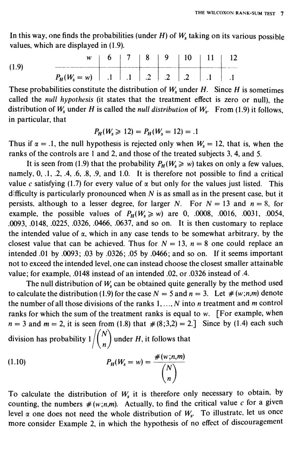
In this way, one finds the probabilities (under H) of Ws taking on its various possible
values, which are displayed in (1.9).
(1.9)
w
PH(WS = w)
6
.1
7
.1
8
1
9
.2
10
.2
11
.1
12
These probabilities constitute the distribution of Ws under H. Since H is sometimes
called the null hypothesis (it states that the treatment effect is zero or null), the
distribution of Ws under H is called the null distribution of Ws. From (1.9) it follows,
in particular, that
PH(WS>\2) = PH(WS=\2) = A
Thus if a = .1, the null hypothesis is rejected only when Ws = 12, that is, when the
ranks of the controls are 1 and 2, and those of the treated subjects 3, 4, and 5.
It is seen from (1.9) that the probability PH(WS^ w) takes on only a few values,
namely, 0, .1, .2, .4, .6, .8, .9, and 1.0. It is therefore not possible to find a critical
value c satisfying (1.7) for every value of a but only for the values just listed. This
difficulty is particularly pronounced when N is as small as in the present case, but it
persists, although to a lesser degree, for larger N. For N = 13 and n = 8, for
example, the possible values of PH(Ws^w) are 0, .0008, .0016, .0031, .0054,
.0093, .0148, .0225, .0326, .0466, .0637, and so on. It is then customary to replace
the intended value of a, which in any case tends to be somewhat arbitrary, by the
closest value that can be achieved. Thus for N = 13, n = 8 one could replace an
intended .01 by .0093; .03 by .0326; .05 by .0466; and so on. If it seems important
not to exceed the intended level, one can instead choose the closest smaller attainable
value; for example, .0148 instead of an intended .02, or .0326 instead of .4.
The null distribution of Ws can be obtained quite generally by the method used
to calculate the distribution (1.9) for the case N = 5 and n = 3. Let # {w;n,m) denote
the number of all those divisions of the ranks 1,..., N into n treatment and m control
ranks for which the sum of the treatment ranks is equal to w. [For example, when
n = 3 and m = 2, it is seen from (1.8) that # (8;3,2) = 2.] Since by (1.4) each such
division has probability 1
(1.10)
under //, it follows that
#(w;n,m)
Ph(Ws = w) =
N
To calculate the distribution of Ws it is therefore only necessary to obtain, by
counting, the numbers #(w;n,m). Actually, to find the critical value c for a given
level a one does not need the whole distribution of Ws. To illustrate, let us once
more consider Example 2, in which the hypothesis of no effect of discouragement

8 RANK TESTS FOR COMPARING TWO TREATMENTS
was being tested against the alternative, that discouragement has an adverse effect.
Under the alternative, the differences in the scores of the treatment subjects (those
being discouraged) will tend to be lower than those of the controls. The hypothesis
will therefore be rejected when Ws is too small, say Ws ^ c, where c is determined so
as to satisfy as closely as possible the equation
Ph(Ws<c) = ol
Since m = n = 5, each possible set of treatment ranks has probability 1 /( J = 7252.
Suppose that a = .05, and let us enumerate systematically the sets of treatment ranks
giving the smallest values to Ws. To see how far this process needs to be carried,
note that the number x of such sets required is given approximately by the equation
x/252 = a = .05, the solution of which is x = 252/20 = 12.6. The resulting count is
displayed in (1.11).
1+2 + 3 + 4 + 5= 15 1+2 + 4 + 5 + 6= 18
1+2 + 3 + 4 + 6= 16 1+2 + 3 + 4 + 9= 19
1+2 + 3 + 4 + 7= 17 1+2 + 3 + 5 + 8 = 19
( ] 1+2 + 3 + 5 + 6= 17 1+2 + 3 + 6 + 7= 19
1+2 + 3 + 4 + 8 = 18 1+2 + 4 + 5 + 7= 19
1+2 + 3 + 5 + 7= 18 1 + 3 + 4 + 5 + 6= 19
This exhausts the cases with Ws ^ 19 and shows that PH(WS ^ 19) = 12/252 = .0476.
This is the closest to a = .05 that we can get since PH(WS ^ 20) = .0754 (Prob. 15).
Now the sum of the treatment ranks in Example 2 was 1+2 + 4 + 6 + 8 = 21, which
is larger than the critical value c = 19. Despite the appearance of a treatment effect
noted in Example 2, the results are therefore not significant at level a = .0476, nor
even at a = .0754.
(N\
Unfortunately, as is seen from Table A, the number I I of possible cases
increases very rapidly with N and n, and enumerations such as that above then
become very cumbersome. It is therefore convenient to have available a table of the
distribution of Ws, and such a table covering the values m = 3,4; m ^ n ^ 12 and
5 ^ m ^ 10; m ^ n ^ 10 is given at the end of the book as Table B.1 To see how
to use this table, note that the distribution of Ws is not the same when the two group
sizes are, say, m = 2, n = 4 as when they are m = 4, n = 2. It turns out, however,
that the distribution of the statistic Ws-\n(n+ 1) is the same in both cases and that
more generally for any integers kx ^ k2 the distribution of Ws-\n(n+ 1) is the same
when the group sizes are m = ku n = k2 as when they are m = /c2, n = kv This
1 For more extensive tables, see, for example: Buckle, Kraft, and van Eeden( 1969b); Milton (1964); and Wilcoxon, Katti,
and Wilcox (1970).

THE WILCOXON RANK-SUM TEST 9
result, which suggests tabling Ws — ?n(n + \) rather than Ws, is proved as (C) at the
end of this section.
There is another reason for preferring to table the distribution of Ws — ?n(n+ 1).
The minimum value of Ws is obtained when the n treatment ranks are 1,2 n and
hence (Prob. 83) is
(1.12) 1+2H +n = ^n(n+l)
The table becomes more compact by subtracting this minimum value, which depends
on n, from Ws. For reasons that will be discussed at the end of the section, the
resulting statistic will be denoted by WXY so that
(1.13) WXY = Ws-$n(n+l)
Table B gives the probabilities
(114) Ph(Wxy^o)
up to at least the first entry that is ^ .5, for all combinations of kx ^ k2 ^ 10, and
for kx = 3,4; k2 = 11,12, where kx denotes the smaller and k2 denotes the larger of
the two group sizes m and n. To illustrate the use of the table, consider the
probability PH(WS ^ 21) of observing a value as small as or smaller than the observed
value 21 of Example 2. (For simplicity of notation, we shall suppress the subscript
H during the remainder of the section.) Here m = n = 5, so that n(n + l)/2 = 15 and
P(WS ^ 21) = P(WS-15 ^ 6) = P(WXY ^ 6)
On entering the table with kx = k2 = 5 and a = 6, we find this probability to be equal
to .1111. Suppose instead that we wish to use the table (instead of the earlier
enumeration method) to find the critical value corresponding to an approximate
significance level of .05. Looking through the entries for kx = k2 = 5, we see that the
two probabilities bracketing .05 are .0476 and .0754. The first of these is the closer
and corresponds to the value a = 4, so that
.0476 = P(WXY ^ 4) = P(WS- 15^4) = P(WS ^ 19)
Thus we find the critical value 19 as before.
From the table it is easy to obtain a probability (^ l/2) that Ws is less than or
equal to a given value. However, the hypothesis is frequently rejected for large
values of Ws. One then needs to solve Eq. (1.7) and hence requires the probability
that Ws is greater than or equal to some constant. These probabilities can be
obtained from the table by either of the following two methods.
Method 1. This method is based on the fact, to be proved at the end of this section,
that the distribution of Ws is symmetric about the point n(N + l)/2. This means that
for each k the two values
in(N+l)-/c and \n(N+\) + k

10 RANK TESTS FOR COMPARING TWO TREATMENTS
which are equally distant from n(N + 1 )/2 on opposite sides, have the same probability.
That is, for all k
(1.15) P[_WS = in(N + l)-fc] = P\_WS = £„(#+ 1) + *]
and hence also
(1.16) P[WS ^ ±n{N + l)-/c] = P{WS > ±n(N + l) + /c]
Suppose now, for example, that m = 4, n = 6 and we wish to find the probability
P( Ws ^ 35). Here n(N + 1 )/2 = 33, and
P(^. ^ 35) = P(^v ^ 33 + 2) = P(Ws ^ 33-2) = P(WS ^ 31)
Entering the table with kx = 4, k2 = 6, we find
P(^. ^ 31) = P(WXY ^ 10) = .3810
which is therefore the desired probability.
Method 2. Let us denote the sum of the control ranks by
(1.17) ^r = R1+-+/C
Since the totality of the ranks is just the set of integers 1 N whose sum by (1.12)
is N(N + l)/2, it follows that
(1.18) Wr+Ws = ±N(N+\)
The sum of Wr and Ws being constant, large values of Ws correspond to small values
of Wr and vice versa. Instead of rejecting H according to (1.6) when Ws is large, it is
therefore equivalent to reject when Wr is small, say, when
(1.19) Wr^c'
Here c is determined by the condition that is equivalent to (1.7), namely,
(1.20) P(Wr^c') = (x
If we wished to table the probabilities on the left-hand side of (1.20), it would
again be convenient to subtract from Wr its minimum value, which is 1 + • • • +m =
m(m+ l)/2, and consider the statistic
(121) WYX= Wr-±m(m+\)
Now at the end of this section it will be proved that the statistics WXY and WYX have
the same null distribution, i.e., that
0-22) P{WXY ^a) = P(WYX ^ a) for all a
Thus, Table B can be used to solve Eq. (1.20) just as it was used to solve Eq. (1.7).
As an illustration of this method, let us consider again the probability that Ws ^ 35

THE WILCOXON RANK-SUM TEST 11
when m = 4, n = 6, obtained previously by Method 1. Since N = 10, it follows from
(1.18) that Ws = 55- Wn and hence that Ws ^ 35 if and only if Wr ^ 20. By (1.21),
WYX = Wr-10 and
P(Wr^ 20) = P(WYX^ 10)
Entering Table B with kx = 4, k2 = 6, and a = 10, we find the probability .3810,
which agrees with the value for P(WS^ 35) obtained by the first method.
Consider now once more the situation of Example 2. The sum of the treatment
ranks turned out to be Ws = 21, and with small values of Ws favoring the alternative
it followed that the hypothesis H (discouragement has no effect on test performance)
is not rejected at the significance level closest to a = .05. Instead of simply reporting
the rejection of // at the given significance level, it is more informative to report the
probability under H of obtaining a value as extreme as, or more extreme than, the
observed value. This probability is called the significance probability of the observed
result. In the case of Example 2, the significance probability is the probability that
Ws is as small as, or smaller than, 21, which was seen above to be equal to
P(Wi^21) = .llll.
The significance probability has the important property of showing, in a single
number, whether or not to reject the hypothesis at any attainable level a. For suppose
that large values of a test statistic, say Ws, are significant. If w denotes the observed
value of Ws, the significance probability is then defined as
(1.23) 5l = Ph(Ws>w)
The hypothesis is rejected when w ^ c, and hence by (1.7) when a ^ a. Conversely,
H is accepted for any critical value exceeding w, and hence for any attainable
significance level a which is less than a. Because of this property, when reporting
the outcome of a statistical test, one should state not only whether the hypothesis
was accepted or rejected at a given significance level; at the least one should also
publish the significance probability, thus enabling others to perform the test at a level
of their choice.
Beyond this, the significance probability provides an intuitive indication of the
strength of the evidence against the hypothesis since it is the probability (under H) of
getting a value of the test statistic as extreme as or more than the observed value.
The smaller a is, the more unlikely it is to observe this extreme a value under //,
and the stronger, therefore, is the evidence against H.
Let us now return to the Wilcoxon test and discuss an alternative interpretation
of the statistics WXY and WYX which will prove useful in Chap. 2. Denote the control
and treatment observations by Xu..., Xm and Y^ ..., Yn, respectively, and consider all
possible pairs of observations (Xh Yj) consisting of one X and one Y Among the
mn such pairs there will typically be some for which X{ < Y, and some with Y, < Xt,

12 RANK TESTS FOR COMPARING TWO TREATMENTS
and it turns out that
(1 24) Wxy = number of pairs (Xh Yj) with Xt < Yj
and
(1 25) WYX = number of pairs (Xh Yj) with Yj < Xt
The statistics WXY and WYX, which by (1.13) and (1.21) are equivalent to the Wilcoxon
rank-sum statistics Ws and Wr, are known as the Mann-Whitney statistics. The
notation WXY and WYX reflects the relationships (1.24) and (1.25).
The interpretation (1.24) provides an alternative method for computing WXY,
which sometimes is more convenient. To illustrate the method, consider once more
the data of Example 2. Instead of ranking the 10 differences, we now count for each
of the treatment differences —6, —5, 1, 4, 6 the number of control differences that it
exceeds, namely, —6:0, —5:0, 1: 1, 4: 2, 6: 3. It follows that
WXY =0 + 0+1+2 + 3 = 6
To conclude this section, we shall now prove relation (1.24), the symmetry of
Ws, and relation (1.22).
(A) Proof of (1.24). Denote the ordered y's by
1(1) < 1(2) < •" < Y(n)
and for each /, compute the number of A"s less than Y(j). Since the rank of y(1) is Sx,
there are Sx — 1 smaller observations. These must all be A"s, so that the number of
A"s less than ^1} is Sx — 1. Similarly, there are S2 — 1 observations less than Y{2).
One of these (namely, y(1)) is a Y, so that the number of A"s less than Y{2) is
(S2 — 1) — 1 = S2 — 2. In the same way, it is seen quite generally that since the number
of y's less than YU) is)- 1, the number of A"s less than YU) is (S,-1)-(/-1) = Sj-j.
The total number of pairs (Xh Yj) with Xt < Yj is therefore
(5i-D + (S2-2)+-+(^-n)=^-(l+2+-+n)=^-in(n+l)=M^y
as was to be proved.
(B) Proof of the Symmetry of the Null Distribution of Ws about ?n(N +1). Let
the N subjects (of which n receive the treatment and m serve as controls) be ranked
in inverse order. The subject that previously held rank 1 now has rank /V, rank 2 is
replaced by rank N-1, and in general rank S is replaced by rank N-S+ 1. Let us
denote by S[ this new inverse rank attached to the treatment subject that had
previously received rank 5f. Then the argument leading to (1.4) shows that
PH(S[=su...^ = sn)= l

ASYMPTOTIC NULL DISTRIBUTION OF THE WILCOXON STATISTIC 13
and hence that Ws- = S[ + • • • +$ has the same null distribution as Ws. Now
ws, = [(N + \)-s1]+--'+[(N+\)-sn] = n(N + \)-ws
so that
It follows that Ws — ?n(N +1) and ?n(N+ 1)— Ws have the same distribution, i.e., that
P[Ws-%n(N+ 1) = /c] = P[in(AT + 1)- Ws = /c]
This is equivalent to (1.15) and hence proves (B).
(C) Proof of(1.22). By(U8),Wr+Ws = %(m + n)(N +l\soth<itWr-$m(N + 1)
= ±n(N + l)-Ws. It thus follows from (B) that Wr-im(N+l) has the same
distribution as Ws - ?n(N + 1) and, on adding \mn to both statistics, that Wr- %m{m +1)
has the same distribution as Ws — ?n(n+ 1), as was to be proved.
3. ASYMPTOTIC NULL DISTRIBUTION OF THE WILCOXON
STATISTIC
Critical values and significance probabilities of the Wilcoxon rank-sum test can be
obtained from Table B when both m and n are less than or equal to 10. For larger
values of m and n, a useful approximation is available for these probabilities. It is a
fundamental fact of probability theory, known as the central limit theorem, that the
sum T of a large number of independent random variables (satisfying some mild
restrictions) is approximately normally distributed. (For a discussion of this theorem
see Appendix, Sec. 3.) If E(T) and Var (T) denote the expectation and variance of T,
(1.26) JT-E(T) 1 %
Lyv^r) j
where <&(a) denotes the area to the left of a under a standard normal curve as shown
in Fig. 1.1, and where % indicates that the right-hand side is an approximation to
the probability on the left-hand side.
FIGURE 1.1
Standard normal curve.

14 RANK TESTS FOR COMPARING TWO TREATMENTS
Now if n is large, the sum of the treatment ranks is the sum of a large number
of random variables but these are not independent. However, if m is also large, the
dependence turns out to be sufficiently weak for the central limit theorem to continue
to hold, so that the normal approximation (1.26) does apply to the Wilcoxon
distribution.
Use of the approximation (1.26) requires knowledge of the expectation and
variance of Ws. These are determined by the distribution of Ws, which in turn rests
on the distribution of the treatment ranks given by (1.4). It is shown in formulas
(A.45) and (A.46) of the Appendix that this expectation and variance are
(1.27) E(Ws) = \n{N+\)
and
(1.28) Var(Ws) = ^mn(N + l)
The corresponding formulas for Wr are obtained by interchanging m and n, and those
for WXY from (1.13), so that
(1.29) E(Wr) = $m(N+\) and E(WXY) = \mn
while
(1.30) Var(M/) = Var(^y) = ^mn(N+\)
The application of (1.26) requires, in addition to the expectation and variance
of Ws, a table of the area d>(a) to the left of a under a standard normal curve. Such
a table is given as Table C at the end of the book for positive values of a. It can
be obtained from this table for negative values of a by using the facts that (i) the
standard normal curve is symmetric about the origin and (ii) the total area under
the normal curve is equal to 1. By (i), the area d>( — a) to the left of —a is equal to
the area to the right of a, and by (ii) this latter area is equal to 1 — d>(a). This provides
the needed relationship
(1.31) <&(-a)= \-<t>(a)
To illustrate both the computation and the accuracy of the normal
approximation, let us take an example at the edge of Table B of the Wilcoxon distribution.
Suppose that m = n = 10 and that we wish to find the probability P(WS ^ 79). Then
E(WS) = 105, Var(Ws) = 175, and hence
nw. < 79, „{Si^, J^l . «,<- ,.965,
\ yi75 y/VJSj \13.23J
Table C shows that <D( 1.965) = .9753, so that (to three digits) <D(-1.965) = .025,
which is therefore the normal approximation to the desired probability. In
comparison, Table B gives .026 for the same probability.
The accuracy of the approximation is frequently improved by the following
refinement, which has its basis in the graphical representation of a distribution by
means of a histogram. This consists of a series of rectangles or bars, each
corresponding to one of the possible values of the random variable in question. The base

ASYMPTOTIC NULL DISTRIBUTION OF THE WILCOXON STATISTIC 15
I I I l I I I
0 1 2
FIGURE 1.2
Histogram for X.
of the rectangle is centered on the value, and its area is equal to the probability with
which this value is taken on. Figure 1.2 shows the histogram for a random variable
X taking on the values 0,1,2 with probabilities %, % and % respectively. Since the
base of each rectangle in this case is equal to 1, the height is equal to the area of
the rectangle, so that the heights of the three rectangles are %, V2, and %
Suppose now that probabilities are being approximated by means of the
appropriate area under a smooth curve (Fig. 1.3), so that the approximation to
P(X ^ a) is the area under the curve to the left of a. Then P(X ^ 1), for example,
is approximated by the area under the curve to the left of 1. However, since P(X ^ 1)
is equal to the area under the histogram corresponding to the rectangles centered
at 0 and 1, that is, the area under the histogram to the left of 1.5, a more natural
and typically more accurate approximation is provided by the area to the left of 1.5.
This modification is called the continuity correction because it compensates for
the fact that a noncontinuous histogram is being approximated by a continuous
curve. As an illustration of its effect, consider the probability P(WS ^ 12) when
m = 11 and n = 3 (although such wide discrepancy between the two group sizes
typically is undesirable). The exact probability, which is easily obtained by
enumeration, is equal to .063. Since E(WS) = 22.5 and X/Var(^s) = ^4125 = 6.423,
the normal approximation gives
Let us now apply the continuity correction. Since the smallest value that Ws
cantakeonisn(n + l)/2 = 6, its possible values are 6,7,..., 12,13,..., and the possible
J I I I L
0 1 2
FIGURE 1.3
Approximation to the distribution of X.

16 RANK TESTS FOR COMPARING TWO TREATMENTS
values of (Ws-22.5)/6A23 are therefore (6-22.5)/6.423, ..., (12-22.5)/6.423,
(13 —22.5)/6.423 These are the centers of the bars making up the histogram of
(Ws — 22.5)/6.423. The normal approximation took in only the area under the curve
to the left of (12 —22.5)/6.423, which is the center of the bar corresponding to Ws = 12.
However, since the whole area of this bar is counted in the probability P(WS ^ 12)
it is better to include the area under the normal curve up to the right-hand endpoint
of this bar, which lies midway between (12-22.5)/6.423 and (13-22.5)/6.423, and is
therefore equal to
1/12-22.5 13-22.5\ 12.5-22.5
+ ■
2\ 6.423 6.423 / 6.423
Thus the continuity correction leads to the approximation
which is closer to the correct value .063 than the value .051 obtained by the uncorrected
normal approximation. In general, the same argument leads to approximating the
probability P(WS ^ c) by1
(1.32) P{W^c)^JcJ^+M\
It is difficult to make reliable general statements concerning the accuracy of this
and similar approximations, but the following two qualitative statements typically
apply not only in the Wilcoxon case but also (with the obvious modifications) to such
approximations throughout the book.
(i) The accuracy of the approximation tends to increase as m and n increase.
(ii) If the accuracy is measured not by the absolute error (the difference between
the exact and approximate values) but by the relative error (the absolute error
divided by the exact value), the approximation tends to become less reliable when
the probabilities being approximated are very close to zero, that is, in the tails of
the distribution.
To (i) can be added that in the Wilcoxon case an increase in the smaller of the
two group sizes typically results in a greater improvement than a corresponding
increase in the larger group size.
These statements leave open the crucial question of how large m and n have
to be for the approximation to be satisfactory. Some light is thrown on this problem
by Table 1.1, which provides a comparison of the Wilcoxon probability P(Wr ^ c)
Kruskal and Wallis (1952. p. 591) state that the continuity correction tends to improve the approximation when the
probability is above .02 and to make it worse when the probability is .02 or less. This is in agreement with the values
shown in Table 1.1 on page 17.

ASYMPTOTIC NULL DISTRIBUTION OF THE WILCOXON STATISTIC 17
with its normal approximation, both with and without continuity correction, for
three combinations of the group sizes m and n. The cases m = 4, n = 12, and
m = n = 8 suggest that at least for the range a = .01 to a = .15, the approximation
with continuity correction will be adequate for most purposes for all group sizes
which are not covered by Table B and in which the smaller group size kx is at least 4.
Incidentally, it is seen from Table 1.1 that the continuity correction does not always
improve the approximation, although on the whole it seems to give very much better
results.
TABLE 1.1
Exact and approximate values of P{Wr ^ c) with
and without continuity correction
10
Exact
Without
With
.012
.010
.014
.024
.019
.026
.048
.035
.047
.083
.061
.078
.131
.098
.123
I m = 3, n = 6 I
13
15
20
23
I m = 8, n = 8
25
Exact
Without
With
c
Exact
Without
With
.004
.005
.006
44
.005
.006
.007
.010
.011
.012
m =
46
.010
.010
.012
.052 .106
.045 .091
.051 .102
4, n = 12~|
48 52
.019 .052
.018 .047
.020 .052
.158
.138
.151
56
.117
.104
.114
58
.164
.147
.159
When the smaller group size kx is 1, 2, or 3, the normal approximation is not
satisfactory. The case kx = 1 is covered by Prob. 74, the case kx = 3 by Table B if
the larger group size does not exceed 12. An exact formula for kx = 2 is given by
Buckle, Kraft, and van Eeden (1969a). These authors also propose an alternative,
quite different approximation that typically does even better than the normal
approximation, and which in particular takes care of the remaining cases with fci = 3.
This approximation is sketched in Sec. 7A. An alternative approach to small values
of kx is given by Fix and Hodges (1955).

18 RANK TESTS FOR COMPARING TWO TREATMENTS
Statements, such as those made above, concerning the validity of an
approximation are typically based on two kinds of evidence. There is the numerical
evidence obtained by comparing the exact and approximate values for a number of
different cases such as those in Table 1.1. This is often supplemented by a theoretical
result, a limit theorem, which states that the left-hand side of (1.26) tends to the
right-hand side as the group sizes increase and tend to infinity. Such a theorem
claims only that the left-hand side will get arbitrarily close to the right-hand side
eventually, that is, for sufficiently large group sizes. However, it also suggests, though
it does not prove, that the accuracy of the approximation tends to improve as the
group sizes increase. Thus, if computation shows the approximation to be
satisfactory for given group sizes and a certain range of significance levels, one may expect
it to be even better for larger sample sizes.
The limit theorem relevant to the present situation states that
1.33) PH\ . = ^ a -> (Da
as m and n tend to infinity. A proof is given in the Appendix, Sec. 4, Example 16.
4. THE TREATMENT OF TIES
The application of rank tests often meets with a difficulty, which so far we have
avoided. We have assumed that either subjective evaluation or numerical
observation leads to a complete ranking of the treatment and control subjects. However,
this is frequently not the case. An instructor asked to rank two students, or a patient
trying to determine on which of two occasions a headache remedy gave greater relief,
may feel unable to make the necessary distinction. Alternatively, when
measurements or other numerical observations are taken, it often happens that two or more
observations are equal, and this leads to the same difficulty. Suppose, for example,
that m = n = 2 and the observations are 1.3, 1.7, 1.7, 2.5. Then the smallest
observation has rank 1 and the largest rank 4, but we do not know which of the other
two has rank 2 and which rank 3. If no extraneous distinction is introduced between
the two tied observations, they should be assigned the same rank, and it then seems
most natural to assign to each the average of the two tied ranks, in the present
case (2 + 3)/2 = 2.5. The four subjects are then assigned the midranks 1, 2.5, 2.5, 4,
and we shall denote the midranks assigned to treatment and control by Sf, 52* and
Rf, R*, respectively.
Clearly the null distribution (1.4) no longer holds because even the possible
values of (5?, £*) are not the same as those of (Sx, S2). However, the argument leading
to (1.4) still applies. Under the hypothesis of no treatment effect, the four subjects
will receive the same midranks regardless of which of them are assigned to treatment

THE TREATMENT OF TIES 19
and which to control. The random selection of two of the subjects to receive the
treatment then also selects their midranks, so that each of the six possible choices of
two of the four midranks as Sf and S£ are equally likely. This leads to the following
null distribution, which now takes the place of (1.4):
P(S? = l9Sf = 2.5) = l P(S1*=1,S2*=4) =£
P(S* = S$ = 2.5) = i P(S? = 2.5,52* = 4) = |
This distribution determines that of the Wilcoxon midrank-sum statistic
as before, and we see that W* takes on the values 3.5, 5. 6.5 each with probability l/3.
The above approach applies quite generally to situations with tied observations,
but instead of giving a general discussion we shall illustrate it with another example.
Suppose that m = n = 3 and that the control observations are 2, 2, 9 and the
treatment observations 4, 9, 9. The six midranks are then 1.5, 1.5, 3, 5, 5, 5, and the
sum of the treatment midranks is
M/* = 3 + 5 + 5= 13
What is the significance probability P(W* ^ 13) of these observations? There are
I I = 20 equally likely choices for the three treatment midranks, and the probabilities
of the possible sets of values of (Sf, S£, 53*) are
(si si si)
Pislslsi)
1.5, 1.5, 3
1/20
1.5, 1.5. 5
3/20
1.5. 3, 5
6/20
1.5, 5, 5
6/20
3,5,5
3/20
5,5.5
1/20
The significance probability is therefore P(W* ^ 13) = 4/20 = .2.
In certain situtations involving tied observations there arises an ambiguity that
is not always resolved correctly. Suppose that the treatment observations are 6,6,6,9
and the control observations 1, 3, 4, 10, with large values of Ws being significant.
Since ties occur only among the treatment observations, no question arises concerning
the value of Ws. The treatment ranks are 4, 5, 6, 7 and the rank sum Ws thus has
the value 22. It is now tempting to compute the significance probability as in Sec. 2
or obtain it from Table B to be 12/70 = 1714. On the other hand, the approach of
the present section gives W* = 22 and the significance probability 11/70=1571
[Prob. 45(i)]. Which of these two values is correct?
Recalling the basis for such probability calculations, we see that the actual
observations must be compared with all possible ways of assigning the eight numbers
1> 3, 4, 6, 6, 6, 9, 10 to treatment and control. Many of these will split the three tied
observations, assigning some to one group and some to the other, and in these cases
the value of Ws is not defined. Hence, there is no validity in the first approach, and
the correct value of the significance probability is .1571.

20 RANK TESTS FOR COMPARING TWO TREATMENTS
Since the distribution of W* depends not only on m and n but also on the
number of observations tied at each value (Prob. 44), tables of the distribution are
not practicable and the need for an approximation is, if anything, even more pressing
than when no ties are present. A normal approximation is again available when m
and n are not too small and the maximum proportion of observations tied at any
value is not too close to 1.
Use of the normal approximation requires the expectation and variance of W*.
The expectation of W* is shown in the Appendix, Example 3, to be the same as that
of Ws and hence to be given by
(1.34) E(W*) = ±n(N + \)
The variance of W* involves the numbers of observations tied at the different
values. Suppose that the N observations take on e distinct values, and that dx of the
N observations are equal to the smallest value, d2 to the next smallest, ...,de to the
largest. If the observations are, for example, 2, 2, 4, 9, 9, 9, as in one of the earlier
examples, then e = 3 and dx = 2, d2 = 1, and d3 = 3. With this notation, it is shown
in the Appendix, Example 3, that
,n_mn(N+l)
mn^idf-dd
(1 35) VarfW) = '^tlZJ2 ^i
The first term is just the variance of Ws\ the second gives the correction for ties.
The effect of the correction tends to be quite small, although exceptions to this rule
are possible (Prob. 93). In particular, when no ties are present, all the d{ are equal
to 1, and the correction term is zero as it should be.
Typically, the normal approximation is not as close in the presence of ties as it
is for the same group sizes without ties. This is not surprising since ties tend to
decrease the number of values taken on by Ws and thereby to increase the lumpiness
of its distribution. A number of comparisons of the exact and approximate
distributions with and without continuity correction are given by Lehman (1961).
Although these comparisons are on the whole favorable to the continuity correction,
in this book—and hence in the present case—we shall use the approximation without
the correction whenever the values of the random variable in question are not
equally spaced.
The normal approximation is supported by a limit theorem, which states that
the null distribution of \W*-E(W*)~\ly/\viv(W*) tends to the standard normal
distribution <D provided both m and n tend to infinity and
(1-36) max ( -M is bounded away from 1 as N -> oo
Condition (1.36) suggests that the normal approximation should be used only when

THE TREATMENT OF TIES 21
the largest of the proportions dJN,..., dJN is not too close to 1. The proof of this
limit theorem is given in the Appendix, Sec. 4, Example 17.
The W^*-test can also be applied in situations in which no numerical responses
are observed but the subjects are divided into a number of categories such as poor,
indifferent, or good, and it is observed how many of the treatment and control
subjects fall into each of these categories. Let us now illustrate the normal
approximation on an example of this kind.
EXAMPLE 3. Psychological counseling. In a test of the effect of psychological counseling,1
80 boys are divided at random into a control group of 40 to whom only the normal counseling
facilities are available, and a treatment group of 40 who receive special counseling. At the end
of the study, a careful assessment is made of each boy who is then classified as having made a
good, fairly good, fairly poor, or poor adjustment, with the following results:
Treatment
Control
Poor Fairly Poor Fairly Good Good
5 7 16 12
7 9 15 9
Total
40
40
The data can be treated as if the observations were capable of taking on only four values,
with 5-I-7 = 12 observations tied at the smallest value, 7-1-9 = 16 at the next smallest, 16-1-15 = 31
at the third, and 12-1-9 = 21 at the largest value. The midrank of the 12 subjects whose
adjustment is classified as poor is then (1-1-2-1- ••• +12)/12 = 6.5; the midrank of the fairly poor is
(13+ ••• +28)/16 = 20.5; and the midranks of the subjects in the third and fourth categories are
44 and 70, respectively. [For a general formula giving the value of the midrank in the ith group,
see (1.41) below.]
The value of W* is thus
W* = 5x 6.5 + 7 x 20.5+16 x 44+ 12 x 70 = 1,720
and the significance probability of the observed results is PH(W* ^ 1,720). Since m = n = 40
and dx -= 12, d2 = 16, d3 = 31, d4 = 21, it follows from (1.34) and (1.35) that E(W*) = 1,620 and
\/Var(Ws*) = 99.27. The normal approximation to the significance probability therefore gives
Ph(Ws* > 1,720) = 1 -0(1.01) = .16
The statistic W* is the natural generalization of the rank sum Ws when the
observations are not all distinct. In the same situation, it is also possible to generalize
the statistic WXY. Recall that WXY counts the number of pairs (Xh Y3) for which
Xt < Yy9 that is, each pair (Xh Yj) is assigned the score 1 or 0 as Xt is less or greater
than Yh and WXY is the sum of these scores. When ties are present, it may happen
that Yj is equal to Xt and it is then natural to assign the score % to the pair (Xh Yj).
An extensive report of a large-scale study of this question is given by Powers and Witmer. An Experiment in the
Prevention of Juvenile Delinquency, Columbia University Press, New York, 1951. Since this study used the matched
samples design (to be discussed in Chap. 3). the data are not suitable as an example here.

22 RANK TESTS FOR COMPARING TWO TREATMENTS
Let us denote the sum of the resulting scores by W&, so that
(137) W& = [number of pairs (Xh Yj) with Xt < Yj\
+ ^[number of pairs (Xh Yj) with X( = Y)]
in generalization of (1.24). Then the tests based on W* and W& are again equivalent
and in fact the two statistics satisfy the relationship corresponding to (1.13) for the
unstarred statistics, namely,
(1.38) WfY=W*-±n(n+l)
It follows that
(1.39) E(Wft) = hmn
and
(1.40) Var(»ft) = Var(»;*)
where the latter variance is given by (1.35). The relation (1.38) provides an alternative
method for computing W*.
We conclude this section by proving (1.38). It is convenient to begin by
obtaining a general expression for the values of the midranks. If dx observations
are tied at the smallest value, the midrank of these observations is the average of
the ranks 1,...,^!, that is,
I + ^i-W. + O
The observations in the second group occupy the positions dx + 1, dx+2, ...ydx + d2,
and their midrank is therefore
= dx +j[d2 + 1)
d2
Similarly, the midrank of an observation in the ith group is
(1.41) (^ + -M-1 + l)+-+(t/1+-M-,M) = ,i + „.M,_i+^[.+ 1)
dt
Suppose now that of the dx observations tied at the smallest value, Ax are A°s
and Bx are y's; that of the d2 observations tied at the next smallest value, A2 are
A"s and B2 are y's; and so on. The sum of the y-midranks is then
(1.42) ^* = B1[iW1 + l)] + B2[d1+iW2 + l)] + B3[d1+d2+iW3 + l)]+---
To obtain a similar expression for M%, consider the contribution to W£Y from
an observation Y in the first group. There are no A"s smaller than this Y, and the
number of A"s equal to Y is Ax. Hence the contribution of this Y is \AV For an
observation Y in the second group the number of A"s smaller than Y is Ax and the
number of X's equal to Y is 42, so that the contribution from this Y is Ax +?A2.

TWO-SIDED ALTERNATIVES 23
Continuing in this way and remembering that the number of y's in the first, second,
and subsequent groups is Bl,B2. and so on, we find that
(1.43) WfY = Bl&Ax) + B2(Ax+±A2) + BMi +*! + &*)+•''
Since d{ = A( + Bh it follows that
W*-Wx\ = BS(Bi^\)] + B2[Bl+^B2 + \)] + B3lBl+B2^^B3+\)]^ -
The sum of the terms in this difference not involving the factor xj2 is
£2£1+£3(£1+£2)+--
which is equal to
Z B(Bj = ? Z BtBj
and hence
K*- wx\ = h\Ifli+Yfli2 + Z BAA = iO+Ea,)2]
Since the sum of the B( is the total number of y's and hence IB, = n, this completes
the proof of (1.38).
5. TWO-SIDED ALTERNATIVES
The Wilcoxon rank-sum test provides a simple and effective method for comparing
a new treatment with a standard one. This comparison is strongly biased in favor
of the latter. In fact, the critical value is set so that the probability is 1 —a (typically
.9 or more) of deciding in favor of the standard treatment when there is actually no
difference between the two. The decision goes to the new competitor only if it has
proved itself beyond a reasonable doubt.
Such an asymmetric procedure is not always appropriate. In particular, a
more symmetric approach is indicated for the following two kinds of problems.
(i) When trying to decide which of two treatments is better, one may be faced
with a situation in which both treatments are "new" and there is therefore no reason
to bias the procedure in favor of one rather than the other. Two equally reputable
firms may, for example, simultaneously and at about the same price, introduce two
drugs for the treatment of a condition for which previously no treatment was known.
Or one may wish to decide with which of two brands of gas a car obtains the better
mileage.
(ii) The problem may not be to decide which of two treatments is better but
only to determine whether they differ at all, and in such situations the two treatments
typically play a symmetric role. In the laboratory of a statistics course, for example,
the instructor may have available two different types of computing machines and he

24 RANK TESTS FOR COMPARING TWO TREATMENTS
may want to know whether students would be handicapped in an examination by
being assigned to one type rather than the other. Similarly, in a study comparing
a surgical approach to a medical problem with a more conservative treatment, it
may be desirable to examine first whether it is necessary to distinguish between two
surgical techniques used by different surgeons.
In the present section we shall show how the Wilcoxon test can be adapted to
problems of these two types. We shall begin with the second problem as the simpler
of the two. To test whether there exists a significant difference between two
treatments, say, A and B, the N subjects are assigned as before, m to A and n to B. The
responses of the N subjects are ranked, with WA and WB denoting the sum of
the ,4-ranks and the B-ranks respectively. The null hypothesis H to be tested is that
there is no difference between A and B. While this is the same as the hypothesis H
(no treatment effect) considered in Sec. 1, the alternatives no longer specify that B
is superior to A, but that it is either superior or inferior to A. The hypothesis is
rejected therefore not only when the sum WB of the B-ranks is too large but also
when it is too small, say, when
(1-44) WB ^ cx or WB > c2 (cx < c2)
The constants cx and c2 are determined so that under H the probability of rejection
is equal to the specified significance level a, that is, so that
(1.45) PH(WB ^ cx) + PH(WB >c2) = ol
Equation (1.45) is not enough to specify cx and c2 since it leaves open the question
of how to distribute the total probability a between the first and the second term.
If the two treatments play a completely symmetric role, it seems natural to choose
cx and c2 so that H is as likely to be rejected when WB is too large as when it is too
small, that is, to put
(146) PH(WB ^ Cl) = PH(WB > c2) = fr
From the fact that the distribution of WB is symmetric about ?n(N+ 1) (Sec. 2),
it follows that cx and c2 must be equally distant from \n{N+\) and hence must
be of the form
ci =iw(N+l)-c, c2 = iw(N + l) + c
The test defined by (1.44) and (1.46), the two-sided Wilcoxon rank-sum test, thus
rejects when WB — \n(N+\) is either ^-cor^c, that is, when
(1.47) \WB-{n(N+\)\>c
Because of the discrete nature of WB, typically there will not exist a value c for which
the equation
(1.48) MlWi-i"(W+l)l^c] = a

TWO-SIDED ALTERNATIVES 25
holds exactly. As in Sec. 2, one may then choose the value of c for which the left-hand
side of (1.48) is as close to a as possible, or the smallest value for which it does not
exceed a. As in the one-sided case, one will typically not only be interested in
rejection or acceptance at a fixed level a, but also in the significance probability of
the data. For the two-sided test (1.47) this is given by
(1.49) PH[\^B-in(N+\)\> |W-±„(JV+1)|]
where w denotes the observed value of WB.
The two-sided test (1.47) can of course also be expressed in terms of WXY. From
(1.13) it is in fact seen that (1.47) is equivalent to
(1.50) \WXY-^mn\^ c
with the constant c being the same in both cases.
For large m and n, the test is carried out with the help of the normal
approximation. Since under H
WB-$n(N+\)
y/nm(N+l)/12
has approximately the standard normal distribution, the significance probability
(1.49) is approximated by the area under the normal curve to the left of
-|w-iw(JV+l)|+i
plus the area to the right of
y/mn(N+\)l\2
|w-±n(JV+l)|-±
y/mn(N+1)/12
These two areas are equal, and the significance probability of the two-sided test
(1.47) is therefore approximated by
(i.5i) Ji-^-^^+1)i-ill
I L y/mn(N+l)/12 Jj
In the presence of ties, the test (1.44) and conditions (1.46) are modified by
replacing WB by WB*. Since the distribution of WB* is in general not symmetric, (1.44)
can no longer be replaced by (1.47). Instead, cx and c2 are determined so that
?h(Wb* ^ a) and PH(WB* ^ c2) each are as close to a/2 as possible. For large m and
*> a normal approximation can again be applied. The symmetry of the normal curve
implies that the distribution of WB* is then approximately symmetric, and the
argument leading to (1.51) now shows that the significance probability of the two-sided
Wilcoxon test can be approximated by
{ L v/VarH(WB*) J3

26 RANK TESTS FOR COMPARING TWO TREATMENTS
Here w is the observed value of WB*, the variance VarH(M^*) is given by (1.35), and
the continuity correction of l/2 in (1.51) has been omitted since the values of WB* are
not equally spaced.
It is important to be clear about the difference between the two-sided test (1.47)
and the one-sided test (1.6). The earlier test is appropriate when it is desired to
reject the hypothesis H of equality only when treatment B is better than treatment A.
(If there is a possibility that B is worse than A, this can be included in the hypothesis,
which can be replaced by //': B is not better than A. This possibility is discussed
more formally in Chap. 2, Sec. 2.) The one-sided test thus provides an answer to the
question: "Can we confidently say that B is better than AT' On the other hand,
the two-sided test is appropriate if it is desired to reject H when B is either better or
worse than A. It provides an answer to the question:" Is either treatment significantly
better than the other?"
A confusion as to which of the two tests is appropriate sometimes arises when
at the beginning of an investigation it is not clear which of the treatments would be
expected to be better should they turn out to differ at all. However, after the
observations have been taken, a visual inspection of the data may suggest that, say,
B is better and also an explanation of why this might have been expected. It is then
tempting to see whether the superiority of B is significant by testing H against the
one-sided alternative that B is better than A. Under the given circumstances this is
not appropriate. If A had come out ahead, an explanation might also have
suggested itself for this finding, and the same line of argument would have led to
testing H against the alternative that A is superior. This shows that H would have
been rejected if WB had been either sufficiently large or sufficiently small and that
the appropriate procedure is a three-decision procedure of the kind considered below.
If c(1) and c{2) denote the critical values corresponding to the same significance
level a in the one- and two-sided cases with rejection rules (1.6) and (1.47). respectively,
they are determined by
P„[WB-±n(N+\)>c{l)] = a
and
PH{\WB-hn(N+\)\>c™-\ = *
Since the second condition is equivalent to
it is seen that c(1) < c{2). To be judged significant, the difference must therefore be
more striking when H is being tested against alternatives in both directions (B better
or worse than A) than when it is tested against a specified direction, say, B better
than A, decided upon before the observations are taken. This corresponds to the
fact that a striking difference in either direction is more likely to be observed "by
pure chance," that is. under //, than the same difference in just one direction.

TWO-SIDED ALTERNATIVES 27
EXAMPLE 4. Anticipation of hypnosis. In a study of the effect of hypnosis. 16 subjects were
divided at random into a group of 8 to be hypnotized and 8 controls. When the results
of the experiment were analyzed, it was noticed that a measure of ventilation taken on each
subject at the beginning of the experiment unexpectedly appeared higher for the experimental
subjects than for the controls. A plausible explanation was that such an increase could be caused
in the experimental subjects by the anticipation of being hypnotized, and it seemed of interest
to test the significance of the effect. The observations were as follows:!
Controls: 3.99 4.19 4.21 4.54 4.64 4.69 4.84 5.48
Treated: 4.36 4.67 4.78 5.08 5.16 5.20 5.52 5.74
Although it is tempting here to use a one-sided test, this is not appropriate since a
corresponding difference in the other direction would also have been noticed and tested. The hypothesis
of no effect would therefore have been rejected for a sufficiently large difference in either direction,
and the rejection rule is that of a two-sided test.
To test the hypothesis of no treatment effect at significance level a = .05, the critical values
d and c2 are computed from (1.46) or the corresponding equations for WXY, with a/2 = .025.
For group sizes m = n = 8, Table B shows that P{WXY ^ 13) = .025. Since
P(WXY ^ 13) = P(Wr ^ 49) = P(Wr > 87)
it is seen that at level a = .05 the data will be significant provided
|Wr-68|^ 19
The observed values are Wr = 49 and hence | Wr-68| = 19, and the hypothesis of no difference
is therefore rejected at level a = .05.
The significance probability of the test (1.47) is the probability PH(\Wr-6S\^ |49-68|).
which happens to be just .05. As an illustration of the normal approximation, let us compute
the significance probability using formula (1.51). Since n = 8. N = 16. this gives the value
2[1 -d>(2.001)] = .0454. (See Prob. 53.)
The two-sided Wilcoxon test accepts the hypothesis of no difference between
A and B when
(1.53) \WB-$n(N+l)\<c
and rejects H in the contrary case. Typically, when rejecting the hypothesis one will
not be satisfied with asserting the existence of a significant difference but will wish to
know which of the two treatments is better. One is thus concerned with choosing
between the three decisions: D0: accepting H; Dx: deciding that B is better than A;
or D2: deciding that A is better than B. The obvious procedure, suggested by (1.53),
is to take decision Dx if WB ^ \n(N + l) + c, decision D2 if WB ^ %n(N+ l)-c, and
decision D0 when (1.53) holds. For this procedure the significance level a retains
its interpretation as the probability of falsely rejecting H (and therefore declaring one
°f the treatments superior to the other) when in fact there is no difference.
Data from Agosti and Camerota (1965). "Some Effects of Hypnotic Suggestion on Respiratory Function." Intern. J.
cHn. Expt. Hypnosis 13:149 156.

28 RANK TESTS FOR COMPARING TWO TREATMENTS
There is a more natural way of looking at the present problem. Rather than
emphasizing the somewhat artificial hypothesis of no difference between A and £,
one may stress the problem of determining which of the two treatments is better. If,
in addition, one permits the possibility of remaining in doubt when the data are not
sufficiently conclusive, the procedure may be reformulated as
Choose B if WB ^ \n(N + 1) + c
(1.54) Choose A if WB ^ \n(N+\)-c
Suspend judgment if \WB-\n(N + 1)| < c
This is seen to be a solution to problem (i) stated at the beginning of this section.
How in such a procedure would one specify the critical value c? Let a' denote
the common probability
(1.55) a' = P[WB ^ \n(N+\)-c~\ = P{WB > ±n(N+ l) + c]
computed under the assumption that there is no difference between the two
treatments. Then 2a' is just the level a defined by (1.48); that is, it is the probability of
concluding that one of the treatments is better than the other (either B better than A,
or A better than B) when, in fact, they are equal. An interpretation which is closer
to the present point of view is obtained by considering the two errors to which the
procedure (1.54) can lead: choosing A when B is the better treatment, or conversely,
choosing B when A is better. Suppose, for example, that B is better but that
WB ^ ?n(N+1) — c, so that erroneously A is selected. It is intuitively plausible that
the probability of this error increases as the quality of B decreases and is largest when
B is essentially equal to A, being better by just a hair's breadth; that is, the probability
of erroneously selecting A is always less than or equal to a' and comes arbitrarily
close to a' when the two treatments get sufficiently close. [A more precise statement
and proof of this result requires a model for the case that one treatment is better
than the other, together with the distribution of the ranks in such a model, in
generalization of the distribution (1.4) for the case that there is no treatment difference.
We shall postpone the development of such a model and its consequences to Chap. 2,
Sees. 1 and 2, and for the moment be content with the above intuitive argument.]
The same argument applies when A is better than B (but note that only one of these
errors is possible in any given situation). Together, the two results show that a' has
the interesting property of being the maximum probability of coming to the wrong
conclusion, that is, of selecting the worse of the two treatments. The critical value
c thus can be determined from (1.55) by specifying the maximum error probability a'
that one is willing to tolerate.

TWO-SIDED ALTERNATIVES 29
EXAMPLE 5. Two diets. In a comparison of a number of diets, 12 rats were assigned at
random, 7 to diet A and 5 to diet B. After 7 weeks they showed the following weight
gains.1
A: 156 183 120 113 138 145 142
B: 130 148 117 133 140
Here the B ranks are 2, 4. 5, 7, and 10, and WB = 28. Since this is less than {n(N+\) = 32.5,
the data favor diet A. To see how strongly they support A, let us determine the smallest level a'
at which the procedure defined by (1.54) and (1.55) would declare the superiority of A over B
significant. This is P( WB ^ w). where w = 28 is the observed value of WB and where the probability
is computed under the assumption that A = B. From Table B it is found that
a' = P(WB ^ 28) = p\WB-\n(n+ 1) ^ 13] = .265
Even when A is very slightly worse than B, there is thus a probability of more than !/4 that A
would come out ahead. At any value of a' < .265 that is a possible value of the Wilcoxon
distribution, procedure (1.54) would suspend judgment as to which of the two diets is superior.
The reader may feel that procedure (1.54), as illustrated in Example 5, contradicts
the admonition made following (1.52) and again in Example 4. It was stressed there
that a one-sided error probability is appropriate only when the direction of the
difference or effect is clear before any observations have been made. Yet, in Example
5, where it is not known a priori whether A or B is better, the error probability,
a' = P(WB ^ 28) is one-sided. The explanation lies of course in the different
interpretations as to what constitutes an error. In the two-sided Wilcoxon test (1.44),
the error to be controlled is falsely declaring one treatment better than the other if
in fact they do not differ at all. On the other hand, in the three-decision procedure
(1.54) the error to be controlled is that of declaring one treatment better than the
other if in fact it is worse—if there is no difference, we now do not care which of the
two treatments is preferred.
Procedure (1.54) provides a symmetric choice between two treatments in
situations where the choice is to be made only when the data are reasonably
conclusive, with judgment being suspended otherwise. An analogous procedure is
available when the choice lies between a new and a standard treatment or in other
asymmetric cases, for example, when one treatment is less expensive than the other
or has fewer undesirable side effects. The resulting three-decision procedure will then
take the form
Choose B if WB ^ c2
(156) Choose A if WB ^ cx
Suspend judgment if cx < WB < c2
1 Data from tables 3 and 4 of Nicman Groot and Jansen. "The Nutritive Value of Butter Fat Compared with That of
Vegetable Fats." Koninkl. Ned. Akad. Wctcnschap. Proc. 55:582 604 (1952). (The diets A and B arc diets B and C of
the original paper.)

30 RANK TESTS FOR COMPARING TWO TREATMENTS
Here cx and c2 can be determined so as to give preassigned values to the maximum
error probabilities
(1.57) a1=P(Hi<c1) and ol2 = P(Wb^c2)
where the probabilities are computed under the assumption of no difference (with
respect to the response being observed) between the treatments, and where, because
of the discrete nature of the distribution involved, one will typically be satisfied with
values cx and c2 for which the equations hold as closely as possible. If A is the
standard treatment or that which is a priori more desirable, one will prefer A to B
when the two treatments are equally effective, and hence will specify a smaller value
for a2 than for a^
The procedure (1.56) generalizes both the symmetric three-decision procedure
(1.54) and the test (1.6). It reduces to the former when olx = a2 = a' and to the latter
when cx = c— 1 and c2 = c and when A and B are identified with the standard and
new treatment, respectively, so that a2 = a and olx = 1 —a. There is no difficulty in
extending (1.56) to the case in which some observations are tied. It is only necessary
for this purpose to replace WB by the sum WB* of the B midranks. The presence of
ties does, however, create a difficulty with respect to the symmetric procedure (1.54)
since the distribution of WB* need no longer be symmetric. One will in this case
determine the critical values cx and c2 so as to make <xx and a2 as close to a' (and
hence to each other) as possible. If the demands of fairness make the equality of olx
and ol2 imperative, this can be achieved through the otherwise undesirable device of
randomization.
The three-decision procedure (1.54) assumes the possibility of not coming to a
decision as to which of the two treatments is better. This will be the case if a decision
can be postponed until further information (for example, additional observations)
becomes available. However, the decision sometimes cannot be delayed and an
immediate choice between A and B is required. A procedure suggested by (1.54) is
then to choose treatment B when WB>\n(N + \) and treatment A when
WB < {n(N + \). This still leaves the question what to do when WB = \n(N + 1) or
equivalently when WXY = \mn. In this case (which cannot arise when both m and
n are odd), exactly half of the pairs Yj-X( are positive and half are negative, and
there seems no reason to prefer either one of the treatments to the other. If a
decision must be taken, it may be possible to base it on some auxiliary consideration
such as the price of the treatment. If no other recourse is available, it may become
necessary to toss a coin (as is sometimes done in tournaments which cannot be
completed because of time or weather).
The above procedure for making a definite choice between A and B can be
given a slightly more intuitive form by noting that by (1.18)
Wi + Hi = i(m + n)(JV+l)

TWO-SIDED ALTERNATIVES 31
A X X X *—
B -X X X X-
(a)
-X—XX—X-
-X—X-
-X- B
(b)
FIGURE 1.4
Observational patterns under alternatives to H.
It is then easy to see (Prob. 97) that
WB = $n(N+\)
>
if and only if
Wb<Wa
n > m
The procedure therefore chooses A or B as WA/m is greater than or less than WB/n.
In discussing the different situations in which each of the three procedures (1.6),
(1.47), and (1.54) is appropriate, it is important to be aware of a common assumption
underlying all three. This is the assumption that if there is a difference between the
two treatments being compared, the difference takes the form of one treatment being
better than the other. More specifically, this means that the responses under one
treatment tend to be larger than under the other [see Fig. 1.4(a)]. We may say that
this assumption describes the alternatives against which the hypothesis H of equality
of the two treatments is being tested. These are, of course, by no means the only
possible alternatives to H. Instead, the responses under one treatment might for
example be more variable or spread out than under the other as illustrated in
Fig. 1.4(b). A test for a comparison in such a case is the Siegel-Tukey test, which
will be discussed in the next section. Or the responses under the two treatments
might differ in some other, more complicated ways such as those illustrated in Fig. 1.5.
A test of equality of the two treatments against the alternatives that there is a
difference without any specification of the form that this difference takes is the
Smirnov test, which will also be discussed in the next section.
A XXX
B-X X*-
(a)
XXX
-X Xr-
(b)
-*rA
-X X- B
FIGURE 1.5
Observational patterns under other alternatives to H.

32 RANK TESTS FOR COMPARING TWO TREATMENTS
6. THE SIEGEL-TUKEY AND SMIRNOV TESTS
In the comparison problems discussed so far, we have assumed that the effect of the
treatment, if any, is to increase (or decrease) the responses over what they would
have been without the treatment. As was pointed out at the end of the last section,
these are not the only possible alternatives to the hypothesis of no treatment effect.
Suppose, for example, that the "treatment" in question is a new method of measuring or
weighing some physical or biological quantity. This method is believed to measure the
same value as the standard method in the sense that neither gives systematically higher
or lower values than the other, so that measurements taken with either will be centered
roughly on the same value. It is, however, hoped that the new method is less variable,
and hence that the resulting measurements will be less dispersed about this value.
The effect of the treatment will then be to bring the response closer to the value being
measured, hence to lower the responses that exceed this value and raise those that
fall short of it. Is the Wilcoxon rank-sum test appropriate in such a situation?
As before, the hypothesis being tested states that there is no difference between
the two treatments. If the critical value c is determined by (1.7), the significance level
of the test will therefore continue to be a, and the same is true if the test is based
on (1.19) and (1.20), or if the two-sided test (1.47) or (1.50) is used. Suppose now
that the treatment has the desired effect. If the lowering of the dispersion is
pronounced, the smallest as well as the largest observations may be expected to be
control measurements. When the control ranks are summed to form Wr, the
occurrence of extremes at both ends will tend to prevent the sum from achieving a
significantly large (or small) value and hence lead to acceptance of the hypothesis.
The Wilcoxon test thus has little power to detect a treatment effect of this kind. (As
a technical term, power denotes the probability of rejecting the hypothesis when it is
false. A test is good if its power is large. The power of the Wilcoxon test will be
studied in Chap. 2.)
To obtain a suitable test, note that in the present situation the least desirable
responses are those at the two extremes, those which tend to be furthest away from
the value being measured. This suggests assigning low ranks to these extreme
observations and having the ranks increase toward the center. One possible such
scheme is the following: Assign rank 1 to the smallest observation, rank 2 to the largest,
rank 3 to the second largest, rank 4 to the second smallest, and so on, as indicated
in Fig. 1.6, If the treatment has the desired effect, the treatment ranks will tend to
be large and the control ranks small. Let Su ..., Sn denote the treatment ranks and Ws
their sum. Then large values of Ws will be significant, and the hypothesis of no
treatment effect will be rejected when
(1.58) Ws>c
The resulting test is known as the Siegel-Tukey test.

THE SIEGEL-TUKEY AND SMIRNOV TESTS 33
X X X—X—X X—X X X
14 589 7632
FIGURE 1.6
Ranking for dispersion.
What is the null distribution of Wsl In view of the assumed random
assignment, the argument that led to (1.4) shows that the null distribution of Sx Sn is
again given by (1.4), even with this new definition of the ranks. Thus, the null
distribution of Ws is that discussed in Sec. 2, or, for large group sizes, in Sec. 3. If ties
are present, the distribution is that given in Sec. 4. As an example, suppose that
m = 5, n = 6 and that the control and treatment observations are, respectively,
.8 .1 .14 .6 .34 and .4 .38 .64 .26 .31 .55
The dispersion ranks, defined as in Fig. 1.6, are then
Observation I .1 .14 .26 .31 .34 .38 .4 .55 .6 .64 .8
Rank I 1 4 5 8 9 11 10 7 63 2
and the values of Wr and Ws are
Wr= 1+2 + 4 + 6 + 9 = 22 and Ws = 3 + 5 + 7 + 8 +10+11 =44
Small values of Wr are significant, and Table B shows that P(Wr ^ 22) = .089.
The test described above requires an important assumption: Both methods
must measure the same quantity, so that the observations will cluster around the
same value. However, this assumption often is not justified. If the difference A
between the quantities being measured by the new and standard method is known,
the problem can be reduced to that for the case A = 0 by subtracting A from each of
the treatment observations. If A is unknown, it is tempting instead to subtract from
each treatment observation an estimate of A (for example, the estimate to be discussed
in Sec. 5 of Chap. 2) and to apply the Siegel-Tukey test to the observations modified
in this way. When m and n are sufficiently large the significance probability of the
resulting test will often be close to that computed for the Siegel-Tukey test with
A = 0 (see Chap. 2, Sec. 7L for references). Alternative procedures that may be
preferable are discussed by Nemenyi (1969) and Shorack (1969).
A slight blemish of the Siegel-Tukey test is its lack of symmetry. Another test
with exactly the same properties can be obtained by reversing the pattern of Fig. 1.6,
assigning rank 1 to the largest observation, rank 2 to the smallest, and so on.
Typically, both of these rankings will lead to the same decision (although not to
exactly the same significance probability). It can. however, happen (Prob. 99) that
they will lead to opposite decisions (one to accept, the other to reject the hypothesis).

34 RANK TESTS FOR COMPARING TWO TREATMENTS
\
1,
u
i
2
ax a2
J
\l
1 4
1
1
I
1
«3 «4
FIGURE 1.7
Sample cumulative distribution function.
which might leave the user in somewhat of a quandary. The asymmetry can be
removed by averaging the ranks assigned to each observation by these two procedures
and rejecting H when the sum of the average ranks for the treatment observations
is sufficiently large. This sum, however, no longer has the Wilcoxon distribution.
Tables of its null distribution are provided by Ansari and Bradley (1960).
We have now considered tests of the hypothesis H of no treatment effect against
two kinds of alternatives: The Wilcoxon rank-sum test, if the treatment effect tends
to increase (or decrease) the response; the Siegel-Tukey test, if it tends to make the
response less (or more) variable. As pointed out in the preceding section (see
Fig. 1.5), these two rather simple types of alternatives by no means exhaust the
possibilities, and for any other given type of alternative one could again design a
suitable rank test. We shall, however, now consider the somewhat different situation
that one wishes to test H without having a clear idea of the likely effect of the
treatment in case H is false.
A test of H against the general alternative of an unspecified treatment effect,
the omnibus alternative, can be based on the following representation of a set of
observations, say, ax<-'<ak. For any number x, the sample cumulative
distribution function (sample c.d.f.) Fk(x) of the set is defined as
(1.59) Fk{x) = number oU's^x
k
Note that Fk(x) is zero for all x < ax; it jumps to l//c at x = ax and stays at that level
until x reaches a2\ at a2 it jumps to 2/fc, and so on, until it finally reaches its maximum
value 1 at x = ah where it remains for all x > ak. Figure 1.7 shows the sample c.d.f.
of flj,..., ak for the case k = 4.
Consider now the case of m control and n treatment observations, and denote
their sample c.d.f.'s by Fm and G„, respectively. What do these tell us about the
relative position of the two groups of observations? Suppose, for example, that
Fm lies above Gn. Then it follows that the treatment observations tend to be larger

THE SIEGEL-TUKEY AND SMIRNOV TESTS 35
FIGURE 1.8
Two sets of observations and their sample c.d.f.'s (dots indicate control, crosses indicate treatment).
than the controls, as is seen in Fig. 1.8, in which the two sets of observations are
shown below the sample c.d.f.'s to which they correspond. Similarly, if Gn is steeper
than Fm, the treatment observations are less dispersed than the controls. More
generally, to any difference in the two sets of observations will correspond some
difference between Fm and Gn. A natural measure of the extent to which the two sets
of observations differ is the largest difference between Fm and Gn
(1.60) /)„,„ = max|G,,(x)-Fm(x)|
X
If Dmn is small, the graphs of Fm and Gn are close together and there is little
difference between the two sets of observations. If it is large, the two graphs differ
substantially, at least at some point, and this reflects the fact that in some way the
two sets of observations must differ considerably. It is thus natural to reject the
hypothesis when the difference Dmn is sufficiently large, say, when
(161) Dm^c
This test was proposed by Smirnov (1939).
Is this Smirnov test, like those considered so far, a rank test? To see whether
the statistic D = Dmn depends only on the ranks of the observations, that is, on their
order but not on their actual values, consider a simple example. Let in = 2, n = 1
and suppose that the ranks of the three observations, in the usual notation, are
IE
G-
(a)
(b)
FIGURE 1.9
Sample c.d.f.'s for two different rankings, (a) K, = 1, R2 = 3, S, = 2; (b) K, = 1, R2 = 2, ^ = 3.

36 RANK TESTS FOR COMPARING TWO TREATMENTS
rx = 1, R2 = 3. and S{ = 2. This means that the single treatment observation lies
between the two control observations; the associated sample c.d.f.'s are shown in
Fig. 1.9(a). It is seen from this figure that D = % and that this will always be the
case when Rx = 1, R2 = 3, and Sx = 2, regardless of the exact values of the
observations that lead to these ranks. On the other hand, if the ranks are changed,
this may (and often will) affect the value of D. In Fig. 1.9(b), for example, which
corresponds to the case Rx = 1, R2 = 2, Sx = 3, the value of D is 1. This value is
again seen to be determined by the ranks and to be independent of the values of the
observations that lead to these ranks.
Quite generally, the ranks of the two groups of observations determine the
relative positions of the steps of the two graphs with respect to each other. A change
in the values of the observations that does not affect the ranks changes the position
at which the vertical distance Gn(x) — Fm(x) occurs but not the value of this distance,
and hence leaves unchanged the maximum difference D. Explicit expressions for Dmn
in terms of the ranks are given in, for example, Hajek (1969).
An important consequence of the fact that the value of D depends only on the
ranks of the observations is that its null distribution is determined by (1.4). To see
how it can be computed, consider once more the case m = 2, n = 1. The ranks can
then take on three possible sets of values: Rx = 1, R2 = 2, Sx = 3; Rx = 1, R2 = 3,
Si = 2; Rx = 2, R2 = 3, Sx = 1. Under //, these are equally likely, so that each has
probability %. The value of D in the three cases is respectively 1, V2, and 1, and the
null distribution of D is therefore P(D = %) = % P(D = 1) = %.
The distribution is particularly simple in the case m = n. Then each of the
sample cumulative distribution functions Fm and Gn takes on the values 0, 1/n,
2/n, ...,(n—l)/n, n/n = 1, and the possible values of D are therefore also 0,
1/n, ...,n/n = 1. (A comparison with Table B shows that the number of available
significance levels in this case is much smaller than for the Wilcoxon test.) If d = a/n,
it can be shown that when m = n
(1.62) P(D>d) =
In \( In \ f In
n — a) \n — 2a) \n — 3a
(2n^
where the series is continued as long as n — a, n — 2a, n — 3a, and so on are greater
than or equal to zero. A proof will not be given here of this formula, which is due
to Gnedenko and Korolyuk (1951),1 but in Table E we give the probabilities (1.62)
form = n= l(l)30.f
1 For a proof sec for example. Drion (1952). "Some Distribution-free Tests for the Difference between Two Empirical
Distribution Functions:' Ann. Math. Statist. 23:563-574, or Feller, An Introduction to Probability Theory and its
Applications. John Wiley & Sons. New York. 1966.
t For an extensive table not restricted to the case m = n see Kim and Jcnnrich (1970).

THE SIEGEL-TUKEY AND SMIRNOV TESTS 37
EXAMPLE 6. Two drugs for pain relief1 In a comparison of two drugs used for the relief of
postoperative pain, the following numbers of hours of relief were observed for 16 patients, of
which 8 had been assigned to a standard drug A and the other 8 to an experimental drug B.
A: 6.8 3.1 5.8 4.5 3.3 4.7 4.2 4.9
B: 4.4 2.5 2.8 2.1 6.6 0.0 4.8 2.3
Suppose it is thought possible that B might give greater or lesser relief than A, or that its effect
might be more or less variable than that of A. or that the two drugs might differ in other ways,
for example, by A being more effective for patients who are highly susceptible to pain but less
effective for patients with a greater tolerance for pain. As a first step in the investigation, it is
therefore decided to test whether there are any differences at all. and for this purpose to apply
the Smirnov test.
The ranks of A and B are. respectively,
A: 6 7 8 10 11 13 14 16
B: 1 2 3 4 5 9 12 15
To find the maximum difference between the sample cumulative distribution functions Fm of A
and G„ of B it is clearly enough to determine the difference between Fm and Gn at the 16 points
at which one or the other of the two graphs has a jump. The first jump occurs in Gn (since
the observation with rank 1 belongs to B). At this point, G„ takes on the value % while Fm is
still zero. The next four jumps also all occur in G„ (since the observations with ranks 2 to 5
all belong to B)\ at the last of these, G„ = %, Fm = 0. The values of Fm and Gn at all 16 points
are listed below, multiplied by 8.
1 2 3 4 5 6 7 8 9 10 11 12 13 14 15 16
Gn 1123455556 6 6 7 7 7 8
Fm 100000 12 33 4 5 5 6 7 7 8
It is seen at a glance that the maximum absolute difference between Fm and G„ is %, which
occurs at point 5. The significance probability is therefore P(D ^ %), and from Table E this
is seen to be equal to .0870. This probability can, of course, also be obtained directly from (1.62).
Since n = 8 and a = 5, it is seen that (1.62) gives
P(D ^ 5/8) = 2
Reference to Table A shows this to be equal to .0870.
m
For large m and n, the standard approximation to the null distribution of D
is not a normal distribution. The probability that yjmn/(m + n) D is greater than
or equal to any given value z is approximated by a value K(z)
(1.63) p( l — D>z)*K(z)
Part of the data of Table la of Meier, Free, and Jackson (1958), "Reconsideration of Methodology in Studies of
Pain Relief," Biometrics 14:330-342. (Two numbers were changed in the second digit to avoid ties; the drugs A
and B are labeled D and T3 in the original paper.) The problems treated in this paper are considered further in
Meier and Free (1961), "Further Consideration of Methodology in Studies of Pain Relief," Biometrics 17:576-583.

38 RANK TESTS FOR COMPARING TWO TREATMENTS
which is shown in Table F, and which was first obtained for a related but slightly
different problem by Kolmogorov. The approximation is supported by a limit
theorem, which for the present problem is due to Smirnov, and which states that the
left-hand side of (1.63) tends to the right-hand side as m and n tend to infinity. [For
a more detailed discussion of the accuracy of the approximation, see Hodges (1958).
An alternative approximation is discussed by Kim (1969); however, his results do not
apply to the present problem since he studies the probabilities P(D > d) instead of the
probabilities P(D ^ d) and the approximations work quite differently in the two
cases.] For a recent survey of the Smirnov test, see Durbin (1973).
As an illustration of the approximation, let us use it to evaluate the probability
P(D ^ %) when m = n = 8. Since
P(D > %) = P
mn
D>
mn
m + n \j m + n 8,
we enter the table with z = (%) jmn/{m + n) = 1.25 to find K(z) = .0879, which is
satisfactorily close to the value .0870 given in the table.
Table 1.2 gives the exact and approximate values of P(D ^ d) for m = n = 10,
20, 30, and a number of values of d. The approximation is seen to work reasonably
well when m = n = 10 in the range .01 to .15 but is less satisfactory for values less
TABLE 1.2 Exact and approximate values of P{D ^ d)
5 6 7 8
d
Exact
Approximate
.5
.1678
.1641
.6
.0524
.0546
.7
.0123
.0149
.8
.0021
.0033
[w = M=l0j
10
12
d
Exact
Approximate
.35
.1745
.1725
.40
.0811
.0815
.45
.0335
.0348
.50
.0123
.0135
.55
.0040
.0047
.60
.0011
.0015
Qn = n = 20]
10
12
13
14
d
Exact
Approximate
.3000
.1350
.1344
.3333
.0709
.0713
.3667
.0346
.0354
.4000
.0156
.0165
.4333
.0065
.0072
.4667
.0025
.0030

THE SIEGEL-TUKEY AND SMIRNOV TESTS 39
than .01. It slowly improves as the common group size increases and at m = n = 30
is adequate for most purposes.
The situation is quite different when the group sizes are unequal. Although
the Smirnov limit theorem continues to hold in this case, the left-hand side of (1.63)
tends to its limit K(z) very slowly, even if the difference between the group sizes is
only 1. For this reason, a very extensive table is required to supplement the large-
sample approximation. Such a table is provided by Kim and Jennrich (1970).
Since the Smirnov test (1.61) was designed as a test of H against all possible
alternatives, it is of course also applicable against the particular alternatives that the
treatment has the effect of increasing the response. However, it tends to be less
powerful against such alternatives than the Wilcoxon rank-sum test. This is not
surprising. The Wilcoxon rank-sum test specializes in these alternatives and thus
needs to reject H only for those of the I J possible arrangements which suggest
that the treatment increases the response. On the other hand, the Smirnov test
must divide the allotment of arrangements it is allowed to reject in such a way as to
guard against many different types of alternatives. In general, if one has an idea
of the way in which a treatment effect would manifest itself, it is preferable to use
a test designed against the specific alternatives.
Ties present no new problems for the Siegel-Tukey test since the null distribution
of the midrank statistic continues to be the same as that of the Wilcoxon statistic
W*. However, the presence of ties does raise difficulties for the Smirnov test. Not
only are the tables of the null distribution of Dm%n no longer applicable to the midrank
statistic
D*,n = max|Gn*(x)-F*(x)|
but even the asymptotic distribution (1.63) no longer applies. It is therefore of interest
to note that the value of PH(Dmn ^ d) given in Table E and for large m and n
approximated by (1.63) provides an upper bound to the corresponding probability
for D*tII, that is,
(1.64) PH(D*.m>d)<PH(DmtH>d)
It follows from (1.64) that if a critical value d is obtained from the Smirnov
null distribution to provide a nominal significance level a, the actual level of the test
in the presence of ties does not exceed a. Of course, if it is much less than a, the test
is also considerably less powerful (i.e., is less likely to detect a treatment effect when
it exists) than if it had been carried out at level a.
To prove the inequality (1.64), suppose that all ties are broken at random; that is,
if for example the second, third, and fourth smallest observations are tied, the ranks
2, 3, and 4 are assigned to these three observations at random. Then the argument

40 RANK TESTS FOR COMPARING TWO TREATMENTS
bi \h b3 , h, • • • h ,
++h—H—H
a b c
FIGURE 1.10
Breaking of ties at b.
leading to (1.4) shows that the null distribution of the resulting ranks Su ...,,$, is still
given by (1.4). If Dmn is the value of the Smirnov statistic obtained by breaking all
ties at random, it follows that Dmn has the Smirnov distribution. If, furthermore,
D*n denotes the statistic computed without breaking ties, the inequality (1.64) will
follow from the fact that D*n is always less than or equal to Dmn.
Suppose that there are ties at a point b (among, possibly, other places), with the
nearest observations to the left and right occurring at, say, a and c (a < b < c). If
k observations are tied at b, the breaking of their tied ranks is equivalent to replacing
the observations with one observation each at k points bx < b2 < * • • < bk, all between
a and c as indicated in Fig. 1.10. If F*, G* and F'm, G'n denote the sample cumulative
distribution functions before and after the breaking of the ties, we have two facts:
(i) For all x <bx and x > bk
F'm(x) = F*(x) and G'n(x) = Gn*(x)
(ii) The functions F* and G* are constant in the intervals a^ x < b and
b ^ x < c.
It follows that every value taken on by G* — F* is also taken on by G'n — F'm
(but the latter difference may take on some additional values) and hence that
D*,n = max|Gn*(x)-F*(x)| ^ max|G;(x)-F;(x)| = D'm„
Application of the above argument consecutively to all points at which ties occur
provides the desired proof.
7. FURTHER DEVELOPMENTS
7A. Other Approximations to the Distribution of Ws
A better approximation to the null distribution of WXY than the normal approximation
of Sec. 3 can be obtained by means of an Edgeworth series. The necessary formulas
are provided by Fix and Hodges (1955), who also present a comparison of the
accuracy of the two approximations. The approximations are studied further by
Verdooren (1963) and Bickel (1974). The corresponding problem in the presence of
ties is investigated by Klotz (1966).

FURTHER DEVELOPMENTS 41
A quite different approximation, proposed by Buckle, Kraft, and van Eeden
(1969a), gives good results not only when both m and n are large but also if only one
of the group sizes is large. To fix ideas, suppose that m = 2 and that n is large.
Then Wr is the sum of two integers selected at random from the integers 1, 2,..., JV
where N = n + 2. Since N is large, the dependence of these two is small, and it is
natural to approximate Wr/N by the sum of two independent random variables, each
uniformly distributed over the points 1/N, 2/N,..., 1. The desired approximation is
obtained by replacing the discrete uniform distribution over these N points by the
continuous uniform distribution over the interval (0, 1).
7B. Censored Observations
In certain situations, there is a point T beyond which the values of the observations
are not recorded. For example, the measuring device may only go up to T, or an
observation may be the time until a piece of equipment fails, a treated patient has
a relapse, or a rat has learned some task, and the study is terminated after time T.
For the values that are not recorded, it is then only known that they exceed 7; they
are said to be censored at T. If a rank test is used, and if there are no ties among
the observations less than T, the situation is one in which all the ties occur at one
end. The Wilcoxon test for this case is discussed by Sugiura (1963) and by Hodges
and Lehmann (1970), and a slight modification of the test by Halperin (1960).
Halperin's test is extended by Gehan (1965a) to the situation in which the study
terminates at a fixed time T but the subjects enter the study at different times, and in
Gehan (1965b) to the case that observations are censored both on the left and the
right. Other papers dealing with related problems are Rao, Savage, and Sobel (1960),
Saw (1966), Gehan and Thomas (1969), and Johnson and Mehrotra (1972).
7C. Early Termination
If the observations are times to failure or to success, the Wilcoxon statistic may at a
certain moment be so large or so small that rejection or acceptance of H is assured
regardless of the values of the remaining observations. The procedure that in this
case discontinues observation is made explicit by Ailing (1963), who also discusses
the expected saving in time of observation. It is further shown how to adapt the
procedure through "backdating" to the case in which the subjects enter the study at
varying times.
7D. Power
It is important to consider the performance of a test not only when the hypothesis
is true but also when it is false. By controlling the significance level, one makes
sure of a small probability of rejecting the hypothesis H of no treatment effect

42 RANK TESTS FOR COMPARING TWO TREATMENTS
when it is true but says nothing about the probability of recognizing that the treatment
has an effect when this is in fact the case. This latter probability, that is, the probability
of rejecting H when the treatment is effective, is called the power of the test. It
depends of course not only on which test is being used but also on the nature and
extent of the effect.
Clearly, one would like the power of the test to be high. If the treatment is
effective, one wants to know that this is so. To make sure that a test has enough
power for the purpose at hand, one must be able to compute the power.
Unfortunately, the framework of the randomization model is not well suited for the
assessment of power because of the difficulty of formulating appropriate alternatives
to the hypothesis. A more suitable model will be described in Chap. 2, where there
is a full discussion of how to evaluate power and how to determine the group sizes
m and n needed to achieve a given level of significance and power.
Here we shall only briefly describe two alternatives to //, which are related to
the randomization model of the present chapter. The first of these, the constant effect
model assumes that the treatment has the effect of adding a fixed amount, say, A, to
the response the subject would have given as a control. This model is discussed by
Hodges and Lehmann (1970), where some examples of the associated power
computations are given. The model has the disadvantage that the value of the power
depends not only on A, which is a natural measure of the effectiveness of the treatment,
but also on the control responses of the m + n subjects.
A different model, which is conceptually less simple but has the advantage of
depending on only one parameter, is proposed by Barton, David, and Mallows (1958).
Consider the situation of Example 1, in which only the ranks of the m + n subjects are
observed and are obtained through a subjective judgment. As a basis for a model,
the authors propose that the mental process leading to this judgment is equivalent
to a pairwise comparison of the subjects. For each pair of patients, the physician
asks himself which of the two is in better condition. Such judgments, of course,
involve an element of randomness. The assumption is made that in the comparison
of two controls, the probability of either being judged to be in better condition than
the other is !/2, and that the same is true in the comparison of two treated patients.
On the other hand, in the comparison of a treated patient with a control, the
probability of the former appearing to be in better condition is assumed to have a fixed
value p ^ y2, which is equal to !/2 when H is true and otherwise greater than !/2. For
these assumptions to be even approximately true, the group of patients would clearly
have to be very homogeneous. Under these assumptions, the authors derive the
probability of any ranking as a function of /?, and give some power values of the
Wilcoxon test. It is also shown that in this model the Wilcoxon test enjoys the
property of having greater power than any other test carried out at the same
significance level.

PROBLEMS 43
Finally, a complication in the model must be mentioned: The pairwise
comparisons may lead to judgments that contradict each other. In this case, it is
assumed that the whole process is repeated until an unambiguous ranking is obtained.
7E. Permutation Tests
Suppose that there are available not only the ranks for the m + n subjects but also
scores (or some other response measurements) as in Example 2. Let these be denoted
by Xx,...,Xm (for the controls) and Yj Yn (for the treated subjects) and suppose
that the treated and control subjects are to be compared in terms not of their ranks
but of a statistic such as Y — X, where Y and X denote the average of the Y's and
X\ respectively. Such a comparison is possible on the basis of the random
assignment of the subjects to treatment and control.
To see this, recall that the hypothesis of no treatment effect implies that the
response of each subject can be assumed to be determined before the assignment
to treatment and control was made. The selection of n subjects to be treated means
the selection of n of these N fixed responses to be called Y's, the remaining m responses
/N\
to be labeled X's. Each of these I I equally likely selections results in a value of
- - (N\ IfN
Y — X. If these I I values are distinct, each of them has probability 1
Suppose that large values of the Y's are significant and that k of the I j possible
divisions of the N responses into X's and Y's lead to values of Y—X larger than
or as large as the one observed. Then the significance probability according to this
test will be k
n
A similar test could be obtained if Y- X were replaced by any other appropriate
test statistic. Unfortunately, the computations required make it impracticable to
carry out such permutation tests exactly (except for very small N). For discussion
of an approximation and further properties of the permutation version of the Y — X
test, see Chap. 2. Sec. 70. The idea of such permutation tests was introduced by
Fisher (1935) and was developed more fully by Pitman (1937, 1938).
8. PROBLEMS
(A)
Section 1
1. Display all possible divisions of the ranks 1 N into m controls and n treatment ranks
as in (1.1) for the cases (i) m = 2, n = 4; (ii) m = 2, n = 5; (iii) m = n = 3.

44 RANK TESTS FOR COMPARING TWO TREATMENTS
2. Use (1.2) to find (i) I
3. Use (1.2) and (1.3) to find (i) (
HI)
4. Use Table A to find (i) ( j; (ii) (I; (iii) ( I. Check the results by means of (1.2).
5. Use Table A and (1.3) to find (i) P5\ (ii) r°j; (iii) (JjjY
6. If m = 2, n = 3, use (1.4) to find the probabilities (i) PH(S, = 1. S2 = 2. S3 = 3); (ii) PH(S, = 1,
52 = 3, S3 = 5); (Hi) PW(S, = 1); (iv) P„(/?, = 1); (v) PH(Sl = 2). [Hint: List all triples which give
rise to the event in question.]
7. If m = 2, n = 3. use (1.4) to find the probabilities (i) PH(S, + S2 + Sj = 7); (ii) PH(S, + S2 +
53 ^ 7); (iii) P„(5, + 2S2 + 3S3 ^ 20); (iv) PH(S{ 2 + S22 + S32 ^ 26).
8. In a study of a new approach to elementary mathematics, 10 children are selected at random
from a group of 21 to be taught by the new method with the other 11 serving as controls.
Find the probability that by chance the treatment group (i) consists of the 10 most intelligent
children; (ii) contains the most intelligent child; (iii) contains the three most intelligent children.
9. A population consists of six subjects A. B. C D, E, F of which three are drawn at random
for observation. Of these three, two are selected at random and assigned to treatment while
/6\
the other one serves as control. Show that each of the I = 15 possible pairs that can be
\2/
formed from the six subjects is equally likely to be chosen as the pair of treatment subjects.
[Hint: To find the probability that AB is the chosen pair, note that this will be the case only
if the three subjects selected for observation are ABC, ABD, ABE. or ABF, and if the pair chosen
from these three is AB.]
Section 2
10. Obtain the null distribution of Ws by the method leading to (1.9) for the cases (i) m = 2,
n = 4; (ii) m = 2, n = 5; (iii) m = n = 3.
11. Use (1.9) to obtain the cumulative distribution function of Ws defined by
FWs(w) = P(Ws^w)
as a function of w for the case m = 2, n = 3, and graph this function.
12. Use the results of Probs. 10(i) and (iii) to find all possible significance levels of the Wilcoxon
test when (i) m = 2, n = 4; (ii) m = n = 3.
13. When m = 2, n = 5. use the results of Prob. 10(ii) to find the attainable significance level
closest to (i) .01 ;(ii) .05; (iii) .1.
14. In the preceding problem, find the closest attainable significance level which is less than or
equal to (i) .01; (ii) .05; (iii) .1.

PROBLEMS 45
15. Continue the enumeration (1.11) to the values Ws = 20 and Ws = 21, and verify the
probabilities PH(WS ^ 20) and PH(WS < 21) given in the text.
16. Use Table B to find the probabilities PH(WS = w) when (i) m = 5, n = 6, w = 21;
(ii) m = 6, n = 4, w = 23; (iii) m = h = 7, w = 34.
17. Use Table B to find PH(WS ^ w) for the three cases of the preceding problem.
18. Use Table B to find PH(WS > w) for the three cases of Prob. 16.
19. Use Table B to find PH(WS ^ w) for the three cases of Prob. 16.
20. Obtain the null distribution of Wr for the three cases of Prob. 10.
21. Use Table B to find PH(Wr = w) when (i) m = 5, n ■= 6, w = 23; (ii) m = 6, n --= 5, w = 23;
(iii) m = 6, n = 4, w = 22; (iv) m = 4, h = 6, w = 22.
22. From a group of nine rats available for a study of the transfer of learning, five were selected
at random and were trained to imitate leader rats in a maze. They were then placed together
with four untrained control rats in a situation where imitation of the leaders enabled them to
avoid receiving an electric shock. The results (the number of trials required to obtain ten correct
responses in ten consecutive trials) were as follows:1
Trained rats: 78 64 75 45 82
Controls: 110 70 53 51
Find the significance probability of these results when the Wilcoxon test is used.
23. The effectiveness of vitamin C in orange juice and in synthetic ascorbic acid was compared
in 20 guinea pigs (divided at random into two groups of 10) in terms of the length of the
odontoblasts after 6 weeks, with the following results:2
Orange juice: 8.2 9.4 9.6 9.7 10.0 14.5 15.2 16.1 17.6 21.5
Ascorbic acid: 4.2 5.2 5.8 6.4 7.0 7.3 10.1 11.2 11.3 11.5
Find the significance probability when the hypothesis of no difference is being tested against
the alternative that the orange juice tends to give rise to larger values.
24. Suppose that a new postsurgical treatment is being compared with a standard treatment
by observing the recovery times of n treatment subjects and of m controls. State for what values
of Ws you would reject the hypothesis of no treatment difference at the closest attainable
significance level to .05 if (i) m = n = 8; (ii) m = 8. n = 9; (iii) m = 9, n = 8.
25. Under the conditions of the preceding problem, suppose that m = n = 9 and the observed
recovery times are (in days)
Controls: 20 21 24 30 32 36 40 48 54
Treatment: 19 22 25 26 28 29 34 37 38
Find the significance probability of these results when the Wilcoxon rank-sum test is used.
26. To determine whether a certain additive prolongs the life of batteries, In batteries are divided
into a control and treatment group of n each. State for what values of Ws you would reject the
1 From Siegel, Nonparametric Statistics, McGraw-Hill Book Company, New York, 1956, p. 119. Original data from
Solomon and Coles (1954). "A Case of Failure of Generalization of Imitation across Drives and across Situations."
J. Ahnorm. Soc. Psychol. 49:7-13.
Data from Crampton, "The Growth of the Odontoblasts of the Incisor Tooth as a Criterion of the Vitamin C Intake
of the Guinea Pig." J. Nutr. 33:491 504 (1947). quoted in Bliss. Statistics in Biology. McGraw-Hill Book Company.
New York, 1967, vol. 1, p. 228. Three of the observations have been increased by .1 to avoid ties.

46 RANK TESTS FOR COMPARING TWO TREATMENTS
hypothesis of no treatment effect at the closest attainable significance level which does not
exceed .02 when (i) n = 6; (ii) n = 8; (iii) n = 10.
Section 3
27. Find the area under the normal curve to the left of (i) 1.23; (ii) -.36; (iii) .893; (iv) -2.051.
28. Find the area under the normal curve to the right of (i) .95; (ii) - 1.16; (iii) 2.087; (iv) -.038.
29. Find the area under the normal curve between (i) .13 and 1.72; (ii) —3.04 and 1.11;
(iii) -1.60 and 1.97; (iv) -.92 and .92; (v) -2.034 and 1.002.
30. Find the value x such that the area under the normal curve (i) to the left of x is .90; (ii) to
the right of x is .85; (iii) between -x and x is .80.
31. Find the normal approximation to the probability PH(WS^ w) and compare it with the value
given in Table B when m = n = 8 and (i) w = 41; (ii) w = 44; (iii) w = 47; (iv) w = 50; (v) w = 53;
(vi) w = 56.
32. Find the normal approximation to the probability PH(\WS — 52.5| ^ w) and compare it with
the value obtained from Table B when m = n = 7 and (i) w = 19.5; (ii) w = 20.5; (iii) w = 21.5;
(iv) w = 22.5; (v) w = 23.5; (vi) w = 24.5.
33. For each combination of m = 4. 6, 8, 10 and n = 4, 6, 8, 10 with m ^ h, use Table B to
find the value of w for which PH(WS^ w) is closest to .05, and compare this probability with
its normal approximation.
34. Draw a histogram of the distribution of Ws for the cases (i) m = n = 3; (ii) m = 3, n = 5;
(iii) m = 3, n = 7.
35. Draw a histogram of the distribution of Ws for the cases (i) m = n = 4; (ii) m = n = 5;
(iii) m = n = 6.
36. For each combination of m = 3, 4, 5 and n = 3, 4, 5 with m ^ h, use Table B to find the
value of w for which PH(WS^ w) is closest to .08, and compare the resulting probabilities with
their normal approximations obtained (i) with and (ii) without continuity correction.
37. Find the normal approximation to the probability PH(WS^ w) both with and without
continuity correction, and compare it with the value given in Table B, when m = 5, n = 3, and
(i)w = 9;(ii)w= 11; (iii) w = 13.
38. In the situation of Example 2, use the normal approximation to determine for what values
of Ws to reject the hypothesis H of no treatment effect at significance level a = .01 when
(i)m = n = 20; (ii) m = 30, n = 20; (iii) m = n = 50.
39. In the situation of Prob. 23, use the normal approximation to determine for what values
of Ws to reject the hypothesis of no difference at significance level a = .05 when (i) m = 20, n = 15;
(n) m = 15, n = 20; (iii) m = n = 25; (iv) m = 20, n = 30. (Here n is the number of guinea pigs
receiving the orange juice.)
40. Use the normal approximation to obtain the critical values c corresponding to a = .02
for the three cases of Prob. 26 and compare (i) the values c with the critical values, say c',
obtained in Prob. 26; (ii) the probabilities PH(WS ^ c) as read from Table B with the nominal
significance level .02.

PROBLEMS 47
Section 4
41. Let the control and treatment observations be
-5-5-20111 and -4-21223
respectively. Find the midranks of the treatment observations.
42. Suppose that 20 treatment patients are being compared with 20 controls, and that the
progress of each patient is classified as very poor, poor, indifferent, good, or very good. If the
data are given in the following table, find the midranks of the treatment subjects.
Very Poor Poor Indifferent Good Very Good
Control
Treatment
2 2 11 4
0 19 7
43. Let the treatment and control observations be —3, —3, 0, 1 and —3, 1, 2. 2, respectively.
Find the significance probability if small values of W* are significant.
44. Find the null distribution of W* and graph its histogram when m = n = 3 and (i) dx = 2,
d2 = 2, d3 = 1, dA = 1; (ii) dx = 1, </2 = 2, d3 = 3; (iii) d{=d2 = d3 = 2; (iv) dx=d2 = d3 = 1,
rf4 = 3;(v)rf, =d2 = 3.
45. By enumeration find (i) PH(W* ^ 22) when m = n = 4 and dx = d2 = d3 = 1, dA = 3,
d5 = d6=\;(ii) PH(W* ^ 28) whenm = n = 6and dx = 2, d2 = 1, d3 = 3, rf4 = 2, d5 = 1, d6 = 2,
dn = 1; (iii) PH(W* ^ 86.5) when m = n = 10 and dx = 5, d2 = 9, d3 = 6.
46. To test the effectiveness of vitamin B, in stimulating growth in mushrooms, vitamin B,
was applied to 13 mushrooms selected at random from a group of 24, while the remaining 11 did
not receive this treatment. The weights of the mushrooms at the end of the period of observation
were1
Controls: 18 14.5 13.5 12.5 23 24 21 17 18.5 9.5 14
Treated: 27 34 20.5 29.5 20 28 20 26.5 22 24.5 34 35.5 19
Use the normal approximation to find the significance probability of these results.
47. In an investigation of a new drug for postoperative pain relief, it was desired to determine
(among other things) whether the relief brought by 3 mg of the drug is significantly higher than
that resulting from a dose of 1 mg. In one phase of the study, 15 freshly opeiated-upon
patients were assigned at random, 7 to the lower dose (7^) and the remaining 8 to the higher
dose (73). The responses (number of hours of pain relief) were2 Tx: 2, 0, 3, 3, 0, 0, 8 and
T3: 6,4, 4, 0, 1, 8, 2, 8. How significant are these results?
48. The following were the differences of all 40 subjects in the experiment described in Example 2:
Controls: -183 13 0162 16 3 14 141 -3 93352
Treated: 7 -5 4 -4 -5 -7 -2 0-6 6 -3 -3 -3 2 -4
-3 1-9-4 0
Use the normal approximation to find the approximate significance probability of these results.
1 From Linder, Statistische Methoden, 2d ed., Birkhauser, Basel, 1951, p. 91. Original data from Schopfer and Blumer,
"Zur Wirkstoflphysiologie von Trichophyton album Sab.," Ber. Schweiz. Botan Ges. 53:409-456 (1943).
From Meier. Free, and Jackson. "Reconsideration of Methodology in Studies of Pain Relief." Biometrics 14:330 342
(1958).

48 RANK TESTS FOR COMPARING TWO TREATMENTS
49. In the context of Prob. 42, suppose that m = n = 10 and the data are given in the following
table :
I Very Poor Poor Indifferent Good Very Good
Control 2 2 5 10
Treatment | 0 2 4 3 1
Find the critical value c giving the significance level closest to .01, and compare P{W*^ c)
with its normal approximation.
50. Letting m = 7, n = 5, suppose that large values of W* are significant, and that
(i) dx = d2 = d3 = dA = d5 = d6 = 2
(ii) dl=d2=ld3 = d4 = d5 = 3.d6=\
(iii) dx = d2 = d3 = dA = 3
In each case, find the critical value which gives the significance level closest to .05, and compare
the actual significance level with its normal approximation.
Section 5
51. Find the critical value c for which the significance level of the two-sided Wilcoxon test
given by (1.47) and (1.48) is as close as possible to .05 if (i) m = 7, n = 10; (ii) m = n = 8;
(iii) m = 9, n = 8.
52. Find the critical value c for which the significance level of the two-sided Wilcoxon test
given by (1.47) and (1.48) is the largest attainable level not exceeding .03 if (i) m = 9, n = 10;
(ii) m = 10, n = 6; (iii) m = 5, n = 8.
53. Verify the exact and approximate values given in the text as the significance probability
of the data of Example 4.
54. Use the normal approximation to obtain the critical values c corresponding to a = .05
for the three cases of Prob. 51 and compare (i) the values c with the critical values, say c\ obtained
in Prob. 51; (ii) the probabilities given by the left-hand side of (1.48) as read from Table B, with
the nominal significance level .05.
55. In the context of Example 5, suppose that the group sizes are m = 3, n = 4. Find the
critical values cx and c2 so that PH(WA* ^ Cj) and PH(WA* ^ c2) are as close to ^a = .05 as
possible if the growth figures are (i) diet A: 240, 230, 240; diet B: 230, 250, 245, 240;
(ii) diet A: 225, 220, 240; diet B: 240, 230, 230, 240.
56. In Example 5, suppose that m = n = 5 and that the B-ranks are 3,4, 5, 8, 10. What decision
will be taken by procedure (1.54) if the maximum allowable error probability is a' = .1 ?
57. In the context of Example 5. find the critical value c which in procedure (1.54) gives the
value of a' closest to .05 if (i) m = n = 8; (ii) m = 6, n = 10; (iii) m = 8, n = 10.
58. With procedure (1.56), determine the critical values cx and c2 which give error probabilities
as close as possible to txj = .1, a2 = .01 when (i) m = n = 9; (ii) m = n = 10; (iii) m = 7, n = 10.
59. Suppose that in the comparison of two headache remedies A and B, the degree of relief is
reported as 0,1 10. To what decision does procedure (1.56) lead if m = n = 4, the maximum
allowable error probability is a' = .05, and the observations are A: 3, 5, 4, 3 and B: 6, 5, 3, 5.

PROBLEMS 49
Section 6
60. Let m = 5, n = 6 and suppose that the treatment and control observations are. respectively,
1.5, 1.8, 2.8, 2.5. 1.9, 2.3 and 2.1, 1.4, 3.1, .8. 2.7. Find the significance probability of the Siegel-
Tukey test if the ranking is (i) that given in Fig. 1.6; (ii) the mirror image of that ranking, which
assigns rank 1 to the largest observation, ranks 2 and 3 to the smallest and next smallest, and
so on.
61. For the two parts of the preceding problem, obtain an approximate significance probability
using the normal approximation, and compare the results with those of Prob. 60.
62. A symmetric alternative to the Siegel-Tukey statistic is obtained by assigning score 1 to
both the smallest and largest observation, score 2 to both the second smallest and second largest,
and so on. Let T be the sum of the scores of the treatment observations. Find the null
distribution of this Ansari-Bradley statistic if m = 3, n = 4.
63. Graph the sample cumulative distribution function for each of the following sets of
observations:
(i) 3.1 1.6 2.1 2.4 3.3 2.8
(ii) 1.5 1.1 1.5 1.5 1.3 2.1 1.4 1.4
(iii) -.7 -.3 -.4 -.7 0 .1 -.3 -.7 .1 -.7
64. Compute the value of Dmn for the control and treatment observations of (i) Prob. 22;
(ii) Example 2; (iii) Prob. 25; (ivj Prob. 60.
65. Use Table E to determine the significance probability of the value Dmn obtained in
Prob. 64 (iii), and compare it with the significance probability obtained in Prob. 25.
66. Use formula (1.4) to determine the null distribution of Dm„ if (i) m = 3, n = 2; (ii) m = 3,
n = 4.
67. Use formula (1.62) to compute P(Dmn ^ d) when (i) m = n = 13, d = 4/13; (ii) m = n = 18,
d = 1/3. Check your answers against the values in Table E.
68. Use the approximation (1.63) and Table F to obtain an approximate value for the probability
P(^m.n > d) when (i) m = n=\5.d = 3/15; (ii) m = n = 22, d = 8/22; (iii) m = n = 27, d = 8/27
In each case, compare your answer with the value given in Table E.
(B)
Section 1
69. If k! = 1 • 2 k (read k! as "/c factorial") denotes the product of the first k integers, show
that (1.2) is equivalent to
/N\_ Nl
U-65) \n)~n\(N~-n)\
70. Prove (1.3) by (i) using (1.65); (ii) using the definition of ( j as the number of samples
of size n from a population of size N. [Hint for (ii): Each sample of size n leaves a remainder
of size N — n.~\

50 RANK TESTS FOR COMPARING TWO TREATMENTS
N\ N/N-l
71. Use (1.65) to show that
"•66> W-tUi
fN\ (N
72. From both (1.2) and by using the definition of I I as in Prob. 70(ii), find (i) I
73. Prove the recursion formula
(N\ (N-\\ (N-
(i) from (1.65); (ii) by using the definition of I I as in Prob. 70(ii). [Hint for (ii): Single out one
of the N subjects from which the sample of n is being drawn, and consider the number of samples
of n which do and which do not contain this particular subject.]
74. Suppose that n = 1 and m = N — 1, and let S denote the rank of the single treatment subject.
Find the possible values that S can take on together with the probabilities of these values.
75. For arbitrary m and n find (i) PH(SX = 1); (ii) PH(SX = 2); (iii) PH(SX = k). Show that this
last probability is nonincreasing in k. [Hint: Once the value sx of S, is fixed, it is only necessary
to count the number of choices for (S2 $,) from the integers exceeding s,.]
76. Generalize the result of the preceding problem to find PH(Sr = k) for any r < n. Check
your formula by comparing it with the special case r = 1 of the preceding problem.
77. Show that the inequalities Ws^ c and Wr ^ c' are equivalent when c' = ?N(N+ \) — c.
78. If S = (Si + • • • + S„)/n and R = (Rx + + Rm)/m, find a constant k such that the inequality
Ws ^ c is equivalent to 5-R ^ k.
79. Determine whether Ws and Wr have the same null distribution when (i) m = n; (ii) m # n.
80. In analogy to (1.23) let a_ = PH(WS > w). Show that the hypothesis H is accepted by the
Wilcoxon rank-sum test at all significance levels a > a_.
81. The minimum value of Ws is n(n+ l)/2. Find the minimum value of Wr and the maximum
value of both Ws and Wr.
82. For arbitrary m and n find (i) PH[WS = {n{n+ 1)]; (ii) PH\WS = ±n(n+ 1)+ 1]; (iii) find
ph[Ws = ?n(n+ 1) + 2] under the restriction that m ^ 2.
n
83. Show that £ /c is given by (1.12) by noting that on the one hand,
*= i
n+ 1 n
£ /c2- ^ /c2 = n2 + 2n
while the left-hand side is on the other hand equal to
£ [l/c+l)2-/c2] = 2X k + n

PROBLEMS 51
84. Show that
(1.68) 12+ •■■+w2 = iw(w+l)(2w+l)
[Hint: In the proof of the preceding problem, replace k2 by /c3.]
85. For n = 2 and arbitrary m, find the null distribution of Ws by enumeration. [Hint: Try
the cases m = 1, 2, 3, 4 and establish a pattern for (a) m = odd, (b) m = even.]
86. For the number #(w;n,m) occurring on the right-hand side of (1.10), prove the recursion
formula
(1.69) #(w;n,m) = #(w-N;n- l,m) + #(w;n,m- 1)
[Hint: Consider separately the number of ways of selecting the n treatment ranks when these
do and when they do not include the maximum rank N.]
87. Use (1.69) to prove the recursion formula
n m
(1.70) PH(WS = w\n,m) = -PH(WS = w-N\n- Um) + -PH(Wa = w|w,m- 1)
N N
where the two numbers behind the vertical bar indicate the group sizes for which the probability
is being computed.
88. Use (1.70) and Prob. 74 to add to Table B the distribution of Ws when n = 11 and m = 5.
Section 3
89. In a study involving 2m subjects, m are assigned to treatment and m to control. Let the
control observations be denoted by X and the treatment observations by Y and suppose that
the ordered set of observations turns out to have the pattern X YX Y... X V, so that the treatment
ranks are 2, 4 2m. If large values of Ws are significant, use the normal approximation to
find the approximate significance probability when m is large.
90. Solve the preceding problem for the case of 3m observations, of which 2m are assigned to
treatment and m to control, when the observations form the pattern XYYXYY ... XYY.
91. Generalize the result of Prob. 90 to the case of (/c+ l)m observations, of which km are
assigned to treatment and m to control.
Section 4
92. (i) Prove that the distribution of W* is symmetric whenever m = n. (ii) With m # n, give
examples of where the distribution of W* is and is not symmetric, (iii) Make a conjecture
concerning a class of situations in which W* is symmetrically distributed for arbitrary m and n,
and prove your conjecture.
93. Show that for large N, the second term in (1.35) (which is the correction term) can be
approximately as large as the first term (the variance without ties).
Section 5
94. Let a be the significance probability (1.49) of the two-sided Wilcoxon test and let

52 RANK TESTS FOR COMPARING TWO TREATMENTS
a = PH(WB ^ w) be the significance probability of the one-sided test. Show that a and a are
related by the equations
* J2a if a < ?
a=[2(l-a) if a>i
95. Suppose that a one-sided test is used incorrectly as described on page 26 when a two-sided
test is appropriate. Denote by a the stated significance probability of the incorrect one-sided
test and by a the significance probability of the correct two-sided test. Show that a = j<x. [Hint:
Use the result of Prob. 94.]
96. Show that the second line in procedure (1.54) is equivalent to choosing A if
WA^imW+\) + c. [Hint: WA + WB = i(m + n)(N +\).]
97. Show that WB is greater than, equal to, or less than \n{N + 1) as WB/n is greater than, equal
to, or less than WJm.
98. If w denotes the observed value of WB% and if a = PH(WB ^ w) and a_ = PH(WB> w), show
that procedure (1.56) leads to the selection of treatment B when a2 ^ a, to the selection of treatment
A when a{ ^ 1—a_, and to the suspension of judgment when a2 < a and ccx < 1—a_. Show
that these three decisions are mutually exclusive provided ai +a2 < 1.
Section 6
99. Give an example of values m, h, a < . 1 and a pattern of A"s and Y's such that the Siegel-Tukey
test rejects the hypothesis when the ranking of Fig. 1.6 is used, and accepts the hypothesis when
the mirror image of this ranking is used.
9. REFERENCES
Ailing, David W. (1963):" Early Decision in the Wilcoxon Two-sample Test," J. Am. Statist. Assoc.
58:713-720.
Ansari. A. R. and Bradley, R. A. (1960): "Rank Sum Tests for Dispersion," Ann. Math. Statist.
31:1174-1189. [Provides tables of critical values for the symmetrized version of the Siegel-
Tukey test, and discusses the normal approximation to the null distribution.]
Barton, D. E.. David, F. N.. and Mallows, L. L. (1958): "Non-randomness in a Sequence of
Two Alternatives. I. Wilcoxon's and Allied Test Statistics," Biometrika 45:166-180.
Bickel, P. J. (1974): "Edgeworth Expansions in Nonparametric Statistics," Ann. Statist.
2:1-20.
Buckle, N., Kraft, C. H., and van Eeden, C. (1969a): "An Approximation to the Wilcoxon-Mann-
Whitney Distribution," J. Am. Statist. Assoc. 64:591-599.
• ——. and (1969b): Tables Prolongees de la Distribution de Wilcoxon-Mann-
Whitney, Pressede TUniversitede Montreal, Montreal. [Gives the cumulative distribution
function to 8 decimals for 1 ^ m ^ n < 25.]
Durbin, J. (1973): "Distribution Theory for Tests Based on the Sample Distribution Function,"
Regional Conference Series in Applied Math. No. 9.
Fisher, Ronald A. (1935): The Design of Experiments. Sec. 21, Oliver & Boyd, Ltd., Edinburgh.

REFERENCES 53
Fix. Evelyn and Hodges. Jr.. J. L. (1955): "Significance Probabilities of the Wilcoxon Test," Ann.
Math. Statist. 26:301 312.
Gehan. Edmund A. (1965a): "A Generalized Wilcoxon Test for Comparing Arbitrarily Singly
Censored Samples," Biometrika 52:203-223.
(1965b): "A Generalized Two-sample Wilcoxon Test for Doubly Censored Data,"
Biometrika 52:650-653.
and Thomas, Donald G. (1969): "The Performance of Some Two-sample Tests in Small
Samples with and without Censoring," Biometrika 56:127-132.
Gnedenko. B. V. and Korolyuk. V. C. (1951):" On the Maximal Deviation between Two Empirical
Distributions," Dokl. Akad. Nauk SSSR 80:525 528.
Goldberg. S. (1960): Probability—An Introduction. Prentice-Hall, Englewood Cliffs. N.J.
Hajek. Jaroslav (1969): Nonparametric Statistics. Holden-Day, Inc.. San Francisco.
Halperin. Max (1960): "Extension of the Wilcoxon-Mann-Whitney Test to Samples Censored
at the Same fixed Point." J. Am. Statist. Assoc. 55:125-138.
Hodges. J. L.. Jr. (1958): "The Significance Probability of the Smirnov Two-sample Test." Arkiv.
for Mathematik 3:469-486.
and Lehmann, E. L. (1970): Basic Concepts of Probability and Statistics. 2d ed.. Holden-
Day. Inc.. San Francisco.
Jacobson. James A. (1963): "The Wilcoxon Two-sample Statistic: Tables and Bibliography."
J. Am. Statist. Assoc. 58:1086-1103. [Surveys the tables of the Wilcoxon distributions
available at the time.]
Johnson, Richard A. and Mehrotra, K. G. (1972): "Locally Most Powerful Rank Tests for the
Two-sample Problem with Censored Data," Ann. Math. Statist. 43:823-831.
Kim, P. J. (1969): "On the Exact and Approximate Sampling Distribution of the Two-sample
Kolmogorov-Smirnov Criterion Dm„.m ^ ;i." J. Am. Statist. Assoc. 64:1625-1638.
and Jennrich. R. I. (1970): "Tables of the Exact Sampling Distribution of the Two-sample
Kolmogorov-Smirnov Criterion, Dmn,m ^ h," Selected Tables in Mathematical Statistics
(Harter and Owen, eds.), Markham Publishing Co., Chicago, vol. 1, pp. 79-170.
Klotz, Jerome(1966): "The Wilcoxon. Ties, and the Computer." J. Am. Statist. Assoc. 61:772-787.
Kolmogorov, A. (1941): "Confidence Limits for an Unknown Distribution Function." Ann.
Math. Statist. 12:461-463. [Points out the conservative nature of the Smirnov test when
F and G are not necessarily continuous.]
Kraft, Charles H. and van Eeden, Constance (1968): A Nonparametric Introduction to Statistics.
The Macmillan Co., New York.
Kruskal, William H. (1952): "A Nonparametric Test for the Several Sample Problem," Ann. Math.
Statist. 23:525-540. [Proves the asymptotic normality of the midrank statistic W*.]
(1957): "Historical Notes on the Wilcoxon Unpaired Two-sample Test." J. Am. Statist.
Assoc. 52:356-360. [Traces the history of the test.]
— and Wallis. W. Allen (1952): "Use of Ranks in One-criterion Variance Analysis." J. Am.
Statist. Assoc. 47:583-621; "Errata." Ibid.. 48:910.
Lehman, Shirley Young (1961): " Exact and Approximate Distributions for the Wilcoxon Statistic
with Ties." J. Am. Statist. Assoc. 56:293 298. [Compares the exact distribution with its
normal approximation for a number of cases.]

54 RANK TESTS FOR COMPARING TWO TREATMENTS
Mann, Henry B. and Whitney, D. R. (1947): "On a Test of Whether One of Two Random
Variables is Stochastically Larger Than the Other," Ann. Math. Statist. 18:50-60.
[Proposes the statistic WXY and provides the first proof of asymptotic normality of the null
distribution.]
Milton, Ray C. (1964): "An Extended Table of Critical Values for the Mann-Whitney (Wilcoxon)
Two-sample Statistic," J. Am. Statist. Assoc. 59:925-934. [Gives critical values for
significance levels .0005, .0025, .005, .001, .01, .025, .1 and n = 1(1)20, m = 1(1)40.]
Moses, L. E. and Oakford, R. V. (1963): Tables of Random Permutations. Stanford University
Press, Stanford.
Mosteller, F., Rourke, R. E., and Thomas, G. B. (1970): Probability with Statistical Applications,
2d ed., Addison-Wesley, New York.
Nemenyi, P. (1969): "Variances: An Elementary Proof and a Nearly Distribution-free Test,"
The Am. Statistician 23:5, 35-37.
Pitman, E. J. G. (1937, 1938): "Significance Tests Which May Be Applied to Samples from Any
Populations," J. Roy. Statist. Soc. 84:119-130, 225-237; Biometrika 29:322-335.
Rao, U. V. R., Savage, I. R. and Sobel, M. (1960): "Contributions to the Theory of Rank Order
Statistics: The Two-sample Censored Case," Ann. Math. Statist. 31:415-426.
Saw, J. G. (1966): "A Nonparametric Comparison of Two Samples One of Which is Censored,"
Biometrika 53:599-602.
Shorack, G. (1969): "Testing and Estimating Ratios of Scale Parameters," J. Am. Statist. Assoc.
64:999-1013.
Siegel, Sidney and Tukey, John W. (1960): "A Nonparametric Sum of Ranks Procedure for
Relative Spread in Unpaired Samples." J. Am. Statist. Assoc. 55:429-444. [Proposes the
test (1.58).]
Smirnov, N. V. (1939): "On the Estimation of the Discrepancy between Empirical Curves of
Distribution for Two Independent Samples," Bull. Univ. Moscow 2(2):3-14. [Proposes
the test statistic (1.60) and derives its asymptotic null distribution in generalization and
simplification of Kolmogorov's work for the goodness-of-fit problem.]
Sugiura, Nariaki (1963): "On a Generalization of the Wilcoxon Test for Censored Data," Osaka
Math. J. 15:257-268.
Verdooren, L. R. (1963): "Extended Tables of Critical Values for Wilcoxon's Test Statistic,"
Biometrika 50:177-186. [Gives critical values for significance levels .001, .005, .01, .025,
.05, and sample sizes m< n= 1(1)25.]
Wilcoxon, Frank (1945): "Individual Comparisons by Ranking Methods," Biometrics 1, 80-83.
[One of the many original sources of this test and the one from which it derives its name.]
. Katti, S. K., and Wilcox, Roberta A. (1970): "Critical Values and Probability Levels
for the Wilcoxon Rank Sum Test and the Wilcoxon Signed Rank Test," Selected Tables
in Mathematical Statistics (Harter and Owen, eds.), Markham Publishing Co., Chicago,
vol. 1, pp. 171-259. [Gives critical values for significance levels .005, .01, .025, .05 and
sample sizes m<n = 3(1)50.]

CHAPTER Z
COMPARING TWO TREATMENTS OR
ATTRIBUTES IN A POPULATION MODEL
1. POPULATION MODELS
The tests of Chap. 1 were derived under the sole assumption of random assignment
of subjects to treatment and control. This derivation has the advantage of simplicity,
and the required randomization is easy to carry out, thereby ensuring that the
assumptions are satisfied. On the other hand, its narrow basis limits the scope of
the resulting inference. Since no assumptions are made concerning the nature or
provenance of the subjects, any inference regarding the effectiveness of the treatment
will refer only to the particular subjects in the study. In some situations this may
be all that is required. For example, a farmer who owns several fields may wish to
know the value of a fertilizer for the particular soil conditions on these fields and
may not be interested in the effectiveness of the fertilizer for other fields. However,
most investigations of any significance are concerned with the effectiveness of the
treatment under study for a large population of potential users. An inference of
this latter kind clearly requires a relationship between the particular subjects in the
study and this population. This relationship may take the tenuous form of a
judgment by the investigator that his group of subjects is representative of some
larger population. However, such judgments require great care and are notoriously
unreliable. Children in a particular school, for example, may not be representative

56 COMPARING TWO TREATMENTS OR ATTRIBUTES IN A POPULATION MODEL
even of the city in which the school is located, much less of the population of school
children at large. The most reliable way of establishing the desired relationship
consists in drawing the subjects from the population according to some well-defined
random-sampling scheme. The theoretically simplest such scheme is the method of
simple (or unrestricted) random sampling according to which all sets of N subjects
from the population have the same chance of being drawn. This may be relatively
easy to carry out when the subjects are items coming from a conveyor belt or pieces of
fruit on a truck, but it may be difficult for large human populations.
Besides the great practical difficulties of drawing random samples from large
populations, there is another problem that tends to weaken the assumption of
random sampling. Most populations of interest are continuously undergoing change.
The new treatment being investigated will be applied to a future population that it is
impossible to sample today. Thus, even under the most favorable circumstances,
judgment will be required whether the findings of a study made at a given time and
place are applicable to populations in other parts of the world or at a later time.
Suppose now that N = m + n subjects are drawn from a given population by
means of simple random sampling and that n of these receive the new treatment while
the other m serve as controls. (Because of the difficulties just mentioned, it is desirable
to make the assignment of the N subjects to treatment and control at random.) Let the
response of a subject drawn from the population at random be denoted by Y if it
receives the treatment and by X if it serves as control. Then X and Y are random
variables with cumulative distribution functions, say, F and G, defined for all real
numbers x and y by the equations
(2.1) P(X^x) = F(x) and P(Y ^ y) = G(y)
The hypothesis of no treatment effect states that X and Y have the same distribution,
i.e., that G = F. If the responses of the m controls are Xx Xm and those of the n
treatment subjects Yx Y„, it follows from the assumption of simple random
sampling that each of the X"s is distributed according to F and each of the Y's
according to G.
To the assumption of simple random sampling we shall now add a second
assumption. The population from which the sample is drawn will be supposed to
be sufficiently large that the dependence of the A"s and Y's (which results from the
finiteness of the population) can be neglected and they can be treated as independent.
The two assumptions together lead to the population model according to which
Xy Xm and Y, Yn are independent random variables, the A"s with distribution
F and the Y's with distribution G. The hypothesis to be tested is the hypothesis of
no treatment effect
(2.2)
H: G = F

POPULATION MODELS 57
The problem of testing H in the above population model is frequently called the two-
sample problem since the A"s and Y's constitute samples from the populations
characterized by the distributions F and G, respectively. It is this problem with
which we shall be mainly concerned in the present chapter.
The reason for introducing the population model was the dependence of the
inference on the particular subjects in the study. In the randomization model, the
conclusion that the new treatment does or does not appear to be an improvement
cannot legitimately be extended to subjects outside of the study. There is, however,
a second related reason. An important aspect of a test is its power, that is, the
probability of rejecting the hypothesis when it is false—in the present context, when
the new treatment is better than the standard one. Both the determination of the size
of the study and the choice of the particular test to be used involve considerations of
power. Unfortunately, in the randomization model of Chap. 1, the power (unlike the
significance probability) depends, not only on the sample sizes m and n and the degree
by which the new treatment is better than the standard, but also on the responses that
would result if all A' subjects were used as controls and hence on the particular
subjects at hand (Probs. 1 and 2). However, these N responses cannot all be known,
since some of the subjects must be assigned to treatment, and none of them are known
at the beginning of the study when the decisions regarding sample size and choice of
test must be made. It is then natural to base these decisions on the kind of subjects
or responses that one would expect. This is exactly the information which is furnished
by the population model, since by (2.1) the distributions F and G provide the
probabilities of obtaining various responses under the two treatments. The use of this
information to compute power, select an appropriate test, and determine the sample
sizes m and n for rank tests such as the Wilcoxon rank-sum test constitutes the
principal topic of the present chapter. However, it is first necessary to consider the
significance level of these tests in the population model.
We must now distinguish two cases. The ranks were seen earlier to be defined
unambiguously only if there are no ties among the observations; tied observations
require special treatment. It is therefore convenient at this point to introduce the
additional assumption that there will be no ties, and to postpone the consideration of
tied observations until later in this section. Since we shall only be concerned with
probability calculations, it is enough to assume that the absence of ties is an event
which has probability 1. A sufficient condition for this is the continuity of the
distribution functions F and G, and apart from some obvious and trivial exceptions
this condition is also necessary. (See Appendix, Theorem 1 and Probs. 9 to 11.)
In particular, under the hypothesis H: F = G, continuity of the common distribution
F is both necessary and sufficient, and the joint distribution of the ranks under H
is then given by the following theorem.

58 COMPARING TWO TREATMENTS OR ATTRIBUTES IN A POPULATION MODEL
Theorem 1. Let Xx,...,Xm, Yx Yn be independently distributed according to a
common continuous distribution F, and let Sx < < S„ denote the ranks of the Y's
in the combined ranking of all N = m + n observations. Then for each of the
possible n-tuples (sx sn) the probability of observing (si, ...,s„) is equal to
(2.3) Ph(Si = *,,...,$, = s„) =
'N
n
Proof. Denote the variables Xu..„Xm; Y^..., Yn by Zx ZN in this order.
Then (2.3) is the probability that the ranks of Zm+l Zm + n among all Z's are
sx sn (not necessarily in this order). Since sx sn must be the ranks of some
n of the Z's and since the joint distribution of the N Z's is symmetric in its N variables,
the members of each subset of n Z's are equally likely to have ranks (sj sn). There
are I I such subsets, the ranks of each of which therefore have probability 1 /1
of being equal to^, ...,s„). Thus, in particular, this is the probability that (su...,sn)
are the ranks of Zm+1,...,Zm+n, that is, of Yi,..., Yn, as was to be proved.
The theorem shows that Eq. (1.4) remains valid in the population model, and so
therefore do all results derived from (1.4). In particular, the null distribution of the
Wilcoxon rank-sum statistic (also known as the Wilcoxon two-sample statistic)
continues to be determined by (1.4); that is, it is the distribution discussed in Chap. 1,
Sees. 2 and 3, and tabulated in Table B. More generally, the null distribution of any
rank statistic continues to be determined by (1.4), and is therefore independent of
F. It is for this reason that rank tests are frequently called distribution-free or
nonparametric, that is, free of the assumption that F belongs to some specified
parametric family of distributions.
Between the randomization model of Chap. 1 and the population model of the
present section there is an intermediate model, which assumes that the N subjects
for the study have been drawn at random from a population of, say, A members
without assuming A to be so large that the dependence of the different members of
the sample can be neglected. This is the finite population model, of which the earlier
population model is the limiting case as A tends to infinity, and which reduces to the
randomization model when A = N. The proof of Theorem 1, which uses the
symmetry of the variables Zx ZN but not their independence, shows that (2.3)
holds also for this more general finite model. However, we shall not consider this
model any further.
In Theorem 1, the distribution F was assumed to be continuous. Let us now
drop this assumption, so that ties do occur with positive probability, and let us

POPULATION MODELS 59
suppose that tied ranks are replaced by their midranks. As a simple example,
suppose that F is a discrete distribution which assigns to the two values a and b
(a < b) the probabilities p and q (p + q = 1), and that m = 2 and n = 1. Then it is
easily steen (Prob. 3) that the midrank Sf of the single treatment observation Y has
the following distribution:
s
P(Sf = s)
1
M2
1.5
2P2q
2
p3+q3
2.5
2w2
3
P2q
The distribution of Sf thus depends on /? and hence on F.
The dependence on F of the distribution of the midranks in the population
model is quite general. It is related to the fact that in the randomization model this
distribution depends on the numbers dud2 de of observations tied at the smallest
value, the next smallest, etc. (These numbers are sometimes called the configuration
of the ties.) In the earlier model, these numbers were assumed given; now they
are random variables (Prob. 5), and their distribution depends on F. However, it
follows from the argument of Theorem 1 that, given e and dx, ...,rfe, the conditional
distribution of the midranks is independent of F and is in fact the distribution derived
for the midranks in Chap. 1, Sec. 4. For the configuration (e\dx de) determines
the N midranks through Eq. (1.41), and with these N numbers given, by the argument
of Theorem 1 the probability that the midranks of (Yl9..., Yn) coincide with any
subset of n of them is 1
Consider now some particular midrank statistic, for example, the sum W* of
the treatment midranks. Since the conditional distribution of the midranks given e
and dl,...,de is independent of F, a critical value C = C(e\du. ..,de) can be determined
so that the conditional significance level
(2.4) PH[W*> C(e;dl,...,de)\e;du...,de'}
of the rejection rule
W*>C{e;dl9...,de)
is as close to the desired significance level a as possible. Clearly C is the critical
value of the H^-test discussed in terms of the randomization model in Chap. 1,
Sec. 4. The WJMest for the population model is thus performed by determining
the values of e and dx de and carrying out the W£*-test for the randomization
model corresponding to these values.
For this test, the probability (2.4) is the conditional significance level, given the
configuration of ties; the unconditional overall significance level of the test is
IPn(*;</i de)PH[_W*>C(e;dx de)\e;dx dj]
0

60 COMPARING TWO TREATMENTS OR ATTRIBUTES IN A POPULATION MODEL
This unconditional level cannot be expected to be exactly equal to a but can only
be guaranteed to lie between the smallest and largest value of (2.4).
In Chap. 1, Sec. 4, it was pointed out (in the context of the randomization
model) that the computation of significance probabilities, or critical values, becomes
difficult in the presence of ties. It is then impracticable to tabulate the exact
distribution of W* and the accuracy of the normal approximation is hard to assess.
Ties are now seen to cause additional complications in the population model. The
null distribution of the Wilcoxon statistic then depends on unknown parameters, so
that the test is no longer distribution-free. Although this difficulty can be overcome
by conditioning on the configuration of ties, the resulting significance level is
conditional; that is, it refers only to situations with the same configuration of ties.
This largely vitiates the advantage of the population model since the inference is
no longer valid for the whole population from which the sample was drawn. A
way out of these difficulties is the one already recommended in Chap. 1: to avoid
ties through more detailed observation or through supplementary criteria.
The above difficulties diminish as the sample sizes increase since the conditional
distribution then tends to become more refined so that it is possible to obtain
conditional levels that are close to the desired level a. Use of the normal
approximation in fact shows the test to become asymptotically unconditional. To see
this, write the rejection rule as
i —= > C(e,du...,de)
With the normal approximation, the critical value C is determined so that the area
to the right of C under the standard normal curve is equal to a, and the test rejects
when
(2.5) W.*-E(W*)
VVarW)
Up to this point, we have considered the conditional distribution of the left-hand
side given e and the d's, and determined C so that the conditional level is
approximately a. However, the unconditional distribution of the left-hand side of
(2.5) is also approximately standard normal (see the Appendix, Prob. 40), and hence
the unconditional level of (2.5) is also approximately a. Thus, asymptotically, the
rejection rule (2.5) defines an unconditional level a test, as was to be shown.
The two-sample problem described at the beginning of this section arises not
only when two treatments are compared by observing their effect on subjects drawn
at random from a large population but also in other comparison problems. An
important class of such problems does not fit the assumptions made so far because the
conditions being compared are not treatments that can be assigned to the subjects
at will but attributes inseparably attached to the subjects. For example, we may

POPULATION MODFLS 61
wish to know whether women tend to be more musical than men, whether voters
favoring candidate A tend to be wealthier than those favoring candidate £, whether
first borns are more independent than second borns, etc. In each of these cases, the
condition—man or woman, favoring candidate A or B, and so on—is an integral
attribute of the subject and therefore cannot be assigned at random.
Suppose that we are interested in comparing the two conditions in question
for some population of subjects: the houses of a city or part of a city; the cars
of a particular make manufactured during a given year; the voters of a district qualified
to vote in a particular election. The two conditions then divide the members of
this population into two categories or subpopulations: the houses in question which
are on the east or west side of the street; the cars with two or four doors; the students
at a university who do or do not smoke; and so on.
In principle, it is now easy to answer the question: Do smokers tend to be
better students than nonsmokers? We ask each member of the student population
under consideration whether or not he or she smokes and compare the grades of the
smokers with those of the nonsmokers. Similarly, if we wish to determine whether
the houses on the east side of the streets in some city tend to be larger than those on
the west side, it is only necessary to obtain the number of rooms (or some other
measure of size) for each house, and to compare the two sets of results. However,
unless the populations are quite small, this procedure is usually not practicable.
Fortunately, an alternative is available: it is enough to take a random sample from
each of the subpopulations. If the sample sizes are m and n, and if the responses
of the subjects are Xx Xm and Yx Yn. respectively, the problem reduces to the
two-sample problem described earlier. The distributions F and G of the two-sample
model here represent the distributions of the responses over the two subpopulations
being compared, and the hypothesis of no difference between the subpopulations
with respect to the responses under consideration is given by (2.2).
EXAMPLE 1. Psychological factors and cancer. To see whether the wide variations found in
the behavior of the same type of cancer in different individuals are linked to psychological factors,
a comparison was made between a number of patients with a rapidly progressing, uncontrollable
form of the disease (Group I) and another group whose disease is progressing slowly and is
easily controllable (Group II). Each subject was given a psychological test, with the test scores
displayed in the following table. Highly negative values of the scores were considered indicative
of high defensiveness or a strong tendency to present the appearance of serenity while under
great stress.1
1 From Blumberg, West, and Ellis. "A Possible Relationship between Psychological Factors and Human Cancers,"
Psychosomat. Med. 16:277-286 (1954), Tables 2 and 3.

62 COMPARING TWO TREATMENTS OR ATTRIBUTES IN A POPULATION MODEL
Scores of Group I: -14 3 1 -16 -21 7 -7 -13 -22 -17 -14 -8 7
-18 -13 -18 -9 -22 -25 -24 -18 -13 -13 -18 -5
Scores of Group II: -18 -16 -9 -14 3 -9 -16 10 -11 -3 -13 -21
-2 -11 -16 -12 -13 -6 -9 -7 -11 -9
The intention here is clearly the comparison of two subpopulations: patients whose disease
is progressing rapidly and those in whom progress of the disease is slow. However, the
populations are not clearly delineated. Patients from what area or time period, of what ages
and backgrounds? Furthermore, it is doubtful whether the subjects were obtained as a random
sample from some population. Rather, they were patients accessible to the investigators so
that the required observations could be made.
This difficulty is not peculiar to the present example, but is typical for studies of this
kind. Nevertheless, although the basis of the inference is then somewhat shaky, it is often not too
farfetched to suppose that the chance mechanisms which have brought the subjects to the
investigator's attention, and hence into the study, have essentially provided him with random
samples from the populations of responses with which he is concerned. Of course, this remark
should not be construed as encouragement to dispense with efforts to obtain subjects by random
sampling, or at least to guard carefully against biases that might be introduced through the use
of a particular group of subjects.
On the assumption that the two groups of responses in the study constitute random
samples from the two subpopulations of interest, it is now possible to test the hypothesis of
no difference in the scores of these populations by means of the Wilcoxon test. Ranking all
N = 47 observations, the midranks of the m = 25 and n = 22 members of the two groups are
found to be
Midranks of Group I: 1 2 3.5 3.5 5.5 9 9 9 9 12 14.5 18 18 22.5 22.5
22.5 22.5 32 35 36.5 39 42 43.5 45.5 45.5
Midranks of Group II: 5.5 9 14.5 14.5 14.5 18 22.5 22.5 26 28 28 28 32
32 32 32 36.5 38 40 41 43.5 47
The sum of the midranks of Group II is W{? = 605. Computation of the significance
probability requires the expectation and variance of Wf* given by formulas (1.34) and (1.35).
The values are
EH(Wxf) = 52S and VarH(Wff) = 2,188
Suppose it was assumed at the outset of the investigation that if the two types of patients differed
at all in their distribution of scores, the difference would be in the direction of lower (more highly
negative) scores for Group I. A one-sided test would then be appropriate, with large values of
Wfi being significant. The significance probability is thus
\ V2J88 y/^mJ
This can be approximated by the area under the normal curve to the right of 77/^2,188 = 1.646,
or about .05. If the direction of the difference could not have been assumed a priori, the
significance probability would of course be twice as large, i.e., equal to .1.

POPULATION MODELS 63
Although the computations for the comparison of two attributes are the same
as those for the comparison of two treatments, there is an important aspect in
which the comparison of two attributes is less satisfactory than the corresponding
comparison of two treatments that can be assigned at random. Consider, for example,
the classical question whether smoking increases the risk of cancer. A natural
procedure is to take a sample of smokers and nonsmokers and to observe them for
many years to determine the incidence of cancer (or the age of onset of cancer, etc.)
for the two groups. However, such a study cannot establish a causal relationship
between cancer and smoking but only an association between the two. Such an
association could be caused, at least theoretically, by certain traits or environmental
factors which would predispose a person toward both smoking and cancer. Nor can
such a study rule out the logical possibility of cancer causing smoking rather than
conversely, for example, by producing an irritation which is relieved by smoking.
The situation would be quite different if smoking and nonsmoking could be
handled as two treatments; that is, if it were possible to assign a number of people
at random to smoking or nonsmoking regardless of their desires in the matter. (Such
an approach is possible in animal experiments and sometimes in human situations
through the use of volunteers.) Then even if there were, for example, certain traits
which would cause both a desire to smoke and a tendency toward cancer, these would
be balanced through random assignment, and a strong preponderance of cancer cases
in the treatment group (those assigned to smoking) would clearly indicate smoking as
the cause.
In the comparison of two subpopulations such as nonsmokers and smokers,
we have assumed that samples of size m and n were drawn from these subpopulations
at random. It may, however, be much easier to draw a sample from the total
population than from the two separate subpopulations. It is, for example, relatively
easy to draw a random sample of students at a university, but it would be quite
difficult to draw a sample from those students who smoke. Suppose, therefore, that
for the sake of convenience a sample of size N is drawn from the combined population.
The numbers m and n of subjects in this sample belonging to the two subpopulations
will then be random variables. However, conditionally, given the values of m and n,
the distribution of the responses Xu...,Xm and Yx,..., Yn will be exactly as if samples
of these two fixed sizes had been drawn from the two subpopulations. The method
discussed above for the comparison of two populations is therefore applicable
without any changes.
A difficulty that could result from this approach is that undesirable values of
m and n might be obtained. (Typically, one would prefer the sample sizes to be equal
or at least nearly so, and a random sample from the combined population can be
expected to yield values of m and n that are approximately proportional to the sizes
of the two subpopulations.) This difficulty can be avoided when it is possible to draw

64 COMPARING TWO TREATMENTS OR ATTRIBUTES IN A POPULATION MODEL
the subjects for the sample one at a time and when it is easy to contact the sampled
subjects. After the sample has reached its quota of, say, N/2 subjects from one of the
subpopulations, any further subjects that are drawn from this subpopulation are then
discarded and sampling is continued until the required quota of N/2 has been obtained
from the other subpopulation.
The null distribution (1.4) (and hence all the procedures of Chap. 1) have now
been shown to be applicable to four different comparison problems, which may be
summarized in the following four models.
Model 1. (Randomization model for the comparison of treatments.) The N subjects
are assumed given and are assigned at random, m to one treatment and n to the other.
Model 2. (Population model for the comparison of two treatments.) The N subjects
are drawn as a simple random sample from the population of potential users of the
two treatments and are assigned, m to one treatment and n to the other.
Model 3. (Comparison of two attributes or subpopulations through a sample from
each.) Random samples of m and n are drawn, respectively, from the first and second
subpopulation.
Model 4. (Comparison of two attributes or subpopulations through a sample from the
total population.) A sample of N is drawn from the combined population, leading
to samples from the two subpopulations with random sample sizes m and n
(m + n = N).
If there are no ties, the distribution of the n ranks corresponding to the second
treatment or subpopulation, under the hypothesis H of no difference between the
treatments or subpopulations, is given by (1.4) for Models 1 to 3. The same
distribution applies in Model 4 as the conditional distribution of the ranks, given the
values of m and n. In the presence of ties, the null distribution of the midranks
under Model 1 is given in Chap. 1, Sec. 4. The same distribution obtains in Models
2 and 3 as the conditional distribution of the midranks given the configuration of
ties, and in Model 4 as the conditional distribution of the midranks given m, n and
the configuration of ties.
Besides the many similarities among the four models, there is the important
distinction discussed earlier in the section: in Models 1 and 2 it is possible to point
to the treatment difference as the cause of the observed difference in the two sets
of responses. In Models 3 and 4, it is only possible to establish an association between
the two attributes in question.
To conclude this section, we shall consider a class of problems in which neither
randomization nor deliberate sampling appears possible. Suppose, for example, that

POWER OF THE WILCOXON RANK-SUM TEST 65
two observatories are each making a number of independent determinations of a
distance, speed, or temperature. Here no possibility of random assignment seems
to exist. Also, a population model is not applicable because the measurements
cannot be obtained as purposeful random samples from a population of such
measurements. Nevertheless, the values in a sequence of measurements will vary and will
give the appearance of randomness. The sources of this variation are fluctuations
in the conditions (such as temperature and humidity) under which the measurements
are performed, fluctuations in the quantity being measured, and physiological and
psychological fluctuations in the observer. Although randomness in these
fluctuations cannot be instituted purposefully, their combined effect—like that of the
fluctuations responsible for producing varying outcomes in the throwing of a die-
produces measurements that portray the features of random variation and which
may reasonably be represented by random variables. The ra + n measurements, say,
Xx Xm and Yx Y„ can often be assumed to be independent, the A"s with a
common distribution F and the F's with a common distribution G. The hypothesis
being tested is that of no difference between the distributions F and G of the two
kinds of measurements. In analogy with Models 1 to 4 the present measurement
model can be summarized as:
Model 5. (Model for the comparison of two sets of measurements.) Independent
sets of m and n measurements are obtained from two sources or by two methods.
The mathematical representation of this model is once more the two-sample
problem that was described at the beginning of the section and which was seen above
to be appropriate for the population Models 2 to 4.
2. POWER OF THE WILCOXON RANK-SUM TEST
The power of a test is the probability of rejecting the hypothesis when it is false.
In a comparative study, this is the probability of recognizing the new treatment to be
superior when this is in fact the case. To evaluate the power, it is necessary to specify
the alternatives to the hypothesis, that is, the models representing the situation in
which one of two treatments is more effective than the other. A general two-treatment
model is that of the two-sample problem of the last section, in which F and G
characterize the response distributions of subjects receiving the two treatments. In
this model the hypothesis G = F corresponds to the hypothesis of no treatment
difference, while the alternatives G ^ F correspond to situations in which the two
treatments do differ in their effect.
However, not all pairs of distributions G ^ F are of equal relevance to the
present comparison problem since the hypothesis H: G = F is to be tested only against

6 COMPARING TWO TREATMENTS OR ATTRIBUTES IN A POPULATION MODEL
he alternatives that the new treatment is more effective than the standard one. This
mplies a relationship between F and G that we shall now try to make precise.
Suppose for the sake of definiteness (as in Chap. 1, Sec. 2) that the success of the
;reatment is indicated by an increase (rather than decrease) in the response. Then
under the alternative that the new treatment is more effective, G will lead to high
response values more frequently than F and to low values less frequently. This
relationship may be expressed by the inequality
(2.6) G(x) ^ F(x) for all x, with strict inequality for at least some x
At first glance it appears that the inequality goes in the wrong direction. However,
G(x) and F(x) are the probabilities of responses ^ x, that is, of small responses, and
(2.6) expresses the fact that small values are less probable under G than under F.
If X and Y are random variables with distributions F and G satisfying (2.6), Y is
said to be stochastically larger than X or also G is said to be stochastically larger
than F.
A simple but important special case of (2.6) is the shift model, which assumes
that for some A > 0
(2.7) G(x) = F(x-A) for all x
so that the distribution G is obtained by shifting F by an amount A (Prob. 29).
This model is the mathematical expression of the assumption of additivity. which
supposes that the treatment adds a constant amount A to the control response of the
subject independent of the value of that response. This assumption is frequently
satisfied at least approximately (sometimes after a suitable transformation of the
responses), and A then measures the effect of the treatment.1
Consider now some fixed continuous distribution F and the power nF(A) of
the Wilcoxon test against the shift alternative (2.7). For the Mann-Whitney form of
the test, it is given by
(2-8) nF(A) = P*(WXY>c)
where PA indicates that the probability is calculated for the model (2.7). It is useful
to extend the definition (2.8) to A = 0 and to negative values of A. Since A = 0
corresponds to the case of no treatment difference, the value nF(0) is just the
significance level of the test. Negative values of A correspond to the possibility
that the treatment, by decreasing the response, has a deleterious rather than a
beneficial effect. The function nF(A), considered as a function of A over the range
- oo < A < oo, is called the power function of the test.
It is intuitively plausible that the probability of rejecting the hypothesis and
thus recognizing the new treatment as superior will increase as the treatment effect
A increases. This finds its formal expression in the following theorem.
' r— -. H..t„ii,.H discussion of additivitv which underlies much of classical statistical analysis sec. for example Cox
(1958, Chap. 2).

POWER OF THE WILCOXON RANK-SUM TEST 67
Theorem 2. The power function nF(A) defined by (2.8) is a nondecreasing function
of A.
Proof. Let A0 < Al9 and let Xl9...,Xm be independently distributed with
distribution F(x) and Yj,..., yn with distribution G0(y) = F(y — A0). If ^ = Y +
(A! — A0), the distribution of the random variables K,,..., K„is Gx(y) = F(>> — A2) since
P(Vj <y) = P[Yj ^ y-(A, -A0)] = Fiy-A,)
It follows that
nF(A0) = P(WXY > c) and nF(A,) = P(WXV > c)
where WXY denotes the number of pairs (Xh Yj) with Xt < Yj and Wxv the number
of pairs (Xh Vj) with Xt < Vy From the fact that Y} < V} for all /, it is seen that
WXY < Wxv and hence that nF(A0) ^ n^A^ as was to be proved.
This theorem has a number of interesting consequences.
(i) If nF(0) = a is the significance level of the Wilcoxon test, it follows from the
theorem that for every continuous F
(2.9) nF(A) ^ a for all A > 0
A test whose power against a class of alternatives never falls below the significance
level is said to be unbiased against these alternatives. The inequality (2.9) thus
shows that the Wilcoxon test is unbiased against the shift alternatives (2.7).
(ii) In formulating the problem of testing the hypothesis of no treatment effect
against the alternatives that the new treatment is better than the standard one, we
tacitly excluded the case in which instead it is worse. This is, however, an ever
present possibility. Patients suffering from pneumonia used to be treated with great
confidence by means of leeches and emetics, treatments that more than doubled the
death rate rather than increasing the number of cures. In the shift model (2.7), this
possibility is represented by negative values of A, and it is reassuring to note that as
a consequence of Theorem 2
(2.10) nF(A)^a for all A <0
This inequality guarantees that the Wilcoxon test will lead to adoption of the new
treatment when it is actually worse than the standard one, with a probability which
never exceeds the level of significance. More formally, the hypothesis of no treatment
effect HA = 0 may be replaced by the hypothesis
(2.11) //': A^O
that the new treatment is no better than the standard one. It follows from (2.10)
that the level a Wilcoxon test of H is also a level a test of //'.
(iii) The shift model and Theorem 2 provide a rigorous answer to a problem
raised in Chap. 1, Sec. 5, concerning the symmetric comparison between two treat-

68 COMPARING TWO TREATMENTS OR ATTRIBUTES IN A POPULATION MODEL
ments A and B. The procedure (1.54) of that section chooses treatment B when
WB^ iw(N+l) + c, treatment A when WB ^ jn(N + l)-c, and otherwise suspends
judgment as to which of the two treatments is better. The critical value c is determined
so that
P(choosing A) = P(choosing B) = a'
when there is actually no difference between the treatments. The intuitive
interpretation of a' as the maximum error probability can now be made rigorous. Let
F(x) and F(y — A) denote the (continuous) response distributions under A and £,
respectively. When A = 0, there is no difference between the treatments and none
of the three choices is considered an error. If A ^ 0, suppose without loss of generality
that A is better than £, so that A < 0. Then an error is committed if and only if
WB ^ iw(N+l) + c. It follows from Theorem 2 (and from the equivalence of the
Wilcoxon and Mann-Whitney forms of the test) that the probability of this inequality
is a nondecreasing function of A, and hence for any negative A is less than or equal
to a', its value for A = 0. This shows that the error probability can never exceed a'.
On the other hand, it tends to a' as A tends to zero (Prob. 38), and this establishes
a' as the maximum error probability.
The shift model (2.7) is based on the assumption of a constant treatment effect.
Consider now the more general case in which the size of the treatment effect depends
on the response that the subject would give without the treatment. (A supplementary
diet, for example, will clearly do more for an undernourished person than for one
who is well fed.) Suppose the treatment adds the amount A(x) when the response of
the untreated subject would be x. Then the distribution G of the treatment responses
is that of the random variable X +A(X\ where X is distributed according to F.
[Some properties of A(x) and the problem of estimating it are discussed by Doksum
(1974).]
The treatment will have a beneficial effect if
(2.12) A(x)^0 for all x
with strict inequality holding for at least some x. Suppose, for example, that X is a
positive random variable such as the amount of rainfall produced by a storm, that
A(x) is the effect of cloud seeding, and that A(x) is proportional to x, say, A(x) = ax,
a>0. Then (2.12) clearly holds. In this example
X+MX) = a+a)X
and the effect of the treatment is to multiply the response by 1 +a, so that F and G
differ only in scale. (A better test for this case than the Wilcoxon test is discussed
in Sec. 7K.)
When (2.12) holds, so does (2.6), and G is stochastically larger than F.
Conversely, (2.6) implies the existence of a function A(x) satisfying (2.12) and such that
G is the distribution of X + A(X) when F is the distribution of X, provided F and G

ASYMPTOTIC POWER 69
are not only continuous but also strictly increasing (Prob. 39). The following
generalizations of properties (i) to (iii) are easily proved (Prob. 40).
(i') The Wilcoxon test is unbiased against the alternatives (2.12).
(ii') The level a Wilcoxon test is not only a level a test of H and of the
hypothesis H' given by (2.11) but also of the still more general hypothesis
(2.13) //': A(xK0 for all x
when the treatment effect is not assumed to be constant.
(iii') In the symmetric comparison of two treatments, the error probability
can never exceed the value a' defined by (1.55), provided the treatment effect A(x)
has the same sign for all x.
Properties (i') to (iii') hold even without the restriction that F and G are strictly
increasing, but we shall not prove this. [It follows by the argument given here from
Lehmann (1959, Chap. 3, Lemma 1).]
3. ASYMPTOTIC POWER
The results on the power of the Wilcoxon rank-sum test obtained in the preceding
section were only qualitative. The computation of numerical values of the power
requires the distribution of the ranks when F and G are continuous distributions
with F 7^ G. This is considerably more complicated than the distribution (2.3) for the
case F = G. and we shall not discuss it here (but see Sec. 7D). Useful results can,
however, be obtained from the normal approximation to the power. This
approximation is most conveniently expressed in terms of the Mann-Whitney form of the test
and corresponds to the fact that the distribution of
(2 14) WXY-E{WXY)
y/Var(WXY)
tends to the standard normal distribution as m and n tend to infinity for any fixed
distributions F and G of X and Y for which
(2.15) 0<P(X < Y)< 1
(proved in the Appendix, Example 20). When P(X < Y) is 0 or 1, the distribution
of Y lies entirely to the left or entirely to the right of the distribution of X. In
either case, WXY reduces to a constant and the limit problem no longer arises.
Application of this approximation requires the expectation and variance of
WXY. The first of these depends on the probability
(2.16) Pi=P(X< Y)
where X and Y indicate two independent random variables with distributions F

70 COMPARING TWO TREATMENTS OR ATTRIBUTES IN A POPULATION MODEL
and G and is shown in the Appendix, Example 5, to be given by
(2.17) E(WXY) = mnpl
As a check, consider the case F = G. The variables X and Y then have the
same distribution, so that P(X < Y) = P(Y < X). If this common distribution is
continuous, P(X = Y) = 0, and hence px = l/2- The resulting value E(WXY) = mn/2
agrees with that given by (1.29).
The probability px defined by (2.16) provides a measure of the degree of
improvement of the new treatment over the standard one and it may be of interest to
estimate it. (Under the shift model, A provides another such measure.) Equation
(2.17) shows that
WXY
(2.18) Pi= —
mn
is an estimator of pl9 which is unbiased in the sense that its expectation is identically
equal to the quantity being estimated. If F and G are completely unknown it is in
fact true, although we shall not prove it here, that among all unbiased estimators of
px, the estimator px has the smallest variance.
The variance of WXY is somewhat more complicated than the expectation. It
depends, besides p,, on the two quantities p2 and p3, where
(2.19) p2 = P(X < Y and X < Y')
X, Y, and Y' being independently distributed, X with distribution F, and Y and Y'
each with distribution G, and
(2.20) p3 = P(X < Y and X' < Y)
X, X\ and Y being independently distributed, X and X' with distribution F and
Y with distribution G. With this notation, the variance formula is
(2.21) Var(^) = mnp1(l-p1) + mn(n-l)(p2-p12) + nm(m-l)(p3-p12)
as is proved in the Appendix, Example 5. It is useful for later applications to note
that p2 = p3 in the shift model (2.7) provided the distribution F is symmetric (Prob. 41).
Again, it is interesting to check the formula for the case that F = G and this
common distribution is continuous. Then p2 becomes the probability that of three
independent variables X, Y, and Y' with the same continuous distribution, X is the
smallest. Since each of the three is equally likely to be the smallest, it follows that
p2 = !/3 and by the same argument that p3 = %. Using the fact that px = l/2 the
resulting value mn(N +1)/12 is seen to agree with the null variance given by (1.30)
(Prob. 7).
If the hypothesis G = F is rejected when
(2.22) wXY > c

ASYMPTOTIC POWER 71
the power I1(F, G) of the test against any fixed alternative F ^ G is
„,.., ^ „r^y~ mnp, c — mnpi 1
U/VarfWiy) VVar(Wiy)J
and hence the normal approximation with continuity correction gives
IVVar(WW_
(2.23) n(F.--' *'- I"WnPl
EXAMPLE 2. Ejffccf of background music. To test whether playing background music would
speed up work, an office employing several typists decides to use 20 consecutive days for an
experiment. On 10 of the days selected at random, soft background music will be provided, and
the average numbers of pages typed will be compared with the numbers for the other 10 days,
which serve as controls. The Wilcoxon test is to be used at a significance level near .05, and
Table B shows that the critical value c = 72 gives significance level a = .0526. What is the power
of this test against the alternative that the playing of music adds 5 pages to the average daily
output?
Suppose that a shift model seems appropriate, and that it is reasonable to assume the
average output to be approximately normally distributed, with the same variance a2 for control
and treatment response. Let us therefore compute the power against the normal shift alternative
(2.24) f(x) = ^(^-) G(y) = <*>( y--~ -) = F(y -A)
with A = 5. If N(a,b2) denotes the normal distribution with mean a and variance fr2, this
alternative can be written more compactly as
(2.25) F = N(l (j2) G = N(£ + A, a2)
It would appear that the power will also depend on the values of the parameters { and a2.
Actually, it is independent of { but does depend on a2 because it is easier to detect a given shift
A when a2 is small so that the A"s are concentrated about their mean <J and the Y's about £ + A
than when a2 is large and the A"s and Y's are widely spread out. Suppose then that past
efficiency studies suggest a value of a2 = 32.
Application of formula (2.23) requires the values of p,, p2, and p3. To determine p,, note
that
L ajl aJ2\
r^/2 oJi\
Since X and Y are independent with means <J and £ + A and common variance a2, the random
variable [X-(Y-A)]/(jy/2 has zero mean and unit variance, and it is normally distributed since
X and Y are normal [see Appendix, formula (A.94).] It follows that
(2.26)
-i-a)

72 COMPARING TWO TREATMENTS OR ATTRIBUTES IN A POPULATION MODEL
In our example A = 5 and a2 = 32, so that Ajajl = .625 and p{ is read from Table C to be
p, = .734.
Analogously it is seen that
= J~*-(r-A) < A_ X-(Y'-A) A 1
I ojl ojl an Gy/l oJlA
where X, Y and Y' are independently distributed, X as N{^g2) and y and y as N(^ + A,<r2).
The random variables
„ x-(y-A) J ^ x-(r-A)
(2.28) Z = -r-- and Z = - ^
.ire both normal with mean zero and unit variance, and their correlation coefficient is xk (Prob. 43).
The probability
P(Z ^z,Z'^ z)
can be obtained from the National Bureau of Standards "Tables of the bivariate normal
distribution function and related functions."1 For z = .625 these tables show the value to be
p2 = .6. Because of the symmetry of the normal distribution p2 and p3 are equal, so that p3 = .6
also. Substitution of these values in (2.21) gives Var (W^y) = 129.76, and for (2.23) we find
n(F,G)% 1-(P(-.167) = .57
Under the assumptions made, the probability of detecting an increase of 5 pages as a result of the
"treatment" is thus less than .6. For an increase of A = 10 pages, the analogous computation
gives an approximate power of .99.
By the same method, the approximate power can in principle be computed
against any alternative (F,G), but the calculation of p2 and p3 may present difficulties.
These can be avoided by an alternative approximation, which is applicable in the
shift model (2.7) when A is small. Let the power FI(F,G) in the shift model (2.7) be
denoted by nF(A) and let F* denote the distribution of the difference of two
independent random variables, each with distribution F. Then if/*(0) is the density
of F* evaluated at zero, the approximation in question is
(2-29) HF(A) * o[^^/*(0)A-k,
where ua is the upper a point of the standard normal distribution determined by
(2.30) <D(iO=l-a
A heuristic derivation of (2.29) is given at the end of this section. A slightly different
form of this approximation is derived from a different point of view as formula
(A.229) (see Appendix, Prob. 47).
To apply (2.29), it is necessary to find/*(0). Consider in particular the case
National Bureau of Standards, Appl. Math. Scr. 50 (1959).

ASYMPTOTIC POWER 73
that F is the normal distribution N(^g2). Then F* is the distribution of the difference
of two independent random variables each distributed according to N(^a2) and
hence is the normal distribution Af(0,2<r2). It follows from the expression of the
normal density [given as formula (A.92)] that/*(0) = l/{2<Fy/n) so that (2.29) becomes
As an illustration, consider once more Example 2, where A = 5, g2 = 32, m = n = 10,
and a = .05. Then ux = 1.645 and (2.31) gives n(A) ^ .595, compared with the value
.57 obtained from the earlier approximation.
In the case of a shift model, what can be said about the accuracy of the
approximations (2.23) and (2.29)? It was seen in Chap. 1, Sec. 3, that (2.23) works
quite well, even for relatively small values of m and n, when G = F. As G moves
away from F, the distribution of WXY tends to become less symmetric, and the
normal approximation therefore less accurate. In particular, for the shift model
(2.7), the approximation (2.23) may be expected to give the best results when A is
small. This is likely to hold even more strongly for (2.29), where the true expectation
and variance have been replaced by their first-order terms in the neighborhood of
A = 0, and which therefore would typically be expected to be less accurate than
(2.23). Table 2.1 below shows the two approximations together with the true values
for a normal shift model and sample sizes m = n = 7. Unfortunately, little is known
about the closeness of the approximation for nonnormal distributions. Some
numerical results given in Chap. 4, Sec. 2, for a related problem suggest that both
approximations may then be quite inaccurate unless the sample sizes are fairly large.
TABLE 2.1 Power of the Wilcoxon rank-sum test for normal shift
alternatives; m = n = 7, a = .049
A/a
1.0 1.5 2.0
Exact
(2.23)
(2.29)
.049
.048
.049
.094
.094
.098
.165
.160
.177
.264
.249
.287
.386
.359
.423
.520
.484
.568
.815
.806
.861
.958
.981
.977
A power of less than .6 for an increase as large as five pages in Example 2 may
be too low to be satisfactory. Higher power against the same alternative can be
achieved by increasing the size of the sample (Prob. 12). Before embarking on a
study, it is desirable to determine the sample size needed to achieve a given power.
An approximation to this sample size is easily obtained from (2.29). Since it is
usually desirable to have the two sample sizes about equal, put m = n in (2.29), and
replace N+\ by N = In. Then (2.29) becomes
(2.32) nF(A) * <t>[y/6n A/*(0)-i/a]

74 COMPARING TWO TREATMENTS OR ATTRIBUTES IN A POPULATION MODEL
Suppose we wish to find the value of n for which nF(A) has a specified value n
against a given alternative A. If un is defined by <D(wn) = 1 — n, so that <D( - un) = n,
it follows that
un % ua-^6riAf*(0)
Solving this equation for n, we find the desired sample size to be approximately
(Ua-Un)2
(2.33) n * 6A2/,2(0)
When F is a normal distribution with variance <r2, it was seen earlier that
/*(0) = l/(2ay/n) so that (2.33) reduces to
i~>iA\ 2nG2(ua-Un)2
(2.34) n * ——2
EXAMPLE 3. Cultural influences on IQ. As part of a study of cultural influences on IQ
scores, a group of culturally underprivileged children are to meet on an individual basis with
college students for 2 hours each week of a school year, and at the end of the year will be compared
with a control group without this experience. It has been decided that the two groups should
be of equal size n. How large should n be if at level of significance a = .01 the power is to be
n = .95 against the alternative that the weekly meetings add about two points to the IQ scores?
In analogy with Example 2. the study could be set up by selecting a sample of In children
of whom n are assigned at random to treatment and the other n to control, and by comparing
the IQ scores of the two groups at the end of the year. However, in the present situation, it is
possible to achieve the same power with fewer observations (or higher power with the same
number of observations) by giving each child an IQ test at the beginning as well as at the end
of the year. The response of interest will then be the difference between the scores obtained on
these two tests.
The reason for the greater efficiency of this approach is easy to see. Since the control
scores may be expected to change only slightly during the year, the difference between the two
control scores will typically be close to zero. Similarly, if the treatment adds A points to the
score, the differences between the two scores for the treatment subjects may be expected to be
close to A. Since the differences within both the control group and the treatment group thus
show little variation, it is easy to detect even a relatively small treatment effect. On the other
hand, the scores at the end of the year (rather than the differences) will be much more variable
since they reflect the range of intelligence of the groups, and the same effect A will therefore show
up much less clearly.
It might seem that with an observation on each child both at the beginning and at the
end of the year one could dispense with the controls since through the initial observation each
child provides his own control. This would certainly be the case if it were possible to decide at
random which of the two occasions (beginning or end) to assign to treatment and which to
control. Examples in which this is possible will be given in Chap. 3. However, in the present
situation, without controls, one could not be sure that an observed effect is the result of the

ASYMPTOTIC POWER 75
treatment rather than of some other cause affecting the group during the year, such as an
exceptionally stimulating teacher or the attaining of a particular age level.
Let us now return to the problem stated at the beginning of the example: The
determination of the sample size m = n which at significance level a = .01 will give power .95 for detecting
an effect of A = 2. To complete the specification of the alternative, it is necessary to specify the
distribution F of the control responses. Suppose that other IQ studies on similar subjects
suggest that the differences of the IQ scores at the beginning and end of the year are approximately
normally distributed with variance a1 = 2. Then formula (2.34) with ua = 2.33 and un = - 1.645
gives n % 16.5 or an approximate sample size of n = 17.
To conclude the section, we shall now give a heuristic derivation of the power
approximation (2.29). Suppose that the sample size is large enough so that the
critical value is determined from the normal approximation rather than the exact
null distribution, and write the rejection rule as
(2.35) —=== ^ ua
y/^mn(N+\)
where ua is determined by (2.30). Comparison of (2.35) with (2.22) shows the critical
values c and ua to be related through the approximate equation
(2.36) c = \mn + uayjTimn(N-\-\)
Substituting this value into (2.23), neglecting the continuity correction, and using the
symmetry of the normal distribution, we can rewrite (2.23) as
(2.37) n(F.o * J^i-^;^^±1^1
As in the argument leading to (2.26), it is seen in the case of the shift alternatives
G(y) = F(y-A) that
Pl = P[X-(Y-A) < A] = F*(A)
If F* has a density/*, an expansion of F* about zero gives the approximation
px % F*(0) + A/*(0)
Since F* is the distribution of the difference of two identically distributed independent
random variables, it is symmetric about zero and hence
Pi-i«A/*(0)
The variance of WXY also depends on A, but for small A it is close to its value for
A = 0, which is mn(N+l)/12. Application of these two approximations to (2.37)
leads to the desired approximation (2.29).

76 COMPARING TWO TREATMENTS OR ATTRIBUTES IN A POPULATION MODEL
4. COMPARISON WITH STUDENT'S f-TEST
The common use of rank tests is of fairly recent origin. Although the Wilcoxon
rank-sum test was proposed independently by a number of writers throughout the
first half of the century [see Kruskal (1957) for the history of the test], it was not
accepted as a standard statistical technique until after the appearance of the papers
by Wilcoxon (1945) and Mann-Whitney (1947).
The classical test for comparing two treatments is not a rank test but Student's
r-test, which rejects the hypothesis of no treatment difference when
Y-X
—==>c
Sy/l/m+l/n
^(Xj-XY + ZiYj-Y)2
m + n — 2
and where the critical value c is determined from the r-distribution with m + n — 2
degrees of freedom. This test is derived for testing the hypothesis A = 0 in the
normal shift model (2.24), that is, when Xu...,Xm and >i,..., Yn are independently,
normally distributed with common unknown variance o2 and with unknown means
E(Xi) = £ and E(Yj) = £ + A. Under these assumptions, the null distribution of the
statistic (2.38) is Student's r-distribution with m + n — 2 degrees of freedom. The
r-test, besides being the likelihood ratio test, has various optimum properties within
this model. It is, for example, unbiased, and among all unbiased tests it maximizes
the power against each alternative £, a2 and A > 0. (A test with this property is
called uniformly most powerful unbiased.)
Since the two tests were developed for different situations—the r-test under the
assumption of normality, the Wilcoxon test without this assumption—there appears
to be little point in comparing them. However, situations commonly arise in which
it is not clear which of the two tests is more appropriate. The ambiguity is caused
by the difficulty of deciding whether, or to what degree, an assumption such as
normality is satisfied in a given situation. There may, for example, be theoretical
reasons for believing that certain observations are approximately normally distributed
but one may not be willing to trust this belief fully. In particular, it is quite common
for observations obtained under standard conditions to follow an approximately
normal distribution but for some of the observations—without knowledge of the
person performing the study—to have been obtained under nonstandard conditions.
Thus, measurements can be misread, a decimal point can be entered incorrectly,
through careless handling a specimen may pick up an impurity, or a patient being
treated for some disease may be suffering from another rare and unsuspected
condition which distorts the results of the treatment. Or, to give a more extreme
(2.38)
where
(2.39)

COMPARISON WITH STUDENT'S /-TEST 77
example, it occasionally happens in a true-false examination with a long list of
questions and a separate answer sheet that the two sheets are not correctly lined up,
which produces results completely at variance with the intentions of the candidate
and with his usual performance. Even a relatively small proportion of such "wild"
observations, or gross errors, may seriously affect the shape of the distribution and
invalidate the assumption of normality for the complete sample. To see which of the
two tests is more appropriate in such situations, it is necessary to compare their
behavior both under the hypothesis (i.e., with respect to the significance level) and
under the alternatives (i.e., with respect to power).
As was seen in Sec. 1, the Wilcoxon test is distribution-free for testing the
hypothesis H: G = F in the two-sample problem; that is, the null distribution of the
test statistic and hence the significance level are independent of F. This is not true
of the r-test. There the significance level is computed under the assumption of
normality and when F is not normal cannot be expected to be equal to the stated
value a. A clue to the strength of the dependence of the level on F is obtained by
considering the case that m and n are large. If a2 denotes the variance of F, it then
follows from the central limit theorem that under H
Oy/l/m+l/n
is approximately normally distributed with zero mean and unit variance.
Furthermore, the quantity S/a tends in probability to 1; that is, the probability that S/a differs
from 1 by less than any preassigned quantity tends to 1 as m and n tend to infinity.
Combining these two statements, it is intuitively plausible, and it follows rigorously
from the Appendix, Theorem 4, that the left-hand side of (2.38) is asymptotically
normally distributed with zero mean and unit variance. If we denote the critical
value c on the right-hand side of (2.38) more precisely by cmjl(cf) and if, as in (2.30),
ua denotes the critical value of the standard normal curve, it follows that
(2.41) cmtn{<x)-> ua asmandn->oo
and hence that the probability of the inequality (2.38) tends to 1 -0(i/a) = a.
The only implicit assumption in the above argument is that the variance g2 of
F is finite. With this restriction, it has now been shown that the asymptotic null
distribution of the r-statistic on the left-hand side of (2.38) is the standard normal
distribution and hence is independent of F. In this sense, the r-test is asymptotically
distribution-free. For sufficiently large m and n, the significance level of the r-test for
any F with finite variance is thus close to its significance level a for normal F. While
this does not prove that the level is close to a for any particular m, n, and F, it does
suggest that the dependence of the level on F will not be too serious for moderate m
and n and for distributions which are not too far from normal.

78 COMPARING TWO TREATMENTS OR ATTRIBUTES IN A POPULATION MODEL
A comparison of the null distributions of the Wilcoxon and r-statistics should
be concerned with the sensitivity of the distributions not only to the assumption of
normality but also to other assumptions such as the independence of the observations
Xu...,Xm, Yu..., Yn and the equality of the variances of the A"s and y's. Some
discussion of these aspects will be given in Sec. 7A, and we now turn to a
comparison of the power of the two tests. For the power n of the Wilcoxon
test, we have found an approximation in (2.29). Let us now obtain an approximation
for the power of the r-test (2.38) in the shift model (2.7). This can be written as
™ J Y-X-A cS
n=p—r >
KaJX/m+X/n G aJX/m+X/n)
where the A"s and (Y — A)'s are independently distributed, each with distribution F.
The facts, that the distribution of the left-hand side of the inequality tends to the
standard normal distribution, that c = cOTf„(a) tends to ua by (2.41), and that S/a tends
to 1 in probability, suggest the approximation
A
(2.42) IT« 1-<D [ua-
Gy/l/m+l/n)
By using (2.29) and (2.42), the values of n and IT can now be compared for
any given m, n, and F. Consider, for instance, Example 2 where at level a = .05
and for m = n = 10, F normal with variance a2 = 32, and A = 5, the approximation
(2.29) or (2.31) to the power of the Wilcoxon test was .595. In the same circumstances,
(2.42) gives an approximate value of .63 for the power of the r-test; the actual power
turns out to be .60. * Whether such an increase in power, in case the assumption
of normality is justified, is worth the uncertainty in the significance level in case it is
not, depends on the confidence placed in this assumption. The answer would also
have to take into account the power of the two tests in case F is not normal. We
shall return to this aspect of the comparison below.
As an alternative to the comparison of n and IT, consider the situation that
presents itself when the study is being planned. Suppose that, as in Example 3, the
sample size m = n has been determined for which the Wilcoxon test will achieve a
specified power for a given F and A. One would then wish to know what sample
size rri = ri is required by the r-test to achieve the same power against the same
alternative. The ratio ri/n is called the efficiency of the Wilcoxon test relative to the
r-test for the given situation, i.e., for the given values of a, n, F, and A. An efficiency
of /2, for example, means that the Wilcoxon test requires twice as many observations
as the r-test to achieve the same power n under the same circumstances. As an
illustration consider Example 3, where the Wilcoxon test was seen to require
Convenient tables of this power are given by Owen (1965), "The Power of Student's f-test," J. Amer. Stat. Assoc.
60:320-333, and by Hodges and Lehmann (1968), "A Compact Table for the Power of the f-test," Ann. Math. Statist.
39:1629-1637.

COMPARISON WITH STUDENT'S f-TEST 79
m = n = 17 observations to achieve power n = .95 at level a = .01 when A = 2 and F
is normal with variance a2 = 2. The approximate size rri = ri required by the r-test
for the same purpose can be determined by substituting ri for m and n and putting
FT = .95 in (2.42), and solving the resulting equation for ri. The result is seen to be
ri = 15.8, so that e = 15.8/16.5 = .95.
To see how the efficiency of the Wilcoxon to the r-test changes in the normal
case with varying A or n, we show the approximation to this efficiency in Table 2.2,
as it is obtained from (2.31) and (2.42) for normal F with unit variance, a = .01 and
n = 25. In each case, rri = ri is the sample size required by the r-test to attain the
same power as that achieved by the Wilcoxon test with m = n = 25 observations. Here
the fractional value obtained by solving (2.42) has been retained. In practice one
would instead take either the closest or the next higher sample size, but the
(approximate) power of the two tests would then no longer be the same. (Alternatively,
it is possible to realize a fractional sample size ri by randomizing between the two
sample sizes bracketing ri.)
TABLE 2.2 Approximate efficiency of Wilcoxon to Mest; a = .01, m = n = 25, F = normal
A//2
n
ri
e
.10
.03
22.6
.91
.20
.08
22.1
.88
.30
.18
21.7
.87
.40
.32
21.5
.85
.50
.50
21.6
.86
.60
.68
21.8
.87
.70
.83
22.2
.89
.80
.93
22.9
.92
.90
.98
23.9
.96
In view of the optimum properties of the r-test in the normal case, and the fact
that the Wilcoxon test is a rank test and hence utilizes only the order relationships
between the observations and not their actual values, the reader may be surprised at
the high efficiencies of Table 2.2. Actually, the situation is even more favorable to
the Wilcoxon test than indicated. The approximation (2.42) overestimates the power
of the r-test in the normal case, and the efficiency loss of the Wilcoxon test in this case
is only about 5 percent rather than the 10 percent shown in the major part of the
table. An exact efficiency has been computed for the case m = n = 5 and is shown
in Table 2.3.
It is remarkable how little the efficiency varies as n ranges from below. 1 to above
.99. This stability is not peculiar to the normal shift model. When the X's and 7's
are distributed according to (2.1) and (2.7) with any F, the efficiency of the Wilcoxon
test to the r-test considered as a function of n over any fixed range of n-values
TABLE 2.3* Efficiency of Wilcoxon to Mest; a = 4/126, m = n = 5, F normal
A
n
.5 1.0 1.5 2.0 2.5 3.0 3.5 4.0
.072 .210 .431 .674 .858 .953 .988 .998
.968 .978 .961 .956 .960 .960 .964 .976
* Taken from Dixon (1954) and Hodges and Lchmann (1956).

80 COMPARING TWO TREATMENTS OR ATTRIBUTES IN A POPULATION MODEL
bounded away from 1 always stabilizes for sufficiently large m and n. More
precisely, for any fixed n satisfying <x< IT < 1, the efficiency tends to a limit
independent of IT as m and n tend to infinity. The limiting efficiency, which turns
out to be independent not only of IT but also of a, is called the Pitman efficiency
(or asymptotic relative efficiency) of the Wilcoxon test to the r-test. We denote it by
ew t(F) to indicate its dependence on the underlying distribution F. An expression
for eWyt(F) is given as formula (A.240) of the Appendix. It is also shown there that
for normal F this efficiency has the value 3/n = .955. Table 2.3 shows that the actual
efficiency is quite close to this limit value even for samples as small as m = n = 5.
Since consideration of the Wilcoxon test as an alternative to the r-test is
motivated by uncertainty concerning the assumption of normality, it is important to
compare the two tests also for nonnormal distributions, and the Pitman efficiency
eWt(F) provides a simple basis for such comparisons. As examples, consider the four
distributions (logistic, double exponential, rectangular, and exponential), the densities
of which are given in the Appendix, Sees. 2D and 2E. The values of ew t(F) in these
four cases are shown in Table 2.4.
TABLE 2.4 Pitman efficiency of Wilcoxon to r-test
F I Logistic Double Exponential Rectangular Exponential
i'wjn I 7i2/9= 1.097 1.5 1 3
The values for the double-exponential and exponential distributions show that for
distributions that are sufficiently far from normal and for sufficiently large sample
sizes the Wilcoxon test can be considerably more efficient than the r-test. It might be
asked whether such a comparison is relevant in situations such as that of exponential
F in which neither test is at all appropriate. The comparison is being made, however,
under the assumption that the true distribution F is unknown, and it therefore
seems interesting to explore the relative efficiency of the two tests for a variety of
distributions. There is in addition another less theoretical reason for such a
comparison. Simple statistical methods are applied in many different situations by
persons with little statistical training who apply whatever method is readily accessible
to them without much regard as to how appropriate it is for the particular distribution
at hand. Although this may be regrettable, the r-test has undoubtedly been applied
on more than one occasion to distributions such as the exponential. It therefore
seems desirable not to exclude such distributions from the comparison.
The efficiency values in the normal case and those displayed in Table 2.4 raise
the question whether there exist distributions F for which the r-test is much more
efficient than the Wilcoxon test. It turns out that in fact
<2-43) eWj(F) > .864
for all F with finite variance. (Without the assumption of finite variance the

ESTIMATING THE TREATMENT EFFECT 81
comparison becomes meaningless since the asymptotic significance level of the f-test
is then in doubt.) For a proof see formula (A.241) of the Appendix.
The above and similar results (Appendix, Probs. 49 to 51), while suggesting
that the Wilcoxon test tends to be superior to the Mest in sufficiently nonnormal
situations, must be taken with a certain amount of caution since the sample sizes
required for the Pitman efficiency to be close to the actual efficiency may be quite
large (this appears to be the case for example when F is the exponential distribution),
and the asymptotic result may then be rather misleading for the values of m and n
with which one is dealing.
An overall comparison of the Wilcoxon and Mests may be summarized as
follow;?.
(i) Significance level The Wilcoxon test has the advantage that its significance
level is independent of the true F and hence is known exactly. On the other hand,
if F is close to normal or the sample sizes are sufficiently large, the level of the
Mest will tend to be close to the nominal level, so that this advantage is not as
marked as might at first be expected.
(ii) Power. The Mest is more powerful when F is normal, but the efficiency
loss of the Wilcoxon test in this case is slight (about 5 percent). For distributions
close to normal such as a normal distribution with a small proportion of moderate
gross errors, there will typically be little difference in the power of the two tests.
When nothing is known about the shape of the distribution, and particularly for
distributions whose tails are very much heavier than those of the normal distribution
[i.e., whose density f(x) tends to zero, as x tends to plus or minus infinity, much
more slowly than the normal density], the Wilcoxon test may be considerably more
efficient than the Mest.
5. ESTIMATING THE TREATMENT EFFECT
Testing the hypothesis of no treatment effect is only one aspect of the comparison
of a new treatment with a standard one. Frequently, it is important to estimate the
degree of the improvement rather than to establish its significance. A natural measure
of the effect of a treatment is available when this effect is additive. The shift model
(2.7) is then appropriate, and the treatment effect can be measured by the amount A
by which the treatment shifts the response distribution.
A possible approach to the problem of estimating A is suggested by the fact
that under the assumptions made, the variables Xx Xm and Yx— A Yn — A
have the same distribution. If the observations are plotted as in Fig. 2.1, one may
then estimate A by the amount A by which the F-values must be shifted to give the
best possible agreement with the X-values. To complete the definition of the
estimator A, it is necessary to specify what is meant by two sets of observations being

82 COMPARING TWO TREATMENTS OR ATTRIBUTES IN A POPULATION MODEL
X-X X X X X
X X-X X X X Y
FIGURE 2.1
Two sets of observations.
in the best possible agreement. Such a specification can be made in terms of a test
of the hypothesis H: A = 0 and then provides a desirable relationship between this
test and the resulting estimator. Suppose that under H the test statistic, say the
Wilcoxon statistic WXY, is symmetrically distributed about some value \i. Let the
two-sided test reject H when WXY ^ \i + c and when WXY ^ \i — c. Then the value of
WXY most supportive of H is the value closest to the center of the distribution, that is,
the value equal to or as close as possible to \i. The two sets Xu...,Xm and
Yx— A,..., Yn — A will therefore be considered as being in best agreement if they
assign to the Wilcoxon statistic Wx.y-h this closest value.
It is easy to get an approximate idea of the resulting estimator A. For any
number a, the statistic WXY-a is by definition the number of pairs (/,/) for which
Yj-a> Xh or equivalently Yj — Xt > a. Thus, W^.y-a will take on its central value if
half of the differences Y} — Xt are greater than a and half are less than a. The
value A of a for which this is achieved is the median of the mn values Y} — X(. Although
this is in fact the desired estimator, a somewhat more careful argument is required to
establish it rigorously.
Denote the ordered set of mn differences Yj — Xi by D{1) < D{2) < • < D{mn),
and consider two cases depending on the parity of mn.
(i) Suppose first that the product mn of the sample sizes is even (this will be
the case if at least one of the two sample sizes is even), say, mn = 2k. The center of
symmetry of the distribution of WXY is mn/2 and hence in the present case is equal
to k. We are therefore looking for the value of a for which WXY-a = /c, that is, for
which exactly k of the differences Yj — Xi exceed a. This is clearly the case if and
only if D{k) < a < D{k+l). Thus, WXY-a takes on its central value /c, not for a single
value of a, but for an interval of such values. The natural estimator is then the
midpoint of this interval
(244) A = i(J>(k,+D(k+1))
which is the median of the D's.
(ii) Suppose on the other hand that mn is odd, say, mn = 2k+\. Then the
center of symmetry of the Wilcoxon distribution is k +±. Since this is not a possible
value of the integer-valued Wilcoxon statistic, let us consider for which values of a
the statistic WXtY.a is greater than or less than k +±. It is seen that
Wjr,y-fl>fc + i if and only if a<D{k+l)

ESTIMATING THE TREATMENT EFFECT 83
since the inequality on the left-hand side states that at least k +1 of the differences
Yj — Xi exceed a, and similarly that
W^.y-a < k + i if and only if D{k + l)<a
since the inequality now states that at most k of the differences Yj — Xi exceed a.
The value of WXJ-a thus jumps down from fc + 1 to k as a moves through the point
D{k+l) and, if (Xh Yj) is the pair whose difference is equal to D{k+l), a tie occurs
between Xt and Yj—a. Taking the contribution of a tie to WXtY-a to be j as
suggested in Chap. 1, Sec. 4, it follows that the associated value of WXY-a is exactly
k + j. We therefore take as estimator in this case
(2.45) A = D(k+1)
which is again the median of the D's.
The computation of A requires finding the median of the mn differences
Yj — Xh which we shall denote by med (Yj — Xt). Since the ordering of a large set
of numbers is rather tedious, in the following example we shall illustrate a
shortcut method of obtaining A.
EXAMPLE 4. Two routes. A man who had just bought a new house found that he had a
choice of two routes for driving to work. His driving times Xu...,Xn for 11 trips on route A
and Yu..., Y5 for 5 trips on route B are given below.1
Routed: 6.0 5.8 6.5 5.8 6.3 6.0 6.3 6.4 5.9 6.5 6.0
Route B: 7.3 7.1 6.5 10.2 6.8
Since mn = 55, the estimate A is the twenty-eighth smallest of the 55 differences Yj — Xt.
To determine the value of this difference, order the 11 observations for route A (the A"s) and the
5 observations for route B (the Ys), and arrange the ordered sets as borders of a rectangle as
shown in Fig. 2.2.
6.5
6.8
7.1
7.3
10.2
5.8
5.8 5.9 6.0 6.0 6.0 6.3 6.3 6.4 6.5 6.5
.7
.8
1.1
1.0
3.7
FIGURE 2.2
Computation of A.
The entries in the body of the rectangle are the differences Y- X, but it is not necessary
to compute all of them. A reduction is possible because of certain monotonicities: the entries
1 Provided by G. W. Haggstrom.

84 COMPARING TWO TREATMENTS OR ATTRIBUTES IN A POPULATION MODEL
decrease as one moves to the right of Fig. 2.2 and also as one moves upward. Consider now
a diagonal connecting the upper-left-hand and lower-right-hand corners of the rectangle. Roughly
half of the entries lie to the right and above such a diagonal and roughly half to the left and
below it. The monotonicity of the entries then suggests that their median should lie on or at
least close to the diagonal.
Let us approximate the diagonal by the five cells indicated in the figure. One can obtain
an idea of the value of A by computing the ranks of the values in the five cells. The number
of entries ^ .7 is seen to be equal to 11 in the first row, to 5 in the second row, to 3 in the
third row, and to zero in the last two rows. The largest rank occupied by .7 is therefore
11 _|_ 5 + 3 = 19, so A must be larger than .7. Similarly, the number of observations ^ .8 is 26 and
the number ^1.0 is 32. Thus. .8 is still too small, but 1.0 is a possibility. Inspection shows
the number of entries equal to 1.0 to be 2 + 2 = 4, so that 1.0 occupies the ranks 29 to 32 and
hence is too large. The median thus must lie strictly between .8 and 1.0. In the present case,
the only value between .8 and 1.0 is .9, which therefore occupies the ranks 27 and 28 and is
the desired median.
For other values of m and n it may not be possible to find as symmetric a choice for
a diagonal as in the present case. Fortunately, it is not crucial which particular set of roughly
diagonal elements is chosen, since these only represent trial values from which, hopefully, it is easy
to arrive at the correct value. [A graphical procedure for obtaining A is given by Ho'yland
(1964).]
It is interesting to compare the value of A with that of the classical estimator A = Y — X,
which in the present case is equal to 7.58 — 6.14= 1.44. The unusually large difference (A
exceeds A by more than 50 percent) is mainly due to a single observation, the value 10.2 among
the Y\. If this observation is deleted, the values of A and A become .8 and .79, respectively,
and hence show good agreement. Some insight can be gained into the relative advantages and
disadvantages of the two estimators by considering a number of different situations that might
have led to such a large observation. (This discussion should not, of course, be understood as
a suggestion to look at the data and then decide which estimator to use; the choice of estimator
should always be made before the observations are taken.)
(i) The figure 10.2 may be the result of an error. Perhaps the driver left l!/2 min after
the hour but when recording the driving time remembered (incorrectly) leaving 1 !/2 min before
the hour, so that the figure should have been 7.2 rather than 10.2. In such cases, it is clearly
preferable to use an estimator which is not too sensitive to the outlying observations.
(ii) A second possible explanation for the observation 10.2 is a delay, which was unrelated
to the route taken. For example, if it was raining and the windshield wiper was not working
properly, it might have been necessary to stop the car and adjust the wiper. Such incidents, as
well as incorrectly recorded observations, affect the normality of the distribution (which might
otherwise be a reasonable assumption) by giving the distribution a heavy tail. For distributions
of this kind, A tends to be more efficient than A in the sense of being more likely to be close to
the true value A. The reason is the greater sensitivity of A to the few outliers which may not
balance (in our example, one outlying observation occurred on route B but none on route A),
and which may then unduly affect the value of A.

ESTIMATING THE TREATMENT EFFECT 85
To illustrate a further aspect of the problem of outliers, imagine that the delay on this
particular day was not 3 min but 5, 10, or 15 min. Let us even be extravagant and suppose
that it was half an hour. (Perhaps it became necessary to change a tire.) At this point, the person
comparing the two routes on the basis of A would presumably declare the day's drive "out
of the ordinary," discard this particular observation, and compute A for the remaining days. A
procedure of this kind provides a reasonable alternative to estimators such as A, but it is legitimate
only if a precise rule for discarding observations is formulated before any observations are
taken. Discarding observations according to vague subjective criteria as to whether an observed
value does or does not constitute a "normal" observation opens the way to the suppression of
data that do not fit sufficiently well into preconceived ideas or do not produce desired results.
It also deprives the statistical procedure of any basis for assessing its performance (the
significance or power of a test, the accuracy of an estimator, etc.). It is an advantage of the
estimator A that there is less temptation to discard such outliers, because of the relatively small
effect they have on the estimated value. In the present example, for instance, the value of A is
unchanged if the observation 10.2 is replaced by 40.2 or 70.2.
(iii) As a last possibility, consider a delay such as that caused by a traffic jam or an
accident, which may be more likely on one of the routes than on the other. In this case a shift
model is no longer appropriate since the distribution with the higher proportion of these delays
will have a heavier tail, and it is then not clear what quantity is being estimated by A. [In this
connection, see Prob. 62 (ii).] On the other hand, A = Y — X continues to estimate E{ Y) — E{X),
which represents the long-run average difference in the time required by the two routes.
The above considerations were motivated by the effect of an outlying
observation on the estimators A and A. Another question is raised by the many ties
occurring among the differences Yj — Xh since the derivation of A assumed these
differences to be untied. The presence of ties, in fact, puts in doubt the appropriateness
of a shift model. If the possible values of the observations are multiples of some
fixed unit, the only possible shifts would be multiples of this unit, and such a restriction
on the amount of shift appears unrealistic. Suppose, however, that the ties are caused
by the rounding of the observations to the nearest unit, in the example the nearest
tenth of a minute, and that the responses before rounding can be considered to be
continuous variables for which a shift model is appropriate. Let the possible values
of the (rounded) observations be 0, ± a, ± 2s If the original responses giving rise
to the (rounded) observations Xt and Y, are X[ and Yj\ then |*/-*,-| < e/2 and
|y/-^l< e/2, and hence
(2.46) |(yy_X;)_(y._X.)|^e
Now it is easy to see (Prob. 54) that if each of a set of numbers is modified by an
amount less than e, then the median of this set is also modified by an amount less
than a, so that med (Yj-Xd differs from med (YJ - X[) by less than e. Suppose that
.we should like to estimate the shift A by A' = med(r/-A7). Unfortunately the

86 COMPARING TWO TREATMENTS OR ATTRIBUTES IN A POPULATION MODEL
variables X[ and Yj are not observable, but the estimator A = medfY, — Xt) differs
from A' by at most s. If e is sufficiently small (relative to A), A will therefore provide
an estimated value that will always be close to what would have been obtained had
the responses been observed exactly, i.e., without rounding.
Let us next consider more formally the performance of the estimator A in the
shift model (2.7) when F is continuous. It is convenient first to note that in this case
the distribution of A is continuous (Prob. 58), so that
P(A = d) = 0 for any given number d
This may seem surprising since A is derived from the statistic WXY whose distribution
is not continuous, but it is important to keep this fact in mind in some of the
considerations below.
Another useful property is described in the following lemma.
Lemma 1. The distribution of the difference A —A, the error of the estimator, is
independent of A.
Proof. The difference A —A = medfY, — X() — A is equal to med (Yj — A — Xt).
Since the distribution of the variables Xt and Yj — A is independent of A, the same is
true of the distribution of A —A, as was to be proved.
Two aspects of the performance of an estimator are of particular interest: how
well it is centered on the true value A and how widely it is dispersed about this value.
An estimator of A is well centered if the center of its distribution (suitably defined)
is equal to A, and hence in particular whenever this distribution is symmetric about
A. The following theorem gives two conditions under which this is the case (the
proof will be given at the end of this section).
Theorem 3. The estimator A = med (Yj — Xt) of the shift parameter A in (2.7) is
distributed symmetrically about A if either of the following two conditions hold:
(i) The distribution F is symmetric about some point \i.
(ii) The two sample sizes are equal, that is, m = n.
This theorem shows in particular that under the stated conditions, the estimator A is
unbiased, i.e., it satisfies
(2-47) E(A) = A
It also follows that A is the median of the distribution of A (an estimator with this
property is called median unbiased) and that in fact
(248) P(A < A) = P(A > A)
so that A is as likely to overestimate A as to underestimate it. Since P(A = A) = 0,
the common probability (2.48) is equal to l/2>

ESTIMATING THE TREATMENT EFFECT 87
When the conditions of the theorem are not satisfied, A will typically no longer
be symmetrically distributed about A, nor even be unbiased. However, (2.48)
continues to hold when mn is odd, and to hold approximately when mn is even. This
and other properties of A are consequences of the following theorem, which provides
a basis for relating the distribution of A to the power of the Wilcoxon test.
Theorem 4. Suppose that the differences Yj — Xi are distinct. If D{1) < ••• < D(mn)
denote the ordered differences Yj — Xh then for any integer / between 1 and mn and
any real number a
(2.49) D{1) ^ a if and only if WXY_a ^mn-l
and hence
(2.50) D{l)>a if and only if WXY_a^mn-l+\
Proof. The first inequality in (2.49) holds if and only if at least / of the differences
(Yj — a) — Xi are less than or equal to zero and hence if at most mn — I of these
differences are greater than zero; that is, if WXY-a does not exceed mn — l.
Consider now Eq. (2.48) and suppose first that mn is odd, mn = 2/c +1 say, so
that A = D(fc + 1). Then
PA(A < A) = PA(A ^ A) = P0(A ^ 0) = P0(D{k + l) ^ 0) = P0(WXtY ^ k) = i
Here the second equality follows from Lemma 1, the fourth from (2.49), and the last
from the fact that the null distribution of WXY is symmetric about k + j. Similarly,
Pa(A> A) = P0(WXtY> k + l) = ±
which proves (2.48) when mn is odd.
Suppose next that mn is even, mn = 2/c say, so that A = ?[D{k) + D{k+l)~]. Then
Po[Dik) ^ 0] = P0(WXJ ^ k) and P0[Dik+1) ^ 0] = P0(WX,Y < k)
and hence
(2.51) Po(Wxj <k)^ PA(A ^ A) ^ P0(WXJ ^ k)
Since the null distribution of WXY is symmetric about /c, the first probability in (2.51)
is less than or equal to j and the third one is greater than or equal to j. Typically,
their difference is small and tends to zero as mn tends to infinity, so that
PA(A < A) = PA(A ^ A) is close to i and hence close to PA(A > A). When m = 8 and
n = 9, for example, it is seen from (2.51) and Table B that
.48 ^ PA(A < A) ^ .52
Having discussed the centering of A, let us now turn to its dispersion about A.
The dispersion of a random variable is traditionally measured in terms of its variance.
This is particularly easy to compute for many classical estimators but less convenient

88 COMPARING TWO TREATMENTS OR ATTRIBUTES IN A POPULATION MODEL
for the type of estimator with which we are concerned here. Instead we shall use
as measures of dispersion the probabilities P(|A —A| ^ a) that A differs from the true
value A by less than a given amount a, which is more convenient and provides a more
direct interpretation. As is seen from Theorem 4, these probabilities are closely
related to the power of the Wilcoxon test, and are therefore also difficult to compute
exactly. However, (2.23) furnishes the basis for an approximation when m and n are
not too small, which will be derived at the end of this section:
(2.52)
P(|A-A|^fl):
'{:
mn(?-Pi)
+ <D
"w(i-/?i)
VVar(Wi,y+fl).
-1
_yVar(^,y_fl)_
where px = P(X < Y—a) and where Var(H^y_fl) is given by the right-hand side of
(2.21) with
p2 = p(x < Y-a and X < Y'-a)
and
p3 = P(X < Y-a and X' < Y-a)
where X, X\ K and V are independent random variables distributed according to F.
When either m = n or F is symmetric, Var(H^y_fl) = Var(H^y+fl) (Prob. 61)
so that (2.52) can be simplified by combining the first two terms. The approximation
(2.52) can be further simplified for small a by applying the argument that led to (2.29).
This suggests the approximation
Pi-i* ~af*(0)
and the replacement of Va.r(WXJ-a) and Va.r{WXJ+a) by the null variance
mn(N+ 1)/12. With these additional approximations (2.52) becomes
\2mn
(2.53)
P(|A-A|^
f*(0)a
-1
When F is a normal distribution with variance
/*(0) = 1/(2(7^/70, and (2.53) then reduces to
(2.54) P(|A-A|^fl)«2<D| 3mn
cr2, it was seen earlier that
(N + l)
-M-
To illustrate the approximations (2.52) and (2.54), suppose that F is normal so
that px and p2 = p3 are given by (2.26) and (2.27) with A = -a, and that a2 = 2.
Then Table 2.5 gives px, p2, and the approximations (2.52) and (2.54) for m = n = 15
and for a number of values of a.
The approximations (2.52) and (2.54) can also be used to determine the sample
size required for A to have a preassigned probability of falling within a stated distance
a of the true value A. In particular, putting m = n, it is easy to solve (2.54) for an
approximation to the unknown sample size n.

ESTIMATING THE TREATMENT EFFECT 89
TABLE 2.5 P(|A-A|<a) according to (2.52) and (2.54);
F = Normal, a2 = 2, m = n = 15
a
P\
Pi
(2.52)
(2.54)
.2
.4602
.2944
.29
.29
.4
.4207
.2577
.55
.54
8
3446
1920
88
86
1.0
.3085
.1633
.95
.94
1.2
.2743
.1376
.98
.97
Even though (2.52) was derived only as an approximation, it is also true that
the difference between the right- and left-hand sides of (2.52) tends to zero as m and
n tend to infinity. This is not difficult to show using the present Theorem 3, and
Theorem 3 and Example 20 of the Appendix. An evaluation of the right-hand side
of (2.52) shows further that it tends to 1 and hence that
(2.55) P(|A —A| ^ a)-> 1 as m and n -> oo
for any positive a. A sequence of estimators of a parameter A, which differs from
the true value A by less than any given amount a with probability tending to 1, is
said to be consistent for estimating A. (In probabilistic terms, consistency states that
the sequence of estimators tends to the true value A in probability.) The limit
relation (2.55) thus shows that A, which should really be denoted by Amn to indicate
the dependence on the sample sizes, is consistent for estimating A as m and n tend
to infinity.
Earlier, we compared the effect of gross errors on A with the effect they have on
the classical estimator A = Y — X. Let us now make a more formal comparison in
terms of the centering and dispersion properties of the two estimators. It is easily
seen (Probs. 56 and 57) that the distribution of A is also symmetric about A under the
conditions of Theorem 3. When these conditions do not hold, the distribution of
A is typically no longer symmetric, but, instead of continuing to be median unbiased,
as was essentially the case for A, A continues to be unbiased in the sense of satisfying
£(A) = A. Of these two unbiasedness properties, neither appears more compelling
than the other, and it seems more important to ask which of the two estimators
tends to be closer to the true value.
It follows from the relationship between the probabilities P(|A —A| ^ a) and the
power of the Wilcoxon test [for example, from (2.37) with ux = 0 and (2.52)] and the
corresponding relationship between P(\K — A| ^ a) and the asymptotic power of the
r-test, that the efficiency results for the Wilcoxon to the r-test essentially carry over
to the efficiency of A relative to A. Here the latter efficiency is defined as the ratio
of sample sizes required for the estimators to have the same probability of falling
within a stated distance of A. The conclusions concerning the power of the two tests
summarized in the preceding section therefore also apply to the accuracy of the two

90 COMPARING TWO TREATMENTS OR ATTRIBUTES IN A POPULATION MODEL
estimators and supplement the comparison made in connection with Example 4. It
should be noted, however, that there is no corresponding carry-over of the remarks
concerning the significance levels of the two tests. In particular, although the
estimator A was derived from a nonparametric test, it cannot be called nonparametric
because this term applies to the significance level of a test, a concept that has no
parallel in the problem of point estimation.
To conclude the section, we shall now (A) prove Theorem 3 and (B) derive the
approximation (2.52).
(A) Proof of Theorem 3. Consider the probabilities PA(A-A < a), where the
subscript A indicates that the probability is being computed under the assumption
that the shift is A. By Lemma 1 we can assume, without loss of generality, that A is
zero. To simplify the writing, let us introduce the notation X for (X1,...,Xm) and
aX + b for {aXx + b,..., aXm + b\ and similarly for Y Then it is easily checked (Prob.
57) that A = A(A\ Y) satisfies the equation
(2.56) A(aX + b<aY + b) = aA(X<Y)
(i) By applying (2.56) with a = 1, b = \i, it is seen that in proving the first part
of Theorem 3 we can assume without loss of generality that \i = 0. Since F is then
symmetric about zero, it follows that ( — X, — Y) has the same joint distribution as
(X, 7), and hence that A(X, Y) has the same distribution as A( - X, - Y) = - &{X, Y).
Thus, A and —A have the same distribution, and A is distributed symmetrically
about zero, as was to be proved.
(ii) If m = n and A = 0, then (X, Y) and (Y, X) have the same joint distribution.
Hence K(X, Y) has the same distribution as A(y, X) = - &{X, Y), and this completes
the proof as before.
(B) Derivationofthe Approximation ( 2.52 ). Considerfirst the case mn = 2fc+ 1.
Then (2.49) with / = fc +1 and (2.23) lead to the approximation
P(A-A < a) * df k + ±-mnP> 1 = J" ""(*-*> 1
U/VarfWi.r-jJ L>/Var(»i,r_„)J
Replacing a by —a in this approximation, we get further
P(A-A < -a) = P(A-A < -a) * J" /™(Wi) "1
with p\ = P(X < Y + a). It is not difficult to see (Prob. 61) that p\ = 1-p, and
hence to obtain (2.52).

CONFIDENCE PROCEDURES 91
In the case mn = 2/c, the approximation is obtained by noting that in
generalization of (2.51), PA(A —A < a) is bounded below and above by
(2.57) P0(D{k+1) <a) = P0(WXtY.a < k) and P0(D{k) ^ a) = P0(Wx,Y_a ^ k)
Application of (2.23) leads to
Po(»i.r-.<*)*fl(-^^Hl and PotW^r^k^J^+t^lJ
LvVar(Mity_fl)J U/Var(Wi,y_fl)J
which suggests the approximation
P(A-A < a) % (D ll = = (D F1 =
Ly/Var{WXmY-att Ly/V*r(Wx.Y-aU
and hence for P(|A —A| ^ a) again the approximation (2.52).
6. CONFIDENCE PROCEDURES
A point estimate, such as the estimate A discussed in the preceding section, provides
one type of solution to the problem of estimating the treatment effect A. It gives
a single value, which hopefully will be close to A. A different formulation of the
estimation problem does not ask for a definite value for A; it is willing to settle
for a less specific statement regarding the position of A but one which can be made
with a prescribed degree of certainty or confidence. At first glance, it might be
thought that (2.52) provides such a statement since it gives (at least approximately)
the probability that A lies between A — a and A + a. However, this probability while
independent of A does depend [through px and Var(H^.y-a)] on the unknown
distribution F of the variables Xt and Y, — A. What is required instead are limits
A and A such that A lies between A and A with specified probability independent
of both A and F.
Such distribution-free confidence intervals (A, A) for A are easily obtained from
Theorem 4. It follows from this theorem that for i = 0, l,...,mn
(2.58) D{i) ^ A < D(l +!) if and only if WXj - a = mn ~ *
where
0(0) = -oo and D{mn+1) = oo
Since the distribution of H^.y-A, computed under the assumption that A is the true
value of the shift parameter, is independent of A, we find that for any value of A
(2.59) PA(D{i) ^ A < D{i+l)) = P0(WXtY = mn-i) = P0(WXtY = 0
for all i = 0,1, ...,mn, where the subscript on P indicates the value of A for which
the probability is being computed.
Thus the order statistics D(1), ...,D(mn) divide the real line into mn+ 1 random
intervals, which contain A with known probabilities, independent of A and F and given

92 COMPARING TWO TREATMENTS OR ATTRIBUTES IN A POPULATION MODEL
exactly by the Wilcoxon null distribution. The mn values D{1 h..., D{mnh together with
the probabilities on the right-hand side of (2.59), will typically provide more
information about A than can easily be assimilated. It may then be preferable to
summarize some of the principal features of this information by giving the D's
corresponding to a number of fixed probability points such as, for example, 1, 5, 10,
25, 50, 75, 90, 95, and 99 percent; these may be said to constitute a set of standard
confidence points.1
EXAMPLE 5. Augmenters and reducers. Petrie has developed an interesting classification of
persons into augmenters (who perceive an exaggerated impression of sensory stimuli), reducers
(whose perception tends to diminish such stimuli), and an intermediate category of moderates.
As a check on his classification, Petrie tested the reactions of a number of subjects, once with
audio analgesia (an acoustic treatment which tends to increase the tolerance to pain) and once
without. According to his theory, the reduction in response due to analgesia should be more
marked for the augmenters, so that the differences (without-with) should tend to be larger for
augmenters than for reducers. Let us assume that the distribution of these differences for the
population of augmenters is shifted to the right by an amount A from the corresponding
distribution for the reducers, and compute a set of confidence points for A from the following
sample of n = 10 augmenters (V's) and m = 1 reducers (X's).2
Augmenters: 17.9 13.3 10.6 7.6 5.7 5.6 5.4 3.3 3.1 .9
Reducers: 7.7 5.0 1.7 0.0 -3.0 -3.1 -10.5
It is seen from (2.50) or (2.59) that
(260) PA(A^D{i)) = P0(WXY^i-\)
The values of i for which
(2-61) y = PA(A ^ D(l))
is closest to the values 1, ...,99 percent when n = 10, m = 1 are seen from Table B to be as
shown in Table 2.6.
To compute the order statistics £>(12), ^(i9> D{59y let us exhibit the differences
Dij = Yj—X( for all mn = 70 combinations of / and j and ignore the fact that a few of these
differences are tied.
7.7
5.0
1.7
0.0
-3.0
-3.1
-10.5
17.9
10.2
12.9
16.2
17.9
20.9
21.0
28.4
13.3
5.6
8.3
11.6
13.3
16.3
16.4
23.8
10.6
2.9
5.6
8.9
10.6
13.6
13.7
21.1
7.6
-.1
2.6
5.9
7.6
10.6
10.7
18.1
5.7
-2.0
.7
4.0
5.7
8.7
8.8
16.2
5.6
-2.1
.6
3.9
5.6
8.6
8.7
16.1
5.4
-2.3
.4
3.7
5.4
8.4
8.5
15.9
3.3
-4.4
-1.7
1.6
3.3
6.3
6.4
13.8
3.1
-4.6
-1.9
1.4
3.1
6.1
6.2
13.6
.9
-6.8
-4.1
-.8
.9
3.9
4.0
11.4
The use of such standard points was proposed by Tukey (1949) and is also discussed by Cox (1958) and Birnbaum
(1961).
Data from Petrie, Individuality in Pain and Suffering, University of Chicago Press, Chicago, 1967. The original data
are given to two digits and have n = 11. One of the 11 treatment differences has been deleted (at random) to bring
the data within the compass of Table B.

CONFIDENCE PROCEDURES 93
There are 11 differences less than 0, 4 differences between 0 and 1, 4 between 1 and 3, and so
on, and the desired confidence points are now easily obtained as
£>(i2)= -4 D(19) = 2.9 D(22)= 3.7 D(28) = 5.6 D(35) = 6.3
D(36) = 6.4 D(43) = 8.7 D(49)=10.7 D(52) = 12.9 D(59) = 16.1
For graphical procedures to obtain the order statistics D(l), see Moses (1965) or Noether (1971,
page 140).
In the preceding discussion, the confidence points were obtained through (2.60) from
Table B. If m and n are too large for Table B, the normal approximation of Chap. 1, Sec. 3,
can be used instead. Applying this approximation with continuity correction to the right-hand
side of (2.61), we find from (2.60) the approximation
T i-Umn + \) "I
(2.62) y*(P
lJmn{N + \)l\2A
Applying (2.62) to the case n = 10, m = 7, one finds for y = .01, .05, and .1, respectively, the
values i = 12, 18, and 22 in good agreement with Table 2.6.
TABLE 2.6 Values of i satisfying (2.61) for n = 10, m = 7
y I .009 .054 .097 .237 .481 .519 .763 .903 .946 .991
i ] 12 19 22 28 35 36 43 49 52 59
Let us now return to the problem of obtaining confidence intervals (A, A) that
have a prescribed probability of containing A. Suppose we would like this
probability, the so-called confidence coefficient, to be equal to .9. By (2.59), it is
then only necessary to combine sufficiently many of the intervals (D0),D0 + n), so that
their total probability is equal to .9. If these intervals are
(D{i),D{i+ l))AD{i+lyD{i+2)\...ADu.!),%)
it is perhaps most natural to choose them symmetrically, i.e., in such a way that
the probabilities of the interval (D(0,D0)) falling entirely to the left or to the right of A
are equal, or
(2.63) P(A < D(0) = P(D{j) < A)
Each of these probabilities should then be equal to half of 1 -.9 and hence equal
to .05. It is seen from Table B that the closest we can come to this for n = 10,
m = 1 is to take i = 19 and; = 52. Then
P(A<D(19)) = P(D(52)<A) = .054
and hence
D(19)^ A^ D(52)
with probability 1 -.108 = .892. In Example 5, this interval extends from 2.9 to

94 COMPARING TWO TREATMENTS OR ATTRIBUTES IN A POPULATION MODEL
12.9. Analogously, the interval (D(12)^(59)) is a confidence interval for A with
confidence coefficient 1— .108 = .892. Quite generally, it follows from (2.60) and
the symmetry of the Wilcoxon distribution that (2.63) will hold when / = mn + 1 — i.
Instead of an interval for A, one may wish to find an upper bound A, which
will be reasonably sure (with specified probability independent of F) not to fall
below A. Such a bound is provided by (2.60) and (2.61). If we again take as
illustration n = 10 and m = 7, Table 2.6 shows that the probability is .903 of D(49) not
falling below A, so that in this case D(49) constitutes an upper confidence bound for
A with confidence coefficient .903. Analogous lower confidence bounds A can be
found by noting that (2.60) implies
PA(D{i) ^ A) = P0(WXY ^ i) = P0(WXY ^ mn-i)
Thus, if n = 10, m = 7, a lower confidence bound for A with confidence coefficient
.991 is provided by D{12).
If one is interested in computing not a whole set of confidence points but
only a confidence bound or confidence interval, it will typically be more convenient
to use the shortcut method described in Example 4 rather than to obtain all the
differences Dtj. For instance, to find the lower confidence bound D(12) in Example 5,
one might start by determining a diagonal that has about 12 entries to the right
and above it. For example, the diagonal connecting the cell in the first row and
sixth column with that in the fifth row and last column has five entries directly on
it and ten entries to the right and above it, so that one would expect D{12) to be close
to this diagonal and can proceed as in Example 4. In fact, it is seen from the completed
rectangle that the value D(12) = .4 happens to lie on this diagonal. This can, of course,
not be expected in general.
So far in this section we have assumed that there are no tied observations. When
there are ties, the order statistics D(1), D(2), ... can be computed as before; however,
the associated confidence statements such as (2.60) will no longer be valid. To obtain
the necessary modifications, suppose as in the preceding section that the ties are the
result of rounding to the nearest multiple of a, and that the unobserved control and
treatment responses X[ and Y/ before rounding are continuous random variables
for which a shift model is appropriate. If the ordered differences Y- — X[ are denoted
by D'{1) < • • • < D[mnY relations (2.60) and (2.61) hold with D{i) replaced by D'{i). On
the other hand, by (2.46)
D'{i)-e^D{i)^D'{i) + e
Suppose now that i is determined from (2.60) or approximately from (2.62) so that
D'{i) is an upper confidence bound for A with confidence coefficient y. It then follows
from the last displayed equation that D(0 + e is an upper confidence bound for A with
confidence coefficient ^ y. Similarly, if D'{i) is a lower confidence bound for A with
confidence coefficient y, then D{i)-e is a lower confidence bound with confidence

FURTHER DEVELOPMENTS 95
coefficient ^ y. Finally, if (D[jh D[k)) is a confidence interval for A with confidence
coefficient y, the same argument shows that
(DU)-fi,D(k) + fi)
is a confidence interval with confidence coefficient ^ y.
7. FURTHER DEVELOPMENTS
7A. The Behrens-Fisher Problem
The shift model (2.7) may be an oversimplification because the response distributions
F and G under the two treatments will often differ not only in location but also in
scale and possibly shape. Two hypotheses may then be of interest in the comparison
of two treatments. One may still be concerned with the hypothesis
(2.64) Hx: G = F
that there is no difference between the effects of the two treatments. Of greater
interest, typically, is the hypothesis that the location of the two distributions is
the same but that they need not necessarily agree otherwise. To make this more
precise, suppose that F and G do not differ in shape, so that they can be represented
as
(2.65) F{x) = E(^) Giy) = *(^J
for some distribution E. The second problem then reduces to that of testing the
hypothesis
(2.66) H2: ri = £
Both when E is arbitrary or when it is given to be normal, this problem is known
as the Behrens-Fisher problem. The hypotheses Hx and H2 differ principally in the
decision that is desirable when rj = £ but x ^ a. In the first problem, one would
then wish to reject Hl; in the second problem, one would still wish to accept H2.
For testing H^ no question arises regarding the significance level of a rank test
such as the Wilcoxon test. However, it is no longer clear that the Wilcoxon test
will have good power against the more general alternative that F and G differ not
only in location but also in scale. A test of//! against this more general alternative is
given by Lepage (1971, 1973). On the other hand, with respect to H2 it is important
to realize that in spite of the description of the Wilcoxon test as nonparametric or
distribution-free, its significance level under H2 will depend on cr, t, and E. The
important question as to how sensitive the Wilcoxon and Student's r-test are to
differences in scale (and possibly shape) is investigated by Wetherill (1960), Van der
Vaart (1961), and Pratt (1964).

96 COMPARING TWO TREATMENTS OR ATTRIBUTES IN A POPULATION MODEL
Since the Wilcoxon test is neither exactly nor even asymptotically distribution-
free for testing //2, one may try to modify it so as to achieve at least this latter
property. If E is symmetric, the expectation of the normal limit distribution of
WXY/mn under H2 is % and the variance depends on cr, t, and E. A test with the
desired property can then be obtained by estimating this variance. Such a test was
proposedbyZaremba(1962)asatestofthemoregeneralhypothesis//:P(Ar < Y) = V2.
Another assumption of the model (2.7) is the independence of the X's and y's.
Some aspects of the performance of the Wilcoxon test when this assumption is
violated are investigated by Serfling (1968) and Hollander, Pledger, and Lin (1974).
7B. The Normal Scores Test
An alternative to the Wilcoxon test is provided by the Normal Scores test, which is
the rank analogue of Student's r-test. Let the combined sample Xu...,Xm\ Yx,..., Yn
be denoted by Zu ...,ZN and suppose for a moment that the Z's are independently
normally distributed, say, with zero mean and unit variance. Imagine now that only
the ranks of the Z's are preserved, the original observations having been lost, and
let us try and reconstruct as well as possible the original observations from their
ranks. Denote the ordered Z's by Z(1) < ••• < Zm and consider, for example,
the random variable Z(s). It has rank s and hence is known to be the sth smallest
of a sample of size N from a standard normal distribution. What value do we expect
such a random variable to take on? A natural estimate is
(2.67) aN(s) = E*(Z(S))
the expectation of Z(s) when the Z's are a sample from the standard normal
distribution d>. The expectations (2.67) are known as Normal Scores. Their use was
first proposed by Fisher and Yates (1938) to replace the original observations in the
standard normal theory tests. Extensive tables of the Normal Scores are provided by
David et al. (1968) and Harter (1961,1969). A table for N < 50 is given, for example,
by Owen (1962).
Let the reconstructed observations be substituted into the r-statistic to obtain
a test resembling the r-statistic but depending only on the ranks Ru...,Rm of the A"s
and Su..., S„ of the y's. The resulting test, after some simplification, rejects when
(2.68) Ts > c
where
(2-69) 7i = a*(Si)+•■•+**($,)
The null distribution of Ts is determined by (2.3) and some critical values are given by
Klotz (1964). For large AT, the distribution of Ts is approximately normal. The
accuracy of the normal approximation and an alternative r-approximation are studied
by Klotz (1964). A discussion of the asymptotic normality of Ts for general scores

FURTHER DEVELOPMENTS 97
aN(s), and a review of the literature on this problem, are given by Dupac and Hajek
(1969).
The asymptotic efficiency eNt(F) of the Normal Scores test relative to Student's
r-test in the shift model (2.7) has the remarkable property of being greater than or
equal to 1 for all F, and of being equal to 1 when F is normal. Asymptotically, and
with the comparison restricted to shift models, the Normal Scores test is thus always
at least as powerful as the r-test. This result was first proved by Chernoff and
Savage (1958); a simpler proof was later found by Gastwirth and Wolff(1968).
The asymptotic efficiency of the Normal Scores to the Wilcoxon test is discussed
by Hodges and Lehmann (1960). This comparison suggests that there is little
difference in the power of these two tests when F is close to normal, that the Normal
Scores test is preferable when the distribution breaks off abruptly (as does the
exponential distribution at zero and the uniform distribution at its two endpoints),
but that the Wilcoxon test will tend to be more powerful for distributions with heavy
tails such as a normal distribution contaminated by a substantial proportion of gross
errors.
A test that is asymptotically equivalent to the Normal Scores test is obtained
by replacing the scores (2.67) in 7^ by
(270) ^^"(w)
where <P_1(z) denotes that number t for which <&(t) = z. The test based on these
scores, introduced by Van der Waerden (1952, 1953), typically differs little from the
Normal Scores test. Its use is discussed in detail in the books by Van der Waerden
and Nievergelt (1956) and Hajek (1969), both of which include the necessary tables.
7C. Increasing the Number of Levels to Improve Sensitivity
An advantage of the Normal Scores test over the Wilcoxon test is the greater number
of values taken on by the Normal Scores statistic. This not only makes it easier to
get close to any desired level, but it also tends to improve the significance probability.
To see how an increase in levels improves the significance of a sample, suppose that
S and 7 are two statistics such that S breaks up the sample more finely than 7 by
taking on a larger number of distinct values. To be specific, suppose that S takes on
the values 1,..., 10 with probability Vi0 each (under the hypothesis), while 7 takes on
only three values, namely, 7 = 0 when S = 1, 2, 3; 7 = 1 when S = 4, 5, 6; and
T = 2 when S = 7,' 8, 9, 10. Let large values of S and 7 be significant and suppose
that S = 9 and hence 7 = 2. Then with S the significance probability is P(S > 9) = .2,
but with 7 it is P(7^ 2) = .4. Similarly, it is seen that the significance probability
with 7 is always at least as large as it is with S and that it is actually larger in
most cases (Prob. 66). Thus, by assigning an unnecessarily high value to the

98 COMPARING TWO TREATMENTS OR ATTRIBUTES IN A POPULATION MODEL
significance probability, the statistic T will tend to underestimate the significance of
the data (recall that small significance probabilities are an indication of high
significance, and conversely). With a rank statistic T, this phenomenon will occur
whenever T has relatively few values since it must then take on the same value for
many different sets of ranks.
Instead of turning to the Normal Scores test one can also increase the number
of ievels of the Wilcoxon statistic Ws = ZS, through a supplementary criterion such
as ES,2 or EfSf. The idea is simple. Determining the significance of a set of
observations involves an ordering of all possible sets of observations (with equality
permitted). The Wilcoxon test orders the sample points according to the value of Ws.
If Z S2 is used as supplementary criterion, two points with the same value of Ws
are ordered according to the value of Z S2. Suppose, for example, that m = 3,
n = 2, and Ws = 7. If large values are significant, the significance probability of the
Wilcoxon statistic is P(WS ^7) = P(WS = 7,8,or9) = 4/10. With Ws = 7, the
treatment ranks can be (2,5) or (3,4). If 5^ H-522 is used as a supplementary criterion,
the significance probability of (2,5) is
P(WS > 1) + P(WS = 1 and Sx2 + S22 > 29) = &
while the significance probability of (3,4) is
P(WS > 1) + P(WS = 1 and Sl2 + S22 > 25) = A
This procedure is proposed in an unpublished report by Tukey (1962); a different
approach to the problem is discussed by Lancaster (1961).
7D. Small-sample Power
The computation of the exact distribution of rank statistics under alternatives to the
hypothesis F = G tends to be difficult, and only few such computations have been
carried out. Milton (1970) provides the probabilities of all ( J possible
rankings of the A"s and Y's for 1 ^ n ^ m ^ 7 for normal shift alternatives and uses
these results to obtain exact values of the power of the Wilcoxon and Smirnov tests
for these sample sizes. Bell, Moser, and Thompson (1966) give the power of the
Wilcoxon test for rectangular shift alternatives and Haynam and Govindarajulu
(1966) do so for exponential shift alternatives, for certain combinations of m and
n. Some power values for the Normal Scores test against normal alternatives are
given by Klotz (1964). For double exponential shift alternatives, sample sizes
m = n = 5, and a = .05, Ramsey (1971) obtains the power of a number of tests
including the Wilcoxon, Normal Scores, and Smirnov tests.
The difficulty of these computations for shift alternatives is related to the fact
that the probability of different rankings under an alternative (F,G) depends only on

FURTHER DEVELOPMENTS 99
G(F~ !), which is typically rather complicated for shift alternatives. This difficulty
disappears, however, if one considers alternatives for which G(F~l) is a simple
function. In particular, for the case that G[F~ *(«)] = uk so that
(2.71) G(x) = [F(x)]fc
an explicit expression of the probability of any ranking is obtained in Lehmann
(1953).
In view of the difficulty of evaluating the probabilities of different rankings for
most alternatives of interest, one may wish to know what order relationships exist
among such probabilities. This problem has been investigated for a number of classes
of alternatives by Savage (1956) and by Savage, Sobel, and Woodworth (1966).
7E. Large-sample Power and Efficiency
The normal approximation to the power of the Wilcoxon rank-sum test can be
improved through an Edgeworth expansion. The necessary third and fourth
moments of WXY are provided by Sundrum (1954), and the corresponding terms of the
expansion are given by Witting (1960). For the mathematical justification of the
expansion, see Bickel (1974).
At a fixed alternative of interest, say, a shift model with shift parameter A, the
power tends to 1 as the sample sizes m and n tend to infinity. A different
approximation to the power is obtained by considering a fixed value n of the
power instead of fixing the alternative. By the preceding remark, the alternative
A at which this power is attained will tend to zero as m and n tend to infinity.
The Edgeworth approximation to the power of such a sequence of alternatives is
discussed by Witting (1960), as is the associated Pitman efficiency of the Wilcoxon
test relative to the Normal test (2.38) with g in place of S.
A different approach to efficiency was suggested by Cochran (1952). To
understand the difference, recall that the Pitman efficiency is defined relative to a
fixed value a of the significance level and a fixed value n of the power. Consider
a shift model with shift parameter A. As was pointed out above, the value of A at
which a fixed power n is achieved tends to zero as the sample sizes tend to
infinity. Instead of fixing a and n and thereby forcing A to tend to zero, one may
fix A and n, which forces a to tend to zero. The resulting efficiencies in many
cases turn out to coincide with a type of efficiency developed from a different point
of view by Bahadur (1967). They have been worked out for the Wilcoxon, Normal
Scores, and r-tests by Hoadley (1967), Stone (1967) and (1968), and Woodworth
(1970). A systematic exposition of this approach is given by Bahadur (1971).
The reader may feel that of two such different approaches, (i) fixing a and n
so that A -> 0 and (ii) fixing A and n so that a -> 0, only one can be correct. In
fact, however, neither corresponds to the actual situation in which not only a, n, and A

100 COMPARING TWO TREATMKNTS OR ATTRIBUTES IN A POPULATION MODEL
but also m and n are fixed. A sequence with m and n tending to infinity is a
mathematical device for obtaining an approximation. Any particular situation, with
particular values of m and n and a, n, and A, can be considered a member of
many different sequences. Which sequence is most useful depends on which provides
the best approximation. No general results on the relative accuracy of the Pitman
and Bahadur efficiencies are available at present.
So far, we have discussed efficiency only within the framework of the shift
model (2.7). Interesting efficiency results in the wider model (2.6) are given by
Behnen(1972).
7F. Efficiency in the Presence of Ties
An alternative to the method of midranks in the presence of ties is to break the ties
at random, as described in Chap. 1, Sec. 6. The relative efficiency of these two
methods as applied to the Wilcoxon test is found by Putter (1955) and Buhler (1967),
and it is shown that the method of midranks is more efficient, as one would expect.
The efficiency of the Wilcoxon midrank statistic W£Y is computed for a number of
discrete situations by Chanda (1963).
7G. Optimality Properties
In the normal shift model [i.e., the model (2.7) with F normal], the Normal Scores
test is asymptotically as good as the optimum test for this model, which is Student's
r-test (see Sec. 7B). In the same model, the Normal Scores test also has an optimum
property for any fixed sample sizes m and n. Consider the power function (2.8) for
F = d>. For any given m and n the Normal Scores test maximizes, among all rank
tests of the same size, the power FMA) for all A that are sufficiently close to zero,
the value under the hypothesis. As a limiting case, it also maximizes the slope of
the power curve Up (A) at A = 0.
The Normal Scores test is thus the locally most powerful rank test in the normal
shift model [Hoeffding (1951) and Terry (1952)]. {Similarly, the Wilcoxon test is the
locally most powerful rank test in a logistic shift model [Lehmann (1953)].} It is
also asymptotically efficient in this model in the sense that its asymptotic efficiency
relative to the best test for this model is 1 [see Capon (1961)]. Most powerful
and locally most powerful tied-rank tests for the case of discrete distributions are
considered by VorliSkova (1970) and by Krauth (1971).
The optimum properties mentioned so far are for parametric models such as the
normal shift model. It is, of course, of interest to see what the best rank test is in such
a specific situation, and how well it performs under the assumptions of this model.
On the other hand, rank tests are employed just when no reliable parametric model is

FURTHER DEVELOPMENTS 101
available, and it may then be more appropriate to look for a test with optimum
properties relative to a broad nonparametric class of distributions.
The following approach differs from those discussed above not only in that the
alternatives are nonparametric but also that they are at a certain distance from the
hypothesis instead of in its vicinity as in the earlier local definitions. Let S(F,G)
be a measure of the distance between F and G; for example, in the case of the
one-sided alternatives satisfying G(x) < F(x) for all x, the measure
(2.72) S(F,G) = max[F(x)-G(x)]
Consider the class of all alternatives to the hypothesis for which this measure has at
least a certain value A0, that is, satisfies
(2.73) S(F,G)^A0
Unless A0 is very small, (2.73) means that the hypothesis is far from being correct,
and we should therefore like the power of the test to be high against all these
alternatives. It may then be of interest to find the test that guarantees as high a
power as possible. This would be the test that maximizes the minimum power it
achieves for the alternatives (2.73). It is shown by Doksum (1966) that for the distance
function (2.72) and in a certain asymptotic sense, the Wilcoxon test maximizes this
minimum power among a large class of rank tests.
7H. Additional Properties of A
In analogy with the questions discussed in Sec. 7A, one may be interested in the
performance of the estimate A when the distributional assumptions of Sec. 5 are not
satisfied. A first problem then is to determine what quantity is being estimated in
this case. If the distributions F and G are symmetric about points £ and r\* respectively,
it turns out that the value being estimated is the difference y\ — £; without these
assumptions, the answer is less simple. A second problem is to find the accuracy
of the estimate and to study, for example, its efficiency relative to Y — X. These
and related questions are considered by H^yland (1965), Ramachandramurty (1966),
and Kniisel (1969). [See also Kraft and Van Eeden (1972).]
Under the assumption G(x) = F(x-A) for all x, the estimate A was defined
in Sec. 5 as the value of A which, when subtracted from the Y"s, brings these shifted
observations into good agreement with the X's. The following is a slightly different
approach. Since G(x) is approximated by G„(x) and F(x) by Fm(x), with Fm and Gn
as defined in Chap. 1, Sec. 6, one would expect the differences between Fm(x-A)
and G„(x) to be small. Let d be a measure of the distance between two distribution
functions, and denote by Fm A the cumulative distribution function defined by
FmJx) = FJx-A)
Then the quantity A* minimizing S(Fm^Gn) with respect to A should be a reasonable

102 COMPARING TWO TREATMENTS OR ATTRIBUTES IN A POPULATION MODEL
estimate of A. A distance function 5 for which the resulting estimate A* turns out
to agree with A is obtained by Fine (1966) and Knusel (1969).
A very different derivation of A and of the intervals (D{iyD{i+l)) for A discussed
in Sec. 6 is given by Beran (1971). He shows that in a certain sense, these intervals
contain all the information about A provided by the observations, and obtains A
as the median of the distribution of A defined by these intervals. However, his
probabilities refer to a quite different concept of replication of the experiment from
the usual one, and they do not agree with those given by (2.62).
Restriction to the confidence points D{i) is justified from a different point of
view by Bauer (1972), who shows that any rank test, when converted to a confidence
statement, leads to confidence points belonging to the set of points D(l).
71. Efficiency of the Siegel-Tukey Test
Let A\,..., Xm and Yi,..., Yn be measurements of a quantity /i, made, for example, by
two different methods or in two different laboratories. Suppose for simplicity that
\x is known. Then the usual normal model (the normal scale model) assumes the
m + n measurements to be independently distributed, say, with normal distributions
(2.74) N(/i,<72) and N(^t2)
respectively. For testing H: t2 < <r2, the best test in this model rejects when
X(Yj-n)2/n
XiXi-tf/m
The null distribution of the left-hand side of (2.75) in the model (2.74) is the so-called
F-distribution with n and m degrees of freedom. Unfortunately, the asymptotic
(Pitman) efficiency of the Siegel-Tukey test relative to the F-test (2.75) has the
disconcertingly low value of 6/tt2 = .608 [Klotz (1962)].
In the more general scale model in which the A"s and Y's are respectively
distributed according to
(2.76) C(^) and G{^
but where G need no longer be normal, the F-test (in contrast to the corresponding
behavior of Student's r-test) is not asymptotically distribution-free. The probability
of (2.75) depends very heavily on the underlying common distribution G, and the
test should not be used if there is any doubt regarding the assumption of normality,
particularly if there is a possibility of gross errors.1
or a review of various alternative procedures not suffering from this defect, and a discussion of their properties, sec
Miller (1968), "Jackknifing Variances," Ann. Math. Statist. 39:576-582; Nemenyi (1969), "Variances: An Elementary
Proof and a Nearly Distribution-free Test," Amer. Statist., 23:5:35 37; and Shorack (1969), "Testing and Estimating
Ratios of Scale Parameters," J. Amer. Statist. Assoc, 64:999-1013.
(2-75) ^kh-Uz:>c

FURTHER DEVELOPMENTS 103
7 J. The Scale Tests of Capon and Klotz
In view of the low asymptotic efficiency of the Siegel-Tukey test relative to the
F-test, it is of interest to construct a rank analogue of the F-test using the methods
of Sec. 7B. The resulting test statistic, given by (2.69) with aN(s) = £<r>[(Z(s))2], the
expected values of the square of a normal order statistic, was proposed by Capon
(1961). The values of the scores for N ^ 20 can be found in Teichroew (1956). An
asymptotically equivalent test, with the aN(s) given by the squares of the scores (2.67),
is discussed by Klotz (1962), who also provides tables of the scores and critical values.
The asymptotic efficiency of these tests relative to the F-test (2.75) is 1. However,
in the more general model (2.76) it is not always ^ 1 (as was the case for the Normal
Scores test relative to the r-test) but can get arbitrarily close to zero [Raghavachari
(1965b); see also Scholz (1970)].
7K. The Savage (or Exponential Scores) Test
The tests of Siegel-Tukey, Capon, and Klotz permit the comparison of two sets of
measurements of a quantity \i that are thought to differ in their degree of dispersion
about fi. Such measurements are typically distributed fairly symmetrically about /i,
for example, with an approximately normal distribution, perhaps disturbed by some
gross errors. However, the testing of two sets of observations for a possible difference
in dispersion arises also in a very different context. Consider the length of life (or
time to failure) of some material or a complex piece of equipment. A particularly
simple type of distribution for this kind of observation, suggested by theoretical
considerations and frequently providing a reasonable fit, is the exponential
distribution with density
(2.77) -e~xla forx>0
a
In reliability theory,1 which is concerned with such times to failure, the exponential
distribution plays a role somewhat analogous to that of the normal distribution in
the theory of measurements.
Consider now the investigation of a treatment that, it is hoped, will prolong
the time to failure. Let Xu ..., Xm and Yi,..., Yn denote the lengths of life of samples of
size m and n observed, respectively, under standard conditions and under the new
treatment. These m + n random variables are assumed to be independent, the A°s
distributed according to (2.77) and the Y's according to the same distribution but
with a replaced by b. As in the measurement problem discussed in Sec. 71, the
distributions of X and Y differ only by a scale factor. There is, however, this
difference between the two situations: Although before r < a meant that the Y's
1 For a survey of the yse of the exponential distribution in this area, see the book by Barlow and Proschan,
Mathematical Theory of Reliability, John Wiley & Sons, New York, 1965.

104 COMPARING TWO TREATMENTS OR ATTRIBUTES IN A POPULATION MODEL
were more concentrated than the X's about /i, the common center of the two
distributions, in the present case b < a means that the y's tend to be closer than the
X's to zero, which is now the common left-hand endpoint of the two distributions.
As a result, in the earlier situation, values x <g implied that one would expect to
find the A°s at both extremes with the y's tending to be concentrated toward the
center of the pattern of observations. On the other hand, in the present case values
b < a will tend to place the X's to the right and the y's to the left of the pattern,
while values b > a (corresponding to an increase in length of life) will conversely
tend to place the A"s to the left and the y's to the right.
The classical test of the hypothesis H:b = a against the alternatives b > a in
the exponential model just described rejects H when
iy
(2.78) ^>c
This test possesses strong optimum properties in this model,1 but the assumption of
an exponential distribution is an idealization on which one should not rely too heavily.
To make the test less sensitive to this assumption, one may again try to reconstruct
the observations from their ranks. To this end, the sth smallest of the N observations
is replaced by
(2.79) aN(s) = EK[Z{s)]
its expectation under the exponential distribution (2.77), where without loss of
generality a can be taken to be equal to 1. The scores (2.79) can be evaluated explicitly
and shown to be equal to
aN(s) = ~ + ----- + • ■ • + — -7-
N N—\ N — s+1
A table for N ^ 20 is provided by Basu (1968) and for N ^ 120 by Harter (1969).
Critical values for the resulting test for 6 ^ m ^ n ^ 10 are given by Hajek (1969,
Tables X and XI). Approximations to the null distribution are discussed by Cox
(1964). For other aspects of the test, which was first discussed by Savage (1956),
see James (1966), Basu and Woodworth (1967), Hajek (1969), Da vies (1971), and
Woinsky(1972).
7L. Scale Tests with Unknown Location
As was pointed out in Chap. 1, Sec. 6, the assumption made there—and in the
preceding Sees. 71 and 7J—that the two methods being compared measure the same
quantity, often cannot be trusted. If £ and r\ denote the quantities measured by the
two methods, it is then natural to estimate £ and r\ by estimates, say, | and f\ and
S, o for i xamplv Lchmann Testing Statistical Hyrothcsc.s John Wiley & Sons New York. 1959.

FURTHER DEVELOPMENTS 105
to apply the scale test to the adjusted observations Xx — I Xm — |; Yx — fj Yn — fj.
The significance level of the resulting test will be affected by the substitution of |
and fj for £ and rj. but one may hope that the effect will not be serious and that
asymptotically the significance level will retain its value. Conditions under which
this is the case are given by Sukhatme (1958), Raghavachari (1965a), and Gross (1966).
7M. Power and Efficiency of the Smirnov Test
The Smirnov test, defined by (1.60) and (1.61), was there considered as a test of the
hypothesis of no treatment effect against the alternative of the existence of an effect,
the nature of which is completely unspecified. Analogously, in the population model
of the present chapter, it is a test of the hypothesis H:F = G against the alternatives
(2.80) F^G
which (except for the assumption of continuity) are not delimited further. It is shown
by Massey (1950) that the Smirnov test is consistent against the class of alternatives
(2.80). This is a desirable feature from one point of view, but it also suggests the
possibility that a test which tries to please all alternatives may end up pleasing none.
That is, by having to guard against all possible deviations from the hypothesis, the
test may spread itself too thin to do a really efficient job against any alternative.
Some exact power values for m = n ^ 5 are provided by Dixon (1954), and a
useful lower bound to the power is given by Massey (1950). He notes that the
power of the test, which is equal to
f,g
max\FJx)-Gn(x)\^ c
is certainly no less than
^G[I^Uo)-Cn(x0)|^c]
where x0 is any fixed value of x, for example, the value that maximizes \F(x) — G(x)\.
This bound is used by Capon (1965) to obtain lower bounds to the Pitman efficiencies
of the test. Other bounds are obtained by Yu (1971), and Bahadur efficiencies
(discussed in Sec. 7E above) are studied by Abrahamson (1967) and Klotz (1967).
For normal shift alternatives, the various approaches give comparable numerical
results, which suggest that for these alternatives the efficiency of the Smirnov test
relative to Student's r-test typically varies between .64 and .75 depending on the
sample sizes and the values of a, n, and A.
7N. Sequential Rank Tests
Application of Wald's theory of sequential probability ratio tests requires the
probability distribution of the ranks both under the hypothesis and under the

106 COMPARING TWO TREATMENTS OR ATTRIBUTES IN A POPULATION MODEL
particular alternative that is under consideration. Since an explicit expression for
this latter distribution is available for the alternatives (2.71), much of the work on
sequential rank tests has been concerned with these alternatives. Tests have been
proposed, and their properties discussed, among others by Wilcoxon, Rhodes, and
Bradley (1963), Bradley, Merchant, and Wilcoxon (1964), and Savage and Sethuraman
(1966). Some more general considerations can be found in Hall, Wijsman, and
Ghosh (1965) and Berk and Savage (1968). For an interesting new development see
Darling and Robbins (1968) and Robbins (1970).
70. The Permutation f-Test
The permutation version of Y — X described in Chap. 1, Sec. 7E, is asymptotically
equivalent to the two-sample r-test and can in fact be viewed as a distribution-free
modification of the r-test. Since its power is asymptotically equal to that of the
r-test [see Hoeffding (1952)], the efficiency results of Sec. 4 also apply when the r-test
is replaced by this modification. For further discussion of this and related
permutation tests see, for example, Lehmann (1959).
8. PROBLEMS
(A)
Section 1
1. In the randomization model of Chap. 1, Sec. 1, with m = 2, n = 2, let the hypothesis of no
treatment effect be rejected when Ws = 7, that is, when the two largest ranks are those of the
two subjects assigned to treatment. If the treatment adds A to the response a subject would
give without treatment, find the power I~I(A) of this test for all values of A not leading to ties,
under the assumption that the four subjects without treatment would give the responses
(i) -1,1,2,5; (ii) -1.0,2,3; (iii) -2,0,4,6. [Hint for (i): Note that the four observations
will be (- 1 + A, 1 + A, 2,5), (- 1,1 + A, 2 + A, 5), and so on, each with probability %.]
2. Solve the preceding problem when m = n = 3, the hypothesis is rejected when Ws ^ 14, and
the six responses without treatment are (i) -2,-1,0,3,5,6; (ii) -6, -3,0,9,15,18.
3. Let Xu X2, Y be independent, each taking on the values a and b (a < b) with probabilities
p and q (p + q = 1). respectively. Show that the midrank Sx* of Y has the distribution given
in the text.
4. Let A\, X2, Y^ Y2 be independently distributed according to the distribution of the preceding
problem, and let S,* and S2* denote the midranks of Yx and Y2, respectively. Find the
distribution of Sx* + S2*.
5. Let du...Jc denote the configuration of ties of the variables XuX2, Y of Prob. 3. Find
(i) the joint distribution of e and du...,de; (ii) the distribution of e.

PROBLEMS 107
6. (i) In a business administration course, a set of lectures was given televised to one group
and live to another. In each case an examination was given prior to the lectures and
immediately following them. The differences between the two examination scores for the
women in the two groups were as follows:1
Live: 20.3 23.5 4.7 21.9 15.6 20.3 26.6 21.9 -9.4 4.7 -1.6 25.0
TV: 6.2 15.6 25.0 4.7 28.1 17.2 14.1 31.2 12.6 9.4 17.2 23.4
Use the two-sided Wilcoxon test to test the hypothesis of no difference at significance level
a = .05.
(ii) Carry out the corresponding test for the scores of the men, which were as follows:l
Live: 12.5 7.8 21.9 -7.8 -3.1 3.1 29.7 18.8 28.1 36.0 4.7 -3.2 45.4
6.3 18.8 9.4 -3.1
TV: 28.1 -7.8 17.1 14.1 18.8 17.2 1.5 20.3 4.7 15.6 34.4 18.8 29.7
39.1 9.4 20.3 14.1 18.7 17.2 1.5 25.0 29.7 25.0 23.4 9.3 1.5 4.7
15.6 26.7 12.5 10.9 32.8 -6.2 3.1 28.1 37.5 20.3
Section 3
7. Show that (2.21) reduces to mn(N+ 1)/12 when p, = l/2 and p2 = p3= l/3.
8. In Chap. 1, Example 2, use (2.31) to find the probability of detecting at significance level
a = .05 that discouragement has an adverse effect if it lowers the score by three points, if the
scores are assumed to be normally distributed with variance a2 = 8, and when the sample sizes
are (i) m = n = 20; (ii) m = 15, n = 25; (iii) m = 10, n = 30.
9. Solve the preceding problem when the significance level is .01 instead of .05.
10. In the context of Chap. 1, Prob. 24, when the recovery times are normally distributed with
variance a1 = 4 and when the sample sizes are m = n = 25, use (2.31) to find the power of the
Wilcoxon test at level .02 if the new treatment decreases the recovery time by (i) A = 1 day;
(ii) A = 2 days; (iii) A = 3 days.
11. In Prob. 8 find the sample size m = n required at significance level a = .02 to achieve power
n = .9 against the alternative that discouragement lowers the score by (i) A = 1 point; (ii) A = 2
points; (iii) A = 4 points.
12. In Example 2, against the alternative A = 5, use (2.34) to find the approximate sample size
m = n required to achieve power (i) n = .7; (ii) n = .8; (iii) n = .9.
13. Under the assumptions of Prob. 10, find the sample size m = n required to achieve power
n = .95 for detecting a decrease of A = 2 in the recovery time at significance level (i) a = .01;
(ii) a = .02; (iii) a = .05.
Section 4
14. From a table of the f-distribution, find the critical value cmJ<x) occurring on the left-hand
side of (2.41) for m = n = 6, 11, 16, 21, 31 and compare it with wa, when (i) a = .01; (ii) a = .05.
1 Data from MacLachlan (1965), "Variations in Learning Behavior in Two Social Situations According to Personality
Type," unpublished master's thesis at University of California at Berkeley.

108 COMPARING TWO TREATMENTS OR ATTRIBUTES IN A POPULATION MODEL
[Hint: A suitable table can be found in Pearson and Hartley (eds.), Biometrika Tables for
Statisticians, vol. 1, Cambridge University Press, London, 1966.]
15. From a table of the f-distribution, find the probability (under the hypothesis) that the
r-statistic on the left-hand side of (2.38) is greater than the approximate critical value ux for the
values of m = n and a of Prob. 14.
16. (i) For a = .05, m = n = 25, and F normal, use (2.31) to find the approximate power of the
Wilcoxon test against the alternatives A/a ■- .1 (.1).9. [Note: The notation a(S)b means
the set of values starting at a and increasing at intervals of S to b.~\
(ii) For the same alternatives obtain the power of the r-test from an appropriate table or
graph, and compare the results.
Section 5
17. In Example 4, replace the observation 10.2 by x and compute the estimators A and A as
functions of x, for x varying from — oo to + oo.
18. Assuming a shift model, use A and A to estimate the effect of discouragement in Chap. 1,
Example 2.
19. At the beginning of a study of the effect of hypnotism, the following measurements of
ventilation were taken on eight treatment subjects (to be hypnotized) and eight controls.1
Controls: 4.69 4.19 3.99 4.21 4.84 4.54 5.48 4.64
Treatment: 5.52 4.36 5.08 5.20 4.78 5.74 4.67 5.16
Assuming a shift model, use A and A to estimate the effect which the anticipation of being
hypnotized has on the subjects.
20. In a comparison of the effect on growth of two diets B and C, a number of growing rats
were placed on these two diets, and the following growth figures were observed after 7 weeks.2
B: 156 183 120 113 138 145 142
C: 109 107 119 162 121 123 76 111 130 115
(i) Assuming a shift model, use A and A to estimate the amount of shift.
(ii) Use a two-sided Wilcoxon test at significance level a = .05 to test the significance of
the difference.
Section 6
21. (i) For m = n = 8, determine confidence intervals (A,A) for A with confidence coefficient
as close as possible to .95.
(ii) Find the numerical values of A and A determined in part (i) for the data of Prob. 19,
and compare them with the corresponding values based on Student's r-test.
22. Solve the preceding problem for m = 11, n = 5, and for the data of Example 4. [Hint: To
extend Tabic B to the case m = 11, n = 5, see Chap. 1, Probs. 87 and 88.]
From Agosti and Camerota, "Some Effects of Hypnotic Suggestion on Respiratory Function," Intern. J. Clin. Exptl.
Hypnosis 13:149 156 (1965).
From Nieman, Groot, and Jansen, "The Nutritive Value of Butter Fat Compared with that of Vegetable Fats, I,"
Koninkl. Ned. Akad. Van. Wetenschap. Ser. C55:588 604 (1952). Original data from Boer and Jansen, Arch. Need.
Physiol. 26:1 (1952).

PROBLEMS 109
23. Use (2.62) to determine approximate confidence intervals for A satisfying (2.63) for (i) y = .90.
m = n = 25; (ii) y = .90. m = 20. n = 30; (iii) y = .95. m = n = 25; (iv) y = .95. m = 20. n = 30.
24. In Prob. 20 suppose that an additional observatton had been taken on diet B and had
produced the value 188. Compute the 1 percent confidence point D(15) by the method discussed
at the end of Sec. 6.
25. (i) In analogy with Table 2.6, determine the confidence points with confidence probability
as close as possible to 1,5, 10, 25, 50, 75, 90, 95, and 99 percent for m = n = 8.
(ii) Find the numerical values of the confidence points of part (i) for the data of Prob. 19,
and compare these values with the corresponding ones based on Student's t.
(B)
Section 1
26. Let Xx,...,Xm and Y,, ..., Y„ be independently distributed, each according to the distribution
of Prob. 3. and let Ax, Bx and A2, B2 denote the number of A"s equal to a, b and the number of
Y's equal to a, b, respectively :
a b
X
Y
A2 B2
n
(i) Find the joint distribution of Ax, B,. A2, B2.
(ii) Find the conditional distribution of B2 given dx and d2.
27. Let Bx and B2 be the number of successes in two independent sequences of m and n binomial
trials with success probability px and /72, respectively, and consider the hypothesis H: p2 = px.
Show that the computation of the null distribution of Bx and B2 can be viewed as an example
of the situation described in the preceding problem and evaluate W* in terms of B2. [Hint:
Use the formula for W* given in Chap. 1, Sec. 4, and the fact that Bx +B2 = d2.~\
28. (i) In Prob. 4, find the critical value C(e\dx,...,de) giving the significance level closest to .2
for each possible set of values (e,dx,...,de), assuming large values of Sx* + S} to be
significant,
(ii) Find the overall unconditional level of (2.5) as a function of p, and determine its
minimum and maximum value for 0 < p < 1.
(iii) Let F denote the number of a's among Xu X2, Y,, Y2, and Z the number of a's among
Y,, Y2. Find the unconditional level of the test which accepts when F = 0, 2, 4; when
F = 1, Z = 0; and when F = 3, Z ^ 1 as a function of p and compare it with the result
of(ii).
Section 2
29. Show that (2.7) and A > 0 imply (2.6).

110 COMPARING TWO TREATMENTS OR ATTRIBUTES IN A POPULATION MODEL
30. Let *F be a cumulative distribution function and let
F(x) = y(^) and G(x) = *(^)
with £ < rj.
(i) If ¥ is strictly increasing from - oo to oo, show that G is stochastically larger than F
if and only if x = a.
(ii) Show that the result of (i) need no longer hold when *F is not strictly increasing.
[Hint: Consider, for example, the case that *F is a uniform distribution.]
31. Let F, be stochastically larger than F0. Show that p'Fx +(1 —p')F0 is stochastically larger
or smaller than pFx +(\-p)F0 as p' > p or p' < p.
32. Let F be a cumulative distribution function with F(0) = 0. and let
F(x) = e(-J and G(x) = f( - J
Show that G is stochastically larger than F if x > <r.
33. If X3 is stochastically larger than X2, and X2 is stochastically larger than Xx, show that X3
is stochastically larger than Xx.
34. If y is stochastically larger than X, and Z is independent of both X and y, show that
y + Z is stochastically larger than X + Z.
35. Let F be symmetric about zero, and let F and G be defined in terms of E as in Prob. 32.
(i) Discuss whether either of the tests defined by the rejection rules (a) WXY^ c,
(b) | WXY — %mn\ ^ c, is reasonable for testing x = a against x > a.
(ii) Describe a rank test which might be preferable to (a) and (b).
36. Prove that the power function nF(A) defined by (2.8) tends to 1 as A -► oo and to zero as
A -► — oo, provided
1 1
^a^ 1-
er ~ o
[Hint: The probability of the ranking sx =m+l,...,5„ = m + « tends to 1 as A -► oo. This can
be seen by comparing it with the probability P(XXy...,Xm < ?A < y,,..., Y„).]
37. (i) If nF(A) denotes the power function of the test (b) of Prob. 35 in the shift model (2.7),
find the limit of nF(A) as A -► oo.
(ii) Find the limits of the power of the tests (a) and (b) of Prob. 35 as x/a -> oo.
38. If F is continuous, prove that the power function (2.8) is a continuous function of A. [Hint:
The joint distribution
P*(XX <*„..., Xm^xm;Yx^ y„.. .,Y„^y„) = F(xx)... F(xm)F(yx -A)... F(y„-A)
is a continuous function of A, and the result therefore follows from Appendix, Theorem 16.]
39. Let F and G be continuous, strictly increasing, and satisfy (2.6). Prove the existence of a
function A(x) ^ 0 such that X + A(X) is distributed according to G when the distribution of X
is F. {Hint: For each x, determine A(x) by the equation F(x) = G[x + A(x)].}

PROBLEMS 111
40. Assuming (2.12), prove the properties (i') to (iii') stated at the end of Sec. 2. [Hint: The
proofs are completely analogous to those given in the text for (i) to (iii) under the shift model
(2.7).]
Section 3
41. (i) Prove that p2 = p$ when G and F are related by (2.7) and when in addition F is
symmetric,
(ii) Show that p2 and p3 need not be equal when F is not symmetric. [Hint: (i) In the
definition of p2 and p3 put Y = K + A, and Y' = K' + A, so that the variables X, X\ K,
and V have the same distribution F. Assume without loss of generality that F is
symmetric about zero. Then p2 is unchanged if X, X', K, V are replaced by their
negatives, (ii) Let P(- 1 < X < 0) = 3/4, P(3 < X < 4) = % and A = -2.]
42. For fixed total sample size m + n = N, show that (2.29) is maximized by putting m = n = k
when N = 2k and m = /c,H = /c+l,orm = /c+l,H = /c when N = 2k+ 1.
43. Show that the correlation coefficient of the variables Z and Z' defined by (2.28) is l/2.
44. In the shift model (2.7) with continuous F, prove that: (i) p, > l/2 when A > 0; (ii) p, < l/2
when A < 0. {Hint for (i): Show that
Pi-i = iP(|*2-*il<A)
where Xx and X2 are independent variables with distribution F, and use the fact that the
probability on the right-hand side is greater than or equal to
J P[iA<*„*2<(i+1)A].}
!= - 00
[Note: It can be shown that px > l/2 for any continuous distribution satisfying (2.6).]
45. Let Xx Xm and V,,..., Yn be distributed with exponential densities e~\ x ^ 0 and
e~(y~A\ y ^ A, respectively, and let m= 11, n = 10. The power n(A) of the Wilcoxon test
WXY ^ c is given in the following table for a number of shifts A, where the value for A = 0 is the
significance level.1
A I 0 .5 1.0 1.5 2.0
n(A) | .021 .316 .736 .930 .985
Compare the tabled values with the approximate values obtained from (2.37). [Hint: The required
formulas for p,, p2< and p$ are given in Appendix, Probs. 35 and 36.] [Note: The approximations
to px and Var(WXY) leading to (2.29) are very poor in the present case because of the abrupt
behavior of the exponential density at x = 0. and the approximation (2.29) therefore gives
misleading results.]
46. Show that the approximate power n(F,G) given by (2.23). (2.29). or (2.37) is unchanged if
(a) the same constant is added to both the A"s and Y's; (b) the distributions F and G are related
by (2.7) and the A"s, Y\ and A are all multiplied by the same positive constant.
47. Show that the exact power of the Wilcoxon test is unchanged under the transformations
(a)and(/>)ofProb.46.
1 These power values are given by Haynam and Govindarajulu (1966).

112 COMPARING TWO TREATMENTS OR ATTRIBUTES IN A POPULATION MODEL
48. (i) If the power of the Wilcoxon test WXY > c is equal to n, show that approximately
c = mnpl+ un v/Var(W^r)
(ii) Equating this expression for c with (2.36), show that approximately
mn(Pl -i) = iiay/hmrtN + \)-iiny/Var~(WXY)
(iii) Putting m = n, neglecting terms of order mn in the expression (2.21) for Var(Hiy), and
replacing N +1 by In in (2.37), show that an alternative to the approximate formula
(2.33) for the sample size required to obtain power n is given by
„~ l"*/\/6-un>/p*-Pi2 + P2-Pi2)2
(Pi-i)2
Section 4
49. Show that the efficiency of the Wilcoxon to the r-test for any given a and n depends on A
and the variance a1 of F only through the ratio A/a. [Hint: See Probs. 46 and 47.]
50. Show that when F is normal. (2.42) is exactly the power of the test which rejects when
Y-X
Oy/\lm+\ln '
51. For any fixed numbers ax am< bx b„ let x, = ax xm = am\ yx — bx >>„_, = />„_,,
yn = b„ + A. Show that as A tends to infinity, the f-statistic on the left-hand side of (2.38) tends
to a finite limit, which is equal to 1 when m = n.
52. (i) Show that the Wilcoxon test has the following monotonicity property. If the test rejects
for the observations x,,...,xm; y,,...,y„ and if y) ^ yj for all j, then the test also rejects
for x,,...,xm;/,,...,)>;.
(ii) Show that this monotonicity property is not shared by the r-test. [Hint: Show that
there exist values x,,..., xm ;y,,..., y„ for which t is arbitrarily large (it is only necessary to
make S small) and apply the result of the preceding problem.]
Section 5
53. Show that for m = n = 2 the two estimators A and A are always equal.
54. Let a, aN and a', a'N be any two sets of N numbers and let Mand M' be their medians.
U\a\-ai\ < e for all L prove that \M'-M\ ^ e. [Hint: Note that M' ^ medfa. + e) = M + c]
55. In the notation used in the proof of Theorem 3. let S(X<Y) be an estimator of A in the
shift model (2.7). and suppose that S satisfies
(2.82) S(X + b;Y + c) = d(X.Y) + (c-b)
and is nondecreasing in each Y coordinate and nonincreasing in each X coordinate. If
\X; - Xt\ ^ e/2 and | YJ - YJ\ < e/2 for all i and j\ prove that
\6(X'.Y')-d(X.Y)\^e
[Hint: Use (2.82) and the inequalities
<5(A" + k r-ie) < S(X, Y) < (5(X'-k r + ie) ]

PROBLEMS 113
56. In the notation used in the proof of Theorem 3. let S(X, Y) be any estimator of A satisfying
(2.82). Prove that the distribution of 3(A\ Y) is symmetric about A in the shift model (2.7) provided
either (i) F is symmetric and S( - X. - Y) = -d(X, Y); or (ii) m = n and S( Y, X) = -S(X, Y).
57. Prove that the estimators A, A, and A = med (Y,) — med (Xt) satisfy
(2.83) 6(aX + b.aY+ c) = ad(X,Y) + (c-b)
and hence in particular (2.82).
58. If Xx Xm and Yx Y„ are independently distributed according to continuous
distributions F and G. prove that the distribution of A is continuous. [Hint: See Appendix,
Theorem 1. and use the inequality
P(A = d)^X$P(YJ-Xi = d)]
59. Let Xi Xm and Yx Y„ be independently distributed according to continuous
distributions F and G. and suppose that F is symmetric about jx and G about v. If S(X.Y)
satisfies (2.83) prove that <5(A\Y) is distributed symmetrically about A = v — ju.
60. Under the assumptions of the preceding problem, discuss the suitability of A as a measure
of superiority of the V's over the X 's for a number of applicational situations including that
of Example 4.
61. Prove (i) the relationship p\ = 1-/7, stated at the end of Sec. 5; (ii) that Var(Wy Y-a) =
Var(W\ y . J if either m = n or F is symmetric. [Hint for (ii): For m = n the result follows
directly from (2.21). For symmetric F use also the fact that p2 = p$ by Prob. 41.]
62. Let Xx Xm and Yx Y„ be independently distributed according to distributions F and
G.
(i) Prove that Y — X is consistent for estimating E(YX) — E(XX) as m and n tend to infinity.
if these expectations exist,
(ii) If the distribution of Yx —Xx has a unique median M. prove that A is consistent for
estimating M as m and n tend to infinity.
[Hint: (i) See Khinchine's result mentioned in the Appendix, Example 7. (ii) Without loss
of generality suppose that M = 0. Then P(YX-XX > a) < l/2 when a > 0, and the result follows
by the argument used to prove (2.55).]
63. Show that the consistency of a sequence of estimators TN of a parameter 0 neither implies
that
(i) E(TN)-+0 (asymptotic unbiasedness)
nor that
(ii) P(TN < ())-P{TN > 0) -►0 (asymptotic mcdian-unbiasedness)
[Hint: (i) Let Xx XN be independently normally distributed with mean 0 and variance 1.
and let TN = XN with probability 1 -eN and TN = AN with probability en where eN and AN are
suitable sequences of constants, (ii) Let Xx XN be independently distributed according to the
uniform distribution over the interval {0.0+ l)and let TN = min(X1 XN).~\
64. Show that the estimator, obtained from the ^-statistic by the method that led from the
Wilcoxon statistic to A, is Y-X.
65. Let X'u...%X'm and Y{ y; be independently distributed according to (2.7) with F

114 COMPARING TWO TREATMENTS OR ATTRIBUTES IN A POPULATION MODEL
continuous, and suppose that each observation is rounded to the nearest value among
0 + £, ± 2e,.... Denote the resulting rounded observations by Xx,..., Xm and Yx,..., Y„.
Determine i < i from a table of the Wilcoxon distribution so that
Po(W5rT'<0 + Po(WiT-^7) = a
and let D(i) and D0) be the ith and y'th smallest of the mn differences Yt - Xk.
(i) Show that
(2.84) P(D(i) ^ A ^ D0)) ^ 1-a
for any value of A which is a multiple of e.
(ii) Show that
(2.85) P(D(l) - £ ^ A ^ D(j) + e) ^ 1 - a
for all A.
[Hint: Assume without loss of generality that A = 0, and note that Xi < Yj implies
Xi ^ Yj, and that X{ > Yj implies Xt ^ Yy If D'(i) denotes the ith smallest of the differences
Y{-Xi it follows that D'(i) < 0 implies D(i) ^ 0 and D'(i) > 0 implies D(i) ^ 0.]
Section 7C
66. For each value s= 1,..., 10 and the associated value of f, compute the probabilities
P(S ^ s) and P(T ^ t) defined in Sec. 7C.
9. REFERENCES
Abrahamson, Innis G. (1967): "Exact Bahadur Efficiencies for the Kolmogorov-Smirnov and
Kuiper One- and Two-sample Statistics," Ann. Math. Statist. 38:1475-1490.
Ansari, A. R. and Bradley, R. A. (1960): "Rank Sum Tests for Dispersion," Ann. Math. Statist.
31:1174-1189. [Establishes the value 6/n2 for the efficiency of the symmetrized Siegel-
Tukey test relative to the F-test.]
Bahadur, R. R.(1967):" Rates of Convergence of Estimates and Test Statistics," Ann. Math. Statist.
38:303-324.
(1971): "Some Limit Theorems in Statistics," Regional Conference Series in Applied
Mathematics No. 4, Society for Industrial and Applied Mathematics.
Basu, A. P. (1968): "On a Generalized Savage Statistic with Applications to Life Testing," Ann.
Math. Statist. 39:1591-1604.
and Woodworth, George(1967): "A Note on Nonparametric Tests for Scale," Ann. Math.
Statist. 38:274-277.
Bauer, D. F. (1972): "Constructing Confidence Sets Using Rank Statistics," J. Am. Statist. Assoc.
67:687-690.
Befinen, Konrad (1969): "Asymptotische Relative Effizienz von Tests und Folgen Benachbarter
Verteilungen:' unpublished Ph.D thesis. University of Munster.
(1972): "A Characterization of Certain Rank-order Tests with Bounds for the Asymptotic
Relative Efficiency, Ann. Math. Statist. 43:1839-1851.

REFERENCES 115
Bell, C. B., Moser, J. M. and Thompson, Rory (1966): "Goodness Criteria for Two-sample
Distribution-free Tests," Ann. Math. Statist. 37:133-142.
Beran, R. J. (1971): "On Distribution-free Statistical Inference with Upper and Lower
Probabilities," Ann. Math. Statist. 42:157-168, 1943-1948.
Berk, Robert H. and Savage, I. Richard (1968): "The Information in Rank-order and the Stopping
Time of Some Associated SPRTs," Ann. Math. Statist. 39:1661-1674.
Bickel, P. J. (1974): "Edgeworth Expansions in Nonparametric Statistics," Ann. Statist. 2:1-20.
Birnbaum, Allan (1961): "Confidence Curves: An Omnibus Technique for Estimation and
Testing Statistical Hypotheses," J. Am. Statist. Assoc. 56:246-249.
Bradley, Ralph A., Merchant, Sarla D., and Wilcoxon, F. (1964): "Sequential Rank Tests. II.
Modified Two-sample Procedures," Technometrics 8:615-623.
Biihler, Wolfgang J. (1967): "The Treatment of Ties in the Wilcoxon Test," Ann. Math. Statist.
38:519-523.
Capon, J. (1961): "Asymptotic Efficiency of Certain Locally Most Powerful Rank Tests," Ann.
Math. Statist. 32:88-100.
(1965): "On the Asymptotic Efficiency of the Kolmogorov-Smirnov Test," J. Am. Stat.
Assoc. 60:843-853.
Chanda, K. C. (1963): "On the Efficiency of Two-sample Mann-Whitney Test for Discrete
Populations," Ann. Math. Statist. 34:612-617.
Chernoff, Herman and Savage, I. Richard (1958): "Asymptotic Normality and Efficiency of
Certain Nonparametric Test Statistics," Ann. Math. Statist. 29:972-994.
Cochran, Wm. G. (1952): "The x2 Test of Goodness of Fit," Ann. Math. Statist. 23:315-345.
Cox, D. R. (1958): Planning of Experiments, John Wiley & Sons, New York.
(1964):"Some Applications of Exponential Ordered Scores," J. Roy. Statist. Soc. 826:103-
110.
Darling, D. A. (1957): "The Kolmogorov-Smirnov, Cramer-Von Mises Tests," Ann. Math.
Statist. 28:823-838. [A survey of the Smirnov test and related procedures.]
and Robbins, Herbert (1968): "Some Nonparametric Sequential Tests with Power One,"
Proc. Nat. Acad. Sci. 61:804-809.
David, F. N., Barton, D. E., Ganeshalingam, S., Harter, H. L., Kim, P. J., and Merrington, M.
(1968): Normal Centroids, Medians and Scores for Ordinal Data, Cambridge University
Press, London.
Davies, R. B. (1971): "Rank Tests for 'Lehmann's Alternative'," J. Am. Statist. Assoc. 66:879-
883.
Dixon, W. J. (1954): "Power under Normality of Several Nonparametric Tests," Ann. Math.
Statist. 25:610-614.
Doksum, Kjell (1966): "Asymptotically Minimax Distribution-free Procedures," Ann. Math.
Statist. 37:619-628.
(1974): "Empirical Probability Plots and Statistical Inference for Nonlinear Models in
the Two-sample Case," Ann. Statist. 2:267-277.
Dupac, Vaclav and Hajek, Jaroslav (1969): "Asymptotic Normality of Simple Linear Rank
Statistics under Alternatives, II," Ann. Math. Statist. 40:1992-2017.

116 COMPARING TWO TREATMENTS OR ATTRIBUTES IN A POPULATION MODEL
Fine, Terrence (1966): "On the Hodges and Lehmann Shift Estimator in the Two-sample
Problem," Ann. Math. Statist. 37:1814-1818.
Fisher, R. A. and Yates, F. (1938): Statistical Tables for Biological, Agricultural and Medical
Research, Oliver and Boyd, Edinburgh. [Proposes the substitution of Normal Scores for
the observations in a Mest. The resulting procedure is a forerunner of the Normal Scores
test.]
Gastwirth, J. L. and Wolff, S. (1968):" An Elementary Method for Obtaining Lower Bounds on the
Asymptotic Power of Rank Tests," Ann. Math. Statist. 39:2128-2130.
Gross, Shulamith (1966): "Nonparametric Tests When Nuisance Parameters are Present,"
unpublished Ph.D. thesis, University of California at Berkeley.
Hajek, Jaroslav (1969): A Course in Nonparametric Statistics, Holden-Day, San Francisco.
and Sidak, Zbynek (1967): Theory of Rank Tests, Academic Press, New York.
Hall, W. J., Wijsman, R. A. and Ghosh, J. K. (1965): "The Relationship between Sufficiency
and Invariance with Applications in Sequential Analysis," Ann. Math. Statist. 36:575-
614.
Harter, H. Leon (1961): "Expected Values of Normal Order Statistics," Biometrika 48:151-165.
[Provides 5-decimal tables of the expected Normal Order Statistics for samples of
sizes N = 2(1)100(25)250(50)400 and discusses the history and uses of these quantities.]
(1969): Order Statistics and Their Use in Testing and Estimation, U.S. Government
Printing Office, Washington D.C., vol. 2.
Haynam, George E. and Govindarajulu, Z. (1966): "Exact Power of Mann-Whitney Tests for
Exponential and Rectangular Alternatives," Ann. Math. Statist. 37:945-953.
Hoadley, A. B. (1967): "On the Probability of Large Deviations of Functions of Several
Empirical c.d.f.'s," Ann. Math. Statist. 38:360-381.
Hodges, J. L., Jr. and Lehmann, E. L. (1956): "The Efficiency of Some Nonparametric
Competitors of the Mest," Ann. Math. Statist. 27:324-335. [Proves that the asymptotic
efficiency of the Wilcoxon to the Mest in a shift model is always ^ .864.]
and (1960): "Comparison of the Normal Scores and Wilcoxon Tests,"
Proceedings of the Fourth Berkeley Symposium on Mathematical Statistics and Probability,
University of California Press, Berkeley, vol. 1, 307-317.
and (1963): "Estimates of Location Based on Rank Tests," Ann. Math. Statist.
34:598-611. [Proposes the estimator A. See also Sen (1963).]
Hoeffding, Wassily (1948): "A Class of Statistics with Asymptotically Normal Distribution,"
Ann. Math. Statist. 19:293-325.
— (1951): "'Optimum' Nonparametric Tests," Proceedings of the Second Berkeley
Symposium on Mathematical Statistics and Probability, University of California Press,
Berkeley, pp. 83-92.
(1952): "The Large-sample Power of Tests Based on Permutations of Observations,"
Ann. Math. Statist. 23:169-192.
Hollander, Myles; Pledger, Gordon; and Lin, Pi-Erh (1974): "Robustness of the Wilcoxon Test
to a Certain Dependency between Samples," Ann. Statist. 2:177-181.
Hpyland, Arnljot (1964): "Numerical Evaluation of Hodges-Lehmann Estimates," Norske Vid.
Selsk. Fork. 31:42-41.

REFERENCES 117
(1965): "Robustness of the Hodges-Lehmann Estimates for Shift," Ann. Math. Statist.
36:174-197.
James, B. (1966): "On Pitman Efficiency of Some Tests for Scale for the Gamma Distribution,"
Proceedings of the Fifth Berkeley Symposium on Mathematical Statistics and Probability,
University of California Press, Berkeley, pp. 389-393.
Klotz, Jerome (1962): "Nonparametric Tests for Scale," Ann. Math. Statist. 33:498-512.
(1964): "On the Normal Scores Two-sample Rank Test," J. Am. Statist. Assoc.
59:652-664. [Gives critical values of the Normal Scores test for significant levels .001,
.005, .010, .025, .050, .075, .100, and sample sizes 6 ^ N ^ 20, 1 < m < ;?.]
(1967): "Asymptotic Efficiency of the Two-sample Kolmogorov-Smirnov Test," J. Am.
Statist. Assoc. 62:932-938.
Kniisel, Leo Franz(1969): "OberMinimum-distance-Schatzungen," thesis at the Federal Institute
of Technology, Zurich.
Kraft, C. H. and van Eeden, C. (1972): "Asymptotic Efficiencies of Quick Methods of Computing
Efficient Estimates Based on Ranks," J. Am. Statist. Assoc. 67:199-202.
Krauth, J. (1971): "A Locally Most Powerful Tied Rank Test in a Wilcoxon Situation," Ann.
Math. Statist. 42:1949-1956.
Kruskal, William H. (1957): "Historical Notes on the Wilcoxon Unpaired Two-sample Test,"
J. Am. Statist. Assoc. 52:356-360.
Lancaster, H. O. (1961): "Significance Tests in Discrete Distributions," J. Amer. Statist. Assoc.
56:223-234.
Lehmann, E. L. (1951): "Consistency and Unbiasedness of Certain Nonparametric Tests," Ann.
Math. Statist. 22:165-179. [Proves the asymptotic normality of the Wilcoxon distribution
when F # G, using the theory of ^/-statistics developed by Hoeffding (1948).]
(1953): "The Power of Rank Tests," Ann. Math. Statist. 24:28-43.
(1959): Testing Statistical Hypotheses, John Wiley & Sons, New York.
(1963): "Nonparametric Confidence Intervals for a Shift Parameter," Ann. Math. Statist.
34:1507-1512. [Discusses the intervals (2.59) that were first proposed by Moses (1953).]
Lepage, Yves (1971): "A Combination of Wilcoxon's and Ansari-Bradley's Statistics," Biometrika
58:213-217.
(1973): "A Table for a Combined Wilcoxon Ansari-Bradley Statistic," Biometrika
60:113-116.
Mann, Henry and Whitney, D. R. (1947): "On a Test of Whether One of Two Random Variables
is Stochastically Larger Than the Other," Ann. Math. Statist. 18:50-60. [Obtains the
formulas (2.17) and (2.21) for the expectation and variance of WXY]
Massey, F. J., Jr. (1950): "A Note on the Power of a Nonparametric Test," Ann. Math. Statist.
21:440-443.
Milton, Roy C. (1970): Rank Order Probabilities: Two-sample Normal Shift Alternatives, John
Wiley & Sons, New York.
Moses, Lincoln E. (1953): "Nonparametric Methods," Statistical Inference (Walker and Lev),
Henry Holt, New York, chap. 18, pp. 426-450. [Proposes the intervals (2.59).]
— (1965): "Confidence Limits from Rank Tests (Query)," Technometrics 7:257-260.
Noether, Gottfried E. (1955): "On a Theory of Pitman," Ann. Math. Statist. 26:64-68.

118 COMPARING TWO TREATMENTS OR ATTRIBUTES IN A POPULATION MODEL
(1971): Introduction to Statistics, Houghton Mifflin, Boston.
Owen, D. B. (1962): Handbook of Statistical Tables, Addison-Wesley, Reading, Mass.
Pitman, E. J. G. (1948): Lecture Notes on Nonparametric Statistics, Columbia University Press,
New York. [Develops the efficiency concept that carries his name. A convenient reference
to his approach is Noether (1955).]
Pratt, John W. (1964): "Robustness of Some Procedures for the Two-sample Location Problem,"
J. Am. Statist. Assoc. 59:665-680.
Putter, Joseph (1955): "The Treatment of Ties in Some Nonparametric Tests," Ann. Math. Statist.
26:368-386.
Raghavachari, M. (1965a): "The Two-sample Scale Problem When Locations Are Unknown,"
Ann. Math. Statist. 36:1236-1242.
(1965b): "On the Efficiency of the Normal Scores Test Relative to the Mest," Ann. Math.
Statist. 36:1306-1307.
Ramachandramurty, P. V. (1966): "On Some Nonparametric Estimates for the Shift in the
Behrens-Fisher Situation," Ann. Math. Statist. 37:593-610.
Ramsey, Fred L. (1971): "Small Sample Power Functions for Nonparametric Tests of Location
in the Double Exponential Family," J. Am. Statist. Assoc. 66:149-151.
Robbins, Herbert (1970): "Statistical Methods Related to the Law of the Iterated Logarithm,"
Ann. Math. Statist. 41:1397-1409.
Savage, I. Richard (1956): "Contributions to the Theory of Rank Order Statistics—The Two-
sample Case," Ann. Math. Statist. 27:590-615.
and Sethuraman, J. (1966): "Stopping Time of a Rank Order Sequential Probability
Ratio Test Based on Lehmann Alternatives," Ann. Math. Statist. 37:1154-1160.
, Sobel, Milton and Woodworth, George (1966): "Fine Structure of the Ordering of
Probabilities of Rank Orders in the Two-sample Case," Ann. Math. Statist. 37:98-112.
Scholz, F. (1970): "Note on Efficiencies of Rank Tests Relative to the F-test in Testing Differences
of Scale," Ann. Math. Statist. 41:1156.
Sen, Pranab Kumar (1963): "On the Estimation of Relative Potency in Dilution (-direct) Essays
by Distribution-free Methods," Biometrics 19:532-552. [Proposes the estimate A and the
confidence intervals (2.59). See also Hodges and Lehmann (1963) and Moses (1953).]
Serfling, R. J. (1968): "The Wilcoxon Two-sample Statistic on Strong Mixing Processes," Ann.
Math. Statist. 39:1202-1209.
Stone, M. (1967): "Extreme Tail Probabilities for the Null Distribution of the Two-sample
Wilcoxon Statistics," Biometrika 54:629-640.
(1968):" Extreme Tail Probabilities for Sampling without Replacement and Exact Bahadur
Efficiency of the Two-sample Normal Scores Test," Biometrika 55:371-375.
Sukhatme, B. V. (1957): "On Certain Two-sample Nonparametric Tests for Variances," Ann.
Math. Statist. 28:188-194.
(1958): "Testing the Hypothesis that Two Populations Differ Only in Location," Ann.
Math. Statist. 29:60-78.
Sundrum, R. M. (1954): "A Further Approximation to the Distribution of Wilcoxon's Statistic
in the General Case," J. Roy. Statist. Soc. 816:255-260.
Teichroew, D. (1956): "Tables of Expected Values of Order Statistics and Products of Order

REFERENCES 119
Statistics for Samples of Size Twenty and Less from the Normal Distribution/' Ann.
Math. Statist. 27:410-426.
Terry, Milton E. (1952): "Some Rank Order Tests Which Are Most Powerful against Specific
Parametric Alternatives," Ann. Math. Statist. 23:346-366.
Tukey, J. W. (1949): "Standard Confidence Points," Unpublished Report 16, Statistical Research
Group, Princeton University.
(1962): "Reduction of Wasted Stringency in Ranking and Counting Procedures Through
the Use of Supplementary Criteria," Unpublished report, Statistical Research Group,
Princeton University.
Van der Vaart, H. R. (1961): "On the Robustness of Wilcoxon's Two-sample Test," in
Quantitative Methods in Pharmacology, Interscience, New York, pp. 140-158.
Van der Waerden, B. L. (1952, 1953): "Order Tests for the Two-sample Problem and Their
Power," Indagationes Math. 14:453-458,15:303-316. "Errata," ibid. (1953), p. 80.
and Nievergelt, E. (1956): Tables for Comparing Two Samples by X-test and Sign Test,
Springer, Berlin.
Vorlickova, D. (1970): "Asymptotic Properties of Rank Test under Discrete Distributions,"
Z. Wahrscheinlichkeitsth Verw. Gebiete 14:275-289.
Wetherill, G. B. (1960): "The Wilcoxon Test and Non-null Hypotheses," J. Roy. Statist. Soc.
827:402-418.
Wilcoxon, Frank (1945): "Individual Comparisons by Ranking Methods," Biometrics 1:80-83.
, Rhodes, L. J., and Bradley, R. A. (1963): "Two Sequential Two-sample Grouped Rank
Tests with Applications to Screening Experiments," Biometrics 19:58-84.
Witting, Hermann (1960): "A Generalized Pitman Efficiency for Nonparametric Tests," Ann.
Math. Statist. 31:405-416.
Woinsky, Melvin N. (1972): "A Composite Nonparametric Test for a Scale Slippage Alternative,"
Ann. Math. Statist. 43:65-73.
Woodworth, George G. (1970): "Large Deviations and Bahadur Efficiency of Linear Rank
Statistics," Ann. Math. Statist. 41:251-283.
Yu, C. S. (1971): "Pitman Efficiencies of Kolmogorov-Smirnov Tests," Ann. Math. Statist.
42:1595-1605.
Zaremba, S. K. (1962): "A Generalization of Wilcoxon's Test," Monatsh. Math. 66:359-370.

CHAPTER 3
BLOCKED COMPARISONS
FOR TWO TREATMENTS
1. THE SIGN TEST FOR PAIRED COMPARISONS
The first two chapters were concerned with the comparison of two treatments when
the N subjects available for observation are either given and are divided at random
into a treatment and control group (Chap. 1) or when they are obtained through
random sampling from a large population (Chap. 2). As has been pointed out, this
type of comparison is likely to be ineffective when the subjects are highly variable
since the inherent variation may then swamp any difference that may exist between
the treatments. In such cases, the effectiveness of the comparison can often be
increased by dividing the subjects into more homogeneous subgroups and comparing
treatment and control subjects only within each subgroup.
It will typically be easier to obtain small homogeneous subgroups than large
ones, and particularly good opportunities are often available for dividing the subjects
into homogeneous subgroups of size two. An obvious example is provided by studies
of twins, where each subgroup consists of a pair of twins. In other situations, the
two eyes or hands of the same person constitute a natural subgroup. Sometimes
a subject can serve as his own control; for example, in taste tests in which two
preparations or products are being compared or in a comparison of two computing
machines through the speeds with which a number of subjects perform the same

THE SIGN TEST FOR PAIRED COMPARISONS 121
type of calculation on both. Divisions into homogeneous subgroups of size two are
not restricted to situations in which there exists a natural pairing but also can often
be achieved through careful matching of subjects, for example, of patients who are
alike with respect to age, sex, and severity of disease, of communities that have the
same size, urban-rural character, geographic location, and so forth.
Suppose that N pairs of subjects are available for such a paired comparison and
that within each pair one subject is selected at random, i.e., with probability !/2, to
receive the treatment while the other serves as control. (If a subject serves as his own
control, it is typically the order of application of the two treatments that is
randomized.) The selections for different pairs are assumed to be independent of each
other. In the present section, it will be assumed that the N available pairs of
subjects are not chosen but are given and that chance enters only through the
random assignments within each pair to treatment and control. In analogy with
the model of Chap. 1, Sec. 1, we shall call this the randomization model for paired
comparisons. A corresponding population model, in which the subjects are not fixed
but are drawn from a population of such subjects, will be discussed in Chap. 4.
A simple test of the hypothesis H of no treatment effect in the above
randomization model can be based on the number SN of pairs for which the treated subject
comes out ahead of the control, for example, gives the higher response when it is
hoped that the treatment will increase the response. The hypothesis is rejected
when SN is sufficiently large.
The statistic SN depends on the responses of the N pairs of subjects only through
the differences between the treatment and control response in each pair. It is in fact
equal to the number of positive such differences and the resulting test is therefore
called the sign test. Since the test does not require the values of the responses or
even of their differences, but only the sign of each difference, it is applicable when
only qualitative comparisons of the two treatments are available, such as " Drug B
gave greater relief than drug A" or "Candidate B made a better impression than
candidate A." Its applicability in such cases is possibly the most valuable feature
of the test. (For further discussion of this point, see Chap. 4, Sees. 1 and 3.)
The null distribution of SN is found by an argument analogous to that of Chap. 1,
Sec. 2. Under //, the responses of the two subjects of a given pair depend only on
the subjects, not on which of them is assigned to treatment and which to control.
The treated subject will therefore come out ahead of the control provided the subject
with the better response happens to be assigned to treatment, an event which occurs
with probability %. Each pair thus constitutes a trial which with probability l/2 ends
in success (treated subject comes out ahead) or failure (control subject comes out
ahead). The test statistic SN is the number of successes in N independent such
trials, and the null distribution of SN is therefore the binomial distribution
corresponding to N trials with success probability V2.

122 BLOCKED COMPARISONS FOR TWO TREATMENTS
This distribution is given by the formula
(3.1) Pnfo = «) = (^J^ for a = 0,l iV
A table of the distribution giving the probabilities PH(^v < a) f°r N ^ 40 up to at
least the first entry that is ^ .5 is found as Table G at the end of this book. For
larger values of a, the probabilities can be obtained from the table using the fact
that the distribution is symmetric about N/2 (Prob. 58).
EXAMPLE 1. A headache remedy. To test the effectiveness of a new remedy for tension
headaches, each of 15 sufferers from such headaches is given a number of the new pills and an
equal number of a standard brand, in bottles labeled at random A and B. The subjects are
asked to take one of the pills at the onset of each headache, alternating between A and 2, and
when the pills are exhausted to report which of the two drugs was more effective. Suppose
that 10 of the subjects report in favor of the bottle that contains the new drug (a list is of course
kept which for each of the subjects states whether A or B contains the new drug). The
significance probability of this result is obtained from Table G to be
PH(Sl5> 10) = P„(S15<5) = .1509
For large N, the distribution of SN is approximately normal. The required
expectation and variance of SN are shown in formulas (A.24) and (A.26) of the Appendix
with p = y2 to be given by
(3.2) EH (SN) = y and Var„ (SN) = j
The approximation is supported by a limit theorem which states that the distribution
of
(3.3) S»~iN
tends to the standard normal distribution. (See Appendix, Example 10.) To illustrate
the normal approximation, consider once more the significance probability
Ph (Sn ^ 10) for N = 15. Using the continuity correction and the values EH (SN) = 7.5
and VarH(5N) = 3.75, we find
which agrees well with the result obtained earlier from the table.
In the description of the sign test it was tacitly assumed that each difference
is either positive or negative. It may however happen that in one or more pairs the
treatment and control observations are equal and the resulting differences are then

THE WILCOXON SIGNED-RANK TEST 123
zero. Similarly, in qualitative evaluations like those of Example 1, a zero may result
from the inability to decide whether the new or standard treatment is more effective.
A natural test statistic in the presence of such ties, analogous to the statistic W}Y
considered in Chap. 1, is obtained by assigning to a pair of subjects the score 1, !/2, or
0 as the difference between the treated and control response is positive, zero, or
negative. If N+, N0, and N- denote the numbers of positive, zero, and negative
differences among the N pairs, the test statistic is then N+ +?N0, and the test rejects
when this statistic is sufficiently large.
Recall now that the subjects and their responses are considered as given and
fixed, and only the assignment of subjects within each pair to treatment and control
as variable. This implies that under the hypothesis of no treatment effect the number
N0 of zero differences is fixed, i.e., is a constant rather than a random variable. A
zero difference occurs only when the responses of the two subjects in that pair are
equal, and the difference of their responses (treated minus control) will then be zero
regardless of which is assigned to treatment and which to control. Thus, under
H the statistics N+ +?N0 and N+ are equivalent, and the test can be based on the
simpler Af+, which has the binomial distribution corresponding to N' = N — N0 trials
with success probability xj2. The resulting test, which rejects the hypothesis when
N+ is sufficiently large, consists in discarding the zeros and applying the sign test
to the N' = N — N0 untied pairs.
2. THE WILCOXON SIGNED-RANK TEST
The sign test, which was discussed in the preceding section, utilizes only the signs
of the differences of the N pairs. More effective tests are possible when the values
of the differences are available, as is indicated by the following example.
EXAMPLE 2. Testing a new fertilizer. To test whether a new fertilizer will give a higher
yield than the fertilizer that has been used in the past, three strawberry fields on a farm are each
divided into two parts which are assigned to the two fertilizers at random. There are then
three pairs, the two parts of each field constituting a pair. Suppose that the yields are 76 and
78 lb on one field, 82 and 91 on the second, and 80 and 86 on the third, so that the
differences are 2, 9, and 6 lb, respectively. The sign test will look only at the number of fields
in which the new fertilizer gave the bigger yield. However, suppose that this is the case for two
of the fields; it is then also of interest to know just which two. The results will appear more
significant if they were the fields with differences 6 and 9, than if they were those with differences
2 and 6. This suggests that the test should be based not only on the signs of the differences
but also on the values or ranks of the differences to which these signs are attached. In (3.4)
are displayed all possible sign combinations of the three differences and below each their signed

124 BLOCKED COMPARISONS FOR TWO TREATMENTS
ranks, that is, the ranks of the absolute values of the differences together with their signs.
-2,-6,-9
-1,-2,-3
+ 2,-6,-9
+ 1,-2,-3
-2,-6,+9
-l,-2,+3
+ 2,-6,+9
+ l,-2, + 3
+ 6,-9
+ 2,-3
+ 6,-9
+ 2,-3
-2, + 6,+9
-l, + 2, + 3
+ 2, + 6, + 9
+ l, + 2, + 3
The signed ranks —1, + 2,+ 3 in the fourth box, for example, correspond to the fact that in
this case the difference with the smallest absolute value (2) is negative, but those with the larger
absolute values (6 and 9) are positive.
Let us now find the null distribution of the signed ranks under the hypothesis H that
there is no difference between the fertilizers. If H is true, the yields of the two halves of the
first field will be 76 and 78 lb, regardless of which half is given the new and which the standard
fertilizer. The difference new —standard will therefore be equal to either +2 or —2, each with
probability !/2. Similarly, with probability l/2 each, the second difference will be + 6 or — 6, and the
third difference will be +9 or —9. Furthermore, the signs of the three differences will be
independent. It follows that the 2 x 2 x 2 = 23 = 8 sign combinations displayed in (3.4) each
have probability %, and the same is therefore true of the 8 possible sets of values of the signed
ranks. This specifies the desired null distribution.
The above considerations easily generalize and provide the basis for the signed-
rank test that will be discussed below. Let there be N pairs of subjects, with random
assignment to treatment and control within each pair, and suppose that N+ = n of the
differences between the treated and control response are positive and the remaining
N- = m = N — n are negative. Rank the absolute values of the differences and to
the rank of each absolute value attach the sign of the difference as in (3.4). Let us
denote the ranks whose signs are negative by R2 < • • • < Rm and those with positive
signs by Si <•••<$,, so that the R's and S's between them are the integers 1,..., N.
There are 2N possible sign combinations ±1, ±2,..., ±N and each is
characterized by the subset (S^ ...,£„) of ranks with positive signs. If, for example,
n = 2 and Sx = 1, S2 = N, the signed ranks are [+1, -2,..., -(N-l), +Af|. This
corresponds to the case that the differences with the smallest and largest absolute
value are positive and all others negative. Similarly, if n = N -1 and Sx = 1, S2 = 3,
S3 = 4,..., S„ = N, the signed ranks are (+ 1, — 2, + 3, +4,..., + N), and the difference
with the second smallest absolute value is negative and all others are positive. A
special case occurs when all differences are negative. Then n = 0 and the set
(Si, ...,$,) is the empty set. A check on the above accounting is obtained by noting
that for any fixed value of n, there are ( ) possible choices for (Si, ...,£). Since

THE WILCOXON SIGNED-RANK TEST 125
n can take on the values 0,1, ...,N, the total number of possible choices for the S's
is therefore
just the same as the total number of sign combinations, as it should be. In obtaining
the signed ranks, we have assumed that no ties occur among the absolute values of
the differences and that none of the differences are zero. The modifications required
in the presence of such ties or zeros will be discussed later in this section.
Under the hypothesis H of no treatment effect, it follows as before from the
random assignment within each pair that each difference is positive or negative with
probability !/2, and that the N signs are independent, so that each of the 2N possible
sign combinations has probability 1/2N. Since each sign combination corresponds
to exactly one value of n and (S^ ...,£„), the joint null distribution of these variables
is given by
(3.5) PH(N+ = n;Sx = s„ ...,£ = sn) = 1/2"
Here the left-hand side denotes the probability that the number of positive differences
is n and that their ranks among the absolute values of the differences are (s,, ...,s„).
This formula plays the same fundamental role for paired comparisons as did formula
(1.4) of Chap. 1 for completely randomized comparisons.
Consider now testing the hypothesis H of no treatment effect against the
alternatives that the treatment tends to increase the response. Rejection of H is
indicated if for many of the pairs the treated subject comes out ahead and if the
differences tend to be larger for the pairs in which the treated subject comes out
ahead than for those in which it is surpassed by the control; that is, if n is large
and if the positive signed ranks (S,, ...,<$,) tend to be larger than the ranks (Ru...,Rm).
A simple statistic that combines these two criteria is the sum of the positive signed
ranks
(3.6) Vs = Sl + ---+Sn
The hypothesis of no treatment difference is rejected when Vs is sufficiently large, say,
when
(3.7) Vs>c
The resulting test is the Wilcoxon signed-rank test. We shall omit the qualification
signed-rank when there is no possibility of confusion with the Wilcoxon rank-sum
test of Chap. 1. The rejection rule Vs = 5, + • • • +S„ ^ c formally looks exactly like
that of the Wilcoxon rank-sum test which rejects H when Ws = Sx + • • • + Sn ^ c.
However, in the earlier test n was fixed, while in the present case n is the value of a
random variable, which can take on the value 0,1,...,/V. As a consequence, the

126 BLOCKED COMPARISONS FOR TWO TREATMENTS
statistics Ksand Ws have quite different null distributions and different critical values
c corresponding to the same significance level a.
The computation of the null distribution of Vs may be illustrated by the case
N = 3. To each set of signed ranks corresponds a value v of Ks, as shown in (3.8):
(3.8)
Signed ranks
V
-1,-2,-3
0
-L-2, + 3
3
-l, + 2,-3
2
-l, + 2, + 3
5
Signed ranks
+ 1,-2,-3 +l,-2, + 3 +1.+2.-3 H-1, + 2, + 3
v I 1 4 3 6
Since the probability of each set of signed ranks is %, the null distribution of Vs
is given by
t; |0123456
(3.9) '
1
00
1
8
2
8
1
8
1
00
1
8
Ph(K = v)
This method of computing the null distribution by enumeration is quite general.
Let #(v;N) denote the number of sign combination of the ranks 1,... ,N for which
the sum of the positive signed ranks is equal to v. For example, when N = 3, it is
seen from (3.8) that
#(2;JV) = 1 and #(3;N) = 2
Since under H the probability of any particular sign combination is 1/2N, it follows that
#(i>;JV)
(3.10)
Ph(Vs = v) =
2N
and the null distribution can be obtained by determining, through enumeration, the
numbers #(v;N). Let us illustrate the method on another example.
EXAMPLE 3. Sutured vs. taped wounds. In a study of the comparative tensile strength of
tape-closed and sutured wounds, the following results were obtained on 10 rats, 40 days after
incisions made on their backs had been closed by suture or by surgical tape.1
Rat
10
Tape
Suture
Difference
Signed rank
659
452
207
6
984
587
397
9
397
460
-63
-1
574
787
-213
-7
447
351
96
4
479
277
202
5
676
234
442
10
761
516
245
8
647
577
70
3
577
513
64
2
Suppose it is desired to test the hypothesis of no difference against the alternatives that the
Data from Ury and Forrester. "More on Scale Dependence of the Wilcoxon Signed-rank Test," Amer. Statist.
24(3):25 26 (June 1970).

THE WILCOXON SIGNED-RANK TEST 127
tape-closed wounds are stronger.1 Since there are fewer negative than positive signed ranks
it will be more convenient to work with the sum
(3.11) Vr = Rl+-+Rm
of the ranks corresponding to the negative differences. The sum of Vr and Vs is equal to the
sum of the integers from 1 to N, so that
(3.12) Kr+Ks = iN(N+l)
The test statistics Vr and Vs are therefore equivalent, with small values of Vr corresponding to
large values of Vs. The observed value of Vr is 1 + 7 = 8 and since small values of Vr are
significant, the significance probability is PH(Vr ^ 8). To compute this probability, let us list the
values of m and (ru ...,rj for which Vr ^ 8:
m = 0 empty set
m=\ n = l,2,...,8
m = 2 (rur2) = (1,2), (1,3), (1,4), (1,5), (1,6), (1,7), (2,3), (2,4), (2,5), (2,6), (3,4), (3,5)
m = 3 (rur2,r3) = (1,2,3), (1,2,4), (1,2,5), (1,3,4)
The total number of cases is 1 +8+ 12 + 4 = 25, and the significance probability is therefore2
PH(Vr ^ g) = 25/210 = .0244
If instead of the Wilcoxon test the sign test is used, the significance probability is
Ph(Sio < 2) = 56/210 = .0547, so that the results appear less significant. A detailed comparison
of the two tests, given in Chap. 4, Sec. 3, indicates that for the type of data most commonly met
in practice the Wilcoxon test is more powerful, that is, has a better chance of detecting a
treatment difference when it exists. For this reason, as has already been mentioned, the principal
use of the sign test is in situations in which only the signs of the differences are available and
not their values. (Another use is described in Chap. 4, Sec. 1.)
To facilitate the use of the Wilcoxon signed-rank test, a table of the null
distribution is given as Table H at the end of the book. It is seen from the
computation of this distribution in the examples that Vr and Vs have the same null distribution,
so that the table applies equally to both. Since the distribution is symmetric about
N(N +1)/4 (Prob. 61) it is again enough to table one tail. The quantity tabled is
Ph(K^v) = Ph(K^v)
for N ^ 20 up to at least the first entry that is ^ .5. As an illustration, let us check
the significance probability PH(Vr ^ 8) when N = 10, of Example 3. Entering the
table with N = 10 and v = 8, we find PH(Vr ^ 8) = .0244 as before. [For more
extensive tables see, for example, McCormack (1965) and Wilcoxon, Katti, and
Wilcox (1970).]
1 Actually, the authors applied a two-sided rather than a one-sided Wilcoxon test.
2 If the hypothesis of no difference is being tested against the two-sided alternatives that the sutured wounds have either
more or less strength than those closed by tape, this significance probability would have to be doubled. (See the
discussion in Chap. 1, Sec. 5.)

128 BLOCKED COMPARISONS FOR TWO TREATMENTS
Beyond the range of the table, one can use the normal approximation (1.26)
with T = Ks.t The expectation and variance of Vs are shown in formulas (A.28)
and (A.29) of the Appendix to be given by
N{N + l)
(3.13)
EH(VS) =
and
(3.14)
Var„(Ks) =
JV(JV+1)(2JV+1)
24
Let us illustrate the normal approximation by applying it to the significance
probability PH( Vr ^ 8) in the case N = 10, which we computed earlier by enumeration.
Here EH(Vr) = 27.5 and VarH(Kr) = 96.25. Using the continuity correction, we
therefore find for the desired probability the approximation
/8.5-27.5\
PH(Vr ^ 8) * 4> noi = 0>(-1.9367) = .0264
9.81
which is in close agreement with the value .0244 obtained earlier.
A more systematic idea of the accuracy of the approximation can be obtained
from Table 3.1, which provides a comparison of the Wilcoxon probability P(VS ^ v)
with its normal approximation, both with and without continuity correction. It
suggests that at least for the range a = .01 to a = .15 the approximation with
continuity correction will be adequate for most purposes when N ^ 20, and hence
for the sample sizes not covered by Table H.
TABLE 3.1 Exact and approximate values of P(VS ^ v) with
and without continuity correction.
11
14
17
Exact
Without
With
V
Exact
Without
With
.0049
.0063
.0072
37
.0047
1 .0055
1 .0059
.0098
.0109
.0124
43
.0096
.0103
.0108
.0527
.0463
.0515
~10~
61
.0527
.0502
.0522
.0967
.0844
.0926
70
.1012
.0957
.0989
.1611
.1423
.1541
76
.1471
.1394
.1437
N = 20
t For an improvement over this approximation see Fellingham and Stoker (1964), Bickel (1974), and Claypool and
Holbert(1974).

THE WILCOXON SIGNED-RANK TEST 129
The normal approximation is supported by a limit theorem which states that
,3,5, r ug^ i
LyjV(JV+l)(2JV+l)/24 J
as N -> oo. A proof is given in Appendix, Sec. 3, Example 13.
The statistic Vs has an interesting alternative interpretation, which will be useful
for later applications. Denote the N differences by ZX,...,ZN and consider the
totality of averages \{Z{ + Zj) with / ^ j. For i < 7, these are averages of two of the
observed differences; for / =y, they reduce to the differences themselves. There are
N
. + N such averages, and we shall now show that Vs is the number among them
that are positive, that is,
(3.16) Vs = number of positive averages i(Z, + Zy) with / ^ j
To see (3.16), note that i(Z, + Z;), or equivalently Zt + Zj, is positive if and only
if the difference with the larger absolute value is positive (or in case / = y, if the
single difference is positive). Suppose without loss of generality that the differences
have been numbered in increasing order of their absolute values, so that the signed
rank of Zj is +j or — j as Zj is positive or negative. Then for a fixed value ofy,
the contribution to the right-hand side of (3.16) from pairs (ZhZj) with / ^ j is zero
when Zj < 0 and is j (and hence equal to the signed rank of Zj) when Zj > 0. Thus
the right-hand side of (3.16) is equal to the sum of the positive signed ranks, as was
to be proved.
The definition of signed ranks in the preceding section presupposes that no ties
occur among the absolute values of the differences and that none of the differences
are zero. The modifications required in the presence of zeros or ties are quite
analogous to those made in the unpaired case (Chap. 1, Sec. 4).
Suppose, for example, that N = 7 and that each observation is a score of — 2,
— 1, 0, 1, or 2, corresponding to an assessment of the subject's response as very
poor, poor, indifferent, good, or very good. Let the seven pairs of observations be
(-1,0) (-2,0) (1,0) (2,2) (0,0) (-1,1) (0,0)
with the first member of each pair representing the control and the second the
treatment response. The seven differences are +1, +2, -1, 0, 0, +2, 0, their absolute
values (in increasing order) 0,0,0,1,1,2, 2, and the midranks of these absolute values
2, 2, 2, 4.5, 4.5, 6.5, 6.5. By multiplying each of the midranks by +1, -1, or 0
as the corresponding difference is positive, negative, or zero, we obtain the signed
midranks shown below:
Difference I -1 0 0 0 +1 +2 +2
Signed midrank
-4.5 0 0 0 +4.5 +6.5 +6.5

130 BLOCKED COMPARISONS FOR TWO TREATMENTS
The sum of the positive signed midranks is thus
V* = 4.5 + 6.5 + 6.5 = 17.5
Let us now compute the null distribution of V*. In this process, the zeros can
be disregarded and attention restricted to the four nonzero signed midranks —4.5,
+ 4.5, +6.5, +6.5. Note that the zeros are dropped only after the midranks have
been computed. (For an alternative approach see Sec. 5B.) This corresponds to the
fact, noted already in the discussion of the sign test, that the zeros do not involve
an element of randomness as do the other signed ranks but will have the same value
(zero) regardless of the assignment within the corresponding pairs to treatment and
control. In the present case, there are 24 = 16 possible sign combinations, and we
list below the different sets of positive signed midranks (sf, ...,s*) together with the
values of their sum Ks*, and their probabilities.
(s?,...,s*)
V*
Probability
(s?,...,s?)
!/*
r s
Probability
None
0
i
T6
4.5,4.5,
15.5
2
T6
4.5
4.5
2
T3
6.5
t
6.5
6.5
2
16
1.5,6.5, <
17.5
2
V5
4.5,4.5-
9
i
TS
5.5
4.5,6.5
11
*
16
4.5,4.5,6.5,6.5
22
TS
6.5,6.5
13
i
16
The probability in the second box, for example, is 2/16 since there are two possible
choices of the midrank 4.5. Similarly, the probability 4/i6 in the fifth box reflects the
fact that there are two choices each of the midranks 4.5 and 6.5 and hence a total
of 2 x 2 = 4 choices. Since there are no duplications in the values of V* shown in
the second row, the second and third row together give the desired null distribution
of V*. If large values of V* are significant, it follows in particular that the
significance probability is PH(V* ^ 17.5) = 3/16.
Since tables for the null distribution of V* are not practicable and enumeration
quickly becomes unmanageable as N increases, we again have recourse to the
normal approximation. The required expectation is given by
N(N+l)-d0(d0+l)
(3/ 7)
MV*) =
where d0 is the number of zero differences. For d0 = 0, this reduces to the expectation
ofKs.
The variance of V* depends not only on d0 but also on the numbers dl9...,de
of ties among the nonzero absolute differences, and is given by the formula
1
(3.18)
Varlf(Ks*) = -[iV(iV+l)(2iV+l)-do(do + l)(2do + l)]
24
-Al4(4-l)(4+i)
40 i = !

THE WILCOXON SIGNED-RANK TEST 131
This reduces, as it should, to the variance of Vs when d0 = 0 and the remaining d(
are equal to 1. Proofs of (3.17) and (3.18) are given in formulas (A.30) and (A.31) of
the Appendix.
The normal approximation is again supported by a limit theorem, which states
that the null distribution of [ V* - EH(V*)~\/y/VarH (V*) tends to the standard normal
distribution as the number of nonzero differences tends to infinity. For a proof
of this fact see Appendix, Example 14 and Prob. 28.
EXAMPLE 4. Vitamins and IQ. In a study of the effect of thiamine (vitamin B) on learning,
74 children living in an orphanage were divided into 37 matched pairs. One child within each
pair was selected at random to receive the thiamine, the other received a placebo and served
as control. Although the study was primarily concerned with learning, a number of other
variables were also observed. The following table shows the gain in IQ during the six weeks
of the experiment for 12 of the pairs.1
Pair
Treated
Control
Difference
Signed midrank
2
14
8
6
8
5
18
26
-8
-10
8
2
-7
9
11
11
4
-1
5
6.5
14
-5
2
-7
-9
17
14
9
5
6.5
20
-3
0
-3
-4
23
-1
-4
3
4
To test the hypothesis of no treatment effect against the alternative that the treated
children tend to show a larger increase than those not treated, we can employ the Wilcoxon
test. The signed midranks of the differences (treated — control) are shown in the last row of the
table. The sum of the positive midranks is 40, and the significance probability is therefore
P(V* ^ 40). Since d0 = 1 and of the remaining <fs, one is equal to 2, one is equal to 3, and
six are equal to 1, it is seen from (3.17) and (3.18) that E(V*) = 38.5 and Var(Ks*) = 161.625.
This gives the approximate significance probability
W>40)*1-<I>(^=^) = .453
The treatment therefore had no significant effect in increasing the IQ scores.
Like Ks, the statistic V* also has an alternative interpretation. Suppose that
the N differences are denoted by ZU...,ZN and that each average 1/2(Z, + Zi), i ^y,
is scored as 1, V2, or 0 as it is positive, zero, or negative. Then Vs* differs from
the sum of these scores by a constant; more precisely,
V* = [number of positive averages \(Z{ + Z^ with i ^ j~\
(3.19) +i[number of averages ^(Z.-hZy) with i ^ j that are zero]
-H>(4) + 1)
1 Data from Ruth Flint Harrell, "Effect of Added Thiamine on Learning," Contrib. Educ. no. 877, Teacher's College,
Columbia University, 1943. Tabic 10.

132 BLOCKED COMPARISONS FOR TWO TREATMENTS
where d0 is the number of zeros among the Z's. The proof of this formula is analogous
to that of formula (1.38), and is indicated in Prob. 71.
3. COMBINING DATA FROM SEVERAL EXPERIMENTS OR BLOCKS
It often happens that after a study has been completed, additional observations
become available and the problem then arises how to combine the data from these
different sources.
EXAMPLE 5. Televised vs. live instruction. To see whether a televised history course is as
effective as having the instructor in the classroom, students are asked to volunteer for an
experiment. Some of them, chosen at random, will attend the lectures in the classroom in
which they are given while the others will watch the lectures on the screen in an adjoining
room. Suppose that 12 students agree to participate in the study, and that these students are
found to vary considerably in background and ability. It is therefore decided to match them
into pairs rather than use a completely randomized comparison. The pairs are formed by
matching on grades in previous history courses, number of years in college, and also on sex
because it is thought that the psychological effect of having the instructor in the classroom
rather than only seeing him on a screen might be different for the two sexes. Suppose that
the final examination gives the following six pairs of scores:
TV
Live
Difference
Signed midrank
70 77 80 80 84 73
73 75 80 83 85 74
-3 2 0-3 -1 -1
-5.5 +4 0 -5.5 -2.5 -2.5
At this point, someone recalls that another instructor had performed a similar experiment
the year before. It turns out that the earlier study involved five pairs of students and gave the
following results:
TV I 85 93 90 91 89
Live 89 92 90 98 87
Difference | -4 1 0 -7 2
These earlier observations may be combined with those of the present study to give the following
set of 11 differences:
-7 -4-3-3-1-100122
Ranking the absolute values of these differences leads to the signed midranks
-11 -10 -8.5 -8.5 -4 -4004 6.5 6.5
and hence to the value
V* = 4 + 6.5 + 6.5= 17
To see how to compute the significance probability PH(V* ^ 17), consider the 29 possible sign
combinations
±1 ±1 ±1 ±2 ±2 ±3 +3 +4 +7

COMBINING DATA FROM SEVERAL EXPERIMENTS OR BLOCKS 133
of the nine nonzero differences. The argument of the preceding sections shows that under the
hypothesis of no difference between the two types of instruction each sign is plus or minus with
probability l/2 (since the sign of each difference is determined solely by the random assignment
of the two subjects to the two methods of instruction) and that the nine signs are independent.
Thus, the joint null distribution of the midranks, and hence the null distribution of V*, is exactly
the same as if the observations had been obtained on a single occasion rather than from two
separate experiments, and the significance probability of the combined observations is .107
(Prob. 44).
Let us now change the conditions of the example. Suppose in the first experiment, without
any pairing, 5 of 10 available students are assigned at random to the televised course, the other
5 serve as controls, and the scores on the final examination are
68 69 74 82 93 and 72 75 83 95 100
for the students attending the televised and live lectures, respectively. Let us assume that the
comparison is repeated in another semester with eight students participating who are assigned
at random, four each, to treatment and control, and that the scores on the final examination
are
47 51 52 56 and 54 59 60 70
for the treatment and control subjects. Can we again proceed as if the observations had been
obtained on a single occasion?
To answer this question, note that the combined study involves 18 students, of whom 9
/18\
have been assigned to treatment, but that not all I 1 = 48,620 assignments are equally likely.
In fact, 5 of the 9 treatment subjects must come from the first group of 10, with the remaining 4
/l0\/8\
coming from the second group of 8, so that only I II I = 252 x 70 = 17,640 of the
assignments are possible. These are clearly equally likely and each has probability J/17,640, and the
remaining assignments have probability zero.
If the 18 scores were now ranked, the joint distribution of the 9 treatment ranks would
no longer be given by (1.4), and the null distribution of the sum of the treatment ranks would
no longer be the Wilcoxon rank-sum distribution but would have to be computed on the basis
of the 17,640 equally likely cases. However, there are reasons for not basing a test on these ranks
at all. A glance at the two sets of observations indicates that the scores in the second set are
significantly lower than those in the first (perhaps the examination was harder, the grading stiffer,
or the students less well prepared). This suggests that the comparison of treatment observations
of one set with control observations of the other, which is implied by a single ranking of all
18 observations, should be avoided.
Before discussing ways of dealing with this difficulty, let us notice that the
same problem arises in the context of the preceding sections where it was assumed
that the subjects available for observation are deliberately divided into subgroups
or blocks, which may differ widely but each of which is relatively homogeneous.

134 BLOCKED COMPARISONS FOR TWO TREATMENTS
These may be natural blocks such such as litters of animals, or observations taken
on the same day or in the same clinic or school; alternatively, they may be obtained
by matching the subjects either by a subjective assessment or by objective criteria
such as age, sex, severity of disease, class standing, or income.
Let there be b blocks, with Nt subjects in the ith block from which nt are
selected at random to receive the treatment, and the remaining m{ = N{ — n{ serve as
controls. The assignments in the different blocks are assumed to be independent.
The number of possible assignments within the ith block is I ' 1, and the total
number of possible assignments is the product
Ni\ (Nh
(3.20)
Under the assumption of independent random assignments, all these assignments are
equally likely and the probability of each is therefore the reciprocal of (3.20). As
in Chaps. 1 and 2, we shall denote the total number of subjects by N, and the
total number of treatment and control subjects by n and m, so that
(3.21) N = Nl + -~+Nb; n = nl + -~+nb\ m = mx +~-+mb
The selection of the n treatment subjects is, however, no longer completely random
since not all I I assignments are possible. Instead, we are dealing with a method
of restricted random assignment, with only those assignments possible (and equally
likely) in which exactly nt subjects from the ith block receive the treatment. It should
be noted that the notation (3.21) does not agree with that of the preceding sections.
In the present notation, paired comparisons correspond to the case N( = 2,
mi = nt = 1 for all i. The number of pairs, which was previously denoted by N, in
the present notation is b, and N now denotes the total number of subjects in the study.
When the observations are divided into blocks, which presumably vary
considerably among each other, observations from different blocks are not directly
comparable. For this reason, suppose that the observations are ranked separately in
each block.
Let Sn < - - < Sin. denote the n{ treatment ranks from the ith block. Then it
follows from the independence of the random assignments within the different blocks
and from formula (1.4) that the joint distribution of the n = nx + • • • +nb treatment
ranks under the hypothesis of no treatment effect is given by
Ph(Su = sn,. ..,SlMi = s'in, ;52i = 521,...,52fl2 =s2n2;...)
1
(3.22)
ni)\n2) \nbj

COMBINING DATA FROM SEVERAL EXPERIMENTS OR BLOCKS 135
Let
(3.23) Wi(0 = $!+•"+$,
'»«.-
denote the Wilcoxon rank-sum statistic computed for the ith block, and consider the
problem of testing the hypothesis of no treatment effect against the alternatives that
the treatment does have an effect and that it is in the same direction for all blocks.
Simple test statistics for this problem are provided by the sum of the statistics Ws{i\
or more generally by linear combinations ^c.-W^0. When the group sizes mt and
n( (and hence the block sizes Nt) are the same for all blocks, it seems natural to
give the same weight to each of the blocks and hence take as test statistic just the
sum of the Ws{i). However, for unequal group and block sizes it turns out that a
more powerful test is obtained by using the weights ct = 1/(N, + 1), and hence by
basing the test on the statistic
(3.24) Ws = V —!—
When the block sizes are equal, this statistic is proportional to the sum of the Ws{i\
and the test therefore reduces to that based on this sum. Since the null distribution
of Ws depends on the group sizes m{ and nh a table of this distribution is not
practicable. We shall therefore illustrate the computation of significance probabilities
by an example and then discuss the normal approximation.
EXAMPLE 6. Two methods of advertising. An advertising agency wishes to test the theory
that a strikingly unpleasant and obnoxious advertisement will be more effective than a more
pleasant one because of its stronger impact. It is thought that the name of the product will
then be remembered longer, and the unpleasant impression will quickly be forgotten. To test
this theory, the agency persuades an interested client to agree to an experimental advertising
campaign for a new product that he is about to introduce in several cities. The advertising
in some of the cities will be intentionally strident and unpleasant; in the other cities, it will be
equally intensive but will try to please rather than repel.
The subjects in this example are the cities, and they could of course be assigned at random
to the two methods, say, half the cities to each. However, the test cities vary considerably in
size, and as a result there will also be great variability in the consumption of the product in
question. If consumption were proportional to the size of the city, allowance could be made
for this factor. Since this assumption is deemed not to be justified, it seems advisable to block
the cities according to size. It turns out that they fall into four fairly homogeneous blocks:
two rather large cities with about equal population, two groups of three each at intermediate
levels, and a group of six smaller towns of about the same size. It is therefore decided to
select in these four blocks one, two, one, and three cities, respectively, to be assigned to treatment
(the strident advertising) with the remaining ones serving as controls (the more pleasant and

136 BLOCKED COMPARISONS FOR TWO TREATMENTS
conventional advertising). The consumption figures at the end of a month are given in the table
below in which the last two columns show the ranks for each block.
Block Control Treatment
1 236 255
2 | 183 179,193
3 ! 115,128 132
4 : 61,70,79 67,84,88
Control Treatment
1 2
2 1,3
1,2 3
1,3,4 2,5,6
To deal with smaller numbers we shall work with the test statistic
(3 25) Wr = ^—
instead of the equivalent Ws (Prob. 72). The weights 1/(N,- + 1) for the four blocks are, respectively,
y3, y4, %, and V7. To avoid fractions, it is convenient to multiply the statistic
wr = ^w^+iw^+iw^+^w^
by the smallest common multiple of the denominators, which is 84, and work with the equivalent
statistic
84w; = 28w;(,)+2iw;(2)+2iw;(3)+i2w;(4)
The observed value of this statistic is
28 x 1+21 x 2 + 21 x 3+12 x 8 = 229
and the significance probability is PH(84Wr ^ 229). To facilitate the computation of this
probability, let us first write down the distributions of the sums Wril\..., Wr(Ar) of the control
ranks in the different blocks, multiplied by 28, 21, 21, and 12, respectively. These can either
be obtained through enumeration (they are trivial for the first three blocks) or read from
Table B. In the table below, the first line gives the value of the statistic and the second its
probability.
28h;(1) 2ih;(2) 2iw;(3) \2wr{A)
28 56
i i
21
1 i
42 63
i i
3 5
63 84 105
i i i
J J J
72 84 96 108 120-
i i
10 215
Let us now fix 28Wr(,), 21Wr(2), and 21Wr(3) at their lowest values 28, 21, and 63; the joint
probability of these values is l/2 x % x % = !/i8, and their sum is 112. The sum will remain less
than or equal to 229 when 12Wr(4) is added provided 12M^r(4) ^ 229-112 = 117, an event of
probability 7/20. The total probability of these cases is therefore- 7/360. Fixing 28Wr(,), 21 Wri2\
and 21W;(3) next at 28, 21, and 84, the sum will remain less than or equal to 229 when 12Wr(4)
is added provided \2Wr{4) ^ 96, and the probability of these cases is 4/360. Continuing in this
manner, we find (Prob. 46)
PH(S4Wr ^ 229) = 3$) = .056
The normal approximation to the distribution of the statistics Wr and Ws poses
no particular problem. The means and variances of these statistics are equal to
the sums of the means and variances of the random variables Wr{i)/(Nt+l) and

COMBINING DATA FROM SEVERAL EXPERIMENTS OR BLOCKS 137
Ws{i)/(Ni+l), respectively, which by (1.27) to (1.30) are given by
(3.26) E„ —— = — ; E„ —-— = —
and
W(i) W(i) mn-
(3.27) Var//-^-r = VarH Ws W,'l,
ty+1 "ty+l 12(A/i+l)
The computation may be illustrated on the data of Example 6. From the expectations
and variances for the different blocks listed in the table below, we find
i mt nt ^ \EH[(Wr{i)/(Ni+\)~]lVsirH[Wrii)/(Ni+\)]
1
2 1
3
4
1
1
2
3
1
2
1
3
2
3
3
6
i
i
i
2
1
3
2
i h
! *
I a
3
that £h(W£) = 3.5 and VarH(Wr) = .218, and hence that the normal approximation
to the significance probability is
(2 73 - 3 5\
Of ' 46? ' j = 0(-1.649) = .050
as compared with the value .056 obtained earlier by enumeration.
Asymptotic normality can be proved in the present case under different
assumptions representing different types of situations. In particular, [ Wr - E( WJ)]/>/Var (Wr)
tends to the standard normal distribution when the number b of blocks tends to
infinity and the block sizes N{ remain bounded. This is a mathematical representation
of the case of many small blocks, and the proof follows easily from Appendix, Prob. 26.
On the other hand, one might be interested in combining the data from a small
number of experiments, each of which is relatively large. This could be represented
by a sequence in which the number b of blocks is fixed but all the group sizes
mx,nx',...,mb,nb tend to infinity. For such a sequence, asymptotic normality follows
from Appendix, Theorem 16 and the asymptotic normality of the individual terms
Wr{i\
Since the blocked comparison of two treatments is a generalization of a
comparison based on pairs, it is interesting to see what happens to the test statistic
Ws in this special case. Each Ws(i) is now 1 or 2 as the control or treated subject in
the ith pair comes out ahead; in the notation of Sec. 2, Ws{i) is 1 or 2 as the difference
Z, is negative or positive. Thus £ Ws(i) is the number of negative differences plus
twice the number of positive differences, and hence is the total number of differences
plus the number of positive differences. Since the former is constant, the M^-test
in this case reduces to the sign test.
As already mentioned, the sign test has the advantage of requiring only the
knowledge of which member of each pair comes out ahead; on the other hand, it

138 BLOCKED COMPARISONS FOR TWO TREATMENTS
typically has relatively low power. The advantage clearly extends to the M^-test,
which requires only a ranking within each block. This is important in situations
in which the ranking is not obtained from numerical measurements but from a
subjective comparison because it is then usually difficult to compare more than a few
subjects at a time. Unfortunately, the disadvantage of low power also extends when
the block sizes are small. It is worst for paired comparisons when each block is at
its minimum value of two and becomes less serious as the block sizes increase. (See
Sec. 5C for references.)
The reason for both the advantage and disadvantage of tests based on separate
rankings in the different blocks is the same: Comparisons are made only between
subjects that belong to the same block. If the blocks are small, there are then too
few comparisons (relative to the total number that are theoretically possible) to permit
an effective overall comparison of the two treatments. When numerical responses
are available, the Wilcoxon signed-rank test provides a substantial improvement over
the sign test in the paired comparison case. We shall now discuss a similar
improvement for the general case.
EXAMPLE 6. Methods of advertising (continued). Consider once more the consumption
figures for the 14 cities of Example 6. These were not directly comparable since they depended
heavily on the size of the cities. Let us try to eliminate or at least reduce this size effect by
subtracting from each observation the average of the observations for that block. The average
of the third block, for example, is (115+128+132)/3 = 125, and subtracting this from each
observation in the block yields the aligned observations
115-125= -10, 128-125 = 3, 'l32-125 = 7
Proceeding in this way with each of the four blocks, we replace the original observations with
the following aligned observations.
Block I Control I Treatment
-9}
-2
-10,3
9}
-6,8
7
-7i9il3£
Since the aligned observations are of about the same order of magnitude, even observations
from different blocks are comparable, and we therefore rank all 14 observations instead of
ranking separately the observations within each block. In this new ranking, the smallest
observation is —13% and therefore is assigned rank 1; next comes —10 with rank 2; and so
on. The ranks of the aligned observations are displayed in the table below.
Block I Control I Treatment
3
7
2,8
1,6,9
13
5,11
10
4,12,14

COMBINING DATA FROM SEVERAL EXPERIMENTS OR BLOCKS 139
To obtain the joint null distribution of the aligned treatment or control ranks, we must
now repeat the standard argument (Chap. 1, Sees. 1 and 4 and Chap. 3, Sec. 1). Note first
that under the hypothesis H of no treatment effect, and with the method of random assignment
that was used, the aligned rank of each subject is independent of which subjects are assigned to
treatment and which to control. This follows from the facts that (i) under H the response of
each subject is the same whether it is assigned to treatment or control, and (ii) the average
response in each block is independent of this assignment. Hence the aligned responses do not
depend on the assignment, and neither, therefore, do the aligned ranks. By selecting the subjects
that are to receive the treatment, the randomization process also selects their aligned ranks:
One from the two aligned ranks 3 and 13 of block one, with probability l/2 each; two from
the three ranks of block two, each pair with probability 1 /( J = !/3; one from block three with
K2,
probability % each; and three from block four, each triple with probability 1 /1 J = V20. Further-
/ W
more, the selections from the four blocks are independent.
This distribution provides the basis for computing the null distribution of any test statistic
that is defined in terms of the aligned ranks. Consider for example the sum Wr of the control
ranks of the aligned observations. The observed value is
3 + 7 + 2 + 8+1+6 + 9 = 36
so that the significance probability is P(Wr ^ 36). This is again most conveniently obtained
by first considering the corresponding sums Wr{l\..., Wr{4) of the aligned control ranks in the
different blocks. Since the minimum value of fy(1)+ Wr{2) + fVr{3) is 3 + 5+ 10 = 18, the largest
value of M>(4) for which Wr ^ 36 is 18. The null distributions of Wr(X\ Wr(1\ Wr(3) and the relevant
part of that of Wr(A) are listed below.
i 112
w 3 13
PH(Wr" = w) i \
11
i
10
i
3
12
i
18
i
11
i
I7J
4
14
i
I7J
16
i
I7J
5 7 11 | 10 12 18 11 14 16 17
ii ill i ii i i i
J J J lj J 5 I I7J I7J I7J I7J
We now proceed as in the first part of Example 6. With Wr{l\ Wr{2\ Wr(3) fixed at their lowest
values 3,5, 10, the sum Wr is less than or equal to 36 provided Wr{4) ^ 18, and the total probability
of these cases is %60. Continuing in this way, we find (Prob. 51) PH( Wr ^ 36) = 13/360 = 036, as
compared with the probability .056 obtained from separate rankings.
The above procedure generalizes in the obvious manner. The observations
in each block are aligned by subtracting the mean of the block, and the totality of
N = Nx + ••• +Nh aligned observations is then ranked. If the aligned treatment
ranks in the ith block are denoted by Sn,..., 5lW|., their joint null distribution is
(3.28)
in complete analogy with (3.22).
1
ni)\n2J \nb/

140 BLOCKED COMPARISONS FOR TWO TREATMENTS
The method of alignment just described is not the only possible one. Instead
of the block mean, some other estimate of location such as, for example, the block
median could be subtracted. The estimate must, however, ignore to which of the two
treatments the observations have been assigned (thus, the mean of the control
observations would not be a permissible estimate) or otherwise the value of the
estimate, and hence the aligned observations, would depend on which observations
are associated with treatment and which with control. The observations can be
aligned with respect to scale as well as with respect to location. If it appears that
the observations in some blocks are more spread out than those in others, it may
be desirable to adjust for this difference by dividing the observations in each block
by the standard deviation of that block (Prob. 52). The observations can be
transformed in still other ways, with the transformation varying from one block to
another. As long as the same transformation is applied to all observations in the
same block, the null distribution (3.28) will remain valid.
From the distribution (3.28), the null distribution of the sum Ws of the aligned
treatment ranks can now be obtained in the usual way. However, except for small
values of N the computation is cumbersome, and one will wish to apply the normal
approximation. Since
(3.29) Ws = YJWs{i)
where Ws{i) is the sum of the aligned treatment ranks associated with the ith block
and since the Ws{i) are independent, the expectation and variance of Ws is the sum
of the expectations and variances of the variables Ws(i). Now Ws(i) is the sum of a
random sample of size n, from the Nt aligned ranks, say kn,...,kiN. of the rth block.
The expectation and variance of Ws(i\ and also of Wr(i\ therefore follow from
formulas (A.39) and (A.42) of the Appendix and are given by
(3.30) E(tfW) = nikt; E(Wr(i)) = m,fc,
where
kn + • •• +kiN
kt. = -
and
(3.31) Var( frf«>) = Var( fy») = ™'"!-n £ (fc«"fc'")2
As in the case of the statistic Ws based on separate rankings, asymptotic
normality can be proved under a number of different assumptions. The method of
aligned ranks is particularly useful when the blocks are small, so we shall here consider
only the case that the number b of blocks tends to infinity and the block sizes Nt
are bounded. Then it follows from Appendix, Prob. 29 that the null distribution of
[Ws-E(tfi)]/N/Var(W3 tends to the standard normal distribution provided each

A BALANCED DESIGN FOR PAIRED COMPARISONS 141
block contains, after alignment, at least one positive and one negative observation.
This condition is always satisfied when the observations are aligned on the block
mean or median.
The test based on the sum Ws of the aligned treatment ranks tries to accomplish
for the general case what was achieved by the paired-comparison Wilcoxon test
when all blocks are of size 2. It is therefore interesting to see what happens to the
Ws test in this case. If the alignment in each block is on the midpoint between
the two observations of that block (which is both the mean and the median of the
block), it turns out (Prob. 73) that Ws and the signed-rank Wilcoxon statistic Vs are
related by the equation
(3.32) ws = 2Vs-SN+±N(N + \)
where N now denotes the number of pairs and SN is the sign test statistic based on
N pairs [in the notation of the present section N should be replaced by b in formula
(3.32)]. Although the two tests are thus not completely equivalent, it follows from
(3.32) that they are asymptotically equivalent in the sense that the probability of their
leading to different conclusions (acceptance or rejection of H) tends to zero as N tends
to infinity.
4. A BALANCED DESIGN FOR PAIRED COMPARISONS
The paired comparisons design in which one member of each pair is assigned to
treatment and the other to control with independent random assignments for each
pair can lead to difficulties when it is possible to distinguish the members of each
pair, as is often the case. For example, when a pair consists of the two hands of
a person, there may well be a systematic difference in the response of the right and
left hand. Similarly, in a study of twins, there may be differences between the first
and second born; and in a taste experiment in which a subject compares two brands
of coffee by tasting one cup of each, it may be important to distinguish which brand
was tasted first. Even when the pairs do not occur naturally but are put together
by the experimenter through matching on a number of variables such as the sex,
age, and severity of disease of a patient, a typing of this kind may be possible. A
physician could examine the case histories and determine for each pair which of the
two patients has the better prognosis.
Suppose in general that one can distinguish two types of subjects A and B
and that one member of each pair is of type A and the other of type B. If the two
members of each pair are assigned at random, one to treatment and one to control,
the probability is l/2 that the treatment is assigned to the member of type A, and
the total number, among the N pairs, in which the treatment is assigned to type A
is a random variable with binomial distribution corresponding to N trials and success

142 BLOCKED COMPARISONS FOR TWO TREATMENTS
probability l/2- I* may t'ien happen by chance that most of the pairs have the
treatment assigned to type A. In such a case, if the results are significant it is not
clear whether this was caused by the treatment being more effective than the control
or by type-A subjects outresponding those of type B. Treatment and type are said
to be confounded.
This difficulty can and should be avoided by employing a different method of
random assignment to treatment and control when there exists a typing of subjects
that might be related to their responsiveness. Instead of letting the number of
treatment cases of type A be random, we can decide that we should like this number
to have a fixed value a, with the number of treatment cases of type B then being
b = N — a. Typically, one will take a and b to be equal or at least nearly so,
and then call the assignment balanced. Suppose therefore that of the N pairs, we
select a at random so that all I I choices are equally likely, and in these a pairs
assign the treatment to the type-A subject, with the type-B subject serving as control.
In the remaining b = N — a pairs, the treatment is assigned to the type-B subject
and the type-A subject serves as control.
Consider now the N differences A — B for each pair, the response of the 4-subject
minus the response of the B-subject. The problem is then of the kind discussed in
Chap. 1, Sees. 1 and 2. The N pairs constitute the N "subjects"; the differences
A — B their " responses." Of these N subjects, a are selected at random and assigned
to situation 1 (/1-subject treated, B-subject not), the remaining b = N — a are assigned
to situation 2 (B-subject treated, /1-subject not). The hypothesis being tested, that
treatment and control do not differ, implies that there is no difference between
situations 1 and 2. Under the alternatives that the response is increased by the
treatment, the responses in situation 1 (treatment-control) tend to be larger than
those in situation 2 (control —treatment). This is exactly the problem for which
the rank-sum Wilcoxon test was developed in Chap. 1, and this test is therefore
applicable in the present case.
EXAMPLE 7. The effect of hypnosis on speech. In a study of the effect of hypnosis on speech,
comparable speech samples were obtained from ten subjects, once under hypnosis and once
in a waking state. Among other measures the numbers of words that the subjects produced in
the two states were recorded. The hypothesis of no difference was to be tested against the
alternative that there would tend to be fewer words under hypnosis. To guard against a
possible order effect it was decided to balance the order of presentation: Five subjects were
selected at random and were observed first under hypnosis (HW), the speech samples of the
remaining five subjects were obtained first while awake (WH). The numbers of words for the
two sets were:1
Hunt (1969), "The Speech of the Subject under Hypnosis," Intern. J. Clin. Exptl. Hypnosis 17:209 215.

FURTHER DEVELOPMENTS 143
I WH I HW
W 255 1250 126 480 371 308 688 345 264 306
H 67 67 89 129 491 304 49 281 131 107
Difference I 188 1183 37 251 -120 [ 4 639 64 133 199
Let A and B refer to the first and second presentation, respectively. Then the differences
A-B are 188, 1183, 37, 251,-120 for the WH cases, and -4, -639, -64, -133,-199 for the
HW cases. Ranking these ten differences we find for the rank-sum of the HW cases
1+2 + 3 + 5 + 6= 17. Small values of the sum are significant since under the alternative of
disinclination to talk the W—H differences should be larger than the H—W differences. The
significance probability is therefore the probability that the rank-sum is ^17. After subtracting
i«(n+l) = 15, we find from Table B that P(WXY ^ 2) = .016, which is therefore the desired
significance probability.
5. FURTHER DEVELOPMENTS
5A. Power of the Sign and Wilcoxon Tests
As we discussed in Chap. 1, Sec. 7D, an important aspect of a test is its power, that
is, the probability of rejecting the hypothesis H of no treatment effect when the
treatment has in fact a beneficial effect. Again, the framework of the randomization
model is not well suited to the assessment of power, and a full discussion of the
problem must be postponed to the next chapter. Here we shall only consider very
briefly two alternatives to H that can be defined in the present context.
The first of these alternatives is provided by the constant effect model, which
is exactly analogous to that discussed in Chap. 1, Sec. 7D. It assumes that the
treatment has the effect of adding a fixed amount A to the response a subject would
have given as a control. The value of A is assumed to be the same regardless of
which subject of a pair receives the treatment and the same for all N pairs. For
some numerical examples, see Hodges and Lehmann (1970).
The second model considered in Chap. 1, Sec. 7D provides an alternative to
H for the sign test. Suppose that for each pair of subjects, a (subjective) judgment
is made as to which of the two came out ahead. Such judgments involve an element
of randomness. Suppose first that the probability p of the treated subject coming
out ahead is the same for all N pairs. Then the sign test statistic S^ has the binomial
distribution b{p,N) corresponding to N trials and success probability /?, and the power
can be determined from a binomial table (for details, see Chap. 4, Sec. 1).
Unless the pairs are very homogeneous, one would expect the probability p
to have different values for different pairs. The exact evaluation of power is then
more laborious. A normal approximation is given by Cramer (1946, pp. 217-218).
In addition, it has been pointed out by Hoeffding (1956) [see also David (I960)]

144 BLOCKED COMPARISONS FOR TWO TREATMENTS
that a lower bound for sufficiently large values of the power (roughly, for values
exceeding V2) is obtained by computing it under the assumption that the N probabilities
are all equal to p = (px + • • • +pN)/N.
5B. Alternative Treatment of Zeros
For a discussion of different ways of handling zeros in the sign test, consider once
more the simple version of the second model of the preceding subsection in which
there is a common probability p for the treated subject to come out ahead, but
suppose that an additional preference statement is permitted, namely, that the treated
and control subject have performed equally well, with neither coming out ahead of the
other. In generalization of the previous model, let us assume that there are three fixed
probabilities: the probability p+ which was previously denoted by p\ the probability
p0 that the two subjects are tied, i.e., that they are judged to have performed equally
well; and the probability p- that the control subject will come out ahead.
In this model, the number N0 of tied pairs is no longer a constant as it was in
the randomization model of Sec. 1. Instead, it is a random variable, distributed
according to the binomial distribution b(p0,N). As a result, the test (a) based on
the statistic N+ +jN0 and the test (b) that discards the N0 tied pairs are no longer
equivalent. It is shown by Hemelrijk (1952) that of these two tests (b) has the better
power. The problem is considered further by Putter (1955), who shows that (b) has
the highest power among a large class of tests. This class includes, in particular,
the test (c), which breaks each tie at random. [For a recent study of this problem,
see Krauth (1973).]
In determining whether and how to take account of the zeros, it is essential to
be clear of the purpose of the analysis. If a definite choice has to be made between
two candidates, two treatments, and so forth, and if no other considerations play a
role (such as the price of the treatment or the possibility of toxic side effects), it is
intuitively clear that the zeros are of no help in reaching a decision. If, on the
other hand, a producer of a brand of coffee wishes to know whether a higher admixture
of a more expensive kind of bean would be preferred by sufficiently many customers,
it is crucial to know how many persons cannot tell the difference.
An important practical problem arises when one sets up a paired comparisons
study based on subjective judgments. Should one insist on a definite decision
(+ or —) for each pair or permit an expression of indecision that could cause a tie?
The answer turns out to depend on the circumstances. The problem is discussed
by Gridgeman (1959); see also Lehmann (1959).
Let us now turn to the treatment of zeros in the Wilcoxon test. In the definition
of V*, all N observations were assigned their midranks and only then were the
zeros discarded. An alternative procedure, suggested by Wilcoxon (1949), consists in

FURTHER DEVELOPMENTS 145
first discarding the zeros and then ranking the remaining observations. A third
possibility, as always, is the breaking of ties at random. A comparison of these
and still other possibilities is the subject of a paper by Pratt (1959). For some further
developments, see VorliSkova (1972) and Conover (1973).
5C. Tests against Omnibus Alternatives
The sign and signed-rank Wilcoxon tests for paired comparisons are designed to test
the hypothesis H of no treatment effect against the alternative that the treatment
is effective in raising (or lowering) the response. However, as was discussed in
Chap. 1, Sec. 6, a treatment may affect the response in many other ways. A test
of H against the omnibus alternative of a completely unspecified treatment effect,
which is analogous to the Smirnov test of Chap. 1, Sec. 6, is discussed by Smirnov
(1947) and Butler (1969).
5D. Efficiency and Generalizations of the Blocked Comparisons Test Ws
In Sec. 3, the test statistic (3.24) was discussed as a means of combining the results
from a number of different studies, or from a single study carried out in a number of
different blocks. A weighting of the statistics Ws{i) other than with the weights
1/(N4+ 1) used in (3.24) is considered by van Elteren (1960), who also proves that the
weights of (3.24) have certain optimum properties. These comparisons are not
discussed in the context of the randomization model of Sec. 3 but in terms of a
population model generalizing that of Chap. 2. This model assumes the observations
in the ith block or ith study to be random variables, say Xn, ...,Xim. (controls) and
lfi,..., Yin. (treatment), which are independent and distributed according to
distributions Fi and Gh respectively. The hypothesis to be tested is Ft = G( for all i = 1,..., b.
In the framework of this model, van Elteren shows that the weights (3.24) maximize
the power locally (i.e., near the hypothesis) under conditions which state roughly
that the treatment has about the same effect in all blocks.
When the blocking is not the result of different studies being carried out at
different times or places but is a deliberate effort to increase the power of the test by
dividing nonhomogeneous subjects into more homogeneous blocks, it is important
to know just what gain in homogeneity is required of the blocks to make up for
the smaller number of comparisons that are a result of blocking. This problem is
studied by Noether (1963), who obtains the efficiency of the blocked test (3.24)
relative to the unblocked Wilcoxon test.
Generalizations of van Elteren's test for Normal and other scores and the
efficiencies of these tests relative to the corresponding linear combination of
r-statistics are discussed by Puri (1965).

146 BLOCKED COMPARISONS FOR TWO TREATMENTS
6. PROBLEMS
(A)
Section 1
1. Use (3.1) to obtain the null distribution of SJv, and draw its histogram, for (i) N = 4;
(ii) N = 5.
2. Use Table G to find PH(SN ^ a) when (i) N = 14, a = 5; (ii) N = 18, a = 12; (iii) N = 30,
a = 21.
3. Use Table G to find Ph(Sn > a) for the three cases of Prob. 2.
4. Use Table G to find Ph(Sn ^ a) for the three cases of Prob. 2.
5. Use Table G to find Ph(Sn = a) when (i) N = 10, a = 5; (ii) N = 20, a = 10; (iii) N = 30,
a= 15.
6. In a taste test, each of 13 subjects is asked to express a preference between a domestic and
a more expensive imported brand of chocolate. If 8 of the 13 prefer the imported brand, find
the significance probability of this result.
7. In the preceding problem, suppose that seven subjects prefer the imported brand, four the
domestic brand, and two are indifferent. Find the significance probability.
8. In Example 1, suppose that eight of the subjects prefer the new drug, four the standard
drug, and three are indifferent. Find the significance probability.
9. Use the normal approximation to compute the probabilities of (i) Prob. 2(i); (ii) Prob. 3(i);
(iii) Probs. 5(i) and (ii) both with and without continuity correction, and compare the results
with those of the earlier problems.
10. For each value of N = 6, 8, 10, 12, use Table G to find the value a for which Ph(Sn ^ a)
is closest to a = .07, and compare these probabilities with their normal approximations obtained
(a) with and (b) without continuity correction.
11. Find the normal approximation to the probability f//(SJv ^ a) both with and without
continuity correction and compare it with the value given in Table G when (i) N = 8, a = 1,2,
3; (ii) N = 10, a = 1, 2, 3; (iii) N = 12, a = 2, 3,4, 5.
12. In Example 1, use the normal approximation to determine for what values of SJv to reject
the hypothesis of no treatment difference at a = .05 when (i) N = 25; (ii) N = 50; (iii) N = 80.
13. If N = 5, use (3.5) to find the probabilities (i) PH(n = 3; S{ = 1, 52 = 2, 53 = 3); (ii) PH(n = 3;
S1 = l);(iii)Pll(w> 1;51 = 1).
14. Use (3.5) to find the probability PH(n = 3;S1+S2+---+S^= 10)when:(i)N = 5;(ii)N = 6;
(iii) N = 7.
15. If N = 5, use (3.5) to find the probabilities (i) PH(Sl + • • • + S„ = 10); (ii) P//(51 + 2S2 + • • • +
«4 = 10).
16. In a paired comparison study on eight pairs of twins, find the probability that by chance
the firstborn of the twins is assigned to treatment (i) in all eight cases; (ii) in at least six of the
eight cases; (iii) in exactly half of the eight cases.

PROBLEMS 147
Section 2
17. Obtain the null distribution of Vs by the method leading to (3.9) and graph its histogram
when(i)N = 4;(ii)N = 5.
18. Use the results of Probs. 1 and 17 to find all significance levels of the sign and Wilcoxon
tests when (i) N = 4; (ii) N = 5.
19. Use Table H to find PH(VS ^ v) when (i) N = 8, v = 12; (ii) N = 14, v = 76; (iii) N = 16,
v = 79.
20. Use Table H to find PH(V ^ v) when (i) N = 11, v = 21; (ii) N = 15, v = 68; (iii) JV = 19,
17= 116.
21. Use Table H to find PH(V = v) when (i) N = 9, v = 23; (ii) N = 16, v = 50; (iii) N = 20,
i>=129.
22. Use Tables G and H to find all attainable significance levels ^ .05 for the sign test and the
Wilcoxon test when (i) N = 8; (ii) N = 11; (iii) N = 14.
23. Use Tables G and H to find the closest attainable significance level to .01 for the sign
and Wilcoxon test when (i) N = 6; (ii) N = 9; (iii) N = 12.
24. For both the sign and the Wilcoxon test find the significance probability of the data of
Example 3 assuming that each of the tensile strengths of the taped wounds is (i) increased by
5; (ii) decreased by 5; (iii) decreased by 10.
25. In a study of the effectiveness of eye exercises in improving near-sightedness, N matched
pairs of children are assigned at random to treatment (an hour's supervised exercise daily) or
control (no special exercises). State for what values of Vs you would reject the hypothesis of
no treatment effect at the closest attainable significance level to .02 if (i) N = 10; (ii) N = 13;
(iii) N = 16.
26. Given N = 21, use (3.34) of Prob. 66 below and Table H to find (i) PH(VS = S2);
(ii) Ph(K = 90); (hi) PH(VS = 97).
27. Find the normal approximation to the probability PH(VS ^ v) both with and without
continuity correction, and compare it with the value given in Table H, when N = 6 and (i) v = 4;
(ii) i? = 6; (iii) i? = 8.
28. For each value of (i) N = 4; (ii) N = 5; (iii) N = 6; (iv) N = 7, use Table H to find the
value of v for which PH(VS ^ v) is closest to a = .05, and compare these probabilities with their
normal approximations obtained (a) with and (b) without continuity correction.
29. In the study of the effect of tape closing on wounds of Example 3, use the normal
approximation to determine for what values of Vs to reject the hypothesis of no effect at significance
level a = .05 when (i) N = 20; (ii) N = 40; (iii) N = 60.
30. Use the normal approximation to obtain the critical values c corresponding to a = .02
for the three cases of Prob. 25, and compare (i) the values c with the critical values obtained in
Prob. 25; (ii) the probabilities PH(VS^ c) as read from Table H with the nominal significance
level .02.
31. Find the null distribution of V* and graph its histogram when N = 5 and (i) d0 = 0,
dx = d2 = 2, d3 = 1; (ii) d0 = 1, ^ = 2, d2 = d3 = 1; (iii) d0 = 2, dx = d2 = d3 = 1; (iv) d0 = I
d{=d2 = 2.

148 BLOCKED COMPARISONS FOR TWO TREATMENTS
32. If d0 = 1, <*i = 2, d2 =l,d3 = 2, show that PH(V* < 4) = 4/32.
33. In Example 3, the results on other sets of 10 rats each were1
(i) After 10 days
Tape I 63 56 32 56 48 45 45 96 56 71
Sutured | 79 143 37 56 40 135 45 96 87 83
(ii) After 150 days
Tape
Sutured
2334 1228 1596 1798 622 1543 1389 1984 1571 1619
1862 1330 1596 1234 692 894 1190 1786 833 1167
Test the hypothesis of no difference (a) by a two-sided sign test; (b) by a two-sided Wilcoxon
test.
34. In 24 pairs of matched patients suffering from chronic schizophrenia, one member of each
pair was assigned at random to treatment with a new drug (Stelazine), and the other received a
placebo. For 8 of the pairs, the trial was not completed. The behavior ratings of the
others after 3 months are shown below, broken down according to the two wards from which
the patients came.2 In each case, the initial value is shown in the first row, the value after
3 months in the second row.
Ward A
Pair
Treatment
Control
1
2.3
3.1
2.4
2.0
2
2.2
2.6
2.0
2.1
3
1.9
2.45
2.1
2.0
4
2.9
2.0
3.1
3.7
5
2.2
2.54
2.2
2.4
7
2.3
3.72
2.4
3.18
9
2.7
3.0
2.8
4.54
10
1.9
1.61
1.9
2.54
12
1.1
1.63
1.3
1.72
Pair
Treatment
Control
WardB
6
1.9
1.45
2.3
2.45
2.0
1.45
1.6
1.72
1.6
1.63
2.7
1.54
1.7
1.54
1.9
1.91
2.4
2.54
2.0
1.81
1.5
1.45
1.5
1.54
2.6
2.45
1.7
2.18
Test the hypothesis that the treatment does not decrease the difference in behavior ratings
(after-before) using the combined data from both wards and applying (i) the sign test; (ii) the
Wilcoxon test.
35. Work the preceding problem under the assumption that no initial scores are available,
by comparing the "after" scores of treatment and control patients.
36. Use the initial scores of the control subjects in Prob. 34 to test the hypothesis of no
difference between the two wards.
1 Data from Ury and Forrester, loc. cit.
Data from Stanley and Walton, "Trifluoperazine (' Stelazine'). A Controlled Clinical Trial in Chronic Schizophrenia."
J. Mental Sci. 107:250-257 (1961).

PROBLEMS 149
37. The initial scores of the eight control patients of Prob. 34 for which the trial was not
completed were
2.3 1.5 1.8 (Ward/4) and 2.6 1.9 2.4 3.2 1.9 (Ward B)
Test the hypothesis of no difference in the initial scores of these patients and the control patients
for whom the trial was completed.
38. To test the effectiveness of group therapy, an investigator divided 44 boys, institutionalized
for delinquency, into 22 matched pairs, with a randomly selected boy from each pair participating
in 20 group therapy sessions. The emotional and social adjustment of all 44 boys was rated
before and after, and the differences (treated — control) in the gains made in these ratings were
as follows:1 - .6, - .9, - .4, .4, .3, - .4, 1.2,0, .6, .7, - .2, 0, .5, .5, 0, .4, 0, - 1.1, .3, 1.0, . 1, .7. To
test the hypothesis that the therapy had no effect against the alternative, that it tended to
lead to greater gains in the ratings, (i) find the value of V*; (ii) find the approximate significance
probability of this value.
39. Suppose that in the comparison of a new with a standard headache remedy (Example 1),
the expressions of preference for the new drug by nine subjects are as follows:
Much more Somewhat more No difference Somewhat less Much less
14 2 11
Show how the Fs*-test can be used in this case and find its significance probability.
40. For each of the four cases of Prob. 31 find the critical value that gives the significance
probability closest to .1, and compare the actual significance level with its normal approximation.
41. In Prob. 39 suppose that the number of subjects in the study is 30 and that the expressions
of preference for the new drug are
Much more Somewhat more No difference Somewhat less Much less
3 12 8 6 1
Use the normal approximation to find the significance probability.
Section 3
42. In a study of the effect that familiarity with the examiner may have on the performance of
a child in an IQ test, 48 first-graders were divided into 24 matched pairs, and one child from
each pair was selected at random for the experimental group. Each child in that group spent
four 20-min periods with the investigator, who then gave it an IQ test. The corresponding test
was also given to the controls, and an initial IQ score was established for all children at the
beginning of the study. The differences (treated -control) in the gains achieved in the IQ scores
were as follows:2 -17, -15,-8,-7, -10,4, -10,4, 12, 1, 21, 2, -20, 2,0, 5, -7, 19, -8,
9, -3, -7, - 1, 34. Obtain the approximate significance probability of the Wilcoxon statistic
for testing the hypothesis of no difference against the alternative that familiarity with the
examiner tends to improve the performance on the test.
43. (i) The experiment of Prob. 42 was repeated with 32 children in another school with the
following results: -12, 13, -5,6, -11,3, 14, -9, -3, 4, 11, -11, -9, -11, 16, 2.
Data from Gerstein, "Group Therapy with Institutionized Juvenile Delinquents," J. Genetic Psychol. 80:35 64 (1952).
1 Data from Marine, "The Effect of Familiarity with the Examiner upon Stanford-Binet Test Performance," Contrib. to
Educ, no. 381, Teacher's College, Columbia University, 1929.

150 BLOCKED COMPARISONS FOR TWO TREATMENTS
Let Vs* be the Wilcoxon statistic computed for all 40 differences. Find the approximate
significance probability of the observed value of Vs*.
(ii) For the combined experiment, find the significance probability if the sign test is used
instead of the Wilcoxon test.
44. For the combined comparison data of the first part of Example 5, show that the significance
probability of V* is. 107.
45. For the combined unpaired data of the second part of Example 5, find the significance
probability of the test statistic (3.24) or (3.25) modified for ties (i) using the exact method indicated
in Example 6; (ii) using the normal approximation.
46. Complete the computation of the significance probability PH(84Wr ^ 229) begun in
Example 6.
47. In Example 6, find the complete null distribution of S4Wr by obtaining first the distribution
of 2SWr(l)+ 12W;(4)and of 21(W;(2)+ Wri3)\ and then the distribution of the sum of these two sums.
48. Suppose that the experiment of Chap. 1, Example 2 on the effect of discouragement is
repeated on another occasion where (without any pairing) four of eight available subjects are
assigned at random to the treatment (discouragement), the other four serve as controls, and the
differences in the scores are —10, —8, —8, —7 and —8, —3, 0, 4 for the treatment subjects
and the controls, respectively. Find the significance probability for the combined data using
the test statistic (3.24) or (3.25) modified for ties (i) by enumeration; (ii) by means of the normal
approximation.
49. Suppose that two studies of the effectiveness of a new medical treatment lead to the data
of Probs. 42 and 49 of Chap. 1. Find the significance probability of the combined data using
the normal approximation on the test statistic (3.24) or (3.25) modified for ties.
50. In the comparison of two types of paper A and £, eight measurements of smoothness were
taken on samples from A and B in each of three different laboratories with the following results:1
Laboratory 1
Laboratory 2
Laboratory 3
A
B
A
B
A
B
15.7 15.7 13.5 10.3 12.1 16.8 17.1 14.3
12.9 12.5 12.8 11.0 9.3 13.7 13.1 14.0
13.4 12.6 12.0 12.2 12.1 12.0 11.0 12.4
11.7 9.8 9.6 10.6 8.4 13.2 9.5 9.8
10.6 10.9 10.2 10.0 10.6 10.1 12.2 8.8
11.3 10.5 8.2 11.2 8.9 8.9 7.6 7.2
Use the Wilcoxon statistic (3.24) to test the hypothesis of no difference between A and B against
the two-sided alternatives that the measurements of B are systematically either higher or lower
than those of A.
51. Show that the significance probability PH(Wr <, 36) of Example 6 (continued) is equal to
.036.
52. (i) Divide each aligned observation of Example 6 by the standard deviation of its block,
where the standard deviation of the ith block is >/Z(x«;-x«)2/(^i- 1) when xn,..., xiNl
denote the observations of the ith block.
Data studied (but not published in full) by Lashof and Mandel, "Measurement of the Smoothness of Paper," fappi
43:385 389(1960).

PROBLEMS 151
(ii) Rank the modified observations obtained in (i), and find their significance probability
when the W^-test is used.
53. Find the significance probability of the combined data of Prob. 48 and of Example 2,
Chap. 1 when the test statistic (3.29) is used and when alignment is (i) on the block median;
(ii) on the block mean.
54. Apply the normal approximation to the test statistic (3.29) to find the approximate
significance probability for Example 6 and compare your result with the value obtained in
Prob. 46.
55. In Prob. 49, assigning scores -2, -1, 0, 1, 2 to the five categories, use the normal
approximation to find the significance probability when the statistic (3.29) is used in place of
(3.24) and alignment is (i) on the block median; (ii) on the block mean.
56. In Prob. 50, use the normal approximation to find the significance probability when the
statistic (3.29) is used in place of (3.24) and alignment is (i) on the block mean; (ii) on the block
median.
(B)
Section 1
57. Prove formula (3.1). [Hint: The probability of any particular set of outcomes for the N
pairs (treatment ahead in first pair; control ahead in second pair; and so forth) is 1/2*. How
many such sets are there for which the treatment comes out ahead in a pairs and the control
in the remaining N — a pairs?]
58. Prove that the null distribution of SN is symmetric about N/2. [Hint: Note that SJv and
N — Sn have the same distribution.]
59. Prove that the probabilities (3.1) increase for a <?N (and by symmetry decrease for a > ?N).
]
[Hint: It is enough to show that a ^?N implies I J < I J, which follows from (1.65).
60. Iff J is defined by (1.2) for n= 1,...,N, show that I J = 1 is the only definition of f j
that is consistent with (i) formula (1.3); (ii) formula (1.67).
Section 2
61. Prove that the null distribution of Vs is symmetric about N{N + l)/4. [Hint: Use (3.12)
and the fact that Vr and Vs have the same null distribution.]
62. Find a constant c' such that the inequalities V5 ^ c and Vr ^ c' are equivalent.
63. Construct a set of N differences for which ^ is more significant than Vs for the cases (i) N = 5;
(ii)N = 6;(iii)N = 8.
64. Show that for v^N, the number #{v;N) occurring on the right-hand side of (3.10) is
independent of N, and evaluate this number for v = 0,1,..., 10 and N ^ v.

152 BLOCKED COMPARISONS FOR TWO TREATMENTS
65. For the number #(v;N) occurring on the right-hand side of (3.10), prove the recursion
formula
(3.33) #(v;N)= #(V;N-\)+ #(v-N;N-\)
[Hint: See the hint for Chap. 1, Prob. 86.]
66. Use (3.33) to prove the recursion formula
(3.34) PH(Vs = v\N) = %PH(Vs = v\N-\) + PH(Vs = v-N\N-\)]
where the number behind the vertical bar indicates the number of pairs of subjects on which
that statistic Vs is based.
67. Suppose that in a paired comparison study each difference (treated — control) is classified
as very poor, poor, indifferent, good, or very good. Assign to these five categories the scores
-2, -1, 0, 1, 2; let the number of subjects in the five categories be A2, Aud0, Bl9 B2\ and let
dx = Ax+Bud2 = A2 + B2.
(i) Express V* in terms of Bl9 B2 and d0, du d2.
(ii) Determine the joint null distribution of Bx and B2, that is, the probability
PH(Bl=bl9B2 = b2).
68. For a fixed value of d0, what are the minimum and maximum possible values of V*l
69. Check relation (3.16) on the data of Example 3.
70. Show that the null distribution of V* is always symmetric. [Hint: Use the method of
Prob. 61.]
71. Prove the identity (3.19). [Hint: Let the number of zero differences be d0, and suppose
that of the dx smallest absolute nonzero differences bx are positive and ax are negative; of the
d2 next smallest b2 are positive and a2 negative; and so on. Then the sum Vs* of the positive
midranks is given by
K*= I^R+-+^-i+M+i)]
where the expression in square brackets is by (1.41) the midrank of the 7th group.
On the other hand, the sum of the scores (1, !/2, 0, as Z-x + Z-} is positive, zero, or negative)
is
I bMo+.- +„,„> + l( *')4l«M*+^l°)]
Here the first two terms are the contributions from pairs i <j with Z{ + Z-j > 0; the fourth from
pairs i = j with Zx + Z, > 0; and so forth.
The difference between the two displayed expressions is seen to be
by using the fact that S* is the sum of the bj.]
Section 3
72. Show that the inequality X ^(0/(N, + l) ^ c is equivalent to X W/'VM+l) ^ d for a
suitable c', and determine d.
= ^oWo+l)

REFERENCES 153
73. To prove relation (3.32), let the N pairs of observations be (XUY{), ...,{XN,YN)f where the
X's denote the control and the Y"s the treatment responses, and let the N pairs be numbered
in increasing order of the absolute differences |Z,| = \Y(-X{\, so that \ZX\ < • • • < \ZN\. Denote
the rank of the treatment observation in the ith pair after alignment by $, so that Ws = Y §t.
put vi = i, ut = 0 when Z, > 0 and vt = 0, ut = / when Z, < 0, and note that Vs = J] i;,-.
(i) Show that $ = N + i = N + i^whenZ, >0and$ = N+l-i = N+ l-ii,whenZ, < 0.
(ii) From (i) it follows that
W^^iN + vd + ^HN + l-ud
where £(1) and £(2) denote summation over the subscripts i for which Z, > 0 and
Z; < 0, respectively. On simplification, the displayed formula reduces to (3.32).
74. If Ws is the aligned-rank Wilcoxon statistic and Vs the paired-comparison Wilcoxon statistic,
both based on N pairs and related by Eq. (3.32), prove that under the null hypothesis of no
treatment difference the probability of the W^s-test and the Fs-test leading to opposite conclusions
tends to zero as N tends to infinity. [Hint: Using (3.13), (3.14), and the asymptotic normality
of Vs and writing the rejection region of the Fs-test in the form
Vs-JN(N+\)
X/N(N+1)(2N+1)/24"C/V
it follows that cN -► w, where a is the significance level and 1 — ^M = a. By (3.32) the W^-test
can be written in the form
Vs-JN(N+\) ^ + SN/2
x/N(N+l)(2N+l)/24^ N y/N(N+l)(2N+l)/24
Here the last term tends to zero in probability {since (SN — iN)/iy/~N tends to the standard
normal distribution} and hence c'N -► ua.~\
7. REFERENCES
Bickel, P. J. (1974): "Edgeworth Expansions in Nonparametric Statistics," Ann. Statist.
2:1-20.
Butler, Calvin, C (1969): "A Test for Symmetry Using the Sample Distribution Function," Ann.
Math. Statist. 40:2209-2210.
Claypool, P. L. and Holbert, D. (1974): " Accuracy of the Normal and Edgeworth Approximations
to the Distribution of the Wilcoxon Signed-rank Statistic," J. Am. Statist. Assoc. 69:255-
258.
Conover, W. J. (1973): "On Methods of Handling Ties in the Wilcoxon Signed-rank Test," J. Am.
Statist. Assoc. 68:985-988.
Cramer, H. (1946): Mathematical Methods of Statistics, Princeton University Press, Princeton,
N.J.
David, H. A. (1960): "A Conservative Property of Binomial Tests," Ann. Math. Statist. 31:1205-
1207. A correction is given in Ann. Math. Statist. 32:1343.

154 BLOCKED COMPARISONS FOR TWO TREATMENTS
van Elteren, P. H. (1960): "On the Combination of Independent Two-sample Tests of Wilcoxon,"
Bull. Inst. Intern. Statist. 37:351-361. [Proposes the statistic (3.24).]
Fellingham, S. A. and Stoker, D. J. (1964): "An Approximation for the Exact Distribution of the
Wilcoxon Test for Symmetry," J. Am. Statist. Assoc. 59:899-905.
Gridgeman, N. T. (1959): "Pair Comparison, With and Without Ties," Biometrics 15:382-388.
Hemelrijk, J. (1952): "A Theorem on the Sign Test When Ties are Present," Indagationes Math.
14:322-326.
Hodges, J. L., Jr., and Lehmann, E. L. (1962): "Rank Methods for Combination of Independent
Experiments in the Analysis of Variance," Ann. Math. Statist. 33:482-497. [Develops the
method of aligned ranks of Sec. 3.]
and (1970): Basic Concepts of Probability and Statistics, 2d ed., Holden-Day,
San Francisco, Sec. 13.3, Probs. 10-12.
and (1973): "Wilcoxon and Mests for Matched Pairs of Typed Subject," J. Am.
Statist. Assoc. 68:151-158. [Gives a more detailed treatment of the issues of Sec. 4.]
Hoeffding, Wassily (1956): "On the Distribution of the Number of Successes in Independent
Trials," Ann. Math. Statist. 27:713-721.
Krauth, J. (1973):" An Asymptotic UMP Sign Test in the Presence of Ties," Ann. Statist. 1:166-169.
Lehmann, E. L. (1959): Testing Statistical Hypotheses, John Wiley & Sons, New York, p. 148.
McCormack, Robert L. (1965): "Extended Tables of the Wilcoxon Matched Pair Signed-rank
Statistic," J. Am. Statist. Assoc. 60:864^871. [Provides critical values for N = 4(1)100.]
Noether, Gottfried E. (1963): "Efficiency of the Wilcoxon Two-sample Statistics for Randomized
Blocks," J. Am. Statist. Assoc. 58:894^898.
Osterhoff, J. (1969): "Combination of One-sided Statistical Tests," Mathematical Centre Tracts
28, Math. Centrum, Amsterdam. [Discusses the general problem of combining the results
from a number of different experiments and surveys the history of this problem.]
Pratt, John W. (1959): "Remarks on Zeros and Ties in the Wilcoxon Signed-rank Procedures,"
J. Am. Statist. Assoc. 54:655-667.
Puri, M. L. (1965): "On the Combination of Independent Two-sample Tests of a General Class,"
Rev. Intern. Statist. Inst. 33:229-241.
Putter, Joseph (1955): "The Treatment of Ties in Some Nonparametric Tests," Ann. Math. Statist.
26:368-386.
Smirnov, N. V. (1947): "Sur un Critere de Symmetric de la Loi de Distribution d'une Variable
Aleatore," Izv. Acad. Sci. USSR 56:11-14.
Tables of the Cumulative Binomial Probabilities, Ordnance Corps Pamphlet ORDP 20-1, 1952.
[Gives the binomial distribution to seven decimal places for n = 1(1)150 and for p at
intervals of .01.]
Tables of the Cumulative Binomial Probability Distribution, Harvard University Press, Cambridge,
Mass., 1955. [Gives the binomial distribution to five decimal places for selected values of
n up to 1,000 and for p at intervals of .01.]
Tukey, John W. (1949): "The Simplest Signed-rank Tests," Memo Report 17, Statistical Research
Group, Princeton University. [Establishes the equivalence of the statistics (3.6) and
(3.16).]

REFERENCES 155
Vorlickova, Dana (1972): "Asymptotic Properties of Rank Tests of Symmetry under Discrete
Distributions," Ann. Math. Statist. 43:2013-2018.
Wilcoxon, Frank (1945): "Individual Comparisons by Ranking Methods," Biometrics 1:80-83.
[Proposes the test statistic (3.6).]
(1946): "Individual Comparisons of Grouped Data by Ranking Methods," J. Econ.
Entomol. 39:269-270.
(1949): Some Rapid Approximate Statistical Procedures, American Cyanamid Co., New
York.
, Katti, S. K., and Wilcox, Roberta A. (1970): "Critical Values and Probability Levels
for the Wilcoxon Rank-sum Test and the Wilcoxon Signed-rank Test," Selected Tables in
Mathematical Statistics, Markam, Chicago, vol. 1, pp. 171-259. [Gives the distribution to
four decimals of Vs for N ^ 50.]

CHAPTER 4
PAIRED COMPARISONS IN A POPULATION
MODEL AND THE ONE-SAMPLE PROBLEM
1. POWER AND USES OF THE SIGN TEST
The randomization models of the preceding chapter share the advantages and
disadvantages of the randomization model of Chap. 1, Sec. 1. The advantages are
the simplicity of the models and the fact that it is easy to carry out the required
randomization, thereby ensuring that the assumptions are satisfied. A chief
disadvantage is the limitation of the findings to the particular subjects that are included
in the study. Unless these bear a known relationship to the population of potential
users of the treatment under investigation, no legitimate extension of the results to this
population is possible. As in the case of the unblocked comparison of two treatments,
this difficulty can be overcome by drawing the subjects for the study from the
population in question by means of a well-defined sampling scheme.
A simple scheme for paired comparison situations, in which the population is
made up of homogeneous pairs, consists in drawing a simple random sample of such
pairs. For example, if the subjects serve as their own controls, the sample of pairs
is obtained by drawing a random sample of subjects. Similarly, if each pair consists
of the morning and afternoon of the same day, one takes a sample of days. As
another illustration, consider the comparison of two newspapers: one might sample
news stories to see how the two papers treat the same story. An important example

POWER AND USES OF THE SIGN TEST 157
of paired comparisons is provided by the study of twins. However, in this case,
even if the twins constitute a random sample from a population of twins the
extrapolation of the findings to the general population requires the assumption that the
responses are distributed in the same way over the subpopulation of twins as over
the population at large.
Suppose now that N pairs of subjects are drawn at random from a population
of pairs, that one subject of each pair is assigned to treatment and the other to control,
and that the assignments are made independently and at random. If the responses
of the control and treatment subject of the ith pair are denoted by Xt and Yu the
assumption of random sampling implies that each of the N pairs of random variables
(Xu Yi\...,(XN, YN) has the same bivariate distribution, say
P(Xi^x,Yi^y) = M(x,y)
In contrast to the independent (unrelated) samples Xu ..., A^and Yu ..., Y„ considered
in Chap. 2, the above control observations (Xu ...,XN) and treatment observations
(Yi,..., YN) are sometimes described as two related samples since Xt and the associated
Yt now typically are dependent.
We shall be concerned only with the differences
Zi=Yi-Xi
which under the above assumptions are also identically distributed, say, with
distribution
(4.1) P(Zi^z) = L(z)
Consider now the hypothesis H of no treatment effect. Under //, the probability
M(x,y) (that the response of a control is ^ x and that of a treatment subject ^ y) and
the probability M(y,x) (that the response of a control is ^ y and that of a treatment
subject ^ x) are equal, so that
(4.2) M{x,y) = M{y,x)
By (4.2) the distribution of the random variables Zx = Yt-Xi is the same as that of
-Z, = *,-y,sothat
(43) PH(Zi^z) = PH(-Zi^z)
or equivalently
(4.4) L(z)= l-L(-z) under//
The hypothesis thus states that the distribution L of the Zx is symmetric about zero.
For the sake of definiteness, suppose that H is being tested against the
alternatives that the treatment has the effect of increasing the response. The Y"s
will then be larger than the X's and the Z's will therefore be slanted towards positive
values. (For a precise definition of this intuitive notion, see Prob. 44.)
An important special case is the shift model, which is the analogue of model

158 PAIRED COMPARISONS IN A POPULATION MODEL AND THE ONE-SAMPLE PROBLEM
(2.7). This model corresponds to the assumption of additivity, according to which
the treatment adds a constant amount A to the control response of a subject. Let
E(z) denote the null distribution of Z, = Y( — Xh which by (4.3) is symmetric about
zero, and suppose the treatment effect is A. Then the distribution of (Y( — A) — Xt
is E, and the distribution of Z, is therefore
(4.5) P{Zi ^ z) = E{z — A) {E is symmetric about 0)
If we now make the additional assumption that the population is large enough
for the dependence of different pairs upon each other to be negligible, we are led
to the following population model:
The observations of interest are the random variables ZX,...,ZN, which are
independently, identically distributed with distribution L. The hypothesis to be
tested is that L is symmetric about zero against the alternatives that it is slanted
toward positive values.
For the more specific shift model (4.5), the problem reduces to that of testing the
hypothesis A = 0 against the alternatives A > 0.
The model (4.6), which we have so far discussed in terms of paired comparisons,
arises also in situations in which the observations consist of N independent
measurements of a quantity A whose value is to be tested. Suppose that the observations
are Z'u ...,Z'N and that the measurement errors Z\ — A are symmetrically distributed
about zero, and consider the hypothesis H':A = A0. Here A0 may, for example,
be the value of a physical or biological constant, predicted by a theory that is being
tested. Or it can be the "normal" or desired value with which the quality of a
product or the level of a physiological reaction is being compared. The problem
can be reduced to the earlier hypothesis H:A = 0 in the model (4.5) by putting
Z, = Z\ — A0. In this context, the problem of testing or estimating A is often called
the one-sample problem. The term distinguishes the present situation, which is
concerned with a sample Zu ...,ZN from a single distribution L, from the problem of
comparing samples Xu...,Xm and Yi,..., Yn from two distributions F and G,
considered in Chap. 2.
The population model not only makes it possible to carry conclusions from
the sample to the population but also permits a more useful treatment of power.
However, before discussing this aspect, it is necessary to check that the significance
level calculated earlier for the randomization model of Chap. 3, Sec. 1 remains valid
in the population model. Consider first the sign test, with which we shall be
concerned in the present section. The test is based on the number SN of positive
differences Z, = Y^-X,- and in the randomization model the null distribution of SN
was seen to be the binomial distribution (3.1), provided none of the Z, are zero.
Let us now consider the distribution of SN in the population model (4.6) where,

POWER AND USES OF THE SIGN TEST 159
to avoid the possibility of zero values for the Z's, the distribution L will be assumed
to be continuous. Under //, the distribution of the Z, is symmetric about zero,
so that the probability of a plus or minus sign is l/2 f°r each i. Since the Z, are
assumed to be independent, so are their signs, and it follows that the null distribution
of the number SN of positive signs is, as in the randomization model, the binomial
distribution (3.1) corresponding to N trials and success probability l/2. This proves
that the significance level is the same in both models.
The power of the sign test in the population model (4.6) is obtained by noting
that under an alternative to //, the Z, and hence their signs continue to be independent,
but that the probability of Z, being positive is no longer l/2 but
(4.7) p=l-L(0)
The number SJy of positive observations therefore has a binomial distribution
corresponding to N trials and success probability p. The probability of failure will
be denoted by q = I—p.
The power function of the test which rejects when
(4.8) Ss>c
depends only on p, and is easily seen to be an increasing function of p (Prob. 39).
This shows in particular [in analogy with the power property (i) of the Wilcoxon
rank-sum test proved in Chap. 2, Sec. 2] that the test (4.8) is unbiased against all
alternatives with p > l/2. Since
(4.9) p= \-E(-A) = E(A)
is greater than or equal to l/2 when A > 0, it follows that the sign test is
unbiased for testing H: A = 0 against the alternatives A > 0 in the shift model (4.5).
It also follows, as was shown for the Wilcoxon rank-sum test in Chap. 2, Sec. 2,
that (4.8) is not only a level a test of H: A = 0 but also of the more general hypothesis
H'\ A ^ 0, which arises when the possibility of a negative treatment effect is admitted.
Since extensive tables of the binomial distribution are readily available,1 we
do not include such a table here but discuss next an approximation to the power
function for large N. As is shown in Appendix, Example 10, {SN-Np)/y/Npq is
asymptotically normally distributed with zero mean and unit variance. The power
of the test (4.8) for the alternative p is
(4.io) niP) = p{Sn >c) = pfc£p > SzM
V s/Npq s/Npq/
and the normal approximation with continuity correction therefore gives
1 For example, "Table of the Cumulative Binomial Probabilities," Ordnance Corps Pamphlet ORDP 20-1 (1952); and
Tables of the Cumulative Binomial Probability Distribution, Harvard University Press, Cambridge, Mass. (1955).

160 PAIRED COMPARISONS IN A POPULATION MODEL AND THE ONE-SAMPLE PROBLEM
EXAMPLE 1. Gas mileage. A consumer's organization is investigating a dealer's claim that
his cars will average 22 miles/gal under ordinary driving conditions in the city. It is planned to
find the average gas consumption for each of a sample of 20 cars and to consider the claim
unfounded if too many of these averages fall below 22. Before beginning the investigation, the
organization would like to know the probability with which the claim will be rejected if the
cars actually average only 21 miles/gal. This probability, which is just the power of the test,
depends of course on the significance level and on the shape and variance of the distribution
of the observations. It is decided to use a significance level of about .05, and from the binomial
tables with N = 20 and p = l/2 it is found that P{SN ^ 14) = .0577 gives the significance level
closest to .05.
Suppose that the average mileage Z of a car in the sample can be assumed to be
approximately normally distributed with variance a2 = 2.25. Then the probability p = P(Z < 22)
is easily seen [Prob. 13(i)] to be equal to
/22-21>
p = <D( ) = <D(.667) = .7476
and the desired power is
n = P{Sn > 14) = p( ^ > 135lM * <t>(.747) = .80
'Npq >jNpq
This value of n may be considered too low, and it may then be of interest to find the
sample size N required to bring the power up to some higher level, say, n = .90. For this
purpose, it is convenient to determine the critical value from the normal approximation rather
than the exact null distribution, and write the rejection rule as
(4.12) *=*>„
Here ua is the upper a-point of the standard normal distribution, defined by Eq. (2.30), which for
a = .05 gives t^ = 1.645. A comparison of (4.12) with (4.8) shows that the critical values c and
i^ are related through the equation
(4.13) c = iN + ^y/N
Substitution in (4.11) and neglecting the continuity correction leads to the approximation of the
power of the test by
(4.14) n(p)*i-af^=^^l
L yfpq J
If the left-hand side is to be equal to {1, the expression in square brackets should be about
un. Solving the resulting equation, we find
K-\/W(p-i)*"riN/w
or the approximate equation
(4.15)
P-J

POWER AND USES OF THE SIGN TEST 161
Substituting the values a = .05, ua = 1.645, n = .9, un = —1.282 gives for N the approximate
value N = 36.
Let us now consider briefly two extensions of the population model (4.6). It
was assumed in (4.6) that the random variables ZU...,ZN are independently and
identically distributed. However, in some situations the Z's cannot be assumed to
have the same distribution. An example occurs in paired comparisons when the
population from which the pairs are to be drawn is made up of relatively homogeneous
subpopulations (or strata). A sample of homogeneous pairs can then be obtained by
drawing two subjects at random from each of these subpopulations. As an
illustration, suppose that in the comparison of two advertising methods of Chap. 3,
Example 6, the cities had not yet been decided upon, and it is desired to draw a
suitable sample of 12 cities. For this purpose, lists could be obtained of all cities
having about 500,000 inhabitants, of those with about 250,000, 100,000, 50,000,
25,000, 10,000, and two cities could be drawn at random from each of these lists.
As another illustration, suppose that a paired-comparison study is to be made of school
children in which the two children of each pair should be of about the same age
and working at about the same level. If, as is the case in some schools, each grade
is divided into fairly homogeneous classes, with the level of work varying greatly from
one class to another, the sample could be obtained by drawing two children at random
from each class.
Let Xt and Y{ denote the responses of a control and treatment subject drawn
at random from the ith subpopulation. Then as in (4.2), the joint null distribution
Mi of Xh Yi satisfies M((x,y) = Mt(y,x). If Z, = Yi~Xh and if L, denotes the
distribution of Z„ it follows as before that under the hypothesis of no treatment
effect the distributions L, are symmetric about zero, and under the alternatives they
are slanted towards positive values. Since the drawings from the different sub-
populations are performed independently, the variables Z, are independent (without
the subpopulations having to be large), and the problem reduces to the following
generalization of (4.6):
The observations ZU...,ZN are independent with distributions LU...,LN.
r41..The hypothesis H' that all these distributions are symmetric about zero
is to be tested against the alternatives that they are slanted towards positive
values.
An important special case is again the shift model, which in generalization of
(4.5) is now defined by
(4.17) P(Zi^z) = Ei(z-A)
with the distributions £, being symmetric about zero. In the paired-comparison

162 PAIRED COMPARISONS IN A POPULATION MODEL AND THE ONE-SAMPLE PROBLEM
situation this corresponds as before to the assumption that the treatment effect is
additive. The shift model (4.17) can also arise in a measurement situation, when N
measurements Zu..., ZN are taken of a quantity A and for some reason the
measurement errors Z,— A do not all follow the same distribution.
Since (4.16) assumes the Z, to be independent, and since under H' (and for
continuous L^ ..., LN)
P(Zi > 0) = i for all i
the null distribution of SN continues to be the binomial distribution corresponding
to N trials and success probability V2 which it was under (4.6). The significance level
of the sign test, computed under (4.6), therefore is also valid under the broader model
(4.16).
The second extension of (4.6) concerns the hypothesis being tested. The
hypothesis that L is symmetric about zero can be viewed as a combination of the
two hypotheses: (i) that the distribution L of the Z's is symmetric; and (ii) that its
center of symmetry is zero (or any other specified value). If (i) is dropped, it may
still be of interest to investigate the location of L by testing the value of its center.
Here a difficulty arises. The natural way of specifying the location of a symmetric
distribution is by its center of symmetry. No such natural measure of location is
available for asymmetric distributions. The expectation, which is the most commonly
used measure of central tendency, is unsuitable when the distribution is not restricted
to a parametric family since arbitrarily large differences in the expectation can result
from minute changes in the distribution (Prob. 48). A simple and intuitively
meaningful measure of the center of an arbitrary continuous distribution L is its median,
that is, the point \i for which
(4.18) P(Z<fi) = P(Z>fi) = ^
when Z has distribution L. (We shall assume here that there is only one point
satisfying this equation.)
Consider now the problem of testing the hypothesis //":/* = fi0 against the
alternatives that n> n0. Suppose that ZU...,ZN are independently distributed
according to L, and denote by SN the number of Z's that are greater than fi0. The
events (Zt > fi0) are independent, and under H" each has probability V2. The null
distribution of SN is therefore, as before, the binomial distribution corresponding to
N trials and success probability p = l/2, while p is greater than V2 when \i > fi0. The
sign test is thus appropriate for testing the median of an arbitrary continuous
distribution.
As an example, suppose that in a hearing test a patient is exposed to a sound
whose pitch is continuously increased up to a level Z at which the patient no longer
hears it. Then Z is a random variable, and the median \i of the distribution of Z
is a possible measure of the upper range of the patient's hearing. It may be desired

POWER AND USES OF THE SIGN TEST 163
to compare his value of fi with some "normal" value fi0 and in particular to test
the hypothesis n = n0 or \i > fi0 against the alternatives that \i < fi0. For this
purpose, the test is repeated N times, leading to observed values Zu ...,ZN, and the
hypothesis is rejected according to the sign test if too many of the Z's are less than
The sign test is seen to be capable of testing three essentially different hypotheses.
(a) If ZU...,ZN are independently distributed according to a common
continuous distribution L, it can be used to test that L is symmetric about zero against
the alternatives that it is slanted toward positive values. More generally, if the Z's
are independently distributed according to continuous distributions Lu ..., LN, it can
be used to test that each L, is symmetric about zero (or any given point).
{b) If it is only known whether each Z, is positive or negative and if
p = P(Z( > 0), the sign test can be used to test the hypothesis p = l/2 against the
alternatives p > V2. In particular, in a paired comparison of two treatments, the sign
test is thus applicable when only qualitative comparisons of the two treatments are
available, which determine for each pair the treatment that comes out ahead.
(c) In case (a) the sign test can also be used to test the broader hypothesis that
the median of L (or of Lu ..., LN) has a specified value.
As has already been indicated, and as will be discussed in more detail in Sec. 3,
alternative tests are available for case (a\ which are typically considerably more
powerful than the sign test, and the main advantage of the latter in this case is its
great simplicity. The principal usefulness of the sign test is in relation to hypotheses
{b) and (c). Of these, we have not emphasized (b) here, in spite of the fact that this
constitutes the most important area of application of the test, because this is a simple
binomial problem, which is essentially parametric rather than nonparametric
(although the distinction is not clear cut) and is treated fully in most statistical texts.
In the above cases, the probability of zero observations has so far been assumed
to be equal to zero. In (a\ let us now drop the assumption that P(Z{ = 0) = 0 under
L and put
P(Zt <0) = p. P(Zt = 0) = p0 P(Zt >0) = p+
If, as in Chap. 3, Sec. 1, the number of negative, zero, and positive Z's is denoted
by AT_, N0, and N + , the joint distribution of these variables is the trinomial
distribution
(4.19) P(N_ = a, N0 = b,N+ = c) = -^l-p. «Po*P+c
where a + b + c= N.
The hypothesis H that L is symmetric about zero asserts that p+ = p~, but
even under H the distribution of the test statistics N+ or N+ +?N0 depend on the

COMPARISONS IN A POPULATION MODEL AND THE ONE-SAMPLE PROBLEM
unknown p0, and the same is true of this hypothesis in case (c). The difficulty can
be overcome by the device that was used in Chap. 2, Sec. 1, namely, by performing
the test conditionally, given the value of N0. Then the test statistics N+ +iN0 and
N + become equivalent, as they were in the randomization model, and the conditional
distribution of N + is the binomial distribution corresponding to N' = N — N0 trials
and success probability p\ = p+/{p~ +p+). In this conditional binomial situation
the hypothesis H reduces to p'+ = % and the test to the sign test in which the zeros
are discarded and consideration is restricted to the nonzero observations, and in
which the number N' = N-+N + of nonzero observations is treated as a constant.
In terms of the present model, it is possible to show, although we shall not do so,
that the conditional sign test just described is more powerful than the sign test
obtained by random breaking of zeros. [See Putter (1955) and Lehmann (1959,
p. 147).]
Although a modified sign test thus continues to be applicable to hypotheses
(a) and (b) even when p0 > 0, the situation is less satisfactory with respect to
hypothesis (c). If L is not necessarily continuous, its median is defined as the point
H such that
(4.20) P{Z < fi) and P(Z > fi) are both less than or equal to ?
If p_, po, and p+ have the same meaning as before, the conditional sign test given
N0 tests the hypothesis that p_ = p+, which is less restrictive than the symmetry
assumption of hypothesis (a\ but it is no longer a test of the median of L. [For
a discussion of this problem see Walsh (1951).]
2. POWER OF THE SIGNED-RANK WILCOXON TEST
The considerations of the last section concerning the performance of the sign test in
a population model have their analogues for the Wilcoxon signed-rank test with which
we shall be concerned in the present section. As in the case of the Wilcoxon rank-
sum test (Chap. 2, Theorem 1) and the sign test, it is necessary first to check that
the null distribution of the Wilcoxon statistic Vs in the population model is the same
as its distribution in the randomization model, which was discussed in Chap. 3,
Sec. 2. This result is a special case of the following theorem, which will be proved
at the end of the section.
Theorem 1. Let ZU...,ZN be independently distributed according to a common
continuous distribution L, and let Su ...,£ be the ranks of the positive Z's among
the absolute values |Zt| \ZN\. Then under the hypothesis H that L is symmetric

POWER OF THE SIGNED-RANK WILCOXON TEST 165
about zero, each of the 2N possible sets (n;su ...,s„) has probability
(4.21) PH(N+ = nA =su...,SH = sn) = (V2f
where as before N+ denotes the number of positive Z's.
It follows from Theorem 1 that the null distribution (3.5) remains valid in the
population model (4.6), and the same argument shows that this distribution continues
to hold if (4.6) is replaced by the more general model (4.16). In particular, the
significance level of the Wilcoxon test for testing the hypothesis of symmetry about
zero in model (4.6) or (4.16) is computed as before from Table H.
Let us now consider the power
(4.22) n£(A) = P*(Vs>c)
of the Wilcoxon test (3.7) in the shift model (4.5). Note first that, as for the Wilcoxon
rank-sum test, the power function n£ (A) is a nondecreasing function of A (Prob.
50). It therefore follows as in the two-sample case that the test is unbiased against
the alternatives A > 0, and that the level a test of H: A = 0 has significance level a
also for testing H'\ A ^ 0.
The evaluation of the exact power is much more difficult for the Wilcoxon test
than for the sign test since it depends on the distribution of the ranks when the
distribution of the Z's is not symmetric about zero. We shall not discuss it here
(but see Sec. 6C). Instead we shall be content with a large-sample approximation
to this power. As is shown in Appendix, Example 21, the distribution of
VS-E(VS)
v/Var(Fs)
tends to the standard normal distribution as N tends to infinity for any distribution
L for which
(4.23) 0 < P(Z < 0) < 1
When P(Z < 0) is 0 or 1, the statistic Vs reduces to a constant, and the limit problem
does not arise. To apply the normal approximation, it is necessary to determine the
expectation and variance of Vs.
The expectation depends on the quantities p = P(Z > 0) and
(4.24) p\ =P(Z + Z'>0)
where Z and Z' are independent random variables with distribution L, and it is
given by
(4.25) E(VS) = ±N(N-l)p\+Np
This formula is proved as formula (A.79) of the Appendix. When L is symmetric
about zero and in addition is continuous, it is seen that p = p\ = l/i and that the
expectation of Vs reduces to N(N+ l)/4, which agrees with formula (3.13).

166 PAIRED COMPARISONS IN A POPULATION MODEL AND THE ONE-SAMPLE PROBLEM
The variance of Vs depends on p and p\ and also on
(4.26) Pi = P(Z + Z' > 0 and Z + Z' > 0)
where Z, Z', and Z" are independently distributed according to L, and in Appendix,
Example 6, is shown to be
(4.27) VarlFJ^NlN-^lN-^^-^^ + ^^'^p^-^^ + SpUl-^i)]
+ Np(l-p)
It is again interesting to check this formula for the case that L is continuous and
symmetric about zero. Then p'2 = % and on substituting this value and those for
p and p\ into (4.27) one regains formula (3.14) (Prob. 52).
Let us now apply the asymptotic normality of Vs to obtain an approximation
to the power of the Wilcoxon test. If the test is expressed in terms of the rejection
rule Vs $5 c, its power Tl(L) against any fixed alternative L is
IVVar(Fs) yVar(Vs)J
and the normal approximation with continuity correction therefore gives
(4.28) n(L)*l-<t>\C~rE{Vs)]
L VVar(K)J
EXAMPLE 2. Treatment for anemia. To test the effectiveness of vitamin Bl2 in treating
pernicious anemia, the treatment is applied to 10 patients suffering from this disease. Let
Xi and Y( denote the hemoglobin levels of the ith subject before and after the treatment, and
let Z, = Yf — Xi. Suppose that the Wilcoxon test is to be used at approximate level .05 to test
the hypothesis of no effect. Table H shows that the critical value c = 44 gives a significance
level a = .0527. What is the power of the test Vs ^ 44 against the alternative that the treatment
raises the hemoglobin level by about 2 g if the Z's are normally distributed with standard
deviation x = 2?
It is useful to determine the probabilities p, p\, p'2, which are required for this power
computation, in the more general case that the Z's are normal with mean A and variance t2.
Then
so that
(4.29)
Similarly,
/Z-A A\
p = p(z>o) = W—->--)
fZ + Z'-2A -2A
P\ =P(Z+Z'>0) = P ^ r >^=-
J2x V2t

POWER OF THE SIGNED-RANK WILCOXON TEST 167
and hence
(4.30)
Consider finally
(4.31)
Since
Z + Z'-2A , Z + Z"-2A
and
J2r v/2t
have a bivariate normal distribution with means zero and unit variances and correlation coefficient
y2 (by Chap. 2, Prob. 43), p'2 can be obtained from published tables.1
For the numerical values A = 2 and x = 2 of the example, one finds (Prob. 9)
p = .8413 p\ = .9213 p'2 = .8657
and on substitution in (4.28), n = .90. The exact value in this case is .89.f
The approximation (4.28) to the power, which in principle can be computed
for any alternative, requires the often cumbersome evaluation of the probability p'2.
This difficulty is avoided by an alternative approximation, which is applicable in the
shift model (4.5) when A is small, and which parallels the approximation (2.29) in
the two-sample case. Let the power for the signed-rank Wilcoxon test in the shift
model (4.5) be denoted by n£(A), and let E* denote the distribution of the sum of
two independent random variables each with distribution E. Then if e(0) and e*(0)
denote the densities of E and E* evaluated at zero, the approximation in question
is given by
(AV\ n ^ jN(N-l)e*(0) + Ne{0) A 1
(4.32) n£(A) % <D A-ng
LjN(N+l)(2N+l)/24 J
A heuristic derivation of (4.32) is given at the end of the section. A slightly different
form of this approximation is derived from a different point of view as formula (A.234)
(see Appendix, Prob. 47).
To apply (4.32), it is necessary to find e*(0) and e(0). Suppose in particular
that E is the normal distribution N(0,t2). Then E* is the distribution of the sum
of two independent normal variables with zero mean and variance t2, and hence is
National Bureau of Standards. "Tables of the Bivariate Normal Distribution Function and Related Functions."
Appl. Math. Ser. 50 (1959).
t Given by Klotz (1963).

168 PAIRED COMPARISONS IN A POPULATION MODEL AND THE ONE-SAMPLE PROBLEM
the normal distribution 7V(0,2t2). It follows that
e(0) = -=- and e*(0) = —=-
yjlnx yjnlx
so that (4.32) becomes
r. /A, J~ N(N-l)/2 + N/J2 ( A \ 1
(4 33) nE(A)«<D v —= )-u*
( } Lx/N(yv + i)(2yv+i)/24VT^/ J
As an illustration, consider once more Example 2, where A = 2, t2 = 4, N = 10, and
a = .05. Then wa = 1.645 and (4.33) gives nE(A) « .91 compared with the value .90
obtained from the earlier approximation and the exact value .89.
For the reasons discussed in Chap. 2, Sec. 3, in the context of the two-sample
problem, both approximations (4.28) and (4.32) can be expected to work well for
sufficiently small A, but particularly the second approximation may become quite
unreliable as A increases. Table 4.1 shows the two approximations and the true
values for a normal shift model with sample size N = 10 and level a = .0244. The
TABLE 4.1 Power of the Wilcoxon signed-rank test for normal shift
alternatives; N = 10, a = .0244
A/t
Exact
(4.28)
(4.32)
0
.0244
.0197
.0242
.25
.1021
.0896
.1156
.50
.2822
.2420
.3354
.75
.5437
.4819
.6360
1.25
.7847
.7728
.8687
1.50
.9276
.9958
.9708
sample size is too small for either approximation to work very well. However, the
approximate power values are at least of the right order of magnitude, and the
approximations will presumably be adequate for N > 20. The situation is, however,
quite different in the Cauchy case illustrated by Table 4.2. Here, the approximation
(4.32) is completely misleading except for very small values of A, and it will presumably
require quite large sample sizes before this approximation will give usable results.
It seems likely that this behavior is a consequence of the unusually heavy tails of the
Cauchy distribution (see Appendix, Sec. 2D) and that for a distribution such as the
logistic, whose tails are intermediate,- the approximations will tend to work better
than in the Cauchy case though probably not quite as well as in the normal case.
Before undertaking a study, it is desirable to determine the sample size needed to
achieve a given power. An approximation to this sample size is easily obtained from
TABLE 4.2 Power of the Wilcoxon signed-rank test against a
shifted Cauchy distribution; N = 10, a = .0244
A
Exact
(4.28)
(4.32)
0
.0244
.0197
.0244
.25
.3725
.2373
.3832
.50
.5026
.5056
.9154
1.00
.7014
.8018
1.0000
2.00
.8297
.9819
1.0000

POWER OF THE SIGNED-RANK WILCOXON TEST 169
(4.32). Suppose we wish to find the value of N for which nE(A) has a specified
value n against a given alternative A (and E). If un is defined by <I>( — wn) = n, it
follows from (4.32) that
N(N-l)e*(0) + Ne(0) A
-un % —======= A-u*
jN(N+l)(2N+l)/24
and it is only necessary to solve this equation for N. If N is expected to be large,
one can obtain an explicit approximation for N by replacing the numerator on the
right-hand side by N2 e*(0) and the denominator by yjN3/\2. Solving the resulting
equation for N one finds the approximation
iAiA\ at (^~"n)2
When E is a normal distribution with variance t2, (4.34) reduces to
(4.35) N * m\2Un)2
As an illustration, suppose that a = .01 and that it is desired to achieve power
n = .95 against the alternatives that the Z's are normally distributed with mean A
and variance t2, where A/t = .5. Then ua = 2.33 and un = — 1.645, and (4.35) gives
the approximate value N = 67.
At the beginning of this section, it was stated in Theorem 1 that the joint null
distribution of the number n of positive Z's and the ranks Su...,Sn of the positive
Z's among the absolute values \ZX\,..., \ZN\ is the same in the population model (4.6)
as in the randomization model of Chap. 3, provided the distribution L is continuous.
If L is not continuous, so that ties occur with positive probability, the situation
is exactly analogous to that discussed in Chap. 2, Sec. 1. In the population model,
the distribution of the midranks then depends on the unknown L, and only the
conditional distribution given the number of zeros and the configuration of ties is
independent of L. For this reason and those discussed in Chaps. 1 and 2 it is
desirable to avoid ties. If this is not possible, the tests can be carried out conditionally
and then reduce to the tests of Chap. 3. However, the inference then also becomes
conditional and the advantages of the population model are lost, exactly as in the case
discussed in Chap. 2, Sec. 1.
To conclude the section, we shall now {A) prove Theorem 1, and (B) give a
heuristic derivation of the approximation (4.32).
(A) Proof of Theorem 1. We begin by proving that the signs of the Z's are
independent of the absolute values \ZX |,..., \ZN\. Since the Z's are independent, it is
enough to show this for a single Z. A simple computation gives
P(Z > 0 and \Z\ ^z) = P(0<Z^z) = \P(\Z\ < z) = P(Z > 0)P(\Z\ ^ z)

170 PAIRED COMPARISONS IN A POPULATION MODEL AND THE ONE-SAMPLE PROBLEM
and similarly
P(Z < 0 and \Z\ < z) = P(Z < 0)P(\Z\ ^ z)
and this proves the desired independence.
It follows from this result that the signs of the Z's are independent also of the
ranks of the absolute values of the Z's. This implies that the particular Z, the
absolute value of which has rank 1, is positive or negative with probability l/2\
independently, the same is true of the Z, the absolute value of which has rank 2;
and so on. Hence, to each of the ranks 1,...,AT of the absolute values, the sign
+ or — is attached independently with probability l/2. The probability that any
particular ranks st < • • • < sn receive the sign + and the remaining ranks the sign —
is therefore {l/2)N = 1/2N, as was to be proved.
(B) Heuristic Derivation of the Power Approximation (4.32). Suppose that
the sample size is large enough so that the critical value of the Wilcoxon test is
determined from the normal approximation rather than the exact null distribution,
and write the rejection rule as
(4.36) ^ Ua
y/N(N+l)(2N+l)/24
Comparison of (4.36) with the rule Vs ^ c shows the critical values u^ and c to be
related through the approximate equation
(4.37, c.WW+l) + «.yW(W+!>('2W+1>
Substituting this value of c into (4.28), neglecting the continuity correction, and using
the symmetry of the normal distribution, we can rewrite (4.28) as
(438) n ^ J±N(N-l)(p\-\) + N(p-\)-uajN(N+l)(2N+l)/24l
L V/Var(Fs) J
As in the argument leading to (4.29) and (4.30), it is seen in the case of the shift
alternative (4.5) that
(4.39) p = P(Z-A> -A) = l-E(-A) = E(A)
and
(4.40) p\ = P[(Z-A) + (Z'-A) > -2A] = £*(2A)
where E* is the distribution of the sum of two independent random variables each
with distribution E. If E and E* have probability densities e and e*, expansion of
these two distributions about A = 0 gives the approximations
p % £(0) + A e(0) and p[ % £*(0) + 2A e*(0)

COMPARISON OF SIGN, WILCOXON, AND f-TESTS 171
and hence, because of the symmetry of E and £*,
p-$*Ae(0) and p\ - $ * 2A e*(0)
The variance of Vs also depends on A, but for small A it is close to its value for
A = 0, which is N(N+ l)(2N+ l)/24. Application of these three approximations to
(4.38) leads to the desired approximation (4.32).
3. COMPARISON OF SIGN, WILCOXON, AND f-TESTS
On the basis of the results obtained in the last two sections for the power of the
sign and Wilcoxon tests, it is now possible to undertake a comparison of these two
tests. However, before doing so, we shall briefly discuss Student's Mest to include it
in the comparison. The one-sample Mest is derived under the assumption that
Zi,...,Zjv are independently, normally distributed with unknown mean A and
variance t2, to test the hypothesis that the mean has a specified value A0. If A0
is taken (without loss of generality) to be zero, the hypothesis is rejected when
(4.4i) y-__ > c
where Z is the average of the Z's and where
(4.42) S2 = RZi~Z)2
The critical value c is determined from Student's ^-distribution with N—l degrees
of freedom, which under the assumption of normality is the null distribution of the
^-statistic (4.41). This one-sample (or paired-comparison, when Z, = Y{ — Xt) Mest,
like its two-sample analogue, has various optimum properties in the above normal
model; it is, for example, uniformly most powerful among all unbiased tests.
In the present section, we shall consider the Mest as a competitor of the sign
and Wilcoxon tests and must therefore begin by investigating its behavior under the
broader hypothesis that the distribution L of the Z's is symmetric about the origin
but no longer necessarily normal. Unlike the sign and Wilcoxon tests, the Mest is
not distribution-free in this situation, and when L is not normal, the significance level
will typically not be equal to the stated value a. However, like the two-sample Mest,
it is asymptotically distribution-free and the significance level is approximately
independent of L for large AT, provided only the variance t2 of L is finite. This
follows from the facts that J~NZ/x tends to the standard normal distribution and
S/t tends to 1 in probability, which show (by Appendix, Theorem 4) that
y/NZ =y/NZ/T
S " S/x

172 PAIRED COMPARISONS IN A POPULATION MODEL AND THE ONE-SAMPLE PROBLEM
is asymptotically normally distributed with zero mean and unit variance
independently of L. If the critical value c on the right-hand side of (4.41) is denoted
more precisely by cN(a\ it follows that
(4.43) Civ(a)-nfe asN-^oo
and hence that the probability of the inequality (4.41) tends to \—<&(ua) = a, as was
to be proved.1
The sign and Wilcoxon tests were seen to be distribution-free not only in model
(4.6) but also in the more general model (4.16). Under mild additional assumptions,
the fact that the Mest is asymptotically distribution-free also extends to (4.16).
To obtain an approximation for the power n of the Mest against a given
alternative L, let E(Z) and t2 denote the expectation and variance of the Z's under
L, and write n as
n^piy/^[.2-E(Z)']>cS E(Z)y/N'
where the Z's are independently distributed, each with distribution L. The asymptotic
normality of the left-hand side of the inequality, together with (4.43) and the fact
that S/t tends to 1 in probability, suggests the approximation
(4.44) n*l-0>[U.-^^]
On the basis of (4.14), (4.28) or (4.32), and (4.44), the power of the three tests
can now be compared for any sufficiently large N and any distribution L. As an
illustration, consider the situation in the paragraph following formula (4.35), where
a normal shift model was assumed with N = 67, a = .01, A/t = .5, and where the
power IV of the Wilcoxon test was .95. Substituting the values of AT, a, and
E{Z)/t = A/t into (4.14) and (4.44), it is found that the power ns of the sign test is
.81 and the power n, of the Mest is .96, so that
ns = .81 IV = .95 n, = .96
An alternative to the direct comparison of the power of the tests is provided,
as in Chap. 2, Sec. 4, by considering the situation with which one is confronted when
planning a study. In the above example, suppose that a power of .95 has been
prescribed. Then (4.15) and (4.44) can be used to give the sample sizes Ns
and Nt required by the sign and Mests for this purpose, and one finds (Prob. 16)
Ns = 101 Nw = 67 Nt = 63
The corresponding efficiencies are
eStt = 63/101 = .62 eWj = 63/67 = .94 eStW = 67/101 = .66
The effect of dependence of the Z's on the level of the sign, Wilcoxon, and Z-tcsts is studied by Gastwirth and Rubin
(1971).

COMPARISON OF SIGN, WILCOXON, AND f-TESTS 173
These computations suggest that in the normal case the Mest is only slightly
more efficient than the Wilcoxon test but that both are considerably more efficient
than the sign test. Would the results be similar for smaller sample sizes? Table 4.3
gives some exact values of eSt (for the two-sided tests) for sample sizes N = 10 and
20.f The first line in each case gives the efficiency, the second the power of the sign test,
for the given values of AT, a, and A/t. A striking feature of the table is the constancy
of the efficiencies over a considerable range of n values. For smaller values of a, the
efficiencies are more variable and tend to be somewhat higher. As in the two-sample
case discussed in Chap. 2, Sec. 4, the efficiency for any fixed values of a and n tends
to a limit as N tends to infinity, which is known as the Pitman efficiency. [A formula
for this efficiency is given in the Appendix as (A.254).] In the normal case, this limit
turns out to be 2/n = .64, which is close to the approximate efficiency computed above
for a = .01, II = .95.
TABLE 4.3 Efficiency of sign to Mest; E = normal
A/t
N = 10, a = .1094
n
N = 20, a = .1153
n
.1257
.768
.13
.698
.15
.2534
.767
.18
.696
.26
.3853
.765
.27
.693
.42
.5244
.761
.38
.688
.61
.6745
.756
.53
.683
.79
.8416
.749
.68
.677
.91
1.0364
.741
.82
.669
.98
1.2816
.729
.93
1.6449
.712
.99
It is seen from the numerical results above that the efficiency loss of the sign
test relative to the Mest in the normal case is considerable. Normality is of course
not the only situation of interest, and distributions exist for which the sign test is much
more efficient than the Mest (this tends to be true for distributions with sufficiently
heavy tails, see Prob. 61). However, the poor showing of the sign test when the
underlying distribution is normal or close to normal limits its usefulness, particularly
since the Wilcoxon test does not suffer from the same disadvantage. This naturally
does not detract from the other uses of the sign test discussed in Sec. 1.
The efficiency eWt, of the Wilcoxon to the Mest in the normal case was seen
to be equal to about .94 when the Wilcoxon test is based on N = 67 observations.
Again the question arises whether this efficiency has similar values for smaller sample
sizes. Table 4.4 shows the results when the Wilcoxon test is based on N = 10
observations, for two different significance levels.1 The first line in each case gives
the efficiency, the second the power of the Wilcoxon test.
The constancy of the efficiency for varying n is even more remarkable here
than it was in the preceding case. The results show good agreement with the
t The efficiencies are from Dixon, "Power Functions of the Sign Test and Power Efficiency for Normal Alternatives,'
Ann. Math. Statist. 24:467 473 (1953), Table HI.
1 From Klotz, "Small Sample Power and Efficiency for the One-sample Wilcoxon and Normal Scores Tests," Ann.
Math. Statist. 34:624 632 (1963), Table 1.

174 PAIRED COMPARISONS IN A POPULATION MODEL AND THE ONE-SAMPLE PROBLEM
approximate value .94 found for N = 67 and with the limiting (Pitman) efficiency,
which is 3/7T = .955. (For a proof see the Appendix, Example 26.) The fact that the
Pitman efficiency in the present case is the same as in the corresponding two-sample
case is not a special feature of the normal distribution. It turns out quite generally
(see the Appendix, Example 26) that the efficiency of the one-sample Wilcoxon test
to the Mest in the shift model (4.5) is the same as that of the two-sample Wilcoxon
test to the Mest in model (2.7) when F = E. Thus the comparison of these tests in
Chap. 2, Sec. 4 also applies to the corresponding tests in the one-sample or paired-
comparison situation.
TABLE 4.4 Efficiency of Wilcoxon to Mest; E = normal
A/t
N = 10, a = .05237
n
N = 10, a = .09668
n
.25
.968
.1844
.960
.2862
.50
.967
.4274
.959
.5669
.75
.966
.7013
.957
.8153
1.00
.965
.8914
.956
.9476
1.25
.965
.9734
.955
.9904
1.50
.964
.9957
.9989
Of the three possible comparisons among the tests under consideration—sign
to t, Wilcoxon to t, and sign to Wilcoxon—it remains to comment briefly on the
last one. The situation here is very similar to that in the comparison of the sign
and Mests. Quite generally, if three tests TY, T2, and T3 require A^, AT2, and N3
observations to achieve the same power, the efficiencies
satisfy the relations
(4.45) e}i = -
and
(4.46) eik = euejk
and these relations hold also for the Pitman efficiencies. Since in the normal case
eWt is typically about .95, the efficiency of the sign to the Wilcoxon test is obtained
by dividing the efficiency of the sign to the Mest by .95. This increases the latter
efficiency slightly but still leaves es yW considerably below 1 [the Pitman efficiency is
(2/n)/(2>/n) = 2/3]. The efficiency esw is less strongly affected by gross errors than
ew t and eSt since it tends to depend more on the central portion than on the tails
of the distribution of the Z's. In view of the prevalence of distributions whose
central part is close to normal, the low value of es w in the normal case thus indicates
the use of the Wilcoxon rather than the sign test when both are available and
applicable.

ESTIMATION OF A LOCATION PARAMETER OR TREATMENT EFFECT 175
Much of the present section has closely paralleled the material of Chap. 2, Sec. 4,
with Tables 4.3 and 4.4 giving additional support to some of the conclusions. An
overall comparison of the Wilcoxon and Mests would just be a repetition of the
corresponding comparisons in the two-sample case, and is therefore omitted. Instead,
the reader may wish to reread the relevant parts of the earlier section as applicable
to the present situation (with only the obvious changes).
4. ESTIMATION OF A LOCATION PARAMETER OR TREATMENT
EFFECT
Averaging a number of observations to obtain a more reliable estimate of the quantity
being observed is perhaps the most commonly used of all statistical procedures. To
find the market value of a house one may average the appraisals of several realtors;
the grade of a student is often determined by averaging the results of his tests or
assignments; and to obtain the gas consumption of a car one averages the mileages
achieved on a number of occasions with the same amount of gas. The average is
not the only possible estimator, however. The median of the observations, for
example, is a frequently used alternative.
We shall here compare these and other estimators under the assumption that
the observations ZY,...,ZN are distributed according to a common symmetric
distribution L whose center of symmetry, say, 0, is to be estimated. This problem
arises not only when a value (such as the long-term average gas consumption of a
car) is being observed with an error that is symmetrically distributed about zero
but also in the paired-comparison situations discussed in Sec. 1. The location
parameter 0 then coincides with the treatment effect, which in (4.5) was denoted by A.
We shall in the present section adhere to the notation 0 even in the latter case.
When the distribution L is normal, the average1
(4.47) Z1 + ---+Z„
' N
has strong optimum properties as an estimator of 0 but it is sensitive to gross errors
and tends to be inefficient for distributions with heavy tails. An extreme example
of this fact is provided by the Cauchy distribution for which the distribution of 0
is, for any N, the same as that of Zu so that the average is no more accurate than a
single observation (Appendix, Prob. 12).2
To obtain a more robust estimator, let us proceed as in Chap. 2, Sec. 5. In
The average, which is here denoted by d to emphasize its being considered as an estimator of 0. will in other
contexts be denoted by Z, and the corresponding convention will also be used for other estimators.
For examples for which the average is even less accurate than a single observation, see Brown and Tukey, "Some
Distributions of Sample Means," Ann. Math. Statist. 17:1 12 (1946).

176 PAIRED COMPARISONS IN A POPULATION MODEL AND THE ONE-SAMPLE PROBLEM
*—x |x xx x x x x-x ►z
0
FIGURE 4.1
Pattern of Z,,..., ZN.
view of the fact that the distribution of the variables Zx — 0, ...,ZN — 0 is symmetric
with respect to zero, take as estimator that value of 0 for which the N values
Zl—0....,ZN — 0 give the best balance relative to the origin. Consider any test
statistic for testing the hypothesis that the common distribution of N variables is
symmetric with respect to zero. Then the variables Zl—0,...,ZN — 0 will be best
balanced with respect to zero when the test statistic, evaluated for the variables
Z, —0, takes on the value giving the strongest support to the hypothesis that their
distribution is symmetric with respect to zero. This will typically be the case when the
statistic takes on its central value. One may expect the resulting estimator to share
some of the properties of the test from which it is derived. (See Fig. 4.1.)
As a first example, consider the sign-test statistic. Evaluated for the variables
Zj — 0, it is the number among these variables that are positive. It gives the greatest
support to the hypothesis that the distribution of the Z, — 0 is symmetric about zero
if half of the variables Z,— 0 are positive and half negative. This occurs for the
value of 0 which is the median of the Zh so that the sign test leads to the estimator
(4.48) ^=med(Zi)
(For a more careful argument see Prob. 67.)
Similarly the Wilcoxon statistic based on the variables Zx — 0 is the number of
pairs {ij) with i ^j for which (Zi — 0) + (Zj—0) is positive. This statistic takes on
its central value if half of the sums (Zi — 0) + {Zj — 0) are positive and half negative,
that is, if 20 is the median of the sums Zt + Z} with i ^j. The resulting estimator is
(4.49) ff=med/<7-[i(Zl + Zj)]
(See again Prob. 67 for a more careful argument.)
EXAMPLE 3. Weight of one-year-old boys. From the weights of a sample of 18 one-year-
old boys, given below, it is desired to estimate the center 0 of the distribution of the weights
(assumed to be symmetric about 0) in the population from which the sample is drawn.1
12.01 8.99 10.21 12.15 9.54 9.85 10.62 9.52 10.66
9.87 10.44 10.51 10.67 11.16 9.32 9.62 11.11 9.14
On ordering the observations, the median is seen to be equal to
0 = £(10.21 +10.44)= 10.325
The computation of the estimator 0 can be simplified by first restricting its range. A look at
1 From Thompson, "Data on the Growth of Children during the First Year after Birth," Human Biol. 23:75-92 (1951).
Table 3.

ESTIMATION OF A LOCATION PARAMETER OR TREATMENT EFFECT 177
the ordered observations together with the value of the median suggest that one might expect
0 to lie between 10 and 10.5. It is simpler to work with the sums Z{ + Zj than with the averages
(Z, + Z;)/2, and an easy count shows that 59 of these sums are less than 20.0 while 64 are greater
than 21.0. Since there are N(N + l)/2 =171 sums with i ^ y, the median will be the eighty-sixth
smallest, and hence the twenty-seventh smallest of those between 20.0 and 21.0, which is 20.48
(Prob. 18). The resulting value 10.24 of 0 is in close agreement with both 0 and the mean
9 = 10.30.
An alternative method for computing 0 is analogous to that of Chap. 2, Example 4.
Use the ordered set of Z's (from the smallest to the largest) to head both the N columns and
the N rows of an N x N square. The cell that is in the /th row and y'th column has as its entry
the sum of the Z's which head that row and column. The only cells of interest are those on or
above the main diagonal, corresponding to i ^ /. To determine the median of these entries,
which is equal to 28, compute the entries on the diagonal connecting the SW corner with the
NE corner of the square, and proceed as in Chap. 2, Example 4 (Prob. 19). [A graphical
method for determining 0 is given by Ho'yland (1964).]
As in the corresponding two-sample problem, a slight difficulty is caused by the ties among
the sums Z^Zy These ties occur because the weights are observed only to the nearest
hundredth, and the difficulty can be resolved as in Chap. 2, Sec. 5. In the present problem of
estimating 0, the difference between the estimator (Y based on the (unavailable) observations
Z\ before rounding, and the estimator 0 based on the rounded observations, cannot in absolute
value exceed the maximum rounding error, which in the example is 1/200 (Prob. 68). If the
rounding error is small, 0 will therefore provide an estimated value that is close to what would
have been obtained had the observations been exact, and the same is true for the estimators
8 and U (Prob. 68).
Let us next consider some properties of the estimators 6, 0, and 0. The proofs
of these properties will be given in the text for 0 and will be left to the Problems
for the other two estimators.
Lemma 1. The distributions of the differences 9-0,0- 0, and 0- 0 are independent
of 0.
Proof for 0. By definition,
0 - 0 = med {±(Z, + Zj)} - 0 = med {i[(Z, - 0) + (Zj -0)]}
Since the distribution of the variables Z, - 0 and Zj - 0 is independent of 0, the same
is true of 0-0, as was to be proved.
Theorem 2. If the distribution L of ZU...,ZN is symmetric about 0, the same is
true of the distributions of 0, S, and 0.
Proof for 0. The theorem is concerned with probabilities such as Pe(0- 0 < a),
where the subscript 0 indicates that, the probability is being computed under the

178 PAIRED COMPARISONS IN A POPULATION MODEL AND THE ONE-SAMPLE PROBLEM
assumption that L is symmetric with respect to 0. By Lemma 1, these probabilities
are independent of 0, and we can therefore assume without loss of generality that 0
is zero. Since L is then symmetric about zero, it follows that — Z has the same
distribution as Z, where Z and —Z stand for (ZU...,ZN) and ( — Zu..., — ZN),
respectively. Thus 0 = 0(Z) has the same distribution as 0( — Z)= —0{Z) = — 0, so
that 0 is symmetrically distributed about zero, as was to be proved.
The theorem shows in particular that when L is symmetric about a point 0, then
0 is unbiased for estimating 0; it also satisfies the equation
(4.50) Pe(0<O) = P0(6>O)
so that 9 is as likely to overestimate 0 as to underestimate it, and these properties
also hold for 9 and 9.
The estimators 0,9, and d of the center of symmetry 0 of a symmetric distribution
L are, by Theorem 2, all centered on 0. Let us next consider their dispersion about
this value, and suppose in the following that the distribution L is continuous. Then
the distribution of B is also continuous (and the same is true for d and #, Prob. 70),
so that
P(0 = d) = 0 for any given number d
It is important to keep in mind the distinction between this property of 0 and the
fact that the distribution of the associated Wilcoxon statistic Vs is not continuous.
For the reasons discussed in Chap. 2, Sec. 5, in relation to A, we shall measure
the dispersion of an estimator in terms of the probability that it falls within a given
distance of the true value 0 rather than in terms of its variance. The following
theorem provides a basis for relating these probabilities to the power of the associated
test. To indicate the dependence of the test statistics SN and Vs on Z, we shall denote
them below by SN(Z) and FS(Z), respectively.
Theorem 3. (i) IfZ(1) < ••• < Z(A0 denote the ordered observations Zu ...,ZN, then
for any integer i between 1 and N and any real number a
(4.51) Z(0< a ifandonlyif^(Z-a)^ N-i
and hence
(4.52) Z(i)>a ifandonlyif^(Z-a)^ N-i + 1
(ii) Let M = N{N + l)/2 and let A(l)<-'<Am denote the ordered
averages (Z, + Z;)/2 for i ^j. Then for any integer j between 1 and M and any real
number a
(4-53) A(i)^a if and only if Vs{Z-a)^ M-i
and hence
(4.54) A{i) > a if and only if VS(Z - a) > M - i +1

ESTIMATION OF A LOCATION PARAMETER OR TREATMENT EFFECT 179
Proof of (ii). The first inequality in (4.53) holds if and only if at least i of the
averages
i(Z,- + Zj) -a = i[(Z, -a) + (Zj - a)]
are less than or equal to zero and hence if at most M — i of these differences are
greater than zero, that is, if Vs(Z — a) does not exceed M — i. [The proof of (i) is
exactly analogous.]
By Theorem 2, the distribution of 9 is symmetric about 0, so that
(4.55) Pe(\8- 6\^a) = P0(\S\ ^ a) = 2P0(S ^a)-\
If AT is odd, say N = 2/c +1, then d = Z{k+l) and it follows from (4.51) that
(4.56) P0(\G-O\ ^ a) = 2P0[SiV(Z-a) ^ N-fc-l]-l
If N is even, say N = 2/c,
Po(Z(k+1) < a) < P0(9 < *K Po(Z(k) < a)
and it follows from (4.55) and (4.51) that
(4.57) IPolS^Z-a) ^ N-/c-l]-l < PJ\B-0\ < a) < 2P0[SN(Z-fl) ^ N-k]-\
Since the distribution of SN{Z — a) is binomial, with p # V2 when a # 0, the relations
(4.56) and (4.57) show that the probabilities Pe{\8—0\ ^ a) can be expressed exactly
(for N odd) or approximately (for N even) in terms of binomial probabilities with
P # V2, which can be obtained from tables of the binomial distribution.
Equation (4.55) remains valid if 8 is replaced by #, and the argument leading
to (4.56) and (4.57) shows that the probabilities Pe(\6-Q\ ^ a) are related to the non-
null distribution of the Wilcoxon statistic. Although this is not tabled and difficult to
compute, a large-sample approximation to these probabilities can be obtained from
(4.38). To derive this approximation, consider first the case that M is odd, say
M = 2k +1. Then (4.53) with j = k +1 and (4.38) lead to the approximation
p^-fl<fl)«»/*+*-£rc(Z-a)]V-i-»-
(^M-to+Nip-t)
yVar[Vs(Z-a)] J [ jVar[Vs(Z-aj]
and hence to
(4-58) P,(|0-0|<a)«l-2<I>
^J(pi-±) + N(p-i)
VVarC^Z-alf-
Here p = P(Z-a > 0) = P(Z > a) and
p\ = P[_(Z-a) + (Z'-a) > 0] = Ptf(Z + Z') > a]

180 PAIRED COMPARISONS IN A POPULATION MODEL AND THE ONE-SAMPLE PROBLEM
Similarly, Var [Vs(Z-a)~\ is given by (4.27) with
p'2 = P[±(Z + Z')>a and ±(Z + Z")>a]
where Z, Z', and Z" are independently distributed according to L. The argument
used for even N and A in Chap. 2, Sec. 5, suggests that (4.58) also provides a reasonable
approximation for the case of even M in the present context.
The approximation (4.58) can be further simplified for small a by applying the
argument that led to (4.32). On using the approximations
p—£« -ae(0) and p\-$* -2ae*(0)
and replacing Var [KS(Z- a)~\ by the null variance N(N + \)(2N + l)/24, it is seen that
(4.58) reduces to
(4.59) Pe(\0- G\^a)* *^(jv + i){2N^fiN " ^*(0)+ *<°>]} " *
When £ is a normal distribution with variance t2, it was seen earlier that
e{0) = —-- and e*(0) = —-^
and (4.58) then reduces to
(4.60, fljj-fl S „ , 2»{aJ^^L^UN-l) + j2l}- I
In view of the relations of the probability that 9 or 5 falls within a given distance
of 0 to the power of the Wilcoxon or sign test and the corresponding relation between
0 and the asymptotic power of the Mest (Prob. 72), the conclusions concerning the
relative efficiencies of these tests to each other carry over to the associated estimators.
Here the relative efficiency of two estimators is defined as the ratio of sample sizes
required so that they will have the same probability of falling within a given distance
of 0. In particular, it follows from the results of Sec. 3 that 9 and 0 are considerably
more efficient than 0 when L is normal, with U then being slightly more efficient
than 0. In the presence of gross errors or more generally for distributions with
tails heavier than the normal, 9 may be considerably more efficient than 0 and in
general appears to be a reasonable compromise solution. When the observations are
easily ordered, the estimator d has the advantage of being the easiest to compute,
which makes it useful when a quick estimate is required. However, the principal use
of 0 occurs when L cannot be assumed to be symmetric, as will be discussed below.
So far we have compared 9, 9, and 0 as estimators of the center of symmetry
of a symmetric distribution L. When the symmetry assumption is not justified, the
three estimators are no longer comparable since they then estimate essentially
different aspects of L, as is shown by the following theorem.

CONFIDENCE PROCEDURES 181
Theorem 4. (i) If L has a finite expectation A, the mean Z is a consistent estimator
of A.
(ii) If L has a unique median /*, the median Z is a consistent estimator of fx.
(iii) Let v be such that
(4.61) P[?(Z + Z') < v] = P[i(Z + Z') > v] = i
where Z and Z' are independently distributed according to L, and suppose that v is
the only point with this property. Then the estimator 2 = Tnedi^j\_j(Zi-\-ZJ)'] is a
consistent estimator of v.
Proof, (i) This is a restatement in statistical language of Khinchine's law of
large numbers. (See Appendix, Example 7.)
(ii) This follows from the fact that the frequency of success in N binomial trials
with success probability p tends to p in probability, or alternatively, is an easy
consequence of the asymptotic normality of the sign-test statistic (Probs. 73 and 74).
(iii) This is proved from the fact that VJM is a consistent estimator of p\
(Prob. 75), where M is defined in Theorem 3(ii).
Of the three measures of location A, /*, and v, the mean X and the median \i
have the advantage of simplicity and intuitive significance. Which measure is most
appropriate depends of course on the nature of the problem and the use to be made
of the estimator. When nothing is known about the distribution L, it is in some
contexts a disadvantage of the mean that a minute change in L can produce an
arbitrarily large change in X (Prob. 76), while \i and v depend on L in a smoother
manner.
The most important application of Z = med (Z,) is as an estimator of the median
H of an arbitrary continuous distribution L. (In this connection, it is interesting to
note that the derivation of this estimator from the sign test at the beginning of the
section, unlike the derivation of 9, made no use of the symmetry of L.) For any odd
value of N, it is easily seen (Prob. 77) that Z satisfies
(4.62) P(2 <fi) = P{2 > n)
so that it is as likely to overestimate the true value as to underestimate it. The
same relationship holds approximately when N is even (Prob. 77). For large N, of
course, Theorem 4 showed Z to be consistent.
5. CONFIDENCE PROCEDURES
Instead of point estimates for n or 0, one may wish to determine confidence intervals,
that is, random intervals which contain the unknown parameter ft or 0 with

182 PAIRED COMPARISONS IN A POPULATION MODEL AND THE ONE-SAMPLE PROBLEM
specified probability. The development of such procedures parallels that of Chap. 2,
Sec. 6 for the two-sample case and is based on the following result.
Theorem 5. (i) Let Zu ...,ZN be independently distributed, each according to the
same continuous distribution L. If Z(1) < ••• < ZiN) denote the ordered Z's, and if
a is any median of L, then / v
(D
(4.63) P(Z(i) <im Zii+l)) = P±(SN = i) = ^r for a11 i = 0,1,..., N
where Z(0) = — oo and Z{N + l) = oo.
Here the median \i is no longer assumed to be unique. The subscript l/2 on the
middle term indicates that the probability is being computed under the assumption
that SN has a binomial distribution with success probability V2.
(ii) Suppose in addition that L is symmetric about 6. Let M = ?N{N + 1),
and let A(l) < ••• < A(M) denote the M averages j(Zi + Zj) for i ^j. Then
(4.64) Pe(A(i) <0^ Aii+l)) = Po(Vs = 0 for all i = 0, ...,M
where A{0) = — oo and AiM+1} = oo. Here the subscript zero on the right-hand side
indicates that the probability is being computed under the null distribution of 1^.
The < signs in (4.63) and (4.64) can be replaced by ^ signs and vice versa because
of the continuity of L.
Proof, (i) The left-hand side of (4.63) is the probability that the number of Z's
less than fi is exactly i. Since the Z's are independent and each has probability l/2 °f
being less than /*, the left-hand side is the probability of exactly N — i (or equivalently
exactly i) successes in N independent trials with success probability % and this proves
the result.
(ii) The left-hand side is the probability that exactly i of the averages j(Zt-\-Zj)
are less than 0, which by the argument of Lemma 1 may be taken to be zero without
loss of generality. Since L is then symmetric about zero, the number of negative
averages has the same distribution as the number of positive averages, and the latter
number is J^. This completes the proof.
Unless N is very small, it may be desirable to condense the information provided
by (4.63) and (4.64), for example, by only giving the values i for which the probabilities
<4-65) y = P,(fi^Z{i)) = P0(SN^i-l)
or
<4-66) y = Pe(0^A{i)) = Po(Vs^i-l)
have some standard values such as 1, 5, 10, 25, 50, 75, 90, 95, and 99 percent. The
associated values Z(0 and A(i) then constitute a set of standard confi ience points.

CONFIDENCE PROCEDURES 183
EXAMPLE 4. Effect of muscle training. To evaluate the effect of an 8-week muscle training
program, the weight was determined that each of a sample of 12 first-graders was able to lift
before and after the training program. The differences (after-before) were as follows: 6.0, 7.0,
5.0, 10.5, 8.5, 3.5, 6.1, 4.0, 4.6, 4.5, 5.9, 6.5.f It is seen from (4.66) and Table H that the values
of i for which y = Pe(0 ^ A(i)) is closest to the values 1, 5,..., 99 percent when N = 12 are given
by Table 4.5.
TABLE 4.5 Values of i satisfying (4.66) for N = 12
y
i
.010
11
.046
18
.102
23
.259
31
.485
39
.515
40
.741
48
.898
56
.954
61
.990
68
To compute the order statistics i4(11),i4(18), ...,4(68) let us exhibit the sums Zt + Zj for all
/12\
M = ( I +12 = 78 combinations of i and j with i ^ j.
6.5
10.0
10.5
11.0
11.1
11.5
12.4
12.5
12.6
13.0
7.0
10.5
11.0
11.5
11.6
12.0
12.9
13.0
13.1
13.5
14.0
8.5
12.0
12.5
13.0
13.1
13.5
14.4
14.5
14.6
15.0
15.5
17.0
10.5
14.0
14.5
15.0
15.1
15.5
16.4
16.5
16.6
17.0
17.5
19.0
21.0
There are two sums less than 8, six between 8 and 9 (including 8 but not 9), ten between
9 and 10, and so on; and the desired confidence points are now easily obtained as
2A{ll) = 9.1 2Ail8)= 9.9 24(23)=10.4 2Am) = 10.9 24(39)=11.6
2/1(40) = 11-8 2Ai49) = 12.4 2Ai56) =13.1 2Ai6l) = 14.0 2Ai68) =15.1
A graphical method for determining the confidence points A(i) can be found in Moses (1965)
andinNoether(1971).
If we were unwilling to assume symmetry for the distribution of the weights, we might
instead wish to use (4.63) to determine confidence points for the median \i of the distribution.
Unfortunately, for a value of N as small as 12 the possible values of y are not close to the
standard values 1 percent, 5 percent, and so on. The closest that one can come in this case
is as shown in Table 4.6.
t From Schweid, Vignos, and Archibald, "Effects of Brief Maximal Exercise on Quadriceps Strength in Children,"
Amer. J. Phys. Med. 41:189-197 (1962) (Table 1).
3.5
4.0
4.5
4.6
5.0
5.9
6.0
6.1
6.5
7.0
8.5
10.5
4.0 4.5 4.6
5.0
5.9
6.0
6.1
7.5
8.0
8.0
8.5
9.0
8.1
8.6
9.1
9.2
8.5
9.0
9.5
9.6
10.0
9.4
9.9
10.4
10.5
10.9
11.8
9.5
10.0
10.5
10.6
11.0
11.9
12.0
9.6
10.1
10.6
10.7
11.1
12.0
12.1
12.2

184 PAIRED COMPARISONS IN A POPULATION MODEL AND THE ONE-SAMPLE PROBLEM
1 .019
3
.073
4
.194
5
.387
6
.613
7
.806
8
.927
9
.981
10
For the data of Example 4, the corresponding order statistics are, of course, trivially
Z(3) = 4.5 Z(4) = 4.6 Z(5) = 5.0 Z(6) = 5.9
Z(7) = 6.0 Z(8) = 6.1 Z(9) = 6.5 Z(10) = 7.0
In the above discussion, the confidence points A(i) and Z(0 satisfying (4.65) and
(4.66) were obtained from Tables H and G. If N is too large for these tables, the
points can be determined instead from the appropriate normal approximation.
Applying the approximation (3.3) with continuity correction to (4.65), one finds
(4.67) y = P,(fi^Z(i))
L Jn J
and similarly (3.15) with continuity correction gives
,4.68, y = W^„,),«f;2i-'-W" + '>]
Lv/N(yv+i)(2yv + i)/6j
Let us now return to the problem of determining confidence intervals for fi or 0.
By (4.63) and (4.64), it is only necessary for this purpose to combine sufficiently
many of the intervals (Z(0,Z(l+1)) or (y4(0,y4(l+1)), so that their probabilities add up
to the desired confidence coefficient. Let us illustrate the procedure with the case
of confidence intervals (A{i),AU)) for 0 with confidence coefficient .9 when N = 12.
Typically, it is most natural to choose the intervals symmetrically, i.e., so that the
probabilities of the interval (y4(l),/40)) falling entirely to the left or right of 0 are equal,
or
(4.69) Pe(0<A(i)) = Pe(AU)<0)
Each of these probabilities should then be equal to half of 1 — .9 and hence equal to
.05. It is seen from Table H that the closest one can come to this for N = 12 is
to take i= 18 and j = 61. Then
Pe(0< Ail8)) = Pe(Ai6l) <()) = .046
and hence
4(i8)^ 0^ Ai6l)
with probability 1-.092 = .908. In Example 4, this interval extends from 9.9 to
14.0.
Quite generally, it follows from (4.66) and from the symmetry of the Wilcoxon
distribution that (4.69) will hold when
(4.70) j = (^) + N+i^i

FURTHER DEVELOPMENTS 185
Analogous confidence intervals for fi will satisfy
(4.71) P^<Z{i)) = P,{ZU)<ii)
when) = N+l — i.
Instead of confidence intervals for \i or 0 one may wish to determine upper or
lower-confidence bounds. Upper-confidence bounds with confidence coefficient y
are given by (4.65) and (4.66). For example, when N = 12 it is seen from Tables 4.5
and 4.6 that Ai6S) is an upper-confidence bound for 0 at confidence level .99 and
that Z(10) is an upper-confidence bound for \i at level .98. Analogous lower-
confidence bounds are easily obtained from (4.69) and (4.71).
If it is desired to compute not a whole set of confidence points but only a
confidence bound or interval, one will typically use the shortcut method described in
Example 3 of the present chapter and toward the end of Chap. 2, Sec. 6.
The treatment of ties is exactly analogous to that of Chap. 2, Sec. 6. For
example, to obtain confidence intervals for 0 at confidence level y from observations
rounded to the nearest multiple of e, one computes the interval (/4(0,/40)) that would
be appropriate without ties. Then the interval A(i) — e to AU) + e will contain 0 with
probability greater than or equal to y.
The confidence statements for fi based on (4.63) can be generalized to quantiles
of L other than the median. Let \ip be a point such that
(4.72) P(Z(>vp)=l-LUip) = p
(The parameter \ip reduces to the median for the special case p = l/2.) Then
(4.73) P(Z(i) <fip^ Z,+1}) = (* W"'
where q = 1 — p. To see this, note that the left-hand side is the probability that the
number of Z's less than \ip is exactly I Since the Z's are independent and each has
probability q of being less than \ip, the left-hand side is the probability of exactly i
successes in N independent trials with success probability q, and this completes the
proof. Confidence bounds or intervals for \ip can now be obtained from (4.73)
exactly as those for \i followed from (4.65).
6. FURTHER DEVELOPMENTS
6A. Power and Efficiency of the Sign Test
The power of the sign test against normal shift alternatives, for selected sample sizes
up to 100, is given by Dixon (1953), and against Cauchy shift alternatives and
sample sizes 5 to 10 by Arnold (1965). An Edgeworth expansion of the power function
is discussed by Gibbons (1964).
The small-sample efficiency of the sign test relative to Student's r-test is studied

186 PAIRED COMPARISONS IN A POPULATION MODEL AND THE ONE-SAMPLE PROBLEM
by Walsh (1946), Dixon (1953), and Hodges and Lehmann (1956). The latter paper
also investigates various properties of the associated Pitman efficiency, which was first
derived in the normal case by Cochran (1937) and for more general shift alternatives
by Pitman (1948). Alternative notions of asymptotic efficiency are discussed by Blyth
(1958), Chernoff (1952), and by Hodges and Lehmann (1956), and the Bahadur
efficiency is considered by Bahadur (1960), Klotz (1965), and Woodworth (1970).
A comparison of the speed of convergence to the Pitman and Bahadur limits is
provided by Hwang and Klotz (1970).
6B. The Absolute Normal Scores Test
An alternative to the Wilcoxon paired-comparison test is provided by the Absolute
Normal Scores test, which is the rank analogue of Student's Mest. Suppose for a
moment that the variables Z, = Yt — Xt are independently normally distributed with
zero mean and, say, unit variance. Imagine that the values of the Z's have been lost
and that only their signs and the rank of each |Z,| among \ZY\,..., \ZN\ are preserved.
From this information it is desired to reconstruct the original values as closely as
possible. Denote the ordered absolute values by |Z|(1) < ••• < \Z\(N) and consider
one of the Z's, say Z„ which is positive and the rank of whose absolute value is s.
Then its expected value is
E[Zi\Zt > 0 and rank of \Z{\ is s] = E[\Zi\\Zi > 0 and rank of \Z{\ is s]
It was shown in the proof of Theorem 1 that |Z,| is independent of the sign of Z,.
Thus, the desired expectation is equal to the expectation of |Z,| given that the rank
of |Z,| is s and hence to
(4.74) aN(s) = £[|Z|(I)]
the expectation of the sth smallest of the N independent absolute values |Zj|,..., \ZN\.
Now the absolute value of a random variable with distribution JV(0,1) has the
^-distribution with 1 degree of freedom and hence (4.74) can be written as
(4.75) aN(s) = EXl[Vis)-]
where Vj,..., VN are independently distributed according to X\, and K(1) < • • • < V(N)
denote the ordered Fs. Tables of the Absolute Normal (or Xi) Scores (4.75) are
provided by Govindarajulu and Eisenstat (1965) for N ^ 100.
Consider next a negative Z, and suppose that the rank of its absolute value is
r. Then the same argument shows that its expected value is -aN{r). Thus, our
attempted reconstruction of the original observations from the ranks Ru ...,K„, and
$!,...,$, are aN{Sl),...,aN(S„) for the positive Zs and -aN(Ri\..., -a^Rm) for the
negative ones. When these reconstructed observations are substituted into the

FURTHER DEVELOPMENTS 187
r-statistic, the resulting test, after some simplification, rejects when
(4.76) Ks S* c
where
(4.77) K8 = aN(Sl)+-+aN(Sk)
The null distribution of Ks is determined by (4.21). Some critical values are
given by Klotz (1963) for N ^ 10 and by Thompson, Govindarajulu, and Doksum
(1967) for 11 ^ N ^ 17 (and for very small values of a up to N = 20). These latter
authors also study the accuracy of the normal approximation and of a more elaborate
Edgeworth approximation.
6C. Power and Efficiency of the Wilcoxon and Absolute Normal Scores Test
The power of the Wilcoxon signed-rank and the Absolute Normal Scores tests is
given by Klotz (1963) for normal shift alternatives and by Arnold (1965) for shifted
r-distributions with/= !/2, 1, 2, and 4 degrees of freedom (/= 1 is the Cauchy case);
in both cases for sample sizes from 5 to 10.
The Pitman efficiency of the Wilcoxon and Absolute Normal Scores tests
relative to each other and to Student's Mest is the same in the one- as in the two-
sample case, so that the results discussed in Chap. 2, Sees. 4 and 7 continue to apply
in the present case. A relationship between Bahadur efficiencies in the one- and
two-sample cases is established by Woodworth (1970).
As in the corresponding two-sample case, the Absolute Normal Scores test has
the advantage over the Wilcoxon test of taking on a larger number of distinct values.
The situation is completely analogous to that discussed in Chap. 2, Sec. 7C.
6D. Tests of Symmetry
The sign and Wilcoxon tests, of the hypothesis H that the common distribution L
of ZU...,ZN is symmetric about zero, have obvious extensions to the problem of
testing that L is symmetric about a known point fi0. It is only necessary to subtract
Ho from each of the Z's to reduce this problem to the earlier one.
A more difficult problem is that of testing the hypothesis H' that L is symmetric
but without specifying the point \i of symmetry. The test obtained by estimating \i by
the average Z and taking as test statistic the number of Z's that are larger than Z
is studied by Gastwirth (1971).
6E. A Generalized Set of Confidence Points
Tests admitting more significance levels than either the sign or Wilcoxon test and
corresponding confidence intervals for 0 are described by Walsh [1949(a) and (b)].

188 PAIRED COMPARISONS IN A POPULATION MODEL AND THE ONE-SAMPLE PROBLEM
Let Z(1) < •• < Zm denote the ordered Z-values, and consider any subset of the
statistics t(Z(0 + Z(y)), 1 ^ i ^ j'^ N. For each member of the subset, choose one of
the inequalities "less than" or "greater than" and make the associated statement
i(Z(0 + ZU)) <0 or i(Z(0 + ZU)) > 0
The probability of the chosen inequalities holding for all pairs of the subset is
independent of the common distribution L of Zu ..., ZN (which is assumed continuous
and symmetric about 0), and hence provides a confidence set for 0 that, of course,
may be empty. In the usual way, the confidence set can be converted into a test
of the hypothesis H:0 = 0o.
By choosing to make only the single statement Z(l) < 0 or the two statements
Z(l) < 0 < Z0), one obtains the sign test inferences described in earlier sections. [A
generalization of these confidence statements is discussed by Noether (1973).] The
Wilcoxon confidence points also can be obtained by specializing the Walsh system,
as is illustrated by the following example (which is particularly simple and in some
ways not quite typical).
Consider the Wilcoxon confidence points AU...,AM defined in Theorem 5
(Sec. 5), for the case N = 3. Then M = jN(N+l) = 6, and the points are Ax = Z(1),
A2 '= t[Z(1) + Z(2)], A3 = min[Z(2),i(Z(1) + Z(3))], A4 = max[Z(2),i(Z(1) + Z(3))],
A5 = t[Z(2) + Z(3)], A6 = Z(3).
The probabilities Pe{0 < A{) are, respectively, %, %, ,3/8, %, %, 7/8. The
Walsh system is able to interpolate one further point into the set and thereby provide
the missing probability % = % One can choose for it either Z(2) or i[Z(1) + Z(3)].
It follows that in this case, there are Walsh points yielding all probabilities
1/2^,1* = l,...^-1. For larger values ofJV, the Walsh points also refine the Wilcoxon
points, although they are no longer able to realize all probabilities i/2N. [For a
different type of extension see Hartigan (1969).]
6F. Bounded-length Sequential Confidence Intervals for 0
Let (Qn,On) be confidence intervals for 0 based on ZU...,ZN such as those discussed
in Sec. 5, and let their length be LN = On — 0^. Then LN is a random variable that
cannot be bounded unless restrictions are placed on the distribution of the Z's since
LN tends in probability to infinity as this distribution becomes more and more spread
out. Confidence intervals for 0 of length not exceeding any given number can
however be obtained by taking observations ZUZ2,..., sequentially as follows.
Having observed Zj,...,Z^, compute (Qn,On) for JV = 2,..., and continue taking
observations until LN ^ /. The coverage probability of the resulting confidence
intervals, their expected length, and their efficiency are investigated by Geertsema
(1970) for the case that (Qx,0n) are the intervals derived from the sign or Wilcoxon
tests. For further work on this problem, see Sen and Ghosh (1971).

further Developments 189
6G. Robust Estimation
In comparison with U, the estimates 0 and 0 of Sec. 4 have the advantage of robustness,
that is, a lack of sensitivity to outlying observations. A general theory of robust
estimation is developed by Hampel (1968,1971,1974). The robustness properties of a
large number of estimates of location are studied in a book-length report by Andrews
et al. (1972). Most of these estimates belong to one of the following three classes,
whose relationships are investigated by Jaeckel (1971).
(i) Estimators derived from rank tests. Consider a signed-rank test for testing
0 = 0 such as the sign, Wilcoxon, or Absolute Normal Scores test. From each such
test, an estimator can be derived by the procedure which in Sec. 4 led to the estimators
0and 0. It is shown by Jaeckel that these estimators are, in a certain sense, weighted
medians of the averages \{ZX + Z^.
(ii) Linear combination of order statistics. These estimators, which are of the
form ^w,Z(0 (typically with w, = v%+i-,), include in particular the median, the
mean, and the trimmed mean. For the asymptotic theory of this class, and references
to earlier work, see Chernoff, Gastwirth, and Johns (1967).
(iii) Maximum-likelihood-type estimators. This class of estimators is defined
by Huber (1964) as solutions of the equations £^(Z,- — a) = 0, where \jj satisfies the
condition \j/( — z)= —\j/(z). Huber develops the theory of these estimators, and
determines the member of the class possessing a certain minimax property.
Jaeckel establishes a correspondence, which relates each member of one class to
a unique member of each of the other two classes. This enables him to conclude
that properties proved for some members of these classes also hold for the
corresponding members of the other classes.
A survey of the present state of robust estimation is given by Huber (1972);
see also Andrews et al. (1972).
6H. Some Optimum Properties of Tests and Estimators
The local optimum properties discussed for the two-sample problem in Chap. 2,
Sec. 7G, carry over to the one-sample problem. Thus, for example, the Absolute
Normal Scores test maximizes the local power among signed-rank tests against
normal shift alternatives. Another such property is possessed by the sign test, which
is locally most powerful (even without the restriction to rank tests) against a shifted
double exponential distribution [Lehmann (1959)].
Minimax results for nonparametric classes of alternatives are given for the sign
test by Hoeffding (1951) and Ruist (1954). A formulation of Doksum and Thompson
(1971), which parallels that of Doksum for the two-sample case, leads not to the

190 PAIRED COMPARISONS IN A POPULATION MODEL AND THE ONE-SAMPLE PROBLEM
one-sample Wilcoxon statistic but to a linear combination of the Wilcoxon and sign-
test statistics.
An interesting model, which is intermediate between parametric and non-
parametric, is considered by Huber (1964) in connection with the problem of
estimating 0. He assumes that the common distribution L of the Z's is of the form
(4.78) L(z) = (l-e)G(z-O) + eH(z-0)
where G is a known distribution (or at least known up to a scale factor) and H is
unknown, both being symmetric about zero. The first term on the right-hand side
represents the cases where observation proceeded normally (with probability 1— e);
the second term represents the proportion e of gross errors, about whose distribution
little is usually known. Huber restricts attention to maximum-likelihood-type
estimators. To obtain an estimator that is robust to departures from G, he then
minimizes the maximum asymptotic variance with respect to the unknown
distribution H. His results are related to a corresponding testing problem by
Gastwirth (1966), and the restriction to symmetric H is weakened by Jaeckel (1971).
A different approach to robust estimation is developed by Hampel (1968). He
gives a definition of the sensitivity of an estimator to small changes in the
underlying distribution and then minimizes the maximum asymptotic variance in a
parametric model among a class of estimators whose sensitivity does not exceed
some given bound.
The optimum choice of an estimator within one of the three classes described
in Sec. 6G depends on the distribution E of the Z's. If this is unknown, it was
first suggested by Stein (1956) that one might use part of the observations to
estimate E, and then adapt the estimate of 0 to this estimated E, and in this
manner obtain an asymptotically efficient estimate of 0. An adaptive estimate of
this kind has been proposed and its performance investigated by Takeuchi (1971).
61. Departures from Assumption
The estimators of the present chapter are intended to estimate the center 0 of a
symmetric distribution, on the basis of N observations ZU...,ZN from that
distribution. What happens if the assumptions of the model are not satisfied?
The performance of 0 (and its efficiency relative to Z) is studied by H^yland
(1964) for the case that the observations occur in blocks, with the observations in
the same block being dependent. [A more general study of robust estimators under
dependence has been undertaken by Gastwirth and Rubin (1970).] Sen (1968)
considers the corresponding problems when ZU...,ZN are independent but not
necessarily identically distributed, although the N distributions are assumed to be
symmetric about a common center 0.

PROBLEMS 191
A departure from the last and most central of the three assumptions-
independence, common distribution, and symmetry—is studied by Jaeckel (1971).
He assumes that L is of the form (4.78) but with H not necessarily symmetric, and
with 0 continuing to be the quantity one wishes to estimate. In this model, he
investigates the asymptotic performance of the maximum-likelihood-type estimators
under the additional assumption that the proportion e of gross errors tends to zero
as N tends to infinity at the rate of l/y/N.
7. PROBLEMS
(A)
Section 1
1. For n = 16 and c = 11, the following table gives some values of the power function Yl(p) of
the sign test (4.8):
p I .40 .45 .50 .55 .60 .65 .70 .75 .80 .85
U{p) I .019 .049 .105 .198 .329 .490 .660 .810 .918 .976
Compare these values with those obtained from the approximation (4.11).
2. In Example 1, find the power of the sign test against the alternative that the gas
consumption is (i) 20 miles per gal; (ii) 21 miles per gal when a sample of N = 25 cars is taken; (iii) 21 miles
per gal when N = 20 and the variance is (a) a2 = 1.00; (b) a2 = 1.50; (c) a2 = 2.00.
3. In Chap. 3, Example 1, suppose that the number of patients in the study is 25. Find the
value of c for which the significance level of the sign test (4.8) is as close as possible to .02,
and use (4.11) to find the power of this test against the alternative that the patients will prefer
the new drug with probability (i) p = .6; (ii) p = .7; (iii) p = .8; (iv) p = .9. Graph the power
function of the test as a function of p.
4. In Chap. 3, Example 1, suppose that the number of patients is 40 and the desired significance
level .01. Use (4.15) to graph the power function of the test.
5. In Chap. 3, Example 4, suppose that the number of children is 30 and that the differences of the
scores are approximately normally distributed with variance a2 = 1.5. If the sign test is used at
level a = .01, and if the thiamine treatment adds about A to the score, use (4.11) or (4.14) to
graph the power function of the test as a function of A.
6. In Example 1, against the alternative that the gas consumption is 21 miles per gal find the
sample size required to achieve power (i) n = .90; (ii) n = .95; when the significance level is
to be (a) a = .01 ;(&)« = .02.
7. How large a number of children is needed in Chap. 3, Example 4, if the sign test is used at
level a = .02 and if power .95 is required against a shift of A = 1 when the differences of the
scores are normally distributed with variance (i) a2 = 2; (ii) a2 = 3; (iii) a2 = 4?
8. In Prob. 5, graph the power function as a function of A/o.

192 PAIRED COMPARISONS IN A POPULATION MODEL AND THE ONE-SAMPLE PROBLEM
Section 2
9. Verify the numerical values of p and p\ given in Example 2.
10. In Example 2, use (4.28) to find the (approximate) power when (i) A/t = .5; (ii) A/t = .75.
(The exact powers, to two digits, are .43 and .70.f)
11. In Example 2, use (4.28) to find the (approximate) power when a = .097 and A/t is equal
to (i) .50; (ii) .75; (iii) 1.00. (The exact powers, to two digits, are .57, .82, and .95, respectively.f)
12. In Chap. 3, Example 3, find the probability of detecting at significance level a = .02 that
tape closing the wounds does increase the tensile strength if in fact it increases it by 10 points,
the differences of the scores are assumed to be normally distributed with standard deviation
t = 15, and if the sample sizes are (i) N = 20; (ii) N = 25; (iii) N = 40.
13. Under the assumptions of the first part of Example 1 (N = 20, a = .0577, A/t = -1/1.5)
(i) verify the value .80 stated in the text for the approximate power; (ii) use (4.28) to find the power
if the Wilcoxon test is used instead of the sign test.
14. Under the assumptions of the second part of Example 1 (a = .05, A/t = - 1/1.5, n = .9),
use (4.35) to find the approximate sample size required if the Wilcoxon test is used instead of the
sign test.
15. Use (4.33) and (4.35) to solve Probs. 2, 5, 6, and 7 when the Wilcoxon test is used instead
of the sign test.
Section 3
16. Use (4.15) and (4.44) to find the approximate sample sizes required by the sign and Mests
at level a = .01 to achieve power n = .95 in the shift model (4.5) when E is normal and A/t = .5.
17. Use the approximations of Sees. 1 and 3 to obtain approximate values for eSj and the
power n of the sign test in the shift model (4.5) when E is normal with unit variance and
(i) N = 10, a = .109, A = .8416;(ii) N = 10, a = .109, A = .3853; (iii) N = 20, a = .115, A = .8416;
(iv) N = 20, a = .115, A = .3853; compare these values with those of Table 4.3.
Section 4
18. Verify the values of #, 0, and U given in Example 3.
19. Compute the value 0 of Example 3 by the alternative method of computation suggested
there.
20. The following are measurements (in cm) of the head circumference of 19 boys at the age
of 16 weeks1
42.8 42.3 40.6 41.7 41.8 40.2 41.1 41.8 42.5 42.2 41.6 41.0 43.0
41.4 41.0 43.4 40.9 38.7 41.8
Determine the estimators #, #, and 0 of the center 0 of the distribution of head circumference
in the population from which the sample is drawn.
t See Klotz, loc. cit.
1 From Thompson, loc. cit., Table 3.

PROBLEMS 193
21. From other data in the study, it appears that the next to last entry (38.7) in the data of
the preceding problem was erroneously recorded. Replace this observation by x and determine
ft,ft, and ft when x has the value (i) x = 35.0; (ii) x = 38.0; (iii) x = 42.0; (iv) x = 45.0; (v) x = 48.0;
and also (vi) when x is deleted from the data.
22. The following figures are behavior ratings before and after 6 weeks of receiving a placebo,
for 12 chronic schizophrenics who were used as controls in a clinical trial.1 Estimate the size
0 of the placebo effect by means of ft, ft, and ft.
Before 2.4 2.2 2.1 2.9 2.2 2.3 2.4 1.5 2.7 1.9 1.8 1.3
After 2.54 3.18 2.54 3.27 2.09 2.45 3.09 1.45 3.45 3.09 1.81 1.45
23. The following data report the weight (in lb) that 12 first-graders were able to lift before
and after an 8-week muscle-training program.2 Determine the estimators ft, ft, and ft of the effect
Oof training.
Before 14.4 15.9 14.4 13.9 16.6 17.4 18.6 20.4 20.4 15.4 15.4 14.1
After 20.4 22.9 19.4 24.4 25.1 20.9 24.6 24.4 24.9 19.9 21.4 21.4
24. Use a table of the binomial distribution to find Pe(\0-0\ ^ a) for a = .05, .10, .20, .25, .30,
.40, .50, .75, 1.00, when N = 15 and ZU...,ZN are independently distributed according to the
following distributions: (i) normal with unit variance and mean 0; (ii) rectangular over the
interval (0-%0+l/2).
25. For N = 20, use a table of the binomial distribution to find bounds for Pe(\(l—0\ ^ a) for
the values of a and the distributions of the preceding problem. {Hint: Note that P0(|ft— 0\ < a) =
2Pa(ft ^a)-l and that Z(10) ^ft<Z(11).]
Section 5
26. In analogy with Table 4.6, determine binomial confidence points for the median n of a
continuous distribution L with confidence probabilities as close as possible to 1,5, 10, 25, 50,
75, 90, 95, and 99 percent for (i) N = 15; (ii) N = 20.
27. Assuming L in the preceding problem to be symmetric about 0, determine the corresponding
Wilcoxon confidence points for 0, in analogy with Table 4.5.
28. Compute the numerical values of the confidence points of Tables 4.5 and 4.6 for the data
of Prob. 23, and compare these values with the corresponding ones based on Student's Mest.
29. Determine confidence intervals satisfying (4.69) for the center of a continuous symmetric
distribution L with confidence coefficient as close as possible to .95 when (i) N = 10; (ii) N = 14;
(iii) N = 19.
30. Determine confidence intervals for the median \x of a continuous (but not necessarily
symmetric) distribution L with confidence coefficient as close as possible to .95 for the three
sample sizes of the preceding problem.
From Stanley and Walton, "Trifluoperazine ("Stelazine"). A Controlled Clinical Trial in Chronic Schizophrenia,"
2 J- Mental Sci. 107:250 257 (1961), Table I.
From Schweid and Archibald, he. cit., Table 1.

194 PAIRED COMPARISONS IN A POPULATION MODEL AND THE ONE-SAMPLE PROBLEM
31. Find the numerical values of the endpoints 0, 6 and ^, fi of the confidence intervals
determined by the two preceding problems for the data of Prob. 20, and compare them with the
corresponding values based on Student's Mest.
32. Solve the preceding problem for the data of Probs. 21 (i) to (v).
33. Use (4.68) to determine approximate symmetric confidence intervals for 0 when
(i) 1 _a = .95, N = 25; (ii) 1 -a = .95, N = 50;(iii) 1 -a = .95, N = 100;(iv) 1 -a = .99, N = 100.
34. Use (4.67) to determine approximate symmetric confidence intervals for n for the four
combinations of 1 -a and N of the preceding problem.
35. Determine an upper-confidence bound for nP with confidence coefficient y as close as possible
to .95 when N = 20 and (i) p = .2; (ii) p = .3; (iii) p = .4.
36. (i) For the values of N and p of the preceding problem and with confidence coefficient
y as close as possible to .95, determine a lower-confidence bound for \ip.
(ii) If the lower- and upper-confidence bounds of this and the preceding problem are
combined to obtain confidence intervals for nP, what is the resulting confidence
coefficient?
37. Use a table of the binomial distribution to determine symmetric confidence intervals for
\xp with confidence coefficient y as close as possible to .95 when N = 25 and (i) p = .2, (ii) p = .25,
(iii) p = .3.
38. Solve Prob. 26 with the quartile //1/4 in place of the median \i for N = 12 and N = 15, and
obtain the numerical values of the resulting confidence points for the data of Prob. 23.
(B)
Section 1
39. (i) Show that the power function U(p) of the sign test (4.8) is a strictly increasing function
of the probability p defined by (4.7).
(ii) In the shift model (4.5), show that the power function of (4.8) is a nondecreasing
function of A.
[Hint for (i): Let N points be selected at random (i.e., independently, each according to
a uniform distribution) on the interval (0,1). Then U(p) is the probability that at least c of the
points fall in the interval (0,p).]
40. If p = P(Z > A0), and the distribution of Z is given by (4.5) with E continuous and symmetric
about zero, show that
(4.79) p = E(A-A0)
41. If E is the normal distribution with mean zero and variance a2, show that (4.79) reduces
to
(4-80) p = <D[(A-A0)/<7]
42. Show that if X and Y have a common marginal distribution F = G but are not independent,
the distribution of Y- X is not necessarily symmetric about zero. [Hint: Let P(X = i,Y = j) =
Pij for ij = 0,1,2, and write down the conditions for F = G.]

PROBLEMS 195
43. Show that both the exact power of the sign test (4.8) and its normal approximation are
unchanged if the distribution of the Z's is given by (4.5) and if the Z's and A are multiplied
by the same positive constant.
44. A random variable Z with distribution L is stochastically positive if
(4.81) L(z) + L(-z)^ 1
for all z, with strict inequality for at least some z.
(i) Explain in what sense (4.81) expresses the fact that L is slanted toward positive values,
(ii) Show that (4.81) holds if and only if there exists a distribution D symmetric about
the origin and such that L is stochastically larger than D in the sense of (2.6).
{Hint for (i): What does (4.81) say about the tails of the distribution? (ii): If (4.81) holds,
letD(z) = i[l+L(z)-L(-z)].}
45. Show that (4.5) and A > 0 imply (4.81).
46. (i) A random variable Z is said to be stochastically negative if -Z is stochastically
positive. Give an example of a random variable which is neither stochastically positive
nor stochastically negative,
(ii) If Z is stochastically positive, determine whether it is true that aZ is stochastically
positive for each a > 0.
(iii) Let X and Y be independent. Show that if Y is stochastically larger than A\ then
Y — X is stochastically positive but that the converse is not necessarily true.
47. IfZi, ...,ZN are independently distributed according to L, show that the sign test is unbiased
against any alternative L satisfying (4.81). [Hint: Put z = 0 in (4.81).]
48. Show that for any integer N there exist two distributions F and G such that
|F(z)-G(z)|< \/N for all z
but the expectations of F and G are arbitrarily far apart. [Hint: Let Z be a random variable
taking on values ax with probabilities pt (i = 1,...,N). Given au...,aN-l and px,...,pN-\ with
Pi-\ +Pn-i = l-l/N, there exists aN such that E(Z) is equal to any preassigned finite
number AN, for example AN = 2N.]
49. (i) Determine the distribution of N+ in the model (4.19).
(ii) Show that (4.20) is equivalent to the condition that both P(Z ^ n) and P(Z ^ n) are
greater than or equal to %
Section 2
50. Prove that the power function n£(A) defined in (4.22) (i) is a nondecreasing function of A;
(ii) tends to 1 or 0 as A tends to +oo or -oo provided 2~N ^ a^ \-2~N. [Hint for (i):
Adapt the method of proof of Chap. 2, Theorem 2 to the present case.]
51. Prove that the Wilcoxon test (3.7) is unbiased against any alternative for which L is
stochastically positive.
52. If L is continuous and symmetric about zero, show that
Pi = %
and that (4.27) reduces to formula (3.14).

196 PAIRED COMPARISONS IN A POPULATION MODEL AND THE ONE-SAMPLE PROBLEM
53. If L and L* denote the distribution of Z and -Z, respectively, and if px and p2 are defined
by (2.16) and (2.19), show that
(4.82) P\ = p\ an(* Pi = p'i when F = L and G = L*
54. Let Pi(A) and p2(A) denote the probabilities Pi and p2 defined by (2.16) and (2.19) when
f (x) = E(x) and G(y) = E(y — A), and let pi(A) and p'2(A) denote the probabilities pi and p'2 in
the shift model (4.5). Show that
(4.83) p\ (A) = Pl (2A) and p'2(A) = p2(2A)
55. Show that p'2 -p\2 ^ 0. [Hint: Divide (4.27) by N3 and let N -► oo.]
56. In the shift model (4.5), prove that p\ is greater than or less than \ as A is positive or
negative. [Hint: This follows from Chap. 2, Probs. 54 and 44.]
*/©•
57. Prove that Vs' I J is consistent for estimating p\. [Hint: By formula (A.Ill) of the
Appendix it is only necessary to show that the variance of the estimator tends to zero as N tends
to infinity.]
58. Show that the statistic Vs' can be expressed as
K= t(sj-l)
j= i
59. Show that an alternative to the approximate formula (4.34) for the sample size required
by the Wilcoxon test to obtain power n is given by
(4.84) Nx4UU^~2-un^?l
[Hint: See Chap. 2, Prob. 48.]
Section 3
60. Let E(z) = (1 - e)<D(z) + eO(z/y).
(i) Show that the approximate sample size required by the Mest according to (4.44) to
achieve a given power n at a fixed level a < n against a given shift A in (4.5) tends to
infinity as y tends to infinity.
(ii) Show that the sample size required by the sign test for the same purpose does not
tend to infinity. [Hint for (ii): Determine the behavior of p as y tends to infinity.]
61. If a < y2 < n, show that the exact sample size required in part (i) of the preceding problem
tends to infinity as y tends to infinity, and hence that eSt tends to infinity. [Hint: When a < V2,
the power of the Mest is less than when a = l/2. In the latter case, it is equal to
(4.85, r^z=>-A^n
and the result follows from Appendix, Theorems 2 and 3 and the fact that Var(Z,) tends to
infinity.]

PROBLEMS 197
62. For any fixed numbers au..., %, let zt = at for i = 1,..., N — 1 and zN = aN + A. Show that
as A tends to infinity, the f-statistic on the left-hand side of (4.41) tends to a finite limit.
63. (i) Show that the Wilcoxon test has the following monotonicity property: if the test rejects
for the observations zx,...,zN, and if z, < z\ for all i, then the test also rejects for
z'i,...,zJr.
(ii) Show that this property is not shared by the Mest. [Hint for (ii): Use the result of
the preceding problem.]
64. (i) Show that the J^*-test does not have the monotonicity property of the preceding
problem by computing the significance probability of the following two sets of
observations: (a) 1, 2, 2, —4; (b) 2, 2, 2, —4; large values of V* being significant,
(ii) Construct an example analogous to (i) with N = 5.
Section 4
65. If N = 3 and the three ordered observations are denoted by Z(1) < Z(2) < Z(3) show that
(4.86) 0 = i[Z(1) + 2Z(2) + Z(3)]
66. Let Zu Z2, and Z3 be independently normally distributed with mean 0 and unit variance.
Use a table1 of the covariances of normal order statistics to determine Var(0) and Var(#), and
compare these variances with that of d.
67. Let 7i,..., Tk be a number of random variables the joint distribution of which depends on a
location parameter 0, and suppose that the T's are considered most supportive of the hypothesis
H:6 = ()0 when the number of positive variables T{ — 0o is as nearly equal as possible to the
number of negative such variables. In analogy with the derivation of the estimator A in Chap. 2,
Sec. 5, explain how this suggests med(7]) as an estimator of 0, distinguishing between the cases
that k is odd or even. Show how this argument applies to the derivation of the estimators
0 and If.
68. Let Z = (Zj,...,ZN) and Z + c = (Zl+c,...,ZN + c), and let S(Z) be an estimator which is
nondecreasing in each of the arguments ZU...,ZN and satisfies
(4.87) (5(Z + c) = (5(Z) + c
Show that |Z;-Z,| < e for all i = 1,...,JV implies that \d(Z')-6(Z)\ ^ e. [Hint: See Chap. 2,
Prob. 55.]
69. Let S satisfy (4.87) and
(4.88) <5(-Z)= -S(Z)
and suppose that the Z's are independent, and distributed symmetrically about 0. Show that
<5(Z) is distributed symmetrically about 0, and point out where in the proof you are using
conditions (4.87) and (4.88).
70. If Zi,...,ZN are independently distributed, each according to a continuous distribution,
Prove that the distributions of (i) Z, (ii) 2 are also continuous. [Hint: See Appendix, Prob. 9,
and Chap. 2, Prob. 58.]
1 Such a table is given in, for example, Owen, Handbook of Statistical Tables, Addison-Wesley, Reading, Mass., 1962,
Sec. 7.3.

198 PAIRED COMPARISONS IN A POPULATION MODEL AND THE ONE-SAMPLE PROBLEM
71. Obtain an approximation for P^\6- 6\ ^ a) analogous to (4.58).
72. Show that U can be obtained from the f-statistic by the same method that led from the
Wilcoxon statistic to 0.
73. If ZU...,ZN are independently distributed according to a continuous distribution L that
has a unique median //, prove that Z = ZN provides a consistent sequence of estimators of n as
N tends to infinity through odd values, by the following two methods: (i) from the fact that
the frequency of success in N binomial trials with success probability p tends to p in probability;
(ii) using the fact that the distribution of (SN — Np)/yJ Npq tends to the standard normal
distribution. [Hint: Let N = 2/c+1 and show that P(Zik+l) < z) -► 0 or 1 as z < \x or z > \x.
If TN(z) denotes the number of Z's less than z, then
P(Z{k+l) <z) = P[TN(z) >*+l]
and the result follows by method (i) from the fact that TN(z)/N tends in probability to
p = P(Z§ < z).]
74. (i) Show that if UN and VN are two consistent sequences of estimators for estimating
a parameter^, then so is (a) min(UN, VN), (b) max(UN, VN\ (c) i(UN+ VN).
(ii) Prove the result of Prob. 73 as N tends to infinity through even values.
[Hint for (i): If AN, BN are two sequences of events such that P(AN) and P(BN) tend to zero
as N tends to infinity, then P(AN or BN) also tends to zero.]
75. Under the assumptions of Theorem 4 (iii), prove that Z = ZN proyides a consistent sequence
of estimators of v as N tends to infinity (i) by showing that Vs I I is consistent for estimating
p\; (ii) using the fact that the difference between the right- and left-hand sides of (4.58) tends to
zero as N -* oo. [Hint for (i): Apply the method of the preceding two problems and see
Prob. 57.]
76. Let Fk be a sequence of distributions and F0 a continuous distribution such that Fk(x) -* F0(x)
for all x as k -*■ oo. Let kk denote the mean of Fk and fik its median and suppose that the latter
is unique.
(i) Prove that fxk -► fx0 as k -► oo.
(ii) Show that it is not necessary for kk to tend to A0 as k -► oo.
[Hint for (i): Suppose that a subsequence of fik tends to a limit different from fi0 and apply
Appendix Theorem 3. (ii): Let Fk(z) = (1 - efc)(I>(z) + £fc<D(z - 0fc).]
77. Let Zj, ...,Zjv be independently distributed according to a continuous distribution L with
median //.
(i) Show that (4.62) holds when N is odd and holds approximately when N is even,
(ii) Determine bounds for P(Z < n) and P(2 > n) when N = 10, 15, 25. [Hint: Use
Eq. (4.63).]
Section 5
78. Let Z\,...,Z'N be independently distributed according to a continuous distribution L
symmetric about 0, and suppose that each observation is rounded to the closest value among
0, ±fi, ±2e,.... Denote the resulting rounded observations by ZX,...,ZN. Determine i <j from

REFERENCES 199
a table of the signed-rank Wilcoxon distribution so that
and let A(i) and A(j) be the ith and7th smallest of the averages ^(Z^ + Z,), k^ I.
(i) Show that
(4.89) P(A{i)^()^A{j))^ 1-a
for any value of 0 which is a multiple of e.
(ii) Show that
(4.90) P(A{i) - e ^ 0 < AU) + e) ^ 1 - a
for all 0. [Hint: See Chap. 2, Prob. 65.]
8. REFERENCES
Andrews, D. F., Bickel, P. J, Hampel, F R., Huber, P. J., Rogers, W. H., and Tukey, J. W. (1972):
Robust Estimation of Location: Survey and Advances, Princeton University Press, Princeton,
N.J.
Anscombe, F. J. (1960): "Rejection of Outliers," Technometrics 2:123-147.
and Tukey, J. W. (1963): "Examination and Analysis of Residuals," Technometrics
5:141-160.
Arnold, Harvey J. (1965): "Small Sample Power for the One-sample Wilcoxon Test for Non-
normal Shift Alternatives," Ann. Math. Statist. 36:1767-1778.
Bahadur, R. R. (1960): "Simultaneous Comparisons of the Optimum and the Sign Tests of a
Normal Mean," in Contributions to Probability and Statistics: Essays in Honor of Harold
Hotelling, Stanford University Press, Stanford, Calif., pp. 79-88.
Blyth, Colin R. (1958): "Note on Relative Efficiency of Tests," Ann. Math. Statist. 29:898-903.
Chernoff, Herman (1952): "A Measure of Asymptotic Efficiency for Tests of a Hypothesis Based
on the Sum of Observations," Ann. Math. Statist. 23:493-507.
, Gastwirth, Joseph L. and Johns, M. V. (1967): "Asymptotic Distribution of Linear
Combinations of Functions of Order Statistics with Applications to Estimation," Ann.
Math. Statist. 38:52-72.
Cochran, William G. (1937): "The Efficiencies of the Binomial Series Test of Significance of a
Mean and of a Correlation Coefficient," J. Roy. Statist. Soc. A100:69-73.
Dixon, W. J. (1953): "Power Functions of the Sign Test and Power Efficiency for Normal
Alternatives," Ann. Math. Statist. 24:467-473.
Doksum, Kjell and Thompson, Rory (1971): "Power Bounds and Asymptotic Minimax Results
for One-sample Rank Tests," Ann. Math. Statist. 42:12-34.
Fraser, D. A. S. (1957): "Most Powerful Rank-type Tests," Ann. Math. Statist. 28:1040-1043.
[Derives the Absolute Normal Scores test as the locally most powerful rank test in a normal
shift model.]
Gastwirth, Joseph L. (1966): "On Robust Procedures," J. Am. Statist. Assoc. 61:929-948.
-— (1971): "On the Sign Test for Symmetry," J. Am. Statist. Assoc. 66:821-823.

200 PAIRED COMPARISONS IN A POPULATION MODEL AND THE ONE-SAMPLE PROBLEM
and Rubin, Herman (1970): "The Behavior of Robust Estimators on Dependent Data,"
Purdue Univ. Statist. Mimeo. ser. no. 197.
— and (1971): "Effect of Dependence on the Level of Some One-Sample Tests,"
J. Am. Statist. Assoc. 66:816-820.
Geertsema, J. C. (1970): "Sequential Confidence Intervals Based on Rank Tests," Ann. Math.
Statist. 41:1016-1026.
Gibbons, Jean (1964): "Effect of Non-normality on the Power Function of the Sign Test," J. Am.
Statist. Assoc. 59:142-148.
Govindarajulu, Zakkula and Eisenstat, Stan (1965): "Best Estimates of Location and Scale
Parameters of a Chi Distribution Using Ordered Observations," Rept. Statist. Appl. Res.
Union Japan. Scientists Engrs. 12:149-164.
Hajek, Jaroslav and Sidak, Zbynek (1967): Theory of Rank Tests, Academic Press, New York.
Hampel, Frank R. (1968): "Contributions to the Theory of Robust Estimation," unpublished
Ph.D. thesis, Univ -sity of California at Berkeley.
(1971): "A General Qualitative Definition of Robustness," Ann. Math. Statist. 42:1887-
1896.
(1974): "The Influence Curve and Its Role in Robust Estimation," J. Am. Statist. Assoc.
69:383-393.
Harter, H. Leon (1969): Order Statistics and Their Use in Testing and Information, U.S.
Government Printing Office, Washington, D.C., vol. 2.
Hartigan, J. A. (1969): "Using Subsample Values as Typical Values," J. Am. Statist. Assoc.
64:1303-1317.
Hodges, J. L., Jr., and Lehmann, E. L. (1956):" The Efficiency of Some Nonparametric Competitors
of the Mest," Ann. Math. Statist. 27:324-335.
and (1963): "Estimates of Location Based on Ranks," Ann. Math. Statist. 34:598
611. [Proposes the estimate 0. See also Sen (1963).]
Hoeffding, Wassily (1951): "'Optimum' Nonparametric Tests," in Proceedings of the Second
Berkeley Symposium on Probability and Statistics, University of California Press, Berkeley,
pp. 83-92.
(1968):" Robustness of the Wilcoxon Estimate of Location against a Certain Dependence,"
Ann. Math. Statist. 39:1196-1201.
H0yland, Arnljot (1964): "Numerical Evaluation of Hodges-Lehmann Estimates," Norske Vid.
Selsk. Forh. 31:42-41.
Huber, P. J. (1964): "Robust Estimation of a Location Parameter," Ann. Math. Statist. 35:73-101.
(1972): "Robust Statistics: A Review," Ann. Math. Statist. 43:1041-1067.
Hwang,Tea-Yuan and Klotz, Jerome (1970): "On the Approach to Limiting Bahadur Efficiency,"
Technical Report No. 237, Department of Statistics, University of Wisconsin.
Jaeckel, Louis A. (1971): "Robust Estimates of Location; Symmetry and Asymmetric
Contamination," Ann. Math. Statist. 42:1020-1034.
Klotz, Jerome (1963): "Small Sample Power and Efficiency for the One-sample Wilcoxon and
Normal Scores Tests," Ann. Math. Statist. 34:624-632.
(1965): "Alternative Efficiencies for Signed-rank Tests," Ann. Math. Statist. 36:1759-1766.
Lehmann, E. L. (1959): Testing Statistical Hypotheses, John Wiley & Sons, New York.

REFERENCES 201
Moses, Lincoln E. (1965):" Query: Confidence Limits from Rank Tests," Technometrics 7:757-760.
Noether, Gottfried (1971): Introduction to Statistics, Houghton Mifflin, Boston.
(1973):" Some Simple Distribution-free Confidence Intervals for the Center of a Symmetric
Distribution," J. Am. Statist. Assoc. 68:716-719.
Pitman, E. J. G. (1948): Lecture Notes on Nonparametric Statistics, Columbia University Press,
New York. [Obtains the Pitman efficiency of the Wilcoxon test relative to the Mest.]
Putter, Joseph (1955): "The Treatment of Ties in Some Nonparametric Tests," Ann. Math. Statist.
26:368-386.
Ruist, Erik (1954): "Comparison of Tests for Nonparametric Hypotheses," Arkiv Matematik
3:133-163.
Sen, Pranab Kumar (1963): "On the Estimation of Relative Potency in Dilution (-direct) Assays
by Distribution-free Methods," Biometrics 19:532-552. [Proposes the estimator 0. See
also Hodges and Lehmann (1963).]
(1968): "On a Further Robustness Property of the Test and Estimator Based on Wilcoxon's
Signed Rank Statistic," Ann. Math. Statist. 39:282-285.
and Ghosh, Malay (1971): "On Bounded Length Sequential Confidence Intervals Based
on One-sample Rank-order Statistics," Ann. Math. Statist. 42:189-203.
Stein, C. (1956): "Efficient Nonparametric Testing and Estimation," in Proceedings of the Third
Berkeley Symposium on Mathematical Statistics and Probability, University of California
Press, Berkeley, vol. 1, pp. 187-195.
Takeuchi,Kei(1971):"A Uniformly Asymptotically Efficient Estimator of a Location Parameter,"
J. Am. Statist. Assoc. 66:292-301.
Thompson, Rory, Govindarajulu, Z., and Doksum, K. A. (1967): "Distribution and Power of
the Absolute Normal Scores Test," J. Am. Statist. Assoc. 62:966-975. [Gives critical
values of the Absolute Normal Scores test for N = 11(1)20, a = .001, .005, .01 and for
N= 11(1)17, a = .025, .05,.1.]
Tukey, John W. (1960): "A Survey of Sampling from Contaminated Distributions," Contributions
to Probability and Statistics: Essays in Honor of Harold Hotelling, Stanford University
Press, Stanford, Calif., pp. 445-485. [A key paper in drawing attention to the influence
of gross errors on standard procedures.]
(1962): "The Future of Data Analysis," Ann. Math. Statist. 33:1-67. [Continues the
discussion of the preceding paper.]
and McLaughlin, D. H. (1963): "Less Vulnerable Confidence and Significance Procedures
for Location Based on a Single Sample: Trimming/Winsorization I," Sankhya A25:331-352.
Walsh, John E. (1946): "On the Power Function of the Sign Test for the Slippage of Means,"
Ann. Math. Statist. 17:358-362.
(1949a): "Some Significance Tests for the Median which are Valid under Very General
Conditions," Ann. Math. Statist. 20:64-81.
— (1949b): "Applications of Some Significance Tests for the Median which are Valid under
Very General Conditions," J. Am. Statist. Assoc. 44:342-353.
— (1951): "Some Bounded Significance Level Properties of the Equal-tail Sign Test," Ann.
Math. Statist. 22:408-417.
Wood worth, George G. (1970): "Large Deviations and Bahadur Efficiency of Linear Rank
Statistics," Ann. Math. Statist. 41:251-283.

CHAPTER J
THE COMPARISON OF MORE THAN TWO
TREATMENTS
1. RANKS IN THE COMPARISON OF SEVERAL TREATMENTS
Comparative studies frequently involve the simultaneous comparison not just of two,
but of three or more treatments or conditions. One may, for example, wish to
compare the effect on growth of several diets, the mileage obtained from a number
of different brands of gasoline, or the weather predictions made by a number of
different forecasters. Although somewhat more complex, such comparisons share
many of the features found in the comparison of only two treatments. In particular,
the development of the present section closely parallels that of Chap. 1, Sec. 1.
EXAMPLE 1. Three tranquilizers. To see whether there is any difference in the effect of three
brands A, B, and C of tranquilizers, comparable patients in a ward of a mental hospital are
assigned at random, two each to brands A and C, and three to brand B. After a month, the
effect of the treatment is assessed and produces the following ranking:
/I: 2,4 B: 3,5,7 C: 1,6
with higher ranks corresponding to greater improvement.
Let H denote the hypothesis that there is no difference in the effect of the three brands.
Since under H the rank of each patient is determined solely by the state of his health, one may
think of each patient's rank as attached to him even before his assignment to one of the drugs.

RANKS IN THE COMPARISON OF SEVERAL TREATMENTS 203
The division of the patients into three treatment groups then also divides the seven ranks into
three groups, and by the randomness of the assignment, each of the possible divisions is equally
likely.
How many such divisions are there? The number of possible choices for the ranks in
group A is I I = 21; they are displayed below:
12 13 14 15 16 17 23 24 25 26 27 34 35 36 37 45 46 47
56 57 67
For each of these choices for group A, there remain five ranks to choose from for B. For example,
when the /4-ranks are 13, the B-ranks must be chosen from 24567 and the possible choices are
displayed below in the row labeled 13. As further illustrations, the second and third rows show
the possible B-ranks when the A -ranks are 16 and 23, respectively.
/1-ranks
13
16
Possible choices for B-ranks
245 246 247 256 257 267 456 457 467 567
234 235 237 245 247 257 345 347 357 457
23 I 145 146 147 156 157 167 456 457 467 567
Once the /1-ranks have been chosen, there are five values available for the three B-ranks, for
which there are then I J = 10 possible choices. Correspondingly, each of the three rows in the
display has 10 entries. A full table of all possible choices of the A- and B-ranks would thus
have 11 = 21 rows, each with 11= 10 entries, so that the total number of these choices is 210.
After the ranks for both A and B have been determined, the remaining two ranks will
automatically constitute the C-group. The total number of possible divisions of the ranks into the three
groups is therefore I II J = 21 x 10 = 210. Under the hypothesis //, each of these possible
divisions is equally likely and therefore has probability l/210-
These considerations are easily generalized. Suppose that N subjects are
available for a comparison of s treatments and that it is decided to allocate nt subjects
to the ith treatment, so that
(5.1) ni+... + „s = yV
with the subjects being assigned to the treatments at random. Let the number of
possible assignments of the subjects be denoted by f ). For example, when
N = 7, s = 3, and nx = 2, n2 = 3, n3 = 2, we have seen that ( J = 210. The
numbers ( ) are known as multinomial coefficients (see Prob. 37), and by the

204 THE COMPARISON OF MORE THAN TWO TREATMENTS
argument oi Example 1 are seen to be equal to
(5.2)
(For an alternative formula, see Prob. 33.) For example, if N = 15, s = 4, and
Hj = 3 n2 = 6, n3 = 2, n4 = 4, Table A and (5.2) show that
By assumption, the N subjects are assigned to the s treatment groups at random;
( N \
that is, all I I possible assignments are equally likely, so that each has
\nu ...,nsJ
probability 1 /1 I. At the termination of the study, the N subjects are ranked,
either directly or according to the values of some response. Let the ranks in the 1st,
2nd, ..., sth treatment group be denoted by
(5.3) Ri i,..., Rini', ^21»-"»^2n2» ••• » Rsl,-'iRsns
where we shall assume that within each group they are numbered in increasing order
so that Rxl < -" < Rini,R2i < '" < ^2nr and so on. Then under the hypothesis
/ N \
H of no difference among the treatments, the possible divisions of the
integers 1,...,N into s groups of sizes nu...,ns as treatment ranks each has
probability
(5.4) PH(Rn = rlu...,RlHl = rlni;...;Rsl = rsU...,Rsns = rsn) =
N
\nu...,nSt
This is the basic null distribution of the ranks, which generalizes the distribution (1.4)
for two treatments to the case of s treatments.
2. THE KRUSKAL-WALLIS TEST
One of the simplest questions that can be asked in a comparison of several treatments
is whether there is any difference among the treatments. To obtain an answer, one
may wish to test the hypothesis H of no difference, and this is the problem with which
we shall be concerned in the present section. Actually, this formulation is frequently
an oversimplification. If the hypothesis is rejected, one usually wants to know
something about the way in which the treatments differ. Which is the best? Which
ones are promising, and which can be discarded ? Which are better than the control ?
And so on. However, the problem of testing H does arise in situations in which it

THE KRUSKAL-WALLIS TEST 205
is hoped that the response is unaffected by some factor that can then be disregarded.
For example, in a study involving several diet groups, each containing a number of
subdiets, one may hope that it is not necessary to distinguish between the diets within
each group; or, in a study of tire wear, that it is not necessary to take into account
the make of the car on which the tires are mounted.
In deciding on an appropriate test statistic, it is not enough to specify the
hypothesis H. One must also be clear about the nature of the alternatives against
which H is being tested. As was discussed in Chap. 1 (at the end of Sec. 5 and in
Sec. 6), treatment differences may manifest themselves in different ways such as the
general level of the responses, the extent to which the responses are spread out, and
so on. We shall here suppose that the treatments mainly affect the response level.
There is then an order among the treatments: one tends to give the lowest responses;
another giving the next lowest responses is second; and so forth. An indication of
the position of a treatment in this ordering is provided by its average rank, which
for the ith treatment will be denoted by
Rt.=
Rn +-m + RirH
If the treatments differ widely among each other, one would expect big differences
among the values of the RL\ On the other hand, when H is true the R('s may be
expected to be close to each other and hence also to the overall average
R ~ N
Since the sum of all the ranks is by (1.12) equal to N(N + l)/2, it follows that
•5.5) *.-«£!
and an indication of the validity of the hypothesis is obtained by noting how close
the averages RL are to (5.5).
A convenient criterion for measuring the overall closeness of the Rim to R. is a
weighted sum of the squared differences [RL-?(N + l)]2, for example, the Kruskal-
Wallis statistic
The weights in this statistic are chosen to provide a simple approximation to the null
distribution when the nt are large.
Since K is zero when the Rt are all equal and is large when there are substantial
differences among the RL, the hypothesis is rejected for large values of K, say, when
(5.7)
K^ c

206 THE COMPARISON OF MORE THAN TWO TREATMENTS
For 5 = 2, this test reduces to the two-sided Wilcoxon test (1.47) (Prob. 38). By
squaring out [R,-.-±(N + l)]2 and replacing RL by RJrtt where
Ri = Ru +-- + Ri„.
is the rank-sum corresponding to the ith treatment, K may be rewritten (Prob. 39) as
This expression for K is more convenient to compute since it does not require
working with the individual differences RL — ±{N + 1).
To determine the critical value c in (5.7) that corresponds to a given significance
level a, it is necessary to be able to compute the null distribution of K. In principle,
this causes no difficulty since the distribution is determined by (5.4). Consider, for
example, the case N = 7, s = 3, and nx = 2, n2 = 3, n3 = 2 of Example 1. To each
of the 210 possible divisions of the N = 7 ranks into the three groups corresponds
a value of K. Thus, in Example 1,
Ru = 2 R12 = 4; R21 = 3 R22 = 5 R23 = 7; R3i = 1 R32 = 6
so that Rx = 6, R2 = 15, R3 = 7, and hence
12 [36 225 49] _ _n
In this manner, it is possible to compute the value of K corresponding to each of
the 210 cases and, since each case has probability V210, to obtain the null distribution
of K.
Unfortunately, except for very small values of N, the amount of labor required
is prohibitive. When s = 3 and none of the group sizes exceeds 5, critical values
corresponding to values of a close to 1, 5, and 10 percent have been tabulated by
Kruskal and Wallis (1952), and the distribution of K has been tabulated for the same
cases by Kraft and van Eeden (1968). Part of the Kruskal and Wallis table is
reproduced as Table I at the end of this book. For nx = 2, n2 = 3, n3 = 2, the table
shows that PH(K ^ 4.4643) = .105, so that the value K = 1.18 of Example 1 is not
significant.
A comprehensive table of the null distribution of K is impracticable since it
would depend on too many arguments. However, Table I may be supplemented by
a simple approximation. As in the normal approximations considered earlier, the
probability PH(K ^ c) is approximated by the area to the right of c under a curve
representing a probability density function. However, instead of the normal density,
it is in the present case the density of the x2 (chi-square) distribution with/ = 5-1
degrees of freedom, which is illustrated in Fig. 5.1 for/ = 3. The total area under
the curve is equal to 1 and the area to the right of c, which provides the desired
approximation for PH(K ^ c), will be denoted by %-i{c).

THE KRUSKAL-WALLIS TEST 207
FIGURE 5.1
Graph of x2 with 3 degrees of freedom.
The approximation is supported by a limit theorem which states that
(5.9) PH{K^c)^^s^{c)
as the group sizes nu...,ns tend to infinity. Exact conditions under which this
theorem holds, and a proof, are given in Appendix, Example 31.
A table of the critical values of c for which
*,-i(c) = a
10, .20, .30, and numbers of degrees of freedom
(5.10)
for a = .001, .005, .01, .025, .05,
/= 6(1)40(5)100, and a more complete listing of right-tail probabilities for/ = 2(1)5
is given in Table J. The approximation typically will be adequate (except for very
small significance levels) when either 5 = 3 and the three group sizes are above 5,
or when 5 > 3 and all group sizes are above 4.1 The accuracy of the approximation
is illustrated by the following comparison with the exact values for 5 = 3 and
ni = n2 = n3 = 5.
c I 8.0000 7.9800 5.7800 5.6600 4.5600 4.5000
Ph(K > c)
T2(c)
.009
.018
.010
.018
.049
.056
.051
.059
.100
.103
.102
.106
EXAMPLE 2. Pooling four subdiets. In a comparative study of certain diet groups, it is
desired to test whether it is necessary to distinguish between the diets within the same group.
The following table gives the growth of 25 rats after 12 weeks on four subdiets of diet A together
with their ranks.2
Ranks
1,4,8, 10, 11, 14, 18,22
2, 5, 6, 20
3, 13, 15, 16,21,23,25
7,9, 12, 17, 19,24
For a Monte Carlo study of the accuracy of the approximation see Gabriel and Lachenbruch (1969).
From Nieman, Groot, and Jansen, "The Nutritive Value of Butter Fat Compared with That of Vegetable Fats, I.'\
Koninkl. Ned. Akad. Wetenschap, C55:588-604 (1952), Table 5. Original data from Boer and Jansen, Arch. Neerl.
Physiol. 26:1 (1952).
Diet
A,
A2
A3
AA
Growth Figures
257, 205, 206, 164, 190, 214, 228, 203
201,231, 197, 185
248,265, 187,220,212,215,281
202, 276, 207, 204, 230, 227

208 THE COMPARISON OF MORE THAN TWO TREATMENTS
Here R = 88, R2 = 33, R3 = 116, R4 = 88, with a check being provided by the fact that the sum
of the R's equals N(N+ l)/2 = 325. The resulting value of K is 4.2. Since for/ = 3 the critical
value corresponding to a = .20 is 4.64 (by Table J), the result is not significant at this level.
Tables I and J do not cover all possible cases. When one or more of the group
sizes are too small for the approximation but others are too large to be included in
Table I, certain alternative approximations, discussed in Kruskal and Wallis (1952),
Rijkoort and Wise (1953), and D. Wallace (1959), are sometimes helpful.
We have assumed so far that there are no ties among the observations. In the
presence of ties, we use the method of midranks described in Chap. 1, Sec. 4, with
the midrank of an observation defined as the average of the ranks with which it is
tied. Suppose as before that the N observations take on e distinct values, and that
di of the N observations are equal to the smallest value, d2 to the next smallest, etc.
Let the midranks of the nt observations on the ith treatment be denoted by /?,*,..., R*„.
and their sum by Rf. If the statistic K* is defined by
,sin _ [i2/yv(yv + i)]i^2M-3(N + i)
the hypothesis H of no difference among the treatments is rejected when
(5.12) K*^c
To illustrate the computation of the null distribution of K*, suppose that in
Example 1 it had not been possible to distinguish between the patients ranked 2, 3,
and 4, so that each of these three now receives midrank 3, and similarly for the
patients ranked 6 and 7, each of whom now receives midrank 6.5. Treatments A,
B, and C of Example 1 would thus have received, respectively, the midranks
A: 3,3 B: 3,5,6.5 C: 1,6.5
As in Example 1, there are I I = 210 equally likely ways of dividing the N = 1
patients (and hence their midranks) into three groups of nx =2, n2 = 3, n3 = 2,
respectively. However, not all these divisions of the midranks are now
distinguishable. Let us count the number of choices leading to the arrangement displayed above.
There are 11 = 3 ways of choosing two of the three patients with midrank 3 to
receive treatment A, and 11 = 2 ways of choosing one of the two patients with
midrank 6.5 to receive treatment B. Once these 3x2 = 6 choices have been made,
there is only one assignment of the remaining patients to their respective treatments
that leads to the displayed arrangement. The probability of this arrangement is
therefore 6/210= %5.

THE KRUSKAL-WALLIS TEST 209
As another illustration, let us compute the probability of the arrangement
A: 1,3 B: 3,5,6.5 C: 3,6.5
Since there are six ways of assigning the three patients with midrank 3, one patient
to each of the three treatments, and two ways of assigning the two subjects with
midrank 6.5, one patient to B and one to C, the desired probability is 12/2i0.
To each of the possible assignments of the seven midranks 1, 3, 3, 3, 5, 6.5,
6.5 to A, B, and C corresponds a value of K*. (These values are 6.2843 and 2.6373
for the two assignments displayed above.) The null distribution of K* is obtained by
computing for each possible arrangement its probability and the associated value of
K*.
This computation soon becomes cumbersome, and tables are impracticable.
However, except for very small values of Af, the null distribution of K* can again
be approximated by the ^-distribution vvith s— 1 degrees of freedom. (For an
associated limit theorem, see Appendix, Example 31.)
EXAMPLE 3. Comparison of four laboratories. Following are four sets of eight measurements
each of the smoothness of a certain type of paper, obtained in four different laboratories:1
Laboratory
A
B
C
D
38.7
39.2
34.0
34.0
41.5
39.3
35.0
34.8
43.8
39.7
39.0
34.8
44.5
41.4
40.0
35.4
45.5
41.8
43.0
37.2
46.0
42.9
43.0
37.8
47.7
43.3
44.0
41.2
58.0
45.8
45.0
42.8
Let us assume that the measurements from the different laboratories are equally variable and
test the hypothesis of no systematic differences among the laboratories. As a first step, the
32 measurements are ranked. The following table displays the resulting midranks.
Laboratory
A
B
C
D
9
11
1.5
1.5
17
12
5
3.5
24
13
10
3.5
26
16
14
6
28
18
21.5
7
30
20
21.5
8
31
23
25
15
32
29
27
19
197
142
125.5
63.5
The sums Rf,...,/?£ of the midranks for the four laboratories are given in the last column.
As a check, we note that
Rt + R2 + R$ + Ri = iN{N + \) = 528
The numerator of K* is
12
*2
X—-3(N+1)= 12.86861
Part of the data from Mandel, The Statistical Analysis of Experimental Data, Wiley. Interscience. New York. 1964,
Table 13.3.

210 THE COMPARISON OF MORE THAN TWO TREATMENTS
Of the d's, 26 are equal to 1 and 3 are equal to 2, so that
I(43-4).
N3-N
= .00055
The denominator of K* is thus .99945, and hence K* = 12.8757. Table J shows the significance
probability P(xl ^ 12.8757) to be approximately equal to .005. Some differences among the
laboratories therefore seem to exist.
3. 2 x t CONTINGENCY TABLES
The observable responses in a comparative study need not be numerical but may
specify only to which of a number of categories each subject belongs. (Such data
are sometimes described as categorical.) The subject is observed to be male or female;
young, middle-aged, or old; to receive a grade of A, B, C, D, or F in a course; to
favor one of several brands of a product or one of several candidates in an election.
EXAMPLE 4. Live vs. televised instruction. Consider first the case of just two treatments,
and suppose that the comparison is between live and televised instruction in a history course.
A number N of students who have volunteered for the study are assigned at random, m to
attend the lectures in the room in which they are given', the remaining n = N — m to watch them
on a television screen in another room. The performance of each student at the end of the course
is measured in terms of his course grade, so that the results can be exhibited as in Table 5.1
below, where, for example, B3 denotes the number of students who watched the course on
TV and received the grade of C, where dx = Ax +BX, and so on.
The problem of testing the hypothesis of no difference in the effectiveness of the two methods
against the alternatives that live instruction is more effective (and hence the grades in the first
row of the table will tend to be better than those in the second row) can be viewed as a special
case of the comparison of two treatments with ties considered in Chap. 1, Sec. 4. There are dx
observations tied in the first category, d2 in the next one, and so on, and the hypothesis may
be tested by means of the Wilcoxon statistics W* or M^V, the latter given by formula (1.37).
(5.13) WfY = BltiAl) + B2(Al+±A2) + B3(Al + A2 + lA3)+'~
The hypothesis is rejected for large values of W$Y. [For an alternative approach to this problem,
see Simon (1973).]
Category
Treatment
Live
TV
Total
TABLE 5.1 2x5 contingency table
A B C D F
Ay
B,
A2
B2
A,
B,
d,
AA
B*
d*
A5
B5
Total
m
n
N

2 X t CONTINGENCY TABLES 211
So far, we have assumed that the effect of following the lectures on TV rather
than live, if there is a difference at all, would be in the direction of decreasing the
effectiveness of the course. It is not a priori clear that this will be the case. Suppose,
for example, that the course is in physics rather than history and that the experiments
performed to illustrate the lectures make an important contribution to the
understanding of the material. In a large lecture hall, it is frequently difficult to get a clear
view of the details of the experiment, and this would give an advantage to the students
who are able to watch the experiments on television. Instead of testing the hypothesis
of no difference against the one-sided alternatives that instruction by TV is less effective
than live teaching, one might then wish to consider the two-sided alternatives that the
televised instruction is either less or more effective. A procedure for dealing with this
problem was discussed in Chap. 1, Sec. 5. It consists in accepting the hypothesis
of no difference when
(5.14) \Wx\-±mn\
is sufficiently small, and to come to the appropriate alternative conclusion when
W/Y is sufficiently much larger or smaller than its expected value \mn.
Even the two-sided situation in which the effect of the treatment, if any, is
assumed to be either beneficial or deleterious does not exhaust all possibilities.
Suppose, for example, that the poorer or less motivated students tend to sit toward
the back, and the better students prefer the front seats. In the large room in which
the lectures are given, the poorer students may then simply stop listening to an
instructor whose words are hard to catch and whose experiments they cannot properly
see. On the other hand, the TV screen that they can watch in a small group,
perhaps under the supervision of a teaching assistant, may stimulate their interest.
In this case, the televised instruction might do more for the poorer students, while the
good students (sitting in front) would benefit more from live instruction. This could
lead to large values o(Al,A2,A4, and A5 in Table 5.1 (the good students are stimulated
and the poor ones give up), and to a relatively large value of B3 in the second row
of the table.
If there are no clear a priori directions for the effect of the treatment, it may
be of interest to test the hypothesis of no treatment effect against the omnibus
alternatives that there is a difference but without specifying in which directions or in
whichcells of the table to expect an increase or decrease. Let us illustrate this situation
with the following example.
EXAMPLE 5. Mail questionnaires vs. personal interview. A study of public opinion polls is
planned to determine whether polls conducted by mail questionnaires lead to comparable results
with those conducted by personal interviews. In an election involving three candidates A, B,
and C, it is decided to poll a sample of 100 voters, of whom 40 are assigned at random to be

212 THE COMPARISON OF MORE THAN TWO TREATMENTS
interviewed in person with the remaining 60 receiving a questionnaire by mail. The results are
displayed in the following table.
Candidate
Polling Method \ A B C \ Total
Questionnaire 25 15 20 60
Interview 16 6 18 40
Total I 41 21 38 I 100
Here a one-sided test would not be appropriate unless it is believed that one of the polling
methods will tend to benefit the candidates relative to the other method in some definite order
(e.g., A the least, B next, C the most). Similarly, a two-sided test would typically not be
appropriate. To see how to apply an omnibus test of the hypothesis H of no difference between
the two methods, let us turn the situation around and pretend for a moment that the three
candidates represent the three treatments to be compared and "mail questionnaire" and
"personal interview" the two possible responses for each subject. Consider the hypothesis
//', appropriate to this point of view, that there is no difference between the three candidates
with respect to their support by questionnaire or interview, and compare it with the original
hypothesis H that the preference for the candidates is independent of the method of polling.
These two hypotheses basically make the same statement: each asserts the independence of
the preference for a candidate from the polling method.
The hypothesis H' that there is no difference among the three treatments A, B, and C
with respect to the two possible responses can be tested by means of the Kruskal-Wallis test.
The sample sizes for this test are ni = 41, n2 = 21, n3 = 38. There are only two possible outcomes,
one of which, say, questionnaire, we may arbitrarily number as 1 and the other, interview, as 2.
Of the 100 observations dx = 60 are then equal to 1, and d2 = 40 are equal to 2. The midranks
of the 60 l's are equal to
1+-+60_61
60 ~T
and those of the 40 2's are equal to
61+•••+100 _ 1+-+40 161
and the rank sums Kf, R%, and R% are
R* = 25(^)+ 16(^4 = 2050.5
R*= 15(^) + 6(1|i) = 940.5
K3* = 20(^)+18(1fi) = 2059
The Kruskal-Wallis statistic defined by (5.11) then has the value 2.00.
Before computing the significance probability of this value, it is necessary to note a
difference between the present assumptions and those underlying the original problem. It was
assumed (under H) that of the 100 subjects, 41 would have expressed a preference for candidate
A, 21 for candidate £, and 38 for candidate C, regardless of which method of polling had been
applied to each; also, that of these 100 subjects 60 were assigned at random to receive the
questionnaire, with the remaining 40 being interviewed. On the other hand, the present model

2 X t CONTINGENCY TABLES 213
presupposes the situation to be just the reverse: of the 100 subjects, 60 are marked "Questionnaire"
and 40 "Interview"; and the 100 are assigned at random, 41 to A, 21 to £, and 38 to C. To
indicate this difference in assumptions we shall denote the statistic (5.11) in the present context
by K* rather than by K*.
As in Table 5.1, let us denote the observations in the first row (labeled "Questionnaire")
by Ax, A2, A3 and those in the second row (labeled "Interview") by £,, B2, B3. The basic
fact, relating the data obtained from the two sets of assumptions, is that the joint null
distribution of Au A2, A3; Bu B2, B3 is the same for both. This fact, which will be proved in
the next section, implies in particular that the statistic (5.11) has the same null distribution
under both sets of assumptions. The significance probability of K* can therefore be computed
from the exact distribution or the ^-approximation discussed in Sec. 2. In the present example,
s = 3 and K* = 2.00. Since s— 1 = 2, it is seen from the ^-approximation1 and Table J that
the significance probability exceeds .1, so that the result is not significant at the usual levels.
Consider now the general 2 x t table obtained from Table 5.1 by labeling the
two treatments A and B and by letting the number of responses be t rather than 5.
To find an expression for K* in terms of the entries of the table, let us arbitrarily
assign to the "treatments" A and B the scores 1 and 2, respectively [the expression
for K* remains unchanged if these values are interchanged or replaced by others;
see Prob. 44(ii)].
Since the total number of subjects receiving treatment A is m, the midrank of
their scores is
1+ •• +m_m+l
m ~~T~
and the midrank of the n 2's receiving treatment B is
(m+l)+-+(m + ,)= +1)
n
In the ith category, there are At l's and Bt 2's, so that the sum of the corresponding
midranks is
(5.i5) #=Aj(^yB(m+^£)
Using the fact that B{ = dx- Ah it is seen after some calculation [Prob. 44(i)] that
(5.16) _^_y^_3(N + l) = ^-fe^-^
The denominator of K* is
/<-t7v mi — m+n3 — n 3mn
( 7) l N3-N "AF=T
1 The accuracy of the ^-approximation in a 2 x t contingency table is studied by Lcwontin and Fclscnstein (1965).

214 1 ME COMPARISON OF MORE THAN TWO TREATMENTS
and this finally gives
_„ N(N-l){^At2 m2
(518) ** = —==—£
The more usual textbook formula replaces the factor N—l by N; in most cases, the
difference will be negligible.
There is a slight difference in the properties of the categories required by the
one-sided and two-sided tests of Example 4, and the omnibus test of Example 5. In
the first case, the categories must be ordered; they and the resulting data may then
be described as ordinal Such an order, although it may be present, is not needed in
the second case. If there is no order relation between the categories, they and the
resulting data are described as nominal since they can then be identified only by the
name of the category, not by a position such as the smallest, the second smallest, and
so forth.
In deciding between an ordered (one- or two-sided) test and an omnibus test,
the main consideration is not whether or not the categories are ordered, but the
purpose of the inference. If we wish to know whether one treatment has pushed
the data in a definite direction (or its opposite), an ordered test is appropriate; if we
wish to know only whether or not there is some difference between the treatments, an
omnibus test should be applied.
The distinction between an ordered two-sided and an omnibus test disappears
in the simplest case, that of a 2x2 table. There are then only two possible alternatives
to the hypothesis of no treatment difference: Treatment 2 is either more favorable to
category 2 (and hence less favorable to category 1) than treatment 1, or vice versa.
Thus, even the most general (omnibus) alternatives are ordered. In terms of the
tabular representation, the first alternative means that the responses under treatment
2 tend to be more to the right than those under treatment 1. The one-sided test
against this one-sided alternative rejects the null hypothesis when WfY is too large,
where WgY is given by the first two terms of (5.13). Similarly, the two-sided test rejects
when \W£Y-?mn\ is too large.
In the present context, these tests can be expressed in a simpler form. Since
the four entries of Table 5.2 satisfy the relations
Ax+A2 = m, Bx+B2 = n, Al+'Bl=du A2 + B2 = d2
only one of the four entries is free in the sense that they can all be expressed in
TABLE 5.2 2x2 contingency table
Category 1 2
Treatment
1
2
Total
A, A2
Bx B2
dx d2
Total
N

2 X t CONTINGENCY TABLES 215
terms of any one of them. In terms of Au for example, the other entries are given
by
(5.19) A2 = m-Au Bl=dl-Au B2 = d2-{m-Al)
Substitution of these values into the statistic (5.13) shows after some simplification
that
(5.20) WX*Y = ±AiN + \m{d2 - m)
Large or small values of W£Y therefore correspond, respectively, to large or small
values of Au which provides an equivalent test statistic.
The null distribution of Ax is the hypergeometric distribution given by the
formula
—C:)C:)/C
(5.21)
where a2 = m — ax. A proof of this formula is given in Appendix, Sec. 2B. For
values of N ^ 25, the binomial coefficients on the right-hand side of (5.21) can be
obtained from Table A.f
EXAMPLE 6. Anxiety and dependence. In a psychological investigation, it was desired to
compare (for a certain type of person) the wish to be alone or in company when in a state of
high and low anxiety. The subjects were divided at random into two groups, and both groups
were told that the experiment, to which they had agreed, would involve their receiving some
electric shocks. These were ominously described to group 1 as intense and quite painful; group 2
was reassured that the shocks would be mild and painless. Both groups were then told that there
would be a 10-min wait before the experiment could be started, and each subject was given the
choice of waiting alone or together with some of the other subjects. This, in fact, completed
the experiment, which gave the following results:1
High anxiety
Low anxiety
Total
Number Choosing
Together Don't Care and Alone
12
4
dx = 16
d2 = 14
Total
m= 17
n= 13
N = 30
Let us consider first whether a one- or two-sided test is appropriate here. If the study
was intended to test the conjecture that high anxiety tends to increase the need to be together
with others who share our problems, the hypothesis of no difference in the effect of high and
t Tables from which critical values of the test can be obtained for 3 ^ dx ^ 30, d2 ^ </, for a = .005, .01, .025, .05 and
for d2 ^ dx ^ 40 for a = .01, .05 are given in Tables for Testing Significance in a 2 x 2 Contingency Table, Cambridge
University Press, 1963, compiled by Finney, Latscha, Bennett, and Hsu with an introduction by Pearson.
Part of more extensive data of Schachter, The Psychology of Affiliation, Stanford University Press, Stanford,
Calif. 1959; taken from Tables 11 and 12.

216 THE COMPARISON OF MORE THAN TWO TREATMENTS
low anxiety would be rejected if Ax is sufficiently large. On the other hand, if at the beginning
of the study it was felt that the results could go in either direction, a two-sided test would be
appropriate, and the hypothesis would be rejected if Ax were either too large or too small. It
follows from (5.21) that
P//Mi^ 12) =
x>a>o(>(xym
The numerator can be computed from Table A, and turns out to be equal to 4,249,350 [Prob.
15(i)]. The denominator I I is beyond the range of the table, but can be found in the more
extensive table mentioned in Chap. 1, Sec. 1 or from Prob. 15(ii) to be 119,759,850. For the
one-sided case, the desired significance probability is therefore a = .035. For the two-sided case,
it is approximately twice this value.
From the limit theorem stated in Chap. 1, Sec. 4, it follows that the limiting
null distribution of W*, and hence of W£Y and of Au is normal, provided both m and
n tend to infinity and that dJN and d2/N are both bounded away from 1 or
equivalent^ (since d1+d2 = N) from 0. The normal approximation may therefore be
expected to work well if m and n are large and neither dJN nor d2/N are too small.
The normal approximation requires the expectation and variance of Au which are
given by
(5.22) EH{Al) = n}p.
^ VzrH(Al)=mndld2
N2{N-l)
These formulas are proved as (A.43) and (A.44) of the Appendix. Alternatively they
can be obtained from (5.20) and formulas (1.39) and (1.40) (Prob. 45).
Consider now the one-sided test that rejects for large values of Ax and hence
when
(5.24) ai-eh(Ai)
VVar^)
is sufficiently large. The significance probability can then be approximated by the
area under the normal curve to the right of
(5 25) N[al-(mdl/N)-±'] = Na.-md.-^N
Jmndxd2/{N-\) y/mndld2/{N-\)
where ax is the observed value of Ax and the terms \ and \N in the numerators

2 X t CONTINGENCY TABLES 217
represent the continuity correction. Using the relations m = ax-\-a2, dx = ax +bu
N = ax -\-a2-\-bl+b2, it is seen that
(5.26) Nax—mdx = alb2 — a2bl
so that finally the approximate significance probability is obtained as the area under
the normal curve to the right of
5 27) axb2-a2bx-\N
y/mndidJiN-l)
Let us illustrate this procedure on the data of Example 6. Here ax = 12, a2 = 5,
bx =4, b2 = 9, so that the value of (5.27) is 73/v/l707 = 1.77. This gives the
approximation 1 —0( 1.77) = .038 to the significance probability .035 computed
earlier.
Consider next the one-sided test that rejects for small values of A j. An argument
completely analogous to that leading to (5.27) shows that the significance probability
can be approximated by the area under the normal curve to the left of
(5.28) a^-a^^N
y/mndMN-l)
As pointed out above, in the case of a 2 x 2 table the two-sided test coincides
with the omnibus test. If the normal approximation is used, it is natural—because
of the symmetry of the normal curve—to reject in this case when (5.24) is too large
in absolute value, or equivalently when
(5 29) \AXB2-A2BX\
is too large. The significance probability of the two-sided test is the probability that
AlB2 — A2B1 is either smaller than — \aib2 — a2bl\ or larger than \alb2 — a2bl\. Using
the normal approximation with continuity correction, this probability is
approximated by the area under the normal curve to the left of
,mndid2
(-|ai62-fl2fcil+iA0: '
N-l
plus the area to the right of
(la^-aAI-iAO: '""^
and therefore by
(5.30) XJ-hfe-q^l-iAni
I LJmndid2/(N-l)_U
This approximation can be expressed in a slightly different way, which is
mentioned here only because it is the form frequently found in the literature. For

218 THE COMPARISON OF MORE THAN TWO TREATMENTS
any constant c, the area under the normal curve to the left of — c plus the area to
the right of c is equal to P(\X\ ^ c), where X is a random variable with a standard
normal distribution. This probability, in turn, is equal to P{X2 ^ c2). It follows
from Appendix, Sec. 2F that the variable X2 has a ^-distribution with 1 degree of
freedom. Hence the significance probability in the two-sided case can also be
approximated by the area under the x2-curve with 1 degree of freedom, to the right of
(5.31) [\alb2-a2bl\-!tNY:[mndld2/(N -I)]
This formula is frequently given without the continuity correction ^N in the
numerator and with the (N— 1) in the denominator replaced by N.
The test statistic K* of Example 5 was developed for the comparison of two
treatments when the response assigns each subject to one of t categories. If instead
there are t treatments and the response is dichotomous (i.e., when it assigns each
subject to one of two categories), the same formal expression (5.18) now represents
the statistic K* of the Kruskal-Wallis test. Here the distinction between treatments
and categories is meant to indicate that the treatments can be assigned to the subjects
at random, but that the category to which a subject belongs is not under the control
of the experimenter.
EXAMPLE 7. Psychological influence of color. In a study of the psychological effect of different
colors, the members of an association were sent cards concerning their membership. Of the 572
members, 147 received white cards, 144 yellow cards, 141 blue cards, and 140 cards of cherry
color. Suppose that the assignments were made at random, and that the response to the mailing
was as follows:1
Response I Yellow Blue White Cherry I Total
Returned 73 65 60 54 252
Not returned 71 76 87 86 320
Total I 144 141 147 140 T 572
Here the four colors represent the treatments, and the two categories are returned and not
returned. The hypothesis of no difference in the effect of the four colors can be tested by means
of the Kruskal-Wallis statistic. Using formula (5.18), we find K* = 5.1 and since s = 4, the
significance probability is seen from Table J to exceed .1.
Under somewhat different circumstances, a one-sided test might have been appropriate;
namely, if the experiment had been performed to test a predetermined order (suggested either
by some theoretical considerations or by the results of some earlier experiment), say, that yellow
may be expected to produce a better return rate than white, white a better rate than blue, and blue
a better rate than cherry.
1 Data from Edwards, Statistical Methods for the Behavioral Sciences, Rinehart, New York, 1960, quoting Dunlap (1950).
"The Effect of Color in Direct Mail Advertising," J. Appl. Psych. 34:280 281.

POPULATION MODELS 219
4. POPULATION MODELS
The tests of the preceding sections were derived for the randomization model in
which the treatments are assigned at random to a given set of N subjects. As was
the case in the comparison of two treatments, this framework is somewhat confining
because it restricts the inference to the particular N subjects in the study. If the
findings of the study are to be applicable to a larger population of potential users
of the treatments, a relationship must exist between the subjects of the study and this
population. As was discussed in Chap. 2, Sec. 1, a simple relationship can be
established by drawing the N subjects at random from the population in question.
Suppose that N = nx + • • • + ns subjects are drawn from the population by means
of simple random sampling and that nx of these receive treatment 1, n2 treatment 2,
and so forth. Let the response of a randomly selected subject from the population
be denoted by Xt when it receives treatment i. Then Xt is a random variable with
distribution, say,
(5.32) Ft(x) = P(Xt ^ x)
and the hypothesis of no difference between the treatments states that the s
distributions Fi,...,Fs are the same, that is, that Fx = • • • = Fs. If the responses of
the Hi subjects receiving the ith treatment are denoted by Xn,..., Xini, it follows from
the assumption of simple random sampling that each of these nt variables is distributed
according to F,.
To the assumption of random sampling let us now add the further assumption
that the population from which the samples are drawn is large enough so that the
dependence of the variables Xtj can be neglected and all N = nx + • • • + ns variables
can be *ated as independent. These two assumptions together lead to the population
model acco/ding to which Xx u..., Xlni; X2l,..., X2„2;...; Xsl,..., Xs„s are independent
random variables, the variables in the first group distributed according to Fu those in
the second group according to F2, and so on. The hypothesis to be tested is the
hypothesis of no difference in the effect of the treatments,
(5.33) H:Fi=F2=-=Fs
The problem of testing H in this population model is frequently called the s-sample
problem because the observations constitute samples of sizes nu ..., ns from the
populations characterized by the distributions Fu ..., Fs, respectively.
To determine the null distribution of the ranks in this model, let us now
introduce the further assumption that the common distribution F of the variables
XtJ is continuous so that the probability of there not being any ties among the
observations is 1. (For a proof of this implication, see Appendix, Probs. 9 and 10
and Theorem 1.) In this case the null distribution of the ranks continues to be given
by (5.4). The proof of this fact is completely analogous to the proof of Theorem 1

220 THE COMPARISON OF MORE THAN TWO TREATMENTS
in Chap. 2, Sec. 1 (Prob. 46). It follows that all results derived from (5.4) for the
randomization model continue to hold in the population model. In particular, the
null distribution of the Kruskal-Wallis statistic K continues to be the distribution
of that statistic discussed in Sec. 2.
Suppose next that F is not continuous, and that ties will therefore occur with
positive probability. Then the null distribution of the midranks depends on the
common unknown distribution F of the variables Xi} (Prob. 47). However, as in the
two-sample case (Chap. 2, Sec. 1), the conditional distribution of the midranks given
the configuration of the ties, that is, the numbers du d2, ...,de of observations tied
at the smallest value, the next smallest, and so forth, is independent of F. It is in
fact the same as the distribution of the midranks in the randomization model discussed
in Sec. 2.
To perform the Kruskal-Wallis test in the population model in the presence of
ties, it is therefore only necessary to determine the values of e and dx,...,de and then
to carry out the K*-test for the randomization model corresponding to these values.
The significance level is then a conditional probability, valid only for the particular
values of e and dx,...,de computed from the data. If all these conditional levels
were exactly equal to a, then the unconditional level of the test would also be a. This
is, however, impossible to achieve (without randomization) because of the discrete
nature of the test statistic. Instead, the conditional levels will be chosen as close to
a as possible; as a result, hopefully, the unconditional level will also be close to a.
(It can be guaranteed only to lie between the smallest and the largest of the
conditional levels.)
The s-sample problem described at the beginning of this section arises not only
in the comparison of s treatments but also when the conditions being compared are
attributes inseparably attached to the subjects rather than being treatments that can
be assigned to the subjects at will. We may, for example, wish to know whether
members of different religious denominations are equally regular in church
attendance, whether there are personality differences between medical students planning to
specialize in different areas of medicine, or whether different weather conditions lead
to different crime rates. Here the conditions—the religious affiliation, the student's
planned area of specialization, the weather conditions (hot and oppressive, sunny but
brisk, cool and overcast, etc.) on a given day—are integral attributes of the subject
and therefore cannot be assigned at random.
Suppose that we are interested in comparing these s attributes or conditions
for some population of subjects: the medical students of some particular state or
country, the days of a given year or season, and so on. They divide the members
of this population into s categories or populations. The equality of the distributions
of responses for these populations can be tested by drawing a random sample for
each. If the sample sizes are nu ...,ns and if the nt responses of the sample from the

POPULATION MODELS 221
ith population are Xn,..., Xini, the problem reduces to the s-sample problem described
above. The distributions FX,...,FS of the s-sample model in the present context
represent the distributions of the responses over the s populations being compared,
and the hypothesis of no difference in these response distributions is given by (5.33).
As was already pointed out in Chap. 2, Sec. 1, there is an important difference
between the comparison of treatments that can be assigned to the subjects at will
and attributes that are inseparably attached to the subjects. In the former case, a
significant result indicates a differential effect of the treatments; in the latter case, it
can only indicate an association between attribute and response. Correspondingly,
the hypothesis being tested is that of the absence, respectively, of treatment differences
or of an association.
EXAMPLE 8. IQ scores at four universities. The following table gives the IQ scores of 100
stage I students at each of four New Zealand universities: Auckland, Wellington, Canterbury,
and Otago.1
IQ
A
W
C
O
Total
90
1
94
1
1
3
2
7
95
1
99
2
2
5
3
12
100
1
104
9
9
7
7
32
105
1
109
13
9
13
13
48
110
1
114
16
12
15
17
60
115
1
119
16
15
14
15
60
120
1
124
14
18
12
11
55
125
1
129
13
14
12
14
53
130
1
134
9
9
9
8
35
135
1
139
5
6
6
5
22
140
1
2
5
4
5
16
Total
100
100
100
100
400
Although they were not obtained by random sampling, but are the scores of students for whom
they were available, let us suppose that the four sets of responses constitute random samples from
the student populations of the four universities.
Ranking all N = 400 scores, the midranks of the 11 columns are found to be, respectively,
4,13.5, 35.5, 75.5,129.5, 189.5, 247, 301, 345, 373.5, 392.5. The sums of the midranks for the four
universities are
Rt = 19,564.5 Kf = 21,395 K3* = 19,397 RZ = 19,843.5
and from formula (5.11) with nx =n2 = n3 = n4= 100 and dx =l,d2= 12,...,dn = 16 given by
the last row of the table, it is found that K* = 1.909. Referring this value to the ^-distribution
with s—1 = 3 degrees of freedom, we find the (approximate) significance probability to be
a* = .592. There is therefore no indication of a significant difference in the IQ distributions for
the four universities.
Instead of drawing a sample from each of the s populations being compared,
it is sometimes considerably easier to draw a sample from the combined population.
Data from Parkyn, Success and Failure at the University, vol. 1, New Zealand Council for Educational Research,
Wellington, 1959, Table 2.10.

222 THE COMPARISON OF MORE THAN TWO TREATMENTS
This would not be the case in the example above, but might be so, for example, if
the samples were to be taken of medical students planning to work in different
specialties. Suppose that for the sake of convenience a sample of size N is drawn at
random from the combined population. The numbers nu...,ns of subjects in this
sample belonging to the s subpopulations will then be random variables. However,
conditionally, given the values of nu ...,rcs, the distribution of the responses Xtj will
be exactly as if samples of these fixed sizes had been drawn from the s subpopulations.
The test discussed above for the comparison of s populations is therefore applicable
without any change, if it is interpreted as a conditional test.
It follows from the above discussion that the null distribution (5.4) of Sec. 1 is
applicable to four different comparison problems. These can be summarized in four
models that are the obvious extensions of Models 1 to 4 described at the end of
Chap. 2, Sec. 1 for the comparison of two treatments or populations. Various
aspects of these models, and also of a measurement model, are discussed there, and
this discussion carries over to the extensions.
In the presence of ties, the null distribution of the midranks for the case of s
samples under Model 1 is given in Sec. 2. The same distribution obtains in Models 2
and 3 as the conditional distribution of the midranks given the configuration of ties,
and in Model 4 given nu..., ns and the configuration of ties.
An explicit expression is available for this distribution in the particular case of
an s x 2 or 2 x t contingency table.1 As in the general case, this distribution applies
both directly in the randomization Model 1 and as a conditional distribution in the
TABLE 5.3
(a) s x 2 table
Treatment
1
2
s
Total
Response
A
A,
A2
As
dA
{b) 2xt table
A
B
Total
1 2 ..
AXA2 ..
BXB2 ..
dxd2 ..
B
Bx
B2
Bs
dB
t
. At
• Bt
. dt
Total
Hi
n2
ns
N
1 Total
m
n
1 N
For extensions to general s x / contingency tables, see Chap. 7. Sec. 4.

POPULATION MODELS 223
population Models 2 to 4. The data can be represented as in Tables 5.3 (a) and (b)
and can arise as special cases of Models 1 to 4, with the first three models each
occurring in two different types of situations, corresponding to parts (a) and (/?),
respectively. The resulting different distributions may be summarized as follows.
Model 1. (a) In a comparison of s treatments, the N available subjects are assigned
at random, nx to treatment 1, n2 to treatment 2, ..., ns to treatment s. There are only
two possible responses A and B, and it is observed how many subjects in each
treatment group give response A and how many B (or how many fall into the
categories A and B). Then the joint null distribution of the A's and B's is the multiple
hypergeometric distribution
(5.34) PH(A1 = au...,As = as\Bx = bu...,Bs = bs)
-( d- Y * )l( N )
[For a proof see Eq. (A.260) in the Appendix, Sec. 7B.]
(b) In a comparison of two treatments A and B, the N available subjects are
assigned at random, m to A and n to B, and it is observed how many of the subjects
receiving each treatment give response (or fall into category) 1,..., t. In this case the
natural expression for the null distribution of the A's and B's is
(5.35) Pa(Ax = au...,At = at\Bx = bu...,Bt = bt) =
[For a proof see Eq. (A.259) in the Appendix, Sec. 7B.]
In the course of Example 5 (in Sec. 3), it was asserted that this distribution is the
same as that given by (5.34) when
(5.36) t = s, m = dA, n = dB, dx = nl,...,ds = ns
This is easily seen by expressing the coefficients on the right-hand sides of (5.34) and
(5.35) in terms of factorials. [See Appendix, Sec. 7B, after Eq. (A.259).]
Models 1(a) and (b) are randomization models. In the corresponding
population models to be considered below some or all of the totals m,n\du...,ds\ etc., all of
which are given constants in Model 1, will instead be random variables. In the
population models it will turn out that the joint distribution of the A's and B's
continues to be the distribution (5.34) or (5.35) provided this distribution is interpreted
as being conditional on those totals that are random.
Model 2. (a) Samples of size nun2,...,ns (nx +n2 + "m + ns = N) are drawn at
random from the population in question and are assigned to treatments 1,2, ...,s,
a-x)

224 THE COMPARISON OF MORE THAN TWO TREATMENTS
respectively, and it is observed how many subjects in each treatment group give
response A and how many B.
The distribution Ft [defined by (5.32)] of the response under the fth treatment
in the present case specifies the probabilities pt and q{ that a randomly selected subject
from the population, when receiving the fth treatment, would give response A or B,
respectively. If the population is sufficiently large so that the N responses can be
considered as independent, the responses of the nt subjects receiving treatment i
constitute nt binomial trials with probability px of success (response A) and qx of
failure (response B). The distribution of A{ is thus binomial,
(5.37) P(At = ad = Pjp/V
The hypothesis being tested states that px = • • • = ps. If this common probability is
denoted by p, the joint null distribution of AX,...,AS and hence of the A's and the
B's is given by
(5.38) P(At = au...,A. = as) = (^V("SV V»
where
(5.39) dA = al + --+as and dB = bl + -- +bs
As was mentioned in Sec. 3 and as follows from the result for general Fx stated
earlier in the present section, the distribution (5.38) becomes independent of p if it is
conditioned on dA and dB, and this conditional distribution is the same as the joint
distribution of Ax in the randomization model, which is given by (5.34). A direct
proof is given in Appendix, Theorem 13(i).
{b) Samples of size m and n (m + n = N) are drawn from the population in
question and are assigned to treatments A and B, respectively, and it is observed how
many subjects in each of the two treatment groups give responses 1, ...J.
Let the response distributions under treatments A and B be denoted by FA and
FB. These distributions specify the probabilities, say nu...,nt, that a subject drawn
at random from the population and receiving treatment A will give response 1, ...,£,
and the probabilities n'u...,n,t of these responses for a randomly drawn subject
receiving treatment B. If the population is sufficiently large that the dependence of
the subjects in the sample can be neglected, the m subjects receiving treatment A
constitute m multinomial trials, and the joint distribution o{ Au...,Atv& given by the
multinomial distribution
(5.40) P{Ai=au_^At = at) = ( m
\au...,at
The joint distribution of the B's is given by the corresponding formula with at replaced
by bb n{ by n'h and m by n. Since the two samples are independent, the joint
J7r1fl»...7rrfl'

POPULATION MODELS 225
distribution of the A's and B's is the product of these two distributions.
The hypothesis being tested states that 7r'i — 7ri,...,7t't — nt, so that the joint
null distribution of the A's and B's is
(5.41) PH(AX = au...,At = at\Bx = bu...,Bt = bt)
\au...,atJ\bu...,btJ
Again, the distribution becomes independent of the unknown probabilities nx,...,nt
through suitable conditioning, this time on dx,...,dt. In Appendix, Theorem 13(i)
the conditional distribution of Au ...,At,Bx, ...,£r given dx,...,dt is in fact shown to
be the distribution (5.35), or equivalently, (5.34) with the notational changes (5.36).
Models 1 and 2 were concerned with the comparison of treatments; Models
3 and 4 represent situations in which the conditions being compared are attributes
of the subject or categories to which they belong.
Model 3. (a) In this model s such categories are being compared and the response
is dichotomous. Samples of size nu...,ns are drawn at random from category
l,...,s and it is observed how many subjects from each category give response A
and how many B. The distribution F, of the responses in category / specifies the
probabilities pt and qx that a subject selected at random from the /th category will
give response A or B. If the number of subjects in the /th category is sufficiently
large so that the nt responses in the sample can be considered independent, the joint
null distribution of AX,...,AS is given by (5.38) as before. This shows that (5.34)
continues to be the conditional null distribution of the A's given the values of dA
and dB.
(b) Here two categories A and B are being compared and there are t possible
responses. Samples of size m and n are drawn at random from A and B, respectively,
and the same argument as before shows that the conditional distribution of
Au ...,At,Bu...,Bt given dx,...,dt is the distribution (5.35).
Model 4. Here a sample of size N is drawn at random from the whole population,
and it is observed how many of the N responses fall into each of the It cells of
Table 5.3(b).f While in Model 1 all the totals m, n, and du...,dt were given
constants, and in Models 2 and 3 one of the sets m, rc, and du...,dt was given and
the other random, in the present case all the totals are random, with only their sum
fixed:
(5.42) m + n = dl+-"+dt = N
t All except notational distinctions between Tables 5.3(a) and (b) disappear in the present case. The discussion could
equally well be given in terms of Table 5.3(a).

226 THE COMPARISON OF MORE THAN TWO TREATMENTS
If the population is again large enough so that the dependence of the subjects
can be neglected, the N responses constitute N multinomial trials, each of which has
It possible outcomes. Ifthe probabilities ofthese outcomes are denoted by pAU ...,pAt
for the cells of the first row and pBu.,PBt for the cells of the second row of
Table 5.3(b), the joint distribution of the A's and B's is
(5.43) ( , k)pAiai...PAtaiPBibl...PBtb'
The hypothesis being tested states that there is no association between the row and
the column category to which a subject belongs. If the marginal row and column
probabilities are
Pa = Pa\ + ''' +PAt Pb = Pbi + '" +PBt
and
Ki=Pai+Pbu •••. nt = PAt + PBt
the hypothesis is formalized by the equations
(5.44) pAl = pAnu...,pAt = PaKx\ Pb\ = PB^u-'^Pm = Pb^x
Under //, the distribution (5.43) therefore reduces to
(5.45) Pa(Al = au...,At = at;Bl = bu...,Bt = bt)
N
\au...,at\bu...,bt)
This distribution, of course, depends on the unknown probabilities pA, pB, nu...,nt.
However, the conditional distribution of the /fs and B's given all the marginal totals
(since all are now random)
(5.46) 4i + ••• +At = m, £! + ••• +Bt = n\ ^i+Bj =du...,At + Bt = dt
is again independent of the unknown probabilities and is, in fact, given by (5.35).
This is proved in Appendix, Theorem 13(H).
5. ONE-SIDED PROCEDURES
The Kruskal-Wallis test for comparing s treatments or populations reduces to the
two-sided Wilcoxon test when s = 2 (Prob. 38). It is then natural to ask what
procedures for comparing s treatments generalize the one-sided Wilcoxon test. In the
present section, we shall sketch two such generalizations.
5A. Comparing Several Treatments with a Control
Suppose that s treatments are under investigation as possible improvements over a
standard treatment (which may consist of doing nothing). These may, for example,
pAax + ••• +atpBbx + •- -r^ii r.;, # # # ^«,

ONE-SIDED PROCEDURES 227
be drugs for combating depression, techniques for soothing babies, or diets for
reducing weight. The question then arises which of these treatments (if any) really
have the desired effect.
A natural procedure here is to apply a separate Wilcoxon test to the comparison
of each of the new treatments with the standard or control. For each /, the nt
observations on the /th treatment and the n0 control observations are combined
and ranked, and the ith treatment is "selected" (i.e., judged to be superior to the
control) if its rank-sum Rt is sufficiently large, say,
(5.47) Rt > c{
Note that R( does not have the same meaning here as in Sec. 2. There it denoted
the rank-sum of the /th treatment in a simultaneous ranking of all N subjects in
the study; in the present case, it is the rank-sum of the /th treatment when only the
rii + rio subjects are ranked that are either in the /th treatment group or are controls.
To determine the procedure completely, it is necessary to specify the critical
values c,. If //, denotes the hypothesis of no effect of the /th treatment (i.e., no
difference between the /th treatment and the control), it seems natural to specify
the critical values in terms of significance levels a, through the relations
(5.48) PHi(Rt > ct) = oct
Suppose in particular that nx = ••• = ns (although these need not necessarily = n0)
and that also in other respects the s new treatments play a sufficiently symmetric
role, so that one would want to choose a, independent of /, say, a, = a. The c, then
also become independent of /, and procedure (5.47) reduces to
(5.49) R( > c
with c determined by
(5.50) PH|(K, > c) = a
Under Hh the statistic R( has the distribution of the Wilcoxon statistic Ws with group
sizes m = n0 and n = nh so that the critical values c, or c can be determined from
Table B or for large values of n0 and nt from the normal approximation, as discussed
in Chap. 1, Sees. 2 and 3.
The error probabilities a, and a refer to the individual comparisons of each
treatment with the control. For the procedure (5.49), a is the error rate per comparison
since it indicates the frequency of false significance statements in a large number of
such comparisons for which Ht is true. If the ultimate decisions or recommendations
based on the s rejections or acceptances are unrelated, it seems reasonable to
determine c from (5.50) and to think of a as one would if only a single test were
applied to a given body of data. (A slight complication in this interpretation is
introduced by the dependence of the statistics Rt that result from the use of a common
set of controls.) It is, however, important to realize a consequence of this point of

228 THE COMPARISON OF MORE THAN TWO TREATMENTS
view. If a is fixed at a conventional level, regardless of the value of s, then for large
s there will be substantial chance for some rejections in any given study, even if none
of the new treatments has any effect.
EXAMPLE 9. Some birth conditions and IQ. To test whether certain conditions are associated
with a lowering of IQ, an IQ score is obtained for 24 girls of which 6 each are, respectively,
normal, anoxic, premature, and Rh negative, with the following results1
(0) Normal: 103 111 136 106 122 114
(1) Anoxic: 119 100 97 89 112 86
(2) Rh negative: 89 132 86 114 114 125
(3) Premature: 92 114 86 119 131 94
As an illustration, let us take a = .05. To obtain a comparison of rows (1) and (0), the 12 scores
from these two rows are ranked, and the resulting rank-sum for row (1) is
1+2 + 3 + 4 + 8 + 10 = 28
A similar ranking of the entries of rows (2) and (0) shows the sum of the midranks of row (2)
to be 38, and a ranking of rows (3) and (0) gives a midrank sum of 33.5 to row (3). It is seen
from Table B that P(WS ^ 28) = .0465, and the probabilities P(W* ^ 38) and P(WS* ^ 33.5) are
substantially larger (of the order of .4 and .2, respectively). The condition of anoxia thus seems
barely significant, and the other two seem to have no effect.
As an alternative to the above approach, it is sometimes suggested that the s
comparisons should be viewed as a package. In particular, one would then specify
the critical value c in (5.49) in terms of the ability of the overall procedure to control
false rejections of the hypotheses Ht. One measure of this ability is the probability
of at least one false rejection among the s comparisons. From this point of view,
the whole experiment is faulted if even a single false rejection occurs. The probability
of at least one false rejection indicates the frequency with which an experiment or
study is spoiled by a faulty analysis in a long sequence of such studies with the same
value of s and such that the number of hypotheses Ht that are true is the same for
all experiments in the sequence. This probability is therefore the error rate per
experiment.
It is intuitively plausible and will be proved below under certain assumptions
that the probability of at least one false rejection takes on its maximum value
when all the hypotheses Ht are true. Let H denote this overall null hypothesis that
none of the treatments has an effect. Under //, the probability of at least one false
rejection with procedure (5.49) is
(5.51) a'= Pi,(max/*,-> c)
where maxPt- denotes the largest of the rank-sums Ru ...,PS. From the present point
1 Data of Graham presented by Steel (1959).

ONE-SIDED PROCEDURES 229
of view, it appears natural to determine c so that the probability (5.51) has a specified
value. Unfortunately, even when nY = • • • = ns, the value of c then depends on the
common value of n u..., ns, on the size n0 of the control group, on the number s of new
treatments, and on ol. For a fixed value of a', it thus depends on three arguments.
Since the required table would be very extensive, critical values have been tabulated
only for the case in which all group sizes are equal:
(5.52) n0 = nl = ••• = ns
Some critical values for s = 2, 3 and the common group size n = 3, 4, 5 are given
by Steel (1959), who first proposed the procedure. A more extensive table for ol = .01
and ol' = .05 is provided by Miller (1966, Table VIII). This latter table is actually
based on an approximation to the null distribution of max Rt. This approximation,
or rather the associated limit theorem, parallels the ^-approximation Qf Sec. 2.
For details, the reader should consult the book by Miller (1966, Chap. 4, Sec. 3).
Determination of c by setting the experimentwise error rate (5.51) equal to a
conventional level a', regardless of the value of s, has the opposite disadvantage
from that found when the error rate per comparison was used for large s. The earlier
error rate led to a liberal selection policy, and, as a result, to a substantial probability
of following some red herrings when H holds or when at least a large number of
the hypotheses Ht are true. Instead, the error rate per experiment ol' sets the value of
c so high when s is large that the selection procedure becomes very exclusive and
provides little chance for an effective new treatment to prove itself unless it is superior
to the control by a very wide margin.
As an illustration of this procedure consider once more the data of Example 9.
The tables of Steel and Miller show that for ol = .05, a rank-sum must be less than
or equal to 26 to be significant. At this level of the error rate per experiment,
therefore, none of the three conditions would be declared significant.
An idea of the relationship between a and a' may be obtained from the two
tables below, which for fixed values of one of the error rates show how the other
changes with s and n. Table 5.4(a) shows how a' increases with the number of
treatments when a is fixed. (Note that the value of a is given by the first column
of the table.) Thus, if n = 3 and c is determined from (5.50) with a = .05, the value
of a' is .119 when three treatments are being compared with the control. Similarly,
Table 5.4(b) shows, for a number of values of s and rc, how small a has to be if a'
is to be equal to .05.
The probability ol' arises also in a context different from the one described above.
Upon looking over the rank averages (in advance of any formal analysis of the data),
one may be struck by a large value for a particular treatment and wish to know
whether it is significantly better than the control at a given level a. A significance
test such as the Wilcoxon test carried out at level a is not appropriate because one

230 THE COMPARISON OF MORE THAN TWO TREATMENTS
(a) Values of a' for various
s and n (s = 1 gives a)
3
4
4
4
5
.05
.014
.029
.057
.016
.088
.027
.052
.100
.030
.119
.037
.072
.144
.041
TABLE 5.4
(/?) Values of a for various s and n when a' = .05
10
.05 .025 .014 .010 .010 .007 .007 .005
.05 .026 .018 .012 .009 .009 .007 .007
must take account of the fact that this particular treatment was suggested by the
data. Instead, the appropriate level and critical value are just a' and c, given by (5.51).
The argument is exactly analogous to that given below in Sec. 6 for the probability
a' defined by (5.74).
So far, we have discussed the procedure (5.49) in terms of fixed levels a and a'
defined by (5.50) and (5.51). These levels play a role analogous to the significance
level a for testing a single hypothesis. As was discussed in Chap. 1, Sec. 2, the
significance probability a in this case provides more information and insight than a
simple decision to accept or reject the hypothesis at the given level. The analogous
remark applies to a multiple testing procedure such as (5.49). For such a procedure,
it is useful to compute the significance probabilities
&i = PHl(Ki>ri) «= 1 s
where r, is the observed value of Rh as was done in fact in Example 9 above.
Related to the error rates a and a' is a third measure of the ability of procedure
(5.47) to control false significance statements. This is the expected number r\ of false
significance statements when in fact all the hypotheses //, and hence the overall null
hypothesis H are true. It follows from the addition law for expectation and more
particularly from Eq. (A.4) of the Appendix that
rj = ocl+- - + as
when the procedure is specified by (5.48), and hence that
(5.53) ,, = sa
when it is specified by (5.50). Typically, r\ provides a better intuitive feeling for the
significance of a set of comparisons than does a.
The quantity r\ also bears an interesting relation to a' in that it always satisfies
(5.54) a' ^ n
To see this, let S denote the number of hypotheses H{ that are rejected, and let
Pk = PH(S = k) /c = 0,l,...,s

ONE-SIDED PROCEDURES 231
Then clearly
a' = P1+P2+"' +Ps
while
rj = Pi+2P2+'" +sps
A comparison of these two expressions shows (5.54) to be true.
If a' is sufficiently small and H is true, it is relatively unlikely that more than one
of the hypotheses Ht will be rejected; that is, p2,..~>ps will be small compared to px.
One would then expect the upper bound r\ to be fairly close to a'. To give an idea
of the closeness of the bound for small s, Table 5.5 shows the values of r\
corresponding to the values of a' given in columns 2 and 3 of Table 5.4(a).
TABLE 5.5 Relation of y\ and a'
I s = 2 I .s = 3
a' .088 .027 .052 .100 .030 .119 .037 .072 .144 .041
y\ I .100 .028 .058 .114 .032 I .150 .042 .087 .171 .048
Of course, for large s the values can no longer be close as is seen from the
fact that r\ increases indefinitely with s? and a' can never exceed 1.
Additional insight into the procedure (5.47) is obtained by assuming a
population model. As in Sec. 4, the responses Xn,..., Xin. of the nt subjects receiving
the /th treatment are then independent random variables with a common distribution
F(. The hypothesis Ht states that there is no difference between the distributions
Ft and F0 corresponding, respectively, to the /th treatment and the control
Ht: F( = F0
Similarly, the overall null hypothesis H states that none of the treatments have an
effect; that is,
H: F0 = Fl=-- = Fs
We shall now make the further assumption of additivity introduced in Chap. 2,
which supposes that each treatment adds a constant amount to the control response
of a subject, independent of the value of that response. If this amount is denoted by
A, for the /th treatment, so that A, measures the effect of the /th treatment, it follows
in generalization of Eq. (2.7) that
(5.55) Fl(x) = F0(x-Al)
In terms of this shift model, the aim of the selection procedure is to select those
of the new treatments (if any) for which A, > 0. The procedure (5.49) attempts this
task by performing a set of tests of the hypotheses HI :At ^ 0 against the alternatives
A,- > 0. We can now make precise a result that was indicated earlier.

232 THE COMPARISON OF MORE THAN TWO TREATMENTS
Theorem 1. For the procedure (5.47), [and hence for (5.49)], the maximum
probability of falsely rejecting at least one of the hypotheses HI occurs when
Proof. Of the A's, some will typically be less than or equal to zero and some
greater than zero. Suppose that
(5.56) A,i,...,Aik<0< A7l,...,A,-
where k + l = s, and for simplicity consider the case (5.49). A false rejection then
occurs if one of the rank-sums Ri{, ...,JRik exceeds c, so that the probability of at least
one false rejection is
(5.57) P[m2Lx(Rir...,Rik)^c]
Now the probability (5.57) increases as the values of any of the parameters A,,,..., Aik
increase. This is seen by applying the proof of Chap. 2, Theorem 2, with only the
obvious modifications. It follows that (5.57) attains its maximum, subject to (5.56),
when Afl = • • • = Alk = 0. To complete the proof, it is only necessary to notice that
(5.57), evaluated at Ai{ =--- = A/jk = 0, increases with k and hence takes on its
maximum value when k = s (and hence / = 0). The argument for (5.47) is exactly
analogous.
For the sake of simplicity, Theorem 1 was stated under the assumption of a shift
model. However, the corresponding result is easily seen to be true in the more general
case that the distributions Ft are only assumed to be stochastically smaller or larger
than F0. This result is an extension of the statements (i') to (iii') at the end of
Chap. 2, Sec. 2.
In the shift model (5.55), the set of tests (5.49) can be used to obtain simultaneous
lower-confidence bounds for Ai,..., As in generalization of the confidence bounds for
A of Chap. 2, Sec. 6. Similarly, one can obtain upper-confidence bounds and hence
simultaneous confidence intervals for the shift parameters Au ..., As. Another use of
(5.49) is the assessment of the significance of one or more values of Af suggested by
the data. These applications are discussed in a similar context on pages 242-244.
5B. Testing Equality against Ordered Alternatives
The one-sided Wilcoxon test provides a comparison of a new with a standard
treatment, and this aspect of the test was generalized in the procedures discussed
above. Let us now instead focus attention on the fact that in the one-sided test, the
hypothesis of equality of two treatments is tested against the alternatives that they
are in a definite order, say, that the second treatment is more effective than the first.
Generalized to s treatments, this suggests the problem of testing the hypothesis of
equality against the alternatives of a definite order of these treatments: that the second
is better than the first, the third better than the second, and so on. In testing the

ONE-SIDED PROCEDURES 233
effectiveness of a headache remedy, one may, for example, compare a control group
with two treatment groups, one of which receives a heavier dose than the other. In
a study of the effect of class size on learning, one may wish to test the hypothesis
of no effect against the alternatives that the effectiveness decreases as the size of the
class increases successively from fewer than 30 students, to 30-60, 60-100, and
more than 100. Similarly, one may compare groups with different degrees of
psychiatric training in their ability to evaluate a diagnostic test that supposedly can
be read fairly mechanically after a few hours of training.
Suppose that N subjects are assigned to the s treatments and their responses
ranked, as in Sec. 1. Under the hypothesis H of no difference among the treatments,
the null distribution of the ranks is then given by (5.4). Suppose now that the
treatments are ordered (of course, before the responses have been observed) in such
a way that under the alternatives to H one would expect larger responses under
treatment 2 than under treatment 1 (which may be the control), under treatment 3
than under treatment 2, and so on. The Kruskal-Wallis test is then no longer
appropriate since it rejects H whenever the rank averages R( are sufficiently different,
regardless of their order, while in the present case only an increasing trend in the
sequence RY , ...,RS. supports the alternatives over the hypothesis.
To obtain a test that is suitable against such ordered alternatives, let us denote
by Xiu...,Xin. and Xju ...,Xjnj the observations on the /th and y'th treatments, and
by Wij the Mann-Whitney statistic (defined in Chap. 1, Sec. 2) for these two sets; that
is, Wtj is the number of pairs (a,/J) for which X& < Xjp. A test statistic proposed
by Terpstra (1952) and Jonckheere (1954) is then the sum of the Wu
(5.58) W=YJWij
the hypothesis being rejected for large values of W A table of the null distribution
of W or rather of
(5.59) J = 2W-YJninj
for equal group sizes nY = • • • = ns = n for several combinations of small values of s
and n is given as Table K. Only the probabilities up to .5 are tabled. The remaining
values can be obtained from the fact that J is symmetrically distributed about zero
(Prob. 49).
For large values of Af, the statistic W is approximately normally distributed.
To apply this approximation, one requires the expectation and variance of W. It
follows from formula (1.29) that the expectation of Wi} is in,*!, and hence (Prob. 50)
that
(5.60) EH{W) = ^ninj = {N2~^ni2)

234 THE COMPARISON OF MORE THAN TWO TREATMENTS
The variance of W is given by
v tw\ N2(2N + 3)-lKt-2(2ttt- + 3)
(5.61) Var„ (W) = —
(see Appendix, Prob. 5). A limit theorem supporting the normal approximation is
given in the Appendix, Prob. 44.
EXAMPLE 10. Three diets. In a comparison of three basic diets A, B, and C, 15 rats were
assigned at random, 5 to each of the three diets. After 7 weeks, the following growth rates were
recorded:1
A
133 139 149 160 184
B
111 125 143 148 157
C
99 114 116 127 146
Suppose that from past experience and for theoretical reasons it is believed that, if there is a
differential effect, the growth rate would be highest for A, intermediate for £, and lowest for C.
It is then of interest to test the hypothesis of no differences among the three diets against the
ordered alternatives that the growth rate decreases from A to C.
To compute W, let us first compare the observations from A and B. It is seen that 133
exceeds 111 and 125, that 139 exceeds 111 and 125, that 149 exceeds 111, 125, 143, 148, and so
on. Thus,
WBA = 2 + 2 + 4 + 5 + 5= 18
and similarly
WCB = 1 + 3 + 4 + 5 + 5= 18 and WCA =4 + 4 + 5 + 5 + 5 = 23
It is seen that W = 18 +18 + 23 = 59 and J = 118 - 75 = 43. Large values of the Ws and hence
of J are significant, and Table K shows that for s = 3 treatments and common group size
ni=n2 = n3 = 5, P(J ^ 43) = .0120.
For comparison, let us compute the same significance probability by means of the normal
approximation. We find
E( W) = 37.5 and SD( W) = 9.465
and hence
/59_37 5\
P(W > 59) * 1 -Of -^H = 0116
i-*(5
This agrees quite well with the exact value.
It should be emphasized that the use of Jonckheere's test in this example is justified only
if the ordered alternatives A > B > C and the decision to use this test were specified before the
experiment was performed, or at least before the observations were obtained. If this was not
the case, but the particular order was suggested by the data, the hypothesis would also have been
rejected had the data been equally significant for some other order such as A < B < C or
The data are taken from Tables 3 and 4 of the study quoted in Example 2. They are the observations on diet groups
^VIII, Bu, and C\\\, with one or two randomly selected observations deleted from each group to bring the data within
the scope of Table K.

ONE-SIDED PROCEDURES 235
A > C > B. (A post hoc theoretical explanation can usually be found for any particular order.)
The computed significance probability for the order A > B > C would then be the probability of
only part of the rejection rule. The true significance probability would be much larger, and the
claimed significance of the result not justified. The issue is exactly the same as that discussed
in Chap. 1, Sec. 5, regarding the choice between a one- or two-sided test in the comparison of
two treatments.
When no particular order is determined a priori as the only possible one (or the only one
of interest), the appropriate test is not Jonckheere's but that of Kruskal and Wallis discussed
in Sec. 2. In the present example, the significance probability with this test turns out to be .072
instead of the value .012 found with Jonckheere's test. As expected, the results appear
considerably less significant if no prior order is assumed.
In the definition (5.58) of W it was assumed that there are no ties. When some
of the observations are tied, the ranks are replaced by the corresponding midranks.
Equivalently, W^can be replaced by Wtf, the Mann-Whitney statistic in the presence
of ties [defined by Eq. (1.37)] for the ith and y'th group, so that W-f is the number
of pairs (a,/J) for which Xh < Xjp plus half the number of pairs (a,/J) for which
Xh = Xjfi. Then the proposed test statistic is
(5.62) W* = X Wif
There are no tables for the null distribution of W*, but a normal approximation can
be applied. For an associated limit theorem as the group sizes n{ -► oo see D'Abrera
(1973). Since it was shown in Chap. 1, Sec. 4, that E(W$) = £(Wy, it follows that
(5.63) E(W*) = E(W)
The variance of W* is more complicated. Suppose as in Sec. 2 that the N observations
take on e distinct values, and that dx of the N observations are equal to the smallest
value, d2 to the next smallest, etc. Then the variance of W* is given by
Var(^*) = ^U(N-l)(2N + 5^
(5M) +36NIN-V-2) D>("'-'W-*>][&M-""H
This formula will not be proved here; a proof can be found in Kendall (1970, p. 72).
Although this is not apparent at first sight, (5.64) reduces to (5.61) when there are
no ties, as it should (see Prob. 51).
Let us now briefly mention an alternative test for testing H against an upward
(or downward) trend in the treatments. If the increasing trend in the alternatives is
sufficiently strong, it will typically be reflected in the rank-averages, and one would

236 THE COMPARISON OF MORE THAN TWO TREATMENTS
ideally expect that /?!.<•••< Rs- Actually, this order will be violated at least in
some places of the sequence. Consider any pair of consecutive treatments, say i and
i+1, for which this is the case, so that Ri+\m < Rir Taking this as an indication
of equality of the ith and (i+ l)st treatments, combine the w,- +w,-+1 ranks from these
two groups into a single group, that is, pretend that they constitute nx + ni+l
observations from a single treatment. With the situation now reduced to s— 1 groups
consisting of Wi,...,w,--i, ni + ni+u ni + 2,...,ns members, respectively, repeat this
amalgamation process by again combining two neighboring groups among the s— 1,
whose average ranks are in the "wrong" order. This process is repeated, reducing
the number of groups by one at each step until all the averages of the consolidated
groups are in the "right" order. When there are several inversions, it is immaterial
in which order they are resolved; the final result will always be the same. [For a
proof of this result, see Miles (1959).]
In the final grouping, after the amalgamation process is completed, let the
number of groups be t; let R'L denote the average of the n\ ranks in the ith amalgamated
group, and consider the test statistic
where large values are significant. This test was proposed for the case of equal group
sizes by Chacko (1963) and extended to the general case by Shorack (1967). At
present, the test suffers from the disadvantage that no tables of the null distribution
exist for small group sizes and even large-sample tables are available only for the
case Hi = ••• = ns. In this case, the probability that K' exceeds a constant c is
approximately equal to
(5.66) P(K'>c)* iPi,sP(x?-i>c)
i = 2
where xf-1 indicates a x2 variable with / — 1 degrees of freedom and the weights pis
are shown in Table L for 3 ^ s ^ 10. The theory behind this approximation will
not be given here; it can be found in the papers by Chacko and Shorack, and in the
book by Barlow et al. (1972).
EXAMPLE 11. Effect of added information on the ranking of candidates. Twelve psychologists
were divided at random into three groups of four each, and presented with information about
15 (hypothetical) candidates for graduate work in psychology. The first group was given the
verbal and quantitative scores on the candidate's Graduate Record Exam; the second group was
furnished in addition with the grade point average, and the status of the candidate's undergraduate
school; finally, the third group was also given the number of undergraduate science courses taken
by each candidate, and the score of the psychology portion of his Graduate Record Exam. On
this basis, each member was asked to rank the 15 candidates.
The corresponding information was then provided for a second set of 15 candidates. These

ONE-SIDED PROCEDURES 237
were ranked twice for each of the 12 psychologists: once directly, and once by a prediction
formula on the basis of his ranking of the first set of candidates. For each member, a measure
of the agreement of these two rankings (the Spearman rank correlation coefficient, which will
be discussed in Chap. 7) was then computed with the following results:1
Group 1
.97 .84 .98 .92
Group 2
.46 .82 .67 .81
Group 3
.65 .69 .83 .95
There are reasons for believing that an increase in information, if it has an effect, would
tend to decrease the closeness of the agreement. Let us therefore test the hypothesis of no
difference among the three groups against the ordered alternatives that the correlation coefficients
tend to decrease from the first to the third group. A ranking of all 12 observations gives Rx = 10,
R2. = 3.75, /?3. = 5.75. Since the predicted order is /*! ^ R2. ^ K3., the observed rank averages
of the second and third groups are in the "wrong" order, and these two groups are therefore
amalgamated into a single group of eight observations. In this new grouping, the rank average
of the first group continues to be 10, and that of the amalgamated second group is 4.75. Since
these two averages are in the " right" order, the amalgamation process is complete, so that t = 2;
n\ = 4, R[ = 10; ri2 = 8, R2 = 4.75. The statistic K' has the value
12[4(10-6.5)2 + 8(4.75-6.5)2] c ^
= 5.65
12.13
and the significance probability is approximately
P(K' > 5.65) * p23P(xi > 5.65) + p33P(x22 7* 5.65)
From Tables J and L we find
P23 = % P33 = %; P(x\ > 5.65) = .018, P(X1 > 5.65) = .059
so that the significance probability is approximately
.009+ .0098 = .019
The question naturally arises whether Jonckheere's test or that of Chacko and
Shorack is preferable. A tentative answer can be given in terms of the population
model that assumes the observations Xiu...,Xini to be distributed independently
according to
(5.67) P(Xix ^ x) = F(x-0i) for a = 1, ...,n£
with the 0's satisfying
(5.68) 0i <02 <■■■ <0.
Work of Bartholomew (1961) suggests that if the 0's are about equally spaced,
Jonckheere's test appears to be more powerful; if the spacings are widely different,
the K' test seems to be preferable. [In this connection, see also Tryon and Hettman-
sperger (1973) and D'Abrera (1973). The D'Abrera paper also proposes a further
test which possesses certain optimal properties when the spacings are unknown.]
1 Part of the data of Einhorn (1971), " Use of Nonlinear, Noncompensatory Models as a Function of Task and Amount
of Information," Org. Behav. Human Perform. 6:1-27.

238 THE COMPARISON OF MORE THAN TWO TREATMENTS
This conclusion is illustrated by Examples 10 and 11. In Example 10, the
difference between treatments A and B appears comparable to that between B and C;
in Example 11 there seems to be a substantial decrease from group 1 to group 2 but
no appreciable further decrease from group 2 to group 3. The significance
probabilities for these examples under the two tests in question are shown in Table 5.6;
the third column shows the corresponding significance probabilities under the
Kruskal-Wallis test.
TABLE 5.6 Significance probabilities for three .s-sample tests
Example 10
Example 11
Jonckheere's Test Chacko-Shorack Test Kruskal-WallisTest
.012 .025 .072
.063 .019 .054
The remark made earlier regarding the choice between the tests of Jonckheere
and Kruskal-Wallis apply equally to the problem of choosing between all three tests:
the choice must be made before the results of the study become known.
Unfortunately, even when a particular order of the treatments is indicated, a prior knowledge
of the spacing of the 0's often will not be available. In this case, the K' test should
be used in preference to Jonckheere's test It is hoped that tables allowing the use
of this test for unequal group sizes will become available before too long.
6. SELECTION AND RANKING PROCEDURES
In the preceding sections, we have discussed generalizations of the one- and two-sided
Wilcoxon test to the case of more than two treatments. We shall now give some
generalizations of the Wilcoxon procedure for determining the better of two
treatments, described in Chap. 1, Sec. 5. [A different approach has been developed by
Gabriel and Sen (1968) and Peritz (1971) and for contingency tables by Gabriel
(1966).]
6A. Ranking Several Treatments
The procedure (1.54) can be viewed as a ranking procedure. It attempts to rank two
treatments A and B, permitting also the possibility of remaining in doubt if the order
cannot be established with enough conviction. Let us now consider how to order s
treatments, again with the possibility of remaining in doubt concerning the relative
order of some of the treatments. Such an ordering can be obtained by reaching a
decision for each of the ( M pairs of treatments, for example, according to (1.54). If
RL denotes the average rank of the ith treatment, they'th treatment is declared superior
to the ith if Rj.-Ri. exceeds a critical value c0,
<5-69) Rj-Rl>cu

SELECTION AND RANKING PROCEDURES 239
where Cjt = c{j. The order of the two treatments is left in doubt if \R} —Rt\ < c,.
The results of such a set of comparisons can be presented visually by marking
the numbers of the treatments on a horizontal line. The number of a treatment is
displayed to the right of another to indicate that it has been found superior; a set of
treatments is underlined to show that it contains no significant pair. Suppose for
example that s = 4. Then 3 2 1 4 indicates that treatment 3 has been found to
be inferior to 2, 1, and 4 but that none of the pairs (2,1), (2,4), and (1,4) have been
found to differ significantly. Similarly,
3 2 14
shows that treatment 3 has been found inferior to 2, 1, and 4, and 2 to 4 but that the
pairs (2,1) and (1,4) have not been found to differ significantly.
The overall comparison will be quite clear-cut if the treatments are divided into
a number of groups without overlap as in the cases 3 2_1 4, 3 2 \_4, or 3 2 1 4.
Alternatively, there may be considerable overlap between the groups, in which case
no simple summary statement is possible. The following three cases with s = 6
illustrate some of the possibilities, where for the sake of simplicity the treatments are
assumed to be numbered in the "correct order."
123456 I 123456 I 123456
(a) (b) (c)
An alternative method of presentation is obtained by using < to indicate that
treatment i has been found inferior to treatment; and % to indicate that the difference
between the two has not been found to be significant. The information summarized
in diagrams (a) to (c) can then also be shown in the following tabular form. Here,
for example, the < sign in row 2 and column 5 of (a) indicates that treatment 5 has
been found to be superior to treatment 2.
23456|23456|23456
< < < <
% % < <
% % <
(a)
< < <
% < <
% <
(b)
< < <
% < <
^ % <
(c)
In determining the critical level c0 of (5.69), one must decide as with procedure
(5.47) of the preceding section whether to control the error rate per comparison or
per experiment (or whether to adopt a compromise between these two extremes).
However, in addition a new choice arises. When comparing the ith and /th treatment,
it is possible to rank only the rii + nj observations in the ith and 7th group (from 1 to
ni + rij\ which requires reranking as the comparison goes from one pair to the next.

240 THE COMPARISON OF MORE THAN TWO TREATMENTS
Alternatively, one can perform a single ranking (from 1 to N) of all N = nx + • • • + ns
observations and base the comparison of the ith and yth treatment on the average
ranks Rim and Rjm resulting from this combined ranking.
From the point of view of available tables, the simplest procedure is that based
on separate ranking of each pair with control of the error rate per comparison. For
a pairwise ranking procedure, the notation (5.69) is inadequate since the average rank
of the ith treatment depends also on the treatment with which it is being compared.
Let us denote the average rank of the ith treatment when it is being compared with
they'th treatment by RLU) and the corresponding rank sum by RiU) = h,-/?,-.0'*. The
procedure then simply consists in applying the three-decision Wilcoxon procedure
(1.54) to all pairs (ij) and declaring treatment; superior to treatment i if
(5.70) Rf'^cu
If the error rate per comparison is to be a, the critical values cl} are determined
by
(5.71) PHij(Rj{i) > cu) = PHtJ(Rffi > Cji) = h*
where Hi} denotes the hypothesis of no difference between treatments i and j. The
sum of the two probabilities (5.71), which is the probability of falsely declaring
the difference between treatments i and j to be significant in either direction, is a.
If all the group sizes n{ are equal, the constant c{j is independent of i and y, and
treatment; is declared superior to treatment i if
(5.72) R/> ^ c
By (1.13) the above procedures can be restated in terms of the variables Wi} of
the preceding section. Treatment; is then declared superior to treatment i if W{j is
sufficiently large. For the computations, it is useful to recall that W{j is distributed
symmetrically about ^h,., and that W^-H- W}i = n.Hy.
EXAMPLE 12. Comparison of four laboratories (continued). In comparing measurements of
the smoothness of paper from four different laboratories in Example 3, we found that the
laboratories differed significantly (a = .005). Let us now try to obtain a more detailed analysis
of the situation through a pairwise comparison of the laboratories. At significance level a = .03,
it is seen from Table B that treatment j will be declared superior to treatment / if Wj{ ^ 11. A
comparison of the first two rows of the data of Example 3 shows that WAB = 15 while
WBA = 64- 15 = 49. The difference between laboratories A and B is thus not significant. If one
neglects the few ties within and between laboratories C and D, the corresponding comparisons
between all laboratories show that the measurements from laboratory D are significantly smaller
than those from laboratories A and £, and that none of the other differences are significant.
The conclusions can be summarized diagramatically as
D C B A

SELECTION AND RANKING PROCEDURES 241
The problem of finding a suitable grouping for a number of treatments arises
also in the one-sided case in which there is a prior order of the treatments. Let us
suppose, as in the preceding section, that the second treatment is known to be at least
as good as the first, the third at least as good as the second, and so on. Then if i < j,
they'th treatment will be declared superior to the ith when (5.70) holds, where ci} is
now determined by
(5.73) PHij(Rj{i) > ctJ) = a
rather than by (5.71), since in the present case (5.70) represents the only way of falsely
declaring the difference between treatments i andy to be significant.
To illustrate this procedure, consider once more the data of Example 12, but suppose
it is known, on the basis of extensive past experience, that the measurements of laboratory A
tend to run higher than those of B, which in turn tend to run higher than those of C, and so on.
If we try to set a = .03 as before, Table B shows that the measurements of laboratory / will be
declared larger than those of i if Wj( ^ 14 (a = .032). The statistics W{j have the values
WAB = 15, WJfc = 13, WJtD = 3, W& = 29, W£D = 8. Wfi, = 16.5, and the conclusions can be
summarized in the following diagram:
D C B A
Let us now return to the case in which no prior order of the treatments is
available and consider the error rate per experiment, restricting attention to the case
of equal group sizes nt = n, so that the procedure is given by (5.72). A traditional
approach considers this error rate for the overall hypothesis H that there exist no
treatment differences and determines c so that the probability is a' of declaring at
least one difference significant when H is true. With this procedure, c is given by
the equation
(5.74) a' = PH(maxR/l)^c)
where the maximum is taken over all s{s— 1) pairs i ^ j.
Tables of the critical values c for a' = .01 and a' = .05 (based on an
approximation) are given by Miller (1966, Table IX) and Steel (1961). In computing
max/*/0, it is actually necessary to determine only half the s(s-\) sums Rj{l\ say,
those for i < 7, since
RSJ> + Rj® = n(2n+l)
This relation follows from the fact that the left-hand side is the sum of all the integers
from 1 to In.
The comparison of the error rates a and a' made in the preceding section
applies qualitatively also to the present problem. The quantitative relationship may
be illustrated as in Table 5.7, which shows the value of a required to achieve

242 THE COMPARISON OF MORE THAN TWO TREATMENTS
a' = .05 for various values of s and n. (The coJumn s = 2 shows in parentheses the
exact values of a' for s = 2 corresponding to the asymptotic value a' = .05.)
A comparison with Table 5.4(b) shows the values of a to be considerably smaller in
the present case; this is because the number of comparisons is now ?s(s— 1) instead
of the previous smaller number s.
TABLE 5.7 Values of a for various s and n when a' = .05
2 3 4 5 6
.05 (.042) .008 .004 .002 .002
.05 (.038) .014 .006 .002 .002
.05 (.044) .014 .006 .004 .002
The definition of error in the discussion above does not correspond to the
definition given in Chap. 1, Sec. 5 and (implicitly) at the beginning of the present
section. There, the problem was viewed as that of determining for each pair of
treatments (ij) which of the two treatments is superior, with a claimed superiority
of 7 over i being considered in error only if treatment / is in fact inferior to treatment
i but not in case of equality.
The probability (5.74) arises, however, in two other contexts, which we shall
now consider. The first refers to a standard significance test of the hypothesis of no
difference between i and j against the alternative that j is better than i but where
the particular values of i and j being tested have been suggested by the data. When
looking over the differences R/^ — R^ between the /th and ith treatments, one may
be struck by a large value for a particular pair and wish to know whether it is
significant at a given level a. A significance test such as the Wilcoxon test carried
out at level a is not appropriate, since one must take account of the fact that it had
not been planned a priori to compare the treatments of this particular pair but that
this comparison was suggested by the data.
Suppose now that a pair (ij) is selected in any way whatever (possibly in the
light of the observations), and consider the maximum probability of falsely declaring
the difference between treatments i and j to be significant under the assumptions of
model (5.67). Here the maximum is taken over all possible choices and all values of
Oi,...J)s. It can be shown that this maximum probability is the value a' given by
(5.74). The proof is based on the fact that the probability of falsely declaring the
difference between the treatments of the selected pair significant is less than or equal
to the probability of at least one false significance statement when all pairs are being
tested. By an argument similar to that of Chap. 2, Sec. 2, which we shall omit here,
this latter probability can be shown to take on its maximum value when ()l = -- = 0V,
and the desired result then easily follows.
Closely related to the problem of deciding on the significance of a pair of
treatments suggested by the data is that of setting simultaneous confidence limits for all
6
8
10

SELECTION AND RANKING PROCEDURES 243
differences Oj — 0, in the model (5.67). For a single difference, confidence intervals were
derived in Chap. 2, Sec. 6. In generalization of the notation used there, let
D$ < D$ < - < DllfX)
denote the n,-^ ordered differences Xjp-Xh (a = 1, ...,ttf;/? = 1,...,^) from the ith
andjth samples, and let Wi}(k) denote the number of pairs (a,/?) for which
^ia < Xjp — A
Then it was seen in Eq. (2.58) that for any fixed integer a
DU} ^ Oj - Oi < DfJl!, if and only if Wij{0j - 0,) = ntnj - a
The argument that led to (2.60) now shows that
(5.75) PlPj-Ot^Dffl foralliJ] = Po[W^0-l for allij]
where actually a could also depend on i and j. Now the differences Xjp — X^ are
just the negatives of the differences Xk — Xjp so that
-z>ii;> = D(<#»_a+1)
Therefore
Ot-Oj^Dffl
if and only if
0j-0t> D$l_a+l)
and the left-hand side of (5.75) is equal to
(5.76) P[D(^_a + 1) ^ 0j-0( ^ D™ for all ij]
To relate the probability (5.76) to a' defined by (5.74), note that by (1.13) the
right-hand side of (5.75) is equal to
(5.77) P0[K/° ^ W"J+ l) + fl" 1 for a11 U]
Suppose now that nl = -" =ns = n and that a' is determined by (5.74) with
c = a + $n(n +1). Then the probability of (5.77) and hence of (5.75) is equal to 1 -a'.
Let us illustrate the computation of the simultaneous confidence intervals (5.76)
for a given confidence level y = 1 -a' on the data of Example 3, where for the sake of
simplicity we shall consider only laboratories A, B, and D and disregard the single
tie in the measurements of laboratory D. To determine simultaneous confidence
intervals for 0A-0B, 0A-0D, and 0B-0D at confidence level .95, note from Table 5.7
with s = 3, n = 8 that a' = .05 corresponds to a = .014. As was pointed out in relation
to (5.71), a is the error probability for a two-sided Wilcoxon test, and the
corresponding one-sided error probability is \a = .007. Table B shows that for
m = n = 8
Po(WiJ^Z) = Po(WiJ>56) = .0Q7

244 THE COMPARISON OF MORE THAN TWO TREATMENTS
so that
P0(Wij ^ 56 for at least one pair ij) = .05
and
P0(Wtj< 55 for all ij) = .95
Thus, finally, by (5.75) and (5.76)
P[P% < Oj-Ot ^ D[% for all ij] = .95
For the data of Example 3, an easy computation shows the numerical values for
the three intervals to be
-\A^0A-9B^ 8.5
2.6 s£ 0A-0D^ 13.7
2^0B-0D^ 8.5
To obtain a grouping of s treatments, we have so far considered procedures
based on separately ranking (from 1 to Wj + w,-) the Wj + Wy observations from each of
the possible pairs {ij). As mentioned earlier, an alternative is provided by the joint
ranking (from 1 to N = nx + • • • +ns) of all N observations. Changing notation, let us
denote by R(. the average rank of the jth treatment under this new ranking. A
grouping of the s treatments can then again be obtained in terms of the inequalities
(5.69). If the sample sizes are equal, the constants ctj will be taken to be equal, and
treatment j will be judged to be superior to treatment i when
(5.78) Rj-R^c
with the order of the treatments left in doubt when \Rj. — R(.\ < c.
No tables of c are available for the error rate per comparison with this procedure.
For a simple normal approximation when the common sample size n is not too
small, see Miller (1966, Chap. 4, Sec. 6.1). Tables of c for the error rate per experiment
under the overall null hypothesis ()l = --- = 0S,
(5.79) a' = P^max (Rjm - Rim) ^ c]
are given by McDonald and Thompson (1967) and by To bach, Smith, Rose, and
Richter (1967). It is, however, doubtful whether this error rate is again equal to the
maximum probability of a false significance statement suggested by the data.
Of the two possibilities, pairwise or joint ranking, the pairwise ranking approach
seems to have a number of advantages: (1) the availability of tables for the error rate
per comparison; (2) the fact that a' controls the probability of significance statements
suggested by the data; (3) the fact, not yet mentioned, that it is much more difficult
to obtain simultaneous confidence intervals for the differences 0j — 0t on the basis
of joint than of pairwise ranking.
Another feature that has been mentioned as a drawback of the joint ranking
procedure leading to (5.78) is that the comparison of a given pair of treatments depends

SELECTION AND RANKING PROCEDURES 245
not only on the observations from these treatments but also on those from all the
other treatments. It is, however, not clear that this phenomenon is as unreasonable
as it may appear at first sight. Suppose that we are willing, once more, to assume
the shift model (5.67), which implies a definite order among the treatments. Such
an order carries with it at least the possibility that the other samples may provide
some useful information for the comparison of a given pair.
Unfortunately, pairwise ranking also has a rather undesirable feature: it may
lead to inconsistencies. More specifically, it can happen that procedure (5.69) will
declare treatment j superior to treatment i and treatment k superior to 7, without
declaring treatment k superior to i. To see this, consider the case of three treatments
with three observations on each. Suppose that the order of the observations is
ZXXYYYZZX
where the X's, 7's, and Z's denote the observations on the first, second, and third
treatment, respectively. Then in a ranking of the A"s and Fs, the rank sum of the
y's is 3 + 4 + 5 = 12; in a ranking of the 7's and Z's, the rank sum of the Z's is
1 + 5 + 6 = 12; but in a ranking of the X's and Z's, the rank sum of the Z's is only
1+4 + 5 = 10. The procedure would therefore be afflicted with the inconsistency in
question if the critical value were 11.
This difficulty, the probability of which tends to be small, does not arise in
joint ranking, at least in the case of equal group sizes. For let £R„ £5,, £Tfc
denote the rank sums of three of the treatments in the joint ranking of s treatments,
and suppose that the difference in a treatment pair is declared significant if the
difference in their rank sums exceeds c. Then the second treatment will be declared
superior to the first if £5,- > £K,- + c and the third to the second if £ Tk > £S/ + C-
These two inequalities together imply that £ Tk > £/?,- +2c and hence that the third
treatment will be declared superior to the first. [Issues related to the inconsistency
problem are discussed by Gabriel (1969). The whole subject of simultaneous tests
and confidence sets is surveyed by Miller (1966) and by O'Neill and Wetherill (1971).]
6B. Selecting the Best of Several Treatments
The problem of selecting the better one of two treatments has generalizations other
than that considered in Sec. 6A. In particular, there is the obvious one to the
problem of selecting the best of a number of treatments, for example, the brand
of gasoline giving the greatest mileage per gallon or the most promising of a
number of candidates for a position. A simple and natural procedure, based on
the joint ranking of the N = nx + • • • +ns observations, consists in selecting as best
the treatment with the largest average rank. (To complete the description, it is
necessary to specify how to act in case of a tie for first place. The choice in that
case can be made at random, or preferably it can sometimes be based on the

246 THE COMPARISON OF MORE THAN TWO TREATMENTS
performance of the tied treatments with respect to an auxiliary criterion.)
The chief problem that has been considered in connection with this procedure
is the determination of appropriate sample sizes. One would typically want to have
equal sample sizes, say nx = ••• = ns = n, and the problem is that of determining
the value of n required to guarantee some desirable property. One such requirement is
P(selected treatment is good) ^ y
where y is a specified probability. Here the ith treatment might for example be
considered good under the assumption of model (5.67), if 0( does not fall too far below
the largest 0, say,
(5.80) 0^0^-A
where A is a given constant. For a discussion of this problem see Lehmann (1963a),
Rizvi and Woodworth (1970), Ghosh (1973), and for certain extensions Puri and Puri
(1969). A sequential procedure is proposed by Geertsema (1972).
Let us'now consider another way of approaching this problem. When trying
to determine the best of a number of treatments, it may be useful as a first stage to
select a subgroup that is reasonably certain to contain the best treatment. Having
narrowed the choice, one could then as a second stage perform more extensive
experimentation on the selected subgroup. Consider now only the first of these stages,
and as before let RL denote the average rank of the ith treatment in the joint ranking
of all N observations. Gupta and McDonald (1970) discuss the following three
selection rules: include the ith treatment in the selected subgroup if Rt. is greater than
or equal to maxRj— c\ maxRjJc; c. Here the constants c are of course different
in the three cases.
In view of the ultimate aim of selecting the best treatment, it is desirable to
control the probability of a correct selection, i.e., the probability that the selected
subgroup will include the best population. (For the sake of simplicity, suppose
that the treatments are distinct, so that the best treatment is uniquely defined.)
This can be achieved through appropriate choice of c, which will therefore be
determined so that
(5.81) P(correct selection) ^ y
Subject to this condition, one would wish the subgroup to be as small as possible.
It is not difficult to see that this means choosing c so that the minimum value with
respect to the 0's of the left-hand side is equal to y.
Consider now once more the shift model (5.67) and suppose that
nx = • • • = ns = n. Without loss of generality the treatments can then be numbered
in such a way that
e\ <o2<-"<08
Under these assumptions Gupta and McDonald show that for any fixed value of

FURTHER DEVELOPMENTS 247
0S, the probability of a correct selection with the third procedure decreases as
0i,02>--->0s-i increase toward 0S. (This is intuitively plausible since it is then
increasingly more difficult to identify 0S as the best population.) It follows that the
probability of a correct selection approaches its minimum value as 01,...,0S_1
approach ()s, and hence that for the third procedure the critical value c is determined
by the condition
(5.82) P0l = ... = o,(Rs->c) = y
Now nRs. is the rank sum of n A°s (namely, of Xsl,...,Xsn) in the joint ranking of
N = sn X% which in (5.82) are assumed to be independently and identically
distributed. Hence, nRs. has the distribution of the Wilcoxon statistic Ws tabled in
Table B, with group sizes m = (s— l)n and n. The critical value c can therefore be
obtained from this table.
The determination of c for the first two procedures is considerably more
complicated. For details, the reader is referred to the paper by Gupta and
McDonald (1970).
7. FURTHER DEVELOPMENTS
7A. Power and Efficiency
An important aspect of any test is its power and, related to it, the determination
of the sample size necessary to achieve a given power. For the two-sample Wilcoxon
test, these problems were treated in Chap. 2, Sees. 2 and 3, and for the sign test
and paired-comparison Wilcoxon tests in Chap. 4. The reason for not providing
here an analogous discussion of the power of the Kruskal-Wallis test is the greater
complication of the problem in this case. It is not difficult to determine the joint
large-sample distribution of the rank sums (RU...,RS) in generalization of the
asymptotic distribution of Ws given in Chap. 2, but unfortunately the resulting
distribution of K is too complicated to be very useful.
There is available an alternative that parallels the approximation (2.29) the idea
of which is due to Neyman (1937). As in the definition of Pitman efficiency, consider
not a fixed alternative but rather a sequence of alternatives for which the power has
a fixed value. For the case of the location model (5.67), the associated limit
distribution of K is obtained by Andrews (1954), and turns out to be a noncentral
^-distribution with a relatively simple noncentrality parameter. Approximate values
of the power can therefore be found from tables of the noncentral ^-distribution
such as the tables of Fix (1949), Fix, Hodges, and Lehmann (1959), Haynam,
Govindarajulu, and Leone (1970), and Patnaik (1949). This approximation may be
expected to give good results for the normal shift model but to be less reliable in
some other cases.

248 THE COMPARISON OF MORE THAN TWO TREATMENTS
The approach in which the power is kept fixed while the alternative is
permitted to vary also leads to the Pitman efficiency of the K test. Andrews (1954)
shows that this efficiency relative to the standard F-test in the shift model (5.67) has
the same value eWft{F) as that of the two-sample Wilcoxon test relative to the t test,
which was discussed in Chap. 2, Sec. 4.
7B. Estimation of Several Differences in Location
One of the central problems concerning the location model (5.67) is the estimation
of the treatment differences 0,- —0,-. Simultaneous confidence intervals for these
differences were discussed in Sec. 6; let us now turn to the problem of point
estimation. Application of the estimate A of Chap. 2, Sec. 5, suggests
(5.83) &u = med(Xtl-Xjfi)
the median of the ntnj differences XiaL — Xjfi (a = 1,...,h,;/J = 1,...,h,) as an estimate
of the location difference A(j = 0,- — Q} between the distribution of the Xia and the Xjfi.
The estimates A0- suffer from the disadvantage that Aik (the estimate of 0,-0*)
will typically not be equal to A(j + Ajk [the sum of the estimates of (0,- — Oj) and (Oj — 0k)~\.
To avoid this awkwardness, Lehmann (1963b) proposes to replace (5.83) by the
estimate
(5.84) Af.-A,-.
s
where Alt = £ A^/s, and then shows that these adjusted estimates of 0, — Oj have
k=l
essentially the same properties as those established for the estimate A in Chap. 2,
Sec. 5.
If the sample sizes are unequal, an improvement over the estimates (5.84) is
suggested by Spj0tvoll (1968). Instead of the unweighted averages Aft he proposes
using the weighted averages
(5.85) Af, = ^
and hence as an estimate of 0,- 07 the difference
(5.86) A*-^
7C. The Estimation of Contrasts
The differences 0,-0, considered in the last subsection are not the only functions
that one may wish to estimate. For comparative studies, an important class are the
so-called contrasts. These are linear functions of the 0's, say,
(5.87) y = ZckOk

FURTHER DEVELOPMENTS 249
with the property that the sum of the coefficients is zero:
(5.88) I<* = 0
The differences 0, — Oj themselves are of course of this form (c, = 1, c} = — 1, the
remaining c's = 0). Another example is the difference between the averages of two
groups of nonoverlapping 0's such as j(0x -\-04)-j{02-\-03-\-05). To see how such
differences arise, suppose that Qu ..., 0l2 indicate the level of some characteristic such
as height or IQ, of children born in January,...,December, respectively. Then one
might wish to estimate the difference in the average 0-values for the summer and
winter months, say, j(01-\-0s-\-09)-j(0l +02 + 03). Still another example of a
contrast is 0, —#, the amount by which the ith treatment exceeds the average of all
treatments.
It follows from (5.88) that the contrast y can be expressed in terms of the
differences 0t — #,-, say, as
(5.89) y = YJYJdij(Oi-0J)
An estimate of y is then obtained by substituting for O^Oj its estimate A,. —A7..
The resulting estimate
(5.90) y = X£rf0.(£,-£,,)
is discussed by Lehmann (1963b), where it is shown to be uniquely defined (although
the dtj are not) and where the asymptotic efficiency of y relative to the classical
estimate XZ^0'(^-— ^0-)ls Proved to be the same as that of Atj relative to Xt. — X}..
Again, in the case of unequal sample sizes it may be preferable to replace y by
(5.9i) y* = EIXA*-4*)
A problem of considerable interest is that of finding simultaneous confidence
intervals for all contrasts since this makes it possible to assess any particular contrasts
whose significance is suggested by the data. Large-sample solutions of this problem
are discussed by Sen (1966) and Marascuilo (1966); for some related work see Crouse
(1969).
7D. Normal Scores and Smirnov Tests for the s-sample Problem
As an alternative to the Kruskal-Wallis statistic K, consider the test statistic
(5-92) „" t-\i aN(Rjk)
N-\
I [MO]2
where the aN(i) are the Normal Scores defined by (2.67). (This can be obtained by
replacing the variables Xu in the classical F-test by their Normal Scores.) It was
proved by Puri (1964) that the null distribution of (5.92), under the hypothesis
FY = • • = Fs, tends to the ^-distribution with s-\ degrees of freedom as the sample

250 THE COMPARISON OF MORE THAN TWO TREATMENTS
sizes tend to infinity. [For a more precise statement see Hajek and Sidak (1967).]
He also showed that the asymptotic efficiency of the test based on (5.92) relative
to the Kruskal-Wallis test or to the classical F-test is the same as that of the Normal
Scores test relative to the Wilcoxon two-sample test or the Mest, respectively. No
tables of the null distribution of (5.92) are available. However, for the .reasons
discussed in Chap. 2, Sec. 7, one would expect the ^-approximation to work well
even for relatively small values of N.
Of the many different possible generalizations of the Smirnov two-sample test
to the problem of s samples [see, for example, Kiefer (1959)], we mention only the
following. Tf F* denotes the sample cumulative distribution function of the nt
observations on the ith treatment, and Fff denotes the sample cumulative distribution
function of all N = I nt observations, consider
maxX^[/^(.x)-f»(x)]2
For this statistic Kiefer obtains and tabulates the limit of the null distribution. As
in the preceding case, no small-sample tables are available. In view of the slow
convergence of the null distribution of the Smirnov test, it seems advisable also in
the present case not to trust the limit distribution unless the sample sizes are fairly
large.
8. PROBLEMS
(A)
Section 1
1. If N = 12, s = 4, and nx — 5, n2 = 2, n3 = 3, n4 = 2, display all possible choices for the second
group of two ranks when the five ranks of the first group are (i) 2, 3, 5, 10, 11; (ii) 1, 4, 9, 10, 12.
2. In the preceding problem, display all possible choices for the third group of three ranks when
the ranks of the first two groups are, respectively, (i) 2, 3, 5, 10, 11 and 7, 9; (ii) 2, 3, 5, 10, 11
and 1, 8; (iii) 1, 4, 9, 10, 12 and 3, 6; (iv) 1, 2, 4, 10, 12 and 5, 11.
3. Use (5.2) and Table A to compute the multinomial coefficients (i) ( ); (ii) ( J;
w V5,2,3,2/ l ; V2,4,2,4/
4. Use (5.2) and Table A to compute the multinomial coefficients (i) ( ); (ii) (
'V 1,1,4,9/'' 'V6,6,2,l/

PROBLEMS 251
5. If nx = 2, n2 = 3, n3 = 3, find the probabilities [defined by (5.4)]
(i) P^R,! = 1, K12 = 2; K21 = 3, K22 = 4, K23 = 5)
(ii) P^R,! = 1, K12 = 3; K21 = 5, K22 = 6, R23 = 1)
(iii) PH(Rn = \,R2l=2) (iv) PH(Rn = \,Rl2 = 2)
(v) Ph(Uii = 1,U2i=4) (vi) Pw(Rn = l,R21=2,R3i=3)
6. If «! = 3, n2 = 2, n3 = 5, find the probabilities [defined by (5.4)]
(i) P^K, , = 1, Rl2 = 2, Rl3 = 3; K21 = 5, K22 = 7)
(ii) PH(Rl i = 2, U12 = 4, K13 = 6; R2l = 1, K22 = 5)
(iii) PW(RH = 1,K12 = 3,K13 = 5;K21+K22 = 10)
(iv) PW(K21=3,K22 = 6;R11+K12 + R13 = 11)
Section 2
7. Obtain the null distribution of K for the cases (i) s = 3, nl= n2= 1, n3 = 6; (ii) s = 3,
Hj = n2 = n3 = 2.
8. Fourteen rats were divided into three groups of sizes n{ = n2 = 5, n3 = 4, and assigned to
three different kinds of food. Their weights in grams after 2 months were1 123, 121, 159, 138,
178; 144, 172, 165, 143, 179; 139, 146, 161, 149. Use Table I to determine whether the data are
significant at level a = .05.
9. In the preceding problem apply the ^-approximation to determine an approximate
significance probability.
10. Compute the significance probability of the data of Example 3 under the assumption that
the measurement 58.0 of laboratory A had been copied incorrectly and really should have been
38.0.
11. The following table shows measurements of the smoothness of a certain kind of paper, five
measurements each by 15 different laboratories.2 Test the hypothesis that there is no difference
between the laboratories.
1 2 3 4 5 6 7 8 9 10 11 12 13 14 15
173 135 165 185 108 120 125 135 98 150 136 104 127 120 125
185 165 175 137 112 135 138 155 93 140 169 132 145 125 178
141 145 155 162 113 140 125 140 142 130 165 113 142 185 143
133 160 135 125 137 135 155 155 106 155 146 77 145 130 118
160 120 160 157 146 130 173 140 114 150 132 134 148 120 148
Section 3
12. A group of 59 kittens was divided into three subgroups of 18, 20, and 21, respectively.
Those in the first group were reared together with a mouse or rat from the age of about one
week; those in the second group were reared in isolation from any rodent; finally, the kittens in
the third group saw their mothers kill a rat or mouse every 4 days outside the cage. In the test
1 Part of the data of Petitpierre quoted by Linder, Statistische Methotten, 2d ed., Birkhaiiser, Basel, p. 12.
2 Data from Mandel, The Statistical Analysis of Experimental Data, Interscience Publishers, New York, 1964, Table 3.5.

252 THE COMPARISON OF MORE THAN TWO TREATMENTS
situation, each kitten was put together with a rat, with the following results.1
Killed
Did not kill
Reared with Rodent
3
15
Reared in Isolation
9
11
Watched Mothers
18
3
Compute the significance probability using (i) the one-sided Wilcoxon test of Chap. 1, Sec. 4;
(ii) the two-sided Wilcoxon test of Chap. 1, Sec. 5; (iii) the Kruskal-Wallis X*-test. Which of
the three do you feel is most appropriate?
13. For the data of Prob. 49 of Chap. 1, suppose that it is not clear a priori what effect the
treatment would have (if any), so that it is desired to test the hypothesis of no treatment effect
against the general alternative of an unspecified effect. Find the approximate significance
probability for the X*-test, and compare the result with that of the earlier problem.
14. The following table2 shows the number of male patients who were free of postoperative
nausea (after ether anesthesia) under four different drugs. Compute the approximate significance
probability using the X*-test for testing the hypothesis of no difference in the effectiveness of
the drugs.
Pentobarbital
Number of patients
Free of nausea
Chlorpromazine
50 mg
64
33
Dimenhydrinate
100 mg
39
14
100 mg
22
150mg
30
18
15. (i) Verify the value given in Example 6 for the numerator of Pw(/li ^ 12); (ii) Compute the
binomial coefficient II using formula (1.66) and Table A.
16. The following table3 shows the incidence of colds among 354 men, of whom 265 received
an infectious secretion while the other 89 served as controls.
Treated
Control
Developed Cold
68
12
Did not Develop Cold
197
77
Total
265
89
Find the approximate significance probability of these results.
Section 4
17. The following table gives the units in the third decimal place for determinations of the
gravitational constant G (for example, 83 corresponds to an observation of 6.683), using three
different substances.4
Gold: 83 81 76 79 76
Platinum:
61 61 67 67 64
Glass: 78 71 75 72 74
Determine the approximate significance probability of K*.
1 Data from (1930), "The Genesis of the Cat's Response to the Rat," J. Comp. Psych. 11:1-33, as reported by
Edwards, Statistical Methods for the Behavioral Sciences, Rinehart, New York, 1960.
From Beecher, Measurement of Subjective Response, Oxford University Press, London, 1959, part of Table 17.12.
Part of data from Dowling, Jackson, and Inouye (1957), "Transmission of the Experimental Common Cold in
Volunteers," J. Lab. Clin. Med. 50:516-525.
4 Data from Heyl (1930), "A Determination of the Constant of Gravitation," J. Res. Natl. Bureau Std. 5:1243-1250, as
quoted by Brownlee, Statistical Theory and Methodology in Science and Engineering, John Wiley & Sons, New York,
1960.

PROBLEMS 253
18. Among appendectomies of 103 female patients, age ten to twenty-nine years, the appendix
of 60 patients was found to be pathological at operation while 43 appendixes were found to be
normal. Sixty-eight of the patients were located for follow-up studies nine to twelve years after
the operation; of these 39 had had a pathological appendix and 26 a normal one.
The following table1 shows the number among these patients who did and did not have
additional operations during the intervening period. Determine whether there is a significant
difference between the two categories in this respect.
Pathological
Normal
No Additional Operations
26
10
One or More Additional Operations
13
16
19. In a survey of Scottish school children, aged approximately ten to twelve years, the teacher
observed whether the pupil wrote with the left or right hand, with the following results:2
Boys
Girls
Left Hand
991
1,478
Number Observed
12,629
25,045
Percentage
7.84
5.89
Is the difference in the proportions significant?
20. The following table3 gives the number of convictions and the number of dismissals among
criminal cases in three California counties during 1931-1932. Test whether the proportions
differ significantly in the three counties.
No. convicted
No. dismissed
Alameda
482
76
Los Angeles
3,672
1,268
San Francisco
804
405
21. The following results were obtained in a study (conducted in 1948) of the 1944 presidential
election in Elmira, N.Y.4
Individual Interviewed on
1944 Presidential Vote
Roosevelt
Dewey
Did not vote
Other or too young
Total
First Call
138
124
90
39
391
Second
or Later Call
217
200
142
78
637
Total
355
324
232
117
1,028
Test the hypothesis that the distribution of responses is the same for individuals reached on the
first call as for those interviewed on the second or later calls.
Section 5
22. The following table5 shows the number of female patients who were free of postoperative
1 Data from Meyer, Unger, and Slaughter (1964), "Investigation of a Psychological Hypothesis in Appendectomies;'
Psychosomat. Med. 26:671 681.
2 From Clark, Left Handedness, University of London Press, London, 1957.
3 Beattie, A System of Criminal Judicial Statistics for California, University of California Press, Berkeley, 1936, Table 12.
4 Taken from McCarthy, Introduction to Statistical Reasoning, McGraw-Hill Book Company, New York, 1957, p. 330.
Data from the same table as those of Prob. 14.

254 THE COMPARISON OF MORE THAN TWO TREATMENTS
nausea under four different drugs and in a control situation where only a placebo was given.
Determine which of the treatments provide a significant improvement over the control at an
error rate per comparison of a = .005.
No. of patients
Free of nausea
Chlorpromazine
50 mg
88
29
Dimenhydrinate
100 mg
46
7
Pentobarbital
100 mg
45
9
150mg
55
10
Placebo
111
12
.82
.68
.47
.76
.81
.95
.73
.82
.55
23. Suppose that s = 5, nl = n3 = n4 = 2, n2 = n5 = 3, and that the ranks of the five groups
are 2, 7; 4, 6, 11; 5, 8; 3, 12; 1,9, 10.
Find the amalgamated rank averages R(, and the values of t, and n\,ri2,....
24. Obtain the null distribution of the statistic W defined by (5.58) for the cases of Prob. 7.
25. In the study of Example 11 there were actually 10 psychologists in each of the three groups,
and the 30 correlation coefficients were as follows:
Group 1 .97 .70 .84 .92 .98 .86 .92
Group 2 .80 .69 .46 .53 .82 .92 .67
Group 3 .89 .84 .65 .23 .69 .80 .83
Find the significance probability of these data using the J-test.
26. In the preceding problem, find the significance probability if the test used is that of (i) Chacko-
Shorack; (ii) Kruskal-Wallis.
27. To determine whether a certain diagnostic test can be interpreted successfully without much
psychological training, 72 judges were presented with the results of the test on 200 carefully
matched patients, half of whom were psychiatrically hospitalized and half medically hospitalized
without apparent psychiatric disturbance. Of the judges, 21 were staff members and 23 trainees
at Veterans Administration hospitals; the remaining 28 were undergraduate psychology majors
who were given only brief instructions on the interpretation of the test. The following were
the accuracies of the judges in terms of percent correctly identified:1
Staff 74.5 75.0 75.0 73.5 74.0 68.5 70.5 70.5 72.0 73.5 73^0 70.5
76.5 69.0 75.5 69.0 74.0 71.5 75.0 76.5 76.0
Trainees 70.5 73.5 71.5 74.0 70.0 68.5 74.0 71.0 70.0 74.5 69.0
71.5 62.5 74.5 69.5 66.0 70.0 69.5 70.5 63.0 74.0 71.5 73.0
74.0
68.5
71.5
74.5
64.5
70.5
72.0
65.5
69.5
72.0
58.0
70.0
71.5
74.0
68.5
71.0
74.0
66.0
72.5
73.0
66.5
69.0
72.0
60.0
69.0 69.0
71.5 71.5
If training and experience have an effect, the staff members could be expected to be most
accurate, the trainees next, and the undergraduates least. Under this assumption, compute the
significance probability of the data using Jonckheere's test.
28. In the situation of the preceding problem, an investigator wishes to determine whether
either the trainees or the students are significantly less accurate than the staff members. Use
1 Data from Oskamp (1962), "The Relationship of Clinical Experience and Training Methods to Several Criteria of
Clinical Prediction," Psychol. Monographs 47, no. 547.

PROBLEMS 255
the procedure defined by (5.47) and (5.48) at levels olx = a2 = 01 to answer this question, treating
the staff members as the controls.
29. Obtain the null distribution of K' for the cases of Prob. 7.
30. Verify the values of Table 5.6 not worked out in the text.
Section 6
31. Suppose that in Example 11 it was not known a priori how the addition of information
would affect the correlation coefficients. Apply a pairwise comparison procedure based on
separate ranking for each pair and with an error rate per comparison of a = .01 to the data of
(i) Example 11; (ii) Prob. 25.
32. The data of Example 10 with the deleted observations restored are
A \ B \ C
133 139 149 160 162 184 I 111 125 137 143 148 153 157 1 99 100 114 116 127 146
Assuming no prior knowledge regarding the likely effect of the three diets, apply a pairwise
comparison procedure based on separate ranking for each pair and with an error rate per
comparison of a = .02.
(B)
Section I
33. Show that an alternative formula for the multinomial coefficients (5.2) is
(5.93) ( N )= »'■
\nun2,...,nj nx\n2\"'ns\
where n! is defined in Chap. 1, Prob. 69. [Hint: In (5.2), express each of the binomial coefficients
by means of (1.65).]
34. It follows from (5.93) that the coefficients (5.2) are unchanged if nun2,...,ns are arranged
in a different order. Check this result by using (5.2) to compute (i) ( I; (ii)
m( 8 W 8 \
'\2,1,1,4/ l \4XU2J
35. Let N = sn. For any integers nu..., ns not all equal and satisfying nx + • • • + ns = N, show
that
\nl9...,nj \n,...,nj
[Hint: It is enough to show that n\ •••«! < nx! -ns\. To see this, cancel each n\ against one
nt\ leaving n(n-l)---(ni+l) on the left-hand side when nt < n and n,(n,- 1)•■•(*!+1) on the
right-hand side when n{ > n. Compare the number and sizes of factors on the two sides after
cancellation.]

256 THE COMPARISON OF MORE THAN TWO TREATMENTS
36 Letn!+ \-ns = N and\etn\ =-• = n's-x = l,ris = N — s+l. Show that
(N )>(.")
\nu...,nj \nln...,nj
[Hint: Cancel ^against the largest of n1?..., ns and apply the argument of the preceding problem.]
37. In the expansion of (ax + • • • +asf, show that the coefficient of a"x • -a"' is ( ).
(This explains the term multinomial coefficient.)
Section 2
38. Show that the Kruskal-Wallis test (5.7) reduces to the two-sided Wilcoxon test when s = 2.
39. Show that the expressions for K given by (5.6) and (5.8) agree.
40. When s = 3, nx = n2 = 2, n3 = 3, find (i) the smallest value that K can take on; (ii) the
probability of K taking on this value.
41. (i) Show that zero is a possible value of K when nu...,ns are all even.
(ii) Find a combination of group sizes for which K cannot take on the value zero.
42. Generalize the scale problem discussed in Chap. 1, Sec. 6, to the case of s treatments, and
discuss whether the statistic K, based on a Siegel-Tukey ranking, would provide a suitable test
statistic for this problem.
43. Show that the maximum value of K is (N3-^n,-3)/N(N+ 1). [Hint: From the identity
it follows that K is maximized by minimizing the second term on the right-hand side. To
complete the proof, note that £ (R0-R,-.)2 is minimized when the R^ take on the values of
7=1
nt consecutive integers and then is equal to (n3-n,)/12.]
Section 3
44. (i) Verify Eq. (5.16).
(ii) In the derivation of the expression (5.18) for /C*, replace the scores 1 and 2 assigned to
treatments A and B by scores a and b. Show that this does not change the expression
for K*.
45. Use (5.20) and the expectation (1.39) and variance (1.40) of W& given in Chap. 1 to prove
formulas (5.22) and (5.23).

REFERENCES 257
Section 4
46. If the variables X^ij = 1, ...,n,-; i = 1, ...,s) have a common continuous distribution F, show
that the distribution of the ranks continues to be given by (5.4).
47. Let F be a discrete distribution that assigns probabilities p and 1 — p to the two values a
and b(a < b). If n{ = n2 = n3 = \, find the joint distribution of the three midranks.
Section 5
48. For the comparison of two treatments with a control, find the null distribution [under H
of (5.51)] of max (RX,R2) when (i) n0 = nx = n2 = 2;(ii)n0 = ^ = 1, n2 = 2.
49. Prove that the null distribution of J is symmetric about zero.
50. Prove formula (5.60).
51. Show that the expression (5.64) for the variance of W* reduces to (5.61) when there are
no ties present.
9. REFERENCES
Andrews, Fred C. (1954): "Asymptotic Behavior of Some Rank Tests for Analysis of Variance,"
Ann. Math. Statist. 25:724-736.
Barlow, R. E., Bartholomew, D. J., Bremmer, J. M., and Brunk, H. D. (1972): Statistical Inference
under Order Restrictions, John Wiley & Sons, New York.
Bartholomew, D. J. (1959): "A Test of Homogeneity of Ordered Alternatives," Biometrika
46:36-48, 328-335.
(1961): "A Test of Homogeneity of Means under Restricted Alternatives," J. Roy. Statist.
Soc. 823:239-281.
Chacko, V. J. (1963): "Testing Homogeneity against Ordered Alternatives," Ann. Math. Statist.
34:945-956.
Crouse, C. F. (1969): "A Multiple Comparison Rank Procedure for a One-way Analysis of
Variance," S. African Statist. J. 3:35-48.
D'Abrera, Howard (1973): "Some Rank Tests for Ordered Alternatives," unpublished Ph.D.
thesis, University of California at Berkeley.
Dunn, O. J. (1964): "Multiple Comparisons Using Rank Sums," Technometrics 6:241-257.
[See also Nemenyi (1963).]
Fix, Evelyn (1949): "Tables of Noncentral *2," Univ. Calif. (Berkeley) Publ. Statist. 1:15-19.
, Hodges, J. L., Jr., and Lehmann, E. L. (1959): "The Restricted Chi-square Test," in
Probability and Statistics (The Harold Cramer volume) (Ulf Grenander, ed.), Almquist and
Wiksell, Stockholm, John Wiley & Sons, New York, pp. 92-107.
Gabriel, K. R. (1966): "Simultaneous Test Procedures for Multiple Comparisons on Categorical
Data," J. Am. Statist. Assoc. 61:1081-1096.
—— (1969): "Simultaneous Test Procedures-Some Theory of Multiple Comparisons," Ann.
Math. Statist. 40:224-250.

258 THE COMPARISON OF MORE THAN TWO TREATMENTS
and Lachenbruch, P. A. (1969): "Non-parametric ANOVA in Small Samples: A Monte
Carlo Study of the Adequacy of the Asymptotic Approximation," Biometrics 25:593-
596.
and Sen, P. K. (1968): "Simultaneous Test Procedures for One Way ANOVA and
MANOVA Based on Rank Scores," Sankhya A30:303-312.
Geertsema, J. C. (1972): "Nonparametric Sequential Procedures for Selecting the Best of k
Populations," J. Am. Statist. Assoc. 67:614-616.
Ghosh, Malay (1973): "Nonparametric Selection Procedures for Symmetric Location Parameter
Populations," Ann. Statist. 1:773-779.
Gupta, Shanti and McDonald, Gary C. (1970): "On Some Classes of Selection Procedures
Based on Ranks," in Nonparametric Techniques in Statistical Inference, M. L. Puri (ed.),
Cambridge University Press, London, pp. 491-514.
Hajek, J. and Sidak, Z. (1967): Theory of Rank Tests, Academic Press, New York.
Haynam, G. E., Govindarajulu, Z., and Leone, F. C. (1970): "Tables of the Cumulative Non-
central Chi-square Distribution," in Selected Tables in Mathematical Statistics, Harter and
Owen (eds.), Markham, Chicago, vol. 1, pp. 1-78.
Jonckheere, A. R. (1954): "A Distribution Free /c-sample Test against Ordered Alternatives,"
Biometrika 41:133-145.
Kendall, M. G. (1970): Rank Correlation Methods, 4th ed., Griffin, London.
Kiefer, J. (1959): "/C-sample Analogues of the Kolmogorov-Smirnov and Cramer-von Mises
Tests," Ann. Math. Statist. 30:420-447.
Kraft, Charles H. and van Eeden, Constance (1968): A Nonparametric Introduction to Statistics,
Macmillan, New York.
Kruskal, William H. (1952): "A Nonparametric Test for the Several Sample Problem," Ann.
Math. Statist. 23:525-540.
and Wallis, W. Allen (1952, 1953): "Use of Ranks in One-criterion Variance Analysis,"
J. Am. Statist. Assoc. 47:583-612 (1952), 48:907-911. [These papers and the preceding
one propose the test statistics K and K*, discuss some of their properties, and prove the
asymptotic null distributions.]
Lehmann, E. L. (1963a): "A Class of Selection Procedures Based on Ranks," Math. Ann.
150:268-275.
(1963b): "Robust Estimation in Analysis of Variance," Ann. Math. Statist. 34:957-966.
Lewontin, R. C. and Felsenstein, J. (1965): "The Robustness of Homogeneity Tests in2x«
Tables," Biometrics 21:19-33.
Marascuilo, L. A. (1966): "Large-sample Multiple Comparisons," Psychol. Bull. 64:280-290.
and McSweeney, Maryellen (1967): "Nonparametric Post Hoc Comparisons for Trend,"
Psychol. Bull. 67:401-412.
McDonald, B. J. and Thompson, W. A. (1967): "Rank Sum Multiple Comparisons in One- and
Two-way Classifications," Biometrika 54:487-497.
Miles, R. E. (1959): "The Complete Amalgamation into Blocks by Weighted Means of a Finite
Set of Real Numbers," Biometrika 46:317-327.
Miller, Rupert G., Jr. (1966): Simultaneous Statistical Inference, McGraw-Hill, New York.
Nemenyi, Peter (1963): "Distribution-free Multiple Comparisons," unpublished Ph.D. thesis,

REFERENCES 259
Princeton University. [Proposes the joint ranking procedure (5.78), which is also discussed
by Dunn (1964).]
Neyman, J. (1937): "Smooth Tests of Goodness of Fit," Skand. Aktuarietidskr. 20:149-199.
O'Neill, R. and Wetherill, G. B. (1971): "The Present State of Multiple Comparison Methods,"
J. Roy. Statist. Soc. 833:218-250.
Patnaik, P. B. (1949): "The Non-central x2- and F-distributions and Their Applications,"
Biometrika 36:202-232.
Peritz,E.(1971):"OnaStatisticfor Rank Analysis of Variance," J. Roy. Statist. Soc. 833:137-139.
Puri, Madan Lai (1964): "Asymptotic Efficiency of a Class of c-sample Tests," Ann. Math.
Statist. 35:102-121.
and Puri, Prem S. (1969): "Multiple Decision Procedures Based on Ranks for Certain
Problems in Analysis of Variance," Ann. Math. Statist. 40:619-632.
Rijkoort, P. J. and Wise, M. E. (1953): "Simple Approximations and Monograms for Two
Ranking Tests," Indagationes Math. 15:294-302, 407.
Rizvi, M. Haseeband Woodworth, George G. (1970): "On Selection Procedures Based on Ranks:
Counter-examples Concerning Least Favorable Configurations," Ann. Math. Statist.
40:1942-1951.
Sen, P. K. (1966): "On Nonparametric Simultaneous Confidence Regions and Tests for the One
Criterion Analysis of Variance Problem," Ann. Inst. Statist. Math. 18:319-336.
Sherman, Ellen (1965): "A Note on Multiple Comparisons Using Rank Sums," Technometrics
7:255-256. [Compares the joint and separate ranking procedures of Chap. 5, Sec. 6 and
obtains their asymptotic efficiency relative to the corresponding normal theory procedures.]
Shorack, Galen R.(1967): "Testing against Ordered Alternatives in Model I Analysis of Variance;
Normal Theory and Nonparametric," Ann. Math. Statist. 38:1740-1752.
Simon, Gary (1973): "Analysis of the Ordered 2x/c Contingency Table," Technical Report 32,
Series 2, Department of Statistics, Princeton University.
Spj^tvoll, Emil (1968): "A Note on Robust Estimation in Analysis of Variance," Ann. Math.
Statist. 39:1486-1492.
Steel, Robert G. D.(1959): "A Multiple Comparison Rank Sum Test: Treatment Versus Control,"
Biometrics 15:560-572. [Proposes the procedure (5.47) and provides some tables.]
(1960): "A Rank Sum Test for Comparing All Pairs of Treatments," Technometrics
2:197-207. [Proposes the pairwise ranking procedure (5.70) and provides some tables.]
(1961): "Some Rank Sum Multiple Comparison Tests," Biometrics 17:539-552. [Further
discussion and additional tables for the procedures (5.47) and (5.70).]
Terpstra, T. J. (1952): "The Asymptotic Normality and Consistency of Kendall's Test against
Trend, When Ties Are Present in One Ranking," Indagationes Math. 14:327-333.
Tobach, Ethel; Smith, Mark; Rose, George; and Richter, Donald (1967): "A Table for Rank
Sum Multiple Paired Comparisons," Technometrics 9:561-567.
Tryon, Peter V. and Hettmansperger, Thomas P. (1973): "A Class of Nonparametric Tests for
Homogeneity against Ordered Alternatives," Ann. Statist. 1:1061-1070.
Wallace, David L. (1959): "Simplified Beta Approximations to the Kruskal-Wallis H Test,"
J. Am. Stat. Assoc. 54:225-230.

CHAPTER 6
RANDOMIZED COMPLETE BLOCKS
1. RANKS IN RANDOMIZED COMPLETE BLOCKS
Chapter 5 was concerned with the comparison of s treatments when the N available
subjects are assigned at random, nx to treatment 1, n2 to treatment 2, and so on.
As pointed out earlier in the case of two treatments, this type of comparison is likely
to be ineffective when the subjects are highly variable, since existing differences
between the treatments are then blurred by the variation among the subjects receiving
the same treatment. In such cases, a sharper comparison can often be obtained by
dividing the subjects into more homogeneous subgroups or blocks and by comparing
the subjects receiving different treatments only within these blocks. This chapter
will be concerned with such blocked comparisons and thus bears the same relationship
to Chap. 5 as did Chap. 3 to Chap. 1.
A particularly simple blocked design is obtained by generalizing the paired-
comparison design for the comparison of two treatments discussed in Chap. 3, Sec. 1.
Such a randomized complete block design for the comparison of s treatments requires
blocks of size s, with the 5 subjects in each block being assigned to the s treatments
at random. The blocks may consist of animals from the same litter, of agricultural
plots that are close together, of students that are matched by class and past
performance, or patients matched on such variables as age, sex, and severity of disease.

RANKS IN RANDOMIZED COMPLETE BLOCKS 261
Important examples are also provided by situations in which the s treatments can be
compared on a single subject, for example, in the comparison of a number of different
headache remedies or sleeping pills, or in taste tests for comparing a number of
different products. In such cases, in which each subject constitutes a block, it is often
the order of application of the s streatments that is randomized.
EXAMPLE 1. Three tranquilizers. Suppose that three brands of tranquilizers, A, £, and C,
are to be compared as in Chap. 5, Example 1 and that 12 patients are available for the study.
In the earlier consideration of such a comparison, the patients were assumed to be "comparable,"
and it was therefore thought appropriate to assign them to the three brands completely at random.
Suppose, however, that the patients vary widely in their response to such medication. Then
the random assignment will tend to balance the subjects, so that to each treatment are assigned
some subjects who react strongly and some who do not. This balance, which is a principal
purpose of the random assignment, will lead to a corresponding balancing of the ranks and
hence to acceptance of the null hypothesis even when the treatments differ in their effectiveness
unless, of course, the treatment differences are so pronounced that they can overwhelm the
differences among the subjects.
For this reason it is decided to restrict the comparisons to patients whose responses may
be expected to be comparable. The possibility is considered of having each patient try all three
brands, in random order. However, this proposal is found to entail a number of difficulties.
In particular, it is feared that there may be a carry-over effect of unknown duration, which
would confound the effects of the different treatments. Also, if each subject was given all three
drugs, the study would take three times as long, which is felt to be undesirable. As a
compromise, it is therefore decided to divide the 12 subjects into four groups of 3 each, in such
a way that the three patients in any one group are fairly homogeneous in their responsiveness
to tranquilizers. The three patients within each group are assigned at random to the three
treatments, with the assignments in different groups being made independently of each other.
At the end of the study, some measure of the effectiveness of the treatment is obtained
for each of the 12 patients, and on this basis the 3 patients in each group are ranked (from
1 to 3) with the following results:
\^^ Group
Treatment ^^-^^^
A
B
C
12 3 4
3 2 3 3
2 3 11
112 2
Let H denote the hypothesis that there is no difference in the effect of the three brands,
and consider one of the groups, say the third. The usual argument (see, for example, Chap. 5,
Sec. 1, Example 1) shows that each of the following 3! = 6 possible orders of the three ranks
123|132|213|231|312|321

262 RANDOMIZED COMPLETE BLOCKS
is equally likely under //, and therefore has probability %. Since the assignments in the different
groups are assumed to be independent, the probability of any of the 64 possible arrangements
of the four columns of ranks is (V6)4.
These considerations easily generalize. In the comparison of s treatments, the
responses of the subjects in each block are ranked separately from 1 to s. Thus,
if Rij denotes the rank of the /th treatment in the 7th block, the ranks (R^, ...,Rsj)
for each j are the integers (l,...,s) in some order, that is, a permutation of the
integers (1, ...,5). Under the hypothesis of no difference among the treatments, the
random assignment of the s treatments to the subjects of each block implies that all
s\= 1-2 5
possible orders of (Rl7, ...,Rsj) are equally likely, so that each has probability 1/s!.
Since the assignments, and hence the ranks, in different blocks are independent, the
overall null distribution of the ranks is given by
(6.1) PH(Ru = rn, ...,Rsi = rsi; ...;RlN = rlN, ...,RsN = rsN) =
where N is the number of blocks.
2. THE TESTS OF FRIEDMAN, COCHRAN, AND McNEMAR
Many different alternatives can be envisaged to the hypothesis H of no difference
among s treatments. As in Chap. 5, Sec. 2, we shall here consider the problem of
testing H against the alternatives that the treatments affect mainly the level of the
response (rather than, for example, its variability). There is then an ordering of the
treatments, one tending to produce the lowest responses, another the next lowest,
and so on. An indication of the position of the /th treatment in this ordering is
provided by the average rank
Rtl + ••• +RiN
*'•" N
which it achieves over the N blocks. Many questions concerning the ordering
pattern of the treatments may be of interest (some of which will be discussed in
Sees. 5B and 5C), but for the moment we shall consider only the simple problem of
testing H.
If the treatments differ widely among each other, this will typically be reflected
in large differences among the RL's. On the other hand, when H is true, chance sees
to it that the RL's tend to be close to each other and hence also to the overall average
R _(Ri1+--+Rsi)+--+(RiN+'-+Rsn)
sN
l\N
si

THE TESTS OF FRIEDMAN, COCHRAN, AND McNEMAR 263
Since the numerator is equal to N^s(s-\-1), it is seen that
(6.2) R ,. = i(s+l)
A convenient criterion for measuring the overall closeness of the RL to %(s+ 1)
is the sum of the squared differences \_Rim — ?(s+ l)]2 or the Friedman statistic
where the factor is chosen so as to provide a simple approximation to the null
distribution when N is large. The statistic Q is zero when the RL are all equal and
is large when there are substantial differences among the RL. The hypothesis is
therefore rejected when
(6.4) Q > c
An alternative expression for Q that is computationally more convenient is
obtained by squaring the terms on the right-hand side of (6.3) and replacing RL by
RJN, where
(6.5) Rl = Rn+---+Rw
is the rank sum associated with the ith treatment. It is then easy to see (Prob. 16) that
The critical value c in (6.4) is obtained from the null distribution of Q. To
illustrate the computation, consider the case s = 3, N = 4 of Example 1. The 12
ranks
Rll Rl2 Rl3 Rl4 ^21 Rn R23 ^24 R31 R32 ^33 R34
can then take on (3!)4 = 1,296 different sets of values, each of which determines a
value of Q. Thus, in Example 1,
Rn = 3 R12 = 2 Ri3 = 3 i?14 = 3
R2i = 2 R22 = 3 R23 = 1 ^24 = 1
R3i = 1 R32 = 1 K33 = 2 R34 = 2
so that Ri = 11, R2 = 7, R3 = 6. [A check is obtained by noting that R{ + +RS
is the sum of all the ranks and hence by (6.2)
(6.7) R, + ---+Ra = iNs(s+l)
For 5 = 3, N = 4, the right-hand side of (6.7) is 24, which agrees with 11 + 7 + 6.]
Substituting the values of the Rt in (6.6) shows that
Q = -—l^—s-(121 +49 + 36)-3 x 4 x 4 = 3.5
^ 4x3x4

264 RANDOMIZED COMPLETE BLOCKS
In this way, the value of Q could be computed for each of the 1,296 cases. Since each
has probability 1/1,296 this would provide the null distribution of Q.
Tables of this distribution are given by Friedman (1937), who first proposed the
test, and by Owen (1962), Kraft and van Eeden (1968), and Kendall (1970). For
the case 5 = 3, N = 4 they show that PH(Q ^ 3.5) = .273. In spite of the rather
striking appearance of superiority of treatment A over B and C, the test therefore
does not establish significance of the results at the usual levels. [A table of the
probabilities less than or equal to .15 for 5 = 3, N = 2(1)15 and 5 = 4, N = 2(1)8 is
given as Table M at the end of the book.]
For values of 5 and N beyond the range of the tables, there is again available
an approximation. As in the case of the Kruskal-Wallis statistic (Chap. 5, Sec. 2),
the probability PH(Q ^ c) can be approximated by the area to the right of c under
the #2-curve with 5— 1 degrees of freedom, so that
(6.8) Pn(Q^c)«¥s-,(c)
Tables and critical values of *F are given in Table J. The approximation (6.8) is
supported by a limit theorem, which states that the left-hand side tends to the right-
hand side as N -► oo. A proof of this theorem is given in the Appendix, Example 29
(Sec. 8).
EXAMPLE 2. Effectiveness of hypnosis. In a study of hypnosis, the emotions of fear,
happiness, depression, and calmness were requested (in random order) from each of eight
subjects during hypnosis. The following table gives the resulting measurements of skin potential
(adjusted for initial level) in millivolts:1
Subject
12 3 4 5
Fear
Happiness
Depression
Calmness
23.1
22.7
22.5
22.6
57.6
53.2
53.7
53.1
10.5
9.7
10.8
8.3
23.6
19.6
21.1
21.6
11.9
13.8
13.7
13.3
54.6
47.1
39.2
37.0
21.0
13.6
13.7
14.8
20.3
23.6
16.3
14.8
Ranking the observations in each of the eight blocks yields the following table of ranks:
Subject
Fear
Happiness
Depression
Calmness
12 3 4 5 6 7 8
4 4 3 4 14 4 3
3 2 2 14 3 14
13 4 2 3 2 2 2
2 113 2 13 1
Total
27
20
19
14
As a check, note that the sum of all the ranks is %Ns(s+ 1) = 80 which agrees with the
sum of totals 27 + 20+ 19+ 14 = 80. The values N = 8, s = 4, Rx = 27, R2 = 20, R3 = 19,
R4 = 14 give Y,Ri2 = 1,686 and Q = 6.45. From Table J, the probability P(Q ^ 6.45) that a
X2-variable with three degrees of freedom exceeds 6.45 is seen to be .09. The results are thus
From Damaser, Shore, and Orne. "Physiological Effects during Hypnotically Requested Emotions." Psychosomatic
Medicine 25:334 343 (1963), Table 2. The data have been rounded for the sake of simplicity.

THE TESTS OF FRIEDMAN, COCHRAN, AND McNEMAR 265
not significant at the 5 percent level. (Table M shows the exact significance probability to be
.091.)
The accuracy of the ^-approximation, which was seen to be quite adequate
in the example, tends to improve as s and N increase. Certain alternative
approximations are discussed by Kendall and Smith (1939), Friedman (1940), Moses
(1953), and Rijkoort and Wise (1953).
So far, we have assumed that there are no ties among the observations within
any one block. (Ties among observations in different blocks cause no difficulty since
only observations in the same block are being ranked.) In the presence of ties, we
can use the method of midranks described in Chap. 1, Sec. 4. In the present case
of randomized blocks, the midrank of an observation is the average of the ranks
in the same block with which the observation is tied. Suppose that the 5 observations
in the first block take on ex distinct values, with dxl of the observations being equal
to the smallest value, d2l to the next smallest, and so forth. Similarly, the 5
observations in the second block take on e2 distinct values, with dl2 of the
observations being equal to the smallest value, d22 to the next smallest, etc. As an
example, suppose that 5 = 5 and that the observations in the first two blocks are
1.3, 1.1, 1.1, 1.6, 1.1 and 1.9, 1.7, 1.9, 1.9, 1.7. Then ex = 3 with dxl = 3, d2l = 1,
d3l = 1, and e2 = 2 with d12 = 2, d22 = 3.
Let the midrank of the subject receiving the ith treatment in the y'th block be
denoted by R* and the sum of the midranks associated with the ith treatment by
R* = Rfi+'-+R$f
If the statistic Q* is defined by
(69) eik = [12/N5(5+l)]X^2-3N(5+l)
!-£ tidij'-d^/Nsis2-!)
j=l i=l
the hypothesis of no difference among the treatments is rejected if
(6.10) Q*>c
The null distribution, which in principle can be obtained by enumeration (Prob. 11),
will in practice again be approximated by the ^-distribution with s-1 degrees of
freedom. Typically, the approximation will work reasonably well provided sN ^ 30,
with the accuracy also depending on the configuration of ties. A limit theorem
supporting the approximation is given in the Appendix, Example 30 (Sec. 8).
EXAMPLE 3. Association and memory. In a study of the effect of emotional associations on
memory, each of 15 subjects was asked to recall the titles of 18 stories, which he had written
earlier. Of these stories, six each had been given a positive rating ( + ), six a negative rating

266 RANDOMIZED COMPLETE BLOCKS
(-), and six had been left unmarked (0). The ratings were believed by the subjects to be
meaningful, but they had in fact been distributed at random. The following table gives the
number of forgotten titles in each category:1
+
0
—
1
3
3
4
2
5
1
3
3
3
0
3
4
2
4
5
5
1
0
1
6
1
4
3
7
2
2
3
8
3
1
5
9
1
4
1
10
1
5
4
11
3
3
4
12
2
1
3
13
0
3
2
14
1
1
2
15
1
3
0
Let us test the hypothesis that the rating has no significant effect on the ability to recall the title
against the alternatives that it has an unspecified effect. It is, for example, conceivable that the
stories with positive and negative ratings are recalled more easily than those left unmarked, or
that those with positive rating are most easily recalled and those with negative rating least
easily, and so on.
For this purpose, the three scores for each subject are ranked. The resulting midranks
are shown in the following table:
+
0
Subject
123 45 67 89 10 11
1.5 3 2.5 1 2.5 1 1.5 2 1.5 1 1.5
1.5 1 1 2 1 3 1.5 1 3 3 1.5
3 2 2.5 3 2.5 2 3 3 1.5 2 3
12 13 14
2 1 1.5
1 3 1.5
3 2 3
15
2
3
1
/?*
25.5
28
36.5
As a check, note that the sum of all the midranks is jNs(s+\) = 90, which agrees with
R% + KJ + K* = 25.5 + 28 + 36.5. Substituting the values N = 15, s = 3, and the values for the
R*'s in (6.9), the numerator of Q* is found to be equal to 4.433. To compute the denominator,
recall that the d's are the numbers of observations tied in the various blocks. Seven of the
<Ts are equal to 2 and 31 are equal to 1, so that
ZZW,/-^) = 7><6 = 42
It follows that the denominator of Q* is equal to .883 and Q* = 5.021. Since P(x22 ^ 5.021) = .082,
the results are not significant at the 5 percent level.
What happens to the Friedman statistic Q when the number 5 of treatments
is 2, so that the complete randomized block design reduces to the paired-
comparisons design considered in Chaps. 3 and 4? In this case, the two ranks in each
block are 1 and 2. Suppose that in A of the blocks treatment 1 receives rank 1 and
treatment 2 rank 2, with the situation reversed in the remaining N — A blocks. Then
Ki = A + 2(N-A) = 2N-A ; R2 = N-A+,2A = N + A
Using the expression (6.3) for Q and the fact that s = 2, it is seen that
Data from Korner (1950), "Experimental Investigation of Some Aspects of the Problem of Repression: Repressive
Forgetting " Contributions to Education, no. 970, Teacher's College, Columbia University, Table HI.

THE TESTS OF FRIEDMAN, COCHRAN, AND McNEMAR 267
The hypothesis is rejected when Q, or equivalently \A/N — ?l is sufficiently large.
Since A is the number of pairs in which the second treatment comes out ahead of
the first, this is seen to be the two-sided sign test, the one-sided version of which
was discussed in Chaps. 3 and 4.
As was pointed out in these chapters (particularly in Chap. 4, Sec. 1), the sign
test finds its principal usefulness in cases where it is known for each pair which of the
two treatments came out ahead, but not by how much. If this additional information
is available, there exist tests such as the paired-comparison Wilcoxon test, which are
typically more effective. This remark generalizes to Friedman's Q-test. For s greater
than 2, this test continues to be best suited to situations in which only the ranks
of the s treatments in each block are available, but no more detailed numerical
observations. We shall discuss an alternative, more effective procedure when such
additional information is available in the next section. The disadvantage of the Q-test
is most serious for small s and decreases as the number of treatments becomes larger.
(For details see Sec. 4.) Besides this drawback, the Friedman test also shares with
the sign test the advantage of simplicity and ease of computation. In particular, the
fact that the observations need to be ranked only within each block makes the test
convenient if ease of computation is a consideration.
The test statistic Q* defined by (6.9) can be given a somewhat simpler form in
the important special case that the responses are dichotomous: yes or no, cure or no
cure, success or failure. If a success is then represented by a one and a failure by a zero,
the responses in each block constitute a set of 5 zeros and ones. Let L, denote the
number of successes in the y'th block and Bx the number of successes for the /th
treatment. Then we shall show below that Q* reduces to the statistic proposed by
Cochran (1950):
5(5-1) fiBi-B)2
<611) e* = —ir^Sf—
i=i J=i
where B denotes the average (Bi+-- + Bs)/s. The computation is simplified if the
numerator is replaced by the equivalent expression
(6.12) (s-l)[s£B,2-(I*«)2]
EXAMPLE 4. Different methods of soothing babies. In a comparison of different methods
of soothing young babies, four methods (warm water, rocking, pacifier, sound) were applied to
each of 12 neonates. Each of the 48 combinations was classified as successful (+) or unsuccessful
( —), with the following results:1
1 Adapted from the data for the first 12 subjects reported in Prob. 10.

268 RANDOMIZED COMPLETE BLOCKS
W
R
P
S
+ -
- +
Subject
5 6 7
+ - +
+ + +
+ + -
+ + -
9 10 11 12
_ _ + +
+ - + +
+ + - +
+ - + +
Total +
4
8
6
6
01 10432231341 24
Here N = 12 and s = 4. The subjects form the blocks, and we suppose that the four
treatments were applied to each subject in random order. The Cs are the block totals:
L{ = 0, L2 = 1,...; and the £'s are the treatment totals: Bx = 4, B2 = 8,.... Substituting these
values in (6.11) and (6.12), it is seen that Q* = 8/17 = .47, and Table J of the ^-distribution
with s— 1 = 3 degrees of freedom shows the significance probability to be P(%\ ^ .47) = .93. The
test therefore indicates no significant differences among the treatments.
A case of the Q*-test that is of special interest is the case 5 = 2, where the blocks
reduce to pairs and there are four possible responses for each block: (0,0), (0,1),
(1,0), and (1,1). The numbers A,B, C, and D of these four types constitute the results
of the experiment and can be shown as in Table 6.1.
TABLE 6.1 Matched pairs experiment with dichotomous response
(0,0) (0,1) (1,0) (1,1) I Total
A B C D \ N
More commonly, although perhaps less conveniently, they are displayed in a
2x2 table as in Table 6.2.
TABLE 6.2 2x2 table for matched pairs
Treatment 2
F S
Treatment 1
F
S
A
C
B
D
It is seen that Bx = C + D and B2 = B + D. On the other hand, A of the L/s
are equal to 0, B+C equal to 1, and D equal to 2, so that £L, = B+C + 2D and
Y,Lj2 = B+C + 4D. On substituting these expressions into (6.11) and (6.12) and
putting 5 = 2, one finds that (Prob. 20)
(B-C)2
(6.13)
Q* =
B + C
The statistic (6.13), which was introduced by McNemar (1947), therefore has a limiting
X -distribution with 5— 1 = 1 degree of freedom. For recent discussions of the above
and related tests, and references to the literature, see Altham (1971) and Nam (1971).
There is a simpler way of looking at McNemar's test, which gives an exact null
distribution and provides the basis for a one-sided test. Note that (6.13) does not

THE TESTS OF FRIEDMAN, COCHRAN, AND McNEMAR 269
involve A and D. In fact, under the usual hypothesis of random assignment within
each pair, the values of A and D are fixed rather than random, and so therefore is
B + C = k. Each of the k pairs in which there is one success and one failure has
probability l/2 of being assigned to either (1,0) or (0,1). Since the assignments in the
different pairs are independent, the number B of cases (0,1) is thus a.binomial random
variable corresponding to k trials and success probability !/2.
The hypothesis is rejected against the one-sided alternatives that treatment 2
tends to increase the number of success if B ^ c and against two-sided alternatives
if \B — \k\ ^ c. Here the critical value c is determined for small values of k from the
binomial distribution with k trials and p = l/2 and for large values of k from the normal
approximation to this distribution discussed in Chap. 3, Sec. 1. This latter
approximation is equivalent to (6.13).
The above tests for matched pairs correspond to the tests for the 2 x 2 table,
Table 5.2, where there is no matching. It is important to note the different
organization of this earlier table from the present Table 6.2. For a more detailed discussion
of the differences between the two tables, see Mosteller (1952).
To complete the section, let us now prove formula (6.11). To this end, we must
relate the quantities LU...,LN and BX,...,BS to those used in defining Q*. In the
general discussion leading up to this definition, it was assumed that the observations
are ranked separately in each block, and the quantities dtj denote the numbers of
observations tied at the ith value in they'th block. Of the s observations in the first
block, for instance (in Example 4, this is the first column), dx x are tied at the smallest
value, d2x at the next smallest, etc. In the present case, therefore, dx x is the number
of zeros in the first block and d2x the number of ones, so that d2l = Lxanddlx = s — Lx
(in Example 4, s = 4, d2l = 0, and dlx = 4). Similarly, the y'th block consists of
d2j = Lj ones and dxj = s — Lj zeros. The midranks of the 5 — L} zeros are
l + 2+---+(s-Lj) X(
J-=i(s-Lj+l)
s — Lj
and the midranks of the Lj ones are
s-Lj + i(Lj+l) = s-iLj + i
[see (1.41)].
Let us now convert the observations of the original table, which are all zeros
and ones, to midranks. Then each zero or one in the y'th block is replaced,
respectively, by fo-Lj+l) or by s-$Lj + $. The sum of the midranks for the ith
treatment is then
r? = Yt1)±(s-Lj+i)+Y!2)(s-±LJ+b
where I(1) extends over the N-Bi blocks in which the ith treatment is a failure and
I(2) over the Bt blocks in which it is a success. Combining the terms in L} from the

270 RANDOMIZED COMPLETE BLOCKS
two sums, it follows that
R? = (N-BdHs+U + BAs + to-l t LJ
j= i
If one now squares the right-hand side and sums over i, it turns out after some
simplification and use of the fact that I Bt = IL, that (Prob. 19)
i=l ^ i=l **
Hence the numerator of Q* reduces to 3sI(£i-5)2/iV(,s+ 1).
Consider now the denominator. Since dl} = s — L} and d2j = Lj9
Z Z (dij3 - dtj) = £ [(5 - L/ - (5 - L,.) + (L/ - L,)]
The terms in L/ cancel, and after some simplification (Prob. 19), the denominator
is seen to be equal to
3(sIL;-IL/)
N(s2-l)
Together with the expression for the numerator this proves formula (6.11).
3. ALIGNED RANKS
The Friedman test for the comparison of 5 treatments was shown in the preceding
section to reduce to the sign test when 5 = 2, that is, for the problem of paired
comparisons. For this case, the Wilcoxon signed-rank test provides a more effective
alternative, and it is therefore natural to seek a similar improvement of the Friedman
test for other values of 5. The relatively low sensitivity of the Friedman test, which
is most pronounced for small values of 5 and becomes less serious as 5 increases, is
a result of the fact that separate ranking in each block provides comparisons only
of the responses within each block. A direct comparison of responses in different
blocks is not meaningful because of the variation between blocks, of which some
may give consistently high and others consistently low responses. The different
blocks can, however, be made more comparable by subtracting from the observations
in each block some estimate of the location of the block, such as the average of the
observations in the block or the median of these observations. This method of
"aligning" the observations was already discussed for blocked comparison of two
treatments in Chap. 3, Sec. 3.
EXAMPLE 5. Effect of hypnosis (continued). Consider once more the data on the effectiveness
of hypnotic suggestion given in Example 2. Here there are eight blocks corresponding to the
eight different subjects. From the observations in the y'th block, let us subtract the average of
this block. The averages are
22.725 54.4 9.825 21.475 13.175 44.475 15.775 18.75

ALIGNED RANKS 271
and the aligned observations are
Subject | 1 2
Fear
Happiness
Depression
Calm
.375
-.025
-.225
-.125
3.2
-1.2
-.7
-1.3
.675
-.125
.975
-1.525
2.125
-1.875
-.375
.125
-1.275
.625
.525
.125
10.125
2.625
-5.275
-7.475
5.225
-2.175
-2.075
-.975
1.55
4.85
-2.45
-3.95
The ranks (or midranks in the case of ties) of these aligned observations are found to be
Subject |12 3 4 5 6 7 8 | Total
Fear
Happiness
Depression
Calm
Total
21 29 24 27 10 32 31 26
18 11 16.5 7 23 28 5 30
15 13 25 14 22 2 6 4
16.5 9 8 19.5 19.5 1 12 3
70.5 62 73.5 67.5 74.5 63 54 63
200
138.5
101
88.5
528
Here the last row shows the rank sums for the eight blocks and the last column the rank sums
for the four treatments. A check is obtained by adding the entries in the last row, and separately
those in the last column. They must of course agree and must be equal to the sum of the integers
from 1 to sN, which is %sN(sN+ 1), or in our case £x4x8x33 = 528.
In general, denote by R0 the aligned rank (or midrank) of the observation in
the y'th block that corresponds to the ith treatment. Suppose now that there is no
treatment effect, so that the s treatments are in fact identical. Then each block would
have received the same set of aligned ranks regardless of which subjects (or positions
in the block) were assigned to which treatment. Thus, in the example, the four
responses in the first block would in any case have been 23.1, 22.7,22.5, 22.6; therefore,
the aligned observations would have been .375, —.025, —.225, —.125; and the aligned
ranks 21, 18, 15, 16.5. The s! possible assignments (in the example, 4! possible orders
of the "treatments") in any given block would simply result in s\ permutations of
the aligned ranks in this block. The total number of equally likely permutations
within the N sets of aligned ranks in all the blocks is {s\)N and the null distribution of
the aligned ranks is therefore
(6.14) Ph(Ku = ^ll,--->^sl = Kl ;•• -i^lN = riNi--->RsN = ?sn) = 7~jyv
It should be emphasized once more that in this distribution not all (sN)! permutations
of the r(j are permissible but only permutations among the aligned ranks within each
block. Thus, (6.14) is completely analogous to the distribution (6.1), with the N sets
of aligned ranks of the N blocks now playing the role of the N s-tuples (l,...,s)
assigned to the N blocks in (6.1).
Under the hypothesis, one would expect the aligned ranks achieved by the
different treatments to average out over the N blocks, so that the average ranks
Ri. =
N

272 RANDOMIZED COMPLETE BLOCKS
would be close to each other. Since the sum of all sN aligned ranks is 1 + • • • + sN =
$sN(sN+l), it follows that
£*,. = i*(sN+l)
If the i?f are close to each other, each must therefore be close to ?{sN+\). By
analogy with (6.3) this suggests as a test statistic a suitable multiple of
ElX-i(sN + l)]2
Since this choice leads to a convenient limit distribution, we shall in fact use
(6.15) Q = YL&j-&j)2& [A^-"iJV(sJV+1)]2
where
£ Rij + '- + RSj
Rj= s
At first sight, the factor may be surprising, since it appears to be a random
variable rather than a constant. This impression is, however, misleading. For
consider
(6.16) H(*u-*j)2 = I Z V"7 £ (**/
1=17=1 sj=i.
The first term on the right-hand side is a constant because it is simply the sum of
squares of all the ranks or midranks. Moreover, sRj is the sum of the ranks in the
yth block, and since this set of s ranks is fixed with only the order being random,
the quantities sRj are also constants and so therefore is the second term on the right-
hand side of (6.16).
For computational purposes, it is typically more convenient to square out the
terms in both the numerator and denominator sum of squares of Q. After slight
simplification one finds for the numerator
(6.17) £ [NRL-\N(sN+\)Y = ^(NRrf-isN^sN+l)2
i=l i=l
If there are no ties, the expression (6.16) for the denominator can be simplified further
since then £Z^0'2 is the sum of squared integers from 1 to sN and hence
W6 2 sN(sN+l)(2sN+l)
Except for very small values of s and N, the distribution of Q is too cumbersome
to compute, and tables are not feasible since the distribution (and even the values of
Q) depend on the way the aligned ranks are distributed over the N blocks. However,
for large values of sN, the statistic Q is approximately distributed as x2 with s- 1
degrees of freedom (see Appendix, Prob. 75). Some numerical values of the accuracy
of this approximation are given by Gilbert (1972).

POPULATION MODELS AND EFFICIENCY 273
As an illustration let us now compute Q for the data of Example 5. We find
the expressions (6.16) and (6.17) to be equal to 2644.75 (Prob. 14) and 7915.5,
respectively, and hence Q = 3 x 7519.5/2644.75 = 8.53. From Table J, it is seen that
P(xl ^ 8.53) = .036, compared with a significance probability of .09 when the
Friedman test was used. With the additional information obtained through
alignment, the data have become significant at the 5 percent level.
Alignment was described at the beginning of the section as "subtracting from
the observations in each block some estimate of the location of the block." It should
have been mentioned that this estimate must be a symmetric function of the
observations of the block (this condition is of course satisfied by both the block mean and
the block median). On the other hand, it is not necessary to restrict alignment to
location. If the blocks show substantial differences in scale, for example, it may be
desirable to adjust the original observations for both location and scale and use as the
aligned observations variables of the form
Aij ~ *
where at and B( are symmetric functions of the observations in the fth block. The
null distribution of the corresponding aligned ranks will then continue to be given by
(6.14), so that the null distribution of Q will be as before. Similar adjustments are
possible also to compensate for other differences among the blocks.
4. POPULATION MODELS AND EFFICIENCY
The randomization model of Sec. 1, which has constituted the framework for the
preceding sections, has the usual disadvantage of restricting the inference to the
subjects in the study. We shall now consider population models that allow
extrapolating from these subjects to populations of potential users of the treatments under
investigation. At the same time, such models provide the basis for determining the
efficiencies of the tests based on separate and aligned ranking.
(i) Suppose first that the blocks represent different laboratories, hospitals,
farms, or different teachers or doctors, to which sN subjects, drawn at random from
a large population n, are assigned at random, s to each block. Let the response Xtj
of a random subject from n be distributed according to
(6.18) P(XtJ < x) = Ftj(x) (i = 1,. ..,s;y = 1 N)
if it is assigned to block j and receives treatment i. The hypothesis of no differences
among the treatments then states that
(6.19) H: Flj='" = Fsj for each/= 1, ...,N
Let us now add the assumption that the population U is large enough so that the

274 RANDOMIZED COMPLETE BLOCKS
subjects in the sample, and hence the variables Xih can be taken to be independent.
Then we have the population model:
The random variables Xtj are independent with distributions Ftj(i = 1, ...,s;
(6.20) j= 1,...,A0; the hypothesis to be tested is that these distributions satisfy
(6.19).
(ii) Actually, somewhat different assumptions frequently are more realistic.
The patients at different hospitals or of different doctors, or the students in different
schools, will often come from different localities with different distributions of religion,
education, income, and so forth. It is then more reasonable to assume that one is
dealing with random samples from different populations or strata, each corresponding
to a different hospital, doctor, or school. The reason for taking such a stratified
sample (i.e., a random sample of given size from each stratum) is of course the same
as that discussed for blocking at the beginning of the chapter. The total population
is assumed to be much less homogeneous than the individual strata, and the
comparisons can then be sharpened by taking the differences between the strata into
account. This can be done either through separate ranking and by considering only
comparisons within each stratum, or by trying to eliminate the strata differences
through alignment.
Let 111, ...,n,v denote the different strata, and suppose that a sample of size s
is drawn from each. If X(j denotes the response of a subject drawn at random
from Ylj and receiving treatment i, and if F(j is the distribution of Xi}, the hypothesis
of no treatment differences is again represented by (6.19). If in addition the
subpopulations 1^, ...,11^ are large enough so that the subjects in the sample can be
taken to be independent, we are thus again led to Model (6.20).
(iii) In Model (i), the blocks were assumed to be fixed and subjects were
assigned to them at random. Instead, the blocks themselves may be drawn at random
from a population of blocks; for example, in taste tests where the block is a subject
comparing a number of flavors, or in the examples of Model (i) when the hospitals,
teachers, doctors, and so on, which constitute the blocks, have been drawn at random
from some population. The s responses in a block are then dependent since they
are all influenced by the particular block produced by the sampling process. In this
case, the N s-tuples {Xxj,...,Xsj) are independently, identically distributed according
to an s-variate distribution M. The hypothesis of no treatment effect finds its
mathematical expression in the assumption that M is symmetric in its s arguments,
i.e., that
M(xli,...,xJ = M(x1,...,xs)
for all permutations (iu ..., is) of (1,..., s).
In Models (i) and (ii), the random variables XXj,...,Xsj in the yth block are—
under //—independent and identically distributed. If this common distribution is

POPULATION MODELS AND EFFICIENCY 275
continuous, it follows from Chap. 5, Prob. 46 that for separate ranking all s\
permutations of the ranks 1, ...,s in they'th block are equally likely so that the null
distribution (6.1) continues to hold. The null distribution of these ranks is given by
(6.1) also in Model (iii), as is clear from symmetry.
It follows from these considerations that the Friedman statistic Q will have the
same null distribution in Models (i) to (iii) as in the randomization model of Sec. 1.
When the joint distribution of the X's is not continuous, so that ties can occur,
the distribution of the midranks depends on this underlying distribution. However,
as in the population models considered in Chaps. 2, 4, and 5, the conditional
distribution of the midranks given the numbers d0 of ties is again distribution-free
and coincides with the distribution of the midranks in the randomization model.
Thus, in particular, the conditional null distribution of the variable B defined in
Tables 6.1 and 6.2, given that B + C = /c, continues to be the binomial distribution
corresponding to k trials and success probability V2.
The above results for Q are not true for Q, whose null distribution depends on
the joint distribution of the X's, even when the latter is continuous. The situation
is quite analogous to that caused by the presence of ties. A distribution-free test can
again be obtained by conditioning; this time, on the configuration of the aligned
ranks in the various blocks, that is, the values of the aligned ranks in block 1,
block 2, ..., block N. The conditional distribution (given the configuration) of the
aligned ranks associated with the various treatments is in fact the same as the
distribution of these ranks discussed for the randomization model in the preceding
section. An analysis based on this conditional distribution of course loses the
advantages of the population model. It turns out, however, that for large N the
conditional null distribution of Q tends to the ^-distribution with s— 1 degrees of
freedom for all configurations (Appendix, Prob. 75) so that asymptotically the (5-test
can be interpreted as unconditional.
The Q-test is considerably more laborious than the Friedman test, and to decide
whether this extra effort is warranted one may wish to know by how much it will
increase the efficiency of the procedure. As a basis for such an efficiency comparison,
let us specialize the above population model. In analogy with the assumptions
made for such models earlier, let us assume that Fi} is of the form
(6-21) Fij(x) = Fj(x-ai)
We shall make the additional assumption that
Fj(x) = F(x-bj)
so that
P(Xij^x) = F(x-ai-bj)
where the ds and b's are unknown constants.

276 RANDOMIZED COMPLETE BLOCKS
In the terminology of Chap. 2, Sec. 1, we are assuming that the effects of block and
treatment are additive, i.e., that the size of one does not depend on the value of the
other. (This assumption would not be satisfied, for example, if the blocks were
teachers and the treatments textbooks, and if different teachers found that they could
be more effective with different texts.)
A more useful representation of the model is obtained by introducing the
"effect" of treatment i as the difference
1A
af = at — a \a =
which compares the fth treatment with the average of all the treatments; and the
"effect" of block j as the difference
Writing 5 = a + B, we then have at + bj = (5+ af+ /?,-, and hence
(6.22) P(XtJ ^x)=F(x-d-a,- fij)
where both the a's and the /J's add up to zero. The representation (6.22) avoids the
difficulty that the parameters at and bj are unidentifiable in the sense that the Xtj
will have the same distribution for ah bj and a'h b) provided at + bj = a\ + b). In model
(6.22), the hypothesis of no treatment difference becomes
(6.23) H: ai = --- = as = 0
That the common value is zero follows from the fact that the sum of the a's is zero.
To complete the model (6.22) it is still necessary to specify F. Classical statistical
theory assumes F to be normal, and under this assumption derives the rejection rule
Nt(Xt-XJ2/(s-l)
(6'24) IZiX-j-X^/iN-lHs-l) > C
as possessing various optimum properties. Here the critical value c is determined
from the F-distribution with s— 1 and (s— l)(N— 1) degrees of freedom.
The reason for the interest in alternatives to (6.24) (such as Q or Q) is, of course,
that one does not trust the assumptions under which (6.24) is derived. In particular,
suppose that we are satisfied with the model (6.22) but have doubts about the
assumption of normality like those discussed in Chap. 2, Sec. 4. As we saw above,
such doubts do not affect the significance level of the Friedman test, which is
distribution-free in the sense that the null distribution of the test statistic, and hence
the significance level, is independent of F. This is not true of the test (6.24), whose
significance level does depend on F. It can, however, be shown, quite analogously
to the corresponding proof for the Mest (Chap. 2, Sec. 4 and Appendix Example 11),

POPULATION MODELS AND EFFICIENCY 277
that the test (6.24) is asymptotically distribution-free in the sense that, as N -► oo, the
null distribution of the statistic (6.24) tends to the ^-distribution vvith s— 1 degrees
of freedom irrespective of F, provided only the variance a2 of F is finite.
Let us now compare the Friedman test with (6.24) in terms of their asymptotic
(or Pitman) efficiency, a concept introduced in Chap. 2, Sec. 4. In the present context,
this efficiency is the limiting value, as N -* oo, of the ratio of the numbers of
observations (or equivalently of the numbers of blocks) required by the two tests to
achieve the same power against the same alternatives when both are carried out at
the same significance level. It turns out [see van Elteren and Noether (1959)] that
the asymptotic efficiency of the Friedman test relative to (6.24) is1
(6.25) -4r^.r(f)
where eWt(F) is the corresponding efficiency of the Wilcoxon test to Student's r-test
discussed in Chap. 2, Sec. 4. The efficiency is therefore lowest when s = 2, in which
case it is only two-thirds of eWit(F), and increases with s, tending to the full value
ew t(F) as s tends to infinity. When F is normal, Table 6.3 shows the value of (6.25)
for a number of values of s:
TABLE 6.3 Asymptotic efficiency of Friedman test vs. test (6.24)
s
Asymptotic efficiency
2
.637
3
.716
4
.764
5
.796
10
.868
15
.895
00
.955
It is seen from (6.25) that the need for improvement of the Friedman test
through alignment is greatest when the block size s is small and becomes less
important as s increases. Let us now see how much the test actually is improved
by alignment. The improvement can be measured by the asymptotic efficiency cq^q(F)
of the aligned test Q to the Friedman test Q. A general expression for this efficiency
was obtained by Mehra and Sarangi (1967), who show that it decreases as s increases
and who give the values shown in Table 6.4 when F is normal. Some numerical
values of the efficiencies of Q and Q relative to (6.24) for somewhat different alternatives
are given by Gilbert (1972).
TABLE 6.4 Asymptotic efficiency e&Q (Normal)
s
e&Q (Normal)
2 3 4 5 oo
1.5 1.355 1.263 1.210 1
In Sec. 2, the Friedman test was seen to reduce to the sign test when s = 2. We
conclude this section by showing that in this case the (5-test is for large N essentially
equivalent to the paired-comparison Wilcoxon test. To see this, denote the difference
1 For some efficiencies in more general models see Sen (1968a and 1968b).

278 RANDOMIZED COMPLETE BLOCKS
between the observation for the second and first treatment in block j by
Zj = X2j-Xlj y=l,...,N
If the observations in they'th block are aligned on the block mean \(Xxj + X2j), the
aligned observation X2j in they'th block becomes
X2j = X2j-j{Xlj+X2j) = \Zj
and the aligned observation £xj becomes — \Zy Consider now the absolute values
|Zi |,..., \ZNl and let Rj denote the rank of \Zj\ among these N absolute values. Then
the aligned rank R2j (that is, the rank of X2j among the IN aligned observations
Xlu ...,XlN; X21,...,X2N and hence of Zj among the IN variables —Zu..., —ZN;
ZX,...,ZN) is equal to
(6.26) £2; =
and similarly
(6.27) fiXJ =
Rj+N ifZ,>0
N+l-Rj ifZ,-<0
N + l-Rj ifZj>0
Rj+N ifZ,<0
The expression for Q will involve two quantities that are familiar from Chap. 3.
The sum of the ranks Rj summed over those values of j for which Zj > 0 is the paired-
comparison Wilcoxon statistic which in Chap. 3 was denoted by Vs, while the number
of positive Zs is the sign statistic SN. Summing (6.26) over j therefore gives
Yjfi2j = N2+Vs + (N-SN)-[2-N(N + \)-Vs-]
and hence
ZA2j-lN(2N+ 1) = 2VS-SN-^N2
Analogously,
YiRij-WN+ 1) = SN-2K + IN2
Substituting these expressions into (6.17), we find that Q is proportional to
(6.28) (Ks-^-iyV2)2
It is easy to show (see Appendix, Example 21) that [Vs-iN(N+\)~\-^[SN-^N'\ is
asymptotically equivalent to Ks-iN(N+l) and hence that (6.28) is asymptotically
equivalent to [VS-$N(N+ l)]2. This latter statistic is the square of the test statistic
for the two-sided Wilcoxon test. Thus, in the case s = 2, the g-test is asymptotically
equivalent to the paired-comparison Wilcoxon test.

FURTHER DEVELOPMENTS 279
5. FURTHER DEVELOPMENTS
5A. More General Blocks
It was assumed in Sec. 1 that the size of each block is equal to the number s of
treatments being compared. However, it is frequently convenient to have blocks of
size less than s, and not every treatment can then be represented in each block (the
blocks are said to be incomplete). Conversely, it may happen (as in Chap. 3, Sec. 3)
that the blocks are larger than s; this might be the case, for example, if it is desired
to combine a number of studies of s treatments, performed under different conditions,
but each of the type considered in Chap. 5. The Friedman test for the absence of a
treatment effect is generalized to cases in which the block sizes may differ from s, and
in particular to the case of balanced incomplete blocks, by Durbin (1951) and Benard
and van Elteren (1953). The asymptotic efficiency of Durbin's procedure is studied
by van Elteren and Noether (1959). A generalization of the Q-test to the situation
in which the number n^ of observations on the ith treatment in the yth block is not
necessarily equal to 1 is developed by Mehra and Sarangi (1967) and by Sarangi and
Mehra (1969); some efficiency results are given by Sen (1971). An extension of the
Q-test to Normal and other scores is given by Sen (1968a).
5B. One-sided Tests and Ranking Procedures
Most of the procedures of Chap. 5, Sees. 5 and 6 have been adapted to the case of
randomized complete blocks. Following are references to some of this work.
(i) The problem of comparing several treatments with a control is considered
by Hollander (1967) following an earlier discussion by Nemenyi (1963).
(ii) A modification of Friedman's test to the case that there is an a priori
ordering of the treatment effects, say, <xi ^ --- < <xs is proposed by Shorack (1967).
It consists simply in applying the amalgamation process described in Chap. 5, Sec. 5,
to the rank sums Rt of the present chapter. The method is extended to the case of
aligned ranks by Sen (1968a). For other approaches see Pirie (1974).
(iii) Paired comparisons leading to a partial ranking of the s treatments are
discussed for the case of ranking within each block by Nemenyi (1963), Miller (1966),
and McDonald and Thompson (1967), and for the case of aligned ranking by Sen
(1968a).
(iv) A method for determining the significance of a treatment suggested by the
data is given by Thompson and Wilkie (1963).
5C. Estimation of Treatment Differences and Other Contrasts
Consider the problem of estimating the treatment difference a, - a, or, more generally,

280 RANDOMIZED COMPLETE BLOCKS
the contrast
s
(6.29) 0= Zc«a« G>i = °)
i= 1
in the model (6.22), under the additional assumption that the distribution F is
symmetric. To obtain an estimate of 0, form the N linear functions
K= tciX* ii=l9...9N
i= 1
Then Vl9...,VN are independent, identically distributed with a common distribution
Gc, which is symmetric about 6. A possible estimate of 0 is therefore given by (4.49),
which in the present case becomes
(6.30) ^=med^<v[i(^ + K)]
As in Chap. 5, Sees. 7B and 7C, the estimates (6.30) for different contrasts may
be inconsistent. For example, the estimate of a!H-a2 — 2a3 does not coincide
with the sum of the estimates of oly — a3 and a2 — a3. This difficulty can be overcome
as in the earlier section. Let 6i} denote the estimate (6.30) of the difference a,- —ay,
so that it is given by
(6.31) 6U = med, ^ v [^ - X* + Xh - *>)]
Then it is proposed by Lehmann (1964) to replace (6.31) by
(6.32) 6i.-Qj.
and to define the estimate of any contrast in analogy with (5.90).
The development up to this point quite closely parallels that of the earlier case,
but this is not true of the properties of the estimates (6.32). The change from the
estimates A^ given by (5.83) to AL — Aj can be shown to involve only a minor
adjustment, with the two estimates being asymptotically equivalent. In contrast,
the estimates (6.31) and (6.32) have different properties, even in large samples.
Fortunately, it turns out that the change from (6.31) to (6.32) represents an
improvement since the asymptotic efficiency of (6.32) relative to (6.31) is always greater than
or equal to 1.
A different approach to estimating 9 is proposed by Doksum (1967), who takes
as his starting point the estimates
(6-33) ^med^-Xy,)
of a, — olj. To avoid inconsistencies, these estimates are replaced by
(6.34) v.-v.
and the estimate of any contrast is defined in analogy with (5.90). The resulting
estimates are simpler to compute than those based on (6.32) but in typical cases tend
to be less efficient.

PROBLEMS 281
5D. Combination of Independent Tests
The problem of combining data from several experiments is essentially the same as
that of combining data from different blocks, but it is treated in a separate literature
and frequently under different assumptions. Let us here consider how to combine the
data on the same s treatments from a number of different experiments, and for this
purpose distinguish three situations. First, there is a natural prior order of the
treatments as in Chap. 5, Sec. 5. The same order would then typically prevail in all
the experiments. For 5 = 2, this is the problem considered in Chap. 3, Sec. 3. The
approach of Jonckheere discussed there is adapted to general 5 by D'Abrera (1974).
Second, the order of the treatments is not assumed known a priori, but if there are
treatment differences, the treatments are assumed to be in the same order in all the
experiments being combined. This is just the problem considered in Sec. 5A.
Third, it may not be realistic in the second situation to assume a common order
for the different experiments (or blocks): the best fertilizer will depend on the type of
soil; which of a number of textbooks is most effective may depend on the type of
school; and so on. In this case, a simple procedure for testing the overall hypothesis
of no treatment differences consists in adding the Kruskal-Wallis statistics Ky,...,Kn
for the N separate experiments. Since each Kt has approximately a ^-distribution
with 5—1 degrees of freedom, the approximate distribution of Kx + • • ■ +KN will be
X2 with N(s—l) degrees of freedom, and large values of the sum are significant.
This test is carried out in the hope that even small effects in the separate
experiments, when combined, will yield a total effect which can be detected. However,
the detection of such a total effect would typically seem to be of little value. One
would want to know instead for which of the different experimental conditions, and
in which direction, any given treatment difference is significant. This would require
noticeable differences in the separate experiments and a multiple testing procedure
such as those described in Chap. 5, Sees. 5 and 6. An interesting discussion of a
number of different tests for the three situations when the data for each separate
experiment consist of a 2 x 2 table is given by Cochran (1954). For more recent
work on this problem, see Radhakrishna (1965) and Zelen (1971).
Much of the literature about the combination of independent tests is concerned
with the case that only significance probabilities are available for the separate
experiments but not the complete data. An account of this work and some recent
results are provided by Oosterhoff (1969) and Littell and Folks (1971).
6. PROBLEMS
(A)
Section 1
1. In Example 1 find the probability that the ranks of treatment A are
(i) Equal to 3 in all four groups

282 RANDOMIZED COMPLETE BLOCKS
(ii) Equal to 3 in the first three groups and equal to 2 in the last
(iii) Equal to 3 in some three of the groups and equal to 2 in the remaining one
2. In Example 1 find the probability that
(i) The sum of the ranks of treatment A is equal to 10
(ii) The sum of the ranks of treatment A is 10 and that of treatment B is 4
3. (i) If N = 5 and s = 3, and if the rank sum of treatments A and B are 10 and 8, respectively,
what is the rank sum for treatment C?
(ii) What is the answer to the question of part (i) if N = 5 and s = 4?
4. If the distribution of the ranks is given by (6.1), what is the probability that
(i) The first treatment receives rank 1 in all N blocks
(ii) The first treatment receives rank 1 and the second rank 2 in all N blocks
Section 2
5. Obtain the null distribution of Q for the cases (i) s = 3, N = 2; (ii) s = 2, N = 4.
6. The following table presents the total number of coughs per day of seven patients, under
three different medications and a placebo administered in random order over a number of days:1
Subject
12 3 4 5 6 7
Heroin, 5 mg
Dextromethorphan, 10 mg
Codeine, 10 mg
Placebo
251 126 49 45 233 291 1385
207 180 123 85 232 208 1204
167 104 63 147 233 158 1611
301 120 186 100 250 183 1913
Determine whether there is a significant difference between the four treatments.
7. Compute the approximate significance probability of the data of Example 2 if the response of
subject 1 under fear is recorded as 13.1 instead of 23.1.
8. Compute the approximate significance probability of the data of Example 2 if instead of
eight subjects there are nine, with the responses of the ninth under fear, happiness, etc., being
43.5,47.4,40.1,42.0.
9. Ten subjects were told under hypnosis to regress to ages fifteen, ten, and eight. At each
stage, an Otis test of Mental Ability was administered. The following table shows the IQ scores,
adjusted to the age requested under hypnosis:2
Subject
Waking
Fifteen yr
Ten yr
Eight yr
A
113
112
110
112
B
118
119
122
120
C
119
121
123
119
D
110
109
107
107
E
123
126
127
125
F
111
113
112
111
G
110
114
112
112
H
118
118
118
119
I
126
127
127
125
J
124
123
126
125
Test the hypothesis of no difference in the four rows.
10. The following table shows the behavior level (1 indicates quiet,...,6 indicates extreme
agitation) summed over three trials, of 35 newborns (2 to 3 days) under four different soothing
Part of the data given in Beecher, Measurement of Subjective Responses, Oxford University Press, London, 1959,
Table 19.4.
Data from Kline (1950), "Hypnotic Age Regression and Intelligence," J. Genet. Psychol. 77:129-132.

PROBLEMS 283
conditions.1 Test the hypothesis that the four methods are equally effective.
Neonate no.
1
2
3
4
5
6
7
8
9
10
11
12
13
14
15
16
17
18
19
20
21
22
23
24
25
26
27
28
29
30
31
32
33
34
35
warm water
\2A
11.3
13.8
13.1
9.3
1 11.3
7.2
16.8
14.3
12.3
8.8
5.7
11.2
12.3
10.9
8.3
13.0
8.3
9.0
13.3
6.6
11.7
11.0
9.7
10.9
11.7
10.4
6.9
10.6
7.8
7.0
11.4
12.1
14.3
10.8
Stimul
Rocking
12.5
11.0
15.3
12.2
9.1
9.2
7.2
10.6
10.8
11.7
10.3
8.3
13.3
11.9
11.3
8.5
9.1
10.4
11.9
10.0
10.7
10.0
9.6
11.0
10.3
11.1
16.1
16.0
12.0
15.9
11.8
11.6
10.8
8.4
12.7
us
Pacifier
13.3
13.1
8.0
11.8
10.7
10.0
11.3
13.8
9.6
10.0
11.3
8.1
10.8
11.3
13.0
8.1
11.5
10.9
10.6
11.7
9.0
12.3
8.9
11.7
10.6
13.0
9.8
10.4
11.1
9.8
10.7
12.3
12.4
17.1
10.6
Sound
11.5
13.7
18.0
11.8
8.4
8.3
12.4
10.9
10.4
13.5
10.9
4.9
10.6
10.2
11.8
9.0
13.3
10.0
9.8
9.8
9.9
10.7
9.7
13.7
15.0
13.5
11.6
10.8
12.9
11.7
9.8
12.5
11.8
12.8
12.0
11. Find the null distribution of Q* if s = 3, N = 2, and the midranks of the two blocks are
(i) 1.5, 1.5, 3 and 1, 2, 3, respectively; (ii) 1.5, 1.5, 3 and 1, 2.5, 2.5, respectively.
12. The experiment of Example 3 was repeated on another set of 23 subjects with the following
results:2
1 Data from Birns, Blank, and Bridger (1966), "The Effectiveness of Various Soothing Techniques on Human Neonates,"
Psychosomat. Med. 28:316-322.
Data from Korner," Experimental Investigation of Some Aspects of the Problem of Repression: Repressive Forgetting,"
Contributions to Education no. 970, Teacher's College, Columbia University, New York,

284 RANDOMIZED COMPLETE BLOCKS
Subject
+
0
1 2 3 4 5 6 7 8 9 10 11 12 13 14 15 16 17 18 19 20 21 22 23
To 12 12 3 2 2 0
2 0 3 2 0 13 11 1
212402400 1
0
1
1
2
3
4
1
3
3
2
3
5
4
3
5
3
4
4
2
0
2
1
0
2
3
2
3
3
3
4
0
1
0
1
0
0
Obtain the significance probability under the hypothesis of Example 3 (i) on the basis of the
present data; (ii) on the basis of the present data combined with those of Example 3.
13. In an investigation of the effect of four different media A, B, C, D for growing diphtheria
bacilli, specimens were taken from the throats of 69 suspected cases. Each specimen was grown
on each of the four media, with the following results:
C D I No. of Cases
Media
Totals
A
1
1
0
0
0
6
B
1
1
1
1
0
10
4
2
3
1
59
7 10
Thus, for example, four specimens exhibited growth on all four media; two specimens showed
growth in media A, B, and D but not in C; and so forth. Find the approximate significance
probability of the Cochran statistic (6.11). (The exact significance probability is .045.t)
Section 3
14. For the data of Example 5 show that (6.16) has the value 2644.75.
15. Find the significance probability of Q for the data of (i) Prob. 6; (ii) Prob. 10; (iii) Prob. 12.
(B)
Section 2
16. Show that the expressions for Q given by (6.3) and (6.6) agree.
17. (i) Show that zero is a possible value of Q when N is even.
(ii) Find a combination of s and N for which zero is not a possible value of Q.
18. Show that the maximum value of Q is (s-l)N. {Hint: From the identity
ZZ[^-i(^i)]2 = ^e+ZZ(^-^)2
it follows that Q is maximized by minimizing the second term on the right-hand side. This term
can be made equal to zero by having K0 = RL for all i and;.}
19. Verify the numerator and denominator of (6.9) given at the end of Sec. 2 for the case of
dichotomous response.
20. Show that (6.11) reduces to (6.13) when s = 2.
t This example is taken from Cochran (1950).

REFERENCES 285
Section 4
21. If
(6.35) {y = ji + a, + ft (£ a, = I ft = 0)
show that fi, the a's, and the /?'s are uniquely determined. [Hint: Sum the equations (6.35)
over i, over y, and over both i and y, and use the resulting equations to express //, a„ and ft in
terms of the <f s.]
7. REFERENCES
Altham, P. M. E. (1971): "The Analysis of Matched Proportions," Biometrika 58:561-576.
Benard, A. and van Elteren, P. (1953): "A Generalization of the Method of m Rankings,"
Indagationes Math. 15:358-369.
Cochran, William G. (1950): "The Comparison of Percentages in Matched Samples," Biometrika
37:256-266. [Proposes and discusses the test statistic (6.11).]
(1954): "Some Methods for Strengthening the Common x2-test," Biometrics 10:417^451.
D'Abrera, Howard (1974): "Rank Tests for Ordered Alternatives in Randomized Blocks" (to be
published).
Doksum, Kjell (1967): "Robust Procedures for Some Linear Models with One Observation Per
Cell," Ann. Math. Statist. 38:878-883.
Durbin, J. (1951):" Incomplete Blocks in Ranking Experiments," Brit. J. Psychol. (Statist. Section)
4:85-90.
van Elteren, P. and Noether, G. E. (1959): "The Asymptotic Efficiency of the #2-test for a
Balanced Incomplete Block Design," Biometrika 46:475-477.
Friedman, Milton (1937): "The Use of Ranks to Avoid the Assumption of Normality Implicit
in the Analysis of Variance," J. Am. Statist. Assoc. 32:675-701. [Develops the test (6.4).]
(1940): "A Comparison of Alternative Tests of Significance for the Problem of m
Rankings," Ann. Math. Statist. 11:86-92.
Gilbert, Richard O. (1972): "A Monte Carlo Study of Analysis of Variance and Competing Rank
Tests for Scheffe's Mixed Model," J. Am. Statist. Assoc. 67:71-75.
Hollander, Myles(1967): "Rank Tests for Randomized Blocks When the Alternatives Have an
A Priori Ordering," Ann. Math. Statist. 38:867-877.
Kendall, Maurice G. (1970): Rank Correlation Methods, 4th ed. (1st ed., 1948), Charles Griffin,
London.
and Babington Smith, B. (1939): "The Problem of m Rankings," Ann. Math. Statist.
10:275-287.
Kraft, Charles H. and van Eeden, Constance (1968): A Nonparametric Introduction to Statistics,
Macmillan, New York.
Lehmann, E. L. (1964): "Asymptotically Nonparametric Inference in Some Linear Models with
One Observation Per Cell," Ann. Math. Statist. 35:726-734.
Littell, Raman C and Folks, J. Leroy (1971): "Asymptotic Optimality of Fisher's Method of
Combining Independent Tests," J. Am. Statist. Assoc. 66:802-806.

286 RANDOMIZED COMPLETE BLOCKS
McDonald, B. J. and Thompson, W. A. (1967): "Rank Sum Multiple Comparisons in One- and
Two-way Classifications," Biometrika 54:487-497.
McNemar, I. (1947): "Note on the Sampling Error of the Difference between Correlated
Proportions or Percentages," Psychometrika 12:153-157.
Mehra, K. L. and Sarangi, J. (1967): "Asymptotic Efficiency of Certain Rank Tests for
Comparative Experiments," Ann. Math. Statist. 38:90-107. [Develops the test based on
(6.15).]
Miller, Rupert G., Jr. (1966): Simultaneous Statistical Inference, McGraw-Hill Book Company,
New York.
Moses, Lincoln E. (1953): "Nonparametric Methods," in Walker and Lev, Statistical Inference,
Henry Holt, New York, chap. 18, pp. 426-450.
Mosteller, F. (1952):" Some Statistical Problems in Measuring the Subjective Response to Drugs,"
Biometrics 8:220-226.
Nam, Jun-Mo (1971): "On Two Tests for Comparing Matched Proportions," Biometrics
24:945-959.
Nemenyi, Peter (1963):" Distribution-free Multiple Comparison Procedures," unpublished Ph.D.
thesis, Princeton University.
Oosterhoff, J. (1969): "Combination of One-sided Statistical Tests," Mathematical Centre Tracts
28, Math. Centrum, Amsterdam.
Owen, Donald B. (1962): Handbook of Statistical Tables, Addison-Wesley, Reading, Mass.
Pirie, Walter R. (1974): "Comparing Rank Tests for Ordered Alternatives in Randomized
Blocks," Ann. Statist. 2:374-382.
Radhakrishna, S. (1965): Combination of Results from Several 2x2 Contingency Tables,"
Biometrics 21:86-98.
Rijkoort, P. G. and Wise, M. E. (1953): "Simple Approximations and Monograms for Two
Ranking Tests," Indagationes Math. 15:294-302, 407.
Sarangi, J. and Mehra, K. L. (1969): "Some Further Results on Hodges-Lehmann Conditional
Rank Tests," Bull. Calcutta Statist. Assoc. 18:25-41.
Sen, Pranab Kumar (1968a): "On a Class of Aligned Rank Order Tests in Two-way Layouts,"
Ann. Math. Statist. 39:1115-1124.
(1968 b): "Robustness of Some Nonparametric Procedures in Linear Models," Ann. Math.
Statist. 39:1913-1933.
(1971): "Asymptotic Efficiency of a Class of Aligned Rank Order Tests for Multiresponse
Experiments in Some Incomplete Block Designs," Ann. Math. Statist. 42:1104-1112
Shorack, Galen R.(1967): "Testing against Ordered Alternatives in Model I Analysis of Variance;
Normal Theory and Nonparametric," Ann. Math. Statist. 38: 1740-1752.
Tate, Merle W. and Brown, Sara M. (1970): "Note on the Cochran Q Test," J. Am. Statist.
Assoc. 65:155-160.
Thompson, W. A., Jr., and Wilkie, T. A. (1963): "On an Extreme Rank Sum Test for Outliers,"
Biometrika 50:375-383.
Walker, Helen M. and Lev, Joseph (1953): Statistical Inference, Henry Holt, New York.
Zelen, M. (1971): "The Analysis of Several 2x2 Contingency Tables," Biometrika 58:129-137.

CHAPTER 7
TESTS OF RANDOMNESS AND INDEPENDENCE
1. THE HYPOTHESIS OF RANDOMNESS
In investigations of the effect of a treatment or some other factor on an observable
characteristic of interest (the response), it often happens that the treatment is not simply
either present or absent, as was assumed in the treatment versus control comparisons
of Chaps. 1 to 4, but that it can be present to different degrees or at different levels.
In the study of the effect of anxiety on dependence (Chap. 5, Example 6), for instance,
anxiety could be provoked at a number of different levels ranging from quite light to
very severe. As another example, consider the effect of the size of a hospital on its
efficiency. Here the factor is size, which can take on a large number of different
values.
In this chapter we shall be concerned primarily with situations in which the
treatment or condition can occur at a number of levels and one observation is taken
at each level. In particular, this is frequently the case when the condition in question
is time; for example, when one wishes to determine whether winters are getting colder,
or whether medical costs are increasing more rapidly than the general cost of living.
EXAMPLE 1. Time of day and quality. Suppose a manufacturer wishes to know whether the
quality of the items coming off a production line tends to deteriorate in the course of the day.

288 TESTS OF RANDOMNESS AND INDEPENDENCE
Let us assume that only one day is available for taking the necessary observations. The raw
material, which is fed into the process in batches, is assigned at random to the first, second,
batch and a finished item is taken off the line for inspection after l!/2, 3, 4!/2, 6, and
7% hr. The quality of the five items is ranked (rank 1 for the best, ..., rank 5 for the worst), with
the following results:
Time period 12 3 4 5
Rank of quality 2 3 5 14
Let H denote the hypothesis that the time of day has no effect so that the quality of an
item is determined by the quality of the raw material (if variations from other sources can be
assumed to be sufficiently small). The rank of the item (and hence of the time period) is then
determined by the rank of the batch of raw material from which it came. Therefore, the
assignment of the raw material also assigns to each of the five periods listed in the first row of the
table one of the five ranks as shown in the second row. By the randomness of these
assignments, they are all equally likely.
To determine how many such assignments there are, note that each possible second row
corresponds to an arrangement of the numbers 1, 2, 3, 4, 5. The number of such arrangements
is easily obtained by an argument similar to that used in Chap. 5, Sec. 1. There are five possible
choices for the first position of the second row, namely, 1, 2, 3, 4, 5; for each of these choices,
there are four numbers left to choose from for the second position. For example, when the
first number chosen is 2, the second number can be 1, 3, 4, 5. The first two positions can
therefore be filled in
4 + 4 + 4 + 4 + 4 = 5 x4 = 20
ways, namely,
12 13 14 15 21 23 24 25 31 32 34 35 41 42 43 45
51 52 53 54
For each of the 20 choices of the first two numbers, three numbers are left to choose from for
the third position, so that the total number of choices for the first three numbers is 5 x 4 x 3 = 60.
Once the first three numbers are chosen, only two numbers are left for the fourth position.
The number of possible arrangements of the first four numbers is thus 5x4x3x2=120,
and this is the total number of possible arrangements since the choice for the first four positions
determines the arrangement completely. (If, for example, the first four numbers are 2531, the
arrangement is 25314.) The total number of equally likely arrangements is therefore
1x2x3x4x5= 120, so that the probability of any one of them is 1/120.
These considerations easily generalize. Suppose that the effect of a treatment is
being investigated by applying it at N levels, to N subjects which are assigned to the
levels at random. Let the responses be ranked and let T{ denote the response-rank
of the subject assigned to the ith lowest level. The results can then be displayed in
the following table, the second row of which constitutes an arrangement (permutation)

THE HYPOTHESIS OF RANDOMNESS 289
of the integers 1,..., N.
Rank of level II 2 . . . N
( ' ' Rank of response 17; T2 . . . 7^
If the treatment has no effect, it follows from the random assignment of the
subjects that all possible arrangements of the second row of (7.1) are equally likely.
How many such arrangements are there? The argument of the example immediately
extends. There are N possible choices for the first position; for each of these,
there are N—l choices for the second position; and so on. The total number of
arrangements is therefore N(N — 1)•••2-1. This product of the first N integers is
denoted by
(7.2) Af!=lx2x-x,JV (called N factorial)
Under the hypothesis of no treatment effect, the probability that the ranks TU...,TN
take on any particular set of values tu ..., tN is therefore equal to
(7-3) PH(T1=tl,...,TN = tN) = -^
which is the desired null distribution of these ranks. The hypothesis expressed by (7.3),
that all AM orderings of the N responses are equally likely, is sometimes called the
hypothesis of randomness.
Instead of dealing with N fixed subjects, which are assigned to the N treatment
levels at random, we may be concerned with a sample of size N drawn at random
from a population of such subjects. Let the responses of the N subjects be denoted
by Zj, ...,ZN, and let the distribution of a subject's response under treatment i be
(7.4) ?{Z{ < z) = Ft(z)
The hypothesis of no treatment effect then states that Fx = ••• = FN. If the population
is sufficiently large, so that the dependence of the subjects can be neglected, the
mathematical assumptions can be summarized in the following population model.
The responses Zl9...,ZN are independent random variables with distributions
FU...,FN respectively. The hypothesis to be tested is
(7.5) H: FX=- = FN
This is completely analogous to the population model of Chap. 2, Sec. 1 and is a
special case of the population model described in Chap. 5, Sec. 4. From the
corresponding fact stated there, it follows that in the present case, the null distribution
of Tu ..., TN continues to be given by (7.3).
Unfortunately, the problems to be considered in the present chapter typically
do not permit random assignment or sampling of subjects. They are much closer
instead to the measurement situation represented by Model 5 in Chap. 2, Sec. 1.
Consider for example the question: Are winters getting colder? The measurements

290 TESTS OF RANDOMNESS AND INDEPENDENCE
here might consist of an average winter temperature, obtained under conditions that
are as similar as possible for a number of consecutive years. Even if there is no trend
or other systematic change of temperature, the observed temperature will vary from
year to year. The fluctuations are due to the cumulative effect of a large number
of factors affecting the weather from day to day, and the resulting observations
will have the character of random variables. It may be reasonable to assume
that these are independent (obviously, this would not be the case if we were studying
the weather on successive days instead of successive years), and the hypothesis of no
systematic change would find its expression in (7.5). The mathematical model would
therefore coincide with the population model considered above.
2. TESTING AGAINST TREND
To test the hypothesis H of the preceding section, that a treatment or factor does not
affect the variable being observed, it is necessary to decide for which arrangements
(f!,..., tN) to reject H. This in turn depends on what type of arrangement one would
expect when the hypothesis is false.
EXAMPLE 2. Pollution of Lake Michigan. In a study of the pollution of Lake Michigan, the
number of "odor periods" were observed for each year, with the following results for the period
1950-1964.1
Year I 50 51 52 53 54 55 56 57 58 59 60 61 62 63 64
Number of odor periods I 10 20 17 16 12 15 13 18 17 19 21 23 23 28 28
Here H denotes the hypothesis that the degree of pollution has not changed with time. Under
//, the measurement model of the preceding section seems appropriate, according to which the
numbers ZU...,ZIS of odor periods in successive years are independent random variables with
the same distribution, which reflects the effects of wind, temperature, and other factors affecting
the intensity of the odor.
Suppose it is believed that the only likely change in pollution (if any) would be a gradual
increase over the period in question, so that the hypothesis is to be tested against the alternative
of an upward trend. The existence of such a trend would increase the probability of arrangements
of the ranks Tu T2,..., in which large f-values occur late in the series and small values early. If
the effect were very marked, it could even happen that the T's would be perfectly ordered, i.e.,
that Tx = 1, T2 = 2,..., 7^ = N, or at least nearly so.
Let us now consider the general problem of testing the hypothesis H of no
change against the alternative of an upward trend. Analogy with the Mann-Whitney
form of the Wilcoxon test statistic suggests as a possible test statistic the number of
1 Data from Gerstein (1965), "Lake Michigan Pollution and Chicago's Supply," Am. Water Works Assoc. J. 57:841-857.

TESTING AGAINST TREND 291
pairs (ThTj) with i <j for which T{ < 7}. If the observations tend to increase with
time, and hence the T's with their subscripts, the number of such pairs will be large.
Large values of the test statistic will therefore be significant. The statistic can be
represented formally as £ U^ where
(7.6) Uij = 1 or 0 as 7] < 7} or 7] > 7}
Instead of this statistic [proposed by Mann (1945)] we shall consider the closely
related statistic
(7.7) D'= £(/-0*/y
which weights more heavily the pairs T{ < 7} for which i and j are further apart.
Again, H is rejected for large values of D' when one is testing against an upward trend
(and for small values of D' when the alternatives specify a downward trend).
The statistic D' has a simple expression in terms of the ranks (Tu ..., TN). As
will be shown at the end of the section, it is equal to
(7.8) D' = iN(N2-l)-i£(7;-02
i=l
Thus, instead of rejecting for large values of D\ it is equivalent to reject for small
values of
(7.9) D = (T1-l)2 + (T2-2)2+ ••• +(TN-N)2
which is more convenient to compute than D'. The statistic D is an intuitively
reasonable test statistic since under the alternatives large values of 7] will tend to
occur for large values of i and small values of Tt for small values of f, so that the
differences (7J — i)2 will tend to be small.
For computing the null distribution of D, it is convenient to realize that D can
take on only even values. To see this, expand the squares in (7.9) to find that
D = YuTi2-2YuiTi + Yji2
Since (Tu..., TN) is a rearrangement of the integers (1,..., N), it follows that £ T}2 = £ i2,
so that the sum of the first and last terms on the right-hand side of the displayed
equation is twice an integer and hence even. The middle term is also even, and the
result follows. Substitution of the expression for the sum of squares given as formula
(1.68) permits rewriting the displayed equation as
(7.10) D = ±N(N+l)(2N+l)-2YiiTt
This representation will prove useful later in the section.
Let us illustrate the computation of the significance probability of an observed
value of D on the data of Example 1. The ranking there was (7i,..., T5) = (2,3,5,1,4),

292 TESTS OF RANDOMNESS AND INDEPENDENCE
sothatD= 1 + 1+4 + 9+1 = 16, and the significance probability is PH(D ^ 16). The
smallest possible value of D is zero, and this is taken on only when (Ti,...,T5) =
(1,2,3,4,5); thus, P(D = 0) = 1/5! = 1/120. The next smallest value, 2, occurs when
(Tu\.\,T5)iseither(1,2,3,5,4),(1,2,4,3,5),(1,3,2,4,5),or(2,1,3,4,5), so that P(D = 2) =
4/120. Similar counts show that P(D = 4) = 3/120 and P(D = 6) = 6/120. We could
continue in this way but shall be content with noting that the significance probability
P(D ^ 16) will certainly be larger than P{D < 6) = 14/120 > .1. The data are thus
not significant at the usual levels.
As N increases, AM grows extremely fast, and even rudimentary computations
quickly become prohibitive. However, the null distribution of D has been tabled for
N ^ 11, and the table is reproduced as Table N.f For N = 5, it is seen from this
table that PH{D ^ 16) = 47/120 = .392, which is therefore the significance probability
sought in the preceding paragraph. The table gives only the probabilities up to the
smallest probability greater than or equal to y2. The rest of the distribution can be
obtained from the fact that it is symmetric about (N3 — N)/6 [Prob. 34(ii)].
For sufficiently large N, the null distribution is approximately normal. The
expectation and variance required for the approximation are (Appendix, Prob. 3)
N3-N
(7.11) EH(D) = ——
and
(7.12) VarH(D) = ^ + *M" U
Jo
Asymptotic normality is proved in Example 18 of the Appendix.
To illustrate the normal approximation, consider once more the probability
P(D ^ 16) when N = 5. Then E{D) = 20 and Var(D) = 100, and P(D ^ 16) is
approximated by
/l6-20\
O^—__j = (D(-.4) = .345
A comparison with the tabular value .392 shows the error to be substantial. The
approximation is improved, at least in this case, by use of the continuity correction.
Since the values taken on by D are ..., 14, 16, 18, ..., the discussion of the continuity
correction in Chap. 1, Sec. 3 suggests that in the computation of P{D ^ 16) the
approximating area should extend halfway to the next value and thus be
O[(17-20)/10] = (D(-.3) = .382.
An idea of the accuracy of the approximation in the area of greatest interest
t Taken from Owen, Handbook of Statistical Tables. For tables of critical values, see Glasser and Winter (1961),
"Critical Values of the Coefficient of Rank Correlation for Testing the Hypothesis of Independence," Biomctrika
48:444-448 for n = 11( 1)30 and Zar (1972), "Significance Testing of the Spearman Rank Correlation Coefficient," J. Am.
Statist. Assoc. 67:578 580 for n = 4(1)50(2)100.

TESTING AGAINST TREND 293
may be obtained by inspecting some examples at the edge of the table. In Table 7.1,
in each case the first line gives the exact value of P(D ^ d)\ the second and third lines
give the normal approximation without and with continuity correction, respectively.
TABLE 7.1 Exact and approximate values of P{D ^ d)
d
Exact
Approximation without continuity correction
Approximation with continuity correction
N = 10
44 74 92
.010 .052 .102
.014 .049 .092
.015 .051 .095
N = 11
66 104 128
.010 .050 .102
.013 .048 .093
.014 .049 .095
Let us consider next the modification of the D-test required in the presence of
ties. As in earlier chapters, we shall replace each rank Tt by its midrank 7]* (defined
in Chap. 1, Sec. 4). Suppose that N fixed subjects are assigned at random to the N
treatment levels, so that we are dealing with a randomization model. The null
distribution of (Ti*,..., T$) is then no longer given by (7.3), but it can be obtained
by the same argument since it follows from the random assignment that all possible
(distinct) arrangements of (Ti*,..., 7^*) are equally likely.
To illustrate, suppose that N = 5 and that the second and third smallest
observations are tied. The five midranks are then 1,2.5,2.5,4,5. If we artificially distinguish
between the two equal values, there are as before 5! = 120 possible orderings, all of
which are equally likely. However, there are only half as many distinct orderings
since each arrangement is equal to that obtained by interchanging the two equal
values. The number of distinct orderings is thus 60, and the 60 possibilities are equally
likely, so that each has probability 1/60.
In general, suppose that the N midranks take on e distinct values, with dx equal
to the smallest, d2 to the next smallest, and so on. If we again artificially distinguish
between equal values, there are AM equally likely orderings of the N midranks.
However, the dx values equal to the smallest can be ordered in dt! ways, all of which
are really indistinguishable. Similarly, the next set of d2 equal values can be ordered
in d2\ ways, and so on. For any possible arrangement, there are thus dl\-"de\
arrangements that are equal to it. This shows that the number of distinct
arrangements is N\/dx! • • de\, each of which has probability
(7-13) PH{Tl* = tt...,TN* = t$) = dllN\del
A possible modification of the test statistic D in the presence of ties is
(7.14) D* = YJ(Ti*-i)2
The null distribution is determined by (7.13), and for large N may again be
approximated by the normal distribution. This approximation is supported by a
limit theorem (proved in the Appendix, Example 19), which states that the null

294 TESTS OF RANDOMNESS AND INDEPENDENCE
distribution of [D* — EH{D*\\/yJVarH (D*) tends to the standard normal distribution
as N tends to infinity provided
/715) max — is bounded away from 1 as N -► oo
Thus, the normal approximation should only be used if the largest of the ratios
dJN,...,dJN is not too close to 1. The expectation and variance required for the
approximation are (see Appendix, Prob. 3)
(7.16) EH(D*) = tiN3-N)-bZ(di3-di)
and
C7.I7) Var„,D.)-^-1)N!<N+l>2'
36
T, W-dd]
I N3-N J
As an illustration of the normal approximation, let us find the approximate
significance probability of the pollution data of Example 2. The following table
shows in the second row the midranks of the number of odor periods for the first
1
1
2
10
3
6.5
4
5
5
2
6
4
7
3
8
8
9
6.5
10
9
11
11
12
12.5
13
12.5
14
14.5
15
14.5
0 8 3.5 1 3 2 4 0 2.5 1 0 .5 .5 .5 .5
through the fifteenth year, and in the third row the absolute difference between each
midrank and the rank of the corresponding year. By squaring the entries in the third
row and adding we find D* = 114.5. From (7.16) and (7.17), the expectation and
standard deviation of D* are seen to be E(D*) = 558.5 and SD(D*) = 149.26. The
significance probability P(D* ^ 114.5) is therefore approximately equal to
/H4.5-558.5\ Q15
V 149.26 / V '
An interesting special case of tied observations occurs when each subject falls
into one of two categories, so that there are only two possible responses. This would
be the case, for instance, in Example 1 if each item were only classified as satisfactory
or defective. Let us call the two categories success and failure, and arbitrarily
associate with each a value, say 1 and 0. If there are m zeros and n ones, it follows
from (7.13) with dx=m and d2 = n that under the hypothesis each of the ( J
possible positions of the n ones are equally likely. On the other hand, under the
alternative of an upward trend, the pattern of zeros and ones will tend to have the
zeros occurring toward the left and the ones toward the right; if the factor under
investigation is time, this means that the zeros tend to occur early and the ones late.
To see what happens to the test in this case, let us expand the squares in the

TESTING AGAINST TREND 295
expression (7.14) for D*, which then becomes
(7.18) d* = £t;*2-2X;7;*+x<'2
Now the m zeros share the ranks 1,..., m, so their midrank is (1 + • • • + m)/m = j(m + 1).
Similarly, the midrank of the n ones is [(m+l) + "--\-{m-\-n)\/n = m + j(n+1).
The first term on the right-hand side of (7.18) is therefore a constant depending only
on m and n. Since the third term is also a constant, rejecting for small values of
D* is equivalent to rejecting for large values of £ iTf. Let us denote, for the present
discussion only, the positions of the m zeros by Ru...,Rm and those of the n ones
by Si,..., $,. The statistic £ iTf then becomes
m n
i=i j=i
Since X^» + XS!j is a constant, rejection for large values of £i7]* is thus equivalent
to rejection for large values of Ws = St + ••• +S„. In the case of a dichotomous
response, the test is therefore seen to be expressible in terms of a test statistic that
has the structure and null distribution of the Wilcoxon statistic.
In this context, the test was proposed by Haldane and Smith (1948) as a
procedure for testing whether some disease or abnormality is more likely to occur in
later children of a family than in the earlier ones. Typically in such a situation the
data would consist of the records not of a single family but of many families. For
this problem Haldane and Smith proposed as test statistic the sum of the rank-
sums Ws obtained for the various families. The corresponding test for the two-sample
problem was discussed in Chap. 3, Sec. 3. The results obtained there apply without
change in the present situation.
That the data for testing the hypothesis of randomness against an upward trend
consist not of a single series of observations but of a number of such series occurs
not only when the response is dichotomous. In the situation of Example 1, for
instance, the test would typically be based on observations taken on a number of
different days, each day providing such a series. A natural procedure is then obtained
by ranking separately the observations in each series and basing the test on £ At,
where Dk denotes the statistic D computed for the fcth series. The distribution
of this sum of the independent statistics Dk will typically be close to normal
provided the total number of observations (the sum of the numbers in the individual
series) is not too small. The expectation and variance of £D* required for the
approximation are of course ££(/)*) and £Var(Dfc), where the expectation and
variance of Dk are given by (7.11) and (7.12) with the size Nk of the fcth series in place
of AT.
EXAMPLE 3. Trend in illegitimate births. The following table shows the number of illegiti-

296 TESTS OF RANDOMNESS AND INDEPENDENCE
mate births during the years 1940, 1945, 1947, 1950, 1955, and 1957 for a number of states.1 Do
the data support the statement that during this period the number has tended to increase in these
states?
1940 1945 1947 1950 1955 1957
Alabama
Delaware
District of Columbia
Kansas
Lousiana
660
113
254
318
520
745 724
127 155
379 457
593 564
517 598
642 661 740
150 164 176
352 409 450
530 694 722
560 691 726
Ranking the numbers for each state leads to the following table of ranks:
1940 1945 1947 1950 1955 1957
Alabama
Delaware
District of Columbia
Kansas
Lousiana
32
2
16
The D-values for the five states are shown in the last column, and it is seen that £ Dk = 62. From
(7.11) and (7.12) it follows that £(£Dfc) = 175 and SD(£Dfc) = 35. Hence P(££>* ^ 62) is
approximately equal to 4>(-3.2) = .0007 (but see Prob. 6).
Let us now return to the problem of ties and the distribution of the midranks,
which were considered above in the framework of the randomization model. Ties
occur not only when it is possible to assign subjects at random to the different
treatment levels but also in the population and measurement stituations discussed at
the end of Sec. 1. The modifications required in these situations are completely
analogous to those discussed in Chap. 2, Sec. 1, and it is therefore enough to
summarize them briefly. Ties may occur if the distributions Fx,..., FN are not continuous,
and it then follows that the distribution of the midranks under the hypothesis
Fx = - • = FN depends on the common distribution F. What is independent of F is
the conditional distribution of the midranks given the configuration of the ties, that
is, the numbers e and dlt...,de. In fact, this conditional distribution is just the
distribution (7.13). Thus, the computation of the null distribution of D* discussed
above for the randomization model remains valid for the population and
measurement models with the proviso that the resulting significance level or probability must
be interpreted as being conditional.
To conclude the section, we now prove formula (7.8). To this end we shall
utilize (7.10) and express £i7J in terms of the variables Uu defined by (7.6). Since
Tj is the rank of theyth observation, 7}- 1 is the number of observations less than
theyth and hence is the sum of the variables Uu summed over all values of i different
1 Data from Vital Statistics Special Reports 47(H) (I960), "Illegitimate Births in the United States 1938 1957." These
numbers may be of great interest to the agencies concerned with the fate of such children, but other considerations
might emphasize rates (rather than numbers) of illegitimate births. For the corresponding data, see Prob. 6.

TESTING FOR INDEPENDENCE 297
from j. Thus
and
(7-19) ZJiTj-1) = Yl JUij + IE JUtJ
Here the single summation sign in the first and the double summation sign in the
second equation indicate that in the first case; is fixed so that the summation is only
with respect to f, while in the second case the summation extends over both i and j.
In the second sum on the right-hand side of (7.19), let us interchange the
summation variable i and j so that this sum becomes XZ*^'- This is permissible
since these variables can be replaced by arbitrary letters without changing the meaning
of the sum. Now
(7.20) Uji-1-Utj
since Un = 1 when UtJ = 0 and Un = 0 when l/0- = 1. Using the fact that by (1.12)
£/ = iN(N+l)
and also interchanging i and; on the left-hand side of (7.19), we thus have
S*7; = iN(N+i)+5:zc/-oi/u+ZZ'
The last sum on the right-hand side is equal to £ i(N — i) = N £ i: — £ i2, and by (1.12)
and (1.68) this reduces to N{N2- l)/6. Consolidation of the first and last term on
the right-hand side now shows that
and substitution of this expression for £/7; in (7.10) completes the proof of (7.8).
3. TESTING FOR INDEPENDENCE
Some of the most important applications of the trend test of the preceding section
occur in situations in which the factors being studied are not treatments that the
investigator can assign to his subjects but conditions or attributes which are
inseparably attached to these subjects. To illustrate the distinction between the two
types of situations, consider a study of the effects of anxiety on dependence. One
possibility, a modification of the study described in Chap. 5, Example 6, would be to
place the subjects (at random) in situations designed to produce anxiety to varying
degrees and then test for the strength of their feeling of dependence. A quite different

298 TESTS OF RANDOMNESS AND INDEPENDENCE
study would determine for each subject measures of his tendency both to anxiety (as
a personality trait) and to dependence.
Often, the second kind of investigation is the only one available. Thus, it is,
for example, not possible to assign people at an early age to various smoking habits
in order to study the effect of smoking on a person's health. The impossibility of
assigning subjects at random to different levels of the factor whose influence is being
investigated has serious consequences for the conclusions that can be drawn from
such a study. As was already discussed in Chap. 2, Sec. 1, it is then no longer
possible to infer a causal relationship. One cannot conclude that anxiety brings
forth a feeling of dependence, that smoking causes lung cancer, but only that an
association exists between the two factors. This association might be the result of a
causal effect of either factor on the other, or it might be the result of certain common
influences acting on both. The hypothesis to be tested thus no longer asserts the
absence of an effect of the first on the second factor but the absence of a relationship
between the two.
When both factors are attached to their subjects so that random assignment
becomes impossible, sampling of subjects at predetermined levels of one of the factors
is often impracticable. Instead, the experimental material may consist of a sample of
N subjects from the population of interest. In such situations, the levels of both
factors will of course be random.
To summarize, the present section will be concerned with testing whether there
exists a relationship between two factors in a population of subjects. These may be
people, manufactured items, institutions, and so on. With each subject are associated
two characteristics: a person's ability for mathematics and music; the color of a
pineapple and its ripeness; the size and crime rate of a city; and so forth. To
test the hypothesis of independence, that there is no relationship between the two
characteristics, a sample of N subjects is drawn from the population, and the values
of the two characteristics are obtained for each member of the sample. Let us now
illustrate how these data can be used to test the hypothesis of independence.
EXAMPLE 4. Performance in language and arithmetic. From a group of 98 students enrolled
for a statistics course, nine are selected at random and given a simple arithmetic test and an
artificial language test with the following results:1
Code no. of student
Language score
Arithmetic score
74
50
38
91 33 27
23 28 34
28 14 26
76
14
18
29
54
40
09
46
23
25 67
52 53
30 27
Taken from Walker and Lev, Statistical Inference, Henry Holt, New York, 1953, Table 13.1, where these and other
test scores are given for 98 students.

TESTING FOR INDEPENDENCE 299
Let us rank separately the scores on each of the two tests to produce the following table:
Code no. of student
Language rank
Arithmetic rank
74 91 33 27 76 29 09 25 67
623419578
861429375
A clearer view of the relationship of the two sets of ranks is obtained by arranging one of them,
say, the first, in its natural order. By discarding the code numbers of the students, we obtain
the following presentation of the data that, at least formally, is seen to be of the kind considered
in the preceding section:
Language rank 1123456789
Arithmetic rank 1261438759
If we denote the ranks in the second row by (7i,..., 7^), with N = 9 in the present case,
what can we say about the null distribution of (7i,..., TN)1 The hypothesis asserts that there is
no relationship between the language and arithmetic scores, or more formally, that the arithmetic
score of each subject is independent of his language score. It seems intuitively clear that under
this assumption all N! orderings of (Tu..., 7^) are equally likely, so that the null distribution (7.3)
continues to apply. A formal proof of this fact is given at the end of the section.
For what val ues of (Tx,..., 7^) should the hypothesis of independence be rejected ? Suppose
we are willing to assume that the two scores are either unrelated or that there is a positive
association in the sense that high scores on one test tend to be associated with high scores on
the other, and similarly for low scores. Under the alternative, the Vs would then behave as in
the case of an upward trend: large values would tend to occur to the right of the second row
and low values to the left. The test statistic D = £(7]-i)2 of the preceding section would
therefore be appropriate also in the present situation, with small values of D being significant.
Since the null distribution of the T's is given by (7.3), the statistic D has the same null
distribution as in the preceding section. In particular, Table N continues to be applicable, as
well as the normal approximation with expectation and variance given by (7.11) and (7.12).
In our example, D has the value
1 + 16 + 4 + 0+4 + 4 + 0+9 + 0 = 38
and from Table N we find PH(D ^ 38) = .025. The hypothesis of independence would therefore
be rejected in favor of the alternative of a positive association at the 5 percent level but not at
1 percent.
An alternative expression is available for the statistic D. Let us denote the ranks
of the two characteristics associated with the first subject by (Ri9Si), those associated
with the second subject by {R2,S2), and so on. In the example, for instance,
(Ri...RN\ /6 2 3 4 1 9 5 7 8\
\SX ...SN)~\s 6 14 2 9 3 7 5/

300 TESTS OF RANDOMNESS AND INDEPENDENCE
(l...N\=(l 2 3
U-W V2 6 1
Since this is just a rearrangement of
3 4 5 6 7 8 9'
4 3 8 7 5 9,
it follows that the differences (Tt — i)2 and ($ — R,)2 are the same N numbers in a
different order, and hence that
(7.21) D = YJ(Si-Ri)2
In computing D, it is thus not necessary to arrange one of the rows in its natural
order.
The statistic D is related to the correlation coefficient of the ranks (RU...,RN)
and (Si, ...,5Jv), which we shall denote by rs and which is defined to be equal to
(722) I(*,-*)(3-3)
where R = £ RJN and S = £ SJ/N. Known as Spearman's rank correlation coefficient,
rs was proposed by Spearman (1904) as a measure of the strength of the
association between the two characteristics. By (A. 12) and (A. 13) of the Appendix,
R = S = |(N + l)and
Z(Ri-R)2 = l(Si-S)2 = (N3-N)/12
Since the numerator of rs is equal to
YJRiSi-SYJRi-RYJSi + N^ = YJRiSi-NRS = YJiTi-iN(N+l)2
it follows from (7.10) that
(7.23) rs=l 6°
N3-N
Thus, rs is an equivalent test statistic to D, with large values of rs significant against
the alternatives of positive association.
It is seen from (7.23) that rs takes on its maximum value if and only if D takes
on its minimum value 0. In this case, which occurs only when Tx = 1,..., TN = N
and hence Rx = Su ...,RN = SN, the rank correlation coefficient has the value rs = 1.
Similarly, rs takes on its minimum value — 1 if and only if Tt = N,..., TN = 1 so that
the two characteristics for the N subjects are ranked in exactly opposite order. In
view of the symmetry of the null distribution of D about (N3 - N)/6 [Prob. 34(ii)], it
follows from (7.23) that the null distribution of rs is symmetric about zero.
The correlation coefficient rs is a popular estimate of the strength of the
association between the two characteristics in the population from which the sample
is drawn. Unfortunately, the precise measure of strength being estimated is somewhat
complicated, and difficult to interpret, and we shall not consider this aspect any
further here. For a detailed discussion of this and related measures see, for example,
Kruskal (1958) and Kendall (1970).

TESTING FOR INDEPENDENCE 301
If ties occur in the ranks (Tu ..., 7^), the test statistic D can be replaced by the
statistic D* defined in the context of the trend problem by (7.14). The null distribution
of D* discussed in the preceding section also applies in the present situation, with
the understanding that it is a conditional distribution, given the configuration of
ties. Here the conditioning is made necessary by the fact that we are dealing with
a population model. The test based on D* can be used when ties occur in either
one of the two characteristics but not in both.
Let us now consider the situation in which ties occur in the ranks of both
characteristics. If R? and St* denote the midranks of the ith subject that result from
ranking each of the two sets of N responses separately, a natural generalization of D
and D* is the statistic
(7.24) D** = X($*-K*)2
To see how to compute the null distribution of D**, consider a simple example.
Suppose that N = 5 and that the two sets of midranks are 1, 2.5, 2.5, 4, 5 and 1, 3, 3,
3, 5. Under the hypothesis of independence of the two sets, it was seen on page 293
that for the first set there are 60 equally likely orderings. Similarly, for the second
set there are five possible positions for rank 1; for each of these, there are four
possibilities for rank 5; and once the positions of these two ranks are fixed, the
remaining three positions are filled with the three 3's, so that altogether there are
5 x 4 = 20 equally likely possibilities. [This is a special case of formula (7.13) with
e = 3,dl=d3 = l,d2 = 3, and hence N\/dl\d2\d3\ = 120/6 = 20.] Putting these
two results together, we see that the total number of distinct, equally likely,
arrangements of (Rf, ...,Rg) and (Sf,...,Sff) is 60 x 20 - 1,200.
In computing the null distribution of D**, a great simplification is possible,
however, for if both the first and second row of
(Rt...RS\
\S?...S$)
are subjected to the same rearrangement, the statistic Z)** remains unchanged. We
can therefore take a fixed arrangement (say, the natural order) of one of the rows, and
then need to consider only the possible arrangements of the other row. In the present
example, the greater saving is achieved by fixing the first row since there are then
only 20 possible arrangements for the second row; this shows that Z)** has at most
20 distinct values. These 20 arrangements, which are equally likely, are easily
displayed. Computation of the corresponding values of D** provides the null
distribution of Z)** (Prob. 13).
For large AT, we again have a normal approximation (see the Appendix, Example
19) with the required expectation and variance given by (Appendix, Prob. 4)
(7.25) EH(D**) = i(Ar3-A0-AS(43-4)-AI(/}3-/})

302 TESTS OF RANDOMNESS AND INDEPENDENCE
and
(7.26) Var„(Z>**) = ^ 1^1 - „,_„ J|_* ^.^ J
where du...,de and/t, ...,fg denote for the first and second series, respectively, the
numbers of observations tied at the smallest value, the next smallest, and so on.
EXAMPLE 5. The crying of babies and their IQ. To test whether children who cry more
actively as babies later tend to have higher IQs, a cry count was taken for a sample of 22 children
aged five days and was later compared with their Stanford-Binet IQ scores at age three with
the results shown below:1
Cry count
IQ score
Cry count
IQ score
1 20
| 90
1 23
1 113
17
94
21
114
15
100
16
118
19
103
12
119
23
103
19
120
14
106
18
124
27
108
19
132
17
109
16
133
18
109
17
141
15
112
26
155
15
112
21
157
As a first step, the midranks are computed for both series; they are shown in the first two rows
of the following table, with the third row displaying the absolute difference of the two midranks:
IQ score
Cry count
IQ score
Cry count
1
16
15
12
19.5
2
9
7
13
3
4
1
17.5
4.5
14
9.5
14
6.5
4.5
19.5
15
15
1
16
14
6
2
4
7
22
15
17
11.5
8.5
9
.5
18
14
8.5
11.5
3
19
6.5
10.5
4
6.5
20
9
21
21
10.5
4
6.5
22
17.5
7.5 4.5 7.5 14 2 5.5 4 12.5 11 0 4.5
Squaring the absolute differences and adding, we find D** = 1601.5. For the calculation of the
expectation and variance of /)**, we note that there are three pairs of ties among the IQ scores,
so that e = 19 and d4 = d-, = d8 = 2 and the remaining d's are equal to 1. Similarly, ties among
the cry counts occur at seven values with f4=f6=f9=fl0 = 2 and f3=f5=f-j = 3, the
remaining/'s being equal to 1. Since N = 22, the expectation and standard deviation are found
to be EH(D**) = 1761.5 and SD(D**) = 384.4. The significance probability is thus approximated
byfl>(- 160/384.4) = fl>(-.4162) = .3386, confirming the visual impression of a lack of association.
Let us finally give a more formal justification of the null distribution (7.3) for
the model of the present section. Recall that this is a population model, in which
the N subjects are assumed to have been drawn at random from a population of such
subjects. With each subject are associated two characteristics, and the hypothesis
asserts that these two characteristics are unrelated. Let the two characteristics of a
randomly drawn subject be denoted by X and Y. Then X and Y are random variables
with a joint distribution
<7-27) P(X < x, Y O) = F{x,y)
1 Part of the data given by Karelitz, Fisichelli, Costa. Karelitz, and Rosenfeld, "Relation of Crying Activity in Early
Infancy to Speech and Intellectual Development at Age Three Years," Child Develop. 35:769-777 (1964).

S X t CONTINGENCY TABLES 303
The formal statement of the hypothesis of independence is that X and Y are
independent, so that F(x,y) factors, say,
(7.28) F(x,y) = Fl(x)F2(y)
where F{ and F2 are the marginal distributions of X and y, respectively. If the
characteristics of the AT subjects in the sample are (XUYX)9 ...,(XN,YN\ it follows from
the assumption of simple random sampling that under the hypothesis each of the
X's is distributed according to Fx and each of y's according to F2.
To the assumption of random sampling let us now add a second assumption.
The population from which the sample is drawn will be assumed to be sufficiently large
so that the characteristics of the N subjects can be assumed to be independent. Then
XU...,XN are independently distributed according to Fu and it follows from the
discussion of the hypothesis (7.5) in Sec. 1 that all AM permutations of RU...,RN
are equally likely, and similarly for Sx, ...,5^.
The argument for (7i,..., TN) is slightly more complicated in the present model.
Let Xir...,Xifl be the X's with ranks 1,...,AT in this order, so that >/,,..., Yifl have
ranks TU...,TN. Then (iu...JN) is a random permutation of (1,...,AT), which under
H is independent of the values of the y's. Now for any fixed permutation (Ju .. .JN),
the variables Yjl9..., YjN are again independently distributed according to F2. Hence
this is also true of Y(l,..., Yifl, and the result now follows from that of the preceding
paragraph.
4. s x t CONTINGENCY TABLES
In Chap. 5, Sees. 3 and 4, we considered 2 x t contingency tables as a means of
representing the data when two treatments are being compared and there are t
possible responses. It was also seen there that the resulting test can be adapted to
cover the comparison of t treatments when the response is dichotomous, that is,
when there are only two possible responses. Further, the test was seen to be
applicable to 2 x t tables resulting from the division of the subjects according to two
attributes (one with two categories, the other with t), neither of which is a treatment
in the sense that it can be assigned to a subject at random. In the present section we
shall drop the restriction that one of the dimensions of the table is equal to 2 and
consider the general case of an s x t table.
EXAMPLE 6. Interviewer effect. A study of possible interviewer effects in a political poll
employs N subjects and s interviewers. Of the subjects, n{ are assigned at random to interviewer
1, n2 to interviewer 2, and so on. Suppose that the response is an expression of preference
for one of t candidates Cu ...,C, running for a political office. Here the interviewers represent
the treatments and the candidates the possible responses. The results of the poll can be displayed

304 TESTS OF RANDOMNESS AND INDEPENDENCE
in the s x t Table 7.2 below, in which, for example, A2 denotes the number of subjects interviewed
by interviewer 1 who express a preference for candidate 2:
TABLE 7.2 s x t contingency table
Interviewer
1
2
s
Total
1
Ai
B,
dx
Response
2
A2
B2
d2
t
At
Bt
dt
Total
"2
ns
N
The hypothesis H to be tested is that the interviewer has no effect on the resulting response.
Since under H the preferred choice of each subject is unaffected by the interviewer, let us assume
that it was decided upon before each subject was assigned to an interviewer. There are then
N subjects: dx favoring candidate 1, d2 favoring candidate 2, and so on. The probability that
of the nx subjects assigned to the first interviewer, ax favor candidate 1, a2 favor candidate 2,
and so on, is then
/ dx y d2 \ ( dt
(7.29) PH(A{ =ax,Ai = a2,...;Bl =buB2
.)•-
(N
For a proof, see formula (A.263) of the Appendix, which agrees with (7.29) except for a change in
notation.
To decide upon an appropriate test, it is necessary to be clear about the
alternatives against which the hypothesis is to be tested. An important distinction was
made in Chap. 5, in the 2 x t case, between one-sided, two-sided, and omnibus
alternatives. The same distinction applies in the present situation.
(i) As a first question one could ask: Are the differences in the responses for the different
interviewers more marked than would be expected by chance, so that there is an indication of an
interviewer effect? This is the generalization of Chap. 5, Sec. 3, Example 5, with omnibus
alternatives and with s instead of two treatments and t instead of three responses.
(ii) As a second possibility, suppose that the candidates can be arranged from 1 to fin
a way that is relevant to the election. In a local election there may, for example, exist one
overriding issue, so that the candidates can be ordered according to their stand on this issue.
Alternatively, an ordering according to a liberal-conservative spectrum may be reasonable. In
such a situation, it is sometimes possible (although this is not necessarily the case) to assume
that any differences would take the form of an ordering also of the interviewers, who might
tend to favor the candidates toward the left or the right of the table. Suppose that such an
assumption is warranted and that the resulting order of the interviewers is unknown, as would
typically be the case. It would then be appropriate to test the hypothesis of no difference among
the rows of the s x t table against the alternatives that some rows are shifted toward the right

S X t CONTINGENCY TABLES 305
and some toward the left, with the pattern of these shifts being unknown. This is a generalization
of the two-sided case of Chap. 5, Example 4 (the two-sided rather than the one-sided case since
it is not assumed known for any pair of rows which is to the left or to the right of the other).
(iii) It remains to consider the generalization of the one-sided alternatives of the 2 x t
table. These alternatives are appropriate in situation (ii), if the order of the interviewers can
be assumed to be known. Such knowledge might have been obtained, for example, by asking
for their ranking of the candidates or through an initial interview.
Of the three cases described above, clearly situation (i) requires the fewest
assumptions and situation (iii) the most. Why then not play it safe and apply the
test appropriate to situation (i)? The reason is, of course, that in that case the test
must divide its power, that is, its ability to detect treatment differences when they
exist, among alternatives in all directions, and thereby has less to spare against the
particular alternatives (ii) and (iii). Put somewhat differently, in deciding between
situations (i) and, say, (ii), the investigator must decide between (a) a more modest
chance of detecting any kind of interviewer effect or (b) a better chance of detecting
the more special effects (ii) but very little chance of detecting an effect if it has a
different form.
In discussing the tests appropriate to these three situations, it will be convenient
to begin with case (ii), continue with (iii), and leave (i) to the end.
Case (ii). Consider the problem of testing the hypothesis of no difference among the
treatments in an s x t table against the alternatives that there is an unknown order
among the treatments: one tends to give the lowest (leftmost) responses; another
gives the next lowest responses; and so on. This situation can be viewed not only
as a generalization of a 2 x t table but also as a special case of the comparison of
several treatments considered in Chap. 5, Sec. 2. The specialization consists in the fact
that the responses can take on only t different values so that there are many ties.
These values have no numerical meaning, but since they are ordered this does not
interfere with the application of a rank test statistic such as X*, which is thus
appropriate in the present situation.
This statistic was defined by Eq. (5.11) as
n-m „* _ [i2/yv(yv+i)]X^2M-3(yy+i)
1 } " i-I(43-4)/(JV3-A0
where R? is the sum of the midranks of the ith treatment and large values of K*
are significant. In terms of the entries of the original s x t table, we have
(7.31) Rf = Alti(dl + l)'] + A2[dl+\(d2 + l)'] + -- + At[dl+' ■• + </,-!+itfi+l)]
The rank sum R$ is given by the same expression with Au A2, and so on replaced
by Bu B2, and so on, and similarly for K£,...,K*. The exact null distribution of K*

306 TESTS OF RANDOMNESS AND INDEPENDENCE
can thus in principle be computed from (7.29) (Prob. 22). For large values of N
the distribution can be approximated by x2 with s~ 1 degrees of freedom provided
none of the n-t are too small and none of the ratios nJN and dJN are too close to 1.
(See Appendix, Example 31.)
EXAMPLE 7. Drugs for nausea. In one phase of a study regarding the effectiveness of several
drugs on postoperative nausea, 167 patients were assigned at random, 30 to drug P, and 67 to
drug C; the remaining 70 received a placebo. The numbers of patients suffering from severe,
moderate, slight, or no nausea are shown below:1
Placebo
Drug P
Drug C
Total
Severe
8
2
3
13
Moderate
8
3
4
15
Slight
19
5
15
39
None
35
20
45
100
Total
70
30
67
167
The midranks of the 13 patients with severe nausea is the average of the ranks 1 to 13,
which is 14/2 = 7; the midrank of the 15 patients with moderate symptoms is 13 H- V2 x 16 = 21;
similarly, the midranks of the third and fourth columns are, respectively, 48 and 117.5. With
these values, the sum of the midranks of the three treatments becomes
R* = 8(7) + 8(21)+ 19(48) + 35(117.5) = 5248.5
R* = 2(7) + 3(21) + 5(48) + 20(l 17.5)= 2667
R* = 3(7)+4(21) + 15(48)+45(117.5) = 6112.5
With dx = 13, d2 = 15, d3 = 39, d4 = 100, nx = 70, n2 = 30, n3 = 67, and N = 167, it is then seen
(Prob. 23) that K* = 5.5009. Table J shows that a /2-variable with two degrees of freedom
(one less than the number of treatments) exceeds the value 5.5009 with probability .064, which
is therefore the approximate significance probability of the observed value of K*.
Case (Hi). The one-sided version of case (ii), in which a known order is assumed
for the treatments, is of course a special case of the one-sided version of the s-treatment
problem considered in Chap. 5, Sec. 4, and the test discussed there is applicable
also in the present situation. Alternatively, the present one-sided problem can also
be viewed as a generalization of the trend problem treated in Sec. 2 of the present
chapter. It differs from that problem in that there are several observations at each
level (i.e., for each treatment) instead of just one.
The test statistic proposed for the trend problem was D* = £(7]*-02, where
Tf is the midrank of the observation on the ith treatment. When there are several
observations on each treatment, it is natural to consider the n{ observations on
treatment i as observations with tied treatment ranks and to assign to them the associated
midrank i*. The proposed test statistic is then
(7.32) /)** = YJ(Ti*-i*)2
1 From Beecher, Measurement of Subjective Responses, Oxford University Press, London, 1959, Table 17.8.

S X t CONTINGENCY TABLES 307
Let us illustrate the computation of Z)** on the data of the preceding example.
EXAMPLE 7. Drugs for nausea (continued). Suppose that in the situation of Example 7 there
is a conviction a priori (that is, before the start of the experiment) that if the drugs have
any effect, this can only be in the direction of decreasing the nausea, and if there is a difference
in the effectiveness of the two drugs, then drug C will be more effective than P.
To compute D**, note that 70 subjects receive treatment 1 (placebo) and are therefore
assigned midrank
,*=1±_±1° = ZI = 35.5
70 2
Similarly, there are 30 applications of treatment 2 (drug P) and 67 of treatment 3 (drug C),
with midranks
2* = 70+i x 31 = 85.5 and 3* = 70 + 30 + i x 68 = 134
Consider now the eight observations receiving treatment 1 and giving response 1 (severe nausea).
Their treatment midrank is 1* and their response midrank is 77 = 7. Their contribution to
D** is therefore
8(77-l*)2 = 8(7-35.5)2
Analogously, the contribution of the eight observations corresponding to treatment 1 and response
2 is
8(72*-l*)2 = 8(21-35.5)2
Continuing in this way with all 12 cells of the 3x4 table, we find (Prob. 24) that D** = 521,459.5.
The general expression for D** in terms of the original s x t table is (Prob. 39)
(7.33) D** = $N(N+\)(2N+\)-&Z(»i3-»i)-&I(df-dJ)
-2{i(n1 + lW + [n1+i(n2 + l)]/?f + --- + [n1+--- + ns_1+i(ns+l)]/?*}
where Rf is given by (7.31) and the remaining R? by analogous expressions. The null
distribution of D** can then in principle be obtained from (7.29) (Prob. 25). For large N, this
distribution is approximately normal, with the necessary expectation and variance given by (7.25)
and (7.26). Although these formulas were derived for a different model (to which we shall
return below), the assumed null distribution is the same, and the formulas are therefore also
applicable in the present situation.
To illustrate the normal approximation, consider once more the situation of Example 7
(continued). Under the assumptions of this example, one finds (Prob. 26)
EH(D**) = 631,606 v/Varw(D**) = 48,955.79
and hence
D**-EH(D**)
HK } = -2.2499
yVarw(D**)
Since small values of D** are significant, the approximate significance probability is therefore of
the order .0123; but the data seemed much less significant in Example 7, where the test statistic
was K*.

308 TESTS OF RANDOMNESS AND INDEPENDENCE
The normal approximation is supported by a limit theorem which states that D** has a
normal limit distribution as nx ns tend to infinity (with s remaining fixed) provided all the ratios
n-IN and d/N are bounded away from 1. This result is proved in the Appendix, Sec. 4 (Example
19).
Case (i). Let us finally consider the case of omnibus alternatives to the hypothesis
of no treatment effect. These do not give any indications about the response
categories that are increased or decreased by the different treatments. Under such
alternatives any ordering of the responses is irrelevant, and accordingly an appropriate
test statistic will not involve any ranking of the observations. Although the problem
is thus outside the scope of this book, we shall for the sake of completeness briefly
describe the standard x2-test for this case.
This test has a somewhat similar structure to the Kruskal-Wallis test of Chap. 5
or the Q- and (5-tests of Chap. 6. In these earlier cases, the test statistics were based
on the sums of the treatment ranks or, more precisely, on the differences of these
sums from their expectation under the hypothesis. The test statistic in each case was a
weighted sum of the squares of these differences. In the present case, the entries
from the different cells of the s x t table should be neither ranked nor should the
different entries from the same treatment be combined into a sum because otherwise
an increase in one cell might be balanced by a decrease in another and hence go
undetected. Instead, we consider the difference of each individual cell entry from its
expectation and use as test statistic a weighted sum of squares of these differences.
The expectation of A} (under the hypothesis) is riidj/N, that of B} is n2dj/N, and so
on (see, for example, Appendix, Sec. 7), and the proposed test statistic is
The null distribution of L, as was the case with K* and D**, is determined by (7.29).
For large values of AT, the statistic L has approximately a ^-distribution vvith
(s— l)(t— 1) degrees of freedom. [Proofs can be found, for example, in Cramfcr (1946),
Rao (1965), and Lancaster (1969).] The conditions for this distribution to provide
a good approximation are different from the corresponding conditions for the
statistics K* and D** defined by (7.30) and (7.32). These latter conditions involve
only the marginal totals nt and dj of the contingency table given by Table 7.2, but the
conditions for L require that the expected number of observations in none of the st
cells be too small. A detailed discussion of these conditions is given by Cochran
(1954).
EXAMPLE 7. Drugs for nausea (continued). As an illustration of the L-test, let us apply it
to the data of Example 7 to test the hypothesis of no difference among the three treatments

S X t CONTINGENCY TABLES 309
against the omnibus alternatives of a completely unspecified difference. The value of L for the
data of Example 7 turns out to be L = 6.358 (Prob. 27). Table J shows that a /2-variable with
(3—1)(4—1) = 6 degrees of freedom exceeds the value 6.358 with probability greater than .3.
This probability turns out to be .384, which is therefore the approximate significance probability
of the observed value of L.
The issue raised by Example 7 is so basic that it may be worthwhile to return to
it once more. The three tests described above give quite different results: the data
appear highly significant under the one-sided test, case (iii); barely significant under
test (ii); not significant under test (i). Test (iii) thus seems to be the most desirable
of the three. The choice of test (iii) is justified if a priori considerations narrow the
possible alternatives to the one-sided class for which this test is appropriate or if there
is no interest in detecting the existence of treatment differences (by rejecting the
hypothesis) if these take other forms.
If such justification on prior grounds is not available, one must guard against
the temptation to choose test (iii) because the particular order of the alternatives is
suggested by the data. If the choice is made under the influence of the data, the
highly significant result becomes illusory, the significance probability meaningless.
Since the hypothesis would then also have been rejected if the data had been equally
significant in some other direction, the computed significance probability is the
probability of only part of the rejection rule. The true significance probability, which
has to take account of all the different arrangements for which the hypothesis would
also have been rejected, is much larger, and the claimed significance is a fraud. To
make sure that a look at the data does not in some way influence the choice between
the three tests, this choice should always be made before the results of the study are
available.
The tests (i) to (iii) were described above in terms of a randomization model, in
which the s treatments are assigned at random to a given set of N subjects. Instead,
it is often more appropriate to assume a population model in which the subjects are
drawn at random from a larger population of potential users of the treatments.
The discussion of this and other population models so closely parallels that of Chap. 2,
Sec. 1 and of Chap. 5, Sec. 4 that it will only be sketched here rather briefly.
Let N = nx + • • • +ns subjects be drawn from a population by simple random
sampling, and let nx be assigned to treatment 1, n2 to treatment 2, and so on. Suppose
that the population is large enough so that the responses of the different subjects can
be assumed to be independent. If pj denotes the probability that a subject receiving
treatment 1 will give response j, the joint distribution of A x,..., At is the multinomial
distribution
P(Al = au...,At = at) = (n "l )pifl»...p,fl'
\al,...,atJ

310 TESTS OF RANDOMNESS AND INDEPENDENCE
If, similarly, qu...,qt denote the probabilities of the different responses for a subject
receiving treatment 2, and so on, it follows from the assumed independence of the N
subjects that the joint distribution of the A% B's, and so on is the product
(7.35) P(AX = au...9At = at\Bx = bu...9Bt = bt\...)
The hypothesis of no treatment effect now takes the form
(7.36) H: p1 = q1 = '~;p2 = q2 =--;...
Under H, the joint distribution of the A% B% and so forth still depends on the
common values pu...,pt, which are unknown. However, a test statistic with known
distribution can be obtained by considering the conditional distribution of the A%
B's, and so forth given the values of du...,dt. In fact, this conditional null
distribution is the distribution (7.29), which was introduced as the unconditional
distribution of the same variables in the earlier randomization model. (For a proof,
see Appendix, Sec. 7.) The three tests described earlier in the section can therefore
be applied as before, with the understanding that the resulting significance
probabilities are now conditional.
Let us next suppose that the comparison is not between s treatments but between
s attributes which cannot be separated from their subjects, such as the size of the
family into which an individual is born, his religious affiliation, or his profession.
These attributes divide the population being studied into s subpopulations. If
samples of sizes nu...,ns are drawn from these, it is seen that the distribution of the
A% B's, and so on continues to be given by (7.35), where pu ...,pr are the probabilities
of the t responses for the first subpopulation, q\,...,qt for the second, and so on.
Often, it is difficult to sample the s subpopulations defined by s categories
such as different smoking habits, different abilities, or medical conditions. If then,
instead, a sample of size N is drawn from the population as a whole, the numbers
nu ...,ns of subjects from the different subpopulations included in the sample become
random variables. Thus, both the row and column totals of the s x t table are then
random. The model for this case is obtained by generalizing (5.35), which defines
the model in question for 5 = 2. As is shown in the Appendix, Sec. 7, the null
distribution (7.29) retains its validity also in this case, if it is taken as the conditional
distribution given the values of both the nt and the dj. With this understanding, the
three tests can be applied as before.
A comparison of attributes rather than treatments requires another important
change in interpretation, which has already been discussed in Chap. 2, Sec. 1.
Suppose that the investigation of Example 6 had been concerned with the influence
on voter preferences not of the interviewer but, say, of religious affiliation. Then
random assignment is not possible and, as a result, a small significance probability

FURTHER DEVELOPMENTS 311
would no longer indicate a causal relationship but only an association, about the
cause of which the data provide no information.
When a sample of size N is drawn at random from the combined population
and the comparison is between attributes rather than treatments, the asymmetry
between rows and columns of the s x t table disappears. Rows and columns then
simply represent two different categorizations (in the study of voter preference, for
example, these would be, respectively, the different religious affiliations of the voters
and the different candidates they might prefer). It is seen that the situation is that of
Sec. 3. Two characteristics are attached to each subject of the population (e.g., his
religion and a preferred candidate). These can be represented by the numbers 1,..., 5
and l,...,r as in Table 7.2. The hypothesis being tested is the independence of the
two characteristics. The alternatives can be one-sided, two-sided, or omnibus. Only
the first of these possibilities was considered in Sec. 3, and the D**-test proposed
there for this case is identical with the D**-test of the present section.
5. FURTHER DEVELOPMENTS
5A. Pitman Efficiency of D
As an alternative to the hypothesis of randomness, suppose that the distribution of
Zf is
(7.37) Fi(z) = F(z-<x-i/})
where F has expectation zero. Here a and /? are unknown, a being a location
parameter and /? indicating the rate at which the center of Ft increases with i. If
F is normal, the standard test of the hypothesis /? = 0 is a r-test. The Pitman efficiency
of D relative to this r-test is obtained in the normal case by Stuart (1954, 1956) and
for general F by Aiyar (1969), who shows it to be equal to [eWtt(F)]1/3. Here the
quantity ew t(F) is the asymptotic efficiency of the Wilcoxon test relative to the r-test
and is given by (A.240) of the Appendix. In the normal case, the value of this
efficiency is (3/7t)1/3 = .98, and by (A.241) it is greater than or equal to .95 for all F.
These results are generalized to alternatives (7.37) with general F by Guillier (1972).
Aiyar and Guillier also investigate the corresponding efficiency against the so-called
autoregressive alternatives according to which the Z's are no longer independent
but each depends on the preceding observation through the equation
(7.38) Z^yZi-i + Ut
where the C/'s are identically and independently distributed.
SB. Estimating the Regression Coefficient ft
A close competitor to D or D' in testing randomness against an upward or downward

312 TESTS OF RANDOMNESS AND INDEPENDENCE
trend is the statistic
(7.39) B=^Uij
where 11^ is given by (7.6). The test based on B and its properties are discussed
by Mann (1945) and Kendall (1970). The latter also provides a table of the null
distribution of B. The Pitman efficiency of B relative to D against the alternatives
(7.37) is shown to be 1 by Stuart (1954) and Aiyar (1969), and against more general
alternatives by Guillier (1972).
An advantage of B is its easy invertibility in the model (7.37), which leads to
simple confidence statements for /?. To perform this inversion, denote the statistic
(7.39) by B(ZU ...,ZN). Putting M = (\let
£>(1) < * < £>(Af)
denote the ordered slopes
Then in analogy with Chap. 2, Theorem 5, it follows that
(7.40) Dik) ^b if and only if B(ZX - q - fc,..., ZN - a - Nb) < M - k
To see this, note that the first inequality of (7.40) holds if and only if at least k of the
ratios
Zj-Zj = (Zj - q -jb) - (Zj - q - ib)
j-i j-i
are less than or equal to zero, and hence if at most M — k of these differences are
greater than zero. Since j — i > 0, this will be the case if for at most M — k pairs i <j,
Zi — oi — ib < Zj — oi—jb
and thus if the right-hand side of (7.40) holds.
One can now proceed as in Chap. 2, Sec. 6. In particular, it follows from (7.40)
that
(7.41) D{k)^p<D{k+l) ifandonlyif B(ZX -q-jS, ...,Zn-ol-NP) = M-k
where D{0)= — oo and Z)(Af+i)=°°- Since the distribution of Zi — cc — i/l is
independent of q and /?, the relation (7.41) shows that for any values of q and /?,
(7-42) PM(D(fc) < p < D{k+l)) = P0f0(B = M-k) for all k = 0,1,...,M
where the subscripts indicate the values of q and /? for which the probability is being
computed. The statistics D{1 >,..., Dm therefore divide the real line into M + 1 random
intervals into which P falls with known probabilities, independent of q, jS, and F, and
given exactly by the null distribution of B. Confidence intervals for P based on (7.42)

FURTHER DEVELOPMENTS 313
were proposed by Theil (1950), who also suggested the median of the slopes
(Zj—Zi)/(j—i) as a point estimate of /?. Some extensions of Theil's result and
references to other estimation methods for /? are given by Sen (1968). It is interesting
to note, as is done by Bhattacharyya (1968), that the same point estimate of /? is
obtained by applying the method of Chap. 2, Sec. 6, to the test statistic D' instead of
to B. The estimate is also derived from a completely different point of view by Beran
(1971).
When one suspects a linear trend and hence a model of the form (7.37), it may be
of interest to test the appropriateness of this model. Two simple tests for this purpose
are proposed by Olshen (1967).
Important problems also arise in the comparison of several regression
coefficients when one is dealing with more than one series of observations for each of
which one assumes a model of the form (7.37) with common distribution function F.
This situation is considered, for example, by Sen (1969), Hollander (1970), Adichie
(1974), and Potthoff( 1974).
For further work on inference concerning regression parameters, including
multiple regression and other approaches to robust estimation, see Adichie (1967),
Bickel (1971), Jureckova (1971), and Koul (1969).
5C. Tests of Randomness Based on Runs
The alternatives of an upward or downward trend considered in Sec. 2 are not the
only alternatives to randomness that may be of interest. Instead, a trend might be
cyclical (for example, seasonal, or following some other pattern), or successive
observations may be dependent, as is the case in model (7.38). The problem of testing
for randomness against these or other less clearly specified alternatives arises, for
example, in quality control if one wishes to know whether the quality of successively
produced items behaves like a sequence of identically, independently distributed
random variables, in the study of economic time series, or when considering a sequence
of physiological or psychological measurements taken on the same individual over
a period of time.
Although the alternatives to randomness are often not clearly defined, a common
feature of a large class of alternatives is a tendency toward clustering so that high
(or low) values tend to occur together. This can be exploited by considering various
kinds of runs of like elements exhibited by the series of observations and rejecting
the hypothesis of randomness when the number of runs is too small, or when too
many long runs occur.
Consider first the important special case in which the response is dichotomous,
so that each observation represents either a success or a failure. If these two outcomes
are denoted by 1 and 0, respectively, the N observations form a sequence of ones

314 TESTS OF RANDOMNESS AND INDEPENDENCE
and zeros. The hypothesis of randomness states that this sequence constitutes a
sequence of N binomial trials with unknown success probability, say, p. A natural
test statistic to test this hypothesis against the alternatives of clustering is the total
number R of runs of ones and zeros. For example, in the series
10 0 0 110 0 11
there are three runs of ones (of lengths 1, 2, and 2) and two runs of zeros (of lengths
3 and 2), so that R = 5.
The null distribution of R depends on p; however, the conditional null
distribution, given that the number of zeros is m and the number of ones is n, does not
since the conditional probability of any particular arrangement of the m zeros and n
ones is 1 /( J. The conditional distribution of R has in fact the simple expression
N
n
(7.43) P(R = 2k) =
and
(7.44) P(R = 2k + l) =
m-l\fn-l\ fm-l\fn-l
:)
As m and n tend to infinity with m/n tending to y, it is shown by Wald and Wolfowitz
(1940) that the distribution of
fl-2m/(l+y)
V4ym/(l+y)3
tends to the Standard Normal distribution. (Wald and Wolfowitz discuss R in the
context of the two-sample problem. For this problem, the R-test is now known to
be very inefficient.) Tables of the null distribution of R are given by Swed and
Eisenhart (1943). As pointed out by David (1947) and Lehmann (1959, pp. 155-156),
the R-test has certain optimum properties against the alternatives that the
observations come from a stationary Markov chain. For further work on the application
of run tests to Markov chains, see Goodman (1958) and a survey paper by Billingsley
(1961).
Other run statistics that have been considered for testing randomness in a
sequence of zeros and ones are the number of runs of length greater than / and the
length of the longest run. For a discussion of some interesting early applications of
runs, see von Mises (1931, Sec. 4.2). A systematic account of the theory of runs of

FURTHER DEVELOPMENTS 315
two kinds of elements and its extension to the case of more than two is given by
Mood (1940). Additional material can be found in the book by David and Barton
(1962).
Let us now return to the general problem of a series ZU...,ZN for which the
hypothesis of randomness (in the population model, the hypothesis that the Z's are
identically and independently distributed) is to be tested against the alternative of
clustering of like values. A possible test is obtained by replacing each observation
by a zero if it falls below and by a one if it falls above the median of the Z's and
by taking as test statistic the number R of runs in the resulting series of ones and
zeros. The statistic R clearly depends only on the ranks of the observations. Both
when N = 2n+ 1 and when N = 2n, the null distribution of R is given by (7.43) with
m = n and N replaced by In.
A class of run statistics different from those based on runs above and below
the median is obtained by considering the signs of the successive differences Z2 — Zu
Z2) — Z1, ..., ZN —Zjv-i- This again constitutes a sequence of two kinds of elements
(a plus sign if Zx — Zx- x > 0, a minus sign if Zx — Zx- x < 0) but the associated runs
up (i.e., runs of plus signs) and runs down (i.e., of minus signs) have a quite different
null distribution. A simple test statistic is the total number of runs up and down,
which is essentially the number of turning points or of peaks and troughs in the series,
considered by Wallis and Moore (1941). A table of the null distribution is given by
Edgington (1961). The distribution of the number of runs of given length and the
joint distribution of numbers of runs of several different lengths has been studied by,
among others, Kermack and McKendrick (1937a,b), Levene and Wolfowitz (1944),
Wolfowitz (1944), and Olmstead (1946). The power of the associated tests and the
problem of choosing a test that is appropriate against a specified class of alternatives
is discussed by Levene (1952).
5D. Other Tests of Independence
The statistic B = £ (Jy discussed in Sec. 5B above for testing randomness against
an upward or downward trend can also be adapted to the problem of testing
independence against positive or negative association of two variables. If the N
pairs of observations (XuYl\...,(XN,YN) are arranged in increasing order of the X%
B counts the number of pairs (ij) with i < j for which Yx < Yy If the A"s are not
first ordered, it follows that B is the number of pairs (ij) with Xx < Xj for which
Yx < Yj. Thus, in general, B is the number of pairs (ij) for which the differences
Xj — Xi and Ys— Yx have the same sign, or equivalently, the number of pairs for which
(7.45) (Xj-Xd(Yj-Yd>0
Such pairs are said to be concordant. The probability p of the event (7.45), which is

316 TESTS OF RANDOMNESS AND INDEPENDENCE
independent of i and 7, is a measure of the strength of the association of X and Y
Because it is conventional to have such measures vary between — 1 and +1, one may
instead consider as a measure of association the quantity
(7.46) t = p-(l-p)
known as KendalPs tau, which goes from — 1 to +1 as p increases from 0 to 1. A
detailed discussion of the history of tau, and of the relative advantages of this and
other measures of association, is given by Kruskal (1958). Properties of tau and the
test based on B are studied by Kendall (1970), where there is also a table of the null
distribution of B and a discussion of the normal approximation to this distribution.
[For more extensive tables, see Kaarsemaker and van Wijngaarden (1953) and Best
(1973).] The case of ties in one of the variables is treated by Sillitto (1947) and that of
ties in both variables by Burr (1960).
Other tests of independence are the corner test of Olmstead and Tukey (1947),
the quadrant test of Blomquist (1950), and the Normal Scores test studied by Fieller
and Pearson (1961) and Bhuchongkul (1964). A test against omnibus alternatives is
considered by Hoeffding (1948b) and by Blum, Kiefer, and Rosenblatt (1961).
5E. Power and Efficiency of Tests of Independence
The study of the power and efficiency of tests of independence is complicated by the
difficulty of defining natural classes of alternatives to the hypothesis of independence.
Some qualitative results requiring only a concept of positive and negative association
are given by Lehmann (1966) and by Yanagimoto and Okamoto (1969). In the normal
case, natural alternatives to independence are provided by the bivariate normal
distributions with nonzero correlation. Some power values in this case are given by
Bhattacharyya, Johnson, and Neave (1970) [see also Kraemer (1974)]. The Pitman
efficiency of the test based on Spearman's coefficient rs, as well as that based on the
statistic B, relative to the test based on the correlation coefficient
. ,„ 2 VX(x,-x)2X(y;-F)2
is(3/tt)2 = .912.
Other classes of alternatives are considered by Konijn (1956), Farlie (1960),
Bhuchongkul (1964), Plackett (1965), and Gokhale (1966). The last of these authors
defines his alternatives as
(7-47) X = U + AZX , Y = K+ AZ2
where I/, V, and Z = (ZX,Z2) are independently distributed with distributions F, G,
and M possessing densities /, #, and m, respectively. Under certain additional
regularity conditions he shows that the Pitman efficiency of rs to R is given by
<7-48) erMW) = [noT\f2(x)dx\g2(y)dy']2

PROBLEMS 317
where a2 and t2 are the variances of U and V and where it is assumed that the
covariance of Zx and Z2 is different from zero. It is interesting to note that the
efficiency is independent of M. It follows from the results on the Pitman efficiency
ew%t(F) of the Wilcoxon to the r-test that
^,,/?(F,G)^(.864)2 = .746
for all pairs (F,G) satisfying the required regularity conditions. Interesting extensions
of Gokhale's results are obtained by Behnen (1971). Efficiencies against Plackett's
alternatives are found by Mardia (1969). For the Normal Scores test mentioned in
Sec. 5D, it is shown by Bhuchongkul (1964) and Gokhale (1966) that its Pitman
efficiency relative to R is greater than or equal to 1 against the alternatives (7.47).
The Bahadur efficiency of the tests of Spearman and Kendall and of the Normal
Scores test is discussed by Woodworth (1970).
5F. Contingency Tables
The asymptotic power of the L-test of independence in the population models, where
either nx, ...,ns subjects are drawn at random from s subpopulations or N subjects
are drawn from the population at large, is discussed by Meng and Chapman (1966).
Various measures of the strength of an association in an s x t table are studied in a
series of papers by Goodman and Kruskal (1954, 1959, 1963, 1972).
The analysis of two-way (and higher-dimensional) contingency tables is a large
and fascinating subject, which, however, is only marginally related to the subject of
the present book. An excellent, detailed exposition of the subject is provided in a
forthcoming book by Bishop, Fienberg, and Holland (1975); see also the book by
Lancaster (1969) and the survey papers of Cochran (1954), Mosteller (1968), and
Mosteller and Tukey (1968). Some recent references are the papers by Bhapkar
and Koch (1968), Bishop (1969, 1971), Fienberg (1970, 1972), Fienberg and Gilbert
(1970), Goodman (1968,1970a, b, 1971), Grizzle, Starmer, and Koch (1969), Haberman
(1973), Light and Margolin (1971), Mantel (1970), Plackett (1969), and Williams and
Grizzle (1972).
6. PROBLEMS
(A)
Section I
1. What is the probability that the 7"s are in the "right order," i.e., that 7^ = 1, T2 = 2, and
soon,if(i)N = 4;(ii)N = 5?
2. If N = 4, find (i) PH(TX = 3); (ii) PH(TX = UT2 = 4)-
3. For arbitrary N find (i) PH(TX = 1); (ii) P„(T, = 1, T2 = 2).
4. UN = 3, find PH(£iTi= 13).

318 TESTS OF RANDOMNESS AND INDEPENDENCE
Section 2
5. By enumeration of cases obtain the null distribution of D when (i) N = 3; (ii) N = 4.
6. Suppose that in Example 3, the measure of interest is not the total number of illegitimate
births but the number of such births per 1,000 total live births. These ratios are as follows:1
Alabama
Delaware
District of Columbia
Kansas
Lousiana
1940
1X0
29.3
23.8
11.5
17.4
1945
"116^2
25.1
34.9
18.3
14.7
1947
~~'lY.5
23.5
32.6
13.2
17.7
1950
T2.9
24.0
31.7
12.6
12 A
1955
~7^.2
18.6
43.3
13.9
13.3
1957
"" 14.2
18.2
58.8
14.5
13.1
(i) Test whether these ratios have tended to increase in time.
(ii) Test whether the ratios tend to form a consistent pattern from state to state by applying
Friedman's statistic Q with the states as blocks and the years as "treatments." Discuss
the appropriateness of the test statistic and its null distribution.
7. Given the following hypothetical IQ scores of a child at the indicated ages (in years), test
the hypothesis of randomness against the alternative of an upward trend.
Age I 3 3i 4 4i 5 5i 6 7 8 9 10 11 12
IQ I 130 132 136 133 135 138 141 140 137 139 150 153 160
8. The following are the (smoothed) IQ scores of a child at the indicated ages (in years).2 Test
the hypothesis of randomness against the alternative of an upward trend.
Age I 3 3i 4 4i 5 5i 6 7 8 9 10 11 12
IQ I 105 110 109 114 114 115 114 118 123 128 128 127 126
9. Let N = 5 and let the values of the five midranks be 1, 2.5, 2.5, 4, 5. (i) Find the number of
distinct arrangements of these midranks; (ii) find PH(T? = T2* = 2.5); (iii) find PH(Tf = 2.5).
10. Solve the three parts of the preceding problem if the five midranks are 1, 2.5, 2.5,4.5, 4.5.
11. Let N = 7 and let the values of the seven midranks be 1,2,4, 4, 4, 6, 7. Find (i) the number
of distinct arrangements of the midranks; (ii) PH(T? = 1,72* = 2); (iii) PH(T? = T2* = 4).
12. Obtain the null distribution of D* when (i) N = 5, dx = 3, d2 = 2; (ii) N = 5, dx = 2, d2 = 1,
d3 = 2; (iii) N = 6,d{=d2 = d3 = 2; (iv) N = 6, dx = 4, d2 = d3 = 1.
Section 3
13. Compute the null distribution of D** for the situation described in the text where N = 5
and the two sets of midranks are 1, 2.5, 2.5, 4, 5 and 1, 3, 3, 3, 5. [Hint: Fix the order of the
first set and consider all possible arrangements of the second set.]
14. Compute the null distribution of D** if N = 5 and if the midranks of the two sets are
(i) 1, 3, 3, 3, 5 and 1, 2.5, 2.5,4.5,4.5; (ii) 1.5, 1.5, 3.5, 3.5, 5 and 1, 2.5, 2.5, 4.5, 4.5; (iii) 1, 2, 4, 4, 4
and 1,2.5,2.5,4,5.
1 Data from same source as in Example 3.
Read (approximately) from the graph of Case 10, one of 140 cases shown by Sontag, Baker, and Nelson, "Mental
Growth and Personality Development: A Longitudinal Study," Monograph. Soc. Res. Child Develop. 23 serial no. 68,
no. 2(1958).

PROBLEMS 319
15. Twenty mediation cases involving small businesses were ranked according to the success of
the mediation effort and the amount of hostility shown in the early part of the mediation session,
with the following results:1
Hostility I 12 3 456789 10 11 12
Success 112 7 10 1141893 6 2 5
(Here 1 corresponds in the first row to the greatest amount of hostility and in the second row
to the greatest degree of success.) Test the hypothesis of independence against the alternative of
a negative association of the two sets of ranks.
16. Fourteen factory supervisors were ranked on their potential for promotion by a psychologist
(on the basis of an information blank and various psychological tests) and by an executive who
had observed the work of the supervisors, with the following results :2
Supervisor IABCDEFGH I JKLMN
A
7
9
B
2
3
C
1
10
D
5
5
E
4
4
F
3
8
G
6
1
H
9
6
I
11
7
J
14
12
K
10
14
L 1
12
11
Executive 7 2 1 5 4 3 6 9 11 14 10 12 8 13
Psychologist I 9 3 10 5 4 8 1 6 7 12 14 11 2 13
Test the hypothesis of independence against the alternatives of a positive association of the two
sets of ranks.
17. The following are the test scores (the totals of a number of psychological tests) of 13
dizygous (i.e., nonidentical) male twins.3 Test the hypothesis of independence against the
alternatives of positive dependence :
1 2 3 4 5 6 7 8 9 10 11 12 13
277 169 157 139 108 213 232 229 114 232 161 149 128
256 118 137 144 146 221 184 188 97 231 114 187 230
18. For a set of 16 male babies aged forty-eight weeks, both the height and head circumference
measurements were taken, with the following results :4
Height
Head circumference
Height
Head circumference
77.3 73.0 73.9 71.7 79.6 75.4 77.6 72.0 76.4
47.5 46.9 45.9 46.3 47.5 47.4 47.1 47.3 48.2
75.6 74.9 70.5 71.6 73.3 70.9 75.0
46.5 46.4 48.2 48.2 45.0 46.1 47.4
Test the hypothesis of independence against the alternatives of positive dependence.
19. The following scores were obtained by 21 monozygous (identical) male twins on a
psychological test (the Progressive Matrices test):5
45 40 48 42 45 44 40 37 27 45 51 44 44 29 27 48 33 39 47 54 32
37 41 50 46 31 39 37 42 27 48 49 52 27 36 29 44 44 43 34 48 33
1 Data from Landsberger, "A Study of Mediation through an Analysis of the Background of Disputes and the Activities
of the Mediator," unpublished Ph.D. thesis, Cornell University, Ithaca, N.Y., 1954, as quoted in McCarthy, Introduction
to Statistical Reasoning, McGraw-Hill Book Company, New York, 1957.
2 Part of the data reported by Edwards, "Statistical Methods for the Behavioral Sciences," from Dulsky and Krout,
"Predicting Promotion Potential on the Basis of Psychological Tests," Personnel Psych. 3:345-351 (1950).
3 Part of the data of Clark, Vandenberg, and Proctor, "On the Relationship of Scores on Certain Psychological Tests
with a Number of Anthropometric Characters and Birth Order in Twins." Human Biol. 33:163-180 (1961).
4 Part of the data of Thompson, "Data on the Growth of Children during the First Year of Life," Human Biol 23:75-92
(1951).
From the same source as Prob. 17.

320 TESTS OF RANDOMNESS AND INDEPENDENCE
Test the hypothesis of independence against the alternatives of positive dependence.
2, and
Section 4
20. Display all possible 3x3 tables with N = 5, nx = n2 = 1, n3 = 3; dt = 1, d2 = 2, d3 ■•
use (7.29) to find the probability of each.
21. Solve the preceding problem if N = 6; nx = n2 = 1, n3 = 4; dx = 1, d2 = 2, d3 = 3.
22. Find the null distribution of K* under the assumptions of (i) Prob. 20; (ii) Prob. 21.
23. Check the value K* = 5.5009 given in Example 7.
24. Check the value D** = 521,459.5 given in Example 7 (continued).
Find the null distribution of D** under the assumptions of (i) Prob. 20; (ii) Prob. 21.
Verify the values of EH(D**) and Varw(D**) given in Example 7 (continued).
Verify the value L = 6.358 given in Example 7 (second continuation).
In the 3 x 4 table of Example 7, suppose the first row is 6, 8, 20, 36 instead of 8, 8, 19, 35.
With this change, compute the significance probability of (i) K*; (ii) D**; (iii) L.
29. Find the null distribution of L under the assumptions of (i) Prob. 20; (ii) Prob. 21.
30. The data of Chap. 5, Prob. 21 combine the two categories "reached on second call" and
reached on third or later call" of the original data into a single category. The original division
into the two subcategories is shown in the following table:
25.
26.
27.
28.
Second call
Third or later call
Total
122
95
217
115
85
200
67
75
142
34
44
78
Compute the significance probability of the resulting 3x4 table using (i) K*; (ii) L.
31. The following table shows the distribution of a Swedish sample of 25,263 couples who had
been married for at most 5 years according to income and number of children:1
Children
0
1
2
3 or more
Total
0-1,000
2,161
2,755
936
264
6,116
Income
1,000-2,000 2,000-3,000
3,577
5,081
1,753
517
10,928
2,184
2,222
640
127
5,173
3,000 +
1,636
1,052
306
52
3,046
Total
9,558
11,110
3,635
960
25,263
Test the hypothesis of independence (i) using the L-test; (ii) using the D**-test against the
alternatives that the couples with higher incomes tend to have fewer children.
32. In a public opinion poll, the following replies were obtained from a sample of 1,464 persons
on the question (among others): "Do you think tax money should, or should not, be spent on
nursery schools for children less than four and a half years old?"2
Taken from H. Cramer. Mathematical Methods of Statistics. Princeton University Press, Princeton, N.J.. 1946.
Horn Rope, "Opinion Conflict and School Support," as cited by Walker and Lev, Statistical Inference, Henry Holt,
New York, 1953. (Actually, the sample in this study was not simple random but highly stratified.)

PROBLEMS 321
Reply
Age | Favorable No Opinion Unfavorable
20-34
35-54
Over 54
Total
153
182
65
35
50
25
377
417
160
Total
565
649
250
1,464
400 110 954
Test the hypothesis that the reply is independent of the age of the respondent (i) using the L-test;
(ii) using the D**-test against the alternatives that with increasing age there is a tendency to be
less favorably disposed to this use of tax money.
33. The following table classifies a number of students by the conditions under which their
homework was carried out (A { = best, ...,A5 = worst) and the teacher's assessment of the quality
of the work (B, = best,..., £3 = worst): *
B,
B2
B3
Total
Al
141
131
36
308
A2
67
66
14
147
A3
114
143
38
295
A4
79
72
28
179
A5
39
35
16
90
Total
440
447
132
1,019
(i) Compute the significance probability using D**.
(ii) Compare the result obtained in (i) with the significance probabilities of K* and L.
(B)
Section 2
34. (i) Show that the null distribution of £ i7J is symmetric about N(N +1)2/4.
(ii) Show that the null distribution of D is symmetric about (N3 — N)/6.
[Hint for (i): If T{ = N +1 — 7J, then £/7J and £i7]' have the same null distribution.]
35. Find the smallest and largest value that the statistics D and £ iTt can take on. [Hint: Use
the result of the preceding problem.]
36. Show that the relationship between D and D' defined by (7.7), (7.8), and (7.9) extends to D*
and D*' = £(./-'W5 where U*= 1, i, or 0 as 7}* is greater than, equal to, or less than 7J*.
[Hint: As in the earlier case, one finds that 7}*-l is the sum of the U* for i #y\ and that
U* = 1 — U*. The argument then proceeds as before.]
Section 3
37. Suppose the ranks TU...,TN should have been 1,...,N in this order. However, the first
observation is misread and as a result the ranks are
7\ =N, T2 = 1,T3 = 2, ..., TN = N-\
For large N, and a typical value of the significance level a, determine whether the hypothesis of
randomness will be accepted or rejected against the alternative of an upward trend.
1 Data of Chapman quoted by Yates (1948). "The Analysis of Contingency Tables with Groupings Based on Quantitative
Characters," Biometrika 35:176 181.

322 TESTS OF RANDOMNESS AND INDEPENDENCE
38. Suppose that N = In and that T{ = 1, T3 = 3,..., T2n _ { = In - 1, and the n-tuple 72,..., T2n
is a random permutation of the integers 2, ...,2n, the probability of each such permutation being
\/n!. Find the limiting distribution of D as n tends to infinity.
Section 4
39. Verify the expression (7.33) for D**.
40. When s = 2, show that (i) the statistic D** is equivalent to the one-sided Wilcoxon statistic;
(ii) the statistic K* is equivalent to the two-sided Wilcoxon statistic; (iii) the statistic L is equivalent
to the statistic K* given by (5.18). [Hint for (i): Use formula (7.33).]
41. When t = 2, show that the tests based on K* and L are equivalent.
7. REFERENCES
Adichie, J. N. (1967): "Asymptotic Efficiency of a Class of Nonparametric Tests for Regression
Scores," Ann. Math. Statist. 38:884-893.
(1974): "Rank Score Comparison of Several Regression Parameters," Ann. Statist.
2:396-402.
Aiyar, Radhakrishnan J. (1969): "On Some Tests for Trend and Autocorrelation," unpublished
Ph.D. thesis, University of California at Berkeley.
Armitage, P. (1955): "Tests for Linear Trends in Proportions and Frequencies," Biometrics
11:375-386. [Discusses alternative tests for trend in 2 x t tables.]
Barnard, G. A. (1947): "Significance Tests for 2 x 2 Tables," Biometrika 34:123-138.
Behnen, Konrad (1971): "Asymptotic Optimality and ARE of Certain Rank Order Tests under
Contiguity," Ann. Math. Statist. 42:325-329.
Beran, R. J. (1971): "On Distribution-free Statistical Inference with Upper and Lower
Probabilities," Ann. Math. Statist. 42:157-168.
Best, D. J. (1973): "Extended Tables for Kendall's Tau," Biometrika 60:429-430.
Bhapkar, V. P. and Koch, Gary C (1968): "On the Hypothesis of No Interaction, in Contingency
Tables," Biometrics 24:567-594.
Bhattacharyya, G. K. (1968): "Robust Estimates of Linear Trend in Multivariate Time Series,"
Ann. Inst. Statist. Math. 20:299-310.
, Johnson, R. A., and Neave, H. R. (1970): "Percentage Points of Non-parametric Tests
for Independence," J. Am. Statist. Assoc. 65:976-983.
Bhuchongkul, S. (1964): "A Class of Nonparametric Tests for Independence in Bivariate
Populations," Ann. Math. Statist. 35:138-149.
Bickel, P. J. (1971): "Analogues of Linear Combinations of Order Statistics in the Linear Model,"
in Statistical Decision Theory and Related Topics, Academic Press, New York.
Billingsley,Patrick(1961): "Statistical Methods in Markov Chains," Ann. Math. Statist. 32:12^0.
Bishop, Yvonne M. M. (1969): "Full Contingency Tables, Logits and Split Contingency Tables,"
Biometrics 25:383-400.

REFERENCES 323
(1971): "Effects of Collapsing Multidimensional Contingency Tables," Biometrics
27:545-562.
, Fienberg, S., and Holland, P. (1975): Discrete Multivariate Analysis, M.I.T. Press,
Cambridge, Mass.
Blomquist, Nils (1950): "On a Measure of Dependence between Two Random Variables," Ann.
Math. Statist. 21:593-600.
Blum, J. R., Kiefer, J., and Rosenblatt, M. (1961): "Distribution-free Tests of Independence
Based on the Sample Distribution Functions," Ann. Math. Statist. 32:485-498.
Burr, E. J. (1960): "The Distribution of Kendall's Score S for a Pair of Tied Rankings,"
Biometrika 47:151-171.
Chapman, D. G. and Nam, Jun-Mo (1968): "Asymptotic Power of Chi Square Tests for Linear
Trends in Proportions," Biometrics 24:315-327. [Discusses the power and required sample
size of the tests considered by Armitage (1955).]
Cochran, WilliamG. (1954): "Some Methods for Strengthening the Common x2 Test," Biometrics
10:417-451.
Cramer, H. (1946): Mathematical Methods of Statistics, Princeton Univ. Press, Princeton, N.J.
Daniels, H. E. (1950): "Rank Correlation and Population Models," J. Roy. Statist. Soc.
812:171-181.
David, F. N. (1947): "A Power Function for Tests of Randomness in a Sequence of
Alternatives," Biometrika 34:335-339.
and Barton, D. E. (1962): Combinatorial Chance, Charles Griffin, London.
Edgington, Eugene S. (1961): "Probability Table for Number of Runs of Signs of First Differences
in Ordered Series," J. Am. Statist. Assoc. 56:156-159.
Farlie, D. J. G. (1960): "The Performance of Some Correlation Coefficients for a General
Bivariate Distribution," Biometrika 47:307-323.
Fieller, E. C. and Pearson, E. S. (1961): "Tests for Rank Correlation Coefficients II," Biometrika
48:29^0.
Fienberg, Stephen E. (1970): "An Iterative Procedure for Estimation in Contingency Tables,"
Ann. Math. Statist. 41:907-917.
(1972): "The Analysis of Incomplete Multiway Contingency Tables," Biometrics
28:177-202.
and Gilbert, J. P. (1970): "Geometry of a Two by Two Contingency Table," J. Am.
Statist. Assoc. 65:694-701.
Gokhale, D. V. (1966): "Some Problems in Independence and Dependence," unpublished Ph.D.
thesis, University of California at Berkeley.
Goodman, Leo A. (1958): "Simplified Run Tests and Likelihood Ratio Tests for Markoff Chains,"
Biometrika 45:181-197.
(1968): "The Analysis of Cross-classified Data: Independence, Quasi-independence, and
Interactions in Contingency Tables with or without Missing Entries," J. Am. Statist. Assoc.
63:1091-1131.
(1970a): "The Multivariate Analysis of Qualitative Data: Interactions among Multiple
Classifications," J. Am. Statist. Assoc. 65:226-256.
(1970b): "The Analysis of Multidimensional Contingency Tables: Stepwise Procedures

324 TESTS OF RANDOMNESS AND INDEPENDENCE
and Direct Estimation Methods for Building Models for Multiple Classifications,"
Technometrics 12:33-61.
(1971): "Partitioning of Chi-square, Analysis of Marginal Contingency Tables, and
Estimation of Expected Frequencies in Multidimensional Contingency Tables," J. Am.
Statist. Assoc. 66:339-344.
(1973): "The Analysis of Multidimensional Contingency Tables When Some Variables
are Posterior to Others: A Modified Path Analysis Approach," Biometrika 60:179-192.
and Kruskal, William H. (1954, 1959, 1963, 1972): "Measures of Association for Cross
Classifications," J. Am. Statist. Assoc. 49:732-764; 54:123-163; 58:310-364; 67:415-421.
Grizzle, J. E., Starmer, C. F., and Koch, G. G. (1969): "Analysis of Categorical Data by Linear
Models," Biometrics 25:489-504.
Guillier, Claude L. (1972): "Asymptotic Relative Efficiencies of Rank Tests for Trend
Alternatives," unpublished Ph.D. thesis, University of California at Berkeley.
Haberman, S. J. (1973): "The Analysis of Residuals in Cross-classified Tables," Biometrics
29:205-220.
Haldane, J. B. S. and Smith, Cedric A. B. (1948): "A Simple Exact Test for Birth-order Effect,"
Ann. Eugenics 14:117-124.
Hoeffding, Wassily (1948a): "A Class of Statistics with Asymptotically Normal Distribution,"
Ann. Math. Statist. 19:293-325. [Proves the asymptotic normality of Spearman's statistic
rs when the hypothesis of independence is not assumed to be true.]
(1948b): "A Non-parametric Test of Independence," Ann. Math. Statist. 19:546-557.
Hollander, Myles (1970): "A Distribution-free Test for Parallelism," J. Am. Statist. Assoc.
65:387-394.
Hotelling, Harold and Pabst, Margaret (1936): "Rank Correlation and Tests of Significance
Involving No Assumption of Normality," Ann. Math. Statist. 7:29-43. [Proves the
asymptotic normality of rs under the hypothesis of independence.]
Jureckova, Jane (1971): "Nonparametric Estimate of Regression Coefficients," Ann. Math. Statist.
42:1328-1338.
Kaarsemaker, L. and van Wijngaarden, A. (1953): "Tables for Use in Rank Correlation,"
Statistica Neerlandika 7:41-54.
Kendall, Maurice G. (1938):" A New Measure of Rank Correlation," Biometrika 30:81-93. [Points
to the distinction between tests of association and tests of trend, which is further elaborated
by Moran (1950) and Daniels (1950).]
(1948, 1955, 1962, 1970): Rank Correlation Methods, Griffin, London.
Kermack, W. O. and McKendrick, A. G. (1937a): "Tests for Randomness in a Series of Numerical
Observations," Proc. Roy. Soc. Edinburgh 57:228-240.
and (1937b): "Some Distributions Associated with a Randomly Arranged Set of
Numbers," Proc. Roy. Soc. Edinburgh 57:332-376.
Konijn, H. S. (1956): "On the Power of Certain Tests for Independence in Bivariate Populations,"
Ann. Math. Statist. 27:300-323. "Errata," ibid. 29:935 (1958).
Koul, Hira Lai (1969): "Asymptotic Behavior of Wilcoxon-type Confidence Regions in Multiple
Linear Regression," Ann. Math. Statist. 40:1950-1979.

REFERENCES 325
Kraemer, Helena Chmura( 1974): "The Non-null Distribution of the Spearman Rank Correlation
Coefficient," J. Am. Statist. Assoc. 69:114-117.
Kruskal, William H.( 1958): "Ordinal Measures of Association," J. Am. Statist. Assoc. 53:814-861.
Lancaster, H. O. (1969): The Chi-squared Distribution, John Wiley & Sons, New York.
Lehmann, E. L. (1953): "The Power of Rank Tests," Ann. Math. Statist. 24:23-43.
(1959): Testing Statistical Hypotheses, John Wiley & Sons, New York.
(1966): "Some Concepts of Dependence," Ann. Math. Statist. 37:1137-1153.
Levene, Howard (1952): "On the Power Function of Tests of Randomness Based on Runs Up
and Down," Ann. Math. Statist. 23:34-56.
and Wolfowitz, J. (1944): "The Covariance Matrix of Runs Up and Down," Ann. Math.
Statist. 15:58-69.
Light, R. J. and Margolin, B. H. (1971): "Analysis of Variance for Categorical Data," J. Am.
Statist. Assoc. 66:534-544.
Mann, Henry B. (1945): " Nonparametric Tests against Trend," Econometrika 13:245 259.
Mantel, N. (1970): "Incomplete Contingency Tables," Biometrics 26:291-304.
Mardia, K. V. (1969): "The Performance of Some Tests of Independence for Contingency Tables,"
J. Am. Statist. Assoc. 61:967-975.
McNemar, I. (1947): "Note on the Sampling Errors of the Differences between Correlated
Proportions of Percentages," Psychometrika 12:153-157.
Meng, R. C. and Chapman, D. G. (1966): "The Power of Chi-square Tests for Contingency
Tables," J. Am. Statist. Assoc. 61:967-975.
von Mises, R. (1931): Wahrscheinlichkeitsrechnung und ihre Anwendung in der Statistik und
Theoretischen Physik, F. Deuticke, Leipzig and Vienna.
Mood, Alexander M. (1940): "The Distribution Theory of Runs," Ann. Math. Statist. 11:367-
392.
Moran, P. A. P. (1950): "Recent Developments in Ranking Theory," J. Roy. Statist. Soc.
812:153-162.
Mosteller, F. (1952): "Some Statistical Problems in Measuring the Subjective Response to Drugs,"
Biometrics 8:220-226.
(1968): "Association and Estimation in Contingency Tables," J. Am. Statist. Assoc.
63:1-28.
and Tukey, John W. (1968): "Data Analysis, Including Statistics," in Handbook of Social
Psychology, rev. ed. (Lindzay and Anderson, eds.), Addison-Wesley, Reading, Mass.
Nam, Jun-Mo (1971): "On Two Tests for Comparing Matched Proportions," Biometrics
24:945-959.
Olmstead, P. S. (1946): "Distribution of Sample Arrangements for Runs Up and Down," Ann.
Math. Statist. 17:24-33.
and Tukey, John W. (1947): "A Corner Test for Association," Ann. Math. Statist.
18:495-513.
Olshen, Richard A. (1967): "Sign and Wilcoxon Tests for Linearity," Ann. Math. Statist.
38:1759-1769.
Pearson, E. S. (1947): "The Choice of Statistical Tests Illustrated on the Interpretation of Data
Classed in a 2 x 2 Table," Biometrika 34:139 167.

326 TESTS OF RANDOMNESS AND INDEPENDENCE
Plackett, R. L. (1965): "A Class of Bivariate Distributions," J. Am. Statist. Assoc. 60:516-522.
(1969): "Multidimensional Contingency Tables," Bull. Int. Statist. Inst. 43(1):133-142.
Potthoff, Richard F. (1974): "A Non-parametric Test of Whether Two Simple Regression Lines
Are Parallel," Ann. Statist. 2:295-310.
Rao, C. R. (1965): Linear Statistical Inference and Its Applications, John Wiley & Sons, New
York.
Roy, S. N. and Mitra, S. K. (1956): "An Introduction to Some Nonparametric Generalizations
of Analysis of Variance and Multivariate Analysis," Biometrika43:36\-316. [In
generalization of the discussion of 2 x 2 tables by Barnard (1947) and Pearson (1947), considers the
different models for an s x t contingency table.]
Sen, Pranab Kumar (1968): "Estimates of the Regression Coefficient Based on Kendall's Tau,"
J. Am. Statist. Assoc. 63:1379-1389.
(1969): "On a Class of Rank-order Tests for the Parallelism of Several Regression Lines,"
Ann. Math. Statist. 40:1668-1683.
Sillitto, G. P. (1947): "The Distribution of Kendall's Coefficient of Rank Correlation in Rankings
Containing Ties," Biometrika 34:36-40.
Spearman, C. (1904): "The Proof and Measurement of Association between Two Things," Am.
J. Psychol. 15:72-101.
Stuart, Alan (1954): "Asymptotic Relative Efficiencies of Distribution-free Tests of Randomness
against Normal Alternatives," J. Am. Statist. Assoc. 49:147-157.
(1956): "The Efficiencies of Tests of Randomness against Normal Regression," J. Am.
Statist. Assoc. 51:285-287.
Swed, Frieda and Eisenhart, C. (1943): "Tables for Testing Randomness of Grouping in a
Sequence of Alternatives," Ann. Math. Statist. 14:66-87.
Theil, H. (1950): "A Rank-invariant Method of Linear and Polynomial Regression Analysis,"
Koninkl. Ned. Akad. Wetenschap. Proc. 53:386-392, 521-525, 1397-1412.
Wald, A. and Wolfowitz, J. (1940): "On a Test Whether Two Samples Are from the Same
Population," Ann. Math. Statist. 11:147-162.
Wallis, W. Allen and Moore, Geoffrey H. (1941): "A Significance Test for Time Series," J. Am.
Statist. Assoc. 36:401-409. [See also Moore and Wallis (1943), "Time Series Significance
Tests Based on Signs of Diligences," J. Am. Statist. Assoc. 38:153-164.]
Williams, O. Dale and Grizzle, James E. (1972): "Analysis of Contingency Tables," Biometrics
28:177-202.
Wolfowitz, J. (1944): "Asymptotic Distribution of Runs Up and Down," Ann. Math. Statist.
15:163-172.
Woodworth, George G. (1970): "Large Deviations and Bahadur Efficiency of Linear Rank
Statistics," Ann. Math. Statist. 41:251-283.
Yanagimoto, Takemi and Okamoto, Masashi (1969): "Partial Orderings of Permutations and
Monotonicity of a Rank Correlation Statistic," Ann. Inst. Statist. Math. 21:489-506.

APPENDIX
1. EXPECTATION AND VARIANCE FORMULAS
The normal approximations and limit theorems that play such an important role throughout
the text and which constitute the main topic of this appendix require for their application the
expectations and variances of the statistics under consideration. In the present section we shall
briefly recall some of the main facts concerning these measures of location and dispersion and
then apply them to derive the expectation and variance formulas that are stated in the text
without proof. Since the distributions in question are all discrete we shall restrict attention to
this case.
Definition 1. Let K be a random variable taking on values ku...,ka. Then the expectation
E(K) of K is
(A.l) E(K) = k{P(K = *,)+ '••+kaP(K = ka)
Typically, the expectation of K is a reasonable measure of the center of its distribution.
Expectation has the obvious properties that for any constant c
(A.2) E(K + c) = E(K) + c and E(cK) = cE(K)
Further, for any random variables Kx,..., Ks(nol necessarily independent), we have the important

328 APPENDIX
addition law of expectation
(A.3) £(*i + - +*J = E(Ki)+ ■+E(KS)
As an illustration of this law, consider s trials, each of which may be a success or failure,
and which are not necessarily independent. Suppose that the probability of success on the
/th trial is ph and let S be the total number of successes in the s trials. Then S is a random variable,
and we shall now show that its expectation is
(A.4) E(S) = pl + '~+p,
To see (A.4), let /; be 1 or 0 as the /th trial is a success or failure. Then
S=il+-.+is
since the right-hand side counts the number of ones among the /'s and hence the number of
successes. From (A.l) it is seen that £(/,) = P(l} = 1) = Pj, and (A.4) now follows from (A.3).
As a last property of expectation, we mention that any two independent random variables
K and L satisfy
(A.5) E(KL) = E(K)E(L)
Definition 2. If p denotes the expectation of K, the variance Var (K) of K is
(A.6) Var(K) = E(K-p)2
On squaring the right-hand side and simplifying, one finds the alternative form
(A.7) Var(K) = E(K2)-p2
The variance of a random variable K is often a reasonable measure of the dispersion of
its distribution, i.e., of the degree to which the distribution is spread out. In particular, it follows
from (A.6) that Var(K) = 0 if and only if K is a constant, or more precisely, if there exists a value
p such that K is equal to p with probability 1.
EXAMPLE 1. Suppose that a population consists of N numbers vu...,vN. Let one of these
numbers be selected at random and denoted by V. If the u's are distinct, it follows from (A.l)
that
(A.8) £(K) = ^±;^±^ = ,
N
where v denotes the average of the r's. If the u's are not distinct, suppose that n{ are equal to
0i,..., wc equal to ac. Then (A.l) gives
E{V) = = v
N
so that (A.8) continues to hold.
To obtain the variance of V, suppose once more that the i/s are distinct. Then by (A.6)
(A.9) Var(K) = r2

EXPECTATION AND VARIANCE FORMULAS 329
where
(A.10)
or equivalently, by (A.7),
(All)
T«-ij>-*
*24i><-*2
The argument used for the expectation of V shows that (A.9) to (A. 11) remain valid when the
u's are not necessarily distinct.
Let us now consider two important special cases.
(i) Suppose that the population values vu ...,vN are the integers 1, ...,N. Then it follows
from (1.12) that
(A.12) „-^±!
and hence from (1.68) that t2 is
(N + \)(2N+\) (N+\
which simplifies to
N2-l
(A.13) t2 = ^T
(ii) Let du...,de be integers adding up to N, and suppose that d{ of the u's are equal to
the average of the integers l,...,rfj, that d2 of the u's are equal to the average ofd{ + l,...,rfi +d2,
and so on. The u's (which are the midranks discussed in Chap. 1, Sec. 4) are then given by
vi='" = vdl =i(</i + l)
(A.14) vdi + l =.-- = Vdl+d2 = dl+i(d2+l)
vdl+d2 + i =--- = Vdl+d2+d3 =dl+d2 + W3 + l)
and so forth. To determine v, note that the sum of the first group of u's is the same as that of the
integers \,...,du that the sum of the second group is the same as that of the integers
dl + \,...,dl+d2i and so on. Thus, the sum, and hence the average, of the i/s is the same as in
case (i), so that again
/Ann - N+1
(A.15) v =
2
To obtain t2, consider the identity
(A.16) J>2= I>i-fl)2 + *fi2
i=l i=l
which holds for any real numbers a{,...,ak. Apply this first to a{ = \,...,adl = d{. Then
a = Vl = '-- = vdi, and by (A.13) we have J](a,-a)2 = d^d^-1)/12, so that
i2+---+^2= Z^2+
7=1
^l(^l2-D
12

330 APPENDIX
Applying (A.16) next to ax=dx + 1, ...,^2 = dx +d2, we similarly find
di+d2 J (J 2_ i\
(d1 + \)2 + -+(dl+d2)2- Z »/+ ,. '
Continuing in this manner, and adding the resulting equations, we get
{*+■■■+N2= Yvj2+Ydl{d'2~l)
i-i i 12
and hence by (1.68)
" 2 JV(JV + 1)(2JV+1) ?^'2-1)
(A17) £ "' " 6 —12—
Subtracting Nv2 and dividing by N, we finally obtain
2_N2-\ £4(42-l)
(A.18) - 12 12N
The properties for variance analogous to (A.2) are
(A.19) Var(K + c) = Var(K) and Var(cK) = c2 Var(K)
However, the addition law corresponding to (A.3) holds only under additional assumptions.
The most important case is that of pairwise independent variables
(A.20) Var(K1+ ••• +Ka) = Var (KJ+-- +Var(Kfl)
if Ki, Kj are independent for all pairs /, j. As a special case of (A.20) one finds with the help of
(A.19) that if X and Y are independent, then
(A.21) Var(y-X) = Var (Y) + Var (X)
EXAM PLE 2. Suppose that a population consists of N numbers uu...,uN. A sample is drawn
by the following method of binomial sampling: each of the u's is included in the sample with
probability p, the decisions on the N numbers being independent. Let the u-values included
in the sample be denoted by Au ..., AB. The number B of included values is a random variable,
which has the binomial distribution corresponding to N trials and success probability p, given
by (A.86) below.
The sum of the u-values that are included in the sample can be written as
(A-22) S = Al + '"+AB = ulIl + ---+uNIN
where Ij is 1 or 0 as Uj is included or not. Since by (A.l)
(A-23) E{Ij) = P{Ij=l) = p
it follows from (A.3) that
<A-24) E(S) = p(ul+-+uN)
Similarly, by (A.7)
(A-25) Var (Ij) = p-p2 = Pq (where q = 1 - p)

EXPECTATION AND VARIANCE FORMULAS 331
and hence by (A. 19) and (A.20)
(A.26) Var(S) = (u{2+ ■•+uN2)pq
Important special cases of (A.24) and (A.26) are obtained by giving particular values to the
u's.
(i) If all the u's are equal to 1, the sum S is simply the number B of items included in
the sample, which has the binomial distribution (A.86) below. It follows from (A.24) and (A.26)
that the expectation and variance of this binomial distribution are, respectively,
(A.27) E(B) = Np and Var(B) = Npq
(ii) If the u's are the integers 1, ...,N and if p = i, the sum S has the null distribution
of the signed-rank Wilcoxon statistic Vs. It follows from (1.12) and (A.24) that
(A.28) E(KJ-^tl)
4
and from (1.68) and (A.26) that
(A.29) Var(Ks) = ^±f^±i)
24
(iii) The next example has the aim of finding the expectation and variance of the signed-
midrank statistic V* of Chap. 3. Let d0,du...,de be integers adding up to N, let N' = N — d0,
and suppose that of the AT values ul,...,uN;dl are equal to d0 + j(di + l), d2 are equal to
do + di +i(d2 +1), and so on. Then V* has the distribution of the statistic S given by (A.22) with
N' in place of N and with p = £. To obtain £wf and £wf2, note that the set of w's augmented
by d0 values equal to i(d0 + l) essentially coincides with the set of N i/s defined by (A. 14).
There is only a slight change of notation: the integers adding up to iV, which were previously
denoted by du..., de, are now denoted by d0,..., de. It follows from (A. 15) that
N' N N(N+\)
i=i j=i l
and hence from (A.24) that
(A.30) E(V*) = i[N(N+\)-d0(d0+ 1)]
Similarly, by (A. 17)
V 2^, ,^n2 v 2 N(N+1)(2N+1) Jo***2 l)
i=l 7=1 °
12
Since
d0(d02-\) d0(d0+\)2 = d0(d0+\)(2d0+\)
12 4 6
formula (A.26) gives
(A.31) Var(Ks*) = W + VW + »-Jo*>+»Wo+l) _ ^^

332 APPENDIX
Many statistics of interest can be represented as sums of dependent variables for which
the variance law (A.20) is not valid. To obtain a generalization of (A.20), consider two random
variables K and L which may be dependent, and denote their expectations by E(K) = \i and
E(L) = v.
Definition 3. The covariance Cov (K,L) is
(A.32) Cov (K,L) = E[(K -p)(L- v)]
On multiplying the two factors on the right-hand side, one finds in analogy with (A.7) the
alternative form
(A.33) Cov(K,L) = E(KL)-iiv
Corresponding to (A. 19), covariance satisfies for any constants c and d
(A.34) Cov (K + c,L + d) = Cov (K,L)
and
(A.35) Cov (cK,dL) = cd Cov (K,L)
Finally, from the definition of covariance and (A.3) one obtains the following addition law for
covariance (Prob. 2):
(A.36) Covf £ Kh t l]\ =it Cov(KhLj)
\i=i j=i / «= i j = i
Using the fact that Cov (K,K) = Var(K) and putting r = s and K( = L„ it is seen that (A.36)
specializes to the general addition law for variance, which states that for any random variables
KU...,KS
(A-37) Var£>,) = £Var(K,) + £I Cov (*,,*;)
«>/
In particular, it is seen that the earlier law (A.20) holds when Cov(KhKj) = 0 for each pair / and
j (the variables Kt and Kj are then said to be unconelated). By (A.5), this condition is satisfied
whenever Kt and Kj are independent, which establishes (A.20) as a special case of (A.37).
EXAMPLE 3. Under the assumptions of Example 1, suppose that n of the i/s are selected by
the method of simple random sampling, i.e., so that all I J possible choices are equally likely.
Let Vl,...,V„ denote the n selected v-values and let
(A.38) t = Vx + • • • + Vn
Since all of the K's have the same distribution, it follows from (A.8) that their common expectation
is v and hence that
(A-39) E(T) = nv
To determine the variance of 7, note that by (A.9) the common variance of the K's is t2,
given by (A.IO) or (A.l 1). Similarly, Co\(VhVj) is independent of i and ; since the pair (VhV})

EXPECTATION AND VARIANCE FORMULAS 333
takes on the pairs of values (vk,vt), k^U each with probability \/N(N-\) for every i and /.
If this common covariance is X, it follows from (A.37) that
(A.40) Var(7) = nT2 + n(n-l)>l
To obtain the value of X, put n = N in (A.40). Then T becomes the constant Vi + • • • +vN, and
hence
Var(7) = Nz2 + N(N-\)X = 0
This shows that
T2
(A.41) ^ = Cov(K,K,.)=- —
Substitution of this value in (A.40) gives, after some simplification,
(A.42) Var(7) = n^n)T2
N-\
Let us now again consider some special cases.
(i) If r of the i/s are equal to 1 and the remaining N — r are equal to 0, then T is just
the number D of ones included in the sample, which has the hypergeometric distribution given
by (A.88) below. By (A.39) the expectation of D is
nr
(A.43)
From (A.l 1) it is seen that
and hence from (A.42) that
(A.44)
E{D) = N
N \NJ N\
x n(N-n)r{
Var(D) = - 1 -
" N
r'
(ii) Suppose next that the i/s are the integers 1, ...,N. The statistic T then becomes the
Wilcoxon rank-sum statistic Ws defined in Chap. 1, Sec. 2. By (A.39) and (A. 12), the expectation
of Ws is
(A.45) Em = n-^1
Similarly, (A.42) and (A. 13) show the variance of Ws to be
/A _ x n(N-n)(N+\)
(A.46) Var(^) = ^ £ }-
(iii) If the i/s have the values (A. 14), the statistic T becomes the Wilcoxon midrank
statistic W* of Chap. 1, Sec. 4. By (A.39) and (A.15) the expectation of W* is still n(N+ l)/2,
while (A.42) and (A. 18) show the variance of W* to be given by (1.35).
The next example is a generalization of Example 3 and provides the basis for determining
the expectation and variance of the statistics D, D*, and D** of Chap. 7.

334 APPENDIX
EXAMPLE 4. Let a(\), ...,a(N) and cu ...,cN be two sets of constants, with averages a and c.
Suppose that (Ti,...,7^) is a random permutation of the integers 1,...,N, that is, (Ti,...,7^) is
one of the N! possible permutations, with probability \/N! for each. Consider the statistic
(A.47) 7 = 2>0(7;)
which reduces to (A.38) if a(\) = • • • = a(n) = 1, a(n+ 1) = • • • = a(N) = 0 and if c, = y, for all i.
It follows from (A.8) that a(TJ has expectation a, and hence from (A.2) and (A.3) that
E(T) = aYJci, so that
(A.48) E(T) = Nad
To obtain the variance of T, note that by (A.9) and (A. 10)
Var[a(7])] = T2 =
Cov|>(73,fl(7})]=-
2_2>(/)-a-]2
and by (A.41)
N-\
Hence, by (A. 19), (A.35), and (A.37),
Var(D = j;cl2T2-52;^T2/(N-l)
Since
II c,c, = (l c,Y - Y ct> = N>? -1 c?
i*j \ i J
it follows after some simplification that
(A.49) Var(r) = I(^IMH]!
N-\
Consider now two special cases.
(i) Let a(i) = c, = /, so that
(A.50) T = YJiTi
It follows from (A.12) that a = c = $(N+1), and hence from (A.48) that
(A.5.) £(r) = N(N4+1)2
Similarly, it is seen from (A.10) and (A.13) that
vr ^ -12 v, -^ ^(N2-l)
I[fl(i)-fl]2 = I(c,-c)2 =
and hence that
(A.52) Var(7) =
N2(N + 1)2(N-1)
144
(ii) Letc, = /as before, but suppose that the a's are the numbers vu...,vN defined in (A. 14).
Then T is the statistic X^* of Chap. 7, Sec. 2. From (A.48), (A.12), and (A.15) it follows that
(A-53) E(T) = N{N+l)

EXPECTATION AND VARIANCE FORMULAS 335
Similarly, from (A.49), (A. 13), and (A. 18), it is seen after some simplification that
(A.54) Var(T) = ^±!>|V_ 1) - ^(d,3-<*,)]
The purpose of the remaining two examples is to provide the expectation and variance of
the Wilcoxon statistics WXY and Vs under alternatives to the null hypothesis.
EXAMPLE 5. Let Xu...,Xmand Yu..., Yn be independent, the A"s identically distributed with
distribution F and the 7's with distribution G. Let q> be a function of two real variables, and let
(A.55) W= £ tcp(XhYj)
i=ij=i
If the common expectation of the variables
UtJ = q>(XhYj)
is denoted by 0, then by (A.3)
(A.56) E(W) = mnO
The variance of W is, by (A.37),
(A.57) Var(W)= £ £ Var(L/0) + XZZZCov(L/,,,L/fc/)
i=i j=i
where the fourfold sum is over all quadruples (/J,/c,/) for which either i # /c, or 7 # /, or both.
Since the variance terms are all equal, their contribution is mn Var(l/0). The covariance terms
are of three types. First, if / # fc and j # /, it follows from the independence of the variables
Xh Yj, Xk, Yt that Uij and Ukl are independent, so that their covariance is zero. Second, there
are terms with / # k but j = /, and these are all equal. To determine their number, note that
there are m possible choices for / and, once / has been chosen, m— 1 choices for k. For each of
the m(m— 1) possible values of / and /c, there are n choices for j. The total number of such
covariance terms is therefore (m— \)mn. Third, there are the terms with / = k and j # /. These
are again all equal and their number is (n- \)mn. It thus follows that
(A.58) Var(W) = mn Var((70)+ mn(m- l)Cov((70,L/fci) + nm(n- l)Cov(l/0,l/,)
An important special case is obtained by assuming that the distributions F and G are
continuous and that
1 if x < y
(A.59) (p(x,y)
[0 otherwise
The variable W then becomes the rank-sum Wilcoxon statistic in its Mann-Whitney form, that
is, the statistic WXY defined by (1.24). The expectation 0 of the Uu then reduces to
(A.60) Pl = P(X> < Yj)
so that
(A.61) E(WXY) = mnPl
The variance of WXY requires the variance of Ui} and the covariances on the right-hand

336 APPENDIX
side of (A.58). The variance of UtJ, by (A.25), is given by
(A.62) Var((70) = p1(l-p1)
To find the covariance of Uu and Uih note that
E(UlJyu) = P(UiJ=Uu=\)
is equal to
(A.63) Pi = P(Xi < Yj and X, < Y{)
Thus, by (A.33),
(A.64) Cov(Uij,Uil) = p2-pl2
In the same way it is seen that
(A.65) Cov(C/0,C/fcj) = p3-Pi2
where
(A.66) p3 = P(X{ < Yj and Xk < Y-)
Substitution of (A.62), (A.64), and (A.65) into (A.58) gives for the variance of WXY the formula
stated as (2.21).
EXAMPLE 6. Let Z1?...,ZN be identically, independently distributed, and let
K' = £5>(Z„Z;)
where q> is a function satisfying
(A.67) (p(a,b) = (p(b,a) for all a and b
If the common expectation of the variables
V^cpiZ^j)
is denoted by £, then by (A.3)
(A.68) £(r) = ^%
The variance of V\ by (A.37), is
(A.69) Var(K') = XZVar(K7) + IIIICov(K>Kw)
i < j i<j k<l
Since the variance terms are all equal, their contribution is I J Var(^). The covariance terms
are of two types. First, there are those in which all four subscripts /, j, k, I are distinct.
The number of such terms is f If J, and they are all equal to zero since Vi} depends
only on Z, and Z7, and Vkl only on Zk and Zh so that Vu and Vkl are independent. Second,
there are those terms in which only three of the four subscripts are distinct. Since the total

EXPECTATION AND VARIANCE FORMULAS 337
f(A.69)is^Y
number of terms on the right-hand side of (A.69) is ( ' I , the number of such terms is
")'-G)(V)-GH"- »<"-»
Furthermore, because of (A.67), these terms are all equal. Thus
(A.70) VsLr(V,) = iN(N-\)Var(Vij) + N(N-\)(N-2)Cov(Vij,Vil)
Actually, the statistic of principal interest in the present example is not V but
(A.71) K = XZ^(Z,.,Zj)=K' + 5
where
(A.72) S= Z<P(ZnZi)
i=i
If the common expectation of q>(ZhZj) = Vi{ is denoted by y\, it follows from (A.3) and (A.68)
that
(A.73) E(V) = ("y + Nrj
The variance of V is
(A.74) Var(K) = Var(K') + 2Cov(K',S) + Var(S)
Here the variance of V is given by (A.70) while the variance of S is, by (A.20),
(A.75) Var(5) = NVar(K-,)
The covariance term of (A.74) is by (A.36)
Cov(K',S) = Covfxi ^1 Vkk) = EIZCovW„ Vkk)
If k is different from both i and;, the variables Vi} and Vkk are independent and their covariance
is zero. The remaining terms are all equal. Since there are \N(N — \) pairs (ij) with / < /, this
is also the number of terms Cov(^7, Vu) and the number of terms Cov(^, K7J), and this shows
that
(A.76) Var (V) = Var (V) + N Var (Vu) + N(N-\) Cov (VtJ, Vu)
An important special case is obtained by assuming that the distribution of the Z's is
continuous and that
(A 77) ( ) = i1 if*i + *;>0
" J [0 otherwise
The variable V then becomes the signed-rank Wilcoxon statistic Vs of Chap. 3, Sec. 2. In this
case, the expectations of Vti and Vit reduce to
(A.78) i = p\ = P(Zt + Zj > 0) and rj = p = ?(Z{ > 0)

338 APPENDIX
so that
(A.79)
E(VS) = [N2)P\ + Np
The variance of Vs requires expressions for Var(^), Cov(^j,^/), Var(|/,), and Cov(V^Vu).
Of these, the two variances are, by (A.25),
(A.80) Var(^) = p\(\-p\) and Var(K.) = p(l -p)
The covariance of Vu and Vu by the argument leading to (A.64) is
(A.81) Cov^K,)^-/?!2
where
(A.82) p'2 = P(Z( + Z, > 0 and Z, + Z, > 0)
Similarly,
(A.83) CovW^Hp'i-w'i
where
(A.84) p"2 = P(Zi + Zj>0 and Z, > 0)
To complete the derivation of Var(^), we shall now show that p"2 can be expressed in
terms of the probabilities p and p\. By definition, p"2 is the probability of the region in the (ZhZj)-
plane above the line Z, + Zj = 0 and to the right of the line Z, = 0. It is thus equal to P(B) + P(C),
where B and C are the regions indicated in Fig. A.l. The regions A and C are defined by the
inequalities A\Zi + Zj>§ and Z, < 0; CiZ. + Z^O and Z7 < 0, and since Z, and Z} are
independent and have the same distribution, P(C) = P(A). From the equations
P(B) = p2 and P(A) + P(B) + P(C) = p\
it therefore follows that P(C) = j(p\ ~P2\ so that
(A.85) />2 = i(p'i+p2)
Substitution of the above values into (A.70) and (A.76) gives formula (4.27).
FIGURE A.l
Events related to p, p\, p'i.

SOME STANDARD DISTRIBUTIONS 339
2. SOME STANDARD DISTRIBUTIONS
In the present section we briefly describe some standard distributions, both as a reference for
their use in the text and as background material for the asymptotic results of the following
sections.
2A. The Binomial Distribution
Consider n independent trials, each having two possible outcomes that (purely as a convention)
we shall call success and failure. If the probability of success is the same for all n trials, say,
P(success) = p
the trials are said to constitute a sequence of binomial trials. Let X denote the number of
successes in such a sequence of n binomial trials. The distribution of X, the binomial distribution
b(p,ri), is then given by
(A.86) P(X = x) = (n )pxqn~x x = 0,1, ...,n
where q = 1 — p is the probability of failure. By (A.27) the expectation and variance of a random
variable X with distribution (A.86) are
(A.87) E(X) = np and Var(X) = npq
2B. The Hypergeometric Distribution
Suppose a population consists of N items, each of which does or does not have a certain
characteristic, say, good or bad. A sample of size n is chosen from the population at random,
that is, in such a way that all I j possible samples are equally likely. Let the number of
good items in the population be d and the number of good items in the sample be X. Then
X is a random variable whose distribution, the hypergeometric distribution H(N,d,n), is given by
™-HT:t)!0
x = 0,l,...,</
[Actually, not all values of x between 0 and d may be possible, in which case the corresponding
probabilities (A.88) reduce to zero. See Prob. 6.] Formula (A.88) follows from the fact that
the number of ways of selecting x items for the sample from the d available good items is
( I while ( ) is the number of ways of selecting the remaining n — x items of the sample
\xj \n-xj
from the N-d available bad items. The expectation and variance of a random variable X
with distribution (A.88) are by (A.43) and (A.44)
(A.89) E(X) = n± and Var(*) = ^„£(l-£
To obtain a random sample of size n one often resorts to the following process of ordered
random sampling without replacement. A first item is drawn at random (i.e., so that each of the

340 APPENDIX
N items has probability \/N of being selected). Then a second item is obtained by drawing at
random an item from the remaining N—\; and so on until the sample of n is completed. It is
not difficult to see that the resulting sample, when its order is neglected, is in fact a random
sample.
Consider now the different scheme of ordered sampling with replacement, in which at each
stage the selected item is replaced before the next item is drawn. Thus at each stage an item
is selected from the full population of N items, with each of the N items having the same
probability, \/N, of being drawn. Let us consider each drawing as a trial, which is a success
if the selected item is good. The n drawings then constitute n binomial trials with success
probability p = d/N and the number X of good items in the sample has the binomial distribution
b(d/N,n). As is seen from (A.87), the expectation of X continues to be given by (A.89); but
the variance is missing the "correction factor" (N — n)/(N— 1) required in (A.89) to compensate
for the decrease in variance resulting from the dependence of the trials when the sampling is
without replacement.
It is plausible that for large N and small n/N there is not much difference between sampling
with and without replacement, and that the binomial distribution b(d/N, n) should then provide a
good approximation to the hypergeometric distribution (A.88). For a limit theorem supporting
this approximation, see Prob. 7.
The distributions (A.86) and (A.88) are discrete, and we now turn to the consideration of
some continuous distributions. A continuous distribution is characterized by the fact that its
cumulative distribution function
(A.90) F(x) = P(X ^ x)
is a continuous function of x, or equivalently (Prob. 8), by the fact that
(A.91) p(x = x) = 0 for all x
An important property of continuous distribution is described by the following theorem, the
proof of which is sketched in Probs. 9 and 10.
Theorem 1. Let Xu...,Xn be n independent random variables with continuous distributions
Fj,..., F„. Then the probability is 1 that no two of the X's will be equal.
The continuous distributions with which we shall be concerned have the additional property
of possessing a density; that is, there exists a nonnegative function p such that
F(x)= J p(t)dt
- 00
Thus F(x) is the area (shown in Fig. A.2) to the left of the point x under the graph of p.
2C. The Normal Distribution
A central role in what follows is played by the normal distribution. Its importance for large-
sample theory stems from the fact that (under assumptions which will be discussed in Sec. 4)
it is the limit distribution of a sum of independent random variables as the number of terms tends
to infinity. Related to this is the observation that the distribution of measurements taken under

SOME STANDARD DISTRIBUTIONS 341
FIGURE A.2
F(x) as area under the density curve.
sufficiently well-controlled conditions is often approximately normal. (It used to be believed that
the normal distribution is practically universal as a distribution of measurements, but it has been
realized more recently that this tends to be true only for the central part of the distribution, with
the tail of the distribution often being distorted by mistakes or other exceptional circumstances —
so-called gross errors.)
The density of a normal distribution is
(A.92) p(x) = -yL- ?-(x-")2/2<t2
If X is a random variable with this density, it is said to be normally distributed or, more
precisely, to have the normal distribution N(ii,a2). The expectation and variance of such a
random variable are
E{X) = n and Var(X) = <r2
A random variable with expectation \i and variance a2 = 0 assigns probability 1 to \i. The
associated distribution can be viewed as the degenerate case of a normal distribution with
(7 = 0.
It is easy to see that if X is normally distributed, so is any linear function Y = aX + b. If
the distribution of X is N(n,a2), that of Y is N{an + b,a2a2). In particular, the random variable
X* = (X—n)/a then has the standard normal distribution with density
1
/in
obtained from (A.92) by setting fi = 0 and a = 1.
Another important property of the family (A.92) of normal distributions is the fact that
the sum of two independent normally distributed random variables is again normal. Combining
this with the property mentioned in the preceding paragraph, we see that if X and Y are
independently distributed as N(\i,a2) and N(v,t2), respectively, the distribution of aX-\-bY is
(A.94) % + l)v,fl2(j2 + l)V)
The normal density (A.92) is symmetric about n and unimodal. It therefore takes on its
maximum value at fi and decreases as x tends away from \i on either side. The feature that
often makes the distribution unrealistic is the rapidity with which the density tends to zero as
x tends to infinity. In the standardized form (A.93), for example, the density is inversely
proportional to e*2/2, which tends to infinity much more rapidly even than e*. Let us now
consider briefly some other densities that have the same general shape (symmetric, unimodal)
(A.93) <p(x) = -^=e-x2/2

342 APPENDIX
as the normal density but which decrease more slowly. In each case, we shall give only one
member of the family of densities, which is centered at 0 and in which the scale is chosen so as
to give the density a simple form. If X is a random variable with this density, the more general
associated location-scale family is obtained as the family of densities of aX + b for arbitrary b and
positive a.
2D. The Cauchy, Logistic, and Double-exponential Distributions
The density of the Cauchy distribution is
(A.95) p(x) =
n(\+x2)
which tends to zero at the very slow rate of 1/x2. An indication of the heaviness of the tails
of this distribution is the fact that not only the variance but even the expected value of \X\ is
infinite, so that a random variable with a Cauchy distribution does not have an expectation.
A curious consequence of this tail behavior concerns the average X of n independent, identically
distributed Cauchy random variables XU...,X„. Typically, the average of n independent
observations from the same distribution has a distribution that is much more concentrated than
that of a single observation Xx. However, in the Cauchy case, the distribution of the average X
is the same as that of a single observation, regardless of the number n of observations being
averaged (Prob. 12). It is often of interest to test the performance of a statistical procedure in
the Cauchy case, not because one believes in the realism of the Cauchy distribution, but to see
how well the procedure stands up under such extreme tail behavior.
A distribution with tail behavior intermediate between that of the normal and Cauchy
distribution is the logistic distribution, whose density is
(A.96) p(x) =
(\+e-*y
This is again symmetric about zero and unimodal (Prob. 13), and tends to zero at the rate of
e~x as x tends to infinity, more slowly than e~*2/2, but much faster than 1/x2. The same tail
behavior is shown by the double-exponential distribution with density
(A.97) P(x) = ie-™
which, however, has a quite different shape in the center where it has a spike.
We have discussed the tail behavior of distributions in terms of the rate at which the
density p(x) tends to zero as x tends to ±oo. Although this is reasonable for the particular
distributions considered here, the general concept of "heavy tails" must be formulated somewhat
differently. Interesting definitions of heavy tails are given by Van Zwet (1964) and Doksum
(1969).
For each of the densities (A.95), (A.96), and (A.97), the function
(A.98) lp
'-t)
defines a probability density provided a > 0. These more general densities and their associated
distributions are again referred to as Cauchy, logistic, and double-exponential, respectively.

SOME STANDARD DISTRIBUTIONS 343
2E. The Rectangular (Uniform) and Exponential Distributions
The totality of densities (A.98), for fixed p but varying a and /?, constitutes a location-scale family,
the parameter a being a measure of scale and b a measure of location. Two further important
location-scale families are provided by the uniform and exponential distributions defined,
respectively, by the densities
- if b-\a < x < b + {a
(A.99) p(x) = <J
and
(A. 100) p(x)= <{
0 otherwise
_e-(x-b)/a [fb<x
a
0 otherwise
The first of these is the probability density of a point selected at random from the interval
(b-ja,b + ia); the second plays an important role in reliability theory (see Chap. 2, Sec. 7K).
2F. The ^-distribution
There are a number of important distributions related to the normal distribution such as the
r-, F-, and ^-distributions. We shall here consider only the last of these.
Let X!,..., Xf be/independent random variables each with distribution N(0,1). Then the
distribution of the sum of squares
(A.101) Y=X?+---+X}
is called the /^distribution with/degrees of freedom. It has the probability density
(A.102) p(y) = Cy*f-le~*y 0 < y < oo
where the constant C is determined so that the area under the curve from 0 to oo is equal to 1.
The expectation and variance of Y are given (Prob. 14) by
E(Y) = f and Var(7) = 2/
Like the normal distribution, the ^-distribution plays an important role as a limit distribution.
In this connection, it is useful to know that not only the sum of squares of independent standard
normal variables has a ^-distribution, but also certain sums of squares of dependent normal
variables, although the number of degrees of freedom may then be smaller than the number of
terms in the sum of squares. The following is an example of this phenomenon, which is proved
in many standard statistical texts.
If Xu..., Xn are independent, each with distribution N(//,ct2), then
(A.103) -1 £(Xt-X)2
is distributed as x2 with n — 1 degrees of freedom.

344 APPENDIX
The following slight extension of this result is an easy consequence. Let Xn,...,Xini
(i = 1, ...,s) be independent, each with distribution N(/u,<t2), and let
Xi = Y —J and X = §&
then
2>(X,,-X,,)2
a2
is distributed as x2 with s- 1 degrees of freedom.
If Y is defined by (A.101), the distribution of y/Y is the /-distribution with/degrees of
freedom. In particular, the /-distribution with one degree of freedom is the distribution of the
absolute value \Z\ when Z is distributed according to N(0,1). The expectation of such a random
variable is (Prob. 15)
E(\Z\)= I*
V n
2G. Order Statistics
Let X{,...,Xn be independent, identically distributed according to a distribution F with density
/, and let X{1) < • • • < X{n) denote the n ordered observations, the so-called order statistics. Then
X{s) has a probability density which is given by
<:::>
(A.104) n[ _l[F(x)]'-1[l-F(x)]--'/(x)
This formula is suggested by noting that the sth smallest must be a particular one of the A°s
whose density is/(x); that [F(x)]s_1 is the probability that there are s— 1 smaller observations
and [1-F(x)]n-S the probability that there are n-s larger ones; finally, that n is the number
of ways of selecting an observation to be the sth smallest and I J is the number of ways of
dividing the remaining n — 1 observations into those that are smaller and those that are larger
than X(s). [For a formal proof of (A.104) see Prob. 16.]
An important special case occurs when the distribution of Xu...,X„ is the uniform
distribution on (0,1). Then F(x) = x and/(x) = 1 for 0 < x < 1, and (A.104) reduces to
n-\\ ,
xs_1(l-x)n~s, 0<x<l
s-iy
This is the density of the beta distribution £(s,n-s+l). The expectation and variance of a
random variable Y with this density are (Prob. 17)
(A.105) E(Y) = -^- and Var(y) = S{"~S+1)
n + \ v ' (n+l)> + 2)

CONVERGENCE IN PROBABILITY AND IN LAW 345
3. CONVERGENCE IN PROBABILITY AND IN LAW
Consider a sequence of random variables Tu..., Tn. It sometimes happens that as n increases
the T's become less variable and that for sufficiently large n they become essentially constant.
For example, if Tn is the frequency of success in n binomial trials with success probability /?, it is
nearly certain that T„ will be very close to p (and hence essentially constant) for sufficiently
large n. More generally, if T„ is an estimate of a parameter 0 based on n observations, one hopes
that T„ will be nearly certain to be close to 0 for large n.
Definition 4. A sequence {7^} of random variables is said to converge in probability to a constant
0 if for every positive number a
(A.106) P(\T„-0\<a)->\ asn-oo
This definition states that for any positive a, no matter how small, we can be nearly certain
that T„ differs from 0 by less than a if n is sufficiently large. Condition (A.106) is clearly
equivalent to
(A.107) P(\Tn-0\ ^ fl)-0 as n-oo
A convenient tool for proving convergence in probability is provided by the following
inequality.
Chebyshev Inequality. For any random variable Z and any positive number a, we have
(A. 108) E(Z2)^a2P(\Z\>a)
Proof. We shall give the proof only for the case of discrete random variables. Except
for notation, exactly the same proof applies in the general case. Let Z take on values z{,z2, etc.,
with probabilities pu p2, etc., so that
E(Z2) = J>i2
Consider the contribution to this sum of those terms for which z2 ^ a2 and denote the resulting
sum by d\ that is,
d = £ p^2 summed over all i for which z2 ^ a2
Then £(Z2) ^ d. If in the sum for d we replace z2 by a2, the result will be less than or equal
to d, so that
d > a2 £ Pi summed over all i for which z2 ^ a2
The coefficient of a2 in this last inequality is just P(Z2 ^ a2), so that
E(Z2)^d^a2P(Z2^a2)
and this completes the proof since P(Z2 ^ a2) = P(\Z\ ^ a).
Through substitution of Tn-0 for Z in (A. 108), the inequality can be written as
(A.109) P(\Tn-0\ >a)^ \e(T„-0)2
az

346 APPENDIX
Comparison of (A.109) with (A.107) proves the important fact,
(A.l10) E(Tn-0)2-^0 implies that Tn-^0 in probability
An interesting special case of (A. 110) obtains when the random variables T„ have a common
expectation fi. Replacing 0 by \i in (A.l 10) one then finds that
(A.lll) E(Tn) = \i and Var(7n)->0 imply that Tn-+\i in probability
EXAMPLE 7. Let Xu...,X„ be independent with common mean jj. and finite variance <r2, and
let Xn = (Xx + • • • + X„)/n denote their average. Then E(Xn) = n, and Var (X„) = a2/n tends to
zero as n tends to infinity. Thus, by (A. 111)
(A.l 12) Xn-^ii in probability
a fact known as the weak law of large numbers. [If the X's are identically distributed with finite
mean /u, (A.l 12) continues to hold even when a2 is infinite. However, the proof of this theorem
of Khinchine is more difficult.]
EXAMPLE 8. Let Xi,...,X„ be independent, identically distributed with finite variance a2.
Then
s2_Z(X(-X)2
(n-\)
tends in probability to a2 (Prob. 20).
EXAMPLE 9. Let Xu...,Xm and YU...,Y„ be independent, with distributions F and G,
respectively, and let p{ = P(X < Y). If W£y is the random variable defined by Eq. (1.24), then
WXY/mn tends to p{ in probability (Prob. 21) as m and n tend to infinity.
Convergence of Tn to 0 in probability means that the differences T„ — 0 tend to be very
small for large n, but it says nothing about how small. Are they, for example, of order 1/n. \/n2.
or even l/e", or are they of larger order such as 1/^/n, 1/^w, or 1/logn?
Let us consider once more Example 7, for which inequality (A.109) becomes
(A-H3) P^-ri^a)^^-
a'n
In an effort to throw some light on the question of the order of the differences X„-fi, let us see
what happens if we put for example a = cj^fn. Then (A.l 13) becomes
p(\Xn-fi\^^-)^-^-
V foJ c2^/n
The right-hand side tends to zero as n tends to infinity, and this shows that for any c and any
given n which is sufficiently large, it is practically certain that \Xh-/j.\ will be smaller than c/tfn,
that is, of order less than X/^fn. Exactly the same argument shows that if b„ is any sequence

CONVERGENCE IN PROBABILITY AND IN LAW 347
of constants tending to infinity more slowly than y/n (that is, in such a way that bnjJ~n -► 0 as
n -> oo), then for any c > 0
(A.114) pfa,-ri^->0
as n -> oo
The question of the order of the differences Xn — /u is closely related to another problem.
To get a better idea of the detailed behavior of the random variables Xn~n, one may try to
magnify them through multiplication by suitable constants bn tending to infinity. The
appropriate magnification would be such that the variables bn(Xn-jj) tend neither to zero nor to
infinity but take on intermediate values, thus opening up the possibility that the distribution of
bn(Xn — n) might tend to a nondegenerate limit distribution in a sense made precise by the
following definition.
Definition 5. Let {7^} be a sequence of random variables and F a continuous distribution. Then
Tn is said to have the limit distribution F (or to be asymptotically distributed according to F),
if for all t
(A.l 15) P(T„ ^ t)-^F(t) as n-oo
If T is a random variable with distribution F, relation (A. 115) is expressed alternatively
by saying that Tn tends to Tin law. [Note: If F is not continuous, condition (A. 115) is required
to hold only at all continuity points of F.~\
Let us now return to Example 7 and the magnified differences bn(Xn — y). It follows from
(A.114) that multiplication by any sequence bn tending to infinity more slowly than J~n is not
enough since bn(Xn-ju) then still tends to zero in probability. The following theorem shows not
only that the correct magnification is bn = yfn, but also determines the resulting limit distribution.
It is one of the simplest versions of the so-called central limit theorem; for a proof see, for
example, Cramer (1946), Sec. 17.4, or Feller (1966), Sec. VIII. 4, Theorem 1.
Theorem 2. If Xu..., X„ are independent, identically distributed with expectation E(X() = fi and
finite variance Var(Ar,) = a2, then y/n(Xn-ii) is asymptotically normally distributed with
distribution N(0,<72).
This result can be given a slightly different form by introducing the notion of
standardization. A random variable Y is said to be expressed in standard units or to be standardized if its
expectation is subtracted and the difference is divided by the standard deviation of Y. The result
is the standardized variable
Y-E(Y)
(A.l 16) 7*= r
yvar(y)
In particular, the variable X„ expressed in standard units is
(A.117) Xf_y/^r^
a
and Theorem 2 states that the limit distribution of X* is the standard normal distribution N(0,1).

348 APPENDIX
If a sequence {Tn} is such that the distribution of the standardized variables T* = [Tn-E{Tn)~\/
/Var(7i) tends to N(0,1), we shall say that the variables Tn are asymptotically normal.
EXAMPLE 10. Let X be the number of successes in n binomial trials with success probability
p, so that X has the binomial distribution b{p,n). To express X as a sum of independent,
identically distributed random variables, let Ij = 1 or 0 as they'th trial is a success or failure. Then
X = Il + '"+IH
the /'s are independent, and clearly have the same distribution with mean £(/,) = p and variance
Var(/,-) = pq. The standardized variable 7* defined by (A.l 17) with the /'s in place of the X's
becomes
(A.l 18) ■=
s/pq
and Theorem 2 shows that (A. 118) is asymptotically normally distributed with zero mean and
unit variance.
In applications of asymptotic theory, it often happens that the value of t on the left-hand
side of (A.l 15) depends on n. This possibility is covered by the following theorem, which is due
to Polya. [A hint for an easy proof is given by Feller (1966), Chap. 8, Prob. 5.]
Theorem 3. Let {7^} be a sequence of random variables with a continuous limit distribution F.
Then for any value — oo ^ t ^ oo and any sequence t„-*t
(A.119) P(Tn^tn)-^F(t) asn-^oo
As an application, let us see what happens in Theorem 2 if we use a factor different from
y/n. Consider first a sequence b„ of constants such that bJyfn-*\. Then
P\bn(Xm-ii) ^ i\ = P[^(Xn-fi) ^ tJn/bn-\ = P[_yfn(Xn-ii) ^ fJ
Here t„ = t(\ +r„), where r„ = (yfn/b^— l-^0 as n-^oo. It thus follows from Theorem 3 that
bn(X„ — jLi) has the same limit distribution as y/n(X„ — /u). Other cases can be handled quite
analogously (Prob. 24).
To establish the asymptotic distribution of complicated statistics from the known limit
distribution of a simpler statistic, the following theorem is often helpful. [For a proof see
Cramer (1946), Sec. 20.6.]
Theorem 4. If Tn tends in law to T, and if Bn and D„ are random variables converging in
probability to b and d, respectively, then B„T„ + Dn tends in law to bT + d. (Note: It is important
to realize that this theorem does not require the variables Bn and D„ to be independent of T„.)
EXAMPLE 11. Under the assumptions of Theorem 2 with \i = 0, consider the large-sample

CONVERGENCE IN PROBABILITY AND IN LAW 349
behavior of Tn = yJnXJS, where S is defined in Example 8. Let us rewrite Tn as
JnXJa
S/a
The numerator has the limit distribution N(0,1) by Theorem 2; the denominator tends to 1 in
probability by Example 8. It therefore follows from Theorem 4 that Tn has the limit distribution
N(0,1). This shows that Tn is asymptotically "distribtrtion-free," i.e., that its limit distribution is
independent of the distribution of the variables X{ under the sole assumption that a2 is finite.
A simple and useful consequence of Theorem 4 is
Corollary 1. If Tn tends in law to T and if
(A.120) £(7n_^)2_0 asn-oo
then Sn also tends in law to T.
Proof. Let Sn — Tn = Rn. Then Rn tends in probability to zero by (A.l 10), and the result
follows from Theorem 4.
The following important modification of Corollary 1 is due to Hajek.
Corollary 2. If \Tn- E(TH)]/jWar (TH) has the limit distribution L and if
(A121) ~^Q-^° aS^°°
then [^-£(^)]/x/Var(S^) also has the limit distribution L.
Proof. Let us prove first that [S^-£(^)]/v/Var(rn) has the limit distribution L. This
follows from Corollary 1 since
(A. 122)
1a
E(Tn-SJ2 Q
V/Var(T„) v/Var(T„)J Var(TJ
The result will therefore follow from Theorem 4 if we can show that
(A.123) Var(T„)_>1 as „
Var(«
Now it follows from (A.122) that (A.121) remains valid if T„ and S„ are replaced by
T„-E(T„) and S„-E(SJ, respectively. We can therefore without loss of generality assume that
E(T„) = E(SJ = 0. Condition (A.121) then becomes
2£($,r„) £($,2)
E(T„2) E(T2)
Since E(S„T„) < N/£(^)£(7^), the left-hand side of (A. 124) is greater than or equal to
(A.124) 1 ^^ + _^' 0 asn-oo
,_2/^»+£,s''1
=['-m
E(T2) E(T2)
which therefore also tends to zero. This completes the proof of (A. 123).

350 APPENDIX
Theorem 2 concerns the limit behavior of Xn when X\,...,Xn are both independent and
identically distributed. We shall conclude this section with a central limit theorem (due to
Lindeberg) for sums of independent variables that are not necessarily identically distributed.
[For a proof, see, for example, Feller (1966), Sec. VIII. 4, Theorem 3.] Some more special
problems involving dependent variables will be considered in the next two sections.
Suppose for the sake of simplicity that the variables Xu X2, ... are discrete, with X\ taking
on values au ^2, -\ X2 taking on values bu b2, ...; etc. If E(Xi) = ii{ and Var(Ar,) = a2, then,
for example,
<Tl2 = £P(*l=fl,)(flj-Jil)2
j
Consider the contribution to this sum of only those terms for which
(A.125) (aj-lul)2>t(Gl2+'-+Gn2)
and denote this contribution to the variance by
(A.126) Tnl2(r) = Y<P(Xi = aj)(aj—Pi)2 summed over all values of; for which (A.125) holds.
The corresponding contribution to a22 we denote by xn22(t\ so that
T„22W = Z W2 = bj)(bj-ii2)2 summed over all; for which(bj-^2)2 > t(al2+--- +on2)
Tn32(0» •••»timi2(0 are defined analogously.
Theorem 5. Let Xu..., Xn be independent, with means £(X;) = \i{ and variances Var(X,) = a2,
and let S* be the standardized sum of the X's
I^rtt)
(A.127) S* =
i=l
Ji-'
Then the limit distribution of S* is the standard normal distribution N(0,1) provided for any
t>0
(A-^o) j 5 ►O asn-^oo
Condition (A. 128) may seem rather forbidding to a reader who has not seen it before.
However, its application often turns out to be much easier than one might expect, as is
illustrated by the following two examples.
EXAMPLE 12. Let the X's be identically distributed with finite variance a . Then
Tm2 = •*• = tnn2 and <7j2 = ••• = a2 = a2, so that condition (A. 128) reduces to
(A.129) ^Lo asn^oo
<7

CONVERGENCE IN PROBABILITY AND IN LAW 351
In the definition of rnl 2(t), the sum (A. 126) now extends over all values / for which (aj-ji)2 > nta2.
Thus
nl2 = £ -J—1— P(X{ = cij) summed over ally for which (aj-tf/o2 > tn.
G (7
The series on the right-hand side, when summed over ally, is a convergent series whose sum is 1.
The contribution from terms for which (aj-jj)2/a2 exceeds tn therefore tends to zero as n tends
to infinity. This completes the verification of (A. 128) in the present case, and shows that
Theorem 2 is a special case of Theorem 5.
EXAMPLE 13. As another application of Theorem 5, let us prove asymptotic normality of the
sum
S, = t iKi
i=l
where the K's are independent and K{ takes on the values 1 and 0 with probabilities p and q,
respectively. Putting X( = iKh we have ii{ = ip, a2 = i2pq, and hence
ffi2+ •" +<r„2 = P<?(12+ •" +"2) = *n(n + \)(2n + \)pq
Since Xt takes on only two values, the sum xn2(t) consists of two, one, or no terms. It has
no terms, and thus is equal to zero, if both (/—ju,)2 = i2q2 and (0—ju,)2 = i2p2 are less than or
equal to tn(n+\)(2n + \)pq/6. Now i2q2 and i2p2 are less than n2 for all i = l,...,n, and n2 is
less than tpqn(n+ l)(2n+1)/6 for sufficiently large n, say, for n > n0 (which of course depends on
t). Thus, for n > n0 it follows that xnl2(t) = • • • = inn2(t) = 0, and this completes the verification
of (A. 128) and hence the proof of the asymptotic normality of S„.
For p = i, this example proves the asymptotic normality of the one-sample Wilcoxon
statistic Vs discussed in Chap. 3, Sec. 2, to which S„ reduces in this case (with N in place of n).
In other applications, the value of /?, rather than being fixed, may depend on n. This situation is
not covered by Theorem 5 as stated, since the random variables K( and hence X{ (and their
distributions) then depend on n.
To state the required extension of Theorem 5, consider a random variable X\ i (with
distribution Fn); random variables X2\ and X2i (independent, with distributions F2i and ^22);
random variables A^, X32, and X33 (independent, with distributions F31, F32, and F33); and so
on. Denote the mean and variance of Xni by fini and oni2, respectively, and let
n
The quantity xnl2(t) is defined as in (A. 125) and (A. 126) but with a{ replaced by ani (the values
taken on by Xnl), /u{ by /unl, and a? by ani2. The definition of xni2(t) for 1 > 1 is modified
analogously. With these modifications, we have

352 APPENDIX
Theorem 5'. If for any t > 0
Tnl2(t)+--'+Znn2(t)
(A.130 2 ,, 2 ^0 asn^oo
the limit distribution of ,$* is the standard normal distribution N(0,1).
This theorem establishes the asymptotic normality of S„ in Example 13 even when p is
allowed to depend on n, provided pnqn does not tend to zero too fast. No changes are required
in the proof.
EXAMPLE 14. Let Xni = vniKi where the v's are constants and K{ is defined as in Example 13.
Then the standardized sum of the A"s
S*_Y(Xni-pVni)
JpqY.vm2
has the limit distribution N(0,1) provided the following condition is satisfied:
max vni2 J /(£ vni2 J -► 0 as n -► oo (Prob. 27).
For p = i, this example can be used to prove the asymptotic normality of the one-sample
Wilcoxon statistic V* in the presence of ties (Prob. 28).
4. SAMPLING FROM A FINITE POPULATION
In the present section we shall obtain the null distribution of the one- and two-sample Wilcoxon
statistics and of the trend and rank correlation statistics of Chap. 7, Sees. 2 and 3, both with
and without ties. The method used is due to Hajek (1961). However, we shall not develop
Hajek's results in their full generality but only as far as is necessary for these particular
applications.
Let a population consist of a number of elements, or members, to each of which is attached
a numerical value (such as age, blood pressure, or bank balance). Actually, we shall be interested
not in a single such population but a sequence of populations of increasing size. Let these
populations be ni,n2,..., with Hi consisting of a single element to which is attached the value
"ni n2 of two elements with values 1^21^22; •••;nN of N elements with values vNl,...,vNN.
Suppose that from each population a random sample is drawn and that n = n(N) is the size
of the sample from the Nth population. Let the n values included in the sample be denoted
by
4vi,...,i4jvn, the sum of these n sample values by
(A131) SN = ANl + --+ANn
and the average of the N values attached to the elements of YlN by
(A.132) =Vni + '~+Vnn
N
Since the terms of Sn are dependent, Theorem 5 is not directly applicable. Nevertheless, S„ is

SAMPLING FROM A FINITE POPULATION 353
(A. 134) ^ v Ni ^-max , -►O as N
'~ ~ ^ \ n N-nJ
asymptotically normal under conditions made precise by the following theorem, which is a special
case of a theorem of Hajek (1961).
Theorem 6. A sufficient condition for the standardized variables S/f = [Sn — E(SN)~\/ ^/Var (SN)
to be asymptotically normally distributed according to N(0,1) is that
(A. 133) n and m = N-n both tend to infinity
and that
max(vNi-vN)2
Proof. To prove this theorem, we shall construct another sequence, which is the sum of
independent random variables, which is asymptotically equivalent to Sn in the sense of Corollary
2, and to which we can apply Theorem 5. To this end, let UU...,UN be independent random
variables, each uniformly distributed on the interval (0,1). In terms of these variables, the process
of drawing a random sample of size n from YlN can be defined by including vNi in the sample
if and only if (7,- is one of the n smallest l/'s; that is, if
(A. 135) R(^n
where R( denotes the rank of (7,-. Since each set of n l/'s is equally likely to constitute the
set of the n smallest L/'s, each of the I I possible samples is then equally likely. If we put
_fl URi^n
[0 otherwise
the sum SN of the rvalues in the sample can be written as
(A.137) $* = !>*../.
Since the J's are dependent, let us also consider the independent variables
(A. 138) Ki={
1 ifl/,<£
0 otherwise
and the sum
(A.139) TN = Z(vNi-vN)Ki + nvN.
Lemma 1. Let Sn and TN be defined by (A.137) and (A.139), respectively, and suppose that
condition (A. 133) holds. Then
(A.140) E(Tn-Sn)2^0 ^^
Var(7N)
Before proving this lemma, we shall show how it provides a basis for proving Theorem 6,
and give some illustrations of this theorem.
Proof of Theorem 6. By Corollary 2, it is enough to show that the standardized variables

354 APPENDIX
7^* have the limit distribution N(0,1). Since the variables Kt are independent, we can apply
Theorem 5' to the variables
(A.141) XNi = (vNi-vN)Ki
The expectation and variance of XNi are
n j 7 n ( n\
HNi = (vNi-vN.)— and oNf = (vNl-vNy—I 1 - — 1
s on only two va
The variable XNi — ^iNi takes on only two values:
(vNi — vN)[ 1 - 77) with probability —
and
-(%,-%.)— with probability 1 - —
Thus TNi2(t) = 0 provided both
(vNi-vNr[ 1 - —J and (vNi-vN)
are
less than or equal to t — I 1 J £(%,— vN)2, that is, provided the left-hand side of (A.134)
is less than or equal to t. If condition (A.134) holds, it follows that for any given t > 0 the
sum zNl2(t)+ • - - +zNN2(t) will be zero for N sufficiently large, and this completes the proof.
Corollary 3. The conclusion of Theorem 6 holds if (A. 133) holds and if
(A.142) max(vNi-vN)2 fe ^^ ^ ^ ^ ^
L(vNj-vN)2/N
that is, if there exists a constant M < 00 such that the ratio displayed in (A.142) is less than or
equal to M for all sufficiently large N.
Proof. Suppose without loss of generality that n ^ N — n, so that
max
(N—n n \ n
~n N-n)~ N-n
Since the left-hand side of (A.134) is then obtained from the quantity in (A.142) through
multiplication by n/N(N-n), it is enough to show that this factor tends to zero. However,
n/N is less than or equal to 1 and N-n tends to infinity, and this completes the proof.
In applications of Corollary 3, the i/s are given constants and it is then only necessary to
check condition (A.142).
EXAMPLE 15. Suppose that dN of the y-values in YlN are equal to 1 and the remaining N-dN

SAMPLING FROM A FINITE POPULATION 355
equal to zero. The sum Sn is then just the hypergeometric random variable X of Sec. 2B. Since
ma\(vNi — vN)2 = max| ( 1
and
-mi]
the ratio in (A. 142) reduces to
max[(l-VN)2,(VN)2]
(dN/N)(\-dN/N)
This is clearly bounded as N -► oo provided dN/N is bounded away from both 0 and 1; that is,
if there exist constants X0 and Xx such that
dN
(A.143) 0 < X0 < — < ^i < 1 for all sufficiently large N
N
We have therefore proved that the standardized hypergeometric random variable has the limit
distribution N(0,1) provided (A. 133) holds and (A.143) holds for some X0 and kx.
EXAMPLE 16. Let the values of Y\N be the integers 1,..., N so that
vNi = \,...,vNN = N for all N
It was shown in (A.13) that £(%,-%)2/N is equal to t2 = (N2-1)/12. Furthermore
y*. = i(N + l)and
max\vNi-vN} = \N-i(N + \)\ = i\N-\\
The ratio in (A. 142) thus reduces to i(N- 1)2/tt(N2 -1). This is clearly bounded as N tends to
infinity, and we have therefore proved the asymptotic normality of Sn provided (A. 133) holds.
This establishes asymptotic normality for the null distribution of the Wilcoxon statistic Ws defined
in Chap. 1, Sec. 2.f
EXAMPLE 17. This example is motivated by the desire to prove asymptotic normality for the
null distribution of the Wilcoxon statistic in the presence of ties. Let dx,...,de be integers
whose sum is N, and let the N v-values vNl, ...,vNN be the midranks given by (A. 14) with vNi = v{.
The numbers e,du...,de will typically depend on N but for the sake of simplicity we delete the
additional subscript N.
To apply Corollary 3, note that vN. = j(N+1) by (A. 15), so that
max(vm-vN)2^i(N-\)2
as in the preceding example. On the other hand, it is seen from (A. 10) and (A. 18) that the
denominator in (A. 142) is
lv, * o.^2-1 W-dd_N2 I43
jjLW*i-»s.) ~ -j2 12AT" " 12 12N
t For an interesting alternative proof by a quite different method, see Haigh (1971).

356 APPENDIX
For e = 1, dx = N, this is zero (as it must since SN is then a constant) and condition (A. 142)
does not hold. Let us therefore impose condition (1.36) that max(d//V) is bounded away from
1 as N tends to infinity. This postulates the existence of a positive number e < 1 such that
dt/N ^ 1 — e for all i, or
(A. 144) di^(\-e)N for all i
Since the d's add up to N, it follows that
£43 ^ (1 -£)2N2£4 = (1 -e)2N3 ^ (1 -e)N3
Thus,
1 N2 N2
^I(%,-%.)2>T2[l-(l-e)] = n«
and the ratio (A. 142) is less than or equal to
N2/4 _3
eN2/\2 " £
This shows that the v-values of the present example satisfy (A. 142), and hence proves the
asymptotic normality of the Wilcoxon statistic W* defined in Chap. 1, Sec. 4, provided (A. 144)
holds.
To complete the proof of Theorem 6, and thereby validate Examples 15 to 17, we must
now prove Lemma 1.
Proof of Lemma I. It is convenient to introduce the functions
n
(A. 145) %(u)H l U<"
0 otherwise
Then
Ji = Qn V ~N ) and Ki = aN^ = %((7(/?'^
where (7(1) < • • • < UiN) denote the ordered (7's. The last equation follows from the fact that R(
is the rank of (7,-. We therefore have
<A-146) TN-SN = Y(vNi-vN)\aN(U{Rl))-aN(^\
To compute E(TN-SN)2 we shall compute first the conditional expectation given the order
statistics (7(1),..., UiNh that is, the N values of the (7's but not which (7, belongs to which value.
Since £[(&,.-J()\U{1),...,(7(N)] is independent of / and since ^(vNi~vN.) = Ot the conditional
expectation of TN-SN given C/(1),..., U{N) is zero and hence
£[(^-^)2|C/(1),...,C/(JV)] = Var[(rN-^)|C/(1),...,C/(JV)]
Now given U{l),...,U{Nh all N! possible assignments of UU...,UN to these values are equally
likely. This shows that, given (7(1),..., Um, the vector of ranks (/*!,...,RN) is one of the AM .

SAMPLING FROM A FINITE POPULATION 357
permutations of (1,...,N), each permutation having probability 1/AM. It follows from (A.49)
with Ci = vNi-vN. and a(Ri) = aN(U(Ri))-aN(Ri/N) = K.-J, that the conditional variance of
Tn — Sn satisfies
(A.147) Var[(rN-^)|L/U),...,L/(NJ<^X(^-M2Z(^-^)2
Now it is easy to verify (Prob. 32) that
Yj(Ki-Ji)2 = \D-n\
where D is the number of (7's less than or equal to n/N. Taking the expectation of the conditional
expectation of (7N-5^)2, we therefore find that
E(TN-SN)2 ^ ^—^(vst-vs)2 E(\D-n\)
Now for any random variable Y with zero expectation
(E\Y\)2^E(Y2) = Var(Y)
Since D has the binomial distribution b(n/N,N), application of this inequality to Y = D — n gives
EflD-nlX./N^l-^
and hence
On the other hand
so that
E(TN-SN)2 N I N
Var(7N) N-1V n(N-n)
Suppose without loss of generality that n ^ N — n, so that n ^ $N. Then
N / 2
n(N-n) V N-n
since N —w tends to infinity, and this completes the proof of Lemma 1.
The proof actually carries us somewhat further than Lemma 1. For let aN(u) be functions
defined on (0,1) but not necessarily given by (A. 145). Lei
(A.148) SN = jj vNiaN(^
and
(A.149) TN = £ (vm-vN)aN(Ut) + vNm £ <J±J

358 APPENDIX
so that TN-SN is given by (A.146). Then the argument leading from (A.146) to (A.147) shows
that
(A.150) Var(TN-SN) ^ ^RvNi-vN)2EW ^aN(Ut)-aN^jj J
=^i(^-%.)24^(c/i)-^(^)]2
while
(A.151) Var(TN) = X(%,-%.)2VarK(C/1)]
We have therefore proved the following extension of Lemma 1.
Lemma 2. The statistics SN and 7^ defined by (A. 148) and (A. 149), respectively, satisfy condition
(A. 140) provided
£K(t/i)-%(*i/AQ]2
A.152 >0 asN-oo
VarLMC/j)]
A simple consequence of this lemma is the following extension of Theorem 6.
Theorem 7. Let the constants vNi satisfy condition (A. 142), and let aN be a sequence of functions
defined on (0,1) satisfying (A.152) and
(A.153) ► O asN-^oo
NVar [%»/)]
where U is uniformly distributed over (0,1). Then if (RU...,RN) is a random permutation of
(1,...,N) and SN is defined by (A. 148), the distribution of the standardized variable \_SN — £(5Jv)]/
^/Var^v) tends to the standard normal distribution N(0,1) as N tends to infinity.
Proof. If 7^ is defined by (A. 149), it follows from Lemma 2 that (A. 140) is satisfied.
Consider now the variables
XNi = (vNi-vN)aN(Ui)
and apply Theorem 5'. As in the proof of Theorem 6, it is seen that zNi2(t) is zero provided
maxQ^-t^,)2 max{aN(u)-E[aN(U)]}2
ilK-»,)> NV^m
<t
By (A. 142) and (A.153), the left-hand side of this inequality tends to zero as N tends to infinity.
The assumptions of Theorem 5' are therefore satisfied, and this completes the proof.
For the applications below, the following corollary is slightly more convenient.
Corollary 4. The conclusion of Theorem 7 holds provided the constants vNi satisfy (A. 142) and
the functions aN satisfy the following three conditions:
(i) The functions aN are uniformly bounded; i.e., there exist constants -oo<m<M<oo

SAMPLING FROM A FINITE POPULATION 359
such that
m ^ aN(u) ^ M for all u and all N
(ii) the variances Var [%((/)] are bounded away from zero as N tends to infinity;
(iii) the expectations £[aN(L/1)-aN(/?1/N)]2 tend to zero as N tends to infinity.
Proof. Assumptions (A. 152) and (A. 153) are consequences, respectively, of (ii) and (iii),
and of (i) and (ii).
EXAMPLE 18. The purpose of this example is to prove asymptotic normality for the trend
statistic D of Chap. 7, Sec. 2. Let
(A.154) aN(u)=± ifJ^}-<u<L (/=1,...,N)
Then aN(Rt/N) = RJN and
(A. 155) S»=^T
With
(A.156) vNi = i for/=l,...,N
Sn is seen to be equivalent to the statistic D of Chap. 7, Sec. 2 (where T( is used to denote the
present Rt).
To prove asymptotic normality of 5N, let us now check the three conditions of Corollary 4.
The first condition is obviously satisfied with m = 0 and M = 1. For the second condition, note
that the random variable NaN(U{) takes on the values 1,...,N with probability \/N each. It
was seen in Example 1 that the variance of such a random variable is (N2- 1)/12, so that
(A.157) Var[%(L/1)] = ^i
This proves condition (ii). It remains to show that the expectation in condition (iii) tends to
zero. This follows easily from the inequality
^g^wM'l,-';)'^
From (A.154) it is clear that [aN(u)-u]2 ^ 1/N2 for all u and that the third term on the right-
hand side is zero. The result will therefore follow if we can show that
(«-$-
(A.158) ElUt M -0 asN-oo
Let us compute this expectation by taking first the conditional expectation given Rv The
condition R{ = i means that Ux = U{i) and hence that the conditional expectation is
iu»-ji)2
As was discussed in Sec. 2G, the /th-order statistic Uit) of Uu..., UN has a beta distribution with

360 APPENDIX
expectation i/(N +1) and variance less than 1/N. Furthermore,
and this completes the proof of (iii).
The above argument shows that SN defined by (A. 155) is asymptotically normal whenever
the coefficients vNi satisfy (A. 142). In particular, it was shown in Example 16 that (A. 142) holds
wheni^,- = /for all/ = 1,...,N. Thus, the statistic £//?,• is asymptotically normal, and so therefore
is the statistic D of Chap. 7, Sec. 2.
EXAMPLE 19. As a last result, we shall now discuss the asymptotic normality of the statistics
D* and D** of Chap. 7, Sees. 2 and 3, which are modifications of D in the presence of ties. If
R? denotes the /th midrank, we have
D* = £(/*,*-/)2
Since (Rf,...,R$) is a random permutation of the N midranks, which in their natural order are
given by (A. 14), it is clear that D* has the same distribution as the statistic
Zw-y2
where (R{,...,RN) is a random permutation of the integers (1,...,N) and the u's are given by
(A. 14). In the preceding example, it was seen that £%,/?,• is asymptotically normal whenever
the vNi satisfy condition (A. 142). That the u's given by (A. 14) satisfy this condition was shown
in Example 17 under assumption (A. 144). Under this assumption, the distribution of £ vNiRi and
hence of D* is therefore asymptotically normal.
Consider next the statistic
D** = Rsr-Rn2
where {Rf,...,Rj$) is a random permutation of the constants vNi defined by (A. 14) and where
(Sf,...,5#) is a random permutation of constants (ujvi,...,i>ivjv) defined by replacing e and
dx,...,de in (A.14) by e' and d\,...,d'e>. The constants vNi will be assumed to satisfy (A.144).
Concerning the constants vNi, we shall assume that the integer e in (A. 14) is independent of N.
(Typically e depends on N although this is not indicated by the notation.) This assumption is
satisfied in the applications to contingency tables considered in Chap. 7. Under the additional
assumption that du...,dc satisfy (A.144), we shall now prove the asymptotic normality of D**
using Corollary 4.
Instead of D**, it is clearly enough to consider the statistic XW-17™)2. which has the
same distribution, or equivalently the statistic
y = IVSiR?
N N
Let UY,..., UN be independent, uniformly distributed on (0,1) as before, let R( denote the rank of

SAMPLING FROM A FINITE POPULATION 361
Uh and let the functions aN be defined by
itfi + l)
NaN(u) = <{
«l+l(«2+l)
ifO< u^
cdl
if — < u <
N N
dA
N
di+d2
Then the AMuple [aN(Rl/N),...,aN(RN/N)~\ has the same distribution as (Rf/N,...,R$/N), and
hence S'N has the same distribution as
$N = *EVNiaN
N
As in Example 18, the first condition of Corollary 4 is satisfied with m = 0, M = 1. For
the second condition note that the distribution of NaN(U) is that of a y-value selected at random
from vNl,...,vNN, so that
I>Ni-%.)2
N2Var[%(l/)];
N
Under condition (A. 144), it was shown in Example 17 that the right-hand side is greater than
or equal to N2e/12, and this proves the validity of condition (ii).
To prove that the functions aN satisfy condition (iii), define e auxiliary functions
aN(l\ ...,%(c) as follows:
m/ , Jl if0<u^-
0 otherwise
n\, , I 1 if — < U <
aN(2)(u)=< N N-
[0 otherwise
and so on
Then aN(u) can be represented as the sum
From the inequality
(xl + ---+xe)2^e(xl2+-~+xe2)
which holds for any numbers xu...,xe [since t2 defined by (A. 11) is ^ 0], and from the fact that
the coefficients ofaNiU(u),...,aNie\u) in the representation of aN{u)are all less than or equal to 1,
it follows that
12
, [mu. ) - a*(^) J <ei [a»(i,(l/' > - ^m(^)

362 APPENDIX
However, the proof of Lemma 1 shows that
£r%(0(^)-%(0(^Jj -0 asN^oo
This establishes the validity of condition (iii), and hence the asymptotic normality of D** under
the stated conditions.
5. C/-STATISTICS
In the preceding section the null distributions of a number of rank statistics were shown to be
asymptotically normal. We shall now investigate the limit behavior of the corresponding
distributions when the null hypothesis does not necessarily hold. The assumptions for the two
sets of results will, however, be somewhat different. In the preceding section, we essentially
assumed a randomization model and covered both cases with and without ties. Now we shall
be concerned with population models (since we defined alternatives to the hypothesis only
within such models), and the results will be of interest only in the continuous case, which is not
compatible with the presence of ties. The present approach is due to Hoeffding (1948), and is
applicable to a large class of statistics, the so-called (/-statistics. Theorems 9 and 10 below deal
with two important special cases of this class.
Let Xu..., Xm and Yu..., Yn be independent, the A"s identically distributed with distribution
F and the 7's with distribution G. Let (p be a function of two real variables, and let
i m n
(A.159) U = — £ ZrtXnYj)
mni=lj=l
Then we shall prove that U is asymptotically normal as m and n tend to infinity. The method
of proof, like that in the preceding section, consists in replacing the variable U by a sum of
independent random variables, which is asymptotically equivalent to U and to which the central
limit theorem can then be applied. It is natural for this purpose to try a sum of the form
(A. 160) S = £*<<*)+ 5M)
but how should one choose the functions a( and bjl The following "projection method,"
introduced in a different context by Hajek (1961), produces the a{ and /?,- most likely to succeed
in the sense of Corollary 1 to Theorem 4, that is, which will minimize E(T — S)2 for a given statistic
T. A discussion of this method requires the basic properties of conditional expectation, which
can be found, for example, in Bickel (1971).
Let Zi,...,ZN be independently distributed, Z, with distribution F„ and let
T = T(ZU ...,ZN) be any statistic satisfying
(A.161) E(T) = 0
Consider the problem of finding the sum
(A-162) S = XMZ.)
for which E(T-S)2 is as small as possible; the minimizing 5 may be considered the "projection"

t/-STATlSTlCS 363
of T onto the linear space formed by the functions 5. Let
(A.163) ri(zi) = E(T\Zi = zi)
be the conditional expectation of T given Z, = zh and let
(A. 164) r* = £r,(Z,)
That T* is the desired minimizing function is an immediate consequence of the following identity,
which holds for all statistics T and S satisfying (A. 161) and (A. 162) for which the required
expectations exist:
(A.165) E(T-S)2 = E(T-T*)2 + E(T*-S)2
To prove this identity, write
E(T-S)2 = E[(T-T*) + (T*-S)Y
Squaring the right-hand side proves (A.165) if it can be shown that
(A.166) E[(T-T*)(T*-S)] = 0
Since the left-hand side of (A.166) is the sum of the expectations of
(A.167) [r,.(Zl.)-/cl(Z,.)](r-r*)
it is enough to show that the expectation of (A.167) is zero for all i. We shall prove this by
showing that the conditional expectation of (A.167) given Z, is zero. In the conditional
expectation of this product, the first factor can be taken out of the expectation sign since it
depends only on Z„ so that it is finally only necessary to show that the conditional expectation
of T — T* given Z, is zero. Now
E[_(T - T*)\Zt] = E{[T - r^) - £ r,(Z,)]|Z,}
From the definition of r&Zi), it is seen that the conditional expectation of T-r^Zi) given Z, is
zero. On the other hand, since Z, and Z7 are independent, the conditional expectation of rj(Zj)
given Z( is equal to the unconditional expectation of r^Z-), which by the definition of r,- is equal
to E(T) and hence equal to zero. This completes the proof of (A.166) and therefore of (A.165).
A useful special case of (A. 165) is obtained by putting 5 = 0, which gives after rearrangement
(A.168) E(T-T*)2 = E(T2)- E(T*2) = Var(T)-Var(T*)
Theorem 8. If T satisfies (A. 161) and S is of the form (A.162), then a necessary and sufficient
condition for S to minimize E(T-S)2 is that for all i
(A. 169) ki(Zi) = ri(Zi) with probability 1
Proof. The sufficiency part of the theorem, which is the part required for applications,
is obvious from (A. 164) since the right-hand side of (A.165) is minimized for 5 = T*. For the
necessity part, see Prob. 34.
Let us now apply Theorem 8 to the (7-statistic (A. 159). Put
(A.170) -E(U) = E[(p(X,Y)] = 0

364 APPENDIX
1°
and
(A. 171) *l'(xy) = <p(xty)-0
To compute the projection of
(A.172) mn[U-E(U)] = YL+(X*,Y,)
onto the space of functions (A. 160), consider first the conditional expectation of (A.172) given
Xt = xt. Since Ei/t(X, Y) = 0, it follows that
f E[iP(xhYp)-] if a = i
Ety(Xa,Yp)\Xi = xi-]=l
[0 if a # i
where in E\p(x, Y) the value of x is fixed and the expectation is taken with respect to Y Similarly,
fE|>(A^)] if 0=7
Putting
il/l0(x) = EiP(x,Y) and i/,0l(y) = Ei/,(X,y)
we therefore see that the expectation of (A.172) given Xt = x( is #io(*i) and the expectation of
(A.172) given ^ = y,- is m^0i (^/)- The desired projection of (A.172) is therefore
(A.173) *ElM*,) + m5>oi(>})
i=l 7=1
We are now in a position to state a limit theorem for U. It involves the variances
(A.174) <7102 = VarGM*,)] and a0l2 = Var|>oi(>})]
Theorem 9. Let (7 be defined by (A. 159), and assume without loss of generality that
(A. 175) m ^ n and m/n -* k as m and w -► oo
where A may be zero. Then
(A.176) T=y/m(U-0)
is asymptotically normal with mean zero and variance
(A.177) a2 = al02 + ka0l2
Proof, (i) By (A. 173) the projection T* of T is
[1 m 1 " ~~l
m, = 1 nJ=1 J
and we shall now show that the expected squared difference (A. 168) tends to zero as m and n tend
to infinity. The variance of T* is by (A. 178)
(A.179) Var(T*) = axo2 + ~aox2 -> a2
n
On the other hand, the variance of T is given by (A.58) multiplied by m/m2n2 = \/mn2. Thus
(A-180) Var (T) - Cov ((/,,, Uu) + kCov( Uih UkJ)

1/-STAT1ST1CS 365
where £/,, = q>(Xh Y,). To determine
Cov (UtjMt) = E[MXhYJMXhYd']
compute first the conditional expectation of the right-hand side given X( = x„ which is
£[^(xi,yj#(xl,y/)] = ^102(xl)
It follows that
(A.181) Cov(UijMi) = oio2
and similarly that
(A.182) Cov(UihUkj) = a0l2
so that
(A. 183) VarCT)-<72
and the difference (A. 168) tends to zero, as was to be shown.
(ii) To complete the proof, it is only necessary to find the limiting distribution of T*.
Now by Theorem 2, the distributions of 2^io(^i)/\/w and Ii/f0i(Y/)/\A tend to normal
distributions with mean zero and variances al02 and <r0i2, respectively. Then by (A.94) and
Theorem 16 below, it follows that T* tends to the normal distribution with mean zero and
variance a2, and this completes the proof.
Corollary 5. Under the assumptions of Theorem 9, the distribution of
tends to the standard normal distribution provided one of the following two conditions holds:
(A.184) X = 0 and <7102>0
or
(A. 185) X > 0 and at least one of al02 and a0l2 is positive
Proof. It follows from (A. 183) that the distribution of U* tends to the standard normal
distribution provided the limiting variance a2 is positive. Condition (A.184) ensures that a2 > 0
if m tends to infinity more slowly than n so that X = 0; condition (A. 185) ensures that a2 > 0
if m and n tend to infinity at the same rate so that X > 0.
EXAMPLE 20. Let q>(xyy) be given by (A.59) so that mnU is the Wilcoxon rank-sum statistic
in its Mann-Whitney form as given by (1.24). To prove asymptotic normality of U or WXY, it is,
by Corollary 5, only necessary to check condition (A.184) or (A. 185). From (A.64) and (A.181)
it is seen that
(A.186) aio2 = P2-Pi2
and from (A.65) and (A.182) that
(A.187) <Joi2 = P3-Pi2

366 APPENDIX
where pi, pi, and p3 are defined by (A.60), (A.63), and (A.66), respectively.
Let us now consider the meaning of the condition
(A.188) <7Oi2 = 0
under the additional assumption that F and G are continuous. It follows from (A.60) and (A.66)
that Pi and p3 can be written as
Pl=E[F(Y)] and p, = E[F2(Y)]
so that
(A.189) <7OI2 = Var[F(y)]
This is zero if and only if the random variable F(Y) is a constant with probability 1, say, if
(A. 190) p\_F(Y) = c]= 1
For any continuous cumulative distribution function F, the set of ^-values for which F(y) = c
is a closed interval, say, a ^ y ^ b. Under condition (A. 190) the probability is zero that Y takes
on values outside of [a,b] [where F(y) # c] so that (A. 190) implies
P(a ^ Y ^ b) = 1
On the other hand, since F(a) = F(b). we have P{a ^ X ^ h) = 0. Thus, condition (A. 190)
implies the existence of constants a ^ b such that
(A.191) P(a^Y^b)=\ and P(X < a) + P(X > b) = 1
Since the distribution of Y is continuous, it follows that a < b. Conversely, (A.191) implies that
(A. 190) holds, with c = P(X < a). Hence ct0i2 = 0 if and only if there exist constants a < b such
that (A.191) holds.
Analogously, the condition ol02 = 0 is equivalent to the existence of constants a' < b' such
that
(A.192) P(a'^X^b')=\ and P(Y < a') + P(Y > b') = 1
Finally, the two conditions (A.191) and (A.192) together mean that either P(X < Y)=\ or
P(X > Y)= 1, i.e., at least one of a0l2 and <7102 is positive provided
(A. 193) 0<P(X < Y)< 1
The next result is quite similar in nature to Theorem 9, but concerns only a single sample.
Let Xu..., XN be independent and identically distributed and let
(A.194) ^ = 7^1 <*><*.••*;)
©'"
where the function q> is symmetric in its two arguments, that is, it satisfies
(p(xhxj) = (p(xhXi)
for all x,-, Xj. Then we shall prove that U is asymptotically normal as N -> oo.
We begin again by obtaining the projection of U through Theorem 8. Put
E(U) = E<p(XhXj) = 0

1/-STATISTICS 367
and
\lf(Xi,Xj) = <p(xhXj)-0
To compute the projection of
(A.195) (TjlV-EiU)-] = £ iP(Xa,Xp)
onto the space of functions S = £M^-), note tnat tne conditional expectation of \jj(Xa,Xp) given
X, = x,- is
fEMxhX,) if a = i
EtyiK.XpWt = x,] = << EMX^Xt) if/? = i
Putting L° otherwise
iPl(x) = Eil/(Xa,x) = EiP(x,Xp)
we see that the expectation of (A.195) given X{ = x( is
(N-l)lM*)
and the desired projection is therefore
(A.196) (N-l)J>i(*)
i=l
We can now state a limit theorem for U; it involves the variance
(A.197) Var[iM*)] = *i2
Theorem 10. Let U be defined by (A. 194).
(a) Then
(A.198) T=y/N(U-0)
is asymptotically normal with mean zero and variance 4ct,2.
(b) If <t, 2 > 0, the standardized variable
yva7(t/)
is asymptotically normal with mean zero and variance one.
Proof, (i) By (A.196), the projection T* of T is
(A.199) r* = _Lj^lOT
and we shall now show that the expected squared difference (A. 168) tends to zero as N -► oo. The
variance of T* is by (A.199)
(A.200) Var(r*) = 4a12
On the other hand, the variance of T is given by (A.70) multiplied by N I J = 4/N{N- l)2.

368 APPENDIX
Thus
(A.201) Var(71->4Cov(fy,KM)
where Vi} = <p(XhXj). To determine
Cov(^,KH) = E[}HXhXj)MXiM]
condition first on X{ and then take the expected value of this conditional expectation. In this
way, it is seen as in (A. 181) that
(A.202) Cov(VihVii) = °i2
so that
(A.203) Var(7)-4(712
and the difference (A. 168) tends to zero as was to be shown.
(ii) To complete the proof of (a\ it is only necessary to note that by Theorem 2, the
distribution of T* tends to the normal distribution with zero mean and variance 4<r{2. The
result now follows from Corollary 1. Finally, statement (b) is an immediate consequence of
(a) and (A.203).
EXAMPLE 21. Let
■O
fl i(xi+Xj>
*<*'^ = jo otherwise
so that I IU is the statistic V of Example 6, with the random variables ZU...,ZN now denoted
by Xu..., XN. To prove asymptotic normality of U or V\ it is by Theorem 10(/>) only necessary
to check that ax2 > 0. From (A.81) and (A.202) it is seen that
(A.204) <7i2 = p'2-Pi2
where p\ and p'2 are defined by (A.78) and (A.82). We shall discuss the meaning of the condition
(A.205) <7!2 = 0
only for the case that the common distribution L of Xu...,XN is continuous. Writing p\ and
p'2as
pi = P(X' > -X) and p'2 = P(X' > -X and X" > -X)
we see that p\ and p'2 are equal to the probabilities p{ and p2 of Example 20 if the distribution
L of X is identified with G and the distribution L* of - X with F. It follows from (A. 192) that
pi —pi2 = 0 if and only if there exist constants a < b' such that
P(a ^ - X ^ b') = 1 and P(X < a') + P(X >b')=\
It is easy to see (Prob. 39) that the first of these conditions implies the second if either a' is positive
or b' negative, but that the two conditions are incompatible if a < 0 < b'. Thus p'2-p\2 = 0
is equivalent to the condition that P(X < 0) = 0 or 1, and we have therefore proved asymptotic
normality of V under the assumptions that L is continuous and that
(A.206) 0 < P(X < 0) < 1

1/-STAT1ST1CS 369
The statistic of principal interest in Chaps. 3 and 4 is not V but
V=V' + SN
where Sn is the number of positive X\ The asymptotic normality of the standardized variable
V* will be established—in view of Corollary 2 and the asymptotic normality of K'*—if we can
show that
E(V-V')2 = £(V)
Var(K') Var(K')~*
From the fact that Sn has the binomial distribution b(p,N) where p = P(X{ > 0), it follows that
E(SN2) = Npq + N2p2
On the other hand,
■-(#
Var(K') = r') Var(E/) = N(N ^ NVar((7)
Since N Var (£/)-► 4ct,2 by (A.203), it follows that the distribution of V* tends to the standard
normal distribution provided (A.206) holds.
Theorem 10 easily generalizes to statistics of the form
(A.207) ^ = 71!* !?(*/,.....*,.)
0'
is assumed to be $
where the function q> is assumed to be symmetric in its m arguments, and where the summation
extends over all I 1 m-tuples 1 ^ i, < i2 < • • • < im ^ N.
The argument is completely analogous to that of Theorem 10, and is sketched in Prob. 41.
The function \\i is again defined as cp minus its expectation, \j/i is now given by
(A.208) ipl(xl) = E[iP(xuX2,...,Xm)]
and <7j2 is defined by (A. 197) as before. Then the distribution of the standardized variable
U* = [U-E(U)]/s/Var{U) tends to the standard normal distribution as N->oo provided
<7!2>0.
EXAMPLE 22. The random variables Xln...,XN in Theorem 10 and in the extension just
stated need not be univariate (as they were in Example 21), and we shall now apply the extended
theorem with m = 3 to a situation in which X{ = (YUZ{\...,XN = (YN,ZN) are a sample from a
continuous bivariate distribution F. (For some general definitions relating to bivariate
distributions, see Sec. 7.) If RU...,RN and SU....SN denote the ranks of the Ts and Z's,
respectively, let rs be the rank correlation coefficient defined in Chap. 7, Sec. 3 by
(A.209) r, = ^J^X[/?,-i(N+ 1)] [S-i(N+ 1)]

370 APPENDIX
To relate this to a (7-statistic, it is convenient to introduce the functions
fO ifw<0
c(u)= <i ifw = 0
[l ifw>0
and
f-1 ifw<0
s(u)= < 0 ifw = 0
[ 1 ifw>0
which are connected by the equation
c(u) = is(u) + i
Consider now the variable Yt. Since its rank is Rh there are /?,— 1 among the 7's that are
smaller than Yh one that is equal to Yh and N — Ri that are larger than Y{. Hence
or equivalently
(A.210) K, = iIsW-ty + i(N + l)
The rank correlation coefficient can therefore be written as
(A.211) rs = -J— Hi »(15- l})s(Z.-Z»)
i\ —l\li=lj=lk=l
In order to prove asymptotic normality of rs, let us introduce the closely related statistic
(A.212) U=*Ys(Yi-Yj) s(Zt - Zk)
0'
where the summation extends not over all N3 triples of subscripts as before, but only over the
N(N—\)(N-2) triples of distinct subscripts. The statistic (A.212) is a (7-statistic of the form
(A.207) with m = 3; the function cp is given by
<P(xhXj,xk) = s(yi - yj) s(zt - zk) + s(y{ - yk) s(zt - Zj) + s(yj - yd s(zj - zk)
+ s(yj - yk) s(zj - zt) + s(yk - yt) s(zk - zj) + s(yk - yj) s(zk - z,)
which has the required symmetry. It follows from the extension of Theorem 10 that U is
asymptotically normal provided ax 2 > 0. This condition is rather complicated, and we shall give
no further analysis of it here.
Let us now return to the statistic rs. From (A.211) and (A.212) it is seen that, after some
simplification,
(A.213) 2rs = — U + -^— D

PITMAN EFFICIENCY 371
and hence that
(A.214) 2[rs-E(rs)]-[U-E(U)] = -A-[D-£(D)] - ^[U-E(U)]
where
D = Zs(Yi-Yj)s(Zi-Zk)
summed over all
N3-N(N-\)(N-2) = 3N2-2N
triples 1 ^ ij, k^ N that are not distinct. From the asymptotic normality of U and Corollary 2
it will then follow that the distribution of the standardized variable r* tends to the standard
normal distribution, if we can show that the expected square of the right-hand side of (A.214)
divided by Var((7) tends to zero as N tends to infinity. This is, however, an easy consequence
of the facts that (i) (a-b)2 ^ 2(a2 + b2) for any a,b; (ii) N Var((7) is bounded away from 0 by
assumption; (iii) N Var (D)/(N3 - N)2 -► 0 as N -► oo. Only the third of these statements requires
proof. Since \s(u)\ ^ 1 for all u, D-E(D) is the sum of 3N2-2N < 3N2 terms each of which
is < 2 in absolute value, and the third statement follows.
This completes the proof of the asymptotic normality of rs provided ox2 > 0.
6. PITMAN EFFICIENCY
The asymptotic normality of (7-statistics, established in the preceding section, forms the basis
for the normal approximation to the power of the one- and two-sample Wilcoxon tests against
a given alternative. For certain applications, this approximation has the disadvantage that the
power against a fixed alternative of interest typically tends to 1 as the sample sizes tend to
infinity. This fact suggests the possibility of obtaining another useful approximation by fixing
not the alternative but the value of the power being approximated. The resulting approximation
tends to be simpler than the earlier one but less accurate. It is being considered here primarily
as a basis for determining Pitman efficiencies.
Without restricting attention to (7-statistics, consider a sequence of statistics 7i,
k = 1,2,..., based on Nk observations with Nk tending to infinity as k-> oo. The distribution of
Tk is assumed to depend on a real-valued parameter 0, and we shall be concerned with the
limiting behavior of the random variables
where n(()) and ak(0) are suitable normalizing constants. In applications, they will often but not
always be the expectation and standard deviation of Tk. Note that \i is assumed to be independent
of/c, as will be the case for example for the expectation of the (7-statistics (A. 159) or (A. 194).
Suppose that the hypothesis H: 0 = 0o is being tested against the alternatives 0 > 0o and
(1) the function /u is differentiable at 0o with derivative //(0O) # 0; and
(2) <7fc(0o)isoforder 1/^

372 APPENDIX
An important quantity in what follows is the limit
(A.216) c= hm
H.yjVrfo)
Let the hypothesis be rejected when
(A'217) -«M->Ck
If the distribution of the left-hand side tends to the standard normal distribution when 0 = 0o,
then Ck -> uk where uk is the upper a-point of the standard normal distribution.
As the sample size increases, the alternative 0 at which the power of the test achieves a
fixed value n will change and typically will tend to the hypothetical value 0o as Nk -> oo. We
shall therefore consider sequences 0k of alternatives for which 0k -► 0o and for which we shall
assume the following:
(3) the distribution of [Tk — n(Oky\/<rk(0k) tends to the standard normal distribution
(4) Gk(Ok)lok(e0)^\
Consider now the power Y\k of the test (A.217) against 0k. This can be written as
= jTk-fi(Ok) > I" fi(0k)-fi(0o)lqk(0o)\
k 1 °k(0k) ' L k °k(0o) J <*k(Q$
We are interested in the circumstances under which Y\k tends to a fixed value n, where a < n < 1.
Let / be the unique solution of the equation
(A.218) (D(i^-/)= 1-n
Then it follows from assumptions 3 and 4 that Y\k -► n if and only if
(a.2.9) Mtm^,
<rkWo)
In view of assumptions 1 and 2, condition (A.219) implies that 0k — 0o is of order l/^/Wk, and
this motivates considering alternatives of the form
(A.220) 0k = Oo + -4=+o( -^= ) (8>0)
fNk \jNk)
that is, satisfying
(A.221) y/Nk(0k-0o)-+S
For such alternatives we have the following result.
Theorem 11. If assumptions 1 and 2 are satisfied, and if assumptions 3 and 4 hold for any
alternatives 0k satisfying (A.220), then the limit of the power Tlk of the test (A.217) against the
alternatives (A.220) is given by
(A.222) nfc-(D[^-^]
where c is given by (A.216). Conversely, under the same assumptions (A.222) implies (A.220).
Proof. Let 0k satisfy (A.220) and hence (A.221). Then by (A.216) the left-hand side of

PITMAN EFFICIENCY 373
(A.219), on multiplication and division by y/Nk(Ok — 0o), is seen to tend to / = cd, and hence
(A.222) follows from (A.218). The converse is seen by following the argument in the inverse
order.
Theorem 11 shows that the limiting power of (A.217) against the alternatives (A.220)
depends on the test only through c and is an increasing function of c when S > 0. The quantity
c defined by (A.216) is called the efficacy of the test sequence (A.217).
EXAMPLE 23. As a first application consider the two-sample translation problem in which
Xu...,Xm and Yu..., Y„ are independently distributed according to distributions
(A.223) P( Xt < x) = F(x) and P( Yj ^ y) = F(y - A)
where we shall assume that F has a density/ We shall be concerned with a sequence of sample
sizes mk and nk satisfying
mk nk
(A.224) T7—>yi ' rr-"^ (Nk = mk + nk,yl+y2= \)
Nk Nk
Let the statistic Tk of Theorem 11 be the Wilcoxon statistic Uk with m = mk and n = nfc,
let fi(A) and ak2(A) be the expectation and variance of Uk and let 0 = A and 0o = 0. To check
condition 1 and at the same time compute //(0) note from Example 20 that
» = j°° F(y)f(y-A)dy=\l
!= f00 F(y + A)-
J-oo A
(A.225) ,i(A) = P(X < Y) = | F(y)f(y-A)dy = \ F(y+A)f(y)dy
Thus
li(A)-H(0) °° F(y + A)-F(y)
—^— = I a f(y)dy
If the limit of the left-hand side exists as A -► 0 and can be obtained by passing to the limit under
the integral sign, it follows that //(0) exists and is given by
•<p»-J;
(A.226) /*'(0) = f2(y)dy
J - oo
Formula (A.226) does in fact hold under mild assumptions on the density / It was proved by
Olshen (1967) and by Mehra and Sarangi (1967) under the sole condition that
(A.227) 1°° f2(y)dy <oo
J - oo
This condition holds in particular whenever/is bounded since O^f(x)^ M implies that
Too f oo
f2(x)dx^M\ f(x)dx = M
J - oo J - oo
A somewhat simpler proof of (A.226) under additional regularity assumptions on F is given by
Hodges and Lehmann (1961).
Condition 2 of Theorem 11 follows from Example 20 and assumption (A.224), and
condition 3 also follows from Example 20. Finally, conditio^ 4 is an easy consequence of the

374 APPENDIX
variance formula (2.21) and Theorem 16 below. To complete the evaluation of the efficacy (A.216)
of the Wilcoxon rank-sum test, it is now only necessary to find lim ^/WV^^O), which by (1.30) is
1/^/127172. The desired efficacy is therefore
(A.228) c = J\2yiy2 f2(y)dy
J - 00
The limit relation (A.222) with c given by (A.228) provides a simple approximation to the
power of the Wilcoxon test. Given a particular value of N and of the alternative A against which
the power is to be computed, one identifies the latter with the value S/y/N and hence obtains
S = y/NA. Substituting this value of <5, and yx = m/N, 72 = n/N in (A.228) leads to the
approximation
(A.229) n * d> [A^^pJ/20>)^-H,J
This is essentially the same as the approximation (2.29) (see Prob. 47).
EXAMPLE 24. As a second application of Theorem 11 let us now obtain the efficacy and the
analogue of (A.229) for the signed-rank Wilcoxon test in the one-sample location problem. Let
ZU...,ZN be independently distributed according to a distribution
(A.230) P(Zi^z) = E(z-A)
where E is assumed to be symmetric about zero and to have a density e. Let Tk of Theorem 1A
be the statistic U = Uk of Example 21 based on N = Nk observations, let ji(A) be its expectation
and (Tk2(A) its variance, and let Ylk be the power of the associated test (A.217) for testing H: A = 0
against A > 0 with Ck tending to t/a.
To check condition 1 and compute //'(()), note from Example 21 that by an argument
similar to that leading to (A.225) we have
(A.231) //(A) = P(Z' > -Z) = E(z + 2A)e(z)dz
J - 00
and hence
fi(A)-fi(0) f00 E(z + 2A)-E(z)
_2f°° e(z+:
j - *
e(z)dz
A J-,0 2A
If the limit of the left-hand side exists as A -* 0 and can be obtained by passing to the limit
under the integral sign, it follows that n'(0) exists and is given by
(A.232) //(0) = 2 e2U)dz
J - oo
As was discussed in the preceding example, a sufficient condition for (A.232) is that (A.227) holds
with/replaced by e. Condition 2 follows from Example 21, and conditions 3 and 4 are proved
as in the preceding example.
To complete the evaluation of the efficacy (A.216) it is only necessary to find X\mJltikok(0\

PITMAN EFFICIENCY 375
which from Example 21 can be seen to be yJ\/3. Thus the desired efficacy is
(A.233) c = yi2 e2(z)dz
J - oo
The statistic U considered above is not the signed-rank Wilcoxon statistic Ks, but rather
the statistic V of Example 6 so that
Kf-ji(A)=K'-MA) Sn
ffk(A) <7*(A) ak(A)
Since it was shown in Example 21 that E(SN2)/ak2(A) -> 0, it follows that the validity of conditions
1 to 4 and the value (A.233) of c remain unchanged if V is replaced by Vs.
As in the preceding example, the limit relation (A.222) with c given by (A.233) provides a
simple approximation to the power n of the Wilcoxon test. For given values of N and A put
S = y/NA as before to find
(A.234) n % d> AJ\2N e2(z)dz
-u*
Theorem 11 provides not only a simple approximation to the power of certain tests but
also the basis for obtaining the asymptotic relative efficiency of two test sequences with respect
to each other. Let T = {Tk} and T' = {Tk} be two sequences of tests for the same problem
based on sample sizes Nk and Nk\ respectively. The limiting ratio of the sample sizes Nk and
Nk required to achieve the same limiting power n, against the same sequence of alternatives when
the significance levels of the two test sequences also have the same limit, is the Pitman efficiency
of T relative to T\
Nk
(A.235) eTT' = lim —
If, for example, eTT = V2, this means that the sequence T requires approximately half as many
observations as the sequence T to achieve the same asymptotic results.
Theorem 12. Let T and T be two sequences of tests for testing H: 0 = 0o, based on sample
sizes Nk and Ni respectively, with significance levels a* and (x'k both tending to a, and with powers
T\k and Yl'k tending to a common limit a < n < 1 against a sequence of alternatives 0k. If
conditions 1 to 4 of Theorem 11 hold for both sequences, and if the efficacies of the two sequences
are c and c', respectively, the Pitman efficiency of T relative to T exists and is equal to
(A.236)
er,r=(j)
Proof. Since Ylk tends to a limit n between a and 1, it follows from Theorem 11 that 0k
satisfies (A.220). Further, since Yl'k tends to the same limit n, Theorem 11 shows that cS = c'S'.
On the other hand, by (A.221)
N* ^Nk(0k-0o) S
and this completes the proof.

376 APPENDIX
EXAMPLE 25. As an application of this theorem, let us obtain the Pitman efficiency of the
Wilcoxon rank-sum test to the two-sample f-test. For this purpose, it is necessary to check
conditions 1 to 4 for the f-test, and determine its efficacy. Let Xi,...,Xm and YU...,Y„ be
distributed as in Example 23 and let the f-test reject when
(A.237) —. > Q
Sj\lmk+\/nk
where
(A238) S N^2
and where Cl-n^. Suppose that F has finite variance a2 and let us apply Theorem 11 to the
statistic
Y-X
T =
S
with //(A) = A/a and ak(A) = y/\/mk+ \/nk (independent of A). (Note that these are not the
expectation and standard deviation of 7^) Then conditions 1, 2, and 4 are trivially satisfied. To
verify condition 3, we must show that
Y-X Ak
Sy/l/mk + \/nk <jj\/mk + \/nk
tends in law to the standard normal distribution, where y/NkAk tends to some finite positive limit
<5by(A.220). Since
Y-X-Ak
Sj\/mk+\/nk
tends in law to N(0,1), it is only necessary to show that the difference
'1
-1)
yi/mt+l//iAS
between these two random variables tends to zero in probability. The first factor tends to
&l\fVyi + \hi by (A.224) and 1/S— l/<x tends to zero in probability. This completes the proof
and shows the efficacy of the t-test to be
(A.239) ,= t l =^^
Oy/Vyi +1/?2 a
Combining (A.239) with the efficacy (A.228) of the Wilcoxon test, we see from Theorem
12 that the Pitman efficiency of the Wilcoxon rank-sum test to Student's f-test in the two-sample
location problem exists and is given by
<A-24°) ewAF)=\2o2[$f2(x)dxY
It is a remarkable fact that this efficiency does not depend on the values of a and n.
As an example, consider the case that/is the standard normal density. Then a2 = 1 and
Sf2(x)dx=-l-Se-x2dx
Zn

PITMAN EFFICIENCY 377
Writing
e~*2 = e~*x2/*
it is seen from the fact that the integral of the normal density with variance i is 1 that
The Pitman efficiency (A.240) in this case is therefore
ewA<l>) = ~ = -*.955
An n
Since eWj(F) is independent of the choice of location and scale (Prob. 48), this is also the value
of the efficiency for any other normal distribution. The value of (A.240) is easily obtained also,
for example, for the double-exponential, logistic, uniform, and exponential distributions (see
Prob. 49), and in each of these cases is found to be greater than or equal to 1. (Of course, a
high value of the efficiency eWt(F) does not mean that the Wilcoxon test is a good test of the
hypothesis A = 0 when F is the true distribution but only that it is good relative to the Mest.)
Quite generally, it can be shown that
(A.241) <V,,(F)^.864
for all F with finite variance. (Without the assumption of finite variance the comparison of the
two tests becomes meaningless since the asymptotic significance level of the Mest is then in
doubt.) We shall now prove (A.241) under the additional restriction that F has a density /
satisfying (A.227).t
Since eWt(F) is independent of location and scale, suppose without loss of generality that
F has expectation 0 and variance 1. Subject to these conditions, let us minimize eWt(F\ or
equivalently,
(A.242) $f2(x)dx
Since/is a probability density, the problem becomes that of minimizing (A.242) subject to the
restrictions
(A.243) $f(x)dx=\ , $xf(x)dx = 0 , $x2f(x)dx=\
as well as
(A.244) f(x) > 0 for all x
Using the method of undetermined multipliers (Prob. 53), we shall instead minimize
(A.245) $[f2(x) + 2ax2f(x) + 2bf(x)] dx
subject to (A.244), and then determine a and b so as to satisfy (A.243). Here (A.245) should really
also include a term 2cxf(x) corresponding to the middle condition of (A.243). However, it will
turn out that the density/minimizing (A.245) will automatically satisfy this middle condition,
so that the associated multiplier c can be taken to be zero.
+ If this assumption is not satisfied, it can be shown that eWj(F) is infinite and hence certainly satisfies (A.241). See
Hodges and Lehmann (1956). "The Efficiency of Some Nonparametric Competitors of the Mest." Ann. Math. Statist.
27:324 355.

378 APPENDIX
yk
(a)
Wi
FIGURE A.3
Minimization of Eq. (A.246).
The integral (A.245) is minimized, subject to (A.244), by minimizing the integrand for each
x. Writing/for/(x), the problem therefore reduces to minimizing, for each x,
(A.246) y=f2 + 2ax2f + 2bf
subject to/^5 0. The quantity y defined by (A.246) is a quadratic function of/ which has its
minimum value at/ = — (ax2 + b). Depending on the value of x, one must now distinguish two
cases. These correspond to the possibilities of — (ax2 + b) being positive or negative, as shown
in Fig. A.3.
Incase (/?), the minimizing/is positive and, since it satisfies the restriction/ ^ 0, is therefore
the desired solution. On the other hand, in case (a) the minimizing / is negative and hence
inadmissible. In this case, it is seen from the figure that y attains its minimum value, subject
to/^ 0, at/= 0. We have therefore shown that y is minimized subject to/^ 0 by
f -(ax2+b) ifax2+b<0
(A.247) f(x) = 4
[0 iiax2 + b>0
It now remains to check that a and b can be found so that the function / defined by (A.247)
satisfies conditions (A.243). It is easy to see (Prob. 54) that (A.247) cannot satisfy these conditions
unless a > 0 and b < 0, in which case (A.247) can be rewritten as
(A(B2-x2) if|x|<£
(A.248) f(x) = 4
|^0 otherwise
A straightforward calculation (Prob. 55) shows that this function satisfies (A.243) for B = ^5
and A = 3/20^/5 and that with these values (A.242) is equal to 3/5^/5, and hence (A.240) is equal
to 108/125 = .864, as was to be proved.
EXAMPLE 26. As another application of Theorem 12 let us determine the Pitman efficiency
of the Wilcoxon signed-rank test to the one-sample r-test. This requires checking conditions
1 to 4 for the r-test, and determining its efficacy. Let Zu..., ZN be distributed as in Example 24,
and let the r-test reject when
(A.249)
^ 4

PITMAN EFFICIENCY 379
where S2 = £ (Z,-- Z)2/(Nfc -1) and where ck -> ua. Then Theorem 11 applies exactly as in the
preceding example to the statistic Tk = Z/S, with fi{A) = A/t and <7fc(A) = 1/^/n*, where t2 is the
variance, assumed to be finite, of the Z's. The checking of conditions 1 to 4 now proceeds as
in the preceding example and leads to the efficacy, for the one-sample r-test
(A.250) c = -
T
Combining this with the efficacy (A.233) of the signed-rank Wilcoxon test, we see from
Theorem 12 that the Pitman efficiency of the Wilcoxon signed-rank test to the one-sample
r-test is
(A.251) ev,t(E)=\2x
'IT/H'
Since this is just the efficiency (A.240) with E and t2 in place of F and a2, the earlier results
concerning this efficiency continue to hold. In particular, its value is 3/n % .955 if E is normal,
and the efficiency is greater than or equal to .864 for all E with finite variance.
EXAMPLE 27. As a last application of Theorem 12, let us obtain for the one-sample location
problem of Examples 24 and 26 the Pitman efficiency of the sign test relative to the r-test and
Wilcoxon test. The sign test based on Nk observations rejects when
Sk-{Nk
(A.252) -i—JL* > ck
hyfK
where Sk is the number of Z's that are greater than zero. Let us first check conditions 1 to 4
of Theorem 11 with Tk = SJNk and with /u(A) and ak2(A) given by the expectation and variance
of Tk. To check condition 1 and determine //(0), note that
ju{A) = p = P(Z > 0) = 1 -£(-A) = E(A)
so that //(0) = e(0). On the other hand, ok2(A) = pq/Nk and, since p = % when A = 0, it follows
that lim^/NfcffnfO) = \. Conditions 3 and 4 are obviously satisfied, and the efficacy of the sign
test is therefore
(A.253) c = 2e(0)
Combining this with the efficacy (A.250) of the r-test, we find the Pitman efficiency of the sign
to the r-test to be
(A.254) es>,(£) = 4T2e2(0)
In the particular case that E is the standard normal distribution, t2 = 1 and e(0) = Xl^/ln, so
that
e,,,(<D) = -*.637
7T
Since the efficiency (A.254) is again independent of scale (Prob. 56), this same value applies to
any normal distribution with zero mean. The implications of this result are discussed in Chapj
4, Sec. 3.

380 APPENDIX
A similar comparison of (A.253) with the efficacy (A.233) of the Wilcoxon test shows that
the Pitman efficiency of the sign to the Wilcoxon test is given by
e2(0)
(A.255) esy(E) =
3[Je2(z)</z]2
7. SOME MULTIVARIATE DISTRIBUTIONS
The remainder of the appendix will be concerned with extensions of the results of Sees. 2 to 4
to the joint distribution of several variables. We begin by considering multivariate generalizations
of some of the distributions discussed in Sec. 2.
7A. The Multinomial Distribution
Consider n independent trials, each having r possible outcomes, say, Ou...,Or (for example, n
throws with a die, each throw resulting in one of the six outcomes "one point," ..., "six points").
If the probabilities of a trial resulting in outcomes Ou ...,Or are the same for all of the trials, say,
P(Oi) = Pi (Pl + '"+Pr= 1)
the trials are said to constitute a sequence of multinomial trials. Let X( denote the number of
trials in such a sequence that result in outcome 0,. Then the joint distribution of Xlt...,Xn
the multinomial distribution M(p,,.. .,pr;n), is given by
(A.256) P(X
\=x1,...,Xr = xr) = ( H )PiXi...PrX'
where (xu ...,xr) is any set of r nonnegative integers adding up to n and where the coefficient on
the right-hand side is the multinomial coefficient
(A.257) / " A "'
This coefficient is just the numbers of ways of dividing n items into r groups of sizes xl9 ...,xr.
To obtain the marginal distribution of Xh consider a trial to be a success if 0, occurs and
a failure if any one of the remaining r— 1 outcomes occurs. Then X{ is seen to be the number
of successes in n binomial trials with success probability pt and hence has the binomial distribution
b(phn). In particular, the expectation and variance of X{ are therefore given by (A.87) with p,
in place of p.
The covariance of Xt and Xj can be obtained by putting
Xi = Ii+"-+IH and Xj = Jl + -- +J„
where
and
-ft
if the /cth trial results in outcome 0t
otherwise
if the /cth trial results in outcome 0}
otherwise

SOME MULTIVARIATE DISTRIBUTIONS 381
Then
and hence
E{I^-\0 if*-/
Cov(X,,^) = XZ[£(W)-P,Pj
= n(0-piPj) + n(n-\)xO
so that
(A.258) Cov(XhXj) = -npiPj (i * j)
7B. The Multiple Hypergeometric Distribution
As in the case of the hypergeometric distribution, suppose that a finite population consists of
N items, but assume now that each item belongs to one of c exclusive and exhaustive categories
instead of belonging to just two such categories. (Students in a class, for example, might be
classified as being in their first, second, third, or fourth year, or as being graduate students.)
Suppose that d{ of the N items belong to the ith category (dx + • • • +dc = N), and that a random
sample of size m is drawn from the population. If A^,..., Xc denote the numbers of items in the
sample belonging to categories 1,..., c (so that Xi + • • • + Xc = m), the joint distribution of the A"s
is the multiple hypergeometric distribution
«*-' *—>=C:)"C:)/Q
To see this, one need only note that is the number of ways of selecting xt items from the
W
d( items of category i. An alternative expression for this distribution is
(A.260) P(XX = xu...,Xc = xe) =
\xu...,xcJ\y u..., yJ
\du...,dj
where n = N — m and y{ = di — Xi. This is seen by writing the right-hand side of (A.259) as
dx\...dc\m\(N-m)\
xl\(d1-x1)\...xc\(dc-xc)\N\
and comparing this expression with (A.260), using (A.257).
To see another way in which this distribution arises, suppose that each of the N items
belongs to one of two exclusive and exhaustive categories A and B, with m belonging to A arid
n to B. Suppose successive samples of sizes dx,...,dc i^di = N) are drawn, and let X( denote the
number of items in the ith sample belonging to category A. Then the distribution of the A"s
is again given by (A.260). This is seen by noting that the denominator of (A.260) gives the total
number of possible assignments of the N items to the c samples, while the numerator provides
the number of such assignments for which X\ = xu..., Xc = xc.
The marginal distribution of Xt is clearly the hypergeometric distribution H(N,dhm), and

382 APPENDIX
it follows from (A.89) that E(X,) = mdJN and
v .v. N~m d>(, d'\
(A.261) v„m-—m-(l--)
The covariance of Xt and X} can be obtained by putting
Xt = Ii + '~+Im and XJ = Jl+'"+Jm
where
' the klh item drawn belongs to category i
_fl if 1
:" [0 otl
otherwise
and Jk is defined analogously with respect to theyth category. Then
, JJl. if*#/
E(IkJd= I N(N-\)
0 ifk = l
and hence
so that
-> v d:d; ^dsd;
N — m did-.
(A.262) Cov (XhXj) = - — m j^- (i *y)
It is interesting to note that the variance and co variances are just (N — m)/(N—\) times what they
would be if the sampling were with replacement, since in this latter case the joint distribution
of the A"s is the multinomial distribution M(dJN,...,dc/N\m).
For large N and small m/N, the multinomial distribution M(dl/N,...,dc/N;m) will
typically provide a reasonable approximation to the distribution (A.259) since there is then little
difference between sampling with and without replacement. For a limit theorem supporting this
approximation, see Prob. 67.
Drawing a sample of size m (and thereby leaving a remainder of n = N — m) can be viewed
as dividing the population at random into two groups of sizes m and n. Let us now consider the
more general problem of dividing the population at random into r groups of sizes n,,....nr
(Z ni = N). Let Xu(i = 1,..., r; / = 1 c) denote the number of items in the ith group belonging
r
to category;, so that d} = £ Xi} and the Xi} can be displayed in the following tableau with r rows
i=l
and c columns:
Xu
X2i
xrl
di
A-,2 '
*" '
*r2 •
d2 ■
xic
x2c
- xrc
- dc
K\
n?
nr
N
where the n's and the d's are the row and column totals. The joint distribution of the XiJt
that is, the probability that Xu = xtj for all i and j, is the generalized multiple hypergeometric

SOME MULTIVARIATE DISTRIBUTIONS 383
distribution, given by
(A.263)
dx V d2 \ ( dc \
CU» '•■^riJ\Xl2,...,Xr2J V-^lo-••'•Xrc/
N
\tii,...,nrj
This result is easy to see. The denominator is the total number of ways of dividing the
population into r groups of sizes nu ...,nr, and the numerator is the number of ways of dividing
the di items in the first category into groups of sizes xn,...,xrl; the d2 items in the second
category into groups of sizes xl2,...,xr2', and so on.
An alternative expression for (A.263) is
(A.264)
L **)C "' -)-(."' -)
\Xlu ...,Xlc/ \-X2i, ..., X2cJ \xrl, •••>-*rc/
W...,dJ
This is seen by using (A.257) to express the multinomial coefficients in (A.263) in terms of factorials
so that (A.263) becomes
(A.265) n^;.^..^
amiiv
and then recombining the factors to produce (A.264).
The marginal distribution of(Xn,...,Xic) is obtained by considering the nt items in the ith
group as a random sample of size n{. This shows the joint distribution of (Xn,...,Xic) to be
given by (A.260) with n( = m and N-n, = n; with Xj replaced by Xtj and Yj by
(Xu+ ••• +Xrj)-Xij. It follows in particular from the results found in connection with (A.260)
that the marginal distribution of Xtj is the hypergeometric distribution //(N,^-,n,), so that
E(Xij) = nt,dj/N and
while the covariance of XtJ and Xik is
(A.267) CovfVo) = - ^y««^r
Because of the symmetry between rows and columns exhibited by (A.265), it follows further that
(A.268) Cov(XihXjk) = - ^kdk ^
Finally, the covariance of two A"s that are neither in the same row or column can be seen to
be equal to
ninkd:di
(A.269) W'W-wliw*
by an argument completely analogous to that leading to (A.262).

384 APPENDIX
The distribution (A.263) arises not only as the distribution of the Xtj under the assumptions
stated above, but also as a conditional distribution in certain multinomial models, as follows.
Theorem 13. (i) Let (XiU...,Xic), i= l,...,r be independent, distributed according to the
multinomial distribution M(pl,...,pc;ni), so that the sample size may vary with i but the
probabilities Pi, ...,pc are independent of i. Then the conditional distribution of the X(j given
r
V x^ = dj for; = 1, ...,c is the generalized multiple hypergeometric distribution (A.263).
i=l
(ii) Let the re variables Xtj (i = l,...,r;y= l,...,c) have the multinomial distribution
M(pi!,...,p^\N) with the probabilities ptj being of the form
c r
Then the conditional distribution of the Xtj given that £ X^ = nt for i = 1, ...,r and £ X{j = dj
j=i i=i
for; = 1, ...,c is the generalized multiple hypergeometric distribution (A.263).
Proof, (i) Since the distribution off £ A'.i,..., £ Xic ] is the multinomial distribution
\i=i i=i /
M(pu ...,pc;N), it follows that
/>U, = x0 for all il £ X„ = dk for all A:J = , "N'"\
P.''...p«*
pr-pf'
This is equal to (A.264) and hence to (A.263).
(ii) The joint distribution of the XtJ is given by
(A270) (x Nx)nw=L Nx)nm*fiW'
\-Ml, ••-,xrc/ i,j \xll*--->xrc/ i=l j=l
To obtain the required conditional distribution, let us first impose only the conditions
c
£ A^- = n,- for i = l,...,r. The marginal distribution of (£A^-,...,^Arrj-) is the multinomial
i=i
distribution corresponding to N trials and probabilities
Pll+'~+Plc = Pu »., Prl+---+Prc = Pr
for the r possible outcomes. Thus
The conditional distribution of the XtJ given £*y = nt for i = 1, ...,r is the ratio of (A.270) to
j
(A.271), which after some simplification is seen to be equal to
fit "' )nw>*
i=l \xil,'--,Xic/ j=\

SOME MULTIVARIATE DISTRIBUTIONS 385
Using the fact that d} = £ x0-, we see that the r vectors (Xiu..., Xic) are independent, distributed
i= 1
according to the multinomial distributions M(pi',...,Pc;n,), and the result now follows from
part (i) of the lemma.
7C. The Multivariate Normal Distribution
A full understanding of this distribution requires a knowledge of linear algebra. We shall sketch
here (without assuming such knowledge and hence without proofs) some of the main results as a
background to the multivariate limit theorems of the next section.
The simplest example of a p-variate normal distribution is the joint distribution of p
independent normal random variables. The most general p-variate distribution is the joint
distribution of p linear functions of any number of independent normal random variables, say,
the joint distribution of
(A.272) Xt = £ aikYk (/=l,...,p)
where the Yk are independent with normal distributions N(jufc,<7fc2). Two immediate consequences
of this definition are:
(i) If (XU...,XP) have a p-variate normal distribution, then the marginal distribution of
any subset (X,,,..., A^), q < p, is g-variate normal.
(ii) If (Xi,..., Xp) have a p-variate normal distribution, and if
Vj= ZbjiXi (/=U..*)
i=l
where the b's are any constants, then (Vx,..., Vs) have an s-variate normal distribution. This follows
from the fact that the A"s are linear functions of the y's and hence the K's can be expressed as
linear functions of the y's.
Let us denote the expectations, variances, and covariances of (A\,...,XP) in (A.272) by
(A.273) Zi = E(Xi) , T^VarCT,.) , Xu = Cov(XlVty
and refer to the set of numbers t,-2 and X^ as the covariance structure of the distribution. These
quantities are related to the corresponding quantities of the y's through the equations
r r r
(A.274) fi = Z aik/jLk , Tt2 = X aik2Gk2 , *a = Z ciikajk(Tk2
k=i k=i fc=i
Starting out with quite different values of the fik, ok2, and the constants aik, one may through
Eqs. (A.274) arrive at the same values for the means, variances, and covariances of the X{. It
follows from Theorem 14 below that then not only the means and covariance structure of the
A's are the same but that they in fact have the same distributions.
Theorem 14. Given any set of p numbers fi,...,^, and any set of p+( J numbers t,-2 and
Aij(i < j) that are possible variances and covariances of a set of p random variables, there exists

386 APPENDIX
one and only one p-variate normal distribution with these means and this covariance structure.
Thus, a multivariate normal distribution is completely specified by its means and its
covariance structure. In particular, the only p-variate normal distributions with p = 1 are the
univariate normal distributions N(ft,T,-2). To introduce another aspect of multivariate normal
distributions, let us consider the following example.
EXAMPLE 28. Suppose that Yu..., Yp are independent, each distributed according to N(0,1),
and let X{ = Yt— F, where 7 = £ YJp. The variables XU...,XP satisfy the linear equation
£ X(i = 0 and thus can take on values only in the (p— l)-dimensional linear subspace of p-space
defined by this equation. The means of the A"s are zero, and from (A.274) it is easily checked
(Prob. 61) that
t,- = and /,-,• = —
P P
The feature of special interest in this example is that the distribution assigns probability 1
to a lower-dimensional linear subspace, or equivalently that the random variables XU...,XP
are connected by one or more linear equations. A multivariate normal distribution with this
property is called singular. A p-variate normal distribution not of this type has positive
probability density at all points of p-space, of the form
(A.275) P(*i,...,x„) = Cexpf"-i £ t^fa-tdfrj-tj^
Here the <fs are the expectations
E(Xt) = ft
and the <Ts are the unique solutions of the p2 equations
V 1 A -I1 if' = *
fc^*-\0 if/**
where for convenience the variances zt2 have been denoted by Xi{ and where Xj{ = Xiy That these
equations have a unique solution is a consequence of the fact that the distribution of the A"s is
nonsingular.
8. CONVERGENCE OF RANDOM VECTORS
In the present section we shall generalize some of the results of Sees. 3 and 4 to the joint
distribution of several random variables.
Definition 6. A sequence T„ = (rln,...,7pn) of random p-vectors converges in probability to a
constant vector (0l9 ...,0p) if for each « = 1 p the random variables Tin converge in probability
to 0t as n -► oo.

CONVERGENCE OF RANDOM VECTORS 387
Since this definition reduces the p-dimensional problem to the one-dimensional problem
considered in Sec. 3, it is not necessary to generalize the results given by (A. 107), (A. 110), and
(A. 111) of that section, and we can go directly to the extension of Definition 5.
Definition 7. Let Tn = (7ln,...,Tpn\ n = 1,2,..., be a sequence of random p vectors and F a
continuous distribution in p-space. Then Tn is said to have the limit distribution F if for all
(A.276) P(TU< tu...,Tpn^ tp)-+F(tu...,tp) asn-oo
If T is a random vector with distribution F, relation (A.276) is expressed alternatively by
saying that T„ tends to T in law. As before, if F is not continuous, (A.276) is required to hold
only at all continuity points (tu..., tp) of F.
In generalization of Sec. 3, Theorem 2, we have the following multivariate central limit
theorem. [For a proof, see Cramer (1946), Sec. 24.7 or Feller (1966), Sec. VIII. 4, Theorem 2.]
Theorem 15. If the vectors X„ = (Xln9...9Xpn) are independent, identically distributed with
expectation (/iu ...>np) and covariance structure given by
(A.277) Var(*ta) = a? Cov(XifrXjn) = XtJ (ij = 1, ...,p)
n
and if XL = £ X^/n, then the sequence of vectors
v = l
iJn(X1-n1\...^n(Xp-n„)-]
has a p-variate normal limit distribution with mean zero and covariance structure (A.277).
The results up to this point were just the natural extensions of the corresponding one-
dimensional results of Sec. 3. We now turn to a question which it was not necessary to consider
in the one-dimensional case. Suppose that T„ tends in law to T, where Tn and T are vectors
in p-space; then if tf is a set in p-space, it will be important to know whether the probability
that T„ falls in Sf tends to the corresponding probability that T falls in £f\ that is, whether
(A.278) P(Tne^)-^P(Te^)
In the case p = 1, the sets $f of principal interest are intervals, for which the answer is trivially
in the affirmative if F is continuous. When p is greater than 1, the following theorem covers
all cases with which we shall be concerned. [A proof of the theorem can be found in Billingsley
(1968), Theorem 2.1.]
Theorem 16. If Tn and T are random vectors in p-space such that Tn -> T in law, and if & is
a set in p-space for which P(T„e^) and P(Te^) are defined, then (A.278) holds provided the
boundary of <f has probability zero under the distribution of T. (A boundary point of Sf is a
point which either belongs to or is a limit point of Sf and also of its complement. The boundary
of Sf is the set of all its boundary points.)

388 APPENDIX
EXAMPLE 29. Let Rn = (Rln,...,Rsn\ n= 1,2,..., be a sequence of independent random
vectors, with a common distribution that specifies that the s components of a vector are a
permutation of the integers (1, ...,s), each of the s! permutations having probability 1/s!. This is
the model for ranks in randomized blocks considered in Chap. 6, Sec. 1. It follows from (A. 12)
that
(A.279) fit = E(Rin) = i(s+l)
and from (A.13) and (A.41) that
(A.280) a? = Var(/U = Us2-1) and X{j = Co v (/*,„,/*,•„) = - A(s+ 1)
n
If RL = £ Rk,/ny then by Theorem 15, the sequence of random vectors
V = 1
^[^i.-i(s+i)],...,^[^.-i(s+i)]
has as its limit distribution the s-variate normal distribution with zero means and covariance
structure given by (A.280).
Consider now the sequence of random variables
12n s
(A.281) Gn = v^TT Z[^-i(^+D]2
s(s+l), = i
the test statistics for the Friedman test of Chap. 6, Sec. 2. To determine the limit distribution
of g,,, let
R;"=vQ^[R'"-^+1)]
n
and let R'L = £ RJn, so that
v= 1
Qn = t Rl2
i= 1
It is seen from (A.280) that the components of the random vector (R[, ...,R'S) have zero means
and covariance structure
(A.282) Var(K;)=— and Cov (/*;,/*})= --
s s
Let us now compare this with the following quite different situation. Let the random
variables Yt(i = 1, ...,s) be independent, each with the standard normal distribution N(0,1), and
let
Zi=Yi-Y
s
where F = £ Yj/s. Then it was pointed out in Example 28 that £(Z.) = 0 and that
j=i
Var(Z.) = — and Cov(Z,-,Z;) = --
s s
Since the Z's have a joint normal distribution, comparison with (A.282) shows that the joint limit
distribution of (R\.,...,/*;.) coincides with the distribution of (Zu ...,ZS).

CONVERGENCE OF RANDOM VECTORS 389
Suppose now that Sf is the sphere in s-space centered at the origin and with radius N/c,
and let P(^) denote the probability assigned to this sphere by the limit distribution of
(Ki,..„/*;.). Then
P(?) = n^2 < C] = P\£(Yt- F)2 < C]
Now it follows from Sec. 2F that £(>*- F)2 has a ^-distribution with s— 1 degrees of freedom,
so that
P(y) = P(X?-i<C)
Since the boundary of Sf has the probability
PllW-Y)2 = C] = P(x2.! = C) = 0
Theorem 16 shows that P(x2-1 < C) is also the limit of the probability P(Q„ < C). This proves
the desired result: that the limit distribution of Qn is the ^-distribution with s-1 degrees of
freedom.
We next state generalizations of Theorem 4 of Sec. 3 and of its corollaries.
Theorem 17. If T„ = (Tln,..., Tpn) tends in law to T = (7\,..., Tp) and if £,„ and Din are random
variables tending in probability to constants b( and dh respectively, for /= l,...,p, then the
sequence
(Blflrlfl + Dlfl,...,Bpflrpfl + Dpfl)
tendsinlawto(^1r1+f/1,...,^prp + f/p).
The following are two immediate corollaries.
Corollary 6. Let Tn = (7ln,..., 7pn) and S„ = (Sln,..., Spn). If T„ tends in law to 7, and if
(A.283) £(7;n-5;.n)2-^0 as n -> oo, for all i = 1 p
then S„ tends in law to T.
Corollary 7. If the distribution of
(Tu-E(Tln) Tpn-E(Tpn)\
\JVar(Tlny'^VM(Tpn)J
tends to a limit distribution L, and if
(A.284) T^2-0 forall/=l,....p
Var(7]„)
then the distribution of
/5ln-£(Sln) SP„-E(5P„)\
Vv/Var(S1„)"'"N/Var(S,,„)/
also tends to L.

390 APPENDIX
The proofs of these corollaries are exactly analogous to those of the corresponding univariate
results.
We finally require an extension of the Lindeberg central limit theorem (Theorem 5 of
Sec. 3).
Theorem 18. Let Xt = (Xlu...,Xpl\ X2 = (X12,...,Xp2\ ..., be a sequence of independent
random p-vectors, not necessarily identically distributed. Let their means be fit = (jun, ...,jupl),
V-i = (^i2> •• '^p2\ •••» and their covariance structure be given by
Cov(Xil,Xn) = AiJil) , Cov(Xi2,Xj2) = lif2) , •••
and suppose that as N -> oo the following two conditions are satisfied:
N
(ii) The Lindeberg condition (A. 128), with the obvious changes in notation, holds for each
of the p sequences of random variables (Ar,1,Ar,-2,Ar,-3,...)/= 1,... p.
Then the joint distribution of
y/N(Xlm — a*i.) y/N(Xp-fip.)
tends to the p-variate normal distribution with means zero and covariances Xi}. (Here
N N
XL = £ X*>/N and //,-. = £ ^/N, as usual.)
V = 1 V = 1
Corollary 8. Let the correlation coefficient of $N = Xn + • • • + XiN and SjN = Xn + • • • + A^ be
(A.285)
and suppose that the limit
(A.286)
exists. Then if
/,..<">- v=i
P-j nv -f
V v = 1 v = 1
Pij = lim p0(N)
N-ao
5W — E(SiN)
^iN — /
x/Var^)
the joint distribution of (S?N,...,S*N) tends to the p-variate normal distribution with covariance
structure pijy provided condition (ii) holds.
Proof. Let
y _ Xiv~ Hh>
n~"—

CONVERGENCE OF RANDOM VECTORS 391
Then the covariance of (7^, Y^) is
;..(v)
„*(v) _ A'J
1 N 1 N
N L, " N \ jJ
Thus condition (i) of Theorem 18 applies to the variables Yu. Furthermore, since $% = y/N Y{,
the result follows.1
EXAMPLE 30. Let us generalize Example 29 to allow for the presence of ties. The random
vector (Rln, ...,Rsn) is then replaced by (Kf„, ...,KS*), which is a random permutation not of the
integers (l,...,s) but of the midranks in the nth block, say (aln,...,asn), as discussed in Chap. 6,
Sec. 2. From the formulas given in Examples 1 and 4 we find that
s
fiin = E(Rfn) = an = j^—
s
and that
s
?*\ = ff2 = J:
and
AHW = Var(/«) = *,,- = -
V° = Cov (*,*,/$) = - ^t for i * j
s— 1
(A.287)
Consider now the joint distribution of
Sln-E(Sln) Ssn-E(SJ
yVar&J VVarJi)
n
where $•„ = J] /?*. To prove joint asymptotic normality of these variables, we shall apply
v = l
Corollary 8. The covariances p,-/0 defined by (A.285) are seen to be equal to p,/n) = — l/(s— 1).
Since this is independent of n, condition (A.286) is automatically satisfied. To check condition
(ii) of Theorem 18, note that 1 < ain < s and hence 1 < R* < s for all i and n. Since the variables
R*n are thus uniformly bounded, it follows from Prob. 26 that (ii) holds provided the sum
(A.288) <7!2+ ••• +<7„2->oo asn->oo
Now the ain can only take on a finite number of distinct values since each is an average of
from 1 to s of the integers l,...,s. It follows that the variances o12y<T22>-^ can on^y ta^e on a
finite number of values. The smallest of these is zero; let the next smallest be b. Then
ai2 + • • • + o2 > b [no. of nonzero terms among ox 2,..., on2~\
1 This theorem, although presumably known to various workers in the field, does not seem to be in the literature. A
proof can be found in Aiyar (1969), "On Some Tests for Trend and Autocorrelation," unpublished thesis. University
of California at Berkeley.

392 APPENDIX
Hence (A.288) holds provided the number of nonzero variances among ax2y ...,<7„2 tends to
infinity as n -► oo. Since av 2 = 0 if and only if a lv = • • • = a^, we have proved the following result:
the joint distribution of the variables (A.287) tends to the s-variate normal distribution with
zero means, unit variances, and covariances pu = — l/(s— 1), provided the number of blocks v in
which the observations (and hence the midranks aiv) take on at least two distinct values tends
to infinity as n -> oo.
To define the statistic of interest, we require some additional notation. Suppose the
midranks alv,...,asv in the vth block take on ev distinct values; that dlv of the a's are equal to the
smallest of these values, d2v to the next smallest, and so on. In terms of the d\ it was shown
in formula (A. 18) that
s
2 _»_-*_ i=i
I (4-4)
(A289) *' = 12 12,
The modification of the statistic Q„ of Example 29, which was considered in Chap. 6, Sec. 2, is
12* £[*«*-&+D]2
(A290) Q?=^TT) [r-ii(^4J/MsT-Tr]
To determine the limit distribution of QJ. let
Rr= , 12" /W-&+1)
' s<s+!) v/i -Zl(4-</iv)/«5(s2-1)
and let K,*' = X^*7« so that
e: = Z(«d2
It is seen from the covariance structure of the vectors (R?V,...,R*\ the independence of these
vectors, and formula (A.289) that the components of the random vector (Rf', ...,/?*') have zero
means and covariance structure (A.282) with R?' in place of /?/.. Their joint asymptotic normality
follows from that of the variables (A.287) from which they only differ by a scale factor. The
discussion of the second part of Example 29 now shows that the limit distribution of Q*, like
that of Q„, is x2 with s— 1 degrees of freedom.
As was the case with Theorem 5, Theorem 18 permits a slight generalization which is
important for applications. It is obtained by considering not a single sequence of p-vectors
X,, X2,..., with distributions F,,F2,--, but a double sequence Xt{1) = (Xx ,(1),...,*pi(1)) with
distribution b\x\ Xx(2) = (Xn(2\...,Xpl{2)), X2{2) = {Xl2{2\...,Xp2(2)) with distributions f21 and
^22; AV3), A"2(3), Ar3(3) with distributions F31,F32, and F33; and so on. The covariances now
require a double superscript. Let us denote them by
cov(V'UV'>) = vlv) ' c°v(x,.2^v°) = V2v)
In analogy with Theorem 5', we then have the following result.
Theorem 18'. Suppose that as N -> 00 the following two conditions are satisfied:
N
(i) The averages £ ^j{kN)/N tend to limits, say, /L,
fc=i

CONVERGENCE OF RANDOM VECTORS 393
(ii) The Lindeberg condition (A. 130), with the obvious changes in notation, holds for
each of the p double sequences of random variables
V d) (V (2) y (2)\ ty (3) y (3) y (3h ; _ i
Ai\ » \Ai\ >Ai2 ) » \Ail >Ai2 >Ai3 ) » ••* , I=l,...,p
Then if
the joint distribution of
yN(A-1.<~'-//1.<w'),...(yN(VNI-^.,A")
tends to the p-variate normal distribution with means zero and covariances Ay. An analogous
generalization holds for Corollary 8, and we shall refer to it as Corollary 8'.
In Sec. 4, we considered the asymptotic behavior of the sample sum in a sample from a
finite population. We are now in a position to generalize these results to the simultaneous
consideration of several samples. As before, let YlN be a population consisting of the N elements,
vNU...yvNN. Suppose that a random sample of size nt = n^N) is drawn, then from the remainder
a second sample of size n2 = n2(N) is drawn, and so on, until finally only ns elements are left
in the population to constitute the sth sample (nt+••• +ns = N). We shall assume that s is fixed
and that as N -► oo
(A.291) n,— oo for all i
and the proportions nJN will each tend to a limit, say,
(A.292) nJN - y, < 1
where some of the y's may be equal to zero.
Let S1N denote the sum of the nt v-values constituting the first sample, S2n the sum of
the n2 v-values constituting the second sample, and so on. The correlation coefficient of $N and
SjN can be shown to be equal to (Prob. 69)
(A.293) - 55?
S(N-n,XN-nj)
and hence will tend to
provided none of the y's are equal to 1.
Theorem 19. A sufficient condition for the joint distribution of the standardized variables
Sin — E(Sin) $sN ~ £(5dv)
v/Var(51N) ' y/Wh)
to tend to the s-variate normal distribution with zero means, unit variances and covariances p,7
is that
/nfl« maMi^-i;*.)2 fN-nk\
1A.295) — max I 1 -► 0 as N -> oo
Z, o k V nk )
(vNv-vNy

394 APPENDIX
Proof. The proof is quite analogous to that of Theorem 6. Again, let UU...,UN be
independent random variables, each uniformly distributed on the unit interval. In terms of these
variables, the process of drawing from TlN successive samples of sizes nu ...,ns can be defined by
including vNv in the first sample if the rank Rv of Uv is less than or equal to n,, in the second
sample, if nx < Rv ^ nx + n2, and so on. This procedure generates random samples of the
required sizes. For each v = 1,..., N, let
Jlv=l ifKv<rt!
J2v =1 if n, < Rv ^ nx+n
■2
Jsv = 1 if nt+ •• +ns-i < Ry^N
and the J's equal to zero otherwise.
Then
N N N
(A.296) SiN = Z jivvn* . S2N = X J2VvNv ,..., 4v = X JsvvNv
Let us similarly put
Klv = \ if Uv^"±
K2v = \ if ^ < Uv ^ -
nx+n2
N v ^ N
Ksv = \ if ni+'"+n-l<u,*\
and the K's equal to zero otherwise, and let
N N
(A.297) TlN = £ Ku(vNv-vN) + nlvN.,...,T^ = £ JU^v-%.) + "*%.
V = 1 V = 1
To prove the theorem let us apply Corollary 8' (mentioned following Theorem 18') to the
variables
The expectations and variances of the A"s are by the corresponding one-sample results
Hiv™ = E(Xiv™) = (vNv-vN)^
and
4""1 = Var(*lv<") = („„,-«,K.)^(l -fj
Furthermore, if i # j9
Coy{Kiv,K,) = E(K,Kj,)-n-^=-n0

CONVERGENCE OF RANDOM VECTORS 395
and hence
(A.298) V"' = - fav~y2"'"J
It follows that
(N) _ ntrij/N2 _ I ntnj
<A299) p,r = ~ grro^j= -^N-niHN-njrpii
N\ NJN\ NJ
The proof of Theorem 6 shows that the Lindeberg condition holds for the double sequence
(Xn{N\...yXiN{N)l N = 1,..., as N->oo provided (A.134) holds with n, in place of n. Now
rii < N — rij when j # i, and hence
tl: N — tl:
——<
N — tii rij
Thus, (A.295) implies that (A.134) holds, with n( in place of n, for all i. This shows that the joint
distribution of
/T1N-E(TlN) TsN-E(TsNj
Vv/Var(r1JV)'"'VVar(^
tends to the s-variate normal distribution with zero means, unit variances, and correlation
coefficients ptj.
Lemma 1 of Sec. 4 shows that
E(TiN — SiN) r 11 •
► 0 as N -> oo for all i
Var(7Lv)
and the result now follows from Corollary 7.
Corollary 9. Condition (A.295) and hence the conclusion of Theorem 19 hold if the constants
vNv satisfy (A. 142) and if
(A.300) n,->oo as N-> oo for all i = l,...,s
Proof. It is clearly only necessary to show that maxfc [(N - nk)/Nn J -► 0. Since
(N — nk)/N ^ 1 for all /c, this is an obvious consequence of (A.300).
Condition (A.142) was checked in Examples 15 to 17 for three different sets of y-values.
It now follows from Corollary 9 that for these three sets the result of Theorem 19 holds.
Corollary 10. Suppose that as N -> oo, the sample sizes n, -► oo and each of the ratios nJN
tends to a limit yt < 1. Then the distribution of the statistic
(A.301) QN = N N~l f l.iSiN-nivN)2
X (vNv-vNy
2,=i"i

396 APPENDIX
tends to the ^-distribution with s- 1 degrees of freedom provided (A.295) holds, and hence in
particular under the assumptions of Corollary 9.
Proof. Let
(A.302) S;N = =f }—2 \—-vN\
so that
QN=t SS
i=l
The expectations of the variables S^ are zero and their covariance structure is given by
(Prob. 70)
N — ri; x/w.-W/
(A.303) Var(5iv) = ^-' , Cov(S^,S;N) = - y-±l
Let us compare this with the following quite different situation. Let the random
variables yiv(v = l,...,wi;i= l,...,s) be independent, each with standard normal distribution
N(0,l),andlet
Zt-yfcW-Y)
where
Y. = Y ^- and Y = 5f^
Then an easy calculation shows [Prob. 70(h)] that E(Z{) = 0 and that the covariance structure
of the 2Ts is also given by (A.303), with Z, in place of S^. Since the Z's have a joint normal
distribution, it follows that the joint limit distribution of (S[N,...,S'sN) coincides with the
distribution of (Zu..., Zs). The proof is now completed in exact analogy with Example 29.
EXAMPLE 31. For vNv = v (v = 1,..., JV), the statistic (A.301) reduces to the Kruskal-Wallis
statistic K defined by Eq. (5.6) (Prob. 71). Since the vNv then satisfy (A.142) by Example 16,
it follows from Corollary 10 that the limit distribution of K is %2 with s-1 degrees of freedom
as the group sizes nt tend to infinity, provided condition (A.292) holds.
If instead the constants vNv are defined as in Example 17, the statistic (A.301) reduces to
the Kruskal-Wallis statistic K* defined by Eq. (5.11) (Prob. 72). It follows from Corollary 10
and Example 17 that the limit distribution of K* is x2 with s— 1 degrees of freedom, provided
condition (1.36) is added to the assumptions of the preceding paragraph.
9. PROBLEMS
Section 1
1. Show that (A.20) is not necessarily true for dependent variables by putting a = 2 and
K2 = Kx.

PROBLEMS 397
2. Prove (A.36).
3. (i) Use (A.51) and (A.52) of Sec. 1, and relation (7.10) to prove formulas (7.11) and (7.12).
(ii) Use (A. 17), (A.53), and (A.54) of Sec. 1, and relation (7.18) to prove formulas (7.16) and
(7.17).
4. Use the method of the preceding example to prove formulas (7.25) and (7.26).
5. Let Xfr (a = l,...,wi;i= l,...,s) be independently distributed according to the same
continuous distribution F. Let Wi} be the number of pairs (a,/?) for which X& < XjP, and let
W = YjWijy summed over all pairs i<j. Show that the variance of W is given by (5.61).
[Hint: The variance of Wi} is given by (1.30). By using the method of Example 5 one finds
that
Section 2
6. If X is the number of good items in a sample of size n from a population of size N, which
contains d good items, show that the possible values x of X satisfy
max(0,d + n-N)^ x < min (d,n)
7. Consider a sequence of hypergeometric distributions H(N,dN,n) with n fixed and dN satisfying
dN/N -► p (0 < p < 1). Show that the probabilities (A.88) then tend to the binomial probabilities
(A.86).
8. (i) For any random variable X and any sequence of positive numbers e„ tending to zero,
show that as n tends to infinity
P(X ^ x + en) - P(X < x) and P(X ^ x-en) - P(X < x)
(ii) Use the results of part (i) to prove that a cumulative distribution function F is
continuous for all x if and only if (A.91) holds.
9. If X and 7are independent random variables with continuous distributions F and G, show
that P(X = Y) = 0. {Hint: For any positive A
P(X = Y) < P(\X-Y\ < A) ^ E[F(Y + A)-F(7-A)]
Since F is continuous, monotone, and bounded, it is uniformly continuous, i.e., given any e > 0,
there exists A > 0 such that F(y + A) — F(y — A) < e for all y.}
10. Use the preceding problem to prove Theorem 1. [Hint: The probability that at least one
pair of observations will be equal is ^ £ P(Xt = y,), summed over all pairs (/J).]
11. If X and 7 are independent random variables with distributions F and G, then P(X = Y) = 0
if and only if F and G have no common point of discontinuity. [Hint: "Only if" is easy. To
see "if," let X and Y have discontinuities at a,,a2,..., and fc,,fe2 respectively. The result
follows by considering separately the cases that the common value of X and Y is one of the
a's or Vs or that it is neither of these, and by applying Prob. 9 to the second of these possibilities.]
12. (i) Let Xu X2 be independent, each distributed according to the Cauchy distribution (A.95).
Find the distribution of ax Xx + a2^2-

398 APPENDIX
(ii) Use (i) to prove (by induction) that if Xx,...,Xn are independent, each distributed
according to (A.95), then X is also distributed according to (A.95).
13. Show that the density (A.96) is symmetric about zero and unimodal.
14. Let Y be defined by (A.101). Use the fact that E(Xt) = E(X?) = 0, E(X?) = 1, and E(X?) = 3
tofind£(y)andVar(y).
15. If Z is distributed according to the standard normal distribution N(0,1), show that
E(\Z\) = Jlfn.
16. Let Xx X„ be independent, each distributed with cumulative distribution function F.
which is assumed to have a density/ Let X(i) < • • • < X{n) denote the ordered A"s.
(i) If Pa denotes the probability that Xu...,X{-i are the i-\ smallest, X( is the ith
smallest, and Xt +!,...,Xn are the n — i largest of the A"s and that x0< Xt< x0 + A,
show that
P(x0 < X{i) < x0 + A) = "L "JVa
(ii) Obtain a lower bound for PA by noting that PA is greater than or equal to the
probability that Xx,...,Xi-x are less than x0, Xt +i,...,X„ are greater than x0 + A,
and x0< Xt< x0 + A.
(iii) Obtain an upper bound for PA by noting that PA is less than or equal to the
probability that A'1,...,-Yl--1 are <x0 + A, Xi+!,..., Xn are ^x0, andx0 < Xt< x0 + A.
(iv) Prove formula (A. 104) by dividing the upper and lower bounds of the preceding parts
by A and letting A tend to zero.1
17. Prove formula (A. 105).
Section 3
18. If Any Bn tend in probability to constants a, />, respectively, show that (i) A„ + B„ tends in
probability to a + b\ (ii) AnBn tends in probability to ab\ (iii) \/An tends in probability to \/a if
a#0.
19. (i) Give a suitable definition of T„ tending in probability to infinity.
(ii) With this definition, show that Prob. 18(iii) remains valid even for a = 0.
20. Under the assumptions of Example 8, prove that S2 tends to a2 in probability. {Hint:
Write S2 = [l/(n -1)] £ Xt2 - \n/(n - 1)]J2, and apply Khinchine's theorem (stated in Example 7)
to show that the first term tends in probability to E(X(2) and the second one to [£(*,)]2.
[Alternatively, the result follows from the weak law of large numbers provided E{X*) is finite.]}
21. Prove the result stated in Example 9 by showing that Var(WXY/mn) tends to zero. [Hint:
See Eq. (1.30).]
22. Show that if Tn tends in probability to d, then it converges in law to a random variable
which takes on the value d with probability 1.
23. (i) If the random variables T„ are distributed according to the normal distributions
N(^.,(7n2)andif^n -► juand<7„2 -► a2 > 0,show that T„ has the limit distribution N(ii,o2).
1 This proof of formula (A. 104) was communicated to me by Louis Jaeckel.

PROBLEMS 399
(ii) Determine whether this statement remains correct when a = 0.
24. Under the assumptions of Example 7, show that bn(Xn — n) tends in probability to zero if
bjyfn tends to zero.
25. Show that (A. 121) implies that the correlation coefficient of $, and Tn tends to 1.
26. Let Xi, X2, . •., be a sequence of independent random variables which is uniformly bounded,
say, satisfying \Xt\ < A for all i. Show that if gx2+ ••• +an2 -> oo as n -► oo, condition (A.128)
holds for all t > 0.
27. Prove the statement made in Example 14.
28. (i) Let d0,...,de be nonnegative integers adding to n, and suppose that of the n numbers
vn\>.. -,vnn,d0 are equal to zero, and the remaining N' = n —d0are the numbers uu...,uN>
of Example 2(iii). with N replaced by n.
Show that the condition of Example 14 is satisfied provided
(A.304) n—d0 tends to infinity as n -> oo
(ii) Show that the Wilcoxon statistic V* defined in Chap. 3, Sec. 2, has a normal limit
distribution provided (A.304) holds.
[Hint for (i): The sum of squares of the i/s is equal to the sum of squares of the i/'s
evaluated in Example 2(iii), with n in place of N. To complete the proof use the fact that
i<*i3<(i4)3=(»-«*o)3.]
1=1
29. If Ws is the statistic defined by (3.29), prove that the distribution of [Ws - E( W£)]/x/Var (Ws)
tends to the standard normal distribution as s tends to infinity, when the block sizes Nt are
bounded and when each block contains, after alignment, at least one positive and one negative
observation.
{Hint: The proof is based on the fact that Ws is the sum of the s independent variables
Ws{i\ and is analogous to the argument of Example 14. Let kijtj = 1, ..., N( denote the aligned
ranks of the ith block, let N = £N,-, and suppose that N( < A for all /. To show that condition
(A. 130) of Theorem 5' is satisfied, it is enough to prove that there exist positive constants a and
b such that
(i) (kij - hi)2 ^ as2 for all i and j
(ii) YElW^-EiW^Y^bs3
The first of these is obvious since N ^ sA. To see (ii), note that the variance (3.31) is minimized
Ni
when n{ = 1, so that it is enough to prove £<r,2 ^ bs3 where a-2 = £ (/c0-/c,.)2/^r Now of
kiU...,kiN. at least one lies on either side of k0, where k0 is the rank of the aligned observation
closest to zero. (For one value of /, one of these two ranks may be k0 itself.) Hence
2 min,(/c0—/c0)2 min,(/c0-/c0)2
N, A
Since the differences \kij-k0\ are integers, and since the k^ are distinct, it follows that
02+l2+-+ "
Z°>2> T^

400 APPENDIX
where [s/2] denotes the greatest integer less than or equal to s/2, and this proves (ii).}
30. To show that the result of the preceding problem is not necessarily true without some
condition on the method of alignment, consider the case in which all blocks are of size two and
the aligned ranks are (2/,2/+1) for the ith block when / = 1, ...,s — 1 and (1,2s) for the 5th block.
Find the limiting distribution of [Ws — E(W^\/^/Var(Ws) and note that it is not normal. {Hint:
When divided by N/Var(^s), the contribution of the first s- 1 terms of
WS-E(WS)= tl^-EW^)-]
i= 1
tends to zero in probability.}
Section 4
31. Show that condition (A. 134) holds if
max.^i-^J2
-=r -2- -► 0 as N -► oo
L(vNJ-vNy
and if n/N is bounded away from 0 and 1 as N -► oo.
32. If JbKi are defined by (A. 136) and (A. 138), respectively, show that £(Kj-4)2 = \D-n\,
where D is the number of (7's that are less than or equal to n/N. [Hint: Suppose that D ^ n
and let J* and K* denote the values of J and K associated with U(i). Then J* = K* = 1 if i ^ D;
J* = 1, K* = 0 for i = D+ 1, ...,n; J* = K* = 0 for / > n. The case D > n can be analyzed
analogously.]
33. Let XNi = (cNi — cN)YNi where the c's are constants and the 7's are independent and
identically distributed with common variance aN2. Show that condition (A. 130) holds provided
(A.305) maxAcNi-cN)2 ^Q as N ^ ^
°N L(cNj-cNy
[Hint: See the proof of Example 12.]
Section 5
34. Prove the necessity part of Theorem 8. [Hint: Note that E(T-S)2 ^ Var(7-S) and apply
the remark that follows Eq. (A.7).]
35. If X and Y are independently distributed with density p(x) and p(y — A), respectively, prove
the following formulas for the probability p{ defined by (A.60):
(i) If p is the exponential density (A. 100) with a = 1,
(A.306) Pi = 1-^-a ifA>0
(ii) If p is the uniform density (A.99) with a = 1,
(A.307) Pl = ^+A-^A2 if 0 < A < 1
(iii) If p is the double-exponential density (A.97)
(A.308) Pi = l-k"A(l+U) ifA>0

PROBLEMS 401
(iv) If p is the logistic density (A.96)
36. If Xy X' and 7, Y' are independently distributed with densities p(x) and p(y — A), respectively,
prove the following formulas for p2 = p$* given by (A.63) or (A.66):
(i) Rectangular: p2 = p3 = £(1 + 3A-A3) if0 < A < 1, a=\
(ii) Double-exponential: p2 = p3 = 1 —(ri + i^e'^ — rie~2A
,..., ¥ . . \-2Ae-A-e~2A
(in) Logistic: p2 = P3
(l-e"A)3
(iv) If p is the exponential density (A. 100) with a = 1, show that
P2 = l-!e"A and p3 = 1-?"A + ^"2A ifA>0
37. In the shift model (2.7) with continuous F, prove that: (i) px > l/2 when A > 0; (ii) p{ < l/2
when A < 0. {Hint: Show that
(A.310) Pi-i = ±P(\X2-Xl\<A)
where A^ and X2 are independent variables with distribution F, and use the fact that the
probability on the right-hand side is greater than or equal to
J P[iA<XuX2<(i+\)A].}
i= - ao
38. Generalize the result of part (i) of the preceding problem by showing that pj > l/2 for any
continuous distributions satisfying (2.6) of Chap. 2. {Hint: Since
Pl-l = E[F(Y)-G(Y)]
it is only necessary to show that F(y) > G(y) on a set of y-values that has positive probability
under G.}
39. Show that P(a ^ - X ^ b) = 1 implies P(X < a) + P(X > b) = 1 if either a > 0 or b< 0 but
that the two conditions are incompatible if a < 0 < b.
40. Show that the distribution of the statistic WfY defined by (1.37), and hence of W*< is
asymptotically normal in the population model of Chap. 2, Sec. 1. [Hint: Express W*Y as a
(7-statistic (A. 159) by letting <p(x.y) be 1, V2, or 0 as y > x, y = x, or y < x.]
41. If U is given by (A.207) and E(U) = 0, show that
(i) The projection of 7^ = ^/N(U — 0) onto the space of functions S = ^Kj(Xj) is
JN
where (/^ is given by (A.208)
(ii) The expected squared difference (A. 168) tends to zero as N -► oo
(iii) The distribution of [C/-£(C/)]/x/Var(C/) tends to the standard normal distribution
provided ax2 > 0 where ox2 = Var [i/jj(A^)]
42. The following is a generalization of Theorems 9 and 10 and of the preceding problem.
We begin by establishing some notation. Let Xx Xnx\Yu...<Yni\...\ be independently

402 APPENDIX
distributed according to distributions F, G,.... Let
(A.311) U = Z'-Z^f \^/ ^j-)
ywi/\m2/
where (/> is a function of mx + m2 + • • +ms variables, which is symmetric in its first m2 arguments,
symmetric in its second m2 arguments, etc. The summation extends over all I Ml 2 J • • I s J
choices of subscripts 1 ^ i{ < ••• < /,„, ^ nx\ 1 ^.A < ••• <ym2 ^ n2; etc. Let E(U) = 0 and put
Let
and let
•Aio...o(xi) = ^(x1,X2,...,Xmi;y1,...,ym2;...)]
and so on,
ffio...o = Var[tff10...o(*i)] , *oio...o = Var[^0io...o(>'i)]
and so on.
(i) If N = «!+••• +ws show that the projection of T = y/~N(U-0) onto the space of
functions £ a,(*,) + £ />,(Y,) + • • • is
7* = v^~5>io...o(*i) + -I>oio...o(ty+ "I
L"l "2 J
(ii) Show that E(T- T*)2 -► 0 as nun2,.. .,ns -► oo.
(iii) If A,- = lim (n,/N) exists and is not equal to zero for any /, show that T has a
normal limit distribution with zero mean and variance
,2_ml'2 ,m2' 2 ....
o — ~:—°io...o ~r ——ooio...o"i"
kx A2
43. In part (iii) of the preceding problem, the restriction that the A's are different from zero
can be dropped if the following changes are made. Let n = min(nu...9ns). In the definition
of the Ts, of 7, and of T* replace N by n.
44. Use the results of Prob. 42 or Prob. 43 to prove asymptotic normality of the statistic W
defined by Eq. (5.58). [Hint: Let
<p(*n;*2i;...;*.i) = EE'V'A,..*,,
where
and note that
'u.v
*u,v
1 if u < v
0 otherwise
a=lp=l d=l

PROBLEMS 403
Section 6
45. Give an example of a distribution F not satisfying (A.227).
46. Let X and Y be independently distributed according to a distribution F with density fand
let the distribution of Y — X be F* with density/*. Then if condition (3) of Sec. 6 holds,
(A.312) f*(0) = \f2(x)dx
[Hint: By definition,/*(0) is the limit of [F*(A)-F*(0)]/A as A -► 0.]
47. Show that formula (A.229) is equivalent to formula (2.29) provided (A.312) holds.
48. Show that the efficiency (A.240) is unchanged under location and scale changes of F, that is,
when F(x) is replaced by F[(x-b)/d], a>0.
49. Evaluate the efficiency (A.240) when the distribution F is (i) double-exponential; (ii) logistic;
(iii) uniform; (iv) exponential.
50. Consider the gross error model
F(x) = (1-£)(D(x) + £(D(x/t)
with e < y2. This represents the distribution of observations from a standard normal distribution
that with probability e are gross errors coming from a normal distribution with mean zero and
variance t2. Show that the efficiency (A.240) tends to infinity as z tends to infinity.
51. Let F be the Cauchy distribution with density / given by (A.95) and let FA denote this
distribution truncated at ±A, so that its density is of the form fA(x) = Cf(x) if |x| ^ A and
fA(x) = 0 if |x| > A. Show that the efficiency (A.240) with fA in place of / tends to infinity
as A -► oo.
52. Generalize the preceding problem to other distributions with infinite variance.
53. Consider the problem of minimizing g0(F) subject to the r side conditions g{(F) =
av...,gr(F) = ar. This problem can sometimes be reduced to a minimization problem without
side conditions by the following method of undetermined multipliers:
Let F0 minimize the quantity
00(F) + c, g, (F) H h crgr(F) where c, cr are constant
Show that if F0 also satisfies the side conditions, it is a solution of the original problem.
54. Show that (A.247) cannot be a probability density unless a > 0 and b < 0.
55. (i) Show that (A.248) satisfies (A.243) if B = ^5 and A = 3/20 ^5.
(ii) With these values of A, B show that (A.240) has the value .864.
56. Show that the efficiencies (A.254) and (A.255) are independent of scale, that is, are unchanged
if E(z) is replaced by E(z/a\ a>0.
57. Evaluate the efficiency (A.254) when E is (i) double-exponential; (ii) logistic; (iii) uniform.
58. Evaluate the efficiency (A.255) when E is (i) Cauchy; (ii) double-exponential; (iii) logistic;
(iv) uniform.
59. Suppose that E coincides with the distribution F of Prob. 50. Find the efficiencies (A.254)
and (A.255) and their limits as t tends to infinity.
60. If E is unimodal, or more generally satisfies the condition
e(z) ^ ^(0) for all z

404 APPENDIX
show that the efficiency (A.254) is greater than or equal to 1/3. [Hint: Without loss of generality
let e(0) = 1. Use the method of undetermined multipliers to show that the minimizing
distribution is the uniform distribution on (- 1/2,1/2).]
Section 7
61. Let Yi,..., Yp be independent, each distributed according to the standard normal distribution
N(0,1), and let Xt = Yt- F. Determine: (i) Var (*,); (ii) Cov (XhXj).
62. Under the assumptions of Prob. 16, let i<j and let Pa,,a2 denote the probability that
Xu...,Xi-x are the i- 1 smallest, X{ is the ith smallest, Xi+u...,Xj-l are the (i+ l)st to (j— l)st
smallest, Xj is the/th smallest of the A"s, and Xj+ j,..., Xn are the n-j largest of the A"s, and that
xt < Xt < x. + Aj and x} < X} < Xj+A2
(i) Show that
n\
P(xt < X{i) < Xt + A^Xj < XU) < Xj + A2) = (/_1)!(/._/)!(n_y)A,A2
(ii) Generalize the lower and upper bounds of Prob. 16 and use these bounds to find the
joint probability density of X(i) and XU).
63. Adapt the argument of Prob. 16 to show (under the assumptions of that problem) that the
joint probability density of X{l),...,X{n) is nlfixj'-fixj when x{ < x2 < ••• < xn and is zero
otherwise.
64. Let X{,..., Xn be independent, each distributed according to the exponential distribution with
density (A. 100) with a = 1,/> = 0, and let Yx = *(1), Y2 = X{2)-X{1)9..., Yn = XM-X{H_ly Use
the result of the preceding problem to show that the joint density of the 7's is
n\exp{-[nyl+(n-\)y2 + (n-2)y3+ '-+y„]} 0< yl9y2,...,yH
and hence that the variables
Zx=nYx , Z2 = (n-\)Y2 , Z3 = (n-2)Y, , •••
are independent, with the probability density of each being given by (A. 100) with a = 1, b = 0.
65. (i) Ifthe probability density of* is given by (A. 100) with a = \,b = 0, show that E(X) = 1.
(ii) With the notation of the preceding problem show that E(YX) = 1/n, E(Y2) = l/(n- 1),
etc.
(iii) If Xv..., Xn are distributed as in Prob. 64, use part (ii) of the present problem to show
that
n n-\ n-s+\
Section 8
66. Let (A^..., Xr) be distributed according to the multinomial distribution (A.256). Show that

REFERENCES 405
have a multivariate normal limit distribution with zero mean, and determine its covariance
structure. [Hint: Represent each Xi as a sum of independent 0,1-variables.]
67. Consider a sequence of random vectors (Xx(N),...,Xcm) N = 1,2,..., each distributed
according to a multiple hypergeometric distribution (A. 259), with m fixed and with d- = d{N)
satisfying d((N)/N -► p,., (0 < pt < 1). Show that the probabilities (A.259) then tend to the
multinomial probabilities (A.256) with m in place of n.
68. Let Xn, Un be independent, distributed according to N(0,1) and N(0,l/n), respectively, and
let Yn = Xn + Un. If Tn = (Xn, Yn) and Sf is the set of points (x,y) for which x = yy show that the
conclusion (A.278) of Theorem 16 does not hold.
69. Prove formula (A.293) for the correlation coefficient of SiN and SjN.
70. (i) If the variables SiN are defined as in the preceding problem, and if S'iN is given by
(A.302), check the variance and covariance formulas (A.303).
(ii) Determine the expectations, variances and covariances of the variables Z{ defined in
the proof of Corollary 10.
71. Show that for vNv = v, the statistic (A.301) reduces to the Kruskal-Wallis statistic K.
72. If the constants vNv are defined as in Example 17, show that (A.301) reduces to the statistic
K* defined by Eq. (5.11).
73. Under the assumptions of Prob. 42, let U(l\..., U{r) be r (/-statistics defined in terms of
functions cp(1),..., (p(r\ Here the values of mv m2, ..., may change from one of these statistics to
the next, but nv...,ns are the same for all. Let 0(,) = E[U{i)] and TN0) = yfN[U(i)-0{i)]. Then
the joint distribution of (TN{1\..., TN{r)) has an r-variate normal limit distribution, and the
variances and covariances of the limit distribution are the limits of the variances and covariances
of the T's. [Hint: For each TN(l\ its projection is found exactly as in the proofs of Theorems
9 and 10. Asymptotic normality of TNa\ ..., TNir) is then proved by applying Theorem 15 to the
vectors of projections.]
74. Let 51N,...,5sN be the variables of Theorem 19 with vNv = v. Use the preceding theorem
to give an alternative proof of the joint asymptotic normality of these variables. [Hint: The
SiN are rank-sums and can be expressed in terms of (/-statistics by utilizing the relationship
between Ws and WXY given as (1.13).]
75. Show that the null distribution of the statistic Q defined by Eq. (6.15) is x2 with s - 1 degrees
of freedom, provided the block sizes are bounded and that each block, after alignment, contains
at least one positive and one negative observation. [Hint: Apply Corollary 8 with R(j in place
of Xtj and use the fact that Cov(Rik,Rjk) = -Var(Rik)/(s-\) by (A.41). To check condition (ii)
of Theorem 18, refer to Prob. 29. To complete the proof, apply the argument given in
Prob. 29.]
10. REFERENCES
Bickel, P. J. (1971): Mathematical Statistics, pt. I, prel. ed., Holden-Day, San Francisco.

406 APPENDIX
Billingsley, P. (1968): Weak Convergence of Probability Measures, John Wiley & Sons, New York.
Cramer, Harald (1946): Mathematical Methods of Statistics, Princeton University Press,
Princeton, N.J.
Doksum, Kjell (1969): "Star-shaped Transformations and the Power of Rank Tests," Ann. Math.
Statist. 40:1167-1176.
Feller, William (1966): An Introduction to Probability Theory and Its Applications, John Wiley &
Sons, New York, vol. II.
Haigh, J. (1971): "A Neat Way to Prove Asymptotic Normality," Biometrika 58:677-678.
Hajek, Jaroslav (1961): "Some Extensions of the Wald-Wolfowitz-Noether Theorem," Ann. Math.
Statist. 32:506-523.
Hodges, J. L., Jr., and Lehmann, E. L. (1961): "Comparison of the Normal Scores and Wilcoxon
Tests," in Proceedings of the Fourth Berkeley Symposium on Mathematical Statistics and
Probability, University of California Press, Berkeley, Calif., vol. 1, pp. 307-317.
Hoeffding, Wassily (1948): "A Class of Statistics with Asymptotically Normal Distribution,"
Ann. Math. Statist. 19:293-325.
Mehra, K. L. and Sarangi, J. (1967): "Asymptotic Efficiency of Certain Rank Tests for
Comparative Experiments," Ann. Math. Statist. 38:90-107.
Olshen, Richard A. (1967): "Sign and Wilcoxon Tests for Linearity," Ann. Math. Statist.
38:1759-1769.
Van Zwet, W. R. (1964): "Convex Transformations of Random Variables," Math. Centrium,
Amsterdam.

^< (N OO t ^
~< r>- so so
^ so so ^ m
~< en
O OO "^ OO O
<n oo so oo r-
00^ ^ w± en^ On
~* so oo O «o"
^ «0 <N
00 so Tf <N Q
so r- <n oo so
nnooyia\
Tt <n ~< «o r-
~< en r- so
00 00 00 00 SO
© ^ «n r- >o
H> \- ^ ^ ^
oo" on" en <n" Tt"
^ Tt On OO
O so OO so Q
On SO O *- rn
en so" <n" ^ o"
ON «£ «0 OO
<N SO en^ r- (N
^ (N«o
SO <N OO Tt Q
~< en r- Tt o
r- Tf o ^Tf
<N u-f <N"so"r«-"
«0 O «n On «0
co r>- m Tt Tt
~* <NTt
352,716
646,646
,144,066
,961,256
268,760
«0 O «0 <N «n
<N I
> O O OO ©
~< <n r- so
•en so en on
© © © ^ m
m <N On © r>-
°v ^ ~i y\°\
" r>-" r>-" r-."<N"
~< <n Tt oo <
«o «o r>- m m
SO On 00 Q <*">
-4 "fr C^ © "fr
~r r<-r so"
© © 00 <N ©
r- ~< >o oo r-
oo^ c*^ r^ u-^ on^
<n" Tt" en «rT u-f
^ <n Tt r- <n
oo^t^m
on r*- ~< r>- r-
m"oCo" «/-f ~-T
O ^«o\noo
<N m Tt r- o
O <N so <n m
r*"i On *—« f*"J r*"i
m r- r-^ Tt^ r^
~<" m" so"
> OO Tt OO O
• Tf (N 0O (N
M^iOOO
*H l/l ~"J. ^i-1^.
so" o" «o" so"©"
~< r- Tt Tt oo
~< ~< <N en Tf
^r-oorto (NTtsomm
- -- so <N ~<
Tt On r^
00 SO Tt <N Q
8r^ so en so
m «o ^* r>-
<N SO On «0 ^
Tf"Tf"©"Tf"r-"
~i SO ^< SO sO <N (N(NMNfO
<N»0<N>0 SO On 00 © ©
^ <n Tt r- r^ O O^
^T <n" en
On Tt on ^ O
m m so «o ^<
Tt SO OO ^ «0
omm^^
«0 m O sO O
~< en r- <n ~<
^< <N en Tt r- <
O O Q sO «0
<n oo so r>- Tt
00^ f*^ 0„ 00^ 00^
~r ^ ^ <n" en cT Tt"
io>o<onOO
OO ^ «0 <N «0
on^ f*^ oo^ sq^ sq^
u-f r*-" oo" o' <n"
^^O 0»OsOTtO «OOsO^«^ QOsOOnQ OQ^^O
—< (Nm«O00(N SO(NOOSO«^ s&OO^sO^" ^.^^P^S
^ ^r^r^r^Tt «osoooon~< n<nrv o^f^
—< r-i so o «o^ooso»o msooo^m osomr-<o °^[p^S
_ ^<N(NfOTf «o so r- on o <N en ^n r- J ^ fq jn £; O
(Nf^Ttm so r- 00 ON O -j <N en <* in so r- OO ON O ^-J £j rn ^J jq
407

TABLE B. Wilcoxon rank-sum distribution: P(WXY ^ a)
a
0
1
2
3
4
5
6
7
8
9
10
11
12
13
14
15
16
17
18
0
1
2
3
4
5
6
7
8
9
10
11
12
13
14
15
16
17
18
19
20
21
22
23
24
*2 = 3
.0500
.1000
.2000
.3500
.5000
.6500
.8000
.9000
.9500
1.0000
k2 = 4
.0286
.0571
.1143
.2000
.3143
.4286
.5714
.6857
.8000
.8857
.9429
.9714
1.0000
.0143
.0286
.0571
.1000
.1714
.2429
.3429
.4429
.5571
.6571
.7571
.8286
.9000
.9429
.9714
.9857
1.0000
k2 = 5
.0179
.0357
.0714
.1250
.1964
.2857
.3929
.5000
.6071
.7143
.8036
.8750
.9286
.9643
.9821
1.0000
.0079
.0159
.0317
.0556
.0952
.1429
.2063
.2778
.3651
.4524
.5476
.6349
.7222
.7937
.8571
.9048
.9444
.9683
.9841
.9921
1.0000
k2 = 6
.0119
.0238
.0476
.0833
.1310
.1905
.2738
.3571
.4524
.5476
.6429
.7262
.8095
.8690
.9167
.9524
.9762
.9881
1.0000
.0048
.0095
.0190
.0333
.0571
.0857
.1286
.1762
.2381
.3048
.3810
.4571
.5429
.6190
.6952
.7619
.8238
.8714
.9143
.9429
.9667
.9810
.9905
.9952
1.0000
*2 = 7
.0083
.0167
.0333
.0583
.0917
.1333
.1917
.2583
.3333
.4167
.5000
.5833
.6667
.7417
.8083
.8667
.9083
.9417
.9667
.0030
.0061
.0121
.0212
.0364
.0545
.0818
.1152
.1576
.2061
.2636
.3242
.3939
.4636
.5364
.6061
.6758
.7364
.7939
.8424
.8848
.9182
.9455
.9636
.9788
/c2 = 8
.0061
.0121
.0242
.0424
.0667
.0970
.1394
.1879
.2485
.3152
.3879
.4606
.5394
.6121
.6848
.7515
.8121
.8606
.9030
.0020
.0040
.0081
.0141
.0242
.0364
.0545
.0768
.1071
.1414
.1838
.2303
.2848
.3414
.4040
.4667
.5333
.5960
.6586
.7152
.7697
.8162
.8586
.8929
.9232
k2=9
.0045
.0091
.0182
.0318
.0500
.0727
.1045
.1409
.1864
.2409
.3000
.3636
.4318
.5000
.5682
.6364
.7000
.7591
.8136
.0014
.0028
.0056
.0098
.0168
.0252
.0378
.0531
.0741
.0993
.1301
.1650
.2070
.2517
.3021
.3552
.4126
.4699
.5301
.5874
.6448
.6979
.7483
.7930
.8350
k2 = 10
.0035
.0070
.0140
.0245
.0385
.0559
.0804
.1084
.1434
.1853
.2343
.2867
.3462
.4056
.4685
.5315
.5944
.6538
.7133
.0010
.0020
.0040
.0070
.0120
.0180
.0270
.0380
.0529
.0709
.0939
.1199
.1518
.1868
.2268
.2697
.3177
.3666
.4196
.4725
.5275
.5804
.6334
.6823
.7303
k2 = 11
.0027
.0055
.0110
.0192
.0302
.0440
.0632
.0852
.1126
.1456
.1841
.2280
.2775
.3297
.3846
.4423
.5000
.5577
.6154
.0007
.0015
.0029
.0051
.0088
.0132
.0198
.0278
.0388
.0520
.0689
.0886
.1128
.1399
.1714
.2059
.2447
.2857
.3304
.3766
.4256
.4747
.5253
.5744
.6234
k2 = 1
.0022
.0044
.0088
.0154
.0242
.0352
.0505
.0681
.0901
.1165
.1473
.1824
.2242
.2681
.3165
.3670
.4198
.4725
.5275
.0005
.0011
.0022
.0038
.0066
.0099
.0148
.0209
.0291
.0390
.0516
.0665
.0852
.1060
.1308
.1582
.1896
.2231
.2604
.2995
.3418
.3852
.4308
.4764
.5236
408

TABLE B. Wilcoxon rank-sum distribution: P(WXY ^ a) (Continued)
*i a
5 0
1
2
3
4
5
6
7
8
9
10
11
12
13
14
15
16
17
18
19
20
21
22
23
24
25
6 0
1
2
3
4
5
6
7
8
9
10
11
12
13
14
15
16
17
18
19
20
21
22
23
24
25
26
27
28
29
30
1*2 = 5
.0040
.0079
.0159
.0278
.0476
.0754
.1111
.1548
.2103
.2738
.3452
.4206
.5000
.5794
.6548
.7262
.7897
.8452
.8889
.9246
.9524
.9722
.9841
.9921
.9960
1.0000
k2 = 6
.0022
.0043
.0087
.0152
.0260
.0411
.0628
.0887
.1234
.1645
.2143
.2684
.3312
.3961
.4654
.5346
.6039
.6688
.7316
.7857
.8355
.8766
.9113
.9372
.9589
.9740
.0011
.0022
.0043
.0076
.0130
.0206
.0325
.0465
.0660
.0898
.1201
.1548
.1970
.2424
.2944
.3496
.4091
.4686
.5314
.5909
.6504
.7056
.7576
.8030
.8452
.8799
.9102
.9340
.9535
.9675
.9794
*2 = 7
.0013
.0025
.0051
.0088
.0152
.0240
.0366
.0530
.0745
.1010
.1338
.1717
.2159
.2652
.3194
.3775
.4381
.5000
.5619
.6225
.6806
.7348
.7841
.8283
.8662
.8990
.0006
.0012
.0023
.0041
.0070
.0111
.0175
.0256
.0367
.0507
.0688
.0903
.1171
.1474
.1830
.2226
.2669
.3141
.3654
.4178
.4726
.5274
.5822
.6346
.6859
.7331
.7774
.8170
.8526
.8829
.9097
/c2 = 8
.0008
.0016
.0031
.0054
.0093
.0148
.0225
.0326
.0466
.0637
.0855
.1111
.1422
.1772
.2176
.2618
.3108
.3621
.4165
.4716
.5284
.5835
.6379
.6892
.7382
.7824
.0003
.0007
.0013
.0023
.0040
.0063
.0100
.0147
.0213
.0296
.0406
.0539
.0709
.0906
.1142
.1412
.1725
.2068
.2454
.2864
.3310
.3773
.4259
.4749
.5251
.5741
.6227
.6690
.7136
.7546
.7932
k2 = 9
.0005
.0010
.0020
.0035
.0060
.0095
.0145
.0210
.0300
.0415
.0559
.0734
.0949
.1199
.1489
.1818
.2188
.2592
.3032
.3497
.3986
.4491
.5000
.5509
.6014
.6503
.0002
.0004
.0008
.0014
.0024
.0038
.0060
.0088
.0128
.0180
.0248
.0332
.0440
.0567
.0723
.0905
.1119
.1361
.1638
.1942
.2280
.2643
.3035
.3445
.3878
.4320
.4773
.5227
.5680
.6122
.6555
k2 = 10
.0003
.0007
.0013
.0023
.0040
.0063
.0097
.0140
.0200
.0276
.0376
.0496
.0646
.0823
.1032
.1272
.1548
.1855
.2198
.2567
.2970
.3393
.3839
.4296
.4765
.5235
.0001
.0002
.0005
.0009
.0015
.0024
.0037
.0055
.0080
.0112
.0156
.0210
.0280
.0363
.0467
.0589
.0736
.0903
.1099
.1317
.1566
.1838
.2139
.2461
.2811
.3177
.3564
.3962
.4374
.4789
.5211 1
k\ a
\l 0~
1
2
3
4
5
6
7
8
9
10
11
12
13
14
15
16
17
18
19
20
21
22
23
24
25
26
27
28
29
30
31
32
33
34
35
*2 = 7
.0003
.0006
.0012
.0020
.0035
.0055
.0087
.0131
.0189
.0265
.0364
.0487
.0641
.0825
.1043
.1297
.1588
.1914
.2279
.2675
.3100
.3552
.4024
.4508
.5000
.5492
.5976
.6448
.6900
.7325
.7721
.8086
.8412
.8703
.8957
.9175
k2 =8
.0002
.0003
.0006
.0011
.0019
.0030
.0047
.0070
.0103
.0145
.0200
.0270
.0361
.0469
.0603
.0760
.0946
.1159
.1405
.1678
.1984
.2317
.2679
.3063
.3472
.3894
.4333
.4775
.5225
.5667
.6106
.6528
.6937
.7321
.7683
.8016
k2 = 9
.0001
.0002
.0003
.0006
.0010
.0017
.0026
.0039
.0058
.0082
.0115
.0156
.0209
.0274
.0356
.0454
.0571
.0708
.0869
.1052
.1261
.1496
.1755
.2039
.2349
.2680
.3032
.3403
.3788
.4185
.4591
.5000
.5409
.5815
.6212
.6597
k2 = 10
.0001
.0001
.0002
.0004
.0006
.0010
.0015
.0023
.0034
.0048
.0068
.0093
.0125
.0165
.0215
.0277
.0351
.0439
.0544
.0665
.0806
.0966
.1148
.1349
.1574
.1819
.2087
.2374
.2681
.3004
.3345
.3698
.4063
.4434
.4811
.5189

TABLE B. Wilcoxon rank-sum distribution: P(WXY < a) (Continued)
/c, a
8 0
1
2
3
4
5
6
7
8
9
10
11
12
13
14
15
16
17
18
19
20
21
22
23
24
25
26
27
28
29
30
31
32
33
34
35
36
37
38
39
40
/c2 = 8
.0001
.0002
.0003
.0005
.0009
.0015
.0023
.0035
.0052
.0074
.0103
.0141
.0190
.0249
.0325
.0415
.0524
.0652
.0803
.0974
.1172
.1393
.1641
.1911
.2209
.2527
.2869
.3227
.3605
.3992
.4392
.4796
.5204
.5608
.6008
.6395
.6773
.7131
.7473
.7791
.8089
k2 = 9
.0000
.0001
.0002
.0003
.0005
.0008
.0012
.0019
.0028
.0039
.0056
.0076
.0103
.0137
.0180
.0232
.0296
.0372
.0464
.0570
.0694
.0836
.0998
.1179
.1383
.1606
.1852
.2117
.2404
.2707
.3029
.3365
.3715
.4074
.4442
.4813
.5187
.5558
.5926
.6285
.6635
k2 = 10
.0000
.0000
.0001
.0002
.0003
.0004
.0007
.0010
.0015
.0022
.0031
.0043
.0058
.0078
.0103
.0133
.0171
.0217
.0273
.0338
.0416
.0506
.0610
.0729
.0864
.1015
.1185
.1371
.1577
.1800
.2041
.2299
.2574
.2863
.3167
.3482
.3809
.4143
.4484
.4827
.5173
/c, a
9 0
1
2
3
4
5
6
7
8
9
10
11
12
13
14
15
16
17
18
19
20
21
22
23
24
25
26
27
28
29
30
31
32
33
34
35
36
37
38
39
40
41
42
43
44
45
k2 = 9
.0000
.0000
.0001
.0001
.0002
.0004
.0006
.0009
.0014
.0020
.0028
.0039
.0053
.0071
.0094
.0122
.0157
.0200
.0252
.0313
.0385
.0470
.0567
.0680
.0807
.0951
.1112
.1290
.1487
.1701
.1933
.2181
.2447
.2729
.3024
.3332
.3652
.3981
.4317
.4657
.5000
.5343
.5683
.6019
.6348
.6668
k2 = 10
.0000
.0000
.0000
.0001
.0001
.0002
.0003
.0005
.0007
.0011
.0015
.0021
.0028
.0038
.0051
.0066
.0086
.0110
.0140
.0175
.0217
.0267
.0326
.0394
.0474
.0564
.0667
.0782
.0912
.1055
.1214
.1388
.1577
.1781
.2001
.2235
.2483
.2745
.3019
.3304
.3598
.3901
.4211
.4524
.4841
.5159
k\ a
10 0~~
1
2
3
4
5
6
7
8
9
10
11
12
13
14
15
16
17
18
19
20
21
22
23
24
25
26
27
28
29
30
31
32
33
34
35
36
37
38
39
40
41
42
43
44
45
46
47
48
49
50
k2 = 10
.0000
.0000
.0000
.0000
.0001
.0001
.0002
.0002
.0004
.0005
.0008
.0010
.0014
.0019
.0026
.0034
.0045
.0057
.0073
.0093
.0116
.0144
mn
.0216
.0262
.0315
.0376
.0446
.0526
.0615
.0716
.0827
.0952
.1088
.1237
.1399
.1575
.1763
.1965
.2179
.2406
.2644
.2894
.3153
.3421
.3697
.3980
.4267
.4559
.4853
.5147

is
1$
p
VO
O
O
3
p
O
O
3
N
1 On r«"i ~*
] V> V> ^-
i m r- —•
! io «o no
1
.5319
.6517
.6879
.5714
.6103
.6480
.6844
.5279
.5675
.6064
.5239
.5636
.5199
.5596
.5160
.6026
.5987
.5557
.5948
.5120
.5517
.5080
.5040
.5000
o
.5478
.5438
.5398
__
.5910
.5871
.5832
.5793
<N
.6443
.6808
.6406
.6772
.6368
.6736
.6331
.6700
.6293
.6664
.6255
.6628
.6217
.6591
.6179
.6554
m Tt
.7224
.7549
.7190
.7517
.7157
.7123
.7088
.7054
.7019
.6985
.6950
.6915
v>
.7852
.8133
.7823
.8106
.7486
.7794
.7454
.7422
.7389
.7357
.7324
.7291
.7257
NO
.8078
.7764
.8051
.7734
.7704
.7673
.7642
.7611
.7580
r-
.8023
.7995
.7967
.7939
.7910
.7881
oo
.8389
.8365
.8340
.8315
.8289
.8264
.8238
.8212
.8186
.8159
ON
.8621
.8830
.9015
.8599
.8810
.8577
.8554
.8531
.8508
.8485
.8461
.8438
.8413
o
.8790
.8770
.8749
.8729
.8708
.8686
.8665
.8643
__
.8997
.8980
.8962
.8944
.9177
.9162
.9147
.9131
.9115
.8925
.9099
.8907
oo
oo
oo
oo
.8869
.9082
.9066
.9049
.8849
.9032
<N
r«->
.9319
.9306
.9292
.9279
.9265
.9251
.9236
.9222
.9207
.9192
-^
.9441
.9429
.9418
.9406
!9394
.9382
.9370
.9357
.9345
.9332
v>
.9545
.9535
.9525
.9515
.9505
.9495
.9484
.9474
.9463
.9452
NO
.9633
.9706
.9625
.9699
.9616
.9693
.9767
.9761
.9756
OO NO O
O oo v>
vOvOh
On On On
OV OO Tf
«o no r-
On On On
.9591
.9671
.9582
.9664
.9573
.9656
.9564
.9649
.9554
.9641
r- oo
.9738
.9732
.9726
.9719
.9713
ON
.9817
.9812
.9808
.9857
.9854
.9850
.9803
.9846
.9798
.9793
.9788
.9783
.9778
.9772
o
<N
.9842
.9838
.9834
.9890
.9916
.9887
.9913
.9884
.9911
.9881
.9909
.9936
.9934
.9932
.9931
OO NO On
r- o <n
OO On On
On On On
.9875
.9904
.9871
.9901
O oo oo
m NO On
oo oo oo
On On On
.9826
.9821
_
<N
.9927
.9925
.9922
.9864
.9896
.9920
.9861
.9893
.9918
<n m tt
<N <N
<N
.9952
t^«vO
no r- oo oo
On On On On
On On On On
~* c> Ci o no
•o no r- oo oo
On On On On On
On On On On On
On <N <N On V>
^- no r- r- oo
On On On On On
On On On On On
.9948
~ ~ On V>
no r- r- oo
On On On On
On On On On
VO O O OO ,^-
^- no r- r- oo
On On On On On
On On On On On
.9945
.9943
.9941
.9940
.9938
v>
<N
On On r- ,^-
•o no r- oo
On On On On
On On On On
r- oo r- r«->
•o no r- oo
On On On On
On On On On
no r- vo <n
•o no r- oo
On On On On
On On On On
V> NO V> <N
•o no r- oo
On On On On
On On On On
Ci V> "^ ~*
•o no r- oo
On On On On
On On On On
nO r- OO On
<N <N <N <N
.9990
.9990
.9989
.9989
.9993
.9993
.9992
.9992
On On On
On On On
On On On
v-> no r-
On On On
On On On
On On On
On On On
On On On
On On On
^- vo r-
On On On
On On On
On On On
On <N ^- NO r-
OO On On On On
On On On On On
On On On On On
.9988
.9988
.9987
.9987
.9987
o
r«->
.9992
.9991
.9991
.9991
^- vo r-
On On On
On On On
On On On
^- no r-
On On On
On On On
On On On
^- v> r-
On On On
On On On
On On On
m v> r-
On On On
On On On
On On On
O rn v> r-
On On On On
On On On On
On On On On
__
<*">
(Nf^TT
C*i C} C*i
1
r~- on on *—■onnO'—« «o on
«o p <n r- oo <n ^ r- ~
«/% On On
v~> On On On On
•O On On On On On On
v~> On On On On On On On On
OnOnOnOnOnOnOnOnOn
On On On On On On On On On
~hV">VOV->V->~h^-^-NO
(N^OOJNhTtWOO
O«(NM^n0 00O(N

>
^
Mh^^t^^Ooo'O^rNiOoo^^^oo^rjowoni
ooO(N^«ooq«Nfn<or^O)«<N^;vqooo;«n^;vqooi
«ONONdNdNONdr^t^r^VVV(»odo6o6odoo'a\a!oNa!o\bddbdbb«^«
Tt(NNONO^f^Of^f^OOOOO(Nm(
ooTtONorjooTtONO^r^fiMTtQ^^NO-Ht^JNoof^oof^o^^a^^a^^a^Tt
^H.rir^.r^'^". ^u^so.s°.r^:r". o0.00.0}^^^^^. <Nrnfn^^«oiovqvq r-# r- oo oq on
r- OO On O ~- <N <
_ ! On OO "^" «"> "^ OO
1 Js j OO f^ fl ^ ^"
I 2 ! ^". f^ on <n ^ r-#
^■ONr^r-^^3r-Or^NO00O<Nr^iONOr~00ONONONOO0N0N0N
>
^
> Tt on r^ r« i-I t
? <N ^- r- On <N ^
- O rn no oo NO r~~ OO On On On ON ON ON
) ON ^ r<^ U^ OO O <N "^ NO OO O <N "^ NO On ^ <N "^ NO
o6o6o6oNa\a\6dddd^««'«n'r^Hr^r^f^rornr^TtTtTt^TtuS«o«o«o
O^O00^-ONO^Hr--^-<Nrs|r^r--<NO^^"^^«O<Nr^0000^O<NO<^Q<^O
^^N0Qrs|Ttu^^r^Or--r^00<N«O00Q^^^^^^O00N0r^0N«O^HN0O,^"r--O<N'^-
n«O00«^(NiOX^flO00iO(NQh^«00Tt«00^-H00Tt^hMO\0(N
^ ^ NO NO NO NO NO NO NO NO NO NO NO NO NO ^V ^VVV t^ ^VVV t^ ^VV M OO OO
lOOTf(N(N(^ONOONOTt(N«<NNO(N-H»Ti(N(
1 on « r- onno
'S
<N<Nr-«o^HNor--^"r--<
Nor-r-<Nr-^-NO^"oo<
~ <^- ^| r<) O r-;; <^l ON ^; (_. _# _ # ._ # . _ _ ,# . ^ ,# _ ._ _. ^ . # _ ;-.--.
fn^^NOr^^odoNONddd««HNf^wr^^ ^^i^in^yoNOvdr^r^^^oo'
^
i ^ 3 c
> m no ~* so r- o <
> <n no Tf «o ~* m 1
l-Hn^V5hOOi
:8i
^^^fNJNINJNJNfnnn^^nnTtttTj-^Tt
O<N«O<N<N000nnO
ONNO^H^r^h-NOTt
ONONONoor-NO«o,>T
-HJNrni-^VOh-MOO^JNi

^WK)mO^OOvIO\Wi^WN)h-
ooooooooooo—
80 O ^ ^ *-* 00 no
N- ^ N> NO OO NO NO
00000000000 —
• U) On SO *NO
1 ^. W K) NO
ooooooppppop—
000000000000'
1 O O O k> !^. ^ NO *NO
poppoopppppo*
Q Q Q Q O o — Kj ^> "--J no no
ppopopopoooo — —
ONJOiW-^JOOO-JO
— - i o .~ - - — - -
— ^ 00 -~j -«j <
■^ <^ 9\ OCA I
-O^ooo>io\y(^ wn)« P
0 0 0 0 0 0 —
> O Kj La no
0\yi^wtJ'
;8!
_) C* — -^j on
. N> O — N> -J
p p p 0 p p o »
Q Q O O KJ On *nO
O O — OO 00 On OO
O N> OO -«J N> O O
N> iy* On O -J ►— —
pppppppp>
b o b b - w 'ni '^
QQOWNJ^WOO
000\WLft-0*0
O --J.W On no -«J — C>
pppopopop.
qqqoo — ^*-j*no
QQO — OOn — OOno
QON>N>N>-«J-«JOn.&.
pppppppppO'
1 O O k> ^. bo no
o p o ►
o n> ^
N> N> -«J
OO OO —
ON ON ^
O O O O <
1 O w bo
8!
I ^1 W> N) O -
0000000000 —
QQQQOOk>L*boNO
OOOO^no^wonno
Q O — vl - vo (71 On VO 00
ON>L*NO.^.<-AOO — OO
_ -«j o -«j
NO *» — O
00000—
8b«^vo
N> ^ vl W
N) ON K> ^ O
N> O NO O -J

00-v)0\<-A^WW«OvOOO>slOs<7>^WK)>-
0\Wi^WK)-O^OONiaWi|ikWN) —
oooooooooopooo — —
QQQQQOOO— to"-^'---.!^©^©
QQQOO — W-Jt-^OO-J — — v©Q
QOO — <-»-^.<-*-J<-»<y><-»0<-»<y>Q
pppppppppppp^-
Q Q Q Q Q O O — L> Lrt bo v© ©
QQQOOK)ONCy>OWO--JC
QOOK)^0\OOWVinI30(XC
00 0 00 0 000000000.— —
OQQOOQOOO — L> L* '-J v© v© ©
QQQQOO — ^Oo--JOOWK)VC»Q
OOOON>-«JOO — OONJ-J — NJONOnQ
© — N> OO On — — OO^yiO — © -J © On ©
©©©©©©©©©©©©©►
Q©©©© — WOO-«JU>-«Jt>JOO<
©©© — .^NJW — .^.^ — N>w<
O — W — OW<-* — <-»On^O — <
ppppppppppppppp — —
OOOOOOOOO — W Oi '■>! VO vO Q
pppppppOpOppp>
Q5955bbb'^wb\bo^i
QQQOO — ^vOvO0sOcy>00<
©pp©©©©©©©©©©©©© — —
I v© '
. . _- _ -. . J ■£» '_
pppppp poop © © © ;
QQQQQOO — Kju>OnOOvO<
QQQOOKJ^O — ^W^J\0(
©©©N>-«J©v©v©OOU>N>— ©<
ON>-«J^.t>JOt>Jt>J^.-^J^.-J^-<
oooooopopopopopo — —
© © © © © © © © © — k> L> l/> '--J v© v© ©
©©©©©© — N>OnN>N>-«J-«Jv©^v©©
©©©©N>^t>JV©t>JN>N>N>N> — — OO©
pppppp p poop © © © ;
5QQ99Qbb-k»^b\boyoi
Q00-W\0^00^0«OOOK)(
oopppppppppppppp;
bbbbbbbbb«'w'wlftbo\o^!
©©©©©© — w-«JW<>JN©N©©vy>v©<
O — OJVO^^OnOnvOO— v© — 00000<
oooooooooooooo — —

©
'•-J
p o
'•-J
On
O VO
o o
On
v©
-P^
<s*
^
-o.
to
►—*
o
On
00
p o
'-J
to
-O,
OO
b
O VO
© p
►—
-o.
©
<-*
to
O
i—
-O,
-O,
-O,
c/i
O
-J
*
to
O
On
-O,
O
^
© b
oo
p p
►—k
OO
c/i
-o.
^
SO
o o
1—k
NO
L*>
NO
^
oo
-O,
O
to
o
to
-&.
-&.
-O,
o o
o
On
On
O
'-J
-O,
£
O
On
C/i
O
'-J
NO
to
O
b b
On
<-*
O O
to
-&.
On
O
to
to
O
to
-&.
c/i
O
o o
£
On
W
o o
bo
O
•-J
w
2
O
to
to
NO
On
ft
OO
to
to
to
b
w
o
to
t>j
NO
to
^
W
O O
OOOOOOOOO
VO
-o.
N
L)
to
to
to
to
H
L)
to
W
On
to
to
O OO
to
<s*
to
On
O On
to
to
On
to
to
-P^
to
oo
to
to
to
to
to
NO
OO
to
to
o
l+>
On
to
►—
oo
W
W
<S*
N
►—
On
O
On
to
O
bo
w
On
OO
o o
On
p
bo
<-*
o
oo
b b
to
o o
to
^
NO
to
^
to
to
<s*
NO
^
■►>
s
o
bo
2
u>
8
o
to
-«J
8
^
O
O
L*
NO
p
is*
oo
o p
bo
-o.
-o.
to
oo
oo
NO
On
O
is*
-o.
o
NO
o
w
o p
is*
On
O
NO
to
-&.
<-*
is*
O
L*
■►>
o o
SO
to
to
OO
NO
p p
L*
t>j
o
NO
<-U ^
to
c/i
cy>
cy>
K)
P P
L*
O O
SO
NO
t-rt
O
O
^
NO
o o
NO
^. Cy> On
NO
•-J
•-J
N>
t>J
NO
NO
•-J
8
o o
^>
OO
^
•-J
o p
SO
•-J
t-ft
t>J
NO
OO
o o
'^
On
^
cy>
O O
SO
OO
2 -^
o
NO
OO
-«J
■►>
o o
'^>
■►>
^
L»J
o o
so
NO
o
w
NO
NO
N)
On
o o o
^
K)
■►>
o o
NO
NO
■►>
<s*
NO
NO
s
s
P P
L*>
NO
o o
NO
NO
->J
K)
NO
NO
oo
W
OO
P °
U»
•-J
W
O
L>
O
L»j
On cy> ^.
O O O O
NO
NO
oo
-«J
NO
NO
NO
N>
NO
NO
NO
t-rt
NO
NO
NO
-«J
p p
L>
t>j
o o
NO
NO
NO
oo
NO
NO
NO
NO
W
to
o
oooooooooooooooooooooooooooo
NO
NO
o
to
oo
o
NO
w
NO
NO
OO
o
to
NO
to
W
OO
NO
-o.
NO
On
p p
L*>
o
w
On
W
-O,
W
is*
NO
is*
p
L*>
to
-O,
^. is*
w
On
W
c/i
"P
^>
NO
W
p p
L»j
t>j
NO
NO
w
■►>
t>J
t-rt
K)
-«J
t>J
t>J
NO
K)
NO
O O
L*>
On
cy>
•-J
w
N>
t>J
•-J
NO
W
8
oo
NO
P P
L*>
NO
K)
-«J
W
O
S
OO
oo
oo
•-J
o o
'^
K)
On O
-«J
K)
NO
NO
K)
OO
-p^
w
<s*
cy>
K)
•-J
oo
On
oo
cy>
O O
^
<s*
■►>
On
O <-*
t>j
K)
On
W
K)
<S*
oo
■►>
OO
UJ
o o
^
oo
^
NO
O On
On
K)
^
N>
N)
U>
oo
K)
oo
P P
L*
K)
cy>
K)
oo
o o
K)
N>
K)
OO
o
-J
NO
p p
L*
I
K)
O
IS*
On
O
iy*
NO
•-J
OO
o
If*
->J
•-J
O
OO
•-J
•-J
O
L*
NO
t>J
On
•-J
•-J
On
•-J
<S*
->J
^
-«J
W
O O O O
On
2
On
ON
to
-J
to
<y>
oooooooooooooooooooooooooooo
b b
w
c/i
■►>
to
1—
^
w
-o.
<-*
h*
l_k
to
o
u>
SO
-«J
to
*-*
O
2
to
o
to
b
oo
o
to
b
On
O
■►>
On
NO
to
£
2
NO
is*
tO
b
to
ooooooooooooo
is*
to
to
to
8
t-rt
t-rt
SO
oo
t-rt
OO
N>
NO
On
On
t>J
NO
^
On
On
4^ oo
ON
SO
NO
•-J
-«J
bo
WOOO
->J
<s*
<s*
bo
On
•-J
NO
■►>
bo
-P^
OO
W
On
bo
OO
-«J
NO
bo
K) O
NO
N>
NO
->J
*► O
'•-J
oo
'-J
ON
2 °
NO
'•-J
-p^
->J
N>
O K)
'•-J
-J
-J
'•~J On
MOOO
K)
W
cy>
On
On
N>
NO
t>J
cy>
^> On
S
On
N>
-p^
to
OS
■►>
p
-p^
oo
On
On
O
NO
W
O
IS*
is*
•-J
to
o
On
•-J
•-J
•-J
to
O
On
to
O On V^> On
S
if*
oo
If*
On
if*
^
N
J
N
^
N
5
N
OOOOOOOOOOOOOOOOOOOOOOOOOOOOOOOOOOOOOOOOI

TABLE G. Distribution of sign-test statistic: P{SN < a)
\N
a \
0
1
2
3
4
0
1
2
3
4
5
6
7
8
a \
0
1
2
3
4
5
6
7
8
9
10
11
12 1
2
.2500
.7500
1.0000
10
.0010
.0107
.0547
.1719
.3770
.6230
.8281
.9453
.9893
18
.0000
.0001
.0007
.0038
.0154
.0481
.1189
.2403
.4073
.5927
.7597
.8811
.9519
3
.1250
.5000
.8750
1.0000
11
.0005
.0059
.0327
.1133
.2744
.5000
.7256
.8867
.9673
19
.0000
.0000
.0004
.0022
.0096
.0318
.0835
.1796
.3238
.5000
.6762
.8204
.9165
4
.0625
.3125
.6875
.9375
1.0000
12
.0002
.0032
.0193
.0730
.1938
.3872
.6128
.8062
.9270
20
.0000
.0000
.0002
.0013
.0059
.0207
.0577
.1316
.2517
.4119
.5881
.7483
.8684
5
.0313
.1875
.5000
.8125
.9687
13
.0001
.0017
.0112
.0461
.1334
.2905
.5000
.7095
.8666
21
.0000
.0000
.0001
.0007
.0036
.0133
.0392
.0946
.1917
.3318
.5000
.6682
.8083
6
.0156
.1094
.3438
.6562
.8906
14
.0001
.0009
.0065
.0287
.0898
.2120
.3953
.6047
.7880
22
.0000
.0000
.0001
.0004
.0022
.0085
.0262
.0669
.1431
.2617
.4159
.5841
.7383
7
.0078
.0625
.2266
.5000
.7734
15
.0000
.0005
.0037
.0176
.0592
.1509
.3036
.5000
.6964
23
.0000
.0000
.0000
.0002
.0013
.0053
.0173
.0466
.1050
.2024
.3388
.5000
.6612
8
.0039
.0352
.1445
.3633
.6367
16
.0000
.0003
.0021
.0106
.0384
.1051
.2272
.4018
.5982
24
.0000
.0000
.0000
.0001
.0008
.0033
.0113
.0320
.0758
.1537
.2706
.4194
.5806
9
.0020
.0195
.0898
.2539
.5000
17
.0000
.0001
.0012
.0064
.0245
.0717
.1662
.3145
.5000
25
.0000
.0000
.0000
.0001
.0005
.0020
.0073
.0216
.0539
.1148
.2122
.3450
.5000
416

TABLE G. Distribution of sign-test statistic: P{SN < a) (Continued)
a \
0
1
2
3
4
5
6
7
8
9
10
11
12
13
14
15
16
a \
0
1
2
3
4
5
6
7
8
9
10
11
12
13
14
15
16
17
18
19
20
26
' XXXX)
.0000
.0000
.0000
.0003
.0012
.0047
.0145
.0378
.0843
.1635
.2786
.4225
.5775
.7214
.8365
.9157
34
.0000
.0000
.0000
.0000
.0000
.0000
.0001
.0004
.0015
.0045
.0122
.0288
.0607
.1147
.1958
.3038
.4321
.5679
.6962
.8042
.8853
27
.0000
.0000
.0000
.0000
.0002
.0008
.0030
.0096
.0261
.0610
.1239
.2210
.3506
.5000
.6494
.7790
.8761
35
.0000
.0000
.0000
.0000
.0000
.0000
.0001
.0003
.0009
.0030
.0083
.0205
.0448
.0877
.1553
.2498
.3679
.5000
.6321
.7502
.8447
28
.0000
.0000
.0000
.0000
.0001
.0005
.0019
.0063
.0178
.0436
.0925
.1725
.2858
.4253
.5747
.7142
.8275
36
.0000
.0000
.0000
.0000
.0000
.0000
.0000
.0002
.0006
.0020
.0057
.0144
.0326
.0662
.1215
.2025
.3089
.4340
.5660
.6911
.7975
29
.0000
.0000
.0000
.0000
.0001
.0003
.0012
.0041
.0121
.0307
.0680
.1325
.2291
.3555
.5000
.6445
.7709
37
.0000
.0000
.0000
.0000
.0000
.0000
.0000
.0001
.0004
.0013
.0038
.0100
.0235
.0494
.0939
.1620
.2557
.3714
.5000
.6286
.7443
30
.0000
.0000
.0000
.0000
.0000
.0002
.0007
.0026
.0081
.0214
.0494
.1002
.1808
.2923
.4278
.5722
.7077
38
.0000
.0000
.0000
.0000
.0000
.0000
.0000
.0001
.0002
.0008
.0025
.0069
.0168
.0365
.0717
.1279
.2088
.3136
.4357
.5643
.6864
31
.0000
.0000
.0000
.0000
.0000
.0001
.0004
.0017
.0053
.0147
.0354
.0748
.1405
.2366
.3601
.5000
.6399
39
.0000
.0000
.0000
.0000
.0000
.0000
.0000
.0000
.0001
.0005
.0017
.0047
.0119
.0266
.0541
.0998
.1684
.2612
.3746
.5000
.6254
32
.0000
.0000
.0000
.0000
.0000
.0001
.0003
.0011
.0035
.0100
.0251
.0551
.1077
.1885
.2983
.4300
.5700
40
.0000
.0000
.0000
.0000
.0000
.0000
.0000
.0000
.0001
.0003
.0011
.0032
.0083
.0192
.0403
.0769
.1341
.2148
.3179
.4373
.5627
33
.0000
.0000
.0000
.0000
.0000
.0000
.0002
.0007
.0023
.0068
.0175
.0401
.0814
.1481
.2434
.3642
.5000
417

TABLE H. Wilcoxon signed-rank distribution: P(V < v)
v \
0
1
2
3
4
5
6
7
8
9
10
11
12
13
14
V \
0
1
2
3
4
5
6
7
8
9
10
11
12
13
14
15
16
17
18
19
20
21
22
23
24
25
26
27
28
29
30
31
32 |
1
.5000
1.0000
8
.0039
.0078
.0117
.0195
.0273
.0391
.0547
.0742
.0977
.1250
.1563
.1914
.2305
.2734
.3203
.3711
.4219
.4727
.5273
.5781
.6289
.6797
.7266
.7695
.8086
.8437
.8750
.9023
.9258
.9453
.9609
.9727
.9805
2
.2500
.5000
.7500
1.0000
9
.0020
.0039
.0059
.0098
.0137
.0195
.0273
.0371
.0488
.0645
.0820
.1016
.1250
.1504
.1797
.2129
.2480
.2852
.3262
.3672
.4102
.4551
.5000
.5449
.5898
.6328
.6738
.7148
.7520
.7871
.8203
.8496
.8750
3
.1250
.2500
.3750
.6250
.7500
.8750
1.0000
10
.0010
.0020
.0029
.0049
.0068
.0098
.0137
.0186
.0244
.0322
.0420
.0527
.0654
.0801
.0967
.1162
.1377
.1611
.1875
.2158
.2461
.2783
.3125
.3477
.3848
.4229
.4609
.5000
.5391
.5771
.6152
.6523
.6875
4
.0625
.1250
.1875
.3125
.4375
.5625
.6875
.8125
.8750
.9375
1.0000
11
.0005
.0010
.0015
'0024
.0034
.0049
.0068
.0093
.0122
.0161
.0210
.0269
.0337
.0415
.0508
.0615
.0737
.0874
.1030
.1201
.1392
.1602
.1826
.2065
.2324
.2598
.2886
.3188
.3501
.3823
.4155
.4492
.4829
5
.0313
.0625
.0938
.1563
.2188
.3125
.4063
.5000
.5937
.6875
.7812
.8437
.9062
.9375
.9687
12
.0002
.0005
.0007
.0012
.0017
.0024
.0034
.0046
.0061
.0081
.0105
.0134
.0171
.0212
.0261
.0320
.0386
.0461
.0549
.0647
.0757
.0881
.1018
.1167
.1331
.1506
.1697
.1902
.2119
.2349
.2593
.2847
.3110
6
.0156
.0313
.0469
.0781
.1094
.1563
.2188
.2813
.3438
.4219
.5000
.5781
.6562
.7187
.7812
13
.0001
.0002
.0004
.0006
.0009
.0012
.0017
.0023
.0031
.0040
.0052
.0067
.0085
.0107
.0133
.0164
.0199
.0239
.0287
.0341
.0402
.0471
.0549
.0636
.0732
.0839
.0955
.1082
.1219
.1367
.1527
.1698
.1879
7
.0078
.0156
.0234
.0391
.0547
.0781
.1094
.1484
.1875
.2344
.2891
.3438
.4063
.4688
.5312
14
.0001
.0001
.0002
.0003
.0004
.0006
.0009
.0012
.0015
.0020
.0026
.0034
.0043
.0054
.0067
.0083
.0101
.0123
.0148
.0176
.0209
.0247
.0290
.0338
.0392
.0453
.0520
.0594
.0676
.0765
.0863
.0969
.1083
418

voooavONX^^^oooootriONON^t^-a^vovoooo
<Nr«"i^-sor-ON~r«"i«/%r-ON~*r«">v->oOO<NU">r-0
i O r~~ m so Ci so rn
i r- m o so <n r- <n
i <N «/"> OO O en v-> oo
^«'>sO0^<N«/%00~■*'^■r-OmsO00~*'^•\O00O^<">,^"
r^r^r^'^-'^-'^-«A>«0«^sOsososor-r-r-r-000000
^H00«A>r-0s<N'^"<Ns0«O,^"00000sOsOr^«O<N«O
r-o^-r--os^^or~r^r-osoosr--<Nsoooosoo
«/->v->«/%sososor-r-r-r-ooooooooooosONONONON
^Hr^'^-<N00<NrOr^0s,^"r-00r-«O^^soO<^«or~-
<N«O00^Hr^sO00O^^r^'^"«Osor-0000OsOsOsOs
r-r-r-ooooooooosososONOsosososososososos
OOMin«(N(NO^O^^OOO
ON~-*C>U">sOr-OOOOONONONON
OO On On On On On On On On On On On
'^"'^"'^"'^"'^•'^"'^•'^"'^"•^•^•O
•«/%sOr--000<N'^"r~Oro
1888888
•»0>0000(N^hO^OOrOMiO
18888888888
i8888888888888888888
•or-oo^cir-^so^oosou^v^oo^r-u^u^oo
— — "^H^H^HtNrslr^r^^u^sOr-ONOtN^-so
>oooooooooooooooo
ooooooooooo

TABLE H. Wilcoxon signed-rank distribution: P(V < v) (Continued)
V
28
29
30
31
32
33
34
35
36
37
38
39
40
41
42
43
44
45
46
47
48
49
50
51
52
53
54
55
56
57
58
59
60
61
62
63
64
65
66
67
68
69
70
71
72
73
74
75
76
77
78
79
15
.0365
.0416
.0473
.0535
.0603
.0677
.0757
.0844
.0938
.1039
.1147
.1262
.1384
.1514
.1651
.1796
.1947
.2106
.2271
.2444
.2622
.2807
.2997
.3193
.3394
.3599
.3808
.4020
.4235
.4452
.4670
.4890
.5110
.5330
.5548
.5765
.5980
.6192
.6401
.6606
.6807
.7003
.7193
.7378
.7556
.7729
.7894
.8053
.8204
.8349
.8486
.8616
16
.0193
.0222
.0253
.0288
.0327
.0370
.0416
.0467
.0523
.0583
.0649
.0719
.0795
.0877
.0964
.1057
.1156
.1261
.1372
.1489
.1613
.1742
.1877
.2019
.2166
.2319
.2477
.2641
.2809
.2983
.3161
.3343
.3529
.3718
.3910
.4104
.4301
.4500
.4699
.4900
.5100
.5301
.5500
.5699
.5896
.6090
.6282
.6471
.6657
.6839
.7017
.7191
17
.0101
.0116
.0133
.0153
.0174
.0198
.0224
.0253
.0284
.0319
.0357
.0398
.0443
.0492
.0544
.0601
.0662
.0727
.0797
.0871
.0950
.1034
.1123
.1218
.1317
.1421
.1530
.1645
.1764
.1889
.2019
.2153
.2293
.2437
.2585
.2738
.2895
.3056
.3221
.3389
.3559
.3733
.3910
.4088
.4268
.4450
.4633
.4816
.5000
.5184
.5367
.5550
18
.0052
.0060
.0069
.0080
.0091
.0104
.0118
.0134
.0152
.0171
.0192
.0216
.0241
.0269
.0300
.0333
.0368
.0407
.0449
.0494
.0542
.0594
.0649
.0708
.0770
.0837
.0907
.0982
.1061
.1144
.1231
.1323
.1419
.1519
.1624
.1733
.1846
.1964
.2086
.2211
.2341
.2475
.2613
.2754
.2899
.3047
.3198
.3353
.3509
.3669
.3830
.3994
19
.0027
.0031
.0036
.0041
.0047
.0054
.0062
.0070
.0080
.0090
.0102
.0115
.0129
.0145
.0162
.0180
.0201
.0223
.0247
.0273
.0301
.0331
.0364
.0399
.0437
.0478
.0521
.0567
.0616
.0668
.0723
.0782
.0844
.0909
.0978
.1051
.1127
.1206
.1290
.1377
.1467
.1562
.1660
.1762
.1868
.1977
.2090
.2207
.2327
.2450
.2576
.2706
20
.0014
.0016
.0018
.0021
.0024
.0028
.0032
.0036
.0042
.0047
.0053
.0060
.0068
.0077
.0086
.0096
.0107
.0120
.0133
.0148
.0164
.0181
.0200
.0220
.0242
.0266
.0291
.0319
.0348
.0379
.0413
.0448
.0487
.0527
.0570
.0615
.0664
.0715
.0768
.0825
.0884
.0947
.1012
.1081
.1153
.1227
.1305
.1387
.1471
.1559
.1650
.1744
420

TABLE H. Wilcoxon signed-rank distribution: P(V < v) (Continued)
^
80
81
82
83
84
85
86
87
88
89
90
91
92
93
94
95
96
97
98
99
100
101
102
103
104
105
15
.8738
.8853
.8961
.9062
.9156
.9243
.9323
.9397
.9465
.9527
.9584
.9635
.9681
.9723
.9760
.9794
.9823
.9849
.9872
.9892
.9910
.9925
.9938
.9949
.9958
.9966
16
.7359
.7523
.7681
.7834
.7981
.8123
.8258
.8387
.8511
.8628
.8739
.8844
.8943
.9036
.9123
.9205
.9281
.9351
.9417
.9477
.9533
.9584
.9630
.9673
.9712
.9747
17
.5732
.5912
.6090
.6267
.6441
.6611
.6779
.6944
.7105
.7262
.7415
.7563
.7707
.7847
.7981
.8111
.8236
.8355
.8470
.8579
.8683
.8782
.8877
.8966
.9050
.9129
18
.4159
.4325
.4493
.4661
.4831
.5000
.5169
.5339
.5507
.5675
.5841
.6006
.6170
.6331
.6491
.6647
.6802
.6953
.7101
.7246
.7387
.7525
.7659
.7789
.7914
.8036
19
.2839
.2974
.3113
.3254
.3397
.3543
.3690
.3840
.3991
.4144
.4298
.4453
.4609
.4765
.4922
.5078
.5235
.5391
.5547
.5702
.5856
.6009
.6160
.6310
.6457
.6603
20
.1841
.1942
.2045
.2152
.2262
.2375
.2490
.2608
.2729
.2853
.2979
.3108
.3238
.3371
.3506
.3643
.3781
.3921
.4062
.4204
.4347
.4492
.4636
.4782
.4927
.5073
421

OOOOJNO^f^-NO^^O^f^OO
Ttf)(N^MNONO^f^M««Q
^,__oooooooooo
8f) Ci r^i O ro O O r^ © r^ r^
ONr-r-OON^NOONQrOrO
0<N<Nmv->oooo©~NO©~«/->
^^^^•^^^•n^^NdNdNO
I V> ~* <N V> ~H
^H»o«OONQr^NO«0«0
«fNVNNOO«f>^fN!
ONOr--^-C»«0<NC»NOr^ONNOr^^^ONr-'^-<N^HsOO<NO'^-^^'^-^^00«0
^^r^rslOOO0NC»c»r--r--r--r--«O«O«O«O«O^--^-r^r^<N<N^H—- © ©
___~.___o©©©©©©©©©©©©©©©©©©©©©
r^©r^~r^^~^~~~r^©r^r^^r^©^©~©o~Tf-©^-o
O<N(Nnf^^iO»ON0r-0000O\^O«n^t^T<OV0MO««fri,tO
^^^^^TfTtTtTtTtTt^TtTtin^wSwSl^^wSwSNONdNdNdNdr^
tn«^OMOOhhiniOt^ff>f,lN(N ^ ^ ^ ^ ^ ^ <~)QQQ
_____oooooooooooo oooooooooo
NOQONr-NONOON<N
) NO r- NO On <N (
> m <n m o oo i
> NO On O ~ — "
<N
<N
<N
a.
o
r-
NO
o
4.57
m
<N
<N
a.
o
«/-> r- oo on
2SSS
«£ © ^- r-
•^ «o r- <*">
^ ^ ^ uS
2,4)
(2,
Q,
«*»
•O Q O <N m Tf ^-
O © On «"> r«"i <N ~*
—- —- © o o o o
r- oo Q ""> <*"> Q Q
no «0 © <N r«"i © ©
~+ Tf; V} ~* r<N. «o ©
•^ ^ ^ US US US NO
NOC»<NO<NC»u->r-^Hr-~r^OONNO'1
"^■r^r^^OONONOOr-NONONOU'iU-*'
_____0©©©©©©©©<
^oor-v^r^r-v^^-rN^ONNOr^^oou"*
^^NqooONO^r^r^r^^Nqr^^ooasq^^^^r^r^oooooN^t^oooooNn
r^r^r^r^r^r^^^^^^^^^^^uSuSuSuSuSuSuSuSwSNONONdNONOr^
rOV->~-HC>«/">CiON«/">NO<NOOTfNOOOO<N
^■r^r^<NONC»r~r-«OU->"^-^-r<-l<N<N^H
^^^^oooooooooooo
f^f^nnTtTtTtTt^TtTttriwiiriNONC)
^OOfNr^Or-^-OO^U^ONCslO
<NOOC»r--NO«0^''^-r^<N<N^
~~~o©©©©©©©©©
r-©r-r-r-©r-r-©r-©r-r-
noonononoononoonoo^^
OOOnO^<NooooOn^nOO^nO
f^fnTj-^Tj-TtTtTtiril^NONCJNC)
'*
—'
c
a.
1
200
r-
rs
•o
—-
c
a.
143
3.8
<N
<N
(i,
a.
200
8
3.6
<*">
<N
(1,
a.
r«"i ©
<*"> ©
r- no
v-> oo
OO <N
<^
<N
(1.
a.
«*■> ~* r-- v->
~ ~ © ©
0»Q«
V> ~* © <N
r- o «o oo
|rn ^ ^" ^
2,5)
(1,
a.
o
~* On «/"> ~* oo NO
r^l *-* On r~~ ^ rO
~ ~ o o © o
<^i O Q O Q O
oov)0^0^
r-; O <N ^ O <N
\rn -rf -rf "rf u^ u^
On © r*"i
O ~* ro
S ^ ^"
^ ^ «/S
3,4)
^H
a.
^ONr^NOON^Hr-ONO^^
f^<NONoor-r-«o«or^rN
— — ©©©©©©©©
r-00OO<Nr-O<Nr^00
cncnTt-tt-rtTtriv^v^u^

TABLE I. Kruskal-Wallis upper-tail probabilities: P = P(K ^ c); (3 groups; sample sizes in parentheses) (Continued)
,3,5)
.146
.139
.137
.132
.129
.125
.122
.120
.117
.113
.101
.091
.089
.087
.085
.071
.067
.063
.062
.060
.053
.052
.049
.046
.044
.043
.041
.037
.034
.033
.033
.026
.025
.024
.021
.020
.017
.016
.015
.012
.010
.009
.006
.004
.002
(2,4,4)
4.009
4.364
4.418
4.446
4.554
4.582
4.691
4.773
4.854
4.991
5.127
5.236
5.454
5.509
5.536
5.646
5.727
5.946
6.082
6.327
6.409
6.546
6.600
6.627
6.873
7.036
7.282
7.854
.142
.125
.120
.103
.098
.094
.080
.075
.071
.065
.057
.052
.046
.044
.042
.039
.034
.028
.025
.024
.022
.020
.017
.016
.011
.006
.004
.002
(2,4,5)
3.818
3.823
3.864
4.041
4.064
4.073
4.091
4.141
4.154
4.200
4.223
4.250
4.323
4.364
4.368
4.404
4.500
4.518
4.541
4.614
4.664
4.768
4.791
4.800
.148
.145
.143
.139
.135
.133
.130
.128
.126
.123
.121
.119
.116
.114
.112
.110
.104
.101
.098
.090
.088
.079
.078
.076
4.818
4.841
4.868
4.950
5.073
5.154
5.164
5.254
5.268
5.273
5.300
5.314
5.414
5.518
5.523
5.564
5.641
5.664
5.754
5.823
5.891
5.954
5.973
6.004
6.041
6.068
6.118
6.141
6.223
6.368
6.391
6.473
6.504
6.541
6.550
6.564
6.654
6.723
6.904
6.914
7.000
7.018
7.064
7.118
7.204
7.254
7.291
7.450
7.500
7.568
7.573
7.773
7.814
8.018
8.114
8.591
.074
.072
.071
.063
.061
.059
.053
.052
.051
.049
.048
.046
.045
.043
.042
.038
.037
.036
.035
.034
.032
.030
.029
.026
.025
.025
.024
.023
.022
.021
.021
.020
.020
.017
.017
.016
.016
.015
.014
.013
.013
.012
.012
.010
.009
.009
.008
.007
.007
.006
.005
.004
.003
.002
.001
.001
(2,5,5)
3.862
3.885
4.015
4.069
4.131
4.138
4.231
4.254
4.438
4.477
4.508
4.623
4.685
4.754
4.808
4.846
4.877
4.992
5.054
5.177
5.238
5.246
5.338
5.546
5.585
5.608
5.615
5.708
5.731
5.792
5.915
5.985
6.077
6.231
6.346
6.354
6.446
6.469
6.654
6.692
6.815
6.838
6.969
7.023
7.185
7.208
7.269
7.338
7.392
7.462
7.577
7.762
7.923
8.008
8.077
8.131
.150
.146
.136
.132
.130
.127
.124
.114
.106
.103
.100
.097
.092
.084
.081
.073
.068
.066
.060
.057
.054
.051
.047
.045
.041
.040
.039
.037
.036
.032
.030
.028
.027
.026
.025
.021
.020
.019
.017
.016
.015
.014
.013
.013
.012
.011
.010
.010
.009
.008
.007
.007
.006
.006
.006
.005
8.169
8.292
8.377
8.562
8.685
8.938
9.423
.003
,003
.002
.002
.001
.001
.000
(3,3,3)
4.267
4.356
4.622
5.067
5.422
5.600
5.689
5.956
6.489
7.200
.139
.132
.100
.086
.071
.050
.029
.025
.011
.004
(3,3,4)
3.836
3.973
4.046
4.091
4.273
4.336
4.382
4.564
4.700
4.709
4.818
4.846
5.000
5.064
5.109
5.254
5.436
5.500
5.573
5.727
5.791
5.936
5.982
6.018
6.154
6.300
6.564
6.664
6.709
6.746
7.000
7.318
7.436
8.018
.150
.143
.132
.126
.123
.117
.111
.106
.101
.092
.085
.081
.074
.070
.068
.064
.062
.056
.053
.050
.046
.036
.034
.027
.025
.023
.017
.014
.013
.010
.006
.004
.002
.001
423

TABLE I. Kruskal-Wallis upper-tail probabilities: P = P(K Js c); (3 groups; sample sizes in parentheses) (Continued)
(3,3,5)
c
5.927
♦.012
4.048
4.170
4.194
4.242
4.303
4.315
4.412
4.533
4.679
4.776
4.800
4.848
4.861
4.909
5.042
5.079
5.103
5.212
5.261
5.346
5.442
5.503
5.515
5.648
5.770
5.867
6.012
6.061
6.109
6.194
6.303
6.315
6.376
6.533
6.594
6.175
6.776
6.861
6.982
7.079
7.333
7.467
7.503
7.515
7.636
7.879
8.048
8.242
8.727
P
.149
.144
.139
.135
.126
.122
.117
.113
.109
.097
.094
.090
.087
.085
.082
.079
.077
.069
.067
.065
.062
.058
.055
.053
.051
.049
.047
.042
.040
.033
.032
.027
.026
.021
.020
.019
.019
.014
.013
.012
.011
.009
.008
.008
.006
.005
.004
.003
.002
.001
.001
424
(3,4,4)
c
3.848
3.932
3.962
4.144
4.167
4.212
4.296
4.303
4.326
4.348
4.409
4.477
4.546
4.576
4.598
4.712
4.750
4.894
5.053
5.144
5.182
5.212
5.296
5.303
5.326
5.386
5.500
5.576
5.598
5.667
5.803
5.932
5.962
6.000
6.046
6.053
6.144
6.167
6.182
6.348
6.386
6.394
6.409
6.417
6.546
6.659
6.712
6.727
6.962
7.000
7.053
P
.150
.145
.140
.135
.131
.129
.125
.121
.116
.113
.106
.102
.099
.097
.093
.090
.087
.084
.078
.073
.068
.066
.063
.061
.058
.054
.052
.051
.049
.047
.045
.043
.041
.040
.039
.035
.032
.031
.030
.027
.026
.025
.023
.022
.021
.020
.019
.018
.017
.016
.014
7.076
7.136
7.144
7.212
7.477
7.598
7.636
7.682
7.848
8.227
8.326
8.909
.011
.011
.010
.009
.006
.004
.004
.003
.003
.002
.001
.001
(3,4,5)
c
3.831
3.865
3.876
3.958
4.015
4.030
4.060
4.122
4.154
4.180
4.195
4.235
4.241
4.276
4.318
4.327
4.368
4.419
4.426
4.487
4.522
4.523
4.549
4.564
4.645
4.676
4.754
4.789
4.810
4.830
4.856
4.881
4.891
4.939
4.953
4.983
5.041
P
.150
.148
.146
.144
.140
.137
.134
.132
.131
.125
.124
.121
.119
.117
.115
.112
.110
.109
.107
.106
.105
.103
.099
.097
.095
.093
.091
.089
.088
.083
.082
.081
.078
.075
.074
.073
.072
5.045
5.106
5.137
5.158
5.180
5.291
5.308
5.342
5.349
5.353
5.414
5.426
5.549
5.568
5.619
5.631
5.656
5.660
5.677
5.718
5.722
5.753
5.780
5.804
5.814
5.862
5.876
5.964
6.026
6.030
6.060
6.087
6.164
6.173
6.231
6.265
6.272
6.337
6.368
6.369
6.395
6.410
6.491
6.522
6.542
6.580
6.635
6.676
6.703
6.780
6.785
.071
.070
.068
.067
.065
.063
.062
.061
.061
.059
.058
.057
.054
.052
.051
.050
.049
.048
.047
.046
.045
.044
.043
.041
.040
.040
.039
.038
.038
.037
.037
.035
.035
.034
.033
.032
.030
.030
.029
.029
.026
.025
.025
.024
.023
.021
.020
.020
.019
.019
.018
6.799
6.830
6.891
7.004
7.010
7.096
7.106
7.188
7.195
7.256
7.260
7.272
7.291
7.318
7.395
7.445
7.465
7.477
7.523
7.568
7.641
7.708
7.753
7.810
7.876
7.887
7.906
7.927
8.030
8.060
8.077
8.118
8.122
8.215
8.256
8.430
8.446
8.481
8.503
8.573
8.626
8.795
9.035
9.118
9.199
9.692
.016
.016
.015
.015
.015
.014
.014
.013
.012
.012
.012
.012
.011
.011
.011
.010
.010
.009
.007
.007
.007
.006
.006
.006
.006
.006
.005
.005
.005
.004
.004
.004
.004
.003
.003
.002
.002
.002
.001
.001
.001
.001
.001
.001
.000
.000

OnOnOnOnOnOnOnOnOnLALALALALALALA
LA^Ui^^^^^^^^^^^^^^^^^^^^^^^>^^^^^^^^^v*JU(>J
L^Lo|sjisjisjKjH-oON©v©bobo^ON^LALA^^^Lotok^
LhN)0\s0O^00(XK)W^vlKJO\OsO^-^a\vlW^K)VOKJ^OW-^00^Os^^«^Ov0\vllXNJ00LhOK>O-^-
r*
"0
(3,5,5]
OO^v0v0v0\0v0v0v00000(X000000(X00000000(X(X0000NlN|v)s|s|v|Nlv|Nl>>l>>lNlNls|^NlNlO\O\O\aO\O\O\^aO\a
^Wi«WK)sOWIXUiOLftOsO^Lft(XvJ^W«a\WO>JK)«sOLftlXO\WKJNl^W«OOOK)OW^sDO\^vOO\^W
O>0Os^-00a\^WK>O^-^OO-^^O\^vl0\\00vK)^s0OWO\K)00Wvj^O\00O\s0«O00WWN)O\NJ^WWO00Lft«
888gJi88888S888888888888888888888222222222222222g^
^^^^^^^^^^^www
wK)iok)k)««bbbbvosovo
v0WWWOO00vA00N)Wiv00\O
r>
"0
(4,4
la
\OsO0000(X(XIXNlNlvlvlvl«>l«>lO\OsO\O\O\O\O\Os^^W^LftLrt^^^^^^^^^W
boKj'^ONLo^-Q^ONl^^LolsjONO^bNLALAl^OQboo^
0\V0V0^ON^O«^00WLftVO(»W«^vlOs000O00K)^000\^K>^s0^O00\0K>*kN)
888888888222222SSSS2S^SggSgSggS8o = f3SwE
rs
"0
(4,4,
^
OnOnOnOnOnOnOnOnOnOnLALALALALALALALALALA
N)WN)M-«OOOOvOOOOONlNlO\ONO\yH/
bbbbbbboooooboooobbb
00000000000000000000(XOOv)v)n)vJv]v)v)'n)
-00yi0\OWv0aOOWslMMWONlvJO^
88888888888888888882
LUL*>L*>.^..£..^.LALALAOnOnOn-«J-«JOOSOnOnOnO*—
LA LA LA
LA ^ ^
m OO OO
NO NO On
bob
LA LA LA
^. On On
-«J -«J -«J
-«J LA LA
N- NO OO
^. On On
O O O
*- N> N>
LA LA
On O
b b
LA LA
-«J -«J
LA ^.
O NO
o o
LA
410
090"
-«j
470
013
LA LA LA LA LA
W W W WN)
OO vl ^ ik K)
•-J O O -U LA
b b b b ©
On On On On On
*- N> LO LA On
-«J -«J -«J ->J ->J
^ ^ K) K) K)
On *- LA ^. L*>
O O O O O
LO ^ *»> -P»> LA
LA LA LA
so tj NO
On N> O
bob
On On -«J
OO NO —
-«J -«J -«J
K> *- »~
O NO K)
L*> O -&>
o o o
LA On On
LA
028
LA LA
o o
bob
-«j -«j -«j
L»J ^. On
->J
101
017
-«J -«J
o o
-«J LA
LA OO
O O
-«J OO
^
975
.077
On
976
.&> ^
.&> .&>
oo oo oo oo
SO LO LO *-
o\ w o w
b b
oo oo
On On
so vO
LA ^.
o o o
so O O
O O
681
.000
187
.000
O "O
n- LA
OO OO
.000
.000
o o
oo oo
^. On
On On
OO OO
NO OO
O -J
o o
so so
^
760
880"
On
870
022
NO
On LA LA
-VON)
WOOO
^> ^> ^>
-«J -«J -«J
.&> N> ~
vlOO «
-&. -&>
-&. -^ -&>
^. ^. ^. *.
•^JONONONLA^.JSfcL»JLw.
OOOOn*-LANO-UOOLw»
— ^OOsDW>vl-vl — M
b b b b b
OO SO NO NO NO
so *- N> -&. On
On On On
OO OO On
o o o
N> N> N>
N> L*> -&.
SO NO NO
LO *- *-
NO On N>
On OO so
On On
On LA
-«J NO
o o
^. On
so sO
O O
NO LA
NO LO
so © ©
OO © N>
On On On
LA LA ^.
•*> -1* ON
-«J ^ N>
OO O
N> N> N>
On -J -«J
oo oo oo
sOOO vl
NO On OO
nIOON)
© © © ~
^ On OO K)
On On On On
LO LO L*> L*>
sOOO ^«
sO K) WO
O O O O
N> N> LO LO
OO so O —
OO OO OO OO
-«J -«J On LA
N> © © -«J
LO K> -P» LA
888888888888888!

ruskal-Wallis upper-tail probabilities: P = P(K ^ c);(3 groups; sample sizes in parenthe,
TABLE I.
(4,5,5)
c
3.883
3.891
3.906
3.926
3.951
3.971
4.043
4.063
4.166
4.200
4.203
4.246
4.271
4.291
4.303
4.363
4.383
4.386
4.486
4.500
4.520
4.523
4.531
4.591
4.611
4.660
4.706
4.806
4.843
4.851
4.866
4.886
4.911
4.943
4.980
5.023
5.071
5.126
5.163
5.171
5.186
5.206
5.231
5.263
5.323
5.400
5.446
5.460
5.483
5.491
5.526
5.571
5.583
5.620
5.643
426
P
.148
.144
.142
.140
.137
.135
.133
.131
.127
.124
.122
.120
.118
.115
.113
.111
.110
.108
.106
.105
.101
.099
.098
.096
.095
.093
.092
.089
.088
.086
.084
.083
.079
.078
.076
.075
.074
.073
.070
.069
.068
.067
.066
.064
.063
.061
.059
.058
.057
.056
.056
.055
.052
.051
.050
5.666
5.711
5.780
5.803
5.811
5.871
5.903
5.963
5.983
5.986
6.031
6.086
6.100
6.123
6.146
6.166
6.211
6.223
6.283
6.303
6.351
6.406
6.440
6.451
6.486
6.531
6.543
6.603
6.623
6.626
6.671
6.760
6.763
6.771
6.786
6.806
6.831
6.900
6.943
7.000
7.046
7.080
7.106
7.171
7.183
7.220
7.243
7.266
7.311
7.320
7.426
7.446
7.471
7.491
7.503
.049
.048
.048
.047
.046
.045
.043
.042
.042
.041
.040
.040
.038
.037
.037
.035
.035
.034
.034
.033
.032
.031
.030
.029
.029
.028
.028
.027
.026
.026
.025
.025
.024
.024
.023
.022
.022
.021
.020
.019
.019
.018
.018
.018
.017
.017
.017
.016
.015
.015
.015
.014
.014
.014
.013
7.563
7.586
7.631
7.646
7.686
7.720
7.766
7.791
7.823
7.860
7.903
7.906
8.006
8.043
8.051
8.066
8.086
8.131
8.143
8.223
8.226
8.271
8.280
8.340
8.363
8.371
8.386
8.431
8.463
8.523
8.543
8.546
8.683
8.691
8.726
8.751
8.771
8.969
8.980
9.000
9.011
9.026
9.071
9.103
9.163
9.231
9.286
9.323
9.411
9.503
9.506
9.606
9.643
9.651
9.686
.013
.012
.012
.011
.011
.011
.010
.010
.010
.010
.009
.009
.009
.009
.008
.008
.008
.008
.008
.007
.007
.007
.006
.006
.006
.005
.005
.005
.005
.005
.005
.004
.004
.004
.004
.004
.004
.003
.003
.003
.003
.003
.002
.002
.002
.002
.002
.001
.001
.001
.001
.001
.001
.001
.001
9.926
9.986
10.051
10.063
10.100
10.260
10.511
10.520
10.566
10.646
11.033
11.083
11.571
.001
.000
.000
.000
.000
.000
.000
.000
.000
.000
.000
.000
.000
(5,5,5)
c
3.860
3.920
3.980
4.020
4.160
4.220
4.340
4.380
4.460
4.500
4.560
4.580
4.740
4.820
4.860
4.880
4.940
5.040
5.120
5.180
5.360
5.420
5.460
5.540
5.580
5.660
5.780
5.820
5.840
6.000
6.020
6.080
6.140
6.180
6.260
6.320
6.480
6.500
6.540
6.620
P
.150
.145
.137
.132
.127
.123
.118
.110
.105
.102
.100
.096
.092
.089
.085
.084
.081
.075
.072
.070
.065
.063
.060
.055
.053
.051
.049
.048
.046
.044
.043
.040
.038
.036
.035
.033
.032
.031
.030
.028
(Continued)
6.660
6.720
6.740
6.860
6.980
7.020
7.220
7.260
7.280
7.340
7.440
7.460
7.580
7.620
7.740
7.760
7.940
7.980
8.000
8.060
8.180
8.240
8.340
8.420
8.540
8.640
8.660
8.720
8.780
8.820
8.880
8.960
9.060
9.140
9.260
9.360
9.380
9.420
9.500
9.620
9.680
9.740
9.780
9.920
9.980
10.140
10.220
10.260
10.500
10.580
10.640
10.820
11.060
11.180
11.520
11.580
12.020
12.500
.027
.026
.025
.024
.021
.020
.019
.018
.018
.016
.015
.015
.014
.013
.012
.012
.011
.011
.009
.009
.008
.008
.007
.007
.006
.006
.006
.005
.005
.005
.004
.004
.004
.003
.003
.003
.003
.002
.002
.002
.001
.001
.001
.001
.001
.001
.001
.000
.000
.000
.000
.000
.000
.000
.000
.000
.000
.000

TABLE J(a). x2 upper-tail probabilities for v = 2, 3, 4, 5 degrees of freedom: 4\(c) = P(*v2 ^ c)
0.06
0.07
0.08
0.09
0.10
0.20
0.30
0.40
0.50
0.60
0.70
0.80
0.90
1.00
1.10
1.20
1.30
1.40
1.50
1.60
1.70
1.80
1.90
2.00
2.20
2.40
2.60
2.80
3.00
3.20
3.40
3.60
3.80
4.00
4.20
4.40
4.60
4.80
5.00
5.20
5.40
5.60
5.80
6.00
6.20
2
.9704
.9656
.9608
.9560
.9512
.9048
.8607
.8187
.7788
.7408
.7047
.6703
.6376
.6065
.5769
.5488
.5220
.4966
.4724
.4493
.4274
.4066
.3867
.3679
.3329
.3012
.2725
.2466
.2231
.2019
.1827
.1653
.1496
.1353
.1225
.1108
.1003
.0907
.0821
.0743
.0672
.0608
.0550
.0498
.0450
3
.9962
.9952
.9941
.9930
.9918
.9776
.9600
.9402
.9189
.8964
.8732
.8495
.8254
.8013
.7771
.7530
.7291
.7055
.6823
.6594
.6369
.6149
.5934
.5724
.5319
.4936
.4575
.4235
.3916
.3618
.3340
.3080
.2839
.2615
.2407
.2214
.2035
.1870
.1718
.1577
.1447
.1328
.1218
.1116
.1023
4
.9996
.9994
.9992
.9990
.9988
.9953
.9898
.9825
.9735
.9631
.9513
.9385
.9246
.9098
.8943
.8781
.8614
.8442
.8266
.8088
.7907
.7725
.7541
.7358
.6990
.6626
.6268
.5918
.5578
.5249
.4932
.4628
.4338
.4060
.3796
.3546
.3309
.3084
.2873
.2674
.2487
.2311
.2146
.1991
.1847
5
.9999
.9999
.9999
.9998
.9991
.9976
.9953
.9921
.9880
.9830
.9770
.9702
.9626
.9541
.9449
.9349
.9243
.9131
.9012
.8889
.8761
.8628
.8492
.8208
.7915
.7614
.7308
.7000
.6692
.6386
.6083
.5786
.5494
.5210
.4934
.4666
.4408
.4159
.3920
.3690
.3471
.3262
.3062
.2872
C ^\
6.40
6.60
6.80
7.00
7.20
7.40
7.60
7.80
8.00
8.20
8.40
8.60
8.80
9.00
9.20
9.40
9.60
9.80
10.00
10.50
11.00
11.50
12.00
12.50
13.00
13.50
14.00
14.50
15.00
15.50
16.00
16.50
17.00
17.50
18.00
18.50
19.00
19.50
20.00
21.00
22.00
23.00
24.00
25.00
26.00
2
.0408
.0369
.0334
.0302
.0273
.0247
.0224
.0202
.0183
.0166
.0150
.0136
.0123
.0111
.0101
.0091
.0082
.0074
.0067
.0052
.0041
.0032
.0025
.0019
.0015
.0012
.0009
.0007
.0006
.0004
.0003
.0003
.0002
.0002
.0001
.0001
.0001
.0001
.0000
.0000
.0000
.0000
.0000
.0000
.0000
3
.0937
.0858
.0786
.0719
.0658
.0602
.0550
.0503
.0460
.0421
.0384
.0351
.0321
.0293
.0267
.0244
.0223
.0203
.0186
.0148
.0117
.0093
.0074
.0059
.0046
.0037
.0029
.0023
.0018
.0014
.0011
.0009
.0007
.0006
.0004
.0003
.0003
.0002
.0002
.0001
.0001
.0000
.0000
.0000
.0000
4
.1712
.1586
.1468
.1359
.1257
.1162
.1074
.0992
.0916
.0845
.0780
.0719
.0663
.0611
.0563
.0518
.0477
.0439
.0404
.0328
.0266
.0215
.0174
.0140
.0113
.0091
.0073
.0059
.0047
.0038
.0030
.0024
.0019
.0015
.0012
.0010
.0008
.0006
.0005
.0003
.0002
.0001
.0001
.0001
.0000
5
.2692
.2521
.2359
.2206
.2062
.1926
.1797
.1676
.1562
.1456
.1355
.1261
.1173
.1091
.1013
.0941
.0874
.0811
.0752
.0622
.0514
.0423
.0348
.0285
.0234
.0191
.0156
.0127
.0104
.0084
.0068
.0056
.0045
.0036
.0029
.0024
.0019
.0016
.0012
.0008
.0005
.0003
.0002
.0001
.0001
427

TABLE J(b). Critical values c of %2 with v degrees of freedom: a = P(xy2 > c)
\ a
6
7
8
9
10
11
12
13
14
15
16
17
18
19
20
21
22
23
24
25
26
27
28
29
30
31
32
33
34
35
36
37
38
39
40
45
50
55
60
65
70
75
80
85
90
95
100
.001
22.458
24.322
26.125
27.877
29.588
31.264
32.910
34.528
36.123
37.697
39.252
40.790
42.312
43.820
45.315
46.797
48.268
49.728
51.179
52.620
54.052
55.476
56.892
58.301
59.703
61.098
62.487
63.870
65.247
66.619
67.985
69.347
70.703
72.055
73.402
80.077
86.661
93.168
99.607
105.988
112.317
118.599
124.839
131.041
137.208
143.344
149.449
.005
18.548
20.278
21.955
23.589
25.188
26.757
28.300
29.820
31.319
32.801
34.267
35.719
37.157
38.582
39.997
41.401
42.796
44.181
45.559
46.928
48.290
49.645
50.993
52.336
53.672
55.003
56.328
57.649
58.964
60.275
61.581
62.883
64.181
65.476
66.766
73.166
79.490
85.749
91.952
98.105
104.215
110.286
116.321
122.325
128.299
134.247
140.169
.01
16.812
18.475
20.090
21.666
23.209
24.725
26.217
27.688
29.141
30.578
32.000
33.409
34.805
36.191
37.566
38.932
40.289
41.638
42.980
44.314
45.642
46.963
48.278
49.588
50.892
52.191
53.486
54.776
56.061
57.342
58.619
59.893
61.162
62.428
63.691
69.957
76.154
82.292
88.379
94.422
100.425
106.393
112.329
118.236
124.116
129.973
135.807
.025
14.449
16.013
17.535
19.023
20.483
21.920
23.337
24.736
26.119
27.488
28.845
30.191
31.526
32.852
34.170
35.479
36.781
38.076
39.364
40.647
41.923
43.195
44.461
45.722
46.979
48.232
49.480
50.725
51.966
53.203
54.437
55.668
56.896
58.120
59.342
65.410
71.420
77.381
83.298
89.177
95.023
100.839
106.629
112.393
118.136
123.858
129.561
.05
12.592
14.067
15.507
16.919
18.307
19.675
21.026
22.362
23.685
24.996
26.296
27.587
28.869
30.144
31.410
32.671
33.924
35.173
36.415
37.653
38.885
40.113
41.337
42.557
43.773
44.985
46.194
47.400
48.602
49.802
50.999
52.192
53.384
54.572
55.759
61.656
67.505
73.312
79.082
84.821
90.531
96.217
101.879
107.522
113.145
118.752
124.342
.10
10.645
12.017
13.362
14.684
15.987
17.275
18.549
19.812
21.064
22.307
23.542
24.769
25.989
27.204
28.412
29.615
30.813
32.007
33.196
34.382
35.563
36.741
37.916
39.088
40.256
41.422
42.585
43.745
44.903
46.059
47.212
48.363
49.513
50.660
51.805
57.505
63.167
68.796
74.397
79.973
85.527
91.062
96.578
102.079
107.565
113.038
118.498
.20
8.558
9.803
11.030
12.242
13.442
14.631
15.812
16.985
18.151
19.311
20.465
21.615
22.760
23.900
25.038
26.171
27.302
28.429
29.553
30.675
31.795
32.912
34.027
35.139
36.250
37.359
38.466
39.572
40.676
41.778
42.879
43.978
45.076
46.173
47.269
52.729
58.164
63.577
68.972
74.351
79.715
85.066
90.405
95.734
101.054
106.364
111.667
.30
7.231
8.383
9.524
10.656
11.781
12.899
14.011
15.119
16.222
17.322
18.418
19.511
20.601
21.689
22.775
23.858
24.939
26.018
27.096
28.172
29.246
30.319
31.391
32.461
33.530
34.598
35.665
36.731
37.795
38.859
39.922
40.984
42.045
43.105
44.165
49.452
54.723
59.981
65.227
70.462
75.689
80.908
86.120
91.325
96.524
101.717
106.906
428

TABLE K. Upper-tail probabilities of Jonckheere's statistic: P{J Js c); {for s groups of size n)
c
0
2
4
6
8
10
12
14
16
18
20
22
24
26
28
30
32
34
36
38
40
42
44
46
48
50
52
54
56
58
60
62
64
66
68
70
72
74
76
78
80
82
84
86
88
90
92
94
96
s = 3
n = 2 n = 4
.5778 .5284
.4222 .4716
.2889 .4156
.1667 .3609
.0889 .3090
.0333 .2602
.0111 .2157
.1756
.1404
.1099
.0844
.0632
.0463
.0330
.0229
.0153
.0099
.0062
.0037
.0021
.0011
.0005
.0002
.0001
.0000
n = 2
.5492
.4508
.3563
.2683
.1929
.1302
.0829
.0484
.0262
.0123
.0052
.0016
.0004
s = 4
n = 3
.5276
.4724
.4177
.3645
.3136
.2659
.2220
.1823
.1472
.1166
.0907
.0691
.0515
.0374
.0266
.0183
.0123
.0080
.0050
.0030
.0017
.0009
.0005
.0002
.0001
.0000
.0000
.0000
n = 4
.5183
.4817
.4454
.4094
.3742
.3400
.3069
.2754
.2454
.2172
.1910
.1666
.1443
.1241
.1058
.0895
.0751
.0624
.0514
.0420
.0339
.0272
.0215
.0168
.0130
.0100
.0075
.0056
.0041
.0023
.0021
.0015
.0010
.0007
.0005
.0003
.0002
.0001
.0001
.0000
.0000
.0000
.0000
.0000
.0000
.0000
.0000
.0000
.0000
s =
n = 2
.5353
.4647
.3951
.3285
.2667
.2110
.1625
.1213
.0878
.0613
.0412
.0265
.0162
.0094
.0051
.0026
.0012
.0005
.0002
.0000
.0000
= 5
n = 3
.5198
.4802
.4408
.4019
.3640
.3273
.2921
.2588
.2274
.1982
.1713
.1468
.1247
.1049
.0874
.0721
.0588
.0475
.0379
.0299
.0234
.0180
.0137
.0102
.0076
.0055
.0039
.0028
.0019
.0013
.0008
.0005
.0003
.0002
.0001
.0001
.0000
.0000
.0000
.0000
.0000
.0000
.0000
.0000
.0000
.0000
s = 6
n = 2
.5271
.4729
.4193
.3670
.3170
.2699
.2265
.1871
.1521
.1215
.0953
.0734
.0553
.0408
.0294
.0207
.0142
.0094
.0061
.0038
.0023
.0013
.0007
.0004
.0002
.0001
.0000
.0000
.0000
.0000
.0000
c
1
3
5
7
9
11
13
15
17
19
21
23
25
27
29
31
33
35
37
39
41
43
45
47
49
51
53
55
57
59
61
63
65
67
69
71
73
75
s =
n = 3
.5000
.4155
.3339
.2595
.1940
.1387
.0946
.0613
.0369
.0208
.0107
.0048
.0018
.0006
= 3
n = 5
.5000
.4589
.4182
.3783
.3396
.3025
.2672
.2340
.2032
.1748
.1489
.1256
.1049
.0867
.0708
.0572
.0456
.0359
.0279
.0214
.0161
.0120
.0087
.0063
.0044
.0030
.0020
.0013
.0009
.0005
.0003
.0002
.0001
.0001
.0000
.0000
.0000
.0000
429

TABLE L. Amalgamation probabilities for Chacko's test: s\pis; (s groups of equal size)
1
2
3
4
5
6
7
8
9
10
s\
3
2
3
1
6
4
6
11
6
1
24
5
24
50
35
10
1
120
6
120
274
225
85
15
1
720
7
720
1,764
1,624
735
175
21
1
5,040
8
5,040
13,068
13,132
6,769
1,960
322
28
1
40,320
9
40,320
109,584
118,124
67,284
22,449
4,536
546
36
1
362,880
10
362,880
1,026,576
1,172,700
723,680
269,325
63,273
9,450
870
45
1
3,628,800
430

TABLE M. Upper-tail probabilities of Friedman's statistic: P(Q ^ c); (s treatments and N blocks)
s = 3,N
c
3
4
s = 3,N
c
4.667
6.000
s = 3,N
c
4.5
6.0
6.5
8.0
s = 3tN
c
4.8
5.2
6.4
7.6
8.4
10.0
s = 3, N
c
4.33
5.33
6.33
7.00
8.33
9.00
9.33
10.33
12.00
s = 3, N
c
4.571
5.429
6.000
= 2
P
.500
.167
= 3
P
.194
.028
= 4
P
.125
.069
.042
.005
= 5
P
.124
.093
.039
.024
.008
.001
= 6
P
.142
.072
.052
.029
.012
.008
.006
.002
.000
= 7
P
.112
.085
.051
7.143
7.714
8.000
8.857
10.286
10.571
11.143
12.286
14.000
s = 3,N
c
4.00
4.75
5.25
6.25
6.75
7.00
7.75
9.00
9.25
9.75
10.75
12.00
12.25
13.00
14.25
16.00
s = 3, N
c
4.667
5.556
6.000
6.222
6.889
8.000
8.222
8.667
9.556
10.667
10.889
11.556
12.667
13.556
14.000
14.222
14.889
16.222
18.000
.027
.021
.016
.008
.004
.003
.001
.000
.000
= 8
P
.149
.120
.079
.047
.038
.030
.018
.010
.008
.005
.002
.001
.001
.000
.000
.000
= 9
P
.107
.069
.057
.048
.031
.019
.016
.010
.006
.003
.003
.001
.001
.000
.000
.000
.000
.000
.000
s = 3,N
c
4.2
5.0
5.4
5.6
6.2
7.2
7.4
7.8
8.6
9.6
9.8
10.4
11.4
12.2
12.6
12.8
13.4
14.6
15.0
15.2
15.8
16.2
16.8
18.2
20.0
s = 3, N
c
4.545
4.909
5.091
5.636
6.545
6.727
7.091
7.818
8.727
8.909
9.455
10.364
11.091
11.455
11.636
12.182
13.273
13.636
13.818
14.364
14.727
= 10
P
.135
.092
.078
.066
.046
.030
.026
.018
.012
.007
.006
.003
.002
.001
.001
.001
.000
.000
.000
.000
.000
.000
.000
.000
.000
= 11
p
.116
.100
.087
.062
.043
.037
.027
.019
.013
.011
.007
.005
.002
.002
.002
.001
.001
.000
.000
.000
.000
15.273
16.545
16.909
17.636
18.182
18.727
20.182
22.000
s = 3,N
c
4.167
4.500
4.667
5.167
6.000
6.167
6.500
7.167
8.000
8.167
8.667
9.500
10.167
10.500
10.667
11.167
12.167
12.500
12.667
13.167
13.500
14.000
15.167
15.500
16.167
16.667
17.167
18.167
18.500
18.667
19.500
20.167
20.667
22.167
24.000
s = 3, N
c
4.154
4.308
.000
.000
.000
.000
.000
.000
.000
.000
= 12
P
.141
.123
.108
.080
.058
.050
.038
.028
.019
.017
.011
.008
.005
.004
.004
.002
.002
.001
.001
.001
.001
.000
.000
.000
.000
.000
.000
.000
.000
.000
.000
.000
.000
.000
.000
= 13
p
.145
.129
4.769
5.538
5.692
6.000
6.615
7.385
7.538
8.000
8.769
9.385
9.692
9.846
10.308
11.231
11.538
11.692
12.154
12.462
12.923
14.000
14.308
14.923
15.385
15.846
16.615
16.769
17.077
17.231
18.000
18.615
19.077
19.538
19.846
20.462
21.385
22.154
22.615
24.154
26.000
s = 3,N
c
4.000
4.429
5.143
5.286
5.571
6.143
6.857
7.000
7.429
8.143
8.714
.098
.073
.064
.050
.038
.027
.025
.016
.012
.008
.007
.006
.004
.003
.002
.002
.001
.001
.001
.001
.000
.000
.000
.000
.000
.000
.000
.000
.000
.000
.000
.000
.000
.000
.000
.000
.000
.000
.000
= 14
p
.150
.117
.089
.079
.063
.049
.036
.033
.023
.018
.011
9.000
9.143
9.571
10.429
10.714
10.857
11.286
11.571
12.000
13.000
13.286
13.857
14.286
14.714
15.429
15.571
15.857
16.000
16.714
17.286
17.714
18.143
18.429
19.000
19.857
20.571
21.000
21.143
21.571
22.286
22.429
23.286
24.143
24.571
26.143
28.000
s = 3,N
c
4.133
4.800
4.933
5.200
5.733
6.400
6.533
6.933
7.600
8.133
8.400
8.533
8.933
9.733
.010
.009
.007
.005
.003
.003
.003
.002
.002
.001
.001
.000
.000
.000
.000
.000
.000
.000
.000
.000
.000
.000
.000
.000
.000
.000
.000
.000
.000
.000
.000
.000
.000
.000
.000
.000
= 15
p
.136
.106
.096
.077
.059
.047
.043
.030
.022
.018
.015
.011
.010
.007
431

TABLE M. Upper-tail probabilities of Friedman's statistic: P(Q ^ c); (s treatments and N blocks) (Continued)
10.000
10.133
10.533
10.800
11.200
12.133
12.400
12.933
13.333
13.733
14.400
14.533
14.800
14.933
15.600
16.133
16.533
16.933
17.200
17.733
18.533
19.200
19.600
19.733
20.133
20.800
20.933
21.733
22.533
22.800
22.933
23.333
24.133
24.400
25.200
26.133
26.533
28.133
30.000
s = 4, N
c
5.4
6.0
s = 4, N
c
5.8
6.6
7.0
7.4
.005
.005
.004
.003
.003
.002
.001
.001
.001
.001
.000
.000
.000
.000
.000
.000
.000
.000
.000
.000
.000
.000
.000
.000
.000
.000
.000
.000
.000
.000
.000
.000
.000
.000
.000
.000
.000
.000
.000
= 2
p
.167
.042
= 3
p
.148
.075
.054
.033 1
8.2
9.0
s = 4, A
c
5.7
6.0
6.3
6.6
6.9
7.2
7.5
7.8
8.1
8.4
8.7
9.3
9.6
9.9
10.2
10.8
11.1
12.0
s = 4,N
c
5.88
6.12
6.36
6.84
7.08
7.32
7.80
8.04
8.28
8.76
9.00
9.24
9.72
9.96
10.20
10.68
10.92
11.16
11.64
11.88
12.12
12.60
12.84
13.08
13.56
.017
.002
= 4
P
.141
.105
.094
.077
.068
.054
.052
.036
.033
.019
.014
.012
.007
.006
.003
.002
.001
.000
= 5
P
.119
.102
.089
.071
.067
.057
.049
.033
.032
.024
.021
.015
.011
.009
.008
.006
.003
.002
.002
.001
.001
.000
.000
.000
.000 1
14.04
15.00
s = 4, A
c
5.6
5.8
6.2
6.4
6.6
6.8
7.0
7.2
7.4
7.6
7.8
8.0
8.2
8.4
8.6
8.8
9.0
9.4
9.6
9.8
10.0
10.2
10.4
10.6
10.8
11.0
11.4
11.6
11.8
12.0
12.2
12.6
12.8
13.0
13.2
13.4
13.6
13.8
14.0
14.6
14.8
15.0
15.2
15.4
15.8
16.0
16.2
16.4
.000
.000
r = 6
P
.127
.113
.109
.088
.087
.073
.067
.063
.058
.043
.041
.036
.033
.031
.027
.021
.021
.017
.015
.015
.011
.010
.009
.008
.006
.006
.004
.003
.003
.002
.002
.001
.001
.001
.001
.001
.000
.000
.000
.000
.000
.000
.000
.000
.000
.000
.000
.000
17.0
18.0
s = 4, A
c
5.571
1 5.743
5.914
6.257
6.429
6.600
6.943
7.114
7.286
7.629
7.800
7.971
8.314
8.486
8.657
9.000
9.171
9.343
9.686
9.857
10.029
10.371
10.543
10.714
11.057
11.229
11.400
11.743
11.914
12.086
12.429
12.600
12.771
13.114
13.286
13.457
13.800
13.971
14.143
14.486
14.657
14.829
15.171
15.343
15.514
15.857
16.029
16.200
.000
.000
r = 7
P
.150
.122
.118
.101
.093
.081
.073
.062
.058
.051
.040
.037
.034
.032
.030
.024
.021
.018
.016
.014
.013
.009
.008
.008
.007
.006
.004
.004
.003
.003
.003
.002
.002
.001
.001
.001
.001
.001
.001
.000
.000
.000
.000
.000
.000
.000
.000
.000 I
16.543
16.714
16.886
17.229
17.400
17.571
17.914
18.257
18.771
18.943
19.286
19.971
21.000
s = 4, A
c
5.55
5.70
5.85
6.00
6.15
6.30
6.45
6.75
7.05
7.20
7.35
7.50
7.65
7.80
7.95
8.10
8.25
8.55
8.70
8.85
9.00
9.15
9.45
9.60
9.75
9.90
10.05
10.20
10.35
10.50
10.65
10.80
10.95
11.10
11.25
11.40
11.55
.000
.000
.000
.000
.000
.000
.000
.000
.000
.000
.000
.000
.000
= 8
p
.144
.122
.120
.112
.106
.098
.091
.077
.067
.062
.061
.052
.049
.046
.043
.038
.037
.031
.028
.026
.023
.021
.019
.015
.015
.013
.013
.011
.010
.009
.008
.008
.008
.007
.007
.006
.005
11.85
12.00
12.15
12.30
12.45
12.60
12.75
12.90
13.05
13.20
13.35
13.50
13.65
13.80
13.95
14.25
14.55
14.70
t
.004
.004
.003
.003
.003
.003
.002
.002
.002
.002
.001
.001
.001
.001
.001
.001
.001
.000
tThe remaining 41 entries are all .000.
432

TABLE N. Distribution of Spearman's statistic: D = £(7J -i)2, P[D < d~\ [distribution is symmetric about (N3 - N)/6]
d
N
0
N
0
2
N
0
2
4
6
8
10
N
0
2
4
6
8
10
12
14
16
18
20
N
0
2
4
6
8
10
12
14
16
18
20
22
24
26
28
30
32
34
N
0
2
4
6
8
10
P
= 2
.5000
= 3
.1667
.5000
= 4
.0417
.1667
.2083
.3750
.4583
.5417
= 5
.0083
.0417
.0667
.1167
.1750
.2250
.2583
.3417
.3917
.4750
.5250
= 6
.0014
.0083
.0167
.0292
.0514
.0681
.0875
.1208
.1486
.1778
.2097
.2486
.2819
.3292
.3569
.4014
.4597
.5000
= 7
.0002
.0014
.0034
.0062
.0119
.0171
d
12
14
16
18
20
22
24
26
28
30
32
34
36
38
40
42
44
46
48
50
52
54
56
N
0
2
4
6
8
10
12
14
16
18
20
22
24
26
28
30
32
34
36
38
40
42
44
46
48
50
52
54
56
58
P
.0240
.0331
.0440
.0548
.0694
.0833
.1000
.1179
.1333
.1512
.1768
.1978
.2222
.2488
.2780
.2974
.3308
.3565
.3913
.4198
.4532
.4817
.5183
= 8
.0000
.0002
.0006
.0011
.0023
.0036
.0054
.0077
.0109
.0140
.0184
.0229
.0288
.0347
.0415
.0481
.0575
.0661
.0756
.0855
.0983
.1081
.1215
.1337
.1496
.1634
.1799
.1947
.2139
.2309
d
60
62
64
66
68
70
72
74
76
78
80
82
84
N
0
2
4
6
8
10
12
14
16
18
20
22
24
26
28
30
32
34
36
38
40
42
44
46
48
50
52
54
56
58
60
62
64
66
68
70
72
74
76
78
P
.2504
.2682
.2911
.3095
.3323
.3517
.3760
.3965
.4201
.4410
.4674
.4884
.5116
= 9
.0000
.0000
.0001
.0002
.0004
.0007
.0010
.0015
.0023
.0030
.0041
.0054
.0069
.0086
.0107
.0127
.0156
.0184
.0216
.0252
.0294
.0333
.0380
.0429
.0484
.0540
.0603
.0664
.0738
.0809
.0888
.0969
.1063
.1149
.1250
.1348
.1456
.1563
.1681
.1793
d
80
82
84
86
88
90
92
94
96
98
100
102
104
106
108
110
112
114
116
118
120
N-
0
2
4
6
8
10
12
14
16
18
20
22
24
26
28
30
32
34
36
38
40
42
44
46
48
50
52
54
56
58
60
62
P
.1927
.2050
.2183
.2315
.2467
.2603
.2759
.2905
.3067
.3218
.3389
.3540
.3718
.3878
.4050
.4216
.4400
.4558
.4742
.4908
.5092
= 10
.0000
.0000
.0000
.0000
.0001
.0001
.0002
.0003
.0004
.0006
.0008
.0011
.0014
.0019
.0024
.0029
.0036
.0044
.0053
.0063
.0075
.0087
.0101
.0117
.0134
.0153
.0173
.0195
.0219
.0245
.0272
.0302
d
64
66
68
70
72
74
76
78
80
82
84
86
88
90
92
94
96
98
100
102
104
106
108
110
112
114
116
118
120
122
124
126
128
130
132
134
136
138
140
142
144
146
148
150
152
154
156
158
160
162
164
N --
0
2
P
.0334
.0367
.0403
.0441
.0481
.0524
.0569
.0616
.0667
.0720
.0774
.0831
.0893
.0956
.1022
.1091
.1163
.1237
.1316
.1394
.1478
.1564
.1652
.1744
.1839
.1935
.2035
.2135
.2241
.2349
.2459
.2567
.2683
.2801
.2918
.3037
.3161
.3284
.3410
.3536
.3665
.3795
.3925
.4056
.4191
.4326
.4458
.4592
.4730
.4865
.5000
= 11
.0000
.0000
d
12
14
16
18
20
22
24
26
28
30
32
34
36
38
40
42
44
46
48
50
52
54
56
58
60
62
64
66
68
70
72
74
76
78
80
82
84
86
88
90
92
94
96
98
100
102
104
106
108
110
112
114
P
.0000
.0000
.0001
.0001
.0001
.0002
.0003
.0003
.0005
.0006
.0007
.0009
.0011
.0014
.0016
.0020
.0023
.0027
.0032
.0037
.0043
.0049
.0056
.0064
.0072
.0081
.0091
.0102
.0113
.0126
.0139
.0153
.0168
.0184
.0201
.0220
.0239
.0260
.0281
.0304
.0328
.0354
.0380
.0409
.0438
.0470
.0502
.0536
.0571
.0609
.0647
.0688
d
116
118
120
122
124
126
128
130
132
134
136
138
140
142
144
146
148
150
152
154
156
158
160
162
164
166
168
170
172
174
176
178
180
182
184
186
188
190
192
194
196
198
200
202
204
206
208
210
212
214
216
218
220
P
.0729
.0773
.0817
.0865
.0913
.0964
.1015
.1070
.1125
.1183
.1242
.1304
.1365
.1431
.1496
.1566
.1634
.1708
.1780
.1857
.1932
.2012
.2091
.2174
.2255
.2342
.2427
.2517
.2604
.2697
.2787
.2883
.2975
.3073
.3168
.3269
.3366
.3469
.3568
.3673
.3773
.3879
.3982
.4090
.4192
.4302
.4406
.4516
.4621
.4731
.4837
.4947
.5053
433

ACKNOWLEDGMENTS
I gratefully acknowledge my indebtedness to:
Ellen Sherman for computing Table E and for modifying existing tables to
produce Table F.
Howard D'Abrera for computing Table G and for modifying existing tables to
produce Tables J(a) and J(b).
Howard D'Abrera and Greg Thompson for computing Table H.
The Trustees of the Biometrika Trust and the authors for permission to
reproduce part of Table 3 of Jonckheere from Biometrika, Vol. 41, pp. 144/145 and
a table of Miles from Biometrika, Vol. 46, p. 325 as Tables K and L.
The University of Montreal Press for permission to reproduce parts of Buckle,
Kraft, and van Eeden: "Tables Prolongees de la Distribution de Wilcoxon-Mann-
Whitney" as Table B.
The Macmillan Company for permission to reproduce part of Table F in Kraft
and van Eeden: "A Nonparametric Introduction to Statistics" as Table I.
Addison-Wesley for permission to reproduce parts of Tables 13.2 and 14.1
from Owen: "Handbook of Statistical Tables" as Tables N and M.
Special thanks go to Howard D'Abrera for his supervision and painstaking
proofreading of all the tables.

ANSWERS TO SELECTED PROBLEMS
CHAPTER 1
(A)
2. (i) 1225
4. (i) 210; (iii) 924
6. (i) 1/10; (iii) 6/10; (v) 3/10
8. (i) 1/352,716; (iii) 31,824/352,716
10. (i) Ws-10 1 0 | 1 | 2 I 3
1/15
1/15
2/15
2/15
3/15
2/15
2/15
1/15
1/15
12. (i) 0, 1/15, 2/15,4/15, 6/15, 9/15, 11/15, 13/15, 14/15, 1
14. (i) 0; (iii) 2/21 = .095
16. (i) .0022 (iii) .0032
18. (i) .9978; (iii) .9913
20. (\)Wr = 2\-Ws\ (\\\) Wr = 2\-Ws
22. .6349
24. (i) Reject if Ws ^ 52 (level .0524); (iii) Reject if Ws ^ 54 (level .0464)
26. (i) Ws ^ 53 (level .0130); (iii) Ws ^ 133 (level .0177)
28. (i) .1711; (iii) .0184
30. (i) 1.2816; (iii) 1.2816
32. normal (with continuity correction) I exact
(i) XM52 .0110
(iii) .0073 I .0040
36.
m = 3; n =
w
exact
normal (a)
normal (b)
3
14
.1000
.0952
.0633
4
21
.0571
.0558
.0386
5
28
.0714
.0680
.0505

436 ANSWERS
38. (i) Ws < 323; (iii) Ws < 2187
40.
n
6
c
52
42. poor
indifferent
good
very good
44. (iii)
(v)
w
P(W*
w
P(WS*
c'
53
Exact Probabilities
P(WS > c')
.0130
4
15.5
31
38.5
= w)
= w)
6.5
2/20
6
1/20
P(WS > c)
.0206
8.5
4/20
9
9/20
10.5
8/20
12
9/20
12.5
4/20
15
1/20
14.5
2/20
46. .0004 (approximately)
48. <D(- 3.756) -.000086
50.
(i)
P(WS* ^ c)
normal
approximation
52.
54.
43.5 | ^ = .0505 | .0355
P{\WB-in(N + \)\>c}
56. Suspend judgment if 20 < WB < 35
58.
(i)
(iii)
60. (i) .1645
62.
C\
70
76
«i
.0951
.0966
c2
112
114
«2
.0094
.0093
normal approximation with
a continuity correction
.0504
(i)
(iii)
(i)
(iii)
27
15
.0280
.0296
c (using continuity correction)
20.584
20.869
c'
20
21
Prob
.0554
.0464
T
Prob
6
1/35
7
4/35
8
7/35
9
8/35
10
9/35
11
4/35
12
2/35
64.
66.
(i) 7/20; (iii) 3/9
(i)
'3,2
Prob
1/3
1/10
1/2
3/10
2/3
4/10
1
2/10

ANSWERS 437
68.
Table F
Table E
(B)
72.
74.
76.
78.
(i) .9250
(iii) .1868
.9383
.1886
(i) 1; (iii) N
s= 1,2,...,N each with probability \/N
a/o
N(c-fr(N+\))
nm
90. 1/2
CHAPTER 2
(A)
(i) n(A) = A
_ 12
- Iff
= 1:7< A
0^A< 1
1 <A<2
2<A<3
3<A<5
5<A<6
6<A<7
S? + Sf
Probability
3
pV
4
2pq(p2+q2)
5
p4 + 4p2q2+q*
6
2pq(p2 + q2)
1
pW
4.
6. (i) accept: 2P(W* ^ 145) - .7724
8. (i) .9444; (iii) .8767
10. (i) .3648; (iii) .9989
12. (i) n- 13; (iii) n - 23
14. (i)
16.
n
c„,„(a)
6
2.764
11
2.528
16
2.457
21
2.423
31
2.390
A/a
Wilcoxon
r-test
.1
.096
.097
.2
.168
.172
.3
.268
.275
.4
.391
.401
.5
.526
.539
.6
.658
.672
.7
.773
.787
.8
.863
.874
.9
.924
.932

438 ANSWERS
18.
20.
22.
24.
28.
A= -6
A= -6.4
(i) A = 25 from C to B
A = B-C = 25.129
(ii) Reject hypothesis at a = .05
since 2P(WXY < 14) = .043
(i) D(11)<A<D(45)
(ii) D(ii) = .5
0(45) = 3.7
r-test: .559 < A ^ 2.37
0(15)= 1
(i) C(l ;4) > 5 (conditional level = 0)
C(2; 3,1) > 6 (conditional level = 0)
C(2; 1,3) > 6 (conditional level = 0)
C(2; 2,2) = 7 (conditional level = 1/6)
(ii) For test in (i)
/ = pV
Maximum is / = -rV at p = i
Minimum is arbitrarily close to zero
(iii) l' = 2pq(p2+q2)>p2q2
45.
A
n
.5
.287
1.0
.707
1.5
.943
2.0
.996
CHAPTER 3
(A)
2. (i) .2120; (iii) .9919
4. (i) .9102; (iii) .0214
6. .2905
8. .1939
10. N = 6,a=\
16.
18.
exact
.1094
with continuity
.1103
without continuity
.0513
12. (i) SN> 17; (iii) 5N^48
14. (i) 1/16; (iii) 1/32
(i) 1/256; (iii) 70/256
(i) Wilcoxon | 0, 1/16, 2/16, 3/16, 5/16, 7/16, 9/16, 11/16, 13/16, 14/16, 15/16, 1
Sign
0, 1/16,5/16, 11/16, 15/16, 1

ANSWERS 439
20.
22.
24.
26.
28.
30.
34.
36.
38.
40.
42.
44.
48.
50.
52.
54.
56.
(i) .8608; (iii) .2090
N = 8
Sign: 0, .0039, .0352
Wilcoxon: 0, .0039, .0078, .0117, .0195, .0273, .0391
Sign
Wilcoxon
(i) .0547 .0186
(iii) .0547 I .0420
(i) .0072; (iii) .0112
N = 5, v = 1
exact
with continuity
.0625
N= 10
c (normal)
without continuity
.0528
c (Problem 25)
48.15
Accept hypothesis;
48
.0398
P(Vs>cl)
Sign
Wilcoxon
.0186
Significance Probability
.5892
.7655 (approx)
Approximate significance probability using two-sided Wilcoxon rank-sum test is .2211
(i) V* = 160.5; (ii) .1016
v = 1.5, P[V* ^v] = 3/32 = .09375, Normal approx. = .0512
(i) .6449; (iii) .6254
(a) .00805; (b) .0092
(i)T*&r=.0134; (ii) .0144
Significance probability is .0013
Reject hypothesis at usual levels
3& = .0556
(i) .0361
(i) .00046; (ii) .00106
(B)
62. c' = bN(N + \)-c
64.
V
#0\A0
0
1
1
1
2
1
3
2
4
2
5
3
6
4
7
5
8
6
9
8
10
10
68. Minimum is 0
Maximum is \_N(N + \)-d0(d0 +1)]/2
72. c'=-c + iIN,

440 ANSWERS
CHAPTER 4
(A)
2,
(i) .99986 approximately
(.99861 exactly)
(iii) (a) .9791
(c) .8139
T 1.1633 -J40(p -.5)1
n-i-d— v VF ;|
fp-q
6. (i) (a) 48 (b) 41
* n^i-cpR^l
LV30^J
where p = d>( -
10. (i) .3861
(ii) .6609
12. (i) .7354
(iii) .9832
14. 20
16. sign test N - 101
r-test N - 63
20. 5 = 41.7
5 = 41.625
5 = 41.568
22. 5 =.260, 9 =.375, 0 =.392
24.
(i) *
Bin. Tables
Normal Approx.
.05
.125
.123
.10
.247
.243
.20
.470
.466
.25
.568
.565
.30
.654
.653
.40
.790
.795
.50
.883
.892
.75
.981
.989
1.00
.9997
.9997
(ii) a
Bin. Tables
Normal Approx.
.05
.307
.303
.10
.574
.571
.20
.900
.909
.25
.965
.975
.30
.992
.996
.40
.99986
1
.50
1
1
.75
1
1
1.00
1
1
26.
(i) i
y
Closest to
3
.0037
1%
5
.0592
5%
5
.0592
10%
7
.3036
25%
8
.5000
50%
9
.6964
75%
11
.9408
90%
11
.9408
95%
13
.9963
99%

ANSWERS 441
(ii) i
y
Closest to
5
.0059
1%
7
.0577
5%
8
.1316
10%
9
.2517
25%
10
.4119
50%
11
.5881
50%
12
.7483
75%
13
.8684
90%
14
.9423
95%
16
.9941
99%
30.
N
Conf. interv.
Conf. coeff.
10
(Z(2), Z(9))
.9786
14
(Z(4), Z(11))
.9426
19
(Z(6), Z(14))
.9364
32. (i)
Wilcoxon
Binomial
t
lower
41.1
41.0
40.5275
upper
42.1
42.2
42.2198
34.
(i)
(iii)
N
25
100
U
Z(8)
Z(41)
fi
Z(18)
^(60)
36. (l) p = .2, lower conf. pt. = Z(13), y = .9679
(ii) p = .2 (Z(13),Z(19)), y = .8987
(B)
66. Var(0) = .3406, Var(0) = .4487, Var(0) = 1/3
CHAPTER 5
(A)
6.
(i) (1,4,6) (1,4,8) (1,4,12) (1,6,8) (1,6,12)
(1,8,12) (4,6,8) (4,6,12) (4,8,12) (6,8,12)
(iii) (2,5,7) (2,5,8) (2,5,11) (2,7,8) (2,7,11)
(2,8,11) (5,7,8) (5,7,11) (5,8,11) (7,8,11)
(i) 15,765,750
(iii) 150, 150
(iv) 1,261,260
(i) 1/2520
(iii) 2/2520

442 ANSWERS
8. k = 2.3057; not significant
10. P(xl> 10.158)*.017
12. (i) (D(-4.30)-9xl0-6
(ii) 2d>(-4.30)~ 1.8xl0"5
(Hi) P(Xi> 18.58)-.0001
14. P(xl> 5.462)*. 141
16. P(x\> 5.632) -.0176
Using formula (27) one-sided probability * .013
18. Exact hypergeometric probability = .0466
normal approximation with cty correction .0487
20. P(K*^79.7)*5xl0-18
22. Significance probabilities are:
Chlorpromazine 50mg: 1-(D(3.65) = .0001
Dimenhydrinate lOOmg: 1-(D( .5 ) = .3085
Pentobarbital 100 mg: 1 -(D(1.26) = .1038
Pentobarbital 150 mg: 1 - (D( 1.07) = . 1423
Only Chlorpromazine 50 mg is significantly better.
w
P(W= w)
0 12 3 4 5...
12 3 4 5 6
JE JE JE JE JE JE
25. P(W* ^ 97.5) - .0228
26. (i) .0175
(ii) .0544
28. Both significant
P(W& > 349.5) - .0055
P{W#s ^ 450) - .0008
14fc'
P(K' = k')
0
40
9tf
3
12
9tf
4
2
9tf
12
14
9tf
16
2
9tf
27
6
9tf
28
2
9tf
36
9U
48
8
9tf
52
2
9S
64
i
9S
31. (i) No significant pairwise comparisons
2P(W2l ^ 16) = .0286
2P(^3i^l4) = .1142
2P(W23^ 11) = .3429
32. A is better than C :
C B /I
2P(W^31) = .1807
2P(WCA > 34) = .0087
2P(Wcb ^ 34) = .0734

47.
Rt
2
1.5
2.5
R$
2
1.5
2.5
R$
2
3
1
Probability
p3+q3
P2q
M2
where q = \—p
48. (ii) msLx(RuR2)
Prob
3
i
7
4
i
5
i
CHAPTER 6
(A)
2. (i)K)
34
4. (ii) f 1 1"
ls(s-l)J
6. Q* = 3.6956
P(x! ^ 3.6956) ^ .297, no significant difference
8. .068
10. Q* = 1.345, P(xl Ss 1.345) =* .719
12. (i) Q* = 3.534, P(zi > 3.534) =* .171
CHAPTER 7
(A)
2. (ii)A
4. i
6. (i) P{EDk< 206} ^.812
(ii) P{Q> 5.114} = .402
8. P(D* < 26.5) * .0007
10. (i) 30
(ii) A
(iii) *

444 ANSWERS
d*
P(D* = d*)
2.5
TO
7.5
i
TO
12.5
2
TO
17.5
2
TO"
22.5
2
TO
27.5
TO
32.5
i
TO
16. w/o cty correction P(D ^ 455) ~ .0302
with cty correction P(D ^ 456) - .0307
18. P(D* ^ 550) - .2338
20. Six of the eight possible tables have prob. 2/20, the other two have prob. 4/20 each.
k
P(K*
= k)
10
1
TO
34
TT
4
TO
76
TT
4
TO
90
17
TO
28. (i) .101
(ii) .022
(iii) .458
30. (i) .259
(ii) .193
32. (i) L = 4.0381, P(xl ^ 4.0381) - .401
(ii) significance probability ~ <D(.6394) = .7387

DATA GUIDE
The following table provides titles for the data presented in the text. (Full
references are given in the text.)
Effect of discouragement in IQ tests, 4
Effect of hypnotic suggestion on respiratory function, 27, 108
Nutritive value of butter fat and vegetable fat, 29, 108, 207, 234, 255
Two drugs for relief of postoperative pain, 37, 47
Transfer of learning, 45
A guinea pig study of the effect of vitamin C, 45
The effect of vitamin Bi on mushroom growth, 47
Psychological factors and human cancer, 61
A comparison of two routes, 83
Augmenters and reducers, 92
Televised vs live instruction, 107
Sutured vs taped wounds, 126, 148
Effect of thiamine on learning, 131
Speech patterns under hypnosis, 142
A new drug for schizophrenia, 148, 193
Group therapy for juvenile delinquents, 149
Effect of familiarity with the examiner on IQ tests, 149
Comparison of measurements in different laboratories, 150, 209, 240, 251
Growth of children during first year after birth, 176, 192, 319
Effect of brief exercise on muscle strength, 183, 193
Anxiety and dependence, 215
The effect of color in mail advertising, 218
IQ scores at four universities, 221
Birth conditions and IQ, 228
Effect of added information on the ranking of candidates, 236, 237, 254
A comparison of three kinds of rat food, 251
Genesis of the cat's response to the rat, 251, 252
Some drugs for nausea, 252, 306, 307, 308
Experimental transmission of the common cold, 252

446 DATA GUIDE
Determination of the gravitational constant G, 252
A psychological hypothesis in appendectomy, 253
Frequency of left handedness in boys and girls, 253
Criminal justice in three California counties, 253
First and second calls in an election poll, 253, 320
Effect of experience and training on making a diagnosis, 254
Physiological effects of hypnotically requested emotions, 264, 270
Effect of emotional associations on memory, 265, 283
Different methods of soothing babies, 267, 282, 283
Comparing medications for cough relief, 282
Age regression under hypnosis, 282
Different media for growing diphtheria bacilli, 284
Pollution of Lake Michigan, 290
Trend of illegitimate births, 295, 318
Performance in language and arithmetic, 298
Relation of crying in infancy to later development, 302
Age trend in IQ, 318
Success of mediation and initial hostility, 319
Predicting potential from psychological tests, 319
Psychological tests in twins, 319
Family size and income, 320
Effect of age on certain opinions, 320
Study conditions and quality of work, 321

AUTHOR INDEX
Abrahamson, 105, 114
Adichie, 313, 322
Aiyar, 311,312, 322, 391
Ailing, 41, 52
Altham, 268, 285
Andrews, D., 189, 199
Andrews, F., 247, 248, 257
Ansari, 34, 52, 114
Anscombe, 199
Arbuthnot, vii, xi
Armitage, 322, 323
Arnold, 185, 187, 199
Bahadur, 99, 114, 186, 199
Barlow, 103,236,257
Barnard, 322, 326
Bartholomew, 237, 257
Barton, 42, 52, 115,315,323
Basu, 104, 114
Bauer, 102, 114
Behnen, 100, 114,317,322
Bell, 98, 115
Benard, 279, 285
Bennett, 215
Beran, 102, 115,313,322
Berk, 106, 115
Best, 316, 322
Bhapkar,317, 322
Bhattacharya, 313, 316, 322
Bhuchongkul, 316, 317,322
Bickel,40,52,99,115,128,153,199, 313, 322, 362,
405
Billingsley, 314, 322,387,405
Birnbaum, 92, 115
Bishop, 317, 322
Blomquist, 316, 323
Blum, 316, 323
Blyth, 186, 199
Bradley, 34, 52, 106, 114, 115, 119
Bremmer, 257
Brown, G., 175
Brown, S., 286
Brunk, 257
Buckle, 8, 17,41,52
Buhler, 100, 115
Burr, 316, 323
Butler, 145, 153
Capon, 100, 103, 105, 115
Chacko, 236, 257
Chanda, 100, 115
Chapman, 317, 323, 325
Chernoff, viii, xi, 97, 115, 186, 189, 199
Claypool, 128, 153
Cochran, 99,115,186,199,267,281,285,308,317,
323
Conover, 145, 153
Cox, 66, 92, 104, 115
Cramer, 143, 153, 308, 323, 347, 348, 387, 406
Crouse, 249, 257
D'Abrera,237,257,281,285
Daniels, 323, 324
Darling, 106, 115
David, F. N., 42, 52, 96, 115, 314, 315, 323
David, H. A., 143, 153
Da vies, 104, 115
Dixon, 105, 115, 173, 185, 186, 199
Doksum, 68,101,115,187,189, 199,201, 280, 285,
342, 406
Drion, 36
Dunn, 257, 259
Dupac, 97, 116 j
Durbin, 38, 52, 279, 285
Edgington, 315, 323
Eisenhart, 314, 326
Eisenstat, 186, 200

448 AUTHOR INDEX
Farlie,316,323
Feller, 36, 347, 348, 350, 406
Fellingham, 128, 154
Felsenstein,213,258
Fieller, 316, 323
Fienberg,317,323
Fine, 102, 116
Finney, 215
Fisher, 43, 52, 96, 116
Fix, 17,40, 53,247,257
Folks, 281, 285
Fraser, 199
Friedman, vii, xi, 264, 265, 285
Gabriel, 207, 238, 245, 257
Ganeshalingham, 115
Gastwirth, 97, 116, 172, 187, 189, 190, 199
Geertsema, 188, 200, 246, 258
Gehan,41,53
Ghosh, 106, 116, 188, 201, 246, 258
Gibbons, 185,200
Gilbert,!, 317, 323
Gilbert, R., 272, 277, 285
Glasser, 292
Gnedenko, 36, 53
Gokhale,316,317, 323
Goldberg, 3, 53
Goodman, 314, 317, 323
Govindarajulu, 98, 111, 116, 186, 187, 200, 201,
247, 258
Gridgeman, 144, 154
Grizzle, 317, 324, 326
Gross, 105, 116
Guillier, 311,312, 324
Gupta, 246, 247, 258
Haberman, 317, 324
Haigh, 355
Hajek, ix, xi, 36, 53, 97, 104, 116, 200, 250, 258,
349, 352, 353, 362
Haldane, 295, 324
Hall, 106, 116
Halperin,41,53
Hampel, 189, 190, 199,200
Harter, 53, 54, 96, 104, 115, 116, 200
Hartigan, 188, 200
Hartley, 108
Haynam,98, 111, 116,247,258
Hemelrijk, 144, 154
Hettmansperger, 237, 25°
Hoadley, 99, 116
Hodges, viii, xi, 3,17, 38,40,41,42, 53, 78,97, 116,
118, 143, 154, 186, 200, 201, 247, 257, 373, 377
Hoeflfding, 100, 106, 116, 143, 154, 189, 200, 316,
324, 362
Holbert, 128, 153
Holland, 317, 323
Hollander, 96, 116, 279, 285, 313, 324
Hotelling, vii, xi, 324
H0yland, 84, 101, 117, 177, 190, 200
Hsu, 215
Huber, 189,190, 199,200
Hwang, 186,200
Jacobson, 53
Jaeckel, 189, 190, 191,200,398
James, 104, 117
Jennrich, 36, 39, 53
Johns, 189, 199
Johnson, 41, 53, 316, 322
Jonckheere, 233, 258
Jureckova, 313, 324
Kaarsemaker, 316, 324
Katti,8, 54, 127, 155
Kendall, vii, xi, 235, 258, 264, 265, 285, 300, 312,
316,324
Kermack,315,324
Khinchine, 346
Kiefer, 250, 258, 316,323
Kim, 36, 38, 39, 53, 115
Klotz, 40, 53, 96, 98, 102, 103, 105, 117, 173, 186,
187,200
Knusel, 101, 102, 117
Koch, 317, 322, 324
Kolmogorov, 38, 53, 54
Konijn, 316, 324
Korolyuk, 36, 53
Koul,313,324
Kraemer, 316, 324
Kraft, 8, 17,41,52, 53,101, 117, 206, 258, 264, 285
Krauth, 100, 117, 144, 154
Kruskal, vii, xi, 16, 53, 76, 117, 206, 208, 258, 300,
316,317,324,325
Lachenbruch, 207, 258
Lancaster, 98, 117, 308, 317, 325
Latscha, 215
Lehman, 20, 53
Leone, 247, 258
Lepage, 95, 117
Lev, 286

AUTHOR INDEX 449
Levene, 315, 325
Lewontin, 213, 258
Light, 317, 325
Lin, 96, 116
Lindeberg, 350
Littell, 281, 285
Mallows, 42, 52
Mann, 12,54,76, 117,312,325
Mantel, 317, 325
Marascuilo, 249, 258
Mardia, 317, 325
Margolin, 317, 325
Massey, 105, 117
McCormack, 127, 154
McDonald, B., 244, 258, 279, 286
McDonald, G., 246, 247, 258
McKendrick,315, 324
McLaughlin, 201
McNemar, 268, 286, 325
McSweeney, 249, 258
Mehra, 277, 279, 286, 373
Mehrotra, 41,53
Meng,317, 325
Merchant, 106, 115
Merrington, 115
Miles, 236, 258
Miller, 102, 229, 241, 244, 245, 258, 279, 286
Milton, 8, 54, 98, 117, 118
Mitra, 326
Mood, 315, 325
Moore, 315, 326
Moran, 324, 325
Moser, 98, 115
Moses, 3, 54, 93, 117, 118, 183, 200, 265, 286
Mosteller, 3, 54, 269, 286, 317, 325
Nam, 268, 286, 323, 325
Neave,316, 322
Nemenyi, 33, 54, 102, 247, 257, 258, 279, 286
Neyman, 247, 259
Nievergelt, 97, 119
Noether,93, 117,118, 145, 154, 183, 188, 200,
279, 285
Oakford, 3, 54
Okamoto, 316, 326
01mstead,315,316, 325
01shen,313, 325, 373
O'Neill, 245, 259
Oosterhoff, 154,281,286
Owen, 53, 54, 78, 96, 118, 264, 286
Pabst, vii, xi, 324
Patnaik, 247, 259
Pearson, 108, 215, 316, 323, 326
Peritz, 238, 259
Pirie, 279, 286
Pitman, viii, xi, 43, 54, 118, 186, 201
Plackett, 316, 317, 326
Pledger, 96, 116
Polya, 348
Potthoff,313, 326
Pratt, 95, 118, 145, 154
Proschan, 103
Puri, M. L., ix, xi, 145, 154, 246, 249, 259
Pun, P. S., 246, 259
Putter, 100, 118, 144, 154, 164, 201
Radhakrishna, 281,286
Raghavachari, 103, 105, 118
Ramachandramurty, 101, 118
Ramsey, 98, 118
Rao, 41, 54, 308,326
Rhodes, 106, 119
Richter, 244, 259
Rijkort, 208, 259, 265, 286
Rizvi, 246, 259
Robbins, 106, 115, 118
Rogers, 199
Rose, 244, 259
Rosenblatt, 316, 323
Rourke, 3, 54
Roy, 326
Rubin, 172, 190,200
Ruist, 189, 201
Sarangi, 277, 279, 286, 373
Savage, vii, viii, xi, 41, 54,97,99,104,106,115,118
Saw, 41, 54
Scheffe, vii, xi
Scholz, 103, 118
Sen, ix, xi, 116, 118, 188, 190, 201, 238, 249, 258,
259,277,279,286,313,326
Serfling, 96, 118
Sethuraman, 106, 118
Sherman, 259
Shorack, 33, 54, 102, 236, 259, 279, 286
Sidak,ix,xi, 116,200,250,258
Siegel, 54
Sillito, 316, 326
Simon, 259
Smirnov, vii, xi, 35, 38, 54, 145, 154
Smith, B., 265, 285
Smith, C A. B., 295, 324

450 AUTHOR INDEX
Smith, M., 244, 259
Sobel,41,54,99, 118
Spearman, 300, 326
Spj0tvoll, 248, 259
Starmer, 317,324
Steel, 229, 241, 259
Stein, 190, 201
Stoker, 128, 154
Stone, 99, 118
Stuart, 311, 312, 326
Sugiura, 41, 54
Sukhatme, 105,118
Sundrum,99, 118
Swed,314, 326
Takeuchi, 190, 201
Tate, 286
Teichroew, 103, 118
Terpstra, 233, 259
Terry, 100, 119
Thei!,313,326
Thomas, D., 41, 53
Thomas, G., 54
Thompson, R., 98, 115, 187, 189, 199, 201
Thompson, W., 244, 258, 279, 286
Tobach, 244, 259
Tryon, 237, 259
Tukey,92,98,119,154,175,199,201,316,317,
Van der Vaart, 95, 119
Van der Waerden, 97, 119
Van Eeden, 8, 17, 41, 52, 53, 101, 117, 206, 258
264, 285
Van Elteren, 145, 154, 277, 279, 285
Van Wijngaarden, 316, 324
Van Zwet, 342
Verdooren, 40
Von Mises, 314,325
Vorlickova, 100, 119, 145, 155
Wald, vii, xi, 105,314,326
Walker, 286
Wallace, 208, 259
Wallis, 16, 53, 206, 208, 258, 315, 326
Walsh, 164, 186, 187,201
Wetherill, 95, 119,245,259
Whitney, 12,54,76, 117
Wijsman, 106, 116
Wilcox, 8, 54, 127, 155
Wilcoxon, vii, xi, 8, 54, 76, 106, 115, 119, 127, 144,
155
Wilkie, 279, 286
Williams, 317, 326
Winter, 292
Wise, 208, 259, 265, 286
Witting, 99, 119
Woinsky, 104, 119
Wolff, 97, 116
Wolfowitz, vii, xi, 314, 315, 325, 326
Woodworth, 99, 104, 114, 118, 119, 186, 187, 201,
246,259,317,326
Yanagimoto, 316, 326
Yates, 96, 116
Yu, 105, 119
Zar, 292
Zaremba, 96, 119
Zelen,281,286

SUBJECT INDEX
Absolute error, 16
Absolute Normal Scores test, 186, 187
optimum property of, 189, 199
Adaptive estimator, 190
Additivity of treatment effect, 66, 276
Aligning of observations, for two treatments, 138,
140
for s treatments, 270, 275, 277, 279
Alternatives, 31, 65
(see also Shift model)
choice of, 31, 34, 39, 304, 309, 313
different types, 31, 42
nonparametric, 189
omnibus, 34, 145,211,304
one-sided, 26, 29, 211, 304
ordered, 232, 241, 279, 305, 306
two-sided, 23,211,304
Ansari-Bradley test, 34, 52, 114
Association, establishment of, 63
(see also Independence)
measures of, 300, 316
positive, 299, 316
test for, 221,299,315, 324
Asymptotic efficiency, 100, 190
Asymptotic normality, 348
Asymptotic relative efficiency (see Efficiency,
Pitman)
Attributes, comparison of two, 60, 63, 64
comparison of s, 220, 225, 310
distinguished from treatments, 60, 220, 297
testing independence, 298
Autoregressive alternative, 311
Average, as estimator of location, 175, 177, 181
Back dating, 41
Balance, in paired comparisons, 142
Behrens-Fisher problem, 95
Beta distribution, 344
Binomial coefficient, 3, 50, 151
recursion formula for, 50
Binomial distribution, 122, 143, 159, 339
comparison of several, 224, 225
expectation and variance of, 331
as limit of hypergeometric, 340
normal approximation, 122, 159
normal limit of, 348
tables of, 122, 154,416
Binomial sampling, 330
Bivariate distribution, independence in, 303, 315
(see also Association, Independence,
Multivariate normal distribution)
Bivariate normal distribution, 72, 167, 316
Blocking for homogeneity, 133,145,156,162,260,
279
(see also Aligning of observations, Combining
independent experiments)
Boundary of a set, 387
Categorical data, 21, 210
(see also Attributes, Contingency table, Two by
two table)
Cauchy distribution, 168, 175, 185, 342, 397, 403
Causal relationship, establishment of, 63, 298
(see also Attributes)
Censored observations, 41
Center of symmetry, testing the value of, 162
Central limit theorem, 13, 347, 350
multivariate, 387, 390, 393
Chacko-Shorack test, 236, 237
table for, 430
Chebyshev inequality, 345
Chi distribution, 186, 344
Chi square distribution, 206, 209, 218, 343
as a limit, 389
table of, 207, 427, 428
Clustering of observations, 313

452 SUBJECT INDEX
Cochran test, 267, 286
Combinations, 3
Combining independent experiments, 132, 145,
154,281
(see also Blocking for homogeneity)
Comparison of treatments, suggested by the data,
242, 279
Concordant pairs of observations, 315
(see also Mann's trend statistic)
number of, 312
Conditional test, given configuration of ties, 59,
64,220,296,301,310
becoming unconditional in the limit, 60, 275
in contingency tables, 223, 310
Confidence bounds, 94, 185
Confidence coefficient, 93
Confidence intervals, for shift, 91, 93
(see also Simultaneous confidence intervals,
Standard confidence points)
for center of symmetry, 181, 188
for median, 182, 188
for quantiles, 185
for regression coefficient, 312
sequential, 188
Configuration of ties, 59
Confounding, of treatment and type, 142
Consistency of a sequence of estimators, 89, 113,
181
Constant effect model, 42
Contingency table, viii, 210, 222, 238, 303, 317,
322,326
(see also Attributes, Two by two table)
Continuity correction, 15, 20, 217
Continuity of distribution function, 57, 340, 397
Contrasts, 248, 280
Controls, 1, 120,226,279
comparison with several treatments, 226, 279
Convergence, in probability, 345, 386, 398
in law, 347, 348, 349, 387, 389, 398
Covariance, 332
structure, 385
Critical value, 6
Cumulative distribution function, 44, 66, 340
(see also Sample cumulative distribution
function)
Cyclical trend, 313
Dependence, effect of, 172, 190
Dichotomous response, 218, 267, 294, 313
(see also Runs, Two by two table)
Dispersion, testing for equality of, 32, 102, 103,
104
(see also Ansari-Bradley test, Scale tests, Siegel-
Tukey test)
Distribution (see Beta, Binomial, Bivariate,
Cauchy, Chi, Chi square, Double
exponential, Exponential, Logistic, Normal,
Rectangular)
Distribution-free tests, 58, 77
confidence intervals, 91
Double exponential distribution, 80, 189, 342,
400, 401
Early termination in the Wilcoxon test, 41
Edgeworth series, for Wilcoxon rank-sum
statistic, 40, 99
for sign test, 185
for Wilcoxon signed-rank statistic, 73
Efficacy, 373
Efficiency, viii, 78, 174
Bahadur, 99, 105, 186, 187,317
Cochran, 99
of estimators, 180
Pitman, 80,118,174,186,187,201,312, 371, 375
in presence of ties, 100
Error, absolute, relative, 16
Error rate, 241
per comparison, 227, 240
per experiment, 228, 241
Estimation of treatment effect, 81, 101
(see also Confidence intervals)
of association, 300
of contrasts, 249, 280
of location parameter, 175
of median, 181
of regression, 311
of several treatment effects, 248, 279
Estimator, unbiased, 70, 86, 178
center of, 86, 178
consistent, 89, 113, 181
derived from rank test, 189
dispersion of, 87, 178
efficiency of, 180
maximum likelihood type, 189
robust, 189
Expectation, 327
consistent estimator of, 181
Expected number of false significance statements,
230
Exponential distribution, 80, 103, 111, 343, 400,
401, 404
Exponential scores test, 103
Factorial, 49, 289

SUBJECT INDEX 453
F-distribution, test, 102, 248, 276
Finite population model, 58
Friedman randomized block test, 263
efficiency, 277
generalization of, 279
modification for prior ordering, 279
relation to sign test, 267
Friedman statistic, 263
aligned, 270, 392,405
asymptotic distribution of, 264, 388
modification for ties, 265, 391
tables of, 264, 431
Goodness of fit, viii
Gross errors, 77, 84, 190, 199, 201, 341, 403
Haldane-Smith test, 295
Heavy tails, 81,342
Histogram, 15
Homogeneity of subjects, 2, 120
(see also Blocking for homogeneity)
Hypergeometric distribution, 215, 333, 339
(see also Multiple hypergeometric distribution)
expectation and variance of, 333
limit of, 216, 340, 355,397
Inconsistency in ranking several treatments, 245
Independence, alternatives to, 316
Independence, tests of, 298, 303, 311,316
(see also Association)
power and efficiency of, 316
Integers, sum of, 50
sum of squares, 51
Joint ranking, 240, 244, 245
Jonckheere-Terpstra statistic, 233, 237, 281, 397,
402
modified for ties, 235
table of, 429
Kendall's tau, 316
Khinchine's theorem, 181, 346
Kruskal-Wallis statistic, 205, 258
applied to contingency tables, 212, 305
asymptotic distribution, 207, 208, 213, 396
combining several, 281
for dichotomous response, 218
modified for ties, 208, 220
in population model, 220
tables for, 206, 422
Kruskal-Wallis test, compared with Jonckheere-
Terpstra test, 235, 238
Pitman, efficiency of, 248, 250
power of, 247
Large sample theory, ix
Law of large numbers, weak, 346
Level of significance, 6, 7
Life testing, 103
Lindeberg central limit theorem, 350, 390, 393
Linear combinations of order statistics, 189
Linear trend, test for, 313
Locally most powerful test, 100, 189
Location parameter, 175
Location-scale family of distributions, 343
Logistic distribution, 80, 100, 342, 401
Mann's trend statistic, 291, 312
(see also Concordant pairs of observations,
Kendall's tau)
Mann-Whitney statistic, 12
(see also Wilcoxon rank-sum statistic)
asymptotic normality of, 69, 365
confidence procedures derived from, 93
estimator derived from, 82
expectation and variance of, 14, 70, 335
modification for ties, 22
Markov chain, 314
Maximin power, 101
Maximum likelihood type estimators, 189, 190
McNemar test, 268
Measurement model, 65, 289
Measures of association, 300, 316
Median, of a distribution, 162, 164, 198
of averages, 176, 181
confidence intervals for, 182, 188
as estimator of location, 176, 177, 181
test for, 162, 163
Median unbiasedness, 86
asymptotic, 113
Midranks, 18, 59, 329
(see also Signed midranks)
general expression for, 22
in trend problem, 293, 296
Minimax test, 101, 189
estimator, 190
Models, for comparing two treatments or
populations, 64
(see also Constant effect model, Measurement
model, Population model, Randomization
model, Shift model)
comparing s treatments or populations, 223,
309
Multinomial coefficients, 203, 255, 256, 380
Multinomial distribution, 224, 226, 309, 380, 384,
405
comparison of two, 225, 310

454 SUBJECT INDEX
Multiple hypergeometric distribution, 223, 381,
405
generalized, 382
Multivariate normal distribution, 385
(see also Bivariate normal distribution)
singular, 386
Multivariate techniques, viii
Nominal data, 214
Noncentral ^-distribution, 247, 257, 258
Nonparametric method test, vii, 58, 90
Normal approximation, 13, 16, 18
(see also Continuity correction)
Normal curve (standard), 13, 14
Normal distribution, 340
tables of, 411
Normal distribution, bivariate, multivariate
(see Bivariate normal distribution and
Multivariate normal distribution)
Normal scale problem, 102
Normal Scores, viii, 96, 116, 145
in randomized blocks, 279
in scale test, 103
in s-sample problem, 249
for testing independence, 316, 317
Normal Scores test, 96, 98, 99, 100, 117
Null distribution of midranks, 19, 59, 64, 293,
296, 301
of aligned ranks, 139,271
of signed midranks, 125, 169, 208
of signed ranks, 124, 125, 165
Null distribution of ranks, for two treatments,
4,7,58,64, 134
for bivariate independence, 299, 302
for randomized blocks, 262
for s treatments, 204, 219, 222
for trend problem, 289
Null hypothesis, 7
Number of combinations, 3
Number of samples, 3
Omnibus tests (see Alternatives)
One-sample problem, 158
One-sided test, compared with two-sided, 26, 226
(see also Alternatives)
Order statistics, linear combinations of, 189
definition, 344
distribution of, 344, 398
joint distribution of, 404
Ordered alternatives (see Alternatives)
Ordered random sampling, 339
Ordinal data, 214
(see also Categorical data)
Paired comparisons, 121, 156
(see also Sign test, Signed ranks, Wilcoxon
signed rank test)
balanced design for, 141
dichotomous response, 268
estimating treatment effect in, 175
omnibus alternatives, 145
in randomized blocks, 279
Pairwise ranking, 239, 245
Permutation tests, viii, 43, 106
Placebo, 1
Polya's theorem, 348
Population model, ix, 5, 362
for comparison of s treatments, 219, 223
for comparison of two treatments, 56, 64, 145
for contingency tables, 309
for hypothesis of independence, 302
for hypothesis of randomness, 289
for paired comparisons, 158, 161
for randomized blocks, 273
Positive association, 299, 316
Power, ix, 32, 42, 57, 65
(see also the various tests listed under Test)
limit of, 372
Power function, 66
Probability density, 340
Projection method, 362, 366, 401, 402
Quality control, 313
Quantiles, confidence intervals for, 185
Random assignment, 1, 3, 56, 121, 203
restricted, 134
Random digits, 3
Random sampling, 56, 332, 352
Randomization model, ix, 5, 64, 362
for comparing several treatments, 204, 219
for contingency tables, 223, 309
for paired comparisons, 121
Randomized blocks, 279
additive model, 276
complete, 260
incomplete, 279
Randomness, alternatives to, 311, 313
Randomness, hypothesis of, 289, 313
Rank correlation coefficient (see Spearman rank
correlation coefficient)
Ranking several treatments, 238, 279
(see also Joint ranking, Pairwise ranking)
Ranks, vii, viii, 2, 134
(see also Midranks, Null distribution, Signed
ranks)
aligned, 139

SUBJECT INDEX 455
Rank-sum test, (see Wilcoxon rank-sum test)
Rectangular distribution, 80, 343, 400, 401
Recursion formula, for binomial coefficients, 50
for Wilcoxon rank-sum distribution, 51
for Wilcoxon signed-rank distribution, 152
Regression coefficients, 311
comparison of several, 313
multiple, 313
Related samples, 157
Relative error, 16
Reliability theory, 103
Restricted random assignment, 134
Robust estimation, 189, 313
Rounding, effect of, 86, 94, 114, 185, 199
Runs, 313
above and below the median, 315
up and down, 315
Sample cumulative distribution function, 34
Sample sum, asymptotic normality, 353
expectation of, 332
joint asymptotic distribution of several, 393
variance of, 333
Samples, number of, 3
Savage test, 104
Scale tests, of Capon and Klotz, 103
(see also Ansari-Bradley test, Dispersion, Siegel-
Tukey test)
of Savage, 104
with unknown location, 104
Selection, of better of two treatments, 28
of best of several treatments, 245
Sensitivity, of an estimator, 190
Sequential, methods, viii
confidence intervals, 188
rank tests, 105
selection procedure, 246
Shift model, 66, 401
for comparing several treatments with a
control, 231
for paired comparisons, 157, 161
Siegel-Tukey test, 32
(see also Scale tests)
efficiency of, 102
in presence of ties, 39
Sign test, vii, 121
(see also Wilcoxon signed rank test)
different uses, 163
efficacy, 379
efficiency, 173, 174, 186, 379
estimator based on, 176
null distribution, 121, 159
optimum property, 189
power, 143, 159, 185, 194
required sample size, 160, 196
special case of Friedman's test, 267
table, 416
treatment of zeros, 123, 144
unbiasedness, 195
Signed midranks, 129, 169
Signed ranks, 123, 164
Significance level, 6
advantage of large number of, 97
Significance probability, 11
for two-sided tests, 25
relation of one- and two-sided tests, 52
Simple random sampling, 56
Simultaneous confidence intervals, for several
treatment effects, 232
for all contrasts, 249
for all differences, 243, 244
Simultaneous point estimation, 248
Smirnov test, 35
generalization to hypothesis of independence,
316
generalization to several samples, 250
power of, 98, 105
in presence of ties, 39, 53
survey of, 115
table, 413, 415
Spearmanrankcorrelationcoefficient,292,300,323
(see also Sum of squared rank differences,
Concordant pairs of observations)
asymptotic normality of, 369
efficiency of, 316, 317
table for, 433
Squares, sum of, 51
Standard confidence points, 92, 182
Standard normal curve, 13
Standard normal distribution, 340
Standard units, 347
Standardized random variable, 347
Stochastically larger, 66, 68, 110
Stochastically positive, 195
Stratified sampling, 161, 274
Student's one-sample Mest, 171
absolute Normal Scores in, 187
efficacy of, 379
efficiency of, 172, 379
is asymptotically distribution-free, 171, 349
lack of monotonicity, 197
power of, 172, 196
Student's Mest for regression, 311

456 SUBJECT INDEX
Student's two-sample Mest, 76
efficacy of, 376
efficiency of, 80, 99, 105, 376
is asymptotically distribution-free, 77
lack of mono tonicity, 197
Normal Scores in, 116
permutation version, 106
power of, 78
Subpopulations, comparison of two, 61, 65
(see also Blocking for homogeneity)
Sum of integers, 50
Sum of squared midrank dif rences, 293,301, 333,
360
Sum of squared rank differences, 291, 333, 359
(see also Mann's trend statistic)
asymptotic normality of, 292, 359
efficiency of, 311
in presence of ties, 293, 296
relation to Haldane-Smith test, 295
relation to Spearman's rank correlation
coefficient, 300
table of, 433
Supplementary criterion to increase number of
levels, 98
Symmetry, estimation of center of, 175, 189
(see also One-sample problem)
test for, 187
Test (see Absolute Normal Scores, Ansari-Bradley,
Cochran, Conditional, Friedman, Haldane-
Smith, Kruskal-Wallis, McNemar, Non-
parametric method, Normal Scores,
Permutation, Savage, Scale, Siegel-Tukey, Sign,
Smirnov, Student's t, Sum of squared rank
differences, Wilcoxon rank sum, Wilcoxon
signed rank)
Ties, 18, 60, 129, 265, 293, 295, 301
(see also Contingency table, Midranks, Signed
midranks, Zeros in sign test)
breaking at random, 39, 100, 144
a common error involving, 19
condition for absence of, 57, 340, 397
configuration of, 59
different methods of dealing with, 100
effect on confidence intervals, 94, 185, 199
effect on point estimation, 85
efficiency in presence of, 100
optimum test in the presence of, 100
reasons for avoiding, 60
Treatment effect, 66, 68
Treatment effect, estimation of, 81, 101, 113
(see also Contrasts)
changing with time, 287
in paired comparisons, 175
in randomized blocks, 276
suggested by the data, 242, 279
Treatments, comparing two, 1, 5, 60, 120
(see also Attributes, Controls, Estimation of
treatment effect, Paired comparisons,
Random assignment, Simultaneous confidence
intervals)
comparing several, 202, 210, 223, 260
ranking several, 238
selecting the best, 245
selecting the better of two, 23
Trend, upward, 290, 324
(see also Mann's trend statistic, Sum of squared
rank differences)
autoregressive, 311
case of several series, 295
cyclical, 313
efficiency of test for, 311
test for, 291, 293, 322
Trinomial distribution, 163
Mest (see Student's Mest)
Twin studies, 157
Two by two table, 214, 215, 217, 267, 268, 326
combining several, 281
Two-sample problem, 57, 60, 314
(see also Behrens-Fisher problem)
Two-sided test, 26
(see also Alternatives)
U-statistics, 362, 366, 402
asymptotic normality of, 364, 367, 369, 401
expectation of, 335, 336
joint limiting distribution of, 405
variance of, 335, 337
Unbiasedness, of test, 67, 76
of estimator, 70
Uncorrelated random variables, 332
Undetermined multipliers, 403
Unidentifiable parameters, 276
Uniform distribution (see Rectangular
distribution)
Upper confidence bound, 94, 185
Variance, 328
Walsh confidence points, 188
Wilcoxon aligned-rank sum statistic, 140
Wilcoxon midrank-sum statistic, 19
asymptotic normality of, 20, 53, 60, 356, 401

SUBJECT INDEX 457
Wilcoxon midrank-sum statistic, contd
expectation and variance of, 20, 333
Mann-Whitney form of, 22
optimum properties for, 100
use in Siegel-Tukey test, 39
Wilcoxon rank-sum statistic, 6
aligned, 139, 140,399
asymptotic normality of, 14, 40, 355, 365
as basis of estimator, 82
in blocked experiments, 135, 145
Edgeworth expansion for, 99
expectation and variance of, 14, 70, 333
higher moments of, 99
relation to Mann-Whitney statistic, 12
tables of, 8, 53, 54,408
Wilcoxon rank-sum test, vii, 6
application to categorical data, 21, 210
application to two by two tables, 214
for balanced paired comparisons, 142
in Behrens-Fisher problem, 95
for censored observations, 41
for comparing several treatments with a
control, 227
for comparing two attributes, 21, 62
comparison with Smirnov test, 39
comparison with Mest, 78, 80, 81
early termination, 41
effect of dependence, 96
efficacy of, 374
efficiency, 78, 80, 99, 100, 376,403
increasing the number of levels, 97
monotonicity, 67, 112
optimum properties, 42, 100
power, 42, 66, 71, 72, 75, 98, 111, 375
in ranking several treatments, 240
required sample size, 74, 112
in selecting a subgroup of treatments, 247
as trend test, 295
two-sided, 24
unbiasedness, 67, 69
Wilcoxon signed midrank statistic, 130
alternative interpretation of, 131
asymptotic normality of, 131, 352, 399
expectation and variance of, 130, 331
Wilcoxon signed rank statistic, 125
(see also Walsh confidence points)
alternative interpretation of, 129
asymptotic normality of, 128, 351, 368
confidence procedures derived from, 182
estimator derived from, 176
expectation and variance of, 128, 165, 166, 331,
336
recursion formula for, 152
table of, 127, 155,418
Wilcoxon signed rank test, vii, 125
in blocked experiments, 133
comparison with sign and Mest, 172
efficacy, 379
efficiency of, 172, 187,379,403
monotonicity of, 197
power of, 143, 165, 166, 167, 187, 233
relation to Wilcoxon aligned-rank sum test,
141, 153
sample size for, 169, 196
treatment of zeros, 144
unbiasedness of, 195
Wilcoxon three-decision procedure, 27, 30, 68
asymmetric, 29
Zeros in sign test, 123, 144, 163
in signed-rank Wilcoxon test, 129, 144