Dynamics of Josephson Junctions and Circuits
Konstantin K. Likharev
Department of Physics Moscow State University Moscow, USSR
GORDON AND BREACH SCIENCE PUBLISHERS New York • London • Paris • Montreux • Tokyo
©1986 by OPA (Amsterdam), B.V. All rights reserved. Published under license by OPA Ltd. for Gordon and Breach Science Publishers S.A.
Gordon and Breach Science Publishers
P.O. Box 786
Cooper Station
New York, NY 10276
United States of America
P.O. Box 197
London WC2E 9PX
England
58, rue Lhomond
75005 Paris
France
P.O. Box 161
1820 Montreux 2
Switzerland
14-9 Okubo 3-chome,
Shinjuku-ku,
Tokyo 160
Japan
Library of Congress Cataloging-in-Publication Data
Likharev, К. K. (Konstantin Konstantinovich)
Dynamics of Josephson junctions and circuits.
Bibliography: p.
Includes indexes.
1. Josephson effect. 2. Josephson junctions.
I. Title.
QO176.8.T8L55 1984	537.6'23	85-12560
ISBN 2-88124-042-9 (France)
ISBN 2-88124-042-9. No part of this book may be reproduced or utilized in any form or by any means, electronic or mechanical, including photocopying and recording, or by any information storage or retrieval system, without permission in writing from the publishers. Printed in Great Britain by Bell and Bain Ltd., Glasgow.
To Mila, Natasha, and Serezha
CONTENTS
Preface	xiii
I INTRODUCTION	1
1	The Josephson Effect	3
1.1	Coherent Phenomena in Superconductivity	3
1.2	Basic Properties of the Josephson Supercurrent	7
1.3	Other Current Components	11
1.4	Secondary Quantum Macroscopic Effects	19
References	25
2	Josephson Junctions: Types and Models	27
2.1	Tunnel Junctions	27
2.2	Weak Links	38
2.3	Models of Josephson Junctions	44
2.4	Formulation of the Dynamics Problems	54
Ref	erences	56
II BASIC PROPERTIES OF A	SINGLE JUNCTION	63
3	The DC Josephson Effect	65
3.1	The S State	65
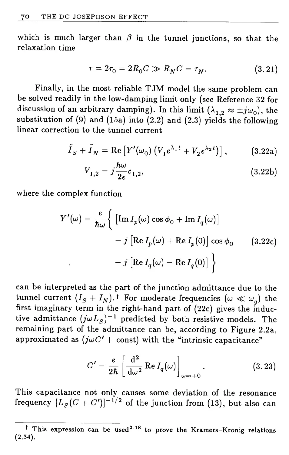
3.2	Small Deviations from ф0	67
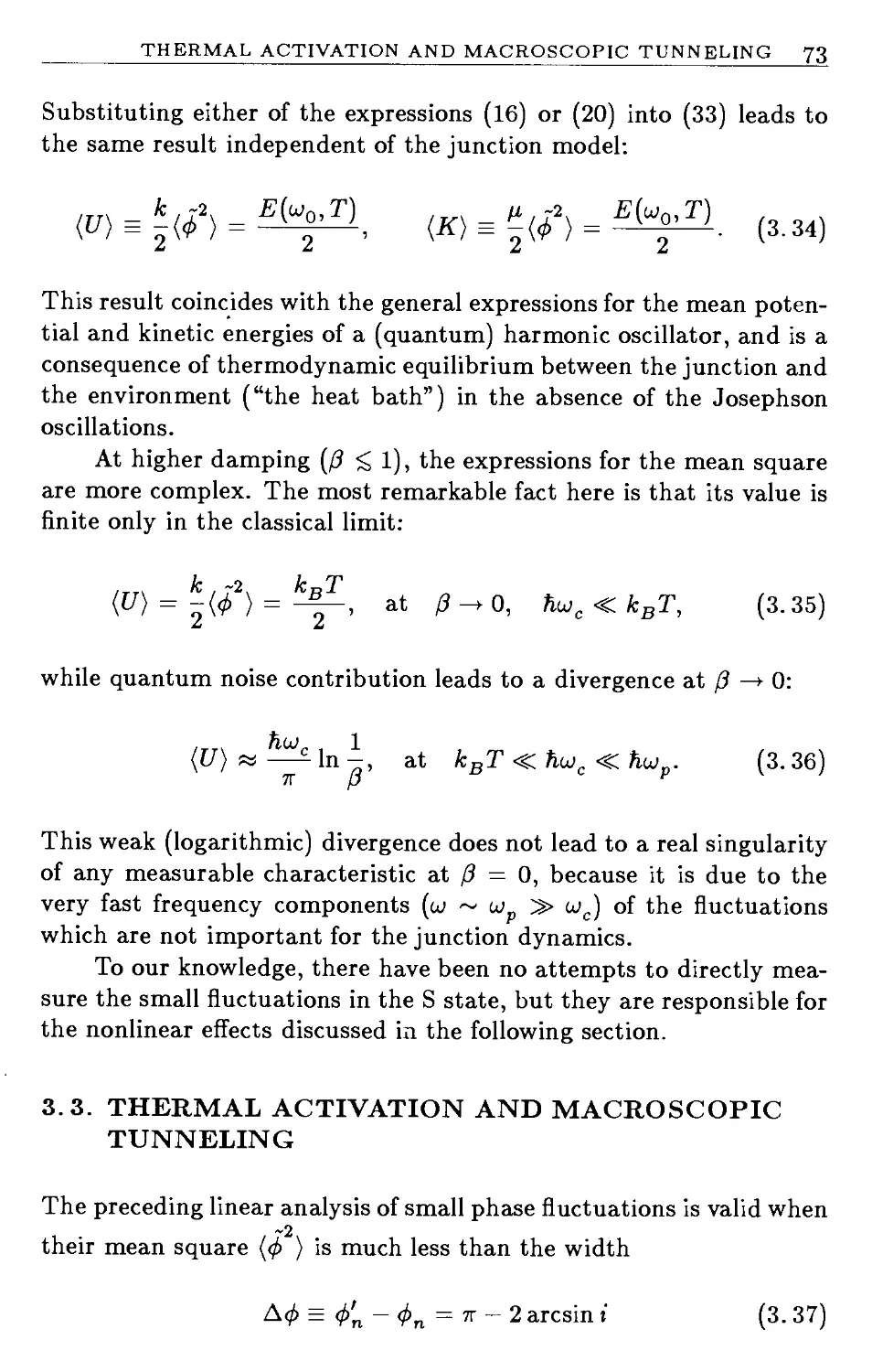
3.3	Thermal Activation and Macroscopic Tunneling	73
3.4	Critical Current Statistics	82
3.5	Some Unsolved Problems	84
Ref	erences	84
4	The AC Josephson Effect	87
4.1	The R State	87
4.2	The I-V Curve	89
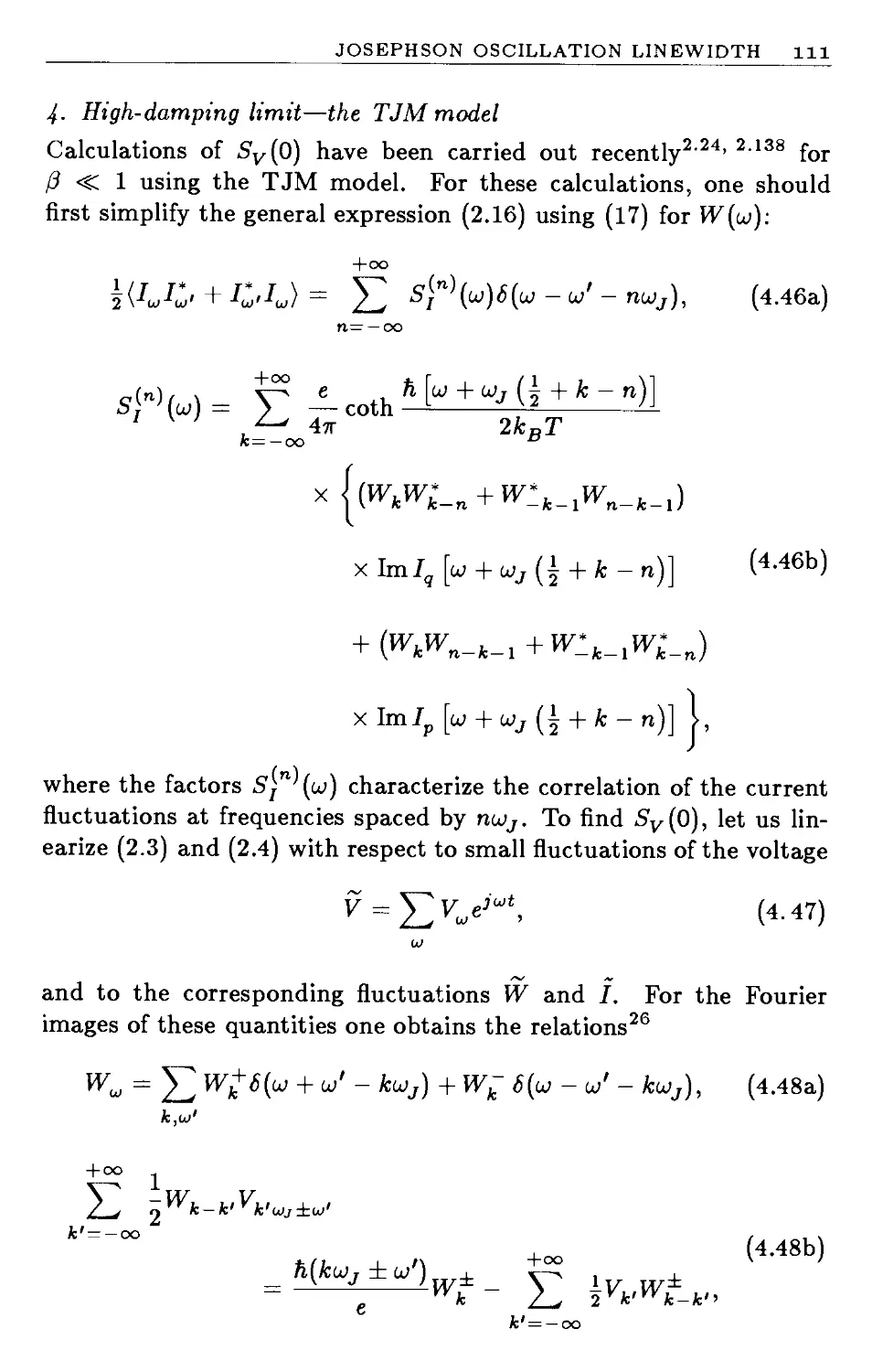
4.3	Josephson Oscillation Linewidth	105
4.4	Large Fluctuations: The I-V Curve	113
4.5	Large Fluctuations: The Voltage Spectrum	123
4.6	Some Unsolved Problems	125
References	127
vii
viii CONTENTS
5	Transient Dynamics	129
5.1	Capacitance Recharge	129
5.2	Josephson Oscillations and the	Delay	Time	132
5.3	Plasma Oscillations and the	Punchthrough	137
5.4	Effect of Fluctuations	143
5.5	Practical Applications	145
5.6	Some Unsolved Problems	148
References	149
III QUANTUM INTERFERENCE IN JOSEPHSON JUNCTION CIRCUITS	151
6	The Single-Junction Interferometer	153
6.1	The Josephson Junction in a Superconducting Loop 153
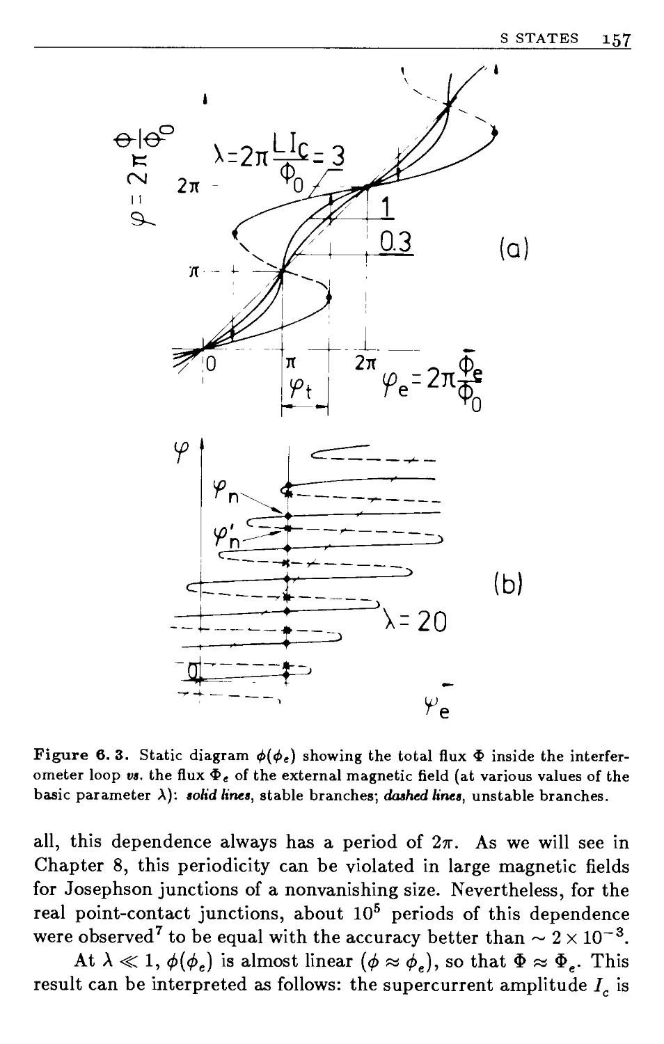
6.2	S States	156
6.3	Effects of Fluctuations	163
6.4	Dynamics of Quantum Phase Jumps	166
6.5	Practical Applications of Superconducting
Interferometers	170
6.6	The Josephson Junction in a Resistive Loop	174
6.7	Fluctuations in Resistive Interferometers	182
6.8	Practical Applications of Resistive Interferometers	184
6.9	Some Unsolved Problems	184
References	185
7	The Two-Junction Interferometer	188
7.1	Two Junctions in a Superconducting Loop	188
7.2	The S States	190
7.3	Josephson Oscillations and the I-V Curve	200
7.4	The DC SQUIDs	206
7.5	Other Applications of Two-Junction Interferometers 217
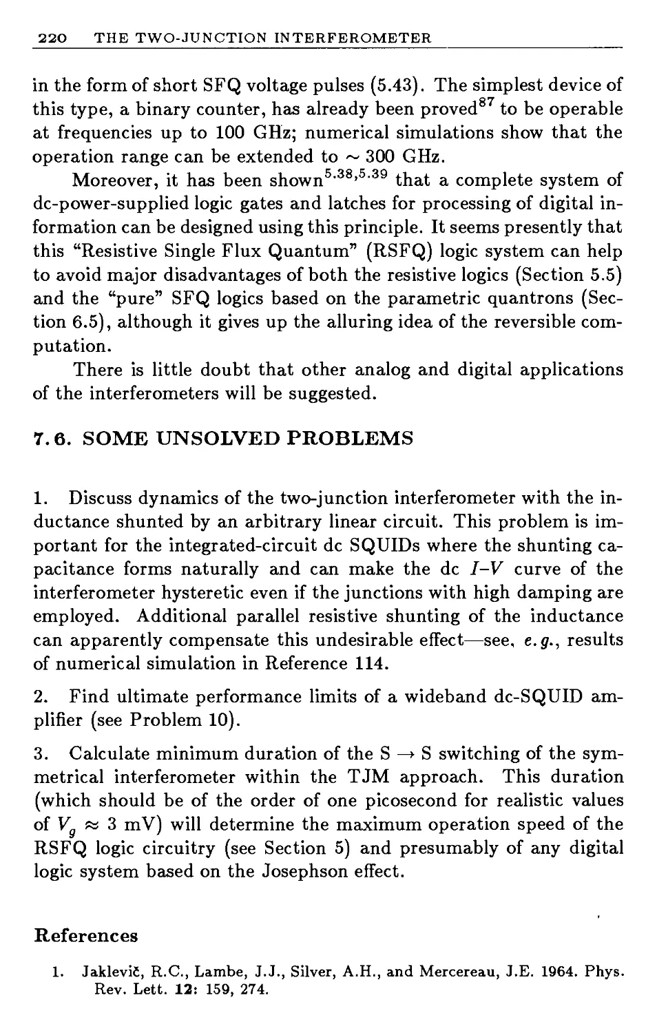
7.6	Some Unsolved Problems	220
References	220
8	Multijunction Interferometers and Distributed Structures 225
8.1	Multijunction Interferometers	225
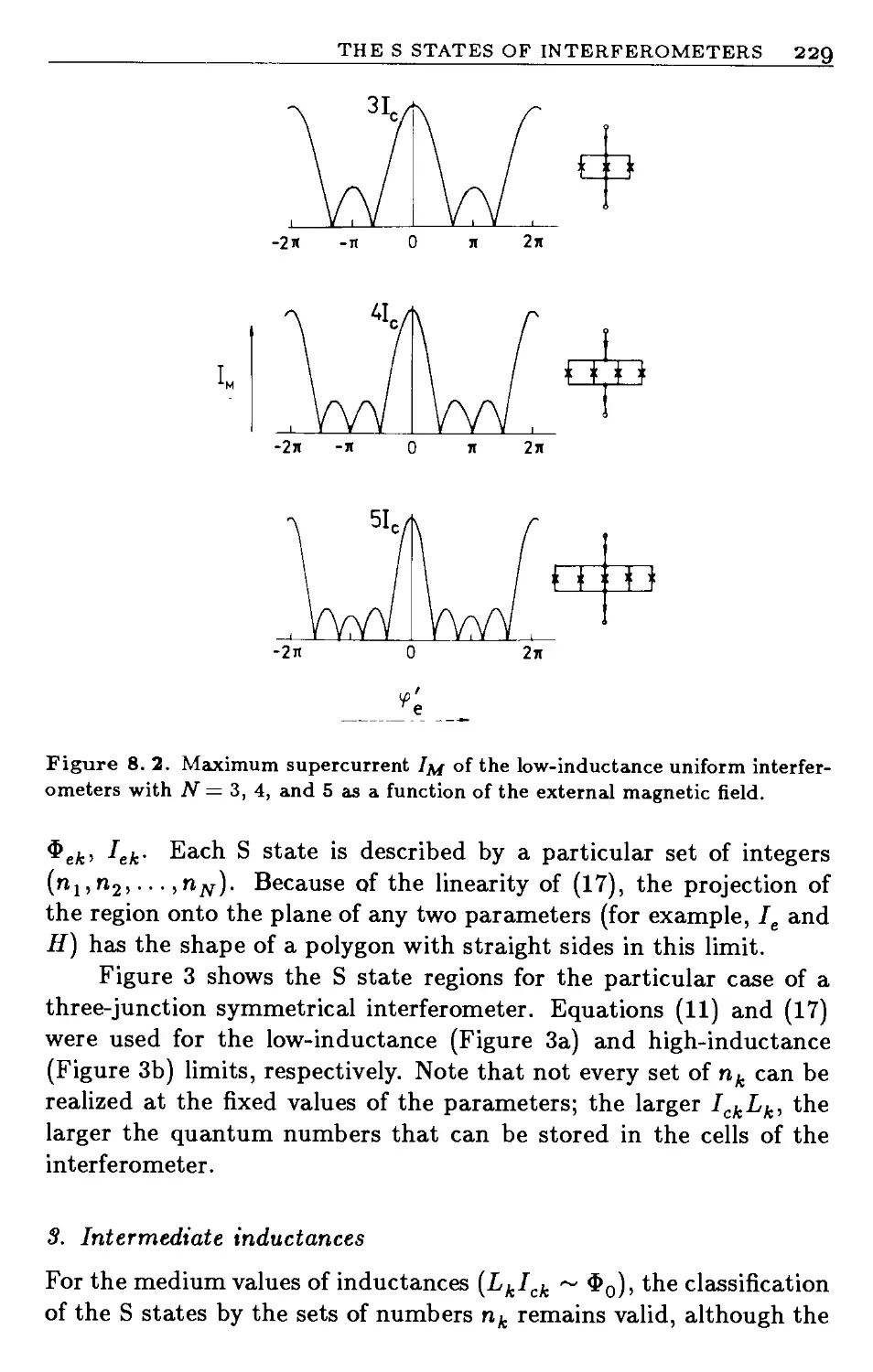
8.2	The S States of Interferometers	227
8.3	Distributed Structures	231
8.4	S States of Long Uniform Junctions	237
8.5	Lateral Current Injection	248
CONTENTS гх
8.6	S States of Nonuniform Junctions	252
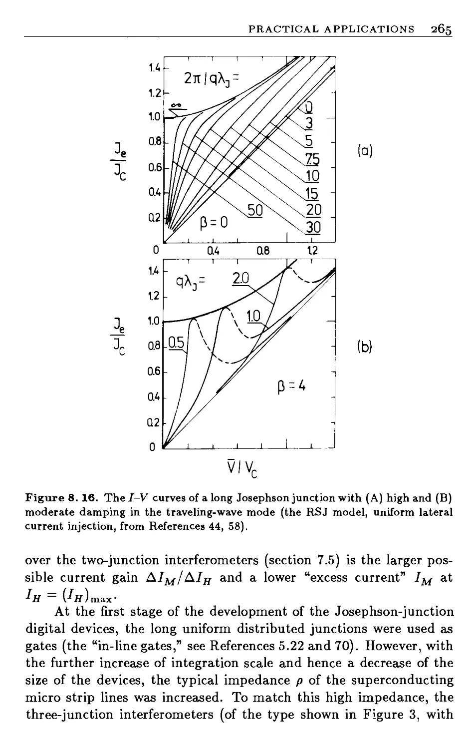
8.7	R States of Distributed Structures	260
8.8	Practical Applications	264
8.9	Some Unsolved Problems	267
References	267
9	Two-Dimensional Distributed Junctions	271
9.1	Equations and Boundary Conditions	271
9.2	Quasi-One-Dimensional Junctions	275
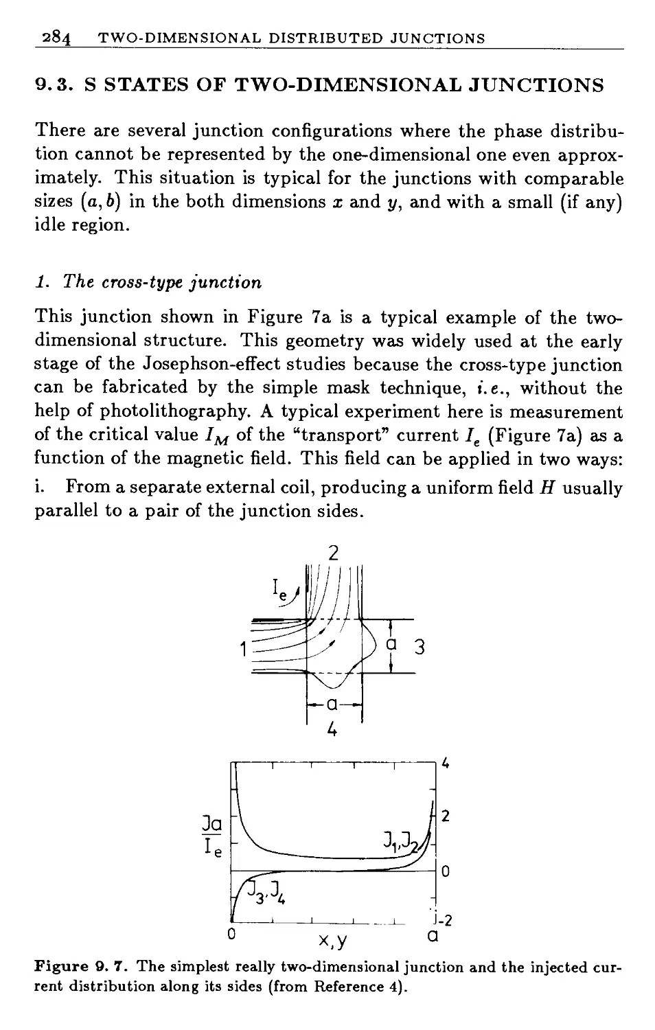
9.3	S States of Two-Dimensional Junctions	284
9.4	R States of Two-Dimensional Junctions	290
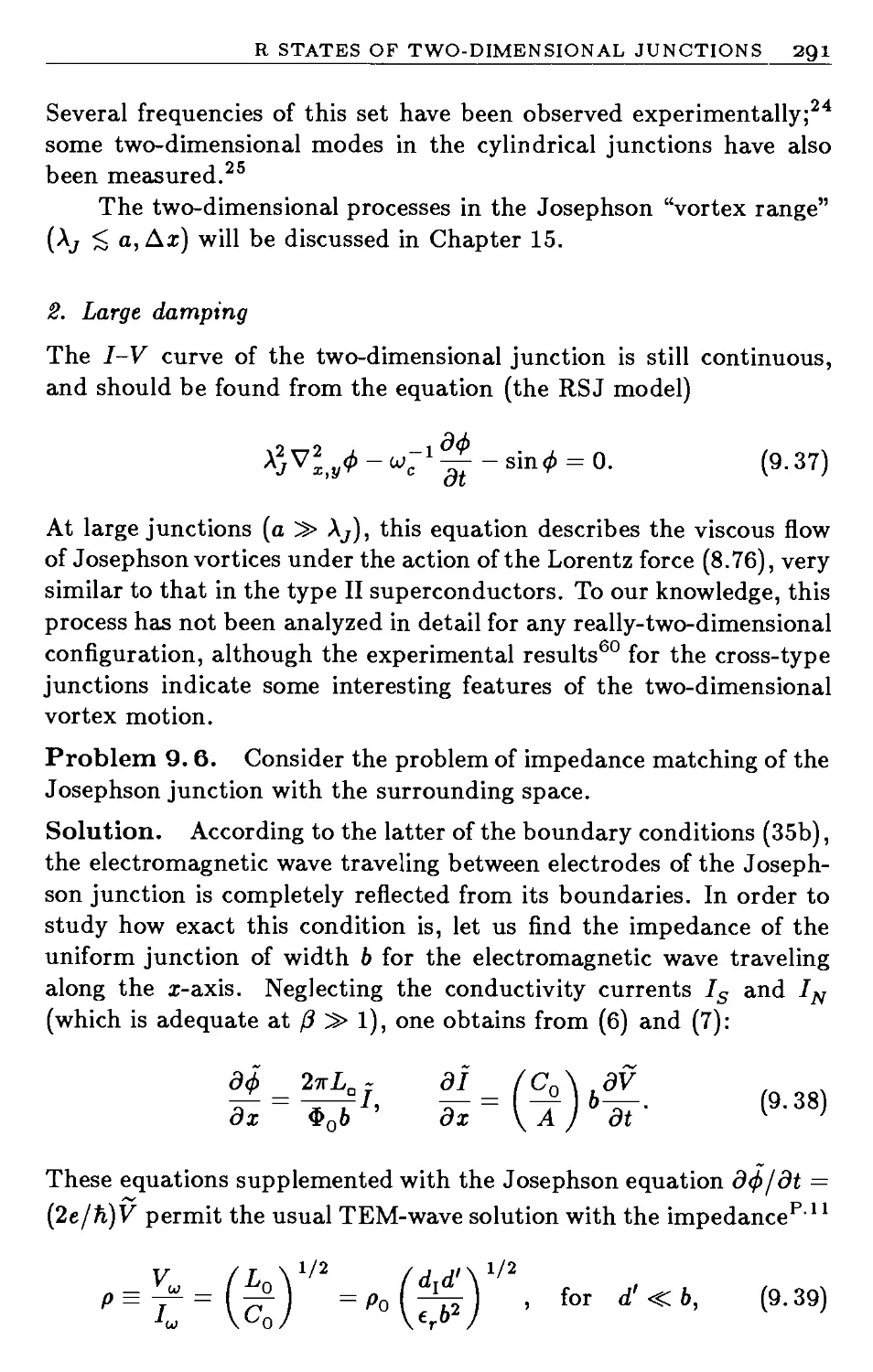
9.5	Practical Applications	292
9.6	Some Unsolved Problems	293
References	294
IV MICROWAVE PROPERTIES OF JOSEPHSON
JUNCTIONS	297
10	Small Microwave Signals	299
10.1	Linear Effects	299
10.2	The Josephson Current Step	310
10.3	Quadratic Effects	320
10.4	Practical Applications	327
10.5	Some Unsolved Problems	328
References	329
11	Large Microwave Signals	332
11.1	Sinusoidal Signal	332
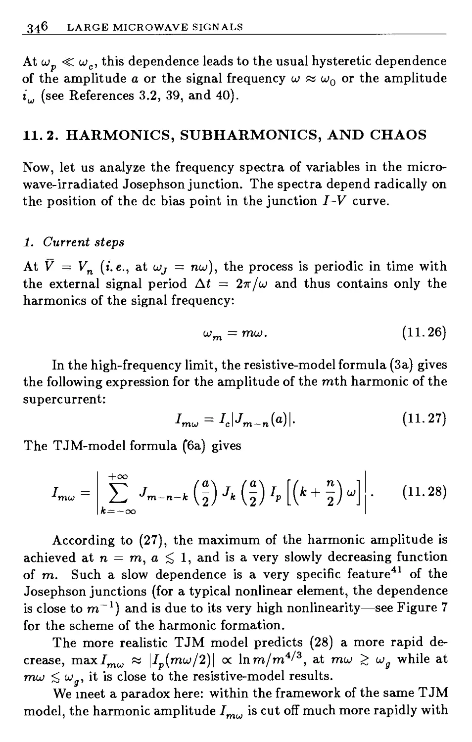
11.2	Harmonics, Subharmonics,	and Chaos	346
11.3	Parametric Effects	351
11.4	Biharmonic Signal	362
11.5	Practical Applications	365
11.6	Some Unsolved Problems	369
References	369
12	Microwave Interactions with External Systems	376
12.1	The Weak Interaction	376
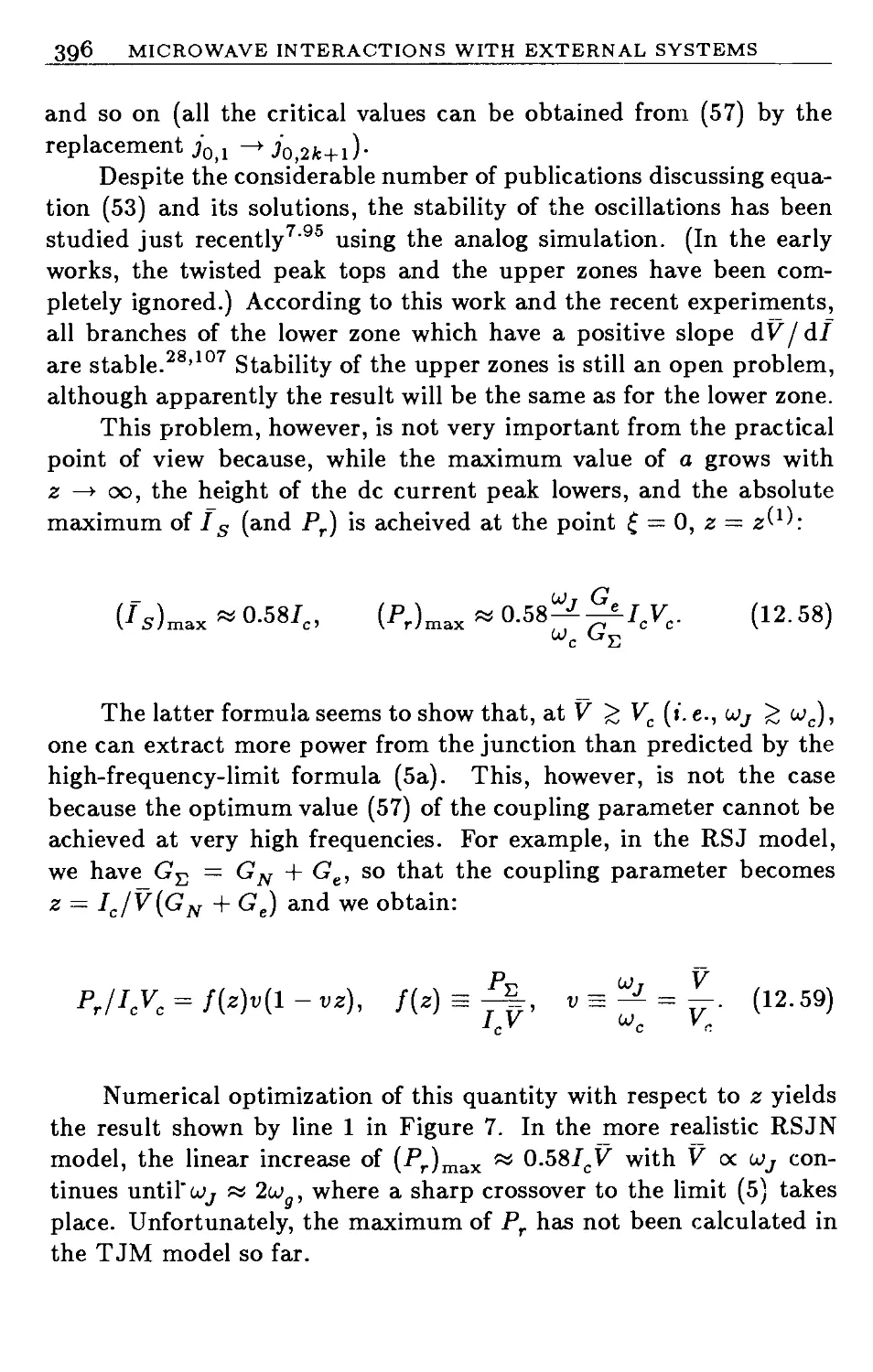
12.2	Junction and Resonator	392
12.3	Parametric Oscillations	401
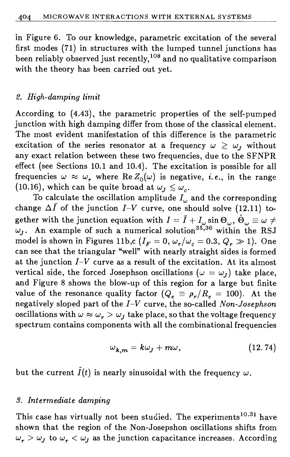
12.4	Junction and Transmission	Line	410
X
CONTENTS
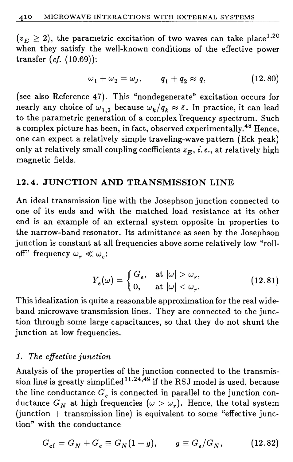
12.5	A Microwave Signal from an External	System	414
12.6	Practical Applications	416
12.7	Some Unsolved Problems	425
References	425
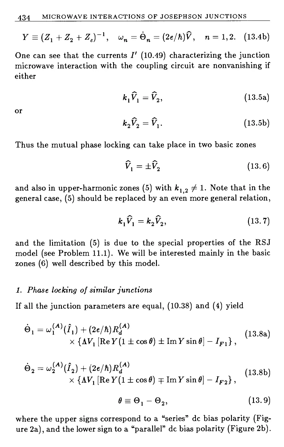
13	Microwave Interactions of Josephson	Junctions	430
13.1	Mutual Phase Locking	430
13.2	Two Junctions	432
13.3	One-Dimensional Arrays	447
13.4	More Complex Arrays	455
13.5	Practical Applications	461
13.6	Some Unsolved Problems	462
References	463
V SUPPLEMENTARY CHAPTERS OF JOSEPHSON DYNAMICS	469
14	AC SQUIDs	471
14.1	The Basic Circuit and General Relations	471
14.2	The Hysteretic Mode of Operation	475
14.3	Fluctuations in Hysteretic SQUIDs	485
14.4	The Nonhysteretic Mode of Operation	490
14.5	Fluctuations in Nonhysteretic SQUIDs	495
14.6	Microwave SQUIDs	497
14.7	Some Unsolved Problems	501
References	502
15	Josephson Vortex Dynamics	505
15.1	Josephson Vortex Motion	505
15.2	Vortex Interaction with the Environment	509
15.3	Vortex Dynamics	518
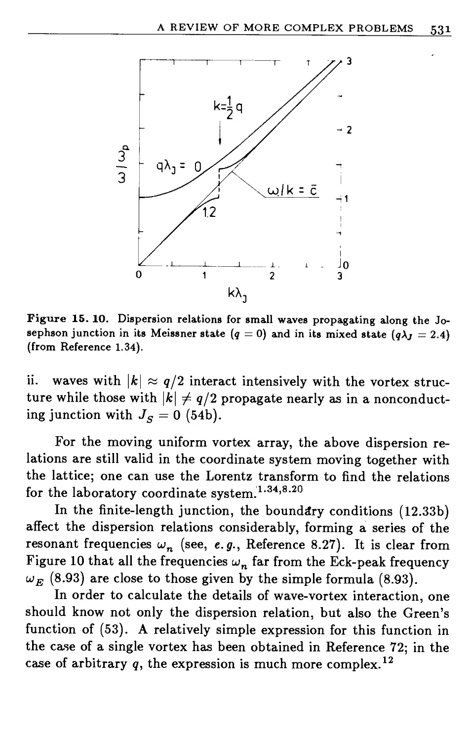
15.4	A Review of More Complex Problems	529
15.5	Practical Applications	534
15.6	Some Unsolved Problems	535
References	536
16	Bloch Oscillations, SET Oscillations, What Comes Next? 541
16.1	Bloch Oscillations in Small Josephson Junctions	541
16.2	SET Oscillations	548
16.3	Coexistence of the SET and Bloch Oscillations	555
CONTENTS xi
16.4	Possible Practical Applications	558
16.5	Experimental Situation	563
16.6	Some Unsolved Problems	563
References	564
Conclusion	566
References	567
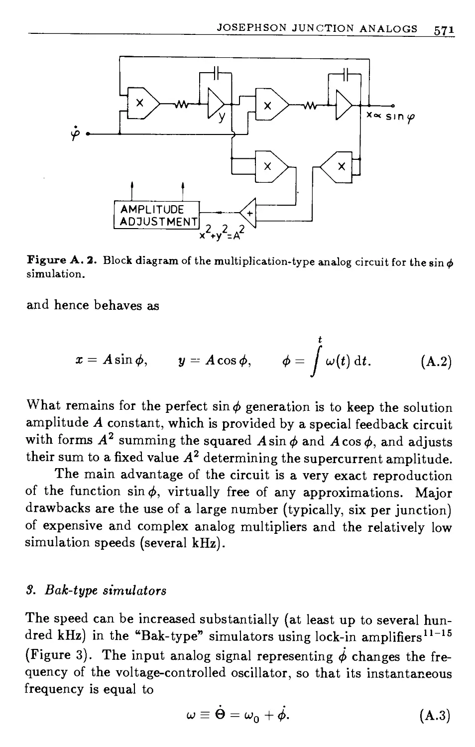
Appendix: Josephson Junction Analog Simulators	569
References	575
Author Index	576
Subject Index	598
Preface
Why with the time do I not glance aside
To new-found methods and to compounds strange?
W. Shakespeare
Sonnet 76
This book gives a detailed description of the statics, dynamics, and statistics of oscillatory and pulse phenomena in superconducting Josephson junctions and in electronic circuits and electrodynamic structures containing such junctions.
The Josephson junctions. In 1962, Brian D. Josephson—then a student at Cambridge University—predicted1 that several new phenomena should “probably” be observed in a weak electrical contact (now called a Josephson junction) between two superconductors. These phenomena would be due to the presence of a specific component— the supercurrent Is—in the net electrical current I flowing through the junction. Josephson pointed out that the supercurrent should be related to the voltage V across the junction by a very unusual formula that follows directly from the basic ideas of quantum mechanics and contains the Planck’s constant h.
As early as 1963, the existence of the Josephson supercurrent had been verified experimentally,2 and active research efforts were started in many laboratories in order to study the physical picture of this “Josephson effect,” the conditions under which it is observed, and the laws governing the effect and related phenomena. As is generally acknowledged, Josephson’s discovery (for which he was later awarded the Nobel Prize in physics3-5) has contributed greatly not only to the science of superconductivity, but also to quantum physics as a whole (see, e.g., References 6-41). In addition, Josephson junctions have enabled electronic engineers to develop several new devices that have extraordinary characteristics, which are presently being used more and more in physics, chemistry, biology and medicine, radioastronomy, metrology, and microelectronics (see, e.g., References 24-26, 31, 32, 38, and 41, and references in the Conclusion). These two aspects have turned the Josephson effect into one of the “hottest” topics of contemporary fundamental and applied physics.
xiii
xiv
PREFACE
Josephson junction dynamics. By the beginning of the 1970’s, it had become more and more evident that it is very convenient to divide the theory of Josephson junctions into two separate parts: solid-state physics and dynamics. The objective of the former part is to derive general expressions relating the functions /(t) and V(t) from the theory of superconductivity, while that of the latter part is to describe, beginning with these expressions, various phenomena observed in Josephson junctions and in practical circuits containing the junctions.
This latter part of the general theory has turned out to be more complex than the solid-state one. In fact, some quite adequate models of the I-V relationship were proposed and verified well before 1970. Moreover, a reliable microscopic theory was derived for the most important type of the Josephson junctions, the tunnel junctions (see, e.g., References 29, 31, and 32). On the contrary, the problems of dynamics have proved to be more various and complex, mainly due to two factors.
First, the Josephson supercurrent has a very unusual and highly nonlinear dependence on the electromagnetic field. As a result, a large part of the great experience accumulated in solving problems of nonlinear dynamics of other systems could not be used here, so that almost all these problems had to be solved from the very beginning, with the simultaneous development of what one can call a “Josephson-effect intuition.” Second, the extremely high sensitivity of the supercurrent to the electromagnetic field leads to its high sensitivity to fluctuations, and a considerable number of the observed properties of the junctions cannot be explained without taking the fluctuations into account.
As a consequence of these factors, the study of quite a few dynamic phenomena, including some effects which are of general importance for modern physics, is just now beginning. It is sufficient to mention only a few of them: chaotic behavior (strange attractors), secondary quantum macroscopic effects including macroscopic quantum tunneling and interference, classical and quantum dynamics and statistics of solitons, phase transitions in arrays of mutually phase-locking oscillators, and percolation effects in one-, two-, and three-dimensional disordered systems.
Publications. The body of original publications on Josephson junction dynamics is rather considerable: related problems were studied
PREFACE XV
in more than half of the approximately 5000 basic papers published on the Josephson effect and its applications (see the bibliography42). In contrast, the number of relevant reviews and monographs is rather limited. For example, the early monographs29, 30 mainly described the solid-state physics of the Josephson effect.
Josephson junction dynamics was the main subject of References 25, 27, and 31. Throughout these treatises, however, only the simplest RS J model of the Josephson junction was used, while at least two other models (RSJN and TJM, see below) are presently believed to be of at least equal importance. Moreover, since the mid-1970’s, so many new results have been obtained that the whole field of Josephson junction dynamics has an entirely new appearance now.
The contents and structure of this book. This monograph is intended to give a relatively complete review of Josephson junction dynamics as it stands in the mid-1980’s. The main idea of the author is to present the reader with as many useful results as possible by the simplest means, rather than to demonstrate theoretical muscle. This is why almost all the topics requiring elaborate techniques for their analysis are shifted to the ends of the chapters and the most complex chapters, to the end of the book. Topics which are of relatively minor importance for further discussion are mainly presented in the form of “problems” at the end of the sections.
Unfortunately, the necessity of keeping the length of (and the time required to write) the monograph within reasonable limits has not permitted any detailed discussion of the experimental data. Only a limited number of experimental results have been included, just enough to allow the reader to understand to what extent the junction models used for the dynamics analysis correspond to real junctions of various types. As a partial compensation, a representative list of references to experimental work is included in each chapter.
A similar approach is used to practical devices based on the Josephson effect. They are briefly discussed at the end of each chapter (starting with Chapter 5), with the main emphasis on the application of the results of the dynamics analysis to the calculation of the device’s characteristics.
This monograph begins with the Introduction (Chapters 1 and 2), which contains a short description of the solid-state physics of the Josephson effect, the types of Josephson junctions, and their fabrica-
XVI
PREFACE
tion technology. This material can be omitted if the reader is familiar with the subject due, for example, to any one of References 15-41. At the end of Chapter 2, the three main models (RSJ, RSJN, and TJM) of Josephson junctions are introduced and discussed.
The remainder of the book is a discussion of various phenomena in Josephson junctions and circuits within the framework of (mainly) those three models. The discussion begins in Part II (Chapters 3-5), with the simplest properties of a single junction. In Part III (Chapters 5-9), the basic properties of superconducting quantum interferometers are analyzed. At this point, the reader is already well-enough armed to understand processes in most practical Josephson junction devices, including de SQUIDs and logic circuits.
Those whose thirst for knowledge is still unslaked are invited to continue with a discussion of the microwave properties of Josephson junctions and circuits in Part IV (Chapters 10-13), which requires somewhat more mathematics. Those who pass through it and survive will understand how Josephson junctions can be used to generate and detect microwaves (SIS mixers and videodetectors are also discussed there).
Finally, the concluding part (V) deals with three “supplementary” problems: ac SQUIDs (Chapter 14), solitons in long junctions (Chapter 15) and recently predicted new oscillation effects in very small junctions (Chapter 16). One can argue that the former topic is already not very interesting from the point of view of applications, while two latter ones are not yet. It seemed impossible, however, to avoid discussing those systems whose dynamics are really fascinating and quite typical of Josephson junction structures.
A description of Josephson junction analog simulators, which have proved to be very powerful tools for solving problems of dynamics, is presented in the Appendix.
Notation, normalization, and units. Together with many others, the author has suffered greatly from the irregularly noted and overnormalized variables used in some original papers in this field. This is why his general policy here is to use the same notation throughout the book (which is by no means easy) and to try to avoid any normalization.
The most frequent exception is a very convenient normalization of currents (7) to their critical values (7C). The resulting dimen
PREFACE xvii
sionless current I/Ic is naturally denoted as i, which inevitably (and unfortunately) leads to the use of j as the imaginary unity (У^Т). The remaining mid-alphabet letters (fc,Z,m,n) are mainly reserved for integers; rare exceptions (due to tradition) will be specified separately.
Another unpleasant surprise can be a set of three different averaging signs: (•'") or (  ) for the fast-time average, (  ) for the complete time average, and (•  •) for the statistical average. It seemed impossible, however, to get rid of this distinction without ruining some basic ideas of Josephson dynamics. The author hopes that the unbiased reader will eventually find this notation quite natural.
The identity sign = is used to denote definitions. The asterisk (•)* denotes the complex conjugate; the dot (•••), differentiation with respect to time.
The SI units (which coincide with the MKSA units in our field) are used throughout the book. The values of the fundamental constants in this system are given only after their first usage.
Numbers of formulas, figures, literature references, sections, and problems are given as follows: number of chapter, point, and number of the item within the chapter. The letters “P” and “A” are used instead of the chapter numbers for items appearing in the Preface and Appendix, respectively. Note, however, that the chapter number is omitted for references within a chapter.
Acknowledgments. Unfortunately, it would be impossible to list everybody from whom the author has benefited while working in this exciting field of physics; at the least, all his colleagues of the Laboratory for Cryoelectronics at Department of Physics, Moscow State University should be mentioned.
Concerning the book itself, it would have never been written without the generous help and encouragement of Professor James E. Lukens of the State University of New York, Stony Brook. Moral support from Academician V. L. Ginzburg, Professor V. V. Migulin, and Professor V. B. Braginskiy during the writing of the book was invaluable.
Separate parts of the manuscript have been looked through by Mr. D. V. Averin, Dr. L. S. Kuzmin, Prof. M. R. Samuelsen, Prof. V. V. Schmidt, Dr. V. K. Semenov, Dr. О. V. Snigirev, Dr. S. A. Vasenko, and Dr. A. B. Zorin, who have offered some useful suggestions. A few
xviii PREFACE
pieces have come to this book from Reference 31 and, in this context, the author acknowledges some useful discussions with Dr. В. T. Ulrich in 1975-76. The considerable help of Dr. V. G. Elenskii and Mrs. S. T. Koretskaya in the preparation of the bibliography is gratefully acknowledged.
Mrs. G. F. Bondarenko and Mrs. S. T. Kocharova are responsible for the prompt and high quality typing and Mrs. L. N. Likhareva for the final figure drawings. It is impossible to express all the author’s gratitude to the last-named person for all her love and patience.
К. K. Likharev
References
Josephson Effect Prediction and Verification
1.	Josephson, B.D. 1962. Phys. Lett. 1: 251.
2.	Anderson, P.W., and Rowell, J.M. 1963. Phys. Rev. Lett. 10: 230.
History of the Josephson Discovery
3.	Anderson, P.W. 1970. Phys. Today 23: 23.
4.	Josephson, B.D. 1974. Science 184: 527.
5.	Pippard, A.B. 1977. In: Superconductor Applications: SQUIDs and Machines, S. Foner and B.B. Schwartz, Eds.: 1. New York: Plenum.
Early Reviews
6.	Anderson, P.W. 1964. In: Lectures on the Many-Body Problem, E. Caianiello, Ed.: 113. New York: Academic Press.
7.	Josephson, B.D. 1964. Rev. Mod. Phys. 36: 216.
8.	Fiske, M.D., and Giaever, I. 1964. Proc. IEEE 52: 1155.
9.	Josephson, B.D. 1965. Adv. Phys. 14: 419.
10.	Langenberg, D.N., Scalapino, D.J., and Taylor, B.N. 1966. Sci. Am. 214: 30.
11.	Langenberg, D.N., Scalapino, D.J., and Taylor, B.N. 1966. Proc. IEEE 54: 560.
12.	Zharkov, G.F. 1966. Usp. Fiz. Nauk. (Sov. Phys.-Usp.) 88: 419.
13.	Mercereau, J.E. 1967. In: Tunneling Phenomena in Solids, E. Burstein and S. Lundquist, Eds.: 461. New York: Plenum.
14.	Scalapino, D.J. ibid.: 477.
More Recent Reviews
15.	Taylor, B.N. 1968. J. Appl. Phys. 39: 2490.
16.	McCumber, D.E. 1968. J. Appl. Phys. 39: 2503.
17.	Mercereau, J.E. 1969. In: Superconductivity, R.D. Parks, Ed.: 393. New York: Marcel Dekker.
18.	Josephson, B.D. ibid.: 423.
19.	Kamper, R.A. 1969. IEEE Trans. Electron. Devices 16: 840.
REFERENCES XZX
20.	Petley, B.W. 1969. Contemp. Phys. 10: 139.
21.	Kamper, R.A. 1969. Cryogenics 9: 20.
22.	Matisoo, J. 1969. IEEE Trans. Magn. 5: 848.
23.	Deaver, B.S., Jr. 1973. In: The Science and Technology of Superconductivity, W.D. Gregory, Ed.: 539. New York: Plenum.
24.	Deaver, B.S., Jr., and Vincent, D.A. 1974. In: Methods of Experimental Physics, R.V. Coleman, Ed. 11: 199. New York: Academic Press.
25.	Vystavkin, A.N., Gubankov, V.N., Kuzmin, L.S., Likharev, K.K., Migulin, V.V., and Semenov, V.K. 1974. Rev. Phys. Appl. 9: 79.
26.	Waldram, J.R. 1976. Rep. Prog. Phys. 39: 751.
27.	Fulton, T.A. 1977. In: Superconductor Applications: SQUIDs and Machines, S. Foner and B.B. Schwartz, Eds.: 125. New York: Plenum.
28.	Likharev, K.K. 1979. Rev. Mod. Phys. 51: 101.
Monographs
29.	Kulik, I.O., and Yanson, I.K. 1970. Josephson Effect in Superconducting Tunnel Structures (in Russian). Moscow: Nauka. 1972. (in English) Jerusalem: Keter Press.
30.	Solymar, L. 1972. Superconductive Tunneling and Applications. London: Chapman and Hall.
31.	Likharev, K.K., and Ulrich, B.T. 1978. Systems with Josephson Junctions (in Russian). Moscow: Moscow Univ. Publ.
32.	Barone, A., and Paterno, G. 1982. Physics and Applications of the Josephson Effect. New York: Wiley.
Other Books with Chapters on Josephson Effect
33.	Feynman, R.P., Leighton, R.B., and Sands, M. 1965. The Feynman Lectures in Physics, 3: Chap. 19. Reading, Mass.: Addison-Wesley.
34.	De Gennes, P.G. 1966. Superconductivity of Metals and Alloys: Chap. 7. New York: Benjamin.
35.	Lynton, E. 1969. Superconductivity, 3rd edition: Chap. 11. London: Chapman and Hall.
36.	Buckel, W. 1972. Supraleiting Grundlagen und Anwendungen (in German): Chap. 3. Weinheim: Physik Verlag.
37.	Rose-Innes, A.C., and Rhoderick, E.H. 1978. Introduction to Superconductivity, 2nd edition: Chap. 11. New York: Pergamon Press.
38.	Lounasmaa, O.V. 1974. Experimental Pronciples and Methods Below 1 K.: Chap. 7. New York: Academic Press.
39.	Tilley, D.R., and Tilley, J. 1974. Superfluidity and Superconductivity: Chap. 5. New York: Van Nostrand Rheinhold.
40.	Tinkham, M. 1975. Introduction to Superconductivity: Chap. 6. New York: Mc Graw-Hill.
41.	Van Duzer, T., and Turner, G.W. 1981. Principles of Superconductive Devices and Circuits: Chaps. 4, 5. New York: Elsevier.
Bibliography
42.	Golovashkin, A.I., Elenskii, V.G., and Likharev, K.K. 1983. Josephson Effect and Applications (Bibliography: 1962-1980). Moscow: Nauka.
XX PREFACE
Lecture Demonstrations and Student Laboratory
43.	Richards, P.L., Shapiro, S., and Grimes, C.C. 1968. Am. J. Phys. 36: 690.
44.	Collings, P.J., and Gordon, J.E. 1964. Am. J. Phys. 37: 293.
45.	Manikopoulos, C.N., and Hannah, E.C. 1973. Am. J. Phys. 41: 888.
46.	Kerr, D., and Zych, D.A. 1975. Am J. Phys. 43: 921.
47.	Stroink, G.W.R., Purcell, C., and Blackford, B. 1978. Am. J. Phys. 46: 424.
48.	Allen, R.P., and Whitehouse, J.E. 1982. Eur. J. Phys. 3:: 136.
49.	Walker, I.R. 1985. Am. J. Phys. 53: 445.
Part I
Introduction
... in the beginning when the world was young there were a great many thoughts but no such thing as a truth
S. Anderson
The Book of Grotesque
The main purpose of the introduction is to present a brief review of the solid-state physics of the Josephson effect and of Josephson junction fabrication technology; it also introduces the three basic models of the Josephson junctions used throughout the remainder of the book.
i
CHAPTER 1
The Josephson Effect
1.1. COHERENT PHENOMENA IN SUPERCONDUCTIVITY
Superconductivity was discovered as early as 1911,1 but it was a long time before the modern concept of the superconducting state of matter was established. The main milestones along the way were the discovery of the Meissner effect,2 the formulation of phenomenological theories by Londons3’4 and by Ginzburg and Landau,5 and, eventually, the creation of the microscopic theory by Bardeen, Cooper, and Schrieffer6 (BCS), with later important contributions by Bogolyubov and Gor’kov7. Nevertheless, the theoretical prediction4-8’13'1 and experimental observation9’10’13'2 of the coherent (or “macroscopic quantum”) phenomena in superconductors have proved to be necessary for the final formulation of the concept. According to this concept, a macroscopic coherence of the current carriers in superconductors— the Cooper pairs of electrons—is the basis of all unusual properties of superconductors observed. We will discuss this point in somewhat more detail (see also References P.29-P.41).
In all substances, current carriers move according to the laws of quantum mechanics. In the usual approximation of weakly interacting particles with negligible spin effects, this motion can be described in terms of the ordinary Schrodinger equation
.7АФ = ЯФ,	(1.1)
where Ф is the complex wavefunction of a particle,
Ф = |Ф(г,<)| exp{j’x(r,t)};	(1.2)
h is Planck’s constant,
h « 1.054 x 10-34 Joule-second;	(1. 3)
3
4 THE JOSEPHSON EFFECT
and H is a Hamiltonian. According to quantum mechanics, |Ф|2 is proportional to the density of the particles. In the stationary state, |Ф| can be assumed to be constant and H can be replaced by the particle energy, E. As a result, (1) takes the simpler form
Ь-Х = -E;	(1.4)
thus, the quantum-specific character is reduced in practice to that of the wavefunction phase x-
In nonsuperconducting (“normal”) substances, (4) does not result in quantum relations for the macroscopic variables because there the current carriers (single electrons or holes) obey Fermi-Dirac statistics and their energies can never be exactly equal. As a consequence, the rates x differ for all particles, and their phases x are uniformly distributed along the trigonometric circle. All macroscopic quantities are sums over all the particles; hence, in normal conductors, the phases x drop out of these quantities.
In contrast with a single electron, the Cooper pair in a superconductor is a bound state of two electrons with opposite momenta and spins. Its net spin equals zero; thus, the pairs obey the Bose-Einstein statistics and are condensed at the lowest (basic) energy level at low temperatures. As a result, their rates x are identically equal. Also, Cooper pairs are of relatively large size, £0 ~ 10-4 cm, which is much larger than the mean spacing between the pairs (which is of the order of atomic distances, ~ 10-7 cm). In other words, the wavefunctions of the Cooper pairs are overlap to a great degree.
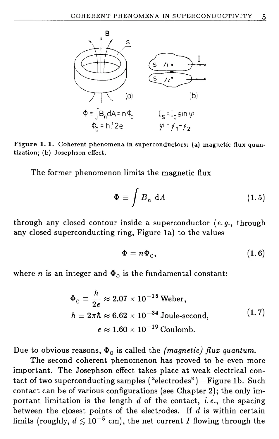
As a result of these two factors, all the pairs at a given point in a superconductor turn out to be “phase-locked” and can be described by a single wavefunction Ф (which is frequently called the order parameter). In other words, a coherent superconducting “condensate” rather than single Cooper pairs is responsible for current in superconductors. It is evident now that x does not drop out during the summation over the particles; thus, the macroscopic variables (current in particular) can depend on %, which changes in a “quantum way” (4) under the action of an electromagnetic field that contributes to E. This quantum dependence leads not only to the superconductor’s zero resistivity and to the Meissner effect, but also to several very specific coherent effects like magnetic flux quantization8 10 and the Josephson effect.p l>p-2
COHERENT PHENOMENA IN SUPERCONDUCTIVITY 5
jBndA=n<t>0 %= hl2e
Is^csin^ ^=/r/2
Figure 1. 1. Coherent phenomena in superconductors: (a) magnetic flux quantization; (b) Josephson effect.
The former phenomenon limits the magnetic flux
Ф = BndA
(1-5)
through any closed contour inside a superconductor (e.g., through any closed superconducting ring, Figure la) to the values
Ф = пФ0,
(1-6)
where n is an integer and Фо is the fundamental constant:
Фп ее — и 2.07 x 10-15 Weber, 0 2e
h = 2nh w 6.62 x 10-34 Joule-second,
e w 1.60 x 10-19 Coulomb.
(1-7)
Due to obvious reasons, Фо is called the (magnetic) flux quantum.
The second coherent phenomenon has proved to be even more important. The Josephson effect takes place at weak electrical contact of two superconducting samples (“electrodes”)—Figure lb. Such contact can be of various configurations (see Chapter 2); the only important limitation is the length d of the contact, i. e., the spacing between the closest points of the electrodes. If d is within certain limits (roughly, d < 10“5 cm), the net current I flowing through the
6 THE JOSEPHSON EFFECT
contact—the Josephson junction—contains a specific component, a supercurrent Is. The supercurrent is a function not of the voltage V across the junction (Figure lb), but of the phase difference (or just “Josephson phase”)
Ф = Xi - X2
of the condensate wavefunctions inside the electrodes. This function is exactly 2?r-periodic and, in the simplest cases, is sinusodial
4 = /csin</>,
where Ic is some constant determined by the shape and structure of the Josephson junction and is usually called its critical current. In turn, ф is related to voltage V by the fundamental law
ф — — V, i.e., ф = ~~V,	(1-10)
fi.	Фо
the so-called Josephson phase-voltage relation.
Let us show that the Josephson effect is a direct consequence of the coherence of the quantum superconducting condensate (this is also true for the flux quantization, but it seems more convenient to discuss this effect later in Chapter 6). Consider points 1 and 2 inside two superconductors. Writing down (4) for each of the points and subtracting, one gets
h</> = E2 — Ev	(1.11)
The right-hand part of this equation contains the energy difference of Cooper pairs placed in points 1 and 2. This difference can exist only if a difference of electrochemical potentials (i.e., a voltage V) exists between these points:
E2-E1=2eV.	(1.12)
Uniting (11) and (12), we arrive at (10). Both simple arguments like ours and a more rigorous theory11-13 show that this equation should be fulfilled to a very high precision. In fact, its verification using the Josephson effect has shown that the </>-to-V ratio varies not more than ~ 10“16 in various superconductors14-16’45 and not more than ~ 10-6 for 100-fold different values of V.17
BASIC PROPERTIES OF THE JOSEPHSON SUPERCURRENT 7
In order to get (9), let us speculate now on what can determine the Cooper-pair current through a small [lumped) Josephson junction. It should certainly be dependent on |Ф|2, i. e., of the Cooper-pair density in electrodes. If the current is small enough, however, it will not change |Ф| considerably, but it can change phases Xi 2 without influencing the physical state of the electrodes. Each phase x is defined within a constant, and a well-defined variable like current can be related to their phase difference ф (8) alone, so that Is = 13[ф). Next, a 2?r-change of any phase results in exactly the same Ф, i. e., the same physical state of the electrodes; hence, 13[ф) should be 27r-periodic:
is№ = is(<i> + ^).	(i.i3)
Lastly, in the absence of current, both electrodes form a single unperturbed superconductor and the phases Xi 2 should be equal:
^s(O) =	— 0.	(1.14)
One can readily showp’28 that /5(тг + 2тгп) should vanish as well. The above arguments show that Is can be written in the form
00
4 = Ц sin Ф + Tm sin тФ	(!-15)
m=2
in the general case. Rigorous theory (see, e.g., Reference P.28) shows that, in most cases, all terms in (15) except the first one can be neglected, and one therefore obtains the equation (9), which was derived by Josephson in his basic рарегрл for a particular case of the tunnel-type junctions.
1.2. BASIC PROPERTIES OF THE JOSEPHSON
SUPERCURRENT
Relations (9) and (10) for the Josephson supercurrent are very unusual from the view of classical electrodynamics, and they deserve a preliminary analysis to clarify the basic properties of the supercurrent.
8 THE JOSEPHSON EFFECT
1.	The S state
According to (9), a de current results in (or, if you prefer, is a result of) a constant Josephson phase:
ф = фп = arcsin(/s//c) + 2тгп,	(1-16)
where
-IC<IS<IC.	(1-17)
Using this in (10) yields V = 0. Therefore, if the current is not large there will be no voltage drop across the junction. We will call this situation the S state; this term can be decoded as either the “superconducting” or “stationary” state (one can meet both terms in the literature).
2.	Energy storage
Due to the zero voltage drop, no energy is dissipated inside the Josephson junction in the S state. Some energy is, however, stored in the junction. To find it, consider a process in which the phase changes from a value фг to a value ф2. During this process, an external system responsible for the phase change does the following work on the supercurrent:
tz
Ws = jlsVdt.	(1.18)
ti
After substitution of (9) and (10), one finds that Ws depends not on the intermediate stages of the process, but only on the initial (ф^) and final (</>2) values of the phase:
02
Ws = ——	я'тфЛф = —£(cos	— cos</>2).	(1.19)
2e J	2e
This suggests that the “potential” energy of the supercurrent
(</>)= £c(l - cos </>) + const, Ec = KIc/2e (1-20)
can be introduced13'6 so that WS = US(^2)-US(^).
BASIC PROPERTIES OF THE JOSEPHSON SUPERCURRENT Q
3.	Nonlinear inductance
Energy storage and conservation in the Josephson junction suggests that it can be considered as having a nonlinear reactance, i.e., it is an energy-storing two-terminal device. To clarify the character of such a reactance, consider an arbitrary process </>(t) and its small variation Ф(*),
ф^ф + ф.	(1.21)
Inserting this formula into (9) and (10) and expanding sin(</> + </>) into a Taylor series in ф, one obtains the following relation between the variations of voltage and supercurrent:
fs = Ls1(t) У V dt, Lg1 = L~x cos</>, Lc =/t/2e/c.	(1-22)
These expressions show that for a weak signal the supercurrent is equivalent to an inductance LSF'4 * * 7’18-20 dependent on the basic process in the junction. The most unusual property of this inductance is its ability to take negative values at the intervals тг/2 + 2тгп < ф < Зтг/2 + 2тгп.
4- Josephson oscillations
The latter feature results in some drastic differences in behavior between the Josephson junction and an ordinary nonlinear inductance. The best way to demonstrate the difference is to consider the case when a nonzero de voltage V is fixed across the junction. From (10) one finds that the phase ф grows linearly in time:
ф = Wjt + const,	(1.23)
and (9) shows that the supercurrent oscillates with a frequency
Wj = (2e/h)V = (2тг/</>0)У,	(1.24a)
which is proportional to V (in an ordinary inductance, current would just increase gradually). This phenomenon, the famous Josephson oscillations, was predicted in the original paper.P1 It accompanies most
IO
THE JOSEPHSON EFFECT
processes in Josephson junctions and should be taken into account in all dynamics considerations.
Note that the frequency-to-voltage ratio, according to (24a), is extremely high:
U- =	= — = Ф”1 « 483 MHz/дУ.
V 2тгУ h 0	1
(1.24b)
The oscillation frequency fj is of the order of 109 to 1013 Hz at typical voltages (10-6 to 10-2V).
5. Mechanical analogs
The unusual properties of the supercurrent have forced many to look for simple mechanical analogs that develop a better understanding of the Josephson dynamics. The first analog of this kind is a plane me-cha’nical pendulum in a uniform gravity field. In this analogy, ф plays the role of the angle of the pendulum’s deviation from equilibrium; the supercurrent is comparable to the torque, and the voltage V is proportional to the angular velocity of the pendulum. The second useful analog is a mechanical particle moving along the coordinate ф with velocity v ос. ф ос V in a periodic field with the potential (20). Both analogies can be extended to some other components of the junction current (see Chapter 2).
Problem 1.1. Investigate the validity of the Manley-Rowe relations for the supercurrent Is.
Solution.21’22 The Manley-Rowe relations23 place some constraints on the power flow between frequency components of a signal acting upon a nonlinear reactance. In particular, the nonvanishing power flow from de component to ac components is forbidden by the relations. The Josephson oscillation is a power flow of just this type, and hence the Manley-Rowe relations cannot be valid for the supercurre'nt in their classical form.
Analysis21 has shown that the ability of inductance (22) to take negative values leads to the following generalized Manley-Rowe relations:
к<Р{к}/ш{к} = 0,	(1.25a)
{k},ki>0
OTHER CURRENT COMPONENTS 11
52 kjP{k}/u{k} =
{ к }, kj > 0
(1.25b)
Here {k} is a set of integers {kj, kx,... kN} which participates in the expansion
N
w{fc} 5 kjWj + 52 ki“i	(!•26)
1 = 1
of an arbitrary combinational frequency component; are independent and incommensurate “basic” frequencies (in typical situations, their number N does not exceed two); and P{k} is a power flow from the external system to the junction at the frequency w{k}. Power flow at the Josephson oscillation frequency, P{l,0,.. .0}, is denoted by Pj. In their classical form, the Manley-Rowe relations do not contain the last term of (25b); in the modified relations (25), this term permits Josephson oscillations. If the external system allows a power flow only at zero frequency ({fc} = {0,0, ...0}) and the Josephson frequency ({fc} = {1,0, ...0}), then (25b) yields the result
PAc + Pj^O.
(1-27)
This new form simply expresses energy conservation and does not require Pj to vanish.
Unfortunately, (25) is valid only for the supercurrent. For the total current I flowing through the junction these relations can be violated (see Chapter 10).
1. 3. OTHER CURRENT COMPONENTS
Only in a few situations can the net current through the Josephson junction be approximated by the supercurrent Is; in most cases, other current components should also be taken into account. In this section, we will have a look at the general properties of these components, leaving a more quantitative analysis for the following chapter.
12
THE JOSEPHSON EFFECT
1.	The normal (quasiparticle) current IN
If the temperature T is nonvanishing, there is always some thermal motion of the charge carriers with energy of the order of kBT, where
kB » 1.38 x 10~23 Joule/Kelvin	(1.28)
is the Boltzmann constant. In a superconductor, this motion breaks some of the Cooper pairs and thus creates a nonvanishing density of single “normal” electrons (the presence of the superconducting condensate makes the properties of these electrons somewhat different from those of normal-metal electrons; thus, they are usually called quasiparticles).
In the S state, where the voltage across the Josephson junction equals zero, the quasiparticles do not contribute to its current. If, however, the Josephson phase ф changes in time and the voltage is nonvanishing (10), then a quasiparticle current component—the normal current IN—appears. This is why the situation is called the resistive state or R state of the junction.
The current IN has two general properties. First, when T is less than but close to the critical temperature Tc of a superconductor, the binding energy 2Д (energy gap) of the Cooper pair becomes much smaller than the thermal energy kBT. As a result, the concentration of Cooper pairs is small, and the concentration of normal electrons (and their properties as well) is close to its value in the normal state (at T > Tc). In this case, the IN-V dependence is close to the usual Ohm’s law:
(1.29)
where GN = R))1 is the normal conductance of the Josephson junction.
Second, if the voltage across the junction is well above the so-called gap value
Vg^[^(T)+A2(T)]/e,	(1.30)
then the following process is energy-advantageous: a Cooper pair in one of the electrodes breaks and one of the two newly-formed quasiparticles passes to another electrode. Such a process is so dominant that, at |V| > V , the IN-V dependence is close to the Ohmic dependence (29) at all temperatures.
OTHER CURRENT COMPONENTS 13
Thus, despite the possibly high nonlinearity of the IN-V dependence, its scale is given by the normal conductance GN. Combining this value with the natural current scale, Ic, one obtains the voltage scale
Vc^/cJ2n = /c/Gn,	(1.31)
which is usually called either the characteristic voltage or the UICRN product” of the junction. According to the microscopic theory of the Josephson effect, the maximum value of Vc is of the order of 3kBTc/e and is close to 3 mV for the typical superconductors used for Josephson-junction fabrication (Pb, Nb, and their alloys).
This voltage scale defines the corresponding frequency scale
wc = (2e/h)Vc = (2тг/Ф0)Ус, /с =	(1.32a)
the characteristic frequency of the junction, via the fundamental volt-age-to-frequency relation (24). Using (22), the last formula can be conveniently rewritten as follows:
wcLc = Rn,	(1.32b)
which shows that wc is just the inverse relaxation time in a system consisting of a normal current and a supercurrent.
According to the above estimate of Vc, the maximum value of fc is somewhat above 1012 Hz for typical superconductors. This is the value which defines the upper boundary of practical microwave devices based on the Josephson effect; beyond this frequency the device performance degrades. In the time-domain formulation, the fastest pulse-rise times in the Josephson junctions are of the order of w”1 and can be as short as a few tenths of a picosecond.
2.	The displacement current
In situations where not only V but also V is nonvanishing, the displacement current ID can be of great importance. Although ID does not flow directly through the Josephson junction, it effectively sums with the other current components. For most practical Josephson junctions, the current can be represented in the usual form,
ID = cv,
(1.33)
14 THE JOSEPHSON EFFECT
where the junction’s capacitance C is just the same as that in its normal state. The capacitance depends on both the junction type and its size. In practice, the relative magnitude of the displacement current ID is of importance rather than the absolute value of C. Let us compare the amplitudes of the current components Is, IN and ID for some process of a frequency w. Equations (9), (10), (29), and (33) yield the estimates
Is < V/uLc, In < VGn, Id и wCV. (1.34)
Defining the junction plasma frequency as
Wp = (LcC)-1/2 Н2Ц,/М1/2,	(1-35)
one finds that the displacement current is smaller than the supercurrent if
w < wp.	(1. 36)
ID is less than the normal current if
и<тй\	(1.37)
where rN is the junction RC constant-.
tn = RNC = wc/w2.	(1.38)
Equations (36) and (37) show that, in order to characterize the capacitance effect at all frequencies up to wc, one should evaluate the dimensionless capacitance parameter
0 = (UJUp)2 = uprN = wcRNC = (2e/h)IcR2NC (1. 39)
introduced by McCumber24 and Stewart.25 Junctions with fl « 1 are usually referred to as those with small capacitance or high damping, and junctions with /3 » 1 as those with large capacitance or low damping.
OTHER CURRENT COMPONENTS 15
3.	The fluctuation current IF
The necessity of taking fluctuations (“noise”) into account in a large number of problems has already been mentioned. In most cases, this account can be carried out by the Langevin method,26’27 i. e., by including in the system equation some additional random “force” that describes the fluctuation source(s). For the Josephson junction, the equation arises from summing all the current components; thus the random force is just some fluctuation current IF (t).
The intensity of this current can be conveniently characterized by the correlation	of its Fourier components. Here brackets (• • •)
stand for statistical averaging (over the ensemble), and the asterisk stands for the complex conjugate. We define the Fourier transform of any variable X as
+00	+00
X(t)= I Хше^АШ, Хш = ~ I X(t)e~^dt. (1.40) — oo	—oo
Note that, according to (40), the spectral density of a stationary process
SMS^-^^X^.+X'.XJ	(1.41)
is defined for both positive and negative frequencies, so that the mean square value of X inside a small interval dw of physical (positive) frequencies is
(X2) dw = <Sx(w) dw + Sx(-w) dw = 2Sx(w) dw. (1. 42)
Let us discuss the main types of fluctuation sources in the Josephson junctions. Current components Is and ID are both of a reactive character and thus do not contribute to the fluctuations. In contrast to them, the current IN is dissipative, and is responsible for at least two types of classical fluctuations: thermal noise and shot noise. Exact formulas for the fluctuations can be rather complex (see Chapter 2), so we will only describe some simple limits here.
For thermal fluctuations such a limit is given by the Johnson-Nyquist formula
S7(w) = ^GNkBT = const,	(1.43)
16 THE JOSEPHSON EFFECT
which is valid for the case of the Ohmic Iy~V dependence (29) with the additional condition
kBT eV, hw.
(1-44)
The relative intensity of the thermal fluctuations can be characterized by the dimensionless parameter
7 = kBT/Ec = (2e/ti)kBT/Ic,	(1.45a)
the ratio of the thermal energy kBT to the supercurrent energy unit Ec (20). Note that (45a) can be rewritten as follows:
^^IT/IC, IT = (2e/h)kBT, [дА] и 0.042T [К].	(1.45b)
Thus, if the junction’s critical current is much larger than IT (~ 0.15 дА at a typical operating temperature T я 4 K), the influence of thermal fluctuations should be small in some sense (see Chapters 3-5 for explanation of this point).
If the voltage across the junction is large, so that eV exceeds kBT (i.e., V > 0.5 mV at T я 4 K), then shot noise is of major importance and one can use the Schottky formula26’27
Z7T
const,
at eV hw, kBT.
(1-46)
At low frequencies, 1/f noise (“excess noise,” or “flicker effect”) can be of importance as well. In contrast with thermal and shot noise, the physical nature of 1// noise is not quite clear yet even for systems in thermodynamic equilibrium (see, e.g., References 28 and 29 for the recent reviews). Moreover, these fluctuations seem to be described more adequately by system parameter fluctuations rather than by a Langevin force
The situation is somewhat simplified by the fact that the upper boundary of the 1/f noise in the Josephson functions is relatively low—from a few tenths of a Hz to a few hundred kHz. This is why the net effect of the 1/f noise upon the Josephson junction is negligibly small compared to that of sources of other types of noise. Therefore, we will not consider it in detail further. One should remember,
OTHER CURRENT COMPONENTS 17
however, that in some practical devices the useful (output) signal is picked up from the Josephson junctions at low frequencies, and it can be seriously contaminated with the 1/f noise. This effect forces one to take some countermeasures like signal or bias modulation (see Chapters 7, 12, and 14).
Finally, some external noise sources (“interferences”) like radio-and TV-broadcasting stations as well as electric power supply lines can contribute to IF. Analysis of fluctuations of this kind is simplified by the fact that their typical frequencies are, as a rule, much lower than the characteristic frequency of the Josephson junction. As a result, the influence of these low-frequency fluctuations can be taken into account in a very simple way:30,31 in the beginning, we neglect IF and calculate a desired quantity F as a function of the de bias current I. Then we average F over all possible values of the “effective bias current” (/ + IF):
(F}= / a(IF,IL)F(I + IF)dIF,
(1-47)
where cr(IF, IL] is the probability density of IF, which can be assumed to be Gaussian (“normal”) in most cases:
o(X, 6) = -t- exp{-A2/2<52}.	(1. 48)
у2тго
Moreover, in contemporary experimental setups, the condition
C IT
(1-49)
is usually fulfilled for the effective amplitude IL of the external noise; thus, one can neglect the effect of interferences upon Josephson junctions. This is why we will not waste a lot of space on a discussion of external noise effects in further chapters.
18 THE JOSEPHSON EFFECT
j. The basic equation of the Josephson junction
According to the above discussion, there are four essential components in the net current I flowing through the Josephson junction:
I = IsW+IN(V)+ID(V)+IF(t).	(1.50a)
This expression, together with (10)
V = (П/2е)ф,	(1.50b)
forms the basic equation for the Josephson junction. This equation enables one to calculate /(t) provided that V(t) is known and vice versa. After writing down this equation (with concrete expressions for the current components), the solid-state-physics part of the problem is over, and its solution is a problem of dynamics (and of this book in particular).
Problem 1. 2i Present an equivalent circuit of the Josephson junction.
Solution. According to (50), the junction can be presented as a parallel connection of the four circuit elements (Figure 2). We will use the “double J” (or “deformed S”) sign to denote the separately considered supercurrent, and the turned cross (x) for the Josephson junction as a whole.
Note that terminals 1 and 2 denote points inside electrodes, quite close to the junction itself (с/. Figure lb). If one needs to describe a circuit equivalent to the complete system (junction + electrodes),
Figure 1. 2. (a) Equivalent circuit and (b) notation of the Josephson junction.
SECONDARY QUANTUM MACROSCOPIC EFFECTS 19
i.e., a circuit reduced to some distant points 1' and 2' then one must take into account the electrode inductances Lx 2 as well.
Problem 1. 3. Find the Josephson-junction energy, taking its capacitance C into account.
Solution.p‘6 If the junction phase ф changes in time (V 7^ 0), then the energy of the electrical field
K =	= S = 9	Q = CV= f lit, (1. 51)
Z	Z\-/ Z	j
makes a contribution to the total energy of the junction
E = К +(t/g = Ec(l — cos</> + ~ш~2ф2) + const. (I-52)
Note that it is very convenient to consider ф as a principal variable (coordinate) of the system. In this case, Us(</>) should be interpreted as potential energy while К ос ф2 as kinetic energy (in contrast with the usual convention considering electrical field energy as a potential one).
Note that, for a junction with high damping, there is not much sense in (51). Such junction is tightly coupled to the “external world” through its normal current IN and the energy E is not conserved even over short time periods.
1.4.	SECONDARY QUANTUM MACROSCOPIC EFFECTS
In our discussion of fluctuation sources in Section 1.3, we have omitted the case when the observation frequency w is large:
hw > kBT, eV.	(1.53)
The quantum fluctuations existing at these high frequencies require a separate discussion.
Let us return again to (9) and (10), which describe the Josephson effect. On the one hand, there is little doubt in their quantum origin; (10) has been shown to follow from the Schrodinger equation directly. On the other hand, the structure of these formulas does contradict
20
THE JOSEPHSON EFFECT
basic quantum-mechanical principles: we are assuming in (9) and (10) that all variables (“observables”) describing a state of the Josephson junction (/, Q, V, ф, etc.) can take definite values simultaneously. Quantum mechanics, however, does not allow definite values for all observables and, in the general case, only the probability distribution of each observable can be calculated.
Thus, the description by (9) and (10) is, at best, an approximate one, and a more correct quantum theory should exist. Such a theory can readily be developed for an insulated junction (/ = 0) with negligibly low damping and a well-defined energy (52). Following the recipes of quantum mechanics (see, e.g., Reference 32), it is sufficient to announce E (52) to be a Hamiltonian of the junction:
Q2
H = ^+USW,	(1.54)
where Q and ф should be treated as operators. The commutation rule
[</>,<?]-2ej	(1.55a)
can be obtained for these operators either from the general structure of the superconductivity condensate wavefunction Фр‘6 or from the mechanical analogs (Section 2).32-35
Physical meaning of the commutation rule is more evident in its other form
N = Q/2e,	(1.55b)
where N is deviation of the number of the Cooper-pairs in the junction electrodes from the electric equilibrium. Equation (55) simply expresses the uncertainty relation for the Cooper pairs:
Д^>1/2.	(1.56)
Equations (54) and (55) allow, in principle, the calculation of the deviations of junction properties from those properties predicted by the “classical” description (9, 10).t Fortunately, these deviations are well known, again due to the analogy with the mechanical systems. * is
t These deviations can be naturally called36 secondary quantum macroscopic effects to distinguish them from the “ordinary” (or primary) effects like the Josephson effect itself. Quantitative distinction between these two groups of effects
is discussed in Reference 37.
SECONDARY QUANTUM MACROSCOPIC EFFECTS 21
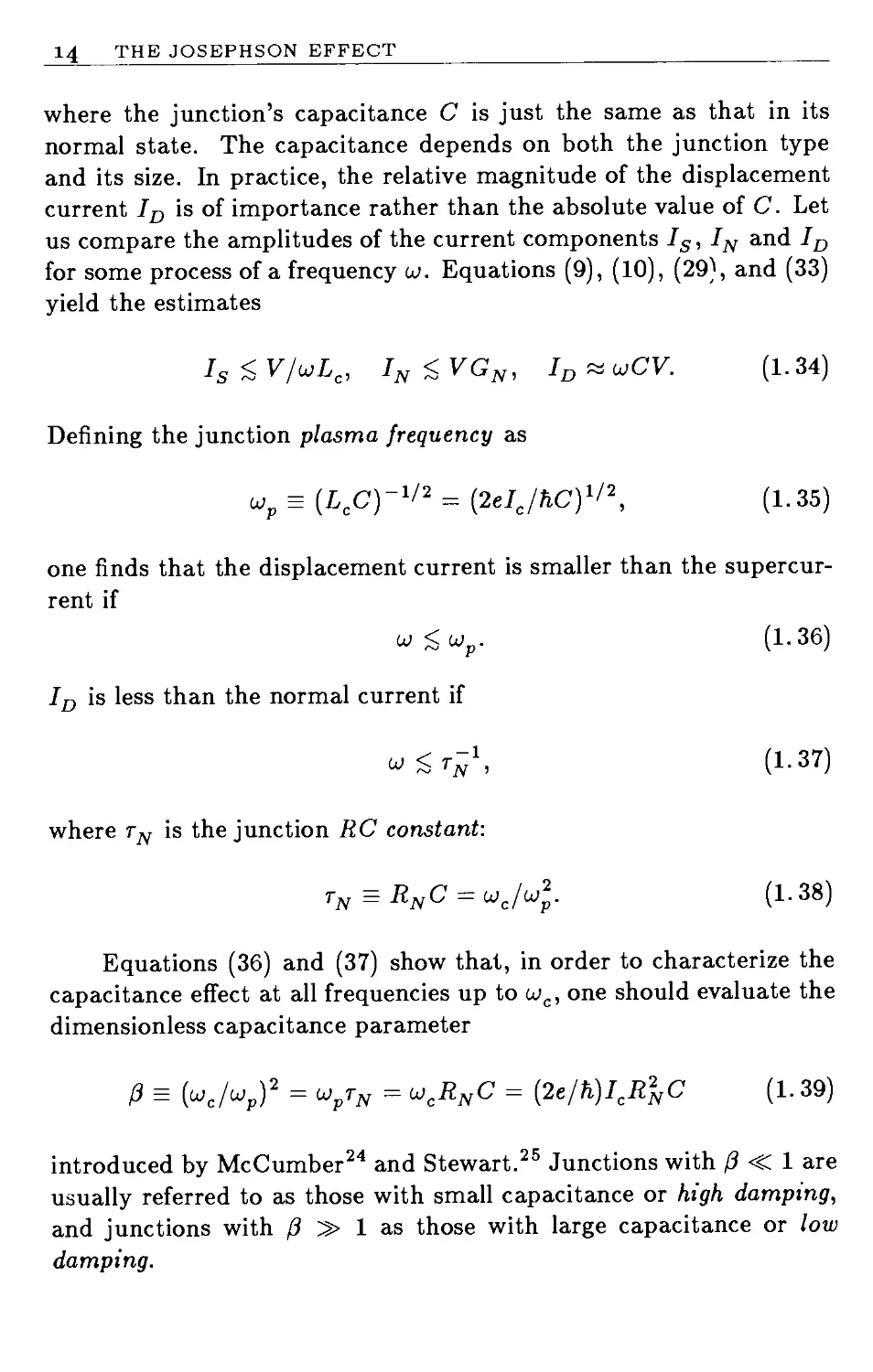
The degree of deviation from the classical description depends on the ratio of two energies, Ec and hwp. If hwp C Ec, the basic (lower) energy levels of the system are localized near the bottom of the “potential wells”, i.e., near the points фп — 2тгп. For this case, one can expand (— cos </>) in Us into the Taylor series with respect to small deviations ф = ф- фп and neglect all terms except ф2/2+ const. The Hamiltonian (54) is thus reduced to that of a harmonic oscillator with frequency wp and energy eigenvalues
En = (n + 2) ’	En ~ Ec"	(1-
The condition hwp C Ec is well fulfilled for all practical Josephson junctions and therefore validates the classical description (9,10). In fact, quantum mechanics shows (see e.g., Reference 32) that the classical theory of the harmonic oscillator coincides with the exact (quantum) one in all details but one: its finite motion (quantum fluctuations) at the lowest energy level n = 0. These fluctuations can be described together with thermal ones in a very convenient way:38-40 it is sufficient to include a Langevin force IF with the proper statistical properties into the classical equations of motion.
These properties are simplest when the thermodynamical “external world” around the junction is in thermal equilibrium (for the Josephson junction, the “world” is just the ensemble of the quasiparticles, and the condition
eV C hw, kBT
(1.58)
is quite sufficient for the equilibrium13'28), and one can use Callen and Welton’s fluctuation-dissipation theorem.38 According to the theorem, the spectral density of IF should be taken in the form
Sz(w) = iRey(w)£(w,T),
(1.59)
where Е(ш, T) is an average energy of a quantum oscillator with frequency w at temperature T
E(w,T} = — coth
hw 2k^T
hw
— + леи
2
exp
( fteu 1
1 -1
-1
(1.60)
22 THE JOSEPHSON EFFECT
and У (w) is the complex admittance of the dissipative subsystem (the normal conductance of the junction in our case); thus, at the Ohmic approximation (29), ReK(w) — GN. With this substitution, (59) describes a smooth transition from the thermal noise described by the Johnson-Nyquist formula at low frequencies (43) to a purely quantum noise
=	C1-61)
Z7T
at very high frequencies (53).
One more convenience of the fluctuation-dissipation theorem is its validity at any rate of damping in the system, i.e., at any values of the junction capacitance parameter fl (the usual quantummechanical methods cannot be applied at high damping, fl С 1, and much more complex quantum-statistical methods should be used; see, e.g., Reference 7). In order to employ the Langevin approach, one should become convinced that the following generalized condition is satisfied:35,36
min[ftwp, ftwc] C Ec.	(1-62)
Again, this condition is well fulfilled for nearly all Josephson junctions, and we can use the classical description (9, 10) of the Josephson effect, taking into account the quantum noise (61) if necessary.
Only a few special experiments where the secondary quantum effects were so large that one would have to go back to the general quantum picture to discuss them are known (see Section 3.3).
Problem 1.4. Analyze the quantum properties of an insulated Josephson junction (/ = 0) at low damping and arbitrary hwplEc ratio. Solution. To find the system’s energy levels we can use a Hamiltonian (54) in a “coordinate” (</>) representation. In this representation, the operator of Q can be written asp‘6
so that the corresponding stationary Schrodinger equation is the usual Mathieu equation
д2Ф
+ (a + 2?соз2г)Ф = 0, z = ф/2,	(1.64a)
dz2
SECONDARY QUANTUM MACROSCOPIC EFFECTS 23
with the parameters
a = 4
E-Ec
„ F (M2
4 E’ r C 2E„
(1.64b)
It can be proved46 48 that the states of the junction which differ by the translation </>—></> + 2тг are physically distinct, so that one should not impose periodic boundary conditions of the type Ф(</>) = Ф(</> + 2тг). This means that the general solution of (64) should be sought as the superposition
= ETM"’ к
(1.65a)
of the Bloch waves
= uln)(^)ejfc^, «ln) (</> + 2tt) =uj:n) (</>),	(1.65b)
with all characteristic numbers к rather than only integer ones.
Figure 3 shows the corresponding energy spectrum of the junction for two typical values of the Ec ratio. One can see that the spectrum consists of allowed energy bands,36,46-48 with the periodic dependence E^n\k) in each of the bands:
£(n)(fc-t-1) = £(n)(fc).	(1.66)
For the practical junctions available today with hwp <C Ec, the bands are exponentially narrow and located at the points En (1.57)—see Figure 3a. For junctions with extremely small capacitances (C < 1015 F) however, the opposite condition can be satisfied, so that the band structure can be well pronounced—see Figure 3b.
According to recent theoretical analyses, several radically new phenomena should be observed due to this energy band structure. Up to the middle of the 1985, these effects have not been observed experimentally, so that we will discuss them only in the last Chapter 16 of this book. Nevertheless, one should remember that, if these phenomena are found, an entirely new field in Josephson junction dynamics will be open for development.
24 THE JOSEPHSON EFFECT
(Ы
Figure 1. 3. Energy spectrum of an isolated (I = 0) Josephson junction with low damping: (a) Er/Ec = 0.4; (b) Er/Ec — 10.
REFERENCES 25
Lastly, we should note a “quasispin” approach that has been applied to the discussion of similar problems by some authors. This approach was based on the formal resemblance of the operators e:=r'', .V to the usual spin operators з±,зг. Such an analogy is, however, incomplete,42 because the operators do commute
=0,
(1-67)
while the real spin operators do not (see, e.g., Reference 32):
[*+>*-] =jsz.
(1.68)
As a result, the quasispin approach can lead to some incorrect conclusions.
Problem 1.5. Reformulate condition (62) in terms of the normal junction resistance.
Solution. In the high-damping limit (/3 С 1, wc C wp), this condition takes an especially simple form
Rn < Rq, RQ=7rh/2e2,
(1.69)
where Rq « 6.7 к fl is a natural quantum unit of resistance. The latter constant arises in quite a few problems of solid-state physics (see, e.g., References 43 and 44) and condition (69) must always be fulfilled in order to neglect the quantum fluctuation effects.
References
1.	Kamerlingh Onnes, H. 1911. Leiden Commun. 122b: 124.
2.	Meissner, W., and Ochsenfeld, R. 1933. Naturwissenschaften 21: 787.
3.	London, F., and London, H. 1935. Proc. Roy. Soc. London A149: 71.1935. Physica (Utrecht) 2: 34.
4.	London, F. 1950. Superfluids. New York: Wiley.
5.	Ginsburg, V.L., and Landau, L.D. 1950. Zh. Eksp. Teor. Fiz. (Sov. Phys.-JETP) 20: 1064.
6.	Bardeen, J., Cooper, L.N., and Schrieffer, J.R. 1957. Phys. Rev. 108: 1175.
7.	Abrikosov, A.A., Gor’kov, L.P., and Dzyaloshinskii, I.E. 1965. Quantum Field Theoretical Methods in Statistical Physics. London: Pergamon Press.
8.	Abrikosov, A.A. 1957. Zh. Eksp. Teor. Fiz. (Sov. Phys.-JETP) 32: 1141.
9.	Deaver, B.S., Jr. and Fairbank, W.M. 1961. Phys. Rev. Lett. 7: 43.
26 THE JOSEPHSON EFFECT
10.	Doll, R., and Nabauer, M. 1961. Phys. Rev. Lett. 7: 51.
11.	McCumber, D.E. 1971. Physica (Utrecht) 55: 421.
12.	Hartle, J.B., Scalapino, D.J., and Sugar, R.L. 1971. Phys. Rev. B3: 1778.
13.	Fulton, T.A. 1973. Phys. Rev. B7: 981.
14.	Clarke, J. 1968. Phys. Rev. Lett. 21: 1566.
15.	Bracken, T.D., and Hamilton, W.O. 1972. Phys. Rev. B6: 2603.
16.	Macfarlane, J.C. 1973. Appl. Phys. Lett. 22: 549.
17.	Finnegan, T.F., Denestein, A., Langenberg, D.N., McMenamin, J.C., Novo-seller, D.E., and Cheng, L. 1969. Phys. Rev. Lett. 23: 229.
18.	Silver, A.H., JakleviJ, R.C., and Lambe, J. 1966. Phys. Rev. 141: 362.
19.	Werthamer, N.R., and Shapiro, S. 1967. Phys. Rev. 164: 523.
20.	Likharev, K.K. 1968. Vestn. Mosk. Univ. (Moscow Univ. Phys. Bull.) 5: 104.
21.	Russer, P. 1971. Proc. IEEE 59: 282.
22.	Thompson, E.D. 1973. IEEE Trans. Electron. Devices 20: 680.
23.	Manley, J.M., and Rowe, H.E. 1956. Proc. IRE 44: 904. 1959. 47: 2115.
24.	McCumber, D.E. 1968. J. Appl. Phys. 39: 3113.
25.	Stewart, W.C. 1968. Appl. Phys. Lett. 12: 277.
26.	Stratonowich, R.L. 1967. Selected Topics in the Theory of Random Noise. New York: Gordon and Breach.
27.	Whalen, A.D. 1971. Detection of Signals in Noise. New York: Academic Press.
28.	Dutta, P., and Horn, P.M. 1981. Rev. Mod. Phys. 53: 497.
29.	Hooge, F.N., Kleinpenning, T.G.M., and Vandamme, L.K.J. 1981. Rep. Prog. Phys. 44: 532.
30.	Kose, V.E., and Sullivan, D.B. 1970. J. Appl. Phys. 41: 169.
31.	Kanter, H., and Vernon, F.L., Jr. 1970. Phys. Rev. B2: 4694.
32.	Landau, L.D., and Lifshitz, E.M. 1958. Quantum Mechanics. London: Perga-mon.
33.	Scott, A.C. 1967. Phys. Lett. A25: 132.
34.	Fetter, A.L., and Stephen, M.J. 1968. Phys. Rev. 168: 475.
35.	Likharev, K.K. 1983. Usp. Fiz. Nauk. (Sov. Phys. Usp.) 139: 169.
36.	Larkin, A.I., Likharev, K.K., and Ovchinnikov, Yu.N. 1985. Physica (U-trecht) B126: 414.
37.	Legget, A. 1982. Suppl. Progr. Theor. Phys. 69: 80.
38.	Callen, H.B., and Welton, T.E. 1951. Phys. Rev. 83: 34.
39.	Senitzky, I.R. 1961. Phys. Rev. 124: 642.
40.	Lax, M. 1966. Phys. Rev. 145: 110.
41.	Abramowitz, M., and Stegun, LA. 1969. Handbook of Mathematical Functions. New York: Dover Publ.
42.	Ferrell, R.A. 1982. Phys. Rev. 25: 496.
43.	Thouless, D.J. 1982. Physica (Utrecht) B109: 1523.
44.	Hebard, A.F., and Fiory, A.T. 1982. Physica (Utrecht) B109: 1637.
45.	Tsai, J.-S., Jain, A.K., and Lukens, J.E. 1983. Phys. Rev. Lett. 51: 316.
46.	Likharev, K.K., and Zorin, A.B. 1984. In: LT-П: Contributed Papers, U. Eckern et al., Eds.: 1153. Amsterdam: Elsevier.
47.	Averin, D.V., Zorin, A.B., and Likharev, K.K. 1985. Zh. Eksp. Theor. Fiz. (Sov. Phys.-JETP) 88: 692.
48.	Likharev, K.K., and Zorin, A.B. 1985. J. Low Temp. Phys. 59: 347.
CHAPTER 2
Josephson Junctions:
Types and Models
2.1. TUNNEL JUNCTIONS
Our brief survey of the Josephson junctions will be started with tunnel junctions proposed1 in 1960 by Ivar Giaever who later shared the Nobel Prize with Brian Josephson. These were the tunnel junctions for which the original Josephson prediction was made1’’1 and in which the effect was experimentally observed for the first time.p’2 Despite a considerable competition from the junctions of other types, the tunnel structures are still the best studied and the most important for applications.
The tunnel junction (or “SIS sandwich”) consists of two superconducting (S) electrodes separated by a thin insulating (I) layer. In most cases, vacuum-deposited superconducting thin films serve as the electrodes, and the oxide of the lower (base) electrode plays a role of the insulator. The oxide layer thickness dj is of the order of ten to thirty atomic sizes so that the electrons have a small but nonvanishing probability (p ~ 10“5-T0“3) of penetrating from one electrode into the other one via quantum tunneling through the energy barrier created by the insulator. Such penetration results in a nonvanishing normal conductance GN when the electrodes are in their normal state (T > Tc), and in the Josephson effect in the superconducting state (T<TC).
1.	Microscopic theory
The smallness of the penetration probability p simplifies the solid-state theory of the tunnel junctions, enabling one to use the powerful “tunnel Hamiltonian” method proposed in 1961 by Cohen, Falicov and Phillips.2 This method has not only helped Josephson to make his
27
28 JOSEPHSON JUNCTIONS: TYPES AND MODELS
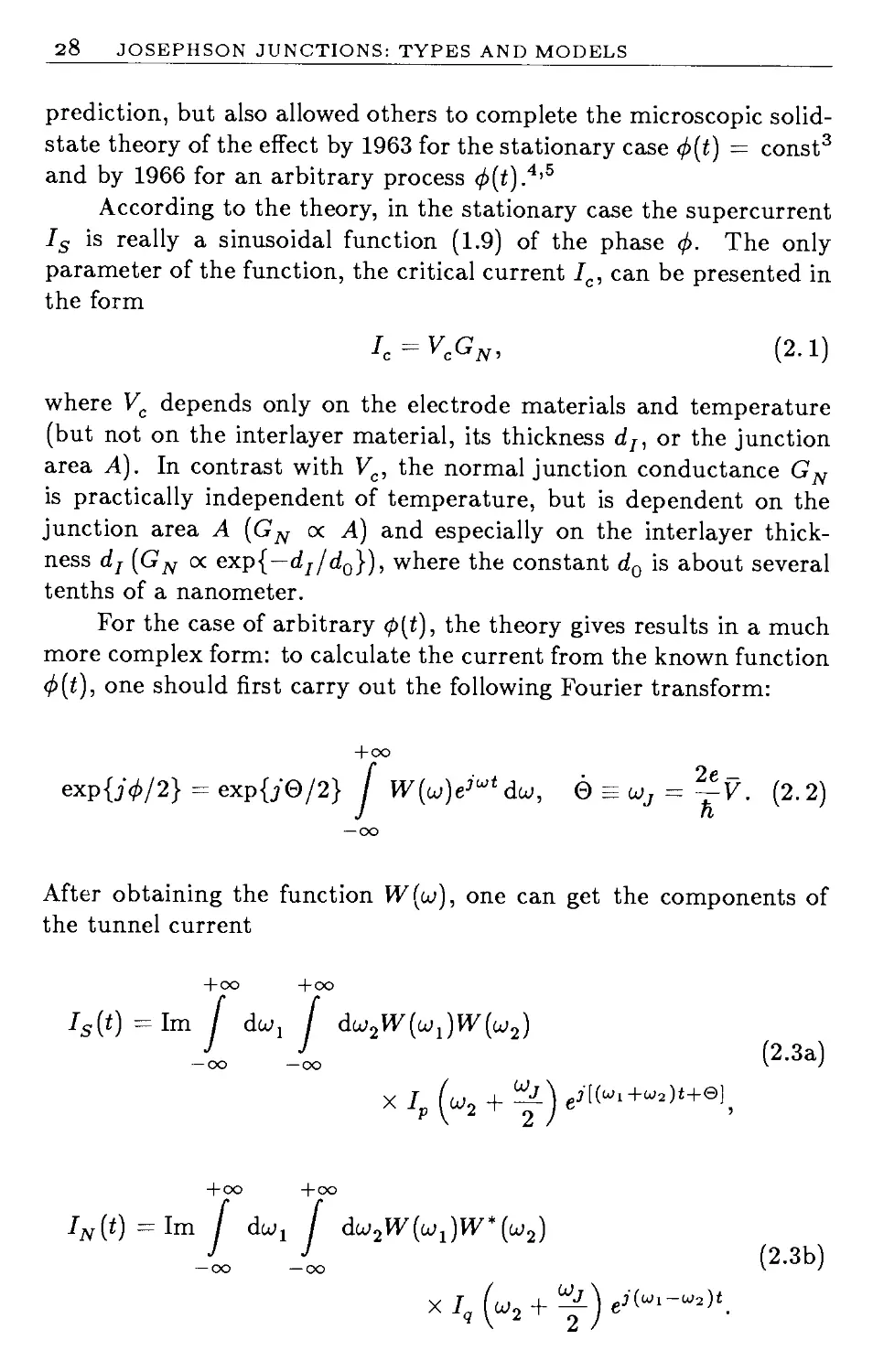
prediction, but also allowed others to complete the microscopic solid-state theory of the effect by 1963 for the stationary case d>(t) = const3 and by 1966 for an arbitrary process «/>(<).4,5
According to the theory, in the stationary case the supercurrent Is is really a sinusoidal function (1.9) of the phase ф. The only parameter of the function, the critical current Ic, can be presented in the form
Jc=VcGn,	(2.1)
where Vc depends only on the electrode materials and temperature (but not on the interlayer material, its thickness dr, or the junction area A). In contrast with Vc, the normal junction conductance GN is practically independent of temperature, but is dependent on the junction area A (GN oc A) and especially on the interlayer thickness dj (GN oc exp{ dj/do}}, where the constant dQ is about several tenths of a nanometer.
For the case of arbitrary 0(t), the theory gives results in a much more complex form: to calculate the current from the known function d>(t), one should first carry out the following Fourier transform:
4-oo
Г		2e -
exp{j‘d>/2} = exp{j’0/2} / W(a/)eJut dw, 0	(2.2)
— oo
After obtaining the function W (w), one can get the components of the tunnel current
4-oo	4-oo /s(t)= Im 1 dwj 1 dw^wjW^wJ — oo	—oo T (	Wj X Ip уш2 + у 4-oo	4-oo /;v(t) = Im У dwj / dw2Wz(w1)Wz*(w2 — oo	—oo X Iq (W2 d	(2.3a) ) ej[(wi h+®], '	(2.3b) 2 /
TUNNEL JUNCTIONS 20
In contrast with W (w), the complex functions Ip g(w) do not depend on the phase dynamics </>(t), but are completely determined by the junction itself. To understand their physical meaning, it is useful to consider a special case when the junction voltage V is constant: V (t) = V. For this case, (1.10) yields
ф = 0 = Wjt + const,
(2.4a)
and according to (2), the function W (w) is very simple:
JV(w) = <5(w),
(2.4b)
where <5(w) is the Dirac delta function. For this case, (3) gives
Is = Ke Ip
sin ф + Im Ip
IN = Im/q (^) ,
(2.5a)
(2.5b)
Thus, according to the microscopic theory, the supercurrent Is contains not only the term with sin</>, but also the term with cos</>. The real and imaginary parts of the Cooper-pair component Ip(eV/Й) define two quadrature components of the supercurrent amplitude as functions of the de voltage (and therefore of the Josephson oscillation frequency) across the junction. The imaginary part of the quasiparticle component Iq(eV/Й) gives the voltage dependence of the normal current (the real part of Iq does not show up in (5) but can contribute to the current in other cases).
The functions Fp (?(w) are defined through the so-called Green’s functions of the superconducting electrodes (for details, see References 1.7 and 2-6).
, hw. tanh----
2kBT
+ tanh
hw2 2k BT
x ImFj (wj) ImF2(w2)(wj + w2 — w + j’0) 1
(2.6a)
2 h. ’
30 JOSEPHSON JUNCTIONS: TYPES AND MODELS
+ oo +oo
/ (w) = GN(2?r3e)~1 [ dwj [ dcu2 ftanh + tanh
7 1	1 J 1 J 2 \ 2kBT 2kBT
— oo	— oo
x ImGjwJ ImG2(w2)(w1 + w2 - w + jO)-1 + const.
(2.6b)
One can see that not only the critical current Ic = Re/p(O) but also all current components are proportional to GN; thus, the IRN product depends only on properties of the electrodes.
2.	BCS approximation
The existing body of experimental data does not leave any doubt in validity of the general formulas (1-6) for any tunnel junctions at practical current densities (up to ~ 105 А/cm2). More vulnerable, however, are the concrete expressions for the functions F(w), G(w) and hence for I (w). The only known simple expressions are those following from the “classical” formulation of the theory of superconductivity1'6 by Bardeen, Cooper and Schrieffer (BCS):
тгД(Т)
F(w) =	------=-----------
[A2(T)-ft2(w TjO)2]1/2
7ГЙШ
(2-7)
G(w) =-------------x------------,
1	[Д2(Т) -ft2(w +j0)2]!/2’
where Д(Т) is the energy gap. In the BCS theory, A(T)/kBTc is the universal function of T/Tc, shown by the dashed line in Figure 1.
Figures 1 and 2 show the main results of substitution of the BCS approximation (7) to the general expressions (6) for the most important case of “symmetrical” junction with similar electrode materials: Д1(Т) и A,2(T) — Д(Т).6-81 The temperature dependence of the critical current (Figure 1) is quite simple,
vc = icRn =
тт Д(Т)
2 e
, A(T) tanh —-—-, 2kBT
(2-8)
t For different electrodes, one can find some plots in References 7 and 8 as well as in Reference P.32.
TUNNEL JUNCTIONS 31
Figure 2. 1. Temperature dependence of the energy gap Д (dashed line) and the characteristic voltage Vc of the symmetrical tunnel junction (solid line) in the “classical” (BSC) approximation.
but formulas for	(Figure 2) can be expressed in a relatively
simple form only at T = 0 (in practice, these expressions are applicable at T < 0.5Tc):
„	, , ,	, , f К (a], .. at x < 1
Re/p(w) = A(0) x !
I X 11 IX I, d I X / 1
(2.9a)
{0,	at x < 1,
x-xK(x'\ atol (2’9b)
X	I X J л U X X
eRNReIQ(w) = A(0)sign(w)
( K(x) ~2E(x),
( (2i — x'~1)K (i1) — 2iEl(i-1),
at x < 1, at x > 1,
(2.9c)
eRN Imfg(w)
A(0)sign(w)
J 0,
X ( 2xE(x') - x~1K(xl),
at x < 1, at x > 1,
(2.9d)
32 JOSEPHSON JUNCTIONS: TYPES AND MODELS
Figure 2. 2. Frequency dependences of the (a, b) real and (c, d) imaginary parts of the complex amplitudes of (a, c) the quasiparticle current Iq and (b, d) the Cooper-pair current Ip in the symmetrical tunnel junction (Ai = Дг = Д) in the BCS approximation (5 = 0). Iq = V9(0)Gjy = 2Д(0)/е7?ту.
TUNNEL JUNCTIONS 33
where x = |w|/wg, x' = (1 - x 2)1,/2, wg is the gap frequency
= eVg/h = 2Д(Т)/й,
(2.10)
and K(x) and E(x) are the complete elliptic integrals of the first and second kind, respectively (see, e.g., Reference 1.41).
Real parts of the functions Ip Q(w) are always even and the imaginary parts are odd. At the point w = w , the real parts of the functions have logarithmic singularities (“the Reidel peak”9):
Re/(w) и Re/ (w) + const и —- In p	4	7Г
ш~шд 8wg
(2.11a)
while the imaginary parts show finite steps:
iw0+O	i^o+O
Im/ (w)	= -Im/(w)	=/c,	(2.11b)
whose height is exactly equal to Ic within the BSC theory.
3.	Deviations from the BCS approximation
There are few substantial deviations of the classical-theory predictions from the observed properties of typical tunnel junctions:
i.	Experimental critical currents are always less than the theoretical value (8). This difference can be especially large (30 to 80%) in tunnel junctions with the electrodes of transition metals (e.g., Nb, V) and their compounds.
ii.	Singularities (11) are always somewhat smoothed and have a nonvanishing width 2<5wg.10-13
iii.	The sign of Im/p(w) appears to be negative at low temperatures14-16 while it is positive in the BCS theory.
The physical reasons for the deviations can be various.17’18 For example, the BCS approximation does not take into account such effects as the possible presence of some very thin normally conducting layers at the boundaries between superconducting electrodes and the insulating barrier. These layers cause smoothing of the squareroot singularities of F and G at the gap edges w = ±wg and lead,
34 JOSEPHSON JUNCTIONS: TYPES AND MODELS
as a result, to all three effects listed above.17 Nevertheless, an exact theory of these effects is rather complex and thus a phenomenological approach is frequently used to correct the classical theory (see Section 3).
4-	Junction capacitance
For the displacement current ID of the tunnel junction, relation (1.33) can be used with the well-known expression for the plane-condenser capacitance
C = ere0A/dI,	(2.12)
where er is the relative dielectric constant of the interlayer dielectric and
e0 и 8.85 x 10“12 Farad/meter	(2.13)
is the vacuum electric constant. According to (12), the specific capacitance of the junction, С/А, is a much slower function of dj than the critical current density
Л =
(2-14)
because Ic is proportional to exp{—dj/dQ}. Hence the specific capacitance is nearly constant within a reasonable range of jc (say, 1 to 104 А/cm) and varies from 3 to 10 pF/cm2 for various insulators.19 Equations (13) and (14) allow one to express the dimensionless parameter /3 (1.39) in the following form
0 = f £r£p\ 
Л c \ di J '
(2-15)
so that /3 does not depend on the junction area and is almost completely determined by the critical current density.
TUNNEL JUNCTIONS 35
5.	Fluctuations
The microscopic theory allows one to calculate not only the mean values of the current components in the tunnel junction but also the intensity of current fluctuations IF(t). For the case of constant voltage (4), the relevant calculations were carried out at the end of the 1960’s20-22 (for review, see Reference 23). The result for arbitrary </>(t) has been, however, obtained just recently by Zorin24 who used the technique developed somewhat earlier by Tucker.25
The main peculiarity of the result is that IF(t) is not a stationary process in the general case, and thus cannot be characterized by the spectral density Sj{w) (1.41). Instead, the Fourier images of IF are mutually correlated,
-(I Г, + Г,1 }
+ (Vj/2) 2kBT
X { [^(Wj	-w)
+ W*(w' - Wj - Wj)kF(w - Wj - Wj)]
x Im/q
(2.16)
+ [JV(W1 - w')JV(w - Wj - Wj)
- w)jy‘(w'- Wj -Wj)]
x lm/p
for any w and w'. Formula (16) presents a non-additive combination of quantum, thermal, and shot noises of the junction. The relations (1.43), (1.46) and (1.61) follow from (16) at the appropriate limits involving kBT, eV, and Kw.
Finally, the 1/ f noise (not accounted for in (16)) can show up in tunnel junctions. For the junction areas A > 10-4 cm2, this noise
36 JOSEPHSON JUNCTIONS: TYPES AND MODELS
Figure 2. 3. Schematic side view on typical tunnel junction structures: (a) planar type and (b) edge type. Notation: 1, dielectric substrate; 2, superconducting base electrode; 3, thick insulating layer; 4, thin insulating layer forming the tunnel barrier; 5, superconducting counter-electrode.
becomes substantial only below ~ 1 Hz26 but this cutoff frequency increases approximately as A-1 with the further increase of the area,148 in approximate accordance with the phenomenological formulas by Hooge1'29 and by Voss and Clarke.27
6.	Fabrication technology
Several excellent reviews are available on the problems of the Josephson junction fabrication,28-30’149-152 and only a brief glimpse will be presented here.
Figure 3a shows a sketch of a typical tunnel junction structure. To fabricate the junction, a thin film (few hundred nanometers) of a superconducting material is deposited over a clean plane surface of an insulating substrate 1. After the film is patterned using photolithography to form the “base electrode” 2 of the desired shape, it is covered with a relatively thick insulating layer 3. Then photolithography is used again to form a “window” in the insulator with the area A defining the area of the future junction (from ~ 10-8 to ~ 10-4 cm2). After cleaning the surface of the base electrode inside the window, it is oxidized to form a very thin (dz и 2-5 nm) insulating barrier 4 of the tunnel junction. The fabrication is completed then by deposition of the upper superconducting layer, and its patterning to form the “counter-electrode” 5.
TUNNEL JUNCTIONS 37
In the beginning of the Josephson effect research in the 1960s, the tunnel junctions were fabricated using the “soft” superconductors (Sn, In, Pb) and thermal oxidation to form the barrier. With such technology, a reproducible critical current density jc did not exceed ~ 102 А/cm2, and the capacitance parameter (15) was therefore large: /3 > 103.
As we will see later, the useful characteristics of nearly all practical devices based on the Josephson effect are improved when /3 is decreased (at least until ~ 1). During the 1970s, the progress in this direction was to a great extent due to the development of the “lead-alloy technology” by experts at the IBM Corporation. In this technology, the base electrodes are fabricated of the alloy of Pb with Au and In, and oxidized in the plasma of the rf glow discharge, while alloys of Pb with Au or Bi are used for the counter-electrodes (the details can be found in References 31-33). This technology provided quite reproducible junctions with thinner barriers and hence greater jc (up to 104 А/cm2). The parameter /3 was still somewhat more than, but close to, unity.
The further progress of technology is directed mainly to get over the main practical drawback of the Josephson junctions—a relatively low stability to their recycling from room (~ 300 K) to “helium” (~ 4 K) temperatures. Although some further progress in the lead-alloy technology was achieved,153-156 it was found that stability can be greatly increased if “rigid” superconductors like Nb are used for at least the base electrode (see, e.g., Reference 34). Niobium oxide barriers, however, have very complex structure35-37 (until special cleaning methods are used157’158) and relatively high specific capacitance,19 so that considerable efforts are being made to replace the oxide with “artificial barriers.” Such barriers can be prepared either by the deposition of an insulator or semiconductor (see Reference 38 and the recent References 39-41) or some other metal with its consequent oxidation.42-44’161’167’169’170
In addition to niobium, several other rigid superconducting com-
pounds are under active study as the electrode materials, including
NbN 49>50>159,162,164-166,168,171-173,177
Nb3Sn,
51,52,160,174
V3Si,52,53
and Nb3Ge.54 For those materials, the use of artificial barriers is
almost inevitable55 (with an important exception of NbN). Espe-
cially promising results have been obtained with amorphous silicon barriers47-55’151’166'172 which can survive deposition of the rigid-su-
38 JOSEPHSON JUNCTIONS: TYPES AND MODELS
perconductor counter-electrodes.47-50,151 ’172
The sharp increase of the typical critical current densities during the 1970s required a proportional decrease of the junction areas to keep the junction impedance
|Z| ~	= Vc/JcA	(2.17)
within necessary limits (~ 1 to ~ 102 * fl for various applications). For the very high values of jc (104 to 10s А/cm2), the area A in most cases should be as small as < 1 ^m2. Such submicron junctions can be fabricated in the usual “planar” configuration (Figure 3a) by using either electron-beam lithography56-58’163 or the special “Dolan technique”59 (see also References 57, 58, 60, 61, 175 and 176).
The edge configuration (Figure 3b) also can give a sufficiently small junction area. In this latter case, the ion milling is used to form a steep edge on the base electrode 2 and the thick insulator 3. After oxidation of the edge area 4, the counter-electrode 5 is deposited, so that one of the junction sizes is close to the base electrode thickness and can be as small as ~ 0.1 ^m. As the result, the junction area can be reduced from 0.1 to 0.01 ^m2 which permits one to operate with the critical current densities up to ~ 105 A/cm2.57,58’59-63’150
For junctions like these the values of fl can be less than unity, which is favorable for some applications. In these small-size junctions, however, some new problems arise, including noticeable self-heating in the R state (V 0) and relatively high 1// noise.150
2. 2. WEAK LINKS
In spite of tunnel-junction domination throughout the history of the
Josephson-effect studies, noticeable attention has been attracted since
late 1960s to the junctions with non-tunnel-type (direct) conductivity, generally known as “weak links.” In these structures, the weak electrical contact between the electrodes is provided by some link made of a normal metal (N) or superconductor (S). Figure 4a shows an example of the structure, the “SNS sandwich,” where two thin-film electrodes 2 are separated by a normal-metal layer 3. Fabrication technology for these junctions can be very similar to that of the SIS sandwiches (Figure 3a), but their properties are rather different (see, e.g., Reference P-.28).
WEAK LINKS 39
Figure 2. 4. Schematic side view on typical weak link structures: (a) SNS sandwich, (b) planar-type variable-thickness bridge, (c) edge-type variable-thickness bridge, (d) combined sandwich-bridge structure. Notation: 1, dielectric substrate; 2, superconducting electrodes; 3, normal metal layer; 4, thick insulating layers.
The Josephson current in the SNS weak links is due to the “proximity effect” p’34’64: the ability of a superconducting condensate of Cooper pairs to conserve the amplitude and phase of its orderparameter Ф(г,<) even in a normal metal at distances of the order of the “coherence length” Due to this effect, the condensate penetrates into the interlayer from both sides, having phase Xj at one side and X2 at the other. If the interlayer thickness does not exceed several £N, the condensate wavefunctions interfere in its middle, creating the supercurrent Is dependent on ф = Xi ~ Хг-65’66
For typical superconductors and normal metals, the coherence length is of the order of tens and even hundreds nanometers and hence the thickness dN of the normal layer can be much greater than that of the oxide layer. As a result, the specific capacitance C/A of the weak links is small, and as a rule the parameter fl is much less than unity.
During the 1970s, a relatively complete picture of the properties of weak links was developed, and we will give only a brief review here (see, e.g., Reference P.28 for details).
1.	The stationary case
For </>(t) = const, the supercurrent is a 2?r-periodic function of ф. Deviations from a simple sinusoidal dependence (1.9) can be, however, quite substantial, and the characteristic voltage can be much less than
40 JOSEPHSON JUNCTIONS: TYPES AND MODELS
in a tunnel junction with the electrodes of the same materials. Both of these deviations are small if the following condition is satisfied: the “effective spacing” def between electrodes should be less than ~ 3^.67,68 The effective spacing is defined as the distance between the closest points of the electrodes where, the condensate wavefunction is weakly perturbed by the weak link—i. e., the order-parameter Ф is equal to its value well inside the electrodes.
2.	The non-stationary case
Unfortunately, for an arbitrary process no simple theory of the weak link behavior has been developed yet. Even for the simplest case, def C the existing microscopic theory69’70 yields results in a form so complex that nobody has attempted to use it for the junctiondynamics analysis (even IN-V dependence has not been calculated in an explicit form).
Nevertheless, it is clear from the theory that the properties of the supercurrent Is are close to those in the tunnel junctions; in particular, the frequency dependences of Re/p and Im/p at |w| > wg are close71 for both types of junctions. In contrast, the properties of the normal current IN are rather different. In tunnel junctions, Im/q is always less than its Ohmic value VGN and is close to this value for |V| > Vg (see Figure 2c); in weak links, IN exceeds VGN (at least for | V| > V) and approaches the linear dependence
/N = yGN + /exsigny,
at
1^1 >vg.
(2.18a)
For Iex, the so-called “excess current”, the theory gives the expression69

(2.18b)
According to (2) and (18b), at usual operation temperatures T < Tj2, the excess current Jex is of the order of the critical current Ic, i.e., is very large. This theorectical conclusion is well confirmed by experiments (see Chapter 4). Such a difference in the normal current behavior between tunnel junctions and weak links is due to a very specific mechanism—the transfer of quasiparticles with energies \E\ < A—that exists only in the latter structures.69
WEAK LINKS 41
Finally, no microscopic theory of the current fluctuations in weak links has been developed yet.
3.	SNS sandwiches
In contrast to tunnel junctions, several types of weak links have been proposed and studied. The SNS sandwich already discussed above (Figure 4a) has the simplest geometry, but by no means the simplest properties. Both experimental72 and theoretical73,74 studies have shown that, with the “usual” normal metals (Cu, Au, Ag, Al, etc.) as the interlayer material, it is impossible to reduce def below several £N. The reason is that the proximity effect at an SN boundary has another side: normal electrons from the normal metal penetrate inside the superconductor to the depth of at least the order of the coherence length £s of the latter material. Thus the normal electrons suppress superconductivity in this region and increase de{ to about (dN + 2fs). This effect is small (and thus de{ и dN) only if the electron density in the interlayer—hence its normal conductivity aN—is low enough:p’28’73
There have been several attempts to fabricate “good” (high Vc, sinusoidal Is (</>)) SNS sandwiches with high-ohmic normal-layer materials like amorphous tellurium,75’76 doped crystalline silicon,77’78 doped amorphous silicon,38’79 and titanium.80 In all these structures the condition (19) was satisfied (or almost satisfied) which resulted in high values of Vc (> 1 mV). Reproducibility of all these structures, however, remains relatively low due to high sensitivity of crN and £N to the regimes of the fabrication process.
Another important disadvantage of the SNS sandwiches is their low normal resistance. For example, even for small area А и 10 ^m2 and typical values dN и 10 nm and «т^1 w 10-5 П-cm, one obtains resistance RN и dN/aNA of ~ 10-4 П, which is too small for almost any practical application. 4
4. Variable-thickness bridges
In order to reduce A and thus to increase RN, several thin-film bridgetype configurations of weak links have been tested (for reviews, see
42 JOSEPHSON JUNCTIONS: TYPES AND MODELS
References P.28, 81). The most successful of them have proved to be the variable-thickness bridges, first discussed in 197182 and experimentally tested in 1973-75.83-85
Figure 4b shows a possible geometry of such a bridge-type junction. The small thickness of the “span” film 3 reduces the proximity effect on the electrodes (“banks”), so that de{ can be close to dN (the latter distance is now the width of the gap between the electrodes 2) for nearly any materials used for the banks and the span. Moreover, in the R state of these junctions, the relatively thick banks improve the thermal flow from the span and thus reduce84-87 its self-heating (which presents quite a problem for the other types of the thin-film bridges).
Requirements for the span material are quite different from those for the bank material: the former should have larger coherence length to allow a larger dN and also a smaller aN to provide larger RN; the latter should have a larger Tc to provide a larger Vc. This is why the most promising results were obtained when either thin normal films88-91 or highly doped surface layers of silicon substrate78’93 were used for a span? Unfortunately, coherence lengths of such materials are rather small: several tens of nanometers. Thus, the bridge length dN should be of the same order; this is the main problem in the variable-thickness bridge fabrication.
There are two ways in forming such a narrow gap between two bank films: either by the use of electron-beam, ion-beam, or X-ray lithographies84’97,98’150'178 to form the planar bridge (Figure 4b) or by the fabrication of the edge-type bridge (Figure 4c). In the latter case, a “step” 4 is first prepared on the substrate using ion milling. Then bank film 2 and span film 3 are deposited from the material sources located at different places in the vacuum chamber, so that a gap is formed in the bank film at the edge of the step. In this geometry, the bridge length dN is close to the step height and thus can be controlled precisely via the parameters of the deposition process.99-103’178
Both ways have already provided the fabrication of thin-film microbridges with good parameters (Vc up to 1 to 2 mV, RN from 1 to
t Several nice results (high Vc, reasonable Rn) obtained94-9® with all-niobi-um bridges with their small £$ (<C dff) should be noted. It cannot be ruled out, however, that these results were due to some complex infrastructure of the bridges (which would make their reproducible fabrication impossible).
WEAK LINKS 43
10 fl). If reproducibility of the technology proves to be comparable with that of the tunnel junctions, the bridges can be successfully used for quite a few applications.
Note also the works104’105’181 where the structures shown in Figure 4d were fabricated by selective etching of the doped silicon. These junctions combine the features of sandwiches (one-dimensional geometry) and bridges (small junction area).
5. Point contacts
We should mention one more type of the Josephson junctions, the “point contacts,” which had played an important role in the history of the field. In fact, superconductivity in point contacts was observed (see, e.g., Reference 106) well before the Josephson discovery, although only after 1964 did their research begin from this point of view107 (for an early review, see Reference 108). The most attractive feature of the point contacts is the extreme simplicity of their fabrication: it is enough to press slightly a sharply pointed superconducting (typically, niobium) needle to a plane surface of another superconducting electrode (Figure 5a) with the help of some adjusting mechanism (see, e.g., References 109-119).
(a)	(b)
Figure 2. 5. (a) Schematic general view and (b) microstructure of a point-contact junction.
While the pressure is weak, the electrodes are separated by the thin oxide layer which inevitably covers their surfaces. At this stage, a weak tunnel-type conductivity (RN > 1 kfl) can be observed.120-123 When pressure is increased, the oxide layer eventually breaks at several places of the contact spot, forming a complex and irreproducible
44 JOSEPHSON JUNCTIONS: TYPES AND MODELS
system of microshorts between the electrodes (Figure 5b). Such point contacts show all the features of the direct-conductivity Josephson junction, e.g., a well-pronounced excess current (18). Using a reasonable adjusting mechanism and repeating the electrode adjustment several times, one has good chances to obtain a point contact with small capacitance (/3 C 1), high Vc (up to 3 mV), and a desirable value of Rn (in the range from ~ 10-2 to 102 fl)J
Even in the range of the direct conductivity, the characteristics (I-V curves, etc.) of various point contacts can differ by a large extent (see, e.g., Reference 129). Recently, it has been noticed,130’131 however, that if some simple empirical rules are observed in the electrode preparation and contact adjustment, one can obtain the junctions with almost similar I-V curves. These “ideal” junctions differ only in their normal resistance RN (and hence in their current scale, I oc Rtf1)- Moreover, their I-V curves turn out to be similar to those of the other weak links of small size (def C f;v)-76’102 Apparently, these “ideal” point contacts have one or a few microshorts of small size, which should, according to the microscopic theory,69’70 have a universal IRN-V dependence (summing of the currents of several microshorts does not violate this universality). In the following chapters, we will compare predictions of the theoretical models with the data obtained mainly with these “ideal” weak links.
Fabrication simplicity was the main reason of the wide use of the point contacts throughout the 1970s for a wide scope of purposes including the first commercial devices (ac SQUIDS, see Chapter 14) based on the Josephson effect. Irreproducibility of their characteristics (which reduces to that of the current scale in the “ideal” contacts) is resulting, however, in gradual replacement of the point contacts by thin-film Josephson junctions in most practical devices.
2.3. MODELS OF JOSEPHSON JUNCTIONS
The main conclusion from the above review of the types of the Josephson junctions can be formulated as follows: a single solid-state
t Similar structures formed by either mechanical piercing124 or electrical discharge125 through a special insulating layer between the films, as well as the drop-type junctions (“Clarke blobs”)12® are less attractive because of a relatively high capacitance between idle parts of the films. This parasitic capacitance can, however, be reduced by lithographic patterning.17e,ls0 Note also relatively high 1/f noise of the point contacts.127’128
MODELS OF JOSEPHSON JUNCTIONS 45
theory which would give an exact and universal relation between the current and voltage of an arbitrary junction has not been and will never be developed. This is why solving dynamics problems requires several models to provide approximations of the real properties of various junctions. Let us consider three of the models which have proved to be the most useful.
1.	The RSJ model
The Resistively Shunted Junction (RSJ) model introduced by Mc-Cumber1,24 and Stewart1,25 accepts the simplest expressions for the current components: (1.9) for the supercurrent, (1.29) for the normal current, and (1.33) for the displacement current. The fluctuation current is accepted to be a stationary one (1.41), with its spectral density Sj(w) given either by (1.43) (thermal noise) or by the more general expressions (1.59) and (1.60) with ReV(<u) = GN:
Sj(w) = — GNE(w,T) — Gn— coth ;	(2.20)
7Г	Z7T 2kb1
one can meet the term “generalized RSJ model” for the last case.
Throughout the 1970s, the RSJ model was widely used for the analysis of junction dynamics (see, e.g., References P.25, P.27 and P.31), especially for that of weak links. The reasons for its popularity were the extreme simplicity of the model and the absence of any reasonable alternative description of weak links.
One should remember, however, that the RSJ model can be claimed quantitatively valid only in a narrow temperature range just below the critical temperature Tc. For example, for the tunnel junctions, (6) and (7) yield at (Tc — T)/Tc C 1 and w ~ <uc С шд:
1р(ш) ~ Ic= const,	jhw/eRN,
so that equations (3) and (4) are reduced to those of the RSJ model. The same holds true for weak links,65’66 but the corresponding temperature range is even more narrow here69:
A(T)re/ft « 1, i.e., (Tc-T)/Tc^(kBTcrJh)2,
46 JOSEPHSON JUNCTIONS: TYPES AND MODELS
Figure 2. 6. (a) Complete and (b) simplified equivalent tircuits of a Josephson junction (inside the dashed box) shunted by a small external resistor (Ge — Aj"1)-
where re is a quasiparticle energy relaxation time, with the values in the range ~ 10-9 to 1.0“11 s for most practical superconductors. At the usual operation temperature, T < Tc/2, the real junctions show several important deviations from the RSJ model; the most substantial ones are the nonlinearity in the tunnel junctions and the excess current in the weak links.
Recently, the RSJ model has become more important because of the wider use of objects whose description by the model is quantitatively correct at any temperatures. These objects are the Josephson junctions of any type, externally shunted by some circuit of small resistance and inductance (Figure 6):

(2.21)
where cu stands for the highest of all frequencies of interest. In fact, if the conditions (21) are fulfilled, a complete equivalent circuit of the shunted junction (Figure 6a) can be simplified to the form shown in Figure 6b. But the latter circuit can be considered as a new “Josephson junction” with the linear normal conductance:
In^G^V, G$*Ge^GN.	(2.22)
MODELS OF JOSEPHSON JUNCTIONS 47
(2.23a)
As the result, the characteristic voltage and frequency of the new “junction” are much lower than that of the original ones:
« ICR^ к Vc(Re/RN) « Vc
“c3) =	< Wc>
c ft c
as well as the capacitance parameter:
2e	/ p \ 2
/?(s) « — IcR2C = /3	< /3	(2.23b)
П	\HN J
(the latter property is the main reason why the externally shunted junctions, first studied in the early 1970s,132’133 are of wider use today. At the frequencies w ~ C wg, the supercurrent amplitude Ip is constant and equal to Ic in any theory of the Josephson effect (see Figure 2b), so that the supercurrent can be taken in the form (1.9). Thus, the externally shunted junction can be well described by the RS J model with the new parameters (22,23).
Finally, let us write down the basic equation (1.50) within the framework of the RSJ model:
2e
I — 1с8тф+ VGN+ VC + IF(t),	(2.24a)
Using definitions of the characteristic (1.32) and plasma (1.35) frequencies, one can rewrite this equation in a more convenient form:
ш~2ф +	+ sin</> + iF(t) = i, i = I/Ic, (2.24b)
which will be widely used throughout the book. In the thermal limit (1.43) the normalized fluctuation current iF = IF/Ic can be treated as a white noise,
{iF{t)iF(t + т)} =	i.e., 5t(w) = 7/тг<ис, (2.25)
with 7 given by (1.45).
48 JOSEPHSON JUNCTIONS: TYPES AND MODELS
Figure 2. 7. Typical experimental 7y-V dependence of a tunnel junction (dotted line) and its various approximations: 1, (1.29); 2, (2.26); 3, (2.27).
2.	The RSJN model
The Nonlinear-Resistive (RSJN) model was introduced134 to avoid the main discrepancy between the RSJ model and the real tunnel junctions. The only new feature of this model is that IN(V) is taken in a nonlinear form to approximate the real dependence Im/q(ey/h). In most cases, a simple piecewise-linear approximation is used (Figure 7):
, x (GL, at IVI < Va,
J“(G> = v x U. iw" <2-26>
The “leakage” current IN at |V| < Vg is thus characterized by the leakage conductance GL; to obtain the best agreement with experiment, relatively small values (0.05 to 0.2) are usually accepted for the Gl/Gn ratio.
Another possibility is to use a simple power dependence of the type IN ос Vn which enables one to obtain analytical solutions for some simple problems of dynamics.135'136 Such an approximation is, however, absolutely unrealistic at |V| > V . Much better results can be obtained with a slightly more complex expression137
IV/V )n
^(V)=VCN1 + |'v/^)n, »>1,	(2.27)
which is especially convenient for fast computer calculations if n =
MODELS OF JOSEPHSON JUNCTIONS 49
2m. In most calculations, however, relation (26) has been assumed, so that we will imply that approximation when referring to the model.
The RSJN model gives a much better description of the real tunnel junctions: for the junctions with low damping (/3 2> 1) the difference between theory and experiment can be as small as a few percent. As a result, this model is widely used for the dynamic analysis, including several systems of computer-aided design (CAD) of practical circuits. Nevertheless one should remember that this model completely neglects the frequency dispersion of the supercurrent Re Ip(w), as well as the very existence of the components Im/p and Re/q. These faults of the RSJN model are clearly displayed in the analysis of tunnel junctions with high damping where all of the tunnel-current components are essential.
There has been no considerable work on fluctuation analysis within the RSJN model, and thus there is no accepted convention for the IF(t) approximation. It seems quite appropriate to use the thermal-equilibrium-noise approximation (2) at small junction voltages (eV < kBT), and the shot-noise approximation (1.46) at larger voltages.
3.	The TJM model
The Tunnel-Junction-Microscopic (TJM) model is introduced by using equations (2), (3) and (16) of the microscopic theory. The expressions for the current amplitudes /pq(<u) can be taken both in their classical BCS form (7-9), and with some corrections to avoid the discrepancies listed in Section 1 (a somewhat arbitrary character of these corrections compels one to consider such a description as a model rather than an exact theory):
i.	The smaller critical current can be accounted for138 by the multiplication of Ip(w) by a “supercurrent suppression parameter” a < 1 (typically from 0.3 to 0.9).
ii.	Energy gap singularities (10) can be smoothed by using one of the phenomenological rules,18,138 either the “Lorentzian”
In |X| -> ln(X2 + 62)1/2, sign(X) —> arctan(X/<5),
(2.28a)
(2.28b)
50 JOSEPHSON JUNCTIONS: TYPES AND MODELS
CJ-
CJg5
Figure 2. 8. The gap-frequency singularities for the real and imaginary parts of the tunnel current amplitudes (thin lines) smoothed according to the Gaussian rule (solid lines) and the Lorentzian rule (dashed lines).
or the “Gaussian”
(2.29a)
oo	-X
sign(X) -> I ff(X',6)dX'- J a(X',6)dX', -X	-oo
(2.29b)
where o(X, <5) is a normal probability distribution (1.48), and <5 is some phenomenological dimensionless parameter describing smearing of the energy gap edges (Figure 8). The best agreement with experiment is achieved138 typically for 0.03 < <5 < 0.1, and the agreement is somewhat better for the Lorentzian shape (28).
iii.	Finally, the energy gap smearing according to (28) automatically eliminates18 the discrepancy of the Im/p sign at low frequencies.
To conclude the discussion of the TJM model, one should note that its formulas can be rewritten from the “frequency-domain” form
MODELS OF JOSEPHSON JUNCTIONS 51
(2, 3), to the “time-domain” form:7,8’139
t
Istt) = /	“ Hsin + <№)]
— OO t
= I dt7q(t-t')sin|i[^(t) — — OO
(2.30)
(for the time-domain form of expression (16) for the fluctuation sources, see Reference 182). The kernels /р(г) and /q(r) (multiplied by tt) are related to the functions Jp(w), and Jq(w) (7) by the Fourier transform (1.40). In particular, when T <C Tc, Aj = Д2 = A, <5 = 0 and the simple formulas (9) are valid, the kernels can be simply t 1 4Q
expressed as
W =	(2.31a)
where Jo, and У0,У1 are the Bessel functions of the first and the second kind, respectively, and тд =. 2w~1 = H/A(0).
According to these equations, at г J> r , the kernels exhibit oscillations with the gap frequency wg and a slowly decreasing amplitude (oc t-1). Such a slow decrease is due to the infinite “memory time” of the system and makes the numerical calculations using (31) rather difficult. This difficulty can be partly eliminated140’141 by multiplying the kernel by the factor exp(—t/tj), which operation is equivalent to the Lorentzian smearing (28) of the energy gap edge with <5 = fc/2r5A(0) =Tg/2T5. _
The TJM model provides an almost exact description of the tunnel junction properties. It is, however, more computationally complex than the RSJ and RSJN models, so that it has been used to solve a rather limited number of problems of the Josephson junction dynamics. Recently, an effective procedure has been developed183 for fast numerical calculations within the TJM model, so that one can expect its much wider use in the near future.
52 JOSEPHSON JUNCTIONS: TYPES AND MODELS
4- Alternative models
Besides the three basic models discussed above, quite a few other models have been proposed. Firstly, we should mention the attempts to introduce the Im/p component to the RSJ model by adding the “cos ф term”
Л = -Gi(V)y cos</>	(2.32)
to the current (24); in all practical calculations, Gr was assumed to be constant (see, e.g., Reference 142). As one can see from Figure 2d, such approximation is rather crude, and leads to some unphysical results at Gr ~ GN.
Secondly, there have been attempts to simplify the exact formulas (30) of the microscopic theory, for example143’144
t
Is= [ dt'ls(t - t') sin </>(«'),	(2.33)
J
— 00
with some phenomenological expressions for Js(t). Such models are not much simpler than the TJM model, but their precision is much worse.
As a result, the three basic models (RSJ, RSJN and TJM) are in wider use presently, and they are considered comparable in their adequacy-to-complexity ratio. This is why these three models will be used in this book for the discussion of the junction dynamics. Note that all three models are identical for the stationary case: I — Ic sin ф for </>(t) = const, so that a considerable part of our results will be independent of the cnoice of model.
Problem 2.1. Discuss the applicability of the Kramers-Kronig relations to the Josephson junctions.
Solution. Dispersion relations by Kramers and Kronig (see, e.g., Reference 145) are applicable for the complex response function of an arbitrary linear system, while (2) and (3) defining Ipq(w) are quite nonlinear. Nevertheless, the real and imaginary parts of the functions do satisfy these relations:
OO
2 f Im Д n (w)
Re^^) = -/d^	’	(2-34a)
/I J	LV 1 LV
0
MODELS OF JOSEPHSON JUNCTIONS 53
£ , w^f (w)
/ dwi—2	2
J
о
(2.34b)
where symbol means the principal value of an integral.
For the BCS approximation (34) can be obtained146 directly from (7-9); but relations (34) are valid in an arbitrary case (2,3) as well.18 Note that the simple RSJ model and the TJM model (with any type of the smearing (28, 29)) do satisfy the relations (34), while the RSJN model (with GL GN) and most alternative models do not.
Problem 2.2. Analyze the possiblility of simplifying (2) and (3) in the case of relatively slow voltage changes, V —> 0.
Solution. If У —>0, (2) and (3) reduce to (5), so that the last formulas give an “adiabatic” approximation for the case V —> 0 (note that even this approximation is much more exact than the RSJN model). If a further improvement is desirable, one can expand V7(<u) into the Taylor series with respect to small V. In the first-order approximation one readily obtains147
Js(t) = Re/p
hV d2Im/p
2e dw2
sin ф
hV d2Re/p
(2.35a)
M) = Im/q
hV d2Re/q
2e dw2
(2.35b)
where all the functions are taken at the point w(t) = eV(t)/h.
Unfortunately, very few calculations have been carried out within this model,147 but it seems promising for application in the CAD systems.
54 JOSEPHSON JUNCTIONS: TYPES AND MODELS
2.4.	FORMULATION OF THE DYNAMICS PROBLEMS
The basic equation (1.50) of the Josephson junction gives us only one, “material”, equation to calculate two functions I(t) and V(t). Another equation relating the two functions should be that of the “external system,” i.e., of the environment of the junction. In most cases, the external system can be assumed to be linear and passive, and one can introduce the external impedance Ze as
ZM = ~VJL,	(2-36)
where and are the complex amplitudes of the junction voltage and current at the frequency w.
Formulation of the problems of dynamics depends essentially on the ratio of Zt to the Josephson junction impedance Z. Typical sizes of the external systems are at least several millimeters—more than or of the order of the wavelengths of the typical Josephson oscillation frequencies wj (~ 109 to ~ 1013 Hz). As a result, |Ze| is always of the order of the free space impedance
p0 = (mo/£o) 1/2 « 377 Ohms,	(2.37)
p.o = 4tt x IO-7 Henry/meter.	(2.38)
On the other hand, the impedance \Z\ does not exceed several Ohms for most junctions at the same frequencies. As a result, the following condition is satisfied at most frequencies of the order of
|Ze(cu)| » |Z(cu)|.	(2.39)
This relation means that, in most cases, the Josephson oscillations and other fast processes in the junction induce a negligibly small ac current through the external circuit and hence the junction,
\~I\ - \V/Ze\ < Vc/\Ze\ < VC/\Z\ ~ lc. (2.40)
In this situation, fast variations of the current can be induced by external microwave sources only. In their absence, the junction current I(t) can be assumed a constant (or slowly varying) in time. Such an approximation of a “current-biased junction” is quite ade
FORMULATION OF THE DYNAMICS PROBLEMS 55
quate for most simple circuits with the Josephson junctions. We will concentrate on this approximation in the two following parts of the book (Chapters 3-5 and 6-9), and only later will we pass to more complex situations where the function J(t) contains rapidly oscillating component(s).
Note that the basic equation (1.50) determines the junction current as a function of voltage rather than vice versa, and thus one should solve the differential equation (or even the integro-differential equation in the case of the TJM model) in order to find V(t). This is essentially the point which makes the Josephson junction dynamics as difficult (and as interesting) as it is.
There is, however, a case when V(t) can be easily expressed in a simple form. This is the high-frequency limit when the condition
w » min[<uc,<up]	(2-41)
is fulfilled for all the essential frequencies. As it follows from the estimate (1.34), in this limit one can neglect the most nonlinear part of the current, Is, in the first approximation and thus find V(t) readily.
Due to this fact and our main principle of starting with the simpler situations, we will consider most non-trivial problems of the dynamics in the following natural consequence.
1.	High-frequency limit for all junction models
Note that, for the junctions with low damping due to their low plasma frequency (cup C wc) the condition (41) is fulfilled for nearly all frequencies of interest; this is why this case can be called the “low-damping limit” as well. According to the above discussion of the junction types and models, this approach is quite adequate for the description of most tunnel junctions, especially if either the RSJN or the TJM models are used.
2.	High-damping limit for the RSJ model
For several important problems, an analytical solution can be readily achieved within the simplest RSJ model if one neglects the junction capacitance. This limit is quite appropriate for quantitative detription of the externally-shunted junctions of any type, and for qualita
56 JOSEPHSON JUNCTIONS: TYPES AND MODELS
tive description of the (unshunted) weak links. Note that the results in the both listed limits should coincide for w » wc and в 1.
3.	High-damping limit for the TJM model
There are a few basic problems which can be solved in this limit as well, mostly using numerical methods. This case is important for describing the behavior of tunnel junctions with very high critical current densities (/?	1).
4-	Arbitrary damping
Lastly, some problems have been solved for an arbitrary damping (mostly in the RSJ model) using numerical calculations or analog modeling. These solutions are useful for understanding the conditions of crossover between low-damping and high-damping regimes.
The closer we come to the end of the book, the increasingly complex problems we solve, and the more frequently the above program will shrink (sometimes leaving only one case where a solution of a particular problem is known).
References
1.	Giaever, I. 1960. Phys. Rev. Lett. 5: 147.
2.	Cohen, M.H., Falikov, L.N., and Phillips, J.C. 1962. Phys. Rev. Lett. 8: 316.
3.	Ambegoakar, V., and Baratoff, A. 1963. Phys. Rev. Lett. 10: 486.
4.	Werthamer, N.R. 1966. Phys. Rev. 147: 255.
5.	Larkin, A.I., and Ovchinnikov, Yu.N. 1966. Zh. Eksp. Teor. Fiz. (Sov. Phys.-JETP) 51: 1535.
6.	Poulsen, U.K. 1973. Rep. Fys. Lab. I (Tech. Univ, of Denmark). 121.
7.	Harris, R.E. 1974. Phys. Rev. BIO: 84.
8.	Harris, R.E. 1975. Phys. Rev. Bll: 3329.
9.	Reidel, E. 1964. Z. Naturforsch. A19: 1634.
10.	Hamilton, C.A., and Shapiro, S. 1971. Phys. Rev. Lett. 26: 426.
11.	Hamilton, C.A. 1972. Phys. Rev. B5: 912.
12.	Buckner, S.A., Finnegan, T.F., and Langenberg, D.N. 1972. Phys. Rev. Lett. 28: 150.
13.	Buckner, S.A., and Langenberg, D.N. 1976. J. Low Temp. Phys. 22: 569.
14.	Pedersen, N.F., Finnegan, T.F., and Langenberg, D.N. 1972. Phys. Rev. B6: 4151.
15.	Pedersen, N.F., Soerensen, O.H., and Mygind, J. 1978. Phys. Rev. B18: 3220.
REFERENCES 57
16.	Rudner, S., and Claeson, T. 1978. J. Phys. (Paris) 39: C6—604.
17.	Golubov, A., Kupriyanov, M.Yu., and Lukichev, V.F. 1984. Fiz. Nizk. Temp.(Sov. J. Low Temp. Phys.) 10: 799.
18.	Zorin, A.B., Kulik, I.O., Likharev, K.K., and Schrieffer, J.R. 1979. Fiz. Nizk. Temp. (Sov. J. Low Temp. Phys.) 5: 1138.
19.	Magerlein, J.H. 1981. IEEE Trans. Magn. 17: 286.
20.	Larkin, A.I., and Ovchinnikov, Yu.N. 1967. Zh. Eksp. Teor. Fiz. (Sov. Phys.-JETP) 53: 2159.
21.	Scalapino, D. J. 1968. In: Proc. Symp. Phys. Supercond. Dev. , B.S. Deaver, Jr., Ed.: 61. Charlottesville: Univ. Virginia.
22.	Dahm, A. J., Denenstein, A., Langenberg, D.N., Parker, W.H., Rogovin, D., and Scalapino, D.J. 1969. Phys. Rev. Lett. 22: 1416.
23.	Rogovin, D., and Scalapino, D.J. 1974. Ann. Phys. (New York) 86: 1.
24.	Zorin, A.B. 1981. Fiz. Nizk. Temp. (Sov. J. Low Temp. Phys.) 7: 709. 1981. Physica (Utrecht) B108: 1293.
25.	Tucker, J.R. 1979. IEEE J. Quantum Electron. 15: 1234.
26.	Clarke, J. and Hawkins, G. 1976. Phys. Rev. B14: 2826.
27.	Clarke, J. 1980. In: SQUID’80, H.-D. Hahlbohm and H. Lubbig, Eds.: 187. Berlin: W. de Gruyter.
28.	Van Duzer, T. 1977. In: SQUIDs and their Applications, H.-D. Hahlbohm and H. Lubbig, Eds.: 63. Berlin: W. de Gruyter.
29.	Tinkham, M. 1978. In: Future Trends in Superconductive Electronics, B.S. Deaver, Jr., et al., Eds.: 269. N.Y.: AIP Publ. No. 44.
30.	Jackel, L.D. 1980. In: SQUID’80, H.-D. Hahlbohm and H. Lubbig, Eds.: 257. Berlin: W. de Gruyter.
31.	Greiner, J.H., et al. 1980. IBM J. Res. Dev. 24: 195.
32.	Broom, R.F. et al. ibid. 206.
33.	Huang, H.-С., et al. 1980. IEEE Trans. Electron. Devices 27: 1979.
34.	Broom, R.F. et al. 1980. IBM J. Res. Dev. 24: 212. 1980. IEEE Trans. Electron. Devices 27: 1998.
35.	Albrecht, G., Richter, J., and Weber, P. 1982. J. Low Temp. Phys. 48: 61.
36.	Kuan, T.S., Raider, S.I., and Drake, R.F. 1982. J. Appl. Phys. 53: 7464.
37.	Raider, S.I., Johnson, R.W., Kuan, T.S., Drake, R.F., and Pollak, R.A.
1983. IEEE Trans. Magn. 19: 803.
38.	Kroger, H. 1980. IEEE Trans. Electron. Devices 27: 2016.
39.	Kroger, H., Smith, L.N., and Jillie, D.W. 1981. Appl. Phys. Lett. 39 : 280.
40.	Smith, L.N., Thaxter, J.B., Jillie, D.W., and Smith, L.N. 1982. IEEE Trans. Magn. 18: 1571.
41.	Kroger, H., Smith, L.N., Jillie, D.W., and Thaxter, J.B. 1983. IEEE Trans. Magn. 19: 783.
42.	Yeh, J.T., and Tsuei, C.C. 1979. IEEE Trans. Magn. 15: 591.
43.	Gurwitch, M., Washington, M.A., and Huggins, H.A. 1983. Appl. Phys. Lett. 42: 472. 1983. IEEE Trans. Magn. 19: 791.
44.	Kwo, J., Wertheim, G.K., Gurwitch, M., and Buchnan, D.N.E. 1983. IEEE Trans. Magn. 19: 795.
45.	Kosaka, S., Shinoki, F., Takada, S., and Hayakawa, H. 1981. IEEE Trans. Magn. 17: 314.
46.	Shinoki, F., Shoji, A., Kosaka, S., Takada, S. and Hayakawa, H. 1981. Appl. Phys. Lett. 38: 285.
47.	Jillie, D.W., Kroger, H., Smith, L.N., Cukauskas, E.J., and Nisenoff, M. 1982. Appl. Phys. Lett. 40: 747. 41: 897.
58 JOSEPHSON JUNCTIONS: TYPES AND MODELS
48.	Van Dover, R.B., Bacon, D.D., and Robert Sinclair, W. 1982. Appl. Phys. Lett. 41: 764.
49.	Shoji, A., Kosaka, S., Shinoki, F., Aoyagi, M., and Hayakawa, H. 1983. IEEE TYans. Magn. 19: 827.
50.	Cukauskas, E.J., Nisenoff, M., Jillie, D.W., Kroger, H., and Smith, L.N. 1983. IEEE Trans. Magn. 19: 831.
51.	Howard, R.E., Rudman, D.A., and Beasley, M.R. 1978. Appl. Phys. Lett. 33: 671.
52.	Rudman, D.A., Howard, R.E., Moore, D.F., Zubeck, R.B., and Beasley, M.R. 1979. IEEE Trans. Magn. 15: 582.
53.	Tarutani, Y., Yamada, K., and Kawabe, U. 1981. IEEE Trans. Magn. 17: 326.
54.	Ihara, H., Kimura, Y., Okumura, H., and Gonda, S. 1983. IEEE Trans. Magn. 19: 938.
55.	Rudman, D.A., and Beasley, M.R. 1980. Appl. Phys. Lett. 36: 1010.
56.	Magerlein, J.H., and Webb, D.J. 1980. IBM J. Res. Dev. 24: 554.
57.	Jackel, L.D., Hu, E.L., Howard, R.E., Fetter, L.A., and Tennant, D.M. 1980. IEEE Trans. Electron. Devices 27: 2030. 1981. IEEE Trans. Magn. 17: 295.
58.	Hu, E.L., Jackel, L.D., and Howard, R.E. 1981. IEEE Trans. Electron. Devices 28: 1382.
59.	Dolan, G.J. 1977. Appl. Phys. Lett. 31: 337.
60.	Dousselin, G., and Rosenblatt, J. 1980. J. Appl. Phys. 51: 802.
61.	Broom, R.F., Oosenbrug, A., and Walter, W. 1980. Appl. Phys. Lett. 37: 237.
62.	Kleinsasser, A.W., Hunt, B.D., Callegari, A.C., Rogers C., Tiberio, R., and Buhrman, R.A. 1981. IEEE Trans. Magn. 17: 307.
63.	Moore, D.F., Vettiger, P., and Forster, T. 1981. Physica (Utrecht) B108: 983.
64.	De Gennes, P.G. 1964. Rev. Mod. Phys. 36: 225.
65.	Aslamasov, L.G., Larkin, A.I., and Ovchinnikov, Yu.N. 1968. Zh. Eksp. Teor. Fiz. (Sov. Phys.-JETP) 55: 323.
66.	Aslamasov, L.G., and Larkin, A.I. 1969. Pis’ma Zh. Eksp. Teor. Fiz. (JETP Lett.) 9: 150.
67.	Likharev, K.K., and Yakobson, L.A. 1975. Zh. Tekh. Fiz. (Sov. Phys.-Tech. Phys.) 45: 1503.
68.	Kupriyanov, M.Yu., Likharev, K.K., and Lukichev, V.F. 1981. Physica (Utrecht) B108: 1001. 1982. Zh. Eksp. Teor. Fiz. (Sov. Phys.-JETP), 83: 431.
69.	Artemenko, S.N., Volkov, A.F., and Zaitsev, A.V. 1979. Zh. Eksp. Teor. Fiz. (Sov. Phys.-JETP) 76: 1816.
70.	Zaitsev, A.V. 1980. Zh. Exp. Teor. Fiz. (Sov. Phys.-JETP) 78: 221. 1983. Fiz. Tverd. Tela (Sov. Phys.-Solid State) 23: 927.
71.	Kruglov, A.H. 1981. Fiz. Tverd. Tela (Sov. Phys.-Solid State) 23: 3404.
72.	Clarke, J. 1969. Proc. Roy. Soc. London A308: 447. 1971. Phys. Rev. B4: 2963.
73.	Ivanov, Z.G., Kupriyanov, M.Yu., Likharev, K.K,, Meriakri, S.V., and Sni-girev, O.V. 1978. J. Phys. (Paris) 39 (Suppl.): C6-556. 1981. Fiz. Nizk. Temp. (Sov. J. Low Temp. Phys.) 7: 560.	\
74.	Kupriyanov, M.Yu., and Lukichev, V.F. 1982. Fiz. Nizk. Temp. (Sov. J. Low Temp. Phys.) 8: 1045.
REFERENCES 59
75.	Seto, J., and Van Duzer, T. 1971. Appl. Phys. Lett. 19: 488.
76.	Nagata, K., Uehara, S., Matsuda, A., and Takayanagi, H. 1981. IEEE Trans. Magn. 17: 771.
77.	Huang, C.L., and Van Duzer, T. 1975. IEEE Trans. Magn. 11: 766.
78.	Schyfter, M., Maah-Sango, J., Raley, N., Ruby, R., Ulrich, B.T., and Van Duzer, T. 1977. IEEE Trans. Magn. 15: 862.
79.	Gudkov, A.L., Makhov, V.I., Samus’, A.N., and Tyablikov, A.V. 1981. Pis’ma Zh. Tekh. Fiz. (Sov. Tech. Phys. Lett.) 502: 552.
80.	Jillie, D.W., and Kroger, H. 1979. IEEE Trans. Magn. 15: 486.
81.	Lindelof, P.E. 1981. Rep. Prog. Phys. 44: 949.
82.	Likharev, K.K. 1971. Zh. Eksp. Teor. Fiz. (Sov. Phys.-JETP) 61: 1700.
83.	Gubankov, V.N., Koshelets, V.P., Likharev, K.K., and Ovsyannikov, G.A.
1973. Pis’ma Zh. Eksp. Teor. Fiz. (JETP Lett.) 18: 292.
84.	Klapwijk, T.M., and Veenstra, T.B. 1974. Phys. Lett. A47: 351.
85.	Klapwijk, T.M., and Mooij, J.E. 1975. IEEE Trans. Magn. 11: 858.
86.	Sandell, R.D., Dolan, G.J., and Lukens, J.E. 1977. In: SQUID, H.-D. Hahl-bohm and H. Lubbig, Eds.: 93. Berlin: W. de Gruyter.
87.	Tinkham, M., Octavio, M., and Skocpol, W.J. 1977. J. Appl. Phys. 48: 1311.
88.	Komarovskikh, N.I., Lapir, G.M., Samus’, A.G., and Semenov, V.K. 1975. Pis’ma Zh. Tekh. Fiz. (Sov. Tech. Phys. Lett.) 1: 1002.
89.	Warlaumont, J.M., and Buhrman, R.A. 1979- IEEE Trans. Magn. 15: 570.
90.	Van Dover, R.B., Howard, R.E., and Beasley, M.R. 1979. IEEE Trans. Magn. 15: 574.
91.	Van Dover, R.B., deLozanne, A., and Beasley, M.R. 1981. J. Appl. Phys. 52: 7327.
92.	Alfeev, V.N., Verbilo, A.V., Kolesnikov, D.P., and Ryzhkov, V.A. 1979. Fiz. Tverd. Tela (Sov. Phys.-Solid State) 13: 164.
93.	Ruby, R.C., and Van Duzer, T. 1981. IEEE Trans. Electron. Devices 28: 1394.
94.	Kuriki, S., and Gundlach, K.H. 1979. J. Appl. Phys. 50: 3514.
95.	Gamo, K., Harada, T., Arimoto, K., and Namba, S. 1980. IEEE Trans. Electron. Devices 27: 2033.
96.	Gu, J., Cha, W., Gamo, K., and Namba, S. 1980. J. Appl. Phys. 50: 6437.
97.	Broers, A.N., and Laibowitz, R.B. 1978. In: Future Trends in Superconductive Electronics, B.S. Deaver, Jr. et al., Eds.: 289. New York: AIP Publ. No. 44.
98.	Lukens, J.E., Sandell, R.D., and Varmazis, C. ibid. 298.
99.	Feuer, M.D., and Prober, D.E. 1980. Appl. Phys. Lett. 36: 226. 1981. IEEE Trans. Magn. 17: 81.
100.	Prober, D.E. 1981. IEEE Trans. Electron. Devices 28: 1368.
101.	Gamo, K., Harada, T., Arimoto, K., and Namba, S. 1980. Jpn. J. Appl. Phys. 19: L441.
102.	Ohta, H. 1980. IEEE Trans. Electron. Devices 27: 2027. 1981. IEEE Trans. Magn. 17: 311. 1983. 19: 601.
103.	DeLozanne, A., Dilorio, M., and Beasley, M.R. 1981. Physica (Utrecht) B108: 1027. 1983. IEEE Trans. Magn. 19: 308.
104.	Kandyba, P.E. et al. 1978. Mikroelektronika (Sov. Microelectronics) 7: 184.
105.	Raley, N.F., Sugiyama, Y., and Van Duzer, T. 1983. IEEE Trans. Magn. 19: 507.
106.	Holm, R.N. 1958. Electrical Contacts Handbook, 3rd. Edit.: 128-130. Berlin: Springer-Ver lag.
6o JOSEPHSON JUNCTIONS: TYPES AND MODELS
107.	Zimmerman, J.E., and Silver, A.H. 1964. Phys. Lett. 10: 47.
108.	Zimmerman, J.E. 1972. In: Proc. Appl. Supercond. Conf.-. 544. N.Y.: IEEE Publ.
109.	Contaldo, A. 1967. Rev. Sci. Instrum. 38: 1543.
110.	Zimmerman, J.E., Thiene, P., and Harding, J.T. 1970. J. Appl. Phys. 41: 1572.
111.	Buhrman, R.A., Strait. S.F., and Webb, W.W. 1971. J. Appl. Phys. 42: 4527.
112.	Blaney, T.G. 1971. J. Phys. E4: 945.
113.	Kulikov, V.A., Kurdyumov, N.N., Leshchenko, G.F., Matveets, L.V., Migu-lin, V.V., and Soldatov, E.S. 1974. Rev. Phys. Appl. 9: 293.
114.	Edrich, J., Cupp, J.D., and McDonald, D.G. ibid. 195.
115.	Antyukh, E.V., and Nad’, F.Ya. 1975. Cryogenics 15: 224.
116.	Neumaier, K. 1976. Cryogenics 16: 117.
117.	So, C.K., and Blair, D. ibid. 618.
118.	Cross, N.R., and Blaney, T.G. 1977. J. Phys. E10: 146.
119.	Taur, Y., and Kerr, A.R. 1978. Appl. Phys. Lett. 32: 775.
120.	Moore, S.E., and Meincke, P.P.M. 1973. J. Appl. Phys. 44: 3734.
121.	Avakyan, R.S., Gubankov, V.N., and Margolin, N.M. 1974. Fiz. Tverd. Tela (Sov. Phys.-Solid State) 16: 1523.
122.	Morita, S., Noguchi, T., Takai, S., Horii, S., Imai, S., Takeuti, Y., and Mikoshiba, N. 1982. Jpn. J. Appl. Phys. 21(1): 71. (2): L344.
123.	Blonder, G.E., and Tinkham, M. 1983. Phys. Rev. B27: 112.
124.	Bondarenko, S.I., Balanov, E.I., Kolin’ko, L.E., and Narbut, T.P. 1970. Cryogenics 10: 508.
125.	Yanson, I.K. 1975. Fiz. Nizk. Temp. (Sov. J. Low Temp. Phys.) 1: 141.
126.	Clarke, J. 1966. Philos. Mag. 13: 115.
127.	Kurdyumov, N.N. 1976. Pis’ma Zh. Tekh. Fiz. (Sov. J. Tech. Phys. Lett.) 2: 973.
128.	Kovalenko, A.S. 1980. Zh. Tekh. Fiz. (Sov. Phys.-Tech. Phys.) 50: 637, 1048.
129.	Gubankov, V.N., Likharev, K.K., and Margolin, N.M. 1972. Fiz. Tverd. Tela (Sov. Phys.-Solid State) 14: 953.
130.	Weitz, D.A., Skocpol, W.J., and Tinkham, M. 1978. J. Appl. Phys. 49: 4073.
131.	Takano, T., Kato, T., Ogawa, H., Omodaka., T., and Hayashi, Y. 1980. Jpn. J. Appl. Phys. 19: 1999.
132.	Hansma, P.K., Rochlin, G.I., and Sweet, J.N. 1971. Phys. Rev. B4: 3003.
133.	Hansma, P.K., and Rochlin, G.I. 1972. J. Appl. Phys. 43: 4721.
134.	Scott, W.C. 1970. Appl. Phys. Lett. 17: 166.
135.	Pedersen, N.F., and Saermark, K. 1973. Physica (Utrecht) 69: 572.
136.	Stewart, W.C. 1974. J. Appl. Phys. 45: 452.
137.	Matsuo, K. 1980. Suppl. Prog. Theor. Phys. 69: 301.
138.	Zorin, A.B., Likharev, K.K., and Turovets, S.I. 1983. IEEE Trans. Magn. 19: 629.
139.	Harris, R.E. 1979. Phys. Rev. B13: 3818.
140.	Harris, R.E. 1977. J. Appl. Phys. 48: 5188.
141.	Gayley, R.I. 1981. J. Appl. Phys. 52: 1411.
142.	Schlup, W.A. 1974. J. Phys. C7: 736.
143.	Schlup, W.A. 1978. J. Math. Phys. (N.Y.) 19: 2469. 1978. J. Appl. Phys.
49: 3011.
REFERENCES 61
144.	Erne, S.N., and Liibbig, H. 1981. IEEE Trans. Magn. 17: 807.
145.	Landau, L.D., and Lifshits, E.M. 1960. Electrodynamics of Continuous Media. Oxford: Pergamon.
146.	Wilkins, J.W. 1967. In: Tunneling Phenomena in Solids, E. Burstein and S. Lundqvist, Eds.: 333. New York: Plenum.
147.	De Lustrac, A., Crozat, P., and Adde, R. 1983. IEEE Trans. Magn. 19: 1221.
148.	Rogers, C.T., and Buhrman, R.A. 1984. Phys. Rev. Lett. 53: 13.
149.	Hayakawa, H. 1983. Jpn. J. Appl. Phys. 22(Suppl. 1): 437.
150.	Buhrman, R.A. 1984. Physica (Utrecht) B126: 62.
151.	Hayakawa, H. 1984. ibid. 206.
152.	Raider, S.I. 1985. IEEE Trans. Magn. 21: 110.
153.	Bright, A.A 1983. J. Vac. Sci. Technol. Al: 1846.
154.	Suzuki, H., Imamura, T., and Hasuo, S. 1985. J. Appl. Phys. 57: 2656.
155.	Waho, T., Hasumi, Y., and Arai, K. ibid. 2597.
156.	Imamura, T., Hasuo, S., and Yamaoka, T. 1985. IEEE Trans. Magn. 21: 122.
157.	Michikami, O., Kato, Y., and Yoshii, S. 1983. Jpn. J. Appl. Phys. 22(2): L91.
158.	Michikami, O., Tanabe, K., Kato, Y., and Takanaka, H. 1985. IEEE Trans. Magn. 21: 528.
159.	Tanabe, K., Katoh, V., and Michikami, O. 1983. Appl. Phys. Lett. 43: 603.
1983. Jpn. J. Appl. Phys. 22(2): L464.
160.	Tsuge, H., Houck, L.L., and Nordman, J.E. 1983. Appl. Phys. Lett. 43: 606. 1984. Jpn. J. Appl. Phys. 23(2): L67.
161.	Celashi, S., Geballe, Т.Н., and Lowe, W.P. 1985. J. Appl. Phys. Lett. 57: 1698.
162.	Cucolo, A.M., Maritato, L., Saggese, A., and Vaglio, R. 1984. Cryogenics 24: 45.
163.	Takayanagi, H., and Kawakami, T. 1984. Jpn. J. Appl. Phys. 23(2): L43.
164.	Tanabe, K., Asaon, H., and Michikami, O. 1984. Appl. Phys. Lett. 44: 559.
165.	Kroger, H., et al. 1984. Appl. Phys. Lett. 44: 562.
166.	Konishi, H., and Kuriki, S. 1984. J. Appl. Phys. 56: 1039.
167.	Gates, J.V., Washington, M.A., and Gurvitch, M. 1984. J. Appl. Phys. 55: 1419.
168.	Iwata, T., Takei, K., and Igarashi, M. 1984. Jpn. J. Appl. Phys. 23(2): L323.
169.	Morohashi, S., Shinoki, F., Shoji, A., and Hayakawa, H. 1985. Appl. Phys. Lett. 46: 1179.
170.	Lumley, J.M., Somekh, R.E., Evetts, J.E., and James, J.H. 1985. IEEE Trans. Magn. 21: 539.
171.	Aoyagi, M., et al. 1984. Jpn. J. Appl. Phys. 23(2): L916.
172.	Kosaka, S., et al. 1985. IEEE Trans. Magn. 21: 102.
173.	Villegier, J.C., Vieux-Rochaz, L., Goiche, M., Renard, P., and Vabre, M. 1985. ibid. 498.
174.	Rudman, D.A., Hellman, F., Hammond, R.H., and Beasley, M.R. 1984. J. Appl. Phys. 55: 3544.
175.	Ono, R.H., et al. 1985. J. Vac. Sci. Technol. B3: 286.
176.	Jain, A.K., et al. 1985. IEEE Trans. Magn. 21: 955.
177.	Shoji, A., et al. 1985. Appl. Phys. Lett. 46: 1098.
178.	Sugano, T., et al. 1985. Microelectron. Eng. 2: 175.
62 JOSEPHSON JUNCTIONS: TYPES AND MODELS
179.	Naito, S., Higashino, Y., and Ibuka, M. 1983. J. Appl. Phys. 54: 2866.
180.	Naito, S., and Higashino, Y. 1984. Jpn. J. Appl. Phys. 23(1): 570, 861.
181.	Gudkov, A.L., Zhuravlev, Yu.E., Makhov, V.I., and Tyablikov, A.V. 1983. Pis’ma Zh. Tekh. Fiz. (Sov. Tech. Phys. Lett.) 9: 1061.
182.	Schon, G. 1985. In: SQUID!85, H.-D. Hahlbohm and H. Liibbig, Eds. Berlin. W. de Gruyter (to be published).
183.	Semenov, V.K., Odintsov, A.A., and Zorin, A.B. 1985. ibid.
Part II
Basic Properties of a Single Junction
Introduce knowledge gradually, avoiding bloodshed if possible.
M.E. Saltykov-Shchedrin
History of One Town
In this part of the book, we discuss the simplest problems of Josephson junction dynamics, i. e., the phenomena in a single junction under the action of a constant or slowly varying current I. We will start (Chapter 3) with the S state of the Josephson junction where the phase ф is constant or nearly constant, then (Chapter 4) consider the R state where </>(t) contains a linearly growing component, and finally (Chapter 5) discuss the possible junction “switching” between the two regimes, as well as the other transients.
63
CHAPTER 3
The DC Josephson Effect
3.1. THE S STATE
We will start our discussion from the simplest case when the de current I flowing through the junction is not too large,
И < Ic-
(3-1)
In this case, the basic equation (1.50) of the junction permits (in the absence of fluctuations, IF = 0) two sets of stationary solutions
ф = фп = arcsinp/Jj + 2тгп,	(3.2a)
ф = ф'п = 7Г - arcsinp/Jj + 2тгп.	(3.2b)
Each solution of this kind corresponds to zero voltage (V = ф — 0), and thus describes the S state of the junction (see Section 1.2). In the beginning of the 1960s, the very fact of the zero voltage drop across the tunnel junction with a nonvanishing de current flowing through it was quite surprising, so that the phenomena obtained a special name: the “de Josephson effect.”
In order to analyze the stability of the solutions (2), it is convenient to use the potential energy U of our system (Josephson junction + current source). To find!/, one can use thefollowing rule (see, e.g., Reference 1), which is general for any^ subsystem (Josephson junction in our case) under the action of constant external “force” F (current J): the total energy Gt is equal to the difference of two terms:
G = E - Fx,
(3-3)
t In thermodynamics, G is called the Gibbs energy (potential) of the subsystem, to be distinguished from its free energy (Helmholtz energy), E.
65
66 THE DC JOSEPHSON EFFECT
where E is intrinsic (free) energy of the subsystem, and x is its generalized coordinate corresponding to the “force” F = I. This coordinate should be chosen in such a way that the product Fx might give the instantaneous power P flowing into the subsystem. For the Josephson junction, the latter product equals IV so that the desirable coordinate is
f	, Кф	,	,
x — V dt =---------H const.	(3-4)
J	2e
The total potential energy of the system is thus
C7(d>) =US - 1^- = Ec(l - cos</> - {ф) + const,
ZC	(o.uJ
« = I/Ic-
For |i| < 1, the function has a “washboard” shape (Figure 1) with the minimums in the points фп (2a) and maximums in the points ф'п (2b). The former solutions are therefore stable while the latter are unstable. Note that within the “classical” theory of the Josephson effect (с/. Section 1.4) all states corresponding to different n are physically equivalent to each other. We will refer only to ф0 for the sake of the notation simplicity.
From (5), the following parameters can be easily found (we will need them in the further discussion),
Uo = t/(</>o) — и(Фо) = 2EC [(1 — t2)1//2 — t(arccost)] , (3.6a)
= £c(l-t'2)1/2.	(3.6b)
Ф = Фо
Note that both quantities approach zero as I —► Ic, and the following approximations are valid near this critical point:
<^o = ^-(2e)1/2,	Ф'о = ^ + (2e)1/2,	(3.7a)
z	z
Uo = ^£с(2б)3/2, к =. £c(2c)1/2,	(3.7b)
where
c = 1 - i = 1 - I/Ic « 1.	(3.8)
SMALL DEVIATIONS FROM ф0 67
3. 2. SMALL DEVIATIONS FROM ф0
Let us discuss now small perturbations of the S state, i. e., the possible phase motion in the vicinity of ф0:
Ф(1) =ф0 + ф(1), \ф\ < 1.
(3-9)
1.	Plasma oscillations
If the junction capacitance is large enough (/? » 1), the slowly damped oscillations of ф can be observed. To find frequency w0 of the oscillations, one can again use the Gibbs energy (3) taking into account the kinetic energy К (1.51):
G = U + К = Ec (^ш~2ф + 1 — созф — 1ф^ + const. (3.10)
Small perturbations ф (9) cause the energy perturbation from
Figure 3. 1. Potential energy U of the current-biased Josephson junction at various values of the current I.
68 THE DC JOSEPHSON EFFECT
the basic value Go = C7(</>0):
E = G - Go = Ec 2ф + У? cos ф0 '^-ф+-ф\
2	2
_ /2е\2
М =	~ ^сшр >
(3.11)
(3.12)
where /z can be interpreted as an effective mass of a particle placed in a one-dimensional field with the potential U (5). The energy (11) corresponds to a harmonic oscillator with the frequency
\ 1/2
Wo = (^/m)1/2=w (l-i2)1/4= (—^)	cos1//2d>0;	(3.13a)
note that
w0 ->• wp(2c)1/4 ->• 0, at c^O.	(3.13b)
Equation (13) describes the dc-current dependence of the junction’s “plasma” resonance frequency. Such dependence, first observed experimentally by Dahm et al.,2 is usually in very good agreement with (13), thus confirming the sinusoidal shape of the dependence. Unfortunately, this method of measurement of the currentphase relationship cannot be used for weak links due to their high damping.
2.	Oscillation damping
To find the damping rate of the plasma oscillations, let us start from the simplest RSJ model where the basic equation (1.50) has the form (2.2^). Linearizing the term sin</> with respect to small phase variations (9), one obtains a linear equation:
wp 2ф + wc гф + совф0 x ф + iF(t) = 0, iF = IFfIc. (3.14)
SMALL DEVIATIONS FROM ф0 6g
In the absence of fluctuations, a general solution of this equation is
ф = cleXlt + c2eA2t, |c1;2| « 1,	(3.15a)
1 /1 \1/2
^1,2 =	± 1 JZ2 W0 I ’	(3.15b)
\ 4rN )
where tn = wc/w2 is just the RC constant time (1.38).
Equation (15) shows that, in the low damping limit (/3 2> 1), the oscillation frequency |ImA| is just equal to w0 (13), and the system relaxation time is large and independent of the de current I:
r = j Re A12j-1 = 2tn > Wo1.	(3.16)
If the capacitance parameter (3 is lower than the critical value
/?cr = 1/4(1-i2),	(3.17)
the process is aperiodic (ImAj 2 = 0). At very small capacitance (/? <C Z?cr) the relaxation takes the time
r=wc-1(l-i2)-1/2,	(3.18)
independent of the junction capacitance. Now the reason is evident why the high value of the parameter /3 is identified with the low damping and vice versa.
To analyze the same problem within the framework of the RSJN model, it is enough to note that for small variations ф (9) the junction voltage is small as well: V <x ф —> 0. Consequently, all the formulas of the RSJ model remain valid if one replaces the normal resistance Rn by the differential (“dynamic”) resistance at the point V = 0:
Ro = Go 1
d^ . v=o
(3.19)
Thus, the plasma oscillation damping should be described by the modified capacitance parameter
2e о
/?о = ticR20c = (3
RA2
Rn /
(3.20)
70 THE DC JOSEPHSON EFFECT
which is much larger than 3 in the tunnel junctions, so that the relaxation time
т — 2r0 = 2R0C » RnC = tn.
(3.21)
Finally, in the most reliable TJM model the same problem can be solved readily in the low-damping limit only (see Reference 32 for discussion of an arbitrary damping). In this limit (\ 2 » ±j'w0), the substitution of (9) and (15a) into (2.2) and (2.3) yields the following linear correction to the tunnel current
Is + IN = Re [У'Ю (VieAlt +	,	(3.22a)
^1,2 = J	(3.22b)
where the complex function
[Im/p(w) cos<?!)0 +ImI,(w)]
- j [Re /p(w) + Re /ДО)] cos ф0 (3.22c)
-j [Re/»-Re/?(O)] |
can be interpreted as the part of the junction admittance due to the tunnel current (/s + Jyj.t For moderate frequencies (w <C wg) the first imaginary term in the right-hand part of (22c) gives the inductive admittance (j'wLs)-1 predicted by both resistive models. The remaining part of the admittance can be, according to Figure 2.2a, approximated as (jwC' + const) with the “intrinsic capacitance”
Г d2

(3.23)
w=+0
This capacitance not only causes some deviation of the resonance frequency [LS(C 4 C")]-1/2 of the junction from (13), but also can
t This expression can be used218 to prove the Kramers-Kronig relations (2.34).
SMALL DEVIATIONS FROM ф0 fl
provide some resonance behavior of the tunnel Josephson junctions with high damping.32
Real part of the admittance y'(w0) yields the following relaxation time in the low-damping limit wor » 1:
r = 2Re{C, R^1 = Gq + Gp(l-i2y/\
=	= Im/p(w0)
’ (ftWo/e) ’	₽	(hw0/e) 
(3.24a)
(3.24b)
Equation (24) confirms the prediction (21) of the RSJN model that the relaxation time can be much larger than rN, but in contrast with (21) it shows that this time can depend on the de current. This dependence was observed in many experiments (see,, e.g., References 2.14-16 and their discussion in Reference 2.18).
3.	Small fluctuations
Not only initial deviations from equilibrium but also current fluctuations IF(t) can be the reason of the small deviations from ф0. To find the frequency spectrum of the phase fluctuations </>(t), one should fulfill the Fourier transforms of ф, V and IF according to (1.40). From (14), one obtains
/ы = -У(ч)Уы,	(3.25)
where У (w) is the total admittance of the junction:
У(ш) = У'(ш) + jwC,	(3.26)
and
y'(w) = Gn + (jwLc)-1 cos</>0, cosф0 = (1 - i2)1//2,	(3.27)
within the RSJ model. The result for the RSJN model can again be obtained by the replacement GN —► Go (19):
y'(w) = Go + (jwLJ-1 cos</>0.	(3.28)
Finally, for the TJM model the admittance has already been found (22c).
72 THE DC JOSEPHSON EFFECT
According to the definition (1.41) of the spectral density, if Fourier transforms of the variables are linearly related (25), the spectral densities of these variables are related as follows:
Sv(w) = |Z(w)|2S/(w), Z(w) = y-1(w).
(3. 29)
Thus, we can express the voltage fluctation spectrum and the phase fluctuation spectrum

(3.30)
via the spectrum Sr(cu) of the fluctuation source IF(t).
The resulting spectrum, according to (23), (26-30), depends on the rate of damping. For the junctions with low damping (/? > 1), the real part of y(w) is small at the resonance point w0 (where Im У = 0), so that Z(w) has a narrow (Aw ~ r-1) resonant peak near this frequency. With the increase of damping, the peak broadens and its frequency shifts towards the origin; at high damping (/3 > /?сг), there is only a smooth maximum of S^(w) at w wc.
It is important that, in spite of the factor w-2 in (30), the low-frequency spectral density of the phase fluctuations is always finite and is given by the universal formula
5Д0) =(Jc2-J2)-1S/(0),
(3.31)
while Sv (w) —► 0 at w —► 0.
Now, integrating S^(w) over all frequencies one can find the mean square of the fluctuations:
(<A = 2 j 8ф(ш) dw. о
(3.32)
At low damping, the plasma resonance peak yields the main contribution to this integral so that
THERMAL ACTIVATION AND MACROSCOPIC TUNNELING 73
Substituting either of the expressions (16) or (20) into (33) leads to the same result independent of the junction model:
=	(3.34)
This result coincides with the general expressions for the mean potential and kinetic energies of a (quantum) harmonic oscillator, and is a consequence of thermodynamic equilibrium between the junction and the environment (“the heat bath”) in the absence of the Josephson oscillations.
At higher damping (/? <5 1), the expressions for the mean square are more complex. The most remarkable fact here is that its value is finite only in the classical limit:
fc -2 к T
(LZ) =	at X? —0, hwc < kBT, (3.35)
while quantum noise contribution leads to a divergence at в —> 0:
(C7)w—In^, at kBT <	< hup. (3.36)
7Г p	P
This weak (logarithmic) divergence does not lead to a real singularity of any measurable characteristic at (3 = 0, because it is due to the very fast frequency components (w ~ wp » wc) of the fluctuations which are not important for the junction dynamics.
To our knowledge, there have been no attempts to directly measure the small fluctuations in the S state, but they are responsible for the nonlinear effects discussed in the following section.
3.3.	THERMAL ACTIVATION AND MACROSCOPIC
TUNNELING
The preceding linear analysis of small phase fluctuations is valid when
-2
their mean square (ф ) is much less than the width
Д</> = ф'п — фп = 7г — 2 arcsin i	(3. 37)
74 THE DC JOSEPHSON EFFECT
of the “potential well” surrounding the point фп (Figure 1). If the -2
intensity of the fluctuation sources becomes larger and {ф } grows to be comparable with (A</>)2, there arises a probability for the phase ф to escape spontaneously from the potential well to one of the adjacent states фп±!- This probability can be characterized by the lifetime tl (or by the decay rate r^ 1) of the S state фп which is now metastable rather than stable. In order to calculate rL, one should take into account the nonlinear terms in the equation of the motion. The direct use of the Langevin approach (1.50) is not convenient here, so that other methods should be used.
1. Thermal activation
When thermal fluctuations dominate, the process IF(t) can be considered as a Markoffian one, and a powerful method of the Fokker-Planck equations can be employed. The simplest results can again be obtained in the framework of the RSJ model, when the Langevin equation has the form (2.24, 2.25). As the general theory of the Brownian motion shows (see e.g., References 1.26, 1.27, 3, and 4), this equation is equivalent to the following Fokker-Planck equation: t
+	+ 0	“’'D = 7/?	(3.38a)
ot оф	ov	ovz
where /(</>) is the effective
fW =
“force’
(3.38b)
v = ш~гф is the effective “momentum,” and <r(t,</>,v) is the probability density of finding our system at the fixed point [ф, v] in phase space at the moment t. After a is found from (38), the statistical average of any variable X(t,</>,v) can be calculated as follows:
+ oo +oo
(X)(t) = I Аф I dv a(t, ф, v)X(t, ф, v).
(3. 39)
— oo	—oo
t This approach was applied to the Josephson junctions for the first time by Ivanchenko and Zilberman5 and Ambegaokar and Halperin.6
THERMAL ACTIVATION AND MACROSCOPIC TUNNELING 75
In particular, for the small fluctuations discussed in the previous sections, (38) has a simple static (da/dt = 0) solution
cr(</>, v)
5 1 exp{—G(</>, cr/fcBT},
dv exp{ —G(</>, v}/kBT},
(3.41)
which is essentially the standard Boltzman distribution, with a constant total probabality
d</> v)
(3.41)
to find the system at the nth metastable state. If the lifetime rL is finite, p can change in time due to the “thermal activation.” The corresponding law is quite simple (see, e.g., References 3 and 4; also References 7-9):
p = -r“1p,	(3.42)
only if tl is large enough,
ЧЛ » 1,
(3.43)
where wA is the so-called “attempt frequency.” In the limit (43), a universal expression can be derived3’4 for rL and wA from (38):
WA f Ury .
TT	К Q J.
(3-44)
where
ША
1	(ш0,	at wor » 1,
2tn ~ ( г-1, at wor <C 1,
(3-45)
and UQ (3.6a) is the height of the lower of the energy barriers separating the metastable state from the neighboring states (Figure 1). According to (43) and (44), the latter formula is valid only at Uo kBT
76 THE DC JOSEPHSON EFFECT
Figure 3. 2. Experimental (dots) and theoretical (solid lines) dependences of the metastable state lifetime (due to thermal activation) with respect to the energy barrier height Uo of a tunnel junction with Ic » 0.92 дА (from Reference 10).
(note that we do not consider the unrealistic case of extremely low damping (wAr » U0/kBT » 1)—see References 3, 27-29, and 31.).
Formula (44) for the decay rate of the metastable state due to thermal activation has been experimentally verified in 1974 for both tunnel junctions with /3 » I10 and point-contact junctions with /3 С I.11 Figure 2 shows the main results of the former experiment; the barrier height Uo was controlled by the current I (see (6a)). The small systematic difference between theory and experiment can be readily explained by small external noise penetrating the apparatus and increasing the effective fluctuation temperature over the measured ambient temperature T. For the junctions with high-damping, the agreement with theory was found11 to be reasonable as well.
Note that, in the limit /3 2> 1, only the model-independent parameters (C70 and w0) enter the result (44), while, in the general case, the details of the model enter there only via the pre-exponential factor, which is of minor experimental importance. Hence, the experiments10’11 can be considered as a successful test of the general concept of using the Fokker-Planck equation to solve the problem, rather than that of the RSJ model.
THERMAL ACTIVATION AND MACROSCOPIC TUNNELING 77
2. Macroscopic quantum tunneling
According to (44),the lifetime should grow infinitely as T —► 0, but in reality this growth is limited by the quantum fluctuations. Even at T = 0, some decay should be observed if the energy barrier height UQ is comparable with hwA. This process is a typical example of the secondary quantum macroscopic effects (see Section 1.4) and can be interpreted as a quantum tunneling of our macroscopic system (the Josephson junction as a whole, not single electrons) through the energy barrier Uo, rather than a transfer over the barrier.
This interpretation is evident from the following derivation of rL for the simplest case /3 » 1, T = 0,12 when one can neglect the junction damping and write down the Hamiltonian of our system (see Section 1.4) with U (5) as the net potential energy. In the “coordinate” «^-representation, one obtains the Schrodinger equation:
Лф	Of2
+	= E' = 1T
Let hw0 be much less than Uo (we will see that this is necessary in order to fulfill the condition (43) and hence to make the concept of the universal lifetime valid). In this case we can write down the solutions of (46) in each of the three regions shown in Figure 3a.
~	~2
In region I (where \ф\ <C A</> and U » (fc/2)</> ), one can neglect the underbarrier tunneling in the first approximation, so that the solution coincides with a wavefunction of the ground state of a harmonic oscillator (see, e.g., Reference 1.32):
Ф, = С1(^)‘/4ехр{-^2}в-С“‘/г,	|C|2| — p. (3.47)
In the region II, which occupies almost all of the barrier width, the condition и(ф) » hw0/2 is satisfied, and thus the quasiclassical (WKB) approximation is valid:
Фц = Сц|ПГ1/2ехр
Аф e~juot/2,
(3.48a)
78 THE DC JOSEPHSON EFFECT
where П is an effective momentum of the system,
~ U&).	(3.48b)
ZifJ,	Zi
A similar solution is valid in region III, i. e., beyond the barrier, where < 0 and |C7(</>) | » hw0/2'.
фш
= С1ПП“1/2 exp
(3.49)
In regions II and III, we have neglected the formally possible solutions in the form of the probablity waves in the opposite, negative direction, which correspond to the back quantum tunneling (III —► I). Such back tunneling is possible in principle due to the wave reflection from the neighboring energy barriers, but is negligibly small if
(3. 50)
и(Ф'п+1) < WJ;
Figure 3. 3. Macroscopic quantum tunneling: (a) three regions of the phase ф and (b) the probability density distribution (schematically).
THERMAL ACTIVATION AND MACROSCOPIC TUNNELING 79
Function Ф1П (49) corresponds to the probability flow1,32
ft гт
i_ — — Im Ф
111 дф 111
— |Clll|2//b
(3.51)
and to find it, we should relate C'nl|2 to IC^I2 = p. To do this, we note that the functions Ф1 and Фп coincide in a broad intermediate region where
Фп и Сп
-2
hw0 < (к/2)ф < Uo :
(3. 52)
, \ !/4 4е \ '
--—	ехр
Q J

(3.53)
here е « 2.71.... Comparing this expression with (47), one obtains
l^iil2 =
8тге /
1/2
P-
(3.54)
For the quasiclassical functions (48) and (49), |Cn|2 and (C^l2 are equal,1'32 and from (51) and (54) one obtains
»<z=P^(-) D> £> = exp< [ |n|d<£
2tt \ e /	nJ
n2<0
(3. 55)
According to probability conservation, p = —ia, so that we arrive at the exponential decay law (42), but with another (quantum) lifetime:
w0 /864тгС70 \ 1//2 f 36C7O
—~ I ---------- I exp \----------
2tt \ ha>0 J [ 5h.w0
(3. 56)
where integration (55) was fulfilled in the limit e —► 0, which is a good approximation at |i| i> 0.5. Note that if one applied the WKB approximation not only for regions II and III, but for the region I as well,5’13 the pre-exponential factor in (56) would differ from the exact
one.
80 THE DC JOSEPHSON EFFECT
In a similar way the temperature dependence of tl can be calculated;12 for this purpose we should take into account the probability of quantum tunneling from the higher energy levels:30
oo
^Елж).
n=0
/(£„) = ^-x^{-EjkBT},
OO
5 = E eXP{~En/kBT}-n=0
(3.57a)
(3.57b)
Figure 4 shows the result of these calculations;1'35’12 the crossover from quantum tunneling to thermal activation takes place at
, = hu0 Q 2лкв
(3.58)
For the typical tunnel junctions with jc ~ 102 А/cm2 the plasma frequency (1.35) is of the order of 1011 Hz, so that Tq is in the range of tens to hundreds millikelvin. This is the reason why the macroscopic quantum tunneling was experimentally observed only recently,14’15 many years after its first theoretical discussion5 (one should note the important role of the review paper by Leggett16 which had attracted new attention to this effect).
To account for damping in quantum tunneling, one must solve a much more complex problem, because, from the point of view of quantum theory, damping is the result of the subsystem (junction) coupling to the environment (the heat bath). Within the RSJ model, this problem was solved by Caldeira and Leggett17 for low damping, and by the same authors18 and also Larkin and Ovchinnikov19 in the high-damping limit (close estimates were also given in Reference 20) for T = 0. According to these works, the damping results in multiplication of (56) by the factor
( Ur}
exp < — Cq2tt—> < 1,	(3.59a)
THERMAL ACTIVATION AND MACROSCOPIC TUNNELING 81
where
Figure 3.4. Rate of the metastable state decay as a function of temperature (low damping): daahedline, the thermal activation rate. From References 1.35 and 12.
, = ( 8K(3)/tt4 « 1,
Q I 3/2,
at wotn » 1, at worv 1-
(3.59b)
(3.59c)
It was found experimentally14’15,31 that for junctions with very small damping, the results are in a good agreement with (56). For the junctions with somewhat larger damping (worN « 0.2), however, the data16 required a factor Cq approximately five times larger than predicted by (59b). This difference could be due to the use of the RSJ model which is inadequate for the unshunted tunnel junctions used in the first experiments. As far as the value (59c) is concerned, the first experiments21-24 with highly-damped point-contact junctions have not been able to verify or deny it.
Recent theoretical work (for reviews, see References 1.36, 33, 34) has shown that, at nonvanishing T, the lifetime can be estimated as
82 THE DC JOSEPHSON EFFECT
follows:
M
J
ША f 2?eXP|
Eo » max
kBT, B ' 2тг
(3.60)
within both the RSJ and TJM models.
Note that rN in (45) should be replaced by the relaxation time т found in Section 2 if a model other than the RSJ model is used and that in the high-damping case the crossover between the classical and quantum limits at kBT » ^wa/2tt is somewhat more smoothed than predicted by (60) and Figure 4. Recent experiments31’35,36 seem to confirm all the main predictions of the theory; for the externally-shunted junctions36 a quantitative agreement with the RSJ-model calculations for the high damping is reached.
Problem 3.1. Consider effects of weak microwave irradiation upon the junction in the S state.
Solution. In the classical limit (KBT » ha>0) the effects are reduced to a classical resonance when the external signal frequency w approaches w0, and the resulting resonant increase of the thermal activation rate r^1.37 In the quantum limit, it is essential that the quantum energy levels En are nonequidistant at hw0 ~ Uo, so that several resonances of tb 1 corresponding to various radiation-induced transitions n —► n + 1 can be registered.38 Lastly, in the extreme quantum limit the low-frequency radiation should lead to the “gaint” stimulation of the decay rate, described by the double exponent of
3.4. CRITICAL CURRENT STATISTICS
If the damping is high, then, after the jump over (or through) the energy barrier, the system will slowly move down along the energy profile (Figure 1) with the energy G и L7(</>) and will stop in the next state фп+1 = Фп + 2тг. Hence, for the junctions with 3 <C 1 the small fluctuations result in rare transitions from one S state to another.
On the other hand, if the damping is low (/? » 1), the total energy G = К + U is almost constant so that after getting over the barrier our system will move along the “washboard” further and further with increasing rate ф <x V. Hence, the fluctuations result in
CRITICAL CURRENT STATISTICS 83
a transition to the R state with a nonvanishing mean voltage across the junction.
Let us start from the S state and increase the current I slowly so that
(3.61)
The energy barrier (6a) is gradually reduced, so that eventually the inevitable fluctuations would induce the S —► R transition of the junction at some current value IM < Ic. This value can also be called the “critical current,” but is in fact a random quantity with a statistical distribution which depends also on the current rate I.
To find this distribution for the low current rate (61), we can assume the phase distribution cr(t, ф, v) describing the system before the transition is equilibrium one. We can thus use all the formulas of the previous section, including (42), but now, however, the lifetime rL is a function of time via the functions U0(I) and l(t). With the initial condition p = 1, one obtains the following probability q — 1 — p for the junction to have been switched to the R state before an instant t:
q(t) ~ 1 — exp •
t

(3. 62)
For the most important case of small thermal fluctuations (7 <C 1) the S —> R transition is possible only at I « Ic, so that one can use the asymptotic expressions (6) in (42). As a result of a simple integration, one obtains:26
9(L) = 1 - exp < Cq
\/4
exp
(3.63a)
, “A
g 67г/
» 1,
_ 1 /37\2/3
£°	2(2/
(3.63b)
The probability density of the observed critical current IM is now readily derived as <r(LM) ~ ^q(IM)/dIM enabling one to find the mean value of any function of IM. In particular, for the mean value
84 THE DC JOSEPHSON EFFECT
of the critical current itself
the equation (63) yields
Ic
0
(3.64)
V0ln2/3Cg«/c.
(3.65)
Hence, deviation of (IM) from the real critical current Ic is proportional to 72/3 a y2/3 and depends logarithmically on the current rate I, increasing at lower rates. This effect can be quite noticeable for the junction with the low critical currents (of several microamperes)—see, e.g., Reference 40. This is the reason why relatively large sweeping rates (f/fc ~ 102-105 Hz) are used in experiments to measure the real values Ic of the critical current.
3. 5. SOME UNSOLVED PROBLEMS
1. Analyze the critical current statistics for the case r-1 <C 111 <C w0. For these rates, a “dethermalization” of the phase fluctuations by the current, i. e., a deviation of a(t, ф, v) from the equilibrium distribution, should take place. As a result, the thermal activation rate should change (increase?).
2. Discuss influence of reflections of the system wavefunction from the next energy barriers upon the decay rate in the case when these reflections are essential (I/1c <, 0.2). The reflections should lead to resonant singularities of r£l near the points In » 2ewon, similar to the resonances observed in semiconductor superlattices.41’42
References
1.	Landau, L.D., and Lifshits, E.M. 1959. Statisical Physics. Oxford: Pergamon.
2.	Dahm, A. J., Denestein, A., Finnegan, T.F., Langenberg, D.N., and Scalapino, D.J. 1968. Phys. Rev. Lett. 20: 859.
3.	Kramers, H.A. 1940. Physica (Utrecht) 7: 284.
4.	Chandrasekhar, S. 1943. Rev. Mod. Phys. 15: 1.
REFERENCES 85
5.	Ivanchenko, Yu.M., and Zilberman, L.A. 1968. Zh. Eksp. Teor. Fiz. (Sov. Phys.-JETP) 55: 2395.
6.	Ambegaokar, V., and Halperin, B.I. 1969. Phys. Rev. Lett. 22: 1364.
7.	Goldman, A.M. 1970. J. Low Temp. Phys. 3: 55.
8.	Lee, A. 1971. J. Appl. Phys. 42: 325.
9.	Kurkijarvi, J. 1972. Phys. Rev. B6: 832.
10.	Fulton, T.A., and Dunkleberger, L.N. 1974. Phys. Rev. B9: 4760.
11.	Jackel, L.D., Webb, W.W., Lukens, J.E., and Pei, S.S. 1974. Phys. Rev. B9: 115.
12.	Likharev, K.K. 1981. Physica (Utrecht) B1O8: 1079.
13.	Kurkijarvi, J. 1980. In: SQUID’80, H.D. Hahlbohm and H. Liibbig, Eds.: 247. Berlin: W. de Gruyter.
14.	Voss, R.F., and Webb, R.A. 1981. Phys. Rev. Lett. 47: 265. 1981. Physica (Utrecht) B1O8: 1307.
15.	Jackel, L.D., Gordon, J. P., Hu, E.L., Howard, R.E., Fetter, L.A., Tennant, D.M., Epworth, R.W., and Kurkijarvi, J. 1981. Bull. Am. Phys. Soc. 86: 382. 1981. Phys. Rev. Lett. 47: 697.
16.	Leggett, A. 1978. J. Phys. (Paris) 39 (Suppl.): C6-1264.
17.	Caldeira, A.O., and Leggett, A. 1981. Phys. Rev. Lett. 46: 211.
18.	Caldeira, A.O., and Leggett, A. 1983. Ann. Phys. 149: 374.
19.	Larkin, A.I., and Ovchinnikov, Yu.N. 1983. Pis’ma Zh. Eksp. Teor. Fiz. (JETP Lett.) 37: 322.
20.	Golub, A.A., and lordatii, V.L. 1982. Pis’ma Zh. Eksp. Teor. Fiz. (JETP Lett.) 36: 184.
21.	Den Boer, W., and de Bruyn Ouboter, R. 1980. Physica (Utrecht) B98: 185.
22.	De Bruyn Ouboter, R., and Bol, D. 1982. Physica (Utrecht) B112: 15.
23.	Bol, D.W., van Weelderen, R., and de Bruyn Ouboter, R. Physica (Utrecht) B122: 1.
24.	Dmitrenko, I.M., Tsoi, G.M., and Shnyrkov, V.L 1982. Fiz. Nizk. Temp. (Sov. J. Low Temp. Phys.) 8: 660.
25.	Ambegaokar, V., Eckern, U., and Schon, G. 1982. Phys. Rev. Lett. 48: 1745.
26.	Snigirev, O.V. 1983. IEEE Trans. Magn. 19: 584.
27.	Volynes, P.G. 1981. Phys. Rev. Lett. 47: 968.
28.	Biittiker, M., Harris, E.P., and Landauer, R. 1983. Phys. Rev. B28: 1268.
29.	Mel’nikov, V.L 1984. Zh. Eksp. Teor. Fiz. (Sov. Phys.-JETP) 87: 663.
30.	Affleck, I. 1981. Phys. Rev. Lett. 46: 388.
31.	Devoret, M.H., Martinis, J.M. and Clarke, J. 1985. Phys. Rev. Lett, (to be published).
32.	Brunk, G., Liibbig, H., and Zurbrogg, Ch. 1984. In: LT-17 (ContributedPapers), U. Eckern et al., Eds.: 219. Amsterdam: Elsevier.
33.	Leggett, A. 1984. In: Percolation, Localization and Superconductivity, A.M. Goldman and S. Wolf, Eds.: 1. New York: Plenum.
34.	Grabert, H. 1985. In: SQUID’85, H.-D. Hahlbohm, and H. Liibbig, Eds. Berlin: W. de Gruyter (to be published).
35.	Washburn, S., Webb, R.A., Voss, R.F., and Faris, S.M. 1985. Phys. Rev. Lett. 54: 2712.
36.	Schwartz, D.B., Sen, B., Archie, C.N., and Lukens, J.E. 1985. Phys. Rev. Lett, (to be published).
37.	Devoret, M.H., Martinis, J.M., Esteve, D., and Clarke, J. 1984. Phys. Rev. Lett. 53: 1260. 1984. Physica (Utrecht) В126: 483.
86 THE DC JOSEPHSON EFFECT
38.	Martinis, J.M., Devoret, M.H., and Clarke, J. 1985. Phys. Rev. Lett, (to be published).
39.	Ivlev, B.I., and Mel’nikov, V.I. 1985. Pis’ma Zh. Eksp. Teor. Fiz. (JETP Lett.) 41: 116.
40.	Danchi, W.C., Bindslev Hansen, J., Octavio, M., Habbal, F., and Tinkham, M. 1984. Phys. Rev. B30: 2503.
41.	Kazarinov, R.F., and Suris, R.A. 1972. Fiz. Tverd. Tela (Sov. Phys.-Solid State) 6: 148.
42.	Chang, L.L., Esaki, L., Howard, W.E., and Ludeke, R. 1973. J. Vac. Sci. Technol. 10: 655.
CHAPTER 4
The AC Josephson Effect
4/ = Ф = y V
4.1. THE R STATE
According to the basic equation (1.9), if the de current I exceeds the value Ic, it cannot be carried through the junction by the supercurrent Is alone. The average values of the current components ID and IF always equal zero, so that some part of the current should be carried by the normal current IN:
I~IS+IN, IN^0.	(4.1)
But IN is nonvanishing only if V 0, so that, at |fj > Ic, the junction should be in a resistive (R) state with a nonvanishing de voltage across it. The averaging of (1.10) shows that the Josephson oscillations of the frequency
(4-2)
is an inevitable attribute of the R state.
This fact is evident from the energy diagram of Figure 3.1 as well: at I > Ic the energy barriers between the S states are suppressed, and the system slides down along the energy profile, bumping into each hump of the “washboard.” These bumps are essentially the Josephson oscillations, or the “ac Josephson effect.” Predicted initially by Josephson,13,1 this effect was experimentally observed in the tunnel junctions in 1965, both via its influence upon the I-V curve of another junction1 and directly (via the junction’s microwave radiation with frequency Wj).2,3 A year later, similar radiation from the pointcontact junctions was observed;4 for the thin-film bridges a similar observation was made5 many years later, after their variable-thickness configuration was suggested and realized.
87
88 THE AC JOSEPHSON EFFECT
Since then, the ac Josephson effect was observed many times for various junctions. Let us emphasize again that the junction simply cannot avoid Josephson oscillations if it is biased to the R state (V ф 0), so that this phenomenon should be taken into account in nearly all problems of the Josephson dynamics.
The average rate </> of the phase motion in the R state satisfies the following condition: the internal energy loss at each 2?r-period
IV,-
(4.3)
should be equal to the energy flow from the current source

2ir/wj
[ IV it = —I,
J	2tt
0
2тг = Фо/.
(4-4)
Of course, the same result follows from the basic equation (1.50).
The energy balance (IV,- = IVe) determines ф and hence the de voltage across the junction (2) at the given de current I, i.e., one point on the junction’s de I-V curve V = V(J). This curve is the most fundamental and easily measured characteristic of any Josephson junction. In contrast with the I-V curves of other solid-state devices (like semiconductor diodes and triodes), those of the Josephson junctions do not follow directly from the solid-state theory, but are strongly influenced by dynamic factors (the junction capacitance, fluctuations, etc.). This is why the main objective of this chapter will be to discuss the influence of these factors upon the junction’s de I-V curve.
Note that one of the curve branches, the S branch, has already been discussed in the previous chapter: in the absence of fluctuations
|J|<JC, at 7 = 0.	(4.5)
What we need now is to find the shape of the R branches with 7^0. Note that the basic equation (1.50) is symmetrical with respect to the
THE I-V CURVE 89
following set of substitutions: I —► —I, V —► — V, ф —► — ф; as a result, the I-V curve is always symmetrical with respect to the origin:
/(_V) =
(4-6)
This symmetry can be broken only for the more complex Josephson structures like multijunction interferometers and distributed junctions (see Chapters 7 and 8).
4. 2. THE I-V CURVE
1. The low-damping limit '
The problem of describing the de I-V curve is most easily solved for the junctions with /3 » 1. In fact, for these junctions, the condition (2.41) of the high-frequency limit is fulfilled for nearly all frequencies of interest (w ~ wc). In this limit, one can neglect the oscillating supercurrent Is in the first approximation, so that the junction voltage is nearly constant, V(t) и V. According to the basic equation (1.10), in this case the phase changes linearly in time (2.4a). For the convenience of further discussion, we will write down this linear dependence in the following form:
</>(t) = 0 + const,
(4.7a)
(4.7b)
In the next order of approximation with respect to a small supercurrent, we can calculate Is. In any basic model of the Josephson junction, this current contributes the sinusoidal oscillations
TS =
(4-8)
with vanishing mean value: Is = 0. It means that within the high-frequency limit the supercurrent contribution to the total de current is absent with a high degree of precision. As a result, the major parts of the R branches simply coincide with the IN-V dependence:
i=in(v), at 4/»min[wp,wc].
(4-9)
go THE AC JOSEPHSON EFFECT
The whole I-V curve, therefore, consists of three separate branches (Figure la).
It means that for nearly all currents below the critical value, not only the S state (see Chapter 3), but also the R state is possible. This result is again evident from the energy diagram (Figure 3.1): the junction with a large capacitance is equivalent to a mechanical particle with a large effective mass /z (3.12), so that with appropriate initial conditions it can move along the energy profile even at |fj < Ic, leaping over the energy barriers by inertia. As /3 —► oo, such motion can exist at any nonvanishing average slope of the profile, ». e., at any nonvanishing current I.
As a result of this multiple-valued V(I) dependence, the I-V curve seems hysteretic if the bias current is supplied from the source with a nonvanishing resistance Re > RN (Figure la).
Figure 4. 1. The de I-V curve of the Josephson junction with low damping: (a) theory (schematically) and (b) experiment (the PbBiln-PbBi tunnel junction, A ss 30/zm2, T = 4.2 K; courtesy by L.S. Kuzmin).
THE I-V CURVE 91
Note that, in spite of the vanishing Is, the instantaneous supercurrent is not equal zero at V ф 0, but oscillates (8) with the Josephson frequency Wj (2) and with quite a noticeable amplitude IA ~ Ic. Within the framework of both resistive models, this amplitude does not depend on Wji
Ja(wj) =Ic= const.
(4.10)
In the TJM model, however, the amplitude shows the logarithmic Refdel singularity at Wj/2 = wg, and decreases as ln(wj)/wj beyond the gap frequency:

(4.П)
2. The high-damping limit
In the limit /3 <C 1, the effective inertia of the quasiparticle is small, and only the S state is possible for |J| < Ic. On the other hand, at |J| > Ic only the R state can exist, so that the junction I-V curve is single-valued (nonhysteretic).
Another important feature of the junctions with high damping is that their displacement current ID is small, so that the Josephson oscillations of the supercurrent Is should be compensated by the oscillations of the normal current IN in order to keep the net current I constant in time. This is possible only if the junction voltage and phase oscillate with the Josephson frequency and its harmonics:
V(t) = V +Im	V = V,	(4.12a)
k>0
#)=0(i)+lm£^e,	=	(4.12b)
JkV
where 0 is again defined by (7b). We will call this variable the phaseleader to distinguish it from the total phase ф. The physical meaning of 0 is quite evident from (12b): it is just the linearly growing part of ф, i.e., the phase ф averaged over the rapid Josephson oscillations (but not over the total time of experiment). As it was mentioned in
Q2 THE AC JOSEPHSON EFFECT
the preface, we will note such an averaging by the hat (...) so that one can write a symbolic formula
0 = ф,
(4.13a)
or more exactly:
0 =	4>dt= (2e/h) / V di,
(4.13b)
Due to the phase oscillations (12b), all calculations become much more complex, so that the I-V curve cannot be expressed analytically in the arbitrary case. A fortunate exception is the RSJ model, where, for /3 —► 0, (2.24b) reduces to a very simple form:
wc 1ф + sin</> + iF — i, i = I/Ic.	(4-14)
At iF = 0 it can be solved readily to obtain1'23’1-25’2-65
</>(t) = 2 arctan [ -----tan — )--------,	(4.15a)
\ i + 1	2 )	2
V(t) = Vc. v2	Vk = V 2v	(4.15b)
г — sin 0	(г + v)l*l
v = V/Vc = sign(t) x (г2 — I)1/2, at |t| > 1. (4.15c)
Expression (15c) shows that the R branches of the I-V curve have a hyperbolic shape (Figure 2). The dynamics of all variables (</>, V, IN = VGn, Is = I — IN) depends strongly on the bias point position in the curve,», e., on the values of I and V.
At v <C 1 (I « Ic) the system moves very slowly along the almost horizontal “steps” of the energy profile (Figure 3.1) in the vicinity of the points zr/2 + 2лп and then slides quickly (in the time At ~ w”1) to the next similar step. Due to this character of the motion, the function V(t) а ф consists of separate regular pulses of a duration At » 3w~1 which is much less than the period At = 2tt(wcv)~1 between the pulses. Slow motion along the steps results in a large mean value of the supercurrent: Is » Ic sin(?r/2 + 2ттп) = Ic.
THE I-V CURVE 93
Figure 4. 2. The I-V curve of the Josephson junction with high damping, and sketches of the phase and voltage dynamics at various points of the curve (the RSJ model).
When v is increased to values of the order of unity (V ~ Vc), the voltage pulses move closer to each other, and upon further increase (v >1), the oscillations of V are almost sinusoidal with the amplitude Vc. At very high de voltages V, these oscillations are small compared with V and one arrives at the high-frequency limit (2.41). We have found already that there is almost no supercurrent contribution to the I-V curve (9) in this limit, so that, in the RSJ model, the curve approaches the linear dependence V = IRN (Figure 2).
All the qualitative results described above remain valid in any other model. Figure 3a shows the shape of the I-V curve calculated by direct numerical or analog solution of the junction equation in the RSJN model:2'138’6
wp 2</> +	1/(</>)+sin</> —г,	(4.16a)
V 7 z	.	(4.16b)
GL/GN, for |</>| < 2w , = ф x <	.	*
t	for \ф\ >
94 THE AC JOSEPHSON EFFECT
Figure 4. 3. The I-V curves for the high-damping case: (a) the RSJN model with various values of leakage conductivity Gl (from Reference 6); (b) the TJM model with various values of the supercurrent suppression parameter a = Is/(Is)max for T = 0, 6 = 0.015 (from Reference 2.138).
where wp » wc, for several values of the leakage conductivity GL (2.26). At Gl < Gn, the initial parts of the R branches turn out to be even more horizontal than those according to the RSJ model (Gl = Gn.)
Figure 3b shows the same curves2'138 for the TJM model for several values of the supercurrent suppression parameter a and a realistic value <5 of the energy gap smearing. To obtain these curves,
THE I-V CURVE 95
one can solve directly the integro-differential equation which results from substitution of the expressions (2.30) into the general equation (1.50). This time-domain approach has proved, however, to be more complex than the following frequency-domain method.
Periodic variation of V and ф (12) leads to the following form of the function W(w) (2.3):
+oo
IV(W)= £ fV„<5(W’-nWj),	(4.17)
П —— OO
where Wn should be found from the set of linear equations
n= —OO
(4-18)
Substitution of (17) into the expressions (2.4) gives the net periodic current
+oo
7(t) = Im £ IkJkQ	(4.19a)
k—~ oo
with the following complex amplitudes of the frequency components:
+ oo
4 = £ wn+kw*iq (kUj +
n~ — oo
(4.19b)
+Wn_k_lwkip	.
In our problem, the de current alone is flowing through the junction, so that
yjk-r_k)=I6kfi,	(4.20)
where 6k k, is the Kronecker symbol. The formulas (18-20) form a set of nonlinear equations which allows one to find Wn and I, provided that Wj is given. Such a calculation was first carried out7 for T = 0 and <5 = 0, and later2’138 for <5 ф 0 (see Figure 3b).
If <5 = 0, the I-V curve exhibits singularities at the voltages
Vn =±Vg/(2n + l),	n>0,
(4-21)
96 THE AC JOSEPHSON EFFECT
where the main peak is at the gap voltage V and the peaks’ amplitudes decrease quickly with the number n. These odd gap subharmonics are due to the Reidel-peak singularities (2.11) of the functions I . Even a small width of the peak (<5 ф 0) results in almost complete suppression of all subharmonic features with n ф 0.
Note that the I-V curves within the framework of the TJM model show some small but nonvanishing hysteresis even for the zero capacitance of the junction. This fact is due to small intrinsic inertia (capacitance (3.23)) which is neglected by the resistive models.
3. Intermediate damping
For ~ 1, the I-V curve calculation cannot be carried out analytically even in the simplest models. Figure 4 shows the result of the numerical solution1-24’1-25’2-138 (see also References 43 and 50) of the junction equations using the various models for several values of One can see that, with the increase of the junction capacitance С ос (3, the I-V curves become more hysteretic, ». e., their “return current” IR decreases (IR = Ij-p^o).
Figure 5 shows the normalized return current r = IR/IC as a function of /?. To understand why the various models yield so different results, let us calculate r(/?) analytically for the case /3 » 1 J-24’9
If the current I is close to IR and hence is much less than Ic, one can neglect both the current and damping in the zero-order approximation. In this case, the energy E (1.52) is conserved, and presents the first integral of the junction equation,
1	-2	.	E	.	.
-wp + (1-cos<£) = —.	(4.22)
2	bc
Using this expression, the energy dissipation Wt- (3) can be expressed
t For the RSJ and RSJM models, the results can be obtained by direct numerical integration of the corresponding differential equations (2.24) or (16). For the TJM model the capacitance is taken into account by replacement of (20) by the following equation:
lu* -ufc) = ISkio+jkUjCVk, k>0.
THE I-V CURVE 97
Figure 4.4. Effect of damping (i.e., of the capacitance parameter f3) upon the Josephson junction I-V curves: (a) the RSJ model (from References 1.24 and 1.25); (b) the RSJN model with Gi/Gjy = 0.25 and a = 0.7 (from Reference 6); (c) the TJM model with a — 1 and various values of 6 (from 2.138; note shifts of the origin).
explicitly. Within the RSJ model
2 s
Wi = *0GNvp I [2
0 c
— 1 + cos </>
1/2
d</>,
(4-23)
where V is a plasma voltage corresponding to the junction plasma
98 THE AC JOSEPHSON EFFECT
Figure 4. 5. “Return current” IR vs. the junction capacitance parameter 0 for the various junction models (from Reference 2.138). Points show the experimental results: closed dots, externally shunted tunnel junctions;2132,2 133 open dot, an edge-type tunnel junction with jc ss 105 A/cm2.257
frequency via the Josephson rule (1.10):
Vp = p = VJT^.	(4-24)
r Ze r
The R state is possible only if the minimum value of the junction kinetic energy is positive, i. e., for E > 2EC; thus, the limit I = IR corresponds to the value E/Ec = 2. In this limit, the right-hand side of (23) can be readily calculated and the result reads
W. =4^^/Г1/2, t(/3) =	= -/T1/2, for /?i»l, (4.25)
7Г	Ic 7Г
in agreement with the numerical calculations using the same junction model (Figure 5).
Formula (25) allows a very simple interpretation. At I > IR, the junction de voltage V is larger than V (24), so that Wj > wp and the high-frequency limit (2.41) is realized. Here, the I-V curve is close to the IN-V dependence (see Figure 4). As soon as V is reduced below the plasma voltage V , the Josephson oscillations are not shunted effectively by the junction capacitance; the voltage V (t)
THE I-V CURVE 99
is not constant; and the supercurrent Is(t) is not sinusoidal, giving a nonvanishing contribution to the I-V curve. In fact, (23) shows that Wt a V is a very steep function of the energy E at Е/Ec > 2 while according to (4) the current I is not, and thus the I-V curve is nearly horizontal below V » Vp, which yields the estimate IR » vpgn « Ic/3~1^2 (see also Reference 45).
Now note that, according to (22), the maximum values of ф are of the order of wp <C wg for I » IR. Hence, in the RSJN model, the result (25) remains valid after /? is replaced by /?0 (3.20). This corresponds to a shift proportional to (RL/RN)2 of the r(/3) dependence to the left; this shift is clearly visible in Figure 5. Finally, the TJM model is close to the RSJN model in its description of the nonlinear IN-V dependence, so that their results for r(/?) are close to each other.
4- Comparison with experiment
First of all, the total body of experimental data does not leave any doubt about our main result (9) for the junctions with low damping. For example, Figure lb shows an experimental I-V curve of a typical tunnel junction with a relatively low critical current density (jc и 8 x 102 А/cm2) and hence with a relatively large capacitance parameter (/? « 3); both the S branch (5) and the R branch (9) are clearly visible. The only possible reason for a difference between theory and experiment here can be the approximate nature of Jjv(V) assumed for each particular model of the junction. We have already discussed this problem (see Section 2.3 and Figure 2.7) and have seen that the TJM model with the appropriate choice of the parameters a and <5 can claim to be in quantitative agreement with the data for the tunnel junctions, although the RSJN model yields a reasonable description as well.
For the case of high damping, one should note an excellent agreement of the results given by the RSJ model (Figure 2) with the experimental data2’132,2’133’10 for the externally shunted tunnel junctions (see, e.g., the closed dots in Figure 5). According to the discussion of Section 2.3, one could expect such an agreement because the details of the junction properties are not important if the conditions (2.21) are satisfied for w » Wj.
For the unshunted tunnel junctions, relatively high values of
1ОО THE AC JOSEPHSON EFFECT
damping (/? < 1) were achieved in very few experiments.2-57-2-63 Figure 6 shows the I-V curve of such a junction (Figure 10 of Reference 2.57), together with its best fits using the various junction models (indicated are the parameters of the TJM model). One can see that the TJM model provides nearly perfect agreement with experiment; for the RSJN model, the agreement is much worse, and the RSJ model is evidently too crude. Unfortunately , it is much more difficult to compare the function r(/?) for the tunnel junctions, because the values of r(/?) in the most interesting range of /? (/? < 1) have only been achieved using structures with very small and poorly defined areas A and hence capacitances C. The only open point in Figure 5 was obtained by an approximate estimate of /?,2,57,6 and a considerable error cannot be ruled out.
Finally, for the weak links (which always have a high damping, see Problem 2), the agreement with the existing models is much worse. Figure 7 shows an I-V curve of an “ideal” point contact2,130 which is typical for all small-size weak links (see, e.g., References 2.76 and 2.102) together with the best fits using the three basic models. One can see that the agreement can be classified as a qualitative one only, and that the replacement of the simplest RSJ model with a more
Figure 4.6. Experimental I-V curve of a high-current-density tunnel junction (dotted line, from Reference 2.130) and its best fits using various junction models.
THE I-V CURVE 1O1
complex one does not improve the situation considerably.
The most noticeable difference is certainly the presence of an excess current /ex (2.18) at V V in real structures. This feature of the I-V curve enables one to make a very simple distinction between the weak-link structures (e.g., tunnel junctions with some microshorts in the oxide layer) and the genuine tunnel structures where Iex = 0.
Note, however, that comparison of the de I-V curves is a very severe test of a junction model: the Josephson oscillation frequency changes from zero to ~ 1013 Hz along the R branch, and the frequency dependence of any current component in this range has a noticeable effect on the I-V curve (at /3 < 1). On the contrary, for the processes with more limited frequency spectrum, even the RSJ model can yield quite good results, if its parameters are chosen properly. For example, measurements of the harmonic amplitudes Vk of the Josephson voltage
Figure 4. 7. Experimental I-V curve of an “ideal” (small-size) weak link (dotted line, from Reference 2.57) and its best fits using the various junction models.
102
THE AC JOSEPHSON EFFECT
oscillations in point contacts11 and thin-film bridges12 at some fixed frequency have shown good agreement with (15b).
Problem 4.1. Discuss the phase-plane portrait of the current-biased junction.
Solution (see, e.g., References 13 and 14). The portrait is always 2тг•periodic in ф and thus can be folded into a cylinder.
For the junctions with small damping, the portraits are qualitatively different in three current ranges. At |Ij < IR, all trajectories approach a single stable equilibrium point which corresponds to the S state (3.2)—Figure 8a. At IR < |Ij < Ic, a separatrix exists in the plane which separates trajectories running to a limit cycle presenting the R state with ф ф 0—Figure 8b. Finally, at Ic < |Ij, only the latter trajectories exist—Figure 8c.
For the junctions with high damping, the medium current range (IR < |-f| < Ic) is practically absent—Figures 8d and 8e. Note that at fl « 1 the system quickly approaches the unique asymptotic curve given by (14) and then moves more slowly along it.
Problem 4. 2. Analyze the possibility to reveal the voltage dependence /jv(V) of a real weak link.
Solution. According to (9) it would be quite sufficient to fix a de voltage V(t) = V across the weak link to obtain a current I = IN(V). Seemingly, the only way to realize such a regime is to connect a large external capacitance C in parallel with the weak link to provide a parameter /3 much larger than unity. Unfortunately, the attempts to do so15’16 have failed due to the relatively large electrode inductances Lj 2 (Figure 1.2). As a result, the IN-V dependence of a real weak link is still a mystery!
Problem 4. 3. Find the shape of the I-V curve for a Josephson junction with considerable self-heating.
Solution. We will only discuss this effect qualitatively (see References 1.89, 2.125, and 17 for the detailed analysis) for weak links: because of high damping their self-heating is most noticeable. At the S branch, V = 0 and the dissipating power P = IV is absent, so that there is no self-heating. In the beginning of the R branch, where I » Ic and V increases, the power P grows proportionally to V. Hence the difference between the real junction’s temperature T' and ambient temperature T is growing, too. If this effect is large so that
THE I-V CURVE
104 THE AC JOSEPHSON EFFECT
Figure 4. 8. Phase-plane portraits of the Josephsc n junction: (a-c) with low damping and (d, e) with high damping, for various values of the de current i = I/Ic (the RSJ model). Note the 2?r-periodicity of the portraits with respect to ф.
T' approaches Tc, the supercurrent amplitude Ic decreases along with the average value of the supercurrent Is ss Ic. Thus the R branch comes closer to the IN-V curve, approximately in the same way as in the junctions with a considerable capacitance, and the total I-V curve exhibits a similar hysteresis (Figure 4). In the beginning of the 1970s, such similarity was the reason for repeated overestimates of the weak link capacitance.
JOSEPHSON OSCILLATION LINEWIDTH 105
4.3. JOSEPHSON OSCILLATION LINEWIDTH
The instantaneous frequency ф of the Josephson oscillations is constant only when the fluctuations are completely absent. In the real case of nonvanishing fluctuations, this frequency is forced to fluctuate around the average value Wj(2). As a result, the current and voltage spectra exhibit peaks of finite width at the frequencies kwj, rather than the 6-shaped singularities predicted by (8) and (12). In this section, we will find the linewidth 2Гк of those spectral lines for the simplest case of small fluctuations when the linewidth is small in the following sense:
TjCWp	(4-26)
1. General analysis2'20'2'21
In the R state, the fluctuations I pit) with spectral density S^w) induce voltage fluctuations V(t) with some frequency spectrum Sv(w). In contrast with the S state, the latter density approaches some nonvanishing value Sv(0) » Rd x Sr(0) as ш -» 0, where Rd is a de differential (or “dynamic”) resistance of the junction:
Rd=dV/dI.	(4.27)
According to the universal relation (3.30), the spectral density S^(w) of the phase fluctuations is growing as w-2 at w —» 0. Hence, these are the lower-frequency components of V (t) which cause the largest phase perturbations and are thus responsible for the Josephson oscillation linewidth.
It means that, for the case of small fluctuations (26), we can again use (8) and (12) with the old values of IA, Vk and фк, but relation (7b) for the “phase-leader” 0 should be generalized as follows:
ё=|р. n
(4-28)
where now the cap means averaging over the following time period At,
wJ^cAtCiy1.	(4.29)
1Об THE AC JOSEPHSON EFFECT
In other words, V is a slowly varying part of the voltage V(t), and includes the fluctuation components responsible for the linewidth.
Equation (28) together with general formulas of the fluctuation theory (see, e.g., Reference 1.26) enables one to express Tfc in terms of 5у(и) for two limits.
i. If the density ^(w) is nearly constant in the range 0 < w <, I\ (i.e., the noise is wideband), then a sinusoidal function of k& has a Lorentzian line shape:
V2 I\
S^sinfce(4)= i(w_fcWj)2+r2’ at “*кч,	(4.30)
with a halfwidth

г1=7ГТ sv(0). \ n /
(4.31)
ii. In the opposite limit of low-frequency noise, when the cutoff frequency of 5у(и) is much less than Г1; the line shape is Gaussian:
^v*sinfce(w) — 4^fc2<7(w kcuJ,ri),	(4-32)
where a(X,6) is given by (1.48), and
rfc = H\,
(4.33)
Thus, the problem of calculating I\ is reduced to that of calculating the voltage spectral density Sv(w).
2.	High-frequency limit2"20 2 23
If (2.41) is satisfied for w = Wj, we can neglect the supercurrent in the general equation (1.50) of the junction. For the small fluctuations V = V — V, we can linearize the remainder of the equation to obtain
dV ~~
C-—+ GdV = I(t), Gd = R~l, I=-IF. (4.34)
JOSEPHSON OSCILLATION LINEWIDTH 107
Using the Fourier transform of V and I (as done previously in Section 3.2), one readily obtains
Sv(w) = Sv(0)/[l + w2^],	(4.35a)
Sv(0) = R2dSj{0), rd = RdC.	(4.35b)
What remains now is to decide which limit, (30-31) or (32-33) is applicable. The time constant rd is of the order of IO-10 sec in a typical tunnel junction and is even less in weak links, while Tj is of the order of 10-8 sec-1 or less in most cases. Hence, the condition 1 is satisfied usually, and one should use (30) for the shape and (31) for the width of the Josephson oscillation line. Together with (35b) one obtains
( 2e \ 2
Г1=тгД;М— 1 S;(0), at Uj » min[wp, wj. (4-36)
For the RSJ model with thermal noise, (1.43) should be taken for Sjfw) to obtain a very simple expression:
zp \2	z2 \2
Г1=^)Г’ r =	W (4-37)
According to the latter formula, at Rd = RN, the linewidth is equal to ~ 40 MHz per each Ohm of the junction normal resistance per each Kelvin of the absolute temperature.
For the tunnel junctions, the TSM model is more appropriate. In the high-frequency limit, one should substitute a simple expression (5b) for the function W(w) into the general equation (2.16) and obtain:
KU + W^A^-^')	(лчя .
i	.	.	(4.38a)
+ Sf (w)6(w — w' + Wj) + Sj (w)6(w — ш' — Wj),
S;(w) = s+(w) + Sf(w),	(4.38b)
SZ(U,) = A imJ С ± ЧЛ coth ±	.	(4.3Sc)
1 V 1 4tt p \	2 J 2kBT	V '
1O8 THE AC JOSEPHSON EFFECT
One can see that, even in this simple limit, the current fluctuations cannot be considered to be stationary (1.41). Nevertheless, for our case of small fluctuations, only the low-frequency noise is of importance. According to (38), such noise can be assumed stationary and having the density:
, , e /w,\	, few, el^fV) .eV ,
5r(0) = — Im I„ ( — ) coth —----- = -------- coth —---. (4.39)
M ’ 2тг 4 \ 2 / 4kBT 2tt 2kBT V ’
This formula describes a nonlinear superposition of thermal noise (1.43) and shot noise (1.46).
Experimental linewidth measurements of microwave radiation from the tunnel junctions (see, e.g., Reference 2.22) have shown a reasonable agreement with the result given by (36) and (39). They were carried out, however, using long (“distributed”) junctions where an extra contribution to can be significant; we will discuss this problem in Chapter 12.
3.	High-damping limit—the RSJ model
At /3	1, it is much more complex to calculate the voltage fluctuation
spectrum because of the intensive Josephson oscillations. A simple analytical result has been obtained18 only for the RSJ model.
Linearization of (14) with respect to small phase fluctuations ф yields
ш~1ф + cos</> x ф = i(t), i = —iF,	(4.40)
where ф denotes the solution (15) in the absence of fluctuations. Using the routine method of the variable coefficients, this linear equation can be easily solved to obtain an expression
t
4>(t) = ucF~l(t) I F(t') i (tz) dtz, — OO
ft
j cos </>(tz) dtz ► , — oo
(4.41a)
(4.41b)
JOSEPHSON OSCILLATION LINEWIDTH IQQ
which can be simplified using the following special property of the solution (15):
F(t) = const x (ф)~1	(4-42)
(the latter formula can be obtained by the time differentiation of (14) with iF = 0). Using (15b) for ф, for the Fourier images of V = (К/2е)ф and I one obtains:
+ oo
= У? ^fc(w “	>	(4.43a)
k = — oo
Zfc(w) . ikw.
Rn ~ fc’° + w(i' +v)lfcl
If (k + 1)(VC
2 ( (г + v) lfc_ 11 (w + Wj)
(fc + 1>C
(t + v) l*+11 (w — Wj)
(4.43b)
where v and i are related by (15c).
Formula (43a) yields the general expression
+ oo
s’v(w) = У? - kw^S^u - kuj), (4.44) k~ — oo
which simplifies drastically at w « due to the special form (43b) of the coefficients Zk:
I2
Sv(0) = ^Sj(O), Sj(O) ее S,(0) +	(4.45a)
Here the differential resistance Rd (27) should be taken in the RSJ-model form
i (a2 + I)1/2
Rd = RN-=RN[	.	(4.45b)
At Wj » wc(v » l,i » 1), the result (45) coincides with that (35b) of the high-frequency limit; at smaller frequencies, however, the second term in S'j can be of an importance. The formula (45) has been repeatedly verified using the externally shunted junctions
по
THE AC JOSEPHSON EFFECT
(see, e.g., References 10, 19), and the contribution of high-frequency current fluctuations to Sv(0) and has been proved reliably.
Of particular interest is the possibility to use this contribution for the experimental measurement of Sj(w) at very high frequencies ~ 10“12 sec-1 where direct quantitative noise measurements are next to impossible. In the externally shunted junctions, the density Sj(u) can be found from (1.59) with Re Y(w) = Ge, and hence the quantum fluctuations (1.61) should give a contribution to Sv(0) at tiWj > kBT. This contribution was observed in the experiments by Koch et al.19 who measured the intensity of the low-frequency voltage fluctuations across the externally shunted tunnel junctions as a function of the de voltage (Figure 9). These experiments have not only demonstrated the existence of the quantum fluctuations of the current (». e., of the first term in the last form of (1.60)) but have also revealed the unique capabilities of a Josephson junction as a device for quantum measurements (see Reference 1.35 for a discussion of this point).
Returning to Sv(0) and Tj in the high-damping limit, we should note that the measurements using unshunted weak links—point contacts20-22 and thin-film bridges23-25—have shown that both these quantities are always somewhat larger than the values predicted within the framework of the RSJ model.
v, mV
Figure 4. 9. Low-frequency spectral density of the voltage fluctuations across an externally shunted tunnel junction (lc ss 1.5 дА, Re ~ 0.1 Q, C ss 0.7 pF): open dots complete density; closed dots, Sy (0) after the term Sj(0)R^ is subtracted; solid line, theory for the latter quantity according to (45) with the experimental values of Rd (from Reference 19).
JOSEPHSON OSCILLATION LINEWIDTH 111
4-	High-damping limit—the TJM model
Calculations of Sv(0) have been carried out recently2'24’ 2 138 for (3	1 using the TJM model. For these calculations, one should
first simplify the general expression (2.16) using (17) for W(w):
+00
1(W+C4,)= E ^’(^ф-о;'-^),	(4.46a)
n= — 00
sj%) = g ±со^ш + ш^ + к~п
1 v 1	,^4%	2knT
K= — OO
x Im/q [w + Wj (| + к — n)]	(4.46b)
+ (WkWn_k_1+Wlk_1W^_n)
x ImJp [w + Uj (| + к - n)]
where the factors sjn\w) characterize the correlation of the current fluctuations at frequencies spaced by nwj. To find Sv(0), let us linearize (2.3) and (2.4) with respect to small fluctuations of the voltage
V=£Vu'’Ut,	(4.47)
GJ
and to the corresponding fluctuations W and I. For the Fourier images of these quantities one obtains the relations26
Wu = £ ^^(^ + wz — fcwj) + Wk <5(w — w' — kwj), (4.48a) k,w'
+ 00	1
>	2 ^k — k' ^3c/gjj±gj/
Ш + n +~	(4'48b)
k' = — 00
112
THE AC JOSEPHSON EFFECT
I = Im ^2^ еНкш-'+ш'>* +	(4.48c)
k,w
+ oo
Л* = У? Wk_k,_xW±Ip [(V + I) Wj ± w] k'-= — oo
+ WkWtk’_JP l(b' + 1) 4z]	(4.48d)
+ wk+k,(w$)4q[(k'+±)uj±u] + w:,w^+k,iq[(kf + ^Uj].
As it follows from (43), the voltage spectrum can be expressed as
+ o°	,
Sv(w) = У^ Zk[w — kwj)Zki[w — к Wj)Sj (w —fcwj), (4.49) k,k' = — oo
where Zfc(w) can be found from the linear equations (48) by using the formal assumption I = езш°*", in this case Zfc(w0) = V +kulJ. Figure 10 shows the results of a numerical calculation of Sv (0) using (46b) and (49). Linear growth of the fluctuation intensity at V —» oo is due to that of both shot noise at low frequencies and quantum noise at frequencies ш = ka>j of the current IF. The singularities at w = wg/(2n + 1) are smoothed because the nonvanishing factor 8 is taken into account. The same figure shows that if the equations (35, 39)—obtained for the low-damping limit—are applied formally for the high-damping case (dashed line),they yield a result rather different from the exact one (solid line). To our knowledge, no results have been published yet of the measurements of either 5^(0) or Tj in the high-critical-current-density tunnel junctions for which this theory is applicable.
5. Arbitrary damping
It is not very hard to extend the above analysis to the case of a nonvanishing capacitance. For this purpose, the matrix Z with the elements
Zk,k' =	—	~	(4.50)
LARGE FLUCTUATIONS: THE I-V CURVE 113
Figure 4. 10. Low-frequency spectral density of the voltage fluctuations for the tunnel junction: Solid lines, complete theory (46,49); dashed lines, simple theory (39) for 0 = 0. So = 7?^Д(О)/тг7?^ ,a = 1,26 =0.1 (from Reference 2.138).
should be replaced by the matrix
Z' = (Z-1+YC)-1,	(4.51)
where Yc is a diagonal matrix with the elements j(w — kwj)C. Also, all the factors Wn should be replaced by those calculated for C 0. Unfortunately, these calculations have not been carried out yet, as far as we know.
Problem 4. 4. Find the shape of the Josephson oscillation line for the case of low-frequency fluctuations (e. g., the external interferences, see Section 2.2).
Solution. For this case, one can apply the general formulas (1.47) and (1.48) with F(I) = (Vfc2/2) 6(w — kwj). As a result, the spectral line of each (fcth) harmonic is extended into the Gaussian line with Гк = /cFjTj = (2e/h)RdIL. The same result follows from (33).
4.4. LARGE FLUCTUATIONS: THE I-VCURVE
If the fluctuation intensity is so large that Tj is comparable with Wj, they affect not only the linewidth of the Josephson oscillations
114 ТНЕ АС JOSEPHSON EFFECT
but their frequency = (ф) as well. The frequency is related rigidly to the average voltage across the junction (in the presence of fluctuations (V) rather than V is expressed by (2)), and hence the large fluctuations change the shape of the junction I-V curve. This effect requires a nonlinear analysis, so that the Langevin approach is not productive here, and only a few analytical results have been obtained.
1. The low-damping limit
In this limit, the shape of the R branch of the I-V curve is very stable with respect to fluctuations. In fact, if the fluctuation intensity
is increased, the halfwidth Tj first grows like 5^(0), according to (31, 36). After the value Tj » rj-1 ~ «С Wj is achieved, the crossover to the limit (33) takes place, so that the further increase of Tj goes much more slowly:2'20	L? , , l. X'
Jr	?	( L 4 S
i /о
Г, = - [тг^С-%(0)] 7 , at Г^»!.	(4.52)
As a result, Tj reaches the value Wj only at an extremely high fluctuation intensity. For the thermal fluctuations, this would happen at the temperature
kBT~±CV2,	(4.53)
which is of the order of 10 К (i.e., greater than Tc) at the typical value V ~ 300 /zV, even for the junctions of very small capacitance (C ~ 10-15F).
Hence, the fluctuations do not essentially change the R branch of the I-V curve of a junction with low damping. On the other hand, its S branch is highly sensitive to fluctuations. As it follows from the analysis of Section 3.3, even at
kBT ~ Ec, i. e., 7 ~ 1,
(4.54)
the lifetime of the S state becomes very small (~ wp *) at any current I, so that the S branch just cannot be registered at all.
LARGE FLUCTUATIONS: THE 1-V CURVE 115
2. The high-damping limit for the RSJ model
In this limit a complete solution of the problem is possible for thermal noise (2.25) due to existence of the Fokker-Planck equation (3.38). This solution was first obtained27 by Stratonovich (see also Reference 1.26) in his discussion of phase locking of classical oscillators, and later by Ambeogakar and Halperin3'6 in the context of Josephson junction fluctuations.
In the high-damping limit (/? —» 0), the Fokker-Planck equation can be further simplified (see, e.g., References 1.26 and 3.3) by the introduction of the probability density integrated over the momentum v,
+oo
cr(t,</>) = У dva(t,<f>,v).	(4-55)
— OO
Using this variable, (3.38) is reduced to the Smoluchowski equation
да d	. , d2a
Шс -47 + 7T	’
at	аф	аф*
(4.56a)
which law:	can be also rewritten in the form of the probability conservation da d . +	= °’	4.56b at аф
where ia is a probability flow
i — —(jj a — c
fa +	= -ш^е~и^^-{аеи^].
(4.56c)
In the latter equation, и denotes the normalized potential energy U (3.5) of the junction:
u(</>) = Ec = — (гф + cos —1),	(4.56d)
so that u/7 is just equal to и(ф)/квТ.
For our problem of the de I-V curve, we need a stationary solution of (56). From (56b) one readily obtains the first integral
ia(<t>) = const,
(4.57)
116 THE AC JOSEPHSON EFFECT
whose value determines the mean voltage
(v) = {V)/Vc = шс 1{ф) = 2ttwc lia.
(4.58)
To find this value, one should express a by (56c) and apply the periodicity and normalization conditions:
а(ф) = a
27Г
У a d</> = 1. о
(4.59)
The result can be expressed in several forms: as a double integral
(v) = 2тг'7(е2’г’/'7 —
{2 7Г	ф
I d</>y d</>'e[u^)_u(^)1/'7 0	0
2?r,b1 d</>I d</>ze[u^)-u(^)1/'7 О ф
(4.60a)
as a single integral
2 7Г
7Г/2
f к (т (2cos<t>\ a, I	cosh I --- I	1 I ------- I	аф
J \	7 /	\	7 /
о
sinh ( — ) , (4.60b) \ 7 /
as a modified Bessel function with the imaginary index1'26
W = -|/?.'л(7 *)l 1 sinh f’	(4'60c)
7Г J ' 1	\ 1 /
or as a series28 30
(v) = i £(2-^,0)(-l)42(7-1) .k=0
2 2 г 7
г272 + 4A:2
(4.60d)
LARGE FLUCTUATIONS: THE I-V CURVE 117
In (60b-d), Ik is a modified Bessel function.1'41 The various forms of (60) are useful for different purposes; in particular, (60c) and (60d) yield an important formula for the mean resistance for a small current
Ло-^|.=о = ад_2(7_1)
f Rn exp{—2/'7}(27Г'у)-1, as 7 —» 0,	И-61)
( Rn[1 — (272)-1], as 7 —» 00.
Nevertheless, all the forms (60) are not convenient for practical calculations, and another method turns out31,32(see also References P.25 and P.31) to be more useful. Let us present a solution of (56) in the form of the Fourier series
+00
а(Ф) = У? °к,ое]кф\ Ф' = Ф+~, °-kfi=°k,o- (4-62) k — — 00
The normalization condition (59) shows that a0 0 = 1, and the mean voltage can be expressed as
(v) = i - (sin</>) = i + Recr10.	(4.63)
Substitution of (62) into (56) yields a very simple system of the linear equations
2(г- 3^)ok 0 + ok_lfi+ok+l fi = 0, at к > 0.	(4.64)
Although this series is formally infinite, it can be cut off at some к — К » 1 by taking aK 0 = oK+1 0 = " • = 0, because ak 0 tends to zero monotonically as к —» 00 (the larger the factor (г2 + 72), the smaller the value of К that can be assigned and still maintain the required precision for cr(</>)). Practically, calculations according to (63) and (64) are considerably simpler than those using the “analytical” expressions (60); moreover, the Fourier-transform approach (62) can be readily extended to more complex problems (see Chapter 10).
Figure 11 shows the universal functions (sin</>), and (cos</>) and Figure 12a shows the junction I-V curves. At 7 = 0, the I-V curve consists of three branches, (5) and (15c), forming corners between them at the points I = ±FC,V = 0. At small 7, the fluctuations lead
118 THE AC JOSEPHSON EFFECT
Figure 4. 11. Average values of sin</> and cos<f> for the RSJ-model equation (14) with thermal noise (/3 = 0).
to smoothing of the I-V curve near the corners. It is quite natural, because stability of the S states is small near the corners, so that even small fluctuations lead to frequent random jumps of the phase between the S states, with some nonvanishing value of {</>).
Generally speaking, these jumps happen at any rate of the current (see Section 3.3). It can be clearly seen from the following asymptotic formula3'6
(v) » 2(1 — г2)1/2 sinh f) exp Г— 6 ) , for T<1, (4.65a) X 7 /	\ *в-‘/
which can be rewritten as follows3'5
W = 2^(t^-t£2),	(4.65b)
where U0(i) is an energy barrier height (3.6a) and are the rates (3.44) of the thermally activated transitions between the neighboring S states:	to the next right state and to the next left state.
LARGE FLUCTUATIONS: THE I-V CURVE 11Q
Figure 4.12. Effect of noise upon the I-V curve of a Josephson junction with high damping (the RSJ model): (a) thermal noise (1.43), from References 27 and 3.6; (b) low-frequency noise with the normal distribution (1.48), from References 1.30 and 1.31; (c) low-frequency sinusoidal current interference of the amplitude 1Ш.
At larger noise, the other parts of the I-V curve are smoothed as well. Note that the noise noticeably affects the value of (V) at a given point only if the condition (26) is no longer valid at this point. At 7 » 1, the “main” part of the curve ((V) ~ Vc) is smoothed, and
120 THE AC JOSEPHSON EFFECT
the entire curve is well described by the approximate formula
which can be obtained by keeping only the first equation (where к — 1) of the system (64):
1 , ,
,o — — 2(t' _ y-у) ’ CT2,o — стз,о —	— 0.	(4.66b)
To verify the theory just described, special experiments have been carried out with tunnel junctions33 and thin-film bridges.34 In the experiments, the temperature T was fixed quite close to its critical value, Tc, for two reasons. Firstly, in this region, the RSJ model is approximately valid for junctions of any type. Secondly, it is easy to control the parameter 7 (1-45) since Ic is proportional to (Tc — T). The experimental I-V curve shapes have turned out to be very close to those predicted from the theory (Figure 12a), although the effective value of 7 was somewhat higher than that calculated, presumably due to external noise penetration (see Problem 5).
3. Intermediate damping—the RSJ model
At ~ 1, two ways are possible for the problem solution: either to solve the Fokker-Planck equation (3.38) with d/dt = 0 by some method or to solve the Langevin equation (2.25) numerically, modeling the random function ip(t) by a random-number-generation program.
The first way was used by Risken and Voolmer35 who applied the “matrix continuous fraction” method similar to the Fourier transform method just discussed, while the second way was used by Kurkijarvi and Ambegaokar36 and later more extensively by Voss.37 The final results by both methods appear to be similar.35t
Figure 13 shows the noise effect upon the I-V curve of the junction with an intermediate damping, /3 = 4. Even a little noise (7	1)
T Note also the work by Lee who has calculated small corrections to the formulas (60-66) due to small values of /3 <C 1; the corrections have proved to be proportional to /?2.
LARGE FLUCTUATIONS: THE I-V CURVE 121
Figure 4. 13. Effect of the thermal noise upon the I-V curve of the Josephson junction with medium damping (the RSJ model, f) = 4, from Reference 37).
destroys both the upper part of the S branch and the lower (quasihorizontal) part of the R branch, and forms a nonhysteretic I-V curve with the nearly horizontal part at some current
Ic<I<Ir-	(4-67)
The reason for such deformation is that not only the S state at I » Ic but also the R state at V < V (24) is very sensitive to fluctuations, and has some finite lifetime with respect to the spontaneous switching to the S state.44’45 As a result of these counter-switchings, a new R branch is formed at the current value (67) where the lifetimes of the S state and R state are nearly equal. The further increase of 7 leads to further smoothing of the I-V curve, almost similar to that for the high-damping case.
Problem 4.5. Discuss the I-V curve smoothing by the low-frequency fluctuations (interferences).
Solution. This problem can be solved using the general rule (1.47). The resulting curves1'30’1'31 (the RSJ model, high damping) are shown in Figure 12b. One can see that the curves differ slightly from those smoothed by the broadband thermal noise (Figure 12a), but the difference is too small to distinguish between these cases in a particular
122
THE AC JOSEPHSON EFFECT
experiment (where, in most cases, some unknown deviations from the RSJ model are present as well).
Sometimes, an external interference can be better presented as a sinusoidal current rather than the normally distributed noise (1.48). Figure 12c shows results of the averaging for this case.
Problem 4. 6. Estimate an effective suppression of the junction critical temperature by the thermal fluctuations.
Solution.39 The junction transition to the superconducting state can be conveniently observed by measurement of its Ro-T dependence, where Ro is the junction resistance for a small de current. At T < Tc, the junction critical current Ic is small, so that the parameter 7 ex I~l is large, the I-V curve is smoothed by the fluctuations, and Ro is close to RN. Let us accept a temperature T' where R0(T') = aRN (a 1) as the transition point. Application of (61) yields
(4.68)
71 = 2 In [ --
\T'C \4тга
Near Tc, the following formula is valid for nearly all Josephson junctions with identical electrodes (see also Figure 2.1):
тг A2(T)
c 4 ekBT ’
д2(Г) = ^jfc3Tc(Tc-T), at TC-T«TC.
(4.69)
For T', one obtains
AT
~Т7
Tc - T'c	7<r(3)	/ 1
Tc 2тг2	\4?ra) Rq ’
(4.70)
where Rq is the quantum unit of resistance (1.69). For quite realistic values (Rn = 103П,а = 10-2), one obtains AT » 0.2Tc, so that the effective suppression of Tc can be quite noticeable.
If Rn > Rq, one should take not only thermal but also quantum fluctuations into account. In this case, the “real” S states (with a reasonable lifetime) are impossible at any temperature—see Sections 1.4 and 3.3).
LARGE FLUCTUATIONS: THE VOLTAGE SPECTRUM 123
4.5.	LARGE FLUCTUATIONS: THE VOLTAGE SPECTRUM
We should be interested not only in the mean value of the voltage across the junction, but also in its frequency spectrum. Just as a reminder: at small fluctuations, the spectrum consisted of the low-frequency part (35) and a set of the narrow Lorentzian lines (30) at the Josephson frequency harmonics.
1.	The high-frequency limit
In this limit, the two parts of the spectrum mentioned above are independent at any fluctuation rate, so that the total spectrum due to thermal fluctuations can be presented as follows:
S’y(w)
kBTRN Tr(l + w2r2)
У' Vk	fc2ri
Rn + 4тгУс2 (w — fcwj)2 + (fc2Fj)2
(4.71)
X
where formula (37) for Tj is valid. According to (71), the increase of noise leads to a gradual broadening of the Josephson-oscillation lines and a decrease of their maximum spectral density.
2.	The high-damping limit—the RSJ model
For this limit, one can use the Smoluchowski equation (56) to find S’y(w). One way here40 (see also Reference P.25) is the direct calculation of the phase correlator
+ oo 27Г
{(ф - Фт)2) = у d</>i у ^ф(ф-фт)2^(т,ф,Ф1), — oo 0
(4.72)
where сг(т, ф, фг) is a probability density of finding the junction phase at the point ф at some moment t under the condition that the phase was at the point фх at the moment (t — r). For this function, the
124 ТНЕ АС JOSEPHSON EFFECT
Smoluchowski equation (56) is valid with the substitution of т instead of t and with the initial condition
= <4</> ~ </>i) ^(</>1),	(4.73)
where cr(</>) is the stationary solution of (56). After the correlator (72) is calculated, its Fourier transform yields the phase spectral density and Sv(w) can be found according to (3.30).
For practical calculations, expansion of tr(r, </>, </>j) into a double Fourier series with respect to arguments ф and фх is very convenient. It results in the following formula (see References 40, P.25 or P.31 for details):
к TR
Sv(u>) =	----^{1 + Re[cj(w) + C1(-w)]}.	(4.74a)
7Г
The factors cfc(w) should be calculated from the following system of linear equations (k > O;co = 0):
2K‘ + ш/кшс) ~jky]ck + ck+l +cfc_! + (l-ji/ky)akfi = 0, (4.74b)
where the coefficients ak 0 satisfy the system (64). Another method of solving the same problem has been used by Arai and Ambegaokar,41 but their final expressions are somewhat less convenient for practical calculations.
Figure 14 shows a typical distribution for Sv(w) where the mean voltage (v) = 0.3 is relatively low (for (y) J> 1, the results are well described by (71)). The dashed line shows the asymptotic dependence for the low-noise limit, calculated according to (43b) and (44). One can see that, at low mean voltages, the Josephson oscillation lines stick together forming a high “pedestal” with a voltage spectral density of the order of Sv (0).
Figure 15a shows the last quantity as a function of the mean voltage for several values of the noise intensity. For comparison, the corresponding dependences of Rd are shown in Figure 15b. One can see that the low-frequency noise is correctly described by (45) if condition (26) is satisfied, but at larger у it is somewhat lower than that prediction. Nevertheless, if the natural definition
Тдг — Sv(w')l\kBRd/'n\
(4-75)
SOME UNSOLVED PROBLEMS 125
Figure 4.14. Spectral density of the voltage fluctuations across the junction (the RSJ model for high damping and thermal fluctuations) for a relatively low de voltage: dashed line, at the small-fluctuation limit (44); solid lines, at finite values of 7: 1, 7 = 2.0; 2, 7 = 0.67; 3, 7 — 0.2; and so on (from References 18 and 40).
for the junction effective noise temperature is accepted, then TN is always larger than T. This evident violation of the Johnson-Nyquist formula is due to the highly nonequilibrium process of the Josephson oscillations (note that the fluctuation source IF was assumed to be an equilibrium one in these calculations!).
8.	Intermediate damping—the RSJ model
For this case, Sv (0) has been calculated37 for several values of /3 by numerical modeling of the Langevin equation (2.25). At /3 > 1, the voltage noise density becomes closer to the high-frequency value (35), i.e., the junction noise temperature TN (75) closer to the equilibrium temperature T.
4.6.	SOME UNSOLVED PROBLEMS
1.	Find the lifetime rL of the junction R state (at the usual limitation l)i at least for » 1. This important problem has been
126 THE AC JOSEPHSON EFFECT
Figure 4. 15. Voltage dependence of (a) the low-frequency spectral density of fluctuations and (b) the de differential resistance for the various values of the thermal fluctuation intensity (the RSJ model for the high-damping limit, from Reference 40).
REFERENCES 127
discussed in References 38, 44 and 45. At 7	1, the lifetime should
be quite large at V <; V , but should decrease sharply below the plasma voltage Vp(24).
2.	Calculate the effect of intensive quantum fluctuations (ftwc )> Ec) upon the I-V curve of a Josephson junction (to begin with, /3 C 1,T = 0, in the RSJ model). An attempt to solve this problem was undertaken42 by modeling the quantum noise IF(t) by the classical noise of the same spectral density (1.59). Such a substitution is valid, however, for linear systems only, because, in the general case, IF is a quantum-mechanical operator rather than a classical function. Hence the problem requires a more consequent quantum-statistical approach (see, e.g., References 3.17-3.19). Recently, the results of calculations of the macroscopic quantum tunneling rates (see Section 3.3) have been used to calculate47"49 the shape of the curve near the corners
I = ±IC, V = 0 at hwc <J Ec.
References
1.	Giaever, I. 1965. Phys. Rev. Lett. 14: 904.
2.	Yanson, I.K., Svistunov, V.M., and Dmitrenko, I.M. 1965. Zh. Eksp. Teor. Fiz. (Sov. Phys.-JETP) 48: 976.
3.	Langenberg, D.N., Scalapino, D.J., Taylor, B.N., and Eck, R.E. 1965. Phys. Rev. Lett. 15: 294.
4.	Dayem, A.H., and Grimes, C.C. 1966. Appl. Phys. Lett. 9: 47.
5.	Gubankov, V.N., Koshelets, V.P., and Ovsyannikov, G.A. 1975. Pis’ma Zh. Eksp. Teor. Fiz. (JETP Lett.) 21: 489.
6.	Prober, D.E., Slusky, S.E.G., Henry, R.W., and Jackel, L.D. 1981. J. Appl. Phys. 52: 4145.
7.	McDonald, D.G., Johnson, E.G., and Harris, R.E. 1976. Phys. Rev. B13: 1028.
8.	Zorin, A.B., and Likharev, K.K. 1977. Fiz. Nizk. Temp. (Sov. J. Low Temp. Phys.) 3: 148.
9.	Zappe, H. 1973. J. Appl. Phys. 44: 1371.
10.	Giffard, R.P., Michelson, P.F., and Soulen, R. J., Jr. 1979. IEEE Trans. Magn. 15: 276.
11.	Adde, R., and Vernet, G. 1972. J. Appl. Phys. 43: 2405.
12.	Schwartz, D.B., Mankiewich, P.M., Jain, A.K., and Lukens, J.E. 1981. IEEE Trans. Magn. 17: 92.
13.	Falco, C.M. 1976. Am. J. Phys. 44: 7333.
14.	Belykh, V.N., Pedersen, N.E., and Soerensen, O.H. 1977. Phys. Rev. B16: 4853, 4860.
15.	Chiao, R.-Y., and Levinsen, M.T. 1977. Appl. Phys. Lett. 30: 144.
16.	Yeh, J.T.C., and Buhrman, R.A. 1977. Appl. Phys. Lett. 31: 362.
17.	Iwanyshyn, O., and Smith, H.J.T. 1972. Phys. Rev. B6: 120.
128 THE AC JOSEPHSON EFFECT
18.	Likharev, K.K., and Semenov, V.K. 1972. Pis’ma Zh. Eksp. Teor. Fiz. (JETP Lett.) 15: 625.
19.	Koch, R.H., Van Harlingen, D.J., and Clarke, J. 1982. Phys. Rev. B26-. 74.
20.	Kanter, H. and Vernon, F.L., Jr. 1970. Phys. Rev. Lett. 25: 588. 1970. Appl. Phys. Lett. 16: 115.
21.	Vernet, G., and Adde, R. 1971. Appl. Phys. Lett. 19: 195.
22.	Claassen, J.H., Taur, Y., and Richards, P.L. 1974. Appl. Phys. Lett. 25: 759.
23.	Pei, S.S., and Lukens, J.E. 1975. Appl. Phys. Lett. 26: 480.
24.	Soerensen, O.H., Mygind, J., Pedersen, N.F., Gubankov, V.N., Levinsen, M.T., and Lindelof, P.E. 1977. J. Appl. Phys. 48: 5372.
25.	Schwartz, D.B., Lukens, J.E., and Dolan, G. J. 1981. Physica (Utrecht) B108: 1297.
26.	Zorin, A.B., and Likharev, K.K. 1981. Radiotekh. Electron. (Radio Eng. Electron . Phys. (USSR)) 26: 834.
27.	Stratonovich, R.L. 1958. Radiotekh. Electron. (Radio Eng. Electron. Phys. (USSR)) 3: 497.
28.	Biswas, A.C., and Jha, S.S. 1970. Phys. Rev. B2: 2543.
29.	Falco, C.M., Parker, W.H., and Trullinger, S.E. 1974. Phys. Rev. B10: 1865.
30.	Bishop, A.R., and Trullinger, S.E. 1978. Phys. Rev. B17: 2175.
31.	.Kalashnik, L.I., Kislov, A.M., Kulik, I.O., Lifshits, E.M., Maslov, K.V., and Motornaya, A.A. 1972. Zh. Tekh. Fiz. (Sov. Phys.-Tech. Phys.) 42: 1296.
32.	Likharev, K.K., and Semenov, V.K. 1973. Radiotekh. Elektron. (Radio Eng. Electron. Phys. (USSR)) 18: 1757.
33.	Anderson, J.T., and Goldman, A.M. 1969. Phys. Rev. Lett. 23: 128.
34.	Simmonds, M.B., and Parker, W.H. 1970. Phys. Rev. Lett. 24: 876.
35.	Risken, H., and Vollmer, H.D. 1979. Z. Phys. B33: 297.
36.	Kurkijarvi, J., and Ambegaokar, V. 1970. Phys. Lett. A31: 314.
37.	Voss, R.F. 1981. J. Low Temp. Phys. 42: 151.
38.	Vollmer, H.D., and Risken, H. 1980. Z. Phys. B37: 343.
39.	Clark, T.D., and Tilley, D.R. 1969. Phys. Lett. A28: 62.
40.	Likharev, K.K., and Semenov, V.K. 1974. Vestn. Mosk. Univ. (Moscow Univ. Phys. Bull.) 15: 493.
41.	Arai, M.R., and Ambegaokar, V. 1982. J. Low Temp. Phys. 47: 499.
42.	Koch, R.H., Van Harlingen, D.J., and Clarke, J. 1980. Phys. Rev. Lett. 45: 2132.
43.	Murayama, Y. 1983. Int. J. Electron. 54: 887.
44.	Ben-Jacob, E., Bergman, D.J., Matkowsky, B.J., and Schuss, Z. 1982. Phys. Rev. A26: 2805.
45.	Mel’nikov, V.I. 1985. Zh. Eksp. Teor. Fiz. (Sov. Phys.-JETP) 88: 1429.
46.	Evans, M.V. 1984. Phys. Lett. A106: 155.
47.	Mel’nikov, V.I. 1984. Pis’ma Zh. Eksp. Teor. Fiz. (JETP Lett.) 40: 56.
48.	Ovchinnikov, Yu.N., Cristiano, R., and Barone, A. 1984. J. Appl. Phys. 56: 1473.
49.	Barone, A., Camerlingo, C., Cristiano, R., and Ovchinnikov, Yu.N. 1985. Phys. Rev. Lett. 54: 157. 1985. IEEE Trans. Magn. 21:626.
50.	Reidel, M., Meyer, H.G., and Krech, W. 1985. Ann. Phys. (Leipzig) 41: 315.
CHAPTER 5
Transient Dynamics
5.1. CAPACITANCE RECHARGE
One of the main results of the last chapter was the hysteretic shape of the de I-V curve of a Josephson junction with low damping (high capacitance, /3 » 1). As a result of this shape, even a gradual change of the current I can lead to rapid transitions from the S branch of the I-V curve to the R branch and vice versa (Figure 4.1). In this chapter we will discuss the dynamics of these S —> R switchings and R S switching as well as that of transients in the junctions with high damping.
For the junctions with very high capacitance C (ft » 1), the main part of the switching period is occupied by the capacitance recharge from its initial voltage to its final voltage. The time scale of the process is given by the junction RC constant rN =	(1.38)
which for (3 » 1 is much larger than a typical period 2tt/wj ~ wc 1 of the Josephson oscillations.
For an approximate analysis of the process, one can again neglect the supercurrent contribution to slowly varying process in the first approximation, so that the junction equation (1.50) can be averaged to obtain (at IF —> 0)
dV
C—+IN(VfaI.	(5.1)
at
The details of the solution of this equation depend on the type of the transient as well as the properties of the junction and current source.
129
130 TRANSIENT DYNAMICS
1. S —> R switching for constant current source
If the de resistance Re of the current source is much larger than RN, the current I can be assumed to be constant during the switching. Then (1) yields a linear recharge law1 for the most important case of an unshunted tunnel junction with small leakage current (GL C GN)t
v = vgx^TR’
at 0 < t < tr, at tr < t,
where rR is the recharge time
R = cvg/i.
(5-2)
(5-3)
At small fluctuations, the S —> R switching takes place at |/| = Ic (Figure 4.1), so that the recharge time tr equals CVg/Ic-, that is, tr is of the order of rN. Hence, rR does not depend on the tunnel junction area; moreover, due to nearly universal values of the specific capacitance (C/A ~ 3 x IO-6 F/cm2 * * *) and the gap voltage (V ~ 3 x 10-3 V,) the recharge time is practically determined only by the critical current density.
Tyjsec] ~ W 8/Ус [A/cm2].
(5-4)
In the first measurements2 of rR, the current density was only about 10 A/cm2, so that the total switching time was close to a nanosecond. A gradual improvement of technology has resulted in densities up to tens of кА/cm2 (Section 2.1). At such values of jc, the recharge time is less than ten picoseconds, and other contributions to the total switching time become important.
2. S —> R switching for a finite load resistance
The first factor affecting the switching time is a finite load resistance.
Let the junction be connected in parallel with the external conduc-
tance Ge (of either the load circuit or the current source), so that
1 = 1,- G,V.
(5-5)
CAPACITANCE RECHARGE 131
Figure 5. 1. The S —+ R switching of a Josephson junction with very high capacitance (f3	1) at various values of external conductance.
Solving (1) and (5), one obtains at Ie = Ic:
p	ato<t<^, or Gef>IJVg,
t V9>	at tr < t and Gef < IJVg,
(5-6)
where the following notation is used,
Ve = IcRef, Te = RetC, R~l =Ge + GL = Gef, (5.7a)
rR = -re\n(l-Vg/Ve) = RefC\n(l-V^} .	(5.7b)
\	JC /
One can see that the voltage transient depends on the net conductance: if Gef is larger than the critical value Ic/Vg, then the approach of V to the limit value Ve is exponential,but if Gef < Ie/V then Ve > Vg, and the exponential curve is cut off at the gap voltage Vg (Figure 1). A physical meaning of the relation between the critical value IJVg and Gef is very simple: at Gef < Ic/Vg the load line (5) in the [I, V] plane hits the junction I-V curve at the gap-voltage part of its R branch (Figure 4.1). In practical logic circuits using the Josephson junctions, Gef is usually made close to the critical value to provide a large load current VGe together with a small switching time.
132 TRANSIENT DYNAMICS
3. R —> S switching
The switching starts from some voltage VR where the R state of the junction becomes unstable. The exact value of VR is quite sensitive to the characteristics of the junction normal current /дг(У) in the subgap region, but generally it is of the order of the plasma voltage V (4.24). In fact, even if the R states are formally stable at V < V , the corresponding part of the I-V curve is nearly horizontal and extremely sensitive to small fluctuations which trigger the R —► S switching.
At voltages below Vg one can usually neglect the nonlinearity of the leakage current and the voltage transient waveform is exponential,
V = Гдехр(-</те)	(5.8)
with the time constant (7a).
5. 2. JOSEPHSON OSCILLATIONS AND THE DELAY TIME
1.	Low damping
At a finite value of capacitance (/3 ф oo,) one should make the next approximation by taking the junction supercurrent Is into account. For this, one can use (4.7) and (4.8) where = (2e/ft)V is the slowly varying Josephson frequency as given by (2), (6), or (8). This oscillating current induces some rapid voltage oscillations V(t). In order to find them, one can use a linearized junction equation (4.34) with IF replaced by 7s(t). For a larger part of the switching process, Wj is much larger than , and one readily obtains:
V(t) «[ Isdt = — cos(cvjt + const). (5-9) C J	WjC
At Wj < 2wg, the supercurrent amplitude is nearly constant, so that the voltage oscillation amplitude is inversely proportional to V. Figure 2a shows the results of numerical calculations2’141 of the complete equation (1.50) for the S —> R switching process for the junction with /3 » 1. One can see that the voltage oscillations V(t)
JOSEPHSON OSCILLATIONS AND THE DELAY TIME 133
Figure 5. 2. The S —+ R switching of junctions with (a) low damping (p ss 102) and (b) high damping (p a 1) after the current through the junctions is increased from Ic to 1.0017c at t — 0 (from Reference 2.141).
are neglible at all stages of the transient except at its very beginning (V r; 0). Here the supercurrent results in some additional “turn-on delay” of the junction switching for a time period3”5

(5.10)
To prove this, let us consider again the energy diagram (Figure 3.1). Let the current be less than Ic at t < 0, and become larger than Ic at t > 0. Under its action, the phase ф (originally in an S state (3.2a)) will start sliding down the energy washboard. At the initial stage of its motion (V <C Vg,Ve)’ one can neglect damping and
134 TRANSIENT DYNAMICS
reduce the junction equation to the following form:
wp 2ф + sin</> = i,
(5-11)
whose time scale is given by ш~г.
However, an additional factor participates in the exact expression for td, depending on the switching-current waveform. This factor is particularly large if the current value at t > 0 is close to Ic. For example, let
Щ =IC*
(l~e),
(1 + m),
at t < 0, at t > 0,
e,/z <C 1.
(5.12)
The main delay time is mainly due to the phase motion near the point тг/2, so that one can accept sin</> » 1 and reduce (11) to a linear equation:
WP 2Ф = M-
(5.13)
Solving this equation with the appropriate initial condition (3.7a),
one readily obtains the expression
/z « 1,
(5- И)
for the time period necessary for the phase to reach the value </> ~ 7Г. At this value, the term sin</> vanishes, so that starting from this moment, one can use the approximation discussed in Section 1. This is why (14) gives the desired expression for the turn-on delay time; it appears to be in good agreement with the numerical solutions3 of the complete equation (1.50). Formula (14) shows that, at the small “current overdrive” /z, the delay time can give quite a noticeable contribution to the total S —> R switching time
s
~td + TR.
(5.15)
JOSEPHSON OSCILLATIONS AND THE DELAY TIME 135
2.	Larger damping
At (3 ~ 1, where (7), (14) and (15) are still applicable, the periods td and tr are quite comparable even at large current overdrives (/z ~ 1). Moreover, for these intermediate values of /?, the Josephson oscillations of voltage can be quite substantial. An example of such a transient is shown in Figure 2b. The figure shows that for /3 < 1 the RSJN model (not to mention the RSJ model) gives the results different from those of the most realistic TJM model, while for low damping both models are in nice agreement (Figure 2a).
Lastly, at high damping (/3	1), the I-V curve is continuous
(Chapter 4), so that one can speak about a transient under some current change rather than about the switching. The only time scale here is , so that the transient time is of this order. Note, however, that if the process is started from the S state, a large additional factor appears again in the formula for the transient time. Taking the same current waveform (12) as an example, instead of (13) one obtains
= М	(5.16)
which yields
7Г — UJ
& '
(5-17)
This expression is a good approximation to the more complex formulas which can be obtained6 from an exact solution (4.15) of the complete junction equation within the framework of the RSJ model.
Problem 5.1. Find a minimum duration rM of a rectangular pulse of the current which results in the S —> R switching.
Solution.7 For the switching to happen, one should drive the junction phase beyond the value </>'o (3.2b) corresponding to the energy maximum (calculated for the current value after the driving pulse). Limiting ourselves to the case of small overdrive (12) and low damping (/3 » 1,) we readily obtain from (13):
2u.-i(^)1/4
TM
(5.18)
136 TRANSIENT DYNAMICS
Equations (14), (17), and (18) show that the switching dynamics is more sensitive to the current overdrive (7„o„ — I„) than to the current value before the beginning of the switching pulse.
Problem 5.2. Find the turn-on delay time td for the case of linearly growing current.
Solution. Let the current growth rate I be small in the sense of (3.61), and the fluctuations be negligible so that the switching would happen at ф rs tt/2. After introduction of the new variable ф = ф — тг/2, |</>| C 1, (11) yields the equation
"p-2^-V =	(5-19)
with the following asymptotic solutions3’26 (all times are from the point where I(t) — Ic):
at d> —> ~oo,
at ф rs 0,
at ф —> +00;
measured
(5.20a)
(5.20b)
(5.20c)
here т0 > 0 is the moment the value ф = тг/2 is reached, and td is the moment when the phase ф formally reaches plus infinity, which can be accepted as the delay time. Equating the asymptotic expressions at the boundaries of their applicability, one obtains
u0 — ciwp(FFwp)3'/5>
TD = с2Шр ЧЛ^рД)175, at Z3»!,
(5.21a)
(5.21b)
where 2 are some constants of the order of unity (numerical solution of (19) shows that Cj rs 1.64, c2 ~ 4.64).
For the high-damping limit, one can simplify (2.25) in the same way to obtain (for the RSJ model)
(5.22)
PLASMA OSCILLATIONS AND THE PUNCHTHROUGH 137
with the same asymptotes (20a,b), but an expression different from (20c):
<£(t)
2/3	11/3
.wc(rD-t).
at </> —> Too.
(5.23)
instead of (21) we get
«0 = ClwcU/4wc)2/3>
TD ~ С2шс 1(-^cwc/-^)1'/3>
Cj « 1.25, c2 « 2.90.
(5.24a)
(5.24b)
These expressions will be used in the following section.
5.3.	PLASMA OSCILLATIONS AND THE PUNCHTHROUGH
Let us analyze now the supercurrent effect on the R —> S switching. The effect depends considerably on the current waveform.
1.	Plasma oscillations
Let the current be decreased from an initial value above the return current IR to another value within the range Ij < IR. In this case, the transient starts with the exponential decay (8) of the mean voltage V, accompanied by the oscillations V (9) of the growing amplitude. Eventually, at some minimum of the oscillations, the net voltage would reach the zero value. At this point, the process is sharply changed to the slowly damping plasma oscillations (see curve 1 in Figure 3a).
This rapid change can be easily understood in terms of the junction energy. Equating V to |V| from (9) one finds that the net voltage reaches the horizontal axis at
WjC 2ecv’
(5.25)
i.e., when the junction energy G (10) is just equal to 2EC. At this moment, one of the potential wells of a junction energy profile (Figure 3b) captures the moving phase, because the system is not
138 TRANSIENT DYNAMICS
Figure 5. 3. The R —+ S switching (curves 1) and R —+ ( —R) switching (the “punchthrough,” curves 2) presented by the time dependences of (a) the junction voltage and (b) the phase dependences of the junction total energies (solid lines) and potential energies (dashed lines). The RSJ model, 0 = 10. For all curves, the current is changed from (+0.57c) to (—0.57c) at t = 0.
able to get over the next energy barrier. The remaining energy of the system leads now to the plasma oscillations, very intensive at first (</>max ~ я-) and slowly damping during the period ~ rN (the RSJ model) or ~ r0 (the RSJN model)—see Section 3.2.
PLASMA OSCILLATIONS AND THE PUNCHTHROUGH 139
2.	Punchthrough
If the final value of the current is beyond the range ±/д, the transient of quite another type can take place (curve 2 in Figure 3a). If I < ~IR, not only the S state, but also the R state” is possible, with the phase motion direction (</> < 0) opposite to that in the initial state (</> > 0). Before the change of the current, the system was moving to the right along the energy washboard with the energy G > 2EC (Figure 3b). After the change, the average slope of potential profile is reversed, so that the motion to the right should be changed by either the phase capture in one of the wells (curve 1) or the reverse motion (curve 2). The former process results in the transition to the S state while the latter one to the —R state—see Figure 3a. The R —> —R switching first studied by Fulton and Dynes8 was called the punchthrough.
The realization of one of these possibilities depends on the value of the Josephson oscillation phase at the moment of the current change. If this value is unknown (as it is in all real cases), one can only calculate8-12,34 the punchthrough probability p.
In order to do this for the most important case /3 » 1, (|L| C Lc) let us consider a process of getting over the last (nth) energy barrier (Figure 4). At the maximum of {/(</>), the junction will have some kinetic energy К = G — U ranging from zero to some value Ffmax (at larger K, the nth barrier would not be the last one, and we would repeat our analysis for the next barrier). Let the energy in the range ^min < К < Kmin be sufficient to get back over the nth barrier after reflection from the (n + l)th barrier. It means that this range corresponds to the punchthrough while the complementary range 0 < К < Km;n corresponds to the phase capture in the well between the nth and (n + l)th barrier. Making a natural assumption8,9 that the probability density a(K) is uniform for all К ~ Ктлх, one obtains
p=l-^-.	(5.26)
Лтах
The threshold energy values and Ffmax can be readily found from the energy balance. In fact, Km-m is just sufficient to move from nth barrier to (n 4- l)th one and back:

(5.27a)
140 TRANSIENT DYNAMICS
Figure 5.4. Sketch of energy vs. phase diagram for ft 1 used to derive the punchthrough probability p. Thin line shows the average slope of the energy profile U(ф).
where Wi, the energy loss per 2?r-period (4.3), is equal to Ф07д in any junction model (see Section 4.2). Energy Jfmax suffices to reach the very top of the (n + l)th barrier, after the energy Wt- is spent for the motion from фп to </>n+1 :
^max -	- C/n+1 - un = -фо1.	(5.27b)
As a result , (26) yields
at 1/1 >Ir- (5,28)
One can see that the larger |/| is after the current change, the closer p is to unity.
3.	Threshold rate
Equation (28) is applicable only for very rapid current changes (|/| » -ZflWp). Practical current rates are much smaller, and we should find the punchthrough probability for the opposite limit of linearly changing current. The general idea of calculation remains the same, but (27) should be replaced by
^nin - 2Wf = -Ф0Щ*+) - Л*-)],	(5.29a)
^max-^. = -^(i+),	(5.29b)
PLASMA OSCILLATIONS AND THE PUNCHTHROUGH I41
where t+ and t_ are the moments of the phase passing to the right and to the left over the potential well, respectively (the time is measured from the moment when J(t) = 0).
The value of the former period, t+, is not very important for the final result and can be just estimated from (8) (at Ge C GN):
t+ ~ tn.
(5. 30)
The difference At = t_ — t+ > 0 is of larger importance and can be found as the duration of the phase reflection from the (n + l)th energy barrier. The reflection process can be described by (11) with (- sin </>)»</> = </> - ф'п+ j, which yields
Ф = </>0 cosh[wp(t - t0)], t0 = (t+ +t_)/2.	(5.31)
Here ф0 < 0 is the minimum deviation of phase from the barrier top, and is defined by the kinetic energy К (for (29a) we need its particular value К = Km[n only):
№ = K^a-Wi + *0I(t+).	(5.32)
Finally, the values of |</>| in the beginning and end of the reflection process can be assumed to be of the order of unity. Uniting all the formulas (26, 29-32), one obtains a single equation for the punchthrough probability p:
Hr
(5.33)
(We have used the RSJ model; in the more accurate RSJN model one should as usually replace (3 by (30 and tn by r0; in the presence of the external load Ge > GL, the replacement GL —> Gef should be made in both r0 and (30).
In our case, (3 is much larger than unity, so that at relatively high current rates, |/| ~ IT, where the threshold rate
%Ir
TN
(5.34)
142 TRANSIENT DYNAMICS
one can neglect the second term in the left-hand part of (33) and obtain a very simple result:8’11
p » 1 — u-1, at и ~ 1, и = |i\/IT = \t\rN/2IR. (5.35a)
Nevertheless, there is a small but nonvanishing punchthrough probability10-12 even at much lower rates, determined by the second terms in both sides of (33):
1^1/2	f £1/2 1
p «--------exp <-------> , at и C 1.	(5.35b)
8 и	( и J
According to the above analysis, this small probability corresponds to the following rare case: in the moment of phase motion reversal (</> = 0), the phase turns to be at the very top of an energy barrier (Figure 4), so that it remains at this unstable point for a relatively long time At » шрХ- When it finally slides down the barrier, the current is already less than	so that the junction energy is
sufficient to move the phase in the opposite direction leaping over the energy barriers.
Expressions (35) have been found to be in a good argreement with both numerical modeling10’11 and experiments.8’13 For the logic circuits with Josephson junctions, the effect of punchthrough is harmful and its probability should be extremely low. In order to do this, one can first decrease the current rate until the exponent (35b) is small enough. For example, for a typical tunnel junction with Ic = 300 /zA, C = 1 pF (A ~ 30 /im2) and Rei и 10 fl one gets ft » 102, IR « 40 /zA, те « 10-11 sec, so that IT « 107 A/sec. Hence, if one changes the current from (+/с/2) to (~dc/2) in 3 nanoseconds, the punchthrough probability is of the order of unity, but if the switching period is extended to 30 nanoseconds, the probability becomes quite small (p ~ IO-20).
Another possibility11 is to use a special current waveform with a horizontal plateau at some value |/| < IR. Calculations11,12 similar to those just discussed yield the estimate
p ~ exp < ~2ftx!2— 1 = exp {—2wpr} , at p<l, (5.36)
I TN )
EFFECT OF FLUCTUATIONS 143
where г is a plateau duration. Comparison of (35b) and (36) shows that if the average current rate is fixed, the latter method leads to a much smaller punchthrough probability.
5.4.	EFFECT OF FLUCTUATIONS
1.	S —> R switching
This transient is the most sensitive to even small current fluctuations. The sensitivity is dependent not only on the noise parameter 7 (1.45), but also on the current growth rate I. If the rate is so low that the following condition
(5.37)
is satisfied together with (3.61), then the fluctuations do have enough time before the moment 7(t) = Ic to get the system over the energy barrier. In this case, all the considerations of 3.3 are valid, and the statistics of the S —> R switchings is given by (3.63). In particular, this statistic enables one to calculate the intensity of the delay time fluctuations:
^-(4)
d) “ f ~ V 2 )
(5.38)
so that the fluctuations decrease with the increase of the current rate I.
In the limit opposite to (37), the relatively large current rate (or the small current fluctuations, if you like) results in small fluctuations of the switching process which takes place after the moment when I(t) = Ли In order t° And {f2D} here,3,26 one can add the Langevin term iF — IFIIC to (22), linearize it with respect to small phase fluctuations <fF, and take the (low) damping into account:
wp Фр wc Фр Ф(1)Фр d“ — 0-	(5. 39)
At t £ ~rD, this is an equation of a linear oscillator with slowly varying frequency wp[—</>(t)]ly/2 and temperature T, hence, the kinetic
144 TRANSIENT DYNAMICS
energy of its random motion can be found as (Section 3.2)
1	/ h \ 2 -2
{K}^2C{2e) ^~kBT-
(5.40)
During the period |t| <, rD, the phase is in the stage of inertial motion (20b), so that the initial fluctuations (40) of the phase velocity would lead to the following fluctuations of the delay time:
(5.41a)
(the last stage (20c) is very rapid and no additional phase fluctuations arise there). Substitution of (21) and (40) yields the estimate
(5.41b)
This formula differs from (38) considerably; in particular, some weak dependence on the plasma frequency appears here.
2. R S and R ~R switchings
These transitions are much less sensitive to fluctuations, at least at relatively high current rates. In fact, even in the absence of fluctuations the switching can be considered as random due to lack of synchronism between the (externally fixed) function J(t) and the Josephson oscillations (see Section 3). The energy of the “random” oscillations is of the order of Ec, so that they play the role of fluctuations with the following effective temperature Tef,
kBTef~Ec,	%f~l-	(5.42)
Consequently, one can expect that only quite intensive current fluctuations (7 > 1) would create a noticeable effect upon the switching and, in particular, upon the punchthrough probability p. This conclusion has been confirmed by numerical modeling of the pro-
PRACTICAL APPLICATIONS 145
Large fluctuations (7 > 1) lead to such frequent S R switchings that it is useless to distinguish these states, and one can only calculate the mean voltage {V) as a function of I and 7; this problem was considered in the previous chapter.
5.5.	PRACTICAL APPLICATIONS
Even the simplest properties of the Josephson junctions discussed in Chapters 3-5 can be used in several important devices. The most intriguing is the possibility to use their highly nonlinear I-V curves in the logic circuits—for reviews see, e.g., References 14-18, 2.149, 2.151.
Figure 5 shows a general scheme of an elementary circuit (the “buffer stage” or “amplifier”) of this kind. A Josephson junction with low damping is fed by the bias current Ie from the voltage source Ve with a load resistor RL connected in parallel (if this load is located far from the junction, the superconducting microstrip line of wave impedance p » RL is used for their connection).
Figure 5. 5. The simplest logic cell (the “buffer stage”) using a single Josephson junction.
When the bias current Ie = Ve/Re is less than the junction critical current Ic, the junction is in its S state with V = 0, so that all the current is flowing through the junction rather than through the load. Now let the current be made larger than Ic, at least for a short time. The junction switches to its R state with V ~ Vg ± 0, and in a period ~ rs, typically ~ 10 picoseconds, a considerable current IL — V/Rl starts flowing through the load. This load current can be used, in particular, for switching other logic elements.
A considerable variety of the circuits of this kind has been suggested and tested;15-18 they differ from each other mainly in the way
146 TRANSIENT DYNAMICS
used to realize the condition I > Ic under the action of an input current pulse. Historically, the first way was to use the pulse for suppression of the junction critical current Ic, leaving the flowing current Ie constant. For this, however, more complex structures, the Josephson gates (based on distributed junctions22 or multijunction interferometers23) should be used rather than the single lumped junctions (we will discuss these structures in Chapters 7 and 8). The second way24 is just to “inject” the input current pulse I(t) into the junction, adding it to the bias current Ie to obtain Ie + ДО > 4 (see Figure 5). At the correct choice of the circuit parameters (Re, RL, Ve,), a considerable current gain IL/I 3> 1 and hence a reasonable fan-out can be achieved using a single lumped Josephson junction. In the present-day logic circuits, the latter way is mainly used, although the real devices can be rather complex and various even within the framework of this basic principle.
Figure 6 shows two examples of the buffer stages which are more convenient practically than that shown in Figure 5. In the Direct Coupled Insulation (DCI) system18 the buffer stage (Figure 6a) is essentially a bridge consisting of two Josephson junctions (/c2 > Jcl) and two resistors (T?2 < Initially, both junctions are in their S states, and the bias current Ie flows mainly along the right arm of the bridge (R2, J2). The input pulse current I adds to the bias current in J2 and induces its S —> R switching. Now the bias current is steered to Jj and switches it to its R state as well. As a result, this current is steered to the load RL through the relatively low resistance R2, and only a small part of it is fed back to the signal source. Thus, an almost perfect insulation of the signal source and load is provided, which property simplifies connection of the logic stages to complex circuits.
Figure 6b shows the buffer stage used in the 4JL logic family (for a review, see Reference 2.151). It provides somewhat better inputoutput insulation (and hence shows wider parameter margins) than the DCI stage. The S —> R switching times close to 5 picoseconds have been demonstrated recently35'3 for the 4JL circuits.
All the buffer stages shown in Figures 5,6 can serve also as OR gates, if J is a sum of the output currents of two preceding gates. In order to obtain gates performing AND, NO and other logic functions, those circuits should be somewhat modified,2149’14-18 but the
PRACTICAL APPLICATIONS 147
Figure 5.6. Buffer stages in (a) DCI and (b) 4JL families of the latching Josephson-junction logic circuits.
main principle of their operation remains just the same. The results described in Chapters 3-5 enable one to estimate all the main characteristics of these devices, although their practical design requires more detailed calculations including extensive numerical simulation for particular values of parameters.
The most undesirable feature of the described latching circuits is the necessity to switch off the bias current Ie in order to restore the initial S state of the junctions. According to the analysis of Section 5.3, the R —> S switching period should be long enough to avoid the junction punchthrough (typically a few nanoseconds, i.e., much more than the S —> R switching duration).
In spite of this difficulty, the Josephson-effect-based logic circuits have an important advantage, the low power consumption, which distinguishes them from all other known digital devices. In fact, using Figure 5 it is easy to estimate that the total power comsumed in such an elementary logic cell is of the order of
Ps « (2-3)V92/p.	(5.43)
For the value p ~ 10 fl, typical for the present-day technology with several-micron layout rules this power is of the order of a microwatt, which is much less than in semiconductor circuits with comparable switching times. This is the main reason for the present intensive development of Josephson-junction digital devices for computer applications14-18,21’2’149,2’151’33 (principles of their memory circuits will be considered in Chapters 6 and 7).
Similar circuits can be also used for superfast pulse devices (for reviews, see References 19-21) including pulse generators, current comparators for high-resolution samplers and A/D converters.25-29
148 TRANSIENT DYNAMICS
Because of the low noise of the Josephson junctions and the helium-cooled circuit resistors, these systems can have very high voltage sensitivity (few microvolts) together with time resolution of a few picoseconds (see also Section 7.5).
Problem 5.3. Analyze dynamics of the circuit shown in Figure 5 for the case of the Josephson junction with high damping (/3 3> 1).
Solution.38,39 If the bias current Ie is less than but close to Ic, a small pulse I will trigger а 2тг-1еар of the junction phase ф to the neighboring stable state. As a result, a voltage pulse with the area
y\dt=$0,	(5.44)
amplitude ~ 2VC and duration ~ 3w~' will be developed across the junction. This pulse can be considerably larger than the incident one, so that the stage performs regeneration of the “single flux-quantum” pulses (43). Calculations39 show that systems of such stages can also be used for transfer, multiplication and channeling the pulses. Supplemented by the superconducting quantum interferometers for information storage, those circuits form a basis of a new “RSFQ” logic system with several important advantages over the latching circuits (see Section 7.5).
5.6.	SOME UNSOLVED PROBLEMS
1.	Calculate more exactly fluctuations of the delay time for the S —> R switching of the junction with /3 » 1. In particular, find the numerical and weak (logarithmic) factors which should be included to (41).
2.	Solve the same problem for the case of high damping, where the mean delay time is given by (24).
3.	Consider dynamical and fluctuation properties of the “balanced” circuit consisting of two similar Josephson junctions (Figure 7). This circuit is an analog of the well-known “Goto pair” of two semiconductor tunnel diodes.40 Its main feature is that the sign of a (weak) signal current I determines which junction of the two will be S —> R
REFERENCES 149
Figure 5. 7. Josephson junction analog of the Goto pair.
switched by the increasing bias current Ie(t) (a negative feedback provided by the conductance Ge > GN prevents similar switching of the complementary junction). This “self-gating” circuit can be conveniently used in the current comparators of the A/D converters and samplers41’42 and in some other devices (in fact, the buffer stage of the 4JL logics, Figure 6b, uses this circuit as its part).
References
1.	Zappe, H.H., and Grebe, K.R. 1973. J. Appl. Phys. 44: 865.
2.	Matisoo, J. 1966. Appl. Phys. Lett. 9: 167.
3.	Harris, E.P. 1979. IEEE Trans. Magn. 15: 562.
4.	Peterson, R.L., and McDonald, D.G. 1977. IEEE Trans Magn. 13: 887.
5.	Peterson, R.L. 1980. In: SQUID’80, H.-D. Hahlbohm and H. Lubbig, Eds.: 685. Berlin: W. de Gruyter.
6.	Migny, P. and Placais, B. 1982. Electron. Lett. 18: 777.
7.	Dhong, S.H., and Van Duzer, T. 1980. IEEE Trans. Electron. Devices 27: 1965.
8.	Fulton, T.A., and Dynes, R.C. 1971. Solid State Commun. 9: 1069.
9.	Fulton, T.A. 1971. Appl. Phys. Lett. 19: 311.
10.	Jewett, R.E. and Van Duzer, T. 1981. IEEE Trans. Magn. 17: 599.
11.	Harris. E.P., and Chang, W.H. 1981. IEEE Trans. Magn. 17: 603.
12.	Enpuku, K., Irie, F., Nagatsuma, T., and Yoshida, K. 1982. J. Appl. Phys. 53: 8894.
13.	Ketchen, M.B., and Anderson, C.J. 1982. Appl. Phys. Lett. 40: 272.
14.	Anacker, W. 1979. IEEE Spectrum 16: 26. 1980. IBM J. Res. Dev. 24: 107.
15.	Matisoo, J. 1980. IBM J. Res. Dev. 24: 113. 1980. Sci. Am. 242(5): 38.
16.	Harris, R.E. 1980. Cryogenics 20: 171.
17.	Van Duzer, T. 1980. IEEE Trans. Microwave Theory Tech. 28: 490.
18.	Gheewala, T.R. 1980. IEEE Trans. Electron. Devices 27: 1857. 1982. Proc. IEEE 70: 26.
19.	McDonald, D.G., Peterson, R.L., Hamilton, C.A., Harris, R.E., and Kautz, R.L. 1980. IEEE Trans. Electron. Devices 27: 1945.
20.	Hamilton, C.A., Lloyd, F.L., and Kautz, R.L. 1982. IEEE Trans. Magn. 17: 577.
150 TRANSIENT DYNAMICS
21.	Faris, S.M. 1981. IEEE Circuit and System Mag. 3: 2.
22.	Matisoo, J. 1967. Proc. IEEE 55: 172.
23.	Zappe, H.H. 1975. Appl. Phys. Lett. 27: 432.
24.	Fulton, T.A., Magerlein, J.H., and Dunkleberger, L.N. 1977. IEEE Trans. Magn. 13: 56.
25.	Hamilton, C.A., Lloyd, F.L., Peterson, R.L., and Andrews, J.R. 1979. Appl. Phys. Lett. 36: 1008.
26.	Tuckerman, D.B. 1980. Appl. Phys. Lett. 36: 1008.
27.	Faris, S.M. 1980. Appl. Phys. Lett. 36: 1005.
28.	Faris, S.M., and Pedersen, N.F. 1981. Physica (Utrecht) B108: 1087.
29.	Iguchi, L, and Nishiura, A. 1982. Appl. Phys. Lett. 41: 759.
30.	Akoh, H., Sakai, S., Yagi, A., and Hayakawa, H. 1983. Jpn. J. Appl. Phys. 22(2): L435.
31.	Hatano, Y., Yamashita, K., Asano, A., Harada, Y., Kotera, N., and Hirano, M. 1983. Rev. Sci. Instrum. 54: 1543.
32.	Wolf, P., Van Zeghbroeck, B.J., and Deutsch, U. 1985. IEEE Trans. Magn. 21: 226.
33.	Ketchen, M.B., Herrell, D.J., and Anderson, C.J. 1985. J. Appl. Phys. 57: 2550.
34.	Yamada, H., Tanaka, T., and Ichimiya, Y. 1985. Jpn. J. Appl. Phys. 23(1): 1446.
35.	Hatano, Y., Nishino, T., Tarutani, Y., and Kawabe, U. 1984. Appl. Phys. Lett. 44: 1095.
36.	Nagata, K., et al. 1985. IEEE Trans. Electron. Device Lett. 6: 94.
37.	Nishino, T., Tarutani, Y., and Hatano, Y. 1985. IEEE Trans. Magn. 21: 959.
38.	Mukhanov, O.A., and Semenov, V.K. 1985. Preprint No. 9/1985. Moscow: Moscow State University.
39.	Likharev, K.K., Mukhanov, O.A., and Semenov, V.K. 1985. In: SQUID’85, H.-D. Hahlbohm and H. Liibbig, Eds.. Berlin: W. de Gruyter (to be published).
40.	Goto, E., et al. 1960. IRE TRans. Electron. Comp. 9: 25.
41.	Hamilton, C.A., Lloyd, F.L., and Kautz, R.L. 1985. IEEE Trans. Magn. 21: 197.
42.	Rylov, S.V., and Semenov, V.K. 1985. Electron. Lett. 21: 829.
Part III
Quantum Interference in Josephson Junction Circuits
Note that because of the quantum nature of the discussed problem one cannot say that the present state of knowledge is exactly equal to zero.
H.J. Zipkin
Journal of Irreproducible Results, 1956, v. 3, p. 6.
Quite new phenomena can arise when one or several Josephson junctions are inserted into superconducting loop(s). These phenomena will be the main subject of study in this part of the book. We start with the simplest single-junction (Chapter 6) and two-junction (Chapter 7) circuits (“interferometers”) and then proceed to more complex multijunction interferometers (Chapter 8). The properties of long (“distributed”) one-dimensional Josephson junctions turn out to be similar to those of the multijunction interferometers, and we will therefore discuss them in the same chapter. In Chapter 9, we discuss real (two-dimensional) large-size Josephson junctions and particularly the cases when their behavior can and cannot be reduced to that of one-dimensional structures.
151
CHAPTER 6
The Single-Junction Interferometer
6.1.	THE JOSEPHSON JUNCTION IN A SUPERCONDUCTING LOOP
Let us start with the simplest system of this kind, i.e., with a single Josephson junction closed with a superconducting loop (Figure 1). This circuit, first studied in the mid-1960s1-6 is usually called the single-junction superconducting quantum interferometer.^
1.	Quantum interference
To obtain the set of equations for the interferometer description, one should note that the voltage V across the junction in this circuit can arise only as a result of a change of the magnetic flux Ф in the loop:
V = Ф,
Ф= / BndA.
(6-1)
Note that due to the Meissner effect, the magnetic field В cannot penetrate the superconducting “walls” of the loop, so that Ф does not depend exactly on the contour of the area A in the integration of (1); it is important only that this contour passes well inside the walls.
Substitution of V from (1) into the basic phase-to-voltage relation (1.10) and its integration over time yields the formula
</> = 271-—-, фо
(6-2)
which is by no means less fundamental than (1.10). Here, Фо = h/2e is the magnetic flux quantum (1.7).
t One can also meet the terms “ac SQUID” and “rf SQUID” in the publications. It is more convenient, however, to associate these terms with more complex systems whose dynamics will be dicussed in Chapter 14.
153
154 THE SINGLE-JUNCTION INTERFEROMETER
Figure 6. 1. (a) Single-junction superconducting quantum interferometer and (b, c) its equivalent circuits.
Note that in order to obtain (2), we have assumed the constant of integration to be equal to zero. One can prove it strictly from the general theory of superconductivity; it is quite evident, however, from the following argument: the system should possess the ground state with zero values of all variables, including ф and Ф.
Thus, the Josephson phase difference between the edges of any superconducting loop is directly related to the magnetic flux in the loop. This relation exists apart from the presence of the Josephson junction closing the loop; if the junction is present, we can combine (2) with the junction equation (1.50). What is most important here is the fact that the supercurrent Is oc sin</> becomes now a periodic function of Ф with the period Фо.
This wonderful phenomenon is usually called the macroscopic quantum interference in superconductors. To feel it better, one can imagine that the magnetic field penetrating inside the loop “twists” the phase of the condensate wavefunction in the walls of the loop. As a result, the wavefunction at one end of the loop interferes inside the Josephson junction with that at its other end to form the current /s; this is a remarkable analogy with the ordinary interference of waves from two coherent sources.
2.	Basic equation
To complete the set of equations of the interferometer, one should take into account that not only the external magnetic field Be, but also the loop current I (equal here to the junction current) can contribute to the net flux Ф:
Ф = Фе-Ы, Фе= I (Be)ndA,
(6-3)
THE JOSEPHSON JUNCTION IN A SUPERCONDUCTING LOOP 155
л — 2/K----.
фо
where L is just the inductance of the loop. It is convenient to unite (2) and (3) into the form
2тг/j
Ф = Фе “ =Фе~ Al> * =	(6- 4)
where фе can be called the “external phase”,
Ф
(6.5)
and A is a basic parameter of the interferometer,
(6.6a)
Using (1.22), one can rewrite the last expression in the form
A = L/Lc,	(6.6b)
so that A can be considered as a normalized inductance of the loop.
3.	Equivalent circuits
Note that (4) can be considered as the balance of “Josephson phase differences” in an equivalent circuit containing three elements (Figure lb): the Josephson junction (phase difference </>), the “ideal phase generator” (phase difference фе independent of the flowing current I), and the inductance (phase drop <f>L, proportional to the flowing current IL):
Generally, for each two-terminal element of any circuit, one can introduce a “phase drop” across it according to (1.10), and then write down the circuit equation using the phases just as the voltages in the usual Kirchhoff rule: evidently, the sum of the phase drops along any closed contour should be equal to zero. For a non-superconducting circuit, such a procedure is of course a formal one and gives nothing
156 THE SINGLE-JUNCTION INTERFEROMETER
!h
(L-LM)
Lm
I y. (P
Figure 6. 2. Interferometer with the direct injection of the current Ij{.
new (after differentiation in time one simply obtains the usual Kirchhoff rule). For the circuits with superconducting elements (Josephson junctions and inductances), this “generalized” rule permits an automatic account of the integration constant in (1.10) and (2), and is thus extremely convenient.
Returning to the single-junction interferometer, one can rewrite (4) in the form:
I = Ie-$/L,	(6.8a)
and hence present another equivalent circuit (Figure lb), with an ideal generator of an “external current”
Ц = ^e/L-
(6.8b)
Such a duality of equivalent circuits will be very convenient for our analysis.
Finally, note that the flux Фе can be due not only to the external magnetic field, but also to some additional current IH flowing through the interferometer ring or just its part with an inductance LM < L (Figure 2). For this case, it is enough to make the substitution Фе —► Фе — LMIH in all the above equations and in later results.
6. 2. S STATES
1.	The ф(фе) diagram
In a stationary state (</> = 0), and in the absence of fluctuations (IF = 0), the current I is equal to Jcsin</> in any junction model. With this substitution, the basic equation (4) takes a simple form
ф + A sin ф = фе.
(6-9)
Figure 3 shows the ф-фе dependence determined by this equation for several values of the loop inductance parameter A. First of
S STATES 157
Figure 6. 3. Static diagram ф(фе) showing the total flux Ф inside the interferometer loop vs. the flux Фе of the external magnetic field (at various values of the basic parameter Л): solid lines, stable branches; dashed lines, unstable branches.
all, this dependence always has a period of 2тг. As we will see in Chapter 8, this periodicity can be violated in large magnetic fields for Josephson junctions of a nonvanishing size. Nevertheless, for the real point-contact junctions, about 105 periods of this dependence were observed7 to be equal with the accuracy better than ~ 2 x 10~3.
At A<1, ф(фе) is almost linear (ф « фе), so that Ф rs Фе. This result can be interpreted as follows: the supercurrent amplitude Ic is
158 THE SINGLE-JUNCTION INTERFEROMETER
too small to create a phase drop фь (7) comparable with 2тг, i.e., to create even one flux quantum in the loop: LIC С Фо, фь <C 2тг.
When A is increased, </>(</>e) becomes increasingly nonlinear, and at the value A = 1 it becomes multivalued at the points фе = тг + 2тгп. At A > A, r; 4.61 the dependence is multivalued at any фе. Finally, at A » 1 the interferometer has approximately (2N + 1) S states at each фе, where
N « A/2tt = ^ » 1.	(6.10)
фо
For (W + 1) of these states (фп), the net magnetic flux Ф is close to пФ0, and for the remaining N states (ф'п) the flux is is close to (п + 1/2)Ф0.
2.	Interferometer energy
In order to analyze the stability of the S states, let us write down the Gibbs energy of the interferometer. As one can clearly see from the equivalent circuit shown in Figure Ic, if differs from that of the current-biased junction (3.10) by the additional term
t/L = LI2/2,
(6-11)
representing the magnetic energy stored in the inductance. As a result, one gets G = К + U, where the kinetic energy is given by (1.51) and the potential energy by
U = Us + UL -	= Ec
1“COS<*+ 2A
+ const. (6.12)
Note that the Gibbs energy has a minimum corresponding to the S states of the system only when фе (i.e., Ie) is fixed (does not depend on ф).
Figures 4 and 5 show the и(ф) dependence for several values of A and фе. At A < 1, the function has one minimum, corresponding to the only S state of the interferometer. At A > 1, there can be several minimums and maximums, and for the minimums the following condition is satisfied:
d2U r ,	. Аф
к = —— = E [совф + X >0,	i.e.,	> 0.	(6.
a<P	Афе
S STATES 159
U(EC
Figure 6. 4. Potential energy of the single-junction interferometer vs. the Josephson phase ф at various values of Л (фе — 0).
The latter condition shows that all S states фп with the positive slopes of the ф(фе) diagram (Figure 3) are stable, while those (ф'п) with negative slopes are unstable.
3.	Flux quantization
At А» 1, most of the stable states correspond to
Фп « 2тгп, i.e., Фп я Фо.	(6.14)
At this point, we arrive at the magnetic flux quantization effect already mentioned in Chapter 1. If the loop were completely superconducting and closed, the phase difference ф would be exactly equal to zero or 2тгп (because it is just the difference ф = Xi ~ X2 the wavefunction phases at the points which coincide), and (2) would lead exactly to (1.6). For the loop closed with the Josephson junction, the phase ф can deviate from 2тгп, so that flux quantization is only approximate (even at A 1).
It is useful now to discuss the ф(фе) diagram in terms of the magnetic flux quanta. The loop “walls” (superconducting wires) cannot pass the magnetic field lines into the loop due to the Meissner effect. Thus, in a closed loop the number of the flux quanta is fixed (t.e., the flux is “trapped”). If one now applies the external magnetic field, the persistent supercurrent I — Фе/Ь will be induced in the loop in order to keep the net flux (3) equal to пФ0.
160 THE SINGLE-JUNCTION INTERFEROMETER
Figure 6. 5. Change of the energy diagram with the gradual increase of the external flux Фе = (2тг/Фо)фе-
j. Phase jumps
In the closed superconducting loop, this “Meissner current” can be quite large. If the loop is interrupted by the Josephson junction with some critical current, then at I = ±IC the superconductivity (S state) of the junction breaks and one or several flux quanta enter the loop through the thus-formed normal “gap”. The difference (Фе — Ф) is now decreased, the Meissner current I = (Фе — Ф)/L is reduced below Ic and the S state of the junction is restored, fixing the new flux quantum number n'.
These quantum S —> S transitions (phase jumps) are shown by arrows in Figure 3. Equations (9) and (13) allow one to easily find the
S STATES 161
threshold values of ф and фе corresponding to the start of each upward and downward jump from the nth branch of the ф(фе) diagram:
ф± = 2тгп ± arccos A-1,	(6.15a)
ф± = 2тгп ± </>t,	(6.15b)
,	/,2	\i/2	л- (A - at A » 1, ,
<t>t = (Л - 1) 1 + arcsm(A )--=<!	(6.15c)
2	((J, atA < 1.
The phase jumps can be presented very clearly at the energy diagram {/(</>) of the interferometer (Figure 5). According to (12), the parabolic part of L is shifted along its oscillating part when фе is changed. As a result, at A > 1 a gradual change of фе leads to the general rise of energy of the system while the phase is “captured” at the bottom of one of the energy wells. With the growth of фе, an energy barrier which separates this well from the lower energy states decreases, and the system eventually (at фе = ф±) “falls down” to one of these lower states.
Problem 6.1. Discuss a simple mechanical analog of the singlejunction interferometer.
Solution. According to (9) or (12), the interferometer is analogous to a mechanical pendulum with a torsional spring connecting the pendulum to an element simulating фе (the “ideal generator of the angle”). The case A > 1 corresponds to.a very soft spring which permits several pendulum positions differing by the nearly integer number of the turns around its axis (for references, see Appendix).
Problem 6.2. Express ф analytically from (9) in two forms convenient for A < 1 and A > 1, correspondingly.
Solution. The solution is given for A < 1 by the series8
ф = фе + 2 ^2(—1)*& 1 Jk(kX) sin кфе,	(6.16a)
k=i
and for A 1 < 1 by9
/+	oo
ф = 2тгп + —— (фе — 2тгп) + 2	к
к = 1
Ubsin —(ф — 2тгп) , (6.16b) L<Pt
162 THE SINGLE-JUNCTION INTERFEROMETER
Figure 6. 6. Threshold model of the ф(фе) diagram, valid at A 1.
where Jk and uk = икг/ф((ф+ ,kirX/<f>t) are the Bessel and the incomplete Anger functions of the first order,1'41 and n denotes the branch number of the ф(фе) diagram (Figure 3) where series (16b) is valid.
At A » 1, one can omit all but the first two terms in (16b) and arrive at a threshold model shown in Figure 6. Note, however, that the soft bendings of the branches near their ends which can be essential for some calculations (Chapter 14), are missed in the threshold model.
Problem 6. 3. Find the resonance frequency of small oscillations near the S state фп.
Solution. For a junction with low damping (/3 » 1), the frequency can again be expressed as wn = (k/p,)1/2, where the “stiffness factor” к is now given by (13), so that
= wP(cos^n + Л 1)1/2-
(6-17)
Note that by contrast with a separate junction (Chapter 3) the various states фп have different frequencies wn.
At A » 1, this difference is small, and wn coincide with the resonance frequency of a separate junction biased by the current Ie = (Фе — n$0)/L (which fact directly follows from the equivalent circuit of Figure Ic at L —► oo). On the other hand, at A< 1 the oscillation frequency is much higher.
wn»wr, wr = WpA-1/2 = (LC)-1/2,	(6.18)
EFFECTS OF FLUCTUATIONS 163
and corresponds to the resonance of the tank circuit formed by the Josephson junction capacitance and the loop inductance. This is again quite evident from Figure Ic: at A 1 the loop inductance L shunts the much larger junction inductance Ls ~ Lc L (1.22), so that the inductance Ls virtually does not contribute to cun.
6.3. EFFECTS OF FLUCTUATIONS
1. Small fluctuations
The effect of very small current fluctuations upon the single-junction interferometer is similar to that upon a separate junction: some small phase fluctuations ф near the S state фп arise.3'7,3'10,1°’11 Note, however, that the finite loop inductance L can result in a much smaller fluctuation amplitude. This influence is particularly substantial at small inductances, A < 1. In this case one can neglect the periodic term in the potential energy (12), so that the thermal equilibrium equality {U) = kBT/2 (see Section 3.2) yields
(ф} = квТЬ(2я/Ф0)2, i.e., (Ф2) = kBTL. (6.19)
This formula is valid for large fluctuations as well, and we can use it to find the point where the fluctuations would suppress the manifestations of quantum interference.12 For this, we can calculate the statistic average of the periodic term in the system energy equation:
4-oo
(Us) = Ec(l — c°sФ} = ~EC / d</><?(</>) cos </>+ const, (6.20) — oo
where <?(</>) is the Boltzmann distribution (3.40). A simple integration shows that the effect of fluctuations is small when (ф )1,/2 < тг, i.e., when
/фп\2 1
L < LF,	Lf =	(6.21)
F F \2тг/ kBT	1	1
but if L > Lf, the interference is effectively suppressed:
(Us) « — Ec cos(</>) exp {— L/2Lf} + const. (6.22)
164 THE SINGLE-JUNCTION INTERFEROMETER
This “fluctuation-threshold inductance” LF (21) is close to 2 x 10~9 Henry at ordinary operation temperatures T ~ 4 K, so that, for all interference experiments, the loops with L < 10~9 Henry should be used (this corresponds to bulk rings of < 1 mm in diameter).
Equation (21) can be rewritten as 7 < A^1 <1; this condition is to be compared with 7 < 1 for a separate junction. One can see that the small loop inductance really decreases the effect of current fluctuations by shunting them out of the junction, which is again evident from Figure Ic.
S. Metastable states
The effects of the larger fluctuations (7 ~ 1) are quite different for the cases A < 1 and A > 1. In the former case, no new effects arise, but in the latter case, a nonvanishing probability for the thermal activation, i.e., for the spontaneous quantum jumps of the phase from one S state to another appears. As a result, only one S state (with the lowest energy, i.e., with фп closest to фе) is really stable, while all the others are metastable and their lifetimes rL are finite (see Section 3.3).
Supposing that the usual condition (3.43) is fulfilled, one can use (3.44) and (3.45) to find tl, if only шп is taken from (17), and the energy barrier height Uo is calculated from (12). In the most interesting case of not very large fluctuations (7 C 1), only the very upper states for which фе и ф± will be thermally activated. In this limit, (12) and (17) yield:3'9
t70 = jE;cA-1(A2-l)-1/4(2^)3/2, фе = \ф±-фе\.	(6.23)
At A > 7Г, these expressions coincide with (3.7) and (3.13), and thus we can use all the results of Chapter 3 for tl, if the current Ie = (Фе — пФ0)/Ь (8b) is substituted instead of I.
3. Large fluctuations
For large fluctuations (7 > 1) the phase jumps over the barriers are so frequent (шАть ~ 1) that there is always a nonvanishing probability to find the interferometer at any point фп. This probability can be calculated from (3.40) where the complete expression (12) for the system potential energy should be used.
EFFECTS OF FLUCTUATIONS 165
Problem 6. 4. Discuss possible secondary quantum macroscopic effects in superconducting interferometers.
Solution. According to discussion of Section 1.4, in order to list the expected effects one should imagine a quantum mechanical particle placed into the one-dimensional potential (12). It is clear from Figures 4 and 5, that for A < 1 no radically new effects are expected: the system should behave as a quantum oscillator, generally with a nonvanishing damping, and an anharmonism increasing gradually as A approaches unity.
For A > 1, the picture is richer. Firstly, the metastable states in the higher potential wells can decay due to the macroscopic quantum tunneling (see Section 3.3). For A > тг, all formulas describing this effect in a single junction are applicable for the interferometer with the substitution I —> Ie. Secondly, for moderate A one can realize the potential и(ф) with two symmetrical (or slightly asymmetrical) energy wells—see, e.g., the case фе = тг in Figure 5. In this situation, simultaneous quantum tunneling from each well to the other one can apparently lead to the macroscopic quantum interference (again, this “secondary” macroscopic quantum effect should not be confused with the “primary” interference expressed by the basic relation (2) and providing the potential energy {/(</>)).
In the absence of damping, the interference would lead to periodic oscillations of the probability to find the system in either energy well, with a frequency ~ т^1. The energy dissipation due to the normal conductance GN provides a nonvanishing damping of these oscillations (see References 3.34 and 75 for comprehensive reviews of the recent theoretical work on this subject). If the junction conductance becomes too high, the probability relaxation becomes aperiodic, so that no signs of the macroscopic quantum interference can be observed; within the RSJ model, the last condition takes the form GnRq > 1/2—see (1.69).
Experimental observation of the interference would be of a considerable importance for the philosophy of the quantum mechanics (although this observation would rectify rather than solve existing problems).76’77 The necessary condition RN 3> Rq imposes, however, very severe limitations upon the parameters of the system. This is why, in spite of several experimental efforts,78-80 the problem remains open (written in mid-1985).
166 THE SINGLE-JUNCTION INTERFEROMETER
6. 4. DYNAMICS OF QUANTUM PHASE JUMPS
In contrast with the current-biased Josephson junction, the singlejunction interferometer does not have permanent R states because the mean voltage across the Josephson junction is always equal to zero. As a result, only the S —► S switchings (phase jumps) are possible in the system. At X 1, there are many S states and not only the switching dynamics, but the very number of the final state is dependent of the system parameters.
With our consequent numeration of the S states (|<£n —2тгп| < тг), the jump from the nth to the n'th state corresponds to the following changes of the variables:
фг
Д|</>| « 2тгДп, Д|Ф| и — Ф0Дп, Д|/| и ——ЯДп,	(6.24)
L
where Дп = |n — n'|. Thus the problem of the final state number (nz) is that of the number Дп of magnetic flux quanta entering the loop during the phase jump.
1.	Large damping
For this particular problem, the case of large damping (/3 —► 0) is the simplest one. In this limit, the phase motion along the potential profile is viscous (noninertial). As a result, the system simply stops in the next S state, |n'| = |n| — 1, so that Д|Ф| « —$0* ап^ ДИ ~ - Фо/£ (see Figure 7). In the most interesting case of relatively high inductance (A 3> 1), this current change is much smaller than the current value I » Ic. Hence, the first stage of the phase transient (with the phase in the vicinity of the energy barrier top, ф'п) is similar to that in a current-biased junction, and one can use (5.17) or (5.24) to find the duration (turn-on delay time) rD of this stage.
To analyze the second stage of the phase jump, t.e., the phase motion along the “external” side of the energy barrier, let us unite equation (2.41) of the RSJ model and (4) to get a complete equation of the interferometer:
cjp % ф + ис ф + sin ф -|- Л ф + i— A <^e(t).	(6. 25)
1 This is just this magnetic flux change which has been observed in the experiments on the thermal and quantum activation of junctions with high damping, see Section 3.3.
DYNAMICS OF QUANTUM PHASE JUMPS 167
Figure 6. 7. The interferometer switching presented at the energy diagram: solid lines, the total energy G — К + U; dashed lines, the potential energy и(ф). The RSJ model, фс = ф^, A = 20.
Let us ignore iF for the time being. In the initial S state (</> = </>n) the static terms are in equilibrium. In the region between the S states (|</> — фп\ и тг) their imbalance is close to 2 (due to change of sin</>, mainly), and thus at /3 < 1 we have the following estimate of the phase rate: \ф\ ~ cjc. It means that the basic interval Д|</>| « тг will be passed in the time
ts и 3^7'.	(6.26a)
Note that, in the RSJN and the TJM models, such a rapid phase change would result in a relatively large voltage V > Vg where all models yield the similar results, so that one obtains the similar estimate:
Tsx2u~l.	(6.26b)
As a result, if the interferometer switching is going under a reasonable overdrive (ДФе > ICL), it can be virtually completed in a very short time ~ 2ШГ1. For the usual values of V. ~ 3 mV, this time is of the order of a picosecond (see also the results of the numerical calculations11’13).
168 THE SINGLE-JUNCTION INTERFEROMETER
2.	Medium damping
If (3 is not very small, the first stage of the phase transient is again similar to that in a separate junction (for (3 > 1, one can use (5-14) or (5-21) for the turn-on delay time td\
Further phase dynamics depends on the damping rate. If (3 is larger than some critical value /Зг, the inertia of the system would be so large that it would get over the next (nonvanishing) potential barriers as well, and thus a “multi-quantum” phase transition (An > 1) would occur. In order to find /31 (which will turn out to be less than unity), one should note that we are interested in the particular value ф± at which the nth S state disappears. Hence, for the next S state (|n'| = |n| — 1) one can use the asymptotic expressions (23) with фе = 2тг. These expressions show that the height of the energy barrier between ф'п and the lower states is proportional to A-1/2 —► 0, and its width A</> is of the order of 4(?r/A)1/2. For (3 » (3X	1, the
system has a phase rate |</>| ~ <jJc before the barrier, and can pass the interval A</> ~	« (3 by inertia. Equating this interval to the
barrier width, one has an estimate*5’31
/31 « 4(tt/A)1/2 « 1.	(6.27)
This estimate is in good agreement with the numerical calculations.14
For the junctions with /3 з> /3X, the number of entering flux quanta is much larger than one, and in order to analyze the second stage of the switching process, one can neglect the rapidly-oscillating term sin</> in (25). The remaining linear equation,
cjp 2ф -|- ^ф -|- Д ^ф = 0, ф = ф — фе, (6.28) describes the damping of oscillations of the resonance frequency wr (18) which (at A 3> 1) is much less than the junction plasma frequency cjp. The approach to equilibrium will be aperiodic if
/3</32> /32 = A/4»1,	(6.29)
and oscillatory in the opposite case (see Figure 7).
In the range 1	/3 < of the damping parameter /3, the fol-
lowing representation of the interferometer switching process is very
DYNAMICS OF QUANTUM PHASE JUMPS 169
convenient.51’15 In the beginning of the process, the junction rapidly (At ~ rN) switches to its R state with the same current I « Ic and the voltage V » Vc. After this, a relatively slow process of the current decay in the interferometer loop starts, and takes the period
r5 » L/Rn — Acjc 1 3> rN, at fl < fl2.
(6. 30)
Finally, when the junction current falls below the return value IR (see Section 4.2), the backward R —► S switching of the junction occurs, also taking a relatively small time ~ tn. This representation yields a very simple expression not only for rs, but also for An (24):
An « (An)max (1 -	, (An)max = N « А/2ТГ. (6.31)
This estimate is in good agreement with the results of the numerical calculations16’17 (for the RSJ model). For the RSJN model, it is enough to make the usual replacement fl —> fl0 in all the results.
3.	Very low damping
At fl > fl2, the periods of the S —> R and R —► S transitions become longer than the period (30), so that the above representation is no longer adequate. According to (28), at such low damping the phase will spend a period ~ rN oscillating about the value ф и фе with the resonance frequency ur. At each extremum of these oscillations, the kinetic energy is close to zero, so there is a significant probability for the system to be captured in one of the local minimums of the energy profile (Figure 7).
As a result, at fl 3> fl2, both the number An and the net switching time ts are some quickly changing functions17’18 of the system parameters, so that for all practical purposes these variables can be considered as random. One can only predict that n' should be within the limits (i.e., An < 27V), and that rs should not be less than a half-period of the oscillations (28) and not much larger than the relaxation time:
ttA1/2cjp 1 < TS < tn, at fl^> fl2.
(6. 32)
170 THE SINGLE-JUNCTION INTERFEROMETER
This conclusion is confirmed by the numerical calculations.18 20
Problem 6. 5. Find the energy dissipation during the interferometer switching.
Solution. The total dissipated energy W is simply equal to the difference of the values of U (12) in the initial and final states. In the most interesting case (A » 1), the oscillating term in (12) is not important so that
Щф)^Ес{~-^.	(6.33)
z л
As a result, at the single-quantum transitions (An = 1)
W. « 2ъЕс = 1СФО,
(6.34)
and at the multi-quantum transitions to the lowest energy state (An = (Mmax « N)
The plots of W(A) dependences for several An and for A ~ 1 can be found in Reference 11.
6. 5. PRACTICAL APPLICATIONS OF
SUPERCONDUCTING INTERFEROMETERS
1.	Memory cells
The most evident application of the single-junction interferometer is the storage of information coded by the S state number n. In fact, such a memory cell does not consume energy for the information storage while dissipating very low energy during its switching. For example, at Ic = 50 p.A which is more than enough for good stability with respect to fluctuations (at T = 4 К we have q » 10~2, so that wArL ~ IO100), (34) gives Wr ~ 10~19 Joule. The cell switching time can be of the order of Зи^-1, i.e., close to one picosecond. Both these parameters are much better than those of memory cells employing other known physical principles.
PRACTICAL APPLICATIONS 171
The possibility of using such memory cells has been repeatedly discussed,14’21-24 and several versions have been tested25-27 experimentally. From the practical point of view, their main disadvantage is the inconvenience of information read-out. In principle, the read-out can be registered as the single-flux-quantum voltage pulse across the junction26’27 which arises from the interferometer switching n —► n ± 1. This pulse is, however, very small: its “area” (5.43) is of the order of Фо a 2x 10~15 Volt-second. Although such pulses can be regenerated and processed (see Problem 5.3 and References 81, 82), another (“non-destructive”) mode of read-out (NDRO) may be more practical. Let the interferometer current I control the critical current of a Josephson gate (see Section 5.5). Such a gate is, however, more complex than the single-junction interferometer, and it appears reasonable to use a similar gate (rather than a single lumped junction) inside the interferometer itself allowing more flexibility in the cell operation. These cells are used in most developed fast but small “cash” memories based on the Josephson effect (see, e.g., References 15, and 28-30). The use of the Josephson gates introduces few new features in the system dynamics, and the basic results of the above analysis are still valid and permit one to carry out a detailed optimization of the memory cells.15
Recently, the stable operation of such cells with single magnetic flux quanta (An — 1) has been demonstrated,28 with the energy dissipation as small as ~ 10~19 Joule per switching. According to calculations, the write-in-read-out cycle time for the 4 Kbit memory based on such cells should be less than one nanosecond and limited by the delay introduced by the external current amplifiers (“drivers”) rather than by the cell switching process.
2.	Logic circuits
Logic operation of a single-junction interferometer is also possible. In the simplest regime, a threshold operation principle can be used.31’32 For example, to fulfill the AND logic function, the amplitude фе of the signal from a similar neighboring cell should be chosen to be insufficient to reach the threshold value ф± (15) while two similar signals from two “input” cells are sufficient for that. An important potential advantage of such logic cells is the possibility to use Josephson junc
172 THE SINGLE-JUNCTION INTERFEROMETER
tions with high damping and thus to decrease the switching time (the “logic delay time”) to less than one picosecond.
Additional flexibility can be introduced33 (see also References 34, 83) into such logic cells by replacing the lumped junction by a Josephson gate. The resulting device (a “parametric quantron”) is able to change its quantum states in a reversible way, i.e., without abrupt phase jumps. This reversibility can allow one to reduce the energy dissipation W not only below the value (34), but even below the thermal fluctuation energy kBT(~ 6 x 10~22 Joule at T = 4 K). The parametric-quantron-based digital circuits has been recently shown35’84* to be able to carry out reversible information processing of almost arbitrary complexity with energy dissipation much less than kBT per logic operation (see Problem 6).
The main disadvantage of all single-flux-quantum logic circuits results from the information representation by the values of the Josephson phase. Any conductor of nonvanishing length and hence of nonvanishing inductance causes the phase drop (7) across its length. As a result, it is very hard to pass information of this form large distances along the computer circuits, and thus the logic cells of this kind can operate only in quasi-uniform conveyor-type processors,84 where the information should be passed only between the neighboring cells. In Section 7.5 we will discuss a recent proposal of a way to eliminate this disadvantage.
3.	Other digital devices
Improving sensitivity of the current comparators of the Josephson junction samplers (see Section 5.5 and references therein) can allow one to employ the ultrashort pulses (5.43) generated by the interferometers to improve time resolution of these devices.87
One more interesting possibility is to use the single-junction interferometer as the A/D converter.31,86 The analog signal is transformed to the flux Фе applied to a hysteretic interferometer (A > 1) so that its increase triggers quantum transitions n —► n + 1 which are sensed and counted by a special digital circuit (see Section 7.5). The most important advantage of such converters is their fundamental calibration (ДФе = Фо) while the main drawback is a lack of any
* We should note the important contributions®6-®8 by Keyes, Landauer, and Bennett to this problem.
PRACTICAL APPLICATIONS 173
parallelism and hence not very high (dynamic range) x (conversion speed) products.86 Parallel-type A/D converters which can allow to increase this product will be discussed in Section 7.5.
4-	The ac SQUIDs
One more important application of a single-junction interferometer is sensitive measurement of weak magnetic flux. We have seen that the interferometer current I is a $0-periodic function of Фе. By measurement of this current one can register flux variations as small as ~ 1О~7Фо (in a one Hertz band).
The main problem here lies in the sensitivity of the current measurements required. Such measurements cannot be carried out by the usual means because one should not interrupt the superconducting loop of the interferometer with a resistive instrument (ammeter). This is why a special flux-sensing device generally called the ac SQUID is used for this purpose. Dynamics of this device is more complex, and it seems reasonable to discuss it separately in Chapter 14 at the end of this book.
Problem 6. 6. Estimate the minimum of the energy dissipation per logic operation in the parameter-quantron-type reversible devices.
Solution.35 In the parametric quantron, the time period of one logic operation is defined by the duration г of the external “clock” pulses which control the critical current of the Josephson gate rather than by the intrinsic relaxation time (~ for fl 1 and ~ rN for /3 » 1) of the circuit. If г is much larger than the relaxation time, one readily obtains the following estimate for the thermal (classical) limit:
Wmin « квТ— ln ( — ) > at I3 »	(6.35a)
T \ P /
where p <C 1/a is a probability of spontaneous thermal switching to the opposite S state, i.e., of an error in logic operation. At low temperatures, T < Tq (3.58), the quantum limitation can be more important,
/ \ 2
ft	/ 'jJrT \	I LJ \
, at 0= M »1.	(6.35b)
\ P /	\“P
174 THE SINGLE-JUNCTION INTERFEROMETER
(b)
Figure 6. 8. (a) The resistive interferometer, (b) its general equivalent circuit, and (c) the equivalent circuit for small fluctuations.
The main conclusion of the analysis is that W can be much less than both kBT In 2 and h/т, which had been believed to be the fundamental limitations on the energy loss at computation.
6. 6. THE JOSEPHSON JUNCTION IN A RESISTIVE LOOP
Let us consider the new features which appear in the interferometer when the loop contains a “normal” part N (Figure 8a) with some small resistance
Re <^Rn.	(6.36)
Such a circuit known since the mid-1960s39-41 (see also References 42, 43, and 44) is usually called the resistive interferometer.
There are two items to note before the beginning the analysis of this circuit. Firstly, in the resistive interferometer, the external current Ie (Figure 8) is not equivalent to some external flux Фе, and thus should be taken into account explicitly. Secondly, if the loop inductance L is so small that the condition (2.21) is fulfilled for all essential frequencies, the circuit is reduced to the externally shunted Josephson junction discussed repeatedly above. Hence, we should concentrate our attention on the loops with relatively large inductances, L > Re/<jJc.
THE JOSEPHSON JUNCTION IN A RESISTIVE LOOP 175
1.	Quantum interference
Even for Ie = 0, the resistive interferometer properties are quite different from those of the superconducting interferometer. As it follows from Figure 8, the basic equation (3) should now be replaced by
-^ + LI-*]=Re(Ie-I).	(6.37)
This equation shows that, at Ie = 0 and $e(t) = const, the loop current I decreases exponentially with the time constant
Te=LfRe	(6.38)
and at i » re the total magnetic flux is exactly equal to that of external field: Ф = Фе, I = 0, ф = 0.
This fact can lead one to the conclusion that the nonvanishing resistance Re completely destroys the quantum interference. Such a conclusion is valid, however, only for constant or slowly changing fields. If the frequency of the Фе variations is high enough,
(6.39)
one can neglect the right-hand part of (37), and thus the quantum interference takes place in the resistive interferometer with the same features as at Re = 0. This fact is well verified by experiment;40-43 moreover, the quantum interference can be observed even when the entire loop is resistive, and only the small regions forming the Josephson junctions are superconducting.48
To summarize, the small resistance Re destroys the quantum interference (i.e., the periodicity of Ф(Фе)) for slowly varying fields, but conserves it for rapidly changing field components.
2.	Josephson oscillations
Now, let the external current Ie be nonvanishing. While |Je| < Ic, the current flows through the Josephson junction in its S state, just as in the S state of a separate junction (Chapter 3). If, however, |/e| > Ic, the junction should be in its resistive state, so that the Josephson oscillations of frequency LUj = (2e/h)V should take place.
176 THE SINGLE-JUNCTION INTERFEROMETER
This phenomenon, however, has some new features if compared with that in a separate junction (Chapter 4).
To analyze these features, there is a very convenient representation of the oscillation process. Note that if the condition (36) is fulfilled, a reasonable oscillation frequency cjj can only be induced by a large current
(6.40)
and one can neglect the junction current contribution to the righthand part of (37). As the result, this part becomes independent of the oscillation process in the circuit and can be combined with Фе(t) to obtain (3), but with the substitution
Фе^Ф'е = Фе + Яе1 Iedt.	(6.41)
One can see that, if Фе(£) = const and /e(t) = const, the resistive interferometer behaves like a superconducting one but with the magnetic flux “pumped” into it with a constant rate ReIe- In other words, the external phase ф'„ = (2тг/Ф0)Ф'е is growing linearly in time with the rate
= ^e/h)IeRe.	(6.42)
Thus one can follow the phenomena in the resistive interferometer using all our knowledge of the previous sections of this chapter, especially the ф(фе) diagram (Figure 3).
3.	Harmonic and subharmonic generation
If the loop inductance is small (A < 1,) the linear rise of фе leads to almost a similar rise in ф, i. e., to almost sinusoidal supercurrent oscillations with frequency (42), without noticeable harmonics or subharmonics. The situation is quite different, however, for A > 1.
If the junction damping is high (J3 < /3r,) the rise of фе leads to successive nearest-state S —► S phase jumps with a switching time of the order of (Section 4). At the generation frequencies uij -C <jc, the junction voltage and current will therefore be rich with harmonics (which is typical for a separate junction as well).
If the junction damping is lower (0 > /3r,) the phase jumps will be multi-quantum: Д\ф\ и 2тгДп, where An > 1. The mean rates of
THE JOSEPHSON JUNCTION IN A RESISTIVE LOOP 177
Figure 6. 9. Subharmonic (Дп = 3) generation in the resistive interferometer with А и 50, fl и 10, wj/ыс a 0.2 (the RSJ model, from Reference 14).	4 8
ф and фе, however, should be equal, according to (3). As the result, the time period between the phase switchings is An times larger than the period of Josephson frequency:
2tt At = —An.
“j
Hence, the spectrum of the junction voltage should contain not only harmonics, but also subharmonics of the Josephson frequency, with the maximum subharmonic number equal to An. This phenomenon was a subject of several experimental and theroretical studies.14’45-48 A typical example of such a process (with An = 3) is shown in Figure 9 (the RSJ model).
4. Chaos
According to the results of Section 4, An increases gradually with (3 in the range /31 < /3 < /32, reaches the value (An)max и Ыс/Ф0 at (3 » (32 = A/4, and its practically random quantity at /3 > (32. At
178 THE SINGLE-JUNCTION INTERFEROMETER
very low damping, the period between the consequent phase jumps is also random and has the mean value
(M) « (An)max^ =	(6.43)
cjj V
In the latter case, the voltage spectrum contains not only harmonics and subharmonics of the Josephson frequency Uj (42), but a continuous background as well (see the numerical calculations49 and the experiments50).
This phenomenon is quite interesting from a general point of view because it is an example of the chaotic behavior^ of a dynamic system even in the absence of any noise sources (for general reviews, see, e. g., References 51 and 52). In agreement with the general theory of the phenomena, the chaos cannot be observed in the resistive interferometer with either (3 = 0 or A = 0 because the differential equation describing the system is of the second order, while the chaotic behavior is an attribute of autonomous systems of the third (and higher) order.
Note that despite the recent progress53 in understanding the nature of chaos, the rigorous proof of its existence has been given for simple mathematical objects (one-dimensional and two-dimensional maps)51’52 rather than for the sets of differential equations describing dynamic systems. To our knowledge, for the latter case there is still no way to tell the “really chaotic” behavior (when the fluctuation sources are completely absent) from the stochastic behavior of a system very sensitive to small external fluctuations. Even when the system of equations without explicit fluctuation sources is solved numerically with very high precision, there is still some “noise” in the system due to the approximate methods of calculations, and it is possible that without this noise the process would have some (say, very large) period.
From the point of view of experiment sources where some noises are always present, there is only a minor difference between these two possibilities, and one can refer to “chaos” in each case when very small fluctuations (if any) lead to a very “noisy” process on a relatively large
t Another key word in this field is “strange attractor.” This is a region of the system phase space, where all the trajectories are pulled to, but which does not contain any stable point or limit cycle.
THE JOSEPHSON JUNCTION IN A RESISTIVE LOOP 179
v/vc
Figure 6. 10. DC I-V curve of the Josephson junction with high damping shunted by the resistive (Re Rn) loop in assumption of the basic-period Josephson oscillations (the RSJ model, from Reference 1.24).
energy scale. There is no doubt that the resistive interferometer with A 3> 1 and 0 > /32 is a very good example of such a system.
5.	Relaxation oscillations
There is another very convenient way to look upon the subharmonic or chaotic oscillation with An » 1, which takes place at A >> 1, /3 » /3r.48,54-57 Let us average the basic equation (37) over the following time period: uj1 C At C cjJ^An.
The result can be presented as follows:
Li=ve-v(i), ve = Re(ie -1),
(6.44a)
(6.44b)
where V (/) is the I-V curve of the Josephson junction shunted by an external circuit with the impedance
ze = Re+ J“L-
(6.45)
Calculations (see, e.g., Reference 1.24) show that, for the junctions with high damping, the R branches of this I-V curve have a positive
180 THE SINGLE-JUNCTION INTERFEROMETER
Figure 6. 11. Relaxation oscillations in the resistive interferometer: solid lines, stable branches of the junction I-V curve; dotted line, the “observed” (averaged) I-V curve.
slope Rd = AV / di (Figure 10). Moreover, for the most interesting case A 3> 1 the curves are similar to those of a separate junction. The latter conclusion is valid for the junctions with low damping (/3 3> 1) as well, but the I-V curves of these junctions have some unstable branches at У < Уд и Vp (Section 4.2). As a result, at the values of Re and Ie where the load line (44b) crosses the unstable branch, the only stationary solution of the system (44) is unstable, and the relaxation oscillations arise. Figure 11 shows an example of the situation; the arrows indicate the sequence of junction states at the oscillations.
If the shape of the junction I-V curve is known (Section 4.2), one can readily calculate the “observed” de I-V curve, i. e., the relation between the values I and V averaged over the period of the relaxation oscillations; a typical shape of the curve is shown by dots in Figure 11. If Re —► 0, virtually the entire curve will consist of a long horizontal branch with
I = (Ic + Ir)/2.	(6.46)
This result has a very simple explanation: the major part of the relaxation oscillation period is occupied by a. linear increase of the current I from the return current IR to Ic as described by (44a) at V = 0:
Li^ReIe.	(6.47)
THE JOSEPHSON JUNCTION IN A RESISTIVE LOOP 181
Figure 6. 12. Averaged I-V curve of the junction in the resistive interferometer for A и 30, и 3 (solid line) and its approximation for A —> oo (dashed line); the RSJ model, from Reference 14.
After I reaches Ic, all the other stages of the relaxation oscillation period (see arrows in Figure 1) occur in almost no time, and the system returns to the point IR, V = 0. A simple averaging of the current j(t) yields (46).
The concept of relaxation oscillations is quite adequate in the limit An 3> 1. If An (which is essentially the number of the Josephson oscillation periods when the R branch is passed) is comparable with unity, the harmonic phase locking of Josephson and relaxation oscillations can be noticeable. Returning again to Figure 9 calculated for A » 50, one can see that this interpretation is quite convenient even at An as small as 3. When the parameters of the circuit (say, current Ie), are changed, An changes abruptly, with possible narrow regions of chaos (random An) between the subharmonic regions, even at p < f32. As a result, some “fine structure” appears in the I-V curve—see Figure 12 as an example, with the dashed line representing the calculation according to (44).
To summarize, one can look upon the subharmonic generation in the resistive interferometer as either the result of multi-quantum phase jumps or the result of the relaxation oscillations phase-locked by the Josephson oscillations. The latter approach is quite convenient because it is valid also in the cases when the unstable branch of the I-V curve of the junction is due to some other mechanism such as the junction self-heating.59’60
182 THE SINGLE-JUNCTION INTERFEROMETER
6.	7. FLUCTUATIONS IN RESISTIVE INTERFEROMETERS
The most important effect of small fluctuations upon the resistive interferometer is the formation of a nonvanishing Josephson oscillation linewidth 2ГР We will consider this problem, assuming that there are neither subharmonic nor chaotic oscillations in the circuit (say, the junction damping is high, /3 < or the voltage is sufficiently large, V > VR—see Figure 11).
According to the results of Section 4.3, the external shunting of the Josephson junction by a small resistance Re leads to a sharp decrease of the oscillation line width Гг oc Re. We can show that this is the case even if the condition (2.21) is not fulfilled at the Josephson oscillation frequency. Consider the opposite limit:
lJjL^>Rn, i.e., (cjj/cjJA » 1.	(6.48)
To calculate the Josephson linewidth (4.31), we need the low-frequency voltage spectral density, Sv(0). Assuming the fluctuations to be small, we can reduce the total equivalent circuit of the resistive interferometer (Figure 8b) to that shown in Figure 8c. In this circuit, IFe is a fluctuation current of the resistance in the usual case when the resistance is in thermodynamic equilibrium with the environment, one can use (1.59) with ReY(u>) = R~l to calculate its spectral density. The Josephson junction is represented, in accordance with the general formula (4.43a), by its fluctuation current IF and a linear element Z with parameters changing in time. This element can be described with its “parametric” or “frequency-conversion” matrix with the elements (4.50).
The equivalent circuit shown in Figure 8c corresponds to the following system of linear equations for the Fourier components of the small fluctuations:
Уш = Re(IFe)u - Ze^)Iu,	(6.49a)
уш= 52 Zk(ai - kuj)(IF +	(6.49b)
/c = —OO
where Ze(u) is given by (45).
FLUCTUATIONS IN RESISTIVE INTERFEROMETERS 183
According to (48), we have the condition
I (w) I I % к (w) I ~	> at w ~ >
which readily allows us to solve (49) for low frequenciesp,25,p’31 w <C
= 7?	+	(6- 50)
Kd + Ze(w)
where Rd = Zo(O) is a differential resistance of the junction, and I'F is its “effective” noise current with the spectral density S((0) defined by (4.45a).
Equation (50) shows that the loop resistance gives its own contribution (oc IFe) to the linewidth, but also decreases it by shunting the fluctuations out of the junction (the factor Ze(w) « Re.) As a result, if both (36) and the requirement
T\LcRN	(6.51)
are fulfilled, then (50) yields a very simple result:2'5’45’60
Sv(0) = f?2Sy(0), rr = (2e/h)2 RekBT.	(6.52)
This formula predicts that Гг is independent of the junction properties, and that it it possible to reduce the linewidth well below the values typical for the same junction without the shunt. Already the first measurements60 of the oscillation linewidth have shown very nice agreement with this formula.
Note that this result does not coincide exactly with that for the “completely” (2.21) externally shunted junction—cf. (4.45) obtained using the RSJ model, with RN —► Re. The reason for the difference is that the relatively high inductive shunt (48) filters out the high-frequency (w » Wj) noise due to Re. In the opposite case, the high-frequency noise mixes with the junction oscillations and yields an additional contribution to Sv(0).
184 THE SINGLE-JUNCTION INTERFEROMETER
6.8.	PRACTICAL APPLICATIONS OF RESISTIVE INTERFEROMETERS
The effect described by (52) can be used for the precise temperature measurements in the milli- and microkelvin range; see the first works in References 4.10, 60-68, 85, and reviews in References 69-72 and P.38. It is very important for these measurements that (except for fundamental constants) the shunt resistance alone participates in the ratio T\/T. The resistance can be independently measured with a high accuracy, for example, by measurement of the mean value of the Josephson oscillation frequency Wj (42) at a relatively large current Ie 3> Ic. In this sense, such a “noise thermometer” is an absolute instrument. In order to measure Wj and Гг, the resistive interferometer is used as a part of an ac SQUID (see Chapter 14).
It is also possible, in principle, to use the same device for absolute voltage measurements.73
6.9.	SOME UNSOLVED PROBLEMS
1.	Find conditions sufficient to observe the “secondary” quantum macroscopic interference (see Problem 4) in the three-well potential of the type shown in Figure 5 for фе = 0. This problem is essential for interpretation of the results of the first attempts79’80 to observe the interference.
2.	Find an exact value of within the framework of the RSJ and TJM models. It is quite possible that in the latter case /3r = 0 at A 1, because of the internal inertia (capacitance) of the supercurrent (see formula (3.23) and its discussion).
3.	Discuss the effect of fluctuations on the phase jump. The main effect should take place at the first (“ turn-on delay”) stage of the process. In the limit A » 1 the results of Chapter 5 should be applicable for the description of the effect.
4.	Discuss new features of the resistive interferometer dynamics arising in the TJM model (some numerical results have already been obtained74).
REFERENCES 185
References
1.	Smith, T.I. 1965. Phys. Rev. Lett. 15: 460.
2.	Goldman, A.M., Kreisman, P.J., and Scalapino, D.J. 1965. Phys. Rev. Lett. 15: 495.
3.	Silver, A.H., and Zimmerman, J.E. 1965. Phys. Rev. Lett. 15: 888.
4.	Zimmerman, J.E., and Silver, A.H. 1966. Solid State Commun. 4: 133.
5.	Shin, E.E.H., and Schwartz, B.B. 1966. Phys. Rev. 152: 207.
6.	Silver, A.H., and Zimmerman, J.E. 1967. Phys. Rev. 157: 317.
7.	Harvey, I.K. 1981. J. Phys. E14: 683.
8.	Erne, S.N., Hahlbohm, H.-D., and Liibbig, H. 1976. J. Appl. Phys. 47: 5440.
9.	Grinberg, Ya.S. 1981. Zh. Tekh. Fiz. (Sov. Phys.-Tech. Phys.) 51: 1318.
10.	Nakajima, S., and Kuroda, Y. 1968. Phys. Lett. A26: 106.
11.	Likharev, K.K. 1974. Radiotekh. Elektron. (Radio Eng. Electron. Phys. (USSR)) 19: 1494.
12.	Khlus, V.A., and Kulik, I.O. 1975. Zh. Tekh. Fiz. (Sov. Phys.-Tech. Phys.) 45: 449.
13.	Erne, S.N., and Lubbig, H. 1977. In: SQUID, H.-D. Hahlbohm and H. Liibbig, Eds.: 579. Berlin: W. de Gruyter.
14.	Dempsey, D.G., Levinsen, M.T., and Ulrich, B.T. 1975. IEEE Trans. Magn. 11: 811.
15.	Henkels, W.H. 1979. J. Appl. Phys. 50: 8143.
16.	Smith, H.J.T., and Blackburn, J.A. 1975. Phys. Rev. B12: 940.
17.	Wang, T.C., and Gayley, R.L 1977. Phys. Rev. B15: 3401.
18.	Ben-Jacob, E., and Imry, Y. 1980. J. Appl. Phys. 51: 4317.
19.	Gayley, R.L 1981. IEEE Trans. Magn. 17 : 809.
20.	Brunk, G., and Liibbig, H. 1981. Physica (Utrecht) B107: 743.
21.	Clark, T.D., and Baldwin, J.P. 1967. Electron. Lett. 3: 178.
22.	Anacker, W., and Zappe, H. 1973. U.S. Patent No. 3705395..
23.	Zappe, H.H. 1975. IEEE J. Solid State Circuits 10: 12.
24.	Blackburn, J.A., and Smith, H.J.T. 1978. Electron. Lett. 14: 597.
25.	Jutzi, W.W. 1976. Cryogenics 16: 81.
26.	Lum, W.Y., and Van Duzer 1977. J. Appl. Phys. 48: 1693.
27.	Lum, W.Y., Chan, H.W.K., and Van Duzer, T. 1977. IEEE Trans. Magn. 1:
48.	1978. J. Appl. Phys. 49: 4302.
28.	Henkels, W.H. 1979. IEEE J. Solid State Circuits 14: 794.
29.	Faris, S.M., Henkels, W.H., Valsamakis, E.A., and Zappe, H.H. 1980. IBM J. Res. Dev. 24: 143.
30.	Zappe, H.H. 1980. IEEE Trans. Electron. Devices 27: 1870.
31.	Hurrell, J.P., and Silver, A.H. 1978. In: Future Trends in Superconductive Electronics, B.S. Deaver, Jr., et al., Eds.: 437. N.Y.: AIP Conf. Proc. No. 44.
32.	Tamura, H., Okabe, Y., and Sugano, T. 1980. IEEE Trans. Electron. Devices
27:	2035. 1981. Appl. Phys. Lett. 39 : 761.
33.	Likharev, K.K. 1977. IEEE Trans. Magn. 13: 242.
34.	Shin, S., Moriya, T., Shiota, F., and Hara, K. 1979. Jpn. J. Appl. Phys. 18: 2011.
35.	Likharev, K.K. 1982. Int. J. Theor. Phys. 21: 311.
36.	Landauer, R.W. 1961. IBM J. Res. Dev. 5: 183.
37.	Keyes, R.W., and Landauer, R.W. 1970. IBM J. Res. Dev. 14: 152.
38.	Bennett, C.H. 1973. IBM J. Res. Dev. 17: 525.
186 THE SINGLE-JUNCTION INTERFEROMETER
39.	Zimmerman, J.E., Cowen, J.A., and Silver, A.H. 1966. Appl. Phys. Lett. 9: 353.
40.	Zimmerman, J.E., and Silver, A.H. 1968. Phys. Rev. 167: 418.
41.	Harding, J.T., and Zimmerman, J.E. 1970. J. Appl. Phys. 41: 1582.
42.	Park, J.G. 1973. J. Phys. F3: 1144. 1974. F4: 2239.
43.	Park, J.G., Farrel, D.E., and Kendall, J.P. 1973. J. Phys. F3: 2169.
44.	Park, J.G. 1977. In: Superconductor Applications: SQUIDs and Machines, S. Foner and B.B. Schwartz, Eds.: 415. N.Y.: Plenum.
45.	Zimmerman, J.E., and Silver, A.H. 1967. Phys. Rev. Lett. 19: 14.
46.	Sullivan, D.B., Peterson, R.L., Kose, V.E., and Zimmerman, J.E. 1970. J. Appl. Phys. 41: 4865.
47.	Sandell, R.D., Wikswo, J.P., Jr., Pickier, J.M., and Deaver, B.S., Jr. 1973. J. Appl. Phys. 44: 3312.
48.	Calander, N., Claeson, T., and Rudner, S. 1981. Appl. Phys. Lett. 39: 504.
1982. Phys. Scripta 25: 837.
49.	Marcus, P.M., Imry, Y., and Ben-Jacob, E. 1982. Solid State Commun. 41: 161.
50.	Miracky, R.F., Clarke, J., and Koch, R.H. 1983. Phys. Rev. Lett. 50: 856.
51.	Eckmamm, J.P. 1981. Rev. Mod. Phys. 53: 643.
52.	Ott, E. 1981. Rev. Mod. Rev. 53: 655.
53.	Feigenbaum, M.J. 1978. J. Stat. Phys. 19: 25. 1979. 21: 665.
54.	Vernon. F.L., Jr., and Pedersen, R.J. 1968. J. Appl. Phys. 39: 2661.
55.	Albegova, I.Kh., Borodai, B.I., Yanson, I.K., and Dmitrenko, I.M. 1969. Zh. Tekh. Fiz. (Sov. Phys.-Tech. Phys.) 39: 911.
56.	Yeh, J.T.C., and Langenberg, D.N. 1975. IEEE Trans. Magn. 11: 683.
57.	Warman, J., and Blackburn, J.A. 1971. Appl. Phys. Lett. 19: 60.
58.	Taur, Y., and Richards, P.L. 1975. J. Appl. Phys. 46: 1793.
59.	Peskovatskii, S.A., and Strizhko, L.P. 1977. Fiz. Tverd. Tela. (Sov. Phys.-Solid State) 19: 3442.
60.	Silver, A.H., and Zimmerman, J.E., and Kamper, R.A. 1967. Appl. Phys. Lett. 11: 209.
61.	Kamper, R.A., and Zimmerman, J.E. 1971. J. Appl. Phys. 42: 132.
62.	Kamper, R.A., Siegwarth, J.D., Radebach, R., and Zimmerman, J.E. 1971. Proc. IEEE 59: 1368.
63.	Soulen, R.J., Jr., and Marshak, H. 1972. In: Proc. 1972Appl. Supercond. Conf.: 588. N.Y.: IEEE Publ..
64.	Soulen, R. J., Jr., and Finnegan, T.F. 1974. Rev. Phys. Appl. 9: 305.
65.	Soulen, R.J., Jr., and Giffard, R.P. 1978. Appl. Phys. Lett. 32: 770.
66.	Soulen, R. J., Jr., Rusly, R.L., and Van Vechten, D. 1980. J. Low Temp. Phys. 40: 553.
67.	Soulen, R.J., Jr., and Marshak, H. 1980. Cryogenics 20: 408.
68.	Soulen, R.J., Jr., Van Vechten, D., and Seppa, H. 1982. Rev. Sci. Instrum. 53: 1355.
69.	Webb, R.A., Giffard, R.P., and Wheatley, J.C. 1973. J. Low Temp. Phys. 13: 383.
70.	Hudson, R.P., Marshak, H., Soulen, R.J., Jr., and Utton, D.B. 1975. J. Low Temp. Phys. 20: 1.
71.	Rubin, L.G., Brandt, B.L., and Sample, H.H. 1982. Cryogenics 22: 491.
72.	Betts, D.S. 1976. Refrigeration and Thermometry Below One Kelvin. Brighton: Sussex Univ. Press.
73.	Zimmerman, J.E., and Silver, A.H. 1968. J. Appl. Phys. 39: 2679.
REFERENCES 187
74.	McDonald, D.G., Peterson, R.L., and Bender, B.K. 1977. J. Appl. Phys. 48: 5366.
75.	Chakravarty, S. 1984. Physica (Utrecht) B126: 385.
76.	Leggett, A. 1984. Contempor. Phys. 25: 583.
77.	Leggett, A., and Garg, A. 1985. Phys. Rev. Lett. 54: 857.
78.	De Bruyn Ouboter, R. 1984. Physica (Utrecht) B126: 423.
79.	Dmitrenko, I.M., Tsoi, G.M., and Shnyrkov, V.I. 1984. Fiz. Nizk. Temp. (Sov. J. Low Temp. Phys.) 10: 211.
80.	Dmitrenko, I.M., Khlus, V.A., Tsoi, G.M., and Shnyrkov, V.I. 1985. ibid. 11: 146.
81.	Silver, A.H., Phillips, R.P., and Sandel, R.D. 1985. IEEE Trans. Magn. 21: 204.
82.	Kratz, H.A., and Jutzi, W. 1985. IEEE Trans. Magn. 21: 582.
83.	Loe, K.F., and Goto, E. 1985. ibid.: 884.
84.	Likharev, K.K., Rylov, S.V., and Semenov, V.K. 1985. ibid.: 947.
85.	Hoffman, A., and Buchholz, B. 1984. J. Phys. E17: 1035.
CHAPTER 7
The Two-Junction Interferometer
7.1. TWO JUNCTIONS IN A SUPERCONDUCTING LOOP
Macroscopic quantum interference acquires new features in the two-junction interferometer—the system where two Josephson junctions connect two parts of a superconducting loop (Figure l).t The most important of these features is the possibility of a nonvanishing mean voltage
yi = y2 = y	(7.1)
across the junctions. Thus, the two-junction interferometer can be described by its de I-V curve, V = V(Ie).
On the other hand, repeating the arguments of Section 6.1, we obtain the quantization equation (6.2) where ф is now the difference of the junction phases (if the phase polarities are chosen in a way shown in Figure la):
Ф
Ф = Ф1 ~ Ф2 =	(7.2)
фо
Thus, the external magnetic field which contributes to the net magnetic flux Ф can change the junction phases and this change the I-V curve of the interferometer. As a result, macroscopic quantum interference in superconductors can be observed using de measurements in this circuit. Apparently, this was the reason why the interference was observed in this system for the first time1 (see also References 2.126 and 2-11).
t One can meet the term “de SQUID” for this system; we will, however, reserve this term for the complete magnetometer circuit discussed in Section 4 of this chapter.
188
TWO JUNCTIONS IN A SUPERCONDUCTING LOOP 189
(a)
Figure 7. 1. (a) Two-junction superconducting quantum interferometer and (b, c) its equivalent circuits.
To obtain a complete set of the interferometer equations1,3,9110 one should write down an equation for Ф, similar to (6.3):
Ф = Фе+Ь2/2-Ь1/1,	(7.3)
and an evident equation
Ie = Ii+l2	(7-4)
for the net current Ie. The complete system is now formed by (2-4) and (1.50) for each of the junctions.
It is more convenient to rewrite12’13 (3) in a form similar to (6.4):
,	2ttL,	Ф„
фе = 2тг—L+ = L1+L2,	(7.5)
where the variable
1L _	(7.e)
can be interpreted as a current circulating around the interferometer loop.
According to the above equations, the two-junction interferometer can be represented by either of two equivalent circuits shown in Figure lb,c. The division of фе into two parts (</>el — фе2 = фе) is arbitrary.
1QO THE TWO-JUNCTION INTERFEROMETER
7. 2. THE S STATES
To find the S states (</>j = ф2 = 0) in the absence of fluctuations, one should consider only the supercurrent components of 2:
4 = 4isin<4, I2 = 42sin</>2.	(7.7)
Generally, the interferometer can have several states which differ in the number n of the magnetic flux quanta in the loop:
Фп = 2тгп + ф, \ф\ < тг.	(7.8)
Note that the system of equations (2, 4-7) is invariant with respect to the following substitutions:
фе —> фе + 2тг,	ф —> ф + 2тг, п —► п + 1.	(7. 9)
It means that, if one knows the boundaries of the nth state (for example, at the plane of the external variables Ie, Фе), the boundaries for the other states can be obtained merely by the successive 2Tr-shifts along the Фе axis.
Let us find these boundaries for the various values of the interferometer inductances.
1.	Low inductances
Ic2 <C Фо, then (5) gives (in the first approximation)
Ф = Фе-	(7.Ю)
After introduction of the “average phase”
Ф = Ф1 + ?) = Ф2 + »7 - Фе>	(7.11a)
tanr? = -27cl tan(</>e/2)[7c+ + Ic_ tan2(</>e/2)]“1, (7.11b) 4± = 41 ± 4г>	(7.11c)
one obtains from (4), (7), and (11):
4 = 4nsin0>
(7.12a)
THE S STATES 1Q1
where
^ = 42i+422+2/c1/c2cos^,	(7.12b)
and
IL= c+sinV> + ^/c2 cosV>sin</>e + £1	£2Ie.	(7.13)
z1m	*m	iL+
Equations (12) show that the two-junction interferometer behaves just as a single Josephson junction with the phase ф (11a) and the critical current IM (12b). This current is now essentially dependent on the external magnetic flux (Figure 2), approaching maximum values at Фе = (n + ^)Ф0 :
max IM = Ic+,	min IM = |Ic_ |.	(7.14)
In a symmetrical interferometer with
Л1 = A:2 =	~ 2^c+’	-^1 = L2 =	(7.15)
the critical current IM becomes zero at the points Фе = (n + -|) Фо.
Physical meaning of such a strong 1М-Фе dependence can be easily understood. At small loop inductance, the external flux Фе fixes the phase difference ф of the Josephson junction phases due to the macroscopic quantum interference (see (10)). As a result, the maximum values Icl and Ic2 of the junction supercurrents cannot be achieved simultaneously at Фе ± пФ0. Moreover, at Фе = (n + Фо the phases are opposite (</>r = ф2 ± тг) and supercurrents flow in opposite directions, canceling each other if Icl = Ic2.
2.	Large inductances
In the opposite limit, L1Icl,L2Ic2 » Фо, the large inductance L+ virtually isolates the junctions from each other. The mathematical expression of this fact is the possibility to neglect the deviation ф (8) in (5). As a result, IL is completely determined by n and Фе:
1ь = ф'е/Ь+, Ф'=Фе-пФ0,	(7.16)
192 THE TWO-JUNCTION INTERFEROMETER
Figure 7.2. (a) The maximum supercurrent Im of the low-inductance two-junc-tion interferometer as a function of Фе and (b) a sketch of its S states.
and (4) and (6) give us a pair of linear equations for 2
I - —I
1  Vе
=Tl1-
К
L+'
Фе
L'
(7-17)
(these equations can be obtained directly from Figure Ic if one neglects the relatively small Josephson-junction inductances (1.22) in comparison with Lx 2).
A boundary of the nth S state is achieved when one of the junction currents achieves its critical vlaue:
I,=±Icl, 72=±A
(7-18)
According to (17-18), these boundaries enclose the parallellogram-
THE S STATES 193
Figure 7. 3. Regions of various S states of the high-inductance interferometer.

shaped region of the nth state with the center at the point Ie — 0, Фе = пФ0 (Ф' = 0). One can easily write down the expressions for Ie and Ф'е in the corners of this region (see these expressions in Figure 3), and also a formula for the point where its boundary hits the axis Ie = 0 :
Фм = L+min[/ci,/c2]-	(7.19)
In our present limit, the latter value is much larger than the distance (Фо) between the centers of the neighboring regions, so that the regions strongly overlap.
In the important case of the symmetrical interferometer (15) the S state regions are rhombic and symmeterical with respect to the axes 1е,Ф'е. On the other hand, for the ultimately asymmetrical interferometer (say, 2> L2Ic2) one pair of boundaries is nearly vertical.
3.	Intermediate values of inductances
At L~ L2Ic2 ~ Фо, the boundaries of the S state regions should be calculated numerically from (2, 5-7). This problem was the subject of several papers (e.g., References 10, 14-16); Figure 4 shows the results for the symmetrical case (15). One can see that the gradual deformation of the region takes place, with its expansion along the
194 THE TWO-JUNCTION INTERFEROMETER
Figure 7. 4. Deformation of the S state boundaries of the symmetrical two-
junction interferometer with the change of its inductance.
0e-axis as the inductance grows. At any values of 2, the boundary always passes through two points of maximum \Ie\,
Ie = ±Ic+, at Ф' =T(L2/c2-L1/c1),	(7.20)
and two “knee points” (maximum of |Ф'|):16
фл
Ie = ±Ic_, at Ф; = ^±(£27с2 + £17с1).	(7.21)
These simple formulas enable one to easily restore all the interfere-ometer parameters from the experimental boundaries of the S state regions. For the same purpose, one can use several approximate formulas16 and numerically calculated plots19 for some other features of the boundaries.
J. Critical current
The “envelope”curve of all the S state regions,
Мфе) = тах1Л(фе,п)] п
(7.22)
determines the critical current, i. e., the maximum supercurrent which can flow through the interferometer. In the low-inductance limit, IM
THE S STATES 195
is given by (12b), so that the modulation depth
= (Avf)max - (Avf)min	(7.23)
is simply expressed as
= 2min[/cl,/c2,].	(7-24)
In the high-inductance limit, (16-18) yield a nearly piecewise-linear 1М-Фе dependence with the depth
- ФоМ+ « 4+,	(7.25)
independent of the interferometer asymmetry.
5. Comparison with experiment
Generally, the calculated boundaries of the S states and, in particular, the 1М-Фе dependences are in fair agreement with experiments (see, e.g., References 1-11, 14 17, 21, and 88). Some deviations can be readily explained by the nonvanishing size of the junctions, which has been neglected in the analysis (see Chapter 8).
There is one curious consequence of the results for an asymmetrical interferometer. According to (5), the junction critical current contributes not only to IM itself, but also to the net flux Ф. As a result, the temperature dependence of IM at fixed Фе (say, Фе = 0) contains a periodic component while Icl(T) and Ic2(T) are nearly linear (see experiments20).
Problem 7.1. Discuss the S states of the interferometer with current injection into two points (Figure 5a).
Solution. Writing down the analogs of (3) and (4) for this case, we arrive at the above equations with the following replacements:
7>_|_ —► Ly + L2 +	(7.26a)
Ie^Iel+Ie2,	(7.26b)
Фе^Ф' =Фе + /е1Ьм + /еЬх,	(7.27a)
L+Il L+I'l = (Lt + £М)Л - L2I2 - LxIe, (7.27b)
196 THE TWO-JUNCTION INTERFEROMETER
Figure 7. 5. (a) Two-junction interferometer with two injection points (b) its particular case, and (c) the S state boundaries of the latter interferometer at LIC = О.4фо.
where Lx is an arbitrary constant. All the relations are linear; hence if one knows the S state boundaries for an interferometer with one injection point (Figure 1), one can readily replot them to find those for the circuit with two and more injection points by a linear transform of the coordinates.
For example, a particular circuit shown in Figure 5b with Фе — 0 can be reduced to the symmetrical interferometer (15) by the following transform
I'e = IA + IB, Ф'е = 1аЬ/2.	(7.28)
Figure 5c shows the states of such an interferometer in the plane of the injected currents	The regions for various n are now located
along the line I'e = IA + IB =0.
Note that the arbitrary Lx gives a degree of freedom to the transform (27). It means that the states of the interferometer with fixed values Icl, Ic2 and L+ can be easily obtained from those of the similar interferometer with the other injection point(s). This fact is quite understandable, because a shift of an injection point along the interferometer inductance results only in some additional magnetic flux
THE S STATES 197
У’е
Figure 7. 6. Static ф(фе) diagram of the two-junction interferometer (Ie = 0) at various degrees of its asymmetry. A s 2?г£+7с1/Фо = n.
Фе oc Iek, i.e., in an additional slope of the boundaries in the [Фе, /е] plane.
Problem 7. 2. Analyze the ф(фе) diagram of the two-junction interferometer at Ie = 0.
Solution.22-24’90 If the critical currents are very different, one can neglect the inductance Ls of the junction with the larger current, and the ф(фе) diagram coincides with that of the single-junction interferometer with the basic parameter (6.6a) where
4 -► min[Zci, /c2]
(7.29)
(see Figure 6a).
In the opposite case of symmetrical interferometer, Icl = Ic2
198 THE TWO-JUNCTION INTERFEROMETER
Ic, the following static solution is apparently possible:
Ф1 = Ф/2, ф2 = -ф/2.	(7.30)
As it follows from (3) and (7). we can again reduce the equations to those of a single-junction interferometer with L —► L+/2, and ф —► ф/2. This replacement would lead to a 4?r-periodic dependence for ф(фе) rather than the 2?r-peiiodic one (see the (+) branch in Figure 6b).
This branch is, however, stable only for cos(</>/2) > 0, as one can be convinced from the following formula for the potential energy of the symmetrical interferometer (at Ie = 0)
U = Ec (1 — cosi/q) + (1 — cos</>2) +
_ 2ttL+/(
+ " Фо
(</>i -ф2- фе)2' 2A ,
(7.31)
In the complementary regions, cos(</>/2) < 0, another solution ф	ф
</’i=^+7r,	</’2 = “+7r	(7-32)
is stable, giving the (—) branch in Figure 6b. Formally, one more (unstable) branch (0) is possible for the case of the complete symmetry. As a result, the total </>(</>e) diagram is 2?r-periodic again.
Even a small violation of the interferometer symmetry smoothes the sharp corners of the last diagram (see Figure 6c), and it becomes quite close to that for the case of strong asymmetry (Figure 6a).
Figure 6b reminds us that the symmetrical interferometer has in fact the negative critical current in all odd-n regions (see (11) and (12)). For example, at Ie = 0 and Фе — Фо, its stable state is </>! = тг,</>2 — - Jr rather than фх = 2л,ф2 — 0. This fact allows, in particular, a considerable extension of the parameter margins of the parametric quantron (see Section 6.5) using the symmetrical two-junction interferometer as the Josephson gate.6'83’6'84
Problem 7. 3. Discuss the stability of the S states with respect to small fluctuations.
THE S STATES 199
Solution25,26 (see also References 92 and 93). In the general case, the potential energy of the two-junction interferometer consists of the Josephson energies (1.20) of the junctions, the magnetic energies (6.11) stored in its two inductances, and the Gibbs term (3.3)
G- E - -(П/2е)1еф,	(7.33a)
where ф is a phase difference between the interferometer “terminals” (».e., the points of the current injection). This phase can be readily found from the equivalent circuit shown in Figure lb:
ф = </>! + A J sin </>! + (const) J
= ф2 + A2 sin ф2 + (const)2,	(7.33b)
\,2 = (2’1’/^o)^'l,2^cl,2
(at A12< Iwe arrive at (Ila)).
At fixed values of Ie and Фе, the energy U can have several stable states (minimums in the [ф}, ф2] plane). At Ie 0 the energy profile has a general slope along the direction ф1 — ф2 = const, so that all states are metastable. Each metastable state is located at the bottom of an energy “valley” surrounded by “hill chains” with one or several “passes” leading to the lower-energy states. One can find several examples of contour maps of ф2) in References 25-27.
If the fluctuations are very small, they simply lead to some phase fluctuations near an S state at the bottom of the valley. At larger fluctuations, spontaneous switching of the system to the neighboring valley can occur over the lowest of the passes. If the corresponding thermal-activation lifetime tl is large enough (3.43), one can28 use (3.44) to calculate tl with UQ being the height of the lowest pass over the initial valley. A similar approach is valid93 for description of the macroscopic quantum tunneling.
For A12< 1, the combination фг — ф2 is virtually fixed, and the direction of the switching is pointed along the axis of ф (Ila). Here one can calculate Uo by substitution of IM (12b) into (3.6) and (3.7) instead of Ic.
For Aj 2 » 1, the phases </>r and ф2 are almost independent, so that the way from an energy valley to the lowest pass is directed along either фх or ф2, depending on which junction current (17) is closer to
200 THE TWO-JUNCTION INTERFEROMETER
its critical value. Here, one again can use the equations of Section 3.3, but with the substitution of currents from (17).
The experiments26’27 have confirmed the correctness of this approach.
7.3. JOSEPHSON OSCILLATIONS AND THE I-V CURVE
In the resistive (R) state, the average voltages 2 across the junctions of the interferometer are always exactly equal (1). This fact can be conveniently presented in terms of the magnetic flux quanta. According to the discussions of Chapter 6, each period of the Josephson oscillation of a junction can be interpreted as the penetration of one flux quantum into the interferometer through the junction. In the two-junction interferometer, the flux quanta that entered the superconducting loop through one junction can leave the loop only through the other junction. Hence, the average rates of flux motion through the junctions are exactly equal. This leads to the exact quality of the average Josephson junction oscillation frequencies Wj and hence the average voltages.
Let us discuss the dependence of the average voltage V = (h/2e) X Wj on the external variables Ie and Фе.
1. High-frequency limit
For the Josephson junctions with low damping (/3	1), the condition
(2.41) is fulfilled for most frequencies of interest (wj ~ wc). Here, repeating all arguments of Section 4.2, one finds that the average values of the junction supercurrents equal zero, and hence the current Ie coincides with the sum of the normal currents:
Ie(V) = lNdV)+lN2(V).	(7.34)
Thus, the I-V curve of the interferometer apparently consists of two separate branches: the vertical S branch whose height 2IM is sensitive to the external flux Фе, and the R branch (34) insensitive to Фе.
The numerical calculations and experiments show, however, that such a picture, being generally correct, does not include some additional features of the I-V curve (absent in a separate junction).
JOSEPHSON OSCILLATIONS AND THE I-V CURVE 201
Firstly, when ujj comes to the resonance frequency of the interferometer
= (L+Cef)-V2,	(7.35a)
the intensive forced oscillations of frequency ujj can appear in the system.29’30 As a result of the nonlinear interaction of these oscillations with the Josephson oscillations in the junctions, a narrow, almost vertical current peak at the voltage
V « Vr =
(7.35b)
arises in the interferometer I-V curve. Moreover, additional peaks can arise at voltages V » nVr. n > 1, as well as a result of subharmonic excitation. Discussion of these resonances requires a more serious treatment of the microwave properties of the Josephson junctions, and will be given in Chapter 12.
Secondly, in the nearly symmetrical interferometers with large inductance (A 1) and not very large capacitance (1	< /32, see
(6.29)), a relaxation mode of oscillations can arise,31-34 very similar to that in the resistive single-junction interferometer (Section 6.6). In this mode the S —» R switching of one junction at the current « ICI induces the R —» S switching of the other junction at the current I~~ where C Ic is the return current discussed in Section 4.2^ The^switching leads to a nearly linear change of the cirrrent_flowing ±he loop until the values sa and I, «7/, are reached, which event results in the opposite pattern of switchings (Figure 7). This simple picture leads to two equations for Ie:
Ц W Icl + IR2 « IC2 + IRli
(7.36)
which can be satisfied for the virtually symmetrical system only. Apparently, this is the reason why this phenomena (which should lead to a small separate_branch of the I-V curve: Ie*Ic + IR,V KVgf2) has not been experimentally observed, to our knowledge.
At moderate values of A, the subharmonic phase locking of these relaxation oscillations by the Josephson oscillations should be observed (Figure 7), again in direct analogy with the phenomena in the resistive interferometer (Figure 6.9).
202
THE TWO-JUNCTION INTERFEROMETER
Figure 7. 7. Relaxation oscillations in an almost symmetrical two-junction interferometer with Ь+Л « 2ОФо, /3 ~ 2. The relaxation oscillations are phase locked with the Josephson oscillations (Дп = 2x8). The RSJ model, from Reference 33.
Lastly, it was found recently94’95 that the RSJ-model equations of the dc-current-biased two-junction interferometer admit chaotic solutions in some regions of the phase space.
S. High-damping limit—the RSJ model
At 0 <, 1, V(/e) is continuous, so that the R branches can be quite sensitive to the external magnetic field.6-10 In the interferometers with low inductances, the equations (12) are valid for the supercurrent not only in the S state, but also in the R state. Hence, the R branches of its I-V curve have the same hyperbolic shape as those of a single junction (Figure 8a).
The same hyperbolic I-V curves are exhibited by the interferometers with large inductances (Aj 2	1), but here the sensitivity
to the magnetic field is almost lost. In this limit, the junction interaction (to be a subject of detailed discussion in Chapters 12 and 13) is small, and the net current Ie is close to the sum of the functions I(V) of the junctions (Figure 8c).
The largest deviations from the hyperbolic shape arise at the moderate inductances (Aj 2 ~ 1), especially at Фе и Ф0(п + ^)—see
JOSEPHSON OSCILLATIONS AND THE I-V CURVE 203
Figure 7.8. The I-V curves of the symmetrical interferometer (high damping, the RSJ model) at (a) small, (b) medium, and (c) large inductance for various values of Фе: 1, Фе = 0; 2, Фе = 0.25Фо; 3, Фе = 0.5Фо.
Figure 8b.85 Note that the I-V curves of the asymmetrical jnterferom-eter can carry quite a noticeable periodic structure in this case (see, e.g., the experiments9). Its reason is the nonvanishing contribution of Ie to the total flux Ф at Lj L2 (3).
3. High-damping limit—other models
General character of the I-V curves is similar to that in the RSJ model, with the large sensitivity of the R branches to magnetic field in the low-inductance interferometer. In the limit Xj 2	1, one can
again use all the I-V curves calculated in Chapter 4 (Figure 4.3) with the replacement of Ic by the value IM (12). For example, the plots in Figure 4.3b can be interpreted as the I-V curves of such an interferometer in the TJM model for the various values of Фе:
а^1м(Фе)/1с+.	(7.37)
Let us repeat again that some hysteresis in these curves is due to the internal inertia (capacitance) of the supercurrent in the TJM model.
4- Intermediate damping
There are no analytical results for the I-V curves in this region, and one can only find some calculated curves for particular values of /3
204 THE TWO-JUNCTION INTERFEROMETER
(see, e.g., Reference 35). The calculations show that even at /3 и 1 the effect of the capacitance on the I-V curves is small (in the RSJ model).
Problem 7.4. Find the mean “persistent” current IL circulating in the interferometer loop.
Solution. The solution of the problem can be expressed analytically for the most important case where (3	1 and Aj 2	1 (in the RSJ
model). In this limit one can use (13) for the supercurrent part of IL. By summing it with the normal-current part

(7.38)
and averaging the sum over the period of the Josephson oscillations, one obtains12’13’89
h = 1сД1с+1е + <12м 42+)] +	(7 39a)
v = V/Vc = [I2e-I2M]1/2/Ic+, L_=LX—L2. (7.39b)
Analytical expressions can be also obtained for the limit Aj 2 » 1 for two ultimate cases of small12’13 (A1/,2v » 1,) and large36 (A1/,2v
1) mean voltage. These formulas are in good agreement with the numerical calculations.35
Problem 7. 5. Discuss properties of the resistive two-junction interferometer (see, e.g., the experiments37).
Solution. Repeating the analysis of Section 6.6, one obtains again that small resistance Re C RN in the interferometer loop acts like a “flux pump,” changing Фе with the rate ReI'e, where I'e is an external current driven through the resistance. If the corresponding frequency ш'j = (2e/h)ReI'e is much less than = (2e/h)V, the interferometer I-V curve is modulated with frequency w j. It is quite possible that the noise thermometers based on this effect could have serious advantages over the ones discussed in Section 6.8.
Problem 7. 6. Discuss transients in the superconducting two-junction interferometer.
JOSEPHSON OSCILLATIONS AND THE I-V CURVE 205
Solution. According to the discussion of Section 3, at Ie = 0 all the properties of the two-junction interferometer are almost similar to those of the single-junction one with the normalized inductance A given by (29) and (6.6a).
If the inductances are small enough16
l^i — ^2 I >	\,2 =	(7-40)
the S states merge, so that their side boundaries (dashed lines in Figure 2b) are conventional, and their crossing leads to a continuous change of the variables (фг, ф2) without any phase jumps (note an analogy with a single-junction interferometer with A-1 > 1). For A > 1, the quantum phase jumps (the S —» S switchings) under the action of the changing Фе are very much like those discussed in Section 6.4.
For Ie 0, not only the transient dynamics, but also the particular mode of switching is strongly dependent on the values of /3, A, and /e. Let Ie and/or Фе be slowly changed so that the point in the [Фе,/е] plane (Figures 2-5) crosses the boundary of the initial S state. Several results are possible here:
i.	If we cross the upper part of the boundary, Ie > IM (Фе), the system does not have other S states, so that the S —» R switching occurs, very similar in dynamics to that of a single junction (see Chapter 5 and References 5.3 and 5.7).
ii.	If the junction damping is high, the system possesses no inertia, and for Ie < 1м(Фе) the S —» S switching occurs to the nearest S state.
iii.	If the damping is very low, the inertia is large, and crossing of the boundary at any point with Ie 0 results in the S —» R switching. This fact makes possible an easy experimental measurment of not only 7дДФе), but of nearly all the boundaries of the S states (see, e.g., References 21 and 88).
iv.	At an intermediate damping, some current value Iq exists which separates the S —> R switchings for |7e| > Iq from the S —» S switchings for |7e| < Iq (see Figure 9). Calculations of the ratio Iq/Ic+ for the symmetrical interferometers as a function of (3 and A can be found in recent Reference 96. The ratio decreases monotonically with (3, and has a broad maximum at A ~ 3 as a function of A.
206 THE TWO-JUNCTION INTERFEROMETER
7.4. THE DC SQUIDS
We will start our discussion of the applications of the two-junction interferometers with their use as the sensors of superconducting magnetometers generally known as SQUIDs (Superconducting QUantum Interference Devices). In contrast with the single-junction interferometer (Chapter 14), the two-junction interferometer enables one to pick up the information about the external magnetic field (more exactly, external magnetic flux Фе) using de circuits, and the resulting devices are thus referred to as the de SQUIDs (for reviews see, e.g., References 38-41, 103).
Figure 10 shows a simplified (“basic”) circuit of the de SQUID. The interferometer with two Josephson junctions with high damping (externally shunted tunnel junctions,42-48 thin-film bridges44’49’50 or point contacts51’52) is fed with the current Ie slightly exceeding the critical value IM, so that the interferometer is in its R state. The voltage V across the interferometer is amplified and passed through a low-pass filter of bandwidth Д/. A small measured flux Фх sums with some special de bias flux Фв to form the external flux Фе = Фх + Фв. Any change of Фх leads to the change of the interferometer mean voltage и(/е,Фе) (see Figure 8) and hence to some change of the output voltage V.
Figure 7. 9. Possible types of switching from the S state (n = 0) of the two-junction interferometer with medium damping.
THE DC SQUIDS 207
1.	Characterization of the SQUIDs
The SQUID properties can be characterized by two basic figures-of-merit, its transfer coefficient
H = дУ/дФх,
(7.41)
and its noise-equivalent flux (NEF, or “flux sensitivity”):
(Ф 1 •	/У2\!/2
where VN is the voltage noise of the interferometer within the band Д/. The first figure is important when the noise output is dominated by that of the amplifier. For the de SQUIDs, however, the opposite situation is typical when the transfer coefficient is so large that the amplifier contribution to VN can be neglected, so that the total flux resolution is defined by the NEF (42).
Note, however, that in most cases the SQUIDs are used to measure some other variables—magnetic field, its gradient, current, voltage, etc.—rather than the magnetic flux itself (see, e. g., References 38, 53, 54, P.31, and P.38). In this case, the flux Фх is induced in the SQUID loop by some signal current Ix flowing in a signal coil Lx : Фх = MXIX, Mx being the mutual inductance between L+ and Lx. A simple analysis (see, e.g., References 12, 55, and 56) shows that if Ix rather than Фх is fixed, the energy sensitivity
_ (NEF)2 _	Sv(0)
v 2L,	2 L, H2
(7-43)
is a more adequate figure-of-merit of the SQUID.
Figure 7. 10. Basic circuit of the de SQUID.
208 the two-junction interferometer
2.	The de SQUID history
The first attempts to use the two-junction interferometers for magnetic measurements were made just after the first observation of the macroscopic quantum interference in superconductivity (see, e.g., References 2.126 and 57). Later, the ac SQUIDs were preferred for some time (late 1960s to mid 1970s), mainly because it was easier to fabricate single-junction interferometers using the simple pointcontact technology. The energy sensitivity.ev of a standard ac SQUID was close to 10-28 Joule/Hertz, which is quite sufficient for most practical purposes.
In 1975, it was demonstrated by Clarke and coworkers42 that by using the externally shunted tunnel junctions and by taking some measures to match the interferometer impedance with that of the transitor amplifiers, one can obtain the energy sensitivity of the order of 10-29 Joule/Hertz, i. e., better than that of the ac SQUIDs. These first results have been obtained with junctions of relatively low critical current density jc and hence with low damping (/? ~ Ю4); to provide high damping (and thus obtain the necessary continuity of V(Je)), the low-resistance external shunts (Re/RN « /I-1/2 ~ 10-2) have been used.
In a few years, improvements in the technology of the tunnel junction fabrication have enabled others to raise jc, increase the RJRN ratio to ~ 10“ *, and thus increase the shunted-junction characteristic voltage Vc и IcRe up to several hundred microvolts. This resulted in an increase of the transfer coefficient H ~ Ус/Ф0 to ~ 1011 Volt/Weber and an improvement of the energy sensitivity to ~ 10-33 Joule/Hertz.43-46,97,100-102
Recently, some further improvements of de SQUIDs have yielded values of ev approaching 10-34 Joule/Hertz,48 (i.e., the Planck’s constant h) at signal frequencies of the order of 105 Hz, although at lower frequencies ev is larger, due to the 1/f noise of the junctions.2,148,38-41 Thus, it has become important to clarify the fundamental limitations on the SQUID sensitivity.
3.	Ultimate sensitivity
Although the real SQUID circuits differ somewhat from the basic one (Figure 10), the latter is quite adequate to analyze sensitivity limitations. The basic noise source in this circuit is the Josephson junction
THE DC SQUIDS 209
fluctuation current (the amplifier noise contribution can be made negligibly small—see the calculations58 and the experiments42-50). Let us calculate the sensitivity limitation due to this noise, using the RSJ model with /3 —» 0 (this description is quite adequate for the practical externally shunted junctions).
In the limit of small induct' _e, one can use thd analogy of the single-junction interferometer ’..ch a single J<j^phson junction with the critical current /M(12), normal conductivity Gn+ = GNi + GN2^ and the fluctuation current = IF1 with the spectral density given by (1.59) with Re У = Gn+. From (4.45) and (4.15) one read:1 obtains:12’13,58,59
Sy(0) -
I2e
I?+G2n+v2
Sl(°) +
(7.44a)
M’
H — шс c\2c2sin^B, фв Фв, V1c+	^0
(7.44b)
The energy sensitivity ev has its optimum in a symmetrical interferometer (15) at low de voltage (y C 1) and фв и тг:
6kBT	2irL.Ic
mm ev = -----, at A , = —------- < 1
^ + шс	Ф0
(7.45b)
(a close estimate was presented by Tesche and Clarke35 on the basis of their semi-quantitative analysis).
In the opposite limit of large inductance, one can again calculate ey(for the most interesting case, v <C 1, where H is large) using the similarity of the interferometer dynamics with that of a single junction.12’59 For the symmetrical interferometer, the result reads:
H = шс
1
A_|_v ’
2tt
Л+ T^L
Фо
(7.46a)
210 THE TWO-JUNCTION INTERFEROMETER
^v(°) “ p2 „2	>
UN+V
ey=3A,-^—, at A, » 1, u«l.
(7.46b)
(7-47)
(According to recent calculations,104 some asymmetry can improve (decrease) ev slightly.) Comparing (45) and (47), we obtain the following expression:
) min
9-^—,
at A.,. « 1.5.
(7-48)
This expression, shown by the solid line in Figure 11, agrees well with the results of numerical calculations60 and also with the recent experimental results48 with the subtracted 1/f noise contribution (points in Figure 11). Formula (48) shows that the energy sensitivity is improved with the increase of the characteristic frequency wc (i.e., of the ratio RJRN < 0~x/2 for the shunted junctions).
Note that the result (48) was obtained with an adequate account of both the thermal and quantum noise which participate in the factors E(wj,T)—see (1.60). Despite this account, the result shows that ev can be made considerably less than the Planck’s constant h at quite realistic values of parameters (wc ~ 1012 sec-1, T ~ 1 K). A detailed analysis of this fact12 shows that it does not contradict the foundations of the quantum mechanics (the Heisenberg’s uncertainty principle), because ev is not an adequate figure-of-merit for a complete measurement process using the SQUID.
In fact, at any measurement by some low-frequency instrument, the ultimate sensitivity is dependent not only on the noise VN at the instrument output, but also on the noise at its input terminals, i.e., of its “back fluctuation effect” upon the signal source. For the de SQUID, this effect is due to low-frequency fluctuations IN of the loop current IL (13), because these fluctuations induce the noise e.m.f.
Vx = -ф = Mx^ = mJ± (7.49) x dt x dt x dt	1	'
in the signal coil. The intensity of this “input noise” can be conve-
THE DC SQUIDS 211
niently expressed in energy units:
Q =
= 2ttL, S,(0), 2Д/	+ M '
(7.50)
as well as its correlation with the “output noise” VN
—	_ 2тг5у/(0)
VI ~ 2HAf H
8У1(Ш)6(и-Ы') = Ш. (7-51)
The ultimate sensitivity of any measurement is determined by some combination of ev, and eVI. For example, if a narrow-band signal of frequency w Wj,wc is received from a high-Q (resonant) source, simple calculations12’56 show that the ultimate sensitivity can be characterized by the noise parameter
En — ^(ever — 4,)1'2.
(7-52)
In the classical limit, EN just equals kBTN, where TN is the noise temperature of the instrument as a low-frequency linear amplifier (see, e.g., Reference 1.27).
In order to calculate EN for the de SQUID, one can use (13), adding to IL the normal-current contribution V(GNl — GN2) and the noise current contribution (IFl — IF2)- Linearization of IL with respect to small fluctuations and its averaging over the Josephson oscillation period yields the following results for the symmetrical interferometer (see Reference 12 for details as well as for complete expressions for the asymmetrical case):
4 =	\e(0,T) +	(^f/2)£(^,T)] ,	(7.53a)
4шс L	21MV	J
= 0, at A.,. C 1.	(7.53b)
Formula (53a) is in good agreement with both numerical calculations61’62 and experiments;62 however, a considerable noise correlation eVI has been found to exist for nonvanishing values of A+.
According to (45) and (53), in the classical limit, the noise parameter En is proportional to the operation temperature12
min En и 5.4—kBT, at kBT^>huc, (7-54)
212
THE TWO-JUNCTION INTERFEROMETER
у = kBT | e Ic Rn
Figure 7.11. Minimum values of the de SQUID output noise ey and total noise parameter E^ (the RSJ model, from Reference 59). Points show the experimental values of ty after subtraction of the 1// noise contribution.48
and approaches a constant value as T —» 0,59
minE’N = hu/2, at kBT « huc, A+ « 1.	(7.55)
Figure 11 shows the complete temperature dependence of (^;v)inin-
At A.,. > 1, En turns out12’13’59 to be proportional to A+, so that the absolute minimum of EN, in contrast with that of ev (48), is achieved at A+ <1 and is given by (55). The later equation is valid at any v and фв and any interferometer asymmetry, which emphasizes its fundamental character (the numerical calculations for A+ ~ 1 have given63 a similar result). General analysis64-67 shows that the quantum limit EN > h-w/2 is a natural consequence of the uncertainty principle applied to any linear phase-conserving (nondegenerate) low-frequency amplifier. 4 * * * * *
4- Practical circuits
According to Figure 11, the limit (55) can be virtually achieved at
kBT « 0.1eVc, i.e., at quite realistic values of the parameters: Vc ~ 1
mV, T ~ 1 K. There is still some way to go, however, before the de
SQUIDs will provide their unique quantum-limited sensitivity for the
practical low-frequency measurements.
THE DC SQUIDS 213
Firstly, the practical thin-film resistors being used for the external shunting of the Josephson junctions, as well as the junctions themselves, provide the SQUID not only with the thermodynamicequilibrium noise IF considered above, but also with a rather substantial 1/f noise (see, e.g., References 1.28, 1.29, 2.27, 38-41, 48, and 68). As a result, the resolution of the most sensitive SQUIDs is limited by the latter noise at all frequencies below ~ 105 Hertz. The study of these noise sources is just beginning presently;2,150 it is possible that the noise can be reduced substantially by the increase of the resistor area.
Secondly, all of the SQUID sensitivity figures discussed above are intrinsic ones, i.e., reduced to the interferometer loop. In order to realize the same sensitivity at the input terminals of the complete instrument, one should provide the optimum inductive coupling of the loop with the signal coil. In the present-day technology, the thin-film single-layer multiturn signal coils deposited over the thin-film interferometer loops are used for this purpose (see, e. g., References 69, 70, 97, 100-102.)
Note also that the basic SQUID circuit (Figure 10) is somewhat impractical because of large 1/f noise and high input impedance of the existing low-frequency amplifiers. To avoid these problems, the circuit is usually modified in at least two aspects (see, e.g., References 53, 54, and 71):
i. The bias flux Фв is modulated with a frequency wM in the range ш С wM C Wj, typically about several hundred kHz. The output voltage across the interferometer is picked up at this frequency, and demodulated after an amplification. This method allows one to avoid the 1/f noise of the amplifier, and also to use resonant circuits and/or transformers for the interferometer-to-amplifier matching.
ii. A deep negative feedback is provided at low frequencies, which allows one to fix the bias point at the most desirable part of the У(Фе) characteristics and makes the SQUID linear even for quite large signals, |ФХ| » Фо.
One more important modern trend (see, e.g., References 72, 73) is the attempts to use similar de SQUIDs fabricated on the same substrate, as the first stage(s) of the amplifier. This measure would simplify the requirements to the SQUID electronics and open a way to more complex superconducting integrated analog circuits.
214 THE TWO-JUNCTION INTERFEROMETER
Problem 7. 7. Find ev and EN within the TJM model.
Solution. According to (48) and (54), the SQUID sensitivity is improved when Vc <x Re is increased. For the Josephson junctions with large capacitance (/3 » 1), this increase is limited by the requirement to keep the I-V curve continuous: Re < RN0~1/2. For the high-jc tunnel junctions2’57-2’63 with their low /3, however, no external shunting is needed.
To find the possible performance of the de SQUIDs using such junctions, one should use the TJM model (with /3 —» 0) rather than the RSJ model. In the most interesting case A < 1, the SQUID analogy with a single junction allows one59,74 to express readily all the results in terms of the factors Wn (4.17) and W± (4.48a). Figure 12 shows the results of the calculation for T C Tc; one can see that, at V V , the total sensitivity EN is again close to its limit (55) while ev is considerably larger than that in the RSJ model. The latter fact is caused by the nonequilibrium shot noise of the tunnel current which is especially large at V > V . A relatively moderate external shunting (Re и Rn) of such junctions virtually cancels this additional noise leaving the effective value of шс high enough.74
Problem 7. 8. Analyse the possible circuits of the de SQUIDs using unshunted tunnel junctions with low damping.
Solution. In the interferometer with the high-/? junctions, the external flux changes only the maximum supercurrent IM, i.e., the amplitude of the S branch of the I-V curve. One can transform this information on the value of IM to some convenient form by the periodic sensing of IM by cycling Ie from ~ IR to Ic.
Two circuits of this type have been suggested. In the first version,75,76 the current Ie(t) is cycled externally, and the moments tn when the junction suffers the S —» R switchings (Ie(tn) « are registered.
In the second version, the two-junction interferometer is incorporated (instead of a single junction) into the resistive interferometer which is then biased to generate the relaxation oscillations (see Section 6.6). In this regime, the average de current (6.46) through the two-junction interferometer contains the information on Ли(Фе):

(7.56)
THE DC SQUIDS 215
Figure 7. 12. (a) Output noise and (b) total noise of the low-inductance symmetrical de SQUID with A <C 1 in the TJM model (high damping, T = 0), from References 59, 74.
The sensitivity analysis of the first version3'26,105 has been carried out using (5.38) and (5.41) for the fluctuations of the turn-on delay time. Extrapolation of the resulting expressions to an optimum value of A_|_ gives the following estimates of the device sensitivity (thermal noise):
kBT (20^-7-V3, wc X I Ю/З7/10,
at шм < up2/3, at шм > w;,T2/3,
(7-57)
where шм is a current cycling frequency. Comparison of (48) and (57) shows that the ultimate sensitivity of the externally shunted SQUIDs is only a little bit better (by the factor of /31/5 ~ 1) than that of the “cycled” SQUIDs. One cannot rule out therefore the probability that the latter SQUID circuits can be more useful in some cases.
Problem 7. 9. Find the input admittance of the usual de SQUID (Figure 10).
216 THE TWO-JUNCTION INTERFEROMETER
Solution. The admittance is naturally defined as a factor y,(w) in the linear relation
=	(7.58)
between the Fourier components of a signal flux Фх and the resulting variation of the loop current IL. At the usual (low) signal frequencies w one should be interested mainly in two principal terms of the admittance:
y-M*zT + G‘-	(7-59)
To find the input inductance, Li, it is enough to calculate the derivative
V =	(’•«>)
For example, in the limit Ax 2	1 expression (13) yields:12’13
-1 _ 2тг	-^c—Л=1 Л=2[J-	^м!^с+ 2v(t + v)]
Фо	2v(i + v)272+
so that L~r approaches zero with the decrease in asymmetry of the interferometer (Ic_ —» 0). In the limit Ax 2	1, the input inductance
is close to the loop inductance L+ (for corrections, see References 12 and 13).
In order to find the input conductance Gi, one should repeat all the above calculations taking into account a nonvanishing (but small) rate Фх, and refine the corresponding term in the formula for the loop current IL. In the limit Ax 2	1, the result reads:12’13
c _ Icllc2 L (Jc+ -Ос082(<Ав/2)+Ф + 1)П	,	}
Gi-^+\	I^{i + Vy г (7-62a)
In the opposite limit, only the following estimate has been obtained analytically:
G^ ~	1 ~ <^N+IV1 at v A_|_ » 1.
(7.62b)
OTHER APPLICATIONS 217
These results seem to be in a reasonable agreement with the recent experiments.106
Problem 7.10. Find an adequate figure-of-merit of a SQUID applied for the wideband measurements (0 < w < Aw).
Solution. The appropriate parameter7 * * * * 12
e = 2[(eg + e*)1/2 - £1],
£o — (£v£r — 4z)1/2 — Enw,	(7.63)
£i = (-^+/Л' — l)£v — (VI’
has a sense of the noise-equivalent energy at the SQUID input in a unit bandwidth Aw near a given frequency w. In order to characterize the whole frequency band, some average value of e should be introduced. An attempt to introduce such integral figure-of-merit and to estimate its extremum for the de SQUID was carried out in the recent Reference 107.
7. 5. OTHER APPLICATIONS OF TWO-JUNCTION INTERFEROMETERS
1. Josephson gates
The two-junction interferometers are the sfrnplest circuits whose crit-
ical current IM can be controlled by the external signal (Фе). Thus it is quite natural to use them as the “Josephson gates” (switches) in logic circuits with the magnetic control (see Section 5.5). In most circuits of this kind, however, three-junction interferometers rather than two-junction ones are used presently, because of greater logic gain of the former devices (see Section 8.7).
In the most developed system of digital circuits (see References 5.14-5.18), there are only two roles where the two-junction interferometer gates are used: firstly, as read-out gates in the fast memory cells,6,28 and, secondly, as AND circuits in the latching circuits of “Current Injection Logic” system.77
In the latter case the currents ^Ai Ib, representing the input logic signals A and B, are injected directly to the interferometer loop, just as shown in Figure 5b. As a result, the regions of the S states
218 THE TWO-JUNCTION INTERFEROMETER
of the interferometer have the shapes presented in Figure 5c (see Problem 1), so that the S —> R switching does occur only if the both currents IA and IB with the values of the order of Ф0/2Т are supplied to the current input. The above results enable one to calculate all the characteristics of interest of these logic gates.
2. Single-flux-quantum memory cells
The two-junction interferometers with L+Ic « Фо are also used as very simple memory cells which do not require any additional circuits for the information read-out.6’29’78-80,91’108’109 In the basic state of the cell, (Ie = 0, Фе и Фо/2), the information is stored in the form of two possible S states; n = 0 or n — 1 (see Figure 4).
To write down new information into the cell, it is switched to the neighboring S state by the Фе-ри1ве of amplitude about Фо/2 and of the corresponding sign. To read-out the cell contents, first the current Ie with the amplitude within the range Iq < Ie < IM is supplied and then the flux Фе и Фо/2. One can see (from Figure 4, for example), that if n = 0 had been stored, the interferometer remains in this S state, and if n = 1, the S —> R switching takes place, so that the de voltage appears across the interferometer, playing the role of the output signal.
Such single-flux-quantum (SFQ) memory cells are presently the likliest candidates for the main memory of the projected cryogenic computers. Their main drawback is the destruction of the cell contents at the read-out. Recently, it was marked,79-81 however, that the R —> S switching of the interferometer can result in a definite S state at some appropriate choice of parameters. At such a “Non-Destructive Read-Out” (NDRO) mode the design of the memory circuits could be drastically simplified. Unfortunately, recent numerical110 and analogA’18 modelling of the interferometers shows that regions of the stable R —> S switching are substantially narrower than it had been supposed in the first papers on this subject. 3
3. A/D converters
The exact Ф0-регюА1ску of /м(Фе) in two-junction interferometers enable them to be used83-86 in very fast parallel analog-to-digital (A/D) converters. Such a converter consists of an input signal divider
OTHER APPLICATIONS 219
and a sequence of N identical comparators based on the symmetrical interferometers; N is the number of bits in the digital output, and hence determines the accuracy e = 2"N of the converter. Each interferometer is supplied by the external flux
Фек = М01х2~к, k = l,...,N,	(7.64)
from the analog divider of the input signal Ix(t). At the moments of signal sampling, the bias currents Ie are injected to the interferometers. Their amplitude is adjusted to such a value (~ Ic+/2) that the S state regions occupy exactly one half of the Фо period at the Фе axis. In the interferometers with Фек outside these regions, the S —> R switching takes place. As a result, the set of voltages across the interferometers gives the binary representation of the input signal, usually in the Gray code.
The maximum operation frequency of the converters is limited by the time required for the plasma oscillation damping at the converter restoration to its initial state (the R —> S switching) by turning off the current Ie. Already in the first versions of the converters, this frequency could be as large as several GHz85—much larger than that in existing semiconductor A/D converters. The basic goal presently is to increase the parameter margins of the comparators and thus to avoid personal adjustments of each comparator. It has been shown recently5'42 that a drastic increase of the margins can be achieved using a redundant coding. Another important recent idea5'42’111 is that the sampling time of the comparators can be significantly reduced using the balanced self-gating comparator circuits. 4 * * * * * * * * *
4- Other applications
The two-junction interferometer is an excellent example of the Joseph-
son-junction circuits which combine the device simplicity with great
variety of dynamic behavior. This allows one to design some surpris-
ingly simple devices with very high performance.
Quite recently, several new ideas have been suggested concerning
storage and processing of the digital information coded by the single
flux quanta using the interferometers.5'38,5'39,87’112’113 In this ideol-
ogy, the information is stored in the interferometers in the SFQ form
(see Figure 4 and its discussion) and is transferred between the cells
220
THE TWO-JUNCTION INTERFEROMETER
in the form of short SFQ voltage pulses (5.43). The simplest device of this type, a binary counter, has already been proved87 to be operable at frequencies up to 100 GHz; numerical simulations show that the operation range can be extended to ~ 300 GHz.
Moreover, it has been shown5,38’5'39 that a complete system of dc-power-supplied logic gates and latches for processing of digital information can be designed using this principle. It seems presently that this “Resistive Single Flux Quantum” (RSFQ) logic system can help to avoid major disadvantages of both the resistive logics (Section 5.5) and the “pure” SFQ logics based on the parametric quantrons (Section 6.5), although it gives up the alluring idea of the reversible computation.
There is little doubt that other analog and digital applications of the interferometers will be suggested.
7.6.	SOME UNSOLVED PROBLEMS
1.	Discuss dynamics of the two-junction interferometer with the inductance shunted by an arbitrary linear circuit. This problem is important for the integrated-circuit de SQUIDs where the shunting capacitance forms naturally and can make the de I-V curve of the interferometer hysteretic even if the junctions with high damping are employed. Additional parallel resistive shunting of the inductance can apparently compensate this undesirable effect—see, e.g., results of numerical simulation in Reference 114.
2.	Find ultimate performance limits of a wideband dc-SQUID amplifier (see Problem 10).
3.	Calculate minimum duration of the S —» S switching of the symmetrical interferometer within the TJM approach. This duration (which should be of the order of one picosecond for realistic values of Vg и 3 mV) will determine the maximum operation speed of the RSFQ logic circuitry (see Section 5) and presumably of any digital logic system based on the Josephson effect.
References
1.	Jaklevid, R.C., Lambe, J.J., Silver, A.H., and Mercereau, J.E. 1964. Phys. Rev. Lett. 12: 159, 274.
REFERENCES 221
2.	JakeleviS, R.C., Lambe, J.J., Mercereau, J.E., and Silver, A.H. 1965. Phys. Rev. 140: 1628.
3.	Zimmerman, J.E., and Silver, A.H. 1966. Phys. Rev. 141: 367.
4.	De Bruyn Ouboter, R., Omar, M.H., Arnold, A.J.P.T., Guinan, T., and Takonis, K.W. 1966. Physica (Utrecht) 32: 1448.
5.	Vant-Hull, L.L., and Mercereau, J.E. 1966. Phys. Rev. Lett. 17: 629.
6.	Omar, M.H., and de Bruyn Ouboter, R. 1966. Physica (Utrecht) 32: 2044.
7.	Dmitrenko, I.M., and Bondarenko, S.I. 1968. Pis’ma Zh. Eksp. Teor. Fiz. (JETP Lett.) 7: 308.
8.	De Waele, A.Th.A.M., and de Bruyn Ouboter, R. 1968. Physica (Utrecht) 41: 225. 42: 626.
9.	Clarke, J., and Fulton, T.A. 1969. J. Appl. Phys. 40: 4470.
10.	De Bruyn Ouboter, R., and de Waele, A.Th.A.M. 1970. Rev. Phys. Appl. 5: 25.
11.	Clarke, J., and Paterson, J.L. 1971. Appl. Phys. Lett. 19: 469.
12.	Danilov, V.V., Snigirev, O.V., and Likharev, K.K. 1980. In: SQUID’80, H.-D. Hahlbohm and H. Liibbig, Eds.: 473. Berlin: W. de Gruyter.
13.	Danilov, V.V., and Likharev, K.K. 1981. Radiotekh. Electron. (Radio Eng. Electron. Phys. (USSR)) 26: 842.
14.	Fulton, T.A., Dunkleberger, L.N., and Dynes, R.C. 1972. Phys. Rev. B6: 855.
15.	Tsang, W.T., and Van Duzer, T. 1975. J. Appl. Phys. 46: 4573.
16.	Beha, H. 1977. Electron. Lett. 13: 218.
17.	Schulz-Du Bois, E.O., and Wolf, P. 1978. Appl. Phys. 16: 317.
18.	Peterson, R.L., and Hamilton, C.A. 1979. J. Appl. Phys. 50: 8135.
19.	Wunsch, J., Jutzi, W., and Crocoil, E. 1982. IEEE Trans. Magn. 18: 735.
20.	Haise, M.R., and Salleh, K.M. 1973. J. Low Temp. Phys. 11: 201.
21.	Wilson, J., and Gayley, R.I. 1972. Solid State Commun. 11: 1183.
22.	Matsinger, A.A. J., de Bruyn Ouboter, R., and van Beelen, H. 1978. Physica (Utrecht) B94: 91.
23.	Zharkov, G.F., and Zaikin, A.D. 1980. Cryogenics 20: 329. Zh. Eksp. Teor. Fiz. (Sov. Phys.-JETP) 78: 206.
24.	Hurrell, J.P., Pridmore-Brown, D.C., and Silver, A.H. 1980. IEEE Trans. Electron. Devices 27: 1887.
25.	Tesche, C.D. 1981. Physica (Utrecht) B108: 1081. 1981. J. Low Temp. Phys. 44: 119.
26.	Klein, M., and Mukherjee, A. 1982. Appl. Phys. Lett. 40: 744.
27.	Naor, M., Tesche, C.D., and Ketchen, M.B. 1982. Appl. Phys. Lett. 41: 202.
28.	Brinkman, H.C. 1956. Physica (Utrecht) 22: 149.
29.	Thomas, G., and Parthasarathy, L. 1971. Physica (Utrecht) 53: 351.
30.	Zappe, H.H., and Landman, B.S. 1978. J. Appl. Phys. 49: 344, 4149.
31.	Imry, Y., and Marcus, P.M. 1977. IEEE Trans. Magn. 13: 868.
32.	Imry, Y., and Schulman, L.S. 1978. J. Appl. Phys. 49: 749.
33.	Blackburn, J.A., and Smith, H.J.T. 1978. J. Appl. Phys. 49: 2452.
34.	Ben-Jacob, E., and Imry, Y. 1981. J. Appl. Phys. 52: 6806.
35.	Tesche, C.D., and Clarke, J. 1977. J. Low Temp. Phys. 29: 301.
36.	Danilov, V.V., and Likharev, K.K. 1981. Radiotekh. Electron. (Radio Eng. Electron. Phys.(USSR)) 26: 1545.
37.	Verschueren, J.M.V., Uiterwaal, A.A., van der Heijden, R.W., and Wyder, P. 1983. Appl. Phys. Lett. 43: 210. 1984. 44: 349.
222
THE TWO-JUNCTION INTERFEROMETER
38.	Clarke, J. 1977. In: Superconductor Applications: SQUIDs and Machines, B.B. Schwartz and S. Foner, Eds.: 67. New York: Plenum.
39.	Ketchen, M.B., Clarke, J., and Goubau, W.M. 1978. In: Future Trends in Superconductive Electronics, B.S. Deaver, Jr. et cd., Eds.: 22. New York: AIP Conf. Proc. No. 44.
40.	Clarke, J. 1980. IEEE Trans. Electron. Devices 27: 1896.
41.	Ketchen, M.B. 1981. IEEE Trans. Magn. 17: 387.
42.	Clarke, J., Goubau, W.M., and Ketchen, M.B. 1975. Appl. Phys. Lett. 27: 155. 1976. J. Low Temp. Phys. 25: 99.
43.	Ketchen, M.B., and Voss, R.F. 1979. Appl. Phys. Lett. 35: 812.
44.	Voss, R.F., Laibowitz, R.B., Raider, S.I., and Clarke, J. 1980. J. Appl. Phys. 51: 2306.
45.	Voss, R.F., Laibowitz, R.B., Broers, A.N., Raider, S.I., Knoedler, C.M., and Viggiano, J.M. 1981. IEEE Trans. Magn. 17: 395.
46.	De Waal, V.J., van der Hamer, P., Mooij, J.E., and Klapwijk, T.M. 1981. IEEE Trans. Magn. 17: 861.
47.	Cromar, M.W., and Carelli, P. 1981. Appl. Phys. Lett. 38: 723.
48.	Van Harlingen, D.J., Koch, R.H., and Clarke, J. 1981. Physica (Utrecht) B1O8: 1085. 1982. Appl. Phys. Lett. 41: 197.
49.	Voss, R.F., Laibowitz, R.B., and Broers, A.N. 1980. Appl. Phys. Lett. 37: 656.
50.	Dilorio, M.S., deLozanne, A., and Beasley, M.R. 1983. IEEE Trans. Magn. 19: 308.
51.	Paik, H. J., Matthews, R.H., and Castellano, M.G. 1981. IEEE Trans. Magn. 17: 404.
52.	Castellano, M.G., and Paik, H.J. 1981. Physica (Utrecht) B1O8: 1089.
53.	Giffard, R.P., Webb, R.A., and Wheatley, J.C. 1972. J. Low Temp. Phys. 6: 533.
54.	Goodman, W.L., Hesterman, V.H., Rorden, L.H., and Goree, W.S. 1973. Proc. IEEE 61: 20.
55.	Claassen, J. 1975. J. Appl. Phys. 46: 2268.
56.	Clarke, J., Tesche, C.D., and Giffard, R.P. 1979. J. Low Temp. Phys. 37: 405.
57.	Forgacs, R.L., and Warnick, A. 1967. Rev. Sci. Instrum. 18: 214.
58.	Danilov, V.V., Likharev, K.K., Snigirev, O.V., and Soldatov, E.S. 1967. IEEE Trans. Magn. 13: 240. Radiotekh. Electron. (Radio Eng. Electron. Phys. (USSR)) 22: 2383.
59.	Danilov, V.V., Likharev, K.K., and Zorin, A.B. 1983. IEEE Trans. Magn. 19: 572.
60.	Bruines, J.J.P., de Waal, V.J., and Mooij, J.E. 1982. J. Low Temp. Phys. 46: 383.
61.	Tesche, C.D., and Clarke, J. 1979. J. Low Temp. Phys. 37: 397.
62.	Martinis, J.M., and Clarke, J. 1983. IEEE Trans. Magn. 19: 446.
63.	Koch, R.H., Van Harlingen, D.J., and Clarke, J. 1981. Appl. Phys. Lett. 38: 380.
64.	Haus, H.A., and Mullen, J.A. 1962. Phys. Rev. 128: 2407.
65.	Giffard, R.P. 1976. Phys. Rev. D14: 2478.
66.	Caves, C.M. 1982. Phys. Rev. D26: 1817.
67.	Vorontsov, Yu. I., and Khalili, F.Ya. 1982. Radiotekh. Electron. (Radio Eng. Electron. Phys.(USSR)) 27: 2392.
68.	Koch, R.H., Clarke, J., Martinis, J.M., Goubau, W.M., Pergum, C.M., and
REFERENCES 223
Van Harlingen, D.J. 1983. IEEE Trans. Magn. 19: 449. 1983. J. Low Temp. Phys. 52: 207.
69.	Jaycox, J.M., and Ketchen, M.B. 1981. IEEE Trans. Magn. 17: 400.
70.	Muhlfelder, B., Johnson, W., and Cromar, M.W. 1983. IEEE Trans. Magn. 19: 303.
71.	Giffard, R.P. 1980. In: SQUID’80, H.-D. Hahlbohn and H. Liibbig, Eds.: 445. Berlin: W. de Gruyter.
72.	Davidson, A. 1983. IEEE Trans. Magn. 19: 295.
73.	Gershenson, M. 1985. IEEE Trans. Magn. 21: 652.
74.	Zorin, A.B. 1984. Radiotekhn. Elektron. (Radio Eng. Electron. Phys. (USSR)) 29: 2224.
75.	Gutmann, P. 1977. In: SQUID, H.-D. Hahlbohm and H. Liibbig, Eds.: 501. Berlin: W. de Gruyter.
76.	Gutmann, P. 1979. Electron. Lett. 15: 372.
77.	Gheewala, T.R. 1978. Appl. Phys. Lett. 33: 781. 1980. IBM J. Res. Dev. 24: 130.
78.	Zappe, H.H. 1974. Appl. Phys. Lett. 25: 424.
79.	Gueret, P., Moser, A., and Wolf, P. 1980. IBM J. Res. Dev. 24: 155.
80.	Beha, H. 1979. Electron. Lett. 13: 596. 1979. IEEE Trans. Magn. 15: 424. 1981. 17: 3426.
81.	Kurosawa, I., and Nitta, M. 1981. Jpn. J. Appl. Phys. 20 (Suppl. 1): 347.
82.	Jutzi, W. et al. 1982. Cryogenics 22: 127.
83.	Harris, R.E., Hamilton, C.A., and Lloyd, F.L. 1979. Appl. Phys. Lett. 35: 720.
84.	Hamilton, C.A., Harris, R.E., and Lloyd, F.L. 1979. IEEE Trans. Electron. Devices 26: 1829.
85.	Hamilton, C.A., and Lloyd, F.L. 1980. IEEE Trans. Electron. Dev. Lett. 1: 92. 1981. IEEE Trans. Magn. 17: 3414. 1983. IEEE Trans. Magn. 19: 1259.
86.	Dhong, S.H., Jewett, R.E., Spargo, J.W., and Van Duzer, T. 1983. J. Appl. Phys. 54: 445.
87.	Hamilton, C.A., and Lloyd, F.L. 1981. IEEE Electron. Dev. Lett. 3: 335.
88.	Cucolo, A.M., Saggese, M.R., and Paterno, G. 1983. J. Low Temp. Phys. 51: 55.
89.	Peterson, R.L., and McDonald, D.G. 1983. J. Appl. Phys. 54: 992.
90.	Heinemann, S. 1983. Phys. Status Solidi A77: 153.
91.	Kojima, K., Noguchi, T., and Hamanaka, K. 1983. IEEE Electron. Dev. Lett. 4: 264.
92.	Ben-Jacob, E., Bergman, D.J., Imry, Y., Matkowsky, B.J., and Schuss, Z. 1983. J. Appl. Phys. 54: 6533.
93.	Auerbach, A., Kivelson, S., and Nicole, D. 1984. Phys. Rev. Lett. 53: 411.
94.	Ketoja, J.A., Kurkijarvi, J., and Ritala, R.K. 1984. Phys. Rev. B30: 3757.
95.	Kornev, V.K., Platov, K.Yu., and Likharev, K.K. 1985. IEEE Trans. Magn. 21: 586.
96.	Maslova, L.A., and Chentsov, R.A. 1984. Mikroelektronika (Sov. Microelectronics) 13: 330.
97.	De Waal, V. J., Klapwijk, T.M., and van der Hamer, P. 1983. J. Low Temp. Phys. 53: 287.
98.	Hilbert, C., and Clarke, J. 1984. Appl. Phys. Lett. 43: 694.
99.	De Waal, V.J., Schrijner, P., and Llurba, P. 1984. J. Low Temp. Phys. 54: 215.
224 THE TWO-JUNCTION INTERFEROMETER
100.	Wellstood, F., Heiden, C., and Clarke, J. 1984. Rev. Sci. Instrum. 55: 952.
101.	Tesche, C.D., et al. 1984. In: LT-17: Contributed Papers, U. Eckern et al., Eds.: 263. Amsterdam: Elsevier.
102.	Muhlfelder, B., Beall, J.A., Cromar, M.W., and Ono, R.H. 1985. IEEE Trans. Magn. 21: 427.
103.	Clarke, J. 1984. Physica (Utrecht) B126: 441.
104.	Drung, D., and Jutzi, W. 1985. IEEE Trans. Magn. 21: 430.
105.	Snigirev, O.V. 1984. Radiotekh. Elektron. (Radio Eng. Electron. Phys. (USSR)) 29: 2216.
106.	Hilbert, C., and Clarke, J. 1984. Appl. Phys. Lett. 45: 799.
107.	Dmitriev, A., and Snigirev, O.V. 1985. ln:.SQUID’85, H.-D. Hahlbohm and H. Liibbig, Eds.. Berlin: W. de Gruyter (to be published).
108.	Harada, N., Suzuki, H., Hasuo, S., and Yamaoka, T. 1984. Jpn. J. Appl. Phys. 23(2): L830.
109.	Takara, S., Kosaka, S., Shoji, A., Aoyagi, M., Shinoki, F., and Hayakawa, H. 1985. IEEE Trans. Magn. 21: 733.
110.	Drung, D., and Jutzi, W. 1984. Cryogenics 24: 179.
111.	Petersen, D.A., et al. 1985. IEEE Trans. Magn. 21: 200.
112.	Oga, G., Yamashita, M., and Sawada, Y. ibid.: 880.
113.	Miyake, H., Fukuda, F., and Okabe, Y. ibid.: 578.
114.	Enpuku, K., Sueoka, K., Yoshida, Y., and Irie, F. 1985. J. Appl. Phys. 57: 1691.
CHAPTER 8
Multijunction Interferometers and
Distributed Structures
8.1.	MULTIJUNCTION INTERFEROMETERS
A multijunction interferometer is a system of N Josephson junctions connected in parallel by two superconducting electrodes (Figure la). This system possesses several important properties of its own and also enables one to follow a gradual crossover from short (“lumped”) to long (“distributed”) Josephson junctions.
To analyze the properties of the ^junction interferometer, let us write down the flux quantization condition (6.2) for a loop enclosed by two adjacent junctions (Figure lb):
2tt
Фк - Фк+1 =	(8Л)
For the net magnetic flux Фк through the fcth loop (or “cell” or “mesh”) we have the equation analogous t<j (6.3) and (7.3):
*k = *ek-LkILk,	(8-2)
where the loop currents IL are related to the externally injected currents Iek and the junction currents Ik ast
Ibk ~ ^L(fc-i) = Лк _ Л-	(8- 3)
Formulas (1-3) give a complete set of the interferometer equations, if considered together with relations (1.50) for each of the N
t The latter equation is strictly valid for the particular case when the current injection points are close to the junctions, and all the inductances are concentrated in the “upper” electrode (Figure lb). It is easy to show that an arbitrary configuration of the interferometer can be reduced to this circuit, with Lk being the total inductance of the Jbth loop.
225
226 DISTRIBUTED STRUCTURES
Figure 8. 1. (a) Multijunction interferometer and (b) the equivalent circuit of one of its cells.
Josephson junctions. Of course, for arbitrary N there is no hope of obtaining any results for arbitrary values of the system parameters. We will concentrate on the most important particular cases with a special attention to the uniform interferometers with the parameters independent of kt
IC1=IC2=^' = I^ Li=^ = --- = L’	(84)
Фе1 = Фе2 = ••• = Фе-
Note that, according to (1-4), similar effects are caused in the uniform interferometer by the uniform external magnetic field H = Фе/ц0А (A is the area of a single cell) and the additional current IH passed along the interferometer elec/rodes:
H0AH^LIH.	(8.5)
As a result, one can reduce all magnetic effects to either the “equivalent magnetic field”
— /и,
or the “equivalent magnetic current”

(8.6a)
(8.6b)
depending on which term is more convenient for a particular discussion.
THE S STATES OF INTERFEROMETERS 227
8. 2. THE S STATES OF INTERFEROMETERS
1. Low-inductance limit
According to (1-3), the condition LkIck Фо is not sufficient for this limit at N 3> 1. In fact, the contribution of the junctions to the currents IL can be cumulative along the structure length and thus be of the order of the net critical current
N
Л+^E^cfc-	(8-7)
fc=i
As the result, only when the condition
N
Ь+1с+«Ф0,	L+=^Lk,	(8.8)
fc‘ = i
is fulfilled can one neglect the junction current contribution to Фк. In this case, (2) and (3) yield
2	fc
Фк = Ф'ек =	®ek =	~ ^k E Л*'»	(8-9)
0	fc' = l
so that the net supercurrent of the interferometer
N /s+= E^fcSin^fc	(8-Ю)
fc=i
is a sinusoidal function of the Josephson phase:
N	к
IS+ = E Tck sin(01 - E Ф'ек1)’	(8. 11)
fc = l	fc' = l
For the uniform interferometer (4) (note that the equality of Lk is not necessary here), the supercurrent amplitude can be readily obtained from (11):
= '+ l-eos4 ' * S *• = “°AH  (8Л2)
228 DISTRIBUTED STRUCTURES
This dependence (Figure 2) is similar13'33’7'3’1’2 to a wave interference pattern obtained from N identical point sources (say, narrow slits) of coherent waves. Note that besides the real period
А0'=2тг, i.e., ДФ' = Фо	(8.13)
(which corresponds to entrance of an additional flux quantum into each cell of the interferometer) the dependence shows a smaller quasiperiod
Д0'=2тг/У, i.e., ДФ'=Ф0/У,	(8.14)
which corresponds to flux quantum entrance into the interferometer as a whole. If the number of the cells N is very large, the interference pattern (12) approaches the following universal behavior near each “high” maximum
Im = ^c+l 8*п(</’е/2)/(0е/2)|, |0eI
(8.15)
0E = N<t>'e = 2тгФе/Ф0, Фе = УФ',
which is similar to the pattern of Fraunhofer diffraction of waves passing through a wide slit. Note that one can obtain quite special IM — Фе dependences by appropriate adjustment of Ick—see, e.g., Reference 85.
2. Large inductance limit
In the opposite limit when the inductance of each cell is large (Lk x Ick 3> Фо), we can neglect the Josephson inductances of the junctions, i.e., substitute
Фк = пкФ0	(8.16)
to (2), where nk is the (integer) number of flux quanta in the fcth cell. As a result, (1-3) give a set of linear equations for the junction currents Ik with the solution
ik = iek +	П*~1Ф°.	(8.17)
Equating these expressions to ±Ick, we obtain formulas for the boundaries of the S state regions in the space of the external parameters
THE S STATES OF INTERFEROMETERS 22Q
-2л -п О л 2л
-2л -л 0 л 2л
-2п	0	2л
Figure 8. 2. Maximum supercurrent 1м of the low-inductance uniform interferometers with N = 3, 4, and 5 as a function of the external magnetic field.
Фек, Iek. Each S state is described by a particular set of integers (rij, n2, • • •, nN). Because of the linearity of (17), the projection of the region onto the plane of any two parameters (for example, Ie and H) has the shape of a polygon with straight sides in this limit.
Figure 3 shows the S state regions for the particular case of a three-junction symmetrical interferometer. Equations (11) and (17) were used for the low-inductance (Figure 3a) and high-inductance (Figure 3b) limits, respectively. Note that not every set of nk can be realized at the fixed values of the parameters; the larger IckLk, the larger the quantum numbers that can be stored in the cells of the interferometer.
3. Intermediate inductances
For the medium values of inductances (LkIck ~ Фо), the classification of the S states by the sets of numbers nk remains valid, although the
230 DISTRIBUTED STRUCTURES
Figure 8. 3. Boundaries of the S states of the symmetrical three-junction interferometer (see insert) at (a) small, (b) large, and (c) medium inductances.
total number of the states decreases (Nk should be close to zero), and the boundaries of corresponding regions become somewhat crooked. Figure 3c shows a typical example of the boundaries for the same three-junction interferometer. One can find in the literature a considerable number of such patterns that were numerically calculated for the three-junction7'15’7'17,7’85’2-8 and multijunction7'17’9’10 interferometers. As a rule, these results give a very fair description of the experimental data (see, e.g., References 4,8), if the junction sizes are small enough.
Problem 8.1. Discuss the fluctuation stability of the S states.
Solution. In the low-inductance limit, all the properties of the interferometer are similar to those of a single junction with the criti
DISTRIBUTED STRUCTURES 231
cal current (12), normal conductivity GN+ = ^2kGNk, capacitance C+ = Ck, and fluctuation current IF+ = l^k^Fk- As a result, one can apply all formulas obtained in Chapters 3-5 to this system, in particular the expressions for the S state lifetimes.
At the large-inductance limit, the junctions are isolated from each other by high impedances; therefore, one should discuss the spontaneous transitions of each separate junction biased by current (17) and under the action of its own fluctuations only. Experiments have confirmed7'26,7'27 these considerations.
8.3. DISTRIBUTED STRUCTURES
There exists a range of interferometer inductances where neither low-inductance nor high-inductance limits are valid. For the interferometer with N 3> 1, this range is quite wide:
^“2 < (2тг/Ф0)Тк/ск < 1.
(8.18)
This case is very important for applications, and we will consider it in the remainder of this chapter.
1.	Differential approximation
In order to simplify the equations (1-3), let us suppose that the phases фк of the neighboring junctions are close to each other: |^+1 — </>fc | <C 1, which is fulfilled if LkIck С Фо, if the magnetic fields are not very large (Фек С Фо(13)), and if the structure is quasiuniform (». e., if the quantities Lk, Ick, Фек do not change strongly between the neighboring junctions). In this case one can rewrite Equations (1-3) in the differential form:
дф _ дфе(к) _ 2тг L(k)
дк дк Фо J
^k=I^~L
(8.19a)
(8.19b)
These equations should be solved with the following boundary condi
tions:
(8.20)
232 DISTRIBUTED STRUCTURES
where I+ and I_ are the currents (possibly) injected into the edges of the structure (Figure la).
2.	Distributed Josephson junctions
The differential equation (19) is of special importance because it describes the dynamics of not only multijunction interferometers, but also of the long (distributed) Josephson junctions.13'9’11
In all of our previous discussions, the term Josephson junction meant a small-size (lumped) structure which could be completely characterized by its phase </>(£). However, if at least one size of the junction is large enough (see below), the Josephson phase difference between the electrodes can change along its length, together with the current density j.
For quantitative analysis, consider a sandwich-type junction (Figures 2.3 and 2.4). Let the phase difference ф change in one direction x only; the corresponding conditions will be specified in the following chapter. Moreover, let the characteristic length a (by which ф changes considerably) be large in comparison with two sizes: the thickness dr of the insulating layer j and the magnetic field penetration depths Aj 2 of the superconducting electrodes. The latter size is typically several tens of nanometers (see, e. g., References P.34-P.41 for its discussion).
If these conditions are satisfied (they usually are), one can divide the junction into strips of width dx (Figure 4a),
<f;,As<di<a	(8-21)
and consider each strip as a separate junction with almost constant phase ф. Owing to the left-hand side of the (21), one can apply all the solid-state analysis to such a “lumped junction” and obtain for it the same results (1.50) as for a really lumped junction with the substitutions:
I—> J dx, Ic—>Jcdx,	(8.22)
where J and Jc are the linear densities (measured in A/m) of the total current and the critical current, respectively.
t For the weak-link structures, a should be much larger than dcf rather than dj, see Section 2.2.
DISTRIBUTED STRUCTURES 233
Figure 8. 4. (a) Sketch of the sandwich-type Josephson junction and (b) current injection into the “working” surfaces of its electrodes.
For a set these elementary “junctions,” the equations (19) are valid again, but now it is more natural to transfer them to the space coordinate x:
дф = дфе(х) _ 2ttL0(x) дх дх Фо ‘
(8.23a)
(8.23b)
where Lo is the specific inductance of the junction (per unit length) and Je is the linear density of the injected external current which generally can be distributed along the junction. If the electrodes of the .sandwich-type junctions are thick enough (dl 2 > 2Aj 2) one can show12 (see also References P.32 and P.41) that the inductance is given by the usual expression for the strip-line:
ъ
bo = / dy (mo^ ) о
d _ dj + Aj + A2,
(8.24a)
with the “magnetic spacing” d' used instead of dj, due to the magnetic field penetration to the surface sheets of the electrodes. In (24), b
234 DISTRIBUTED STRUCTURES
stands for the junction size in the direction у ± x so that
b	b
J = l dyj(x,y), Jc = I dyjc(a:,y), о	0
b
Co= [ dy-^-0-. j djfay) о
(8.24b)
In the literature, one can find a single-equation representation of (23) more frequently, with the variable IL excluded:
— ( Ф° - j = JL( Фо _ j (x dx \2ttL0(x) dx / dx \2ttL0(x) dx / e
3.	Josephson penetration depth
For a uniform junction without the distributed currect injection, i.e.,
L0(x) — const, Jc(x) = const, Je(x)	(8.26)
the equation (25) takes an especially simple form:
A^-i = 0, i = J(x,t)/Jc,	(8.27)
where Aj is the so-called Josephson penetration depth:
For the sandwich-type junction, equations (24) show that Aj does not depend on the junction sizes a and 6:
Aj — (^o/27r)(/zod/Jc) *
(8. 29)
DISTRIBUTED STRUCTURES 235
Moreover, in the typical tunnel junction, the contribution of the insulator thickness dj ~ 0.3 nm to the magnetic spacing d' ~ 100 nm is negligibly small, so that this spacing and hence the product
I = A2 - —Ф° 0 - 3'-J ~ 2^od'
(8.30)
are some constants for the fixed materials of the electrodes; typically, Io is close to 1 mA. Equation (30) shows that, for the usual junctions of the 1960s with their low critical current densities (jc ~ 10 A/cm2), the values of Aj were of the order of 100 gm, while for the present-day high-current-density junctions (jc ~ 103-104 А/cm2) the penetration depth can be less than 10 gm. Nevertheless, the condition Aj A, dr is always satisfied, and thus all our arguments leading to (25) and (27) are valid.t
According to (20) and (23a), the differential equation (27) should be solved with the following boundary conditions,
. дф I-x=0 I/
дф Xjdi
(8.31a)
Ij = JcXj, I± = I’± + ^-H = I'± + Hb. (8.31b)
The last expression has a simple physical meaning (Figure 4b): the phase behavior is determined by the total currents 7± injected to the “working” (adjacent) surfaces of the electrodes. These currents consist of the “really-injected” currents I'± and the “Meissner current” with the linear density JH = H (cf. (6)).
Problem 8. 2. Find the energies G and E of the distributed Josephson structure.
Solution. The Gibbs energy density g = dG/dx consists of the supercurrent energy
(fcJc/2e)(l — cos ф),
(8.32a)
t Some deviations from this description have been noted13 for the SNS sandwiches with their large values of jc and def-
236 DISTRIBUTED STRUCTURES
the magnetic energy
and (for the time-dependent phenomena) the electrical energy
2
lc0V2 = (fc/c/2e)-<2( ?)
2 о V Jd >2p\dtl
(8.32c)
where Co is a specific capacitance (per unit length). Note again that the plasma frequency wp (1.35) and hence the capacitance parameter (i (1.39) do not depend on the junction dimensions a, b.
To obtain the free energy density e = dE/ dx, one should delete фе from (32b). Note that, in a uniform junction, the term proportional to (дф/дх) x (дфе/дх) can be integrated by parts to obtain:
С-Е=~(1_ф\	-1+ф\
2б \ lz=O	lz = a
(8.33)
which is an evident generalization of (3.3).
Problem 8. 3. Find Aj for a junction with finite thicknesses d1 2 of the electrodes.
Solution.14-17 If dj 2 2Aj 2, the magnetic field penetrates well inside the electrodes, and the surface Meissner currents are less than those for the thick electrodes. The same fact can be treated as some additional “kinetic” inductance of the electrodes. As a result, the effective value of the magnetic spacing increases, and d' in (24a) should be replaced by
d" = dj + Aj coth —+ A2 coth	(8. 34)
Aj	A2
Moreover, the boundary conditions for the equation (27) do not have the simple form as in (31). In the particular case when the currents
S STATES OF LONG UNIFORM JUNCTIONS 237
I± are due to the external magnetic field H alone, one should use the conditions
дф дх
x=O,a $0
d!" = dj + A, tanh —+ A, tanh
11 2Aj 1	2A2
(8.35)
In the limit d12 > 2Aj 2, all three values d', d", and d!" are equal, but for the thin electrodes, d'" <C d' <C d".
8.4. S STATES OF LONG UNIFORM JUNCTIONS
In the S state, (27) is reduced to a simple form
2 d2</>
Aj-r^ — sin 0 = 0 dx2
(8. 36)
which is usually called the (stationary) sine-Gordon equation.18 According to (31) and (36), the type of solution of the equation depends on the relation of three length parameters: the Josephson penetration depth Aj, the junction length a, and the phase period
*	„ .	d</> 2тг
Дх = 2tt/q,	q =	= —dB.
dx Фо
(8.37)
Formally, solutions of this equation can be expressed20,21 in terms of elliptic Jacobi functions. A typical boundary problem for this equation admits, however, several (at a 3> Aj, many) such solutions, and only some of them can be realized. We will, therefore, prefer a more transparent discussion in physical terms, which proved to be more useful.
238 DISTRIBUTBD STRUCTURES
1.	Low-inductance limit
If the following condition,
Aj min[a, Ax],	(8.38)
is satisfied, one can neglect the sin</> term in the first approximation^ and obtain a very simple solution
ф = qx + ф0, q = qe,	(8.39)
where qe, according to (6) and (31b), can be represented in two equivalent forms:
2tt „	. 2tt „ I' , H' I' ,
9eAj ~ Ta-~ T-’	(8’40)
*0	V0 °	JcAJ iJ
For the net current through the junction, (39) yields a
Ie = I_ - I+ = I Jdx = IMsin^, ф = ф0 — ^qea, (8.41) о
where IM is again expressed by the “Fraunhofer-diffraction-pattern” formula (15) with
Л+ = Л/(0) = Л = Ла>	(8.42a)
= 9e° = 27rl^> фе = Moad1]# + IH/b\. (8.42b) фо
Note that even the maximum value 1^(0) = abjc of the supercurrent is much less than the current
Д/я « Фо/£оа = a6jc(Aj/a)2	(8.43)
which would produce a noticeable change of the phase distribution. It means that in the low-inductance limit the currents I+ and I_
1 Note quite a deep analogy between this limit and the high-frequency limit
(2.41) for the lumped junctions.
S STATES OF LONG UNIFORM JUNCTIONS 239
Figure 8. 5. (a) Maximum supercurrent of the short (a <C Aj) uniform distributed junction vs. the external magnetic field and (b) the distribution of the phase and supercurrent along the junction at Ф^ = Фо.
(Figure 4b) are not distinct, and one can use either of them in (6, 40):
(8.44)
According to (42), the quasiperiod of the diffraction pattern (Figure 5a) АФе = Фо corresponds to penetration of one flux quantum to the junction area ad' (as seen by the magnetic field, Figure 4). The origin of the zero values of IM at ФЕ = пФ0 can be easily understood from (39): at these particular field values the phase change along the junction exactly equals 2тг, and the integration of the oscillating supercurrent over the junction length gives zero at any ф0 (Figure 5b).
Historically, observation of this diffraction-type pattern finally confirmed that the supercurrent in tunnel junctions was caused by the uniform tunneling rather than by the current due random microshorts in the oxide layer.p'8 Starting from these first experiments, the IM-H dependence of this type has been repeatedly observed in a large number of experiments, and in many cases, no considerable deviations from (15) have been observed. If present, the observed deviations are attributed mainly to a nonuniform distribution of Jc(x) in the junctions (see Problem 4).
240 DISTRIBUTED STRUCTURES
Moreover, (42b) gives one a simple way to measure d' (1. e., practically, Aj + A2), via the quasiperiod of the diffraction pattern. Note that for the thin electrodes the quasiperiod equals Д/f = Фо//гоа</"', where d'" is defined by (35).
2.	Josephson vortices
Condition (38) is not satisfied if a small magnetic field (qe\j < 1) is applied to a long Josephson junction:
a>Aj.	(8.45)
In this case, a very vivid representation of the S states is possible in terms of penetration of the magnetic flux quanta into the junction. If a single quantum has penentrated inside a long uniform junction, it takes the form of a Josephson vortex, i.e., a region with a length of the order of ttAj, filled by magnetic field lines, and surrounded by a persistent circulating current (Figure 6). Mathematically, the vortex is described by the following partial solution of the sine-Gordon equation (36)
x~x0
j = ,2 j sinh[(i - i0)/Aj] Ccosh[(x - x0)/Aj] ’
В = ± Ф° x __________-______
Trd'Aj cosh[(x-x0)/Aj]’
</>(x) = ±4 arctan < exp
+ 2тгп,
(8.46a)
(8.46b)
(8.46c)
where the signs define one of two possible orientations (or polarities) of the vortex.
Figure 6 shows the vortex structure; both the field and the current are decreasing exponentially at |x — x0| 3> Aj. This is why the vortex does not interact with the junction edges, if it is placed well inside the long junction. On this condition the position of the vortex center, x0, is not fixed and can take any value.
Note, however, that the (free) energy of the vortex, calculated from (32) and (46), turns out to be positive:15,9
Ei = (ftJc/2e)8AJ > °-
(8-47)
S STATES OF LONG UNIFORM JUNCTIONS 241
Figure 8.6. Sketch of a single Josephson vortex and distribution of the main variables along its length.
Hence, its formation is impossible without external fields and/or currents. Let some current Ie be injected into one edge of the long junction (Figure 7). The boundary conditions (31) show that the solution of (36) is again given by the formulas (46), but with the point x0 outside the junction:
x0 < 0, cosh 1[x0/XJ]~ Ie/2Ij.
(8.48)
Figure 7 shows the solution at various values of the injected current. At |/e| <C Ij, the current is shorted by the supercurrent flowing at the distances ~ Aj near the junction edge and decreasing exponentially with x. At larger currents, it is more natural to look at the solution as a Josephson vortex “pushed” inside the junction by the external current. As the current approaches the critical value
— 21 j ~ 2JcXj,
(8.49)
the point x0 approaches the junction edge (x = 0). At |Je| > IM, there are no stationary solutions of the junction equation; physically it means that the vortex separates from the junction edge and starts
242 DISTRIBUTED STRUCTURES
Figure 8. 7. Josephson vortex penetration into a long uniform junction.
traveling inside the junction while the current produces another vortex at the edge of the same polarity and with the same fortune. Using (32), it is easy to show that the unipolar vortices repulse each other (i.e., the energy of the two vortices increases when their spacing decreases below ~ 4Aj). As result, the edge current Ie > IM produces an entire vortex (or “array”) train pushing it inside (or through) the junction.
3.	The S states of the long junction
The further fortune of the vortex array depends on the current injected into the other junction edge. If this current is absent (or is small enough), it will not be able to keep the vortices from “falling out” of the junction, and as a result a continuous vortex flow will be established; this is the resistive (I?) state of the junction with V 0. If, however, the latter edge current is of the same polarity as the former one (for example, if only the external magnetic field is applied, I_ = I+ — Hb, see (31b)) it can keep the vortices inside the junctions, and a stationary distribution (the S state) will be established.
The discussed two states are frequently called the dynamic or static mixed states of the Josephson junctions. All this terminology
S STATES OF LONG UNIFORM JUNCTIONS 243
Figlire 8. 8. Boundaries of the S states of the long (a/Aj > 00) uniform Josephson junction. Notation: Ms, Meissner state (q = 0); Mx, stationary mixed states (? 7^ 0)i Ms-Mx, both the Ms and Mx states are possible.
has come to this field from the theory of the type II superconductors (see, e.g., References P.34-41), where quite similar structures, the “Abrikosov vortices,” can be formed (it is even possible to follow the crossover between the two types of vortices in the weak-link structures;23 see also Reference P.28).
Figure 8a shows the regions of the various states of the long junction at the plane of the injected currents I±.24 According to the above discussion, the vortex-free (“Meissner,” or Ms) state can exist inside the square with the side 4Ij. In two of the square quarters, the static mixed (Mx) state can also exist (here the currents 7± can not produce vortices but can keep them inside the junction if the vortices had been placed there earlier). Finally, in the two “tails” along the axis I+ = Ionly the Mx state can exist (the unspecified parts of the plane correspond to the dynamic mixed state). To find the boundaries of the tails, one should write down the first integral of the equation (36)
1 \2 / d0\2	,	E	,
-Aj ( —— ) + (1 — cos0) = — = const. (8.50)
2	\ dx /	Ec
The maximum values of the edge currents correspond to
cos </>(0) cos </>(a) =—1,	(8.51)
which gives the desired boundaries24
in-/!| = (2Fj)1 2.
(8.52)
244 distributed structures
Figure 8.9. Equilibrium magnetization curve of the very long (a/Aj —< oo) uniform junction (from Reference 20).
4-	Edge pinning
Note that each point in the “Mx” regions in Figure 8a corresponds to several (at a/\j —» oo, many) solutions of our boundary problem (31) and (36), described by the different numbers N of vortices inside the junction, i.e., their different densities (Ax)-1 = ?/2тг « N/a. There are, of course, more and less energy-advantageous states among them. One can calculate20 the optimum value of q for the case I+ = I_ = IH when there is no net current Ie through the junction (at Ie ф 0, the R state is always more advantageous, see Section 3.1 and Figure 3.1). For this case, equations (32) give the following expression for the average Gibbs energy of the vortex array
9 = (ftJc/2e)
4 E(s)
K(s)
* E(se) ses K(s)
(8.53)
+ 2(!-^)
where К and E are the complete elliptic integrals of the arguments •s and se (0 < s, se < 1). These arguments are directly related to the real (q) and “external” (qe ос H) vortex densities:
„x _	n A - 4
— ts( \ '	9e\j —
sK(s)	7Г se
(8.54)
The minimum of g (53) is achieved at s = se, so that (54) gives the
S STATES OF LONG UNIFORM JUNCTIONS 245
Figure 8. 10. Boundaries of the S states of a long but finite uniform junction (from Reference 20).
equilibrium dependence of q(qe) (see Figure 9). One can see that the vortex penetration is energy-advantageous at H > Hcl, where Hcl is the “first critical field,” p'9
H - 2 ф°
cl 7Г2 p0\jd' тг c ‘
(8.55)
On the other hand, if the field is increased starting from its lower values, so that the junction is in its Meissner state (9 = 0), the real penetration of vortices will start at
- 2JC J — —Hcl,	(8.56)
0 it
which is just the value IM (49) reduced to the magnetic field according to the universal rule (31b): I <-> Hb.
The relation HM > Hcl can be interpreted as the vortex pinning at the sharp edges of the uniform junction. In the next section, we
246 DISTRIBUTED STRUCTURES
Figure 8. 11. Maximum supercurrent Im for the single-edge current injection vs. the junction length (from Reference 21).
will see that the pinning can be suppressed by the junction “shaping,” i.e., gradual reduction of Jc(x) at its edges.
Lastly, note that q « qe at the large values of the external field (qeXj » 1), where the condition (38) is satisfied, and hence the solution (39) is valid.
5. Intermediate lengths
A gradual crossover between the limits a Aj and a Aj should be calculated numerically21 (see also some other results25-30). Figure 10 shows the boundaries of the S states at the [L+,/_] plane for a large but finite junction length a = 10Aj (с/. Figure 8). The boundaries (52) shown by the dashed lines give the envelopes of the secondary maximums (side lobes) of the diffraction pattern.
Figure 11 shows the size IM of the primary maximum, i.e., the maximum zero-field supercurrent at the one-edge current injection, as the function of the junction length. One can see that the crossover takes place at a 2Xj (for the equal injection to the both edges, at а«4А721).
Already the first experiments30 34 have confirmed the fact of the crossover and more generally the whole above theory of the S states. For the really uniform junctions, the deviations from the theory can be as small as a few tenths of a percent (see, e.g., References 26 and 34).
Problem 8.4. Consider the IM-H dependence for the current injection into one of the junction edges (x = 0).
S STATES OF LONG UNIFORM JUNCTIONS 247
Figure 8. 12. Boundaries of the S states for various values of the junction length for the single-edge current injection (from Reference 26).
Solution. Equation (31b) gives the following relations for this case
I_=Ie + IH, I+ = IH, IH=Hb, (8.57)
and one can use them to replot the results shown in Figures 5, 8, and 10 to the new coordinates Ie,IH- Figure 12 shows the boundaries of the S states for several values of a/Aj.26 At a » Aj, 1м(Iи) has a typical “sawtooth” shape convenient for some applications (see Section 8).
Problem 8. 5. Discuss properties of the superconducting interferometers using the distributed Josephson junctions.
248 DISTRIBUTED STRUCTURES
Solution. The case when the effective junction area A' = ad' is much less then the interferometer area A is of the most practical importance. If, moreover, a is much less than Aj, it is not important where precisely the junction is connected to the interferometer, and one can use (41) as an expression for the junction supercurrent via an average phase ф across the junction.
Consequently, one can use all the results for the lumped junctions discussed in Chapters 6 and 7, replacing Ic with IM (15). Since IM is a slowly varying function of </>E ос H, all the amplitudes of the interference patterns with the basic period ДЯ = Ф0/ц0А (see Figures 6.2 and 7.2-7.4) will now have a much larger quasiperiod ДЯ' = Ф0/ц0А'. At very high fields, \H\ » Ф0//г0А, IM vanishes and thus the interference patterns are suppressed.
Note that not only IM but also the phase shift (41)
г/ = ф0-ф= — = — =	(8-58)
is changed by the field. As a result, an effective sign of IM is changed to the opposite one at each zero of the function	so that the
phase of the interference pattern is changed to the opposite one at these points.7'23,35 Several experimental methods have been developed36-39 which permit measurement of including the phase shift (58) but these methods have not been applied yet to the distributed junctions.
The case a » Aj is much more complex and can be adequately treated in terms of the input and output of flux quanta to and from the interferometer loop through the junction.7’23’35’40’41 Note that generally the 2?r-change of the Josephson phase can always be consistently interpreted as a junction crossing by the Josephson vortex, although in the lumped junction (a Aj), the vortex has too small space to “develop” itself completely.
8. 5. LATERAL CURRENT INJECTION
In the preceding section, we considered the junctions with edge current injection (Je(x) = 0 at 0 < x < a). Let us analyze what new features can appear at the lateral (or “distributed”) current injection into the internal points of the junction, Je(x) 0.
LATERAL CURRENT INJECTION 249
First of all, for the small junctions, the net current (41) is much less than the value (43) necessary to produce a noticeable magnetic field in the junction. Hence, at a C Aj, the kind of the current injection is not important, and the net supercurrent is always expressed by (41). On the other hand, for the long junctions, the form of injection is quite important.24,42,43
1.	Uniform injection
If all current Je is injected uniformly along the junction length, the equation (36) is satisfied by a uniform solution
</>(x) = arcsin(Je/Jc) + 2тгп = const	(8.59)
and the critical current
=	=	(8-60)
can be much larger than that using edge current injection (49), if the junction length is much larger than 2\j.
It is not difficult to calculate24 the effect of the external magnetic field H (or equivalently the additional edge current IH) upon the maximum current at a Ajj the function Im(Ih) is shown in Figure 13a. The height of the sidelobes (at |/я| > 21 j) is of the same order (~ 21 j) as for the edge current injection (с/. Figure 12), but this height is small compared with the height at lM(0) (60).
2.	Single-point injection
If current Ie is injected at one internal point (xj) in the junction, one should put an additional boundary condition at this point (с/. (31)):
дф
Zi+0 &X
(8.61)
In the long junction (r^a — Xj » Aj), the boundary problem is evidently satisfied by a symmetrical solution:
0(x)
Фо(х~ *1), 0o(xi - x),
at x > Xj at x < Xj
(8.62)
250 DISTRIBUTED STRUCTURES
Figure 8. 13. Maximum supercurrent vs. the magnetic current 1ц for the long uniform junctions with the lateral current injection (from Reference 24).
where </>0(x) is the solution (46) and (48) for the edge injection of the current I'e = Ie/2. The solution is valid until \Ie\ < IM, where
=	=	(8.63)
according to (62), a pair of antipolar vortices (a vortex-anti vortex pair) is produced by the current Ie > IM, which pushes them apart to the opposite parts of the junction.
The field dependence of the critical current can also be readily calculated at a » Aj24 and is shown in Figure 13b. Recently, this result has been confirmed experimentally—see the next chapter for details.
LATER AL CURRENT INJECTION 251
3.	Multipoint injection
Finally, if current Ie is injected at several points xltx2,    ,xN, one can write down condition (61) at each of the points. If the points are well separated
xltxn+1-xn,a-xN » Xj, n = 2,...,N-l,	(8.64a)
we obtain
1M=4^.	(8.64b)
The effect of the external magnetic field for this case is shown in Figure 13c. Note a very sharp decrease of the critical current at \IH| = 2Ij (or, equivalently, at H = HM, see (56)). This result (for discussion of experiments, see next chapter) has a simple physical sense:24 at |JH | < 21 j and |Je| < IM, there are no Josephson vortices in the junction, and it is able to carry quite a noticeable supercurrent through N regions adjacent to the injection points. At IH = ±21 j, the edge current starts generating the vortex train at one of the junction edges. The distributed current Ie gives an additional force pushing this train through the junction, and thus even a relatively small Ie leads now to the dynamic (resistive) state.
4-	Vortex transitor
It is worthwhile to note a deep analogy between the dynamics of the last structure (Figure 13c) and the usual bipolar semiconductor transitor.23’44 In both the structures, a strong field (the magnetic field of the current Ie in our case) is applied to some part of the structure—the “collector” (the middle part of the junction). When a weak field (of the current IH) injects some carriers (the Josephson vortices) through another part of the structure—an “emitter” (the junction edge)—the carriers are accelerated by the strong field, and thus the weak field (/;/) can control considerable power in the collector circuit (that of the current Ie). A detailed discussion of the properties of such a “vortex transistor”, as well as several dependences for the case a ~ Aj, can be found in Reference 44.
This analogy between semiconductor and superconductor devices can be extended to quite a few circuits (see, e.g., Reference 45). In all cases, the magnetic flux quantum Фо plays the role analogous to
252 DISTRIBUTED STRUCTURES
the electron charge e. Very recently, this analogy has proved to be very useful—see Chapter 16.
Problem 8. 6. Analyze the possible S states of the “circular junction,” with one end (x = 0) connected to the other one (x = a).
Solution. For such a junction, the boundary conditions (31) take the form46
ф I = ф I +2ttN, I x=0 lz=a
дф	дф
дх	дх
Z=U
(8.65)
where N determines a number of magnetic flux quanta trapped inside the junction. At N 0, the static solution </>(x) of the boundary problem is periodic (Ax — a/N) and gives no net supercurrent through the electrodes: Is — 0. Thus, at N 0 the junction critical current equals zero: any current Ie leads to the circular motion of the vortices, i. e., to the R state with V 0.
At N = 0, however, the circular junction can have a considerable critical current (Ic at the uniform injection) which does not depend on the external magnetic field until the latter is strong enough to destroy the superconductivity of the electrodes. Recently, this conclusion has been confirmed experimentally.47
8.6. S STATES OF NONUNIFORM JUNCTIONS
1. Low-inductance limit
If (38) is satisfied, and the external magnetic field is uniform, the solution (39) is valid, and we have the following general formula for the net supercurrent:
!s = 1Ли|8*п(<£о + а*&1м\
Q
Тм(<1) = У dxJc(x)eJ9a:, q = qe.
0
(8.66)
In real experiments, Jc(x) can be an unknown function, t and its calculation from the experimental data is actually quite a problem.50
t Note the recent works48,49’87-92 on the direct measurement of j(x, y) and ;c(z, y) with the help of the junction scanning using a laser and electronic beams.
S STATES OF NONUNIFORM JUNCTIONS 253
Equation (66) shows that generally the problem cannot be solved with knowing only \IM|(<?) because the argument of the complex function 7M(?) must be known as well. In principle, this argument can be measured directly (see Problem 5 and References 36-39), but this opportunity has not been used yet.
By making some assumptions about the properties of the function Jc(x), one can restore this function approximately from its dependence on |7M|(?).50~55’100 For example, if Jc(x) is symmetrical with respect to the junction mid-point (x = a/2), then (66) yields
Jc 1) = n / I/mK9)cosM(“ 1)П(?) d9> 0
(8.67)
where n is a number of zeros of \IM |(<?) between 0 and q.
According to (66), if Jc(x) increases towards the junction edges, the secondary maximums of the diffraction pattern will decrease more slowly with the field than described by (15) (see some plots in Reference 52 or P.32). On the other hand, if Jc(x) is larger in the middle of the junction, the maximums reduce more rapidly. In the extreme limit when
Jc (*) = Jo exP { -	} >
I zx0 )
(66) gives the similar field dependence
1Ли1(9) = (27r)1/2JoioexP (-7-2 I I 29o )
x0 <C a,	(8.68a)
?o =	(8-68b)
2x0
without any secondary maximums at all.
Finally, if the junction Jc(x) is random, the diffraction pattern can be readily calculated at the following assumption:
(ЛС^ЛСИ) = ^i2exp{-|x-x'|/xi}, JC = JC-(JC). (8.69)
For example, if the correlation length хг is much less than the
254 DISTRIBUTED STRUCTURES
junction length a, we obtain55
I2M = (i2-i2)
sin(<?a/2) 2 (90/2)
(8.70)
+ A2,
7C — (Jc)a, — Jxa.
One can see that a field-independent pedestal of height Ix oc (J?)1/2 arises beneath the diffraction pattern.
2. Vortex pinning in long junctions
In the long junctions (a » Aj), the effect of junction inhomogeneities can be conveniently discussed in terms of the internal pinning of the Josephson vortices. If the parameter variations Jc(x) are small, one can apply a perturbation theory to analyse56 the effect.
In the first approximation with respect to small Jc, one can substitute the sum Jc(x) = Jc(x) + (Jc) into (32) for the Gibbs energy density g and obtain its variation g due to J c:
g =- — Jc(x)cos<l>(x).	(8.71)
Ze
This formula shows that the inhomogeneous junction acts upon the vortex structure with the pinning force F of the following linear density:
7 =	(8.72)
UXq uT\	uX
where x0 is a virtual shift of the structure.
According to (72), if there is a single inhomogenity
J(x) = I^fx - xj,
(8.73)
the maximum pinning force acting on a single vortex equals
(8-74)
S STATES OF NONUNIFORM JUNCTIONS 255
In the opposite limit when the fluctuations in Jc are random and (69) is valid, the force F is random as well:
(F)=0,
^7Г	\ X i /
qxx <C 1,
(8.75a)
where the function 7 can be readily calculated in two limits:
8/-\/15,	at z <C 1,
4^/тг3/3г1/2, at z » 1.
(8.75b)
The pinning force results in the S state of the vortex structure until some current sufficient to overcome the pinning is applied. In order to calculate this current, it is enough to note that for the small external current Je, (72) is also applicable. If Je is constant over the vortex width, the integration over the width yields the so-called Lorentz force’.
^ = ФоЛ-	(8-76)
Note that this formula is valid only at Je(x) = const in the Josephson junctions while in the type-II superconductors it is valid (see, e.g., References P.34 and P.39-P.41) at virtually any current distribution, because the Josephson vortices have much wider nonlinear regions (~ 2Aj) than the Abrikosov vortices (~ 2£s <C As).
Equating the Lorentz force (76) with the pinning force (74) or (75), we again obtain the field-independent pedestal of IM(H\
Formula (72) is also applicable to the specially created periodic inhomogeneities (parameter modulation) of the junction. In this case, the vortex energy becomes a periodic function of its center position, x0, and it will be kept by the pinning force in one of these “cells” until it is shifted to another cell by the external force (76).
3. Shaped junctions
One more important group of nonuniform junctions is represented by the long shaped57 junctions, where the parameters change along their
256 DISTRIBUTED STRUCTURES
length. If the change is gradual and the distributed current is small
A, dJ.	Aj dL.	J	A,	,	,
Jc dx	Lo dx	Jc	a
then one can reduce the junction equation (25) to a much simpler form.58
The main idea of the method is based on the fact that some parts of the junction can be filled with the stationary vortex train (“array”) while its remainder is in the vortex-free (Meissner) state. If the condition (77) is fulfilled, the vortex density q inside the array is a slow function of x, and one can derive the equation for this function from (25).
For this purpose we look for the solution of the latter equation in the form
0(z) = 0o(®>9) +0i(0,9) +	« Л (8-78)
which is typical for the asymptotic methods of nonlinear dynamics (see, e.g., Reference 59). Here </>о(0,<?) is the solution of the uniform equation (36), rewritten in the form •
(gAj)2a2<a°€>^9) = sin ^o(0,9),	(8-79)
with the period 2тг with respect to the “phase-leader” 0(x); the latter phase is defined by the equation
in a very clear analogy with (4.7). Substituting (78) into (25) and equating the terms proportional to e in the same power, one readily obtains (in the first approximation with respect to e) the following “reduced” equation for ?(x):
4-[jcAj(9Aj)A(9Aj)] =	(8.81a)
dx
A(qAj) = (дф0/деу,
(8.81b)
S STATES OF NONUNIFORM JUNCTIONS 257
where Aj(x) is a local value of the penetration depth (28). For the function A, the following formula can be obtained from (79):
(qXj) X A(qXj) = (4/tt)E'(s)/s,	(8.82)
where s is related to qXj by (54). In particular,
t.	( z, at z » 1,	(8.83a)
zA(z) = <
(4/тг, atz«l.	(8.83b)
In the absence of lateral current injection (Je(x) = 0), (81) can be readily integrated. Consider as an example a shaped Josephson junction with a nearly constant inductance L0(x), and the critical current density decreasing gradually at the junction edges. Let the current Ie be injected to the junction edge at x = 0, where Jc(x) = 0. Then, using (31) and (83a), one obtains the following equation for 9(x):
QXjA(qXj) = —. ®	. .	(8.84)
*'c(a')Aj(I)
This equation shows that q decreases with x (Figure 14a) and reaches zero at some point x0 defined by the formula
^(1о)Л(1о) =	(8.85)
According to (85), the larger the injected current Ie, the deeper the vortex array penetrates inside the junction (Figure 14). When the frontier x0 of the array reaches the point xM where the product Aj(x) Jc(x) is maximum, the vortices start to move through the junction, i. e., the R state is achieved. Thus, the critical current IM of the shaped junction is given by (85) with x0 = xM. If the junction is uniform along the whole length except its “pointed” edges (where Jc —► 0), the critical current is just equal to the “first critical field” Hcl (55) reduced to current units according to the general rule (31b). Thus, the critical current IM = IC1 is a factor of (тг/2) lower than that for the sharp-edged (uniform) junction (49).
This important result can be interpreted in the following way: the pointed edges of the junction with their gradual increase of Jc do not pin the entering vortices, so that the vortex penetration inside
258 DISTRIBUTED STRUCTURES
Figure 8.14. (a) Vortex array penetration into a long (a/Aj —< 00) shaped junction with Jc(x) or sin(?rz/a), Lq(z) = const and (b) boundaries of the S states of such a junction. Notation is similar to that of Figure 8 (from Reference 58).
the junction starts as soon as it is energy-advantageous. As a consequence, the boundary of the possible S states in the [7+,7_] plane has the shape of a square of reduced size (2JC1) and with very narrow “tails” along the direction I+ = I_ (Figure 14b). Such a sharp boundary of the S states is quite favorable for the applications of shaped junctions as Josephson gates.57
The described results have been found58 to be in very good agreement with the experimental data even for junctions that are not very long (a « 6Aj); see the next chapter for details.
Problem 8. 7. Apply the reduced equation (81) for analysis of the shaped junctions with lateral current injection.
Solution. The analysis shows58 that the forms of Im(Ih) are al"
S STATES OF NONUNIFORM JUNCTIONS 259
most similar to those shown in Figure 13, but they have virtually no secondary maximums: IM ~	at 7Я| > Icl, where a' is the
length of the pointed edges of the junction.
Problem 8. 8. Discuss influence of fluctuations upon the function 7M(jff) for interferometers and distributed junctions.
Solution. To describe the fluctuation sources in the multijunction interferometer one should take into account the independent fluctuation currents IFk of the junctions. In the distributed structure these currents have the density JF(x,t) which are mutually independent for all points:60
(JAX)JZAX')} = Sj(w)6(w -w')6(x- x'),	(8.86)
where the spectral density Sj(w) is similar to that of the single junction (see Chapters 1 and 2).
For thermal noise, the Fokker-Planck equation for the multidimensional density	... ,</)N,vl,v2,    ,vN) can also be easily
written down,60 where, 1,2,... ,N is the set of interferometer junctions (or the points of the distributed structure). Unfortunately, even for the simplest case of the uniform structure, this equation cannot be reduced to an equation for a one-dimensional density <?(£,</>, v). Due to this difficulty, quite few results have been obtained using the Fokker-Planck equation for the long junctions (see Chapter 15).
For the low-inductance interferometer (or for the short junction, a Aj), only the net fluctuation current
N
^/+W = У? =
k= 1 participates in all the equations, so that one can use all results for the lumped junction with the replacement of Je by	As it
follows from (3.63) and (3.65), the fluctuations suppress the observed critical current by some quantity weakly dependent on IM. Hence, all the IM(H) distributions (say, the diffraction pattern shown in Figure 5a) are somewhat “pressed” against the axis IM = 0, so that the noticeable regions with IM ~ 0 arise between the maximums of 7М(Я) (see the experiments55’60’69).
(8.87)
2бо DISTRIBUTED STRUCTURES
8. 7. R STATES OF DISTRIBUTED STRUCTURES
If one neglects the supercurrent in the general equation (25), the resulting equation (strictly speaking, with d2</>e / dx2 = 0 and Je(x) = 0) admits a very simple solution
</>(x, t) = Wjt 4- qex + const,	(8.88a)
which is an evident generalization of the solutions (4.7) and (39). Substitution of this solution to the expression Js = Jc sin ф gives us a traveling current wave:
Js(x,t) = Jc sin(wjt 4- qex 4- const)	(8.88b)
where the frequency is determined by the applied de electrical field
2e -	2e-
wJ=-V = -d1E,	(8.89)
and the wave number by the applied magnetic field
2tt p0Hd'	2e -	В	.	.
= -.®, ,Л = _	(8.90)
Note that the phase velocity и = Wj/qe of the wave is determined by the ratio of these fields and can be both less and larger than the light velocity c.
Let us analyze when the solution (88) is valid. For this, one should substitute (88b) back into (25) and consider its effect upon the solution (88a). Such an analysis gives the following results.
1. Low-damping limit
For the junctions with very low damping, the solution (88) is valid at all frequencies w, except in the vicinity of the frequencies wn of the junction resonance modes, the so-called Fiske modes, first discussed in References P.7, P.8, and 61-64. To calculate these frequencies, one can linearize the junction equation with respect to small variations ф(х, t) representing the (small) electromagnetic wave in the junction,
R STATES OF DISTRIBUTED STRUCTURES 261
neglecting the supercurrent, the dissipative normal current, and the fluctuations. For the uniform junction (26), the resulting equation
2д2ф	-2^ 0
Xjdx2	p dt2
(8.91)
shows that the wave propagation velocity equals
ё = AjWp = (LqCo)-1/2.	(8.92a)
In the uniform tunnel junction (2.12), (24), and (92) yield the Swihart velocity12	;
c = c(dz/erd')1/2;	(8.92b)
c is 10 to 20 times less than the free-space wave velocity c.
To obtain wn, one should note that, according to (31), the derivatives дф/дх should vanish at the junction boundaries. As a result, the general solution of (91) is the sum of standing waves
OO	_
E	7ГПХ • t	7ГС
(Z>_ cos-----eJ n ,	= —n.
n a	n a
n — 1
(8.93a)
For a typical “long” junction (a ~ 0.1 mm) the first Fiske mode frequencies are of the order of IO10 Hz, so that the corresponding de voltages
---(jj z= n----------у
2e n a p
(8.93b)
are of the order of several tens of microvolts, which is much less than the gap voltage Vg ~ 3 mV.
As a result, at all de voltages V Vn, a simple solution (88) is valid, giving a zero average supercurrent. Hence, the junction I-V curve is very close to the function IN(V), just as in the lumped junction (Section 4.2). At V « Vn, the nonlinear interaction of the current wave (88b) and standing waves (89) leads to narrow peaks (the Fiske steps) in the I-V curve, whose heights depend on the applied
262 DISTRIBUTED STRUCTURES
Figure 8. 15. The I-V curves of a long Josephson tunnel junction at (a) medium and (b) high magnetic field (schematically).
magnetic field and can be of the order of Ic (Figure 15a). A. detailed analysis of the shape of these peaks will be given in Chapter 12.
The above analysis is valid for the ^junction interferometers as well, but here the number of the resonance frequencies is limited: n = 1,2,..., TV — 1 (see, e.g., Reference 94). For example, the three-junction interferometer (Figure 3) with junction capacitances С, 2C, and C has two resonance frequencies Wj = (LC1)-1/2 and w2 V^LC)-'/2.
2. Fiske steps and the Eek peak
If the damping and/or the magnetic field are somewhat higher (we will leave the discussion of the exact conditions until Chapter 12), the widths of the resonance peaks at V ~ Vn increase, so that they merge into a single Eek peak (Figure 15b) at the voltage62
VE =	= Vp(qeXj),	(8.94a)
corresponding to the following Josephson oscillation frequency:
uE = ^ve =	= (9eAj) wp.	(8.94b)
R STATES OF DISTRIBUTED STRUCTURES 263
This peak can be interpreted as a result of the nonlinear interaction of the current wave (88b) with the traveling electromagnetic wave of the same velocity:
и = Wj / qe = c, at V = VE.	(8.95)
In fact, the traveling wave of current (88b) excites only the traveling electromagnetic wave of the same direction. When damping is low, the electromagnetic wave, reflected from the junction edge, can reach the opposite edge almost without the loss of amplitude, so that a standing wave (93a) is formed. At larger damping, the backward wave decreases rapidly after the reflection—see numerical results in References 95-97.
3. Medium and large damping
In the case when the reflected wave can be neglected, the Eck peak and the I-V curve as a whole can easily be found for any damping.44 In fact, for this case the solution can be looked for in the form of a single traveling wave
= </>0(t'), t' = t + x/u.
(8.96)
Substitution of this expression into (25) yields (for a uniform junction with a uniform lateral current injection* ) the following equation for the function </>0:
w 2ф0 +шс *ф0 + sinф0 = i = JjJc, (8.97a)
(8.97b)
But this is just the equation for the lumped junction (for the sake of simplicity, the equation written here is for the RSJ model, but the same reduction is valid in any model). Hence, if one knows the
* Some I-V curves for the more complex case of the edge current injection obtained by numerical solution of the equation (25) can be found in References 66 and 67 (the RSJ model, no magnetic field, high-damping limit).
264 DISTRIBUTED STRUCTURES
I-V curves of the lumped junction for all values of the capacitance parameter /3, V = Vo(I/Ie,0), one obtains the following equation for the I-V curve of the distributed junction:
V = VO(JJJC, ?\1-V*(q)/V2\).	(8.98)
Figure 16 shows the resulting curves within the RSJ model for two values of /344 (initial parts of such curves have been calculated in Reference 68). The figures show that, in the high-damping limit, there is no Eck peak, and that the magnetic field gradually suppresses the supercurrent contribution to the I-V curve (this is quite natural, because at qXj 1 the limit (88) should be realized for any damping). At 0 » 1, the I-V curve shows the well pronounced Eck peak at the voltage (94a) which increases proportionally to the external magnetic field. Such behavior has been registered already in the first experiments where the peak has been observed.621 Recently, the result (98) has been confirmed quantitatively in experiments with the circular junctions.98,99
4- Vortex limit
The obtained relations describe most practically interesting situations. In fact, there is only one case where an entirely new approach to the R states is necessary: long junction (a > 3Aj) in weak magnetic (qeXj <> 1) and electrical (V V,VC) fields. In this region, the dynamics are more adequately described in terms of the Josephson vortex motion. Taking into account a relatively small practical importance of these processes and mathematical complexity of their description, we will abandon them until Chapter 15.
8. 8. PRACTICAL APPLICATIONS
1. Josephson gates
The main comtemporary application of the multijunction interferometers and distributed junctions is their use as Josephson gates (Section 5.5) in logic and memory circuits. Their main advantage
t Note that all the positive sloped parts of the I-V curves are stable83 (cf. Reference 84) including those with и > c.
PRACTICAL APPLICATIONS 265
Figure 8.16. The I-V curves of a long Josephson junction with (A) high and (B) moderate damping in the traveling-wave mode (the RSJ model, uniform lateral current injection, from References 44, 58).
over the two-junction interferometers (section 7.5) is the larger possible current gain &.IM/&.IH and a lower “excess current” IM at IH {I H ) max'
At the first stage of the development of the Josephson-junction digital devices, the long uniform distributed junctions were used as gates (the “in-line gates,” see References 5.22 and 70). However, with the further increase of integration scale and hence a decrease of the size of the devices, the typical impedance p of the superconducting micro strip lines was increased. To match this high impedance, the three-junction interferometers (of the type shown in Figure 3, with
266 DISTRIBUTED STRUCTURES
LIC « О.ЗФо) have been found to be more useful,5'23 and presently the latter gates are used in experimental logic circuits,514-518’4 memory cells,6'29 and some pulse devices (see, e.g., References 5.19-5.21).
The long-junction gates are used presently only in current amplifiers (“drivers”) for main memories.7'79 In these gates, the shaped (pointed-edge) junctions are used;57 according to the above discussion, such a shaping suppresses the “excess current” IM at | /я| > Icl to several percent of
Note that by using the multijunction interferometers or distributed junctions with lateral current injection, one can provide a considerable current gain of the Josephson gate even in the case of high damping—see Figure 13c as an example24 (one can achieve a similar effect using a positive feedback in the lumped-junction gates71-73). Logic circuits with such gates could have some important advantages over the latching ones, including larger switching speed and the unipolar de power supply. To our knowledge, however, there have been no reports yet on the development of the logic circuits of this kind.
2. Shift registers
Another quite intriguing possibility is to use a uniform multijunction interferometer with N 1 as a single-flux-quantum shift register (a “flux shuttle”).74 In this system, the information is coded by the presence (binary “1”) or absence (binary “0”) of a flux quantum in a given cell of the interferometer. Several practical configurations have been suggested9’10,75-78’82 and tested75,78 which allow a simultaneous shift of all the flux quanta along the structure. Generators, annihilators, switches, read-out circuits, and other circuits can be designed, which would allow the use of shift registers as the basis for intermediatespeed cycle-access memories of the future cryogenic computers. The design of the memories could be quite similar to those using the magnetic bubbles, but the speed could be much higher (shift periods below 10 ps.)
In this context, we should also note several proposals to design similar memories using the Abrikosov vortices in superconducting thin films. For example, the structure proposed in Reference 79 is an exact analog of the shift register described earlier for the Josephson vortices.761 The Abrikosov vortices, however, have a nonlinear
t See also the proposals80'81 of other ways to use the Abrikosov vortices in the memory cells.
REFERENCES 267
region (a “core”) of quite a small size ~ 2fs, typically close to 0.1 gm. As a result, these vortices suffer a strong pinning to the irregularities (grain boundaries, etc.) of the real superconducting films. This is why the practical shift registers using the Abrikosov vortices should have the minumum feature size of roughly several tenths of a micron (or less) in order to overcome the pinning effects.
Some suggestions of “ballistic” digital circuits using the Josephson vortices in long junctions will be discussed in Chapter 15.
8.9.	SOME UNSOLVED PROBLEMS
1.	Find a value Ac of the inductance parameter A for the uniform multijunction interferometer such that only a single flux quantum can be stored in each cell at A < Ac.
2.	Find analytical expressions for the boundaries of the nth S state of the long junction. Figure 10 shows that the S states with |n| a/AXj have straight boundaries similar to those of the high-inductance interferometers and hence should admit a simple description similar to (17).
3.	Extend the asymptotic approach (78) to the R state of the junction. In this state, both the wave number q and the Josephson frequency Wj can change in both space and time, so that one should get two reduced equations for q and Wj instead of (81). Some approaches to this problem have already been discussed.58
References
1.	De Waele, A.Th.A.M., Kraan, W.H., and de Bruyn Ouboter, R. 1968. Phys-ica (Utrecht) 40: 302.
2.	Stuehm, D.L., and Wilmsen, C.W. 1972. Appl. Phys. Lett. 20: 456. 1975.
J. Appl. Phys. 44: 2881.
3.	Landman, B.S. 1977. IEEE Trans. Magn. 13: 871.
4.	Geppert, L.M., Greiner, J.H., Herrell, D.F., and Klepner, S. 1979. IEEE Trans. Magn. 15: 412.
5.	Baechtold, W. 1979. IEEE J. Solid State Circuits 14: 887.
6.	Beha, H., and Jackel, H. 1981. IEEE Trans. Magn. 17: 3423.
7.	Chang, W.H. 1982. J. Appl. Phys. 53: 8901.
8.	Imamura, T., Hasuo, S., and Yamaoka, T. 1981. IEEE Trans. Magn. 17: 3429.
268 DISTRIBUTED STRUCTURES
9.	Beha, H., Jutzi, W., and Mischke, G. 1980. IEEE Trans. Electron. Devices 27: 1882.
10.	Simons, R., Jutzi, W., and Beha, H. 1983. IEEE Trans, Magn. 19: 44.
11.	Ferrel, R.A., and Prange, R.E. 1963. Phys. Rev. Lett. 10: 479.
12.	Swihart, J.C. 1961. J. Appl. Phys. 32: 461.
13.	Barnes, S.E. 1980. J. Appl. Phys. 51: 6438.
14.	Ferrell, R.A. 1965. Phys. Rev. Lett. 15: 527.
15.	Weihnacht, M. 1969. Phys. Status Solidi 32: K169.
16.	Owen, C.S., and Scalapino, D.J. 1970. J. Appl. Phys. 41: 2047.
17.	Klein, M. 1977. IEEE Trans. Magn. 13: 59.
18.	Rubinstein, J. 1970. J. Math. Phys. 11: 258.
19.	Rowell, J. 1963. Phys. Rev. Lett. 11: 200.
20.	Kulik, I.O. 1966. Zh. Eksp. Teor. Fiz. (Sov. Phys.-JETP) 51: 1952.
21.	Owen, C.S., and Scalapino, D.J. 1967. Phys. Rev. 164: 538.
22.	Ivanchenko, Yu.M., Svidzinskiy, A.V., and Slyusarev, V.A 1966. Zh. Eksp. Teor. Fiz (Sov. Phys.-JETP) 51: 194.
23.	Likharev, K.K. 1975. Fiz. Tverd. Tela (Sov. Phys.-Solid State) 17: 2787.
24.	Kupriyanov, M.Yu., Likharev, K.K., and Semenov, V.K. 1967. Fiz. Nizk. Temp. (Sov. J. Low Temp. Phys.) 2: 1252.
25.	Zharkov, G.F. 1978. Zh. Eksp. Teor. Fiz. (Sov. Phys.-JETP) 75: 2196.
26.	Basavaiah, S., and Broom, R.F. 1975. IEEE Trans. Magn. 11: 759.
27.	Gorbonosov, A.F., and Kulik, I.O. 1971. Zh. Eksp. Teor. Fiz. (Sov. Phys.-JETP) 60: 688.
28.	Zharkov, G.F. 1976. Zh. Eksp. Teor. Fiz. (Sov. Phys.-JETP) 71: 1951.
29.	Zharkov, G.F., and Vasenko, S.A. 1978. Zh. Eksp. Teor. Fiz. (Sov. Phys.-JETP) 74: 665. 1978. 75: 180.
30.	Goldman, A.M., and Kreisman, P.J. 1967. Phys. Rev. 164: 544.
31.	Matisoo, J. 1969. J. Appl. Phys. 40: 1813.
32.	Schroen, W.H., and Pritchard, J.P., Jr. 1969. J. Appl. Phys. 40: 2118.
33.	Mahutte, C.K., Leslie, J.D., and Smith, H.J.T. 1969. Can. J. Phys. 47: 627.
34.	Schwidtal, K. 1970. Phys. Rev. В 2: 2526.
35.	Zharkov, G.F., and Zaikin, A.D. 1979. Zh. Eksp. Teor. Phys. (Sov. Phys.-JETP) 77: 223.
36.	Jackel, L.D., Buhrman, R.A., and Webb, W.W. 1974. Phys. Rev. BIO: 2782.
37.	Waldram, J.R., and Lumley, J.M. 1975. Rev. Phys. Appl. 10: 7.
38.	Meservey, J.E., Tedrow, P.W., and Paraskevopoulos, D. 1975. IEEE Trans. Magn. 11: 720.
39.	Rifkin, R., and Deaver, B.S., Jr. 1976. Phys. Rev. B13: 3894.
40.	Shmidt, V.V. 1976. Solid State Commun. 20: 295.
41.	Shmidt, V.V., and Stelmakh, V.G. 1977. Fiz. Nizk. Temp. (Sov. J. Low Temp. Phys.) 3: 1508.
42.	Johnson, W.J., and Barone, A. 1970. J. Appl. Phys. 41: 2958.
43.	Stuehm, D.L., and Wilmsen, C.W. 1971. J. App. Phys. 42: 869.
44.	Likharev, K.K., Semenov, V.K., Snigirev, O.V., and Todorov, B.N. 1979. IEEE Trans. Magn. 15: 420.
45.	Davidson, A., and Beasley, M.R. 1979. IEEE J. Solid State Circuits 14: 758.
46.	Tilley, D.R. 1966. Phys. Lett. 20: 117.
47.	Sherrill, M.D. 1981. Phys. Lett. A82: 191.
REFERENCES 269
48.	Epperlein, P.W., Seifert, H., and Huebener, R.P. 1982. Phys. Lett. A92: 146.
49.	Scheuermann, M., Lhota, J.R., Kuo, P.K., and Chen, J.T. 1983. Phys. Rev. Lett. 50: 74.
50.	Dynes, R.C., and Fulton, T.A. 1971. Phys. Rev. B3: 3015.
51.	Zappe, H.H. 1975. Phys. Rev. Bll: 2535.
52.	Barone, A., Paterno, G., Russo, M., and Vaglio, R. 1977. Phys. Status Solidi A41: 393.
53.	Richter, J., and Seidel, P. 1978. Exp. Tech. Phys. 26: 217.
54.	Kohler, H.J., Muller, U., Weber, P., and Bluthner, K. 1979. Phys. Status Solidi A56: 521.
55.	Yanson, I.K. 1970. Zh. Eksp. Teor. Fiz. (Sov. Phys.-JETP) 58: 1497.
56.	Mineev, M.B., Feigelman, M.B., and Shmidt, V.V. 1981. Zh. Eksp. Teor. Fiz. (Sov. Phys.-JETP) 81: 290.
57.	Broom, R.F., Kotyczka, W., and Moser, A. 1980. IBM J. Res. Dev. 24: 178.
58.	Vasenko, S.A., Likharev, K.K., and Semenov, V.K. 1981. Zh. Eksp. Teor. Fiz. (Sov. Phys.-JETP) 81: 1444. 1981. IEEE Trans. Magn. 17: 800.
59.	Bogolyubov, N.N., and Mitropol’skii, Yu.A. 1961. Asymptotic Methods in the Theory of Nonlinear Oscillations.. New York: Gordon and Breach.
60.	Zilberman, L.A., and Ivanchenko, Yu.M. 1970. Fiz. Tverd. Tela (Sov. Phys.-Solid State) 12: 1922.
61.	Fiske, M.D. 1964. Rev. Mod. Phys. 36: 221.
62.	Eck, R.E., Scalapino, D.J., and Taylor, B.N. 1964. Phys. Rev. Lett. 13: 15.
63.	Dmitrenko, I.M., Yanson, I.K., and Svistunov, V.L 1965. Pis’ma Zh. Eksp. Teor. Fiz. (JETP Lett.) 2: 17.
64.	Kulik, I.O. 1965. Pis’ma Zh. Eksp. Teor. Fiz. (JETP Lett.) 2: 134.
65.	Coon, B.D., and Fiske, M.D. 1965. Phys. Rev. A138: 774.
66.	Waldram, J.R., Pippard, A.B., and Clarke, J. 1970. Philos. Trans. R. Soc. London A268: 265.
67.	Clarke, J., Pippard, A.B., and Waldram, J.R. 1971. Physica (Utrecht) 55: 405.
68.	Marcus, P.M., and Imry, Y. 1980. Solid State Commun. 33: 345.
69.	Galkin, A.A., Borodai, B.I., Zilberman, L.A., Ivanchenko, Yu.M., and Svistunov, V.M. 1971. Zh. Eksp. Teor. Fiz. (Sov. Phys.-JETP) 60: 651.
70.	Broom, R.F., Jutzi, W., and Mohr, Th.O. 1975. IEEE Trans. Magn. 11: 755.
71.	Howard, R.E., Jackel, L.D., and Epworth, R.W. 1980. J. Appl. Phys. 51: 5898.
72.	Slusky, S.E.G., and Jackel, L.D. 1982. J. Appl. Phys. 53: 740.
73.	Howard, R.E., Hu, E.L., Jackel, L.D., and Fetter, L.A. 1980. J. Appl. Phys. 51: 6041.
74.	Fulton, T.A., Dynes, R.C., and Anderson, P.W. 1973. Proc. IEEE 61: 28.
75.	Fulton, T.A., and Dunkleberger, L.N. 1973. Appl. Phys. Lett. 22: 232.
76.	Likharev, K.K. 1977. IEEE Trans. Magn. 13: 245.
77.	Ishida, A., and Yamada, H. 1978. Jpn. J. Appl. Phys. 17(Suppl. 1): 349.
78.	Jutzi, W., Crocoil, E., Herwig, R., Kratz, H., Neuhaus, M., Sadorf, H., and Wunsch, J. 1983. IEEE Trans. Electron. Dev. Lett. 4: 49.
79.	Baechtold, W. 1979. IEEE Trans. Magn. 15: 588.
80.	Hebard, A.F., and Fiory, A.T. 1978. In: Future Trends in Superconductive Electonics, B.S. Deaver, Jr. et al., Eds.: 465. N.Y.: AIP Conf. Proc. No. 44.
270 DISTRIBUTED STRUCTURES
81.	Uehara, S., and Nagata, K. 1981. Appl. Phys. Lett. 39: 992.
82.	Zubkov, A.A., and Lapir, G.M. 1983. Mikroelektonika (Sov. Microelectronics) 12: 237.
83.	Maginu, K. 1980. J. Diff. Eqs. 37: 238.
84.	Burkov, S.E., and Lifshits, A.E. 1982. Pis’ma Zh. Eksp. Teor. Fiz. (JETP Lett.) 35: 190.
85.	Wunsch, J. 1985. IEEE Trans. Magn. 21: 1204.
86.	Cirillo, M., Pace, S., Pagano, S., and Paterno, G. 1985. Phys. Lett. A109: 117.
87.	Chang, J.-J., and Scalapino, D.J. 1984. Phys. Rev. B29: 2843.
88.	Chang, J.-J., and Ho, C.H. 1984. Appl. Phys. Let. 45: 182.
89.	Meepagala, S.C., Shen, W.D., Kuo, P.K., and Chen, J.T. 1984. In: LT-17 (Contributed Papers), U. Eckern et al., Eds.: 473. Amsterdam: Elsevier.
90.	Bosch, J., Gross, R., Koyanagi, M., and Huebener, R.P. 1985. Phys. Rev. Lett. 54: 1448.
91.	Scheuermann, M., and Chi, C.C. 1985. Phys. Rev. B31: 4676.
92.	Chang, J.-J., Но, C.H., and Scalapino, D.J. 1985. Phys. Rev. B31: 5826.
93.	Hadrich, T. 1984. Phys. Stat. Sol. 83(a): 387.
94.	Peyrard, M. et al. 1984. Physica D14: 88.
95.	Nagatsuma, T., Enpuku, K., Yoshida, K., and Irie, F. 1984. J. Appl. Phys. 56: 3284.
96.	Yoshida, K., Nagatsuma, T., Sueoka, K., Enpuku, K. and Irie, F. 1985. IEEE Trans. Magn. 21: 899.
97.	Nagatsuma, T., Enpuku, K., Sueoka, K., Yoshida, K., and Irie, F. 1985. J. Appl. Phys. 58: 441.
98.	Davidson, A., and Pedersen, N.F. 1984. Appl. Phys. Lett. 44: 465.
99.	Dueholm, B. et al. 1984. In: LT—17 (Contributed Papers), U. Eckern et al., Eds.: 691. Amsterdam: Elsevier.
100.	Yoshida, K., Uchida, N., Enpuku, K., Tanaka, T., and Irie, F. 1984. ibid.: 471.
CHAPTER 9
Two-Dimensional Distributed
Junctions
9.1. EQUATIONS AND BOUNDARY CONDITIONS
Generally, the Josephson phase difference Ф = Xi ~ X2 between junction electrodes can change in both directions x,y along the plane (more generally, a surface) separating the electrodes. Thus, in the general case, any junction should be treated as a two-dimensional structure (for early works on the subject, see References 8.42, 8.43, and 1-3). The main aim of this chapter will be to derive equations for the ф(х, у) distribution and to find out when a junction can be treated as one-dimensional (where the results of Chapter 8 are applicable) or even as zero-dimensional (the lumped junction of Chapters 3-7). For the really-two-dimensional structure where such reduction is not possible we discuss new features of the junction dynamics due to this higher dimensionality.
1. Sandwich-type junction
Figure 1 shows the general schematic view of the junction (с/. Figures 2.3 and 2.4). The thin-film electrodes overlap in some region A = A1 + A11, where A1 is the Josephson junction area and A11 the “idle” region where the overlapped electrodes are not in an electrical contact (the latter region can be absent in some structures). In virtually all real structures, the following conditions are well satisfied,
d12 » 2A12,	d'«a,\j.	(9.1)
Let us write down the equations for the field distribution in these two regions, using the conditions (1).
In the superconducting electrodes, the current can flow in the surface sheets only. In the depths of the electrode the current density and magnetic field should vanish due to the Meissner effect, so
271
272 TWO-DIMENSIONAL DISTRIBUTED JUNCTIONS
Figure 9. 1. (a) General view of the sandwich-type junction, and (b) the current distribution along its cross-section and (c) near the edge of one of the electrodes (schematically).
that according to the Maxwell equations the magnetic field В at the electrode surface is strictly related to the sheet current:

(9-2)
where пг is a unit vector normal to the surface. Applying this formula to the adjacent surfaces of the two electrodes, we see that the sheet currents are equal and opposite to each other (Figure lb).
The magnetic field В creates some flux between the electrodes and hence a gradient of the Josephson phase difference. If the axis x is directed perpendicular to В (Figure lb), one can write the flux quantization condition for an elementary cell of the sizes dz, dj/:
d' <C dz, dy <C a, Aj
(9-3)
where a is the junction size in the direction x. The equation (8.23a) takes the form
(9-4)
дф _ дфе _ 2тг дх дх Фо 0	’
Here di = J dy, and the specific inductance Lo (per unit length) is
defined by (8.24a):
Lo = LJ d2/,	= P-od'^
(9-5)
EQUATIONS AND BOUNDARY CONDITIONS 273
where La is usually called the sheet inductance (or the “inductance per square”), and d' is the magnetic spacing (8.24a) between the electrodes.
Substituting (5) into (4) and the choice of coordinate axes is arbitrary, one obtains
2tt
- 7-y -	<A=X1-X2,	(9-6)
where the sign choice corrseponds to the sheet current J in the “first” electrode with the wave-function phase
Instead of (8.23b), one should write an evident formula
^x,y • J =	(9.7)
where j(x,y) is the density of the current between the electrodes. In the idle region II, the current consists of the displacement current only, but in region I the conductivity current contributes to j.
For the S state in particular, (6) and (7) yield
A^V^^sin^1, in region I,	(9.8a)
V’X = 0, in region II	(9.8b)
because уфе = 0 for all realistic sources of the external magnetic field.
At the boundary C between the regions (Figure la), the Josephson phase ф and the normal component Jn of the sheet current should be continuous, so that, using (6), one obtains the following boundary conditions:4
= А» I	£££. I = 1 I
c Ic’	L\ dn Ic L*1 dn Ic ’
(9-9)
At the boundary C' between the idle region II and the “external world” (i.e., at the edge of one of the thin-film electrodes, see Figure la,c), the normal component of Jn in the remaining electrode is also continuous, so that (6) yields the boundary condition
ф0 I =j
2ttL” dn Ic' '
(9.10)
274 TWO-DIMENSIONAL DISTRIBUTED JUNCTIONS
2. The Short-Circuit Principle
Generally speaking, (8-10) should be solved together with the Maxwell equations describing the field distribution in the “external world” and particularly the current distribution of the sheet currents J111 at the outer surfaces of the junction electrodes. This problem is, however, greatly simplified due to what is called the Short Circuit Principle,t which is valid if all plane sizes (~ a) of the structure are much larger than the magnetic spacing d'. According to this principle, the spatial distribution of the fields and currents in the structure’s external regions would not change if one shorted (connected) the adjacent surfaces of the electrodes (i.e., when dj,d' —► 0).
To prove this principle, it is sufficient to note that at the boundary C' the currents J111 should be equal to each other because they should both be equal to J11 (Figure Ic). Hence, if one shorted the adjacent surfaces, the sheet currents ±Jn would simply cancel, but this fact would be unnoticed by the external world at the distances much larger than d!.
As a result of the Short-Circuit Principle, one can start a solution of any problem with a thought shorting the electrodes. Usually this reduced “external problem” is linear, so that the distribution of the external currents J111 can be found by the regular methods used in the classical electrodynamics. After this, one should “open” the gap between the electrodes and solve the nonlinear “internal” problem (8-10) assuming Je in (10) to be fixed, i.e., not influenced by the processes inside the regions I and II. In most cases, the distribution of Je along the boundary C is highly nonuniform, in contrast to what was suggested in some early works on the subject (see, e. g., References 8.42, 1-3, and 8-10).
Note also that the Short-Circuit Principle is very useful for the analysis of the other superconducting thin-film structures like microstrip lines and thin-film transformers. These transformers are used for the coupling of the signal sources with the SQUID interferometer loops7-69-7-70 and also in the ас-power-supply circuits for the Josephson junction digital devices (see, e.g., Reference 7).
t This principle has been repeatedly applied for the thin-film device analysis since the early 1960s (see, e.g., References 5 and 6). To our knowledge, however,
it was explicitly formulated only in Reference P.31.
QUASI-ONE-DIMENSIONAL JUNCTIONS 275
Problem 9.1. Find the expressions for the free energy E and the Gibbs energy G of the two-dimensional junction.
Solution. Rewriting the expressions (8.32) for an elementary cell of the area d.4 = dz Ay, one obtains for g = dG/d.4:
’={1 -	2 L
(9.11) in the expression for e = dE/dyl, this gradient of </>e should be excluded. In the constant external field H, this gradient can be neglected in g everywhere except the junction boundaries, and the difference G — E is reduced to an integral along the boundary:
h f
G=E~2eJ J^d/’ c
(9-12)
which is an evident generalization of (3.3) and (8.33).
For the idle region, the second (Josephson) term in braces of (11) should be canceled.
9. 2. QUASI-ONE-DIMENSIONAL JUNCTIONS
There are two main cases when (8-10) can be reduced to the onedimensional equations of Chapter 8.
1. Strong magnetic field
If a uniform external magnetic field H is large enough,
_ 2nHfiQd' _ H
(9.13)
one can neglect the self-inductance effects and use (8.39-8.42), where x is the direction perpendicular to the magnetic field. In this limit, the distribution of Je along the junction boundary is not important, because only the net current
276 TWO-DIMENSIONAL DISTRIBUTED JUNCTIONS
participates in the junction equations.
Note that the small-size junction (a, b < Aj) in weak magnetic field (qe\j < 1) behaves like a lumped one: ф(х,у) — const. The same behavior is also predicted by the one-dimensional equations. As a result, the small junctions can be described by the theory of Chapter 8 at an arbitrary magnetic field. Nevertheless, one should remember that IM(H) for such a junction is only reduced to a simple diffraction pattern (8.15) if the junction parameters (8.24) are constant along the z-axis; for example, the magnetic field for the rectangular uniform junction should be parallel to one of its sides.
2.	Long junctions
If the self-inductance effects are significant (Aj a, Az) (8-10) can be reduced to the one-dimensional equations only when one junction parameter b is much less than the other two parameters: a and the Josephson penetration depth Xj (Figure 2). In this case, any noticeable gradient of phase in the ^-direction would give too large a contribution to the junction energy (11), so that one can accept ф = ф(х). Recent numerical calculations51’52 have shown that this approximation works especially well in the absence of the lateral current injection.
Integrating the equations (8) along the width = 51 + bu of the structure, one arrives at (8.25) with8'58
(9.15a)
L0-1(x) = (L1)-4I + (L1I)-1bn.	(9.15b)
The latter equation shows that for the current IL flowing along the structure the inductances of the junction region I and the idle region II are connected in parallel.
Figure 9. 2. Top view of the quasi-one-dimensional junction (schematically).
QUASI-ONE-DIMENSIONAL JUNCTIONS 277
Now the distribution of the current Je(x) can be quite essential; let us find it for some particular configurations of junction electrodes.
3.	“In-line” geometry (Figure 3)
If both electrode films are well separated from the other superconductors, the “transport” current Ie is equally distributed between the upper and lower film surfaces. Applying the Short-Circuit Principle, one obtains the distribution of the currents Je shown in Figure 3b. One can see that the current is injected equally to the edges of the junction. This can be expressed using the notation of Chapter 8:
Je(x) =0, I_ = —1/2, I+ = 1/2.	(9.16a)
If a magnetic field H is applied perpendicular to the junction (but parallel to the film plane), it would give equal additional contributions (8.31b) IH = H/b^ to J±. According to the results of Chapter 8, this leads to the symmetrical function I mW-
In practice, a superconducting ground plane is frequently used to decrease the electrode capacitance and signal cross talk (see, e.g., Reference 6). This ground plane is a wide superconducting film insulated (as a rule) from the other films of an integrated circuit but placed quite close (d <C a, b) to the films.
In the presence of the ground plane (Figure 3c), the current distribution changes: it is energy-advantageous for the current to flow
Figure 9. 3. (a) Top and (b,c) side views of the in-line junction, (b) without and (c) with the ground plane.
278 TWO-DIMENSIONAL DISTRIBUTED JUNCTIONS
along the “lower” film surface (adjacent to the ground plane) with the equal counter-flow along the “upper” surface of the ground plane. Using the Short-Circuit Principle again, one finds that now the current is fed to the right edge of the junction alone:
Je(x)=O, I_ = 0, I+ = Ie. (9.16b)
As it has been shown in Chapter 8, IM(H) is strongly asymmetrical in this case (see Figure 8.12).
With the increase of the spacing d to values of the order of the structure width b, the gradual crossover takes place11 between the two situations considered.
4.	“Overlap” geometry (Figure 4)
It would seem that a uniform current injection should occur for this junction configuration. It is not the case, however, because the supercurrent distribution across the thin-film width is highly nonuniform5
Figure 9. 4. (a) Overlap junction and (b) current distribution in its electrodes (no ground plane).
(9.17a)
QUASI-ONE-DIMENSIONAL JUNCTIONS 279
until its cross-section is extremely small.12 In the overlap geometry, this highly nonuniform current distribution causes considerable deviations of the stationary properties from those of the junction with the edge current injection.53-55
Of even more interest is the situation where the overlap junction is placed close to the superconducting ground plane. Here the current distribution across the electrodes becomes uniform
JAX) = Л/°,
(9.17b)
but only at distances far from the junction itself. At |j/| < a, the phase distribution </>(1) can cause quite noticeable deviations of the electrode sheet currents J(x,y) from the uniform distribution (17b). Moreover, the phase distribution itself is described by an integral equation rather than the differential equation (8.25). Let us analyze the situation in more detail.13’14’45
5.	Nonlocal electrodynamics
Consider a quasi-one-dimensional Josephson junction between two thin-film superconducting electrodes over the ground plane (Figure 5); our analysis will be valid not only for the long planar sandwiches (Figures 2.3a and 2.4a), but also for the wide edge-type tunnel junctions (Figure 2.3b) and the wide variable-thickness bridges (Figure 2.4b-d). Repeating all the arguments of Section 1, we obtain the two-dimensional Laplace equations (8b) for both phase differences
Фк^Хк~Х0, к = 1,2,	(9.18)
between the fcth electrode and the ground plane. For the quasi-one-dimensional geometry the general solution of this equation can be expressed in the “potential” form:
Фк(х,У) = ФеАх,У)~	I Кk(x, у, x\ у') ^A-dx',	(9.19)
Xo I	c
where Kk(x,y,x',y') is the Green’s function of the fcth electrode. This function should satisfy the Laplace equation (8b), the type II
280 two-dimensional distributed junctions
Figure 9. 5. An example of the geometry of the junction over the ground plane, which admits reduction of the integral equation (22) to the usual differential form (8.27).
boundary conditions дК/дп = 0 at the open edges of the electrode, and the following boundary conditions at the Josephson junction
K{x,y,x',y') ln[(z - x')2 + (y - t/)2l1/2,	(9 20)
as x —> x , у —у y' — 0.
In (19), Aq^ is a constant with the dimension of length,
L^=nod'k.	(9.21)
27rLi ’Jc
Subtracting the phase difference equations written down for the two electrodes, one obtains the following integral equation:
a
<KX) = Фе(х) + у- У dx’K(x,	(9.22)
° 0	c
for the Josephson phase difference ф = Xi — x2 = фх — ф2- In (22), K(x, x') is the net Green’s function taken at у = у' = 0:
^-K(x,x’) = -^1(*,0,<0) +-^K2(;r,0,<0).	(9.23)
ло	Ay	Ay
QUASI-ONE-DIMENSIONAL JUNCTIONS 281
It is not difficult to find the Green’s function for the typical electrode configurations using the routine methods of the complex function theory.
If at least one of the electrodes is narrow enough (b' <C a, Ao, Figure 5, see References 46 and 47), the kernel К has the form
«•(»,»') =-in sinh’11;1') v ’ 1 тг	2b'
(9-24)
at |г-г'|»у. o'
In the limit |i — i'| 3> b', the double differentiation of (22) with respect to x leads again to (8.25) with Xj = (A^')1/2 <C Ao.
In the general case, however (take, for example, the junction with the geometry shown in Figure 4a, but placed over the ground plane), (22) cannot be reduced to a differential equation, so that all calculations of Chapter 8 should be revised for such a junction with the “nonlocal electrodynamics.” Several basic properties of such junctions have been found;13’14 their deviations from those of the local-electrodynamic junctions turn out not to be very large, and the reader is referred to the mentioned publications for details.
To summarize, it is not so easy to fix the uniform distribution of the external current injected into the quasi-one-dimensional Josephson junction (in spite of a lot of theoretical papers where such a distribution has been assumed—see Chapter 15 and references therein). One way to do that is to use injection through a uniform set of narrow electrodes of the type shown in Figure 5;46’47 this method has been used in References 48-50. Another way is to supply the current through a normal (resistive) section in one of the electrodes located close to the overlap-type junction.49
Problem 9. 2. Find IM(H) for the shaped junction shown in Figure 6a.8-57
Solution. At 6max a, Xj one can use (15) to reduce the two-dimensional equation of the junction to the one-dimensional form (8.25), with Jc(x) gradually increasing from the junction edges to its center, and L0(x) almost constant (if the magnetic spacings in the regions I and II are of the same order). At a 3> Xj we can use the
282 TWO-DIMENSIONAL DISTRIBUTED JUNCTIONS
Figure 9. 6. (a) Shaped in-line junction and (b) its “control characteristic” (schematically).
result of the asymptotic method discussed in Section 8.6:8’58
4
^m(O) =/C1 = -JcAjbmax-	(9.25)
7Г
The action of the magnetic field H (Figure 6a) is equivalent to that of the additional edge currents I+ = I_ = IH = H/b, so that the diagram of Figure 8.14b can be replotted to the IM-H dependence shown in Figure 6b. The critical current is quite small at \H\ > Яс1; using the next (first) approximation with respect to the small parameter (8.77) one can show8’58 that it oscillates under the following envelope:
/\3/rI\2	>	/ j-j- 2 \
ЛЛ#) £ (4)	+ a+)CZ/cl )’	(9-26)
at \H\>HC1.
Formulas (25) and (26) turn out to be in good agreement with the experimental data,8’57 although the junction length was as small as ~ 6Aj in the experiments.
Note that the result (26) is only valid for a junction with the smooth functions Jc(x) and L0(x); for example, in the rhombic junctions15 the additional vortex pinning at the middle point takes place, and the sidelobes of the function IM(H) are more pronounced.
QUASI-ONE-DIMENSIONAL JUNCTIONS 283
Problem 9. 3. Analyze the effect of the magnetic field perpendicular to the electrode plane upon the junction critical current.
Solution.16’17 A superconducting ground plane screens the junction of the perpendicular component of the field, so let us consider the situation without the plane. The uniform field induces the following current in a superconducting strip of width a :12
T( \ - it 2^x/a ±[1-(2Ax/a)2]‘/2’
a
2
Az = x —
(9. 27)
In the in-line geometry (Figure 3), this current density does not change the injected currents (16a), because it has zero average value. In the overlap geometry (Figure 4), however, the current (27) sums directly with the injected current (17a), and changes the junction critical current IM.
One can estimate this effect approximately by replacing the distributed injection by the edge injection I+ = I_ — IH with the amplitude IH chosen to provide the same “first moment”:
a/2 Mi=IH/2= I J(z)dz.
0
(9.28)
Calculating the integral, one obtains
rr _	~ rr a
H'{- b ~H±b’
(9.29)
so that the effect of the perpendicular field upon the overlap junction is the factor of (a/b) » 1 larger than that of the parallel field; this is just what has been observed experimentally.18 The similar problem for the cross-type two-dimensional junctions (see below) has been solved56 only using a very arbitrary approximation of the boundary conditions.
284 TWO-DIMENSIONAL DISTRIBUTED JUNCTIONS
9.3.	S STATES OF TWO-DIMENSIONAL JUNCTIONS
There are several junction configurations where the phase distribution cannot be represented by the one-dimensional one even approximately. This situation is typical for the junctions with comparable sizes (a, b) in the both dimensions x and y, and with a small (if any) idle region.
1.	The. cross-type junction
This junction shown in Figure 7a is a typical example of the two-dimensional structure. This geometry was widely used at the early stage of the Josephson-effect studies because the cross-type junction can be fabricated by the simple mask technique, i. e., without the help of photolithography. A typical experiment here is measurement of the critical value IM of the “transport” current Ie (Figure 7a) as a function of the magnetic field. This field can be applied in two ways: i. From a separate external coil, producing a uniform field H usually parallel to a pair of the junction sides.
Figure 9. 7. The simplest really two-dimensional junction and the injected current distribution along its sides (from Reference 4).
S STATES OF TWO-DIMENSIONAL JUNCTIONS 285
ii.	Passing an additional current IH along one of the strip electrodes.
According to the general recipe of solving the problem (Section 1), one should first find the distribution of the injected current Je along the junction boundaries (there is no idle region here, so that the boundary problem is represented by (8) and (10), with the replacement </>n —> ф1 in the latter equation). This problem can be solved using the Short-Circuit Principle; Figure 7 shows the distribution for the transport current Ie (it has been found by modeling the electrode configuration in a special three-dimensional electrolyte batht ). One can see that, in contrast with the assumptions of some early papers, this distribution is highly nonuniform: nearly 75% of the current Ie is injected to the junction near the corner 1-2 while its remaining part is flowing around the junction through three other corners.
The “magnetic” current IH shows a similar nonuniform distribution although it is symmetrical with respect to the strip axes (the corresponding functions Je(z) and Je(y) can be obtained merely by the summation and subtraction of the functions = J2 and J3 — J4 shown in Figure 7b. On the other hand, the external field H leads to the uniform current injection Je = H along the two opposite junction sides.
What remains is to calculate the phase distribution and the maximum supercurrent from (8a). An example of the numerically calculated4 function	is shown in Figure 8 by the dotted line.
One can see that, in the relatively large junctions, the deviations from the one-dimensional pattern (с/. Figure 8) are quite substantial; in particular, the central maximum of the dependence has a specific flat top. These peculiarities of	for two-dimensional junctions
have been confirmed experimentally.4,58
2.	The two-dimensional reduced equations
To understand the origin of these pecularities better, the asymptotic approach to the large-size junctions (Section 8.4) can be extended to the two-dimensional case.19 The solution of the sine-Gordon equation (8a) is again looked for in the form (8.78) but now q = {qx,qy} is a
t It is worthwhile mentioning that this method4 is very convenient for the solution of linear electrodynamic problems concerning the superconducting thin films, particularly to determine their self- and mutual inductances.
286 TWO-DIMENSIONAL DISTRIBUTED JUNCTIONS
Figure 9. 8. Maximum supercurrent Im as a function of the magnetic current In for the cross-type junction shown in Figure 7: solid line, numerical calculations from the reduced equation (31) with exact boundary conditions; thin line, the round-vortex approximation; dots, numerical calculations from the two-dimensional sine-Gordon equation (8a) for a/Xj — 6 (from References 4 and 19).
slowly changing wave vector,
q =^x,y <=>•
(9.30)
Substitution of (8.78) and (30) into (9a) yields the following generalization of the reduced equation (8.81):
V{(qAJ)A(gAJ)} = 0,	[V,(qAz)]=0,	(9.31a)
where the function A is just the same as in the Section 8.4-see (8.54), (8.82), and (8.83).
The reduced equations (31) should be solved in region I with the following boundary conditions (which follows from (10)):
9nA7 =^-Л-1(?А7)
C JcAJ
(9.31b)
Although in most cases this boundary problem should be solved numerically, its large advantage over the initial problem (8-10) is the absence of rapid oscillations of the solution. For junctions of a large size (a 3> Aj), this advantage is decisive because the integration steps
S STATES OF TWO-DIMENSIONAL JUNCTIONS 287
can be much larger than the oscillation period (». e., the Josephson vortex size).
3.	Round vortex arrays
The reduced equation (31) can be solved analytically in the case of axial symmetry, e.g., if all the current Ie is injected exactly to a corner of the junction at an angle a. Using the asymptotes (8.83), one readily obtains from (31):
(?Wj) = -^, ro = TLJb (9-32) тг r	4ajcAj
where r is the distance from the corner. Figure 9 shows the resulting distributions of the phase-leader 0 (30), the average supercurrent density
J — J = Jc\j (П'Х/),	(9- 33)
Figure 9. 9. Phase-leader 0, electrode current density J, and tunnel supercurrent density j vs. the distance r from the corner of the junction; ro is a radius of the round-vortex array: solid lines, results from the reduced equations (31) valid at tq/Xj 1; dots, results for J from the original sine-Gordon equation (from Reference 19).
288 TWO-DIMENSIONAL DISTRIBUTED JUNCTIONS
and the average electrode current density
j = jcAj(qAj).	(9.34)
Dotted lines show the exact solutions, J(r), of the sine-Gordon equation (8a) for the same geometry for two values of the Tq/Xj ratio.
One can see that the current Ie induces the formation of the round Josephson-vortex array in the junction corner, with the radius r0 (32) proportional to the current.! This static vortex configuration can be well understood as a balance of two types of forces acting upon a vortex line: the gradient force which tries to reduce the vortex energy E{ by decreasing its length ar(E1 <x r), and the repulsion force from the adjacent vortices. The latter force reduces to the Lorentz force (8.76) of the current Ie pushing the vortices inside the junction.
4-	Round-vortex approximation
Figure 10 shows the typical shape of the vortex arrays (i.e., the lines of constant 0 and hence ф) formed in the cross-type junction at the real distribution of the injected current (Figure 7). The shape of each of the vortices is close to the axially symmetrical one, so that the following approximation can be applied:4’19 the real current injection is approximated by the injection into the junction corners, and the critical current is found from the condition that the sum of the radii of the adjacent round vortex arrays (32) becomes equal to the junction side size a (at this condition, the domains touch each other, merge, and the vortices start their persistent motion through the junction, Figure lOd).
The resulting Im~Ih dependence is shown by the dashed line in Figure 8 while the solid line shows the same dependence obtained by the numerical solution of the reduced equations (31) with exact boundary conditions. ♦ One can see that the simple round-vortex
t Mathematically, it means that the boundary problem (31) can be solved (for an arbitrary geometry of the junction) inside the array region alone, with the additional zero boundary condition for 0 at the boundary of this region with the vortex-free region of the junction. This boundary is, however, loose (unfixed) and should be found simultaneously with the solution. This formulation leads to several nuances of the numerical solution techniques.57
! Note Reference 58 where these calculations are applied to restore the main parameters jc and Xj of the junction from the experimental dependences — 1ц and Ijvf — H.
S STATES OF TWO-DIMENSIONAL JUNCTIONS 289
Figure 9. 10. Shape of vortex arrays (lines of equal 0) in (a) the cross-type junction for (b) Ie/jcaXj — 1.00, (c) 1.74 and (d) 1.76. The last value slightly exceeds the critical current Im, and the figure shows the beginning of the vortex motion just after the adjacent arrays merge. Arrows, the direction of magnetic field inside the junction; solid lines, the array frontiers (0 — 0).
approximation gives quite reasonable results (note that the reduced equation corresponds to the limit a/Aj —> oo and thus does not describe the sidelobes of the function; their amplitudes vanish in this limit).
However, if a considerable uniform field H is applied to the junction or if it is surrounded by the broad idle region, then the current injection is closer to the uniform one, and the round-vortex approximation is less appropriate.19
Problem 9. 4. Discuss the case when a nearly lumped junction (a < Aj) is surrounded by a relatively large idle region.
Solution. In this case, the current distribution is fixed not only at the external (C") but also the internal (C) boundary of the region II. For example, at the boundaries of a small round junction (this shape is widely used in practice) of radius r0, the current density Je is nearly constant and equal to /е/2тгг0. Hence, the only important problem here is to solve the Laplace equation (8b) for region II in order to find the effective inductance of this region. Several results
2QO TWO-DIMENSIONAL DISTRIBUTED JUNCTIONS
for the typical electrode configurations can be found in References 20 and 21.
Problem 9. 5. Find the phase distribution in a circular Josephson junction formed between two cylinder-shaped electrodes.
Solution.22 According to the discussion of the Problem 8.6, the phase distribution along the angle coordinate 0 depends on the number N of the flux quanta trapped between the superconducting cylinders. At N = 0, the angular distribution is uniform: ф(х,0) — ф(х), where x is a coordinate along the cylinder. Substitution to (8a) shows that the ф(х) dependence is just the same as in the one-dimensional junction. At N ф 0, ф(х,0) is a periodic function of 0 with vanishing average, so that the net supercurrent through the junction always equals zero.
9.4.	R STATES OF TWO-DIMENSIONAL JUNCTIONS
Generally speaking, the R states of the two-dimensional junctions, as well as their I-V curves, are close to those of the one-dimensional junctions.
1. Low damping
If the conditions (2.41) or (8.38) are satisfied, the only new feature of the two-dimensional junctions is that the junction resonance frequencies cannot be expressed by (8.33). Instead of this, one should find them from the following set of equations
ГЫ! +	W2	-I,II (.-1,11)2^	“°’		in regions I, II,		(9.35a)
1 дф1	1 дфП		дфП	= 0. &	(9.35b)
L' dn	„ LI1 dn C	ci	5 c	dn		
For a rectangular junction without the region II, one obtains23 the following set of the resonance frequencies
R STATES OF TWO-DIMENSIONAL JUNCTIONS 2Q1
Several frequencies of this set have been observed experimentally;24 some two-dimensional modes in the cylindrical junctions have also been measured.25
The two-dimensional processes in the Josephson “vortex range” (Aj < а,Дг) will be discussed in Chapter 15.
2. Large, damping
The I-V curve of the two-dimensional junction is still continuous, and should be found from the equation (the RSJ model)
=	(9-37)
At large junctions (a » Aj), this equation describes the viscous flow of Josephson vortices under the action of the Lorentz force (8.76), very similar to that in the type II superconductors. To our knowledge, this process has not been analyzed in detail for any really-two-dimensional configuration, although the experimental results60 for the cross-type junctions indicate some interesting features of the two-dimensional vortex motion.
Problem 9. 6. Consider the problem of impedance matching of the Josephson junction with the surrounding space.
Solution. According to the latter of the boundary conditions (35b), the electromagnetic wave traveling between electrodes of the Josephson junction is completely reflected from its boundaries. In order to study how exact this condition is, let us find the impedance of the uniform junction of width b for the electromagnetic wave traveling along the z-axis. Neglecting the conductivity currents Is and IN (which is adequate at (3 5> 1), one obtains from (6) and (7):

дф = 2л L~ дх Ф0Ь
di dx
(9. 38)
These equations supplemented with the Josephson equation dф|dt = (2e/h)V permit the usual TEM-wave solution with the impedanceP11
V / L \ 1/2	/ d d' \ 172
P=~T =	=/’o(-T2	> f°r <*'«*>	(9-39)
\G0/	\ er° /
2Q2 TWO-DIMENSIONAL DISTRIBUTED JUNCTIONS
where p0 is the free-space impedance (2.37)J In the typical situation with dj ~ 10“7 cm, d' ~ 10“5 cm, and b ~ 10“2 cm, the ratio p/p0 is very small—of the order of 10“4. Because of this impedance mismatch, the electromagnetic waves inside the junction really do suffer a virtually complete reflection from the junction’s boundary with free space, just as it follows from (35b).
This mismatch is the main reason why it is so difficult to extract the Josephson microwave radiation from the tunnel junctions. Several methods to solve this problem have been suggested (see, e.g., References 8.16 and 28-38). The most promising of those seems to be the use of the idle region for the impedance matching. In fact, the impedance of the region can be made close to the value p' = (ppo)1/2 necessary for the optimum impedance transform.
Note that the idle regions are analogous in their properties to the superconducting micro-strip lines (usually formed by one of the junction electrodes and the ground plane) which are used in the cryogenic integrated circuits to pass signals between the active devices. These strip lines can have very small attenuation and distortion (see, e.g., References 39 and 40), and their importance for the digital cryoelectronics is comparable with that of the Josephson junctions. For example, it is the increase of the microstrip-line impedance (resulting from the reduction of the line width with the increase of the scale of circuit integration) which has dictated several radical changes in the Josephson-junction logic circuit design, in order to match the effective impedance of the circuits to that of the lines (see, e.g., References 5.14-5.18).
9. 5. PRACTICAL APPLICATIONS
Up to now, only the quasi-one-dimensional junctions have found practical applications as Josephson gates, and we have already discussed characteristics of such gates in Section 8.8. What remains for us here is to describe the real design of the gate. Its structure is shown schematically in Figure 11 together with the distributions of the sheet currents induced by the “gate current” Ie (a) and the “control current”
(6) (these distributions can be readily found using the Short-Circuit Principle).
T For d > b more complex expressions should be used. ’
SOME UNSOLVED PROBLEMS 293
(a)
CONTROL LINE j GATE
GROUND PLANE
Figure 9. 11. Schematic view of the Josephson gate with the magnetic control and the distribution of (a) the “gate current” and (b) the “control current.”
The latter current is usually passed through a special control line, which is essentially the superconducting thin film placed over the gate junction electrodes. Figure 11 shows that, if the magnetic spacings d' between all the films are much less than their “horizontal” sizes a and b, then the effect of the control current is equivalent to that of the directly injected “magnetic current” IH. As the result, the “control characteristics” IM	of the in-line gate shown in Figure 11 coincide
with those shown in either Figure 8.12 (for the uniform junction) or Figure 6b (for the shaped junction).
The same gate structure is used with the interferometers of two and three lumped junctions, until the direct current injection is used (see Section 7.2 and Figure 7.5).
9.6.	SOME UNSOLVED PROBLEMS
1.	Discuss the origin of the so-called “displaced linear branch” of the I-V curves for long Josephson junctions with moderate damping.41-43
2.	Find the exact form of	for the quasi-one-dimensional
overlap-type junctions (Figure 4). The expressions (17a) can be used here for the injected current distribution.
2Q4 TWO-DIMENSIONAL DISTRIBUTED JUNCTIONS
3.	Solve the last problem for the edge-type junctions (see Figures 2.3b and 2.4c,d), where the shape of one electrode can be approximated by a semiplane, and of the second one, by a strip of the width a equal to that of the junction.
References
1.	Goldman, A.M., and Kreisman, P.J. 1967. Phys. Rev. 164: 544.
2.	Yamashita, T., Kunita, M., and Onodera, Y. 1968. J. Appl. Phys. 39: 5396.
3.	Mitani, M., Aihara, K., and Hara, K. 1971. Appl. Phys. Lett. 18: 489.
4.	Barone, A., Esposito, F., Likharev, K.K., Semenov, V.K., Todorov, B.N., and Vaglio, R. 1982. J. Appl. Phys. 53: 5802.
5.	Bremer, J.W. 1962. Superconducting Devices. New York: McGraw-Hill.
6.	Goree, W.S., and Hesterman, V.W. 1975. In: Applied Superconductivity, V.L. Newhous, Ed.: 113. New York: Academic Press.
7.	Arnett, P.O., and Herrel, D.J. 1979. IEEE Trans. Microwave Theory Tech. 28: 500. 1979. IEEE Trans. Magn. 15: 554.
8.	Stuehm, D.L., and Wilmsen, C.W. 1974. J. Appl. Phys. 45: 429.
9.	Barone, A., Johnson, W.J., and Vaglio, R. 1975. J. Appl. Phys. 46: 3628.
10.	Vaglio, R. 1976. J. Low Temp. Phys. 25: 299.
11.	Jutzi, W. 1975. Cryogenics 15: 249.
12.	Likharev, K.K. 1971. Izv. Vuzov: Radiofizika (Radio Phys, and Quantum Electron.) 14: 909.
13.	Lapir, G.M., Likharev, K.K., Maslova, L.A., and Semenov, V.K. 1975. Fiz. Nizk. Temp. (Sov. J. Low Temp. Phys.) 1: 1235.
14.	Kupriyanov, M. Yu., Likharev, K.K., and Semenov, V.K. 1976. Fiz. Nizk. Temp. (Sov. J. Low Temp. Phys.) 2: 706.
15.	Epperlein, P.W. 1980. In: SQUID’80, H.-D. Hahlbohm and H. Liibbig, Eds.: 131. Berlin: W. de Gruyter.
16.	Hebard, A.F., and Fulton, T.A. 1975. Phys. Rev. Lett. 35: 1310.
17.	Likharev, K.K. 1976. Fiz. Nizk. Temp. (Sov. J. Low Temp. Phys.) 2: 209.
18.	Rosenstein, L, and Chen, J.T. 1975. Phys. Rev. Lett. 35: 303.
19.	Vasenko, S.A., Likharev, K.K., and Semenov, V.K. 1983. IEEE Trans. Magn.
19:	1027. 1984. Zh. Teor. Eksp. Fiz. (Sov. Phys.-JETP) 86: 1032.
20.	Chang, W.H. 1980. J. Appl. Phys. 51: 3801. 1981. IEEE Trans. Magn. 17: 764. 1981. J. Appl. Phys. 52: 1417.
21.	Zahn, W. 1981. Phys. Status Solidi A64; K43.
22.	Burt, P.B., and Sherrill, M.D. 1981. Phys. Lett. A85: 97.
23.	Nerenberg, M.A.M., Forsyth, P.A., Jr., and Blackcurn, J.A. 1976. J. Appl. Phys. 47: 4148.
24.	Jung, G. 1982. J. Phys. D15: 321.
25.	Berman, S., and Mesak, R.M. 1976. J. Appl. Phys. 42: 4488.
26.	Chang, W.H. 1978. J. Appl. Phys. 50: 8129.
27.	Alsop, L.E., Goodman, A.S., Gustavson, F.G., and Miranker, W.L. 1979. J. Comput. Phys. 31: 216.
28.	Sirkeinen, YSomervuo, P., and Wiik, T. 1974. Rev. Phys. Appl. 9: 131.
29.	Bystrov, V.A., Dmitriev, V.M., and Pavlyuk, V.A. 1974. Rev. Phys. Appl. 9: 309.
REFERENCES 295
30.	Finnegan, T.G., Wilson, J., and Toots, J. 1975. IEEE Trans. Magn. 11: 821.
31.	Somervuo, P., and Sirkeinen, Y. 1975. J. Appl. Phys. 46: 1415.
32.	Ganz, T., and Mercereau, J.E. 1975. J. Appl. Phys. 46: 4986.
33.	Finnegan, T.F., Holdeman, L.B., and Wahlsten, S. 1977. IEEE Trans, Magn. 13: 392.
34.	Andrusenko, A.M., Bogomolov, A.S., Kravchenko, V.F., and Scherstyuk, N.I. 1977. Pis’ma Zh. Tekh. Fiz. (Sov. Tech. Phys. Lett. 3: 471.
35.	Finnegan, T.F., and Wahlsten, S. 1978. Physica (Utrecht) B94: 219.
36.	Hohenwarter, G.K., and Beyer, J.B. 1981. IEEE Trans. Magn. 17: 826.
37.	Finnegan, T.F., and Soerensen, O.H. 1981. Electron. Lett. 17: 79.
38.	Finnegan, T.F., Laequaniti, V., and Vaglio, R. 1981. J. Appl. Phys. 52: 5863.
39.	Kautz, R.L. 1978. J. Appl. Phys. 49: 308. 1979. IEEE Trans. Magn. 15: 566.
40.	Azusa, M., and Haruo, Y. 1981. J. Appl. Phys. 52: 5727.
41.	Scott, A.C., and Johnson, W.J. 1969. Appl. Phys. Lett. 14: 316.
42.	Barone, A., and Johnson, W.J. 1969. Vuoto Sci. Tec. 2: 215.
43.	Barone, A. 1971. J. Appl. Phys. 42: 2747.
44.	Pace, S., and Vaglio, R. 1979. J. Appl. Phys. 50: 7254.
45.	Enpuku, K., Yoshida, K., and Irie, F. 1979. Phys. Lett. A72: 42.
46.	Bakhtin, P.A., Lapir, G.M., Makhov, V.I., Samus, A.N., Semenov, V.K., and Tyablikov, A.V. 1982. Mikroelektronica (Sov. Microelectronics) 11: 413.
47.	Rajeevakumar, T. 1982. Physica (Utrecht) B109: 2048.
48.	Matsuda, A., and Uehara, S. 1982. Appl. Phys. Lett. 41: 770.
49.	Van Zeghbroeck, B.J. 1983. Appl. Phys. Lett. 42: 736.
50.	Radparvar, M., and Nordman, J.E. 1985. IEEE Trans. Magn. 21: 888.
51.	Eilbeck, J.C., Lomdahl, P.C., Olsen, O.H., and Samuelsen, M.R. 1985. J. Appl. Phys. 57: 861.
52.	Lomdahl, P.O., Olsen, O.H., Eilbeck, J.C., and Samuelsen, M.R. ibid.:. 997.
53.	Olsen, O.H., and Samuelsen, M.R. 1983. J. Appl. Phys. 54: 6522.
54.	Samuelsen, M.R., and Vasenko, S.A. 1984. In: LT-П: Contributed Papers, U. Eckern et al., Eds.: 469. Amsterdam: Elsevier.
55.	Bindslev Hansen, J., Eriksen, G.F., Mygind, J.. Samuelsen, M.R., and Vasenko, S.A. 1984. In: LT-17: Contributed Papers, U. Eckern et al., Eds.: 699. Amsterdam: Elsevier.
56.	Miller, S.L., Biagi, K.R., Clem, J.R., and Finnemore, D.K. 1985. Phys. Rev. B31: 2684.
57.	Vabishchevich, P.N., Vasenko, S.A., and Semenov, V.K. 1985. Vestn. Mosk. Univ. (Moscow Univ. Phys. Bull.) 26: 24.
58.	Barone, A., Esposito, F., Semenov, V.K., and Vaglio, R. 1985. In: SQUID’85, H.-D. Hahlbohm and H. Liibbig, Eds. Berlin: W. de Gruyter (to be published).
59.	Mygind, J., and Pedersen, N.F. 1985. IEEE Trans. Magn. 21: 632.
60.	Nevirkovets, I.P., and Rudenko, E.M. 1984. Fiz. Nizk. Temp. (Sov. J. Low Temp. Phys.) 10: 56.
Part IV
Microwave Properties of Josephson Junctions
For everything there is a season and a time for every matter under heaven...
Eccl. 3:1 [RSV]
Now, the time has come to study more complex properties of the Josephson junctions and circuits. For this, we should first discuss the behavior of a single Josephson junction under the action of external microwave signals (Chapters 10 and 11). This would enable us to discuss the junction interactions with external microwave circuits (Chapter 12) and the microwave interactions of several junctions (Chapter 13).
297
CHAPTER 10
Small Microwave Signals
10.1.	LINEAR EFFECTS
We will start our consideration of the microwave signal influence upon the Josephson junction with the simplest case of a small signal. According to the discussion of Section 2.4, the signal is represented by an ac current I(t) with sufficiently small amplitude Iu (the exact conditions on the amplitude will be specified later). For the small signal, one can expand its effects to the Taylor series with respect to Iu and consider consequently the linear (а 1Ш), quadratic (a 1%) and higher-order effects. The first-order (linear) effects are, of course, the most significant ones at Iu —> 0.
1.	Linear effects in the S state
If the junction is in its S state (Ф = Фп — const, V = 0), the application of a small signal J(t) results in small oscillations </>(t) of the phase around the value фп :
ФЮ=Фп+ФЩ, \ф\С1.	(10.1)
Consequently, the signal also produces small voltage oscillations V(t). To find the main (linear) part of the oscillations, one should linearize the junction equation (1.50) with respect to ф. For the resulting linear equation, the superposition principle is valid, and enables one to limit oneself to a sinusoidal signal t
I(t) =Im[V'e“],	0w=W,	(10.2)
t The reader should not feel uncomfortable because of our use of the phaseleader concept for the external signal as well. Throughout Chapters 10 and 11, is nothing more than the total phase, wt + const, but in Chapter 12 we will demonstrate all the convenience of this notation.
299
300 SMALL MICROWAVE SIGNALS
because the junction response to a more complex signal can be found as a sum of its responses to the sinusoidal components of the signal.
At this point, the attentive reader should note that this problem has already been solved in Section 3.2 in the course of the fluctuation analysis: the settled solution of the linear equation has a simple sinusoidal form
ф = Im[^/e"]	(10.3a)
with the complex amplitude
2e
=	vu = z(^ Z(U) = Y~\U),	(io.3b)
J ’IM)
where the complex admittance V(w) is given by (3.26) with V'(w) determined by (3.23), (3.27), or (3.28), depending on the junction model.
According to these formulas, the junction response to the small signal is similar to that of the linear oscillator with the resonance frequency w0 (3.13) and the relaxation time т (3.16), (3.21), or (3.24). Note that this time constant does not depend on </>0 (i.e., on the de bias current i = T/Ic — sin</>0) within the frameworks of the RSJ and the RSJN models, but, according to the TJM model, the relaxation time (3.24) should change with »: increase if ImJp(w) is positive and decrease if Imlp(w) is negative. In the classical (BCS) approximation (2.7-2.9), ImTp(w) is positive at all relatively low frequencies (w <C %,)-
In the experiments214 216 with the tunnel junctions, it has been found that the relaxation time grows with the de current only at T « Tc, and the sign of the change is opposite at lower temperatures, so that Im/p(w) is negative at the experimental frequencies w « w0 « 10“3ws. In later calculations, it has been noticed,2'18 however, that taking into account even a small (6 ~ 10“2) energy gap smearing according to (2.28) leads to a reversal of the sign of this term and hence cancels the contradiction.
Note that the imaginary part of the admittance Y (w) of the weak links also increases considerably at |i| —> 1 (see, e.g., the experiments1-7), thus demonstrating once more the very approximate character of the resistive models. The modern microscopic theory of the
LINEAR EFFECTS 301
weak links2'69,2'70 allows one to describe this increase, although its quantitative verification has yet to be carried out.
2.	Linear effects in the R state
Formally, the above analysis should be carried out in the same way at V/0, but here (3) should be replaced by the more general formula (4.43a). In our case of the sinusoidal signal (2), it is more convenient to rewrite it in the form
4-oo
V(t) = Im £	V„k=Zk(u)I„, (10.4)
k = — oo
wk = w + kwj, 0 = Wj = (2ejh)V.	(10.5)
These expressions show that the junction response contains all combinational (or composite) frequencies wk arising from the signal mixing with the Josephson oscillation. In other terms, the Josephson junction performs parametric conversion of the external signal frequency, because its self-inductance (1-22) changes with the Josephson frequency Wj in the R state. Hence, in contrast with the usual parametric elements (see, e.g., the monographs 8, 9), the Josephson junction can possess the self-pumping effect via its own self-oscillations.1'20’10
Experimentally, the combinational frequencies (5) have been repeatedly observed (see, e.g., References 11-16, those in Section 4, and 12.7). Let us calculate the parametric coefficients Zk(u) which characterize the intensity of the combinational components.
3.	High-frequency limit
If the condition (2.41) is fulfilled for the Josephson oscillation frequency Wj, one can use the simple expression (4.7) for the phase </>(t) in the absence of the microwave signal. In the RSJ model, it results in the following linear equation for the $(t) (cf. (3.14)):
ш~2ф + Ш~гф + cos 0 x Ф = i(t) = i(t)/Ic. (10.6)
302 SMALL MICROWAVE SIGNALS
Substitution of (4) into (6) leads to the following system of the linear equations for Zfc(w):
+ Gn)Zk + ——	+ wfc_i\Zfc+1) = 6k0.	(10. 7)
Now, if the high-frequency condition (2.41) is fulfilled for all the combinational frequencies (5) as well, the last bracket in the left-hand side of (7) is small, and one can solve the system by successive approximations with respect to this term. In the zeroth order approximation, only the zeroth parametric coefficient is nonvanishing,
Z(w) = Z0(a>) = (jwC + Gn) \	(10.8)
defining the junction impedance (in fact, this expression has been implicitly used to obtain (4.35)). This simple formula shows that the oscillating inductance does not contribute to the junction admittance, and consequently the junction does not exhibit the plasma resonance in its R state. It is useful to write down explicit expressions for the junction phase and voltage in this approximation:
</>(t) = 0 + Im[<^/e“], V(t) = V + Im[Vwe,e"], (10.9a)
2eV
= V„ = Z(u)I„, 0 = Wj, 0w=W. (10.9b)
In the next, first order approximation with respect to wkr, (7) and (8) yield
Zfc(w) = Z0(wfc)yfc(w)Z0(w),	(10.10a)
where Yk(w) are the coefficients of the voltage-to-current parametric conversion:
=	Lk 1 —	1(^fc,±i =	(10.10b)
L ’ ri ’
The last expression coincides with that for the usual time-dependent inductance (for the capacitance, the impedance coefficients Zk are expressed similarly—see, e.g., References 8 and 9). Hence, in the high-frequency limit, the parametric properties of the Josephson junction
LINEAR EFFECTS 303
are similar to those of the classical time-dependent reactance, except that it is self-pumped. This analogy allows one to write down a simple expression17
wcr —	1 — шс1^
(10.11)
for the main parameter of any parametric element, its critical frequency. According to (11), this frequency can be as high as ~ 103 GHz.
In the RSJN model, all the above results are valid if the replacement Rn —> Rd(V) is made. The TJM model yields slightly different expressions: from (2.3) it follows that (10a) is valid with
Z~l(U) = jwC +	{ [imJ, (cv +	+ ImJ, (W - ^)]
->[ReJ9(W + ^) +ReJ?(W-^) -2ReJ?(^)]}, (10.12)
and
Lk 1 - 2h [/p	/) + Ip 2	(Ю.13)
At not very high frequencies (w,Wj <C wg) these results are reduced to those of the RSJN model with Jjy(V) = Im 1q(eV/h) and Ic = ReJp(0).
4.	High-damping limit—the RSJ model
We have already calculated the expression for Zfc(w) in this limit— see (4.43b)—first obtained in Reference 18 (see also References 4.18 and 19-21). This formula shows that, in this limit, the parametric properties of the junction differ drastically from the classical ones. It is already evident from the expression for the junction impedance
Z(w) _ Z0(a>) — Rn
, ш (	1	1
1 -I--------— I-----------1--------
2(i + v) — ш (aJj+ш
, CV2 -^(t'/v) N
(10.14)
v = # °,
i = I/Ic = (v2 + I)1/2 sign v,
304 SMALL MICROWAVE SIGNALS
which is real at all frequencies except ш = ±Wj:
Im Z (w) = —
2(,’ + v) ~ wj) +	+ wj)1-
(10.15)
The real part is negative in the frequency range
Wj < w < Wj[(v2 + 1) 1/2/v]1/2
(10.16)
(see Figure 1). The latter fact means that the power flow
P = | Re^*) = \1ШУШ Re Z(w)	(10.17)
can be negative, i.e., directed from the Josephson junction to the source of the small signal. Note that the de differential resistance (4.45b) is positive in this limit, so the effect has nothing to do with the usual regeneration by a negative resistance.
This effect of the Single-Frequency Nondegenerate Parametric Regeneration (SFNPR)18 was experimentally registered in the pointcontact junctions at the end of 197222 and was later observed repeatedly in various weak links (see, e.g., References 23-29). This phenomenon is most interesting because it is forbidden by not only the classical but also the modified Manley-Rowe relations.1’23 The detailed analysis of the SFNPR effect18,30 shows that it can be observed in any periodically cycled reactance if its parameter (L^1 = L~x cos<£(t) in our case) takes negative values during a part of the cycle. During this period, the loss of local stability takes place, and an avalanche-like process arises involving the energy redistribution between the frequency components. During this avalanche, the inevitable energy dissipation plays an important role even at relatively small frequencies of the pumping and amplified signals (w,Wj <C wc in our case). It is just this feature which has not been taken into account in the Manley-Rowe energy relations (see Reference 30 for a detailed discussion).
Not only Z0(w) but all parametric coefficients (4.43b) differ from their classical form. In particular, they have a singularity not at cv —> 0 (с/. (10)), but at (w ± Wj) —> 0. This peculiarity has also been verified experimentally.22 At w,Wj wc all the results reduce to those of the high-frequency limit (with C = 0).
LINEAR EFFECTS 305
5.	High-damping limit—other models
The junction impedance Z(a>) has been numerically calculated4'26 within the TJM model using the system (4.48). Figures 2 show the typical results of the calculations (see also the results of the analog simulation66). ReZ(w) exhibits two types of singularities: at
ш = muj
(10.18)
Figure 10. 1. Microwave impedance of the junction with high damping vs. the de voltage across the junction (the RSJ model, 7 = 0). Points, the experimental results28 for a point contact with Ic ~ 240 дА, a 0.14 fl at the signal frequency 9.37 GHz.
Зоб SMALL MICROWAVE SIGNALS
and at
Figure 10. 2. Microwave impedance of a junction with high damping vs. the signal frequency (the TJM model, a = 1, -7 = 0, 6 — 0). Arrows show the singularities (18) and (19).
w = (n +	±w9.
(10.19)
The singularities (18) are caused by the above SFNPR effect, which, in the general case, is revealed not only near the self-pumping frequency but also near its harmonics. The second type (19) of singularities is due to the Reidel peaks of the current amplitudes /p 9(w); these “gap” singularities are smoothed if the finite width 2<5 of the peak is taken into account (in Reference 4.26 the BCS approximation has been accepted for /p?).
Note that the Reidel peak is revealed in the high-frequency limit
LINEAR EFFECTS 307
as well. For example, according to (13), the parametric coefficient Z±1 has a (smoothed) singularity at w « Wj « 2wg, which allows one to measure the shape of the peak via the measurement of the amplitude of the voltage component with the difference frequency
6.	Intermediate damping
Some calculations have been carried out31 for the RSJ model in the high-frequency approximation (wj » wc) but with an arbitrary value of the difference |wj — w|. The most interesting feature of the result is the change in sign of the singularity of Z(w) at ш « Wj from that predicted by (14) to the opposite one with the increase of the junction capacitance. With the further increase of /?, the amplitude of the singularity is suppressed.
This result has been confirmed32 by the analog modeling of the RSJ-model equation. Another important feature noted in the latter work is the rise of a nonvanishing inductive component of the junction impedance at Uj < wp. As a result, the junction can exhibit a plasmatype resonance for a signal with the frequency ш ~ cup.
Problem 10.1. Analyze the effect of fluctuations upon the linear properties of the junctions.
Solution. It has been shown in Section 4.3 that the main effect of small fluctuations in the R state is the formation of the nonvanishing linewidths 2Гк of the Josephson oscillation harmonics kuj. It is evident from (5) that the linewidth of the signal at a combinational frequency wk should be equal to 2Гк as well; this conclusion is well supported by the numerous experiments (see, e.g., References 11-16).
In particular, the junction voltage response Vu at the signal frequency ш (k = 0) remains monchromatic, and hence the junction impedance still has some finite value. Moreover, at small fluctuations (Tj чД the only noticeable change is a smoothing of the impedance singularities. For example, the calculations13’31 (it will be more convenient for us to reproduce them somewhat later) show that the broadband (for example, thermal) fluctuations lead to the following
3O8 SMALL MICROWAVE SIGNALS
replacements in (4.43b) and (14):
w ± Wj	.	Tj
(W±Wj)2+r? ±J(W±Wj)2+rf
(10.20)
This dependence is shown in Figure 3a by the solid line, together with the dependence resulting from the action of the narrow-band noise (dashed line); the latter curve was obtained via the general rule (1.47) and (1.48).
At larger noise levels (I\ > Wj), Z(w) is smoothed even more. This effect can be readily calculated4'32 for the case of high damping and thermal noise within the framework of the RSJ model by using the Smoluchowski equation (4.56) with
/ = /(<M) = » + sin Gu - sin ф.	(10.21)
Taking cr(</>, t) in the Fourier form
i +°°
= E ok>kle^'+k'^\ k,k' — —OO
ф' = ф + ~,	0' = 0 + -,
'r v 1 2’ ш ш 2’
(10.22)
one obtains4'31,4,32 the following system of equations for the factors
°k,k':
’ [v + ьГ) ~зк^ °к'к' +<7fc-b*' +<7fc+i,v
"1“ ,w(°k,k'-1 + <гкifc/+1) =0, at к ф 0;	~
(10.23)
In the linear approximation with respect to iw —> 0, the equations for ok 0 reduce to (4.64), and the factors ak ±1 can be described by the following relations:
2
^,±1 — *wck ’
Co = °,
Ш \ » + kwr /
Ck + Cfc-1 + Cfc+i + Ofc,0 — 0,
(10.24)
at к > 0.
LINEAR EFFECTS 309
Figure 10. 3. Noise effect upon the junction impedance: (a) smoothing of the 1/x type singularity (thin line) by the high-frequency noise (solid line) and the low-frequency noise (dashed line); (b) real part of the junction impedance at various levels of the thermal noise (the RSJ model, high damping, from Reference 4.32).
By solving (4.64) and (24), one can find and hence the entire linear response of the junction, including its impedance
ад = ад + с+ + сг).
(10.25)
310 SMALL MICROWAVE SIGNALS
Figure 3b shows a typical result of such calculations.4'32 One can see that the SFNRP effect (Re Z < 0) is completely suppressed by noise at Г j « Wj. The exact boundaries of the effect are presented in References P.25 and 4.32 for both thermal and low-frequency noise.
Some similar results for finite damping (the RSJ model) can be found in References 32 and 33.
10.2.	THE JOSEPHSON CURRENT STEP
The formulas (10) and (14) describing the linear response of the junction have a singularitiy at w = ±Wj. The origin of this singularity is quite simple: even a small external signal of frequency w « Wj can synchronize (phase-lock) the Josephson oscillations. This phenomenon, quite ordinary for self-oscillators of any kind, is of particular interest for the Josephson junctions because it is revealed by the appearance of the Josephson current step, i.e., a vertical part in the junction de I-V curve. This effect was predicted by Josephson13,1 and experimentally observed by Shapiro34 for the first time. Since then, it was repeatedly observed and is one of the main manifestations of the Josephson effect.
It is easy to show that the current step should be present at the I-V curve: within the range of the de current I where the phase locking occurs, the average rate ф = Wj of the Josephson phase change should be equal to either (+<Vj) or (—Wj). Averaging the basic formula (1.10), one finds that, within this entire current range, the de voltage across the junction should be constant:
У = ±У1; V1=hcu/2e, at I~ < I < I?.	(10.26)
What remains is to calculate the step height, i.e., the boundaries of the phase-locking range.
1.	High-frequency limit
In this limit, (9) can be used for the phase in the first approximation, with Z(a>) defined by (8) or (12). Substituting this phase into the expression Is = Jcsin</> of the resistive models, one finds that the average supercurrent is in fact different from zero at w = Wj:
I = JcsM = |JcIm[</>wey(e““e)] = Ijsintf, (10.27)
THE JOSEPHSON CURRENT STEP 311
Figure 10. 4. Effect of small microwave signal upon the de I-V curves of junctions with (a) low and (b) high damping (schematically). Dashed lines, the I-V curves of the “autonomous” junction (Iu = 0).
Л =	0 = 0 - 0e + const, at \фш\ <C 1.	(10.28)
For the TJM model, a similar substitution of (27) into (2.2) and (2.3a) yields (27) with
\ X / £
(10.29)
which reduces to (28) at w <C wg.
Formula (27) shows that the phase locking takes place within the following de current range


(10.30)
so that /j determines the amplitude (half-height) of the Josephson current step. At ш 7^ Wj, the average supercurrent equals zero in this limit, so that the step has the form of a vertical “spike” at the I-V curve (Figure 4a).
312 SMALL MICROWAVE SIGNALS
2.	High damping limit—the RSJ model
Here the calculation of Ц can be carried out in several ways, and we will prefer to use the “Slowly Varying Phase” (SVP) method developed by several authorsp'25’35-38 because this method will be extremely useful for discussion of other problems as well. It is just a modification of the usual “Slowly Varying Amplitude” (SVA) method* (see, e.g., Reference 8.59) for the very specific nonlinearity of the Josephson supercurrent. We will follow the most complete version37 of the SVP method.
Just as in all asymptotic methods, let us expand the needed solution </>(t) into the Taylor series
Ф = Фо + Ф1 + Ф2 • • • > \Фк\ x e>C (10.31)
with respect to the small parameter e oc i(t), where i in the general case can include both the microwave signal ie (2) and the high-frequency components of the current fluctuations iF = iF — iF. The substitution of the series (31) into the junction equation would lead, in the first order approximation, to the expression (14) with its singularity at w —► Wj; this does not allow the analysis of the phase locking. In order to rectify the situation, let us take into account that the microwave signal can change the average supercurrent as well. This is done by formally expanding the de current into the similar Taylor series;
i = t0 + i j + i2 ..., ikozek.	(10.32)
Sign (• • ) or (•  ) means here an “intermediate” averaging over the time period At where
аГ1, ш}1 <C At « |w-ЧгГ', Г71,	(10.33)
introduced with the purpose of analyzing both the phase-locking region and its vicinity where all the current components ik can suffer oscillations with a “beating” frequency |w — Wj|. Substitution of (31)
* One can meet some other names, such as Van der Pol method, Averaging method, Rotating-Wave approximation, etc.
THE JOSEPHSON CURRENT STEP 313
and (32) into the RSJ-model equation (2.24) yields the following system of equations:
+ sin’/’o = *0 + *e - *f,	(10.34)
ислфк + cos</>0 х фк = fk(t), at к > 0,	(10.35а)
-	-	-	.	ф2,
Л=г1+ге-гУ, /2 =I2+sin</>0^-,...,	(10.35Ь)
which can be solved consequently. The corresponding solutions have already been written down (see (4.15), (4.28), (4.41), and (4.42)), and all that remains now is to determine ik. For this purpose, one should require that the phase deviations фк are not cumulative in time:
фк=0, at к > 0,	(10.36)
in each of the successive approximations. Together with (4.41) and (4.42), this yields the following condition if the method is to be self-consistent:
-sin©)C = 0.	(10.37)
In the first approximation (fk = Д), the substitution of (35b) and (37) into the definition (4.28) of the phase-leader 0 gives the following reduced equation:
(h/2e)Q = V^A\l) + R{A)
( .	_	_	_->	(10.38a)
x^-^-A^-^sinO] },
A 4 = 2(1-Л)./*' ’ = vW!v- ‘I0-38b> where у(А)(/) and R^A\l) are the “autonomous” values (i.e., the values at I = 0) of the junction de voltage V and differential resistance in the RSJ model they are given by (4.15c) and (4.45b). An important advantage of the reduced equation (38) over the initial RSJ-model equation (2.24) is that the former one contains only the slowly varying (or constant) terms in its right-hand part. After
314 SMALL MICROWAVE SIGNALS
this equation is solved, one use (4.15b) and (4.28) to find the rapidly varying (V) and slowly varying (V) parts of the junction voltage y(t) = V + V.
Returning to the problem of the Josephson current step, when Ie = 0, and Ie is given by (2), one obtains the equation
—+ I. sintf = Af - I'At), MeI-I^VJ, (10.39a) 2eRd >
Ц =	= ^, l'F = IF - A(2JF(t) sin 0)~,	(10.39b)
for the phase difference в = 0 — 0Ш — тг/2. This equation coincides with the RSJ-model equation (4.14) for an imaginary autonomous Josephson junction with the critical current Ix, normal resistance RdA\ and fluctuation current I'F with the spectral density Sj(O) given by (4.45a).
This equation gives ready answers to all our problems:
i.	In the absence of fluctuations, the phase difference в is constant, and hence V = V1 within the range | AJ| < Ix, so that the first of the formulas (39b) gives an expression for the amplitude of the Josephson current step. Note that the expression coincides with (28b) at <v 3> <vc and /3 — 0.
ii.	In contrast with the case of low damping, the I-V curve in the vicinity of the current step has the familiar hyperbolic-shaped “R branches” (0^0), where the beatings with the difference frequency |w — Wj| take place (Figure 4b).
iii.	At nonvanishing fluctuations, the current step is smoothed exactly like the autonomous junction I-V curve (Figure 4.12a) with the following effective noise parameter:
r	г(А)	2e
-7-71=-7/-^-(1 + 2a2) = -L,	uc1 = -1^{А\ (10.40)
li Rn	wcl	n
where 2FjA^ is the linewidth of the autonomous junction oscillation as determined by (4.30) and (4.45). All our results are valid at Ix so that "i! >7, and the complete “washing out” of the current step
THE JOSEPHSON CURRENT STEP 315
takes place at much smaller fluctuations (-7 ~ 1) than that of the I-V curve as a whole (-7 ~ 1).
3. High-damping limit—other models
Although to our knowledge the expression for Ix has not been calculated in any other model of the Josephson junction, one should note a remarkable stability of the reduced equation (38) with respect to the change of junction model. In fact, the basic reason for the RSJ-model deviations from the real weak links is its inability to describe the frequency dispersion of the supercurrent amplitude Ic and of the normal conductance GN (see Section 2.3). In the vicinity of the current step, however, all the essential frequencies of the process are close to the external signal frequency w. As a result, the nuances of the junction behavior lead to the deviation of the parameters	A and
Sj(0) from their RSJ-model values, rather than to a change of the form of the reduced equation (38).
This conclusion has been repeatedly confirmed in experiments with various types of weak links: for a considerable variety of the I-V curves, their shape in the vicinity of the Josephson current step is either hyperbolic or (at 7^ > 1) corresponds to one of the smoothed curves shown in Figure 4.12a.
4. Intermediate damping
Unfortunately, no reduced equation similar to (38) has been derived for arbitrary /?, even for the RSJ model. However, due to the very transparent sense of this equation, it is evident that one can extend it to the case of nonvanishing /3 by:
i. adding the capacitive term C(h/2e)Q to the left-hand part of (38);
ii. changing in some way the parametric conversion factor A. The vagueness of the latter modification is not so important because A does not exceed 0.5 even at (3 = 0 and should decrease with the increase of (3 (one can show that A = l/2v(l + v2/?2)1/2 at v > minfU/r1]).
For the sinusoidal signal (2), one therefore obtains the reduced equation similar to the RSJ equation for an autonomous junction with
316 SMALL MICROWAVE SIGNALS
the replacement
т r^a)
^=uc1R^C = I3-±-±~.	(10.41)
At /j <C Ic, the effective capacitance parameter ,3l is much less than /3. Consequently, at the small signal the I-V curve can be nonhysteretic at the current-step vicinity (Figure 4b) even at (3	1 when
the I-V curve as a whole is hysteretic. At larger signals (or larger capacitances) when (Зг ~ 1, the step vicinity looks similar to one of the I-V curves shown in Figure 4.4a (or in Figure 4.13 for substantial fluctuations). Note that, at (Зг 1, the phase-locked state of the junction is metastable, and its lifetime can be calculated using all the results of Section 3.3 with the replacements /с —> Ro —> Rd.
Problem 10. 2. Find the shape of the junction I-V curve near the point Vj as	—► 0 at a constant value of fluctuations.
Solution. Using the analogy with the autonomous junction and the asymptotic formula (4.66a), one obtains the following expression for the de voltage change AV = V — y(A) due to the microwave signal:p'31
AV = p /2 p =	--- (10.42a)
V V 2 d (A/)2+/2’ V !
where Д/ (39a) is the de current deviation from the center of the would-be current step, and 2/r is the linewidth of the Josephson oscillations 2FjA^ expressed in current units:
/г = Vr/R{A\ Vr = (ft/2e)r(A).	(10.42b)
Formula (42) shows that the “step embryo” (42) has a universal shape with a height proportional to the signal power Рш ос /2 rather than its amplitude 1Ш. This fact has been first noticed in References P.25, 4.32, and 39 -41, where (42a) has been obtained for the particular case V Vc (here RdA'J — RN, = Г, A = шс/2ш <C 1).
At larger signal amplitudes, when ~ 1, the deviations from the quadratic law (42) arise, and eventually the current step is formed with the amplitude Ix proportional to 1Ш (Figure 5).
THE JOSEPHSON CURRENT STEP 317
Figure 10. 5. Formation of the Josephson current step at nonvanishing fluctuations with increase of the microwave signal amplitude . Scales Vr and Jr =	are proportional to the Josephson oscillation linewidth 2Г^ \
Problem 10. 3. Prove formula (20) and calculate the junction impedance for larger signal amplitudes.
Solution. At qfj » 1 (t.e., at Ц Jr), (39) can be solved by successive approximations with respect to the small parameter . In the zeroth order approximation,
0 = 0O, 0o = ^A) + e(t), ^=^R^l'F.	(10.43)
This equation yields the Josephson oscillation frequency fluctuations resulting in the linewidth 2PjA^ (4.36, 4.45). In the first order ap
318 SMALL MICROWAVE SIGNALS
proximation, the phase-leader is:
2eR^ I f
© = ©!, 0!=0O+-------у cos(0o-0jdt. (10.44)
— OO
Substitution of this expression into (4.12a) for the voltage yields its first-harmonic component:
t
Vi(t) = Vi sin0i — -r—— sin0o / cos(0o - 0Ш) di. (10.45) г + v J
— OO
At the low frequencies which determine the oscillation linewidth (w ~ Г(А)), the fluctuations £(t) can be assumed to be white noise, so that the well-known formula (see e.g., Reference 1.26)
2Г(А)<5И = (e(t)e(t + r)),
(10.46)
can be applied. As a result, (45) gives the following expression for the average junction impedance Z(w) = (V\ exp{-/wt})/ 1Ш:
Z(W) =
1	CUc
(10.47)
which is valid at |w — Wj| <C Wj just as the reduced equation (38) is. This expression proves the formula (20), because it coincides with the main part of (14) if the substitution (20) is made there. The second order approximation would give us (42).41
One can see that , while the signal amplitude is small (I\ <C /г), the junction ac response is linear and can be characterized by the linear impedance Z (w). If 1Ш is increased so that the step embryo becomes noticeable in the I-V curve (Ij ~ /г), the linearity is violated and, strictly speaking, the very term “impedance” is inapplicable. If
THE JOSEPHSON CURRENT STEP 319
one holds the definition Z(w) =	the resulting |Z| decreases
with the growth of 1Ш. In fact, the equation (4.15) yields
Z(w) = p-(e>(e-e^)) = Il_±_(e>*),	(10.48)
'w 1 + v
where 0 should be calculated from (39). According to Figure 4.11, far of the current step (cos в) = 0, (sin 0) ос 1Ш, and (14) is still valid. At the step edges and at the small fluctuations (^ « 1), we have 0 = ±tt/2, and Re Z is inversely proportional to 1Ш. This result has been confirmed by numerical calculations21’43,44 as well as by experiments.22-24 The amplitudes of the combinational frequencies (5) suffer a similar “saturation” (see, e.g., Reference 14).
Problem 10. 4. Discuss an equivalent circuit of the Josephson junction within the accuracy of the reduced equation (38).
Solution. According to (38), the action of the high-frequency components of external and fluctuation currents is equivalent to the generation of some additional low-frequency current
I' = - A[2(Ie - IF) sin 0]Л.	(10.49)
Hence, the equivalent circuit can be presented in the form shown in Figure 6 (suggested by Forder45 for the particular case V » Vc and IF — 0). Here the high-frequency and low-frequency parts are formally separated, although in fact they are mutually related via (49) and the equation
Vj(t) = Vr1sin0(t)	(10.50)
for the first-harmonic component of the ac junction voltage.
Figure 10. 6. Equivalent circuit of the junction with high damping for small microwave (Ie) and/or low-frequency (Ie) signals.
320 SMALL MICROWAVE SIGNALS
Problem 10. 5. Discuss the frequency spectrum of the voltage for the de bias point located at or near the Josephson current step.
Solution. At the step (w = Wj) the junction voltage V(t) consists of the de component (V = Vj and the Josephson oscillations with the harmonics kuj = кш. Note that because of phase locking by the sinusoidal external signal, the linewidths of all the spectral lines are much less than those in the autonomous junction.
In the vicinity of the step, the voltage spectrum contains all the frequencies (5), including the beating frequency
= Pi = Pj -w|.	(10.51)
Moreover, if 6Ш is small enough (6Ш <C min[wp, wcl]), the beatings are highly nonsinusoidal (see Figure 4.2), and the spectrum contains the frequencies
шк,к' — кш + k'6u.	(10.52)
At /?! <C 1, the amplitudes of all components (52) can be readily written down using the analogy of the reduced equation (39) with (4.14) and (4.15) (see, e. g., References 46 and 47). The linewidths of all components with к' ± 0 are somewhat larger than 2Г^А\ so that the spectral lines can be completely washed out by even relatively small fluctuations (see Section 4.5).
10. 3. QUADRATIC EFFECTS
According to the general formula (4), the linear part of the junction response does not contain a de component atw^Wj. Hence, in the first (linear) approximation, a small microwave signal does not change the junction I-V curve. The region near the Josephson current step is an exception, but even here the junction de response is quadratic at nonvanishing fluctuations (see (42a)). Thus, to find the de response AV (and hence the de responsivity pv = AV/1^) one should analyze the next-order, quadratic effects.
QUADRATIC EFFECTS 321
1.	High-frequency limit
Here we can use (27) as the first approximation and substitute it into the expressions for the supercurrent Is and the normal current IN. As we have seen in Section 2, the average supercurrent vanishes at ш Uj, and the entire de response is due to the nonlinearity of IN(V) in the high-frequency limit.
For the latter response, the resistive models give a “classical-detection” expression
i10-53)
which shows that the response is absent at the S branch of the I-V curve (where = 0) and is small at all parts of the R branch with the exception of its sharp bends near the gap voltage Vg (Figure 4a). This conclusion is qualitatively confirmed by the more accurate
TJM model, which yields
(10.54)
This expression is reduced to (53) at w —► 0. Note, however, that at V « Vg this reduction is quantitatively valid only if the signal frequency is quite small, so that the distance between the neighboring “photon points”
w(P)^^ + nw
П 2
is much less than the energy gap smoothing
<5wg = wg<5.
(10.55)
(10.56)
At the typical values Vg « 3mV, <5 « 0.03, the limit (53) is valid at frequencies below ~ 20 GHz.
322 SMALL MICROWAVE SIGNALS
2.	High damping—the RSJ model
To calculate pv, one can apply the asymptotic method of Section 2. In order to obtain results valid for frequencies w far from Wj (for ш « Uj, the result have already been obtained—see (42)), one can abandon the concept of slowly varying phase by replacement of all the “intermediate” averages (...) or by the complete ones (...).
In this case (37) yieldsp'31’38
1^=0, i2 — — ^;(1 — i sin 0)</>i.	(10.57)
Using (4.41) and (4.42)
formula
to solve (35a) with к = 1, one obtains the
first derived by Kanter and Vernon48 by a more complex method. At ш <C Wj, (58) reduces to the classical-detection formula
_ 1 d2V(A)
Pv = 4 d/2 ’
(10.59)
which is similar in structure to (53) (their difference is due to the fact that in the case /5 < 1 the signal voltage V across the junction is by no means sinusoidal—see (4)). In the opposite limit of small de voltages (wj < w, V < Vj the “current response”
AJ _ pv ~
(10.60)
is weakly dependent on the de bias point. Finally, near the current step (w и Wj), (58) coincides with (42) at	—> 0 and predicts a
large “selective”response (Figured).
QUADRATIC EFFECTS 323
3.	High-damping—other models
To our knowledge, no calculations of the de responsivity have been carried out within the framework of any other model (of course, at w Wj the classical formula (59) is always valid).
4-	Intermediate damping
Analog calculations of pv have been carried out32 for several values of /9 (the RSJ model). Generally, the responsivity is suppressed by the increase of the junction capacitance, but at Wj < wp a resonant increase of pv is observed at w w cup due to a plasma-type resonance (see Section 1).
Problem 10.6. Find the effect of large fluctuations on the junction de responsivity.
Solution. The К ant er-Ver non formula (58) is valid at = 0. Small fluctuations (Г,А)	w7) change pv only in the very vicinity
of the point w = Wj, according to (42), but larger fluctuations affect the de response at any point. To find this effect for the RSJ model with the thermal noise, one can use the Smoluchowski equation (4.56) with (21). A convenient method for its solution is to use the Fourier expansion (22); in particular, the general equation (23) yields (in the second order approximation)
^kfi = dkil,	(10.61)
where the factors dk which determine the de responsivity,
pv = ^-Red1,	(10.62)
can be found from the following system of linear equations49
2[»' - jk^]dk + dk _Y + dk+l + c+ + ck = 0, at к > 0, d0 = 0.
The system can be readily solved numerically after the factors are calculated from (24).
324 SMALL MICROWAVE SIGNALS
Figure 7a shows the de responsivity as the function of (V) and -7 for a fixed signal frequency. One can see that the fluctuations first suppress the “selective” resonant response of the junction at « w, so that a “wideband” response alone shows up at -7 >1, with a weak dependence on the both w and Wj. Figure 7b50 shows the frequency dependence of pv for a typical intermediate noise value -7 и 0.4. Further increase in noise (-7 > w) suppresses the de response at all voltages and simultaneously smoothes out the entire junction I-V curve (Figure 4.12a).
Numerous experiments with weak links (mainly, point-contact junctions; see, e.g., References 51-57, 68-70 and those to Chapter 12) have been found to be in quantitative agreement with the above results. Some deviations are doubtless due to those of the junction properties from the simple RSJ model. Unfortunately, no similar data have been published for the externally shunted junctions which should be in quantitative agreement with the theory.
Problem 10. 7. Discuss the junction de response to a signal with a more complex frequency spectrum.
Solution. If all frequency components are independent (this is the case, for example, for stationary fluctuations—see (1.41)), a “quadratic superposition principle” is valid for the Josephson junction as well as for any quadratic videodetector (see, e.g., Reference 1.27). According to this principle, if
J(t) = Im52v>wt,	(10.64)
then
AV = £pv(W)|/J2,	(10.65)
where pv (w) is the de responsivity for the sinusoidal signal discussed above.
Note that in a particular case when formula (58) is valid, (65) reduces58 to the Hilbert’s transform of the signal spectrum:
+00
. -, , If Sr(cu)dcu
^V(uj)oc-I	—.	(10.66)
7Г J W - UJj — 00
QUADRATIC EFFECTS 325
GJ I GJC
Figure 10. 7. The de responsivity of a junction with high damping to a weak microwave signal in the presence of thermal noise (the RSJ model, from References 49 and 50).
326 SMALL MICROWAVE SIGNALS
In particular, the net response to a broadband noise, S;(w) = const, is exactly equal to zero. Note that this is true only in the limit -7 —► 0 when (58) is valid; at -7 7^ 0, the junction de response to white noise can be calculated either by frequency integration of the result (62) or as the junction response to a small change of its temperature:50
—	d(V}(A^ d(v}
AV(X ЯТ	к я ’	(10-67)
al cry
where the function	is defined by (4.60) and (4.63) (see Fig-
ure 4.12a). As a matter of principle, (66) allows the reconstruction of the signal frequency spectrum from the function AV(wj). For a practical realization of this reconstruction, however, a quantitative agreement with (58) is necessary and is apparently possible only for the externally shunted junctions.
If some frequency components of the signal are related, an additional interference components appear in the de response (see, e.g., the formula (4.101) of the monograph P.31).
Problem 10. 8. Analyze the range of validity of the small-signal theory.
Solution. A general condition of applicability is the smallness of the phase deviation |</>(t)| in comparison with unity. For the high-damping limit (the RSJ model) in particular, (4.41) and (4.42) give the following condition for the amplitude of a sinusoidal signal (2):
£ (i - 1) min
W W ±Wj iwc ’ wc
(10.68a)
One can see that near the Josephson current step (w —> ±w7) the small-signal theory is valid only for very small signals. This limitation, however, concerns only the results of a “simple” successive-approximation method, like (14) and (58). The SVP method and hence (38) are much more tolerant to the signal amplitude in this •	47
region:
£ (» - !)/»•
(10.68b)
PRACTICAL APPLICATIONS 327
10.4. PRACTICAL APPLICATIONS
The response of the Josephson junctions to a small microwave signal can be used in several microwave receiving devices: linear response in parametric amplifiers and mixers with self-pumping, and quadratic de response in videodetectors.
In this section we will, however, discuss only the first type of the listed devices, the self-pumped parametric amplifiers, because in these devices the interaction of the Josephson oscillations with the external circuits can be neglected, and all the results of the above analysis can be used (see Section 12.7 for analysis of the other Josephson junction microwave receivers). Two modes of operation turn out to be possible in the parametric amplifiers.
1. Classical mode59"61
Here the junction is matched with an external system in one or two relatively narrow frequency bands near the signal frequency ws and (for the nondegenerate regime) the idle frequency wt. These two frequencies are related as follows:8’9
ws + w, = mwd,	(10.69)
where the frequency cud is of an intensive ac drive (“pumping”) signal which modulates the nonlinear reactance of the junction. In the selfpumped amplifier, the Josephson oscillations of the same junction play the role of the pumping, cud = a>j.
An important advantage of the classical mode of operation is the possible low noise temperature TN of the amplifier. For example, in the high-frequency limit one can use (see Section 1) the well-known expressions8’9 for TN and the value (11) of the critical frequency to yield the expression
(^)min«^T, at Ws«Wc,	(10.70)
шс
for the thermal noise. This formula shows that noise temperature well below T can be achieved in the amplifiers, not only in centimeter-wave band, but also at the long-wave edge of the millimeter-wave band.
328 SMALL MICROWAVE SIGNALS
Experimental realization of such a high performance is somewhat hampered, however, by the necessity to decrease the drive (i.e., Josephson oscillation) linewidth below the bandwidths of the signal frequency and the idle-frequency resonators. This problem has been overcome recently61 with the help of external shunting of the tunnel junctions; the achieved values of TN have been below 20 К for the X-band signal. Probably, further improvement of the amplifiers can be obtained using coherent arrays of the Josephson junctions—see Chapter 13.
2. Nondegenerate single-frequency mode22,23,28’61-64
This mode is possible due to the SFNPR effect (see Section 1); a junction (point contact22,23’28,62 or thin-film bridge63’64) with high damping is matched with the external system (signal source and load) in one narrow band near the signal frequency w3. The de bias voltage is fixed such that the pumping frequency wd(= Mj) is somewhat higher than ws:
^d>^s.	(10.71)
Thus, the real part of the junction impedance for the signal frequency is negative (see Figures 13), and as a result, the signal is amplified. An important advantage of this mode is the absence of the response line broadening due to the finite linewidth 2Pj of the self-pumping (k = 0 in (5)). As a result, one can use high-Q resonators to provide the optimum matching of the junction with the external system. However, the amplifier noise temperature is relatively high in this mode,28’65
(Г„)т1п«42Т, at Ws«Wc,	(10.72)
for the thermal noise. This result has been confirmed by experiments in the X-band28’63 where minimum values of TN between 150 and 200 К have been obtained at T « 4 K.
10.	5. SOME UNSOLVED PROBLEMS
1.	Calculate the de response of a tunnel junction with high damping to a weak microwave signal. The approach of Section 4.3 can be
REFERENCES 329
used, with the Taylor series expansion of V, I and W with respect to
2.	Find the de responsivity of a Josephson junction with high damping (the RSJ model, to begin with) at T = 0 and Ec ~ ft.wc. Before this, the second problem of Chapter 4 should be solved.
3.	Develop the SVP method for the case /3^0 (the RSJ model), i.e., generalize the reduced equation (38) to this case. In particular, use it to prove (410).
References
1.	Vincent, D.A., and Deaver, B.S., Jr. 1974. Phys. Rev. Lett. 32: 212.
2.	Nisenoff, M., and Wolf, S. 1975. Phys. Rev. B12: 1712.
3.	Callegari, A.J., Atwater, H.N., and Deaver, B.S., Jr. 1976. Phys. Lett. A59: 55.
4.	Rifkin, R., and Deaver, B.S., Jr. 1976. Phys. Rev. B13: 3894.
5.	Rifkin, R., Vincent, D.A., Deaver, B.S., Jr., and Hansma, P.K. 1976. J. Appl. Phys. 47: 2645.
6.	Schnyrkov, V.L, Khlus, V.A., Tsoi, G.M., and Chetaev, M.P. 1978. Fiz. Nizk. Temp. (Sov. J. Low Temp. Phys.) 4: 719.
7.	Michelson, P.F., and Giffard, R.P. 1981. IEEE Trans. Magn. 17: 815.
8.	Blackwell, L.A., and Kotzebue, K.L. 1961. Parametric Amplifiers with Semiconductor Diodes. Englewood Cliffs, N.J.: Prentice-Hall.
9.	Penfield, P., and Rafuse, R. 1961. Varactor Applications. Cambridge: MIT Press.
10.	Russer, P. 1969. Arch. Elektr. Ubertrag. 23: 417.
11.	Zimmerman, J.E. 1970. J. Appl. Phys. 41: 1589.
12.	Longacre, A., Jr. 1971. Electronics 41(5): 44.
13.	Jenkins, V., Parker, E.A., and Little, L.T. 1972. Electron. Lett. 8: 540.
14.	Vernet, G., and Adde, R. 1974. J. Appl. Phys. 45: 2678. 1974. Rev. Phys. Appl. 9: 275. 1975 10: 165. 1975. IEEE Trans. Magn. 13: 825.
15.	Avakyan, R.S., Vystavkin, A.N., Gubankov, V.N., and Shtykov, V.D. 1975. Pis’ma Zh. Tekh. Fiz. (Sov. Tech. Phys. Lett.) 1: 1147. 1975. Radiotekh. Elektron. (Radio Eng. Electron. Phys. (USSR)) 20: 216. 1975. IEEE Trans. Magn. 11: 838.
16.	Vernet, G., and Adde, R. 1976. Appl. Phys. Lett. 28: 559.
17.	Vystavkin, A.N., Gubankov, V.N., Leshchenko, G.F., Likharev, K.K., and Migulin, V.V. 1970. Radiotekh. Elektron. (Radio Eng. ELectron. Phys. (USSR)) 15: 2404.
18.	Vystavkin, A.N., Gubankov, V.N., Kuzmin, L.S., Likharev, K.K., and Migulin, V.V. 1972. Radiotekh. Electron. (Radio Eng. Electron. Phys. (USSR)) 17: 896.
19.	Kanter, H., and Vernon, F.L., Jr. 1972. J. Appl. Phys. 43: 3174.
20.	Nad’, F.Ya. 1972. Radiotekh. Electron. (Radio Eng. Electron. Phys. (USSR)) 17: 2360.
330 SMALL MICROWAVE SIGNALS
21.	Auracher, F., and Van Duzer, T. 1973. J. Appl. Phys. 44: 848.
22.	Vystavkin, A.N., Gubankov, V.N., Kuzmin, L.S., Likharev, K.K., Migulin, V.V., and Spytsyn, A.M. 1973. Pis’ma Zh. Eksp. Teor. Fiz. (JETP Lett.) 17: 284.
23.	Kanter, H. 1973. Appl. Phys. Lett. 23: 350. 1974. Rev. Phys. Appl. 9: 227.
24.	Franson, J.D., and Mercereau, J.E. 1976. J. Appl. Phys. 47: 3261.
25.	Gubankov, V.N., Koshelets, V.P., and Ovsyannikov, G.A. 1977. IEEE Trans. Magn. 13: 228.
26.	Pedersen, N.F., Soerensen, O.H., Mygind, J., Lindelof, P.E., Levinsen, M.T., Clark, T.D., and Danielsen, M. 1977. IEEE Trans. Magn. 13: 248.
27.	Claridge, D.E., Giffard, R.P., Michelson, P.F., and Fairbank, W.N. 1977. IEEE Trans. Magn. 13: 593.
28.	Vystavkin, A.N., Gubankov, V.N., Kuzmin, L.S., Likharev, K.K., Migulin, V.V., and Semenov, V.K. 1977. IEEE Trans. Magn. 13: 233.
29.	Forder, P.W., and Waldram, J.R. 1981. J. Phys. D14: 1585.
30.	Vystavkin, A.N., Gubankov, V.N., Kuzmin, L.S., Likharev, K.K., and Migulin, V.V. 1981. Radiotekh. Elektron. (Radio Eng. Electron. Phys. (USSR)) 26: 1706.
31.	Ulrich, B.T., and Levinsen, M.T. 1975. Appl. Phys. Lett. 26: 131.
32.	Poorter, T., and Tolner, H. 1980. J. Appl. Phys. 51: 6305.
33.	Risken, H., and Vollmer, H.D. 1982. Mol. Phys. 46: 55.
34.	Shapiro, S. 1963. Phys. Rev. Lett. 11: 80.
35.	Volkov, A.F., and Nad’ F. Ya. 1970. Pis’ma Zh. Eksp. Teor. Fiz. (JETP Lett.) 11: 92.
36.	Stephen, M.J. 1969. Phys. Rev. 186: 393.
37.	Likharev, K.K., and Kuzmin, L.S. 1977. Radiotekh. Elektron. (Radio Eng. Electron. Phys. (USSR)) 22: 1689.
38.	Thompson, E.D. 1973. J. Appl. Phys. 44: 5587.
39.	Ohta, H. 1972. J. Appl. Phys. 43: 5161.
40.	Vasenko, S.A. 1973. Radiotekh. Electron. (Radio Eng. Electron. Phys. (USSR)) 18: 1694.
41.	Likharev, K.K., and Semenov, V.K. 1973. Radiotekh. Elektron. (Radio Eng. Electron. Phys. (USSR)) 18: 2595.
42.	Gubankov, V.N., and Likharev, K.K. 1974. Radiotekh. Elektron. (Radio Eng. Electron. Phys. (USSR)) 19: 388.
43.	Russer, P.H., and Bayegan, H. 1973. Proc. IEEE 61: 46.
44.	Stancampiano, C.V. 1980. IEEE Trans. Electron Devices 27: 1934.
45.	Forder, P.W. 1977. J. Phys. D10: 1413.
46.	Hendricks, E., and Lindelof, P.E. 1976. J. Appl. Phys. 47: 4653.
47.	Henaux, J., Vernet, G., and Adde, R. 1983. IEEE Trans. Microwave Theory Tech. 31: 177.
48.	Kanter, H., and Vernon, F.L., Jr. 1971. Phys. Lett. A35: 349.
49.	Likharev, K.K., and Semenov, V.K. 1973. Radiotekh. Electron. (Radio Eng. Electron. Phys. (USSR)) 18: 2390.
50.	Zavaleev, V.P., and Likharev, K.K. 1978. Radiotekh. Elektron. (Radio Eng. Electron. Phys. (USSR)) 23: 1268.
51.	Grimes, C.C., Richards, P.L., and Shapiro, S. 1966. Phys. Rev. Lett. 17: 431. 1968. J. Appl. Phys. 39: 3905.
52.	Richards, P.L., and Sterling, S.A. 1969. Appl. Phys. Lett 14: 394.
53.	Blaney, T.G. 1971. Phys. Lett. A37: 19.
REFERENCES 331
54.	Divin, Yu.Ya., and Nad’, F.Ya. 1973. Radiotekh. Elektron. (Radio Eng. Electron. Phys. (USSR)) 18: 879. 1979. IEEE Trans. Magn. 15: 450.
55.	Tolner, H., and Andriesse, C.D. 1974. Phys. Lett. A49: 255.
56.	Tolner, H. 1977. J. Appl. Phys. 48: 691.
57.	Poorter, T., and Tolner, H. 1979. Infrared Phys. 19: 317.
58.	Divin, Yu.Ya., Polyanskii, O.Yu., and Shul’man, A.Ya. 1980. Pis’ma Zh. Tekh. (Sov. Tech. Phys. Lett.) 6: 1056.
59.	Kanter, H., and Silver, A.H. 1971. Appl. Phys. Lett 19: 515.
60.	Kanter, H. 1975. IEEE Trans. Magn. 11: 789.
61.	Calander, N., Claeson, T., and Rudner, S. 1981. Appl. Phys. Lett. 39: 504.
1982. J. Appl. Phys. 53:5093.
62.	Kanter, H. 1975. J. Appl. Phys. 46: 4018.
63.	Radzikhovskii, V.N., Gushchin, V.P., and Krut’ko, A.P. 1977. Elektronaya Tekhnika 1(12): 35 (in Russian).
64.	Gubankov, V.N., Koshelets, V.P., Ovsyannikov, G.A., and Vystavkin, A.N. 1979. IEEE Trans. Magn. 15: 284.
65.	Kuzmin, L.S., Likharev, K.K., Radzikhovskii, V.N., and Semenov, V.K. 1977. Radiotekh. Elektron. (Radio Eng. Electron. Phys. (USSR)) 22: 1306.
66.	Jablonski, D.G. 1983. J. Low Temp. Phys. 51: 433.
67.	Vernet, G., Henaux, J.-C., and Adde, R. 1984. J. Appl. Phys. 55: 3020.
68.	Divin, Yu.Ya., and Mordovets, N.A. 1983. Pis’ma Zh. Tekh. Fiz. (Sov. Phys. (Techn. Phys. Lett.) 9: 245.
69.	Henaux, J.-C., Vernet, G., and Adde, R. 1983. J. Appl. Phys. 54: 7078.
70.	Stumper, V., Hinken, J.H., Richter, W., Schiel, D., and Grimm, L. 1984. Electron. Lett. 20: 540.
CHAPTER 11
Large Microwave Signals
11.1.	SINUSOIDAL SIGNAL
At large amplitudes of the signal, the superposition principle is no longer valid, and one should specify the signal waveform in order to obtain concrete results. We will start with the simple sinusoidal signal (10.2) of arbitrary amplitude 1Ш.
The most noticeable consequence of this signal is the appearance of a set of vertical current steps at de voltages
Vn = nVI = n(h/2e)u>,
(П-1)
rather than a single step at Vj as for the weak signal (Chapter 10). This effect (also predicted by Josephson13’1) is due to the formation of higher harmonics wn = nw of the signal frequency w because of the Josephson junction nonlinearity; the nth step of the set (1) corresponds to the junction oscillation phase locking by this nth harmonic.
Let us find the boundaries I± of the locking ranges at the axis of the de bias current I, i.e., the boundaries of the current steps (1), keeping the other variations of the I-V curve within our sight as well.
1. High-frequency limit
If (2.41) is fulfilled for both w and one can use (10.9) in the zeroth approximation in Ist
</> = О + asin 0Ш, Q = Wj, 0Ш = w,
(11.2a)
where we have introduced the real amplitude
a = \K\
(11.2b)
332
SINUSOIDAL SIGNAL 333
of the external signal (this amplitude can be arbitrary now). Substitution of (2) into the expresssions for Is and IN of the resistive models gives the result
= /csin(0 + a sin 0 J = Ic Jk(a) sin(0 + fc0J> (11.3a) k=—oo
IN = IN(V +VWCOS0J, V„ = (hu/2e)a-,	(11.3b)
in (3a) we have used a well-known1’41 identity for the Bessel functions Jfc(a) of the first kind.
Equation (3a) shows that the mean value of supercurrent vanishes everywhere except at the steps (1) where1
Is=InsinO, 6 =в — п0ш,	(11.4a)
In = IcJ_n(a).	(11.4b)
It means that the steps (1) look like the “spikes” at the junction I V curve (Figure 1) and have the amplitudes In (11.4b). According to the well-known properties of the Bessel functions, as the signal amplitude а ос 1Ш increases, the nth step first increases as an, reaches its maximum amplitude at
max |F | « 0.675	at a « n,	(11.5)
a
and then slowly (as a-1/2) decreases oscillating with the period Да w 2tt.
The most important feature of Jn(a) is the surprisingly slow decrease of their maximum (5) with the step number at n > 1. This feature holds within the TJM model as well, where substitution of (2) into (2.2) and (2.3) yields
4-oo
Is = Im E (1) (1)
к,к'=-оо	(11.6a)
Х1р(кш+^е^к+к'^+^,
334 LARGE MICROWAVE SIGNALS
Figure 11.1. Effect of microwave signal with (a) medium and (b) large amplitude Iu> upon the I-V curve of the Josephson junction with low damping (schematically). Dashed lines, the I-V curve of the “autonomous” junction (Iu = 0).
+ oo
IN = lmkJ^ (2)(2)	, ы
= —OO	(11.6b)
X Iq (kw +
so that the current step amplitude is:
+ 00
Jn= E jk
fc = —oo

(11.7)
The typical signal frequencies (w ~ 109 to 1011 Hz) are well below the gap frequency (wg ~ 1013 Hz), and \I \ is close to Ic = Re/p(0) for all its essential arguments (k ~ n). Taking into account another important identity1'41
k = — 00
(П-8)
SINUSOIDAL SIGNAL 335
one can reduce (7) to the “Bessel law” (4b) for not very high step numbers, n < w /w, i.e., Vn < V . For higher “postgap” steps such a reduction is impossible; however, the formula (5) for the step height is still approximately valid if the signal frequency is not too high:2
ш/шд<п~1/3.	(11.9)
Note that all the above equations including (1) and (4b) are valid for the S branch of the I-V curve (V = 0) as well, if the condition (2.41) is fulfilled for the signal frequency w. Thus one can formally consider this branch as the “zeroth current step” with the maximum amplitude Ic at a = 0.
Starting from the first experiments,10'34’1 the Josephson current steps have been repeatedly observed in all types of Josephson junctions. For the lumped tunnel junctions, the Bessel law (4b) has been found in fair agreement with the experimental data, for not very high frequencies and step numbers (Vn < Vg). For higher frequencies, ш ~ wg, the recent measurements3’4’141’142 have shown better agreement with the more accurate TJM-model prediction (7).
As an example, Figure 2 shows the frequency dependence of the maximum (with respect to 1Ш <x a) amplitude of the first current step. The dotted line shows the prediction of (4b) and the dashed line that of (7). Large closed points present the data for the small-size tunnel junctions4 while small closed points and open points for the point contacts4’5’29 (in the latter case, the high-frequency limit is achieved at w > wg). One can see that the tunnel-junction data are close to the TJM-model prediction, while those for weak links fall well below the theoretical values given by any model at ш шд. Note that the data from Refererence 5 are already corrected for the junction self-heating, which can be one of the main reasons of the step attitude decrease at large n.2'85’2'129,2.130
2. Normal current and quasiparticle steps
Before proceeding to the other cases, let us pay some attention to the
shape of the I-V curve outside the Josephson current steps, which
serves as a pedestal for them:
I = InsinO + IN(V).
(11.10)
ззб LARGE MICROWAVE SIGNALS
Figure 11. 2. Maximum amplitude of the first Josephson current steps as a function of the signal frequency: lines, the results of calculations for the various models (see insert), points, the experimental results for tunnel junctions (large closed points4) and point contacts (open points;4’23 small closed points.5)
The function IN(V) can be obtained by time averaging of (3b) or (6b). According to the former equation (in the RSJ model), the microwave signal does not affect IN(V) at all, while in the RSJN model it leads to a gradual smoothing of the I-V curve.
At a ~ 1 < wj/w (Kv Vg) when the first Josephson steps achieve their maximums, this smoothing is essential only at the sharp corners at V = V (Figure la). Note that IN remains small at low voltages (V ~ VJ, so that the first current steps can cross the axis I — 0. As a result, even if the junction is fed with ac current alone (J — 0), it can be in the R state with one of the nonvanishing de voltages (1). This fact is well confirmed by experiments (see, e.g., References 6-8).
At large signals a )> (Vw )> V ) corresponding to the maximums of the postgap current steps (n « a > wg/w, Vn Vg), the R branches are almost completely smoothed, i.e., nearly linear: IN(V) ^GnV (Figure lb).
SINUSOIDAL SIGNAL 337
Formula (6b) of the TJM model gives the expression9^
4-oo
E ^2(1)1т/Д^+т)
k~ — oo
(11-11)
which agrees generally with that of the RSN model, but with one important exception. If the signal frequency is so large that the distance (ftw/e) between the neighboring “photon points” (10.55) is larger than the energy gap smoothing range 2(51^ (10.56), then the I-V curve exhibits a set of additional current steps (see Figure la) at the voltages
V^=Vg + k^~, k^O.	(11.12)
Note that these quasiparticle steps, first observed by Dayem and Martin,11 are due to the normal (quasiparticle) current and have nothing to do with the Josephson effect. In contrast with the Josephson steps, the quasiparticle ones (12) are somewhat smoothed (AV w 2<5Vff) even at negligibly small fluctuations.
Already the first experiments12 with the small-size (lumped) tunnel junctions have shown a fair agreement with (11). Recently, numerous observations of the quasiparticle steps have been carried out (see, e.g., References 13-22) because of the importance of this effect for SIS mixers (to be discussed in Chapter 12), and no substantial deviations from (11) have been found.
3.	High-damping limit—the RSJ model
Here the I-V curve shape should be generally found numerically (or using an analog simulation) from the corresponding equation
шс 1<j> + sin</> = i + iwsin0w,
(11.13)
t The last form of (11) is valid for the I-V curve of any weak contact of two metals where only the single-electron current component is essential.10
338 LARGE MICROWAVE SIGNALS
despite considerable efforts of its analysis (see, e.g., References 145 and 146). Such calculations were first carried out23-25 by several authors; a typical variation of the I-V curve with increase of the signal amplitude = 1Ш/1С is shown in Figure 3a. An important feature of the curve is its continuity (absence of hysteresis),26 so that the adjacent edges (/+ and F~+1) of the steps are connected by gradual “risers” that are of simple form. Because of the latter property, the shape of the I-V curve is practically defined by the set of values I±. These values are plotted in Figure 4 for relatively low (a) and relatively high (b) signal frequencies.
The calculations show that the current step amplitudes are ruled by the Bessel law (4b), not only at w wc (2.41), but even if at least one of the following conditions is satisfied:

(11.14a)
Figure 11. 3. The I—V curve of a junction with high damping at various values of the sinusoidal signal amplitude: (a) calculations using the RSJ model with w/wc = 1; (b) experimental curves for a Nb-Nb point contact28 at w/2?r = 72 GHz. Note the shifts of the origin.
SINUSOIDAL SIGNAL 339
(a)
(b)
LA
Figure 11. 4. The current step boundaries In vs. the signal amplitude I„ for (a) low and (b) medium signal frequencies (the RSJ model, /5 = 0, from Reference 24).
n(w/wc)3 » 1,	(11.14b)
w/wc 1.	(11.14c)
One can see that only in the cases of relatively low signal amplitude, frequency, and step number does the junction not follow the Bessel law. For the last case, the following simple result can be obtained:p’31’27 the I-V curve changes just as if smoothed by the low-frequency sinusoidal signal (Figure 4.12c) plus some small current steps with the adjacent edges virtually coinciding,
in = 1 - L “ (w/wc) L/2(2n ± !), at » -1 L £ wc/w, (11.15)
so that the “risers” of the I-V curve are nearly horizontal (see spectacular experimental records in Reference 143). According to (15),
340 LARGE MICROWAVE SIGNALS
the maximum amplitude of the step falls off as w —> 0:
max/n и/с(ш/\), at w <C wc, n < wc/w. (11.16)
This dependence is clearly visible in Figure 2 where the RSJ-model result (numerically calculated23 from (13)) is shown by the dash-dotted line.
The plots of Figure 2 are quite convenient for comparison with experiment because they do not require a direct measurement of the microwave signal amplitude 1Ш. Another plot useful for this purpose24 is shown in Figure 5, where кп is defined as
Kn = ^-1,	(11.17)
Jn,l
In k is the value of 1Ш corresponding to /cth zero of
The plots of Figures 2-5 have been repeatedly used for comparison with the experimental data obtained for various weak links; for the junctions of small size (“ideal” point contacts, etc.) the agreement can be classified as reasonable—see open points in Figure 2 and also Figure 3b28 for typical examples. However, there is no quantitative agreement; in particular, the step amplitudes are decreasing more rapidly with frequency at w > wg than in the RSJ model (Figure 2).
Figure 11. 5. Step-zero parameters к.п defined by (17) vs. the signal frequency (the RSJ model, /5 = 0, from Reference 24).
SINUSOIDAL SIGNAL 341
4-	High-damping limit—other models
Numerical calculations of the step amplitudes have been carried out30 in the TJM model, using the set of equations (4.17-4.19) with
|(A _ I-k) ~ ^,o + ^k,+i-	(11.18)
The calculations show that the I-V curve is already not completely continuous and that the step projections to the current axis can overlap (/+ > J~+1). The main result of the calculations, (Ii)ma*, is shown in Figure 2 by the solid line. It is to be compared with the data from the high-current-density tunnel junctions4 shown by the large closed points. The agreement can be qualified as a quite reasonable one, especially taking into account a possible error in experimental measurement of Ic and Ц due to noise effects (see below).
5.	Intermediate damping
The most visible effect of the junction capacitance is that upon the I-V curve between the current steps rather than upon the steps themselves. With the increase of /3, the supercurrent contribution to the I-V curves at V Vn decreases, so that the curve becomes hysteretic in the vicinity of each step.
This effect can be followed qualitatively for the case when at least one of the conditions (14) is fulfilled, so that the step amplitudes are ruled by the Bessel law (4b). In this case, one can apply the SVP method described in Section 10.2, modified by using an expansion with respect to the term Is = /csin</> instead of I(t). The reduced equation (10.39) now takes the formp’31
ш~20 + ш~10 + insinO = ^t + tF(t), i = I/Ic, (11.19a)
similar to the RSJ-model equation (2.25) for the autonomous junction (7Ш = 0) with the replacements
Ic^In, I^M = I-I^(Vn).	(11.19b)
Hence, the shape of the junction I-V curve near the nth step is just the same as those studied in Chapter 4 (Figures 4.4a, 4.12a) but with
342 LARGE MICROWAVE SIGNALS
the effective parameters
/3^/3n=/3\Jn(a)\,	7^7n=7|J-i(a)|,	(n.20)
so that the hysteresis is decreased as Jn —► 0 (Figure la). This fact is well confirmed experimentally.
Problem 11.1. Discuss the “subharmonic” current steps at the de voltages
rr	n rr n ( h \	z
Solution. A step (21) corresponds to phase locking of the mth harmonic of the Josephson oscillations by the nth harmonic of the external signal: mw, = nw. One could conclude that such a step should occur as soon as the Josephson oscillations contain the mth harmonic of a noticeable amplitude. Nevertheless, in the RSJ model with /3 = 0 there are no subharmonic steps (21)24’27’31 although the oscillation harmonics are present (4.15).
The origin of this paradox is the specific form (13) of the corresponding equation which has an autonomous solution (4.15) with no upper harmonics in the quantity ф *. Any slight change of the model, i.e., the introduction of a small capacitance,32’33 results in appearance of the subharmonic steps; in the TJM model they are present30 even at /3 = 0.
One should remember, however, that as /3 —> oo, the high-frequency limit becomes valid. The subharmonic steps vanish in this limit, so the steps are not large at any /3.
Problem 11. 2. Discuss the noise effect upon the current steps.
Solution. For the junctions with low damping and hence with hys-teretic I-V curve near the step, the fluctuations result in a finite lifetime tl of the phase-locked state. This lifetime can be calculated using the formulas of Section 3.3 with the replacements (19, 20). In particular, as soon as 7n (20) approaches unity, the step completely disappears. This effect can be used for measurement of the effective temperature T of the fluctuation sources, which can be larger than the physical temperature because of, say, the shot noise contribution.3'49
SINUSOIDAL SIGNAL 343
For the overdamped junctions in the case (14) when the Bessel law (4b) is valid, the noise smoothes the current step just as the autonomous junction I-V curve with the effective value of 7 given by (20). At 7n J> 1, only an “embryo” (Figures 4.12a, 10.5) of the step remains. According to (20), the height of this embryo oscillates with the microwave signal amplitude; this effect can be observed experimentally (see, e.g., References 34 and 35).
Qualitatively, the noise effect is similar in the other cases as well, although no analytical results have been obtained yet outside the “Bessel-law range” (14).
Problem 11. 3. Analyze the effect of the microwave modulation of the supercurrent amplitude upon the junction I-V curve.
Solution. This problem has been solved numerically36’132’147 for several particular values of parameters. Qualitatively, the effect of modulation is similar to that of the direct action of the microwave “force” l(t): the junction I-V curve exhibits the current steps at voltages (1).
Note that, according to the results of chapters 7-9, such a modulation description can be adequate for low-inductance interferometers and small distributed junctions under the action of microwave magnetic field (in practice, it seems difficult to realize this case without induction of some microwave component l(t) in the total junction current 1).
Problem 11.4. Discuss the shape of the current steps in the presence of a noise phase modification of the microwave signal.
Solution. The shape can be easily found37 within the framework of the reduced equation (19) by making the substitution 0 —► 0 — n0w(t), where 0Ш is the fluctuating phase of the signal. Qualitatively, the effect is similar to that of the junction noise.
Problem 11.5. Analyze the phase-plane portrait of the junction under microwave irradiation.
Solution. Within the “Bessel-law range” (14) the solution is given by (2): the limit cycle in the [ф, ф] plane generally represents an epicycloid which is 27rn-periodic in ф if the bias point is located at the nth current step and is aperiodic at the “risers” between the steps.
344 large microwave signals
Figure 11.6. Limit cycles of the junction under the action of microwave signal shown in the modified phase plane (the RSJ model, fl = 0,	= 0.8,	= 0.3,
from Reference 38).
Outside the range (14) (low frequencies, medium amplitudes, high damping), the shape of the limit cycle is more complex—see Figure 6 for some examples (the RSJ model, /3 = 0, w/wc = 0.3) presented in the plane + sin</>, ф] for convenience of interpretation.38 At relatively small signal amplitudes (I < 1$ ,V = 0), the cycle tends toward the stable part of 1$(Ф) = Ic sin</> (cos ф > 0). When I approaches the boundary Iq of the zeroth current step, the cycle becomes symmetrical with respect to the point ф = тг/2, and thus has an essential branch passing along the virtually unstable «branch ofls(<£).
Now even a small variation of I or Iu leads to drastic changes of the cycle; for example, at the lower boundary 1^ of the first current step (If и Iq ), the cycle is again symmetrical, but its shape is quite different!
t Note a special point I = if =	Iu = IQ, where ф = and ф = ы,
so that the trajectory follows the function 1з(Ф)- This point is very convenient for checking the numerical methods used in the solution of the junction equations (13) or (22).
SINUSOIDAL SIGNAL 345
In the range I® < I < 1^ corresponding to the first “riser” (0 < V < Vj) the limit cycle is aperiodic, oscillating between the cycles shown in Figure 6b with the “beating frequency” = (2e/h)V (see Reference 38 for examples). One can see that at the step edges and at the risers between the steps the junction phase dynamics is extremely sensitive to very small influences (as well as to its own fluctuations). This sensitivity is due to the motion of the system along the statically unstable parts (cos</> < 0) of Is (</>).
Problem 11. 6. Discuss the nonlinear plasma resonance at a finite amplitude of the external signal.
Solution. The high-Q plasma resonance can be observed only for the junctions with low damping (/? > 1). At a relatively small signal amplitude, one can again look for the solution in the form (2), but now the amplitude a = \фш\ should be found anew from the junction equation because at w и шр the high-frequency condition (2.41) is not fulfilled and one cannot use relation (10.3b) of the small-signal theory.
In order to find a, one can employ the “Harmonic Balance” method substituting (2) into the junction equation, for example, to
шр2ф + ш~1ф + /(ф) = i: + гш sinwt,	/(</>)= sin ф, (11.22)
and by equating the amplitudes of the sinwt and coswt terms (this approach is valid while the terms with other frequencies are relatively small, until a ~ 1 in our case). As a result, one obtains for the zeroth current step (V = 0, 0 = const) :
2J1 (a) cos 0 a
(11.23a)
i — Jo(a)sin0, at a <C 1.	(11.23b)
These equations show that the Josephson junction behaves like an oscillator with the amplitude-dependent frequency w(a): 9
9 . ,	9 2 Ji (fl)	') ( Ct \
w2(a) — w2 —cos 0 и Wq ( 1----------------— ) .
v a	\	8 J
(П-24)
346 LARGE MICROWAVE SIGNALS
At wp C wc, this dependence leads to the usual hysteretic dependence of the amplitude a or the signal frequency ш и ш0 or the amplitude iu (see References 3.2, 39, and 40).
11. 2. HARMONICS, SUBHARMONICS, AND CHAOS
Now, let us analyze the frequency spectra of variables in the microwave-irradiated Josephson junction. The spectra depend radically on the position of the de bias point in the junction I-V curve.
1.	Current steps
At У = Vn (i.e., at = nw), the process is periodic in time with the external signal period At = 2?r/w and thus contains only the harmonics of the signal frequency:
wm = mw.	(11.26)
In the high-frequency limit, the resistive-model formula (3a) gives the following expression for the amplitude of the mth harmonic of the supercurrent:
=	(11-27)
The TJM-model formula (6a) gives
mw
к— — oo
(11.28)
According to (27), the maximum of the harmonic amplitude is achieved at n — m, a < 1, and is a very slowly decreasing function of m. Such a slow dependence is a very specific feature41 of the Josephson junctions (for a typical nonlinear element, the dependence is close to m -1) and is due to its very high nonlinearity—see Figure 7 for the scheme of the harmonic formation.
The more realistic TJM model predicts (28) a more rapid decrease, max/mu и |I (mw/2)| a lnm/m4/3, at тш > шд while at тш < шд, it is close to the resistive-model results.
We meet a paradox here: within the framework of the same TJM model, the harmonic amplitude 1тш is cut off much more rapidly with
HARMONICS, SUBHARMONICS, AND CHAOS 347
Figure 11.7. Time dependences of Ig and </> at ac and de bias providing the maximum amplitude of the mth current step, without (solid line) and with (dashed line) the frequency dependence of the supercurrent amplitude Ip (schematically, from Reference P.28).
its number m than the amplitude of the corresponding current step (n = m) in the junction I-V curve (compare (5) and (25)) even though the step is apparently due to the very same harmonic. The resolution13'28 of the paradox lies in the specific mechanism of the current step formation.
Consider </>(t) from (2) at the optimum conditions Wj = mw and а и m (Figure 7). One can see that, during nearly half of the signal period, the rate of the phase motion is not very high (</> ~ w <C ты at m > 1). Let the supercurrent amplitude have a strong frequency dispersion, so that |lp(mw)| <C |lp(w)| « |lp(0)|. Figure 7 shows that the average supercurrent (and hence the amplitude Im of the current step) is almost independent of Ip(mw) because the main contribution to Is comes from the intervals of the slow phase motion. In contrast with the step amplitude, that of the mth harmonic is highly dependent on |lp(mw)| because the harmonic is due to rapid oscillations of Is during the intervals of rapid phase motion (</> ~ 2mw).
Thus, the appearance of the mth current step in the junction I V curve is by no means a sufficient indication of either the generation of the mth harmonic or the possibility of considerable self-oscillations at the frequency mw (on the other hand, the appearance of the first
348 LARGE MICROWAVE SIGNALS
step at some voltage V = У, is a sufficient indication of the junction self-oscillations at this voltage—see (7) with n = 1).
2.	Risers
At У ф Vn, i.e., at the I-V curve “risers” between the steps, the junction lacks the phase locking by the external signal, so that the frequencies and w are incommensurate, and all the combinational components
A = mw + fcwj	(11.29)
show up in the spectra of the variables. According to (3a) and (6a), in the high-frequency limit only the components with \k\ = 1 show up, so there is no external frequency multiplication between the steps. Note, however, that for this conclusion to be valid all frequencies (29) should satisfy the condition (2.41). If the condition is valid for signal frequency ш, the reduced equation (19) is valid at У и Уп and shows that the frequencies (29) with all к can be essential in the voltage spectrum if |У — Уп| < InRN and (3n < 1. The reduced equation (19) together with (4.15b) readily enable one to write down analytical expressions for the amplitudes of these components.
Outside the Bessel-law range, all the components (29) are present at any voltage У Vn, so that the spectrum can be quite rich at the observation frequencies below wc.
3.	Chaos
Even more complex spectra are possible42 in the frequency range43
т^<>ш<шр	(11.30)
for junctions with low damping (/3 = (wprN}2 » 1) and for large amplitudes of the external signal (1ш > lc). In this range, the junction phase can exhibit chaotic behavior (see Section 6.6 and References 6.51 and 6.52), and a continuous pedestal appears in the frequency spectrum of the junction voltage (Figure 8).
Despite a large number of recent papers devoted to study of the chaotic solutions of (22)42"49’150"174 and of a more general equation for a single-junction interferometer (/(</>) = sin </> + A-1</>),50,51,171 the
HARMONICS, SUBHARMONICS, AND CHAOS 349
Figure 11. 8. Spectral density of the junction voltage before and after the chaos excitation (the RSJ model, ш/ыс = 1, £ = 25, from Reference 11.44). A small noise background at I^/IQ < 0.64 results from computation errors.
exact conditions of the chaos excitation have not yet been found (for reviews, see, e.g., References 52, 148, 149). The numerical calculations and analog simulations show that the parameter regions corresponding to chaos can have rather fancy shapes and are mixed thoroughly with the regions of solutions with the basic period At = 2tt/w and those of the subharmonic generation (period At = 2тгп/ш,п > 1)—see Figure 9 as an example.
A simple criterion of the chaos absence has been suggested in Reference 53 (see also Reference 50). According to this criterion, chaos cannot be induced if the derivative Af / Аф (i.e., the smallsignal value of the system reactance) is positive during the whole process. In particular, no chaos can be present in a nonhysteretic interferometer where A < 1 and df / Аф = созф + A1 >0. Analog simulations50’53 have shown that this criterion is fulfilled for single Josephson junctions and single-junction interferometers. There are several other systems,54’55 however, where chaos has been observed despite fulfillment of the criterion, so this problem needs a further study.
Experimentally, chaos can be registered via a sharp simultaneous increase in the spectral density of voltage fluctuations in several frequency ranges.56 In most cases, chaos leads to the breaking of the average phase locking of the Josephson oscillations by the external signal43’47 and thus generates very specific “wiggles” at the Joseph-
350 LARGE MICROWAVE SIGNALS
1.2
0.6
A=1G
0.4
______i-----1-----1-----1— - Jo
0	0.2	0.4	0.6	0.8	1
GJ I CJQ
p=25
0.2
1 = 0
Figure 11. 9. State diagram of the single-junction superconducting interferometer under the action of the sinusoidal signal: solid lines, boundaries of the singlestate regions; dashed lines, the regions with several (mainly two) possible states. Notation of the regions is as follows: dots, subharmonic generation; cross-hatched, chaos; hatched, chaos or basic period; dot-hatched, chaos or subharmonics; rare dots, basic period or subharmonics (the RSJ model, from References 50 and 53).
son current steps. Such wiggles have been observed repeatedly in experiments (see, e.g., References 57 and 58), although for many years they have not been identified with the chaos.
Unfortunately, there is a trend in some publications to confuse chaos with the multi-harmonic aperiodic processes, for example, with those at the risers of the I-V curve of the junction with high damping. In the latter case only the selected frequencies (29) are present in the spectra. Although each interval dw contains an infinite number of these frequencies, the amplitudes of the components decrease rapidly with the index N = |m| + |fc|, so that visually the spectrum is lined, rather than continuous typical for the chaotic behavior, Figure 8 (see also Reference 177). Of course, in the presence of considerable fluctuations, it is much more difficult (if possible at all) to distinguish the two regimes.
PARAMETRIC EFFECTS 351
11. 3. PARAMETRIC EFFECTS
The case when the external microwave signal is the sum of a large-amplitude sinusoidal current 1Ш sin 0Ш and a small-amplitude signal I (t) is of special interest for applications. Limiting ourselves to effects linear in I , one reduces the problem to that of the sinusoidal I (t), because the superposition principle is valid for the small signal. In the linear approximation, the junction response V to the small signal of frequency ш' consists of the combinational frequencies
шк,т = ш'. + ТПЫ + kWj,	(11.31)
(с/. (10.5) and (29)) where the amplitudes are proportional to the signal amplitude 1Ш,;
+oo
V=Im V	e>(e„,+me„+Ae)
/	w 4-mu>4-/cujj	,	/- -
m,k = — 00	' * '
V ,	= Z T
Equation (32) can be considered as describing the parametric conversion by the Josephson junction whose parameters for the small signal are changing in time under the influence of its self-oscillations with frequency large external signal with frequency ш and their combinational frequencies (29).
Of all the parametric coefficients Zm k describing the parametric conversion, the factors
Zm^') = Zmfl	(11.33)
are of the most importance because small fluctuations do not broaden the lines of the corresponding components.
Let us find the coefficients (33) for some particular cases.
1. High-frequency limit
In this case, repeating all the arguments of Section 10.1, one arrives at the expression similar to (10.10a):
zrn(w') = zo(w'+mw)Ym(w')zo(w'), m^o, (11.34)
352 LARGE MICROWAVE SIGNALS
where one can use the former expressions (10.8) or (10.12) for the junction impedance Z(w) = Z0(w). Thus the problem reduces to calculation of the factors Ym(w'), which are essentially the parametric coefficients describing the conversion of the applied sinusoidal voltage of frequency ш' to the junction current component of frequency шт — ш1 + ты. Thus, in order to calculate Ym, one should substitute the expression
d> — 0 + asin0w + a' sin 0Ш/,	Qu,=w', |az| <C 1,	(11.35)
into the formulas for Is and IN and pick up the terms proportional to a1 with the frequency wm. This procedure yields the following results.
In the resistive models, Ym can be presented as follows:
Ym^') = Gm + 1^—,	(11.36)
where the factors L”1 do not vanish at the current steps (wj = nw) alone:38-40’59'61
+ J_n_m(a)e-J4 (11.37)
This formula shows that the parametric conversion due to the junction supercurrent is again classical in character (с/. (10.10b)), and thus can be characterized by the critical frequency (10.11), which has a maximum equal to wc/2 at n = m, | cos 0| = 1, and a < 1. Despite a formal similarity of (37) with the expression (10.10b), one should keep in mind an important difference between parametric conversion with self (Chapter 10) and external (Chapter 11) pumping: in the latter case, small fluctuations do not contribute to the linewidths of the combinational frequencies wm = w' + ты.
Parametric amplification and frequency conversion with external pumping have been repeatedly observed in the tunnel junctions (see, e.g., References 32, 39, 40, and 62-69); in the cases when quantitative measurements have been done, the results have been in reasonable agreement with (37).
For the resistive-conversion factors Gm the resistive models give the expression
Gm = 2cos(m0Jx(dlJV/dy) ?	.	(11.38)
V - r “f“ V fjj С AJ' ц,
PARAMETRIC EFFECTS 353
The RSJ model lacks this kind of conversion (Gm = GN6m 0) while the RSJ model shows that the intensive conversion takes place at V « V ± Vw. This expression, however, is in good agreement with the experimental data only for relatively small frequencies ш <, wg (see (10.56)).
At higher frequencies, one should use the more accurate TJM model which yields Ym = Ym'1 + Ym^ with:
+	+	(Ч.ЗЭЬ)
I \	it /	\	Lt /
- Iq [(A: + m)w + w' +	+ I [(fc + т)ш + 77] к
L	J L	J I
At the usual microwave frequencies (w <C wff), the former of the expressions (39) is reduced to the result (36) and (37) of the resistive models with the help of the summation rule (8). There is one important case when the difference between the results is essential: when a very high-frequency (w') small signal is mixed with a high harmonic of relatively low-frequency (w) large signal and the junction response is picked up at an even lower combinational frequency
ш_т=ш'— muj, |w_m| < ш < w'.	(11.40)
Equation (39a) yields the following maximum of the corresponding parametric coefficient
at ш<шдт~'/\ a m, (11.41)
354 LARGE MICROWAVE SIGNALS
which decreases with w' faster than the supercurrent amplitude (4.11). Note that the total parametric coefficient Z_m (34) is extremely low as w_m —> 0 because of the very low “output impedance” |Z0(w_m)| ~ |w_rn|Lc of the junction biased at the Josephson current step.
In contrast with the frequency conversion via the supercurrent (39a), the conversion via the quasiparticle current loses its classical character already at w > according to the formula (39b). This formula can be simplified radically for the most important case13-21’178-180 when two close frequencies ш and w' are mixed to produce a relatively low frequency
—	|w_j|Cw,w'.	(11.42)
According to (39b), one can write
Y^') =	= Gl= dIN(V,Vu)/dVu, (11.43)
where IN(V, Vw) describes the shape of the R branch of the junction I-V curve in the absence of the small signal (see (11)). This simple result has a clear physical sense: the sum of two signals with close frequencies w,w' can be presented as follows:
cos 0Ш + Vu, cos Qu, = Vc(t)cos0w + Ve(t)sin0w,
vc = vu + vulCOSo, va = vu,Sinti, е =	1 • 1
where Vc and Va are slowly varying functions. At Vu, <C any nonlinear device pays attention only to the largest quadrature component Vc » Va, so that the signal effect reduces to that of the amplitude-modulated signal Vc(t) cos 0Ш:
1=	0 = w_i,	(11.45)
which immediately gives (43) for any nonlinear I-V curve Г(У). Note that, in contrast with the frequency conversion via the supercurrent, the conversion via the quasiparticle current is maximum when the de bias is outside the current steps (Vopt « Vp), so that not only Y_1 but also the total coefficient (34) can be quite large (|Z_J ~ RN).
PARAMETRIC EFFECTS 355
2. High-damping limit—the RSJ model
The most important new feature of the junctions with high damping is their ability to perform a very effective mixing (down-conversion) of the types (40) and (42) with the de bias at the risers of the I-V curve (V 4 Vn) 28. To prove this fact let us linearize the equation
wc {ф + sin0 = i + iu sin 0Ш + i , i = гш/8т0ш,,	(11.46)
with respect to the small signal i. For the junction response ф a i one obtains (4.40) with the solution (4.41), but now </>(t) should be substituted from (13), so that (4.42) is not valid. Let us expand71 the function F (4.41b) into the double Fourier series
+oo
= 52 Cm,AeXpO’(m0u + fc0)}
— oo
(П-47)
(we have used the fact that cos</> = 0 at the risers as well as at the step edges38). Substitution of this expression into (4.41a) yields
4-oo
Zm(w') = rn £ k^rrt'^ — oo
c. ™ t(w'+ mw)
m—т,к m,k\ 1	/
w' + m'w + fcwj
(11.48)
This sum contains a term (fc = 0, m' = m) which does not vanish at cu	—> 0:
= RNc0,0c-m,0’ at Ш-т °-	(11.49)
so that the effective down-conversion is really possible at |c+m 0| ~ 1.
The last expression can be rewritten in an especially singular form for the most important case (42). To obtain it, let us differentiate (13) with respect to and become convinced that we have arrived at
356 LARGE MICROWAVE SIGNALS
(4.40) with the right-hand term of unit amplitude. As a result, one can write down
qj —	— -^vco,oc-i,o>	(11.50)
so that one arrives at the formula
4s|"| = ±|g|,	(11.51)
which was obtained earlierp'25,72-75 from the following simple arguments. Just as in the case of the biharmonic voltage (44), the junction response to the biharmonic current (46) with w и ш' and <C coincides with its response to a sinusoidal signal
l(t) = 1 + lc(t) sinQ, lc(t) = Iu + 1Ш, cos0, 6 = ш_1. (11.52)
with the slowly varying amplitude lc(t). In a junction with low damping, this only results in oscillations of the step amplitude with the low frequency w_j (Figure la), but in junction with high damping, the risers between the steps are also oscillating (Figure 10), providing quite a noticeable voltage response
V_t = Z_lIu, =±RdAJu,.	(11.53)
Figure 11. 10. Formation of the difference-frequency voltage across the junction with high damping (schematically).
PARAMETRIC EFFECTS 357
Figure Ila shows a typical dependence71 of the “static conversion factor” A on the de bias point position at the risers of the junction I-V curve, while the maximum value of A (with respect to /, is shown in Figure 11b as a function of the signal frequency w' « w;72’73 one can find more results for A in References 71, 73, and 76. In the Bessel-law region (14), the conversion factor does not vanish in the vicinity of the current steps alone, and achieves its maximum at the step edges. According to the reduced equation (19),
maxA = — I J' (a)|, a , at и пы, (11.54) i w	w
so that the maximum with respect to I and 1Ш is achieved at n = 0, where J' = (J,)„„v « 0.58, in accordance with the numerical results at ш > wc (Figure 11b).
In the more general case (40), the reduced equation gives
Z_m = RN^Jn-M + Jn+m(a)], at	(11.55)
Atljj
so that the down-conversion is maximum at а и n и m/2, and this maximum depends weakly on the harmonic number m (similar to (5)) at a fixed signal frequency <jz.
The situation is entirely different if the de bias current corresponds to one of the current steps (w7 — nw). Here one can limit oneself to a single-frequency Fourier expansion of the function F (4.41b)38
+oo
F±i = e±qt c±?me,	(11.56a)
m = — oo
where the average reactance of the supercurrent is taken into account:
q = cos	1L~l	0	(11.56b)
After substitution of (56a), the formula (4.41) yields the expression
4-00	!
E_	, W + ТПШ
+	(11.57)
m'=-oo	J
358 LARGE MICROWAVE SIGNALS
Figure 11. 11. Conversion factor A characterizing the mixing of two signals with close frequencies as a function of (a) the de bias voltage and (b) the signal frequency. In (a), the junction I-V curve and the noise factor tj are also shown for the same values of 1Ш and ш (the RSJ model, fl = 0, from References 71-73).
which shows that Zm(w') —> 0 as wm —> 0. Thus, the frequency conversion at the current steps (g ф 0) is of a reactive character, just as in the high-frequency limit. Nevertheless, (57) is somewhat different from the classical expression Zm(w') a wm, the difference being especially large near the step edges where q —> 0. In particular,
PARAMETRIC EFFECTS 359
the junction impedance Z(w') = Z0(w') for the small signal can have a negative real part (Figure 12). This means38,77,78 that the SFNPR effect (Section 10.1) can take place not only at the self-pumping of a parametric element but also at its external pumping.
3. High-frequency limit—the other models
No results for Zm have been obtained, to our knowledge, in any other model for arbitrary frequencies.
In the Bessel-law range (14) of parameters, one can use all the results of the high-frequency limit if the bias point is located at a current step. Outside the step, the results are applicable only if all
Figure 11. 12. Real part of the junction microwave impedance for the small signal vs. the signal frequency ш in the presence of a large (Iu/Ic = 0.2) signal of frequency ш = 0.3wC) and for various deviations 61 = I — 1° of the de bias current Г from the edge Ig of the zeroth current step (the RSJ model, /3 — 0, from Reference 38).
360 LARGE MICROWAVE SIGNALS
the combinational frequencies including |w7 — nw| satisfy the high-frequency condition (2.41).
There is one important case when the above results can be extended79 to the vicinity near the step edge. Let us consider a low combinational frequency as in (40) or (42). At и nw, the phase dynamics is very close to that at the step edge, so that, in any junction model, we can use (34) in the form:
Z_m^,) = RdRNY_m^),	(11.58)
where Y_m is calculated for the current step edge (see, for example, (36-43)). According to (39a) and (41), the TJM model gives results close to those by the RSJ model with the exception of the replacement Ic - \IP (w')|, which gives some additional reduction of the parametric coefficients Z_m at ш' шд.
The first experimental work in this field28 has been followed by numerous experiments on the mixing of signals with close frequencies (42)2Л19,1ОЛ5’72,79-83 and on “harmonic mixing” (4O);91’94-105 the point-contacts have been used in all experiments except for the works72,85’87,89 with the thin-film bridges and the work181 with the SNS sandwiches. The data obtained confirm the discussed theory, with deviations typical for the RSJ-model description of weak links. The same degree of agreement with the theory is typical for the experiments on parametric interactions of a weak signal with external pumping in thin-film bridges106-109 and point contacts110 with the de bias point located at one of the current steps.
Problem 11. 7. Discuss the effect of an intensive sinusoidal signal upon the Josephson oscillation linewidth.
Solution. At a current step, = пш, the Josephson oscillations are phase locked by the external signal and their linewidth is extremely small even in the presence of some junction fluctuations; thus, one should find Г; at the risers only. In the high-frequency limit (2.41), the supercurrent does not contribute to Sv(0), and thus one can use (4.35) and (4.36) with Rd calculated for the new shape (11) of the I-V curve.
In the high-damping limit, one can use the results of the last section to calculate Sv(0), because the linear superposition principle allows one to consider each Fourier component 1Ш, of the small current
PARAMETRIC EFFECTS 361
fluctuations IF(t) as an independent weak signal. For nw, (49) gives:71
+oo
£y(o) — ^Ico.ol2 57 lCm,fc|2‘"’r(mW + ^Wj)>	(11.59)
m,fc = —oo
so that, for the thermal noise (1.43), the result can be presented in the form
„ z?2	+°°
£у(0) =	r] = |c0)0| 2 57 IcX,aI2- (11.60a)
m,fc= —oo
Expression (47) permits one to rewrite the “noise factor” r] as
r? = (^)/(Г)2;	(11.60b)
the last expression is much more convenient for numerical calculations. Figure Ila shows a typical result71 of such calculations; r] is larger than but of the order of unity in quite a broad range of the parameters I, 1Ш, and w, although Sv(0) can be very large at the nearly horizontal risers because Rd is large. This result is in a qualitative agreement with the experimental data4’22 obtained for point contacts.
Problem 11. 8. Analyze new features of the frequency mixing (42) which arise when the difference frequency w_j is increased.
Solution. The problem has been solved in Reference 111. The simple expression (51) for Z_x has been proved to be valid at
W-i ri5|wj-nw|.	(11.61)
At higher w_15 the coefficient Z_x is no longer proportional to Rd but exhibits the resonant peaks of width 2Fj at the de voltages
V = Vn±V_, V_ = ^_r	(11.62)
This effect was first observed experimentally102 by the mixing of two F-band signals with the difference frequency w_1/2?r close to 9 GHz.
362 LARGE MICROWAVE SIGNALS
Problem 11.9. Discuss the weak signal influence upon the I-V curve of the junction already irradiated by an intensive signal.
Solution. In the linear approximation the signal creates “satellite” current steps at the de voltages
V = Vn ±V' = — (nw ±w')	(11.63)
2e
with small amplitudes а 1Ш,. In the following (quadratic) approximation, there is some de response ДГ a 12( at any voltage. Although common sense and the experiments112 indicate that the large signal significantly changes the de responsivity pv (Section 10.3), no quantitative calculations of this effect have been reported, to our knowledge.
11.4.	BIHARMONIC SIGNAL
To finish with the external signal effects, let us discuss briefly the case when the signal is a sum of two sinusoidal signals with large amplitudes 1Ш and Iw,. Hopefully, the intuition acquired by the reader makes it evident to him/her that the biharmonic signal induces the following set of the current steps at the junction I-V curve:28’113’114
Vn,n'=Vn + Vn' = £(™+nV).	(11.64)
’	2e
1. High-frequency limit
Amplitudes of the steps can be expressed analytically only if the high-frequency condition (2.41) is fulfilled not only for ш and w' but for all combinational frequencies
шт mi k = ты 4- mJ 4- kwj,	к = 0,1,	(11.65)
whose index N = |m| + |m'| is not very large. In this case, the phase dynamics is described by (35) but now with arbitrary amplitudes a and a'. Substitution of this formula into the expressions for the
BIHARMONIC SIGNAL 363
junction current gives the following results for the amplitudes of the combinational components (65): in the RSJ models
(11.66a) o = +т'вш, + 0,
Тт,т',к = 2In(V + Vu cos &ш + уш' cos 0Ш') cos(mOw + m'Qu,)6kfi,
(11.66b) while in the TJM model
+oo
1^ = У 7;(-Ът l(-)
(11.67a)
(az\	(a!\	/	, ,	w,\
— )	,, ( — I I„ 11ш + 1'ш' + — ) 8k .,
2 / m — 1 \ 2 / ? \	2 / л»!’
r(«)	= Y" j(-\j
\2J	\2/
,’,'=-°o	(11.67b)
(az\ (a'\	/	, ,
) Лп' + Z' I у ) Iq + ^w + V) ^k’0'
The current step (64) arises when one of the combinational frequencies шт,т' ,H
m = — n, m'=—n, к = 1,	(11.68)
becomes zero, so that formulas (66a) and (67a) with the substitution (68) determine the amplitudes of the steps.
Comparison of these formulas with (4b) and (7) shows that the obtained step pattern admits a simple interpretation: each harmonic step Vn(l) can be considered as the S branch of some new (nth) Josephson junction. The “I-V curve” of this “junction” is modified by the other signal (w') just as the usual I-V curve of a real junction is modified. This fact is especially evident if the relation ш <C w' (or vice versa) is satisified: each “basic” step Vn is surrounded by a family of the satellite steps Vn n,. Of course, most steps of the infinite set (64) have very small amplitudes and are completely smoothed out by the inevitable fluctuations.
364 LARGE MICROWAVE SIGNALS
2. High damping limit—the RSJ model
As usual, the I-V curve is continuous here, i.e., V(I) is continuous, so that the current steps (64) with the risers connecting their edges can form quite an intricate structure (a devil’s staircase) (see, e.g., the results of numerical calculations in References 10.43 and 115).
Some guidelines in this mess of current steps are revealed when one of the Bessel-law conditions (14) is fulfilled for at least one of the signals (say, w) and the frequency w' of the other signal is much less than w. In this case, one can use the reduced equation (19) with the additional term
t'= A(2tw, sin0Ш, sin0)	= Aiw, cos 0(t), f) = nw — w', (11.69)
which makes the equation similar to the RSJ-model equation for the initial phase ф of a Josephson junction under the action of a sinusoidal current of frequency nw — w'. As a result, each basic step (1) is accompanied by a set of satellite steps, so that the I-V curve in the vicinity of the basic step looks just cis shown in Figures 3 (see experimental curves in Reference 116).
Problem 11.10. Discuss effects of the biharmonic signal with nearly commensurate frequencies, Iw « l'w'.
Solution. In this case, all combinational frequencies (65) with ml = m'U are small, so that their coherent mixture rather than separate components (66) will be registered by a low-frequency instrument. The summation of the components is simple when the amplitudes 1Ш and 1Ш, are so small that the lowest-order composites are only essential. Some calculations for the case I = 2,1' = 1 (i.e., 2w « w') can be found in Reference 182.
Note that the last work is a rare example of a useful contribution to the Josephson junction dynamics coming from another field, in this case the physics of the charge density waves in quasi-one-dimensional conductors. A noticeable analogy of these structures and the Josephson junctions is, however, at least not complete—see discussion in References 183-186.
PRACTICAL APPLICATIONS 365
11. 5. PRACTICAL APPLICATIONS
1.	Measurement of2elh and the de voltage standards
Virtually vertical Josephson current steps (1) arising at the microwave irradiation of the junction have proved to be of high importance for the fundamental-constant measurement and the quantum metrology cis a whole. A monograph117 and several special reviews118’119 are available on the subject, and we will restrict ourselves to a few guidelines.
In the end of the 1960s, a comparison of the de voltages (1) at large-number (n ~ 102) current steps with galvanic voltage standards was carried out120 with the precision of about 6 ppm (i.e., 6 x 10-6). With the well characterized frequency ш of the microwaves, the ratio 2e/ft = w/V has thus been measured with virtually the same accuracy. Combining the obtained value of this ratio with the independently measured values of some other fundamental constants, the authors of this work have succeeded in obtaining a more exact value of the fine-structure constant a « 1/137 and thus in canceling previous contradictions between quantum-electrodynamic calculations and experimental data (see also References 117 and 118). This result was crucial to the confirmation of the basic ideas of the quantum electrodynamics.
In the beginning of the 1970s, the accuracy of the instruments used for the comparison of Josephson step voltages with those of the galvanic cells has been improved by another order of magnitude. As a result, the error of comparison has become less than the differences between the various galvanic voltage standards, and a more accurate definition of the 2e/ft has become impossible. A certain value
2e	ж-i	MHz
= ф 1 = 483.594 000—--------- (11. 70)
h	mV|76_bipm
has been prescribed121’122 to this ratio, and thus each instrument used for the voltage comparison has been automatically turned into the standard of e.m.f., based on Josephson effect (see, e.g., Reference 123). Presently, such standards are accepted in many countries and at the BIPM (Bureau International des Poids et Mesures, Paris, France), and their precision is approaching 10-2 ppm (see, e.g., Reference 124).
366 LARGE MICROWAVE SIGNALS
The modern trends in this field are: firstly, to create more compact secondary e.m.f. etalons (see, e.g., Reference 125), and, secondly, to improve the standards by use of arrays of many junctions connected in series for the de current (see, e. g., References 7 and 126-128). The main objective of the latter direction is to increase the output voltage V of the array to about one volt and thus avoid the complex voltage comparators being used presently. Recently, quite a substantial progress in this direction has been achieved.187-189
2.	Laser frequency measurements
Irradiation of the Josephson junction with a laser beam of frequency ш' and with an intensive microwave signal of frequency ш « ш'fm (m
1)	results in the appearance of many combinational components in the voltage across the junction including one with a relatively low frequency w_m = ш' — тш (42). By picking up this component and measuring its frequency, one can find the laser frequency, provided that ш is known with a higher accuracy.91’94-101’104’105 Moreover, by using ш_т as feedback, one can produce laser phase locking by the microwave source and thus employ it in unified standards of time, frequency, and length (see, e.g., Reference 129).
The nonlinearity of the Josephson supercurrent allows one to achieve quite a slow decrease in the amplitude of the output (w_m) signal as one increases ш'. Experimentally, a satisfactory signal has been obtained at the laser frequencies up to ~ 4 x 1012 GHz.104 With the use of point-contact junctions, the output signal, however, decreases somewhat more rapidly (~cx w'~2) than that predicted by the above theory (~cx w'-1) (see (41) and cf. Figure 2). Probably, the use of the edge-type tunnel junctions with high critical current density (low (3) and small area (i.e., reasonable Z(w') « RN) can help to improve the performance of such mixers at much higher laser frequencies.
3.	Parametric amplifiers with external pumping
By irradiating the Josephson junction with an intensive microwave signal and placing the de bias point at one of the induced current steps, one obtains an externally pumped parametric element (periodically cycled inductance) with a critical frequency of the order of шс
PRACTICAL APPLICATIONS 367
(37). Just as in the case of self-pumping (Section 10.4), one can use this element for the parametric amplification in both classical (10.69) and nondegenerate single-frequency (10.71) modes.
Calculations based on the analysis for Section 3 show38 that in the latter mode, the minimum noise temperature of the amplifier (the RSJ model, thermal noise),
(^)min « 23T,	(11.70)
is only slightly lower than its value (10.72) at the self-pumping, so that there is no reason to use this mode in practice.
On the other hand, in the classical mode (10.69), the external pumping has an important advantage if compared with the selfpumping: all the essential combinational frequencies have narrow lines (<C Г|Л)), and one can use the high-Q resonators for the junction matching with the external systems (signal source and load). Calculations show38 that, within the RSJ model and the thermal-noise approximation, the minimum of TN in the simple quasi-degenerate case (wa « wt) is
(2\)min «6^T, at Wa«Wc,	(11.71)
шс
for the junctions with high damping. This value is in reasonable agreement with the experimental figure TN « 20 К achieved for an X-band signal at T « 2.6 K.108
The quite large numerical factor in (71) (cf. (10.70)) is due to the quite complex phase dynamics in junctions with high damping at low pumping frequency <C wc (see Figure 6), which leads to the nonclassical form (57) of the parametric coefficients Zm, and to additional contributions to TN. The coefficients Zm have the classical form for junctions with low damping, but it is hard to match these junctions with the external systems because of their (junctions’) low impedance Zo (wa)—see, e.g., Reference 10.61.
A possible resolution of this problem130’135’140 is to use an array of a large number of single-junction interferometers with Л <J 1, as a parametric element. The coefficients Zm of this element are close to their classical form, and its impedance can be increased by increasing N (estimates show that the number N ~ 102 is enough for impedance matching at reasonable values of the junction parameters and
368 LARGE MICROWAVE SIGNALS
the amplification bandwidth). Moreover, using N 1 junctions proportionally increases the saturation power, which is relatively low in the amplifiers.131’133’134 Note that the properties of the interferometer arrays130 are quite stable with respect to the inevitable junction parameter scattering which prevents effective use of the simple arrays of the series-connected junctions.66’69’106-109
Recent experiments191’192 with the single tunnel-junction interferometers (X — 1) of this type are quite encouraging: the noise temperatures about 20 К have been achieved in the X-band, in a good agreement with theoretical predictions for given junctions. Increasing N and improving the junction quality (increasing wc), one can hopefully obtain noise temperatures so low (well below 1 К in the X-band) that the quantum noise contribution can become significant . A detailed analysis of this noise (together with thermal and shot noise) has been undertaken recently.140,192 In the quantum range of sensitivity, the noise temperature TN has been proved to be an inadequate figure-of-merit of the sensitivity of a microwave linear amplifier. A convenient measure is the noise parameter EN defined by the equality
dPout = G [E(u„Te) + EN]( dw/2?r),	(11.72)
where dPout is the output power of the amplifier measured within a small frequency band dw, with the amplifier input matched with the source of thermodynamic ally-equilibrium fluctuations of temperature T3; E(w,T) is defined by (1.60), G is the power gain of the amplifier. The meaning of the parameter EN is very close to that (7.52) of the low-frequency amplifier; in the classical limit (EN ha>3),EN simply equals kBTN.
The analysis140 has shown that in the nondegenerate regime (ws wt), we have
(£,v)min = fcWa/2	(11.73)
for any Josephson junction model; the result coincides with the fundamental quantum limitations on sensitivity of a linear phase-conserving microwave amplifier.7-65,7-66 Jn the degenerate amplifier (ws = wt), however, the sensitivity can be much better than the “quantum limit” (73); in the RSJ model one obtains
CMmin « hu3 (	, at ^а«шсг~шс,	(П-74)
\шс/
REFERENCES 369
provided that wc (but not ws!) is large enough, hwc > kBT (the last condition can be readily fulfilled, see Figure 2.1). In the TJM model, (E'JV)min turns out to be even less (see the plots in References 140 and 192).
The result EN <C ftwa/2 does not contradict136*138 the quantummechanical uncertainty principle because such a degenerate (coherent) amplifier is phase-sensitive: at large gain (G » 1), it amplifies only one quadrature component of the input signal.
4- Other microwave receivers
The intensive external signal is also used in SIS mixers and Josephson-junction mixers. The performance of these receiving devices is, however, highly dependent on the junction interaction with the external microwave system, and it will be more convenient for us to discuss them in the following chapter.
11.6. SOME UNSOLVED PROBLEMS
1. Find more exact criteria for the chaotic behavior of systems described by the equations of the type (22).
2. Prove the identity cos</> = 0 for the solutions of (13) at = ф ф nw.
References
1.	Shapiro, S., Janus, A.R., and Holly, S. 1964. Rev. Mod. Phys. 36: 223.
2.	Borovitskii, S.I., and Malinovskii, L.L. 1976. Radioteckh. Electron. (Radio Eng. Electron. Phys. (USSR)) 23: 1477.
3.	Danchi, W.C., Habbal, F., and Tinkham, M. 1982. Appl. Phys. Lett. 41: 883.
4.	Morita, S., Takai, S., Imai, S., Takeuti, Y., and Mikoshiba, N. 1983. IEEE Trans. Magn. 19: 608.
5.	Weitz, D.A., Skocpol, W.J., and Tinkham, M. 1978. Phys. Rev. B18: 3282.
6.	Langenberg, D.N., Scalapino, D.J., Taylor, B.N., and Eck, R.E. 1966. Phys. Lett. 20: 563.
7.	Chen, J.T., Todd, R.J., and Kim, Y.W. 1972. Phys. Rev. B5: 1843.
8.	Levinsen, M.T., Chiao, R.Y., Feldman, M.J., and Tucker, B.A. 1977. Appl. Phys. Lett. 31: 776.
9.	Tien, P.K., and Gordon, J.P. 1963. Phys. Rev. 129: 647.
370 LARGE MICROWAVE SIGNALS
10.	Artemenko, S.N., Volkov, A.F., and Zaitsev, A.V. 1979. Solid State Com-mun. 30: 771.
11.	Dayem, A.H., and Martin, R.J. 1962. Phys. Rev. Lett. 8: 246.
12.	Hamilton, C.A., and Shapiro, S. 1970. Phys. Rev. B2: 4494.
13.	Richards, P.L., Shen, T.M., Harris, R.E., and Lloyd, F.L. 1974. Appl. Phys. Lett 34: 345.
14.	Dolan, G.J., Phillips, T.G., and Woody, D.P. 1979. Appl. Phys. Lett. 34: 347.
15.	Rudner, S., Feldman, M.J., Kollberg, E., and Claeson, T. 1981. IEEE Trans. Magn. 17: 690.
16.	Phillips, T.G., Woddy, D.P., Dolan, G.J., .Miller, R.E., and Linke, R.A. 1981. IEEE Trans. Magn. 17: 684.
17.	Dolan, G.J., Linke, R.A., Sollner, T.C., Gerhard, L., Woody, D.P., and Phillips, T.G. 1981. IEEE Trans. Magn. 29: 87.
18.	Hartfuss, H.J., and Gundlach, K.H. 1981. Int. J. Infr. and MM Waves 2: 809.
19.	McGrath, W.R., Richard, P.L., Smith, A.H., van Kemper, H., Batchelor, R.A., Prober, D.E., and Santhanam, P. 1981. Appl. Phys. Lett 39: 655.
20.	Callegari, A.J., and Buhrman, R.A. 1982. J. Appl. Phys. 53: 823.
21.	Vystavkin, A.N., Gubankov, V.N., Konstantinyan, K.I., Koshelets, V.P., and Obukhov, Yu.V. 1982. Physica (Utrecht) B109: 2064.
22.	Habbal, F., Danchi, W.C., and Tinkham, M. 1983. Appl. Phys. Lett. 42: 296.
23.	Fack, H., and Kose, V. 1971. J. Appl. Phys. 42: 320.
24.	Likharev, K.K., and Semenov, V.K. 1971. Radiotech. Elektron. (Radio Eng. Electron. Phys. (USSR)) 16: 2167.
25.	Russer, P. 1971. Acta Phys. Austriaca 32: 373. 1972. 35: 140. 1972. J. Appl. Phys. 43: 2008.
26.	Abidi, A.A., and Chua, L.O. 1979. IEEE J. Electron. Circ. Syst. 3: 186.
27.	Renne, M.J., and Polder, D. 1974. Rev. Phys. Appl. 9: 25.
28.	Grimes, C.C., and Shapiro, S. 1968. Phys. Rev. 169: 397.
29.	Noguchi, T., Morita, S., Imai, S., Takeuti, Y., and Mikoshiba, N. 1981. Jpn. J. Appl. Phys. 20: L257. 1981. Physica (Utrecht) В107: 991.
30.	Zorin, A.B., and Likharev, K.K. 1980. Pis’ma Zh. Tekh. (Sov. Tech. Phys. Lett.) 6: 96.
31.	Waldram, J.R., and Wu, P.H. 1982. J. Low Temp. Phys. 47: 363.
32.	Hamilton, C.A., and Johnson, E.G., Jr. 1972. Phys. Lett. A41: 393.
33.	Braiman, Y., Ben-Jacob, E., and Imry, Y. 1981. IEEE Trans. Magn. 17: 784.
34.	Dmitrenko, I.M., Karamushko, V.L, and Snigireva, L.K. 1972. Zh. Eksp. Teor. Fiz. (Sov. Phys.-JETP) 63: 981.
35.	Henkels, W.H., and Webb, W.W. 1971. Phys. Rev. Lett. 26: 1164.
36.	Vanneste, C., Gilabert, A., Sibillot, P., and Ostrowsky, D.B. 1981. J. Low Temp. Phys. 45: 517.
37.	Bava, G.P., Andreone, D., Bava, E., and Godone, A. 1982. J. Appl. Phys. 53: 6325.
38.	Kuz’min, L.S., Likharev, K.K., and Migulin, V.V. 1979. IEEE Trans. Magn. 15: 454. 1980. Radiotekh. Elektron. (Radio Eng. Electron. Phys. (USSR)) 25: 2195; 2204.
39.	Dahm, A.J., and Langenberg, D.N. 1975. J. Low Temp. Phys. 19: 145.
REFERENCES 371
40.	Balkashin, O.P., and Yanson, I.K. 1976. Fiz. Nizk. Temp. (Sov. J. Low Temp. Phys. 2: 289.
41.	Shapiro, S. 1976. J. Appl. Phys. 38: 1879.
42.	Huberman, B.A., Crutchfield, J.P., and Packard, N.H. 1980. Appl. Phys. Lett. 37: 750.
43.	Kautz, R.L. 1981. J. Appl. Phys. 52: 3528.
44.	Pedersen, N.F., and Davidson, A. 1981. Appl. Phys. Lett. 39: 830.
45.	Levinsen, M. 1982. J. Appl. Phys. 53: 4294.
46.	Cirillo, M., and Pedersen, N.F. 1982. Phys. Lett. A90: 150.
47.	D’Humieres, D., Beasley, M.R., Huberman, B.A., and Libchaber, A. 1982. Phys. Rev. A26: 3483.
48.	MacDonald, A.H., and Plischke, M. 1983. Phys. Rev. B27: 201.
49.	Yeh, W.J., and Kao, Y.H. 1982. Phys. Rev. Lett. 49: 1888.
50.	Kornev, V.K., and Semenov, V.K. 1983. IEEE Trans. Magn. 19: 633.
51.	Fesser, K., Bishop, A.R., and Kumar, P. 1983. Appl. Phys. Lett. 43: 123.
52.	Kautz, R.L. 1983. IEEE Trans, Magn. 19: 465.
53.	Kornev, V.K., and Likharev, K.K. 1985. Radiotekh. Electron. (Radio Eng. Electron. Phys. (USSR)) to be published.
54.	Ueda, Y. 1979. J. Stat. Phys. 20: 181.
55.	Chua, L.O., Hasler, M., Neirynck, J., and Verburgh, Ph. 1982. IEEE Trans. Circ. and System. 29: 535.
56.	Gubankov, V.N., Konstantinyan, K.I., Koshelets, V.P., and Ovsyannikov, G.A. 1982. Pis’ma Zh. Eksp. Teor. Fiz. (JETP Lett.) 8: 1332. 1983. IEEE Trans. Magn. 19: 637.
57.	Pedersen, N.F., Soerensen, O.H., Dueholm, B., and Mygind, J. 1980. J.Low Temp. Phys. 38: 1.
58.	Okuyama, K., Hartfuss, H.J., and Gundlach, K.H. 1981. J. Low Temp. Phys. 44: 283.
59.	Pedersen, N.F., Sainuelsen, M.R., and Saermark, K. 1973. J. Appl. Phys. 44: 5120. 1974. Rev. Phys. Appl. 9: 223.
60.	Pedersen, N.F. 1976. J. Appl. Phys. 47: 696.
61.	Soerensen, O.H., Dueholm, B., Mygind, J., and Pedersen, N. F. 1980. J. Appl. Phys. 51: 5483.
62.	Zimmer, H. 1967. Appl. Phys. Lett. 10: 103.
63.	Densham, M., and Beck, A. H. 1974. Int. J. Electron. 37: 437.
64.	Bak, C.K., Kofoed, B., Pedersen, N.F., and Saermark, K. 1975. J. Appl. Phys. 46: 886.
65.	Mygind, J., Pedersen, N.F., and Soerensen, O.H. 1976. Appl. Phys. Lett. 29: 317.
66.	Wahlsten, S., Rudner, S., and Claeson, T. 1977. Appl. Phys. Lett. 30: 298. 1978. J. Appl. Phys. 49: 4248.
67.	Mygind, J.., Pedersen, N.F., and Soerensen, O.H. 1978. Appl. Phys. Lett. 32: 70.1979. 35: 91.
68.	Soerensen, O.H., Pedersen, N.F., Mygind, J., and Dueholm, B. 1979. J. Appl. Phys. 50: 2988.
69.	Goodall, F., Bale, F., Rudner, S., Claeson, T., and Finnegan, T.F. 1979. IEEE Trans. Magn. 15: 458.
70.	Levinsen, M.T., Pedersen, N.F., Soerensen, O.H., Dueholm, B., and Mygind, J. 1980. IEEE Tians. Electron. Devices 27: 1928.
71.	Zavaleev, V.P., and Likharev, K.K. 1979. Radiotekh. Elektron. (Radio Eng. Electron. Phys. (USSR)) 24: 1630.
372 LARGE MICROWAVE SIGNALS
72.	Auracher, F., and Van Duzer, T. 1972. In: Proc. 1972 Appl. Supercond. Conf. 603. New York; IEEE Publ.. 1974. Rev. Phys. Appl. 9: 233.
73.	Hamilton, C.A. 1973. J. Appl. Phys. 44: 2371.
74.	Kanter, H. 1974. Rev. Phys. Appl. 9: 255.
75.	Gubankov, V.N., and Likharev, K.K. 1974. Radiotekh. Elektron. (Radio Eng. Electron. Phys. (USSR)) 19: 583.
76.	Ohmae, Y., Kubo, K., Kita, S., and Fujisawa, K. 1981. Jpn. J. Appl. Phys. 20: 423.
77.	Levinsen, M.T., and Ulrich, B.T. 1975. IEEE Trans. Magn. 11: 807.
78.	Likharev, K.K., and Radzikhovskii, V.N. 1979. Radiotekh. Electron. (Radio Eng. Electron. Phys. (USSR)) 24: 1695.
79.	McDonald, D.G., Petersen, F.R., Cupp, J.D., Danielsen, B.L., and Johnson, E.G. 1974. Appl. Phys. Lett. 24: 335. 1974. Rev. Phys. Appl. 9: 273.
80.	Taur, Y., Claassen, J.H., and Richards, P.L. 1974. Appl. Phys. Lett. 24: 101. 1974. Rev. Phys. Appl. 9: 263. 1974. IEEE Trans. Magn. Microwave Theory Tech. 22: 1005.
81.	Blaney, T.G. 1974. Rev. Phys. Appl. 9: 279.
82.	Akimenko, A.I., Solov’ev, V.S., and Yanson, I.K. 1975. Pis’ma Zh. Eksp. Teor. Fiz. (Jetp Lett.) 21: 592. 1976. Phys. Status Solidi A33: 53.
83.	Edrich, J. 1976. IEEE Trans. Microwave Theory Tech. 24: 706.
84.	Edrich, J., Sullivan, D.B., and McDonald, D.G. 1977. IEEE Trans. Microwave Theory Techn. 25: 476.
85.	Froome, P.K.D., and Beck, A.H. 1977. IEEE J. Solid State and Electron. Dev. 1: 117.
86.	Vystavkin, A.N., Gubankov, V.N., D’yakov, V.P., and Spytsyn, A.M. 1977. Radiotekh. Elektron. (Radio Eng. Electron Phys. (USSR)) 22: 2641.
87.	Wang, L.K., Callegari, A., Deaver, B.S., Jr., Barr, D.W., and Mattauch, R.J. 1977. Appl. Phys. Lett. 31: 306.
88.	Claassen, J.H., and Richards, P.L. 1978. J. Appl. Phys. 49: 4130.
89.	D’yakov, V.P., Gubankov, V.N., Tarasov, M.A., and Vystavkin, A.N. 1981. IEEE Trans. Magn. 17: 819.
90.	Blaney, T.G. 1978. In: Future Trends in Superconductive Electronics, B.S. Deaver, Jr. et al., Eds.. New York: AIP Conf. Proc..44230
91.	Kita, S. and Fujisawa, K. 1981. Jpn. J. Appl. Phys. 20: LI. 1982. 21: 497.
92.	Il’in, V.A., Kamenetskaya, M.S., Shurminova, T.M., and Etkin, V.S. 1982. Zh. Tekh. Fiz. (Sov. Phys.-Tech. Phys.) 52: 1869.
93.	Blaney, T.G., Cross, N.R., and Jones, R.G. 1982. J. Phys. D15: 2103.
94.	McDonald, D.G., Risley, A.S., Cupp., J.D., and Evenson, K.M. 1971. Appl. Phys. Lett. 18: 162.
95.	Blaney, T.G., Bradley, C.C., Edwards, G.J., and Knight, D.J.E. 1871. Phys. Lett. A36: 285.
96.	McDonald, D.G., Risley, A.S., Cupp, J.D., Evenson, K.M., and Ashley, J.R. 1972. Appl. Phys. Lett. 20: 296.
97.	Blaney, T.G., and Knight, D.J.E. 1973. J. Phys. D6: 936.
98.	Wells, J.S., McDonald, D.G., Risley, A.S., Jarvis, S., and Cupp, J.D. 1974. Rev. Phys. Appl. 9: 285.
99.	Blaney, T.G., and Knight, D.J.E. 1974. J. Phys. D7: 1882; 1887.
100.	Risley, A.S., Shoaf, J.H., and Ashley, J.R. 1974. IEEE Trans. Instrum. Meas. 23: 187.
101.	Blaney, T.G., Cross, N.R., and Knight, D.J.E. 1976. J. Phys. D9: 2175.
REFERENCES 373
102.	Gubankov, V.N., D’yakov, V.P., Spytsyn, A.M., and Vystavkin, A.N. 1977. IEEE Trans. Magn. 13: 237.
103.	Lourtioz, J.M., Adde, R., Vernet, G., and Henaux, J.C. 1977. Rev. Phys. Appl. 12: 487.
104.	Blaney, T.G., Gross, N.R., Knight, D.J.E., Edwards, G.J., and Pearce, P.R. 1980. J. Phys. D13: 1365.
105.	Basov, N.G., Belenov, E.M., Vedeneev, S.I., Gubin, M.A., Glasachev, K.N., Nikitin, V.V., and Stepanov, V.A. 1983. Kvant. Elektron. (Moscow) (Sov. J. Quantum Electron.) 10: 574.
106.	Parrish, P.T., Feldman, M.J., Ohta, H., and Chiao, R.Y. 1974. Rev. Phys. Appl. 9: 229.
107.	Parrish, P.T., and Chiao, R.Y. 1974. Appl. Phys. Lett. 25: 627.
108.	Feldman, M.J., Parrish, P.T., and Chiao, R.Y. 1975. J. Appl. Phys. 46: 4031.
109.	Chiao, R.Y., and Parrish, P.T. 1976. J. Appl. Phys. 47: 2639.
110.	Taur, Y., and Richards, P.L. 1977. IEEE Trans. Magn. 48: 1321.
111.	D’yakov, V.P., Likharev, K.K., and Tarasov, M.A. 1980. Radiotekh. Elektron. (Radio Eng. Electron. Phys.) 25: 1736.
112.	Gubankov, V.N., Koshelets, V.P., and Ovsyannikov, G.A. 1974. Zh. Tekh. Fiz. 49: 832.
113.	McDonald, D.G., Kose, V.E., Evenson, K.M., Wells, J.S., and Cupp, J.D. 1969. Appl. Phys. Lett. 15: 121.
114.	Blaney, T.G., and Bradley, C.C. 1972. J. Phys. D5: 180.
115.	Risley, A.S., Johnson. E.G., Jr., and Hamilton, C.A. 1977. IEEE Trans. Magn. 15: 381.
116.	Henningsen, J.O., Lindelof, P.E., and Streingrimson, B.S. 1975. Appl. Phys. Lett. 27: 702.
117.	Taylor, B.N., Parker, W.H., and Langenberg, D.N. 1969. The Fundamental Constants and Quantum Electrodynamics. New York: Academic Press.
118.	Clarke, J. 1970. Am. J. Phys. 38: 1071.
119.	Kamper, R.A. 1977. In: Superconductor Applications: SQUIDs and Machines, B.B. Schwartz and S. Foner, Eds.. New York: Plenum.
120.	Parker, W.H., Taylor, B.N., and Scalapino, D.J. 1967. Phys. Rev. Lett. 18: 287.
121.	Field, B.F., Finnegan, T.F., and Toots, J. 1973. Metrologia 9: 155.
122.	Report of CODATA Task Group on Fundamental Constants. 1973. In: CODATA Bull.. (11). 1975. Metrologia 11: 182.
123.	Finnegan, T.F., Denestein, A., and Langenberg, D.N. 1971. Phys. Rev. B4: 1487.
124.	Witt, T.J., and Reymann, D. 1983. IEEE Trans. Instrum. Meas. 32: 260.
125.	Holdeman, L.B., Field, B.F., Toots, J., and Chang, C.C. 1978. In: Future Tends in Superconductive Electronics, B.S. Deaver, Jr. et al., Eds.: 182. New York: AIP Conf. Proc. No. 44.
126.	Joly, R., Hannah, E.C., Opfer, J.E., and Cutler, L.S. 1979. IEEE J. Solid State Circ. 14: 685.
127.	Kautz, R.L. 1980. Appl. Phys. Lett. 36: 386.
128.	Kautz, R.L., and Costabile, G. 1981. IEEE Trans. Magn. 17: 780.
129.	McDonald, D.G., Risley, A.S., and Cupp, J.D. 1974. In: Proc. ISth Int. Low Temp. Conf., K.D. Timmerhaus et al., Eds. 4: 542. New York: Plenum.
130.	Kuzmin, L.S., Likharev, K.K., and Migulin, V.V. 1981. IEEE Trans. Magn. 17: 822.
374 large microwave signals
131.	Feldman, M.J. 1977. J. Appl. Phys. 48: 1301.
132.	Seifert, H. 1979. J. Low Temp. Phys. 37: 595.
133.	Feldman, M.J., Levinsen, M.T., Dew-Hughes, D., and Jones, R. 1980. Appl. Phys. Lett. 36: 854.
134.	Feldman, M.J., and Levinsen, M.T. 1981. IEEE Trans. Magn. 17: 834.
135.	Silver, A.H., Pridmore-Brown, D.C., Sandell, R.D., and Hurrell, J.P. 1981. IEEE Trans. Magn. 17: 412.
136.	Takahasi, H. 1965. Adv. Commun. System. 1: 227.
137.	Braginsky, V.B., Vorontsov, Yu. L, and Thorne, K.S. 1980. Science 209: 547.
138.	Caves, C.M., Thorne, K.S., Drever, R.W.P., Sandberg, V.D., and Zimmerman, M. 1980. Rev. Mod. Phys. 52(1): 341.
139.	Poorter, T. 1981. J. Appl. Phys. 53: 51.
140.	Kuzmin, L.S., Likharev, K.K., Migulin, V.V., and Zorin, A.B. 1983. IEEE Trans. Magn. 19: 618.
141.	Danchi, W.C., Free, J.U., Habbal, F., Tinkham, M., and Smith, L.N. 1985. IEEE Trans. Magn. 21: 219.
142.	Morita, S., Imai, S., Senoh, T., and Mikoshiba, N. 1985. ibid.: 644.
143.	Vanneste, C. et al. 1985. Phys. Rev. B31: 4230.
144.	Imai, S., Morita, S., Shinagawa, M., Tekeuti, Y., and Mikoshiba, N. 1985. IEEE Trans. Magn. 21: 910.
145.	Odyniec, M., and Chua, L.O. 1983. IEEE Trans. Circ. Syst. 30: 308. 1985. 32: 34.
146.	Sanders, J. A. 1983. In: Asymptotic Analysis. II. Surveys and New Trends, F. Verhulst, Ed.: 288. Berlin: Springer-Verlag.
147.	Sobolewski, R., and Stancampiano, C.W. 1985. Phys. Rev. B31: 6063.
148.	Kautz, R.L., and Monaco, R. 1985. J. Appl. Phys. 57: 875.
149.	Imry, Y. 1983. In: Statics and Dynamics of Nonlinear Systems, G. Benedek, et al., Eds.: 170. Berlin: Springer-Verlag.
150.	Miracky, R.F., and Clarke, J. 1983. Appl. Phys. Lett. 43: 508.
151.	Seifert, H. 1983. Phys. Lett. A98: 213. 1984. A101: 230.
152.	Ritala, R.K., and Salomaa, M.M. 1983. J. Phys. C16: 477. 1984. Phys. Rev. B24: 6143.
153.	Genchev, Z.D., Ivanov, Z.G., and Todorov, B.N. 1983. IEEE Trans. Circ. Syst. 30: 633.
154.	Pikovskii, A.S. 1984. Zh. Tekhn. Fiz. (Sov. Phys.—Techn. Phys.) 54: 381.
155.	Bak, P., Bohr, T., Jensen, M.H., and Christiansen, P.V. 1984. Solid State Commun. 51: 231.
156.	Goldhirsch, L, Imry, Y., Wasserman, G., and Ben-Jacob, E. 1984. Phys. Rev. 29: 1218.
157.	Octavio, M. 1984. Phys. Rev. B29: 1231.
158.	Wiesenfeld, K., Knobloch, E., Miracky, R.F., and Clarke, J. 1984. Phys. Rev. A29: 2102.
159.	Aiello, A., Barone, A., and Ovsyannikov, G.A. 1984. Phys. Rev. B30: 456.
160.	Sakai, K., and Yamaguchi, Y. 1984. Phys. Rev. B30: 1219.
161.	Alstr0m, P., Jensen, M.H., and Levinsen, M.T. .1984. Phys. Lett. A103: 171.
162.	Ketoja, J.A., Kurkijarvi, J., and Ritala, R.K. 1984. Phys. Lett. A105: 425.
163.	Bohr, T., Bak, P., and Jensen, M.H. 1984. Phys. Rev. A30: 1970.
164.	Geisel, T., and Nierwetberg, J. 1984. Z. Phys. B56: 59.
165.	He, D.-R., Yeh. W.J., and Kao, Y.H. 1985. Phys. Rev. B31: 1359.
REFERENCES 375
166.	Miracky, R.F., Devoret, M.H., and Clarke, J. 1985. Phys. Rev. A31: 2509.
167.	Cronemeyer, D.C., Chi, C.C., Davidson, A., and Pedersen, N.F. 1985. Phys. Rev. B31: 2667.
168.	Kadanoff, L.P. 1985. Phys. Scripta T9: 5.
169.	Geisel, T., Nierwetberg, J., and Zacherl, A. 1985. Phys. Rev. Lett. 54: 616.
170.	Noldeke, Ch., and Seifert, H. 1985. Phys. Lett. A109: 401.
171.	Alstr0m, P., Levinsen, M.T., and Jensen, M.H. 1984. LT-17, U. Eckern et al., Eds. 1133.
172.	Gwinn, E.G., and Westervelt, R.M. ibid.:. 1139.
173.	Ritala, R.K., and Salomaa, M.M. 1983. J. Phys. C16: L474. 1984. Phys. Rev. B29: 6143.
174.	Gubankov, V.N., Ziglin, S.L., Konstantinyan, K.I., Koshelets, V.P., and Ovsyannikov, G.A. 1984. Zh. Eksp. Teor. Fiz. (Sov. Phys.-JETP) 86: 343.
175.	Octavio, M., and Readi Nasser, C. 1984. Phys. Rev. B30: 1586.
176.	Hu, Q., Free, J.U., lansiti, M., Liengme, O., and Tinkham, M. 1985. IEEE Trans. Magn. 21: 590.
177.	Grebogi, C., Ott, E., Pelikan, S., and Yorke, J.A. 1984. Physica D13: 261.
178.	Hayashi, Y. 1983. Jpn. J. Appl. Phys. 22(2): L358.
179.	Winkler, D. 1984. Physica (Utrecht) B126: 479.
180.	Winkler, D., Claeson, T., and Rudner, S. 1985. IEEE Trans. Magn. 21: 896.
181.	Takayanagi, H., Nagata, K., and Vehara, S. 1982. Jpn. J. Appl Phys. 21: 848.
182.	Wonneberger, W. 1983. Z. Phys. B53: 167.
183.	Gruner, G., Zawadowski, A., and Chaikin, P.M. 1981. Phys. Rev. Lett. 46: 511.
184.	Zettl, A., and Gruner, G. 1984. Phys. Rev. B29: 755.
185.	Miller, J.H. et al. 1984. Phys. Rev. B29: 2328.
186.	Brown, S.E., Mozurkewich, G., and Gruner, G. 1984. Phys. Rev. Lett. 52: 2277.
187.	Niemeyer, J., Hinken, J.H., and Kautz, R.L. 1984. Appl. Phys. Lett. 45: 478.
188.	Niemeyer, J., Hinken, J.H., and Kautz, R.L. 1985. IEEE Trans. Instrum. Meas. 34: 185.
189.	Niemeyer, J., Vollmer, E., Hinken, J.H., and Meier, W. 1985. In: SQUID’85, H.-D. Hahlbohm and H. Liibbig, Eds.. Berlin: W. de Gruyter (to be published).
190.	Smith, A.D., Sandell, R.D., Burch, J.F., and Silver, A.H. 1985. IEEE Trans. Magn. 21: 1022.
191.	Kuzmin, L.S., Likharev, K.K., Migulin, V.V., Polunin, E.A., and Simonov, N.A. 1985. In: SQUID’85, H.-D. Hahlbohm and H. Liibbig, Eds.. Berlin: W. de Gruyter (to be published).
192.	Devyatov, LA., Kuzmin, L.S., Likharev, K.K., Migulin, V.V., and Zorin, A.B. J. Appl. Phys, (to be published).
CHAPTER 12
Microwave Interactions with External Systems
12.1. THE WEAK INTERACTION
From the very beginning of our analysis (Chapter 3), we have assumed that the Josephson oscillations taking place in the R state of the junction do not contribute to the net current L(t). Although in most cases, this assumption is correct (see discussion in Section 2.4), the “forced oscillations” L(t) become noticeable if the junction is connected to some special external circuits (generally, electrodynamical systems).
Let us find the interaction current /(t), starting from the simplest case of a passive (dissipative) linear external system connected to a single junction (Figure 1). In this case, the current /(t) can be expressed via the junction ac voltage V(t) cis
i(t) = ~ye[v(t)],	(i2.i)
where Уе is a linear operator with its Fourier transform being the complex admittance Ye of the external system:
ye(W)sZe-1(W) = e-^tl/eKt].	(12.2)
Let us first analyze the case of the weak interaction where the admittance Ye and current I are small enough that the arising phase perturbation ф is much less than unity.
376
THE WEAK INTERACTION 377
1. High-frequency limit	
Here we can take (4.7) cis the zeroth approximation, so that the supercurrent is expressed cis (4.8). These rapid current oscillations of the frequency cannot flow through the de bias circuit (Figure 1), so that they are divided between the external admittance Ye and the “passive” admittance Уо = Zif1 (10.8, 10.12) of the junction:
f(t)=Im[V>e],	=	УЕ = Уо + Уе. (12.3)
There are two quantities of even more interest than 1Ш itself. The first one is the Josephson oscillation power Pr, which is dissipated in the external circuit (in the case of microwave external circuit, the term “power radiated by the junction” is more appropriate):
PT IlVRey-1 = ||'a|2^-	(12-4)
This quality is of course positive for a dissipative external system (Re Ye > 0) and achieves its maximum
maxPr = J \ja\2/ReYo
Ie	О
(12.5a)
if the following conditions are fulfilled:
1тУе = — 1тУ0, Reye = Reyo. (12.5b)
Kt)
T(t) Ze
Figure 12. 1. Scheme of a Josephson junction connected to an external circuit.
378 MICROWAVE INTERACTIONS WITH EXTERNAL SYSTEMS
Note, however, that this maximum can not be achieved for every Josephson oscillation frequency. In fact, as it follows from (3), the current I causes the phase perturbation ф of the following amplitude:
2e	I
and all our analysis is valid only at \фш\ <C 1. In the case of the optimum coupling (5b), we have
\<K,\=^a/V\Y0\;	(12.7a)
for example, in the RSJ model, this relation becomes
|^| = Vc/2V=Wc/2Wj.	(12.7b)
Thus, the maximum (5) can be achieved at > wc (or, in the RSJN and TJM models, at Wj > wg) and the opposite case requires a special analysis—see Sections 2-5.
The second quantity of interest is the back reaction Д/ of the current I upon the Josephson junction de I-V curve because, this reaction can be easily registered experimentally. Using the procedure similar to that which gave us (10.27), one obtains
Д/ = Is = j Re/p (^) \lp (^) | ReY^/V- (12.8)
for ш <C Uj, the resistive-model approximation Ip « Ic is valid, so that
Д/= ^V-'ReY-1^) =	(12.9)
For a dissipative system, this contribution to the de current is always positive, so that the I-V curve is somewhat raised due to the interaction with external circuit. The de current is also a maximum on the conditions (5b):
maxAL =	at У = У0‘;	(12.10)
Ye Ь 4 CV RN
THE WEAK INTERACTION 379
this value should be much less than Ic, according to the limitation \ФШ\ « 1-
2. High, damping limit—the RSJ model
Here, the Josephson oscillation voltage V (t) and hence the current 7(t) can be highly nonsinusoidal (4.12):
V(t) = Im£ Vkue’k&, I(t) = Im£ 1кше>к*, k>0	k>0	(12-11)
1кш = -K(fc^)v(M-
However, not only the power radiated at the basic harmonic
Pr = I IK, 12 Re Z-1^) = ||/J2ReZeb), (12.12a)
but also the change of the I-V curve Д/ = I — 1^ depends only on the first harmonic amplitude Vu. In fact, substitution of (11) into (10.49) yields1
Д/ = -ARe/w = -ARe[K,ye(Wj)].	(12.12b)
In order to find Vu which can differ from its autonomous (Ye = 0) value К (4.15), one should substitute (10.37) into (10.35b) for к = 1 and pick up the first-harmonic terms from the solution (4.41) of this equation. As a result, one obtains10'37
Vw = K-[-Ro(^)Re/w+jXo(Wj)Im/w].	(12.13a)
The factors Ro, Xo are equal at large frequencies
Rq « Xo « Rn, at Wj > wc,	(12.13b)
but are expressed by more complex formulas at wc. These formulas10,37 are not important for us, however, because according to (10.68b), our linear approximation (13) is valid at wc only if |Ze| Xq,Rq\ under this condition, Xo and Ro fall out of the final results. Taking this fact into account, one can rewrite (13a) cis
VU = V1- Z0(^j)Iu; with Zo = RN at ш > wc, (12.14)
380 MICROWAVE INTERACTIONS WITH EXTERNAL SYSTEMS
so that (11-13) give
= VJZE(a>j), ZE = Zq + Ze,	(12.15a)
Pr = tV?KeZel\Zv\\	(12-15b)
A/=-AVjReZj?1.	(12.15c)
The radiated power is again a maximum when (5b) is valid:
maxPr — jV2 Re Zq\ at Ze	— Zq.	(12.16)
This expression is applicable only at large frequencies (w7 > wc) where it coincides with (5a) because Vt « Vc at a>j > wc (see (4.5b)). However, (15c) shows that the de current should decrease due to microwave interaction, in seeming contradiction with (9b) of the high-frequency limit.
To resolve this paradox, one should remember that Д/ (15c) is the deviation of the I-V curve from its autonomous shape (4.15c), which at Wj > wc can be written cis
I{A\V}=In{V} + ^V~XRn.	(12.17)
Uniting this expression with (15c) (where the RSJ-model values A = VC/2V, Vj — Vc should be taken at Wj <; wc), one arrives again at (9b).
The latter equation, quantitatively valid only at I <C Ic, gives a correct qualitative general description of the Josephson junction I-V curve: if the net admittance Yy of the junction passive elements (Уо) and the external circuit (Ye) exceeds the supercurrent admittance
~ (juiLJ-1	(12.18)
at the Josephson oscillation frequency then the oscillations are sinusoidal and the R branches of the I-V curve are close to IN(V). At lower admittance, |УЕ| ~ |У51, the deviation from the sinusoidal Is(t) law arises, leading to the additional positive contribution Is to the I-V curve. The maximum value of Is is achieved at the minimum of УЕ, i.e., in the autonomous junction with low capacitance (УЕ = Gjy).
THE WEAK INTERACTION 381
The intrinsic capacitance of the junction gives a contribution to УЕ similar to that of the external circuit, and thus the plots shown in Figure 4.4 can be assumed cis a confirmation of the discussed general trend.
8. High-damping limit—the other models
There have been no detailed calculations of Д/ and Pr in any other model, to our knowledge. Note, however, that according to the discussion in the end of Section 10.2, (15) should be qualitatively valid in any other model if the experimental values of the parameters Vt and A are used. Moreover, the most valuable results (5a) and (8) are of course valid in any model.
J. Parallel resonator
Using the obtained results, let us estimate now what external circuits can cause a noticeable deviation of the Josephson junction I-V curve from its autonomous shape. The situation is quite different for the junctions with low and high damping.
For the junctions with low damping (/3 » 1) the passive admittance Уо = jwC + Gn is much larger than |У5| (18) at most frequencies of interest (w > wp), so that the external admittance Ye should compensate the capacitance component of Уо and make |УЕ| of the order of |У5|. This is possible in the vicinity of one or several frequencies wr where
Im УЕ(шг) = wrC + Im Уе(шг) = 0.	(12.19)
Near each of these points, one can expand Уе(ш) into a Taylor series with respect to the small detuning (w — wr) to obtain
УЕ(у) « GE(1 + Я), C = (w - wr)/B, (12.20a)
Ge = ReyE(wr) = Reye(wr) + Reyo(wr), (12.20b)
B~l = (dImyE(W)/dW)|w=Wr/ReyE(Wr). (12.20c)
Equation (20a) is similar to that provided by a high-Q parallel LC-
382 MICROWAVE INTERACTIONS WITH EXTERNAL SYSTEMS
resonator (“tank circuit”) with the parameters
wr = (LrCr)~^2, Qr = wr/2B, ,	(12.21)
pr = (LrtICr)1/2 =G“1Qr-1 « G^1,
so that they say that the system has a parallel-type resonance at wr.
According to (9), the junction responds to each of such resonances by forming a nearly vertical current peak of the universal shape:
A/(F) =	,	(12.22)
1 I s
where $ is a normalized detuning
. w, - шт „ V -Vr
$ =	—-2Qr =	v 2Qr,	(12.23a)
and the parameter
z = IC/VGB = (Icpr/V)Qr	(12.23b)
characterizes the junction-to-resonator coupling (according to (6), all our analysis is valid at z C 1).
5. Series resonator
In the weak links (or the externally shunted junctions), the supercurrent impedance Zs ~ jwLc is not shunted by the junction capacitance and is of the order of 10-3-10 fl for the typical junction parameters (Ic ~ 10-5-10-3 A) and most frequencies of interest (109-1012 Hz). This is much less than the typical impedance of the junction electrodes wL = w(Lj + L2)—see Figure 1.2; thus the external circuit should compensate this inductive impedance and make |Ze| of the order of |ZS|. This is possible in the vicinity of one or several resonance frequencies wr where
Im ZE (wr) = wrLe + Im Ze(wr) = 0.	(12.24)
THE WEAK INTERACTION 383
In contrast with the preceding case (20), the system impedance rather than admittance can be expanded into a simple Taylor series near wr:
ZE(w) «Re(1+j$),	(12.25a)
= ReZE(wr) = ReZe(wr) + ReZ0(wr),	(12.25b)
B~x = (dImZE(w)/dw)|w=Wr/ReZE(wr),	(12.25c)
so that the system properties at w « wr are similar to those of the series LC-resonator, and the related phenomena are referred to cis a series-type resonance.
According to (15c), each of the high-Q resonances of this type produces a narrow negative peak at the junction I-V curve, with the shape (22); the coupling parameter has the form
г = 2А~4->	at V/Vc^oo.
ICR^	R-^V 1 c
6. Comparison with experiment
The effect of the I-V curve deformation near the resonance frequencies of the external systems has been repeatedly observed for the weak
links, and the reader is referred to the first experiments of this kind with point contacts4'4’10'12,2-8 and the thin-film bridges.6 * * 9’10 (Note that the recent observations105 of the electron-spin resonances of rare-earth atoms inside the interlayer of the SNS sandwiches fall into the same category.) In agreement with the above considerations, the resonances are revealed cis the negative peaks; a quantitative comparison of their heights is, however, difficult because the resonance impedance
Re of the external resonator has not been measured independently as a rule.
For the tunnel junctions, most observations of the microwave interactions with the external circuits were made in interferometers and distributed structures (see the problems below). Only recently, the resonance peaks at frequencies (19) have been observed in the I-V curves of single lumped tunnel junctions interacting with either the “idle” area An/of the thin-film structures (see Section 9.1),106,107 or specifically designed micro-strip resonators.108 These microwave
384 MICROWAVE INTERACTIONS WITH EXTERNAL SYSTEMS
interactions were quite intensive (z 1) and we need a more complete theory of the next section to discuss these results.
Problem 12.1. Find an analog of (9) for the two-junction interferometer (Chapter 7).
Solution. One could use (7.4-7.6) for this purpose, but it is more valuable to consider a more general circuit where the impedance Ze of the junction circuit can be different from jwL. This enables us to extend our analysis to interferometers with resistively shunted inductances (Figure 2a).
In the high-frequency limit, the average supercurrents of the junctions are small, so that the time averaging of the quantization condition (7.5) yields
©1 - ©2 = ($1 - Ф2) = Ф'е = const,
(12.27)
Фе = Фе — (2?Г/^о)(-^1^А1 —
and
IS1 = 41sin©l> ^2 = 42sin©2, ©i = 02 = wJ- (12.28)
Thus, the interferometer equivalent circuit can be reduced to that shown in Figure 2b. From this circuit, one readily obtains:
Figure 12. 2. Two-junction interferometer with (a) the externally shunted inductance and (b) its equivalent circuit in the high-frequency limit.
(12.29a)
THE WEAK INTERACTION 385
(Ye~ 4,2 = Ze +	(УЕ)1>2 = (Уе)1>2 + (Уо)1)2. (12.29b)
Substitution of this formula into (10.28) for each of the junctions yields an expression which simplifies considerably for the symmetrical interferometer:7'30
I = I SI + IS2
-ад+^-,-4 (I2-30)
l L 1 + J	J
This expression turns out to be in a quite good agreement with the experiments7'30 (see also Reference 109). For the simple interferometer (Ze = juL). the current Д/ has a narrow peak near the resonance frequency wr = (LC/2)-1/2 (7.35), because at this frequency the imaginary part of (2 + ZeYQ) vanishes, and Re[Ze + 2У0 *] has a sharp maximum. The resistor shunting the inductance L reduces the quality factor of this resonance and thus reduces the height of the resonance peak. Such a reduction is desirable for the interferometers used cis Josephson gates (see Sections 5.5, 7.5, and 8.8) because it avoids the possibility of the junctions S —> R switching to the peak voltage rather than to the main R branch of the I-V curve.
Problem 12. 2. Find an analog of (9) for the distributed junction. Solution.8'62’8'65 Within the framework of the RSJ model, the equation (8.27) of a uniform quasi-one-dimensional junction takes the form
- шр 2=	-	(12.31)
According to the discussion of Section 8.7, if the following condition is fulfilled
max [wj/w^Wj/Wp^Aj] > 1,	(12.32)
then this equation is satisfied by the solution (8.88) in the zeroth order approximation with respect to its small right-hand side. To find the following approximation </>(x,t), one should substitute (8.88) into the right-hand side of (31):
9 д'2ф	—^дф
2—J -шс — = sin(0 + qx) - J JJc.	(12.33a)
U X	UL	\J L
386 MICROWAVE INTERACTIONS WITH EXTERNAL SYSTEMS
This linear equation is then solved with the boundary conditions (7.31):
дф _дф
dx x=0 дх
(12.33b)
By expanding the solution into the Fourier series similar to (8.93a),
ф = Im фп cos---------eJ0, 0 = Wj,	(12.34)
n>0
and by equating the amplitudes of similar space amd time harmonics, one obtains:8'65
Фп = *n^„($s/$oM(wj/wc,<?n),	(12.35a)
„ , .	.	, . ,	( COS7TC, for n
rnU) = 27rkk - (n/2 x i л f
(sinTTf, for n
odd, even,
(12.35b)
A(y,Q) = [Q(y2-l)/y-j]-1,	(12.35c)
. ,2
Z^^TQn’	=	(12.36)
wJwn	шр
It is not difficult to calculate the change in functions Fn caused by the inhomogeneity of the junction11-13’103 or to extend the calculations to the two-dimensional case.9'23’14
By substituting the phase (ф0 + ф) into sin</>, integrating the supercurrent over the junction length, and calculating its time average yields
IS = |/c£H„|F„|2ImA(Wj/W,Q„), Ic = Jca. (12.37) n>0
The functions |.Fn|2 and Im A which characterize the current dependence on the magnetic field H = Фк//хоа</' and of the Josephson oscillation frequency = (2e/h)V are shown in Figure 3. One can see that, if the Fiske mode damping is low enough (Qn 3> 1), the junction I-V curve shows nearly vertical separated peaks at the voltages (8.93b) corresponding to the resonance frequencies (8.93a)
THE WEAK INTERACTION 387
Figure 12. 3. (a) Magnetic-field and (b) dc-voltage dependences of the average supercurrent at the nth Fiske peak (see (37)). Daahed line, the magnetic-field dependence of the junction critical current (8.15) shown for comparison.
(see Figure 8.15a). One can see that the peaks are observed as steep current steps, if the junction is fed from the high-resistance de current source. At zero magnetic field, the peaks vanish; their main maximums (l^nlmax w 1,) are achieved at
ФЕ « =$0, ».e., at q^qn=^n.	(12.38)
The last condition has a simple physical meaning: at q = qn the velocity и = Wj/q of the supercurrent density wave (8.88b) is simply equal to the electromagnetic wave velocity c (8.92), so that the electromagnetic wave is induced most effectively. With the increase of the magnetic field, the number n of well induced Fiske modes (|Fn | « 1)
388 MICROWAVE INTERACTIONS WITH EXTERNAL SYSTEMS
increase proportionally. Eventually, the condition n > Qn is fulfilled; at this point, the neighboring Fiske steps merge and form a single Eck peak at the voltage VE ос H (8.94a).
One can calculate the peak shape in two equivalent ways: either by summing up the terms in (37) using the condition n » Qn or by looking for the solution of (33a) in the form of a traveling wave
ф(х, t) = Im[^^(e+’x)];	(12. 39)
the boundary conditions (33b) can be ignored at this point because of the large damping of the wave (39)—see the discussion following the formula (8.95). The result reads8'62
Фш ~ ze-^{uj/ШЕ1	(12.40a)
As = ^ICZE Im A(wj/we, Qe),	(12.40b)
w2
ZE = / Qe, Qe = шЕт0 =	’	(12'41) so
so that the shape of the peak is similar to that of the Fiske peaks (Figure 3b).
Experimentally, the Fiske steps are observed for nearly all tunnel junctions of not very small size (at wn > wg, the mode damping is too large and the step amplitude is small)—see, for example, the first experiments,8'61-8'63 and the more detailed studies in References 14 23. While the interaction of the supercurrent and electromagnetic waves is weak (zn C 1) and hence the peak height is small (/s C Ic), both the voltage and magnetic-field dependences of Is are in quite fair agreement with the above theory, with the exception of expression (36) for the mode quality factor Qn.
It turns out that the experimental values of Qn can be both larger and smaller than their RSJ-model values (36), because this model overestimates the energy losses due to normal current (at wn < 2wg) but does not account for the losses due to microwave currents in the junction electrodes. In fact, when the basic equation (8.25) was derived, only the electrode inductance Lo was taken into account, despite the fact (see, e.g., References P.35-41) that some energy dissipation takes place in any superconductor at any nonvanishing frequency,
THE WEAK INTERACTION 389
due to motion of the quasiparticles. An adequate account of this dissipation is rather complex even in the usual BCS approximation.15,17,24 An alternative approach to this problem is much more realistic: one can find the power dissipation in the electrodes from the experimental measurements of the Fiske peak shape.18-23
Note that the condition zn > 1 can be easily fulfilled in experiment when the above linear approximation is no longer valid and a more complex nonlinear theory becomes necessary (see the next section).
Problem 12.3. Examine the external system influence upon the Josephson oscillation linewidth.
Solution. Even a weak interaction with an external system can lead to a significant change of the linewidth 2ГР In fact, even if the de current change is relatively small (|Д/| C Jc), the change of the differential de conductance
(12-42)
can be very large if the external system admittance Ye(w) is a steep function of the frequency. As a result, the total de conductance
Gd = di/ dV = G{dA) +	(12.43)
can be much less than its autonomous value G^. According to the discussion of Chapter 4, generally 1\ ex Gd 2, and hence the microwave interaction can result in a strong reduction of the linewidth.
On the other hand, each dissipative circuit or microwave system has its own fluctuations which can be described by the current generator Iye(t) connected in parallel with the system admittance Уе(и). Mixing with the junction Josephson oscillations, these current fluctuations can give an additional contribution to 5v(0) and hence increase the linewidth 2ГГ Let us analyze these two effects within our two main approximations.
i. In the high-frequency limit, the junction can be represented by its admittance У0(и) for small fluctuations (see Section 10.1), so that
390 MICROWAVE INTERACTIONS WITH EXTERNAL SYSTEMS
the equivalent circuit takes the form shown in Figure 4. For the phase fluctuations with frequencies w « Wj, the circuit yields
2e	1
=	= jVY^ ^Fe ~
Y^ = Y0 + Ye. (12.44)
These phase fluctuations produce those of the average supercurrent, Is = Fc(cos 0 x ф) , so that the total low-frequency spectral density is:
1 i >2
S'(0) = S/O) +
2
Sz(wj) +-^ ReK (wj)^(wj,T ) 7Г
(12.45)
X
where we have used the fluctuation-dissipation theorem (1.59) for the external circuit noise IFe. The oscillation linewidth 2Fj can now be found from (4.36) with the replacement Sr(0)	S}(0) and with the
value of Rd = G^1 taken from (43).
Figure 12. 4. Equivalent circuit of a junction connected to a resonator, valid for small fluctuations.
In the absence of an external circuit, cis well cis at most values of de voltage in the presence of the circuit, УЕ is dominated by the junction capacitance admittance (wC 3> GN), so that one arrives at the results of Section 4.3. However, at the parallel-type resonance (19), the second term in the (45) can become comparable with the first one. It is essentially evident from the simplest expression25 (see also Reference 2.23):
€ -S/(°) = /jvCOth 2tt
eV	eV
——— + 214 coth -——
2kBT s kBT
(12.46)
which follows from (4.39), (9), and (45) at Te = T.
THE WEAK INTERACTION 391
An especially simple form of (46)
^/(0) — N +2eIs)^
(12.47)
which is valid at eV > kBT, creates a temptation to interpret the second term cis the shot noise of the Cooper pairs (just cis the first term is the shot noise of the quasiparticles). Note, however, that this term has been derived from (1.59) which is valid for the thermodynamically equilibrium noise sources and thus does not contain the shot noise of the electrons. The formal resemblance is originated by the fact that the fluctuation-dissipation theorem (1.59) can be interpreted cis a description of the thermal and shot noise of photons in the process of their absorption by the external circuit. This random absorption leads to random variations of the average supercurrent (9) and thus to the second term of (47). Note again that the supercurrent itself cannot be the source of fluctuations because of its reactive character.
ii. In the high-damping limit, one can use the equivalent circuit shown in Figure 4 again, but here Уо is a reciprocal junction impedance Zo (14) and generally includes the parametric frequency conversion. The expression
(12.48)
following from this representation should be substituted instead of (7e — IF) into the reduced equation (10.38) to obtain10’37
Sj(O) = S,(0) + 2 A2
x
Sz(wj) + ReK (wj)^(wj,T ) 7Г
(12.49)
This expression is similar in structure to (45), and these results coincide at C = 0 and Wj 3> cuc. Note, however, that at w < wc, the expressions (46) and (47) are inapplicable to the weak links, in contrast with the opposite claims in some papers on the subject.
In both limits (45) and (49), the external circuit contribution to Sj(O) is roughly of the same order (at Te ~ T) as the intrinsic
3Q2 MICROWAVE INTERACTIONS WITH EXTERNAL SYSTEMS
fluctuations of the junction, so that this contribution is not decisive. On the other hand, the reduction of Tj due to that of Rd (43) can be extremely large: according to (22), at a resonance with the quality factor QT 3> 1, Rd can be of the order of Q~2RdA\ so that
(ri)min«r(/)Qr-2«r(1A),	(12.50)
if the de bias point is located at the steepest place of the correponding current peak (|f| ss 1). For the junctions with large capacitance, the resonance should be of the parallel type and for those with small capacitance, of the series type.
For the latter junctions (mainly point contacts), the effect of the drastic reduction of Tj has been repeatedly observed (see e.g., the first experiments).3 For the tunnel junctions, this effect was observed just qualitatively in the recent Reference 108. Note, however, that the main formulas (46) and (47) for these junctions remain valid for the self-resonances in the interferometers and distributed junctions if the condition (32) is fulfilled. Already the first experiments with the distributed junctions turned to be in quite reasonable agreement with this theoretical result.2’22
12.2. JUNCTION AND RESONATOR.
All the formulas obtained above are valid for the weak interactions, i.e., at \ф\ С 1 and |A/C| Ic. For the strong interactions, some analytical results can be obtained for particular external systems only. According to the above discussion, the most simple way to realize the strong interaction is to connect the junction to a high-Q resonator.
1. Parallel resonator
For the junction with low damping (/? 3> 1), its interaction with the parallel-type resonator (19-21) is the most effective. At |f| ~ 1 and QT » 1, the higher order harmonics of the junction voltage are negligibly small, so we can accept expression (11.2) for the junction phase and obtain (11.3a) for the supercurrent (in the remainder of this chapter, we will use the resistive models which are quite satisfactory at wr <wfl). This gives at 0Ш — 0 =
1 = -7cJ1sinO + /7V(y),	(12.51a)
JUNCTION AND RESONATOR 393
L	= jlc(JQe’e + J2e~^) + YOVU, (12.51b)
where Jn are the Bessel functions of the first kind of the argument a = On the other hand, according to (1),
(12.52)
should be fulfilled for the complex amplitude 1Ш. Equations (51) and (52) yield the “Harmonic-Balance” equation for а:рл Ь1-19.2-4.26.27
a = z\J*(a) - J2(a)|	z
x {[J0(a) + J2« + $2[J0(a) - J2«}1/2 , (12’53)
where $ and z are defined by (22) and (23). (For the purely inductive external circuit, Ze = the coupling parameter z admits another very convenient representation
(12.54)
our approach is quantitatively valid for wr » wp, i.e., for z <C Qr.) According to (53), one can rewrite (51a) in a more convenient form:
(12.55)
The latter quantity determines also the total oscillation power = ISV and the power radiated from the junction:
Figure 5 shows a, Is, and Pr as functions of £ ос (V — Vr) at various values of the coupling parameter z, and the curves with m = 1 in Figure 6 show the “resonance” values (at f = 0) of a and Is as functions of z, obtained from (53). At z < 1, the resonance peaks have the universal shape (22) and their heights increase proportionally to z. At the first critical value,
~ Jo,i /2J\ (jo,i) ~ 2.92,
(12.57)
394 MICROWAVE INTERACTIONS WITH EXTERNAL SYSTEMS
Figure 12. 5. (a, c) Average supercurrent and (b, d) the phase-oscillation amplitude vs. the Josephson frequency detuning from the resonance frequency of the parallel resonator, for (a, b) small and (c, d) large values of the coupling parameter z. Daehed Knee, the unstable branches.
JUNCTION AND RESONATOR 395
Z
Figure 12. 6. Resonance values of (a) the average supercurrent and (b) the oscillation amplitude for the parallel-resonator excitation at the Josephson frequency (m = 1) and at its subharmonics (m > 1); m = uj /ш.
where j0 j «1.84 is the first root of the function J0(x), the peak becomes “sharp” and at z > its top becomes “twisted.” Moreover, at г = z^2) w 38 the new twisted zone shows up disconnected from the lower one, at z = z^> w 130 a similar third zone emerges
396 MICROWAVE INTERACTIONS WITH EXTERNAL SYSTEMS and so on (all the critical values can be obtained from (57) by the replacement jO i -> J0,2fc + i ).
Despite the considerable number of publications discussing equation (53) and its solutions, the stability of the oscillations has been studied just recently7’95 using the analog simulation. (In the early works, the twisted peak tops and the upper zones have been completely ignored.) According to this work and the recent experiments, all branches of the lower zone which have a positive slope dV/ d/ are stable.28’107 Stability of the upper zones is still an open problem, although apparently the result will be the same as for the lower zone.
This problem, however, is not very important from the practical point of view because, while the maximum value of a grows with г —> oo, the height of the de current peak lowers, and the absolute maximum of Is (and Pr) is acheived at the point f = 0, z = z^:

(Л)тах«0.58^^/сУс.
Шс GE
(12.58)
The latter formula seems to show that, at V > Vc (». e.,	> wc),
one can extract more power from the junction than predicted by the high-frequency-limit formula (5a). This, however, is not the case because the optimum value (57) of the coupling parameter cannot be achieved at very high frequencies. For example, in the RSJ model, we have GE — GN + Ge, so that the coupling parameter becomes z — Ic/V(Gn + Ge) and we obtain:
Pr/JcVc = f(z)v(l-vz), = у = ^- = У-. (12.59) PV	Шс Vc
Numerical optimization of this quantity with respect to z yields the result shown by line 1 in Figure 7. In the more realistic RSJN model, the linear increase of (Р,)„я„ « 0.587. V with V ex w, con-tinues until’Wj « 2ws, where a sharp crossover to the limit (5) takes place. Unfortunately, the maximum of PT has not been calculated in the TJM model so far.
JUNCTION AND RESONATOR 397
2. Series resonator
For the junction with high damping (,5 C 1), one can obtain the maximum radiation power using the series-type resonator (24) and (25). In such a resonator the oscillation current 7(t) rather than the voltage V(t) is sinusoidal at Qr » 1 and |f| ~ 1, so that one should solve (52) together the junction equation with I = I + j^sinO^. Unfortunately, at z £ 1 this problem should be solved numerically even within the framework of the simplest RSJ model of the junction. The typical results of such a calculation29 (see also Reference 30) are shown in Figure 8 and also by the line 2 in Figure 7.
For Re Rn, i.e., z <C 1, the peak shape corresponds to the universal dependence (22) with the negative sign. With the further increase of Re, the radiated power PT reaches its maximum (shown by line 2 in Figure 7) and then decreases, while the deformation of the I-V curve proceeds further until it approaches the IN(V) dependence at Re —> 0.
Note that at Wj шс the maximum radiation power is again proportional to Wj,
Figure 12.7. The maximum power of the Josephson-frequency radiation to various external systems ve. the radiation frequency: 1, parallel-type resonator; 2, series-type resonator; 3, ideal transmission line; 4, traveling-wave power inside a long distributed junction. The RSJ model, from References 11.24 and 29.
398 MICROWAVE INTERACTIONS WITH EXTERNAL SYSTEMS
Figure 12. 8. Average supercurrent and the radiation power vs. the de voltage across the junction with high damping connected to the series-type resonator with <5e — 100 and шт/шс — 0.3 for several values of the Rn /Re ratio: 1, Rn /Re = 0;
2, 0.3; 3, 1.0; 4, 3.0; 5, 10; 6, 30; 7, Rn/Rc —► oo. Dashed lines, the unstable branches of the curves (the RSJ model, from Reference 29).
and is achieved at low values of Re,
(Re/RN)Opt=cR“j/“e, CR ^4(тг-2)/тг^1.5,	(12.60b)
because the resonator impedance should be matched with the supercurrent impedance |ZS| ~ (wj/uc)RN rather than with the normal resistance RN.
Problem 12.4. Develop a nonlinear theory of the internal resonance in the two-junction interferometer.
Solution. In the high-frequency limit and Qr » 1, we can look for the solution in the form
</•1,2 = 01,2 + al,2sin0cv> 01 = 02 = 0cv = WJ- (12.61)
If the interferometer inductance is low (Aj 2	1), then
ф=е1~е2 = фе.	(12.62)
JUNCTION AND RESONATOR 399
By substituting (61) and (62) into the interferometer equations at ш и шг, one arrives again at (53) (for the symmetrical interferometer) with the coupling parameter28’31’32
г = (/c+/V’GN+) sin(</>e/2), Gn+ = GN1 + GN2, (12.63) and the net average supercurrent
Is = IC+J-i (°) sin#sin(</>e/2).	(12.64)
According to (58), the maximum height of the supercurrent peak at Wj — wr is achieved at фе — тг + 2тгп and equals ~ 0.58/c+ for the optimum coupling (57).
By shunting the interferometer inductance by the parallel resistor (Figure 2), one increases the effective damping and thus reduces the factor z which can make the resonance peak smaller.
Problem 12. 5. Develop a nonlinear theory of the Fiske-mode resonances in the distributed quasi-one-dimensional junction.
Solution. Here the approach discussed in Problem 2 is valid again, with two modifications:
i. The resonance widths are small at QT 3> n, and one can limit oneself to a single term in the sum (34);
ii. The amplitude a = \фп\ of this term can be arbitrary. This gives the following equation for a:33
a = *пРМ*о)АЫыпЯп№(а/2}>	(12.65a)
where the notation is the same cis in Problem 2; for Qn 3> 1 the function A merely equals (f— j)1, where $ is the dimensionless detuning (23a) of the Josephson oscillation frequency from the resonance frequency wn (8.93). After a is found from (65a), the de current can be calculated as follows (с/. (37)):
I s = IcJ0(a/2)J\(a/2)\Fn\ImA, Im A = (I + £2)1/2. (12.65b)
For zn < 1, we arrive at the result given by the nth term of the sum (37). At higher zn oc Qn, however, the maximum amplitude a
400 MICROWAVE INTERACTIONS WITH EXTERNAL SYSTEMS
(achieved at = 0, ImA = 1) is limited by nonlinear effects, and the height of the Fiske peak decreases (Figure 9), so that
maxfs«0.34/c|Fn|, at zn\Fn\«3.	(12.67)
This maximum is somewhat less than that (58) for the lumped junction. Another difference is that the a£ dependences are not twisted (с/. Figure 12), and the higher zones merging at « 45, z^ « 150, etc., give Is less than that of the basic zone at the same z (see lower right corner of Figure 9). Asa result, these “higher” zones can hardly be excited in experiment, and have never been observed, to our knowledge.
Generally, experiments with distributed junctions (see, e.g., References 14-23) are in good agreement with the above formulas if the Fiske-mode quality factor Qn is calculated from the microscopic theory or measured experimentally (see the discussion following (41)).
Problem 12.6. Develop a nonlinear theory of the Eck peak.
Solution. The solution of an even more general problem within the framework of the resistive models has been given in Section 8.7. In fact, formula (8.98) is valid even in the case of large damping where the traveling wave </>0(r) (8.96) is more complex than that suggested
Figure 12. 9. Height of the nth Fiske peak as a function of the coupling parameter zn. Thin line, the result (37) of the linear theory.
PARAMETRIC OSCILLATIONS 401
by (39). According to (8.98) (see also Figure 8.16b), the maximum height of the Eck peak is larger than for all the above cases:
maxfa = T'c[(l + v2)1/2-v], v = Wj/wc, (12.68)
and can reach Ic at small voltages:
(^s)max = /c> at	(12.69)
Note that the maximum (69) is achieved in the region where the function ф0(т) is highly nonsinusoidal, even if the damping is low (Qe » 1)- It means that the form (39) of the solution is inadequate at zE > 1 and С wc because (in contrast with the lumped or standing-wave resonators) the long Josephson junction does not have a strong frequency dispersion. The velocities of all the wave harmonics are therefore close to c, and energy is easily pumped to these harmonics from the “basic” current wave.
At the top of the peak, the solution ф0(т) coincides with that (4.15) of the lumped junction, which enables one to write down an analytical expression for the power “radiated” (». e., transformed into a traveling wave) at the basic harmonic:
1	1)2	!
mtxF' = 2,‘V‘{iT7p-	•'s(v! + 1) '	<12™)
This dependence is shown by line 4 in Figure 7; one can see that at Wj С шс the power is much less than for all the above cases when one of the variables is kept sinusoidal.
12.3. PARAMETRIC OSCILLATIONS
In the preceding sections we have considered forced oscillations with the basic Josephson frequency Wj. However, it is clear from the results of Section 10.1 that the considerable variation of the junction inductance with the same frequency (the junction “self-pumping”) can lead to excitation of parametric oscillations in a high-Q resonator with a frequency ш / Uj.
402 MICROWAVE INTERACTIONS WITH EXTERNAL SYSTEMS
1.	Low-damping limit
Here the parametric excitation at subharmonic frequencies
w = Wj/m, m = 2,3...	(12.71)
is possible.119 In order to analyze the resulting oscillations, one can again look for the solution in the form (11.2) but with 0Ш = w = Wj/m. The resulting Harmonic-Balance equation
° = г1^т-1 (°) — ^m+l (°)l
x { [(Лп-i(a) + Лп+1(а)]	(12.72a)
+ e K-i(a)-^+i(a)]2}“1/2
for the amplitude a ~ \фш\ of the resonator oscillations and the expression
is = V-rn(a)sin(? =	(12.72b)
z mz
are evident generalizations of (51), (53) and (55).
Figure 10 shows several “resonance curves”, i. e., functions a(f) and Is(£) for the main subharmonic excitation region (m = 2). One can see that the main difference between this “parametric resonance” and the “forced resonance” (Figure 5) is the limited range of the parametric excitation:
a^O at г2 — 4(1 + £2) > 0	(12.73)
(this condition can be also obtained directly from (10.10) for the parametric coefficients and the general formulas for parametric oscillations—see, e.g., References 8.59, 10.8, and 34).
For higher subharmonics (m > 2), the “soft” self-excitation is not possible at all (again, in accordance with the general principles of the subharmonic generation34) although the “rigid” excitation is possible: the oscillations are maintained if excited initially. The corresponding relations of a(£) and Is(£) look just like the higher zones of the forced oscillations (Figure 5) and are twisted in a similar way, so that each zone gives three values of a and Is at f = 0; these values are shown
PARAMETRIC OSCILLATIONS 403
Figure 12.10. (a) Average supercurrent and (b) the phase oscillation amplitude at the second-harmonic excitation of the parallel-type resonator, as functions of the frequency detuning £ oc (wj — 2wr).
404 MICROWAVE INTERACTIONS WITH EXTERNAL SYSTEMS
in Figure 6. To our knowledge, parametric excitation of the several first modes (71) in structures with the lumped tunnel junctions has been reliably observed just recently,108 and no qualitative comparison with the theory has been carried out yet.
2.	High-damping limit
According to (4.43), the parametric properties of the self-pumped junction with high damping differ from those of the classical element. The most evident manifestation of this difference is the parametric excitation of the series resonator at a frequency w > w, without any exact relation between these two frequencies, due to the SFNPR effect (see Sections 10.1 and 10.4). The excitation is possible for all frequencies w к, wr where ReZ0(w) is negative, i.e., in the range (10.16), which can be quite broad at w, < wc.
To calculate the oscillation amplitude and the corresponding change Д/ of the junction I-V curve, one should solve (12.11) together with the junction equation with I = f + fusin0w, = W Wj. An example of such a numerical solution35’36 within the RSJ model is shown in Figures 11b,c (IF = 0, wr/wc = 0.3, Qr » 1). One can see that the triangular “well” with nearly straight sides is formed at the junction I-V curve as a result of the excitation. At its almost vertical side, the forced Josephson oscillations (cu = Wj) take place, and Figure 8 shows the blow-up of this region for a large but finite value of the resonance quality factor (Qe = pr/Re = 100). At the negatively sloped part of the I-V curve, the so-called Non-Josephson oscillations with w w wr > w, take place, so that the voltage frequency spectrum contains components with all the combinational frequencies
WA,m =
(12.74)
but the current 7(t) is nearly sinusoidal with the frequency w.
3.	Intermediate damping
This case has virtually not been studied. The experiments10'31 have shown that the region of the Non-Josepshon oscillations shifts from wr > Wj to wr < Wj as the junction capacitance increases. According
PARAMETRIC OSCILLATIONS 405
Figure 12. 11. (a, b, d) The junction I—V curve and (c, e) the de voltage dependence of the radiated power for the junction connected with the series-type resonator with Qr 1. The left column (b, c) demonstrates the effect of the coupling factor	while the right column (d, e) that of fluctuations.
to calculations carried out in the same work, such a transition should take place at wrr0 w 1, i.e., at (3 w шс/шг (see Section 10.1).
Problem 12. 7. Analyze the fluctuation effect upon the parametric excitation.
Solution. For the “classical” subharmonic excitation (71), no quantitative analysis has been carried out, and we will give an estimate
4O6 MICROWAVE INTERACTIONS WITH EXTERNAL SYSTEMS
only. The mth subharmonic oscillations of a reasonable amplitude (a > 1) act upon the junction just like an external signal of the same frequency, reducing the Josephson oscillation linewidth drastically: Г j ~ Г Q~2. Thus the effect of noise upon the junction is nearly similar to that for the case of the mth Josephson current step formed in the external microwave field. According to the discussions of Sections 3.3 and 11.1, the small fluctuations (7 <€: 1) lead to a finite lifetime of the junction bias at the related current peak:
йх ~ (wp/27r)exp{-^^},	(12-75)
which is comparable to that of the junction S state for relatively large peaks (fs ~ Ic).
For the Non-Josephson oscillations at w > Wj in the series resonator, the analysis can be carried out35,36 using the reduced equation (10.39), which is valid for not very large oscillation amplitudes (see (10.68b)). To obtain a complete set of equations for 9, and Vu, one should solve (10.39) together with (10.50) and (52), where the exact dependence Ze(w) is not important as soon as it exhibits a series-type resonance at the frequency Wj with Qr 1. Averaging of these equations gives
Afe(V) = ^(sinfl),	(12.76a)
71 = -A7CJ = -(V1/7?e)(sin0).	(12.76b)
The relation (sin0) = i — (v) can be found from (4.60-4.64) or Figure 4.11, where the following substitutions should be made:
ф^9, i = I/Ic^ Al/Ц, Af= f-J(A)(Vr), (12.77a)
7 - 7i = Г^/^i, cvcl = (2е//г)А^Л),	(12.77b)
(see (10.44)).
Figures lld,e show the results of the solution of these equations. As 7 —> 0, one obtains an exactly triangular Well at the I-V curve with the negative slope Rd = — R^ and a width Д VM/2, where
AVM = ^)AV1/(7?e+J?7V).	(12.78a)
PARAMETRIC OSCILLATIONS 407
Note that the depth A/M =	°f the well is exactly equal
to that (15c) of the negative peak due to the forced Josephson oscillations, so that there is a continuous crossover between the two types of oscillations at the lower corner of the well.
With the increase of noise, the excitation range narrows and finally vanishes at the critical vlaue
Г(!Л) = Гс = AwM/2, AwM = (2e/h)AVM. (12.78b)
An experimental observation of the Non-Josephson parametric oscillations is complicated by the necessity to fix the de bias point at the negative-slope part of the well (the use of a simple low-impedance de source with Rt < R^ would lead to relaxation oscillations of the bias point between the regions V w Vr and (Vr — AVM) < V < (Vr — AI'm/2) producing no parametric oscillations at all). This is why direct measurements of the parametric oscillations have been carried out only once,35’36 to our knowledge, although the associated triangle well has been observed repeatedly.4’4’10’12,2,5,7 In the experiments,35’36 deviations of point-contact junctions from the RSJ model have resulted in a slight positive slope for the left side of the well in the I-V curve, allowing a stable de bias there. Possibly, these oscillations have been indirectly observed in the experiments5,10’31’37 as well.
Problem 12. 8. Analyze the parametric excitation of the two-junc-tion interferometer at low damping.
Solution. This problem has been solved28 for several particular cases. At the assumptions made in Problem 4, one can reduce the Harmonic-Balance equations to the form (72) (the de supercurrent Is and coupling parameter z should be multiplied by sin(</>e/2)). The results (Figures 6, 10) for m = 2 are in a good agreement with the experimental data.28,31
Problem 12.9. Study the possibility of parametric excitation of the Fiske modes as in (71) for the distributed junction.
Solution. If the solution of (33) is looked for in the simple form (с/. (34))
<^(z,t) = Im[<£weje"]cos —, <ЭШ = Uj/m, a
4o8 microwave interactions with external systems
then one finds38,38 (see also References 40-42) that, at H = 0, the nth mode can be excited only as an even subharmonic m = 21 (at II / 0, all subharmonics can exist40-42), and its amplitude a = \фш\ should satisfy the equation:
(12.79a)
The oscillations produce the average supercurrent
/s 2lIc
(12.79b)
Figure 12 shows the resonance values (6 = 0) of the de supercurrent Is calculated from (79). One can see that the self-excitation of the second subharmonic (/ = 1, m = 2) is possible at zn > 2, while the higher subharmonics (/ > 1) admit only rigid excitation, just as for the lumped junction. A nonvanishing magnetic field suppresses the subharmonic generation at qa > 1, i. e., at ФЕ > Фо.
This theory has explained the rise of the zero-field steps at the de voltages
-	h 7ГС
V w V2 = 2n-----------
2n 2e a
which had been repeatedly observed at H = 0 in relatively short Josephson junctions (see, e.g., References 14, 43, and 44).t According to the above results, the steps can be due to, for example, the second-subharmonic generation at the nth mode (the possibility of the higher-subharmonic excitation cannot be ruled out either).
Note, however, that real processes at large zn can be even more complex: the Fiske modes are virtually equidistant, and thus the second-subharmonic excitation of the nth mode can be accompanied
* At a > Aj, these steps admit an explanation in terms of the Josephson vortex motion (see Chapter 15).
PARAMETRIC OSCILLATIONS 409
Figure 12. 12. Heights of the zero-field current steps in the I-V curve for a distributed Josephson junction at H = 0 due to the even-subharmonic excitation of one of the Fiske modes (wn = wj/21) as functions of the coupling parameter 2n.
by intensive forced oscillations of the modes with the numbers n' = m X n, m — 2, 3,.... Moreover, any couple of the modes with the numbers nl, n2 can be parametrically excited at V w Vn, where n = n1 + n2.104
To describe these effects, one should look for the solution of (33) in the form (34) with arbitrary </>n. Unfortunately, the resulting system of equations for </>n is highly nonlinear and should be solved numerically. Calculations of this kind45’46’110’111 show that large average supercurrents (Is ~ 0.5Jc) can be generated as a result of this joint excitation of several modes.
Hence, the exact description of the processes in the real junctions at small magnetic fields (ФЕ < Фо) can be rather complicated; at ФЕ > Фо the subharmonic generation is impossible and the situation is greatly simplified (see Problem 5).
Problem 12.10. Discuss the possibility of the parametric excitation of traveling waves.
Solution. The virtual absence of frequency dispersion of the wave velocity complicates the situation in the traveling-wave regime (1 < Qn <, n) as well. If the coupling parameter zE = <?b(wp/wb)2 of the supercurrent wave with the electromagnetic wave is large enough
410 MICROWAVE INTERACTIONS WITH EXTERNAL SYSTEMS
(zE — 2), the parametric excitation of two waves can take place1,20 when they satisfy the well-known conditions of the effective power transfer (с/. (10.69)):
w1+w2=wJ, ?i + ?2 ~ 9,	(12.80)
(see also Reference 47). This “nondegenerate” excitation occurs for nearly any choice of Wj 2 because wk/qk w c. In practice, it can lead to the parametric generation of a complex frequency spectrum. Such a complex picture has been, in fact, observed experimentally.48 Hence, one can expect a relatively simple traveling-wave pattern (Eck peak) only at relatively small coupling coefficients zE, i. e., at relatively high magnetic fields.
12.4. JUNCTION AND TRANSMISSION LINE
An ideal transmission line with the Josephson junction connected to one of its ends and with the matched load resistance at its other end is an example of an external system opposite in properties to the narrow-band resonator. Its admittance as seen by the Josephson junction is constant at all frequencies above some relatively low “rolloff” frequency wr <€: cuc:
ye^) =
Ge,
0,
at |w| > wr, at |w| < wr.
(12.81)
This idealization is quite a reasonable approximation for the real wideband microwave transmission lines. They are connected to the junction through some large capacitances, so that they do not shunt the junction at low frequencies.
1.	The effective junction
Analysis of the properties of the junction connected to the transmission line* is greatly simplified11,24’49 if the RSJ model is used, because the line conductance Ge is connected in parallel to the junction conductance Gn at high frequencies (w > wr). Hence, the total system (junction + transmission line) is equivalent to some “effective junction” with the conductance
Gef = GN+Ge=-GN(l + <7),	9 = GJGN, (12.82)
JUNCTION AND TRANSMISSION LINE 411
which also behaves according to the RSJ model. In order to take the roll-off (81) of the transmission line admittance into account, it is enough to connect an imaginary current generator
= VGe
(12.83)
to the junction (Figure 13c), where the voltage is averaged over the following period At : wj1 At w”1.
The relation (82) enables one to write down readily the basic parameters of the effective junction:49,50
£ef =/?(!+ g)~2,
'let = 7(1 + g) 1 X
(12.84)
at Tj » wr, at Tj <€; w,.,
where Te — teT is the temperature of the load at the other end of the transmission line; using (83) and (84) one can easily describe all the system properties.
Figure 12. 13. (a) Equivalent circuit of a Josephson junction connected to an ideal transmission line, (b) its detailed description for the RSJ model of the junction, and (c) the circuit reduction to that containing the “effective junction” indicated by the dashed box.
412 MICROWAVE INTERACTIONS WITH EXTERNAL SYSTEMS
2.	The I-V curve and Josephson oscillations
At low damping (/? » 1), the transmission line does not affect the junction I-V curve. At high damping (/?	1), however, already
a moderate conductivity of the line (g ~ 1) leads to a substantial lowering of the R branch (Figure 14). Note that such a deformation is in agreement with the general discussion of Section 1.
At /3 = 0 and 7 = 0, (82) and (83) give a simple expression for the I-V curve (Figure 14a)
i=I/Ic = [l + (l+ff)2v2]1/2-ffv, v = V/Vc = uj!uc, (12.85)
Figure 12. 14. Influence of (a) the ratio g = Ge/G^ and (b) the fluctuations upon the I-V curve of the junction connected to the ideal transmission line (the RSJ model, /3 — 0, from References 11.24 and 49).
JUNCTION AND TRANSMISSION LINE 413
so that a part of the R branch between the points
«m-,n = 0, vmax = <z(l +	+	(12.86)
has a negative slope. The fluctuations draw the values vm-ln and vmax closer to each other, so that the negative-slope part vanishes eventually (Figure 14b); the plots of vm-ln and vmax vs. can be found in Reference 49.
One can readily find11’24’51 the power at the Josephson-oscilla-tion frequency,
Pr = 11КЖ,	(12.87)
radiated to tne transmission line by the junction (at (3 = 0 and 'y = 0) using the solution (4.15):
PrIIcVc = 2^v2 | [1 + (1 + j)2v2]1/2 + (1 + j)v| \	(12.88)
The function Pr(v) is described by line 3 in Figure 7 for g = <7opt(v).
The reader is referred to Reference 49 for a more detailed treatise of the system properties, in particular, for the calculations of the Josephson oscillation linewidth 2ГГ
3.	Absence of parametric oscillations
Note that the parametric excitation in the wideband external circuit is completely ruled out for any (3. This follows from the reduction of our system (junction + ideal line) to the effective autonomous Josephson junction where the parametric excitation with self-pumping is impossible (Chapter 4).
The same fact holds true for any external signal with a bandwidth 2B large enough (the bandwidth can be defined as a frequency interval where the admittance Te(w) changes significantly). The value of В permitting parametric oscillations can be estimated from the following argument: the basic idle combinational frequencies must not penetrate into the external system in order to avoid additional energy losses.
For the classical degenerate parametric excitation (say, with the frequency w = Wjji), the main combinational frequency is 2w = Wj,
414 MICROWAVE INTERACTIONS WITH EXTERNAL SYSTEMS
so that the limitation for В is quite tender: В < Wj. For the singlefrequency nondegenerate parametric excitation with the frequency ш > Wj typical for junctions with high damping (Section 3), the main combinational frequency is wM = 2wj — w. Thus, this kind of parametric excitation vanishes at В > Д^’м (78).
Problem 12.11. Discuss the influence of an imperfect matching of the transmission line with the load at its end opposite the Josephson junction.
Solution. In this case, the wave reflection causes alternating parallel-type and series-type resonances of the line impedance superimposed over its average value. According to the discussion of Sections 1 and 2, these resonances add positive and negative peaks to the R branch of the junction I-V curve. The experiments3 where such alternating resonances have been observed can be well interpreted29 using this approach.
For the very long transmission lines with their basic resonance frequencies wn much less than wc, the time-domain representation turns out to be more convenient than the frequency-domain one used above, because the generated waveforms represent short single pulses in most cases. Numerical calculations52 have shown that the pulse waveforms in this system can be quite specific; in particular, each pulse can follow the “pre-oscillations” with exponentially growing amplitude.
12. 5. A MICROWAVE SIGNAL FROM AN EXTERNAL SYSTEM
To conclude our analysis, let us discuss briefly the most complex situation when the external microwave signal is acting upon a Josephson junction connected to an external microwave circuit. This situation arises particularly when this circuit is used to match the junction impedance with that of the signal source.
According to the discussion of the previous section, the wideband (low-<?) external circuit does not lead to any new effects and only changes the effective parameters of the junction. At the finite bandwidth 2B of the system, however, the relation between its resonance (central) frequency wr and the signal frequency w becomes important.
A MICROWAVE SIGNAL FROM AN EXTERNAL SYSTEM 415
If ш and wr are close to each other (|w — wr| < B), the main effect observed in the junction I-V curve is the formation of the basic (first) Josephson current step. In contrast with the case of an external signal alone (i.e., with the case |Уе| С |У0|), the vertical Josephson step is formed at a side of the resonance peak with the finite slope Gd oc Qr—see Figure 15. Analysis of the situation (see, e.g., References 26, 53, and 54) shows that the resonator gives only some quantitative changes to the current step shape:
i. The effective amplitude of the microwave current can be Qr-fold multiplied due to the impedance matching effect of the resonator; ii. The differential resistance in the step vicinity and hence the linewidth of all the combinational frequency components (10.52) can be small enough to be measurable.53
O-pV
Figure 12.15. The vertical Josephson current steps formed upon the finite-slope resonance current steps under the effect of an external signal with the frequency w ~	(a) low damping, parallel-type resonance; (b) high damping, series-type
resonance (schematically).
416 MICROWAVE INTERACTIONS WITH EXTERNAL SYSTEMS
In the opposite case when the signal frequency is outside the resonator band (|w — wr| B), the resonator does not change the processes and hence the I-V curve shape near the first current step (w « Wj). In return, some new processes arise9,59,10,31,55-57 at
Wj«mw+wr, m 7^ 0.	(12.89)
When this frequency relation is satisfied, the combinational frequency jWj — mw\ enters the resonator band and forces oscillations very similar to those discussed in Sections 1 and 2. Moreover, at relatively high Qr, parametric oscillations can be excited in the resonator at Wj = тш + m'wr, \m'\ > 1. It is curious that now, when the total external system (resonator + microwave source) is not passive, the current peaks arising in the junction I-V curve at the voltages V = mVt + m'Vr can be inclined in the opposite direction from those arising from the resonator alone; for example, for the junction with high damping, the peaks can be both positive and negative.10,31
12.6. PRACTICAL APPLICATIONS
The results described in Chapters 10-12 allow us to discuss the characteristics of quite various microwave devices using both the Josephson effect itself and the nonlinearity of the “normal” (quasiparticle) current of the tunnel junctions. Several recent reviews of the devices are available,58 61,112,113 and thus we will limit ourselves to a brief glimpse, paying our main attention to their ultimate performance limits as calculated within the frameworks of the various models.
1.	Microwave generators
Just after the Josephson discovery, large hopesp'n have emerged to use the junctions as the ac (microwave) generators of Josephson oscillations with simple electronic tuning. Three main drawbacks of such generators, however, have been quickly spotted:
i.	a relatively large oscillation linewidth (see (4.37) and its discussion);
PRACTICAL APPLICATIONS 417
ii.	small maximum power (see Figure 7); in experiment, the maximum values of Pr have been close to 1 nanowatt;62,63*
iii.	an output impedance Уо < GN typically less than 1 Ohm—too small for broadband matching with the typical microwave loads.
The most promising way to overcome these problems is to use large (N 1) special coherent arrays of the junctions. We will discuss such arrays in the following chapter.
2.	Frequency multipliers
According to the results of Chapter 11 (see, e.g., (11.28) and its discussion), the Josephson supercurrent has a unique nonlinearity which exhibits a very slow decrease in the maximum amplitude of the external signal harmonic with the increase of its number m. Except for the output signal linewidth (which can be quite small), the problems similar to those of the generators did prevent the practical use of such multipliers. Possibly, the use of the multijunction arrays can be a solution of the problems, although no detailed analysis of this approach has been carried out, to our knowledge.
3.	Microwave receivers
The best prospects for microwave applications of the superconducting junctions are connected with the various microwave receivers. They turn out to be the most sensitive devices in the range starting from the short-wave end of the centimeter-wave band, through the entire millimeter-wave band, and up to the long-wave end of the submillimeter band (frequencies roughly between IO10 and IO10 Hz). In Sections 10.4 and 11.5, we have already discussed the most narrowband receivers—the parametric amplifiers using the Josephson junctions— and what remains is to discuss the more wideband receivers like frequency mixers and videodetectors. Each of these devices can use either the Josephson supercurrent nonlinearity or the quasiparticle current nonlinearity IN(V) of the tunnel junctions.
* Power as large as ~ 10"® watt of the wave travelling inside a large tunnel junction can be achieved readily (see, e.g., References 8.95-8.97), but it is difficult to extract it out of the junction due to the impedance matching problem—see Problem 9.6.
418 MICROWAVE INTERACTIONS WITH EXTERNAL SYSTEMS
4-	Josephson-junction videodetectors
These devices can operate in one of the two modes: self-selective or wideband.
i. In the former mode, a junction with relatively low resistance (and large damping) is used. The condition Tj Wj is therefore satisfied, and the junction videoresponse to a weak sinusoidal signal of frequency w has a narrow resonance-like peak at w « w, due to formation of the Josephson current step embryo (see (10.42) and Figure 10.7a). An effective input (pre-detector) bandwidth of such a detector is close to 2Tj and its center coincides with Wj = (2e/h)V, so that an easy electronic tuning of the detector is possible. Such a detector is very convenient for observation of the lined spectra—see the experiments.10'53,11J 14,64,65
Theoretical analyses of this videodetection mode have been carried out 10-39—10-41>10-50>66’67 within the framework of the RSJ model with (3 = 0 (which is reasonable for the point contacts used in most experiments of this kind) in the thermal noise limit. According to the most complete version10'50 of the theory, the most important figure-of-merit of the detector, the noise-equivalent power
NEP = Pm;n/(A/)1/2,	(12.90)
(where A f is the post-detector bandwidth, see, e.g., Reference 1.27) can be expressed as
NEP = fcBTN/(A/J)1/2, Д/^гГ^тг, (12.91a)
where TN is an effective noise temperature of the device, whose minimum has turned out to be quite low (the thermal noise limit):
,	,	i/o fl,	at w < w./3,	,	, ,
(TN)min «2^T x '	~ c/ (12.91b)
/ uj c) , at < wc.
Recently, a quantum-statistical analysis of this problem has been carried out114’11'192 within the same RSJ model. It has been shown that the result (91a) remains valid in the quantum range of sensitivity as well, if kBTN is replaced by a noise parameter EN, similar in its physical sense to that introduced for the linear receivers
PRACTICAL APPLICATIONS 419
like parametric amplifiers—see (11.72). Calculations show that if the condition kBT < hwc is satisfied, the parameter EN can be made less than the “quantum noise limit” (11.73) for not very high signal frequencies (w < wc/3). This fact can be explained just as for the degenerate (coherent) parametric amplifiers: according to the reduced equation (10.38), only one quadrature component of the incident radiation (with the Josephson oscillations serving as a reference) affects the junction in the self-selecting mode.
The minimum experimental values of 64,65 are much higher than those predicted by (91), because in order to achieve the latter value, the Josephson junction should satisfy two contradictory requirements: on one hand, its RN should be small enough (few tenths of an Ohm, in practice), to make the input bandwidth Afj small enough; on the other hand, RN should be large enough (at least several tens of Ohms) in order to match the junction impedance with that of real microwave sources in a reasonable tuning range
Again, a possible resolution of the contradiction can be the utilization of coherent multijunction arrays (see Chapter 13).
ii. In the wideband mode of operation, the relatively high-ohmic junctions (Лд- ~ 102fl, 7 ~ 1) are used, so that the selective response peak at w = Wj is completely smoothed out by the junction fluctuations. In this mode, the videoresponse is a weak function of w and V (see Figure 10.7), and its input bandwidth can be as large as ~ 30%.
There is virtually no impedance-matching problem for such high-ohmic junctions, and this is why the wideband mode of videodetection has been studied in quite a number of experimental works (see, e.g., References 2.113, 10.51-10.57, and 67-76) and the point-contact detectors operating in this mode have been used as radiotelescope receivers.67,69,74,75
Sensitivity of the wideband devices can be characterized by the noise-equivalent temperature (or the “fluctuation sensitivity”)1'27
NET = (AT)ffiin/(4/)1/2,	(12.92)
where (AT)m-ln is the change of the blackbody temperature Te of the wideband radiation source, which gives a detector output signal equal to its rms output noise.
Calculations of the NET within the RSJ model with the thermal
420 MICROWAVE INTERACTIONS WITH EXTERNAL SYSTEMS
noise and wideband approximation (81) of the external circuit10’50 (see also References 10.49 and 77) show that its minimum is a strong function of the background value Te, because the device is easily “saturated” by the input radiation. In the most realistic case, Te » T, the calculations give
(NET)min«2.2Te//c1/2,	/c=wc/2%.	(12.93)
Such a strong input-temperature dependence of the sensitivity has been observed in a number of experiments10’54’69,73 and is one of the main drawbacks of the device. The best laboratory values of NET are approaching one millikelvin (at Te = 77 K) while those of the practical radiotelescope receivers were in the vicinity of ten millikelvin. According to (93), these figures can be inproved by nearly one order of magnitude, if the externally shunted tunnel junctions are used instead of the usual point contacts (see the first experiments76 of this kind).
5.	Quasiparticle (SIS) videodetectors
These devices, which have just recently been tested (see, e.g., References 11.13, 11.18, 78, and 115), use tunnel junctions with low damping (/? » 1) and dc-biasing just below the gap singularity: Vg — h<jj/e <, V < V . Here, the supercurrent contribution to the videoresponse virtually vanishes, and the response is determined by (10.53) and (10.54).
The main advantage of these detectors is the possibility to use the thin-film tunnel junctions rather than the less reproducible point contacts, while their main disadvantage is a very narrow input frequency band:
2B^2tn\ tn =RnC = w71/?»wc*1.	(12.94)
As a result, the obtained values of NET (measured indirectly) are worse than those of the Josephson-effect videodetectors, although the values of the NEP have been as low as ~ 10-15 W/Hz1/2.11’13’11’18
In the first attempts to find an ultimate limit for NEP (see References 2.25, 79), formulas (10.53) and (10.54) were combined with
PRACTICAL APPLICATIONS 421
expression (4.39) for the low-frequency noise of the autonomous junction. This procedure results in expression
NEP^n = y/2M^(VW/2-	(12-95)
This result is in a good agreement with the best experimental data, but is by no means fundamental: the “leakage” current IN(V) can be apparently decreased without bounds via improving the tunnel junction quality (avoiding microshorts in the oxide layer and reducing the energy-gap smearing <5) and reducing the operation temperature— see Figure 2.2C and its discussion in Sections 2.1, 2.3.
The recent quantum-statistical theory of the videodetector (see References 11.192, 114) has shown that the earlier calculations did not take into account an additional low-frequency noise resulting from rectification of the high-frequency background radiation. This noise leads to an additional contribution to the NEP with the following mimimum:
NEPmin = ~hwB^\ne{ne + 1)]1/2,	(12.96a)
where ne is the mean photon number at the background temperature те-.
ne = [exp(hw/кBTe) - l'/"1.	(12.96b)
Estimates11'192 show that the latter limit (typical for the ideal photon counters) can be approached in very small junctions with small leakage currents.
A possible way to improve (reduce) the NET=NEP//cb(B/tt) is to use high-current-density junctions with (3 ~ wc/w, i. e., with curN ~ 1. The main problem of this approach is in fabricating junctions of a very small area A ~ 10~9 cm2, which would have a reasonable microwave impedance. One possibility of evading this problem is to use one-dimensional arrays of junctions which are connected in series for the microwave signal, while being connected in parallel for the de bias for the exact fixation of the junction de voltages even at some considerable random scattering of the junction parameters—see Figure 16 (the arrays of this kind have been used earlier to provide mutual phase locking—see Chapter 13).
422 MICROWAVE INTERACTIONS WITH EXTERNAL SYSTEMS
6.	Josephson-junction mixers with self-pumping
Receivers of this kind are the simplest possible mixers (for the general review of microwave mixers, e.g., see Reference 80) using the nonlinearity of the Josephson supercurrent, and are very similar in their structure and dynamics to the self-selecting videodetectors. A weak signal comes to the junction through a relatively wideband (В/w ~ 10-2 — 10“1) matching system. The signal components with frequencies ws close to Wj are down-converted to the relatively low “intermediate” frequency (IF)
wif =	— wjI-	(12.97)
The IF signal is picked up from the junction and is passed to further amplification stages (see the experiments10'11-10'16).
A theory of the mixer dynamics and performance10'42’81 has been developed for the high-frequency limit and later extended10'50 to arbitrary frequencies (for the RSJ model with /3 = 0, thermal noise, and the wideband approximation (81) of the external circuit). The theory has shown that the mixer noise temperature TN in the usual double-sideband (DSB) mode80 is again expressed by (91b) but without the factor 27г1/2. Thus, at wc > 3we, the noise temperature can
Figure 12. 16. Multijunction array uniting the junctions in series for the high-frequency currents and in parallel for the low-frequency (and de) currents.
PRACTICAL APPLICATIONS 423
be quite low:
(12.98)
Moreover, the recent quantum-statistical analysis82’11 192 has shown that in the DSB mode the minimum value of the quantum-noise-limited noise parameter EN (11.72) can be less than the “quantum limit” hw3/2 (11.73). The reason is that any DSB-mode mixer is in fact a coherent device, sensitive to only one quadrature component of the input signal (see the discussion concluding Section 11.5).
The best experimental values, T^SB ~ 500 K10’15 for the millimeter-wave signals are much worse than the ultimate theoretical predictions; this fact is due to deficiencies similar to the ones (described above) for the self-selecting videodetector. Apparently, one can again approach the fundamental sensitivity limits by using multijunction coherent arrays instead of single junctions (see Section 13).
7.	Josephson-junction mixers with external pumping
In these devices, a weak signal w3 is mixed with the intensive pumping signal wLO from the external “local oscillator” (LO):
wif = lws — wloI-	(12.99)
The output signal line is not broadened here by the junction noise, so that one can use the relatively high-ohmic junctions (RN ~ 30 — 100 П) in the mixers. Their matching with the signal source and the IF load is not a difficult problem—see the experiments with point-contact junctions in References 2.119, 11.80, 11.83,11.84,11.88, 11.90, 11.92, 11.93, 11.139 and 116. As a result, T^SB values gradually increasing with the signal frequency (from ~ 30 К at 36 GHz1180 to ~ 300 К at 450 GHz11’93) have been achieved, and some radiotelescope observations have been carried out with such a receiver in the 2 mm-wave band.83
The theory of the externally pumped mixers, developed within the framework of the usual RSJ model with thermal noise11’75’84’85 (see also Reference 86), has shown that these relatively high values of TN originate from the intensive frequency conversion of the junction noise from all the combinational frequencies w]F + mw3 + kwj to the signal frequency, while the useful signal is transformed from only two
424 MICROWAVE INTERACTIONS WITH EXTERNAL SYSTEMS
frequencies of this set (k = 0, m = ±1). The most consistent theory85 using the approximation (81) shows that, due to the above effect, the DSB noise temperature of the mixer is always considerably higher than the physical one:
№)min«5T, at Ws<0.3Wc.	(12.100)
This expression is close to the best experimental results.
8.	Quasiparticle (SIS) mixers
These devices suggested recently by Richards1113 can operate only with the external LO signal and require the tunnel junctions with their sharp I-V dependence at V w Vg (note also a recent suggestion78 of making similar use of the sharp peak of IN at V — |Д j — Д2 l/e *n the junctions with electrodes of different superconductors, Aj ф Д2). According to (11.11) and (11.43), the intensive (a > 1) LO signal produces a series of the quasiparticle current steps at the photon points (11.12) (see Figure 11.1), and the effective mixing described by (97) is possible at the top of each step (see the experiments in References 11.13-11.21, 87-89, and 118-126 and also reviews in References 59, 90, 91, 112 and 113).
Theoretical analyses of the SIS mixer make complete use of the fact that, in nearly every device made, the input bandwidth (94) was relatively small, (B «	11.192,59,82,90-97,100,127,128 because of
the large junction capacitance. This is why one can limit oneself to accounting for only three frequency components of the junction voltage: wIF and wLO ± w!F (except the intensive LO signal wLO) and thus apply the 3x3 matrix description typical for the classical parametric frequency converters and mixers.10’8’10’9’80 The matrix elements can be found from (11.39b) and the intensity of the noise sources from (2.16) with the function W(w) determined by (11.35).
Theory shows that the power conversion loss of the mixer can be negative (i.e., it can have a conversion power gain larger than unity) at finite LO admittance; this conclusion has been confirmed experimentally.87’88’90,91 A consequent quantum analysis11’192’82’128 has shown that the mixer sensitivity can be well inside the quantum range, and its noise parameter (11.72) can be lower than the
REFERENCES 425
“quantum limit” (11.73) in the DSB mode of operation, while being really limited as EN > hw3/2 in the single-sideband (SSB) mode.
Experimentally measured values of the DSB-mode noise at the signal frequency 36 GHz are really approaching the quantum range: T#SB = (1.8 ± 0.4) K, i.e., En = (1.1 ± 0.2)hws.129 At larger frequencies, the acheived DSB noise temperatures increase to ~ 30 К at 230 GHz.11’16 As a result, the SIS mixers appear to be the most sensitive linear receivers in the entire millimeter-wave band, well ahead of the cooled Schottky-diode mixers (see, e.g., Reference 98) and the “Super-Schottky-diode” mixers (see, e.g., Reference 99). The practical use of the SIS mixers in the radioastronomy is already being made.11-16-90-120'122-125
The further improvement of the SIS-mixer noise performance can be obtained apparently through the use of multijunction arrays of the type shown in Figure 16 (note that a simple series connection of the junctions (for review, see Reference 91) does not allow an exact de bias voltage fixation across each junction because of the inevitable random scattering of the junction parameters).
12.7.	SOME UNSOLVED PROBLEMS
1.	Find the maximum radiation power, the height and shape of the current peaks at the I-V curve of the low-damping junction (see Sections 2 and 3) within the framework of the TJM model.
2.	Introduce an adequate figure-of-merit for the wideband videodetectors in the quantum range of sensitivity, and calculate its ultimate values for the Josephson-junction and SIS detectors.
3.	Discuss other possible microwave receivers based on the Josephson effect (in particular, the parametric up-converters,101’102) and calculate their ultimate performance limits.
References
1.	Volkov, A.F. 1972. Radiotekh. Electron. (Radio Eng. Electron. Phys. (USSR)) 17: 2581.
426 MICROWAVE INTERACTIONS WITH EXTERNAL SYSTEMS
2.	De Bruyn Ouboter, R., Kraan, W.H., de Waele, A.Th.A.M., and Omar, M.H. 1967. Physica (Utrecht) 35: 335.
3.	Zimmerman, J.E. 1971. J. Appl. Phys. 42: 30.
4.	Puma, M., and Deaver, B.S., Jr. 1971. Appl. Phys. Lett. 19: 539.
5.	Ulrich, B.T. 1972. Phys. Lett. A42: 119.
6.	Bondarenko, S.I., Dmitrenko, I.M., and Narbut, T.P. 1972. Fiz. Tverd. Tela (Sov. Phys.-Solid State) 14: 36C х 9
7.	Andriesse, C.D. 1974. Rev. Phys. Appl. 9: 119.
8.	Deaver, B.S., Jr. 1974. Rev. Phys. Appl. 9: 297.
9.	Dmitriev, V.M., Khristenko, E.V., and Solov’ev, A.L. 1973. Phys. Status Solidi A19: K157.
10.	Levinsen, M.T. 1974. Appl. Phys. Lett. 24: 247. 1974. Rev. Phys. Appl. 9: 135.
11.	Russo, M., and Vaglio, R. 1978. Phys. Rev. B17: 2171.
12.	Wang, T.C. 1979. J. Appl. Phys. 50: 2859.
13.	Camerlingo, C., Russo, M. and Vaglio, R. 1982. J. Appl. Phys. 53: 7609.
14.	Paterno, G., and Nordman, J. 1978. J. Appl. Phys. 49: 2456.
15.	Matisoo, J. 1969. J. Appl. Phys. 40: 2091.
16.	Blackburn, J.A., Leslie, J.D., and Smith, H.J.T. 1971. J. Appl. Phys. 42: 1047.
17.	Broom, R.F., and Wolf, P. 1977. Phys. Rev. B16: 3100.
18.	Barnes, S.E. 1977. J. Phys. CIO: 2863.
19.	Wang, T.C., and Gayley, R.L 1978. Phys. Rev. B18: 293.
20.	Lum, W.Y., and Van Duzer, T. 1978. J. Appl. Phys. 49: 4560.
21.	Cucolo, A.M., Pace, S., and Vaglio, R. 1980. Phys. Lett. A77: 463.
22.	Cucolo, A.M., Pace, S., Vaglio, R., Lacquaniti, V., and Marullo, G. 1981. IEEE Trans. Magn. 17: 812.
23.	Smith, H.J.T. 1981. Phys. Rev. B24: 190.
24.	Ngai, K.L. 1969. Phys. Rev. 182: 555.
25.	Stephen, M.J. 1969. Phys. Rev. 182: 531.
26.	Likharev, K.K. 1969. Vestn. Mosk. Univ. (Moscow Univ. Phys. Bull.) 6: 83.
27.	Smith, T.I. 1974. J. Appl. Phys. 45: 1875.
28.	Tuckerman, D.B., and Magerlein, J.H. 1980. Appl. Phys. Lett. 37: 241.
29.	Likharev, K.K., and Semenov, V.K. 1972. Radiotekh. Electron. (Radio Eng. Electron. Phys. (USSR)) 17: 1983.
30.	Longacre, A. 1979. J. Appl. Phys. 50: 6451.
31.	Song, Y., and Hurrell, J.P. 1979. IEEE Trans. Magn. 15: 428.
32.	Gueret, P. 1979. Appl. Phys. Lett. 35: 889.
33.	Kulik, I.O. 1967. Zh. Tekh. Fiz. (Sov. Phys.-Tech. Phys.) 37: 157.
34.	Hayashi, T. 1964. Nonlinear Oscillations in Physical Systems. New York: McGraw-Hill.
35.	Vystavkin, A.N., Gubankov, V.N., Kuzmin, L.S., Likharev, K.K., Migulin, V.V., and Semenov, V.K. 1975. IEEE Trans. Magn. 11: 834.
36.	Gubankov, V.N., Kuzmin, L.S., Likharev, K.K., and Semenov, V.K. 1975. Zh. Eksp. Teor. Fiz. (Sov. Phys.-JETP) 68: 2301.
37.	Ulrich, B.T., and Kluth, E.O. 1973. Proc. IEEE 61: 51.
38.	Takanaka, K. 1979. Solid State Commun. 29: 443. 1982. J. Phys. Soc. Jap. 51: 1089.
39.	Gou, Y.S., and Chung, C.S. 1979. J. Low Temp. Phys. 37: 367.
40.	Chang, J.-J., and Chen, J.T. 1980. Phys. Rev. B22: 2392.
REFERENCES 427
41.	Gou, Y.S., Chung, C.S., and Chow, T.C. 1980. J. Low Temp. Phys. 41: 583.
42.	Chang, J.-J. 1983. Phys. Rev. B28: 1276.
43.	Gou, Y.S. and Gayley, R.L 1974. Phys. Rev. BIO: 4584.
44.	Rajeevakumar, T.V., Przybysz, J.-X., Chen, J.T., and Langenberg, D.N. 1980. Phys. Rev. B21: 5432.
45.	Chang, J.-J., Chen, J.T., and Scheuermann, M.R. 1982. Phys. Rev. B25: 151.
46.	Enpuku, K., Yoshida, K., and Irie, F. 1981. J. Appl. Phys. 52: 344.
47.	Yoshida, K., and Irie, F. 1975. Appl. Phys. Lett. 27: 469.
48.	Langenberg, D.N., Parker, W.H., and Taylor, B.N. 1966. Phys. Lett. 22: 259.
49.	Zavaleev, V.P., and Likharev, K.K. 1978. Radiotekh. Electron. (Radio Eng. Electron. Phys. (USSR)) 23: 1061.
50.	Blackburn, J.A., and Warman, J. 1972. Appl. Phys. Lett. 20: 459.
51.	Fack, H., and Kose, V. 1971. J. Appl. Phys. 42: 322.
52.	Kornev, V.K., and Likharev, K.K. 1980. Radiotekh. Electron. 25: 656.
53.	Stancampiano, C.V., and Shapiro, S. 1975. IEEE Trans. Magn. 11: 800.
54.	Acharya, K.C., and Thompson, E.D. 1977. IEEE Trans. Magn. 13: 883.
55.	Silver, A.H., and Zimmerman, J.E. 1967. Appl. Phys. Lett. 10: 142.
56.	Chen, J.T. 1970. Phys. Lett. A32: 347.
57.	Akimenko, A.I., Yanson, I.K., and Solov’ev, V.S. 1975. Radio. Electron. (Radio Eng. Electron. Phys. (USSR)) 20: 1118.
58.	Likharev, K.K., and Migulin, V.V. 1980. Radiotekh. Elektron. (Radio Eng. Electron. Phys. (USSR)) 25: 1121.
59.	Richards, P.L., Shen, T.-M. 1980. IEEE Trans. Electron. Devices 27: 1909.
60.	Hamilton, C.A. 1980. Cryogenics 20: 235.
61.	Pedersen, N.F. 1980. In: SQUID ’80, H.-D. Hahlbohm and H. Liibbig, Eds.: 739. Berlin: W. de Gruyter.
62.	Finnegan, T.F., Wilson, J., and Toots, J. 1974. Rev. Phys. Appl. 9: 199.
63.	Elsley, R.K., and Sievers, A.J. 1974. Rev. Phys. Appl. 9: 295.
64.	Fife, A.A., and Gygax, S. 1972. J. Appl. Phys. 43: 2391.
65.	Kulikov, V.A., and Likharev, K.K. 1976. Izv. Vuzov-Radiofizika (Radio Phys, and Quantum Electron.) 19: 543.
66.	Ohta, H., Feldman, M.J., Parrish, P.T., and Chiao, R.Y. 1974. Rev. Phys. Appl. 9: 61.
67.	Ulrich, B.T. 1971. J. Appl. Phys. 42: 2. 1974. Rev. Phys. Appl. 9:111.
68.	Tolner, H., Andriesse, C.D., and Schaeffer, H.H.A. 1976.*Infrared Phys. 16: 213.
69.	Kulikov, V.A., Matveets, L.V., and Migulin, V.V. 1978. Radiotekh. Electron. (Radio Eng. Electron. Phys. (USSR)) 23: 1764.
70.	Antyukh, E.V., Divin, Yu.Ya., Zabolotnyi, V.F., Nad’, F.Ya., and Yudin, B.F. 1979. Astron. Zh. (Sov. Astron.) 56: 216.
71.	Il’in, V.A., Fatykhov, K.Z., and Etkin, V.S. 1980. Pis’ma Zh. Tekh. Fiz. (Sov. Tech. Phys. Lett.) 6: 649.
72.	Kulikov, V.A., and Matveets, L.V. 1980. Radiotekh. Elektron. (Radio Eng. Electron. Phys. (USSR)) 25: 1313.
73.	Il’in, V.A., Shurminova, T.M., and Etkin, V.S. 1981. Radiotekh. Elektron. (Radio Eng. Electron. Phys. (USSR)) 26: 1760.
74.	Kislyakov, A.G., Kulikov, V.A., Matveets, L.V., and Tszernyshev, V.I. 1981. Zh. Tekh. Fiz. (Sov. Phys.—Tech. Phys.) 51: 1738.
428 MICROWAVE INTERACTIONS WITH EXTERNAL SYSTEMS
75.	Etkin, V.S., Il’in, V.A., Fatykov, K.Z., and Tsherygin, V.M. 1981. Astron. Tsirkulyar (in Russian) No. 1153.
76.	Hartfuss, H.J., Gundlach, K.H., and Shmidt, V.V. 1981. J. Appl. Phys. 52: 5411.
77.	Kadlec, J., Gundlach, K.H., and Hartfuss, H.J. 1979. Infrared Phys. 19: 329.
78.	Smith, A.D., McGrath, W.R., Richards, P.L., Harris, R.E., Lloyd, F.L., Prober, D.E., and Santhanem, P. 1983. IEEE Trans. Magn. 19: 490.
79.	Gundlach, K.H., Hartfuss, H.J., and Okuyama, K. 1980. Phys. Status Solidi A60: 123.
80.	Pound, R.V. 1964. Microwave Mixers (MIT Radiation Laboratory Series). Lexington, Mass.: Boston Tech. Publ..
81.	Habib, S.E.-D.E.-S., and Dmitrevsky, S. 1975. J. Appl. Phys. 46: 900.
82.	Zorin, A.B., and Likharev, K.K. 1985. Radiotekh. Elektron. (Radio Eng. Electron. Phys. (USSR)) 30: 1200.
83.	Ablyasov, V.S. etal. 1981. Radiotekh. Elektron. (Radio Eng. Electron. Phys. (USSR)) 26: 167.
84.	Taur, Y. 1979. IEEE Trans. Magn. 15: 465. 1980. IEEE Trans. Electron. Devices 27: 1921.
85.	Zavaleev, V.P., and Likharev, K.K. 1981. Radiotekh. Elektron. (Radio Eng. Electron. Phys. (USSR)) 26: 1554. 1981. IEEE Trans. Magn. 17: 830.
86.	Poorter, T. 1982. J. Appl. Phys. 53: 51.
87.	Shen, T.-M., Richards, P.L., Harris, R.E., and Llyod, F.L. 1980. Appl. Phys. Lett. 36: 777.
88.	Slusky, S.E., Trambarulo, R., and Fetter, L.A. 1981. IEEE Trans. Magn. 17: 694.
89.	Feldman, M.J., Pan, S.-К., Kerr, A.R., and Davidson, A. 1983. IEEE Trans. Magn. 19: 494.
90.	Phillips, T.G., and Dolan, G.J. 1981. Physica (Utrecht) B109: 2010.
91.	Feldman, M.J., and Rudner, S. 1983. In: Reviews of Infrared and Multimeter Waves, K.J. Button, Ed.: 1: 47. New York: Plenum.
92.	Shen, T.-M., and Richards, P.L. 1981. IEEE Trans. Magn. 17: 677.
93.	Slusky, S.E.G., and Trambarulo, R. 1981. Appl. Phys. Lett. 39: 442.
94.	Smith, A.D., and Richards, P.L. 1982. J. Appl. Phys. 53: 3806.
95.	Whitley, S.R. 1982. Appl. Phys. Lett. 40: 842.
96.	Roukes, M.L., and Wilkins, J.W. 1982. Appl. Phys. Lett. 41: 767.
97.	Sollner, T.C.L.G., and Powell, S.D. 1983. IEEE Trans. Magn. 19: 605.
98.	Raisanen, A.V., Predmore, R.C., Parrish, P.T., Goldsmith, P.F., Marrero, J.L.R., Richard, A., and Schneider, M.V. 1980. In: Proc. lOthEur. Microwave Conf.: 717. Sevenoaks.
99.	Tucker, J.R., and Millea, M.F. 1979. IEEE Trans. Magn. 15: 288.
100.	Roesler, R.F., and de Zafra, R.L. 1982. Int. J. Infr. MM Waves 3: 241.
101.	Kanter, H. 1975. J. Appl. Phys. 46: 2261.
102.	Kovalenko, A.S. 1978. Radiotekh. Elektron. (Radio Eng. Electron. Phys (USSR)) 23: 601. 1982. 27: 1192.
103.	Enpuku, K., Yoshida, K., Hamasaki, K., and Irie, F. 1981. Jpn. Appl. Phys. 20: 265.
104.	Yoshida, K., Hamasaki, K., and hie, F. 1979. Jpn. Appl. Phys. 18: 373.
105.	Barbeschke, K., Bures, K.D., and Barnes, S.E. 1984. Phys. Rev. Lett. 53: 98.
REFERENCES 429
106.	Paterno, G., Cucolo, A.M., and Modestino, G. 1984. In: LT-17: Contributed Papers, U. Eckern et al., Eds.: 215. Amsterdam: Elsevier.
107.	Kistenev, V.Yu., Kuzmin, L.S., Odintsov, A.G., Polunin, E.A., and Syromyatnikov, I.Yu. 1985. In: SQUID’85, H.-D. Hahlbohm and H. Liibbig, Eds. Berlin: W. de Gruyter.
108.	Kuzmin, L.S., Olsson, H., and Claeson, T. ibid..
109.	Paterno, G., Cucolo, A.M., and Modestino, G. 1985. J. Appl. Phys. 57: 1680. 1985. IEEE Trans. Magn. 21: 614.
110.	Takanaka, K., and Nagashima, T. 1983. Solid. State Commun. 48: 839.
111.	Soerensen, M.P., et al. 1984. Phys. Rev. B30: 2640.
112.	Tucker, J.R., and Feldman, M.J. 1985. Rev. Mod. Phys, (to be published).
113.	Rudner, S., and Claeson, T. 1985. In: SQUID’85, H.-D. Hahlbohm and H. Liibbig, Eds. Berlin: W. de Gruyter (to be published).
114.	Devyatov, I.A., Likharev, K.K., and Zorin, A.B. 1985. ibid..
115.	Irwin, K.E., Van Duzer, T., and Schwartz, S.E. 1985. IEEE Trans. Magn. 21: 216.
116.	Yamaguchi, A., Kita, S., and Fujisawa, K. 1985. Electron. Lett. 21: 397.
117.	Henaux, J.-C., Vernet, G., and Adde, R. 1983. Int. J. Infr. MM Waves 4: 665.
118.	Ibruegger, J., Okuyama, K., Blundell, R., Gundlach, K.H., and Blum, E.J. 1984. In: LT-17: Contributed Papers, U. Eckern et al., Eds.: 937. Amsterdam: Elsevier.
119.	Sutton, E.C. 1983. IEEE Trans. Mier. Theor. Techn. 31: 589.
120.	Pan, S.-К., Feldman, M.J., Kerr, A.R., and Timble, P. 1983. Appl. Phys. Lett. 43: 786.
121.	Blundell, R., Ibruegger, J., Gundlach, K.H., and Blum, E.J. 1984. Electron. Lett. 20: 476.
122.	Olsson, L., Rudner, S., Kollberg, E., and Lindstrom, C.O. 1984. Int. J. Infr. MM Waves 5: 847.
123.	Crete, D., Pernot, J.C., Letrou, C., and Encranaz, P. ibid.:. 965.
124.	D’Addario, L.R. 1984. ibid.: 1419.
125.	Woody, D.P., Miller, R.E., and Wengler, M.J. 1985. IEEE Trans. Mier. Theor. Techn. 33: 90.
126.	McGrath, W.R., Raisanen, A.V., and Richards, P.L. 1985. IEEE Trans. Magn. 21: 212.
127.	Hartfuss, H.J., and Tutter, M. 1984. Int. J. Infr. MM Waves 5: 717.
128.	Zorin, A.B. 1985. IEEE Trans. Magn. 21: 939.
129.	Face, D.W., Prober, D.E., McGrath, W.R., and Richards, P.L. 1985. (to be published).
CHAPTER 13
Microwave Interactions of Josephson Junctions
13.1.	MUTUAL PHASE LOCKING
The most important effect in interactions between several Josephson junctions is doubtless their mutual phase locking (“synchronization”), i.e., the formation of their coherent state. This state of an array consisting of N junctions should be defined (see Reference 1) as one where not only the average Josephson oscillation frequencies Wj (1.24) of the junctions, but also their slow frequencies
w =0 =<k, n = l,2...,N,	(13.1a)
are equal. In (la), the cap means averaging over the following time period At,
wJ^Atcr;1,	(13.1b)
where 2Г( is the Josephson oscillation linewidth.
To explain the condition (1), let us note that to make the average frequencies Wj equal, it is enough to connect the Josephson junctions in parallel by superconducting electrodes (Chapters 7 and 8). We will see, however, that in this situation the differences between the phase-leaders 0n of the junctions can be quite considerable due to fluctuations. On the other hand, one could not require the junction’s instantaneous frequencies ф <x P(t) to be equal, because these frequencies exhibit substantial rapid oscillations in the Josephson junctions with high damping.
Perhaps the best argument for the formulated coherence criterion is as follows: the junction phase-leaders 0n define the phases of the Josephson oscillation harmonics (see (4.12)), and thus their equality is the necessary and sufficient condition for oscillation coherence.
430
MUTUAL PHASE LOCKING 431
Let us start the discussion of phase-locking conditions with the statement that this phenomena does not take place at a simple series connection of the junctions (Figure 1). In fact, if the current L(t) through such an array is a fixed function of time, then the dynamics of each of the junction phases фп is completely determined by the function I(t) (see the basic equation (1.50)) and thus does not depend on the other phases фп,. This conclusion is confirmed by numerous experiments—see, e.g., References 2-5. (Note that the mutual phase locking should not be confused with the simultaneous phase locking of several junctions by a microwave external signal— see, e.g., the experiments.6’130 The latter effect does not require the junction interaction and of course vanishes as soon as the external signal is turned off.)
To be more exact, let us acknowledge that in a real physical series connection of several junctions some interaction can take place due to one of the following two mechanisms not accounted for by the junction models discussed above.
1.	Interaction via the Cooper pairs
If two weak links are located within the coherence length £s from each other (i.e., within about several tenths of a micron), they can interact due to the “tails” of their order parameter Ф(г,/) variation inside their common electrode (see calculations7-9). Although some indications10’11 of such an interaction have been noted in the experiments, it is usually much weaker than the following mechanism.
^2
-
Figure 13. 1. Series connection of the Josephson junctions as an example of the situation where the junctions do not interact.
432 MICROWAVE INTERACTIONS OF JOSEPHSON JUNCTIONS
2.	Interaction via the quasi particles
If a weak link is in its R state with V 0, it acts like a generator of nonequilibrium quasiparticles, with their current modulated by the Josephson oscillations of the junction. These quasiparticles penetrate into the junction electrodes, gradually decaying at a length Aq(w), typically of a few microns (see, e.g., References 12 and 13). If another weak link is located within this distance, the quasiparticles modulate its normal current and hence lead to some microwave interaction of the junctions (see the calculations14-17). This type of interaction has been repeatedly observed10’11,17-24,130 jn the arrays of closely located thin-film bridges.
Both considered mechanisms do not work for either tunnel junctions with the ordinary values of jc (< 106 А/cm2) or for junctions of any kind separated by more than a few micrometers. In these cases, the microwave interaction which can be described by the usual models of the junctions, is the only way to provide the phase locking. This interaction shows up when the current I(t) is not fixed by an external circuit but can change under the. action of the dynamics of the junction voltages Vn(t). As a result, the current I becomes modulated with the frequencies (1) of the junction oscillations, so that the junctions can interact with each other via this current. In this chapter, the microwave interaction will be studied first for the simplest and then for more complex arrays.
13.2.	TWO JUNCTIONS
The simplest structure where the microwave interaction can lead to the mutual phase locking is shown in Figure 2.26,27 To begin with, let us suppose that the complex admittance Te(w) = Z-1(w) of the linear “coupling circuit” is nonvanishing for high frequencies w ~ Wj only. As a result of the Josephson oscillations of the junctions, the ac current
I(t)=ye{VAt)±V2W	(13.2)
is flowing through the circuit and hence through both junctions:
A)2(i) = aJi)2Tf(t).	(13.3)
TWO JUNCTIONS 433
Figure 13. 2. The two-junction cell with (a) the “series” and (b) the “parallel” de bias of the junctions.
According to (2) and to the results of Chapters 4 and 12, the coupling current I can be especially strong in two cases:
i. When the junctions have a high damging, so that their voltages V„(t) contain substantial ac components Vn(t) (see> e-<7-, (4-15)).
ii. When the junctions have a low damping, so that Vn(t) are small, but the coupling circuit provides a resonance at the oscillation frequency.
Up to the moment when this monograph is being completed (mid 1985), only the first case has been studied in detail,1’28 and we will mostly limit ourselves to the junctions with high damping, using the simplest RSJ model for their description (note also the somewhat less general analytical considerations19-32,132 and the numerical or analog simulations15,33-36,130,132 of the phase locking in the same theoretical framework). The second case is addressed briefly in Problem 3.
In practical circuits, the coupling current I is small enough to use the reduced equations (10.38) of the junctions. Using (12.14), one can rewrite (2) as follows:
I(t) = - Im £ [У(fcW1)Vfcle>fce‘ ± Y^2)Vk2e^] ,	(13.4a)
k>0
434 MICROWAVE INTERACTIONS OF JOSEPHSON JUNCTIONS
Y = (Zj+Z2= 0„ = (2e/h)V, n=l,2. (13.4b)
One can see that the currents I' (10.49) characterizing the junction microwave interaction with the coupling circuit are nonvanishing if either
(13.5a) or
к2У2=Уг.	(13.5b)
Thus the mutual phase locking can take place in two basic zones
У1=±У2	(13.6)
and also in upper-harmonic zones (5) with fcj 2	1. Note that in the
general case, (5) should be replaced by an even more general relation,
*Л = k2V2,	(13.7)
and the limitation (5) is due to the special properties of the RSJ model (see Problem 11.1). We will be interested mainly in the basic zones (6) well described by this model.
1.	Phase locking of similar junctions
If all the junction parameters are equal, (10.38) and (4) yield
®i = wi \Л) + (?e/tl)Rd )	(13.8a)
x {AVj [ReK(l ± cos d) ± Im У sin 6] — IFl} ,
®2 — w2 \Л) + (2eM)-^d	(13.8b)
x {AVj [Re Y(1 ± cos в) =(= Im Y sin 6] — IF2} ,
6 = 01-02,	(13.9)
where the upper signs correspond to a “series” de bias polarity (Figure 2a), and the lower sign to a “parallel” de bias polarity (Figure 2b).
TWO JUNCTIONS 435
Subtraction of (8b) from (8b) gives us the familiar equation
h 
—O±ILsm0 = M-IF_(t),	(13.10)
where
R = R(dA}, IL ^гЛУ^тУ^), (13.11a)
A/=|fl| — |f2b ^n = ^eni Ip± = Ifi ± If2- (13.11b)
This equation has been discussed in detail in Sections 4.1 and 10.2, so that we can simply write down all the results of interest.
At negligibly small fluctuations IF_(t), (10) has a stable static solution в — const (i.e.,	= w2) inside the range
1Л1 = 1Л1±4	(13.12)
and the amplitude IL of this locking range is proportional to the imaginary part of the total “coupling loop” conductivity (4b) of the coupling circuit Ze and the two junctions connected in series (Figure 2). At the fixed impedance Zo = Zx = Z2 of the junctions, the amplitude is a maximum at
Re Ze — 0, ImZe = 2ReZ0 — ImZ0;	(13.13a)
max/L = AVj/ReZQ.	(13.13b)
Within the framework of the RSJ model, this maximum value changes as v/i(i + v) with the oscillation frequency. At v < 1, the latter expression cannot be used because of the limitation (10.68b), but nevertheless, IL should be approximately proportional to r at v < 1. Thus, the absolute maximum of IL is achieved at v w 1, i.e., in the region where one still can use the reduced equations to obtain
UJmax « 0-34, at V « 1, i.e., Uj^uc. (13.14)
One can see that the mutual phase locking can be quite a noticeable effect at the proper choice of the coupling circuit parameters.
436 MICROWAVE INTERACTIONS OF JOSEPHSON JUNCTIONS
The phase difference 0 inside the locking range (12) depends on the “detuning” Д/ (11b) and also on the sign of ImY. For example, in the center of the range (Д/ = 0) the stable value of 0 equals
0, at %, at	1шУ < 1тУ :	; о, >	
		> 0.	|at the series de bias,
%, at	1тУ <	; о,	j-at the parallel de bias.
0, at	1тУ :	> о,	
(13.15)
In practice, the coupling loop impedance is usually inductive, so that Im У < 0.
It is important to note that, together with the change of the phase shift 0 at a change of the de bias polarity, the positive direction of V2 changes simultaneously, so that some variables are invariant. The most important variable of this type is the amplitude of the first (basic) harmonic of the Josephson oscillation voltage УАС across the two-junction cell (Figure 2):
VAC = Im £ Vk[e^ ± e^],	(13.16a)
k>0
so that
I(^ac)J = I^|(1±cos6).	(13.16b)
Equations (15) and (16b) show that if the coupling is inductive (Im У < 0), the amplitude is a maximum in the center of the locking range and equals 2Vj for any de bias polarity.
2.	Effects of fluctuations
Small fluctuations with effective parameter
ее r\A)/BL « 1, BL= ^ILR^	(13-17)
leave the locking range the same, but form a nonvanishing linewidth 2Г( of the coherent oscillation inside the range. To find the linewidth, let us assume
0 = 0o + 0(t), 0j = 02 = -{V + У),	(13.18)
TWO JUNCTIONS 437
in (8) and linearize these equations with respect to small в and V. The resulting linear equations yield
в = IF_/ILcos60,	(13.19a)
V = |JR<A)[7F+ + T7F_tanfl0], T = Re У/ Im Y. (13.19b)
The former expression shows that if the condition (17) is fulfilled, the fluctuations в of the phase difference between the Josephson oscillators are in fact small and all our analysis is valid. The latter expression, according to the universal rule (4.30), defines the halfwidth of the coherent oscillation linewidth:
1 /9o\2
ri = - v) ^A)(l + T2tan4)S;(0)
2 ' П 1	(13.20)
= |(1 + T2 tan2 0О)Г(А).
One can see that in the middle of the locking range the linewidth is a factor of two less than that of a single autonomous junction.
At larger fluctuations (qL ~ 1), the edges of the locking range are smoothed by the fluctuations, and large fluctuations (qL 3> 1) completely wash out the phase locking (see Figures 4.11 and 4.12). For these effects, however, the low-frequency conductance of the coupling circuit is important.
3.	Effects of low-frequency conductance
In real structures, the coupling circuit can be conducting at low frequencies (w ~ Tj C wn) as well:
Ge = Уе(0) # 0.	(13.21)
To take the conductance into account, one should note that the low-frequency currents In through the junctions are not equal to the de bias currents Ien and generally can change in time:
in = Ien ± (yt ± V2)Ge + IFe(t),	(13.22)
438 microwave interactions of josephson junctions
where IFe describes the low-frequency current fluctuation source associated with the coupling circuit (spectral density of this source can be found from (1.59) with T —> Te and Re У —> Ge). Substitution of (22) into (8) shows that the following replacements in the above results should be made. The phase-locking equation (10) is valid with the same parameters (11) for the series de bias, but for the parallel bias the following parameter changes should be made:
R = R(A\l+2g)~1, g = GeR{A\	(13.23a)
IF_ = IFi IF2	(13.23b)
It means that the nonvanishing de conductance Ge does not change the locking range amplitude IL expressed in the currents Ix 2 flowing through the junctions, but for the series bias, a large Ge can considerably change (increase) the range expressed in the external de currents Л1 and ^2-
The effect of fluctuations is now drastically dependent on the de bias polarity: for the weak fluctuations (qL C 1) the linewidth is still given by (2) for the parallel bias (Figure 2b), but for the series bias (Figure 2a), the formula should be modified:
Г j = |(1 + 2д)-2[Г(!Л) + 2<72Г(/°],	(13.24)
where Г is defined by (6.52). In practice, the modification (24) leads to a reduction of the linewidth at g > 1.
On the other hand, the effective noise parameter of (10) is expressed by the former formula (13) for the series bias, but is modified as
<p p(^)
71 =(l+2<Z)-1(l+2^)-T-	(13.25)
for the parallel bias. In practice, the modification (25) leads to reduction of qL, so that the phase locking is more stable to fluctuations for the parallel bias.
This difference of the fluctuation effects can be simply explained: two independent fluctuation sources IF1 and IF2 (Figure 3) can be always presented as consisting of the “series” (a) and “parallel” (b)
TWO JUNCTIONS 439
Figure 13. 3. Effect of the external low-frequency conductance upon (a) the “series” and (b) the “parallel” component of the junction fluctuations.
components. The external conductance Ge shunts the series component but does not shunt the parallel one. For the series de bias (Figure 2a) the series fluctuation component induces unipolar variations of V1 and V2 and hence forms the coherent oscillation linewidth 2Г1; so that the shunt conductance Ge reduces Гг The series component tries to push the junction voltages apart, i.e., to break their phase locking, and this latter component (not influenced by Ge) is responsible for the noise parameter ^L. For the opposite (parallel) de bias (Figure 2b), the roles of the fluctuation components (and hence the effects of Ge) exchange.
j. Phase locking of dissimilar junctions
If the parameters of the two junctions are only slightly different, it leads to modification of the expression for the “detuning” A j alone:
д/=ГТ^(дЛ±д/г)’
(13.26)
where A/n are the deviations of the de currents from the values where l^il = 1^21 in the absence of the microwave interaction (i.e., T(w) = 0).
However, at the large difference of parameters, some new features arise in the phase locking:
i. The effect becomes possible at the purely resistive coupling (Im Y
440 MICROWAVE INTERACTIONS OF JOSEPHSON JUNCTIONS
= 0), with the locking range proportional to \RNi — RN21 (see References 1 and 28 for the detailed expressions).
ii. At a large difference of the junction resistances, say, RN2 » Rn j , the phase locking represents a “one-way street”: the low-ohmic junction is almost unaffected by the action of the high-ohmic one, and the latter is locked by the Josephson oscillations of the former just as by an external signal (Chapter 10). In particular, a nearly vertical current step with the amplitude
42 =A2/W	(13.27)
is formed at the I-V curve of the high-ohmic junction.
The harmonic phase locking (5) is very close in character to that of the dissimilar junctions, with the lower-frequency junction playing the role of the more “strong” one.1
5. Comparison with, experiment
To our knowledge, the mutual phase locking was first observed in experiments38 with a couple of tunnel junctions without any special coupling circuit, but located closely at the same substrate. In this situation, the current I(t) was induced by the weak Josephson radiation leaking from one junction to another through free space, and this is why the locking range was very small (BL ~ Tj ~ 10“4Wj) and hardly observable.
After the necessity of a special coupling loop for the strong phase locking was recognized, the first experiments26,27 with this loop demonstrated a very nice consistency with the theory discussed above (in fact, these experiments preceded the theory in its present form). For example, Figure 5 shows the experimental I-V curves of a two-junction cell (Figure 2) for the series (a) and parallel (b) de bias, while Figure 4 shows the curves obtained from the reduced equations (8) and (22) with the experimental values of R^A\ Ge, and T and with the best-fit values of IL and Sj(O).1 Such a fair agreement is typical only if the last parameters are independently measured or fitted, because the properties of the junctions (thin-film bridges) used in the experiments were rather far from the predictions of the RSJ model. The reader is referred to the review1 for a detailed comparison of not only for the I-V curves but also of the frequency spectrum of
TWO JUNCTIONS 441
Figure 13.4. The de voltages across the junctions of the two-junction cell as functions of one of the de bias currents for the (a) series and (b) parallel bias as calculated from the reduced equations (8) and (22) (/j, = 2.8 дА, = 0-210, = 0.23 Q, Re = 0.09 Q, Le = 10“11 H). Dashed lines, the voltages in the absence of fluctuations, from Reference 1.
the microwave radiation of the two-junction cells (see also the recent experiments39 with a slightly different cell).
Lastly, note that the resistive two-junction interferometer (see Problem 7.5) can be also represented by the equivalent circuit shown in Figure 2b. Experiments6'41,7'Э7 indicate that while at Re C Rd the characteristics of this circuit can be more adequately presented in terms discussed in Problem 7.5, at higher resistances (7?e ~ _Rd) the terms of the mutual phase locking become more appropriate.
Problem 13.1. Consider the effect of a relatively low-frequency (wz ~ BL C Wj) external signal upon the coherent two-junction cell. Solution. This signal can be described by addition of the term
44^ MICROWAVE INTERACTIONS OF JOSEPHSON JUNCTIONS
Figure 13. 5. Experimental dependences similar to those shown in Figure 4, for a cell consisting of two variable-thickness bridges (lci = 120 дА, IC2 = 200 дА) looped by a thin-film resistor (Re = 0.09 Q, Le « 10“11 H), from Reference 1.
Iu,smQul to the right-hand parts of (8). If the junctions are not absolutely identical, a similar term will appear in (10), so that this equation will be similar to that of a single junction under the same external irradiation. As a result, the UI-V curve” AV(AJ), where AV = Vj — V2, will exhibit current steps at the voltages
—	, , h
AV = п'ш' — 2e
which correspond to phase locking of the beating frequency Aw = |wj — w2| by the n'th harmonic of the external signal.
This effect has been clearly observed in the experiments.40 The most remarkable feature of the current steps (28) is their dependence on the amplitude 1шг. the dependence virtually coincides with that calculated from the RSJ model, while the total I-V curves of the junctions (thin-film bridges) are rather far from the predictions of the model. This is one more confirmation of a wide range of validity of the reduced equation (10.38).
TWO JUNCTIONS 443
Note also Reference 133 where the chaotic behavior of this system has been demonstrated by numerical simulation.
Problem 13. 2. Discuss peculiarities of the junction coupling via a high-Q resonator.
Solution. For the junction with high damping, the series-type resonator is the most effective (see Section 12.1). To describe the situation, one can again use the reduced equations (8) with the coupling loop impedance Z = У-1 taken in the form (12.25). Analysis of References 1, 31, and 32 shows that if the resonator bandwidth Br is much larger than the width BL (17) of the locking range, then all the above results are applicable. In particular, according to the conclusions of Section 12.2, only the “inductive” branch (w7 > wr, Imy(wj) < 0) of the current peak induced by the resonator at the junction I-V curve is stable. This is just the branch where the junction oscillation voltages are in phase (for the first harmonics), so that the radiated power Pr x (FAC)W|2 can be a factor of four larger than that for a single autonomous junction; this fact has been observed in the experiments.41
Note, however, that in our discussion of (8), we have accepted implicitly that Y is some fixed complex number. If BL > Br, this assumption is no longer valid, and one should carry out all the analysis from the very beginning; this has not yet been done. Qualitatively, the phase locking will be limited to the resonator bandwidth Br > |wj — wr|, but inside the bandwidth, the phase difference в will be quite close to its central value (15).
Problem 13. 3. Analyze a possibility of mutual phase locking of the Josephson junctions with low damping (high intrinsic capacitances).
Solution.795’134 The main problem here is to avoid shunting of the Josephson oscillations of the junctions by their capacitances. In Sections 12.1 and 12.2 we have seen that the admittance jwC of the capacitance can be compensated by that (Уе) of the environment in a vicinity of the resonance frequency (12.19).
An evident generalization shows that in the two-junction cell (Figure 2) the similar compensation, and hence a strong phase locking, can be achieved near the resonance frequency wr defined as
jwrCE+hnye(wr) =0,	=СГ*+C2-1.	(13.28)
444 MICROWAVE INTERACTIONS OF JOSEPHSON JUNCTIONS
Analysis of this circuit shows134 that nearly all discussion of the previous problem is valid for this case, except that the strongest locking can be obtained at wj < wr (where Ye is inductive again). Analog modelling7’95’134 demonstrates that in spite of a rather limited frequency range of the phase locking (wr — Wj < Br) its de current range can be approximately as wide as that (14) for the junctions with high damping, if the coupling parameter z (12.23b) is not very far from its optimum value zopt « 3.
Experimental studies of these systems (very promising for applications) are still to be carried out.
Problem 13.4. Discuss the mutual phase locking of two coupled two-junction interferometers.
Solution. In Chapter 7, we have seen that the microwave behavior of the low-inductance interferometer is similar to that of a single junction, so that generally the phase locking should be close in character to that described above. This conclusion is confirmed by the experiments.41,42 Nevertheless, the most interesting type of interferometer coupling, t. e., inductive coupling via the loop fluxes, has not been analyzed quantitatively yet.
Problem 13. 5. Discuss the symmetrical two-junction interferometer in terms of the mutual phase locking.
Solution. The analysis of Section 1 has shown that a finite conductivity Ge of the coupling circuit does not affect the phase-locking amplitude IL because the additional low-frequency currents due to the conductivity are proportional to Vn (i.e., to 0n) and cannot compete with the phase-locking currents depending on the phase-leaders 0n themselves. The situation is different in the two-junction interferometer, where the coupling circuit is superconducting.t Averaging the equation (7.5) over the time interval (lb), one obtains7’36’1 (see also References 7.89 and 44):
«	«	ф
Л = Л1+^> I2 = le2-I'L,	(13.29)
2ТГЬ_|_
t The first (qualitative) discussion of the two-junction interferometer from this point of view has been carried out as early as 1967.43
TWO JUNCTIONS 445
where L+ is the interferometer inductance, and фе is the normalized external magnetic flux (6.5). As a result, the reduced equation (10) is modified as follows:
h	Ф
-~~e = IL sin 9 + —5-(^e - 8) + IF._(t),	(13.30a)
7гь_|_
Фе — Фе + TrL_|_(/el — /е2)/Фо	(13.30b)
(note that according to the limitation (10.68b), this equation is valid only at Л, Av2 » 1, i.e., outside the parameter range typical for the de SQUIDs).
Equation (30a) shows that two competing terms are now acting upon the phase difference (except the fluctuation source IF_). The first term describing the microwave interaction tries to place 9 into one of the values тг + 2тгА:, which correspond to the in-phase oscillations of the junction. The second term describing the low-frequency interaction due to flux quantization tries to place 9 into the value ф'е corresponding to the applied magnetic field (with the field of the currents Ien taken into account by (30b)). These two forces do compete (until ф'е is specially adjusted), and thus the low-frequency interaction disturbs the in-phase oscillations.
This fact is illustrated by Figure 6, which shows the phase difference 6, the circulating current I'L (29), and the Josephson radiation power Pr a |(K\c)wl2 35 functions of the external magnetic field. One can see that when the locking parameter
AL = 7rJLL+/$o	(13.31)
is much less than unity, the microwave interaction is weaker than the low-frequency one, and the phase difference 9 is well controlled by the external magnetic field.
For XL 3> 1, however, the junction phase locking is acting just as in the absence of the superconducting coil, but with one important exception. In the non-superconducting coupling circuit, the current detuning Д/ leads directly to the phase difference deviation from the in-phase value тг + 2тгп (see (10)) and eventually (at |Д/| > IL) to the break of the phase locking. In the superconducting interferometer, the detuning gives an additional contribution to ф'е (30b) and cannot
446 MICROWAVE INTERACTIONS OF JOSEPHSON JUNCTIONS
^е12Л
Figure 13. 6. (a) Mean phase difference, (b) mean circulating current, and (c) the radiation power of a two-junction interferometer vs. the applied magnetic flux (the RSJ model, /? = 0, A«2 Э> 1, from References 7.36 and 1).
break the coherent oscillation of the junctions (this is evident from (7.i)).
One can ask why the microwave interaction is so important and why the coherent oscillations cannot be provided simply via the low-frequency interaction (AL <C 1). The answer is that at such a coupling the phase в is very unstable against both external field variations and fluctuations: according to (30), the fluctuations of the phase are small only if L < Lf (6.21). Such low inductances are very inconvenient, because they shunt the junctions’ coherent Josephson oscillations and thus reduce the available power Pr.
Thus, it would be desirable to increase L+ and still keep the phase difference в stable with respect to fluctuations with the help of the microwave-interaction term T^sin# in (30). In a simple de
ONE-DIMENSIONAL ARRAYS 447
interferometer (Figure 7.1), it is impossible, because the parameter XL is always less than unity: (Ila) and (31) give (the RSJ model):
1 wL ! (uL. + 2ImZ0)
L = (wL+ +2ImZ0)2 + (ReZ0)2 “ k ^13’
If however, one shunts the interferometer inductance by an additional circuit (see, e.g., Figure 12.2a) with a finite de conductance Ge oo and a low inductance Le C L+, the parameter AL becomes much larger than unity. According to (30) and Figure 6, in this case the superconducting inductance L+ 3> $0//L does not disturb the in-phase coherent oscillations of the junctions. Such an approach, first realized in Reference 45, has allowed one to obtain a strong mutual phase-locking with wide margins for the junction parameters. These experiments have confirmed the results presented in Figure 6 as well as some other consequences of the reduced equation (30); see Reference 1 for details.
13.3.	ONE-DIMENSIONAL ARRAYS
1.	General equations
Let us consider1’46 (see also References 47 and 48) a general situation of N junctions with the microwave interaction between them. Such an interaction can be described by N linear operators
n = l,...,N (13.33a)
and characterized completely by the matrix of their Fourier images
(^)n,n- =e~^yn[O,...,e^,...,O].	(13.33b)
Equations (12.14) and (33) yield the following expression for the basic-harmonic coupling current through the nth junction
N
In(t) = Im £ (^)п,Уп>п,(о;п,)е^»',	(13.34)
nz —1
448 MICROWAVE INTERACTIONS OF JOSEPHSON JUNCTIONS
where the total coupling matrix Y is expressed as
Y=Ye(l + ZoYe)-1,
(13.35)
where Zo is a diagonal matrix of the junction impedances. In practice, it is easier to find the elements Yn n, from (34) rather than from (35): according to the former formula, Yn n, (w) is essentially the complex amplitude of the current through the nth junction in the array where all the junctions are replaced by their impedances Zo while the n'th junction by its impedance in series with the e.m.f. source of frequency w and unit amplitude. Figure 7 shows the simplest types of one-dimensional junction arrays with the following coupling matrix coefficients Yn n,:
Упп/= (Ze + .YZ0)-1,	(13.36a)
(2(Ze + 2Z0)-1,
< — (Ze + 2Z0)-1, . o,
for n1 — n, for n' = n ± 1, for n' Ф n, n ± 1,
(13.36b)
f (Zo + Zj + 2Z') *, for n = n',
Yn,n> ~	[Yn,n(zJZ")\n-n'\, forn^n',
Z' = j {[(Zo + Z2)2 + 4Z^Z0 + Z2)]*/2 - (Zo + Z2)} Z" = Z' + Z1+Z2+Z0.
(13.36c)
Figure 13. 7. The simplest uniform one-dimensional arrays with the (a) large, (b) small, and (c) medium “interaction radius” tno-
ONE-DIMENSIONAL ARRAYS 449
Substitution of (34) into the reduced equation (10.38) for the nth junction gives the following system of equations for an array of N almost identical junctions:
e. =
xLv, Re £ rniB,?<e--e-> - IrM \	n' = l
(13.37)
2.	In-phase state
Let us start our analysis of (37) with the simplest case of a onedimensional uniform array, where
Уп>п/=У(т), m = n' — n.	(13.38)
Note that all the following conclusions will be valid if (38) is fulfilled for all the junctions including the array edges (n « 1 and n « N). The most natural examples of these arrays are loop structures either of the type shown in Figure 7a, or of the types shown in Figures 7b,c with their opposite edges connected.
For the uniform array of the identical junctions with negligible noise, (37) always has a “uniform” solution
0n = ©,	0 = <jJj
(13.39)
describing coherent in-phase Josephson oscillations (we will see later that this solution is stable if all the admittances Y (m) are inductive, Im Y (m) < 0).
In such an in-phase state, the net e.m.f. of the array
N
(13.40a)
n= 1
is a factor of N larger than that of a single autonomous junction:
I(VE)^| = 2V|V1|,
(13.40b)
450 MICROWAVE INTERACTIONS OF JOSEPHSON JUNCTIONS
as well as the microwave impedance of the array:
(13.41)
As a consequence, the power Pr of the Josephson radiation into an unmatched load |ZL| |ZE| grows as N2 with the number of junctions (while the power radiated into the matched load ZL = NZq grows as N only).
To find the linewidth of the radiation,.let us linearize (37) with respect to the small variations вп = 0n —0 and V = Vn — V to obtain
OO
V -	£ 1тУ(п - п')(ёп - ёп,) = R{dA)IFn(t). (13.42)
n' = l
By summing these equations written for all the junctions, the second terms of the left-hand sides cancel, because for the uniform array (38) the following equality takes place:
1 N
— Y(n — nz) = const = У,	(13.43)
n' = l
so that
d(A) N
ri = ^r(iA)-	(13-44)
n—1
This result is an evident generalization of (20) (with 60 = 0) and admits a simple interpretation as follows. In the coherent mode, the junction oscillation frequencies (1) coincide, so that the junctions behave as if connected in parallel via their microwave interaction. For such a “connection,” the differential resistance decreases TV-fold while Sj increases TV-fold. Due to the general relation 1\ a RdSj(0) (see (4.36)) the resulting linewidth decreases TV-fold.
Equations (40), (41), and (44) show that using the multijunction arrays in the in-phase state can drastically improve the parameters of the Josephson-junction microwave generators and receivers (see Section 12.6), so the problem of stability of this becomes quite important.
ONE-DIMENSIONAL ARRAYS 451
3.	Stability of the in-phase state
Let us study the stability against not only fluctuations IFn but also against random scattering of the junction parameters. If the scattering is small it reduces to random current “detunings”
Mn=in-lW(V),	(13.45)
which should be added to the right-hand side of (42). Let us expand the small variations вп into the “space” Fourier series
L = E вче1ПЧ’	(13‘46)
k=-N/2
Substitution of this expression into (42) gives
. Вг1тУ0-1тК
’• - T ImK 4 =
(13.47)
where Yq and £ are the Fourier images of the functions Y(m) (38) and
(13-48)
which are defined just as for 6q (46); BL is. defined just as for the two-junction cell by (11a) and (17)
BL = 2(2e/h)KV1R{dAhmY,	(13.49)
where Y is now given by (43).
For all practical arrays,26’45’49-52 the following two conditions for the function У(т) are satisfied. Firstly, the coupling circuit consists of resistors and inductances only, so that 1тУ(т) < 0. Secondly, the junction interaction Y(m) is either constant (36a) or decreases with the junction “spacing” |m| = |n — n'| (36b,c). Thus the condition
1тУ0 - 1тУд < 0
(13.50)
is always fulfilled, so that the in-phase state (39) is stable in time.
452 MICROWAVE INTERACTIONS OF JOSEPHSON JUNCTIONS
For the (most important) slow (or constant in time) phase variations, (47) gives an expression
2£q Im У
’ Вь1тУ,-1тУ0
(13.51)
which shows that the variations are strongly dependent on the junction interaction radius m0. The latter quantity can be defined as the cutoff point of the Y(m) dependence; according to (36), m0 = oo for the circuit shown in Figure 7a and m0 — 1 for that shown in Figure 7b. For the circuit shown in Figure 7c, the radius m0 depends on the relation between Z,, Zx and Z2 (see (36c)): m0 — ln\Zll/Z1\ > 1.
If the interaction radius m0 is larger than the total number N of the junctions in the array (i.e., the junction interaction is a long-range one, Y(m) ss const), all the Fourier coefficients Yq are small except Yo ss Y. In this case (51) can be Fourier transformed back into the form
A2*
0„-2b- = -(A/n-/Fn(t)),	(13.52)
BL *L
where IL is expressed by (Ila). Thus, the in-phase mode stability increases with IL', according to (43), the maximum value of this parameter does not depend on N, because
(1тУ)тах = (ReZ0)-1,
(13.53)
so that IL/Ic can be as large as in the two-junction cell (14).
On the other hand, at m0 C N (the close-range interaction) when У (m) is nearly a delta function, all Fourier components Yq are close to each other, so that the difference in the denominator of (51) is small, especially for the smallest q:
Im Yo — Im Yq « Im У ( —- j , at
mQq C 1.
(13.54)
Thus, in the arrays with the close-range interaction (Figure 7b), the long-wave modes of the phase variations are extremely large. Estimates1 show that there is no hope to obtain the in-phase state
ONE-DIMENSIONAL ARRAYS 453
(i.e., provide the condition |0n — 0n»| < 1 for all n,n') at the realistic values of the junction parameter scattering (A/c//c > 10%) using arrays of this kind.
4-	Effects of the de bias polarity and low-frequency coupling
In real arrays, one should always provide junctions with some de bias, so that the question arises, whether the phase locking is sensitive to the polarity of the de bias voltage (in the preceding analysis of this section, an implicit assumption of the “series” bias was made). The answer to this question is:1’46 fortunately, no; all the above results are valid for arbitrary signs of the de bias voltages across each junction (reason for that are just the same as for the particular case N = 2, see Section 2).
This fact permits one to use several practical modifications of the basic array shown in Figure 7a (see References 11.130, 49, 50, and 137). In particular, superconducting circuits of the type shown in Figure 12.16 are very convenient for the de biasing49’50 because they fix equal de voltages (and hence equal average frequencies Wj) across all the junctions despite the random scattering of their parameters.
The question arises again whether such a circuit alone is enough to provide the coherent operation of the array (several attempts to achieve the coherence by these means have been made49’51). The answer confirmed by these experiments is even more negative than that for the two-junction cell, because such a circuit is equivalent to that shown in Figure 7b for the ac currents. As a result, it provides rather weak close-range interactions (both microwave and low-frequency ones), so that the in-phase state is completely destroyed by fluctuations and random parameter scattering at any reasonable values of L and N.
This is why the stable phase locking in the arrays of 10, 51 and 99 junctions (thin-film bridges) were achieved1’50’52 only after an additional microwave coupling loop was formed by connecting the array edges with a thin-film strip of small resistance and inductance (wL ~ NRn). The microwave equivalent circuit of such an array is close to that shown in Figure 7a, so that it enjoys all advantages of the long-range interaction. The experiments of this kind have confirmed all the basic conclusions of the above theory, including the main formulas (40b), (41), and (44).
454 MICROWAVE INTERACTIONS OF JOSEPHSON JUNCTIONS
Problem 13. 6. Discuss dynamics of multijunction interferometers and quasi-one-dimensional distributed junctions in terms of phase locking.
Solution. In a multijunction interferometer (Chapter 8), the electrodes fulfill two functions: they supply the junctions with equal de bias voltages Vn and provide their microwave coupling. The latter function, however, is not fulfilled as successfully as the former one: one can readily obtain from Figure 8.1 that the interaction radius
m0 « Re(Z0/Z1)1>/2, Zi=jwLk, (13.55)
is by no means large in interferometers with high damping:
m0 « A-1/2 = (Ф0/2тгЫс)1/2.	(13.56a)
For distributed junctions, the latter formula can be expressed in the units of length:
x0 w Aj.	(13.56b)
According to the above analysis, it means that the in-phase oscillations in long junctions (a » Aj) are rather unstable against fluctuations.
For junctions with low damping, the interaction radius (55) increases sharply in the vicinity of its resonance frequencies wn and reaches x0 ~ Qn\j for the distributed junctions. This explains, in particular, why the Fiske-mode oscillations for the junctions are relatively stable.
Problem 13. 7. Discuss properties of a superconducting loop containing three Josephson junctions connected in series.
Solution.128’138-140 In the three-junction loop, simultaneous phase locking of all junctions is impossible, because the Josephson oscillation frequencies shouid satisfy the relation ± w2 ± w3 = 0. This is why dynamics of the circuit can be understood as an interplay of the phase locking of the various pairs of the junctions.128
If considered as a three-terminal device (a “triode”), this structure can exhibit a considerable power gain at relatively low frequencies w <C wc. A similar gain can also be achieved in the loops with a larger number N of junctions.135’137 Note, however, that already the
MORE COMPLEX ARRAYS 455
system with N — 2, i.e., the two-junction interferometer (Chapter 7) possess the gain if the magnetic current IH is considered as the input signal and the voltage V across the junctions as the output signal. It is therefore not clear whether the systems with N > 2 can have advantages as the practical amplifiers.
Note also References 61-63 where the mutual phase locking was studied for several other systems of few junctions.
13.4.	MORE COMPLEX ARRAYS
Although two-dimensional and three-dimensional arrays of the Josephson junctions have not been analyzed in detail, the above theory of the one-dimensional uniform arrays enables one to arrive at several important qualitative conclusions. In our brief survey, the arrays should be distinguished, first, according to their dimensionality and, second, according to the degree of their uniformity.
1.	Uniform two-dimensional arrays
It may seem strange at first glance, but the most simple and predictable behavior can be found in “complex” structures specially designed to ensure the stable coherent in-phase state of oscillation. A typical example of such a structure1 is presented in Figure 8. Small resistors in each of the array branches (R C NRn) break the de quantum interference and thus prevent random phase shifts between the branches due to small inhomogeneities of the structure dimensions. It is straightforward to show that stability of the in-phase coherent state of the array oscillations with respect to fluctuations and random scattering of its parameters is quite close to that of the two-junction cell (Section 1) only if N < M and the inductance of the branches is not too high (wL ~ MRN). Structures like that can be quite useful for relatively high-power (Pr a NM) microwave generation and some other applications.
The two-dimensional arrays that are simpler in structure (Figure 9) exhibit, however, a much more complex behavior—see the experiments.53-60,141-148 First of all, the low-frequency interaction of the Josephson junctions due to the flux quantization (see Problem 13.5) should be taken into account there. The most evident manifestation of this interaction is a complex dependence of the critical
456 MICROWAVE INTERACTIONS OF JOSEPHSON JUNCTIONS
Figure 13. 8. A special two-dimensional multijunction array whose coherent in-phase state can be very stable.
current of the array of the external magnetic field applied perpendicular to the plane of the array.141-148
In the R state of the arrays, the microwave interaction is also important. However, writing down the coefficients Yn n, of the coupling matrix (34), one can become convinced that the interaction radius is again given by (56a), where L is the inductance of an elementary cell of the array, and Ic is the critical current of a single junction. Thus, the coherent behavior of the array can be observed if the number of junctions is not too large, M,N < A-1/2, and the parameter random scattering is small (< 10%). In fact, some degree of coherence has been observed experimentally.53’54
In large arrays (N,M 3> A-1/2) the junction interaction effects are small, and independent processes take place in various spots of the array. Some idea about the character of these processes can be obtained from the analogy64 between the arrays and superconducting thin films (see, e.g., References P.34-P.40). Let the inductance parameter A of a single cell be small, and the external magnetic field not too high, so that the Josepshon phase variations between the neighboring junctions are small. In this case, one can formally introduce a continuous wave function Ф(х, у) = |Ф| exp{y’x} which coincides with the real wave function of the superconducting condensate at some middle point of each superconducting electrode.
At a weak supercurrent, we can linearize the Josephson equation (1.9) as Is « 1сф and average it over neighboring junctions to obtain
MORE COMPLEX ARRAYS 457
Figure 13. 9. Examples of simpler two-dimensional arrays with a lower stability of the coherent mode.
the linear current density:
Js = (/t/2e/i0)AjJ VX,	(13.58a)
Лх = й/2ем0/с,
(13.58b)
where the junction density v (per unit length) is assumed to be the same in the both directions x and y. Equation (58a) is similar to that of the superconducting thin film (with a thickness d < 2AS) where A± = A|/d. The equations for larger currents (Js ~ /czz) are also close to those of the film if another important parameter, the coherence length £s, is accepted to be of the order of p-1.
This analogy enables one to extend the well established picture of the dynamics of superconducting thin filmsp’34-40 to the two-dimensional arrays. In the S state, the picture predicts supercurrent concentration at the edges (Ai ~ Ax) of the structure; in the R state, it predicts boundary nucleation and consequent motion of the singleflux-quantum vortices with two characteristic length parameters—the electromagnetic radius ~ A± and the core radius ~ £s < z/-1 < Ax '{see, e.g., Reference 129).
2.	Nonuniform two-dimensional arrays
Even more experiments (References 64-84, 149-153, to mention just a few of them) have been carried out with granular superconducting films.t If the average size of the grains is relatively large (of the
t The elegant experiments85 where some well-known degree of disorder has been introduced to an initially uniform array are worthy of special note.
458 MICROWAVE INTERACTIONS OF JOSEPHSON JUNCTIONS
order of £s), and if the electrical contacts between the grains are relatively weak, the film can be considered86 as a disordered (nonuniform) array of Josephson junctions connecting the “electrodes” (grains). The random scattering of the junction parameters is large in these arrays (AJC/JC ~ 1), let alone the random character of the array topology. In the light of the theory described in the previous sections of this chapter, it is clear that the stable mutual phase locking is impossible in such arrays. This condition is well confirmed by the data available; a remarkable exception is the series of the recent experiments79-81’149-151 with the films of BaPbj_j.Bi3.O3 where some observed de I-V curves have been interpreted as evidence of the mutual phase locking of junctions in several cross sections of the narrow strip samples. The data published do not enable the present author to come to a definite conclusion.
The observed I-V curves and other characteristics of the granular thin films admit relatively simple interpretation in two limits. Firstly, certain fabrication methods can provide the films with such a small probablility p of electrical contact between the adjacent granules that the entire film is just at the “percolation threshold” p « pcr. At the threshold, all of the current flowing through the film passes along a limited number of clusters (Figure 10), i. e., continuous chains of junctions. In this limit, the critical value pCT as well as some other characteristics of the films can be found87’88 from the general “theory of percolation” (for reviews see, e.g., References 89 and 154).
Of special interest are the nonlinear properties of the limitedsize samples of this type, where a single active cluster connecting the external electrodes of the array, dominates in its conductivity.
Figure 13. 10. The (1.) active and (2) passive clusters in the nonuniform two-dimensional Josephson-junction array (schematically).
MORE COMPLEX ARRAYS 459
The junctions of the cluster are connected in series, and according to the discussion in the beginning of this chapter, each junction can be treated as independently.90 Such an approach allows one to describe quite well 90,91 the observed properties of the granular thin-film bridges at the percolation threshold67,74’91 (probably , the films described in References 68-73, 77, and 82 also fall into this category). An important conclusion resulting from this description is that such quasi-one-dimensional arrays can exhibit some Josephson properties (microwave-induced current steps, quantum interference, etc.) only at small de bias currents I comparable with the critical current Ic of the weakest junction of the array. At larger currents, I 2> Ic, the other junctions are in their R states as well, the Josephson relation between the current and the net phase drop </>E = £) Фп across the array is lost, and no coherent Josephson behavior is observed.
In the opposite limit, p > pCT, nearly all the adjacent grains are coupled, and the averaging leading to (58) is valid. Thus, the properties of the granular films again become quite similar to those of the “usual” (uniform) thin films, except that the vortex pinning at the elementary cells of the granular film is somewhat larger than that in the more uniform films.
Recently, much attention has been paid to the phase transition in two-dimensional structures from the normal to the superconducting state as the temperature T is reduced (see, e.g., the experiments56-60 with uniform arrays, the theoretical works,88,92-101,155-159 and the review in Reference 160./1 In the percolation-threshold films where the junction interaction is small, the general picture of the transition discussed in Problem 4.6 and the estimate (4.70) for the transition width hold true. For a granular film with a sheet resistance Ra this estimate can be rewritten as follows:
ATC/TC « RJRq,
(13.59)
where Rq is the quantum unit of resistance (1.69).
Moreover, the latter estimate turns out to be also valid for the nearly continuous granular films (p > pcr) and for the continuous uniform films.102’103 For the latter films, however, the phase transition can be discussed more naturally in quite different terms: its high-temperature tail (T > Tc) as a fluctuation pairing of electrons102 and its low-temperature tail as fluctuation formation of the vortex-
460 MICROWAVE INTERACTIONS OF JOSEPHSON JUNCTIONS
antivc-tex pairs103’104 (the latter process is frequently referred to as the Kosterlitz-Thouless transition—for reviews, see References 1.43 and 1.44). Such a general character of (59) leaves no doubt that this estimate is valid for the disordered arrays as well, although in this case the exact theoretical description is complicated by the percolation statistics.154
Possibly, the most interesting consequence of the result (53) is its prediction that the arrays with Ra > Rq would exhibit no “pure” superconductivity (S state) even as T —> 0 because of quantum fluctuations. This conclusion has been seriously supported by the recent experiments59 with uniform arrays of small-size tunnel junctions.
3.	Three-dimensional arrays
No uniform three-dimensional arrays have been experimentally studied yet because the present-day integrated-circuit technology is substantially two-dimensional. On the other hand, it is quite easy to fabricate a disordered three-dimensional array of Josephson junctions: it is enough to press slightly a powder of small grains of some superconducting metal, typically niobium (see References 2.113, 4, 105-115, and 161).
Arguments similar to those for the two-dimensional arrays show that the mutual phase locking is impossible in the disordered three-dimensional structures, and the experimental data confirm this prediction. t The classification of these arrays is also similar to that of the two-dimensional ones except that the quasi-one-dimensional structures can be formed in an array with p < pcr by an intensive electrical discharge, apparently creating a single active cluster.108’110 The properties of such a quasi-one-dimensional structure are similar to those in the granular films—see the above discussion.
Well beyond the percolation threshold (p > pcr), the electrodynamics of the three-dimensional array is close to that of a bulk superconductor with the magnetic field penetration depth

ka ,1/2 2ep0^c
(13.60)
t The opposite statement in Reference 109 was probably due to the Josephson-step-like shape of the de I-V curve common to all superconducting samples under the action of a sinusoidal ac signal (see Figure 4.12c).
PRACTICAL APPLICATIONS 461
where a is an average grain size, and with the coherence length £s ss a. The width (4.70) of the phase transition now takes the form
AT/TC« pNIRQa,	(13.61)
where pN is a specific conductivity of the array in its normal state; already the first experiments105 have confirmed this estimate.
Unfortunately, we cannot pay much attention to two other interesting classes of three-dimensional objects: the layered superconductors (see, e.g., review in Reference 116 and some recent publications112-125), whose properties can be explained in terms of the Josephson coupling between parallel two-dimensional layers, and the superconducting superlattices165’166 with the similar coupling of layers with three-dimensional properties. We should only note that from the point of view of their dynamics these structures present the three-dimensional analog of the array shown in Figure 9a, so that the mutual phase locking between the Josephson oscillations in the various layers is hardly possible.
13. 5. PRACTICAL APPLICATIONS
Fabrication of the first coherent multijunction arrays,50’52 with their relatively high stability against fluctuations and the random scattering of parameters, gives a hope for a substantial improvement in some of the microwave devices considered in Section 12.6.
1. Microwave generators
Here, the multijunction arrays enable one to increase the available power and the output impedance and to reduce the oscillation linewidth (see the formulas of Section 3). The main problem now is to fabricate such arrays of (externally shunted?) tunnel junctions; these junctions are preferred to the thin-film bridges used in the first arrays because they extend the operation range to the millimeter-wave band. Presumably, with uniform arrays of 30 to 100 junctions one would be able to obtain 0.1 to 1 microwatt power with a relative linewidth 2ri/(vJ of the order of 10-5. Such generators could be quite useful for some applications as local oscillators for SIS mixers, for example.
462 MICROWAVE INTERACTIONS OF JOSEPHSON JUNCTIONS
2. Josephson-junction self-selective videodetectors and self-pumped mixers
Coherent arrays, similar to those just discussed, can remove11’130 the deficiencies specific to these devices (see Section 12.6) and hence enable one to approach the ultimate limits (12.91) and (12.96) of their sensitivity. Practically, it would mean that one could obtain, for example, very simple mixers with T^SB < 10 К and video detectors with NEP < 10-17 W/Hz1/2 with the input bandwidth ~ 1 MHz in the middle of the millimeter-wave band. The saturation power of these devices (a V) would be of the order of a nanowatt, which is still somewhat less than desirable, but generally acceptable for radiotelescope receivers and other applications.
Let us emphasize again that all these improvements require in-phase coherent arrays and hence “simple” multijunction arrays (Figure 9), let alone the disordered structures like the granular two-dimensional and three-dimensional superconductors, cannot be used here. The latter structures can be used only in devices that do not require exact fixation of the de bias across the junctions—for example, in the wideband videodetectors2’113’67’69’78’91’100’108’110’115’153 and the SQUID interferometers71-74’91’112. Even in these devices, however, the disordered structures do not give a possibility to approach the ultimate characteristics calculated for the single junctions (those calculations are valid for the coherent arrays11’130).
13.6. SOME UNSOLVED PROBLEMS
1. Analyze transients in the uniform arrays, particularly those leading to establishment of the coherent state. These transients are especially complex when the coupling circuit is resonant with the bandwidth 2Br < 2BL.
2. Discuss the analogy of array transition to the coherent state with the second-order phase transitions in solids. The most evident case here is that of the high-Q resonant coupling circuit (Br C BL) when the complex amplitude of the oscillations in the resonator plays the role of the complex order parameter. In this case, the above analogy is formally valid even for N = 1 (!), which is evident from the analysis of the Non-Josephson oscillations described in Section 12.3 (this is just
REFERENCES 463
the reason why the analysis126 of this phenomenon for the array of N junctions has given the same results as for a single junction12’35’12,36).
The case of wideband coupling is less evident; apparently, the amplitude of the forced oscillations in the coupling circuit is a good order-parameter only for N 3> 1.
3.	Discuss the behavior of a coherent array of N junctions under the action of an intensive external microwave signal. If it is possible to lock externally the phase of the array as a whole at large values of the signal amplitude (« ип > 1), then it would create a promising way to design the de voltage standards with very high output voltages V = (h/2e)nNw, where n is the Josephson current step number.
4.	Analyze the possibility of wideband phase locking in long (qa 3> 1, q = w/c) one-dimensional arrays. If damping in the array (or a distributed junction) is very low, an effective microwave interaction is possible only near the resonance frequencies wn (Problem 6, see also Reference 127). This is why the traveling-wave resonance (the Eck-peak mode) should be used for the wideband operation. The ordinary distributed junctions, however, have too low impedances p in this mode to be used as practical generators (see Section 9.5). In order to increase the impedance, a traveling-wave array of the lumped junctions with p 3> RN has been suggested,1 but its dynamics have not been studied in detail so far.
5.	Consider the possibility of designing “multiterminal” Josephson junctions that cannot be reduced to a circuit of several ordinary “two-terminal” lumped junctions. The most evident possibility of this kind is a weak link connecting several electrodes. The analysis128 of such a structure has shown, however, that it can be reduced to some set of the ordinary junctions.
References
. 1. Jain, A.K., Likharev, K.K., Lukens, J.E., and Sauvageau, J.E. 1984. Phys. Rep. 109: 309.
2.	Kao, Y.H. 1968. Phys. Lett. A26: 471.
3.	Prans, G.P., and Meissner, H. 1974. IEEE Trans. Electron. Devices 21: 605.
4.	Dmitrenko, I.M., Ivanov, N.I., and Yurchenko, I. 1976. Zh. Tekh. Fiz. (Sov. Phys.-Tech. Phys.) 46: 2220.
464 MICROWAVE INTERACTIONS OF JOSEPHSON JUNCTIONS
5.	Hebard, A.F., and Eick, R.H. 1978. J. Appl. Phys. 49: 338.
6.	Jillie, D.W., Lukens, J.E., and Kao, Y.H. 1975. IEEE Trans. Mag. 11: 671.
7.	Blackburn, J.A., Schwatrz, B.B., and Baratoff, A. 1975. J. Low Temp. Phys. 20: 523.
8.	Kovalenko, A.S. 1976. Pis’ma Zh. Tekh. Fiz.(Sov. Tech. Phys. Lett.) 2: 715.
9.	Deminova, G.F., and Kovalenko, A.S. 1979. IEEE Trans. Magn. 15: 291.
10.	Jillie, D.W., Lukens, J.E., Kao, Y.H., and Dolan, G.J. 1976. Phys. Lett. A55: 381.
11.	Jillie, D.W., Lukens, J.E., and Kao, Y.H. 1977. Phys. Rev. Lett. 38: 915.
12.	Chang, J.-J., and Scalapino, D.J. 1977. In: Superconductor Applications: SQUIDs and Machines, B.B.Schwartz and S. Foner, Eds.: 447. New York: Plenum.
13.	Artemenko, S.N., and Volkov, A.F. 1979. Usp. Fiz. Nauk. (Sov. Phys.-Usp.) 128: 3.
14.	Artemenko, S.N., Volkov, A.F., and Zaitsev, A.V. 1978. Pis’ma Zh. Eksp. Teor. (JETP Lett.) 27: 122. 1978. J. Phys. (Paris) 39 (Suppl.): C6-588.
15.	Nereberg, M.A.H., Blackburn, J.A., and Jillie, D.W. 1980. Phys. Rev. B21: 118.
16.	Amatuni, L.E., Gubankov, V.N., Zaitsev, A.V., and Ovsyannikov, G.A. 1982. Zh. Esp. Teor. Fiz. (Sov. Phys.-JETP) 83: 1851. 1983. IEEE Trans. Magn. 19: 597.
17.	Blackburn, J.A. 1983. J. Low Temp. Phys. 50: 475.
18.	Palmer, D.W., and Mercereau, J.E. 1974. Appl. Phys. Lett. 25: 467. 1975. IEEE Trans. Magn.11: 667. 1977. Phys. Lett. A61: 135.
19.	Daalmans, G.M., Klapwijk, T.M., and Mooij, J.E. 1977. IEEE Trans. Magn. 13: 719.
20.	Jillie, D.W., Lukens, J.E., and Kao, Y.H. 1977. IEEE Trans. Magn. 13: 578.
21.	Lindelof, P.E., Bindslev Hansen, J., Mygind, J., Pedersen, N.F., and Soere-sen, O.H. 1977. Phys. Lett. A60: 451.
22.	Lindelof, P.E., and Bindslev Hansen, J. 1977. J. Low Temp. Phys. 29: 369.
23.	Jillie, D.W., Nerenberg, M.A.H., and Blackburn, J.A. 1980. Phys. Rev. B21: 125.
24.	Amatuni, L.E., Gubankov, V.N., and Ovsyannikov, G.A. 1983. Fiz. Nizk. Temp. (Sov. J. Low Temp. Phys.) 9: 939.
25.	Lindelof, P.E., and Bindslev Hansen, J. 1984. Rev. Mod. Phys. 56: 431.
26.	Sandell, R.D., Varmazis, C., Jain, A.K., and Lukens, J.E. 1978. In: Future Trends in Superconductive Electronics, B.S. Deaver, Jr. et al., Eds.: 327. New York: AIP Conf. Proc. No. 44.
27.	Varmazis, C., Sandell, R.D., Jain, A.K., and Lukens, J.E. 1978. Appl. Phys. Lett. 33: 357.
28.	Kuzmin, L.S., Likharev, K.K., and Ovsyannikov, G.A. 1981. IEEE Trans. Magn. 17: 111. 1981. Radiotekh. Electron. (Radio Eng. Electron Phys. (USSR)) 26: 1067.
29.	Jain, A.K., Lukens, J.E., Li, K., Sandell, R.D., and Varmazis, C. 1980. In: Inhomogenous Superconductors—1979:265. New York: AIP Conf. Proc. No. 58.
30.	Borovitskij, S.I., and Klushin, A.M. 1981. Pis’ma Zh. Eksp. Teor. Fiz. (JETP Lett.) 7: 890.
31.	Dai, Y., and Kao, Y.H. 1981. J. Low Temp. Phys. 43: 411. 1981. J. Appl. Phys. 52: 4135.
REFERENCES 465
32.	Krech, W. 1981. Ann. Phys. (Leipzig) 39: 50.
33.	Giovannini, B., Weiss-Parmeggiani, L., and Ulrich, B.T. 1978. Helv. Phys. Acta. 51: 69.
34.	Jillie, D.W. 1981. Physica (Utrecht) B1O7: 741.
35.	Deakin, A.S., and Nerenberg, M.A.H. 1982. Phys. Rev. B25: 1559.
36.	Ambegaokar, V., and Arai, M.R. 1981. Appl. Phys. Lett. 39: 763.
37.	Finnegan, T.F., and Wahlsten, S. 1972. Appl. Phys. Lett. 21: 541.
38.	Zhang, L., Dai, V.-D., and Kao, Y.H. 1983. J. Appl. Phys. 54: 4494.
39.	Jain, A.K., Likharev, K.K., Lukens, J.E., and Sauvageau, J.E. 1982. Appl. Phys. Lett. 41: 566. 42: 305.
40.	Stern, M., Howard, W., and Kao, Y.H. 1978. J. Phys. (Paris) 39(Suppl.): C6-577.
41.	Chi, C.C., Krusin, L., and Tsuei, C.C. 1981. Physica (Utrecht) B108: 1085.
42.	Bindslev Hansen, J. 1982. Phys. Scripta 25(1): 844.
43.	Silver, A.H., and Zimmerman, J.E. 1967. Phys. Rev. 158: 423.
44.	Dai, Y.-D., and Kao, Y. H. 1983. J. Low Temp. Phys. 52: 1.
>45. Sandell, R.D., Varmazis, C., Jain, A.K., and Lukens, J.E. 1978. IEEE Trans. Magn. 15: 462.
46.	Ovsyannikov, G.A., Kuzmin, L.S., and Likharev, K.K. 1982. Radiotekh. Elektron. (Radio Eng. Electron Phys. (USSR)) 27: 1613.
47.	Nerenberg, M.A.H., and Blackburn, J.A. 1981. Phys. Rev. B23: 1149.
48.	Krech, W. 1982. Ann. Phys.(Leipzig) 39: 117, 349.
49.	Lindelof, P.E., Bindslev Hansen, J., and Jespersen, P. 1978. In: Future Trends in Superconductive Electronics, B.S. Deaver, Jr., Eds.: 22. New York: AIP Conf. Proc. No. 44.
50.	Jain, A.K., Mankiewich, P., and Lukens, J.E. 1980. Appl. Phys. Lett. 36: 774.
51.	Bindslev Hansen, J., Lindelof, P.E., and Finnegan, T.F. 1981. IEEE Trans. Magn. 17: 95.
52.	Jain, A.K., Mankiewich, P.M., Kadin, A.M., Ono, R.H., and Lukens, J.E. 1981. IEEE Trans. Magn. 17: 99.
53.	Clark, T.D. 1968. Phys. Lett. A27: 585.
54.	Clark, T.D. 1971. Physica (Utrecht) 55: 432. 1973. Phys. Rev. B8: 137. 1974. Rev. Phys. Appl. 9: 207.
55.	Mooij, J.E., Gorter, C.A., and Noordam, J.E. 1974. Rev. Phys. Appl. 9: 173.
56.	Berchier, J.L., and Sanchez, D.H. 1979. Rev. Phys. Appl. 14: 757.
57.	Sanchez, D.H., and Berchier, J.L. 1981. J. Low Temp. Phys. 43: 65.
58.	Resnick, J., Garland, J.C., Boyd, J.T., Shoemaker, S., and Newrock, R.S. 1981. Phys. Rev. Lett. 47: 1542.
59.	Voss, R.F., and Webb, R.A. 1982. Phys. Rev. 25: 3446.
60.	Abraham, D.W., Lobb, C.J., Tinkham, M., and Klapwijk, T.M. 1982. Phys. Rev. В 26: 5268.
61.	Clark, T.D., and Lindelof, P.E. 1976. Appl. Phys. Lett. 29: 751.
62.	Yamashita, T., Ogawa, Y., and Onodera, Y. 1979. J. Appl. Phys. 50: 3547.
63.	Aomine, T., Hidaka, M., Kusundei, S., Miyake, K., Matsuo, K., Kitagawa, T., and Suzuki, C. 1982. Jpn. J. Appl. Phys. 21: 490.
64.	Tilley, D.R. 1969. Phys. Lett. A29: 11.
65.	Abeles, B., Cohen, R.W., and Stowell, W.R. 1976. Phys. Rev. Lett. 18: 902.
66.	Abeles, B., and Hanak, J.J. 1971. Phys. Lett. A34: 165.
466 MICROWAVE INTERACTIONS OF JOSEPHSON JUNCTIONS
67.	Berlin, C.L., and Rose, K. 1971. J. Appl. Phys. 42: 631.
68.	Deutscher, G., Fenichel, H., Gershenson, M., Grunbaum, E., and Ovadyahu, Z. 1973. J. Low Temp. Phys. 10: 231.
69.	Katz, R.M., and Rose, K. 1973. Proc. IEEE 61: 55.
70.	Hansma, P.K., and Kirtley, J.R. 1974. J. Appl. Phys. 45: 4016.
71.	Deutscher, G., and Rosenbaum, R. 1975. Appl Phys. Lett. 27: 366.
72.	Abraham, D., Alterovitz, S., and Rosenbaum, R. 1977. IEEE Trans. Magn. 13: 866.
73.	Wolf, S.A., Cukauskas, E.J., Rachford, F.J., and Nisenoff, M. 1979. IEEE Trans. Magn. 15: 595.
74.	Gudkov, A.L., Likharev, K.K., Snigirev, O.V., Soldatov, E.S., Tinchev, S.S., and Khanin, V.V. 1979. Pis’ma Zh. Tekh. Fiz. (Sov. Tech. Phys. Lett.) 5: 1206.
75.	Muller, K.A., Pomerantz, M., and Knoedler, C.M. 1980. Phys. Rev. Lett. 45: 832.
76.	Hebard, A.F., and Vandenberg, J.M. 1980. Phys. Rev. Lett. 44: 50.
77.	Cukaukas, E.J., and Nisenoff, M. 1981. J. Appl. Phys. 52: 1555. 1981. IEEE Trans. Magn. 17: 408.
78.	Fujimaki, N., Okabe, Y., and Okamura, S. 1981. J. Appl. Phys. 52: 912.
79.	Enomoto, Y., Suzuki, M., Murakami, T., Inukai, T., and Inamura, T. 1981. Jpn. J. Appl. Phys. 20: L661.
80.	Enomoto, Y., Suzuki, M., Murakami, T., and Inamura, T. 1982. Jpn. J. Appl. Phys. 21: L384.
81.	Suzuki, M., Murakami, T., Enomoto, Y., and Inamura, T. 1982. Jpn. J. Appl. Phys. 21: L437.
82.	Claassen, J.H. 1982. Appl. Phys. Lett. 40: 839.
83.	Knoedler, C.M., and Voss, R.F. 1982. Phys. Rev. B26: 449.
84.	Bogomolov, V.N., Zhuravlev, V.V., Zadorozhnyj, A.I., Kolla, E.V., and Kuzmerov, Yu.A. 1982. Pis’ma Zh. Eksp. Teor. (JETP Lett.) 36: 298.
85.	Davidson, A., and Tsuei, C.C. 1981. Physica (Utrecht) B108: 1243.
86.	Parementer, R.H. 1967. Phys. Rev. 154: 353.
87.	Deutscher, G., Entin-Wohlman, O., Fishman, S., and Shapira, Y. 1980. Phys. Rev. B21: 5041.
88.	Ioffe, L.B., and Larkin, A.I. 1981. Zh. Eksp. Teor. Fiz. (Sov. Phys.-JETP) 81: 707.
89.	Stauffer, D. 1979. Phys. Repts. 54: 1.
90.	Likharev, K.K. 1973. Fiz. Tverd. Tela. (Sov. Phys.-Solid State) 15: 2524.
91.	Likharev, K.K., Snigirev, O.V., and Soldatov, E.S. 1984. In: LT-17: Contributed Papers, U. Eckern, et al., Eds.: 915. Amsterdam: Elsevier.
92.	Thompson, R.S., Strongin, M., Kammerer, O.F., and Crow, J.E. 1969. Phys. Lett. A29: 194.
93.	Deutscher, G. 1971. Phys. Lett. A35: 28.
94.	Slusarev, V.A., and Burakhovich, LA. 1972. Phys. Status Solidi 54: K103.
95.	Rosenblatt, J. 1974. Rev. Phys. Appl. 9: 217.
96.	Deutscher, G., Imry, Y., and Gunther, L. 1974. Phys. Rev. B10: 4598.
97.	Abeles, B. 1977. Phys. Rev. B15: 2828.
98.	Barnes, S.E. 1978. Phys. Lett. A66: 422.
99.	Efetov, K.B. 1980. Zh. Eksp. Teor. Fiz. (Sov. Phys.-JETP) 78: 2017.
100.	Doniach, S. 1981. Phys. Rev. B24: 5063.
101.	Lobb, C.J., Abraham, D.W., and Tinkham, M. 1983. Phys. Rev. B27: 150.
REFERENCES 467
102.	Aslamasov, L.G., and Larkin, A.I. 1968. Fiz. Tverd. (Sov. Phys.-Solid State) 10: 1104.
103.	Beasley, M.R., Mooij, J.E., and Orlando, T.P. 1979. Phys. Rev. Lett. 42: 1165.
104.	Halperin, B.I., and Nelson, D.R. 1979. J. Low Temp. Phys. 36: 599.
105.	Rosenblatt, J., Cortes, H., and Pellan, P. 1970. Phys. Lett. A33: 143.
106.	Warman, J., Jahn, M.T., and Kao, Y.H. 1971. J. Appl. Phys. 42: 5194.
107.	Pellan, P, Dousselin, G., Cortes, H., and Rosenblatt, J. 1972. Solid State Commun. 11: 427. 1973. Rev. Phys. Appl. 8: 471.
108.	Yurchencko, I.I., Karatavtsev, V.S., Matveev, V.I., and Dmitrenko, I.M. 1973. Fiz. Tverd. Tela. (Sov. Phys.-Solid State) 15: 328. 1973. Zh. Tekh. Fiz. (Sov. Phys.-Tech. Phys.)43: 2174.
109.	Yu, M.L., and Saxena, A.M. 1975. IEEE Trans. Magn. 11: 674.
110.	Kovalenko, A.S., and Leshchenko, G.F. 1975. IEEE Trans. Magn. 11: 681.
111.	Solov’ev, A.L., Khristenko, E.V., and Dmitriev, V.M. 1978. Fiz. Nizk. Temp. (Sov. J. Low Temp. Phys.) 4: 152.
112.	Chetaev, M.P., and Shnyrkov, V.I. 1978. Zh. Tekh. Fiz. (Sov. Phys.-Tech. Phys.) 48: 1983.
113.	Jahn, M.T. 1978. J. Low Temp. Phys. 30: 529.
114.	Feyral, P., and Rosenblatt, J. 1978. J. Phys. (Paris) 39 (Suppl.): C6-583.
115.	Rabotou, A., Rosenblatt, J., and Peyral, P. 1980. Phys. Rev. Lett. 45: 1035.
116.	Bulaevskij, L.N. 1975. Usp. Fiz. Nauk. (Sov. Phys.-Usp.) 116: 449.
117.	Klemm, R.A., Luther, A., and Beasley, M.R. 1975. Phys. Rev. B12: 877.
118.	Schwall, R.E., Stewart, G.R., and Geballe, Т.Н. 1976. J. Low Temp. Phys. 22: 557.
119.	Entel, D., Crisan, M., Bongi, G., and Klose, W. 1976. J. Low Temp. Phys. 23: 157.
120.	Bulaevskii, L.N., and Kuzii, V.V. 1979. Solid State Commun. 23: 281.
121.	Whitney, D.A., Fleming, R.M., and Coleman, R.V. 1977. Phys. Rev. B15: 3405.
122.	Deutscher, G., and Entin-Wohlman, O. 1978. Phys. Rev. B17: 1249.
123.	Efetov, K.B. 1979. Zh. Eksp. Teor. Fiz. (Sov: Phys.-JETP) 76: 1781.
124.	Guseinov, A.A. 1979. Fiz. Nizk. Temp. (Sov. J. Low Temp. Phys.) 5: 198.
125.	Artemenko, S.N. 1980. Zh. Eksp. Teor. Fiz. (Sov. Phys.-JETP) 79: 162.
126.	Khlus, V.A., Rozhavskii, A.S., and Kulik, I.O. 1978. Fiz. Nizk. Temp. (Sov. J. Low Temp. Phys.) 5: 357.
127.	Davidson, A. 1981. IEEE Trans. Magn. 17: 103.
128.	Likharev, K.K. 1975. Radiotekh. Elektron. (Radio Eng. Electron. Phys. (USSR)) 20: 660.
129.	Nakajima, K., and Sawada, Y. 1981. J. Appl. Phys. 52: 5732.
130.	Escudero, R., and Smith, H.J.T. 1984. J. Appl. Phys. 56: 3271.
131.	Leeman, Ch., Lerch, Ph., and Martinoli, P. 1984. Physica (Utrecht) B126: 475.
132.	Lee, G.S., and Schwartz, S.E. 1984. J. Appl. Phys. 55: 1035.
133.	Nerenberg, M.A.H., Blackburn, J.A., and Vik, S. 1984. Phys. Rev. B30: 5084.
134.	Kornev, V.K., Likharev, K.K., Soldatov, E.S., and Tsar’gorodtsev, Yu.P. 1985. In: SQUID’85, H.-D. Hahlbohm and H. Liibbig, Eds. Berlin: W. de Gruyter (to be published).
135.	Nakanishi, M., and Hara, K. 1984. Jpn. J. Appl. Phys. 23(2): L321.
468 MICROWAVE INTERACTIONS OF JOSEPHSON JUNCTIONS
136.	Takanaka, K., Kobayashi, T., and Yamashita, T. 1984. Jpn. J. Appl. Phys. 23(1): 1216.
137.	McDonald, D.G. 1984. Appl. Phys. Lett. 45: 1243.
138.	Dai, Y.-D., Yeh, W.J., and Kao, Y.H. 1983. J. Low Temp. Phys. 52: 99.
139.	Hosogi, S., and Aomine, T. 1984. In: LT-17 (Contributed Papers), U. Eckern, et al., Eds.: 443. Amsterdam: Elsevier.
140.	Strenski, P.N., and Doniach, S. 1985. J. Appl. Phys. 57: 867.
141.	Webb, R.A., Voss, R.F., Grinstein, G., and Horn, P.M. 1983. Phys. Rev. Lett. 51: 690.
142.	Tinkham, M., Abraham, D.W., and Lobb, C. J. 1983. Phys. Rev. B28: 6578.
143.	Teitel, S., and Jayaprakash, C. 1983. Phys. Rev. Lett. 51: 1999.
144.	Shih, W.Y., and Stroud, D. 1983. Phys. Rev. B28: 6575.
145.	Kimhi, D., Leyrraz, F., and Ariosa, D. 1984. Phys. Rev. B29: 1487.
146.	Shih, W.Y., Ebner, C., and Stroud, D. 1984. Phys. Rev. B30: 134.
147.	Hasley, T.C. 1985. Phys. Rev. B31: 5728.
148.	Pannetier, B., Chaussy, J., Rammal, J., and Villegier, J.C. 1985. Phys. Rev. Lett. 53: 1845.
149.	Ito, M., Enomoto, Y., and Murakami, T. 1983. Appl. Phys. Lett. 43: 314.
150.	Moriwaki, K., Suzuki, M., and Murakami, T. 1984. Jpn. J. Appl. Phys. 23(2): L115; L181.
151.	Suzuki, M., Enomoto, Y., and Murakami, T. 1984. J. Appl. Phys. 56: 2083.
152.	Claassen, J.H. 1984. J. Appl. Phys. 55: 3367.
153.	Carr, G.L., Karecki, D.R., and Perkowitz, S. 1984. J. Appl. Phys. 55: 3892.
154.	Alexander, S. 1984. Physica (Utrecht) B126: 294.
155.	Simanek, E. 1983. Solid State Commun. 48: 1023. 1984. Phys. Lett. A101: 161.
156.	Jacobs, L., Jose, J.V., and Novotny, M.A. 1984. Phys. Rev. Lett. 53: 2177.
157.	Simanek, E., and Stein, K. 1984. Physica (Utrecht) A129: 40.
158.	Fazakas, P., Muhlschlegel, B., and Schroter, M. 1984. Z. Phys. B57: 193.
159.	Kopec, T.K. 1985. Phys. Lett. A108: 468.
160.	Lobb, C.J. 1984. Physica (Utrecht) B126: 319.
161.	Rosenblatt, J., Peyral, P., and Rabotou, A. 1983. Phys. Lett. A98: 463.
162.	Takanaka, K. 1983. J. Phys. Soc. Jpn. 52: 2173.
163.	Gvozdikov, V.M., and Manninen, E. 1983. Fiz. Nizk. Temp. (Sov. J. Low Temp. Phys.) 9: 1141.
164.	Klemm, R.A. 1983. Solid State Commun. 9: 705.
165.	Chun, C.S.L., Zheng, G.-G., Vicent, J.L., and Schuller, I.K. 1984. Phys. Rev. B29: 4915.
166.	Jalochowski, M. 1984. Z. Phys. B56: 21.
Part V
Supplementary Chapters of Josephson Dynamics
Instead—to your kind hand I render The motley chapters gathered here...
A. Pushkin
Eugene Onegin (translation by W. Arndt)
For the sake of simplicity of the three main parts of this book, several topics have been omitted until now. Logically, the description of the ac SQUIDs (Chapter 14) should follow Chapter 6, but many terms and definitions of Section 7.4 will be used there. The discussion of the Josephson vortex dynamics (Chapter 15) continues the analysis of Chapters 8 and 9, but some ideas and results of Chapter 12 will be necessary as well. Lastly, the concluding Chapter 16 is based on ideas of Section 1.4, but refers the reader to nearly all aspects of dynamics and applications of the Josephson junctions.
469
CHAPTER 14
AC SQUIDs
14.1. THE BASIC CIRCUIT AND GENERAL RELATIONS
Despite the increasing competition from the de SQUIDs, their simpler counterparts, the ac SQUIDs^ (see the first works2,110’12’3’1 and References 7.38, 7.40, 7.53, 7.54, 2-5, P.31, P.32, P.38, P.40, and P.41), are still used in most practical SQUID systems. Moreover, the ac SQUID dynamics is so typical for the Josephson junction circuits that our treatise would suffer without its analysis.
Figure 1 shows a simplified (“basic”) circuit of the ac SQUID (с/. Figure 7.10). A single-junction interferometer (see Chapter 6 for its detailed description) is inductively coupled via mutual inductance M to a tank circuit with the resonance frequency wT = (LTCT}~1/2. The tank circuit is fed with an ac drive (or “pumping”) current I(t) of frequency w « wT from a high-impedance source, so that the current amplitude 1Ш is virtually independent of the tank circuit oscillations. The frequencies w and wT are much larger than the frequency of the measured magnetic flux Ф1 applied to the interferometer; in most cases, the former frequencies are in the range 10-30 MHz.
The principle of the ac SQUID operation is clear from Figure 1: the measured flux Ф1 superimposed over some de bias flux Фв changes the average value of the phase ф across the Josephson junction. The nonlinearity of the junction results in some related change of its impedance for the ac drive oscillations, and hence in some change of the amplitude Vu of the ac voltage VT(t) across the tank circuit. This change, after preliminary amplification, is detected, low-pass filtered and serves as the output signal V which is proportional to Ф1 at least at Фх « Фо.
t The terms “single-junction SQUIDs” and “rf SQUIDs” are used sometimes for the same devices.
471
472 AC SQUIDS
Figure 14.1. (a) Basic circuit of the ac SQUID and (b) the equivalent circuit of its amplifier.
The basic circuit can be impractical because of the same drawbacks as those of the de SQUID (see discussion in Section 7.4). As a result, the same supplementary circuits (modulating the bias flux Фв and providing low-frequency negative feedback) are used to get rid of these drawbacks. Nevertheless, one can use the basic circuit to find the main characteristics of the device.
The complete set of equations of the ac SQUID consists of the interferometer equation (6.3) with
Фе(!)=Фв + Фх + М1ь,	(14.1)
the Josephson junction equation (1.50), and the following evident equations for the tank circuit:
Il +	~	(14.2a)
VT = LTIT + MI = C~l / Ic dt = Ig/G^.
(14.2b)
Here Gs = GT + GA is the net active conductivity of the tank circuit (other dissipative elements can be included into GT) and of the first stage of the amplifier; IFT and IA are the associated noise sources
THE BASIC CIRCUIT AND GENERAL RELATIONS 473
(their spectral density can be expressed by (1.59) with some effective temperatures TT and TA and active conductivities GT and GA, respectively). The same parameters TA and GA participate in a similar expression
sv(w) = -g;1^,ta)	(14.3)
7Г
for the spectral density of the voltage noise VA of the amplifier which sums with the tank circuit voltage VT:
Vv = VT + VA	(14.4)
Note that one should take two noise sources (IA and VA) (Figure lb) into account for an adequate analysis of the amplifier noise contribution (see, e.g., References 7.65 and 7.67).
Even at negligibly small fluctuations (IF = IFT = IA = VA = 0), the analytical solution of the system of equations is impossible because of the high nonlinearity of the junction equation (1.50). The situation is simplified by two conditions which are fulfilled in most real SQUIDs:
i. the quality factor of the tank circuit is large:
Q = ^TCT/G^ » 1;	(14.5a)
ii. the coupling of the interferometer with the tank circuit is weak:
k2 = M2/LLt C 1.	(14.5b)
These conditions provide the smallness of the nonlinear effects in the tank circuit (but not in the interferometer!) and enable one to apply6-8 the Harmonic-Balance method for (2) by looking for their solution (IL у !&> Ic and VT) in a sinusoidal form of the same frequency w. The resulting equation can be written down in the following convenient form:7'12’7’8
41 + Яг) =	+ jk2QAi(a) + »/E(t),	(14.6)
where a is the real amplitude of the tank circuit oscillations normalized in such a way that
2tt
<6e(t) = —= asin©w, ©W=w,	(14.7)
474 AC squids
so that the (1) takes the form
A	A 2tt
^e(t) = ^e + asin0w, фе= — (Фх + Фв). (14.8) фо
The amplitudes of all other tank-circuit variables are proportional to a: in particular, the complex amplitude of the voltage VT = Im[Vw ехр{у0ш}] is equal to
V = jw ———a.	(14.9)
“ J M 2tt	V ’
The other parameters of (6) are as follows: £T is the frequency detuning normalized just as in Chapter 12:
£T = (w — wT)/B, 2B = wT/Q-,
(14.10)
iu is the normalized complex amplitude of the drive current IT =
Im[/wexp{jOw}]:
. _ 2tt MGe
(14-И)
and t(a) is the complex amplitude of the first harmonic of the interferometer current:
.(a) = 2j[z(t)e>e“] ,
i = WZ-
(14-12)
Note that the complex amplitude of the tank circuit and amplifier fluctuations, which participates in (6):
2tt AfGy. . t r r \ ve ’/s = *“777 x 2l(^r +
Q Cv Ijfp
(14.13)
it is a slowly varying random function of time, so that a and »(a) can have some slowly varying parts as well. This is why the “intermediate” averaging (...) over the following time interval
ш 1 « At « В *,
(14.14)
rather than the complete averaging is used in (12) and (13).
THE HYSTERETIC MODE OF OPERATION 475
In order to avoid the multiquantum phase transitions typical for junctions with low damping, weak links with /3 <C 1 (mainly point contacts2'110 and sometimes thin-film bridges1) are used in ac SQUIDs (see Problem 3). This is why one can use the RSJ model for the Josephson junction; in this case (1.50), (6.3), and (8) can be united as follows:
»(t) = w"1^ + sin</> + iF(t) = A-1(^e - ф+ asin0w), (14.15)
and the problem of the ac SQUID analysis reduces to the joint solution of the equations (6) and (15). Practically, it is more convenient first to find the complex function i(a) from the differential equation (15), after which the algebraic equation (6) can be readily solved.
14. 2. THE HYSTERETIC MODE OF OPERATION
In most practical ac SQUIDs, the basic parameter of the interferometer, A = 27гЛ/с/Ф0 is large enough:
A » 1.	(14.16)
This condition allows one to use the simple threshold model (Figure 6.6) of the static ф-фе dependence. Moreover, the ac drive frequency is not very high usually, so that
ш wc, wcA-1,	(14.17)
and thus the duration ts of quantum phase transitions between the branches of ф(ф^ is negligibly small in comparison with 2тг/си—see Section 6.4. The conditions (16) and (17) allow one to obtain analytical expressions for i(a), neglecting fluctuations for the time being.
1. Hysteretic loops
If the oscillation amplitude is small, a < A, the interferometer state corresponds to one of the branches of ф(фе), the phase moving back and forth along this nearly linear branch. To make the discussion more definite, let фе be within the limits |^e| < тг, and the ф branch correspond to the absence of flux quanta in the interferometer loop,
476 AC SQUIDS
п = 0 (Figure 2а). According to the threshold model, ф « А гфе, and hence
i(t) = A-1(<^e + asin0w),	(14.18a)
so that
i = Х~1фе, i(a) = A-1a.	(14.18b)
If the oscillation amplitude reaches the “first threshold” value
ai = <t>t - \Фе\~	\Фе\,	(14.19)
one of the extremums of the </>e(t) dependence reaches one of the values ф± (6.15b), and the interferometer performs two phase jumps (Figure 2b) during each period of the ac drive frequency. In other words, a hysteretic loop is formed in the ф(фе) diagram (this hysteresis
Figure 14. 2. Dynamics of the hysteretic SQUID at various values of the oscillation amplitude, represented in the [^, plane.
THE HYSTERETIC MODE OF OPERATION 477
has given its name to this mode of the SQUID operation). As it follows from the expression (6.3) for the interferometer current, the hysteretis produces nearly rectangular current pulses of the amplitude At ~ 2тг/А and duration Д0Ш = тг, and thus the following change in the current Fourier components:
At = — (тг/а) sign фе, at a « A,	(14.20a)
At(a)=j(4/a)	(14.20b)
(the last formula can be readily obtained from energy balance as wellp’31).
The further increase of a leads to the growth of “tails” of the cycles in ф(фе) (Figure 2c); one is easily convinced that (18) along with (20) is still valid until a = a2, where
a2 — fit + \Фе\ + \Фе\-	(1^.21)
At this value, a new hysteretic loop is formed in ф(фе) (Figure 2d), now with the opposite polarity of the additional current pulse At, and with its тг-shift along the 0w-axis. As a result, the pulse gives the new contribution to i(a) expressed by (20b), but its contribution to the average current i is opposite in sign to that of the first pulse (20a).
Following the similar further evolution of ф(фе) with the formation of new and new hysteretic loops at the threshold values
а |^ + 7Г(*-1)_1^1’ atA: odd’	(14 22)
[ ф1. + тг(/с — 2) + \фе\, at к even,
one obtains the following general formulas valid at ak < a < afc+1 :
к
i = Фе/Х + (тг/а) sign(<£e) (-l)fc'9fc,(a),	(14.23)
k1 = 1
к
i(a) = a/A + j(4/a)	?k'(a),	(14-24)
kf = 1
478 AC SQUIDS
where qk(a) is the unit step function
{0, at a < ak,
1, at a > ak.
(14.25)
The functions i(a), Rei(a), and Imi(a) are shown in Figure 3.
From Figure 2, one can readily be convinced that outside the range |^e| < тг, all the obtained formulas are valid if the following replacement
фе фе — 2тгп, at \фе — 2тгп| < тг (14.26)
is made in (22), so that the threshold values ak plotted versus the applied de field form a very specific “triangle-roof” pattern (Figure 4a),
Figure 14. 3. (a) The zero-frequency and (b) the first-harmonic components of the interferometer current vs. the oscillation amplitude in the hysteretic mode (A » 1).
THE HYSTERETIC MODE OF OPERATION 479
with the universal slope
dlad
—= 1.	(14.
<4
Фе
Figure 14. 4. (a) Theoretical and (b) experimental2110 dependences of the plateau positions an at the ac I-V curve of the hysteretic SQUID.
480 AC SQUIDS
2. The ac I-V curve
Substitution of (24) into the Harmonic-Balance equation (6) yields
k
|»w12 = [a + 4k2QAa~1 («)]2 + fa2 (14. 28) k'= 1
where £ is the ac drive frequency detuning from the effective resonance frequency шг = шт(1 + к2/2):
£=£т~к2<Э-	(14.29)
According to (28), the dependence of the tank circuit oscillations amplitude Vu oc a on the ac drive current amplitude 1Ш oc iu contains horizontal parts (plateaus), connected by finite-slope risers (Figure 5). The positions a = ak of the plateaus are quite sensitive to the de flux Фе = (Ф0/2тг)<^е applied to the interferometer loop, while the risers are not. This is why the ac SQUIDs are usually biased to operate at the first plateau (a = сц) of the Vu-Iu dependence (usually called the “ac I-V curve” of the SQUID).
In spite of simple shape (28) of the curve, the process at a plateau is rather complex.9 Within the corresponding range of the ac drive amplitude ij < iu < (Figure 5), the ac energy pumped into the tank circuit is large enough to reach the first plateau value at in the absence of the energy loss due to hysteretic loops. After the ac drive is turned on, the amplitude a increases until this value is reached and the first couple of the phase jumps takes place. According to (6.34), the jumps result in dissipation of the energy
W«2/^o	(14.30)
in the Josephson junction and hence in an almost instantaneous decrease of the oscillation amplitude:
a -* a — 6a, 6a — 2irk2/a\	ax.	(14.31)
The ac drive amplitude is not suffucient, however, to restore the initial value of the amplitude before the next extremum of <t>e(t) (this would be the case at iu > i\). Whether a hysteretic loop is
THE HYSTERETIC MODE OF OPERATION 481
Figure 14. 5. (a) The ac I-V curve of the hysteretic SQUID and (b) its deformation with the de magnetic field applied to the interferometer (schematically).
performed during the next period or not, depends now on the exact initial value of a before the first phase jump. Such a process will then continue, with a complex sequence of ac drive periods with and without the phase jumps. Formally, this process can either have some very large period {i.e., show very high-order subharmonics of the frequency cu) or be aperiodic (chaotic).10’63’64 As a result, the plateau is only approximately horizontal and has a “fine structure” with the amplitude of the order of 6a (31).10,11
The only thing one can predict here is the average frequency of the phase jumps. In fact, all the above equations remain valid if averaged over a large number of periods, and thus the value calculated from (28) at ц < iu < i\ (0 < qx < 1) gives just the “quasi-probability” of the events.
482 AC SQUIDS
8. Transfer coefficient
Using (28), it is straightforward to write down the expression
Ail _ »j »j
4pQ
1 + e2
(14.32)
for the length of the first plateau. This is considerably less than the first riser length
•i = (1 + e2)1/2aj ~ (1 + e2)1/2A	(14.33)
at A » 1, because all our analysis is valid for not too large k2Q products (k2Q ~ 1	A). In practice, the coupling constant A:(56) is
made close to the following critical value A:0,3’7’12
fc2Q = ^(l + e2).	(14.34)
4
At к > k0, the plateau is so long that the point A in Figure 5 is located to the left of the point B, and one can choose an ac drive amplitude in such a way to operate at the first plateau at any фе. In this case, the tank-circuit voltage amplitude |иш| is a “triangle” function of the de magnetic flux Фе, repeating а1(фе). According to (27), the SQUID transfer coefficient, i.e., the slope of the “signal curve” |УШ| (Фе), (с/. (7.41))
я-та и_^(ьт\1/2
(14.35)
is independent of such parameters of the hysteretic ac SQUID as the ac drive amplitude 1Ш, the tank circuit detuning £, the Josephson junction critical current Ic, and its normal resistance RN.
It is therefore not surprising that the SQUID characteristics measured in experiment are generally in very good agreement with the above results (see Figure 4b as a typical example) as long as the inductance parameter A is not too small (A > 3). Some small deviations from the theory, particularly the finite slope of the plateaus, are due to nonvariishing fluctuations and can be readily described as well (see the next section). Such a stability of the ac SQUID characteristics (which makes this device so convenient in practice) results from the
THE HYSTERETIC MODE OF OPERATION 483
very idea of its operation: the only property of the interferometer which is essentially used here is the phase jumps at some threshold flux values ф± rather than their exact values or other concrete features of the Josephson junction.
For example, this mode of operation is possible with not only point contacts or variable-thickness bridges, but even with the uni-form-thickness “Dayem” bridges (see, e.g., Reference 1), with their highly nonsinusoidal and even multivalued 13(ф) relationship. Such a deformation of the current-phase relation is, however, nearly equivalent to some additional “kinetic” inductance Lk of the weak link (see the review Reference P.28 for details) which adds to L and thus decreases the transfer coefficient H (35) and degrades other figures-of-merit of the SQUID.
At a drive frequency of several tens MHz, quality factors Q of several hundred can be readily obtained, so that k0 ~ 10“ *. With the typical ratios LT/L ~ 102, (35) shows that the transfer coefficients H of the hysteretic ac SQUIDs are of the order of few tens of /zV/Фо and thus are much less than those in the de SQUIDs (H ~ 103/zV/$0). This is why the amplifier noise VA rather than the interferometer fluctuations gives the maximum contribution to the total noise (7.42) of a typical ac SQUID:
NEF «
№/2 Я0(А/)1/2
~ 10"4-^. Hz1/2
(14. 36)
The last estimate uses the typical figure
(У^ДД/)1/2 ~ IO"9 V/Hz1/2
for the low-noise transitors in this frequency range, and coincides well with the real sensitivities of the commercial ac SQUIDs (see, e.g., References 7.38, 7.39, 4, and 5).
Problem 14.1. Calculate the SQUID input admittance Yi in the hysteretic mode of operation.
Solution. The admittance can be defined by (7.58), and represented in the form (7.59) at a low signal frequency. By calculating the derivative (7.60) from (23, 27, 28) at iu = const and фе = const,
484 AC SQUIDS
one finds that the SQUID input inductance Li can be either positive or negative at the plateau:712’13-15
L~l =	k2/k2),	(14.37)
depending on whether or not the coupling constant к exceeds the critical value k0 (34). This fact has been confirmed by experiment.16-18
In order to find the active conductivity Gi (7.59), one should use the reduced dynamic equations which can be obtained by mere addition of the term B~l Aa/ dt to the left-hand side of the Harmonic-Balance equation (6) (see, e.g., Reference 8.59). Simple calculations yield712-13-14
(14.38)
c
*	2 k2wL ’
so that G, can be negative at small detuning (see Reference 18). This fact can be quite essential for the situation where the signal Фх is picked up from a high-Q resonant source (see the discussion in Reference 7.12).
Problem 14.2. Analyze new features arising from SQUID operation at higher plateaus.
Solution. The expression (24) is valid until к » А/тг; at larger plateau numbers each new hysteretic loop produces a change in not only the imaginary (dissipative) but also the real (reactive) quadrature component of the interferometer current19'
a » A + nk. (14.39)
Moreover, the “background” part of »(a) deviates from the value a/X (24) as well; the last deviation is almost similar to that due to an effective resistance
Ref«uub(y-1)	(14.40)
inserted into the interferometer loop.
This modification leads to a drastic change in Уш(Фе) for large negative detunings20 and to a gradual decrease of the plateau length for к > А/тг; both these effects have been observed19’20 experimentally.
FLUCTUATIONS IN HYSTERETIC SQUIDS 485
Problem 14. 3. Consider effect of the finite junction capacitance upon the hysteretic SQUID operation.
Solution.66 At A » 1, even a small capacitance /3 > /32 (6.29) leads to random multiquantum phase jumps that destabilize the ac SQUID operation. At relatively small inductances A < Aj » 4.6, the interferometer, however, has only two stable states, so that the “misjumps” are impossible even at /3 3> 1, and all the SQUID characteristics do not change until the chaos appears at wrN ~ 1. These conclusions have been confirmed66 by analog simulations and experiments with the tunnel-junction SQUIDs.
14.3. FLUCTUATIONS IN HYSTERETIC SQUIDS
In spite of the relatively low transfer coefficient H (35), the development of special low-noise amplifiers21-24 has allowed many to reduce their contribution to the SQUID noise, so that the intrinsic fluctuations of the device have become important.
Let the ac SQUID be biased at its fcth plateau: ik < гш < i'k. In this case, even small fluctuations (7 C 1) will considerably affect not only its noise but also signal characteristics. In fact, at the plateau, one of the extremum values of the external flux </>e(t) = фе + a sin is close to the threshold value ф±, and at | sin Qu | и 1 the small fluctuations can induce the phase jump into the neighboring stable state. This process has been first analyzed by Kurkijarvi and Webb25 in a semi-qualitative manner; we will follow the more exact analysis presented in References P.31, 7.12, and 14.
1. Phase jump probability
Let the noise intensity 7 satisfy the conditions
ш/шс « h/2)2/3 < тг/А	(14.41)
(in the practical SQUIDs with 7 ~ 10-2, A ~ 10, and w/wc ~ 10-3, these conditions are really satisified). The left-hand condition (41) enables one to apply (3.62) to find the probability of the fluctuation-induced transition with the thermal-activation lifetime determined
486 AC SQUIDS
by (3.44). The integration in (3.62) should be extended over a time interval near the extremum of </>e(t):
I dt—I d0,	0^0ш±тг/2,	(14.42)
where (6.23) can be used with
~	. aQ2
фе = a ± ..- , a = ak — a.	(14.43)
Using the right-hand condition in (41), the integral can be readily taken:
4k = l-exp{-Cgu1/4exp{-u3/2}},
(14.44)
The parameter и is a normalized deviation of the oscillation amplitude from the value ak (22) corresponding to the fcth plateau in the absence of fluctuations:
CL CL^ — CL
Ла Ла ’
Ла = A
4у/2/
(14.45)
Figure 6 shows qk and the probability density a = &qk/ du as functions of u for several values of the parameter Cq. One can see that qk changes from zero to unity in an interval of length ~ Да, shifted from ak to the lower-amplitude side by ~ Да1п2>/3 Cq. If the additional requirement
k2/X3 < h/2)2/3	(14.46)
is fulfilled, then the segment Да is much larger than the uncertainly 6a (31) of the amplitude introduced by the previous oscillation periods so that one can consider qk as a well-defined (rather than quasi-) probability to obtain the fcth hysteretic loop in ф(ф„} ^of course, qk, =
FLUCTUATIONS IN HYSTERETIC SQUIDS 487
Figure 14.6. Probability g* of the phase jump (i.e., of the hysteretic loop formation) and the probability density a — dqk/du as functions of the oscillation amplitude for several values of the parameter Cq oc w-1 (from References P.31, 7.12, and 14).
1 at k1 < k). As a consequence, one can again use (24) with the probabilities qk determined by (44).
Formula (28) shows that now the A:th plateau is located somewhat lower than the value ak and has a nonvanishing slope
4M=^(i+^2)i/2>	(i4-47)
di*j у
488 AC SQUIDS
where the parameter
Qd= 4А;Ш ZXa
(14.48)
can be considered as a dynamic quality factor of the SQUID. In contrast with the assumptions of the early works on the subject,25-27 the slope (47) is essentially dependent on the position of the bias point at the plateau, increasing near its edges where the smooth plateau-to-riser crossover takes place. Nevertheless, the temperature dependence of the slope (47) (rd a Aa a T2/3) remains the same as was accepted in these early works. This dependence has been verified experimentally,311 thus providing a proof of the thermal-activation theory discussed in Section 3.3.
2. Noise of the SQUID
The probability approach enables one to calculate not only the average values of :(a) and i but also their low-frequency fluctuations. According to (23) and (24), at the A; th plateau one can write
* = la<ak +(тг/а) sign(<£e) f(t), :(a) = i(a) |a<afc +j(4/a) f(t),
(14.49а)
(14.49b)
where f (t) is a process consisting of unit-amplitude rectangular pulses of duration 2tt/w, which occur with the probability qk. The low-frequency spectral density of such a process is given by the well-known formula (see, e.g., Reference 1.26):
Sf(O) = gfc(l-gfc)/W.	(14.50)
By taking these fluctuations into account together with the fluctuations iof the tank circuit and the amplifier, and after linearizing (6), one obtains712’14
Да
aF = ~T
<7 (a
[g-(4k Q) (ReiFEImiFE)], (14.51a)
FLUCTUATIONS IN HYSTERETIC SQUIDS 489

77(l + 62)f + (4A;2Q)-1(RetFE+j6Im:FE)
(14.51b)
f = f - (f) = f ~Qk-	(14.51c)
Expressions (50) and (51) allow one to readily write down the low-frequency spectral densities of all the SQUID variables as well as their mutual correlations. In the analysis of the obtained results, one should not forget to add (4) the amplifier voltage noise VA to the tank circuit voltage fluctuations (VF)W = (Фо/2тг)Яоа^. Referring the reader to the papers7'12’14 for a detailed analysis of the problem,t we will note only that the intrinsic noise of the hysteretic SQUID turns out to be much larger than that of the de SQUID (Section 7.4). For example, the Josephson junction contribution to the “output” energy sensitivity ev (7.43) is expressed as
ev = Ы^~Як)х( ±?У/3 а Г4/3/2/3 w ст2 (а)	\4х/2/
and is much larger than its minimum value in the de SQUID (7.48), mainly due to the factor wc/w 3> 1 (note that the noise intensity is quite sensitive to the bias point position at the plateau (Figure 7)). The reason for this noise is the rapid phase jumps; at such “super-regenerative” processes, the fluctuations are always amplified more than the useful signal.
As a consequence, the best reported value66ty « 1.5xlO-31J/Hz for the hysteretic ac SQUIDs is much higher than that (ey ~ 10-34 J/Hz) for the de SQUIDs.
Problem 14. 4. Analyze the effect of small quantum fluctuations upon the hysteretic SQUID properties.
Solution. First of all, let us give a simple physical meaning to the expression (45) for Да: at фе и Да, the energy barrier height Uo
t Earlier, somewhat simplified analyses of the SQUID output fluctuations (at the suggestion of the constant slope r3) has been carried out in References 25-27. The problem of the SQUID “input noise” ip was first considered in References P.31, 13, and 28-30; see Reference 14 for a critical analysis of these works.
490 AC SQUIDS
Figure 14. 7. Output noise of the hysteretic SQUID vs. the probability g*, i.e., vs. the bias point location at the plateau of the ac SQUID I-V curve (from References P.31, 7.12, and 14).
(6.23) becomes equal to kBT. This fact enables one to write down the condition
2/K
hwc / ekBT\ 1>/3 г _л ~ 2tt \ hl J фс = ^а	\ c /
(14.53)
which should be fulfilled for the macroscopic quantum tunneling to be the dominant reason for phase jumps in the SQUID interferometer. As T —> 0, the above formulas are valid if the following replacement
is made:
Да —>
A / hw. \	тг ,
-	= “A
8 \ Ec J 4
\Rq J
(14.54)
In particular, this parameter participates in the plateau slope (47), so that one can study the macroscopic quantum tunneling via the shape of the SQUID ac I-V curve.3'22’3'24 Estimates31 of the SQUID ultimate sensitivity using (54) show that even as T —> 0 the intrinsic noise of the device remains rather large.
14.4. THE NONHYSTERETIC MODE OF OPERATION
Much lower noise can be obtained in the nonhysterettc mode of operation where the phase jumps do not take place in the interferometer. At
THE NONHYSTERETIC MODE OF OPERATION 4gi
A < 1, ф(фе) is single-valued (Figure 6.3), and this mode is the only possible one. The nonhysteretic regime has been qualitatively discussed in early papers,6'6’1 but its first quantitative analysis has been carried out somewhat later.6 We will follow the worksp'31’712’7’8’14 where the convenient representation of the SQUID characteristics has been introduced, and its fluctuation properties have been studied in detail.
Let us consider the limit A <C 1; in practice, the obtained results will be quite accurate up to A » 0.3. In this limit, (15) gives
<£(t) » фе(ф) = фе -basin0Ш,
(14.55)
and the interferometer current is expressed as
»(t) = wc + sin<£e + :F(t).	(14.56)
Expanding this expression into the Fourier series, one obtains
: = J0(a) sin Фе + ip,	(14.57)
:(a) = 2J.(a)cos фе - )a + i'F,
(14-58)
= 2(:F(t)exp{-j0w}) ,
where Jo and Jj are the Bessel functions of the first kind.
1. Nonlinear resonance
At negligibly small fluctuations, substitution of (58) into the Harmonic-Balance equation (6) yields
|:'J2 = a2[(l + k2QAw/wc)2 + 62(a)],	(14.59а)
f(a) =	— 2k2QA[J1(a)/a]cos фе.	(14.59b)
This is the equation of a resonator with the somewhat reduced quality factor Qd:
Qd — Q -Ь k2Acj jio(
(14.60)
492 AC SQUIDS
and an amplitude-dependent resonance frequency
w(a) = wT ^1 + fc2A*^1^a^ cos0e^ .	(14.61)
Equation (59) shows that the amplitude a of the tank circuit oscillations can be more naturally represented as a function of the detuning rather than of the ac drive amplitude iu.
In fact, to obtain the resonance curve a(fT), it is enough to bend the axis of the usual linear-resonance curve according to the rule (61) (see Figure 8). The experimentally obtained dependences ^(w) are in good agreement with this picture.32-34 In contrast with the frequency dependences, the ac I-V curves—so simple in the hysteretic SQUID (see, e.g., Reference 34), and a simple picture can be obtained only at k2Q\ <C 1 where the nonlinear term in (59) is small.6'8’35-39
The bend of the “skeleton curve” £(a) =0 and hence of the whole resonance curve depends periodically on фе, and thus the amplitude and phase of the tank circuit oscillations are periodic functions of Фе. When k2QA 1, the dependences are especially strong, and the resonance curve can be multivalued. In particular, if the bias point is located near the infinite-slope points, the transfer coefficient
Figure 14. 8. Resonance curves of the nonhysteretic ac SQUID (fc2QA = 5, iu = 10). Thin line, the “skeleton curve” ((a) = 0 for фе — 0.
THE NONHYSTERETIC MODE OF OPERATION 493
H = <9|УШ|/дФе can be formally infinite. In fact, differentiation of (59) yields
h = —— = £h0, h0 = 2k2QXD~1 J^a) sin фе (14.62a) дфе
D = (1 + fc2QAw/wc)2 + £(a)£(a),	(14.62b)
where £(a) is the dynamic detuning:
6(a) еб = eT - 2Xk2QJ,1(a)cos фе.	(14.63)
The transfer coefficient H = Hoh diverges at the infinite-slope points where the system determinant D vanishes.
This property determines both advantages and drawbacks of the nonhysteretic SQUID as a practical device. On one hand, the large possible values of the transfer coefficient H enable one to avoid the amplifier noise contribution VA to the device noise and thus to improve its sensitivity. On the other hand, at the bias points with large H, the SQUID is extremely sensitive to small variations of its parameters, particularly to those of the ac drive amplitude and frequency.40
Problem 14. 5. Discuss the possibility to study the Josephson junction properties using the ac SQUID in the nonhysteretic mode.
Solution. Using the simple expression(55), one can generalize (60) and (61) as follows (at a C 1):
QJ1 = Q-1 + k2wL Rey(w,<£e),	(14.64a)
w = wT — k2L 1шУ(ш, фе),	(14.64b)
where У(а>,</>) is the junction impedance in the S state with the de current I = Ic sin ф. Measuring the system weak-signal resonance frequency and its quality factor by standard methods, one can measure У at the ac drive frequency and hence study validity of the various models for the junction behavior—see References 10.1-10.7 and their discussion in Section 10.1.
Problem 14. 6. Find the input admittance of the ac SQUID in the nonhysteretic mode.
494 AC squids
Solution. Acting just as in the case of the hysteretic mode (see Problem 1), one can obtain7'12’14
L~x L~1[J0(a)cos<t>e - hJx (a) sin фе] (14.65a)
C/,2
G, = -	+ k2QAw/wc).	(14.65b)
(jJL/
At the infinite-slope points where D —> 0 and h,0 —> oo, both L~l and Gi diverge.
Problem 14. 7. Find the signal bandwidth of the ac SQUID in both modes of operation.
Solution.14 Using the reduced equations (see Problem 1), one can readily find that, at a nonvanishing but small signal frequency wa, the transfer coefficient becomes
Н(шв) = Я(0) (1 -	, at	(14.66)
where in the hysteretic mode the bandwidth 2Be is given by
Ba = |(1 - e^/Qd,	(14.67)
while in the nonhysteretic mode
Ba = l£>w/Q.	(14.68)
One can see that in the former mode, the SQUID bandwidth is much larger than that of the tank circuit (2B = w/q) and in the latter case, it can be much smaller than 2B, especially near the infiniteslope points where D —> 0 and Bs —> 0 (while the product HB3 remains constant).
Note that in practical SQUIDs, the real signal bandwidth is determined by the negative feedback circuit, but nevertheless Bs is an important parameter defining the device’s ability to operate at relatively large flux rates d$I/dt.
FLUCTUATIONS IN NONHYSTERETIC SQUIDS 495
14. 5. FLUCTUATIONS IN NONHYSTERETIC SQUIDS
The absence of phase jumps makes the SQUID nonhysteretic mode quite easy for the analysis of small fluctuations. It is enough to take the fluctuation terms in (6), (57), and (58) into account and linearize these equations with respect to the small fluctuations aF and iF. The simple calculations yield:7'12’7’8’14
aF =-[(! + fc2QAw/wc)ta +	(a) sin фе], (14.69)
*7 =iF~ ^oK1 + A:2QAw/wc):a + $:9],	(14.70)
where ia and ie are independent low-frequency noise processes
*a = (*Fcos<=C) + (2k2QA) 'Retf5;, = (»Fsin0j + (2k2QA)-1 Im:FE
with equal spectral densities
в I
5<(0) =	1	+ (*2<?Aw/wc)-1
(14.71)
(14.72)
Е^,Тт) + ^Е(ш,Та) Ct j»
X
Expressions (69-72) enable one to calculate all the noise characteristics of the nonhysteretic SQUID. In particular, the minimum value of the “output” energy sensitivity (7.43) turns out to be equal to to7'59
3
(^)min «	+ (k2QXu/uc)~1E(u,TT)],	(14.73)
and can be made less than the “quantum limit” h/2 (in the TJM model, ev can even be much lower7'73).
Recently, the value ev = (2.5±0.7) x 10-33 J/Hz » 20Й. has been achieved in the nonhysteretic mode of operation of a tunnel-junction SQUID,11191 two orders of magnitude better than for any hysteretic
496 AC SQUIDS
SQUID. Intrinsic noise of the nonhysteretic SQUID was estimated as 2h, and apparently can be further improved.
On the contrary, the total sensitivity of the ac SQUID as of the narrow-band amplifier, the noise parameter EN (7.52), is limited as
(EN)m.in = E^,TA)^>^.	(14.74)
(aJ Z
This limit is similar to that of the de SQUID (7.55), but in the ac SQUID it is determined by the quantum noise of the amplifier rather than by that of the SQUID itself. This fact is quite understandable, because the SQUID behaves as an ideal parametric up-converter in its nonhysteretic mode and thus can make a negligible contribution to the device noise.
Problem 14. 8. Analyze the possibility of increasing the ac SQUID sensitivity via the modification of its basic circuit.
Solution. This problem has been repeatedly worked on.7'12’19’41-46 The first possible approach to this problem41’42’44’45 is to use a phase detector or a lock-in amplifier instead of the amplitude detector, because a change of фе leads to some change of the phase 0 = arg(Vw) of the tank circuit oscillations, not only their amplitude. Another possibility43 is to pick up higher harmonics of the ac drive frequency which are formed at the SQUID interferometer due to its nonlinearity. Finally, one can separate the ac bias circuit from the signal pick-up circuit, using either a separate “drive coil”19’44 or a balanced tank circuit.7'12’44 Analysis7'12’44 shows, however, that all these modifications do not enable one to obtain a larger integral output signal Д V than that (_Н0Ф0/2) of the basic circuit (Figure 1).
One should, nevertheless, note the proposal46 to use arrays of several (A) interferometers in the SQUID. If the interferometer parameters do not differ considerably, the circuit can enable one to reduce TV-fold the tank-circuit contribution to the SQUID noise (in the nonhysteretic mode), which can be quite large according to (72). In the hysteretic mode, however, the required parameter margins Да/ак) seem quite small for practical realization.
Another inportant proposal7'59 (see also Reference 67) concerns a way to avoid the quantum-mechanical limitation (74). According to the general arguments,7'66’11'137’11'138 this goal can be achieved by
MICROWAVE SQUIDS 497
making the SQUID sensitive to only one quadrature component of a (narrow-band) input signal—see discussion of Section 11.5. It is easy to get convinced that an ac SQUID driven by a biharmonic signal
I(t) = Im(I+e’“+t + /_?“-*), |7+|=|7_|, w+-	= 2ws,
(14.75) does possess this property near the high-gain points where H —> oo. A similar method had been proposed earlier for the capacitive sensors of small mechanical shifts68. No serious experimental efforts to use this “degenerate” mode of operation to overcome the limit (74) have yet been reported.
14.6.	MICROWAVE SQUIDS
According to (35) and (52), the sensitivity of the hysteretic SQUID increases with the ac drive frequency w. The increase of w also enables one to increase the signal bandwidth 2Ba (67,68) of the device. As a result, several ac SQUIDs have been realized with centimeter-waveband47-52 and even millimeter-wave-band53’54 drive frequencies. At such frequencies, the condition (17) can be violated, and one should analyze the SQUID dynamics from the very beginning.
1.	Nonhysteretic mode
The analysis is simplest for the case A « 1. In order to take into account an arbitrary w, one should keep the term ш~1ф of (15) in the zeroth approximation in A:
dd>
к~^ + Ф = Фе^)^	(14.76a)
where the parameter
к, = Aw/wc = wL/Rn	(14.76b)
can be comparable with unity. By substituting an evident solution of (76a) into the expression (15) for the junction current, one
498 AC SQUIDS
obtains7’8’28
Q^(a) = Q~l
к2
-I- «* 2
2Jj(z) 2/c	»
/c-А-------- cosфе ,
z 1 + /С2
6(a) = 6T -
k2Q 2(1 +/с2)
z = a/(l + к2)1/2.
к,2 + A
2 Jj (г) 1 — к2 z 1 + №
cos0e
(14.77а)
(14.77b)
(14.77c)
According to these formulas, at w » wc all the expressions of the preceding sections remain valid, but when the drive frequency exceeds the value wc/A = RN/L, the frequency modulation by the external de flux decreases, and all the useful characteristics of the SQUID degrade. Typical values of wc/A 3> wc are, however, quite large, so that these effects have been demonstrated only using special SNS-type point contacts with their very small values of wc.34
2.	Hysteretic mode
Achievement of the condition w > wc/A is much more real at A 3> 1, i. e., in the hysteretic mode of the SQUID operation. Let us start from the case of very high frequencies, w > wc.55 At this condition, the variable part of sin</> can be neglected in (15), and one arrives at the same expressions (77), but with the replacement фе —> ф. The last quantity should be found from the equation
AJ0(z) sin<£ + ф = фе — iF(t),	z » a/k,	(14.78)
which follows from the time averaging of (15). This equation is similar to that of the interferometer without the ac drive, but with the replacement
A —► Aef = AJ0(z),	i.e., Ic-+IcJ0(z). (14.79)
According to the analysis of the Section 6.2, the equation provides a noticeable ф-фе dependence only at Aef ~ 1, i. e., in the narrow intervals
Дг ~ A-1 < 1
(14.80)
MICROWAVE SQUIDS 499
of the oscillation amplitude near "the points z(n) « тгп where the function J0(z) passes its zeros. The function a(iu, £) and the SQUID sensitivity in this mode have been analyzed in Reference 55 (see also Reference 69); the real situation can be simplified somewhat by assuming that the sensitivity rolls off as w-1.
In the intermediate frequency range
wc/A <>w <,wc	(14.81)
the processes are somewhat more complex; here, the ac drive period 2tt/w is longer than the second stage (6.26) of the phase jump, but the duration rD of the first stage of the jump (see Section 5.2) is of the order of 2tt/w if the bias point is located at a plateau (see the numerical calculations56).
In this situation, no analytical expressions have yet been obtained for the interferometer current components. The numerical calculations and experiment (Reference 56) show that the ac I-V curve VU(IU) exhibits nearly horizontal plateaus similar to those in the usual hysteretic mode of operation. The magnetic field modulation depth of the plateau position is also nearly the same, but distance between neighboring plateaus grows with the drive frequency
so that there are long nearly linear field-independent risers between the plateaus, just as at the quasi-nonhysteretic mode (w > wc) described above.
Summing up, the signal characteristics of the hysteretic SQUID begin seriously degrading only at w » wc, although the frequency dependence of the noise characteristics at w > wc/A has not been clarified yet.
3.	Microwave SQUID circuits
High ac drive frequency is not the only pecularity of the microwave SQUIDs. Firstly, at the frequencies exceeding ~ 1 GHz it is quite convenient to use the circulator-based microwave circuits where the ас-drive incident wave is reflected from the resonator coupled with
500 AC SQUIDS
the interferometer. This reflected wave is amplified and detected and serves as an output signal. A simple calculation (see Appendix in Reference 52) shows that this circuit can be reduced to a low-frequency (lumped-circuit) ac SQUID with some effective quality factor Q < QT. The output signal of the microwave SQUID, i.e., the complex amplitude Ar of the reflected wave, is a linear combination of the incident wave amplitude А,- and the effective lumped-circuit SQUID voltage Vu. As a result, Ar(A,-) differs from VU(IU) for a lumped-circuit SQUID, although all the expressions for its sensitivity remain the same if the optimum lock-in-amplifier detection of the reflected wave is used.52
Secondly, it can be more convenient to use the microwave SQUIDs without the resonator. In this case the incident wave is reflected by a Josephson junction (usually point contact) placed near the shorted end of the waveguide. Analysis53 (see also Reference 70) shows that the dynamics of such a SQUID is close to that of the tank-circuit SQUID with к » 1, Q и 1. Equations (35), (48), and (67) show that by getting rid of the high-Q resonator, one loses in the output signal amplitude but gains in the signal bandwidth. The latter quality is especially important for such microwave SQUID applications as the rf attenuator calibration (see, e.g., References 47, 48, and 58-60).
Problem 14.9. Discuss the peculiarities of the so-called “R-SQUID,” i.e., the ac SQUID using the resistive interferometer (see Section 6.6).
Solution. Generally, the R-SQUID dynamics is close to that of the usual SQUID, because (6.39) is usually well fulfilled for the ac drive frequency w. Thus, we can use all the expressions derived above for the current components i and »(a) if only фе is considered as the quantity dependent on not only the external magnetic field but also on the de bias current Ie (Figure 6.8).
For Ie = 0, the time averaging of (6.37) gives a natural result
T = 0,	(14. 83)
which should be used to find фе. According to (23), in the hysteretic mode of operation, the risers at the ac I-V curve keep their form while the plateaus are replaced by negative-slope segments (connecting, for example, the points A and В in Figure 5b)—see Reference 2.110.
SOME UNSOLVED PROBLEMS 501
Except the average value фе, the phase фе now has considerable fluctuations with the mean square
~2
(фе) at ^X = L/LF	(14.84)
in the frequency band 0 < w <, Re/L. The upper frequency of this band can be very low (at Re C so that all the fluctuation components are well inside the SQUID bandwidth Bs. Because of these fluctuations, the negative-slope parts of the ac I-V curves are rather noisy.2110
In the nonhysteretic mode according to (57), созфе = ±1 (the sign of the stable solution depends on that of J0(a)). As a result, the resonance curve can be very curiously bent at k2QX > 1 (unfortunately, no experiments of this kind have been reported, to our knowledge).
For a nonvanishing external de current Ie, the Josephson oscillations can start in the resistive interferometer (at |/e| > Фо/Л in the hysteretic mode and at |/e| > IcJ0(a) in the nonhysteretic mode). The averaged equation (6.37)
’e^ = *e-*(^)+4e(t), ie = IeIIc (14.85)
together with the SQUID equations enables one to find the “de I-V curve” of the R-SQUID, i.e., the function V(/e),61,62 which can closely resemble that of a single Josephson junction.
If Ie is much larger than the mentioned critical value, (85) shows that the Josephson oscillation frequency w, = фе is given by (6.42) and the oscillation linewidth by (6.52). These oscillations are reproduced at the SQUID ouput with large power gain. This is why the R-SQUID is used for the noise thermometry (see Section 6.8 and references therein, and also recent Reference 71) rather than the resistive interferometer alone.
14.	7. SOME UNSOLVED PROBLEMS
1.	Find analytical expressions for the signal and noise characteristics of the hysteretic SQUID within the intermediate frequency range (81) using, in particular, the results of Sections 5.2 and 5.4 (at fl C 1).
502 AC SQUIDS
2.	Find a convenient way to realize the degenerate operation mode of a de SQUID, and thus to overcome the quantum limitation (74). The only known proposal of this kind7'59 suggests flux pumping into the interferometer through a very low resistor in order to provide very narrowband beatings of the Josephson oscillations of the junctions with the frequency = Wj - w2 » 2we (с/. Problems 7.5 and 8).
3.	Analyze the ac SQUID sensitivity limitations at the broadband measurements (see Problem 7.10).
References
1.	Goodkind, J.M., and Stolfa, D.L. 1970. Rev. Sci. Instrum. 41: 799.
2.	Webb, W.W. 1972. IEEE Tians. Magn. 8: 51.
3.	Clarke, J. 1973. Proc. IEEE 61: 8.
4.	Clarke, J. 1977. In: SQUID, H.-D. Hahlbohm and H. Liibbig, Eds.: 213. Berlin: W. de Gruyter.
5.	Giffard, R.P. 1978. In: Future Trends in Superconductive Electronics, B.S. Deaver, Jr. et al., Eds.: 11. New York: AIP Conf. Proc. No. 44.
6.	Hansma, P.K. 1973. J. Appl. Phys. 44: 4191.
7.	Vasiliev, B.V., Danilov, V.V., and Likharev, K.K. 1975. IEEE Trans. Magn.
11:	743.
8.	Danilov, V.V., and Likharev, K.K. 1975. Zh. Tekh. Fiz. (Sov. Phys.-Tech. Phys.) 45: 1110.
9.	Simmonds, M.B., and Parker, W.H. 1971. J. Appl. Phys. 42: 38.
10.	Ben-Jacob, E., and Abraham, D. 1981. Appl. Phys. Lett. 39: 835.
11.	Krasnopolin, I. Ya. 1983. Zh. Tekh. Fiz. (Sov. Tech. Phys. Lett.) 9: 656.
12.	Pascal, D., and Sauzade, M. 1974. J. Appl. Phys. 45: 3085.
13.	Ehnholm, G.J. 1977. J. Low Temp. Phys. 29: 1.
14.	Danilov, V.V., and Likharev, K.K. 1980. Radiotekh. Elektron. (Radio Eng. Electron. Phys. (USSR)) 25: 1725.
15.	Tinchev, S.S. 1981. Pis’ma Zh. Tekh. Fiz.(Sov. Tech. Phys. Lett.) 7: 457.
1983. IEEE Trans. Magn. 19: 594.
16.	Giffard, R.P., and Hollenhorst, J.N. 1978. Appl. Phys. Lett. 32: 767.
17.	Ehnholm, G.J., Islander, S.T., Ostman, P., and Rantala, B. 1978. J. Phys. (Paris) 39 (Suppl.): C6-1206.
18.	Bordoni, F., Carelli, P., Modena, L, and Romani, G.L. 1979. Appl. Phys. Lett. 35: 642.
19.	Tinchev, S.S., Likharev, K.K., and Snigir.ev, O.V. 1979. IEEE Trans. Magn. 15: 439.
20.	Vasiliev, B.V., Danilov, V.V., and Likharev, K.K. 1976. Zh. Tekh. Fiz. (Sov. Phys.—Tech. Phys.) 46: 2409.
21.	Ahola, H., Ehnholm, G.J., Ostman, P., and Rantala, B. 1978. J. Low Temp. Phys. 35: 313.
22.	Ehnholm, G.J., Islander, S.T., and Juvonen, P. 1979. J. Phys. E12: 381.
23.	Pang, C.S., Falco, C.M., and Schuller, I.K. 1980. Rev. Sci. Instrum. 51: 1272.
REFERENCES 503
24.	Potts, M.W., Long, A.P., Prance, R.J., Clark, T.D., and Goodall, F. 1981. Cryogenics 21: 501.
25.	Kurkijarvi, J., Webb, W.W. 1972. In: Proc. 1972 Appl. Supercond. ConJ.: 581. New York: IEEE Publ..
26.	Kurkijarvi, J. 1973. J. Appl. Phys. 44: 3729.
27.	Jackel, L.D., and Buhrman, R.A. 1975. J. Low Temp. Phys. 19: 201.
28.	Gusev, A.V., and Rudenko, V.N. 1977. Zh. Eksp. Teor. Fiz. (Sov. Phys.-JETP) 72: 1217.
29.	Hough, J., Pugh, J.R., Edelstein, W.A., and Martin, W. 1977. J. Phys. E10: 993.
30.	Hollenhorst, J.N., and Giffard, R.P. 1980. J. Appl. Phys. 51: 1719.
31.	Kurkijarvi, J. 1981. J. Low Temp. Phys. 45: 37.
32.	Shnyrkov, V.I., Khlus, V.A., and Tsoi, G.M. 1980. J. Low Temp. Phys. 39: 477.
33.	Park, J.G. 1981. Physica (Utrecht) B107: 745.
34.	Dmitrenko, I.M., Tsoi, G.M., Shnyrkov, V.I., and Kartsovnik, V.V. 1981. Physica (Utrecht) B107: 739. 1982. J. Low Temp. Phys. 49: 417.
35.	Rifkin, R., Vincent, D.A., Deaver, B.S., Jr., and Hansma, P.K. 1976. J. Appl. Phys. 47: 2645. 1975. IEEE Trans. Magn. 11: 873.
36.	Soerensen, O.H. 1976. J. Appl. Phys. 47: 5030.
37.	Odehnal, M., Petricek, V., and Tichy, R. 1976. J. Low Temp. Phys. 24: 187.
38.	Callegari, A.J., and Deaver, B.S., Jr. 1977. J. Appl. Phys. 48: 5328.
39.	Fernandez, P., Salvo, C., Parodi, R., Siri, A., and Vaccarone, R. 1979. IEEE Trans. Magn. 15: 482.
40.	Shnyrkov, V.I., Tsoi, "G.M., and Kartsovnik, V.V. 1981. Pis’ma Zh. Tekh. Fiz. (Sov. Tech. Phys. Lett.) 7: 545.
41.	Erne, S.N. 1977. In: SQUID, H.-D. Hahlbohm and H. Liibbig, Eds.: 511. Berlin: W. de Gruyter.
42.	Krenn, H., Schmidt, R., and Gross, F. 1978. Appl. Phys. 16: 59.
43.	Yamashita, T., and Onodera, Y. 1979. J. Appl. Phys. 50: 4503.
44.	Belonogov, S.A., Snigirev, O.V., Tinchev, S.S., and Likharev, K.K. 1980. Radiotekh. Elektron. (Radio Eng. Electron. Phys. (USSR)) 25: 2639.
45.	Krenn, H., and Gross, F. 1980. Appl. Phys. 23: 73.
46.	Furakawa, H., Shirae, K., and Kishida, K. 1981. Jpn. J. Appl. Phys. 20: L526.
47.	Kamper, R.A., and Simmonds, M.B. 1972. Appl. Phys. Lett. 20: 270.
48.	Petley, B.W., Morris, K.A., Yell, R.W., and Clarke, R.N. 1976. Electron. Lett. 12: 237.
49.	Rachford, F.J., Wolf, S.A., Hirvonen, J.K., Kennedy, J., and Nisenoff, M. 1977. IEEE Trans. Magn. 13: 875.
50.	Rogalla, H., and Heiden, C. 1977. Appl. Phys. 14: 161.
51.	Hollenhorst, J.N., and Giffard, R.P. 1979. IEEE Trans. Magn. 15: 474.
52.	Kornev, V.K., Likharev, K.K., Snigirev, D.V., Soldatov, E.S., and Khanin, V.V. 1980. Radiotekh. Elektron. (Radio Eng. Electron. Phys. (USSR)) 25: 2647.
53.	Kanter, H., and Vernon, F.L., Jr. 1977. IEEE Trans. Magn. 13: 389.
54.	Miki, L, and Masumi, T. 1980. Jpn. J. Appl. Phys. 19: L498.
55.	Snigirev, O.V. 1981. Radiotekh. Elektron. (Radio Eng. Electron. Phys. (USSR)) 26: 2178.
56.	Buhrman, R.A., and Jackel, L.D. 1977. IEEE Trans. Magn. 13: 879.
504 AC SQUIDS
57.	Kornev, V.K., and Snigirev, O.V. 1981. Radiotekh. Elektron. (Radio Eng. Electron. Phys. (USSR)) 26: 2187.
58.	Kamper, R.A., Simmonds, M.B., Adair, R.T., and Hoer, C.A. 1973. Proc. IEEE 61: 121.
59.	Sullivan, D.B., Adair, R.T., and Frederick, N.V. 1978. Proc. IEEE 66: 454.
60.	Seppa, H. 1983. IEEE Trans. Instrum. Meas. 32: 253.
61.	Peterson, R.L., and Van Vechten, D. 1981. Phys. Rev. B24: 3588.
62.	Peterson, R.L. 1981. J. Appl. Phys. 52: 7321.
63.	Dmitrenko, I.M., Konotop, D.A., Tsoi, G.M., and Shnyrkov, V.L 1983. Fiz. Nizk. Temp. (Sov. J. Temp. Phys.) 9: 666. 1985. ibid. 11: 281.
64.	Soerensen, M.P., Bartuccelli, M., Christiansen, P.L., and Bishop, A.R. 1985. Phys. Lett. A109: 347.
65.	Tinchev, S.S., and Gutmann, P. 1983. Cryogenics 23: 471.
66.	Butusov, D.A., Kornev, V.K., Kuzmin, L.S., and Simonov, N.A. 1985. In: SQUID’85, H.-D. Hahlbohm and H. Liibbig, Eds.. Berlin: W. de Gruyter (to be published).
67.	Bordoni, F., Carelli, P., Foglietti, V., and Fuligni, F. 1985. IEEE Trans. Magn. 21: 421.
68.	Panov, V.L, and Khalili, F.Ya. 1980. In: Abstr. of Contributed Papers, 9th Int. Conf, on General Relativity and Gravitation, E. Schmutzer, Ed. 2: 397. Jena: F. Shiller Univ. Press.
69.	Vendik, O.G., Gorin, Yu.N., and Stepanova, M.G. 1983. Pis’ma Zh. Tekh. Fiz. (Sov. Tech. Phys. Lett.) 9: 1007.
70.	Arsaev, I.E., Butrov, M.V., and Tokatly, V.L 1983. Radiotekh. Elektron. (Radio Eng. Electron. Phys.) 28: 183.
71.	Seppa, H. 1984. J. Appl. Phys. 55: 1572.
CHAPTER 15
Josephson Vortex Dynamics
15.1. JOSEPHSON VORTEX MOTION
According to the discussion of Sections 8.7 and 12.1-12.3, the space and time dependence of the Josephson phase ф across a distributed junction is quite simple (nearly linear) as soon as the condition (12.32) is satisfied. There is only a relatively small range of the junction parameters, where a completely new approach is necessary, namely the range where the following conditions are satisfied simultaneously:
ttAj < a, TrqAj <1, Uj < шр,шс. (15.1)
Nevertheless, this limit can be readily achieved experimentally in long tunnel junctions in weak magnetic fields at small de bias voltages (V < Vp), and we should consider this range for the sake of completeness of our treatise.
A clear physical description of the junction dynamics within this range (1) can be obtained in terms of the Josephson vortex motion inside the junction. Several extensive reviews of this problem are available15'27’8'18’1-6’116 with a large attention to its mathematical side; we will limit ourselves to a simple physical discussion with an emphasis on the phenomena observed in real junctions.
1. Josephson vortex as a soliton
Let us neglect the following effects for the time being:
i.	finite length of the junction,
ii.	junction nonuniformity,
iii.	lateral current injection,
iv.	power dissipation,
505
5Об JOSEPHSON VORTEX DYNAMICS
v. fluctuations.
At these assumptions, the equation (8.25) of a one-dimensional Josephson junction is reduced to the nonstationary sine-Gordon equation
_2д2ф х2д2ф
“я Ж -A^+Sin<* = °	(15-2)
valid in the infinite plane x,t (to our knowledge, the equation was first discussed as early as 19327 in another context and first applied to the detailed analysis of the Josephson junctions in References 8.20 and 8). Within the range (1), the listed effects can be small and thus considered as perturbations of the solutions of (2). At small magnetic fields, qXj —> 0, the most important partial solution of (2) is a soliton (or “fluxon,” or “kink”)
ф(х, t) = ±4 arctan < exp
x~xo(t)
+ 2тгп,
(15.3)
xo ~ и(Ф ^o)> A J ~ u Ic ) / i c ~	(15.4)
representing a single Josephson vortex (8.46) (see also Figure 8.6) which travels with the constant velocity |u| < c along the junction. Equation (3) shows that the vortex keeps its pulselike shape (</> —> const as x, t —> ±oo) during the motion. Consider now two slightly more complex functions8’9*
ф(х, t) = ±4 arctan
и sinh(x/Aj) c cosh(ut/Aj)
ф(х, t) = ±4 arctan
c sinh(ut/A j) и cosh(x/A j)
(15.5a)
(15.5b)
which are also the solutions of (2). One is easily convinced that these solutions represent collisions at the point x = 0, t = 0 of two unipolar (a) and antipolar (b) vortices with the initial velocities ±u (Figure 1). Although the Vortices suffer a considerable deformation
* A convenient way to generate these and more complex solutions of (2) from the simpler ones is to use the so-called Backlund transform (see e.g., References 2-6, 9, 117 and 118).
JOSEPHSON VORTEX MOTION 507
Figure 15.1. Collision of (a) unipolar and (b) antipolar vortices with the initial (and finite) velocities u = ±0.5c in the infinite Josephson junction according to the sine-Gordon equation.
at the collision, neither their final shape nor final velocity change in the result of this event. Thus, a single Josephson vortex (3) is a real soliton (see, e.g., Reference 3 for the definition of the term) eis long as equation (2) is valid.
2. Lorentz contraction
A remarkable feature of the moving vortex is its contraction (4) quite similar to the Lorentz contraction in special relativity (with the replacement of the light velocity c by the lower velocity c (8.92)). Substitution of (3) into the general expressions (8.32) shows that the vortex energy also changes similarly with its velocity u:
^(«) = ^i(0)[l-(u/C-)2]-1/2,	(15.6)
^1(О) = ^оЛ-
(15-7)
5o8 JOSEPHSON VORTEX DYNAMICS
This analogy allows one to use the relativistic expression
, . E, (0) и p(«) = -32- [l_(u/c)2]l/2	(15- 8)
for the vortex momentum. This formula (which is just a definition presently) will enable us later to write down the equation of the vortex motion in a simple form.
The relativistic analogy is extended to all solutions of the sine-Gordon equation, because the equation itself is invariant to the Lorentz transform (with c —> c).
Note that in contrast with the finite-density vortex array (Section 8.7), the single vortex is unstable at |u| > c.1
S. Experimental observation
A first direct detection of the single vortex propagation along the long Josephson junction has been fulfilled recently9'48 (see also References 138-141). However, clear evidence of the propagation had been obtained repeatedly since the early 1970s. It will be more convenient for us to discuss these experiments somewhat later (Section 3).
4- Perturbation theory
The Josephson vortex manifestation comes via its interaction with the other “objects”: junction current, junction edges, other vortices, etc. In rare cases, this interaction can be described exactly in an analytical form; two examples are given by (5). More frequently, approximate expressions are available, which can be obtained under the assumption that the interaction is small.
Several perturbation-theory techniques have been developed (see, e.g., References 8.56, 8, 11-17, and 117-119) to obtain these expressions. The relative convenience of the techniques depends on the quantities to be determined. For our purposes, the simplest “energetic” approach is quite sufficient, which has already been used for the analysis of the stationary sine-Gordon equation (Section 8.6; see also Reference 11 and 13). In this approach, one should substitute the unperturbed solution (3) into (8.32) with a perturbation, and calculate
VORTEX INTERACTION WITH THE ENVIRONMENT 509
the energy variation G due to the perturbation. The derivative
F = —dG/dx0	(15.9a)
where x0 is the vortex center position, determines the force acting upon the vortex. This force can then be used in the relativistic equation
p = F	(15.9b)
of the vortex dynamics, and therefore allows one to calculate x0(t), и = i0(t), and p(t) (8) provided that the initial conditions are known. In the following section, we will calculate the force F given by the effects listed above.
Problem 15.1. Consider a simple mechanical analog of the distributed Josepshon junction.
Solution. A linear array of pendula which can rotate in the vertical plane and are connected with the neighbors by torsional springs satisfy the sine-Gordon equation (2) if the spacing between the neighbors is much less than Xj. It is not complex to imitate the effects neglected in this equation eis well. Such analog models (see, e.g., References P.27, 1, and 18-20) have proved to be useful for a qualitative understanding of the Josephson vortex dynamics. For example, a single vortex (3) is represented by a moving boundary between two parts of the array which differ by one turn of the pendula.
15. 2. VORTEX INTERACTION WITH THE ENVIRONMENT
1.	Passive edge
Let the vortex (3) come close to a junction edge located at x = 0. If the edge is “passive,” i. e., free of the external current injection and external magnetic field, then the problem has an analytic solution. In fact, (2) with the corresponding boundary condition (8.31)
дф dx
= 0
x=o
(15.10)
510 JOSEPHSON VORTEX DYNAMICS
is satisfied by the solution (5b) (Figure lb). Considering only one half-plane region (say, x > 0), the solution represents the vortex reflection from the passive edge of the junction, with the conservation of its energy and the reversal of its polarity and velocity, i. e., transformation of the vortex to “antivortex”.p'27,21,22 Note that there is absolutely no electromagnetic wave radiation at this reflection.
2.	Active edge
For the vortex interaction with an “active” edge of the junction, where
дф
Xjdx
= ^#0, x = 0
(15.11)
an analytical solution is impossible. For weak current |/e | <C Ij, one can use the perturbation approach to obtain
G = (fc/2e)/e<£(0,t).	(15.12)
For |t| 3> \j/u, one finds that the vortex energy change due to the boundary reflection equals
ДЕ/1=±2Ф07е,	(15.13)
the sign depending on the vortex polarity. This expression has a simple physical sense:21’22 according to Figure lb, both the original vortex and its mirror image cross the current Je, so that the phase variation equals 4тг in each point including x = 0, and the energy contribution A-Ej = G — E (3.3) from the external current source is equal to (h/2e)Ie4n, which coincides with (13).
At |/e| ~ Ij, the injected current can change both the vortex energy and the result of the interaction. Several possibilities of this kind are shown in Figure 2.23 If the current polarity corresponds to the positive energy contrbution , the reflected antivortex is just accelerated (a). At the opposite polarity, however, the current can push the vortex out of the junction (b); the remains of the vortex energy are transformed into the electromagnetic wave pulse radiated into the junction. Eventually, the current can be so large that it repulses the vortex from the boundary with conservation of its polarity (c),
VORTEX INTERACTION WITH THE ENVIRONMENT 511
Figure 15. 2. Vortex interaction with the active edge of the Josephson junction: (a) antivortex formation at small positive current Ic = 0.2Ij\ (b) vortex annihilation at medium negative current Ic = —0.8Ij-, (c) vortex reflection with its polarity conservation at large negative current Ie = — 1.995/j. The initial vortex velocity u is 0.5ё; the junction length is 20Aj; the time interval is 50wp 1; Фх а дф/дх (from Reference 23).
512 JOSEPHSON VORTEX DYNAMICS
so that AEy = 0. At the very high currents |/e| ~ Ij, the incident vortex (especially, that of the high energy, и » c) can trigger the generation of a “bunch” of vortices, antivortices, their bound pairs (see below), and electromagnetic waves (Figure 3). The (the most important) boundary between the two last cases permits23 a simple approximation: the multiple vortex generation is possible if energy contribution (13) exceeds the minimum energy 5^(0) of the single vortex (6), which gives
4
(W.n« -Ij,	(15.14)
7Г
in reasonable agreement with the numerical results (see the upper boundary in Figure 3).
3.	Junction inhomogenity
A weak but “steep” inhomogenity of the junction parameters (say, some function Jc(x)) results in transformation of a part of the initial vortex energy to that of the electromagnetic waves, and thus to some decrease of the vortex energy and velocity. Calculations of the effect for the random inhomogenities have been carried out in Reference 8.56. For “smooth” inhomogenities this radiation vanishes, and the main effect is an adiabatic variation of the speed of the vortex moving through the nonuniform junction.120
A larger point inhomogenity can result in the vortex pinning (at AJC < 0) or repulsion (at AJC > 0) (see the perturbation analyses,13’14 the analog simulations19,20 and the numerical calculations) ,24
4-	Lateral current injection
For the uniform current injection Je(x) = const, the perturbation approach gives
G = —Ф07ех0 + const, i.e., F = Ф0/е = const, (15.15a)
so that the current creates a uniform accelerating field for the vortex. On the other hand, the localized current injection Je(x) = Ie6(x — xj
VORTEX INTERACTION WITH THE ENVIRONMENT 513
u I c
Figure 15. 3. The diagram of the vortex-edge interaction. V means vortex of the initial polarity, V the antivortex, 0 means no single vortices (generation of wave pulses and/or breathers takes place at any parameters except for Ie = 0). At |le| > 2Ij the vortex (or antivortex) generation takes place even without the incident vortex (from Reference 23).
gives the force localized at x w x1; so that the energy contribution to the vortex passing the point is fixed:
Д£1 = ±Ф0/е.
(15.15b)
5.	Dissipation due to the normal junction current
In order to account for the normal current in the framework of the RSJ model, one should add the term ш~хдф/д1 to (2). In contrast with the above perturbations, the force F created by this term is not conservative: F = F(p), and one should calculate rate of the
514 JOSEPHSON VORTEX DYNAMICS
associated energy dissipation
4-oo
[ dx(d<l>/dt)'2 = -Fu (15.16)
2тг J
rather than the energy variation G. Substitution of (3) into (16) yields the following:8’12-14’25’26
_i 4	u/c
= -TN P = -- 0 J^N ^.^/^/2’	(15 17)
TN = “с/Шр-
It is evident that this expression describes a viscous friction force; its good description of the exact solutions of the perturbed sine-Gordon equation has been checked up in Reference 125.
6.	Dissipation due to the electrode losses
Expression (16) does not account for power dissipation due to the quasiparticle current in the junction electrodes (see discussion in Problem 12.2). The dissipation is proportional to the squared quasiparticle current density, which can be approximated eis follows:26
IN oc SN = dV/дх ос д2ф/дхд1.	(15.18)
Adding this current to IL in (8.19) results in the following additional term in (2)
А2 д3ф cjl dx2dt
and results in the following additional power dissipation
4-oo	o
2tt wl J	\dxdtJ
— OO
(15.19)
(15.20)
where is some constant with the dimensionality of frequency (for the real tunnel junctions wL is much higher than wp but can be of
VORTEX INTERACTION WITH THE ENVIRONMENT 515
the order of wc). Calculation for a single vortex similar to one carried above yields13’25’26 the viscous friction force
F=~3Tl [1- (u/c)2]’ ть = шь/шр-	(15.21)
7.	Vortex-vortex interaction
For the interaction of several vortices (in the absence of the other perturbations), the exact expressions similar to (5) can be readily calculated (see, e.g., Reference 3). For our analysis, it is more important to express this interaction in terms of the energy variation G and the interaction force F. This is readily possible if the distance between the vortex centers r = |xj — x2| exceeds A j and hence the interaction is small:25
F = ±8ФО/С exp{—r/A j}, at r > A'j.	(15.22)
The signs correspond to the repulsion of vortices of similar polarity and to the attraction of those of opposite polarities.
The latter case of the vortex-antivortex pair is quite important. The corresponding solution of the sine-Gordon equation is given by (5b) for the case when the energy of the pair E2 = 2El(u) exceeds 2E'1 (0) and hence the pair is unbound. For the opposite case, E2 < El(0), the solution (the so-called “breather”) has the form
( [1 - (w/w)2]1/2 sin(wt) 1	,	4
Ф = ±4 arctan < --------—-----------	> ,	(15.23a)
[ ш ш cosh(x/A"j) J
A"j = Aj/[1-W“p)2]1/2,	(15.23b)
where the oscillation frequency w depends on the breather energy:
£2 = 2F;1(O)[1-(W/Wp)2]1/2	(15.24)
As is evident from Figure 4, the breather represents oscillations of the vortex-antivortex pair around its “mass center” (x = 0 in the
516 JOSEPHSON VORTEX DYNAMICS
Figure 15. 4. Breather dynamics in the infinite junction according to the sine-Gordon equation. EijlEx(0) = 0.954, so that w/wp = 0.3.
solution (23); a more general solution is possible with the center moving with a constant velocity |u| < c). At E2 —► 2E'1(0) the oscillation frequency vanishes because during a larger part of the period the vortices are far from each other, their attraction (22) is small, and hence their motion is slow.
Solutions (5) and (23), eis well eis similar solutions for the vortices of the same polarity (see, e.g., Reference 3), show that the character (sign) of the vortex interaction is conserved at any distance r. This conclusion is confirmed by numerical calculations27’28 which show that a pulse consisting of several unipolar vortices dissolves eventually into the separate single vortices because of their mutual repulsion.
8.	Small fluctuations
Fluctuation effects can be described by the addition of the random
VORTEX INTERACTION WITH THE ENVIRONMENT 517
term
iF(x,t) = JF(x,t)/Jc	(15.25)
to (2), with the correlation function (8.86). For the thermal noise, one obtains:
(iF(x,t)iF(x',t'y) = 2^qXj(jj~x- t')6(x - x'),	(15.26)
7o — kBT ЦФ01 j(15.27)
By calculating the corresponding random force F(t) acting upon a single vortex using the same perturbation method , one obtains31
(Ф 1 \ 2
-p) [l-(u/c)2]-l/4(t-t'). (15.28) Z7T /
Problem 15. 2. Calculate the viscous friction force for the case of nonlinear IN(V).
Solution. This problem has been solved in Reference 29 for IN oc V |У | and in Reference 30 for IN ос V |V |n-1 with arbitrary n.
Problem 15. 3. Discuss the simultaneous action of several perturbing factors upon the vortex.
Solution. The above expressions for the forces F have been obtained in the first (linear) approximation of the perturbation theory and are thus additive. We will consider the action of the resulting net force in the following section, and here we should discuss only the perturbation effect upon exact results like (5) and (23). The following effects of the viscous friction (17, 21) are the most important:
i. Any friction suppresses the breather oscillations and results in the annihilation of the vortex-antivortex pair, taking a time period of the order of rN or f/,.13,25,32 Even if the initial energy E2 of the pair is somewhat larger than 2E'1(0) before the vortex collision, a large enough viscosity can result in their mutual capture and consequent annihilation.13,33,34,126,127 On the contrary, external current, injected into the region occupied by the pair, pulls its components apart, and can lead to their complete separation.128-130
518 JOSEPHSON VORTEX DYNAMICS
ii. If friction of the type (21) is large enough, it can alter considerably the vortex interaction force. In particular, the unipolar vortices can attract leading to the formation of “vortex bunches.”25,26’35 A similar “bunching” is produced by the point-injected external current (or the “active” junction edge): the unipolar fluxons passing the injection point close to each other (r < A j) are pulled up even closer—see the numerical calculations.36-39’131
15.3. VORTEX DYNAMICS
The equation (10) of the vortex dynamics together with the expressions for the forces F acting from its “environment” allow one to analyze the vortex dynamics, first in the simplest situations and then in real finite-length junctions.
1. Motion damping
If a vortex with an initial velocity u0 is injected to some passive part of the junction with Je(x) = 0, the only acting force is that of the viscous friction expressed by (17) and (21). The resulting equation
-i 1 -i P
[1 - (ц/с-)2]
(15.29)
shows that the vortex slows down with the time scale
At « min[r?/,7L]
and the length scale
Ax » u0At,
(15.30a)
(15.30b)
which equals ~ Aj/71/2 at u0 ~c and tn < rL.
VORTEX DYNAMICS 519
2. Viscous permanent motion flow
A constant vortex velocity is possible at the uniform current injection Je(x) = const. At Je <C Jc (14) yields the vortex dynamics ,.	26
equation:
-1 l-i P
Ц _	+ M.,
(15.31)
so that one obtains и —> и with
u/c
[1- (u/c)2]V2
1
[1 - (й/с)2]
4 wp Jc ’
(15.32)
The equation shows that the constant velocity й is achieved after an acceleration period characterized by the scales (30).
While the expression (32) is valid for | Je | C Jc only, one can find the complete form of й — Je dependence within the RSJ model (i.e., tn C rL) provided that the function r(fl) shown in Figure 4.5 is known.8'58’40’41 In fact, (8.98) represents a solution of an even more complex problem of the permanent motion of a uniform vortex array of finite density. To obtain the single-vortex limit, one should take V C Vc, which is possible when Je coincides with the return current JR = Jcr(/3) (see Section 4.2). Next, according to (8.95), the ratio У/VE simply equals u/c, so that (8.98) takes the form
У0(г,/3|1 — c2/u2|) = 0, or Je/Jc = r(^|l-c2/u2|).	(15.33)
This function is shown in Figure 5 for several values of /3 = (wc/wp)2 (this function wets first calculated42 by direct numerical solution of the corresponding equation (8.97), but some deviations from the exact result (33) have been committed). At Je/Jc «С 1, the asymptotic formula (4.25) is valid and reduces (33) to the perturbation result (32), so that at /3 3> 1 the very top of the Eck peak alone cannot be described by the latter formula.
520 JOSEPHSON VORTEX DYNAMICS
Figure 15. 5. Equilibrium velocity of a single vortex as a function of the uniform lateral current density (from References 40 and 41).
3. Zero-field step—low-damping limit
Now let the vortex move along a long but finite (a » ttAj) Josephson junction with very low damping:
fi » (o/ttAj)2 » 1.	(15.34)
In this case, the relaxation length Ax (30b) is much larger than the junction length a, and the vortex can pass through the entire junction with almost no loss of its initial velocity. At the passive edges (10) of the junction, it will be reflected with the change of its polarity.
Now, the injection of even a small external current Ie to any point of the junction can compensate the viscous-friction energy loss and make such a vortex-antivortex motion permanent (periodic)—see the sketch marked by a closed point at V = V2 in Figure 6. The time period T of this motion determines the average voltage across the junction
V = 2$o/T	(15.35)
where the factor two arises because of two vortices crossing any junction point during one period (the signs of their polarities and velocities are both opposite so that the associated voltage pulses V = (Ф0/2тг) </> are of the same sign).
In order to calculate T and V, it is sufficient to equate the one-period energy gain 2Ф0/е (according to (13-15), this expression is
VORTEX DYNAMICS 521
v=%	v=v2
-A---+	--- -
Figure 15. 6. Possible modes of the vortex motion corresponding to the several first Fiske steps at Vn = nVpfirXj/a) (schematically). The zero-field modes are marked by closed points.
valid for any type of the current injection) with the power loss TF, where F is the nearly constant friction force (17) or (21). As a result one obtains an evident result
T = 2aju, i.e., V = Фой/а,	(15.36)
where the average vortex velocity й is expressed by (32). One can see that the back-and-forth single-vortex motion leads to a nearly vertical dc-current step at the junction I-V curve located close to the value
V2 -=	= 2^Vp« Vp,	(15.37)
which coincides with the position of the second Fiske step (8.93) and is usually called the first zero-field step. Such steps were first observed by Chen et al.43 and later explained by Fulton et al.21’22 (see also Reference P.27), who had also developed the above theory of this effect.
Note that the theory does not enable one to calculate the height (^e)max °f the step. This height is of the order of the junction critical current, so that the perturbation theory is inapplicable, but nevertheless some semi-qualitative estimates can be made. For the uniform lateral current injection, stable vortex motion is possible until
522 JOSEPHSON VORTEX DYNAMICS
Je = Jc, so that
(^e)max ~	ca
(15.38)
(the approximate equality is due to the fact that at Je и Jc the vortex velocity is very close to c, and its large energy may be sufficient to create a vortex-antivortex avalanche at the reflection from the junction boundary).
On the other hand, for the one-edge current injection (realized at the in-line geometry with the ground plane, see Section 9.2) a much smaller current
(Л)тах« $b=	(15.39)
results in multiple vortex generation (see the upper boundary in Figure 3), so that the single-flux mode becomes unstable. Finally, for equal current injection to both junction edges (the in-line junction without the ground plane), the value (39) doubles
(15.40)
together with that of the maximum supercurrent.
4- Higher zero-field steps
At a » ttAj, not one but several (TV) Josephson vortices can travel back and forth inside the junction almost without affecting the motion of each other. The voltage pulse produced by each of the vortices sum, so that one can use (32) with
—	ф
V = 2N$0/T = N-?-, a
which gives the current peak at the voltage V < V2N,
V2N = 2N^Vp a
(15.41)
(15.42)
corresponding to the 2 TV th Fiske step. The lower parts (Ie C IM) of the peaks are similar in shape, according to the perturbation theory. This conclusion, as well as the whole picture of the zero-field steps
VORTEX DYNAMICS 523
described above agrees well with experiment (see, for example, References 21, 39, and 44, and especially the recent work, Reference 45).
Figure 7 shows the general picture of the zero-field steps at the I-V curve of long junctions of the overlap (a) and the in-line (b) geometry, while Figure 8 illustrates that the step shapes are really similar at Ie <C Ic and are well described by (32) if the values of тN and rL are fitted. Unfortunately, there is no quantitative theory for the lower edges of the steps; apparently, they result from the nonvanishing’ damping which can cause the vortex falling out of the junction at the lower curent rates. Another deviation from the simple theory is some “fine structure” of the steps;45,46 this structure can be qualitatively explained as a result of the vortex interaction with the wave pulses generated by vortex reflection from the active edges of the junction (see Figure 2).
5. Magnetic field effects
In both the overlap and in-line geometries (without the ground plane), the current injection to the junction is symmetrical (J+ = —I_) with respect to its midpoint, and only the symmetrical vortex modes described above are possible. An externa] magnetic field H, however,
Figure 15. 7. Zero-field steps (V « in the I-V curves of long (a) overlap and (b) in-line Josephson junctions with a/Aj « 35 (from Reference 45).
524 JOSEPHSON VORTEX DYNAMICS
Figure 15. 8. Zero-field steps of the overlap junction compared with (a) each other and (b) the perturbation-theory result (32) and (41), with wp/wc « 0.04 and Tff Tf,, shown by dots (b) (from Reference 45).
breaks up this symmetry* making additional contributions A7 = Hb to the edge currents. According to Figures 2 and 3, such a change of the edge currents can lead39’48’49’132’133 to qUjte various periodic processes, with some number Aj of the vortices moving to one side of the junction and another number N2 of antivortices moving to the other side.
It is interesting to note that one of these numbers can be zero! Such a process is illustrated in Figure 9:49 a vortex creates an intensive electromagnetic wave pulse (or a breather) which reaches the other junction edge and triggers the generation of a vortex of the original polarity. The vortex crosses the junction and the process repeats itself.
At the arbitrary , N2\ process, the total phase change during the period is equal to 2тг(Л’1 + N2), and hence all the processes with
* Another effect of the magnetic field is the deformation of the lower part of the steps47 at nonvanishing damping f) ~ (a/Xj)2 when the vortex velocity changes considerably along the junction length.
VORTEX DYNAMICS 525
Figure 15. 9. The long junction dynamics at the first Fiske step (V и Vj = (irAj/aJVp) in the presence of magnetic field (from Reference 49).
the fixed sum (Л\ + N2) give similar current peaks at the voltages v^vn
Vn = n ^4’ n = Ni+ N2'	(15- 43)
Comparing this expression with (8.93), one sees that, at H 0, both even and odd Fiske current steps can be induced by the vortex motion.
Figure 6 shows schematically the possible types of motion corresponding to the several first steps. Presumably, in the magnetic field with some wave number qe = (2тг/Ф0)</'/х0Я (8.40), the average vortex numberN = Nx — N2 should not differ considerably from the equilibrium value
= ФЕ/Ф0-	(15-44)
4 2тг
Although all modes with equal (Л\ + N2) give similar I-V curves as a/'nXj —> oo, at a finite junction length the de voltage changes slightly at the switching between the modes (see References 50 and 51).
526 JOSgPHSON VORTEX DYNAMICS
6. Microwave radiation spectrum
During the reflection from the junction edges, the vortex produces weak electromagnetic pulses, which differ in shape for virtually any location of the receiving device. As the result, the spectrum of the radiated signal at any [^,^2] Process has the same lower (basic) frequency
Ш = 27г/Т= ^V--,	(15.45)
Я TVj + 7V2 -IV1 4“ -IV2
which is clearly observed in experiment (see, e.g., References 48 and 49). At zero magnetic field, + TV2 = 2./V, so that only even subharmonics can be generated. In this case, the vortices can move at equal distances after each other, which results in disappearance of all the subharmonics except the second one: w = Wj/2.
7. Short-to-long-junction crossover
Comparison of the results of Chapter 12 with those of this chapter shows that all the features of the junction behavior at the Fiske steps coincide qualitatively for the “short” (a ttXjN) and the “long” (a rrXjN) junctions. In both the cases the harmonic and subharmonic generation is possible; at H = 0 only the even subharmonics can be generated; the nearly vertical current peaks (steps) at the voltages (8.93) appear, etc. Presently, we do not know a single phenomenon which would exist in one of the limits alone.
This fact shows that we are really dealing with the same processes, but for the short junctions (or, equivalently, high magnetic fields, qeXj 1) the vortices are compressed inside the junction and the discussion of Chapter 12 in terms of the “microwave interactions” is more convenient. In the long junctions, the self-limitation effects compress both supercurrent and electromagnetic waves to separate “clots” (vortices), and the discussion in terms of this chapter is more convenient.
This conclusion is supported by numerous calculations of the junction behavior in the crossover range (a » ttAj with N ~ 1 or N » 0,/^Xj at a » ttAj)—see, for example, References 12.46, 36, 38, 39, 44, 52, 53, 134 and 135. Unfortunately, the analytical expressions even for the lower parts of the current steps in this region
VORTEX DYNAMICS 527
are very complex,54’55 let alone the problem of step heights. Generally, calculating this height and its dependence on the magnetic field for the junctions with real Je(x) distributions seems to be the most important practical problem in this field.
Problem 15. 4. Discuss the effect of larger damping upon the vortex propagation.
Solution. With the increase of damping, the slope of the steps decreases. For an infinite (or circular) junction, this effect is completely described by the plots shown in Figure 5, because й/с = V/Уе here. For the finite-length junction, the dependences are qualitatively similar (see References 56 and 57), but the quantitative analysis is much more difficult because the antivortices reflected from the junction edge can annihilate with the incident vortices (see References 57 and 58). At uniform current injection and H = 0, one can reduce this problem to that for the infinite junction (nonuniform injection, however, creates some hard problems for the analysis). Perhaps, in this way, one can find an explanation of the “displaced linear branch” observed at the I-V curves of some junctions (see Section 9.6 and references therein).
At even larger damping (/3	1) and relatively large magnetic
fields, the vortices form a nearly uniform lattice, and one can use (8.98) (see also Figure 8.16). The result shows that in this limit all the current steps merge into a single Eck peak (tZ и с, V » VE) just as in the short junctions (see References 59-62).
Problem 15. 5. Compare the Josephson vortex viscosity with that of the Abrikosov vortices.
Solution. According to (38), at low vortex velocity (u < c), the friction force due to the normal tunnel current is proportional to Je
“ =	(15.46)
c 4 Jc
(according to (8.98), this expression holds true at any vortex lattice density q) and hence can be characterized by the viscocity coefficient8
r!j =	= 4 <j> j ^1,/2 = ^oaN^ci^ aN = GN/A, (15.47)
528 JOSEPHSON VORTEX DYNAMICS
where Bcl = p0Hcl is given by (8.55). The viscosity of the Abrikosov vortex in the type-II supercondictor can be expressed in a similar form (see References P.34, P.40, P.410 and 63):
r>A~^0aNBc2-	(15.48)
For a typical Josephson junction, Bcl is of the order of 10-5 Tesla, while the second critical field Bc2 of a type-II superconductor can be more than 10 Tesla, so that t)j C r)A. The ultimate velocity (с ~ 109 cm/sec) of the Josephson vortices is also much higher than that (~ 105 cm/sec) of the Abrikosov vortices.
Problem 15. 6. Discuss the Josephson vortex motion in the essentially two-dimensional junctions.
Solution. This problem can be quite difficult to solve in the general case. Now the vortex represents a flexible “thread” that can move through the junction in quite complex ways (see, e.g., the results of the numerical modeling24). Of course, many relatively simple partial solutions of the nonstationary two-dimensional sine-Gordon equation can be readily found (see, e.g., References 64-66), but most of them never arise in real junctions.
Just as in the stationary case (Section 9.3), the situation simplifies drastically in the case of axial symmetry where the vortices form closed rings around the junction center (see, for example, References 67-69 and 136). It is not clear, however, whether the axial configuration can be of any general or applied importance (the device suggested in Reference 68 can hardly be practical).
Note also a reasonable discussion70 of the vortex deformation in a quasi-one-dimensional junction of width 6 < a.
Problem 15. 7. Discuss the effect of small fluctuations upon the single-vortex motion.
Solution.31 The small fluctuations (27) with 70	1 result in a
weak random force F (28) acting upon the vortex with the constant spectral density
(\ 2
[l-(u/c)2]-1/2.	(15.49)
Z7T /
A REVIEW OF MORE COMPLEX PROBLEMS 529
At the free (inertial) vortex motion, this force will lead to small fluctuations pF = f F dt of the momentum (see also Reference 137) and hence to those of the vortex velocity and the low-frequency voltage:
т
VF и F ди 1 f	,	4
~^ = — =	/ Fdt.	(15.50)
V и др и J о
Comparing this expression with the formulas
= dV/dJe = rN(du/dp)^0/a)2,	(15.51a)
Re<=T=^RN[l-Wt)2]'/2	(15.51b)
re Z a
following from (32) and (36) at rN ^rL, one arrives at a very simple result
1	1 T
Sv(0)=--±kBT, i.e., Sj(O) = -^,	(15.52)
7Г ltef	7Г V
similar to that for the lumped junction in a resonator (see the second term in (12.46)).
One can see that, at the steep parts of the current steps where Rd/RN 0, the voltage fluctuations and the corresponding Josephson radiation linewidth can be very small (note that the linewidth of the subharmonic component (45) is a factor of (Ar1 + N2}2 less than that of the Josephson junction frequency component). Experimentally, linewidths of a few kHz of the subharmonic component with frequency ~ 10 GHz has been obtained.116
15.4. A REVIEW OF MORE COMPLEX PROBLEMS
There are many results obtained for the sine-Gordon equation with and without perturbations, which can hardly be useful presently for the discussion of the dynamics of the real Josephson junctions. We will give a brief survey of the major results, accompanied by an extensive (but not exhaustive) list of references.
530 JOSEPHSON VORTEX DYNAMICS
1.	Small electromagnetic waves
We have already mentioned that the vortex interaction with the junction boundaries and inhomogenities can create electromagnetic waves which can in turn affect the vortex motion. To find the basic properties of the small-amplitude waves, one should linearize the sine-Gordon equation (2) with respect to small variations ф = ф — ф0 to obtain
-2 д2Ф ,o d2d> .	.	-
+ cos^o(I><) х </> = О,
(15.53)
where ф0(х, t) is the basic solution decribing a periodic vortex structure.
Substitution of the wave solution ф = /(x) exp {j (cut + kx)} into (53) gives a linear equation for the periodic function /(x) = f(x + 2тг/А:). The dependence к(ш) given by this equation determines the dispersion relation for the small waves.
The vortex-free (“Meissner”) state of the infinite junction (cos</>0 = 1) has a “plasma-type” (or “waveguide-type”) dispersion rela-tionp'9
(\ 2
— j +(kXj)2 = 1,	(15.54a)
шр J so * *
so that only the waves with w > шр can travel through the junction
(Figure 10). Note that in Chapter 12 the case ш » шр was discussed
where (54a) reduces to a linear relation:
wjk = wp\j = c = const
(15.54b)
For stationary periodic vortex array with the vortex density n = the dispersion relation becomes linear at small ш (cu » kc) but shows a finite frequency gap (A(cu2) = cu2) at к = ±9/2 (Figure Ю).1-34-8'20-8-71 This fact shows that:
i. the waves can be distinguished as either “long waves” (“vortex oscillations,” for \k\ < q/2) or “short waves” (“plasma oscillations,” for |A:| > 9/2);
A REVIEW OF MORE COMPLEX PROBLEMS 531
kX3
Figure 15. 10. Dispersion relations for small waves propagating along the Josephson junction in its Meissner state (? = 0) and in its mixed state (gAj = 2.4) (from Reference 1.34).
ii. waves with |A:| ~ q/2 interact intensively with the vortex structure while those with |A:|	q/2 propagate nearly as in a nonconduct-
ing junction with Js = 0 (54b).
For the moving uniform vortex array, the above dispersion relations are still valid in the coordinate system moving together with the lattice; one can use the Lorentz transform to find the relations for the laboratory coordinate system.1'34’8'20
In the finite-length junction, the boundary conditions (12.33b) affect the dispersion relations considerably, forming a series of the resonant frequencies шп (see, e.g., Reference 8.27). It is clear from Figure 10 that all the frequencies far from the Eck-peak frequency aiE (8.93) are close to those given by the simple formula (8.93).
In order to calculate the details of wave-vortex interaction, one should know not only the dispersion relation, but also the Green’s function of (53). A relatively simple expression for this function in the case of a single vortex has been obtained in Reference 72; in the case of arbitrary q, the expression is much more complex.12
532 JOSEPHSON VORTEX DYNAMICS
2. Large electromagnetic waves
The waves with the amplitude </>max ~ тг are strongly nonlinear. In the Meissner state, one can express their properties in terms of the elliptic Jacobi functions for the infinitely-long1'34’8'20 and the finite-length54’73 junctions. In the presence of vortices, the wave-vortex coupling is so strong that the distinction between them is impossible; for example, a moving vortex can be considered as a unification of the vortex itself and the wave pulse.
Such strong coupling makes the analysis of the wave-vortex interaction very difficult. This is why several experiments74-79 with external microwave irradiation of the long junctions are still waiting for a quantitative analysis. Nevertheless, the results of these experiments are quite understandable qualitatively.
At low intensity of irradiation, its effect is limited to phase locking of the frequency of the vortex motion inside the junction. As a manifestation of the locking, the small Josephson current steps, both harmonic (11.1) and subharmonic (11.21), show up in the junction I-V curve.79 At larger intensities, the microwave signal seriously affects all the junction dynamics: the critical current and the current steps (both zero-field and Fiske ones) are suppressed74’78 and the I-V curve becomes quasilinear near the origin.74-77
It is quite interesting that this quasilinear branch can hit the voltage axis outside the origin (V ^0 at I = 0), so that a de voltage can appear across the junction in the absence of any de current bias.75-77 In contrast with the similar effect in lumped junctions (see Section 11.1), the voltage can be a continuous function of the microwave power and the magnetic field H (it is an odd function of H). This dependence shows that if the microwave irradiation is introduced asymmetrically into the junction, it can cause vortex motion in the direction of the microwave power flow along the junction.
This effect can be readily explained (see, e. g., Reference 80) if one recalls that, at large currents Ie injected into a junction edge, the arising force F acting upon the vortices is a very nonlinear function of Ie. Hence, in the presence of both magnetic field and microwaves (7e = Hb + Iu sin©^), the average force can differ from that applied to the vortex array at the other junction edge (Je = Hb) and can result in the microwave-induced vortex motion.
We should also note several calculations82-84 concerning a much
A REVIEW OF MORE COMPLEX PROBLEMS 533
less realistic situation when the microwave current is injected uniformly into the infinite junction: Je = Je(t). Nevertheless, the calculated effects can be qualitatively similar to those for more real distributions of the microwave current. Small irradiation causes small vortex oscillations around its average trajectory83 and hence re-radiation of the applied frequency in the form of small waves inside the junction;81 their frequency can differ from that of the incident wave due to the Doppler effect. In a finite junction, the irradiation can lead either to phase locking of the vortex motion and hence to the periodic process or (at large amplitudes) to the chaos excitation and hence to an aperiodic process.82,84 Presumably, the long junctions with their many degrees of freedom and high nonlinearity can exhibit the chaotic behavior even without external ac force. This effect was possibly observed in recent experiments.144
3. Large fluctuations
In contrast with small noise which causes small vortex fluctuations (see Problem 7 and the calculations1'34), large junction noise (70 > 1) can result in spontaneous generation of all the types of the junction excitations: electromagnetic waves, breathers, and vortex-antivortex pairs (due to the magnetic flux conservation, the generation of single vortices is possible only at the junction edges). A theory of this phenomena has been discussed in many papers, for both therm-a|85-94,i45,i47 an(j quantum95-104 fluctuations in systems with low damping, and also for thermal fluctuations in systems with high damping.40’105-109’146 (Note the first results148 concerning large quantum fluctuation effects at nonvanishing damping.)
Most of these analyses have been carried out in the context of some other systems described by the sine-Gordon equation: magnetic-domain walls, charge-density waves, etc. (see References 2-6). In the context of Josephson junctions, the most interesting result is the strong effect of fluctuations upon the long-junction resistance Ro for a small de current in a nearly zero magnetic field. At low fluctuations, Ro is very close to zero because of the absence of the energy dissipation in the Meissner state of the junction. The larger fluctuations create an equilibrium density
n oc exp{—E2/kBT} ~ exp{-q^1} E2 « 2^i(0),	(15.55)
534 JOSEPHSON VORTEX DYNAMICS
of the vortex-antivortex pairs, which are spontaneously generated by fluctuations and then annihilate. A weak de current pushes the vortices in one direction and the antivortices in the opposite direction. As the result, the average phase rate and hence average de voltage {V} becomes nonvanishing ((V) = R0I at I C Ic), and some small de resistance Ro oc n arises. At very large fluctuations, there are so many vortex-antivortex excitations that the average supercurrent vanishes, and Ro —► RN.
Although this behavior is qualitatively similar to that of the lumped junction (4.61), its qualitative theory is much more complex (see, e.g., References 40 and 105-108), and it seems that the exact result has not been obtained yet.
15. 5. PRACTICAL APPLICATIONS
Two possible applications of the long Josephson junctions in the single-vortex mode have been discussed in the literature.
1. Microwave generators
They are sometimes claimed (see, e.g., References 13, 86 and 102) to be one of the possible applications of long junctions de biased at one of the current steps. An advantage of such generators is their relatively narrow linewidth (Aw/w ~ 10~6-10~7). This advantage is, however, achieved for the price of almost fixed oscillation frequency (only a very limited tuning by the de current and external magnetic field is possible—see e.g., Reference 36).
The main disadvantage of such generators is of course their low radiation power, mainly due to the impedance mismatch of the tunnel junction and the external space (see the discussion in Problem 9.6). Moreover, even if the matching problem has been overcome somehow, the single-vortex-oscillation modes would have been probably less power-advantageous than the multiple-vortex modes achieved in higher magnetic fields (Chapter 12). In fact, when a single vortex travels back and forth in a long junction, only a small part of the junction length (Ar « тгА j) is used for the power generation while all the other parts remain idle.
SOME UNSOLVED PROBLEMS 535
2. Soliton logics
A vortex traveling along a long junction can carry the information coded by its presence/absence, polarity, or timing. By using junction segments with open and shorted edges, their interconnections, resistive terminations,t and current point injection, one can generate, annihilate, propagate, and switch the vortices. Several logic devices using these principles have been proposed.33’34’110 In these devices, the information is represented by the Josephson phase, just as in the lumped single-flux-quantum devices (Section 6.5), but the harmful effect of the connecting-line inductances is considerably reduced here due to the “ballistic” character of the operation.
The main disadvantages of the devices are their considerable complexity (and hence a relatively large size) and the necessity to use Josephson junctions with very large areas: at such areas the requirements for reproducibility in the fabrication technology can be forbidding. Simpler single-vortex devices proposed recently5'38’5'39 seem to be a better basis for extremely high-speed, quasi-uniform, conveyor-type digital signal processors.
15.6. SOME UNSOLVED PROBLEMS
1. Calculate the size of the microwave-induced current steps in the I-V curves of long junctions with a realistic geometry (in-line, overlap), and compare them with those calculated from the “frequencydomain” theory of Chapter 12. For the long junctions, the latter theory should take several spatial and time harmonics of the </>(x,t) dependence into account.
2. Find the small-current resistance Ro of the finite-size junction with high damping in zero magnetic field resulting from the intensive thermal fluctuations (the RSJ model). In other words, analyze whether the large junction size affects the lumped-junction result (4.61). Compare the solution with ones obtained in References 40, 105-108 and 146.
t Note several papers where the vortex reflection and absorption in such resistive terminations and interconnections are studied.111-115’140’141
536 JOSEPHSON VORTEX DYNAMICS
References
1.	Scott, A.C. 1969. J. Phys. 37: 52.
2.	Barone, A., Esposito, F., Magee, C.J., and Scott, A.C. 1971. Rev. Nuovo Cim. 1: (2).227
3.	Scott, A.C., Chu, F.Y.F., and McLaughlin, D.W. 1973. Proc. IEEE 61: 1443.
4.	Parmentier, R.D. 1978. In: Solitons in Action, K. Lonngren and A.C. Scott, Eds.: 173. New York: Academic Press.
5.	Bishop, A.R., Krumhansl, J.A., and Trullinger, S.E. 1980. Physica (U-trecht) DI: 1.
6.	Savo, B. 1980. In: Leet. Notes Phys. 120: 299. Berlin: Springer-Verlag.
7.	Frenkel, J., and Kontorova, T. 1938. Phys. Z. Sowjetunion 13: 1.
8.	Lebwohl, P., and Stephen, M.J. 1967. Phys. Rev. 163: 376.
9.	Seeger, A., Dorth, H., and Kqchendorfer, A. 1952. Z. Phys. 134: 173.
10.	Perring, J.K., and Skyrme, T.H.R. 1962. Nucl. Phys. 31: 550.
11.	Gorshkov, K.A., Ostrovsky, L.A., and Pelinovsky, E.N. 1974. Proc. IEEE 62: 1511.
12.	Keener, J.P., and McLaughlin, D.W. 1977. Phys. Rev. A16: 777. 1977. J. Math. Phys. 18: 2008.
13.	McLaughlin, D.W., and Scott, A.C. 1977. Appl. Phys. Lett. 30: 545. 1978. Phys. Rev. A18: 1652. 1978. In: Solitons in Action, K. Lonngren and A.C. Scott, Eds.: 201. New York: Academic Press.
14.	Fogel, M.B., Trullinger, S.E., Bishop, A.R., and Krumhansl, J.A. 1977. Phys. Rev. B15: 1578.
15.	Karpman, V.I., and Maslov, E.M. 1977. Phys. Lett. A60: 307. 1978. Zh. Eksp. Teor. Fiz. (Sov. Phys.-JETP) 75: 504.
16.	Spatschek, K.H. 1974. Z. Phys. 32: 425.
17.	Pelinovsky, E.N., and Shavratsky, S.Kh. 1980. Physica (Utrecht) DI: 317. 1981. D3: 410.
18.	Nakajima, K., Yamashita, T., and Onodera, Y. 1974. J. Appl. Phys. 45: 3141.
19.	Yamashita, T., Rinderer, L., Nakajima, K., and Onodera, Y. 1979. J. Low Temp. Phys. 17: 191.
20.	Cirillo, M., Parmentier, R.D., and Savo, B. 1981. Physica (Utrecht) D3: 565.
21.	Fulton, T.A., and Dynes, R.C. 1973. Solid State Commun. 12: 57.
22.	Fulton, T.A., and Dunkleberger, L.N. 1974. Rev. Phys. Appl. 9: 299.
23.	Olsen, O.H., and Samuelsen, M.R. 1981. J. Appl. Phys. 52: 6247.
24.	Christiansen, P.L., and Lomdahl, P.S. 1981. Physica (Utrecht) D2: 482.
25.	Karpman, V.I., and Solov’ev, V.V. 1981. Phys. Lett. A82: 205. A84: 39. 1981. Physica (Utrecht). D3: 487.
26.	Johnson, W.J. 1968. Nonlinear Wave Progation on Superconducting Tunneling Junctions. Ph.D. Thesis, Univ, of Wisconsin (unpublished).
27.	Scott, A.C. 1970. Nuovo Cim. B69: 241.
28.	Olsen, O.H. 1979. Phys. Lett. A74: 18.
29.	Parmentier, R.D., and Costabile, G. 1978. Rocky Mountain J. Math. 8: 117.
30.	Olsen, O.H., and Samuelsen, M.R. 1984. Phys. Rev. B29: 2803.
31.	Joergensen, E., Koshelets, V.P., Monaco, R., Mygind, J., Samuelsen, M.R., and Salerno, M. 1982. Phys. Rev. Lett. 49: 1093.
REFERENCES 537
32.	Costabile, G., Parmentier, R.D., and Savo, B. 1978. J. Phys. (Paris) 39 (Suppl.): C6-567.
33.	Nakajima, K., Onodera, Y., and Ogawa, Y. 1976. J. Appl. Phys. 47: 1620.
34.	Nakajima, K., and Onodera, Y. 1978. J. Appl. Phys. 49: 2958.
35.	Karpman, V.I., Ryabova, N.A., and Solov’ev, V.V. 1981. Phys. Lett. A85: 251. 1981. Zh. Eksp. Teor. Fiz. (Sov. Phys.-JETP) 81: 1327.
36.	Erne, S.N., and Parmentier, R.D. 1980. J. Appl. Phys. 51: 5025. 1981. 52: 1091. 1981. IEEE Trans. Magn. 17: 804.
37.	Karpman, V.I., Ryabova, N.A., and Solov’ev, V.V. 1982. Phys. Lett. 92: 255.
38.	Erne, S.N., Ferringno, A., and Parmentier, R.D. 1983. Phys. Rev. B27: 5440. 1983. IEEE Trans. Magn. 19: 1007.
39.	Radpamyar, M., and Nordman, J.E. 1983. IEEE Trans. Magn. 19: 1017.
40.	Buttiker, M.L., and Landauer, R.W. 1979. Phys. Rev. Lett. 43: 1453. 1981. Phys. Rev. A23: 1397.
41.	Tateno, H., and Sakai. S. 1982. Jpn. J. Appl. Phys. 21: L7. 22: 161.
42.	Nakajima, K., Onodera, I., Nakamura, T., and Sato, R. 1974. J. Appl. Phys. 45: 4095.
43.	Chen, J.T., Finnegan, T.F., and Langenberg, D.N. 1971. Physica (Utrecht) 55: 413.
44.	Lomdahl, P.S., Soerensen, O.H., and Christianzen, P.L. 1982. Phys. Rev. B25: 5737.
45.	Pedersen, N.F., and Weiner, D. 1984. Phys. Rev. B29: 2551.
46.	Scheuermann, M.R., Rajeevakumar, T.V., Chang, J.-J. and Chen, J.T. 1981. Physica (Utrecht) B107: 543.
47.	Levring, O.A., Pedersen, N.F., and Samuelsen, M.R. 1982. Appl. Phys. Lett. 40: 846. 1983. J. Appl. Phys. 54: 987.
48.	Dueholm, B., Levring, O.A., Mygind, J., Pedersen, N.F., and Soerensen, O.H. 1981. Phys. Rev. Lett. 46: 1299.
49.	Dueholm, B., Joergensen, E., Levring, O.A., Mygind, J., Pedersen, N.F., and Samuelsen, M.R. 1981. Physica (Utrecht) B108: 1303. 1983. IEEE Trans. Magn. bf 19: 1196.
50.	Lomdahl, P.S., Soerensen, O.H., Christiansen, P.L., Scott, A.C., and Eil-beck, J.C. 1981. Phys. Rev. B24: 7460.
51.	Scheuermann, M.R., and Chen, J.T. 1983. Appl. Phys. Lett. 42: 48.
52.	Soerensen, O.H., and Christiansen, P.L., and Lomdahl, P.S. 1984. Physica (Utrecht) B108; 1299.
53.	Christiansen, P.L., Lomdahl, P.S., Scott, A.C., Soerensen, O.H., and Eil-beck, J.C. 1981. Appl. Phys. Lett. 39: 108.
54.	Costabile, G., Parmentier, R.D., Savo, B., McLaughlin, D.W., and Scott, A.C. 1978. Appl. Phys. Lett. 32: 587.
55.	Watanabe, K., and Ishii, C. 1981. Progr. Theor. Phys. 66: 749.
56.	Rajeevakumar, T.V., Przybysz, J.-X., Chen, J.T., and Langenberg, D.N. 1980. Phys. Rev. B21: 5432.
57.	Rajeevakumar, T.V., Geppert, L.M., and Chen, J.T. 1980. J.Appl. Phys. 51: 2744.
58.	Yoshida, K., Irie, F., and Hamasaki, K. 1977. Phys. Lett. A63: 144. 1978. J. Appl. Phys. 49: 4468
59.	Scott, A.C. 1979. In: Led. Notes Phys. 93: 167. Berlin: Springer-Verlag.
60.	Enpuku, K., Yoshida, K., Irie, F., and Hamasaki, K. 1980. IEEE Trans. Electron. Devices 27: 1973.
538 JOSEPHSON VORTEX DYNAMICS
61.	Nakajima, K., Ichimura, H., and Onodera, Y. 1978. J. Appl. Phys. 49; 4881.
62.	Kuwada, M., Onodera, Y., and Sawada, Y. 1983. Phys, Rev. B27: 5486.
63.	Gor’kov, L.P., and Kopnin, N.B. 1975. Usp. Fiz. Nauk. (Sov. Phys.-Usp.) 116: 413.
64.	Bogolyubskij, I.L., and Makhrukov, V.G. 1976. Pis’ma Zh. Eksp. Teor. Fiz. (JETP Lett.) 24: 12.
65.	Leibbrandt, G. 1977. Phys. Rev. B15: 3353. 1978. Phys. Rev. Lett. 41; 435.
66.	Leibbrandt, G., and McKeon, G. 1977. Phys. Lett. A61: 83.
67.	Olsen, O.H., and Samuelsen, M.R. 1980. Phys. Lett. A77: 95.
68.	Christiansen, P.L., Lomdahl, P.S., and Zabusky, N.R. 1981. Appl. Phys. Lett. 39: 170.
69.	Geike, J. 1981. Phys. Lett. 5: 207. 1982. Physica (Utrecht) D4: 197.
70.	Yoshida, K., and Irie, F. 1977. Phys. Lett. A61; 253.
71.	Hirota, R. 1972. J. Phys. Soc. Jpn. 23: 279.
72.	Mkrtchyan, G.S., and Shmidt, V.V. 1979. Solid State Commun. 30: 791.
73.	De Leonardis, R.M., Trullinger, S.E., and Wallis, R.F. 1980. J. Appl. Phys. 51: 1211. 1982. 53: 699.
74.	Rajeevakumar, T.V., Przybysz, J.-X., and Chen, J.T. 1978. Solid State Commun. 25: 767.
75.	Hamasaki, K., Yoshida, K., Irie, F., Enpuku, K., and Inoue, M. 1980. Jpn. J. Appl. Phys. 19: 191.
76.	Hamasaki, K., Enpuku, K., Irie, F., and Yoshida, K. 1981. J. Appl. Phys. 52: 6816.
77.	Yoshida, K., Hamasaki, K., Enpuku, K., and Irie, F. 1981. Physica (Utrecht) B109: 2052.
78.	Cirillo, M., Costabile, G., Pace, S., and Savo, B. 1983. IEEE Trans. Magn. 19: 1014.
79.	Scheuermann, M., Chen, J.T., and Chang, J.-J. 1983. J. Appl. Phys. 54: 3286.
80.	Scott, A.C., Chu, F.Y.F., and Reible, S.A. 1976. J. Appl. Phys. 47: 3272.
81.	Mineev, M.B., and Shmidt, V.V. 1980. Zh. Eksp. Teor. Fiz. (Sov. Phys.-JETP) 79: 893.
82.	Nozaki, K. 1982. Phys. Rev. Lett. 49: 1883.
83.	Olsen, O.H., and Samuelsen, M.R. 1983. Phys. Rev. B28: 210.
84.	Bishop, A.R., Fesser, K., Lomdahl, P.S., Kerr, W.C., and Williams, M.B. 1983. Phys. Rev. Lett. 50: 1095.
85.	Gupta, N., and Sutherland, B. 1976. Phys. Rev. A14: 1790.
86.	Currie, J.F., Fogel, M.B., and Palmer, F.L. 1977. Phys. Rev. A16: 796.
87.	Schneider, T., Stoll, E.P., and Morf, R. 1978. Phys. Rev. B18: 1417.
88.	Schneider, T., and Stoll, E. 1978. Phys. Rev. Lett. 41: 1429.
89.	Stoll, E., Schneider, T., and Bishop, A.R. 1979. Phys. Rev. Lett. 42: 937.
90.	Schneider, T., and Stoll. E. 1980. Phys. Rev. B22: 395.
91.	Trullinger, S.E. 1980. Phys. Rev. B22: 418.
92.	Wonneberger, W. 1981. Physica (Utrecht) A108: 257.
93.	Wada, Y., and Ishiuchi, H. 1982. J. Phys. Soc. Jpn. 51: 1372.
94.	Yoshida, F., Okawamoto, Y., and Nakayama, T. 1982. J. Phys. Soc. Jpn. 51: 1929.
95.	Faddeev, L.D., and Takhtajan, L.A. 1974. Teor. Matem. Fiz. (Theor. Math. Phys.) 21: 60.
96.	Dashan, R.F., Hasslasher, B., and Neveu, A. 1975. Phys. Rev. Dll: 3424.
REFERENCES 539
97.	Faddeev, L.D., and Korepin, V.E. 1978. Phys. Repts. 42: 1.
98.	Rennie, R. 1979. Phys. Lett. A72: 287.
99.	Maki, K., and Takayama, H. 1979. Phys. Rev. B20: 3223, 5002.
100.	Currie, J.F., Krumhansl, J.A., Bishop, A.R., and Trullinger, S.E. 1980. Phys. Rev. B22: 477.
101.	Kawamoto, H., and Wada, K. 1981. J. Phys. Soc. Jpn. 50: 3549.
102.	Nagatsuma, T., Enpuku, K., Irie, F., and Yoshida, K. 1983. J. Appl. Phys. 54: 3302.
103.	Maki, K., and Chang, M. 1981. Phys. Rev. B23: 6067.
104.	Chung, S.G. 1982. Physica (Utrecht) D4: 207, 216.
105.	Trullinger, S.E., Miller, M.D., Guyer, R.A., Bishop, A.R., Palmer, F., and Krumhansl, J.A. 1978. Phys. Rev. Lett. 40: 206.
106.	Guyer, R.A., and Miller, M.D. 1978. Phys. Rev. A17: 1205, 1774.
107.	Guyer, R.A. 1980. Phys. Rev. B21: 4484.
108.	Guyer, R.A., and Miller, M.D. 1981. Phys. Rev. B23: 5880.
109.	Gupta, H.C. 1981. Phys. Lett. A86: 5.
110.	Rajeevakumar, T.V. 1981. IEEE Trans. Magn. 17: 591.
111.	Christiansen, P.L., and Olsen, O.H. 1980. Physica (Utrecht) DI: 412.
112.	Salerno, M. 1981. Phys. Lett. A87: 116.
113.	Erne, S.N., and Parmentier, R.D. 1981. J. Appl. Phys. 52: 1608.
114.	Newman, H.S., and Davis, K.L. 1982. J. Appl. Phys. 53: 7026.
115.	Olsen, O.H., and Samuelsen, M.R. 1983. J. Appl. Phys. 54: 2777.
116.	Pedersen, N.F. 1985. Report No. 288, Physics Laboratory I, Lyngby, Technical Univ, of Denmark.
117.	Lamb, G.L., Jr. 1980. Elements of Soliton Theory. New York: John Wiley.
118.	Zakharov, V.E., Manakov, S.V., Novikov, S.P., and Pitaevskii, L.P. 1980. Theory of Solitons. Moscow: Nauka.
119.	Dash, P.C. 1984. Phys. Lett. A104: 309.
120.	Salerno, M., Samuelsen, M.R., Lomdahl, P.S., and Olsen, O.H. 1985. Phys. Lett. A108: 241.
121.	Solov’ev, V.V. 1984. Izv. Vuzov Radiofizika (Radio Phys, and Quantum Electron.) 27: 1185.
122.	Fillippov, A.T., and Gal’pern, Yu.S. 1983. Solid State Commun. 48: 665.
123.	Abdullaev, F.Kh., and Dzhangiryan, R.G. 1983. Zh. Tekh. Fiz. (Sov. Phys.-Tech. Phys.) 53: 2307.
124.	Aslamazov, L.G., and Gurovits, E.V. 1984. Pis’ma Zh. Eksp. Teor. Fiz. (JETP Lett.) 40: 22.
125.	Levring, O.A., Samuelsen, M.R., and Olsen, O.H. 1984. Physica (Utrecht) Dll: 349.
126.	Pedersen, N.F., Samuelsen, M.R., and Weiner, D. 1984. Phys. Rev. B30: 4057.
127.	Bodin, P., Pedersen, N.F., Samuelsen, M.R., and Weiner, D. 1985. IEEE Trans. Magn. 21: 636.
128.	Inoue, M. 1979. J. Phys. Soc. Jpn. 47: 1723.
129.	Kosevich, A.M., and Kivshar, Yu.S. 1983. Phys. Lett. 98: 237.
130.	Lomdahl, P.S., Olsen, O.H., and Samuelsen, M.R. 1984. Phys. Rev. A29: 350.
131.	Karpman, V.I., and Ryabova, N.A. 1984. Phys. Lett. A105: 72.
132.	Watanabe, K. 1985. Progr. Theor. Phys. 73; 539.
133.	Cirillo, M., Cucolo, A.M., Pace, S., and Savo, B. 1984. J. Low Temp. Phys.
54: 489.
540 JOSEPHSON VORTEX DYNAMICS
134.	Soeresen, M.P., et al. 1984. Phys. Rev. B30: 2640.
135.	Cirillo, M., Gambardella, U., Pace, S., and Savo, B. 1985. IEEE Trans. Magn. 21: 618.
136.	Maslov, E.M. 1985. Physica D15: 433.
137.	Bass, F.G., Konotop, V.V., and Sinitsyn, Yu.A. 1985. Zh. Eksp. Teor. Fiz. (Sov. Phys.-JETP) 88: 541.
138.	Matsuda, A., and Kawakami, T. 1983. Phys. Rev. Lett. 51: 694.
139.	Sakai, S., Akoh, H., and Hayakawa, H. 1983. Jpn. J. Appl. Phys. 22(2): L479.
140.	Nitta, J., Matsuda, A., and Kawakami, T. 1984. Appl. Phys. Lett. 44: 808. 1984. J. Appl. Phys. 55: 2758.
141.	Akoh, H., Sakai, S., Yagi, A., and Hayakawa, H. 1985. IEEE Trans. Magn. 21: 737.
142.	Abdullaev, F.Kh., Darmanyan, S.A., and Umarov, B.A. 1985. Phys. Lett. A108: 7.
143.	Maginu, K. 1983. SIAM J. Appl. Math. 43: 225.
144.	Cirillo, M., Costabile, G., Pace, S., Parmentier, R.D., and Savo, B. 1984-In: LT-П: Contributed Papers, U. Eckern. et al., Eds.: 1131.. Amsterdam: Elsevier.
145.	Marchesoni, F., and Vazquez, L. 1985. Physica (Utrecht) D14: 273.
146.	Каир, D.J. 1983. Phys. Rev. B27: 6787.
147.	Giachetti, R., Sorace, E., and Tognetti, V. 1984. Phys. Lett. A101: 323.
148.	Hida, K., and Eckern, U. 1984. Phys. Rev. B30: 4096.
CHAPTER 16
Bloch Oscillations, SET Oscillations, What Conies Next?
16.1. BLOCH OSCILLATIONS IN SMALL JOSEPHSON JUNCTIONS
In Sections 1.4, 3.3, 4.3 and 6.3, we have briefly discussed the “secondary” quantum macroscopic effects arising in very small Josephson junctions at low temperatures. It has been shown that these effects can be observed if the energy quantum tiwA corresponding to the attempt frequency (3.45)
» min[wp,wc]
(16-1)
is not too small in comparison with the energy scales of the junction nonlinearity (Ec) and of the masking thermal fluctuations (kBT).
The purpose of this chapter is to describe recently predicted and even more surprising phenomena which presumably should take place in the current-biased junctions if a more strong requirement,
hwA ~ Ec^> kBT
(16-2)
is satisfied. These predictions are based upon reliable but somewhat complex quantum-statistical methods (see the most complete original References 1.48 and 1); in tradition of this book a simpler description will be presented here.
541
542 BLOCH OSCILLATIONS AND SET OSCILLATIONS
1.	The real electric charge and the quasicharge
According to the solution of Problem 1.4, the energy spectrum of a lossless (G N = RNl = 0) unbiased (J = 0) Josephson junction consists of a series of allowed energy bands (n = 0,1,2,...) separated by energy gaps—see Figure 1.3. The lowest gap is the widest one:
A<°) « min[/iwp,Ec],	(16.3)
so that if condition (2) is satisfied, this gap is wider than the thermal activation energy kBT, and the state of the junction can correspond to the lowest energy band alone: n = 0.
According to (1.65), this state can be described by the dimensionless characteristic number к of the Mathiew equation (1.64), or alternatively by the quantity
q = 2ek	(16. 4)
with the dimension of the electric charge. Generally, this variable does not coincide with the real electric charge Q = CV of the junction. For example, in the state (1-65), q is a “c-number”, i. e., has a definite value, while Q should be described as an operator (1.63) which does not commute with q and thus has no definite value (one can calculate only the probability density n(<2) of the charge in this state). This situation is quite similar to that arising at the electron motion in a crystal lattice (see, e.g., References 2 and 3) where the real momentum is not fixed while its quasimomentum is; on the basis of this analogy, q was named the quasicharge.1'46-1'48
Now let a small current J(t) C Ic flow through the junction. According to the mechanical-particle analogy, this current acts similarly to a force pushing the particle along the “coordinate” ф. The standard quantum theory shows2’3 that the force determines rate of the time evolution of the quasimomentum. Translation to the Josephson-junction language yields*
q = I(t).	(16.5)
* This equation was obtained for the first time in Reference 4 from the me-chanical-particle analogy. Nevertheless, the distinctness of the 2?r-translations of ф (see Problem 1.4) and hence validity of the analogy for the quantum case has not been proved there. Apparently it was the main reason why this result has been ignored until it was rediscovered by others.1-46-1-48,5,(5
BLOCH OSCILLATIONS IN SMALL JOSEPHSON JUNCTIONS 543
This equation does not take into account the energy loss and associated fluctuations due to normal conductance GN of the junction. Analysis1'48 shows that if the conductance is not too high,
GnRq < 1,	i.e.,	> 2лЕс,	(16.6)
the RSJ model of the junction yields the following natural generaliz-ation1'48-1'50 of (5):
q = I(t)-GNV(q)-IF(t).	(16.7a)
Here the junction voltage V should be considered as a (periodic) function of the quasicharge q :
d_E(°)
V(q) =	V(q + 2c) = V(q),	(16.7b)
where is the eigenenergy of the Schrodinger-Mathieu equation (1.64) corresponding to n = 0 (Figure 1.3). IF is a random function of time with the spectral density (2.20); in the low temperature limit (2) these fluctuations are small.
2.	The Bloch oscillations
Equation (7) for q is quite similar in structure to the RSJ-model equation for ф in the high-damping limit (4.14) (the only difference is that the V — q dependence can deviate from the sinusoidal form at > Ec, see Figure 1.3). This similarity enables one to obtain readily all the results of interest and in particular to find the de I-V curve of the junction.
While the junction is fed with a relatively small de current I < It where
It = GNVt, Vt = {dE^/dq)max,	(16.8)
equation (7) has a single stable solution g(t) = q0 = const (see, e. g., point A in Figure 1). Complete set of these S states forms a linear de branch of the junction I-V curve (Figure 2):
V = RnI, for |J| < It.
(16.9)
544 BLOCH OSCILLATIONS AND SET OSCILLATIONS
Figure 16. 1. Scheme of states of a small Josephson junction at various stages of the Bloch oscillations.
If, however, the bias current exceeds its “threshold” value (8), equation (7) can be satisfied with a time-dependent periodic solution g(t) of the frequency
WB = -(/-GArV).	(16.10)
e
A straightforward numerical integration of (7) (with IF(t) = 0) shows that the corresponding branches of the de I-V curve (Figure 2) have negative slope dV / d/ and approach the current axis in the limit |/| > It. Equation (7) enables one to calculate all features of the oscillations (10), including their nonvanishing linewidth at T 0, effect of the thermal fluctuations upon the I-V curve, etc.,1,47,1 48 but here we will restrict ourselves to a discussion of the physical origin of these oscillations.
The periodic process (10) is an exact analog of the so-called Bloch oscillations well known in the solid-state theory2’3 and experimentally observed (indirectly) in narrow-band semiconductors (see References 7 and 8 and bibliography therein) and semiconductor su-
BLOCH OSCILLATIONS IN SMALL JOSEPHSON JUNCTIONS 545
Figure 16. 2. DC I-V curve of a noise-free (T —» 0) small Josephson junction for various values of the hwp/Ec ratio (from Reference 1.48).
perlattices.9 What follows is a translation of the physical picture of these oscillations to the Josephson-junction language, for the simplest case hijjp » Ec.
In this limit, the macroscopic quantum tunneling (Section 3.3) through the tops of the potential Us($) is so intensive that a particular state of the junction should be described by a broad wave packet Ф(</>) (1.65) rather than by some definite value of ф. Mathematically this fact is expressed by the Bloch wave (1.65b) is close in shape to plane wave exp(jfc</>) just as in the absence of the periodic potential Us(<f>). Thus, the quantum-mechanical average of the supercurrent
= WWIsMlW))
(16.11)
546 BLOCH OSCILLATIONS AND SET OSCILLATIONS
vanishes, and the junction behaves as a normal one, until
=	i.e., q и qm = (2m + l)e. (16.12)
At the points (12) (see, e.g., point C in Figure 1) the Bloch wave suffers an intensive coherent reflection from the tops of the periodic potential Us($), so that an intensive reflected component arises:
« c^e^ + c^k-^, Icl0^ ~ |40)|,	(16.13a)
and the supercurrent attains a nonvanishing quantum-mechanical average
^)=4l4O)4O2il/[l4O)|2 + l4°2i|2] 7^0, at q ^qm. (16.13b)
It is easy to check up that the current provides transfer of an exactly one Cooper pair through the junction while the quasicharge q passes a point qm (12) (i.e., from В to D in Figure 1).
Now the physical meaning of Equation (7) becomes clear: for most values of the quasicharge (q ф qm) it describes merely the recharge of the junction capacitance C by the difference of the bias and normal currents:
(Q) = I(t) -Gn(Q}/C,	(Q)^q-2em,	(16.14)
from (—e) to (+e). When a point Q и e, i.e., q ~ qm, is reached, the transfer of one Cooper pair (A<2 — —2e) changes the real charge from (+e) to (—e) rapidly, after which event the supercurrent vanishes again and the whole process (see Figure 1) is repeated with the frequency (10).
3.	Relation to the Josephson oscillations
One can ask, where are the Josephson oscillations? The answer 1.47,1.48	basic Josephson relation (1.10) remains valid for
the Heisenberg-picture operators of ф and V, so that some oscillations with the Josephson frequency Wj = (2e/h)V are superimposed over the Bloch oscillations with the much smaller frequency (Ю). The
BLOCH OSCILLATIONS IN SMALL JOSEPHSON JUNCTIONS 547
amplitude of the Josephson oscillations of any observable quantity is, however, extremely small if the conditions (2, 6) are fulfilled.
Relation between the “classical” Josephson behavior {i.e., the “primary” quantum effect) and the Bloch oscillations (the “secondary” quantum effect) can be conveniently presented (at T = 0) at the phase diagram introduced by Schmid10—see Figure 3. The upper right corner of the diagram corresponds to the usual Josephson effect where the phase difference ф behaves as a nearly-classical variable. The lower left corner corresponds to the opposite limit1'48 where the quasicharge q rather than ф is a nearly classical quantity, and the Bloch oscillations take place. As soon as one moves up and down from corners, the corresponding effects still hold on at T = 0 but become rather vulnerable by small thermal fluctuations which suppress both the coherent effects. As soon as one crosses the diagram from left to right or vice versa, the quantum fluctuations of the corresponding variable (either q or </>) are growing, leading first to the macroscopic
Figure 16. 3. Phase diagram of the Josephson junction for T = 0 (from Reference 1.48).
548 BLOCH OSCILLATIONS AND SET OSCILLATIONS
quantum tunneling along the corresponding axis and finally (at RN и Rq) to a complex behavior which is still to be analyzed.
This picture1’48 is confirmed by calculations1’48’10-13 of the Josephson phase “mobility”
p = (hGN/2e) [im — R0/RN. i->o J
In the Josephson-effect limit the system is trapped in a minimum of the potential Us($), so that p —> 0. In the Bloch-oscillation limit a similar trapping occurs in the “conjugate” «/-space, (q) —> 0, which, according to (7a), corresponds to {V) —> RNI and hence p —> 1 (see Figure 3).
16.2.	SET OSCILLATIONS
The RSJ model yields quite an adequate account of the Josephson coupling at not very high frequencies, w <C w , which condition is well fulfilled for the expected frequencies of the Bloch oscillations (see Section 5). The situation with the normal current is not so satisfactory: the oscillations should be observed at rather low temperatures (2) and relatively high voltages, V ~ Vt (8), so that relation (1.58) can be readily violated. In this situation, discreet nature of not only supercurrent but also the normal (single-electron) current can become essential for the non-shunted tunnel junctions (in the well shunted junctions, Ge » Gn, the normal current is practically continuous and the above picture of the Bloch oscillations is quite adequate1 if one accepts GN —> Ge).
A recent microscopic analysis1’14 of this problem gave an unexpected result: even in absence of the Josephson coupling (Ec — 0) a kind of coherent oscillations can arise in small tunnel junctions, with the frequency twice as high as the Bloch oscillation frequency (10): t
2?r-
Ws = -(7-GeV).	(16.15)
e
t A possibility of oscillations with this frequency (with Ge ~ 0) was mentioned in an independent Reference 15, but the picture of this effect proposed there seems inadequate presently and is rather different from that presented below.
SET OSCILLATIONS 549
We will present a simple description of these Single-Electron-Tunneling (SET) oscillations which yields most essential results of the more accurate quantum-statistical theory.1
1.	Coulomb blockade of the single-electron tunneling
Consider a current-biased junction with the quasiparticle de I-V curve IN(V) = ImIq(eV/К), generally shunted by an external shunt with the Ohmic conductance Ge. If both conductances, Ge and
GT= d/N/dV|v=0
(16.16)
are small in the sense (6), one can describe this system by a simple “master” equation for the probability density <r((J,t) :
да d .
----H----г
dt dQ ’
= Fr,
(16.17a)
ia = -т-1СквТе-Е^/квТ-^-[оеЕ^/квТ\,	(16.17b)
С/
E{Q) = Q2/2C, те = C/Ge.	(16.17c)
This equation differs from the Smoluchowski equation (4.56), firstly, by a specific form of the energy E which is now electrostatic (17c) rather than the Josephson one, and secondly, by the term FT describing the single-electron tunneling (we disregard the Josephson coupling for the time being).
Due to quantized character of the tunneling, the term FT can relate only the junction states with the electric charge values which differ by ±e :
FT = a(Q +	+ e) + a{Q - e)
where 1 (Q) are rates of the single-electron tunneling events increasing (+) or decreasing (—) the initial charge Q by e. These rates can be
550 BLOCH OSCILLATIONS AND SET OSCILLATIONS
readily calculated using the “quantum-mechanical golden rule” (see, e.g., Reference 1.32):
h V	(16.19)
x6{[E(Q)+E^-[E(Q±e)+Ef\},
where (77r)t- у are the matrix elements of the tunnel Hamiltonian; the summation is carried out over all initial (i) and final (/) states of the single electrons (quasiparticles) in both the electrodes of the junction; Ei and Ej are energies of the electrodes in these states, and /(£/) is the Gibbs distribution:
f(Ei) = E~1exp{—El/kBT),	(16'2°)
Calculation of the sum (19) simplifies a lot if one realizes that the quasiparticle I-V curve 7jv(V) of the same junction at the fixed de voltage bias can be expressed via the same golden rule:
7„^)=е^£|Яг|2 Ж)
«,/	(16.21)
x {ё[Е{ - (Ef - eV)] - ё{Ег - (Ef + eV)]} .
Comparing (19) and (21), one finally obtains
7±1(<?) =F±(Q±|),
\ /
c \ Cz J
e(±)
e(+) — e(—)’
(16.22)
e(±) = exp
} 2CkBT \
At relatively high temperatures and/or large capacitances, the master equation (17, 18, 22) yields all the results of the “classical”
SET OSCILLATIONS 551
theory of the single-electron tunneling where the electrical charging effects are negligible. If, however, the condition
e2
ZU
(16.23)
is fulfilled, the situation changes. Now the functions F_(F+) vanish for positive (negative) values of their arguments, so that FT = 0 when the charge is localized within the range
(16.24)
Physically it means that in this range the single electron tunneling is completely blocked. The origin of this “Coulomb blockade” of the single-electron tunnelingt is quite simple: in the current-biased junction, each tunneling event leads to a change of its electrical charging
energy
ДЕ =
(Q±<02 2C
— = — Iq ± -2C С V* 2
(16.25)
If the initial charge Q is within the limits (24), this energy is positive for any sign of AQ = ±e (Figure 4), and hence at low temperatures (23) the tunneling events are virtually impossible.
The Coulomb blockade leads to a very simple junction behavior at the de bias current lower than the threshold value
J = — =
‘ 2re 2ReC
(16.26)
In fact, for |7| < It, the master equation has a very simple static solution (Figure 5a)
=g(Q-Qo) = ^^exp	.УК (16.27a)
v2ttQ ( 2Q )
t A similar phenomenon was observed and identified earlier in somewhat more complex tunnel structures: granular thin films1® (see also Reference 17) and junctions with metallic grains inside the barrier19’20 (see also Reference 21). In a broader context, this effect merges with the well known “space-charge limitation” of the injection currents.22’2®
Figure 16. 4. Energy diagram illustrating the origin of the Coulomb blockade of the single-electron tunneling. Solid lines show energy-advantageous and dashed lines energy-disadvantageous transitions.
Q = (CkBT)1/2 < e,	(16.27b)
Qo = Ire, |Q0| < e/2.	(16.27c)
Complete set of these S states forms a linear branch of the de I-V curve of the junction similar to (9) but with GN —> Ge. In the absence of external shunting this branch is exactly horizontal (Figure 6a):
1 = 0, for |Г| < e/2C,
(16.28)
a very clear manifestation of the blockade indeed!
2.	SET oscillations
The same phenomenon leads to more interesting dynamics (to our knowledge, overlooked until quite recently1’14) when the bias current exceeds the threshold (26): in this case the master equation can be satisfied only by a periodic solution <r(Q,t) with the frequency (15). This fact becomes evident in the simplest limit
J(t) e/rr,
(16.29)
т т = RT C;
SET OSCILLATIONS 553
note that according to (26) this relation is possible only for weak or vanishing external shunting, Re » RT.
At I > 11, the stationary point (27c) is located outside the blockade range (24), so that for any initial condition the average charge Qo will eventually reach the boundary (+e/2) of the range. Beyond this point, the term Fr arises and, according to (18, 22), provides a rapid (At ~ rT) transfer of the “probability packet” (27a) to a new packet of the similar shape, located at the new point Q'o = Qo — e, i. e., close to the opposite boundary (—e/2) of, but inside, the blockade range (Figure 5b). After the transfer, FT vanishes again; the remaining part of (17) describes a slow motion (Figure 5c) of Qo from (—e/2) to (+e/2) according to the equation
Qo = I(t) -GeQ0/C,	(16.30)
very similar to (14). After the point (+e/2) is reached, the whole process repeats again and again. Direct time averaging of (30) yields the relation (15) for the frequency ws of this process (the SET oscillations), although the latter relation is valid well outside the limit (29) as well.
Figure 16. 5. Scheme of states of a small tunnel junction at various phases of the SET oscillations.
554 BLOCH OSCILLATIONS AND SET OSCILLATIONS
Figure 16.6. The SET oscillations in a small de current-biased NIN junction at G, = 0, T = 0 : (a) the de I-V curve; (b) the oscillation waveforms, (c) static probability distribution and (d) frequency spectrum of the junction voltage in various points of the I-V curve. Within this limit the SET oscillation lines are infinitely narrow and high; their amplitudes shown in the figure (d) correspond to their sensing by a spectrum analyzer with the bandwidth Дш = l/tr? (from References 1,14).
COEXISTENCE OF THE SET AND BLOCH OSCILLATIONS 555
Right column in Figure 5 illustrates the physical picture of the SET oscillations. While the junction charge is localized within the blockade range (24), the junction capacitance is recharged by the difference of the bias and shunt currents, see Equation (30). As soon as the boundary of the range is reached, the blockade is run, and exactly one electron is transferred through the junction (see also the solid arrow in Figure 4). The junction state now again corresponds to the blockade range, so that the whole process repeats periodically.
Thus, the external picture of the SET oscillations within the limit (29) is very similar to that of the Bloch oscillations, with a natural replacement 2e —> e in all relations. One should note, however, that the physical origins of these two processes are quite different: at the single-electron tunneling the Coulomb effects act upon individual electrons while at the Josephson tunneling they act upon the coherent superconducting condensate. Thus, the SET oscillations (in contrast to the Bloch oscillations) are not the secondary quantum macroscopic effect as defined in Section 1.4, i.e., not the quantum behavior of a single macroscopic object.
This difference develops itself in several distinctions of the Bloch and SET oscillations. For example, the amplitude of the latter oscillations decreases rapidly with the increase of their frequency up to ~ г?1. This behavior can be clearly seen in Figure 6 which shows the result of a numerical solution of the master equation for the normalelectrode (NIN) tunnel junction for T = 0 and Ge = 0 (p(Q) is the amplitude of the moving probability packet, see the dashed line in Figure 5c.) Simultaneously with the decrease of the amplitude of the coherent oscillations of the junction voltage, a noise “pedestal” arises in the frequency spectrum of the voltage; at wsrT > 1 this pedestal is well described by the usual Shottky formula for the shot noise. The SET oscillations are also suppressed by the shunt conductance Ge GT and by the thermal fluctuations with temperature T e2/kBC (see Reference 1 for details).
16.3.	COEXISTENCE OF THE SET AND BLOCH OSCILLATIONS
Superconductivity of the junction electrodes does not alter the above picture of the SET oscillations qualitatively, until the Josephson coupling energy becomes large enough, Ec kBT. If it does, the picture
556 BLOCH OSCILLATIONS AND SET OSCILLATIONS
changes radically. It can be shown1 that in the simplest case
kBT « Ec < hup	(16.31)
the junction can be again described by the master Equation (17), but now the cyclic boundary conditions
<t(—e, t) = <r(+e, t)	(16.32)
should be imposed on its solution a(Q,t). The physical meaning of (32) is quite simple: even if the junction charge succeeded to reach the point (+e) (say, because the single-electron tunneling rate Qo ~ QqItt is small in comparison with the bias-current-induced rate Qo = I) it is changed to (—e) via the transfer of a Cooper pair due to the Bloch oscillation process (Figure 1).
Figure 7 shows results of a numerical solution of the boundary problem (17, 18, 22, 32) for the case T = 0, Ge = 0, IN{V) = GTV. One can see a crossover from a typical SET-oscillation behavior of the junction I-V curve (с/. Figure 6a) at low currents (J < 0.05e/rr) to a typical Bloch-oscillation behavior (с/. Figure 2) at larger currents. According to Figures 7a,b, at the large currents the single-electron (quasiparticle) tunneling does affect neither the stationary probability distribution nor the I-V curve, so that one could expect a pure Bloch-oscillation frequency spectrum of the junction voltage. Calculations of the spectrum show, however, that those oscillations are highly influenced by the quasiparticle quantization (Figure 7c). The Bloch oscillation lines, i.e., the odd harmonics of the basic frequency wB = лТ/е acquire nonvanishing linewidths 2Г ~ 2т?1 even at T = 0. On the contrary, the SET oscillation lines, i.e., the even harmonics of the frequency wB, remain unbroadened (while Ge = 0) and hold substantial amplitudes even at large currents I > e/rT.
This very unusual behavior results from the fact that in a purely Bloch oscillation case (when FT = 0) the solution of our boundary problem would have a form of a single “probability packet”
~ g[Q - Q0(t)], Q0 = I(t),	\Q0\ < e, (16.33)
moving from ( —e) to (+e) with the Bloch oscillation period 2e/J. Any nonvanishing quasiparticle tunneling leads to eventual transfer to the
COEXISTENCE OF THE SET AND BLOCH OSCILLATIONS 557
Figure 16. 7. Coexistence of the Bloch and SET oscillations in a small Josephson junctionl with Ec hup: (a) the de I-V curve; (b) static probability density and (c) frequency spectrum of the junction voltage in various points of the I-V curve. Amplitudes of the SET oscillation lines are reduced exactly as in Figure 6 (from Reference 1).
double-packet solution
- <?o(t)J + g[Q - Q0(t) - e x signQoWl}- (16.34) it
producing oscillations with the SET oscillation period e/7. The Bloch oscillation lines are merely a consequence of a transient process before the limit form (34) is achieved.
Thus, the ac state of a small unshunted Josephson junction is a superposition of the SET and Bloch oscillations with the frequencies related merely as ws = 2wB. Moreover, at large currents the SET oscillation components are enhanced rather than suppressed by a weak Josephson coupling Ec hup. The last conclusion, however, can be not valid in the opposite case Ec > hwp (still to be studied) where the picture should be closer to the purely Bloch oscillations. Note also
558 BLOCH OSCILLATIONS AND SET OSCILLATIONS
that the picture of these oscillations discussed in Section 1 should be quantitatively valid for the Josephson junctions with strong external shunting (Ge » GT) because high conductance Ge smears out the SET oscillation lines.
16.4.	POSSIBLE PRACTICAL APPLICATIONS
According to the discussion of Section 1, the Bloch oscillations (and hence the SET oscillations) are at least qualitatively dual to the Josephson oscillations. It means that if the following replacements,
Ф <-» Q (in particular, Фо <-» e)
I V
R <-» G (in particular, Rq <-» Rq1)	(16.35)
C L
parallel <-» series (connection of the circuit elements)
are made in any circuit discussed in the previous chapters of this book, and the usual Josephson junctions are replaced by the small junctions (2), one should obtain a circuit with similar properties. This analogy enables one to “invent” readily a broad range of devices using the small junctions and estimate their possible characteristics.1’48’1’27 Here we will restrict ourselves to a very brief review of the arising prospects.
1.	Fundamental standard of the de current
The Bloch and/or SET oscillations can be phase locked by an external microwave signal. Figure 8 shows the calculated de curve of a small unshunted NIN junction at T = 0 fed by the current
= / + A sin Lot.	(16.36)
One can see that the basic-frequency, harmonic and subharmonic phase locking of the SET oscillations (mws = nw) results in arising “voltage steps” at the de currents
= (n/m) e(w/2TT);	(16.37)
POSSIBLE PRACTICAL APPLICATIONS 559
Figure 16. 8. DC I-V curve of a small NIN junction (Ge = 0, T = 0) irradiated by microwaves with frequency / = 0.02ry 1 and several amplitudes A of the ac current. Note that origins are displaced for clarity (from Reference 1).
cf. (11.21) and Figure 11.1. At relatively large values of A the “harmonic” steps (m = 1) are the largest ones; they are separated by the de current intervals multiple to
А/ — ef, f = w/2tt.
(16.38)
It is evident that this effect can be used1'48’1’5’24,25 to create a fundamental standard of de current, quite similar in structure to the standards of de voltage using phase locking of the Josephson oscillations (с/. Section 11.5). Such standard would be valuable not only for immediate practical applications, but also could be used to close the “quantum metrology triangle”,1'48,5’25 with two other sides formed by the classical Josephson effect and the quantum Hall effect. If realized in one laboratory, this triangle would reveal possible solid-state
560 BLOCH OSCILLATIONS AND SET OSCILLATIONS
corrections to simple formulas
n,	n, 2e —	— n, h -
/=—e/,	f = --rV,	V = ^-~I,	16.39
m1	m2 h	m3 e2
describing these effects.
2.	Low-frequency analog applications
Figure 9 shows circuits1 with small tunnel junctions, which are dual to the single-junction (a) and two-junction (b) superconducting quantum interferometers (с/. Figures 6.1 and 7.1). For the former circuit, the impedance measured between the terminals 1,2 is a e-periodic
Figure 16. 9. Circuits with (a) one and (b) two small tunnel junctions, which are dual to the superconducting quantum interfereometers, and (c) the threshold curve of the latter circuit for the case of the normal (NIN) junctions (from Reference 1).
POSSIBLE PRACTICAL APPLICATIONS 561
function of the “external charge”
Qe = jledt	(16.40)
injected to its central electrode and a e/C1'-periodic function of VE.
It is curious that some traces of this periodicity have been observed as early as in the sixties! The authors of Reference 20 studied a special granular structure which could be approximated as a parallel connection of a large number of the circuits shown in Figure 9a, with Ie = 0 and random parameters С, C and GT for each circuit. They have found a sort of oscillations of the capacitance of their structure as a function of due to the parameter randomness these oscillations where highly damped, so that only few of their periods could be distinguished.
In the circuit shown in Figure 9b, the external charge Qe changes not only the impedance but also the de I-V curve (VE). This I-V curve exhibits a horizontal S branch (JE = 0) at the origin; Figure 9b shows limits Vm of this branch as functions of Qe for the simplest case of the normal (NIN) junctions. At |VE| > Vm, the I-V curve slope rapidly but continuously approaches the “classical” value (GT1 + GT2)’
It is important that the main properties of the ciruits shown in Figure 9 are not violated if the voltage is supplied by a voltage source, e. g., with a large capacitance Co » С, C (although such capacitances violates the exact analogy of these circuits with the usual superconducting interferometers and in particular suppresses the SET oscillations in the two-junction circuit). This fact has permitted the first clear observations18’19 of the Coulomb blockade of tunneling in granular structures which could be considered as a parallel connection of a large number of the circuits shown in Figure 9b (with Ie = 0). Due to randomness of parameters Cx, C2, GTl, GT2, the horizontal branch of the net I-V curve was smeared,18-20 but a displacement of the I-V curve asymptotes and a maximum of the dynamic resistance at « 0 could be well observed.
The circuits shown in Figure 9 can be used for sensitive measurements of the electrical charge Qe, quite similar to measurements of the external flux Фе by the ac and de SQUIDs. Simple estimates show27 that their sensitivity figure similar to NEF (7.42) can be made at least
562 BLOCH OSCILLATIONS AND SET OSCILLATIONS
as small as ~ 10 5e/Hz^2; note that the best existing electrometers provide the charge resolution of the order of 102e/Hz1/^2.
3.	High-frequency analog applications
Nonlinearity of a small (2) Josephson junction is very similar to that of the “large” (usual) junction. For example, according to Equation (16.7), the small junction confined in the lower energy band exhibits k48’25’26 a dynamic capacitance Cd determined as
,	d2E(°)
which changes sign from positive one near the points q = 2em to negative one near the points q = 2e(m + 1/2). This similarity enables one to design analogs of all microwave devices discussed in Chapters 11 and 12, including generators, parametric amplifiers, mixers and videodetectors. It is not yet clear whether or not these devices will prove useful in practice: estimates1’48’25 show that their cutoff frequency and saturation power will be relatively low, at least for the junction areas which seem realistic presently (see Section 5).
One can also try to use the radiation-induced transitions between the energy bands of the small Josephson junction (say, from n = 0 to n = 1, see Figure 1.3) for the “photo-detection” of the radiation.1’48
4-	Digital applications
The largest prospects, however, could be open in digital electronics. In fact, the device shown in Figure 9b (which can be called the SET transistor1’27) presents essentially a single-electron version of a usual semiconductor FET transistor. Just as for a usual MOSFET device, its de input impedance for the gate current Ie is virtually infinite at low temperatures (23). In the same time its voltage gain can be large enough to design a variety of nonlatching logic circuits which could be complemented by memory cells using the similar principles.27
Attractive possible features of these circuit elements are, first, their extremely low power consumption (~ 10"12 Watt for the helium temperatures and ~ 10"6 Watt for the room temperatures), second, a possible very small size of the SET transistor (physically limited
SOME UNSOLVED PROBLEMS 563
only by the necessary thickness of the tunnel barrier of order 1 nm). Of course, it will be extremely hard to fabricate devices so small, but the above ideas of the “single-electronics” 27 seem at least much more realistic than many other proposals concerning the future of the digital microelectronics.30
16.	5. EXPERIMENTAL SITUATION
A detailed analysis1’48’1 of the effects limiting the Bloch and SET oscillations in small tunnel junctions shows that the most essential condition of their observation is expressed by (23) (another important condition (6) can be readily fulfilled by an appropriate increase of the tunnel barrier thickness). Intrinsic capacitance of the lead-alloy tunnel junction of the area A » 0.1 gm2 quite available using the modern technology methods2150 is ~ 3 x 10“15 F. This value gives the condition T < 0.3 К for the temperature, which can be readily fulfilled in many laboratories.
Note, however, that C is the net capacitance between the electrodes of the junction, including a contribution of the necessary current and voltage leads. Simple estimates show that this contribution in a usual experimental setup is much larger than the above figure for C. This problem can be solved,1’48 for example, by insertion of large resistors (RL » Rq) into each of the leads, very close to the junction.
An analysis of concrete experimental possibilities shows at least several ways to get over all the problems and thus to observe the Bloch and/or SET oscillations at temperatures of the order of several tens millikelvin. Moreover, there seem to be some prospects to carry out these experiments at much larger (possibly, room) temperatures, using, e. g., the modern techniques of the scanning tunnel microscopy— see, e.g., Reference 28. At the moment when these words are being written (mid-1985), the experimental efforts towards observation of the predicted effects have been started in several laboratories although no definite results have been reported.
16.6.	SOME UNSOLVED PROBLEMS
In this particular field, the number of the urgent unsolved problems well exceeds that of the solved ones, so that we will list only the most important of them.
564 BLOCH OSCILLATIONS AND SET OSCILLATIONS
1.	Analyze qualitatively the crossover between the Josephson and Bloch oscillations within the framework of the RSJ model, i. e.. find what exactly happens in the middle of the phase diagram shown in Figure 3 (to begin with, for T = 0).
2.	Analyze the similar crossover (here it should take place at GtRq ~ 1 and look more like a phase transition) between the SET oscillations and incoherent shot noise in an unshunted junction with Ec = 0; for the sake of simplicity, one can start with the NIN junction.
3.	Calculate the de I-V curve and the oscillation spectrum for a small unshunted Josephson junction for an arbitrary ratio Ec/hbjp (cf. Figure 7 calculated for Ec <C hup).
4.	Find thermal and quantum limitations upon sensitivity of the analog devices discussed in Section 4.
5.	Discuss properties of a one-dimensional array of the series-connected small tunnel junctions. According to the duality (35), these properties should be much like those of the distributed Josephson junction (more exactly, of the multijunction interferometer, Section 8.1); in particular, it should allow an inertial motion of a singleelectron solitons along the array. Possibly, some results obtained in Reference 29 are relevant to this problem.
6.	Problem for experimentators: demonstrate that the coherent oscillation effects discussed in this chapter do really exist.
References
1.	Averin, D.V., and Likharev, K.K. 1986. J. Low Temp. Phys. 62: 345.
2.	Ziman, J. 1972. Principles of the Theory of Solids, Chs. 3, 6. Cambridge: Univ. Press.
3.	Callaway, J. 1976. Quantum Theory of the Solid State, Ch. 4. New York: Academic Press.
4.	Widom, A., Megaloudis, G., Clark, T.D., Prance, H., and Prance, R.J. 1982. J. Phys. A15: 3877.
5.	Likharev, K.K., and Zorin, A.B. 1984. Preprint No. 7/198^. Moscow: Moscow State University.
6.	Sugahara, M., Nagai, M., Yoshikawa, N., Ando, N., Ogawa, Y., and Kaneda, H. 1984. J. Phys. Soc. Jpn. 53: 3146. 1985. IEEE Trans. Magn. 21: 935.
REFERENCES 565
7.	Koss, R.W., and Lambert, L.M. 1972. Phys. Rev. B5: 1479.
8.	May, D., and Vecht, A. 1975. J. Phys. C8: L505.
9.	Esaki, L., and Chang, L.L. 1974. Phys. Rev. Lett. 33: 495.
10.	Schmid, A. 1983. Phys. Rev. Lett. 51: 1506.
11.	Bulgadaev, S.A. 1984. Pis’ma Zh. Eksp. Teor. Fiz. (JETP Lett.) 39: 264.
12.	Weiss, U., and Grabert, H. 1985. Phys. Lett. A108: 63.
13.	Guinea, F., Hakim, V., and Muramatsu, A. 1985. Phys. Rev. Lett. 54: 263.
14.	Averin, D.V., and Likharev, K.K. 1985. Preprint No. 23/1984- Moscow: Moscow State University. 1985. In: SQUID’85 (to be published). H.-D. Hahlbohm and H. Liibbig, Eds. Berlin: W. de Gruyter.
15.	Ben-Jacob, E., and Gefen, Y. 1985. Phys. Lett. A1O8: 289.
16.	Neugebauer, C.A., and Webb, M.B. 1962. J. Appl. Phys. 33: 74.
17.	Shekhter, R.I. 1972. Zh. Eksp. Teor. Fiz. (Sov. Phys.-JETP) 63: 1410.
18.	Giaever, I., and Zeller, H.R. 1968. Phys. Rev. Lett. 20: 1504.
19.	Zeller, H.R., and Giaever, I. 1969. Phys. Rev. 181: 789.
20.	Lambe, J., and Jaklevic, R.C. 1969. Phys. Rev. Lett. 22: 1371.
21.	Kulik, I.O., and Shekhter, R.I. 1975. Zh. Eksp. Teor. Fiz. (Sov. Phys.-JETP) 68: 623.
22.	Adirovich, E.I. 1960. Fiz. Tverd. Tela (Sov. Phys.-Solid State) 2: 1410.
23.	Lampert, M., and Mark, L. 1970. Injection Current in Solids, Chs. 1, 2, and 9. New York: Academic Press.
24.	Gallop, J.C., and Radcliffe, W.J. 1984. Report No. QU67. Teddington: National Physical Laboratory.
25.	Likharev, K.K., and Zorin, A.B. 1985. IEEE Trans. Magn. 21: 943.
26.	Widom, A., et al. 1984. J. Low Temp. Phys. 57: 651.
27.	Likharev, K.K. 1986. Preprint No. 2/1986. Moscow: Moscow State University.
28.	Binning, G., and Rohrer, H. 1983. Surface Sci. 126: 236.
29.	Bradley, R.M., and Doniach, S. 1984. Phys. Rev. B3O: 1138.
30.	Carter, F.L. (ed.). 1982. Molecular Electronic Devices. New York: Marcel Dekker.
Conclusion
Knowledge should lead to wisdom and ... if it does not, it’s just a disgusting waste of time
J. D. Salinger
Zooey
The author has tried to compose this book in a manner allowing a piecemeal consumption of the material. There is a small hope that in our rat-race age somebody would be ready to push him/herself through all the chapters, making all the intermediate calculations and enjoying the understanding of each new phenomenon.
Nevertheless, the author feels that the knowledge obtained by reading even some noticeable part of the monograph should lead one to what can be called the “Josephson-junction wisdom,” or in other words, to some intuition of the junction dynamics. Such a reader would probably agree that this dynamics is not just a mess of new and new and new phenomena but contains some general principles (although the author feels himself unable to express these principles in a few words). Experience shows that this intuition and these ideas can be quite useful for a clearer understanding of complex nonlinear phenomena not only in Josephson junctions but also in many other fields of science and technology, at least in those of physics and electronics.
However, the most important application of the intuition is the practical activity, because development of new devices based on the Josephson effect seems impossible without it. Presently, the range of applications of these devices is not very wide (for reviews, see References 1-28), but it is expanding, because more and more elaborate superconducting integrated circuits are fabricated in many laboratories now when the most severe technological problems seem to be overcome (see Chapter 2).
The author’s personal estimate of the future prospects of these devices (or at least several of them) is quite optimistic. Even if we leave alone the concrete persent-day needs in various SQUID-based
566
REFERENCES 567
instruments and low-noise millimeter-wave band receivers, the Josephson junctions look as the only circuit elements enabling one to approach the fundamental quantum-mechanical limitations on sensitivity of analog instruments in the wide frequency range from ~ 104 to ~ 1011 Hz (at lower frequencies, the 1/f noise still presents an unsolved problem, and at higher frequencies the SIS junction receivers look more promising, see Reference 12.192). Moreover, with these circuit elements in hand, one can seriously hope to clarify the basic concepts of the quantum theory of measurements, and hence of the quantum mechanics as a whole.1 35
The situation in the digital applications is nearly similar: there seem to be no other practical ways to carry out reversible computations (and hence to approach the fundamental limitations on the related energy consumption) in the picosecond time-delay range, than to use the parametric-quantron-based circuits. In contrast with the analog instruments, those limitations are well beyond present needs, but the situation evolves more rapidly in digital microelectronics than in any other technological field.
Development of more complex and perfect devices based on the Josephson effect will doubtless stimulate solution of new problems of the Josephson junction dynamics, which in return should give ideas of the new devices (the novel effects discussed in Chapter 16 could be an example, if observed experimentally). The author would be happy if this book could be useful for this fruitful positive-feedback process.
References
General Reviews of the Josephson Effect Applications
(see also References P.S8, P.30, P.35, and P.36)
1.	Falco, C.M. 1978. Phys. Technol. 9: 148.
2.	Swithenby, S.J. 1980. J. Phys. E13: 201.
3.	Petley, B.W. 1980. Contem. Phys. 21: 607.
4.	McDonald, D.G. 1981. Phys. Today 34(2): 37.
5.	Barnard, B.R. 1984. GEC J. of Research 2: 205.
6.	Kirschman, R.K. 1985. Cryogenics 25: 115.
7.	Adde, R., and Crozat, P. 1985. Ann. Chim.—Sci. Mat. 9: 911.
Characteristics of Commercial Devices
(see also References 11.124 and 11.125)
8.	Simmonds, M.B. 1977. In: Superconductor Applications: SQUIDs and Machines, B.B. Schwartz and S. Foner, Eds.: 403. New York: Plenum.
568 CONCLUSION
9.	Goree, W.S., and Philo, J. 1978. In: Future Trends in Superconductive Electronics, B.S. Deaver, Jr. et al., Eds.: 130. New York: AIP Conf. Proc. No. 44.
Applications in fundamental physics and quantum metrology
(see also References P.42,11.117-11.119, and 27)
10.	Cabrera, B. 1978. In: Future Trends in Superconductive Electronics, B.S. Deaver, Jr. et al., Eds.: 73. New York: AIP Conf. Proc. No. 44.
11.	Sullivan, D.B., Holdeman, L.B., and Soulen, R.J., Jr. ibid.: 171.
12.	Odehnal, M. 1985. Fiz. Nizk. Temp. (Sov. J. Low Temp. Phys.) 11: 5.
13.	Fryberger, D. 1985. IEEE Trans. Magn. 21: 84.
Applications for Magnetic Measurements
14.	Deaver, B.S., Jr., Bucelot, T.J., and Finley, J.J. 1978. In: Future Trends in Superconducting Electronics, B.S. Deaver, Jr. et al., Eds.: 171. New York: AIP Conf. Proc. No. 44.
Biological and Medical Applications
15.	Williamson, S.J., Brenner, D., and Kaufman, L. ibid.: 106: 1. 1977. In: Superconductor Applications: SQUIDs and Machines, B.B. Schwartz and S. Foner, Eds.: 355. New York: Plenum.
16.	Geselowtiz, D.B. 1979. IEEE Trans., MBE 26: 497.
17.	Farrel, D.E., and Zanzucchi, P. 1983. CRC Critical Reviews in Solid State and Material Sciences 11: 99.
18.	Romani, G.L. 1984. Physica (Utrecht) B126: 70.
Applications in Geophysics
19.	Goubau, W.M. 1980. In: SQUID’80, H.-D. Hahlbohm and H. Liibbig, Eds.: 603. Berlin: W. de Gruyter.
20.	Clarke, J. 1983. IEEE Trans. Magn. 19: 282.
21.	Chan, H.A., Paik, H.J., Moody, M.V., and Parke, J.W. 1985. IEEE TYans. Magn. 21: 411.
Prospects of Applications in Digital Electronics
(see also References 5.15-5.28)
22.	Wolf, P. 1978. Cryogenics 18: 478.
23.	Bosch, B.G. 1979. Proc. IEEE 67: 340.
24.	Faris, S.M. 1982. In: Hardware and Software Concepts in VLSI, G. Rabbat, -Ed.: Ch. 9. Amsterdam: Van Nostrand Reinhold.
Prospects of Space Applications
25.	Sullivan, D.B., and Vorreiter, J.W. 1979. Cryogenics 19: 627.
26.	Zimmerman, J.E. 1980. Cryogenics 20: 3.
27.	Peterson, R.L. 1980. Cryogenics 20: 299.
28.	Vorreiter, J.W. 1980. Contemp. Phys. 21: 201.
APPENDIX
Josephson Junction Analog Simulators
Throughout this book, there were numerous examples of how the high nonlinearity of the Josephson junctions makes analytical “asymptotic” (or “perturbation”) methods inadequate for discussion of the junction dynamics. Numerical calculations using digital computers are the main way to obtain the (virtually) exact results in these cases, and such calculations are widely used in this field.
Nevertheless, an eternal enemy of numerical calculations—the large number of possible parameters of the system under study— makes it difficult sometimes to find out all the possible types of system behavior. In such situations, analog simulation with its possibility of easy parameter variations may be more valuable than the more precise numerical calculation.
Historically, simple mechanical analogs of the lumped15'27,7'14’1’2 and distributed15'27’15'18’15'19 Josephson junctions based upon the pendulum analogy (see Section 1.2 and Problem 15.1) have proved to be quite useful due to vividness of their dynamics. Presently, however, more complex processes (e.g., high-number subharmonic generation, chaotic behavior, punchthrough, etc.) which take large time periods At 1» w"1, w^1 to be established, are of the most interest. This is why electronic analog simulators with their much higher integration speed are the most useful.
Most commercially available electronic analog simulators are inapplicable for Josephson-junction modeling because of a special character of the Josephson phase ф: in the R state of the junction this variable can increase without bound and hence cannot be simulated by some bound quantity, say, by the analog voltage. Hence, a sinusoidal function of this variable Is = Jcsin</> should be produced directly from the derivative ф which is always bound.
Presently, three main types of the electronic analogs have been suggested, differing in the method used to produce sin</> from ф.
569
570 APPENDIX
1.	Switch-type simulators
These analogs3-7 use mechanical3 or electronic4-7 switches to change the variable simulating ф or ф when the phase reaches one of the values ±tt/2.
Figure 1 shows the block diagram of a possible circuit generating sin ф.3,5 When the voltage V at the integrator output reaches ±F0, the flip-flop changes its state and the position of the switch and thus changes the sign of V for the opposite one until the next extremum of sin<^ is reached.
Such simulators may be quite simple (consist of about ten standard integrated circuits) and have a reasonable simulation speed (frequencies ф up to several tens kHz). Their main disadvantage is the artificial way of generating sin ф with the use of a nonlinear resistor or a set of the dc-biased diodes, which limits the simulation accuracy.
2.	Multiplication-type simulators
A more natural way of the supercurrent simulation was used in the analogs11,25,8,9 employing the circuit described earlier.10 This circuit is shown schematically in Figure 2. Two integrators are united in a closed loop with two multipliers. It is evident that the circuit obeys the equations
x — —w(t)y, у = u(t)x, w а ф,	(A.l)
Figure A. 1. Block diagram of the switch-type circuit for the generation of the analog signal presenting sin<£ from that presenting ф.
JOSEPHSON JUNCTION ANALOGS 571
Figure A. 2. Block diagram of the multiplication-type analog circuit for the sin ф simulation.
and hence behaves as
t
х = Айпф, y —Acos<f>, ф = J" w(t) dt.	(A.2)
What remains for the perfect sin</> generation is to keep the solution amplitude A constant, which is provided by a special feedback circuit with forms A2 summing the squared Asin</> and Acos<^, and adjusts their sum to a fixed value A2 determining the supercurrent amplitude.
The main advantage of the circuit is a very exact reproduction of the function sin <f>, virtually free of any approximations. Major drawbacks are the use of a large number (typically, six per junction) of expensive and complex analog multipliers and the relatively low simulation speeds (several kHz).
3.	Bak-type simulators
The speed can be increased substantially (at least up to several hundred kHz) in the “Bak-type” simulators using lock-in amplifiers11-15 (Figure 3). The input analog signal representing ф changes the frequency of the voltage-controlled oscillator, so that its instantaneous frequency is equal to
(A.3)
w = 0 = w0 + ф.
572 APPENDIX
REFERENCE OSCILLATOR
CONTROLLED
OSCILLATOR
Figure A. 3. Block diagram of the lock-in-amplifier (“Bak-type”) circuit for the sin ф simulation.
The generated signal
x = A sin 0	(A.4)
is mixed by a lock-in amplifier with that of the constant-frequency (reference) oscillator,
x0 = A cos 0O,
©0 = w0.
(A.5)
After the low-pass filter, one gets the output voltage
Vout oc xx0 a sin(0 - 0O) = sin<£.
(A.6)
This method of the sin<^ generation is again almost free of approximations and uses quite few circuit components (say, only three standard integrated circuits, except for the reference oscillator15). Its operation range is limited by the low-pass filter cut-off frequency, which can be as much as a few percent of the reference oscillator frequency w0. In practice, there is no problem for the latter frequency to be as high as ~ 1 MHz, so that the operation frequencies up to several tens kHz can be readily achieved (some further increase of the simulation speed can be obtained by the use of a square-wave voltage-controlled oscillator and a “sample-and-hold” circuit instead of the analog lock-in amplifier15). Various generalizations of the resistive models of the junctions can be readily incorporated into this analog,11'14 including quite a reasonable approximation of the TJM model.14
JOSEPHSON JUNCTION ANALOGS 573
The main drawbacks are the possible temperature drifts of the oscillator frequencies and parasitic phase locking of the oscillators. These faults can be readily overcome by a suitable choice of the analog components and design (see, e.g., the detailed description in Reference 15), and this is why the Bak-type analogs seem to be the most suitable for both research and demonstration purposes presently.
4- Analog simulation of superconducting interferometers
In single-junction interferometers, the phase ф is a bound function (Chapter 6), and one can represent ф by the analog signal. Hence, one can use the routine analog circuits (say, a set of the dc-biased diodes) to generate some segment (say, several periods) of the sin^ function directly from ф—see, e.g., Reference 14.9.
Such generation, however, requires quite a complex set of nonlinear elements in order to reach a reasonable accuracy of a few percent, and thus the question arises whether one can use the circuits described above for this purpose. The answer is: no, if one uses independent integration of ф to obtain ф (Figure 4a); and yes, if sin<f> and ф are generated in a correlated way (Figures 4b,c).
In fact, in the first case we would obtain two integrators in parallel (because sin ф is produced by an implicit integration of ф) with independent drifts. The “external” (feedback) part of the analog simulator can compensate small drifts of one integrator but not those of two integrators, so that the single-interferometer model would behave like the interferometer with some additional random walk of фе.
There have been found two ways to generate ф and sin</> in a correlated way using the Bak-type circuit. The first possibility,6'34’16 is to pick up the signals of the voltage-controlled and reference oscillators, and to use a phase detector to generate ф from them (Figure 4b). Apparently, in this way it is quite hard (although not completely impossible) to distinguish the 2?r-changes in the phase shifts between the oscillators and to change the output signal ф accordingly. Thus, this way is quite convenient for modeling the phase within a phase range less than 2тг.
In order to increase the range, another way17’18 using the circuit shown in Figure 4c is more convenient: first to generate ф, say, by the mere integration of ф, and then to use a voltage-controlled timedelay circuit to shift the phase of the reference oscillator accordingly.
574 APPENDIX
Figure A. 4. (a) Unstable and (b, c) stable circuits for the simultaneous generation of analog signals representing sin ф and ф.

A standard comparator fed by a triangle wave from the reference oscillator can be naturally used as such a circuit. To simulate n periods of the ф variation, one should have the phase delay for 2тгп. In the original work,17 this goal was achieved with the help of a prelimary frequency divider, while the more recent version18 of the analog uses a set of several sequential time-delay circuits controlled by the same input analog signal (the latter approach allows an n-fold increase of the analog simulation speed).
Using these “modified” Bak-type simulators, one can readily model not only the single-junction interferometers, but also two-junction interferometers17’18 and more complex circuits.19,7-95 The general principle here is to unite all the Josephson junction phases into linear combinations of two types: bound and unbound phases (say, in the two-junction interferometer, the phase difference ф = фх — ф2 is of
REFERENCES 575
the first type, while any phase </>l and </>2 considered separately is of the second type). For the former variables, the “modified” simulators should be used, while the latter combinations can be modeled by the oscillation phase shifts in the original Bak-type simulators.
References
1.	Sullivan, D.B., and Zimmerman, J.E. 1971. Am. J. Phys. 39: 1504.
2.	Rochlin, G.I., and Hansma, P.K. 1973. Am. J. Phys. 41: 878.
3.	Semenov, V.K. 1969. Diploma Thesis. Department of Physics, Moscow State Univ, (unpublished).
4.	Hahlbohm, H.-D., Hoffman, A., Liibbig, H., Luther, H., and Seeck, S. 1972. Phys. Status Solidi A13: 607.
5.	Magerlein, J.H. 1978. Rev. Sci. Instrum. 49: 486.
6.	Tuckerman, D.B. 1978. Rev. Sci. Instrum. 49: 835.
7.	Yagi, A., and Kurosawa, I. 1980. Rev. Sci. Instrum. 51: 14.
8.	Hamilton, C.A. 1972. Rev. Sci. Instrum. 43: 445.
9.	Harris, RjE. 1972. Rev. Sci. Instrum. 43: 1728.
10.	Howe, R.M., and Gilbert, E.G. 1957. IRE Trans. Electron. Comput. 6: 86.
11.	Bak, C.K., and Pedersen, N.F. 1973. Appl Phys. Lett. 22: 149.
12.	Bak, C.K. 1974. Rev. Phys. Appl. 9: 15.
13.	Tannton, J.C., and Haise, M.R. 1977. J. Phys. E10: 505.
14.	Jablonski, D.G. 1982. J. Appl. Phys. 53: 7458.
15.	Henry, R.W., Prober, D.E., and Davidson, A. 1981. Am. J. Phys. 49: 1035.
16.	Ishikawa, M., Hara, T., Shiota, F., and Hara, K. 1978. Oyo Buturi (in Japanese) 47: 641.
17.	Henry, R.W., and Prober, D.E. 1981. Rev. Sci. Instrum. 52: 902.
18.	Kornev, V.K., and Semenov, V.K. 1983. IEEE Trans. Magn. 19: 633.
19.	Hara, K., Kobayashi, H., Takagi, S., and Shiota, F. 1980. Jpn. J. Appl. Phys.
19: 2519.
Author Index
Abeles, B., 13.65, 13.66, 13.97
Abdullaev, F.Kh., 15.123, 15.142
Abidi, A.A., 11.26
Ablyasov, V.S., 12.83
Abraham, D.A., 13.72, 14.10
Abraham, D.W., 13.60, 13.101, 13.142
Abramowitz, M., 1.41
Abrikosov, A.A., 1.7, 1.8
Acharya, K.C., 12.54
Adair, R.T., 14.58, 14.59
Adde, R., 2.147, 4.11, 4.21, 10.14, 10.16, 10.47, 10.67, 10.69, 11.103, 12.117, C.7
Adirovich, E.I., 16.22
Affleck, I., 3.30
Ahola, H., 14.21
Aiello, A., 11.159
Aihara, K., 9.3
Akimenko, A.I., 11.82, 12.57
Akoh, H., 5.30, 15.139, 15.141
Albegova, I.Kh., 6.55
Albrecht, G., 2.35
Alexander, S., 13.154
Alfeev, V.N., 2.92
Allen, R.P., R48
Alsop, L.E., 9.27
Alstrom, P., 11.161, 11.171
Alterovitz, S., 13.72
Amatuni, L.E., 13.16, 13.24
Ambegaokar, V., 2.3, 3.6, 3.25, 4.36, 4.41, 13.36
Ames, I., 2.31
Anacker, W., 5.14, 6.22
Anderson, C.J., 5.13, 5.33
Anderson, J.T., 4.33
Anderson, P.W., P.2, P.3, P.6, 8.74
Ando, N., 16.6
Andreev, S.A., 12.83
Andreone, D., 11.37
Andrews, J.R., 5.25
Andriesse, C.D., 10.55, 12.7, 12.68
Andrusenko, A.M., 9.34
Antyukh, E.V., 2.115, 12.70
Aomine, T., 13.63, 13.139
Aoyagi, M., 2.49, 2.171, 2.172, 2.177, 7.109
Arai, K., 2.155
Arai, M.R., 4.41, 13.36
Archie, C.N., 3.36
Arimoto, K., 2.95, 2.101
Ariosa, D., 13.145
Arnett, P.O., 9.7
Arnold, A.J.P.T., 7.4
Arsaev, I.E., 14.70
Artemenko, S.N., 2.69, 11.10, 13.13,
13.14, 13.125
Asano, A., 5.31
Asaon, H., 2.164
Ashley, J.R., 11.96, 11.100
Aslamasov, L.G., 2.65, 2.66, 13.102, 15.124
Atwater, H.N., 10.3
Auerbach, A., 7.93
Auracher, F., 10.21, 11.72
Avakyan, R.S., 2.121, 10.15
Averin, D.V., 1.47, 16.1, 16.14
Azusa, M., 9.40
I3acon, D.D., 2.48
Baechtold, W., 8.5, 8.79
Bak, C.K., 11.64, A.11, A.12
Bak, P., 11.155, 11.163
Baker, J.M., 2.31
Bakhtin, P.A., 9.46
Balanov, E.I., 2.124
Baldwin, J.P., 6.21
Bale, F., 11.69
Balkashin, O.P., 11.40
Baratoff, A., 2.3, 13.7
576
AUTHOR INDEX 577
Barbeschke, K., 12.105
Bardeen, J., 1.6
Barnard, B.R., C.5
Barnes, S.E., 8.13, 12.18, 12.105, 13.98
Barone, A., P.32, 4.48, 4.49, 8.42, 8.52, 9.4, 9.9, 9.42, 9.43, 11.159, 15.2
Barr, D.W., 11.87
Bartuccelli, M., 14.64
Basavaiah, S., 2.31, 2.33, 8.26
Basov, N.G., 11.105
Bass, F.G., 15.137
Batchelor, R.A., 11.19
Bava, G.P., 11.37
Bawa, E., 11.37
Bayegan, H., 10.43
Beall, J.A., 7.102
Beasley, M.R., 2.51, 2.52, 2.55, 2.90, 2.91, 2.103, 2.174, 7.50, 8.45, 11.47, 13.103, 13.117
Beck, A.H., 11.63, 11.85
Beha, H., 7.16, 7.80, 8.6, 8.9, 8.10
Belenov, E.M., 11.105
Belonogov, S.A., 14.44
Belykh, V.N., 4.14
Bender, B.K., 6.74
Ben-Jacob, E., 4.44, 6.18, 6.49, 7.34, 7.92, 11.33, 11.156, 14.10, 16.15
Bennett, C.H., 6.38
Berchier, J.L., 13.56, 13.57
Bergman, D.J., 4.44, 7.92
Berman, S., 9.25
Bertin, C.L., 13.67
Betts, D.S., 6.72
Beyer, J.B., 9.36
Biagi, K.R., 9.56
Bindslev Hansen, J., 3.40, 13.21, 13.22, 13.25, 13.51
Binning, G., 16.28
Bishop, A.R., 4.30, 11.51, 14.64, 15.5, 15.14, 15.84, 15.89, 15.100, 15.105
Biswas, A.C., 4.28
Blackburn, J.A., 6.16, 6.24, 6.57, 7.33, 9.23, 12.16, 12.50, 13.7, 13.15, 13.17, 13.23, 13.47
Blackford, В., P.47
Blackwell, L.A., 10.8
Blair, D., 2.117
Blaney, T.G., 2.112, 10.53, 11.81, 11.90, 11.93, 11.95, 11.97, 11.99, 11.101, 11.104, 11.114
Blonder, G.E., 2.123
Blum, E.J., 12.118, 12.121
Blundell, R., 12.118, 12.121
Bluther, K., 8.54
Bodin, P., 15.127
Bogolyubov, N.N., 8.59
Bogolyubskii, I.L., 15.64
Bogomolov, V.N., 9.34, 13.84
Bohr, T., 11.155, 11.163
Bol, D., 3.22, 3.23
Bondarenko, S.I., 2.124, 7.7, 12.6
Bongi, G., 13.119
Bordoni, F., 14.18, 14.67
Borodai, B.I., 6.55, 8.69
Borovitskii, S.I., 11.2, 13.30
Bosch, B.G., C.23
Bosch, J., 8.90
Boyd, J.T., 13.58
Bracken, T.B., 1.15
Bradi, M.J., 8.99
Bradley, C.C., 11.95, 11.114
Bradley, R.M., 16.29
Braginsky, V.B., 11.137
Braiman, Y., 11.33
Brandt, B.L., 6.71
Bremer, J.W., 9.5
Brenner, D., C.15
Bright, A.A., 2.153
Brinkman, H.C., 7.28
Broers, A.N., 2.97, 7.45, 7.49
Broom, R.F., 2.32, 2.34, 2.61, 8.26, 8.57, 8.70, 12.17
Brosious, P.R., 2.31
Brown, K.H., 7.101, 8.99
Brown, S.E., 11.186
Bruines, J.J.P., 7.60
Brunk, G., 3.32, 6.20
Bucelot, T.J., C.14
Buchanan, D.N.E., 2.44
Buchholz, B., 6.85
578 AUTHOR INDEX
Buckel, W., P.36
Buckner, S.A., 2.12, 2.13
Buhrman, R.A., 2.62, 2.89, 2.111, 2.148, 2.150, 4.16, 8.36, 11.20, 14.27, 14.56
Bulaevskii, L.N., 13.116, 13.120
Bulgadaev, S.A., 16.11
Burakhovich, LA., 13.94
Burch, J.F., 11.190
Bures, K.D., 12.105
Burkov, S.E., 8.84
Burt, P.B., 9.22
Butrov, M.V., 14.70
Biittiker, M.L., 3.28, 15.40
Butusov, D.A., 14.66
Bystrov, V.A., 9.29
C>abrera, В., C.10
Calander, N., 6.48, 10.61
Caldeira, A.O., 3.17, 3.18
Callaway, J., 16.3
Callegari, A.C., 2.62, 7.101, 11.143
Callegari, A.J., 10.3, 11.20, 11.87, 14.38
Callen, H.B., 1.38
Camerlingo, C., 4.49, 12.13
Carelli, P., 7.47, 14.18, 14.67
Carr, G.L., 13.153
Carter, F.L., 16.30
Castellano, M.G., 7.51, 7.52
Caves, C.M., 7.66, 11.138
Celashi, S., 2.161
Cha, W., 2.96
Chaikin, P.M., 11.183
Chakravarty, S., 6.75
Chan, H.A., C.21
Chan, H.W.K., 6.27
Chandrasekhar, S., 3.4
Chang, C.C., 11.125
Chang, J.J., 8.87, 8.88, 8.92, 12.40, 12.42, 12.45, 13.12, 15.46, 15.79
Chang, L.L., 3.42, 16.9
Chang, M., 15.103
Chang, W.H., 5.11, 8.7, 9.20, 9.26, 11.125
Chaussy, J., 13.148
Chen, J.T., 8.49, 8.89, 9.18, 11.7, 12.40, 12.44, 12.45, 12.56, 15.43, 15.46, 15.51, 15.56, 15.57, 15.74, 15.79
Chen, M.M., 7.101, 8.99, 11.143
Cheng, L., 1.17
Chentsov, R.A., 7.96
Chernyshev, V.P., 12.83
Chetaev, M.P., 10.6, 13.112
Chi, C.C., 8.91, 11.147, 11.167, 13.41
Chiao, R.Y., 4.15, 11.8, 11.106, 11.107, 11.108, 11.109, 12.66
Chow, T.C., 12.41
Christiansen, P.L., 11.155, 12.111, 14.64, 15.24, 15.44, 15.50, 15.52, 15.53, 15.68, 15.111, 15.134
Chu, F.Y.F., 15.3, 15.80
Chua, L.O., 11.26, 11.55, 11.145
Chun, C.S.L., 13.165
Chung, C.S., 12.39, 12.41
Chung, S.G., 15.104
Cirillo, M., 11.46, 15.20, 15.78, 15.133, 15.135, 15.144
Claassen, J.H., 4.22, 7.55, 11.80, 11.88, 13.82, 13.152
Claeson, T., 2.16, 6.48, 10.61, 11.15, 11.66, 11.69, 11.180, 12.108, 12.113
Claridge, D.E., 10.27
Clark, T.D., 4.39, 6.21, 10.26, 13.53, 13.54, 13.61, 14.24, 16.4, 16.26
Clarke, J., 1.14, 2.26, 2.27, 2.72, 2.126, 3.31, 3.37, 3.38, 4.19, 4.42, 6.50, 7.9, 7.11, 7.35, 7.38, 7.39, 7.40, 7.42, 7.44, 7.48, 7.56, 7.61, 7.62, 7.63, 7.68, 7.98, 7.100, 7.103, 7.106, 8.66, 8.67, 11.118, 11.150, 11.158, 11.166, 14.3, 14.4, C.20
Clarke, R.N., 14.48
Clem, J.R., 9.56
Cohen, M.H., 2.2
Cohen, R.W., 13.65
Coleman, R.V., 13.121
Collings, P.J., P.44 Contaldo, A., 2.109 Coon, B.D., 8.65 Cooper, L.N., 1.6 Cortes, H., 13.105, 13.107
AUTHOR INDEX 579
Costabile, G., 11.128, 15.29, 15.32, 15.54, 15.78, 15.144
Cowen, J.A., 6.39
Crisan, M., 13.119
Cristiano, R., 4.48, 4.49
Crocoil, E., 7.19, 7.82, 8.78
Cromar, M.W., 7.47, 7.70, 7.102
Cronemeyer, D.C., 11.167
Cross, F., 14.42, 14.44
Cross, N.R., 2.118, 11.93, 11.101, 11.104
Crow, J.E., 13.92
Crozat, P., 2.147
Crutchfield, J.P., 11.42
Cucolo, A.M., 2.162, 7.88, 12.21, 12.22, 12.106, 12.109, 15.133
Cukauskas, E.J., 2.47, 2.50, 2.165, 13.73, 13.77
Cupp, J.D., 2.114, 11.79, 11.94, 11.96, 11.98, 11.113, 11.129
Currie, J.F., 15.86, 15.100
Cutler, L.S., 11.126
Daalmans, G.M., 13.19
D’Addario, L.R., 12.124
Dahm, A.J., 2.22, 3.2, 11.39
Dai, Y.-D., 13.31, 3.38, 13.44, 13.138
Danchi, W.C., 3.40, 11.3, 11.22, 11.141
Danielsen, B.L., 11.79
Danielsen, M., 10.26, 11.79
Danilov, V.V., 7.12, 7.13, 7.36, 7.58, 7.59, 14.7, 14.8, 14.14, 14.20
Darmanyan, S.A., 15.142
Dash, P.C., 15.119
Dashan, R.F., 15.46
Davidson, A., 7.72, 8.45, 8.98, 8.99, 11.44, 11.167, 12.89, 13.85, 13.127, A.17
Davis, K.L., 15.114
Dayem, A.H., 4.4, 11.11
Deakin, A.S., 13.35
Deaver, B.S., Jr., P.23, P.24, 1.9, 6.47, 8.39, 10.1, 10.3, 10.4, 10.5, 11.87, 12.4, 12.8, 14.35, 14.38, C.14
De Bruyn Ouboter, R., 3.21, 3.22, 3.23, 6.78, 7.4, 7.6, 7.8, 7.10, 7.22, 8.1, 12.2
De Gennes, P.G., P.34, 2.64
De Leonardis, R.M., 15.73
DeLozanne, A., 2.91, 2.103, 7.50
De Lustrac, A., 2.147
Deminova, G.F., 13.9
Dempsey, D.G., 6.14
Den Boer, W., 3.21
Denenstein, A., 1.17, 2.22, 3.2, 11.123
Densham, M., 11.63
Deutsch, U., 5.32
Deutscher, G., 13.68, 13.71, 13.87, 13.93, 13.96, 13.122
Devoret, M.H., 3.31, 3.37, 3.38, 11.166
Devyatov, LA., 11.192, 12.114
De Waal, V.J., 7.46, 7.60, 7.97, 7.99
De Waele, A.Th.A.M., 7.8, 7.10, 8.1, 12.2
Dew-Huges, D., 11.133
Dhong, S.H., 5.7, 7.86
D’Humieres, D., 11.47
Dilorio, M.S., 2.103, 7.50
Divin, Yu.Ya., 10.54, 10.58, 10.68, 12.70
Dmitrenko, I.M., 3.24, 4.2, 6.55, 6.79, 6.80, 7.7, 8.63, 11.34, 12.6, 13.4, 13.108, 14.34, 14.63
Dmitrevsky, S., 12.81
Dmitriev, A., 7.107
Dmitriev, V.M., 9.29, 12.9, 13.111
Dolan, G.J., 2.59, 2.86, 4.25, 11.14, 11.16, 11.17, 12.90
Doll, R., 1.10
Doniach, S., 13.100, 13.140, 16.29
Dorth, H., 15.9
Dousselin, G., 2.60, 13.107
Drake, R.F., 2.36, 2.37
Drever, R.W.P., 11.138
Drung, D., 7.104, 7.110
Dueholm, B., 8.99, 11.57, 11.61, 11.68, 11.70, 12.111, 15.48, 15.49, 15.134
Dunkleberger, L.N., 3.10, 5.24, 7.14, 8.75, 15.22
5&0 AUTHOR INDEX
Dutta, P., 1.28
D’yakov, V.P., 11.86, 11.89, 11.102, 11.111
Dynes, R.C., 5.8, 7.14, 8.50, 8.74, 15.21
Dzhangiryan, R.G., 15.123
Dzyaloshinskii, I.E., 1.7
Ebner, C., 13.146
Eck, R.E., 4.3, 8.62, 11.6
Eckern, U., 3.25, 15.148
Eckmann, J.P., 6.51
Edelstein, W.A., 14.29
Edrich, J., 2.114, 11.83, 11.84
Edwards, G.J., 11.95, 11.104
Efetov, K.B., 13.99, 13.129
Ehnholm, G.J., 14.13, 14.17, 14.21, 14.22
Eick, R.H., 13.5
Eilbeck, J.C., 9.51, 9.52, 15.50, 15.53
Elenskii, V.G., P.42
Elsley, R.K., 12.63
Encrenaz, P., 12.123
Enomoto, Y., 13.79, 13.80, 13.81, 13.149, 13.151
Enpuku, K., 5.12, 7.114, 8.95, 8.96, 8.97, 8.98, 8.100, 12.46, 12.103, 15.60, 15.75, 15.76, 15.77, 15.102
Entel, D., 13.119
Entin-Wohlman, O., 13.87, 13.122
Epperlein, P.W., 8.48, 9.15
Epworth, R.W., 3.15, 8.71
Erne, S.N., 2.144, 6.8, 6.13, 14.41, 15.36, 15.38, 15.113
Esaki, L., 3.42, 16.9
Escudero, R., 13.130
Esposito, F., 9.4, 9.58, 15.2
Esteve, D., 3.37
Etkin, V.S., 11.92, 12.71, 12.73, 12.75
Evans, M.V., 4.46
Evenson, K.M., 11.94, 11.96, 11.113
Evetts, J.E., 2.170
Face, D.W., 12.129
Fack, H., 11.23, 12.51
Faddeev, L.D., 15.96, 15.97
Fairbank, W.H., 1.9, 10.27 Falco, C.M., 4.13, 4.29, 14.23, C.l Falikov, L.N., 2.2 Faris, S.M., 3.35, 5.21, 5.27, 5.28, 6.29, C.24
Farrel, D.E., 6.43, C.17 Fatykhov, K.Z., 12.71, 12.75 Fazakas, P., 13.158 Feigelman, M.B., 8.56 Feigenbaum, M.J., 6.53
Feldman, M.J., 11.8, 11.15, 11.106, 11.108, 11.131, 11.133, 11.134, 12.66, 12.89, 12.91, 12.120, 12.112
Fenichel, H., 13.68 Fernandez, P., 14.39 Ferrell, R.A., 1.42, 8.11, 8.14 Ferringno, A., 15.38 Fesser, K., 11.51, 15.84 Fetter, A.L., 1.34
Fetter, L.A., 2.57, 8.73, 12.88, 3.15 Feuer, M.D., 2.99 Feynman, R.P., P.33 Feyral, P., 13.114 Field, B.F., 11.121, 11.125 Fife, A.A., 12.64 Fillippov, A.T., 15.122 Finley, J.J., C.14 Finnegan, T.F., 1.17, 2.12, 2.14, 3.2, 6.64, 9.30, 9.33, 9.35, 9.37, 9.38, 11.69, 11.121, 11.123, 12.62, 13.37, 13.51, 15.43
Finnemore, D.K., 9.56 Fiory, A.T., 1.44, 8.80 Fishman, S., 13.87 Fiske, M.D., P.8, 8.61, 8.65 Fleming, R.M., 13.121 Fogel, M.B., 15.14, 15.86 Foglietti, V., 14.67 Forder, P.W., 10.29, 10.45 Forgacs, R.L., 7.57 Forsyth, P.A., Jr., 9.23 Franson, J.D., 10.24 Frederick, N.V., 14.59 Free, J.U., 11.141, 11.176 Frenkel, J., 15.7 Froome, P.K.D., 11.85
AUTHOR INDEX 581
Fryberger, D., C.13
Fujimaxi, N., 13.78
Fujisawa, K., 11.76, 11.91, 12.116
Fukuda, F., 7.113
Fuligni, F., 14.67
Fulton, T.A., P.27, 1.13, 3.10, 5.8, 5.9, 5.24, 7.9, 7.14, 8.50, 8.74, 8.75, 9.16, 15.21, 15.22
Furakawa, H., 14.46
Galkin, A.A., 8.69
Gallen, H.B., 1.38
Gallop, J.C., 16.24
Galpern, Yu.S., 15.122
Gambardella, U., 15.135
Gamo, K., 2.95, 2.96, 2.101
Ganz, T., 9.32
Garg, A., 6.77
Garland, J.C., 13.58
Gates, J.V., 2.167
Gayley, R.L, 2.141, 6.17, 6.19, 7.21, 12.19, 12.43
Geballe, Т.Н., 2.161, 13.118
Gefen, Y., 16.15
Geike, J., 15.69
Geisel, T., 11.164, 11.169
Genchev, Z.D., 11.153
Geppert, L.M., 8.4, 15.57
Gerhard, L., 11.17
Gershenson, M., 7.73, 13.68
Geselowitz, D.B., C.16
Gheewala, T.R., 5.18, 7.77
Giachetti, R., 15.147
Giaever, I., P.8, 2.1, 4.1, 16.18, 16.19
Giffard, R.P., 4.10, 6.65, 6.69, 7.53, 7.56, 7.65, 7.71, 10.7, 10.27, 14.5, 14.16, 14.30, 14.51
Gilabert, A., 11.36
Gilbert, E.G., A.10
Ginzburg, V.L., 1.5
Giovannini, B.. 13.33
Glazachev, K.N., 11.105
Godone, A., 11.37
Goiche, M., 2.173
Goldhirsch, I., 11.156
Goldman, A.M., 3.7, 4.33, 6.2, 8.30, 9.1
Goldsmith, P.F., 12.98
Golovashkin, A.I., P.42
Golub, A.A., 3.20
Golubov, A.A., 2.17
Gonda, S., 2.54
Goodall, F., 11.69, 14.24
Goodkind, J.M., 14.1
Goodman, W.L., 7.54, 9.27
Gorbonosov, A.F., 8.27
Gordon, J.E., P.44
Gordon, J.P., 3.15, 11.9
Goree, W.S., 7.54, 9.6, C.9
Gorin, Yu.N., 14.69
Gor’kov, L.P, 1.7, 15.63
Gorshkov, K.A., 15.11
Gorter, C.A., 13.55
Goto, E., 5.40, 6.83
Gou, Y.S., 12.39, 12.41, 12.43
Goubau, W.M., 7.39, 7.42, 7.68, C.19
Grabert, H., 3.34, 16.12
Grebe, K.R., 5.1
Grebogi, C., 11.177
Greiner, J.H., 2.31, 2.33, 7.101, 8.4, 8.99, 11.143
Grete, D., 12.123
Grimes, C.C., P.43, 4.4, 10.51, 11.28
Grimm, L., 10.70
Grinberg, Ya.S, 6.9
Grinstein, G., 13.141
Gross, F., 14.42, 14.45
Gross, R., 8.90
Grozat, P., C.7
Grunbaum, E., 13.68
Griiner, G., 11.183, 11.184, 11.186 Gu, J., 2.96
Gubankov, V.N., P.25, 2.83, 2.121, 2.129, 4.5, 4.24, 10.15, 10.17, 10.18, 10.22,	10.25,	10.28,	10.30,	10.42,
10.64,	11.21,	11.56,	11.75,	11.86,
11.89, 11.102, 11.112, 11.174, 12.35, 12.83,	13.16,	13.24
Gubin,	M.A.,	11.105
Gudkov, A.L., 2.79, 2.181, 13.74
Gueret, P., 7.79, 12.32
582 AUTHOR INDEX
Guinan, T., 7.4
Guinea, F., 16.13
Gundlach, K.H., 2.94, 11.18, 11.58, 12.76, 12.77, 12.79, 12.118, 12.121
Gunther, L., 13.96
Gupta, N., 15.85, 15.109
Gurovits, E.V., 15.124
Gurvitch, M., 2.43, 2.44, 2.167
Guseinov, A.A., 13.124
Gusev, A.V., 14.28
Gushchin, V.P., 10.63
Gustavson, F.G., 9.27
Gutmann, P., 7.75, 7.76, 14.65
Guyer, R.A., 15.105, 15.106, 15.107, 15.108
Gvozdikov, V.M., 13.163
Gwinn, E.G., 11.172
Gygax, S., 12.64
Habbal, F., 3.40, 11.3, 11.22, 11.141
Habib, S.E.-D.E.-S., 12.81
Hadrich, T., 8.93
Hahlbohm, H.-D., 6.8, A.4
Hakim, V., 16.13
Halperin, B.I., 3.6, 13.104
Haise, M.R., 7.20, A.13
Hamanaka, K., 7.91
Hamasaki, K., 12.103, 12.104, 15.58, 15.60, 15.75, 15.76, 15.77
Hamilton, C.A., 2.10, 2.11, 5.19, 5.20, 5.25, 5.41, 7.18, 7.83, 7.84, 7.85, 7.87, 11.12, 11.32, 11.73, 11.115, 12.60, A.8
Hamilton, W.O., 1.15, 11.12, 11.73
Hammond, R.H., 2.174
Hanak, J.J., 13.66
Hannah, E.C., P.45, 11.126
Hansma, P.K., 2.132, 2.133, 10.5, 13.70, 14.6, 14.35, A.2
Hara, K., 6.34, 9.3, 13.135, A.16, A.19
Hara, T., A.16
Harada, N., 7.108
Harada, T., 2.95, 2.101
Harada, Y., 5.31
Harding, J.T., 2.110, 6.41
Harris, E.P., 233, 3.28, 5.3, 5.11
Harris, R.E., 2.7, 2.8, 2.139, 2.140, 4.7, 5.16, 5.19, 7.83, 7.84, 11.13, 12.78, 12.87, A.9
Hartfuss, H.J., 11.18, 11.58, 12.76, 12.77, 12.79, 12.127
Hartle, J.B., 1.12
Haruo, Y., 9.40
Harway, I.K., 6.7
Hasler, M., 11.55
Hasley, T.C., 13.147
Hasslasher, B., 15.96
Hasumi, Y., 2.155
Hasuo, S., 2.154, 2.156, 7.108, 8.8
Hatano, Y., 5.31, 5.35, 5.37
Haus, H.A., 7.64
Hawkins, G., 2.26
Hayakawa, H., 2.45, 2.46, 2.49, 2.149, 2.151, 2.169, 2.171, 2.172, 2.177, 5.30, 7.109, 15.139, 15.141
Hayashi, T., 12.34
Hayashi, Y., 2.131, 11.178
He, D.-R., 11.165
Hebard, A.F., 1.44, 8.80, 9.16, 13.5, 13.76
Heiden, C., 7.100, 14.50
Heinemann, S., 7.90
Hellman, F., 2.174
Henaux, J.C., 10.47, 10.67, 10.69, 11.103, 12.117
Hendricks, E., 10.46
Henkels, W.H., 6.15, 6.28, 6.29, 11.35
Henningsen, J.O., 11.1
Henry, R.W., 4.6, A.15, A.17
Herrell, D.J., 5.33, 8.4, 9.7
Herwig, R., 7.82, 8.78
Hesterman, V.H., 7.54, 9.6
Hida, K., 15.148
Hidaka, M., 13.63
Higashino, Y., 2.179, 2.180
Hilbert, C., 7.98, 7.106
Hinken, J.H., 10.70, 11.187, 11.188, 11.189
Hirano, H., 5.31
Hirota, R., 15.71
Hirvonen, J.K., 14.49
AUTHOR INDEX 58,
Но, C.H., 8.88, 8.92
Ноег, C.A., 14.58
Hoffman, A., 6.85, A.4
Hohenwarter, G.K., 9.36
Holdeman, L.B., 9.33, 11.125, C.ll Hollenhorst, J.N., 14.16, 14.30, 14.51 Holly, S., 11.1
Holm, R.N., 2.106
Hooge, F.N., 1.29
Horii, S., 2.122
Horn, P.M., 1.28, 13.141
Hosogi, S., 13.139
Houck, L.L., 2.160
Hough, J., 14.29
Howard, R.E., 2.51, 2.52, 2.57, 2.58, 2.90, 3.15, 8.71, 8.73
Howard, W.E., 3.42, 13.40
Howe, R.M., A.10
Hu, E.L., 2.57, 2.58, 3.15, 8.73
Hu, Q., 11.176 ,
Huang, C.L., 2.77
Huang, H.-C., 2.31, 2.33
Huberman, B.A., 11.42, 11.47
Hudson, R.P., 6.70
Huebener, R.P., 8.48, 8.90
Huggins, H.A., 2.43
Hunt, B.D., 2.62
Hurrell, J.P., 6.31, 7.24, 11.135, 12.31
lansiti, M., 11.176
Ibruegger, J., 12.118, 12.121
Ibuka, M., 2.179
Ichimiya, Y., 5.34
Ichimura, H., 15.61
Igarashi, M., 2.168
Iguchi, I., 5.29
Ihara, H., 2.54
Il’in, V.A., 11.92, 12.71, 12.73, 12.75
Imai, S., 2.122, 11.4, 11.29, 11.142, 11.144
Imamura, T., 2.154, 2.156, 8.8
Imry, Y., 6.18, 6.49, 7.31, 7.32, 7.34, 7.92, 8.68, 11.33, 11.149, 11.156, 13.96
Inamura, T., 13.79, 13.80, 13.81 Inoue, M., 15.75, 15.128
Inukai, T., 13.79
Ioffe, L.B., 13.88 lordatii, V.L., 3.20
Irie, F., 5.12, 7.114, 8.95, 8.96, 8.97, 8.100, 9.45, 12.46, 12.47, 12.103, 12.104, 15.58, 15.60, 15.70, 15.75, 15.76, 15.77, 15.102
Irwin, K.E., 12.115
Ishibashi, Y., 5.40
Ishida, A., 8.77
Ishida, H., 5.40
Ishii, C., 15.55
Ishikawa, M., A. 16
Ishiuchi, H., 15.93
Islander, S.T., 14.17, 14.22
Ito, M., 13.149
Ivanchenko, Yu.M., 3.5, 8.22, 8.60, 8.69
Ivanov, N.I., 13.4
Ivanov, Z.G., 2.73, 11.153
Ivlev, B.I., 3.39
Iwanyshyn, O., 4.17
Iwata, T., 2.168
Jablonski, D.G., 10.66, A.14
Jackel, H., 8.6
Jackel, L.D., 2.30, 2.57, 2.58, 3.11, 3.15, 4.6, 8.36, 8.71, 8.72, 8.73, 14.27, 14.56
Jacobs, L., 13.156
Jaggi, R., 2.32
Jahn, M.T., 13.106, 13.113
Jain, A.K., 1.45, 2.175, 2.176, 4.12, 13.1, 13.26, 13.27, 13.29, 13.39, 13.45, 13.50, 13.52
Jaklevic, R.C., 1.18, 7.1, 7.2, 16.20
Jalochowski, M., 13.166
James, J.H., 2.170
Janus, A.R., 11.1
Jarvis, S., 11.98
Jayaprakash, C., 13.143
Jaycox, J.M., 7.69
Jenkins, V., 16.13
Jensen, M.H., 11.155, 11.161, 11.163, 11.171
Jespersen, P., 13.49
584 AUTHOR INDEX
Jewett, R.E., 5.10, 7.86, 7.111
Jha, S.S., 4.28
Jillie, D.W., 2.39, 240, 241, 2.47, 2.50, 2.80, 2.165, 13.6, 13.10, 13.11, 13.15, 13.20, 13.23, 13.34
Joergensen, E., 12.111, 15.31, 15.49, 15.134
Johnson, E.G., Jr., 4.7, 11.32, 11.79, 11.115
Johnson, R.W., 2.37
Johnson, W.J., 7.70, 8.42, 9.9, 9.41, 9.42, 15.26
Joly, R., 11.126
Jones, H.C., 7.101, 8.99, 11.143
Jones, R.G., 11.93, 11.133
Jose, J.V., 13.156
Josephson, B.D., P.l, P.4, P.7, P.9, P.18
Jung, G., 9.24
Jutzi, W.W., 6.25, 6.82, 7.19, 7.82, 7.104, 7.110, 8.9, 8.10, 8.70, 8.78, 9.11
Juvonen, P., 14.22
I^adanoff, L.P., 11.168
Kadin, A.M., 13.52
Kadlec, J., 12.77
Kalashnik, L.I., 4.31
Kamenetskaya, M.S., 11.92
Kamerlingh Onnes, H., 1.1 Kammerer, O.F., 13.92
Kamper, R.A., P.19, P.21, 6.60, 6.61, 6.62, 11.119, 14.47, 14.58
Kandyba, P.E., 2.104
Kaneda, H., 16.6
Kanter, H., 1.31, 4.20, 10.19, 10.23, 10.48, 10.59, 10.60, 10.62, 11.74, 12.101, 14.53
Kao, Y.-H., 11.49, 11.165, 13.2, 13.6, 13.10, 13.11, 13.20, 13.31, 13.38, 13.40, 13.44, 13.106, 13.138
Karamushko, V.I., 11.34
Karatavtsev, V.S., 13.108
Karecki, D.R., 13.153
Karpman, V.I., 15.15, 15.25, 15.35, 15.37, 15.131
Kartsovnik, V.V., 14.34, 14.40
Kato, T., 2.131
Kato, Y., 2.157, 2.158
Katoh, V., 2.159
Katz, R.M., 13.69
Kaufman, L., C.15
Каир, D.J., 15.146
Kautz, R.L., 5.19, 5.20, 5.41, 9.39,
11.43, 11.52, 11.127, 11.128, 11.148,
11.187, 11.188
Kawabe, U., 2.53, 5.35
Kawakami, T., 2.163, 15.138, 15.140
Kawamoto, H., 15.101
Kazarinov, R.F., 3.41
Keener, J.P., 15.12
Kemper, H., 11.19
Kendall, J.P., 6.43
Kennedy, J., 14.49
Kerr, A.R., 2.119, 12.89, 12.120,
15.84
Kerr, D., P.46
Kerr, W.C., 15.84
Ketchen, M.B., 5.13, 5.33, 7.27, 7.39, 7.41, 7.42, 7.43, 7.69, 7.101
Ketoja, J.A., 7.94, 11.162
Keyes, R.W., 6.37
Khalili, F.Ya., 7.67, 14.68
Khanin, V.V, 13.74, 14.52
Khare, A.V., 1.37
Khlus, V.A., 6.12, 6.80, 10.6, 13.126, 14.32
Khristenko, E.V., 12.9, 13.111
Kim, K.K., 7.101, 8.99, 11.143
Kim, Y.W., 11.7
Kimhi, D., 13.145
Kimura, Y., 2.54
Kircher, C.J., 2.31, 2.33
Kirschman, R.K., C.6
Kirtley, J.R., 13.70
Kishida, K., 14.46
Kislov, A.M., 4.31
Kislyakov, A.G., 12.74, 12.83
Kistenev, V.Yu., 12.107
Kita, S., 11.76, 11.91, 12.116
Kitagawa, T., 13.63
Kivelson, S., 7.93
Kivshar’, Yu.S., 15.129
AUTHOR INDEX 585
Klapwijk, T.M., 2.84, 2.85, 7.46, 7.97, 13.19, 13.60
Klein, M., 7.26, 8.17
Kleinpenning, T.G.M., 1.29
Kleinsasser, A.W., 2.62, 7.101, 8.99, 11.143
Klemm, R.A., 13.117, 13.164
Klepner, S.P., 2.31, 2.33, 8.4
Klose, W., 13.119
Klushin, A.M., 13.30
Kluth, E.O., 12.37
Knight, D.J.E., 11.95, 11.97, 11.99,
11.101, 11.104
Knobloch, E., 11.158
Knoedler, C.M., 7.45, 13.75, 13.83
Ko, H., 7.111
Kobayashi, H., A. 19
Kobayashi, T., 13.136
Koch, R.H., 4.19, 4.42, 6.50, 7.48, 7.63, 7.68
Kochendorfer, A., 15.9
Kodaka, I., 5.36
Kofoed, B., 11.64
Kohler, H.J., 8.54
Kojima, K., 7.91
Kolesnikov, D.P., 2.92, 2.104
Kolin’ko, L.E., 2.124
Kolla, E.V., 13.84
Kollberg, E., 11.15, 12.122
Kolyasnikov, V.A., 2.104
Komarovskikh, N.I., 2.88
Konishi, H., 2.166
Konotop, D.A., 14.63
Konotop, V.V., 15.137
Konstantinyan, K.I., 11.21, 11.56, 11.174
Kontorova, T., 15.7
Kopec, T.K., 13.159
Kopnin, N.B., 15.63
Korepin, V.E., 15.97
Koretskaya, S.T., 2.104
Kornev, V.K., 7.95, 11.50, 11.53, 12.52, 13.134, 14.52, 14.57, 14.66, A.18
Kosaka, S., 2.45, 2.46, 2.49, 2.171, 2.172, 2.177, 7.109
Kose, V.E., 1.30, 6.46, 11.23, 11.113, 12.51
Kosevich, A.M., 15.129
Koshelets, V.P., 2.83, 4.5, 10.25, 10.64, 11.21, 11.56, 11.112, 11.174, 12.111, 15.31, 15.134
Koss, R.W., 16.7
Kotera, N., 5.31
Kotyczka, W., 8.57
Kotzebue, K.L., 10.8
Kovalenko, A.S., 2.128, 12.102, 13.8, 13.9, 13.110
Koyanagi, M., 8.90
Kraan, W.H., 8.1, 12.2
Kramers, H.A., 3.3
Krasnopolin, I.Ya., 14.11
Kratz, H.A., 6.82, 7.82, 8.78
Kravchenko, V.F., 9.34
Krech, W., 4.50, 13.32, 13.48
Kreisman, P.J., 6.2, 8.30, 9.1
Krenn, H., 14.42, 14.45
Kroger, H., 2.38, 2.39, 2.41, 2.47, 2.50, 2.80, 2.165
Kruglov, A.H., 2.71
Krumhansl, J.A., 15.5, 15.14, 15.100, 15.105
Krusin, L., 13.41
Kruskal, M.D., 8.94
Krut’ko, A.P., 10.63
Kuan, T.S., 2.36, 2.37
Kubo, K., 11.76
Kubo, S., 5.36
Kulik, I.O., P.29, 2.18, 4.31, 6.12, 8.20, 8.27, 8.64, 12.33, 13.126, 16.21
Kulikov, V.A., 2.113, 12.65, 12.69, 12.72, 12.74
Kumar, P., 11.51
Kunita, M., 9.2
Kuo, P.K., 8.49, 8.89
Kupriyanov, M.Yu., 2.17, 2.68, 2.73, 2.74, 8.24, 9.14
Kurdyumov, N.N., 2.113, 2.127
Kuriki, S., 2.94, 2.166
Kurkijarvi, J., 3.9, 3.13, 3.15, 4.36, 7.94, 11.162, 14.25, 14.26, 14.31
Kuroda, Y., 6.10
586 AUTHOR INDEX
Kurosawa, I., 7.81, A.7
Kusundei, S., 13.63
Kuwada, M., 15.62
Kuzii, V.V., 13.120
Kuzmerov, Yu.A., 13.84
Kuzmin, L.S., P.25, 10.18, 10.22, 10.28, 10.30, 10.37, 10.65, 11.38, 11.130, 11.140, 11.191, 11.192, 12.35, 12.36, 12.107, 12.108, 13.28, 13.46, 14.66
Kwo, J., 2.44
Lacquaniti, V., 9.38, 12.22
Lahiri, S.K., 2.31
Laibowitz, R.B., 2.34, 2.97, 7.44, 7.45, 7.49
Lamb, G.L., 15.117
Lambe, J.J., 1.18, 7.1, 7.2, 16.20
Lambert, L.M., 16.7
Lampert, M., 16.23
Landau, L.D., 1.5, 1.32, 2.145, 3.1
Landauer, R.W., 3.28, 6.36, 6.37, 15.40
Landman, B.S., 7.30, 8.3
Langenberg, D.N., P.10, P.ll, 1.17, 2.12, 2.13, 2.22, 3.2, 4.3, 6.56, 11.6, 11.39, 11.117, 11.123, 12.44, 12.48, 15.43, 15.56
Lapir, G.M., 2.88, 8.82, 9.13, 9.45
Larkin, A.I., 1.36, 2.5, 2.20, 2.65, 2.66, 3.19, 13.88, 13.102
Lavrishchev, B.P., 2.104
Lax, M., 1.40
Lebwohl, P., 15.8
Lee, A., 3.8
Lee, G.S., 13.132
Leeman, Ch., 13.131
Leggett, A., 1.37, 3.16, 3.17, 3.18, 3.33, 6.76, 6.77
Leibbrandt, G., 15.65, 15.66
Leighton, R.B., P.33
Lerch, Ph., 13.131
Leshchenko, G.F., 2.113, 10.17, 13.110
Leslie, J.D., 8.33, 12.16
Letrou, C., 12.123
Levinsen, M.T., 4.15, 4.24, 6.14, 10.26, 10.31, 11.8, 11.45, 11.70, 11.77, 11.133, 11.134, 11.161, 11.171, 12.10
Levring, O.A., 12.111, 15.47, 15.48, 15.49, 15.125, 15.134
Leyvraz, F., 13.145
Lhota, J.R., 8.49
Li, K., 13.29
Libchaber, A., 11.47 Liengme, O., 11.176 Lifshits, A.E., 8.84 Lifshitz, E.M., L32, 2.145, 3.1, 4.31 Likharev, K.K., P.25, P.28, P.31,
P.42, 1.20, 1.35, 1.36, 1.46, 1.47, 1.48, 2.18, 2.67, 2.68, 2.73, 2.82, 2.83, 2.129, 2.138, 3.12, 4.8, 4.18, 4.26, 4.32, 4.40, 5.39, 6.11, 6.33, 6.35, 6.84, 7.12, 7.13, 7.36, 7.58, 7.59, 7.95, 8.23, 8.24, 8.44, 8.58, 8.76, 9.4, 9.12, 9.13, 9.14, 9.17, 9.19, 10.17, 10.18, 10.22, 10.28, 10.30, 10.37, 10.41, 10.42, 10.49, 10.50, 10.65, 11.24, 11.30, 11.38, 11.53, 11.71, 11.75, 11.78, 11.111, 11.130, 11.140, 11.191, 11.192, 12.26, 12.29, 12.35, 12.36, 12.49, 12.52, 12.58, 12.65, 12.82, 12.85, 12.114, 13.1, 13.28, 13.39, 13.46, 13.74, 13.90, 13.91, 13.128, 13.134, 14.7, 14.8, 14.14, 14.19, 14.20, 14.44, 14.52, 16.1, 16.5, 16.14, 16.25, 16.27
Lindelof, P.E., 2.81, 4.24, 10.26, 10.46, 11.116, 13.21, 13.22, 13.25, 13.49, 13.51, 13.61
Lindstrom, C.O., 12.122 Linke, R.A., 11.16, 11.17 Little, L.T., 10.13
Lloyd, F.L., 5.20, 5.25, 5.41, 7.83, 7.84, 7.85, 7.87, 11.13, 12.78, 12.87
Llurba, P., 7.99
Lobb, C.J., 13.60, 13.101, 13.142, 13.160
Loe, K.F., 6.83
Lomdahl, P.S., 9.51, 9.52, 15.24,
AUTHOR INDEX 587
15.44, 15.50, 15.52, 15.53, 15.68, 15.84, 15.120, 15.130
London, F., 1.3, 1.4
London, H., 1.3
Long, A.P., 14.24
Longacre, A., Jr., 10.12, 12.30
Lounasmaa, O.V., P.38
Lourtioz, J.M., 11.103
Lowe, W.P., 2.161
Liibbig, H., 2.144, 3.32, 6.8, 6.13, 6.20, A.4
Ludeke, R., 3.42
Lukens, J.E., 1.45, 2.86, 2.98, 2.175, 2.176, 3.11, 3.36, 4.12, 4.23, 4.25, 13.1, 13.6, 13.10, 13.11, 13.20, 13.26, 13.27, 13.29, 13.39, 13.45, 13.50, 13.52
Lukichev, V.F., 2.17, 2.68, 2.74
Lum, W.Y., 6.26, 6.27, 12.20
Lumley, J.M., 2.170, 8.37
Luther, A., 13.117
Luther, H., A.4
Lynton, E., P.35
Lyons, W.G., 11.185
aah-Sango, J., 2.78
MacDonald, A.H., 11.48
Macfarlane, J.C., 1.16
Magee, C.J., 15.2
Magerlein, J.H., 2.19, 2.56, 5.24, 12.28, A.5
Maginu, K., 8.83, 15.143
Mahutte, C.K., 8.33
Makhov, V.I., 2.79, 2.181, 9.46
Makhrukov, V.G., 15.64
Maki, K., 15.99, 15.103
Malinovskii, L.L., 11.2
Manakov, S.V., 15.118
Manikopoulos, C.N., P.45
Mankiewich, P.M., 4.12, 13.50, 13.52
Manley, J.M., 1.23
Manninen, E., 13.163
Marchesoni, F., 15.145
Marcus, P.M., 6.49, 7.31, 8.68
Margolin, N.M., 2.121, 2.129
Maritato, L., 2.162
Mark, L., 16.23
Marrero, J.L.R., 12.98
Marshak, H., 6.63, 6.67, 6.70
Martin, R.J., 11.11
Martin, W., 14.29
Martinis, J.M., 3.31, 3.37, 3.38, 7.62, 7.68
Martinoli, P., 13.131
Marullo, G., 12.22
Maslov/E.M., 15.15, 15.136
Maslov, K.V., 4.31
Maslova, L.A., 7.96, 9.13
Masumi, T., 14.54
Mathews, R.H., 7.51
Matisoo, J., P.22, 5.2, 5.15, 5.22,
8.31, 12.15
Matkowsky, B.J., 4.44, 7.92
Matsinger, A.A.J., 7.22
Matsuda, A., 2.76, 9.48, 15.138,
15.140
Matsuo, K., 2.137, 13.63
Matsuoka, Y., 5.40
Mattauch, R.J., 11.87
Matveets, L.V., 2.113, 12.69, 12.72, 12.74
Matveev, V.I., 13.108
May, D., 16.8
McCumber, D.E., P.16, 1.11, 1.24
McDonald, D.G., 2.114, 4.7, 5.4, 5.19, 6.74, 7.89, 11.79, 11.84, 11.94, 11.96, 11.98, 11.113, 11.129, 13.137, C.4
McGrath, W.R., 11.19, 12.78, 12.126, 12.129
McKeon, G., 15.66
McLaughlin, D.W., 15.3, 15.12, 15.13, 15.54
McMenamin, J.C., 1.17
Meepagala, S.C., 8.89
Megaloudis, G., 16.4, 16.26
Megerlein, J.H., 2.56
Meier, W., 11.189
Meincke, P.P.M., 2.120
Meissner, H., 13.3
Meissner, W., 1.2
Mel’nikov, V.I., 3.29, 3.39, 4.45, 4.47
Mercereau, J.E., P.13, P.17, 7.1, 7.2, 7.5, 9.32, 10.24, 13.18
588 AUTHOR INDEX
Meriakri, S.V., 2.73
Mesak, R.M., 9.25
Meservey, J.E., 8.38
Meyer, H.G., 4.50
Michelson, P.F., 4.10, 10.7, 10.27
Michikami, O., 2.157, 2.158, 2.159, 2.164
Migny, P., 5.6
Migulin, V.V., P.25, 2.113, 10.18, 10.17, 10.22, 10.28, 10.30, 11.38, 11.130, 11.140, 11.191, 11.192, 12.58, 12.69
Miki, I., 14.54
Mikoshiba, N., 2.122, 11.4, 11.29, 11.142, 11.144
Millea, M.F., 12.99
Miller, J.H., 11.185
Miller, M.D., 15.105, 15.106, 15.108
Miller, R.E., 11.16, 12.125
Miller, S.L., 9.56
Mimura, Y., 5.36
Mineev, M.B., 8.56, 15.81
Miracky, R.F., 6.50, 11.150, 11.158, 11.166
Miranker, W.L., 9.27
Mischke, G., 7.82, 8.9
Mitani, M., 9.3
Mitropolskii, Yu.A., 8.59
Miyake, H., 2.178, 7.113
Miyake, K., 13.63
Mkrtchyan, G.S., 15.72
Modena, I., 14.18
Modestino, G., 12.106, 12.109
Mohr, Th.O., 2.32, 2.34, 8.70 Monaco, R., 11.148, 12.111, 15.31, 15.J.34
Moody, M.V., C.21
Mooij, J.E., 2.85, 7.46, 7.60, 13.19, 13.55, 13.103
Moore, D.F., 2.52, 2.63
Moore, S.E., 2.120
Mordovets, N.A., 10.68
Morf, R., 15.87
Morita, S., 2.122, 11.4, 11.29, 11.142, 11.144
Moriwaki, K., 13.150
Moriya, T., 6.34
Morohashi, S., 2.169
Morris, K.A., 14.48
Moser, A., 7.79, 8.57
Moto-oka, T., 5.40
Motornaya, A.A., 4.31
Mozurkewich, G., 11.186 Muhlfelder, B., 7.70, 7.102 Miihlschlegel, B., 13.158 Mukhanov, O.A., 5.38, 5.39
Mukherjee, A., 7.26
Mullen, J.A., 7.64
Muller, K.A., 13.75
Muller, U., 8.54
Murakami, T., 2.31, 2.33, 13.79, 13.80, 13.81, 13.149, 13.150, 13.151
Muramatsu, A., 16.13
Murata, K., 5.40
Murayama, Y., 4.43
Mutton, J.E., 16.26
Mygind, J., 2.15, 4.24, 9.59, 10.26, 11.57, 11.61, 11.65, 11.67, 11.68, 11.70, 12.111, 13.21, 15.31, 15.48, 15.49, 15.134
^^abauer, M., 1.10
Nad’, F.Ya., 2.115, 10.20, 10.35, 10.54, 12.70
Nagai, M?, 16.6
Nagashima, T., 12.110
Nagata, K., 2.76, 5.36, 8.81, 11.181
Nagatsuma, T., 5.12, 8.95, 8.96, 8.97, 15.102
Naito, S., 2.179, 2.180
Nakagawa, H., 2.171, 2.172
Nakagawa, K., 5.40
Nakajima, K., 7.111, 13.129, 15.18, 15.19, 15.33, 15.34, 15.42, 15.61
Nakajima, S., 6.10
Nakamura, T., 15.42
Nakanishi, M., 13.135
Nakano, J., 5.36
Nakayama, T., 15.94
Namba, S., 2.95, 2.96, 2.101
Nandakumar, V., 7.111
Naor, M., 7.27
AUTHOR INDEX 589
Narbut. T.P., 2.124, 12.6
Neirynck, J., 11.55
Nelson, D.R., 13.104
Nerenberg, M.A.H., 9.23, 13.15, 13.23, 13.35, 13.47, 13.133
Neugebauer, C.A., 16.16
Neuhaus, M., 7.82, 8.78
Neumaier, K., 2.116
Neveu, A., 15.96
Nevirkovets, I.P., 9.60
Newman, H.S., 15.114
Newrock, R.S., 13.58
Ngai, K.L., 12.24
Nicole, D., 7.93
Niemeyer, J., 11.187, 11.188, 11.189
Nierwetberg, J., 11.164, 11.169
Nikitin, V.V., 11.105
Nisenoff, M., 2.47, 2.50, 2.165, 10.2,
13.73, 13.77, 14.49
Nishino, T., 5.35, 5.37
Nishiura, A., 5.29
Nitta, J., 15.140
Nitta, M., 7.81
Noguchi, T., 2.122, 7.91, 11.29
Noldeke, Ch., 11.170
Noordam, J.E., 9.50, 13.55
Nordman, J.E., 2.160, 12.14, 15.39
Notarys, H.A., 7.101, 8.99, 11.143
Novikov, S.P., 15.118
Novoseller, D.E., 1.17
Novotny, M.A., 13.156
Nozaki, K., 15.82
Obukhov, Yu.V., 11.21
Ochsenfeld, R., 1.2
Octavio, M., 2.87, 3.40, 11.157, 11.175
Odehnal, M., 14.37, C.12
Odintsov, A.A., 2.183
Odintsov, A.G., 12.107
Odwamoto, Y., 15.94
Odyniec, M., 11.145
Ofter, J.E., 11.126
Oga, G., 7.112
Ogawa, Y., 2.131, 13.62, 15.33, 16.6
Ohigashi, H., 2.172
Ohmae, Y., 11.76
Ohta, H., 2.102, 10.39, 11.106, 12.66
Okabe, Y., 2.178, 6.32, 7.113, 13.78
Okamura, H., 2.54
Okamura, S., 13.78
Okawamoto, Y., 15.94
Okuyama, K., 11.58, 12.79, 12.118
Olsen, O.H., 9.51, 9.52, 15.23, 15.28, 15.30, 15.67, 15.83, 15.111, 15.115, 15.120, 15.125, 15.130
Olsson, H., 12.108
Olsson, L., 12.122
Omar, M.H., 7.4, 7.6, 12.2
Omodaka, T., 2.131
Ono, R.H., 2.175, 7.102, 13.52
Onodera, Y., 9.2, 13.62, 14.43, 15.18, 15.19, 15.33, 15.34, 15.42, 15.61, 15.62
Oosenbrug, A., 2.32, 2.61
Opfer, J.E., 11.126
Orlando, T.R., 13.103
Ostman, P., 14.17, 14.21
Ostrovsky, L.A., 15.11
Ostrowsky, D.B., 11.36
Ott, E., 6.52, 11.177
Ovadyahu, Z., 13.68
Ovchinnikov, Yu.N., 1.36, 2.5, 2.20, 2.65, 3.19, 4.48, 4.49
Ovsyannikov, G.A., 2.83, 4.5, 10.25, 10.64, 11.56, 11.112, 11.159, 11.174, 13.16, 13.24, 13.28, 13.46
Owen, C.S., 8.16, 8.21
Pace, S., 8.86, 9.44, 12.21, 12.22, 15.78, 15.133, 15.144
Packard, N.H., 11.42
Pagano, S., 8.86
Paik, H.J., 751, 7.52, C.21
Palmer, D.W., 13.18
Palmer, F.L., 15.86, 15.105
Pan, S.-K., 12.89, 12.120
Pang, C.S., 14.23
Pannetier, B., 13.148
Panov, V.I., 14.68
Paraskevopulos, D., 8.38
Park, J.G., 6.42, 6.43, 6.44, 14.33
590 AUTHOR INDEX
Parke, J.W., C.21
Parker, E.A., 10.13, 14.9
Parker, W.H., 2.22, 4.29, 4.34, 11.117, 11.120, 12.48, 14.9
Parmenter, R.H., 13.86, 15.113 Parmentier, R.D., 12.111, 15.4, 15.20, 15.29, 15.32, 15.36, 15.38, 15.54, 15.113, 15.134, 15.144
Parodi, R., 14.39
Parrish, P.T., 11.106, 11.107, 11.108, 11.109, 12.66, 12.98
Parthasarathy, L., 7.29
Pascal, D., 14.12
Paterno, G., P.32, 7.88, 8.52, 8.86, 12.14, 12.106, 12.109
Paterson, J.L., 7.11
Pavlyuk, V.A., 9.29
Pearce, P.R., 11.104
Pedersen, N.F., 2.14, 2.15, 2.135, 4.14, 4.24, 5.28, 8.98, 9.59, 10.26, 11.44, 11.46, 11.57, 11.59, 11.60, 11.61, 11.64, 11.65, 11.67, 11.68, 11.70, 11.167, 12.61, 12.111, 13.21, 15.45, 15.47, 15.48, 15.49, 15.116, 15.126, 15.127, A.11
Pedersen, R.J., 6.54 Pei, S.S., 3.11, 4.23 Pelikan, S., 11.177 Pelinovsky, E.N., 15.11, 15.17 Pellan, P., 13.105, 13.107 Penfield, P., 10.9
Pergum, C.M., 7.68
Perkowitz, S., 13.153
Pernot, J.C., 12.123
Perring, J.K., 15.10
Peskovatskii, S.A., 6.59
Petersen, D.A., 7.111
Petersen, F.R., 11.79
Peterson, R.L., 5.4, 5.5, 5.19, 5.25, 6.46, 6.74, 7.18, 7.89, 14.61, 14.62, C.27
Petley, B.W., P.20, 14.48, C.3 Petricek, V., 14.37
Peyral, P., 13.115, 13.161
Peyrard, M., 8.94
Phaneuf, L.E., 2.165
Phillips, J.C., 2.2
Phillips, R.P., 6.81
Phillips, T.G., 11.14, 11.16, 11.17, 12.90
Philo, J., C.9
Pickier, J.M., 6.47
Pikovskii, A.S., 11.154
Pippard, A.B., P.5, 8.66, 8.67
Pitaevskii, L.P., 15.118
Placais, B., 5.6
Platov, K.Yu., 7.95
Plischke, M., 11.48
Polder, D., 11.27
Pollak, R.A., 2.37
Polunin, E.A., 11.191, 12.107
Polyanskii, O.Yu., 10.58
Pomerantz, M., 13.75
Poorter, T., 10.32, 10.57, 11.139, 12.86
Potter, C.N., 2.165
Potts, M.W., 14.24
Poulsen, U.K., 2.6
Pound, R.V., 12.80
Powell, S.D., 12.97
Prance, H., 16.4, 16.26
Prance, R.J., 14.24, 16.4, 16.26
Prange, R.E., 8.11
Prans, G.P., 13.3
Predmore, R.C., 12.98
Pridmore-Brown, D.C., 7.24, 11.135
Pritchard, J.P., Jr., 8.32
Prober, D.E., 2.99, 2.100, 4.6, 11.19, 12.78, 12.129, A.15, A.17
Proto, G., 7.101, 8.99, 11.143
Przybysz, J.X., 12.44, 15.56, 15.74
Pugh, J.R., 14.29
Puma, M., 12.4
Purcell, С., P.47
^Rabotou, A., 13.115, 13.161
Rachford, F.J., 13.73, 14.49
Radcliffe, W.J., 16.24
Radebanch, R., 6.62
Radparvar, M., 9.50, 15.39
Radzikhovskii, V.N., 10.63, 11.78
Rafuse, R., 10.9
AUTHOR INDEX 591
Raider, S.I., 2.36, 2.37, 2.152, 7.44, 7.45
Raisanen, A.V., 12.98, 12.126
Rajeevakumar, T.V., 9.47, 12.44, 15.46, 15.56, 15.57, 15.74, 15.110
Raley, N., 2.78, 2.105
Rammal, J., 13.148
Rantala, B., 14.17, 14.21
Readi Nasser, C., 11.175
Reible, S.A., 15.80
Reidel, E., 2.9
Reidel, M., 4.50
Renard, P., 2.173
Renne, M.J., 11.27
Rennie, R., 15.98
Resnick, J., 13.58
Reymann, D., 11.124
Rhoderick, E.H., P.37
Richard, A., 12.98
Richard, J., Jr'., 11.185
Richards, P.L., P.43, 4.22, 6.58, 10.51, 10.52, 11.13, 11.19, 11.80, 11.88, 11.110, 12.59, 12.78, 12.87, 12.92, 12.94, 12.126, 12.129
Richter, J., 2.35, 8.53
Richter, W., 10.70
Rifkin, R., 8.39, 10.4, 10.5, 14.35
Rinderer, L., 15.19
Risken, H., 4.35, 4.38, 10.33
Risley, A.S., 11.94, 11.96, 11.98, 11.100, 11.115, 11.129
Ritala, R.K., 7.94, 11.152, 11.162, 11.173
Robert Sinclair, W., 2.48
Rochlin, G.I., 2.132, 2.133, A.2
Roesler, R.F., 12.100
Rogalla, H., 14.50
Rogers, C., 2.62, 2.148
Rogovin, D., 2.22, 2.23
Rohrer, H., 16.29
Rolder, D., 11.27
Romani, G.L., 14.18, C.18
Rorden, L.H., 7.54
Rose, K., 13.67, 13.69
Rose-Innes, A.C., P.37
Rosenbaum, R., 13.71, 13.72
Rosenblatt, J., 2.60, 13.95, 13.105, 13.107, 13.114, 13.115, 13.161
Rosenstein, I., 9.18
Roukes, M.L., 12.96
Rowe, H.E., 1.23
Rowell, J.M., P.2, 8.19
Rozhavskii, A.S., 13.126
Rubin, L.G., 6.71
Rubinstein, J., 8.18
Ruby, R., 2.78, 2.93
Rudenko, E.M., 9.60
Rudenko, V.N., 14.28
Rudman, D.A., 2.51, 2.52, 2.55, 2.174
Rudner, S., 2.16, 6.48, 10.61, 11.15, 11.66, 11.69, 11.180, 12.91, 12.113, 12.122
Rulev, K.A., 12.83
Rusby, R.L., 6.66
Russer, P., 1.21, 10.10, 10.43, 11.25
Russo, M., 8.52, 12.11, 12.13 Ryabova, N.A., 15.35, 15.37, 15.131 Rylov, S.V., 5.42, 6.84
Ryzhkov, V.A., 2.92, 2.104
Sadorf, H., 8.78
Saermark, K., 2.135, 11.59, 11.64
Saggese, A., 2.162
Saggese, M.R., 7.88
Sakai, K., 11.160
Sakai, S., 5.30, 15.41, 15.139, 15.141
Salerno, M., 15.31, 15.112, 15.120
Salleh, K.M., 7.20
Salomaa, M.M., 11.152, 11.173
Salvo, C., 14.39
Sample, H.H., 6.71
Samus’, A.N., 2.79, 2.88, 2.104, 9.46
Samuelsen, M.R., 9.51, 9.52, 11.59, 12.111, 15.23, 15.30, 15.31, 15.47, 15.49, 15.67, 15.83, 15.115, 15.120, 15.125, 15.126, 15.127, 15.130, 15.134
Sanchez, D.H., 13.56, 13.57
Sandberg, V.D., 11.138
Sandell, R.D., 2.86, 2.98, 6.47, 6.81, 11.135, 11.190, 13.26, 13.27, 13.29, 13.45
592 AUTHOR INDEX
Sanders, J.A., 11.146
Sands, M., P.33
Santhanem, P., 11.19, 12.78
Sato, R., 15.42
Sauvageau, J.E., 2.175, 2.176, 13.1, 13.39
Sauzade, M., 14.12
Savo, B., 15.6, 15.20, 15.32, 15.54, 15.78, 15.133, 15.135, 15.144
Sawada, Y., 7.112, 13.129, 15.62
Saxena, A.M., 13.109
Scalapino, D.J., P.10, P.ll, P.14, 1.12, 2.21, 2.22, 2.23, 3.2, 4.3, 6.2, 8.16, 8.21, 8.62, 8.87, 8.92, 11.6, 11.120, 13.12
Schaeffer, H.H.A., 12.68
Scheidel, A., 7.82
Scherstyuk, N.I., 9.34
Scheuermann, M.R., 8.49, 8.91, 12.45, 15.46, 15.51, 15.79
Schiel, D., 10.70
Schlup, W.A., 2.142, 2.143
Schmid, A., 16.10
Schmidt, R., 14.42
Schneider, M.V., 12.98
Schneider, T., 15.87, 15.88, 15.89, 15.90
Schnyrkov, V.I., 6.79, 6.80, 10.6
Schon, G., 2.182, 3.25
Schrieffer, J.R., 1.6, 2.18
Schrijner, P., 7.99
Schroen, W.H., 8.32, 9.32
Schroter, M., 13.158
Schuller, I.K., 13.165, 14.23
Schulman, L.S., 7.32
Schultz-Du Bois, E.O., 7.17
Schuss, Z., 4.44, 7.92
Schwall, R.E., 13.118
Schwartz, B.B., 6.5, 13.7
Schwartz, D.B., 2.175, 2.176, 3.36, 4.12, 4.25
Schwartz, S.E., 12.115, 13.132
Schwidtal, K., 8.34
Schyfter, M., 2.78
Scott, A.C., 1.33, 9.41, 15.1, 15.2, 15.3, 15.13, 15.27, 15.50, 15.53, 15.54, 15.59, 15.80
Scott, W.C., 2.134
Seeck, S., A.4
Seeger, A., 15.9
Seidel, P., 8.53
Seifert, H., 8.48, 11.132, 11.151, 11.170
Semenov, V.K., P.25, 2.88, 2.104, 2.183, 4.18, 4.32, 4.40, 5.38, 5.39, 5.42, 6.84, 8.24, 8.44, 8.58, 9.4, 9.13, 9.14, 9.19, 9.46, 9.57, 9.58, 10.28, 10.41, 10.49, 10.65, 11.24, 11.50, 12.29, 12.35, 12.36, A.3, A.18
Sen, B., 3.36
Senitzky, I.R., 1.39
Senoh, T., 11.142
Seppa, H., 6.68, 14.60, 14.71
Seto, J., 2.75
Shapira, Y., 13.87
Shapiro, S., P.43, 1.19, 2.10, 10.34, 10.51, 11.1, 11.12, 11.28, 11.41, 12.53
Shavratsky, S.Kh., 15.17
Shaw, D.M., 2.165
Shekhter, R.I., 16.17, 16.21
Shen, T.-M., 11.13, 12.59, 12.87, 12.92
Shen, W.D., 8.89
Sherrill, M.D., 8.47, 9.22
Shin, E.E.H., 6.5
Shin, S., 6.34
Shin, W.Y., 13.144, 13.146
Shingawa, M., 11.144
Shinoki, F., 2.45, 2.46, 2.49, 2.169, 2.171, 2.172, 2.177, 7.109
Shiota, F., 6.34, A.16, A.19
Shirae, K., 14.46
Shmidt, V.V., 8.40, 8.41, 8.56, 12.76, 15.72, 15.81
Shnyrkov, V.I., 3.24, 13.112, 14.32, 14.34, 14.40, 14.63
Shoaf, J.H., 11.100
Shoemaker, S., 13.58
Shoji, A., 2.46, 2.49, 2.169, 2.171, 2.172, 2.177, 7.109
Shtykov, V.D., 10.15
Shul’man, A.Ya., 10.58
Shurminova, T.M., 11.92, 12.73
AUTHOR INDEX 593
Sibillot, P., 11.36
Siegwarth, J.D., 6.62
Sievers, A.J., 12.63
Silver, A.H., 1.18, 2.107, 6.3, 6.4, 6.6, 6.31, 6.39, 6.40, 6.45, 6.60, 6.73, 6.81, 7.1, 7.2, 7.3, 7.24, 10.59, 11.135, 11.190, 12.55, 13.43
Simanek, E., 13.155, 13.157 Simmonds, M.B., 4.34, 14.9, 14.47, 14.58, C.8
Simonov, N.A., 11.191, 14.66
Simons, R., 8.10
Sinitsyn, Yu.A., 15.137
Siri, A., 14.39
Sirkeinen, Y., 9.28, 9.31
Skocpol, W.J., 2.87, 2.130, 11.5
Skovgaard, O., 12.111, 15.134
Skyrme, T.H.R., 15.10
Slusky, S.E.G., 4.6, 8.72, 12.88, 12.93
Slyusarev, V.A., 8.22, 13.94
Smith, A.D., 11.19, 11.190, 12.78, 12.94
Smith, H.J.T., 4.17, 6.16, 6.24, 7.33, 8.33, 12.16, 12.23, 13.130
Smith, L.N., 2.39, 2.40, 2.41, 2.47, 2.50, 2.165, 11.141
Smith, T.I., 6.1, 12.27
Snigirev, O.V., 2.73, 3.26, 7.12, 7.58, 7.105, 7.107, 8.44, 13.74, 13.91, 14.19, 14.44, 14.52, 14.55, 14.57
Snigireva, L.K., 11.34
So, C.K., 2.117
Sobolewski, R., 11.147
Soerensen, M.P., 12.111, 14.64, 15.134
Soerensen, O.H.., 2.15, 4.14, 4.24, 9.37, 10.26, 11.57, 11.61, 11.65, 11.67, 11.68, 11.70, 13.21, 14.36, 15.44, 15.48, 15.50, 15.52, 15.53
Soldatov, E.S., 2.113, 7.58, 13.74, 13.91, 14.52, 13.134
Sollner, T.C.L.G., 11.17, 12.97
Solov’ev, A.L., 12.9, 13.111
Solov’ev, V.S., 11.82, 12.57
Solov’ev, V.V., 15.25, 15.35, 15.37, 15.121
Solymar, L., P.30
Soma, T., 5.40
Somekh, R.E., 2.170
Somervuo, P., 9.28, 9.31
Song, Y., 12.31
Sorace, E., 15.147
Soulen, R.J., Jr., 4.10, 6.63, 6.64, 6.65, 6.66, 6.67, 6.68, 6.70, C.ll
Spargo, J.W., 7.86, 7.111
Spatschek, K.H., 15.16
Springer, K.T., 2.175, 2.176
Spytsyn, A.M., 10.22, 11.86, 11.102
Stancampiano, C.V., 10.44, 11.147, 12.53
Stauffer, D., 13.89
Stegun, I.A., 1.41
Stein, K., 13.157
Steingrimson, B.S., 11.116
Stelmakh, V.G., 8.41
Stepanov, V.A., 11.105
Stepanova, M.G., 14.69
Stephen, M.J., 1.34, 10.36, 12.25, 15.8
Sterling, S.A., 10.52
Stern, M., 13.40
Stewart, G.R., 13.118
Stewart, W.C., 1.25, 2.136
Stolfa, D.L., 14.1
Stoll, E.P., 15.87, 15.88, 15.89, 15.90
Stowell, W.R., 13.65
Strait, S.F., 2.111
Stratonovich, R.L., 1.26, 4.27
Streingrimson, B.S., 11.116
Strenski, P.N., 13.140
Strizhko, L.P., 6.59
Stroink, G.W.R., P.47
Strongin, M., 13.92
Stroud, D., 13.144, 13.146
Stuehm, D.L., 8.2, 8.43, 9.8
Stumper, V., 10.70
Sueoka, K., 7.114, 8.96, 8.97
Sugahara, M., 16.6
Sugano, T., 2.178, 6.32
Sugar, R.L., 1.12
Sugiyama, Y., 2.105
Sullivan, D.B., 1.30, 6.46, 11.84, 14.59, A.l, C.ll, C.25
594 AUTHOR INDEX
Suris, R.A., 3.41
Sutherland, B., 15.85
Sutton, E.C., 12.119
Suzuki, C., 13.63
Suzuki, H., 2.154, 7.108
Suzuki, M-, 13.79, 13.80, 13.81, 13.150, 13.151
Svidzinsky, A.V., 8.22
Svistunov, V.M., 4.2, 8.63, 8.69
Sweet, J.N., 2.132
Swilhart, J.C., 8.12
Swithenby, S.J., C.2
Syromyatnikov, I.Yu., 12.107
^Tahara, S., 2.172
Takada, S., 2.45, 2.46, 2.172
Takagi, S., A.19
Takahasi, H., 11.136
Takai, S., 2.122, 11.4
Takanaka, H., 2.158
Takanaka, K., 12.38, 12.110, 13.136, 13.162
Takano, T., 2.131
Takara, S., 7.109
Takatsu, M., 2.178
Takayama, H., 15.99
Takayanagi, H., 2.76, 2.163, 11.181
Takei, K., 2.168
Takeuti, Y., 2.122, 11.4, 11.29, 11.144
Takhtajan, L.A., 15.95
Takonis, K.W., 7.4
Tamura, H., 2.178, 6.32
Tanabe, K., 2.158, 2.159, 2.164
Tanaka, T., 5.34, 8.100
Tannton, J.C., A.13
Tarasov, M.A., 11.89, 11.111, 12.83
Tarutani, Y., 2.53, 5.35, 5.37
Tateno, H., 15.41
Taur, Y., 2.119, 4.22, 6.58, 11.80, 11.110, 12.84
Taylor, B.N., P.10, P.ll, P.15, 4.3, 8.62, 11.6, 11.117, 11.120, 12.48
Tedrow, P.W., 8.38
Teitel, S., 13.143
Tennant, D.M., 2.57, 3.15
Tesche, C.D., 7.25, 7.27, 7.35, 7.56, 7.61, 7.101
Thaxter, J.B., 2.40, 2.41
Thiene, P., 2.110
Thomas, G., 7.29
Thompson, E.D., 1.22, 10.38, 12.54
Thompson, R.S., 13.92
Thorne, K.S., 11.137, 11.138
Thorne, R.E., 11.185
Thouless, D.J., 1.43
Tiberio, R., 2.62
Tichy, R., 14.37
Tien, P.K., 11.9
Tilley, D.R., P.39, 4.39, 8.46, 13.64
Tilley, J., P.39
Timble, P., 12.120
Tinchev, S.S., 13.74, 14.15, 14.19, 14.44. 14.65
Tinkham, M., P.40, 2.29, 2.87, 2.123, 2.130, 3.40, 11.3, 11.5, 11.22, 11.141, 11.176, 13.60, 13.101, 13.142
Todd, R.J., 11.7
Todorov, B.N., 8.44, 9.4, 11.153
Tognetti, V., 15.147
Tokatly, V.I., 14.70
Tolner, H., 10.32, 10.55, 10.56, 10.57, 12.68
Toots, J., 9.30, 11.121, 11.125, 12.62
Trambarulo, R., 12.88, 12.93
Trullinger, S.E., 4.29, 4.30, 15.5, 15.14, 15.73, 15.91, 15.100, 15.105
Tsai, J.-S., 1.45
Tsang, W.-T., 7.15
Tsar’gorodtsev, Yu.P., 13.134
Tsherygin, V.M., 12.75
Tsoi, G.M., 3.24, 6.79, 6.80, 10.6, 14.32, 14.34, 14.40, 14.63
Tsuei, C.C., 2.42, 8.99, 13.41, 13.85
Tsuge, H., 2.160
Tsernyshev, V.I., 12.74
Tucker, B.A., 11.8
Tucker, J.R., 2.25, 11.185, 12.99,
12.112
Tuckerman, D.B., 5.26, 12.28, A.6
Turner, C.W., P.41
Turovets, S.I., 2.138
AUTHOR INDEX 595
Turygin, S.Yu., 12.83
Tutter, M., 12.127
Tyablikov, A.V., 2.79, 2.181, 9.46
TJchida, N., 8.100
Ueda, Y., 11.54
Uehara, S., 2.76, 8.81, 9.48
Uiterwaal, A.A., 7.37
Ulrich, B.T., P.31, 2.78, 6.14, 10.31, 11.77, 12.5, 12.37, 12.67, 13.33
Umarov, B.A., 15.142
Utton, D.B., 6.70
abishchevich, P.N., 9.57
Vabre, M., 2.173
Vaccarone, R., 14.39
Vaglio, R., 2.162, 8.52, 9.4, 9.9, 9.10, 9.38, 9.44, 9.58, 12.11, 12.13, 12.21, 12.22
Valsamakis, E.A., 6.29
Van Beelen, H., 7.22
Vandamme, L.K.J., 1.29
Vandenberg, J.M., 13.76
Van der Hamer, P., 7.46, 7.97
Van der Heijden, R.W., 7.37
Van Dover, R.B., 2.48, 2.90, 2.91
Van Duzer, T., P.41, 2.28, 2.75, 2.77, 2.78, 2.93, 2.105, 5.7, 5.10, 5.17, 6.26, 6.27, 7,15, 7.86, 7.111, 10.21, 11.72, 12.20, 12.115
Van Harlingen, D.J., 4.19, 4.42, 7.48, 7.63, 7.68
Van Kemper, H., 11.19
Vanneste, C., 11.36, 11.143
Vant-Hull, L.L., 7.5
Van Vechten, D., 6.66, 6.68, 14.61
Van Weelderen, R., 3.23
Van Zeghbroeck, B.J., 5.32, 9.49
Varmazis, C., 2.98, 13.26, 13.27, 13.29, 13.45
Vasenko, S.A., 8.29, 8.58, 9.19, 9.57, 10.40
Vasiliev, B.V., 14.7, 14.20
Vazquez, L., 15.145
Vecht, A., 16.8
Vedeneev, S.I., 11.105
Veenstra, T.B., 2.84
Vehara, S., 11.181
Vendik, O.G., 14.69
Verbilo, A.V., 2.92
Verburgh, Ph., 11.55
Vernet, G., 4.11, 4.21, 10.14, 10.16, 10.47, 10.67, 10.69, 11.103, 12.117
Vernon, F.L., Jr., 1.31, 4.20, 6.54, 10.19, 10.48, 14.53
Verschueren, J.M.V., 7.37
Vettiger, F., 2.63
Vicent, J.L., 13.165
Vieux-Rochaz, L., 2.173
Viggiano, J.M., 7.45
Villegier, J.C., 2.173, 13.148
Vincent, D.A., P.24, 10.1, 10.5, 14.35
Volkov, A.F., 2.69, 10.35, 11.10, 12.1, 13.13, 13.14
Vollmer, E., 11.189
Vollmer, H.D., 4.35, 4.38, 10.33
Volynes, P.G., 3.27
Vorontsov, Yu.I., 7.67, 11.137
Vorreiter, J.W., С.25, C.28
Voss, R.F., 3.14, 3.35, 4.37, 7.43, 7.44, 7.45, 7.49, 13.59, 13.83, 13.141
Vystavkin, A.N., P.25, 10.15, 10.17, 10.18, 10.22, 10.28, 10.30, 10.64, 11.21, 11.86, 11.89, 11.102, 12.35, 12.83
Wada, E., 5.40
Wada, K., 15.101
Wada, Y., 15.93, 15.101
Wahlsten, S., 9.33, 9.35, 11.66, 13.37
Waho, T., 2.155
Waldram, J.R., P.26, 8.37, 8.66, 8.67, 10.29, 11.31
Walker, I.R., P.49
Wallis, R.F., 15.73
Walter, W., 2.34, 2.61
Wang, L.K., 11.87
Wang, R.H., 7.101, 8.99, 11.143
Wang, T.C., 6.17, 12.12, 12.19
Warlaumont, J.M., 2.89
Warman, J., 6.57, 12.50, 13.106
Warnecke, A.J., 2.31
Warnick, A., 7.57
596 AUTHOR INDEX
Washburn, S., 3.35
Washington, M.A., 2.43, 2.167
Watanabe, K., 15.55, 15.132
Webb, D.J., 2.56
Webb, M.B., 16.16
Webb, R.A., 3.14, 3.35, 6.69, 7.53, 13.59, 13.141
Webb, W.W., 2.111, 3.11, 8.36, 11.35, 14.2, 14.25
Weber, P., 2.35, 8.54
Weihnacht, M., 8.15
Weiss, U., 16.12
Weiss-Parmeggiani, L., 13.33
Weitz, D.A., 2.130, 11.5
Wells, J.S., 11.98, 11.113
Wellstood, F., 7.100
Weiner, D., 15.45, 15.126, 15.127
Welton, T.E., 1.38
Wengler, M.J., 12.125
Wermund, H.J., 7.82
Werthamer, N.R., 1.19, 2.4
Wertheim, G.K., 2.44
Wesserman, G., 11.156
Westervelt, R.M., 11.172
Whalen, A.D., 1.27
Wheatley, J.C., 6.69, 7.53
Whitehouse, J.E., P.48
Whitley, S.R., 12.95
Whitney, D.A., 13.121
Widom, A., 16.4, 16.26
Wiesenfeld, K., 11.158
Wiik, T., 9.28
Wikswo, J.P., 6.47
Wilkins, J.W., 2.146, 12.96
Williams, M., 15.84
Williamson, S.J., C.15
Wilmsen, C.W., 8.2, 8.43, 9.8 Wilson, J., 7.21, 9.30, 12.62 Winkler, D., 11.179, 11.180 Witt, T.J., 11.124
Wolf, P., 5.32, 7.17, 7.79, 12.17, C.22
Wolf, S.A., 10.2, 13.79, 14.49 Wonneberger, W., 15.92, 11.182 Woody, D.P., 11.14, 11.16, 11.17, 12.125
Wu, P.H., 11.31
Wunsch, J., 7.19, 7.82, 8.78, 8.85
Wyder, P., 7.37
Yagi, A., 5.30, 15.141, A.7
Yakobson, L.A., 2.67
Yamada, H., 5.34, 8.77
Yamada, K., 2.53
Yamaguchi, A., 12.116
Yamaguchi, Y., 11.160
Yamaoka, T., 2.156, 7.108, 8.8
Yamashita, K., 5.31
Yamashita, M., 7.112
vamashita, T., 9.2, 13.62, 13.136, 14.43, 15.18, 15.19
Yanagawa, F., 5.36
Yanson, I.K., P.29, 2.125, 4.2, 6.55, 8.55, 8.63, 11.40, 11.82, 12.57
Yeh, J.T.C., 2.42, 4.16, 6.56
Yeh, W.J., 11.49, 11.165, 13.138
Yell, R.W., 14.48
Yen, E.T., 2.31
Yogi, T., 7.101, 8.99, 11.143
Yorke, J.A., 11.177
Yoshida, K., 5.12, 7.114, 8.95, 8.96, 8.97, 8.100, 9.45, 12.46, 12.47, 12.103, 12.104, 15.58, 15.60, 15.70, 15.75, 15.76, 15.77, 15.94
Yoshii, S., 2.157
Yoshikawa, N., 16.6
Yu, M.L?, 13.109
Yudin, B.F., 12.70
Yurchenko, 1.1., 13.4, 13.108
Zabolotnyi, V.F., 12.70
Zabusky, N.R., 15.68
Zacherl, A., 11.169
Zadorozhnyi, A.I., 13.84
Zafra, R.L., 12.100
Zahn, W., 9.21
Zaikin, A.D., 7.23, 8.35
Zaitsev, A.V., 2.69, 2.70, 11.10, 13.14, 13.16
Zakharov, V.E., 15.118
Zanzucchi, P., C.17
Zappe, H.H., 4.9, 5.1, 5.23, 6.22, 6.23, 6.29, 6.30, 7.30, 7.78, 8.51
AUTHOR INDEX 597
Zavaleev, V.P., 10.50, 11.71, 12.49, 12.85
Zawadowski, A., 11.183
Zeller, H.R., 16.18, 16.19
Zettl, A., 11.184
Zhang, L., 13.38
Zharkov, G.F., P.12, 7.23, 8.25, 8.28, 8.29, 8.35
Zheng, G.-G., 13.165
Zhukov, A.P., 12.83
Zhuravlev, V.V., 13.84
Zhuravlev, Yu.E., 2.181
Ziglin, S.L., 11.174
Zilberman, L.A., 3.5, 8.60, 8.69
Ziman, J., 16.2
Zimmer, H., 11.62
Zimmerman, J.E., 2.107, 2.108, 2.110, 6.3, 6.4, 6.6, 6.39, 6.40, 6.41, 6.45, 6.46, 6.60, 6.61, 6.62, 6.73, 7.3, 10.11, 12.3, 12.55, 13.43, A.l, C.26
Zimmerman, M., 11.138
Zorin, A.B., 1.46, 1.47, 1.48, 2.18, 2.24, 2.138, 2.183, 4.8, 4.26, 7.59, 7.74, 11.30, 11.140, 11.192, 12.82, 12.114, 12.128, 16.5, 16.25
Zubeck, R.B., 2.52
Zubkov, A.A., 8.82
Zurbrogg, Ch., 3.32
Zych, D.A., P.46
Subject Index
-A-brikosov vortices, 243, 255, 266 67, 527-28
AC I-V curve, 480-81 plateaus in, 479-90, 499-500 risers in, 480-90, 499-500 fine structure of, 481
A/D converters, 147, 149, 172, 218-19
Admittance (Y)/Impedance (Z), 70 of Bloch/SET structures, 560-61 of coherent multijunction array, 449 of distributed junction, 291-92 of external circuit (system), 54, 376-425
of free space (po)> 54
of idle region, 292
of supercurrent, 380, 382
in R state, 302-9
in S state, 70-71, 299-300, 353-54, 493-94
input, of SET transistor, 562 input, of SQUID, 215-16, 483-84, 493-94
matching, 291-92, 368, 414-16, 423-534
net, 380
passive, of junction, 377, 381 saturation of, 319
wave, of microstrip line, 145, 292
Alternative models, 52-53
Analog simulation vs. numerical calculations, 569
Antivortex, 510, 524, 527, 534
Attempt frequency, 75, 541
Autonomous
junction, 314-16, 320, 341, 380-381, 413, 420, 437, 443
shape of I-V curve, 380-81 solution, 342
value of variable, 313, 389
Averaging
complete, xvii
fast-time (intermediate), xvii
method, 312 signs, xvii statistical, xvii
В ackground radiation, 420
Backlund transform, 506
BCS approximation
deviations from, 33
for current amplitudes IPlq, 30-33, 300, 306
for energy dissipation, 389
for Green’s functions, 30
Bloch
oscillations, 541-48, 555-64
waves, 23, 545-46
Boltzmann
constant (&в), 12
distribution, 75, 163
Breather, 515-18, 524, 533
Brownian motion theory, 74
Buffer stage, 145-49
Cad system, 49, 53
Capacitance (C)
as effective mass, 68, 90, 184 contribution to energy, 19 dynamic (differential), 562 intrinsic, of supercurrent, 70, 96, 203
598
SUBJECT INDEX 599
negative, 562 net, 563
recharge of, 129-32, 546, 555 of Josephson junction, 13-14 of tunnel junction, 34, 37-38 specific, 34, 37, 130 vs. external admittance, 380
Capacitance (McCumber-Stewart) parameter (/?), 14 critical values of, 168 effective, near Josephson steps, 316, 342
modified (/?o), 69
of effective junction, 411
of shunted junction, 47
relation to damping, 69
Centimeter-wave band, 327, 417, 497
Chaos, 177-79
in ac SQUID, 481, 485
in distributed junction, 533
in resistive interferometer, 177-81 in single junction, 348-50, 69 in single-junction interferometer, 348-50, 485
in two-junction interferometer, 202 in two-junction cell, 443 simulation of, 569
Characteristic voltage (Vc), 13 maximum value of, 13 of externally shunted junctions, 208 of point contacts, 43 of tunnel junctions, 30, 31 of variable-thickness bridges, 42 of weak links, 39
Charge density waves, 364
Cluster
active, 458, 460 passive, 458
Coherence length in
normal metals 39, 41, 42 superconductors ($5), 41, 431, 457
Coherent
arrays, 328, 417-79, 423, 430-32, 447-63
(macroscopic quantum) phenomena, 3-7
reflections, 546
state, 430
Combinational (composite) components
frequencies of, 301, 307, 348, 351, 362, 366, 404, 416, 423
linewidths of, 320, 351
Commutation relations, 20, 25
Conductance (G)/Resistance (R) differential (dynamic), 105, 381 effective, 484 input, of SQUID, 215-16, 493-94 leakage (Gl/Rl)> 48
normal (Gjv/Rjv), 12
of coupling circuit, 437-70
of externally shunted junction, 46-47
of SNS sandwich, 41
of tunnel junction, 28
of weak link, 41-44
quantum unit of (Rq), 25, 122, 459
sheet (Ro), 459
Control
characteristics, 293
current, 292
line, 293
Conveyor-type processors, 172
Cooper pair(s), 3-7, 12
binding energy of, 12
discrete transfer of, 546, 556
in weak link, 39
uncertainty relation for, 20
cos ф term, 29, 52
Coulomb blockade of tunneling, 549, 551
range of, 549, 553
in granular structures, 551, 561
Coupling
circuit, 432
constant, 482
current, 433, 447, 462-63
loop, 435-40, 453
6oo SUBJECT INDEX
matrix, 448, 456 parameter, 282-83, 393, 399, 407, 409
resistive, 439-40
Critical
coupling, 393-396 magnetic field, 245, 257 temperature, 12, 122
Critical current (maximum supercurrent, ICi Im)> 6, 83
density (jc) of, 34, 37-38, 130, 208, 235, 366-67
linear density (Jc) of, 232 of distributed junctions, 238-41, 246-54, 257-60, 277-83, 532 of multijunction interferometers, 227-31, 259-61
of tunnel junctions, 28
of two-junction interferometers, 191-95
statistics of, 82-84 temperature dependence of, 30-31, 195
Current (7), xiii, 5-6 -biased junction, 54 comparators, 147, 172, 219 control, 292 density (j) of, 273 displacement (7p), 13-14 excess (7ex)j 40, 44, 101 fluctuation (If)> gain, 145 gate, 293, 562 leakage, 48, 421 linearly increasing/decreasing, 136-37, 140-44, 180
magnetic (7я), 226, 250, 285-86 Meissner, 160, 235-36 net, 183 normalization, xvii overdrive, 134, 135 space-charge limitation of, 551 sweeping rate, 84 wave, 260-63
Current injection, 145, 225
distributed, 233, 234, 271-94
edge, 232, 233, 235, 241-48, 250,
257, 509-10, 532
lateral (internal-point), 248-52,
257-59, 276, 512, 517-20, 535
multipoint, 251, 252
single-point, 249, 250, 518, 535
symmetrical, 523
two-point, 195-97
Damping, 14
DC I-V curve(s), 88
effect of external systems on, 378-416
effect of fluctuations on, 113-22,
126, 127
effect of microwave irradiation on, 310-17, 332-343, 363, 365, 414-16
experimental, 48, 90, 100, 101, 120
hysteretic, 90, 96, 316, 341, 342
of inductively shunted junction, 179
of resistive interferometer, 179-81
of R-SQUID, 501
of single junction, 89-102, 299-364
of SET/Bloch junction, 543, 555-56, 560-61
of two-junction interferometer, 188, 200-5
nonhysteretic (continuous), 91, 315-16, 341-42
R branches of, 88
S branch of, 88, 335
DC (video) response/responsivity, 320 classical-detection, 321, 322 current, 322
due to normal current, 320-21
effect of fluctuations on, 324
selective, 322-23
to complex signals, 324-26
to white noise, 326
wideband, 324
Dethermalization, 84
Devil’s staircase, 364
SUBJECT INDEX 6oi
Diffraction pattern, 228, 238-40, 253 Dispersion relation, 530-31
Displaced linear branch, 293, 527 Distributed junction (structure) active edge of, 509-511, 518, 523 Bloch/SET analog of, 564 boundary conditions for, 231, 235-37, 249, 252, 273, 280, 286, 291-92, 509-10
circular, 252, 264, 290, 527 cross-type, 284-90
electromagnetic waves in, 261-64, 291-92, 285-89, 397-401, 407-410, 416-17, 530-533
energy of, 235-37
in-line, 277-78, 283, 523-24, 535 interconnections of, 535 long, 526
magnetization crjrve of, 244 mechanical analogs of, 509 Meissner state of, 243-46, 530-33 mixed states of, 242-46
nonuniform (inhomogenous), 252-59, 386, 512
overlap, 278-81, 283, 293, 523-24, 535
(quasi-) one-dimensional, 231-67, 275-83, 292, 293, 385-89, 399-401, 454, 505-35
quasiuniform, 231
passive edge of, 509-10, 420
R state of, 260-67, 385-89, 505-35 resistive termination of, 535 S states of, 237-59 shaped, 246, 255-59, 281, 293 two-dimensional, 271-94, 386, 528 uniform, 234, 237-52, 257, 261, 263, 293
with lateral injection, 248-52, 257-59, 512-13
Distribution
Boltzman, 75, 163
Gaussian (normal), 17, 50
Gibbs, 550
Doppler effect, 533
Drive (pumping) signal, 328, 266-67, 423-25, 471-502
Driver, 266
DSB mode, 423
Eck peak, 262-64, 288-89, 400-1, 463, 519, 520, 527, 531
Electrometer, 562
Electronic simulators of sin</>
Bak-type, 571-75
multiplication-type, 570-71 switch-type, 570
Energy
bands, 23, 542, 562
barrier (Uo), 66, 76
diagrams, 67, 157-61, 167, 551
free (Helmholtz) (E), 65, 236, 240, 275
gap (A), 30
gap edge smearing (smoothing), 30, 50, 51, 300, 421
Gibbs (G), 65-66, 157, 167, 199, 235, 244, 254, 275
Energy dissipation (loss) at SFNPR effect, 306 at vortex motion, 513-14 fundamental limitations on, 173-74 in ac SQUID, 480 in electrodes, 388, 514 in R state, 88 in single-junction interferometer, 170-71
in S state, 8
Equivalent circuit of
externally shunted junction, 46
junction and resonator, 390
junction and transmission line, 411, 412
low-frequency amplifier, 472-73 multijunction interferometer cell, 226
single junction, 18-19, 319-20 single-junction interferometer, 154, 155, 174
two-junction interferometer, 189, 384
602 SUBJECT INDEX
External charge (Qe), 561 current (Ie), 156 current density (Je), 232 magnetic field (H), 154 microwave signals, 299-369, 414-46 magnetic flux (Фе), 154 phase (фе), 155 pumping, 327, 366-69, 423-25 shunting of inductance, 220, 384, 399, 447
shunting of junction, 46-47
External circuit (system), 54-55 admittance/impedance of, 54, 376-425
bandwidth (B), 414
-junction coupling parameter (z), 382, 383, 393, 399, 407, 409 linear, 54
narrowband (high-Q, resonant), 382-84, 391-98, 414, 443
passive (dissipative), 376, 378, 389 weak interaction with, 376-92 wideband, 410-14
External noise (interferences), 17 effect on I-V curve, 119, 121 effective amplitude, 17 linewidth due to, 113
Externally shunted junction, 46-47 Bloch oscillations in, 541-48, 558 coherent arrays of, 461 in de SQUID, 206 in parametric amplifiers, 327-28 in videodetectors, 420 macroscopic quantum tunneling in, 82
quantum fluctuations in, 110 return current of, 98 videoresponse of, 325
vs. resistive interferometers, 174-179
F'-band, 361
FET transistor vs. SET transistor, 562
Figures-of-merit (FOMs) of microwave amplifier, 368 mixer, 422-25 SQUID (low-frequency amplifier), 207, 211, 217 videodetector, 418, 419, 425
Fiske modes/steps/peaks, 260-61, 386-89, 399, 400, 507-9, 454, 521-27, 532
Flip-flop (circuit), 569
Fluctuation/noise sources, 15-17 in external circuits, 182, 390, 437-38 in low-frequency amplifiers, 473 in RSJ model, 49 in RSJN model, 49 in tunnel junctions (TSM model), 35-36
Fluctuation-dissipation theorem, 21-22, 390, 391
Fluctuations, xiv, 111 at mutual phase locking, 436-37, 446-47
at vortex motion, 515-16, 528-29 correlation of, 15, 211, 489, 517 effect of, on transients, 143-44 effect of, on microwave properties, 307, 310, 314
in ac SQUIDs, 485-90, 495-96
in de SQUIDs, 206-17
in distributed junctions, 259
in single-junction interferometers, 164-65, 485-90
in resistive interferometers, 182-83 large, 113-22, 533-34 low-frequency, 17, 113, 119, 121-22 mean square of, 72 small, in R state, 105-13 small, in S state, 71-73 spectral density of, 15
Fokker-Planck equation, 74
Fourier
components (images), 15 transform, 15
SUBJECT INDEX 603
Frequency
attempt (шд), 75-76, 541
average, 430, 453
beating, 312, 314, 320, 345, 442, 502
characteristic (wc), 13
cut-off, 572
instantaneous (</>), 430
intermediate (IF), 422
mixing (down-conversion), 354-62, 390
multiplication, 417
plasma (wP), 14
roll-off (wr), 410-16
slow (0), 430
spectra, 123-25, 320, 346-50, 440, 555-56
Fundamental constants in SI units
e, 5
kB, 12
К and h, 3
2е/Л, 365
co, 34
Д0, 54
P0> 54
frequency (wff), 96
subharmonics, 96
voltage (Vg), 96
Gaussian
(normal) distribution, 17, 50
line (shape), 160, 113
rule, 49-50
Gibbs distribution, 550
Gibbs energy, 65-66
of distributed junction, 235-36, 275
of single junction, 66
of single-junction interferometer, 158-59
of two-junction interferometer, 197, 199
of vortex array, 244, 254
Goto pair, 148-49
Granular
structures, 457-61, 551, 560-62 thin films, 457-60, 551
Green’s functions
BCS approximation for, 30 of Laplace equation, 279, 280-81 of superconductor, 29-30
Ground plane, 277-84, 292
Hamiltonian
of single particle, 3-4 of unbiased junction, 20, 22 tunnel, 27, 550
Harmonic-Balance
equations, 345, 393, 402, 473, 480, 484, 491
method, 345, 473
Harmonics of
Bloch oscillations, 556
external microwave signal, 346-48, 417, 418, 442, 491-92
Josephson oscillations, 91, 176-77, 342, 440
High-damping limit, 55-56
High-frequency limit, 55
Hilbert’s transform, 324
Hysteretic loops, 475-78, 480
Idle
frequency, 327
part of junction, 534
region of thin-film structure, 271-73, 275, 285, 289
Impedance, see Admittance
Inductance (L) fluctuation-threshold (Lp), 163-64 input, of SQUIDs, 215-17, 483-84 kinetic, 236-37, 483 mutual (Af), 207-471 normalized (A), 155 of electrodes, 18-19 of external shunt (Lc), 46
6o4 SUBJECT INDEX
of idle region, 289
of supercurrent (Lg), 9
of thin-film structure, 285
sheet (La), 272
specific (Lq)i 233
Interaction
between junctions, 430-63
close-range, 452-53
long-range, 452-53
low-frequency, 445-47
microwave, 432
radius, 452
via Cooper pairs, 431
via quasiparticles, 432
with external system, 376-425
Josephson current step(s)
amplitude of, 311-15, 332-43, 363 and phase locking, 310, 332, 342 basic, 363
Bessel law for, 333, 335, 338-39, 342, 343, 348, 359, 364
effects of external circuits on, 415-16
effects of noise on, 316-19, 342, 343
embryo, 316, 343, 418
in distributed junctions, 532, 535 risers between, 338, 339, 343, 345,
355, 357
satellite, 362-64
subharmonic, 342, 532
zeros of, 339
zeroth, 335, 344, 359
Josephson effect, xii, 4-7
ac, 87
bibliography, xv, xix
de, 65
early reviews, xvii
history of discovery of, xvii lecture demonstrations, xx monographs, xiii-xiv, xix more recent reviews, xviii-xix reviews of applications, 566-68
Josephson gates, 146
with in-line junctions, 264-66
with interferometers, 217, 385
with shaped junctions, 258, 266
Josephson junction(s), xiii, 6 displacement current in, 13-14 dynamics of, xiv, 567 effective, 410-11 fabrication technology, 36, 535 fluctuation/noise sources in, 15-17 models of, xvi, 44-53 normal (quasiparticle) current in, 12-13
notation, 18
self-heating of, 42, 99, 104, 181
solid-state physics of, xiv symmetrical, 30
Josephson oscillation(s), 9-10
and R state, 87
as nonequilibrium process, 125
forced, in external system, 201, 376-404, 410-16
frequencies, 9-10, 430
harmonics of, 91, 176, 342, 440
in resistive interferometer, 175-81, 182-83
in two-junction interferometer, 200-5
linewidth of, 105-13, 307, 320, 359-61, 389-92, 406, 413, 416, 430, 436-39, 450, 529
of voltage, 91
phase locking of, 310-20, 332-42, 431-63, 532, 533, 558
power of, 377-80, 393-98, 413, 417, 425, 443, 445, 450, 455, 534
subharmonics of, 176, 395, 402-4, 405-9, 526, 529
vs. Bloch oscillations, 546-47, 564
Josephson phase (ф), 6
at constant voltage, 9 combinations, 574-75 drop, 155, 172 generator, 155 mobility, 548
SUBJECT INDEX 605
translations, 23, 542
-voltage relation, 6, 547
Josephson vortex, 240-41 annihilation, 511, 517, 527, 534, 535 -antivortex pair, 250, 459-60, 515, 517, 522, 533, 534
as soliton, 506
bunching, 518
collisions, 506-7
density, 244
edge pinning of, 244-46, 252
edge reflection of, 510
energy, 240, 288, 507, 510
equation of motion, 509 fluctuations, 528-29, 533 formation/generation of, 24J, 510, 522, 535
internal pinning of, 254, 282, 512 interaction, 515-16
Lorentz contraction of, 507 momentum, 508 motion, 242-45, 251, 263-64, 291, 505-35
oscillations, 530
polarity, 240 transistor, 251-52 viscous flow, 291, 519 viscous friction, 514-18, 527, 529
I^anter-Vernon formula, 322, 323
Kirchhoff rule, generalized, 155-56
Kosterlitz-Thouless transition, 460
Kramers-Kronig relations, 52-53, 70
Kronecker symbol, 95
Langevin
equation, 74
force, 15, 21
method/approach, 15, 22, 74, 114
Laplace equation, 273, 279-80
Green’s function of, 279 potential solution of, 279-80
Laser frequency measurements, 366 phase locking, 366
Layered superconductors, 461
Lifetime (77,) of metastable R state, 121, 125-26, 315-16, 405-6
metastable S state, 74, 164, 199, 230-31, 485-86
Load, 130, 145, 410. 417, 423, 450
Local oscillator, 423, 461
Lock-in amplifier, 571-73, 496, 500
Logic circuits, 145-48 current-injection, 217 DCI system of, 146 latching, 147 power/energy consumption of, 147, 173-74
reversible, 172, 220
RSFQ system of, 148, 220 self-gating, 149 soliton (ballistic), 535 threshold-principle, 148-49, 171 with Josephson gates, 265-66 with SET transistors, 562 4JL system of, 146-47
Lorentz
force, 255, 288, 291, 509, 513 transform, 507-8
Lorentzian
line (shape), 106, 123 rule, 49-50
Low-damping limit, 55
Low-pass filter, 206, 471, 572 bandwidth of, 206, 418
Lumped Josephson junction(s), 7 basic equation of, 18 basic properties of, 63-150 Bloch/SET oscillations in, 541-64 electronic analogs of, 569-73 equivalent circuit of, 18 in interferometers and SQUIDs, 153-231, 471-502
боб SUBJECT INDEX
kinetic energy of, 19 mechanical analogs of, 10-11, 569 microwave properties of, 297-383, 388-98, 401-7, 410-68 multiterminal, 463 potential energy of, 19, 65 vs. distributed junctions, 247-48, 259, 401, 407-9, 463
acroscopic quantum interference in resistive systems, 175 in superconductivity (primary), 154, 208
in two-junction systems, 184, 191 secondary, 165, 184
Macroscopic quantum tunneling, 77 and Bloch oscillations, 544-45, 547 effect of damping on, 80-81 effect of microwaves on, 82 in ac SQUIDs, 490 in interferometers, 165, 199 in single junctions, 77-82
Magnetic bubbles, 266 -domain walls, 533 spacing, 233, 236, 266-67, 281
Magnetic flux (Ф), 5
and Josephson phase, 153-55 and Josephson vortex, 240 bias (Фв), 206, 471 conservation, 533 external (Фе), 154 measured (Фх), 206, 471 net (total), 154 pumping, 176, 204 quantization, 4-6, 159-60, 235, 272 quantum (Фо), 5 rate, 494 shuttle, 266
Manley-Rowe relations, 10-11, 304
Markoffian process, 74
Master equation, 549
boundary conditions for, 556
Mathieu equation, 22-23, 542 characteristic number of, 23, 542
Matrix continous fraction method, 120
Meissner
current, 160, 235, 236
effect, 3, 153, 159, 266-67, 271
Memory cells
single-flux-quantum, 171-218
with Bloch/SET junctions, 562
with destructive read-out, 170-71, 218
with nondestructive read-out
(NDRO), 171, 218
Metastable state, 74
lifetime/decay rate of, 74, 121, 125-27, 164, 199, 231, 315-16, 406, 485-86
Microstrip
line, 145, 265, 292
resonator, 383-384
Microwave
generators, 416-17, 461, 562 receivers, 324-28, 366-69, 417-25, 462, 562, 567
SQUIDs, 497-502
Microwave signals
biharmonic, 351-64
large sinusoidal, 332-50, 422-25, 463, 558
small complex, 299, 324
small sinusoidal, 299-324
Millimeter-wave band, 327, 417, 425, 461, 462, 497, 567
Mixers
Bloch/SET-junction, 562
Josephson-junction, 422-24, 462
SIS (quasiparticle), 424-25, 461
Schottky-diode, 425
Super-Schottky-diode, 425
Multijunction arrays
coherent in-phase state in, 449-55 in microwave generators, 416-17 in multipliers, 417
SUBJECT INDEX 607
in mixers, 423, 425
in videodetectors, 420, 422
in voltage standards, 365 interaction radius in, 452-56 junction spacing in, 451 nonuniform, 457-61
of Bloch/SET junctions, 564 of interferometers, 417, 496-97 one-dimensional, 421, 422, 447-55 quasi-one-dimensional, 459, 460 three-dimensional, 460-61 travelling-wave, 463 two-dimensional, 455-60 uniform, 448-57
^Narrow-band semiconductors, 544 Noise
factor (r?), 358, 361
input, 210-11
output, 211
parameter (Ejy), 211-12, 368, 418, 423
thermometers, 184, 204
Noise temperatures (T/v) of Josephson junction, 125 low-frequency amplifiers, 211 mixers, 423-25 parametric amplifiers, 327-28, 366-67
Noise-equivalent
flux (NEF, flux sensitivity), 207 power (NEP), 418 temperature (NET, fluctuation sensitivity), 419
Nonlocal electrodynamics of distributed junctions, 279-81
Normal (quasiparticle) current (In), 12
approximations for, 48-49
complex amplitude (Iq) of, 29-30 frequency dispersion, 314-15 general properties of, 12-13 in tunnel junctions, 28-29 in weak links, 40
Notation, xvi
Order parameter in
phase transitions, 462
superconductivity, 4
iP arallel
component of fluctuations, 438-39 connection of Bloch/SET structures, 560-62
connection of Josephson junctions,
188, 225, 421, 422, 430
de bias, 434-43, 453
Parameter(s)
margins, 145, 219, 447, 496
negative values of, 304
(random) scattering of, 368, 451, 453, 456, 461, 561-62
Parametric
element, 302, 367
interactions, 301-10, 351-62, 367-69
quantron, 172, 198, 220, 567
resonance, 402
up-converters, 425, 496
Parametric amplifiers
classical-mode, 327-28, 367-69
degenerate, 369, 419
nondegenerate single-frequency-
mode, 327-28, 366-67
quasi-degenerate, 367-69
with Bloch/SET junctions, 562
with external pumping, 367-69
with self-pumping, 327-28
Parametric (frequency) conversion by external signal, 351 by Josephson oscillations, 301 coefficients, 301-7, 351-62, 367, 402 factor (Л), 356-59, 361-62 matrix, 112-13, 182 saturation of, 319 via normal current, 352-54
Parametric oscillations/generation, 401, 413-16
higher-subharmonic, 402, 406, 407-9 Non-Josephson, 404-7, 413, 462 nondegenerate two-frequency, 410 second-subharmonic, 402-4, 405-6, 407-9
6o8 SUBJECT INDEX
Penetration depth (of magnetic field) to
granular superconductor, 460
Josephson junction (Aj), 234
superconductor (A5), 232, 460
Percolation, 458-60 threshold, 459
Phase
average, 190
detector, 496, 573
transition, 459, 462, 564
Phase locking (synchronization) external, of beating frequency, 441-43
external, of Bloch/SET oscillations, 558-59
external, of Josephson oscillations,
310, 332, 342, 431, 440, 532-33
external, of laser, 366, 559 external, of relaxation oscillations, 181, 201
mutual, in electronic simulators, 573 mutual, in multijunction arrays,
447-63
mutual, in two-junction cells, 432-47 mutual, in two-junction interferometer, 444-47
mutual, of interferometers, 444 parameter, 445-47
range, 435-44
Phase-leaders (<Э), 91, 255, 299 equations for, 105, 256, 286-87
Phase-plane portraits, 102-4, 343
Photo-detection, 562
Photon
counter, 421
points, 321, 337
Plasma
frequency (wp), 14
oscillations, 67, 530
resonance (frequency), 68, 302, 307, 345
voltage (Vp), 97-98
Plateau
in ас I-V curve, 479-90, 499
in bias current waveform, 143
Point contact(s), 43-44
and Josephson steps, 335-36, 338, 340
and resonance peaks, 383
capacitance of, 44
de response of, 324
frequency mixing in, 360, 366 ideal, 44, 100-1, 340-41
in ac SQUIDs, 208, 475, 498, 500
in de SQUIDs, 206
in mixers, 423-24
in videodetectors, 418-20
Josephson oscillations in, 87 mechanisms for adjustment of, 44 microstructure of, 43
MQT experiments with, 81
parametric interactions in, 328, 360, 407
SFNPR effect in, 304
SNS-type, 498
thermal activation in, 75
Ф(Фе) periodicity in, 157-58 1/f noise in, 43
Power (P)
consumption, 147, 562
gain, 368, 424, 454, 501
microwave-radiation, 377-80, 393-
98, 413, 417, 425, 443, 445, 450, 455, 534
saturation, 368, 462, 562
Pre-oscillations, 414
Primary and secondary quantum macroscopic effects, 19-22, 165, 547
Probability (p, q) conservation law, 115 density (cr) of, 74, 115, 486 flow (i<r), 79, 115 of electrical contact, 458 of punchthrough, 139 of transition, 82-83 of tunneling, 27-28 packet, 553
SUBJECT INDEX 609
Proximity effect, 39-41
Pulse generators, 147
Punchthrough, 137-43, 144, 147 probability of, 139-43, 144
(Quantum metrology, 365 theory of measurements, 210, 567
Quantum fluctuations/noise, 19-22 experimental observation of, 109-10 in ac SQUIDs, 489-90, 496 in de SQUIDs, 210-12 in distributed junctions, 533 in mixers, 422-25 in multijunction arrays, 460 in parametric amplifiers, 368-69 in SET/Bloch junctions, 547 in tunnel junctions (TJM model), 35-36
in videodetectors, 419, 420 Quantum-mechanical
golden rule, 550
limitations, 210-12, 368, 419, 423, 424-25, 496, 564, 567
operators, 20, 22-23, 115 546 uncertainty principle, 210-12, 369
Quasicharge, 542-47
Quasiclassical (WKB) approximation, 77-79
Quasimomentum, 542
Quasiparticle, see Single electron, Normal
Quasiparticle (Martin-Dayem) current steps, 337
Quasispin approach, 25
(resistive, dynamic) state, 12 and ( — R) state, 139 lifetime of, 121, 125-26 of distributed junctions, 242-43, 251, 260-67, 290-92 of multijunction arrays, 457
of single junctions, 87-127, 543, 552, 553
of two-junction interferometers, 200-5
RC constant (^v), 14, 69
Reactance of supercurrent, 9, 357 nonlinear, 9, 327 time-dependent, 302-3, 304
Recharge of capacitance, 129-30, 546, 555
exponential, 131
linear, 130
time (тд) of, 130-31
Reduced equations for ac SQUID, 484 lumped junction, 313-20, 329 (quasi-) one-dimensional junction, 256, 258-59, 267 two-dimensional junction, 285-87
Reference, 419 oscillator, 572-73
Reidel peak, 33, 96, 306
Relaxation length, 520 oscillations, 179-81, 201-2, 214 time (r), 13, 70-71, 169, 173, 300
Resistance, see Conductance Resonance(s) alternating, 414 curve, 402, 492 electron-spin, 383 Fiske-mode, 260, 261 nonlinear, 345, 491 parallel-type, 381-82, 390-95, 414 plasma, 68 series-type, 383, 392, 397-98, 414, 443
(super)current peaks, 262, 382-89, 396-409, 415-16, 443
Resonance frequencies of ac SQUIDs, 480, 491-93 breather, 515 distributed junctions, 260, 261, 290, 291, 531
610 SUBJECT INDEX
external circuits, 381-82 multijunction interferometers, 262 single junction, 68, 162, 300, 302 single-junction interferometer, 161,
168, 307
two-junction cell, 443
two-junction interferometer, 201
Return current (/д), 96
and phase jumps, 169
and relaxation oscillations, 181, 201 and punchthrough, 137-43
at low damping, 96-99
experiment vs. theory, 99
normalized (r), 96
Reversible computation, 172-73, 220, 567
Rotating-Wave approximation, 312
Round-Vortex approximation, 286, 288-90
RSJ model, 45-47
basic equation in, 47
generalized, 45
vs. Kramers-Kronig relations, 52-53
RSJN model, 48-49
basic equation in, 93-94
vs. Kramers-Kronig relations, 52-53
S (superconducting, stationary)
states, 8
linear effects in, 299-301
of Bloch/SET junctions, 544, 552
of distributed junctions, 237-59, 267-90
of multijunction arrays, 457
of multijunction interferometers, 227-31
of single junctions, 65-66
of single-junction interferometers, 156-63
of resistive interferometers, 175
of two-junction interferometers, 190-200
small fluctuations in, 67-73
Samplers, 147-79, 172-73
Sandwich-type structures, 27, 232, 235, 271-74
SIS (planar tunnel junctions), 27, 36
SNS (weak link junctions), 38, 41, 235, 369, 383
Scanning (vacuum) tunnel microscopy, 562
Schrodinger equation
energy bands of, 23, 542, 562-63
for current biased junction, 77
for quantum particle, 3
for unbiased junction, 19-20, 22
Secondary quantum macroscopic effects, 19-25, 77, 165, 541, 547, 555
Self-pumping, 301
Josephson-junction mixers with, 422-23
on a harmonic of Josephson frequency, 306
parametric amplifiers with, 327-28
Series
component of fluctuations, 439 connection of Bloch/SET junctions, 564
connection of Josephson junctions, 367, 421, 422, 431, 454, 459
de bias, 433-43 resonator, 383, 392, 397-98, 414, 443
SET
oscillations, 541, 552-60 transistor, 562
SFNPR effect, 304, 306, 310, 328
Shift register, 266-67
Short-Circuit principle, 274, 277, 278, 285, 292
Shot noise sources, 16
in RSJN model, 49
in tunnel junctions (TJM model), 35-36
photon, 391
Schottky formula for, 16
SUBJECT INDEX 611
Sine-Gordon equation nonstationary, 506 stationary, 237, 273
Single electron (quasiparticle) energy relaxation time of, 45-46 in superconductor, 12 quantized tunneling, 549 tunneling, 12, 28
Single-electronics, 563
Single-flux-quantum (SFQ) logic circuits, 171-72, 535 memory cells, 170-71, 218 shift registers, 266 voltage pulses, 147-48, 171, 220
SIS (quasiparticle) mixers, 337, 369 videodetectors, 420-21
Skeleton curve, 492
Smoluchowski equation, 115
and Fourier series, 117, 308 and microwave response, 308-310, 323
and voltage fluctuations, 123
vs. master equation, 549
Soliton, 507
single-electron, 564
SQUIDs, 207 ac, 173, 208, 471-502 basic circuits of, 207, 472, 496 bias flux modulation in, 213, 471 biological and medical applications of, 566-67
Bloch/SET junction analogs of, 561 commercial, 483, 567 coupling with signal source, 274 de, 202-17, 445, 471, 472, 489, 502 degenerate, 497, 502 history of, 208 hysteretic, 475-490, 494, 501 in fundamental physics, 567 in geophysics, 567 input admittance of, 215-16, 483, 493-94
intrinsic noise of, 207-17, 488-90, 495-501
microwave, 497-501
noise parameter (E^) of, 211-15, 496
nonhysteretic, 490-98
(output) energy sensitivity (ey),
208, 215, 489
practical circuits of, 212-14
R-, 500-1
signal bandwidth of, 494-97, 500
signal curve of, 482
transfer coefficient (H) of, 207-8, 482, 483, 485, 493, 494
ultimate sensitivity of, 208-12, 490, 496
Standards
of de current, 558-59
of de voltage/e.m.f., 365-66, 463, 559
unified, of time, frequency and length, 367
Step function, 478
Strange attractor, 178
Structure of this book, xv-xvi
Subharmonic oscillations/generation, 201, 348-50, 395, 402-4, 405, 408-9, 526, 529, 569
Superconducting condensate, 4-7, 39, 555 electrodes, 5 granular films, 457-60 thin films, 266, 456-57
Superconducting quantum interferometers
basic parameter (A) of, 155
Bloch/SET junction analogs of, 560-62
electronic analogs of, 573-75 mechanical analogs of, 161, 569 multijunction, 225-31, 259, 262, 264, 267, 454
resistive, 174-84, 204-5, 441, 500-1 single-junction, 153-74, 348-50, 367, 471-501
symmetrical, 191
three-junction, 217, 230, 265, 293 two-junction, 188-220, 265, 293,
612 SUBJECT INDEX
384-85, 398-99, 407, 440-41, 44o-47
uniform, 226, 227, 229, 267
with distributed junctions, 247-48
Superconductivity, 3
Supercurrent, xiii, 6
admittance/impedance of, 380, 382 basic properties of, 7-11
complex amplitude (/p) of, 8 dependence of Josephson phase, 6-7 energy of, 8
frequency dependence (dispersion) of, 32, 49, 314, 347
inductance of, 9
periodicity of, 7
suppression parameter (a), 49, 94
Superlattices
semiconductor, 84
superconductor, 461, 544-45 Superposition principles
linear, 301, 351, 360
quadratic, 324
SVA method, 312
SVP method, 312, 326, 329, 341
Swihart velocity, 261
Switching (transition)
R —► —R (punchthrough), 137-43, 144
R-t S, 132, 137-38, 144-48, 169, 218, 219
S —► R, 129-37, 144-48, 169, 205, 214, 218, 219, 385
S —► S (phase jump), 160-61, 166-70, 205, 220, 476, 480, 481, 485
JTank circuit, 382, 471-97 balanced, 496
Thermal activation, 73
effect of microwaves on, 82
in ac SQUIDs, 485-88
in distributed junctions, 533
in single junction, 73-76
in single-junction interferometer, 164-66
in two-junction interferometer, 199
Thermal fluctuation/noise parameter (7), 16
effective, at mutual phase locking, 436, 438
effective, near Josephson steps, 314, 342
Thermal fluctuation/noise sources, 15-16
in distributed junctions, 259, 517 in tunnel junctions (TJM model), 35
Johnson-Nyquist formula for, 15, 22
Thermal/thermodynamic equilibrium condition of, 21 in amplifiers, 368 in interferometers, 163, 182 in single junctions, 73
Thin-film bridge(s), 41
and resonance current peaks, 383 and thermal fluctuation effects, 120 banks of, 42 edge-type, 39, 42 frequency mixing in, 364 in ac SQUIDs, 475, 483 in de SQUIDs, 206
Josephson oscillations in, 87 parametric interactions in, 328, 360 phase locking of, 432, 440-43, 453, 461
planar-type, 39, 42
span of, 42
uniform-thickness (Dayem), 483 variable-thickness, 39, 41-42
Thin-film transformers, 274
Three-terminal devices, 454-55
Threshold model, 162, 475 rate of current, 140-43
Threshold value(s) of amplitude, 476-79 current, 544, 551 flux/phase, 171, 483, 485
SUBJECT INDEX 613
TJM model, 49-51
adiabatic approximation of, 53
analog modelling of, 573
fluctuation sources in, 35-36 frequency-domain formulation of,
28-30
time-domain formulation of, 50-51, 95
vs. Kramers-Kronig relations, 52-53
Transients in
single junction, 129-49 single-junction interferometer,
166-70
two-junction interferometer, 204-5
Tunnel junction(s), xiv, 7, 27
and Josephson steps, 335-36, 341
and quasiparticle steps, 337
and resonance steps, 383, 388
and thermal fluctuation effects, 120
capacitance of, 34
edge-type, 38, 294, 366
fluctuations in, 35-36
in ac SQUIDs, 185, 495
in de SQUIDs, 206, 208, 214
in microwave generators, 461
in multijunction arrays, 456, 460
in parametric amplifiers, 328, 368
in SIS mixers, 424
in SIS videodetectors, 420
Josephson oscillations in, 87
Josephson oscillation linewidth in, 108, 529
mutual phase locking of, 440
normal (NIN), 555-60
parametric interactions in, 564
planar-type (SIS sandwich), 352,
402
technology of fabrication of, 38
theory of, 36-38
thermal activation in, 27-35
with grains inside barrier, 75
Turn-on delay, 551
fluctuations of, 133, 166, 168, 184
time (rp), 143-44
Type II superconductors, 243, 291, 528
Units, xvi-xvii
an der Pol method, 312
Videodetectors, 324, 326, 418 figures-of-merit of, 418-19, 425 Josephson-junction self-selective, 418, 414-15, 462
Josephson-junction wideband, 419-20, 425, 462
SIS (quasiparticle), 420-21, 425 using Bloch/SET junctions, 562
Voltage (V), xiii, 6 characteristic (Vc) -controlled oscillator, 572-73 -controlled time delay, 573-74 gap {Vg), 12 gain, 562 plasma (Vp), 97-98 relation to Josephson phase, 6 steps at Bloch/SET oscillations, 558
ashboard potential, 66, 87, 133, 139
Wavefunction of current-biased junction, 77-78 superconducting condensate, 3-4, 456
unbiased junction, 23, 545-46
Weak links, 38
and Josephson steps, 340 capacitance of, 39 de I-V curves of, 100-1, 315 interaction via Cooper pairs, 431 interaction via quasiparticles, 432 Itf-V dependence in, 102 microwave impedance of, 300 nonstationary properties of, 40-41 SFNPR effect in, 304 stationary properties of, 39-40 types of, 41-44 vortex crossover in, 243 1/f noise in, 44
614 SUBJECT INDEX
^C-band, 328, 368
Zero-field steps, 408-9, 520-29, 532
Ф(Фе) diagrams
of single-junction interferometer, 154-56 of two-junction interferometer, 197-98
threshold model of, 162, 475
1/f (excess, flicker) noise, 16-17, 567
in de SQUIDs, 210
in point contacts, 43-44
in tunnel junctions, 35-36