PRINCETON MATHEMATICAL SERIES
Editors: Phillip A. Griffiths, Marston Morse, and Elias M. Stein
1. The Classical Groups, By Hermann Weyl
3. An Introduction to Differential Geometry, By Luther Pfahler Eisenhart
4. Dimension Theory, By W. Hurewicz and H. Wallman
6. The Laplace Transform, By D. V. Widder
7. Integration, By Edward J. McShane
8. Theory of Lie Groups: 1, By C. Chevalley
9. Mathematical Methods of Statistics, By Harald Cramer
10. Several Complex Variables, By S. Bochner and W. T. Martin
11. Introduction to Topology, By S. Lefshetz
12. Algebraic Geometry and Topology, edited By R. H. Fox, D. C. Spencer,
and A. W. Tucker
14. The Topology of Fibre Bundles, By Norman Steenrod
15. Foundations of Algebraic Topology, By Samuel Eilenberg and Norman
Steenrod
16. Functionals of Finite Riemann Surfaces, By Menahem Schiffer and
Donald C. Spencer.
17. Introduction to Mathematical Logic, Vol. 1, By Alonzo Church
19. Homological Algebra, By H. Cartan and S. Eilenberg
20. The Convolution Transform, By 1.1. Hirschman and D. V. Widder
21. Geometric Integration Theory, By H. Whitney
22. Qualitative Theory of Differential Equations, By V. V. Nemytskii and
V. V. Stepanov
23. Topological Analysis, By Gordon T. Whyburn (revised 1964)
24. Analytic Functions, By Ahlfors, Behnke and Grauert, Bers, et al.
25. Continuous Geometry, By John von Neumann
26. Riemann Surfaces, by L. Ahlfors and L. Sario
27. Differential and Combinatorial Topology, edited By S. S. Cairns
28. Convex Analysis, By R. T. Rockafellar
29. Global Analysis, edited By D. C. Spencer and S. Iyanaga
30. Singular Integrals and Differentiability Properties of Functions, By
E. M. Stein
31. Problems in Analysis, edited By R. C. Gunning
32. Introduction to Fourier Analysis on Euclidean Spaces, By E. M. Stein and
G. Weiss

Convex Analysis
BY
R. TYRRELL ROCKAFELLAR
PRINCETON, NEW JERSEY
PRINCETON UNIVERSITY PRESS

Copyright © 1970, by Princeton University Press
L.C. Card 68-56318
ISBN 0-691-08069-0
AMS 1968: 26A51, 90C25
Second Printing, 1972
All rights reserved. No part of this book may be reproduced in
any form or by any electronic or mechanical means including
information storage and retrieval systems without permission in
writing from the publisher, except by a reviewer who may quote
brief passages in a review.
This book was composed in Times New Roman type
Printed in the United States of America

This book is dedicated to
WERNER FENCHEL

Prefc
ace
Convexity has been increasingly important in recent years in the study
of extremum problems in many areas of applied mathematics. The purpose
of this book is to provide an exposition of the theory of convex sets and
functions in which applications to extremum problems play the central
role.
Systems of inequalities, the minimum or maximum of a convex function
over a convex set, Lagrange multipliers, and minimax theorems are among
the topics treated, as well as basic results about the structure of convex
sets and the continuity and differentiability of convex functions and saddle-
functions. Duality is emphasized throughout, particularly in the form of
Fenchel's conjugacy correspondence for convex functions.
Much new material is presented. For example, a generalization of linear
algebra is developed in which "convex bifunctions" are the analogues of
linear transformations, and "inner products" of convex sets and functions
are denned in terms of the extremal values in Fenchel's Duality Theorem.
Each convex bifunction is associated with a generalized convex program,
and an adjoint operation for bifunctions that leads to a theory of dual
programs is introduced. The classical correspondence between linear
transformations and bilinear functionals is extended to a correspondence
between convex bifunctions and saddle-functions, and this is used as the
main tool in the analysis of saddle-functions and minimax problems.
Certain topics which might properly be regarded as part of "convex
analysis," such as fixed-point theorems, have been omitted, not because
they lack charm or applications, but because they would have required
technical developments somewhat outside the mainstream of the rest of
the book.
In view of the fact that economists, engineers, and others besides pure
mathematicians have become interested in convex analysis, an attempt has
been made to keep the exposition on a relatively elementary technical
level, and details have been supplied which, in a work aimed only at a
mathematical in-group, might merely have been alluded to as "exercises."
Everything has been limited to Rn, the space of all w-tuples of real numbers,
even though many of the results can easily be formulated in a broader
setting of functional analysis. References to generalizations and extensions
are collected along with historical and bibliographical comments in a
special section at the end of the book, preceding the bibliography itself.
As far as technical prerequisites are concerned, the reader should be
able to get by, for the most part, with a sound knowledge of linear algebra
vu

Vlll PREFACE
and elementary real analysis (convergent sequences, continuous functions,
open and closed sets, compactness, etc.) as pertains to the space Rn.
Nevertheless, while no actual familiarity with any deeper branch of abstract
mathematics is required, the style does presuppose a certain "mathematical
maturity" on the part of the reader.
A section of remarks at the beginning of the book describes the con-
contents of each part and outlines a selection of material which would be
appropriate for an introduction to the subject.
This book grew out of lecture notes from a course 1 gave at Princeton
University in the spring of 1966. In a larger sense, however, it grew out of
lecture notes from a similar course given at Princeton fifteen years earlier
by Professor Werner Fenchel of the University of Copenhagen. Fenchel's
notes were never published, but they were distributed in mimeographed
form, and they have served many researchers long and well as the main,
and virtually the only, reference for much of the theory of convex functions.
They have profoundly influenced my own thinking, as evidenced, to cite
just one aspect, by the way conjugate convex functions dominate much of
this book. It is highly fitting, therefore, that this book be dedicated to
Fenchel, as honorary co-author.
I would like to express my deep thanks to Professor A. W. Tucker of
Princeton University, whose encouragement and support has been a
mainstay since student days. It was Tucker in fact who suggested the title
of this book. Further thanks are due to Dr. Torrence D. Parsons, Dr.
Norman Z. Shapiro, and Mr. Lynn McLinden, who looked over the man-
manuscript and gave some very helpful suggestions. I am also grateful to my
students at Princeton and the University of Washington, whose comments
on the material as it was taught led to many improvements of the pres-
presentation, and to Mrs. Janet Parker for her patient and very competent
secretarial assistance.
Preparation of the 1966 Princeton lecture notes which preceded this
book was supported by the Office of Naval Research under grant NONR
1858B1), project NR-047-002. The Air Force Office of Scientific Research
subsequently provided welcome aid at the University of Washington in
the form of grant AF-AFOSR-1202-67, without which the job of writing
the book itself might have dragged on a long time, beset by interruptions.
R. T. R.

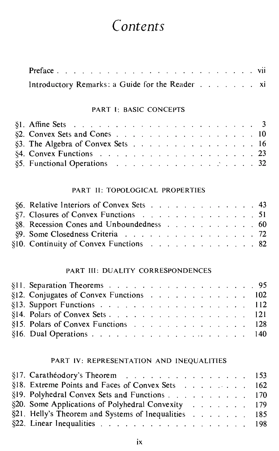
Contents
Preface vii
Introductory Remarks: a Guide for the Reader xi
PART i: BASIC CONCEPTS
§1. Affine Sets 3
§2. Convex Sets and Cones 10
§3. The Algebra of Convex Sets 16
§4. Convex Functions 23
§5. Functional Operations • .... 32
PART II: TOPOLOGICAL PROPERTIES
§6. Relative Interiors of Convex Sets 43
§7. Closures of Convex Functions 51
§8. Recession Cones and Unboundedness 60
§9. Some Closedness Criteria 72
§10. Continuity of Convex Functions 82
PART III: DUALITY CORRESPONDENCES
§11. Separation Theorems 95
§12. Conjugates of Convex Functions 102
§13. Support Functions 112
§14. Polars of Convex Sets 121
§15. Polars of Convex Functions 128
§16. Dual Operations 140
PART IV: REPRESENTATION AND INEQUALITIES
§17. Caratheodory's Theorem 153
§18. Extreme Points and Faces of Convex Sets 162
§19. Polyhedral Convex Sets and Functions 170
§20. Some Applications of Polyhedral Convexity 179
§21. Helly's Theorem and Systems of Inequalities 185
§22. Linear Inequalities 198
ix

X CONTENTS
PART V: DIFFERENTIAL THEORY
§23. Directional Derivatives and Subgradients 213
§24. Differential Continuity and Monotonicity 227
§25. Differentiability of Convex Functions 241
§26. The Legendre Transformation 251
PART VI: CONSTRAINED EXTREMUM PROBLEMS
§27. The Minimum of a Convex Function 263
§28. Ordinary Convex Programs and Lagrange Multipliers . . . 273
§29. Bifunctions and Generalized Convex Programs 291
§30. Adjoint Bifunctions and Dual Programs 307
§31. Fenchel's Duality Theorem 327
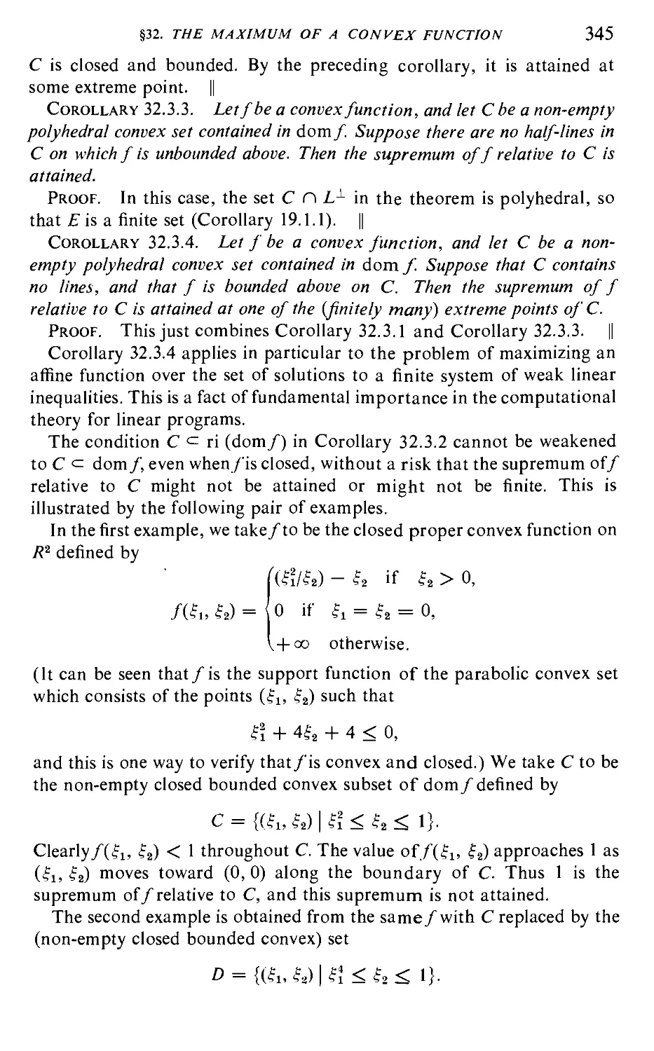
§32. The Maximum of a Convex Function 342
PART VII: SADDLE-FUNCTIONS AND MINIMAX THEORY
§33. Saddle-Functions 349
§34. Closures and Equivalence Classes 359
§35. Continuity and Differentiability of Saddle-functions .... 370
§36. Minimax Problems 379
§37. Conjugate Saddle-functions and Minimax Theorems .... 388
PART VIII: CONVEX ALGEBRA
§38. The Algebra of Bifunctions 401
§39. Convex Processes 413
Comments and References 425
Bibliography 433
Index 447

Introductory Remarks: A Guide
Jor the Reader
This book is not really meant to be read from cover to cover, even if
there were anyone ambitious enough to do so. Instead, the material is
organized as far as possible by subject matter; for example, all the pertinent
facts about relative interiors of convex sets, whether of major or minor
importance, are collected in one place (§6) rather than derived here and there
in the course of other developments. This type of organization may make it
easier to refer to basic results, at least after one has some acquaintance with
the subject, yet it can get in the way of a beginner using the text as an intro-
introduction. Logical development is maintained as the book proceeds, but in
many of the earlier sections there is a mass of lesser details toward the
end in which one could get bogged down.
Nevertheless, this book can very well be used as an introduction if one
makes an appropriate selection of material. The guidelines are given below,
where it is described just which results in each section are really essential
and which can safely be skipped over, at least temporarily, without causing
a gap in proof or understanding.
Part I: Basic Concepts
Convex sets and convex functions are denned here, and relationships
between the two concepts are discussed. The emphasis is on establishing
criteria for convexity. Various useful examples are given, and it is shown
how further examples can be generated from these by means of operations
such as addition or taking convex hulls.
The fundamental idea to be understood is that the convex functions on
Rn can be identified with certain convex subsets of Rn+1 (their epigraphs),
while the convex sets in Rn can be identified with certain convex functions
on Rn (their indicators). These identifications make it easy to pass back
and forth between a geometric approach and an analytic approach.
Ordinarily, in dealing with functions one thinks geometrically in terms of
the graphs of the functions, but in the case of convex functions pictures
of epigraphs should be kept in mind instead.
Most of the material, though elementary, is basic to the rest of the book,
but some parts should be left out by a reader who is encountering the
subject for the first time. Although only linear algebra is involved in §1

Xll INTRODUCTORY REMARKS
(Affine Sets), the concepts may not be entirely familiar; §1 should therefore
be perused up through the definition of barycentric coordinate systems
(preceding Theorem 1.6) as background for the introduction of convexity.
The remainder of §1, concerning affine transformations, is not crucial to a
beginner's understanding. All of §2 (Convex Sets and Cones) is essential
and the first half of §3, but the second half of §3, starting with Theorem 3.5,
deals with operations of minor significance. Very little should be skipped
in §4 (Convex Functions) except some of the examples. However, the end
of §5 (Functional Operations), following Theorem 5.7, is not needed in any
later section.
Part II: Topological Properties
The properties of convexity considered in Part I are primarily algebraic:
it is shown that convex sets and functions form classes of objects which
are preserved under numerous operations of combination and generation.
In Part II, convexity is considered instead in relation to the topological
notions of interior, closure, and continuity.
The remarkably uncomplicated topological nature of convex sets and
functions can be traced to one intuitive fact: if a line segment in a convex
set C has one endpoint in the interior of C and the other endpoint on the
boundary of C, then all the intermediate points of the line segment lie in
the interior of C. A concept of "relative" interior can be introduced, so
that this fact can be used as a basic tool even in situations where one has to
deal with configurations of convex sets whose interiors are empty. This is
discussed in §6 (Relative Interiors of Convex Sets). The principal results
which every student of convexity should know are embodied in the first
four theorems of §6. The rest of §6, starting with Theorem 6.5, is devoted
mainly to formulas for the relative interiors of convex sets constructed
from other convex sets in various ways. A number of useful results are
established (particularly Corollaries 6.5.1 and 6.5.2, which are cited often
in the text, and Corollary 6.6.2, which is employed in the proof of an
important separation theorem in §11), but these can all be neglected
temporarily and referred to as the need arises.
In §7 (Closures of Convex Functions) the main topic is lower semi-
continuity. This property is in many ways more important than continuity
in the case of convex functions, because it relates directly to epigraphs:
a function is lower semi-continuous if and only if its epigraph is closed.
A convex function which is not already lower semi-continuous can be made
so simply by redefining its values (in a uniquely determined manner) at
certain boundary points of its effective domain. This leads to the notion
of the closure operation for convex functions, which corresponds to the
closure operation for epigraphs (as subsets of Rn+1) when the functions are

INTRODUCTORY REMARKS Xlll
proper. All of §7, with the exception of Theorem 7.6, is essential if one is to
understand what follows.
All of §8 (Recession Cones and Unboundedness) is also needed in the
long run, although the need is not as ubiquitous as in the case of §6 and
§7. The first half of §8 elucidates the idea that unbounded convex sets are
just like bounded convex sets, except that they have certain "points at
infinity." The second half of §8 applies this idea to epigraphs to obtain
results about the growth properties of convex functions. Such properties
are important in formulating a number of basic existence theorems
scattered throughout the book, the first ones occurring in §9 (Some
Closedness Criteria).
The question which §9 attempts to answer is this: when is the image of a
closed convex set under a linear transformation closed? It turns out that
this question is fundamental in investigations of the existence of solutions
to various extremum problems. The principal results of §9 are given in
Theorems 9.1 and 9.2 (and their corollaries). The reader would do well,
however, to skip §9 entirely on the first encounter and return to it later, if
desired, in connection with applications in §16.
Only the first theorem of §10 (Continuity of Convex Functions) is basic
to convex analysis as a whole. The fancier continuity and convergence
theorems are a culmination in themselves. They are used only in §24 and
§25 to derive continuity and convergence theorems for subdifferentials
and gradient mappings of convex functions, and in §35 to derive similar
results in the case of saddle-functions.
Part III: Duality Correspondences
Duality between points and hyperplanes has an important role to play
in much of analysis, but nowhere perhaps is the role more remarkable
than in convex analysis. The basis of duality in the theory of convexity is,
from a geometric point of view, the fact that a closed convex set is the
intersection of all the closed half-spaces which contain it. From the point
of view of functions, however, it is the fact that a closed convex function
is the pointwise supremum of all the affine functions which minorize it.
These two facts are equivalent when regarded in terms of epigraphs, and a
geometric formulation is usually preferable for the sake of intuition, but
in this case both formulations are important. The second formulation of
the basis of duality has the advantage that it leads directly to a symmetric
one-to-one duality correspondence among closed convex functions, the
conjugacy correpsondence of Fenchel.
Conjugacy contains, as a special case in a certain sense, a symmetric
one-to-one correspondence among closed convex cones (polarity), but

XIV INTRODUCTORY REMARKS
it has no symmetric counterpart in the class of general closed convex sets.
The analogous correspondence in the latter context is between convex
sets on the one hand and positively homogeneous convex functions (their
support functions) on the other. For this reason it is often better in applica-
applications, as far as duality is concerned, to express a given situation in terms of
convex functions, rather than convex sets. Once this is done, geometric
reasoning can still be applied, of course, to epigraphs.
The foundations for the theory of duality are laid in §11 (Separation
Theorems). All of the material in this section, except Theorem 11.7, is
essential. In §12 (Conjugates of Convex Functions), the conjugacy corre-
correspondence is defined, and a number of examples of corresponding func-
functions are given. Theorems 12.1 and 12.2 are the fundamental results which
should be known; the rest of §12 is dispensible.
Conjugacy is applied in §13 (Support Functions) to produce results
about the duality between convex sets and positively homogeneous convex
functions. The support functions of the effective domain and level sets of a
convex function / are calculated in terms of the conjugate function /*
and its recession function. The main facts are stated in Theorems 13.2,
13.3, and 13.5, the last two presupposing familiarity with §8. The other
theorems, as well as all the corollaries, can be skipped over and referred to
if and when they are needed.
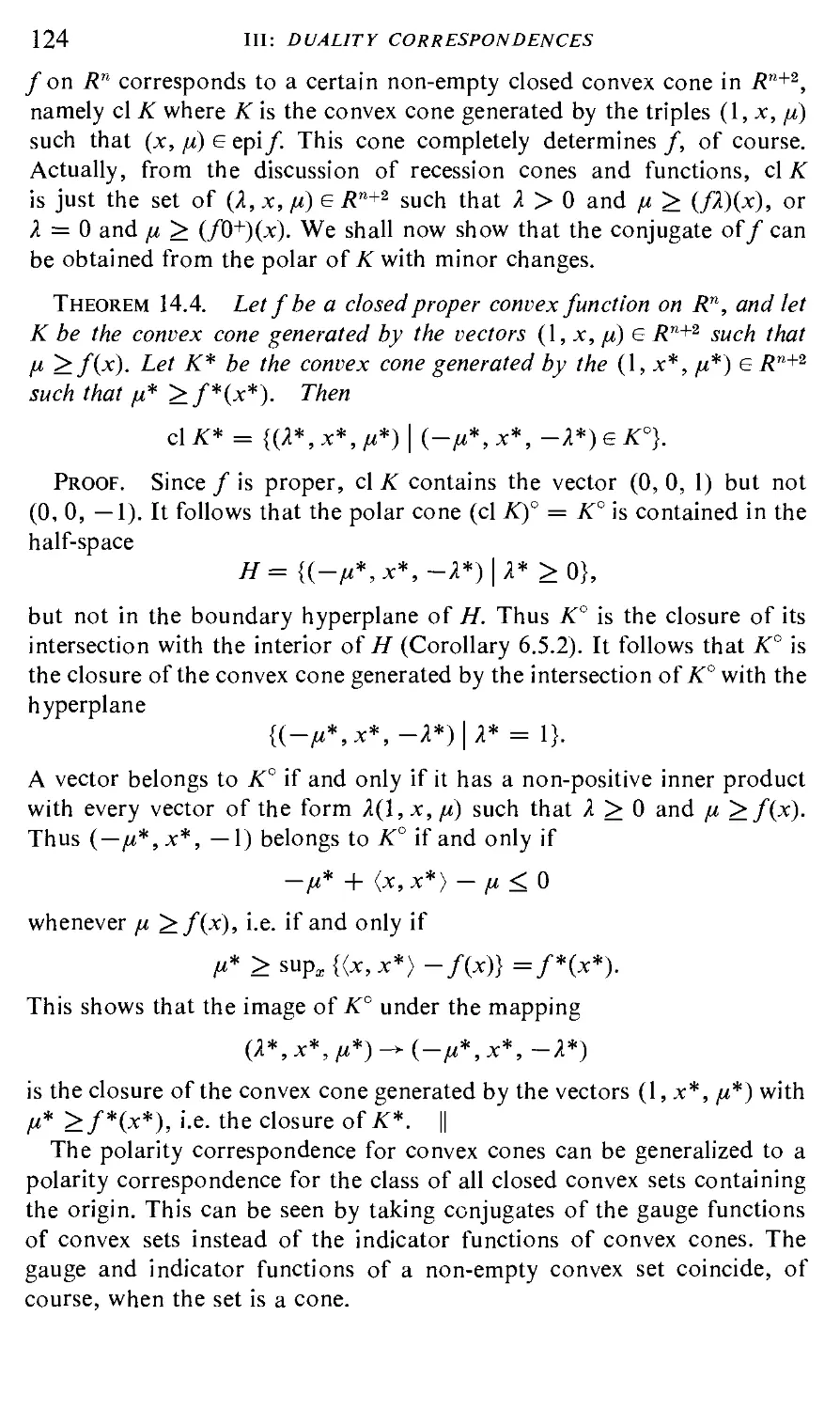
In §14 (Polars of Convex Sets), the conjugacy correspondence for con-
convex functions is specialized to the polarity correspondence for convex
cones, whereupon the latter is generalized to the polarity correspondence
for arbitrary closed convex sets containing the origin. Polarity of convex
cones has several applications elsewhere in this book, but the more general
polarity is not mentioned subsequently, except in §15 (Polars of Convex
Functions), where its relationship with the theory of norms is discussed.
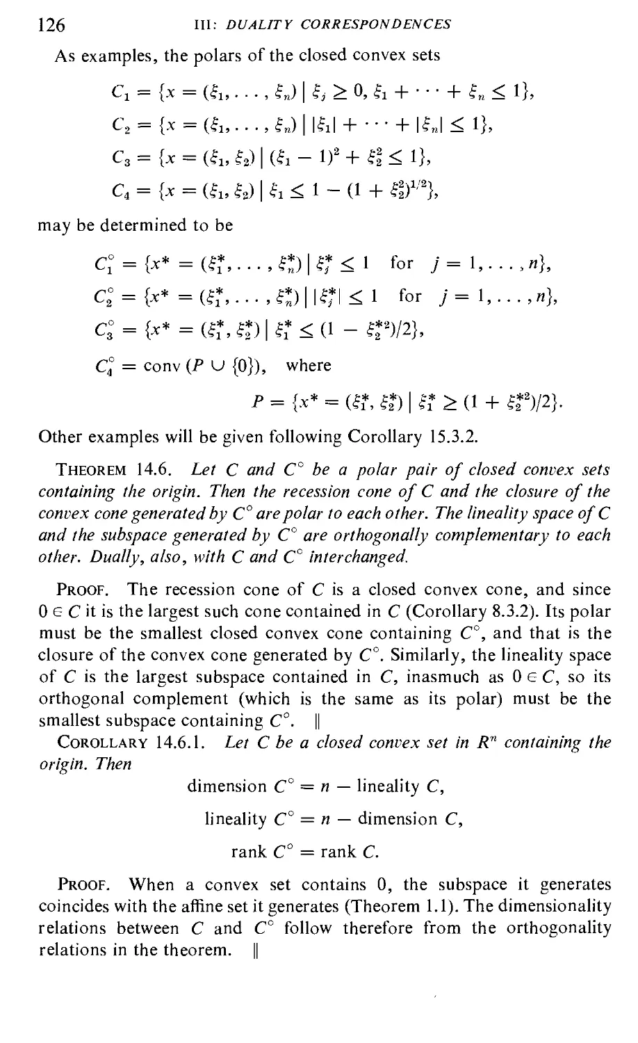
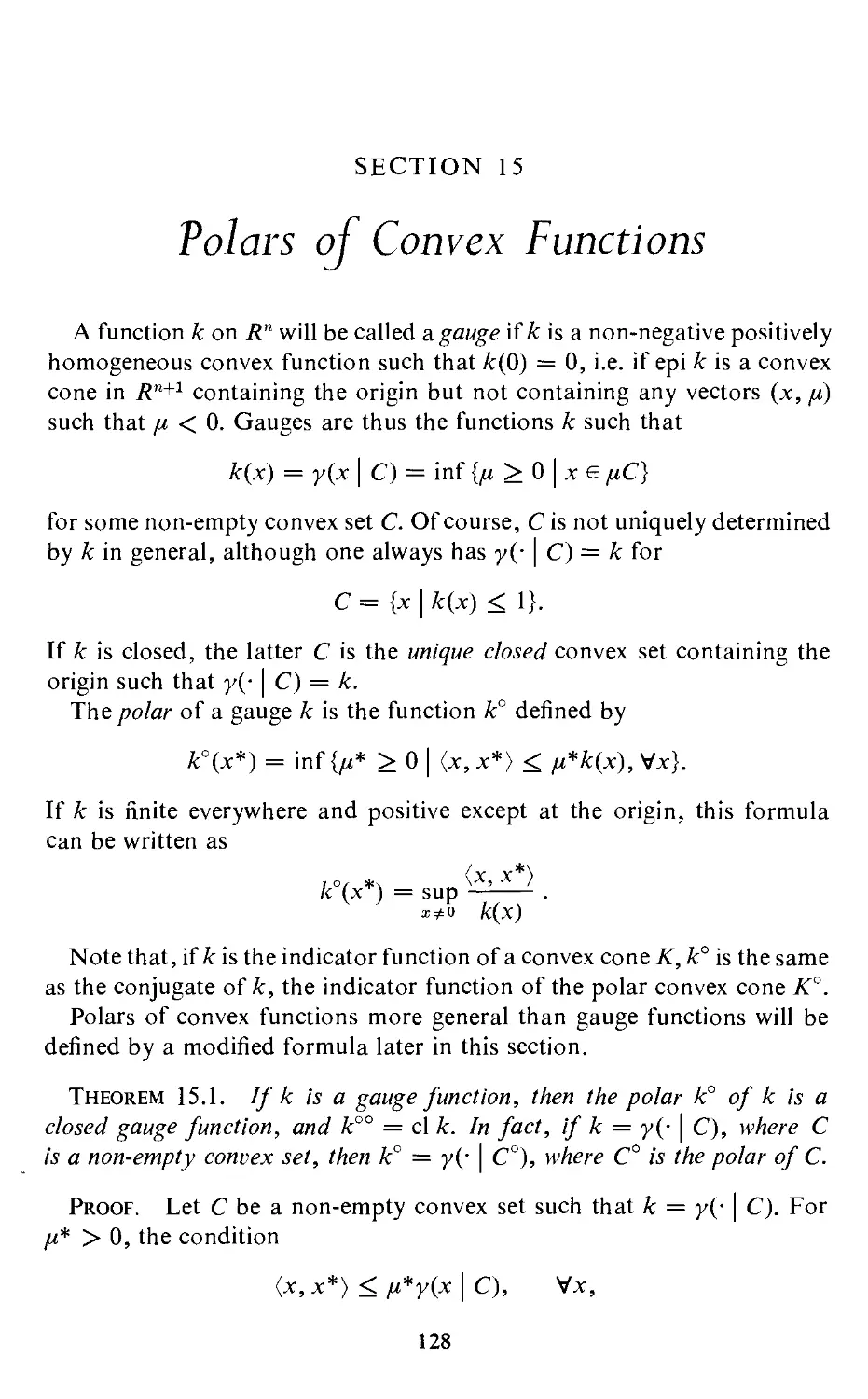
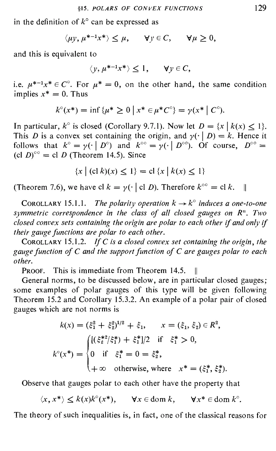
The purpose of §15, besides the development of Minkowski's duality
correspondence for norms and certain of its generalizations, is to provide
(in Theorem 15.3 and Corollary 15.3.1) further examples of conjugate con-
convex functions. However, of all of §14 and §15, it would suffice, as long as
one was not specifically interested in approximation problems, to read
merely Theorem 14.1.
The theorems of §16 (Dual Operations) show that the various functional
operations in §5 fall into dual pairs with respect to the conjugacy corre-
correspondence. The most significant result is Theorem 16.4, which describes
the duality between addition and infimal convolution of convex functions.
This result has important consequences for systems of inequalities (§21)
and the calculus of subgradients (§23), and therefore for the theory of
extremum problems in Part VI. The second halves of Theorems 16.3,
16.4, and 16.5 (which give conditions under which the respective minima

INTRODUCTORY REMARKS XV
are attained and the closure operation is not needed in the duality formulas)
depend on §9. This much of the material could be omitted on a first reading
of §16, along with Lemma 16.2 and all corollaries.
Part IV: Representation and Inequalities
The objective here is to obtain results about the representation of convex
sets as convex hulls of sets of points and directions, and to apply these
results to the study of systems of linear and nonlinear inequalities. Most
of the material concerns refinements of convexity theory which take special
advantage of dimensionality or the presence of some degree of linearity.
The reader could skip Part IV entirely without jeopardizing his under-
understanding of the remainder of this book. Or, as a compromise, only the more
fundamental material in Part IV, as indicated below, could be covered.
The role of dimensionality in the generation of convex hulls is explored in
§17 (Caratheodory's Theorem), the principal facts being given in Theorems
17.1 and 17.2. Problems of representing a given convex set in terms
of extreme points, exposed points, extreme directions, exposed directions,
and tangent hyperplanes are taken up in §18 (Extreme Points and Faces
of Convex Sets). All of §18 is put to use in §19 (Polyhedral Convexity);
applications also occur in the study of gradients (§25) and in the maximiza-
maximization of convex functions (§32). The most important results in §19 are
Theorems 19.1, 19.2, 19.3, and their corollaries.
In §20 (Some Applications of Polyhedral Convexity), it is shown how
certain general theorems of convex analysis can be strengthened in the
case where some, but not necessarily all, of the convex sets or functions
involved are polyhedral. Theorems 20.1 and 20.2 are used in §21 to establish
relatively difficult refinements of Helly's Theorem and certain other
results which are applicable in §27 and §28 to the existence of Lagrange
multipliers and optimal solutions to convex programs. Theorem 20.1
depends on §9, although Theorem 20.2 does not. However, it is possible
to understand the fundamental results of §21 (Helly's Theorem and Systems
of Inequalities) and their proofs without knowledge of §20, or even of §18
or §19. In this case one should simply omit Theorems 21.2, 21.4, and
21.5.
Finite systems of equations and linear inequalities, weak or strict, are
the topic in §22 (Linear Inequalities). The results are special, and they are
not invoked anywhere else in the book. At the beginning, various facts are
stated as corollaries of fancy theorems in §21, but then it is demonstrated
that the same special facts can be derived, along with some improvements,
by an elementary and completely independent method which uses only
linear algebra and no convexity theory.

XVI INTRODUCTORY REMARKS
Part V: Differential Theory
Supporting hyperplanes to convex sets can be employed in situations
where tangent hyperplanes, in the sense of the classical theory of smooth
surfaces, do not exist. Similarly, subgradients of convex functions, which
correspond to supporting hyperplanes to epigraphs rather than tangent
hyperplanes to graphs, are often useful where ordinary gradients do not
exist.
The theory of subdifferentiation of convex functions, expounded in §23
(Directional Derivatives and Subgradients), is a fundamental tool in the
analysis of extremum problems, and it should be mastered before proceed-
proceeding. Theorems 23.6, 23.7, 23.9, and 23.10 may be omitted, but one should
definitely be aware of Theorem 23.8, at least in the non-polyhedral case
for which an alternative and more elementary proof is given. Most of §23 is
independent of Part IV.
The main result about the relationship between subgradients and ordi-
ordinary gradients of convex functions is established in Theorem 25.1, which
can be read immediately following §23. No other result from §24, §25,
or §26 is specifically required elsewhere in the book, except in §35, where
analogous theorems are proved for saddle-functions. The remainder of
Part V thus serves its own purpose.
In §24 (Differential Continuity and Monotonicity), the elementary theory
of left and right derivatives of closed proper convex functions of a single
variable is developed. It is shown that the graphs of the subdifferentials of
such functions may be characterized as "complete non-decreasing curves."
Continuity and monoticity properties in the one-dimensional case are then
generalized to the n-dimensional case.
Aside from the theorem already referred to above, §25 (Differentiability
of Convex Functions) is devoted mainly to proving that, for a finite
convex function on an open set, the ordinary gradient mapping exists
almost everywhere and is continuous. The question of when the gradient
mapping comprises the entire subdifferential mapping, and when it is
actually one-to-one, is taken up in §26 (The Legendre Transformation).
The central purpose of §26 is to explain the extent to which conjugate
convex functions can, in principle, be calculated in a classical manner by
inverting a gradient mapping. The duality between smoothness and strict
convexity is also discussed. The development in §25 and §26 depends to
some extent on §18, but not on any sections of Part IV following §18.
Part VI: Constrained Extremum Problems
The theory of extremum problems is, of course, the source of motivation
for many of the results in this book. It is in §27 (The Minimum of a Convex

INTRODUCTORY REMARKS XV11
Function) that applications to this theory are begun in a systematic way.
The stage is set by Theorem 27.1, which summarizes some pertinent facts
proved in earlier sections. All the theorems of §27 concern the manner in
which a convex function attains its minimum relative to a given convex
set, and all should be included in a first reading, except perhaps for refine-
refinements which take advantage of polyhedral convexity.
Problems in which a convex function is minimized subject to a finite
system of convex inequalities are studied in §28 (Ordinary Convex Pro-
Programs and Lagrange Multipliers). The emphasis is on the existence, inter-
interpretation, and characterization of certain vectors of Lagrange multipliers,
called Kuhn-Tucker vectors. The text may be simplified somewhat by
deleting the provisions for linear equation constraints, and Theorem 28.2
may be replaced by its special case Corollary 28.2.1 (which has a much
easier proof), but beyond this nothing other than examples ought to be
omitted.
The theory of Lagrange multipliers is broadened and in some ways
sharpened in §29 (Bifunctions and Generalized Convex Programs). The
concept of a convex bifunction, which can be regarded as an extension of
that of a linear transformation, is used to construct a theory of perturba-
perturbations of minimization problems. Generalized Kuhn-Tucker vectors measure
the effects of the perturbations. Theorems 29.1, 29.3, and their corollaries
contain all the facts needed in the sequel.
In §30 (Adjoint Bifunctions and Dual Programs) the duality theory of
extremum problems is set forth. Practically everything up through Theorem
30.5 is fundamental, but the remainder of §30 consists of examples and
may be truncated as desired. Duality theory is continued in §31 (Fenchel's
Duality Theorem). The primary purpose of §31 is to furnish additional
examples interesting for their applications. Later sections do not depend on
the material in §31, except for §38.
Results of a rather different character are described in §32 (The Maximum
of a Convex Function). The proofs of these results involve none of the
preceding sections of Part VI, but familiarity with §18 and §19 is required.
No subsequent reference is made to §32.
Part VII: Saddle-functions and Minimax Theory
Saddle-functions are functions which are convex in some variables and
concave in others, and the extremum problems naturally associated with
them involve "minimaximization," rather than simple minimization or
maximization. The theory of such minimax problems can be developed by
much the same approach as in the case of minimization of convex functions.
It turns out that the general minimax problems for (suitably regularized)
saddle-functions are precisely the Lagrangian saddle-point problems

XV111 INTRODUCTORY REMARKS
associated with generalized (closed) convex programs. Understandably,
therefore, convex bifunctions are central to the discussion of saddle-
functions, and the reader should not proceed without already being
familiar with the basic ideas in §29 and §30.
Saddle-functions on Rm x jR" correspond to convex bifunctions from
Rm to Rn in much the same way that bilinear functions on Rm X Rn cor-
correspond to linear transformations from Rm to Rn. This is the substance of
§33 (Saddle-functions). In §34 (Closures and Equivalence Classes), certain
closure operations for saddle-functions similar to the one for convex
functions are studied. It is shown that each finite saddle-function defined on
a product of convex sets in Rm x Rn determines a unique equivalence
class of closed saddle-functions defined on all of R'" x R'\ but one does
not actually have to read up on the latter fact (embodied in Theorems
34.4 and 34.5) before passing to minimax theory itself.
The results about saddle-functions proved in §35 (Continuity and Differ-
Differentiability) are mainly analogues or extensions of results about convex
functions in §10, §24, and §25, and they are not a prerequisite for what
follows.
Saddle-points and saddle-values are discussed in §36 (Minimax
Problems). It is then explained how the study of these can be reduced to the
study of convex and concave programs dual to each other. Existence theo-
theorems for saddle-points and saddle-values are then derived in §37 (Conjugate
Saddle-functions and Minimax Theorems) in terms of a conjugacy corre-
correspondence for saddle-functions and the "inverse" operation for bifunctions.
Part VIII: Convex Algebra
The analogy between convex bifunctions and linear transformations,
which features so prominently in Parts VI and VII, is "pursued further in
§38 (The Algebra of Bifunctions). "Addition" and "multiplication" of
bifunctions are studied in terms of a generalized notion of inner product
based on Fenchel's Duality Theorem. It is a remarkable and non-trivial
fact that such natural operations for bifunctions are preserved, as in linear
algebra, when adjoints are taken.
The results about bifunctions in §38 are specialized in §39 (Convex
Processes) to a class of convex-set-valued mappings which are even more
analogous to linear transformations.

Part 1 • Basic Concepts

SECTION 1
Affine Sets
Throughout this book, R denotes the real number system, and Rn is the
usual vector space of real w-tuples x = (|1; . . . , £„). Everything takes
place in Rn unless otherwise specified. The inner product of two vectors
x and x* in Rn is expressed by
(x, x*) = £,£? + • • • + ij*n
The same symbol A is used to denote an m x n real matrix A and the
corresponding linear transformation x -*■ Ax from Rn to Rm. The transpose
matrix and the corresponding adjoint linear transformation from Rm
to R" are denoted by A*, so that one has the identity
(Ax,y*) = (x,A*y*).
(In a symbol denoting a vector, * has no operational significance; all
vectors are to be regarded as column vectors for purposes of matrix
multiplication. Vector symbols involving * are used from time to time
merely to bring out the familiar duality between vectors considered as
points and vectors considered as the coefficient n-tuples of linear functions.)
The end of a proof is signalled by ||.
If x and y are different points in Rn, the set of points of the form
A — X)x + ly = x + X{y — x), Xe R,
is called the line through x andy. A subset M of Rn is called an affine set
if A — X)x + ly e M for every x e M, y e M and X e R. (Synonyms for
"affine set" used by other authors are "affine manifold," "affine variety,"
"linear variety" or "flat.")
The empty set 0 and the space Rn itself are extreme examples of affine
sets. Also covered by the definition is the case where M consists of a
solitary point. In general, an affine set has to contain, along with any
two different points, the entire line through those points. The intuitive
picture is that of an endless uncurved structure, like a line or a plane in
space.
The formal geometry of affine sets may be developed from the theorems
of linear algebra about subspaces of/?". The exact correspondence between
affine sets and subspaces is described in the two theorems which follow.

4 I: BASIC CONCEPTS
Theorem 1.1. The subspaces of Rn are the affine sets which contain the
origin.
Proof. Every subspace contains 0 and, being closed under addition and
scalar multiplication, is in particular an affine set.
Conversely, suppose M is an affine set containing 0. For any xeM
and X £ R, we have
Xx = A - AH + Xx e M,
so M is closed under scalar multiplication. Now, if x e M and y e M, we
have
|(jr + y) = lx + A - h)y e M,
and hence
x+y = 2(i(* + y)) e A/.
Thus M is also closed under addition and is a subspace. ||
For M <= Rn and a e R", the translate of M by a is defined to be the set
M + a — {x + a\x€ M).
A translate of an affine set is another affine set, as is easily verified.
An affine set M is said to be parallel to an affine set L if M = L + a for
some a. Evidently "M is parallel to L" is an equivalence relation on the
collection of affine subsets of Rn. Note that this definition of parallelism
is more restrictive than the everyday one, in that it does not include the
idea of a line being parallel to a plane. One has to speak of a line which is
parallel to another line within a given plane, and so forth.
Theorem 1.2. Each non-empty affine set M is parallel to a unique
subspace L. This L is given by
L=M-M={x-y\xeM,yeM}.
Proof. Let us show first that M cannot be parallel to two different
subspaces. Subspaces Lx and L2 parallel to M would be parallel to each
other, so that L2 = Lx + a for some a. Since 0 e L2, we would then have
—a e Lu and hence a e Lv But then Lx => Lx + a = L2. By a similar
argument L2 => Lu so Lt = L2. This establishes the uniqueness. Now
observe that, for any y e M, M — y — M + (—y) is a translate of M
containing 0. By Theorem 1.1 and what we have just proved, this affine
set must be the unique1 subspace L parallel to M. Since L = M — y no
matter which y e M is chosen, we actually have L = M — M. \\
The dimension of a non-empty affine set is defined as the dimension of
the subspace parallel to it. (The dimension of 0 is —1 by convention.)
Naturally, affine sets of dimension 0, 1 and 2 are called points, lines and
planes, respectively. An (« — l)-dimensional affine set in Rn is called a

§1. AFFINE SETS 5
hyperplane. Hyperplanes are very important, because they play a role dual
to the role of points in n-dimensional geometry.
Hyperplanes and other affine sets may be represented by linear functions
and linear equations. It is easy to deduce this from the theory of orthog-
orthogonality in Rn. Recall that, by definition, x ± y means (x,y) = 0. Given a
subspace L of R", the set of vectors x such that x _|_ L, i.e. x _]_ y for
every y e L, is called the orthogonal complement of L, denoted L- . It is
another subspace, of course, and
dim L + dim L1 = n.
The orthogonal complement (LL)L of L1 is in turn L. If bx, . . . , bm is a
basis for L, then illis equivalent to the condition that x _L bu . . . ,
x _L bm. In particular, the (n — l)-dimensional subspaces of Rn are the
orthogonal complements of the one-dimensional subspaces, which are the
subspaces L having a basis consisting of a single non-zero vector b (unique
up to a non-zero scalar multiple). Thus the (n — l)-dimensional subspaces
are the sets of the form {x \ x _|_ b), where b ^ 0. The hyperplanes are the
translates of these. But
{.v | a- _L b) + a = {x + a | (x, b) = 0}
= {y | (y - a, b) = 0} = {y \ (y, b) = ft,
where /S = (a, b). This leads to the following characterization of hyper-
hyperplanes.
Theorem 1.3. Given ft e R and a non-zero b e Rn, the set
H = {x | <jc, b) = /?}
is a hyperplane in Rn. Moreover, every hyperplane may be represented in
this way, with b and fi unique up to a common non-zero multiple.
In Theorem 1.3, the vector b is called a normal to the hyperplane H.
Every other normal to //is either a positive or a negative scalar multiple of
b. A good interpretation of this is that every hyperplane has "two sides,"
like one's picture of a line in R2 or a plane in R3. Note that a plane in R*
would not have "two sides," any more than a line in R3 has.
The next theorem characterizes the affine subsets of Rn as the solution
sets to systems of simultaneous linear equations in n variables.
Theorem 1.4. Given b e Rm and an m x n real matrix B, the set
M ={xeRn\ Bx = b}
is an affine set in Rn. Moreover, every affine set may be represented in this
way.

I: BASIC CONCEPTS
Proof. If x e M, y e M and X e R, then for z = A — X)x + Aj one
has
Bz = A - AM* + ^j = A - X)b + AZ> = b,
so z e M. Thus the given Af is affine.
On the other hand, starting with an arbitrary non-empty affine set M
other than Rn itself, let L be the subspace parallel to M. Let bx, .. . , bm
be a basis for L1. Then
L = (L1I = {* | x _L fcx,. .. , x ± bm}
= {x | <x, fc<> = 0, / = 1,. . ., rn} = {x | Bx = 0},
where -B is the m x n matrix whose rows are bx, . . . , bm. Since M is
parallel to L, there exists an a e Rn such that
Af = L + a = {* | B(x - a) = 0} = {x \ Bx = b},
where b = Ba. (The affine sets i?" and 0 can be represented in the form in
the theorem by taking B to be the m X n zero matrix, say, with b = 0
in the case of Rn and b ^ 0 in the case of 0.) ||
Observe that in Theorem 1.4 one has
M = {x | <.x, ftt> = ft, i = 1, . . . , m} = nSLi Ht,
where ft, is the zth row of B, ft is the ith component of b, and
Ht = [x | (x, tf) = ft}.
Each //, is a hyperplane (Z>4 ?^ 0), or the empty set (bf = 0, ft 5^ 0), or
Rn (b( = 0, ft = 0). The empty set may itself be regarded as the inter-
intersection of two different parallel hyperplanes, while Rn may be regarded
as the intersection of the empty collection of hyperplanes of Rn. Thus:
Corollary 1.4.1. Every affine subset of Rn is an intersection of a
finite collection of hyperplanes.
The affine set Min Theorem 1.4 can be expressed in terms of the vectors
b[, . . . , b'n which form the columns of B by
M = {x = (Su . . . , fn) I StK + ■>■ + £nb'n = b}.
Obviously, the intersection of an arbitrary collection of affine sets is
again affine. Therefore, given any S c Rn there exists a unique smallest
affine set containing S (namely, the intersection of the collection of affine
sets M such that M => S). This set is called the affine hull of S and is
denoted by aff S. It can be proved, as an exercise, that aff S consists of all
the vectors of the form Xxxx + • • • + Xmxm, such that x(e S and
Xx+--- +Xm=l.
A set of m + 1 points b0, bx, . . . , bm is said to be affinely independent

§!. AFFINE SETS 7
if aff{60, bu . . . , bm} is /w-dimensional. Of course
aff {b0, bu . . . , bm} = L + b0,
where
L = a.ff{O,bl-bo,...,bm-bo}.
By Theorem 1.1, L is the same as the smallest subspace containing bx —
b0, . . . , bm — b0. Its dimension is m if and only if these vectors are linearly
independent. Thus b0, bx, . . . ,bm are affinely independent if and only if
bx — b0, . . . , bm — b0 are linearly independent.
All the facts about linear independence can be applied to affine
independence in the obvious way. For instance, any affinely independent
set of m + 1 points in Rn can be enlarged to an affinely independent set
of n + 1 points. An m-dimensional affine set M can be expressed as the
affine hull of m + 1 points (translate the points which correspond to a
basis of the subspace parallel to M).
Note that, if M = aff{60, bx, . . . , bm}, the vectors in the subspace L
parallel to M are the linear combinations of bx — b0, . . . , bm — b0. The
vectors in M are therefore those expressible in the form
x = Xx(bY - b0) + ■ ■ ■ + Xm{bm - b0) + bg,
i.e. in the form
x = Xobo + Xxbx + ■ ■ ■ + Xmbm, l0 + ;.j + • ■ • + Xm = 1.
The coefficients in such an expression of x are unique if and only if b0,
bx, .. . , bm are affinely independent. In that event, Xo, A1; . . . , Xm, as
parameters, define what is called a barycentric coordinate system for M.
A single-valued mapping T:x -> Tx from Rn to Rm is called an affine
transformation if
7XA - X)x + Xy) = A - X)Tx + XTy
for every x and y in Rn and X e R.
Theorem 1.5. The affine transformations from Rn to Rm are the mappings
T of the form Tx = Ax + a, where A is a linear transformation and a e Rm.
Proof. If T is affine, let a = TO and Ax = Tx — a. Then A is an
affine transformation with ^0 = 0. A simple argument resembling the
one in Theorem 1.1 shows that A is actually linear.
Conversely, if Tx = Ax + a where A is linear, one has
7XA - X)x + Xy) = A - X)Ax + XAy + a = A - X)Tx + XTy.
Thus T is affine. ||
The inverse of an affine transformation, if it exists, is affine.

8 I: BASIC CONCEPTS
As an elementary exercise, one can demonstrate that if a mapping T
from Rn to Rm is an affine transformation the image set TM = {Tx | x e M}.
is affine in Rm for every affine set M in Rn. In particular, then, affine
transformations preserve affine hulls:
aff (TS) = T
Theorem 1.6. Let {b0, bu . . . , bj and {b'o, b\, . . . , b'm) be affinely
independent sets in Rn. Then there exists a one-to-one affine transformation
T of Rn onto itself, such that Tbt = b\for i = 0, . . . , m. Ifm = n, T is
unique.
Proof. Enlarging the given affinely independent sets if necessary, we
can reduce the question to the case where m = n. Then, as is well known in
linear algebra, there exists a unique one-to-one linear transformation A
of Rn onto itself carrying the basis bx — b0, . . . , bn — b0 of Rn onto the
basis b'x — b'o,. . . , b'n — b'o. The desired affine transformation is then
given by Tx = Ax + a, where a = b'o — Ab0. \\
Corollary 1.6.1. Let Mx and M2 be any two affine sets in R" of the
same dimension. Then there exists a one-to-one affine transformation T of
Rn onto itself such that TMX = M2.
Proof. Any w-dimensional affine set can be expressed as the affine
hull of an affinely independent set of am + 1 points, and affine hulls are
preserved by affine transformations. ||
The graph of an affine transformation T from Rn to R is an affine
subset of Rn+m. This follows from Theorem 1.4, for if Tx = Ax + a the
graph of T consists of the vectors z = (x,y), x e Rn and y e Rm, such
that Bz = b, where b = —a and B is the linear transformation (x, y) —»
Ax - y from Rn+m to Rm.
In particular, the graph of a linear transformation x —*■ Ax from Rn to
Rm is an affine set containing the origin of R"+m, and hence it is a certain
subspace L of Rn+m (Theorem 1.1). The orthogonal complement of L is
then given by
L1 = {(x*, y*) | x* e R", y* e Rm, x* = -A*y*},
i.e. L1 is the graph of —A*. Indeed, z* = (x*,y*) belongs to L1 if and
only if
0=(z,z*) = {x,x*) + {y,y*)
for every z = (x,y) with y = Ax. In other words, (x*,y*) eLx if and
only if
0 = (x, x*} + (Ax,y*) = (x, x*) + (x, A*y*} = (x, x* + A*y*)
for every x e Rn. That means x* + A*y* = 0, i.e. x* = —A*y*.

§1. A FFINE SETS 9
Any non-trivial affine set can be represented in various ways as the graph
of an affine transformation. Let M be an n-dimensional affine set in RN
with 0 < n < N. First of all, one can express M as the set of vectors
x = (i1,.. . , £v) whose coordinates satisfy a certain linear system of
equations,
Pa£i + ■•• +Pi.\$x = Pt, i=l,...,fc.
This is always possible, according to Theorem 1.4. The ^-dimensionality
of M means that the coefficient matrix B = (j3w) has nullity n and rank
m = N — n. One can therefore solve the system of equations for
£^,.. . , fy in terms of £7, . . . , fs, where I,... , N is some permutation
of the indices 1, . . . , N. One obtains then a system of the special form
%—i = <*ah + • • ■ + *in£r, + a*> / = 1, . . . , w,
which again gives a necessary and sufficient condition for a vector x =
(fi, . . . , I v) to belong to M. This system is called a Tucker representation
of the given affine set. It expresses M as the graph of a certain affine
transformation from Rn to /?m. There are only finitely many Tucker
representations of M (at most N\, corresponding to the various ways m
of the coordinate variables f, of vectors in M can be expressed in terms of
the other n coordinate variables in some particular order).
Often a theorem involving an affine set can be interpreted as a theorem
about "linear systems of variables," in the sense that the affine set may be
given a Tucker representation. This is important, for example, in certain
results in the theory of linear inequalities (Theorems 22.6 and 22.7) and in
certain applications of Fenchel's Duality Theorem (Corollary 31.4.2).
The Tucker representations of a subspace L are, of course, of the homo-
homogeneous form
£~i = a»i£l + " " ' + a«nf«> i=\, . . . ,m.
Given such a representation of L as the graph of a linear transformation,
we know, as pointed out above, that LL corresponds to the graph of the
negative of the adjoint transformation. Thus x* = (If, . . . , £*) belongs
to LL if and only if
-I* = !£n<xly + • • • + l^am3, j = 1, • • • , n.
This furnishes a Tucker representation of L1. Thus there is a simple and
useful one-to-one correspondence between the Tucker representations of
a given subspace and those of its orthogonal complement.

SECTION 2
Convex Sets and Cones
A subset C of Rn is said to be convex if A — X)x + Xy e C whenever
x 6 C, y e C and 0 < A < 1. All affine sets (including 0 and /?" itself) are
convex. What makes convex sets more general than affine sets is that they
only have to contain, along with any two distinct points x and y, a certain
portion of the line through x and y, namely
{A - X)x + A>'|0< X < 1}.
This portion is called the (closed) line segment between x and y. Solid
ellipsoids and cubes in i?3, for instance, are convex but not affine.
Half-spaces are important examples of convex sets. For any non-zero
b e Rn and any /J e R, the sets
{x | (x, b) < 0}, {x | (x, b) > /}},
are called closed half-spaces. The sets
{x\{x,b)<($}, {x\(x,b)>p},
are called open half-spaces. All four sets are plainly non-empty and convex.
Notice that the same quartet of half-spaces would appear if b and 0 were
replaced by Xb and Xft for some A^O. Thus these half-spaces depend only
on the hyperplane H = {x | (x, b) = /?} (Theorem 1.3). One may speak
unambiguously, therefore, of the open and closed half-spaces correspond-
corresponding to a given hyperplane.
Theorem 2.1. The intersection of an arbitrary collection of convex sets
is convex.
Proof. Elementary. ||
Corollary 2.1.1. Let bt e Rn and ^eRfor i e I, where I is an
arbitrary index set. Then the set
C = {x e Rn | (x, bt) < &, V/ e /}
is convex.
Proof. Let Ct = {x | (x, bt) < /SJ. Then Ct is a closed half-space or
Rn or 0 and C = f)ieI C,-. ||
10

§2. CONVEX SETS AND CONES 11
The conclusion of the corollary would still be valid, of course, if some
of the inequalities < were replaced by >, >, < or =. Thus, given any
system of simultaneous linear inequalities and equations in n variables, the
set C of solutions is a convex set in Rn. This is a significant fact both in
theory and in applications.
Corollary 2.1.1 will be generalized by Corollary 4.6.1.
A set which can be expressed as the intersection offinitely many closed
half spaces of Rn is called a polyhedral convex set. Such sets are con-
considerably better behaved than general convex sets, mostly because of their
lack of "curvature." The special theory of polyhedral convex sets will be
treated briefly in §19. It is applicable, of course, to the study of finite
systems of simultaneous linear equations and weak linear inequalities.
A vector sum
^■1*1 + " " ' + XmXm
is called a convex combination of xlt . . . , xm if the coefficients Xt are all
non-negative and Xx + ■ • • + Xm = 1. In many situations where convex
combinations occur in applied mathematics, 21;. . . , Xm can be interpreted
as probabilities or proportions. For instance, if m particles with masses
a1; . . . , am are located at points xx, . . . , xm of Ra, the center of
gravity of the system is the point Xxxx + ■ • ■ + Xmxm, where Xt =
ai/(ai + • • ■ + am)- 1° this convex combination, li is the proportion of
the total weight which is at xt.
Theorem 2.2. A subset of R" is convex if and only if it contains all the
convex combinations of its elements.
Proof. Actually, by definition, a set C is convex if and only if Xxxx +
X2x2 e C whenever xx e C, x2 e C, Ax > 0, X2 > 0 and Ax + A2 =v 1. In
other words, the convexity of C means that C is closed under taking convex
combinations with m = 2. We must show that this implies C is also closed
under taking convex combinations with m > 2. Take any m > 2, and make
the induction hypothesis that C is closed under taking all convex com-
combinations of fewer than m vectors. Given a convex combination x =
^1*1 + ' ' ' + Xmxm of elements of C, at least one of the scalars Xt differs
from 1 (since otherwise Xr + • • • + Am = m ^ 1); let it be At for con-
convenience. Let
y = A'2x2 + h X'mxm, X\ = XJ(\ - Xj).
Then Xt > 0 for i = 2, . . . , m, and
K + ■ ■ ■ + K = ih + ■ ■ ■ + KMh + • • • + aj = i.
Thus y is a convex combination of m — 1 elements of C, and y e C by
induction. Since x = A — X-^y + ?nxt, it now follows that x e C. ||

12 I: BASIC CONCEPTS
The intersection of all the convex sets containing a given subset S of Rn
is called the convex hull of S and is denoted by conv S. It is a convex set by
Theorem 2.1, the unique smallest one containing S.
Theorem 2.3. For any S <= /?", conv S consists of all the convex
combinations of the elements of S.
Proof. The elements of S belong to conv S, so all their convex
combinations belong to conv S by Theorem 2.2. On the other hand, given
two convex combinations x = Xxxx + • • • + Xmxm and y = [ixyx + ■ • • +
pryr, where xt e S and ys e S. The vector
A - X)x + Xy
= A - X)X1xl + ■ • • + A - X)Xmxm + X1/i1y1 + • • • + Xrfj,ryr,
where 0 < X < 1, is another convex combination of elements of S. Thus
the set of convex combinations of elements of S is itself a convex set. It
contains S, so it must coincide with the smallest such convex set, conv S. ||
Actually, it suffices in Theorem 2.3 to consider convex combinations
involving n + 1 or fewer elements at a time. This important refinement,
known as Caratheodory's Theorem, will be proved in §17. Another
refinement of Theorem 2.3 will be given in Theorem 3.3.
Corollary 2.3.1. The convex hull of a finite subset {b0, . . . , bm} of
Rn consists of all the vectors of the form Xobo + ■ ■ ■ + Xmbm, with
Xo>O,...,Xm>O,Xo + --- + Xm = l.
Proof. Every convex combination of elements selected from
{b0, . . . , bm} can be expressed as a convex combination of b0, . . . , bm by
including the unneeded vectors b{ with zero coefficients. ||
A set which is the convex hull of finitely many points is called apolytope.
If {b0, bly . . . , bm} is affinely independent, its convex hull is called an
m-dimensional simplex, and b0, . . . , bm are called the vertices of the
simplex. In terms of barycentric coordinates on aff {b0, bx, . . . , bm}, each
point of the simplex is uniquely expressible as a convex combination of the
vertices. The point Aobo + ■ ■ ■ + Xmbm with Xo = ■ • • = Xm = 1/A + m)
is called the midpoint or barycenter of the simplex. When m = 0, 1, 2 or 3,
the simplex is a point, (closed) line segment, triangle or tetrahedron,
respectively.
In general, by the dimension of a convex set C one means the dimension
of the affine hull of C. Thus a convex disk is two-dimensional, no matter
what the dimension of the space in which it is embedded. (The dimension
of an affine set or simplex as already defined agrees with its dimension as a
convex set.) The following fact will be used in §6 in proving that a non-
nonempty convex set has a non-empty relative interior.

§2. CONVEX SETS AND CONES 13
Theorem 2.4. The dimension of a convex set C is the maximum of the
dimensions of the various simplices included in C.
Proof. The convex hull of any subset of C is included in C. The
maximum dimension of the various simplices included in C is thus the
largest m such that C contains an affinely independent set of m + 1
elements. Let {b0, bu . . . , bm} be such a set with m maximal, and let M
be its affine hull. Then dim M = m and M <= aff C. Furthermore C <= M,
for if C \ Mcontained an element b, the set of m + 2 elements b0, . . . , bm,
b in C would be affinely independent, contrary to the maximality of m.
(Namely, aff {b0, . . . , bm, b} would include M properly and hence
would be more than m-dimensional.) Since aff C is the smallest affine set
which includes C, it follows that aff C = M and hence that dim C = m. \\
A subset K of R" is called a cone if it is closed under positive scalar
multiplication, i.e. Xx e K when x 6 A^and X > 0. Such a set is a union of
half-lines emanating from the origin. The origin itself may or may not be
included. A convex cone is a cone which is a convex set. (Note: many
authors do not call K a convex cone unless, in addition, K contains the
origin. Thus for these authors a convex cone is a non-empty convex set
which is closed under non-negative scalar multiplication.)
One should not necessarily think of a convex cone as being "pointed."
Subspaces of Rn are in particular convex cones. So are the open and closed
half-spaces corresponding to a hyperplane through the origin.
Two of the most important convex cones are the non-negative orthant
of Rn,
{x = (flf... , |J | i, > 0,... , |n > 0},
and the positive orthant
{x = (flf... , !„) | ^ > 0,.. . , f„ > 0}.
These cones are useful in the theory of inequalities. It is customary to
write x > x if x — x belongs to the non-negative orthant, i.e. if
Sj > £ for 7 = 1,..., n.
In this notation, the non-negative orthant consists of the vectors x such
that x > 0.
Theorem 2.5. The intersection of an arbitrary collection of convex cones
is a convex cone.
Proof. Elementary. ||
Corollary 2.5.1. Let bt e R" for i e I, where I is an arbitrary index set.
Then
K={xeRn\ (x, bt) < 0, / £ /}
is a convex cone.

14 I: BASIC CONCEPTS
Proof. As in Corollary 2.1.1. ||
Of course, < 0 may be replaced by >, >, < or = in Corollary 2.5.1.
Thus the set of solutions to a system of linear inequalities is a convex cone,
rather than merely a convex set, if the inequalities are homogeneous.
The following characterization of convex cones highlights an analogy
between convex cones and subspaces.
Theorem 2.6. A subset of Rn is a convex cone if and only if it is closed
under addition and positive scalar multiplication.
Proof. Let K be a cone. Let x e K and y e K. If AT is convex, the
vector z = (l/2)(x + y) belongs to K, and hence x + y = 2z e K. On the
other hand, if K is closed under addition, and if 0 < X < 1, the vectors
A — X)x and Xy belong to K, and hence A — X)x + Xy e K. Thus K is
convex if and only if it is closed under addition. ||
Corollary 2.6.1. A subset of Rn is a convex cone if and only if it
contains all the positive linear combinations of its elements {i.e. linear
combinations Xxx^ + ■ ■ ■ + Xmxm in which the coefficients are all positive).
Corollary 2.6.2. Let S be an arbitrary subset of Rn, and let K be the
set of all positive linear combinations of S. Then K is the smallest convex
cone which includes S.
Proof. Clearly K is closed under addition and positive scalar multipli-
multiplication, and K => S. Every convex cone including S must, on the other
hand, include K. \\
A simpler description is possible when S is convex, as follows.
Corollary 2.6.3. Let C be a convex set, and let
K = {Xx | X > 0, x e C}.
Then K is the smallest convex cone which includes C.
Proof. This follows from the preceding corollary. Namely, every
positive linear combination of elements of C is a positive scalar multiple
of a convex combination of elements of C and hence is an element of
K. ||
The convex cone obtained by adjoining the origin to the cone in Corollary
2.6.2 (or Corollary 2.6.3) is known as the convex cone generated by S
(or C) and is denoted by cone S. (Thus the convex cone generated by S
is not, under our terminology, the same as the smallest convex cone
containing S, unless the latter cone happens to contain the origin.) If
S 9^ 0, cone S consists of all non-negative (rather than positive) linear
combinations of elements of S. Clearly
cone S = conv (ray S),

§2. CONVEX SETS AND CONES 15
where ray S is the union of the origin and the various rays (half-lines of the
form {Xy \ X > 0}) generated by the non-zero vectors y e S.
Just as an elliptical disk can be regarded as a certain cross-section of a
solid circular cone, so can every convex set C in Rn be regarded as a
cross-section of some convex cone K in Rn+1. Indeed, let K be the convex
cone generated by the set of pairs A, x) in Rn+1 such that x e C. Then K
consists of the origin of Rn+1 and the pairs (X, Xx) such that X > 0, x e C.
The intersection of K with the hyperplane {(X, y) | X = 1} can be regarded
as C. This fact makes it possible, if one so chooses, to deduce many
general theorems about convex sets from the corresponding (usually
simpler) theorems about convex cones.
A vector x* is said to be normal to a convex set C at a point a, where
a £ C, if x* does not make an acute angle with any line segment in C with a
as endpoint, i.e. if <.v — a, x*) < 0 for every x e C. For instance, if C
is a half-space {x | (x, b) < /?} and a satisfies (a, b) = /S, then b is normal
to C at a. In general, the set of all vectors x* normal to C at a is called the
normal cone to C at a. The reader can verify easily that this cone is always
convex.
Another easily verified example of a convex cone is the barrier cone of a
convex set C. This is defined as the set of all vectors x* such that, for some
P e R, <x, x*) < fi for every x e C.
Each convex cone containing 0 is associated with a pair of subspaces as
follows.
Theorem 2.7. Let K be a convex cone containing 0. Then there is a
smallest subspace containing K, namely
K - K = {x - y | x e K, y e K} = aff K,
and there is a largest subspace contained within K, namely (-K) n K.
Proof. By Theorem 2.6, K is closed under addition and positive scalar
multiplication. To be a subspace, a set must further contain 0 and be
closed under multiplication by —1. Clearly K — Kh the smallest such set
containing K, and (—K) n K is the largest such set contained within K.
The former must coincide with aff AT, since the affine hull of a set contain-
containing 0 is a subspace by Theorem 1.1. ||

SECTION 3
The Algebra of Convex Sets
The class of convex sets is preserved by a rich variety of algebraic
operations.
For instance, if C is a convex set in R" then so is every translate C + a
and every scalar multiple XC, where
XC = {Xx | x e C}.
In geometric terms, if A > 0, XC is the image of C under the transformation
which expands (or contracts) Rn by the factor A with the origin fixed.
The symmetric reflection of C across the origin is — C = (— 1)C. A
convex set is said to be symmetric if — C = C. Such a set (if non-empty)
must contain the origin, since it must contain along with each vector x,
not only —x, but the entire line segment between x and —x. The non-
nonempty convex cones which are symmetric are the subspaces (Theorem 2.7).
Theorem 3.1. If Cx and C2 are convex sets in Rn, then so is their sum
Ci+ C2, where
Q + C2 = {Xl + xt | Xl g Cu xt e C2}.
Proof. Let x and y be points in C\ + C2. There exist vectors xx and y\
in Cj and x2 and y2 in C2, such that
X = -Y! + X2, V = J'! + >'2.
For 0 < A < 1, one has
A - X)x + Xy = [A - a)x, + Xyi] + [(I - A).v2 + Ay2],
and by the convexity of Cx and C2
A - X)Xl + Avi e d, A - A)x2 + Aj/2 e C2.
Hence A — X)x + Xy belongs to CL + Ca. ||
To illustrate, if Cx is any convex set and C2 is the non-negative orthant,
then
Ci + C2 = {*! + x21 Xj £ C1; x2 > 0}
= {x I 3^! £ C1; ^! < x}.
16

§3. THE ALGEBRA OF CONVEX SETS 17
The latter set is thus convex by Theorem 3.1 when Cx is convex.
The convexity of a set C means by definition that
A - A)C + ICc C, 0 < I < 1.
We shall see in a moment that equality actually holds for convex sets.
A set K is a convex cone if and only if XK <= K for every A > 0, and
IC+ K<= K (Theorem 2.6).
If Cx, . . . , Cm are convex sets, then so is the linear combination
c = ?.xc, + ■■■ + xmcm.
Naturally, this C is called a convex combination of C\, . . . , Cm when
Xx *>. 0, • • ■ , Am > 0 and Xx + • ■ ■ + /.,„ — 1. In that case, it is appropri-
appropriate to think of C geometrically as a sort of mixture of C\, . . . , Cm. For
instance, let C\ and C2 be a triangle and a circular disk in R'1. As X pro-
progresses from 0 to 1,
C= A -;.)Cj + AC,
changes from a triangle to a triangle with rounded corners. The roundness
dominates more and more, until ultimately there is just a circular disk.
For the sake of geometric intuition, it is sometimes helpful to regard
Cx + C2 as the union of all the translates \\ + C2 as .\1 varies over Cv
What algebraic laws are valid for the addition and scalar multiplication
of sets? Trivially, even without convexity being involved, one has
Cl + C, = C, + C\,
(Cx + Co) + C3 = Cx + (C, + C3),
/..(LC) = (aA2)C,
1! + C2) = ).CX + /.Co.
The convex set consisting of 0 alone is the identity element for the
addition operation. Additive inverses do not exist for sets containing more
then one point; the best one can say in general is that 0 e [C + ( —C)]
when C ^ 0.
There is at least one important law of set algebra which does depend on
convexity, as is shown in the next theorem. The satisfaction of this dis-
distributive law is in fact equivalent to the convexity of the set C, since the
law implies that XC + A - k)C is included in C when 0 < X < 1.
Theorem 3.2. If C is a convex set and ?.x > 0, ?.2 > 0, then
(K + L)C = XXC + LC.
Proof. The inclusion <= would be true whether C were convex or not.

18 I: BASIC CONCEPTS
The reverse inclusion follows from the convexity relation
c =
upon multiplying through by Xx + ?.2, provided Xx + A2 > 0. If Xx or A2
is 0, the assertion of the theorem is trivial. ||
It follows from this theorem, for instance, that C + C = 2C,C + C +
C = 3C, and so forth, when C is convex.
Given any two convex sets Cx and C2 in 7?", there is a unique largest
convex set included in both Cx and C2, namely Cx n C2, and a unique
smallest convex set including both Cx and C2, namely conv (Cx U C2).
The same is true starting, not just with a pair, but with an arbitrary family
{C,-, / el}. In other words, the collection of all convex subsets of Rn is a
complete lattice under the natural partial ordering corresponding to
inclusion.
Theorem 3.3. Let {C, | / £ /} be an arbitrary collection of non-empty
convex sets in R'\ and let C be the convex hull of the union of the collection.
Then
c = U {2*7 Kct),
where the union is taken over all finite convex combinations {i.e. over all
non-negative choices of the coefficients Xt such that only finitely many are
non-zero and these add up to 1).
Proof. By Theorem 2.3, C is the set of all convex combinations
x = fily1 + • • • + /imym, where the vectors yx, . . . ,ym belong to the
union of the sets Ct. Actually, we can get C just by taking those com-
combinations in which the coefficients are non-zero and vectors are taken from
different sets Ct. Indeed, vectors with zero coefficients can be omitted from
the combination, and if two of the vectors with positive coefficients belong
to the same C{, say yx and j>2, then the term fi1yx + /n2y2 can be replaced by
[iy, where pt — ^ + /n2 and
y = (
Thus C is the union of the finite convex combinations of the form
where the indices ix,. . . , im are all different. Except for notation, this is
the same as the union described in the theorem. ||
Given any linear transformation A from Rn to Rm, we define
AC = {Ax \xeC} for C <= /?",
AXD = {x I Ax e D} for D <= /?m,

§3. THE ALGEBRA OF CONVEX SETS 19
as is customary. We call AC the image of C under A and A XD the inverse
image of Z) under ,4. It turns out that convexity is preserved when such
images are taken. (The notation A~XD here is not meant to imply, of
course, that the inverse linear transformation exists as a single-valued
mapping.)
Theorem 3.4. Let A be a linear transformation from Rn to Rm. Then
AC is a convex set in Rm for every convex set C in Rn, and A~lD is a convex
set in Rn for every convex set D in R.
Proof. An elementary exercise. ||
Corollary 3.4.1. The orthogonal projection of a convex set C on a
subspace L is another convex set.
Proof. The orthogonal projection mapping onto L is a linear trans-
transformation, the one which assigns to each point x the unique y e L such
that (x — y) -L L. ||
One interpretation of the convexity of A-1D in Theorem 3.4 is that, as y
ranges over a convex set, the solutions x to the system of simultaneous
linear equations expressed by Ax = y will range over a convex set too.
[f D = K + a, where K is the non-negative orthant of Rm and a e Rm,
then A~*D is the set of vectors x such that Ax > a, i.e. the solution set to a
certain linear inequality system in Rn. If C is the non-negative orthant of
Rn, then AC is the set of vectors y e Rm such that the equation Ax = y
has a solution x > 0.
Theorem 3.5. Let C and D be convex sets in Rm and Rv, respectively.
Then
C® D = {x = (y, z)\yeC,ze D}
is a convex set in Rm+V.
Proof. Trivial. ||
The set C © D in Theorem 3.5 is called the direct sum of C and D.
The same name is also applied to an ordinary sum C + D, Cc Rn,
D c R'\ jf each vector x e C + D can be expressed unli<auely in the form
x = y + z, y e C, z e D. This happens if and only if the symmetric
convex sets C— CandD — £) have only the zero vector of Rn in common.
(It can be shown that then Rn may be expressed as a direct sum of two
subspaces, one containing C and the other containing D.)
Theorem 3.6. Let C1 and C2 be convex sets in Rm+P, and let C be the
set of vectors x = (y,z) (where y e Rm and z e Rv) such that there exist
vectors z1 and z2 with (y, zt) e Cu(y, z2) e C2 and zx + z2 = z. Then C is a
convex set in Rm+v.

20 I: BASIC CONCEPTS
Proof. Let (y, z) e C, with zx and z2 as indicated. Likewise (_>>', z'), z'x
and z'r Then, for 0 < A < 1, v" = A - X)y + A/ and z" = A - A)z +
Az', we have
(v", A - x)z, + azO = A - A)(y, zt) + A(/, z{) e Clf
(>■", A - A)z2 + r)z2) = (I - A)(y, z2) + A(/, z2) e C2,
r" = A - x)(z! + -2) + Mz[ + z't)
= (A - /)Zl + /z{) + (A - A)z2 + Az2).
Thus the vector
A -X)(y,z) + X(y',z') = (y",z")
belongs to C. ||
Observe that Theorem 3.6 describes a certain commutative and associative
operation for convex sets in Rm+V. Now there are infinitely many ways of
introducing a linear coordinate system on R" and then representing every
vector as a pair of components y e Rm and z e Rp relative to the co-
coordinates. Each of these ways yields an operation of the type in Theorem
3.6. (The operations are different if the corresponding decompositions of
R" into a direct sum of two subspaces are different.) An operation of this
type will be called a. partial addition. Ordinary addition (i.e. the operation
of forming Cx + C2) can be regarded as the extreme case corresponding to
m = 0 in Theorem 3.6, while intersection (i.e. the operation of forming
Cj n C2) corresponds similarly to p = 0. Between these extremes are
infinitely many partial additions for the collection of all convex sets in
R", and each is a commutative, associative binary operation.
The infinitely many operations just mentioned seem rather arbitrary
in character. But, by more special considerations, we can single out four
of these operations as the "natural" ones. Recall that, corresponding to
each convex set Cin R", there is a certain convex cone A^in R"+1 containing
the origin and having a cross-section identifiable with C, namely the convex
cone generated by {A, .v) | a- e C}. The correspondence is one-to-one.
The class of cones K forming the range of the correspondence consists
precisely of the convex cones which have only @, 0) in common with the
half-space {(A, x)\ X < 0}. An operation which preserves this class of
cones in R"^1 corresponds to an operation for convex sets in Rn. The
decomposition of R"+1 into pairs (A, x) focuses our attention on four
partial additions in R"+1. These are the operation of adding in the x
argument alone, the operation of adding in the A argument alone, and the
two extreme cases of partial addition, namely the operations of adding
in both A and .v, and of adding in neither. All four operations clearly do
preserve the special class of convex cones K in question.

§3. THE ALGEBRA OF CONVEX SETS 21
Let us see what four operations for convex sets these partial additions
amount to. Suppose Kx and K2 correspond to the convex sets Q and C2
respectively. If we perform partial addition in the x argument alone on A\
and K2, A, x) will belong to the resulting K if and only if x = xx + x2
for some A, xx) e K1 and A, x2) e K2. Thus the convex set corresponding
to K will be C = C1 + C2. If we perform partial addition in both argu-
arguments, A, x) will belong to K if and only if .v = xx + x2 and 1 = ).l + X2
for some (Xx, xx) e Kx and (?.2, x2) g K2. Thus C will be the union of
the sets X1C1 + X2C2 over Ax ;> 0, 12 > 0, Ax + A2 = 1, and this is
conv (Cx U C2) by Theorem 3.3. Adding in neither X nor x is the same
as intersecting/^ and K2, which obviously corresponds to forming Cx n C2.
The remaining operation is addition in ). alone. Here A, x) e A^ if and only
if (A1; .y) e A"x and (^2, x) e A^2 for some Ax > 0 and A2 > 0 with /lx + A2 =
1. Thus
C = U {AiQ n 1,C21 ^ > 0, Ai + ;.2 = 1}
= U {(i - ^Ci n ac, | o < ;. < i}.
We shall denote this set by Cx # C2. The operation # will be called inverse
addition.
Theorem 3.7. lfCx and C2 are convex sets in R", then so is their inverse
sum Cx # C2.
Proof. By the preceding remarks. ||
Inverse addition is a commutative, associative binary operation for the
collection of all convex sets in R". It resembles ordinary addition in that it
can be expressed in terms of a pointwise operation. To show this, we note
first that Cx # C2 consists of all the vectors x which can be expressed in
the form
x = Xxx = A - X)x2, 0 < X < 1, x1eC1, x2e Ca.
Such an expression requires that xu x2 and x lie along some common ray
{a.e | a > 0}, e # 0. Then, in fact, for some at > 0 and a2 > 0, one has
xx = ate, x2 = a2e and
(The last coefficient may be interpreted as 0 if o^ = 0 or a2 = 0.) Here x
actually depends only on xx and x2, not on the choice of e. We might call
it the inverse sum of xx and x2 and denote it by xx # x2. Inverse addition
of vectors is commutative and associative to the extent that it is defined,
which is only for vectors on a common ray. We have
Ci # C2 = {XX # ,Y2 I Xl 6 d, X2 G C2}
in parallel with the formula for Cx + C2.

22 I: BASIC CONCEPTS
All the operations we have been discussing clearly preserve the class of
all convex cones in Rn, except for the operation of translation. Thus the
sets Kx + K2, Kt # K2, conv (Kt U K2), Kx O K2, Kx ® K2, AK, A^K
and XK are convex cones when Kx, K2 and K are convex cones. Positive
scalar multiplication is a trivial operation for cones: one has XK — AT for
every X > 0. For this reason, addition and inverse addition reduce
essentially to the lattice operations in the case of cones.
Theorem 3.8. If K1 and K2 are convex cones containing the origin, then
Kr + K2 = conv (A\ U K2),
Kt # K2 = Klr\ K2.
Proof. By Theorem 3.3, conv (Kx U K2) is the union over X e [0, 1]
of A — X)KX + XK2. The latter set is Kx + K2 when 0 < X < 1, A"x when
X = 0, and K2 when X = I. Since 0 e Kx and 0 e K2, Kx + K2 includes both
Kt and K2. Thus conv (A^ U K2) coincides with A\ + K2. Similarly,
Kx # K2 is the union over X e [0, 1] of (XKt) O A - X)K2. The latter set
is Kt n K2 when 0 < X < 1, and it is {0} <= Kx n K2 when X = 0 or
X = 1. Thus A\ # A:2 = Kxr\ K2. ||
There is one other interesting construction which we would like to
mention here. Given two different points x and y in /?", the half-line
{A — X)x + Xy | 2 > 1} might be thought of as the "shadow of y cast by a
light source at x." The union of these half-lines as y ranges over a set C
would be the "shadow of C." This suggests that we define the umbra of C
with respect to S, for any disjoint subsets C and S1 of Rn, as
and the penumbra of C with respect to S as
We leave it to the reader to show, as an exercise, that the umbra is convex
if C is convex, and that the penumbra is convex if both S and C are
convex.

SECTION 4
Convex Functions
Let/be a function whose values are real or ± °° and whose domain is a
subset S of RH. The set
is called the epigraph of/and is denoted by epi/. We define/to be a convex
function on S if epi/is convex as a subset of Rn+1. A concave function on S
is a function whose negative is convex. An affine function on S is a function
which is finite, convex and concave.
The effective domain of a convex function /on S, which we denote by
dom/, is the projection on Rn of the epigraph of/:
dom/ = {x | 3/u, (x, fj) £ epi/} = {x \f(x) < + co}.
This is a convex set in Rn, since it is the image of the convex set epi/"
under a linear transformation (Theorem 3.4). Its dimension is called the
dimension of/. Trivially, the convexity of/ is equivalent to that of the
restriction of/to dom/. All the interest really centers on this restriction,
and S itself has little role of its own.
There are weighty reasons, soon apparent, why one does not want to
consider merely the class of all convex functions having a certain fixed C
as their common effective domain. Two good technical approaches remain.
One could limit attention to functions which are nowhere +00, so that S
would always coincide with dom/(but would vary with/). Or one could
limit attention to functions given on all of Rn, since a convex function/
on 5 can always be extended to a convex function on all of R" by setting
f{x) = + 00 for x $ S.
The second approach will be taken in this book. Thus by a "convex
function" we shall henceforth always mean a "convex function with possibly
infinite values which is defined throughout the space /?"," unless otherwise
specified. This approach has the advantage that technical nuisances about
effective domains can be suppressed almost entirely. For example, when a
convex function/is constructed according to certain formulas, the same
formulas specify the effective domain of/implicitly, because they specify
where/(x) is or is not +00. In the other approach, one would always
23

24 I: BASIC CONCEPTS
have to describe the effective domain of/explicitly before the values of/
on that domain could be given.
The approach taken here does, however, lead to arithmetic calculations
involving +00 and —00. The rules we adopt are the obvious ones:
a+co = oo + a=oo for — 00 < a < 00,
a— 00 = — 00 + a = —00 for — 00 < a < 00,
a00 = cox = 00, a(—00) = (—oo)a = — 00 for 0 < a < 00,
aco = 00a = — 00, a(— 00) = (—oo)x = 00 for — 00 < a < 0,
Ooo = 00O = 0 = 0(-oo) = (-oo)O, _(-oo)=oo,
inf0=+oo, sup 0 = — 00.
The combinations 00—00 and —00+00 are undefined and are avoided.
Under these rules, the familiar laws of arithmetic:
ax + a2 = a2 + a1; (ax + a2) + a3 = ax + (a2 + a3),
a(at + aj = aa, + aa2,
are still valid, provided that none of the indicated binary sums a + /? is
the forbidden 00—00 (or —00 +00). This can be verified directly by
testing all possible combinations of finite versus infinite values for the a's.
Avoiding 00—00 naturally requires some cautious attention, like
avoiding division by zero. In practice, one or the other of the infinities is
usually excluded automatically from a given calculation by the hypothesis,
so no complications arise.
A convex function/is said to be proper if its epigraph is non-empty and
contains no vertical lines, i.e. if/(.r) < +00 for at least one x andf(x) >
— 00 for every x. Thus/is proper if and only if the convex set C = dom/
is non-empty and the restriction of/to C is finite. Put another way, a
proper convex function on Rn is a function obtained by taking a finite
convex function/on a non-empty convex set C and .then extending it to
all of R" by setting f(x) = +00 for x $ C.
A convex function which is not proper is improper. Proper convex
functions are the real object of study, but improper functions do arise
from proper ones in many natural situations, and it is more convenient to
admit them than to exclude them laboriously from consideration. An
example of an improper convex function which is not simply identically
+ 00 or —00 is the function/on R defined by
j'-00 if |*| < 1,
/(*)= 0 if |*| = 1,
U°° ^ l-v| > 1.
Convex functions have an important interpolation property. By

§4. CONVEX FUNCTIONS 25
definition,/is convex on 5" if and only if
A - X)(x, p) + X(y, v) = (A - X)x + Xy, (I - % + Xv)
belongs to epi/whenever (x, /u) and (y, v) belong to epi/and 0 < X < 1.
In other words, one is to have A — X)x + Xy e S and
/((I - X)x + Xy) < A - X)/* + Xv,
whenever x e S, y e S, f(x) </* e R, /(>•) <ve/?andO<A<l. This
condition can be expressed in several different ways. The following two
variants are especially useful.
Theorem 4.1. Let f be a function from C to (-co, +oo], where C is
a convex set {for example C = Rn). Then f is convex on C if and only if
/((I - X)x + Xy) < A - X)f(x) + Xf(y), 0 < X < 1,
for everv x and y in C.
Theorem 4.2. Let f be a function from R" to [— oo, +oo]. Then f is
convex if and only if
/((i - x)x + Xy) < (i - xyj. + ;./?, o < x < 1,
whenever f(x) < a andf(y) < /?.
Another useful variant can be deduced by applying Theorem 2.2 to
epigraphs.
Theorem 4.3 (Jensen's Inequality). Let f be a function from Rn to
(—oo, +oo]. Then f is convex if and only if
f(XlXl +■■■ + Xmxm) < V(-vO + • • • + Xmf(xm)
whenever X1 > 0, . . . , /„, > 0, Xr H + Xm = 1.
Proof. An elementary exercise. ||
Concave functions, of course, satisfy the opposite inequalities under
similar hypotheses. Affine functions satisfy the inequalities as equations.
Thus the affine functions on Rn are the affine transformations from Rn
to R.
The inequality in Theorem 4.1 is often taken as the definition of the
convexity of a function / from a convex set C to (— oo, +oo]. This
approach causes difficulties, however, when/can have both + oo and — oo
among its values, since the expression oo — oo could arise. Of course, the
condition in Theorem 4.2 could be used as the definition of convexity in
the general case, but the definition given at the beginning of this section
seems preferable because it emphasizes the geometry which is fundamental
to the theory of convex functions.

26 I: BASIC CONCEPTS
Some classical examples of convex functions on the real line are obtained
from the following theorem.
Theorem 4.4. Let f be a twice continuously differentiable real-valued
function on an open interval (a, /?). Then jis convex if and only if its second
derivativef" is non-negative throughout (a, fl).
Proof. Suppose first that/" is non-negative on (a, /?). Then/' is non-
decreasing on (a, /?). For a < x <_>></?, 0 < A < 1 and z = A — ?.)x +
Xy, we have
f(z)-f(x) = \f\t) dt <f\z){z - x),
f(y)-f(z) = JV'(O dt >f'(z)(y - z).
Since z — x = X(y — x) and v — z = A — 2)(j — x), we have
(l - X)f'(z)(y - A").
Multiplying the two inequalities by A — /I) and X respectively and adding
them together, we get
A - X)f(z) + Xf(z) < A - ;.)/(*) + Xf(y).
The left side is just/(z) =/((l — X)x + Xy), so this proves the convexity
of/on (a, (i) by Theorem 4.1. As for the converse assertion of the theorem,
suppose that/" were not non-negative on (a, E). Then/" would be negative
on a certain subinterval (a', /?') by continuity. By the obvious argument,
exactly parallel to the one just given, on (a', /?') we would have
/(z)-/(.*) >/'(z)(z-x),
f(y)-f(z)<f'(z)(y-z),
and hence
/((I - X)x + Xy)>(l~ X)f(x) + ;/(>•)•
Thus/would not be convex on (oc, E). ||
Theorem 4.4 will be generalized in Theorems 24.1 and 24.2.
Here are some functions on R whose convexity is a consequence of
Theorem 4.4.
1. f(x) = e"x, where — oo < a < oo;
2. f(x) = xp if x > 0,/(x) = oo if x < 0, where 1 < p < oo.
3. f(x) = -x*1 if x > 0,/(x) = oo if x < 0, where 0 < p < 1;
4. /(x) = x* if x > 0,/(x) = oo if x < 0, where - oo < p < 0;
5. /(x) = (a2 - x2)-1'2 if |x| < a,/(x) = oo if |x| > a, where a > 0;
6. /(x) = -log x if x > 0,/(x) = oo if x < 0.

§4. CONVEX FUNCTIONS 27
fn the multidimensional case, it is trivial from Theorem 4.1 that every
function of the form
f{x) = (x,a) + a, aeR'\ v.eR
is convex on R", in fact affine. Every affine function on R" is actually of
this form (Theorem 1.5). A quadratic function
f(x) = i(x, Qx) + (x, a) + a,
where Q is a symmetric n x n matrix, is convex on R" if and only if Q is
positive semi-definite, i.e.
<z, Qz) > 0 for every z 6 «".
That is immediate from the following multidimensional version of
Theorem 4.4.
Theorem 4.5. Let f be a twice continuously dijferentiable real-valued
function on an open convex set C in Rn. Then f is convex on C if and only if
its Hessian matrix
is positive semi-definite for every x e C.
Proof. The convexity of/on C is equivalent to the convexity of the
restriction of/to each line segment in C. This is the same as the convexity
of the function giK) = fiy + Xz) on the open real interval {A|_y +
Az g C} for each y e C and z e Rn. A straightforward calculation shows
that
g"iX) = (z, Qxz), x=y + Iz.
Thus, by Theorem 4.4, g is convex for each y e C and z e Rn if and only if
(z> Qxz) > 0 for every z e Rn and x e C. \\
An interesting function on /?" whose convexity may be verified by
Theorem 4.5 is the negative of the geometric mean:
(g i . . . | y/n
if £i > 0,. . . , !„ > 0,
+ co otherwise.
Direct computation shows that
(z, Qxz) = n-2/(x)[B?=1C,/|/ - n !?_! (£,/f ,)8]
for z = (£ls . . . , £„), x = (f1; . . . , |n), |x > 0, . . . , fB > 0. This

28 I: BAS/C CONCEPTS
quantity is non-negative, because/(.y) < 0 and
(aL + • • • + a,,J < n(«i + • • • + a2)
(inasmuch as 2a;aA. < a? + a|) for any real numbers a,-.
One of the most important convex functions on Rn is the Euclidean norm
This is, of course, just the absolute value function when n = 1. The
convexity of the Euclidean norm follows from the familiar laws
\x + y\ < \x\ + \y\, \Xx\ = ). \x\ for X > 0.
There are several useful correspondences between convex sets and
convex functions. The simplest associates with each set C in R" the
indicator function d(- | C) of C, where
@ if xeC,
d(x | C) =
(+00 if X$C.
The epigraph of the indicator function is a "half-cylinder with cross-
section C" Clearly C is a convex set if and only if 6(- | C) is a convex
function on Rn. Indicator functions play a fundamental role in convex
analysis similar to the role of characteristic functions of sets in other
branches of analysis.
The support function d*(- \ C) of a convex set C in R" is defined by
d*(x | C) = sup {(x,y) j y e C}.
The gauge y(- | C) is defined by
y(x\C) = inf{X>0\xeXC], C # 0.
The (Euclidean) distance function d{-, C) is defined by ^
rf(x-, C) = inffl.v -y\ |.feCJ.
The convexity of these functions on Rn could be verified now directly,
but we shall wait until the next section, where the convexity can be shown
to follow from general principles.
Convex functions give rise to convex sets in an important way.
Theorem 4.6. For any convex function f and any a. e [— oo, +<x>], the
level sets {x \f(x) < a} and {x \f(x) < a} are convex.
Proof. In the case of strict inequality the result is immediate from
Theorem 4.2, with /? = a. The convexity of {.v \f(x) < a} then follows
from the fact that it is the intersection of the convex sets {x \f(x) < fj,} for

§4. CONVEX FUNCTIONS 29
/i > a. A more geometric way of seeing this convexity is to observe
that {x \f(x) < a] is the projection on 7?" of the intersection of epi/and
the horizontal hyperplane {(x, /x) | ,u = a} in RH+1, so that {.y |/(.y) < a}
can be regarded as a horizontal cross-section of epi/. ||
Corollary 4.6.1. Let f be a convex function on Rn and a, be a real
number for each i 6 /, where I is an arbitrary index set. Then
is a convex set.
Proof. Like Corollary 2.1.1. \\
Taking / to be a quadratic convex function in Theorem 4.6, we can
conclude that the set of points satisfying a quadratic inequality
\{x, Qx) + (x, a) + a < 0
is convex when Q is positive semi-definite (Theorem 4.5). Sets of this form
include all "solid" ellipsoids and paraboloids, and in particular spherical
balls like {.y | (x,x) < 1}.
Theorem 4.6 and Corollary 4.6.1 have a clear significance for the theory
of systems of nonlinear inequalities. But convexity enters into the analysis
of other aspects of the theory of inequalities too, because various classical
inequalities can be regarded as special cases of Theorem 4.3. For example,
take/on R to be the negative of the logarithm, as in example 6 above. For
a convex combination of positive numbers xx, . . . , xm, we have
-log (?.1x1 + • ■ ■ + Xmxm) < -Xx log *!-•••- Am log xm
by Theorem 4.3. Multiplying by —1 and taking the exponential of both
sides, we have
In particular, for At = • • • = An( = \\m,
(*! + ••• + xJIm > (x, ■ ■ ■ xmY'm.
This is the famous inequality between the arithmetic mean and geometric
mean of a family of positive numbers.
Sometimes a non-convex function can be transformed into a convex
one by a nonlinear change of variables. An outstanding example is the
class of (positive) algebraic functions on the positive orthant of R" which
are sums of terms of the form
g(x) = g(Su ...,£„) = PQ ■ ■ ■ ft,
where /3 > 0 and the exponents a,- are arbitrary real numbers. (Such
functions occur in an important application at the end of §30.) A particular

30 I: BASIC CONCEPTS
function in this class would be
/(fi, is) = ir2 + (£i&I/3 + 2f j, ^ > o, i, > o.
The substitution £,- = log f, converts the general term g into
Hz) = /z(^,. . . , O = /3e"f' • • • e*»» = /^"'2>,
where a = (ax, . . . , aB). [t will be seen in the next section that h, and any
sum of functions of the form of h, is convex. Notice that the same change
of variables transforms the set {x \g(x) = a} into a hyperplane
{z | h(z) = a} = {z | (a, z) = log (a//?)}.
A function/on R" is said to be positively homogeneous (of degree 1) if
for every x one has
f(Xx) = ?.f(x), 0 < a < oo.
Obviously, positive homogeneity is equivalent to the epigraph being a
cone in Rn+1. An example of a positively homogeneous convex function
which is not simply a linear function isf(x) = \x\.
Theorem 4.7. A positively homogeneous function f from R" to (—oo,
+ oo] is convex if and only if
f(x+y)<f(x)+f(y)
for every x e R", y e Rn.
Proof. This is implied by Theorem 2.6, because the subadditivity
condition on/is equivalent to epi/being closed under addition. ||
Corollary 4.7.1. If f is a positively homogeneous proper convex
function, then
/(Vi + • • • + AmxJ < hf(xi) + ■■■ + Kf(xm)
whenever lx > 0, . . . , lm > 0.
Corollary 4.7.2. If f is a positively homogeneous proper convex
function, then f(—x) > —f(x) for every x.
Proof. f(x) +f(-x) > f(x - x) =/@) > 0. ||
Theorem 4.8. A positively homogeneous proper convex function f is
linear on a subspace L if and only iff(-x) = —f(x) for every x e L. This
is true if merely fl—bj) = —f(b^ for all the vectors in some basis bu . . . , bm
forL.

§4. CONVEX FUNCTIONS 31
Proof. Assume the latter. Then f{?Hb^ = ^Ab,) for every /., e R,
not just for Xt > 0. For any x = ?.1b1 + ■ ■ ■ + i.mbm e L we have
/(aA) + ■ • " +fambj > f(x) > -f(-x)
(Theorem 4.7 and Corollary 4.7.2), and hence
Ax) =Ahh) + ■■■ +A*J>«) = V(*i) + • • • +
Thus /is linear on L, and in particular/(—x) = —f(x) for x e L. j|
Certain positively homogeneous convex functions will be characterized
in §13 as support functions of convex sets and in §15 as gauge functions of
convex sets (including norms). Convex functions which are "positively
homogeneous of degree p > 1" will be considered in Corollaries 15.3.1
and 15.3.2.

SECTION 5
Functional Operations
How can new convex functions be obtained from functions already
known to be convex? There are many operations which preserve convexity,
as it turns out. Some of the operations, like pointwise addition of functions,
are familiar from ordinary analysis. Others, like taking the convex hull of
a collection of functions, are geometrically motivated. Often the con-
constructed function is expressed as a constrained inflmum, thereby suggesting
applications to the theory of extremum problems.
Familiarity with the operations below is helpful, especially, when one
has to prove that a given function with a complicated formula is a convex
function.
Theorem 5.1. Let f be a convex function from R" to (—00, +00], and
let <p be a convex function from R to (—00, +00] which is non-decreasing.
Then h(x) = <p(f(x)) is convex on R" (where one sets ^(+oo) = +00).
Proof. For x and y in R" and 0 < X < 1, we have
/((I - A) x + Xy) < A - X)f(x) + Xf(y)
(Theorem 4.1). Applying q> to both sides of this inequality, we get
h({\ - X)x + Xy) < <p({l - X)f(x) + Xf(y)) < A - X)h(x) + Xh(y).
Thus h is convex (Theorem 4.1). ||
It follows from Theorem 5.1 that h(x) = efM is a proper convex
function on Rn if/ is. Also, h(x) = f(x)p is convex for p > 1 when /is
convex and non-negative. This is proved by taking
f _ p" if £ > 0,
q] s)~(o if f <o.
In particular, h(x) = |.v|'' is convex on Rn for p > 1 (|x| being the
Euclidean norm). If g is a concave function, then h(x) = l/g(x) is convex
on C — {x I g(x) > 0}. To see this, apply to the convex function/= —g
the function <p defined by
r-l/f if !<0,
l+oo if I > 0.
32

§5. FUNCTIONAL OPERATIONS 33
Taking <p to be an affine function on R with positive slope A, we get the
important fact that Xf + a is a proper convex function when/is a proper
convex function and X and a are real numbers, X > 0. Further examples
based on Theorem 5.1 will be found in Theorem 15.3.
Theorem 5.2. If fi and f2 are proper convex functions on Rn, then
s convex-
Proof. Evident from Theorem 4.1. ||
Notice that (J\ +f2)(x) < oo if and only if/i(jc) < °o and/2(.v) < oo.
Thus the effective domain of/j + /2 is the intersection of the effective
domains of/! and/2, which might be empty, in which case/! +/2 would
be improper. The properness in the hypothesis of Theorem 5.2 is for the
sake of avoiding co — oo when/i +/, is formed.
A linear combination Xxfx + • • • + Xmfm of proper convex functions
with non-negative coefficients is convex.
If/is a finite convex function, say, and C is a non-empty convex set, then
f/(.v) if xeC,
l+oo if x$C,
where d(-1 C) is the indicator function of C. Thus adding an indicator
function to/amounts to restricting the effective domain of/.
A common device for constructing convex functions on Rn is to con-
construct a convex set Fin R"+1 and then take the function whose graph is the
"lower boundary" of F in the sense of the following theorem.
Theorem 5.3. Let F be anv convex set in /?"+1, and let
/(.v) = inf> | (.v, p) e F}.
Then f is a convex function on R".
Proof. Evident from Theorem 4.2. (Notice the usefulness here of the
convention that an infimum over the empty set of real numbers is + oo.) ||
As the first application of the device in Theorem 5.3, we introduce the
functional operation which corresponds to the addition of epigraphs as
sets in Rn+1.
Theorem 5.4. Let fu . . . ,/„ be proper convex functions on R", and let
f(x) = inf {/!<>!) + • • • +/m(.vM) | .v, e R", x, + ■ • • + xm = x}.
Then f is a convex function on /?".
Proof. Let F{ = epi/ and F = F1 + • • • + Fm. Then F is a convex
set in Rn+1. By definition, (x, /u) e F if and only if there exist xt e R",

34 I: BASIC CONCEPTS
Hi e R, such that fxt > f(.xt), ^ = ^ + • • • + /um and x = .v1 + • • • +
xm. Thus the/defined in the theorem is the convex function obtained
from F by the construction in Theorem 5.3. ||
The function/in Theorem 5.4 will be denoted by/t n/2 □ • • ■ □/„,.
The operation D is called infimal convolution. This terminology arises
from the fact that, when only two functions are involved, □ can be
expressed by
(fa g)(x) = inf, {f(x - v) + g(y)},
and this is analogous to the classical formula for integral convolution.
Infimal convolution is dual to the operation of addition of convex
functions in a sense to be explained in §16.
If g = d(- | a) for a certain point a e R" (where d(x j a) = co if x -^ a
and 6(a | a) = 0), then (fng)(x) =/(.v — a). Thus /□ <5(- | a) is the
function whose graph is obtained by translating the graph of/horizontally
by a. For an arbitrary g and for h(y) = f(—y), the infimal convolute/ □ g
expresses the infimum over R" of g plus the translate h □ d(- x), as a
function of the translation x. The effective domain of/n g is the sum of
dom/and domg.
Taking/to be the Euclidean norm and g to be the indicator function of
a convex set C, we get
(/ □ g)(x) = inf {\x -y\ + d(y | C)} = inf |x - y\ = d(x, C).
This establishes the convexity of the distance function </(■, C).
Other examples of infimal convolution will be found following
Corollary 9.2.2.
Properness of convex functions is not always preserved by infimal
convolution, since the infimum in the formula in Theorem 5.4 may be — oo.
Nor is infimal convolution of improper functions defined by this formula,
because of the rule of avoiding oo — oo. However,/! □/, can be defined
for any functions fx and/2 from Rn to [— oo, +oo] directly in terms of
addition of epigraphs:
(A n/aX*) = inf {/^ | (x, ix) e (epift + epi/2)}.
As an operation on the collection of all functions from Rn to [— oo, + oo],
infimal convolution is commutative, associative and convexity-preserving.
The function <5(-1 0) acts as the identity element for this operation.
It has already been pointed out that the operation of non-negative left
scalar multiplication preserves convexity, where
{Xf)(x) = X{f(x)\
There is also a useful operation of right scalar multiplication, which

§5. FUNCTIONAL OPERATIONS 35
corresponds to scalar multiplication of epigraphs. For any convex
function /on Rn and any X, 0 < X < oo, we define/A to be the convex
function obtained from Theorem 5.3 with F = A(epi/). Thus
(fX)(x) = Xf(X-Kx), I > 0,
while for X = 0 we have
( \ +oo.
(Trivially /0 = /if/ = +oo). A function/is positively homogeneous if
and only iffX =/for every X > 0.
Let /; be any convex function in R", and let F be the convex cone in
R"+1 generated by epi h. The function obtained by applying Theorem 5.3
to .Fhas as its epigraph a convex cone in Rn+1 containing the origin. It is
the greatest of the positively homogeneous convex functions /such that
/@) < 0 and/< h. Naturally, we shall call this/the positively homo-
homogeneous convex function generated by h. Since /"consists of the origin and
the union of the sets A(epi h) for X > 0, we have
f(x) = inf{(/d)(x)| X> 0}
when h ^ +oo. Of course, X = 0 can be omitted from the infimum if
xjt 0or if h@) < +oo.
For any proper convex function / on Rn, the function g on Rn+1
defined by
UfX)(x) if A>0,
g{X, x) =
{ +oo if X <0,
is a positively homogeneous proper convex function, the positively homo-
homogeneous convex function generated by
f/(x) if X= 1,
(+oo if X ^ 1.
In particular, then, <p(A) = (//l)(.v) is a proper convex function of X > 0
for any x e dom/
The gauge of a non-empty convex set C in 7?" is the positively homo-
homogeneous convex function generated by 8(-1 C) + 1. Indeed, for /?(x) =
d(x | C) + 1 we have (hX){x) = d(x \ XC) + X, so that
inf {(hX)(x) | X > 0} = inf {X > 0 | x e XC} = y(x \ C).
Theorem 5.5. The pointwise supremum of an arbitrary collection of
convex functions is convex.

36 I: BASIC CONCEPTS
Proof. This follows from the fact that the intersection of a collection
of convex sets is convex. Indeed, if
/(*) = sup {/,(*) |/e/},
the epigraph of/is the intersection of those of the functions/. ||
The convexity of the support function <5*(-1 C) of a set Cin Rn is implied
by Theorem 5.5, because this function is by definition the pointwise
supremum of a certain collection of linear functions, namely the functions
(■,y) asy ranges over C.
As a further illustration, consider the function/which assigns to each
-Y = (|t,. . . , £„) the greatest of the components |3- of x. This/is convex
by Theorem 5.5, because it is the pointwise supremum of the linear
functions {x, e,), j = 1, ...,«, where e} is the vector forming the y'th
row of the n x n identity matrix. Observe that/is also positively homo-
homogeneous; in fact/is the support function of the simplex
C = {y = Oh, . . . , Vn) \rii > 0, »h + ■■■ + r)n= !}■
The convexity of the function
k(x) = max {|£;| \j — 1, . . . , n},
which is called the Tchebychejf norm on Rn, can be seen similarly from
Theorem 5.5. The latter function is the support function of the convex set
D = {y = (»h, •••.»?») | l*hl + • • • + h»l < 1}
and at the same time the gauge of the ^-dimensional cube
E = {x = &, . . . , f
(Any non-negative support function is the gauge of some closed convex
set containing the origin, and conversely, as will be explained in §14.)
The convex hull of a non-convex function g is the function/= conv^
obtained from Theorem 5.3 with
F = conv (epi g).
It is the greatest convex function majorized by g. By Theorem 2.3, a point
(x, ia) belongs to F if and only if it can be expressed as a convex com-
combination
(X, fl) = /■!(*!, fix) + • ■ ■ + Am(xm, flm)
where (x^,,«,-) e epi g (i.e. gC^) < fit e R). Thus
/(.y) = inf {/^(.Yi) + • • ■ + Amg(,Ym) | A^ H + lmxm = .y

§5. FUNCTIONAL OPERATIONS Til
where the infimum is taken over all expressions of x as a convex combin-
combination of points of Rn (provided g does not take on the value — oo, so that
the summation is unambiguous).
The convex hull of an arbitrary collection of functions {ft | i e /} on Rn
is denoted by
conv {/,-1 / e /}.
It is the convex hull of the pointwise infimum of the collection, i.e. it is
the function / obtained via Theorem 5.3 from the convex hull F of the
union of the epigraphs of the functions/,. It is the greatest convex function
/(not necessarily proper) on R" such thatf(x) < /(a-) for every x e R"
and every / e /.
Theorem 5.6. Let {f{ | / e /} be a collection of proper convex functions
on Rn, where I is an arbitrary index set, and let f be the convex hull of the
collection. Then
f(x) = inf Bi6/ IJtiXf) | 2!£/ Kxi = x},
where the infimum is taken over all representations of x as a convex com-
combination of elements xt, such that only finitely many coefficients Xi are non-
nonzero. (The formula is also valid if one actually restricts xi to lie in dom/.)
Proof. By definition f(x) is the infimum of the values of fi such that
(x, fi) e F, where F is the convex hull of the union of non-empty convex
sets Ct = epi/. By Theorem 3.3, (x, /j) g F if and only if (x, ft) can be
expressed as a finite convex combination of the form
(X, fX) = 2,-6/ *i(Xi, i«i) = die/ KXi, Tiel *if*i)>
where (xt, fj,^ e C, (only finitely many of the coefficients being non-zero).
Thus/(.x) is the infimum of ]Ti6/ Xi}ii over all expressions of x as a finite
convex combination ~£ieI Xtxt with /^ >fi(xt) for every i. This is the same
as the infimum in the theorem. ||
A useful case of Theorem 5.6 occurs when all the functions/ are of the
form
I olj if x = a,-,
f(x) = d(x | a,) + a4 =
l+ if x ?£ ao
a, and ol( beingfixed elements of Rn and R, respectively.Then /is the greatest
convex function satisfying
/Oi) < «„ Vi e /,
and we have
f(x) = inf

38 I: BASIC CONCEPTS
where the infimum is taken over all representations of x as a convex
combination of the at (with only finitely many non-zero coefficients).
A somewhat stronger version of Theorem 5.6 will be given in §17 as a
consequence of Caratheodory's Theorem.
The formula in Theorem 5.6 can also be expressed by infimal convolution.
For simplicity of notation, let us assume / = {1, . . . , m}. Then / is
obtained via Theorem 5.3 from the set
F = conv {Cu . . . , CJ = u ^d + • • • + KCJ,
where the union is taken over all convex combinations of the sets C,- =
epi/ (Theorem 3.3). But/^ □ • • • nf,mXm is the function obtained via
Theorem 5.3 from the convex set ^.lC1 + • • • -f ^mCm in R"+1. Taking a
union of epigraphs in Rn+1 amounts to taking the pointwise infimum of the
corresponding functions. Therefore/= conv {/1; . . . ,fm} is also given by
f(x) = inffC/i^ □ • • • OfJm)(x) | A< > 0, lx + • • ■ + lm = 1}
when/j, . . . ,fm are proper convex functions.
The collection of all convex functions on Rn, regarded as a partially
ordered set relative to the pointwise ordering (where/< g if and only if
f(x) < g(x) for every x), is a complete lattice. The greatest lower bound
of a family of convex functions/ is conv {/■ | / e /} (relative to this par-
particular partially ordered set!), while the least upper bound is sup {f{ | / e /}.
Constructions involving a linear transformation are considered in the
next theorem.
Theorem 5.7. Let A be a linear transformation from R" to Rm. Then,
for each convex function g on Rm, the function gA defined by
(gA)(x) = g(Ax)
is convex on Rn. For each convex function hon R", the function Ah defined by
(Ah){y) = inf{h(x)\Ax=y}
is convex on Rm.
Proof. Direct verification is elementary using the criterion in Theorem
4.2. The convexity of/= Ah also follows from applying Theorem 5.3
to the image F of the epigraph of h under the linear transformation
(x, ju) -> (Ax, n) from Rn+1 to Rm+1. \\
The function Ah in Theorem 5.7 is called the image ofh under A, while
gA is called the inverse image of g under A. This terminology is suggested
by the case where g and h are indicators of convex sets.
As an important example of the operation h —*■ Ah, we mention the case
where A is a projection. For
A:x = (Ix, ... ,im, £m+1, ...,£„) -> (!i, . . • , fm),

§5. FUNCTIONAL OPERATIONS 39
say, we have
• ■ • , f J = inf h{^, ..., f m, £m+1,..., £„).
This is convex in y = (fx, . . . , |m), when /; is convex, according to the
theorem.
When A is non-singular, Ah = hA~x.
Partial addition of epigraphs can be used to define infinitely many
commutative, associative binary operations for the collection of all
convex functions on Rn. An example is the partial infimal convolution
h(y, z) = infK {/(>-, z-u)+ g(y, «)},
where x = (y, z) with y e Rm, z e Rv, m + p — n.
In the case of convex sets, there is a "natural" set of four commutative
associative binary operations, and these reduce to only two operations
when the sets are cones containing the origin. These operations are
obtained from partial additions of convex cones of the form
K = {(A, x) | X > 0, x e AC} <= Rn+1
corresponding to convex sets C in R"; see the discussion following
Theorem 3.6. One is led similarly to eight "natural" commutative associ-
associative binary operations in the collection of all convex functions on R'\
when the sets C are replaced by epigraphs. Specifically, we associate with
each convex function /the convex cone K which is the epigraph of the
positively homogeneous convex function on Rn+1 generated by h, where
h(l, x) =/(*) + <5(A | 1). If/is not identically +00,
K = {(/, x, p) I I > 0, x e R", p > (/*)(*)} c /?»+*.
(If/= +co, K is the non-negative ^tt-axis.) There are eight partial additions
which arise from adding sets in R"+i in various combinations of the three
arguments A, x and /u. In each case, we take the partial sum K of the cones
Kx and K2 corresponding to two convex functions/! and/, on R". We then
apply Theorem 5.3 to
F={(x,p)\(Ux,p)eK}
to get/ The resulting operation (f1,f2) ->/is evidently commutative and
associative. Four of the operations defined in this manner turn out to be
among those previously defined. Namely, adding in /u, alone forms/x +/>.
Adding in x and p, forms/i □/,. Adding in A, x and /n forms conv {./i,/2}.
Adding in none of the arguments forms the pointwise maximum of fx
and/2. The remaining four operations are described in the theorem below.
(Here max {als. . . , am) denotes, of course, the greatest of the m real
numbers al5 . . . , am.)

40 I: BASIC CONCEPTS
Theorem 5.8. Let flt . . . ,fm be proper convex functions on R". Then
the following are convex functions also:
f{x) = inf {max {MxJ, . . . ,fm(xm)} \ Xl + ■ ■ ■ + xm = x],
g(x) = inf {(/AX-y) + • • • + (fjm)(x) | Xt ^ 0, K + ■ ■ ■ + K = 1},
h(x) = inf {max {(/^(-v),.. . , (fmU(x)} | k > 0, kt + ■ ■ • + Xm = 1},
k(x) = inf {max {^Mxj), . . . , Zmfm(xJ}},
where the last infimum is taken over all representations of x as a convex
combination x = ^.1x1 + ■ ■ ■ + ?-mxm.
Proof. In the sense of the preceding discussion, adding in x alone
yields/. Adding in X and /u yields g. Adding in X alone yields h. Adding in
X and x yields k. ||
The first operation in Theorem 5.8 can be expressed in "convolution"
form when m = 2:
f(x) = inf,, max {f^x - y),f,(y)}.
Observe that, with this operation,
{x \fix) < a} = {x |/i(*) < a} + {.v |/2(.v) < a},
for any a. The third operation amounts to inverse addition of epigraphs.

Part II • Topological Properties

SECTION 6
Relative Interiors of Convex Sets
The Euclidean distance between two points x and y in Rn is by definition
d(x, y) = \x — y\ = (x — y, x — yI/2
The function d, the Euclidean metric, is convex as a function on R2n. (This
follows from the fact that d is obtained by composing the Euclidean norm
f(z) = \z\ with the linear transformation (x, y) —»■ x — y from R2n to R".)
The familiar topological concepts of closed set, open set, closure, and
interior in Rn are usually introduced in terms of convergence of vectors
with respect to the Euclidean metric. But such convergence is, of course,
equivalent to the convergence of a sequence of vectors in /?" component
by component.
The topological properties of convex sets in R" are notably simpler
than those of arbitrary sets, as we shall see below.
Convex functions are one important source of open and closed convex
sets. Any continuous real-valued function / on R" gives rise to a family
of open level sets {x \f(x) < a} and closed level sets {x \f(x) < a}, and
these sets are convex if/ is convex (Theorem 4.6).
Throughout this section, we shall denote by B the Euclidean unit ball
in R":
B = {x | |x| < 1} = {x | d(x, 0) < 1).
This is a closed convex set (a level set of the Euclidean norm, which is
continuous and convex). For any a e jR", the ball with radius e > 0 and
center a is given by
{x | d(x, a) < e} = {a + y\\y\ < e} = a + eB.
For any set C in R", the set of points x whose distance from C does not
exceed e is
{x | 3^ e C, d(x, y) <e) = \J{y + eB\yeC) = C + eB.
The closure cl C and interior int C of C can therefore be expressed by the
43

44 II: TOPOLOGICAL PROPERTIES
formulas
clC= PI {C + sB\ e > 0],
int C = {x | 3e > 0, x + eB <= Q.
In the case of convex sets, the concept of interior can be absorbed into
a more convenient concept of relative interior. This concept is motivated
by the fact that a line segment or triangle embedded in R3 does have a
natural interior of sorts which is not truly an interior in the sense of the
whole metric space R3. The relative interior of a convex set C in Rn, which
we denote by ri C, is defined as the interior which results when C is
regarded as a subset of its affine hull aff C. Thus ri C consists of the points
x 6 aff C for which there exists an e > 0, such that y e C whenever
y e aff C and d{x, y) < s. Fn other words,
ri C = {x £ aff C \ 3e > 0, (x + eB) O (aff C) <= C}.
Needless to say,
riCcCcclC.
The set difference (cl C) \ (ri C) is called the relative boundary of C.
Naturally, C is said to be relatively open if ri C = C.
For an «-dimensional convex set, affC= R" by definition, so
ri C = int C.
A pitfall to be noted is that, while the inclusion C\ => C2 implies
cl C\ => cl C2 and int C\ => int C2, it does not in general imply ri C\ =>
ri C2. For example, if C\ is a cube in /?3 and C2 is one of the faces of C\,
ri Q and ri C2 are both non-empty but disjoint.
An affine set is relatively open by definition. Every affine set is at the
same time closed. This is clear from the fact that an affine set is an inter-
intersection of hyperplanes (Corollary 1.4.1), and every hyperplane //can be
expressed as a level set of a continuous function (Theorem 1.3):
// = {* = (Ix,.. ., Sn) | P& + ■■■ + [SJn = p}.
Observe that
cl C c cl (aff C) = aff C
for any C. Thus any line through two different points of cl C lies entirely
in affC.
Closures and relative interiors are preserved under translations and more
generally under any one-to-one affine transformation of Rn onto itself.
Indeed, such a transformation preserves affine hulls and is continuous in
both directions (since the components of the image of a vector x under an
affine transformation are linear or affine functions of the components £,-
of x). One should keep this in mind as a useful device for simplifying

§6. RELATIVE INTERIORS OF CONVEX SETS 45
proofs. For example, if Cisan w-dimensional convex set in Rn, there exists
by Corollary 1.6.1 a one-to-one affine transformation T of Rn onto itself
which carries aff C onto the subspace
L = {x = (£lt ...,£m, fM+1, . . . , ln) | £,,Hl = 0, ...,!„ = 0}.
This L can be regarded as a copy of Rm. Ft is often possible in this manner
to reduce a question about general convex sets to the case where the
convex set is of full dimension, i.e. has the whole space as its affine hull.
The following property of closures and relative interiors of convex sets
is fundamental.
Theorem 6.1. Let C be a convex set in R". Let x e ri C and y e cl C.
Then A — X)x + Xy belongs to ri C {and hence in particular to C) for
Proof. In view of the preceding remark, we can limit attention to the
case where C is M-dimensional, so that ri C = int C. Let X e [0, 1). We
must show that A — X)x + ).y + sB is contained in C for some s > 0.
We have y e C + sB for every e > 0, because y £ cl C. Hence for every
e>0 '■■ ■: L ., _. a
A - /)\" + >-y + eB <= A - A).v + X(C + eB) + eB
= A - X)[x + e(l + /)A - XrlB] + IC.
The latter set is contained in A — ?.)C + AC = C when e is sufficiently
small, since x e int C by hypothesis. ||
The next two theorems describe the most important properties of the
operations "cl" and "ri" on the collection of all convex sets in Rn.
Theorem 6.2. Let C be any convex set in Rn. Then cl C and ri C are
convex sets in Rn having the same affine hull, and hence the same dimension,
as C. {In particular, ri C ^ 0 ifC # 0.)
Proof. The set C + eB is convex for any e, because it is a linear
combination of convex sets. The intersection of the collection of these sets
for e > 0 is cl C. Hence cl C is convex. The affine hull of cl C is at least as
large as that of C, and since cl C <= aff C it must actually coincide with
aff C. The convexity of ri C is a corollary of the preceding theorem (take
y to be in ri C). To complete the proof, it is enough now to show that, in
the case where C is n-dimensional with n > 0, the interior of C is not
empty. An n-dimensional convex set contains an M-dimensional simplex
(Theorem 2.4). We shall show that such a simplex S has a non-empty
interior. Applying an affine transformation if necessary, we can assume
that the vertices of S are the vectors @, 0, . . . , 0), A, 0, . . . , 0), . . . ,

46 H: TOPOLOGICAL PROPERTIES
@,...,0, 1):
S = {(Su ■■-, IJ I Sj > 0, ^ + • ■ • + |n < 1}.
But this simplex does have a non-empty interior, namely
int 5 = {(|1; . . . , £„) | f, > 0, ^ + • • ■ + f „ < 1}.
Hence int C # 0 as claimed. ||
For any set C in Rn, convex or not, the laws
cl (cl C) = cl C, ri (ri C) = ri C,
are valid. The following complementary laws are valid in the presence of
convexity.
Theorem 6.3. For any convex set C in R", cl (ri C) = cl C and
ri (cl C) = ri C.
Proof. Trivially, cl (ri C) is contained in cl C, since ri C <= c. On the
other hand, given any y e cl C and any x e ri C (such an x exists by the
last theorem when C # 0), the line segment between x and y lies entirely
in ri C except perhaps for y (Theorem 6.1). Thus y e cl (ri C). This proves
cl (ri C) = cl C. The inclusion ri (cl C) => ri C holds, since cl C => C and
the affine hulls of cl C and C coincide.
Now let z £ ri (cl C). We shall show z e ri C Let x be any point of ri C.
(We can suppose x 5^ z, for otherwise z e ri C trivially.) Consider the line
through x and z. For values n > 1 with /U — 1 sufficiently small, the point
V = A - /U)-Y + //Z = Z - (ji - 1)(X - Z)
on this line still belongs to ri (cl C) and hence to clC For such a y, we
can express z in the form A — X)x + Ay with 0 < A < 1 (specifically with
X = n~r). By Theorem 6.1, z e ri C. ||
Corollary 6.3.1. Let Ct and C2 £>e convex sets in Rn. Then cl Cx =
cl C2 // awe/ only if ri Cx = ri C2. These conditions are equivalent to the
condition that ri Cl c C2 <= cl Ct.
Corollary 6.3.2. If C is a convex set in Rn, then every open set which
meets cl C also meets ri C.
Corollary 6.3.3. /f Ct <s a convex subset of the relative boundary of a
non-empty convex set C2 in Rn, then dim Cx < dim C2.
Proof. If Cx had the same dimension as C2, it would have interior
points relative to aff C2. But such points could not be in cl (ri C2), since
ri C2 is disjoint from Cu and hence they could not be in cl C2. ||
The following characterization of relative interiors is frequently helpful.

§6. RELATIVE INTERIORS OF CONVEX SETS 47
Theorem 6.4. Let C be a non-empty convex set in Rn. Then z e ri C if
and only if, for every x e C, there exists a jjl > 1 such that A — f£)x + fiz
belongs to C.
Proof. The condition means that every line segment in C having z
as one endpoint can be prolonged beyond z without leaving C. This is
certainly true if z e ri C. Conversely, suppose z satisfies the condition.
Since ri C ^ 0 by Theorem 6.2, there exists a point x e ri C. Let y be the
corresponding point A — /u)x + /az in C, pt > 1, whose existence is
hypothesized. Then z = A — X)x + Xy, where 0 < X = fj," < 1. Hence
z e ri C by Theorem 6.1. ||
Corollary 6.4.1. Let C be a convex set in Rn. Then z e int C if and
only if, for every y e Rn, there exists some e > 0 such that z + ey e C.
We turn now to the question of how relative interiors behave under the
common operations performed on convex sets.
Theorem 6.5. Let Ci be a convex set in Rn for i e I (an index set).
Suppose that the sets ri C{ have at least one point in common. Then
If I is finite, then also
ri
i g /} = n (ri Ct | / g /}.
Proof. Fix any x in the intersection of the sets ri Ct. Given any y in
the intersection of the sets cl Ct, the vector A — X)x + Xy belongs to every
ri C( for 0 < X < 1 by Theorem 6.1, and y is the limit of this vector as
A| 1. It follows that
PI, cl Ct <= cl D; ri Ct c cl n» Ci <= n, cl Ct.
This establishes the closure formula in the theorem, and it proves at the
same time that f^ ri Ct and f"^ Ct have the same closure. By Corollary
6.3.1, these last two sets must also have the same relative interior.
Therefore
Assuming / is finite, we now demonstrate the opposite inclusion. Take
any z e f\{ ri Ct. By Theorem 6.4, any line segment in f); C4 with z as
endpoint can be prolonged slightly beyond z in each of the sets C{. The
intersection of these prolonged segments, since there are only finitely
many of them, is a prolongation in (~|j Ci of the original segment. Thus
z g ri Hi Q by the criterion of Theorem 6.4. ||
The formulas in Theorem 6.5 can fail when the sets ri Ct do not have a
point in common, as is shown by the case where / = {1, 2}, C1 is the
positive orthant in R2 with the origin adjoined, and C2 is the "horizontal

48 I': TOPOLOOICAL PROPERTIES
axis" of R*. The finiteness of / in the second formula is also necessary:
the intersection of the real intervals [0, 1 + a] for a > 0 is [0, 1], but the
intersection of the intervals ri [0, 1 + a] for a > 0 is not ri [0, 1].
Corollary 6.5.1. Let C be a convex set, and let M be an affine set
(such as a line or a hyperplane) which contains a point of ri C. Then
ri (M n C) = M n ri C, cl (M n C) = M n cl C.
Proof, ri M = M = cl M for an affine set. ||
Corollary 6.5.2. Let Cx be a convex set. Let C2 be a convex set
contained in cl Cx but not entirely contained in the relative boundary of Cx.
Then ri C2 <=■ ri Cx.
Proof. The hypothesis implies ri C2 has a point in common with
ri (cl Cx) = ri Cx, for otherwise the relative boundary cl Cx \ ri Cx, which
is a closed set, would contain ri C2 and its closure cl C2. Hence
ri C2 n ri Cx = ri C2 n ri (cl Cx) = ri (C2 C\ cl Q) = ri C2,
i.e. ri C2 <= ri Cx. \
Theorem 6.6. Let C be a convex set in R", and let A be a linear trans-
transformation from Rn to Rm. Then
ri (AC) = A{r\C), cl (AC) => A(c\ C).
Proof. The closure inclusion merely reflects the fact that a linear
transformation is continuous; it does not depend on C being convex. To
prove the formula for relative interiors, we argue first that
cl A(ri C) => A(c\ (ri C)) = A(c\ C) => AC => ^(ri C).
This implies that AC has the same closure as A(ri C), and hence also the
same relative interior by Corollary 6.3.1. Therefore ri (AC) c A(ri C).
Suppose now that z e A (ri C). We shall use Theorem 6.4 to show that
z e ri (AC). Let .v be any point of AC. Choose any elements z' e ri C and
x' e C, such that Az' = z and Ax' = x. There exists some /lc > 1 such
that the vector A — fj)x' + /iz' belongs to C. The image of this vector
under A is A — fi)x + [iz. Thus, for the same /x > I, (\ — fi)x + fiz
belongs to AC. Therefore z e ri (AC). \\
The possible discrepancy in Theorem 6.6 between cl (AC) and <4(cl C),
and how to ensure against it, will be discussed in §9.
Corollary 6.6.1. For any convex set C and any real number X,
ri (AC) = A ri C.
Proof. Take A: x -»■ Xx. ||
It is elementary that, for the direct sum Cx © C2 in Rm+V of convex sets

§6. RELATIVE INTERIORS OF CONVEX SETS 49
d c Rm and C2 c i?", one has
ri (d © C2) = ri d © ri C2,
cl (d © C2) = cl d © cl C2.
When this is combined with Theorem 6.6, we get the following fact.
Corollary 6.6.2. For any convex sets C1 and C2 in Rn,
ri (d + Q) = ri d + ri C2,
cl (d + C2) => cl d + cl C2-
Proof, d + Q = ^4(d © C2)> where ,4 is the addition linear trans-
transformation from Rin to Rn, i.e. ,4: (xu x2) -* xt + x2. ||
Corollary 6.6.2 will be sharpened in Corollaries 9.1.1 and 9.1.2.
Theorem 6.7. Let A be a linear transformation from Rn to Rm. Let C
be a convex set in Rm such that /("'(ri C) # 0. Then
ri (A~lC) = A~\n C), cl (A^C) = A^icl C).
Proof. Let D = Rn © C, and let A/ be the graph of A. Then M is an
affine set (in fact a subspace as explained in §1), and M contains a point of
ri D. Let P be the projection (x, y)~^x from /?"+m to Rn. Then ^""C =
P(M n D). Calculating with the rules in Theorem 6.6 and Corollary
6.5.1, we get
ri (A^C) = P(ri (M O £>)) = P(M O ri D) = ^-^ri C),
cl (/4-JC) =5 /"(cl (M O £))) = P(M O cl D) = A^icl C).
The remaining inclusion cl {A~lC) c A^fcl C) is implied by the continuity
of A. ||
A counterexample for Theorem 6.7, in the case where the relative interior
condition is violated, is obtained when m = n = 2, C is the positive
orthant of R2 with the origin adjoined, and A maps (f1; |2) onto (fl5 0).
The class of relatively open convex sets is preserved under finite inter-
intersections, scalar multiplication, addition, and taking images or inverse
images under linear (or affine) transformations, according to the results
above.
Theorem 6.8. Let C be a convex set in Rm+1>. For each y e Rm, let Cv
be the set of vectors z e Rv such that (y,z)e C. Let D = {y \ Cy ^ 0}. Then
(y, z) e ri C if and only if y e ri D and z 6 ri Cy.
Proof. The projection (y, z) ->y carries C onto D, and hence ri C
onto ri D by Theorem 6.6. For a given y en D and the affine set M =
{(y, z)\z e R"}, the points of ri C projecting onto y are the points of
M O ri C = ri (M n C) = {(y, z) \ z e ri CJ.

50 II: TOPOLOGICAL PROPERTIES
The first inequality in the latter formula is justified by Corollary 6.5.1.
Thus, for any given y en D, we have (y, z) e ri C if and only if z e ri Cy,
and this proves the result. ||
Corollary 6.8.1. Let C be a non-empty convex set in Rn, and let K
be the convex cone in Rn+1 generated by {A, x) \ x e C}. Then ri K consists
of the pairs (A, x) such that A > 0 and x e A ri C.
Proof. Apply the theorem with Rm = R, Rv — Rn. ||
The reader can show as a simple exercise that, more generally, the
relative interior of the convex cone in Rn generated by a non-empty
convex set C consists of the vectors of the form Xx with A > 0 and x e ri C.
A formula for the closure of this cone will be given in Theorem 9.8.
Observe that the relative interior and the closure of a convex cone are
always convex cones too. This is immediate from Corollary 6.6.1, because
a convex set C is a convex cone if and only if XC — C for every A > 0.
Theorem 6.9. Let Cx,. .. , Cm be non-empty convex sets in Rn, and
let Co = conv (Cx U • • • U Cm). Then
ri Co = (J Ui ri Q + • • • + Xm ri Cm | Xt > 0, Xx + • • • + Xm = 1}.
Proof. Let Kt be the convex cone in Rn+1 generated by {A, xt) | xt e Ct),
i = 0, 1, . . . , m. Then
^0 = conv (Kx U • ■ • U Km) = Kx + ■ • • + Km
(Theorem 3.8), and hence by Corollary 6.6.2
ri tf0 = ri Kx + ■ ■ ■ + ri Km.
By Corollary 6.8.1, ri Kt consists of the pairs (Ai( xt) such that Xt > 0,
x( 6 Aj ri C,. Thus x0 e ri Co is equivalent to A, x0) e ri Ko, and that is
equivalent in turn to
x0 e (Aj ri Ct -\ h Am ri Cm)
some choice of Xx > 0,. .. , Xm > 0 with X1 + • ■ ■ + Xm = 1. ||
The closure of the Co in Theorem 6.9 will be considered in Theorem 9.8.

SECTION 7
Closures of Convex Functions
The continuity of a linear function is a consequence of an algebraic
property, linearity. With convex functions, things are not quite so simple,
but still a great many topological properties are implied by convexity
alone. These can be deduced by applying the theory of closures and
relative interiors of convex sets to the epigraphs or level sets of convex
functions. One of the principal conclusions which can be reached is that
lower semi-continuity is a "constructive" property for convex functions.
It will by demonstrated below, namely, that there is a simple closure
operation which makes any proper convex function lower semi-continuous
merely by redefining it at certain relative boundary points of its effective
domain.
Recall that, by definition, an extended-real-valued function/given on a
set S1 <= RH is said to be loner semi-continuous at a point x of S if
f{x) < limf(xt)
i—*cc
for every sequence a^, a,, . . . , in S such that x{ converges to x and the
limit of /(ay),/(.y2), . . . , exists in [—00, +00]. This condition may be
expressed as:
f(x) = lim inf/00 = lim (inf {f(y) | \y - x\ < e}).
y-*x £ 10
Similarly,/is said to be upper semi-continuous at x if
fix) = lim sup/0;) = Mm (sup {fiy) \ \y - x\ < s}).
y->x do
The combination of lower and upper semi-continuity at x is ordinary
continuity at x.
The natural importance of lower semi-continuity in the study of convex
functions is apparent from the following result.
Theorem 7.1. Let f be an arbitrary function from Rn to [—00, +00].
Then the following conditions are equivalent:
(a) f is lower semi-continuous throughout R";
(b) {x \fix) < a} is closed for every a £ R;
(c) The epigraph offis a closed set in Rn+1.
51

52 II: TOPOLOGICAL PROPERTIES
Proof. Lower semi-continuity at x can be reexpressed as the con-
condition that n >f(x) whenever fi = lim fxi and x = lim xi for sequences
fa, fj,2, . . . , and xlt x2, . . . , such that //, >/(*,•) for every /. But
this condition is the same as (c). It also implies (b) (take a = fi = fa =
fi2 — • • •)• On the other hand, suppose (b) holds. Suppose xt converges
to x and/(xj) converges to /j,. For every real a > fi,f(xf) must ultimately
be less than a, and hence
x e cl {y \f(y) < a} = {j |/(y) < a}.
Hence/(x) < ju. This proves (b) implies (a). ||
Given any function/on Rn, there exists a greatest lower semi-continuous
function (not necessarily finite) majorized by / namely the function
whose epigraph is the closure in Rn+1 of the epigraph of/, fn general, this
function is called the lower semi-continuous hull off.
The closure of a convex function / is defined to be the lower semi-
continuous hull of/ if/ nowhere has the value — oo, whereas the closure
of/is defined to be the constant function — oo if/is an improper convex
function such that/(x) = — oo for some x. Either way, the closure of/is
another convex function; it is denoted by cl/. (The purpose of the excep-
exception in the definition of cl/is to make the formula/** = cl/in Theorem
12.2 valid even when/is improper, as is often convenient, especially in
the theory of saddle-functions.)
A convex function is said to be closed if cl/ = /. For a proper convex
function, closedness is thus the same as lower semi-continuity. But the only
closed improper convex functions are the constant functions + oo and
— oo.
If/ is a proper convex function such that dom/is closed and/is con-
continuous relative to dom/ then/is closed by criterion (b) of Theorem 7.1.
However, a convex function can be closed without its effective domain
being closed, for example the function on R given by f(x) = l/x when
x > 0,f(x) = oo when x < 0.
Suppose/is a proper convex function. Then
epi (cl/) = cl (epi/)
by definition. It is clear from this and the proof of Theorem 7.1 that cl/
can be expressed by the formula
(cl/)(x) = lim inf/OO.
Alternatively, (clf)(x) can be regarded as the infimum of values of j.i
such that x belongs to cl {x \f(x) < /j). Thus
{x | (df)(x) < a} = n,>B cl {x \f(x) < p}.

§7. CLOSURES OF CONVEX FUNCTIONS 53
In any case cl/</ and/i </2 implies cl/i < cl/2. The functions/and
cl/plainly have the same infimum on Rn.
To get a good idea of what the closure operation is like, consider the
convex function/on R defined byf(x) = 0 for x > 0,f(x) = oo for x < 0.
Here cl/agrees with/everywhere except at the origin, where its value is 0
instead of +co. For another example, take any circular disk C in R2. Let
f(x) be 0 in the interior of C and + oo outside of C, and assign arbitrary
values in [0, oo] to /on the boundary of C. Then/is a proper convex
function on Rn. The closure of/is obtained by redefining/(x) to be 0 on
the boundary of C.
These examples suggest that the closure operation is a reasonable
normalization which makes convex functions more regular by redefining
their values at certain points where there are unnatural discontinuities.
This is the secret of the great usefulness of the operation in theory and in
applications. It usually enables one to reduce a given situation, without
significant loss of generality, to the case where the convex functions in the
situation are closed. The functions then have the three important properties
in Theorem 7.1.
We proceed now with the detailed comparison of cl/and/in the general
case. It is expedient to treat improper convex functions first. For this we
need the following fact, which is really the chief theorem that can be proved
about improper convex functions.
Theorem 7.2. Iff is an improper convex function, thenf(x) = — oo for
every x e ri (dom/). Thus an improper convex function is necessarily
infinite except perhaps at relative boundary points of its effective domain.
Proof. If the effective domain of/contains any points at all, it con-
contains (by the definition of "improper") points where/has the value — oo.
Let u be such a point, and let x e ri (dom/). By Theorem 6.4, there exists
a fi > 1 such that y e dom/, where y = A — fi)u + fix. We have
x = A — X)u + ?.y, where 0 < X = /j,~l < 1. Hence by Theorem 4.2
f(x) =/((l - X)u + ly) < A - X)ol + tf
for any a > f(u) and £ > f(y). Since/(«) = -oo and/(y) < +<x>,f(x)
must be — oo. ||
Corollary 7.2.1. A lower semi-continuous improper convex function
can have no finite values.
Proof. The set of points .v where f(x) = — oo must include
cl (ri (dom/)) by lower semi-continuity, and
cl (ri (dom/)) = cl (dom/) => dom/
by Theorem 6.3. ||

54 H: TOPOLOGICAL PROPERTIES
Corollary 7.2.2. Let f be an improper convex function. Then cl/
is a closed improper convex function which agrees with f on ri (dom/).
According to these results, the closure of a convex function/which has
the value — oo somewhere is not so drastically different from the lower
semi-continuous hull/of/as might have been gathered from the seeming
arbitrariness of the definition. Indeed,/(x) is — oo on cl (dom/) and +00
outside cl (dom/), whereas (cl/)(x) is —00 everywhere, for such a
function/
We would like to point out another consequence of Theorem 7.2 in
passing, even though it has nothing to do with the main topic of this
section, lower semi-continuity.
Corollary 7.2.3. If f is a convex function whose effective domain is
relatively open (for instance «/dom/= Rn), then either f(x) > -co for
every x orf(x) is infinite for every x.
As a typical application of this corollary (and therefore of the theory
of improper convex functions), consider any finite convex function/on
R2. The function
is convex (see the comment after Theorem 5.7), and its effective domain
is R. We may conclude that the infimum is finite for every |x or it is — 00
for every fx. Thus, if/ is bounded below along just one of the lines
parallel to the £2-axis, it is bounded below along every such line.
The most important topological property of convex sets in Rn is the
intimate relationship between their closures and relative interiors. Since
closing a proper convex function /amounts to closing epi/ the relative
interior of epi/will understandably be important in the analysis of cl/.
Lemma 7.3. For any convex function f ri (epi/) consists of the pairs
(x, fj) such that x e ri (dom/) andf(x) < /lc < 00.
Proof. This result is the special case of Theorem 6.8 where m = n,
p = 1 and C — epi/, and it can easily be deduced directly from Theorems
6.4 and 6.1. However, we shall also furnish an alternative proof, [t suffices
actually to show that
int (epi/) = {(x, p)\xe int (dom/),/(x) < [i < 00}.
The inclusion c is obvious, so only => needs verification. Let x e
int (dom/), and let jl be a real number such that p, > f(x). Let alt. . . ,aT
be points of dom/such that x e int P, where
P = conv {au . . . , ar},
and let
a = max{/(fli)| /=!,...,/•}.

§7. CLOSURES OF CONVEX FUNCTIONS 55
Given any x 6 P, we can express x as a convex combination
x = X1al +■■■ + lrar, ?.t>0, Xt + ■■■ + Xr=\,
and therefore
fix) < KMa,) + ■■■+ KfrM < tti + ■ ■ ■ + K)* = a.
Hence the open set
{(x, //) | x e int P, a < n < oo}
is included in epi/. [n particular, for every /n > a we have
(x, /*) e int (epi/),
and it follows that (x, fi) can be viewed as a relative interior point of a
"vertical" line segment in epi/which meets int (epi/). This implies
(x, jl) g int (epi/)
by Theorem 6.1. ||
Corollary 7.3.1. Let a. be a real number, and let f be a convex function
such that, for some x, f(x) < a. Then actually f(x) < a for some
x e ri (dom/).
Proof. Ff the open half-space {(x, fi)\xe Rn, p < a} in Rn+1 meets
epi/, then it also must meet ri (epi/) (Corollary 6.3.2). ||
Corollary 7.3.2. Let f be a convex function, and let C be a convex
set such that ri C c dom/. Let a. be a real number such that f(x) < a. for
some x G cl C. Then actually f{x) < a for some x e ri C.
Proof. Let g(x) =f(x) for x e cl C, g(x) = + oo for x ^ cl C. Then
riCc domg <= cl C,
and hence ri (dom g) = ri C. By hypothesis, there is an x such that
g(x) < a. Then g(x) < a for some x g ri (dom g) by the preceding
corollary. In other words,/(x) < a for some x e ri C. \\
Corollary 7.3.3. Let f be a convex function on Rn, and let C be a
convex set on which f is finite. If f(x) > a for every x e C, then also
f(x) > a for every x e cl C.
Proof. This is obvious from the preceding corollary. ||
Another easy consequence of Lemma 7.3 is the fact that the closure of a
convex function / is completely determined by the restriction of / to
ri (dom/):
Corollary 7.3.4. Iffandg are convex functions on Rn such that
ri (dom/) = ri (domg),
and f and g agree on the latter set, then cl/= cl g.

56 II: TOPOLQGfCAL PROPERTIES
Proof. The hypothesis implies that
ri (epi/) = ri (epi g)
and hence by Theorem 6.3 that
cl (epi/) = cl (epi g).
This relation says precisely that cl/= clg, at least if/and g are proper.
In the case of improper functions, the conclusion follows trivially from
Theorem 7.2. ||
The most important theorem about cl/is the following.
Theorem 7.4. Let f be a proper convex function on Rn. Then cl/'is a
closed proper convex function. Moreover, elf agrees with f except perhaps
at relative boundary points o/dom/.
Proof. Since epi (cl/) = cl (epi/), and epi/ is convex, epi (cl/) is
a closed convex set in Rn+1 and cl/ is a lower semi-continuous convex
function. The properness of cl/ and hence also its closedness, will follow
from the last assertion of the theorem in view of Corollary 7.2.1, because
/is finite on dom/. Given any x e ri (dom/), consider the vertical line
M = {{x, ft)\ fi e R}. This M meets ri (epi/) by Lemma 7.3. Hence
M O cl (epi/) = cl (M n epi/) = M O epi/
by Corollary 6.5.1 (or by an argument directly based on Theorem 6.1).
This says (cl f)(x) = f(x). Now suppose on the other hand that
x $ cl (dom/). From the "lim inf" formula for cl/we have
cl (dom/) => dom (cl/) => dom/,
and hence (cl/)(x) = oo = f(x). ||
Corollary 7.4.1. If f is a proper convex function, then dom (cl/)
differs from dom/ at most by including some additional relative boundary
points of dom f. In particular, dom (cl/) and dom f have the same closure
and relative interior, as well as the same dimension.
Corollary 7.4.2. Iffis a proper convex function such that Aomfis an
affine set (which is true in particular if f is finite throughout Rn), then f is
closed.
Proof. Here dom/ has no relative boundary points, so cl/ agrees
with /everywhere. ||
Theorems 7.2 and 7.4 imply that a convex function/is always lower
semi-continuous except perhaps at relative boundary points of dom/.
We shall see in §10 that/ is actually continuous relative to ri (dom /).
Various formulas for the closures of convex functions constructed
by the operations in §5 will be derived in §9.

§7. CLOSURES OF CONVEX FUNCTIONS 57
The closure operation for convex functions has been described in terms
of a "lim inf". We can now show that much simpler limits really suffice for
calculating cl/from/.
Theorem 7.5. Let f be a proper convex function, and let x e ri (dom/).
Then
(cl/H0 = lim/((l - X)x + Xy)
All
for every y. {The formula is also valid whenf is improper andy e cl (dom/).)
Proof. Since cl/is lower semi-continuous and cl/</, we have
(cl/)(v) < lim inf/((I - X)x + Xy).
We only need to show that
(cl f)(y) > Mm sup/((l - X)x + Xy)
xtl
as well. Assume /? is any real number such that /? > (clf)(y). Take any
real number a > f(x). Then
while (.v, a) e ri (epi/) by Lemma 7.3. Therefore
A - X)(x, a) + X(y, 0) e ri (epi/), 0 < X < 1
(Theorem 6.1), so that
/((I - x)-v + Xy) < A - A)a + /J, 0 < A < 1.
Consequently
lim sup/((l - A)x + Xy) < lim sup [A - A)a + /,5] = E,
a!i ;.ti
which is the desired conclusion. The formula also holds when/is improper
andy e cl (dom/), because then/((l — X)x + Xy) = -co for 0 < X < 1
by Theorem 6.1 and Theorem 7.2. ||
Corollary 7.5.1. For a closed proper convex function f one has
f(y) = lim/((I - X)x + Xy)
All
for every x e dom/ and every y.
Proof. Let y{X) =/((l — X)x + Xy). Then <p is a proper convex
function on R with <p@) =f(x) < oo and <p(l) =f(y). Moreover, <p is
lower semi-continuous by Theorem 7.1, since {X <p(X) < a} is the inverse
image of the closed set {z |/(z) < a} under the continuous transformation
X-* A — X)x + Xy = z. The effective domain of y is a certain interval.

58 H: TOPOLOGICAL PROPERTIES
If interior points of the interval lie between 0 and 1, then the limit of
as X ] 1 is (cl 9>)A) = 95A) by the theorem. Otherwise the limit and 93A)
are both trivially +00. ||
Theorem 7.5 and Corollary 7.5.1 will be extended in Theorems 10.2 and
10.3.
Sometimes Theorem 7.5 is useful in showing that a given function is
convex. For instance, let/(jc) = -A - |x|2I/2 for \x\ < \,f{x) = +00
for [x| > l(xeRn). The effective domain of/ is the unit ball B =
{x I \x\ < 1}. On the interior of B, the convexity of/can be proved from
the second partial derivative condition (Theorem 4.5). Since the values of/
on the boundary of B are the limits of its values along radii, Theorem 7.5
then implies/is a closed proper convex function.
In the theory of inequalities and elsewhere, level sets of the form
{x \f(x) < a} are naturally important. The advantage of being able to
arrange, by means of the closure operation for convex functions, that such
sets are closed, is clear enough. The relative interiors of such sets, likewise,
are conveniently obtained from the function/itself, as we now show.
Theorem 7.6. Let f be any proper convex function, and let cueR,
a > inf/. The convex level sets {x \f(x) < a} and {x \f(x) < a} then have
the same closure and the same relative interior, namely
{x I (cl/)W < a}, {x £ ri (dom/) \f(x) < a},
respectively. Furthermore, they have the same dimension as dom/ {and/).
Proof. Let M be the horizontal hyperplane {(x, a) | x e Rn} in Rn+1.'
By Corollary 7.3.1 and Lemma 7.3, M meets ri (epi/). We are concerned
with the closure and relative interior of
By Corollary 6.5.1, these are M n cl (epi/) and M n ri (epi/), respec-
respectively. Of course, cl (epi/) = epi (cl/). Therefore
ri {x \f(x) < a} = {x e ri (dom/) \f(x) < a}.
The latter formula implies that
ri {x \f(x) < a} c {x \f(x) < a} c {x \f(x) < a},
and hence that {x \f(x) < a} has the same closure and relative interior as
{x \f(x) < a} (Corollary 6.3.1). The dimensions of these sets are equal by
Theorem 6.2. They coincide in fact with the dimension of M O ri (epi/),
which is obviously one less than the dimension of ri (epi/). The latter
dimension is one more than the dimension of dom/. ||

§7. CLOSURES OF CONVEX FUNCTIONS 59
Corollary 7.6.1. Iff is a closed proper convex function whose effective
domain is relatively open (in particular if dom/ is an affine set), then for
inf/ < <x < + oo one has
Proof. Here cl/ = /and ri (dom/) = dom/ ||
The relationship in the corollary depends on the convexity of/ not just
on the convexity of the level sets. For example, consider the non-convex
function/on R denned by
fO if 1*1 < 1,
U if W>i.
All the level sets {x \f(x) < a} and {x \f(x) < a} of this function are
convex. Moreover, /is lower semi-continuous (by condition (b) of Theorem
7.1), and its "effective domain" is relatively open, being all of R. But
{x f{x) < 1} is not the relative interior of {x \f(x) < 1}, nor is
{x f{x) < 1} the closure of {x \f(x) < 1}.
All the closure and relative interior formulas in Theorem 7.6 and
Corollary 7.6.1 are trivially valid also when a < inf/ because all the sets
in question are empty in that case. The formulas can fail when a = inf/
since then {x |/(x) < a} is empty but {x \f(x) < a} might not be empty.

SECTION 8
Recession Cones and Unboundedness
Closed bounded subsets of R" are usually easier to work with than
unbounded ones. When the sets are convex, however, the difficulties with
unboundedness are very much less, and that is fortunate, since so many
of the sets we need to consider, like epigraphs, are unbounded by their
nature.
Unbounded closed convex sets have a simple behavior "at infinity,"
according to one's intuition. Suppose that C is such a set and x is a point
of C. It seems that C must actually contain some entire half-line starting
at x, or the unboundedness would be contradicted. The directions of such
half-lines seem not to depend on x: the half-lines in C starting at a different
point y are apparently just the translates of those starting at x. These
directions in which C recedes indefinitely might possibly be thought of as
ideal points of C lying at infinity, "horizon points," after the fashion of
projective geometry. The half-lines in C starting at x could then be inter-
interpreted as the segments joining x with such ideal points of C.
The objective below is to put these intuitive notions on a sound mathe-
mathematical foundation and to apply them to the study of convex functions.
Let us first see how the concept of "direction" can be formalized. Each
closed half-line in Rn should have a "direction," and two should have the
same "direction" if and only if they are translates of each other. We
therefore define a direction of Rn simply to be an equivalence class of the
collection of all closed half-lines of R" under the equivalence relation
"half-line Lx is a translate of half-line L2." The direction of the half-line
{x + Xy | X > 0}, where y # 0, is then by definition the set of all translates
of the half-line, and that is independent of x. We shall also call this the
direction of y. Two vectors in Rn have the same direction if and only if
they are positive scalar multiples of each other. The zero vector has no
direction. It is clear what one would mean by the opposite of a given
direction.
Under the natural correspondence between points of/?" and points of the
hyperplane M = {A, x) \ x e Rn} in Rn+1, a point x e Rn can be repre-
represented by the ray {2A, x) | A > 0}. The directions of Rn can then be represented
60

§8. RECESSION CONES AND UNBOUNDEONESS 61
by the rays {X@, y) | X > 0}, y # 0, lying in the hyperplane parallel to A/
through the origin of R"+1. This suggests referring to the directions of Rn
alternatively as points of Rn at infinity. (This usage differs from that of
projective geometry, where a point at infinity is an equivalence class of
parallel lines; each such point of projective geometry would correspond
to a pair of opposite points at infinity in our sense.) Forming the convex
hull of two rays in R"+1 which intersect M corresponds to forming the
line segment between the points of R" they represent. If one of the rays
represents a point at infinity, one gets, instead of a line segment, a half-
line with a certain endpoint and direction.
Let C be a non-empty convex set in Rn. We shall say that C recedes in the
direction D if C includes all the half-lines in the direction D which start at
points of C. In other words, C recedes in the direction of y, where y # 0,
if and only if x + Ay e C for every X > 0 and x e C. The set of all vectors
y £ Rn satisfying the latter condition, including y = 0, will be called the
recession cone of C. The recession cone of C will be denoted by 0+C, for
reasons to be explained shortly. Directions in which C recedes will also be
referred to as directions of recession of C.
The recession cone of cl C has elsewhere been called the asymptotic cone
of C. We shall not adopt that terminology here, since it does not really
agree with other uses of "asymptote" and "asymptotic" and might be
misleading.
Theorem 8.1. Let C be a non-empty convex set. The recession cone
0+C is then a convex cone containing the origin. It is the same as the set
of vectors y such that C + y c C.
Proof. Each y e 0+C has the property that x + y eC for every
x e C, i.e. C + v c C. On the other hand, if C + y <= C then
C + 2>< = (C + y) + y <= C + y <= C
and so forth, implying x + my e C for every x e C and positive integer m.
The line segments joining the points x e C, x + y, x + 2y, . . . , are then
all contained in C by convexity, so that x + Ay e C for every A > 0. Thus
y e 0+C. Since positive scalar multiplication does not change directions,
0+C is truly a cone. It remains to be shown that 0+C is convex. Ify1 and y2
are vectors in 0+C and 0 < X < 1, we have
A - X)y, + Xy2 + C = A - X)(yi + C) + X(y2 + C)
<= A - X)C + XC = C
(using the distributive law in Theorem 3.2). Hence A — X)y1 + Xy2 is in
0+C. II

62 II: TOPOLOGICAL PROPERTIES
As examples of recession cones of convex sets in R2, for
C1 = {(l1,l2)|l1>0,f2>l/|1},
C3 = {(ll, £2) | ^ + f2 < 1},
C4 = {(&, f.) I li > 0, f2 > 0} u {@, 0)},
one has
0+C, = {(fi, f2) I ^ > 0, f2 > 0},
0+C2 = {(|x, |2) I Ix = 0, |2 > 0},
0+C3 = {(fx, |S) I fx = 0 = |2} = {@, 0)}.
0+C4 = {(f ls |2) I f x > 0, I, > 0} U {@, 0)} = Q.
The recession cone of a non-empty affine set M is, of course, the subspace
L parallel to M. If C is the set of solutions to a system of weak linear
inequalities on Rn,
C = {x\ (x, bt) > /?,-, Vi e /} 7^ 0,
the recession cone of C is given by the corresponding system of homo-
homogeneous inequalities, as is easily verified:
0+C = {x I (x, b^ > 0, V, e /}.
When points of Rn are represented by rays in Rn+1 in the manner
described above, a non-empty convex set C is represented as the union of
the rays representing its points. This union is the convex cone
K = {{X, x) I X > 0, x e XC},
which, except for the origin, lies entirely in the open half-space {(X, x) | X >
0}. Let us consider how K might be enlarged to a convex cone of the form
K U Ko, where Ko is a cone lying in the hyperplane {@, x) | x e Rn}.
Since K is already a convex cone, for K u Ko to be a convex cone it is
necessary and sufficient that Ko be convex and K + Ko <= K U Ko
(Theorem 2.6). We will have K + Ko <= K u Ko if and only if each @, x) e
Ko has the property that A, x') + @, x) belongs to A^for every A, x') e K.
This property means that x + x e C for every x e C, and hence by
Theorem 8.1 that xeO+C. It follows that there exists a unique largest
convex cone K' in the half-space {{X, x) | X > 0} whose intersection with
the half-space {(X, x) \ X > 0} is K\{@, 0)}, namely
K' = {{X, x) I X > 0, x e AC} u {@, x) | jc £ 0+C}.
In this sense, 0+C can be regarded as what happens to XC as X —»■ 0+,
whence the notation.

§8. RECESSION CONES AND UNBOUNDEDNESS 63
Theorem 8.2. Let C be a non-empty closed convex set in R". Then 0+C
is closed, and it consists of all possible limits of sequences of the form
?.1x1, X2x2, . . . , where xi e C and X{ \ 0. In fact, for the convex cone K
in Rn+1 generated by {A, x) | x e C} one has
cl K = K u {@, x)\xe 0+C}.
Proof. The hyperplane M — {A, x) | x e /?"} must intersect ri K
(e.g. by Corollary 6.8.1), so
M C\c\K=c\(M r\K)= M r\K= {(\,x)\xeC)
by the closure rule in Corollary 6.5.1. The cone K' defined just prior to the
theorem must therefore contain cl K, because of its maximality property.
On the other hand, since A" is contained in the half-space H =
{(X, x) | X > 0} and meets int H, ri K' must be entirely contained in int H
(Corollary 6.5.2). Hence ri K' <=■ K, and we have
cl K <= K' <= cl (ri K') <= cl K.
This proves the formula cl K — K' asserted in the theorem. The set
{@, x) | x e 0HC} is the intersection of cl K with {@, x) | x e Rn}, so it is
closed and consists of the limits of sequences of the form ^(l,^),
A2(l, x2),. . . , where xte C and Xt [ 0. ||
The fact that 0+C can fail to be closed when C is not closed is shown
by the set C4 above.
Suppose that C is a closed convex set and z is a point such that, for
some x e C, the relative interior of the line segment between x and z
lies in C. Then z e C, so that the same property holds for every x e C. The
next theorem may be interpreted as a generalization of this fact to the case
where z is a point at infinity.
Theorem 8.3. Let C be a non-empty closed convex set, and let y # 0.
If there exists even one x such that the half-line {x + Ay | 2. > 0} is contained
in C, then the same thing is true for every x e C, i.e. one has y e 0+C.
Moreover, then {x + Xy | A > 0} is actually contained in ri C for each
x e ri C, so that y e 0+(ri C).
Proof. Let {x + Xy | X > 0} be contained in C. Then y is the limit of
the sequence Xxx±, X2x2,. . . , where Xk = \\k and xk = x + ky e C.
Hence y e 0+C by Theorem 8.2. The last assertion of the theorem is
immediate from the fact that any line segment in C which meets ri C must
have its relative interior in ri C (Theorem 6.1). ||
Corollary 8.3.1. For any non-empty convex set C, one has 0+(ri C) =
0+(cl C). In fact, given any x e ri C, one has y e 0+(cl C) if and only if
x + Xy e C for every X > 0.

64 H: TOPOLOGICAL PROPERTIES
Corollary 8.3.2. IfC is a closed convex set containing the origin, then
0+C = {y | e-iy e C, Ve > 0} = a>o eC.
Corollary 8.3.3. If {C, | / e /} is an arbitrary collection of closed
convex sets in R" whose intersection is not empty, then
Proof. Let x be any point in the closed convex set C = f\ieI C;. The
direction of a given vector y is a direction in which C recedes, if and only
if the half-line {x + Xy | X > 0} is contained in every Ct. But the latter
means that every Ct recedes in the direction of y. \\
Corollary 8.3.4. Let A be a linear transformation from R" to Rm,
and let C be a closed convex set in Rm such that A~XC 5^ 0. Then
Proof. Since A is continuous and C is closed, A~lC is closed. Take
any x e A~XC. We have y e O+^A^C) if and only if, for every / > 0, C
contains A(x + Xy) = Ax + XAy. The latter means AyeO+C, i.e.
v g A~\0+C). II
The first assertion of Theorem 8.3 is not valid when C is not closed:
the C4 above contains the half-line consisting of all points of the form
A, 1) + A(l,0), but A,0) does not belong to 0+C4. Observe also, in
connection with Corollary 8.3.1, that 0+(ri C4) is properly larger than 0+Q.
An unbounded closed convex set contains at least one point at infinity,
i.e. recedes in at least one direction, according to the next theorem. Its
unboundedness, therefore, is really of the simplest sort that can be hoped
for.
Theorem 8.4. A non-empty closed convex set C in R" is bounded if and
only if its recession cone 0+C consists of the zero vector alone.
Proof. If C is bounded, it certainly contains no half-lines, so that
0+C = {0}. If C is unbounded, on the other hand, it contains a sequence
of non-zero vectors xu x2, ■ ■ ■ , whose Euclidean norms \xt\ increase
without bound. The vectors Xtx{, where Xt = 1/lxJ, all belong to the unit
sphere S = {x \x\ = 1}. Since S is a closed bounded subset of Rn, some
subsequence of Xxxx, X2x2, . . . , will converge to a certain y e S. This y
is a non-zero vector of 0+C by Theorem 8.2. ||
Corollary 8.4.1. Let C be a closed convex set, and let M be an affine
set such that M C\ C is non-empty and bounded. Then M' O C is bounded
for every affine set M' parallel to M.
Proof. We have 0+M' = 0+M by definition of "parallel." Assuming
M' O C is not actually empty, we have
0+(A/' KC) = 0+M' r\ 0+C = 0+M n 0+C = 0+(M O C)

§8. RECESSION CONES AND UNBOUNDEDNESS 65
by the intersection rule in Corollary 8.3.3. Since M C\ C is bounded, this
implies 0+(A/' n C) = 0, and hence M' n C is bounded. ||
If C is a non-empty convex set, the set (—0+C) n 0+C is called the
lineality space of C. Ft consists of the zero vector and all the non-zero
vectorsy such that, for every x e C, the line through x in the direction of y
is contained in C. The directions of the vectors y in the lineality space are
called directions in which C is linear. Of course, if C is closed and contains
a certain line M, then all the lines parallel to M through points of C are
contained in C. (This is a special case of Theorem 8.3.) The lineality space
is the same as the set of vectors y such that C + y = C; this may be
proved as an elementary exercise.
The lineality space of C is a subspace, the largest subspace contained in
the convex cone 0+C (Theorem 2.7). Us dimension is called the lineality
of C.
Consider, for example, the cylinder
The lineality space of C is the £3-axis, so that C has lineality 1. Here C is
the direct sum of a line and a circular disk.
In general, if C is a non-empty convex set with a non-trivial lineality
space L, one can obviously express C as the direct sum
C = L + (C n L1),
where L-L is the orthogonal complement of L. The lineality of the set
C n LL in this expression is 0. The dimension of Cn LL, which is the
dimension of C minus the lineality of C, is called the rank of C. It is a
measure of the nonlinearity of C.
The convex sets of rank 0 are the affine sets. The rank of a closed convex
set coincides with its dimension if and only if the set contains no lines.
In the case where
C = {x\{x,bi)>pi,VieI),
the lineality space L of C is given by a system of equations:
L = {x\ {x,b,) = 0,V/e/}.
We turn now to the application of the above results to convex functions.
Let/be a convex function on R" not identically +oo. The epigraph of/,
as a non-empty convex set in R"+1, has a recession cone 0+(epi/). By
definition, (y, v) e 0+(epi/) if and only if
(x, ft) + A( v, v) = (,v + ly, pi + Xv) e epi/
for every (.v, ju) e epi/and X > 0. This means that
f(x + Xy)<f(x) + Xv

66 II: TOPOLOGICAL PROPERTIES
for every x and every A > 0. Actually, by Theorem 8.1, the latter inequality
holds for every x and every X > 0 if it merely holds for every x with X = 1.
At all events, for a given y, the values of v for which (y, v) e 0+(epi/) will
form a closed interval of R unbounded above, or the empty interval.
Thus 0+(epi/) is the epigraph of a certain function. We call this function
the recession function off, and we denote it by/O+. By definition, then,
epi (/0+) = 0+(epi/).
Thus the/O+ notation is in line with our previous notation of right scalar
multiplication in §5.
Theorem 8.5. Let f be a proper convex function. The recession function
/0+ offis then a positively homogeneous proper convex function. For every
vector y, one has
(fO+)(y) = sup {f(x + y) -f{x) | x e dom/}.
If' fis closed, f0+ is closed too, and for any x 6 dom/, /0+ is given by the
formula
Proof. The first formula is a consequence of the observations just
made. The condition v > (/0+)(y) also means that
v > sup {[fix + Ay) - fix)]jX}, Vie dom/.
(Note from this that (/0+)(j) cannot be — oo.) For any fixed x e dom/
the supremum gives the smallest real v (if any) such that epi/contains the
half-line in the direction of iy, v) with endpoint (x,/(*)). If/is closed,
epi/is closed, and by Theorem 8.3 this v is independent of x. This proves
the second supremum formula in the theorem. The supremum is the
same as the limit as X -> oo, because the difference quotient [fix + Xy) —
fix)\\X is a non-decreasing function of A by the convexity of/(see Theorem
23.1). The epigraph 0+(epi/) is a non-empty convex cone, closed if/ is
closed; therefore/0+ is a positively homogeneous proper convex function,
closed if/is closed. H
Corollary 8.5.1. Let f be a proper convex function. ThenfQ^ is the
least of the functions h such that
The recession function of/can be viewed in terms of a closure con-
construction, when/is a closed proper convex function. Let g be the positively

§8. RECESSION CONES AND UNBOUNDEDNESS 67
homogeneous convex function generated by h, where
In other words,
((fA)(x) if *>0,
g("'X) = l+oo if A<0.
It is immediate from Theorem 8.2 and the definition of/0+ that
/'(/AKx) if a>o,
(dg)(A,x) = (/0+)(x) if A = 0,
(+00 if A < 0.
Corollary 8.5.2. IfJis any closed proper convex function, one has
(/0+)(y) = Hm (fA)(y)
;Uo
for every y e dom/. If 0 6 dom/ /Aw formula actually holds for every
yeRn.
Proof. If 0 e dom/, the last formula in Theorem 8.5 yields
(/O+)O0 = lim [f(Ay) -/@)]/A = lim
AToo Alo
Even if 0 ^ dom/ we have (for g as above)
(cl g)@, y) = lim (cl g)(A, y)
by Corollary 7.5.1 when (A, y) belongs to dom (cl g) for some 1 > 0. The
latter condition is certainly met when y e dom/ ||
To illustrate, consider
where g is a symmetric n x n positive semi-definite matrix. (The convexity
of fx may be deduced from Theorem 5.1 and the convexity of fo(x) =
{x, QxI12, which follows easily by diagonalizing Q.) By Corollary 8.5.2,
On the other hand, for
/,(*) = (x, gx) + (a, x> + a

68 II: TOPOLOGICAL PROPERTIES
one has by the same formula
(/20+H0 = lim [X~\y, Qy) + {a, y) + Aa]
((a, y) if Qy = 0,
~ t+ oo if Qy jt 0.
In particular, in the case where Q is positive definite (i.e. also non-singular)
one has/20+ = <5(-1 0). The latter formula would also hold, of course,
for any proper convex function whose effective domain was bounded.
An especially interesting example is
fix) = log (e*> + ■■■ + eH x = (Slt ..., f „), n > 1.
(The convexity of/3 follows from Theorem 4.5 by a classical argument,
but a separate derivation will also be given following Theorem 16.4.)
The reader may calculate as an exercise that
(/sO+XjO = max {tjj \j = 1,...,«}, y = {rjx, . . . , »?„).
Thus/30+ is not differentiable, even though/30+ is finite everywhere and/3
itself is analytic.
The recession function of a closed proper convex function / will be
characterized in Theorem 13.3 as the support function of the effective
domain of the convex function conjugate to/
Theorem 8.6. Let f be a proper convex function, and let y be a vector.
If one has
lim inf/(x + Xy)< + oo,
for a given x, then x actually has the property that f(x + Xy) is a non-
increasing function of X, — oo < A < +oo. This property holds for every x
if and only if(fO+)(y) < 0. When f is closed, this property holds for every x
if it holds for even one x e dom/
Proof. By definition, (fO+)(y) < 0 if and only if the recession cone
of epi/contains the vector (y, 0), which means that/(z + Xy) </(z)
for every z and every A > 0. Thus (/0+)(j) < 0 if and only iff(x + Xy) is
a non-increasing function of A, — oo < A < +oo, for every x. If /is
closed, we have (fO+)(y) < 0 by the last formula in Theorem 8.5 if there
exists even one x e dom/ such that f(x + Xy) is non-increasing in A.
Suppose now that x is a point such that
lim inf/(.x + Xy) < a,
where cue R, and let h be the proper convex function on R defined by

§8. RECESSION CONES AND UNBOUNDEDNESS 69
h(X) = f(x + Xy). The epigraph of h contains a sequence of points of the
form (Xk, a), k = 1, 2, . . . , such that Xk -»■ + oo. The convex hull of this
sequence is a half-line in the direction of the vector A,0), and this half-line
is contained in the closed convex set epi (cl h). Hence A, 0) belongs to the
recession cone of epi (cl h), i.e. cl h is a non-increasing function on R.
The effective domain of cl h must be an interval unbounded above.
The closure operation at most lowers the value of h at the boundary of
its effective domain (Theorem 7.4), so h itself must be a non-increasing
function on R. Thus/(x + Xy) is a non-increasing function of X. \\
Corollary 8.6.1. Let f be a proper convex function and let y be a
vector. In order that f{x + Xy) be a constant function of X, — oo < X < oo,
for every x, it is necessary and sufficient that (fO+)(y) < 0and(f0+)(— y) < 0.
When f is closed, this condition is satisfied if there exists one x such that,
for some real number a,
f{x + Xy)<*, VXeR.
Corollary 8.6.2. A convex function f is constant on any affine set M
where it is finite and bounded above.
Proof. Redefining/to be + oo outside M if necessary, we can assume
that M = dom/ Then / is closed (Corollary 7.4.2). By the preceding
corollary,/is constant along every line in M. Since M contains the line
through any two of its (different) points,/must have the same value at all
points of M. ||
The set of all vectors y such that (fO+)(y) < 0 will be called the recession
cone of/(not to be confused, of course, with the recession cone of epi/).
This is a convex cone containing 0, closed if/is closed. (It corresponds to
the intersection of 0+(epi/) with the horizontal hyperplane {(y, 0) | y e R"}
in Rn+1.) As suggested by Theorem 8.6, the directions of the vectors in
the recession cone of/will be called directions in which f recedes, or direc-
directions of recession of/.
The set of vectors y such that (J0+)(y) < 0 and (f0+)(-y) < 0 is the
largest subspace contained in the recession cone of/ (Theorem 2.7). We
shall call it the constancy space of/ in view of Corollary 8.6.1. The
directions of the vectors in the constancy space of/will be called directions
in which f is constant.
In the examples preceding Theorem 8.6, the recession cone and
constancy space of/ are both equal to {y | Qy = 0}, whereas the recession
cone and constancy space of/2 are
{y | Qy = 0, (a, y) < 0} and {y \ Qy = 0, (a, y) = 0},
respectively. The recession cone of f3 is the non-positive orthant of Rn,
but the constancy space of/3 consists of the zero vector alone.

70 II: TOPOLOGICAL PROPERTIES
Theorem 8.7. Let f be a closed proper convex function. Then all the
non-empty level sets of the form {x \f(x) < a}, a e R, have the same
recession cone and the same lineality space, namely the recession cone and
the constancv space off, respectively.
Proof. This follows from Theorem 8.6: y belongs to the recession
cone of {x \f(x) < a} if and only if f(x + Ay) < % whenever/(.v) < a
and X > 0. II
Corollary 8.7.1. Let f be a closed proper convex function. If the level
set {x \f(x) < a} is non-empty and bounded for one a, it is bounded for
every a.
Proof. Apply Theorem 8.4. ||
Theorem 8.8. For any proper convex function f, the following conditions
on a vector y and a real number v are equivalent:
(a) f{x + Xy) = f(x) + Xv for every vector x and X e R;
(b) (y, v) belongs to the lineality space of epi f;
(c) -(/0+X-jO = (fO+)(y) = v.
When f is closed, y satisfies these conditions with v = (fO+)(y) if there is
even one x e dom f such that f(x + Xy) is an affine function of X.
Proof. Under (a), f(x + y) — f(x) = v for every x e dom /, so
that v = (/0+)(y) and — v = (/0+)(— y) by the first formula in Theorem
8.5. Thus (a) implies (c). Now (c) says that (y, v) and (—y, —v) both belong
to epi (/0+), i.e. (y, v) and —(y, v) both belong to 0+(epi/). This is the
same as condition (b). Finally, (b) implies
(epi/) - X(y, v) = epi/, WX e R.
For any X, the set on the left is epi g, where g is the function defined by
g(x) =f(x + Xy) - Xv,
so (a) must hold. Thus (a), (b) and (c) are equivalent. The last assertion
in the theorem follows from the last formula in Theorem 8.5. ||
The set of vectors y such that (/0+)(—j) = -(fO+)(y) will be called the
lineality space of the proper convex function/, ft is a subspace of Rn, the
image of the lineality space of the convex set epi/under the projection (y,
v) —*■>', and on it/0+ is linear (Theorem 4.8). The directions of the vectors
in the lineality space of/ will be called directions in which f is affine. The
dimension of the lineality space is the lineality off. The rank of/is defined
to be the dimension of/minus the lineality of/
The proper convex functions of rank 0 are the partial affine functions,

§8. RECESSION CONES AND UNBOUNDEDNESS 71
i.e. the functions which agree with an affine function along a certain affine
set and are +00 elsewhere. A closed proper convex function/has
rank/= dim/
if and only if it is not affine along any line in dom/.
The rank of a convex set plainly coincides with the rank of its
indicator function.

SECTION 9
Some Closedness Criteria
There are many operations for convex sets which preserve relative
interiors but have a more complicated behavior with respect to closures.
For example, given a convex set C and a linear transformation A, one has
ri (AC) = ^(ri C), but in general only cl (AC) => A(cl C) (Theorem 6.6).
When is cl (AC) actually equal to A(c\ C)? When is the image of a closed
convex set closed?
Such questions are worth careful attention. One reason is that they are
connected with the preservation of lower semi-continuity. The epigraph
of the image Ah of a proper convex function h under a linear transfor-
transformation A is of the form F U Fo, where F is the image of epi h under the
linear transformation B: (x, fi) ->■ (Ax, ft) and Fo is the "lower boundary"
of F (in the sense of Theorem 5.3). If F is closed, one actually has F =
epi (Ah), so that Ah is lower semi-continuous (Theorem 7.1). One is thus
led to study conditions under which the image of epi h under B is closed.
The condition that epi A itself be closed, i.e. that h be lower semi-con-
semi-continuous, is generally not sufficient: if h is the closed proper convex function
on R2 given by
(exp [-(^fcI"] if x=(£u |2)>0,
h(x) =
l+ otherwise,
and A is the projection (f^ f2) -*• |1? then the image of epi h is not
closed and in fact
so that Ah is not lower semi-continuous at 0.
A second reason for interest in closedness criteria is the bearing they
have on the existence of solutions to extremum problems. For instance,
(Ah)(y) is the infimum of h on the affine set {x | Ax = y). The infimum is
attained if and only if the vertical line {(y, [i)\(iB R} intersects the above
set Fin a closed half-line (or the empty set), which would be true if Fwere
72

§9. SOME CLOSEDNESS CRITERIA 73
closed and did not have the "downward" direction as a direction of
recession. Again we need conditions under which the image F of epi h is
sure to be closed.
Simple conditions for the preservation of closedness under various
operations will be deduced below from the theory of recession cones.
Several of these conditions will be dualized in §16 and sharpened in §19
and §20 to take advantage of polyhedral convexity.
The theorem we are about to prove will be at the root of all the other
results in this section. For motivation, it is good to think about a case
where the image of a closed convex set C under a projection A is not
closed, as when
c = {(^ f2) | Si > o, i2 > fr1},
The source of difficulty here is that the hyperbolic convex set C is
"asymptotic" to a line which A carries onto a point, ft seems clear that, if
C were instead some closed convex set in R2 whose intersection with each
of the lines parallel to the £2-axis was bounded, then the image would be
closed as desired. This condition could be expressed in terms of recession
cones: 0+C should not contain any vector in the direction of @, 1) or
@,-1).
Theorem 9.1. Let C be a non-empty convex set in R'\ and let A be a
linear transformation from Rn to Rm. Assume that every non-zero vector
z G 0+(cl C) satisfying Az = 0 actually belongs to the lineal ity space of
cl C. Then cl {AC) = A{c\ C), andO+A{c\ C) = A@+(c\ Q). In particular,
if C is closed, and z = 0 is the only z e 0+C such that Az = 0, then AC is
closed.
Proof. We already know that cl {AC) => A{c\ C). Let y be any point
of cl {AC). We shall show that y = Ax for some x e cl C. Let L be the
intersection of the lineality space of cl C and the null space of A, i.e.
L = (-0+(cl C)) n 0+(cl C) n {z | Az = 0}.
This L is a subspace of Rn, and by the hypothesis on 0+(cl C) we also have
L = 0+(cl C) n {z I Az = 0}.
The set LL n cl C has the same image under A as cl C, inasmuch as
cl C = {LL n cl C) + L.
Furthermore, y is in the closure of this image. Hence, for every e > 0,
the intersection
CE = LL n (cl C) n D,, DE = {x \y - Ax\ < e},

74 II: TOPOLOGICAL PROPERTIES
is non-empty. Clearly CE is a closed convex set in Rn. Furthermore, Cc
is bounded. We prove this via Theorem 8.4 by showing that 0+C£ contains
only the zero vector: by Corollary 8.3.3,
0+C£ = 0+L1 n 0+(cl C) O 0+D£
= LL n 0+(cl C) n {z | /4z = 0} = L1 n L = {0}.
Now, since the sets CE for e > 0 form a nest of closed bounded subsets of
Rn, the intersection of these sets is not empty. For any x in this inter-
intersection, we have x e cl C and y — Ax = 0.
All that remains to be proved is that A@+C) = 0+(AC) if C is closed.
Consider the convex cone
K = {(X, x) | X > 0, x 6 XC} <= «"+i
and the linear transformation
Assuming that C is closed, we have
cl K = 0+(cl K) = KKJ {@, z) | z e 0+C}
(Theorem 8.2). The vectors (A, z) whose image under 5 is the origin are
those such that X = 0 and Az = 0. Therefore the part of the theorem
which has already been proved can be applied to K and B. Thus cl (BK) =
B(cl K), where
B(c\ K) = {(a, Ax) | I > 0, .v 6 AC} U {@, ,4z) | z e 0+C}.
Since AC is closed, we also have
cl (BK) = cl {(X,y) | A > 0,y e A(XC) = XAC)
= {(X, y) | X > 0, j £ XAC} u {@, _y) | j e 0+04C)}
(Theorem 8.2). The equality of cl E/Q and fl(cl K) implies that the set
{Az | z £ 0+C} is the same as 0+(/4C). ||
It should be noted that 0+(AC) can differ from ^@+C) sometimes, even
if C and AC are closed, for example if
C = {(£lf |g) | f2 > £}, X :(£x, f2) -* |x.
Corollary 9.1.1. Let Cu . . . , Cm be non-empty convex sets in Rn
satisfying the following condition: if z1; . . . , zm are vectors such that
zi e 0+(cl C,-) a«i/ zx + • • • + zm = 0, then actually zt belongs to the
lineality space of cl Ctfor i = 1, . . . , m. Then
cl (Q + • • • + Cm) = cl C, + ■ ■ ■ + cl Cm,
0+(cl (CX + ■ • • + CJ) = 0+(cl cx) + • • ■ + 0+(cl CJ.

§9. SOME CLOSEDNESS CRITERIA 75
In particular, Ct + • • • + Cm is closed under this hypothesis if the sets
Cl, . . . , Cm are all closed.
Proof. Let C be the direct sum Q © • • • © Cm in Rmn, and let A be
the linear transformation
(xx, . . . , xm) -> xx + • • • + xm, xtG Rn.
Then AC = C\ + ■ • • + Cm. Since
cl C = cl Q © • • • © cl Cm,
we have (as an elementary consequence of the definition of "recession
cone")
0+(cl C) = O+(cl d) © • ■ • © 0+(cl CJ.
Apply the theorem. ||
Corollary 9.1.2. Let Cx and C2 be non-empty closed convex sets in Rn.
Assume there is no direction of recession ofC1 whose opposite is a direction
of recession ofC2. (This is true in particular if either Cx or C2 is bounded.)
Then Cx + C2 is closed, and
0+(Cx + C2) = 0+Q + 0+C2.
Proof. Specialize the preceding corollary to m = 2. \\
Refinements of Corollary 9.1.2 will be given in Corollary 19.3.2 and
Theorem 20.3.
Corollary 9.1.3. Let Kt, . . . , Km be non-empty convex cones in Rn
satisfying the following condition: if zt e cl Kt for i = 1, . . . , m and
zt + ■ • ' + zm = 0, then zt belongs to the lineality space of cl Ktfor i =
1, . . . , m. Then
cl (K, + ■ ■ ■ + Ktn) = cl *!+•■■+ cl Km.
Proof. Take Ct = Kt in Corollary 9.1.1. ||
These results will now be applied to convex functions.
Theorem 9.2. Let h be a closed proper convex function on R", and let A
be a linear transformation from Rn to Rm. Assume that Az 7^ Ofor every z
such that (hO+)(z) < 0 and (hO+)(—z) > 0. Then the function Ah, where
(Ah)(y) = inf{h{x)\ Ax = y),
is a closed proper convex function, and (AhH+ = A(h0+). Moreover, for
each y such that (Ah)(y) # +00, the infimum in the definition of{Ah)(y) is
attained for some x.
Proof. Consider the non-empty closed convex set epi h and the linear
transformation B:(x, /j.) -» (Ax, fi). The recession cone of epi h is
epi (M)+), and the lineality space of epi h consists of the vectors (z, /j) such

76 II: TOPOLOGICAL PROPERTIES
that (hO+)(z) < n and (AO+)(-z) < -p. Thus epi A and B satisfy the
hypothesis of Theorem 9.1, and we may conclude that fl(epi h) is a non-
nonempty closed convex set whose recession cone is fl(epi {hO+)). Moreover
fi(epi h) = epi {Ah),
B(epi (A0+)) = epi (/4(/jO+)).
The conclusions of the theorem will follow if we can establish that epi {Ah)
contains no vertical lines. The presence of vertical lines would imply that
the recession cone B(epi (A0+)) contained a vector of the form @, p) with
[x < 0. Then epi (M)+) would contain some (z, p.) with Az = 0 and /x < 0.
For this z we have(A0+)(z) < 0 and
(Corollary 4.7.2), contrary to the hypothesis of the theorem. ||
The hypothesis of Theorem 9.2 concerning h0+ is trivially satisfied, of
course, if h has no directions of recession and in particular if dom h is
bounded. Observe that this hypothesis is violated in the example given at
the beginning of this section.
Corollary 9.2.1. Letfu . . . ,fm be closed proper convex functions on
Rn. Assume that zx + ■ ■ ■ + zm =^ 0 for all choices of vectors zl7 . . . , zm
such that
^) + • • • + (/mo+)(zj < o,
) + • • • + (/m0+)(-zm) > 0.
Then the infimal convolute fx □ • • • ofm is a closed proper convex function
on R", and the infimum in the definition of{j\ D • • • n/m)(x) is attained for
each x. Moreover,
(/i □••• o/jo+=^0+0 ••• □/„(>+
Proof. Let A be the "addition" linear transformation from Rmn to
R":
A: (.Vi, . . . , .vj ->x1 + ••■ + xm, Xi e R",
and let h be the closed proper convex function on Rmn defined by
h{Xl, ...,xj =f1{xl) + ■■■ +fm{xm), Xi e R".
The result is obtained by applying Theorem 9.2 to this h and A. The
details are left to the reader as an exercise. ||
Other forms of Corollary 9.2.1 will appear in Corollaries 19.3.4 and 20.1.1.
Corollary 9.2.2. Let fx andf2 be closed proper convex functions on Rn
such that
(/10+)(z) + (/20+)(-z) > 0, Vz/ 0.

§9. SOME CLOSEDNESS CRITERIA 11
Then fx n/2 is a closed proper convex function, and the infimum in the
formula
(A □/,)(*) = inf. UAx-y) +/2O')}
is attained for each x by some y.
Proof. Take m = 2 in the preceding corollary. ||
As an illustration of Corollary 9.2.2, let/ = /> be an arbitrary closed
proper convex function, and let/t be the indicator function of — C, where
C is a non-empty closed convex set. Then
(/i □/*)(*) = inf {d(x - y | -C) + f(y) \ y e R"}
= \nf{f(y)\ye(C + x)}.
The recession condition in the corollary is satisfied if/ and C have no
common direction of recession. In that case, the infimum of/over the
translate C + x is attained for each x, and it is a lower semi-continuous
(convex) function of x.
Taking C to be the non-negative orthant of Rn, for instance, we have
C + x = {y\y>x}
for each x. Tf/is a closed proper convex function on Rn whose recession
cone contains no non-negative non-zero vectors, we may conclude that
the infimum in the formula
g(x) = inf {f(y)\y>x}
is attained for each x, and that g is a closed proper convex function on Rn.
Note that g is the greatest function such that g </and g(li,. . . , £J is a
non-decreasing function of the real variable f, fory = 1, ...,«.
The closure properties of other operations for convex sets and functions
are as follows.
Theorem 9.3. Let /x,. . . ,fm be proper convex functions on Rn. If
every f is closed and fx + ■ ■ ■ + fm is not identically + oo, thenf + ■ ■ • +
fm is a closed proper convex function and
(A + • • • +/J0+ =/1o+ + • ■ • +/mo+.
If the f are not all closed, but there exists a point common to every
ri (dom/), then
Proof. Let/ = /x + • • •/„, and let
x G ri (dom/) = ri (f"|™ i dom/,).

78 II: TOPOLOCICAL PROPERTIES
For every y, we have
/(( - X)x + Xy) = 2SLi lim/-((l - X)x + Xy)
(Theorem 7.5). If each/ is closed, the latter sum is/i(y) + • • • +fm(y),
so that cl/ = / On the other hand, if the sets ri (dom/) have a point in
common, then
n:=i ri (domft) = ri (dom/)
by Theorem 6.5. In this case x e ri (dom/) for / = 1,. . . , m and the/,
limit in the above sum is (cl f)(y); thus cl/= cl/ + • • • + cl/m. The
formula for/+ follows from the limit formula in Theorem 8.5. ||
Theorem 9.4. Let / be a proper convex function on Rn for i e I {an
arbitrary index set), and let
/ = sup {/,-1 / e/}.
Iff is finite somewhere and every f is closed, then f is closed and proper, and
/0+ = sup {/;.0+ | / e /}.
If the f are not all closed, but there exists a point x common to every
ri (dom/) such that f(x) is finite, then
cl/=SUp{cl/|/G/}.
Proof. Since epi/is the intersection of the sets epi/, it is closed when
every/ is closed. The formula for/0+ follows from Corollary 8.3.3. The
closure formula follows from Theorem 6.5 and Lemma 7.3: the intersec-
intersection of the sets ri (epi/) will contain the point (x,f(x) + 1). ||
Theorem 9.5. Let A be a linear transformation from Rn to Rm, and let g
be a proper convex function on Rm such that gA is not identically +oo. If g
is closed, then gA is closed and (gAH+ = (gO+)A. If g is not closed, but
Ax e ri (dom g) for some x, then cl (gA) = (cl g)A.
Proof. We already know gA is a proper convex function (Theorem
5.7). The epigraph of gA is the inverse image of epi g under the (continuous)
linear transformation B: (x, /j) —>• (Ax, //), so gA is closed if g is closed.
The formula for (gAH+ is then immediate from Corollary 8.3.4. The
closure formula follows from Theorem 6.7 and Lemma 7.3. ||
Theorem 9.6. Let C be a non-empty closed convex set not containing the
origin, and let K be the convex cone generated by C. Then
cl K = K U 0+C = U {XC I A > 0 or X = 0+}.

§9. SOME CLOSEDNESS CRITERIA 79
Proof. Let K' be the convex cone in Rn+l generated by {A, x) x e C}.
Then
cl K' = {{X, x) | X > 0, .y e XC} U {@, x) \ x e 0+C}
(Theorem 8.2). Under the linear transformation A: (X, x) —> x, the image of
cl K' is K u 0+C. There is no non-zero B, x) in cl K' = 0+(cl A:') having 0
as its image under A, so
A(c\K') = d(AK') = c\K
by Theorem 9.1. ||
Corollary 9.6.1. If C is a non-empty closed bounded convex set not
containing the origin, then the convex cone K generated by C is closed.
Proof. Here 0+C = {0}. || (This result is also easy to prove by a
direct argument using compactness.)
The need for the condition 0 <£ C in Theorem 9.6 and Corollary 9.6.1
is shown by the case where C is a closed ball with the origin on its boundary.
The need for the boundedness assumption in Corollary 9.6.1 is shown by
the case where C is a line not passing through the origin.
Theorem 9.7. Let f be a closed proper convex function on R" with
/@) > 0, and let k be the positively homogeneous convex function
generated by f. Then k is proper and
(cl k)(x) = inf {{JX){x) | X > 0 or X = 0+},
the infimum being attained for each x.IfO e dom/, k is itself closed, and
X = 0+ can he omitted from the infimum {but the infimum then might not
be attained).
Proof. Here epi/is a non-empty closed convex set in Rn+1 not con-
containing the origin. The closed convex cone it generates, which is cl (epi k),
is then the union of the sets X (epi/) = epi {fX) for X > 0+ by the preceding
theorem. This union does not contain any vectors @, //) with [i < 0, so it
is actually epi (cl k) and k is proper. The formula follows at once. If
0 6 dom/, we have
(/0+)(x) = lim [/(ax) -/@)]/a = lim {JX){x)
by the last formula in Theorem 8.5, so it is enough to take the infimum of
(fX){x) over X > 0. This infimum gives k itself, by definition. ||
Corollary 9.7.1. Let C be a closed convex set in Rn containing 0. The
gauge function y{- | C) of C is then closed. One has
{x | y(x | C) < X} = XC
for any X > 0, and
{X I y{X I Q = 0} = 0+C.

80 II: TOPOLOG/CAL PROPERTIES
Proof. Apply the theorem to f(x) = d(x\ C) + 1. One has k =
y{- | C) by definition,
(fX)(x) = d(x | AC) + A, V2 > 0,
and/0+ = <5(-1 0+C). ||
Theorem 9.8. Z-e/ Cl5 . . . , Cm be non-empty closed convex sets in R"
satisfying the following condition: if zlt. . . , zm are vectors such that
Zi e 0+Ct and zl + ■ ■ ■ + zm = 0, then z{ belongs to the lineality space of
Cifor i = 1, . . . ,m. Let C = conv (d U • • • U Cm). Then
cl C = U {^Q + • ■ • + lmCm | Xt > 0+, K + ■ ■ ■ + Xm = 1}
(where the notation Xt > 0+ means that }HC{ is taken to be 0+C( rather
than {0} when A,- = 0). Moreover
0+(cl C) = 0+d + • • • + 0+Cm.
Proof. Let ^ be the convex cone in R"+1 generated by {A, xf) \ xt e
Ct), i = 1, ... ,m. We have
cl Kt = Wh, Xi) | )H > 0, Xt e Xt CJ U {@, xt) \ xl e 0+CJ
(Theorem 8.2). Corollary 9.1.3 is applicable to the cones K( by virtue of
the condition on the cones 0+Ct. Thus
cl (*! + ■•■ + Km) = cl Kj. + ■ ■ ■ + cl Km.
The intersection of cl (A\ + ■ • ■ + KJ with Hx = {A, x) \ x e R"} is the
closure of the intersection of A\ + ■ • • + Km with Hu and that consists
of the vectors (\,x) such that x belongs to some convex combination
X1C1 + • • • + XmCm. The union of all such convex combinations is C
(Theorem 3.3). Therefore
cl (*! + ■•• + Km) n/f1 = {A, x) | x e cl C}.
This same set coincides on the other hand with the intersection of
cl K± + • • • + cl Km and Hlt and that consists of the pairs A, x) such that
x belongs to the union described in the theorem. This establishes the
formula for cl C. From what we have shown, cl (A\ + • • • + Km) must
actually be the closure of the convex cone in Rn+1 generated by {A, x) x e
cl C}, so the vectors it contains of the form @, x) are those with x e
0+(cl C) (Theorem 8.2). The vectors of the form @, .y) contained in
cl Kt + ■ ■ ■ + cl Km are those with x e 0+Cl + • • • + 0+Cm. Thus
0+(cl C) is the same as 0+d H + 0+Cm. ||
Corollary 9.8.1. If Cu . . . , Cm are non-empty closed convex sets
in Rn all having the same recession cone K, then the convex set C =
conv (C1 U ■ • • U Cm) is closed and has K as its recession cone.

§9. SOME CLOSEDNESS CRITERIA 81
Proof. Suppose zx, . . . , zm are vectors such that z, e K and
zx + ■ ■ ■ + zm = 0. Then
-zt = z2 + • • • + zm e (-/0 n K,
and similarly for z2, . . . , zm. Thus zt belongs to the lineality space of Ci
for / = 1, . . . , m, and the theorem is applicable. It is unnecessary to
substitute 0AC, for {0} = 0C, in the union in the theorem, because
0+Ct + XtC, = XjiK + Ct) = AjCj = 0Q + k,C,
for any index j with \i > 0. Thus cl C = C (Theorem 3.3). ||
Corollary 9.8.2. If Cx, . . . , Cm are closed bounded convex sets in R'\
then conv (C\ U • • • U C,n) is likewise closed and bounded.
Proof. Any Ct which is empty can be omitted without changing
the convex hull, and every other C,- has 0+Ct = {0}. ||
A stronger result than Corollary 9.8.2 will be given in Theorem 17.2.
A result analogous to Theorem 9.8 can obviously be stated for convex
functions. We shall only treat the analogue of Corollary 9.8.1, however.
Corollary 9.8.3. Let fx, . . . ,fm be closed proper convex functions on
R" all having the same recession function k. Then f = conv {fx, . . . ,fm} is
closed and proper and likewise has k as its recession function. In the formula
forf(x) in Theorem 5.6, the infimum is attained for each x by some convex
combination.
Proof. Here we invoke Corollary 9.8.1 with Ct = epi/, X"—<-epi/t.
The convex hull C of the sets C, is a non-empty closed convex set in Rn+1,
and by the nature of its recession cone K it must be the epigraph of a
closed proper convex function. This function can be none other than/,
and/0+ must therefore be k. The numbers /lc expressible as one of the
combinations over which the infimum is taken in Theorem 5.6 are just
those such that (x, ft) belongs to C, as explained in the proof of Theorem
5.6. Here C — epi/, so fx =/(v) itself is so expressible, i.e. the infimum
is attained. II

SECTION 10
Continuity of Convex Functions
The closure operation for convex functions alters a function "slightly"
to make it lower semi-continuous. We shall now describe some common
situations where a convex function/ is automatically upper semi-continuous,
so that cl/ (or / itself to the extent that it agrees with cl/) is actually
continuous. Uniform continuity and equicontinuity will also be con-
considered. In every case, a strong conclusion about continuity follows from
an elementary hypothesis, because of convexity.
A function/on Rn is said to be continuous relative to a subset S of Rn if
the restriction of/to S is a continuous function. Continuity relative to S
means, in other words, that, for x e S, f(y) has to approach/(x) as y
approaches x along S, but not necessarily as y approaches x from the
outside of S.
The following continuity theorem is the most important, although
stronger results will be stated in Theorems 10.2 and 10.4.
Theorem 10.1. A convex function f on Rn is continuous relative to any
relatively open convex set C in its effective domain, in particular relative to
ri (dom/).
Proof. The function g which agrees with/on C but is + oo everywhere
else has C as its effective domain. Replacing/by g if necessary, we can
reduce the theorem to the case where C = dom/. We can also assume
without loss of generality that C is M-dimensional (and hence open,
rather than merely relatively open). If/ is improper, it is identically — oo
on C (Theorem 7.2), and continuity is trivial. Assume therefore that/is
proper, i.e. finite on C. We have (cl/)(x) =f(x) for x e C (Theorem 7.4),
so / is lower semi-continuous on C To prove continuity, it suffices to
prove that the level sets {x \f(x) > a} are all closed, since that will imply
/is upper semi-continuous everywhere (Theorem 7.1). Since C = dom/
is open, we have by Lemma 7.3 that
int (epi/) = {(x, fi) \ [x >/(*)}.
Therefore, for any a 6 R, {x \f{x) < a} is the projection on Rn of the (open
convex) intersection of int (epi/) and the half-space {(x, /j) | fi < a} in
82

§10. CONTINUITY OF CONVEX FUNCTIONS 83
Rn+1, implying that {x \f(x) < a} is open and its complement
{x \f(x) > a} is closed. ||
Corollary 10.1.1. A convex function finite on all of Rn is necessarily
continuous.
One source of usefulness of this continuity result is the fact that con-
convexity is preserved by certain operations that could not usually be expected
to preserve continuity.
For example, let/be a real-valued function on Rn X T (where Tis an
arbitrary set), such that/(x, t) is convex as a function of x for each t and
bounded above as a function of t for each x. (This situation would arise,
say, if one had a finite convex function on Rn continuously dependent on
the time t over a certain closed interval T.) Then
h(x) = sup {f(x, t)\teT]
depends continuously on x. To deduce this from Corollary 10.1.1, one
only has to observe that h is finite everywhere by hypothesis and, being a
pointwise supremum of a collection of convex functions, h is convex.
As another interesting example, consider any convex function / finite
on all of Rn and any non-empty convex set C in Rn. For each x e Rn, let
h(x) be the infimum of/over the translate C + x. We claim h(x) depends
continuously on x. In the first place,
h(x) = inf. {/(* - z) + d(z | -O} = (/ □ g)(x)
where g is the indicator function of —C. Thus A is a convex function on Rn.
Since/is finite everywhere, dom h = Rn. Therefore, either h is identically
— oo or it is finite everywhere (Theorem 7.2). At all events, h is
continuous.
What can be said about continuity at relative boundary points of
effective domains? Here is an instructive example of what can go wrong.
On R\ let
feS/2fi if fi>0,
/(&, |2) =0 if |x = 0, |2 = 0,
V+ co otherwise.
As a matter of fact,/is the support function of the parabolic convex set
C = {(^, f8) | ^ + (f|/2) < 0},
whence its convexity. Observe that/is continuous everywhere, except at
@, 0), where it is only lower semi-continuous. The limit of /(!]., l2) is a
as (f^ f2) approaches @, 0) along the parabolic path with fx = ||/2a; here
a can be any positive real number. However, the limit is 0 along any line
segment joining the origin to a point x in the open right half-plane; this

84 II: TOPOLOGICAL PROPERTIES
can be seen directly, but it also follows from Theorem 7.5. Trouble only
arises, it seems, when the origin is approached along a path "tangent"
to the boundary of dom/. When the path stays within a fixed simplex in
dom/having the origin as one vertex, the limit is 0 =/@, 0).
The example leads one to conjecture that a closed convex function is
necessarily continuous on any simplex in its effective domain. The con-
conjecture is valid in the case where the simplex is a line segment, by Corollary
7.5.1. We shall show that an even stronger conjecture is actually valid in
general.
Let us agree to agree to call a subset S of Rn locally simplicial if for
each x e S there exists a finite collection of simplices Sx,. . . , Sm con-
contained in S such that, for some neighborhood U of x,
U n (S1 u • • • u sm) = U n s.
A locally simplicial set need not be convex or closed. The class of locally
simplicial sets includes, besides line segments and other simplices, all
polytopes and polyhedral convex sets. This will be verified later, in
Theorem 20.5. It also includes all relatively open convex sets.
In the proof below, we shall make use of the following intuitively obvious
fact. Let C be a simplex with vertices x0, xu . . . , xm, and let x e C. Then
C can be triangulated into simplices having x as a vertex, i.e. each y e C
belongs to a simplex whose vertices are x and m of the m + 1 vertices of C.
(The argument can obviously be reduced to the case where x cannot be
expressed as a convex combination of fewer than m + 1 of the vertices of
C, i.e. the case where x e ri C. Each y e C lies on some line segment
joining x with a relative boundary point z of C. This z can be expressed as a
convex combination of m vertices of C, say xx, . . . , xm. The points
x, xlt . . . , xm are affinely independent, and the simplex they generate
contains y.)
Theorem 10.2. Let f be a convex function on Rn, and let S be any
locally simplicial subset ofdomf. Then f is upper semi-continuous relative
to S, so that iff is closedf is actually continuous relative to S.
Proof. Let x e S, and let Slt. . . , Sm be simplices in S such that some
neighborhood of x has the same intersection with St U • • • u Sm as it
has with S. Each of the simplices S{ which contains x can be triangulated
into finitely many other simplices, each having x as one vertex, as explained
above. Let the simplices obtained this way be 7\,. . . , Tk. Thus each Tt
has x as one of its vertices, and some neighborhood of x has the same
intersection with 7\ u • • • U Tk as it has with S. If we can show that/
is upper semi-continuous at x relative to each of the sets T}, it will
follow that / is upper semi-continuous at x relative to T1 u • • • u Tk,

§10. CONTINUITY OF CONVEX FUNCTIONS 85
and hence that / is upper semi-continuous at x relative to S. Thus the
argument is reduced to showing that, if T is a simplex contained in dom/
and x is a vertex of T, then/is upper semi-continuous at x relative to T.
There is no loss of generality in supposing that T is n-dimensional. In
fact, applying an affine transformation if necessary, we can suppose that
x = 0 and that the vertices of T other than 0 are «i = A, 0, . . . , 0),
. . . , en = @, . . . , 0, 1). Then for any z = (fi, . . . , C) in T we have
/(*) < A - £i 0/@) + Uf(e1) + ■■■ + U(en)
by the convexity of/ (This holds even though /might be improper; the
expression co — oo cannot arise here because / nowhere has the value
+ oo on T.) The "lim sup" of the left side of this inequality as z goes to
0 in T cannot exceed the "lim sup" of the right side, which is/@). Thus
/is upper semi-continuous at 0 relative to T. ||
The uses of Theorem 10.2 are well demonstrated by the following
application to the problem of extensions.
Theorem 10.3. Let C be a locally simplicial convex set, and let f be a
finite convex function on ri C which is bounded above on every bounded
subset of ri C. Then f can be extended in one and only one way to a continuous
finite convex function on the whole of C.
Proof. Set/(x) = + oo for x $ ri C, and form cl/ The function cl/
is convex, closed and proper, and it agrees with/on ri C (Theorem 7.4),
moreover, cl/is finite on the relative boundary of C by the boundedness
condition on / By Theorem 10.2, cl/ is continuous on C. Thus the
restriction of cl/to C is a continuous finite convex extension of/. There can
be only one such extension, since C <= cl (ri C). \\
The extension in Theorem 10.3 can be effected, of course, by setting/(x)
(for a relative boundary point x of C) equal to the limit of f(y) as y
approaches x along any line segment joining x with a point of ri C.
As an example, consider the case where C is the non-negative orthant
of Rn (which is locally simplicial according to Theorem 20.5). The
interior of C is the positive orthant. Let/be any finite convex function on
the positive orthant which is non-decreasing, in the sense that/(fl5 ...,£„)
is a non-decreasing function of £s for/ = 1, ...,«. For each positive real
number X, we have
for all the vectors x = (fl5 . . . , |J such that 0 < fs < 1 for all j.
Therefore / is bounded above on every bounded subset of the positive
orthant. It follows from Theorem 10.3 that/can be extended uniquely to

86 H: TOPOLOGICAL PROPERTIES
a finite continuous (non-decreasing) convex function on the whole non-
negative orthant.
A real-valued function / on a set S c R" will be called Lipschitzian
relative to 5" if there exists a real number a > 0 such that
1/00 - /Ml < a \y - x\, VycS, Vx e S.
This condition implies in particular that/is uniformly continuous relative
to 5.
The following theorem gives a significant refinement of Theorem 10.1.
Theorem 10.4. Let f be a proper convex function, and let S be any
closed bounded subset of ri (dom/). Then f is Lipschitzian relative to S.
Proof. There is no loss of generality if we suppose that dom/ is
n-dimensional in Rn, so that S is actually in the interior of dom / Let B
be the Euclidean unit ball. For each e > 0, S + eB is a closed bounded set
(the image of the compact set S x B under the continuous transformation
(x, m) —> x + eu). The nest of sets
{S + sB) n (R" \ int (dom/)), e > 0,
has an empty intersection, and hence one of the sets in the nest is empty.
Hence, for a certain e > 0,
S+e5c int (dom/).
By Theorem 10.1,/is continuous on S + eB. Since S + sB is a closed
bounded set, it follows that/is bounded on S + eB. Let ax and a2 be
lower and upper bounds, respectively. Let x and y be any two distinct
points in S, and let
z=y + (e/| v - x\)(y - x).
Then z e S + eB and
y = A - X)x + Xz, X = | v - x|/(e + IV - x|).
From the convexity of/, we have
fiy) < A - W(x) + Xf{z) =/(x) + X{f(z) -/(*))
and consequently
fiy) —fix) < ^(«a - ai) < « \y — x\, a = (a2 — a^/e.
This inequality is valid for any x andy in 5, so/is Lipschitzian relative to
5. II
A finite convex function / on Rn is uniformly continuous, even Lip-
Lipschitzian, relative to every bounded set by Theorem 10.4, but/need not be

§10. CONTINUITY OF CONVEX FUNCTIONS 87
uniformly continuous or Lipschitzian relative to Rn as a whole. The
circumstances under which /has these additional properties will now be
described.
Theorem 10.5. Let f be a finite convex function on R". In order that f
be uniformly continuous relative to Rn, it is necessary and sufficient that the
recession function /0+ of f be finite everywhere. In this event, f is actually
Lipschitzian relative to Rn.
Proof. Suppose that / is uniformly continuous. Choose any e > 0.
There exists a d > 0 such that \z\ < d implies
f(x + z)-f(x)<E, Vx.
For this b, one has (/0+)(z) < e when \z\ < <5, by the first formula in
Theorem 8.5. Since /0+ is a positively homogeneous proper convex
function, this implies/0+ is finite everywhere.
Conversely, suppose /0+ is finite everywhere. Then/0+ is continuous
everywhere, according to Corollary 10.1.1, and hence
oo > a = sup {(/0+)(z) | \z\ = 1}
= sup {|zhK/0+)(z) | z jt o}.
It follows that
* \y - x\ > (/0+)(v - x) >f(y) -f{x), Vx, Vy
(Corollary 8.5.1). Thus / is Lipschitzian and in particular uniformly
continuous relative to R". \\
Corollary 10.5.1. A finite convex function f is Lipschitzian relative to
R" if
lim i
Proof. The limit equals (/0+)(j) by Theorem 8.5. ||
Corollary 10.5.2. Let g be any finite convex function Lipschitzian
relative to Rn {for instance, g{x) = a |jc| + /3, a > 0). Then every finite
convex function f such that f < g is likewise Lipschitzian relative to Rn.
Proof. One has/0+ < g0+ when/ < g. \\
Theorem 10.5 will be dualized in Corollary 13.3.3.
We turn now to the continuity properties of collections of convex
functions and closely related properties of convergence.
Let {ff i e /} be a collection of real-valued functions on a subset S of
Rn. We shall say that {ft \i e 1} is equi-Lipschitzian relative to S if there
exists a real number a > 0 such that
\fi(y)-f(x)\<*\y-x\, VyeS, VxeS, Vie I.

88 II: TOPOLOG1CAL PROPERTIES
When this condition is satisfied, the collection is in particular uniformly
equicontinuous relative to S, i.e. for every e > 0 there exists a S > 0 such
that
\fi(y)-f(x)\<e, Vie/,
whenever y e S, x e S and \y — x\ < d. The collection {ft | i e /} is said
to be pointwise bounded on S, of course, if the set of real numbers f(x),
i e I, is bounded for each x e S. It is said to be uniformly bounded on 5
if there exist real numbers cxj and a2 such that
<*2, VxeS, Vie/.
Theorem 10.6. Le/ C be a relatively open convex set, and let {fi i e /}
fee an arbitrary collection of convex functions finite and pointwise bounded
on C. Let S be any closed bounded subset ofC. Then {ff | / e /} is uniformly
bounded on S and equi-Lipschitzian relative to S.
The conclusion remains valid if the pointwise boundedness assumption is
weakened to the following pair of assumptions:
(a) There exists a subset C" of C such that conv (cl C") => C and
sup {fi(x) | i e /} is finite for every x e C;
(b) There exists at least one x e C such that inf {ft(x) \i e 1} is finite.
Proof. There is no loss of generality if we suppose that C is actually
open. Assuming (a) and (b), we shall show that {ft i e 1} is uniformly
bounded on every closed bounded subset of C. The equi-Lipschitzian
property will then follow by the proof of Theorem 10.4, since the Lip-
schitz constant a constructed in that proof depended only on the given
lower and upper bounds o^ and a2. Let
f(x) = sup {ft{x) | / e /}.
This /is a convex function, and by (a) we have, since cl dom/ contains
cl C" and hence conv cl C" and C,
dom/ => int (cl (dom/)) => int C = C.
(The first inclusion holds by Theorem 6.3, since dom/is convex.) There-
Therefore/is continuous relative to C (Theorem 10.1). In particular,/is bounded
above on every closed bounded subset of C, i.e. {f{ | / e 1} is uniformly
bounded from above on every closed bounded subset of C. To prove that
{fi | / e /} is also uniformly bounded from below on every closed bounded
subset of C, it is enough to construct a continuous real-valued function g
such that
/«(*) > gM, Vx e C, Vi e /.

§10. CONTINUITY OF CONVEX FUNCTIONS 89
Making use of (b), select any point x e C such that
-oo< ft = inf {/,(*) |/e/}.
Choose e > 0 so small that x + eB <= C, where B is the Euclidean unit
ball, and let /?2 be a positive upper bound to the values of/on x + eB.
Given any x e C, x 5^ x, we have x = A — X)z + Xx for
- = x + (el\x - x\)(x - x),
X = e/(e + |* - x|).
Since 0 < X < 1 and \z — x\ = e, we have (for any / e /)
Pi </X-v) < A - X)f{z) + Xf(x)
< A - A)/3, + kf((x) <^ + Xft(x)
and consequently
fi(x) > 0x - ft)/A = (« + 1^ " x\)(Pi - ft)/e-
The quantity on the right depends continuously on x. The inequality is
valid for every x e C and every / e /, so the theorem is proved. ||
Theorem 10.7. Let C be a relatively open convex set in R", and let T
be any locally compact topological space (for instance, any open or closed
subset of Rm). Let f be a real-valued function on C x T such that f(x, t) is
convex in x for each t e T and continuous in t for each x e C. Then f is
continuous on C X T, i.e. fix, t) is jointly continuous in x and t.
The conclusion remains valid if the assumption about continuity in t is
weakened to the following: there exists a subset C ofC such that cl C => C
and f{x, ■) is a continuous function on Tfor each x e C'.
Proof. Let {x0, t0) be any point of C x T. Let To be any compact
neighborhood of t0 in T. For each x e C", the function f(x, •) is con-
continuous on To and hence bounded on To. Thus{/(-, /) | t 6 2} is a collection
of finite convex functions on C which is pointwise bounded on C'. It
follows from Theorem 10.6 that the collection {/(•, t) | te To} is equi-
Lipschitzian on closed bounded subsets of C and in particular equi-
continuous at x0. Given any e > 0, we can therefore find a 8 > 0 such that
\f(x,t)-f(xo,t)\<sl4, Vt£T0,
whenever \x — xo\ < 8. Let xx be a point of C" such that \xt — xo\ < 8.
Since f(xu •) is continuous at t0, we can find a neighborhood V of t0 in To
such that

90 II: TOPOLOGICAL PROPERTIES
For any (x, t) such that \x — xo\ < 6 and t e V, we have
|/(x, t) -fix,, /0)| < \f(x, t) -fix,, 01 + \f(x0, t) -f{xu t)\
+ l/(*i, 0 -/(*i, >o)l + l/(*i, /0) -/(*„, ro)|
< (e/4) + (e/4) + (e/4) + (e/4) = e.
This shows that/is continuous at (x0, t0). ||
Theorem 10.8. Let C be a relatively open convex set, and letf,f2,...»
be a sequence of finite convex functions on C. Suppose that the sequence
converges pointwise on a dense subset of C, i.e. that there exists a subset
C" of C such that cl C => C and, for each x e C", the limit of fix),
/2(x),. . . , exists and is finite. The limit then exists for every x e C, and the
function f, where
fix) = lim/,(*),
i-> CO
is finite and convex on C. Moreover the sequence fu f2, . . . , converges to f
uniformly on each closed bounded subset of C.
Proof. There is no loss of generality if we assume C to be open. The
collection {/,- / = 1,2,...} is pointwise bounded on C, and hence by
Theorem 10.6 it is equi-Lipschitzian on each closed bounded subset of C.
Let S be any closed bounded subset of C. Let S' be a closed bounded
subset of C such that int 5" => S. (The argument which establishes the
existence of S' is given at the beginning of the proof of Theorem 10.4.)
There exists a real number a > 0 such that
\fi(v) -/«(*)! <.oi\y-x\, V>- e S', Vx e S', V/.
Given any e > 0, there exists a finite subset C'o of C' n S' such that each
point of S lies within the distance e/3a of at least one point of C'o. Since
C'o is finite and the functions/ converge pointwise on C'Q, there exists an
integer /„ such that
|/4(r) -fiz)\ < e/3, V/>/0, V/ > /„, V:eQ
Given any x e S, let z be one of the points of C, such that |r — x\ < e/3a.
Then, for every / > /„ andj > /„, we have
\Ux) -f,{x)\ < \Mx) -fiz)\ + \ft{=) -/,(-)! + I//-") ~M*)\
< a \x - z\ + (e/3) + % \z - x\ < s.
This proves that, given any e > 0, there exists an integer i0 such that
\ft(x) -fix)\ < e, V/ > /„, V; > j0, Vx e S.
It follows that, for each x e S, the real numbers/1(x),/a(x), . . . , form a

§10. CONTINUITY OF CONVEX FUNCTIONS 91
Cauchy sequence, so that the limit/(x) exists and is finite. Moreover,
given any e > 0, there exists an integer /„ such that
\ft{x) -f(x)\ = lim \f,(x) -/(x)| <e, Vxe S, V/ > i0.
Thus the functions/, converge to/uniformly on S. Since S was any closed
bounded subset of C, we may conclude in particular that/exists through-
throughout C. Of course, the convexity inequality
/((I - X)x + ly) < A - X)f{(x) + Xfty)
is preserved for each x e C, y e C and X e [0, 1] as i —>- oo, so / is
convex. ||
Corollary 10.8.1. Let f be a finite convex function on a relatively open
convex set C. Let fufz, . . . , be a sequence of finite convex functions on C
such that
limsup/Xx)</(x), VxeC.
Then, for each closed bounded subset S of C and each s > 0, there exists
an index /„ such that
fi(x) <f(x) + s, V/>/0, VxeS.
Proof. Let gi(x) = max {fi{x),f(x)}. The sequence of finite convex
functions gi converges pointwise to / on C, and hence it converges uni-
uniformly to /on S. (|
Theorem 10.9. Let C be a relatively open convex set, and letf^,f^,. . . ,
be a sequence of finite convex functions on C. Suppose that the real number
sequence fl(x),f2(x), . . . , is bounded for each x e C (or merely for each
x e C', where C is a dense subset of C). It is then possible to select a
subsequence of f,f2, . . . , which converges uniformly on closed bounded
subsets of C to some finite convex function f.
Proof. A basic fact is needed: if C" is any subset of Rn, there exists a
countable subset C" of C such that cl C" => C". (Outline of proof: let Qx
be the collection of all closed (Euclidean) balls in Rn whose centers have
rational coordinates and whose radii are rational. Let Q be the sub-
collection consisting of the balls in Q1 which have a non-empty intersec-
intersection with C". Form C" by selecting a point of D n C" for each D e Q.)
We apply this fact to a subset C" of C such that cl C" => Cand {/(x) | / =
1, 2,. . . ,} is bounded for every x e C. The C" we obtain has these same
properties, and it is countable as well. In view of Theorem 10.8, all we
need to show is that there is a subsequence of /i,/2, . . . , converging
pointwise on C". Let x1; x2,. . . , be the elements of C" arranged in a

92 II: TOPOLOGICAL PROPERTIES
sequence. The real number sequence {/(xi) | / = 1,2,...} is bounded,
and consequently it has at least one convergent subsequence. Thus we can
find a real number oq and an infinite subset /x of {1, 2, . . .}, such that the
values of the functions/, in the subsequence corresponding to /x converge
at xx to ax. Next, since {/j(x2) | i e /t} is bounded, we can find a real number
a2 and an infinite subset I2 of IY, not containing the first (i.e. least) integer
in /j such that the values of the functions/ in the subsequence correspond-
corresponding to /2 converge at x2 to a2 (as well as converge at xx to ocj). Then we can
find a real number oc3 and an infinite subset F3 of /2, not containing the
first integer in /2, such that/(x3) for / e /3 converges to a3, etc. Continuing
in this way, we get an /,■ and a; for each x3. Let / be the infinite set consisting
of the first integer in Iu the first integer in /2, etc. The sequence of real
numbers /(x,), / e I, converges to a3 for each / Thus the sequence of
functions/, / e /, converges pointwise on C". ||

Part III • Duality Correspondences

SECTION 11
Separation Theorems
The notion of separation has proved to be one of the most fertile notions
in convexity theory and its applications. It is based on the fact that a
hyperplane in Rn divides Rn evenly in two, in the sense that the complement
of the hyperplane is the union of two disjoint open convex sets, the open
half-spaces associated with the hyperplane.
Let Cx and C2 be non-empty sets in Rn. A hyperplane H is said to
separate Q and C2 if Cx is contained in one of the closed half-spaces
associated with //and C2 lies in the opposite closed half-space. It is said to
separate C1 and C2properly if Cx and C2 are not both actually contained in
//itself. It is said to separate Cx and C2 strongly if there exists some e > 0
such that C1 + eB is contained in one of the open half-spaces associated
with H and C2 + eB is contained in the opposite open half-space, where
B is the unit Euclidean ball {x | \x\ < 1}. (Of course, Ct + eB consists of
the points x such that \x — y\ < e for at least one y e Ct.)
Other kinds of separation are sometimes considered, for instance
strict separation, where Cx and Ca must simply belong to opposing open
half-spaces. Proper separation and strong separation seem the most
useful by far, however, perhaps because they correspond in a natural
way to extrema of linear functions.
Theorem 11.1. Let C1 and C2 be non-empty sets in Rn. There exists a
hyperplane separating C1 and C2properly if and only if there exists a vector b
such that
(a) inf {{x, b) \ x e Cx} > sup {<*, b)\xe Q},
(b) sup {{x, b)\xeC1}> inf {(x, b)\xe C2}.
There exists a hyperplane separating Cx and C2 strongly if and only if there
exists a vector b such that
(c) inf {{x, b) | x e Q} > sup {{x, b) | x e C2}.
Proof. Suppose that b satisfies condition (a) and (b), and choose any
/3 between the infimum over C1 and the supremum over C2. We have i ^ 0
and /? e R, so that H = {x \ (x, b) = /?} is a hyperplane (Theorem 1.3).
95

96 III: DUALITY CORRESPONDENCES
The half-space {x | (x, ft) > fi} contains Q, while {x \ (x, ft) < fi}
contains C2. Condition (b) implies C1 and C2 are not both contained in H.
Thus H separates C\ and C2 properly.
Conversely, when Q and C2 can be separated properly, the separating
hyperplane and associated closed half-spaces containing Cx and C2 can be
expressed in the manner just described for some b and fi. One has
(x, b) > fi for every x e C1 and (x, b) < fi for every x e C2, with strict
inequality for at least one x e C\ or x e C2. Thus 6 satisfies conditions
(a) and (b).
If b satisfies the stronger condition (c), we can actually choose fi e R
and d > 0 such that (x, b) > fi + 3 for every x e Q, and (x,b) < fi — d
for every x e C2. Since the unit ball B is bounded, e > 0 can be chosen
so small that \(y, b)\ < 6 for every y in e5. Then
Cl + eB^{x\ (x, b) > fi},
C2 + eB c {x | <x, ft) < /?},
so that H = {x | (x, ft) = /?} separates Q and C2 strongly. Conversely, if
C1 and C2 can be separated strongly, the inclusions just described hold
for a certain ft, fi and e > 0. Then
fi < inf{(;c, ft) + e(y,b)\xeC1,yeB} < inf {(x, ft) | x e CJ,
/? > sup {(x, ft) + e(y, b) \ x e C2, y e B} > sup {(x, b)\x<= C2},
so that condition (c) holds. ||
Whether or not two sets can be separated is an existence question, so it
is not surprising that the most celebrated applications of separation theory
occur in the proofs of various existence theorems. Typically, what happens
is that one needs vectors ft with certain properties, and one is able to
construct a pair of convex sets C1 and C2 such that the vectors ft in question
correspond to the hyperplanes separating Cx and C2 (if any). One then
invokes a theorem which says that Cl and C2 can indeed be separated in
the required sense.
As it happens, the existence of separating hyperplanes in Rn is a
relatively elementary matter, not involving the axiom of choice. The
fundamental construction is given in the proof of the following theorem.
Theorem 11.2. Let C be a non-empty relatively open convex set in Rn,
and let M be a non-empty affine set in Rn not meeting C. Then there exists
a hyperplane H containing M, such that one of the open half-spaces
associated with H contains C.
Proof. If M itself is a hyperplane, one of the associated open half-
spaces must contain C, for otherwise M would meet C contrary to the

§11. SEPARATION THEOREMS 97
hypothesis. (If C contained points x and y in the two opposing open
half-spaces, some point of the line segment between x and y would lie in the
mutual boundary M of the half-spaces.) Suppose therefore that M is not a
hyperplane. We shall show how to construct an affine set M' of one higher
dimension than M which again does not meet C. This construction will
furnish a hyperplane H with the desired properties after n steps or less,
and hence will prove the theorem.
Translating if necessary, we can suppose that 0 e M, so that M is a
subspace. The convex set C — M includes C but not 0. Since M is not a
hyperplane, the subspace ML contains a two-dimensional subspace P.
Let C = P n (C — M). This is a relatively open convex set in P
(Corollary 6.5.1 and Corollary 6.6.2), and it does not contain 0. All we
have to do is find a line L through 0 in P not meeting C', for then M' =
M + L will be a subspace of one higher dimension than M not meeting C.
(Indeed, (M + L) n C ^ 0 would imply L n (C — M) ^ 0, contrary
to L n C" = 0.) For simplicity, we can identify the plane P with R2. The
existence of the line L is trivial if C is empty or zero-dimensional. If aff C
is a line not containing 0, we can take L to be the parallel line through 0.
If aff C is a line containing 0, we can take L to be the perpendicular line
through 0. In the only remaining case, C is two-dimensional and hence
open. The set K = \J {XC \ X > 0} is the smallest convex cone containing
C" (Corollary 2.6.3), and it is open because it is a union of open sets. It
does not contain 0. Therefore K is an open sector of R2 corresponding to
an angle no greater than it. We can take L to be the line extending one of
the two boundary rays of the sector. ||
The main separation theorem follows.
Theorem 11.3. Let Cx and C2 be non-empty convex sets in Rn. In order
that there exist a hyperplane separating Cx and C2 properly, it is necessary
and sufficient that ri Cj and ri C2 have no point in common.
Proof. Consider the convex set C = Cx — C2. Its relative interior is
ri Cx — ri C2 by Corollary 6.6.2, so Q ^ ri C if and only if ri Q and ri C2
have no point in common. Now if 0 ^ ri C there exists by the preceding
theorem a hyperplane containing M = {0} such ri C is contained in one
of the associated open half-spaces; the closure of that half-space then
contains C, since Cc cl (ri C). Thus if 0 ^ ri C there exists some vector b
such that
0 < inf (x, b) = inf (xu b) — sup (x», b),
xeC xieCi S2EC2
0 < sup (x, b) = sup (Xj, b) — inf (x2, b).

98 HI: DUALITY CORRESPONDENCES
But this means C1 and C2 can be separated properly, according to Theorem
11.1. These conditions imply in turn that O^riC, for they assert the
existence of a half-space D = {x | (x, b) > 0} containing C whose
interior ri D = {x | (x, b) > 0} meets C. In that situation ri C <= ri D
(Corollary 6.5.2). ||
Proper separation allows that one (but not both) of the sets be contained
in the separating hyperplane itself. That this provision is needed in
Theorem 11.3 is shown by the sets
Q = {(£i, h) I fi > 0,1, > IT1},
Q = {to, 0) | ^ > 0}
in /?2. These convex sets are disjoint. The only separating hyperplane is the
fj-axis, which contains all of C2. This example also shows that not every
pair of disjoint closed convex sets can be separated strongly.
Theorem 11.4. Let C1 and C2 be non-emptv convex sets in R". In order
that there exist a hyperplane separating C\ and C2 strongly, it is necessary
and sufficient that
inf {\Xl - x2\ | *! e Cl5 x2 6 C2} > 0,
in other words that 0 <£ cl (Q — C2).
Proof. If Q and C2 can be separated strongly, then, for some e > 0,
Cl + eB does not meet C2 + eB. On the other hand, if the latter holds the
convex sets C\ + eB and C2 + e5 can separated properly, according to
the preceding theorem. Since eB = e'B + e'B for e' = e/2, the sets
(Q + e'5) + f'S and (C2 + s'^) + e'B then belong to opposite closed
half-spaces, so that C1 + e'B and C2 + e'B are in opposite open half-
spaces. Thus C1 and C2 can be separated strongly if and only if, for some
e > 0, the origin does not belong to the set
(C\ + eB) - (C2 + ejS) = Q - C2 - 2£jS.
This condition means that
2eB n (Q - C2) = 0
for some e > 0, in other words 0 ^ cl (Cx — C2). ||
Corollary 11.4.1. Let C1 and C2 be non-empty disjoint closed convex
sets in Rn having no common directions of recession. Then there exists a
hyperplane separating Cx and C2 strongly.
Proof. We have 0 £ (Q — C2) since C1 and C2 are disjoint. But
cl (Cx — Ca) = Cx — C2 under the recession condition by Corollary
9.1.2. II

§11. SEPARATION THEOREMS 99
Corollary 11.4.2. Let Ct and C2 be non-empty convex sets in Rn
whose closures are disjoint. If either set is bounded, there exists a hyperplane
separating Cx and C% strongly.
Proof. Apply the first corollary to cl C1 and cl C2, one of which has no
directions of recession at all. ||
Special separation results which take advantage of polyhedral convexity
will be presented in Corollary 19.3.3, Theorem 20.2, Corollary 20.3.1 and
Theorem 22.6.
The set of solutions x to a system of weak linear inequalities (x, b() <
/?,-, / e /, is a closed convex set, since it is an intersection of closed half-
spaces. We shall now show that every closed convex set in R" can be
represented as some such solution set.
Theorem 11.5. A closed convex set C is the intersection of the closed
half-spaces which contain it.
Proof. We can assume 0 # C # ^", since the theorem is trivial
otherwise. Given any a $ C, the sets Cx = {a} and C2 = C satisfy the
condition in Theorem 11.4. Hence there exists a hyperplane separating
{a} and C strongly. One of the closed half-spaces associated with this
hyperplane contains C but does not contain a. Thus the intersection of the
closed half-spaces containing C contains no points other than those in
C. ||
Corollary 11.5.1. Let S be any subset of Rn. Then cl (conv S) is the
intersection of all the closed half-spaces containing S.
Proof. A closed half-space contains C = cl (conv 5") if and only if it
contains S. \\
Corollary 11.5.2. Let C be a convex subset of Rn other than Rn itself.
Then there exists a closed half-space containing C. In other words, there
exists some b e Rn such that the linear function {■, b) is bounded above on C.
Proof. The hypothesis implies that cl C ^ Rn (for otherwise Rn =
ri (cl C) <= C). By the theorem, a point belongs to cl C if and only if it
belongs to every closed half-space containing cl C, so the collection of
closed half-spaces containing cl C cannot be empty. ||
A sharper version of Theorem 11.5 will be given in Theorem 18.8.
The geometric concept of tangency is one of the most important tools
in analysis. Tangent lines to curves and tangent planes to surfaces are
defined classically in terms of differentiation. In convex analysis, the
opposite approach is exploited. A generalized tangency is defined geo-
geometrically in terms of separation. This notion is subsequently used to
develop a generalized theory of differentiation.
The generalized tangency is expressed by "supporting" hyperplanes and
half-spaces. Let C be a convex set in Rn. A supporting half-space to C is a

100 HI: DUALITY CORRESPONDENCES
closed half-space which contains C and has a point of C in its boundary. A
supporting hyperplane to C, is a hyperplane which is the boundary of a
supporting half-space to C. The supporting hyperplanes to C, in other
words, are the hyperplanes which can be represented in the form
H = {x | (x, b) = p), b ^ 0, where (x, b) < /S for every xeC and
(x, b) = (I for at least one x e C. Thus a supporting hyperplane to C is
associated with a linear function which achieves its maximum on C.
The supporting hyperplanes passing through a given point a e C
correspond to vectors b normal to C at a, as defined earlier.
If C is not n-dimensional, so that aff C # /?", we can always extend
aff C to a hyperplane containing all of C Such supporting hyperplanes
are hardly of interest, so we usually speak only of non-trivial supporting
hyperplanes to C, i.e. ones which do not contain C itself.
Theorem 11.6. Let C be a convex set, and let D be a non-empty convex
subset of C (for instance, a subset consisting of a single point). In order that
there exist a non-trivial supporting hyperplane to C containing D, it is
necessary and sufficient that D be disjoint from ri C.
Proof. Since D <= C, the non-trivial supporting hyperplanes to C
which contain D are the same as the hyperplanes which separate D and C
properly. By Theorem 11.3, such a hyperplane exists if and only if ri D is
disjoint from ri C. This condition is equivalent to D being disjoint from
ri C (Corollary 6.5.2). ||
Corollary 11.6.1. A convex set has a non-zero normal at each of its
boundary points.
Corollary 11.6.2. Let C be a convex set. An xeC is a relative
boundary point of C if and only if there exists a linear function h not constant
on C such that h achieves its maximum over C at x.
The preceding results can be refined slightly in the case of convex cones.
Theorem 11.7. Let Q and C2 be non-empty subsets of Rn, at least one
of which is a cone. If there exists a hyperplane which separates C1 and C2
properly, then there exists a hyperplane which separates Cx and C2 properly
and passes through the origin.
Proof. Assume that C2, say, is a cone. If Q and C2 can be separated
properly, there exists a vector b satisfying the first two conditions in
Theorem 11.1. Let
P = sup {<*, b) | x e CJ.
Then, as shown in the proof of Theorem 11.1, the set
H={x\ (x, b) = p)

§11. SEPARATION THEOREMS 101
is a hyperplane which separates Cx and C2 properly. Since C2 is a cone,
we have
X{x, b) = (Ax, b) < p < oo, Vxe C2, VI > 0.
This implies that /S > 0 and (x, b) < 0 for every x in C2. Hence /S = 0
and 0 e //. ||
Corollary 11.7.1. A non-empty closed convex cone in R" is the
intersection of the homogeneous closed half-spaces which contain it (a
homogeneous half-space being one with the origin on its boundary).
Proof. Use the theorem to refine the proof of Theorem 11.5. ||
Corollary 11.7.2. Let S be any subset of Rn, and let K be the closure
of the convex cone generated by S. Then K is the intersection of all the
homogeneous closed half-spaces containing S.
Proof. A homogeneous closed half-space is in particular a closed
convex cone containing the origin, and such a cone includes S if and only
if it includes K. Apply the preceding corollary. ||
Corollary 11.7.3. Let K be a convex cone in Rn other than Rn itself
Then K is contained in some homogeneous closed half-space of Rn. In
other words, there exists some vector 6^0 such that (x, b) < 0 for every
xeK.
Proof. Like Corollary 11.5.2. ||

SECTION 12
Conjugates of Convex Functions
There are two ways of viewing a classical curve or surface like a conic,
either as a locus of points or as an envelope of tangents. This fundamental
duality enters the theory of convexity in a slightly different form: a closed
convex set in Rn is the intersection of the closed half-spaces which contain
it (Theorem 11.5). Many intriguing duality correspondences exist as
embodiments of this fact, among them conjugacy of convex functions,
polarity of convex cones or of other classes of convex sets or functions, and
the correspondence between convex sets and their support functions. The
basic theory of conjugacy will be developed here. It will be used
subsequently to deduce the theorems about the other correspondences.
The definition of the conjugate of a function grows naturally out of the
fact that the epigraph of a closed proper convex function on Rn is the
intersection of the closed half-spaces in Rn+1 which contain it. The first
step is to translate this geometric result into the language of functions.
The hyperplanes in Rn+1 can be represented by means of the linear
functions on R"M1, and these can in turn be represented in the form
(x, /x) ->■ (x, b) + /xfio, b e RH, /30 e R.
Since non-zero linear functions which are scalar multiples of each other
give the same hyperplanes, only the cases where /?0 = 0 or fH = — 1 need
concern us. The hyperplanes for /So = 0 are of the form
{(x, fx) | (x, b) = /?}, O^beR", /3 6 R.
These we call vertical. The hyperplanes for /?0 = — 1 are of the form
{{x, fx) | (x, b) -f* = P}, beRn, ft e R.
These are the graphs of the affine functions h(x) = (x, b) — /? on R".
Every closed half-space in Rn+1 is thus of one of the following types:
1. {(x, n) | (x, b) < /?} = {(x, fx) | h(x) < 0}, b 5^ 0,
2. {(x,i
3. {(x,i
We shall refer to these types as vertical, upper and lower, respectively.
Theorem 12.1. A closed convex function f is the pointwise supremum
of the collection of all affine functions h such that h </.
Proof. We can take / to be proper, since the theorem is trivial
otherwise (by the definition of the closure operation for improper convex
102

§12. CONJUGATES OF CONVEX FUNCTIONS 103
functions). Inasmuch as epi/is a closed convex set, epi/is the intersection
of the closed half-spaces in R"^1 containing it, as already pointed out. Of
course, no lower half-space can contain a set like epi/, so only vertical
and upper closed half-spaces are involved in the intersection. The half-
spaces involved cannot all be vertical, for that would imply that epi/
was a union of vertical lines in Rn+l, contrary to properness. The upper
closed half-spaces containing epi/ are just the epigraphs of the affine
functions h such that h </. Their intersection is the epigraph of the point-
wise supremum of such functions h. Thus, to prove the theorem, we must
show that the intersection of the vertical and upper closed half-spaces
containing epi/ is identical to the intersection of just the upper closed
half-spaces containing epi/ Suppose that
V = {(x, M)\0> (x, V - ft = h,{x)}
is a vertical half-space containing epi/, and that (x0, pt0) is a point not in
V. It is enough to demonstrate that there exists an affine function h such
that h </and /x0 < h(x0). We already know there exists at least one
affine function h2 such that epi h2 => epi/, i.e. h2 </. For every x e dom/
we have hx(x) < 0 and h2(x) </(x), and hence
AAito + a^x) £/(*), VA>0.
The same inequality holds trivially when x $ dom/, because then/(x) =
+ oo. Thus if we fix any X > 0 and define h by
h(x) = Xhx(x) + h2(x) = (x, % + bt) - (Aft + ft)
we will have h </. Since Ai(x0) > 0, a sufficiently large X will ensure that
h(x0) > jj.o as desired. |[
Corollary 12.1.1. /// is any function from Rn to [— oo, oo], then
cl (conv/) is the pointwise supremum of the collection of all affine functions
on Rn majorized by f.
Proof. Since cl (conv/) is the greatest closed convex function
majorized by/, the affine functions h such that h < cl (conv/) are the
same as those such that h </ ||
Corollary 12.1.2. Given any proper convex function f on R", there
exists some b e Rn and ft e R such that f(x) > (x, b) — ft for every x.
Notice, by the way, that Theorem 12.1 contains the corresponding
theorem for convex sets, Theorem 11.5, as a special case. In fact, if/ is
the indicator function of a convex set C and h(x) = (x, b) — ft we
have h </if and only if h(x) < 0 for every x e C, i.e. if and only if
C c {x | (x, ft) < 0}.
Let/be any closed convex function on Rn. According to Theorem 12.1,
there is a dual way of describing/: one can describe the set F* consisting

104 III: DUALITY CORRESPONDENCES
of all pairs (x*)(a*) in Rn+1 such that the affine function h(x)—
(x, x*) — [i* is majorized by/ We have h{x) </(x) for every x if and
only if
H* > sup {(x, x*} -f{x) | x 6 Rn}.
Thus F* is actually the epigraph of the function/* on Rn denned by
/•(*•) = sup, {(x, x*) -f(x)} = -infx {fix) - (x, x*)}.
This/* is called the conjugate of/. It is actually the pointwise supremum
of the affine functionsgix*) = (x, x*) — fi such that (x, fx) belongs to the
set F — epi/. Hence/* is another convex function, in fact a closed convex
function. Since/is the pointwise supremum of the affine functions A(x) =
(x, x*) — /a* such that (x*, p,*) e F* = epi/*, we have
fix) = sup,, {(x, x*> -/*(x*)} = -infB. {/*(x*) - (x, x*)}.
But this says that the conjugate/** of/* is/.
The constant functions +00 and —00 are plainly conjugate to each
other. Since these are the only improper closed convex functions, all the
other conjugate pairs must be proper.
The conjugate/* of an arbitrary function/from Rn to [—00, +00]
can be denned by the same formula as above. Since/* simply describes
the affine functions majorized by/,/* is then the same as the conjugate of
cl (conv/) (Corollary 12.1.1).
The main facts are summarized as follows.
Theorem 12.2. Let f be a convex function. The conjugate function /* is
then a closed convex function, proper if and only if f is proper. Moreover,
(cl/)* =/* andf** = cl/
Corollary 12.2.1. The conjugacy operation /—►/* induces a symmetric
one-to-one correspondence in the class of all closed proper convex functions
on Rn.
Corollary 12.2.2. For any convex function f on Rn, one actually has
f*ix*) = sup {{x, x*) -fix) I x e ri (dom/)}.
Proof. The supremum gives g*(x*), where g is the function which
agrees with / on ri (dom/) but is +00 elsewhere. We have clg = cl/
(Corollary 7.3.4), and hence g* =/* by the theorem. ||
Taking conjugates clearly reverses functional inequalities: f <fz
implies/* >/2*.
The theory of conjugacy can be regarded as the theory of the "best"
inequalities of the type
(x,y)<fix)+giy), Vx, Vy,
where/and g are functions from Rn to (—00, +00]. Let W denote the
set of all function pairs (/, g) for which this inequality is valid. The "best"

§12. CONJUGATES OF CONVEX FUNCTWNS 105
pairs (/, g) in W are those for which the inequality cannot be tightened,
i.e. those such that, if (f',g')e W,f </and g' < g, then/' =/and
g' = g. Clearly, one has (/, g) e W if and only if
g(y) > sup, {{x, y) -f(x)} = /*(/>, Vy,
or equivalently
f(x) > sup, {(x, y) - g(y)} = g*(x), Vx.
Therefore, the "best" pairs in W are precisely those such that g = /*
and/=g*. The "best" inequalities thus correspond to the pairs of
mutually conjugate closed proper convex functions.
It is useful to remember, in particular, that the inequality
<x,x*)</(x)+/*(x*), Vx, Vx*,
holds for any proper convex function /and its conjugate/*. We shall
refer to this relation as FencheVs inequality. The pairs (x, x*) for which
Fenchel's inequality is satisfied as an equation form the graph of a certain
multivalued mapping df called the subdifferential of/; see Theorem 23.5.
Many properties of this mapping are described in §23, §24, and §25.
The conjugacy operation /—>-/* is closely related to the classical
Legendre transformation in the case of differentiable convex functions.
This relationship is discussed in detail in §26.
Various examples of conjugate functions follow.
As a start, consider the closed proper convex function/(x) = ex, x e R.
By definition
/*(**) = sup, {xx* - er}, Vx* e R.
If x* < 0, xx* — e" can be made arbitrarily large by taking x very
negative, so the supremum is + oo. If x* > 0, the elementary calculus can
be used to determine the supremum, which turns out to be x* log x* — x*.
If x* = 0, the supremum is 0 trivially. Thus the function conjugate to the
exponential function is
!x* logx* — x* if x* > 0,
0 if x* = 0,
oo if x* < 0.
Notice that the value of/* at x* =0 could also have been determined as
the limit of x* logx* — x* as x* J, 0 (Corollary 7.5.1). The conjugate of
/* is in turn given by
sup^. {xx* — /*(**)} = sup {xx* — x* logx* + x* I x* > 0},
and this supremum is e* by the calculus. Of course, the calculus is super-

106 HI: DUALITY CORRESPONDENCES
fluous in reaching this conclusion, for we already know from Corollary
12.2.1 that/** =/.
Notice from this example that a function which is finite everywhere
need not have a conjugate which is finite everywhere. Properties of the
effective domain of the conjugate of a convex function/will be correlated
with properties of/in §13.
Here are some other conjugate pairs of closed proper convex functions
on R (where (l//>) + (l[q) = 1):
!", Kp< +oo,
/•(**)= (llq)\x*\", 1 <q < +oo.
i-(\[p)xv if x> 0, 0 <p < 1,
2. /(x) =
J l+oo if x < 0,
*|* if x* <0, -od <q
+oo if x* >0.
-(a2 -x2I'2 if |x| <a,a>0,
3. /(x) =
(+o if |x| > a,
f*(x*) = a{\ + x*2I'2.
-|-log.Y if x > 0,
4- /(*) = ,
(+oo if x<0,
f-1 -log(-x*) if x* < 0,
/*(**) =
7 l+oo if x* >0.
Tn the last example, one has/*(x*) =/(—x*). There are actually
many convex functions which satisfy this identity. The identity/* =/is
much more restrictive, however: it has a unique solution on Rn, namely
/= w, where , . ,
M'(x) = A/2)(X, X)
, X).
Indeed, one can see by direct calculation of w* that w* = w. On the other
hand, if/is any convex function such that/* =/, then/is proper, and
by Fenchel's inequality
Thus /> w. This inequality implies that /* < w*. Since f*=f and
vv* = w, it must be that/= w.
For quite a different example of conjugacy, consider the case where/is
the indicator function of a subspace L of Rn. Then
/*(**) = supx {(x, x*) - d(x | L)} = sup {<x, x*> | x e L}.
The latter supremum is 0 if (x, x*) = 0 for every x e L, but otherwise it is

§12. CONJUGATES OF CONVEX FUNCTIONS 107
+ oo. Thus/* is the indicator function of the orthogonally complementary
subspace LL. The relation/** =/corresponds to the relation L11 = L.
In this sense, the orthogonality correspondence for subspaces can be
regarded as a special case of the conjugacy correspondence for convex
functions. This observation will be broadened at the beginning of §14.
We can generalize the orthogonality correspondence for subspaces
slightly by taking the basic element to be, not a subspace, but a non-empty
affine subset on which a certain affine function (perhaps identically
zero) is given. Such elements can be identified, of course, with the partial
affine functions, i.e. the proper convex functions / such that dom/is an
affine set and / is affine on dom/. It turns out that the conjugate of a
partial affine function is another partial affine function. Since a partial affine
function is necessarily closed (Corollary 7.4.2), it is the conjugate of its
conjugate. Thus partial affine functions, like subspaces, come in dual
pairs. It is easy to derive a formula for this duality. Any partial affine
function can be expressed (non-uniquely) in the form
/(*) = d(x\L + a)+ (x,a*) + a,
where L is a subspace, a and a* are vectors, and a is a real number. The
conjugate partial affine function is then
f*(x*) = d(x* | L1 + a*) + (x*, a) + a*
where a* = — a — (a, a*'). This result is obtained by applying the follow-
following theorem to h = d(-\ L), A = I.
Theorem 12.3. Let h be a convex function on R", and let
f(x) = h(A(x - a)) + (x, a*) + a,
where A is a one-to-one linear transformation from R" onto R", a and a*
are vectors in Rn, and a e R. Then
f*(x*) = h*(A*~1(x* - a*)) + [x*, a) + a*,
where A* is the adjoint of A and a* = — a — (a, a*).
Proof. The substitution y = A(x — a) enables us to calculate/* as
follows:
f*(x*) = supx {(x, x*') - h(A(x - a)) — (x, a*) — a}
= supB {(A~\v + a, x*) — h(y) — {A~\y + a, a*) — a.}
= sup,, {(A}', x* — a*) — //(v)} + (a, x* — a*) — a
= sups {{v, A*-*(x* - a*)) - h(y)} + (x*, a) + a*
The supremum in the last expression is h*(A*~1(x* — a*)) by
definition. II

108 III: DUALITY CORRESPONDENCES
The conjugacy correspondence for partial affine functions can be
expressed conveniently by means of Tucker representations of affine sets.
Let / be any n-dimensional partial affine function on Ry, 0 < n < N.
Each Tucker representation of dom/(as described at the end of §1) yields
an expression of/of the form
1ifl + • • - + aonfs - aoo 'f
f— = **k + • • • + «,-„£* ~ aio for / = 1,.. . , m,
+ oo otherwise.
Here f, is the y'th component of x, m = N — n, and 1,.. . , N is some
permutation of the indices 1, . . . , N. (The coefficients a,,- are uniquely
determined once the permutation has been given.) If we have such an
expression of/, we can immediately write down a corresponding expression
of/*, namely
/*(**) = % = fti£n + • • • + ^J*—m ~ fU for /= 1,...,«,
\+oo otherwise,
where fiH = — a.tj for / = 0, 1,. . . , m and j = 0, 1,. . . , n. This is
proved by direct calculation of/* in terms of/.
The conjugates of all the quadratic convex functions on R" can be
obtained from the formula in Theorem 12.3 (with A = /) as soon as one
knows the conjugates of the functions of the form
h(x) = (l/2)(x, Qx),
where Q is a symmetric positive semi-definite n x n matrix. If Q is non-
singular, one can show by the calculus that the supremum of (x, x*) —
h(x) in x is attained uniquely at x = Q~1x*, so that
h*(x*)= (l/2)(x*,e~^*)-
If Q is singular, Q~x does not exist, but there nevertheless exists a unique
symmetric positive semi-definite n x n matrix Q[ (easily calculated from
Q) such that QQ' = Q'Q=P,
where P is the matrix of the linear transformation which projects R"
orthogonally onto the orthogonal complement L of the subspace
{x | Qx = 0}. For this Q' one has
U\l2){x*,Q'x*) if x*eL,
h*(x*) =
(+oo if x* <£ L.

§12. CONJUGATES OF CONVEX FUNCTIONS 109
The verification of this is an exercise in linear algebra.
Let us call a proper convex function f'a partial quadratic convex function
if/can be expressed in the form
f(x) = q{x) + d(x | A/),
where q is a finite quadratic convex function on R" and M is an affine
set in R". For example, the formula
h(z) = (l/2)(^ + • • • + XJ&), 0 < k, < + oo,
defines a partial quadratic convex function with
dom h = {z = (£lr . . . , £„) | £,- = 0, Vy such that Xt = + co}.
Such a function h may be called an elementary partial quadratic convex
function. The conjugate of h is another function of the same type. Indeed,
by direct calculation we have
h*(z*) = (\/2)(A*C*2 +■■■ + A%*2), 0 < A* < + oo,
where X* = I/A, (with l/oo interpreted as 0 and 1/0 interpreted as +oo).
It can be seen that, in general,/is a partial quadratic convex function on
R" if and only if/can be expressed in the form
f(x) = h(A(x - a)) + (x, a*) + a,
where h is an elementary partial quadratic convex function on Rn, A is a
one-to-one linear transformation from R" onto itself, a and a* are vectors
in R", and a is a real number. Given such an expression of/, we have a
similar expression for/* by Theorem 12.3. It follows that the conjugate of a
partial quadratic convex function is a partial quadratic convex function.
Let / be any closed proper convex function, so that /** =/. By
definition,
infx/(jc) = -sup, {(x, 0) -f{x)} = -/*@),
and dually
infs./*(*•)= -/**(())= -/@).
Therefore, the relation
holds if and only if
inf,./*(x*) = 0=/*@).
In other words, the conjugacy correspondence preserves the class of non-
negative closed convex functions which vanish at the origin.
A closed convex function/is symmetric, i.e. satisfies
f(-x) =f(x), Vx,
if and only if its conjugate is symmetric. The direct verification of this fact
is simple enough, but it is also a special case of a more general symmetry
result which can be deduced from Theorem 12.3. Let G be any set of

110 III: DUALITY CORRESPONDENCES
orthogonal linear transformations of R" onto itself. A function/is said
to be symmetric with respect to G if
f(Ax)=f(x), Vx, VAgG.
Ordinary symmetry corresponds to the case where G consists of the single
transformation A: x —>■ — x.
Corollary 12.3.1. A closed convex function fis symmetric with respect
to a given set G of orthogonal linear transformations if and only iff* is
symmetric with respect to G.
Proof. Specializing Theorem 12.3 to the case where h = /, a = 0 =
a*,a = 0, we see that fA = /implies/*,4*~1 = /*. When A is orthogonal,
A* = A by definition. Thus if fA =/for every A e G, then/*^4 =/*
for every A e G. When/is closed, the converse implication is also valid,
since/** =/. [|
The functions on R" which are symmetric with respect to the set of all
orthogonal transformations of R" are, of course, those of the form
/(*) = g(\x\),
where [ - | is the Euclidean norm and g is a function on [0, + oo). Such an
/ is a closed proper convex function if and only if g is a non-decreasing
lower semi-continuous convex function with g(Q) finite (Theorem 5.1,
Theorem 7.1). In the latter case, the conjugate function must be of the
same type, i.e.
/*(x*)=g+(|x*|)
where g+ is a non-decreasing lower semi-continuous convex function on
[0, + oo) with g+@) finite. As a matter of fact, we have
/*(x*) = sup,{(x,x*}-/(x)}
= sup sup {(x, x*) — g(£)}
= sup {c ix*i - gan,
C'O
so that g+ must be given by the formula
g+a*) = sup m* - g(o i c > o}.
We shall call g+ the monotone conjugate of g. Since/** =/ we have
= sup {U* _ g+a*} i £* > 0}_
Monotone conjugacy thus defines a symmetric one-to-one correspondence
in the class of all non-decreasing lower semi-continuous convex functions on
[0, +oo) which are finite at 0.
In the preceding paragraph, the Euclidean norm can be replaced by any
closed gauge function in a sense to be described in Theorem 15.3.
Monotone conjugacy can be generalized to n dimensions. Consider the
class of functions / on Rn which are symmetric in each coordinate, i.e.

§12. CONJUGATES OF CONVEX FUNCTIONS 111
which are symmetric with respect to G = {Au . . . , AJ, where As is the
(orthogonal) linear transformation which reverses the sign of the y'th
component of every vector in /?". Clearly/ belongs to this class if and only if
f(x) = g(abs x),
where g is a function on the non-negative orthant of R" and
abs(|1; ...,!„) = (llxl,... JfJ).
In order that/be a closed proper convex function, it is necessary and
sufficient that g be lower semi-continuous, convex, finite at the origin and
non-decreasing (in the sense that g(x) < g(x') when 0 < x < x', i.e.
when 0 < f, < ^ for y = 1, . . . , n). In this case, by Corollary 12.3.1,
f*(x*) = g+(abs x*),
where g+ is a certain other non-decreasing lower semicontinuous convex
function on the non-negative orthant of Rn such that g+(Q) is finite. It is
easily established that
g+{z*) = sup {{z, z*) - g(z) I z > 0}, Vz* > 0.
In view of this formula, g+ is called the monotone conjugate of g. We may
draw the following conclusion.
Theorem 12.4. Let g be a non-decreasing lower semi-continuous convex
function on the non-negative orthant of Rn such that g@) is finite. The
monotone conjugate g+ of g is then another such function, and the monotone
conjugate ofg+ is in turn g.
It can be shown that the formulas
g~(z*) = inf {(z, z*) - g(z) | z > 0},
g(z) = inf {(z, z*> - g"(z*) | z* > 0},
similarly give a one-to-one symmetric correspondence in the class of all
non-decreasing upper semi-continuous concave functions on the non-
negative orthant of Rn which have values in [— oo, +oo) and are not
identically — oo. (The proof is obtained by associating with each g in this
class the closed proper convex function / which agrees with — g on the
non-negative orthant and has the value +oo everywhere else; the prop-
properties of/are dualized to properties of/*, and/* turns out to be express-
expressible in terms of g-~ in a certain way.) This correspondence is called
monotone conjugacy for concave functions.
The general conjugacy correspondence for concave functions, which is
closely related to the one for convex functions, will be considered in §30.
Other examples of conjugate convex functions will be given in the next
three sections, especially §16.

SECTION 13
Support Functions
A common sort of extremum problem is that of maximizing a linear
function (•, x*) over a convex set C in Rn. One fruitful approach to such a
problem is to study what happens as x* varies. This leads to the con-
consideration of the function which expresses the dependence of the supremum
on x*, namely the support function d*(- C) of C:
d*(x* | C) = sup {(x, x*) | x e C}.
The appropriateness of the d* notation for the support function will be
clear below.
Minimization of linear functions over C, as well as maximization, can
be studied in terms of <5*(- | C), because
inf {(x, x*)\xeC}= -d*(-x* \ C).
The support function of C describes all the closed half-spaces which
contain C. Indeed, one has
C<= {x\(x,x*)<P}
if and only if
/? > d*(x* | C).
The effective domain of <$*(• | C) is the barrier cone of C. Clearly, for any
convex set C, one has
d*(x* | C) = d*(x* | cl C) = 6*(x* | ri C), Vx*.
Separation theory yields the following result.
Theorem 13.1. Let C be a convex set. Then x e cl C if and only if
(x,x*) < S*(x* | C)
for every vector x*. On the other hand, x e ri C if and only if the same
condition holds, but with strict inequality for each x* such that
_,5*(-x* | C) ^ <3*O* | C). One has x e int C if and only if
{x,x*) < d*(x* | C)
112

§13. SUPPORT FUNCTIONS 113
for every x* 5^ 0. Finally, assuming C # 0, one has x e aff C if and only if
(x,x*) = 6*(x* | C)
for every x* such that — <5*( —x* C) = d*(x* | C).
Proof. The characterizations of cl C and ri C are immediate from
Corollary 11.5.1 and Corollary 11.6.2, respectively. The case where ri C
is actually int C is the case where C is not contained in any hyperplane,
i.e. where -d*{-x* | C) ^ <5*(x* | C) for every x* ^ 0. This yields the
characterization of int C. The characterization of aff C expresses the fact
that the smallest affine set containing C is the same as the intersection of
all the hyperplanes containing C (Corollary 1.4.1). ||
Corollary 13.1.1. For convex sets C1 and C2 in R", one has cl Ct <=
cl C2 if and only ifd*(- \ C\) < <$*(• \ C2).
It follows that a closed convex set C can be expressed as the set of
solutions to a system of inequalities given by its support function:
C = {x | (x, x*) < d*(x* | C), V.y*}.
Thus C is completely determined by its support function. This fact is
interesting, because it shows there is an important one-to-one corre-
correspondence between the closed convex sets in R" and objects of quite a
different sort, certain functions on R".
This correspondence has many remarkable properties. For example, the
support function of the sum of two non-empty convex sets C\ and C2 is
given by
d*(x* | C\ + C2) = sup {(.Yj + .y2, .y*> | x1 e d, x2 e C2}
= sup {(xj, x*} I x1 e Q} + sup {(a-2, x*) \ x2 e C2}
= d*(x* | Q) + o*(x* | C2).
Addition of sets is therefore converted into addition of functions. Further
properties of this sort will be encountered in §16.
Just what class of functions is involved? Given a function on R", how
does one recognize whether it is the support function of some set C? This
question will be answered in a moment.
It happens that the support function correspondence can be regarded
as a special case of conjugacy. We need only keep in mind the trivial one-to-
one correspondence between convex sets C and indicator functions
<5(- | C). The conjugate of c)(- | C) is by definition given by
sup {{x, x*) - d(x | C)} = sup (x, x*) = d*(x* | C).

114 HI: DUALITY CORRESPONDENCES
The conjugate of d*(x* \ C) then satisfies
(<5*(- | C))* = cl d(- | C) = d{- | cl C),
according to the nature of the conjugacy correspondence (Theorem 12.2).
Theorem 13.2. The indicator function and the support function of a
closed convex set are conjugate to each other. The functions which are the
support functions of non-empty convex sets are the closed proper convex
functions which are positively homogeneous.
Proof. Practically everything is obvious from Theorem 12.2 and the
remarks just made. We only have to show that a closed proper convex
function/has no values other than 0 and +oo if and only if its conjugate
is positively homogeneous. The first property of/is equivalent to having
/(x) = A/(x) for every x and A > 0. The second property is equivalent to
having
/*(x*) = Xf*{X-\x*) = (/*A)(x*)
for every x* and A > 0. But
(A/)*(x*) = SUP,{<X,X*>-A/(x)}
= sup, {A«x, A^x*) -/(*))} = A/^x*).
Thus/= A/for every A > 0 if and only/* =/*A for every A > 0, when
/is a closed convex function. ||
In particular, Theorem 13.2 says that <5*(x* | C) is a lower semi-
continuous function of x*, and
C) < d*(x? | C) + d*(xl | C), V.Xi*, Vx
Corollary 13.2.1. Let f be any positively homogeneous convex
function which is not identically +oo. Then c\fis the support function of a
certain closed convex set C, namely
C = {x* |Vx, (x,x*) </(*)}.
Proof. Either cl/ is a closed proper positively homogeneous convex
function, or cl/is the constant function — oo (the support function of 0).
Thus cl/= <5*(- C) for a certain closed convex set C. It follows that, by
definition, /* = (cl/)* = <5(- | C), and C = {x* | /*(**) < 0}. But
/*(**) < 0 if and only if (x, x*> -/(x) < 0 for every x. ||
Corollary 13.2.2. The support functions of the non-empty bounded
convex sets are the finite positively homogeneous convex functions.
Proof. A finite convex function is necessarily closed (Corollary
7.4.2). In view of the characterization of support functions in the theorem,
we need only observe that a convex set C is bounded if and only if

§13. SUPPORT FUNCTIONS 115
d*{x* | C) < +00 for every x*. Indeed, a subset C of Rn is bounded if
and only if it is contained in some cube, and that is true if and only
if every linear function is bounded above on C. ||
The Euclidean norm, for instance, must be the support function of
some set, because it is a finite positively homogeneous convex function.
What is the set? The Cauchy-Schwarz inequality
\(*,y)\<M-\y\
implies that (x,y) < \x\ when \y\ < 1. Of course, (x,y) = \x\ if x = 0
or if y — [xl^x. Thus
\x\ = sup{(x,y)\\y\<l} = d*(x\B),
where B is the unit Euclidean ball. More generally, the support function
of the ball a + IB, I > 0, is
f{x) = (x, a) + 1 \x\.
As further examples, the support functions of the sets
Q = {* = (fi, • • •, L) | h > 0, Si + ■ • ■ + !„ = 1},
C2 = {x = (&,..., U I Ifil + • ■ • + |fB| < 1},
Q = {x = (fx, i2) | fx < o, i2 < ir1},
c4 = {x = (f ls <r2) j 2ix + f | < o},
are readily calculated to be
d*(x*\ C2) = max {||*| | 7 = 1 "},
2(fl|2) if x -(l1;f2)>0,
+ oo otherwise,
(if 12^ if lf>0,
3*(x*|C4)= 0 if |* = 0 = f2*,
I+oo otherwise.
The support functions of convex sets are positively homogeneous
convex functions according to Theorem 13.2, but so are the gauge
functions of convex sets. Relationships between support functions and
gauge functions will be explored in §14.
A convex function/is accompanied by various convex sets, such as its
effective domain, epigraph, and level sets. We shall show how the sup-
support functions of these sets may be derived from the conjugate convex
function/*.

116 Ul: DUALITY CORRESPONDENCES
Theorem 13.3. Let f be a proper convex function. The support function
of dom f is then the recession function /*0+ off*. Iff is closed, the support
function of dom f* is the recession function /0+ off.
Proof. By definition, f* is the pointwise supremum of the affine
functions h{x*) = {x,x*) — fi, (x,/s.) eepif. Therefore epi/* is the
(non-empty) intersection of the corresponding closed half-spaces epi h.
The recession cone 0+(epi/*) is then the intersection of the sets O+(epi h)
(Corollary 8.3.3). This means that/*0+ is the pointwise supremum of the
functions hO+. Trivially, (hO+)(x*) = (x, x*) when h(x*) = (x, x*) — /n.
Thus/*0+ is the pointwise supremum of the linear functions (x, ■) such
that (x, fx) e epi/for some fi, i.e.
(/*0+)(x*) = sup {(x, x*) | x e dom/} = d*(x* | dom/).
The second assertion of the theorem follows by duality, because/** =/
when /is closed. ||
A convex function / will be called co-finite if / is closed and proper
and epi/contains no non-vertical half-lines, i.e.
(fO+)(y)=+oo, Vj^O.
The latter condition is in particular satisfied, of course, if dom/is bounded.
Corollary 13.3.1. Let f be a closed convex function on Rn. In order
that f* be finite everywhere, so that dom/* = Rn, it is necessary and
sufficient that f be co-finite.
Proof. We have dom/* = Rn if and only if dom/* is not contained
in any closed half-space of Rn (Corollary 11.5.2). This is equivalent to the
condition that S*(x | dom/*) < +oo only for x = 0. ||
Corollary 13.3.2. Let f be a closed proper convex function. In order
that dom/* be an affine set, it is necessary and sufficient that (/0+)(j) =
+ co for every y which is not actually in the lineality space off.
Proof. As an exercise in separation theory, it can be shown that a
convex set C is affine if and only if every linear function which is bounded
above on C is constant on C. This condition means that — d*(— y \ C) =
d*(y
8*(y
C) whenever d*(y | C) < +oo. For C = dom/*, we have
C) = (/0+)(j), and the vectorsy such that -(/0+)(-y) = (fO+)(y)
are by definition the vectors in the lineality space off. ||
Corollary 13.3.3. Let f be a proper convex function. In order that
dom/* be bounded, it is necessary and sufficient that f be finite everywhere
and that there exist a real number a > 0 such that
|/(z)-/(x)|<a|z-x|, Vz, Vx.
The smallest a. for which this Lipschitz condition holds is then
a = sup {\x*\ | x* 6 dom/*}.

§13. SUPPORT FUNCTIONS 117
Proof. We can assume that/is closed, because/and cl/have the
same conjugate, and the Lipschitz condition is satisfied by/if and only
if it is satisfied by cl/. The first assertion then follows from Theorem
10.5, since dom/* is bounded if and only if its support function, which is
/0+ by Theorem 13.3, is finite everywhere. Now the Lipschitz condition on
/is equivalent to having
f + ai\y\, Vx,
and that is in turn equivalent to
(Corollary 8.5.1). But g(y) = a \y\ is the support function of aB, where B
is the unit Euclidean ball. Hence /0+ < g means cl (dom/*) <= aB
(Corollary 13.1.1). This shows that the Lipschitz condition holds for a
given a if and only if |x*| < a for every x* e dom/*. ||
Corollary 13.3.4. Let f be a closed proper convex function. Let x*
be a fixed vector and let g(x) =f(x) — (x, x*). Then
(a) x* G cl (dom/*) if and only if(gO+)(y) > Ofor every y;
(b) x* e ri (dom/*) if and only if(gO+)(y) > Ofor all vectors y except
those satisfying —(gO+)(—y) = (gO+)(y) = 0;
(c) x* e int (dom/*) if and only if(gO+)(y) > Ofor every y # 0;
(d) x* e aff (dom/*) // and only if (gO+)(y) = 0 for every vector y
such that -(gO+)(-y) = (gO+)(y).
Proof. Let C = (dom/*) - x*. Clearly x* e cl (dom/*) if and
only if 0 e cl C, and so forth. We have g*(y*) =f*(y* + x*) (Theorem
12.3), and hence domg* = C. The support function of C is therefore
g0+ by Theorem 13.3, and conditions (a), (b), (c)and (d) follow immediately
from the corresponding support function conditions in Theorem 13.1. ||
Theorem 13.4. Let f be a proper convex function on Rn. The lineality
space off* is then the orthogonal complement of the subspace parallel to
aff (dom/). Dually, iff is closed the subspace parallel to aff (dom/*) is
the orthogonal complement of the lineality space off, and one has
lineality/* = n — dimension/,
dimension/* = n — lineality/
Proof. The lineality space L of/* consists of the vectors x* such that
-(/*0+)(-x*) = (/*0+)(x*). By Theorem 13.3, (/*0+)(x*) and
— (/*0+)(—x*) are the supremum and infimum of the linear function
(•, x*) on dom/ respectively. Thus x* e L if and only if (■, x*) is constant
on dom/, or equivalently constant on aff (dom/) (since the hyperplanes
containing aff (dom/) and dom/are the same). A linear function (■, x*)

118 III: DUALITY CORRESPONDENCES
is constant on a non-empty affine set M if and only if
0= (xux*)- (x2,x*)= (Xl-x2,x*), VXleM, Vx2 e M
This condition means that x* e (M — M)L. Thus L = (M — M)x,
where M = aff (dom/). But M — M is the subspace parallel to M
(Theorem 1.2). This establishes the first assertion of the theorem. Since
the dimensions of orthogonally complementary subspaces in Rn add up
to n, and affine sets parallel to each other have the same dimension, it
follows that
dim M + dim L = n.
By definition, however, dim M is the dimension of/and dim L is the
lineality of /*. The second assertion of the theorem and the second
dimensionality formula must be true, because/** = /when/is closed. ||
Corollary 13.4.1. Closed proper convex functions conjugate to each
other have the same rank.
Proof. This is immediate from the formulas in the theorem and the
definition of rank. ||
Corollary 13.4.2. Let f be a closed proper convex function. Then
dom/* has a non-empty interior if and only if there are no lines along
which f is {finite and) affine.
Proof. The dimension of/* is n if and only if the lineality of/is 0. ||
Given a convex function h, a level set of the form
C= {x\h(x)<(} + (x,b*)}
can always be expressed as {x \f(x) < 0}, where
f(x) = h(x)-(x,b*)-p.
The conjugate of/ is
/*(x*) = h*(x* + b*) + p.
The following theorem then gives the support function of C.
Theorem 13.5. Let f be a closed proper convex function. The support
function of {x | f(x) < 0} is then cl g, where g is the positively homoge-
homogeneous convex function generated by f*. Dually, the closure of the positively
homogeneous convex function k generated by f is the support function of
{x* \f*(x*)< 0}.
Proof. Only the second assertion needs to be proved, by virtue of the
duality between/and/*. By Corollary 13.2.1, cl k is the support function
of D, where D is the set of vectors x* such that <•, x*) < k. The linear
functions majorized by k correspond to the upper closed half-spaces in
Rn+1 which are convex cones containing epi k. But, by the definition of k,

§13. SUPPORT FUNCTIONS 119
the closed convex cones containing epi k are the same as those containing
epi/. Thus D consists of the vectors x* such that (x, x*) <f(x) for every
x, in other words f*(x*) < 0. ||
The support function of epi/may be obtained by dualizing the following
result (and reversing signs).
Corollary 13.5.1. Let f be a closed proper convex function on Rn. The
function k on Rn+1 defined by
((fX){x) if X>0,
k(X, x) = (/0+)(x) if X = 0,
[+oo if X < 0,
is then the support function of
C = {(X*, x*) | X* <, -f*(x*)} <= Rn+\
Proof. Let h(X,x) =f(x) + d(X\ 1) on Rn+\ The closure of the
positively homogeneous convex function generated by h is k, as pointed out
after Theorem 8.5. Hence k is the support function of
{(X*,x*)\h*(X*,x*)<0}
by the present theorem. But
h*(X*, x*) = sup {XX* + (x, x*) -fix) - diX | 1) | X e R, x e Rn}
= sup, {X* + (x, x*} -fix)} = X* +f*ix*).
Thus h*iX*, x*) < 0 means that X* < -f*(x*). ||
More explicit formulas for the support functions in Theorem 13.5 can be
obtained from the formulas in Theorem 9.7 for the positively homogeneous
function generated by a given function.
As an example, let us calculate the support function of an "elliptic"
convex set
C = {x\ (l/2)(x, Qx) + (a, x) + a < 0}.
where Q is a positive definite n x n symmetric matrix. We have C =
{x | fix) <. 0} for a certain finite convex function / on Rn. By Theorem
13.5, <5*(- | C) is the closure of the positively homogeneous convex
function g generated by/*. As seen in the preceding section,
f*ix*) = (l/2)(x* - a, Q~\x* - a)) - a
where b = -Q~xa and /3 = (l/2)(a, Q^a) - a. For any x* # 0, gix*)
is by definition the infimum of if*X)ix*) = Xf*iX~1x*) in X > 0. Since

120 IH: DUALITY CORRESPONDENCES
dom/* = R", we have dom g = Rn. Hence g is itself closed, and
d*(x* I C) = g(x*) = inf {{\j2X){x*, Q^x*) + (b, x*) + X$}.
This infimum is readily calculated. Assuming C t* 0, we have
0<supx {-/(*)} =/*@) = /?.
If p = 0, the infimum is plainly (Z>, x*). If /S > 0, we can get the infimum
by taking the derivative with respect to X and setting that equal to 0. The
general formula so obtained is
d*(x* I C) = (b, x*) + [2P(x*, Q-^x*)]1'2.

SECTION 14
Polars of Convex Sets
The correspondence between convex sets and their support functions
reflects a certain duality between positive homogeneity and the property
of being an indicator function. Namely, suppose / is a proper convex
function on Rn. If/is an indicator function, its conjugate/* is positively
homogeneous (Theorem 13.2). If/ is positively homogeneous,/* is an
indicator function (Corollary 13.2.1). It follows that, if/ is a positively
homogeneous indicator function, then/* is a positively homogeneous
indicator function. Of course, the positively homogeneous indicator
functions are simply the indicator functions of cones. Thus, if f(x) =
d(x K) for a non-empty convex cone K, then/*(x*) = d(x* | A^°) for a
certain other non-empty convex cone K°, which must be closed since/*
is closed. This K° is called the polar of K. By Corollary 13.2.1, we have
K° = {x* | Vx, (x, x*) < d(x | A:)}
= {x* \VxeK, (x,x*) < 0}.
The polar K°° of K° is cl K, since the conjugate of/* = <5(- | K°) is in
turn cl/= <5(- | cl K). Also, (cl K)° = K° (inasmuch as (cl/)* =/*). The
conjugacy correspondence among convex functions thus includes a special
symmetric one-to-one correspondence among convex cones, as follows.
Theorem 14.1. Let K be a non-empty closed convex cone. The polar K°
of K is then another non-empty closed convex cone, and K°° — K. The
indicator functions of K and K° are conjugate to each other.
The first assertion of Theorem 14.1 could also be derived directly from
the fact that a non-empty closed convex cone is the intersection of the
homogeneous closed half-spaces which contain it (Corollary 11.7.1).
The second assertion of Theorem 14.1 is noteworthy because the indi-
indicators of convex cones appear frequently in extremum problems, and their
conjugates are needed in determining the corresponding dual problems.
Observe that, if AT is a subspace of Rn, then K° is the orthogonally
complementary subspace. In general, for any non-empty closed convex
cone K, K° consists of all the vectors normal to K at 0, while K consists
of all the vectors normal to K° at 0.
121

122 HI: DUALITY CORRESPONDENCES
If if is the non-negative orthant of Rn, then K° = — K (the non-positive
orthant). If A"is the convex cone generated by a non-empty vector collection
{fls | iel}, then K consists of all non-negative linear combinations x of
the o/s, and it follows that
A:o= {x* \VxeK, (x,x*) < 0}
= {x* | Vie/, {at,x*) <0}.
The polar of K° is in turn cl K by the above. Thus the polar of a convex
cone of the form
{y\VieI,{ai,y)<0}
is the closure of the convex cone generated by the a;'s. If the latter cone is
closed (as is always the case for example when the collection {at | / e /} is
finite, as will be seen in Theorem 19.1), the polar consists of all non-
negative linear combinations of the a/s.
An extension of the polarity correspondence to a more general class of
convex sets will be discussed below, but first we shall describe some
further connections between polars of convex cones and conjugates of
convex functions.
Theorem 14.2. Let f be a proper convex function. The polar of the
convex cone generated by dom f is then the recession cone off*. Dually, iff
is closed, the polar of the recession cone of f is the closure of the convex
cone generated by dom/*.
Proof. For any a > inf/*, the recession cone of/* is by Theorem 8.7
the same as the recession cone 0+C of the (non-empty closed) convex set
C = {x* \f*(x*) < a}
= {x*|<x,x*)-/(x)<a,Vx}
= {x* \(x,x*)<* +/W,Vjcedom/}.
It is clear from the latter expression that a vector y* has the property that
x* + Ay* e C, Vx* eC, VA > 0,
if and only if
(x,y*)<0, Vxedom/.
Therefore
0+C = {y* | (x, y*) < 0, Vx e dom/}
= {y* | (y,y*) <o,VycK},
where
K = {y | 3x e dom/, 3A > 0, y = Ax}.

§14. POLARS OF CONVEX SETS 123
Thus 0+C = K°, where Kis the convex cone generated by dom/. The dual
part of the theorem follows by the fact that/** = /when/is closed. ||
Corollary 14.2.1. The polar of the barrier cone of a non-empty closed
convex set C is the recession cone of C.
Proof. Take/to be the support function of C (so that/* is the indi-
indicator function of C by Theorem 13.2). ||
Corollary 14.2.2. Let f be a closed proper convex function. In order
that {x \f(x) < a} be a bounded set for every a e R, it is necessary and
sufficient that 0 6 int (dom/*).
Proof. We have 0 e int (dom/*) if and only if the convex cone K
generated by dom/* is all of R" (Corollary 6.4.1). On the other hand, the
level sets {x | f(x) < a} are all bounded if and only if the recession cone of
/, which is K°, consists of the zero vector alone (Theorem 8.7 and Theorem
8.4). We have K° = {0} if and only if cl K = {0}° = Rn, and cl K = Rn
implies that actually K = Rn. ||
Theorem 14.3. Let f be a closed proper convex function such that
/@) > 0 > inf/. The closed convex cones generated by {x \f(x) < 0}
and by {x* \f*(x*) < 0} are then polar to each other.
Proof. Since /*@) = —inf/ and /@) = —inf/*, the hypothesis
implies that/*(O) > 0 > inf/*. Thus {x \f(x) < 0} and {x* \f*(x*) <
0} are non-empty closed convex sets not containing the origin. Let k be
the positively homogeneous convex function generated by /. Since cl k
and the indicator function of {x* \ f*(x*) < 0} are conjugate to each other
(Theorem 13.5, Theorem 13.2), the recession cone K of cl k and the closure
of the convex cone generated by {x* |/*(jc*) < 0} are polar to each other
(Theorem 14.2). We must show that K is the closure of the convex cone
generated by {x \f(x) < 0}. We have (clkH+ = cl k by positive homo-
homogeneity, so
K={x\(clk)(x)<0}
by definition. Therefore
K = cl {x | k(x) < 0} = cl {x | k(x) < 0}
by Theorem 7.6, provided the last set is not empty. Now k(x) is the infimum
of (/A)(x) in X > 0 for each x ^ 0. Moreover, (/A)(x) < 0 for a positive X
if and only if X^x e {y \f(y) < 0}; likewise with <C replaced by <. Since
inf/ < 0, the set {x \ k(x) < 0} is not empty. The convex cone generated
by {x \f(x) < 0} lies between {x \ k(x) < 0} and {x \ k(x) < 0}, so its
closure must be K. \\
The polarity correspondence for convex cones has been derived from
the conjugacy correspondence for convex functions, but the converse
derivation is also possible. Recall that each closed proper convex function

124 III: DUALITY CORRESPONDENCES
/on Rn corresponds to a certain non-empty closed convex cone in Rn+2,
namely cl K where K is the convex cone generated by the triples A, x, /n)
such that (x, /u) e epi/. This cone completely determines /, of course.
Actually, from the discussion of recession cones and functions, cl K
is just the set of (X, x, p) e Rn+2 such that X > 0 and fx > (fX)(x), or
X = 0 and /x > (/0+)(x). We shall now show that the conjugate off can
be obtained from the polar of K with minor changes.
Theorem 14.4. Let f be a closed proper convex function on Rn, and let
K be the convex cone generated by the vectors A, x, fx) e Rn+2 such that
H >/(x). Let K* be the convex cone generated by the A, x*, fx*) e Rn+2
such that ft* >/*(**). Then
cl K* = {(X*, x\ p*) | (-p*, x*, -X*) e K°}.
Proof. Since f is proper, cl K contains the vector @, 0, 1) but not
@, 0, — 1). It follows that the polar cone (cl K)° = K° is contained in the
half-space
H={(-fi*, x*, -X*) | X* >0},
but not in the boundary hyperplane of H. Thus K° is the closure of its
intersection with the interior of H (Corollary 6.5.2). It follows that K° is
the closure of the convex cone generated by the intersection of K° with the
hyperplane
{(-/**, x*,-X*)\X* = 1}.
A vector belongs to K° if and only if it has a non-positive inner product
with every vector of the form X{\, x, /u) such that X > 0 and /a >f(x).
Thus (-/**, x*, -1) belongs to K° if and only if
-ix* + (x,x*)- [x<0
whenever /u ~i>f(x), i.e. if and only if
p* > sup, {<*,**> -/(*)} =/•(**).
This shows that the image of K° under the mapping
is the closure of the convex cone generated by the vectors A, x*, /u*) with
H* >/*(%*), i.e. the closure of A^*. ||
The polarity correspondence for convex cones can be generalized to a
polarity correspondence for the class of all closed convex sets containing
the origin. This can be seen by taking conjugates of the gauge functions
of convex sets instead of the indicator functions of convex cones. The
gauge and indicator functions of a non-empty convex set coincide, of
course, when the set is a cone.

§14. POLARS OF CONVEX SETS 125
Let C be a non-empty convex set. By definition, the gauge function
y(- | C) is the positively homogeneous convex function generated by
f==d{-\C)+ 1. The closure of y(- \ C) is the support function of
{x* | /*(**) < 0} (Theorem 13.5). But/* = <5*(- | C) - 1. Thus
cly(-|C)=0*(-|C°),
where C° is the closed convex set given by
C° = {x* | d*(x* | C) - 1 < 0}
= {x* | VxeC, (x,x*) < 1}.
The set C° is called the polar of C. Note that C° contains the origin. The
polar of C° is
C°° = {x | Vx* 6 C°, {x, x*) < 1}
= {x I d*(x I C°) < 1} = {x | cl y(x | C) < 1}.
If C itself contains the origin and is closed, the latter set is just C according
to Corollary 9.7.1. In general C° = D°, where
D = cl (conv (C U {0})),
because a set of the form {x (x, x*) < 1} contains C if and only if it
contains D. Since D°° = D, it follows that
C°° = cl (conv (C U {0})).
In particular, we have another symmetric one-to-one correspondence.
Theorem 14.5. Let C be a closed convex set containing the origin.
The polar C° is then another closed convex set containing the origin, and
C°° = C. The gauge function of C is the support function of C°. Dually,
the gauge function of C° is the support function of C.
Corollary 14.5.1. Let C be a closed convex set containing the origin.
Then C° is bounded if and only ifO e int C. Dually, C is bounded if and only
if 0eintC°.
Proof. We have C° bounded if and only if the support function y(- | C)
of C° is finite everywhere (Corollary 13.2.2.). On the other han'd, y(- | C)is
finite everywhere if and only if 0 e int C (Corollary 6.4.1). ||
The polar of a convex cone K, as previously defined, coincides of course
with the polar of AT as a convex set, since the half-space {x \ (x, x*) < 1}
contains K if and only if {x | (x, x*) < 0} contains K.
Observe that polarity is order-inverting, i.e. C1 <=■ C2 implies C° = C°.

126 IH: DUALITY CORRESPONDENCES
As examples, the polars of the closed convex sets
Q = {x = (&,.
C2 = {x = (&,.
C, = {x = (flf &
, > 0, & + • ■
J + • ■ • + ||
Ix - IJ + H < 1},
1},
1},
may be determined to be
C° = {** = (£*, . . . , O | f* < 1 for y = 1, ...,„},
C° =
= (ff, I*) | ff < A - |*2)/2},
C° = conv (P U {0}), where
P = {.x* = (If, !*) | If > A + f
Other examples will be given following Corollary 15.3.2.
Theorem 14.6. Let C and C° be a polar pair of closed convex sets
containing the origin. Then the recession cone of C and the closure of the
convex cone generated by C° are polar to each other. The lineality space ofC
and the subspace generated by C° are orthogonally complementary to each
other. Dually, also, with C and C° interchanged.
Proof. The recession cone of C is a closed convex cone, and since
0 e C it is the largest such cone contained in C (Corollary 8.3.2). Its polar
must be the smallest closed convex cone containing C°, and that is the
closure of the convex cone generated by C°. Similarly, the lineality space
of C is the largest subspace contained in C, inasmuch as 0 e C, so its
orthogonal complement (which is the same as its polar) must be the
smallest subspace containing C°. |j
Corollary 14.6.1. Let C be a closed convex set in Rn containing the
origin. Then
dimension C° = n — lineality C,
lineality C° = n — dimension C,
rank C° = rank C.
Proof. When a convex set contains 0, the subspace it generates
coincides with the affine set it generates (Theorem 1.1). The dimensionality
relations between C and C° follow therefore from the orthogonality
relations in the theorem. II

§14. POLARS OF CONVEX SETS 127
Ordinarily, there is no simple polarity relation between the level sets
of a convex function and the level sets of its conjugate. A useful inequality
does hold, nevertheless, for an important class of functions.
Theorem 14.7. Let f be a non-negative closed convex function which
vanishes at the origin. Then f* likewise is non-negative and vanishes at the
origin, and for 0 < a < oo one has
{x \f(x) < a}° cz a-1{x* \f*(x*) < a} c 2{x \f(x) < a}0.
Proof. By hypothesis, inf/ = /@) = 0. Since inf/= —/*@) and
inf/* = -/**@) = -/@), we have inf/* =/*@) = 0 too, as already
noted in §12. Let C = {x \f(x) < a}, 0 < a < oo. This C is a closed
convex set containing the origin. We can write C = {x\ h(x) < 0}, where
h(x) —f(x) — a. Then h*{x*) =f*(x*) + a, and the closure of the
positively homogeneous convex function generated by h* is the support
function d*(- | C) of C (Theorem 13.5). But d*(x* | C) = y(x* | C°) by
Theorem 14.5. Since 0 < /z*@) < oo, the positively homogeneous convex
function generated by h* is itself closed (Theorem 9.7), and we have the
formula
y(x* | C°) = inf {(h*X)(x*) | 2 > 0}.
In particular, y(x* C°) <. h*(x*), so that
{x* \f*(x*) < a} = {x* | h*(x*) < 2a}
c {x* | y(x* | C°) < 2a} = 2aC°.
This establishes the second inclusion in the theorem. To establish the
first inclusion, it is enough to show that
{x* | y(x* | C°) < a} c {x* |/*(x*) < a},
since the first set has <xC° as its closure and the second set is closed (/*
being closed). Given any vector x* such that y{x* \ C°) < a, there exists
(by the formula above) some X > 0 such that
a > (h*X)(x*) = A/*B-^*) + la..
Since/* > 0, X has to be less than 1. We have
/*(**) =/*((l - AH + A(A-^*)) < A - A)/*@) + Xf*{k^x*)
= Xf*(X~lx*) < A - X)a.
Thus/*(x*) < a. ||

SECTION 15
Polars of Convex Functions
A function k on Rn will be called a. gauge if A: is a non-negative positively
homogeneous convex function such that A:@) = 0, i.e. if epi A: is a convex
cone in Rn+1 containing the origin but not containing any vectors (x, //)
such that /j, < 0. Gauges are thus the functions k such that
k(x) = y(x | C) = inf {/j, > 0
x e
for some non-empty convex set C. Of course, C is not uniquely determined
by k in general, although one always has y(- \C) = k for
If k is closed, the latter C is the unique closed convex set containing the
origin such that y(- | C) = k.
The polar of a gauge k is the function k° defined by
k°(x*) = inf fa* > 0 | (x, x*) <
If k is finite everywhere and positive except at the origin, this formula
can be written as
{x, x*)
k (x*) = sup
k(x)
Note that, if k is the indicator function of a convex cone K, k° is the same
as the conjugate of k, the indicator function of the polar convex cone K°.
Polars of convex functions more general than gauge functions will be
defined by a modified formula later in this section.
Theorem 15.1. If k is a gauge function, then the polar k° of k is a
closed gauge function, and k°° = cl k. In fact, if k — y(- | C), where C
is a non-empty convex set, then k° = y(- \ C°), where C° is the polar of C.
Proof. Let C be a non-empty convex set such that k — y{-\ C). For
H* > 0, the condition
(x, x*) <, n*y(x | C), Vx,
128

§15. POLARS OF CONVEX FUNCTIONS 129
in the definition of k° can be expressed as
{liy,li*-xx*)<,n, VyeC, Vp > 0,
and this is equivalent to
i.e. fi*~xx* e C°. For p* = 0, on the other hand, the same condition
implies x* = 0. Thus
k°(x*) = inf {p* > 0 | x* ep*C°} = y(x* | C°).
In particular, k° is closed (Corollary 9.7.1). Now let D = {x\ k(x) < I}.
This D is a convex set containing the origin, and y(- D) = k. Hence it
follows that k° = y(- \ D°) and A:00 = y(- | D°°). Of course, D°° =
(cl D)°° = c\D (Theorem 14.5). Since
{x | (cl k)(x) < 1} = cl {x | k(x) < 1}
(Theorem 7.6), we have cl k = y(- | cl D). Therefore k°° = cl k. \\
Corollary 15.1.1. The polarity operation k -+ k° induces a one-to-one
symmetric correspondence in the class of all closed gauges on Rn. Two
closed convex sets containing the origin are polar to each other if and only if
their gauge functions are polar to each other.
Corollary 15.1.2. If C is a closed convex set containing the origin, the
gauge function of C and the support function of C are gauges polar to each
other.
Proof. This is immediate from Theorem 14.5. ||
General norms, to be discussed below, are in particular closed gauges;
some examples of polar gauges of this type will be given following
Theorem 15.2 and Corollary 15.3.2. An example of a polar pair of closed
gauges which are not norms is
k(x) = (I? + ID1/2 + f i, x = (Su h) e R\
k°(x*) = 0 if i* = 0 =
.+ 00 otherwise, where x* = (ff, f*).
Observe that gauges polar to each other have the property that
(x, x*) < k(x)k°(x*), Vxedomk, Vx*edomk°.
The theory of such inequalities is, in fact, one of the classical reasons for

130 III: DUALITY CORRESPONDENCES
studying polar convex sets. Just as conjugate pairs of convex functions
correspond to the "best" inequalities of the type
(x,y)<f(x)+g(y), Vx, Vy,
as explained in §12, polar pairs of gauges correspond to the "best"
inequalities of the type
(x,y)<h(x)j(y), Viei/, VyeJ,
where H and J are subsets of Rn and h and j are non-negative real-valued
functions on H and /, respectively. Namely, given any inequality of the
latter type, one can get a "better" inequality as follows. Let
k(x) = inf {m > 0 | (x,y) < (tj(y), Vy eJ}.
This formula expresses the epigraph of k as the intersection of a certain
collection of closed half-spaces in Rn+1 whose boundary hyperplanes pass
through the origin, so A: is a closed gauge. We have
(x, y) < k(x)j(y), Vx e dom k, Vy e /,
and this inequality is "better" than the given one in the sense that
dom k ^ H and
k(x) < h(x), Vx e H.
The new inequality implies that dom k° ^ J and
Hence there is an even "better" inequality, namely
{x, y) <, k(x)k°(y), Vx e dom k, Vy e dom k°.
It follows that the "best" inequalities, i.e. the ones which cannot be
tightened by replacing h or j by lesser functions on larger domains, are
precisely those such that, if one sets h{x) = + oo for x ^ Handj'(y) = + oo
for y <£J, h and ) are closed gauges polar to each other.
In the case where k is the Euclidean norm, k is both the gauge function
and the support function of the Euclidean unit ball, so that k° = k. The
corresponding inequality is then just the Schwarz inequality:
{x,y)<\x\-\y\.
In general, a gauge k is called a norm if it is finite everywhere, symmetric,
and positive except at the origin. Norms are thus characterized (in view of

§15. POLARS OF CONVEX FUNCTIONS 131
Theorem 4.7) as the real-valued functions k such that
(a) k(x) > 0, Vx ^ 0,
(b) k(Xl + x2) < k(Xl) + k(x2), Vx1; Vx2,
(c) k{Xx) = Xk(x), Vx, VA > 0,
(d) k(-x) = k{x), Vx.
Properties (c) and (d) can be combined as
k(Xx) = |A| k(x), Vx, VI
Theorem 15.2. The relations
\C), C= {x|£(x)< 1},
define a one-to-one correspondence between the norms k and the symmetric
closed bounded convex sets C such that 0 6 int C. The polar of a norm is a
norm.
Proof. Norms, being finite convex functions, are continuous (Theorem
10.1) and hence closed. We already know that the relations in the theorem
define a one-to-one correspondence between the closed gauge functions k
and the closed convex sets C containing the origin. Symmetry of k is
obviously equivalent to symmetry of C. The condition that k be finite
everywhere is equivalent to the condition that C contain a positive
multiple of every vector, and this is satisfied if and only if 0 e int C
(Corollary 6.4.1). The condition that k{x) > 0 for x ^ 0 is equivalent to
the condition that C contain no half-line of the form {lx \ X > 0}, and
this is satisfied if and only if C is bounded (Theorem 8.4). If C is a sym-
symmetric closed bounded convex set such that 0 e int C, the support function
of C is finite everywhere, symmetric, and positive except at the origin. The
support function of C is the gauge function of C°, the polar of y(- C), so
in this case the polar of y(- | C) is a norm. ||
An example of non-Euclidean norms polar to each other is
k(x) = max {\^\,. . . , ||J}, x = (|l5 . . . , £„),
k°(x*) = |f*| + • • ■ + \Z*n\, x* = (!*, . . . , O-
More examples will be given below.
If A: is a norm, the inequality associated with k can be expressed as
\(x,x*)\ <k(x)k°(x*), Vx, Vx*,
by virtue of the finiteness and symmetry of k and k°.
The concept of a norm is natural to the study of certain metric structures
and corresponding approximation problems. By definition, a metric on

132 III: DUALITY CORRESPONDENCES
Rn is a real-valued function p on Rn x Rn such that
(a) p(x, y) > 0 if x ^ y, p(x, y) = 0 if x = y,
(b) p(x,y) = P(y,x),Vx,Vy,
(c) P(x, z) < p(x, y) + P(y, z), Vx, Wy, Vz.
The quantity p(x, y) is interpreted as the distance between x and j> with
respect to p. Generally speaking, a metric on /?" need not have any
relation with the algebraic structure of Rn: an extreme example is the
metric denned by
fO if x = y,
p(x, y) =
U if x ^ y.
Two properties which may naturally be demanded of a metric p, in order
that it be compatible with vector addition and scalar multiplication, are
(d) p(x + z,y + z) = p(x,y), Vx,y, z,
(e) P(x, A - X)x + Xy) = XP{x,y), Vx,y, VA e [0, 1].
Property (d) says that distances remain invariant under translation, and
(e) says that distances behave linearly along line segments. A metric
which has these two extra properties is called a Minkowski metric on Rn.
There is a one-to-one correspondence between Minkowski metrics and
norms. If A: is a norm, then
p(x, y) = k(x - y)
defines a Minkowski metric; moreover, each Minkowski metric is defined
in this way by a uniquely determined norm. These facts are easy to prove,
and we leave them as an exercise for the reader.
It follows by Theorem 15.2 that there is a one-to-one correspondence
between Minkowski metrics and symmetric closed bounded convex sets
C such that 0 e int C. Given any such C, there is a unique Minkowski
metric p such that
{y | p(x,y) < e} = x + eC, Vx, Ve > 0.
Note that, since C is bounded and 0 e int C, there exist positive scalars a.
and /3 such that
where B is the unit Euclidean ball. For such scalars one has
^d(x,y)>p(x,y)>t1d{x,y), Vx, Vy,
where d(x, y) is the Euclidean distance. This implies that all the Minkowski
metrics on Rn are "equivalent" to the Euclidean metric, i.e. they all

§15. POLARS OF CONVEX FUNCTIONS 133
define the same open and closed sets and Cauchy sequences in the sense of
metric theory.
Some important examples of convex functions conjugate to each other
can be constructed from gauges polar to each other, namely certain gauge-
like convex functions. An extended-real-valued function /on R" is said
to be gauge-like if/@) = inf/and the various level sets
{x\f(x)<*}, /@)<a<+oo,
are all proportional, i.e. can all be expressed as positive scalar multiples
of a single set.
Theorem 15.3. A function f is a gauge-like closed proper convex
function if and only if it can be expressed in the form
fix) = g(k(x)),
where k is a closed gauge and g is a non-constant non-decreasing lower
semi-continuous convex function on [0, +co] such g(£) is finite for some
£ > 0. (g(+ao) is to be interpreted as +oo in the formula for f.) If f is
of this type, thenf* is gauge-like too. In fact
f*(x*) = g+{k°(x*)),
where g+, the monotone conjugate of g, satisfies the same conditions as g.
Proof. Suppose first that / is a function given by f{x) = g(k(x)),
where g and k have the properties described. Let / be the interval where g
is finite, and let C = {x k(x) < 1}. The conditions on g imply that g(Q —»-
+ oo as £^+oo (Theorem 8.6). For any real a>/@)=g@), the
number
A = sup {^ > 0 I g@ < a}
is finite and positive, and one has
{x \f(x) < a} = {x | k{x) <X} = AC.
This shows that/is gauge-like. The conjugate of/may be calculated as
f*(x*) = sup {(x, x*> - g(k(x))} = sup sup {(x, x*) - £(£)}
x £e7 xs(,C
= sup {£(sup (y, x*» - g(£)}.
The inner supremum is S*(x* | C) by definition, and that is the same as
y(x* | C°) (Theorem 14.5). In fact it is the same as k°(x*), since k =
y(-1 C). On the other hand, for £* > 0,
sup {a* - g(£)} = sup

134 HI: DUALITY CORRESPONDENCES
It follows that/*(x*) = g+(k°(x*)). Our discussion of monotone conjugacy
towards the end of §12 makes it clear that g+ satisfies the same conditions
that we have imposed on g. Therefore/* is gauge-like, and by the same
calculation used for/* we have
/**(*) = g++(k°°(x)) = g(k(x)) =/(*).
Inasmuch as/** =/, and/@) is finite by the conditions on g, this shows
that/is a closed proper convex function (Theorem 12.2).
It remains only to show that, given any gauge-like closed proper convex
function /, we have f(x) = g(k(x)) for some g and k as described. The
conditions on/imply that the level sets
C« = {x |/O) <, a}, a>ao=/(O) = inf/,
are closed convex sets containing the origin, and they are all positive
multiples of a certain C. If they are all actually the same multiple XC, then
trivially
fix) =/@) + 6(x | XC) = g(k(x)),
where k is the gauge of C and
foo if 0 < i < X,
l+QO if £> X.
We can suppose therefore that C is not a cone, and that/is not merely
constant on dom/. In this case we define g instead by
^(O = inf{a|Ca=SC}> £>0.
Clearly g is non-decreasing, non-constant and
{g(O| 0 0} < oo.
For every vector x, we have
f(x) = inf {oc | a > a0, x e Cx}
= inf{a| C> 0, x g SC <= Q
- inf {g@ U > y(x | C) = k(x)} = g(k(x)).
Since C is not a cone, there exist vectors x such that k{x) = 1, and for
such a vector we have
g{Q = £(£*«) = g(kax)) =f{U), V^ > 0.
The convexity and lower semi-continuity of/are therefore inherited by
g, and it follows that g has all the required properties. ||

§15. POLARS OF CONVEX FUNCTIONS 135
The main application of Theorem 15.3 is to functions/with the property
that, for a certain exponent/?, 1 <p < oo,
/(ybc) = Vf(x), VA > 0, Vx.
Such a function is said to be positively homogeneous of degree p.
Corollary 15.3.1. A closed proper convex function f is positively
homogeneous of degree p, where 1 </> < oo, if and only if it is of the form
fix) = (\ip)k{xy
for a certain closed gauge k. For such an f, the conjugate of f is positively
homogeneous of degree q, where 1 < q < oo and (l/p) + (i/q) = 1; in fact
/•(**) = (llq)k°(x*y.
Proof. If/is positively homogeneous of degree/?, then/is gauge-like.
The corollary follows from the fact that the function g(£) = (l/pK", £ > 0,
satisfies the conditions of the theorem and has g+(£*) = (\jq)t,*q. \\
Of course, if/= A//>)** as in the corollary, then (pfI/p = k. Thus:
Corollary 15.3.2. Let f be a closed proper convex function positively
homogeneous of degree p, where 1 < p < oo. Then (pfI/p is a closed gauge
whose polar is (qf*I'", where 1 < q < oo and (l//>) + A/^) = 1. Thus one
has
(x, x*) < [pf(x)]1/p[qf*(x*)]1/Q, Vx g dom/, Vx* e dom/*,
and the closed convex sets
C={x\ [pf(x)Y>* < 1} = {x \f(x) < \/p},
C* = {x* | [qf*(x*)]"« < 1} = {x* \f*(x*) ^ \lq),
are polar to each other.
Proof. This is immediate from the preceding corollary and the general
properties that k = (pfI/v has by virtue of its being a closed gauge. ||
For example, for any p, 1 </> < oo, define
Then/is a closed proper convex function on Rn positively homogeneous
of degree p, and the conjugate of/is given by
where 1 < q < co and (\jp) + (l/q) = 1, as is readily calculated. By
Corollary 15.3.2, the function

136 HI: DUALITY CORRESPONDENCES
is a closed gauge whose polar is given by
fc°(£,..., a = (i^r + • • • + if si8I",
and the closed convex sets
c = {x = &, ...,*„) | i^r + • • • + ifBr < i},
c* = {x* = (f*...., id | iffi9 + • • • + if ;r < i],
are polar to each other. As a matter of fact, k and A:° are in this case norms
polar to each other.
For another example, let Q be any symmetric positive definite n x n
matrix, and let
fix) = (l/2)(x, Qx).
As pointed out in §12,/is a (closed proper) convex function on Rn whose
conjugate is given by
/*(**) = (l/2)(x*, Q^x*).
Since / is positively homogeneous of degree 2, we have by Corollary
15.3.2 that
k(x) = {x, Qx)m
is a gauge—in fact a norm—with polar
k°(x*) = <x*,g-1jc*I/2.
Moreover, the polar of the convex set
C = {x | (x, Qx) < 1}
is given by
C° = {x*| {x*,Q-*x*)< 1}.
Thus, for instance, the polar of the elliptic disk
is the elliptic disk
C° = m, H) | aff" + aff« < 1}.
It follows further that, for any g satisfying the hypothesis of Theorem 15.3,
a pair of closed proper convex functions conjugate to each other is given
by
fix) = g((x, Qx)Vt), f*(x*) = g+({x*, Q^x*y'*).
Gauges belong in particular to the class of non-negative convex
functions / which vanish at the origin. The polarity correspondence for
gauges can actually be extended to this larger class by defining the polar f°
of/by
/°(x*) = inf {ft* > 0 | (x, x*) < 1 + p*f(x), V*}.

§15. POLARS OF CONVEX FUNCTIONS 137
If/is a gauge, this definition reduces to the definition already given,
because of the positive homogeneity of/. If/is the indicator function of a
convex set C containing the origin, then/0 is the indicator function of C°.
Theorem 15.4. Let f be a non-negative convex function which vanishes
at the origin. The polar f° offis then a non-negative closed convex function
which vanishes at the origin, andf°° = cl/.
Proof. Certainly/0 is non-negative and/°@) = 0. The epigraph of/°
consists of the vectors (x*, /u*) in Rn+1 such that
(x,x*) —/u/u* < \, V(x, ft) eepi/,
and consequently one has
epi/° = (A(epif)r = A((epif)°),
where A is the vertical reflection in Rn+1, i.e. the linear transformation
(x*, ft*) -* (x*, — ft*). Thus epi/° is a closed convex set (implying that
f° is a closed convex function). Moreover,
epi (/°°) = (A (epi/°))° = (AA((cpiff))°
= (epi/H0 = cl (epi/) = epi (cl/)
(Theorem 14.5), so that/00 = cl/ ||
Corollary 15.4.1. The polarity operation f^-f° induces a symmetric
one-to-one correspondence in the class of all non-negative closed convex
functions which vanish at the origin.
Note that functions polar to each other in the extended sense always
satisfy
(x,x*) < 1 + /(x)/°(x*), Vxedom/, Vx* e dom/°.
They yield the "best" inequalities of a certain type. The details of this may
be developed as a simple exercise.
Let / be a non-negative closed convex function which vanishes at the
origin. Then/0 has these same properties, as we have just seen. But so
does the conjugate function/*, as is apparent from its definition. What is
the relationship between/0 and/*? The answer to this question can be
reached through a geometric analysis of the epigraph of the function
g =/*° in comparison with the epigraph of/
First we calculate g from/*. By definition, if g(x) < X < oo we have
A > 0 and
1 > sup {<x, x*) - A/*(x*)} = X sup {(A.*, x*) -f*(x*)}
X* X*
= A/**(r\x) = A/(A*) =

138 III: DUALITY CORRESPONDENCES
On the other hand, by the same computation, if 0 < X < co and
(fX)(x) < 1 we have X > g(x). Therefore
g(x) = mf{X>O\(fX)(x)< 1}.
We shall call this function g the obverse of/.
Notice that, if/ is the indicator function of a closed convex set C
containing the origin, then g is the gauge of C. On the other hand, if/is
the gauge of C, then g is the indicator function of C. The indicator and
gauge functions of C are thus the obverses of each other.
In general, there is a simple geometric relationship between epi/and
epi g. Since (fX)(x) approaches (fO+)(x) in the above formula as X I 0
(Corollary 8.5.2), we have
epig = {(x,X)\h(X,x)< 1},
where
KfX)(x) if A>0,
h(X, x) = (/0+)(x) if X = 0,
[+oo if X < 0.
As we have observed in §8, P = epi h is a closed convex cone in Rn+2, and
it is the smallest such cone containing {(l,*,^) /u >/(*)}. The inter-
intersection of P with the hyperplane {(X, x, /a) | X = 1} thus corresponds to
epi/. The calculation above shows that the intersection of P with the
hyperplane {(X, x, /n)\ /u = 1} corresponds to epi g. What is more, P must
be the smallest closed convex cone containing {(X, z, 1) | X > g(x)},
since P is the closure of its intersection with the open half-space
{(X, x, /u.) fi > 0} (inasmuch as/> 0). Thus/and g lead to the same
closed convex cone P in Rn+2, except that in passing between/and g the
roles of X and fi are reversed.
Theorem 15.5. Let f be a non-negative closed convex function which
vanishes at the origin, and let g be the obverse off. Then g is a non-negative
closed convex function which vanishes at the origin, and f is the obverse ofg.
One has f° = g* andf* = g°. Moreover f° andf* are the obverses of each
other.
Proof. The fact that/is the obverse ofg is clear from the symmetry
just explained. Thus/= g*°. This implies/0 = g*°° = g*. On the other
hand,g =/*°impliesg° =/*°° =/*. The obverse of/* is/**0 =/°. ||
Corollary 15.5.1. If f is any non-negative closed convex function
vanishing at the origin, one has f*° =/°*.
Proof. /°* = g** = g =/*°. ||
Ordinarily, the level sets of f° are not simply the polars of the level

§15. POLARS OF CONVEX FUNCTIONS 139
sets of/ and the gauge functions k and k° in Theorem 15.3 cannot be
replaced by arbitrary polar pairs of functions. For the obverse g of/,
we have (fX)(x) < /j. if and only if (gfj.)(x) < X (assuming X > 0 and
fj, > 0). Consequently, for 0 < a < oo, one does have
{x | g(x) < a} = {x | (fa)(x) < 1} = a{x |/(x) < a-i}.
Since/0 is the obverse of/*, we may conclude that
{x* \f°(x*) ^ a-1} = a-1^* \f*(x*) < a}, Va > 0.
Note that this set is the middle set in the inequality in Theorem 14.7.

SECTION 16
Dual Operations
Suppose we perform some operation on given convex functions
fi,. . . ,fm, such as adding them. How is the conjugate of the resulting
function related to the conjugate functions/,*,. . . ,/*? Similar questions
can be asked about the behavior of set or functional operations under the
polarity correspondences. In most cases, it turns out that the duality
correspondence converts a familiar operation into another familiar
operation (modulo some details about closures). The operations thus
arrange themselves in dual pairs.
We begin with some simple cases already covered by Theorem 12.3.
Let h be any convex function on Rn. If we translate h by a, that is if we
replace h by f(x) = h(x — a), we get /*(**) = h*(x*) + (a, x*). On
the other hand, if we add a linear function to ft to form/(x) = h(x) +
{x, a*), the conjugate of/is given by f*(x*) = h*(x* — a*), a translate
Of/!*.
For a real constant <x, the conjugate of h + a is A* — a.
For a convex set C, the support function of a translate C + a is given
by d*(x* | C) + (a, x*). This is easy enough to demonstrate directly, but
one should note that it is also a special case of what we have just pointed
out. The conjugate of the indicator function h = <5(- | C) is the support
function d*(- \ C), and translating C is the same as translating its indicator
function.
The operations of left and right non-negative scalar multiplication are
dual to each other:
Theorem 16.1. For any proper convex function f, one has (A/)* =/*A
and (ft)* = 2f*,Q< I < oo.
Proof. When A > 0, this is elementary to verify from the definition
of the conjugate. When X = 0, it simply expresses the fact that the constant
function 0 is conjugate to the indicator function 8(- | 0). ||
Corollary 16.1.1. For any non-empty convex set C, one has
d*(x* | 1C) = M*(x* | C), 0 < X < oo.
Proof. Take/(x) = d(x | C). ||
140

§16. DUAL OPERATIONS 141
The polar of a convex set C is a level set of the support function of C
namely
C° = {x* | S*(x* | C) < 1}.
Any support function result like Corollary 16.1.1 can therefore be trans-
translated immediately into a polarity result.
Corollary 16.1.2. For any non-empty convex set C one has (ACH =
A^C0 for 0 < I < oo.
In dealing with the duality of various other operations for convex sets
and functions, we need to invoke the conditions of §9 to settle questions
about closures. These conditions will first be dualized.
Lemma 16.2. Let L be a subspace of RH and let f be a proper convex
function. Then L meets ri (dom/) // and only if there exists no vector
x* e Lx such that (/*0+)(x*) < 0 and (/*0+)(-x*) > 0.
Proof. Since L is relatively open, we have L O ri (dom/) empty if
and only if there exists a hyperplane separating L and dom/ properly
(Theorem 11.3). Proper separation corresponds to the existence of some
x* e Rn such that
inf {(x, x*) | x e L} > sup {(x, x*) | x edom/},
sup {(x, x*) | x e L} > inf {(x, x*)\xe dom/}.
(See Theorem 11.1.) The supremum and infimum over dom/are
(f*0+)(x*) and -(
respectively, since/*0+ is the support function of dom/(Theorem 13.3).
The infimum over L is 0 if x* e Lx and — oo if x* <£ LL. The two extremal
conditions on x* are therefore equivalent to the conditions that x* el1,
0 > (/*0+)(x*) and 0 > -(/*0+)(-x*). ||
Corollary 16.2.1. Let A be a linear transformation from Rn to Rm.
Let g be a proper convex function on Rm. In order that there exist no vector
y* £ Rm such that
A*y* = 0, (g*0+)(y*) < 0, (g*0+)(-j*) > 0,
it is necessary and sufficient that Ax e ri (dom g) for at least one x e Rn.
Proof. For the subspace L = {Ax | x e Rn} one has
LL = {y* | A*y* = 0}.
Apply the lemma to L and g. ||
Corollary 16.2.2. Let fx, . . . ,fm be proper convex functions on Rn.

142 III: DUALITY CORRESPONDENCES
In order that there do not exist vectors x*, . . . , x*m such that
*? + •■•+**=<>,
(/i*O+)(-xf) + • • • + (f*O+)(x *) < 0,
(/ro+X-xf) + • • • + (f$)*K-xZ) > o,
it is necessary and sufficient that
ri (dom/) O • • • n ri (dom/J 5* 0.
Proof. Regard Rmn as the space of w-tuples x = (xl5 . . . , xm),
xte R", so that the inner product is expressed by
(x, x*) = (xlt xf> + ■ ■ • + (xm, x*).
The convex function/on Rmn defined by
f(xu ...,xj =/1(x1) + ■ • • +/m(xJ
then has as its conjugate
and the recession function of/* is given by
(/*0+)(x*, . . . , x*) = (/fO+)(x*) + • • • + (/:0+)(x*).
The subspace
Li — \X | Xj = X2 = ■ ■ " = Xm;
has as its orthogonal complement
Lx = {x* | x* + • • • + x* = 0}.
Apply the lemma to /and L. ||
We shall now show that the two functional operations in §5 involving
linear transformations are dual to each other.
Theorem 16.3. Let A be a linear transformation from Rn to Rm. For
any convex function f on Rn, one has
(Aff =f*A*.
For any convex function g on Rm, one has
((clg)A)*=c\(A*g*).
If there exists an x such that Ax e ri (dom g), the closure operation can be
omitted from the second formula; then
(gA)*{x*) = inf {g*(y*) | A*y* = x*},
where for each x* the infimum is attained (or is +co vacuously).

§16. DUAL OPERATIONS 143
Proof. Direct calculation proves the first relation:
(Af)*(y*) = sup {(y, v*> - inf/(x)} = sup sup {(y, y*) - f(x)}
V Ax=y y Ax=v
= sup {{Ax, y*) -f{x)} = sup {(x, A*y*) - f(x)} = f*(A*y*).
X X
Applying this relation to A* andg*, we get
(A*g*)*=g**A** =
and consequently
((cl g)A)* = (A*g*)** = cl (A*g*).
The rest of the theorem is trivial if g takes on — oo somewhere (since then
g(y) = —oo throughout ri (doing) according to Theorem 7.2, so thatg*
and (gA)* are identically +00). Assume, therefore, that g(y) > —00
for every y and that, for some x, Ax belongs to ri (dom g). Theorem 9.5
asserts that in this case (c\g)A = cl(gA). Hence ((clg)A)* = (gA)*.
On the other hand, Corollary 16.2.1 says that g* and A* satisfy the con-
condition in Theorem 9.2. This condition guarantees that cl (A*g*) = A*g*
and that the infimum in the definition of A*g* be attained. ||
Corollary 16.3.1. Let A be a linear transformation from Rn to Rm.
For any convex set C in Rn, one has
d*(y* I AC) = d*(A*y* I C), Vj* e Rm.
For any convex set D in Rm, one has
d*(-1 ^-Hcl D)) = cl (A* d*(- I D)).
If there exists some x such that Ax e ri D, the closure operation can be
omitted in the second formula, and
S*(x* I A~*D) = inf {8*(y* \ D) \ A*y* = x*},
where for each x* the infimum is attained (or is + 00 vacuously).
Proof. Take/(x) = 5(x \ C),g(y) = 8(y | D). \\
Corollary 16.3.2. Let A be a linear transformation from Rn to Rm.
For any convex set C in Rn, one has
(AC)° = A*-\C°).
For any convex set D in Rm, one has
(A-^dD)H = cl(A*(D°)).
If there exists some x such that Ax en D, the closure operation can be
omitted from the second formula.
Proof. Immediate from the preceding corollary. ||

144 III: DUALITY CORRESPONDENCES
It will follow from Corollary 19.3.1 that, wheng is "polyhedral" in the
sense that the epigraph of g is a polyhedral convex set, the condition
Ax e ri (dom g) in Theorem 16.3 can be weakened to ^xedomg. Of
course, the need for the relative interior condition in the general case can
be seen via Corollary 16.2.1 from the need for the corresponding recession
function condition in Theorem 9.2, shown by the example at the beginning
of §9.
As an illustration of Theorem 16.3, suppose that
h(^) = inf/(f l512), Si e R,
Is
where / is a convex function on R2. Then h = Af, where A is the pro-
projection (fi, f2) ->■ £j. The adjoint A* is the transformation |* -»■ (£*, 0),
so we have
/,*(!*) =/•(£*, 0).
For another example, consider a convex function h on Rn of the form
h{x) = giOi, x)) + ■ ■ ■ + gm{{am, x»,
where at, . . . , am are elements of i?" and glf. .. , gm are closed proper
convex functions of a single real variable. To determine the conjugate of h,
we observe that h = gA, where A is the linear transformation
x -+ «als x), . .. , (am, x))
and g is the closed proper convex function on Rm given by
g(y) = gi(Vi) + • ■ • + gmiVm) for y = {r]i, ■■■ , r)m).
The adjoint A* is the linear transformation
y* = (»?*, • • •, Vm) -* v*ai + • • • +»? *fl™.
while obviously
g*(y*) = gi*(»?i*) + • • • + g».
Therefore (^4*g*)(x*) is for each x* e Rn the infimum of
over all the choices of the real numbers ??*,..., jjJS, such that
The conjugate of h is the closure of this convex function A*g* by Theorem
16.3. If there exists an x e Rn such that
(af, x) e ri (dom gt) for / = 1,.. . , m,

§16. DUAL OPERATIONS 145
then the infimum in the definition of (A*g*)(x*) is attained for each x*
by some choice of t)*,. . . , r*m, and we have simply h* = A*g*.
Observe in Theorem 16.3 that, in the case where the closure operation
can be omitted, the formula (gA)* = A*g* says that (for any x* e R")
sup {(x, x*) - g{Ax) | x e Rn} = inf {£*(/*) | A*y* = x*}.
Thus Theorem 16.3 yields a non-trivial fact about the relationship
between two different extremum problems. Similar results are embodied
in Theorems 16.4 and 16.5 below. The derivation and analysis of such
"inf = sup" formulas is the subject matter of the general theory of dual
extremum problems to be developed in §30 and §31.
We proceed now to show that the operations of addition and infimal
convolution of convex functions are dual to each other. This is the most
important case of dual operations as far as applications to extremum
problems are concerned.
Theorem 16.4. Let fx,. . . ,fm be proper convex functions on Rn. Then
(/iD ■•
(d/i + • • • + ci/j* = el (A* n ■ • • □/„!).
If the sets ri (dom/J, / = 1, . . . , m, have a point in common, the closure
operation can be omitted from the second formula, and
= inf {/*(*•) + ■ • • + f*(x*J \ x* + • • • + x* = x*},
where for each x* the infimum is attained.
Proof. By definition,
(A a ■ ■ ■ a fj*(x*) = sup {(x, x*) - inf {/x(Xl) + • • • + fjxj}}
= SUp SUP {(X, X*> - /^Xi) fjxj }
X Xi-{ YXm=X
= sup {{xl5 x*) + • ■ • + <xm, x*)
*1, . ■ • ,X,n
- /lOl) fm(Xm)}
This implies that
(it □ • • • □/*>• =/r + ■ • ■ +/r = ci/x + • • • + d/m,
and hence that
(clA + • ■ ■ + cl/J* = (f* D • • • □/:)** = cl (/* □ • •

146 III: DUALITY CORRESPONDENCES
If the sets ri (dom/) have a point in common, cl/i + • • • + cl/m is the
same as cl (A + • • • + /J according to Theorem 9.3. The conjugate of
the latter function is (A + • • • +fm)*- On the other hand, Corollary
16.2.2 says that, under the same intersection condition, f*,. . . ,f*
satisfy the hypothesis of Corollary 9.2.1, which ensures that A* □•••□/*
be closed and that the infimum in the definition of A* □ •■•□/„ always
be attained. ||
Corollary 16.4.1. Let C1,. . . , Cm be non-empty convex sets in Rn.
Then
d*(- | d + • • • + CJ = <5*C | Q) + • • • + <5*(- | CJ,
d*(- | cl Q O • • • n cl CJ = cl («*(• | d) □ • • ■ D <5*(- I CJ).
If the sets ri Cit i = 1, . . . , m, have a point in common, the closure
operation can be omitted from the second formula, and one has
d*(x* Ic.n--- ncj
= inf {d*(x*\ d) + • ■ • + o*(x*m\ CJ| x? + • • • + x* = x*},
where for each x* the infimum is attained.
Proof. Take A = <5(- | Ct). \\
Corollary 16.4.2. Let Kx,. . . , Km be non-empty convex cones in Rn.
Then
(K1 + --- + KJa = Kl K--- n K°m,
(cl Kj, O • ■ • n cl KJ° = cl (KJ + • • • + KJ.
//" ?/;e co«e^ ri AT, / = 1,. . . , m, have a point in common, the closure
operation can be omitted from the second formula.
Proof. Apply the theorem to A = «5(" | Kt). One has f* = d(- \ K°),
as explained at the beginning of §14. ||
An important refinement of the last part of Theorem 16.4 in the case
where some of the functions/; are "polyhedral" will be given in Theorem
20.1.
An example of the use of Theorem 16.4 is the calculation of the con-
conjugate of the distance function
/(*) = d(x, C) = inf {\x-y\\yeC},
where C is a given non-empty convex set. As remarked after Theorem 5.4,
we have/ = /i □ fz, where

§16. DUAL OPERATIONS \A1
Therefore
(lC) if |x*|<l,
/*(**) =/?(**)+/*(**)=,
l+oo otherwise.
For a similar example of interest in approximation theory, consider the
function
f(x) = inf {||x - £lfll imam\\ a\^E R},
where a1;. . . , am are given elements of Rn and
||x || a, = max {|^| \j =],... ,n} for x = (fl5 . . . , fn).
Here/=/! n/2, where
/i«=IML, /,(*) = <5(* | *<)>
L being the subspace of/?™ generated by al5 . . . , am. Since/ is the support
function of the set
D = {x* = (£*, ...,O\ If i*l + • • • + IStl < 1},
/,* is the indicator of D (Theorem 13.2). On the other hand, f* is the
indicator of the orthogonally complementary subspace
LL = {x* | (x*, a,.) = 0, i = l,..., m).
Therefore/*, which is/x* +f* by Theorem 16.4, is the indicator function
of D n Lx. It follows that/itself is the support function of the (poly-
(polyhedral) convex set D n L-.
The second part of Theorem 16.4 is illustrated by the calculation of the
conjugate of
(h(x) if x > 0,
fix) = ~
l+oo it x^O,
where h is a given closed proper convex function on Rn. We have/ =
h + <5(- | AT), where A'is the non-negative orthant of/?". The conjugate of
d(- | AT) is by Theorem 14.1 the indicator of the polar cone K°, which
happens to be —K, the non-positive orthant. By Theorem 16.4,/* is the
closure of the convex function
g = h* □ d(- | -A"),
and this g is given by
gix*) = inf{/7*(z*)|z* >x*}.
If ri (dom h) meets ri AT (the positive orthant), we have the formula
/*(**) = min {h*iz*) | z* > x*}.

148 111: DUALITY CORRESPONDENCES
We shall see in Theorem 20.1 that (since K is polyhedral) the latter is
valid even if ri (dom h) merely meets the non-negative orthant K itself,
rather than ri K.
As a final example of the way in which Theorem 16.4 can be used to
determine conjugate functions, we calculate the conjugate of the important
function
! + ■■• + £„ log £,, if £j > 0 for
f(ix,..., f „) = { 7=1 n and $x + ■ • • + fn = 1,
otherwise
(where 0 log 0 = 0). Note that/is a closed proper convex function on R",
since
f(x) = g(x) + (H-V I C)
where
C = {.Y = (I,. . . . , £„) | l! + ■ • ■ + £„ = 1},
g(.v) = A A0 + • • • + A-U,,),
ilogt for ss > 0,
0 for f = 0,
+ oo for f < 0.
The relative interiors of the effective domains of g and <5(- | C) have a
non-empty intersection, so by the last part of Theorem 16.4 we have
/* = [g + H-1 OF = g* □ «(• | o* = g* □ <*•(• | c),
in other words
/*(.y*) = infa. {?*(^* -}'*) + &*(y* | C)},
where for each .y* the infimum is attained by some v*. Obviously
g*(x*) = k*(|J") + • • • + /c *(|*),
and by elementary calculation
On the other hand,
[A if .v* = /(I, . . . , 1) for a certain X e R,
l+oo otherwise.
Therefore
d*(x* I C) =
= min {a + z.j=\ e }.

§16. DUAL OPERATIONS 149
This minimum can be calculated by taking the derivative with respect to I
and setting it equal to zero. The result is the formula
/*(**) = log (e*T + ••■ + e**)-
The fact that the conjugacy correspondence is order-inverting leads to
the duality of the pointwise supremum operation and the convex hull
operation for convex functions.
Theorem 16.5. Let f be a proper convex function on R" for each i el
(an arbitrary index set). Then
(conv {/(/£/})* = sup {/*|/e/},
(sup {cl/, | / e /})* = cl (conv {/* | / e /}).
If I is finite and the sets cl (domf) are all the same set C (as is the case of
course when every f is finite throughout /?"), then the closure operation can
be omitted from the second formula. Moreover, in this case
(sup {/ | /£/})*= inf{I,.e/AJ*(x*)},
where for each x* the infimum (taken over all representations of x* as a
convex combination ]>\g7 A,x*) is attained.
Proof. Let /= conv {f | /£/}. The elements (x*,/u*) of epi/*
correspond to the affine functions h = (•,**) — /u* such that h <f.
These functions h are the same as the ones such that h <f for every /.
Thus /a* >/*(**) if and only if (i* >.f*(x*) for every /, which proves the
first formula. Applying this formula to the/^*, we get
(conv {/* | i e /})* = sup {/** | i e 1} = sup {cl/, | i e /},
and consequently
(sup {cl/ | / e /})* = (conv {/* | / 6 /})** = cl (conv {/* | i e /}).
If there exists a point common to the ri (domf) at which the supremum
of the_^- is finite, we have by Theorem 9.4
(sup {cl/, I / e /})• = (cl (sup {f( | / e /}))* = (sup {ft \ ' e /})*.
This is valid in particular when / is finite and cl (domf) = C for every /.
In the latter case, the support functions of the sets domf, which are the
recession functions //*0+ (Theorem 13.3), are all equal to d*(- | C), so
that by Corollary 9.8.3 conv {/* | / e /} is closed and is given by the
infimum formula as described. ||
Corollary 16.5.1. Let Ct be a non-empty convex set in Rn for each
i e I (an index set). Then the support function of the convex hull D of the

150 MI: DUALITY CORRESPONDENCES
union of the sets C, is given by
E*(-| 0) = sup{d*O|C«)|/e/},
while the support function of the intersection C of the sets cl Ct is given by
d*0 | C) = cl (conv {E*0 | C,-) | / e /}).
Proof. Take/; = ^(- | Ct) in the theorem. ||
Corollary 16.5.2. Let C, be a convex set in Rn for each i e I (an index
set). Then
@ {cl Ct | i e I})° = cl (conv {C? \ i e /}).
Proof. This is obvious from the preceding corollary. It also follows
directly from the fact that the polarity correspondence is order-
inverting. |)
An illustration of Theorem 16.5 is the calculation of the conjugate of
f(x) = max {\x — at\ \ i = 1,. . . , m),
where alt . . . , am are given elements of R". Here / is the pointwise
maximum of the convex functions
f(x) = \x — at\, i = 1, . . . , m,
whose conjugates are given by
/*(**) = d(x* | B) + (ah x*},
where B is the Euclidean unit ball. Since the functions f have the same
effective domain, namely all of Rn, the last part of Theorem 16.5 is
applicable and we may conclude that, for each x*,/*(jc*) is the minimum
of
over all x* and X,t satisfying
A* + ■ ■ • + ^mx* = x*,

Part IV • Representation and Inequalities

SECTION 17
Caratheodory's Theorem
If S is a subset of R", the convex hull of S can be obtained by forming all
convex combinations of elements of S. According to the classical theorem
of Caratheodory, it is not really necessary to form combinations involving
more than n + 1 elements at a time. One can limit attention to convex
combinations ^.1x1 + • • • + %mxm such that m < n + 1 (or even to com-
combinations such that m = n + 1, if one does not insist on the vectors x{
being distinct).
Caratheodory's Theorem is the fundamental dimensionality result in
convexity theory, and it is the source of many other results in which
dimensionality is prominent. We shall use it in §21 to prove Helly's
Theorem, concerning intersections of convex sets, as well as various
results about infinite systems of linear inequalities.
In order to formulate a comprehensive version of Caratheodory's
Theorem which covers the generation of convex cones and other unbounded
convex sets as well as the generation of ordinary convex hulls, we consider
the convex hulls of sets S1 which consist of both points and directions
(points at infinity).
Let So be a set of points of R", and let S1 be a set of directions of Rn as
defined in §8. We define the convex hull conv S of S = So U St to be the
smallest convex set C in Rn such that C => So and C recedes in all the
directions in Sv Obviously, this smallest C exists. In fact
C = conv (So + ray SJ = conv 50 + cone Sx,
where ray S1 consists of the origin and all the vectors whose directions
belong to Su and
cone Sx = conv (ray St),
i.e. cone S1 is the convex cone generated by all the vectors whose directions
belong to Sv Algebraically, a vector x belongs to conv S if and only if it
can be expressed in the form
x = A1x1 + ■ ■ ■ + A]Cxlc + 4+i%i + ■ ■ ■ + Amxm,
where xu . . . , xk are vectors from So and xk+1,.. . , xm are arbitrary
153

154 IV: REPRESENTATION AND INEQUALITIES
vectors having directions in Sx(l < k < m), all the coefficients A,- are
non-negative, and Ax + • • • + Xk = 1. Let us call such an x a convex
combination of m points and directions in S. Such convex combinations
correspond to the non-negative linear combinations
AiO, *i) + • •' + 40, **) + Vi@, **+i) + • • ' + AB@, xj
in /?n+1 which lie in the hyperplane H = {A, x) | x e /?"}. Thus another
way to obtain conv S is to intersect the hyperplane H with the convex
cone in ^"+1 generated by 5", where S' consists of all vectors in Rn+1 of the
form A, x) with x e So or @, x) with x e S^, S^ being any subset of Rn
such that the set of directions of the vectors in S[ is Sv
The convex cone generated by a set 7 c Rn can be thought of equally
well as the convex hull of the set S consisting of the origin and all the
directions of vectors in T. A convex combination x of m elements of this
S is necessarily a convex combination of 0 and m —■ 1 directions in S,
and hence it is simply a non-negative linear combination of m — 1 vectors
inT.
The affine hull aff S of a mixed set of points and directions in Rn is
denned of course to be aff (conv 5), the smallest affine set which contains
all the points of S and recedes in all the directions of S. Trivially, aff S =
conv S = 0 if S contains directions only. We say S is affinely independent
if (aff S) = m — 1, where m is the total number of points and directions
in S. For S non-empty, this condition means that S contains at least one
point and that the vectors
are linearly independent in R'l+1, where xu . . . , xk are the points in S
and xk+1,. . . , xm are any vectors whose directions are the different
directions in 5".
By a generalized m-dimensional simplex, we shall mean a set which is
the convex hull of m + 1 affinely independent points and directions, the
points being called the ordinary vertices of the simplex and the directions
the vertices at infinity. Thus the one-dimensional generalized simplices
are the line segments and the closed half-lines. The two-dimensional
generalized simplices are the triangles, the closed strips (the convex hulls
of pairs of distinct parallel closed half-lines) and the closed quadrants (the
convex hulls of pairs of distinct closed half-lines with the same end-point).
A generalized m-dimensional simplex with one ordinary vertex and
m — 1 vertices at infinity will be called an m-dimensional (skew) orthant.
The m-dimensional orthants in Rn are just the images of the non-negative
orthant of Rm under one-to-one affine transformations from Rm into Rn.
These orthants are all closed sets, since the non-negative orthant of Rm is
closed.

§17. CARATHEO DORY'S THEOREM 155
More generally, every generalized w-dimensional simplex in Rn is
closed, since such a set can be identified with the intersection of an
(m + l)-dimensional orthant in Rn+1 and the hyperplane {A, x) | x e /?"}
as indicated above.
Theorem 17.1 (Caratheodory's Theorem). Let S be any set of points
and directions in Rn, and let C = conv S. Then x e C if and only ifx can be
expressed as a convex combination ofn + 1 of the points and directions in S
(not necessarily distinct). In fact C is the union of all the generalized d-
dimensional simplices whose vertices belong to S, where d = dim C.
Proof. Let So be the set of points in S and Sx the set of directions in S.
Let S[ be a set of vectors in Rn such that the set of directions of the vectors
in S[ is Sv Let S' be the subset of Rn+1 consisting of all the vectors of the
form A, x) with x e So or of the form @, x) with x e S[. Let K be the con-
convex cone generated by 5". As pointed out above, conv 5 can be identified
with the intersection of A" and the hyperplane {A, x) \ x e Rn}. Translating
the statement of the theorem into this context in Rn+1, we see that it is
only necessary to show that any non-zero vector y e K, which is in any
case a non-negative linear combination of elements of 5', can actually be
expressed as a non-negative linear combination of d + 1 linearly independ-
independent vectors of S', where d + 1 is the dimension of A" (= the dimension of
the subspace of Rn+1 generated by 5'). The argument is algebraic, and it
does not depend on the relationship between S' and S. Given y e K, let
yu . . . , ym be vectors in S' such that y = Xly1 + • • • + hmym, where the
coefficients Af are all non-negative. Assuming the vectors y( are not them-
themselves linearly independent, we can find scalars filt. . . , /um, at least one
ofwhich is positive, such that^j/! + • ■ • + /J.mym = 0. Let X be the greatest
scalar such that Xfii < Xt for i = I,. . . , m, and let X\ = Xi — X/u{. Then
K}\ H 1- K,ym = <*i.Vi + 1- Xmym - Xi^y-^ + h i.imym) = y.
By the choice of X, the new coefficients X't are non-negative, and at least
one of them is 0. We therefore have an expression of y as a non-negative
linear combination of fewer than m elements of S'. If these remaining
elements are not linearly independent, we can repeat the argument and
eliminate another of them. After a finite number of steps we get an
expression of v as a non-negative linear combination of linearly independent
vectors z1,. . . ,zr of S'. Then r < d + 1 by definition of d + 1. Choosing
additional vectors zr+1,... , zd+1 from 5" if necessary to make a basis for the
subspace generated by S", we get the desired expression of v by adding
the term 0zr+1 + • • • + 0zd+1 to the expression in terms of zx,. . . , zr. ||
Corollary 17.1.1. Let {Q | / el} be an arbitrary collection of convex
sets in Rn, and let C be the convex hull of the union of the collection. Then

156 IV: REPRESENTATION AND INEQUALITIES
every point of C can be expressed as a convex combination of n + 1 or
fewer affinely independent points, each belonging to a different Ct.
Proof. By the theorem, each x e C can be expressed as a convex
combination Aoxo + • • • + Adxd, where x0, xlt. . . , xd are affinely
independent points in the union of the collection and d = dim C < n.
Points with zero coefficients can be dropped from this expression. If two
of the points with non-zero coefficients belong to the same Q, say x0
and x1, the corresponding term Aoxo + ^lxl can be coalesced to juy,
where /u = Xo + Ax and
y = (a.0I/i)x0 + (hln)xx e Cf
This y is affinely independent of x2, ■ ■ ■ , xd. This shows that the expres-
expression ofx can be reduced to one involving points belonging to different sets
in the collection. ||
Corollary 17.1.2. Let {C{ | / e /} be an arbitrary collection of non-
nonempty convex sets in R", and let K be the convex cone generated by the union
of the collection. Then every non-zero vector of K can be expressed as a
non-negative linear combination ofn or fewer linearly independent vectors,
each belonging to a different C{.
Proof. Take 5 in the theorem to consist of the origin and all the
directions of vectors in the sets Ct. By the theorem, each x e K belongs to a
^/-dimensional orthant with the origin as vertex, where d = dim K. Thus
each non-zero x e A'can be expressed as a non-negative linear combination
of d linearly independent vectors in the union of the sets Ct. By the argu-
argument given in the proof of the preceding corollary, this expression can be
reduced to one in which no two vectors belong to the same C,. ||
Corollary 17.1.3. Let {ft | / e /} be an arbitrary collection of proper
convex functions on R", and let f be the convex hull of the collection. Then,
for every vector x,
f{x) = inf {£.e/ IJiiXf) | 2,e/ k*i = x},
where the infimum is taken over all expressions ofx as a convex combination
in which at most n + 1 of the coefficients Xt are non-zero and the vectors xt
with non-zero coefficients are affinely independent.
Proof. This is proved by applying Corollary 17.1.1 to the sets Ct =
epi/j. The argument is the same as in Theorem 5.6, except for one feature.
From Corollary 17.1.1, we have the fact that /u > fix) if and only if there
is some a < /u such that (.v, a) belongs to a simplex with vertices in sets
epi/^ with different indices /. Now when (x, a) belongs to a simplex in
Rn+1, there is a minimal a' < a such that (x, a') belongs to the same sim-
simplex. The vertices of the simplex needed to express (x, a') as a convex
combination generate a "subsimplex" which contains no "vertical" line

§17. CARATHEODORY'S THEOREM 157
segment. These vertices ()\, ax), . .. , (ym, am) thus have the property
that yu . ..,ym are themselves affinely independent. Therefore/(x) is
the infimum of the values of a such that (x, a.) can be expressed as a
convex combination of points (yx, at),... , (ym, <xm) (belonging to sets
epi fi with different indices/) such thatyu . . . ,ym are affinely independent.
The affine independence of ylt. . . ,ym implies of course that m < n + 1,
and the desired formula follows at once. ||
We would like to point out that Corollary 17.1.3 contains Corollary
17.1.1 as a special case. (Take/ to be the indicator function of Q.)
Corollary 17.1.4. Let {/ j / e /} be an arbitrary collection of proper
convex functions on Rn. Let f be the greatest positively homogeneous convex
function such that f <f for every is I, i.e. the positively homogeneous
convex function generated b\> conv {fi | / e /}. Then, for every vector x ^ 0,
f{x) = inf {£,£/ AJiiXi) | 2!E/ h*i = *}>
where the infimum is taken over all expressions of x as a non-negative linear
combination in which at most n of the coefficients X{ are non-zero and the
vectors xt with non-zero coefficients are linearly independent.
Proof. This is proved just like the last corollary, except that one
applies Corollary 17.1.2 (instead of Corollary 17.1.1) to the sets Q =
epi/. The convex cone K generated by the sets Ct yields epi/, of course,
when its "lower boundary" is adjoined (in the sense of Theorem 5.3). ||
Corollary 17.1.5. Let f be an arbitrary function from Rn to (— oo,
+ oo]. Then
(conv/)(x) = inf {2,»_W | 2l
where the infimum is taken over all expressions ofx as a convex combination
of n + 1 points. {The formula is also valid if one takes only the com-
combinations in which the n + 1 points are affinely independent.)
Proof. Apply Theorem 17.1 to S = epi/ in Rn+1, and use the argu-
argument in the proof of Corollary 17.1.3 again to reduce the number of points
needed from n + 2 to n + 1. ||
Corollary 17.1.6. Let f be an arbitrary function from Rn to (— oo,
+ oo], and let k be the positively homogeneous convex function generated by
f (i.e. by conv/). Then, for each vector x#0,
k(x) = inf &U XJ(xt) | 2JU V* = x},
where the infimum is taken over all expressions ofx as a non-negative linear
combination of n vectors. {The formula is also valid if one takes only the
convex combinations in which the n vectors are linearly independent.)
Proof. Apply Theorem 17.1 to the set S in Rn+1 consisting of the
origin and the directions of the vectors in epi/ and use the argument in

158 IV: REPRESENTATION AND INEQUALITIES
the proof of Corollary 17.1.3 to reduce the number of vectors needed
from n + 1 to n. ||
One of the most important consequences of Caratheodory's Theorem
concerns the closedness of convex hulls. In general, of course, the convex
hull of a closed set of points need not be closed. For example, conv S is
not closed when S is the union of a line in /?2 and a single point not on the
line.
Theorem 17.2. IfS is a bounded set of points in Rn, then cl (conv S) =
conv (cl S). In particular, if S is closed and bounded, then conv S is closed
and bounded.
Proof. Let m = (n + IJ, and let Q be the set of all vectors of the
form
(/(,, • ■ • , An, Xo, . . . , Xn) £ Rm
such that the components At e R and xt e Rn satisfy
^>0, lo+■■■+ln= I, x.eclS.
The image of Q under the continuous mapping
V'. (/q, . . . , /„, Xo, . . . , Xn) —*■ AoXq + • ■ • -f- AHXn
from Rm to Rn is conv (cl S) by Caratheodory's Theorem. If S is bounded
in Rn, Q is closed and bounded in Rm, and hence the image of Q under 6
is closed and bounded too. Then
conv (cl S) = cl (conv (cl 5)) => cl (conv S).
Of course, in general
cl (conv S) = conv (cl (conv S)) => conv (cl S),
so the commutativity of "conv" and "cl" follows. ||
Corollary 17.2.1. Let S be a non-empty closed bounded set in Rn. Let
f be a continuous real-valued function on S, and let f(x) = +oo for x $ S.
Then conv f is a closed proper convex function.
Proof. Let F be the graph of/over S, i.e. the subset of Rn+1 consisting
of the points of the form (x,f(x)), x e 5*. Since S is closed and bounded and
/is continuous, Fis closed and bounded. It follows from the theorem that
conv Fis closed and bounded. Let Kbe the vertical ray {@, /u) | /u > 0} in
Rn+1. The non-empty convex set K + conv F is closed (as can be seen
by an elementary argument on the closedness of K and compactness of
conv F), and it contains no "vertical" lines. It is therefore the epigraph of a
certain closed proper convex function. This function must in fact" be
conv/. ||

§17. CARATHEODORY'S THEOREM 159
Note that, under the hypothesis of Corollary 17.2.1, the convex func-
function h defined by
*(z) = sup {<z, *>-/(*) | xeS}
is finite everywhere (and hence continuous everywhere). Corollary 17.2.1
implies that the conjugate of A is the function conv/ (Theorem 12.2).
Caratheodory's Theorem concerns the convex hull of a given set S of
points and directions. Results dual to Caratheodory's Theorem concern
instead the intersection of a given set of half-spaces.
Any closed half-space //in Rn can, of course, be represented by a vector
(x*, /**) in Rn+1 with x* ^ 0:
H= {xeRn\ (x, x*) < n*}.
Suppose that S* is a given non-empty set of vectors (x*, /x*) in R"+1, and
consider the closed convex set C which is the intersection of the closed
half-spaces corresponding to these vectors, i.e.
C = {x | V(x*, n*) e 5*, (x, x*) < /**}.
In general, there will be other closed half-spaces containing C besides the
ones corresponding to vectors of S*. How may the vectors (x*,/j,*)
representing these other half-spaces be expressed in terms of the vectors in
The vectors representing closed half-spaces containing C are of course
the vectors (x*, /j,*), x* =^ 0, in the epigraph of the support function of C,
since the inequality (x, x*) < /x* holds for every x e C if and only if
fi* > sup {(x, x*) | x e C} = d*(x* | C).
In order that a function k be the support function of a convex set D such
that D is contained in all the half-spaces corresponding to vectors of S*,
it is necessary and sufficient that k be a positively homogeneous closed
convex function on Rn such that S* <= epi k (Theorem 13.2). Since C is
the largest of such sets D, its support function must be the greatest of such
functions. It follows that d*(- C) = cl/, where/is the positively homo-
homogeneous convex function generated by S*, i.e. the function defined by
where K is the convex cone in Rn+1 generated by S* and the "vertical"
vector @, 1) in Rn+1. Assuming C is not empty, we have
epi <5*(- | C) = epi (cl/) = cl (epi/) = cl K.
The most general closed half-space containing C therefore corresponds to
a vector (x*, /**), x* 5^ 0, which is a limit of vectors in K. The vectors in

160 IV: REPRESENTATION AND INEQUALITIES
AT itself, on the other hand, can be represented in terms of the vectors in S*.
One has (x*, /n*) e K if and only if there exist vectors {x*,/h*)eS*,
i = 1, . . . , m, such that
(**,,«*) = xo(o, D + h(x*,,iA_) + ■■■ + /,,,(x*,/4)
for certain non-negative scalars Ao, Xx, . . . , Xm. This condition says that
x* = ?nx* + ■■■ + Xmx*maudfi* > X^* + ■■■ + Xmix*n.ApplyingCara-
theodory's Theorem to the set S consisting of the origin, the "upward"
direction in R"+1 and the directions of the vectors in S* (this S has conv S =
K), we see that m can always be taken < n + 1. Actually, here only the
"bottoms" of the simplices in Rn+1 are really needed, so (as in the proof
of Corollary 17.1.3) m can always be taken <«. It follows that, when
cl K = K, we can represent every closed half-space containing C in terms
of n or fewer of the given half-spaces corresponding to S*.
Here is one example of such a representation.
Theorem 17.3. Let S* be a non-empty closed bounded set of vectors
(x*,/i*) in R"+\ and let
C = {x | V(x*, ix*) e S*, (x, x*) < n*}.
Suppose the convex set C is n-dimensional. Then, for a given vector
(.v*, pi*), x* ?£ 0, the half-space
H = {x\ (x,x*) < ft*}
contains C if and only if there exist vectors (x*, p,*) e S* and coefficients
?.i > 0, / = 1, . . . , m, where m < n, such that
XlX* + ■■■ + Amxt = X*, Vf + ■ ■ • + XnlX*m < ft*.
Proof. Let D be the union of S* and @, 1) in Rn+1. Let Kbe the convex
cone generated by D. By the preceding remarks, all we have to do is to
show that cl K = K. Since D is closed and bounded, conv D is also closed
and bounded by Theorem 17.2. Furthermore, K is the same as the convex
cone generated by conv D. If the origin of R"+1 does not belong to conv D,
then cl K = AT as desired (Corollary 9.6.1). To show that the origin is not
in conv D, we make use of then-dimensionality of C. The ^-dimensionality
implies the existence of a point x in int C. For such an x, we have
(.y, x*) < n* for every (x*, /i*) e S*. Thus the open upper half-space
{(x*,p*)\ (x,x*)-p* <0}
in R"+1 contains D (and hence conv D), but it does not contain the
origin. ||

§17. CARATHEO DORY'S THEOREM 161
The condition in Theorem 17.3 is, of course, equivalent to the existence
of n half-spaces of the form
Ht = {x | (x, xf) < M*}, (xf, fif) 6 S*
(not necessarily distinct) with the property that
H1 n ■ • • n Hn <= H.

SECTION 18
Extreme Points and Faces of Convex Sets
Given a convex set C, there exist various point sets 5" such that C =
conv S. For any such S, the points of C can be expressed as convex com-
combinations of the points S as in Caratheodory's Theorem. One may call
this an "internal representation" of C, in distinction to an "external
representation" of C as the intersection of some collection of half-spaces.
Representations of the form C = conv S or C = cl (conv S) can also be
considered in which S contains both points and directions, as in the
preceding section. Of course, the smaller or more special S is, the more
significant the internal representation of C. A smallest S actually exists in
the most important cases. We shall demonstrate this below from the general
theory of facial structure.
A face of a convex set C is a convex subset C" of C such that every
(closed) line segment in C with a relative interior point in C" has both
endpoints in C". The empty set and C itself are faces of C. The zero-
dimensional faces of C are called the extreme points of C. Thus a point
x e C is an extreme point of C if and only if there is no way to express x
x as a convex combination A — X)y + Xz such that y e C, z e C and
0 < 1 < 1, except by takings = z = x.
For convex cones, the concept of an extreme point is not of much use,
since the origin would be the only candidate for an extreme point. One
studies extreme rays of the cone instead, an extreme ray being a face which
is a half-line emanating from the origin. In general, if C is a half-line face
of a convex set C, we shall call the direction of C" an extreme direction of C
(extreme point of C at infinity). The extreme rays of a convex cone are thus
in one-to-one correspondence with the extreme directions of the cone.
If C" is the set of points where a certain linear function h achieves its
maximum over C, then C" is a face of C. (Namely, C" is convex because it
is the intersection of C and {x h(x) = a}, where a is the maximum. If the
maximum is achieved on the relative interior of a line segment L <= C,
then h must be constant on I, so that L <= C.) A face of this type is called
an exposed face. The exposed faces of C (aside from C itself and possibly
the empty set) are thus precisely the sets of the form CO//, where H
is a non-trivial supporting hyperplane to C. An exposed point of C is an
162

§18. EXTREME POINTS AND FACES OF CONVEX SETS 163
exposed face which is a point, i.e. a point through which there is a
supporting hyperplane which contains no other point of C. We define the
exposed directions (exposed points at infinity) of C to be the directions of
the exposed half-line faces of C. An exposed ray of a convex cone is an
exposed face which is a half-line emanating from the origin. Notice that
an exposed point is an extreme point, an exposed direction is an extreme
direction, and an exposed ray is an extreme ray.
Faces are not always exposed. For example, let C be the convex hull of a
torus, and let D be one of the two closed disks forming the sides of C. The
relative boundary points of D are extreme points of C but not exposed
points of C. (They are exposed points of D, however, and D is an exposed
face of C.)
If C" is a face of C and C" is a face of C, then C" is a face of C. This is
immediate from the definition of "face." In particular, an extreme point or
extreme direction of a face ofC is an extreme point or extreme direction ofC
itself. The parallel statement for exposed faces is not true, as the torus
example shows.
If C" is a face of C and D is a convex set such that C" <= D <= C, then C
is a fortiori a face of D. If C' is exposed in C, it is also exposed in D.
For example, let C be a closed convex set, let C be a half-line face of C
with endpoint x, and let D = x + 0+C. Then C" <= D <= C (Theorem
8.3), so C is a half-line face of D and C" — x is an extreme ray of the cone
0+C It follows that every extreme direction of C is also an extreme direc-
direction of 0+C. Similarly, every exposed direction of C is an exposed direction
of 0+C. The converses do not hold: if C is a parabolic convex set in R2, say,
0+C is the ray in the direction of the axis of C; in this case 0+C has one
extreme (actually exposed) direction, while C itself has no half-line faces
and hence no extreme or exposed directions at all.
The definition of "face" implies a stronger property involving arbitrary
convex subsets, not just line segments:
Theorem 18.1. Let C be a convex set, and let C be a face of C. If D
is a convex set in C such that ri D meets C, then D <= C'.
Proof. Let z e C n ri D. If x is any point of D other than z, there
exists a y e D such that z is in the relative interior of the line segment
between x andy. Since C is a face, x andy must be in C". Thus D <= C'. \\
Corollary 18.1.1. If C is a face of a convex set C, then C =
C n cl C. In particular, C' is closed if C is closed.
Proof. Take D = C n cl C ||
Corollary 18.1.2. If C and C" are faces of a convex set C such that
ri C' and ri C" have a point in common, then actually C = C".

164 IV: REPRESENTATION AND INEQUALITIES
Proof. C" <= C" because ri C" meets C", and likewise C" <= C"
because ri C meets C". ||
Corollary 18.1.3. Let C be a convex set, and let C be a face of C
other than C itself. Then C is entirely contained in the relative boundary of
C, so that dim C" < dim C.
Proof. If ri C met C", we would have C <= C". The assertion about
dimensions stems from Corollary 6.3.3. ||
Let F(C) be the collection of all faces of a given convex set C. Regarded
as a partially ordered set under inclusion, F(C) has a greatest element and
a least element (C and 0). The intersection of an arbitrary set of faces is
obviously another face, so every set of elements of F(C) has a greatest
lower bound in the partial ordering. Every set of elements then has a
least upper bound too (since the set of all its upper bounds has a greatest
lower bound). Thus F(C) is a complete lattice. Any strictly decreasing
sequence of faces must be finite in length, because the dimensions of the
faces must be strictly decreasing by Corollary 18.1.3.
Theorem 18.2. Let C be a non-empty convex set, and let U be the
collection of all relative interiors of non-empty faces of C. Then U is a
partition of C, i.e. the sets in U are disjoint and their union is C. Every
relatively open convex subset of C is contained in one of the sets in U, and
these are the maximal relatively open convex subsets of C.
Proof. The relative interiors of different faces of C are disjoint by
Corollary 18.1.2. Given any non-empty relatively open convex subset D
of C (for instance D may consist of a single point), let C" be the smallest
face of C containing D (the intersection of the collection of faces which
contain D). If D were contained in the relative boundary of C", there
would be a supporting hyperplane H to C" containing D but not all of C"
(Theorem 11.6). Then D would be in the exposed face C" = C n H of C
which would be a face of C properly smaller the C". Thus D cannot be
entirely contained in the relative boundary of C and must meet ri C". This
implies that ri D <= ri C" (Corollary 6.5.2). But ri D = D. Thus D is
contained in one of the sets in U. Since none of the sets in U is contained
in any other, we may conclude that the sets in U are the maximal relatively
open convex subsets of C and that their union is C. ||
Note that, given two different points x and v in C, there exists a
relatively open convex subset D of C containing both x and y if and only
if there is a line segment in C having both x and y in its relative interior.
If we define x ~ y to mean that either x and y satisfy this line segment
condition or .v = y, it follows from the theorem that ~ is an equivalence
relation on C whose equivalence classes are the relative interiors of the
non-empty faces of C.

§18. EXTREME POINTS AND FACES OF CONVEX SETS 165
If C = conv S, there is a one-to-one correspondence between the faces
of C and certain subsets of S, according to the following theorem.
Theorem 18.3. Let C = convS, where S is a set of points and directions,
and let C be a non-empty face of C. Then C" = conv S', where S" consists
of the points in S which belong to C and the directions in S which are
directions of recession of C'.
Proof. We have C" => conv 5" by definition. On the other hand, let x
be any point of C". We shall prove that x e conv 5". Since x e conv S,
there exist points xx,. . . , xk in S and non-zero vectors xk+l,. . . , xm
whose directions belong to S A < k < m), such that
x = A1x1 + • • • + Xkxk + }ik+lxk+1 + • ■ ■ + Xmxm,
where X{ > 0 for / = 1,. . . , m and Xt + ■ ■ ■ + Xk = 1. (See §17.) Let
D — conv S", where S" consists of the points xx, . . . , xk and the directions
of xk+1, . . . , xm. Then x e ri D, inasmuch as the coefficients Xt in the
above expression are all positive (Theorem 6.4). Hence ri D meets C". By
Theorem 18.1, D <= C". Thus xx,. . . , xk belong to C", and (assuming
k < m) C contains certain half-lines whose directions are those of jcs+1,
. . . , xm. These directions are therefore directions in which cl C" is receding.
They are also directions of recession of C (because they belong to S and
C = conv S). Since C" = C n cl C by Corollary 18.1.1, they are in fact
directions in which C" is receding. Therefore S" c: S' and x e conv S". ||
Corollary 18.3.1. Suppose C = conv 5\ where S is a set of points
and directions. Then every extreme point of C is a point of S. If no half-line
in C contains an unbounded set of points of S (which is true in particular
if the set of all points in S is bounded), then everv extreme direction of C
is a direction in S.
Proof. Take C" to be a face ofC which is a single point or a half-line. ||
A convex set C has no extreme points or extreme directions whatsoever,
of course, if its lineality is non-zero. In this case, however, we have
C = Co + L, where L is the lineality subspace of C and Co = C n LL is
a convex set which has lineality zero. The faces C" of C are evidently in
one-to-one correspondence with the faces Co' of Co by the formulas C" =
C,J + L, Cg = C" n L1. Thus in studying faces it really suffices, for the
most part, to consider convex sets with lineality zero.
We turn now to the question of internal representations, fn the first
place, when is a closed convex set C the convex hull ofits relative boundary?
This is obviously not true when C is an affine set or a closed half of an
affine set (the intersection of an affine set and a closed half-space which
meets it does not contain it). But it is true in all other cases by the following
theorem.

166 IV: REPRESENTATION AND INEQUALITIES
Theorem 18.4. Let C be a closed convex set which is not an affine set
or a closed half of an affine set. Then each relative interior point of C lies
on some line segment joining two relative boundary points of C
Proof. Let D be the relative boundary of C. Since C is not affine, D
is not empty. We shall show first that D cannot be convex. Tf D were con-
convex, there would be a non-trivial supporting hyperplane //to Cwith // => D
(Theorem 11.6). Let A be the corresponding open half-space containing
ri C but disjoint from D. Since C is not a closed half of aff C, there must
exist a point x in A n aff C such that x <£ ri C. Any line segment joining x
with some point of ri C must intersect C in a line segment having one of its
endpoints in D. This is incompatible with A being disjoint from D. Thus
D is not convex, and there must exist distinct points xx and x2 in D whose
connecting line segment contains a point of ri C. Let M be the line through
x1 and xz. The intersection of M with C must be the line segment connect-
connecting xx and x2, for if it were any larger x1 or x2 would have to be in ri C
by Theorem 6.1. Every line parallel to M must likewise have a (closed)
bounded intersection with C by Corollary 8.4.1. Thus, given any y e ri C,
the line through y parallel to M intersects C in a segment whose two end-
points are in D. \\
Here is the fundamental representation theorem. It is stated for closed
convex sets with lineality zero, but there is an obvious extension to closed
convex sets of arbitrary lineality, as seen from the remarks above.
Theorem 18.5. Let C be a closed convex set containing no lines, and let
S be the set of all extreme points and extreme directions of C. Then
C = conv S.
Proof. The theorem is trivial if dim C < 1 (in which case C is 0, or a
single point, or a closed line segment, or a closed half-line). Let us make the
induction hypothesis that the theorem is true for all closed convex sets of
dimension smaller than a given m > 1, and that C is itself m-dimensional.
We have C => conv 5 by definition, because the points in 5 belong to C
and the directions in S are directions of recession of C. Since C con-
contains no lines and is not itself a half-line, it is the convex hull of its
relative boundary by Theorem 18.4. Therefore, to show C c: conv S, we
need only show that every relative boundary point of C belongs to conv S.
By Theorem 18.2, a relative boundary point x is contained in the relative
interior of some face C" other than C itself. This C" is closed by Corollary
18.1.1, and it has a smaller dimension than C by Corollary 18.1.3. The
theorem is valid for C" by induction, so x e conv 5", where S' is the set of
extreme points and extreme directions of C. Since S' c S, we have
x 6 conv S. II

§18. EXTREME POINTS AND FACES OF CONVEX SETS 167
Corollary 18.5.1. A closed bounded convex set is the convex hull of
its extreme points.
Corollary 18.5.2. Let K be a closed convex cone containing more than
just the origin but containing no lines. Let T be anv set of vectors in K such
that each extreme ray of K is generated by some x £ T. Then K is the convex
cone generated by T.
Proof. To say that K is the convex cone generated by T is to say that
K = conv S, where S consists of the origin and the directions of the
vectors in T. Here the origin is the unique extreme point of K, and the
directions of the vectors in T are the extreme directions of K. \\
Corollary 18.5.3. A non-empty closed convex set containing no lines
has at least one extreme point.
Proof. If the 5 in the theorem contained only directions, conv S
would be empty by definition. ||
Observe that the set S in Theorem 18.5 is minimal in the sense that (by
Corollary 18.3.1) if 5" is any set of points and directions such that C =
conv S' and no half-line contains an unbounded set of points of S", then
S' => S.
The set of extreme points of a closed bounded convex set C need not be
closed. For example, let C1 be a closed circular disk in R3, and let C2 be a
line segment perpendicular to Cx whose midpoint is a relative boundary
point of Cv The convex hull C of Q u C2 is closed. But the set of extreme
points of C consists of the two endpoints of C2 and all the relative
boundary points of C1 other than the midpoint of C2, and this set is not
closed.
By means of the following theorem, one obtains internal representations
of the type C = cl (conv S). Extreme points are replaced by exposed
points.
Theorem 18.6 (Straszewicz's Theorem). For any closed convex set C,
the set of exposed points ofC is a dense subset of the set of extreme points
of C. Thus every extreme point is the limit of some sequence of exposed
points.
Proof. Let B be the unit Euclidean ball. For any a > 0, the points x
with \x\ < a which are extreme or exposed points of C are the same as
those which are extreme or exposed points of C n &B. It suffices therefore
to prove the theorem in the case where C is bounded (and non-empty).
Let S be the set of exposed points of C. Of course, S is contained in the set
of extreme points of C, and cl S <= C. We must show that every extreme
point belongs to cl S. Assume x is an extreme point of C not in cl S.
Then x cannot be in Co = conv (cl S) (Corollary 18.3.1). Since Co is
closed (Theorem 17.2), there exists a closed half-space H containing Co

168 IV: REPRESENTATION AND INEQUALITIES
but not x (Theorem 11.5). We shall construct an exposed point p of C
not in H, and this contradiction will establish the theorem. Let e be an
"outward" normal to H with \e\ = 1. Let e be the smallest positive scalar
such that (x — ee) e H, and let y — x — Xe for some X > e. Consider the
Euclidean ball Bo of radius X with center y. The boundary of Bo contains x.
However, the points of //which are not interior to Bo are at a distance of
at least BeXI/2 from x, as one can calculate from the Pythagorean
Theorem. Assume now that X was chosen so large that BeAI/2 > r, where
r is the supremum of |z — x\ for z e C O H. Then C contains points whose
distance from y is at least X (namely jc), but no point of C n H meets this
description. Choose ap e C which maximizes \p — y\ (i.e. a,farthest point
of C from y). Then p fi H. Let B1 be the Euclidean ball with center y
having/) on its boundary. The supporting hyperplane to Bx atp contains
no point of B1 other than/?. Since/? e C <= BX,[X follows that/ is an exposed
point of C. ||
Theorem 18.7. Let C be a closed convex set containing no lines, and
let S be the set of all exposed points and exposed directions of C. Then
C = cl (conv S).
Proof. We can assume for simplicity that C is ^-dimensional in Rn,
and that n > 2 (the theorem being true trivially when C is less than two-
dimensional). Since the 5 specified here is contained in the one in Theorem
18.5, we have C => cl (conv S). Also, cl (conv S) is a closed convex set
which contains all the extreme points of C (Theorem 18.6) and hence is
non-empty (Corollary 18.5.3). Suppose cl (conv S) is not all of C; we
shall argue from this to a contradiction. By Theorem 11.5, there exists a
hyperplane H which meets C but does not meet cl (conv S). The convex
set C n H must have at least one extreme point (Corollary 18.5.3) and
hence at least one exposed point x (Theorem 18.6). According to the
definition of "exposed point," there exists in H an (n — 2)-dimensional
affine set M which meets C n //only at x. In particular, this M does not
meet the (non-empty) interior of C, so by Theorem 11.2 we can extend M
to a hyperplane H' which does not meet int C. This H' is a supporting
hyperplane to C, and C" = C n H' is a (closed) exposed face of C. The
extreme points or exposed points of C are extreme points of C too, and
consequently they belong to cl (conv S) and not to H. The hyperplane H
meets C" at x alone. Inasmuch as x cannot be an exposed point of C, we
must have {x} = H n ri C" and consequently dimC'=l. By the
hypothesis, C" cannot be a line. Nor can C" be the line segment between
two points, for these points (being extreme points of C") would belong to
S contrary to x $ conv S. The only other possibility is that C" is a closed
half-line with its endpoint in 5. The direction of C" then belongs to S,

§18. EXTREME POINTS AND FACES OF CONVEX SETS 169
since it is an exposed direction of C by definition. That implies C" <=
conv S contrary to x $ conv S. \\
Corollary 18.7.1. Let K be a closed convex cone containing more than
just the origin but containing no lines. Let T be any set of vectors in K such
that each exposed ray of K is generated by some x e T. Then K is the closure
of the convex cone generated by T.
The exposed points of a closed convex set C will be characterized in
Corollary 25.1.3 as the gradients of the support function of C.
The concept dual to that of "exposed point" is that of "tangent hyper-
plane." A hyperplane H is said to be tangent to a closed convex set C at a
point x if H is the unique supporting hyperplane to C at x. A tangent
half space to C is a supporting half-space whose boundary is tangent to C
at some point. It will be seen later, from the discussion of the differentiabil-
differentiability of convex functions, that tangent hyperplanes can also be defined by
differential limits as in classical analysis.
The following "external" representation theorem may be viewed as the
dual of Theorem 18.7. Ft is a stronger version of Theorem 11.5.
Theorem 18.8. An n-dimensional closed convex set C in R" is the inter-
intersection of the closed half-spaces tangent to it.
Proof. Let G be the epigraph of the support function <5*(- | C). This
G is a closed convex cone in ./?"+1 containing more than just the origin.
Since C is n-dimensional, C has a non-empty interior, so that
-fi*(-x* | C)< d*(x* | C)
for every x* # 0. Hence G can contain no lines through the origin. By
Corollary 18.7.1, we have G = cl (conv S), where S is the union of all
exposed rays of G. It follows that the linear functions (x, •) majorized by
d*(- C), which correspond of course to the points x of C (Theorem 13.1),
are the same as the linear functions whose epigraphs contain every "non-
vertical" exposed ray of G. Put another way, C is the intersection of all the
half-spaces {x | (x, x*) < a} such that the set of non-negative multiples of
(x*, a) is a "non-vertical" exposed ray of C The latter condition means that
there is some non-vertical supporting hyperplane to G (the graph of a
certain linear function (v, •)) which intersects G only in the ray generated
by (x*, a). In other words, there is some yeC such that (v,x*) =
d*(x* C) = a but \y, y*) < b*(y* | C) for every y* which is not a non-
negative multiple of x*. This says that the half-space {x | (.v, x*) < a} is
tangent to C at v. Thus C is the intersection of all such half-spaces. ||

SECTION 19
Polyhedral Convex Sets and Functions
A polyhedralconvex set in R" is by definition a set which can be expressed
as the intersection of some finite collection of closed half-spaces, i.e. as
the set of solutions to some finite system of inequalities of the form
(x, bt) < ft, / = 1, . . . , m.
Actually, of course, the set of solutions to any finite mixed system of
linear equations and weak linear inequalities is a polyhedral convex set,
since an equation (x, b) = /? can always be expressed as two inequalities:
(x, b) < j3 and (x, —b) < — ft Every affine set (including the empty set
and Rn) is polyhedral (Corollary 1.4.1).
It is clear that a polyhedral convex set is a cone if and only if it can be
expressed as the intersection of a finite collection of closed half-spaces
whose boundary hyperplanes pass through the origin. A polyhedral convex
cone is thus the set of solutions to some finite system of homogeneous
(ft = 0) weak linear inequalities.
The property of being "polyhedral" is a finiteness condition on the
"external" representations of a convex set. There is a dual property of
importance which is a finiteness condition on the "internal" representations
of a convex set. A finitely generated convex set is defined to be a set which
is the convex hull of a finite set of points and directions (in the sense of
§17). Thus C is a finitely generated convex set if and only if there exist
vectors ax,. . . , am such that, for a fixed integer k, 0 < k < m, C consists
of all the vectors of the form
x = Ajfl! + • ■ • + Xkak + Ak+1ak+l + ■ ■ ■ + kmam,
with
K + ■ • • + 4 = ', k > 0 for / = I, . . . , m.
The finitely generated convex sets which are cones are the sets which can
be expressed this way with k = 0, i.e. with no requirement about certain
coefficients adding up to 1; in such an expression, {a1,. . . , am} is called a
set of generators for the cone. A finitely generated convex cone is thus the
convex hull of the origin and finitely many directions.
The finitely generated convex sets which are bounded are the poly topes,
170

§19. POLYHEDRAL CONVEX SETS AND FUNCTIONS 171
including the simplices. The unbounded finitely generated convex sets may
be regarded as generalized polytopes having certain vertices at infinity,
like the generalized simplices in §17.
It turns out that the polyhedral convex sets are the same as the finitely
generated ones. This classical result is an outstanding example of a fact
which is completely obvious to geometric intuition, but which wields
important algebraic content and is not trivial to prove. The proof we
shall give is based on the theory of faces of convex sets. This approach
stresses the intuitive reasons why the theorem is true. Self-contained
algebraic proofs which require less elaborate machinery are also possible,
however.
Theorem 19.1. The following properties of a convex set C are equivalent:
(a) C is polyhedral;
(b) C is closed and has only finitely many faces;
(c) C is finitely generated.
Proof, (a) implies (b): Let H1, . . . , Hm be closed half-spaces whose
intersection is C. Let C" be a non-empty face of C. For each /, ri C must
be contained in int Ht or in the boundary hyperplane M{ of H^ Let D be
the intersection of the finite collection consisting of the relatively open
convex sets int //, or Mt containing ri C". This D is a convex subset of C,
and it is relatively open (Theorem 6.5). Since ri C" is a maximal relatively
open convex subset of C (Theorem 18.2), we must really have ri C = D.
There are only finitely many intersections of the form D, and different
faces of C have disjoint relative interiors (Corollary 18.1.2), so it follows
that C can have only finitely many faces.
(b) implies (c): First consider the case where C contains no lines.
According to Theorem 18.5, C is the convex hull of its extreme points
and extreme directions. Since C has only finitely many faces, it has only
finitely many extreme points and extreme directions. Hence C is finitely
generated. Now suppose C does contain lines. Then C = Co + L, where L
is the lineality space of C and Co is a closed convex set containing no lines,
namely Co = C O LL. The faces of Co are of the form C'o= C n Lx
where C" is a face of C, so Co has only finitely many faces. Hence Co is
finitely generated. Let bx,. . . , bm be a basis for L. Any x e C can be
expressed in the form
x = x0 + /^A + • • • + nmbm + fi'ii-by) + ■ ■ ■ + fi'm(-bm),
where x0 e Co, [it > 0 and [ii > 0 for / = 1, . . . , m. Hence C itself is
finitely generated.
(c) implies (b). Assuming that C = conv S, where 5 is a finite set of
points and directions, we can express C as the union of finitely many

172 IV: REPRESENTATION AND INEQUALITIES
generalized simplices by Caratheodory's Theorem (Theorem 17.1). Each
generalized simplex is a closed set, so C is closed too. There is a one-to-one
correspondence between the faces of C and certain subsets of Sby Theorem
18.3, so C can have only finitely many faces.
(b) implies (a). It suffices to treat the case where C is /i-dimensional in
Rn. In that case C is the intersection of its tangent closed half-spaces
(Theorem 18.8). If H is the boundary hyperplane of a tangent closed half-
space there exists by definition some x e C such that H is the unique
supporting hyperplane to C through x. Thus H is the unique supporting
hyperplane to C through the exposed face C (~\ H. Since C has only
finitely many faces, it follows that it can have only finitely many tangent
closed half-spaces. Hence C is polyhedral. ||
The proof of Theorem 19.1 shows, incidentally, that every face of a
polyhedral convex set is itself polyhedral.
Corollary 19.1.1. A polyhedral convex set has at most a finite
number of extreme points and extreme directions.
Proof. This is immediate from the fact that extreme points and
extreme directions correspond to faces which are points and half-lines,
respectively. |J
A polyhedral convex function is a convex function whose epigraph is
polyhedral. Common examples of such functions are the affine (or partial
affine) functions and the indicator functions of polyhedral convex sets
(especially the non-negative orthant of R").
In general, for/to be a polyhedral convex function on R", epi/must
be the intersection of finitely many closed half-spaces in Rn+l which are
either "vertical" or the epigraphs of affine functions. In other words,/
is a polyhedral convex function if and only if/can be expressed in the
form
f(x) = h(x) + d(x I C),
where
h(x) = max {(x, ^j) — /3l7. . . , (x, bk) — pk},
C={x\ (x, bk+1) < pk+1,... ,(x, bm) < pj.
A convex function/is said to be finitely generated if there exist vectors
au . . . , ak, ak+1, . . . , am and corresponding scalars a, such that
f{x) = inf {Vl + • • •
where the infimum is taken over all choices of the coefficients A, such that
Vi H + V* + h+iOu+i + ■ • • + lmam = x
h + ■ ■ ■ + h = 1, Af > 0 for i =],... ,m.

§19. POLYHEDRAL CONVEX SETS AND FUNCTIONS 173
This condition on/means that
where Fis the convex hull of a certain finite set of points and directions in
Rn+1, namely the points (at, aj, / = 1,. . . ,k, and the directions of
(a,-, «,•), i = k + 1,. . . , m, along with the direction of @, 1) ("up").
According to Theorem 19.1, such an Fis a closed set and hence coincides
entirely with epi/. This implies in particular that, for any x such that/(x)
is finite, the point (x,f(x)) belongs to F, and hence the infimum defining
f(x) is actually attained. We may draw the following conclusions.
Corollary 19.1.2. A convex function is polyhedral if and only if it is
finitely generated. Such a function, if proper, is necessarily closed. The
infimum for a given x in the definition of "finitely generated convex
function," if finite, is attained by some choice of the coefficients A,.
The absolute value function is a polyhedral convex function on R.
More generally, the function/defined by
is polyhedral convex on R", since it is the pointwise supremum of the 2"
linear functions of the form
x ~* eji + • ■ ■ + £n£n> £, = +1 or — 1.
Note that/is actually a norm. Another commonly encountered polyhedral
convex norm is the Tchebycheff norm/defined by
This /is the pointwise supremum of the 2« linear functions of the form
x-^-e^j, £,= +1 or —1, j=l,...,n.
We shall demonstrate now that the property of being "polyhedral"
is preserved under many important operations. We begin with duality.
Theorem 19.2. The conjugate of a polyhedral convex function is
polyhedral.
Proof. If/is polyhedral, it is finitely generated and can be expressed
as above for certain vectors au . . . , ak, ak+1, . . . , am and corresponding
scalars a.t. Substituting this formula for/into the formula which defines
the conjugate function/*, we get
/*(**) = sup {{2™, kfit, x*) - 2»i VJ,
where the supremum is taken over

174 IV: REPRESENTATION AND INEQUALITIES
It is easy to see that when
(at, x*) — <xt < 0 for / = k + 1, . . . , m
one has
f*(x*) = max{(aj,x*) - «.t \ i = 1,. . . , k],
but otherwise/*(**) = +oo. Thus/* is polyhedral. ||
Corollary 19.2.1. A closed convex set C is polyhedral if and only if its
support function d*(- C) is polyhedral.
Proof. The indicator function and support function of C are conjugate
to each other, so by the theorem one is polyhedral if and only if the
other is. ||
As an example, consider the problem of maximizing a linear function
{a, •) over the set C which consists of all the solutions to a certain finite
system of weak linear inequalities. The supremum is d*(a | C). Since C is
polyhedral, it follows from Corollary 19.2.1 that the supremum is a poly-
polyhedral convex function of a.
Iff is any polyhedral convex function, the level sets {x \f(x) < a} are
obviously polyhedral convex sets. Since the polar C° of a convex set C
is the level set of the support function S*(- | C) corresponding to a. — 1,
we have:
Corollary 19.2.2. The polar of a polyhedral convex set is polyhedral.
The intersection of finitely many polyhedral convex sets is polyhedral.
Likewise, the pointwise supremum of finitely many polyhedral convex
functions is polyhedral.
Theorem 19.3. Let A be a linear transformation from Rn to Rm. Then
AC is a polyhedral convex set in K for each polyhedral convex set C in Rn,
and A~lD is a polyhedral convex set in Rn for each polyhedral convex set D
in Rm.
Proof. Let C be polyhedral in Rn. By Theorem 19.1, C is finitely
generated, so there exist vectors au . . . , ak, ak+1,. . . , ar such that
C = {^Li Ifli | /j H + Ak = 1, At > 0 for i = 1, . . . , r}.
Let bt be the image of at under A. Then
AC = {2Li Kbt | K + ■ ■ ■ + K = 1, K > 0 for i = 1, .... r}.
Thus AC is finitely generated, and hence polyhedral by Theorem 19.1.
Now let D be a polyhedral convex set in Rm. Express D as the set of
solutions y to a certain system

§19. POLYHEDRAL CONVEX SETS AND FUNCTIONS 175
Then A~XD is the set of solutions x to
(Ax, a*) < tx-t, i = \, . . ., s.
This is a finite system of weak linear inequalities on x, so A~1D is
polyhedral. ||
Corollary 19.3.1. Let A be a linear transformation from Rn to Rm.
For each polyhedral convex function f on Rn, the convex function Af is
polyhedral on Rm, and the infimum in its definition, if finite, is attained. For
each polyhedral convex function g on Rm, gA is polyhedral on Rn.
Proof. The image of epi/ under the linear transformation {x, fx) ->■
{Ax, n) is a polyhedral convex set, and it equals epi {Af). The inverse
image of epi g under this same transformation is a polyhedral convex set,
and it equals epi {gA). ||
Corollary 19.3.2. If Cx and C2 are polyhedral convex sets in R", then
d + C2 is polyhedral.
Proof. Let C = {{xu x2) | xt e Cu x2 e C2}. It is-clear that C can be
expressed as the intersection of finitely many closed half-spaces in R2n.
Hence C is polyhedral. The image of C under the linear transformation
A: {xi, x2) —*■ *i + xz is polyhedral too, by the theorem, and this image is
Cx + Q. ||
Corollary 19.3.3. If C1 and C2 are non-empty disjoint polyhedral
convex sets, there exists a hyperplane separating Ct and C2 strongly.
Proof. We have 0 <£ Q — C2, and Q — C2 is closed because it is
polyhedral by the preceding corollary. Strong separation is then possible
according to Theorem 11.4. ||
Corollary 19.3.4. Iff andf2 are proper polyhedral convex functions on
Rn, thenf Df2 is a polyhedral convex function too. Moreover, iff of2 is
proper, the infimum in the definition of{fx Df2){x) is attained for each x.
Proof, epi/i + epi/2 is a polyhedral convex set, and it equals
epi (/i □/«)• II
Theorem 19.3 implies in particular that the orthogonal projection of a
polyhedral convex set C <= Rn on a subspace L is another polyhedral
convex set.
To illustrate Theorem 19.3 further, along with Corollary 19.3.2, let A
be a linear transformation from R" to Rm, and let
C = {ze Rn |3jc > z, Ax e conv {bu . . . , br}},
where bu . . . , br are fixed elements of Rm. We have
C = A-*D - K,
where K is the non-negative orthant of Rn (a polyhedral convex cone) and
D = conv {61; . . . ,br)

176 IV: REPRESENTATION AND INEQUALITIES
(a finitely generated convex set), and therefore C is a polyhedral convex set.
A good illustration of Corollary 19.3.4 is the case where
Mx) = d(x | C),
C = {x | (flj, x) < a,-, / = 1, . . . , m}.
Here
(A □/«)C) = infx t/iO' - *) +/»W)
= inf{||v-x||x|xeC},
and this quantity is of interest when y is to be approximated as closely as
possible with respect to the Tchebycheff norm || • || VJ by some solution x
to the system
{ait x) < oq, / = 1, . . . , m.
Since/i and/2 are polyhedral convex functions, (/x □/2)(j) is a polyhedral
convex function of y.
Theorem 19.4. Iffx andf% are proper polyhedral convex functions, then
/i + ft is polyhedral.
Proof. We have//*) = ht(x) + d(x \ Ct) for / = 1, 2, where Q and
C2 are polyhedral convex sets and
= max {(x, a,-) — oq
= max {(x> bj) — /?,-
/=
Let C = C1 (^ C2, du = at + bj and /xis = yH + /?,. Then C is a poly-
polyhedral convex set, and
where
h(x) = max {{x, diS) — (iu \ i = 1,. . . , k and j — 1,. . . , r).
Thus/! 4-/2 is polyhedral. ||
Obviously A/is polyhedral for A > 0 if/is a polyhedral convex function.
Theorem 19.5. Let C be a non-empty polyhedral convex set. Then XC
is polyhedral for every scalar 1. The recession cone 0+C is also polyhedral. In
fact, if C is represented as conv S, where S is a finite set of points and
directions, then 0+C = conv 50, where So consists of the origin and the direc-
directions in S.
Proof. Express C as the set of solutions to a finite system of inequalities:
(*> bf) < Pi, i = 1, . . . , m. Then XC, for A > 0, is the set of solutions
to: (x, bi) < A/3,-, / = 1, . . . , m. Furthermore, 0+C is the set of solutions

§19. POLYHEDRAL CONVEX SETS AND FUNCTIONS 177
to (x, bt) < 0, / = 1,. . . , m. Thus XC for X > 0, and 0+C, are polyhedral.
Trivially 0C is polyhedral, since by definition 0C = {0}. Also — C is
polyhedral, since — C is the image of C under the linear transformation
x ->■ —x, and it follows that 1C is polyhedral for X < 0. Now suppose
C = conv 5, where S consists of ax, . . . , ak and the directions of
ak+1, . . . , am. Let K be the polyhedral convex cone in Rn+1 generated by
the vectors A, at),. . . , (l,ak), @, ak+1), . .. , @, am). The intersection of
K with the hyperplane {A, x) e Rn+1 \ x e Rn) can be identified with C,
and (since K is closed) the intersection of K with the hyperplane {@, x) e
Rn+1 | x e Rn} can be identified with 0+C. Thus 0+C is generated by
ak+1, . . . , am. In other words, 0+C = conv So. ||
Corollary 19.5.1. If f is a proper polyhedral convex function, then
fk is polyhedral for A > 0 and X = 0+.
Proof. Apply Theorem 19.5 to C = epi/. ||
The convex hull of the union of two polyhedral convex sets need not be
polyhedral, as is seen for instance in the case of a line and a point not on
the line. The difficulty is that the ordinary convex hull operation does not
adequately take account of directions of recession. A pair of non-empty
polyhedral convex sets Cx and C2 in R" can be expressed as Q = conv St
and C2 = conv S2, where Sj and S2 are finite sets of points and directions,
and one then has
conv (d u C2) <= conv (S1 U S2),
but equality need not hold. In general, by Theorem 19.5 one has
conv (S1 U S2) = (Cj + 0+C2) U @+C! + C2) U conv (Q U C2).
However, cl (conv (Ct U C2)) must recede in all the directions in which
C1 and C2 recede, since it is a closed convex set containing Q and C2
(Theorem 8.3). Thus cl (conv (C1 u C2)) contains C1 + 0+C2 and 0+Cj +
C2, and hence conv (S1 u S2). Since conv (S1 u S2), being finitely gener-
generated, is polyhedral and hence closed, this implies
conv (Sx u S2) = cl (conv (Cx U C2)).
The following conclusion may be drawn.
Theorem 19.6. Let Cl5 . . . , Cm be non-empty polyhedral convex sets in
Rn, and let C = cl (conv (Q U • • • U CJ). Then C is a polyhedral
convex set, and
C=u {^Q + • • ■ + XnCm},
where the union is taken over all choices of Xt>0, X1 + ■ ■ ■ + Xm = 1,
with 0+C,- substituted for 0Q when Xt = 0.
The situation is quite similar when convex cones are generated.

178 IV: REPRESENTATION AND INEQUALITIES
Theorem 19.7. Let C be a non-empty polyhedral convex set, and let K
be the closure of the convex cone generated by C. Then K is a polyhedral
convex cone, and
K = U {AC | A > 0 or A = 0+}.
Proof. Let the latter union be denoted by K'. The convex cone
generated by C is contained in K', and its closure K in turn contains K'.
(Since K is a closed convex set containing C and 0, K must contain the
recession cone 0+C by Theorem 8.3.) Thus cl K' = K. It will be enough
therefore to show that K' is polyhedral. Express C as conv S, where S
consists of ax, . . . , ak and the directions of ak+1,. . . , am. For A > 0,
AC is the convex hull of Xax, . . . , Xak and the directions of ak+1,. . . , am,
while 0+C is by Theorem 19.5 the convex hull of the origin and the
directions of ak+1, . . . , am. Thus K' is simply the set of all non-negative
linear combinations of at,. . . , ak, ak+1,. . . ,am. This shows that K' is
finitely generated and hence polyhedral. ||
Corollary 19.7.1. IfC is a polyhedral convex set containing the origin,
the convex cone generated by C is polyhedral.
Proof. If 0 e C, 0+C is contained in the sets XC for A > 0 and
consequently may be omitted from the union in the theorem. The union is
then just the convex cone generated by C, and the theorem says that this
union is polyhedral. ||
As a miscellaneous exercise in polyhedral convexity, it may be shown
that, if C is a convex polytope in Rn and S is an arbitrary non-empty
subset of C, then
D = {y | S + y c C}
is a convex polytope. Also, under what circumstances are the "umbra"
and "penumbra" defined at the end of §3 polyhedral convex sets?

SECTION 20
Some Applications of Polyhedral
Convexity
In this section, we shall show how certain separation theorems, closure
conditions and other results which were proved earlier for general convex
sets and functions may be refined when some of the convexity is polyhedral.
We begin with the general formula for the conjugate of a sum of proper
convex functions (Theorem 16.4):
Suppose that every/ is polyhedral, and that
dom/ n • ■ • r\ domfm ^ 0-
Then cl/ = /, and/ + ■ • • + fm is a proper polyhedral convex function
(Theorem 19.4). The conjugate of/ + •••+/„, must be proper too, so
f* 3 • • • □/* must be proper. Every/* is polyhedral (Theorem 19.2).
Hence/* n • • • Zl/* is polyhedral (in particular, closed) by Corollary
19.3.4, and it follows that
Moreover, the infimum in the definition of (/* □ • • • Of^)(x*) is
attained for each x* by Corollary 19.3.4. This result is a refinement of the
second half of Theorem 16.4.
We shall now show that, in the general mixed case, where some of the
functions/ may be polyhedral and some not, the conjugation formula in
Theorem 16.4 remains valid if ri (dom/) is replaced by dom/ for each i
such that/ is polyhedral.
Theorem 20.1. Let /, . . . ,fm be proper convex functions on R" such
that /, . . . ,/. are polyhedral. Assume that the intersection
dom/ n ■ ■ ■ n dom/. n ri (dom/.+1) n • • • n ri (dom/J
179

180 IV: REPRESENTATION AND INEQUALITIES
is not empty. Then
•(**) = (/*□••• af*J(x*)
xZ) \xt + --- + x* = x*},
where for each x* the infimum is attained.
Proof. We already know the validity of this formula in the case where
all the sets ri (dom/j, / = 1,. . . , m, actually have a point in common
(Theorem 16.4) and in the case where k = m (as just described). Assume
therefore that 1 < k < m, and set
gi =/i H +/*. gi = /*+i H +fm-
The formula is valid for calculating the conjugates of gx and g2, so we have
g*(rf) = inf {/*(x*) + • • • +/*(x*) | x* + --- + x* = yt],
gt(yt) = inf {/*+1 (x^i) + " ■ • + fl(x*) | x*H a + • • • + x * = y*},
where for each y* and y* the infima are attained. Hence it is enough to
show that
(gi + g2)*(x*) = mf{g*(yr) + st(yt) | y? + yt = x%
where for each x* the infimum is attained by some y* and y*. The convex
functions gl and^2 are proper, and^j is polyhedral (Theorem 19.4). Since
dom^ = dom/i d ■ ■ ■ n domfk,
domg2 = dom/fc+1 O • • • O dom/m,
we have
ri (dom g2) = ri (dom/fc+1 n • • • O dom/J
= ri (dom/i+1) n • • • n ri (dom/TO)
(Theorem 6.5), and hence
dom g! n ri (dom g2) ^ 0.
This implies that, for the affine hull M of dom gz,
ri (M O dom gx) n ri (dom ^2) ^ 0.
The proper convex function h = d(- \ M) + g1 has M n dom g-x as its
effective domain, so
ri (dom h) n ri (dom g2) ^ 0
and the formula in the theorem is valid for calculating (h + g2)*. Further-
Furthermore, h + g2 = g1 + g2- Thus
(gi + g2)*(^*) = (h* □ g?)(x*)
= inf {h*{z*) + g*(y*) 1 z* + y* = x*},

§20. SOME APPLICATIONS OF POLYHEDRAL CONVEXITY 181
where for each x* the infimum is attained. On the other hand, since
6(- | M) and g1 are polyhedral, the formula in the theorem is also valid for
calculating h*:
h*(z*) = inf {d*(u* | M) + gt(yt) | u* + y$ = z*}
with the infimum always attained. Therefore
(gi + g2)*(x*)
= inf {d*(u* | M) + gt(yt) + gt(y*) | u* + yt + y* = **},
where for each x* the infimum is attained. Since the relative interiors of
the effective domains of 3(- M) and g2 trivially have a point in common
we can apply the established formula yet again to see that
inf {E*(u* | At) + gt(y*) | u* + y* = yt}
= (8(- | M) + g2)*(y*) = gt(y*)
with the infimum always attained. Thus we have simply
(gi + g2)*(x*) = inf {gl(yf) + g*(yt) \ yt + )'t = **},
where for each x* the infimum is attained. This proves the theorem. ||
Corollary 20.1.1. Letf-^, . . . ,fm be closed proper convex functions on
Rn such that fly . . . ,fk are polyhedral. Assume that the intersection
domf* n ■ ■ ■ n dom/j* n ri (domf*+1) O • • • n ri (dom/^)
is not empty. Thenfx n • • • Dfm is a closed proper convex function, and the
infimum in its definition is always attained.
Proof. Apply the theorem to the conjugate functions/j*,. . . ,f*. \\
The following special separation theorem for polyhedral convex sets
may be used to analyze the intersection condition in Theorem 20.1 and
Corollary 20.1.1.
Theorem 20.2. Let Cx and C2 be non-empty convex sets in R" such that
Q is polyhedral. In order that there exist a hyperplane separating C1
and C2 properly and not containing C2, it is necessary and sufficient that
C1 n ri C2 = 0.
Proof. If H is a hyperplane separating Cx and C2 properly and not
containing C2, then ri C2 lies entirely in one of the open half-spaces
associated with H and hence does not meet Cx. This shows the necessity
of the condition.
To prove the sufficiency, we assume that Cx n ri C2 = 0. Let D =
Cx n aff C2. If D = 0, we can separate the polyhedral convex sets Cx and
aff C2 strongly by Corollary 19.3.3, and any strongly separating hyper-
hyperplane will in particular separate Cx and C2 properly without containing C2.

182 IV: REPRESENTATION AND INEQUALITIES
We assume therefore that D 7^ 0. Since ri D n ri C2 = 0, there exists by
Theorem 11.3 a hyperplane H which separates D and C2 properly. This //
cannot contain C2, for that would imply
H => aff C2 => C2 U £>
contrary to what is meant by "proper" separation. Let C'o be the inter-
intersection of aff C2 with the closed half-space containing C2 and having
boundary H. Then C2 is a closed half of aff C2 such that C2 => C2 and
ri C2 => ri C2. Moreover, C2 is polyhedral and
Cj n ri C = D n ri C2 = 0.
If actually d n C.J = 0, we can separate Q and C2 strongly (by Corollary
19.3.3 again), and the strongly separating hyperplane will in particular
separate C1 and C2 as required. Hence we can suppose that C1 O C2 7^ 0.
In this case Q n Af 5^ 0, where M is the affine set which is the relative
boundary of C2, i.e. M = H n aff C2. Translating all the sets if necessary,
we can suppose that the origin belongs to Cx O M, so that M is a subspace
and C2 is a cone. The convex cone K generated by Cx is polyhedral by
Corollary 19.7.1, and K n ri q = 0. Let C[ = K+ M. Then q' is a
polyhedral convex cone (Corollary 19.3.2), C[ => Q and C^ C2 = M.
Express C[ as the intersection of a finite collection of closed half-spaces
Hi, ■ ■ ■ , Hv, where each Ht has the origin on its boundary. Each Ht
must contain M. If a given Ht contains a point of ri C2, it must contain all
of C2 (because C2 is a cone which is a closed half of an affine set). Since
ri C2 is not contained in C't, it follows that one of the half-spaces Ht does
not contain any point of ri C'v The boundary hyperplane of this Ht
separates Cj and C2 properly and does not meet ri C2. Since Ca <= C[ and
ri C2 c ri C'2, this hyperplane separates C\ and C2 properly and does not
contain C2. ||
The separation condition in Theorem 20.2 can be translated into a
support function condition:
Corollary 20.2.1. Let Q and C2 be non-empty convex sets in R" such
that C1 is polyhedral. In order that C1 O ri C2 be non-empty, it is necessary
and sufficient that every vector x* which satisfies
d*(x* I CO < -d*(-x* I C2)
also satisfies
d*(x* I Q) = d*(x* I Ca).
Proof. Suppose x* ?4 0. By definition, d*(x* | Q) is the supremum
of the linear function (■, x*) on Cu while —E*(—x* | C2) is the infimum
of (:,x*) on C2. Thus the numbers a between 5*(x* Cx) and

§20. SOME APPLICATIONS OF POLYHEDRAL CONVEXITY 183
— n*( — x* | C2) correspond to the hyperplanes {x\ (x,x*) = a} which
separate Q and C2. Such a hyperplane contains all of C2 if and only if
a = d*(x* C2). Thus the support function condition in the corollary
asserts there is no hyperplane which separates Q and C2 properly without
containing C2. By the theorem, this is equivalent to Cx O ri C2 being
non-empty. ||
Here is another closure condition which makes use of polyhedral
convexity.
Theorem 20.3. Let Cx and C2 be non-empty convex sets in Rn such that
C1 is polyhedral and C2 is closed. Suppose that every direction of recession
of Q whose opposite is a direction of recession of C2 is actually a direction
in which C2 is linear. Then Cx + C2 is closed.
Proof. The idea is to apply Corollary 20.1.1 to the functions f =
6(- | Q) and f2 = <5(- | C2). If dom/* n ri (dom/*) is not empty,
Corollary 20.1.1 implies that f af2 is closed, and this is the same as
C\ + C2 being closed. Now the sets Kx = dom/* and K2 = domf* are
just the barrier cones of Cx and C2, and Kx is polyhedral since/* is
polyhedral (Theorem 19.2). According to Corollary 20.2.1, Kx C\ ri K2 is
non-empty if every vector x* which satisfies
d*(x* | Kx) < -d*(-x* | K2)
also satisfies
d*(x* | K,) = d*(x* | K2).
The support functions of the barrier cones Kt and K2 are simply the in-
indicator functions of the polars of these cones, which are the recession
cones 0+Cl and 0+C2 (Corollary 14.2.1). Thus the support function
condition is just the condition that every x* in 0+Q n ( —0+C2) be in
0+C2 (and therefore in the lineality space 0+C2 n (-0+C2) of C2). This
condition is the same as the direction condition in the theorem, and hence
it is satisfied by hypothesis. ||
Corollary 20.3.1. Let C\ and C2 be non-empty convex sets in Rn such
that Q is polyhedral, C2 is closed and Cx O C2 = 0. Suppose that Cx and
C2 have no common directions of recession, except for directions in which C2
is linear. Then there exists a hyperplane separating Q and C2 strongly.
Proof. According to Theorem 11.4, strong separation is possible if
0 £ cl (Q — C2). We have 0 £ Cx — C2, of course, since Q and C2 are
disjoint. The direction hypothesis implies by the present theorem that
Q + ( —C2) is closed, i.e. that C\ - Q = cl (Cx — C2). ||
A useful fact in some applications of polyhedral convexity is that any
closed bounded convex set in Rn can be "approximated" as closely as one

184 IV: REPRESENTATION AND INEQUALITIES
pleases by a polyhedral convex set:
Theorem 20.4. Let C be a non-empty closed bounded convex set, and
let D be any convex set such that C c int D. Then there exists a polyhedral
convex set P such that P <= int D and C c int P.
Proof. For each x e C it is possible to choose a simplex Sx such that
x e int Sx and Sx c= int D. Since C is closed and bounded, we must have
C <=■ U {int Sx | x e Co}
for a certain finite subset Co of C. Let
P = conv U {Sx | x e Co}.
Then int D => P and int P => C. Moreover Pisa polytope and hence is
polyhedral by Theorem 19.1. ||
The following result has already been cited in connection with the
continuity of lower semi-continuous convex functions on locally simplicial
sets (Theorem 10.2).
Theorem 20.5. Every polyhedral convex set is locally simplicial. In
particular, every polytope is locally simplicial.
Proof. Let C be a polyhedral convex set, and let x e C. Let U be a
simplex with x in its interior. Then U n C is a polyhedral convex set.
Since U n C is also bounded, it can be expressed as the convex hull of a
finite set of points (Theorem 19.1). Then by Caratheodory's Theorem
(Theorem 17.1)
u n c = s1 u • ■ • u sm,
where S±, . . . , Sm are certain simplices, and it follows by definition that C
is locally simplicial. ||

SECTION 21
Helly's Theorem and Systems of
Inequalities
By a system of convex inequalities in Rn, we shall mean a system which
can be expressed in the form
fi(x)<*i, Vie A,
/,(*) < a,, Vi e /„
where / = Ix U /2 is an arbitrary index set, each/f is a convex function on
R", and — co < a.t < +00. The set of solutions x to such a system is, of
course, a certain convex set in Rn, the intersection of the convex level sets
I< aj, /e/,.
If every/j is closed and there are no strict inequalities (i.e. /2 = 0), the set
of solutions is closed. The system is said to be inconsistent if the set of
solutions is empty; otherwise it is consistent.
If a,- is finite and gt is the convex function ft — a,-, the inequality
fi(x) < Kiis tne same as #<(*) < 0, &n&ft{x) < a, is the same asgv(x) < 0.
For this reason, one simply considers, for the most part, systems of in-
inequalities in which all the right-hand sides are 0.
Linear equations may be incorporated into a system of convex
inequalities by the device of writing (x, b) = j3 as a pair of inequalities:
(x,b) </3and (x, -b) < -p.
The theorems proved below mostly concern the existence of solutions to
certain finite and infinite systems of convex inequalities. The systems are
generally nonlinear. In the case of finite systems of purely linear inequalities
(weak or strict), there is a special, more refined existence and representation
theory involving so-called elementary vectors. This will be treated in the
next section.
The first result which we establish is a fundamental existence theorem
expressed in the form of two mutually exclusive alternatives.
185

186 IV: REPRESENTATION AND INEQUALITIES
Theorem 21.1. Let C be a convex set, and let f, . . . ,fm be proper
convex functions such that domf => ri C. Then one and only one of the
following alternatives holds:
(a) There exists some x e C such that
/i(x) < 0, . . . ,fm(x) < 0;
(b) There exist non-negative real numbers Xt, . . . , Xm, not all zero, such
that
ViW + • • • + Xmfm(x) > 0, Vx e C.
Proof. Assume that (a) holds. Given any x satisfying (a) and any
multipliers Xl > 0, . . . , Xm > 0, each term of the expression
AJito + ■ • • + XJm{x)
is non-positive. Terms for which Xt is not zero are actually negative, so
that the whole expression must be negative if the multipliers Xt are not all
zero. Therefore (b) cannot hold.
Assume now that (a) does not hold. We must show that in this case (b)
holds. We can suppose C to be non-empty since otherwise (b) holds
trivially. Let
for i=
It is easy to see that Cx is a non-empty convex set in Rm. Since (a) does
not hold, Cx does not contain any z with £; < 0 for / = 1,. . . , m. The
non-positive orthant
Q = {z = (Ci, ...,U|^0 for i=\,...,m]
(which is a convex set) is thus disjoint from Cx, so that Cx and Ca can be
separated properly by some hyperplane (Theorem 11.3). Thus, for a
certain non-zero vector z* = (Ax, . . . , Xm) and a certain real number a,
we have
a< {z*,z) = X1l1 + --- + XJm, VzgC1(
oc > (z*, z) = X^ + ■■■ + XmCm, Vz 6 C2.
Since C2 is the non-positive orthant, the second of these two conditions
implies that a > 0 and Xl > 0 for / = 1, . . . , m. (\fXx, say, were negative,
the inequality a > (z*,z) would be violated by any z of the form
(Ci, 0,. . . , 0) with £x sufficiently negative.) From the first condition, we
then have that
0 < htx + ■■■+ Kl,n
whenever there exists an x e C such that t,t > f(x) for / = 1, . . . , m.

§21. HELLY'S THEOREM AND SYSTEMS OF INEQUALITIES 187
Therefore, for each x in the set
D = C O dom/x n ■ ■ ■ n dom/m,
we have
0 < WiW + e] + • • • + Am [/,„(*) + e]
for arbitrary e > 0, implying
0 < AiAW + • • • + Am/m(x).
The convex function /= A^ + • • • + Am/m is thus non-negative and
finite on D. Then/is also non-negative on cl D (Corollary 7.3.3). Since
riCc D by hypothesis, we have
C <= cl (ri C) <= cl D,
and consequently/(x) > 0 for every x e C. Thus (b) holds. ||
Some condition like the condition ri C c dom/j in Theorem 21.1 is
necessary, as is shown by the following example. Let/X be the convex
function on R defined by fix) = -x1/2 if x > 0,/i(x) = +oo if x < 0.
Let/2(x) = x and C = R. Then there is no x e C such that/lC*) < 0 and
f%{x) < 0 (i.e. (a) does not hold), and yet the only non-negative multipliers
Xx and A2 such that ^f^x) + Aa/2(x) > 0 for every x e C are Xy = 0,
A2 = 0 (i.e. (b) does not hold either). The condition riCc domfx is
violated in this example.
The next result is a modification of Theorem 21.1 to take special account
of affine functions. (Note that Theorem 21.1 can be regarded as the case
where k = m.)
Theorem 21.2. Let C be a convex set, and let /1; . . . ,fk be proper
convex functions such that dom/ ^> ri C. Let fk+1, . . . ,fm be affine
functions such that the system
fk+i(x) < 0, . . . ,fm(x) < 0,
has at least one solution x in ri C. Then one and only one of the following
alternatives holds:
(a) There exists some x e C such that
fx{x) < 0, . . . ,fk(x) < 0, fk+1(x) < 0, . . . ,/„(*) < 0;
(b) There exist non-negative real numbers Al5 . . . , ?.m such that at least
one of the numbers Al5 . . . , Xk is not zero, and
KhiA + ■■■ + xmfm(x) > o, v*ec.
Proof. The proof is like that of Theorem 21.1, except that a more
careful separation argument is needed. It is evident, as in the previous

188 IV: REPRESENTATION AND INEQUALITIES
proof, that if (a) holds (b) cannot hold. Assume now that (a) does not
hold. We shall show that (b) holds. Let C1 be the set of vectors z =
(£1?. . . , £m) in Rm for which there exists anieC satisfying
/,(*)< U for i=l....,*,
and
ft(x) = U for i = k+\,...,m.
(Here C\ # 0, provided that C ^ 0, as can be supposed without loss of
generality.) Let C2 be the non-positive orthant,
Evidently C1 and C2 are convex sets, and C2 is polyhedral. We have
Cj n C2 = 0, because (a) does not hold. According to a special separation
theorem which we have proved for polyhedral convex sets, Theorem 20.2,
there exists a hyperplane which separates Cx and C2 properly and does not
contain C\. Thus there exists a real number a and a vector z* =
(Aj,. . . , Xm) such that
A£ C . . . , U e Q,
...,Ue C2,
and such that the first inequality holds as a strict inequality for at least one
element of C\. The second inequality implies that
a > 0, ;.x > 0, . . . , Xm > 0.
The first inequality implies then that
whenever x e C and £,- > ft{x) for / = 1, . . . , k. Hence
AiAW + • • ■ + Afc/fc(jc) + kk+Jk+l(x) + ■■■ + XJJx) > a
for every x in the convex set
D = C n dom/j n • ■ • n dom/fc.
Since the convex function / = X-Jx + • • • + ?-mfm satisfies f(x) > a for
every x e D, it also satisfies/(x) > a for every x e c\ D (Corollary 7.3.3).
By hypothesis riCc D, so for every x e C we have f(x) > a, and
consequently
hh(x) + ■■■ + X,Jm(x) > 0,
as desired. To complete the proof that (b) holds, we need only show that
the multipliers Al5 . . . , ?.k are not all zero. Suppose At = • • • = Xk = 0;
we shall argue to a contradiction. We have/= Ak+1fk+1 + • ■ • +Xmfm,

§21. HELLY'S THEOREM AND SYSTEMS OF INEQUALITIES 189
so /is affine. By the hypothesis of the theorem, there exists at least one
x e ri C such that ft(x) < 0 for / = k + 1, . . . , m, and for such an x,
we have/(*) < 0. But/(x) > a > 0 for every x e C, so this implies that
a = 0 and that the infimum of/over C is attained on ri C. Then/, being
an affine function, must actually be constant on C, i.e.f(x) = 0 for every
x e C. On the other hand, according to the choice of the hyperplane
separating C1 and C2, there is some (^, . . . , £m) e C1 such that
a < A^ + ■■■ + lmlm.
Thus there is some x e C such that
« < Vl/*+lW + • ■ • + ^mfm(x) =f(x).
For this x we have/(x) # 0, and the constancy of/is contradicted. ||
Our main existence theorem for solutions to systems of weak (rather
than strict) convex inequalities is the following.
Theorem 21.3. Let {ft \ i e 1} be a collection of closed proper convex
functions on R", where I is an arbitrary index set. Let C be any non-empty
closed convex set in Rn. Assume the functions f have no common direction
of recession which is also a direction of recession ofC. Then one and only one
of the following alternatives holds:
(a) There exists a vector x e C such that
fix) < 0, V/ £ /;
(b) There exist non-negative real numbers A,-, only finitely many non-zero,
such that, for some e > 0, one has
lm Kfiix) >e, Vie C.
If alternative (b) holds, the multipliers Xt can actually be chosen so that at
most n + 1 of them are non-zero.
Proof. Adding the indicator function of C to the given collection if
necessary, we can reduce the theorem to the case where C = Rn. Obviously
(a) and (b) cannot hold simultaneously. Assume that (a) does not hold.
We shall prove that (b) holds, and that will establish the theorem.
Let k be the positively homogeneous convex function generated by
h = conv {f* | / e /}.
The conjugate of A; is the indicator function of the convex set {x h*{x) <
0} (Theorem 13.5). Since every/ is closed by hypothesis, we have

190 IV: REPRESENTATION AND INEQUALITIES
by Theorem 16.5. Therefore A:* is the indicator function of
But D is empty, because (a) does not hold. Thus k* is the constant
function +00, and c\k = k** must be the constant function —00. In
particular, (cl k)@) = — 00.
The rest of the proof is in two parts: we show that alternative (b) holds
if /c@) = (clfc)@), and then we prove that k@) = (cl k)(O) under our
hypothesis about directions of recession.
Suppose k@) = —00. Then h@) < 0. Applying Caratheodory's
Theorem in the form of Corollary 17.1.3, we get the existence of vectors x*
and non-negative scalars Ai5 at most n + 1 of which are non-zero, such that
IteAxT = 0, 2*A/?(*?) < 0.
For notational simplicity, let us suppose that the indices i corresponding
to non-zero scalars Xt are just the integers 1, . . . , m (m < n + 1). Setting
y* = 7-iX?, we then have
yt + --- + vl = 0,
(fUiXy*) + ■■■ + (f*K)(yl) < 0.
Therefore
V?Xi □ ■ • • n/^m)@) < 0.
The latter inequality implies a certain property of the function / =
Kf\ + • • • + hmfm- Namely, we have
by Theorems 16.4 and 16.1, and consequently /*@) < 0. But, by
definition,
/•@) = sup, {(x, 0) -f(x)} = -infxf(x).
Therefore inf/> 0, i.e. there exists some e > 0 such that
A1/1W + • • • + Kfjx) >e, Vxe R".
The multipliers A, thus satisfy alternative (b).
We must prove now that ^@) = (cl £0@). The effective domain of k is
the convex cone generated by the union of the sets dom/*, / e /. If the
relative interior of this set contains 0, then certainly k@) = (cl k)@) as
desired. Now if 0 ^ ri (dom k), we can separate 0 from dom k (Theorem
11.3). In this case, therefore, there exists a non-zero vector y such that
{y, x*) < 0 for every x* e dom k. We have
(y, x*) < 0, Vx* g dom/;*, V/ e /,

§21. HELLY'S THEOREM AND SYSTEMS OF INEQUALITIES 191
so the direction of y is a direction of recession of/, for every i e I (Theorem
13.3). But the existence of such directions has been excluded by hypothesis.
Thus it is impossible that 0 <£ ri (dom k), and this finishes the proof. ||
Theorem 21.3 applies both to infinite systems and finite systems. One
of its main consequences, as far as infinite systems are concerned, is that
existence questions for such systems can be reduced in the following sense
to existence questions for finite systems.
Corollary 21.3.1. Let {f{ i e 1} be a collection of closed proper convex
functions on Rn, where I is an arbitrary index set. Let C be any non-empty
closed convex set in R". Assume that the functions f have no common
direction of recession which is also a direction of recession ofC. Assume also
that, for every e > 0 and every set of m indices i\, . . . , im in I with m <
n + 1, the system
fh(x) <£,... ,fjx) < S,
is satisfied by at least one x e C. Then there exists an x e C such that
f(x) < 0, Vjc e /.
Proof. It is enough to show that alternative (b) of the theorem is
incompatible with the assumption here about subsystems having solutions.
Under (b), there would exist a non-empty subset /' of/, containing n + 1
indices or less such that, for certain positive real numbers Xt (where i e /')
and a certain 6 > 0,
liel- ^ifi(x) > ^ V.V 6 C.
Define I = ^ier Xt and e = bjX. Then
and consequently
I - e) > 0, Vig C.
This is impossible since, by our hypothesis, there exists anieC such that
f(x) < e for every / e /'. ||
Corollary 21.3.1 includes an important classical result, known as
Helly's Theorem.
Corollary 21.3.2 (Helly's Theorem). Let {Ct \ i e /} be a collection of
non-empty closed convex sets in Rn, where I is an arbitrary index set.
Assume that the sets Ct have no common direction of recession. If every
subcollection consisting ofn + 1 or fewer sets has a non-empty intersection,
then the entire collection has a non-empty intersection.
Proof. Apply the preceding corollary to the functions/; = d{- | CJ,
with C = Rn. ||
The recession hypothesis in Helly's Theorem is satisfied of course if

192 IV: REPRESENTATION AND INEQUALITIES
one or more of the sets C{ is bounded. As a matter of fact, it is satisfied if
and only if some finite subcollection of the C,'s has a bounded inter-
intersection, assuming that every finite subcollection has a non-empty inter-
intersection. The proof of this fact is left as an exercise.
A counterexample which shows the need for the hypothesis about
directions of recession in Theorem 21.3 may be obtained by taking C =
R\ 1= {1,2} and
f2(x) = (I?, + II'2 — I],
for every x ~ (£1; |a). The "hyperbolic" convex sets
i > (f! + D1/2},
have no point in common, so the first alternative of Theorem 21.3 does
not hold. But the second alternative does not hold either, because for
every choice of coefficients )n > 0 and X2 > 0 the infimum of
is 0 along the ray emanating from the origin in the direction of the vector
A, 1). The latter direction happens to be a direction of recession common
to/x and/2.
A similar counterexample shows the need for the hypothesis about
directions of recession in Helly's Theorem. With f and /a as above,
consider the collection consisting of all the (non-empty closed convex)
subsets of R2 of the form
Ck,c = {x\fk(x)<e}, e>0, Ar =1,2.
Every subcollection consisting of three (= n + 1) or fewer sets has a non-
nonempty intersection, since each Ckc contains the half-line
but the intersection of the entire collection is empty.
The two counterexamples just given depend on the fact that the convex
sets involved have non-trivial asymptotes. It may be hoped, therefore,
that stronger results can be obtained in cases where there is enough
linearity or polyhedral convexity present to prevent unsuitable asymptotic
behavior. Refinements of this sort will be described in the next two theorems.
Theorem 21.4. The hypothesis about directions of recession in Theorem
21.3 and Corollary 21.3.1 may be replaced by the following weaker hypothesis
if C = Rn. There exists a finite subset /„ of the index set I such that f is

§21. HELLY'S THEOREM AND SYSTEMS OF INEQUALITIES 193
affine for each i e 70, and such that each direction which is a direction of
recession off for every i e / is actually a direction in which f is constant for
every i e I\ /„.
Proof. We have to show how to modify the proof of Theorem 21.3 to
fit the weaker hypothesis. Only the last part of the proof, concerned with
showing that (cl &:)@) = k@), is affected. It is assumed that alternative
(a) does not hold.
Let Ix = I \ Io. It suffices to show that (cl A;)@) = A:@) in the case
where /0 and 7\ are both non-empty. (We could always add new indices to
/0 and /i with the corresponding new functions ft identically zero. The
augmented system would still satisfy the hypothesis, and alternative (a) or
(b) would hold if and only if the same alternative held for the original
system.) For j = 0, 1, let A:, be the positively homogeneous convex
function generated by
hj = conv {f* i e I,}.
Let k be as in the proof of Theorem 21.3. It is clear that
k = conv {k0, k^,.
Since the epigraphs of k0 and kx are convex cones containing the origin, and
the convex hull of two such cones is the same as their sum (Theorem 3.8),
we have
where
K --
k(x
= epi
*) =
k0
inf
k{x*
+ epi k
{fco(xo*>
) = inf{^
(;
[. Therefore
+ k^x*)
+ x*
eK},
= ^*, x*
+ , dom fc,}.
In particular, setting x* = 0, we have
k@) = inf {/to( —z) + ky(z) \ z e (-dom k0) n dom ky).
Holding this fact in reserve for the moment, let us consider the nature of
k0 and dom k0 more closely.
For each / e /0, the function/^ is affine by hypothesis, say
/«(*) = ',at, x) - «,,
The conjugate function is then of the form
/*(x*) = d(x* | a,) + a,,
i.e. epi/* is a vertical half-line in Rn+1 emanating upward from the point
(at, a,-). Thus epi k0 is the convex cone in Rn+1 generated by the points
(a,-, aj together with @, 1). Since
ka(x*) = inf {u | (x*, fi) e epi k0},

194 IV: REPRESENTATION AND INEQUALITIES
it follows that
ko(x*) = inf {^ie/,, k*i I K > 0, 2ie/0 ^ = x*},
so that /c0 is a finitely generated convex function. Therefore k0 and dom fc0
are polyhedral (Corollary 19.1.2).
As the next step, we claim that
( — dom k0) n ri (dom k,) ^ 0.
This will be proved from the recession hypothesis by a separation argu-
argument. Suppose the polyhedral convex set — dom A:o does not meet
ri (dom kx). By Theorem 20.2, there exists a hyperplane which separates
— dom ^0 and dom kx properly without containing dom kx. This hyper-
hyperplane necessarily passes through the origin, since the origin belongs to
both dom kn and dom kx. Thus there exists some vector y # 0 such that
(y,x*)>0, Vjc* g (-dom ko)
<y,jc*><0, Vx*edomA:1,
where (v, x*> < 0 for at least one x* e dom kv Then
(y, x*) < 0, Vx* G dom/*, V( g /,
so the direction of y is a direction of recession of ft for every i e I
(Theorem 13.3). By hypothesis, such a direction is a direction in which/;
is constant for every / g /x. Thus/^, for every / g [1, also has the direction
of — y as a direction of recession, so that
\-y, x*) < 0, Vx* Gdom/f, Vi g Iv
But dom kx is the convex cone generated by the sets dom/*, i e Ix. Hence
we have
(-v, x*)<0, Vi*
This contradicts the fact that (y, x*) < Ofor at least one x* g dom klt The
contradiction shows that the intersection of —dom k0 and ri (dom kx) is
non-empty as claimed.
If k0 is improper, it must be identically — oo on dom k0 (since it is a
polyhedral convex function). If k1 is improper, it is identically — oo on
ri (dom kj. In either case, for
z g ( — dom k0) n ri (dom kj)
we have
and hence, by the formula for k which was established at the beginning
of the proof, A:@) = — oo. Then £@) = (cl/c)(O), and there is nothing
more to prove.

§21. NELLY'S THEOREM AND SYSTEMS OF INEQUALITIES 195
Assume therefore that k0 and k1 are both proper. Let g be the poly-
polyhedral convex function defined by g(z) = ko( — z), so that dom g =
— dom k0. In terms of g, we have
Ar(O) = inf, {g(--) + k^z)}
= -sup2 {@, :) -(g + *!)(-)} = -(g + kJ^O).
The conjugate of (g + kx)* is given by the formula in Theorem 20.1, since
g is polyhedral and dom g meets ri (dom kx). Therefore
-k@) = (g* 3 fc*)@).
Now, by the same argument given for k at the beginning of the proof of
Theorem 21.3, k* is the indicator function of the convex set
C, = {.T|/i(.Y)<0,V/e/,}, ; = 0,l.
Consequently g* is the indicator function of — Co, and g* n k* is the
indicator function of — Co + Cx. The set
D = Co O d
is empty, because alternative (a) is assumed not to hold. The origin thus
does not belong to — Co + Cu and we have
— Ar(O) = <3@ | -Co + Cx) = +oo.
This implies again that (cl k)@) = k@) = — oo, and the proof of the
theorem is complete. ||
Theorem 21.5. The hypothesis in Hellv's Theorem (Corollary 21.3.2)
about directions of recession may be replaced bv the following weaker
hypothesis. There exists a finite subset f0 of the index set I such that Ci is
polyhedral for every i e /0, and such that each direction which is a direction
of recession ofC{for every i e I is actually a direction in which Ct is linear
for every i e / \ /0.
Proof. Let {Ct | / e /} be a collection satisfying this modified hypothesis
for Helly's Theorem. First consider the case where, for every / e /0, C, is a
closed half-space. For / e /0, let/; be an affine function such that
C, = {x\ft(x)<0}.
For / e / \ /0, let/ be the indicator function of Ct. Corollary 21.3.1 can be
applied to C — Rn and the collection {ft | / 6 /} under the weaker hypoth-
hypothesis just established in Theorem 21.4, and from this we may conclude that
the intersection of {Ct | / e /} is not empty. Now in the general polyhedral
case, each C( for / e /„ can be expressed as the intersection of a certain

196 IV: REPRESENTATION AND INEQUALITIES
finite collection of closed half-spaces. Put all these half spaces together
into one collection denoted by {C \ i e I'a}. Let C" = C, for / e I \ /„, and
form the collection
This collection again has the n + 1 intersection property that {Cf | i s 1}
has. Any direction in which C. is receding for every i e /' is a direction in
which C( is receding for every /' e /, and hence is a direction in which C'{
is linear for every iel'\ I'Q. Thus the collection {C[ | i e /'} satisfies the
modified hypothesis for Helly's Theorem, with C't a closed half-space for
i e/g. The result has already been verified in the half-space case, so the
intersection of {C,'|/e/'} (which is the same as the intersection of
{Cf i e /}) must be non-empty. ||
In the case of a finite collection of convex sets, Helly's Theorem is true
without any hypothesis about directions of recession, as we now
demonstrate.
Theorem 21.6. Let {Ct | / e /} be a finite collection of convex sets in Rn
{not necessarily closed). If every subcollection consisting of n + 1 or fewer
sets has a non-empty intersection, then the entire collection has a non-empty
intersection.
Proof. For each subcollection consisting of n + 1 or fewer sets,
select one of the vectors in the intersection of the subcollection. The
selected vectors then make up a certain finite subset S of Rn. For each
/ e /, let C'{ be the convex hull of the non-empty finite set S n Ct. Each C[
is a closed bounded convex set contained in C,. If/ is any set of n + 1 or
fewer indices in /, the intersection of the sets Ct- for ieJ contains one
of the vectors in S, and this vector then belongs to the intersection of the
sets C^ for / e/. The collection {C- | / e /} thus satifies the hypothesis of
Corollary 21.3.2 and has a non-empty intersection. This intersection is
contained in the intersection of the original collection, so that too is
non-empty. ||
This version of Helly's Theorem is applicable to finite systems of convex
inequalities:
Corollary 21.6.1. Let there be given a system of the form
AW < 0,. . . ,fk(x) < 0, fk+1(x) < 0,.. . ,fjx) < 0,
where fx,. . . ,fm are convex functions on Rn. (The inequalities may be all
strict or all weak.) If every subsystem consisting of n + 1 or fewer inequalities
has a solution in a given convex set C, then the system as a whole has a
solution in C.

§21. HELLY'S THEOREM AND SYSTEMS OF INEQUALITIES 197
Proof. Let Co = C,
Ci = {x\fi(x)<0} for 1=1,...,*
and
Ci = {x\fi(x)<10} for / = k + 1,. . . ,m.
Apply the theorem to the collection {Q | / = 0,. . . , m}. ||
Corollary 21.6.2. If alternative (b) holds in Theorem 21.1 or Theorem
21.2, the numbers A, can actually be chosen so that no more than n + 1 of
them differ from 0.
Proof. If alternative (a) fails in Theorem 21.1 or Theorem 21.2, it
already fails for a subsystem consisting of n + 1 or fewer inequalities,
according to Corollary 21.6.1. Alternative (b) holds for this subsystem. ||

SECTION 22
Linear Inequalities
This section treats the theory of finite systems of (weak or strict) linear
inequalities. First we shall state various existence results as special cases of
relatively difficult theorems that have been established in §21 for more
general systems of inequalities. An alternate method of development will
then be presented which yields the same results in an elementary way
independent of the general theory of convexity.
Theorem 22.1. Let at e Rn and a{e R for i = 1,. . . , in. Then one
and only one of the following alternatives holds:
(a) There exists a vector x e Rn such that
(b) There exist non-negative real numbers A1; . . . , lm, such that
2™ x AA = 0 and 2™ i li*i < °-
Proof. Let/X*) = (an x) — a.t for i = 1,. . . , m. The hypothesis of
Theorem 21.4 is then satisfied with /„ = / = {1,.. . , m}. Hence one and
only one of the alternatives in Theorem 21.3 is satisfied (with C = Rn).
Alternative (a) is the same as the present alternative (a). Alternative (b)
in Theorem 21.3 says that, for certain non-negative numbers K1, . . . , km,
the function
fix) = JZx V<« = <Sii *<«<> *> - IZi *i*i
has a positive lower bound on Rn. Since/is an affine function, this can
only happen if/is a positive constant function, and this is the meaning of
alternative (b) in the present theorem. ||
In situations where strict inequalities are involved, the following result
can be used.
Theorem 22.2. Let af e Rn and xt e Rfor i = 1,. . . , m, and let k be an
integer, 1 < k < m. Assume that the system
(o%, x) < a-i for i = k + 1, . . . , m
is consistent. Then one and only one of the following alternatives holds:
198

§22. LINEAR INEQUALITIES 199
(a) There exists a vector x such that
(a{, x) < ol( for i = 1, . . . , k,
{at, x) < a, for i = k + 1, . . . , m;
(b) There exist non-negative real numbers Al5. . . , km, such that at least
one of the numbers k1, . . . , Xk is not zero, and
2^1^ = 0 and 2™i^<°-
Proof. Let f(x) = (af, x) — <x.t, i = 1, . . . , m. The hypothesis of
Theorem 21.2 is satisfied with C = Rn. Alternatives (a) and (b) of
Theroem 21.2 correspond to the present (a) and (b), just as in the preceding
proof. ||
Theorem 22.1 is, of course, applicable to the system in the hypothesis of
Theorem 22.2. Thus the hypothesis of Theorem 22.2 fails to be satisfied if
and only if there exist non-negative real numbers Aft+1,. . . , Xm such that
Zi-n-i a<*i = 0 and 2™,+iAA<0
Altogether then, one has a necessary and sufficient condition for the
existence of solutions to any finite system of (weak and/or strict) linear
inequalities.
An inequality (a0, x) < a0 is said to be a consequence of the system
(ot, x) < a,, / = 1, . . . , m
if it is satisfied by every x which satisfies the system. For example, the
inequality |j + £2 > 0 is a consequence of the system
this is the case where (fx, |a) = x, a0 = (— 1, —1), a1 = (—1,0), a2 =
@, — 1) and <x0 = at = a2 = 0.
Theorem 22.3. Assume that the system
<«,-,*> < <*-i, 7" = 1, . . . , W,
is consistent. An inequality (a0, x) < a0 is then a consequence of this system
if and only if there exist non-negative real numbers Als. . . , Xm such that
^LZJ-iai = a0 and JZA^i < ao-
Proof. The inequality (a0, x) < a0 is a consequence if and only if the
system
<—«o> x) < — oc0, (af, x) < a.f for i=\,...,m,
is inconsistent, i.e. has no solution x. By Theorem 22.2, such inconsistency
is equivalent to the existence of non-negative real numbers X'o, k[,. . . , X'm

200 IV: REPRESENTATION AND INEQUALITIES
such that Ao' ^ 0,
K(-a0) + Ka\ H + Knam = 0.
This condition is equivalent to the one in the theorem under the relations
Corollary 22.3.1 (Farkas' Lemma). An inequality {a0, x) < 0 is a
consequence of the system
{at,x) < 0, / = 1, . . . , m
if and only if there exist non-negative real numbers Xu . . . , Xm such that
Proof. The hypothesis of Theorem 22.3 is satisfied, because the zero
vector satisfies (a(, x) < 0 for / = 1,. . . , m. ||
Farkas' Lemma has a simple meaning in terms of polar convex cones.
The set of all non-negative linear combinations of au . . . , am is the convex
cone K generated by au . . . , am, and the solutions x to the system
fai, x) < 0, / = 1,. . . , m, form the cone A polar to K. An inequality
(a0, x) < 0 is a consequence of the system if and only if (a0, x) < 0 for
every x e K°, in other words a0 e K°°. Farkas' Lemma says that K°° = K.
This result could also have been reached in another way. For any convex
cone K, one has Koa = cl K, as shown in §14. Here K is finitely generated,
and hence closed (Theorem 19.1), so that Koa = K.
Theorem 22.3 and Farkas' Lemma are also valid for certain infinite
systems
(a{, x) < <xf / e /,
according to Theorem 17.3. The condition for validity is that the set of
solutions to the system have a non-empty interior and that the set of points
{(al,<zl)\ iel}
be closed and bounded in Rn+1.
If one of the inequalities in alternative (a) of Theorem 22.1 is changed to
an equality condition, the effect on alternative (b) is to remove the non-
negativity requirement from the multiplier X( corresponding to this con-
condition. The reader can prove this, as an exercise, by applying Theorem
22.1 to the modified system in which each equation is expressed by a pair
of inequalities.
Theorem 22.3 can easily be generalized to mixed systems of weak and
strict inequalities (using the same proof), but the statement of the result
becomes somewhat complicated in this case.

§22. LINEAR INEQUALITIES 201
It is often convenient to express systems of inequalities in matrix
notation. In the case of Theorem 22.1, for example, let A be the mxn
matrix whose rows are au . . . ,am, and let a = (a1;. . . , am). The system
in alternative (a) can be expressed as
Ax < a,
using the convention that a vector inequality is to be interpreted component
by component. Setting w = {Xx,. . . , Xm), we can express the conditions
in alternative (b) by
w > 0, A*w = 0, {w,a)<0,
where A* is the transpose matrix. This formulation makes it clear that (b),
like (a), simply concerns the existence of a solution to a certain system
which can be expressed by a finite number of linear inequalities. The
system in (b) may be called the alternative to the system in (a). The two
systems are dual to each other, in the sense that, no matter what coeffi-
coefficients are chosen, one of the systems has a solution and the other does not.
Other dual pairs of inequality systems can be constructed. For example,
an alternative to the system
x > 0, Ax = a,
may be found from Farkas' Lemma. Let ax, . . . , an denote the columns of
A. The given system concerns non-negative real numbers f1? . . . , fn
(the components of x) such that f^ + ■ • • + £nan = a. According to
Farkas' Lemma, such numbers fail to exist if and only if there is a vector
w £ Rn such that <a,, w) < 0 for ; = 1, . . . , n and (a, w) > 0. The
system
A*w < 0, (a, w) > 0,
is thus dual to the given system.
For the sake of an exercise, it can be shown that the system
x > 0, Ax < a,
and the system
w > 0, A*w > 0, (a, w) < 0,
are dual to each other.
There are many dual pairs of systems that can be obtained by considering
various mixtures of equations and weak and strict inequalities, and one
cannot hope to write them all down. Nevertheless, there is a unified way
of approaching the subject which provides one with a good "formula"
for the alternative to a given system.
We may say that, in general, we are interested in finding an alternative

202 IV: REPRESENTATION AND INEQUALITIES
to a system which can be expressed in the form
CjBlj for j=\,...,N,
where N — m -\- n, A = (a.iS) is a given real coefficient matrix, and each /,-
is a certain real interval. (By a mz/ interval, we mean merely a convex
subset of R; thus I, may be open or closed or neither, and it may consist
of just a single number.) For instance, the system Ax < a corresponds to
the case where I,■ = (— oo, + oo) for j = 1,. . . , n and In+i = (— oo, oq]
for / = 1,. . . , m. The system x > 0, Ax = a, corresponds to Is =
[0, + oo) fory = 1,. . . , n and In+i = {aj for / = 1,. . . , m.
The alternative system in each of the cases we have already mentioned
concerns a condition on the numbers £*,...,£* which satisfy
-£? = I,1i£+,«« for j = l,...,n.
In the alternative to Ax < a, the condition is that
'C* = 0 for j = l,...,n,
£*+< > 0 for i = 1, .... in,
Now notice that this condition is equivalent to the condition that
for every choice of numbers £1( . . . , t,N such that Cn+i 5s ai f°r' = 1 > • • • >
m, in other words for every choice of £l5. . . , £ v such that £,- e It for
j = \,. . . , N. The condition in the alternative system can thus be
expressed simply by
(Here "<0" really means <= (— oo, 0).) Similarly, in the alternative system
to x > 0, Ax = a, the condition is that
(* > 0 for j=\,...,n,
£+i«i + • • • + c;+««m > o,
and this can be expressed in terms of the corresponding intervals /,■ as
£?/i + • • • + CRv > 0.
One may conjecture that in the general case, no matter what intervals
I±,. . . , IN are specified, there will be an alternative system which can be

§22. LINEAR INEQUALITIES 203
expressed in the form
£?/i + • • • + fflN > 0,
-tf = 2r-iZU*i, for j=\,...,n.
(Note that there is no loss of generality in taking only the case ">0,"
because a solution exists for this case if and only if a solution exists for the
case "<0.") We shall prove below that this conjecture is true.
The vectors z = (£x,. . . , £v) in RN which satisfy
in+i = TU *»£i fOr ' = l> ■ ■ ■ ' m
form a certain n-dimensional subspace L of /?A. As pointed out at the end
of §1, the orthogonally complementary subspace Z,x consists of the vectors
z* = (£,..., £*) such that
-£? = 2r=iO« for j=\,...,n.
We can simplify matters therefore by speaking of L and L1 rather than of
linear relationships given by a coefficient matrix A. (Any subspace and its
orthogonal complement can, of course, be expressed in terms of a coeffi-
coefficient matrix by taking a Tucker representation, as in §1.)
Thus we may suppose we are given simply a subspace L of RN and certain
real intervals Iu . . . , IN. The question is whether there exists a vector
(Ci, ■ ■ ■ , £aO e L such that £,■ e I, for j = 1, . . . , N. The conjecture is
that such a vector fails to exist if and only if there exists a vector
(£,..., O e ZA such that 2li %h > °- The set Hi Qh >s a real
interval, by the way, since a linear combination of convex sets is convex.
The conjecture is really in the form of a separation theorem: either the
subspace L meets the generalized rectangle
C = {«! gK,ey=l JV),
or there exists a hyperplane {z | (z, z*) = 0} containing L and not meeting
C. This furnishes some geometric motivation for the conjecture. The
proof given below makes no use of the geometry, however, and it does not
invoke any general theorems about convexity. It is a completely
independent proof of a combinatorial nature, and it provides a good ele-
elementary way of deriving results like Farkas' Lemma directly.
Everything depends on the concept of an "elementary vector" of a
subspace L of RN. Thinking of a vector z = (£t). . . , £v) as a real-valued
function on the set {1, . . . , ./V) (the value of the function being £, at the
pointy), one is led to define the support of z to be the set of indicesy such
that £j 5<£ 0. Each vector in L then has a certain subset of {1,. . . , N}
assigned to it, namely its support. An elementary vector of L is a non-zero
vector z in L whose support is minimal with respect to L, i.e. whose support

204 IV: REPRESENTATION AND INEQUALITIES
does not properly include the support of any other non-zero vector in L.
If z is an elementary vector of L, then obviously so is Xz for any X ^ 0.
The concept of an elementary vector is derived from an important
example in the theory of graphs, which we shall now sketch for the sake
of motivation.
A directed graph G may be defined formally, for purposes of this example,
as a triplet {£, V, C} where E = {eu . . . , e v} is an abstract set of elements
called edges (branches, lines, arcs or links), V = {v1, . . . , vy} is an
abstract set of elements called vertices (nodes or points), and C = (cti) is
an M X N matrix, called the incidence matrix, whose entries are all +1,
— 1 or 0, with exactly one +1 and one —1 in each column. The inter-
interpretation of the incidence matrix C is that, for each edge et, the vertex at
the "initial end" of e; is the i\ with ctj = +1, while the vertex at the
"terminal end" of e,, is the vt with cu = — 1.
Given a directed graph G, consider the subspace L of Rx consisting of
all the vectors z = (£lf . . . , £v) such that
2^1^ = 0 for /= 1,...,M.
If we think of G as a representation of a network of pipes, say, and interpret
Cj as the amount of water per second flowing through pipe e3 (a positive £,■
being regarded as a flow from the initial vertex of et to the terminal vertex
and a negative ^ as a flow in the oppsoite direction), then the vectors in L
can be interpreted as the circulations in G, i.e. flows which are conservative
at every vertex. The support of such a vector z gives the set of edges e3 in
which the associated amount of flow £;- is non-zero. An elementary vector
of L therefore corresponds to a non-zero circulation in G which is non-zero
in a minimal set of edges. Without going into the details, it can be said
that the minimal sets of edges in question comprise the elementary circuits
of G (closed "paths" which do not intersect themselves), and that each
elementary vector of L is in fact of the form
z = A(el5 . . . , e.v), I =* 0,
where (sl,. . . , ev) is the incidence vector for some elementary circuit
(£j = +1 if the circuit passes through the edge e; from the initial vertex
to the terminal vertex, e,- = —1 if the circuit passes through e, in the
opposite direction, £_, = 0 if the circuit does not use et at all).
A further important example of elementary vectors can be obtained by
considering the orthogonal complement Lx of the circulation space L. Of
course, L- is the subspace of Rx generated by the rows of the incidence
matrix C, or in other words L L consists of the vectors z* = (£*, . . . , £*,)
such that, for some vector p = (n1, . . . , 7J"lf), one has
47= -2;-i".-<•/, ^ j = \,...,N.

§22. LINEAR INEQUALITIES 205
If 77; is interpreted as the "potential" at the vertex vt, this formula says
that £* is obtained simply by subtracting the potential at the initial vertex
of e, from the potential at the terminal vertex of e,. Thus the vectors z* in
L1- can be interpreted as the tensions in G, with £* the amount of tension
or potential difference across e,. The support of such a vector gives the set
of edges in which the associated amount of tension is non-zero. An elemen-
elementary vector of LL corresponds to a tension in G which is non-zero in a mini-
minimal set of edges. It can be shown that such sets of edges comprise the
so-called elementary cocircuits of G, and that the elementary vectors of LL
are of the form * .. , , ,n
z* — X(eu . . . , ev), / 7^ 0,
where (e1, . . . , ev) is the incidence vector of some elementary cocircuit.
(The elementary cocircuits of G, which correspond to "minimal cuts" of
G, can be obtained as follows, assuming for simplicity that G is connected.
Take any subset W of the vertex set V such that deletion from G of all the
edges with one vertex in Wand one vertex not in W would leave a directed
graph with exactly two connected components. The elementary cocircuit
associated with H7 consists of the edges just described, with e3 = +1 if e,
has its initial vertex in W and its terminal vertex not in W, e, = — 1 if e,
has its terminal vertex in H'and its initial vertex not in W, and e, = 0 if
et has neither or both of its vertices in W.)
In the case of a general subspace of R* which is not the space of all
circulations or tensions in some directed graph, it is not necessarily
true, of course, that every elementary vector is a multiple of a vector whose
components are all +1, —1 or 0. Nevertheless the elementary vectors do
have certain special properties, as shown in the following lemmas which
will be needed in the proof of the main result, Theorem 22.6.
Lemma 22.4. Let L be a subspace of Rx. If z and z are elementary
vectors of L having the same support, then z and z are proportional, i-e.
z = Xz for some X ^ 0.
Proof. Lety be any index in the common support of 2 and z , and let
^ = Cj7£j (where £a and t,'t are they'th components of 2 and 2'). The vector
y = 2' — Xz belongs to L. The support of y is contained in the support of
z, and it is properly smaller than the support of z because it does not
contain/ Since 2 is an elementary vector of L, it follows by definition that
y has to be the zero vector. Thus z — Xz. ||
Corollary 22.4.1. A subspace L ofRs has only finitely many elementary
vectors, up to scalar multiples.
Proof. There are only finitely many subsets of {1, . . . , N) appearing
as the supports of elementary vectors of L. The correspondence between
these sets and the elementary vectors is one-to-one up to scalar multiples
by the lemma. ||

206 IV: REPRESENTATION AND INEQUALITIES
Lemma 22.5. Every vector in a given subspace L can be expressed as a
linear combination of elementary vectors of L.
Proof. Let z be any non-zero vector of L. There must exist an ele-
elementary vector z1 of L whose support is contained in that of z. Let/ be one
of the indices in the support of zx, and let \x be the quotient of the/th
component of z by the y'th component of zt. The vector z1 = z — X1z1
belongs to L and has its support properly contained in that of z. If z' is
elementary (or if z' = 0), the expression z = z + Kzi meets the require-
requirement. Otherwise, we can apply the same argument to z' to get a further
decomposition
z = (z" + l2z2) + klZl,
where za is an elementary vector of L and z" is a vector of L whose support
is properly contained in that of z'. (The support of z" thus contains at
least two indices fewer than that of z.) After a finite number of decom-
decomposition steps, the required expression of z must result. ||
In the proof below, we shall need one other intuitively obvious fact:
if Ju . . . , Jm are real intervals such that no two are disjoint, then there is a
point common to all m intervals. This is a special case of Helly's Theorem
(Theorem 21.6 with n = 1), but it is such a simple case that we want to
point out an easy independent proof. Form a symmetric m x m matrix A
by choosing an element aH from each intersection /, n /,. Let
Ey = max (min a,,),
i j
/?2 = min (max ai}) = min (max a,3).
i i i i
Then fix < /?2. Let /? be any number between & and /?2. For / = 1,. . . , m,
we have
min a,; < /3 < max a,,,
i i
so that /? lies between two numbers in Jt. Thus /3 e Jt for / = 1, . . . , m.
Theorem 22.6. Let L be a subspace of Rx, and let Iu . . . , IN be real
intervals. Then one and only one of the following alternatives holds:
(a) There exists a vector z = (£1; . . . , £Y) e L such that
(b) There exists a vector z* = (£*,..., £*,) e LL such that
Kh +■■■ + Wx > 0.
If alternative (b) holds, z* can actually be chosen to be an elementary
vector of L1-.

§22. LINEAR INEQUALITIES 207
Proof. Alternatives (a) and (b) cannot both hold, for that would
entail the existence of two vectors z and z* simultaneously satisfying
z* _L z and (z*, z) > 0. Assume that (b), in the stronger form involving
elementary vectors, does not hold. In other words, assume that
o e arii + ■■■ + &iN)
for every elementary vector of LL. We shall demonstrate that (a) holds.
Let p be the number of non-trivial intervals among Iu . . . , IN, i.e.
intervals which contain more than one point but are not simply the whole
of (— oo, + oo). The proof is by induction on p.
In the case where/) = 0, we can suppose (for simplicity of notation) that
/,■ consists of a single number a3- forj = 1,. . . , k, and /, = (— oo, +oo)
for j = k + 1,. . . , N. Let Lo be the subspace of RN consisting of the
vectors z' = (£j, . . . , £'v) for which there exists a z e L with C',- = £,■ for
j = 1,. . . , k. The subspace L^ then consists of the vectors z* e LL
such that £* = 0 for j = k + 1, . . . , N. The elementary vectors of L^
are just the elementary vectors of Lx which belong to L^. Since by
assumption
0 e Kfo + ■ • • + &?at + SU-oo, oo) + • • • + «{-«>, oo)]
for every elementary vector z* of LL, we have
0 = Civ-r + ■■■+ £at + &.,. ■ 0 +■•• + &• 0
for every elementary vector z* of L^. The vector (ax,. . . , ak, 0,. . . , 0)
is thus orthogonal to all the elementary vectors of L^-. Since L^ is generated
algebraically by its elementary vectors according to Lemma 22.5, we have
(ax, . . . , a,, 0, . . . , 0) e L^ = Lo.
This means there exists a vector z e L such that £, = a3 fory = 1, . . . , k.
This z satisfies alternative (a).
Now consider a case where at least one of the given intervals is non-
trivial, say Ix. Make the induction hypothesis that (a) holds in all the
cases where there are fewer non-trivial intervals than in the given case. We
shall show that there exists a number a.x e I± such that
for every elementary vector z* of LL. This will mean that /x can be
replaced by a trivial subinterval, so that, by induction, (a) is satisfied.
The cn1 e /x which we need merely has to satisfy

208 IV: REPRESENTATION AND INEQUALITIES
for every elementary vector z* of L- such that £* = — 1. By Lemma 22.4
there are only finitely many elementary vectors of this type. Denote the
set of them by £, and for each z* e E let Jz* denote the interval £*/2 +
• • • + £ v/v. To prove the existence of the desired a1, we must show that the
finite collection of intervals consisting of /x and the Jz*, z* e E, has a non-
nonempty intersection. It suffices to show that no two of the intervals in this
collection are disjoint. For r* e E we have Ix C\ Jz* ^ 0, because
o e \{-\)\x + e*/E + ■ ■ • + Cxi.x) = -h + ■/,*
by our assumption that 0 e 2j=l t,*Is for every elementary vector z* of
L1 -. Observe that the latter condition is still satisfied if/! is replaced by
(-co, + oo). This replacement yields a system with fewer non-trivial
intervals than the given system, and for this other system (a) holds by
induction. Thus there exists a vector z e L such that £2 e /2, . . . , C.v G Is-
For each z* e E, this z satisfies
0 = (z*, z) = (-1L, + £*£2 + ■ ■ • + £*£A,
Thus £t s/2* for every z* e £, and no two of the intervals Jz* can be
disjoint. The theorem now follows. ||
In the case of Theorem 22.6 where L is the space of all circulations in some
directed graph G, as described above, alternative (a) asserts the existence
of a circulation z such that the amount of flow £3 in the edge e, lies in a
certain prescribed interval /3 for every j. Alternative (b), on the other hand,
asserts something about the elementary vectors of EL, which is the space
of all tensions in G. In fact, bearing in mind the relationship between the
elementary vectors of L1 and the elementary cocircuits of G, we can
express (b) as follows: there exists an elementary cocircuit of G whose
incidence vector (e1; . . . , ev) has the property that
e^i + • • ■ + e.y/v > 0.
Similarly, in the case of Theorem 22.6 where L is the space of all
tensions in some directed graph G, so that L- is the space of all circulations
in G, alternative (a) asserts the existence of a tension whose amounts lie in
prescribed intervals, while alternative (b) asserts the existence of an
elementary circuit of G whose incidence vector (e1, . . . , ev) has the
property that
£1/1 + • • • + e.Y/.v > °-
As an application of Theorem 22.6, we shall prove:
Theorem 22.7 (Tucker's Complementarity Theorem). Given any sub-
space L of Ry, there exist a non-negative vector z = (£l5 . . . , £_v) e L and
a non-negative vector r* = (£*,..., £*•) e LL such that the supports of z

§22. LINEAR INEQUALITIES 209
and z* are complementary (i.e. for each index i either £,. > 0 and £* = 0,
or £,- = Oand £* > 0). The supports of z and z* (but not z and z* themselves)
are uniquely determined by L.
Proof. We note first that, for each index k, one and only one of the
following alternatives holds:
(a) There exists a non-negative z e L such that £fc > 0;
(b) There exists a non-negative z* e Lx such that £* > 0.
This is seen by applying Theorem 22.6 to the case where lt = [0, +oo)
for i =£ k and Ik = @, + oo). Now let S be the set of indices k such that (a)
holds, and for each k e S let zk be one of the non-negative vectors in L
whose &th component is positive. Let S* be the set of indices k such that
(b) holds, and for each k e S* let z* be one of the non-negative vectors in
L1- whose Arth component is positive. Then S and S* are complementary
subsets of {1,. . . , /V}, and the non-negative vectors
have S and S* as their supports, respectively.

Part V • Differential Theory

SECTION 23
Directional Derivatives and
Sub gradients
Convex functions have many useful differential properties, and one of
these is the fact that one-sided directional derivatives exist universally.
Just as the ordinary two-sided directional derivatives of a differentiable
function/can be described in terms of gradient vectors, which correspond
to tangent hyperplanes to the graph of /, the one-sided directional
derivatives of any proper convex function/, not necessarily differentiable,
can be described in terms of "subgradient" vectors, which correspond
to supporting hyperplanes to the epigraph of/
Let/be any function from R" to [— oo, + oo], and let x be a point where
/ is finite. The one-sided directional derivative of/ at x with respect to a
vector v is defined to be the limit
,,, , r Ax + h) - fix)
f (x; v) = hm : ,
if it exists (+ oo and — oo being allowed as limits). Note that
—fix; — y) = lim — ,
so that the one-sided directional derivative/'(.y; y) is two-sided if and only
iff'ix; — y) exists and
fix;-y)=-f'ix;y).
Of course, if/ is actually differentiable at x, the directional derivatives
fix; v) are all finite and two-sided, and one has
,v>, Vv,
where V/(x) is the gradient of/at x. (See §25.)
Theorem 23.1. Let f be a convex function, and let x be a point where f is
finite. For each y, the difference quotient in the definition of f'(x;y) is a
213

214 V: DIFFERENTIAL THEORY
non-decreasing function of I > 0, so that f(x; y) exists and
Moreover, f'(x;y) is a positively homogeneous convex function of y, with
f'(x;0)= Oand
-f'(x;-y)<f'(x;y), Wy.
Proof. The difference quotient for X > 0 can be expressed as X~xh(Xy),
where h(y) =f(x + y) — f{x). The convex set epi h is obtained by
translating epi/so that the point (x,f(x)) is moved to @, 0). On the other
hand X~%{Xy) = (hX^Xy), where by definition hX~l is the convex function
whose epigraph is X-1 epi h. Since epi h contains the origin, the latter set
increases, if anything, as X increases. In other words, for each y, the
difference quotient {hX~l)(y) decreases if anything as X decreases. It follows
that
M(hX^){y) =f'{x\y), Vy.
A>0
Thus the directional derivative function/'(x; •) exists,anditisthepositively
homogeneous convex function generated by h. One has/'(x; 0) = 0 by
definition. Furthermore, given any ^ >f'(x; —y) and any /j,2 >f'(x;y),
one has
= 0
by convexity. Therefore —f'(x; —y) <f'(x;y) for every y. ||
Observe that the effective domain off'(x;y) as a convex function of y
is the convex cone generated by the translate (dom/) — x (which contains
the origin).
In the case where/is a convex function on the real line R, the directional
derivatives of/ at x are completely described by the right derivative
flix) =/'(*; 1)
and the left derivative
/!(*) =-/'(*;-!)•
According to Theorem 23.1,/^ and/_^ are well-defined throughout dom/,
if/is proper, and/_^(x) </^(x). This one-dimensional case will be treated
in detail in §24.
A vector x* is said to be a subgradient of a convex function/at a point x
if
f(z)>f(x)+ (x*,z- x), Vz.
This condition, which we refer to as the subgradient inequality, has a
simple geometric meaning when/is finite at x: it says that the graph of the

§23. DIRECTIONAL DERIVATIVES AND SUBGRADIENTS 215
affine function h(z) =f(x) + (x*, z — x) is a non-vertical supporting
hyperplane to the convex set epi/at the point (x,f(x)).
The set of all subgradients off at x is called the subdifferential of fat x
and is denoted by df(x). The multivalued mapping dfx —>■ df(x) is called
the subdifferential off. Obviously df(x) is a closed convex set, since by
definition x* e df(x) if and only if x* satisfies a certain infinite system of
weak linear inequalities (one for each z). In general, df(x) may be empty,
or it may consist of just one vector. If df(x) is not empty,/is said to be
subdifferentiable at x.
For example, the Euclidean norm f(x) = |x| is subdifferentiable at
every x e R", although it is differentiate only at every x # 0. The set
5/@) consists of all the vectors x* such that
\z\>{x*,z), Vz;
in other words, it is the Euclidean unit ball. For x j£ 0, df(x) consists of
the single vector |x|-1x. If/ is the Tchebycheff norm instead of the
Euclidean norm, i.e.
f(x) = max {||3| \j = 1, . . . , n) for x = (f1( . . . , fn),
it can be seen that
5/@) = conv {±eu ..., ±en}
(where e} is the vector forming theyth row of the n x n identity matrix),
while for x # 0
df(x) = conv {(sign f,)e,- \jeJx},
with
/« = 01 If,I =/(*)}•
An example of a convex function which is not subdifferentiable every-
everywhere is
f-(i -\x\*y* if w < i,
(+co otherwise.
This/is subdifferentiable (in fact differentiable) at x when \x\ < 1, but
df(x) = 0 when \x\ > 1, even though x e dom/for \x\ = 1.
An important special case in the theory of subgradients is the case
where/is the indicator of a non-empty convex set C. By definition, x* e
dd(x | C) if and only if
6(z\C)>d(x\C)+{x*,z-x), Vz.
This condition means that x e C and 0 > (x*, z — x) for every z e C,
i.e. that x* is normal to C at x. Thus dd(x C) is the normal cone to C at x

216 V: DIFFERENTIAL THEORY
{empty if x $ C). The case where C is the non-negative orthant of Rn will
be considered at the end of this section.
It will be shown in Theorem 25.1 that df(x) consists of a single vector x*
if and only if the convex function / is finite in a neighborhood of x,
differentiable (in the ordinary sense) at x and has x* as its gradient at x.
In this event, of course, df(x) completely describes the directional
derivatives of/at x. It turns out, however, that there is a close relationship
between df(x) and the directional derivatives of/ at x even when df(x)
does not consist of just a single vector. This will be demonstrated in the
next three theorems.
Theorem 23.2. Let f be a convex function, and let x be a point where f
is finite. Then x* is a subgradient of fat x if and only if
f'(x;y)>(x*,y), Vj.
In fact, the closure of f\x\y) as a convex function of y is the support
function of the closed convex set df{x).
Proof. Setting z = x + Xy, we can turn the subgradient inequality
into the condition that
[f(x + Xy)-f(x)]IX>(x*,y)
for every y and X > 0. Since the difference quotient decreases to f'(x;y)
as X I 0, this inequality is equivalent to the one in the theorem. The
theorem now follows from applying Corollary 13.2.1 to the positively
homogeneous convex function/'(x; •)• II
In the one-dimensional case of Theorem 23.2, the subgradients are the
slopes x* of the non-vertical lines in R2 which pass through (x,f(x))
without meeting ri (epi/). These form the closed interval of real numbers
between/i(x) and/+(*).
The consequences of Theorem 23.2 are many. First we give the main
results on the existence of subgradients.
Theorem 23.3. Let f be a convex function, and let x be a point where f is
finite. Iff is subdifferentiable at x, thenf is proper. Iff is not subdifferentiable
at x, there must be some infinite two-sided directional derivative at x, i.e.
there must exist some y such that
f'(x;y) = -f'(x, -y) = -co;
in fact the latter must hold for every y of the form z — x with z e ri (dom/).
Proof. Subdifferentiability at x implies that / majorizes a certain
affine function, and hence that/is proper. The set df(x) is empty if and
only if its support function is the constant function — oo. This support

§23. DIRECTIONAL DERIVATIVES AND SUBGRADIENTS 217
function is cl (f'(x; •)) by the preceding theorem. The closure of a convex
function is identically — oo if and only if the function itself has the value
— co somewhere. Thus if/ is not subdifferentiable at x there must exist
some y such thaX f'{x;y) = — oo (in which case —f'(x; —y) = — co
too, since by Theorem 23.1 one always has —f'(x; —y) <f'{x;y)). In
this case,/'(*;•) must have the value — co throughout the relative
interior of its effective domain D (Theorem 7.2). But D is the union of
the convex sets XC over all X > 0, where C is the translate (dom/) — x,
and since 0 e C this implies that
C c D c aff C.
Thus ri C <= ri D, both relative interiors being interiors relative to the same
affine set. This shows that/'(x; •) must have the value — oo throughout
(dom/) — x, and the proof is complete. ||
Theorem 23.4. Let f be a proper convex function. For x $ dom/,
df(x) is empty. For x e ri (dom/), df(x) is non-empty, f (x; y) is closed
and proper as a function of y, and
f'(x;y) = sup {(x*,y) | x* e df(x)} = d*(y | df(x)).
Finally, df(x) is a non-empty bounded set if and only if x e int (dom/), in
which casef'(x;y) is finite for every y.
Proof. Taking z e dom/in the subgradient inequality, we see that the
inequality cannot be satisfied by any x*when/(x) = +oo.Ifx eri (dom/),
the effective domain off'(x; •) is an affine set, the subspace parallel to the
affine hull of dom/. Since f'(x; •) vanishes at the origin, it cannot be
identically — oo on this affine set. Hence/'(x; •) is proper (Theorem 7.2)
and closed (Corollary 7.4.2). But then/'(x; •) is itself the support function
of df(x) by Theorem 23.2, whence the supremum formula and the non-
emptiness of df(x). If actually ri (dom/) = int (dom/), the effective
domain of/'(*;•) is the whole space, so that the support function
<^*0 | df(x)) is finite everywhere. On the other hand, since <5*(-1 df(x)) is
the closure of/'(x; •), if <5*(- df(x)) is finite everywhere/'(*; •) must
be finite everywhere, implying by Corollary 6.4.1 that xe int (dom/).
The last statement of theorem now follows from the fact that a non-
nonempty convex set is bounded if and only if its support function is finite
everywhere (Corollary 13.2.2). ||
There is also a more geometric way to prove that a proper convex
function/is always subdifferentiable on ri (dom/). For any x e ri (dom/),
one has (x, fx) in ri (epi/) for f(x) < /j, < co (Lemma 7.3), whereas
(x,f(x)) is itself a relative boundary point of epi/. By Theorem 11.6,
there exists a non-trivial supporting hyperplane to epi/ containing

218 V: DIFFERENTIAL THEORY
(x,f(x)). This hyperplane cannot be vertical, so it is the graph of some
affine function corresponding to a subgradient x* at x.
An important case to keep in mind is where/is a finite convex function
on Rn. Then, at each point x, the subdifferential df{x) is a non-empty
closed bounded convex set, f'(x; •) is a finite positively homogeneous
convex function, and for each vector y the directional derivative/'(x; >0
is the maximum of the various inner products (x*,y) as x* ranges over
df(x).
A generalization of the assertion in Theorem 23.4 that df{x) is bounded
when x e int (dom/) is this: for any x e dom/such that df(x) 9^ 0, the
recession cone of df(x) is the normal cone to dom/ at x. This may be
proved as an exercise; the verification will be given later as part of the
proof of Theorem 25.6, which explains how df(x) may be constructed
from limits of sequences of ordinary gradients when int (dom/) is not
empty.
The set of points where a proper convex function is subdifferentiable
lies between dom/and ri (dom/) according to Theorem 23.4, but it need
not actually be convex. For example, on R2 let
/(*!,!,) = max {g(f0,11.1},
where g(^) = 1 - f}/2 if |x > 0, g(^) = +00 if ^ < 0. The effective
domain of / is the right closed half-plane, and / is subdifferentiable
everywhere on this half-plane except in the relative interior of the line
segment joining @, 1) and @, —1).
Duality is prevalent in the theory of subgradients, due to the following
fact.
Theorem 23.5. For any proper convex function f and any vector x,
the following four conditions on a vector x* are equivalent to each other:
(a) x*edf(x);
(b) (z, x*) — f(z) achieves its supremum in z at z = x;
(c)f(x)+f*(x*)<(x,x*);
(d)/(*)+/•(**)=<*,*•>.
If(c\f)(x) =f(x), three more conditions can be added to this list;
(a*) xedf*(x*);
(b*) (x, z*) — f*(z*) achieves its supremum in z* at z* = x*;
(a**) x* e d(c\f)(x).
Proof. The subgradient inequality defining (a) can be rewritten as:
(x, x*) -f(x) > (z, x*) -f(z), Vz.
This is (b). Since the supremum in (b) is/*(**) by definition, (b) is the

§23. DIRECTIONAL DERIVATIVES AND SUBGRADIENTS 219
same as (c) or (d). Dually, (a*), (b*) and (a**) are equivalent to
f**(X)+f*(X*)=(X,X*),
and this coincides with (d) when/(jc) = (c\f)(x) =f**(x). ||
Corollary 23.5.1. Iffis a closed proper convex function, df* is the
inverse of df in the sense of multivalued mappings, i.e. x e df*(x*) if and
only if x* e df(x).
Corollary 23.5.2. Iffis a proper convex function and x is a point
wheref is subdijferentiable, then (c\f)(x) = f{x) and d(clf)(x) = df(x).
Proof. In general,
fix) > (cl/)(x) =f**(x) > (x, x*) -/*(**).
If/is subdifferentiable at x, there exists at least one x* such that (d) holds,
implying/(x) = (clf)(x). Then d(cl/)(x) = df(x) by the equivalence of
(a) and (a**) in the theorem. ||
Corollary 23.5.3. Let C be a non-empty closed convex set. Then, for
each vector x*, dd*(x* | C) consists of the points x (if any) where the linear
function (•, x*) achieves its maximum over C.
Proof. Take/= d(- | C) in the theorem, so that/* is the support
function E*0 | C). Invoke the equivalence of (a*) and (b). ||
Corollary 23.5.4. Let K be a non-empty closed convex cone. Then
x* e dd(x | K) if and only if x e dd(x* | A^°). These conditions are equivalent
to having
xeK, x*eK°, (x, x*) = 0.
Proof. Take/= d(- \ K),f* = d(- \ K°), in the theorem and invoke
the equivalence of (a), (a*) and (d). ||
We have shown that the support function E*0 | df(x)) can be obtained
by closing the directional derivative function fix; •)• However, dis-
discrepancies can exist between the values of these two functions at certain
relative boundary points of their effective domains. These discrepancies
have a dual meaning which is disclosed by the study of "approximate
subgradients."
Let / be any convex function finite at x. A vector x* is called an e-
subgradient of/at x (where e > 0) if
/(z) > (fix) -b) + (x*, z - x), Vz.
The set of all such e-gradients is denoted by def(x).
Insight into the nature of e-subgradients can be obtained from the
function
h(y) = f(x + y) - fix),

220 V: DIFFERENTIAL THEORY
whose conjugate is given by
h*(x*) =/*(**) +/(*) - (x, x*).
Observe that h* is a non-negative closed convex function on Rn, and that
the set of points where h* vanishes is df{x) (Theorem 23.5). We have
x* e def(x) if and only if
e>(x*,y)-h(y), Vj.
The supremum of (x*,y) — h(y) my is h*{x*); thus
dj{x) = {x* | h*(x*) < e}.
In particular, therefore, dEf(x) is a closed convex set. As e decreases,
def(x) gets smaller, if anything, and the intersection of the nest of sets
dj(x), e > 0, is df(x).
Although dEf(x) decreases to df(x) as e decreases to 0, the supremum
d*(y | dj{x)) of a linear function (•, j>) on dj\x) does not necessarily
decrease all the way to its supremum d*(y | df(x)) over df(x). This
discrepancy corresponds exactly to the possible discrepancy between
fix; y) and d*(y | df(x)), as we shall now demonstrate.
Theorem 23.6. Let f be a closed proper convex function, and let x be a
point where f is finite. Then
f'(x;y) = \imd*(y\dj(x)).
no
Proof. Setting h(y) — f(x + y) — f(x) as above, we can express
3£/(x)asthe level set{x* | h*(x*) — s < 0}. Since h* — e is the conjugate
of h + e, it follows from Theorem 13.5 that <5*(-1 d£f(x)) is the closure of
the positively homogeneous convex function generated by h + e. Since
h + s is finite and positive at the origin, the positively homogeneous
function generated by h + s is itself closed according to Theorem 9.7, and
its value at y is the infimum of
((h + e)X)(y) = X[f(x + X~iy) - f(x) + s]
over 1 > 0. Replacing A by its reciprocal, we get the formula
As e | 0, this decreases to
which is f'(x;y) by Theorem 23.1.

§23. DIRECTIONAL DERIVATIVES AND SUBGRADIENTS 221
To illustrate Theorem 23.6, we consider the function
/= conv{/i,/2}
on R2, where for each x = {ix, i2)
fo if it + (h - iJ < i,
Ato =
I + oo otherwise,
[l if ii = 1,
l+oo otherwise.
It can be seen that, for y = (»?l5 tj2),
0 if t]2 > 0, or if rj! = 0 = %,
*?i if *?i > 0 and j?2 = 0,
■oo if % < 0, or if rj1 < 0 and ??2 = 0.
The closure of the function/'@; •), on the other hand, has the value 0
when rjz > 0 and the value + oo when f]2 < 0. The dual meaning of the
discrepancies between /'@; •) and its closure may be seen from an
inspection of the sets
3£/@) = {x* |/@) +/•(**) - @, **> < e}
= {x* \f*(x*) < £}, e > 0.
By Theorem 16.5,/* is the pointwise maximum off* and/*. We have by
direct calculation
and therefore 9£/@) consists of all the vectors x* = (f*, |*) which satisfy
max {(i*" + |fI/2 + i*, it-l}<e.
In other words, dEf(O) is for e > 0 the intersection of the "parabolic"
convex set
{x* | i* < (c/2) - (it2 12b)}
and the closed half-space
{x* | ff < 1 + e},
whereas
3/@) = dj(p) = {x* | it = 0, f * < 0}.
For ji = A, 0), the supremum of (-,_yi> over 9E/@) is 1 for all e > 0,
but the supremum over 5/@) is just 0. This corresponds to the fact that

222 V: DIFFERENTIAL THEORY
the values of/'(();•) and its closure at yx are 1 and 0, respectively.
Similarly, fory2 = (—1,0) the supremum of (■, j2) over 3c/@) is +°o for
all e > 0, but the supremum over 5/@) is 0, and this corresponds to the
fact that the values of/'@; ■) and its closure at ja are +co and 0,
respectively.
In classical analysis, one generally expects the gradient of/ at x to be
orthogonal to the level surface of/ through x. An analogous result for
subgradients may be stated in terms of normals to convex sets.
Theorem 23.7. Let f be a proper convex function. Let x be a point such
that f is subdifferentiable at x but f does not achieve its minimum at x. Then
the normal cone to C = {z\ f{z) < f{x)} at x is the closure of the convex
cone generated by df{x).
Proof. The set {z \f(z) <f(x)} has the same closure as C by Theorem
7.6, since/(x) > inf/by hypothesis. Hence, for x* to be normal to C at x,
it is necessary and sufficient that (z — x, x*) < 0 whenever/(z) <f(x).
Now the vectors y of form X(z — x) with X > 0 and f(z) < f(x) are
precisely those such that/'(x; y) < 0 (Theorem 23.1). The normal cone
Ko to C at x is thus the polar of the (non-empty) convex cone
K={y\f'(x;y)<0}.
We have (by Theorem 7.6 and Theorem 23.2)
cl K = {y | clj'(x; y) < 0} = {>■ | 6*{y \ df(x)) < 0}
= {y | (y, x*) < 0, V.x* e df(x)} = K\,
where Kx is the convex cone generated by df(x) (consisting of all non-
negative multiples of elements of df(x)). Thus
Ko= K° = (cl K)° = K°° = cl Kx,
and this is what we wanted to prove. ||
Corollary 23.7.1. Let f be a proper convex function, and let x be an
interior point of Aom f such thatf(x) is not the minimum off. A vector x* is
then normal to C = {z |/(z) </(*)} at x if and only if there exists a
X > 0 such that x* e X df(x).
Proof. The hypothesis implies by Theorem 23.4 that df(x) is a non-
nonempty closed bounded convex set not containing the origin. In this case,
the closure of the convex cone generated by df(x) is simply the union of
the sets X df(x) for X > 0 (Corollary 9.6.1). ||
It is immediate from the definition of subgradient that
d(Xf)(x) = X df(x), Vx, VA > 0.

§23. DIRECTIONAL DERIVATIVES AND SUBGRADIENTS 223
This formula is also valid trivially for X = 0, provided that df(x) ^ 0.
A more surprising fact is that the formula
+ • • • +/JW = d/iW + • • • + dfjx), Vx,
is valid when fx, . . . ,fm are proper convex functions whose effective
domains overlap sufficiently.
Theorem 23.8. Let fx,. . . ,fm be proper convex functions on Rn, and
■+/„,. Then
df(x) = df{x) + ■■■ + dfm(x), Vx.
If the convex sets ri (dom/j), / = 1, . . . , m, have a point in common, then
actually
= dft(x) + ■■■ + dfm(x), Vx.
This condition for equality can be weakened slightly if certain of the
functions, say f, . . . ,fk, are polyhedral: then it is enough if the sets
domf, i = 1, . . . , k, and ri {Aomf), i = k + 1,. . . , m, have a point in
common.
Proof. If x* = x* + ■ ■ ■ + x*t, where x* e df{x), we have for
every z
f(z) =A(z) + • • ■ +fm(z) >/iW + <z - x, x?) + ■■■ +fm(x) + (z-x, x •>
= /(x) + (z - x, x*+---+ x*) =f(x) + (z-x, x*),
and hence x* e df(x). This proves the general inclusion. Assuming the
ri (dom/V) have a point in common, we have/* given by the last formula
in Theorem 16.4. Hence, by Theorem 23.5, x* e df(x) if and only if
+ inf {/,*(**) + ■ • • +/*(**)| x* + • • • + x* = x*},
where for each x* the infimum is attained by some x*,. . . , x*. Thus
df(x) consists of the vectors of the form x* + ■ • • + x^ such that
(x, x*} + ■ ■ ■ + (x, x*J =/1(x) + • • • + /m(x) + f*(xt) + ■■■+ f*m(x*J.
But one always has (x, x*) <f(x) +f*(xf), with equality if and only if
x* g df{x). Thus df(x) is the same as 5/i(x) + • • • + dfm(x). In the case
where some of the functions are polyhedral, one invokes Theorem 20.1
in place of Theorem 16.4. ||
Corollary 23.8.1. Let Cu . . . , Cm be convex sets in Rn whose relative
interiors have a point in common. Then the normal cone to Q n • ■ ■ n Cm
at any given point x is Kx + ■ • ■ + Km, where K( is the normal cone to Ct

224 V: DIFFERENTIAL THEORY
at x. [/certain of the sets, say C\, . . . , Ck, are polyhedral, the conclusion
holds if merely the sets Cl5. . . , Ck, ri Cfc+1,. . . , ri Cm have a point in
common.
Proof. Apply the theorem to the indicator functions/ = d(- | C,-). ||
Because of the importance of Theorem 23.8 in various applications, it
seems worthwhile to give a second proof which does not cover the final
assertion (concerning polyhedral convexity), but which invokes only
separation theory, rather than Theorem 16.4 or Theorem 20.1.
Alternative proof. Carrying over the above proof of the general
inclusion in Theorem 23.8, we proceed to show that, when the sets
ri (domf), i = 1, . . . , m, have a point in common, then for any x
9(/i + • • • +/J(*) c 3/i(*) + • • ■ + dfm(x).
We shall consider only the case where m = 2, since the general case will
follow from this by induction (upon application of Theorem 6.5 to the sets
dom/,). Thus, given any x and x* such that
x*ed(A+f2)(x),
we shall show that
x* e dfiix) + dft(x).
Replacing/X and/2 by the proper convex functions
gi(x) =Mx + x) -/i(x) - (x, x*),
gi(x) =f2(x + x) -f2(x)
if necessary, we can reduce the argument to the case where
x = 0, x* = 0, /i@) = 0 =/a@),
and consequently (since x* e 9(/x + f2){x) by assumption)
minx C/i +fflx) = C/i +/a)@) = 0.
Let us consider now the convex sets
C2 = {(x, p) e /?»+i | f, < -Mx)}.
According to Lemma 7.3, we have
ri Cx = {(x, ft)\xeri (dom/i), fi >fi(x)},
ri C2 = {(x, ju)\xeri (dom/a), fi < —/a(x)
and since the minimum of/j^ +/2 is 0 it follows that
ri d O ri C2 = 0.

§23. DIRECTIONAL DERIVATIVES AND SUBGRADIENTS 225
Hence Cy and C3 can be separated properly by some hyperplane in Rn+1
(Theorem 11.3). The separating hyperplane cannot be vertical, for if it
were its image under the projection (x, fi) -> x would be a hyperplane in
Rn separating dom fx and dom/2 properly, and this is impossible because
ri (dom/i) n ri (dom/2) # 0
(Theorem 11.3). The separating hyperplane must therefore be the graph of
an affine function on R", in fact a linear function since C1 and C2 have the
origin of Rn+1 in common. Thus there exists an x* e Rn such that
ix>{x,x*), V(x,^eC,
fi<{x,x*), Vfe^eCj.
The latter conditions can be expressed respectively as
/iW >/x@) + (x - 0, x*}, Vx e Rn,
Mx) >/2@) + (x - 0, -x*), Vx e *\
or in other words,
x* 6 3/x@) and -x* e 3/2@).
It follows from this that
o e a/i(o) + a/2(o),
and the proof is complete. ||
Here is another result which is useful in the calculation of subgradients.
Theorem 23.9. Let fix) = h(Ax), where h is a proper convex function
on Rm and A is a linear transformation from Rn to Rm. Then
df(x) => A*dh(Ax), Wx.
If the range of A contains a point of ri (dom h), or ifh is polyhedral and the
range of A merely contains a point of'dom h, then
df(x) = A*dh(Ax), Vx.
Proof. If x* e A*dh{Ax), then x* = A*y* for some y* e dh(Ax).
For every z e Rn we have
/(z) = h(Az) > h(Ax) + (y*, Az - Ax) =/(x) + (x*, z - x),
and hence x* 6 d/(x). On the other hand, suppose that the range of A
contains a point of ri (dom h). Then/is proper and
/•(**) = inf {h*(y*) | A*y* = x*}
by Theorem 16.3, where the infimum is attained by some y* for each x*

226 V: DIFFERENTIAL THEORY
such that/*(x*) # + oo. Given any x* e df{x), we have
/(x)+/*(x*) = <x,x*>
by Theorem 23.5, and hence there exists a vectory* such that A*y* = x*
and
fix) + h*(y*) = {x,A*y*).
This condition says that
h(Ax) + h*(y*) = (Ax,y*),
in other words that y* e 3/j(ylx) by Theorem 23.5. Thus x* e A*dh(Ax).
Hh is polyhedral, the same proof is valid if merely Ax e dom h for some
x, because the formula for/* in terms of h* can be obtained still from
Theorem 16.3 via Corollary 19.3.1. ||
For polyhedral convex functions, the theory of directional derivatives
and subdifferentials is considerably simplified by the following theorem.
Theorem 23.10. Let f be a polyhedral convex function, and let x be a
point where f is finite. Then f is subdifferentiable at x, and 3/(x) is a poly-
polyhedral convex set. The directional derivative function f'(x; ■) is a proper
polyhedral convex function, and it is the support function of df(x).
Proof. The polyhedral convex set
(epi/) - (x,/(x))
contains the origin, so the convex cone it generates is polyhedral and in
particular closed (Corollary 19.7.1). This cone just is the epigraph of
f'(x; ■), so/'(x; ■) is a polyhedral convex function. Since/'(x; 0) = 0,
fix; •) is proper. (A polyhedral convex function which has the value — co
somewhere cannot have any finite values at all.) It follows in particular
that/'(x; •) coincides with the support function of df(x) (Theorem 23.2).
This implies that df(x) is a non-empty polyhedral convex set (Corollary
19.2.1). ||
A polyhedral convex function whose subdifferential appears very often
in extremum problems is the indicator function / of the non-negative
orthant of R":
@ if ^>0, ...,!„ >0,
f{x) = Six | x > 0) =
(+oo if not,
where (fl5. . . , !„) = x. The subgradients x* of/at x form the normal
cone to the non-negative orthant at x, so
dfix) = {x* = (f *, . . . , O | x* £ 0, (x, x*) - 0}.
In other words, for this/the relation x* e df(x) is equivalent to n comple-
complementary slackness conditions:
!, > 0, I* < 0, f,f* = 0, ■=!,...,«.

SECTION 24
Differential Continuity and
Monotonicity
Let / be a closed proper convex function on Rn. The subdifferential
mapping df denned in the preceding section assigns to each x e Rn a
certain closed convex subset df(x) of Rn. The effective domain of df, which
is the set
is not necessarily convex, but it differs very little from being convex, in the
sense that
ri (dom/) <= dom df <= dom/
(Theorem 23.4). The range of df as a multivalued mapping is denned by
range df= U {d/(x) | x e Rn}.
The range of df is the effective domain of df* by Corollary 23.5.1, so
ri (dom/*) c range 3/<= dom/*.
Certain continuity and monotonicity properties of df and the set
graph df = {(x, x*) e R2n \ x* e
will be proved in this section. These properties correspond to continuity
and monotonicity properties of the directional derivatives of/, and they
imply Lipschitz properties of/ itself. Necessary and sufficient conditions
will be given in order that a multivalued mapping be the subdifferential
mapping of a closed proper convex function.
The one-dimensional case will be treated first, because it is much
simpler and it helps to motivate the general results.
Theorem 24.1. Let f be a closed proper convex function on R. For
convenience, extend the right and left derivative functions f+ andf^_ beyond
the interval dom/ by setting both = + oo for points lying to the right of
227

228 V: DIFFERENTIAL THEORY
dom/ and both = — co for points lying to the left. Then f[and f'_ are non-
decreasing functions on R, finite on the interior of dom f, such that
z2) when Zl <*<*„.
Moreover, for every x one has
lim /;(z) = f+{x), lim /;(z) = f'_(x),
2* X %t X
lim/l(z) = f'+(x), Hm/l(z) = f'__(x).
Z i X Z\X
Proof. For any x e doni/, we have by definition
= lim fU™ = lim fk
zlx z — x ;. I o
/1(x) lim lim /Xx; 1}
iix Z — X Aio —A
According to Theorem 23.1, these limits exist in the monotone decreasing
and monotone increasing sense, respectively, and /l(x) </4'(x)- (The
latter inequality also holds by definition if x £ dom/.) It is clear, from the
monotonicity of the difference quotients, that/+(x) < + co if and only if
x lies to the left of the right endpoint of cl (dom/), and/_^(x) > — co if
and only if x lies to the right of the left endpoint. Thus the points where
fl and/^ are both finite are precisely those in int (dom/). If y and z are
both in dom/ and y < z, we have
z y y z
\iy and z are not both in dom/, andy < z,then/^(y) </l(z) by definition.
The triple inequality in the theorem now follows. This inequality implies
in particular that/^ and/^ are non-decreasing. It further implies that
To prove that equality really holds, it suffices to show that the second limit
is no greater than f'^x) in the case where dom/ contains the interval
(x, x + e) for some e > 0. (Otherwise equality holds by the extended
definition of/^ and/_\) In this case the limit of/(z) as z j. x is f(x) by
Corollary 7.5.1, so that for x < y < x + e we have

§24. DIFFERENTIAL CONTINUITY AND MONOTONICITY
229
Therefore
y — x
The other two limit formulas in the theorem are proved similarly. ||
Under the hypothesis of Theorem 24.1, we have
3/V,.\ fv* (- n I ft (v\ jS * j* rt fv\\
aJ\X) — \x £K \j-\X) S x si+W;
for every x, as already pointed out after Theorem 23.2. For example, let
\x\ - 2A - xI'2 if -3 <x< 1,
[+co otherwise.
This/is a closed proper convex function on R. We have
' + oo if x > 1,
1 + A - x)/2 if 0 < x < 1,
-l+(l-x)/2 if -3<x<0,
— oo if x < —3,
+ oo if x > 1,
1 + A - x)/2 if 0 < x < 1,
-l+(l-x)-1/2 if -3<x<0,
-oo if x < -3,
f0 if x > 1,
{1 + A -x)-1/2} if 0<x< 1,
[0,2] if x = 0,
{-1 + A -x)-1/2} if -3<x<0,
(-oo, -1/2] if x= -3,
\9 if x < -3.
Observe that when the graph of df is drawn it takes the form of a "con-
"continuous infinite curve." We shall see in Theorem 24.3 that the graphs of the
subdifferential mappings of the closed proper convex functions on R can
be characterized in fact as the "complete non-decreasing curves" in R2.
To see that the limit formulas in Theorem 24.1 can fail when/is not
/-« =
so that
df(x) =

230 V: DIFFERENTIAL THEORY
closed, consider the case where
@ if x > 0,
/(*)= 1 if x = Q,
(+oo if x < 0.
In this case
[O if x > 0,
+ I-oo if x<0,
and therefore/+ is not right-continuous at 0.
When/is closed and proper, each of the functions/^ and/_^ determines
the other by the limit formulas in the theorem. Indeed, let q> be any
function from R to [— oo, + oo] such that
fL(x)<cp(x)<f'+(x\ VxeR,
and let
wjx) = lim w(z\ wJx) = lim w(z).
Then <p is non-decreasing by Theorem 24.1, and one has/I = <p+ and
f'_ = q>_. Thus 99 determines d/completely. The next theorem shows how <p
determines/itself up to an additive constant. (Note that 99 can be taken to
be finite on the (non-empty) interval / = domain df. Outside of /, <p is
necessarily infinite, while on int / it is necessarily finite.)
Theorem 24.2. Let a e R, and let <p be a non-decreasing function from
R to [—00, +00] such that cp{a) is finite. Let cp+ and q>_ be the right and
left limits of qp as above. Then the function f given by
f{x) = Cq>(t) dt
Ja
is a well-defined closed proper convex function on R such that
fl = <P-<<P <,<P+ =fl-
Moreover, if g is any other closed proper convex function on R such that
g- < f < g+, then g = f + a for some a e R.
Proof. Let J be the interval where 93 is finite. Since 93 is non-decreasing,
f(x) is well defined and finite as a Riemann integral for x e J. At
finite endpoints of cl J,f(x) is well-defined as a limit of Riemann integrals
(or as a Lebesgue integral), while for x $ cl / the integral is unambiguously
+ 00. We shall show that/is convex on /. It will then follow from the
continuity of the integral on cl J that/is a closed proper convex function

§24. DIFFERENTIAL CONTINUITY AND MONOTONICITY 231
on R. Let x and y be points of /, x < y, and let z = A — X)x + Ay with
0 < A < 1. Then X = (z - x)/(y - x) and A - A) = (y - z)l(y - x).
We have
f(z) - f(x) = \\(t) dt<(z- x)<p(z),
Jx
f(y) -/(z) = fVo <" > (y - z)<p(z)-
Therefore
(l - X)[f(z) -f(x)]
< [A - X)(z -x)- l(y - z)]<p(z) = 0,
and we have
This proves the convexity of/. For any x eJ, we have
1 ' -dt^q>(x), Vz>x,
Z — X Z — X Jx
so that fl_(x) > 9?(x). Similarly, <p(x) >/_^.(x) for xg/. These two in-
inequalities also hold trivially when x $J, so we must have f'+ = cp+ and
fi = <f_ as explained just before the theorem. Now ifg is any other closed
proper convex function on R such that g'_ < cp < g'+, we also have
g'+ = <p+ and g'_ = <p^, and hence g'+ = /+ and gl =/_!.• Then
ri (dom g) = ri (dom/) = ri /
by the finiteness properties of left and right derivatives in Theorem 24.1
and the fact that
J c: dom/c ciy.
Inasmuch as/and g are closed, their values on R are completely deter-
determined by their values on ri /. Thus we need only show thatg = / + const,
on ri J. This is trivial if / consists of a single point, so we suppose ri J =
int./ # 0. On int/, the left and right derivatives of/and g are finite by
Theorem 24.1. By the additivity of limits, the left and right derivatives of
the function h = / — g on int / exist and
h'+(x) = f'+(x) — g'.(x) = 0,
h'_(x) = f'Jx) - g'_(x) = 0.
Thus the two-sided derivative of h on int / exists and is identically 0.
This implies/— g = const, on int J. \\
Corollary 24.2.1. Let f be a finite convex function on a non-empty

232 V: DIFFERENTIAL THEORY
open real interval I. Then
f(y) -fix) = (*7;@dt = f/KOdt
Jx Jx
for any x and y in I.
Proof. Extend / to be a closed proper convex function on R, and
apply the theorem with <p = fl or q> = f'_. ||
A complete non-decreasing curve is a subset of R2 of the form
T = {(x, x*)\xe R, x* e R, <p__(x) < x* < <p+(x)},
where q> is some non-decreasing function from R to [— oo, + oo] which is
not everywhere infinite. Such a set F resembles the graph of a continuous
non-decreasing function on the interval
/ = {x | (x, x*) e T for some x*},
except that it may contain vertical segments as well as horizontal segments.
It is an elementary exercise to show that, for any complete non-decreasing
curve F, the mapping (x, x*) -*■ x + x* is one-to-one from F onto R
and continuous in both directions. Thus F is a true curve and is "unbounded
at both ends."
The complete non-decreasing curves can be characterized as the
maximal totally ordered subsets of R* with respect to the coordinatewise
partial ordering. (In this ordering, a subset F of R2 is totally ordered if and
only if, for any two pairs (x0, x*) and (xlt x*) in F, one has x0 < x± and
x* ^ x*' or one has xo ^ xi and x* > x*. A maximal totally ordered
subset is one which is not properly contained in any other totally ordered
subset.)
The results in this section furnish the following simple characterization
of subdifferential mappings from R to R.
Theorem 24.3. The graphs of the subdifferential mappings df of the
closed proper convex functions f on R are precisely the complete non-
decreasing curves F in R2. Moreover f is uniquely determined by F up to an
additive constant.
Proof. Immediate from Theorem 24.1 and Theorem 24.2. ||
Tf F is a complete non-decreasing curve, then so is
F* = {(x*,x)\ (jc,jc*)eF}.
In fact, if /is a closed proper convex function on R such that F = graph
df, then F* = graph df* by Theorem 23.5. By the same theorem, F con-
consists of the points where the non-negative lower semi-continuous function
h(x, x*) =f(x) +f*(x*) - xx*
on ,/?2 vanishes.

§24. DIFFERENTIAL CONTINUITY AND MONOTONICITY 233
In the general n-dimensional case, the nature of subdifferential mappings
is not so easy to picture. Before characterizing such mappings abstractly,
we shall establish some fundamental continuity results.
Theorem 24.4. Let f be a closed proper convex function on Rn. If
xu xa, . . . , and x*, x*, . . . , are sequences such that x* e df(xt), where xt
converges to x and x* converges to x*, then x* e df(x). In other words, the
graph ofdfis a closed subset of Rn x Rn.
Proof. By Theorem 23.5,
<*,-,x*> >/(*,)+/*(*,*), V/\
Taking the "lim inf" as / -> oo, and using the fact that/and/* are closed,
we get
(x,x*)>f(x)+f*(x*)
and hence x* e df(x). \\
Theorem 24.5. Let f be a convex function on Rn, and let C be an open
convex set on which f is finite. Let f\,f%, . . . , be a sequence of convex
functions finite on C and converging pointwise to f on C. Let x e C, and let
xx, xz, . . . , be a sequence of points in C converging to x. Then, for any
y e Rn and any sequence y\,yi, ■ ■ ■ , converging to y, one has
fc; yt) £f'(x; y).
i~* go
Moreover, given any e > 0, there exists an index i0 such that
3/iW c df(x) + eB, Vi > i0,
where B is the Euclidean unit ball of Rn.
Proof. Given any (i > f'(x;y), there exists a A > 0 such that x +
Xy e C and
[f{x + Xy) -f(x))/X < p.
By Theorem 10.8, f{xt + Xy,) tends to/(x + Xy) and/*(*,■) tends iof(x).
Hence, for all sufficiently large indices /, one has
Since
it follows that
< fi.
This is true for any /i ~> f'(x;y), so the "lim sup" inequality in the
theorem is valid. We may conclude in particular (by taking yt = y for

234 V: DIFFERENTIAL THEORY
every /) that
lim sup/'fejO <f'(x;y), V>- e R\
The convex functions/^x^; ■) and/'(x; •) are the support functions of the
non-empty closed bounded convex sets df(x{) and df(x), respectively
(Theorem 23.4), and hence they are finite throughout Rn. Therefore,
given any e > 0, there exists by Corollary 10.8.1 an index z'o such that
V/ > /0.
y)<f(x;y) + s,
By positive homogeneity we have
f'Miiy)
in other words
**(y\dft(Xi
This implies that
<f'(x;y) + e\y
)<d*(y df(x)) -
= d*(y\ df(x) 4
. Vj
f 6E*0*
- eB),
B)
Vj e R'\ Vi
(Corollary 13.1.1). ||
Corollary 24.5.1. Iff is a proper convex function on Rn,f'(x;y) is an
upper semi-continuous function of
(x,y)e [int(dom/) x Rn].
Moreover, given any x £ int (dom/) and any e > 0, there exists a 6 > 0
such that
3f(z) c df(x) + eB, Vz 6 (x + 6B),
where B is the Euclidean unit ball of Rn.
Proof. Take C = int (dom/) and/* =/for every/'. ||
The fact that one generally has only a "lim sup" relation in Theorem
24.5 is illustrated by the case where C = R,f(x) = \x\ and
/,(*) = 1*1", Pt>h Pi~* I.
The right derivatives f'.@; 1) are here all 0, but/'(O; 1) itself is 1. It is
clear also from the one-dimension case, of course, that the upper semi-
continuity in Corollary 24.5.1 cannot be strengthened in general to con-
continuity (although one does have continuity in y for each fixed x e
int (dom/), since/'(x; •) is a finite convex function on Rn). It will be
seen in Theorem 25.4 that the question of the continuity of/'(x;/) in x
is closely related to that of the existence of two-sided directional
derivatives.
Suppose that / is a proper convex function, and let x e int (dom/).

§24. DIFFERENTIAL CONTINUITY AND MONOTONICITY 235
Let xu x2, ■ ■ ■ , be a sequence of vectors tending to x, and let x* e df(x()
for each /. According to Corollary 24.5.1, the sequence x*, x*,. . . , tends
toward the (non-empty closed bounded) set df(x), but it need not actually
have a limit, unless df(x) consists of just one vector. More can be said,
however, if the sequence xx, x2,. . . , approaches x from a single direction,
i.e. if the sequence is asymptotic to the half-line emanating from x in the
direction of a certain vector y. In this event, according to the theorem
below, x*, x*,. . . , must tend toward the portion of the boundary of
df(x) consisting of the points x* at which y is normal to df(x). If there is
only one such x* (and this is true for almost all vectors y, as we shall
see in the next section), then x*, x*, . . . , must converge to x*.
For any x e dom/and any y such that/'(x; y) is finite, we shall denote
the directional derivatives of the convex function/'(x; •) at y by f'(x;y; •).
Thus
fix; y;z) = lim [f'(x; y + Xz) -/'(*; y)]/X.
Observe that, by the positive homogeneity of/'(x; •),
f'(x;y + Xz)<f'(x;y) + Xf'(x;z)
and hence
f'(x;y;z)<f'(x;z), Vz.
Theorem 24.6. Let f be a closed proper convex function and let
x e dom/. Let Xi, xz, . . . , be a sequence in dom/ converging to x but
distinct from x, and suppose that
lim |x,- — xp1^ — x) = y,
i-* oo
wheref'{x;y) > — oo and the half line {x + Xy A > 0} meets int (dom/).
Then
limsupf'(xi;z)<f'(x;y;z), Vz.
Moreover, given any e > 0 there exists an index i0 such that
df(Xi) c df(x)y + eB, V/ > /0,
where B is the Euclidean unit ball and df(x)y consists of the points x* e df(x)
such that y is normal to df(x) at x*.
Proof. Let a > 0 be such that x + ay belongs to int (dom/). We
can find a simplex S such that y e int S and x + xS <= int (dom/). Let P
be the convex hull of x and x + a.S. Then P is a polytope in dom/. Fix
any vector z, and choose X > 0 so small that y + Xz e int S. Set e, =
\xt — x|, yt = |xs — x|"*(*.■ — *) and t^ = jf + Az. By our hypothesis,
e, tends to 0 and yt tends to y. It is possible to choose an index i1 so large

236 V: DIFFERENTIAL THEORY
that, for every / > /1; one has yt e int S, ut e int 5 and e,- < a. Then, for
every / > ix, the vectors x{ = x + etyt and xt + stXz = x + e^ belong
to P, and we have
0 = e-r'ifix + e,y,:) - f(x)] + ^[/(x + etut) - f(x + etyt)]
+ ejVW - f(x + eiUi)]
>f'(x; yt) +f'(x + ej^ ut - yt) + f'(x + eiUi; -ut).
Since ut — yt = Xz, it follows from the relations in Theorem 23.1 that
f'{x;yt) + Xf'(Xi; z) < -f'{x + eiUi; -ut)
<f'(x + siUi; k,) < [fix + eiUi + fa) -f{x + e^tf,
where /? is an arbitrary number in the open interval @, a). We take the
"lim sup" of both sides of this inequality as /->■ oo. Since ut-*y + Xz
and e{ I 0, we have x + ziui + ^u( in P, as well as x + e^ in P, for
sufficiently large indices /. Since the polytope P is a locally simplicial set
(Theorem 20.5),/is continuous relative to P (Theorem 10.2). Thus
+ siui) =f(x),
\imf(x + etUi + put) =f(x + p{y
i-> oo
The vector x + ony belongs to the interior of dom/, so y belongs to the
interior of dom/'(x; •)• Hence/'(x; •) is continuous aty (Theorem 10.1),
and
lim/'(x ;>>,■) =f'(x;y).
i-* go
Therefore
fix- y) + X lim sup/'(x4; z) < [f(x + p(y + Xz)) -/(x)]//S
7-»0O
for 0 < /3 < a. Taking the limit as /? J, 0, we get
f'(x; y) + X lim sup/'(x4; z)<f'(x; y + Xz).
i -* oo
By hypothesis/'(x;y) > — oo, and it follows that
lim sup/'(*,; z) < [/'(x; y + Xz) - f'(x; v)]/l
This inequality holds for any sufficiently small X > 0, and the limit of the
difference quotient as X tends to 0 is/'(x; y; z) by definition. This proves
the first assertion of the theorem. The second assertion follows by exactly
the same argument as in the proof of Theorem 24.5, with/'(x; •) replaced
by f'(x;y; ■). By Theorem 23.4 the latter function is finite everywhere

§24. DIFFERENTIAL CONTINUITY AND MONOTONICITY 237
(because the convex function/'(x; •) has j in the interior of its effective
domain and is finite at y), and it is the support function of the closed
convex set df(x)y described in the theorem (Corollary 23.5.3). ||
The next theorem describes a boundedness property of df and relates it
to Lipschitz properties of/which were established in §10.
Theorem 24.7. Let f be a closed proper convex function, and let S be a
non-empty closed bounded subset o/int (dom/). Then the set
df(S) = u {df(x) \xeS}
is non-empty, closed and bounded. The real number
a = sup {|x*| | x* e df(S)} < oo
has the property that
f'(x;z)<*\z\, VxeS, Vz,
1/00 - /Ml < « \y ~ x\, V>> e S, VxeS.
Proof. We shall show first that df(S) is bounded. For each x e S,
df(x) is non-empty, bounded and has/'(*;•) as its support function
(Theorem 23.4). Hence
a = sup sup (x*, z)
x'edf(S) |«|=1
= sup sup sup (x*, z)
|«|=1 xeS x'edf(x)
= sup supf'(x; z).
|s|=l xeS
Since S is closed and bounded and/'(;c; z) is upper semi-continuous in x
on S (Corollary 24.5.1), the quantity
£(z) = sup {/'(*; z) | xeS}
is finite for each z. The function g is the pointwise supremum of a collection
of convex functions. Thus g is a finite convex function and must be
continuous (Theorem 10.1). It follows that
co > sup{g(z)| \z\ = 1} = a,
and hence that df(S) is bounded.
To see that df(S) is closed, consider any sequence x*,x*, . . . , in
df(S) converging to a point x*. Choose x(eS such that x* edf(xt).
Since S is closed and bounded, we can suppose (extracting subsequences
if necessary) that the sequence xlt x2,. . . , converges to a point x e S.
Then x* e df(x) by Theorem 24.4, so x* e df(S) and the closedness of

238 V: DIFFERENTIAL THEORY
df{S) is established. For any points x andy in S, x ^ y, we have
f(y) -fix) >f'(x;y - x) > -f'{x; x - y),
(Theorem 23.1), and hence
fix) -fiy) </'(*; x-y) = \x-y\ -f'(x; z),
where z = \x — y\~*ix — y). This z has \z\ = 1, so/'(x; z) < a. Thus
fix) - f{y) <, *\x - y\
for any x and y in S, and the theorem follows. ||
The subdifferentials of convex functions on Rn will now be characterized
in terms of a monotonicity property. A multivalued mapping p from Rn
to R" will be called cyclically monotone if one has
<Xj - Xo, X$) + <X» - Xi, X*) + ■ ■ ■ + <X0 — Xm, X *> < 0
for any set of pairs (x,-, x*), / = 0, 1,. . . , m (m arbitrary) such that
x* e p(Xj). A maximal cyclically monotone mapping is one whose graph
is not properly contained in the graph of any other cyclically monotone
mapping.
If/is a proper convex function, df is cyclically monotone. Indeed, if
x* e df(x,) for / = 0, . . . , m, we have
<Xj. - X0, X0*> < fiXj) - /(XO),
and so forth, for each of the inner products in the sum in the definition of
"cyclically monotone," so that the sum is majorized by
l/T*i) -/(*«,)] + [fix,) -fix,)] + ■■■+ [/(x0) -/(*„)] = 0.
Theorem 24.8. Let p be a multivalued mapping from Rn to Rn. In order
that there exists a closed proper convex function f on Rn such that pix) <=
df(x)for every x, it is necessary and sufficient that p be cyclically monotone.
Proof. The necessity is clear, since a subdifferential mapping df is
itself cyclically monotone. Suppose on the other hand that p is cyclically
monotone. Fix any pair (x0, x*) in the graph of p (which can be supposed
to be non-empty), and define/on Rn by
fix) = SUp {<X — Xm, X*) + • • • + <Xj — Xo, X?>},
where the supremum is taken over all finite sets of pairs (xi; x*), i = 1,
. . . , m, in the graph of p. Since/is the supremum of a certain collection
of affine functions (one for each choice of ix1, x*), . . . , (xm, x^)),/is a
closed convex function. The cyclic monotonicity of p implies that/(x0) = 0
and hence that/is proper. Now let x and x* be any vectors such that
x* e p(x). We shall show that x* e d/(x). It is enough to show that, for

§24. DIFFERENTIAL CONTINUITY AND MONOTONICITY 239
any a </(x) and any y e Rn, we have
/(y) > a + {y — x, x*).
Given a </(x), there exist (by the definition of/) certain pairs (xi5 x*),
/ = 1, . . . , m, such that x* e p(x;) and
a < (x - xm, x*) + ■ ■ ■ + <Xi — x0, x?>.
Setting xTO+1 = x and x^+1 = x*, we have
J \y> <C. \y xm+l> xm+l.' T V*m+1 — Xm» Xm/> -f -f- \Xl — ^0; *0 /
> <y — x, x*) + a
by the definition of/. This proves that p <= 3/ ||
Theorem 24.9. The subdifferential mappings of the closed proper convex
functions on Rn are the maximal cyclically monotone mappings from Rn to
Rn. The function is uniquely determined by its subdifferential mapping up
to an additive constant.
Proof. If p is a maximal cyclically monotone mapping, there exists by
Theorem 24.8 some closed proper convex function / such that p <= df.
Since 9/is itself cyclically monotone, we must actually have p = df. On
the other hand, let/be any closed proper convex function, and let p be a
cyclically monotone mapping such that df c p. By Theorem 24.8, p <= dg
for a certain closed proper convex function g. Then 9/(x) c dgix) for
every x. To prove the theorem, it will be enough to show that this implies
g = /+ const. From the relation df <= dg, we have
ri (dom/) c: dom df <= dom dg <= dom g
(Theorem 23.4). For any x 6 ri (dom/) and y e Rn,
fix; y) = sup (x*, y) < sup <x*, y) < g'(x; y)
x*edf(x) x'edg (x)
(Theorem 23.4 and Theorem 23.2). It follows that, for any xx and x2 in
ri (dom/), the convex functions h and k defined by
/i(A) =/((l — A)xx + Ax2), kiX) = gUl — X)xt + Ax2),
have the property that
fcl(A) < h'_iX) < h'+iX) < k'+ik), 0 < A < 1.
By Theorem 6.4, the interval / = int (dom h) is non-empty, and we have
[0, 1] <= / = {A | A - A)xj + Ax2 e ri (dom/)}
c {A | A — A)xx + Ax2 e dom g) = dom k.
Hence by Corollary 24.2.1
*2 XX - -J^ +( A) - @) - g(x2) - g(Xi).

240 V: DIFFERENTIAL THEORY
Thus there exists a real constant a such that g(x) = f{x) + a for every
x eri (dom/). Since/and g are closed, we must actually have g(x) =
f(x) + a for every x e cl (dom/) by Corollary 7.5.1. For x $ cl (dom/),
/(x) = +00 so that g(x) </(x) + a trivially; equality must be proved.
We shall make use of a dual argument. For the conjugate functions /*
and g*, we have
so there exists a real constant a* such that g*(x*) </*(x*) + a* for
every x*, with equality for x* e cl (dom/*). For any vectors x and x*
such that x* e d/(x), we have x* e dg{x) too and hence
f(x) +f*{x*) = (x, x*) = g(x) + g*(x*);
moreover x e dom/ and x* edom/*, so this implies a* = — a. Thus
g* </* — a = (/+ a)*. Since the conjugacy correspondence is order-
inverting, we may conclude thatg > / + a. But we already hadg < / + a.
Thusg=/+a. ||
A multivalued mapping p from Rn to Rn is said to be monotone if
(xt - x0, x? - x0*) > 0
x0)
*
for every (x0, x*)and(x!, x*) in the graph of p. This condition corresponds
to the case where m = 1 in the definition of cyclic monotonicity; thus every
cyclically monotone mapping is in particular a monotone mapping.
When n = 1, the monotone mappings are simply the mappings whose
graphs are totally ordered in R2 with respect to the coordinatewise partial
ordering, so that the maximal monotone mappings correspond to the
complete non-decreasing curves F. It follows from Theorem 24.3 and
Theorem 24.9 that, when n = 1, the monotone mappings and the cyclically
monotone mappings are the same. However, when n > 1 there exist
monotone mappings which are not cyclically monotone. For example,
when p is the (single-valued) linear transformation from Rn to Rn corre-
corresponding to an n x n matrix Q, pis cyclically monotone if and only if Q
is symmetric and positive semi-definite (as may be deduced from Theorem
24.9 as an exercise). Yet p is monotone if merely
(x1 - x0, Q(xx - xo)> > 0, Vx0, xu
i.e. if the symmetric part A/2)(Q + Q*) of Q is positive semi-definite.
It will be proved in §31 (Corollary 31.5.2) that the subdifferential mapping
9/ of any closed proper convex function / is also a maximal monotone
mapping. (Note that this is not immediate from Theorem 24.9 and the
fact that every cyclically monotone mapping is a monotone mapping.)
Other examples of maximal monotone mappings will be constructed in
§37 from the subdifferential mappings of saddle-functions.

SECTION 25
Differentiability of Convex Functions
Let/be a function from Rn to [— oo, + oo], and let x be a point where/
is finite. According to the usual definition,/is dijferentiable at x if and only
if there exists a vector x* (necessarily unique) with the property that
f(z) =f(x) + (x*,z-x) + o(\z - x\),
or in other words
lim
\z — X\
Such an x*, if it exists, is called the gradient of/at x and is denoted by
v/(*).
Suppose that/is differentiate at x. Then by definition, for any y ^ 0,
X\y\
Therefore/'(*;y) exists and is a linear function of y:
f'(x;y) = (Vf(x),y), Vj.
In particular, fory = 1, ...,«,
where e,- is the vector forming the yth row of the n x n identity matrix,
and f3 denotes theyth component of x. It follows that
so that for any y = (rj1, . . . , r\ J
241

242 V: DIFFERENTIAL THEORY
In the case where / is convex, one may ask how the concept of
"gradient" is related to concept of "subgradient" which has been developed
in §23 and §24. The relationship turns out to be very simple.
Theorem 25.1. Let f be a convex function, and let x be a point where f is
finite. Iff is differentiable at x, then V/(jc) is the unique subgradient offat
x, so that in particular
,z-x), Vz.
Conversely, iff has a unique subgradient at x, then f is differ entiable at x.
Proof. Suppose first that/is differentiable at x. Then/'(x; •) is the
linear function (V/(x), •). By Theorem 23.2, the subgradients at x are the
vectors x* such that
and this condition is satisfied if and only if x* = V/(x). Thus Yf(x) is the
unique subgradient of / at x. Suppose on the other hand that / has a
unique subgradient x* at x. The convex function g defined by
g{y)=f{x+y)-f{x)-{x*,y)
then has 0 as its unique subgradient at the origin. We must show that this
implies
lim tW = 0.
s/-o \y\
The closure of g'@; ■) is the support function of dg@), which here is the
constant function 0 (Theorem 23.2). Therefore g'@; ■) itself is identically
0, since g'@; •) cannot differ from its closure other than at boundary
points of its effective domain, and we have
0 = g'@; „) = lim [g(AM) - g@)]/A, Vw.
Hereg(O) = 0, and the difference quotient is a non-decreasing function of
A. The convex functions hx, where
hk(u) = g{Xu)IX, A > 0,
thus decrease pointwise to the constant function 0 as A decreases to 0. Let
B be the Euclidean unit ball, and let {ax, . . . , am} be any finite collection
of points whose convex hull includes B. Each ue B can be expressed as a
convex combination

§25. DIFFERENTIABILITY OF CONVEX FUNCTIONS 243
and one then has
o < hx(u) < 2™ i KUad
< max {hx(at) | i = 1, . . . , m}.
Since hx{a^) decreases to 0 for each / as A j 0, we may conclude that hk(u)
decreases to 0 uniformly in u e B as A J, 0. Given any e > 0, there exists
therefore a E > 0 such that
g(A«)/A<e, VAe@, <5], VueB.
Since each vector j such that 0 < \y\ < d can be expressed as A« with
A = \y\ and u e 5, we have g(y)j\y\ < s whenever 0 < \y\ < d. This
proves that the limit of g(y)/\y\ is 0 as claimed. ||
Corollary 25.1.1. Let f be a convex function. Iff is finite and differ-
entiable at a given point x, then f is proper and x e int (dom/).
Proof. The inequality in the theorem implies that /(z) > — oo for
every z, and hence that/is proper. It is obvious from the definition of
differentiability that, if/is differentiable at x,/must be finite in some
neighborhood of x. \\
We notice from Corollary 25.1.1 that the gradient mappings V/and
V(cl/) coincide, inasmuch as/and cl/coincide on int (dom/).
Corollary 25.1.2. Let f be a proper convex function on Rn. Then the
exposed points of the convex set epi/* in Rn+1 are the points of the form
(x*,f*(x*)) such that, for some x,f is differentiable at x and ^f(x) = x*.
Proof. Since (cl/)* =/*, and V(cl/) = V/ as just remarked, we
can assume/is closed. By definition, {x*, /a*) is an exposed point of epi/*
if and only if there is a supporting hyperplane H to epi/* which meets
epi/* only at (x*, ju*). Such an H has to be non-vertical, and /u* must be
f*(x*). In fact H must be the graph of an affine function (x, •) — ft such
that x g df*(x*), and x $ 9/*(z*) for every z* # x*. By Theorem 23.5,
this condition means that x* is the unique element of df(x). Thus the
exposed points of epi/* are of the form (x*,f*(x*)) where, for some x,
x* is the sole element of df(x). Apply the theorem. ||
Corollary 25.1.3. Let C be a non-empty closed convex set, and let g
be any positively homogeneous proper convex function such that
C = {z\ (y, z) < g{y), Vy}.
{In particular, g may be taken to be the support function ofC.) Then z is an
exposed point ofC if and only if there exists a point y such that g is differ-
differentiable at y and Vg{y) = z.
Proof. The indicator function of C is g* by Corollary 13.2.1. Apply
the preceding corollary to g. \\

244 V: DIFFERENTIAL THEORY
Theorem 25.2. Let f be a convex function on Rn, and let x be
a point at which f is finite. A necessary and sufficient condition for f to
be differentiable at x is that the directional derivative function f (x\ ■) be
linear. Moreover, this condition is satisfied if merely the n two-sided partial
derivatives df(x)jd^j exist at x and are finite.
Proof. If the function/'^; •) is linear, it is a closed convex function
and hence directly equal to the support function of df(x) (Theorem 23.2).
Then df(x) must consist of a single point, implying by Theorem 25.1 that
/is differentiable at x. To complete the proof, we need only show that the
existence and finiteness of the dfjd^ at x implies/'(x; •) is linear. Let e3
be the vector forming theyth row of the n x n identity matrix. We have
f'(x; e,) = ^ (x) = -/'(*; -e,\ j = \,...,n.
The effective domain of/'(x; •) therefore contains the 2n vectors ±e3, and
consequently it contains all positive multiples of the ±e3 by positive
homogeneity. Since the effective domain is convex, it must be all of R".
It follows that/'Oc; •) is proper, for otherwise it would be identically — co
(Theorem 7.2). The linearity is assured by Theorem 4.8. ||
Results about the existence of two-sided directional derivatives and
gradients may be deduced from the continuity theorems of §24, as will be
demonstrated next.
Theorem 25.3. Let f be a finite convex function on an open interval I
of the real line. Let D be the subset of I where the {ordinary two-sided)
derivative f exists. Then D contains all but perhaps countably many
points of I (so that in particular D is dense in I), andf is continuous and
non-decreasing relative to D.
Proof. Extend / to be a closed proper convex function on R. By
Theorem 24.1,/^x) =f!_(x) if and only if/+ is continuous at x. Thus D
consists of the points of/where/^ is continuous. The points of/not in D
are those where the non-decreasing function/^ has a jump, and there can
be only countably many such jumps. Since/' agrees with/[. on D,f is
continuous and non-decreasing relative to D. \\
Theorem 25.4. Let f be a proper convex function on R". For a given
y ?£ 0, let D be the set of points x in int (dom/) where f'(x;y) =
—f'(x; —y), i.e. where the ordinary two-sided directional derivative

§25. DIFFERENTIABILITY OF CONVEX FUNCTIONS 245
exists. Then D consists precisely of the points o/int (dom/) where f'(x;y)
is continuous as a function of x. Moreover, D is dense in int (dom/). In
fact, the complement of D in int (dom/) is a set of measure zero, and it can
be expressed as a countable union of sets Sk closed relative to int (dom/),
such that no bounded interval of a line in the direction of y contains more
than finitely many points of any one Sk.
Proof. In view of Corollary 24.5.1, the points of int (dom/) where
f'(x;y) is continuous as a function of x are the same as those where it is
lower semi-continuous as a function of x. We claim, however, that
lim inf/'(z; y) = -f'(x; -y), Vx e int (dom/).
Proving this relation will establish the continuity assertion in the theorem.
In the first place, > must hold, because/'(z; y) > —f'(z; — y) for every
z in dom/by Theorem 23.1, and/'(z; —y) is upper semi-continuous in
z on int (dom/). On the other hand, < must hold because, for the one-
dimensional convex function g(X) =f(x + ky), one has
lim/'(x + ly\ y) = lim g'+(X) = gl@) = -f'(x; -y)
(Theorem 24.1). Thus the "lim inf" relation holds as claimed. We
demonstrate next how the complement of D in int (dom/) can be expressed
in the manner described in the theorem. The complement consists of the
points x of int (dom/) where
0<f'(x;y)+f'(x;-y) = h(x).
Hence it is the union of the increasing sequence of sets
Sk = {x e int (dom/) | h(x) > I/A:}, k = 1, 2,. ..
As the sum of two upper semi-continuous functions of x, h is itself upper
semi-continuous on int (dom/). Thus each Sk is closed relative to
int (dom/) (and hence is a measurable set). Given any x e Rn, let Lx be the
line through x in the direction of y. Suppose Lx meets Sk. By restricting/
to Lx one gets a one-dimensional convex function g as above, and the
points z = x + ky in Lx C\ Sk correspond to the values of X such that
g'+(X) - gL(X) > Ilk.
The inequality in Theorem 24.1 ensures that there cannot be more than a
finite number of such points in any bounded interval. This proves that
each Sk has the required intersection property, which implies that 5^ has
measure zero. (The measure of Sk can be obtained by integrating the
measure of Lx n Sk as a function of x e S'k, where S'k is the projection of

246 V: DIFFERENTIAL THEORY
Sk on the subspace of Rn orthogonal to y.) Since the complement of D in
int (dom/) is the union of the sets Sk, it too must have measure zero. In
particular, then, this complement can have no interior points, so that D is
dense in int (dom/). ||
The main theorem about the gradient mapping of a convex function is
the following.
Theorem 25.5. Let f be a proper convex function on Rn, and let D be
the set of points where f is differentiable. Then D is a dense subset of int
(dom/), and its complement in int (dom/) is a set of measure zero.
Furthermore, the gradient mapping V/:x -> V/(x) is continuous on D.
Proof. Let ex, . . . , en be the rows of the n x n identity matrix.
Applying Theorem 25.4 to y = et, we see that the subset Dj of int (dom/)
where 5//3|3 exists has complement of zero measure in int (dom/). The
union of these complements fory = 1, . . . , n likewise has measure zero.
It is the complement of Dx n • • • n Dn, and the latter set is D by
Theorem 25.2. In particular, the complement of D in int (dom/) has no
interior, i.e. D is dense in int (dom/). Each partial derivative function
dfjd^j is continuous on the corresponding D, by Theorem 25.4, so all n
partial derivatives are continuous on D. Since V/(x) is the vector of first
partial derivatives where it exists, V/is continuous on D. ||
Corollary 25.5.1. Let f be a finite convex function on an open convex
set C. Iff is differentiable on C, then f is actually continuously differentiable
on C.
The set D in Theorem 25.5 is topologically a Gd, i.e. the intersection of a
countable collection of open sets. Indeed, the proof shows that D is the
intersection of sets Du . . . , Dn, each of which is a Gs by Theorem 25.4.
We shall now show how the entire subdifferential mapping df of a
convex function / can be constructed from the gradient mapping V/,
when/is closed and V/is not vacuous.
Theorem 25.6. Let f be a closed proper convex function such that
dom/has a non-empty interior. Then
df(x) = cl (conv S(x)) + K(x), Vx,
where K(x) is the normal cone to dom fat x {empty if x $ dom/) and S(x)
is the set of all limits of sequences of the form ^f(x^), V/(x2),. . . , such thatf
is differentiable at xt and xt tends to x.
Proof. For each x we have S(x) <= 5/(x), because the graph of df is
closed (Theorem 24.4). Since df{x) is a closed convex set, this implies
cl (conv S{x)) is included in df(x). We observe next that, for any x such
that df(x) 5^0 (and hence xedom/), K(x) is the recession cone of

§25. DIFFERENTIABILITY OF CONVEX FUNCTIONS 247
df(x). Indeed, given any x* e df(x), the recession cone of df(x) consists of
the vectors y* such that
.y* + At-* e df(x), V2 > 0,
(Theorem 8.3), i.e. such that
f(z) >/(.v) + (x* + Ay*, z - x), Vr, VA > 0.
This condition is satisfied if and only if
(y*,= - x) <0, VzEdom/,
which means by definition that v* e K(x). Ft follows that
cl (conv S(x)) + K(x) c df(x) + K(x) = a/(x).
The opposite inclusion must now be proved. Since int (dom/) is not
empty, K(x) contains no lines, and this implies that df(x) itself contains
no lines, because x* + K(x) is included in df(x) for every x* e df(x).
Hence df(x) is the convex hull of its extreme points and extreme direc-
directions by Theorem 18.5. Every extreme point of df(x) is a limit of exposed
points by Theorem 18.6. On the other hand, every vector whose direction
is an extreme direction of df(x) belongs (by Theorem 8.3, since df(x) is
closed) to the recession cone of df(x), i.e. to the convex cone K(x). Thus
df(x) c conv (cl E) + K(x),
where E is the set of all exposed points of df(x). Of course
conv (cl E) <= cl (conv E),
since cl (conv E) is a convex set containing cl E. Therefore, to prove that
df(x) <= cl (conv S(x)) + K(x)
it suffices to prove that E <= S(x), i.e. that every exposed point of df(x)
can be expressed as the limit of a sequence of gradients V/(x,) with xt
tending to x.
Given any exposed point x* of df(x), there exists by definition a
supporting hyperplane to df(x) which meets df(x) only at x*. Thus there
exists a vector y with \y\ = 1 such that y is normal to df(x) at x*, but y
is not normal to df(x) at any other point, i.e.
(y, x*) > (y, z*), Vz* e df(x), z* ^ x*.
Since K(x) is the recession cone of df(x), the latter condition on y
implies in particular that
<j,j*}<0, Vj* e K(x), y* ^ 0.
Hence (since K(x) is also the normal cone to dom/ at x) there does not
exist a vector y* jt 0 such that
(z,y*)< (x,y*)< {x + rj.y,y*)

248 V: DIFFERENTIAL THEORY
for every z e dom/ and every a > 0. In other words, the half-line
{x + ay | a > 0} cannot be separated from dom/ It follows from
Theorem 11.3 that this half-line must meet the (non-empty) interior of
dom/. Thus (by Theorem 6.1 and the fact that x e dom/) there exists an
a > 0 such that x + ey e int (dom/) when 0 < e < a. Choose any
sequence e1; e2, . . . , tending to 0 such that 0 < e, < a for all /. Since/
is differentiable on a dense subset of int (dom/) by Theorem 25.5, there
exists for each ; an ij / x such that/is differentiable at x, and
\Xf — (x + e(y)\ < e*.
We have
lim x, = x,
lim |x,- - x\~\xt - x) = y,
and this implies by Theorem 24.6 that, given any e > 0, we have
df(xt) c df(x)v + sB
for all sufficiently large indices /, where B is the closed unit Euclidean ball
and df(x)y is the set of all points of df(x) at which y is a normal vector.
Here df{xt) consists of just V/(Xj) (Theorem 25.1), while df(x)y consists
of just x*. Thus, given any s > 0, we have
) - x*\< e
for all sufficiently large indices /. This shows that
lim V/OO = x\
and since x* was an arbitrary exposed point of df(x), the proof of the
theorem is complete. ||
Ordinarily, of course, if/1,/2, . . . , is a sequence of differentiable func-
functions on an open interval /converging pointwise to a differentiable /on /,
the sequence of derivatives f^,f2, . ■ . , need not converge to/' and may
diverge wildly. It is a remarkable fact, however, that if the functions are
convex f[,/'%, ■ ■ ■ , not only converges to/' but converges uniformly on
each closed bounded subinterval of /. This is a corollary of the following
theorem.
Theorem 25.7. Let C be an open convex set, and let f be a convex
function which is finite and differentiable on C. Le?/i,/2,. . . , be a sequence
of convex functions finite and differentiable on C such that lim/(x) =/(x)
for every x e C. Then '~* °°
lim V/4(x) = V/(x), Vx e C.

§25. DIFFERENTIABILITY OF CONVEX FUNCTIONS 249
In fact, the mappings Vf converge to Vfuniformly on every closed bounded
subset of C.
Proof. Let S be a closed bounded subset of C. To prove the theorem,
it is enough to prove that the partial derivatives of/ converge to those of/
uniformly on S. Thus it is enough to prove that, given any vector y and
any e > 0, there exists an index /„ such that
I<Vfi(x),y) ~ <V/(*), y)\ < e, V» > /„, Vx e S.
This inequality can be written as a pair of inequalities
<V/(x), -y) < <V/(x), -y) + e.
We shall show that there exists an index ix such that the first inequality
holds for every / > i\ and every x e S. An index z'a can be produced
similarly for the second inequality, and the desired i0 is then obtained by
taking the larger of ix and /2. Arguing by contradiction, we suppose that
there is no i1 with the specified properties. Then there are infinitely many
indices / for which one can select a corresponding vector xt e S such that
Passing to subsequences if necessary, we can suppose that this holds for
every index /, and that the selected sequence xu x2,. . . , converges to a
point x of S. For any 1 > 0 small enough that x + ly e C, we have
Xf + Xy e C for all sufficiently large indices / and
(VfMy) < [ft(xt + Xy) -/«(*<)]/A.
The functions/ converge to/uniformly on closed bounded subsets of C
(Theorem 10.8), and since/is continuous on C this implies that/^)
tends to/(x) and/(.>Q + Xy) tends to/(x + Xy). Since V/is continuous
by Theorem 25.5, V/(x8) tends to V/(x). Therefore
= lim <V/(x4), y) + e
i -* go
< lim sup <V/;(x,), _v>
[-*■ CO
< Wm[fi(xi + Xy)-fi(xl)}IX
i —* co
= lf(x + Xy)-f(x)]IX.

250 V: DIFFERENTIAL THEORY
This is supposed to hold for every sufficiently small X > 0. But
<V/(x), y) =/'(*; y) = lim [f(x + Ay) -/(x)]/A,
so this situation is impossible. ||
It may be remarked that, in the hypothesis of Theorem 25.1 ,ft(x) need
only converge to/(;t) for every x e C, where C is some dense subset of C.
This implies by Theorem 10.8 and the continuity of finite convex functions
on C that/fa) converges to/(;c) for every x e C.

SECTION 26
The Legendre Transformation
The classical Legendre transformation for differentiable functions defines
a correspondence which, for convex functions, is intimately connected
with the conjugacy correspondence. The Legendre transformation will be
investigated here in the light of the general differential theory of convex
functions. We shall show that the case where it is well-defined and
involutory is essentially the case where the subdifferential mapping of the
convex function is single-valued and in fact one-to-one.
A multivalued mapping p which assigns to each x e Rn a set p{x) <= Rn
is said to be single-valued, of course, if p(x) contains at most one element
x* for each x. (Thus p is to reduce to an ordinary function on dom p =
{x | p(x) ^ 0}, but dom p is not required to be all of Rn.) If p and p~* are
both single-valued, p is said to be one-to-one. Here p denotes the inverse
of p, which in the sense of multivalued mappings is defined by
p-i(x*) = {X | x* e P(x)}.
Thus p is one-to-one if and only if the set
graph p = {(x, x*) e R2n | x* e />(*)}
does not contain two different pairs with the same x component, or two
with the same x* component.
An extended-real-valued function/on Rn is said to be smooth, of course,
only if / is actually finite and differentiable throughout Rn. However,
we shall call a proper convex function/essentially smooth if it satisfies the
following three conditions for C — int (dom/):
(a) Cis not empty;
(b) /is differentiable throughout C;
(c) lim |V/(x,)| = +00 whenever xu x2,. . . , is a sequence in C
converging to a boundary point x of C.
Note that a smooth convex function on Rn is in particular essentially
smooth (since (c) holds vacuously).
Theorem 26.1. Let / be a closed proper convex /unction. Then df is a
single-valued mapping if and only i// is essentially smooth. In this case, d/
251

252 V: DIFFERENTIAL THEORY
reduces to the gradient mapping V/, i.e. df(x) consists of the vector V/(x)
alone when x e int (dom/), while df(x) = 0 when x ^ int (dom/).
Proof. From Theorem 25.1, we see that the mapping df is single-
valued if and only if it reduces everywhere to V/. The criterion for this is
just that df(x) be empty whenever/is not differentiable. Since df(x) # 0
when x e ri (dom/) (Theorem 23.4), this condition implies that / is
differentiable throughout ri (dom/). All points where / is differentiable
belong to int (dom/), however. Thus 5/is single-valued if and only if the
above conditions (a) and (b) hold for C = int (dom/), and df(x) = 0
when x $ C. Of course df(x) is always empty for x $ dom/. It will be
enough therefore to show (assuming (a) and (b)) that condition (c) fails
for a given boundary point x of C if and only if df(x) # 0. Now, if (c)
fails, there exists a sequence xlt x2,. . . , converging to x such that the
sequence V/^), V/(x2),. . . , is bounded. Extracting a subsequence if
necessary, we can assume that V/(x,) converges to a certain vector x*.
This x* must belong to df(x) (Theorem 24.4), so df(x) ^ 0. Conversely,
suppose df(x) 5^ 0. Then df(x) contains the limit of some sequence
V/(Xi), V/(jc2), . . . , by Theorem 25.6, so (c) fails. ||
The definition of essentially smooth may be expressed in terms of
directional derivatives instead of norms of gradients:
Lemma 26.2. Condition (c) in the definition of essentially smooth is
equivalent to the following condition (assuming (a) and (b)):
(c') f'(x + X(a — x); a — x) I — oo as A J, 0 for any a e C and any
boundary point x of C.
Proof. Both (c) and (c') involve the behavior of/only on the open
convex set C, so there is no loss of generality if we suppose the proper
convex function/to be closed. Let a e C and let xbea boundary point of
C. As demonstrated in the proof of Theorem 26.1, (c) fails for x if and
only if df(x) ^ 0. On the other hand, according to Theorem 23.3,
df(x) # 0 if and only if/(.x) < oo and f'(x;y) > — oo for every y. The
last property is implied simply by f'(x;a — x) > — oo (Theorem 7.2),
because/'(x; •) is a convex function with a — x in the interior of its effec-
effective domain. Thus (c) fails for x if and only if/(x) < coand/'(x;a — x) >
— oo. We claim, however, that the latter holds if and only if (c') fails for x.
Consider the closed proper convex function g on R defined by g(X) =
f{x + \(a - x)). By Theorem 24.1,
lim/'Oc + A{a - x); a - x) = lim g'+(X) = gl(O),
a)o ;.!o
where (by the extended definition of g'+ in Theorem 24.1)
(f'(x; a — x) if 0 e dom g, i.e. x e dom/,
•oo if 0 ^ dom g, i.e. x^dom/.

§26. THE LEGENDRE TRANSFORMATION 253
The limit in (c') thus fails to be — oo if and only if x e dom/ and
f'(x;a-x) > -co. ||
Theorem 26.1 will now be dualized with respect to the conjugacy
correspondence.
A real-valued function/on a convex set C is said to be strictly convex
on Cif
/((I - X)Xl + Ax2) < A - X)f(Xl) + Af(x2), 0 < X < 1,
for any two different points xt and x2 in C. A proper convex function/on
Rn will be called essentially strictly convex if/ is strictly convex on every
convex subset of
{x | df(x) ^ 0} = dom df.
Since by Theorem 23.4
ri (dom/) <=■ dom df <=■ dom/,
this condition implies/is strictly convex on ri (dom/). (As demonstrated
in §23, dom d/itself is not always a convex set.)
A closed proper convex function /which is essentially strictly convex
need not be strictly convex on the entire convex set dom/ as is shown by
((£1/210 - 2#8 if i,>0, <?2>0,
/(*)= 0 if |1 = 0 = f2,
\+oo otherwise, where x = (|1; f2).
Here dom df is an open convex set, namely the positive quadrant of R2,
and/is strictly convex on dom df, but along the non-negative ^-axis/is
identically zero and hence not strictly convex. Observe incidentally that
this/happens to be, not only essentially strictly convex, but essentially
smooth.
It is also possible for a closed proper convex function/to be strictly
convex on ri (dom/) but fail to be strictly convex on some other convex
subset of dom df (and therefore fail to be an essentially strictly convex
function on Rn). An example of this behavior is
0, l2 > 0,
otherwise, where x = (iju f2).
For this function, ri (dom/) is the positive quadrant of/?2, and/is strictly
convex on this set, but dom df also includes the entire non-negative fx-
axis, which is a convex set on which/is constant.
Theorem 26.3. A closed proper convex function is essentially strictly
convex if and only if its conjugate is essentially smooth.

254 V: DIFFERENTIAL THEORY
Proof. Let/be a closed proper convex function. According to Theorem
23.5, the subdifferential mapping of the conjugate function/* is (df),
and by Theorem 26.1 this mapping is single-valued if and only if/* is
essentially smooth. Thus it suffices to show that / is essentially strictly
convex if and only if df(xx) n df(x2) = 0 whenever xx ^ x2.
Suppose first that / is not essentially strictly convex. Then there exist
two different points xx and x2 such that, for a certain x = A — X)x1 +
Xx2, 0 < I < 1, one has df(x) # 0 and
f(x) = A - A)/(xx) + A/(x2).
Take any x* e df(x), and let H be the graph of the affine function h(z) =
f(x) + (x*, z — x). This H is a supporting hyperplane to epi/at (x ,f(x))
Now (x,/(x)) is a relative interior point of the line segment in epi/
joining (x^ffa)) and (x2,/(x2)), so the points (x^/Oq)) and (x2,/(x2))
must belong to H. Thus x* e d/^) and x* e 9/(x2), implying
df(Xl) n 3/(x2) # 0.
Suppose conversely that x* is an element of d/(xi) n df(x2), where
Xj # x2. The graph of h{z) = (x*, z) — /u for a certain /i (namely fi =
/*(x*)) is then a non-vertical supporting hyperplane //to epi/containing
(x1,f(x1)) and (x2,/(x2)). The line segment joining these points belongs
to H, so/cannot be strictly convex along the line segment joining xx and
x2. Every x in this line segment has x* e df(x). Hence/is not an essentially
strictly convex function. ||
Corollary 26.3.1. Let f be a closed proper convex function. Then df
is a one-to-one mapping if and only iff is strictly convex on int (dom/) and
essentially smooth.
Proof. We have {df)'1 = df* by Corollary 23.5.1. Thus, by Theorem
26.1, df is one-to-one if and only if/and/* are both essentially smooth.
Since/is the conjugate of/*, the essential smoothness of/* is equivalent
to the essential strict convexity of/. When/is essentially smooth, essential
strict convexity reduces to strict convexity on int (dom/) by Theorem
26.1. ||
Various results about the preservation of essential smoothness may be
derived from Theorem 26.3.
Corollary 26.3.2. Let f andf2 be closed proper convex functions on
Rn such that f is essentially smooth and
ri (dom/f) n ri (dom/*) 5* <f>.
Thenf D/2 is essentially smooth.
Proof. By Theorem 26.3,/* is essentially strictly convex. Furthermore,
/iD/2 = (/*+/*)*

§26. THE LEGENDRE TRANSFORMATION 255
by Theorem 16.4 and
3(/f + /?)(*•) = df*(x*) + df*(x% Vx*
by Theorem 23.8. The latter implies in particular that
dom d(/x* + /2*) <= dom 9/*,
and it follows from this and the essential strict convexity of/* that/* +
/* is essentially strictly convex. Therefore (/* + /*)* is essentially
smooth by Theorem 26.3. ||
Corollary 26.3.3. Let f be a closed proper convex function on Rn
which is essentially smooth, and let A be a linear transformation from Rn
onto Rm. If there exists a y* e Rm such that A*y* e ri (dom/*), then the
convex function Af on Ryu is essentially smooth.
Proof. By Theorem 26.3,/* is essentially strictly convex. Furthermore,
Af= (f*A*)*
by Theorem 16.3, and
d{f*A*){y*) = A df*(A*y*)
by Theorem 23.9, so that
dom d{f*A*) = A*~l dom df*.
Here A* is single-valued (inasmuch as A maps Rn onto Rm), and it
follows therefore from the essential strict convexity of/* that/*^4* is
strictly convex. Hence (f*A*)* is essentially smooth by Theorem 26.3. ||
Corollary 26.3.2 implies, for instance, that if C is any non-empty closed
convex set in Rn and
f(x) = inf{\x-y\"\yeC}, p>\,
then / is a differentiate convex function on Rn (hence continuously
differentiate by Corollary 25.5.1). Namely/ = /1 □ />, where
/iW = Mv, AW = d(x | c),
and dom/* is all of Rn (Corollary 13.3.1).
Corollary 26.3.3 implies that, if/ is any (finite) differentiable convex
function on Rn and A is a linear transformation from Rn onto Rm such
that
Ax = 0 and jc # 0 imply (fO+)(x) > 0,
then Af is a differentiable convex function on Rm. (The condition here on
/0+ implies by Corollary 16.2.1 that the range of A* meets ri (dom/*).)
In particular, taking A to be a projection of the form
(si> • • • , lm, lm+i, ■ • • , !„) —*■ (li, • • • , f m),

256 V: DIFFERENTIAL THEORY
we see that if/ is a differentiable convex function whose recession cone
contains no non-zero vectors of the form
@,. . . , 0, |m+1,. . . , £„),
then the convex function g defined by
is (continuously) differentiable throughout 7?'". Needless to say, differ-
differentiability could hardly be expected to be preserved under this kind of
construction if/were not convex.
Let/be a differentiable real-valued function on an open subset C of Rn.
The Legendre conjugate of the pair (C,f) is defined to be the pair (D, g),
where D is the image of C under the gradient mapping V/, and g is the
function on D given by the formula
It is not actually necessary to have V/one-to-one on C in order that g be
well-defined (i.e. single-valued). It suffices if
whenever V/(xx) = V/(x2) = x*. Then the value of g(x*) can be obtained
unambiguously from the formula by replacing (V/^^x*) by any of the
vectors it contains.
Passing from (C,f) to the Legendre conjugate (D,g), if the latter is
well-defined, is called the Legendre transformation.
In the case where/and C are convex, we can extend/to be a closed
convex function on all of Rn with C as the interior of its effective domain.
The Legendre conjugate of (C,f) is then related to the (ordinary) conjugate
of the extended/as follows.
Theorem 26.4. Let f be any closed proper convex function such that
the set C = int (dom/) is non-empty and f is differentiable on C. The
Legendre conjugate (D, g) of (C,/) is then well-defined. Moreover, D is a
subset of dom f* (namely the range o/V/), and g is the restriction of f*
to D.
Proof. On C, df reduces to V/ (Theorem 25.1). For a given x* in the
range of V/, the vectors x such that V/(x) = x* are the vectors in C
where the function (-,x*) —/happens to attain its supremum/*(x*)
(Theorem 23.5). Thus, no matter which x we choose in (V/)-^*), we
get the same value for (x, x*> —/(x), namely/*(x*). The formula for
g(x*) is therefore unambiguous, and it gives/*(x*). ||

§26. THE LEGENDRE TRANSFORMATION 257
Corollary 26.4.]. Let f be any essentially smooth closed proper
convex function, and let C = int (domf). (In particular, f may be any
differentiable convex function on Rn, in which case C = Rn.) Then the
Legendre conjugate (D, g) of (C,f) is well-defined. One has
D = {x* | df*(x*) ^ 0},
so that D is almost convex in the sense that
ri (dom/*) <=£>(= dom/*.
Furthermore, g is the restriction off* to D, andg is strictly convex on every
convex subset of D.
Proof. The hypothesis implies that d/ = V/(Theorem 26.1), so that
(V/)-1 = df* (Theorem 23.5). The range D of V/therefore consists of the
set of points x* such that df*(x*) ^ 0. This set lies between dom/* and
ri (dom/*) according to Theorem 23.4. The strict convexity of g follows
from the fact that/* is essentially strictly convex (Theorem 26.3). ||
Corollary 26.4.1 says, among other things, that the conjugate of an
essentially smooth convex function/may be obtained from the Legendre
conjugate (D,g) of (C,f) merely by extending g to be a closed proper
convex function. We have/* = g on D, and at any boundary point x*
of D the value of/* can be obtained as the limit of g along any line segment
joining x* with a point of ri D (Theorem 7.5). Outside of cl D, we have
/*(**) = +oo.
Although the Legendre conjugate in Theorem 26.4 is well-defined, one
can not always invert V/ explicitly to get a workable formula in a given
case. Notice, however, that the mapping V/, which is continuous from C
onto D by Theorem 25.5, provides a natural parameterization of D. Under
the (nonlinear) change of variables x* = V/(x), we have
/*(V/(x)) = (x, V/(*)> -f{x).
In this sense, the Legendre conjugate of (C,f) can be treated as a (non-
convex) function on C itself.
If/ is a differentiable convex function on a non-empty open convex
set C such that condition (c) of the definition of essentially smooth is not
satisfied, then the domain D of the Legendre conjugate might not be
"almost convex." For example, let C be the open upper half-plane in R2,
and let
/(£x, l2) - !?/4f2
on C. Then/is differentiable and convex, but the image D of C under V/
is not convex, in fact D is the parabola
P = m, m | £ = -(f r^-
Condition (c) fails for/at the origin.

258 V: DIFFERENTIAL THEORY
In general, the Legendre conjugate of a differentiable convex function
need not be differentiable or convex, and we cannot speak of the Legendre
conjugate of the Legendre conjugate. The Legendre transformation does,
however, yield a symmetric one-to-one correspondence in the class of all
pairs (C,f) such that C is an open convex set and/is a strictly convex
function on C satisfying conditions (a), (b)and (c) (or (c')) of the definition
of essentially smooth. This is shown in the theorem below. For convenience,
a pair (C,f) in the class just described will be called a convex function of
Legendre type. By Corollary 26.3.1, a closed proper convex function/has
df one-to-one if and only if the restriction of/ to C = int (dom/) is a
convex function of Legendre type.
Theorem 26.5. Let f be a closed convex function. Let C = int (dom/)
and C* = int (dom/*). Then (C,f) is a convex function of Legendre type
if and only if (C* ,/*) is a convex function of Legendre type. When these
conditions hold, (C*,/*) is the Legendre conjugate of (C,f), and (C,f)
is in turn the Legendre conjugate of (C*,/*). The gradient mapping V/ is
then one-to-one from the open convex set C onto the open convex set C*,
continuous in both directions, and V/* = (V/).
Proof. Since df* = (df)~l, we have df one-to-one if and only if we
have df* one-to-one. The first assertion of the theorem thus follows from
Corollary 26.3.1. The rest of the theorem is then immediate from Theorem
26.1 and Corollary 26.4.1, except for the continuity of V/and V/*, which
is guaranteed by Theorem 25.5. ||
To illustrate Theorem 26.5, we return to an example considered earlier
in this section:
ftf!^) - 2#* if |, > 0, f2 > 0,
f(x)= 0 if f1 = 0 = |2,
V+oo otherwise, where x = (|j, |2).
As already remarked, this / is both essentially strictly convex and
essentially smooth. Thus (C,/) is a convex function Legendre type, where
C = int (dom/) = {x = ($lt £„) | |x > 0, fs > 0}.
For x e C and x* = (£*, f *), we have x* = V/(x) if and only if
I* =
These nonlinear equations can easily be solved explicitly for |x and |2 m
terms of |* find f * (in most examples, unfortunately, this would not be the

§26. THE LEGENDRE TRANSFORMATION 259
case), and we see that the equation x = (V/)-J(x*) is expressed by
for x* eC*, the range of V/, where
"— l"^ — V^l ) ^2 / £l ^ ^' ^2 \ V—^^l) )•
According to Theorem 26.5, we actually have
C* = int (dom/*),
and from the formula
which is valid for x* e C*, we obtain
/*(**) = l/[(-2|1*I/2 - £*].
The Legendre conjugate of (C,/) is (C*,/*), and (C*,/*) is therefore
another convex function of Legendre type. It may be verified as an
exercise that the Legendre conjugate of this (C*,/*) is indeed (C,f)
again.
The values of the conjugate function/* on the whole space can always
be determined from the values on ri (dom/*) by a closure construction,
and in this example we obtain, from the knowledge of (C*,/*), the formula
= f1/K-2l1*I/2 - !*] if If < 0, # < (-2£fI/a,
l+oo otherwise.
To finish off this section, we shall describe the case where the Legendre
transformation and the conjugacy correspondence coincide completely.
Recall that, according to the definition given in §13, a finite convex
function/on Rn is said also to be co-finite if epi/contains no non-vertical
half-lines, and this is equivalent (by Corollary 8.5.2.) to the condition that
+ co = (J0+)(y) = limf(Xy)ll, Vy jt 0.
A-*- ao
Theorem 26.6. Let f be a {finite) different table convex function on Rn.
In order that Vfbe a one-to-one mapping from Rn onto itself, it is necessary
and sufficient that f be strictly convex and co-finite. When these conditions
hold,f* is likewise a different table convex function on Rn which is strictly
convex and co-finite, andf* is the same as the Legendre conjugate off, i.e.
/•(**) = <(V/)-i(x*), x*) -/((V/)-»(jc*)), Vjc*.
The Legendre conjugate off* is then in turnf.

260 V: DIFFERENTIAL THEORY
Proof. This is obvious from Corollary 26.3.1, Theorem 26.5 and the
fact that dom/* = Rn if and only if/is co-finite (Corollary 13.3.1). j|
The following characterization of co-finiteness is helpful in applying
Theorem 26.6.
Lemma 26.7. Let f be a differentiable convex function on Rn. In order
that f be co-finite, it is necessary and sufficient that
<)| = +oo
for every sequence xx, x2, . . . , such that
lim |x,| = +co.
Proof. Since dom/* = Rn if and only if/ is co-finite, it suffices to
show that int (dom/*) # Rn if and only if there exists an unbounded
sequence x1} x2,. . . , such that the sequence V/"(*i), V/(x2),. . . , is con-
convergent. Suppose the latter holds. Let x* = V/^) for / = 1, 2, . . . ,
and let x* = lim x*. Then xt e df*(x*) for every /. If x* were an interior
point of dom/*, df*(x*) would be bounded (Theorem 23.4), and by
Corollary 24.5.1 there would exist an index /„ such that
df\x*) c df*(x*) + B, i> /„,
(B = unit ball). This would contradict the unboundedness of the sequence
x1, x2,. . . , so we may conclude that x* $ int (dom/*). Suppose now
conversely that int (dom/*) # Rn. Let x* be any boundary point of
dom/*. Either df*(x*) is unbounded or 3/*(x*) = 0. If df*(x*) is
unbounded, it contains an unbounded sequence xt, x2, . . . , and for each
x{ we have x* e df(xt), i.e. x* = V/(jc,.), so that VfixJ, V/(x2),. . . , is
trivially a convergent sequence. On the other hand, if df*(x*) = 0 let
x*, x*, . . . , be any sequence in ri (dom/*) converging to x*. For each
i, choose an element xt e 9/*(x*), which is possible since/* is subdifTer-
entiable on ri (dom/*) by Theorem 23.4. Then x* = V/(xs) for every i,
so that V/(Xi) tends to x*. The sequence xu x2, . . . , must be unbounded,
for if not some subsequence would converge to a point x, and we would
have x e 9/*(x*) by Theorem 24.4, contrary to df*(x*) = 0. ||

Part VI • Constrained Extremum Problems

SECTION 27
The Minimum of a Convex Function
The great importance of extremum problems and variational principles
in applied mathematics leads one to the general study of the minimum or
maximum (or of certain minimax extrema) of a function /; over a set C.
When a sufficient amount of convexity is present, the study is greatly
simplified, and many significant theorems can be established, particularly
as regards duality and characterizations of the points where the extrema
are attained.
In this section we shall study the minimum of a convex function h over
a convex set C in Rn. There is no real loss of generality in assuming /; to be
a proper convex function on R". Minimizing h over C is of course equiva-
equivalent to minimizing
lh(x) if xeC,
f(x) = h(x) + d(x | C) =
l+oo if x$C,
over all of R". We therefore begin with a discussion of the (unconstrained)
minimum of a (possibly infinity-valued) convex function/on Rn and then
specialize to the case where/= h + d(-\ C). fn §28 we shall consider in
detail the case where C is the set of solutions to some system of inequalities.
fn what follows, our attention will be focused on the properties of the
parameterized nest of level sets
lev,/= {x\f(x)< a}, a e R,
belonging to a given proper convex function/. The sets leva/are convex,
and if/is closed (a sensible regularity assumption) they are all closed. The
union of the leva/for a 6 R is dom/ Minimizing/over Rn is the same as
minimizing/over the convex set dom/
Let inf/denote the infimum of/(x) as x ranges over Rn. fn terms of
level sets, inf/is characterized by the property that leva/= 0 for on <
inf/ For a = inf/, leva/consists of the points x where the infimum of/
is attained; we call this level set the minimum set of/ Obviously it is of
great importance in a given case to know whether the minimum set is
empty or non-empty, or whether it consists of a unique point. Certainly it
cannot contain more than one point if/is strictly convex on dom/. In
263

264 VI: CONSTRAINED EXTREMUM PROBLEMS
any event, the minimum set off is a certain convex subset ofR", closed iff
is closed.
The manner in which the sets lev,, / decrease to the minimum set as
a I inf/ is important in situations where one is concerned with the con-
convergence of vector sequences x±, x2,. ■ ■ , such that /(x,) decreases to
inf/.
A necessary and sufficient condition for a given point x to belong to the
minimum set of/is that 0 e df(x), i.e. that x* = 0 be a subgradient of/at x.
Indeed, this is true simply by the definition of "subgradient." What makes
the condition 0 6 df(x) useful and significant is the general differential
theory of convex functions, particularly the results in §23 relating sub-
gradients and directional derivatives, and the formulas for computing
subgradients in various situations.
According to Theorem 23.2, one has 0 e df(x) if and only if/is finite at x
and
f'(x;y)>0,Vy.
Of course, the one-sided directional derivatives f (x; y) depend only on the
values of/ in an arbitrarily small neighborhood of x. It follows that, if
x is a point where/has a finite local (relative) minimum, i.e. if x e dom/
and/(z) >f(x) for every z within a certain positive distance e of x, then
0 e df(x), so that x is a point where/has its global minimum. This is one
of the most striking consequences of convexity, and it is one of the main
technical justifications for assuming convexity in the first attempts at
analyzing a new class of minimum problems.
The theory of the minimum of a convex function is rich with duality,
and a great deal will be said on this topic in the following sections. At the
heart of this duality is the fact that there is an extensive correspondence
between properties of the nest of level sets leva / and properties of the
conjugate function /* at the origin. The correspondence has been
established bit by bit in previous sections, and it is appropriate to summarize
it here for convenience.
Theorem 27.1. The following statements are valid for any closed proper
convex function f.
(a) inf/= —f*(Q). Thus f is bounded below if and only if 0 e domf*.
(b) The minimum set off is 3/*@). Thus the infimum off is attained if and
only iff* is subdijferentiable at 0. This condition is satisfied in particular
when 0eri(dom/*); moreover, one has 0eri(dom/*) if and only if
every direction of recession of f is a direction in which f is constant.
(c) For the infimum off to be finite but unattained, it is necessary and
sufficient thatf*@) be finite andf*'{0;y) = —oo for some y.

§27. THE MINIMUM OF A CONVEX FUNCTION 265
(d) The minimum set of f is a non-empty bounded set if and only if
0 e int (dom/*). This holds if and only if f has no directions of recession.
(e) The minimum set off consists of a unique vector x if and only iff*
is differentiable at 0 and x = V/*@).
(f) The non-empty sets among the sets lev^ f {including the minimum set
off, if that is non-empty) all have the same recession cone. This coincides
with the recession cone off It is the polar of the convex cone generated by
dom/*.
(g) For each a £ R, the support function oflevaf is the closure of the
positively homogeneous convex function generated by f* + a. Iff is bounded
below, the support function of the minimum set offis the closure of the
directional derivative function /*''@; •)•
(h) Ifinf/is finite, one has
lim d*(y\levJ)=f*'(O;y),Vy.
ariint/
(i) One has 0 e cl (dom/*) if and only if(fO+)(y) > Ofor every y. Thus
0 <£ cl (dom/*) if and only if there exists a vector y ^ 0 and a real number
e > 0 such that
f(x + Xy) <f(x) - Xe, VA > 0, V* 6 dom/.
Proof, (a): By the definition of/*@) in §12. (b): Theorem 23.5,
Theorem 23.4 and Corollary 13.3.4. (c): By (a), (b) and Theorem 23.3.*
(d): By (b), Theorem 23.4 and Corollary 13.3.4. (e): By (b) and Theorem
25.1. (f): Theorem 8.7 and Theorem 14.2. (g): Theorem 13.5 applied to
/-a, Theorem 23.2. (h): By (a) and Theorem 23.6, the set dJ*@) being
leva /for a = inf/+ e. (i): Corollary 13.3.4 and Theorem 8.5. ||
The directions of recession of/are by definition the directions of the
non-zero vectorsy (if any) such that/(x + Xy) is a non-increasing function
of A for every choice of x. If such a direction exists, there will obviously
exist unbounded sequences xx, x2, . . . , such that/(Xj) j inf/, and hence
the infimum of/might not be finite or attained. It is a remarkable fact
about closed convex functions that such behavior is possible only if a
direction of recession exists.
Theorem 27.2. Let f be a closed proper convex function which has no
direction of recession. The infimum offis then finite and attained. Moreover,
for every e > 0 there exists a d > 0 such that every vector x satisfying
f(x) < inf/ + d lies within the distance e of the minimum set of f {i.e.
z — x\ < e for at least one z such that f{z) = inf/), the minimum set here
being a non-empty closed bounded convex set.
Proof. That the infimum is finite and attained is immediate from
Theorem 27.1 (d). Also, since there are no directions of recession, all the

266 VI: CONSTRAINED EXTREMUM PROBLEMS
(closed, convex) sets lev^/are bounded (Theorem 27.1(f) and Theorem
8.4). Let M denote the minimum set of/, and let B denote the unit
Euclidean ball. Fix any s > 0. The set M + e(int B) is open, because it is a
union of translates of the open set £ (int B). For each d > 0, let Ss denote
the intersection of the complement of M + e (int B) with leva/, where
a = inf/+ 6. The sets Ss form a nest of closed bounded subsets of/?". If
every Sd were non-empty, there would exist a point x common to every Sr
Such an x would have the contradictory property that f(x) < inf/+ d
for every d > 0 (hence x e M), yet x £ M + e (int B). Thus Sd must be
empty for some d > 0. For this d, the level set {x \f(x) < inf/+ «5} lies
entirely in M + e (int B) as required. ||
Corollary 27.2.1. Let f be a closed proper convex function which has
no direction of recession. Let xx, x2,. . . , be any sequence such that
lim/(x!) = inf/.
Then xu x2,. . . , is a bounded sequence, and all its cluster points belong to
the minimum set off.
Corollary 27.2.2. Let f be a closed proper convex function which
attains its infimum at a unique point x. If xu x2, . . ■ , is any sequence of
vectors such that /(Xi),/(x2)> • • • , converges to inf/, then xx, x2, ■ ■ ■ ,
converges to x.
Proof. If the minimum set (a certain leva/) consists of a single point,
/cannot have any directions of recession. Apply the theorem. ||
A closed proper convex function on the real line attains its infimum if
it is neither a non-increasing function nor a non-decreasing function.
This is the one-dimensional case of Theorem 27.2. In the n-dimensional
case, the theorem says that a closed proper convex function /attains its
infimum if the restriction of/to each line in Rn is a one-dimensional
convex function of the sort just described (or the constant function + co).
It suffices actually if each restriction which is not a constant function is of
the sort described. This follows from part (b) of Theorem 27.1.
A reasonable conjecture is that, if/is a closed proper convex function
on Rn which attains its infimum relative to each line in Rn (i.e. the restric-
restriction of/to each line is a function whose infimum is attained), then/
attains its infimum on Rn. Here is an example which shows that this
conjecture is false. Let P be the "parabolic" convex set in R2 defined by
P = {(fi, h) | f* > If}.
For each x e R2, let/0(x) be the square of the distance of x from P, i.e.
/„(*) = inf {\x - y\2 \yeP} = (/i □/,)(*)

§27. THE MINIMUM OF A CONVEX FUNCTION 267
where/i(x) = \x\2 and/2(x) = d(x \ P). Let
f(x) =/(|1; |2) =/0(l1; l2) - fx.
Then/is a finite convex function on R2. (In fact, it can be shown that/
is continuously differentiate.) Along any line which is not parallel to the
fg-axis, the limit of/(x) is +00 in both directions, so the infimum of/
relative to such a line is attained. Along any line parallel to the |2-axis,
f(x) is non-increasing as a function of f2 and constant for large positive
values of f2 and hence attains its infimum. Thus/satisfies the hypothesis
of the conjecture. But / does not attain its infimum on R2. Along the
parabola f2 = £\, the value off(£x, f2) is —f1; so/is not even bounded
below!
In particular one can have (/0+)(y) > 0 for everyy, and yet inf/ = — 00.
This corresponds to the case where 0 e cl (dom/*) but 0 ^ dom/* (see
parts (a) and (i) of Theorem 27.1).
We shall now take up the special case where/is explicitly of the form
h + d(- C), i.e. where a convex function h is to be minimized over a
convex set C not necessarily equal to dom h. Properties of the infimum
are to be described in terms of the relationship between h and C.
Theorem 27.3. Let h be a closed proper convex function, and let C be a
non-empty closed convex set over which h is to be minimized. If h and C
have no direction of recession in common (which is trivially true if either h
or C has no direction of recession at all), then h attains its infimum over C.
In the case where C is polyhedral, h achieves its infimum over C under the
weaker hypothesis that every common direction of recession of h and C is a
direction in which h is constant.
Proof. Let/(x) = h(x) + d(x | C). The infimum of h over C is the
same as the infimum of/ over Rn. If/ is identically + 00, the infimum is
trivially attained throughout C. If/is not identically +00,/is a closed
proper convex function whose directions of recession are the common
directions of recession of h and C. By Theorem 27.2,/attains its infimum
when there are no such directions. This establishes the non-polyhedral
case of the theorem. A different argument is needed to get the refinement for
C polyhedral. Setting
P = inf {/!(*) I xeC} < +00,
we consider the collection of closed convex sets consisting of C and the
sets leva h, a > /S. By hypothesis, C is polyhedral, and the only directions
in which all the sets in the collection recede are directions in which all the
sets other than C are linear (Theorem 27.l(f)). Helly's Theorem, in the
form of Theorem 21.5, is applicable to such a collection. Every finite

268 VI: CONSTRAINED EXTREMVM PROBLEMS
subcollection has a non-empty intersection by the choice of /3, so the whole
collection has a non-empty intersection. The points of this intersection are
the points where the infimum of h relative to C is attained. ||
Corollary 27.3.1. Let h be a closed proper convex function such that
every direction of recession of h is a direction in which h is affine. (This
condition is satisfied of course ifh is an affine or quadratic convex function,
or merely e/dom h* is an affine set (Corollary 13.3.2).) Then h attains its
infimum relative to any polyhedral convex set C on which it is bounded
below.
Proof. Under the hypothesis, any common direction of recession of
h and C must be a direction in which h is affine. Thus, if y is a vector with
such a direction, one has, for any xe C,
x + ).y e C and h(x + ?.y) = h(x) + vX, VA > 0,
where
v= (hO+)(y)= -(h0+)(-y)<0.
When h is bounded below on C, this condition implies that v = 0, so that
every common direction of recession of h and C is actually a direction in
which h is constant, and the theorem is applicable. ||
The hypothesis of Corollary 27.3.1 is also satisfied by any polynomial
convex function, i.e. a convex function h such that h(ix, . . . , !„) can be
expressed as a polynomial in the variables |1;. . . , !„. (Then h(x + Xy)
is a polynomial convex function of the single real variable X, no matter
what x and v are chosen, and such a function of X must either be affine or
have limit + co as \X\ —>- oo.)
Corollary 27.3.2. A polyhedral (or equivalently: finitely generated)
convex function h attains its infimum relative to any polyhedral convex set
C on which it is bounded below.
Proof. Let D be the intersection of epi h with the "vertical prism" in
Rn+1 consisting of the points (x, /x) such that x e C. Since C and h are
polyhedral, D is the intersection of two polyhedral convex sets and hence
is polyhedral. Minimizing h over C is equivalent to minimizing the linear
function (x, //) —>■ fj, over D. This infimum is attained, if it is not — oo, by
the preceding corollary. ||
Corollary 27.3.3. Letf0 andf be closed proper convex functions on Rn
for i e I, where I is an arbitrary index set (finite or infinite). Assume that the
system of constraints
f(x)<0, Vie/,
is consistent. If there is no direction of recession common to f0 and all the
functions f, then the infimum off0 subject to these constraints is attained.
More generally, the infimum is attained if there exists a finite subset Io of I

§27. THE MINIMUM OF A CONVEX FUNCTION 269
such thatf is polyhedral {or affine,for example) for i e /„, and such that the
only directions of recession common tof0 and all the functionsf are directions
in which f0 and all the functions f, for i e / \ /„, are constant.
Proof. In the non-polyhedral case, let h =f0, and let C be the set of
vectors satisfying the constraints; the theorem is then applicable. For the
polyhedral refinement, let
f/oW ^ f(x)<0, V/6/\/0,
h(x) =
[+00 if not.
Let C be the polyhedral convex set consisting of the vectors x satisfying
fi(x) < 0 for every / e /„. The polyhedral case of the theorem is then
applicable. ||
For an illustration of Corollary 27.3.3, consider the problem of minimiz-
ing/oM subject to the constraints
/iW < 0, . . . ,fm(x) < 0, x > 0,
where f is of the form
/,(*) = (\lpd(x, QiX)*'12 + (at, x) + a,
for / = 0,. . . , s with /?, > 1 and Qt an n x n symmetric positive semi-
definite matrix, while/; is of the form
ft{x) = {at, x) + *i
for / = s + 1, . . . , m. (The convexity of f for / = 0, 1, . . . , s follows
from the fact that the function
gi(x) = (x, QiX)^
is a gauge; see the example following Corollary 15.3.2.) The condition
x > 0 can be written, of course, as the system
fm+i(x) < 0, . . . ,fm+n(x) < 0,
where
/«+*(*)=-£> for * = (!!,...,!„).
To get a sufficient criterion for the attainment of the minimum in this case,
we can apply the last part of Corollary 27.3.3 with
I={1,... ,m + n}, /„ = {s + 1,.. . ,m + n}.
The directions of recession off are by definition the directions of the vectors
y 5* 0 such that (ffi+Xy) < 0, and by the formula in Corollary 8.5.2 we
have
if

270 VI: CONSTRAINED EXTREMUM PROBLEMS
for i = 0, 1, ... ,s,
(ffl+)(y)=(ai,y)
for i = s + 1, . . . , m, and
Wm+fi+)(y) = -Vi for y = (»?i. • • • > »?»)•
The existence criterion furnished by Corollary 27.3.3 is that the system
(ffi+)(y) < 0 for / = 1, . . . , m + n
should not be satisfied by any y which does not also satisfy
-y) < 0 for / = 0, 1, . . . , s.
In other words, fo(x) attains its minimum subject to the given constraints
if every solution y to the system
y > 0, (ai,y)<0 for / = 0, \,...,m,
Qi}, = 0 for / = 0, 1, ... ,s,
actually satisfies
(at, y) = 0 for / = 0, 1, . . . , s.
The points at which a constrained infimum is attained may be character-
characterized by means of subdifferential theory. Suppose, for example, that we
want to minimize a function of the form
on R", where fu . . . ,fm are proper convex functions and Al5. . . , Am
are non-negative real numbers. (Some of the functions may be indicator
functions.) A necessary and sufficient condition for the infimum to be
attained at the point x is that 0 e df(x). Now, under certain mild
restrictions specified in Theorem 23.8, the formula
df(x) = Xx df,{x) + ■ ■ ■ + lm dfn{x), Vx,
is valid. In this case, then, we get a necessary and sufficient subdifferential
condition:
0 e [K dfy(x) + ■ ■ ■ + lm dfm(x)},
which can be analyzed further according to the nature of fu . . . ,fm.
The following theorem exemplifies this approach.
Theorem 27.4. Let h be a proper convex function, and let C be a non-
nonempty convex set. In order that x be a point where the infimum ofh relative
to C is attained, it is sufficient that there exist a vector x* e dh(x) such that
—x* is normal to C at x. This condition is necessary, as well as sufficient,

§27. THE MINIMUM OF A CONVEX FUNCTION 271
if ri (dom h) intersects ri C, or if C is polyhedral and ri (dom /;) merely
intersects C.
Proof. We want to minimize h + d(-\ C) on R". By Theorem 23.8,
the condition
0 e [dh(x) + dd(x | C)]
is always sufficient for the infimum to be attained at x, and it is a necessary
condition under the given assumptions about the intersection of dom h
and C. The set dd(x | C) is just the normal cone to C at x. \\
The condition in Theorem 27.4 can also be derived easily from separation
theory without invoking Theorem 23.8. The argument, which is a
specialization of the alternative proof of Theorem 23.8 given in §23, may
be sketched as follows. Let a be the infimum of/; over C, and consider in
RH+1 the convex sets Cx = epi h and
C2 = {(.v, p) | x e C, p < a}.
These sets can be separated by a non-vertical hyperplane, i.e. the graph of
some affine function (•, x*) + ft. If x is any point where the infimum of
h over C is attained, then this x* belongs to dh(x), and — x* is normal to
C at x. The details of this proof can be developed as an exercise.
If h is actually differentiate at x in Theorem 27.4, dh(x) reduces to the
single vector Vh{x) (Theorem 25.1). The minimality condition is then that
— Vh(x) be normal to C at x. In the case where C is a subspace L, say,
this condition would say that x e L and Vh(x) _]_ L.
As an application of Theorem 27.4, consider the problem of finding
the nearest point of a convex set C to a given point a. This is the same as the
problem of minimizing the differentiate convex function
h(x) = A/2) \x - a?
over C. The intersection hypothesis of Theorem 27.4 is satisfied trivially,
so a necessary and sufficient condition for x to be the point of C nearest to
a is that the vector
— Vh(x) = a — x
be normal to C at x.
For another application, consider the problem of minimizing a function
of the form
+ ■••+/„(£„) for x = (Su...,Sn)
over a subspace L of Rn, where/, is a closed proper convex function on R

272 VI: CONSTRAINED EXTREMUM PROBLEMS
for/ = 1, ...,«. Here dh(x) is a generalized rectangle:
dh(x) = {x* = (£*, ...,ft)\S*e dftf,) for j = 1, . . ., n}
= {x* e R» | /!(£,) < |* < /!(!,) for j = 1,. . . , n},
and for any x e dom h and z = (^, . . . , £„) one has
/i'(.x; 2) =/i(|x; Si) + •••+/;(!»; £„)
= sup &£• + • • • + SBf
where (since each df^j) is a closed interval) the latter supremum is
attained unless it is infinite. In particular, for any x e dom h and z e R",
h'(x; z) = sup {(z, x*) | x* e a^(x)}.
Suppose that L contains at least one element of ri (dom h), i.e. an x such
that
f j e ri (dom/,) for j = \, . . . ,n.
Then by Theorem 27.4 the infimum of A over L is attained at a given point
x if and only if x e L and there exists an x* e L-1 satisfying the inequality
system
«, < I,* < J8,, i = 1, • • • , n,
where a, =/l(W and ft =/;(f,).
Observe incidentally that, if such an x* does not exist, then there
exists by Theorem 22.6 an elementary vector z = (£1; . . . , £„) of Z. such
that
or in other words, in view of the above formula for h'(x; z),
h'(x;z) <0.
Thus, given any x e L n dom h, either the infimum of h over L is already
attained at x, or one can move away from x in the direction of some
elementary vector of L (and there are only a finite number of such
"elementary directions" according to Corollary 22.4.1) to a point x' e
L n dom h with A(x') < h(x). In situations where the elementary vectors
of L are convenient to work with, as for example when L is the space of
all circulations (or the space of all tensions) in some directed graph as dis-
discussed in §22, this observation leads to an efficient algorithm for minimiz-
minimizing h over L (at least when the functions/, are suitably polyhedral, i.e.
piecewise linear).
Further remarks on the preceding example will be made following
Corollary 31.4.3.

SECTION 28
Ordinary Convex Programs and
Lagrange Multipliers
The theory of Lagrange multipliers tells how to transform certain
constrained extremum problems into extremum problems involving fewer
constraints but more variables. Here we shall present the branch of the
theory which is applicable to problems of minimizing convex functions
subject to "convex" constraints.
By an ordinary convex program (P) (as opposed to a "generalized"
convex program, to be defined in §29), we shall mean a problem of the
following form: minimize fo(x) over C subject to constraints
/iW < 0, . . . ,f(x) < 0, fT+1(x) = 0, . . . ,fm(x) = 0,
where C is a non-empty convex set in /?", f is a finite convex function
on C for i = 0, 1, . . . , r, and f is an affine function on C for i = r +
1, . . . , m. Included here are the special cases where r = m (i.e. no equality
constraints) or r = 0(i.e. no inequality constraints).
Of course, to define (P) as a "problem" is rather vague, and it might
lead to misunderstandings. For the sake of mathematical rigor, we must
say that what we really mean by an ordinary convex program (P) is an
(m + 3)-tuple (C,/o, . . . ,fm, r) satisfying the conditions just given.
Technically speaking, the fact that we have constrained minimization in
mind is only to be inferred from the concepts we define in terms of (P) and
the theorems we prove concerning them.
Only the values of the functions f on C itself are actually involved in
the definition of (P). However, we shall assume for convenience that each
fi is defined on all ofRn in such a way that (a)/0 is a proper convex function
with dom/0 = C, (b)fi, . . . ,fr are proper convex functions with
ri (dom/i) => ri C, dom/^ => C,
and (c)f is affine throughout Rn for every / 5^ 0 such thatf is affine on C.
There is no loss of generality in this assumption. (One can always arrange
273

274 VI: CONSTRAINED EXTREMUM PROBLEMS
for (a) and (b) to be satisfied by setting f((x) = + co when x fi C, for
/ = 0, 1, . . . , r. As for (c), one need only recall that the graph of each
affine function/; on C is contained in at least one non-vertical hyperplane,
and such a hyperplane is the graph of an affine extension of/ to all of Rn.)
A vector x will be called a. feasible solution to (P) if x e C and x satisfies
the m constraints of (P). In other words, the set of feasible solutions to
(P) is denned to be the (possibly empty) convex set
Co = C r\C1 n • • • ncm,
where
Q = {x |/(x) < 0}, i=l,...,r,
The convex function/on Rn defined by
(/„(*) if xeC0,
/(x)=/0(x) + <5(x Co) =
(+o if x£C0,
will be called the objective fund ion for (P). Note that/has Co as its effective
domain, and that/is closed when/,,/, ...,/. are closed. Minimizing
/over Rn is the same as minimizing/0(x) over all feasible solutions x.
The infimum of/(which may be finite or — oo or + oo) will be called the
optimal value in (P). The points where the infimum of/is attained will be
called the optimal solutions to (P), provided that/is not identically + oo,
i.e. that Co 9^ 0. The set of all optimal solutions is thus a (possibly empty)
convex subset of the set of all feasible solutions.
Some theorems about the existence of optimal solutions can be obtained
by applying the results in §27, most notably Corollary 27.3.3. There is no
need to discuss such results any further here. We shall focus our attention
rather on various characterizations of optimal solutions.
It should be emphasized that, by our definitions, two ordinary convex
programs can have the same objective function (and hence the same
feasible solutions, optimal value and optimal solutions), and yet be
significantly different. An ordinary convex program has structure not
reflected by its objective function alone, since its definition requires the
specification of the values of the functions/ throughout C, and it is this
further structure which is all-important where Lagrange multipliers are
concerned.
We define (Al5 . . . , Xm) e Rm to be a vector of Kuhn-Tucker coefficients
for (P), or simply a Kuhn-Tucker vector for (P), if Xt > 0 for / = 1, . . . , r
and the infimum of the proper convex function
/„ + Kfl + ■ ■ ■ + ^mfm

§28. ORDINARY CONVEX PROGRAMS AND LACRANGE MULTIPLIERS 275
(whose effective domain is C) is finite and equal to the optimal value in
(P). (This terminology is discussed on p. 429.)
One reason for theoretical interest in Kuhn-Tucker coefficients is that
such coefficients Xt, if known, would make it possible to commute
operations in (P). Instead of first determining the feasible solutions to (P)
and then minimizing /„ over these, one would be able first to minimize
/o + ^1/1 + ' • " + ^mfm over Rn and then eliminate from the minimum
set the points which fail to satisfy certain constraints. This is explained in
the following theorem.
Theorem 28.1. Let (P) be an ordinary convex program. Let (Al5 . . . , Am)
be a Kuhn-Tucker vector for (P), and let
h = /o + Kh + * • • + *mU
Let D be the set of points where h attains its infimum over R". Let I be the
set of indices i such that 1 < i < r and Xt = 0, and let J be the complement
ofI in {1, . . . , m}. Let Do be the set of points x e D such that
f(x) = 0, Vie/,
fi(x)<0, Vie I.
Then Do is the set of all optimal solutions to (P).
Proof. By hypothesis inf h = inf/, where /is the objective function
for (P) and inf/is finite. For any feasible solution x to (P), we have
KM*) < 0, ( = 1, . . . , m,
so that
/oW + ViW + • • • + Kfm(x) <fo(x).
Thus h(x) <f{x) for every x, with equality if and only if x is a feasible
solution such that
XJ^x) = 0, / = 1, . . . , m.
It follows that the minimum set of/is contained in the minimum set of h
and is in fact Do. But the minimum set of/is the set of optimal solutions
to(P). ||
The fact that the Do in Theorem 28.1 can be a proper subset of the mini-
minimum set D is clear from the case where C = Rn and every/ is affine. In
this case h, being an affine function which is bounded below on Rn, must
be constant; thus D = Rn, while Do <= Co. However, there is another
important case where Do does coincide with D, so that no further con-
conditions have to be checked after a point has been determined which
minimizes h:

276 VI: CONSTRAINED EXTREMVM PROBLEMS
Corollary 28.1.1. Let (P) be an ordinary convex program, and let
(Aj,. . . , Am) be a Kuhn-Tucker vector for (P). Assume that the functions
f are all closed. If the infimum of
h = U + Vl + • * • + Wm
is attained at a unique point x, this x is the unique optimal solution to (P).
Proof. The hypothesis implies that h and the objective function/of
(P) are closed. Suppose that the infimum of h is attained at a unique
point x. The corollary will follow from the theorem if we show that (P)
has at least one optimal solution, i.e. that the infimum of/ is attained
somewhere. Since the minimum set of h consists.of x alone, h has no
directions of recession, i.e. the closed convex set epi h contains no
"horizontal" half-lines. We have/> h by the proof of the theorem so
epi/likewise contains no "horizontal" half-lines. Thus/has no directions
of recession, and by Theorem 27.2 the minimum set of/is not empty. ||
Ft should be noted in Corollary 28.1.1 that, if/0 is strictly convex on C,
then h is strictly convex on C, so that the infimum of h is attained at a
unique point if attained at all.
Kuhn-Tucker coefficients can be interpreted heuristically as "equilib-
"equilibrium prices," and this is an important motivating idea. For each u =
(vlt. . . , wm)f in Rm, \ttp(u) = p(vy, . . . , vm) denote the infimum of/0(x)
over C subject to the constraints
A(x) <vt, i-\,... ,r,
ft{x) = vt, i — r + 1, . . . ,m.
(The infimum is +co by convention if these constraints cannot be
satisfied.) Of course, p@) is the optimal value in (P), and in general p(u)
is the optimal value in the ordinary convex program (Pu) obtained by
replacing / by / — v{ for / = 1, . . . , m. Thinking of the vectors u as
representing "perturbations" of (P), we call/? the perturbation function for
(P) and direct our attention to the properties of p around u = 0.
Let us assume that/0(x) can be interpreted as the "cost" of x; thus in
(P) we want to minimize cost subject to certain constraints. It may be
possible, however, to modify the constraints to our advantage by buying
perturbations u. Specifically, let us assume that we are allowed to change
(P) to any (Pu) that we please, except that we must pay for the change, the
price being v* per unit of perturbation variable vt. Then, for any pertur-
perturbation u, the minimum cost we can achieve in the perturbed problem
t Here the symbol v, to be distinguished from the italic v, is the Greek letter upsilon.

§28. ORDINARY CONVEX PROGRAMS AND LAGRANGE MULTIPLIERS 277
(Pu), plus the cost of u, will be
PiVu ...,vm) + vt«i + • • • + v*vm = p(u) + (u*, u).
A perturbatioii will be "worth buying" if and only if this quantity is less
than/>@,. . . , 0), the optimal value in the unperturbed problem.
Now here is where Kuhn-Tucker coefficients come in. We claim that,
when the optimal value in (P) is finite, (Al5 . . . , Am) is a Kuhn-Tucker
vector for (P) if and only if, at the prices v* = Xt, no perturbation what-
whatsoever would be worth buying (so that one would be content with the
constraints as given, an "equilibrium" situation). Indeed, the infimum
in u of the cost p(u) + («*, u) is the same as the infimum of
/„(*) + v*Vl + ■■■+ v*mvm
in u and x subject to vt >/<(*) for / = 1, . . . , r and vt =fi{x) for
/ = r + 1, . . . , m. The latter is
• • • +v*fjx)}
if v* > 0 for / = 1, . . . , r, but — oo otherwise. Thus, when p@, . . . , 0)
is finite and v* = kt, the inequality
p(v1} ... ,vm) + Xxv^ H + Xmvm > p@, . . . , 0)
holds for every u = (v1( . . . , vm) if and only if Xt > 0 for / = 1, . . . , r
and
inf, {/,W + Kfiix) + ■■■ + Am/m(x)} = p@,. . . , 0).
This condition means that (A1; . . . , Am) is a Kuhn-Tucker vector for (P).
The next theorem shows that Kuhn-Tucker coefficients can usually
be expected to exist.
Theorem 28.2. Let (P) be an ordinary convex program, and let I be
the set of indices i # 0 such that ft is not affine. Assume that the optimal
value in (P) is not — oo, and that (P) has at least one feasible solution in
ri C which satisfies with strict inequality all the inequality constraints for
i e I. Then a Kuhn-Tucker vector (not necessarily unique) exists for (P).
Proof. We shall first treat the case where there are no equality
constraints, i.e. r = m. Let the indices in / be 1, . . . , k for convenience,
and let the optimal value in (P) be denoted by a. By hypothesis, the system
Ux) < 0, . . . ,fk(x) < 0, fk+1(x) < 0, . . . ,fjx) < 0,
has at least one solution in ri C. However, by the definition of a, the
system
/0(x) - « < 0, f,(x) < 0, . . . ,fk(x) < 0,
/wW < 0, . . . ,/„(*) < 0,

278 VI: CONSTRAINED EXTREMUM PROBLEMS
has no solution in C. The second system satisfies the hypothesis of
Theorem 21.2, so there exist non-negative real numbers Ao, X1, . . . , Am,
not all zero, such that
Woto - «) + ^i/iW + • • • + U»W > 0, V* e C.
Actually Ao itself must be positive, for if Ao = 0 we would have A^ +
' ' ' + ^mfm non-negative on C with at least one of the coefficients Al5. . . ,
Aj. positive, and this would contradict the assumed existence of a solution
to the first inequality system. Dividing all the coefficients A, by Ao if
necessary, we can suppose that Ao = 1. The function
h=fo + hA + ■■■ + Kfm
then satisfies h(x) > a for all x e C and /;(*) = + oo for all x $ C, so that
inf/j > a. On the other hand, for any feasible solution x one has h(x) <
fo(x) (since Xt > 0 and /X*) < 0 for / = 1, . . . , w), and hence inf h
cannot be greater than the infimum of/0 over the set of feasible solutions,
which is a. Thus inf/; = a, and (A1; . . . , Am) is a Kuhn-Tucker vector for
(P). The theorem is now established for the case where there are no
equality constraints.
When equality constraints are present, i.e. r < m, the corresponding
functions/r+1, . . . ,fm are affine by the definition of (P). Each constraint
fi(x) = 0 can be replaced by two constraints
fM < 0, (-/,)(*) < 0,
to obtain an "equivalent" ordinary convex program (P') with only
inequality constraints. The part of the theorem which has already been
proved is applicable to (/"')• Kuhn-Tucker coefficients for (/*') are non-
negative real numbers Alf . . . , Ar, X'r+i, . . . , X'm, A"+1, . . . , A^ such that
the infimum of the function
is finite and equal to the optimal value in (P'), which is the same as the
optimal value in (P). Setting Ai = X't — A" for i = r + 1,. . . , m, one
obtains from such coefficients a Kuhn-Tucker vector (A1;. . . , Am) for
OP). II
Corollary 28.2.1. Let (P) be an ordinary convex program with only
inequality constraints, i.e. with r = m. Assume that the optimal value in (P)
is not — oo, and that there exists at least one x e C such that
AW < o,... ,fm(x) < o.
Then a Kuhn-Tucker vector exists for (P).
Proof. If x 6 C satisfies ft{x) < 0 for / = 1, . . . , m and y is any

§28. ORDINARY CONVEX PROGRAMS AND LAGRANCE MULTIPLIERS 279
point of ri C (and hence of ri (dom/^) for / = 1, . . . , m by assumption
(b) at the beginning of this section), then the point
z = A - X)x + Ay
for / > 0 sufficiently small satisfies ft(z) < 0 for i = 1, . . . , m and z e
ri C (Theorem 7.5 and Theorem 6.1). Thus the hypothesis of the theorem
is satisfied. ||
Corollary 28.2.1 can also be given a more direct proof which, unlike the
proof of Theorem 28.2 via Theorem 21.2, uses only the separation results
in §11 and no facts about polyhedral convexity. The argument is almost
the same as in the first half of the proof of Theorem 28.2 (under the
assumption that there are only inequality constraints), except that one
uses the more elementary Theorem 21.1 instead of Theorem 21.2; the
details of this proof make an easy exercise.
Another important special case of Theorem 28.2, whose proof does
depend on the theory of polyhedral convexity, is the following.
Corollary 28.2.2. Let (P) be an ordinary convex program with only
linear constraints, i.e. with
f(x) = (at, x) - <xt, i = 1, . . . , m.
If the optimal value in (P) is not — oo and (P) has a feasible solution in ri C,
then a Kuhn-Tucker vector exists for (P).
For an example of an ordinary convex program for which Kuhn-Tucker
coefficients do not exist, let C = R2, foi^, f2) = Si, /i(£i, £2) = fg>
/a(fi, £2) = fi - £2, r = 2. The only x = (fx, £2) satisfying the
constraints
/i(li, h) < 0, /,(*!, h) < 0,
is x = @, 0). This program therefore has @, 0) as its unique optimal
solution and 0 as its optimal value. However, if (Ax, A2) were a Kuhn-
Tucker vector we would have Xt > 0, 22 > 0 and
which is impossible. The hypothesis of Theorem 28.2 is not satisfied here,
since there is no (|1; |2) such that/id^, f2) < 0 and/^, £2) < 0.
This example can be modified to show that something like the relative
interior condition in Theorem 28.2 and Corollary 28.2.2 is needed, even
when/0 is linear on C and all the constraints are linear equations. Let
C = {(<?!, fg) g K21 f J - f2 < 0},
/o(fi> £2) = fi, /i(fi. £2) — £2, r = 0. In the ordinary convex program

280 VI: CONSTRAINED EXTREMUM PROBLEMS
given by this choice of elements, x = @, 0) is again the unique optimal
solution and 0 is the optimal value. A Kuhn-Tucker vector would consist
of a single real number Ax such that
0 </0(fi, &) + AJid!, f.) = h + KU, V(f1; f.) 6 C.
But no such Xl exists.
Kuhn-Tucker coefficients can be characterized in terms of the directional
derivatives of the perturbation function/) of (P) at u = 0, as we shall show
in a more general setting in §29. It will follow from this characterization
that Kuhn-Tucker coefficients always exist, except for certain situations
where their existence would be highly unnatural from the heuristic
"equilibrium price" point of view.
We shall now show how Kuhn-Tucker coefficients and optimal
solutions in an ordinary convex program (P) can be characterized in terms
of the "saddle-point" extrema of a certain concave-convex function on
Rm x Rn.
The Lagrangian of (P) is the function L on Rm x Rn defined by
f/oW + t#i(x) + • ■ • + vlfjx) if u*e£r,xeC,
L(u*, x) = I - oo if u*$Er,xeC,
l+oo if x$C,
where
Er = {u* = (vt, ...,v*JcRm\v*>0,i = h.-.,r}.
The variable v* is known as the Lagrange multiplier associated with the z'th
constraint in (P).
If v* is interpreted heuristically as the price per unit of perturbation
variable v( as above, L has a natural meaning. For any given u* e Rm and
x e Rn, we have
L(u*, x) = inf {/„(*) + v*Vl + • • • + v*mvm \ u e Ux},
where Ux is the set of perturbations u = (vu . . . , vm) such that v( >fi(x)
for / = 1, . . . , r and v{ =fi(x) for i = r + 1, . . . , m, i.e. such that x
satisfies the constraints in the perturbed problem (Pu)- Thus L(u*, x)
can be interpreted as the minimum cost at which x can be obtained when
the price for perturbations is u*.
Observe that L is concave in u* for each x and convex in x for each u*.
Moreover, L reflects all the structure of (P), because the (m + 3)-tuple
(C,/o, . . . ,fm, r) can be recovered completely from L. (Namely, C and r
are uniquely determined by L because the set of points where L is finite is
Er x C. The values of the functions /0,/i, . . . ,fm on C can be obtained

§28. ORDINARY CONVEX PROGRAMS AND LACRANGE MULTIPLIERS 281
from L by the formulas
/„(*) = L@, x), xeC,
fi(x) = L(e{, x) — L@, x) for i = 1, . . . ,m, xeC,
where et is the vector forming the rth row of the m x m identity matrix.)
There is thus a one-to-one correspondence between ordinary convex programs
and their Lagrangians.
A vector pair («*, x) is said to be a saddle-point of L (with respect to
maximizing in u* and minimizing in x) if
L{u*,x) < L{u*,x) < L{u*,x), Vm*, Vx.
Theorem 28.3. Let (F) be an ordinary convex program in the notation
above. Let u* and x be vectors in Rm and Rn, respectively. In order that u*
be a Kuhn-Tucker vector for (F) and x be an optimal solution to (F), it is
necessary and sufficient that (u*, x) be a saddle-point of the Lagrangian L
of(P). Moreover, this condition holds if and only ifx and the components kt
of u* satisfy
(a) lt > 0,f(x) < 0 and XJiipc) = 0, / = 1, . . . , r,
(b) f(x) = 0 for / = r +],... ,m,
(c) 0 6 [dfo(x) + Xx df(x) + ■ ■ ■ + lm dfm{x)].{Omit terms with ^-Q.)
Proof. By the definition of "saddle-point," («*, x) is a saddle-point
of L if and only if
supM* L(u*, x) = L(u*, x) — infj. L(u*, x).
However, the inequality
supu» L(u*, x) > L{u*, x) > inf. L{u*, x)
always holds. Thus (u*, x) is a saddle-point if and only if
supu. L(u*, x) = inf, L(u*, x).
No matter what the choice of x, we have
supM. L(u*, x) = sup {fo(x) + vtMx) + ■■■ + v*mfm{x) | («*, ...,v*)e Er)
= f0(x) + d(x\C0)> -oo,
where Co is the set of all feasible solutions to (P). On the other hand, for
any given u* = (ku . . . , Am) we have
(infh if u*eET,
+ oo > inf,. L(u*, x) =
I—oo if u*$Er,
where h =/„ + Kf\ + • ■ • + Amfm- Thus («*, x) is a saddle-point of L

282 VI: CONSTRAINED EXTREMVM PROBLEMS
if and only if
(d) ii* e Er, x e Co, inf h =fo(x).
Condition (d) is satisfied when u* is a Kuhn-Tucker vector and x is an
optimal solution, since then inf h = a and fo(x) = a, where a is the
optimal value in (P) and is finite. On the other hand, suppose (d) is
satisfied. For any x e Co we have
and consequently h(x) <fo(x). Therefore
inf h = inf h{x) < inf fo(x) = a < fo(x),
xeCo xeCo
and it follows that
inf h = a =fo(x).
Thus (d) implies that u* is a Kuhn-Tucker vector and x is an optimal
solution.
Of course, from the argument just given we have
infA <h(x) </,(!)
when u* e Er and x e Co, where the second inequality is strict unless
XJi(x) = 0, i=l r.
Thus (d) implies (a), (b) and the condition:
(c') h(x) = inf/;.
Conversely, (a), (b) and (c') imply (d), because h(x) =/0(x) under (a)
and (b). To complete the proof of the theorem, we need only show that
(c') is equivalent to (c), assuming u* e Er. By definition, h attains its
infimum at x if and only if 0 is a subgradient of h at x, i.e. 0 e dh(x). Since
n™ori(dom./;.) = riC^0
(by our blanket assumption on p. 273), we have
dh(x) = dfo(x) + 9(AJi)W + • ' • + 3(U)W
= dfo(x) + Xx dMx) + ■ ■ • + Xm dfm(x)
for every x by Theorem 23.8. Thus the condition 0 e dh{x) is equivalent
to(c). ||
Conditions (a), (b) and (c) are known as the Kuhn-Tucker conditions for
(P). When the functions ft are actually differentiate at x, df^x) reduces
of course to the gradient V/j-(jc) of/j at x (Theorem 25.1), and (c) becomes
the gradient equation
V/0(x) + X^fx{x) + ■■•+ XmVfm(x) = 0.

§28. ORDINARY CONVEX PROGRAMS AND LAGRANCE MULTIPLIERS 283
It follows from Theorem 28.3 that, in circumstances where Kuhn-
Tucker vectors are sure to exist, solving the constrained minimization
problem in (P) is equivalent to solving the unconstrained (or rather: more
simply constrained) extremum problem of finding a saddle-point of L.
Corollary 28.3.1 (Kuhn-Tucker Theorem). Let (P) be an ordinary
convex program satisfying the hypothesis of Theorem 28.2. In order that a
given vector x be an optimal solution to (P), it is necessary and sufficient
that there exist a vector u* such that (u*, x) is a saddle-point of the
Lagrangian L of (P). Equivalently, x is an optimal solution if and only if
there exist Lagrange multiplier values Af which, together with x, satisfy the
Kuhn-Tucker conditions for (P).
It is interesting to see that the Kuhn-Tucker conditions for an ordinary
convex program could also be derived in a different and rather instructive
way directly from the theory of subdifferentiation. For simplicity of
exposition, we shall assume that C = Rn, r — m, and that the system
/iW < 0, . . . ,/m(x) < 0,
has at least one solution. (The argument could be extended to the general
case, however.) Setting as above
C, = {x | f(x) < 0}, i =\,..., m,
we may express the objective function f for (P) by
f{x) =/„(*) + Six | Cx) + • • • + Six | CJ.
The optimal solutions to (P) are the vectors x such that 0 e dfix). Our
assumption about the system ft(x) < 0, / = 1, . . . , m, implies (by the
continuity of finite convex functions on Rn) that
int Ci n • • • n int Cm ^ 0.
Of course, Ci is the effective domain of E(- | C,) for / = 1, . . . , m, and
Rn = dom/0. It follows from Theorem 23.8 that
dfix) = dfo(x) + ddix | Q) + • • • + d&{x | CJ.
Furthermore, ddix \ C,-) is the normal cone to C{ at x, and according to
Corollary 23.7.1 this is given by
(U R dfix) | Xt > 0} if fix) = 0,
3^1^)= {0} if /,(*)< 0,
1^0 if fix)>0.
It follows that dfix) is non-empty if and only if x satisfies fix) < 0 for

284 VI: CONSTRAINED EXTREMUM PROBLEMS
i = 1, . . . , m, in which case df(x) is the union of
over all choices of coefficients A, > 0 such that
= 0 for i=\,...,m.
Thus 0 e df(x) if and only if there exist coefficients Xu . . . , Xm which
along with jc satisfy the Kuhn-Tucker conditions.
Theorem 28.3 shows how the optimal solutions and Kuhn-Tucker
vectors for (P) can be characterized in terms of the Lagrangian L of (P).
The following theorem shows how the optimal value in (P) can likewise be
characterized in terms of the Lagrangian L.
Theorem 28.4. Let (P) be an ordinary convex program with Lagrangian
L. If u* is a Kuhn-Tucker vector for (P) and x is an optimal solution, the
saddle-value L(u*, x) is the optimal value in (P). More generally, u* is a
Kuhn-Tucker vector for (P) if and only if
— oo < inf L(m*, x) — sup inf L(u*, x) = inf sup L(u*, x),
* *
X U X X II
in which case the common extremum value in the latter equation is the
optimal value in (P).
Proof. If ii* = (Al5 . . . , Xm) is a Kuhn-Tucker vector and x is an
optimal solution, we have
L(u*, x) =fo(x) + Vi(*) + ■ • • + *mfm(x)
by the Kuhn-Tucker conditions in Theorem 28.3, and hence L{u*, x) is
the optimal value in (P). Now in general, as was shown in the proof of
Theorem 28.3,
suptt. L{u*, x) =/„(*) + d(x | Co) =/(*),
where/is the objective function for (P). Thus
infx supu. L(u*, x) = a,
where a is the optimal value in (P). For any u* = (Al5 . . . , Am) we have
supu.L(u*,x) > L(u*,x), Vx,
so that
a > inf,. L(u*, x).
Moreover, according to the proof of Theorem 28.3,
finf (/„ + AJi + ■ ■ ■ + ljm) if u* e Er,
fj. L(m*, x) =
I—co if it* $ Er.

§28. ORDINARY CONVEX PROGRAMS AND LAGRANGE MULTIPLIERS 285
Therefore u* is a Kuhn-Tucker vector if and only if the supremum of the
function
g = inf. L{-, x)
over Rm is a > — oo and is attained at u*. This is the assertion of the
theorem. ||
Corollary 28.4.1. Let (P) be an ordinary convex program having at
least one Kuhn-Tucker vector, e.g. an ordinary convex program satisfying
the hypothesis of Theorem 28.2. Let g be the concave function defined by
g{u*) = infx L(u*,x),
where L is the Lagrangian of{P). The Kuhn-Tucker vectors for (P) are then
precisely the points u* where g attains its supremum over Rm.
The concavity of g in Corollary 28.4.1 is immediate, of course, from
the fact that g is the pointwise infimum of the concave functions L(-, x),
x e R". Note that, as a matter of fact, g is the pointwise infimum of the
affine functions of the form
u* = K, ...,<) -^/0(x) + v*Mx) +■■■+ v*fn(x)
+ v*U + ■■■+ vr%,
where x e C and £, >; 0 for ; = 1, . . . , r.
Corollary 28.4.1 shows that the problem of determining a Kuhn-Tucker
vector for a given (P) can be reduced to the numerical problem of
maximizing a certain concave function g on Rm. In some cases the latter
problem is computationally feasible, since an explicit representation is
known for g as the pointwise infimum of a collection of affine functions,
even though no "analytic" formula for g may be known. It is interesting
to note that
g{u*) = -/>*(-«•),
where p is the perturbation function for (P) introduced earlier in this
section. (In terms of the conjugacy correspondence for concave functions
defined at the beginning of §30, one has g = (—/>)*. The function p is
convex, as will be shown in Theorem 29.1.)
An important decomposition principle can be derived from the Lagrange
multiplier theory for ordinary convex programs. Suppose that the functions
fi in (P) can be expressed in the form
fix) =/„(*!) + • • • +/„(*.), / = 0, 1, . . . , m,
where each/^. is a proper convex function on Rn" (affine for / > r) and
x = (xj, . . . , xs), xk e R"k, «! + •••+ ns = n.
Let
Ck = dom fOk c i?"*, k=l,...,s,

286 VI: CONSTRAINED EXTREMUM PROBLEMS
so that (by our convention that dom /0 = C)
C = {x = (*!, . . . , xs) I xk e Ck, k = 1, . . . , s}.
Then (P) can be described as the problem of minimizing
/oi(*i) + • ■ • +fos(xs)
subject to
xkeCk for k= \,...,s,
/«i(*i) + ■■■ +Mx.) < 0 for / = 1 r
/<i(*i) + • • ' + /i.(*,) = 0 for / = r + 1, . . . , m.
Heuristically, we may think of such a problem as arising when s different
problems of the form
minimize fOk over Ck, k = 1,. . . , s
(where the convex set Ck may given by some system of inequalities or
equations in /?"*) become interdependent through the introduction of a
few joint constraints. The decomposition principle asserts that, when a
Kuhn-Tucker vector (A1? . . . , Am) exists for (P), it is possible to break
(P) down again into s independent problems over the sets Ck by appropriate
modification of the functions/0&.
Specifically, given the coefficients 1t, we can reduce (P), as explained
in Theorem 28.1 (or Corollary 28.1.1) to the problem of minimizing h
over C, where
h =/o + Kfx + ■ ■ ■ + KU
In view of the given expressions for/0, . . . ,fm, however, we have
h(x) = h^xj + ■■■ + *,(*,), xk e Rn",
where
K =fok + hflt + 1" Kfmk, k = 1, . . . , S,
so that the problem of minimizing h over C is equivalent to the s
independent problems:
minimize hk over Ck, k = 1, . . . , s.
Note that the latter extremum problems are in the spaces Rn", whereas
by Corollary 28.4.1 the problem of determining a Kuhn-Tucker vector
(A1;. . . , Xm) is an extremum problem in Rm. Thus, by means of the
decomposition principle, the extremum problem (P) of dimensionality n
can be replaced by s + 1 extremum problems of (possibly much lower)
dimensionalities nu . . . , ns, and m. In many cases such a reduction in
dimensionality makes possible the numerical solution of problems which
would otherwise be hopelessly large.

§28. ORDINARY CONVEX PROGRAMS AND LAG RANGE MULTIPLIERS 287
A good illustration of the decomposition principle is provided by the
problem of minimizing
subject to
x = (|1; ...,fB) >0, fi + --- + fn =
where each ^ is a proper convex function on R such that
dom^ => [0, 1].
To express this problem in the above form, we set
(qk(£k) if |, > 0,
l+co if &<0,
for k = 1,...,« and
/i*(f*) = f*> & = 1,. . . ,n — 1,
/i»(f»)=f»-l.
In terms of these functions, the problem is to minimize
/oW =/oi(li) + ■ • ■ +/o»(fB)
subject to the linear constraint
/iW =/n(fi) + • • • +/i»(fB) = o.
Thus we have an ordinary convex program to which the decomposition
principle is applicable, namely the (P) given by (C,/o,/1; 0), where
C = dom/0 = {x | ^ 6 dom/0i., k = 1,...,«}.
The infimum in (/") is finite (since the functions^., being finite and convex
on [0, 1], are all bounded on [0, 1]), and the interior of C contains points
x such that/i(x) = 0. Hence by Corollary 28.2.2 a Kuhn-Tucker vector,
consisting here of just a single Kuhn-Tucker coefficient Xu exists for (P).
If such a Ax can be calculated, we can replace the original problem by n
problems of one dimension:
minimize fOk(£k) + hfu:(£k) in h-
Having determined for k = 1,. . . , n the real interval Ik consisting of the
points where the latter minimum is attained, we can get all the optimal
solutions to the original problem by taking all the vectors x = (gu . . . , f „)
such that |j. e Jk for k = 1,...,« and !i + • • • + f „ = 1 (Theorem
28.1).
To see how a Kuhn-Tucker coefficient Ax may be calculated, we apply

288 VI: CONSTRAINED EXTREMUM PROBLEMS
Corollary 28.4.1. The Lagrangian of (P) is given simply by
Hi*, x) = -vf + 2,;u [fOk(tk) + vU*\
for every u* 6 R and x e R", where v* is the Lagrange multiplier
associated with the constraint /i(x) = 0, and hence the g in Corollary
28.4.1 is given by
Thus X1 is a Kuhn-Tucker coefficient for (P) if and only if v* = Xk
minimizes the quantity
-gK) = v* +fSl(-vT) + ■■■ +fl«(-vf).
Computing the minimum of the convex function —g is, of course, a
relatively easy matter, since only one real variable v* is involved and the
conjugate functions f*k are fairly simple to determine. Thus the decom-
decomposition principle allows us in this example to replace a problem in
essentially n — 1 real variables (one of the original variables ffc being
redundant because of the constraint £i + ••• + £„ = 1) by n + 1
problems, each in a single real variable.
A more general example of an application of the decomposition principle
is the following. For k = 1, . . . , s, let/0J. be a proper convex function on
R"k and let Ak be an m x nk real matrix. We shall consider the problem of
minimizing
subject to
A*i + • • • + Asxs = a,
where a is a given element of Rm. Here each/Ofc might itself be the objective
function in some ordinary convex program (Pk); in particular, the effective
domain Ck of fOk might be given by some further system of constraints.
However, at the moment we are only concerned with the constraints
which make jc1s . . . , xs interdependent, and we are supposing that these
constraints are linear.
For i = 1, . . . , m and k = 1,. . . , s let aik denote the vector in R"k
forming the ith row of the matrix Ak, and let a4 be the ith component of a.
Let
/<*(**) = (aik, xk) for k=\,. .. ,s -\,
fis(xs) = -{au, xs) - ai;
and let
fiix) =fn(x1) + ■■■ +fis(xs),
where
x = (*!,. . . , x,), xk e RnK

§28. ORDINARY CONVEX PROGRAMS AND LAGRANGE MULTIPLIERS 289
The ordinary convex program (P) we want to consider is the one given by
(C,/o, . . . ,fm, 0), where
C = domf0 = {x | xk e C", k = 1, . . . , s}.
Observe incidentally that, if each Ck happens to be the set of feasible
solutions to some (Pk), the interior of C could well be empty; it is for the
sake of situations like this that we have formulated Theorem 28.2 and
Corollary 28.2.2 in terms of ri C.
According to Corollary 28.2.2, if the innmum in (P) is finite and it is
possible to choose vectors xk e ri Ck such that
Alxl + ■ ■ ■ + Asxs = a,
then a Kuhn-Tucker vector
exists for (P). Given such a u*, we could replace (P) by the s independent
problems in which the function hk is minimized over R"k for k = 1, . . . , s,
where
hk — fok + hflk + ' ' ' + %mfmk
_ 'fM+(-,A*u*) if fc = 1 s — 1,
/Os + < • , A*u*) - (a, u*) if k = s
(A* being the transpose of Ak). The set of optimal solutions to (P) would
then consist of the vectors x = (x1, . . . , xs) such that xk e Dk and
2;Li ^kxk = ai where Dk is the set of points where hk attains its minimum
(Theorem 28.1).
The Lagrangian in this example is
L{u*,x) = -{a, u*) + ILJ/oA) + <xk> A>*X
so that in Corollary 28.4.1 we have
g(u*) = -{a, u*) - ILi sup {{xk, -A*u*) -fok(xk)}
= -(a, u ) - Zk=ifo!c(-A.ku )•
The Kuhn-Tucker vectors for (P) can therefore be obtained by minimizing
the convex function
w(u*) = (a, u*) +f*l(-A*1u*) +■■■ +ft(-A?u*)
onRm.
The problem of minimizing w is not necessarily easy, but it is worth
noting that it may be tractable even in certain cases where the conjugate

290 VI: CONSTRAINED EXTREMUM PROBLEMS
functions f*k can not be written down explicitly. Let us assume for
simplicity that each of the functions fOk is co-finite (this being true in
particular if/0J. is closed and Ck is bounded), so that/*,, is finite throughout
Rm. Then w is finite throughout Rm, and by Theorems 23.8 and 23.9 the
subgradients of w are given by the formula
dw(u*) = a-Ax dfU-A*u*) A. 9/*,(-^«*).
On the other hand, by Theorem 23.5 we have
if and only if xk minimizes the function
JOk > { ' > AkU ),
the minimum value itself being, of course, f*k( — A*u*). Thus, given any
u* e Rm, it is possible to calculate w(u*) and dw{u*) by solving the s
problems
minimize fOk(xk) + (xk, A*u*) in xk.
It follows that, in cases where the latter problems are relatively easy to
solve (as for example when every fOk is of the form
_ \gk(xk) if xk > 0, Bkxk = bk,
{+00 otherwise,
with gk some finite differentiate convex function on Rnk), one could
minimize w by any method which demanded only the ability to calculate
w(u*) and an element of dw(u*) for any given u*. Note in particular that, if
every fok is actually strictly convex on Ck, then every f*k is differentiate
(Theorem 26.3) and dw{u*) reduces to Vw(u*), so that gradient methods
could be considered.

SECTION 29
Bifunctions and Generalized Convex
Programs
In an ordinary convex program (P), one is interested in minimizing a
certain convex function on Rn, the objective function for (P), whose
effective domain is the set of all feasible solutions to (P). But there is more
to (P) than just this abstract minimization problem. Another ordinary
convex program can have the same objective function as (P) and yet
have a different Lagrangian and different Kuhn-Tucker coefficients. If
one is to have a full generalization of the concept of "convex program,"
one must somehow take this fact into account.
The Kuhn-Tucker vectors corresponding to an ordinary convex
program can be characterized in terms of a certain class of perturbations
of the objective function for the program, as we have shown in §28, and
this is the key to the generalization which will be developed below. A
convex program will be denned in effect as an (extended-real-valued)
convex "objective function" together with a particular class of "convex"
perturbations of this "objective function." For such generalized programs
a Lagrangian theory will be given in which Kuhn-Tucker vectors can be
interpreted in terms of "equilibrium prices" for the perturbations, much
as in §28.
In order to express the dependence of the objective function in a mini-
minimization problem on a vector u corresponding to a perturbation, we find
it convenient to introduce the concept of a "bifunction," as a generalization
of a multivalued mapping. This is not so much a new concept as a different
way of treating an old concept, the distinction between "variables" and
"parameters." Actually, there is nothing in the present section which
would compel us to introduce bifunction terminology. All the results
could just as well be stated in more conventional terms. But the concept
of a bifunction will be increasingly useful as this book progresses, so we
might as well begin exploiting it now.
We define a bifunction from Rm to Rn to be a mapping F which assigns
to each u e Rm a function Fu on Rn with values in [— oo, + oo]. The value
291

292 VI: CONSTRAINED EXTREMUM PROBLEMS
of Fu at a point x e Rn will be denoted by (Fu)(x). The function
(u, x) -> (Fu)(x), (u, x)eRm x Rn = Rm+n,
will be called the graph function of i\ (The concept of a bifunction could
be developed in more general terms, but the definition given here will
suffice for present purposes.)
It is clear that each extended-real-valued function / on Rm+n is the
graph function of exactly one bifunction from Rm to Rn, namely the F
defined by
Fu=f(u,-), VueRm.
Thus a bifunction can simply be regarded as the first stage of a function
broken down into two stages:
F:u ^ Fu:x -^ (Fu)(x).
The one-to-one correspondence between bifunctions from Rm to Rn and
extended-real-valued functions on Rm+n is analogous to the one-to-one
correspondence between multivalued mappings from Rm to Rn and
subsets of Rm+n (the graphs of the mappings). The terminology of bi-
bifunctions is useful in the same contexts where the terminology of multi-
multivalued mappings is useful, i.e. where one wants to stress analogies with
notions familiar for single-valued mappings from Rm to Rn.
For heuristic purposes, it is helpful to think of a bifunction as a
generalization of a multivalued mapping in the following way. Let F be
any bifunction from Rm to Rn such that (Fu)(x) is never — oo, and for
each u e Rm let Su be the set of points x e Rn such that (Fu)(x) < + oo.
To specify Fcompletely, it is enough to specify for each u the set Su and a
certain real-valued function on Su (the restriction of Fu), since Fcan be
reconstructed from this information by a + oo extension. Thus F may be
identified heuristically with a correspondence which assigns to each u e Rm
a set Su equipped with a distinguished real-valued function (a "valuation"
giving the "cost," say, of each element x of Su). This correspondence
reduces to the multivalued mapping S:u—>Su if the distinguished function
is identically zero on Su for every u, i.e. if F is the (+ oo) indicator bi-
bifunction of S:
(O if xeSu,
(Fu)(x) =
l+co if xfSu.
(Here we have invoked + oo extensions and excluded — oo as a possible
value of Fu, but in later sections, where concave bifunctions as well as
convex bifunctions appear, the opposite situation—where the roles of + co
and — oo are reversed—will also have to be kept in mind. In particular, we

§29. BIFUNCTIONS AND GENERALIZED CONVEX PROGRAMS 293
will sometimes make use of indicator bifunctions which have — oo in
place of +00.)
A bifunction F from Rm to Rn will be called convex if its graph function
is convex on Rm+n. This implies in particular that Fu is a convex function
on Rn for each u e Rm. A convex bifunction will be said to be closed or
proper according to whether its graph function is closed or proper,
respectively.
The graph domain of a convex bifunction jF from Rm to Rn is defined
to be the effective domain of the graph function of F (a certain convex set
in Rm+n). The effective domain of F, denoted by dom F, is defined to be
the set of all vectors u e Rm such that Fu is not the constant function + oo.
Thus dom F is the projection on Rm of the graph domain of F in Rm+n
and hence is a convex set in Rm. If Fh proper, dom ^consists of the vectors
u such that the convex function Fu is proper.
A simple example of a convex bifunction which will be very important
to us theoretically, although not in conjunction with generalized convex
programs, is the (+00) indicator bifunction of a linear transformation A
from Rm to Rn, i.e. the F defined by
@ if x = Au,
(fu)(x) = 8(x \Au) = \
l+oo if x 5^ Au.
This Fis convex, because its graph function is the indicator function of the
graph of A, which happens to be a convex set (a subspace) in Rm+n.
Observe that F is closed and proper, and dom F = Rm. This example,
as will be seen later, provides a useful bridge between linear algebra and
the theory of convex bifunctions.
The main example for present purposes is the following. Let (P) be an
ordinary convex program in the notation of §28. For each u =
(vu. . . , vm) e Rm, let Su denote the subset of Rn consisting of the
vectors x such that
fi(x) <vu... ,fr(x) < vT, fr+1(x) = vr+1,. . . ,fm(x) = vm.
Define the bifunction F from Rm to Rn by
Fu =/0 + <5(- I Su), Vu.
We shall call F the convex bifunction associated with the ordinary convex
program (P). The convexity of F follows from the fact that the graph
function of F can be expressed as a sum of functions g, on Rm+n, each of
which is obviously convex:
(Fu)(x) = go(u, x) + gx(u, x) + ■ ■ • + gju, x)

294 VI: CONSTRAINED EXTREMUM PROBLEMS
where
ffo(x) for « = 0,
gi(u, x) = | d(u, x | fiix) < Vi) for / = 1, . . . , r,
\S(u, x I fi(x) = vt) for i = r + 1, . . . , m.
(The notation here means that, for / = 1, . . . , r, gt(u, x) is 0 when the
/th component vt of u satisfies vt >fi(x), and otherwise gt(u, x) = + go.
Thus, for / = 1, . . . , r,gi is the indicator function of a copy of the
convex set epi/,. Analogously for / = r + 1, . . . , m.) We have
dom F= {ueRm\Su nC 7±<D},
where C = dom/0. The convex set dom F is not empty, because it con-
contains the vector
C/iW, ■ • • »/»(*))
for each x e C. Since dom F ^ 0 and (Fm)(x) is never -co, F is proper.
If the convex functions fQ,fx, . . . ,fr are closed, F is closed. (Recall that,
in the notation of §28, it is assumed that/r+1, . . . ,fm are affine functions
on R" and hence closed.)
It is important to realize that an ordinary convex program (P) is uniquely
determined by its associated bifunction F. The (m + 3)-tuple (C,/o, . . . ,
fm, r) can be reconstructed from Fas follows. In the first place,
C = {x e Rn | 3m e Rm, (Fu)(x) < + oo}.
For any x e C and any u such that (Fu)(x) < + oo, one has
fo(x) = (Fu)(x).
This fixes/0. For any x e C, one has
{"£^| (Fu)(x) < + co} = (/i(x), . . . ,/„(*)) + tf,
where /T is the convex cone in Rm consisting of the vectors y =
(t]1,.. . , rjm) such that rjt > 0 for / = 1, . . . , r and r\i = 0 for / =
r + 1,. . . , m. This characterizes the integer r and determines the values
of the functions/x,. . . ,fm on C.
Thus, instead of defining an ordinary convex program on Rn formally
in terms of a certain (m + 3)-tuple, we could just as-well define it in terms
of a certain convex bifunction from Rm to Rn. This is the approach which
we shall now take in a more general setting.
Let F be any convex bifunction from Rm to Rn. We define the
(generalized) convex program (P) associated with Fto be the "minimization
problem with perturbations" in which the function FO is to be minimized
over Rn and the given perturbations are those that replace FO by Fu for

§29. BIFUNCTIONS AND GENERALIZED CONVEX PROGRAMS 295
different choices of we Rm. (The rigorous definition of (P) is that (P) is
simply F itself; cf. the remarks at the beginning of §28. However, the
introduction of (P) and of terminology tied to (P) rather than to F is
useful, even if redundant, because there are contexts in which we shall
want to use the notion of a convex bifunction without evoking the picture
of a particular "minimization problem with perturbations.")
The convex function FO will be called the objective function for (P),
and its infimum (over Rn) will be called the optimal value in (P). The
vectors in the convex set
dom FO = {x e Rn \ (F0)(x) < + 00}
will be called the feasible solutions to (P), and (P) will be said to be
consistent if at least one such vector exists. (Thus (P) is consistent if and
only if the optimal value in (P) is < + 00.) We define an optimal solution
to (P) to be a vector x e Rn such that (F0)(x) is finite and equal to the
optimal value in (P). (Thus we do not speak of optimal solutions to (P)
when (P) is inconsistent, even though in that case (F0)(x) is the optimal
value + co in (P) for every x.)
The set of all optimal solutions to (P) is empty unless FO is proper;
when FO is proper it is the minimum set of FO, a (possibly empty) convex
subset of the set of all feasible solutions to (P).
A general condition for the existence of optimal solutions to (P) may
be obtained by applying Theorem 27.2 to FO. In what follows we shall be
concerned not so much with optimal solutions as with generalized Kuhn-
Tucker vectors.
Thinking of the convex function Fu on Rn as the objective function for
(P) perturbed by the amount u, we define the perturbation function for (P)
to be the (extended-real-valued) function inf F on Rm given by
(inf F)(u) = inf Fu = inf,. {Fu)(x).
Note that the value of inf F at u = 0 is just the optimal value in (P).
We define a vector u* e Rm to be a Kuhn-Tucker vector for (P) if the
quantity
infM {<«*,«> + inf Fu} = inf^ {(u*, u) + (Fu)(x)}
is finite and equal to the optimal value infFO in (P). Since (u*,u) +
inf Fu equals infFO when u = 0, this condition on u* is equivalent to the
condition that (infFO be finite and)
inf Fu + (u*, u) > infFO, Vw.
Kuhn-Tucker vectors for (P) can therefore be interpreted heuristically

296 VI: CONSTRAINED EXTREMUM PROBLEMS
as equilibrium price vectors exactly as in §28, and this is one of the main
motivations for studying them.
The function L on Rm x Rn given by
L{u*,x) = infu {<«*, u) + (Fu){x)}, Vu*, Wx,
will be called the Lagrangian of (P). Since
infUiiB {<«*, «> + (fM)(x)} = inf, L(u*, x),
the definition of a Kuhn-Tucker vector for (P) can be stated in terms of L
just as well as in terms of inf F: u* is a Kuhn-Tucker vector if and only
if the infimum of the function L{u*, •) on Rn is finite and equal to the
optimal value in (P). We shall demonstrate below that Kuhn-Tucker
vectors and optimal solutions under the generalized definitions correspond
to saddle-points of the Lagrangian L, just as in the case of ordinary
convex programs in Theorem 28.3, at least when Fis closed and proper.
If (P) is an ordinary convex program, the concepts just defined do, of
course, reduce to those defined earlier. The function inf F becomes the
perturbation function p in the discussion of "equilibrium prices" in §28.
The formula for the Lagrangian of (P) reduces to
L(u*, x) = inf {v*Vl + ■■■ + v*mvm + /„(*) | u e Ux},
where Ux is the set of vectors u = (vu . . . , vm) e Rm such that v( >fi(x)
for i = 1, . . . , r and vi =fi(x) for i = r + 1,. . . , m, and therefore
|7o« + v*fi(x) + ■ ■ ■ + vZfn(x) if u*eEr,xeC
L(w*, x)=j-oo if u*$Er,xeC,
l+oo if xfC,
as in §28, where Er is the set of vectors u* = (v*, . . . , «*) such that
v* > 0 for / = 1, . . . , r. The definition of a Kuhn-Tucker vector u* in
terms of L(u*, •) becomes, for this L, the definition in §28.
For a miscellaneous but illuminating example of a generalized convex
program which is not an ordinary convex program, consider the bi-
function F: R2 -* Rn defined by
([(x, Qx)l(\ + vx)] + (a, x) if vx > -1 and x e B + v2e,
0 if vx = — 1, Qx = 0 and x e B + v2e,
+ oo otherwise,
where u = (vu vz), Qisa. symmetric n x n positive semi-definite matrix, B
is the Euclidean unit ball of R", and a and e are elements of Rn with \e\ =
1. This F is a closed proper convex bifunction, as is easily seen from the

§29. BIFUNCTIONS AND GENERALIZED CONVEX PROGRAMS 297
fact that
(Fu)(x) =/i(l + vu x) + f2(v2, x)
where/x is given in terms of the quadratic convex function
q(x) = (x, Qx) + {a, x)
by the formula
UqX)(x) if A>0,
/j(A, x) = (qO+)(x) if A = 0,
(+oo if A<0
(see the remarks preceding Corollary 8.5.2), and/2 is the indicator of the
convex set
{(v2,x)\ \x - v2e\ < 1}.
The objective function in the convex program (P) associated with F is
FO = q + d(- | B).
Thus in (P) we want to minimize q over the Euclidean unit ball B, and B
is the set of all feasible solutions. We are also interested in what happens
when this minimization problem is perturbed through right scalar
multiplication of q and translation of B in the direction of the vector e
(or the opposite direction). Specifically, with each u = (v1, v2) with
v1 > — 1 we associate the problem of minimizing
Fu = q-A +v1) + d(-\B + v2e)
over Rn (or equivalently q ■ A + Vj) over B + v2e), and we study the
minimum in this problem (the quantity inf Fu) as a function of the
perturbation variables vt and v2 in a neighborhood of vx = 0, v2 = 0.
The Lagrangian L in this generalized convex program is easily calculated
from the formula in the above definition: for u* = (v*, v*) one has
L(u*, x) = 2[v*(x, Qx)f2 - v* - (x, a - v*2e)
- \v*\ [\-\x-- (x, e)e\2]1/2
if v* > 0 and \x — {x, e)e\ < 1, whereas
f-oo if v*<0 and \x - (x, e)e\ < 1,
L(«*, x) =
l+oo if \x - (x,e)e\ > 1.
Further examples of generalized convex programs involving perturba-
perturbation by right scalar multiplication or translation will be investigated in
§30 and §31.

298 VI: CONSTRAINED EXTREMUM PROBLEMS
The reader should note that, in a certain sense, "generalized" convex
programs are really no more general than ordinary convex programs. In
fact they can be expressed in a roundabout way as ordinary convex
programs with linear equations as the only explicit constraints. Let F be
any proper convex bifunction from Rm to Rn. Let
D = {(u, x) | (Fu)(x) < + 00} <= #">+«,
go(u, x) = (Fu)(x),
gt(u, x) = gi(vu . . . , vm, x) = vt, i = 1, . . . , m.
Let (Q) be the ordinary convex program in which go(u, x) is minimized
over D subject to the constraints
gf(u, x) = 0, i = 1, . . . , m.
The objective function g for (Q) is essentially the same as the one for the
convex program (P) associated with F, namely
((F0Hc) if u = 0,
g(w.x) =
l+oo if MO,
and the perturbations associated with (Q) correspond in a direct way to
those in (P). Moreover, the Kuhn-Tucker vectors u* = {v*,. . . , v^)
for (Q) can be identified with those of (P). To a certain extent, therefore,
the theory of (P) could be expressed equivalently in terms of (Q). However,
this would not be very natural (cf. the case where (P) is itself an ordinary
convex program with inequality constraints). The Lagrangian of (Q)
involves u, as well as u* and x, and it therefore differs from the Lagrangian
of (P) in an essential way. An attempt to make ordinary convex programs
with linear equation constraints the basic model for everything, rather
than "generalized" convex programs, would consequently lead to a
seriously restrictive theory of Lagrangians and duality. We shall show in
§36 that the saddle-point problems corresponding to the Lagrangians of
generalized convex programs are in effect the most general ("regularized")
concave-convex minimax problems.
The fundamental fact about the perturbation function of any convex
program, ordinary or generalized, is the following.
Theorem 29.1. Let Fbe any convex bifunction from Rm to Rn. Then the
perturbation function infF in the convex program (P) associated with F
is a convex function on Rm whose effective domain is dom F. When the
optimal value in (P) is finite, the Kuhn-Tucker vectors for (P) are precisely
the vectors u* e Rm such that —u* is a subgradient of inf Fat u = 0, i.e.
-u*e d(in

§29. B1FUNCTIONS AND GENERALIZED CONVEX PROGRAMS 299
Proof. Let/(«, x) = (Fu)(x), and let A be the linear transformation
(w, x) -*■ u. Then/is a convex function on Rm+n and Af= inf F, whence
it follows from Theorem 5.7 that inf Fis a convex function. Since the value
of inf Fat a given point u is + co only if Fu is the constant function + go,
we have
dom (inf F) = dom F.
By definition, u* is a Kuhn-Tucker vector for (P) if and only if inf F is
finite at 0 and
(inf F)(u) > (inf F)@) + {-u*, u), Vw.
This inequality says that — u* e 3(inf F)@). ||
The importance of Theorem 29.1 is that it enables us to bring to bear
on the study of perturbations and Kuhn-Tucker vectors the whole theory
of continuity and differentiability of convex functions. We shall state some
of the principal results as corollaries to Theorem 29.1.
Corollary 29.1.1. Let F be any convex b if unction from Rm to Rn.
Suppose that the optimal value in the convex program (P) associated with
F is finite. Then the one-sided directional derivative
exists for every u e Rm and is a positively homogeneous convex function ofu.
The Kuhn-Tucker vectors u* for (P)form a closed convex set in Rm whose
support function is the closure of the function
w-*(infF)'@; -u).
Proof. Apply Theorems 23.1 and 23.2 to inf F. ||
Corollary 29.1.2. Let F be any convex bifunction from Rm to Rn.
Suppose that the optimal value in the convex program (P) associated with F
is finite. A Kuhn-Tucker vector then fails to exist for (P) if and only if there
exists a vector u e Rm such that the two-sided directional derivative
j (infF)(Au) -(infF)@)
exists and equals — oo.
Proof. Apply Theorem 23.3 to inf F. \\
Corollary 29.1.1 makes possible a complete interpretation of Kuhn-
Tucker vectors in terms of rates of change of the optimal value in (P) with
respect to the given perturbations of the objective function for (P). From
the "equilibrium price" point of view, Corollary 29.1.2 is the definitive
result about the existence of Kuhn-Tucker vectors. It says that a convex

300 VI: CONSTRAINED EXTREMUM PROBLEMS
program with a finite optimal value has at least one Kuhn-Tucker vector,
unless the program is unstable in a certain sense which obviously precludes
all possibility of an "equilibrium." If there exists a vector u with the prop-
property in Corollary 29.1.2 then u gives a direction of perturbation in which
the optimal value in the program drops off infinitely steeply. Perturbation
in this direction is "infinitely advantageous" in the sense of the heuristic
remarks in §28, and therefore no equilibrium price vector u* = (v*, . . . ,
v*^ can exist, because no finite prices can compensate for an infinite
marginal improvement in minimum cost.
The question of the uniqueness of Kuhn-Tucker vectors has a satisfying
answer:
Corollary 29.1.3. Let F be any convex hi function from Rm to Rn.
Suppose that the optimal value in the convex program (P) associated with F
is finite. Then (P) has a unique Kuhn-Tucker vector u* — (v*, . . . , v*m) if
and only if the function inf F is differentiable at u = 0, in which case u* is
given by the formula
v* = - — (infF)
Proof. This is immediate from Theorem 29.1 and Theorem 25.1. ||
For example, consider an ordinary convex program (P) in the notation
of §28 with r = m. Assume that (P) has unique Kuhn-Tucker coefficients
v*,. . . , v*. By definition, (inf F)(v1, 0, . . . , 0) is the infimum of fo(x)
v
subject to the constraints
/iW < «i, /»(*) < 0, . . . ,/m(x) < 0.
The derivative of this function of v1 is — v* at vt = 0, according to Corol-
Corollary 29.1.3.
We have already defined a convex program (P) to be consistent if it has
feasible solutions, i.e. if 0 e dom F. To aid in stating further corollaries of
Theorem 29.1, we shall call (P) strongly consistent if 0 6 ri (dom F) and
strictly consistent if 0 e int (dom F). When (P) is an ordinary convex
program in the notation of §28, (P) is strongly consistent if and only if
there exists an x e ri C such that
f{x) < 0, . . . ,/r(x) < 0, fr+1(x) = 0,. . . ,fm(x) = 0.
This may be proved by the reader as an exercise. It is obvious that, when
(P) is an ordinary convex program with r = m, i.e. with only inequality
constraints, (P) is strictly consistent if and only if there exists an x e C
such that
/iW < 0,. .. ,fm(x) < 0.
In general, a convex program (P) is strictly consistent if and only if, for

§29. B1FUNCTIONS AND GENERALIZED CONVEX PROGRAMS 301
every u e Rm, there exists a X > 0 such that hi e dom F, i.e. such that
F(Xu) on /?" is not the constant function +00 (Corollary 6.4.1). Thus,
informally speaking, a consistent convex program is strictly consistent
unless there is some direction of perturbation in which the set of feasible
solutions immediately becomes vacuous.
Corollary 29.1.4. Let F be any convex bifunction from Rm to Rn.
Suppose that the optimal value in the convex program (P) associated with F
is finite and that (P) is strongly (or strictly) consistent. Let U* denote the
set of all Kuhn-Tucker vectors for (P). Then U* # 0 and
(infF)'@;u) = -inf {<«*, u) \ u* e £/*}, VueRm.
Proof. Apply Theorem 23.4 to inf F. (Here inf F is necessarily proper
by Theorem 7.2, since by hypothesis it is finite at 0, and 0 is a relative
interior point of its effective domain.) ||
Corollary 29.1.5. Let F be any convex bifunct ion from Rm to Rn.
Suppose that the optimal value in the convex program (P) associated with F
is finite and that (P) is strictly consistent. Then there is an open convex
neighborhood ofO in Rm on which inf Fis finite and continuous. Moreover,
the Kuhn-Tucker vectors for (P)form a non-empty closed bounded convex
subset of Rm.
Proof. Byhypothesis, inf Fis finite at 0 and 0 e int (dom F). Moreover,
dom F is the effective domain of inf F by Theorem 29.1. Therefore inf F
is finite and continuous on int (dom F) (Theorems 7.2 and 10.1). By
Theorem 23.4, 9(inf F)@) is a non-empty closed bounded convex set, and
hence so is the set of all Kuhn-Tucker vectors for (P). \\
Corollary 29.1.6. Let F be any convex bifunction from Rm to Rn.
If there exists a vector u e Rm such that inf Fu = — co, then inf Fu = — 00
for every u e ri (dom F) (whereas inf Fu = + co for every u £ dom F).
Proof. Apply Theorem 7.2 to inf F. \\
When (P) is an ordinary convex program, Corollary 29.1.4 does not
provide quite as broad a criterion for the existence of Kuhn-Tucker
vectors as does Theorem 28.2, because Theorem 28.2 takes into special
account the fact that certain of the inequality constraints may be affine.
Corollary 29.1.4 and other results for general convex programs can be
refined to some extent, however, by invoking polyhedral convexity.
A convex bifunction F will be called polyhedral if its graph function is
polyhedral. The convex programs associated with such bifunctions will
be called polyhedral convex programs.
As important examples of polyhedral convex programs, we mention the
linear programs; these we define to be the ordinary convex programs in
which (in the notation of §28) the functions/0,/x, . . . ,fm are all affine

302 VI: CONSTRAINED EXTREMUM PROBLEMS
on C and C is of the form
for some integer s, 0 < s < «. The Lagrangians of linear programs are
thus the functions L on Rm x /?" of the form
(K(u*,x) if (f!,..., £s)>0, «...,<) >0,
L(«*, x) = - oo if (|ls. . . , |.) > 0, («*,. . . , w?) £ 0,
1+ oo if (f!,. . . , £,) i 0,
where A" is a bi-affine function on /?m X /?", i.e. a function of the form
K(u*, x) = {u*, Ax) + («*, a) + (a*, x) + a.
(The reader may wonder why we do not simply define a linear program
to be an ordinary convex program in which every fi is affine and C = Rn,
since conditions like |3 >. 0 can always be assumed to be represented
explicitly among the constraints/^x) < 0. The reason is that, in the theory
of §28, constraints corresponding to the functions/^ have Lagrange multi-
multipliers assigned to them, whereas constraints incorporated into the mini-
minimization problem by the specification of the set C do not. It should be
recalled that, from our point of view, two convex programs can involve
exactly the same minimization problem and yet be different, because they
are associated with different convex bifunctions. The bifunction chosen
in a given case depends on what perturbations and Kuhn-Tucker vectors
one is interested in. Different bifunctions yield different Lagrangians and
furthermore, as will be seen in §30, lead to different dual programs.)
An example of a polyhedral convex program which is not just a linear
program may be obtained, for instance, from the problem of minimizing
||x|U = max {||;.| |; = 1, ...,«}, x= (fj,. . . , !„),
over the polytope
conv {alt. . . , as},
where the a^s are given points in Rn. To get a convex program from a
minimization problem, one needs to introduce some suitable class of
perturbations; let us take the perturbations here to be translations of the
points ak in the directions of certain vectors blt. . . , bm. Specifically, let us
consider the bifunction F: Rm -> Rn defined by
Fw= Ij-lloc +d(-\Cu),
where for each m = (v1;. . . , vm)
Cu = flt™ i conv {d + vtbit . . . , as + u.-ftj.

§29. BIFUNCTIONS AND GENERALIZED CONVEX PROGRAMS 303
This F is a (proper) polyhedral convex bifunction, since the graph
function of F on Rm+n is the sum of the polyhedral convex function
and the indicators of the m polyhedral convex sets
{(«, x)\x - vibi e conv {ax,. .. , as}}, i = 1, . . . , m
(see the theorems in the second half of §19). The convex program (P)
associated with Fis by definition polyhedral, and the objective function in
(P)is
^0 = II - II oo + <5(- | conv {au . . . , ar}),
so that the minimization problem in (P) is the given problem.
Polyhedral convex programs have many special properties. The most
important of these are listed in the next theorem.
Theorem 29.2. Let F be a polyhedral convex bifunction from Rm to Rn.
The objective function FO and the perturbation function inf F in the poly-
polyhedral convex program (P) associated with F are then polyhedral convex
functions. If the optimal value in (P) is finite, (P) has at least one optimal
solution and at least one Kuhn-Tucker vector. Moreover, the set of all
optimal solutions and the set of all Kuhn-Tucker vectors are polyhedral
convex sets.
Proof. The graph function/(w, x) = (Fu)(x) is a polyhedral convex
function on Rm+n, and hence (F0)(x) is a polyhedral convex function of
x e Rn. As was shown in the proof of Theorem 29.1, inf Fis the image of/
under a certain linear transformation A. Since linear transformations
preserve polyhedral convexity (Corollary 19.3.1) we may conclude from
this that inf F is polyhedral. Assume now that the optimal value in (P) is
finite. Then FO is bounded below on Rn, and by Corollary 27.3.2 the
infimum of FO is attained. Of course, the minimum set of FO is polyhedral,
being a level set of the form {x | (F0)(x) < a}. Thus (P) has optimal
solutions, and these form a polyhedral convex set. Since inf Fis polyhedral
and (inf F)@) is finite, d (inf F)@) is a non-empty polyhedral convex set
(Theorem 23.10). It follows from Theorem 29.1 that the Kuhn-Tucker
vectors for (P) form a non-empty polyhedral convex set. ||
We turn now to the Lagrangian characterization of Kuhn-Tucker
vectors and optimal solutions.
Theorem 29.3. Let Fbe a closed proper convex bifunction from Rm to Rn,
and let L be the Lagrangian of the convex program (P) associated with F. Let
u* and x be vectors in Rm and Rn, respectively. In order that u* be a Kuhn-
Tucker vector for (P) and x be an optimal solution to (P), it is necessary and

304 VI: CONSTRAINED EXTREMUM PROBLEMS
sufficient that (u*, x) be a saddle-point of L, i.e.
L(u*, x) < L(u*, x) < L(u*, x), Vm*, Vjc.
Proof. As observed at the beginning of the proof of Theorem 28.3, the
saddle-point condition is equivalent to
supu, L(u*, x) = Mx L(u*, x).
We have already pointed out, in connection with the definition of L, that
inf,. L(ii*,x) = infu {(u*, u) + infFu} < inf F0.
On the other hand, in terms of the convex function h(u) = (Fu)(x), we
have
L(u*,x) = infu {(u*,u) + h(u)}
= -sup {(-w*, u) - h(u)} = -h*(-u*)
and hence
supu. L(u*, x) = supu. {@, -«*> - h*(-u*)}
Since F is closed by hypothesis, we have cl h = h and
supM. L(u*, x) = (FQ)(x) > inf F0.
The properness of F implies that
infu {<«*, u) + infFu} < +oo, (F0)(x) > -oo.
Therefore («*, Jc) is a saddle-point of L if and only if
infu {(«*, m) + inf Fu} = inf F0 = (F0)(x) e J?.
This condition means by definition that u* is a Kuhn-Tucker vector for
(P) and Jc is an optimal solution to (P). ||
A generalization of the Kuhn-Tucker Theorem follows at once:
Corollary 29.3.1. Let Fbe a closed proper convex bifunction from Rm
to Rn. Suppose that the convex program (P) associated with Fis strongly (or
strictly) consistent, or that (P) is polyhedral and merely consistent. In order
that a given vector x e Rn be an optimal solution to (P), it is necessary and
sufficient that there exist a vector u* e Rm such that (u*,x) is a saddle-point
of the Lagrangian L of(P).
Proof. Under the given consistency hypothesis, if (P) has an optimal
solution x it also has at least one Kuhn-Tucker vector u* (Corollary
29.1.4 and Theorem 29.2). ||
Generalized Kuhn-Tucker conditions may be formulated in terms of the

§29. BIFUNCTIONS AND GENERALIZED CONVEX PROGRAMS 305
"subgradients" of the Lagrangian L, which is actually a concave-convex
function on Rm x Rn. We refer the reader to §36, where the general nature
of the Lagrangian saddle-point problem corresponding to (F) is explained
in detail. Another form of Corollary 29.3.1, the general Kuhn-Tucker
Theorem, is stated as Theorem 36.6.
Theorem 28.4 can likewise be generalized from ordinary convex pro-
programs to the convex programs associated with arbitrary closed proper
convex bifunctions. However, we shall leave this as an exercise at present,
since the result will be obvious from the theory of dual programs.
In order to apply Theorem 29.3 and the duality theory which will be given
in §30, it is sometimes necessary to regularize a given convex program by
"closing" its associated bifunction. If Fis any convex bifunction from R™
to Rn, the closure cl F of Fis denned to be the bifunction from Rm to Rn
whose graph function is the closure of the graph function of F. Thus cl F
is a closed convex bifunction, proper if and only if .Fis proper. The follow-
following theorem and corollary describe the relationship between the convex
programs associated with F and cl F.
Theorem 29.4. Let F be a convex bifunction from Rm to Rn. For each
u 6 ri (dom F), one has
(cl F)u = cl (Fu),
inf(clF)« = i
Moreover, assuming that F is proper, one has
dom F c dom (cl F) <= cl (dom F).
Proof. For/(w, x) = (Fu)(x), one has
(c\f)(u,x)= ((cl F)u)(x)
by definition. Since dom Fis the projection on Rm of dom/, ri (dom F) is
the projection of ri (dom/) (Theorem 6.6). Hence, given any u eri (domF),
there exists some x such that (u, x) e ri (dom/). In particular such an x
belongs to ri (dom Fu) (Theorem 6.4), and if/(w, x) > — oo we have /
and Fu proper (Theorem 7.2) and
((cl F)u)(y) = lim/(u, A - X)x + ky) = (d(Fu))(y), Vy
(Theorem 7.5). If/(w, x) = -co, of course
((cl F)u)(y) = - oo = (cl (Fu))(y), Vy.
Therefore, at all events, (cl F)u = cl (Fu) for every u e ri (dom F). The
convex functions Fu and cl (Fu) have the same infimum on Rn, so Fu and
(cl F)u have the same infimum when u £ ri (dom F). Thus the functions

306 VI: CONSTRAINED EXTREMUM PROBLEMS
infi7 and inf (clF) agree on ri(domi7). When F is proper, its graph
function/is proper and
dom/<= dom (cl/) <= cl (dom/).
Projecting these sets on Rm, we get the effective domain inclusions in the
theorem. ||
Corollary 29.4.1. Let F be a convex bifunction from Rm to Rn. Let
(P) be the convex program associated with F, and let (cl P) be the convex
program associated with cl F. Assume that (P) is strongly consistent. Then
(cl P) is strongly consistent. The objective function for (cl P) is the closure of
the objective function for (P), so that (P) and (cl P) have the same optimal
value and every optimal solution to (P) is an optimal solution to (cl P). The
perturbation functions for (P) and (clP) agree on a neighborhood ofO, so
that the Kuhn-Tucker vectors for the two programs are the same.

SECTION 30
Adjoint Injunctions and Dual Programs
A fundamental fact about generalized convex programs is that each
such "minimization problem with perturbations" has a dual, which is a
certain "maximization problem with perturbations," a generalized concave
program. In most cases, two programs dual to each other have the same
optimal-value, and the optimal solutions to one are the Kuhn-Tucker
vectors for the other.
The duality theory for convex programs is based on a concept of the
"adjoint" of a convex bifunction. The adjoint operation for bifunctions
may be regarded as a generalization of the adjoint operation for linear
transformations, and a considerable "convex algebra" parallel to linear
algebra may be built around it, as will be shown in §33 and §38.
Only minimization problems have been discussed in preceding sections,
but here we shall need to deal on an equal footing with maximization
problems in which the objective function is an extended-real-valued
concave function. The changes in passing from minimization to maximiz-
maximization and from convexity to concavity are essentially trivial and obvious.
The roles of +oo, < and "inf" are everywhere interchanged with those
of —oo, > and "sup." We shall summarize the most important
alterations.
A function g from Rn to [— oo, + oo] is concave if — g is convex. For a
concave function g, one defines
epi g = {(x, n) | x g Rn, fj, e R, [j, < g{x)},
dom g = {x | g(x) > - co}.
One says that g is proper ifg(x) > — oo for at least one x and g(x) < + oo
for every x, i.e. if — g is proper. The closure cl g of g is the pointwise
infimum of all the affine functions h such that h> g, i.e. it is — (cl (—#)).
If g is proper, or if x e cl (dom g), one has
(cl g)(x) = lim sup g(y).
y—x
If g is the constant function — oo, then c\g = g; but if g is an improper
concave function which has the value +oo somewhere, then clg is the
307

308 VI: CONSTRAINED EXTREMUM PROBLEMS
constant function + oo. One says that g is closed if cl g = g (i.e. if — g is
closed). If g is proper, g is closed if and only if it is upper semi-continuous,
i.e. if and only if the convex sets
{x | g(x) >*}, a 6 R,
are all closed.
The conjugate of a concave function g is defined by
g*(x*) = infB {{x, x*) - g(x)},
and one has g** = clg. Caution: in general,
For the convex function/= —g, one has, notg*(x*) = —/*(x*), but
g*(x*) = -/•(-*•).
The set dg(x) consists by definition of the vectors x* such that
g(?)<>g(x)+ <x*,z-x),Vz.
We shall call such vectors x* subgradients of g at x, and the mapping
x -> dg{x) the subdijferential of g, for simplicity, even though terms like
"supergradients" and "superdifferential" might be more appropriate.
One has
dg(x) = -d(-g)(x).
If g is proper, one has
g(x) + g*(x*) < (x, x*), Vx, Vx*,
with equality holding if and only if x* e dg(x). If g is closed, one has
x* e dg(x) if and only if x e dg*(x*).
A bifunction from Rm to /?" is said to be concave if its graph function is
concave, and so forth. For a concave bifunction G, dom G is defined to
be the set of vectors u e Rm such that Gu is not the constant function — oo
on Rn. The concave program (Q) associated with G is defined to be the
"maximization problem with perturbations" in which the concave
function GO is to be maximized over Rn and the given perturbations are
those in which GO is replaced by Gu for different choices of u e Rm. One
calls GO the objective function for (Q). The vectors x such that (G0)(x) >
— oo (i.e. those in dom GO) are the feasible solutions to (Q). The supremum
of GO over Rn is the optimal value in (Q), and if this supremum is finite the
points where it is attained (if any) are called optimal solutions to (Q). The
perturbation function for (Q) is the function sup G on Rm defined by
(sup G)(m) = sup Gu = sup^ (Gw)(x).

§30. ADJOINT BIFUNCTIONS AND DUAL PROGRAMS 309
This is an (extended-real-valued) concave function on Rm, and its effective
domain is dom G. A vector u* e Rm is said to be a Kuhn-Tucker vector for
(Q) if the quantity
supu {<!/*, u) + sup Gu) = supUia. {<«*, m> + (Gw)(X)}
is finite and equal to the optimal value in (Q). This condition holds if and
only if sup G is finite at 0 and
-u* e 3(sup G)@).
The Lagrangian L of (Q) is defined by
L(«*. x) = supu {<«•, u) + (Gu)(x)}.
Consistency, strong consistency and strict consistency for a concave
program mean (as for a convex program) that 0 e dom G, 0 e ri (dom G)
and 0 e int (dom G), respectively.
So much for the terminology of concave functions and concave
programs. The results in §29 can be translated into this terminology
without difficulty.
For any convex bifunction F from Rm to Rn,
F:u->-Fu:x-+ (Fu)(x),
the adjoint of F is defined as the bifunction
F*:x*-+F*x*:u* -> (F*x*)(u*)
from Rn to Rm given by
(F*x*)(u*) = inf {(Fu)(x) - <x, x*) + (u, «•>}.
The adjoint of a concave bifunction is defined in the same way, except
with the infimum replaced by a supremum.
The adjoint correspondence for bifunctions is actually just a modifi-
modification of the conjugacy correspondences for convex and concave
functions. Let/be the graph function of the convex bifunction F. Regarding
(u, -«•) + (x, x*)
as the inner product of the vectors (w, x) and (—u*, x*) in Rm+n; we have
(F*x*)(u*) = inf {/(«, x) - (x, x*) + (u, u*)}
U,X
= -sup {<a, -u*> + (x, x*) -/(«, x)} = -/*(-«*, x*),
u,x
where/* is the conjugate of/. The graph function of F* is thus a closed
concave function, i.e. F* is a closed concave bifunction. By definition,

310 VI: CONSTRAINED EXTREMUM PROBLEMS
then, the adjoint F** of F* is the bifunction from Rm to Rn given by
(F**u)(x) = sup {(F*x*)(u*) - <u*, u> + <x*, x)}
= sup {<«, -u*) + <x, x*) -/*(-«*, x*)}
**
= /**(u,x) =
But the convex bifunction from Rm to 7?" whose graph function is cl/is,
by definition, the closure cl FofF. The fundamental facts about the adjoint
operation may therefore be summarized as follows.
Theorem 30.1. Let F be any convex or concave bifunction from Rm to
Rn. Then F* is a closed bifunction of the opposite type from Rn to Rm,
proper if and only if F is proper, and
F** = c\F.
In particular, F** = F if F is closed. Thus the adjoint operation establishes
a one-to-one correspondence between the closed proper convex (resp.
concave) bifunctions from Rm to Rn and the closed proper concave {resp.
convex) bifunctions from Rn to Rm. If F is polyhedral, so is F*.
Proof. By Theorem 12.2 and the preceding remarks. The fact that the
adjoint operation preserves polyhedral convexity is immediate from
Theorem 19.2. ||
As a first example of the adjoint operation for bifunctions, let F be the
convex indicator bifunction of a linear transformation A from Rm to Rn, i.e.
@ if x = Au,
(Fu)(x) = 3(x \Au) = \
1+ oo if x ?£ Au.
Calculating F* directly, we get
(F*x*)(w*) = inf {<5(x | Au) - (x, x*> + (u, u*)}
u,x
= inf {-(Au, x*> + (m, u*)} = inf (u, u* - A*x*)
U U
0 if u* = A*x*,
— oo if u* t^ A*x*.
Thus F* is the concave indicator bifunction of the adjoint transformation A*
from Rn to Rm,
F*x* = -d(-\A*x*), Vx*ei?n.
This shows that the adjoint operation for bifunctions can rightly be viewed

§30. ADJOINT BIFUNCTIONS AND DUAL PROGRAMS 311
as a generalization of the adjoint operation for linear transformations;
see also §33.
Other notable examples of adjoint bifunctions will be given shortly.
However, it is clear from the relationship between the graph functions of
Fand F*, as explained before Theorem 30.1, that numerous examples of
convex and concave bifunctions adjoint to each other could be generated
just from the examples in Part III of convex functions conjugate to each
other.
The explicit calculation of the adjoint of a given convex bifunction is, of
course, not always an easy task, but the applicability of the general
formulas in §16 should not be overlooked. Further formulas of use in this
connection will be derived in §38 for the adjoints of bifunctions con-
constructed by means of certain natural operations which are analogous to
addition and multiplication of linear transformations.
Let F be a convex bifunction from Rm to Rn, and let (P) be the
associated convex program. The concave program associated with the
(concave) adjoint bifunction F* will be called the program dual to (P)
and will be denoted by (P*).
In (P) we minimize F0 as a function of x e Rn, and we perturb F0 by
replacing it by Fu for different choices of u e Rm. In the dual program
(P*), we maximize F*0 as a function of u* e Rm, and we perturb F*0 by
replacing it by F*x* for various choices of x* e Rn. The optimal value in
(P) is inf F0, and the optimal value in (P*) is sup F*0. A Kuhn-Tucker
vector for (P) is a u* e Rm such that the quantity
inf {<m, u*> + inf Fu} = inf {(u, u*) + (Fm)(x)}
u u,x
is finite and equal to the optimal value in (P), while a Kuhn-Tucker vector
for (P*) is an x e R" such that the quantity
sup {(x, x*) + sup F*x*} = sup^x, x*) + (F*x*)(u*)}
X X* ,U
is finite and equal to the optimal value in (P*).
In the case where F is closed and proper (the only case really of
interest), we have F** = F by Theorem 30.1, so that program dual to
(P*) is in turn (P).
The relationship between a general dual pair of programs will be
analyzed in a moment, but first we want to display the classic dual pair
of linear programs as an example. Let A be a linear transformation from
Rn to Rm, and let a and a* be fixed vectors in Rm and Rn, respectively.
The linear program (P) which we want to consider is the ordinary convex
program in which
fo(x) = (a*, x) + d(x I x > 0)

312 VI: CONSTRAINED EXTREMUM PROBLEMS
is to be minimized subject to the m linear constraints fi(x) < 0 expressed
by the system
a - Ax <, 0.
The bifunction associated with (P) is the polyhedral proper convex
bifunction F from Rm to Rn defined by
(Fu)(x) = (a*, x) + d(x | x > 0, a - Ax < u).
Here, of course, we are employing the convention that a vector
inequality like z > z is to be interpreted componentwise, i.e. £,- > ^ for
every index j. The indicator function notation has the obvious meaning:
for C = {x | x > 0}, we simply write d(x | x > 0) instead of d(x | C),
etc. Thus d(x | x > 0) is the function of x which has the value 0 when
x > 0 and + oo when x ^ 0.
To determine the program (/"*) dual to (P), we calculate the adjoint of
F. By definition,
(F*x*)(u*) = inf {(a*,x) + d(x \ x > 0, a - Ax < u) - (x, x*) + («, u*}}
= inf {{x, a* - x*) + {a - Ax + v, m*)}
= inf {(a, u*) + {v, u*> + (x, a* - x* - A*u*)}
= (a, u*) + inf (v, u*> + inf (x, a* - x* - ^4*u*>
_ f(a, «*) if u* > 0 and a* - x* - A*u* > 0,
(—oo otherwise.
In other words,
(F*x*)(u*) = (a, «*) - <5(m* I m* > 0, a* - ^*m* > jc*),
and (P*) is the linear program (of the maximizing type) in which one
maximizes
go(«*) = (a, u*) - d(u* | u* > 0)
subject to the « linear constraints gj(M*) > 0 expressed by the system
a* _ a*u* > 0.
In (P*), the perturbations which receive attention are those which replace
a* by a* — x* for different choices of x* e /?", whereas in (P) they are
those that replace a by a — u for different choices of m e 7?™.
As a further illustration consider the problem which was examined at
the end of §28 in connection with the decomposition principle: minimize

§30. ADJOINT BIFUNCTIONS AND DUAL PROGRAMS 313
subject to the linear constraints expressed by the vector equation
' • • + Asxs = a,
where a is an element of Rm, Ak is a linear transformation from Rn« to Rm,
fOk is a proper convex function on Rn" and
x = {xu . . . ,xs) e Rn, xk e Rn", nx + • • • + ns = n.
Here we are interested in an ordinary convex program (P) whose assoc-
associated convex bifunction F:Rm -> Rn is given by
(Fu)(x) =/„(*) + d(x | Ax = a + u),
where
Ax = Axx± + • • ■ + Asxs.
The adjoint bifunction F* may be calculated as follows, where
x* = (x*,...,x*y.
(F*x*)(»*) = inf {/0(x) + 6(x \Ax = a + u)-(x, x*) + (u, u*)}
u,x
= inf {-(a,u*) + ZU\Mx)-(xk,x*k) + (Akxk,u*)}}
Xi,■ ■ ■ ,X*
= -(a, u*) - JLi sup {(xk, x* - A*u*) -fOk(xk)}
Xk
= -(a, u ) - 2fc=i/ofc0ft - ^*" )
The objective function in the concave program (P*) dual to (P) is therefore
given by
(F*0)(m*) = -(a, u*> -fU-Atu*) -f*s(-Atu%
and the problem of maximizing this expression in u* is to be perturbed
by translating each conjugate function/,,* on R"k by an amount — x* e Rn«.
The components xk of the Kuhn-Tucker vectors x — (x±,. . . , xs) for
(P*) will measure (in the sense of the analogue of Theorem 29.1 and its
corollaries for the case of concave programs) the differential effect such
translations would have on the optimal value in (/"*).
Observe in the example just given that the objective function in (P*) is
the function whose maximization yields the Kuhn-Tucker vectors for
(P), when such vectors exist, as explained at the end of §28. Thus, if a
Kuhn-Tucker vector exists for (P), the set of such vectors is the same as
the set of all optimal solutions to (P*). We shall see below that the same
thing is actually true for any convex or concave program and its dual.
Duals of ordinary convex programs with inequality constraints will be
discussed at the end of this section, and further examples of dual programs

314 VI: CONSTRAINED EXTREMUM PROBLEMS
will be considered in §31. We proceed now, however, with the development
of the general theory of such programs.
Almost everything, about the general relationship between a convex
program and its dual, hinges on the following fact.
Theorem 30.2. Let F be a convex bifunction from Rm to Rn, and let (P)
be the convex program associated with F. The objective function F*0 in
the concave program (P*) dual to (P) is then the conjugate of the concave
function — inf F in (P), i.e. one has
(-inf F)* = F*0, (F*0)* = -cl (inf F).
If F is closed, the objective function F0 in (P) is the conjugate of the convex
function —sup F* in (P*), i.e. one has
(-sup F*)* = F0, (F0)* = -cl (sup F*).
Proof. By definition,
(F*0)(u*) = inf {(Fu)(x) - <x, 0) + (u, u*)}
= inf {(u,u*) + inf (Fu)(x)}
U X
= inf «w, «*> - (-inf F)(u)} = (-inf F)*(u*).
u
On the other hand, if F is closed we have F** = Fand hence
(F0)(x) = (F**0)(x) = sup {(F*x*)(u*) - @, «*) + (x, x*)}
x*,u'
= sup {<x, x*) + sup (F*x*)(u*)}
X* U*
= sup {(x, x*> - (-sup F*)(x*)} = (-sup F*)*(x).
x*
The formulas for (F*0)* and (F0)* are then consequences of the basic
properties of the conjugacy correspondences. ||
Observe from the preceding proof that the objective function in (P*)
is given by
(F*0)(m*) = infx L(u*, x), Vm*,
where L is the Lagrangian of (P). If Fis closed, the objective function in
(P), on the other hand, is given by
(F0)(jc) = supu, L(m*,x),Vx,
as was shown in the proof of Theorem 29.3. Thus the optimal value in
(P*) is
supu. infx L(u*,x),

§30. ADJOINT BIFUNCTIONS AND DUAL PROGRAMS 315
whereas, assuming that Fis closed, the optimal value in (P) is
inf,. supM» L{u*, x).
The role of Lagrangians in the theory of dual programs will be discussed
further towards the end of §36; see also Corollary 30.5.1 below.
The formulas in Theorem 30.2 lead to immediate results about the
relationship between the optimal value in (P) and the optimal value in
(P*) and in particular to results about the consistency of (P) and (P*).
Corollary 30.2.1. Let F be a closed convex bifunction from Rm to Rn,
and let (P) be the convex program associated with F. The dual program (P*)
is inconsistent if and only if there is a vector u e Rm such that Fu has no
lower bound on Rn. On the other hand, (P) is inconsistent if and only if
there is a vector x* e Rn such that F*x* has no upper bound on Rm.
Proof. The inconsistency of (P) means that the function F0 is identi-
identically + co. Since FO is the conjugate of the convex function — supF* by
the theorem, this happens if and only if — supF* has the value — oo
somewhere, i.e.
+ oo = (sup F*)(x*) = sup (F*x*)
for some x* s Rn. Dually for the inconsistency of (P*). ||
Corollary 30.2.1 should be considered in conjunction with Corollary
29.1.6.
Corollary 30.2.2. Let F be a closed convex bifunction from Rm to Rn,
and let (P) be the convex program associated with F. Then the optimal value
inf FO in (P) and the optimal value sup F*0 in (P*) satisfy
(cl (inf F))@) = (sup F*)@) = sup F*0,
(cl (sup F*))@) = (inf F)@) = inf FO.
In particular, one always has
infF0> supF*0.
Proof. According to Theorem 30.2,
(cl (inf F))@) = -(F*0)*@) = -infu. {@, «•> - (F*0)(w*)}
= supu. (F*0)(m*) = sup F*0.
Similarly for the other formula. ||
Corollary 30.2.3. Let F be a closed convex bifunction from Rm to Rn,
and let (P) be the associated convex program. Except in the case where

316 VI: CONSTRAINED EXTREMUM PROBLEMS
neither (P) nor (/•*) is consistent, one has
lim inf (inf Fu) = sup F*0,
M->0
lim sup (sup F*x*) = inf FO.
Proof. From what we know in general about the closure operation
for convex functions, the formula
(cl (inf F))@) = lim inf (inf F)(u)
holds except in cases where the left side is — oo and the right is + oo. The
left side equals sup F*0 by the preceding corollary, and this is — oo only
when (P*) is inconsistent. When the right side is +00, we have inf FO =
+ 00 in particular, so that (P) is inconsistent. Thus the first formula in the
corollary holds unless both (P) and (P*) are inconsistent. Similarly for the
second formula. ||
Let us agree to call a convex program (P) normal if its perturbation
function inf /"is closed at u = 0, i.e.
(cl(infF))@) = (infF)@).
If (P) is consistent, or if merely 0 e cl (dom F), this condition is equivalent
to inf Fu being a lower semi-continuous function of u at u = 0. This is a
natural property to demand of a convex program, for without this lower
semi-continuity there would exist some v e Rm such that the limit of the
convex function h{X) = inf F{Xv) as X { 0 is strictly less than h@) = inf FO
(Theorem 7.5). The program would thus be very unstable with respect to a
certain direction of perturbation. If 0 ^ cl (dom F), (P) is normal trivially,
except in the situation described in Corollary 29.1.6.
Normality is defined analogously for concave programs. Thus the dual
of a convex program is normal if and only if
(cl(supF*))@)=(supF*)@);
this implies the upper semi-continuity of sup F* at x* = 0.
Theorem 30.3. Let F be a closed convex bifunction from Rm to R", and
let (P) be the convex program associated with F. Then the following con-
conditions are equivalent:
(a) (P) is normal;
(b) (F*) is normal;
(c) infF0= sup F*0, i.e. the optimal value in (P) equals the optimal
value in (/**).
Proof. This is immediate from Corollary 30.2.2. ||

§30. ADJOINT BIFUNCTIONS AND DUAL PROGRAMS 317
We shall say simply that normality holds for a dual pair of programs if
the three equivalent conditions in Theorem 30.3 are satisfied. Normality
does hold "normally," as the next theorem shows.
Theorem 30.4. Let F be a closed convex bifunction from Rm to Rn,
and let (P) be the convex program associated with F. Then any one of the
following conditions is sufficient to guarantee that normality holds for (P)
and(P*)\
(a) (P) is strongly (or strictly) consistent;
(b) (P*) is strongly (or strictly) consistent;
(c) The optimal value in (P) is finite, and a Kuhn-Tucker vector exists
for(P)\
(d) The optimal value in (P*) is finite, and a Kuhn-Tucker vector exists
for(P*);
(e) (P) is polyhedral and consistent;
(f) (P*) is polyhedral and consistent;
(g) ix | (F®)(x) < <*} is non-empty and bounded for some a;
(h) {u* | (F*0)(u*) > a} is non-empty and bounded for some a;
(i) (P) has a unique optimal solution, or the optimal solutions to (P)
form a non-empty bounded set;
(j) (P*) has a unique optimal solution, or the optimal solutions to (P*)
form a non-empty bounded set.
Proof. Under (a), 0 belongs to the relative interior of the effective
domain of inf F (Theorem 29.1), so inf F agrees with cl (inf F) at 0
(Theorems 7.2, 7.4). Under (c), inf F is subdifferentiable at 0 (Theorem
29.1), and this too implies inf F is closed at 0 (Corollary 23.5.2). Under
(e), inf F is a polyhedral convex function with 0 in its effective domain
(Theorem 29.2). A polyhedral convex function always agrees with its
closure on its effective domain. Thus (a), (c) and (e) imply that normality
holds. Dually, (b), (d) and (f) imply that normality holds. Condition (g)
is equivalent by Theorem 27.1 (d) to having 0 e int (dom (F0)*), i.e. (P*)
strictly consistent. Thus (g) is a special case of (b), and similarly (h) is a
special case of (a). Of course, (i) and (j) are contained in (g) and (h). ||
Theorem 30.4 can be applied, for example, to the dual pair of linear
programs described earlier in this section. These are polyhedral convex
programs, so it follows that the optimal value in (P) and the optimal value
in (P*) are equal, unless both programs are inconsistent. This result is
known as the Gale-Kuhn-Tucker Duality Theorem. Of course, a poly-
polyhedral convex or concave program has an optimal solution by Theorem
29.2 when its optimal value is finite.
There do exist convex programs which are not normal, although such
programs are necessarily rather freakish and are not of much interest in

318 VI: CONSTRAINED EXTREMUM PROBLEMS
themselves, as is clear from Theorem 30.4. For an example of abnormality
consider the closed proper convex bifunction F from R to R defined by
(exp ( — yjux) if u > 0, x > 0,
(Fu)(x) =
I+co otherwise.
The function inf F is given by
inf Fu =
Thus the optimal value in (P) is 1, whereas
(cl(infF))@) = 0.
The optimal value in (P*) must be 0, by Corollary 30.2.3. Note that (P)
is not strongly consistent.
The reader can easily construct other, similar examples of abnormality
in which (infF)@) is finite but (cl (inf F))@) = — oo, or in which
(inf F)@) = + oo but (cl (inf F))@) is finite or - oo.
The next theorem describes a remarkable duality between Kuhn-Tucker
vectors and optimal solutions.
Theorem 30.5. Let F be a closed convex bifunction from Rm to Rn, and
let (P) be the convex program associated with F. Suppose that normality
holds for (P) and (P*). Then u* is a Kuhn-Tucker vector for (P) if and only
ifu* is an optimal solution to (P*). Dually, x is a Kuhn-Tucker vector for
(P*) if and only if x is an optimal solution to (P).
Proof. As we know from Theorem 29.1, u* is a Kuhn-Tucker vector
for (P) if and only if inf FO is finite and —u* belongs to 9(inf F)@). Since
normality holds by assumption, inf Fagrees with cl (inf F) at 0, and hence
inf F and cl (inf F) have the same subgradients at 0 (see Theorem 23.5).
Moreover, -cl (inf F) = (F*0)* by Theorem 30.2. Thus u* is a Kuhn-
Tucker vector for (P) if and only if (F*0)*@) is finite and
u* e d(F*0)*@),
i.e. (by Theorem 27.1 in the concave case) if and only if the supremum of
F*0 is finite and attained at u*. Thus the Kuhn-Tucker vectors u* for (P)
are the optimal solutions to (P*). The proof of the dual assertion of the
theorem is parallel. ||
Corollary 30.5.1. Let F be a closed convex bifunction from Rm to R",
and let (P) be the convex program associated with F. Then the following
conditions on a pair of vectors x e Rn and u* e Rm are equivalent:

§30. ADJOINT BIFUNCTIONS AND DUAL PROGRAMS 319
(a) normality holds, and x and u* are optimal solutions to (P) and (P*)
respectively;
(b) (u*, x) is a saddle-point of the Lagrangian L of{P);
(c) (F0)(x) < (F*0)(w*) (in which case equality must actually hold).
Proof. The equivalence of (a) and (b) is immediate from Theorem
29.3, since the existence of a Kuhn-Tucker vector implies normality by
Theorem 30.4. The equivalence of (a) and (c) is by the definition of the
phrase "normality holds." ||
An example of a normal convex program (P), such that (P) has an
optimal solution but (P*) has no optimal solution, is obtained when F is
the closed convex bifunction from R to R given by
!x if x2^ u,
+ 00 if x2>u.
The perturbation function is then given by
f-u1'2 if u>0,
inf Fu =
l+oo if u < 0.
This function is lower semi-continuous at u = 0, but it has derivative — oo
there. Thus (P) is normal but has no Kuhn-Tucker "vector" u* (Corollary
29.1.2). No optimal solution can exist for (P*), in view of Theorem 30.5,
although x = 0 is trivially an optimal solution for (P).
Existence theorems for optimal solutions to (P) can be deduced from
Theorem 30.5 by applying to (P*) the various existence theorems for
Kuhn-Tucker vectors.
Corollary 30.5.2. Let F be a closed convex bifunction from Rm to Rn,
and let (P) be the convex program associated with F. If(P) is consistent and
(P*) is strongly consistent, then (P) has an optimal solution. Dually, if(P)
is strongly consistent and (P*) is consistent, then (P*) has an optimal
solution.
Proof. If (P*) is strongly consistent, normality holds (Theorem 30.4),
so that the optimal values in (P) and (P*) are equal. The common value
cannot be — oo (because (P*) is consistent) nor +oo (because (P) is
consistent), and hence it is finite. At least one Kuhn-Tucker vector x
exists for (P*) by Corollary 29.1.4, and this x is an optimal solution to
(P) by Theorem 30.5. ||
Other duality results are clearly possible, in view of the conjugacy
relationship between objective functions and perturbation functions in
Theorem 30.2 and the correspondences listed in Theorem 27.1. Generally
speaking, any property of the perturbation function in (P) is dual to some
property of the objective function in (P*), and any property of the

320 VI: CONSTRAINED EXTREMUM PROBLEMS
perturbation function in (P*) is dual to some property of the objective
function in (P).
The rest of this section is devoted to a discussion of the dual of an
ordinary convex program. The discussion will be limited, for notational
simplicity, to the case where all the (explicit) constraints are inequalities.
Let (P) be the ordinary convex program in which/0(x) is to be minimized
over C subject to
AW < 0, . .. JJx) < 0,
where fo,fi, ■ ■ ■ ,fm are proper convex functions on Rn such that dom/0 =
C and
dom/, => C, ri (dom/^) => ri C, i = 1,. . . , m.
The convex bifunction F from Rm to Rn associated with (P) is given by
(Fu)(x) =/„(*) + d(x \ft{x) <vt, i=\,...,m),
where u = {vlt . . . , vm). The adjoint F* of F may be calculated as
follows, with z = (d,. . . , £J:
(F*x*)(u*) - inf {(Fu)(x) - (x, x*> + (u, u*)}
U,X
=^nf jnfj/o(x) + d(x \ft{x) < vt, i = 1,. . ., m)
- (x, x*) + v*Vl + ■■■ + v*vm)
= inf inf (/„(*) - (x, x*) + | vfiUx) +
xeC z>0\ i=l
Ux) + 2 vtflx) - (x, x*)\ + inf (M*, z)
i=l j z>0
(m \
(x, x*) -fo(x) - 2 v*flx)\ - d(u* I u* > 0).
If u* ^ 0, this expression is — oo, whereas if u* > 0 it is
-sup {(x, x*> - (/„ + vtf1 + ■■■+ v*fj(x)}
xeR
= -c/o + «i7i + ■ • ■ + v:fj*(X*).
By Theorem 16.4 and Theorem 16.1, the latter is
-(/* □ (i*A)* □ • • ■ □ (um*/J*Xx*)
(m m. \
i=l i=0 )

§30. ADJOINT BIFUNCTIONS AND DUAL PROGRAMS 321
where the infimum is attained and
</,VXx?) = K*^*} if w*>0'
[d(x* | 0) if vf = 0.
Therefore F* is given by
f — (/*□/*«*□'■■ Of*v*)(x*) if u* > 0,
l-oo if u*JO.
By definition, in the (generalized) concave program (P*) dual to (P)
one maximizes the concave function F*0 over /?"', and one perturbs
F*0 by replacing it by F*x* for different choices of x* e 7?". Since the
effective domain of
/?□/i «*□■■• □/>*
(for v* > 0) is the convex set
C* + «*C* + • • ■ + v*C* <= R\
where
C* = domf* , i = 0, 1, . . . , m,
the feasible solutions to (P*) are the vectors u* = (v*, ...,«*,) such that
Over the convex subset of Rm consisting of all such vectors u*, one is to
maximize the (finite) concave function
(v*, ...,«*) ^ -(/* □ AV □ • • • □ />:.)@)
= -inf {/*(z*) + v*f*(zf) + ■■■ + vZf*m(z*J |
z* g Q*. / = 0, 1,. . ., m, z* + «*z* + • • • + v*z* = 0}
(where infimum is attained by some z*, . . . ,z* for each feasible «*).
The perturbation corresponding to a given x* e Rn changes this problem
by replacing 0 by x* in the constraints
0 e (Co* + v*C* + ■•■+ v*CZ),
0 ' 11 ' ' mm
As the above calculations show, the objective function in (P*) can also
be expressed by
f inf (f0 + v*fi + • • • + v*fm) if u* > 0,
(F*0X«*) = .
I—oo if u* $ 0.

322 VI: CONSTRAINED EXTREMUM PROBLEMS
Hence the feasible solutions to (P*) can also be described as the vectors
u* > 0 such that the infimum of the proper convex function
/o + v*A + ■■■ + v*fm
on Rn is not — oo. If the infimum is attained whenever it is not — oo, and if
the functions/; are differentiable throughout Rn, then the feasible solutions
are the vectors u* > 0 such that, for some x e Rn,
+ v? V/i(x) +••• + «* V/m(x) = 0;
for any such u* and x one has
(F*0)(u*) = /0(x) + t>£/i(x) + • • • + «*/»(*)•
It may seem strange that the objective function for the dual of an
ordinary convex program should itself need to be expressed in terms of an
extremum problem. In a certain sense, this is due to the fact that the
perturbations which are naturally associated with an ordinary convex
program are not enough to compensate for the non-linearity of the
constraint functions. A more explicit dual program can be obtained by
replacing the given ordinary convex program (P) by a generalized convex
program (Q) having the same objective function as (P) but more per-
perturbations.
Specifically, given (P) as above, let (Q) be the convex program
associated with the convex bifunction G from Rk to Rn defined by
(Gw)(x) =fo(x — x0) + <5(x \f((x — xt) <vt, i = 1, . . . , m),
where
w = (m, x0, . . . , xm) 6 Rm x Rn x • ■ ■ X Rn = Rk,
k = m + (m + l)n. In (Q), as in (P), we minimize fo(x) subject to
fi(x) < 0, i = \,. . . , m, but in (Q) the given class of perturbations is
larger: we perturb the constraint ft{x) < 0 to/^x) < vt as in (P), but we
also perturb each function /, by translating it by an amount xt e Rn.
Setting
w* = (u*,x*,...,x*)eRk,
we can calculate G* to determine the concave program dual to (Q).
Making use of the initial steps in the calculation of F* above, we get,
for u* > 0,
{m \
(Gw)(x) - (x, x*) + <«, u*) + 2 (x,, xf>
i=0 )
!m rn, \
/o(* - x0) + I vfMx - x,) - <x, x*) + 2 (xit x*> .
4=1 «=>0 I

§30. ADJOINT BIFUNCTIONS AND DUAL PROGRAMS 323
Upon substitution of y{ = x — xu this becomes
(m / m \ m
MJo) + 2, viJi\yi> ~~ \ X> X ~ 2.Xi / ~ 2, N^O Xi )
= -sup (x, x* - 2 x*)j - sup {(y0, x*> -/oCVo)}
- I sup {{Vi, xf) - (yl
+ /o*(xo*) +
If m* ^ 0, we get (G*x*)(w*) = — oo as in the calculation of F*. It
follows that
(
(G*x*)(w*) =| if u* > 0 and x£ + • • • + x* = x*,
—oo otherwise.
The feasible solutions to the dual program (Q*) are thus the vectors
w* = (u*,x*,.. . , x*)such that
u* > 0, x* + x? + ■ ■ ■ + x* = 0,
A0 fc *^0 ' *1 tcl *-l ) • • • > xm t "m^M!
where C* = dom/* as above. Over the set of these vectors w*, we want
to maximize the concave function
-L/o*(xo*) + (AVXxn + • • ■ + (/*O(x*)].
The perturbation in B*) corresponding to a given x*eP alters the
constraint x* + • ■ ■ + x*m = 0 to x* + • • • + x* = x*.
Of course, x* is related to the z* in the expression of (P*) above by
x* = z*, x* = vfzf for i = 1, . . ., m.
According to the general duality theory, the x* components of the optimal
solutions w* to (Q*) describe the rates of change of
with respect to translating the functions/ by amounts xt.
If there are directions in which certain of the functions/ are affine, the
corresponding convex sets C* = dom/* are less than n-dimensional

324 VI: CONSTRAINED EXTREMUM PROBLEMS
(Theorem 13.4). The dual problem (Q*) is then degenerate, in the sense
that there is a proper subspace of Rk which contains dom G*x* for every
x*. In this case, in passing from (P) to (Q) one has overcompensated for
the nonlinearity of the/j by introducing redundant degrees of perturbation:
a translation of ft by an amount xf in a direction in which ft is affine
merely alters f{ by a constant, i.e. it has the same effect as a perturbation
corresponding to the variable vt.
It is sometimes desirable in such cases to consider convex programs
"intermediate" between (P) and @ in which the perturbations are chosen
more carefully, so as to match the particular nonlinearity at hand. Suppose
that each ft is expressed in the form
fix) = hiiAfX + at) + (af, x) + a,-,
where ht is a closed proper convex function on Rni, At is a linear trans-
transformation from Rn to Rn', at and a* are vectors in Rn> and Rn respectively,
and a-t is a real number. (The vectors in the null space of Ai then give
directions in which/^ is affine.) Let (R) be the convex program associated
with the convex bifunction H from Rd to Rn denned by
'ho(Aox + a0 — p0) + (a$, x) + a0 if
,„ w . , hi(Aix + ai - Pi) + <A*> x) + cti< Vi
for i = 1, . . . , m,
, + oo otherwise,
where d = m + «0 + • • • + nm and
w= (u,p0,... ,pm), ueRm, PiERn*.
The objective function in (R) is again the same as in the ordinary convex
program (P), i.e. in (R) one minimizes fo(x) over C subject to ft(x) < 0
for/ = 1, . . . , m. The adjoint of //may be determined by direct calculation
as above. One finds that
(a0, pt) - K(pt)
| +1Zi Mf + (ait pt) ~ {h*v*){p*)}
(H*x*)(w*) = { if u* > 0 and
. — co otherwise,
where
W — (U ,po,...,pm), U EK ,
Thus, in the dual program (/?*), one maximizes
«o + <fl0, Po*> - K(P*) + 2£i M* + <a«.

§30. ADJOINT BIFUNCTIONS AND DUAL PROGRAMS 325
subject to
po*eD*. p*ev*D* and v* > 0 for i = 1,. . . , m,
«o* + 2£i vfa* + 2,*„ 4*A* = 0,
where D* = dom A* for / = 0,. . . , m. If the expression of each ff is
such that there are no directions in which ht is affine, the convex set D*
will be of dimension nt and hence will have a non-empty interior in R.
(It is easily seen that, when C is n-dimensional, such an expression of/;
always exists with nt = rank/i5 unless fi is affine, in which event ht, A{,
at,Pi and/?* can simply be omitted from all the formulas.)
The Lagrangian L of (R) may be calculated from the defining relation
L(w*, x) = inf. {(w, w*) + (Hw)(x)}.
One obtains
L(w*, x) = a0 + (a0, p?) - /i?(p*)
if m* > 0, whereas L(w*, x) = — oo if m* ^ 0.
As an illustration of programs (R) and (./?*), consider the important
case where
/<(*) = log Br"ii exp D0 + 2?-i <£,))
for / = 1,. . . , m. Here fi is a finite convex function on Rn (affine if
ni = 1); see the example preceding Theorem 16.5. (Note that, under the
substitution ts = e^', each of the terms
takes on the general form
ft J>l-P* . . . -fin
P0Tl T2 Tn >
where /30 > 0.) The problem of minimizing fo(x) subject to/;(x) < 0 for
i = 1, . . . , m corresponds to (R) in the case where
A,(",i,..., **„,) = log (Z£i«*"),
At is the linear transformation given by the nt X n matrix (a^.), a;- is the
vector in Rn< with components a£0, and a* = 0, a{ = 0. From the cal-
calculation preceding Theorem 16.5, we have
, „, „ , , jlrU vfT log 7T* if n* > 0, 2"il < = 1.
"i GT»i. • • • > '"W =
I+ oo otherwise.

326 VI: CONSTRAINED EXTREMUM PROBLEMS
It follows that in (R*) one maximizes the concave function
2«=o <««, p*) - hS(pS) - 2." i (hfvfM)
= 2Zo TrU «OJ0 - 77* lOg 77*) + 2™ i«f log V*
subject to the linear constraints
"£ > 0 f°r ' = 0,. . . , m and r = 1, . . . , n,,
2£i < = 1 and 2"=i *£ = v* for j = 1,. . . , m,
2*-oZ£i<<4, = O for ;=l,...,n,
where
Pi = Gra, . . . , 7riw.) for / = 0, 1, . . . , m.
By the general duality theory, the components £t of an optimal solution
x to (R) describe the rates of change of the supremum in (R*) with respect
to perturbing the latter constraints to
Zi=oZr=l ^ir^rj — Sj IOr J — X, ... ,11,
whereas the components v* and 77*. of an optimal solution to (R*) describe
the rates of change of the infimum in (R) with respect to perturbing the
functions ft by subtracting certain constants vt and performing certain
translations. Optimal solutions to (R) and (R*) correspond to saddle-
points of the Lagrangian function
ZoIZi ««Jo - < log <) + 2*™! v* log v*
L(w*, x) =
w*eD*,
-00 if w*<£D*,
where D* is the set of vectors w* = {u*,p*,. . . ,p%) such that
Trfr ^ 0 for 1 = 0, . . . , m and r = 1, . . . , nt,
2£i<=l and 2^i ^=«* for i=l,. ••,»!.

SECTION 31
FencheVs Duality Theorem
Fenchel's duality theorem pertains to the problem of minimizing a
difference/(x) — g(x), where/is a proper convex function on Rn and g
is a proper concave function on Rn. This problem includes, as a special
case, the problem of minimizing/over a convex set C (take g = — d(-\ C)).
Tn general,/— g is a certain convex function on Rn. The duality resides
in the connection between minimizing/— g and maximizing the concave
function g* —/*, where/* is the (convex) conjugate of/and g* is the
(concave) conjugate of g. This duality is a special case of the general
duality in §30, as we shall show, but it can also be deduced independently of
the general theory by an elementary separation argument.
Note that the minimization of/— g effectively takes place over the
convex set
dom {f — g) = dom/ n dom g,
whereas the maximization of g* —/* effectively takes place over the
convex set
dom (g* —/*) = dom g* n dom/*.
Theorem 31.1 (Fenchel's Duality Theorem). Let f be a proper convex
function on R", and let g be a proper concave function on Rn. One has
inf, {fix) - g(x)} = supx, {g*(x*) -f*(x*)}
if either of the following conditions is satisfied:
(a) ri (dom/) n ri (dom g) ^ 0;
(b) / and g are closed, and ri (dom g*) n ri (dom/*) 5^ 0.
Under (a) the supremum is attained at some x*, while under (b) the infimum
is attained at some x; if (a) and (b) both hold, the infimum and supremum
are necessarily finite.
If g is actually polyhedral, ri (dom g) and ri (dom g*) can be replaced by
dom g and dom g* in (a) and (b), respectively (and the closure assumption
in (b) is superfluous). Similarly if f is polyhedral. (Thus, if f and g are both
polyhedral, ri can be omitted in all cases.)
Proof. For any x and x* in Rn, we have
f(x) +f*(x*) > (x, x*) > g(x) + g*(x*)
327

328 VI: CONSTRAINED EXTREMUM PROBLEMS
by Fenchel's Inequality, and hence
f(x)-g(x)>g*(x*)-f*(x*).
Therefore
inf(/-g)> sup (£*-/*).
If the infimum is — oo, the supremum is — oo too and is attained
throughout Rn. Assume now that (a) holds and that a = inf (/— g) is
not —oo. Then a is finite, and it is the greatest of the constants /?such that
/> g + ^- To show that the supremum of g* — f* is a. and is attained,
it is enough to show that there exists a vector x* such that g*(x*) —
f*(x*) > a. Consider the epigraphs
C = {(x, ju)\xe Rn, fieR,
D = {{x, ju) | x £ Rn, fj, £ R, fx < g(x) + a}.
These are convex sets in Rn+1. According to Lemma 7.3,
ri C = {(*, /t) | x £ ri (dom/),/(x) < u, < oo}.
Since/> g + a, ri C does not meet D. Hence there exists a hyperplane
H in Rn+1 which separates C and D properly (Theorem 11.3). If H were
vertical, its projection on Rn would be a hyperplane separating the
projections of C and D properly. But the projections of C and D on Rn
are dom/and domg, respectively, and these sets cannot be separated
properly because of assumption (a) (Theorem 11.3). Therefore H is not
vertical, i.e. H is the graph of a certain affine function h,
h(x) = {x, x*) — a*.
Since H separates C and D, we have
fix) > (x, x*) - a* > g(x) + a. V.v.
The inequality on the left implies that
a* > sup,, {(x, jc*) -/(a-)} =/*(**),
while the inequality on the right implies that
a* + a < inf,. {(x, x*) - g(x)} = g*(x*).
It follows that a < g*(x*) -/*(**) as desired.
When g is polyhedral, i.e. when D is a polyhedral convex set, we can
sharpen the proof by invoking Theorem 20.2, instead of Theorem 11.3,
to get a separating hyperplane H. By Theorem 20.2, H can be chosen so
that it does not contain C. If H were vertical, its projection on Rn would
be a hyperplane separating dom/and dom g and not containing all of

§31. FENCHEL'S DUALITY THEOREM 329
dom/. When ri (dom/) and doing (which is polyhedral) have a point in
common, this situation is impossible by Theorem 20.2, so that H must be
non-vertical and the proof goes through as before. Similarly when/, rather
than g, is polyhedral.
When both/and g are polyhedral, a somewhat different argument, not
involving relative interiors at all, can be used in the case where a =
inf (/— g) is finite to show the existence of an x* such that g*(x*) —
f*(x*) > a. In this case, by the definition of a, the closure of the convex
set C — D in Rn+1 contains the origin @, 0), but C — D does not contain
any (x, /jl) with x = 0 and /u < 0. Since C and D are polyhedral (by the
fact that/and g are polyhedral), C — D is polyhedral by Corollary 19.3.2
and hence is closed. Let C — D be expressed as the intersection of a finite
collection of closed half-spaces in Rn+1. These half-spaces all contain the
origin of R"+1, but at least one of them must be disjoint from the half-line
{@, /u) | fi < 0}, for otherwise this half-line would meet C — D, contrary
to what we have just observed. At least one of these half-spaces must
therefore be the epigraph of a linear function {■, x*) on Rn.
For this x* we have
for every (xt, /^x) e C and every (jr2, /u2) e D, or in other words
(x2,x*) - g(x2) - a > (xu x*) -f(xj), Va-1; Vx2.
This implies that
g*(x*) - a >/*(**)
as required.
The part of the theorem concerning condition (b) follows by duality,
since/= /** and g = g** when/and g are closed. Of course,/* and g*
are polyhedral when / and g are polyhedral, respectively (Theorem
19.2). [|
The next theorem shows how the extremum problems in Fenchel's
Duality Theorem, in a generalized form, can be regarded as a dual pair
of convex and concave programs in the sense of §30. The theorems in
§29 and §30 can be applied to these programs, and in this way one can
refine the conclusions of Fenchel's Duality Theorem and gain insight into
their meaning.
Theorem 31.2. Let f be a proper convex function on Rn, let g be a
proper concave function on Rm, and let A be a linear transformation from
Rn to Rm. Let
(Fu)(x) =/(x) - g(Ax + u), Vx e R", Vu e Rm.

330 VI: CONSTRAINED EXTREMUM PROBLEMS
Then F is a proper convex bifunction from Rm to Rn, closed iffandg are
closed. The optimal value in the convex program (P) associated with F is
infx{f(x)~g(Ax)} = MF0,
and (P) is strongly consistent if and only if there exists a vector x e ri (dom/)
such that Ax e ri (dom g). The adjoint of F is given by
(F*x*)(u*) = g*(u*)-f*(A*u* + x*), Vu*eRm, Vx*eRn.
The optimal value in the dual concave program (P*) is
suptt. {g*(u*) -f*(A*u*)} = sup F*0,
and (P*) is strongly consistent if and only if there exists a vector u* e
ri (domg*) such that A*u* e ri (dom/*).
Proof. It is obvious that fix) — g(Ax + u) is a proper convex
function of (w, x), closed if/and g are closed. The assertions about F
are thus valid. The optimal value in (P) is the infimum of F0 by definition.
The function Fu is identically + oo unless there exists an x such that/(x)
and g(Ax + u) are both finite, i.e. unless Ax + u e domg for some x e
dom/. Thus
dom F = dom g — A dom/,
and by the calculus of relative interiors (Theorem 6.6, Corollary 6.6.2) we
have
ri (dom F) = ri (dom g) — A (ri (dom/)).
It follows that (P) is strongly consistent if and only if
0 e [ri (dom g) — A (ri (dom/))],
i.e. if and only if ri (domg) and A (ri (dom/)) have a point in common.
The formula for F* is proved by direct calculation using the substitution
y = Ax + u:
(F*x*)(«*) = inf {(Fu)(x) - (x, x*) + (u, u*)}
x,u
= inf {/(.x) - g(Ax + u) - (x, x*) + (u, u*)}
X,U
= inf {f{x) - g(H - (x, x*) + (y, u*) - {Ax, u*)}
= inf {f{x) - (x, A*u* + x*)} + M{(y, u*) - giy)}
X V
= -f*(A*u* + x*) + g*(u*).
The statement about (f*) is justified like the statement about (P). ||

§31. FENCHECS DUALITY THEOREM 331
The convex and concave programs in Theorem 31.2 reduce to the
extremum problems in Fenchel's Duality Theorem when m = n and A
is the identity transformation /: Rn -+ Rn. Thus Fenchel's Duality Theorem
is obtained from the problem of minimizing / — g by introducing the
perturbation which replaces g by a translate gu for each u, where
g»W = g(x + u).
The perturbation function in this convex program (P) is the (convex)
function p given by
p(u) = inf (/-gj.
The duality between minimizing/— g and maximizing g* — f* has to
do with the behavior of p(u) around u = 0. Indeed, g* — /* is the
objective function in the dual concave program (/"*) (in which perturbation
corresponds to translation of/*), so g* —/* is the concave conjugate of
—p (Theorem 30.2). Assuming that dom/ n domg is not empty, or that
domg* n dom/* is not empty (and assuming for simplicity in applying
results of §30 that/and g are closed, so that F is closed by Theorem
31.2—this assumption is actually unnecessary in view of Corollary
29.4.1), we have
sup(g*-/*) = liminfX")<KO) = inf(/- g)
M->0
(Corollary 30.2.3). Condition (a) of Theorem 31.1 (which corresponds to
(P) being strongly consistent, according to Theorem 31.2) is sufficient, as
we have seen, for the existence of at least one vector x* such that
g*(x*) -/•(*•) = sup (g* -/*) = inf (/- g).
When inf (/— g) is finite, such vectors x* are precisely the Kuhn-Tucker
vectors for (P) (Theorem 30.5), and a necessary as well as sufficient con-
condition for their existence is that
p'@;y)> -co, Vy
(Corollary 29.1.2). For there to exist exactly one such vector x*, it is
necessary and sufficient that p be finite and differentiate at u = 0, in
which case the unique x* is — Vp@) (Corollary 29.1.3).
Of course, the results in §29 and §30 can be applied in the same way
to the more general programs in Theorem 31.2 to get conditions under
which
inf, {f{x) - g(Ax)} = supI(. {£*(«*) -f*(A*u*)},
and so forth. In particular, Theorem 30.4 and Corollary 30.5.2 yield a
generalization of Fenchel's Duality Theorem to these programs:

332 VI: CONSTRAINED EXTREMUM PROBLEMS
Corollary 31.2.1. Let f be a closed proper convex function on R", let
g be a closed proper concave function on R'", and let A be a linear trans-
transformation from R" to Rm. One has
•nf* i/M - g(Ax)} = SUP,,- {£*("*) ~f*(A*u*)}
if either of the following conditions is satisfied:
(a) There exists an x e ri (dom/) such that Ax e ri (dom g);
(b) There exists a u* e ri (dom g*) such that A*u* e ri (dom/*).
Under (a) the supremum is attained at some u*, while under (b) the infimum
is attained at some x.
It can be shown that in Corollary 31.2.1, just as in Theorem 31.1, "ri"
can be omitted whenever the corresponding function / or g is actually
polyhedral. However, the proof will not be given here.
The convex programs in Theorem 31.2 have some interesting special
cases. When
f(x) = (a*,x) + d(x\x>0),
g(u) = -d(u\u> a),
for given vectors a and a* in R'" and R", respectively, (P) is the
linear program on p. 311, whose optimal value is
inf {{a*, x) \ x >0,Ax> a}.
The conjugate functions in this case are given by
f*(x*) = d(x* | x* < a*),
g*(u*) = <«*, a) - d(u* | u* > 0),
so that (P*) is the dual linear program, whose optimal value is
sup {(«*, a) | u* > 0,A*u* < a*}.
Another case worth noting is where/is an arbitrary positively homo-
homogeneous closed proper convex function on Rn (e.g. a norm) and g(u) =
— d(u | D), where D is a non-empty closed convex set in Rm. By Theorem
13.2,/ is the support function of a certain non-empty closed convex set C
in R", and/*(x*) = S(x* C). The conjugate of g is given by
g*(u*) = inf {(u, u*) | u e D} = -<5*(-m* | D),
and hence it is a positively homogeneous closed proper concave function.
Jn (P) one minimizes f(x) subject to the constraint Ax e D, whereas in
(P*) one maximizes g*(u*) subject to the constraint A*u* e C.
The theory of subgradients can be employed to get conditions for the
attainment of the extrema in Theorem 31.2. A necessary and sufficient

§31. FENCHEVS DUALITY THEOREM 333
condition for the infimum of/ — gA to be attained at x is trivially that
0 e d(f - gA)(x).
In general, we have
d(f-gA)(x) ^ df(x) - A*dg(Ax)
by Theorems 23.8 and 23.9, with equality in particular when the image of
ri (dom/) under A meets ri (domg) (Theorem 6.7). The condition
0eC/(x) - A*dg(Ax))
is thus always sufficient and "usually" necessary for the infimum of/ — gA
to be attained at x. Similarly, the condition
0 e (dg*(u*) - A df*(A*u*))
is always sufficient and "usually" necessary for the supremum of g* —
f*A* to be attained at «*. When/and g are closed (so that df* = (9/)
and dg* = (dg)^1 by Theorem 23.5), there is a remarkable duality between
these two sufficient-and-usually-necessary conditions. This may be seen
by considering the subdifferential relations
A*u*<=df(x), Axedg*(u*),
which we shall call the Kuhn-Tucker conditions for the programs in
Theorem 31.2. (This terminology will be justified in §36, where Kuhn-
Tucker conditions will be defined for arbitrary convex programs.) A
vector x satisfies
0 e (df(x) - A*dg(Ax))
if and only if there exists a vector u* such that x and u* together satisfy
the Kuhn-Tucker conditions. On the other hand, a vector u* satisfies
0 e (dg*(u*) - A df*(A*u*))
if and only if there exists a vector x such that u* and x satisfy the Kuhn-
Tucker conditions. Thus the sufficient-and-usually-necessary condition
for (P) can be satisfied if and only if the corresponding condition for (P*)
can be satisfied.
The significance of the Kuhn-Tucker conditions for the programs in
Theorem 31.2 can also be stated and proved more directly, as follows.
Theorem 31.3. Let f be a closed proper convex function on R", let g
be a closed proper concave function on Rm, and let A be a linear transfor-
transformation from Rn to R'". In order that x and u* be vectors such that
f(x)-g(Ax) = inf(f-gA)
= sup (g* -f*A*) = g*(u*) -f*(A*u*),

334 VI: CONSTRAINED EXTREMUM PROBLEMS
it is necessary and sufficient that x and u* satisfy the Kuhn-Tucker
conditions:
A*u*edf(x), Axedg*(u*).
Proof. The Kuhn-Tucker conditions are equivalent to the conditions
/(.y) +f*(A*u*) = (x, A*u*),
g(Ax) + g*(u*) = {Ax, «*)
(Theorem 23.5), and these are in turn equivalent to
f{x) - g(Ax) = g*(u*) -f*(A*u*),
in view of the general inequality
fix) +f*(A*u*) > (x, A*u*)
= (Ax,u*)>g(Ax)+g*(u*).
The general inequality implies that
> sup (g* -f*A*),
so the theorem follows. ||
Corollary 31.3.1. Assume the notation of the theorem. Assume also
that the image of ri (dom/) under A meets ri (domg). Then, in order that
x be a vector at which the infimum off — gA is attained, it is necessary and
sufficient that there exist a vector u* such that x and u* satisfy the Kuhn-
Tucker conditions.
Proof. Apply Corollary 31.2.1. ||
In the linear program example mentioned above we have
f{x) = (a*,x) + 8{x\x > 0)
g*{u*) = (u*, a) - 6{u* | u* > 0)
for certain vectors a and a*. Calculating by the rule in Theorem 23.8, we
get
df(x) = a* + dd(x | x > 0)
(a* + {.v* < 0 | (x*, x) = 0} if x > 0,
if x £ 0;
dg*(n*) = a - dd(u* | u* > 0)
a + {u > 0 | <«*, u) = 0} if u* > 0,
~ 0 if u* ^ 0.

§31. FENCHEL'S DUALITY THEOREM 335
The Kuhn-Tucker conditions in this case are therefore
x > 0, A*u* - a* < 0, (x, A*u* - a*) = 0,
Ax — a>0, w* > 0, (^x - a, «*) = 0.
In the example of "homogeneous" programs introduced following
Corollary 31.2.1, we have
f{x) = S*(x | C), g*(u*) = -d*(-u* | D),
where C and £> are closed convex sets. The Kuhn-Tucker conditions then
mean that x is normal to C at the point A*u*, and u* is normal to D at the
point Ax (Corollary 23.5.3).
In the case of the extremum problems in Fenchel's Duality Theorem, A
is the identity transformation and the Kuhn-Tucker conditions reduce to
x* e df(x), x e dg*(x*).
Some important consequences of Fenchel's Duality Theorem will now
be stated.
Theorem 31.4. Let f be a closed proper convex function on Rn, and let
K be a non-empty closed convex cone in Rn. Let K* be the negative of the
polar of K, i.e.
K* = {x* | (x*, x) > 0, WxeK}.
One has
inf{/(x)|x£A:} = -inf{f*(x*)\x*eK*}
if either of the following conditions hold:
(a) vi{domf) nnK^ 0;
(b) ri (dom/*) O ri K* ^ 0.
Under (a), the infimum of f* over K* is attained, while under (b) the
infimum off over K is attained.
If K is polyhedral, ri K and ri K* can be replaced by K and K* in (a)
and (b).
In general, x and x* satisfy
f(x) = inf/= -inf/* = -/*(*•),
if and only if
x* e dfix), x eK, x* e K*, (x, x*) = 0.
Proof. Apply Theorem 31.1 with gix) = —d(x\K). The conjugate
of d(-1 K) is «5(- | K°) (Theorem 14.1), so we have
g*ix*) = -d(-x* I K°) = -d(x* I K*).

336 VI: CONSTRAINED EXTREMUM PROBLEMS
The Kuhn-Tucker conditions in Theorem 31.3 reduce to x* e df(x),
x e dg*(x*). We have x e dg*(x*) if and only if
(x, x*) = g(x) + g*{x*) = -d(x I K) - d(x* | K*)
(Theorem 23.5), and this means that x e K, x* e K* and (x, x*) = 0. ||
Corollary 31.4.1. Let f be a closed proper convex function on Rn.
One has
inf {f(x) | x > 0} = -inf {/*(**) | x* > 0}
if either of the following conditions holds:
(a) There exists a vector x e ri (dom/) such that x > 0;
(b) There exists a vector x* e ri (dom /"*) such that x* > 0.
Under (a), the second infimum is attained, while under (b) the first infimum
is attained. In general, in order that the two infima be the negatives of each
other and be attained at x = (fj, . . . , £„) and x* = (£*, . . . , £*),
respectively, it is necessary and sufficient that x* e df\x) and
f, >0, f*>0, !,£• = 0, 7 = 1, ...,«•
Proof. Take A^ to be the non-negative orthant of Rn. \\
Corollary 31.4.2. Let f be a closed proper convex function on R",
and let L be a subspace of R". One has
inf {fix) | x e L} = -inf {/*(**) | x* e L1}
if either of the following conditions is satisfied:
(a) L Hri (dom/) ^ 0;
(b) L1 n ri (dom/*) ^ 0.
t/n^e?- (a) the infimum off* on LL is attained, while under (b) the infimum
off on L is attained. In general, x and x* satisfy
fix) = infLf= -infL±f* = -/*(*•)
if and only ifx e L, x* e L- and x* e dfix).
Proof. Take K = L. \\
If fix) — hiz + x) — (z*, x), where z and z* are given vectors and h
is any closed proper convex function, then
f*ix*) = h*iz* + x*) - (z, x*) - (z, z*)
(Theorem 12.3). A remarkable duality between h and h* is brought to
light when Theorem 31.4 and its corollaries are applied to/with z and
z* regarded as parameters. For simplicity, we shall state this duality only
in the case where h and h* are both finite everywhere.
Corollary 31.4.3. Let h be a convex function on Rn which is both
finite and co-finite. Let K be any non-empty closed convex cone in Rn, and

§31. FENCHEL'S DUALITY THEOREM 337
let K* = —Kc. Then for every z and z* in R" one has
inf {h(z + x) - (z*, x>} + inf {h*(z* + x*) - (z, x*>} = (z, z*>,
xeK x'eK'
where the infima are both finite and attained.
Proof. Since h is co-finite, h* is finite everywhere (Corollary 13.3.1).
The convex function
/(x) = h(z + x) - (z*, x)
and its conjugate/* thus have dom / = R" and dom/* = Rn. Apply
Theorem 31.4 to/. ||
If/is taken to be a partial affine function in Corollary 31.4.1, one
obtains the Gale-Kuhn-Tucker Duality Theorem for linear programs.
This is obvious from any Tucker representation of/and the corresponding
Tucker representation of/*; see §12. Duality theorems for "quadratic"
programs can be derived similarly from Corollary 31.4.1 by taking/to be a
partial quadratic function, and so forth.
The subspaces L and Lx in Corollary 31.4.2 can, of course, be given
various Tucker representations, as explained in §1, and in this way one
can interpret the corollary as a result about extremal properties of "dual
linear systems of variables." Observe that L can in particular be taken
to be the space of all circulations in some directed graph G, in which event
L1- is the space of all tensions in G (see §22). Then the two problems
dual to each other are, on the one hand, to find a circulation x in G which
minimizes/(jc), and on the other hand to find a tension x* in G which
minimizes /*(#*).
An especially important case of Corollary 31.4.2 is the one where/is
separable, i.e.
fix) =f(i1, ...,U =/1(f1) + ■ • • +/„(£„),
where fu . . . ,fn are closed proper convex functions on R. Then /* is
separable too. In fact, as is easily verified,
where f* is the conjugate of /. The extremum problems in Corollary
31.4.2 then become:
A) minimize Afo) + • ■ • + /„(!„) subject to (|l5 ...,£„) e L;
(II) minimize j?(f *) + • • • + /*(£*) subject to (£,. . ., £*n) e L1.
The Kuhn-Tucker conditions at the end of Corollary 31.4.2 become:
(III) (^,...,IJgL, (#,.. ,£*n)eL\
(f3,|*)er,. for j = l,...,n,

338 VI: CONSTRAINED EXTREMVM PROBLEMS
where rs is the graph of the subdifferential dft. (The fact that, in this
separable case,
x* e df{x) if and only if f* e dftf,) for j = 1,. . . , n,
can be deduced, as an exercise, directly from the definition of "sub-
gradient.")
The interesting thing about these Kuhn-Tucker conditions is that,
according to Theorem 24.3, the sets FV which can occur are precisely the
complete non-decreasing curves in R*. Thus, given any set of n complete
non-decreasing curves F, in R2 and subspaces L and Lx in Rn, Corollary
31.4.2 gives an extremal characterization of the solutions to system (III)
in terms of problems (I) and (II), where each/J is a closed proper convex
function on R determined by F., uniquely up to an additive constant. (In
the case where L and LL are the circulation space and tension space,
respectively, of a directed graph G as described in §22, the curve F3 can be
interpreted as a specified "resistance" relation between the amount of
flow £j in the edge e3 and the potential difference f * across e}-.)
Theorem 22.6 can be put to good use in the analysis of problems (I)
and A1), because so many of the sets associated with the functions/^, like
domf, dom df and df^,), are real intervals.
Theorem 31.5 (Moreau). Let f be a closed proper convex function on
Rn, and let w(z) = (|) \z\\ Then
(faw) + (f*aw) = w,
i.e. for each z e Rn one has
inf, {/« + wB - x)} + inf.. {/*(**) + w(z - x*)} = w(z),
where both infima are finite and uniquely attained. The unique vectors x and
x* for which the respective infima are attained for a given z are the unique
vectors x and x* such that
z = x + x*, x* e df{x),
and they are given by
x = V(/* □ w)(z), x* = V(/n w)(z).
Proof. Fix any z, and define g by
g(x) = -w(z - x).
Then g is a finite concave function on Rn, and by direct calculation
g*(x*) = infB {{x, x*) + w(z - x)}
= —w(z — x*) + w(z).

§31. FENCHEL'S DUALITY THEOREM 339
According to Fenchel's Duality Theorem,
where both infima are finite and attained. This proves the infimum
formula in the theorem. The vectors x and x* for which the respective
infima are attained are unique, due to the strict convexity of w, and they
are characterized as the solutions to the Kuhn-Tucker conditions
x* e df(x), x = Vg*(x*) = z - x*.
Since df* = {df)'1 (Corollary 23.5.1), it follows from the uniqueness
that x and x* satisfy these conditions if and only if
z - x e df(x), z - x* e df*(x*).
The latter conditions can be written as
z e [df(x) + Vw(x)] =d(f+ w)(x),
z e [df*(x*) + Vw(x*)] = d(f* + w)(x*)
(Theorem 23.8), and hence as
x e d(f + w)*{z), x* e d(f* + w)*{z).
The uniqueness of x and x* implies that d can be replaced by V (Theorem
25.1). Of course
(f+w)*=f*ow*, (f* + w)*
by Theorem 16.4, where w* = w by direct calculation. ||
According to Theorem 31.5, given any closed proper convex function
/on Rn, each z e Rn can be decomposed uniquely with respect to/into a
sum
Z = X + X*
such that (x, x*) belongs to the graph of df. The component x in this
decomposition, which is the unique x for which
inf. {f{x) + A/2) \z - x|2}
is attained, is denoted by prox (z\f), and the mapping
z ~> prox (z \f)
is called the proximation corresponding to/ The proximation correspond-
corresponding to /* is thus related to the proximation corresponding to / by the
formula
prox (z |/*) = z — prox (z\f), Vz.

340 VI: CONSTRAINED EXTREMUM PROBLEMS
If / is the indicator function of a non-empty closed convex set C,
prox (z \f) is the point of C nearest to z. If / = d(-1 K), where AT is a
non-empty closed convex cone, so that/* = <5(-1 K°), the decomposition
of z with respect to f yields a unique expression of z as a sum z =
x + x* such that
xeK, x*eK°, (x,x*) = 0.
This reduces to the familiar orthogonal decomposition of z with respect to
a subspace L when K = L, K° = L1.
Theorem 31.5 says that prox (• |/) is the gradient mapping of a certain
differentiable convex function on Rn, namely/* □ w. It follows then from
Corollary 25.5.1 that prox (■ |/) is a continuous mapping of Rn into itself.
The range of prox (• |/) is of course dom df, the image of the graph of df
under the projection (x, x*) —> x.
The continuity of prox (• |/) also follows from the fact that prox (• |/)
is a contraction, i.e.
Iprox (zx |/) - prox (z01/)| < \zx - zo\, Vz0) zv
To verify the contraction property, observe that for
xi = prox (zt \f), i = 0,l,
x* = prox (zt |/*), 1 = 0,1,
one has zi = xt + x*, i = 0, 1, and consequently
\zx - zo|2 = |xj - xo|2 + 2(x2 - x0, xt - xt) + \x* - x?|2.
Furthermore, since x* e 9/(x,), / = 0, 1, and 9/ is a monotone mapping
(as explained at the end of §24), one has
(Xj xo> Xi x0) > 0.
Therefore
l^i - *ol2 > l*i - *ol2,
and |Xi — xo| < \zx — zo\ as claimed.
The theory of proximations leads to two important conclusions about
the geometric nature of the graphs of subdifferential mappings:
Corollary 31.5.1. Let f be any closed proper convex function on Rn.
The mapping
(x, x*) -*■ x + x*
is then one-to-one from the graph of df onto Rn, and it is continuous in both
directions. {Thus the graph of df is homeomorphic to Rn.)
Corollary 31.5.2. If f is any closed proper convex function on Rn,
df is a maximal monotone mapping from Rn to Rn.

§31. FENCHEL'S DUALITY THEOREM 341
Proof. We already know from the end of §24 that df is a monotone
mapping. To prove maximality, we must show that, given any (y, y*)
not in the graph of df, there exists some (x, x*) in the graph of df such
that
(y - x,y* - x*) <0.
This is easy: by Theorem 31.5, there exists some (x,x*) in the graph of df
such that
y + y* = x + x*,
and for this (x, x*) we have
(y - x,y* - x*) = -\y - x|2 = -\y* - x*\*.

SECTION 32
The Maximum of a Convex Function
The theory of the maximum of a convex function relative to a convex
set has an entirely different character from the theory of the minimum.
For one thing, it is possible, even likely, in a given case that there are many
local maxima besides the global maximum. This phenomenon is rather
disastrous as far as computation is concerned, because once a local
maximum has been found there is, more or less by definition, no local
information to tell one how to proceed to a higher local maximum. In
particular, there is no local criterion for deciding whether a given local
maximum is really the global maximum. Generally speaking, one would
have to make a list of all the local maxima and find the global maximum
by comparison.
There is some consolation, however, that the global maximum of a
convex function/relative to a convex set C, generally occurs, not at just
any point of C, but at some extreme point. This will be seen below.
A good illustration of the difference between minimizing and maximizing
a convex function is obtained by taking C to be a triangular convex set in
R2 and/to be a function of the form/(X) = \x — a\, where a is a point in
R2. Minimizing/over C is the same as looking for the point of C nearest
to a. This problem always has a unique solution, which could lie anywhere
in C, depending on the position of a. Maximizing/over C, on the other
hand, is the same as looking for the point of C farthest from a. The farthest
point can only be one of the three vertices of C, but local (non-global)
maxima may well occur at these vertices.
The first fact to be established is a maximum principle resembling the
one for analytic functions.
Theorem 32.1. Let f be a convex function, and let C be a convex set
contained in dom/. If f attains its supremum relative to C at some point of
ri C, then f is actually constant throughout C.
Proof. Suppose the relative supremum is attained at a point z e ri C.
Let x be a point of C other than z. We must show that/(x) = /(z). Since
342

§32. THE MAXIMUM OF A CONVEX FUNCTION 343
z e ri C, there is a real number ju > 1 such that the pointy = A — ju)x +
juz belongs to C. For I = «~\ one has
z={\-l)x + Xy, 0 < A < 1,
and the convexity of/implies that
At the same time, f(x) <j\z) and f{y) <f(z) because f{z) is the
supremum of/relative to C. If fix) t^/(z), we would necessarily have
/(z) > f{x). Then/0) would have to be finite in the convexity inequality,
(since otherwise/O) = —<x> and/(z) = — oo), and we would deduce the
impossible relation
/(*) < A - X)j\z) + Ifiz) =f{z).
Therefore/O) =/(z). ||
Corollary 32.1.1. Let f be a convex function, and let C be a convex
set contained in dom/ Let W be the set of points (Jf any) where the
supremum off relative to C is attained. Then W is a union of faces of C.
Proof. Let x be any point of W. There exists a unique face C of C
such that xeriC' (Theorem 18.2). The supremum of/relative to C" is
attained at x, so/must be constant on C' by the theorem. Thus C" c: W.
This demonstrates that W is a union of faces. ||
Theorem 32.1 implies that a convex function/which attains its supremum
relative to an affine set M in dom/must be constant on M. As a matter of
fact, this conclusion holds even if the supremum is merely finite, as has
already been noted in Corollary 8.6.2.
The convex hull operation is important in the study of maximization,
according to the following theorem.
Theorem 32.2. Let f be a convex function, and let C = conv S, where
S is an arbitrary set of points. Then
sup {fix) I x e C] = sup {fix) \xeS},
where the first supremum is attained only when the second imore restrictive)
supremum is attained.
Proof. This is obvious from the fact that a level set of the form
{x |/(x) < a}, being a convex set, contains C if and only if it contains
S. ||
Corollary 32.2.1. Let f be a convex function, and let C be any closed
convex set which is not merely an affine set or half of an affine set. The
supremum off relative to C is then the same as the supremum off relative
to the relative boundary of C, and the former is attained only when the
latter is attained.

344 VI: CONSTRAINED EXTREMUM PROBLEMS
Proof. Here C is the convex hull of its relative boundary by Theorem
18.4. ||
Theorem 32.2 can be applied to a given closed convex set C by represent-
representing C as the convex hull of its extreme points and extreme directions as in
§18.
Theorem 32.3. Let f be a convex function, and let C be a closed convex
set contained in dom/. Suppose there are no half-lines in C on which f is
unbounded above. Then
sup {f(x) | x e C} = sup {/(x) | x e E},
where E is the subset of C consisting of the extreme points of C n L1, L
being the lineality space of C. The supremum relative to C is attained only
when the supremum relative to E is attained.
Proof. The hypothesis implies that/is constant along every line in C
(Corollary 8.6.2). The set D = C n L1 is a closed convex set containing
no lines, and C = D + L. Given any x e C, the affine set x + L in C
intersects D, and on this affine set/is constant. Hence the supremum over
C can be reduced to the supremum over D. Now, D is the convex hull of
its extreme points and extreme directions (Theorem 18.5), so
D — K + conv E
for a certain convex cone K. Every point of D which is not actually in
conv E belongs to a half-line of the form
{x + Xy | A > 0}, x e conv E, y e K.
Along such a half-line, f(x + Xy) is bounded above as a function of X by
hypothesis and hence is non-increasing as a function of X (Theorem 8.6).
The supremum of/relative to such a half-line is thus attained at the end-
point x. This demonstrates that the supremum over D can be reduced to
the supremum over conv E. The desired conclusion follows then from
Theorem 32.2. ||
Corollary 32.3.1. Let f be a convex function, and let C be a closed
convex set contained in dom/. Suppose that C contains no lines. Then, if
the supremum off relative to C is attained at all, it is attained at some
extreme point of C.
Proof. If C contains no lines, then L = {0} and C n LL = C. ||
Corollary 32.3.2. Let f be a convex function, and let C be a non-empty
closed bounded convex set contained in ri (dom/). Then the supremum off
relative to C is finite, and it is attained at some extreme point of C.
Proof. Since C <=■ ri (dom/),/is continuous relative to C (Theorem
10.1). The supremum of/relative to C is then finite and attained, because

§32. THE MAXIMUM OF A CONVEX FUNCTION 345
C is closed and bounded. By the preceding corollary, it is attained at
some extreme point. ||
Corollary 32.3.3. Let f be a convex function, and let C be a non-empty
polyhedral convex set contained in dom/. Suppose there are no half-lines in
C on which f is unbounded above. Then the supremum off relative to C is
attained.
Proof. In this case, the set C n I1 in the theorem is polyhedral, so
that E is a finite set (Corollary 19.1.1). ||
Corollary 32.3.4. Let f be a convex function, and let C be a non-
nonempty polyhedral convex set contained in dom /. Suppose that C contains
no lines, and that f is bounded above on C. Then the supremum of f
relative to C is attained at one of the {finitely many) extreme points of C.
Proof. This just combines Corollary 32.3.1 and Corollary 32.3.3. ||
Corollary 32.3.4 applies in particular to the problem of maximizing an
affine function over the set of solutions to a finite system of weak linear
inequalities. This is a fact of fundamental importance in the computational
theory for linear programs.
The condition C <=■ ri (dom/) in Corollary 32.3.2 cannot be weakened
to C c dom/ even when/is closed, without a risk that the supremum of/
relative to C might not be attained or might not be finite. This is
illustrated by the following pair of examples.
In the first example, we take/to be the closed proper convex function on
R2 defined by
((Sllte-h if &>0,
/(£„&)= 0 if ^ = ^ = 0,
I+oo otherwise.
(It can be seen that/is the support function of the parabolic convex set
which consists of the points (£ls f2) such that
and this is one way to verify that/is convex and closed.) We take C to be
the non-empty closed bounded convex subset of dom/defined by
Clearly/(£1; f2) < 1 throughout C. The value of/(fls £2) approaches 1 as
(f1; |2) moves toward @, 0) along the boundary of C. Thus 1 is the
supremum of/relative to C, and this supremum is not attained.
The second example is obtained from the same/with C replaced by the
(non-empty closed bounded convex) set
D = {(flt &) | S* < f2 £ 1}.

346 VI: CONSTRAINED EXTREMUM PROBLEMS
Along the boundary curve |* = f2 of D, the value of/dx, £2) is l^2 ~ ^2.
and this rises to + go as di, f2) moves toward the origin. Thus/is not
even bounded above on D.
The theory of subgradients can be used to some extent to characterize
the points where a relative supremum is attained.
Theorem 32.4. Let f be a convex function, and let C be a convex set on
which f is finite bat not constant. Suppose that the supremum off relative to
C is attained at a certain point x e ri (dom/). Then every x* e df(x) is a
non-zero vector normal to C at x.
Proof. Here / must be proper by Theorem 7.2, since / is assumed
to be finite at a point of ri (dom/). Let the supremum be a, and let
By hypothesis, C is contained in D and x is a point of C such that/(x) = a.
Since/is not constant on C, we have inf/</(x) and hence 0^ df{x).
The set df(x) is non-empty, because x e ri (dom/) (Theorem 23.4).
Every vector in df(x) is normal to D at x (Theorem 23.7) and hence in
particular is normal to C at x. \\
Corollary 32.4.1. Let f be a proper convex function, and let S be a
non-empty set on which f is not constant. Suppose the supremum of f
relative to S is attained at a certain point x e ri (dom/). Then every
x* e df(x) is a non-zero vector such that the linear function (•, x*) attains
its supremum relative to S at x.
Proof. Let C = conv S. By Theorem 32.2, the supremum of/relative
to C is the same as the supremum relative to S. The supremum is f(x),
which is finite because x e ri (dom/). The theorem can be applied to C.
Thus every x* e df{x) is a non-zero vector normal to C at x. The normality
means that the linear function (■, x*) attains its supremum relative to C
(which is again the supremum relative to S) at x. \\
A noteworthy case of Theorem 32.4 is where C is the unit Euclidean
ball. The vectors normal to C at a boundary point x are then just the vectors
of the form Xx, X > 0, so that the maximization of/over C leads to the
"eigenvalue" condition
Xxedf(x), \x\ = l.

Part VII • Saddle-Functions and Minimax Theory

SECTION 33
Saddle-Functions
Let Cand D be subsets of Rm and Rn respectively, and let K be a function
from C X D to [— oo, + oo]. We say that AT is a concave-convex function if
A^(m, v) is a concave function ofweC for each v e D and a convex function
of v e Z) for each ueC. Convex-concave functions are denned similarly.
We speak of both kinds of functions as saddle-functions.
The theory of saddle-functions, like that of purely convex or concave
functions, can be reduced conveniently to the case where the functions
are everywhere defined but possibly infinity-valued. There are some
ambiguities, however, which at first may seem awkward or puzzling.
Let K be a concave-convex function on C x D. In extending K(u, v)
beyond D as a convex function of v for a fixed u e C, we can set K(u, v) =
+ co. On the other hand, in extending K(u, v) beyond C as a concave
function of u for a fixed v e D, we naturally set K(u, v) = — oo. This leaves
us in doubt as to how K{u, v) should be extended to points (w, v) such that
u $ C and v $ D. It turns out that there is usually not one natural extension
but two, or even more. The functions Kx and K2 defined by
K,(u, v) =
K(u,v) if ueC, veD,
+ 00 if u e C, v^D,
-oo if uiC,
(K{u, c) if «eC, ve D,
K2(u, v) = I — oo if u$C, v e D,
(+oo if v$D,
are the simplest examples of concave-convex functions on Rm x Rn which
agree with K on C x D. We shall call Kt the lower simple extension of K
and K2 the upper simple extension of K. Either Kx or K2 is adequate for
most of the analysis of K. We shall therefore develop most of the theory
of saddle-functions in terms of saddle-functions on all of Rm x Rn,
pointing out from time to time relationships with results about restricted
saddle-functions.
349

350 VII: SADDLE-FUNCTIONS AND MINIMAX THEORY
Given a concave-convex function K on R x R", we can apply the
convex and concave closure operations to achieve some regularization.
The function obtained by closing K(u, v) as a convex function off for each
fixed u is called the convex closure of K and is denoted by cl9 K or cl2 K.
Similarly, the function obtained by closing K(u, v) as a concave function of
u for each fixed v is called the concave closure of K and is denoted by clM K
or clx K. We shall see in a moment that these closure operations preserve
concavity-convexity. If K coincides with its convex closure, we say K
is convex-closed, etc.
There is a surprising correspondence between saddle-functions and
convex bifunctions which is at the heart of the theory of saddle-functions.
This correspondence is a generalization of the classical correspondence
between bilinear functions and linear transformations.
If A is any linear transformation from Rm to Rn, the function K defined
by
K(u, x*) = (Au, x*)
is a bilinear function on R'" x R". Conversely, of course, any bilinear
function K on R'" x Rn can be expressed this way for a unique linear
transformation A from R'" to Rn. The analogous correspondence between
saddle-functions K on Rm x Rn and bifunctions .Ffrom R'" to Rn is one-
to-one modulo closure operations, and it is based on the conjugacy
correspondence rather than the ordinary inner product.
For the sake of emphasizing the analogies with linear algebra, it is con-
convenient to introduce an inner product notation for the conjugate of a
convex or concave function/:
(f,x*) = (x*,f)=f*(x*).
(More general "inner products" (/, g), where/is a convex function and g
is a concave function, will be defined in §38.) Note that (/, x*) = (x, x*)
when/is the indicator of the point x, i.e. when
0 if z = x,
+OO it Z y± X.
For any convex or concave bifunction Ffrom Rm to R", we form
(Fu, x*) = (x*, Fu) = (Fu)*(x*)
as a function of («, x*) on R'" x Rn. Thus, by definition,
(Fu, x*) = s\xVx {(x, x*) - (Fu)(x)}

§33. SADDLE-FUNCTIONS 351
if Fis convex, whereas
(Fu, x*) = Mx {{x, x*) - (Fu){x)}
if Fis concave.
If F is the convex indicator bifunction of a linear transformation A
from Rm to R", i.e.
(Fu)(x) = d(x | Au),
we have
(Fu, x*) = (Au, x*).
(Note: when the graph function of the bifunction F is actually affine,
it would be possible to regard F as either convex or concave, so that
(Fu, x*) might be ambiguous. This causes no real technical difficulty,
however, since it is always clear from the context how a given Fis to be
regarded. Such ambiguities could be eliminated rigorously by introducing
a concept of an "oriented bifunction," meaning a bifunction paired with
one of the symbols "sup" or "inf." For a "sup" oriented bifunction one
would define (Fu, x*) using "sup," while for an "inf" oriented bifunction
one would define (Fu, x*) using "inf." This device is not worth the effort
in the present case, although we shall have occasion to employ it in a
related situation in §39.)
Theorem 33.1. If F is any convex bifunction from Rm to R", then
(Fu, x*) is a concave-convex function of (u, x*) which is convex-closed, and
one has
(cl (Fu))(x) = sup,, {(x, x*) - (Fu, x*)}.
On the other hand, given any concave-convex function K on R'" x Rn, define
the bifunction F from Rm to Rn by
(Fu)(x) = sup,, {(x, x*> - K(u, x*)}.
Then F is convex, Fu is closed on Rn for each u e Rm, and one has
(Fu, x*) = (cl2 K)(u, x*).
(Similarly for concave bifunctions F and convex-concave functions K.)
Proof. Since (Fu, ■) is just (Fu)* by definition, it is a closed convex
function of x*, and its conjugate is cl (Fu) (Theorem 12.2). This proves the
first part of the theorem, except for the fact that (Fu, x*) is concave in u.
To prove the concavity, fix any x* in Rn. We have
-(Fu, x*) = infx h(u, x), VueR,
where h is the convex function on Rm+n defined by
h(u, x) = (Fu)(x) - (x, x*).

352 VII: SADDLE-FUNCTIONS AND MINIM AX THEORY
Thus — (Fu, x*) as a function of u is Ah, where A is the projection
(u, x)-+u. It follows that —{Fu, x*) is convex in u (Theorem 5.7), and
hence that {Fu, x*) is concave in u.
Next consider the bifunction F defined in the theorem for a given
concave-convex function K. For each x*, the function
kx.(u, x) = {x, x*) - K{u, x*)
is a (jointly) convex function of (u, x) on /?"'+". As the pointwise supremum
of the collection of such functions, the graph function of F is a convex
function on Rm+n. Thus Fis a convex bifunction. Of course, the formula
for Fu says that Fu is the conjugate of the convex function K(u, •) for each
u e Rm, so Fu is closed and (Fu)* = {Fu, •) is the closure of K(u, •)• The
latter is (cl2 K)(u, •) by definition. ||
Corollary 33.1.1. If K is any concave-convex function on R'" x Rn,
then cli K and cl2 K are concave-convex functions such that clx K is concave-
closed and cl2 K is convex-closed. (Similarly for convex-concave functions.)
Proof. According to the theorem, (cl2 K)(u, x*) is of the form
{Fu, x*) for a certain convex bifunction F, where {Fu, x*) is concave in u
and closed convex in x*. Similarly in all the other cases. ||
The convex bifunctions F from Rm to Rn correspond one-to-one with
their graph functions
f(u, x) = (Fu)(x),
which are just the convex functions on Rm+n, To obtain (Fu, x*) from/,
one takes the conjugate of f(u, x) as a function of x for each u. This may
be thought of as a partial conjugacy operation, as opposed to the ordinary
conjugacy operation, where one takes
/*(«*, x*) = sup {{u, u*> + (x, x*) -f(u, x)}.
u.x
In this sense, Theorem 33.1 says that convex-closed saddle-functions are
just the partial conjugates of (purely) convex functions.
Let us call a convex or concave bifunction F image-closed if the function
Fu is closed for every u. (If F is closed, then F is in particular image-
closed.) For such bifunctions, a one-to-one correspondence is implied by
Theorem 33.1.
Corollary 33.1.2 The relations
K(u, x*) = (Fu, x*), Fu = K(u, •)*,
express a one-to-one correspondence between the convex-closed concave-
convex functions K on Rm X Rn and the image-closed convex bifunctions F

§33. SADDLE-FUNCTIONS 353
from R'" to R". (Similarly for concave-closed saddle-functions and image-
closed concave bifunctions.)
In the case of polyhedral convexity, the correspondence between
saddle-functions and bifunctions is somewhat simpler.
Corollary 33.1.3. Let F be a polyhedral convex bifunction from Rm
to Rn. Then (Fu, x*) is a polyhedral convex function of x* for each u and
a polyhedral concave function of u for each x*. Moreover, assuming F is
proper, F can be expressed in terms of (Fu, x*) by the formula
(Fu)(x) = sup,, {{x, x*) - (Fu, x*)}.
Proof. For each u, Fu is a polyhedral convex function. If Fis proper,
Fu nowhere has the value — oo; since the epigraph of Fu is a closed set,
this implies cl (Fu) = Fu. The conjugate (Fu, •) of Fu is a polyhedral
convex function by Theorem 19.2. Now in the proof of Theorem 33.1
it was shown that the function u —* — (Fu, x*) was the image of a certain
convex function h under a linear transformation A. When Fis polyhedral,
the /; involved is actually polyhedral, so that the image Ah is not only
convex but polyhedral (Corollary 19.3.1). Therefore (Fu, x*) is polyhedral
concave in u. |[
By Corollary 33.1.2, the relations
L(u, x*) = (u, Gx*}, Gx* = L(-, x*)*,
express a one-to-one correspondence between the concave-closed concave-
convex functions L on Rm x Rn and the image-closed concave bifunctions
G from R" to Rm. Of course, if Fis any convex bifunction from Rm to Rn,
F:u-^Fu:x-+(Fu)(x),
the adjoint F* of Fis a closed concave bifunction from Rm to Rn,
F*:x*->F*x*:u* -> (F*x*)(u*).
It follows that (u, F*x*) is concave-convex and concave-closed.
The exact relationship between (Fu, x*) and (u, F*x*) is explained by
the next theorem and its corollaries.
Theorem 33.2. For any convex or concave bifunction Ffrom Rm to Rn,
one has
(u, F*x*) = clu (Fu, x*),
c\x, (u, F*x*) = ((cl F)u, x*).

354 VII: SADDLE-FUNCTIONS AND MINIM AX THEORY
Proof. Suppose that F is convex. By definition
(F*x*)(u*) = inf {(Fu)(x) - (x, x*> + (u, u*)}
u ,x
— inf {(m, m*) — sup {(x, x*) — (Fu)(x)}}
n x
= mf{(u,u*)-(Fu,x*)}.
u
Thus, for the concave-convex function K(u, x*) = (Fu, x*), F* is the
bifunction from Rn to R'" obtained by taking the (concave) conjugate of
K(u, x*) in u for each x*. This situation is covered by Theorem 33.1 (with
only differences in notation): one has
(u, F*x*) = (cli K){u, x*) = c\u (Fu, x*).
The same formula holds when F is concave, as is seen by interchanging
"inf" and "sup." Applying this formula to F* in place of F, one gets
(F**u,x*) = clx.(u,F*x*).
By Theorem 30.1, F** = cl F. ||
Corollary 33.2.1. Let F be any convex or concave bifunction from
Rm to Rn.Ifue ri (dom F), one has
{Fu, x*) = (u, F*x*)
for every x* e Rn. On the other hand, if F is closed and x* e ri (dom F*)
the same equation holds for every u e R'".
Proof. Suppose F is convex. If u £ dom F, Fu is identically + oo and
(Fu, x*) = — oo for every x*. If u e dom F, Fu is not identically + oo, so
(Fu, x*) > — oo for every x*. Thus, for each x*, the effective domain of
the concave function u ->■ (Fu, x*) is dom F. A concave function agrees
with its closure on the relative interior of its effective domain, and here
the closure function is (■, F*x*) by Theorem 33.2. Thus (Fu, x*) and
(u, F*x*) agree when u e ri (dom F). The argument is similar when F is
concave. The second fact in the corollary is proved by applying the first
fact to F*. ||
Corollary 33.2.2. Let F be a proper polyhedral convex or concave
bifunction. Then
(Fu, x*) = (u, F*x*)
holds, except when both u <£ dom F and x* £ dom F*. (In the exceptional
case, one of the quantities is + oo and the other — oo.)
Proof. Since F is polyhedral, we have cl F = F. The function u —>■
(Fu, x*) is polyhedral by Theorem 33.1, and hence it coincides with its
closure on its effective domain (rather than just on the relative interior of

§33. SADDLE-FUNCTIONS 355
this effective domain). The proof of Corollary 33.2.1 may be sharpened
accordingly. ||
The preceding results show that, for a convex or concave bifunction F,
the inner product equation
(Fu, x*) = (u, F*x*)
holds for "most" choices of u and x*. This provides more justification for
the "adjoint" terminology which we have introduced for F*. Even though
{Fu, x*) and (u, F*x*) may differ for certain choices of u and x*,
Theorem 33.2 implies that, when cl F = F, the functions (Fu, x*) and
(u, F*x*) completely determine each other and determine F and F* as
well.
When F is the convex indicator bifunction of a linear transformation
A from Rm to i?n, F* is the concave indicator bifunction of the adjoint
transformation A*, and the inner product equation for F and F* reduces
to the classical relation
(Au, x*) = (u, A*x*).
The inner product equation for a convex bifunction F and its adjoint
asserts (by definition) that
sup, {(x, x*) - (Fu)(x)} = infu. {(u, u*) - (F*x*)(u*)}.
In other words, it asserts a certain relationship between a problem of
maximizing a concave function of x and a problem of minimizing a convex
function of u*. There is a close connection between this and the duality
theory for convex programs.
In the generalized convex program (P) associated with a closed convex
bifunction F as in §29, one studies the function inf F around u = 0. By
definition,
(inf F)(u) = inf Fu = -sup, {(x, 0) - (Fu)(x)} = -(Fu, 0).
In the dual program (/**), one studies sup F* around x* = 0, where
(sup F*)(x*) = sup F*x* = -infu. {@, «*> - (F*x*)(u*)}
= -@,F*x*).
The condition that the optimal values in (P) and (P*) be equal, i.e. that
infFO = supF*0,
is thus equivalent to the condition that
(F0, 0) = @, F*0).
More generally, fix any ue Rm and x* e Rn, and define the convex

356 VII: SADDLE-FUNCTIONS AND MINIMAX THEORY
bifunction H from Rm to Rn by
(Hv)(y) = (F(u + v))(y) - (y, x*).
The (concave) adjoint H* of H is then given by
(H*y*)(v*) = inf {(Hv)(y) - (y, v*> + (v, v*)\
v,y
= inf {(F(H + i;))C0 - <y, x* + 3;*) + (v, v*)}
o,y
= inf {(Fw)(y) — 0>, x* + v*) + (w — w, i;*)}
= (F(x* + v*))(i'*) - (m, v*).
Thus in the convex program (Q) associated with H the optimal value is
inf HO = inf, {(Fu)(y) - (y, x*)} == -{Fu, x*),
while in the dual concave program (g*) the optimal value is
sup H*0 = supB. {(F*x*)(v*) - (u, v*)} = -{u, F*x*).
Therefore, in general, the question of whether
(Fu, x*} = (u, F*x*)
for a certain u and x* is equivalent to the question of whether normality
holds for a certain dual pair of programs (Q) and (g*).
The fact that one can sometimes have (Fu, x*) — — 00 and (u, F*x*) =
+ 00 corresponds to the fact that (g) and (g*) can sometimes both be
inconsistent. This extreme situation occurs when both u $ dom F and
x* £ dom F* (because then Fu is the constant function +00, while F*x*
is the constant function — 00). Similarly, since there exist dual pairs of
(abnormal) programs in which the optimal values are both finite but
unequal, or in which one of the optimal values is finite and the other is
infinite (see the examples in §30), it really is possible on some occasions to
have (Fu, x*) and (u, F*x*) both finite but unequal, or one finite and the
other infinite. The possibility of such discrepancies will be analyzed
thoroughly in §34, where explicit examples will be given.
A saddle-function K on Rm x Rn is said to be fully closed if it is both
convex-closed and concave-closed. For example, K is fully closed if it is
finite everywhere (inasmuch as a finite convex or concave function is
continuous and hence closed). By Corollary 33.1.2 and Theorem 33.2, the
fully closed concave-convex functions are the functions of the form
K(u, x*) = (Fu, x*), where Fis a convex bifunction such that
(Fu, x*) = (u, F*x*), Vw, Vx*.

§33. SADDLE-FUNCTIONS 357
Clearly /"has this property if dom F = Rm, or if /"is closed and dom F* =
Rn, by Corollary 33.2.1. But /"cannot have this property if dom F ^ Rm
and dom F* ?£ Rn, since in this case, as pointed out in the preceding
paragraph, (Fu, x*) and (u, F*x*) are oppositely infinite for certain
choices of (u, x*). The class of fully closed saddle-functions thus corre-
corresponds to only a special class of closed bifunctions. For many purposes,
weaker notions of closedness are needed.
A concave-convex function K will be said to be lower closed if
cl2 (cli K) = K and upper closed if clx (cl2 K) — K. The way to remember
which is which, is that lower closedness entails lower semi-continuity in the
argument of K for which this is natural, the convex argument, whereas
upper closedness entails upper semi-continuity in the concave argument.
(If K is convex-concave, instead of concave-convex, we say K is lower
closed if clx (cl2 K) = K and upper closed if cl2 (clj K) = K.)
A saddle-function is fully closed if and only if it is both lower closed and
upper closed.
Theorem 33.3. The relations
K(u, x*) = (Fu, x*), Fu = K(u, •)*,
define a one-to-one correspondence between the lower closed concave-convex
functions K on R™ X Rn and the closed convex bifunctions Ffrom Rm to Rn.
Similarly for upper closed saddle-functions and closed concave bifunctions.
Proof. By Theorem 33.2, the convex bifunction cl F satisfies
<(cl F)u, x*) = cl,. <«, F*x*) = cl,. clH (Fu, x*).
Thus the saddle-function K(u, x*) = (Fu, x*} is lower closed if and only if
<(cl F)u, x*) = (Fu, x*), Vm, Vx*.
For image-closed convex bifunctions F, the latter condition is equivalent
to cl F = F. The result thus follows from the correspondence already
established in Corollary 33.1.2. ||
Corollary 33.3.1. Let K and K be concave-convex functions on
Rm x Rn. In order that there exist a closed convex bifunction F (necessarily
unique) such that
K(u, x*) = (Fu, x*), Kiu, x*) = (u, F*x*),
it is necessary and sufficient that K and K satisfy the relations
cli K = K, c\2K= K.
These relations imply that K is lower closed, K is upper closed, and K < K.

358 VII: SADDLE-FUNCTIONS AND MINIMAX THEORY
Proof. The necessity of the condition is already known from Theorem
33.2. To prove the sufficiency, we observe that the closure relations imply
cl2 (clj K) = cl2 K = K,
so that K is lower closed and K(u, x*) = {Fu, x*) for a unique closed
convex bifunction F. We then have
R(u, x*) = (clj K)(u, x*) = clM {Fu, x*) = (u, F*x*)
by Theorem 33.2, and everything follows. ||
Corollary 33.3.2. The relations
R=c\1K, K = cl2 K,
define a one-to-one correspondence between the lower closed concave-convex
functions K and the upper closed concave-convex functions K on Rm x Rn.
Proof. This is immediate from Theorem 33.3, Theorem 33.2 and the
fact that the adjoint correspondence for closed convex and concave
bifunctions is one-to-one. ||
Corollary 33.3.3. Let C and D be non-empty closed convex sets in
Rm and Rn, respectively, and let K be any finite continuous concave-convex
function on C x D. Let Kand Rbe the lower and upper simple extensions of
K to Rm X Rn, respectively. Then K is lower closed, R is upper closed, and
there exists a unique closed convex bifunction F from Rm to Rn such that
K(u, x*) = (Fu, x*), R(u, x*) = (u, F*x*).
The bifunctions F and F* are expressed in terms of K by
fsup {(x, x*) - K(u, x*) | x* e D} if ueC,
(Fu)(x) =
l+oo if u$C,
inf {(«, u*) - K(u, x*) \ueC} if x* e D,
(F*x*)(u*) =
In particular, dom F = C and dom F* = D.
Proof. The continuity of K and the closedness of C and D ensure that
cli K = R and cl2 R = K. The result is then immediate from Corollary
33.3.1 and the definitions. II

SECTION 34
Closures and Equivalence Classes
A pairing has been established in §33 between the lower closed saddle-
functions K and the upper closed saddle-functions R on Rm x Rn, where
each pair corresponds to a uniquely determined closed convex bifunction
and its (closed concave) adjoint. This pairing will be extended below to an
equivalence relation among closed saddle-functions, "closed" being
a slightly weaker notion than "lower closed" or "upper closed." The
structure of closed saddle-functions will be analyzed in detail. We shall
show that each "proper" equivalence class of closed saddle-functions is
uniquely determined by its "kernel," which is a finite saddle-function on
a product of relatively open convex sets.
Let K be any saddle-function on R" x R". Having formed c^ K and
cl2 K (which are saddle-functions by Corollary 33.1.1), we can proceed
to formclacli A" and clx cl., K. If AT is concave-convex, cl2 clx A; is called the
lower closure and clj cl2 K the upper closure of K. If K is convex-concave,
the terminology is reversed. By definition, then, K is lower closed if and
only if it coincides with its lower closure, etc. It is not obvious that lower
and upper closures are always lower and upper closed, respectively, i.e. that
ci2ci1ci2ci1A: = ci2ci1A:, vat,
cli cl2 cli cl2 K = clj cl2 K, VA",
but this is true, as we now demonstrate.
Theorem 34.1. If K is any saddle-function on Rm x Rn, the lower
closure of K is a lower closed saddle-function and the upper closure of K is an
upper closed saddle-function.
Proof. We assume for definiteness that K is concave-convex. Let F be
the bifunction from R" to Rn defined by Fu = K(u, •)*• According to
Theorem 33.1, Fis convex and
(Fu,x*) = (c\tK)(u,x*).
When the closure operation in u is applied to both sides of this equation,
we get
(u, F*x*) = (cli cl2 K){u, x*)
359

360
VII: SADDLE-FUNCTIONS AND MINIM AX THEORY
by Theorem 33.2. Since F* is a closed concave bifunction (Theorem 30.1),
we may conclude from Theorem 33.3 that c^ cl2 K is an upper closed
concave-convex function. The proof for the lower closure operation is
analogous. ||
For reasons explained just prior to Theorem 33.3, one cannot hope to
construct from an arbitrary given saddle-function K a saddle-function
which is both lower closed and upper closed by repeated application of
cli and cl2. In general, the lower and upper closure operations do not
quite produce the same result:
cl2 clx K j£ clj cl2 K.
This discrepancy is a fundamental one, and it plays a crucial role in the
theory of saddle-functions. The typical nature of the difference between
cl2 clj K and clj cl2 K will be illustrated by examples.
The saddle-function in the first example will be concave-convex on the
plane R X R. Let C and D be the open unit interval @, 1). On the open
square C X Z), let AT be given by the formula
K(u,v) = uv, 0<m<1, 0<i><1.
(Note that this formula does give a function which is concave in u and
convex in v.) To get the values of K on the rest of R X R, take either the
lower simple extension or the upper simple extension of this function on
C x D. (It makes no difference which extension one takes.) The reader
may verify (as a very good exercise for understanding the nature of the
closure operations for saddle-functions) that
if ii 6 [0,l],»e [0,1], («,»)* @,0),
if («,») = @,0),
cl2 K)(u, v) = +oo if we [0, 1], v$ [0, 1],
-oo if u$[0, 1], ve[0, 1],
+ oo if u$ [0, 1], v$ [0, 1],
(cl2 cU K)(u, v) =
V if M6[0, 1], ve [0, 1], («, v) ^ @, 0),
0 if (w, v) = @, 0),
+ oo if ue [0, 1], v$ [0, 1],
-oo if u$ [0, 1], ve [0, 1],
.-oo if w^ [0, 1], v$ [0, 1].
Thus clj cl2 K and cl2 clj K differ in two places. The less significant place
is where u $ [0, 1] and v <£ [0, 1], one of the functions having the value + oo
and the other — oo. To some extent, this discrepancy is a just consequence

§34. CLOSURES AND EQUIVALENCE CLASSES
361
of our conventions regarding +_ oo, although it does have a natural meaning
in minimax theory, as will be seen later. The really interesting discrepancy is
at the origin, where one of the functions has the value 1 and the other the
value 0. This reflects an intrinsic property of the function uv on the unit
square: there simply is no way to define 0° so as to have uv both lower semi-
continuous in v and upper semi-continuous in u at the @, 0) corner of the
square. Any value between 0 and 1 can be assigned to 0° so as to make uv
concave-convex on the square, but there is no unique natural value.
As another example, let Kbe the lower or upper simple extension of the
concave-convex function on the positive quadrant of R x R with values
given by ujv. Then
'ujv if u > 0, v > 0,
(cli cl2 K)(u, v) = — oo if w < 0, v > 0,
+ oo if v < 0,
(ujv if u > 0, v > 0,
I 0 if (m, v) = @, 0),
-oo if u > 0, v < 0 and (u,v)^@,0),
,-oo if u < 0.
Thus cli cl2 K differs from cl2 clt K when u < 0 and v < 0 (c^ cl2 K
having the value +oo and cl2 c\x K the value — oo), and when («, v) =
@, 0) (clj cl2 Shaving the value + oo and cl2 c^ A^the value 0). The notable
feature of this example is that the set of points where cl2 c^ K is finite is
not the same as the set where clx cl2 K is finite, and it is not even a product
set in R x R.
In certain freakish cases, clj cl2 K and cl2 c^ K differ so completely as
to be almost unrelated to each other. Let A" be the concave-convex function
on R x R defined by
f+oo if uv > 0,
K(u, v) = {0 if uv = 0,
i—oo if uv < 0.
Then trivially
cl2 K)(u, v) =
0
if u = 0,
— oo if u # 0,
fO if v = 0,
(cl2 ch K)(u, v) =
l+oo if v 5^ 0.

362 VII: SADDLE-FUNCTIONS AND MINIMAX THEORY
Note that the set of points where K{u, v) is finite is far from being a product
of convex sets.
In the uv example, one plainly has
cl, (clj cl2 R) = cl2 clx K,
clx (cl2 clx K) = cli cl2 K.
Further application of clx and cl2 thus merely produces an oscillation
between the lower and upper closures, and it accomplishes nothing.
Indeed, the concave-convex functions R = clx cl2 K and K = cl2 clj K
satisfy the relations
clj K = R, c\2R = K,
so that by Corollary 33.3.1 there exists a unique closed convex bifunction
F from R to R such that
(el, cli K){u, v) = (Fu, v),
(cli cl2 K)(u, v) = (u, F*v).
The situation is entirely the same in the u/v example. In the freakish
example, however, the functions clx cl2 K and cl2 clx K are fully closed, yet
different, and no application of cli or cl2 turns either function into the
other.
The concept of the effective domain of a saddle-function will be useful
in describing the general structure of lower and upper closures. Given any
concave-convex function K on Rm x Rn, we define
i K = {u | K(u, v) > - oo, Vi>},
dom2 K={v\ K(u, v)< +00, Vw}.
Observe that dom2 K is the intersection of the effective domains of the
convex functions K{u, •) as u ranges over Rm, while domj K is the inter-
intersection of the effective domains of the concave functions K(-, v) as v
ranges over Rn. In particular, donix AT is a convex set in Rm and dom2 K
is a convex set in Rn. The (convex) product set
dom K = dom! K x dom2 R
is called the effective domain of K. Since
- 00 < K(u, v) < + 00
when u e dom! K and v e dom2 K, K is finite on dom K. However, there
may also be certain points outside of dom K where K is finite, as in the
ujv example above. If dom K 9^ 0, K is said to be proper.

§34. CLOSURES AND EQUIVALENCE CLASSES 363
If K is the lower simple extension of a finite saddle-function on a non-
nonempty convex set C x D, one has domj K = C and dom2 K = D, so that
dom K= C x D
and K is proper. Similarly if K is an upper simple extension.
Two concave-convex functions K and L on Rm x Rn are said to be
equivalent if c^ ^ = cli L and cl2 ^ = cl2 L. For example, the lower and
upper simple extensions of a finite saddle-function on a convex C X D ^ 0
are equivalent. It is clear from the properties of the closure operations for
convex and concave functions that equivalent saddle-functions must
nearly coincide.
If clj K and cl2 K are both equivalent to K, K is said to be closed. In
view of the fact that
cli clj K = clj K, cl2 cl2 K = cl2 K,
the conditions
cli cl2 K = clj K, cl2 clj K = cl2 K,
are necessary and sufficient for A" to be a closed saddle-function. Trivially,
if K is closed and L is equivalent to K, then L is closed.
Theorem 34.2. Given any closed convex bifunction Ffrom Rm to Rn, let
K(u, x*) = (Fu, x*), K{u, x*) = (u, F*x*),
and let Q(F) be the collection of all concave-convex functions K on Rm x Rn
such that KKKKR. Then O.(F) is an equivalence class {containing K and
K), and all the functions in O.(F) are closed. Conversely, every equivalence
class of closed concave-convex functions is of the form O(F) for a unique
closed convex bifunction F.
For any K in O(F), one has
clj K = K, c\2K= K,
dom K = dom F x dom F*,
(Fu)(x) = sup,, {{x, x*> - K(u, x*)},
(F*x*)(u*) = infM {(u, «•) - K(u, x*)}.
Moreover,
K(u, x*) = (Fu, x*) = («, F*x*)
ifueh (domF) or if x* e ri (dom F*).
Proof. First we shall show that each equivalence class of closed
concave-convex functions is contained in a unique Q(F). Then we shall
show that the functions in £2(F) are equivalent and have all the properties
claimed. This will establish the theorem.

364 VII: SADDLE-FUNCTIONS AND MINIMAX THEORY
Let A" be any closed concave-convex function on Rm x Rn. Then
cli (cl2 K) = cU K, cl2 (cU K) = cl2 K,
so by Corollary 33.3.1 there exists a unique closed convex bifunction F
such that
(cl2 K)(u, x*) = (Fu, x*), (clx K)(u, x*) = <m, F*x*).
Inasmuch as
cl2 K < K < cli K,
K must belong to O(F). Furthermore, if L is any concave-convex function
equivalent to K, we have
cl2 K = cl2 L < L < clj L = clj ^,
and therefore L too must belong to Q.(F).
Now let K be an arbitrary member of O.{F). By Theorem 33.2,
clx £ = clj clj K=cl1K= K,
cl2 ^ = cl2 cl2 K=cl2K= K.
Since K < K < K, this implies that
cli ^ = R, c\2K= K,
and consequently
clx cl2 A' = cl! K, cl2 clj A: = cl2 K.
Thus A" is closed and equivalent to K and K. Since the convex function
K(u, •) has A^(m, •) as its closure, we have
K(u, •)* = K(u, •)* = Fu, Vm.
In particular, it follows that u $ domj K if and only if Fu is the constant
function + oo, i.e. u $ dom F. Similarly,
K(-, x*)* = K{-, x*)* = F*x*, Vx*,
and we have x* $ dom2 K if and only if F*x* is the constant function
— co, i.e. x* ^ dom F*. This proves that
dom! K X dom2 K = dom F x dom F*
and that the formulas for F and F* in terms of K are valid. The last
assertion of the theorem is justified by Corollary 33.2.1. ||
Corollary 34.2.1. Let K be a closed saddle-function on Rm x Rn,
and let L be a saddle-function equivalent to K. Then dom L = dom K, and
one has L{u, v) = K(u, v) whenever u e ri (domj A") or v 6 ri (dom2 A").

§34. CLOSURES AND EQUIVALENCE CLASSES 365
Corollary 34.2.2. A lower closed or upper closed {or fully closed)
saddle-function is in particular closed. Each equivalence class of closed
saddle-functions contains a unique lower closed function {the least member of
the class) and a unique upper closed function {the greatest member of the
class).
Proof. By Theorem 33.3. ||
For a closed convex bifunction F, the class O(F) in Theorem 34.2
consists of all the concave-convex functions equivalent to the function
(«, x*) -* {Fu, x*).
We define Q.{G) for a closed concave bifunction G as the class of all
concave-convex functions equivalent to the function
{x*, u)-+(x*, Gu)
(so that under the Q. notation we are always speaking of concave-convex
functions rather than convex-concave functions). Thus, for the concave
adjoint F* of a closed convex F, Q{F*) consists of all the concave-convex
functions equivalent to
(«, x*) ->■ (v, F*x*).
By Theorem 34.2, these are precisely the concave-convex functions K
such that
(Fu, x*) < K{u, x*) < (u, F*x*), Vm, Vx*,
and we have
Q{F*) = Q{F).
The latter formula might be regarded as the "true" analogue of the
formula
(Au,x*) = (u, A*x*)
defining the adjoint of a linear transformation A.
How is the properness of the saddle-functions in O.(F) related to the
properness of Fl If F is proper, F* is proper by Theorem 30.1, so that
dom F ^ 0 and dom F* ^ 0. Then every K e 0.{F) is proper, because
dom K y± 0 by Theorem 34.2. On the other hand, if F is a closed convex
bifunction which is not proper, the graph function of Fmust be identically
+ oo or identically — oo. In the first case, we have
(Fu, x*) = (u, F*x*) = -oo, Vm, Vx*,
while in the second case
(Fu, x*) = (u, F*x*) = + oo, Vm, Vx*.
The following conclusion may be drawn.

366 VII: SADDLE-FUNCTIONS AND MINIMAX THEORY
Corollary 34.2.3. The only improper closed saddle-functions on Rm x
Rn are the constant functions + oo and — oo (which are not equivalent).
The structure of certain equivalence classes of proper closed saddle-
functions can also be described without further ado.
Corollary 34.2.4. Let C and D be non-empty closed convex sets in
Rm and Rn, respectively, and let K be a finite continuous concave-convex
function on C X D. Let Q. be the class of all concave-convex extensions of
Kto Rm x Rn satisfying
{+oo if u e C, v & D,
— oo if u $ C, veD.
(The lower simple extension of K and the upper simple extension of K are the
least and greatest members of Q, respectively.) Then Q. is an equivalence
class of proper closed saddle-functions.
Proof. This is immediate from Theorem 34.2 and Corollary 33.3.3. ||
We shall now show that the structure of general equivalence classes of
proper closed saddle-functions is only slightly more complicated.
Theorem 34.3. Let K be a proper concave-convex function on Rm x Rn.
Let C = doni! K and D = dom2 K. In order that K be closed, it is necessary
and sufficient that K have the following properties:
(a) For each u en C, K(u, ■) is a closed proper convex function with
effective domain D.
(b) For each u e (C \ ri C), K(u, ■) is a proper convex function whose
effective domain lies between D and cl D.
(c) For each u $ C, K(u, •) is an improper convex function which has the
value — oo throughout ri D (throughout D itself if actually u $ cl C).
(d) For each v e ri D, K(-, v) is a closed proper concave function with
effective domain C.
(e) For each v e (D \ ri D), K(-, v) is a proper concave function whose
effective domain lies between C and cl C.
(f) For each v <£ D, K(-, v) is an improper concave function which has
the value + oo throughout ri C (throughout C itself if v ^ cl D).
Proof. Assume that K is closed. Let F be the unique closed proper
convex bifunction from Rm to Rn such that K e Q.(F) as in Theorem 34.2.
Then C = dom F and D = dom F*. Let K(u, v) = (Fu, v) and R(u, v) =
<«, F*v). We have
K(u, v) > - oo, Vd,
K(u,v) = -oo,Vt;,
K(u, v) < +oo, Vm,
R(u,v) = +oo, Vm,
if
if
if
if
it
u
V
V
ic,
eD,
6D.

§34. CLOSURES AND EQUIVALENCE CLASSES 367
For each u, the convex function K(u, ■) lies between the convex function
K(u, •) and the closure of K(u, ■), all three functions coinciding when
ueriC (Theorem 34.2). The ±oo relations imply that, for each ueC,
K(u, ■) has D as its effective domain and K(u, ■) is proper. Properties (a)
and (b) are immediate from this and the basic properties of the closure
operation for convex functions. The proof of (d) and (e) is similar.
Properties (c) and (f) are trivial consequences of (a), (b), (d) and (e).
Conversely, assume that K has properties (a) through (f). By (a) we have
(cl2 K)(u, v) = K(u, v), Vv,
when uexiC. On the other hand, by (c)
(cl2 K){u, v)=-n,Vv,
when u $ C. Hence, for each v £ D, the concave functions (cl2 K){-, v) and
K(-, v) are both improper with the value +00 on ri C. For each v e D,
(cl2 K){-, v) and K{-, v) are proper and their effective domains have the
same relative interior, namely ri C, on which they coincide. It follows
that (cl2 K)(-, v) and K(-, v) have the same (concave) closure for every v,
i.e. cli cl2 K = cli K. By a parallel argument, cl2 clj K = cl2 K. Thus K
is closed. ||
The restriction of a saddle-function K to dom K is a certain finite
saddle-function on a product of convex sets, as we have already noted.
The restriction of K to
ri (dom K) = ri (dom! A") x ri (dom2 K)
will be called the kernel of K.
Theorem 34.4. Two closed proper concave-convex functions on Rm X
Rn are equivalent if and only if they have the same kernel.
Proof. Let K and L be closed proper concave-convex functions on
Rm x Rn. If L is equivalent to K, then L has the same kernel as K by
Corollary 34.2.1. Conversely, suppose that L has the same kernel as K,
Then, in particular, the effective domains of K and L have the same
relative interior. Let
C" = ri (dom! K) = ri (dom! L),
D' = ri (dom2 K) = ri (dom2 L).
Property (a) of Theorem 34.3 asserts that, for each u e C" the convex
function K(u, ■) is closed and has D' as the relative interior of its effective
domain; likewise L(u, •)• Moreover K(u, ■) and L(u, •) agree on D' when
u e C, because K and L have the same kernel. Since a closed convex
function is uniquely determined by its values on the relative interior of its

368 VII: SADDLE-FUNCTIONS AND MINIMAX THEORY
effective domain, it follows that K{u, ■) and L(u, •) agree throughout R"
when u e C". In particular, dom2 K and dom2 L must be the same convex
set D by property (a) of Theorem 34.3. The agreement of K(u, •) and
L(u, •) when u e C can be expressed another way: the concave functions
K(-, v) and L(-, v) agree on C for each v e Rn. By properties (d), (e) and
(f) of Theorem 34.3, K{-, v)andL(-, v) are proper and have C" as the relative
interior of their effective domains when v e D, whereas both are improper
with the value +oo throughout C" when v £ D. Thus K(-, v) and L(-, v)
must have the same (concave) closure for each v e R", i.e. clj K = clx Z.
By a parallel argument, cl2 K = cl2 L. Thus L is equivalent to K. ||
According to Theorem 34.4, each equivalence class of closed proper
saddle-functions has a uniquely determined kernel, and the correspondence
between equivalence classes and kernels is one-to-one. Each kernel is a
finite saddle-function on a non-empty product of relatively open convex
sets. Is every function of the latter sort the kernel of some equivalence
class of closed proper saddle-functions? The answer is yes. To prove this,
we need to examine more closely the lower and upper closure operations.
A concave-convex function K on Rm x Rn will be said to be simple if
the effective domain of the convex function K(u, •) is contained in
cl (dom2 K) for every « e ri (donij K), and the effective domain of the
concave function K{-, v) is contained in cl (domx K) for every
v e ri (dom2 K).
The most important examples of simple saddle-functions, for our
purposes, are the lower and upper simple extensions of finite saddle-
functions on convex sets C x D. Every closed proper saddle-function is
simple by Theorem 34.3. The reader can show, as an exercise, that every
saddle-function of the form
K(u, x*) = (Fu, x*)
(F a convex or concave bifunction from Rm to Rn) is simple. It can be
shown further that every saddle-function whose effective domain has a
non-empty interior is simple. An example of a concave-convex function
which is not simple is a function on R x R already encountered:
(+oo if uv > 0,
0 if uv = 0,
— oo if uv < 0
Theorem 34.5. Let K be any proper concave-convex function on Rm x
Rn which is simple. The lower closure cl2 clx K and upper closure c^ cl2 K
of K are then equivalent, and
cl2 clj K < cK cl2 K.

§34. CLOSURES AND EQUIVALENCE CLASSES 369
The concave-convex functions between cl2 clx K and c^ cl2 K form an
equivalence class of closed proper concave-convex functions having the same
kernel as K.
Proof. We shall demonstrate first that cl2 K is simple and has the same
kernel as K. By the definition of domj K and dom2 K, when u £ domj K
the convex function K(u, •) has the value — oo somewhere, whereas when
u £ domr K the effective domain of K(u, •) includes the non-empty set
dom2 K and K{u, ■) is proper. Thus (cl2 K)(u, ■) is the constant function
— co when u $ dom! K, whereas when u e doni! K it is again a proper
convex function whose effective domain includes dom2 K. This shows that
donij (cl2 A") = dorri! K,
dom2 (cl2 A") => dom2 K,
and in fact that domj K is the effective domain of every one of the concave
functions (cl2 K){-, v). Since A"is simple, for each u e ri (domj K) the convex
function (cl2 K)(u, •) actually agrees with K(u, •) on ri (dom2 A"), and its
effective domain is contained in cl (dom2 K). Therefore
dom2 (cl2 K) <= cl (dom2 K),
and dom2 (cl2 A') has the same relative interior and closure as dom2 K. It
follows that cl2 K is simple, and that the relative interior of its effective
domain is the same as ri (dom K). The kernels of cl2 A'and AT are the same,
because cl2 K agrees with K on ri (dom K). This proves that the operation
cl2 preserves the class of simple proper concave-convex functions and
their kernels. By a parallel argument, clx has this property too. Therefore
cl2 clj K and clj cl2 A"must be simple proper concave-convex functions having
the same kernel as K. Since cl2 clj A" is lower closed and clx cl2 K is upper
closed (Theorem 34.1), these two functions are in particular closed (Corollary
34.2.2), and by Theorem 34.4 they must be equivalent. The saddle-
functions equivalent to cl2 clx K and clj cl2 K likewise have the same
kernel as K by Theorem 34.4. The equivalence class contains a unique
lower closed K and upper closed K with K<R, and it consists of the
concave-convex functions between Kand A* (Theorem 34.2). The functions
K and A* must be cl2 c^ A" and clj cl2 K, respectively. ||
Corollary 34.5.1. Let C and D be non-empty convex sets in Rm and Rn
respectively, and let K be a finite concave-convex function on C X D. Then
there exists one and only one equivalence class of closed proper concave-
convex functions on Rm x Rn having as its kernel the restriction of K to the
relative interior of C x D.
Proof. To see that an equivalence class with this kernel exists, one
need only apply the theorem to the lower (or upper) simple extension of A"
to all of Rm x Rn. The class is unique by Theorem 34.4. ||

SECTION 35
Continuity and Differentiability of
Saddle-Functions
The purpose of this section is to show how the main results about
regularity properties of convex functions, such as continuity and differ-
differentiability, can be extended to saddle-functions. The continuity and
convergence theorems in §10 will be dealt with first.
Theorem 35.1. Let C and D be relatively open convex sets in Rm and Rn,
respectively, and let K be a finite concave-convex function on C x D. Then
K is continuous relative to C X D. In fact, K is Lipschitzian on every
closed bounded subset of C x D.
Proof. It suffices to show that K is Lipschitzian on S X T, where S
and Tare arbitrary closed bounded subsets of C and D, respectively. By
Theorem 10.1, K{u, v) is in any case continuous in u e C for each v e D
and continuous in v e D for each u e C. The collection of concave
functions K{-, v), v e T, is therefore pointwise bounded on C, and hence
by Theorem 10.6 it is equi-Lipschitzian on S. Thus there exists a non-
negative real number o^ such that
\K(u', v) - K(u, v)\ < ai|«' -u\, Vu',ueS, VoeT.
At the same time, the collection of convex functions K(u, ■), u e S, is
pointwise bounded on T, so that there exists a non-negative real number
a2 such that
|^(u,»')-^(«,»)l^«2l»'-»l. Vv',veT, VueS.
Let a = 2(a! + a2). Given any two points (w, v) and («', v') in S X T, we
have
\K(u', »') - K(u, v)\ < \K(u', »') - K(u, v')\ + \K(u, v') - K(u, v)\
< ai \u' - u\ + a2 |d' - v\ < a(|«' - u\ + \v' - d|)/2
< a(|«' - m|2 + |d' - dI2I'2 = a \(u', »') - («, d)|.
Thus /r is Lipschitzian as claimed. ||
370

§35. CONTINUITY AND DIFFERENTIABILITY OF SADDLE-FUNCTIONS 371
Theorem 35.2. Let C and D be relatively open convex sets in Rm and Rn,
respectively, and let {Kt | i e /} be a collection of finite concave-convex
functions on C x D. Suppose there exist subsets C and D' of C and D,
respectively, such that
conv (cl (C X D')) => C x D
and {K{ \i e 1} is pointwise bounded on C" X D'. Then, relative to every
closed bounded subset ofCxD,{Kf\ieI} is uniformly bounded and equi-
Lipschitzian.
Proof. It suffices to consider a closed bounded subset of C x D
having the form S X T. For each u e C, the collection of convex functions
{Kf(u, •) | i: e /} is pointwise bounded on D' and hence uniformly bounded
on Tby Theorem 10.6. The collection of concave functions
{Ki(-,v)\ieI,veT}
is therefore pointwise bounded on C, so that by Theorem 10.6 it is uni-
uniformly bounded on S and there exists a non-negative real number a1
such that
\Ki(u', v) - Kt(u, v)\ < ax \u' - u\, V«', ueS, VveT, Vie I.
By a parallel argument, there exists a non-negative real number a2 such
that
\Kt(u, v')- Kt{u, v)\ < ol2\v' - v\, Vv',vcT, VueS, Vie I.
Then for any (u, v) and (u', v') in S x T we have
\Kt(u', v") - Kt(u, o)| < a \{u', v') - (u, v)\, Vi e I,
where a = 2^ + a2), by the calculation in the proof of preceding
theorem. ||
Theorem 35.3. Let C and D be relatively open convex sets in Rm and Rn,
respectively, and let T be any locally compact topological space. Let K be a
real-valued function on C X D x T such that K(u, v, t) is concave in ufor
each v and t, convex in vfor each u and t, and continuous in tfor each u and v.
Then Kis continuous on C x D x T, i.e. jointly continuous in u, v and t.
The conclusion remains valid if the assumption about continuity in t is
weakened to the following: there exist dense subsets C and D' of C and D,
respectively, such that K{u, v, ■) is a continuous function on T for each
(u, v) e C x D'.
Proof. The same as the proof fo Theorem 10.7, except for changes of
notation. Theorem 35.2 is invoked in place of Theorem 10.6. ||

372 VII: SADDLE-FUNCTIONS AND MINIMAX THEORY
Theorem 35.4. Let C and D be relatively open convex sets in Rm and Rn,
respectively, and let Ku K2, . . . , be a sequence of finite concave-convex
functions on C x D. Suppose that, for each (u, v) in a certain dense subset
C" X D' of C X D, the limit of K^(u, v), K2(u, v), . . . , exists and is
finite. The limit then exists for every (u,v) e C X D, and the function K,
where
K(u, v) = lim Kt(u, v),
i-* oo
is finite and concave-convex on C x D. Moreover, the sequence Kx, K2, . . . ,
converges to K uniformly on each closed bounded subset of C X D.
Proof. The same as the proof of Theorem 10.8, except for changes of
notation. Again Theorem 35.2 is invoked in place of Theorem 10.6. ||
Theorem 35.5. Let C and D be relatively open convex sets in Rm and
Rn respectively, and let Kly K2, . . . , be a sequence of finite concave-convex
functions on C X D. Suppose that, for every {u, v) in a certain dense subset
C x D' of C X D, the sequence Kx(u, v), K2(u, v), . . . , is bounded. Then
there exists a subsequence of Klt K2, . . . , which converges uniformly
on closed bounded subsets of C x D to some finite concave-convex func-
function K.
Proof. An imitation of the proof of Theorem 10.9, with Theorem
35.4 invoked instead of Theorem 10.8. ||
We turn now to results about directional derivatives and subgradients
of saddle-functions.
Let K be a saddle-function on Rm x Rn, and let (u, v) be a point where
Kis finite. The (one-sided) directional derivative of A^at (u, v) with respect
to («', v') is, of course, defined to be the limit
K'(u, v; u', v') = lim [K(u + ku', v + Xv') — K(u, v)]jX,
xl o
if this limit exists. The directional derivatives
K'(u, v; u', 0) = lim [K(u + hi', v) - K(u, u)]/A,
xl o
K'(u, v; 0, v') = lim [K(u, v + Xv') - K(u, v)]/X,
xl o
certainly exist by Theorem 23.1, but the existence of K(u,v;u',v') is
problematical. In most of what follows, we shall restrict ourselves, for
the sake of simplicity, to the study of directional derivatives at interior
points of dom K.

§35. CONTINUITY AND DIFFERENTIABILITY OF SADDLE-FUNCTIONS 373
Theorem 35.6. Let K be a concave-convex function on Rm x Rn, and
let C x D be an open convex set on which K is finite. Then, for each
(u, v) e C X D, K'(u, v; u', v') exists and is a finite positively homogeneous
concave-convex function of (u!, v') on Rm x Rn. In fact,
K'(u, v; u', »') = K'(u, v; «', 0) + K'(u, v; 0, »').
Proof. We know from §23 that, for each u e Candy e D,K'(u, v; 0, v')
is a finite positively homogeneous convex function of v' and K'(u, v;u',0)
is a finite positively homogeneous concave function of «'. The properties
claimed for K'(u,v;u',v') follow therefore from the equation in the
theorem, and only this equation needs to be established. We shall show
that
lim sup [K(u + Au', v + Xv') - K(u, v)]/X
xl o
< K'(u, v; u', 0) + K'(u, v, 0, »')■
By a dual argument, we will have
lim inf [K(u + Au', v + Xv') - K(u, v)]/X
> K'(u, v; u',0) + K'(u, v, 0, v'),
and the existence of K'(u, v;u', v') and the equality in the theorem will
both be proved. The difference quotient
[K(u + Xu', v + Xv') - K(u, v)]/X
can be expressed as
{[Kiu + Xu', v) - K{u, v)]/X)
+ ([K(u + Xu', v + Xv') - K{u + hi, v)]/X),
where the first quotient has limit K'(u, v; u , 0) as X J, 0. We must show that
lim sup [K(u + Xu', v + Xv') - K(u + Xu', v)]/X < K'(u, v; 0, v').
Given any ft > K'(u, v; 0, v'), there exists an a > 0 such that
H > [K(u, v + olv') - K(u, v)]/ol.
Since K is continuous on C x D by Theorem 35.1, for all sufficiently
small values of X, 0 < X < a, we have
ft > [K(u + Xu', v + at>') - K(u + Xu', v)]/a.
> [K(u + Xu', v + Xv') - K(u + Xu', v)]/X.

374 VII: SADDLE-FUNCTIONS AND MINIM AX THEORY
The "lim sup" of the latter quotient thus cannot exceed fi, and the result
follows. ||
The directional derivatives of saddle-functions correspond to certain
"subgradients," much as in the case of purely convex or concave functions.
Given any concave-convex function K on Rm x Rn, we define
d^iu, v) = duK{u, v)
to be the set of all subgradients of the concave function K(-, v) at u, i.e. the
set of all vectors u* e Rm such that
K(u', v) < K(u, v) + (u*, u' - u), Vw' e Rm.
Similarly, we define
d2K(u, v) = dvK(u, v)
to be the set of all subgradients of the convex function K(u, •) at v, i.e. the
set of all vectors v* e Rn such that
K(u, v') > K(u, v) + (v*, v' - v), Vi/ e Rn.
The elements («*, v*) of the set
dK(u, v) = d^iu, v) x d2K(u, v)
are then defined to be the subgradients of K at (w, v), and the multivalued
mapping
dK:(u, v)->dK(u, v)
is called the subdijferential of K.
Note that dK(u, v) is a (possibly empty) closed convex subset of 7?™ x
Rn for each (u, v) e Rm x Rn. By Theorem 23.2, if (w, v) is any point
where K is finite, the closure of the convex function
u'^-K'(u,v; -w',0)
is the support function of d^K{u, v), while the closure of the convex
function
v' -+ K'(u, v; 0,v')
is the support function of d2K(u, v). If i^is proper and (u, v) is an interior
point of dom K, then u is an interior point of dom K{-, v) and v is an
interior point of dom K(u, •), so that d^{u, v) and d2K{u, v) are non-
nonempty closed bounded convex sets by Theorem 23.4 and
K'(u, v; u', 0) = inf {<«*, u") \ u* e dtK{u, v)},
K'(u, v; 0, v') = sup {{v*, v') | v* e d2K(u, v)}.
It follows in this case from Theorem 35.6 that K' (u, v; u', v') is a "minimax"

§35. CONTINUITY AND DIFFERENTIABILITY OF SADDLE-FUNCTIONS 375
of the function
(u*,v*)-+ <«*,«') + <»*,»'>
over dK(u, v).
The theorems which follow concern the continuity and single-valuedness
of dK. Certain other general results about dK will be stated in §37.
Theorem 35.7. Let K be a concave-convex function on Rm x Rn, and
let C x D be an open convex set on which K is finite. Let Ku K2,. . . , be a
sequence of concave-convex functions finite on C X D and converging
pointwise onC x DtoK. Let (u, v) e C x D, and let (u{, vt), i = 1, 2, . . . ,
be a sequence in C X D converging to (u, v). Then
lim inf K'i(u{, vt; u', 0) > K'(u, v; u', 0), Vu' e Rm,
lim sup K'lUi, vt; 0, v') < K'(u, v; 0, v'), Vu' e Rn.
2-+ 00
Moreover, given any e > 0, there exists an index i0 such that
dK^Ui, vt) c dK(u, v) + eB, Vj ^ /0,
where B is the Euclidean unit ball of Rm x Rn = Rm+n.
Proof. All of this is immediate from Theorem 24.5 and the continuity
properties of K(u, v). \\
Corollary 35.7.1. Let C X D be an open convex set in Rm x Rn, and
let K be a concave-convex function finite on C X D. Then, for each u ,
K'(u, v;u',0) is a lower semi-continuous function of (u, v) on C x D and,
for each v', K'iu, v; 0, v') is an upper semi-continuous function of («, v) on
C x D. Moreover, given any (u, v) in C X D and any e > 0, there exists a
d > 0 such that
dK{x,y) <= dK(u, v) + eB, V(*. y) e [(«, v) + SB]
(where B is the Euclidean unit ball).
Proof. Take Kt = K for all indices i. ||
Theorem 35.8. Let K be a concave-convex function Rm x Rn, and let
(u, v) be a point where K is finite. If K is differentiable at (u, v), then
VK(u, v) is the unique subgradient of K at (u, v). Conversely, if K has a
unique subgradient at (u, v), then K is differentiable at x.
Proof. By definition, A^has a unique subgradient at (u, v) if and only
if the convex function K(u, •) has a unique subgradient at v and the concave
function K(-, v) has a unique subgradient at u. This situation is equivalent
to K being differentiable in its concave and convex arguments separately at
(w, v), according to Theorem 25.1. The only question is whether separate

376 VII: SADDLE-FUNCTIONS AND MINIM AX THEORY
differentiability implies joint differentiability, i.e. whether
K(u + u', v + v') - K(u, v) - (u*, u') - (v*, v')
= Q
when u* = ViK(u, v) and v* = V2K{u, v). This can be established by the
following argument similar to the one in Theorem 25.1. For each A > 0,
let hx be the concave-convex function on Rm X Rn defined by
hx(x,y) = [K(u + A*, v + Xy) - K(u, v) - X(u*, x) - X{v*, y)]/X.
Assuming that Kis separately differentiable at (u, v), one has in particular
lim hx (x, y) = 0, Wx, Vy.
It follows from this by Theorem 35.4 that, as A decreases to 0, the func-
functions hx must actually converge to 0 uniformly on all bounded sets. Thus,
given any e > 0, there exists a d > 0 such that, when 0 < A < d, one has
\hx(x,y)\ < s for all (x,y) with (|x|2 + |_y|2I/2 < 1. Then
K(u + u',v + v') - K(u, v) - < «*, u' > - < v*, v ]
for every (m', v') such that
o <
as is seen by taking A = (|w'|2 + |u'|2I/2 and (x,y) = A-^m', u')- Since,
given any e > 0, there exists a d > 0 with this property, .K is jointly
differentiable at (u, v) as claimed. ||
Corollary 35.8.1. Let K be a concave-convex function on Rm X Rn,
and let (w, v) be a point at which K is finite. A necessary and sufficient
condition for K to be differentiable at (u, v) is that K be finite on a neighbor-
neighborhood of (u, v) and the directional derivative function K'(u, v; •, •) be linear.
Moreover, this condition is satisfied if merely the m + n two-sided partial
derivatives of K exist and are finite.
Proof. This follows by Theorem 25.2. ||
Theorem 35.9. Let C x D be an open convex set in Rm x Rn, and let
K be a concave-convex function finite on C x D. Let E be the subset of
C X D where K is differentiable. Then E is dense in C x D. In fact the
complement of E in C X D is a set of measure zero. The gradient mapping
VK is continuous from E to Rm x Rn.
Proof. Let Ev be the subset of C x D where the finite two-sided
partial derivative of K with respect to the /?th of its m + n real arguments
exists. Since E = Ex n • • • n Em+n by the preceding corollary, it suffices

§35. CONTINUITY AND DIFFERENTIABILITY OF SADDLE-FUNCTIONS 377
to prove that the complement of Ev in C x D is of measure zero and that
the partial derivative corresponding to Ep is continuous on Ev. For
simplicity of exposition, we shall limit ourselves to the case where p =
m + n. Let e = @,. . . , 0, 1) e Rn. The set Em+n consists of the points
(u, v) e C x D such that
-K'(u, v; 0, -e) = K'(u, v; 0, e).
Since K'(u, v; 0, e) and K'{u, v; 0, —e) are both upper semi-continuous
functions of (u, v) by Corollary 35.7.1, the (m + «)th partial derivative is
simultaneously upper and lower semi-continuous on Em+n, i.e. it is con-
continuous. For k = 1, 2, .... let
Sk = {(«, v) e C x D\ K'(u, v; 0, e) + K'{u, v; 0, -e) > I/A:}.
Since in general
-K'(u,v;0, -e)< K'(u, v;0,e),
the complement of Em+n in C x Z> is the union of the sets S^, ^2, . . . ,
each of which is closed by the upper semi-continuity of K'. Thus Em+n is
measurable. For a given point (u, v), the values of X such that (u, v + Xe) e
5fc are those where the right derivative of the convex function
h{X) = K(u, v + Xe)
jumps by at least as much as l/k. Since the right derivative of a convex
function is non-decreasing, there can be only finitely many jumps as large
as I/A" in any bounded interval of X values. Thus, for a given k, each line
parallel to the {m + n)th coordinate axis has at most finitely many points
of Sk in any bounded interval and therefore meets Sk in a set of measure
zero. It follows that 5^ itself is of measure zero, and hence that the
complement of Em+n in C X D is of measure zero. ||
Theorem 35.10. Let C x D be an open convex set in Rm x R", and
let K be a finite differentiate concave-convex function on C x D. Let Klt
K2, ■ ■ . , be a sequence of finite differ entiable concave-convex functions on
C x D such that lim Kt{u, v) = K(u, v)for every (u, v) e C x D. Then
i-*tx>
lim VKi(u, v) = VX(m, v), V(h, v) e C x D.
In fact, the mappings VKt converge uniformly to VK on all closed bounded
subsets of C x D.
Proof. It is enough to prove the convergence for each of the m + n
partial derivatives, and this can be done exactly as in the case of Theorem

378 VII: SADDLE-FUNCTIONS AND MINIMAX THEORY
25.7. The citations of Theorems 10.8 and 25.5 in the proof of Theorem 25.7
are replaced by citations of Theorems 35.4 and 35.9. ||
It suffices actually, in the hypothesis of Theorem 35.10, if Ki(u,v)
converges to K(u, v) for every (u, v) in a certain dense subset C" X D'
of C X D. This implies by Theorem 35.4 and the continuity of finite
saddle-functions on C x D that Kt{u, v) converges to K(u, v) for every
(w, v) e C x D.

SECTION 36
Minimax Problems
Minimax theory treats a class of extremum problems which involve,
not simply minimization or maximization, but a combination of both.
Let C and D be arbitrary non-empty sets, and let K be a function from
C x D to [—00, +co]. For each u e C, one can take the infimum of
K(u, v) over v e D and then take the supremum of this infimum as a
function on C. The quantity so obtained is
sup inf K(u, v).
ueC veD
On the other hand, for each v e D one can take the supremum of K{u, v)
over u £ C and then take the infimum of this supremum as a function on
D. This forms
inf sup K(u, v).
veD ueC
If the "sup inf" and "inf sup" are equal, the common value is called the
minimax or the saddle-value of K (with respect to maximizing over C and
minimizing over D).
One of the tasks of minimax theory is to furnish conditions under which
the saddle-value exists and is attained in some suitable sense. In general,
of course, the "sup inf" and the "inf sup" might not be equal, but a
certain inequality is at least satisfied.
Lemma 36.1. If K is any function from a non-empty product set C x D
to [—oo, +co], then
sup inf K(u, v) < inf sup K(u, v).
ueC veD veD ueC
Proof. Let/(i<) = inf {K{u, v) | v e D} for each u e C, and let
a = sup inf K(u, v).
tieC veD
For each veD, one has K{u, v) >/(w) for every u e C, and consequently
sup K(u, v) > sup/(«) = a.
ueC ueC
379

380 VII: SADDLE-FUNCTIONS AND MINIM AX THEORY
Since this relation holds for every v e D, one has
inf sup K(u, v) > a,
veD ueC
and the lemma is proved. ||
It is not entirely obvious what one should mean by a saddle-value being
"attained." The proper concept is that of a saddle-point. By definition, a
point (it, v) is a saddle-point of K with respect to maximizing over C and
minimizing over D if (w, v) e C X D and
K(u, v) < K(u, v) < K(u, v), Vm e C, Vv e D.
This means that the function K(u, •) attains its infimum over D at v, while
K(-, v) attains its supremum over C at u. The relationship between saddle-
points and saddle-values is as follows.
Lemma 36.2. Let K be any function from a non-empty product set
C x D to [—00, + oo]. A point {u, v) is a saddle-point of K {with respect to
maximizing over C and minimizing over D) if and only if the supremum in
the expression
sup inf K(u, v)
ueC veD
is attained at u, the infimum in the expression
inf sup K(u, v)
veD ueC
is attained at v, and these two extrema are equal. If(u, v) is a saddle-point,
the saddle-value of K is K(u, v).
Proof. If (w, v) is a saddle-point, we have
K{u, v) = inf K(ii, v) < sup inf K(u, v),
veD ueC vsD
K(u, v) = sup K(u, v) > inf sup K(u, v).
ueC veD ueC
In view of the inequality in Lemma 36.1, these quantities must actually all
be equal, so the three conditions in the lemma are satisfied. Conversely,
if these conditions are satisfied, the saddle-value a of Sexists, and one has
sup K(u, v) = a = inf K(U, v),
ueC veD
where the supremum is at least as great as K(u, v) and the infimum is no
greater than K{u, v). Thus a = K(u, v), and {u, v) is a saddle-point. ||
There is an elementary heuristic interpretation of saddle-values and
saddle-points which is worth knowing for the sake of motivation. Given
K on C x D, we may think of the following game for two players I and
II. At each play of the game, I selects a point u of C and II selects a
point v of D. The players make their choices known to each other simul-
simultaneously, and at that time II must pay K(u, v) units of money to I. (A

§36. MINIM AX PROBLEMS 381
negative K(u, v) corresponds to a positive payment from I to II instead
of from II to I.) For each u e C, inf {K(u, v) | v e £>} is the amount of
winnings which I can guarantee for himself in selecting u. The highest
amount of winnings which player I can guarantee in this way is
sup inf K(u, v).
ueC veD
A point u for which the supremum is attained is an optimal strategy for I
(according to the von Neumann minimax principle). On the other hand,
consider the game from the point of view of II. For each v e D,
sup {K{u, v) | u e C} is the most that II can possibly lose if he selects v.
Thus
inf sup K(u, v)
veD ueC
is the lowest ceiling which II can put on his losses. A point v for which the
infimum is attained is an optimal strategy for II.
When the lowest ceiling to the losses of II coincides with the highest
floor to the winnings of I, the common level is the saddle-value of K. A
saddle-point represents an "equilibrium" choice of points for I and II, in
the sense that neither player can gain any advantage by unilaterally altering
his choice.
As already observed, the problem of minimizing a real-valued function
/ over a subset S of Rn can be expressed conveniently as the problem of
minimizing/over all of Rn, if one defines/(x) to be +00 for every x $ S.
A similar technical device is useful in the study of minimax problems.
Let C and D be non-empty sets in Rm and Rn, respectively, and let K
be a real-valued function on C x D. Suppose that one extends K beyond
C x D by setting
(+00 if ueC,v$D,
-00 if u£C,v<=D,
any value in [—00,+00] if u$C,v$D.
Then obviously
inf K(u, v) = inf K(u, v)< + 00, V« e Rm,
where the infima are — co if u $ C, and hence
sup inf K(u, v) = sup inf K(u, v).
ueRm ver" ueC veD
Similarly,
sup K(u, v) = sup K(u, v) > — 00, Vue Rn,
ueRm ueC

382 VII: SADDLE-FUNCTIONS AND MIN1MAX THEORY
where the suprema are + oo if v $ D, and hence
inf sup K(u, v) = inf sup K(u, v).
veR" ueRm veD ueC
In particular, if either the saddle-value of K with respect to Rm x Rn or
the saddle-value of K with respect to C x D exists, then both exist and are
equal. Furthermore, the saddle-points of K with respect to Rm X Rn are
the same as the saddle-points of K with respect to C x D (if any). Indeed,
according to what we have just established, (u, v) satisfies the condition
sup K(u, v) = K{u, v) = inf K(u, v)
ueRm veRn
if and only if it satisfies
sup K(u, v) = K(u, v) = inf K(u, v),
use veD
in which case one necessarily has (m, v) e C x D. (If u were not in C, the
infimum would be — oo and hence could not possibly equal the supremum.
Similarly, if v were not in D the supremum would be +00 and could not
equal the infimum.)
In what follows, we shall be concerned only with saddle-values and
saddle-points of concave-convex (or convex-concave) functions on products
of convex sets. It is to be understood always that the minimization takes
place in the convex argument of the function, and that the maximization
takes place in the concave argument. The observations above allow us to
reduce almost everything to the case of concave-convex functions defined
on all of Rm x Rn. The closedness of such functions is imposed as a
natural (and essentially constructive) regularity condition.
In general, minimax problems for closed proper saddle-functions on
Rm x Rn correspond in the following way to minimax problems for certain
finite saddle-functions on convex product sets.
Theorem 36.3. Let K be a closed proper concave-convex function on
Rm x Rn, and let C = don^ K and D = dom2 K. Then
sup inf K(u, v) = sup inf K(u, v),
ueRm veRn ueC veD
inf sup K(u, v) = inf sup K(u, v).
veRn neR™ veD ueC
The saddle-value and saddle-points of K with respect to Rm x Rn are the
same as those with respect to C x D.
Proof. For a convex function/on Rn, one has
inf {f(v) \veRn} = inf{f(v) \veD}

§36. MINIMAX PROBLEMS 383
for any set D containing ri (dom/) (Corollary 7.3.1). Similarly in the case
of the supremum of a concave function. The domain relations in Theorem
34.3 imply therefore that
inf K(u,
sup K(u,
V)
V)
= inf
veD
= sup
K(u,
K(u,
v)
v)
<
>
+
00,
■CO,
Vu
Wv
G
G
Rm,
Rn,
where the infima are — 00 if u $ C and the suprema are + 00 if v $ D. The
desired conclusions follow from these facts exactly as in the discussion
preceding the theorem. ||
Corollary 36.3.1. Let K be a closed proper saddle-function on Rm x
Rn. If K has a saddle-point, this saddle-point lies in dom K, and the saddle-
value of K is finite.
Proof. Let (it, v) be a saddle-point of K (with respect to Rm x Rn).
By the theorem, (u, v) is also a saddle-point with respect to the set C X D =
dom K, so that (it, v) e C x D. The saddle-value of A^is K(H, v) by Lemma
36.2, and this is finite because K is finite on dom K. \\
In particular, according to Theorem 36.3, the minimax theory of closed
proper saddle-functions on Rm x Rn includes as a special case (in view of
Corollary 34.2.4) the minimax theory of continuous finite saddle-functions
defined on non-empty products C x D, where C is a closed convex set in
Rm and D is a closed convex set in Rn.
Minimax problems for saddle-functions on Rm x Rn really correspond
to equivalence classes of saddle-functions, rather than to individual
saddle-functions:
Theorem 36.4. Equivalent saddle-functions on Rm x Rn have the same
saddle-value and saddle-points (if any).
Proof. Let K and K' be equivalent concave-convex functions on
Rm x Rn. By the definition of equivalence, c\x K = c\x K' and cl2 K =
cl2 K'. Two convex functions with the same closure have the same infimum,
and two concave functions with the same closure have the same supremum.
Thus
infs K(u, v) = inf,, K'(u, v), Vw,
supu K(u, v) = supM K'(u, v), Vu.
But the saddle-values and saddle-points of AT and K' depend only on these
infimum and supremum functions. ||
According to the above, the natural objects of concave-convex minimax
theory are the equivalence classes of closed proper concave-convex
functions on Rm x Rn, each class corresponding to a single "regularized"

384 VII: SADDLE-FUNCTIONS AND MINIMAX THEORY
saddle-point problem. We shall now show that there is a one-to-one
correspondence, in terms of Lagrangians, between such saddle-point
problems and the generalized convex programs associated with closed
proper convex bifunctions.
If Fis any bifunction from Rm to Rn, the inverse of Fis denned to be the
bifunction
from Rn to Rm given by
(F*x)(u) = -(Fu)(x), Vx e Rn, Vm e Rm.
Note that F* is concave if F is convex, and vice versa. This notion of
"inverse" generalizes the one for single-valued or multivalued mappings
in the sense that, if F is the + oo indicator bifunction of a mapping A
from Rm to Rn, then F* is the — oo indicator bifunction of A.
The inverse operation F —> F^ clearly preserves closedness and proper-
ness of convex or concave bifunctions, and it is involutory, i.e.
(F J_ = F.
Moreover, the inverse operation commutes with the adjoint operation for
convex and concave bifunctions:
(FJ* = (F%.
To see this, suppose that Fis convex, so that F* is concave. Then by defini-
definition (F.,.)* is given by
((F*)*u*)(x*) = sup {(f»(«) - (u, m*> + (x, x*)}
U, X
= sup {-(F«)(x) - (u, u*) + (x, x*}}
U, X
= -inf {(Fu)(x) - <x, x*> + (u, u*)}
= -(F*x*)(m*) = ((F%u*)(x*).
(The argument is the same if Fis concave instead of convex, except that
"inf" and "sup" are interchanged.)
The relation (F*)* = (F*)* may be regarded as a generalization of the
fact that
for any non-singular linear transformation A.
One may simply write Fjin place of (F*)* or (F*%. Of course, if Fis a
convex bifunction from Rm to Rn, then F% is likewise a convex bifunction

§36. MINIMAX PROBLEMS 385
from Rm to Rn, and
{F%)% = F** = cl F.
By definition, the Lagrangian of the convex program (F) associated with
a convex bifunction F from Rm to /?" is the function L on 7?m x Rn given
by
L(w*, x) = infM {(«*, «> + (Fu)(x)}.
In terms of i7*, the formula for L becomes
L(u*, x) = infu {<«*, «) - (F,x)(u)}
= <«*, i^x).
Therefore L is a concave-convex function on /Jm x 7?" by Theorem 33.1,
and we have the following characterization.
Theorem 36.5. In order that L be the Lagrangian of a convex program
(P) associated with a closed convex bifunction F from Rm to Rn, it is
necessary and sufficient that L be an upper closed concave-convex function
on Rm x Rn.
Proof. This is immediate from Theorem 33.3. ||
Given any upper closed concave-convex function L on Rm x Rn, the
unique "closed" convex program (P) having L as its Lagrangian is easily
determined from the correspondences in §33. Indeed, (P) is the convex
program associated with F, where F is the closed convex bifunction such
that F#x is the (concave) conjugate of L{-, x) for each x, i.e.
(Fu)(x) = -infB. {(«*! u) - L(u*, x)}
= supM. {L(u*, x) — (u*, u)}.
The objective function in (P) is thus the convex function
supu. L(u*, ■),
and the optimal value in (P) is
inf,.supM.L(M*,x).
At the same time, the adjoint of Fis given by
(F*x*)(u*) = infu infe {{Fu){x) - (x*, x) + (u*, u)}
= iafx{L(u*,x)- <x*,x)},
so that the objective function in the concave program (/**) dual to (P)
is the concave function
infxL(-,x),

386 VII: SADDLE-FUNCTIONS AND MINIMAX THEORY
and the optimal value in (/**) is
supu. inf. L(u*, x).
The saddle-points of L correspond to optimal solutions and Kuhn-Tucker
vectors for (P) and (/"*), as explained in Theorem 29.3 and Theorem 30.5.
Each equivalence class of closed proper concave-convex functions on
Rm x Rn contains a unique upper closed function L (Corollary 34.2.2).
Thus the general "regularized" saddle-point problems which we arrived
at by the natural considerations of minimax theory turn out to be
precisely the Lagrangian problems corresponding to the (generalized)
"closed proper" convex programs.
It follows that the main results of (concave-convex) minimax theory
concerning existence of saddle-values and saddle-points will essentially
be corollaries to theorems already proved in §29 and §30. These results
will be presented in §37 in terms of a conjugacy correspondence for
saddle-functions.
Since the Lagrangian L of a convex program (P) is a concave-convex
function, the theory of subgradients can be used to characterize the saddle-
points of L. The condition
Liu*, x) < L(u*, x) < L{u*, x), Vu*, Vx,
holds if and only if the convex function L(u*, •) achieves its minimum at x,
i.e.
0ed2L(u*,x),
and the concave function L{-, x) achieves its maximum at u*, i.e.
0 e 3iL(m*, x).
But, by the definition in §35,
dL(u*, x) = d^iu*, x) x 52Z.(h*, x).
Thus (u*, x) is a saddle-point of L if and only if
@, 0) e dL(H*, x).
The latter relation will be called the Kuhn-Tucker condition for (P). It
reduces to the Kuhn-Tucker conditions in Theorem 28.3 when (P) is an
ordinary convex program, as is seen simply from the calculus of sub-
gradients. On the other hand, it reduces to the Kuhn-Tucker conditions in
Theorem 31.3 when (P) is a convex program of the type in Theorem 31.2,

§36. MINIMAX PROBLEMS 387
since the Lagrangian of (P) in that case is of the form
L(u*, x) = infu {(«•, u) +f(x) - g(Ax + «)}
_ (fix) + £*(«*) - <«*, Ax) if x e domf,
l+oo if x<£domf
The general Kuhn-Tucker Theorem for convex programs (Corollary
29.3.1) may be restated as:
Theorem 36.6. Let {P) be the convex program associated with a closed
proper convex bifunction F from Rm to Rn. Assume that (P) is strongly (or
strictly) consistent, or that (P) is polyhedral and consistent. In order that a
given vector x e Rn be an optimal solution to (P), it is necessary and sufficient
that there exist a vector u* e Rm such that
@,0)edL(ii*,x),
where L is the Lagrangian of (P). The vectors u* satisfying this condition
for a given x (if any) are precisely the Kuhn-Tucker vectors for (P).

SECTION 37
Conjugate Saddle-Functions and
Mini max Theorems
Questions about saddle-values and saddle-points of concave-convex
functions can be reduced essentially to questions about (generalized)
convex programs and their associated Lagrangian problems, as has been
shown in §36. The main existence theorems will be presented here in terms
of a conjugacy correspondence among concave-convex functions, much as
the main theorems concerning the minimum of a convex function were
presented in §27 in terms of the conjugacy correspondence for convex
functions.
The notion of the conjugate of a saddle-function is derived from
properties of the inverse operation for convex bifunctions, which was
introduced in the preceding section. Thus, as it turns out, the inverse
operation is the natural foundation for minimax theory, just as the
adjoint operation for convex bifunctions was the natural foundation for
the duality theory of convex programs in §30.
If F is any convex bifunction from Rm to Rn, the inverse F% of F is a
concave bifunction from Rn to Rm, and hence (u*,F,f.x} is a concave-
convex function of («*, x) on Rm x Rn (Theorem 33.1). How is (u*, F^x)
related to (Fu, x*), which similarly is concave-convex in (u, x*O By
definition,
<«*, f» = (F*x)*(M*)
= infH {<«, u*> - (ivc)(«)}
= infB {<«, u*) + (Fu)(x)}.
If Fis closed (or merely image-closed), we have
(Fu)(x) = sup,, {(x, x*) - (Fu, x*)}
by Corollary 33.1.2 and consequently
(u*, F*x) = inf sup {{u, u*) + (x, x*> - (Fu, x*)}.
U X*
388

§37. CONJUGATE SADDLE-FUNCTIONS AND MINIMAX THEOREMS 389
This reasoning, applied also to the bifunctions F* and F%, leads to the
following basic result.
Theorem 37.1. Let F be a closed convex bifunction from Rm to R", and
let K be any one of the closed concave-convex functions in the equivalence
class Q.(F) corresponding to F, i.e. any concave-convex function on Rm X Rn
such that
(Fu, x*) <, K(u, x*) < (u, F*x*), Vm, Vx*.
Then, for every u* e Rm and x e Rn,
inf sup {<«, u*> + (x, x*) - K(u, x*)} = (u*, F*x),
sup inf {(u, w*> + (x, x*> - K(u, x*)} = (F*u*, x).
X* U
On the other hand, let K* be any one of the closed concave-convex functions
in the equivalence class Q(F%) corresponding to F*, i.e. any concave-convex
function on Rm x Rn such that
(F%u*, x) < K*(u*, x) < (u*, F*x), Vu*, Vx.
Then, for every u e Rm and every x* e Rn,
inf sup {<«, u*> + (x, x*) - K*(u*, x)} = (u, F*x*),
U* X
sup inf {(m, u*> + (x, x*) - K*(u*, x)} = {Fu, x*).
X U*
Proof. This is immediate from the definition of the inverse operation
and the properties of the equivalence class O.{F) in Theorem 34.2. ||
The saddle-function correspondence in Theorem 37.1 can be regarded as
a generalization of the conjugacy correspondences for convex or concave
functions. Let K be any concave-convex function on Rm x Rn. For each
u* eRm andv* eRn,
(u, u*) + {v, v*) - K{u, v)
is a convex-concave function of (w, v), the sort of function one naturally
minimizes in u and maximizes in v. We define the lower conjugate K* of K
by
K*(u*, v*) = sup inf {(u, u*} + {v, v*) - K(u, »)}
V U
and the upper conjugate R* of K by
£*(„*, „•) = inf sup {{u, «*> + (v, v*) - K(u, «>)}.
U V
Of course, K* < K* by Lemma 36.1.

390 VII: SADDLE-FUNCTIONS AND MINIMAX THEORY
Corollary 37.1.1. Let K be any closed concave-convex function on
Rm X Rn. The lower conjugate K* of K is then a lower closed concave-
convex function on Rm X Rn, and the upper conjugate R* of K is an upper
closed concave-convex function on Rm x Rn. Moreover, K* and R* are
equivalent, and they depend only on the equivalence class containing K. If
K* is any closed concave-convex function equivalent to K* and K*, the
lower and upper conjugates of K* are in turn equivalent to K.
Proof. By Theorem 34.2, the equivalence classes in Theorem 37.1
are the most general equivalence classes of closed concave-convex functions.
The fact that K* is lower closed and K* is upper closed is deduced by
applying Theorem 33.3 to F* and F%, since for K e O(F) one has
K*(u*, v*) = (F*u*, v*),
K*(u*, v*) = (u*, />*>,
by Theorem 37.1. ||
Any saddle-function K* which is equivalent to both the lower and upper
conjugates of a given saddle-function K will simply be called a conjugate
of A". In this terminology, Corollary 37.1.1 describes a conjugacy corre-
correspondence among closed saddle-functions which is symmetric and one-to-
one up to equivalence. The constant functions + oo and — co on Rm x R"
are closed saddle-functions conjugate to each other; since these are the
only improper closed saddle-functions, a saddle-function conjugate to a
closed proper saddle-function must be proper. In general, the equivalence
class conjugate to the equivalence class Q(F), where F is a closed convex
or concave bifunction, is QCF*) according to Theorem 37.1.
The importance of Corollary 37.1.1 for minimax theory is that it reduces
the possible discrepancies between "sup inf" and "inf sup" to the possible
discrepancies between saddle-functions which are equivalent to each
other. The fact that sometimes
sup inf ^ inf sup
is thus (by the results in §34) precisely dual to the fact that in general
and the peculiar non-uniqueness of closures and infinity-valued extensions
of saddle-functions turns out to have a natural dual significance.
Corollary 37.1.2. The lower and upper conjugates K* and K* of a
closed proper saddle-function K have the structural properties in Theorem
34.3 with respect to a certain non-empty convex product set C* X D* (the
effective domain of both K* and K*), and they satisfy the relations
c\1K* = K*, c\2K*=K*.

§37. CONJUGATE SADDLE-FUNCTIONS AND MINIMAX THEOREMS 391
In particular, one has
K*{u*, v*) = K*(u*, v*)
if either u* e ri C* or v* e ri D*.
Proof. By Theorem 34.2 and Theorem 34.3. ||
Since by definition
K*@, 0) = sup inf {<«, 0} + (v, 0) - K(u, v)},
V U
R*@, 0) = inf sup {(«, 0)+ (v, 0) - K(u, »)}.
U V
one has
inf sup K(u, v) = -K*@,0),
V 11
sup inf K{u, v) = -K*@, 0).
U V
The existence of the saddle-value of K depends therefore on the position
of @, 0) relative to
C* x D* = dom K* = dom K*.
In particular, we have:
Corollary 37.1.3. Let Kbe a closed proper concave-convex function on
Rm x Rn,and let C* x D* be the common effective domain of the concave-
convex functions conjugate to K. If either ri C* contains the origin of Rm
or ri D* contains the origin of Rn, then
inf sup K(u, v) = sup inf K(u, v).
V U W V
If both conditions hold, this saddle-value must be finite.
In order to get the most use out of the minimax criterion in Corollary
37.1.3, we need a direct characterization of the sets C* and D* in terms of
K. This is provided by the next theorem.
Theorem 37.2. Let K be a closed proper concave-convex function on
Rm x Rn with effective domain C X D. Let C* X D* be the common
effective domain of the concave-convex functions K* conjugate to K. The
support functions ofC* and D* are then given by the formulas
d*(w | £>*) = sup sup {K(u, v + w)- K(u, v)},
ueri C veD
-<5*(-z | C*) = inf inf [K(u + z, v) - K(u, v)}.
vert D ueC
Proof. Let F be the unique closed proper convex bifunction from
Rm to Rn such that
(cla K)(u, v) = (Fu,v),Vu,Vv

392 VII: SADDLE-FUNCTIONS AND MINIM AX THEORY
(see Theorem 34.2). We have C = dom F. Since the equivalence class of
saddle-functions conjugate to ^corresponds to F%, we have D* = domF*.
Let G be the effective domain of the graph function of F, i.e.
G = {(«, x) | (Fu)(x)< +co}.
We have
D* = {x | 3m, (m, x)eG} = U {dom Fu \ u e C).
In fact, by Theorem 6.8
ri D* = {x | 3m, («, x) e ri G} — U {ri (dom Fu)\ue ri C}.
Therefore
5*(w | D*) = sup {(*, w) | x 6 ri £>*}
= sup {(jc, w) I x e ri (dom Fu), u e ri C}
= sup {E*(h> | dom Fm) | m e ri C}.
On the other hand, for each u e ri C, K(u, •) is a closed proper convex
function with effective domain D (Theorem 34.3), and hence it agrees with
(cl2 K)(u, •), which is the conjugate of the closed proper convex function
Fu. The support function of dom Fu is the recession function of the
conjugate of Fu, according to Theorem 13.3. Thus, for each u e ri C,
d*(- dom Fu) is the recession function of K(u, ■), and we have
d*(w | dom Fu) = sup {K(u, v + w) — K(u, v) | v e D}
by the first recession function formula in Theorem 8.5. This proves the
formula for <5*(-1 £>*). The proof of the formula for <5*(-1 C*) is
similar. ||
Corollary 37.2.1. In the notation of the theorem, one has 0 e int D*
if and only if the convex functions K(u, ■) for u eh C have no common
direction of recession. Similarly, one has 0 e int C* if and only if the convex
functions —K(-, v) for v eh D have no common direction of recession.
Proof. One has 0 ^ int D* if and only if there exists a vector w ^ 0
such that d*(w | D*) < 0, i.e. (according to the preceding proof)
K(u, v + w) - K{u, v) < 0, Vv e D, Vm e ri C.
Since the effective domain of K(u, •) is D for every uehC, the latter
conditions means that w belongs to the recession cone of K(u, ■) for every
uehC. The proof of the other part of the corollary is analogous. ||
The main theorem about the existence of saddle-values may now be
stated.
Theorem 37.3. Let K be a closed proper concave-convex function on
Rm X Rn with effective domain C X D. Then either of the following

§37. CONJUGATE SADDLE-FUNCTIONS AND MINIMAX THEOREMS 393
conditions implies that the saddle-value of K exists. If both conditions hold,
the saddle-value must be finite.
(a) The convex functions K(u, -)for u e ri C have no common direction of
recession.
(b) The convex functions —K(-, v)for v eri D have no common direction
of recession.
Proof. This simply combines Corollary 37.1.3 and Corollary 37.2.1. |j
Corollary 37.3.1. Let Kbe a closed proper concave-convex function on
Rm x Rn with effective domain C x D. If either C or D is bounded, the
saddle-value of K exists.
Proof. The effective domain of K(u, •) is D for every w e ri C by
Theorem 34.3, so condition (a) is fulfilled when D is bounded. Similarly,
condition (b) is fulfilled when C is bounded. ||
The saddle-value of K with respect to Rm x Rn in Theorem 37.3 and
Corollary 37.3.1 is of course the same as the saddle-value of K with respect
to C X D, as explained in §36. To emphasize this, we state as a special
case:
Corollary 37.3.2. Let C and D be non-empty closed convex sets in
R™ and Rn, respectively, and let K be a continuous finite concave-convex
function on C x D. If either C or D is bounded, one has
inf sup K(u, v) = sup inf K{u, v).
veD ueC ueC vsD
Proof. Apply the preceding corollary to the lower (or upper) simple
extension of K to all of Rm X Rn, which is a closed proper concave-
convex function with effective domain C x D by Corollary 34.2.4. ||
We shall see below that, when both conditions hold in Theorem 37.3
a saddle-point actually exists. This result will be obtained from properties
of the subdifferential mappings dK defined in §35, where dK(u, v) is the
closed convex set
dtK(u, v) x d2K(u, v)
for each u and v, and
dom dK = {(u, v) \ dK(u, v) ^ 0}.
Theorem 37.4. Let K be a concave-convex function on Rm x R". For
each (u, v), dK(u, v) consists of the pairs (u*, v*) such that the concave-
convex function K — (•, u*) — {•, v*) has (u, v) as a saddle-point. If K is
closed and proper, one has
ri (dom K) <= dom dK c dom K.
Proof. The sets d^u, v) and d2K(u, v) are closed and convex in Rm
and Rn respectively, so dK(u, v) is closed and convex. By definition,

394 VII: SADDLE-FUNCTIONS AND MINIM AX THEORY
(u*, v*) belongs to dK(u, v) if and only if
K(u', v) - {u1, u*) < K(u, v) - (u, «*), Vm',
K(u, v') - (v', v*) > K(u, v) - (v, v*), Vi/.
Setting Ko = K — (•, u*) — (•, v*), we can express these inequalities as
the condition that
K0(u', v) < K0(u, v) < K0(u, v'), Vm', V»\
which means that (w, v) is a saddle-point of Ko. Assume now that K is
closed and proper. Then Ko is closed and proper, and dom Ko = dom K.
The saddle-points of Ko all lie in dom Ko, according to Corollary 36.3.1.
The condition (u*, v*) e dK{u, v) therefore implies that («, v) e dom K.
In other words, dom dKis included in dom K. On the other hand, suppose
that
(u, v) e ri (dom K) = ri (domj K) x ri (dom2 K).
Then v is in the relative interior of the effective domain of the convex
function K(u, •) (Theorem 34.3), and consequently K{u, •) has at least one
subgradientat?;(Theorem23.4).Thusd2K(u, v) ^ 0.Similarlyd^u, v) ^
0, so that dK(u, v) ^ 0. II
Corollary 37.4.1. // K and L are equivalent saddle-functions on
R'" x Rn then dK = dL. Moreover, the values of K and L agree on the
set dom dK = dom dL.
Proof. For any (u*, v*), the saddle-functions
K0(u, v) = K(u, v) - (u, u*) - (v, v*),
L0(u, v) = L(u, v) — (u, «*> - (v, v*),
are equivalent like AT and L. According to the theorem, one has («*, v*) £
dK(u, v) if and only if (u, v) is a saddle-point of Ko, in which case the saddle-
value of Ko is of course K0(u, v). Since equivalent saddle-functions have the
same saddle-value and saddle-points if any (Theorem 36.4), one has
(u*, v*) e dK(u, v) if and only if (m*, v*) e dL(u, v), in which case
K(u, v) = L(u, v). ||
The subdifferential of a saddle-function depends only on the equivalence
class containing the saddle-function, by Corollary 37.4.1. Thus we may
speak of the subdifferential of an equivalence class.
Of course, the equivalence classes of closed proper concave-convex
functions on Rm X Rn correspond one-to-one with the closed proper
convex bifunctions from Rm to Rn (Theorem 34.2), and the latter corre-
correspond one-to-one with the closed proper convex functions on Rm+n. The
next theorem describes how subdifferentials behave under these corre-
correspondences. It asserts in particular that, for saddle-function equivalence

§37. CONJUGATE SADDLE-FUNCTIONS AND MINIMAX THEOREMS 395
classes which are conjugate to each other, the associated subdifferentials
are the inverses of each other in the sense of multivalued mappings, just
as in the case of the subdifferentials of purely convex functions in
Corollary 23.5.1.
Theorem 37.5. Let K be a closed proper concave-convex function on
Rm x Rn, and let K* be one of the equivalent concave-convex functions
conjugate to K. Let F be the {unique) closed proper convex bifunction from
Rm to Rn such that (cl2 K)(u, v) — (Fu,v), and let f be the graph function
ofFonRm+n, i.e.
f(u, v*) = sup, {(v, v*) - K(u, »)}.
Then the following conditions on (u, v) and (u*, v*) are equivalent:
(a) (u*,v*)edK(u,v);
(b) («, v) e dK*{u*, v*);
(c) (-«*, v) e 3f{u, v*);
(d) {Fu){v*) - (v, v*) = {F*v){u*) - (u, «*).
Proof. We show first that (a) implies (d). By definition, v* e d2K{u, v)
if and only if the supremum of the function (•, v*) — K(u, •) on Rn is
attained at v. This supremum is {Fu){v*), since the convex function Fu
is conjugate to the closure of the convex function K{u, •)• Thus v* e
d2K{u, v) if and only if
(v, v*) - K(u, v) = {Fu){v*).
By a dual argument, u* e d^iu, v) if and only if
(u, u*) - K{u, v) = {F*v){u*).
Thus («*, v*) e dK{u, v) if and only if
(v, v*) - (Fu)(v*) = K{u, v) = (u, u*) - {F*v){u*).
This condition implies (d), and the reverse implication is also true because
of the general inequality
(v, v*) - {Fu){v*) < (Fu, v) < K{u, v)
< (u, F*v) < (u, w*> - (F*v){u*).
Therefore (a) is equivalent to (d). Since K* corresponds to the inverse
bifunctions F| and F* in the same way that K corresponds to F and F*
(i.e. as in Theorem 37.1), it follows that (b) is equivalent to the condition

396 VII: SADDLE-FUNCTIONS AND MINIM AX THEORY
This is identical to (d), because
{F%u*)(v) = -(F*v)(u*).
We have
(F*v)(u*) = inf {(Fu)(i>*) - <i>, t>*> + (u, «*)}
11,V *
= -sup {<k, -u*) + (v, v*) -f(u, v*)} = -/*(-«*, »)
by definition, so that (d) can also be expressed by
f(u, v*) + /*(-«*, v) = (w, -«*) + A7, y*).
This condition is equivalent to (c) by Theorem 23.5. ||
The equivalence of (a) and (b) in Theorem 37.5 means, according to
Theorem 37.4, that the concave-convex function K— (•, u*) — {■,»•>
has a saddle-point at (m, v) if and only if the concave-convex function
K* — (m, •) — (v, •) has a saddle-point at (u*, d*).
The equivalence of (a) and (c) shows that the multivalued mappings
which are the subdifferentials of closed proper saddle-functions K can be
obtained in a simple way by "partial inversion" of the subdifferentials of
closed proper convex functions/. The results which have been established
about the geometric nature of the mappings df therefore yield results
about the mappings dK.
Corollary 37.5.1. If K is a closed proper concave-convex function on
R"'- X Rn, the graph of dK is closed, and it is homeomorphic to Rm X R"
under the mapping
(u, v, u*, v*) ->■ (u — u*, v + v*).
Proof. This is immediate from Theorem 24.4 and Corollary 31.5.1. ||
Corollary 37.5.2. If K is a closed proper concave-convex function on
Rm x Rn, the mapping
p:(u, v) — {(-«*, v*) | («*, v*) e 3K(u, »)}
is a maximal monotone mapping from Rm x Rn to Rm x Rn. In particular,
if K is everywhere finite and differentiable,
(M.iO —(-ViATt/.tO, V»K(u,v))
is a maximal monotone mapping.
Proof. By the theorem, one has
(«*, v*) e p{u, v)

§37. CONJUGATE SADDLE-FUNCTIONS AND MINIMAX THEOREMS 397
if and only if
(«*, V) 6 df(U, V*),
where/is a certain closed proper convex function. The maximal mono-
tonicity of p follows from the maximal monotonicity of df (Corollary
31.5.2). ||
For the purpose of studying the existence of saddle-points, the following
corollary is the most important fact embodied in Theorem 37.5.
Corollary 37.5.3. Let K be a closed proper saddle-function on Rm x
Rn, and let K* be one of the equivalent saddle-functions conjugate to K. Then
dK*@, 0) is the set of saddle-points of K. The saddle-points of K thus form
a closed convex product set in Rm x Rn, and a saddle-point exists if and
only if
@, 0) 6 dom dK*.
In particular, K has a saddle-point if
@, 0) <= ri (dom K*).
Proof. We have (w, v) e dK*@, 0) if and only if @,0) e dK(u,v),
i.e. if and only if (u, v) is a saddle-point of K. Apply Theorem 37.4 to
K*. ||
To get an existence theorem for saddle-points, we need only translate
the condition @, 0) e ri (dom K*) in Corollary 37.5.3 into a convenient
condition on ATitself. This can easily be done using the formula in Theorem
37.2 for the support functions of dom! K* and dom2 K* in terms of K.
For the sake of simplicity, we shall only state the general saddle-point
theorem which corresponds to the condition
@, 0) e int (dom K*) = int (dom! K*) X int (dom2 K*).
Theorem 37.6. Let K be a closed proper concave-convex function on
Rm x Rn with effective domain C x D. If conditions (a) and (b) of Theorem
37.3 are both satisfied, K has a saddle-point {which necessarily lies in
C x D).
Proof. The hypothesis implies by Corollary 37.2.1 that Oe
int (dom! K*) and 0 e int (dom2 K*). In this case AT has a saddle-point by
Corollary 37.5.3. ||
Corollary 37.6.1. Let K be a closed proper concave-convex function
on Rm x Rn with effective domain C x D. If C and D are bounded, K
has a saddle-point and a finite saddle-value.
Proof. As for Corollary 37.3.1. ||
Corollary 37.6.2. Let C and D be non-empty closed bounded convex
sets in Rm and Rn, respectively, and let K be a continuous finite concave-
convex function on C X D. Then K has a saddle-point with respect to

398 VII: SADDLE-FUNCTIONS AND MINIMAX THEORY
C x D, i.e. there exists some u e C and v e D such that
K(u, v) < K{u, v) < K{u, v), Vm eC, Vus D.
Proof. As for Corollary 37.3.2. ||
More generally, given a finite saddle-function K on a. non-empty
relatively open convex product set Co x Do in Rm x Rn, one can always
extend K to get a closed proper saddle-function on Rm x Rn such that
Co X Do c dom K c cl (Co X Do)
(Corollary 34.5.1). If Co x Do is bounded, the extended K has a saddle-
point with respect to C X D = dom AT by Corollary 37.6.1 and Theorem
36.3.

Part VIII • Convex Algebra

SECTION 38
The Algebra ofBijunctions
The adjoint and inverse operations for convex and concave bifunctions
generalize the adjoint and inverse operations for linear transformations
in the following sense, as has already been pointed out. Let A be a linear
transformation from Rm to Rn, and let F be the convex indicator
bifunction of A, i.e. the closed proper convex bifunction from Rm to Rn
defined by
@ if x = Au,
(Fu)(x) = d(x \Au) = \
(+oo if x 5^ Au.
The adjoint F* of .Fis then the concave indicator bifunction of the adjoint
linear transformation A*,
@ if u* = A*x*,
(F*x*)(u*) = -d(u* I A*x*) =
(-00 if u* ?* A*x*,
and we have
(Fu, x*) = (Au, x*) = (u, A*x*) = (u, F*x*).
If A is nonsingular, the inverse F* of .Fis the concave indicator bifunction
of A~x, and F* is the convex indicator bifunction of {A*)-1 = (A^)*.
Our purpose here will be to show how other familiar operations of
linear algebra, such as addition and multiplication of linear trans-
transformations, can be generalized in a natural way to bifunctions, and to
explain the behavior of these generalized operations with respect to taking
adjoints.
Given any proper convex bifunctions F1 and F2 from Rm to Rn, we
define the bifunction F = Fr □ F2 from Rm to Rn by infimal convolution
of FjU and F2u for each u, i.e.
(Fu)(x) = (FlU a F2u){x) = inf. {(FlU)(x - y) + (F2u)(y)}.
This operation generalizes the addition of linear transformations, in the
sense that F1 □ F2 is the convex indicator bifunction of Ax + A2 when
Ft and F2 are the convex indicator bifunctions of linear transformations
401

402 VIII: CONVEX ALGEBRA
A1 and A2, respectively. For the concave bifunctions, the operation' □ is
defined in the same way, except that the infimum is replaced by a
supremum.
Theorem 38.1. Let F1 and F2 be proper convex bifunctions from Rm
to Rn. Then Ft □ F2 is a convex bifunction from R'" to Rn, and
dom (Fr □ F,) — dom F, n dom F2.
Furthermore, one has
<(Fj □ F2)u, x*) = (FlU, x*) + (F2u, x*), V«, V**,
if one sets oo — oo=— co+oo=— co. (Similarly for concave bi-
bifunctions, but with oo— oo=—oo+oo=+ oo.)
Proof. The graph function of Fx □ F2 is obtained by partial infimal
convolution of the graph functions of F1 and F2, which are proper convex
functions, and hence it is a convex function. Thus Fj □ F2 is a convex
bifunction. If u belongs to dom F1 O dom F2, both FyU and F2u are proper
convex functions on Rn. Then (F1 □ F2)u is not identically + °o, so that
u e dom (F1 n F2), and by Theorem 16.4
({Fx u F2)u)* = (FlU □ F2u)* = (FlU)* + (F2u)*.
In inner product notation, this relation is
((F, □ F2)u, •) = (FlU, •> + (F2u, ■).
If u does not belong to dom F1 n dom F2, one of the functions Ftu and
F2u is identically +oo. Then (Ft □ F2)u is identically +oo, implying
u $ dom (i7! □ F2). The function ((/^ n F2)u, •) is then identically — oo,
as is one of the functions {F-^u, ■) or (F2u, ■), so that the inner product
equation in the theorem holds if one takes oo — oo to be — oo. ||
The operation n is a commutative, associative operation in the class of
convex bifunctions from Rm to Rn to the extent that it is defined, inasmuch
as infimal convolution of convex functions has these properties. One can
extend □ to improper bifunctions using the "geometric" definition of
infimal convolution of improper convex functions given in §5. The class
of all convex bifunctions from Rm to Rn is then a commutative semigroup
under □, with the indicator of the zero linear transformation as the identity
element.
The next theorem generalizes the familiar formula
{Ax + A2)* = A? + At
for linear transformations to the case of bifunctions.

§38. THE ALGEBRA OF BIFUNCTIONS 403
Theorem 38.2. Let Fx and F2 be proper convex bifunctions from Rm
to R". If ri (dom Fx) and ri (dom F2) have a point in common, one has
(Fi □ F*)* = F* □ F*.
Proof. For any x*, (Fx n F2)*x* is the conjugate of the concave
function (•, (F1 a F2)*x*), since (Fj □ F2)*, being the adjoint of the
convex bifunction Ft □ F2, is closed (Theorem 30.1) and hence in partic-
particular image-closed. On the other hand, <•, (F1 □ F2)*x*) is the closure of
the concave function
(Theorem 33.2). It follows by the formula in Theorem 38.1 that (Fx □ F2)*.x*
is the conjugate of g, where
g(u) = {Fxu, x*) + (F2u, x*)
with co — co = — oo. Now (by Theorem 33.1 and the fact that the
conjugate of Ftu has the value — oo at x* if and only if F{u is identically
+ oo, i.e. u $ dom Fr) the concave functions
gi(«) = (FiU, x*), g2(u) = (F2u, x*)
have dom F1 and dom F2 as their effective domains, respectively, and
these sets have a relative interior point in common by hypothesis. If
x* e dom (F* □ F*) = dom F* n dom F*,
gt and g2 nowhere assume the value + oo, and we have
g* = (gi + g2)* = g* □ gf
by (the concave version of) Theorem 16.4. Since g* = F*x* and g* =
F*x*, this relation says that
(Fx □ F2)*x* = (F* □ F*)x*.
If x* is not in dom (F* □ F*), then (F* □ F*)x* and one of the concave
functions F*x* or F*x* must be identically — oo. One of the functions
gx or g2 must then take on + oo somewhere. A concave function which
takes on + oo must actually have + oo throughout the relative interior of
its effective domain (Theorem 7.2), so in this case g likewise takes on + oo
somewhere. Then (Fx □ F2)*x* = g* is identically — oo and coincides
again with (F* D F*)x*. ||
Corollary 38.2.1. Let Fj and F2 be closed proper convex bifunctions
from Rm to Rn. If ri (dom F*) and ri (dom F*) have a point in common,
then Fj □ F2 is closed and
(Fi D F2)* = cl (Ft □ F*).

404 VIII: CONVEX ALGEBRA
Proof. The relative interior condition implies that
(F* D F*)* = F** O F**.
But F** = Fx and F** = F2, since Fx and F2 are closed. The adjoint of a
convex or concave bifunction is always closed, so it follows that Ft □ F2
is closed and
(Fx a F2)* = (F* a f2*)** = cl (F* a f*)
(Theorem 30.1). ||
In general, of course, F1 D F2 need not be closed. One does, however,
have
(cl (Fx □ F2))m = cl {Fxu D F2w)
by Theorem 29.4 for each u in the relative interior of dom (Fx □ F2), and
hence in particular for each
u e ri (dom Fx) n ri (dom F2).
Scalar multiples FX are denned for A > 0 by the formula (FX)u = (Fw)A,
i.e.
{(FX)u)(x) = X{Fu){X-ix).
This corresponds to scalar multiplication of linear transformations: if F
is the convex indicator bifunction of the linear transformation A, then
FX is the convex indicator bifunction of 1A.
Theorem 38.3. Let F be a convex bifunction from Rm to R", and let
X > 0. Then FX is a convex bifunction, closed or proper according as F
itself is closed or proper, and one has
{{FX)u, x*) = X{Fu, x*), Vm, Vx*.
Moreover {FX)* = F*X.
Proof. Let / be the graph function of F, i.e. f(u, x) = (Fu)(x). The
epigraph of the graph function of FA is the image of epi/under the one-to-
one linear transformation
(u, x, ju) -»- (u, Xx, X/u)
from Rm+n+1 onto itself, so the graph function of FX is convex, and so
forth. The inner product formula follows from the fact that
((Fu)X)* = X{Fu)*, Vm
(Theorem 16.1). The bifunctions (FA)* and F*X are both closed (Theorem
30.1), and by applying the inner product formula just established we have
<«, (FX)*x*) = clB {(FX)u, x*) = X clu (Fu, x*>
= X(u, F*x*) = (u, (F*X)x*)
(Theorem 33.2). Therefore (FX)* = F*X (Theorem 33.3). ||

§38. THE ALGEBRA OF BIFUNCTIONS 405
Let F be a proper convex bifunction from Rm to Rn. Given any convex
function/on Rm which does not take on — oo, we define the function Ff,
the image of f under F, by the formula
(Ff)(x) = infB {/(«) + (F«Xx)} = inf (/- F».
(Analogously when / and F are concave instead of convex.) If F is the
indicator of a linear transformation A, then Ff = /!/•
Theorem 38.4. Let F be a proper convex bifunction from Rm to Rn, and
let f be a proper convex function on Rm. Then Ffis a convex function on Rn.
If the sets ri (dom/) and ri (dom F) have a point in common, one has
(Ff)* = F*f*
and the infimum in the definition of (F%f*)(x*) is attained for each x*.
Proof. Let h(u, x) = f(u) + (Fu)(x). Then h is a convex function on
Rm+nJ and Ffis the image of h under the projection (u, x) —»■ x. Hence Ff
is convex (Theorem 5.7). For any x* e Rn, we have
(Ff)*(x*) = sup, {(x, x*) - infu {/(«) + (Fu)(x)}}
= sup{(x,x*)-(Fu)(x)-f(u)}.
u,x
The concave function
g(u) = (Fu, x*) = sup, {(x, x*) - (Fu)(x)}
has dom F as its effective domain and F*x* as its conjugate. Assume that
ri (dom/) meets ri (domg) = ri (dom F). If x* edomP, g is proper
and by Fenchel's Duality Theorem (or more exactly by the result obtained
when both sides of the equation in Theorem 31.1 are multiplied by —1)
we have
(Ff)*(x*) = supM {g(u) -/(«)} = infu. {/*(«*) - g*(ti*)}
= infu. {/*(«*) + (Ftu*)(x*)} = (F*f*)(x*),
where the infimum is attained. On the other hand, if x* $domF* the
concave function g is improper and hence identically + oo on the relative
interior of its effective domain. Then (Ff)*(x*) must be + oo. At the same
time, F*x* is the constant function — oo, so that the infimum defining
(F*f*)(x*) is + oo and trivially attained. ||
Corollary 38.4.1. Let F be a closed proper convex bifunction from
Rm to Rn, and let f be a closed proper convex function on Rm. If ri (dom/*)
meets ri (domi7*), then Ffis closed, and the infimum in the definition of
(Ff)(x) is attained for each x. Moreover, then (Ff)* = cl (F*f*).

406 VIII: CONVEX ALGEBRA
Proof. We have (F*)% = F and /**=/. Apply the theorem to F*
and/*. ||
The operation of taking the image of a function under a bifunction
suggests the natural way to define the product of two bifunctions. Let F be
a proper convex bifunction from Rm to Rn, and let G be a proper convex
bifunction from Rn to Rp. We define the bifunction GF from Rm to I?" by
(GF)u = G(Fw),
or in other words
((GF)u)(y) = inf, {(Fu)(x) + (Gx)(y)} = inf {Fu - G^}.
WhenFand Gare concave, one takes the supremum instead of the infimum.
Obviously
(GF)* = F,G,.
Observe that, when F and G are the convex indicator bifunctions of
linear transformations A and B respectively, GF is the indicator of BA.
Theorem 38.5. Let F be a proper convex bifunction from Rm to Rn,
and let G be a proper convex bifunction from Rn to Rp. Then GF is a convex
bifunction from Rm to Rv. If ri (dom F*) and ri (dom G) have a point in
common, one has
(GF)* = F*G*,
and the supremum in the definition of ((F*G*)y*)(u*) is attained for each
u* eRm andy* eRp.
Proof. Let
h(u,x,y)=(Fu)(x) + (Gx)(y).
Then h is a convex function on Rm+n+v. The graph function of GF is the
image of h under the linear transformation (u, x,y) ->■ (u,y), and hence
it is convex (Theorem 5.7). For any u* e Rm and y* £ Rv, we have
((GF)V)(«*) = inf inf {(F«)(x) + (Gx)(y) - (y, y*) + (u, u*)}
u ,y x
- inf {<«, «•> - (F*x)(u) - (y, y*) + (Gx)(y)}.
The concave function
g(x) = (Gx,.v*> = sup, {{y,y*) - (Gx){y)}
has dom G as its effective domain and G*y* as its conjugate. The convex
function
f(x) = <«*, F*x) = infu {(«, «*) - (F#x)(u)}
has dom F* as its effective domain and F*w* as its conjugate. Assume that

§38. THE ALGEBRA OF BIFUNCTIONS 407
dom G and dom F* have a relative interior point in common. If y* e
dom G* and u* e dom F*, g and / are proper and by Fenchel's Duality
Theorem we have
((GF)*y*)(u*) = infB {/(*) - g(x)} = suPiC. {g*(x*) -f*(x*)}
= sup,. {(G*y*)(x*) + {F*x*)(u*)} = ((F*G*)y*)(u*),
where the supremum is attained.
If y* $ dom G*, g is improper and hence identically + oo on the relative
interior of its effective domain.Then, for any x in ri (dom F*) n ri (dom 6)
and any u such that {F^x){u) is finite, we have
inf, {(u, u*> - (F,x)(m) - (y, y*) + (Gx)(y)} = -oo
and hence ((GF)*y*)(«*) = — oo. At the same time, y* $ dom G*
implies that G*y* is the constant function — oo, so that the supremum
defining {{F*G*)y*)(u*) is — oo and trivially attained. Thus
((GF)*y*)(u*) = ((F*G*)y*)(u*)
whenever y* $ dom G*. A similar argument covers the case where
Corollary 38.5.1. Let F be a closed proper convex bifunction from
Rm to Rn, and let G be a closed proper convex hi function from Rn to Rv. If
ri (dom F*) andn (dom G%) have a point in common, then GFis closed and
the infimum in the definition of ((GF)u)(y) is always attained. Moreover,
then (GF)* = cl (F*G*).
Proof. Apply the theorem to F* and G*. Since Fand G are closed, we
have F** = F, G** = G, and hence (F*G*)* = GF. As the adjoint of
something, GFis closed. ||
The convex set dom F* in Theorem 38.5 is, of course, the image of the
effective domain of the graph function f(u, x) = (Fu)(x) under the
projection (u, x) ^- x (whereas dom F is the image under (w, x) —>■ u).
Thus dom F# is the union of all the sets dom Fu. Moreover ri (dom F%)
is the image of ri (dom/) under (w, x) -> x (Theorem 6.6), so
ri (dom F*) = U {ri (dom Fu) \ u e ri (dom F)}
by Theorem 6.8. The condition in Theorem 38.5 that ri (dom F^.) and
ri (dom G) have a point in common can therefore be stated equivalently
as the condition that there exist some u e ri (dom F) such that ri (dom Fu)
meets ri (dom G). It is not difficult to show that, when such vectors u
exist, they form ri (dom (GF)). Of course, in general, dom GF itself con-
consists of the vectors u e dom F such that dom Fu meets dom G.
Multiplication of convex bifunctions is plainly associative to the extent

408 VIII: CONVEX ALGEBRA
that it is defined, i.e. one has
H(GF) = (HG)F
when F, G, H, GF and HG are proper. The associative law is valid even
for improper convex bifunctions, if one extends the definition of GF to the
improper case simply by invoking the rule go — co = +00 to interpret
(Fu)(x) + (Gx)(y) where necessary. Under the extended definition of
multiplication, the class of all convex bifunctions from Rn to itself is a
(non-commutative) semigroup having as identity element the indicator
of the identity linear transformation. Products F2 = FF, F3 = FFF,. . . ,
may be studied, etc.
A more general notion of inner product is helpful in describing the
properties of expressions like {(GF)u,y*). Let/ be a proper convex
function on Rn, and let g be a proper concave function on Rn. Let C =
dom/and D = domg. If the quantity
sup inf {(x, y) -f{x) - giy)} = sup {g*(x) -f(x)}
xeC V£D x
and the quantity
inf sup {(x, y) -f{x) - giy)} = inf {f*(y) - giy)}
veD xeC v
are equal, we call the common extremum the inner product of/and g and
denote it by (f,g). (If the quantities are not equal, (/, g) is undefined.)
According to Fenchel's Duality Theorem, (/, g) exists in particular when
g is closed and ri (dom/) meets ri (doing*), or when / is closed and
ri(domg) meets ri (dom/*). For instance, a simple condition which
ensures the existence of (/, g) is that/and g be closed and either C or D
be bounded. (If C is bounded, dom/* is all of Rn by Corollary 13.3.1.
Similarly, if D is bounded, domg* is all of Rn.)
When/and g are the indicators of points a and b, i.e. fix) = Six | a)
and giy) = — <5(y | b), one has (f,g) equal to the ordinary inner product
(a, b).
The new definition of inner product agrees with the notation (/, x*)
for/*(x*) introduced in §33, in the sense that </, g) = (/, x*) when
giy)= -d(y\x*).
The two extrema in the definition of (/, g) can equally well be expressed
as
sup {g*ix) —fix) x 6 (domg* O dom/)},
inf {f*iy) -giy)\ye (dom/* n domg)}.
These expressions are unambiguous even when / or g is improper, and
they therefore allow us to extend the definition of (/, g) to the case of

§38. THE ALGEBRA OF BIFUNCTIONS 409
improper convex and concave functions. It can be verified without
difficulty that the relative interior conditions cited above also suffice for
the existence of (/, g) in the improper case.
Lemma 38.6. Let f be a convex function on Rn, and let g be a concave
function on Rn. If {f, g) exists, then (/*, g*) exists and
(f*,g*)=-<f,g)-
Moreover, then (cl/, cl g) exists and coincides with (f, g).
Proof. Given any vector x such that/* *(x) < +ccandg*(x) > — oo,
and given any vector y such that g**(y) > — oo and/*(y) < +00, we
have
+ 00 >/**(*) +f*(y)> (x,y)>g*(x) + g**(j)> -00
by Fenchel's Inequality, and consequently
f**(x)-g*(x)>g**(y)-f*(y).
Since/** </and g** > g, it follows that
inf {/(x) — g*(x) I x e (dom/ O dom g*)}
> inf {/**(*) - g*(x)\xe(domf** ndomg*)}
> sup {#**(>>) -f*(y)\ ye (dom g** n dom/*)}
> sup {g(y) - f*(y) I y e (dom g n dom/*)}.
The two middle extrema give (/*, g*> when they are equal. If </, g) exists,
the first and last extrema equal —(f, g), so that all four extrema coincide.
The existence of (/*,£*) implies in turn that the inner product
(/**,g**) = (clfclg) exists and equals —(f*,g*). Thus (cl/, clg) =
</.£>• II
Theorem 38.7. Let F be a proper convex bifunction from Rm to Rn. Let
f be a proper convex function on Rm, and let g be a proper concave function
on Rn. Assume there exists at least one u in ri (dom/) n ri (dom F) such
that ri (dom Fu) meets ri(domg). Then the following equation holds
(where in particular all four inner products exist):
(Ff, g*> = (/, F*g*) = -(f*, F*g) = -(FZf*, g).
Proof. Let C and D be the convex sets defined by
C = {(«, x)
D = {(«#, x)
u e Rm, x 6 Rn, {Fu)(x) < + 00},
w e Rm, x g Rn,f(u) < + 00}.
The image of C n D under the linear transformation (u, x) —>■ x is dom Ff,

410 VIII: CONVEX ALGEBRA
and hence the image of ri (C n D) is ri (dom Ff) (Theorem 6.6). We have
ri C = {(«, x) | m 6 ri (dom F), x e ri (dom Fm)}
according to Theorem 6.8. Since ri (dom/) n ri (dom F) is non-empty by
hypothesis, ri C n ri £> is non-empty, so that
ri (C O Z)) = ri C n ri /)
(Theorem 6.5). Thus ri (dom Ff) is the image of ri C n ri £> under
(m, x) —>■ x, and we have
ri (dom Ff) = (J {ri (dom Fu) | m e ri (dom/) n ri (dom F)}.
The latter set meets ri (dom g) by hypothesis. Hence ri (dom Ff) meets
ri (domg**) and (Ff,g*) exists. Similarly, ri (dom (Ff)**) meets
ri(domg) and ((Ff)*,g) exists. By Theorem 38.4, (Ff)* = F*f*.
Therefore (F*f*,g) exists, and from Lemma 38.6 we have
(F*f*, g) = ((Ff)*, g) = -<cl (Ff), g*> = -(Ff, g*>.
A dual argument can now be applied to the inverse bifunction F%. The
formula
ri C = {(u, x) | x e ri (dom F^), u e ri (dom F*x)}
holds by Theorem 6.8. Our hypothesis about relative interiors can there-
therefore be expressed equivalently as follows: there exists at least one x in
ri (domg) O ri (dom F,.) such that ri (dom F^x) meets ri (dom/). Of
course, (F%)* = F*. Thus by the reasoning above (f*,Ft,g) exists,
(/, F*g*) exists and
</, F*g*) = -(/*, F*g).
By definition,
{/, F*g*) = inf {/*(«*) - (F*g*)(u*) | u* g (dom/* n dom F*g*)}
= inf {/*(«*) - g*(x*) - (F*x*)(u*)}.
u*,x'
On the other hand,
(F*f*, g) = sup {g*(x*) - (Fj/*)(x*) | x* e (dom g* n dom F*/*)}
= sup {g*(x*) - /*(«*) - (F*u*)(x*)}.
X*,U*
Therefore
(F*f*,g)= -(/,F*g*)
and the proof is complete. ||
Corollary 38.7.1. Let F be a proper convex bifunction from Rm to Rn.
Let f be a proper convex function on Rm such that ri (dom/) meets

§38. THE ALGEBRA OF BIFUNCTIONS 411
ri (dom F). Then (f, F*x*) exists for every x* e Rn, and
(Ff, x*) = </, F*x*).
Proof. Given any x*, apply the theorem with g = {■, x*). \\
Corollary 38.7.2. Let F be a proper convex bifunction from Rm to Rn,
and let G be a proper convex bifunction from Rn to Rv. Assume that
ri (dom F#) and ri (dom G) have a point in common. Then, for each
u e ri (dom GF), (Fu, G*y*) exists for every y* e Rp and
{GFu,y*} = {Fu, G*y*) = (u, F*G*y*).
Proof. The first and last of these inner products are equal simply by
Corollary 33.2.1, since F*G* = (GF)* by Theorem 38.5. On the other
hand, the first equality is valid by the preceding corollary if ri (dom Fu)
meets ri (dom G). It suffices therefore to show that
ri (dom GF) = {u e ri (dom F) | ri (dom Fu) n ri (dom G) # 0}
under the hypothesis that
ri (dom F*) n ri (dom G) ^ 0.
We leave this to the reader as a pithy exercise in the calculus of relative
interiors (cf. the remarks following Corollary 38.5.1). ||
The results above take on an especially nice form when the bifunctions
are co-finite. A convex (or concave) bifunction F from Rm to R" is said to
be co-finite if, for every u e Rm, the convex (or concave) function Fu is
co-finite (i.e. closed, proper and without any non-vertical half-lines in its
epigraph). This condition implies that dom F = Rm, and that jp is closed
and proper (Theorem 29.4).
Since the co-finite convex (or concave) functions are precisely the
conjugates of the finite convex (or concave) functions (Corollary 13.3.1),
F (closed) is co-finite if and only if {Fu, x*) is finite for all u and x*. The co-
finite convex (or concave) bifunctions F from Rm to Rn are thus in one-
to-one correspondence with the finite saddle-functions on Rm x Rn
(Corollary 33.1.2). It follows that the adjoint F* of a co-finite F is co-
finite and satisfies
{Fu, x*) = {u, F*x*), Vw, Vx*
(Corollary 33.2.1). It follows further that a closed convex bifunction F
from Rm to Rn is co-finite if and only if dom F = Rm and dom F* = Rn
(Theorem 34.2).
The indicator bifunctions of linear transformations from Rm to Rn are,
of course, examples of co-finite bifunctions. They correspond to the saddle-
functions which are bilinear functions on Rm x Rn.

412 VIII: CONVEX ALGEBRA
If F1 and F2 are co-finite convex bifunctions from Rm to Rn, then
Fj n F2 is co-finite and
(F1 □ f2)* = f* n f*.
This is immediate from Corollary 38.2.1 and the inner product formula in
Theorem 38.1. The operation F->-Fl, X > 0, likewise preserves co-
finiteness.
If F is a co-finite convex bifunction from Rm to Rn and G is a co-finite
convex bifunction from Rn to Rp, then GF is a co-finite convex bifunction
from Rm to /?" and
(GF)* = F*G*
(Theorem 38.5 and Corollary 38.5.1). The co-finite convex bifunctions
from Rn to itself thus form a non-commutative semigroup under
multiplication.
The inner product equation
is always valid when F,/and g* are co-finite (Theorem 38.7).
Most of the results in this section can be sharpened in the case of
polyhedral bifunctions. However, we shall leave this to the reader.

SECTION 39
Convex Processes
The notion of a convex process is intermediate between that of a linear
transformation and that of a convex bifunction. Convex processes form an
algebra of multivalued mappings with many interesting duality properties.
These properties can be deduced from theorems already established for
bifunctions, which they help to illuminate.
A convex process from Rm to Rn is a multivalued mapping A:u-^-Au
such that
(a) A(ut + u2) => Au± + Au2, Vi/j, Vw2,
(b) A{Xu)= AAu,Vu,VA>0,
(c) Oe.40.
Condition (c) means that the set
graph A = {(«, x)\ue R1", xeRn,xe Au)
contains the origin of Rm+n. Condition (a) is equivalent to the condition
that
(wx, *j) + (w2, x2) e graph A,
V(m1; Xj) e graph A, V(«2, x2) e graph A,
while (b) is equivalent to
X{u, x) e graph A, V(m, x) e graphs, VA > 0.
Thus a multivalued mapping A from Rm to Rn is a convex process if and
only if its graph is a non-empty subset of Rm+n closed under addition and
non-negative scalar multiplication, i.e. a convex cone in Rm+n containing
the origin.
Various elementary properties of convex processes are immediate from
the definition. If A is a convex process from Rm to Rn, Au is a convex set
in Rn. The set A0 is a convex cone containing the origin, and it consists
precisely of the vectors y such that
Au + y c Au, Vw.
The domain of A, which is defined of course by
dom A — {u | Au # 0},
413

414 VIII: CONVEX ALGEBRA
is a convex cone in Rm containing the origin, and the range of A,
range A = \J {Au \ u e Rm),
is a convex cone in Rn containing the origin.
The inverse A~* of A, where
A~xx = {u | x e Au}, Vx,
is a convex process from Rn to /?m such that
dom A~x = range A
range ^4-1 = dom A.
The convex cone A~x0 consists of the vectors v with the property that
A{u + v) => Au, Vw.
If A is a single-valued mapping with dom A = Rm, condition (a) in the
definition of "convex process" reduces simply to
A(ux + u2) — Aux + Au2.
Linear transformations are therefore special cases of convex processes.
They are the only convex processes A such that Au is a non-empty bounded
set for every u, as the following theorem shows.
Theorem 39.1. If A is a convex process from Rm to Rn such that
dom A = Rm and AO is bounded, then A is a linear transformation.
Proof. Since ^40 is a convex cone containing the origin, boundedness
implies that .40 consists of the origin alone. The relation
Au + A(-u) cz AO
then implies that Au consists of a single vector (also denoted by Au) for
each u, and A( — u) = —Au. In this case A(ux + m2) = Aut + Au2 for
every ux and u2 as pointed out above, and A(Au) = XAu for every X e R
by condition (b) in the definition of "convex process." Thus A is linear. ||
A good example of a convex process which is not a linear transformation
is the mapping A defined by
({x I x < Bu] if u > 0,
Au =
[0 if u £ 0,
where B is a linear transformation from Rm to Rn. Note that
A~*x = {« | u > 0, Bu > x}, Vx.
The convex process A~x thus expresses the dependence upon x of the set of

§39. CONVEX PROCESSES 415
solutions to a certain linear inequality system having x as its "vector of
constants."
A convex process is said to be polyhedral if its graph is a polyhedral
convex cone. The convex processes A and A in the preceding paragraph
are polyhedral, as are of course all linear transformations. The results
below which involve conditions on closures and relative interiors can be
stated much more simply in the case where the convex processes are
polyhedral, although we shall not pursue this point.
Let A be a convex process from Rm to R". The closure of the graph of A
is a convex cone in Rm+n containing the origin, and hence it is the graph
of a certain convex process. We call this convex process the closure of
A and denote it by c\ A. Obviously x e (cl A)u if and only if there exist
sequences u1,u2,..., and xu x2, . . . , such that u( converges to u, xt s Aut
and x{ converges to x. We say that A is closed if cl A = A. Clearly, cl A
is itself closed, and
cl (A-1) = (cl A)~\
If A is a closed convex process, all the sets Au for u e dom A are closed,
and they all have the same recession cone, namely AO. (The latter is
apparent from the fact that the sets Au correspond to the "parallel"
cross-sections
Lu O graphs, ueRm,
where Ln is the affine set in Rm+n consisting of all of the pairs (w, x),
x e Rn. The recession cone of Lu n (graph A) is Lo for every u by Corollary
8.3.3.)
Scalar multiples XA of a convex process A from Rm to Rn are defined for
every X e R by
(U)u = ?.(Au).
These scalar multiples are obviously convex processes.
If A and B are convex processes from Rm to Rn, the sum A + B is
defined by
(A + B)u = Au + -Bw.
It follows immediately from the definitions that A + B is another convex
process, and
dom (A + B) = dom ^ n dom 5.
Addition is a commutative, associative operation under which the
collection of all convex processes from Rm to Rn is a semigroup with an
identity element (the zero linear transformation).
If C is a convex set in Rm and A is a convex process from 7?"' to Rn, the
image of C under ^4 is defined as
AC=\J{Au\ue C}.

416 VIII: CONVEX ALGEBRA
This image is a convex set in Rn, because, for 0 < X < 1,
A - X)AC + XAC = A((\ - X)C)
+ A(XC) c A((\ - X)C + XC) <= AC.
The image Af of a convex function / on Rm under a convex process A
from /?m to R" is defined by
It is easy to verify that Af is a convex function on 7?".
The product BA of a convex process A from jR'" to Rn and a convex
process B from 7?" to /?" is defined by
(BA)u = B(Au) = \J{Bx\xe Au).
One has
BA(ux + u2) => B(Aux + Au2) => BAux + BAu2,
BA{Xu) = B(XAu) = X(BAu), WX > 0,
0 e B(A0) = (BAH,
so that BA is a convex process from R to Rp. Clearly
(BA) = A-i-B-K
Note that A'1 A is generally a multivalued mapping and not just the
identity transformation. Multiplication of convex processes is an associ-
associative operation. The collection of all convex processes from Rn to itself
is a (non-commutative) semigroup under multiplication, with the identity
linear transformation I acting as the identity element.
The distributive law does not generally hold between addition and
multiplication. Instead one has distributive inequalities:
A(A1 + A2) = AAX + AA2,
(A1 + A2)A <= AXA + A2A.
Inclusion here is in the sense of graphs, i.e. in the sense that A => B if and
only if Au => Bu for every u.
The collection of all convex processes from Rm to Rn is, of course, a
complete lattice under the partial ordering defined by inclusion (inasmuch
as the collection of all convex cones containing the origin in Rm+n is a
complete lattice under inclusion).
In order to develop a sound duality theory for convex processes, one
needs to introduce a concept of orientation which reflects the convexity-
concavity dualism in the theory of bifunctions. A convex set C can be
treated as a special case of a convex function by identifying it with its

§39. CONVEX PROCESSES All
convex indicator function d(-1 C), or as a special case of a concave function
by identifying it with — <5(-1 C). When the first identification is made we
speak of C as having a supremum orientation and define
(C, x*) = (x*, C) = sup {(x, x*) | x 6 C}, Vx*,
while when the second identification is made we speak of C as having an
infimum orientation and define
(C, x*) = (x*, C) = inf {{x, x*) \xeC), Vx*.
(Strictly speaking, we should say that an oriented convex set is a pair
consisting of a convex set and one of the words "supremum" or "infimum."
This word is the "orientation" of the set, and it specifies how the set is to
be manipulated in various formulas below.) For a supremum oriented
convex set, (C, •) is the support function of C, the convex conjugate of
<5(-1 C), while for an infimum oriented convex set one has
(C,x*)= -d*(-x*\C),
i.e. (C, •) is the concave conjugate of — d(- C).
A supremum oriented convex process is a convex process A with Au
supremum oriented for every u; similarly for an infimum oriented convex
process. The inverse of an oriented convex process is given the opposite
orientation. The sum or product, etc., of convex processes with like
orientation is given this same orientation. (Only sums and products of
convex processes with like orientation are considered below.)
The indicator bifunction F of a supremum oriented convex process A
from Rm to Rn is the bifunction from Rm to Rn defined by
(Fu)(x) = d(x | Au).
Clearly Fis convex and proper, since the graph function of Fis the indicator
function of a non-empty convex cone in Rm+n, namely the graph of A.
Also, F is closed if and only if A is closed. One has
dom jF = dom A.
If A is infimum oriented, instead of supremum oriented, the indicator
bifunction of A is concave, instead of convex, and it is defined by
(Fu)(x)= -d(x\Au).
The algebraic operations for convex processes correspond to operations
introduced for bifunctions in the preceding section. For example, if Ax
and A2 are supremum oriented convex processes from Rm to Rn with
indicator bifunctions F1 and F2 respectively, then the indicator bifunction
of Ax + A2 is F1 □ F2. If A is a supremum oriented convex process from

418 VIII: CONVEX ALGEBRA
Rm to Rn with indicator bifunction F, and B is a supremum oriented
convex process from Rn to Rp with indicator function G, then the indicator
function of BA is GF.
Adjoints of convex processes can be defined unambiguously by con-
consistent use of orientations. Given a supremum oriented convex process A
from Rm to Rn, we take the adjoint of A to be the infimum oriented mapping
A* (actually a convex process, as will be shown below) defined by
A*x* = {u* | (u, «*> > (x, x*), Vjc e Au, Vw}
= {«* | (M, W*> > <^M, X*
The adjoint of an infimum oriented convex process is defined in the same
way, except that it is supremum oriented and the inequality in the
definition is reversed. Evidently
(A*)-1 = (A-1)*.
Note that, when A is a linear transformation, the adjoint of A as a
convex process (given either orientation) is the adjoint linear transforma-
transformation. Indeed, the condition
(u,u*)> (Au,x*),Vu,
implies that
(u, «*) = {Au, x*}, Vw,
i.e. that u* is the image of x* under the adjoint linear transformation.
Theorem 39.2. Let A be an oriented convex process from Rm to Rn.
Then A* is a closed convex process from Rn to Rm having the opposite
orientation, and A** = cl A. The adjoint of the indicator bifunction of
A is the indicator bifunction of A*.
Proof. Suppose that A is supremum oriented. Let K = graph A,
and let/ be the graph function of the indicator bifunction F of A, i.e.
/= o{-1 K). The conjugate/* of/is d{- \ K°), where K° is the polar of K
(see §14), whereas
(F*x*)(u*) = -f*(-u*, x*)
by definition. The graph of A* consists of the vectors z* = (u*, x*) in
ftm+n suc}1 tnat ^z> 2*) < 0 for every z in the graph of A, where z* =
(-u*,x*). Thus
graph A* = {(«*, **) | {-u*, x*) e K°}.
It follows that the graph of A* is a closed convex cone in Rm+n containing
the origin, and hence that A* is a closed convex process. In fact, we have
(F*x*)(u*) = -<5(w* | A*x*).
Thus F* is the indicator bifunction of A*.

§39. CONVEX PROCESSES 419
The case of an infimum oriented convex process is argued similarly.
The relation A** = c\ A follows from F** = cl F (Theorem 30.1), or
equivalent^ from K°° = cl K. \\
If A is an oriented convex process with indicator bifunction F, we have
(Au,x*) = (Fu,x*),Vu,Vx*,
by definition. The general theorems about inner products involving convex
and concave bifunctions can be specialized in this way to theorems about
inner products involving convex processes.
Theorem 39.3. If A is a supremum oriented convex process from Rm
to Rn, then (Au, x*) is a positively homogeneous closed convex function of
x* for each u and a positively homogeneous concave function of u for each x*.
Likewise when A is infimum oriented, except that then convexity and
concavity are reversed. In either case,
(u,A*x*) = clu (Au, x*).
If A is closed, one also has
(Au, x*) = el,, (u, A*x*).
Indeed, if A is closed,
(Au,x*) = (u,A*x*)
whenever u e ri (dom A) or x* e ri (dom .4*).
Proof. The positive homogeneity in x* follows from the fact that
(Au, •) is the support function of A, while the positive homogeneity in u
follows from condition (b) in the definition of "convex process." Every-
Everything else is just a special case of Theorem 33.1, Theorem 33.2 and
Corollary 33.2.1. ||
Theorem 39.4. The relations
K(u,x*) = (Au,x*),
Au = {x | (x, x*) < K(u, x*), Vx*},
define a one-to-one correspondence between the lower closed concave-convex
functions K on Rm X Rn such that K@, 0) = 0 and
K(lu, x*) = XK(u, x*) = K(u, he*), VA > 0, Vw, Vx*,
and the supremum oriented closed convex processes A from Rm to R".
{Similarly for upper closed convex-concave functions and infimum oriented
convex processes.)

420 VIII: CONVEX ALGEBRA
Proof. This specializes Theorem 33.3. It is an easy exercise to show
that F is the indicator bifunction of a convex process in Theorem 33.3 if
and only if K has the additional properties cited here. ||
We would like to emphasize that the relation
(Au,x*) = (u,A*x*),
which "usually" holds according to the last statement in Theorem 39.3,
expresses a duality between two extremum problems, as has already been
pointed out in the more general context of bifunction following Corollary
33.2.2. If A is a supremum oriented convex process, A* is infimum oriented
and for each fixed u and x* we have
{Au, x*) = sup {(x, x*) | x e Au},
(u, A*x*) = inf {(u, u*) | u* e A*x*}.
Thus (Au, x*) is obtained by maximizing the linear function (•, x*) over
a certain convex set Au, whereas (u, A*x*) is obtained by minimizing the
linear function (u, •) over a certain convex set A*x*. If A is polyhedral,
implying by Theorems 39.2 and 30.1 that A* too is polyhedral, the sets
Au and A*x* are polyhedral, as is easy to see, so that these two extremum
problems can be expressed by linear programs.
For instance, suppose as in the example described earlier in this
section that
l{x \x <Bu} if u > 0,
Au = \
|0 if mJ 0,
A-*x = {u | u > 0, Bu > x},
where B is a linear transformation from Rm to Rn. Let A be supremum
oriented, so that A'1 is infimum oriented. We then have
<{Bu,x*) if « > 0, x* > 0,
(Au, x*)={+oo if « > 0, x*3:0,
•oo if aiO.
Closing (Au, x*) as a concave function of u for each x* yields (u, A*x*)
according to Theorem 39.3. Thus
(u, A*x*) =
(u,B*x*) if u > 0,x* > 0,
-oo if «3:0,x*>0,
+ oo if i*J0.

§39. CONVEX PROCESSES All
It follows that
({u* I m* > B*x*} if x* > 0,
A*x* =
if x* £ 0,
{A-y)*u* = A*-*u* = {x* I x* > 0, B*x* < u*},
where A* is infimum oriented and {A-1)* = A*~x is supremum oriented.
For each fixed x and u*, we have
{u*, A~1x) = inf {{u, u*) | m > 0, jBm > x},
{{A~^)*u*, x) = sup {(x, x*) | x* > 0, £*x* < «*}.
The fact that these two extrema are usually equal has already been
encountered following the proof of Theorem 30.4 as the Gale-Kuhn-
Tucker Duality Theorem for linear programs.
Results about sums and products of convex processes can be obtained
simply by specializing the results in the preceding section to indicator
bifunctions.
Theorem 39.5. Let Ay and A2be convex processes from Rm to Rn with
the same orientation. Ifri (dom A±) and ri (dom A2) have a point in common,
one has
{A, + A2)* = A* + A*.
If Ax and A2 are closed and ri (dom ^4*) and ri (dom ^4*) have a point in
common, then A1 + A9Js closed and {A1 + A2)* is the closure of A* + A*.
Proof. This is a special case of Theorem 38.2 and Corollary 38.2.1. ||
Theorem39.6. For any oriented convex process A, one has (/L4)* = XA*
for every X > 0.
Proof. This is a special case of Theorem 38.3. ||
Theorem 39.7. Let Abe a supremum oriented convex process from Rm
to Rn, and let f be a proper convex function on Rm. Ifri (dom/) meets
ri (dom A), one has
)* = A*-y*,
and the infimum in the definition of (A*~f*)(x*) is attained for each x*.
If A and f are closed and ri (dom/*) meets ri (dom A*'1), then Af is
closed and the infimum in the definition of (Af)(x) is attained for each x.
Moreover, then {Af)* is the closure of A*~]f*.
Proof. This specializes Theorem 38.4 and Corollary 38.4.1. ||
Corollary 39.7.1. Let A be a closed convex process from Rm to Rn,
and let C be a non-empty closed convex set in Rm. If no non-zero vector in

422 VIII: CONVEX ALGEBRA
A~XQ belongs to the recession cone of C (which is true in particular if C is
bounded), then AC is closed in Rn.
Proof. Make A supremum oriented, and apply the theorem with
/ = <3(-1 C). The set K = dom/* is the barrier cone of C, and its polar is
the recession cone of C (Corollary 14.2.1). If the convex cones K and
dom A*~x — range A*
have relative interior points in common, Afis closed by the theorem, and
since 4/is the indicator function of AC it follows that AC is closed. On
the other hand, if these cones had no relative interior points in common
they could be separated properly by some hyperplane. Thus there would
exist some non-zero v e Rm such that (v, «*> < 0 for every u* e K and
(v, «*) i> 0 for every u* in the range of ,4*. Then v e K° and (inasmuch
as A** = A) v e A~10. But this case is excluded by hypothesis. ||
Theorem 39.8. Let A be a convex process from Rm to Rn, let B be a
convex process from Rn to Rp, and let A and B have the same orientation.
Ifn (range A) meets ri (dom B), one has
{BA)* = A*B*.
If A and B are closed and ri (range 1?*) meets ri (dom/1*), then BA is
closed and (BA)* is the closure of A*B*.
Proof. This specializes Theorem 38.5 and Corollary 38.5.1. ||
Let C and D be non-empty convex sets in Rn such that C is supremum
oriented and D is infimum oriented. If the quantity
sup inf <x, y) = sup (x, D)
xec v£D xec
and the quantity
inf sup (x, y) = inf (C, y)
«eD xeC veD
are equal, we call this the inner product of C and D and denote it by
(C, D) (or by (D, C)). This definition agrees with that of the inner product
of a convex and concave function in §38, in the sense that (C, D) = (/, g)
when /= <5(-1 C) and g = -<5(-1 D). Note that (C, D) always exists
when C and D are both closed and either C or D is bounded (Corollary
37.3.2).
If h is a proper concave function on Rn, we naturally define (C, h) =
(/, h), where/= <5(-1 C). Thus
(C, h) = sup {h*(x) \xeC} = inf, {(C,y) - h(y)}
when these two extrema are equal, and otherwise (C, h) is undefined.
Similarly, if h is a proper convex function on Rn the inner product of h

§39. CONVEX PROCESSES 423
with the infimum oriented set D is defined as
(h, D) = inf {h*{y) \y e D} = sup, {(x, D) - h{x)}
when these extrema are equal, and otherwise it is undefined.
If C and C" are supremum oriented non-empty convex sets in Rn and
D and D' are infimum oriented non-empty convex sets in Rn, the following
laws hold (to the extent that all the inner products in question exist and
oo — oo is not involved):
(XC, D) = X(C, D) = (C, XD), VA > 0,
(C+C',D)> {C,D) + (C',D),
(C+C',y)=(C,y) + (C',y), VyeR\
(C, D + D')< (C, D) + (C, D'),
(x, D + D')= (x, D) + (x, £>'), Vx e Rn.
These laws are all elementary consequences of the definitions.
Using this expanded inner product notation, Theorem 38.7 and its
corollaries can be specialized in the obvious way to the case of oriented
convex processes and oriented convex sets.
The set of all convex processes A from Rn to itself is a non-commutative
semigroup under multiplication, and it includes the semigroup of all
linear transformations from R" to itself. The structure of an individual A
may be analyzed in terms of the powers A2, A3,. . . , and more generally
in terms of convex processes given by expressions such as A — XI or
/ + ocj/4
Eigensets of A, i.e. convex sets C such that
AC = XC
for some X, may also be studied.

Comments and References
Part I: Basic Concepts
The foundations of the general theory of convex sets and functions
were laid around the turn of the century, chiefly by Minkowski [1,2].
For a survey of the progress of the subject up to 1933, at least in those
aspects pertinent to geometry, see the book of Bonnesen-Fenchel [1].
For the history of the role of convex functions in the theory of inequalities
up to 1948, consult Beckenbach [1].
Modern expositions of convexity in Rn have been written by Fenchel
[2], Eggleston [1], Berge [1] and Valentine [1], among others. Valentine's
book treats infinite-dimensional spaces to some extent, as well as Rn;
material on infinite-dimensional convexity can also be found in almost
any text on functional analysis, such as Bourbaki [1]. The 1967 lecture
notes of Moreau [17] provide an excellent reference for the theory of
convex functions in topological vector spaces of arbitrary dimension; the
reader should turn to these notes for generalizations of various results
about conjugate convex functions which have been presented in this book
in the finite-dimensional case only.
The matrix representations of afnne sets referred to as Tucker represen-
representations in §1 have been used extensively by Tucker [4, 5, 6] in developing
the theory of linear programs.
Our approach to the theory of convex functions in §4 and §5 is based on
that of Fenchel [2], except that Fenchel handled everything in terms of
pairs (C,f) rather than infinity-valued functions. In particular, the idea of
identifying convex sets with certain "degenerate" convex functions (their
indicator functions) originates with Fenchel, as does the important
operation of infimal convolution. For discussions of the arithmetic of ±oo
and of infimal convolution with respect to convex cones, see Moreau
[3, 6, 7, 8].
Part II: Topological Properties
The results about relative interiors of convex sets in §6 are almost all
classical; see especially the paper of Steinitz [1]. The theory of the closure
operation for convex functions in §7 is due to Fenchel [1, 2].
425

426 COMMENTS AND REFERENCES
Unbounded convex sets were first studied systematically by Steinitz [1],
who proved most of the basic facts about recession cones, such as Theorem
8.3. Recession cones have been used to prove closedness theorems, such
as those in §9, by Fenchel [2] and later by Choquet [1] and Rockafellar
[1, 6]. Theorems about the closedness of sums and projections of convex
sets have also been established by Klee [10] and Gale-Klee [1].
Theorems 10.2 and 10.3 stem from Gale-Klee-Rockafellar [1], but all
the other continuity and convergence theorems in §10 must be regarded as
classical, even though some of them do not seem to have been stated
explicitly anywhere in the literature. Similar theorems in a more geometric
formulation appear in the theory of convex surfaces; see Bonnesen-
Fenchel [1], Alexandroff [2] and Busemann [1]. The continuity of various
operations with respect to convergence of convex sets and functions has
been studied recently by Wijsman [1, 2] and Walkup-Wets [1].
Part III: Duality Correspondences
Separation theorems were first investigated by Minkowski. The tradi-
traditional proofs in R" rely on nearest-point arguments; see for instance the
exposition of Botts [1]. The approach taken in §11, however, is the ap-
approach typical of functional analysis, where Theorem 11.2 corresponds to
the Hahn-Banach Theorem. Theorem 11.3 was first proved in its full
generality by Fenchel [2]. For other results on separation, both in finite-
and infinite-dimensional spaces, we refer the reader to the definitive papers
of Klee [1,2, 3,4, 5, 15].
The general conjugacy correspondence for convex functions was
discovered by Fenchel [1], although conjugates of functions of a single-
variable were considered earlier by Mandelbrojt [1]. Monotone conjugacy
on R has a long history beginning with the work of Young [1] and
Birnbaum-Orlicz [1]; see the book of Krasnosel'skii-Rutickii [1].
Monotone conjugacy of n-dimensional non-decreasing concave functions
has been studied by Bellman-Karush [3]. See Moreau [2,4] and
Brondsted [1] for the generalization of Fenchel's correspondence to
infinite-dimensional spaces.
Support functions, originally defined by Minkowski for bounded
convex sets, have been studied for general convex sets by Fenchel [1, 2]
and in infinite-dimensional spaces by Hormander [1]. Theorems 13.3 and
13.5 are from Rockafellar [1, 6]; however, see Klee [7] for an earlier
proof that/* is finite everywhere when dom/is bounded. Theorem 13.4
has been proved by Brondsted [1].
Steinitz [1] invented the polarity correspondence for convex cones, but
polars of bounded convex sets were considered earlier by Minkowski, as

COMMENTS AND REFERENCES 427
were the correspondences between gauge functions and support functions
described in §15, at least in the case of dual norms. For the theorems
relating polarity to conjugacy, see Rockafellar [6]. Theorem 14.7 should
be credited to Moreau [9, 11]; special cases are also known in the theory
of Orlicz spaces, see Krasnosel'skii-Rutickii [1]. Theorem 15.3 in its
general form comes from Aggeri-Lescarret [1], but Corollary 15.3.2 was
developed earlier in terms of the Legendre transformation by Lorch [1].
The general polarity correspondence for non-negative convex functions
vanishing at the origin is denned here for the first time.
The duality results in §16 are virtually all contained in the lecture notes
of Fenchel [2]. The duality between infimal convolution and addition has
been used by Bellman-Karush [1, 2, 3, 4, 5] to solve certain recursive
functional relations.
Part IV: Representation and Inequalities
For an account of Caratheodory's Theorem and some of its extensions,
see the 1965 monograph of Reay [1].
Our presentation of the theory of extremal structure of convex sets in
§18 is based on the work of Klee [2, 6, 7, 8]. The fact that a compact
convex set in Rn is the convex hull of its extreme points (Corollary 18.5.1)
was first proved by Minkowski. More famous, however, is an infinite-
dimensional generalization by Krein-Milman [1], to the effect that a
compact convex set in a locally convex Hausdorff topological vector space
is the closure of the convex hull of its extreme points. Related results for
convex functions have been formulated by Aggeri [1] and Brandsted
[2]. Theorems 18.6 and 18.7 were first established for bounded convex
sets by Straszewicz [1].
Theorem 19.1 is a celebrated result attributable primarily to Minkowski
[1] and Weyl [1]. The early history of polyhedral convexity can be found
in the book of Motzkin [1]. As excellent sources for further information
about polyhedral convexity, we recommend Griinbaum [l],Klee [8,13]and
the 1956 collection of papers edited by Kuhn-Tucker [2]. Theorem 20.1
is new. Theorems 20.2 and 20.3 seem to be stated here for the first time,
but a broader result, from which Theorem 20.2 could be deduced, has
been proved by Klee [15, Theorem 4(i)]. Theorems 20.4 and 20.5 are
classical.
Theorem 21.1 and its proof are due to Fan-Glicksberg-Hoffman [1].
A different proof of Theorem 21.2 in the case where C = Rn is given in
the book of Berge-Ghouila-Houri [1]. Fenchel [2] originated the version
of Helly's Theorem involving recession cones which we have stated as
Corollary 21.3.3, as well as Theorem 21.3 itself in the special case where C

428 COMMENTS AND REFERENCES
and the effective domains of the functions ft have no common direction
of recession. For an earlier proof of Theorem 21.3 in the case where C is
compact, see Bohnenblust-Karlin-Shapley [1]. Theorems 21.4 and 21.5
stem from Rockafellar [4]. Theorem 21.6 is one of the forms of Helly's
Theorem due to Helly [1] himself. A thorough review of the literature on
Helly's Theorem up to 1963 has been put together by Danzer-Grunbaum-
Klee [1]. Some further results about infinite systems of inequalities may
be found in papers of Fan [3, 4].
For other expositions of the classical results in §22 about the consistency
of linear inequalities, along with historical comments, we refer the reader
to Tucker [2], and also to Kuhn [1]. Theorem 22.6 is a recent outgrowth of
graph-theoretic investigations and should be credited mainly to Camion
[1], although the proof is based on an earlier argument of Ghouila-Houri.
Consult Rockafellar [13] for a different proof of Theorem 22.6 and an
explanation of the relationship with earlier results of Minty [1 ] concerning
flows in networks.
Part V: Differential Theory
The existence of one-sided derivatives of convex functions was noted as
early as 1893 by Stoltz [1]. The properties of such derivatives received much
attention in the beginning decades of this century in connection with the
theory of convex bodies and convex surfaces; cf. Bonnesen-Fenchel [1],
Alexandroff [2] and Busemann [1]. Most of the results in §24 and §25
concerning differentiability and differential continuity or convergence may
be said to date from this period, although it is difficult to give explicit
references apart from Fenchel's 1951 exposition, the older context being
one of geometry rather than analysis. The explicit development of the
theory of multivalued subdifferential mappings is comparatively recent;
the reader should refer to Moreau [16, 17] for a general review of the
literature.
Theorems 23.1 through 23.5 are essentially contained in the lecture notes
of Fenchel [2] (and to a certain extent in Bonnesen-Fenchel [1]). Theorems
23.6,23.8, 23.9, 24.8 and 24.9 are from Rockafellar [1,7], while Theorems
24.6 and 25.6 are new. Complete non-decreasing curves in R2 were first
studied in their full generality by Minty [1].
The nature of the set of points where a convex function is not differ-
entiable is known in much greater detail than indicated in Theorem 25.5;
see Anderson-Klee [1]. Much is also known about the second derivative
of convex functions; see Alexandroff [1], Busemann-Feller [1] and
Busemann [1].

COMMENTS AND REFERENCES 429
The relationship between the Legendre transformation and conjugacy
was noted by Fenchel [1]. Some classical applications of the Legendre
transformation are described in Courant-Hilbert [1].
Part VI: Constrained Extremum Problems
The constrained minimization of convex functions is a subject which
has attracted a great deal of attention since about 1950. For some of the
computational aspects, see Dantzig [1], Goldstein [1] and Wolfe [2, 3].
For some of the applications to mathematical economics, see Karlin [1].
The theory of ordinary convex programs is historically an outgrowth of
the paper of Kuhn-Tucker [1]. Although Lagrange multiplier conditions
closely related to the Kuhn-Tucker conditions were derived earlier for
general (differentiable) inequality constraints by John [1], it was Kuhn
and Tucker who discovered the connection between Lagrange multipliers
and saddle-points and who focused attention on the role of convexity.
This is why we have called the special Lagrange multiplier values corre-
corresponding to saddle-values of Lagrangian functions Kuhn-Tucker coeffi-
coefficients. (In most of the literature, the term "Lagrange multiplier" is used,
not only as we have used it to refer to the coefficients lt as variables, but
also, perhaps confusingly, to refer to the particular values of these
variables which satisfy certain relations such as the Kuhn-Tucker con-
conditions. In non-convex programming such values of the A/s do not
necessarily correspond to saddle-points of the Lagrangian. On the other
hand, Kuhn-Tucker coefficients are well-defined even in programs in
which, due to the lack of an optimal solution x, the Kuhn-Tucker con-
conditions cannot be satisfied.)
The original theorems of Kuhn and Tucker relied on the differential
calculus, but it was foreseen by those authors and soon verified by others
that, in the case of convex functions, gradient conditions could be replaced
by something not involving differentiability. Slater [1] seems to have been
the first to substitute for the constraint qualification condition of Kuhn-
Tucker [1] a hypothesis like the one in Theorem 28.2 about the existence
of a feasible solution satisfying the inequality constraints with strict
inequality. Theorem 28.2 (and hence the Kuhn-Tucker Theorem) has
previously been proved by Fan-Glicksberg-Hoffman [1] in the case
where there are no equality constraints, and by Uzawa (see Arrow-
Hurwicz-Uzawa [1, p. 36]) in the case where there are (linear) equality
constraints, C is the non-negative orthant of R", and the functions fi
are all finite throughout Rn.
The decomposition principle was first discovered in the case of linear
programs by Dantzig and Wolfe; see Dantzig [1] for a thorough treatment

430 COMMENTS AND REFERENCES
in that case. Our more general exposition is based to some extent on
Falk [1].
The theory of generalized convex programs in §29 has never been
presented before, but it owes very much to a paper of Gale [1] in which,
in effect, generalized convex programs are considered in the context of
economics, and Theorem 29.1 and some of its corollaries are demonstrated
(although not in terms of "perturbations" or bifunctions). The Lagrangian
theory in §29 and the general duality theory in §30 are both new. However,
duality has a long history in the study of ordinary convex programs and
other types of problems, such as those in §31.
The basic duality result which has served as a model for all subsequent
developments is the theorem of Gale-Kuhn-Tucker [1] for linear pro-
programs, discovered around 1948. The duality theorem of Fenchel [2] in §31
dates from 1951. Duals of ordinary convex programs have been defined in
terms of the differential calculus by Dorn [2] (linear constraints), Dennis
[1] (linear constraints) and Wolfe [1]. Wolfe's dual problem, which has
stimulated work of Huard [1,2], Mangasarian [1] and many others,
corresponds in our notation to maximizing
in x and u* subject to w* > 0 and
V/0(x) + «*V/i(x) + ■ • • + <V/m(x) = 0.
The connection between this and the dual program (P*) in §30 is explained
following Corollary 30.5.1. A closely related generalization of Wolfe's
dual problem has been given by Falk [1]. In the logarithmic example at the
very end of §30, program (R) is equivalent to the standard "geometric
program" of Duffin-Peterson [1], whereas the dual program (R*) is the
so-called general chemical equilibrium problem when n0 = 1; see Duffin-
Peterson-Zener [1, Appendix C] and the references given there.
A general duality theory in which constrained minimization or
maximization problems are derived from Lagrangian minimax problems,
rather than the other way around, has been developed by Dantzig-
Eisenberg-Cottle [1], Stoer [1, 2] and Mangasarian-Ponstein [1]. It can
be shown that the pairs of mutually dual problems considered by these
authors can essentially be expressed in the form
(I) minimize y(x) = sup {L(u*, x) \u*e A} subject to x e Bo,
(II) maximize ip{u*) — inf {L(u*, x) | x e B) subject to u* e Ao,
where A and B are given non-empty closed convex sets in Rm and Rn,
respectively, L is a given continuous real-valued concave-convex function
on A x B satisfying certain regularity conditions, and Ao and Bo are

COMMENTS AND REFERENCES 431
certain subsets of A and B (e.g. the sets of points for which the supremum
in (I) and the infimum in (II) are attained, respectively). Such pairs of
problems can be viewed as restricted versions of the problems in §30
according to the discussion in §36 following Theorem 36.5.
The original version of Fenchel's Duality Theorem did not include the
final assertion of Theorem 31.1 concerning polyhedral convexity. The
extensions of the theorem to take advantage of polyhedral convexity, and
to include a linear transformation A as in Theorem 31.2, were carried out
by Rockafellar [1, 2, 9]; see also Berge-Ghouila-Houri [1] and Eisenberg
[1] for special cases.
As remarked, Corollary 31.4.1 yields the Gale-Kuhn-Tucker theorem
for linear programs when/is taken to be a partial affine function, as can
be seen by giving / any Tucker representation. The various Tucker
representations which are possible correspond to the various "tableaus"
which may be encountered in the course of solving a given linear program
by the well-known simplex algorithm of Dantzig. Similarly, it can be shown
that Corollary 31.4.1 yields the duality theorem of Cottle [1] for quadratic
programs when/is taken to be a partial quadratic function; cf. Rockafellar
[12]. For some additional duality results which may be viewed as special
cases of Corollary 31.4.2, although they are developed in terms of the
Legendre transformation rather than Fenchel's conjugacy operation, see
Dennis [1] and Duffin [2]. Corollary 31.4.2 can be sharpened in the case
where/is separable, a very important case for many applications, e.g. to
extremum problems involving flows and potentials in networks; see
Minty [1], Camion [2], Rockafellar [10].
The theory of proximations, including Theorem 31.5 and its corollaries,
has been developed by Moreau [13].
Theorem 32.3 may be found in Hirsch-Hoffman [1]; see also
Bauer [1].
Part VII: Saddle-Functions and Minimax Theory
Proofs of most of the results in §33 and §34 have already been given
elsewhere by Rockafellar [3, 12], but not in terms of bifunctions. The
results in §35 are new, as are Theorems 36.5, 36.6, 37.2 and Corollaries
37.5.1, 37.5.2.
Minimax theorems have been investigated by many authors, starting
with von Neumann; in particular, the result stated as Corollary 37.6.2
was first proved by Kakutani [1]. For an excellent summary of the
literature up to 1958, see Sion [2]. The sharpest results described in the
Sion paper generally require something less than the concavity-convexity of
K(u, v) but require the compactness of C or D. In contrast, Theorems 37.3

432 BIBLIOGRAPHY
and 37.6 (which come from Rockafellar [3]; see also Moreau [12])
require concavity-convexity but something less than compactness.
For the original development of the conjugacy correspondence for
saddle-functions, see Rockafellar [3, 12].
Part VIII: Convex Algebra
The theory in §38 and §39 is new. However, see Rockafellar [14] for a
generalization of some of the theory of non-negative matrices to a special
class of convex processes arising in mathematical economics.

Bibliography
J.-C. Aggeri
[1] "Les fonctions convexes continue et le theoreme de Krein-Milman,"
C.R. Acad. Sci. Paris 262 A966), 229-232.
J.-C. Aggeri and C. Lescarret
[1] "Fonctions convexes duales associees a une couple d'ensembles
mutuellement polaires," C.R. Acad. Sci. Paris 260 A965), 6011-6014.
[2] "Sur une application de la theorie de la sous-differentiabilite a des
fonctions convexes duales associees a un couple d'ensembles mutuelle-
mutuellement polaires," Seminaire de Mathematiques, Faculte des Sciences,
Universite de Montpellier A965).
A. D. Alexandroff
[1] "Almost everywhere existence of the second differential of a convex
function and some properties of convex surfaces connected with it,"
Leningrad State Univ. Ann., Math. Ser. 6 A939), 3-35 (Russian).
[2] The Inner Geometry of Convex Surfaces, Moscow, 1948 (Russian).
German translation: Berlin, 1955.
R. D. Anderson and V. L. Klee
[1] "Convex functions and upper semi-continuous collections," Duke
Math. J. 19 A952), 349-357.
K. J. Arrow and L. Hurwicz
[1] "Reduction of constrained maxima to saddle-point problems,"
in Proceedings of the Third Berkeley Symposium on Mathematical
Statistics and Probability, J. Neyman, ed., Univ. of California Press,
1956, Vol. V, 1-20.
K. J. Arrow, L. Hurwicz, and H. Uzawa
[1] Studies in Linear and Nonlinear Programming, Stanford University
Press, 1958.
[2] "Constraint qualifications in maximization problems," Naval Res.
Logist. Quart. 8 A961), 175-191.
E. Asplund
[1] "Positivity of duality mappings," Bull. Amer. Math. Soc. 73 A967),
200-203.
[2] "Frechet differentiability of convex functions," Acta Math. 121
A968), 31-48.
433

434 BIBLIOGRAPHY
E. Asplund and R. T. Rockafellar
[1] "Gradients of convex functions," Trans. Amer. Math. Soc. 139
A969), 443-467.
H. Bauer
[1] "Minimalstellen von Funktionen und Extremalpunkte," Arch. Math.
9 A958), 389-393.
[2] "Minimalstellen von Funktionen und Extremalpunkte. II," Arch.
Math. 11 A960), 200-205.
E. F. Beckenbach
[1] "Convex functions," Bull. Amer. Math. Soc. 54 A948), 439-460.
E. F. Beckenbach and R. Bellman
[1] Inequalities, Springer, Berlin, 1961.
R. Bellman and W. Karush
[1] "On a new functional transform in analysis: the maximum trans-
transform," Bull. Amer. Math. Soc. 67 A961), 501-503.
[2] "On the maximum transform and semigroups of transformations,"
Bull. Amer. Math. Soc. 68 A962), 516-518.
[3] "Mathematical programming and the maximum transform," J. Soc.
Indust. Appl. Math. 1 A962), 550-567.
[4] "On the maximum transform," J. Math. Anal. Appl. 6 A963), 67-74.
[5] "Functional equations in the theory of dynamic programming XII:
an application of the maximum transform," /. Math. Anal. Appl. 6
A963), 155-157.
A. Ben-Israel
[1] "Notes on linear inequalities, I: the intersection of the non-negative
orthant with complementary orthogonal subspaces," J. Math. Anal.
Appl. 10 A964) 303-314.
C. Berge
[1] Espaces Topologiques, Paris, 1959.
[2] "Sur une propriete combinatoire des ensembles convexes," C.R.
Acad. Sci. Paris 248 A959), 2698.
C. Berge and A. Ghouila-Houri
[1] Programmes, Jeux et Reseaux de Transport, Dunod, Paris, 1962.
Z. Birnbaum and W. Orlicz
[1] "Ober die Verallgemeinerung des Begriffes der zueinander kon-
jugierten Potenzen," Studia Math. 3 A931), 1-67.
H. F. Bohnenblust, S. Karlin, and L. S. Shapley
[1] "Games with continuous pay-off," in Annals of Mathematics
Studies, No. 24 A950), 181-192.

BIBLIOGRAPHY 435
T. Bonnesen and W. Fenchel
[1] Theorie der konvexen Korper, Springer, Berlin, 1934.
T. Botts
[1] "Convex sets," Amer. Math. Soc. Monthly 49 A942) 527-535.
N. Bourbaki
[1] Espaces Vectoriels Topologiques I, II. Hermann, Paris, 1953 and
1955.
A. Brandsted
[1] "Conjugate convex functions in topological vector spaces," Mat.-
Fys. Medd. Dansk. Vid. Selsk. 34 A964), No. 2, 1-26.
[2] "Milman's theorem for convex functions," Math. Scand. 19 A966),
5-10.
A. Brandsted and R. T. Rockafellar
[1] "On the subdifferentiability of convex functions," Proc. Amer. Math.
Soc. 75A965), 605-611.
F. E. Browder
[1] "On a theorem of Beurling and Livingston," Canad. J. Math. 17
A965), 367-372.
[2] "Multivalued monotone non-linear mappings in Banach spaces,"
Trans. Amer. Math. Soc. 118 A965), 338-351.
H. Busemann
[1] Convex Surfaces, Interscience, New York, 1958.
H. Busemann and W. Feller
[1] "Krummungseigenschaften konvexer Flachen," Acta Math. 66
A935), 1-47.
P. Camion
[1] "Modules unimodularies," /. Comb. Theory 4 A968), 301-362.
[2] "Application d'une generalisation du lemme de Minty a une
probleme d'infimum de fonction convexe," Cahiers Centre Res. Op.
7 A965), 230-247.
C. Caratheodory
[1] "Uber den Variabilitatsbereich der Fourier'schen Konstanten von
positiven harmonischen Funktionen," Rend. Circ. Mat. Palermo 32
A911), 193-217.
G. Choquet
[1] "Ensembles et cones convexes faiblement complets," C.R. Acad. Sci.
Paris 254 A962), 1908-1910.

436 BIBLIOGRAPH Y
G. Choquet, H. Corson, and V. L. Klee
[1] "Exposed points of convex sets," Pacific J. Math. 16 A966), 33-43.
R. W. Cottle
[1] "Symmetric dual quadratic programs," Quart. Appl. Math. 21 A963),
237.
R. Courant and D. Hilbert
[1] Methods of Mathematical Physics, Vol. I, Berlin, 1937; Vol. II,
New York, 1962.
G. B. Dantzig
[1] Linear Programming and Extensions, Princeton University Press,
1963.
G. B. Dantzig, J. Folkman, and N. Shapiro
[1] "On the continuity of the minimum set of a continuous function,"
J. Math. Anal. Appl. 17 A967), 519-548.
G. Dantzig, E. Eisenberg, and R. W. Cottle
[1] "Symmetric dual nonlinear programs," Pacific J. Math. 15 A965),
809-812.
L. Danzer, B. Griinbaum, and V. L. Klee
[1] "Helly's theorem and its relatives," in Convexity, V. L. Klee, ed.,
Proceedings of Symposia in Pure Mathematics, Vol. VII, American
Mathematical Society, 1963, 101-180.
C. Davis
[1] "All convex invariant functions of hermitian matrices," Arch. Math.
8 A957), 276-278.
J. B. Dennis
[1] Mathematical Programming and Electrical Networks, Technology
Press, Cambridge, Mass., 1959.
U. Dieter
[1] "Dual extremum problems in locally convex linear spaces," in
Proceedings of the Colloquium on Convexity, Copenhagen, 1965,
W. Fenchel, ed., Copenhagen, Matematisk Institut, 1967, 185-201.
[2] "Dualitat bei konvexen Optimierungs- (Programmierungs-) Auf-
gaben," Unternehmensforschung 9 A965), 91-111.
[3] "Optimierungsaufgaben in topologischen Vektorraumen I: Dualitats-
theorie," Z. Wahrscheinlichkeitstheorie verw. Geb. 5 A966), 89-117.
L. L. Dines
[1] "On convexity," Amer. Math. Monthly 45 A938), 199-209.

BIBLIOGRAPHY 437
W. S. Dorn
[1] "Duality in quadratic programming," Quart. Appl. Math. 18 A960),
155-162.
[2] "A duality theorem for convex programs," IBM J. Res. Develop. 4
A960), 407-413.
[3] "Self-dual quadratic programs," J. Soc. Indust. Appl. Math. 9
A961), 51-54.
[4] "On Lagrange multipliers and inequalities," Operations Res. 9
A961), 95-104.
R. J. Duffin
[1] "Infinite programs," in Annals of Mathematics Studies, No. 38
A956), 157-170.
[2] "Dual programs and minimum cost," J. Soc. Indust. Appl. Math. 10
A962), 119-124.
R. J. Duffin and E. L. Peterson
[1] "Duality theory for geometric programming," S.I.A.M. J. Appl.
Math. 14 A966), 1307-1349.
R. J. Duffin, E. L. Peterson, and C. Zener
[1] Geometric Programming—Theory and Application, Wiley, New
York, 1967.
H. G. Eggleston
[1] Convexity, Cambridge Univ., 1958.
E. Eisenberg
[1] "Duality in homogeneous programming," Proc. Amer. Math. Soc.
12 A961), 783-787.
[2] "Supports of a convex function," Bull. Amer. Math. Soc. 68 A962),
192-195.
J. E. Falk
[1] "Lagrange multipliers and nonlinear programming," J. Math. Anal.
Appl. 19 A967), 141-159.
Ky Fan
[1] "Fixed-point and minimax theorems in locally convex topological
linear spaces," Proc. Natl. Acad. Sci. U.S. 38 A952), 121-126.
[2] "Minimax theorems," Proc. Natl. Acad. Sci. U.S. 39 A953), 42-47.
[3] "On systems of linear inequalities," in Annals of Mathematics
Studies, No. 38 A956), 99-156.
[4] "Existence theorems and extreme solutions for inequalities con-
concerning convex functions or linear transformations," Math. Z. 68
A957), 205-216.

438 BIBLIOGRAPH Y
[5] "On the equilibrium value of a system of convex and concave
functions," Math. Z. 70 A958), 271-280.
[6] "On the Krein-Milman theorem," in Convexity, V. L. Klee, ed.,
Proceedings of Symposia in Pure Mathematics, Vol. VII, American
Mathematical Society, 1963, 211-219.
[7] "Sur une theoreme minimax," C.R. Acad. Sci. Paris 259 A964),
3925-3928.
[8] "A generalization of the Alaoglu-Bourbaki theorem and its appli-
applications," Math. Z. 88 A965), 48-60.
[9] "Sets with convex sections," Proceedings of the Colloquium on
Convexity, Copenhagen, 1965, W. Fenchel, ed., Copenhagen,
Matematisk Institut, 1967, 72-77.
Ky Fan, I. Glicksberg, and A. J. Hoffman
[1] "Systems of inequalities involving convex functions," Proc. Amer.
Math. Soc. 8 A957), 617-622.
J. Farkas
[1] "Uber die Theorie der einfachen Ungleichungen," J. Math. 124
A902), 1-24.
W. Fenchel
[1] "On conjugate convex functions," Canad. J. Math. 1 A949), 73-77.
[2] "Convex Cones, Sets and Functions," mimeographed lecture notes,
Princeton University, 1951.
[3] "A remark on convex sets and polarity," Medd. Lunds Univ. Mat.
Sent. (Supplementband, 1952), 82-89.
[4] "Uber konvexe Funktionen mit vorgeschriebenen Niveaumannig-
faltigkeiten," Math. Z. 63 A956), 496-506.
[5] (editor), Proceedings of the Colloquium on Convexity, Copenhagen,
1965, Copenhagen, Matematisk Institut, 1967.
M. Frank and P. Wolfe
[1] "An algorithm for quadratic programming," Naval Res. Logist.
Quart. 3 A956), 95-110.
D. Gale
[1] "A geometric duality theorem with economic application," Rev.
Econ. Studies 34 A967), 19-24.
D. Gale and V. L. Klee
[1] "Continuous convex sets," Math. Scand. 7 A959), 379-391.
D. Gale, V. L. Klee, and R. T. Rockafellar
[1] "Convex functions on convex polytopes," Proc. Amer. Math. Soc.
19 A968), 867-873.

BIBLIOGRAPHY 439
D. Gale, H. W. Kuhn, and A. W. Tucker
[1] "Linear programming and the theory of games," in Activity Analysis
of Production and Allocation, T. C. Koopmans, ed., Wiley, New York,
1951.
M. Gerstenhaber
[1] "Theory of convex polyhedral cones," in Activity Analysis of Pro-
Production and Allocation, T. C. Koopmans, ed., Wiley, New York,
1951,298-316.
A. Ghouila-Houri
[1] "Sur l'etude combinatoire des families de convexes," C.R. Acad.
Sci. Paris 252 A961), 494.
A. J. Goldman and A. W. Tucker
[1] "Theory of linear programming" in Annals of Mathematics Studies,
No. 38 A956), 53-98.
A. A. Goldstein
[1] Constructive Real Analysis, Harper and Row, New York, 1967.
B. Griinbaum
[1] Convex Poly topes, Wiley, New York, 1967.
M. Guignard
[1] "Conditions d'optimalite et dualite en programmation mathe-
matique," these (Univ. de Lille, 1967).
M. A. Hanson
[1] "A duality theorem in nonlinear programming with nonlinear
constraints," Austral. J. Statist. 3 A961), 64-72.
E. Helly
[1] "Uber Systeme linearer Gleichungen mit unendlich vielen Un-
bekannten," Monatschr. Math. Phys. 31 A921), 60-91.
W. M. Hirsch and A. J. Hoffman
[1] "Extreme varieties, concave functions, and the fixed charge problem,"
Comm. Pure Appl. Math. XIV A961), 355-369.
L. Hormander
[1] "Sur la fonction d'appui des ensembles convexes dans une espace
localement convexe," Arkiv for Mat. 3 A954), 181-186.
P. Huard
[1] "Dual programs," IBM J. Res. Develop. 6 A962), 137-139.
[2] "Dual programs," in Recent Advances in Math. Programming,
R. L. Graves and P. Wolfe, eds., McGraw-Hill, New York, 1963,
55-62.

440 BIBLIOGRAPHY
J. L. W. V. Jensen
[1] "Om konvexe Funktioner og Uligheder mellem Middelvaerdier,"
Nyt Tidsskr. Math. 16B A905), 49-69.
[2] "Sur les fonctions convexes et les inegalites entre les valeurs
moyennes," Acta Math. 30 A906), 175-193.
F.John
[1] "Extremum problems with inequalities as subsidiary conditions,"
in Studies and Essays, Courant Anniversary Volume, Interscience,
New York, 1948, 187-204.
W. L. Jones
[1] "On conjugate functional," dissertation (Columbia University,
1960).
R. I. Kachurovskii
[1] "On monotone operators and convex functionals," Uspekhi 15
A960), 213-215 (Russian).
S. Kakutani
[1] "A generalization of Brouwer's fixed point theorem," Duke Math. J.
8 A941), 457-459.
S. Karlin
[1] Mathematical Methods and Theory in Games, Programming and
Economics, Vol. I, McGraw-Hill, New York, 1960.
V. L. Klee
[1] "Convex sets in linear spaces," Duke Math. J. 18 A951), 443-466.
[2] "Convex sets in linear spaces, II," Duke Math. J. 18 A951), 875-883.
[3] "Convex sets in linear spaces, III," Duke Math. J. 20 A953), 105-112.
[4] "Separation properties for convex cones," Proc. Amer. Math. Soc.
6 A955), 313-318.
[5] "Strict separation of convex sets," Proc. Amer. Math. Soc. 7 A956),
735-737.
[6] "Extremal structure of convex sets," Arch. Math. 8 A957), 234-240.
[7] "Extremal structure of convex sets, II," Math. Z. 69 A958), 90-104.
[8] "Some characterizations of convex polyhedra," Acta Math. 102
A959), 79-107.
[9] "Polyhedral sections of convex bodies," Acta Math. 103 A960),
243-267.
[10] "Asymptotes and projections of convex sets," Math. Scand. 8
A960), 356-362.
[11] (editor), Convexity, Proceedings of Symposia in Pure Mathematics,
Vol. VII, American Mathematical Society, 1963.

BIBLIOGRAPHY 441
[12] "Infinite-dimensional intersection theorems," in Convexity, V. L.
Klee, ed., Proceedings of Symposia in Pure Math., Vol. VII,
American Mathematical Society, 1963, 349-360.
[13] "Convex polytopes and linear programming," in Proceedings of the
IBM Scientific Computing Symposium on Combinatorial Problems,
Yorktown Heights, 1964.
[14] "Asymptotes of convex bodies," Math. Scand. 20 A967), 89-90.
[15] "Maximal separation theorems for convex sets," Trans. Amer. Math.
Soc, 134A968) 133-148.
H. Kneser
[1] "Sur une theoreme fondamentale de la theorie des jeux," C.R. Acad.
Sci. Paris 234 A952), 2418-2420.
M. A. Krasnosel'skii and Ya. B. Rutickii
[1] Convex Functions and Orlicz Spaces, Noordhoff, Groningen, 1961.
M. Krein and D. Milman
[1] "On the extreme points of regularly convex sets," Studia Math. 9
A940), 133-138.
K. S. Kretchmer
[1] "Programmes in paired spaces," Canad. J. Math. 13 A961), 221-238.
H. W. Kuhn
[1] "Solvability and consistency for linear equations and inequalities,"
Amer. Math. Monthly 63 A956), 217-232.
H. W. Kuhn and A. W. Tucker
[1] "Nonlinear programming," in Proceedings of the Second Berkeley
Symposium on Mathematical Statistics and Probability, Univ. of
California Press, Berkeley, 1951, 481-492.
[2] (editors), Linear Inequalities and Related Systems, Annals of
Mathematics Studies, No. 38 A956).
F. Lanner
[1] "On convex bodies with at least one point in common," Medd.
Lunds Univ. Mat. Sem. 5 A943), 1-10.
C. Lescarret
[1] "Sur la sous-differentiabilite d'une somme de fonctionelles convexes
semi-continues inferieurement," C.R. Acad. Sci. Paris 262 A966),
443_446.
E. R. Lorch
[1] "Differentiable inequalities and the theory of convex bodies,"
Trans. Amer. Math. Soc. 71 A951), 243-266.

442 BIBLIOGRAPHY
S. Mandelbrojt
[1] "Sur les fonctions convexes," C.R. Acad. Sci. Paris 209 A939), 977-
978.
O. L. Mangasarian
[1] "Duality in nonlinear programming," Quart. Appl. Math. 20 A962),
300-302.
[2] "Pseudo-convex functions," S.I.A.M. J. Control 3 A965), 281-290.
O. L. Mangasarian and J. Ponstein
[1] "Minimax and duality in nonlinear programming," J. Math. Anal.
Appl. 11 A965), 504-518.
H. Minkowski
[1] Geometrie der Zahlen, Teubner, Leipzig, 1910.
[2] Theorie der Konvexen Korper, Insbesondere Begriindung ihres Ober-
fldchenbegriffs, Gesammelte Abhandlungen II, Leipzig, 1911.
G. J. Minty
[1] "Monotone networks," Proc. Roy. Soc. London (Ser. A) 257 A960),
194-212.
[2] "On the monotonicity of the gradient of a convex function," Pacific
J. Math. 14 A964), 243-247.
J.-J. Moreau
[1] "Decomposition orthogonale d'un espace hilbertien selon deux
cones mutuellement polaires," C.R. Acad. Sci. Paris 255 A962),
238-240.
[2] "Fonctions convexes en dualite," multigraph, Seminaires de Mathe-
matiques, Faculte des Sciences, Universite de Montpellier A962).
[3] "Inf-convolution," multigraph, Seminaires de Mathematiques,
Faculte des Sciences, Universite de Montpellier A962).
[4] "Fonctions duales et points proximaux dans un espace hilbertien,"
C.R. Acad. Sci. Paris, 255 A962), 2897-2899.
[5] "Proprietes des applications prox," C.R. Acad. Sci. Paris 256
A963), 1069-1071.
[6] "Inf-convolution des fonctions numeriques sur un espace vectoriel,"
C.R. Acad. Sci. Paris 256 A963), 5047-5049.
[7] "Fonctions a valeurs dans [—oo,+oo]; notions algebraiques,"
Seminaires de Mathematiques, Faculte des Sciences, Universite de
Montpellier A963).
[8] "Remarques sur les fonctions a valeurs dans [— oo, +oo] definies
sur on demi-groupe," C.R. Acad. Sci. Paris 257 A963), 3107-3109.
[9] "Etude locale d'une fonctionelle convexe," multigraph, Seminaires
de Mathematiques, Faculte des Sciences, Universite de Mont-
Montpellier A963).

BIBLIOGRAPHY 443
[10] "Fonctionelles sous-differentiables," C.R. Acad. Sci. Paris 257
A963), 4117-4119.
[11] "Sur la fonction polaire d'une fonction semi-continue superieur-
ment," C.R. Acad. Sci. Paris 258 A964), 1128-1131.
[12] "Theoremes 'inf-sup'," C.R. Acad. Sci. Paris 258 A964), 2720-2722.
[13] "Proximite et dualite dans un espace hilbertien," Bull. Soc. Math.
France 93 A965), 273-299.
[14] "Semi-continuite de sous-gradient d'une fonctionelle," C.R. Acad.
Sci. Paris 260 A965), 1067-1070.
[15] "Convexity and duality," in Functional Analysis and Optimization,
E. R. Caianello, ed., Academic Press, New York, 1966, 145-169.
[16] "Sous-differentiabilite," in Proceedings of the Colloquium on Con-
Convexity, Copenhagen, 1965, W. Fenchel, ed., Copenhagen, Mate-
matisk Institut, 1967, 185-201.
[17] "Fonctionelles Convexes," lecture notes, Seminaire "Equations aux
derivees partielles," College de France, 1966.
T. Motzkin
[1] Beitrdge zur Theorie der linearen Ungleichungen, Azriel, Jerusalem,
1936.
J. von Neumann
[1] "Zur Theorie der Gesellschaftsspiele," Math. Ann. 100 A928), 295-
320.
H. Nikaido
[1] "On von Neumann's minimax theorem," Pacific J. Math. 4 A954),
65-72.
T. Popoviciu
[1] Les Fonctions Convexes, Hermann, Paris, 1945.
J. R. Reay
[1] Generalizations of a Theorem of Caratheodory, Amer. Math. Soc.
Memoir No. 54 A965).
R. T. Rockafellar
[1] Convex Functions and Dual Extremum Problems, thesis, Harvard,
1963.
[2] "Duality theorems for convex functions," Bull. Amer. Math. Soc.
70 A964), 189-192.
[3] "Minimax theorems and conjugate saddle-functions," Math.
Scand. 14 A964), 151-173.
[4] "Helly's theorem and minima of convex functions," Duke Math.
J. 32 A965), 381-398.
[5] "An extension of Fenchel's duality theorem for convex functions,"
Duke Math. J. 33 A966), 81-90.

444 BIBLIOGRAPHY
[6] "Level sets and continuity of conjugate convex functions," Trans.
Amer. Math. Soc. 123 A966), 46-63.
[7] "Characterization of the subdifferentials of convex functions,"
Pacific J. Math. 17 A966), 497-510. (A correction to the maximality
proof given in this paper appears in [17].)
[8] "Conjugates and Legendre transforms of con vex functions," Canad.
J. Math. 19 A967), 200-205.
[9] "Duality and stability in extremum problems involving convex
functions," Pacific J. Math. 21 A967), 167-187.
[10] "Convex programming and systems of elementary monotonic
relations," /. Math. Anal. Appl. 19 A967), 543-564.
[11] "Integrals which are convex functions," Pacific J. Math. 24 A968),
867-873.
[12] "A general correspondence between dual minimax problems and
convex programs," Pacific J. Math. 25 A968), 597-611.
[13] "The elementary vectors of a subspace of Rn," in Combinatorial
Mathematics and Its Applications, R. C. Bose and T. A. Dowling,
eds., University of North Carolina Press, 1969, 104-127.
[14] Monotone Processes of Convex and Concave Type, Amer. Math. Soc.
Memoir No. 77 A967).
[15] "Duality in nonlinear programming," in Mathematics of the Decision
Sciences, Part 1, Lectures in Applied Mathematics, Vol. 11,
American Mathematical Society, 1968, 401-422.
[16] "Monotone operators associated with saddle-functions and minimax
problems," in Nonlinear Functional Analysis, Proceedings of Sym-
Symposia in Pure Mathematics, American Mathematical Society, 1969.
[17] "On the maximal monotonicity of subdifferential mappings,"
Pacific J. Math., to appear.
L. Sandgren
[1] "On convex cones," Math. Scand. 2 A954), 19-28.
F. W. Sinden
[1] "Duality in convex programming and in projective space," J. Soc.
Indust. Appl. Math. 11 A963), 535-552.
M. Sion
[1] "Existence de cols pour les fonctions quasi-convexes et semi-
continues," C.R. Acad. Sci. Paris 244 A957), 2120-2123.
[2] "On general minimax theorems," Pacific J. Math. 8 A958), 171-176.
M. Slater
[1] "Lagrange multipliers revisited: a contribution to non-linear pro-
programming," Cowles Commission Discussion Paper, Math. 403
A950).

BIBLIOGRAPHY 445
E. Steinitz
[1] "Bedingt konvergente Reihen und konvexe Systeme, I, II, III," /.
Math. 143 A913), 128-175; 144 A914), 1-40; 146 A916), 1-52.
J. Stoer
[1] "Duality in nonlinear programming and the minimax theorem,"
Numer. Math. 5 A963), 371-379.
[2] "Uber einen Dualitatsatz der nichtlinearen Programmierung,"
Numer. Math. 6 A964), 55-58.
J. J. Stoker
[1] "Unbounded convex sets," Amer. J. Math. 62 A940), 165-179.
O. Stolz
[1] Grundzilge der Differential- und Integralrechnung, Vol. I, Teubner,
Leipzig, 1893.
M. H. Stone
[1] "Convexity," mimeographed lecture notes, U. of Chicago, 1946.
S. Straszewicz
[1] "Ober exponierte Punkte abgeschlossener Punktmengen," Fund.
Math. 24 A935), 139-143.
A. W. Tucker
[1] "Extensions of theorems of Farkas and Steimke," Bull. Amer.
Math. Soc. 56 A950), 57.
[2] "Dual systems of homogeneous linear relations," in Annals of Mathe-
Mathematics Studies, No. 38 A956), 53-97.
[3] "Linear and nonlinear programming," Operations Res. 5 A957),
244-257.
[4] "A combinatorial equivalence of matrices," in Combinatorial
Analysis, R. Bellman and M. Hall, eds., Proceedings of Symposia in
Applied Mathematics, Vol. X, American Mathematical Society,
1960, 129-134.
[5] "Combinatorial theory underlying linear programs," in Recent
Advances in Mathematical Programming (L. Graves and P. Wolfe,
eds.), McGraw-Hill, New York, 1963.
[6] "Pivotal Algebra," mimeographed lecture notes compiled by T. D.
Parsons (Princeton University, 1965).
F. A. Valentine
[1] Convex Sets, McGraw-Hill, New York, 1964.
[2] "The dual cone and Helly type theorems," in Convexity, V. L. Klee,
ed., Proceedings of Symposia in Pure Mathematics, Vol. VII,
American Mathematical Society, 1963, 473-494.

446 BIBLIOGRAPHY
R. M. Van Slyke and R. J.-B. Wets
[1] "A duality theory for abstract mathematical programs with appli-
applications to optimal control theory," /. Math. Anal. Appl. 22 A968),
679-706.
D. W. Walkup and R. J.-B. Wets
[1] "Continuity of some convex-cone-valued mappings," Proc. Amer.
Math. Soc. 18 A967), 229-235.
H. Weyl
[1] "Elementare Theorie der konvexen Polyeder," Commentarii Math.
Helvetia 7 A935), 290-306.
A. Whinston
[1] "Some applications of the conjugate functions theory to duality," in
Nonlinear Programming, J. Abadie, ed., North-Holland, Amsterdam,
1967, 75-96.
R. A. Wijsman
[1] "Convergence of sequences of convex sets, cones and functions,"
Bull. Amer. Math. Soc. 70 A964), 186-188.
[2] "Convergence of sequences of convex sets, cones and functions, II,"
Trans. Amer. Math. Soc. 123 A966), 32-45.
P. Wolfe
[1] "A duality theorem for nonlinear programming," Quart. Appl.
Math. 19 A961), 239-244.
[2] "Methods of nonlinear programming," Chap. 10 of Recent Advances
in Mathematical Programming, R. L. Graves and P. Wolfe, eds.,
McGraw-Hill, 1963.
[3] "Methods of nonlinear programming," Chap. 6 of Nonlinear Pro-
Programming, J. Abadie, ed., North-Holland, Amsterdam, 1967.
W. H. Young
[1] "On classes of summable functions and their Fourier series," Proc.
Royal Soc. (A) 87 A912), 225-229.

Index
abnormal program 318
addition of convex sets 16-17, 49, 74-
75, 146, 175, 183; of convex cones
22; of convex functions 33, 77, 145,
176, 179-80, 223, 263; of convex
processes 415, 421; of epigraphs 34;
of saddle-functions 402
adjoint of a linear transformation 3, 9,
310; of a bifunction 309-26, 330,
353-58, 401-12; of a convex process
417ff
aff, see affine hull
affine functions 23, 25, 27, 102-103;
partial 70, 107, 431
affine hull 6, 45, 154; characterization
113; of convex cone 15
affine independence 6-7, 154
affine sets 3-9; closed halves 165-66;
representation 4-8
affine transformations 7-8, 44-45
alternative system of inequalities 201
asymptotic cone 61
ball 43
barrier cone 15, 113, 123
barycenter 12
barycentric coordinates 7
bi-affine functions 302
bifunction 29Iff. See also convex bi-
functions
bilinear functions 351-52, 411
boundedness conditions 54, 64, 68-69,
88, 123
Caratheodory's Theorem 153-57, 427
chemical equilibrium problem 430
circulations 204, 208, 272, 337-38
cl, see closure
closed bifunction 293
closed concave function 308
closed convex function 52. See also
closure
closed saddle-function 363. See also
closure
closure of a convex set 43-50, 72-81,
112, 421-22; of a bifunction 293,
305-306, 310, 403, 407; of a concave
function 307-308; of a convex func-
function 51-59, 72-81, 102-104, 218-19,
425; of a convex process 415; of an
epigraph 52; of a saddle-function
359-69, 390
co-finite 116, 259-60, 411-12
complete non-decreasing curves 232,
338,428
composition of convex functions 32; of
a convex function and a linear trans-
transformation 38, 78; of convex processes
416, 422-23
concave bifunctions 3O8ff
concave closure of a saddle-function
350-53
concave-convex functions 349ff
concave functions 25, 307-308, 426;
monotone conjugates 110
concave programs 3O8ff
cone 13
conjugacy correspondence 104, 123-24;
for saddle-functions 389ff
conjugate concave functions 111, 308
conjugate convex functions 104-11,
113-18, 121-24, 133-37, 140-50,
173, 179-80, 263-64, 405, 421, 425-
26; definition 104; subgradients 218
conjugate saddle-functions 390-91, 395,
432
consequence 199
consistency 185, 295, 309, 315
constancy space 69
continuity of convex functions 82-89,
426; of derivatives 227-38; of gra-
gradient mappings 246, 376-77; joint
89; of saddle-functions 370-71; uni-
uniform 86-87
continuous extensions 85
conv, see convex hull
convergence of convex functions 90-91,
426; of gradients 248-49; of saddle-
functions 372, 375-78; of subgradi-
subgradients 233-36
convex bifunctions 293-306, 309-11,
350-58, 384-89, 401-12, 417-18

448
INDEX
convex closure of a saddle-function
350-53
convex combinations 11-12; of points
and directions 154
convex-concave functions 349ff
convex cones 13-15, 22, 50; generation
78, 122, 126, 156, 178; polar 121-25;
polyhedral 170, 178; separation 100-
101
convex function 23; co-finite 259; dif-
differential conditions for convexity 26-
27; finitely generated 172-73; inter-
interpolation properties 25; Legendre type
258; partial quadratic 109, 431; poly-
polyhedral 172-177; polynomial 268;
quadratic 27, 108; separable 270-71,
285-90, 337-38; symmetric 109-10
convex hull 12, 177, 427; of a bounded
set 158; of a collection of convex
functions 37, 81, 149, 156; of a col-
collection of convex sets 18, 80, 156—
57; of a non-convex function 36, 103,
157-58; relative interior 50; of a set
of points and directions 153-55; of
two convex cones 22
convex processes 413-23, 432; poly-
polyhedral 415
convex programs, generalized 291-326,
355-56, 385-87; normal 316-19; or-
ordinary 273-91, 293-94, 296, 298, 300,
320-26, 429; polyhedral 301-303
convex set 10; as a cross-section of a
cone 15; finitely generated 170-71;
polyhedral 11; symmetric 16
cyclically monotone mappings 238-40
decomposition principle 285-90, 312-
13, 429
derivatives, directional 213-21, 226,
244-45, 264, 299-301, 372-77; par-
partial 241, 244, 376; right and left 214,
216, 227-32
differentiability 241-46, 428; of saddle-
functions 375-76
dim, see dimension
dimension of an affine set 4; of a con-
convex function 23, 71; of a convex set
12-13, 45-46, 126
direct sums 19, 49
directed graphs 204, 208, 272, 337-38
direction 60; of affinity 70; of constancy
69; of linearity 65; of recession 61,
69, 264-70
directional derivatives 213-21, 226,
244-45, 264, 299-301, 372-77
distance function 28, 34
distributive inequalities 416
dom, see effective domain
dual programs 310-38, 355-56, 429ff
dual systems of inequalities 201
effective domain of a convex function
23, 25, 122; of a bifunction 293; of a
concave function 307; of a convex
process 413; relative interior 54; of
a saddle-function 362, 366, 391-92
eigeiisets 423
elementary vectors 203-208, 272, 428
epi, see epigraph
epigraph 23, 307; closure 52; relative
interior 54; support function of 119
equicontinuity 88
equilibrium prices 276-77, 280, 299-
300
equi-Lipschitzian 87-88
equivalent saddle-functions 363-69, 383,
394
essentially smooth function 251-58
essentially strictly convex function 253-
60
Euclidean metric 43
exposed directions 163, 168
exposed faces 162-63
exposed points 162-63, 167-68, 243,
427
exposed rays 163, 169
extensions of saddle-functions 349, 358,
363, 366, 369
extreme directions 162-66, 172
extreme points 162-67, 172, 344-45,
427; at infinity 162
extreme rays 162, 167
faces 162-65, 171, 427; exposed 162-
63
Farkas' Lemma 200-201
feasible solutions 274, 295, 308, 315
Fenchel's Duality Theorem 327ff, 408,
430
Fenchel's inequality 105, 218

INDEX
449
finitely generated convex function 172-
73
finitely generated convex set 170-71
flat 3
flows 204, 208, 272, 337-38
fully closed saddle-function 356, 365
Gale-Kuhn-Tucker Theorem 317, 337,
421, 430-31
gauge 28, 35, 79, 124-25, 128-31, 427
gauge-like functions 133
generalized convex programs 291-326,
355-56, 385-87
generalized polytope 171
generalized simplex 154-55
generators 170
geometric mean 27, 29
geometric programming 324-26, 430
gradients 213, 241-50, 300, 375-78, 396
graph domain 293
graph function 292
half-spaces 10, 99, 112, 160; homo-
homogeneous 101; tangent 169; upper 102;
vertical 102; in R" + 1 102
Helly's Theorem 191-97, 206, 267, 427-
28
Hessian matrix 27
hyperplanes 5; in Rn + 1 102; representa-
representation 5; supporting 100; tangent 169;
vertical 102
image-closed bifunction 352-53
image of a convex set 19, 48, 73, 143,
174, 414-15, 421-22; of a convex
function 38, 75, 142, 175, 255, 405,
409-12, 416, 421
improper convex function 24, 34, 52-53
improper saddle-function 366
incidence matrix 204, 208
inconsistency 185, 315
indicator bifunction 292-93, 310, 355,
417
indicator function 28, 33, 425; conju-
conjugate 113-14
inequalities 129-30, 425, 428; be-
between functions, 38, 104; between
vectors 13; consistent 185;. convex
29, 55, 58, 185-97; homogeneous 14;
linear 10-11, 13-14, 62, 65, 113, 122,
170, 185, 198-209
infimal convolution 34, 38, 76-77, 145,
175, 179-81, 254, 425, 427; of bi-
functions 401-404; partial 39
inner product equation 355, 409-12,
419-21
inner product of two vectors 3; of two
functions 408-12; of two sets 422-23;
of a vector and a function 350; of a
vector and a set 417
int, see interior
interior 43-44, 47, 112
intersections of convex sets 10, 64, 145;
of convex cones 13, 22; relative in-
interiors 47
interval 202
inverse addition 21; of epigraphs 40
inverse bifunction 384-85, 388-89, 401,
405-406
inverse image of a convex set 19, 49,
64, 143, 174; of a convex function
38, 78, 141, 225
inverse process 414, 418
kernel of a saddle-function 367-69
Kuhn-Tucker coefficients 274-77, 280,
429
Kuhn-Tucker conditions 282-84, 304,
333-38, 386-87, 429
Kuhn-Tucker Theorem 283, 387
Kuhn-Tucker vectors 274-90, 295-306,
309, 387
Lagrange multipliers 273-74, 280, 283,
429
Lagrangian function 280-90, 296-98,
302-305, 309, 314, 385-87
lattice of convex sets 18; of convex
functions 38; of convex processes 416
Legendre conjugate 256-60
Legendre transformation 251, 256, 427,
429
level sets 28-29, 55, 58-59, 70, 123,
127, 222, 263-65; of support func-
functions 118
line 3-4
linearity 65, 126; of a convex function
70, 117

450
INDEX
lineality space 65, 70, 117, 126
linear combinations, positive and non-
negative 14; convex 11; of convex
functions 33; of convex sets 17-18
linear programs 301-302, 311-12, 317,
332, 334-35, 337, 425
linear variety 3
line segment 10, 12
Lipschitz conditions 116, 237, 370-71
Lipschitzian 86
locally simplicial sets 84-85, 184
lower boundary 33
lower closed saddle-function 365
lower closure 357-59, 368
lower conjugate 389-91
lower semi-continuity 51-52, 72, 77.
See also closure
lower semi-continuous hull 52, 54
lower simple extension 349, 358
maximum of a convex function 342-46
minimax 379, 391-93, 397-98, 431
minimum set 263-66; of a convex func-
function 263 ff
Minkowski metric 132
monotone conjugacy 111, 426
monotone mappings 240, 340, 396
monotonicity 68-69, 77, 85-86
Moreau's Theorem 338
multiplication of bifunctions 409-12;
of convex processes 422-23
network programming 272, 337-38, 431
non-decreasing curves 232, 338
non-decreasing functions 68-69, 77, 85-
86, 232, 338
non-negative orthant 13, 122, 226
norm 129-32, 136, 427; Euclidean 28,
115, 130; polar 131; polyhedral 173;
Tchebycheff 36, 147, 173, 176, 215
normal cone 15, 215, 222-24
normal program 316-19
normal vector 15, 100, 215; to a hyper-
plane 5
objective function 274, 295, 308, 314
obverse 138
one-to-one mapping 251
optimal solutions 274-75, 295, 308
optimal value 274, 295, 308, 315-17
ordinary convex programs 273-91, 293-
94, 296, 298, 300, 320-26, 429
orientations of convex processes 416ff
orthant, non-negative 13, 122, 226; gen-
generalized 154; positive 13
orthogonal complement 5, 121, 203,
336-38; Tucker representation 9
parallelism 4
partial addition 20; of epigraphs 39
partial afHne functions 70, 107, 431
partial conjugacy 352
partial derivatives 241, 244, 376
partial infimal convolution 39, 402
partial quadratic functions 109, 431
penumbra 22
perturbation function 276, 280, 295-
306, 308, 314, 331
perturbations 276-77, 280, 294-98,
301-302, 311-13, 316, 320-26, 331
points at infinity 61
pointwise boundedness 87
pointwise supremum 35, 78
polar of a convex cone 121-25, 146,
206, 219, 335, 426; of a convex func-
function 136-39; of a convex set 124-27,
136, 174, 426; of a gauge 128-30; of
a norm 131, 135
polyhedral bifunctions 301-303, 354
polyhedral convex programs 301-303
polyhedral convex sets 11, 170-78, 181-
84, 345, 427
polynomial convex functions 172-77,
179-81, 226, 268, 272
polytope 12; generalized 171
positive orthant 13
positive semi-definiteness 27
positively homogeneous functions 30-
31, 66-67, 114, 121; of degree p
135; generation 35, 79, 118, 157
products of bifunctions 409-12; of con-
convex processes 422-23
projection of a convex set 19; of a con-
convex function 38-39, 144, 255-56
proper concave function 307
proper convex bifunction 293
proper convex function 24

INDEX
451
proper saddle-function 362
proximations 339-40, 431
quadratic convex functions 27, 108; par-
partial 109, 431
rank 65, 71, 118, 126
rays 15
recede 61, 69
recession cone 61-65, 73-81, 126, 176,
264-70, 426; of a convex function
69-70, 122-23
recession function 66-70, 75-81, 87
relative boundary 44, 100
relative interior 43-50, 425; behavior
under operations 47-50; characteriza-
characterizations 47, 49, 112; of a convex cone
50; of an epigraph 54
relatively open sets 44, 49, 59, 164
ri, see relative interior
saddle-functions 349ff
saddle-points 281, 283, 380-83, 386,
393, 396-98
saddle-value 379-83, 386, 391-93, 397-
98
scalar multiplication of convex sets 16-
18, 48, 141, 176; of bifunctions 404;
of convex functions 33-35, 140, 177,
222; of convex processes 421; left
33-34, 140; right 35, 140; of saddle-
functions 404
Schwarz inequality 130
semi-continuity 51-52
separable convex functions 270-71,
285-90, 337-38
separation 95-101, 175, 181-83, 426
simple extensions 349, 358
simple saddle-function 368
simplex 12; generalized 154-55
simplex algorithm 431
single-valued mapping 251
smooth function 251
strictly consistent 300-301, 306, 309
strictly convex function 253-60
strongly consistent 309
subdifferentiability 215-17, 226; of
saddle-functions 393
subdifferential 215-27, 232-40, 242,
246; of a concave function 308; of a
saddle-function 374-75, 393-97
subdifferential mappings 105, 254, 270-
72, 340, 396, 428
subgradient inequality 214
subgradients 214-27, 232-40, 242, 246,
264, 270-72, 298, 332-33, 338-41; of
concave functions 308; of saddle-func-
saddle-functions 374-75, 393-97
sums, see addition
support functions 28, 36, 112-20, 125,
129, 140, 143, 146, 150, 173, 216,
219, 417, 426-27; effective domain
116; level sets 118
support of a vector 203
supporting half-space 99; hyperplane
100
supremum of a collection of convex
functions 35, 78
symmetric convex function 110
symmetric convex set 16
tangent half-space 169
tangent hyperplane 169
Tchebycheff approximation 147, 176
Tchebycheff norm 173, 215
tensions 205, 208, 272, 337-38
totally ordered sets 232
translate of a set 4; of a function 34,
140
triangulation 84
Tucker representations 9, 108, 425, 431
Tucker's Complementarity Theorem
208-209
umbra 22
uniform boundedness 88
uniform continuity 86-87
uniform equicontinuity 88
unit ball 43
upper closed saddle-function 365
upper closure 359-60, 368
upper conjugate 389-91
upper semi-continuity 51, 82
upper simple extension 349, 358
vertex 12; at infinity 154
vertical 102