/


Текст
Lecture Notes
in Control and Information Sciences
Editor: M. Thoma
Springer
Berlin
Heidelberg
New York
Barcelona
Budapest
Ho ng Ko ng
London
Milan
Paris
Tokyo
205
OlleKotta
Inversion Method in the
Discrete-time Nonlinear
Control Systems
Synthesis Problems
~ Springer
Series Advisory Board
A. Bensoussan • M.J. Grimble • P. Kokotovic • H. Kwakemaak
J.L. Massey· Y.Z. Tsypkin
Author
Olle Kotta, DSc
Institute of Cybernetics, Akadeemia tee 21, Tallinn, Estonia
ISBN 978-3-540-19966-3
DOI 10.1007/978-3-540-39376-4
ISBN 978-3-540-39376-4 (eBook)
British Library Cataloguing in Publication Data
A catalogue record for this book is available from the British Library
Apart from any fair dealing for the purposes of research or private study, or criticism or review, as
permitted under the Copyright, Designs and Patents Act 1981, this publication may only be reproduced.
stored or transmitted, in any form or by any means, with the prior permission in writing of the
publishers, or in the case of repro graphic reproduction in accordance with the terms of licence• wued
by the Copyright Licensing Agency. Enquiries concerning reproduction outside those terms should be
sent to the publishers.
e Spmger-Verlag Lcmdon 1995
OrigiDally publislu:d by SpriDser-Vc:rlag Loudon Limilal in 1995
The publisher makes no representation, express or implied, with regard to the accuracy of the
information contained in this book and cannot accept any legal responsibility or liability for any error•
or omi11ions that may be made.
Typesetting: Camera ready by author
69/3130·543210 Printed on acid-free paper
Preface
This book is devoted to the study of discrete-time nonlinear control systems whose
behaviour is governed by state equation~. Our attention is focused on synthesis of the
closed-loop systems with prespecified (completely or partially) input-output maps
and the systematic approach basing on system inversion has been developed for this
purpose.
During the past two decades or so, there has been a great deal of interest in the
study of nonlinear control systems as a separable discipline itself. The differential
geometric theory of nonlinear control systems is an especially well-developed area,
reflected in books by A.Isidori [Nonlinear Control Systems, Springer-Verlag, Berlin,
Heidelberg 1985 and 1989] and H.Nijmeijer and A. van der Schaft [Nonlinear Dynamical Control Systems, Springer-Verlag, New York 1990], containing fundamentals
of theory of nonlinear control systems.
Our purpose in writing this book is twofold. On the one hand, the aim of this
book is to cover nonlinear control systems theory from another viewpoint. Namely,
our purpose is to survey the control system design methods, based on system inversion techniques. We call these methods inversion methods. Of course, the scope
of our book is much more narrow than those of the above mentioned two books.
On the other hand, we want to collect in one place many of the recent results on
discrete-time nonlinear systems. Continuous emphasis on the study of discrete-time
and sampled-data control systems has been greatly motivated by new generations
of low cost and small size digital computers. Though the book by Nijmeijer and van
der Schaft contains a chapter devoted to discrete-time control systems, there is not
at present a book on the topic of discrete-time nonlinear control systems.
The basic ideas used in this book are the ideas of many people. It is known for
a long time that inverse systems either implicitly or explicitly may be used to solve
numerous control problems. The inversion problem is of direct interest in control
problems such as servo, output tracking and feedforward control. Despite the apparent importance and great conceptual simplicity of the notion of right invertibility
there seems to be no monograph written on this topic.
Control system design via the inversion method is a systematic design technique
which bases on fundamental property - invertibility property - of the system. There
are really two important types of invertibility. The property of left invertibility, in
broad terms, means the possibility to compute the input uniquely from the knowledge of the output. The property of right invertibility means the ability of the control
system to reproduce an arbitrary function at the output by manipulating the cont-
vi
rol input. The inversion method is based on the notion of right invertibility and its
application reduces to the construction of the right inverse system for the system to
be controlled.
For this reason at first we shall consider the problem of right invertibility of the
control system in its various aspects: necessary and sufficient conditions for right
invertibility, the algorithms for constructing the right inverses, the properties of
right inverses etc. Then the possibility to apply the right inverse for designing the
control systems with given input-output maps will be considered and the inversion
method will be proposed. The author then applies the inversion method to several
control problems of long-standing interest: input-output decoupling, input-output
linearization, disturbance decoupling, and various conbinations of these problems,
The book consists of two parts. We have tried to present the material and the
main ideas in a systematic manner starting from elementary topics in the first part
of the book and progressing to areas of current research in the second part of the
book. The first part of this book deals with special subset of right invertible systems,
the so-called ( d l , . . . , dp)-forward time-shift right invertible systems. The methods
described in Part I are elaborated on in Part II. In the second part of the book the
notion of the forward time-shift right invertibility will be introduced in such a way
that the notion of ( d l , . . . , dp)-forward time-shift right invertibility is a special case
of the first notion. On the bases of the generalized notion of right invertibility both
inversion method and the earlier results on control system design will be extended
to the wider class of systems - to forward time-shift right invertible systems, or even
only to partly right invertible systems. The book has also an introductory chapter
Chapter 1 - which presents several examples of discrete-time nonlinear control
systems, taken from different scientific disciplines and discusses briefly the specific
features of discrete-time nonlinear control systems. At the end of the book the open
problems will be discussed. In the text the references are not given to the original
sources. At the end of each chapter we have added bibliographical notes about main
sources we have used, as well as some partial historical information. Furthermore, we
have occasionally added some references to related work and further developments.
Though the aim of this book is to survey the inversion method and the results
that can be obtained by this method in connection with discrete-time nonlinear
control systems, the basic ideas are also applicable to several classes of systems such
as continuous-time nonlinear systems, implicit systems, 2-D systems, distributed
parameter systems and, of course, to linear systems.
-
Acknowledgements
Many people own my gratitude without whose assistance and/or motivation this
book would not have been written. At" first, I wish to acknowledge Prof. M.Fliess
whose inspiring papers revealed to me, many years ago, the wonderful roads of
theory of nonlinear control systems. I Started my research on the topic of discretetime nonlinear control systems being guided his papers, as well as those of S.Monaco
and D.Normand-Cyrot. My special gratitude belongs to Henk Nijmeijer who actually
opened me (living at that time in the USSR) the door to the western world. Over
the years, cooperation with him and with his colleagues from Twente University
has learnt me much. I would like to thank him also for his helpful criticism and
vii
suggestions for improvement the manuscript of this book. More recently, I owe much
to the contacts with J.Descusse, C.Moog and their colleagues from the Laboratoire
d'Automatique de Nantes. Over the years the Institute of Cybernetics (Estonian
Academy of Sciences) has offered me excellent surrounding for research. I am much
indebted to my former supervisor Prof. l~l.Jaaksoo who aroused my interest in inverse
systems. I wish to express my sincerest gratitude to Prof. J.Engelbrecht for his
constant encouragement and to Pilvi Veeber for her skilful typing of the manuscript.
Partial support towards the development of the book was provided by Estonian
Science Foundation.
The book represents the revised lecture notes which were prepared for a course
on discrete-time nonlinear control systems, given for the first time at the Centre of
Research and Advanced Studies of the National Polytechnic Institute (CINVESTAV)
in Mexico City for M.S. and Ph.D. students in engineering. The author is pleased to
be able to express her gratitude to prof. R.Castro and his colleagues from Automatic
Control Group for this opportunity.
Table of Contents
Introduction . . . . . . . . . . . . . . . . . . . . . . . . . . . . . . . . . .
1.1 Examples of Discrete-time Nonlinear Control Systems . . . . . . . . .
1.1.1 An Example of Discrete-time Nonlinear Control Model in Economics . . . . . . . . . . . . . . . . . . . . . . . . . . . . . . .
1.1.2 Stagewise Processes in Chemical Engineering . . . . . . . . . .
1.1.3 An Example of Discrete-time Nonlinear Control Model in Medicine . . . . . . . . . . . . . . . . . . . . . . . . . . . . . . .
1.1.4 An Example of Discrete-time Nonlinear Control Model in Renewable Resource Management . . . . . . . . . . . . . . . . .
1.1.5 Sampled-data Systems . . . . . . . . . . . . . . . . . . . . . .
1.2 Discrete-time Nonlinear Control Systems . . . . . . . . . . . . . . . .
1.3 Static and Dynamic State Feedback . . . . . . . . . . . . . . . . . . .
Notes and References . . . . . . . . . . . . . . . . . . . . . . . . . . . . . .
Control System
shift
Right
Design for (dl,...,dp)-forward
Invertible
Systems
1
1
1
2
3
3
4
6
9
10
Time-
System Inversion. Special Case . . . . . . . . . . . . . . . . . . . . . . . .
2.1 The Concept of Right Invertibility . . . . . . . . . . . . . . . . . . . .
2.2 The Concept of Forward Time-shift Right Invertibility . . . . . . . .
2.3 The Delay Orders with Respect to Control . . . . . . . . . . . . . . .
2.4 The Definition of (dl,...,dv)-forward Time-shift Right Invertibility .
2.5 Necessary and Sufficient Conditions for (dl,...,dv)-forward Timeshift Right Invertibility . . . . . . . . . . . . . . . . . . . . . . . . .
2.6 Construction of (dl,...,dp)-fo~ward Time-shift Right Inverse System
2.7 An Approximate (dl,...,dp)-forward Time-shift Right Inverse System
2.8 The Reduced Order Inverse System. State-free Inverse System . . . .
2.9 Examples . . . . . . . . . . . . . . . . . . . . . . . . . . . . . . . . .
Notes and References . . . . . . . . . . . . . . . . . . . . . . . . . . . . . .
13
15
16
17
18
21
21
24
25
26
28
31
The Inversion Method and Applications . . . . . . . . . . . . . . . . . . .
35
3.1 An Inversion Method for (da,..., dp)-forward Time-shift Right Invertible System . . . . . . . . . . . . . . . . . . . . . . . . . . . . . . . .
35
3.2 The Formal Definition and the Solution of the Model Matching Problem 38
x
Table of Contents
3.3
3.4
The Strong Model Matching Problem--Formulation and Solution . . 40
The Formulation and the Solution of the Input-output Linearization
Problem via Static State Feedback . . . . . . . . . . . . . . . . . . .
42
3.5 The Formulation and the Solution of the Input-output Decoupling
Problem via Static State Feedback . . . . . . . . . . . . . . . . . . .
46
Notes and References . . . . . . . . . . . . . . . . . . . . . . . . . . . . . .
48
Systems with Input Disturbances . . . . . . . . . . . . . . . . . . . . . . . .
4.1 Structural Characterization of a System with Disturbances . . . . . .
4.2 The Notion of (dl,... ,dp)-forward Time-shift Right Invertibility for
Systems with Disturbances . . . . . . . . . . . . . . . . . . . . . . . .
4.3 Construction of (dl,...,dp)-forward Time-shift Right Inverse System
with Respect to Control for Systems with Input Disturbances . . . .
4.4 The Solution of the Model Matching Problem in the Presence of Unmeasurable Disturbances . . . . . . . . . . . . . . . . . . . . . . . . .
4.5 The Solution of the Disturbance Decoupling Problem (DDP) . . . . .
4.6 Classes of Disturbance Decoupling Control Laws . . . . . . . . . . . .
Notes and References . . . . . . . . . . . . . . . . . . . . . . . . . . . . . .
II
51
51
53
55
56
59
63
64
Control System Design for Partly or Completely
Right Invertible Systems
67
System Inversion. General Case . . . . . . . . . . . . . . . . . . . . . . . .
5.1 The Inversion (Structure) Algbrithm . . . . . . . . . . . . . . . . . .
5.2 Invertibility Indices, Rank and Tracking Order of the System . . . . .
5.3 Termination of the Inversion Algorithm . . . . . . . . . . . . . . . . .
5.4 Necessary and Sufficient Conditions for Forward Time-shift Right Invertibility . . . . . . . . . . . . . . . . . . . . . . . . . . . . . . . . .
5.5 The Construction of Forward Time-shift Right Inverse System . . . .
5.6 Reduced-order Right Inverse System. State-free Right Inverse System
5.7 Two Versions of the Inversion Algorithm for Systems with Input Disturbances . . . . . . . . . . . . . . . . . . . . . . . . . . . . . . . . .
Notes and References . . . . . . . . . . . . . . . . . . . . . . . . . . . . . .
Applications of the Inversion Method
....................
6.1 The Solution of the Model Matching Problem . . . . . . . . . . . . .
6.2 The Solution of the Input-Output Linearization Problem via Static
State Feedback . . . . . . . . . . . . . . . . . . . . . . . . . . . . . .
6.3 The Singh Compensator . . . . . . . . . . . . . . . . . . . . . . . . .
6.4 Input-Output Decoupling of Discrete-time Nonlinear Systems by Dynamic State Feedback . . . . . . . . . . . . . . . . . . . . . . . . . . .
6.5 The Solution of the Input-Output Linearization Problem via Dynamic
State Feedback . . . . . . . . . . . . . . . . . . . . . . . . . . . . . .
6.6 Immersion a Discrete-time Nonlinear System by Regular Dynamic
State Feedback into a Linear System . . . . . . . . . . . . . . . . . .
69
70
72
76
78
80
81
82
84
89
89
94
97
100
101
113
Table of Contents
xi
Notes and References . . . . . . . . . . . . . . . . . . . . . . . . . . . . . .
124
Systems with Input Disturbances. The General Case . . . . . . . . . . . .
7.1 The Formulation of the Model Matching Problem in the Presence of
Disturbances . . . . . . . . . . . . . . . . . . . . . . . . . . . . . . .
7.2 The Solution of the Model Matching Problem in the Presence of Measurable Disturbances . . . . . . . . . . . . . . . . . . . . . . . . . .
7.3 The Solution of the Model Matching Problem in the Presence of Unmeasurable Disturbances . . . . . . . . . . . . . . . . . . . . . . . . .
7.4 The Formulation of the Dynamic Disturbance Decoupling P r o b l e m . .
7.5 The Dynamic Disturbance Decoupling Problem Solution: the Case of
Unmeasurable Disturbances . . . . . . . . . . . . . . . . . . . . . . .
7.6 The Dynamic Disturbance Dec oupling Problem Solution: the Case of
Measurable Disturbances . . . . . . . . . . . . . . . . . . . . . . . . .
7.7 An example . . . . . . . . . . . . . . . . . . . . . . . . . . . . . . . .
Notes and References . . . . . . . . . . . . . . . . . . . . . . . . . . . . . .
127
127
129
132
137
139
142
144
147
Conclusions and Future Perspectives . . . . . . . . . . . . . . . . . . . . . . .
149
Index
151
........................................
1. I n t r o d u c t i o n
This book is concerned with discrete-time nonlinear control systems described by
difference equations of the form
x(t + 1) = f(x(t), u(t), w(t)),
y(t)=h(x(t),u(t)),
(1.1)
where x denotes the state of the system, u and w are the inputs, y is the output.
By u is denoted the control input, i.e. the input which we can manipulate and by
w is denoted the disturbance input which we cannot manipulate. In some cases
the disturbance is unknown, the other cases it can be measured or it is missing
Mtogether. In this book by outputs we mean the variables-to-be-controlled, i.e. the
variables in whose behaviour we are especially interested, and not the measurements
that we can perform on the system. We assume throughout the book that the state
vector x of the system can be measured.
Before we will discuss the main ass.umptions on the system (1.1) which will be
supposed to hold throughout the book and the types of feedback that will be applied
to the system (1.1), we focus on several examples of control systems which fit into
(1.1). The examples serve as a motivation for considering discrete-time nonlinear
control systems. As one will see, the examples are taken from different scientific
disciplines such as economics, chemical engineering, biology and medicine.
1.1
Examples
of Discrete-time
Nonlinear
Control
Systems
1.1.1 A n E x a m p l e of D i s c r e t e - t i m e N o n l i n e a r C o n t r o l M o d e l in
Economics
Discrete-time nonlinear dynamic models arise naturally in economics. Here we present a simple macroeconomic model that describes an economy composed of two
sectors:
Xl(~: +
1)--- 1 - - ~ [xl(t) +
w(t)f(x~(t),x~(t))l- ~S(xl(t),x~(t))Ul(t),
.
x2(t + l)= l +.yX2(t+)
" "~f(xl(t), x2(t))ul(t) +
i
+1 -1- - w(t)
- - ~ - f(xl(t)'
x2(t))u2(t) .
In the above model by xl and x2 are denoted the capital stocks in the private
and the government sectors, respectively; ul is the saving tax rate and u2 is the tax
2
1. Introduction
rate of consumption. The rate of saving by the private sector is denoted by
V is a constant.
w(t) and
1.1.2 Stagewise P r o c e s s e s in C h e m i c a l E n g i n e e r i n g
Chemical engineers make extensive use of stagewise processes whose typical examples axe plate absorption and distillation columns and a series of batch reaction,
extraction or leaching tanks. In each case the operation is characterized by a finite
between-stage change in the value of the dependent variable. The finite transition
between stages can be best modelled by difference equations. We shall present here
a simple example of countercurrent liquid-liquid extraction.
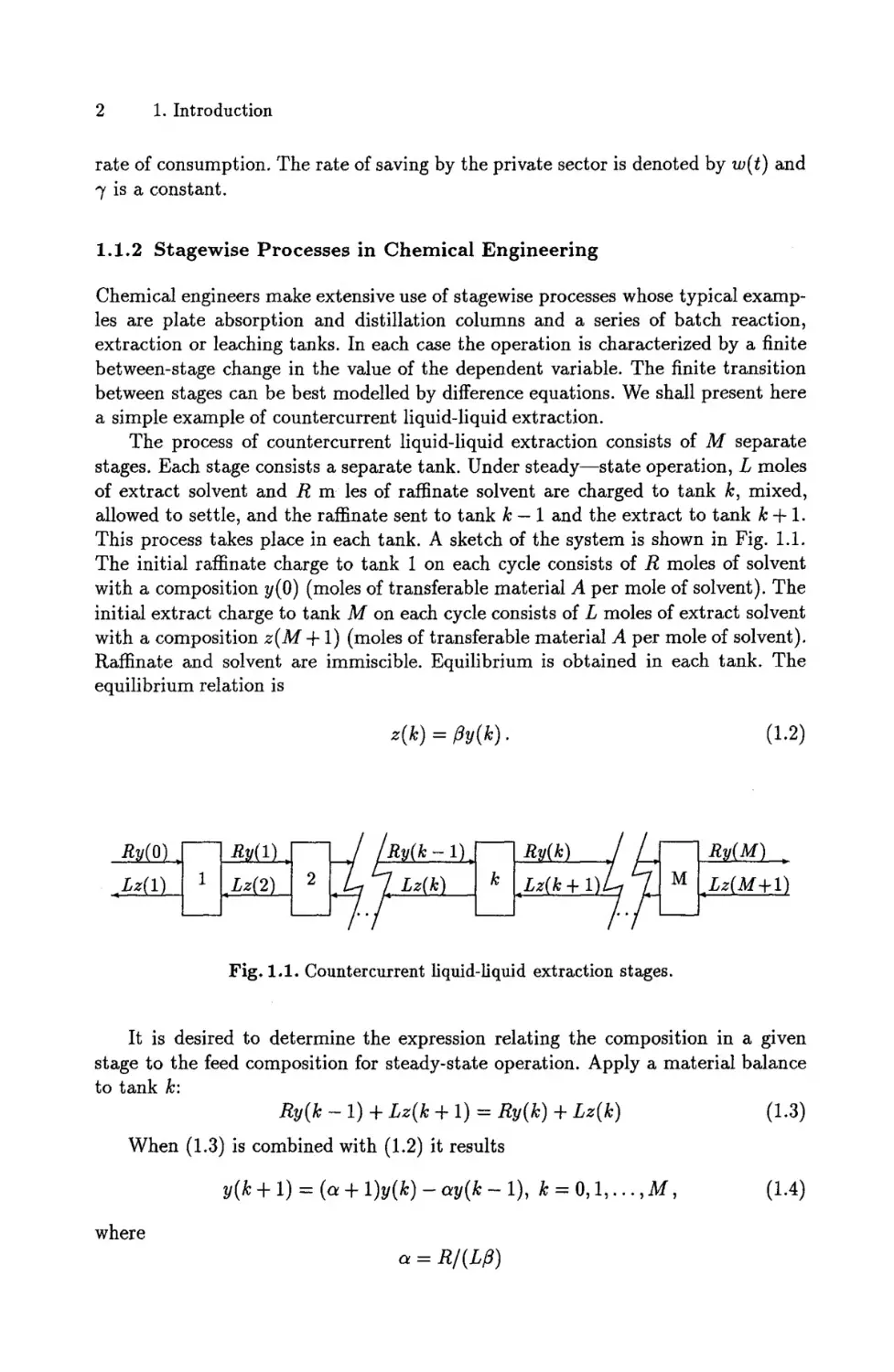
The process of countercurrent liquid-liquid extraction consists of M separate
stages. Each stage consists a separate tank. Under steady--state operation, L moles
of extract solvent and R m les of raffinate solvent are charged to tank k, mixed,
allowed to settle, and the raffinate sent to tank k - 1 and the extract to tank k -b 1.
This process takes place in each tank. A sketch of the system is shown in Fig. 1.1.
The initial raffinate charge to tank 1 on each cycle consists of R moles of solvent
with a composition y(0) (moles of transferable material A per mole of solvent). The
initial extract charge to tank M on each cycle consists of L moles of extract solvent
with a composition z(M--b1) (moles of transferable material A per mole of solvent).
Raffinate and solvent are immiscible. Equilibrium is obtained in each tank. The
equilibrium relation is
z(k)=fly(k).
Ry(O) J ~ ] ~ j
/Ry(k-1)J
Lz(l) ~ ~ L z ( k k) .
-'
(1.2)
]Ry(k) i ~
Ry(M) .
[-Lz(k+l) . M Lz(M+I)
Fig. 1.1. Countercurrent liquid-liquid extraction stages.
It is desired to determine the expression relating the composition in a given
stage to the feed composition for steady-state operation. Apply a material balance
to tank k:
ny(k - 1) -b Lz(k q- 1) = Ry(k) ÷ Lz(k)
(1.3)
When (1.3) is combined with (1.2) it results
y(k + 1) =
where
(a q- 1)y(k) -
ay(k -
a = R/(Lfl)
1), k = 0, 1 , . . . , M ,
(1.4)
1.1 Examples of Discrete-time Nonlinear Control Systems
3
cazl be considered as the control variable u. Denoting
y(k) = x2(k)
the difference equation (1.4) may be written in the state space form
xl(k-[-1)--x2(k)
x~(k+l)=(u+l)z2(k)
y(k)=~(k).
-uxl(k),
k=0,1,...,M
(i.5)
1.1.3 A n E x a m p l e of Discrete-time Nonlinear C o n t r o l M o d e l in
Medicine
Nonlinear control systems often appear in pharmacokinetics and chemotherapy. There is a certain temptation to employ discrete-time models since in clinical practice
and in laboratory, systems are generally observed at discrete times.
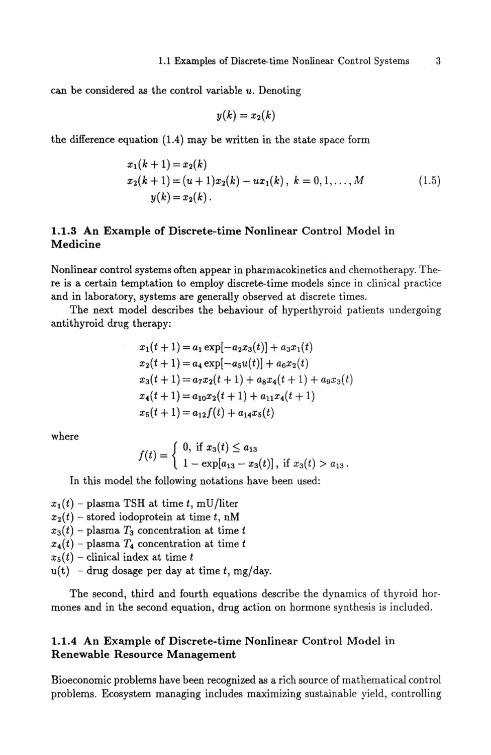
The next model describes the behaviour of hyperthyroid patients undergoing
antithyroid drug therapy:
x l ( t -t- 1) = al exp[-a2xa( t ) ] + a3x l ( t )
z 2 ( t + 1) = a4 exp[-ahu( t )] + a6x2( t )
x3(t + i)= a ~ ( t + i) + asx4(t + 1) + a~x~(t)
x4(t -~- 1) = alox2(t +
i) + anx4(t +
1)
xs(t + 1) = a12f(t) d- ai4xh(t)
where
f(t)
f O, if x3(t) < a~3
1 - exp[a13 - xs(t)], if xs(t) > al~.
In this model the following notations have been used:
xl(t)
x2(t)
xa(t)
x4(t)
xs(t)
u(t)
-
plasma TSH at time t, mU/liter
stored iodoprotein at time t, nM
plasma Ts concentration at time t
plasma T4 concentration at time t
clinical index at time t
drug dosage per day at time t, mg/day.
The second, third and fourth equations describe the dynamics of thyroid hormones and in the second equation, drug action on hormone synthesis is included.
1.1.4 An E x a m p l e of D i s c r e t e - t i m e N o n l i n e a r C o n t r o l M o d e l in
Renewable Resource Management
Bioeconomic problems have been recognized as a rich source of mathematical control
problems. Ecosystem managing includes maximizing sustainable yield, controlling
4
1. Introduction
pests and diseases. There are many situations where a difference equation model is
more appropriate than differential equation. This happens when population growth
occurs at discrete times and when generations are completely nonoverlapping. Biological examples are provided by some insect populations and certain fishes which
live in isolated generations. Discrete-time formulation is also widely used for describing age-structured population models since one ordinarily keeps track of age groups
instead of exact age. Very often there is a natural unit of time associated with a
particular resource system. In most cases, the structure of the model is a crude approximation to reality and it is difficult to find instances where control may be applied
precisely to actual situation. It is common to see the control policies as indicative.
It has been recognized that ecosystem models must include a degree of uncertainty in their description. In real ecosystems, this uncertainty arises due to fluctuations in the environment, or neglecting less important interactions between populations in the ecosystem. Usually, these uncertainties are described via external
perturbation vector in the model over which we have no control and the model is
exactly (1.1) with w(t) as perturbation vector. The elements x~ of x, i = 1 , . . . , n
usually denote the density (biomass, number) of the ith species, although in ecosystem models, some of the variables x~ may represent the concentration of nutrients
and chemical pollutants. By u(t) is usually denoted the harvesting rate and by w(t)
the perturbations which describe uncertainties of the model. One-dimensional state
equations describe the growth of one species. The multidimensional models describe
the complex interactions between animal and plant populations in the development
of the ecosystem. Animal and plant populations compete and cooperate with one
another to obtain sufficient natural resources to sustain their growth and survival.
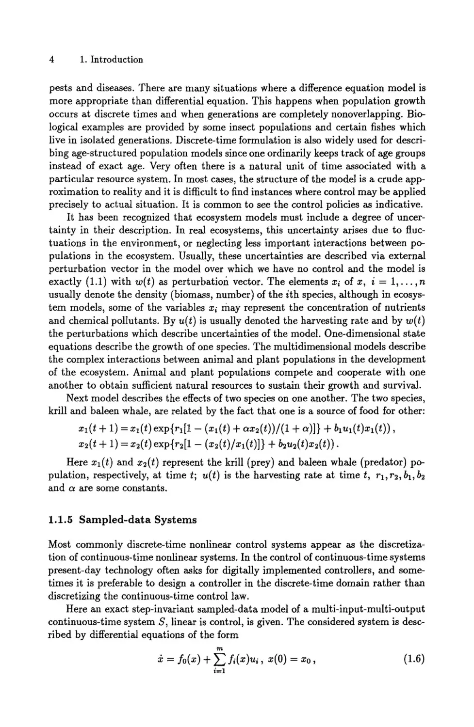
Next model describes the effects of two species on one another. The two species,
krill and baleen whale, are related by the fact that one is a source of food for other:
xl(t + 1) = xl(t)exp{r,[1 -- (xl(t) + ax2(t))/(1 + a)]} -4- blul(t)xl(t)) ,
x2(t + 1) = x2(t)exp{r2[1 - (x2(t)/xl(t)]} + b2u2(t)x2(t)).
Here xl(t) and x2(t) represent the krill (prey) and baleen whale (predator) population, respectively, at time t; u(t) is the harvesting rate at time t, rl, r2, bl, b2
and a are some constants.
1.1.5 S a m p l e d - d a t a S y s t e m s
Most commonly discrete-time nonlinear control systems appear as the discretization of continuous-time nonlinear systems. In the control of continuous-time systems
present-day technology often asks for digitally implemented controllers, and sometimes it is preferable to design a controller in the discrete-time domain rather than
discretizing the continuous-time control law.
Here an exact step-invariant sampled-data model of a multi-input-multi-output
continuous-time system S, linear is control, is given. The considered system is described by differential equations of the form
m
~c = fo(x) + ~ , fi(x)ul, x(O) = xo,
i=1
(1.6)
1.1 Examples of Discrete-time Nonlinear Control Systems
5
where x E X C R ~, u = (ul ... u,,,) E R ~, fi : X -+ X, i = 0, 1 , . . . , m are analytic
functions.
The exact step-invariant sampled-data model of a continuous-time system (1.6)
is defined as the one whose response to a step input (i.e. the type of control usually
available under digital control)
u(kT + t) = u(kT) , O < t < T
is identical to that of the continuous-time system at discrete instants of time kT,
k > 0, provided the initial states of both systems are the same.
Derivation of sampled-data model is based on the representation of the solution
of the differential equation (1.6) in terms of a formal Lie exponential series
• (kT + t) = ~
t~ ~
0 _< t < T
LI0 + E y=l f,~, x I~(kT) '
(1.7)
where by Lio+~,~ ~l~u~ is denoted the Lie differential operator associated with the
function fo(x) + ~'~=1fi(x)ui
LSo+E'?=Is,~,, =
by L ~ ~.~
10"1"~.~i=1 ~iUi
j=l
Yo,j(x) +
fl,j(x)ul Oxj'
its r-multiple composition
fiui
=
/O+ff'~i= 1/iui
L
,~
f o + ~ i = l fiui
'
r>2,
--
and by L ~ 0 + ~ f.~ an identity operator I. Of course, (1.7) m a y only be defined for
T sufficiently small.
As we are interested in the states x only at sampling instants kT + T, we obtain
from (1.7) for t = T
x(kT + T) = ~_, ~v. L~o+E~,/,,,,xl~(kT)
F(x(kT), u(kT)),
r>0
where F(x, u) because of
L
,~
= L/o + f i u~L/~
i=1
takes the following form
F(x,u)=F0(x)+ F,l(x)u,1+ E
i1=1
...
-]-
+...
i1~i2=1
fi
Fil...i,(x)ttil
. . . ui,
+...
(1.8)
,
il,...,is=l
& ' " i ' ( x ) = f i (rTr+V
+p)!
r=O
Z:
el + ...+Cp+l = r
Cl > O,.-.,e-a-I-1>0
,1
o2
L/oLlilLfoL$i2
...
l-v f i z a ~r°,+l~
fo
~.
6
1. Introduction
The exact step-invariant sampled-data model (1.8) is defined in terms of infinite
series both with respect to the sampling period T and the control u. So, in the
general case, the model (1.8) is usually not computable. In reality, to compute the
model, one must confine oneself with finite number of terms in this series. In that way
we reach the notion of approximate sampled-date-models. Computing approximate
sampled-date model corresponds to the truncation of the infinite series with respect
to the sampling period T as well as to the control u, at the fixed orders r and A,
respectively, which define the orders of approximation of the sampled system
F¢':~(x,u)=F;(x)+ ~ F[~(xlu,~ + . . . +
11=1
-p Tr+p
+ p)!
r=O
fi
F~...,~(x)u,,...u,~,
Q ,...,i~=1
cl +...+clo+ 1 = r
Cl >O,...,Cp+l >0
L °'
"
fOIJhl"~/o
.'"
L h p L fo
X.
The response of the (% A)th-order-approximate sampled-date model to a step
input will agree with that of the continuous-time system at given instants of time
t = kT, k >_ O, up to an error of order O(T'+l,u~+l).
The rth-order approximate sampled-date model can be computed recursively on
the bases of the (r - 1)th-order model, starting with the first-order model which is
equivalent to the classical Eulel discretization scheme
Fil...ip(x ) = ifoFi,...,~(x
~--1 ) + if, Fi2...,p(x
"r-1 ) .
1.2
Discrete-time
Nonlinear
Control
(1.9)
Systems
Next we will briefly discuss discrete-time nonlinear control systems given by (1.1),
i.e. by the equations
x(t + 1) = f(x(t), u(t), w(t)),
y(t)=h(x(t),u(t)),
where as before x, u, w and y denote reprectively the state, the control, the disturbance and the output. We shall work on a finite time interval, that means we assume
(1.1) to hold for t = 0 , 1 , 2 , . . . ,tF, where tF is some finite time instant, tF < 00.
We assume that the states x(t) belong to an open subset X of R ~, the controls u(t)
belong to an open subset U of R m, the disturbances wit ) belong to an open subset
W of/i7 and the outputs y(t) belong to an open subset Y of R p, all for 0 < t < tF.
Then (1.1) is a shorthand writing for
xl(t + 1) = fl(xl(t),... ,x~(t),ul(t),... ,um(t),wl(t),... ,w~(t)),
..o
x~(t + 1)
{ vl(t) =
yp(t)
f~(xl(t),... ,x,(t),ul(t),... ,um(t),wl(t),... ,w~(t)),
ui(t),...,
hp(xl(t),..,x,(t),ul(t),
..,u,,(t)).
(I.i0)
1.2 Discrete-time Nonlinear Control Systems
7
We assume the state transition map f : X x U x W --* X to be smooth
mapping. In this context smooth means C °O, i.e. that all of the partial derivatives Os+~+k/Oxh... Oxi~ Oujl... Ouj, C3wh...Owlk exist and are continuous, though
m a n y results which will be given in the next chapters hold under weaker conditions.
In m a n y circumstances f only needs to be sufficiently many times continuously differentiable with respect to x, u and w. We work with C °O functions in order not to
have to keep track of the exact number of derivatives required in different situations.
Note that if f : X x U --* X and h : X ~ Y are smooth and X , U , Y are open
subsets, then the composition h o f : X x U --+ Y is also smooth. Sometimes it
will be useful to strengthen the smoothness condition and to require that f is (real)
analytic. Similarly we assume the output map h : X x U --~ Y to be smooth or
analytic. For convenience we consider the system (1.10), initialized at t = 0; since
the system is time-invaxiant (i.e. not explicitly depending on time) this may be done
without loss of generality.
The system (1.1) has as inputs the'sequences u = {u(t); 0 < t < tF} of control
vectors from U C R m and sequences w = {w(t); 0 < t < tF} of disturbance vectors
from W C R ~. We denote the sets of such time sequences by L / a n d ~Y respectively.
Together with (1.1) we have to specify the classes of admissible controls L/ and
admissible disturbances }/Y. For discrete-time system (1.1), U may be any set of
time functions u : Z tr --~ U where Z~F stands for the set { 0 , 1 , 2 , . . . , tF}. Similarly,
a class of admissible disturbances 14/may be any set of time functions w : Z tr --+ W.
For difference equation
x(t + 1) = f(x(t), u(t), w(t)), x(O) = Xo,
as long as f is a well-defined function on X x U x W, there is no problem regarding existence and uniqueness of its solution x(t), 0 < t < t r , for any admissible
control sequence u E/~, any admissible disturbance sequence w E W and any arbitrary initial state x0 E R ~. Such a solution will usually be denoted as x(t, Xo, u, w)
which is a shorthand writing for x(t, Xo, u(O),..., u(t), w(O),..., w(t)). Similarly,
we let y(t, x0, u, w) = y(t, Xo, u(O),..., u(t), w(O),..., w(t)) denote the trajectory
of the output for the system (1.1) corresponding to a choice of the control sequence
u ( 0 ) , . . . , u(t), the disturbance sequence w ( 0 ) , . . . , w(t) and the initial state x0.
In chapters 2, 3, 5, 6 we shall consider systems without disturbances
x(t + 1) = f(x(t), u(t)),
y(t)=h(x(t),u(t))
x(O) = Xo,
(1.11)
where z, u, y and h are defined as before and f : X × U ~ X.
The system S = {U, Y,X, f, h} given by (1.11) generates for each initial state
x0 the input-output (IO) map Sff0 on the set U. The IO map
assigns to each input sequence u E / g the output sequence y = {y(t) E Y; 0 < t <
< tF} E Y according to the recursion (1.11) and assuming x(0) = x0.
8
1. Introduction
If C = {U c, y c , X c, i t , h e} is another control system of the form (1.11) with
Y ° C_ U, we m a y define the series connection of S with C, denoted by S o C, to be
the system
S o C = { U v , y , x x X V , f s ° c , hS°°},
where
fa°C(x, xC, u ° ) = [
and
f ( x ' h o( x' °u'°u)° ) )
hS°°(x, x ° , . )
=
Thus S o C is the system which results when the output of C is made the input
to S. The initial state of S o C is (x0, Xoc) where by x0c is denoted the initial state
of C.
Clearly, the IO m a p of the composite system S o C is the composition of the IO
maps for S and C:
zSoC
=
~S
o
.
(1.12)
Throughout the book we shall adopt a local viewpoint. In the discrete-time case
the local study is useless around an arbitrary initial state since even in one step, the
state can move far away from the initial state, regardless of the small control and
disturbance values. In order not to loose localness one possibility is to work around
an equilibrium point of the system, that' is around (x °, u °, w °) 6 X x U x W such that
f ( x °, u °, w °) = x °. Since in general the disturbances w(t), 0 < t < tF need not be
necessarily close to w °, for systems with disturbances working around an equilibrium
point is more restrictive if compared to the case without disturbances. Another, a
more general possibility, is to work around certain set of time sequences of state,
control, disturbance and output {~(t), ~(t),,~(t), ,3(t); 0 < t < tF} that satisfy the
system equations (1.1). This set of time sequences is called the (reference) trajectory
of the system. Note that an equilibrium point can also be considered a trajectory,
namely it is a trajectory consisting only in one point. Working around a trajectory
is useful in situations where there is no natural equilibrium point or an equilibrium
point has little relevance for control purposes. In this book mainly the first approach
will be followed but for a few problems local solutions will be presented around a
given trajectory.
If we assume to work in a neighbourhood of an equilibrium point and on a finite
time interval 0 < t < tf, then, using the control sequence {u(t); 0 < t < t f }
with each u(t) sufficiently close to u ° and provided that in the disturbance sequence
{w(t); 0 < t < t f } each w(t) is sufficiently close to w ° and that the initial state Xo
is sufficiently close to x ° we can assure that the states x(t) are sufficiently close to
x °, and the outputs y(t) are sufficiently close to yO = h(xO), both for 0 < t < tf.
Let us denote by X ° the open subset of X such that II x - x ° II< 7 for some
7 > 0. Let us denote by U ° the set of controls u which are sufficiently close to u °, that
is II u - u ° II< ~ for some 6 > 0. Let us denote by Y°(Yi° ) the set of outputs y (scalar
output components Yi) which are sufficiently close to yO(yO), that is II Y - y0 H<
< s(ll y ~ _ yO ii < e) for some s > 0. Denote by b/° and 3;°(3~i) the sets of control
1.3 Static and Dynamic State Feedback
9
sequences {u(t) E U°; 0 < t < tF} and output sequences {y(t) E y0; 0 < t < tF}
(output component sequences {y~(t) E ~0; 0 < t < tF}), respectively.
1.3 Static and D y n a m i c State Feedback
In the next chapters we will discuss changing the structure of nonlinear control
systems via feedback. Since we assume throughout the book that the whole state
vector of the system can be measured, we shall only consider state feedback. We
will be interested in two types of state feedback for a system (1.1) or (1.11)--static
state feedback and dynamic state feedback.
A static state feedback for the nonlinear system (1.11) or (1.1) is definedas a
relation
u(t) = ~(x(t), v(t))
(1.13)
where v E R '~ represents a new control vector. Note that since we are working locally
around an equilibrium point (x °, u °) of the system (1.11), the feedback (1.13) is also
defined only locally around a point (x °, v °, u°), such that v ° satisfies the relation
~o = ~(xo, v0).
A feedback (1.13) is called a regular static state feedback if O~(x, v)/Ov is a
nonsingular matrix for all x and v in the domain of ~.
The regularity of feedback implies that the closed loop system, i.e. the system
composed from the original system (1.1) and the feedback (1.13)
x(t + 1) = f(x(t), ~(x(t), v(t)), w(t))
y(t) = h(x(t), ~o(x(t), v(t) ) )
admits as m a n y independent controls as the original system.
The adjective "static" indicates the fact that the feedback (1.13) decides what
the value of u at a time-instant t should be only on the basis of what the value of
x and v at that specific time-instant is. In this sense (1.13) could also be called a
memoryless feedback. If we also incorporate some kind of m e m o r y in the feedback
we arrive at what is called a dynamic state feedback.
A dynamic state feedback for the system (1.11) or (1.1) is defined as
xc(t + 1) = F(x(t), xc(t), v(t))
u(t) = ~(x(t), xC(t), v(t))
where x ° E X c C R ~c, f c : X x X. ° x V --~ X o,
smooth mappings and v E V C R m represents a new
be interpreted as the m e m o r y of feedback. Sometimes
compensator.
A feedback (1.14) is called a regular dynamic state
(1.14)
~o : X × X c × V ~ U are
control vector. Here x c can
the system (1.14) is called a
feedback if the system (1.1),
(1.14)
x(t + 1) = f(x(t), ~o(x(t), xC(t), v(t) ), w(t) )
xC(t + 1) = fC(x(t), xe(t), v(t))
~(t) = ~(x(t), ~°(t), v(t))
(1.15)
10
1. Introduction
with inputs v(t) and outputs u(t) defines a one-to-one (x, x ¢, w)-dependent correspondence between the input variables v and the output variables u.
In the case when measurements of the disturbances are available, we allow the
feedback to depend on disturbance w. So, in this case we shall use a static state
feedback of the form
u(t) =
v(t), w(t))
and a dynamic state feedback of the form
xc(t + 1) =
u(t) =
Notes
and
v(t), w(t))
v(t), w(t)).
References
The economic example has been taken from [Aok75a]. The other examples of
discrete-time dynamic models in economics, simple as well more advanced can be
found in [Aok75a], [Aok75b], [Aok76], INij89], [NS90]. A detailed exposition of the
process of countercurrent liquid-liquid extraction was given in [MSR57] where more
examples of discrete-time nonlinear stagewise processes are discussed. For a further
discussion of the drug therapy model we refer to [Swa84]. The ecosystem model is
discussed in [Fis87]. For more ecosystem and renewable resourse management models, simple and advanced see [Cla76], [Fis87], [Get87], [KL88], [Lev84], [May74],
[May78], [Ost78], [PalS3], [Pie77], [Sch85].
The problem of finding the exact sampled-data model for continuous-time linearanalytic system was first addressed and solved by Monaco and Normand-Cyrot
[MNC85] for single-input systems. The sampled-data model (1.8) ha been taken
from [Kot89] and the formulas (1.9) for recursive computation of the approximate
sampled-data model from [Kot94]. The different formulas for computing sampleddata models can be found in [MNC86a], [MNC90]. While all formulas for computing
sampled-data models are similar in the sense that their derivation is based on the
representation of the solution of the continuous-time system in terms of a formal Lie
exponential series [FLL83], and that all formulas give the same smpled-data models
when applied to any concrete system, they have several differences. The formulas
given in [MNC86a], [MNC90] have a form which is better suited for studing several properties of the sampled-data models, such as controllability and observability.
However, they are more complicated to "apply tha~n (1.8) since they contain combinatorics, shuffle products and ad-operators. If one wants just to find the sampled-data
model of some concrete process, the easier formulas (1.8) will do the job. An exact
sampled-data model for multi-input continuous-time system, nonlinear in control is
presented in [Kot94]. In [Bar89] the program written with the aid of computer algebra system REDUCE for computing sampled-data model of linear-analytic system
has been presented.
We should like to end up with some remarks concerning the form of the state
transition map f in (1.11) (or in (1.1)). No significant simplification occurs when f
is linear in control, i.e. when f has the structure commonly used in the continuous
time. This is due to the fact that in discrete-time, one extensively uses the operation
Notes and References
11
of composition of functions which generally does not preserve the specific structure
[MNC86b]. Moreover, by the results of section 1.1.5, the linear analytic dynamics
under sampling are no longer linear in control.
[All91]
Allen L.J.S. Discrete and continuous models of populations and epidemics.
Journal of Mathematical Systems, Estimation and Control, 1991, v. 1,335369.
[Aok75a] Aoki M. Some examples of dynamic bilinear models in economics. Lecture
Notes in Economics and Mathematical Systems. Springer Verlag, Berlin, 1975,
v. 111,163-169.
[Aok75b] Aoki M. On a generalization of Tinbergen's condition in theory of policy to
dynamic models. Review of Economic Studies, 1975, 42,293-296.
[Aok76]
Aoki M. Optimal Control and System Theory in Dynamic Economic Analysis.
North-Holland, New York, 1976.
[Bar89]
Barbot J.P. A computer-aided design for sampling a nonlinear analytic systems. Lect. Notes Comp. Sci., 1989, v. 357, 74-88.
[Cla76]
Clark C.W. Mathematical Bioeconomics. The Optimal Management of Renewable Resources. John Wiley, New York, 1976.
[fis87]
Fisher M.E. Variability in ecosystem models: a deterministic approach. Lect.
Notes in Biomathematics, v. 72, 1987, 139-151.
[FLL83] Fliess M., M.Lamnabhi, and F.Lamnabhi-Lagarrigue. An algebraic approach
to nonlinear functional expansions. IEEE Trans. on Circuits and Systems,
1983, v. 30,554-570.
[Get87]
Getz W.M. Modeling for biological resource management. Lect. Notes in
Biomathematics, v. 72, 1987, 22-42.
[KL88]
Kaitala V. and G.Leitmann. Control of uncertain discrete systems: an application in resource management. Proc. 27th IEEE Conference on Decision
and Control, Austin, Texas, 1988, 497-502.
[Kot89]
Kotta ~l. On the discretization of continuous-time linear-analytic systems (In
Russian). Proc. Estonian Acad. Sci. Phys. Math., 1989, v. 38,222-224.
[Kot94]
Kotta U. Discrete-time models of a nonlinear continuos-time system. Proc.
Estonian Acad. Sci. Phys. Math., 1994, v. 43, 64-78.
[Lev84]
Levin S.A. Mathematical population biology. In: Population Biology. Proc. of
Syrup. in Applied Mathematics. American Mathematical Society, Providence,
l~ode Island, 1984.
[May74]
May R.M. Biological populations with nonoverlapping generations: stable
points, stable cycles and chaos. Science, 1974, v. 186,645-647.
[May78]
May R. Mathematical aspects of the dynamics of animal populations. In: Studies in Mathematical Biology. Part II. Populations and Communities. Levin
S.A. (Ed.). The Mathematical Association of America, 1978, 317-366.
[MNC85] Monaco S. and D.Normand-Cyrot. On the sampling of a linear analytic control
system. Proc. 2~th IEEE CDC, Fort Landerdale, 1985, 1457-1462.
[MNC86a] Monaco S., and D.Normand-Cyrot. Approximation entree-sortie d'un systeme
non lineaire continu par un systeme discret. Lect. Notes in Contr. and Inf.
Sciences, 1986, v. 83, 354-367.
[MNCS6b] Monaco S. and D.Normand-Cyrot. Nonlinear systems in discrete-time. Lecture
Notes in Control and Inf. Sci., 1986, v. 83,411-430.
12
1. Introduction
[MNC90]
[MSR57]
[Nij89]
[NS90]
[ost78]
[PalS3]
[Pie77]
[Sch85]
[Swa84]
Monaco S., and D.Normand-Cyrot. A combinatorial approach of the nonlinear
sampling problem. Lect. Notes in Control and Inf. Sciences, 1990, v. 144, 788797.
Mickley H.S., T.K.Sherwood, and C.E.Reed. Applied Mathematics in Chemical
Engineering. McGraw-Hill Book Company, New York, Toronto, London, 1957.
Nijmeijer H. On dynamic path decoupling and dynamic path controllability in
economic systems. J. of Economic Dynamics and Control, 1989, v. 13, 21-39.
Nijmeijer H., and A. vast der Schaft. Nonlinear Dynamical Control Systems.
Springer-Verlag, New York, 1990.
Oster G. The dynamics of nonlinear models with age structure. In: Studies
in Mathematical Biology. Part 11. Populations and Communities. Levin S.A.
(Ed.) The Mathematical Association of America, 1978, 411-438.
Palm III W.J. Modeling, Analysis and Control of Dynamic Systems. John
Wiley & Sons. New York, 1983.
Pielou E.C. Mathematical Ecology. John Wiley & Sons. New York-LondonSidney-Toronto, 1977.
Schnute J. A general theory for fishery modeling. Leet. Notes in Biomathematics, v. 61, 1985, 1-27.
Swan G.W. Applications of Optimal Control Theory in Biomedicine. Marcel
Dekker, New York and Basel, 1984.
2. S y s t e m
Inversion.
Special
Case
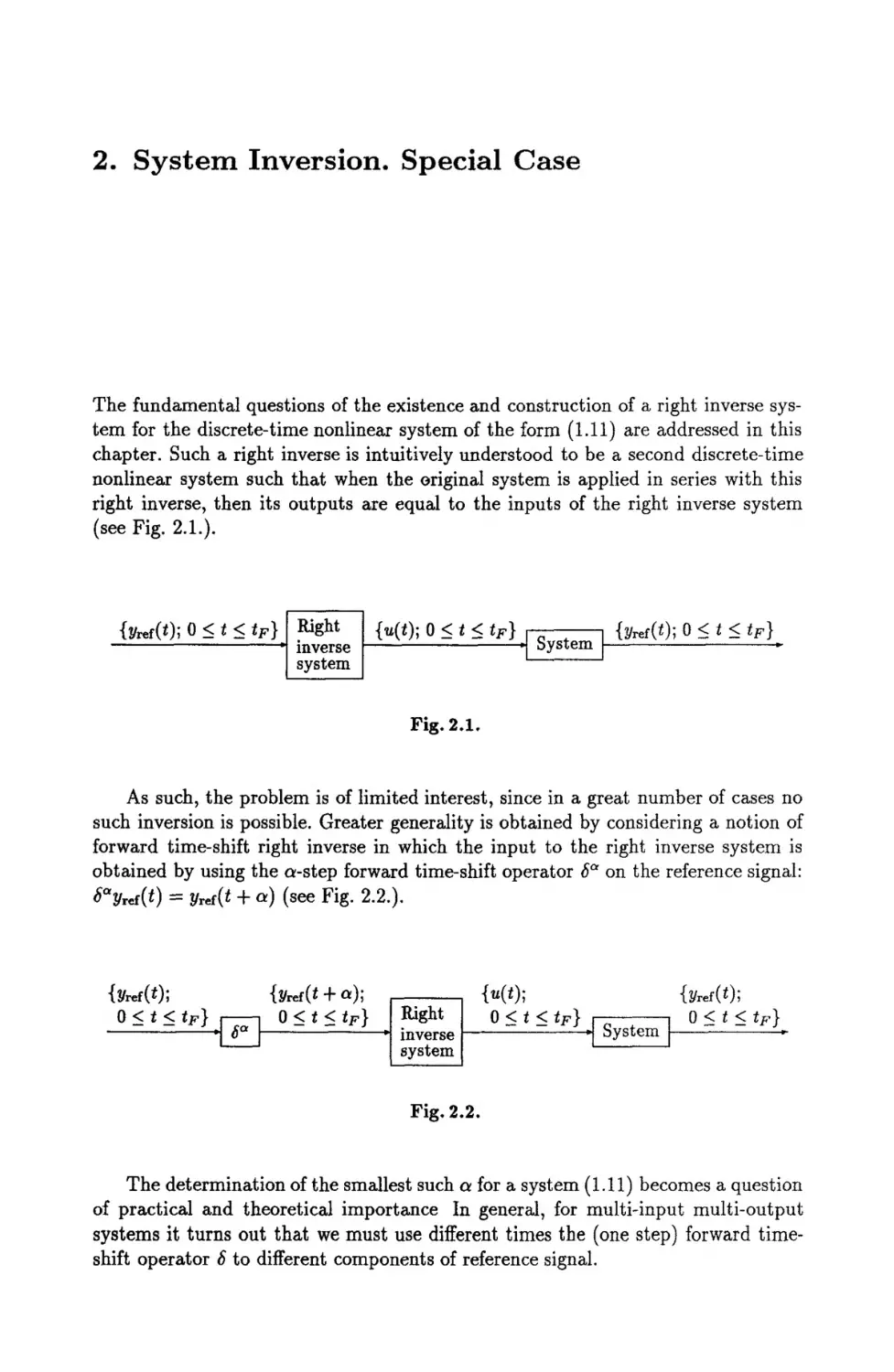
The fundamental questions of the existence and construction of a right inverse system for the discrete-time nonlinear system of the form (1.11) are addressed in this
chapter. Such a right inverse is intuitively understood to be a second discrete-time
nonlinear system such that when the original system is applied in series with this
right inverse, then its outputs are equal to the inputs of the right inverse system
(see Fig. 2.1.).
{y~f(t); o < t < t F } . ~
{~(t); 0 < t < t F } , ~
{yr~f(t);0 < t < tF}
Fig.2.1.
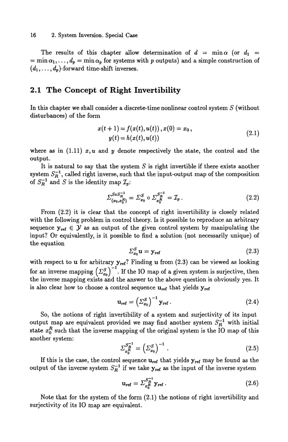
As such, the problem is of limited interest, since in a great number of cases no
such inversion is possible. Greater generality is obtained by considering a notion of
forward time-shift right inverse in which the input to the right inverse system is
obtained by using the a-step forward time-shift operator 5~ on the reference signal:
5"y,a(t) = yra(t + a) (see Fig. 2.2.).
{y,,(t);
O<t<t }.l
{o(t<);t
O<t<',,}
{yro,(t);
i sys,em I
Fig. 2.2.
The determination of the smallest such a for a system (1.11) becomes a question
of practical and theoretical importance In general, for multi-input multi-output
systems it turns out that we must use different times the (one step) forward timeshift operator 5 to different components of reference signal.
16
2. System Inversion. Special Case
The results of this chapter allow determination of d = m i n a (or dl =
= min a l , . . . , dp = min ap for systems with p outputs) and a simple construction of
( d l , . . . , dp)-forward time-shift inverses.
2.1 The Concept of Right Invertibility
In this chapter we shall consider a discrete-time nonlinear control system S (without
disturbances) of the form
x(t + 1) = f(x(t), u(t)), x(O) = xo,
= h(x(t),
(2.1)
where as in (1.11) x,u and y denote respectively the state, the control and the
output•
It is natural to say that the system S is right invertible if there exists another
system S~ 1, called right inverse, such that the input-output map of the composition
of S~ 1 and S is the identity map Z~:
~SoS~ 1
(~o.~g) = •s~o o .ZTso~I = Zp •
(2.2)
From (2.2) it is clear that the concept of right invertibility is closely related
with the following problem in control theory. Is it possible to reproduce an arbitrary
sequence Yref E Y a s an output of the given control system by manipulating the
input? Or equivalently, is it possible to find a solution (not necessarily unique) of
the equation
~S0u = y,~f
(2.3)
with respect to u for arbitrary Y~ef? Finding u from (2.3) can be viewed as looking
s
for an inverse mapping (Z~o)
. If the IO map of a given system is surjectIve, then
the inverse mapping exists and the answer to the above question is obviously yes. It
is also clear how to choose a control sequence U,ef that yields Yref
u,., =
Yro,.
(2.4)
So, the notions of right invertibili~y of a system and surjectivity of its input
output map are equivalent provided we may find another system S~ 1 with initial
state x0R such that the inverse mapping of the original system is the IO map of this
another system:
~S/~ 1
5
-1
o"
•
(2.5)
ff this is the case, the control sequence u~f that yields Yref may be found as the
output of the inverse system SR 1 if we take y~¢f as the input of the inverse system
~s~l
Ur~ = ~ o R y,~f.
(2.6)
Note that for the system of the form (2.1) the notions of right invertibility and
surjectivity of its IO map are equivalent.
2.2 The Concept of Forward Time-shift Right Invertibility
17
Since we have adopted a local viewpoint in this book, we are interested in local
right invertibility (surjectivity) around an equilibrium point (x °, u °) of the system
(2.1) and require (2.2) to hold only locally.
Next we shall give the formal definition of local right invertibility. In order to
do this, let us denote by X ° the open subset of X such that [[ x - x ° t[< 7 for
some 7 > 0. Let us also denote by U ° C U the set of the controls u, which are
sufficiently close to u °, that is [I u - u ° ][< A for some A > 0. Let us denote by
y 0 C Y the set of the outputs y which are sufficiently close to yO = h(x o, uO), that is
[[ y _yO H< ~ for some e > 0. Denote by H ° and 3)°, the sets of the control sequences
{u(t) • V°; 0 < t < rE} and the output sequences {y(t) • y 0 ; 0 < t < t f }
respectively.
D e f i n i t i o n 2.1 The system (2.1) is called locally right invertible in a neighbourhood
of its equilibrium point ( x °, u°), if there exist sets H ° and 3)° such that given Xo C X °,
we are able to ~nd f o r any sequence {yr.f(t) ; 0 < t < t~} C y0 a control sequence
{Ur~f(t) ; 0 < t < rE} E H ° (not necessarily unique) such that
y(t, xo, u , ~ ( o ) , . . . , u,~(t)) = yre,(t), 0 < t < t~.
The above definition says that every sequence Yref whose elements are close
enough to yO = h(x o, u o) can be generated as the output signal.
Definition 2.2 We call an equilibrium point (x °, u °) of the system (2.1) regular with
respect to local right invertibility if the rank of the matrix Oh(x, u)/Ou is constant
around this point.
It is well-known that the system (2.1) with p < m is locally right invertible in a
neighbourhood of its regular equilibrium point (x °, u °) if and only if the rank of the
matrix Oh(x, u)/Ou is equal to p at the equilibrium point (x °, u°). This rank condition
is certainly too restrictive for most systems and obviously useless for systems whose
output m a p h does not depend explicitly on the control u. Such systems cannot be
invertible in the sense of Definition 2.1 since the output y at t = 0 is not affected by
the input and is completely defined by.x0, i.e. y(0) = h(xo). In general, the output
m a y be defined completely by Xo also at a few next time instances t = 1, 2 , . . . , d - 1.
Therefore, for those systems it is useless to require that all sequences could be locally
reproducible and the best we can achieve is that all sequences could be locally
reproducible beginning from certain time instant t = d.
We shall modify the definition of local right invertibility according to the above
observations and introduce the notion of forward time-shift right invertibility.
2.2 The Concept of Forward Time-shift Right Invertibility
Definition 2.3 The system (2.1) is called locally foT~ward time-shift right invertible
in a neighbourhood of its equilibrium point (x °, u °) if there exist integers 0 < ~1 <_
18
2. System Inversion. Special Case
<_ a2 <_ ... <_ ap, a reordering of output components Yi, i = 1 , . . . , p , sets Lt °
and ~)o such that given xo • X ° we are able to find for any sequence {y~f(t);
0 < t < tF} • yo a control sequence {ura(t) ; 0 < t < tF} • Lt ° yielding
y,(t;Xo, Ura(O),...,U~cf(t)) = yra,i(t), a, ~_ t <_ tF, i = 1 , . . . ,p.
Denote by y/o the set of output components yi which are sufficiently close to
yO = hi(xO, uO), that is II Y l - Y ° ]1< ei for some ei > 0 and by ~ the set of sequences
{y~(t) • y 0 ; 0 < t < tF}. Then the above definition says that for the ith output
component it is possible to reproduce locally all sequences Yra,i from ~/beginning
from time instant hi. But forward time-shift right invertibility does not allow us to
reproduce the first al terms in the arbitrary sequence {yra,i(t) ; 0 < t < t f } • J~i"
Define the operator d i a g { 6 ~ , . . . , 5~p}, acting on sequences y as follows
d i a g { 5 ~ , . . . , 5"p}y = (6aly1,... , 5aPyp)T
where for i = 1 , . . . , p
5"'yl = {yi(t + al); 0 < t < t f } ,
5~'yi(t) = y i ( t + al), for 0 < t < tF -- ai ,
and
~a~yi(t) = 0, for tF -- Oti< t ~_ t F
since y(t) is not defined for t > tF.
Then the IO map of the forward time-shift right invertible system satisfies locally
around the equilibrium point the equation
diag{5~',..., 5~p} o z:s0 o (Z•s0)-' = d i a g { ~ l , . . . , 5~,} o Zp.
(2.7)
A very important concept in treating system inversion from this generalized
point of view, is the concept of delay orders. In the next section the set of system
structural parameters, the so-called delay orders dl, i = 1 , . . . , p , with respect to
the control u of the system (2.1) are defined, one for each output component. The
determination of these system structural parameters tells us immediately how many
delays have been associated between the ith component Yl of the output and u and
thus provides a lower bound on the number of output shifts required in an inverse
system.
2.3 T h e Delay Orders w i t h Respect to Control
With each component of the output yl we can associate a delay order di (refered
also in the literature as characteristic number or relative order) with respect to the
control u in the following manner.
Denote the ith component of h(x, u) by hi(x, u) and define h°(x, u) = hi(x, u).
Given an arbitrary state x E X, and an arbitrary u E U we can compute for
i = 1, 2,... ,p the derivative
2.3 The Delay Orders with Respect to Control
19
From the analyticity of the system (2.1) it follows that either the vector
ah°(x,u)/au is nonzero for all (x, u) belonging to an open and dense subset Oi
of X × U or this vector vanishes for all (x, u) E X x U. In the first case we define
di = 0 whereas in the latter case we continue by observing that the function h°(x, u)
does not depend on u and so we may write
h~(x,u)=h~(x)
for some analytic h~ on X. Next we apply the one-step forward-shift operator 8 to
the equation
yi(t) = h~(z(t))
which gives
yi(t + 1) = h~(f(x(t), u(t)))
and compute in an analogous fashion the derivate
Oh (f(x, ul).
If this vector is nonzero on an open and dense subset
otherwise we continue with the function
Oi of X × U, we set dl = 1;
In this way the number d~--if it exists--determines the inherent delay between
the inputs and the ith output. Namely, the input u(t) affects the ith output only
after dl steps, that is at the time instant t + di. In the case none of the iterated
functions
hkl-l(x) = hki(f(x,u)), k > 1,
depend on u, we define dl =
independently from the input
reasonable to assume that all
Define by r : X × U ~ X
c~. When di = c~, the ith output evolves in time
sequence applied to the system (2.1). Thus, it seems
delay orders are finite.
the projection along U on X.
Assume that di < oo. Then the row vectors Oh~(x)/Ox,..., Ohd'(x)/Ox
are linearly independent on ~r(Oi).
L e m m a 2.4
Proof. For notational convenience we drop the index i. By the definition of delay
order, using
OhJ(Of kOf
we have
Oh3+kOf
j+k<d
20
2. System Inversion. Special Case
OhJ (Of~k Of = { O~.~uifj + k < d
Oz \Ox]
Ou
hd(f(x,u))#O, i f j + k = d ,
and(x,u) E O .
The above condition shows that the matrix
:
[0f,0f0f,
t
(0f
d0f]
0
=
.
.
...
.
.
.
.
.
•
.
.
-~uuhd(f(x,u)) ...
*
has rank d in 0 and thus, the row vectors OhX(z)/Oz,..., Ohd(x)/Oz are linearly
independent on r(O).
•
The following result gives an upper bound on each finite delay order.
L e m m a 2.5 Each finite delay order eli, i = 1,... , p, satisfies the inequality dl < n.
Proof. For notational convenience we drop the index i. If the delay order d is finite
but greater than the dimension of state vector, d > n, then by Lemma 2.4 the n + 1
rows of the (n + 1) × n-dimensional matrix
h~(~)
~ z H(x) = ~x
0
...
h=(x)
h"+'(z)
would be linearly independent on O which is dearly impossible. The contradiction
proves the lemma.
•
L e m m a 2.6 For arbitrary feedback, the delay orders of the original system are less
than or equal to the corresponding delay orders of the feedback modified system,
di < all, i = 1,... ,p. In case of regular static state feedback the equality holds.
Proof. At first we show that
~,~(x) = h,%)
for all 1 < k < di and all x E 0~. This fact can be easily proved by induction. It is
true for k = 1 and, if true for some 1 < k < di, then
~,~+l(x) = i¢(](~, ~)) = h~(f(~,
~(~,.))) = h,~+l(x).
This proves eli < di.
The equality of the delay orders under regular static state feedback follows from
2.4 The Definition of (dl,..., dp)-forward Time-shift Right Invertibility
21
2.4 The Definition of ( d l , . . . , dp)-forward Time-shift Right
Invertibility
From the definition of delay orders di with respect to the control u it is clear that
the initial part of every reproducible sequence must satisfy the following conditions
y,(O) = h~(xo)
yi(1) = h~(xo)
(2.8)
yi(di -'1) = h~'(Xo)
and that only for yi(di) arise the possibility to change it arbitrarily.
The notion of ( d l , . . . , dp)-forward time-shift right invertibility can be obtained
as a special case of Definition 2.3.
Definition 2.7 The system (2.1) is called locally (dl,...,dp)-forward time-shift
((dl,..., dp)-FTS) right invertible in a neighbourhood of its equilibrium point (x °, u °)
if there exist sets bt ° and 3)0 such that given xo E X ° we are able to find for any
sequence {yr¢f(t) ;0 < t < tF} E 3)° a sequence of controls {ur~f(t) ; 0 < t < tF} C LI°
yielding
y i ( t ; XO, ~ r e f ( O ) , . . . , U r e f ( t ) )
=
y r e f , i ( t ) , d i < t <_ t F , i ~--- 1, . . . , p .
The above definition says that for ith output it is possible to reproduce all
sequences from 3~ beginning from time instant d~. But ( d l , . . . , dp)-FTS right invertibility does not allow us to reproduce the first di terms in the arbitrary sequence
{yrcf,i(t) ; 0 < t < tF} from 3~/.
The input-output map of the (dx,..., dp)-FTS right inverse system S~ 1 satisfies
locally around the equilibrium point tt/e equation
diag{U',..., 6d'} o s~s o ~so~l = diag{Sdl,..., 5d,} o :[p,
(2.9)
where by 5d is denoted the d-step forward time-shift operator and by 2-p the identity
map.
Note that the adjective local in this definition is related to the fact that the
reproducibility property for a nonlinear system in general holds only in the neighbourhood X ° x U° of the equilibrium point (x °, u °) and for reference sequences
{yrCf(t) ; 0 < t < tF} from restricted set of output sequences 323.
2.5 Necessary and Sufficient Conditions for
( d l , . . . , dp)-forward Time-shift Right Invertibility
To be useful in a state-space approach, the conditions for invertibility should be
phrased directly in terms of the functions f and h. Such a condition is developed in
this section.
22
2. System Inversion. Special Case
Rather than first looking for conditions under which S is right invertible, we
shall directly attack the problem of obtaining a representation S~ 1 for the inverse
mapping (S~so)-1 when it exists.
The basic idea is to apply the one step forward time-shift operator 5 on those
output components which do not explicitly depend on the input. Assuming that each
delay order di is finite, we modify the output equation of the system by repeatedly
operating on each of the scalar output equations the forward time-shift operators so
as to obtain a system of equations each of which depends explicitly on the control
u(t). From the definition of delay orders di, i = 1,... ,p, we obtain
(~dlyl(t) = yl(t "~- dl)= hdl1 (f(x(t), u(t)))
5d"yp(t) = yp(t q- dp) = h~p(f(x(t), u(t) ) )
(where h°(f(x, u)) = hi(x, u) by definition), or in the vector form
yl(t q- dl) ]
:
J = A(x(t),u(t)).
yp(t + dp)
(2.10)
We introduce the so-called decoupling matrix K(x, u) in the following way
K(x,u) =
A(x,u) = -~u
hdp(f(x,u) )
From the definition of the di's the rows of the matrix K(x, u) are nonzero functions on an open and dense subset O = Ox f3 02 N... f30p of X × U. It is obvious that
the rank of K(x, u) is, in general, state and control dependent. To ensure smoothness of the solution of (2.10) with respect to u(t) we have to assume that g ( x , u )
has a constant rank. This assumption is formalized in the notion of regularity of an
equilibrium point.
D e f i n i t i o n 2.8 We call the equilibrium point (x°,u °) of the system (2.1) regular
with respect to (dl,... ,dp)-forward time-shift right invertibility, if the rank of the
decoupling matrix K(z,u) of the system (2.1) is constant around (x °, u°).
T h e o r e m 2.9 Assume that for the system (2.1) dl < n, i = 1 , . . . , p . Then the
system (2.1) is locally (all,..., dv)-forward time-shift right invertibIe around a regular
equilibrium point (x °, u °) if and only if rank g ( x °, u °) = p.
Proof. Sufficiency. Consider the system of equations (2.10). By the definition of the
equilibrium point we have yO = A(x o, uO). Observe that the Jacobian matrix of the
right hand side of (2.10) with respect to the control u equals to the decoupling matrix
K(x, u). By the assumption of the theorem the rank of the decoupling matrix K(x, u)
is equal to p at the equilibrium point (x °, u°). So, we may apply the Implicit Function
Theorem in order to solve the system of equations (2.10) with respect to the control
2.5 Necessary and Sufficient Conditions for (dl,..., dp)-FTS Right Invertibility
23
u. After a possible reordering of the control components we may assume that the
Jacobian matrix of the right hand side of (2.10) with respect to u ~ = ( u l , . . . , up) T
around the point (x°,u °) has full row rank p. Therefore, equation (2.10) can be
solved for ul(t) uniquely around (x °, u°). Define u 2 = (Up+l,..., urn) T.
The Implicit Function Theorem says that in some (possible small) neighbourhood )~o x (/o x l/° of (x °, u °, y0) there exists an analytic function ~ of variables
x(t), yl(t + dl),... ,y,(t + d,), and u2(t) i.e.
ul(t) = ~(x(t),yl(t -t- dl),. . . ,yp(t + dv), u2(t) )
which is such that
(2.11)
qo(xo, yO, u2O) = ulO
and
[yl(t T d l ) , . . . , y,(t -~- dp)] T - A(x(t), ~(x(t), yl(t + d l ) , . . . , yp(t + dp), u2(t)), u2(t)).
Notice that the above identity is lost if we leave the neighbourhoods 2~o × ]~o × 02o
or ~/lO.
Necessity. Suppose that the system (2.1) is locally ( d l , . . . , dv)-FTS right invertible around its regular equilibrium point (x °, u°). This implies, in particular, that
at time instant t = di at the ith output yi of the system (2.1) we can reproduce
by suitable choice of u(0) = Uref arbitrary Yref,i sufficiently close to yO, that is the
following holds
urof)) = y ef,,, i = 1 , . . .
,p.
Assume that rank K ( x °, u °) = k < p. As by regularity of (x °, u°), k is constant
in some neighbourhood ~ 0 x ~-o of (x °, u°), the rank K(x, u) in X ° × U ° is less than p.
This implies that the functions h d'(f(xo, u~f)), i = 1 , . . . , p of u~a are functionally
dependent, that is there exists the map R(-) such that
R(h~ 1 o f , . . . , h d, o f ) = R(yref,i,..-, Yref,,)
=
0.
The last equality means that Yref is not arbitrary but satisfies the equation
R(y~d,1,..., y~f,p) = 0 which gives contradiction.
Remark. Clearly, rank K(x°,u °) = p requires m _> p. So, p _< m is always a
necessary condition for system to have a (dl,..., dp)-FTS right inverse, that is the
system must have least as many inputs as outputs.
Remark. We should like to stress that the assumption of the regularity of the
equilibrium point (x °, u °) in Theorem 2.9 is extremely vital. If the point (x °, u °)
is not regular, that is around the point (x °, u °) the rank of the decoupling matrix
K(x, u) is not necessarily constant, then the condition K(x °, u °) = p is not necessary
for (all,..., dp)-FTS right invertibility. The illustration of this phenomenon is given
in the following simple example:
x(t + 1) = ua(t)
y(t) = x(t).
24
2. System Inversion Special Case
We have
. %
g(x, u) = £ A ( x , u) = 3u 2 .
At the equilibrium point x ° = 0, u ° = 0 the rank of K(x, u) is equal to 0 which
is less than p = 1. Still, the arbitrary sequences are reproducible by the choice of
control
u(t) = ~/y(t + 1).
The reason is that the point x ° = 0, u ° = 0 is not a regular equilibrium point.
The rank of the matrix K(x, u) is equal to 1 at all points u ~ 0.
2.6
Construction
of (dl,...,
dp)-forward
Time-shift
Right
Inverse System
The system SR1 is said to be a ( d l , . . . , dp)-forward time-shift right inverse for S, if
its IO map satisfies equation (2.9).
We are now going to derive the equations of S~ 1. Apply to the each scalar
output equation of the system (2.1) the one step forward time-shift operator 5 until if
becomes explicitly dependent on the control u(t), that is for the ith output equation
d~ times. Doing this we obtain equation (2.10). To get the equations of right inverse,
we have to be able to solve the system of equations (2.1), (2.10) with respect to u(t)
and x(t + 1) in terms of x(t) and yx(t + d~),..., yp(t + dr). The solution of (2.10)
is given by (2.11) with arbitrary u2(t) E 0 2°. Equation (2.11) defines the required
control for the given system (which yields the reference output) in terms of state
and reference output. We can take this equation as the output equation of a right
inverse system. To obtain the dynamic part of the right inverse, we must substitute
(2.11) into (2.1)
x(t + 1) = f(x(t), ~(x(t), y~(t + dl),..., yp(t + dp), u2(t)), uS(t)).
(2.12)
So, the equations of S~ 1 axe the following
xn(t + 1) = f(xn(t), ~(xU(t), yl(t + dl),..., yp(t +dp), ~(t)), A(t))
ul(t) -- ¢fl(xR(t), yl(t + d l ) , . . . , yp(t + dp), ~(t))
u2(t)=A(t),
(2.13)
where by ~(t) is denoted the free parameter.
Remark. Note that the states x(t) of the system (2.1) under the state feedback
(2.11) and the states of the (dl,...,dp)-FTS right inverse system (2.13) coincide,
provided the initial states of these systems are equal, i.e. if x(0) = xR(0).
From the equations (2.13) it is clear that the state space systems of the form
(2.1) are not closed under system inversion: the inverse system in general depends
on the future values of the outputs of the original system.
2.7 An Approximate (dl,..., dv)-forward Time-shift Pdght Inverse System
25
There exist no right inverse for a strictly causal system S such that the input
to the original system can be computed as the output of the inverse system without
using the future values of the reference signal, or equivalently, without using forward
shift operators on reference signal. To be more precise we must apply the dl-step
forward time-shift operator for ith component of reference signal.
Actually, the output of the right inverse system (i.e. the control of the original
system) at time instant t will depend on the ith component of the reference output
at time instant t + d;. As Yref is generated by the designer, in the actual control law
design this implies that a change of reference signal must be preplanned some time
steps ahead, which is often a realistic assumption. When it is possible, the right
inverse system can be realized.
If the reference signal can be generated from a model M, the need for future
values of model inputs is avoided under conditions that the composite system S~ 1oM
contains no forward time-shift operators.
The disadvantage of the definition (2.9) lies in the fact that S~ 1, defined by it,
is not, in general, a causal system (see equations (2.13)), and therefore, cannot be
realized via state equations. One can decompose the noncausal system S~ 1 into two
systems, a causal system ~ 1 and a system which transforms signals by applying
on them forward time-shift operator diag{hdl,..., hap}. Hence, one can express the
input-output map of S~ 1, that is ..%0R , in the following form
#
~o~
o
.
.
Then, one can define a causal (d~,..., dp)-forward time-shift right inverse SR 1
of S as such which satisfies the equation
o
o
° diag{
, .-.
= diag{5
....
o Z;.
(2.14)
Note that ~ 1 can be realized via the state equations
£n(t + 1) =
f(£n(t),
~(~,n(t), un(t), A(t)), A(t))
Yn(t) = [ ~(xn(t)'A(t) un(t)'£(t))] '
(2.15)
where by u n and yn are denoted the input and output of ~ 1 respectively.
Remark.
The states x(t) of the system (2.1) under the state feedback ul(t) =
= ~(z(t),un(t),A(t)),uS(t) = A(t) and the states of the causal (dl,...,d~)-FTS
right inverse system (2.15) under input un(t) coincide, provided the initial states of
these systems are equal, i.e. x(0) = ~n(0).
2.7 An Approximate (dl,...,dp)-forward Time-shift Right
Inverse System
The Implicit Function Theorem says that equation (2.10) can be solved for u(t) but
does not indicate how to find the solution. Assume for simplicity that m = p. We
26
2. System Inversion. Special Case
recall here a result due to Grhbner for the inversion of a family of analytic functions
Ai(ua,...,up)
= yi, i = 1 , . . . , p .
Assuming that d e t { O A i ( . ) / O u j } ¢ 0 at a fixed point u*, the inverse functions
ul, i = 1 , . . . ,p can be e x p 1 i c i t 1 y expressed by means of Lie series which
are absolutely and uniformly convergent in a neighbourhood of (u*, y*) such that
y~ = Ai(u*):
u =
D'...
~,~=o,...,~,p=o ul!.., u,,[ 1
D~Uil~=~ * (y~ - y ; ) ~ . . . (yp - y ; ) ~
where D k , k = 1,... ,p axe the following commuting linear differential operators
=
, {-4.,k} = (OAi(')/Ouj) -x •
i=1
So, denoting by A~k(x,u) the elements of the matrix O A ( x , u ) / O u and by
D j ( x , u ) , j = 1,... ,p the differential operators S~=a,4ij(x,u)o-~ , the solution of
equation (2.10) with respect to the components ul of the control vector u in the
neighbourhood of (x °, u °, y0) can be expressed via the series
=
1
~,=o,....~p=o vl! . 7. vfl D ~ l ( x ( t ) ' u ) o . . .
...
D;p(x(t), u)uq~=~o[(Y~(t + dl) - y0]~l.., [(yp(t
-{- d p ) -
yO]vp ,
(2.16)
i = 1,...,p.
The exact solution (2.16) of (2.10) is defined via infinite series and in reality, to
compute the solution, one must confine oneself with finite number of terms in this
series. In that way we reach the approximate solution of (2.10) and the notion of
approximate (dx,..., dp)-FTS right inverse system, if we substitute (2.16), truncated
at Vl + . . . + up = t, into (2.1).
2.8 The
System
Reduced
Order
Inverse
System.
State-free
Inverse
The order of the inverse system (2.13) (or (2.15)), discussed in Section 2.6, is the
same as that of the original system. It will now be shown that, provided the system
is (dl, • •. dp)-forwaxd time-shift right invertible, an inverse system of order n - S ~ = l d l
can always be obtained if we utilize yi(t + j ) , 0 < j < di - 1, 1 < i < p as the
additional inputs of an inverse system. (Note that the inputs of the right inverse
system of order n are yl(t + d x ) , . . . ,yp~t + dp)). Thus, if dx + . . . + dp is close to n,
a relatively low order inverse system can be found.
In the sequel we need the following. Lemma.
2.8 The Reduced Order Inverse System. State-free Inverse System
27
L e m m a 2.10 Suppose that the system (2.i) is locally ( d l , . . . , dp)-forward time-shift
right invertible in the neighbourhood X ° × U ° of its regular equilibrium point (x °, u°).
Then the functions h{(x), 1 <_ j <_ di, 1 < i < p are functionally independent on
~ ( X ° × V°).
Proof. The proof is similar to the proof of Lemma 2.4. Define d
and
'
h~(~)
= max{dl,...,
dp}
'
hl~'(~)
H(x)= h ix)
• h~,(x)
Consider the matrices P(x) = OH(x)/Ox and
Using
Ohi (0s
0 s _ 0hi
0S _
'
+ k < d,
and the definition of delay order, it is easy to see that the matrix
P(x). Q(x, u),
after possibly a reordering of the rows, exhibits a block triangular structure in which
the diagonal blocks consist of rows of the decoupling matrix K(x, u). This shows
the linear independence of the rows of OH(x)/Ox in ~r(X ° × U °) which completes
the proof.
•
Remark. If all di < co, an immediate implication of the above lemma is that
the sum of relative degrees of an nth order system is always equal or less than n,
because otherwise there would be more than n linearly independent vectors in an
n-dimensional space.
Our approach to construct a reduced-order inverse is to construct first a nonreduced inverse of order n and then reduce its dimension by expressing some components of the state via the outputs yi(t + j), 0 < j < di - 1, 1 < i < p and the
remaining components of state.
The following equalities result from the definition of delay orders d~ of the system
(2.1) (See Section 2.3):
yi(t + j) = hJ+l"xt
~ ( ()),j=O,...,d~-l,i=l,...,p.
(2.17)
28
2. System Inversion. Special Case
In case of ( d l , . . . , d p ) - F T S
invertible systems by L e m m a 2.10 the functions
hJi(x), 1 < j < di, 1 < i < p are functionally independent on 7r(X ° × U°).
After a possible reordering of the state components we may assume that
0
rank O(Xl,..., x~,) H(x) = #.
Therefore, equations (2.17) can be solved by Implicit Function Theorem with respect
to xl(t) = ( x l ( t ) , . . . ,
xl(t) = ~({yi(t + j ) , j = 0 , . . . , d i -
1, i = 1 , . . . , p } ,
x2(t)),
where x2(t) = ( X , + l ( t ) , . . . , xn(t)). Substituting xl(t)into (2.11) we have
ul(t) = ~p(~({y/(t + j ) , j = 0 , . . . ,d~ - 1,i = 1 , . . . ,p} ,x2(t)),x2(t),
yl(t + d ~ ) , . . . , yp(t + dp), u2(t))
and consequently, the dynamics of the right inverse system (2.13) of order n can be
replaced by equations of order n - it:
xR2(t + 1) = f2(~({yi(t + j ) , 1 < i <_p,O < j <_dl - 1},xm(t)),xm(t),
qo(~({yi(t + j), 1 < i <_ p, 0 < j _< di - 1}, x m ( t ) ) , xn2(t),
yl(t + d l ) , . . . , yp(t + dp), A(t)), )~(t)) :=
:=](xm(t), {yi(t + j ) , j = 0 , . . . ,dl, i = 1 , . . . , p } , ~ ( t ) ) .
(2.18)
Note that the number of inputs of ('2.18) is p + ~i=1
P di which is of course greater
than p - the number of inputs of (2.13).
If dim x 2 = 0, that is if ~i=1
P di = n, the reduced order right inverse is said to
be ,,state-free". In that case the input, which produces the reference signal, can be
computed from the knowledge of the reference signal {y~f(t) ; 0 < t < tF} only:
ul(t) = ~(~({yi(t + j ) , j = 0 , . . . ,di - 1,i = 1 , . . . ,p}),y~(t + d~),...
... ,yv(t + dv),u2(t)) a=~({yi(t + j ) , j = 0,... ,dl, i = 1,... ,p},u2(t)).
2.9
Examples
In this section we show on two examples how to construct the (dl,. •., dp)-FTS right
inverse system.
E x a m p l e 2.11 Bilinear model of neutron kinetics can be described by the following
equations
xl(t q- 1) = (1 -- al)xl(t) + alx2(t) + blx~(t)u(t)
x2(t + 1 ) = a 2 x l ( t ) + (1 - a2)x2(t)
y(t)=xl(t).
(2.19)
2.9 Examples
29
At first we shall find the delay order. Compute
0
0
Ou(t) h(x(t -t- 1)) = uut~)-~77~x(t+ 1) = blxl(t)
which is different from zero if xl(t) # O. So, d = 1.
Now we are going to construct the d-forward time-shift right inverse system for
neutron kinetics model. Following the theory in Section 2.6 we apply to the output
equation of the system (2.19) the forward shift operator 5 until it becomes explicitly
dependent on the control u(t). In our example we need to apply the operator 5 only
once. Doing this we reach the equation
y(t + 1) = (1 - al)xl(t) + alx2(t) + blx(t)u(t).
(2.20)
To get the output equation of the system S ~ 1 we must solve equation (2.20) for
u(t):
u(t) =
(1-
al)xl(t) +alx2(t) t- ~ y (1t
blXl(t)
+ 1).
(2.21)
To obtain the dynamic part of the S~ 1 we must substitute (2.21) into (2.19):
xl(t + 1) = -y(t + 1)
x2(t + 1) = a2xl(t) + (1 - a2)x2(t).
(2.22)
From the equations (2.21), (2.22) i.t is easy to obtain the &forward time-shift
right inverse system ~,~1
xl(t -t- 1) = -uR(t)
x2(t + 1) = a2xl(t) + (1 a2)x2(t)
yR(t) = (1 ai)xi(t) + alx2(t)
1
blxl(t)
-t- ~ u
-
-
(2.23)
-
-
R
(t).
To construct the reduced-order right inverse system we replace in equations
(2.21), (2.22) x,(t) by y(t):
x2(t + 1) = a2y(t) + (1 - a2)x2(t)
u(t)= (1 al)y(t) + a,x2(t) + 1 y(t + 1).
bly(t)
olyl,~)
-
E x a m p l e 2.12 DC/AC convertor.
Consider the system
x (t)
xl(t + 1) = - 4 x l ( t ) - x - ~ + 5ul(t)
x=(t + 1) = -6x2(t) - -x~(t)
- ~ "~ 5x2(t)u
- - ~ II,tt ~) + 2Xl(t)u2(t)
yl(t) =Xl(t), y2(t) = x2(t).
30
2. System Inversion. Special Case
At first, let us find the delay orders dl and ds. Compute
~(t)hl(x(t + 1)) = ~ -0~ x l ( t + 1 ) = [5,0] # 0 ,
0
O~t)h
(x(t+l))=
xs(t+l)=
L x~(t) '
2z~(t) ¢ 0
if xl(t) # 0.
So, dl = d~. = 1.
We are now going to check if this system is (dl,..., dv)-forward time-shift right
invertible. For this purpose, we have to construct the decoupling matrix K(x, u) and
check if the rank of this matrix equals to the number of the outputs of the system.
The rank of the decoupling matrix
K(x,u)
=
[ 5 0 1
5xs 2Xl
Xl
is equal to 2, if xl # 0.
Now, let us find the equations of (dl,...,dp)-forward time-shift right inverse
system ~ 1 . First we derive the equations of S~ 1. For that we need to solve the
system of equations
yl(t + l) =--4xl(t)
- ~x22(t)+ 5ul(t)
y~(t + 1) = -6x~(t) - x~(t) + 5 x~s(t)
-~Ul(t ) +
with respect to
2xl(t)u2(t)
ul(t) and us(t):
i
{
~(t)
ul(t) = -~ yl(t + 1) + 4x~(t) + z~(t) J
xs(t) lylt t
x~(t)~
us(t)= _ 2x~(t)
[ ' + 1) + 4 x l ( t ) + x - - ~ ] +
1 (
x3(t)
+2~1(t) y2(t+ i) + 6xs(t) + 2x~(t) J
"
These are the output equations of the system S~ i. To obtain the output equations of ~,~1 we must replace yl(t + 1) by u~(t) and ys(t + 1) by u~(t). At last, to
obtain the state equations of right inverse, we must substitute so found ui(t) and
us(t) into state equations of the original system
xl(t + 1) = -4xi(t)
-
xs(t + i) = - 6 ~ ( t )
- ~x3(t) + ~xs(t) {UlR(t) + 4xi(t) + x~(t)
~(t) j -
_ .~(t)
x~(t) + u~(t) + 4xl(t) + ~x~(t) = URl(t)
x-~
-~l,U x-~ {u~(t) T 4xl(t) ÷ ~
}+
• ~(t)~j = ~ ( t ) .
+Xl(t) x-~ {u~(t) + 6x2(t) + x~(t)
Notes and References
Notes
and
31
References
The delay orders were first introduced in the discrete-time nonlinear context by
Monaco and Normand-Cyrot [MNC83b] for the very restricted subclass of linearanalytic systems. The definition of delay orders used here is taken from [Nij87]. Note
that sometimes one defines the delay order as the minimal number of d for which
y(t+d+l) (and not y(t+d) as in our definition) depends explicitly on u(t) [MNC83b],
[KotS6a], [Kot90]. As we do allow the output function in (2.1) explicitly depend on
the control, this slight change in the definition will avoid possible introduction of
negative delay order. The Lemma 2.5, giving the upper bounds for delay orders, and
Lemma 2.10 were first proved by Nijmeijer [Nij87], but the proofs described here
are the discrete-time analogues of the proofs given in [IsiS9].
The definition of forward time-shift (FTS) right invertibility is actually a discretetime analogue of the definition due to Respondek (see Definition 4.2 in [Res90]).
The special case of FTS-right invertibility, the notion of ( d l , . . . , dp)-FTS right invertibility has been introduced in [Kot90]; necessary and sufficient conditions for
(dl,...,dp)-FTS right invertibility are taken from [Kot90]. Note that in the case
of continuous-time systems, the equivalent notion of (all,..., dp)-FTS right invertibility is the notion of system with vector relative degree [Isi89]. The concepts of
reduced-order and ,,state-free" (left) inverse system for discrete-tilne nonlinear systems are developed in [MNC87]. The tlsefulness of the Lie series in the solution of
the system of nonlinear equations (which is required for construction of the right
inverse system) was pointed out by Monaco, Normand-Cyrot and Isola [MNCI89].
The earlier results on discrete-time nonlinear system inversion, dealing with the very special subclasses of systems (2.1) may be found in [MNC83a], [Kot83], [Kot85],
[Kot86a-c].
In our definition of right invertibility x(0) is fixed. If we do allow the initial
state x(0) in (2.1) to vary, we obtain a slightly different notion of right invertibility, because sometimes we can satisfy the conditions (2.8) by a proper choice of
x(0) = x0. For continuous-time nonlinear systems the role played by the initial state
in system inversion has been studied in [l:tN88], [Res90].
Note that the Examples 2.11 and 2.12 are taken from [BMSS0] and [PasS9]
respectively.
More notes and references on discrete-time system inversion can be found in
Chapter 5.
We would like to end up with some remarks concerning the terminology around
the problem of right invertibility which seems not to be quite standard. Besides the
notion of right invertibility other notions such as functional reproducibility [BM65],
[AGW86], [Nij89], functional controllability [SM69] and path controllability [Woh85],
[AGW86], [Nij89] are used to denote the same property of the system. Throughout
this book we use the notion of right invertibility. Note that the concept of output
controllability [KS64] is different from the concept of right invertibility. Output
controllability, unlike right invertibility, is a pointwise property, i.e. it is concerned
with the existence of an input sequence that drives the output to a specified point
in output space at a specified time instant. The concept of right invertibility, on
32
2. System Inversion. Special Case
the other hand, is a functional property, concerned with the existence of an input
sequence which produces a specified output sequence (function).
Albrech F., K.A.Grasse and N.Wax. Path controllability of linear input-output
systems. IEEE Trans. Aurora. Control, 1986, v. 31,569-571.
Baheti R.S., R.R.Mohler, H.A.Spang III. Second order correlation method
[BMS80]
for bilinear system identification. IEEE Trans. Autom. Control, 1980, v. 25,
1141-1146.
Brockett R.W. and M.D.Mesarovic. The reproducibility of multivariable sysIBM65]
tems. J. Math. Anal. Appl., 1965, v. 11,548-563.
Grasse K.A. Sufficient conditions for the functional reproducibility of time[Gra88]
varying, input-output systems. SIAM J. Contr. and Optimiz., 1988, v. 26,
230-249.
[Isi89]
Isidori A. Nonlinear Control Systems. Berlin, Springer-Verlag, 1989.
Kotta U. On the inverse of a special class of MIMO bilinear systems. Proc.
[Kot83]
Estonian Acad. Sci. Math., Phys., 1983, v. 32, 323-326.
Kotta U. Invertibility of bilinear discrete-time systems. Proc. of IFAC/IFORS
[Kot85]
Conf. on Control Science and Technology for Development. Beijing, 1985.
Kotta U. Inversion of discrete-time linear-analytic systems. Proc. Estonian
[got86a]
Academy. of Sci. Phys. Math., 1986, v. 35, 425-431.
Kotta U. On the inverse of discrete-time linear-analytic system. Control[Kot86b]
Theory and Advanced Technology, 1986, v. 2, 619-625.
Kotta U. Construction of inverse system for discrete time nonlinear systems
[Kot86c]
(In Russian). Proc. Acad. Sci. o f USSR. Technical Cybernetics, 1986, 159-162.
Kotta U. Right inverse of a discrete time non-linear system. Int. J. Control,
[Kot90]
1990, v. 51, 1-9.
Kreindler E. and P.E.Sarachik. On the concepts of controllability and observa[KS64]
bility of linear systems. IEEE Trans. Aurora. Control, 1964, v. 9, 129-136.
[MNC83a] Monaco S. and D.Normand-Cyrot. Some remarks on the invertibility of nonlinear discrete-time systems. Proc. American Control Conference, 1983, 229245.
[MNC83b] Monaco S. and D.Normand-Cyrot. The immersion under feedback of a multidimensional discrete-time non-linear system into a linear system. Int. J. Control,
1983, v. 38, 245-261.
[MNC87] Monaco S. and D.Normand-Cyrot. Minimum-phase nonlinear discrete-time
systems and feedback stabilization. Proc. 26th IEEE Conf. on Desision and
Control, Los Angeles, CA, 1987, 979-986.
[MNCI89] Monaco S., D.Normand-Cyrot and T.Isola. Nonlinear decoupling in discrete
time. Prepr. of 1st IFAC Syrup. on Nonlinear Control Systems Design, Italy,
Capri, 1989, 48-55.
Nijmeijer H. Local (dynamic) input-output decoupling of discrete-time nonli[Nij87]
near systems. IMA J. of Mathematical Control and Information, 1987, v. 4,
237-250.
Nijmeijer H. On dynamic decoupling and dynamic path controllability in eco[Nij89]
nomic systems. Journal of Economic Dynamics and Control, 1989, v. 13, 2139.
Passino K.M. Disturbance rejection in nonlinear systems: examples. IEE Proc.
[Pas89]
D., 1989, v. 136, 317-323.
[AGW86]
Notes and References
[~s9o]
[RNS8]
[Sin82]
[SM69]
[Woh85]
33
Respondek W. Right and left invertibility of nonlinear control systems. In:
Nonlinear Controllability and Optimal Control, (ed. H.J.Sussmann), 1990~
133-176.
Respondek W. and H.Nijmeijer. On local right invertibility of nonlinear control
systems. Control-Theory and Advanced Technology, 1988, v. 4, 325-348.
Singh S.N. Functional reproducibility of multivariable nonlinear systems.
IEEE Trans. Autom. Contr., 1982, v. 27, 270-272.
Sain M.K. and J.L.Massey. Invertibility of linear time-invariant dynamical
systems. IEEE Trans. Autom. Contr., 1969, v. 14, 141-149.
Wohtlmann H.W. Target path controllability of linear time-varying dynamical
systems. IEEE Trans. Aurora. Control, 1985, v. 30, 84-87.
3. The Inversion M e t h o d and Applications
In this chapter we shall assume that the system (1.11) is (all,..., dv)-forward timeshift right invertible, and explain the basic ideas of the inversion method for this
special class of systems. A more general case is left for Chapter 6. In Section 3.1
the inversion method will be introduced as a method to solve the model matching
problem (MMP).
In the MMP one considers the problem of designing a compensator for a nonlinear discrete-time system under which the input-output map of the compensated
system becomes the same as that of a prespecified model. In general, the model is
also assumed to be nonlinear. The MMP is a typical design problem in the sense that
it plays a role in various other problems like the disturbance decoupling problem,
the input-output (I/O) linearization and decoupling problems.
There are two possibilities in specifying the model--either we can fix the equations of the model completely, or, we can require only some structural properties of
the model. For example, we may require that the model is either linear or decoupled
but otherwise arbitrary. The case of a completely fixed model is considered in Sections 3.2 and 3.3, the case of linear model in Section 3.4 and the case of decoupled
model in Section 3.5.
It should be stressed that the main theorems in this chapter are established
under the assumption that the decoupling matrix of the system has a constant
rank around an equilibrium point (x °, u °) of the system. Note that the rank is in
general state and control dependent. This assumption is formalized in the notion
of regularity of the equilibrium point (x°,u °) with respect to (d~,... ,dp)-forward
time-shift right invertibility.
3 . 1 A n Inversion M e t h o d for ( d l , . . . ,
Time-shift Right Invertible System
dp)-forward
Consider a discrete-time nonlinear system S, described by equations of the form
x(t + 1) = f ( x ( t ) , u ( t ) ) , x(O) = Xo,
y(t)=h(x(t)),
(3.1)
where as before x ~ X, u E U, y E Y denote respectively the state, the control and
the output.
36
3. The Inversion Method and Applications
Let a discrete-time nonlinear model M be also given, described by equations of
the form
x M ( t + 1) =
uM(t)), xM(o) = x y ,
yM(t) = hM(xM(t)),
(3.2)
where the states xM(t) belong to an open subset X M of/P~', the inputs uM(t) belong
to an open subset U M of R m and the outputs yM(t) belong to an open subset yM
of R p, all for 0 < t < tF. The mappings fM and h M are supposed to be smooth.
The compensator C used to control the system S is a discrete-time nonlinear
system described by equations of the form
xC(t + 1) = fC(xC(t), x(t), uM(t)), xC(O) = XCo,
u(t) = hC(ze(t), x(t), uM(t))
(3.3)
with the state xC(t) E X c, an open subset of R ~c and f c and h e are smooth
mappings.
The composition of (3.1) and (3.3), initialized at (x0, x0C), is denoted by S o C:
x(t + 1) = f(x(t), hC(xC(t), x(t), uM(t)))
xC(t + 1) = fC(xC(t), x(t), uM(t))
yS°C(t)=h(x(t)).
(3.4)
Let the I/O maps of the original system and the model be denoted by •s °
and ~Yff0Mrespectively, and the I/O map of the compensator be denoted by ~ z .
The MMP is defined as follows. Given the system S and the model M, find a causal
compensator C and a map ~ : X M ~ X c such that the I/O map of the compensated
system S o C coincides with the I/O map of the model; or equivalently, that
(~o,~(~o~)) =
(3.5)
holds.
Our purpose in this chapter is to develop a method for solving the MMP under
the assumption that the system S is ( d l , . . . , dp)-FTS right invertible. It would be
desirable to achieve (3.5) via suitable ~hoice of feedback, but for considered class
of systems we are not able to do this, unless there exists certain correspondence
between the initial states of the original system and the model. The crucial fact is
that the ith output of the (all,..., dp)-FTS right invertible system for time instants
0 < t < di - 1 is completely determined by the initial state Xo and this property
cannot be changed under any feedback. The best one can achieve is the coincidence
of the ith output of the closed-loop system and the model starting from t = d i . So,
replacing (3.5) by
,~SoV
= diag{6dl ,. ..,6dP} o 2?~M
diag{6dl,..., 5d~} o z~(~o,e(~0M))
(3.6)
seems to be the best adapted to our theory. For ( d l , . . . , dp)-FTS right invertible
system S there exists a causal inverse Sn I so that
3.1 An Inversion Method for ( d l , . . . , dp)-FTS Right Invertible System
37
diag{6d,,..., 5dp} o ESo o ~7~0
~1 o diag{Sdl,..., 6 dp} = diag{Sal,..., 5d~} o 2-p
holds. Comparing the above equality with (3.6) leads to the compensator C with
the I/O map
S}(x0M
) v = "'~o
R't~a o diag{Sd~,... ,5 d~} o S ~ .
(3.7)
Really, ,U~(~M)
c
defined by (3.7) satisfies the equality
c ) = diag{Sdl,..., (~dp} o SMM
diag{6dl,..., 5dp} o s~s0 o S~(x0M
or equivalently, talcing into account the equality (1.12), the equality (3.6).
So, to obtain the desired control law via the inverse system, ( d l , . . . , dp)-forward
time-shift right inverse system ~ 1 of S must be first determined. Then a solution
of the MMP is obtained as the output of the right inverse system 1
~n(t + 1) = f(2n(t), ~(zn(t), un(t))), 2n(O)
~(t) = ~(~R(t), uR(t) ) ,
= x(O),
(3.8)
if we feed into equations (3.8) the appropriate shifts of the outputs of the model
system
an(t) = [ylM(t Jr dl),... ,yM(t Jr dr)] T
(3.9)
and replace yM(t + di), i = 1,... ,p in (3.9) by a function
hy'd'(xM(t), aM(t),...,
u ' ( t + d, - 1)).
The latter can be found by applying to the ith output equation of the model
= h,'(xM(t))
d~ times the forward shift operator (~ like we did in computing the delay orders in
Section 2.2. Note that we obtain a causal solution to the MMP if and only if the
functions h y 'di, i ---- 1 , . . . ,p, do not depend on the future values of the model input
u M ( t ~- 1 ) , . . . , u M ( t + d i - 1), or equivalently, the delay orders of the model are
equal or greater than the corresponding delay orders of the system. Of course, the
development sketched above is not possible if the system is not (all,..., dv)-forward
time-shift right invertible.
The control law so obtained is not a state feedback but an open-loop compensator. The behaviour of the compensator C will be defined completely by the states
x M and 2n of the model M and the inverse system S~ 1 respectively, as well as by
the model input uM; it is not affected explicitly by the states x of the system S.
This open-loop compensator can be replaced by an equivalent state feedback compensator. The replacement is based on a very simple observation. Namely, the states
2n of the right inverse system (3.8) and the states x of the original system
x(t + 1) = f(z(t), u(t))
1For notational ease we drop the (m -p)-dimensional free parameter ,~(t) in the description of
the right inverse system.
38
3. The Inversion Method and Applications
under the feedback u(t) = ~(x(t), ua(t)), i.e. under the feedback we use, coincide,
provided ~R(0) = x(0). So, the open-loop compensator can be interpreted as the
feedback control if we just replace ~R(t) by x(t) in the equations of the compensator.
Note that making this replacement, there is no more need for the dynamic part of
the right inverse (3.8) in the equations of the compensator, and we drop it.
The system design procedure using the inversion method may be summarized
in the following algorithm.
1) Given S, compute a ( d l , . . . , dp)-forward time-shift right inverse B~ 1.
2) Choose the model, which corresponds to the design objectives and satisfies the
condition dM > di, i = 1,... ,p.
3) Compute the outputs of the model yM(t + di), i = 1,... ,p in terms of the
model state xM(t) and model input uM(t) using the state equations of the
model
yM(t + di) = hM'd'(fM(xM(t), uM(t))).
4) The output equation of the compensator C can be found as the output equation
of the right inverse system ~ 1 under the control
un(t) = hM'~'(fM(xM(t), uM(t))), i = 1,... ,p).
5) The dynamic part of the compensator is the dynamic part of the model with
x°(0) = xM(0).
The methodology, described above, is simple to implement. The other advantage
of this approach is that various results on inverses can be used here. Furthermore,
after ~,~1 has been found, solutions C for different M's can be easily calculated.
Note that in many problems M is not completely but only partially fixed and one
may be interested in finding compensators for different models.
This approach also indicates how to choose M so that a causal solution C to (3.6)
does exist. From (3.9) it is clear that the delay orders of the model must be equal or
greater than the corresponding delay orders of the system. Only in that case uR(t) in
(3.9) does not depend on future values of the reference input uM(t). Let us remark
that in cases when the model is not completely specified like in problems of I/O
linearization and I/O decoupling, one can choose M which meets this requirement.
So, the inversion method gives us both the conditions of the existence of solution and a method to find the solution. In addition, it also shows which structural
properties can be achieved in the closed-loop.
3.2 The Formal Definition
Matching
Problem
and the Solution
of the Model
Let us first give the formal definition of the local MMP for (dl,...,dp)-forward
time-shift right invertible system.
3.2 The Formal Definition and the Solution of the Model Matching Problem
39
Recall that we assume to work in a neighbourhood of an equilibrium point of
the system (3.1), that is around a point (z °, u °) • X × U such that f(x °, u °) = x °.
We say that the equilibrium point (x M°, u M°) of the model M is corresponding to
the equilibrium point (x °, u °) of the system S if yO = yMO = hM(zMO).
Definition 3.1 Local m o d e l m a t c h i n g problem. Given the (dl,..., dp)-FTS
invertible system S defined by equations (3.1) around an equilibrium point (x °, u°),
the model M defined by equations (3.2) around an equilibrium point (x u°, u M°)
corresponding to (x °, u °) and a point (x(0), xM (O) ) , find if possible, a compensator
C defined by equations of the form (3.3) together with an initial state xC(O), an
equilibrium point x c°, neighbourhoods V1 = X ° × X c° × U M° of (x °, x c°, u M°) in
X × X c × UM and V2 ofu ° in U, being the domain and the range of C respectively,
as well a neighbourhood X M° of x M° and a map ~ : X M° -+ X c° with the property
that
yS°C(t, x(0), ~(xM(O)), uM(0),..., uM(t -- 1)) =
= yM(t, xM(O),uM(O),...,uM(t-- 1)),d, < t < tF, i = 1 , . . . , p
for all (x(0), xM(o)) • X ° × X M°, and for all uM(t) in the domain of C.
Note that we do not require the first terms in the output sequences of S o C
and M (which are completely defined by the corresponding initial states) to be the
same.
The next theorem is established under the assumption that we work around a regular (with respect to ( d l , . . . , dp)-FTS right invertibility) equilibrium point (x °, u °)
of the system S. Recall that regularity in the above sense means that the decoupling
matrix of the system has a constant rank around an equilibrium point.
T h e o r e m 3.2 Consider the system (3.1) around a regular equilibrium point (x °, u °)
and the model (3.2) around an equilibrium point (xMO,uMO), corresponding to
(x °, u°). Suppose that the system (3.1) is locally around (x °, u °) ( d l , . . . , dp)-forward
time-shift right invertible. Then the model matching problem is locally solvable if
and only if the delay orders of the model (3.2) are equal or greater than those of the
original system: dM > di, i = 1,... ,p.
Proof. The proof relies on the inversion method and on the Theorem 2.9. Let us
consider the model around the equilibrium point (x M°, u M°) which corresponds to
the regular equilibrium point (x °, u °) of the system (3.1). Then from (2.11) it follows
that if and only if we apply a compensator C given by the equation
u(t) = ~(x(t), yM(t + d l ) , . . . , yM(t +dp))
(3.10)
to the system (3.1), then the outputs of the model and the compensated system
coincide (starting from time instant t = d~ for the ith output component), i.e.
yiS°CIt~
L)=yM(t)
,
di<_t<_tF, i E { 1 , . . , p }
as long as (x(t),yM(t + d l ) , . . . ,yM(t +dp)) C 2 o x ~/o and u(t) C (]%
40
3. The Inversion Method a~d Applications
The compensator (3.10) can be given in the form (3.3) if and only if the delay
orders dM of the model are equal or greater than the corresponding delay orders of
the system (3.1), that is dM > di, i = 1,... ,p. In that case, defining the functions
hM'd'(xM) analogously to the functions h~'(x) (see Section 2.3) we obtain
yM(t +dl) = hM'a'(fM(xM(t),uM(t))), i = 1,... ,p,
(3.11)
and substituting (3.11) into (3.10) gives
u(t) = qo(x(t), hM'd'(fM(xM(t), uM(t))), i = 1,... ,p) ~ ~(x(t), xM(t), u~(t)).
Note that the states of the model x M in this control law can be computed from
the dynamic equations of the model which thus determine the dynamic equations
of the compensator.
So, the compensator C together with its initial condition xC(O), solving the
MMP is the following
zC(t + 1) = fM(xC(t), uM(t)), xV(O) = x M ,
u(t) = ~(x(t), xV(t), uM(t) ) ,
(3.12)
and since Xo
v = Xo
M, ~ = Id (identity map).
From (3.11) we can see that (x(t), yM(t +dl),..., yM(t + riM)) belong to 2 ° × ~o
as long as (x(t), xc(t), uM(t)) belong to some neighbourhood V1 of (x °, x c°, uM°).
This completes the proof.
•
Let us remark that proof of the Theorem 3.2, up to application of the Implicit
Function Theorem, is constructive. If we know how to solve equation (2.10), the proof
indicates how to find the equations of the compensator which solves the MMP.
3.3 The Strong
and Solution
Model
Matching
Problem--Formulation
In the strong MMP (SMMP), unlike the Definition 3.1, the equality yS°C(t) = yM(t)
is required also for 0 < t < di - 1, i.e. for the first terms in the output sequences
of S o C and M. As the values of ySoV(j), j = O, 1,...,dl - 1, i = 1,...,p are
completely defined by initial state of the system (3.1), the necessary condition for
solvability of the SMMP is
(A1) HM(xM(O)) = H(x(0)),
where
H ( x ) = [hl(x),...,hd'(x),...,h~(x),...,hap(x)]
T,
HM(x M) = [hM'X(xM),..., hM'd'(xM),..., hM,I(xM),..., hM,dp(xM)] r .
are (dr + . . . + dp)-dimensional vector functions.
3.3 The Strong Model Matching Problem--Formulation and Solution
41
If the SMMP is solvable, then it is possible to reduce the order of the dynamics of the compensator (3.12) and in .some special cases even replace the dynamic
compensator by static state feedback. We are going to show this.
From the coincidence of outputs of the closed-loop system and the model
yiS°C(t + j) = yM(t + j), 0 < t + j <_ tF, i = 1 , . . . , p ,
in particular for j = 0,..., dl - 1, it follows that for each 0 < t < tF -- d, where
d = max di
S
H(x(t)) = HM(xM(t)).
(3.13)
Let us denote dl + ... + dp by #. If the rank of the (# x nM)-dimensional
OHM(xM)/OxM is equal to # (which by Lemma 2.10 is true for example for
(all,..., dp)-forward time-shift invertible models) then equation (3.13) can be solved
for # components of the vector x M, denoted by xM: 2
matrix
Xl
=
in terms of x and the remaining n M - - It components of x M, denoted by x M.
Substituting x M into the equation u(t) = ~(x(t), xM(t), aM(t), uM(t)) we have
to take into account only the dynamic.s of x M which allows us to reduce the order
of the compensator:
xv(t + 1) = fM(¢(x(t), xV(t)), xe(t), uM(t)), xC(O) = xM(o),
u(t) = ~(x(t), ¢(x(t), xC(t)), xC(t), uM(t)).
Furthermore, if the following assumptions hold
(A2) di = dM, i = 1 , . . . , p
(A3) the order of the model
rt M
satisfies
n M =dl
+ . . . + dp ~ It
(A4) the (It x nM)-dimensional matrix OHM(xM)/OX M has the full rank:
rallk[ OHM (xM ) / Ox M] = It,
then the s t a t e xM(t) of the model can be expressed by the state of the original
system x(t):
xM(t) = (HM) -' o H(x(t)).
Substituting xM(t) in the equation u(t) = ~(x(t),xM(t),uM(t))
compensator in the form of the static state feedback:
gives us the
u(t) =- ~(x(t), (HM) -1 o H(x(t)), uM(t)) ~=a(x(t), uM(t)).
Summarizing, we have the following theorem.
2The vector xM =[ lg11,'",
M
aM
i,], ii E {1,...,nM} ,ischosenso that rank[OHM(xM)/oaM] = #
holds.
42
3. The Inversion Method and Applications
T h e o r e m 3.3 Consider the system (3.1) around a regular equilibrium point (x °, u °)
and the model (3.2) around an equilibrium point (xMO,uMO), corresponding to
(x°,u°). Suppose that the system (3.1) is locally around (z°,u °) ( d l , . . . ,dp)-FTS
right invertible and that for (3.1) and (3.2) the conditions (A1)-(A4) hold. Then
the strong model matching problem is locally solvable via the static state feedback of
the form
u(t) =
3.4 T h e Formulation and the Solution of the I n p u t - o u t p u t
Linearization P r o b l e m via Static State Feedback
In this section we are interested in the problem of compensating the nonlinearities of
the system (3.1), via feedback control. There axe essentially two types of approaches
to this problem. The first one consists in trying to find a state feedback (either static
or dynamic) such that the dynamics of the closed loop system are, after a change
of coordinates in the state space, locally equivalent to a linear system. The second
approach tries to find a state feedback such that the input-output map of the closedloop system becomes linear. In this bo6k we are interested in the second approach,
to be more precise, in linearizing the input-dependent part of the input-output map
of the closed-loop system.
The input-output map of the system (3.1) around an equilibrium point (x °, u °)
takes the form of a Volterra series expansion
y(t)=w°(t,x0)+E E
t-1
~'1
E E.-.
j>_l il,i2,...,ij=l "rl=0 r 2 = 0
"'E
w,l,J
0 ...
u,l]
uo ], (3.14)
"rj=O
where wlJli~..k is the j t h triangular Volterra kernel.
There are two kinds of terms in the Volterra series (3.14): those that depend
on the initial state x0 alone and those that depend both on the controls u and the
initial state x0. Note that the kernels wil..J.~, depend on the initial state z0. Unlike the
linear case, the response is not simply the sum of the forced and unforced responses.
The system (3.1) is said to have a linear input-output map if its Volterra series
expansion reduces to one of the form
m t-1
y(t) = w°(t, xo) + ~_~ ~_~ w~(t - Q[u,(r) - u°], 0 < t < tF,
' = 1 ~'=0
that is if the input-dependent part of this expansion is
(i) linear in input u and
(ii) independent on the initial sate.
(3.15)
3.4 The Formulation and the Solution of the Input-output Linearization Problem
43
Note that the kernels w i1 in (3.15) unlike those of (3.14) do not depend on
x0. So, the response (3.15) is simply a sum of the forced and unforced responses.
The term w°(t, xo) in (3.15) which represents the response to the reference input
u(t) = u °, 0 < t < tF, need not necessarily be the same as the one of a linear
system. However, this term affects the response to different inputs around reference
input in the same way.
If the system is such that (3.15) is not true, we may try to satisfy this property
via feedback, that is to find a state feedback such that for every 0 < t < tu the
input-dependent part of the input-output map of the closed-loop system is linear.
In this chapter we are looking for a static state feedback C with a new mdimensional control v, described by equations of the form
u(t) = a(x(t), v(t) )
(3.16)
defined locally around (to be found) a point (x °, v °, u °) such that u ° = a(x °, v°).
We call the compensator C described by equation (3.16) regular, if the matrix
Oa(x, v)/Ov is nonsingular around a point (x °, v °, u°).
The closed-loop system (3.1), (3.16), initialized at Xo, that is the system
x(t + 1 ) = f ( x ( t ) , a ( x ( t ) , v ( t ) ) ) , x(O) = Xo,
y(t)=h(x(t)),
(3.17)
is denoted by S o C.
The closed-loop system (3.17) is said to have a linear input-output map if its
Volterra series expansion reduces to one of the form
m
t--1
y(t) = w°(t, xo) + E E ~ ( t - ~)[v,(~) - v°], 0 < t < t . .
(3.18)
i = l "r~-0
D e f i n i t i o n 3.4 L o c a l s t a t i c i n p u t - o u t p u t l i n e a r i z a t i o n p r o b l e m . Given the
system (3.1) around a regular equaibrium point (xO, uO, yO) find, if possible, a regular
static state feedback C defined by equations of the form (3.16) together with a point
(x °, v °, u °) and neighbourhoods A = X ° × V ° of (x °, v °) and U ° of u °, being the
domain and the range of C, respectively, so that the outputs of the closed-loop system
rn
t--1
ys°°(t, xo, v(O),... ,v(t - 1)) = w°(t, xo) + E E w~(t - ~-)[v,(~-) - v°], o < t < t .
i = l 1"=0
for every Xo E X °, v(k) C V °, 0 < k < t - 1.
The problem of input-output (I/O) linearization can be considered as a special
case of the MMP. If in the MMP the equations of the model are completely specified,
in the case of I/O linearization we require only that the model is linear
xM(t + 1) = A x M ( t ) + B y ( t ) , xM(o) = xOM ,
yM(t)=cixM(t), i = 1 , . . . , p .
(3.19)
44
3. The Inversion Method and Applications
The degree of freedom in a choice of model order, its initial state and the elements
of the matrices A, B, C = [cT,..., cT] T are limited only by the possibility to solve
the problem. By the results of the previous section it means that the inequalities
dM > di, i = l , . . . , p .
(3.20)
must hold.
As we can always find a linear model which satisfies the constraints (3.20), the
I/O linearization problem for ( d l , . . . , dp)-FTS right invertible systems is always
solvable.
As we shall see in the following, freedom in the choice of the linear model has one
important consequence. For ( d l , . . . , dv)-FTS right invertible systems, the solution of
the I/O linearization problem can be found in the class of more simple compensators
than compensators of the form (3.3), namely in the class of static state feedback
control laws of the form (3.16). The compensator of the form (3.16) is of course, a
special case of the compensator (3.3), when the dimension of dynamic part is equal
to zero, that is the compensator has no dynamic part.
In order to find a solution in the class of static state feedback compensators, the
model must satisfy the following properties (see the previous section):
(AI') The initial state x M of the model satisfies the following equation
x M = (HM)-IH(xo),
where x0 is the initial state of the system and
h l(x)
H(x) ....
hl( )
(A2') The delay orders of the model are equal to the corresponding delay orders of
the system: dM = dl, i = 1,... ,g, which in case of linear model in equivalent
to the following condition
ciB = ciAB . . . . .
ciAd~-2 B = O,
ciAdi-XB#O, i = 1 , . . . , p .
(A3) The dimension
rt M
of the model satisfies
(A4') The matrix O H M ( x M ) / o X
equivalent to
M
rt M =
dx + . . . + dp.
has full rank which in case of linear model is
3.4 The Formulation and the Solution of the Input-output Linearization Problem
45
Cl
clA
. . .
rank o ~ HM xM = rankH M = rank
el A dl- 1
~Tt M
cp
. o .
• cpA alp-1
The following theorem holds.
T h e o r e m 3.5 Suppose that the system (3.1) is locally ( d l , . . . , dv)-forward time-shift
right invertible around a regular equilibrium point (x °, u°). Then the input-output
linearization problem is locally solvable around (x °, u °) by static state feedback (3.16).
Proof. The proof relies on Theorem 2.9 and on the fact that one can always choose
a linear model that satisfies the conditions (A1)-(A4). From (2.11) it follows, that
if we apply the compensator C of the form
u(t) = ¢fl(x(t), ylM(t -~-d l ) , . . . , y~ (t ~- dp) )
(3.21)
for system (3.1), then the outputs of the compensated system and the model coincide,
that is
y~°C(t + d~) = y~(t +dl), 0 < t + d, <_rE, i = 1,... ,p
(3.22)
as long as (x(t),yM(t + dl),...,yM(t +dp)) E ~o × ~o and u(t) • (]o. Next we
show that under the chosen model the compensator C can be expressed in the form
(3.16).
Really, under the condition (A1) we have
yM(t +
=
Ad'zM(t) + c Ad'-lBv(t), i = 1 , . . . , p .
(3.23)
Furthermore, combining the condition (A4) with the equality (3.22), to be more
precise, with
yS°V(t + j) = yM(t + j), j = 0 , . . . , d ~ - 1, i = 1 , . . . , p
we have that for all 0 < t < tF
H(x(t)).= HMxM(t).
(3.24)
By the conditions (A2)-(A3)
xM(t) = ( H M ) - I H ( x ( t ) ) .
(3.25)
The proof is completed by showing that substituting (3.25) into (3.23) and then
(3.23) into the equation of the compensator (3.21) gives the compensator in the form
(3.16).
"
46
3. The Inversion Method and Applications
Remark. The proof of the theorem is, up to application of the Implicit Function
Theorem, constructive. The solution of the input-output linearization problem is as
follows
u(t) = ~(x(t), c~Aa'(HM)-IH(x(t)) + ciAd'-lBv(t), i = 1,... ,p).
(3.26)
where the function qo is obtained via the solution of the set of nonlinear equations.
Remark. The (all,..., dp)-FTS right invertibility is sufficient for linearization of the
I/O map of the system via static state feedback but not necessary. The necessary and
sufficient condtions for solvability of the I/O linearization problem will be presented
in Section 6 after generalization of the notion of (d~,..., dp)-FTS right invertibility.
3.5 The Formulation
Decoupling
Problem
and the Solution of the Input-output
via Static State Feedback
The system (3.1) is said to be input-output decoupled if--after a possible reordering
of the outputs--the ith input ul only influences the ith output component yi and
none of the other outputs Yi,j ~ i. In the case the system does not possess the
above property one may try to satisfy this property via state feedback compensator.
In this chapter we are looking for a static state feedback C, described by equations
of the form (3.16).
Definition 3.6 Local static input-output decoupling problem. Given the
system (3.1) around a regular equilibrium point (x °, u°), find if possible, a regular
static state feedback C, defined by equations of the form (3.16) together with a point
(x °, v °, u °) and neighbourhoods 0 = X ° x V ° of (x °, ,o) in X × V and U° of u ° in U,
being the domain and the range of C so that the closed-loop system S o C, described
by (3.1), (3.16) is input-output decoupled on 0 x Uo, for all 0 < t < tF. That is the
first p components v M
1 , . . . , vM of the new control v M influence independently the p
outputs Y l , . . . , Yp and all other components vp+l.., vm affect none of the outputs.
In the input-output (I/0) decoupling problem one is looking for the state feedback under which the I / 0 behaviour becomes the same as that of some decoupled
system. This problem can be also considered as the special case of the model matching problem where the equations of the model are not completely specified, but
we require only that the I / 0 map of the model is decoupled. The degree of freedom
in the choice of model is limited only by the possibility to solve the problem. By
the results of the Section 3.3 it means that the inequalities (3.20) must hold. As
we can always find the decoupled model which satisfies the constraints (3.20), the
I/O decoupling problem for ( d l , . . . , dp)-forward time-shift right invertible systems
is always solvable via dynamic state feedback of the form (3.3).
3.5 The Formulation and the Solution of the Input-output Decoupling Problem
47
Analogously to the case of I / 0 linearization problem it is easy to show that the
solution of I/O decoupling problem for ( d l , . . . , dp)-FTS invertible systems can be
found in the class of static state feedback control laws of the form (3.16).
The following theorem holds.
T h e o r e m 3.7 The system (3.1) with m = p is locally around a regular equilibrium
point (x °, u °) I / 0 decouplable by regular static state feedback of the form (3.21), if
and only if the system (3.1) is locally (dl,..., dp)-forward time-shift right invertible
around (x °, u°).
Proof. Sufficiency. Choose a decoupled model that satisfies the conditions (A1)(A4). We can easily verify that the assumptions (A2)-(A4) hold if the decoupled
model is described by the equations
• 5 ( t + 1) ----Xi,k+l(t),
M
k = 1,...,di - 1,
xM,(t
+ 1)=¢i(xM(t),.. ., x ,,d,(t),~,(t)),
M
,
yM(t)=xM(t.), i = 1,... ,p.
(3.27)
Furthermore, if we assume that x M = H(xo), then assumption (A1) holds,
because H M = InM. The rest of the proof is analogous to the proof of Theorem 3.5
and is left to the reader.
Necessity. Suppose that the I/O decoupling problem for system (3.1) is locally
solvable in a neighbourhood of the regular equilibrium point (x °, u°). It means that
there exists a smooth regular feedback
u(t) = .(~(t),.(t))
(3.28)
defined around the points (x °, v°) and u ° (with v° as the solution of the equation
u ° = a(x °, v°)) such that the feedback modified system
x(t + 1) = f(x(t), ~(x(t), v(t))) ~ / ( x ( t ) , v(t))
y(t) = h(x(t)) a h(x(t))
(3.29)
is I/O decoupled. Then we know from the analysis of delay orders that, in particular,
for all k and all 1 < i _<p
0
whenever j ~ i. The above condition written for k = di shows that the decoupling
matrix K(x, v) of the closed-loop system has a diagonal structure. But we have also
that (see Lemma 3.8 below)
k(x,v) = K(x,u)l,,=.(~,,,)
0~(x, v)
Ov
Thus, since the matrix Oa/Ov is nonsingular by regularity of the feedback (3.28),
and each row of K(x, u) is nonzero by construction, each row o f / f ( x , v) is nonzero.
48
3. The Inversion Method and Applications
/{(x, v) being diagonal, this implies that the p rows of/¢(x, v) are linearly independent and so are the p rows of K(x, u).
,,
L e m m a 8.8 Consider the system (3.1) around an equilibrium point (x °, u°), and let
u = o~(x, v) be an arbitrary analytic state feedback defined around the points (x °, v °)
and u °. Then around (x°,u°,v °) we have that
v9v a(x, v)
if(x, v) = K(x, u)l~=,(~,O~
(3.30)
where/{(x, v) is the decoupling matrix of the feedback modified system (3.29).
Proof. The functions h~(x),..., h~'(x), depending only upon x and not on the control, are not altered by applying state feedback. So, the systems (3.1) and (3.29)
define the same functions hi~, k = 1,..., di, i = 1,... ,p. The ith row of the decoupling matrix K(x, u) is determined as
On the other hand, the ith row of/{(x, v) is determined as
Ox
=a
"I~=s(~,~(~,~))~u
These two expressions yield (3.30).
_a (x,.)
I~=,~(~,~)Ov
,,
Remark. Unlike the I/O linearization problem, the (dl,..., dv)-forward time-shift
right invertibility is also necessary for the solvability of the I/O decoupling problem,
if we work around a regular equilibrium point.
Notes
and
References
The inversion method was first explicitly suggested in [Kot87a], see also [Kot88]. The
MMP was solved for single-input single-output (SISO) systems in [Kot91], and for
the subclass of linear analytic systems in [Kot87a], [Kot90]. The solution presented
here, is taken from [Kot92]. The I/O linearization problem in the discrete-time was
first studied by Monaco and Normand:Cyrot for linear-analytic [MNC83a] and for
SISO [MNC83b] systems. The problem of approximate I/O linearization has been
addressed in [Kot89]. The general case (Theorem 3.5) has never appeared in the
literature. Note, however, that the problem is closely related to the I/O decoupling
problem and the solution of the latter problem is known to provide a solution to
the I/O linearization problem. The I/O decoupling problem in the discrete-time
was first studied for the very restricted subclass of linear-analytic systems [MNC84],
[Kot85]. The complete solution of the I/O decoupling problems, via static state
feedback, in the general case is due to Nijmeijer [Nij87]. Additional results can be
found in [MNC89]. A geometric approach to the block I/O decoupling problem has
Notes and References
49
been given in [Gri86]. The notes and references given in this chapter concern the
subclass of (all,..., dp)-FTS right invertible systems. Notes and references on the
MMP, I/O linearization and decoupling problems, in the general case, can be found
in Chapter 6.
[Gri86]
Grizzle J.W. Local input-output decoupling of discrete-time nonlinear systems. Int. J. Contr., 1986, v. 43, 1517-1530.
[Kot85]
Kotta U. Decoupling of discrete-time nonlinear systems by state feedback.
Prepr. of AFCET Congress "Automatique 85". Toulouse, 1985.
[got87a]
Kotta ~J. The matching of a prespecified linear input-output behaviour in a
discrete time nonlinear system. Prepr. of 7th Int. Conf. on Control Systems
and Computer Sci., Bucharest, 1987.
[Kot87b]
Kotta lJ. Model matching of nonlinear discrete time systems. Prepr. of 1st
Int. Conf. on Industrial and Appl. Mathematics. Paris, 1987.
[Kot881
Kotta U. Discrete-time linear-analytic system linearization and decoupling via
application of right inverse system. Proc. Estonian Acad. Sci. Phys. Math.,
1988, v. 37, 257-262.
[Kot89]
Kotta U. Approximate input-output linearization of discrete-time nonlinear
systems. Proc. Estonian Acad. Sci. Phys. Math., 1989, v. 38, 460-462.
[Kot90]
Kotta (l. Model matching of linear-analytic discrete time systems via dynamic
state feedback. Proc. Estonian Acad. Sci. Phys. Math., 1990, v. 39, 236-246.
[Kot91]
Kotta U. Model matching of nonlinear single-input single-output discrete-time
systems: formal and local solutions. Proc. Estonian Acad. Sci. Phys. Math.,
1991, v.40, 89-98.
[Kot92]
Kotta l). Model matching of nonlinear discrete-time systems via dynamic state
feedback. Proc. Estonian Acad. Sci. Phys. Math., 1992, v. 41,109-117.
[Nij87]
Nijmeijer H. Local (dynamic) input-output decoupling of discrete-time nonlinear systems. IMA J. of Mathematical Control and Information~ 1987, v. 4,
237-250.
[MNC83a] Monaco S., and D.Normand-Cyrot. The immersion under feedback of a multidimensional discrete-time non-linear system into a linear system. Int. J. Control, 1983, v. 38,245-261.
[MNC83b] Monaco S., and D.Normand-Cyrot. Formal power series and input-output linearization of nonlinear discrete-time systems. Proc. 22nd IEEE Conf. on
Decision and Control, San Antonio, 1883, 665-670.
[MNC84] Monaco S., and D.Normand-Cyrot. Sur la commande non interactive des
syst~mes non lin~aires en temps discrets. Lect. Notes in Contr. and Inf. Systems, 1984, v. 63, 364-377.
4. Systems with Input Disturbances
In the preceding two chapters, disturbances were not taken into consideration. We
concentrated on developing the methods for constructing the right inverse system
and solving the MMP for systems without disturbances. The aim of this chapter is
to extend the results of Chapters 2 and 3 to the systems of the form
x(t + 1) = f(x(t), u(t), w(t)), x(O) = Xo,
y(t)=h(x(t)),
(4.1)
where as in (1.1) x E X,u E U,w E W,y E Y denote respectively the state,
the control, the disturbance and the output. Like in the previous chapters we are
assumed to work in a neighbourhood of an equilibrium point of the system.
4.1 S t r u c t u r a l C h a r a c t e r i z a t i o n o f a S y s t e m w i t h
Disturbances
In Section 2.3, certMn structural parameters, the so-called delay orders dl, for system
without disturbances were introduced. The number di determines the inherent delay
between the input and ith output. The systems of the form (4.1) have two types
of inputs--the controls and the disturbances. Therefore, for the system of the form
(4.1) two sets of integer indices will be defined: the delay orders d~ with respect
to the control u and the delay orders ci with respect to the disturbance w. These
indices will be defined analogously to the definitions of Section 2.3.
With each component of the output yi we can associate a delay order di (refered
also in the literature as characteristic number or relative order) with respect to the
control u in the following manner.
Given an arbitrary initial state x(t) E X, arbitraxy u(t) E U, arbitrary
w(t) E W we can compute for i = 1,2,... ,p the derivative
Off(t) h~(x(t + 1 ) ) = O~(t) h~(f(x(t),u(t),w(t))) ,
where by definition we set h~(x) = hi(x). From the analyticity of the system
(4.1) it follows that either the vector Oh~(f(x(t),u(t),w(t)))/Ou(t)is nonzero for
all (x(t),u(t),w(t)) belonging to an open and dense subset O4 of X x U x W
or this vector vanishes for all (x(t),u(t),w(t)) E X × U x W. In the first case we define di = 1 whereas in the latter case we continue by observing that
52
4. Systems with Input Disturbances
the function h~(f(x(t),u(t),w(t))) does not depend on u(t) and so we m a y write
h~(f(x(t), u(t), w(t))) = h~(z(t), w(t)) for some analytic h~ on X × W.
Next we compute in an analogous fashion
If this vector is nonzero on an open and dense subset
we set dl = 2; otherwise we continue with the function
Oi of X x U x W x W,
h3(x(t), w(t), w(t + 1)) = h~(f(x(t), u(t), w(t)), w(t + 1)).
In this way the number di--if it exists--determines the inherent delay between
the controls and the ith output no matter what the disturbances are. Namely, the
control u(t) possibly affects the ith output only after di steps, that is at the time
instant t + di. In the case none of the iterated functions
hk(x(t), u(t), w(t), w(t + 1), w(t + 2 ) , . . . , w(t + k - 1)), k >__1,
depend on u(t), we define di = co. When di = c~ the ith output evolves in time
independently from the control sequence applied to the system (4.1).
Note that the condition
0
Ou(t) h~'(f(z(t), u(t), w(t)), w(t + 1 ) , . . . , w(t + dl)) # 0
need not to hold, and consequently u(t) need not affect the ith output at t + di if
(x(t), u(t), w(t), w(t q- 1 ) , . . . , w(t q- dl)) ~- Oi.
With each component of the output yi we Call associate a delay order c~ with
respect to the disturbance w in a similar manner. We can compute
O~t) h~(f(x(t), u(t), w(t) ) .
If this vector is nonzero on an open and dense subset Mi of X × U × W, we
ci = 1, otherwise we continue with the function h~(x(t), u(t)) = h~(f(x(t), u(t),
w(t))). The number ei--if it exists--determines the inherent delay between the dis-
set
turbances and the ith output no matter what the controls are. Namely, the disturbance w(t) possibly affects the ith output only after ci steps, that is at time instant
t+c4.
The slight change in the proof of Lemma 2.5 shows that the following holds.
The finite delay orders, both with respect to the control and the disturbance, satisfy the inequalities: dl <_n, ci <_n, i = 1,... , p.
L e m m a 4.1
So, the
effect of the
Yl- Thus, by
disturbance
delay orders dl and c~ provide a measure of how fast is the dynamic
control and the disturbance respectively, on the ith output component
comparing d~ and cl, one can determine which input, the control u or the
w, has more faster effect on the ith output component yi. Consequently,
4.2 The Notion of (dl,..., dp)-FTS Right Invertibility
53
one should intuitively expect a different nature of the solution of control problems
depending on the relation between delay orders. The following classification seems
meaningful:
A. cl > dl i = 1 , . . . , p .
B. ci > d~ i = 1 , . . . , p and cl = di for somei e {1,...,p}.
C. c~ < di for some i E {1,... ,p}.
It is clear that for class A, the effect of the disturbance on the system output is
less fast than the effect of the control
yi(t + d,) = h~' (f(x(t), u(t), w(t))) = a,(x(t), u(t)), i = 1 , . . . , p.
(4.2)
All the useful information on how the disturbance changes the system output
can be found in the system states.
On the other hand, in the case B, both the disturbance and the manipulated
input affect the ith output in the same way; to be more precise, provided c~ = d~ we
have
y,(t + dl) = h~'(f(x(t), u(t), w(t)) = ai(x(t), u(t), w(t)).
(4.3)
Finally, for the case C, the disturbance affects the ith output earlier than the
control, to be more precise, provided ~ > di we have
yi(t+dl)=hd'(f(x(t),u(t),w(t)),w(t+l),...,w(t+di-ci)).
4.2
The
Notion
Invertibility
of (dl,...,
for Systems
dp)-forward
with
Time-shift
(4.4)
Right
Disturbances
In case of systems with the disturbances one can distinguish between two versions
of invertibility, and consequently between two types of inverse systems. In the first
version invertibility is defined with regard to both types of inputs, the controls
and the disturbances, whereas the other version considers disturbances as system
parameters and invertibility is defined with regard to the controls only. In this section
we are only interested in the second version of invertibility.
Let us introduce the definition of ( d l , . . . , dp)-forward time-shift right invertibility with respect to the controls for systems with the disturbances.
D e f i n i t i o n 4.2 One says that the system (4.1) is locally in the neighbourhood X ° x
× U ° × W ° of the equilibrium point (x °, u °, w° ) ( d l , . . . , dp)-forward time-shift right
invertible with respect to the control, if for arbitrary sequence {yref(t), 0 < t < tF}
from the set 3#, for arbitrary x(O) E X ° and for arbitrary disturbance sequence
{w(t), 0 < t < tF} from 142° there exists the sequence of controls {Uref(t),
0 < t < tF} from the set LI° with the property that
yi(t, x(O), Uref(0),..., Uref(t -- 1), W(0),..., w(t -- 1)) = yref,i(t) ,
di < t < tF, i = l , . . . , p .
54
4. Systems with Input Disturbances
Assuming that each delay order di is finite we introduce the so-called decoupling
matrix
0
K(x(t), u(t), w(t) .... , w(t + 7)) = O-~-~A(x(t), u(t), w ( t ) , . . . , w(t + 7)) =
- I 0
[ohdll(f(x(t)'u(t)'w(t))'w(tT
"'"
n
(
t
x) ) ' ' ' ' ' w ( t + d l - c l ) )
h~p(f(x(t),u(t),w(t)),w(t+l),
,w(t+dp
%))
where 7 := max{(dl - c~),..., (dp - %)}. From the definition of the di's the rows of
this matrix are nonzero functions on an open and dense subset 0 of X × U × W ×
x...×W.
In the sequel we need a notion of regularity of the equilibrium point which will
be defined below.
D e f i n i t i o n 4.3 We call an equilibrium point (x °, u °, w°) of the system (4.1) regular
with respect to the (da,..., dp)-forwardtime-shift right invertibility, if the rank of the
decoupling matrix K(x, u , w , . . . , w ) of the system (4.1) is constant in a neighbourhood of (x °, u °, w°, . . . , w°).
The following theorem will give necessary and sufficient condition for local
( d l , . . . , dp)-forward time-shift right invertibility with respect to the control around
the regular equilibrium point (x °, u °, w°).
T h e o r e m 4.4 The system (4.1) is locally around a regular equilibrium point
(xo, u o,
(all,..., dp)-forward time-shift right invertible with respect to the control
if and only if rank K(x °, u °, w°,..., w °) = p.
Proof. Sufficiency. From the definition of delay orders di with respect to the control
it is clear that
[yl (t + d l ) , . . . , yp(t + dp)]T = A(x(t), u(t), w ( t ) , . . . , w(t + 7)).
(4.5)
If we can solve this equation for u(t), 0 <_ t <_ tF -- maxd~, after replacing
yi(t + di), i = 1,... ,p by yref,i(t + di) E Yi°, then the system (4.1) is locally right
invertible.
Observe that the Jaeobian matrix of the right hand side of (4.5) with respect to
the control u equals to the decoupling matrix K(x, u, w , . . . , w). By the assumption
of the theorem the rank of the decoupling matrix K(x,u, w , . . . , w ) is equal to p
at the point (x °, u °, w ° , . . . , w°). So, we may apply the Implicit Function Theorem
in order to solve the system of equations (4.5) with respect to the control vector
u. After a possible reordering of the control components we may assume that the
Jacobian matrix of the right hand side of (4.5) with respect to u I ~--- ( U l , . . . , Up)T
around the point (x °, u °, w ° , . . . , w°) has full row rank p. Moreover, by the definition
of an equilibrium point we have
yO = A(xO, u o, wO,..., wO).
4.3 Construction of (dl,..., dp)-FTS Right Inverse System
55
Therefore, equation (4.5) can be solved for ut(t) uniquely around the point
(x o, u o, w o, yO) by applying the Implici£ Function Theorem. Define u 2 = (up+t,...
..., urn) T. The Implicit Function Theorem says that in some (possible small) neighbourhood ~ o x [70 x 1;'° x I~ ° x ... x l?V° of (x °, u °, yO, wO,..., w0) there exists
an analytic function ~ of variables x(t), yt(t + d r ) , . . . , yp(t +dp), w ( t ) , . . . , w(t + 3'),
and u2(t) i.e.
ut(t) = ~o(x(t), yfft + dr),..., yv(t +dp), w ( t ) , . . . , w(t + 3"), u2(t))
which is such that
(4.6)
¢p(xo, yO, wO,. . . , w o, u20) = ut0
and
[yt(t -4- d r ) , . . . ,yp(t + G)I T -
- A(x(t),~(x(t),yfft + dl),...,yp(t + dp),w(t),...,w(t + 3"),u2(t)),
(4.7)
u2(t), ~(t),..., ~(t + 3')).
Notice that the identy (4.7) is lost if we leave the neighbourhoods )~o × 9o ×
x 17V° x ... x I?d° x ~r2o or ~to.
Necessity. We omit the proof, because it is analogous to the proof of Theorem 2.9.
Remark. In the case of systems with the disturbances we must distinguish between
two questions:
1) the existence of a control that gives y(t) = yrcr(t) and
2) the possibility to compute such a control. The latter, in general, (provided the
answer to first question is yes) depends on the availability of future values of
disturbances.
4.3 Construction of ( d l , . . . , dp)-forward Time-shift Right
Inverse S y s t e m with Respect to Control for Systems with
Input Disturbances
If we consider the disturbances as parameters we can define for system S described
by (4.1) the input-output map (at Xo and at {wt}) written Z~0,{~,}] , to be tlhe
function from 5 / t o 3)
which assigns to each control sequence the output sequence assuming x(O) = Xo and
w(t) =
w,,
t ___0.
In this section we shall assume that the system S described by equations (4.1) is
locally around (x °, u °, w °) right invertible with respect to the control, i.e. the rank
56
4. Systems with Input Disturbances
condition of Theorem 4.4 holds. Under this assumption we derive the equations of
right inverse system with respect to the control for system (4.1), that is the equations
of the system S~ 1, whose input-output map satisfies the equation
S
~S~ 1
diag{hdl,..., ~dp} o ,U[~0.(~t}
] o ~[~g,(~,}]
= diag{6dl,..., 6dP}zp.
The derivation is analogous to the case of systems without disturbances (see
Section 2.6). Apply to the output equation of the system (4.1) the forward shift
operator until it becomes explicitly dependent on the control u(t). Doing this we
reach equations (4.5). To get the equations for a right inverse, we have to be able
to solve the equations (4.1), (4.5) with respect to u(t) and x(t + 1) in terms of
x(t), yl(t +dl),..., yp(t +dp), and w(t),. . . , w(t + 7). The solution of (4.5) is given
by (4.6) with arbitrary u2(t). Equation (4.6) defines the required control of the given
system (which yields the reference output) in terms of the state, the future values of
the reference output and the disturbances. We can take this equation as the output
equation of the right inverse system. To obtain the dynamic part of the inverse, we
must substitute (4.6) into (4.1)
x(t + 1) = f(x(t), ~o(x(t), yl(t +dl),..., yp(t +dp), w(t),..., w(t + ~/), u2(t)),
u2(t),w(t)).
(4.8)
As in Section 2.6 we can easily obtain from equations (4.6) and (4.8) the causal
( d l , . . . , dv)-forward time-shift right inverse system
2(t + 1) = f(2(t), ~o(2(t), uR(t), w(t),..., w(t + 7), A(t) ), A(t), w(t) )
[ ~o(2(t), uR(t),w(t),..., w(t + 3'), A(t)) ]
y (t) =
(4.9)
i.e. the system ~ 1 whose input-output map satisfies the equation
diag{zda,...,zap}oZ~o,(,odlOZ
-~',{,,,dlodiag{zaa ,. ..,zdp} = diag{z a~,..., ~",} oZ~.
So, the (dl,..., dp)-FTS right inverse with respect to the control of the system
(4.1), in general, depends on the future values of the disturbances. Therefore, although the system (4.1) is right invertible, to compute the actual control Uref(t ) which
yields yrcf(t), future values of disturbances are needed.
4.4 T h e S o l u t i o n of t h e M o d e l M a t c h i n g P r o b l e m in t h e
P r e s e n c e of U n m e a s u r a b l e D i s t u r b a n c e s
If we consider the case of unmeasurable disturbances, the compensator cannot depend on the disturbances. So, a suitable compensator we must look for is a compensator of the form described by equations (3.3). This leads us to the following
definition.
4.4 The Solution of the Model Matching Problem
57
Definition 4.5 T h e local model m a t c h i n g p r o b l e m in t h e p r e c e n c e of
u n m e a s u r a b l e d i s t u r b a n c e s . Given the system S described by equations (4.1)
around an equilibrium point (x°,u°,w°), the model M defined by equations (3.2)
around an equilibrium point (x M°, u M°) corresponding to (x °, u °, w °) and a point
(x(0), xM(O)), find, if possible, a compensator C defined by equations of the form
(3.3) together with an initial state xV(0) and an equilibrium point x C°, neighbourhoods V1 = X ° × X C° × UM° of (x °,x c°,u M°) in X × X C x UM, V2 of u ° in U,
being the domain and the range of C respectively, as well a neighbourhood X M° of
x M° and a map ~ : X M° --* X e° with the property that
yiS°C(t, x(O), ~(zM(o)), uM(o),..., uM(t -- 1), w(O),..., w(t -- 1)) =
= yM(t, xM(O),uM(O),...,uM(t-- 1)), di <_t <_tF, i = 1 , . . . , p
for all (x(0),xM(0)) E X ° × X M°, for all uM(t) in the range of C, and for all
w(t) • W.
Next we formulate our result on the MMP in the presence of unmeasurable
disturbances for ( d l , . . . , dp)-forward time-shift right invertible systems.
T h e o r e m 4.6 Consider the system (4.1) around a regular equilibrium point (x °, u °,
w °) and the model (3.2) around an equilibrium point (x M°, uM°), corresponding to
(x °, u °, w° ) . Suppose that the system (4.1) is locally around (x °, u °, w °) ( d l , . . . , alp)forward time-shift right invertible with respect to the control. Then the model matching problem in the presence of unmeasurable disturbances is locally solvable if the
following two conditions hold.
A. The delay orders with respect to the control of the model (3.2) are equal or
greater than those of the original system (4.1): d M > dl, i = 1,... ,p.
B. The delay orders of the system (4.1) with respect to the disturbances are greater than the corresponding delay orders with respect to the controls: ci > di,
i = 1,...,p.
Proof. The proof relies on the inversion method and on the Theorem 4.4. Let us
consider the model (3.2) around an equilibrium point (x M°, u M°) which corresponds
to the equilibrium pint (x °, u °, w °) of the system (4.1). Then from (4.6) and (4.7) it
follows that if we apply a compensator C given by the equation 1
u(t) = ~(x(t), y~(t + dl),..., y2(t + dp), w(t) .... , w(t + z))
(4.10)
to the system (4.1) then the outputs of the compensated system and the model
coincide, i.e.
y.S,°c(t + di) = yM(t + all), 0 < t < t f -- di, i = 1,... ,p
1For notational ease we drop the (m - p)-dimensional free parameter u2(t) in (4.6).
58
4. Systems with Input Disturbances
as long as (x(t),yM(t +dl),... ,yM(t. "4-dp),w(t),...,w(t + 7)) • ~-0 × 1~0 x l?d° x
. . . × 1~ ° and u(t) • (_To.
The compensator (4.10) can be given in the form (3.3) if the conditions A and
B hold. If condition A holds, then
y~(t + d,) = hy'd'(fM(xM(t), ~M(t)).
Otherwise yM(t + d,) will depend on uM(t + 1). If condition B holds, the compensator
(4.10) does not depend on disturbances since then it reduces to
u(t) = ~(x(t), ylM(t + all),..., ypM(t + dp)).
(4.11)
So, the compensator C and the mapping ~, solving the M M P in the presence of
unmeasurable disturbances are the following
x°(t +
= fM(zC(t), uM(t)), XO(0) = x0M,
~(t) = ~(x(t), hy'd'(fM(xC(t), ~M(t)), i = 1,... ,p) ~=
~=@(x(t), xC(t), u.M(t)),
1)
(4.12)
= Id (identity map).
From (4.12) we can see that (x(t), yM(t+d,),..., yM(t+dp)) belongs to 2 ° x I7I°
as long as ix(t), xC(t), uM(t)) belongs to some neighbourhood V1 of (x °, x e°, uM°).
Theorem has been proved.
Remark. Condition B is not necessary for solvability of the MMP in the presence of
unmeasurable disturbances. We shall illustrate this remark by means of an example.
Consider the nonlinear system
xl(t +
x2(t +
x3(t +
1) =
1) =
1) =
yl(t) =
and the model
xM(t +
xM(t +
xl(t)u,(t) + wl(t)ul(t)
x3(t)u2(t)
x3(t)w2(t)
xl(t), y2(t) = x2(t)
(4.13)
1) = 0
1) =
uM(t)
~(t) = ~(t),
(4.14)
y~(t) = x~(t).
For system (4.13) Cl = d l = 1. Nevertheless there exists a state-feedback
ul(t)----0
us(t) = uM(t)/x3(t)
(4.15)
which gives the solution to the MMP problem. The reason lies in the following.
If cl = dl, equation (4.5) that must be solved in order to find the feedback (4.12),
depends on the disturbances. Consequently, in general, also the feedback depends on
4.5 The Solution of the Disturbance Decoupling Problem (DDP)
59
the disturbances. This is not the case for model (4.14) where we can find a solution
for the system of equations
0 = x,(t)ul(t) + wl(t)ul(t)
uM(t) =x3(t)u~(t)
(4.16)
which does not depend on w(t). In order to avoid situations described in the above
example, we should work around a stronger regularity assumption of an equilibrium
point (x °, u °, w°) than the one given by Definition 4.2. Namely, we should require
that also the rank of the matrix
0
O(w(t),..., w(t + 7)) A(x(t), u(t), w(t),..., w(t + 7))
is constant around an equilibrium point. Under this stronger regularity assumption
the conditions A and B of Theorem 4.6 are also necessary.
In the strong MMP (SMMP) unlike the Definition 4.5, the equality
yiS°C(t) = yM(t) is required also for 0 < t < di - 1.
Under the conditions of Theorem 4.6 the SMMP is solvable if also the condition
(A1) holds. If the SMMP is solvable,, then it is possible to reduce the order of
the dynamics of the compensator (4.12) and in some special cases even replace
the dynamic compensator by a static state feedback. The latter is possible if the
conditions (A1)-(A4) from Section 3.4 hold. In that case the control is defined by
the equation
u(t) = ~(x(t), (HM) -1 o H(x(t)), uM(t)) a=~*(x(t), uM(t)).
So, we have found the control laws that lead to elimination of the effect of
unmeasurable disturbances on the output of the compensated system and at the
same time provide the disturbance-free closed-loop system with desirable I/O map.
The Solution of
(DDP)
4.5
the
Disturbance
Decoupling
]Problem
The system (4.1) is said to be disturbance decoupled if its output y is not affected by
the disturbance w. In the case the system does not possess the above property, one
may try to satisfy this property via state feedback. In this chapter we are looking
for a static state feedback C with a new m-dimensional control v, described either
by equations of the form
u(t) -- ~(x(t), v(t), w(t) )
(4.17)
or
u(t) = a(x(t), v(t))
(4.18)
depending on the fact if the measurements of the disturbances are available or
not. If the measurements of the disturbances are available and incorporated in the
controller, they allow improvement in the control quality or allow to solve the control
60
4. Systems with Input Disturbances
problems under more relaxed assumptions. Note that (4.17) and (4.18) are defined
locally around the points (x °, v°, w°, u °) and (x °, vo, u °) respectively. We call the
feedback (4.17) regular, if the matrix Oo~(.)/Ov is nonsingular around (z °, v°, w°, u°).
The regularity of (4.18) is defined analogously.
In this section we solve the disturbance decoupling problem (DDP) under the additional assumption that the system is ( d l , . . . , dv)-FTS right invertible with respect
to the control. In Chapter 7 we solve the disturbance decoupling problem without
any assumption on the system to be controlled.
Necessary and sufficient conditions in terms of delay orders for local solvability
of the DDP are proposed separately for the cases of unmeasurable and measurable
disturbances with more relaxed conditions for the latter case.
Definition 4.7 T h e local d i s t u r b a n c e decoupling p r o b l e m in case of unm e a s u r a b l e d i s t u r b a n c e s ( D D P u d ) . Given the system S described by equations
(4.1) around an equilibrium point (x °, u °, w°), find~ if possible, a regular static state
feedback C defined by equations of the form (4.18) together with a point (x °, v °, u °)
and neighbourhoods X ° × V ° of (x °, v °) in X x V, U ° of u ° in U being the domain
and the range of C respectively such that for all 0 < t < t F the outputs y(t) of the
closed-loop system S o C are independent of w(t) for every Xo E X °, all v(t) E Y °,
and all w( t ) E W.
Next we shall present the solution to the DDPud.
T h e o r e m 4.8 Consider the system (4.1) around a regular equilibrium point (x °, u °,
w°). Suppose that the system (4.1) is locally (dl,...,dp)-forward time-shift right
invertible with respect to the control around (x °, u °, w°). Then the DDP in case
of unmeasurable disturbances is locally solvable if and only if the delay orders with
respect to the disturbance are greater than the corresponding delay orders with respect
to the control, that is, iff ci > di, i = 1,...,p.
Proof. Sufficiency. The proof relies on Theorem 4.6 and on the fact that one can
always find the model of the form (3.2)
x M ( t + 1) =
v(t)),
=
,
y (t) = hM(sM(t))
such that the conditions (A1)-(A4) from the Section 3.4 hold, i.e.
(A1) H(x(O)) = HM(xM(O)),
(A2) dM = d~, i = 1 , . . . , p
(A3) the order of the model n M = dl + . . . + dp
(A4) the matrix O H M ( x M ) / o 5 M has the full rank.
The following model, for example, satisfies those above mentioned conditions
4.5 The Solution of the Disturbance Decoupling Problem (DDP)
xS(t + l)=xS+1(t),
xS,(t + 1)= ~,(t)
k= l,...,di-1,
61
i= l,...,p
y y ( t ) = x~(t),
• M(0) ~ [~(0),...,~1~1(0),...,
M
~(0),...,,~(0)]
T
= H(x(0)).
Then by the proof of Theorem 4.6 the compensator
u(t) = ~(x(t), v l ( t ) , . . . , vp(t)),
(4.19)
which has been obtained as the solution of the system of equations
vl(t) = h~l' (f(x(t), u(t) ) ,
%(t) = h~'(f(x(t), u(t)),
implies
y,(t + d~)= v,(t), i = 1,... ,p
yi(t+j)=h~+l(x(t)),
i = 1 , . . . , p , j = 0 , . . . , d i - 1.
Necessity. Now let us assume that there exists a regular compensator C of the
form (4.18) for S that locally around a regular equilibrium point (x °, u °, w °) solves
the disturbance decoupling problem. Consider, for arbitrary i and for 1 < k < dl - 1
yi(t + k) = h~(f(x(t), u °, w(t)), w ( t ) , . . . , w(t + k - 1)).
(4.20)
Since (4.18) solves the DDP for S, the w-dependence of (4.20) should disappear
if we substitute (4.18) into (4.20). Since (4.20) does not depend on the control
explicitly by the definition of di, it cannot depend on w either and therefore
yi(t + d, - 1) = h~'(x(t)).
So, we have proved that c/ must be equal to or greater than di, i.e. ci _> d~,
i = 1,... ,p. Now consider
yi(t + di) = h~'(f(x(t),u(t),w(t))),
i = 1,... ,p.
(4.21)
If we plug the control u(t) = a(x(t), v(t)) in (4.21), the equation does not depend
on w any more, since u(t) = a(x(t),v(t)) solves the DDP for S. This implies that
either
O ~ t ) h~'(f(z(t), u(t), w(t) ) ) = 0,
(4.22)
holds or that there exists the feedback u = a(x, v) such that
Ohm' Of (,:, a(x, v), w) = 0
& ~
The latter equality, of course, will imply the nonregularity of the feedback. Consequently, (4.22), or equivalently, c~ > di holds.
62
4. Systems with Input Disturbances
Remark. The condition c~ > di is not any more necessary if we allow for a
nonregular feedback. The reason is that even if cl = dl, the independence of
h~'(f(x(t), a(x(t), v(t)), w(t)) from w can sometimes be satisfied by the choice of
such u = a(x, v) that
cobd' Of (x, a(x, v), w) = 0
Oz -~w
The latter equality means that u satisfies an equation ~(x, u, w) = 0, not depending on v, which of course, will imply the nonregularity of the feedback. This can
be illustrated by the following example:
xl(t -~- 1) -- xi(t)ul(t) + wl(t)ul(t)
x~(t + 1) = x3(t)u~(t)
x3(t + 1) = xs(t)~2(t)
y l ( t ) = x l ( t ) , y2(t) ----x2(t).
Here
yl(t 71- 1) -- xl(t)ul(t ) -~- wl(t)ul(t)
y2(t + 1) = x3(t)u2(t)
and so dl = cl = 1. Hence by Theorem 4.8 the DDP with unmeasurable disturbances
is not solvable. Nevertheless, there exists a nonregular static state feedback
ux(~) = 0
,~(t)
u~(O- x3(t)
which achieves decoupling between the disturbances and the outputs. The reason is
that we can satisfy the requirement
Oh1 Of
Ox Ow - ux = 0
by the choice ul = 0.
The formulation of DDP with measurable disturbances is analogous to the case
of Definition 4.7 except that now one allows the disturbance measurements w(t) to
be incorporated in the feedback (4.17).
Next we shall give a local solution to the DDP with measurable disturbances.
T h e o r e m 4.9 Consider the system (4.1) around a regular equilibrium point (x °, u °,
w° ) . Suppose that the system (4.1) is locally around (x 0, u °, w0) (di,..., d~)-forward
time-shift right invertible with respect to the control. Then the DDP with measurable
disturbances is locally solvable if and only if the delay orders with respect to the
disturbance are equal to or greater than the corresponding delay orders with respect
to the control, that is, iff c~ > dl, i = l",...,p.
Proof. The proof of Theorem 4.9 is quite analogous to the proof of Theorem 4.8
and will be omitted.
Note that under the feedback (4.17) the class of systems for which the D D P can
be solved becomes larger if compared to the case with the feedback (4.18).
4.6 Classes of Disturbance Decoupling Control Laws
4.6
Classes
of Disturbance
Decoupling
Control
63
Laws
The specific function u(t) = ~ ( x ( t ) , v ( t ) ) defined by (4.19) in the proof of Theorem 4.8 is only one of the possible feedbacks that may be used to achieve a closedloop system that is disturbance decoupled. The input-output map for the closed-loop
system (4.1), (4.19) is determined by
yi(t + di)= vi(t), i = 1 , . . . ,p
y,(t+j)=hi+l(x(t)),
i = 1 , . . . , p , j = O , . . . , d ~ - 1.
(4.23)
(4.24)
Since d~ is constant, the order of the difference equation (4.23) is invariant. A
more general I/O map can be obtained by choosing
(4.25)
u(t) = ~(x(t), v;(t), . . ., v~(t) )
where
k l
,426,
and a~k, bik are arbitrary coefficients such that the (p × p)-dimensional matrix with
elements blk is nonsingular (in order to get the regular compensator) and where
v*(t) = ( v ; ( t ) , . . . , v;(t)) e y o (which can be guaranteed by the appropriate choice
of v°). Then the input-output map of the ith disturbance decoupled subsystem is
given by (4.24) and
Therefore, the output of (4.1), (4.25), (4.26) is invariant with respect to the
disturbances and the control law (4.25), (4.26) is also a disturbance decoupling
control law for the system (4.1). Moreover, the input-output map (4.27) is linear
and by an appropriate selection of the constants a)T , bik w e can get a desired inputoutput characteristics.
We can choose the control law even more general than the one given by (4.25),
(4.26):
~(t) = ~(x(t), { ~ , ( h ; ( x ( t ) ) , k = 1 , . . . , p , ~ = 1 , . . . , d~, v(t)), i = 1 , . . . , p})
(4.28)
where ~i E y0 are such arbitrary analytic functions of their arguments, that the
p × p matrix with elements O~i(h~(x), v)/Ovj is nonsingular for all x(t) E X ° and
v(t) E V °. Now, by (4.6) and (4.7), the'input-output map of the closed-loop system
(4.1), (4.28) is given by (4.24) and
yi(t + d,) = ~ i ( y , ( t + r - 1 ) , k
= l,...,p,r
= l,...,dk,v(t)),i
= l,...,p.
(4.29)
We see that the output of this new feedback system is still disturbance decoupled.
Thus the control law (4.28) is a disturbance decoupling control law.
64
4. Systems with Input Disturbances
Consider now the case of measurable disturbances. The proof of Theorem 4.9
will provide the following disturbance decoupling control law
~,(t) = ~(x(t), vl(t),..., vp(t), w(t))
(4.30)
which has been obtained as the solution of the system of equations
vl(t) = h~lI (f(x(t), u(t), w(t))
(4.31)
v,(t) = h~p(f(x(t), u(t), w(t)).
To get the larger class of decoupling control laws we can act similarly as in the
case of unmeasurable disturbances. So, we can choose the class of control laws
u(t) = qo(x(t), {~i(h~k(x(t)), k = 1,... ,p, r = 1 , . . . , dk, v(t)), i = 1,... ,p}, w(t))
(4.32)
where ~i E y0 are such arbitrary analytic functions of their arguments that the
p x p-matrix with elements O~(h~(x), v)/Ovj is of full row rank for all x(t) E X °
and v(t) E V °.
Notes
and
References
The definition of delay orders for systems with disturbances have been extended for
the discrete-time nonlinear case in [Kot89] and [Kot91a]. In the above two papers
the DDP, under the assumption of ( d l , . . . , dp)-FTS right invertibility of the system,
has been solved for single input and for multi-input discrete-time nonlinear systems,
respectively. The solvability conditions though obtained by different methods (inversion method versus variational approach) are in fact the discrete-time analogue
of the conditions [SI84] for continuous-time systems. For the earlier results on the
problem, see [Kot90].
Note that ( d l , . . . , dp)-FTS right invertibility assumption is not necessary for the
solvability of the DDP via static state feedback. Grizzle [Gri85] studies the problem
via the geometric method and establishes necessary and sufficient conditions for its
local solvability. See also [Kot91b] which can be considered as the generalization of
the results [Kot91a] via the inversion method to less restricted class of systems than
(dx,... dp)-FTS right invertible systems, namely to the class of systems, linearizable
via static state feedback.
[Gri85]
[Kot89]
[Kotg0]
Grizzle J.W. Controlled invariance for discrete-time nonlinear systems with
an application to the disturbance decoupling problem. IEEE Trans. Autom.
Contr.,..1985, v. 30, 868-874.
Kotta U. The disturbance decoupling problem in nonlinear discrete-time systems. Prepr. of IFAC Nonlinear Control System Design Symposium. Italy,
Capri, 1989, 59-63.
Kotta U. The disturbance decoupling problem for discrete-time nonlinear systems (In Russian). Automatics and Telemechanics, 1990, 20-27.
Notes and References
[Kot91a]
[Kot91b]
[si84]
65
Kotta U. The locl disturbance decoupl~ng problem for nonlinear discrete-time
systems. Prepr. of IMA CS Syrup. on Modelling and Control of Technological
Systems. Lille, 1991.
Kotta ~l. The disturbance decoupling by static state feedback for nonlinear
discrete-time systems. Prepr° of Int. Workshop "Control System Synthesis:
Theory and Applications". Novosibirsk, 1991, 37-42.
Shima M. and Y.Isurugi. Variational system theory II. Prepr. 9th IFAC World
Congress. Budapest, 1984, 63-68.
5. S y s t e m Inversion. General Case
For each initial state x0 = x(0), the system S described by equations
x(t + 1) = f(x(t), u(t))
y(t)=h(x(t))
(5.1)
defines a mapping ,Uff0 : H ~ 32 (see Section 2.1). In this chapter we are concerned
with the problem of determining when the mapping Sffo is locally right invertible
(surjective) and with the problem of finding a state representation of the inverse
when it exists. Rather than first looking for conditions under which Zs0 is right
invertible for each x0, we directly attack the problem of obtaining a representation
for the inverse mapping when it exists.
As is clear from the first part of the book, for system S defined by (5.1) no
possibility exist to reproduce at the ohtput an arbitrary reference signal starting
from time instant t = 0. We are able to reproduce the reference signals at the
output with some time-shifts and the smallest possible value of the time-shift is di
for ith output component. These smallest values can be realized if the system of
equations
:
= A(x(t), u(t))
(5.2)
y (t + 4)
can be solved for u(t) for arbitrary [y,(t + d l ) , . . . , y p ( t + alp)]T. If this system of
equations is not solvable, or equivalently, S is not (dl,... ,dp)-forward time-shift
right invertible, then it is not possible to reproduce at each output an arbitrary
reference signal starting from time instant di for the ith output component.
Note that we cannot solve the system of equations (5.2) for u(t) in case of arbitrary left hand side if some components of the vector function A(x, u), as functions
of the control, depend functionally on the others, or equivalently, if
rank
ff---~A(x,u) < p.
The idea to generalize the notion of right invertibility is to represent the functionally dependent components via the independent ones and apply to the dependent
equations the one-step forward time-shift operator and repeat the whole procedure
(say a times) until we obtain a system of equations which can be solved for the
control u(t) in terms of x(t) and y(t + 1),y(t + 2),... ,y(t + a) in case of arbitrary
70
5. System Inversion. General Case
reference signal, or it will become clear that the latter is impossible. If it is possible
to obtain a system of equations which can be solved for the control then we are able
to reproduce at the ith output yi an arbitrary reference signal starting from certain
time instant 7i > di with 71 > dl for some j E {1,... ,p}.
5.1
The
Inversion
(Structure)
Algorithm
In this section an inversion (structure) algorithm for constructing an inverse of a nonlinear discrete-time system is presented. The word structure in another name for an
inversion algorithm, that is the "structure algorithm", indicates that the algorithm
is somehow related to the structure of the system. In system theoretic terms the
inversion (structure) algorithm simply reorganizes the information contained in the
system equations into a different form which is more efficient for system inversion.
The main operations at each step of the inversion algorithm are the following.
1) Separation of the functionally independent and dependent output components.
Note that since we are trying to obtain a system of equations that can be solved
for u (and not for both x and u), we are interested in functional independence
with respect to the control only and not with respect to all arguments.
2) Elimination the control from the functionally dependent output components
expressing the latter via the independent components.
3) Application of the forward time-shift operator 5 to the functionally dependent
output components.
These operations when repeated will eventually allow to invert the original system provided the inverse exists. The action of the inversion algorithm is best understood by considering a few steps of the algorithm.
Now we shall present the inversion algorithm for system (5.1).
Denote ~0(t) = h(x(t)) and p0 = 0.
Step 1. Compute
y(t + 1) =
h(f(x(t), u(t)),
(5.3)
and define
Pl = rank
Oh(f(x,
u))[~ ~o ~ ~0
Let us assume that rank Oh(f (x, u))/Ou is const in some neighbourhood 01 of
(x °, u°). Reorder, if necessary, the system outputs Yl,..-, yp to ensure that the linearly independent rows of the matrix Oh(f (x, u))/Ou are the first Pl ones. Decompose
y(t + 1) and h(f(x, u)) according to
y(t+l)=
~1(t+1)
'
h(f(x,u))=
gh(x,u)
'
where ~)l(t + 1) and 51(x,u) consist of the first pa components of y(t + 1) and
h(f(x, u)) respectively. The last P-P1 rows of the matrix Oh(f (x, u))/Ou are linearly
5.1 The Inversion (Structure) Algorithm
71
dependent on the first Pi rows, which means that hi(x, u), as a function of u, depends
functionally on ~l(x, u) and can be expressed as a function of ~l(X, u) and x, that is
al(x(t), ?.t(t)) = ~)l(x(t), ~tl(x(t),
u(t))) ---- ¢l(x(t), yl(t q- 1)).
So, equation (5.3) can be locally around (x °, u °, y0) split up into the following
two equations
~,(t + i)= ~l(x(t), Kt))
~l(t + 1) =¢l(x(t),~li(t + 1))
where the matrix 0hi(x, u)/Ou has full row rank pl.
Denote 51(x, u) by Al(x, u).
Step k + l(k > 1). Suppose that in Steps 1 through k, ~ ( t + 1), $2(t + 2),...
• .., ~k(t + k), ~k(t + k) have been defined so that
{
yl(t q- 1) =~l(x(t),u(t))
2(t + 2) = a2(x(t), Kt), l(t + 2))
(5.4)
~k(t + k)=E~k(x(t),u(t),{~li(t + j), 1 < i < k - 1 ,
ftk(t+k)=¢k(x(t),{fli(t+j),
1 <i<k,
i + 1 < j < k})
i<j<_k}).
(5.5)
Suppose also that the matrix OAk/Ou = 015T... 5T]T/Ou has full row rank equal
to Pk in some neighbourhood Ok of (x °, u°). In the following we leave the first Pk
equations unchanged and modify only the equations which do not depend explicitly
on the control. Apply the forward time-shift operator 6 upon (5.5)
0k(t + k + 1) = Ck(f(x(t), u(t)), {fli(t + j + 1), 1 < i < k, i < j < k}) =
~=ak+l(x(t), u(t), {~i(t + j), 1 < i < k, i + 1 < j < k + 1})
aad define
#k+i
1
ak+l(') ]~=~o.... o,~=~o=h¢~o) "
Let us assume that rank a[A T, a~+l]T/Ou is const in some neighbourhood Ok+~
of (x °, u°). Reorder, if necessary, the components of ~k(t+ k+ 1) and ak+l s o that the
first Pk+i rows of the matrix 0[A T, aT+l]T/Ou are linearly independent. Note that
this procedure does not change the rows of OAk/Ou, obtained at the previous steps.
Decompose ~k(t + k + 1) a~id ak+l according to
yk+l(t + k + 1)
'
ak+l =
ak+l
'
where Yk+l(t + k + 1) and ak+l consist of the first pk+i - Pk components of #k(t + k + 1)
and ak+i respectively. Since the last p-~ Pk+l rows of the matrix cg[Ak,ak+l]
T T T/Cgu are
linearly dependent on the first Pk+l rows, we can write
72
5. System Inversion. General Case
yl(t q- 1)= al(x(t), u(t))
.
.
.
#k+a(t + k + 1) = ak+~(z(t),u(t), {~,(t + j), 1 < i < k, i + 1 <_ j <_ k + 1})
~k+l(t + k + 1) = ~bk+l(x(t), {~li(t + j), 1 < i < k + 1, i <_j <_ k + 1}).
Denote
mk+l =[ar, akr+a]T.
End of step k + 1.
Note that we can apply the inversion algorithm not necessarily in a unique
way. There exist, in general, different reorderings (permutations) of output components ~k(t + k + 1) at step k q- 1, k > 0, so that the first pk+l rows of the matrix
O[A T, ark+~]r/Ou are linearly independent. Different permutations of output components, that is, different selections of ~Tk+l(t+ k + 1) in each step k + 1, k > 0, result
in different functions Ak+l(') and ~4+1(').
In the inversion algorithm certain constant rank conditions have been imposed
to ensure that the algorithm can be applied around a given equilibrium point. We
shall summarize these conditions in the definition of regularity, associated with the
inversion algorithm, of an equilibrium point.
Definition 5.1 We call the equilibrium point (x °, u °) of the system (5.1) regular with
respect to the inversion algorithm if for some specific application i of the inversion
algorithm rank Olaf, a~+l]r/Ou, k >_ 1, is constant around (x °, u°). We call (x °, u °)
strongly regular if the above assumptions hold for each application of the algorithm.
The notion of regularity of an equilibrium point introduced in Definition 5.1
generalizes the one given by Definition 2.8.
5.2 Invertibility Indices, R a n k and Tracking Order of t h e
System
Through the result of application of the inversion algorithm apparently depends on
the choice of admissible permutations made at each step of the algorithm, we have
the following Lemma.
L e m m a 5.2 Around a strongly regular equilibrium point the integers P'k,. k > 1, do
depend on the specific application i of the algorithm, that is p,1 = p,k2,k > 1, for
each il and is.
not
Proof. We shall prove that the selected ordering of the output components at the
first step of the algorithm does not influence the integer p2, defined at the second
step. The proof for the next steps may be handled in much the same way.
Let us consider two specific orderings of the components of the vector v(t + 1),
where the second is obtained from the first by exchange the pl-th and the
5.2 Invertibility Indices, Rank and Tracking Order of the System
73
(Pl q- 1)th components (every other permutation can be obtained as a sequence
of such elementary permutations and does not cause additional difficulties):
YlT -~- [ Y l , . . . , Ypl-1, YPl] : [91, YPl],
~T : [Ypl+I, Ypl"F2,''', Yp] "~" [~)11,Yl],
and
~;T ~_ [ Y l , ' ' ' , Y o l - 1 , Ypl+I] : [Y;,Ypl+I],
9~ T = [YPl, Ypl+2,""", YPl ~- [Y;1,911"
In correspondence with these notations we introduce the following ones
a~ = [.1,..., ~,~-1, ~.,1 = [as, ~.~l,
a T : [apl+l , a p l + 2 , . . . , ap] = [apl+l , a l l ,
¢~ = [¢11, ~1],
and
ar T = [ a l , . . . , apl-1 , ap,+l] = [a~, ap,+l] ,
a~T = lap, , a,1+2,...
err = [¢11, ¢11.
, a,] =
[am, ~t*l],
Observe that
(5.6)
1 = Yl, ~1 : a l .
The permutation is admissible, if
T
pl = rank
[ k Ou ,] ' \ OU ]
J
0al
0a~
= rank ~ = rank Ou
'
which implies
Oapl+l
a~
-[~l(x,~),...,~o,_l(x,~l,~,,(x,~)l~-~a
~10al
~ ~ [a(x,~),~,l(x,~j~-,
(5.7)
where apl (x, u) ~ 0.
We must show that
p2 = rank B = rank B*,
where
B = Ouu Cx(f(x,u),~l)
'
B"
0 [ a~(z,u)
]
=-~u ¢~(f(x,u),~);) "
By differentiating the identities
al(x, ~) = ¢1(x, al(x, ~)),
aT(x, ~) = ¢;(x, aT(x, ~))
with respect to x, we obtain
0 a l __ 0~)._....~1-I- 0¢1 0 a l
0x
01/7
(gyl tgx '
(5.8)
74
5. System Inversion. General Case
oa~
o¢;
o¢; oa~
Oz
Oz
O-*
Yl Ox
(5.9)
Taking into account (5.6)-(5.9) we obtain
Ou
Oap~
Ou
( Oam+l 0¢11 0al 07~b11Oapl
Ox
O~I1 O~, OYal Oz
Oh1 0¢1 0~1 O(kl Oap~
Ox 0~1 Ox Oypx Ox
B=
,
(5.10)
of
Ou
Oal
Oap~
a-~u + a.~ Ou
Oapx 01/3~1Oal
Ox
O'Yl--* OX
-
B* =
(5.11)
OCh Oa.,+l
0/
Oyp~+x Ox
O(/J; Oa.x+l
Ox O---*
Yl cox Oypx+l Ox
Let us express the elements of the matrix 0¢1 / 0~*
Yl via the entries of the matrix
*
0¢1/0#1. For this, differentiate the identity
a~(x,~) = ¢~(x,a~(x,u))
with respect to u taking into account (5.6):
Oapa __ 0¢~1 0~1
Ou 0~'10u
0¢;10apl+l
(5.12)
Oypl+l OU '
0¢; Oa.,+l
Ou
(5.13)
0"-*
Yl Ou + OYax+l Ou
-
-
Analogously, from the identity
al(X,U)=¢l(x, ax(x,u))
we obtain
0apl+l 0~bll Oal 0~311Oapl
o----U- o~ o~ -~ ovp, Ou'
(5.14)
Oal
O~)I Oal
O~)I Oapl
Ou -- Oyl "Ou "[- Oyp--~ Ou "
From (5.13) and (5.15), taking into account (5.7) we obtain
O~b; O~tl
Yl OU
( O(bx O(bl 6~I On, (0(~,
0~)1
~ Oaal
k~ 1 ~
] -~U + ~k~ypl O--y--"--pl+l
Olpl] O'IZ
(5.15)
"
5.2 lmvertibility Indices, Rank and Tracking Order of the System
75
Let us multiply both sides of the last equality with the right inverse matrix
(O~l/Ou) + of the full row rank matrix c9~1/c9u. As
Ou \ Ou ]
(gap~ (O~tl~ +
0u \ 0u ] = [0...0 1],
we obtain
[(~1, i O] ~-- [~1 -- (~1 (~ ~ ~1
~10Lpl]
which implies, that
O(b~
c9¢I 1
- --,
Oypl+l = Oypx Otpx
(5.16)
o~; o4,1 o(bl
0--*
+ -- --.
Yl =-~1
Oypl a;~
(5.17)
Substituting (5.7) in (5.12) and (5.14), and multiplying both equalities by the
matrix (051/0u) +, we obtain:
081
LOyp~+l
Oyp~+l
J
'
OYal ]
which implies that
0¢~ 1
1
OYpl+l
apl
(5.1s)
0¢;1
0~1
a,1 '
0¢11
081 - ~'
(5.19)
(5.20)
(~¢11
(5.21)
Oy,1 = apl .
Taking into account (5.20) and (5.21) we rewrite (5.10)
0al
B=
Ou
Oapx
Ou
[ Oa.~+x _.Oal
[
Oap~
Of
Oal
Ox
0¢10al
0~10X
0¢10a.,
Oypl OX
76
5. System Inversion. General Case
Using (5.16)-(5.19) rewrite (5.11)
Ou
_ Oal
B*--
Oapl
Oqapl
1
0%1+1
~Pa
0x
~ 0~a
+ (2pi
0X
Of
0~)1 1 0%1+1
Oyp~ ap~ Ox
Now it is easy to see that
rank B* = rank B
as
Pl --1
0
0
B.
~pa
0
=
'
-apl
" 0
B.
1 a(~l
- - r a m
ap~
Oypl
This proves the result.
Thus, using the inversion algorithm around a strongly regular equilibrium point,
by L e m m a 5.2 we obtain a uniquely defined sequence of integers
0 _< Px _< ... _ pk _< .-. _< min(p, m ) .
Define the rank p* of the system as p* = max{pk, k > 1} and let a be defined as
the smallest k E N such that pk = p*. In analogy with continuous-time case we call
the p~s invertibility indices of the system (5.1). The list of integers pi, 1 < i < n,
is called the (algebraic) structure at infinity. These integers form a generalization of
the notion of delay orders. The tracking order fl of the systm S is defined to be the
least integer k such that Pk = P or/3 = o% if pk < p for all k > 0.
5.3
Termination
of the
Inversion
Algorithm
In this section we show that around a regular equilibrium point the inversion algorithm terminates in at most n steps, where n = dim x. To be more precise,
(i) p, is the limiting value of a sequence {Pk, k >_ 1} in the sense that if one were
to continue the inversion algorithm, then p~+j = p~ for all integers j > 0;
77
5.3 Termination of the Inversion Algorithm
(ii) the number of dependent output components does not decrease after the nth
step, that is ~,~ = ~,+j for all integers j > 0.
To prove it, we need the following Lemma.
L e m m a 5.3 If the rank of the matrix OAo(.)/Ou is equal to p (i.e. p~ = p) in some
neighbourhood 0 of (x°,u°,y°,...yO) e X × U × yo-1 then for k = 0, 1,... ,c~ - 1
on IIk(O) (where II k : X × U × yo-x __~ X × y k is the projection along U × y = - l - k
on X × y k ) the following equalities hold:
C0(x)
0
rank ~x
¢~(x, ~a(t + 1))
h
= ~--~.(p- p,).
.°.
(5.22)
i=0
Ok(x, {.~i(t + j), 1 < i < k, i < j < k})
Proof. We shall prove the lemma only for the case k = a - 1; the proof for the other
c~ses is analogous. Denote by Cik(') the k-th component of Ci('). Assume that
rank~
...
Co-:0)
~(pp,),
i=o
<
and let, without loss of generality, the last row of the matrix 0 (coT,... ,Co-:)
T T /0x
be linearly dependent on the other rows. Therefore, on a neighbourhood of (x °, y0,...
...,yO) E 11~_:(0) there exist functions 7,k(z, {~i(t + j), 1 < i < ~ - 1, i < j <_
< c~ - 1}) such that
a-2 p-pi
¢o-1,,_0°_1(.1 = ~ ~ ~,k(.)
i=0 h=l
-~X
¢,k(.) +
p-pc,-a-1
~2
k=l
0
~_1,~(.)~¢o_1.k().
(5.23)
Note that (5.23) holds also around the point ( f ( x ° , u ° ) , y ° , . . . , y °) =
= (xO, yO,...,yO). Multiplying both sides of (5.23) with Of(x,u)/Ou and taking
into account that
of
~¢,M(x,u),.)= °¢,j(~,.)l._:i.,.)~l(.,~
)
we obtain
O¢•_•,._.._,(f(•,•),-)
~--2 P--Pl
= Y]~ Y~ ~ik(')
i=0
k=:
=
_~
¢ik(f(x, u), .) +
P--PQ--I--1
~
7~_:,k(.)~u¢~_l,k(f(x, u), .).
k=l
Using the inversion algorithm the last equality results in
78
5. System Inversion. General Case
~uft~.,_,._,(x, {~ti(t + j), 1 < i < a - 1, i <_j <_ a - 1}) =
=
+
+
i=0 \
k=pi+l-pi+l
k=l
P--Pa--t--1
+
k=l
~_~
"yo-ls(')
(5.24)
ft.,k(.).
The left hand side of (5.24) is actually the last row of the matrix OA,(.)/Ou.
The only difference is that instead of ff~(t+ j) in this matrix there stay ~(t + j - 1)
for 1 < i < a, i + 1 < j < or. This fact, of course, does not restrict the generality
because ~Ti(t+ j ) can take arbitrary values around y0. Recall that by the inversion
algorithm O¢i~(.)/Ou = 0. Thus the right hand side of (5.24) is a linear combination
of the p - 1 first rows of the matrix OA,(.)/Ou (where [ti(t + j ) = [t,(t + j - 1)). This
contradiction proves the lemma.
I
Next we prove the main result of this section.
L e m m a 5.4 Around a regular equilibrium point the inversion algorithm terminates
in at most n steps, i.e. p* = Pn.
Proof. Assume at first that p* = p. Then by Lemma 5.3 we obtain
a-1
=E(P-Pi)
¢a--1(')
i=0
c~--1
> E
i=0
l=a.
On the other hand, as x E X C R", for every x we have
rank~w
"'"
¢0(')
1< n .
¢.-1(-)
In the case o~ > n this will give us a contradiction. Therefore, if p* = p, then
OL<n.
In the case when p* < p, we can extract a subsystem from the system (5.1) that
has p* outputs, and result still holds.
5.4
Necessary
and
Sufficient
Conditions
for Forward
Time-shift Right Invertibility
The inversion algorithm incorporates a relatively simple criterion for determining,
under the regularity assumption of an equilibrium point, if the system is right invertible.
5.4 Necessary and Sufficient Conditions for Forward Time-shift Right Invertibility
79
T h e o r e m 5.5 Consider the system (5.1) around a regular equilibrium point (x °, u °)
with respect to the inversion algorithm: The system (5.1) is locally around (x °, u °)
forward time-shift right invertible if and only if the rank p* of the system is equal to
the number of the outputs, that is iff p* = p.
Proof. Sufficiency. If p~, = p then at the last vL-th step of the inversion algorithm
we obtain
~l(t + 1) = al(x(t), u(t))
~2(t 4- 2) = a2(x(t), ~t(t), ~l(t --~ 2))
~3(t + 3) = 53(x(t), u(t), fl~(t + 2), ~t(t + 3), #2(t + 3))
(5.25)
~l~(t + a) = gz~(x(t), u(t), {.~i(t + j), i + 1 < j < a, 1 < i < a - 1}),
where at the point (x °,u °, yO) the value of the vector function A~(.) = [~T(.),...
. . . , sT(-)] T is equal to yO and moreover, in a neighbourhood of the point (x °, u °, yO)
rank ~uA~(-) = p.
Consequently, according to the Implicit Function Theorem the system of equations (5.25) is solvable for the control "u(t) around the point (x °, u °, yO), i.e. there
exists the analytic function ~(-),
u(t) = ~o(x(t), {~,(t + j), 1 < i < ~, i <_j <<_c~}),
(5.26)
such that u ° = ~(x °, yO,..., yO) and around the point (x °, u °, y0) the following holds
~T
T
+ 1),...,yo(t +
-_-A~(x(t),~o(.),{~i(t+j), 1 < i < a - 1 ,
i+l<_j<a}).
(5.27)
Therefore, at ~i(t), i = 1 , . . . , a, an arbitrary sequence from 3~ is reproducible
for t > i.
Similarly to the case of (dl,...,dp)-forward time-shift right invertibility, the
function T is analytic in some (possible small) neighbourhoods V3 and V2 of
(xO, yO,... ,yO) in X ° × (y0)~-I and u ° in V °. It means that for the control (5.24)
the equality (5.25) holds as long as (x(t), {~li(t + j), 1 < i < a, i < j < a)) E V3
and u(t) E V2. The identity (5.25) is lost if we leave the neighbourhoods V3 or V2.
The sufficiency part has been proved.
Necessity. Suppose that the system (5.1) is locally forward time-shift right invertible around a regular equilibrium point. (x °, u°). In particular, it means that at t = i
as the subvector ~(t) we can reproduce by suitable choice of u(0) = u* arbitrary ~
sufficiently close to ~o, i.e. the following holds
~;
~
= a~(x(0),u*)
= 52(x(0),u*,~)~(t + 2))
~
=~(x(O), u*, {~,(t + j), l < / < s - 1 ;
i+l_j_<~}).
80
5. System Inversion. General Case
Assume that the rank of the matrix OA~(x °, u °, yO,..., yo)/Ou = r < p. As the
rank is constant in some small neighbourhood O of the point (x °, u °, yO) by the regularity of the equilibrium point, the rank ° A ~ ( . ) on O is less than p. Consequently,
the components of the functions ill, 52,..., ha are functionally dependent in O, i.e.
there exists a map R such that
R ( a l , . . . , as, x(0)) =
R
( yN,l , . . . , 9 * , x ( 0 ) )
= 0
which implies that ~ , i = 1,... , a are not arbitrary and gives us a contradiction.
The theorem has been proved.
•
Remark. Clearly p* = p requires m > p.
Remark• Note that if the system is not invertible, the inversion algorithm provides
the maximal number of output components that can be assigned arbitrarily.
5.5 The
System
Construction
of Forward
Time-shift
Right
Inverse
If the inversion algorithm applied to the system S terminates while p* = p, that is
if the system is right invertible, then the inversion algorithm provides a systematic
procedure for constructing a right inverse system.
We are now going to derive the equations of the right inverse system S~ a for
system (5.1), that is the equations of the system, whose I / 0 map satisfies the equation
block diag{6Ipl,~2I~_pl,. • . ,~ ~ I p~_po_~} o Zs o Zs7,, =
= block diag{6Ip,, 6~Im_p,,..., 6~Ip~_p=_l }.
Note that the derivation is analogous to the case of (all,..., dp)-forward timeshift right invertible systems (see Chapter 2). Modify the output equation of the
system (5.1) according to the inversion algorithm until we can solve the modified equation for u(t). At the a-th step of the inversion algorithm we reach
such a system of equations (5.25). To get the equations for the right inverse, we
must solve equations (5.1), (5.25) with respect to u(t) and x(t + 1) in terms of
x(t), f/~(t + j), 1 < i < a, i <_ j <<_a. The solution of (5.25) is given by (5.26).
Equation (5.26) defines the required control of the given system (which yields the
reference output) in terms of state, and the future values of the reference output.
We can take this equation as the output equation of the right inverse system. To
obtain the dynamic part of the right inverse, we must substitute (5.26) into (5.1)
x(t + 1) = f(x(t), ~o(z(t), {9,(t + j), 1 < i < a, i <_j <_ a}).
The resulting inverse
zn(t + 1) = f(xR(t), ~o(xn(t), {~i(t + j), 1 < i < a, i <_ j _< a}))
u(t) = ¢p(xn(t), {~(t + j), 1 <: i < a, i < j < a}).
(5.28)
5.6 Reduced-order Right Inverse System. State-free Right Inverse System
81
is not causal.
As in the Chapter 2 we can easily obtain from equations (5.28) the forward
time-shift right inverse system in state space form
~R(t + 1) = f(~R(t), qo(2R(t), uR(t)))
yn(t) = v(~n(t), uR(t) ) ,
(5.29)
i.e. the system ~,~x whose I/O map satisfies the equation
block diag{6Ip,, 62Io~_p~,..., 6 Ip,,_o,,_ ~}
0
T',SR a o
~ oS o ,-%n
[I 10]
62[b 0]
[bo0]
= block diag{6/p,, 52I,~_01,..., 6"Ioo_po_ ~}.
The resulting right inverse system has more inputs than there are outputs in the
original system.
Remark. The states of the system (5.t) under feedback u(t) = ~(x(t), uR(t)) and
the states of the forward time-shift right inverse system (5.29) under the input uR(t)
coincide, provided the initial states of both systems axe equal, x(0) = 2R(0).
5.6
Reduced-order
Inverse
Right
Inverse
System.
State-free
Right
System
In Section 2 it was shown for (dl,...,dp)-forward time-shift right inverse system
that the order of the dynamic part of the inverse system can be reduced to n - #
(where # is the sum of delay orders of the given system) without increasing the
maximal number of forward time-shifts in the representation of the inverse system.
Lemma 5.3 is utilized now to reduce the order of the dynamic part of (5.28), i.e. the
inverse system in the general case. It is shown that r , = ~i~0(P - pi) rather than #
plays the role in the generalization.
T h e o r e m 5.6 Suppose that a forward time-shift right inverse of (5.1) exists and
that a is the smallest k E N such that Pk = p. Then there exists an inverse system
representation whose dynamic part is af order n - r~.
Proof. Consider the vector valued function L(x) : R ~ -* R TM defined by
¢0(x)
=
ez(X,~l(t + 1))
¢ ~ - l ( X , ~ ( t + j), 1 < i < a - 1 ,
i < j <_ a - 1 } )
82
5. System Inversion. General Case
By Lemma 5.3, the matrix OL(x)/Ox has full row rank r~. Hence r~ functions
L(x) can be completed by n - r= functions M(x) such that (~, ~/) = (L(x), M(x))
defines a diffeomorphism on R ~. In new coordinates (~, r])
[~T(t), ~T(t + 1 ) , . . . , ~T_l(t + ~
-
1)] T = [~l(t)... ~o(t)] r •
Writing (5.1) in the new coordinates it follows from (5.29) that
i)
f2(~l(t), um~(t))
yR(t) =
RR(t) )
~/(t +
=
where the input of the reduced order inverse is composed of
um:t(t) = [yT(t), yT(t + 1 ) , . . . , yT(t + a)]T.
y(t + j), 0 < j _< a :
5.7 T w o Versions of the Inversion A l g o r i t h m for S y s t e m s
w i t h Input D i s t u r b a n c e s
In this section we shall consider the systems of the form
x(t + 1) = f(x(t), u(t), w(t))
(5.30)
y(t) = h ( x ( t ) )
where x, u, w , y , f and h are specified as in Chapter 1. For this type of systems
two special versions of the inversion algorithm can be considered. The first version
accomplishes inversion with respect to both types of inputs, the controls and the
disturbances, whereas the other version considers disturbances as system parameters
and accomplishes inversion with respect to the controls only. If we define u = (u, w),
then applying the first version of the IA to system (5.30) means just applying the
algorithm given in Section 5.1 with respect to u. In this section we present the second
version of the inversion algorithm for system (5.30).
Step 1. Compute
y(t + 1) = h(f(x(t),u(t),w(t))) = al(x,u,w)
and define
p,,1 = rank
O h ( f (x, u, w)) IZ ~ Z 0 ,U~-.~to ~tt/~tOo
Let us assume that rank Oh(f (x, u, w))/Ou const in some neighbourhood O1 of
(x °, u °, w°). Permute, if necessary, the components of the output so that the first P,,,a
rows of the matrix Oh(f (x, u, w))/Ou are linearly independent. Decompose y(t + 1)
and h(f(x, u, w) ) according to
l(t+l)
'
'
where .~l(t + 1) and 51(x,u,w) consist of the first p~,~ components of y(t + 1) and
h( f (x, u, w) ) respectively. Since the last p - p~,a rows of the matrix Oh(f (x, u, w) ) / Ou
are linearly dependent on the first P~,l rows, we can write
5.7 Two Versions of the Inversion Algorithm for Systems with Input Disturbances
~l(t + 1) = 51(x(t), u(t),
83
w(t)),
~,(t + 1)= ¢,(~(t),~(t), ~(t + 1)).
Denote 51(') by AI(-).
Step k + l(k _ 1). Suppose that in Steps 1 through k,~l(t + 1),~2(t + 2 ) , . . . ,
~k(t + k), !)~(t + k) have been defined so that
~:(t + :) = a:(x(t), ~(t), w(t))
~,(t + 2) = a,(x(t), ,,(t), w(t), ~,(t + 1), ~, (t + 2))
. . .
ftk(t + k) = ?tk(x(t), u(t), w(t),..., w(t + k - 1), {~i(t + j), 1 < i < k - 1,
i+l<j<k))
~ ( t + k) = ¢~(~(t), w(t),..., w(t + ~ - 1), {~,(t + j), 1 < i < k, i <_ j < k}).
Suppose also that the matrix OAk(.)/Ou, where Ak = [bT... 5TIT has full rank
equal to P~,,kin some neighbourhood Ok of (x °, u °, w°). Compute
~k(t + k + 1) = Ck(y(x(t), uCt), w(t)), w(t + 1),...
. . . , ~ ( t + k),{~,(t + j + 1), 1 < i < k, i < j < ~}) =
= ak+l(x(t), ~t(t), w(t),...
...,~o(t + k),{~(~ + j), 1 < i < k, i + 1 _<j < k + 1})
and define
flu,k+1
=
rank~uu
ak+l(') ~=~o~=~0. . . . o "
Let us assume that rank OlAf,
T ak+l]
T T/Ou coast in some neighbourhood Ok+l
of (x°,uO, w°). Permute, if necessary, the components of ~)k(t + k + 1) so that the
first P~,k+~ rows of the matrix O[AT, a~+l]r/Ou are linearly independent. Decompose
~ ( t + k + 1) and ak+l according to
y k + l ( t -~ k -}- 1)
'
ak+l =
ak+l
'
where ~k+l(t + k + 1) and 5k+1 consist of the first P~,k+l - P~,~ components of
~ ( t + k + 1) nnd ak+l respectively. Since the last p - p~,k+l rows of the matrix
cOlAT, aT+~]r/Ou axe linearly dependent on the first p~,k+~ rows, we can write
#l(t + 1) = al(z(t), u(t), w(t))
yk+l(t + k + 1) = ?tk+,(x(t), u(t), w(t),..., w(t q- k),
{~i(t + j ) , l <i <k, i+ l < j < k + l})
~+~(t + k + 1)= ¢~+l(X(t),w(t),..., w(t + k),
{~i(t + j ) , l < i < k + 1, i < j _< k + 1))
T a~+~]
~T T . End of the step k + 1.
Denote A~+~ = [A~,
84
5. System lxtversion. General Case
In the sequel a notion of regularity, associated with the second version of the
inversion algorithm, of an equilibrium point will be defined.
D e f i n i t i o n 5.7 We call the equilibrium point (x °, u °, w °) of the system (5.30) regular
with respect to the second version of the IA if for some specific application i of the
inversion algorithm the constant rank assumptions of the algorithm are satisfied. We
call (z °, u °, w °) strongly regular if the constant rank assumptions of the algorithm
hold for each application of the algorithm.
Using the second version of the inversion algorithm around a regular equilibrium
point (x °, u °, w °) of the system (5.30), we obtain a sequence of integers
0 < p=,l < . . . < p~,k < . . . < p .
Let p* = max{pu,k, k > 1} and let a be defined as the smallest k E N such that
p~,,k = P*~.The result of the inversion algorithm, that is the functions ~i('), i > 1
and ¢i(-), i > 1, is not unique: it depends on the choice of admissible permutation
of output components at every step of the algorithm. In analogy with the case
without input disturbances it can be proved that the integers P~,a,"., p~,,h,.., do
not depend on the particular permutation of the components of ~k(t + k + 1). Thus
around a strongly regular equilibrium Point of the system, these integers define some
structural properties of the system. We call the P~,,k,k > 1 the invertibility indices
of the system (5.30) with respect to control.
The sequence of integers 0 < P~,I < ... < p~,k < ..- < P we obtain when
using the first version of the IA, will be called the invertibility indices with respect
to both inputs, the controls and the disturbances.
Moreover, in analogy with the case without disturbances it can be proved that
around a regular equilibrium point the inversion algorithm terminates in at most n
steps, that is
p* = p . . . .
N o t e s and References
The inversion algorithm [Si169], [SinS1], [LF87], [LFG93] has been generalized for
discrete-time nonlinear systems in [Kot90]. The more efficient form which corresponds to the one presented in Section 5.1, has been given in [KN91] and is actually
a discrete-time analogue of [BGM89]. A restricted version of the inversion algorithm
has been introduced by Lee and Marcus in [LM87]. In order to apply the resticted
version of the algorithm, the system must satisfy certain additional assumptions.
Namely, the function ek('), k > 1, obtained at the kth step of the algorithm, must
have the following form
k
¢k(z(t),
k
+ j), 1 < i < k, i <_j <_ k}) =
+ j ) + bk(x(t)). (5.31)
i=1 j = i
Notes and l~eferences
85
The inversion algorithm, presented in Section 5.1, involves the solution of system
of nonlinear equations and therefore, in general, asks for the use of the Implicit Function Theorem. Recently, Grizzle [Gri93] introduced another form of the inversion
algorithm which, instead of working with the outputs y(t), works with differentials
dy(t) of the output, thus linearizing the computations. A new form of the algorithm
is certainly more efficient for computing the invertibility indices pk and the rank
p* of the system. Of course, this form of the algorithm cannot be used to find the
equations of the right inverse system. For this purpose, we still need the inversion
algorithm, presented in Section 5.1.
Our approach to the problem of right invertibility is based on the inversion
algorithm which provides both the criterion for determining if the system is right
invertible and a systematic procedure for constructing a right inverse system if the
system is right invertible. Another way of achieving a constructive procedure for the
local right invertibility is given in [Nij90]. The difference is that, in the inversion
algorithms [LM87], [Kot90], [KN91], [Gri93], state dependent transformations of
the outputs are used, whereas in the so-called extension algorithm [Nij87], state
dependent transformations of the inputs (the static-state feedback) are used. The
latter enables to make a direct connection with the input-output decoupling problem.
If it is possible to carry out the inversion algorithm or its dual variant, the extension algorithm, then the system is right invertible. The important point to emphasize
is that in order to apply the above algorithms, certain constant rank conditions at
each successive step of the algorithm have to hold. These conditions were formalized
in the notion of regularity of the equilibrium point, associated with the inversion
algorithm (see Sec. 5.1). Our definition of regularity of the equilibrium point reminds
the one of [Hui91] in continuous-time. In case the equilibrium point is not regular,
the inversion method in the present form breaks down. However, the system can be
invertible without being able to carry out the inversion algorithm. It was recently
showed (in case of continuous-time nonlinear systems) by Respondek [Res93] that
the inversion algorithm-based regularity conditions can be softened. He introduced
a new regularity notion consisting also in a constant rank requirement but only after
a certain order of application of shift operator 6 on the outputs, thus allowing some
rank degeneracies before that order. The idea of softening the inversion algorithmbased regularity conditions was first proposed for linear time-varying systems by
Grasse [Gra88]; see also [Cam89]. Grasse conjectured the necessity of certain rank
conditions and showed that the system may be right invertible even if the inversion
algorithm cannot be carried out because of time-varying ranks at intermediate steps.
A different approach for studying invertibility of discrete-time nonlinear systems
is based upon difference algebra lEAF92] where the invertibility is defined in terms
of transformal transcendence degree of the system. The latter gives the maximal
number of the output components which are algebraically independent, i.e. can not
be related by any algebraic difference equation.
Linear algebraic framework was extended to the class of discrete-time nonlinear systems by Grizzle [Gri93]. Through the introduction of a chain of subspaces
naturally associated with the output of a system, it provides a system-intrinsic interpretation of the inversion algorithm, showing that the invertibility indices defined
86
5. System Inversion. General Case
by the inversion algorihm are actually tied with dimensions of certain subspaces, providing so algorithm-independent structural parameters of the system. In addition,
via the linear algebraic approach the relationship between the inversion algorithm
and the difference algebraic approach, is established. In [Gri93] it has been proved
that the rank p* defined by the inversion algorithm, when specialized to systems
whose right hand side depends polynomially on components of x and u, corresponds
to the transformal transcendence degree.
It has been proved by Kotta and Nijmeijer [KN91] that the integers Pk, k > 0,
do not depend on the particular application of the inversion algorithm. The above
integers are called the invertibility integers in analogy with continuous-time case
[Moo88]. In [GN86] another set of integer invariants for a discrete-time nonlinear
system has been introduced, the so-called (geometric) stucture at infinity. For linear systems the both sets coincide, this is not the case for nonlinear systems. The
geometric structure at infinity has some rather surprising anomalies [GN86] if compared to the linear case. For instance, the number of zeros at infinity can exceed
the number of outputs, which is of course impossible for a linear system. Next, in
the case of linear systems, zeros at infinity can be used to characterize when the
system is right invertible. Indeed, a linear system is right invertible if and only if
the number of zeros at infinity equals the number of outputs. Unfortunately, this
does not hold for general nonlinear discrete-time systems. The algebraic structure at
infinity does not have the above anomalies and can be considered the more appropriate generalization of the structure at infinity to the nonlinear case. However, for
the subclass of systems which satisfy (5.31) (i.e. for the systems to which the special
case of inversion algorithm by Lee and Marcus [LM87] is applicable) the geometric
and algebraic structures at infinity coincide.
The output zeroing problem and the zero dynamics algorithm are closely related
to the problem of right invertibility and the inversion algorithm, respectively. The
zero dynamics algorithm has been generalized in [MNC87] for discrete-time nonlinear
systems; see also [Kot93] for systems with measurable input disturbances.
The results described in Sections 5.4 and 5.5 may be found in [Kot90]. The
Lemma 5.3 and 5.4 have been proved in [Kot92]. The reduced-order and state-free
(left) inverse systems have been constructed in [MNC87].
The idea of using two versions of inversion algorithm [MPC91] was extended to
discrete-time nonlinear systems in [Kot92a].
[BGM89]
[Cam89]
[EAr92]
[Gra88]
[Gri93]
Di Benetto M.D., J.W.Grizzle and C.H.Moog. tL~nk invariants of nonlinear
systems. SIAM J. Control and Optimiz., 1989, v. 27, 658-672.
Campbell S.L. Comments on functional reproducibility of time-varying inputoutput systems. IEEE Trans. on Automatic Control, 1989, v. 34, 922-924.
E1Asmi S. and M.Fliess. Invertibility of discrete-time systems. Proc. 2nd IFAC
Syrup. on Nonlinear Control Systems Design, Bordeaux, 1992, 192-196.
Grasse K.A. Sufficient conditions for the functional reproducibility of timevarying, input-output systems. SIAM J. Control and Optimization, 1988, v.
26, 230-249.
Grizzle J.W. A linear algebraic framework for the analysis of discrete-time
nonlinear systems. SIAM J. Control Optimiz., 1993, v. 31, 1026-1044.
Notes and l~eferences
[GN86]
[Hni91]
[Kot90]
[Kot92a]
[Kot92b]
[Kot93]
[KN91]
[LF87]
[LFG93]
[LM87]
[MNC87]
[Moo88]
[MPC91]
[Nij87]
[Nij90]
[ties93]
[Si169]
[Sin81]
87
Grizzle J.W. and H.Nijmeijer. Zeros at infinity for nonlinear discrete time
systems. Math. Systems Theory, ]986, v. 19, 79-93.
Huijberts H.J.C. Dynamic Feedback in Nonlinear Synthesis Problems. Ph.D.
Thesis. University of Twente, Enschede, 1991.
Kotta l). Right inverse of a discrete-time non-linear system. Int. J. Control,
1990, v. 51, 1-9.
Kotta [l. Model matching of nonlinear discrete-time systems in the presence of
unmeasurable disturbance. Prepr. IFA C Syrup. on Nonlinear Control Systems
Design,. Bordeaux, 1992, 563-568.
Kotta U. Dynamic disturbance decoupling for discrete-time nonlinear systems:
the nonsquare and noninvertible case. Proc. Estonian Acad. Sci. Phys. Math.,
1992, v. 41, 14-22.
Kotta U. On zero dynamics of discrete-time nonlinear system in the presence
of disturbances. Prepr. of European Control Conference, Groningen, 1993, v.
2, 767-769.
Kotta U. and H.Nijmeijer. Dynamic disturbance decoupling for nonlinear
discrete-time systems (In Russ]an). Proc. of the Academy of Sciences of USSR.
Technical Cybernetics, 1991, 52-59.
Li S.-W. and Y.-K.Feng. Functional reproducibility of general multivariable
analytic nonlinear systems. Int. J. Control, 1987, v. 45, 255 268.
Li S.-W., Y.-K.Feng and Y.Gong. Comment on 'Functional reproducibility of
general multivariable analytic nonlinear systems'. Int. J. Contr., 1993, v. 58,
733-734.
Lee H.G. and S.I.Marcus. On input-output linearization of discrete-time nonlinear systems. Systems and Control Letters, 1987, v. 8, 249-259.
Monaco S. and D.Normand:Cyrot. Minimum-phase nonlinear discrete-time
systems and feedback stabilization. Proc. 26th IEEE Conf. on Decision and
Control, Los Angeles, CA, 1987, 979-986.
Moog C.H. Nonlinear decoupling and structure at infinity. Math. of Contr.,
Signals and Syst., 1988, v. 1,257-268.
Moog C.H., A.M.Perdon and G.Conte. Model matching and factorization for
nonlinear systems: a structural approach. SIAM J. Control and Optimization,
1991, v. 29, 769-785.
Nijmeijer H. Local (dynamic) input-output decoupling of discrete-time nonlinear systems. IMA J. Math. Coni/., In.form., 1987, v. 4, 237-250.
Nijmeijer H. Remarks on the control of discrete-time nonlinear systems. In:
Perspectives in Control Theory. (Eds. B.Jakubczyk, K.Malanowski, W.Respondek). Birkh£user, Boston Inc., 1990, 261-276.
Respondek W. Dynamic input-output linearization and decoupling of nonlinear systems. Proc. European Control Conference, Groningen, 1993.
Silverman L.M. Inversion of multivariable linear systems. IEEE Trans. Autom.
Contr., 1969, v. 14, 270-276.
Singh S.N. A modified algorithm for invertibility in nonlinear systems. IEEE
Trans. Autom. Contr., 1981, v. 26,595-598.
6. A p p l i c a t i o n s of the Inversion M e t h o d
6.1
T h e S o l u t i o n of t h e M o d e l M a t c h i n g P r o b l e m
This section considers the problem of designing a compensator for a nonlinear
discrete-time system S under which input-output behavior of the compensated system becomes the same as the one of the prespecified nonlinear model M. In Chapter 3
we posed and solved the problem under the additional assumption that the system
S is (dl,...,dp)-forward time-shift right invertible. In this Chapter we study the
general case.
Definition 6.1 Local m o d e l m a t c h i n g problem. Given the system S defined
by equations (5.1) around an equilibrium point (x°,u°), the model M defined by
equations (3.2) around an equilibrium point (xM°,u M°) corresponding to (x °,u °)
and a point (x(0), xM(O)), find, if possible, a compensator C defined by equations
of the form (3.3) together with an initial state xC(O), an equilibrium point x c°,
neighbourhoods Vx = X ° × X c° × U M° of (x °, x c°, u M°) in X × X c × U M and V2 of
u ° in U, being the domain and the range of C respectively, as well as neighbourhood
X M° of x M° and a map ~ : X M° --+ X c° with the property that
yS°C(t, x(0), ~(xM(0)), uM(0),..., uM(t -- 1))-- yM(t, xM(O), u M ( o ) , . . . , uM(t -- 1)), 0 < t < tF
does not depend on u M for all (x(O),xM(O)) E X ° × X M° and for all u M in the
domain of C.
The solution is obtained via the inversion (structure) algorithm and is formulated
in terms of the invertibility indices of the so-called extended system S M , formed by
the original system S and the model M.
An extended system S M of the form (1.1) can be associated with the original
system S and the model M as follows:
x(t + 1) = f ( x ( t ) , u(t))
xM(t + 1) = fM(xM(t), uM(t))
ySM(t) : hSM(x(t), xM(t)) = h(x(t)) - hM(xM(t))
(6.1)
with the state x TM = (27T, xM'T) T, the control u(t), the measurable disturbances
uM(t), the output ySM(t) and with the equilibrium point (x °, X MO, UO, uMO).
90
6. Applications of the Inversion Method
In the proof of our main result we need the following Lemma.
L e m m a 6.2 Around a strongly regular equilibrium point (x °, XMO, U O, UMO) of S M
the invertibility indices with respect to the control of the extended system S M and
the original system S are equal, i.e.
p~,i(SM) = p,,i(S), 1 > 1.
In particular, the ranks with respect to the control of both systems are equal, i.e.
p*(SM) = p*(S).
Proof. The proof is straightforward. Applying the first step of the inversion algorithm (with respect to u) for SM, we obtain
p=,I(SM) = rank~[h(f(x(t),u(t)))
- hM(fM(xM(t),
uM(t)))] =
= rank~uh(f(x(t), u(t))) = flu,l(S) •
From the special form of the output function h sM we have
flSxM(t + 1) = a~s(x(t), u(t)) -- a~(xM(t), uM(t)) =
= ~)~(t + 1) -- aT(xM(t), uM(t))
~SlM(t + 1) = a~S(x(t), u(t)) -- a~(xM(t), uM(t)) =
= ¢~S(z(t), ~S(t + 1)) -- aT(zM(t), uM(t)).
At the second step of the inversion algorithm we compute
~SlM(t + 2) = ¢~(x(t + 1), ~Ts(t + 2)) -- a~(xM(t + 1), uM(t + 1)) =
= aS(x(t), u(t), flsl(t + 2)) - a~(xM(t), uM(t), uM(t + 1))
and define
p,,2(SM) = rank~uu
aS(.)
a~(.)
=
aS(. )
= p,,2(S).
Decomposing ~SM(t + 2) and aS(.) - a~(.), we have:
flSM(t + 2) = a2s(x(t), u(t), ~f(t + 2)) - a~(xM(t), uM(t), uM(t + 1)) =
= ~ff(t + 2) - a~(xM(t), uM(t), uM(t + 1))
~SM(t + 2) = CS(x(t), ~S(t + 1), ~TS(t+ 2), .~S(t + 2))---g~(xM(t), uM(t), uM(t + 1)).
The rest of the proof runs as before.
T h e o r e m 6.3 Consider the system S described by equations (3.1) around an equilibrium point (x °, u °) and the model M described by equations (3.2} around an equilibrium point (x M°, uM°), corresponding to (x °, u°). Assume that the equilibrium point
6.1 The Solution of the Model Matching Problem
91
(XO, XMO, U 0, UMO) of the extended system S M is strongly regular with respect to both
versions of the inversion algorithm. The local model matching problem for S and M
is solvable if and only if the invertibility indices of the extended system S M and the
original system S are equal, i.e. if and only if
p,,,,u,i(SM) = p,,,i(S), i >_ 1.
(6.2)
Proof. Sufficiency. Assume that (6.2) holds. Then by Lemma 6.2 we have
p~,i(SM) = p,,M,i(SM).
(6.3)
which implies that both versions of the inversion algorithm applied to system S M
coincide and consequently, at the ath step of the algorithm we obtain
[~SlM'T(t + 1 ) , . . . , ~SM'T(t + a)]T =
= Aa(x(t),xM(t),u(t),uM(t), {~SM(t + j ) , 1 < i < a -- 1, i + 1 < j _< ~})
(6.4)
and
^SMtt t +a)
Y~
=
cSM(x(t),xM(t),{~SM(t+j)
,
l<i<a,i<_j<_a})
•
(6.5)
According to the inversion algorithm the Jacobian matrix of the right hand side of (6.4) with respect to u has full row rank p* around the regular equilibrium
point (xO,xMO,uO,uMO). Moreover, Aa(X°,xMO, uO, uMO,o,...,O) = 0. So we may
solve equation (6.4) for u(t) (not necessarily uniquely) around the equilibrium point
(x °, x M°, u °, u M°) by applying the Implicit Function Theorem. Without loss of generality we can choose zero values to ftiSM(t + j) in (6.4). In this way we obtain a
solution of (6.4)
u(t) = ~a(x(t), xM(t), uM(t))
(6.6)
which is such that
A~(x(t),xM(t),~(x(t),xMit),uM(t)),uM(t),O,... ,0) ------0.
(6.7)
Notice that qo : 1/1 --* V2 is defined for some (possible small) neighbourhoods 1/1
and ½ of (x °, z M°, u M°) in X × X M x U M and u ° in U. The equality (6.7) is lost if
we leave either Vx or 1/2.
Construct the compensator C as
x C ( t -t-
1)=fM(xC(t),uM(t)), x C ( O )
=
xC(t), uM(t)).
= xM ,
(6.8)
We claim that (6.8) and ~ = Id (identity map) serve as a solution of the MMP.
In order to show this, let us first remark that by (6.3), yo
^SM(t + k) in (6.5) remains
independent from uM(t) for all k > a, since otherwise p ~ , k ( S M ) would be strictly
greater than p~,k(S M ). Therefore, ~ ° c (t + k ) - flM(t + k ) = fl~M(t + k ) is independent
from u M for every k > 1. From (6.7), it follows that fls°c(t + j) = ~4(t + j),
92
6. Applications of the Inversion Method
j = 1 , . . . , a . So, yS°C(t) - yM(t) is independent from tt M for 0 < t < tF. This
completes the sufficiency part of the proof.
Necessity. Suppose that there exists a compensator C of the form (3.3) for S
and M that, around the strongly regular equilibrium point (x °, x M°, u °, u M°) of S M
with respect to both versions of the inversion algorithm, locally solves the MMP.
Apply the first step of the inversion algorithm to S M with respect to control u only,
considering disturbances u M as parameters, to obtain
+
+
i)= a
i)=
M(x(t), xM(t), u(t),
+ i)),
(6.3)
where by the inversion algorithm rank O?tS~M(.)/Ou = p,,.~(SM).
If we plug the output of C in (6.9), .the equations no longer depend on u M, since
C solves the MMP for S and M. In particular this means that either
O¢~IM(.)IauM = 7 ( x , xM, ~ , , ~1~) = 0
(6.10)
everywhere around the point (x °, x M°, u M°, ySM,O), o r the compensator C will guarantee the equality (6.10). Note that around the strongly regular equilibrium point
O¢S1M(')/OUM is everywhere either equal to zero or different from zero since otherwise p=~M,I(SM) would not be constant around the equilibrium point. This
means that working around a strongly regular equilibrium point we can never make
o~)S1M(')/OUM equal to zero by a suitable choice of the compensator since doing so
we fall into the nonregular equilibrium point. According to the above remark, we
have ocSM(.)/OuM -- 0 which gives us
,,,~M,l(SM)=rank[
OaSlM/Ou
o(tS1M/ouM ]
0
ocSM/OuM =
rank
~-~
alsM = p=,I(SM).
Applying this argument repeatedly, we finally obtain
p,~M.I(SM) = p=,i(SM), i >__1.
The conclusion of the necessity part of the theorem follows using Lemma 6.2. •
Remark. Of course, working around a nonregular equilibrium point associated with
the inversion algorithm with respect to both inputs it is sometimes possible to make
OcSM/OuM equal to zero by the proper choice of C. Such a choice will exploit the
nonregularity of the equilibrium point around which we work, namely with this
choice we fall into a nonregular equilibrium point. Note that p==M,k(SM), evaluated
at this point, is less than optimal, and exactly equal to p=,k(SM).
The following example will illustrate the above remark
E x a m p l e 6.4 Consider the system S, described as
xa(t --~ 1) = Ztl(t)
x2(t + 1) = u2(t)
xz(t + 1 ) = xl(t) + x~(t)u~(t)
yl(t) = x l ( t ) , y2(t) ---- x2(t), y3(t) = x3(t)
6.1 The Solution of the Model Matching Problem
93
and the model M, described by the equations
xM(t + 1) = xM(t) + uM(t)
xM(t + 1) = x6M(t)
xM(t + 1) = xM(t)
xM(t + 1) = uM(t)
xM(t + 1) = xM(t) +
+ x (t)
xM(t + 1) = xM(t)
, y
(t) =
y (t) =
=
The compensator, described by
xc(t + 1)
~tl(~ ) =
xC(t)2V ~tlM(t)
= 0
solves the MMP, although the conditions (6.2) do not hold for k = 2. Indeed,
p~,2(S) = 2, but
p,.~M,2(SM) = rank
1
0
l+z~(t+2)
0 -1)
1
0
0 -I
is not constant around the equilibrium point (0, 0, 0, 0) of the extended system: in
case x2 = 0 it is equal to two, but in all other cases it is equal to three.
Around a strongly regular equilibrium point of the extended system SM with
respect to both versions of the inversion algorithm, necessary and sufficient conditions (6.2) for solvability of the nonlinear discrete-time MMP are in full accordance
with the correspdnding conditions for linear systems. Of course, this similarity no
longer holds around a nonregular equilibrium point, where the conditions (6.2) are
not necessary.
Note that the assumption of regularity of the equilibrium point of the extended system SM with respect to both versions of the inversion algorithm is slightly
stronger than the assumption actually needed in the sufficiency part of the proof of
Theorem 6.3. The latter requires regularity of the equilibrium point with respect to
the first version (inversion with respect to u) of IA only.
Remark. The compensator (6.8) is not the only possible compensator that solves
the MMP for S and M. Recall that we obtained (6.8) by solving equation (6.4)
under the assumption that ~SM(t + j) = O. We may generalize the procedure for
obtaining the MMP solving compensator in the following way. We may assume
(if it is possible in case of fixed S and M) that the vector functions ~SM(t + j),
1 < i < a, i < j < a, 0 < t + j <<tF have a form #ij(x(t), xM(t)), where
1) #ij is a function which for all k > 0 satisfies the following relation for some
function #i~
94
6. Applications of the Inversion Method
• ij(x(t + k),xM(t + k)) = ~(x(t),xM(t)),
i.e. that ~ij(x(t + k), xM(t + k)) does not depend on control u(t) and uM(t).
2)
~ i j ( z °, z M°) = O.
Note however, that if in case of the compensator (6.8) the difference between
the outputs of the closed loop system and the model will be equal to zero beginning
from some time instant, then in case of the generalized compensator
~is°c(t + i) - ~lM(t + i) = ~(x(t), xM(t)), 1 < i < a, 0 <_t + i <_ tF.
Corollary 6.5 Consider the system S described by equations (3.1) around an equilibrium point (x °, u °) and the model M described by equations (3.2) around an equilibrium point (x M°, uM°). Assume that the system is right invertible around (x °, u°).
Then the local model matching problem for S and M is solvable if the delay orders
of the model are greater than the corresponding essential orders of the system, that
is
d~(M) > ei(S), i = 1 , . . . , p .
6.2 The Solution of the Input-Output
Problem via Static State Feedback
Linearization
In this section, like in Section 3.3, we study the problem of linearizing the inputoutput map of a nonlinear system via static state feedback locally around a regular
equilibrium point. But unlike Section 3.3 where the problem has been solved for
(di,..., dp)-forward time-shift right inv'ertible systems, we consider now the general
case where no additional assumptions have been made on system S. Necessary and
sufficient conditions are given for the existence of a regular static state feedback
control law under which the input-dependent part of the response of a nonlinear
system becomes linear in the input and independent of the initial state.
So, in this Section we are looking for an analytic static state feedback with a
new m-dimensional control v, described by equations of the form
u(t) = ~(x(t),v(t)),
(6.11)
defined locally around a point (x °, v °, u °) where v ° may be found from the equality
u ° = ~(z °, v°).
We call the feedback described by equation (6.11) regular if O~p(.)/Ov is nonsingular around (x °, v°), that is, if the map ~(x, .) : V ° --+ U ° is invertible around the
point (x °, v °, u°).
The closed-loop system (3.1), (6.11), initialized at x0, that is the system
6.2 The Solution of the Input-Output Linearization Problem
x(t + 1) = f(x(t), ~(x(t), v(t))), x(0) = x0,
y(t) =
95
(6.12)
is denoted by S o C.
The closed-loop system (6.12) is said to have a linear input-output map if its
Volterra series expansion reduces to one of the form
m
t--1
y(t) = wO(t, Xo) + ~-~ ~ w~(t-- r)[Vi(T) -- vO] , O < t < tF.
(6.13)
i----1 ~-=0
Definition 6.6 Local static i n p u t - o u t p u t linearization problem. Given the
system (3.1) around an equilibrium point (x °, u °, yO) find, if possible, a regular static
state feedback C defined by equation of the form (6.11), neighbourhoods A = X ° x V °
of (x °, v °) and U ° of u °, so that the outputs of the closed-loop system
m
t--1
yS°C(t, Xo, v(0),..., v(t - 1)) = w°(t, Xo) + ~ , ~ w~(t - ~-)[v,(~-) - v°], 0 < t < tF,
i = 1 ~-=0
for every xo E X °,v(k) e V °, O < k < t F - 1 .
The solution of the considered problem is formulated in terms of the inversion
algorithm.
T h e o r e m 6.7 Consider the system S described by equations (3.1) around a regular
equilibrium point with respect to the inversion algorithm. The static input-output
linearization problem for S is locally solvable around the regular equilibrium point if
and only if the functions
Ck(x(t),{~,(t + j ) , 1 ~ i < k, i _< j < k}), k > 1
in some application of the inversion algorithm (See (5.4)) reduce to the following
special form
k
k
¢~(x(t), {~i(t + j), 1 < i < k, i < j _< k}) = ~ y ] K ~ i ( t + j) + bk(x(t)), k >_ 1.
i=1 j=i
(6.14)
Proof. Sufficiency. Apply the inversion algorithm to S. From (6.14) we obtain at
the ath step of the algorithm
~l(t -4- 1) -- ~t;(x(t), u(t))
" ' "
(6.15)
Or--1
+
= F_,
+ j) + a;(x(t), u(t)).
i=1 j = i + l
Note that by the Inversion Algorithm, possibly after reordering the inputs, the
Jacobian matrix of the right hand side of (6.15) with respect to u 1 = ( u l , . . . , uo*)r
around the regular equilibrium point (x °, u °) has full row rank p~ = p*. Moreover,
96
6. Applications of the Inversion Method
a~(x o,u o) = ~o _ y~.
~o := v~O, k = 1 , . . . , a .
i=l j=i+l
By Implicit Function Theorem, the following system of equations
vl(t) . . . .[
~*(x(t),u(t))
v2(t)=u2(t)
can be solved for
ul(t)
vlO
,[v1
= [vl0,Lv2o,]T,
=
]
around the point (x°,u°,v°), where
o,Tuniquely
.vyZ]
..
and
= uo. The solution of (6.16)
(6.16)
v° =
ul(t) = ~(x(t), vl(t), u2(t))
u2(t ) = v2(t)
(6.17)
which is such that
vl(t) - [ ~(x(t)'~(x(t)'vl(t)'u2(t))'u2(t))
.
.
.
.
]
5*(x(t), qo(x(t), vl(t), U2(t)), u2(t))
Oqo(.)/cgv1 is nonsingular.
Notice that qo : M1 ~ M2 is defined for some (possible small) neighbourhoods
M1 and M2 of (x °, v 1°, u 2°) and of u 1°.
Now, it is easy to see that the feedback (6.17) applied to (3.1) yields locally
around (x °, u °, yO) for i = 1 , . . . ,
and
~l(t+l)=v~(t)
~1 ~
i=lj=i+l
Moreover, inspection of the inversion algorithm gives that for the compensated
system (3.1), (6.17) we have that
k k
#k(t + k) = y~y~ g~#,(t + j) + bk(x(t)), k > O.
i=1 j=i
Necessity. This
is clear.
(6.18)
•
E x a m p l e 6.8 Consider the system
xl(t + 1) = x2(t)ul(t) + x3(t)
x2(t + 1) = 2ul(t)x2(t)
x3(t + 1) = x4(t)
x4(t + 1) = x4(t)u2(t) + ul(t)
yl(t)
=
xl(t), y2(t)
=
x2(t).
6.3 The Singh Compensator
97
Applying the inversion algorithm to this system, we obtain
yi(t+ 1)= x~(t)ui(t) + xa(t)
y~(t + i)= 2yl(t + I) - 2~s(t)
y~(t + 2) = 2y,(t + 2) - 2~4(t)
y2(t + 3 ) = 2yl(t + 3) - 2x4(t)u2(t) - 2ul(t).
Note that for this system the conditions (6.14) of Theorem 6.7 are satisfied and
a desired static state feedback can be obtained by solving the following system of
equations (see (6.16))
vl(t) -= x2(t)ul(t) + xa(t)
v2(t) = --2x4(t)u2(t) - 2ui(t)
with respect to ul(t) and u2(t). Solving the above, we obtain the feedback
ui(t) -- vl(t) - x3(t)
-2vl(t) + 2x3(t) - v2(t)x2(t)
x2(t)
, u2(t)=
2x4(t)x2(t)
'
which yields
yl(t + 1) = V l ( t )
y2(t + 1) = 2vl(t) - 2x3(t), y2(t + 2) = 2vl(t + 1) - 2x4(t),
y~(t + 3) =2v~(t + 2) + v~(t).
6.3
The
Singh
Compensator
The discrete-time equivalent of the so-called Singh compensator can be obtained
as follows. Consider the nonlinear system (5.1) and let (x °, u °) be a strongly regulax equilibrium point of (5.1) with respect to the Inversion Algorithm. Apply the
Inversion Algorithm to (5.1). This yields at the last' step:
~i(t + 1)
~2(t + 2)
= A~(x(t),u(t),{f/i(t + j ) , l < i < c~- l , i + l <_j < c~}), (6.19)
~o(t + ~)
and
fl~(t+a)=¢,(x(t),{gi(t+j),
1 <i<a,
i<_j<_~}),
where
A,~(x(t), u(t), {~i(t + j ) , 1 < i < a - 1, i + 1 _< j _< c~}) =
a~(~(t),,~(t))
a,(x(t), u(t), ~(t + 2))
a.(x(t),u(t), {~i(t + j), 1 < i < ~ - 1, i + 1 < j <_ c~})
(6.20)
98
6. Applications of the Inversion Method
and the Jacobian matrix of the right hand side of (6.19) with respect to u, i.e.
OA~(.)/Ou has full row rank p* on a neighbourhood of the equilibrium point
(x °, u°). After a possible permutation of the controls we may assume that the matrix
OA~(.)/Ou ~ consisting of the first p* columns of OA~(.)/Ou is invertible on this neighbourhood. Therefore, equation (6.19) can be solved for u l(t) = ( u l ( t ) , . . . , Up. (t)) w
uniquely around the point (x °, u °) by applying the Implicit Function Theorem. Denoting u2(t) = (Up.+l(t),..., urn(t)) T, we obtain from (6.19)
u~(t)=~(x(t),{~,(t+j),
1 <i<a,
i<_j<_a},u2(t))
(6.21)
which is such that
~l(t + 1)
2(t + 2)
!~(t+a)
=_ A~(x(t), ~(x(t), {~,(t + j), 1 < i < ~, i _< j < ~}, u2(t))
{~i(t+j), l<i~-l,
i+l<j<a}).
In order to introduce the Singh compensator, we need the following notation.
For i = 1 , . . . , p*, let t + 7i be the lowest time instant and t + ci be the greatest time
instant in which the ith scalar component yl of the output y appears in equations
(6.21). In this notation we can rewrite (6.21) as follows
ul(t) =~(x(t),{yi(t + j), 1 ~_i ~_p*,'y~ <_j _< ~ } , u 2 ( t ) ) .
(6.22)
Now construct the compensator for (5.1) in the following way. Let x~ =
c
= ( x L . . .,x~,~_.y~)
, i = 1 , . . . , p * , be a vector of dimension ei -~,~, v 2 a vector
of dimension m - p* and consider the system
x~(t + 1) = x~(t)
XCi,ei_3,i_l(t -~- 1)=x~,~,_~,(t), i = 1,... ,p*
(6.23)
x~,~,_~,(t + 1) = v,(t)
ul(t) = ~(x(t), {x~(t), 1 < j _< e, - 7 , v,(t), 1 <_i <_p*}, v2(t))
Moreover, in accordance with (6.23) and (6.22) define
xiCj0 =yO, i = 1 , . . . , p * , j = 1 , . . . , e l - 7 ~
v°=y °, i = l,...,p*,
V 20 ~
U 20 ,
The dynamic system (6.23) with the controls vl(t) = (Vl,..., vp,) and v 2, the
outputs u I and u 2 is called a Singh compensator for (5.1).
L e m m a 6.9 Any Singh compensator defined around a strongly regular equilibrium
point (x °, u °) of (5.1) is a regular dynamic state feedback for (5.1).
6.3 The Singh Compensator
99
Proof. Obviously, (6.23) is regular if and only if the system with the input vl(t) =
= (vl ( t ) , . . . , vp. (t)) T and the output u 1(t)
xT(t + 1) = Aix~(t) + Bivi(t), i = 1 , . . . , p*,
ul(t) = ¢p(x(t), X Cl(t),..., xpC.(t), vl (t), v 2°)
(6.24)
where
0
0
1
0
0
1
...
...
0
0
0
,
A i ~-
0
0
0
...
1
0
0
0
...
0
/31=
0
'
1
defines a (x, xC)-dependent one-to-one map between variables vl(t) and ul(t).
Recall that we obtained the function ~o by applying the Implicit Function Theorem. By the same theorem, ~o is one-valued function. It remains to show that the
inverse mapping of ~o is also one-valued. From (6.24) we obtain
,,(t) = ~7.o, ~.(t + 1) =
= ~(t
+ ~, -
~,)
(6.25)
Denote the ith row of ak in the inversion algorithm by akl. Taking into account
that the output equation of (6.24) has been obtained as a solution of (6.19) with
u s = u 2°, yi(t + 7, + J - 1) = x~(t), j = 1 , . . . , e i - 7 1 and yi(t + el) = vdt), we
obtain
x~(t) = al,(x(t), ul(t), u2°), 1 < i < p l ,
and taking into account (6.25),
vi(t) = a u ( x ( t + ¢i - "Yi), ul(t + ¢i - "7i), u2°), i = 1 , . . . , Pl .
(6.26)
Let us denote
kca ( t ) = {x~(t) : El > 2, i = 1 , . . . , p , }
6l(t) = {vi(t): el = 2, i = 1 , . . . , p , } .
Then we obtain
x~(t) = a2i(x(t), u~(t), u2°), ~ca (t), O~(t) ) , p~ + 1 <_ i < p2 ,
and taking into account (6.25), (6.26),
v,(t) = a2,(x(t + ~, - 7,), ul(t + ~, -"~,), u2°), ~ f ( t + ~, - 7~), ~l(t + ~, -
-~,)),
pl + l < i < p2.
Applying the above arguments repeatedly, we prove the theorem,
i
100
6. Applications of the Inversion Method
6.4 Input-Output
Decoupling
of Discrete-time
Systems by Dynamic
State Feedback
Nonlinear
The system is said to be input-output decoupled if each scalar control variable (input) affects one and only one scalar output variable. If the given system does not
possess such a property, then one may try to compensate the original system in order to achieve a decoupled system. Depending on the permitted control laws, either
static or dynamic decoupling problems can be formulated. In Section 3.4 we considered static decoupling problem. Our interest here is in the dynamic input-output
decoupling problem in which one achieves decoupling by dynamic state feedback.
The local dynamic input-output decoupling problem can be stated as follows.
Local d y n a m i c i n p u t - o u t p u t decoupling p r o b l e m . Given
the system S, described by equations (5.1) around an equilibrium point (x °, u°), find
if possible, a compensator C defined by equations of the form (1.1~) together with an
initial state XCo and neighbourhoods 01 = X e° ×X ° × V ° of (x C°, x °, v °) in X c ×X x V
and 02 of u ° in U, being domain and range of C, such that the closed-loop system
S o C, described by (5.1), (1.1~) and initialized at (x0c, x0) is input-output decoupled
on 01 × 02. That is, the first p components of the new control v, Vl,..., vv, influence
independently the p outputs y l , . . . ,Yv and all other components Vp+l,... ,vm affect
none of the outputs.
D e f i n i t i o n 6.10
In this section we shall show that for locally right invertible system the Singh
compensator (6.23) solves the input-output decoupling problem.
T h e o r e m 6.11 Consider the system S described by equations (5.1) around a strongly
regular equilibrium point (x °, u °) with respect to the inversion algorithm. The dynamic input-output decoupling problem for S is around (x °, u °) locally solvable if and
only if the system S is locally around (x °, u °) FTS-right invertible, or equivalently,
p*(S) = p.
Proof. Sufficiency. Suppose that the system (5.1) is locally FTS-right invertible, or
equivalently, that p* = p.
It is easy to see that the Singh compensator (6.23) with p* = p and with arbitrary initial state, applied to (5.1) yields locally around the equilibrium point for
i = 1,... ,p
Y,(~/i + j - 1) = x~(0),
j = 1,...,el-7i
(6.27)
yi(t + ~) = vi(t)
0 < t < tF.
Moreover, the inspection of the inversion algorithm gives that for the compensated system (5.1), (6.23) we have that yi(0),...,yi(~i - 1), i = 1 , . . . , p depend
only on x(0), xC(0) and are therefore independent of the new control. Hence any
compensator (6.23) obtained via the inversion algorithm, solves the input-output
decoupling problem locally around a strongly regular equilibrium point (x °, u°).
Necessity. Assume that there exists a dynamic compensator of the form (1.14)
which achieves local input-output decoupling of the closed-loop system (5.1), (1.14)
6.5 The Solution of the Input-Output Linearization Problem
101
around an equilibrium point (x °, x c°, v°). This means that the decoupling matrix
of the closed-loop system has full row rank in the neighbourhood of (x °, x c°, v°),
or equivalently, that the closed-loop system is (d~,..., dp)-FTS right invertible. The
latter implies the local reproducibility property. Given an arbitrary set of sequences
{y*(t), 0 < t < tF} C Y~, i = 1,...,p, one is able to find the control sequence
{v*(t), 0 < t < rE} such that the closed-loop system (5.1), (1.14) feeded with these
controls produces as output
y~(t) = y~(t), d~ < t _ t~, i = 1 , . . . , p .
(6.28)
Therefore the original system possesses the same reproducibility property, i.e.
there exist controls {u*(t), 0 < t < tF} such that (6.28) holds when these controls
axe applied. This follows from computing the controls u*(t) from (1.14) with inputs
v* (t). The aforementioned reproducibility property of the original system means that
the original system is right invertible, or equivalently, p* = p.
,,
6.5
The
Problem
Solution
of the Input-Output
via Dynamic
State
Linearization
Feedback
In this section, like in Section 6.2, we study the problem of linearizing the inputoutput map of a nonlinear system. But unlike Section 6.2 now we try to solve the
problem via regular dynamic state feedback and adopt a bit more general local
viewpoint than in the previous sections. Instead of working around an equilibrium
point we work around a certain set of time sequences {2(t),~(t),~(t); 0 < t < tr}
that satisfies (5.1), and where tF is some given final time instant. This set of time
sequences will be called the (reference) trajectory of the system (5.1). Then, using
the control sequence {u(t); 0 < t < tF} with each u(t) sufficiently close to ~(t), and
provided that the initial state x0 is sufficiently close to 2(0), we can assure that the
states x(t) are sufficiently close to 2(t) "and the outputs y(t) are sufficiently close to
~(t), both for 0 < t < rE.
It is obvious from the results of the last section that if the system is invertible then the decoupling compensator solves the input-output linearization problem.
However, in this section we do not assume the invertibility of the system and give
necessary and sufficient conditions for solvability of the problem around a regular
reference trajectory.
The input-output map of the system (5.1) around the given trajectory
{2(t), fi(t), ~(t); 0 < t < rE} takes the form of a Volterra series expansion
y(t)=w°(t,.o)+
t-1
71
E ~: E E.-j ~ l il,i2....,ij=l
"rl = 0 "r2=O
~'j-1
• .. E
~,1,~...,~ (t, r l , . . . , ~ , x0)[~,l (~1) - ~,, (~1)1... [u,, (Tj) - ~,:, (Tj)],
~-j=0
where wilJi2...ii is the j t h triangular Volterra kernel.
102
6. Applications of the Inversion Method
This system (5.1) is said to have a linear input-output map if its Volterra series
expansion reduces to one of the form
m
t--1
y(t) = ~°(t, xo) + E E ~1(t - r)[~,(~) - ~,(~)], 0 <_ t _< t~,
(6.29)
that is, if the input-dependent part of this expansion is linear in u and independent
of the initial state x0. Note that the term wo(t, xo) in (6.29) which represents the
response to the input u(t) = fi(t), 0 < t < tF, need not necessarily be the same
as the one of a linear system. However, this term affects the response to different
inputs in the same way.
If the system (5.1) is such that (6~29) is not true, we may try to satisfy this
property via feedback; that is to find a state feedback compensator such that for
every 0 < t < tF the input-dependent part of the input-output map of the closedloop system is linear.
We are looking for an analytic compensator C (dynamic state feedback) with a
#-dimensional state x c, a new m-dimensional control v, described by equations of
the form
x°(t + 1) = ~(xc(t), ~(t), v(t)), ~c(o) = ~o
u(t) = ~(~°(t), ~(t), v(t))
(6.30)
defined locally around a set (to be found) of time sequences {2c(t), 5~(t), 9(t), fi(t);
0 < t < tF} that satisfies equations (6.30) and correspond in a certain way to the
trajectory {2(t), fi(t), ~(t); 0 < t < tF}. We should like to stress that we allow the
expression of the function ~ to change from point to point of the trajectory. Similarly,
we allow the domain xC(t) x X(t) × V(t) and the range U(t) of the compensator C
to be different for different time instances and to depend on the chosen trajectory.
We call the compensator C described by (6.30) regular, if it defines around
the set of time sequences {~(t), 2c(t), ~(t), fi(t); 0 < t < t f } the ( x, xe)-dependent
one-to-one map between the variables v(t) and u(t).
The closed-loop system (5.1), (6.30), initialized at (Xo, x0c), that is the system
x(t + 1) = f(x(t), hC(xC(t), x(t), v(t))), x(O) = Xo, xC(O) = xCo ,
xC(t + 1) = fC(xC(t), x(t), v(t))
y(t) = h(~(t)),
(6.31)
is denoted by S o C.
The closed-loop system (6.31) is said to have a linear input-output map if its
Volterra series expansion reduces to one of the form
m
t--1
y(t) = ~°(t, ~o, Xo~) + ~ ~ ~ ( t - r)[~(~) - ~,(~)], 0 < t < t~.
(6.32)
i=1 ~'=0
Definition 6.12 Local dynamic input-output linearization problem. Given
the system (5.1) around the set of time sequences (~(t),~(t),fl(t); 0 < t < tr} find,
if possible, a regular compensator C defined by equations of the form (6.30) together
with an initial state xCo, the set of time sequences {2c(t),~(t); 0 < t < tF}, and
6.5 The Solution of the Input-Output Linearization Problem
103
neighbourhoods A(t) = XV(t) x X(t) x V(t) of (~v(t), £e(t), ~(t)) and U(t) of ~t(t),
being the domain and the range of C for each time instant t, so that
(i) the outputs of the closed-loop system
v ( t - 1)) =
m
xo,
)+
t--1
+ E E w (t -
-
,o < t _<
i = l ~'=0
for every Xo e X(O), and v(k) • Y ( k ) , 0 < k < t - 1;
(ii) the dimension # of the compensator C does not continue to increase as the
length tF of the time interval increases, i.e. limtF-~oo# # ~ .
Remark. If we allow the compensators C whose dimension # continues to increase
as the length tF of the time interval increases, a peculiar phenomenon appears.
This phenomenon will be described below in the Example 6.19. Namely, if we are
working on finite time interval, we can always formally solve the problem without any
additional conditions via a compensator with enormously high order. This situation
should be, of course, avoided. However, not allowing the dependence of # on tF
altogether, would exclude the cases when nonlinear evolution may die out in a finite
number of steps. (See Example 6.20 below). This situation should be also avoided.
Instrumental in the problem solution is the inversion (structure) algorithm for
discrete-time nonlinear system. Firstly, the solvability conditions are expressed in
terms of the inversion algorithm. Secondly, the proof of the existence and construction of the dynamic state feedback compensator relies on this algorithm.
An inversion algorithm for discrete-time nonlinear system around an equilibrium point was given in Section 5.1. The difficulties that can arise in performing
the algorithm, not around an equilibrium point but around the given trajectory
{Y~(t),fi(t),~(t); 0 < t < tF}, are the following.
(i) Certain matrices in the algorithm may have different ranks at different points
of the trajectory, or equivalently, the invertibility indices (see Section 5.2 for
details about the notion of invertibility indices) may change from point to
point of the trajectory.
(ii) Independent rows of certain matrices in the algorithm are not the same for all
points of trajectory.
Of course, if we impose the conditions which ensure that the invertibility indices
remain constant and independent rows of certain matrices are the same along the
given trajectory, then the generalization of the basic algorithm is quite straightforward, and we shall not repeat it here.
Like in the basic inversion algorithm certain constant rank conditions have been
imposed to ensure that the algorithm can be applied around a given trajectory. We
shall summarize these conditions in the definition of regularity of the trajectory.
104
6. Applications of the Inversion Method
D e f i n i t i o n 6.13 We call the trajectory {~'(t), fi(t), if(t); 0 < t < tF} of the system
(5.1) regular with respect to the inversion algorithm if for some specific application
of the inversion algorithm
Pk = r a n k
~uAk(.)
is constant in some neighbourhood of {~(t), fi(t),if(t); 0 < t < tF}.
Like in L e m m a 5.4 it can be shown that around a regular trajectory the inversion
algorithm terminates in, at most, n steps.
Define the rank p* of the system as p* = max{p~, k > 1} and let a be defined
as the smallest k E N such that Pk = P*In order to apply the inversion algorithm around the given trajectory {~(t), fi(t),
~(t); 0 < t < tF} we need to require that tF > a.
The solution will be formulated in terms of the inversion algorithm.
Decompose ~k and Ck according to
where
~kl(k) =¢kl(xo, {Yi(j), 1 < i < k, 7i <- J <_min(k, ei)}),
=
=
< j _< k } ) .
{ y , ( j ) , 1 < i < k,
Note that by the inversion algorithm for k >__c~, ~)k(k) = ~)~(k), ~/'k = ¢k2.
Now we are ready to formulate one of our results.
T h e o r e m 6.14 Consider the system S described by (5.1) around the regular trajectory {~(t), fi(t),~3(t); 0 < t <_ tF} with respect to some specific application of
the inversion algorithm. The dynamic input-output linearization problem for S is
around the regular trajectory locally solvable via the Singh compensator (6.23) if and
only if, in case of this specific application of the inversion algorithm for all integers
0 < k < tF, ~ ( k ) = [yp.+l(k),... ,yp(k)] T, obtained at the kth step of the inversion
algorithm, i.e.
~,(k) = Ck2(x0, {Yi(j), 1 < i <_Pk, "[i ~ j < k}),
reduces to the following form
Pk
ft,(k) = ¢~(x0, {yi(j), 1 g i < pk, 7i < J < ¢i - 1}) + ~
k
~
a~jyi(j),
(6.33)
i=1 j = e i
where the elements of (p - p*)-dimensional vectors a,jk.. are constants.
Proof. Sufficiency. It is easy to see that the Singh compensator (6.23) 1, with arbitrary initial state, applied to (5.1), yields locally around {~(t), fi(t), {fli(t + j),
1 < i < p*, 7 i < j < < _ e i } ) f o r i = l , . . . , p *
1Note that now in order to obtain the Singh compensator we solve equation (6.19) around the
point (£(t), fi(t), {.~i(t + j), 1 _<i _<p*, 71 + 1 _<j < ~i}) and the function ~ is defined around the
same point. Moreover, ~c(t) = f/i(t+'yi + j - l ) , j = 1..... el-Ti, i = 1..... p*, ~i(t) = ~i(t+¢i).
6.5 The Solution of the Input-Output Linearization Problem
Y~(7~+ J -
1)=xC(0), j = 1 , . . . , ~ i - 7,,
105
(6.34)
y~(t + ~ ) = v~(t), 0 < t < t~ - ~ .
Moreover, inspection of the inversion algorithm gives that for the compensated
system (5.1), (6.23) we have that y,(0),..., yi(vi- 1), i = 1 , . . . , p* only depend on x0
and x0c and are therefore independent of the new controls. Hence, any compensator
(6.23) obtained via the inversion algorithm, then linearizes the input-dependent part
for the first p* outputs.
Consider now the outputs (Yp*+l,..., yp)T = ~ = 9,+1 = ~+2 . . . . .
By assumption, ~ ( k ) for k > 0 reduces to the form
Pk
k
~ ( k ) = ¢°(Xo, {y,(j), 1 < i < Pk, 74 <--J <--e, -- 1}) + y~ ~ a~jy,(j),
i=1 J=¢i
which under the application of the Singh compensator (6.23), yields
Pk
k
~,(k) = ¢°(x0, XCo) + E E a~jv,(j - ~,)
i=1 J=¢i
So, the input-dependent part of ~ ( k ) for all k k 0 is linear in v and independent
of initial state (x0, XoC). Hence, the Singh compensator also linearizes the inputdependent part of the last p - p* outputs.
Necessity. Let us assume that the Singh compensator defined by (6.23) locally
around the regular trajectory of S solves the dynamic input-output linearization
problem. Apply the inversion algorithm for S. If we plug the output of (6.23) in
(6.19), (6.20), the input-dependent parts of the outputs must be linear in v and
independent of the initial extended state (x0, Xo
c) since the Singh compensator solves
the dynamic input-output linearization problem for S. Note that by the inversion
algorithm for all k >_ O, ~k(k) does not depend on control. More precisely,
y k l ( k ) ----~)kl(X0, {Yi(j), 1 < i <_ Pk, 7i <--J <--Ci -- 1})
9~(k) = ¢k2(x0, {yi(j), 1 <_ i <_ Pk, 7i <--J <-- k}).
This means that under the application of the Singh compensator
Ykl(k) = e k l ( X 0 , X0C)
and implies that ¢k2 must reduce to the form (6.33). This completes the proof.
•
In most cases, if ~,(~,) depends nonlinearly on y,(~,) = v,(0), then ~ ( e l + k)
for all k > 1 depends nonlinearly on y~(¢~+ k). Obviously, in these cases, allowing
other compensators does not help to solve the problem of input-output linearization,
since by the inversion algorithm the components of ~), cannot be affected by control.
However, in some exceptional cases (see Example 6.19 below) a following typically
discrete-time dead-beat phenomenon may appear. Namely, nonlinear evolution may
die out in a finite number of steps. Obviously, the "order of dead-beat" ~ is an
arbitrary number between zero and the dimension n of the system. In these cases,
106
6. Applications of the Inversion Method
even if the condition (6.33) is not satisfied, the input-output linearization problem
can still be solved provided one allows the other compensators. The next theorem
considers the general case.
T h e o r e m 6.15 Consider the plant S described by (5.1) around the regular trajectory
{2(t), ~(t), ~(t); 0 < t < t F } with respect to some specific application of the inversion
algorithm. The dynamic input-output linearization problem for S is locally solvable
around the regular trajectory if and only if, in case of this specific application of the
inversion algorithm, there exists an integer 0 < A < tF -- a such that for all integers
a + A < k < tF, ~lk(k), obtained at the kth step of the inversion algorithm, i.e.
~k(k) : Ck(x0, {Yi(j), 1 _< i < p*, Vi --<J ~ k}),
reduces to the following form
yk(k)
=
¢~(x0, {yi(j),
p*
1 < i ~ p*, Vi -~ J -< a + A - 1}) + ~
k
~
a~iy,(j), (6.35)
i=1 j=a+)~
where the elements of (p - p*)-dimensional vectors aljk are constants.
Proof. Sufficiency. If the assumption (6.33) of Theorem 6.14 is not satisfied, but the
milder assumption (6.35) is, then the Singh compensator does not solve the problem,
but there exists a compensator of higher dimension that does the job.
If ¢0, k > 0, depend nonlinearly on Yr(er),-.-,Yr(a + A - 1) for some r E
E {1,..., p*}, then we may add a + A - e, time-shifts
•
, _
1 ) - x-
.° . . . _ , ~ + l ( t )
x.V,._z.+x_l(t + 1) = c
t
into the Singh compensator C, defined by (6.23). Divide the set {1,..., p*} into the
two parts - / 1 and Is. Let I1 contain those values of i E {1,..., p*} in whose case
all ¢~, k >_ 0, depend linearly on yi(e~),... ,yi(a + A - 1), and let/2 contain the
remaining values of i. Now, instead of compensator C consider the compensator C1
defined by
6.5 The Solution of the Input-Output Linearization Problem
X~l(t 4- 1) =
'"
x~(t)
xlc,~,_7,_l(t + 1) = xC~,_v,(t),
107
]
/
i•h
xC, i_~i(t 4"- 1) = vi(t)
c
c
Xrl(t "-[-1) - x,2(t )
/
. . .
xc
c
r,a+A_ffr_l(t -~- 1) = x,,.+~_~,(t),
x~+~_.y,(t + 1) = v,(t)
r • I2
(6.36)
uX(t) = ~t(x(t), {x~(t), 1 _<j < ei - 7,, vi(t),i • It},
{z~(t), 1 <_j <_ ei - 7, + 1, i • / 2 } , v2(t))
u (t)
=
It is easy to see that under application of (6.36), ¢0, k _> 0, depends only on
x0 and x0C, and therefore, taking also .into account (6.35), we may conclude that
compensator (6.36) linearizes the input-dependent parts of the last p - p* outputs.
Note that adding time-shifts into the Singh compensator leaves the inputdependent parts of the first p* outputs linear in new control v and independent
of the initial state.
Necessity. Let us assume that there exists a dynamic feedback control defined by
(6.30) for (5.1) that, locally around the regular trajectory of S, solves the dynamic
input-output linearization problem. Apply the inversion algorithm for S. If we plug
the output of (6.30) in (6.19), and (6.20), the input-dependent parts of the outputs
must be linear in v and independent of initial state since C solves the dynamic
input-output linearization problem for S. Note that by the inversion algorithm for
all k > 0,
~k(k) = Ck(X0, {Yi(j), 1 _< i < p*, 7, --<J --< k})
does not depend on control u. This implies that the input-dependent part of
~k(k), k > 0, must be linear in v and independent of initial extended state (x0, x0C),
which by regularity, by the form of the. compensator, and especially by (ii) of Definition 6.12, means that there must exist 0 < A < t F - - a such that flk(k), k >_ a + A,
reduces to the form (6.35).
,,
C o r o l l a r y 6.16 For systems that are locally right invertible about a given trajectory
(i.e. for systems with p* = p) the dynamic input-output linearization problem is
always locally solvable.
Proof. The proof follows from the fact that, in the case of invertible systems, Ck = 0,
for k_> a.
•
108
6. Applications of the Inversion Method
Now, let us compare our necessary and sufficient conditions given in this section with the result of Section 6.2. Comparing (6.14) with (6.35) we see that the
conditions (6.35) are less restrictive than (6.14). So, we may conclude that the solvability of the dynamic input-output linearization problem does not necessarily imply
that the static input-output linearization problem is solvable. Of course, if the latter
problem is solvable, then so is the dynamic input-output linearization problem.
Our procedure for constructing the compensator unfortunately leads us to a dynamic compensator even if static solution exists. That is, the compensator (6.23)
does not necessarily reduce to static state feedback, if the static input-output linearization problem is solvable.
The non-minimality of the Singh compensator (6.23) with respect to the inputoutput linearization problem occurs since it produces a compensated system for
which p* outputs are decoupled, i.e. yi(t + el) = v l ( t ) , . . . , y v . ( t + ~p.) = %.(t);
while this property does not have to hold for a regular feedback that renders inputdependent parts of output components linear. The problem of how to construct
the dynamic compensator with minimal dimension that solves the input-output
linearization problem remMns a topic for future research.
However, we can check condition (6.14) without extra computations during the
first part of our procedure, i.e. while applying the inversion algorithm to system (5.1).
Then, if condition (6.14) is satisfied, we can, instead of compensator (6.23), construct
the static state feedback in correspondence with (6.17). Note, that if condition (6.14)
is satisfied, then (6.19) reduces to
l(t +
i)= a ; ( 4 t ) ,
(6.37)
~--1
~,(t + a) = E ~ K,]~,(t + j) + a*~(x(t),u(t)).
i = l j=/-I-1
and a static state feedback compensator u(t)
solution of the following system of equations
= ~o(x(t),v(t))
can be obtained as a
I a;(x(t),u(t)) ]
v'(t)
.
.
.
.
a:(x(t), u(t))
v (t)
Now we present various examples that illustrate our theory.
E x a m p l e 6.17 Consider the system
xl(t + 1) = x2(t) + Ul(t)
x2(t + 1) = x3(t)ul(t)
x3(t + 1) = xa(t)u2(t)
• 4(t +
i)= 4(t) + l(t)
yl(t)----Xl(t), y2(t) = x2(t), y3(t) = x4(t)
(6.38)
6.5 The Solution of the Input-Output Linearization Problem
109
Applying the inversion algorithm to this system, we obtain
yl(t + 1) = x~(t) + .~(t)
y2(t + 2) = x3(t)u2(t)[yl(t + 2) - x3(t)ul(t)]
and
y3(t + 2) = x4(t) - x2(t) - x3(t)[yl(t + 1) - x2(t)] + yl(t + 1) + yx(t + 2)
k
y3(t + k) = x4(t) - x2(t) - x3(t)[yl(t + 1) - x2(t)] + ~ Yl (t + j ) j-1
k-1
- ~_,y2(t + j), k > 3:
j=2
The trajectory {2(t), 5(t), 9(t); 0 < t _< tF} is regular if, for 0 < t < tF, 23(t) ¢ 0
and 23(t)ftl(t) ~ yl(t + 2). Moreover, a = 2, 71 : 1, ~71 "~- 2, 72 - e: = 2. Since the
conditions of Theorem 6.14 are satisfied, the system is input-output linearizable by
the dynamic compensator of the form (6.23) with arbitrary initial state xC(O) = ZOo
such that XVo ~ X2o + va(O)/xao
x e ( t + 1) = vl(t)
~ ( t ) = ~c(t) - ~ ( t )
v:(t)
u~(t) = xa(t){vl(t) - x3(t)[xC(t) - x:(t)]} "
(6.39)
Applying this compensator, it is easy to see that the input-dependent parts of
the output components are linear in new control v and independent of initial state
(Xo, X0C):
yl(t + 1)= x ° ( t ) , ~l(t + 2) = vl(t),
y:(t + 1) = x3(t)[xV(t) - x2(t)], y2(t + 2) = v2(t),
y3(t + 1) = x,(t) + x°(t) - ~ ( t ) ,
,j3(t + 2) = x4(t) - x2(t) - x3(t)[xC(t) - x2(t)] + xC(t) + vl(t),
y3(t + k) = x4(t) - x2(t) - x3(t)[xe(t) - x2(t)] + xC(t)+
k
+ Y]~vl(t + j j=2
k-1
2) - ~_v~(t + j -
2), k > 3 .
j=2
Note that for this system, conditions (6.14) are not satisfied. So, there exist no
static state feedback that solves input-output linearization problem.
The Singh compensator (6.23) is certainly not a regular dynamic state feedback
of minimal dimension, which solves the input-output linearization problem. This is
illustrated by the following example.
110
6. Applications of the Inversion Method
E x a m p l e 6.18 Consider the system
xl(t + 1 ) = xa(t)x4(t) + ul(t)
x2(t -4- 1) = xs(t) -t- 2ul(t)
x3(t + 1) = u2(t)xs(t)
• ~(t + 1) = ~,(t)
xh(t + 1 ) =
• s(t + i) =
• 7(t + i) =
yl(t) =
Hi(t) + xo(t)
xr(t)
~,a(t)
~ l ( t ) , y2(t) = x2(t), ys(t) = ~ ( t ) .
Applying the inversion algorithm to this system, we obtain
yl(t + 1) =
y2(t + 1) =
ys(t + 1) =
y2(t + 2 ) =
x3(t)x4(t) + ul(t)
2yl(t + 1) + [1 - 2z4(t)]xa(t)
yl(t + 1) - xa(t)x4(t) + x6(t)
2yl(t + 2) + xz(t)u2(t)[1 - 2z4(t)]
y3(t + 2) = yl(t + 2) + xr(t)
1 -x4(t)
2x4(t) [y2(t + 2) - 2yi(t + 2)]
ys(t + 3) = yi(t + 3) + u3(t)
1 -2-~x4(t)[y2(t + 3) - 2yl(t + 3)1.
~,(t)
This system has full rank p* equal to three and 3'1 = 1, G1 = 3, 3'2 - - 2 , ~ 2 : 3,
3'3 = ~3 = 3. By Theorem 6.14 (see also Corollary 6.16) the system is input-output
linearizable by dynamic state feedback of the form (6.23) with dimension # =
= (~1 - 71) + (~2 - 3'2) + (~3 - 3'3) = 3. However, it can be easily checked that
another regular first order dynamic compensator with arbitrary initial state Xov
xC(t + 1) = v2(t), xC(O) = xo,
ul(t) = rift) - x3(t)x,(t)
xV(t)
u2(t) = xz(t)[1 - 2x,(t)]
v2(t)x,(t)
~(t) = ~(t) +
(6.40)
1 -- 2x4(t)
also solves the input-output linearization problem. Actually, applying (6.40) yields
yl(t + 1 ) = v l ( t )
y2(t + 1) = xa(t) + 2vl(t) - 2x3(t)x4(t),
y2(t + 2) = x ° ( t ) + 2vl(t + 1),
y2(t + 3) = v2(t) + 2vl(t + 2)
ys(t + I) = x6(t) + vl(t) - xs(t)x4(t),
x4(t)xc(t)
y~(t + 2) = x7(t) + vl(t + i) i - 2~,(t) '
y3(t + 3) = v3(t) + vx(t + 2).
6.5 The Solution of the Input-Output Linearization Problem
111
Note, that we obtained the compensator (6.40) via solving the following system
of equations for u(t)
vl(t) = xa(t)x4(t) + ul(t)
v2(t -- 1) = x3(t)[1 -- 2x4(t)]u2(t)
• ,(t)
va(t)=ua(t)
,.,
1 --2-~x4(t) v2[U
and replacing v2(t - 1) by xC(t).
Allowing compensators C whose dimension # increases as the length tF of the
time interval increases, a peculiar phenomenon appears. We shall explain this phenomenon via the following example.
E x a m p l e 6.19 Consider the system
xl(t
x2(t
xa(t
x4(t
xs(t
+ i) =
+ i) =
+ i) =
+ 1) =
+ i) =
ul(t)
Za(t)ul(t)
x2(t) +
u2(t)
xs(t)ul(t)
xs(t)
yl(t) = x l ( t ) , w(t) = x~(t), y3(t) = ~ ( t ) .
The Singh compensator C, defined by (6.23)
X16'(t q- 1) = Vl(t)
Ul(t) =XCl(t) -- x2(t),
v2(t)
u2(t) = vl(t) - xa(t)[x~(t) - x2(t)]
does not solve the input-output linearization problem because the input-dependent
parts of y3(2), ya(3), ya(4) etc. are not lines:
y3(2)-~-x5(0){Vl(0) - Xa(0)[.Tf(0) -- X2(0)]}
y3(3) = xs(O)[vl(X) - v2(O)]
y3(4) = Xs(0)[vl(2) - v=(1)].
Now, add a time-shift into the compensator C
x ° ( t + 1) = xC(t)
and consider the compensator C1:
x ~ ( t + 1) =xCz(t)
x ~ ( t + 1) = vl(t)
ul(t) =XCl(t) -- x2(t),
v2(t)
u2(t) = x~(t) - xa(t)[xCl (t) - x2(t)] '
112
6. Applications of the Inversion Method
With this compensator the input-dependent part of
y3(2) = x~(O){xC(O)
- x3(O)[x~(O)
- =2(0)1 }
is equal to zero, and therefore, can be considered linear. Of course
y3(3) = =5(0)['o1(0)
- v2(0)]
is still not linear. But, by adding two more time-shifts into the compensator, i.e.
using C2 defined by the equations
xC(t + 1 ) = x ~ ( t ) ,
=~(t +
i)=
=~(t),
xC(t + 1) = v l ( t ) ,
xc(t + 1) = v2(t),
ul(t) =xOl(t ) -- x2(t),
~,~(t)
u2(t) =
XC2 (t)
_
x3(t)[xC(t ) _ x2(t)]
we can make also y3(3) independent on new control v
y~(3) = x,(0)[x~(0) - x~(0)].
As we are working on a finite time interval, we can always formally solve the
input-output linearization problem around the regular trajectory without any additional conditions. Of course, we must use for this purpose a compensator with
enormously high dimension.
The next example considers the case when the Singh compensator does not solve
the problem, but there exists a compensator of higher dimension that does the job.
E x a m p l e 6.20 Consider the system
=,(t + 1) =,,,(t)
x2(t + 1) = x3(t)ul(t)
• ~(t +
x4(t +
xs(t +
• 6(t +
xT(t +
x,(t +
1) = u2(~)
1) = xs(t)ul(t). + Xl(t)
1) = x¢(t)
1) = xT(t) - ~s(t)
1) = xs(t)
1) = =8(0
yl(t) = =l(t), y2(t) = ~2(t), ~3(t) = =4(t).
Applying the inversion algorithm to this system, we obtain
ys(t + 1)="1(0
y2(t + 2) = u2(t)yl(t + 2)
6.6 Immersion a Discrete-time Nonlinear System into a Linear System
and
113
y2(t + 1) = xs(t)yl(t + 1)
ya(t + 1) =xs(t)yl(t + 1) + xl(t)
y3(t + 2) = x6(t)yl(~ + 2) + yl(t + 1)
y3(t + 3) = [xT(t) - xs(t)]yl(t + 3) + yl(t + 2)
y3(t + 4) = yl(t + 3)etc.
So, a = 2,~'1 = 1,el = 2,~/2 = ~2 = 2.
Since the condition of Theorem 6.14 is not satisfied, the input-dependent part
of the output of the system cannot be linearized by the Singh compensator
x~(t + 1) = v,(t)
ul(t) =XlV(t),
(6.41)
u2(t) = v2(t)/vl(t).
However, the following compensator
x~(t + 1) = x~(t)
• ~(t + 1) = ~ ( t )
x~(t + i)= v~(t)
(6.42)
ul(t)=xel (t),
u2(t)=v2(t)/x~(t)
of higher dimension than the Singh compensator (6.41) solves the problem of linearizing the input-dependent part of the output. Really, using this compensator,
we can make also y3(t + 2) and y3(t + 3) independent of new control (so they are no
more nonlinear in v):
y3(t + 2) = x ~ ( t ) ~ ( t ) + ~ ( t )
y3(t + 3) = [xT(t) - xs(t)]x~(t) + x~(t)
y3(t + 4) = x~(t)etc.
6.6 Immersion
a Discrete-time
Nonlinear System by
Regular Dynamic State Feedback into a Linear System
There is another slightly different notion of input-output linearity, expressed via
the notion of immersion into a linear system. Suppose that we have a discrete time
linear system L
x*(t + 1)=Ax*(t) +By(t), x* • R q,x*(O) = x~,
y(t)=Cx*(t).
The input-output map of (6.43) has the form
t-1
y(t) = CAtx~ + ~ CA'-~-IBv(T).
T----O
(6.43)
114
6. Applications of the Inversion Method
Definition 6.21 The system S o C is said to be locally around the trajectory
{2(t),YJ(t),~(t),~(t); 0 < t < tF} immersed into a linear system, if there exist
a triplet of matrices ( A , B , C ) , respectively of size q × q, q × m, p × q, and an analytic map x* = Q(x,x C) defined around (2(0),~v(0)) such that
t-1
y(t) = CAtQ(xo, XVo)+ ~ C A t - r - l B v ( r ) , 0 < t < rE.
(6.44)
r=0
Here Q represents a map from X × X c to X* c Rq, which is said to be an
immersion map.
In other words, the system S o C is immersed into a linear system, if there exist
a linear system L and an analytic map x* = Q(x, x c) such the systems S o C and
L, initialized at (Xo, xVo) and x~ = Q(xo, XVo) respectively, have exactly the same
input-output map.
D e f i n i t i o n 6.22 The system S is said to be locally around the trajectory
{2(t),~(t), if(t); 0 < t < rE} immersedby regular (analytic) dynamic state feedback
into a linear system if there locally exists a regular (analytic) dynamic state feedback C of the form (6.30) defined locally around the trajectory {~c(t), 2(t), ~(t), fi(t);
0 < t < tF} such that
(i) the resulting closed-loop system S o C , described by (6.31), is locally around the
trajectory {$(t), ~c(t), O(t), ~(t); 0 < t < tF} immersed into a linear system,
(ii) the it-dimensional compensator C that solves the problem for tF = n, solves it
also for each finite tF > n.
The objective of immersion by regular dynamic state feedback into a linear
system is not only to make the input-dependent part of the output of closed-loop
system linear in the new input v and independent of initial state as in (6.32), but to
make output sequence jointly linear in the new input v and some analytic function
Q of the initial (extended) state col(x0, x0v) as in (6.44).
Clearly, immersion by regular dynamic state feedback into a linear system is
stronger (requires more) than linearization of the input-dependent part of the output
by regular dynamic state feedback. So, a solution to the second problem may exist
even in cases where the solution to the first problem does not exist. Necessary and
sufficient conditions for the second problem we presented in Section 6.5. The purpose
of this section is to find necessary and sufficient conditions to the first problem, that
is to the problem of local immersion a discrete-time nonlinear system via a regular
dynamic state feedback into a linear system.
Remark. The static immersion problem is obtained when # = dim z c = 0.
Remark. If we allow the compensators C whose dimension # monotonously increases
as the length t f of the time interval increases, we can always solve the problem posed
6.6 Immersion a Discrete-time Nonlinear System into a Linear System
115
in last section without any additional conditions. In the problem of immersion by
feedback into a linear system, the compensators with high dimension cannot in
general be combined with immersion maps of high dimension so that the problem
would be always solvable. This will be explained in the Example 6.29 below. However,
we included (ii) in Definition 6.21 in order to make our results on immersion into a
linear system comparable with the results on linearizing the input-dependent part
of the output.
T h e o r e m 6.23 Consider the system S described by equations (5.1) around the regular trajectory {~(t), fi(t), .~(t); 0 < t < tF} with respect to some specific application
of the inversion algorithm and suppose that t f > n, the dimension of the state of
the system. The system S is locally around the regular trajectory immersed by the
regular dynamic state feedback into a linear system if and only if in case of this
specific application of the inversion algorithm there exists an integer 0 < ~ < n - a
such that
(.4) for all integers a + )~ < k < tF, ~k(k), obtained at the kth step of the inversion
algorithm, i.e.
~k(k) = Ck(x(0), {y,(j), 1 <_i <_ p*, 71 <_ j <_ k}),
reduces to the following form
p*
k
~(k) = ¢~(x(0), {y,(j), 1 <_ i < p*, .y~ < j <_ a + )~ - 1}) + ~
akjyi(j ) ,
i=1 jmc, q-A
where the elements of (p - p*)-dimensional vectors aijk are constants and
(B) dim ¢ is finite, where ¢ is the vector space (over R) generated by functions
¢~, k > o .
Proof. Sufficiency. Suppose that (A) and (B) hold.
The condition (A) is actually sufficient condition for local linearizability of the
input-dependent part of the output by the regular dynamic state feedback (see
Theorem 6.15 in Section 6.5).
Note that if (A) holds then the following dynamic state feedback, obtained on
the basis of the Singh compensator by adding time-shifts into it, linearizes the inputdependent part of the output
x~(t
+
1) = x~(t)
xS,_.~,_l(t + 1)=x~8,_,,(t), i e {1,...
+
I) =
+
i) =
,p*}
(6.45)
116
6. Applications of the Inversion Method
x~,+x_~,(t + 1) = vi(t)
ul(t) = ~t(x(t), {x~(t), 1 _~ i < p*, 1 ~ j ~ a + A -- 71}, v(t))
~(t)=~(t).
Note that the compensator of the form (6.45) was chosen in order to make the
proof technically more simple and illuminating. Actually a lower order compensator
m a y solve the problem. See Remark after the proof of theorem.
The compensator (6.45) with arbitrary initial state, applied to (5.1), yields locally around the reference trajectory
Yi(7, + J - 1 ) = x ~ ( 0 ) , i = 1 , . . . , p * , j = 1 , . . . , a +
yi(t + a + A)=vi(t), O < t < t F - - a - - A.
A-7,
(6.46)
By (6.46) we can rewrite the functions ek, 1 < k < a + A, as follows:
ek(x(0), {Yi(j), 1 < i _< pk, 7/_< J _< k}) =
= ek(x(0),xv(0)), k = 1 , . . . , a + ) , 1,
¢~+~(x(O), {Yi(j), 1 <_ i'<_ p*, 7i <_j <_ a + A}) by(.~_A)
(6.47)
p*
~(~)
~+~
= ¢°+~(~(0), ~°(0)) + ~ ai,.+~vi(O).
i=1
Since d i m e is finite by assumption, we may choose a basis
{xo¢o(~), ¢11(x,x
0
o
0
c ),...,¢~l(X, xc)}
),¢21(x,~
for
¢+ = spanR{~ o, ¢0°(x), ¢°(x, x c ) , . . . , ¢~(x, x ° ) , . . . } .
By inversion algorithm, k > a + A - 1 and ¢°1, r = 1 . . . . , k are (p - Pr - fir)dimensional subvectors (for some suitable 0 < fir -~ P - pr+l) of (p - pr)-vectors
¢o.
Let us define the analytic m a p Q : R ~+~ --~ R q : col(x, x v) ~ x* by
Q(z,x C) =
¢o°(x)
X *1
¢1°1(x,x c )
X*2
=
¢°l(X, xc)
XC
x*k+l
x.k+2
= x*.
(6.48)
Next we prove that the analytic m a p Q(x, x v) just defined serves as an immersion
map. For this purpose, we shall first show that variable x* satisfies a linear difference
equation, and then we show that the input-output m a p of this linear difference
equation is the same as that of the compensated system (5.1), (6.45). In order to
see that x* satisfies a linear difference equation, one has simply to take into account
(6.47), condition (B), and to recall the steps of the inversion algorithm (IA). Indeed,
6.6 Immersion a Discrete-time Nonlinear System into a Linear System
x*l(t + 1) = ¢o°(x(t + 1)) =
h(f(x(t), ~(xC(t), x(t), v(t)))) :
~;~+~+'(t)
x~,(t)
byla,__(6.46)
117
Xp~,l(t)
¢01(x(t),
¢02(x(t),
x *~+~+1
(t~
P1,1
k/
by(S.4_8),(B)
X*2(t)
xC(t))
xC(t))
k-t-1
E b}x*J+l(t)
j=O
where ¢° 2 is a subvector of ¢o, not belonging to the basis of ¢.
x*Z(t + 1) = ¢ l ( x ( t + 1),xC(t + 1)) =
X*a+A+l/t•
pl-{-1,1 \ ]
X~+l,l(t)
bylA,(6.46)
¢°,(40,
X*Ve'+)~+l{+~
p2,1
\~']
by(6.48),(B)
X2,1(t )
,
~*"(t)
z°(t))
k+l
E ~x
2 *j+l
j=O
¢°~(x(t), ~°(t))
(t)
where ¢° 2 is a subvector of ¢o, not belonging to the basis of ¢.
..................
, ...........................
, ..................................
X'a+A(t "4- i)= Ca+A--I,I(X(~ -~- 1),
=
XC(~ -~ 1))
[ ~b°a+~,i(x(t),xC(t)) ]
-~ k+l
P*
bylA;(6.4____S),(S.47)
ai,~+;~vi(t ) =
~- E ai,aTA vi(t).
E bF~'~+~(t)
,=,
j=0
where ¢,+a,2
o
is a subvector of ¢o, not belonging to the basis of ¢.
x*k+~(t + 1) = ¢°dx(t + 1), xo(t + 1)) b~,(,A_),¢.4)
p*
=¢kl(x(t + 1),xC(t + 1)) - ~
k
y ~ a~lyi(t + j + 1) =
i=1 j=~+A
p* k+l
= ¢~+l,2(x(t),xC(t))+~-~
i=1
p*
~_, aiik+l'2Yi[~'"+ j ) _
j=a+)t
k
-- y~ y~ aklyi(t + j + 1) =
i=1 j=a+)~
by(B),(6.46) ~
j=O
k+l *j+l
b; x
P"
(t) + X:
i=1
~+~'~
(6.49)
118
6. Applications of the Inversion Method
since by the inversion algorithm
k+l,2
~- ak.1
ai,j+l
,~ •
Note that by definition of ¢0(x), the output of the closed-loop system (5.1),
(6.45) can be expressed as
y(t)
=
x*l(t)
.
(6.50)
Now, it is not difficult to see, that the input-output maps of the systems (5.1),
(6.45) and (6.49), (6.50), under the initial conditions (x0, x0c) and Q(xo, XCo) = x~
respectively, coincide.
Necessity. Suppose that the system (5.1) is locally immersed, by means of regular
dynamic state feedback, into a linear system.
Clearly, immersion by feedback into'a linear system is stronger than linearization
by feedback the input-dependent part of the output. If a solution to the first problem
exists, then there also exists a solution 'to the second problem. The necessity of (A)
results from the fact that by Theorem 6.15, (A) is necessary for local solvability of
lineaxization the input-dependent part of the output.
Now, we are going to show the necessity of (B). If the system (5.1) is locally
immersed by regular dynamic state feedback into a linear system, then there exists a
regular dynamic state feedback C such that the closed-loop system SoC is immersed,
by means of Q(x, x c ) : R ~+" --* R q into a linear system L. At (x0, x0e) 6 R ~+" and
x~ = Q(xo, xCo) 6 R q the Volterra series of S o ¢ given by
Y(t)=w°(t, xo, xCo) + E
t-1
E E~. -
fi
j > 1 i1,12,..-,ij = 1 "rl = 0 'r2 = 0
~'j-1
...~
-/
wl,i,...~
(t, n , • • •, ~'j, Xo, xf)[vl, (~-,) -- ei, ( n ) ] . . . [% (rj) -- % (,'j)],
•"rj= 0
(6.51)
and that of L given by
t-1
y(t) = CAtx~ + ~_, CAt-¢-~Bv(r), t > 0
"r=O
coincide
m
by
definition.
CAtx~
Because
corresponds
to w°(t,~o,xo° ) -
t--1
-Z~ Z~ ~1(t, ~1~,(~1 in (6.51/(or, in (6.44//and
i = 1 ~-=0
rn t--1
i = 1 "r----O
= {ho/(.,~(t-1))o
"'"
0](.,~(0))-~--ho
,=o O~(r)
o](., v(t - 1)) o . . . o f(., v(0))l.(~=.(k~,o_<k_<,_, ~(~)}(~' ~ ° ) '
6.6 Immersion a Discrete-time Nonlinear System into a Linear System
119
w h e r e / ( x , x C, v) = [ ~(xC,x,
v ) f ( xT(x,
'
x c, v)) ] , the Cayley-Hamilton theorem implies that
dim # is finite, where
# = spanR{#O,#l,...,#t,... } .
Note that by the inversion algorithm and the dynamic state feedback (6.45)
which linearizes the input-dependent part of the output, we have
h = ¢o
#I
=
#2 =
col(=
i,
"
*
'
p l , l '
col(x~2,.. " , x C
x cp l + I , I , ' ' ' ' X p 2 , 1 ' ¢ 2C( X '
p,,2,
COI(XlC,a_I, .
"
C
"
"
•
#a+l
=
"
"
'
=c
•
"
"
'
po~-l+l,l'
eol(xmC,,~+l,
"
C
' Xpl,o~--l'
" " " '
"
#a+A-1
=
=
. ~ Xpa_l+l,2,
COI(x~+A_I, "
.
#a+A+j
.
.
C
. , Xpa_l+l,A,
" " " '
C
• . . , Xpa,2,
"
"
0
¢~+1
.o
~ a~pl,a-[-)~--l~
C
- .
C) )
XpC2 ~ o t - - 2 '
x pC2 , a - - l '
" ' '
" " "
Xp~,I~
x pcl , o ~ + l ' x Pcl + l ~ o t '
" '
" " " '
3c
0
X
Ca_,(,xC))
zC
xC
pl~a~
pl-{-l~ot--l'
C
.
XpCl + l , a - - 2 '
• XC
" " ~ pa-l,l'
" ' Xp~-2+l,l'
col(x~,
"
o
0
" " " '
(X, x
C
c
Xp~,C~'
"""
)),
x pCl + l , c ~ - { - ~ - - 2 ,
• ,Xp,,,.k,¢cx+A-I(X,
x
C
" ' " ,
x p2,a-]-A--2'
c
"""
))
col(O,..., O,¢°+~+j(x, xc)), j > O.
The last equalities imply that ¢ C # = ¢+. Thus, d i m e is finite, and the proof
is complete.
•
Remark. Note that the proof of sufficiency is constructive and the compensator C
together with the immersion m a p Q(x, x v) have been given. However, we should like
to stress that the form (6.45) of the compensator C was chosen in order to make
the proof technically more simple and illuminating. If we take into account that for
every i E { 1 , . . . , p*} there m a y exist different ~i, 0 _< ~ < a + A - 5~ such that #k(k)
takes the form
p*
t~k(k) = ¢~,(x(0), {y,(j), 1 < i <_ p', 7i <_J < 51 + ~, - 1}) + ~
i=1
k
~
a~jy,(j)
j = S z +,~i
then we m a y obtain a lower order compensator than (6.24) and a simpler immersion
m a p than (6.48) that solve the problem. Actually, the compensator C m a y be chosen
as follows
120
6. Applications of the Inversion Method
x~(t + 1)
o . .
C
= zi,6,+e,-~,
(t)
x,,%,+e,_~,(t +
I) =v,(t)
.'(t)
= ~ ( x ( t ) , {x~(t), 1 <_j <_ 6, - ~/,, v,(t),
i e (1,...,p* I ~i = 0)},{x~(t), 1 < j _< 6 i - 7 i + 1,
i e (1,...,p*
=2(t) = v2(t)
> 0)},v2(t))
and the immersion map Q(x, x c) may be chosen as follows
¢°1(x)
¢ l(x,x °)
:
°)
XC
We want to stress that the dynamic state feedback that solves the problem
of linearization the input-dependent part of the output, provides also the solution
to the problem of immersion into a linear system, provided the assumption (B) is
satisfied (see the sufficiency part of the proof).
Comparing the conditions of Theorem 6.15 and those of Theorem 6.23, we may
conclude that the difference between solvability conditions for the problem of immersion into a linear system and that of linearization the input-dependent part of the
output, is related to finite dimensionality (over the reals) of the space ¢ of certain
functions, obtained in the application of the inversion algorithm. Note that these
functions ¢~ correspond to those output components which cannot be affected by
inputs. So, the class of systems for which the two problems are equivalent consist
of systems for which the condition (B) holds automatically. One such subclass is a
subclass of right invertible systems, i.e" systems with p* = p. Really, the condition
(B) of Theorem 6.23 holds for right invertible systems automatically since in case of
right invertible systems ¢o+~ - 0 for A'>
_ 0. This observation generalizes the result
of (Isidori and Ruberti 1985) which says that for continuous-time right-invertible
systems, the problem of linearization the input-dependent part of the output and
that of immersion into a linear system, via static state feedback, coincide.
C o r o l l a r y 6.24 For systems that are locally right invertible about a given trajectory
the problem of immersion a system by regular dynamic state feedback into a linear
system, is always solvable.
Proof. For systems that are locally right invertible about the given trajectory the
problem of linearizing the input-dependent part of the output is always solvable
by Corollary 6.16. The fact that the condition (B) always holds for right invertible
systems, concludes the proof.
•
6.6 Immersion a Discrete-time Nonlinear System into a Linear System
121
T h e o r e m 6.25 Consider the system S described by equations (5.1) around the regular trajectory {~(t), fi(t), if(t); 0 < t < tF} with respect to some specific application
of the inversion algorithm. The system S is locally around the regular trajectory immersed by the Singh compensator into a linear system if and only if in case of this
specific application of the inversion algorithm
(A) for all integers 0 < k < tF, ~a(k) := [ y f + l ( k ) , . . . ,yp(k)] T, obtained at the kth
step of the inversion algorithm, i.e.
~,(k) = Ck2(x(0), {yi(j), 1 <_i <_pk, 71 <- J <- k}),
reduces to the following form
Pk
k
~ ( k ) = ¢°(x(0), {yi(j), 1 < i < pk, 7i < j < 6, -- 1}) + ~ ~ akjyi(j),
i=1 J=Si
where the elements of (p - p*)-dimensional vectors a ,~
k.. are constants and
(B) d i m e is finite, where ¢ is the vector space (over R) generated by functions
elk>0,
~3= spanR{¢0,0 ¢ 10, ' ' ' , ¢ ~ , ' ' "}-
The proof of Theorem 6.25 is similar to though technically more complicated
than the proof of Theorem 6.23 and will be omitted.
Now, let us compare our necessary and sufficient conditions with the result by
Lee and Marcus (1988). For this purpose let us reformulate their result in terms of
our (more general) inversion algorithm.
T h e o r e m 6.26 Consider the system S, described by equations (5.1) around the
regular trajectory with respect to some specific application of the inversion algorithm.
The system S is locally around the regular trajectory immersed by regular static state
feedback into a linear system if and only if in case of this specific application of the
inversion algorithm
(A ') for all integers 0 < k < tF the ~tk(k ), obtained at the kth step of in the inversion
algorithm, i.e.
~k(k) = Ck(x(0), {y,(j), 1 <_i <_Pk, 71 <_J <_ k})
reduces to the following special form
k
k
r)k(k) = Y~ ~ K~ft,(j) + bk(z(O)),
i=1 j = i
where the elements of ( p - pk) × ( p i - pi_l)-dimensional matrices K~ are
constants and
122
6. Applications of the Inversion Method
(B') dim~b is finite, where
~b = span a{b,+j(x), j > 0}.
Comparing (A), (B) with (A'), (B') we may conclude that solvability of the dynamic immersion problem does not necessarily imply that the static immersion problem is solvable. Of course, if the latter problem is solvable, then is also the dynamic
immersion problem.
Our procedure for constructing the compensator unfortunately leads us to a
dynamic compensator even if a static solution exists. That is, the compensator
(6.23) does not necessarily reduce to static state feedback, if a static immersion
problem is solvable. However, we can check condition (A') and (B') without extra
computations during the first part of our procedure, i.e. during applying the inversion
algorithm to system (5.1). Then, if these conditions are satisfied, we can instead of
the compensator (6.23) construct the static state feedback in correspondence with
(Lee and Marcus 1988). Note, that if the condition (A') is satisfied, then equation
(6.19) reduces to
01(t +
.
.
i) = a;(~(t), u(t))
(6.52)
.
O°(t + ~) = ~
i=l
K ~ , ( t + j) + a:(~(O, ~(0).
j=i+l
Lee and Marcus (1988) obtained a static state feedback compensator u(t) =
= ~o(x(t), v(t)) as a solution of the following system of equations
h;(x(t),u(t))
vl(t) . . . .
~t*(x(t),u(t))
v2(t)=u2(t).
(6.53)
Now we shall present various examples that illustrate our theory.
E x a m p l e 6.27 (Continuation of Example 6.17)
Applying the first order dynamic compensator (6.39) as suggested in Section 6.5
we obtain the closed-loop system
xl(t + 1) =°(t)
x2(t -1- 1) = x3(t)[xC(t) - x2(t)]
v2(t)
x3(t + 1)
vl(t) - x3(t)[xC(t) - x2(t)]
x4(t + 1) = x,(t) + = ° ( t ) - =2(0
z(t + 1) v,(t)
yi(t) = xl(t), y2(t) -- x2(t), y3(t) -- x4(t)
=
=
=
(6.54)
6.6 Immersion a Discrete-time Nonlinear System into a Linear System
123
whose input-dependent part of the output is linear in the new control v.
Under the (extended) state-space transformation
Xl.
:
~ 1.,
X 2 =. X2~ . X3 ~ ~ 4 ,
X4 ~" X3 ( XC
- z ~ ) , z s = x*, + ~ v - x 2 ,
the system C6.54) is immersed into the following linear system
x~(t
z;(t
x;(t
x~(t
x~(t
+ 1) =
+ 1) =
+ 1) =
+ 1) =
+ 1) =
yl(t) =
x;(t) + x~(t) - x;(t)
z;(t)
x~(t)
v2(t)
x~(t) - x~(t) + rift)
~ ( t ) , y~(t) = ~ ( t ) , y~(t) = ~ ( t ) .
Note that for this system the condition (A') is not satisfied. So, there exist no
static state feedback that solves the problem of immersion the system into a linear
system.
E x a m p l e 6.28 Consider the system
~l(t + 1) = ~ ( t ) + ~ ( t )
x2(t + 1) = x3(t)ul(t)
x3(t + 1) = x3(t)u2(t)
x4Ct q- 1) = xs(t)x4(t) + ul(t)
• ~(t + 1) = ~ ( t )
y~(t) = ~ ( t ) , y~(t) = ~2(t), y~(t) = ~,(t).
Applying the inversion algorithm to this system, we obtain
yl(t + 1) = x2(t) + u,(t)
y2(t + 2) = xz(t)u2(t)[yfft + 2) - x3(t)ul(t)]
and
y3(t + 2) =~](t)~,(t) - ~2(t) - x3(t)[y,(t + 1) - x~(t)] + yi(t + 1) + yl(t + 2)
y~(t + k) = ~ ( t ) x ~ ( t ) - ~ ( t ) - ~ ( t ) [ ~ ( t + 1) - ~ ( t ) ] +
k
k-1
+ Y~yl(t + j) - ~-~y~(t ÷ j), k >_ 3.
j=l
So, a
j=2
= 2, '71 -- i, el = 2, "72 = ~2 = 2.
Since the condition CA) of Theorem 6.23 (as well of Theorem 6.25) is satisfied,
the input-dependent part of the output of the system is linearizable by dynamic
compensator of the form (6.23) with arbitrary initial state xC(0) = xoC such that
x0~ # x20 - ~1(0)/~0
124
6. Applications of the Inversion Method
xC(t -{- 1) = vl(t)
~l(t) = zc(t) - ~2(t)
.~(t)
~2(t)
= ~3(t){,l(t)
-
~3(t)[~o(t)
-
~(t)]}"
Applying this compensator, it is easy to see that the input-dependent parts of
the output components are linear in new control v and independent of initial state
(x0,~0~):
yl(t + 1) = ~ c ( t ) , y~(t + 2) = v,(t),
y2(t
y3(t
yz(t
yz(t
+
+
+
+
1) =
1)=
2) =
k) =
x3(t)[xc(t) - x2(t)], y2(t -{- 2) = v2(t),
zs(t)z4(t) + xv(t) - x2(t),
x](t)z4(t) - x2(t) - z3(t)[xv(t) - x2(t)] + zv(t) + vl(t),
z~(t)x,(t) - z2(t) - z3(t)txV(t) - x2(t)] + z e ( t ) +
k
k-1
"-1-~ Vl(~ "-~-j - - 2 ) -- ~ _ , v 2 ( t + j - 2 ) ,
j----2
j=2
k > 3.
The condition (B) of Theorem 6.23 for this system is not satisfied since dime,
where
¢ = s p ~ n R { z ° , Xl, X2, X4, Z3(X ° --'Z2), .T5Z4 "Ji-X° -- .T2, Z5Z4 -~- X° -- X2--
~s(~o _ ~),..., ~ 4
+
~c
_ ~
_ ~(~o
_
~),...}
is not finite.
E x a m p l e 6.29 (Continuation of Exarnple 6.19)
Adding time-shifts into the compensator C changes the vector space ¢, generated
by ¢~(x, xc), 0 < k < tF. Note that in case of C, ¢°(z, x c) = x s x 3 ( x ~ - x 2 ) , whereas
in case of C1, ¢°(z, z c) = xs[x~ X 3 ( X lO - - .T2)].
In order to solve the problem of immersion a system considered in this example
into a linear system by feedback C1 on the time interval 0 < t < 2,
-
¢°(z, x c) = zh[x~ - z s ( x e l - z2)]
must depend linearly on the components of ¢0°(x) = [Xl, x2, x4], ¢°(x, x c) = [~3(x~-x2), xh(x~ - x2)] and z c, which is of course impossible since the term xhxC2.
Consider now the time interval 0 < t < 3 and compensator C2.
In order to solve the problem of immersion an original system into a linear system
by feedback C2 on the time interval 0 "~ t < 3, ¢°(x, x c) = x s [ x ~ - x ~ ] must depend
linearly on the components of ¢°(x) = [Xl, x2, X4], ¢10(X, XC) = [X3(XlC -- X2), Xh(XlC -z2)], ¢°(x, x c) = xsx~ - xhxa(x~ - x~) and x c, which is of course impossible since
¢°(x, x c) depends on x~ and x~.
Notes and References
The local model matching problem formulation for discrete-time nonlinear systems
(Definition 6.1) reminds the corresponding problem formulation for continuous-time
Notes and References
125
systems [MPC91]. In the MMP the requirement that ySoC _ yM does not depend
on u M amounts, in the linear case, to the equality of the transfer functions of the
compensated system and of the model. In the nonlinear case, the so-called higher
order Volterra kernels of S o C and M have to coincide. Note that in the given
formulation of the MMP, the zero-th order Volterra kernels of S o C and M, which
represent the responses to the input uM(t) = UM°, 0 < t < tF, are not required to
be the same, thus following a practice in use for the linear MMP.
The proof on Lemma 6.2 may be found in [Kot92a]; it is a discrete-time analogue
of the one given in [MPC91].
The solution of the MMP is due to Kotta [Kot93]; the solvability conditions (see
Theorem 6.3) are in full accordance with the corresponding conditions for linear
systems [Ma182], and are the same as those for continuous-time nonlinear systems
[MPC91]. However, it has been claimed in [MPC91] that the above conditions are
only sufficient and not necessary; an example due to Huijberts [Hui92] has been presented to confirm the argument. It has been shown later [Kot94b] that under slightly
stronger regularity assumptions on the equilibrium point than those of [MPCgl], the
conditions by Moog, Perdon and Conte are also necessary and that the example due
to Huijberts treats precisely the situation when these slightly stronger regularity
assumptions are not satisfied.
The input-output linearization problem via static state feedback has been solved
in [LM87]. The here presented solution is different in order to be able to compare
the solvability conditions via static and dynamic compensators.
The Singh compensator has been introduced by Huijberts [Hni91] for the
continuous-time nonlinear systems.
The input-output decoupling problem has been solved by Nijmeijer [Nij87, Nij90].
However, the solution presented here is different since Nijmeijer did not use the
inversion algorithm to construct the compensator but its dual version, the so-called
extension algorithm [Nij87]. In [Nij90] it is shown that under generic conditions the
problems of dynamic input-output decoupling and right invertibility for discrete-time
nonlinear systems are solvable around an equilibrium point if and only if the same
problems are solvable for the linearization of the nonlinear system. For differential
geometric conditions for solvability of dynamic I/O decoupling problem, see [Gri86],
[CG921.
The results on input-output linearization problem and immersion a nonlinear
system into a linear system, via dynamic state feedback may be found in [KN94a]
and [KN94b], respectively. For the results on immersion problem via static state
feedback, see [LM88].
[BI86]
[CC92]
[Fli87]
Di Benedetto M.D. and A.Isidori. The matching of nonlinear models via dynamic state feedback. S I A M J . Control and Optimization, 1986, v. 24, 1063-1075.
Chung S.T. and J.W.Grizzle. Internally exponentially stable non-linear discrete-time non-interacting control via static feedback. Int. J. Contr., 1992, v.
55, 1071-1092.
Fliess M. Esqnisses pour une th6orie des systemes non lin~aires en temps
discret. Rend. Sem. Mat. Univ. Politec. TorillO. Fasc. Spec. Control Theory,
1987, 55-67.
126
[Gri86]
6. Applications of the Inversion Method
Grizzle J.W. Local input-output decoupling of discrete-time nonlinear systems. Int. J. Control, 1986, v. 43, 1517-1530.
[Hui91]
Huijberts H. Dynamic feedback in nonlinear synthesis problems. Ph.D. Thesis,
University of Twente, Enschede, 1991.
[H~i92]
Huijberts H.J.C. A nonregular solution of the nonlinear dynamic disturbance
decoupling problem vith an ap.plication to a complete solution of the nonlinear
model matching problem. SIAM J. Control and Optimization, 1992, v. 30,
350-366.
Kotta 0. Model matching of nonlinear discrete-time systems in the presence
[Kot92a]
of unmeasurable disturbances. Prepr. 2nd IFAC Syrup. on Nonlinear Control
Systems Design. Bordeaux, 1992, 563-568.
Kotta 0. Model matching of nonlinear discrete-time systems in the presence of
[Kot92b]
measurable disturbances. Prepr. 11th Int. Conf. on Systems Science, Wroclaw,
Poland,.. 1992.
Kotta U. Structural approach to discrete-time nonlinear model matching.
[Kot93]
Prepr. of 12th IFAC World Congress, Sydney, 1993, v. 9, 261-264.
Kotta 0. Model matching of nonlinear discrete-time systems in the presence
[Kot94a]
of disturbances. Proc. Estonian Acad. Sci. Phys. Math., 1994, v. 43, 7-14.
Kotta U. Comments on a structural approach to nonlinear model matching
[Kot94b]
problem. SIAM J. Control and Optimization, 1994, v. 32, 1555-1558.
Kotta 0. and H.Nijmeijer. On dynamic input-output linearization of discrete[KN94a]
time nonlinear systems. Int. J. Control, 1994, v. 60, 1319-1337.
Kotta l). and H.Nijmeijer. Immersion a discrete-time nonlinear system by
[KN94b]
regular dynamic state feedback into a linear system. Submitted for publication.
Lee H.G. and S.I.Marcus. On input-output linearization of discrete-time non[LM87]
linear systems. Systems and Control Letters, 1987, v. 8, 249-259.
Lee H.G. and S.I.Marcus. Immersion and immersion by nonsingular feedback
[LM88]
of a discrete-time nonlinear system into a linear ststem. IEEE Trans. on Aurora. Control, 1988, v. 33, 479-483.
Malabre M. Structure a l'infini des triplets invariants. Application a la pour[Mal82]
suite parfaite de modele. Lect. Notes in Control and Inf. Sci., 1982, v. 44,
43-53.
[MNCI89] Monaco S., D.Normand-Cyrot and T.Isola. Nonlinear decoupling in discrete systems. Proc. IFA C Syrup. on Nonlinear Control Systems Design, Capri,
Italy, 1989, 48-55.
[MPC91] Moog C.H., A.M.Perdon and G.Conte. Model matching and factorization for
nonlinear systems: a structural approach. SIAM J. Control and Optimization,
1991, v. 29, 769-785.
Nijmeijer H. Local (dynamic) input-output decoupling of discrete-time nonli[Nij87]
near systems. IMA Journal of Mathematical Control gz Information, 1987, v.
4, 237-250.
Nijmeijer H. Remarks on the control of discrete-time nonlinear systems. In:
[Nij90]
Perspectives in Control Theory. (Eds.) B.Jakubczyk, K.Malanowski, W.Respondek. Birkh~user, Boston, 1990, 261-276.
Nijmeijer H. and A. van der Schaft. Nonlinear Dynamical Control Systems.
[NS90]
Berlin, Springer-Verlag, 1990.
7. Systems with Input Disturbances. The
General Case
This chapter studies the model matching problem for a discrete time nonlinear
system in the presence of disturbances and the dynamic disturbance decoupling
problem. The problems are treated locally around an equilibrium point of the system
and both the cases of measurable and unmeasurable disturbances are considered.
The complete solutions to the considered problems, that is necessary and sufficient
conditions as well the procedures for constructing the compensator, are given under
certain regularity assumptions of the equilibrium point. Instrumental in the solution
of these problems are the two versions of the inversion (structure) algorithm for the
discrete time nonlinear system with disturbances which produce two finite sequences
of uniquely defined integers, the so-called invertibility indices, either with respect
to control, or with respect to both inputs (See Chapter 5). Necessary and sufficient
conditions for local solvability of the considered problems are derived in terms of
the invertibility indices of three systems: the original system, the so-called extended
system, formed by the original system and the model, and the auxiliary system which
has obtained from the original system by delaying its input. If these conditions are
satisfied, the inversion algorithm provides the systematic procedures for constructing
the compensators that solve the considered problems.
The organization of the chapter is as follows. In the following section the mathematical formulation of the model matching problems in the presence of disturbances,
either measurable or unmeasurable, will be given. In sections 7.2 and 7.3 we give our
main results on MMP for the cases of measurable and unmeasurable disturbances
respectively. In section 7.4 the formulation of the dynamic disturbance decoupling
problem will be given, again both for the cases of measurable and unmeasurable
disturbances. The sections 7.5 and 7.6 provide the solutions to these problems for
the cases of measurable and unmeasurable disturbances, respectively.
7.1 T h e F o r m u l a t i o n of t h e M o d e l M a t c h i n g P r o b l e m in
t h e P r e s e n c e of D i s t u r b a n c e s
Consider a discrete-time nonlinear plant S, described by equations (4.1), i.e. the
equations of the form
128
7. Systems with Input Disturbances. The General Case
x(t + 1) =
(x(t), ~(t), w(t)), ~(0) = ~o,
v(t)=a(~(t)),
(7.1)
where x( t ), u( t ), w(t), y( t ), f and h are defined as before.
Furthermore, let a discrete-time nonlinear model M be given:
xM(t + 1) = fM(xM(t), uM(t)), xM(o) = XoM ,
yM(t) = hM(xM(t)),
(7.2)
where again ~u(t), uM(t), uM(t), yM and h M are defined as before (See Section 3.1).
In the case of measurable disturbances, the compensator C~ used to control the
system S is a discrete-time nonlinear system described by
xC(t + 1) = fo(xo(t), x(t), uM(t), w(t)), xO(O) = XCo,
u(t) = hC(xC(t), x(t), uM(t), w(t))
(7.3)
with the state xC(t) E X c, an open subset of R "c, and real analytic f c and h c.
When the disturbances are not available for measurement, the equations of compensator cannot depend on w and then the compensator C is described by
~°(t + 1) = Y°(~°(0, x(t), ~ ( t ) ) , ~°(0) = ~0~ ,
u(t) = hC(xV(t),.x(t), uM(t))
(7.4)
with the state xO(t) E X o, an open subset o f / ~ c and real analytic f o and h °.
The composition of (7.1) and (7.3)
x(t + 1) = f(z(t), hC(zc(t), x(t), uM(t), w(t) ), w(t) )
xc(t + 1) = fC(xe(t), x(t), uM(t), w(t))
yS°V(t) =h(x(t)),
(7.5)
initialized at (Xo,xoc) is denoted by S o C~; the composition of (7.1) and (7.4)
x(t + 1) = f(x(t), he(xc(t), x(t), uM(t)), w(t))
zc(t +
1) =
fc(xc(t), x(t), uM(t))
(7.6)
yP°C(t) = h(x(t)),
initialized at (Xo,Xo
c) is denoted by S o C.
We assume to work in a neighbourhood of an equilibrium point of the system
(7.1), that is around (x°,u°,w°) E X x V x W such that f(x°,u°,w °) = x °. The
equilibrium point (x M°, u M°) of the model M is said to correspond to the equilibrium
point (x °, u °, w°) of the system S if the following equalities hold:
fM (xMO, UM°) = XM°
hM(~ ~o) = vMo = Vo = h(~°).
Again, we say that the equilibrium point (x °°, x °, u M°, w °, u °) of the compensator (7.3) corresponds to the equilibrium points (x °, u °, w°) and (x M°, u M°) of the
system S and the model M, if the following equalities hold:
7.2 The Solution of the Model Matching Problem
fC(xCO '
129
xO, uMO, W o) = xCO, hC(xco, x o, uMO W o) = U o "
The correspondence of the equilibrium point (x c°, x °, UMO,UO) of the compensator (7.4) to the equilibrium points of S and M is defined analogously:
fe(xCO ' x o, uMO) = xeO, hC(xCO, xO, uMO) = u o "
Definition 7.1 Local m o d e l m a t c h i n g p r o b l e m in t h e p r e s e n c e of m e a s u r a b l e d i s t u r b a n c e s . Given the system S around an equilibrium point (x °, u °, w°),
the model M around an equilibrium point (x M°, u M°) corresponding to (xO, u o, wo)
and a point (xo, xM), find if possible, a compensator C~ of the form (7.3) together with an initial state xCo and neighbourhoods V1 = X c° x X ° x U M° x W ° of
(xCO, xO, uMO, w o) in X c x X x U M x W and V~ o f u ° in U, being domain and range
of C,~, as well a neighbourhood X M° of x M° and a map ~ : X M° ~ X c° with the
property that
ySoC~ (t, Xo, ~(xoM),w(O),..., w(t -- 1), u M ( o ) , . . . , uM(t -- 1))--- yM(t, XoM,U M ( O ) , . . . , u M ( t - - 1)), 0 < t < t F ,
does not depend on ~tM and w for all (Xo,Xo
M) C X °
domain of C~.
x
X MO, for all w and u M in the
Definition 7.2 Local m o d e l matching problem in t h e p r e s e n c e of u n m e a s u r a b l e d i s t u r b a n c e s . Given the system S around an equilibrium point (x °, u °, w°),
the model M around an equilibrium point (x M°, u M°) corresponding to (x °, u °, w °)
and a point (Xo, xoM), find if possible, a compensator C defined by equations of the
form (7.~) together with an initial state XCo and neighbourhoods V~ = X c° x X ° x U M°
of (xV°,x°, u M°) in X c x X x U M and V2 of u ° in U, being domain and range of C,
as well a neighbourhood X M° of x M° and a map ~ : X M° --~ X c° with the property
that
ys°c(t, =o, ~(Xo~), w(0),..., w(t - 1), uM(0),..., uM(t -- 1))--- y~(t, =oM, UM(0),..., u~(t -- 1)), 0 < t < tF,
does not depend on u M and w for all ( Xo, x M) E X ° x X M°, for all u M in the domain
of C, and for all w around w °.
7.2 T h e Solution of the M o d e l Matching P r o b l e m in t h e
P r e s e n c e of Measurable Disturbances
We now give necessary and sufficient conditions for the local solvability of the MMP
for S and M in the presence of measurable disturbances. For this purpose, like in
Section 6.1 we introduce the extended system S M , associated with the system S
and the model M:
130
7. Systems with Input Disturbances. The General Case
x(t + 1) = f(x(t), u(t), w(t))
xM(t + 1) = fM(xM(t), uM(t))
ySM(t) = hSM(x(t), xM(t)) = h(x(t)) - hM(xM(t)).
(7.7)
The extended system (7.7) can be viewed as the system of the form (7.1) with
control u(t), with measurable disturbances w(t) and uM(t), and with equilibrium
point (x °, X MO , U 0 , W O, u M O ) .
T h e o r e m 7.3 Consider the system S described by equations (7.1) around an equilibrium point (x °, u °, w °) and the model M described by equations (7.2) around an
equilibrium point (x M°, uM°), corresponding to (x °, u °, w°). Assume that the equilib-
rium point of the system S M is strongly regular with respect to both versions of the
inversion algorithm. The local model matching problem in the presence of measurable
disturbances for S and M is solvable, if and only if
(7.8)
p~,,u,i(SM) = p,,,i(S), i > 1.
Proof. SuJficiency. Assume that (7.8) holds. Then by Lemma 6.2 we have
(7.9)
p~,,(SM) = p ~ , ~ . i ( S M ) .
This implies that both versions of the inversion algorithm applied to system S M
coincide and at the ath step we obtain
[lSM(t + 1) = ?tSlM(x(t), xM(t),'u(t), uM(t), w(t))
~SM(t + 2) = a~(~(t), ~ ( t ) , ~,(t), ~,~(t), w(t), ~ ( t
.
.
+ 2))
(7.10)
.
~SaM(t q- C~)= aSaM(x(t), xM(t), u(t), uM(t), w(t),
{~liSM(t + j), 1 < i < a-- 1, i + 1 < j < a})
and
~SM = cSM(x(t), xM(t), {fl.SM(t + j), 1 < i < a, i <_j < a}).
(7.11)
According to the inversion algorithm, the Jacobian matrix of the right hand side
of (7.10) with respect to u around the point (x °, x M°, u °, u M°, w°) has full row rank
p*. Moreover, aSM(x °, x M°, u °, u M°, w°), {0,..., 0}) = 0, i = 1 , . . . , ~. So we may
solve equation (7.10) for u(t) around the point (x °, x M°, u °, u M°, w°), {0,..., 0}) by
applying the Implicit Function Theorem. In order to get the simplest compensator
we solve equation (7.10) under the assumption ftSM (t + j ) = O, 1 < i < a, i < j < a:
u(t) = ~(x(t), xM(t), ~M(t), w(t))
(7.12)
which is such that for i = 1 , . . . , a
?~SM(x(t), xM(t), qo(x(t), xM(t), uM(t), w(t)), uM(t), wit), {0,..., 0}) = 0.
(7.13)
7.2 The Solution of the Model Matching Problem
131
Notice that ~o : 171 ~ V2 is analytic for some (possible small) neighbourhoods
171 and 172 of (x °, x M°, u M°, w °) in X x X M x U M x W ° and u ° in U °. This implies
that (7.13) will be hold as long as (x(t), xM(t), uM(t), w(t)) e Va and u(t) e V2. Of
course, the equality (7.13) is lost if we leave the neighbourhoods V1, or 172.
Construct the compensator C~ as
xC(t + 1)= fM(xC(t), uM(t)), xC(o) = xoM ,
.(t) = ~(=(t), =M(t), . ' ( t ) , w(t)).
(7.14)
We proceed to show that (7.14) and ~ = Id (identity map) serve as the solution
of the MMP in the presence of measurable disturbances. Our proof starts with the
observation that by (7.9), ftSM(t + k) in (7.11) remains independent from uM(t)
and w(t) for all k > a, since otherwise p~,M,k(SM) would be strictly greater than
p~,k(SM). Therefore, ~s°c(t + k) - ~M(t + k) is independent from U M and w for
every k _> 1. It is immediate from (7.13) that
-S°C" t + '~
Yj
t
jj=fl~(t+j),j=l,...,a.
Thus, yS°C(t) - yM(t) is independent from u M and w for 0 < t < tF which
completes the sufficiency part of the proof.
Necessity. Let us assume that there exists a compensator C~o of the form (7.3)
for S and M that locally around a strongly regular (with respect to both versions of
the inversion algorithm) equilibrium point of S M solves the MMP. Apply the first
step of the inversion algorithm to S M with respect to the control u only, considering
disturbances w and u M as parameters
~fM(t + 1) =
af~'(~(t), ~M(t),u(t),.M(t), ~,(t))
!~SM(t + 1) = eSM(x(t), xM(t), uM(t), w(t), ~ISM(t+ 1)),
(7.15)
where
rank £aSlM(') = P~,I(SM).
Substituting the output of C~o in (7.15), we can assert that the equations do not
depend on u M and w any more since C~ solves the MMP for S and M. In particular,
this means that either
O¢~M(') -- 0
(7.16)
0(w, uM)
everywhere around the point (x °, x M°, u M°, w °, ftSM'°), or, if not, the compensator C~
will guarantee equality (7.16). The latter is impossible around the strongly regular
equilibrium point where by definition OeSlM/O(w, u M) is either equal to zero everywhere or different from zero everywhere. This means that if oeSM/O(w, u M) ~ O, we
can never make it equal to zero by the suitable choice of compensator. This implies
that o¢SM /O(W, u M) -- 0 which gives us
puwuM,l(SM) = rank
[ 0asM/0u 0alSM/0(W,UM) ]
0
,o-SM
OCfM/O(~,~M)----rank ~-~ua1
= p~,,(SM).
132
7. Systems with Input Disturbances. The General Case
Applying this argument repeatedly, we finally get p~M,~(SM) = p~,~(SM),
i > 1. The conclusion of the necessity part of the theorem follows using Lemma 6.2.
7.3 The
Presence
Solution
of the Model
of Unmeasurable
Matching
Problem
in the
Disturbances
We now give necessary and sufficient conditions for the local solvability of the MMP
for S and M in the presence of unmeasurable disturbances. For this purpose we
introduce the auxiliary system S~ formed from the original system S by adding onestep bazkward shift (delay) operator into the control loop. So, the auxiliary system
S~ with the states (x(t), u(t)) and the inputs u~(t) is defined as follows
x(t + 1) f(x(t), u(t), w(t))
u(t + 1) = u~(t)
y(t)=h(x(t)).
=
(7.17)
The equilibrium point of S~is (x o,u o,u~,w
0 0) with u~0 = u o.
First we prove several lemmas.
L e m m a 7.4 Apply the inversion algorithm to S with respect to u around an equilibrium point (x °, u °, w°). Suppose that the point (x °, u °, w °) is strongly regular equi-
librium point of S with respect to both versions of the inversion algorithm. Then at
every step of the algorithm OCk(.)/Ow = 0 if and only if puw,k(S) = p~,ik(S) for all
k.
Proof. Let us consider in detail the first step of the inversion algorithm. Compute
y(t + 1) = h(f(x(t), u(t), w(t))) and define
Pu,1 rank ~---~h(f(x, u, w))lx=:,u=~ ° . . . . 0'
=
p.~,l = rank ~ h ( f ( x ,
u, w)) I~.~.X 0 ~ U ~
0 ~tU~---Wo
Now permute the components of the output so that the first p~,z rows of
h(f(x, u, w))/Ou are linearly independent and write azcordingly
~l(t +
~l(t +
i)=
i)=
a~(x, u, w)
al(X, u, w),
(7.i8)
where Oal(X,u,w)/0~ has full row rank P~,I. T h e n from (7.18) we have ~ =
~(x,w, ffl(t + 1)) for some ~ aad hence yl(t -1- 1) = al(x,~(x,w,~/z(t + 1)),w) =
¢1(x, w, ~i(t + 1)). Moreover, from the .identity ~ = 5z(x, ~(x, w, ~ ) , w) we obtain
7.3 The Solution of the Model Matching Problem
133
where (O5,/Ou) + is a right inverse of O5,/Ou, that is (0a,/0u)(0al/0U) + = I. Now,
assume that
0 ¢ , ( t + 1)
o~
0a I 0a, 0~ 051
-o--~ + o ~ o w - o ~
0al (05,~+ 051
o~\ou]
~V=°
Talcing into account that O5,/Ou =. a(x, u, w)[Oa~/Ou], we can easily check that
this yields
oal oa,
=
Puw,, :
[-~u OwJ'
0a,
rank A*
= Pu,, •
Conversely, assume that p~,, = p ~ , , . This implies that there is a matrix
a(x, u, w) such that
0ill
05, 0ill
o~ - ~ o ~ ' ow -
051
~-~
Hence
0a,
ow
0a, (051~ + 051
051
051 (051~ + 051
ou \ ou ] -b-~ = ~ - ~ - ~ - ~ k Ou ] 5-~ = °
and thus
Ow
-
oa,
oa, ( oa, +
Ow
Ou \ O n ]
ow =O"
Applying the above arguments repeatedly, we prove the lemma.
L e m m a 7.5 Apply the inversion algorithm with respect to control u around a strongly regular equilibrium point (x °, u °, w °) to S. Let the point (x °, u °, w °) be such that
o w o) with u~o = u ° is a strongly regular equilibrium point of Sa with res(x °, u °, u~,
pect to both versions of the inversion algorithm. Then at every step of the algorithm
OaS(.)/Ow = 0 if and only if
p . . . . k(Sa) = p~.,k(S~) for all k >_ 1.
Proof. Let us consider the first step of the inversion algorithm applied to S and Sa.
Compute
y( t +
i) ----h(f(x(t),
u( t), w(t) ) = aS(x, u, w) = aS°(x, u, w)
and define
0 aS
p~,,(S)=rank N
~ (')
e~°,,(So) = rank O@~f°(.),
P
,(So) = rank ~, °=-K-=~f°(.) .
atuo, w)
134
7. Systems with Input Disturbances. The General Case
Assume that OaS(.)/Ow = 0. As aS(-) = aS'(.), this yields
p.... ,(so) = p.°,~(so).
Conversely, assume that p . . . . l ( ~ a ) ----pua,l(~a). Take into account that by construction of the system Sa, p~o,l(S~) = 0; this implies that OaS°(.)/Ow = OaS(.)/Ow =
= 0. So,
OaS(.)/Ow
= 0 iff p . . . . I ( S o )
pua,l(Sa)-
=
Permute the components of the outputs of both systems S and S~ so that the
first p=,~ rows of c3aS(.)/Ou are linearly independent and write accordingly (taking
into account that either cOaS(.)/Ow = 0, or equivalently p . . . . 1(S~) = p~o,l(S~)):
~lS(t + 1)= 51s(x,u)
~lS(t + 1) = hs(x, u),
(7.19)
where Oas(.)/Ou has full row rank pu,l(S). Then from (7.19) we have u(t) =
= ~(x(t),~s(t + 1)) and hence ~s(t + 1) = @(x(t),~(x(t),#s~(t + 1))). Moreover,
from the identity ~/s(t + 1) = ~tS(z(t), ~(x(t), flsl(t + 1))) we obtain
0a
Z + 0a
Z 0~ _ 0
Oz
Ou Oz
or
Ou _
Oz
(oaS'l + oaS
\ Ou ] Ox '
(7.20)
where (05S/Ou) + is a right inverse of OhS/c3u , that is (05S/cOu)(cO?tS/cOu)+ = I.
Now, consider in detail the second step of the inversion algorithm for S and Sa.
Compute
~lS(t + 2) = hSl(f(x , u, w), ~(f(x, u, w), .fis(t + 2))) = aS(x, u, w, ~ts(t + 2))
(7.21)
and
&S(f(x,u,w),ua)
aS2~(x,u,w, ua)
From (7.22) we obtain
0 aS
p=o,2(Sa) = rank (OaS~(.)/Ou~) = rank Ouu 1 (') = p,,1 (S).
(7.23)
Assume that OaS(.)/Ow = 0. As
Oa~ b~(7.21)0a~ 0S Oa~ 0~ 0S ,,(72o) 0aS 0S
Ow
=
Ox O-G + o---~o--; o-G Ox Ow
b,(7.22)__,(7.23) cOaS~ _ Oa~ ( Oa~.~ + (gaS2~
Ow
this implies
Oua \ O u o )
Ow '
0aS (0aS~ + 0aS 0:
O~ \ 0 = /
ox o w (7.24)
7.3 The Solution of the Model Matching Problem
A*=
=
+
135
\ Ou~ Ow]
Thus
p . . . . 2(S~) -- rank A* = p~,2(S~) •
Conversely, assume that p . . . . 2(S~) = p~,2(S~). This implies that there is a
matrix a(x, u, w, u~) such that
Oa~
- Ouo
Oa~[ Oa~
- Ouo ' Ow
-- Ol--
Oa~[
Ow "
-- OI--
Hence
OaS2~ Oa~ ~ Oa~[~ + Oa~
Ow
Ou~ t, Ouo J
Ow - 0 '
and thus by (7.24), Oa~(.)/Ow = 0. Applying the above arguments repeatedly, we
prove the lemma.
•
Now we are ready to prove our main result.
7.6 Consider the system S .described by equations (7.1) around an equilibrium point (x °, u °, w °) and the model M described by equations (7.2) around an
equilibrium point ( x M O , u M O ) , corresponding to (x °, u °, w°). Assume that the equilibrium points of the systems S, S~ and S M are strongly regular with respect to all
versions of the inversion algorithm considered in the formulation of the theorem.
The local model matching problem in the presence of unmeasurable disturbances for
S and M is solvable, if and only if
Theorem
p . . . . d s o ) = p~°,,(so), i >_ 1
(7.25)
p~,~,M,I(SM) = pr,,,(S), i > 1.
(7.26)
and
Proof. Sufficiency. By (7.25) and by L e m m a 6.2 we have
p.... I(S~M) = p~o,i(S~M), i > 1,
and therefore by L e m m a 7.5
Oa~M/(gw=O,
k ~ 1.
Furthermore, assume that (7.26) holds. Then by L e m m a 6.2
p,,,,M,i(SM) = p,,,i(SM), i > 1
and therefore by L e m m a 7.4
(7.27)
136
7. Systems with Input Disturbances. The General Case
o¢~sv(.)/o~ ~ = 0, k > 1.
(7.28)
Now, apply the inversion algorithm with respect to control u to SM. By (7.27)
and (7.28) we obtain at the last step of the algorithm
~tSM(t + 1) = gtSM(x(t), xM(t), u(t), uM(t))
~SM
y2
(t + 2) = a~M(x(t), xM(t), u(t), uM(t),.~M(t + 2))
.
.
(7.29)
°
y~-SM(t + a) = ag~'(.(t), .M(t), u(t), uM(t),
{[tiSM(t+j), 1 < i < a - - I , i + 1 N j < a})
and
[ISM(t + a) = cSM(x(t), xM(t), {[ISM(t + j), 1 < i < a, i <_j <_a}).
(7.30)
The rest of the proof may be handled in much the same way as the proof of Theorem 7.3, the only difference is that unlike equations (7.10), equations (7.29) do not
depend on w(t). Therefore, the solution of (7.29), i.e. u(t) = ~o(x(t), xM(t), uM(t)),
does not depend on w either.
Necessity. Let us assume that there exists a compensator C of the form (7.5)
for S and M that locally solves the MMP. Assume at first that the condition (7.25)
does not hold for i = 1, that is
By Lemma 7.5 this means that OaS(.)/Ow # O. Then at the first step of the
inversion algorithm ySM(t -k 1) explicitly depends on w
ySM(t + 1) = h(x(t + 1)) - hM(xM(t + 1)) = aSl(x(t), u(t), w(t)) -- aM(xM(t), uM(t)).
(7.31)
Since (7.5) solves the MMP for S and M, this w-dependence should disappear,
if we plug (7.5) into (7.31). Since (7.5) does not depend on w, this is not possible,
except the case if (7.5) is such that it imposes the constraint
Oaf(.)
Ow - O.
(7.32)
Of course, the latter is not possible around the regular equilibrium point of Sa.
The reason is that around the regular equilibrium point OaS(.)/Ow is everywhere
either equal to zero or different from zero. This means that if OaS(.)/Ow # 0, we
can never make if equal to zero by the suitable choice of the compensator. So we
necessarily have that (7.25) holds for i = 1. Applying the same arguments repeatedly,
we finally have that (7.25) holds for everY i > 1.
Now, let assume that (7.26) does not hold for i = 1, that is
By Lemma 6.2 this means that
7.4 The Formulation of the Dynamic Disturbance Decoupling Problem
137
fluuM,I(SM) 4 p~,I(SM).
Then applying the first step of the inversion algorithm to S M with respect to
control u only, by Lemma 7.4 we obtain
ocfM(') ¢ 0
Ou M
and that
sM(t + 1) =
uM(t),
f'(t + 1))
(7.33)
explicitly depends on u M. Since (7.5) solves the MMP for S and M, this u Mdependence should disappear, if we plug (7.5) into (7.33). But as (7.33) does not
depend on u explicitly, this is not possible except (7.5) is such that it imposes the
constraint
OCf~'(t + 1) _ O.
Ou M
Of course, the latter is not possible around the regular equilibrium point of S M .
So we necessarily have that (7.26) holds for i = 1. Applying the same arguments
repeatedly, we finally have that (7.26) holds for every i > 1.
,,
7.4
The
Formulation
Decoupling
of the Dynamic
Disturbance
Problem
In this section we shall formulate the disturbance decoupling problem with the dynaraic state feedback. The problem deals with the situation in which by means of
the dynamic state feedback compensator we want to achieve decoupling between the
input disturbances entering the system and the outputs leaving the system. Clearly, the dynamic disturbance decoupling problem (DDDP) is essentially a nonlinear
problem: for linear systems the DDDP is solvable if and only if the disturbance
decoupling problem is solvable by static state feedback.
Consider a discrete time nonlinear system S, described by equations (7.1), i.e.
by equations
x(t + 1) = f ( x ( t ) , u ( t ) , w ( t ) ) , x(O) = Xo,
y(t)=h(x(t)).
We shall consider separately the cases of unmeasurable and measurable disturbances. In the case of unmeasurable disturbances the compensator C (dynamic state
feedback) used to control the system is a discrete-time nonlinear system described
by the equations of the form
x°(t + 1) =/°(x°(t),
u(t) = hC(xC(t), x(t), v(t) ) ,
x°(o) = xg,
(7.34)
with the state xC(t) E X c, an open subset of R ~z with a new m-dimensional control
v(t) E V, an open subset of R ~ and real analytic f c and h e.
The r e g u 1 a r i t y of (7.34) means that the dynamical system
138
7. Systems with Input Disturbances. The General Case
x(t + 1) = f(x(t), hC(xe(t), x(t), v(t)), w(t))
xV(t + 1) = fC(xC(t), x(t), v(t))
u(t) = hC(xV(t), x(t), v(t))
(7.35)
with inputs v(t) and outputs u(t) defines a one-to-one (x, x c, w)-dependent correspondence between the input variable v and output variable u.
The closed-loop system (7.1), (7.34), that is the system
x(t + 1) = f(x(t), ha(xC(t), x(t), v(t)), w(t)),
xe(t + 1) = fC(xC(t), x(t), v(t)),
y(t)=h(x(t)).
(7.36)
initialized at (x0, x0c) is denoted by S o C.
D e f i n i t i o n 7.7 Local (regular) d y n a m i c d i s t u r b a n c e d e c o u p l i n g p r o b l e m
in t h e case of u n m e a s u r a b l e d i s t u r b a n c e s ( D D D P u d ) . Given the system (7.1)
around an equilibrium point (x °, u °, w°), find, if possible, a (regular) compensator
C defined by equations of the form (7.34) together with an initial state xCo and
neighbourhoods Va = X c° x X ° x V ° of (x c°, x °, v °) in X c x X x V and V2 of u ° in
U, being the domain and the range of C, as well a neighbourhood W ° of w ° so that
the outputs of the closed-loop system
yS°C(t; Xo, xCo,w(O),..., w(t - 1), v(O),..., v(t - 1)), 0 < t < tF
do not depend on disturbances w(t) for every Xo q X °, all v(t) 6 V ° and all w(t) 6
W °.
In the case of the measurable disturbances the compensator Cw (dynamic state
feedback) used to control the system is a discrete-time nonlinear system described
by the equations of the form
• c(t + 1) = f°(~°(t), ~(t), ,(t), ~(t)), ~°(o) = ~o,
u(t) = he(xC(t), x(t), v(t), wit))
(7.37)
with the state xC(t) 6 X c C IP c, with a new m-dimensional control v(t) 6 V C
R m and real analytic f c and h c. The r e g u 1 a r i t y of (7.37) means that the
dynamical system
~(t + 1) = f(~(t), h°(x°(t), ~(t), v(t), ~(t)), ~(t)),
xC(t + 1) = fV(xV(t), x(t), v(t), w(t)),
u(t) = hC(xC(t), x(t), v(t), w(t) )
(7.38)
with inputs v(t) and outputs u(t) defines a one-to-one (x, x c, w)-dependent correspondence between the input variable v and output variable u.
The closed-loop system (7.1), (7.37), that is the system
7.5 The Dynamic Disturbance Decoupling Problem Solution
139
x(t + 1) = f(x(t), hC(xC(t), x(t), v(t), w(t)), w(t)),
x°(t + 1) = f°(x°(t),
v(t),
(7.39)
y(t)=h(x(t))
initialized at (Xo,xoc) is denoted by S o C~,.
Definition 7.8 Local (regular) d y n a m i c d i s t u r b a n c e decoupling p r o b l e m
in t h e case of t h e m e a s u r a b l e disturbances ( D D D P m d ) . Given the system
(7.1) around an equilibrium point (x °, u °, w°), find, if possible, a (regular) compensator C~ defined by equations (7.37) together with an initial state xCo' and neighbourhoods V1 = X c° x X ° x V ° x W ° of (x c°,x °,v °,w °) in X c x X / V x W and Vz of
u ° in U, being the domain and the range of C~, as well a neighbourhood W ° of w °
so that the outputs of the closed-loop system
yS°C~(t;xo, x e o , w ( O ) , . . . , w ( t - 1 ) , v ( O ) , . . . , v ( t - 1)), 0 < t < t r
do not depend on disturbances w(t) for every Xo E X °, for all v(t) C V °, and for all
w(t)
7.5
w °.
The
Dynamic Disturbance
Decoupling Problem
Solution: the Case of Unmeasurable
Disturbances
Performing the Inversion Algorithm at system (7.1) gives in each step 0 < k < n - 1
a function Ck representing the functionally dependent part of the output which does
not depend on control. Considering the effects of applying the compensator to the
output components, it will come as no surprise that the Ck'S will play a crusial role
in solving the DDDP.
At first, necessary and sufficient conditions are given in terms of functions
Ck, 0 < k < n - 1, appearing in the inversion algorithm.
T h e o r e m 7.9 Apply the inversion algorithm to S, described by equations (7.1), with
respect to the control u around a strongly regular equilibrium point (x °, u °, w°). Then
the DDDPud for system S is locally solvable around (x °, u °, w°) via regular dynamic
state feedback if and only if for 0 < k < n - 1
~wCS(f(x, u, w), {91(t + j + 1), 1 < i < k, i < j _< k}) = 0.
(7.40)
Moreover, if (7.40) holds, the DDDPud can be solved around (x °, u °, w °) by
means of the Singh compensator (6.23) with arbitrary initial state.
Proof. Sufficiency. If (7.40) holds, then applying the inversion algorithm to (7.1)
with w = w° gives the same result as applying it to (7.1) where we consider w
as a parameter. Therefore, the compensator (6.23) applied to (7.1) locally around
(x °, u °, w° ) yields
140
7. Systems with Input Disturbances. The General Case
Y,(7, + J
-
1) = x~(0),
yi(t + ¢i)=vi(t),
j = 1 , . . . , ¢,
-
7,
0 < t < tF, i = 1,...,p*
which are, of course, independent from w(t). Furthermore, if (7.40) holds for
0 < k < n - 1, it will also hold for every k > n - 1. Therefore,
y~(j) for (l < i < p*, 0 _ < j _ < 7 ~ - l )
and(p*+l_<i_<p,j_>0)
being the components of ~k(t + k), k > O, are independent from w(t) by assumption.
Therefore, (6.23) solves the DDDPud.
Necessity. Let us assume that there exists a regular dynamic state feedback
defined by (7.37) for (7.1) that locally solves the DDDPud. Furthermore, assume
that (7.40) does not hold for k = 0, that is
oh(f(x(t), ~(t), w(t))) # 0.
Ow
Then at the first step of the inversion algorithm we have that y(t + 1) explicitly
depends on w:
y(t + 1) = h(f(x(t), u(t), w(t))).
(7.41)
Since (7.37) solves the DDDPud for (7.1), this w-dependence should disappear
if we substitute (7.37) in (7.41). However, this is not possible since (7.37) does not
depend on w. Thus (7.37) must be such that it imposes the constraint
Oh(f(x(t), u(t), w(t))) a=~l(x(t), u(t), w(t)) = 0
Ow
i.e. that there exists at least one companent of u(t) which does not depend on the
new control v.
The latter would imply the nonregularity of the compensator. So we necessarily
have that (7.40) holds for k = 0.
Next, assume that (7.40) does not hold for k = 1. Then we obtain at the second
step of the inversion algorithm (where we consider w as a parameter):
O¢l(f(x(t), u(t), w(t) ) , .yl(t -~-2))
Ow
# o.
Using the same argument as above, we can see that this w-dependence will not
disappear, unless (7.37) is constructed in such a way that the constraint
O¢l(f(x(t), u(t), w(t)), ~/l(t + 2)) a__~2(x(t), u(t), w(t), ~l(t + 2)) = 0
Ow
is imposed on the system which would contradict the regularity of (7.37). Therefore,
(7.40) has to hold for k = 1. Following the same way, we can show that (7.40) holds
for k = O, 1 , . . . , n - 1 .
One m a y ask whether Theorem 7.9 is still true if we replace 'regular dynamic
state feedback' by 'dynamic state feedback'. The next example demonstrates that
this is not the case.
7.5 The Dynamic Disturbance Decoupling Problem Solution
141
E x a m p l e 7.10 Consider the system
xl(t + 1) = z2(t)u(t)
• 2(t + 1) = z3(t) + w(t)
z3(t + 1) =
l(t)u(t)
yl(t)----Xl(t), y2(t)----x2(t).
It is easy to see that we can solve the DDDP for this system by u = 0 while
confition (7.40) is not satisfied.
Now we are going to translate necessary and sufficient conditions for solvability
of the DDDPud via regular compensator, formulated by Theorem 7.9 in terms of
the inversion algorithm, into system-intrinsic and algorithm-independent conditions
stated in terms of the invertibility indices p. . . . k and P,o,k of the auxiliary system S~,
defined by equations (7.17). In order to be able to define the invertibility indices of
Sa, we have to work under slightly stronger regularity assumption than that assumed
in Theorem 7.9. (See Section 5.7). Namely, we must assume strong regularity with
respect to both versions of the inversion algorithm and not just with respect to the
second version (i.e. inversion with regard to control).
T h e o r e m 7.11 Consider the system S described by equations (7.1) around a strongly
regular equilibrium point (x °, u °, w °) with respect to the inversion algorithm with regard to the control. Let the point (x °, u °, w °) be such that (x°, u°, u~,° w o) with u a° = u o
is a strongly regular equilibrium point of Sa with respect to both versions of the inversion algorithm. Then the regular DDDPud for S is locally solvable around (x °, u °, w °)
if and only if for all 1 < k < n + m
p.... k(si) =
(7.42)
Proof. The proof of Theorem 7.11 follows easily from Theorem 7.9 and Lemma 7.5.
II
The conclusion is not affected if we replace 'regular DDDPud' by 'DDDPud' in
Theorem 7.11.
T h e o r e m 7.12 Consider the system S described by equations (7.1) around a strongly
regular equilibrium point (x°,u°,w °) with respect to the inversion algorithm with
regard to control. Let the point (x °, u °, w °) be such that (x °, u °, u °, w °) with u ° = u °
is a strongly regular equilibrium point of Sa with respect to both versions of the
inversion algorithm. Then the DDDPud for S is locally solvable if and only if (7.42)
holds.
Proof. Sufficiency. As in Theorem 7.9.
Necessity. Let us assume that there exists a dynamic feedback control in the form
(7.34) for (7.1) that locally around a strongly regular equilibrium point (x °, u °, w°)
142
7. Systems with Input Disturbances. The General Case
solves the DDDPud. Apply the first step of the inversion algorithm to S with respect
to control u. Then we obtain
y(t + 1) = h(f(x(t), u(t), w(t))).
(7.43)
If we plug (7.34) in (7.43), the equation does not depend on w any more since
(7.34) solves the DDDPud for (7.1). This means that either
Oh(f (x, u, w)) _ 0
Ow
(7.44)
everywhere around the point (x °, u °, w°) or, if not, the compensator (7.34) will
guarantee the equality (7.44). Note that around the strongly regular equilibrium
0 w 0 ) of Sa, Oh(f (x, u, w))/Ow is everywhere either equal to zero or
point (x °, u °, ua,
different from zero. This means that if Oh(f (x, u, w))/Ow # 0 we can never make
it equal to zero by the suitable choice of the compensator. This implies that (7.44)
holds which by Lemma 7.5 means that also (7.42) holds for k = 0. Applying this
argument repeatedly, we can show that (7.42) holds for k k = 0 , 1 , . . . , n - 1.
•
Theorems 7.11 and 7.12 may be summarized by saying that nothing can be gained from nonregular compensators if we work around a strongly regular equilibrium
point with respect to both versions of the inversion algorithm. Around a nonregular
equilibrium point with respect to the first version of the inversion algorithm (i.e.
inversion with respect to both inputs), the conditions (7.40) are not necessary for
the solvability of the DDDPud. Sometimes, if the conditions (7.40) are not satisfied,
a nonregular compensator can still be found that imposes the constraint (7.40) and
solves the DDDPud.
7.6
The
Solution:
Dynamic
the
Case
Disturbance
of Measurable
Decoupling Problem
Disturbances
In this section we shall consider the case of measurable disturbances. We shall prove
the following theorem.
T h e o r e m 7.13 Apply the inversion algorithm to (7.1) with respect to the control
u around a strongly equilibrium point (x °, u °, w°). Then the regular DDDPmd for
system (7.1) is locally solvable around (x°,u°,w °) if and only if for I < k < n
~wCk(x, w, {~/(t + j), 1 < i < k, i _< j _< k}) = 0.
(7.45)
Proof. Sufficiency. Notice at first that~ if (7.45) holds for 1 < k < n, then it holds
for every k > 0 since the inversion algorithm terminates in at most n steps. If (7.45)
holds, then applying the second version of the inversion algorithm to (7.1) gives at
the nth step
7.6 The Dynamic Disturbance Decoupling Problem Solution
143
Yn = An(x(t), u(t), w(t), {~i(t + j), 1 < i < n - 1, i + 1 < j < n}) (7.46)
~)~(t + n) =¢~(x(t), {.~i(t + j ) , 1 < i < n, i _< j < n})
(7.47)
where Y~ = [gT(t + 1), ~T(t + 2 ) , . . . , ~lT(t + n)] T and the matrix OA~(.)/Ou has full
row rank p~,,~ on a neighbourhood O,~ of (x °, u °, w°). Like in Section 6.3, equation
(7.46) can be solved for ul(t) locally by applying the Implicit Function Theorem
ul(t) = ~(x(t), {yi(t + j), 1 < i < p*, 7i < j <- el}, u2(t), w(t)).
(7.48)
Now construct the compensator for (7.1) in the following way. The dynamic
part of the compensator coincides with that of the Singh compensator (6.23) and
the output equation of the compensator is defined as follows
ul(t)=~(x(t),{xC(t+j),
1 < j _< e i - T i , vi(t), 1 <_i<_ p*},v2(t),w(t)),
u2(t) = v 2 ( t ) .
(7.49)
It can be shown that the compensator described above is regular on a neighbourhood of (x °, u °, yO, w0). We omit the proof which is quite analogous to the case with
unmeasurable disturbances.
Now, it is easy to see that the above compensator with arbitrary initial state,
applied to (7.1) locally around (x °, u °, w°) yields for i = 1 , . . . , Pn
yi(Ti+j--1)=xC(O),
yi(t + el) = vi(t),
j=l,...,el--Ti,
0 < t < tg
which of course are independent from w(t). Moreover, Yi(j) for 1 < i < p*, 0 < j <
71 - 1 and for p* + 1 < i _< p, j _> 0, being the components of ~)k(k), do not depend
on w(t) by assumption. Hence, the compensator (6.23), (7.49) solves the regular
DDDPmd locally.
Necessity. Let us assume, that there exists a regular dynamic feedback control
defined by (7.37) for (7.1) that locally around the equilibrium point (x o, u °, w°)
solves the regular DDDPmd. Furthermore, assume that (7.45) does not hold for
k = 1, that is
~-~¢x(X,w, 9,(t + 1)) # 0.
Then at the first step of the inversion algorithm we have that ~1(t + 1) explicitly
depends on w:
~l(t + 1) = ¢l(x(t),w(t),~x(t + 1)).
(7.50)
Since (7.37) solves the DDDPmd for (7.1) this w-dependence should disappear,
if we use the compensator (7.37). Since (7.50) does not depend on control, the only
possibility is that (7.37) must be such that it imposes the constraint
0
yl(t + 1)) =
= 0.
But this would imply the nonregula~ity of the compensator. 8% (7.45) must hold
for k = 1. Following the same way, we prove the theorem.
"
144
7. Systems with Input Disturbances. The General Case
Note that the result of Theorem 7.13 provides us a constructive procedure for
solving the regular DDDPmd. Namely, we proceed by applying the second version
of the inversion algorithm to (7.1), checking at every step 1 < k < n if (7.45) holds.
If (7.45) does not hold for some k, we conclude that the regular DDDPmd is not
solvable. If (7.45) does hold for 1 < k < n, then the regular DDDPmd can be solved
by means of the compensator (6.23), (7.49) with arbitrary initial state.
Now, we are going to translate necessary and sufficient conditions for solvability
of the regular DDDPmd, formulated by Theorem 7.13 in terms of the inversion
algorithm into system-intrinsic and algorithm-independent conditions.
T h e o r e m 7.14 Consider the system S, described by equations (7.1) around a strongly regular equilibrium point (x °, u °, w°), associated with both versions of the inver-
sion algorithm. Then the regular DDDPmd for system S is locally solvable around
(x°,u°,w °) if and only if fori < k < n
pu~,k(S) = p~,l(S).
(7.51)
Proof. The proof of Theorem 7.14 follows easily from Theorem 7.13 and Lemma 7.5.
Again, like in Section 7.5, if we work around a strongly regular equilibrium
point with respect to both versions of the inversion algorithm, the conclusition is
not affected if we replace 'regular DDDPmd' by 'DDDPmd' in Theorem 7.14.
T h e o r e m 7.15 Consider the system S described by equations (7.1) around a strongly
regular equilibrium point (x °, u °, w°), associated with both versions of the inversion
algorithm. Then the DDDPmd for system S is locally solvable around (x °, u °, w °) if
and only if (7.51) holds for i < k < n.
Proof. Sufficiency. As in Theorem 7.13.
Necessity. Similar to the proof of Theorem 7.12.
7.7 An example
In this section we show explicitly for a particular nonlinear economic model that it is
disturbance decouplable via dynamic state feedback. Consider the following model
of a closed economy:
Y(t
R(t
K(t
W*(t
+
+
+
+
1) = Y(t) + ~{C(Y(t)) + I(Y(t), R(t), K(t)) 3- P - l ( t ) G ( t )
1) = R(t) + ~{L(Y(t), R(t))-- P-l(t)U(t)}
1) = K(t) + I(Y(t), n(t), K(t)
1) = l)V(t)
l~(t + 1) = W(t)
-
Y(t)}(7.52)
(7.53)
(7.54)
(7.55)
(7.56)
7.7 An example
Y(t) = F( N(t), g(t) )
N(t) = H(W*(t), P(t) ) .
145
(7.57)
(7.58)
In this model the quantities have the following interpretation:
Y
C
I
R
K
P
G
L
M
N
W
=
=
=
=
=
=
=
=
=
=
=
real output;
real private consumption;
real private net investment;
nominal interest rate;
real capital stock;
price level;
nominal government spending;
real money demand;
nominal money stock;
labour demand;
nominal wage rate.
In (7.52) and (7.53) a and fl are given positive constants. In this model, G and
M are the control variables, W is a known disturbance variable, Y and P are the
variables-to-be-controlled (the outputs).
We first have to transform (7.52)-(7.58) into the state space form (1.1); that is we
have to rewrite (7.57)-(7.58). We will do this around a particular equilibrium point
of (7.52)-(7.58), say (~',/~, h', l?d, G, 3~., N). Consider the relation N - H(W, P)
which holds at the equilibrium point (~r, l?d, P). Provided that
OH
OF
oP Iw,p # o, ~-~l.,~ # 0
(7.59)
we may locally apply the Implicit Function Theorem yielding the equations
P =/-/(W*, N ) , N = F(Y, K ) ,
and thus we obtain as the second output equation
P(t) = [-I(W*(t), F(Y(t), K(t)).
(7.60)
Altogether we have obtained - locally - a model of the form (7.1)
Y(t + 1) = fl(Y(t), R(t), K(t), W*(t), G(t) )
R(t + 1) = f2(Y(t), R(t), K(t), W*(t), M(t))
K(t + 1) = fa(Y(t), R(t), It'(t))
W*(t + 1) = qc(t)
# ( t + 1) = w(t)
Ql(t)=Y(t)
Q2(t) = [t(w*(t), F(Y(t), K(t)))
(7.61)
146
7. Systems with Input Disturbances. The General Case
where Q1 and Q2 are the outputs (the variables-to-be-controlled) and the functions
fl, f2 and f3 directly follow from (7.52)-(7.54) and (7.60).
Applying the first step of the inversion algorithm to system (7.61), we obtain
Ql(t + 1) = f~(Y(t), n(t), K(t), W*(t), G(t))
and
(7.62)
Q2(t + 1) =[I(W*(t + 1), F(Y(t + 1), K(t + 1)) =
¢(iv(t), Y(t), n(t), K(t), W*(t), Ql(t + 1)).
At the second step of the algorithm we compute
Q2(t + 2)= ¢(iv(t + 1), Y(t + 1),n(t + 1), K(t + 1), W*(t + 1), Ql(t + 2)) =
~(W(t), Y(t), R(t), K(t), W*(t), W(t), G(t), M(t), Ql(t + 2)). (7.63)
By the Implicit Function Theorem the system of equations (7.62), (7.63) is
locally around the equilibrium point solvable with respect to G(t) and M(t),
G(t) ]
M(t) = 7(Y(t)' R(t), K(t), W*(t), 17V(t),W(t), Ql(t + 1), Ql(t -F 2), Q2(t -4-2))
if and only if the following conditions hold
0fl
¢ 0
-$6 le,~,R,¢¢,o
'
0~
0F
O/s
0y2
0F [W,~70--K]F,R-~ I~',n,RO-'M[?,&R,W,M ~ O.
(7.64)
(7.65)
By the structure of fl, (7.64) holds. By the structure of f2, Of2/OM ~ 0 at the
equilibrium point. Moreover, from (7.59) we obtain
0~
and so, in order to be able to solve the system of equations (7.62), (7.63) for G and
M
OF
0f3
(7.66)
aU I~,~O--RJe,n,e :~ o
has to be hold. Provided (7.66) holds, we can compute a disturbance decoupling
control law
z(t "-[- 1)= Vl(t)
a(t) ]
. = 7(Y(t), R(t), K(t), W*(t), Iv(t), W(t), z(t), vl(t), v2(t)).
M(t) J
Notes and References
147
Notes and References
The solution of the MMP in the presence of disturbances is presented in [Kot92b],
[Kot92d], [Kot94a]. The problem has not been studied earlier for continuous-time
nonlinear systems.
The regular DDDP for discrete-time systems has been solved locally around an
equilibrium point in [KN91], [Kot92a], [Kot92c], [Kot94b]. The obtained results are
actually discrete-time counterparts of results [HNW91], [HNW92] for continuoustime systems. For continuous-time nonlinear systems, the nonregular DDDP where
the dynamic state feedback is not necessarily regular, is reported in [Hui92]. Up to
now, no solution of the nonregular DDDP for discrete-time systems is available.
The example presented in Section 7.7, is taken from [KN91] and is actually a modification of the example, given in [NS90]. See [WK84] for an economic interpretation
of (7.66).
In [FN94] the DDDP for discrete-time nonlinear systems is studied in a neighbourhood of a given trajectory. Furhtermore, in the above paper the connection
between the solvability of this problem and the solvability of the corresponding problem for the time-varying linear system obtained by linearizing the original system
along the given reference trajectory is investigated.
[FN94]
[HNW91]
[HNW92]
[Hui92]
[Kot92~
[Kot92b]
[Kot92c]
[Kot92d]
[Kot94a]
Fliegner Th. and H.Nijmeijer. Dynamic disturbance decoupling for nonlinear
discrete-time systems. Proc. 33rd IEEE Conf. on Decision and Control, Buena
Vista, Florida, 1994, v. 2, 1790-1791.
Huijberts H.J.C., H.Nijmeijer, and L.L.M van der Wegen. Dynamic disturbance decoupling for nonlinear systems: the nonsquare and noninvertible case. In: Controlled Dynamical Systems, B.Bonnard, B.Bride, J.P.Gauthier and
I.Kupka (Eds.), Boston, Birkhguser, 1991, 243-252.
Huijberts H.J.C., H.Nijmeijer and L.L.M. van der Wegen. Dynamic disturbance decoupling for nonlinear systems. SIAM J. Contr. and Optimization,
1992, v. 30,336-349.
Huijberts H.J.C. A nonregular solution of the nonlinear disturbance decoupling problem with an application to a complete solution of the nonlinear model
matching problem. SIAM J. Contr. and Optimization, 1992, v. 30,350-366.
Kotta (l. Dynamic disturbance decoupling for discrete-time nonlinear systems:
the nonsquare and noninvertible case. Proc. Estonian Acad. Sci. Phys. Math.,
1992, v. 41, 14-22.
Kotta (l. Model matching of nonlinear discrete-time systems in the presence of
unmeasurable disturbances. Proc. IFA C Symp. on Nonlinear Control Systems
Design,. Bordeaux, 1992, 563-568.
Kotta U. Dynamic disturbance decoupling for discrete-time nonlinear systems:
a solution in terms o~system invariants. Prepr. 2nd IFAC Workshop on System
Structure and Control, Prague, 1992, 200-203.
Kotta U. Model matching of nonlinear discrete time systems in the presence of
measurable disturbances. Proc. 11th Int. Conf. on Systems Science, Wroclaw
1992.
Kotta U. Model matching of nonlinear discrete-time systems in the presence
of disturbances. Proc. Estonian Acad. Sci. Phys. Math., 1994, v. 43, 7-14.
148
[Kot94b]
[KN91]
[NS90]
[WK84]
7. Systems with Input Disturbances. The General Case
Kotta U. Dynamic disturbance decoupling for discrete-time nonlinear systems:
a solution in terms of system invariants. Proe. Estonian Acad. Sci. Phys.
Math., 1994, v. 43, 147-159.
Kotta U. and H.Nijmeijer. Dynamic disturbance decoupling for nonlinear
discrete-time systems (In Russian). Proc. of the Academy of USSR. Technical
Cybernetics, 1991, 52-57.
Nijmeijer H. and A. van der Schaft. Nonlinear Dynamical Control Systems.
Berlin, Springer-Verlag, 1990
Wohltmann H.-W. and W.KrSmer. Sufficient conditions for dynamic path
controllability of economic systems. Journal of Economic Dynamics and Control, 1984, v. 7, 315-330.
Conclusions
and Future Perspectives
The inversion method has numerous nice properties.
(i)
(ii)
It is straightforward and intuitively well understood.
The approach indicates how to set up the control objective so that a causal
compensator that achieves this objective, exists.
(iii) After the inverse system has been found, compensators for different control
problems can be easily designed with little extra computing.
(iv)
The method can be used for a wide class of systems. Note that the application
of the inversion method does not always require the complete invertibility of
the system, sometimes the partial invertibility is enough.
However, a lot has remained to be done.
(i) The principal weakness of the method is that it assumes the complete knowledge of the system equations. To make the method more realistic, it should be
combined with adaptive control methods. These questions are open for the future research. The preliminary results may be found in [BGC87] and [LNCM87]
(see also [BS93], [SI89], [NA87], [BS91] for continuous-time systems).
(ii) At this point, one might feel that the problems of input-output linearization
and decoupling, disturbance decoupling and model matching have been solved.
However, one must remember that input-output maps only account for part
of the closed-loop dynamics. Except the papers [Gri86], [CG92], [MNC87] the
issues like what are the internal dynamics associated with the solutions of the
above problems have been not treated for discrete-time nonlinear systems. If
~=0(P - pi) < n, some state variables become unobserable after applying the
feedback and the unobservable part (which is closely related to the reduced
order right inverse system) has no reason to be stable, it stability depends nonlinearly on the choice of the reference trajectory. If the (reduced order) right
inverse system is unstable, the control will be unbounded. One possibility is
to replace the exact unstable inverse in (3.7) by a suitable stable approximate.
These questions have been treated in [Ben73] for continuous-time linear systems. The stable inversion problem has recently been considered in [CP92] for
a class of continuous-time nonlinear nonminimum phase systems with well defined relative degree whose zero dynamics has a hyperbolic equilibrium point.
150
Conclusions and Future Perspectives
A numerical procedure is also developed in [Che93] for constructing noncausal
stable inverses based on iterative linearization and decomposition of the stable/unstable subspaces.
(iii) Finally, let us note that in [BJM93] the first attempts to consider invertibility
and output dead-beat control for a clas of discrete-time nonlinear systems,
described by input-output recursive representation, has been done.
Bengtsson G. A theory for control of linear multivariable systems. Lund Institute of Technology, Division of Automatic Control, 1973.
[BGC87] Bastin G., A.M.Guillaume, and G.Campion. A discrete-time self tuning computed torque controller for robotic manipulators. Proc. of the 26th IEEE Conf.
on Decision and Control, Los Angeles, CA, 1987, 1026-1028.
[BJM93]
Bastin G., F.Jarachi, I.M.Y.Mareels. Dead beat control of recursive nonlinear
systems. Proc. of the 32nd IEEE Conf. on Decision and Control, 1993, 29652971.
[BS91]
Di Benedetto M.D. and S.S.Sastry. Adaptive tracking for MIMO nonlinear
systems. Proc. ECC'91.
[BS93]
Di Benedetto M.D. and S.S.Sastry. Adaptive linearization and model reference
control of a class of MIMO nonlinear systems, J. of Mathematical Systems,
Estimation and Control, 1993, v. 3, 73-106.
Chung S.T. and J.W.Grizzle. Internally exponentially stable non-linear discrete[CG92]
time non-interacting control via static feedback. Int. J. Contr., 1992, v. 55,
1071-1092.
[Che93]
Chen D. An iterative solution to stable inversion of nonlinear nonminimum
phase systems. Proc. of American Control Conf., San Francisco, 1993.
Chen D., Paden B. Stable inversion of nonlinear nonminimum phase systems.
[CP92]
Proc of Japan/USA Syrup. on Flexible Automation, 1992, 791-797.
Grizzle J.W. Local input-out,put decoupling of discrete-time nonlinear sys[Cri861
tems. Int. J. Cont., 1986, v. 43, 1517-1530.
[LNCM87] Landau I.D., D.Normand-Cyrot and A.Montano. Adaptive control of a class of
nonlinear discrete-time systems. Application to a heat exchanges. Proc. of the
26th IEEE Conf. on Decision and Control, Los Angeles, CA, 1987, 1990-1995.
[MNC87] Monaco S. and D.Normand-Cyrot. Minimum-phase nonlinear discrete-time
systems and feedback stabilization. Proc. 26th IEEE Conf. on Decision and
Control, Los Angeles, CA, 1987, 979-986.
Nam K. and A.Arapostathis. A model reference adaptive control scheme for
[NA87]
pure-feedback nonlinear systems. IEEE Trans. Aurora. Control, 1988, v. 33,
803-811.
[si89]
Sastry S.S. and A.Isidori. Adaptive control of linearizable systems. IEEE
Trans. Autom. Control, 1989, v. 34, 1123-1131.
[Ben73]
Index
auxiliary system 132
characteristic number, s e e delay order
compensator 9, 36, 37, 128, 138
composition
of systems 8, 16
of input-output maps 8
decoupling matrix 22, 39
delay order
- with respect to the control 18, 20, 50, 52
- with respect to the disturbance 51, 52
disturbance deeoupling
- dynamic 137
the case of measurable disturbances
62, 139, 142
the case of unmeasurable disturbances
138, 139
- static 59
the case of unmeasurable disturbances
60
dynamic state feedback, s e e state feedback
equilibrium point 8, 9, 39, 72, 128
extended system 89, 129
forward time-shift operator 15, 70
functional
- controllability 31
- reproducibility 31
immersion 113
immersion by feedback 114, 115, 120, 121
immersion map 114
Implicit Function Theorem 25, 28, 40, 46,
98
input-output
- decoupling 46, 47, 100
linearization 42, 43, 45, 94, 95, 101, 102,
104, 106
- map 7, 16, 18, 36, 42, 94
inversion
-
-
-
- algorithm 70, 76, 82
- method 35, 38
invertibility
- (dl,...,dp)-forward time-shift right 21,
53
- forward time-shift right 17, 79
- condition 21, 54, 78
indices 76, 84
model matching
- for a ( d l , . . . , d p ) - F T S right invertible
system 39
- for a FTS right invertible system 89, 91
- in the presence of disturbances
measurable 129, 130
unmeasurable 56, 57, 129, 132, 135
output controllability 31
path controllability 31
reference
output 24
- trajectory 101
regular
- compensator 102
- feedback
static 9, 20, 43, 46, 47, 94
dynamic 9, 98, 114, 137, 138
- e q u i l i b r i u m point 9, 17, 39
with respect to (dl,. •., dB)-FTS right
invertibility 22, 54
with respect to the inversion algorithm 72, 84
- reference trajectory 104
right inverse system 15, 16, 80, 81
- approximate 25
- reduced order 26, 27, 28, 81
state free 26, 28, 81
construction 24, 55, 80
relative order, s e e delay order
-
-
-
-
152
Index
sampled-data system 4
Singh compensator 97, 100, 104, 121
smooth mapping 7, 9, 36
state
- feedback 9, 42
static 9, 10, 41, 42, 43, 45, 46, 94
dynamic 9, 10, 100, 101, 102, 114,
137
transition map 7
strong model matching 40, 42, 59
strongly regular equilibrium point 72, 84
structure algorithm, s e e inversion algorithm
tracking order 76
Volterra
kernel 42, 101
series 42, 101
-
-
-
Lecture Notes in Control and Information Sciences
Edited by M. Thoma
1 9 9 2 - 1 9 9 5 Published Titles:
Vol. 167: Rao, Ming
Integrated System for Intelligent Control
133 pp. 1992 [3-540-54913-7]
Vol. 168: Dorato, Peter; Fortuna, Luigi;
Muscato, Giovanni
Robust Control for Unstructured
Perturbations: An Introduction
118 pp. 1992 [3-540-54920-X]
Vol. 169: Kuntzevich, Vsevolod M.; Lychak,
Michael
Guaranteed Estimates, Adaptation and
Robustness in Control Systems
209 pp. 1992 [3-540-54925-0]
Vol. 170: Skowronski, Janislaw M.;
Flashner, Henryk; Guttalu, Ramesh S. (Eds)
Mechanics and Control. Proceedings of the
4th Workshop on Control Mechanics,
January 21-23, 1991, University of
Southern California, USA
302 pp. 1992 [3-540-54954-4]
Vol. 171: Stefanidis, P.; Paplinski, A.P.;
Gibbard, M.J.
Numerical Operations with Polynomial
Matrices: Application to Multi-Variable
Dynamic Compensator Design
206 pp. 1992 [3-540-54992-7]
Vol. 172: Tolle, H.; Ers0, E.
Neurocontrol: Learning Control Systems
inspired by Neuronal Architectures and
Human Problem Solving Strategies
220 pp. 1992 [3-540-55057-7]
Vol. 173: Krabs, W.
On Moment Theory and Controllability of
Non-Dimensional Vibrating Systems and
Heating Processes
174 pp. 1992 [3-540-55102-6]
Vol. 174: Beulens, A.J. (Ed.)
Optimization-Based Computer-Aided
Modelling and Design. Proceedings of the
First Working Conference of the New IFIP
TC 7.6 Working Group, The Hague, The
Netherlands, 1991
268 pp. 1992 [3-540-55135-2[
Vol. 175: Rogers, E.T.A.; Owens, D.H.
Stability Analysis for Linear Repetitive
Processes
197 pp. 1992 [3-540-55264-2[
Vol. 176: Rozovskii, B.L.; Sowers, R.B.
(Eds)
Stochastic Partial Differential Equations and
their Applications. Proceedings of IFIP WG
7.1 International Conference, June 6-8,
1991, University of North Carolina at
Charlotte, USA
251 pp. 1992 [3-540-55292-8]
Vol. 177: Karatzas, I.; Ocone, D. (Eds)
Applied Stochastic Analysis. Proceedings of
a US-French Workshop, Rutgers University,
New Brunswick, N.J., April 29-May 2,
1991
317 pp. 1992 [3-540-55296-0]
Vol. 178: Zol6sio, J.P. (Ed.)
Boundary Control and Boundary Variation.
Proceedings of IFIP WG 7.2 Conference,
Sophia-Antipolis, France, October 15-17,
1990
392 pp. 1992 [3-540-55351-7]
Vol. 179: Jiang, Z.H.; Schaufelberger, W.
Block Pulse Functions and Their
Applications in Control Systems
237 pp. 1992 [3-540-55369-X[
Vol. 180: Kall, P. (Ed.)
System Modelling and Optimization.
Proceedings of the 15th IFIP Conference,
Zurich, Switzerland, September 2-6, 1991
969 pp. 1992 [3-540-55577-3[
Vol. 181: Drane, C.R.
Positioning Systems - A Unified Approach
168 pp. 1992 [3-540-55850-0[
Vol. 182: Hagenauer, J. (Ed.)
Advanced Methods for Satellite and Deep
Space Communications. Proceedings of
an International Seminar Organized by
Deutsche Forschungsanstalt f~ir Luft-und
Raumfahrt (DLR), Bonn, Germany,
September 1992
196 pp. 1992 [3-540-55851-9]
Vol. 183: Hosoe, S. (Ed.)
Robust Control. Proceesings of a Workshop
held in Tokyo, Japan, June 23-24, 1991
225 pp. 1992 [3-540-55961-2]
Vol. 184: Duncan, T.E.; Pasik-Duncan, B.
(Eds)
Stochastic Theory and Adaptive Control.
Proceedings of a Workshop held in
Lawrence, Kansas, September 26-28,
1991
500 pp. 1992 [3-540-55962-0[
Vol. 185: Curtain, R.F. (Ed.); Bensoussan,
A.; Lions, J.L.(Honorary Eds)
Analysis and Optimization of Systems:
State and Frequency Domain Approaches
for Infinite-Dimensional Systems.
Proceedings of the lOth International
Conference, Sophia-Antipolis, France, June
9-12, 1992.
648 pp. 1993 [3-540-56155-2[
Vol. 186: Sreenath, N.
Systems Representation of Global Climate
Change Models. Foundation for a Systems
Science Approach.
288 pp. 1993 [3-540-19824-5]
Vol. 187: Morecki, A.; Bianchi, G.;
Jaworeck, K. (Eds)
RoManSy 9: Proceedings of the Ninth
CISM-IFToMM Symposium on Theory and
Practice of Robots and Manipulators.
476 pp. 1993 [3-540-19834-2]
Vol. 188: Naidu, D. Subbaram
Aeroassisted Orbital Transfer: Guidance
and Control Strategies
192 pp. 1993 [3-540-19819-9]
Vol. 189: Ilchmann, A.
Non-Identifier-Based High-Gain Adaptive
Control
220 pp. 1993 [3-540-19845-8]
Vol. 190: Chatila, R.; Hirzinger, G. (Eds)
Experimental Robotics 14: The 2nd
International Symposium, Toulouse,
France, June 25-27 1991
580 pp. 1993 [3-540-19851-2]
Vol. 191: Blondel, V.
Simultaneous Stabilization of Linear
Systems
212 pp. 1993 [3-540-19862-8]
Vol. 192: Smith, R.S.; Dahleh, M. (Eds)
The Modeling of Uncertainty in Control
Systems
412 pp. 1993 [3-540-19870-91
Vol. 193: Zinober, A.S.I. (Ed.)
Variable Structure and Lyapunov Control
428 pp. 1993 [3-540-19869-5]
Vol. 194: Cao, Xi-Ren
Realization Probabilities: The Dynamics of
Queuing Systems
336 pp. 1993 [3-540-19872-5]
Vol. 195: Liu, D.; Michel, A.N.
Dynamical Systems with Saturation
Nonlinearities: Analysis and Design
212 pp. 1994 [3-540-19888-1|
Vol. 196: Battilotti, S.
Noninteracting Control with Stability for
Nonlinear Systems
196 pp. 1994 [3-540-19891-1]
Vol. 197: Henry, J.; Yvon, J.P. (Eds)
System Modelling and Optimization
975 pp approx. 1994 [3-S40-19893-8]
Vol. 201: Kogan, J.
Robust Stability and Convexity
192 pp. 1994[3-S40-19919-5]
Vol. 198: Winter, H.; N01~er, H.-G. (Eds)
Advanced Technologies for Air Traffic Flow
Management
225 pp approx. 1994 [3-540-19895-4]
Vol. 202: Francis, B.A.; Tannenbaum, A.R.
(Eds)
Feedback Control, Nonlinear Systems,
and Complexity
288 pp. 1995 [3-540-19943-8]
Vol. 199: Cohen, G.; Quadrat, J.-P. (Eds)
1 l t h International Conference on
Analysis and Optimization of Systems Discrete Event Systems: Sophia-Antipolis,
June 15-16-17, 1994
648 pp. 1994 [3-540-19896-2]
Voh 200: Yoshikawa, T.; Miyazaki, F. (Eds)
Experimental Robotics IIh The 3rd
International Symposium, Kyoto, Japan,
October 28-30, 1993
624 pp. 199413-540-19905-5]
Vol. 203: Popkov, Y.S.
Macrosystems Theory and its Applications:
Equilibrium Models
344 pp. 1995 [3-540-19955-1]
Vol. 204: Takahashi, S.; Takahara, Y.
Logical Approach to Systems Theory
192 pp. 1995 [3-540-19956-X[