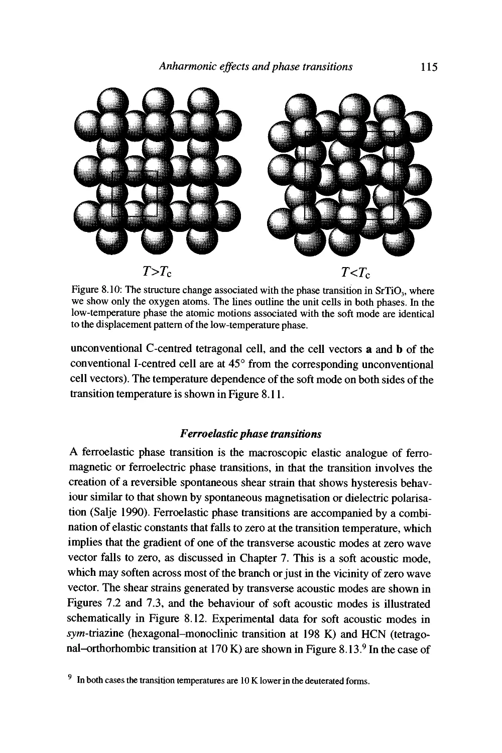
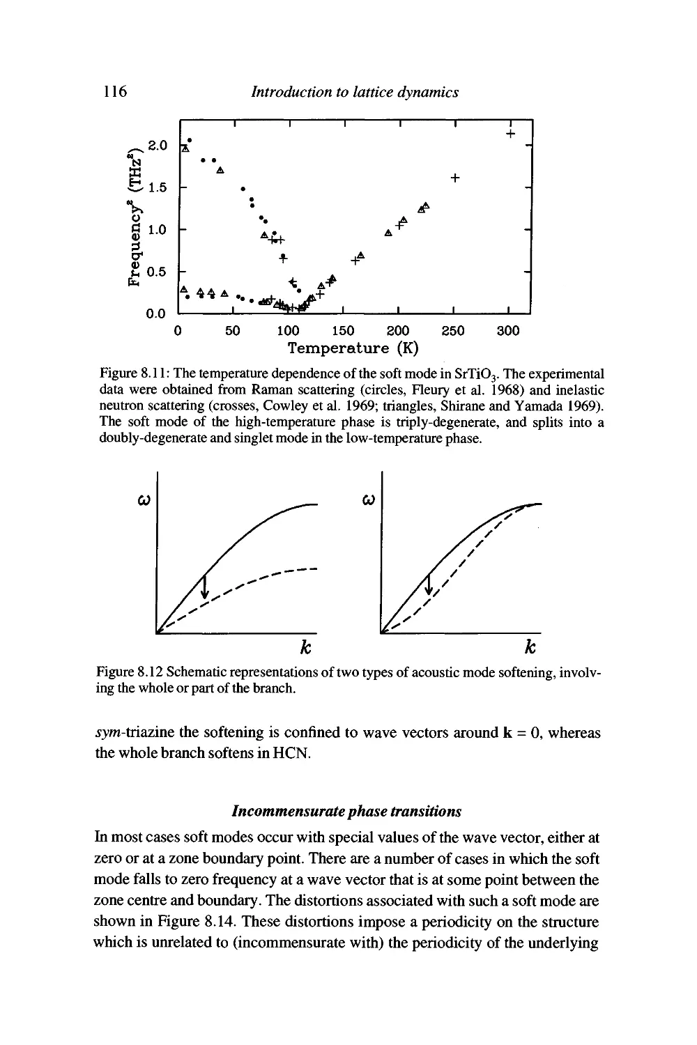
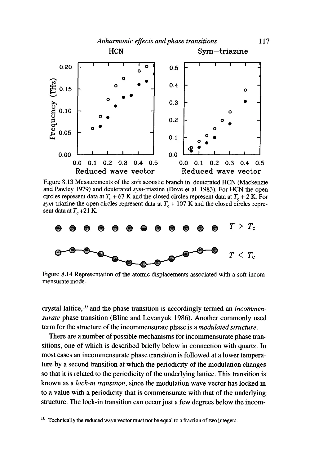
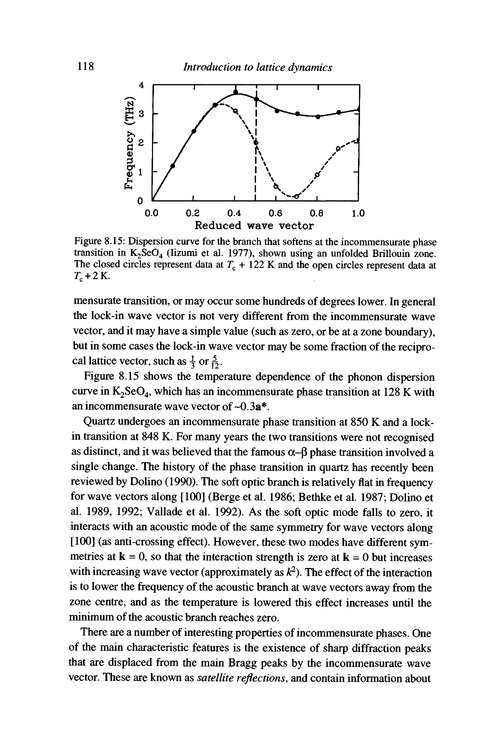
/


Текст
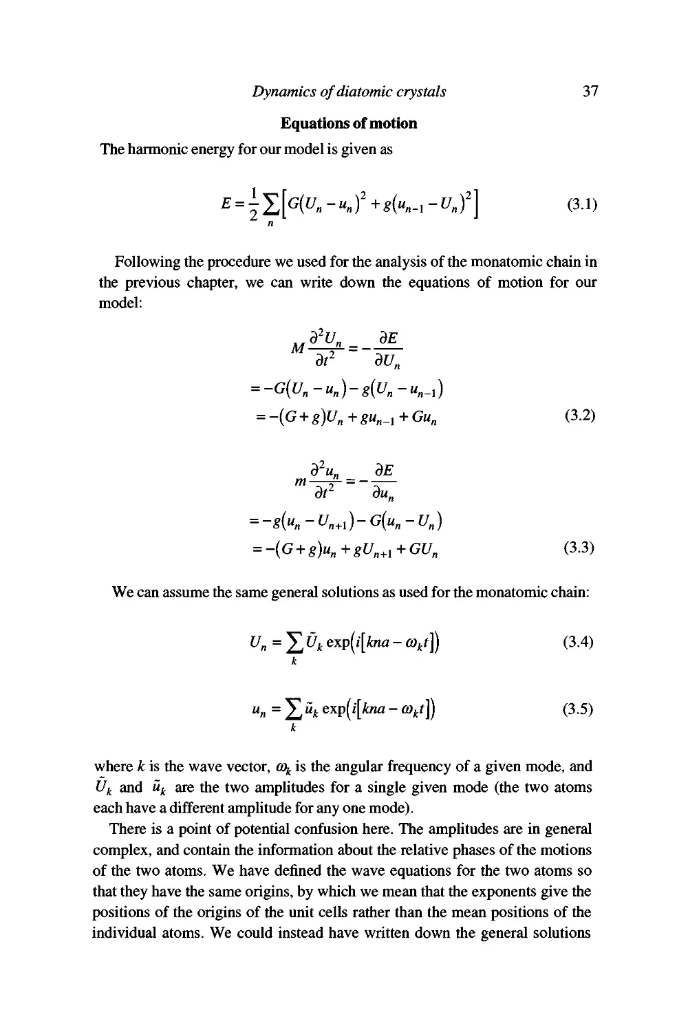
The vibrations of atoms inside crystals - lattice dynamics - are basic to many
fields of study in the solid state and mineral sciences, and lattice dynamics are
becoming increasingly important for work on mineral stability. This book
provides a self-contained text that introduces the subject from a basic level and
then takes the reader, through applications of the theory, to research level.
Simple systems are used for the development of the general principles. More
complex systems are then introduced, and later chapters look at
thermodynamics, elasticity, phase transitions and quantum effects. Experimental and
computational methods are described, and applications of lattice dynamics to
specific studies are detailed. Appendices provide supplementary information
and derivations for the Ewald method, statistical mechanics of lattice
vibrations. Landau theory, scattering theory and correlation functions.
The book is aimed at students and research workers in the earth and sohd
state sciences who need to incorporate lattice dynamics into their work.
INTRODUCTION TO LATTICE DYNAMICS
CAMBRIDGE TOPICS IN MINERAL PHYSICS AND CHEMISTRY
Editors
Dr Andrew Putnis
Dr Robert C. Liebermann
1 Ferroelastic and co-elastic crystals
E. K. H. SALJE
2 Transmission electron microscopy of minerals and rocks
ALEX C. MCLAREN
3 Introduction to the physics of the Earth's interior
JEAN-PAUL POIRIER
4 Introduction to lattice dynamics
MARTIN T. DOVE
INTRODUCTION TO LATTICE
DYNAMICS
MARTIN T. DOVE
Department of Earth Sciences
University of Cambridge
CAMBRIDGE
UNIVERSITY PRESS
Published by the Press Syndicate of the University of Cambridge
The Pitt Building, Trumpington Street, Cambridge CB2 IRP
40 West 20th Street, New York, NY 10011-4211, USA
10 Stamford Road, Oakleigh, Melbourne 3166, Australia
© Cambridge University Press 1993
First published 1993
A catalogue record for this book is available from the British Library
Library of Congress cataloguing in publication data available
ISBN 0 521 39293 4 hardback
Transferred to digital printing 2004
For Kate, Jennifer-Anne and Emma-Clare,
and our parents
Contents
Preface page xiii
Acknowledgements xvi
Physical constants and conversion factors xvii
1 Some fundamentals 1
Indications that dynamics of atoms in a crystal are important:
failure of the static lattice approximation 1
Interatomic forces 3
The variety of interatomic forces 3
Lattice energy 8
Worked example: a simple model for NaCl 10
Transferable models 12
Waves in crystals 14
The wave equation 14
Travelling waves in crystals 15
Summary 17
2 The harmonic approximation and lattice dynamics of
very simple systems 18
The harmonic approximation 18
The equation of motion of the one-dimensional monatomic chain 20
Reciprocal lattice, the Brillouin zone, and allowed wave vectors 21
The long wavelength limit 24
Extension to include distant neighbours 25
Three-dimensional monatomic crystals 26
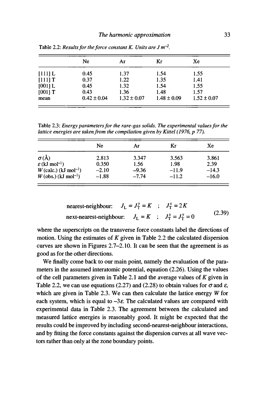
Worked example: the lattice dynamics of the rare-gas solids 28
Summary 34
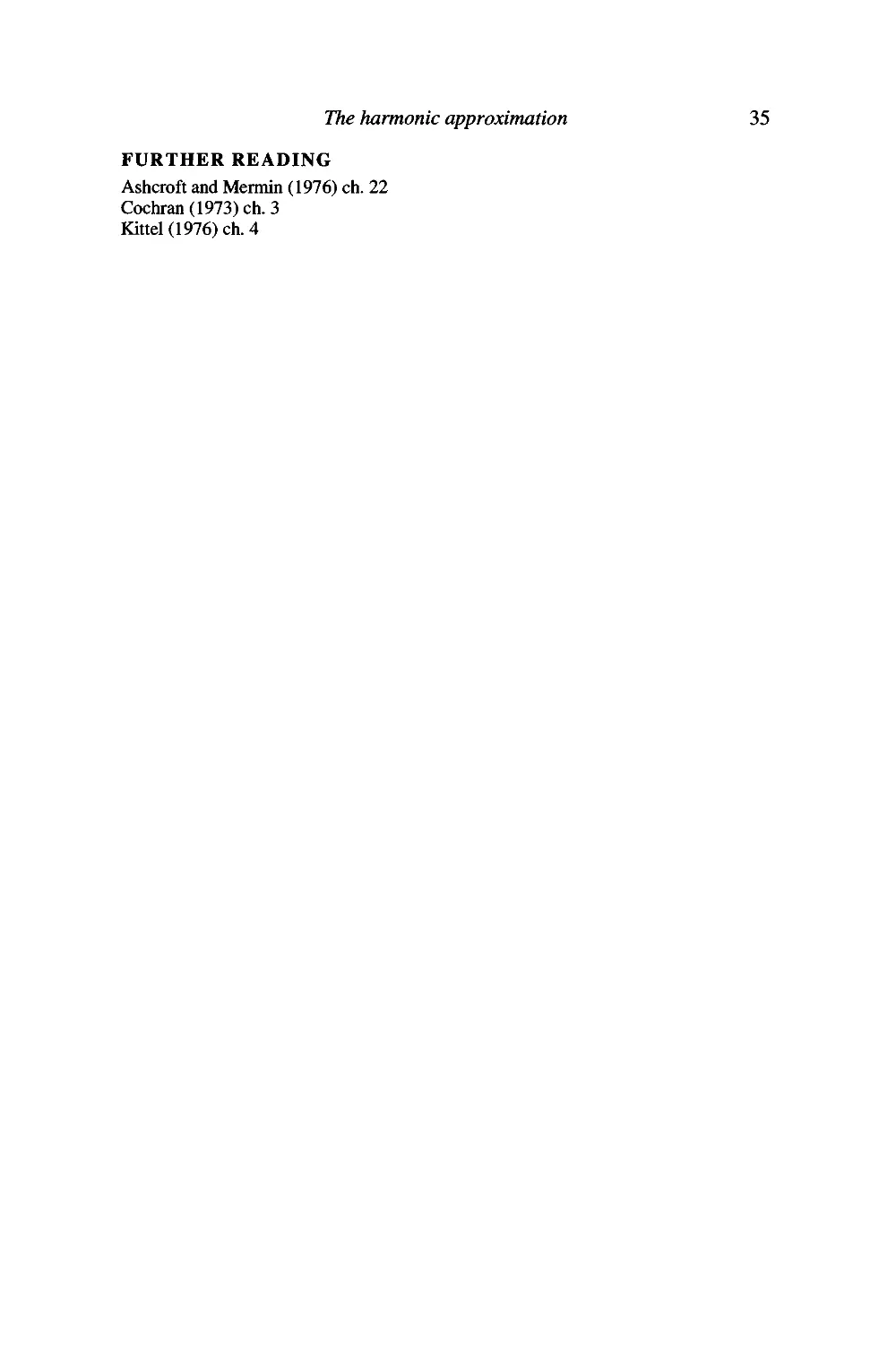
3 Dynamics of diatomic crystals: general principles 36
The basic model 36
Equations of motion 3 7
IX
X Contents
Solution in the long-wavelength Umit 38
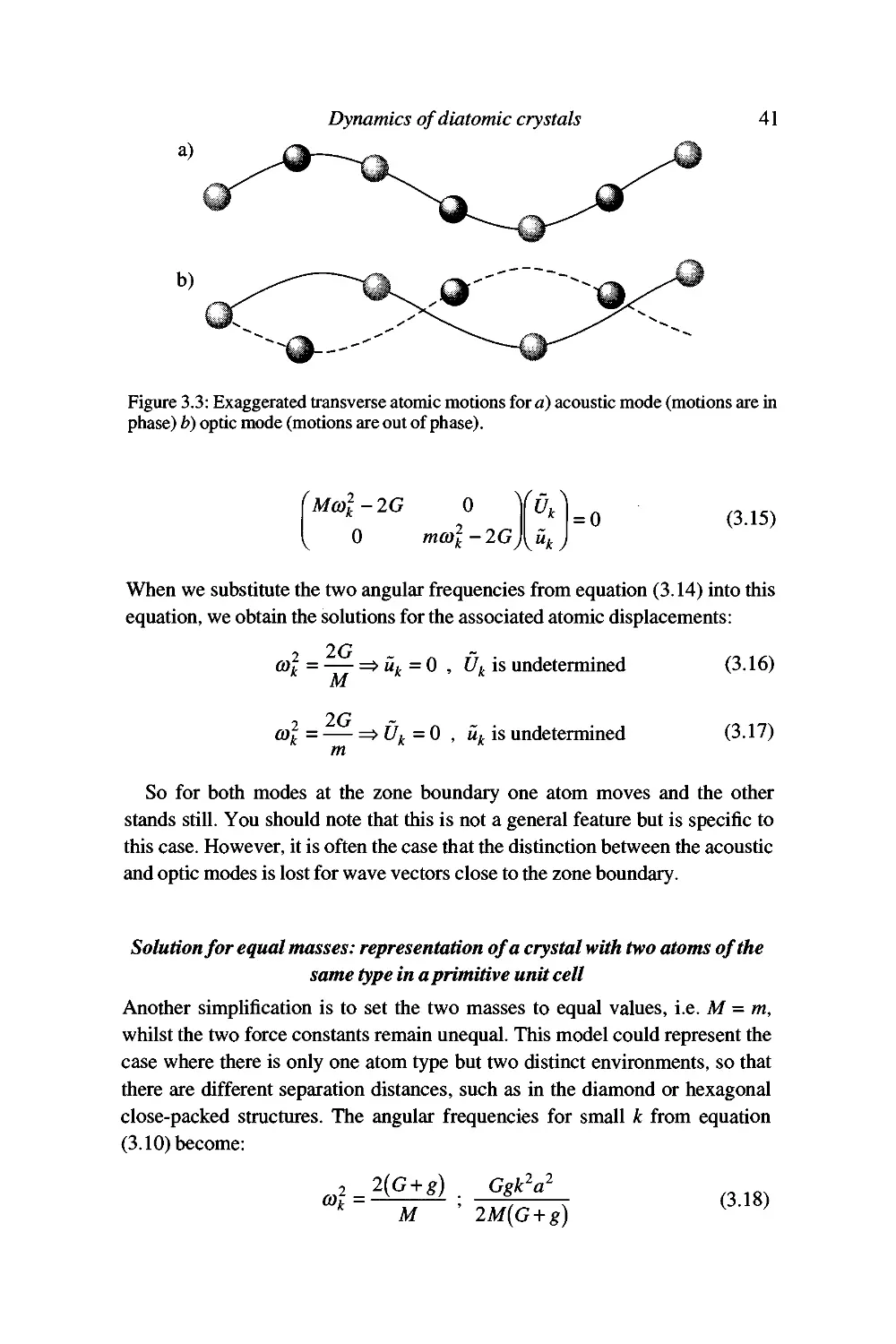
Some specific solutions 40
GeneraUsation to more complex cases 43
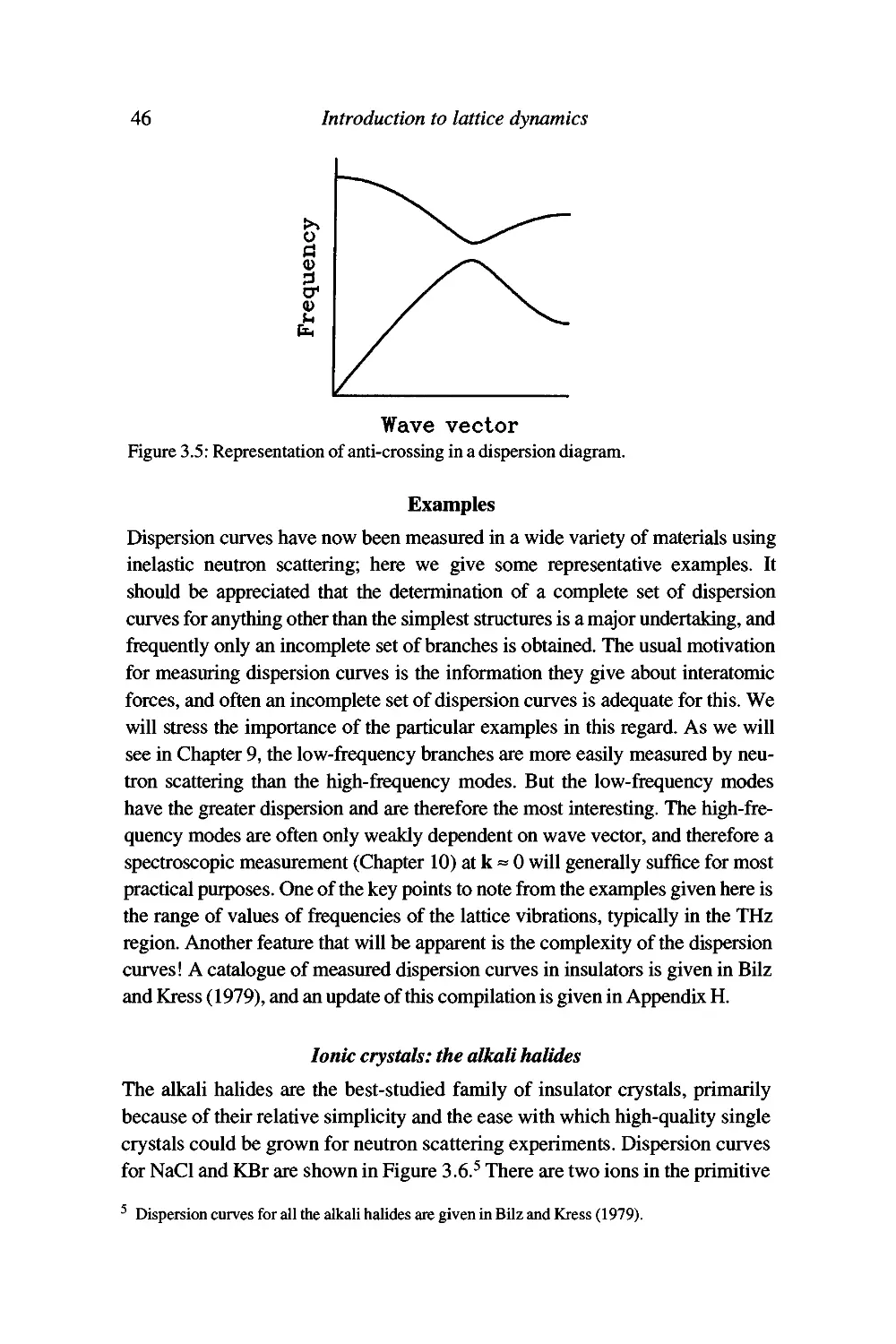
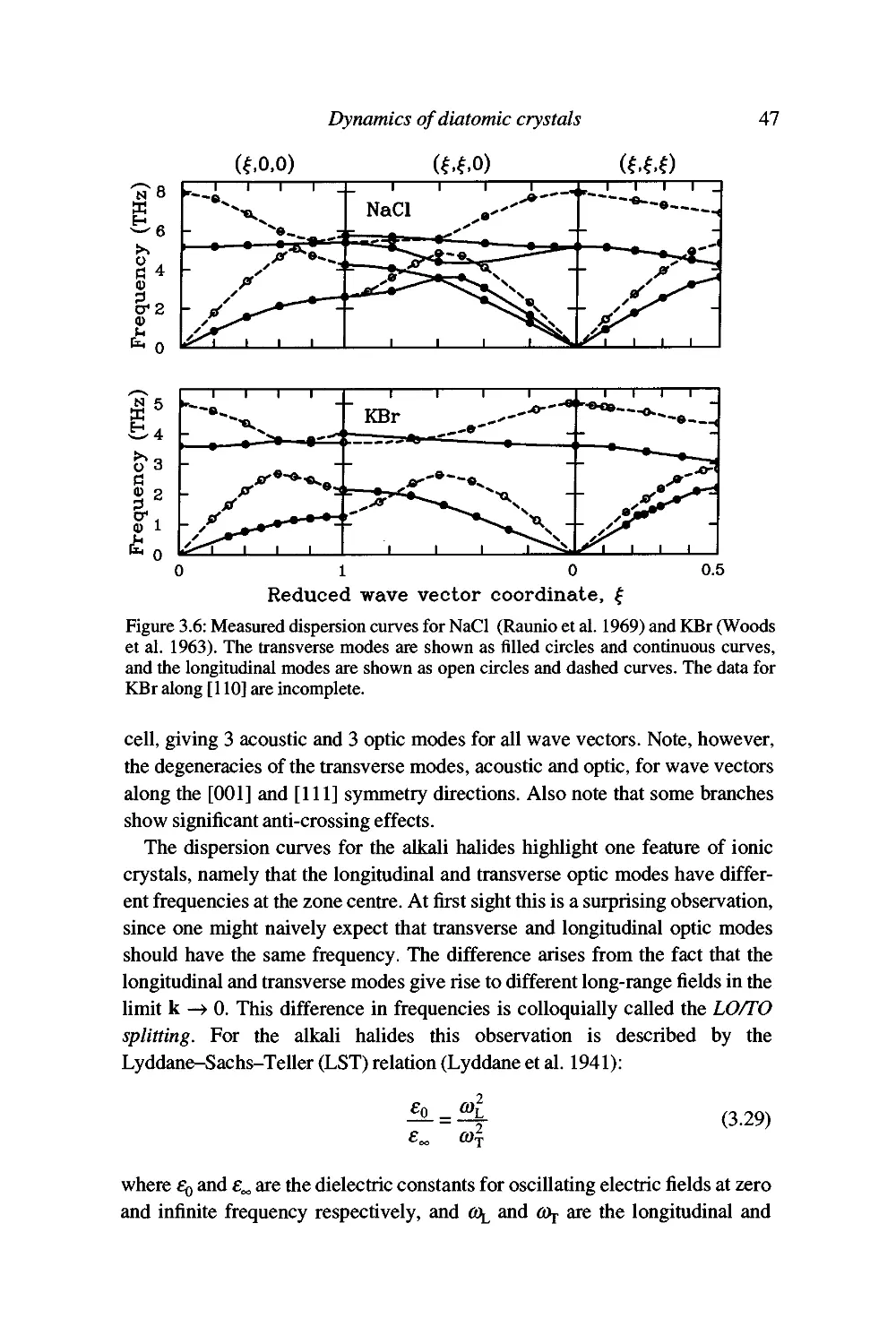
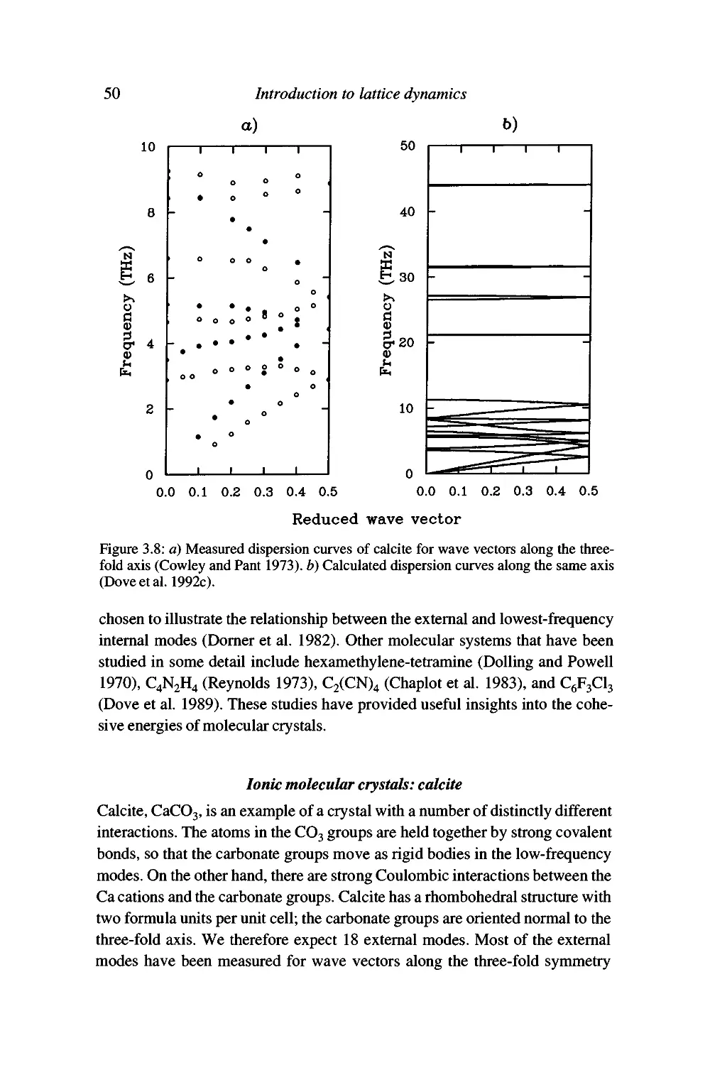
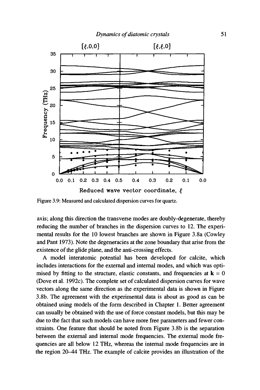
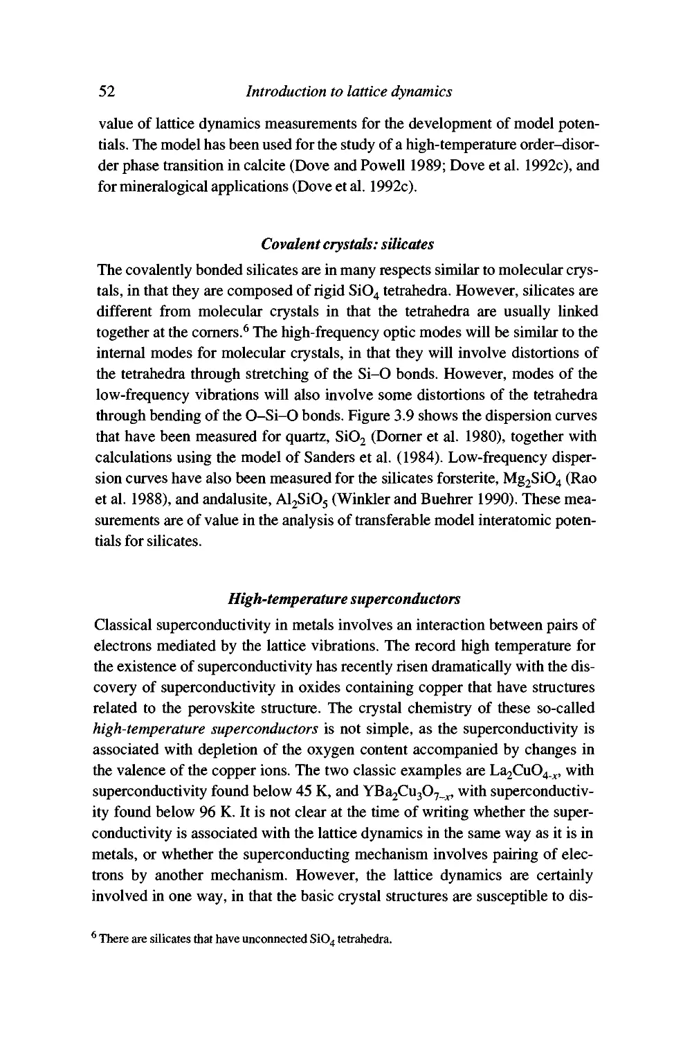
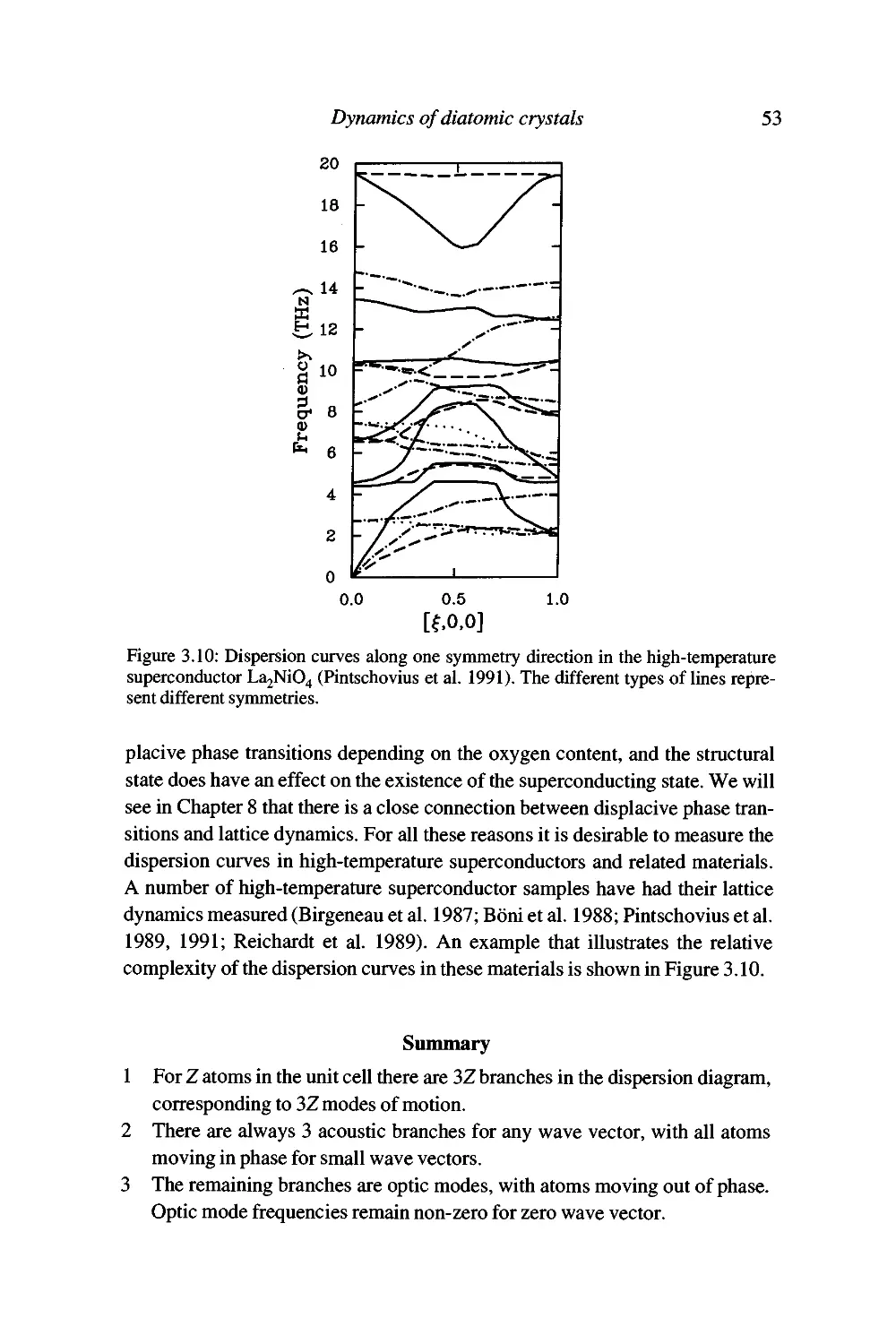
Examples 46
Summary 53
4 How far do the atoms move? 55
Normal modes and normal mode coordinates 55
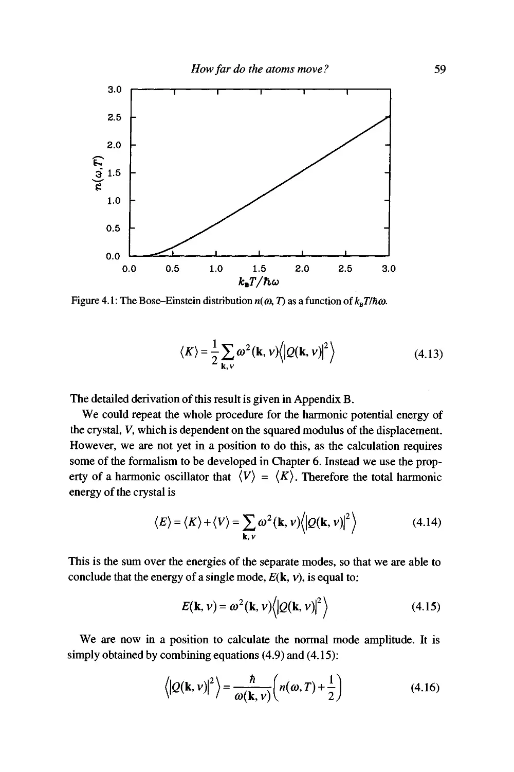
The quantisation of normal modes 5 7
Vibrational energies and normal mode amplitudes 58
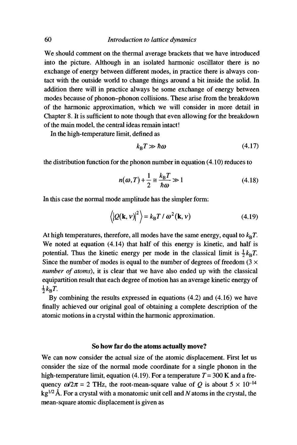
So how far do the atoms actually move? 60
The crystallographic temperature factor 62
Summary 63
5 Lattice dynamics and thermodynamics 64
The basic thermodynamic functions 64
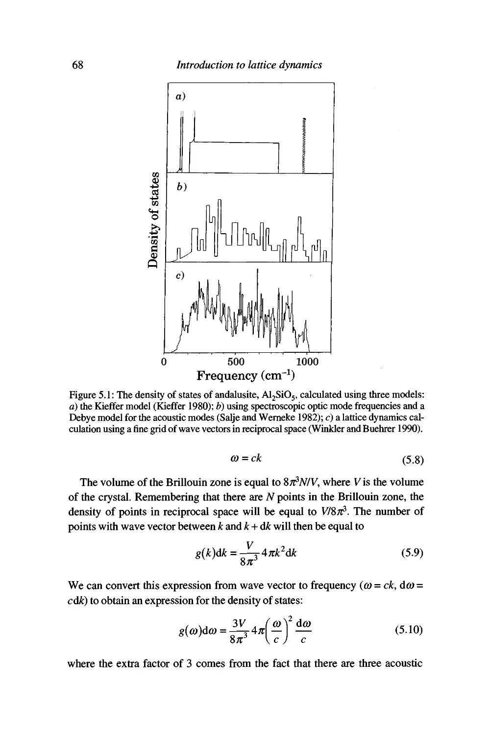
Evaluation of the thermodynamic functions and the density of states 66
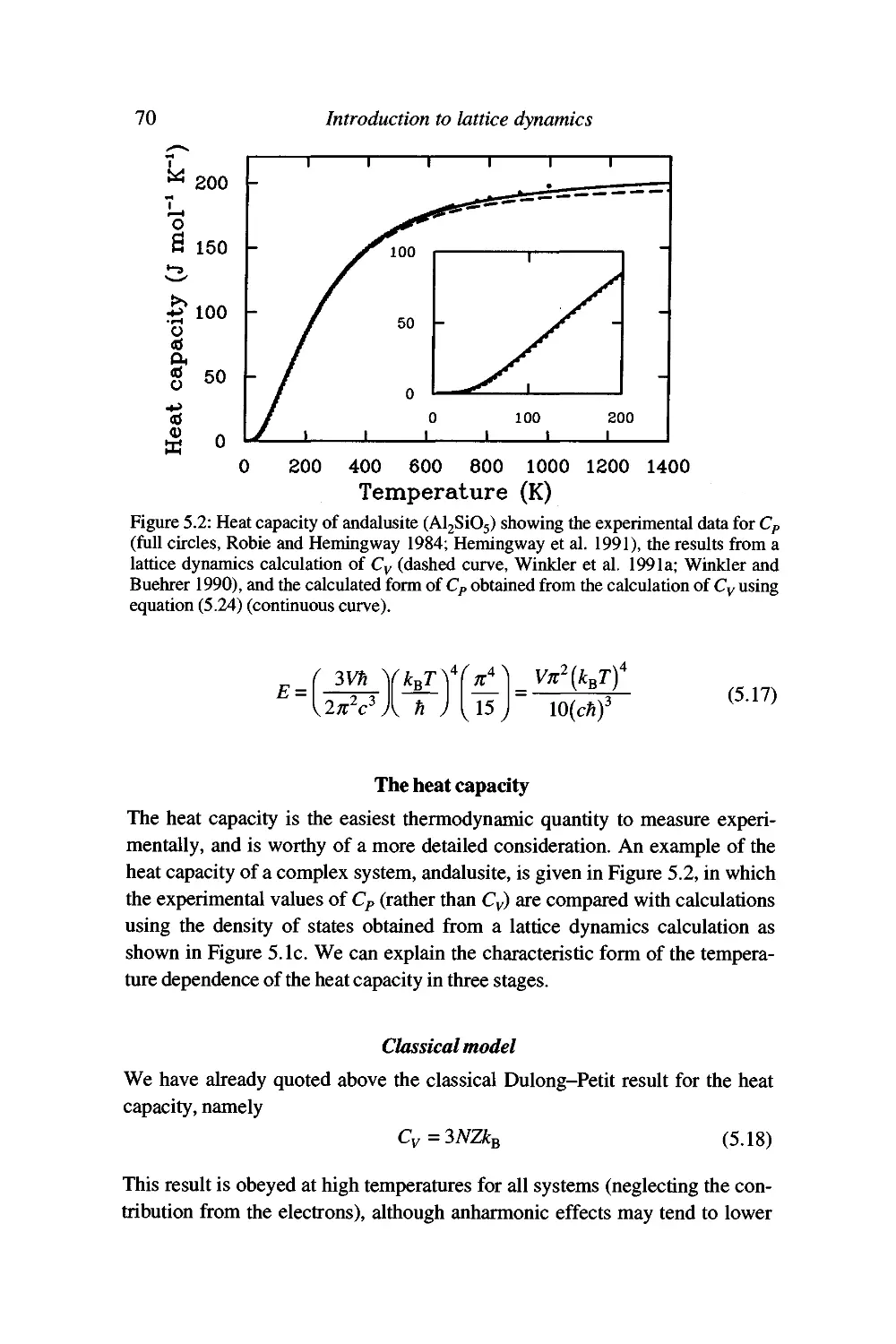
The heat capacity 70
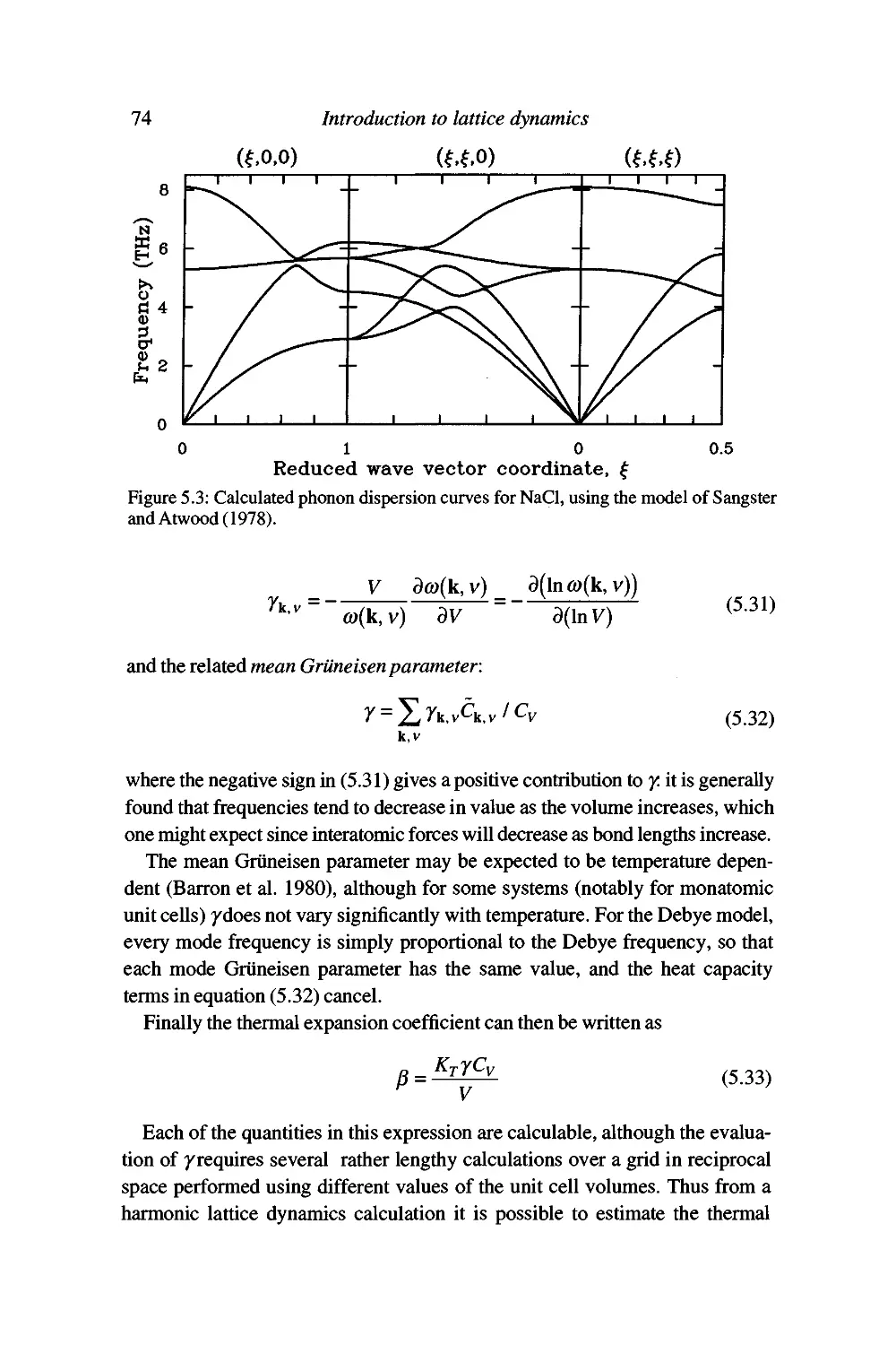
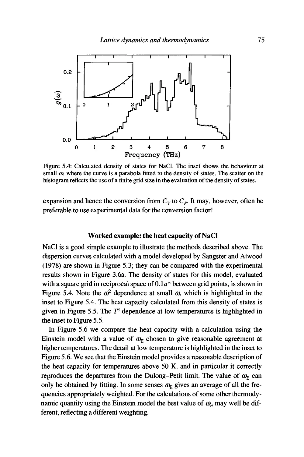
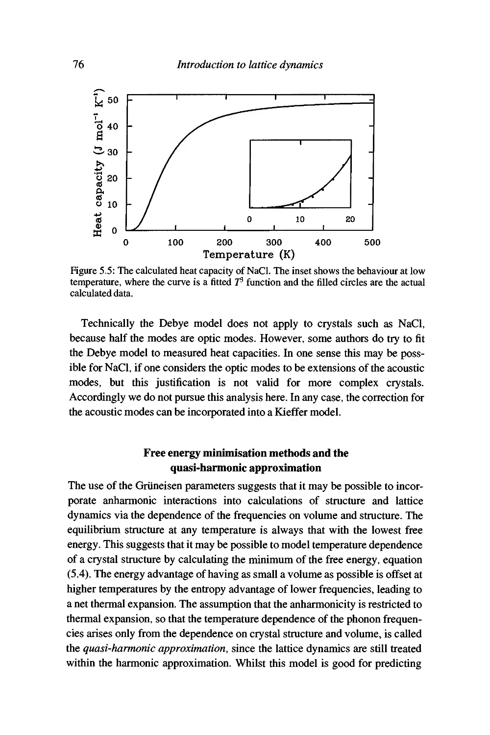
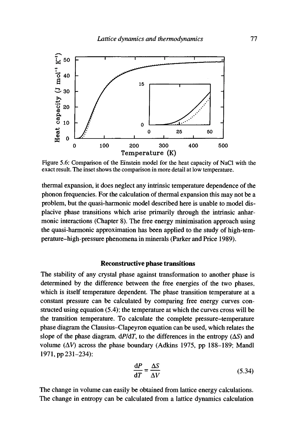
Worked example: the heat capacity of NaCl 75
Free energy minimisation methods and the quasi-harmonic
approximation 76
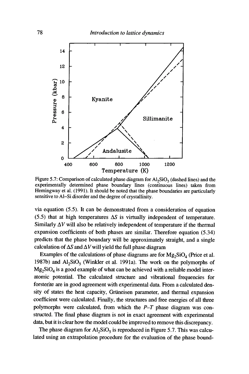
Reconstructive phase transitions 77
Surranary 79
6 Formal description 80
Review and problems 80
The diatomic chain revisited 81
The equations of motion and the dynamical matrix 83
Extension for molecular crystals 87
The dynamical matrix and symmetry 88
Extension for the shell model 88
Actual calculations of dispersion curves 91
Normal mode coordinates 93
Surranary 94
7 Acoustic modes and macroscopic elasticity 95
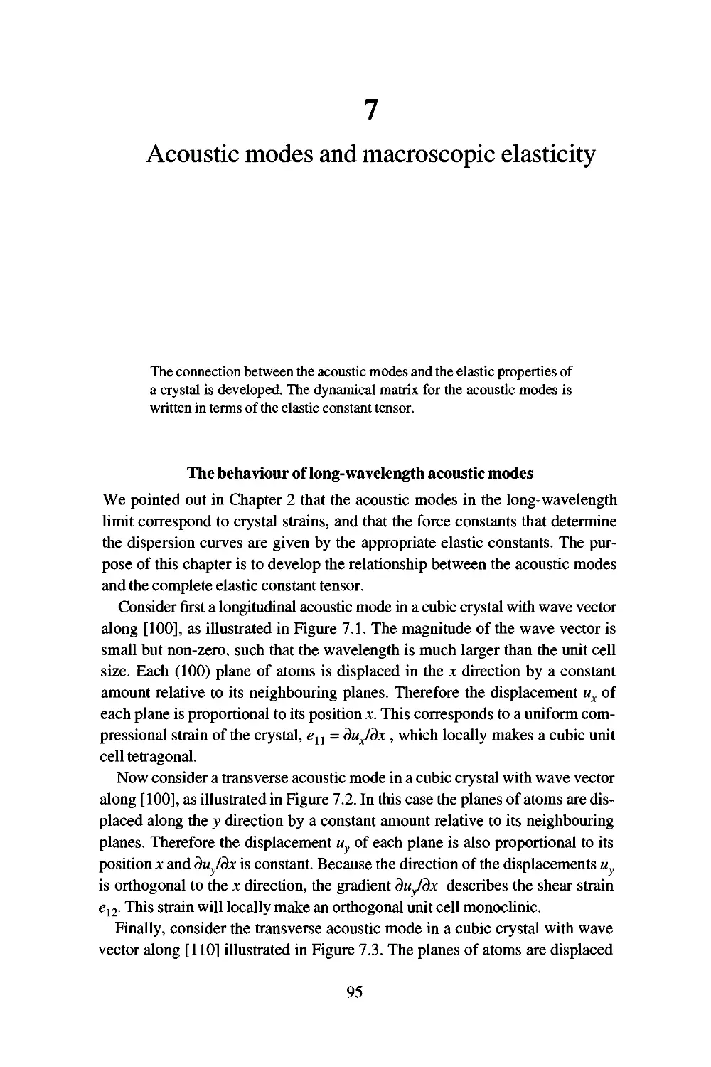
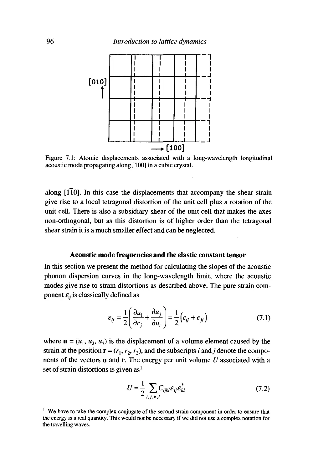
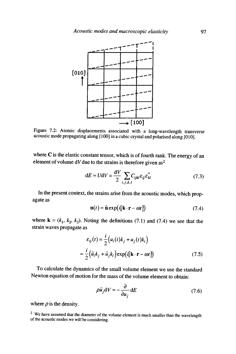
The behaviour of long-wavelength acoustic modes 95
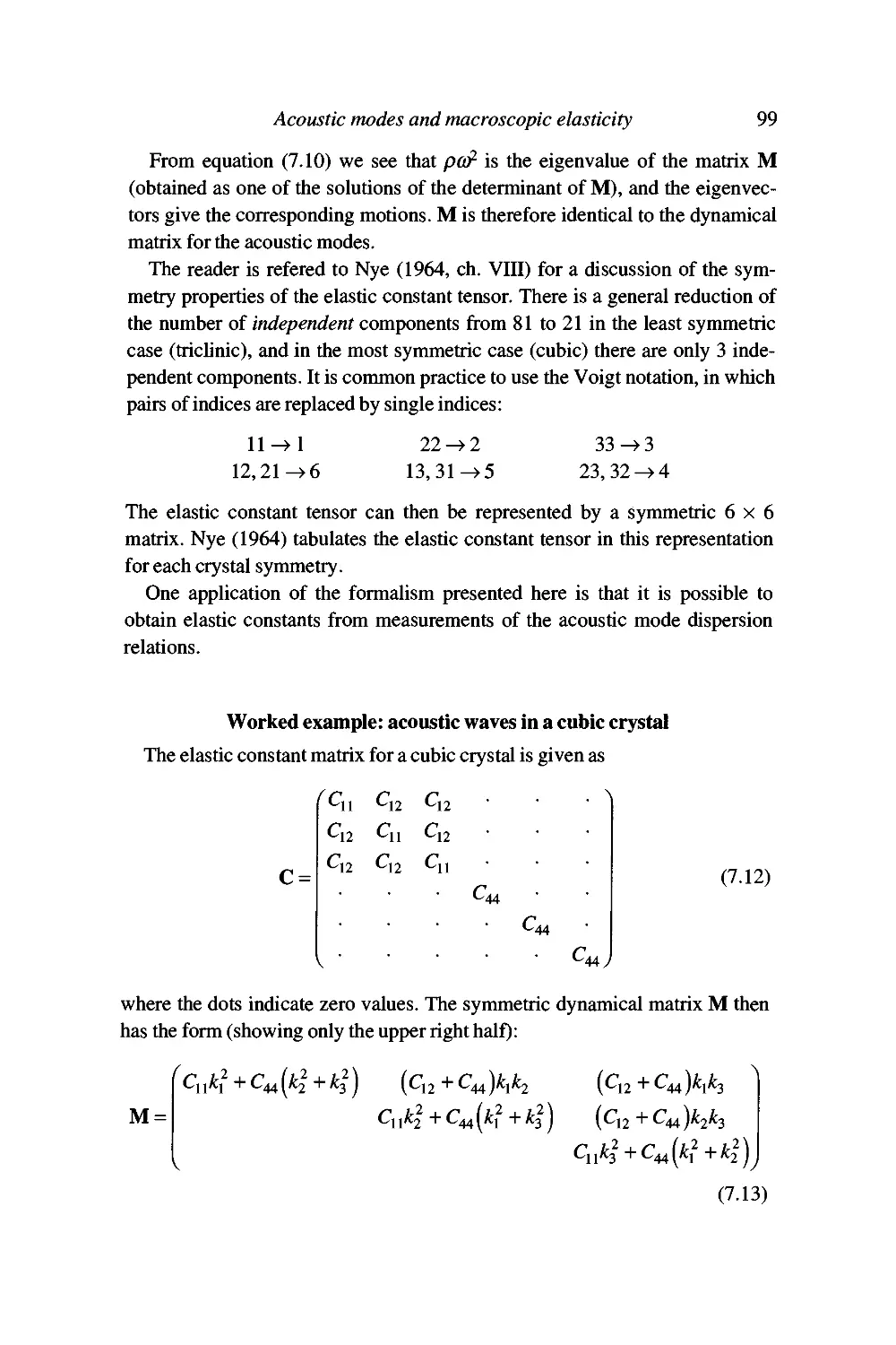
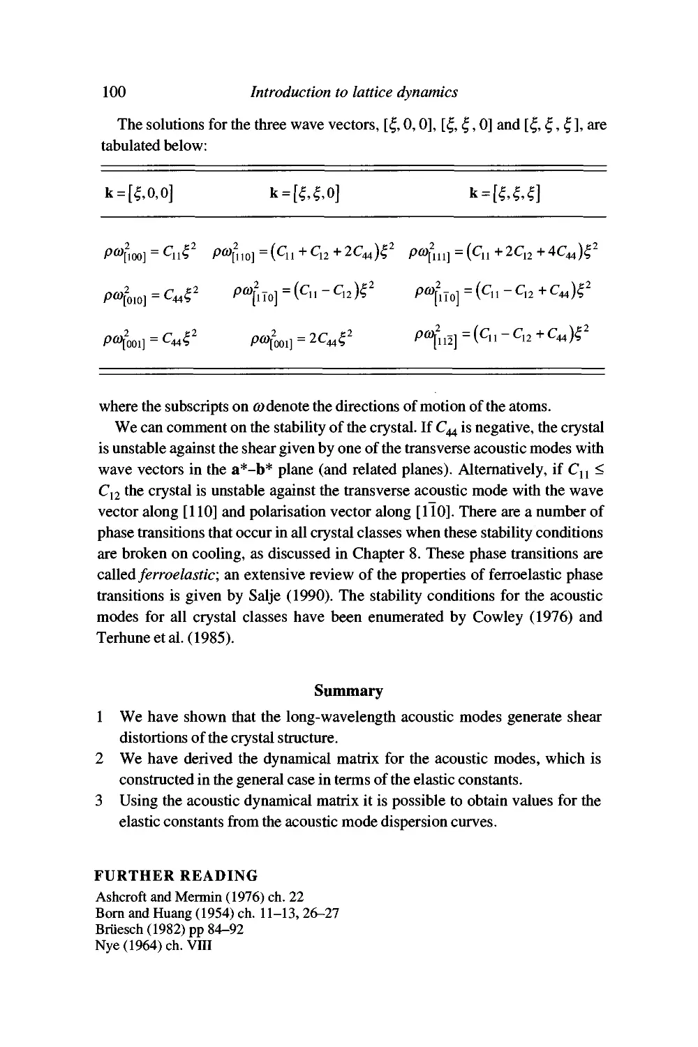
Acoustic mode frequencies and the elastic constant tensor 96
Worked example: acoustic waves in a cubic crystal 99
Surranary 100
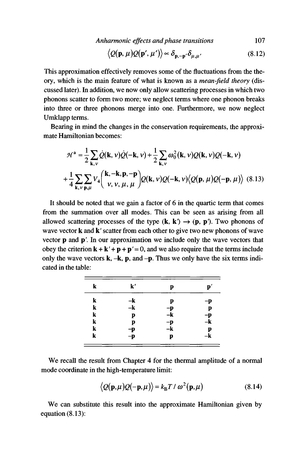
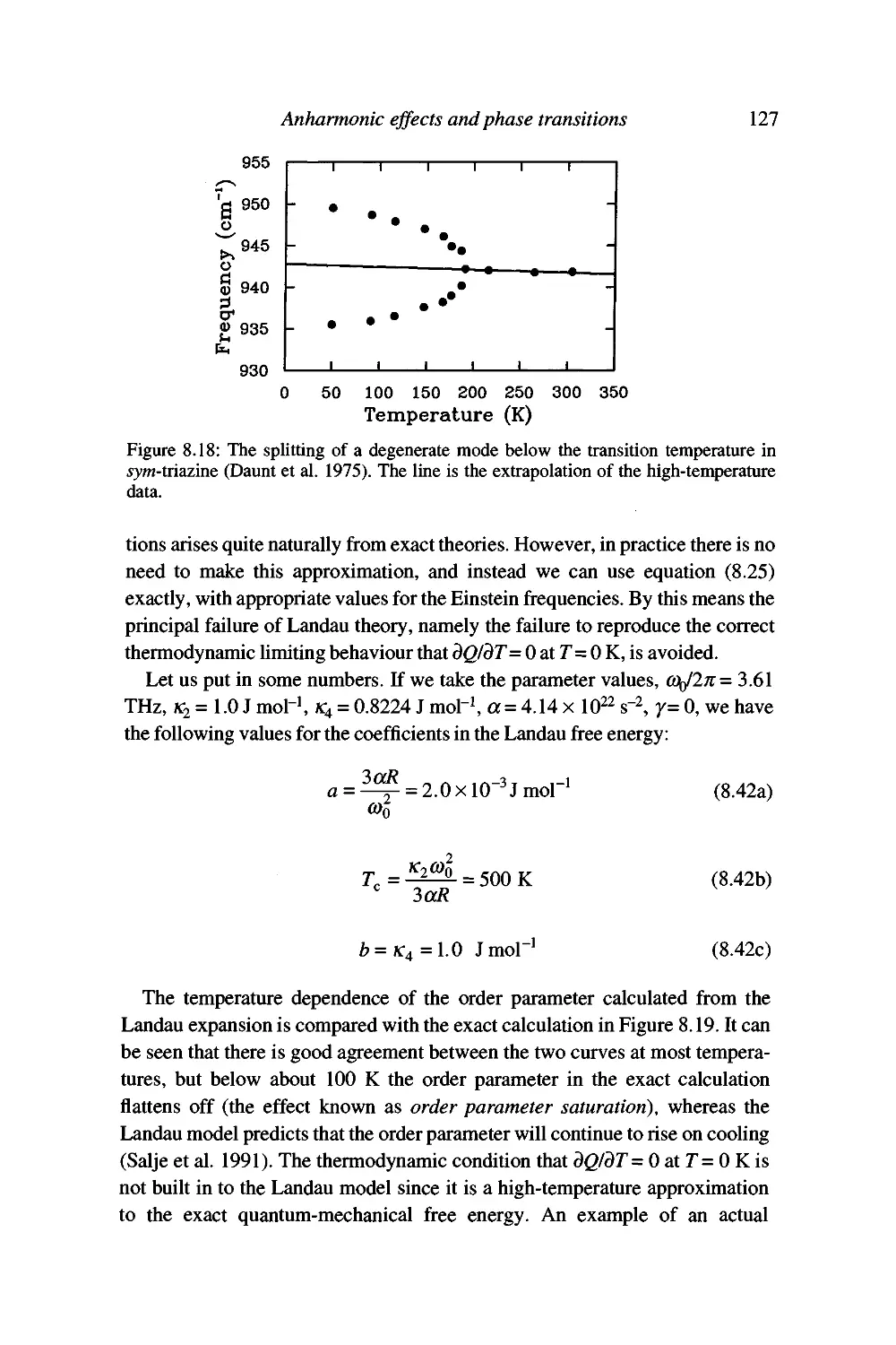
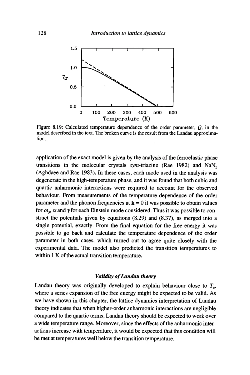
8 Anharmonic effects and phase transitions 101
Failures of the harmonic approximation 101
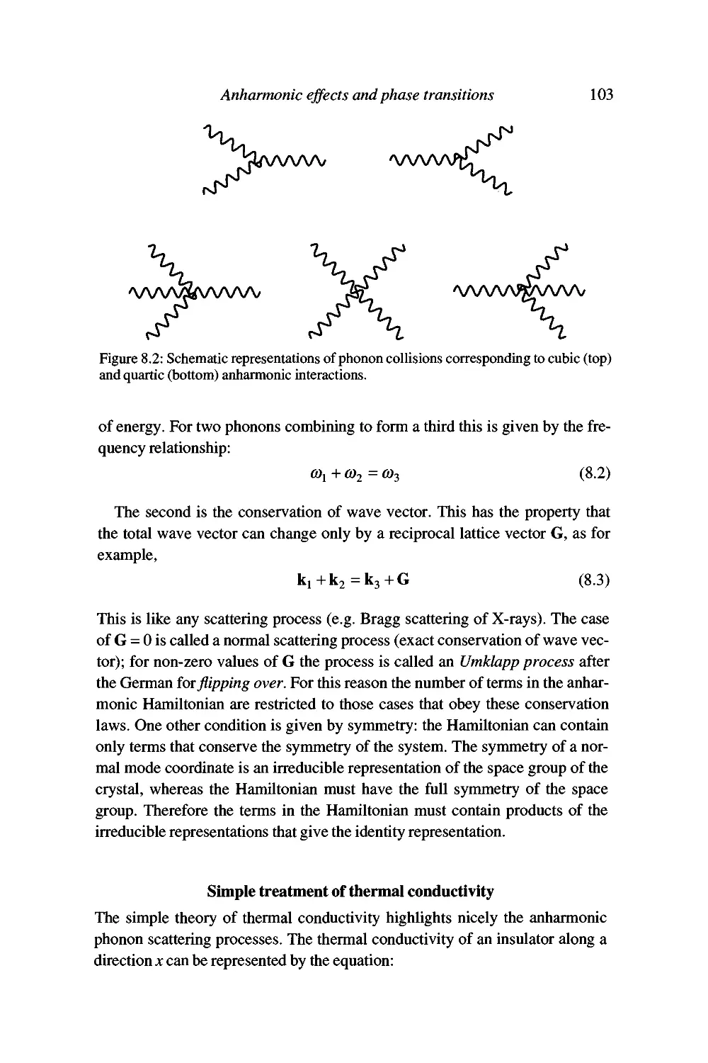
Anharmonic interactions 101
Simple treatment of thermal conductivity 103
Contents xi
Temperature dependence of phonon frequencies 105
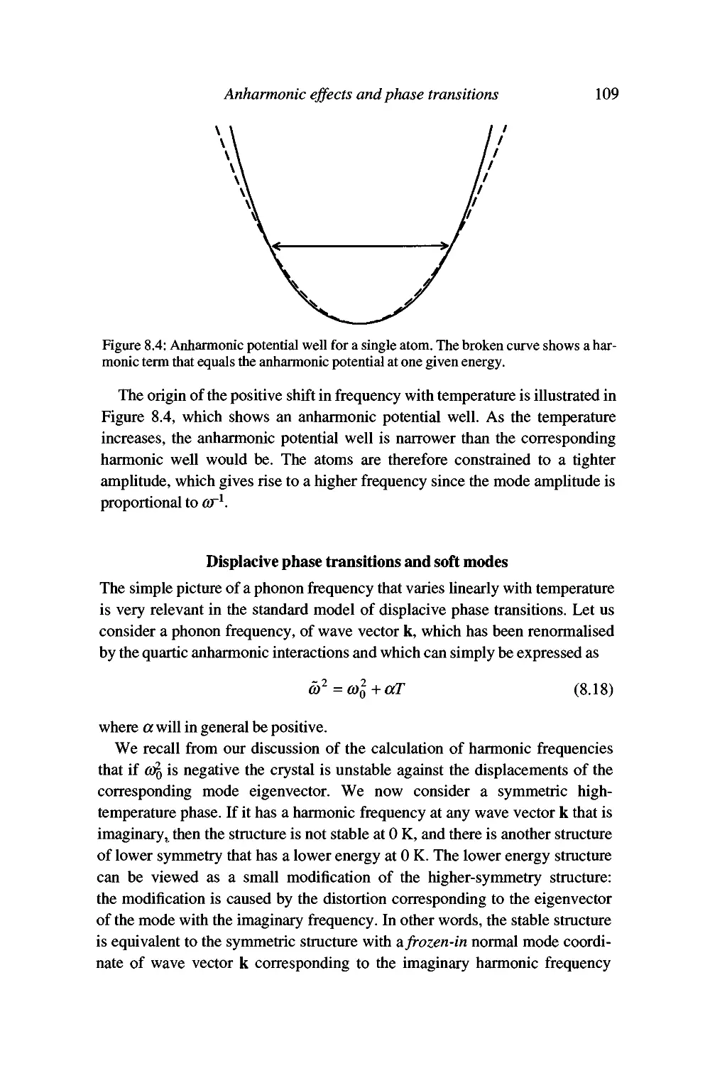
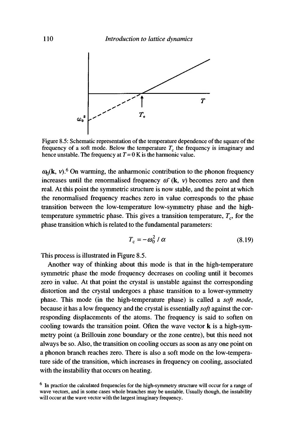
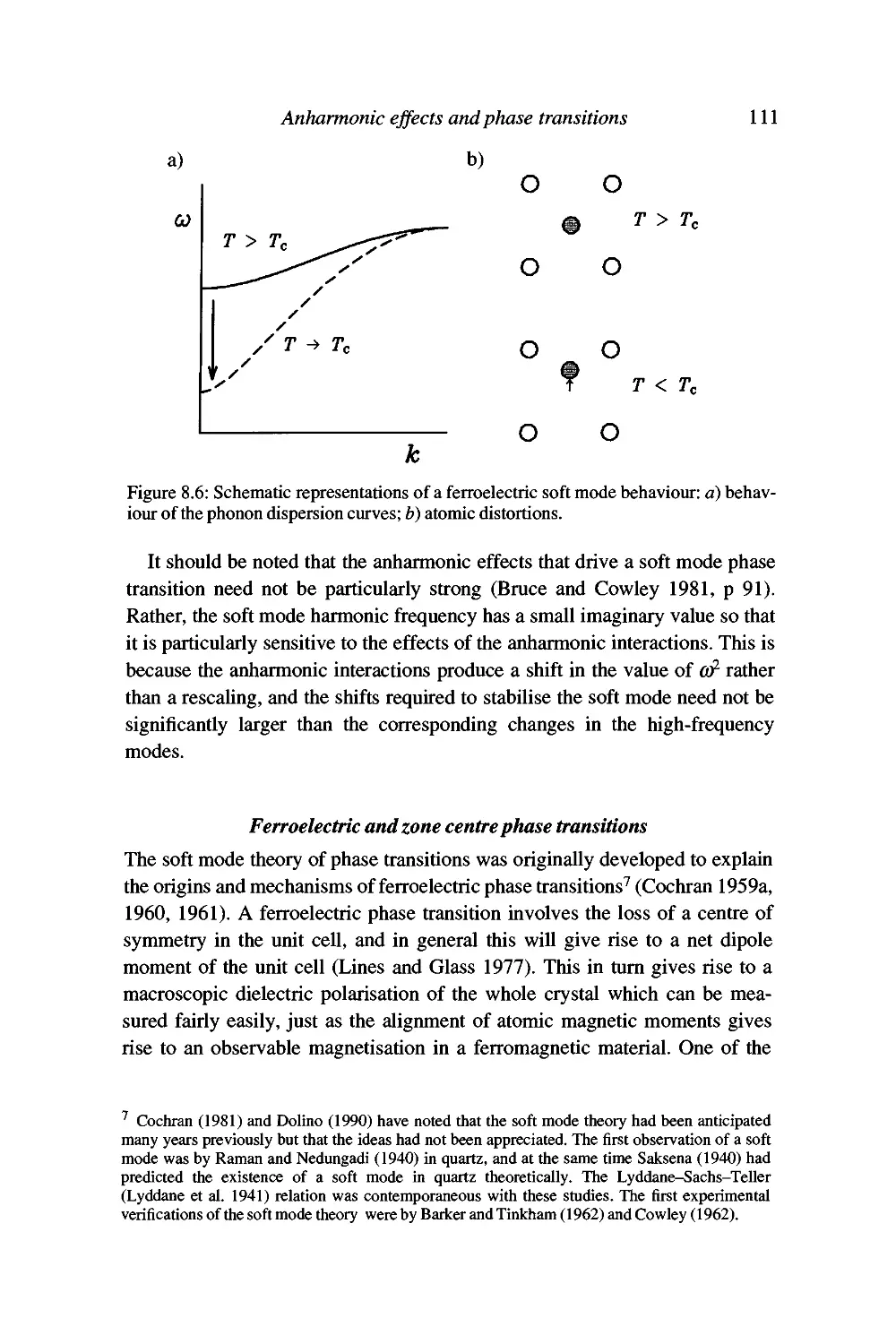
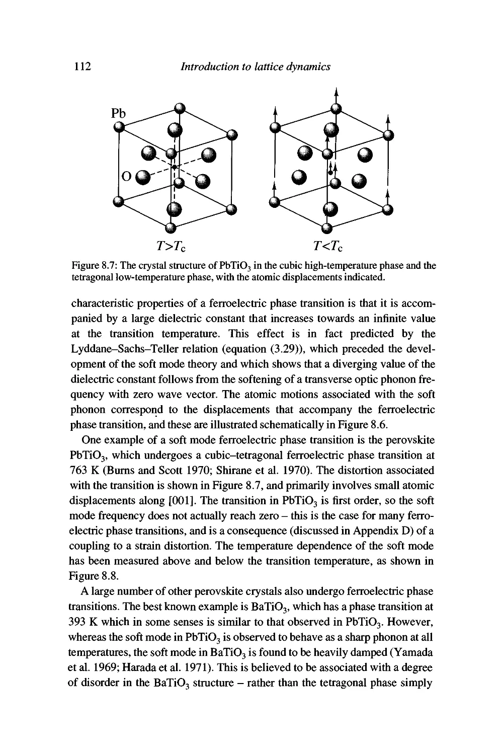
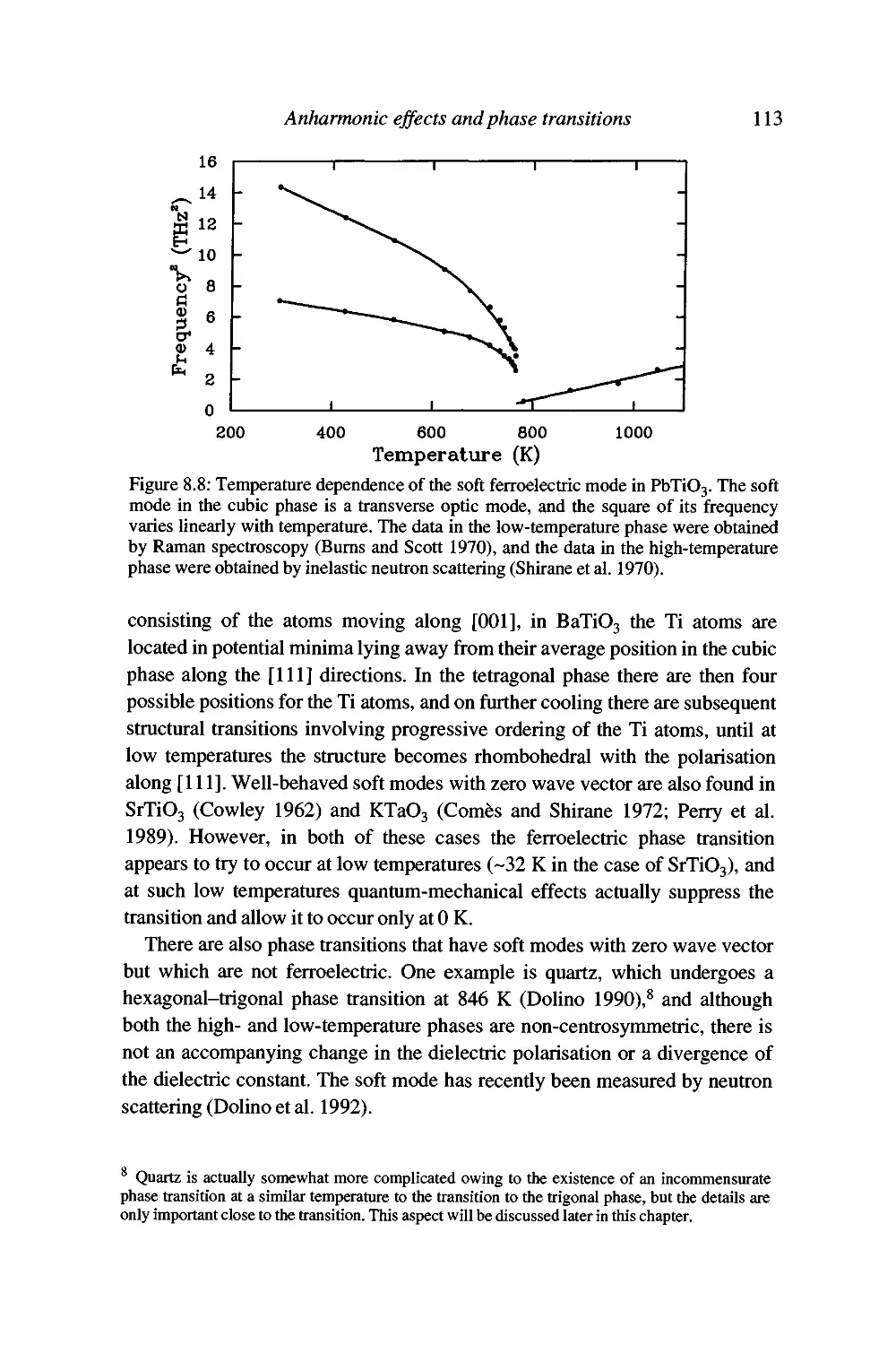
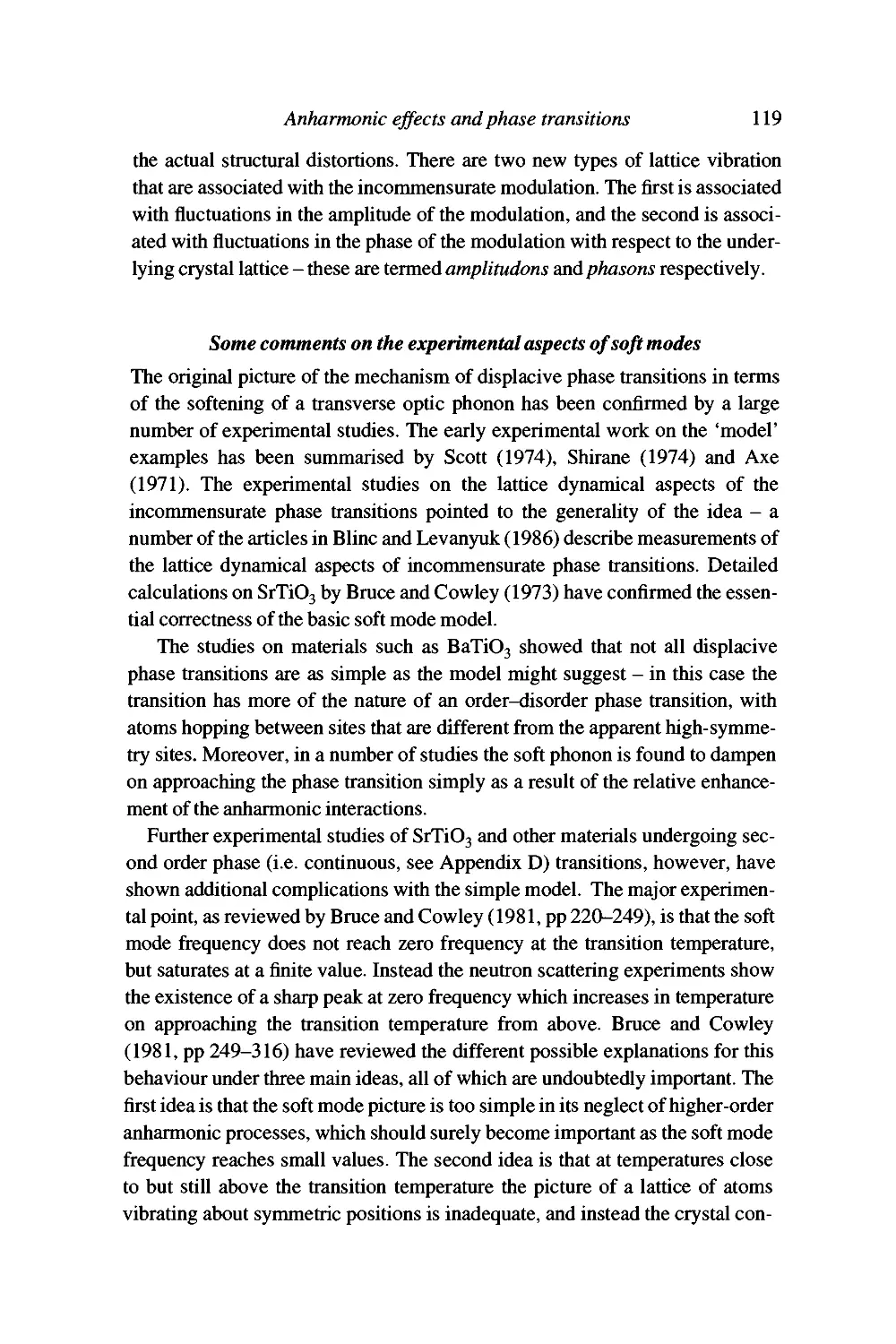
Displacive phase transitions and soft modes 109
Soft modes and the Landau theory of phase transitions 120
The origin of the anharmonic interactions 130
Summary 130
9 Neutron scattering 132
Properties of the neutron as a useful probe 132
Sources of thermal neutron beams 134
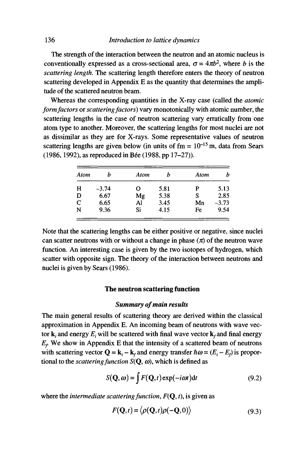
Interactions of neutrons with atomic nuclei 135
The neutron scattering function 136
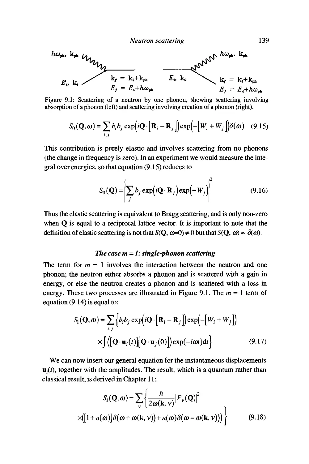
Conservation laws for one-phonon neutron scattering 141
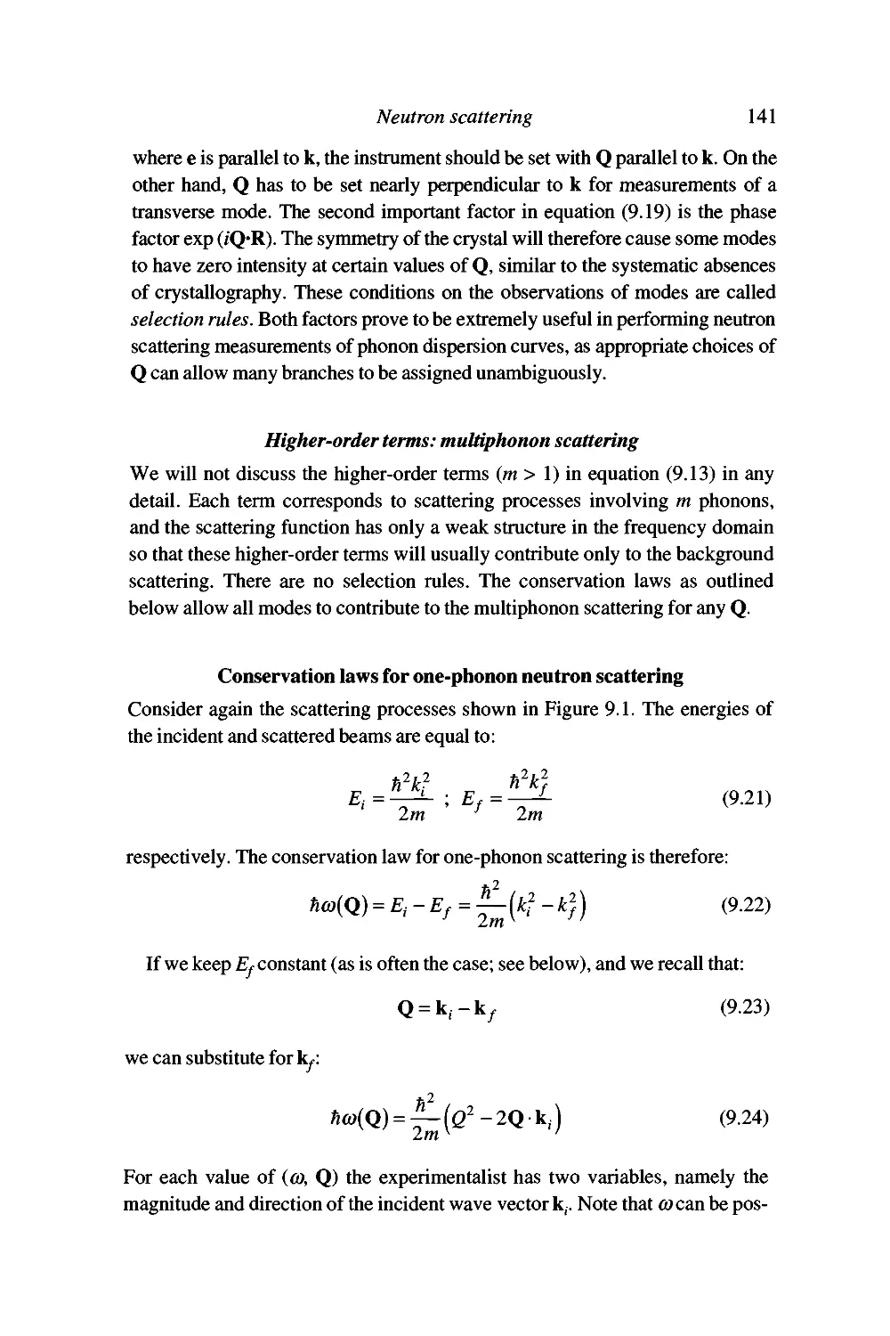
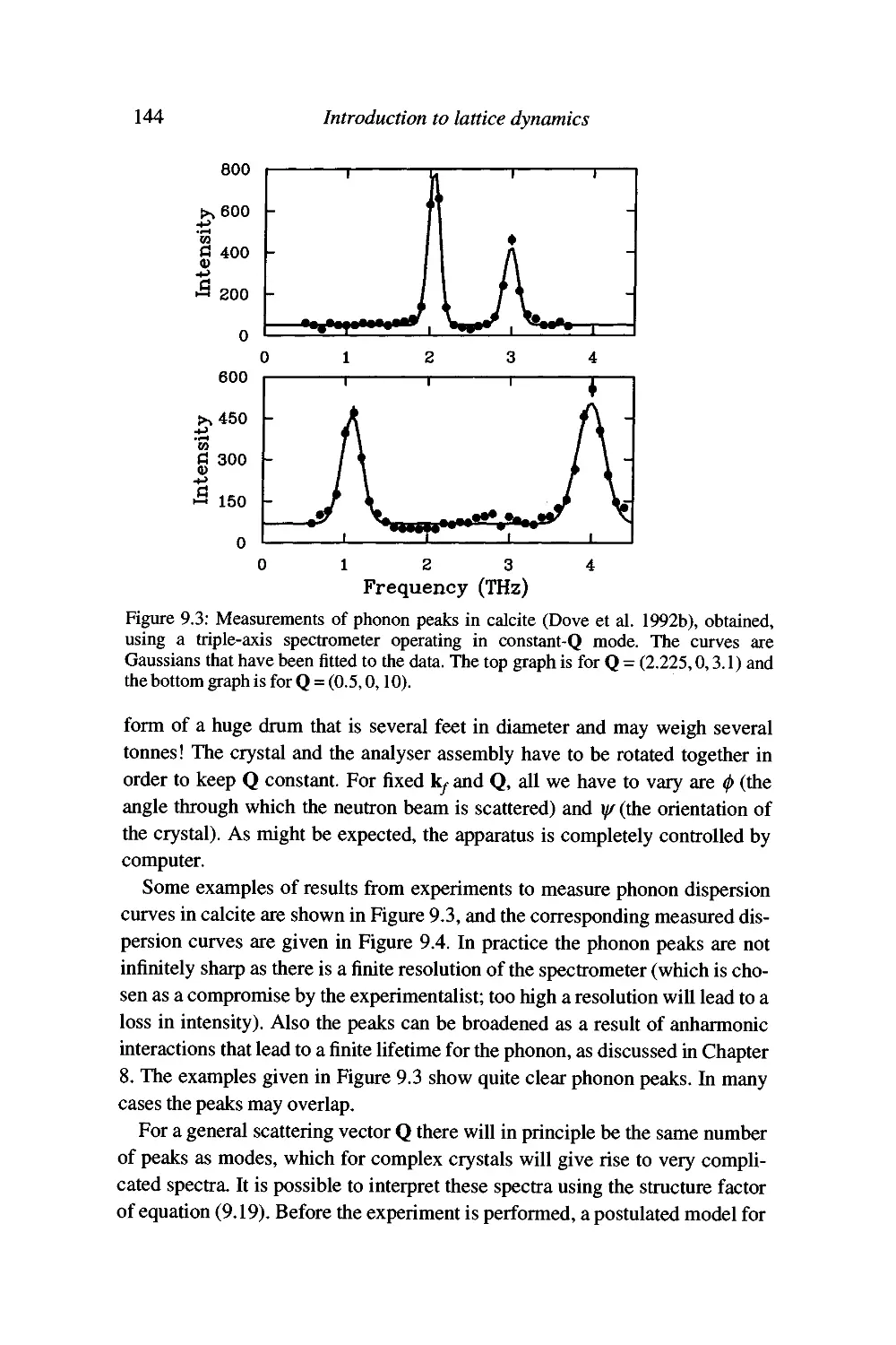
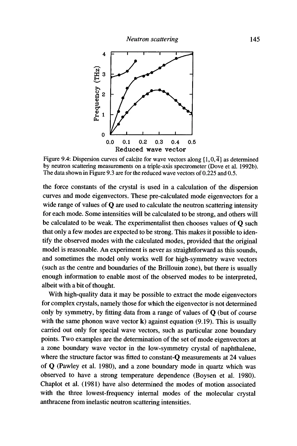
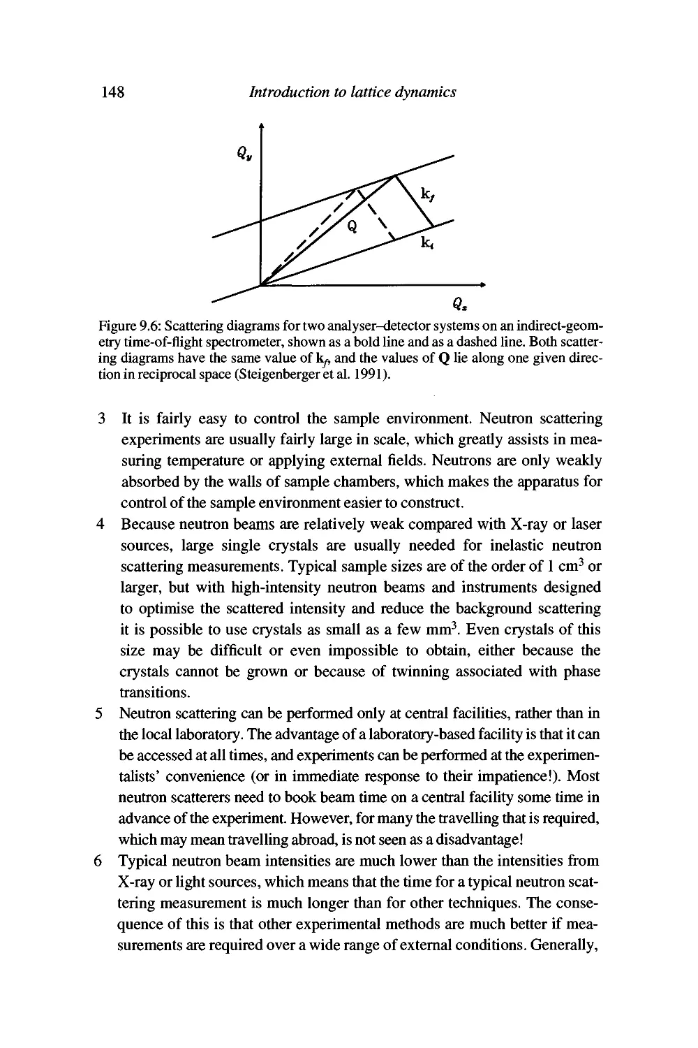
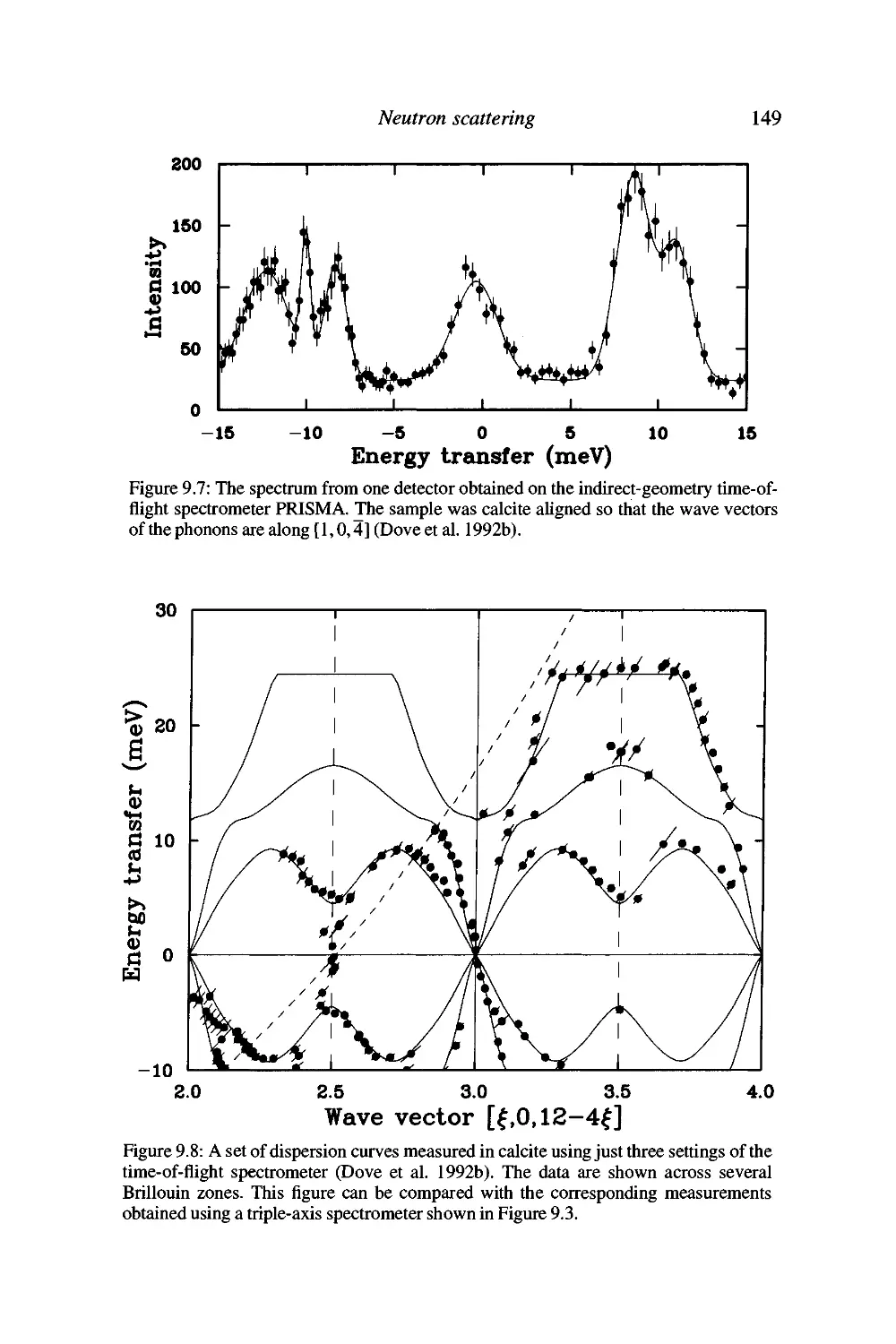
Experimental inelastic neutron scattering 142
Advantages of neutron scattering and some problems with
the technique 147
Summary 150
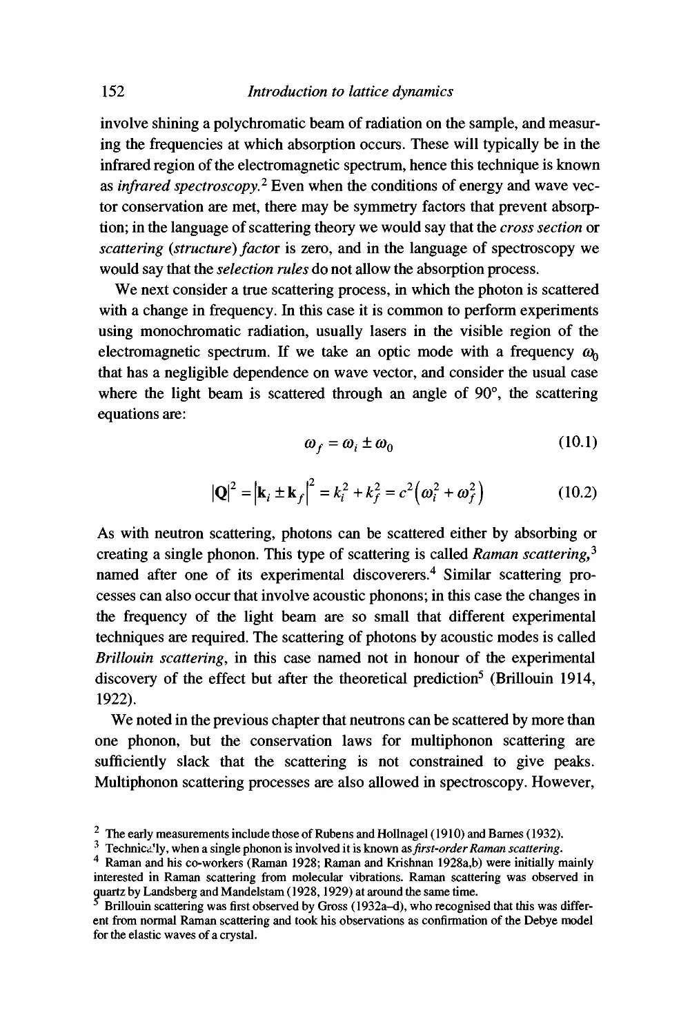
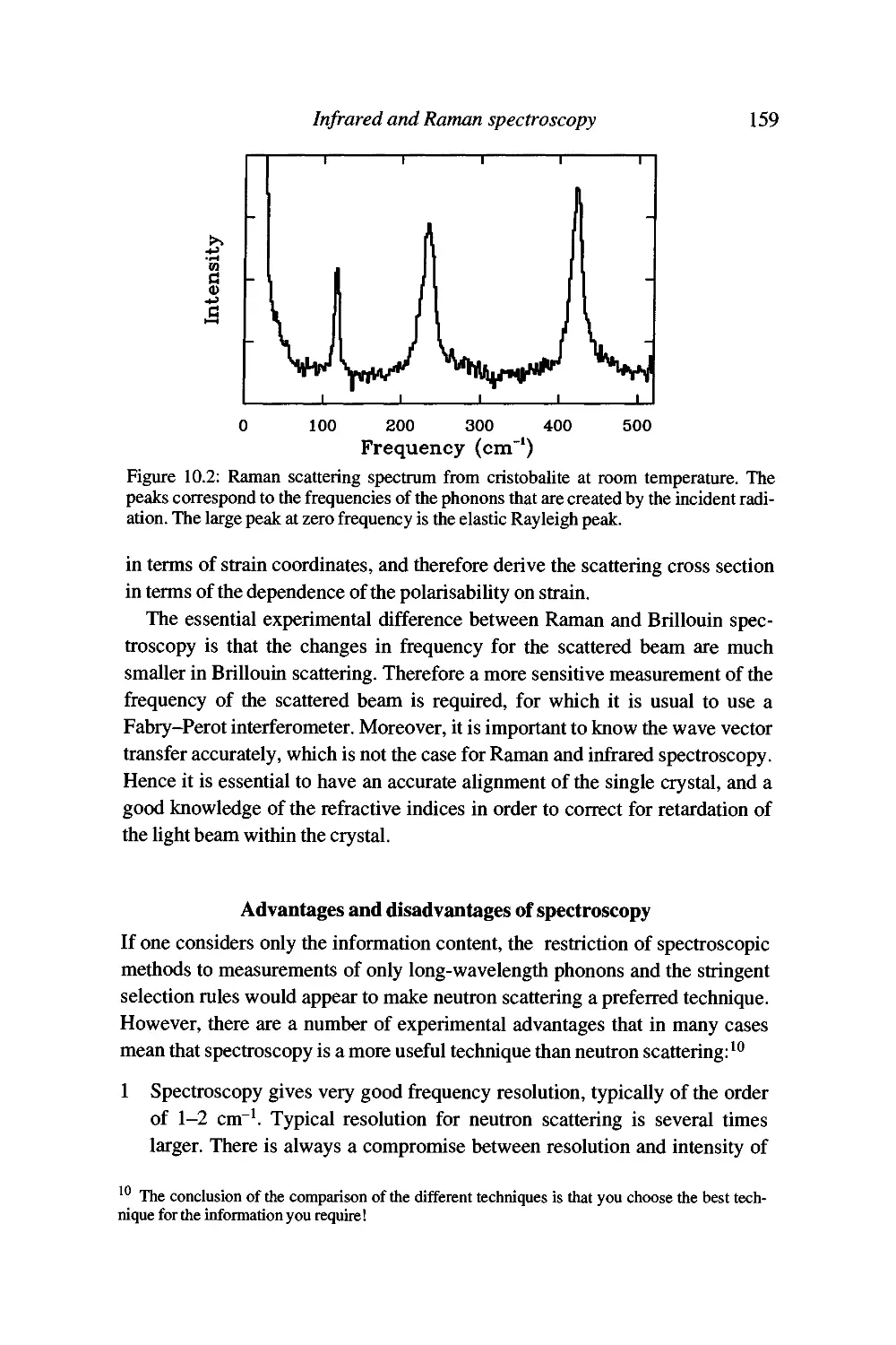
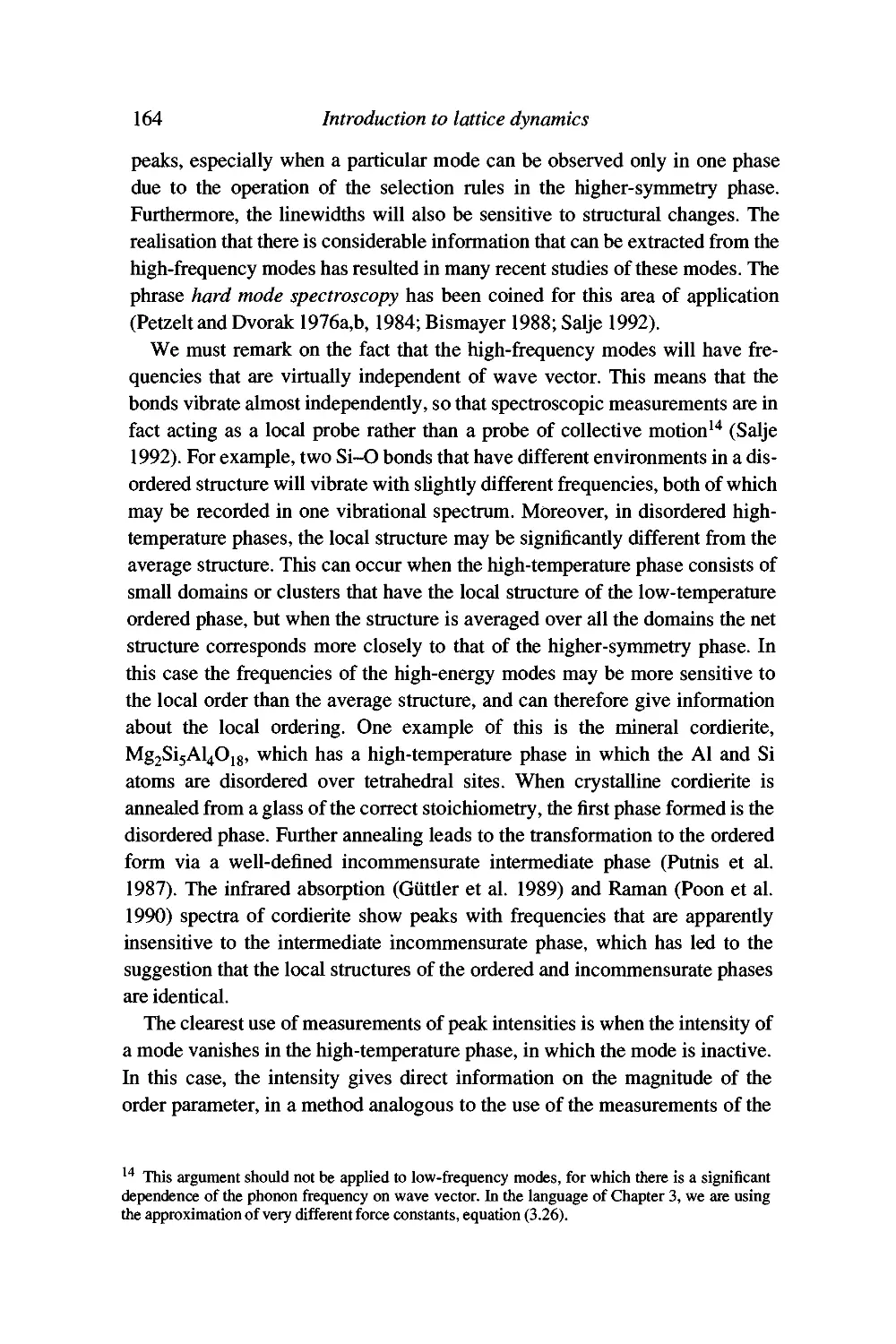
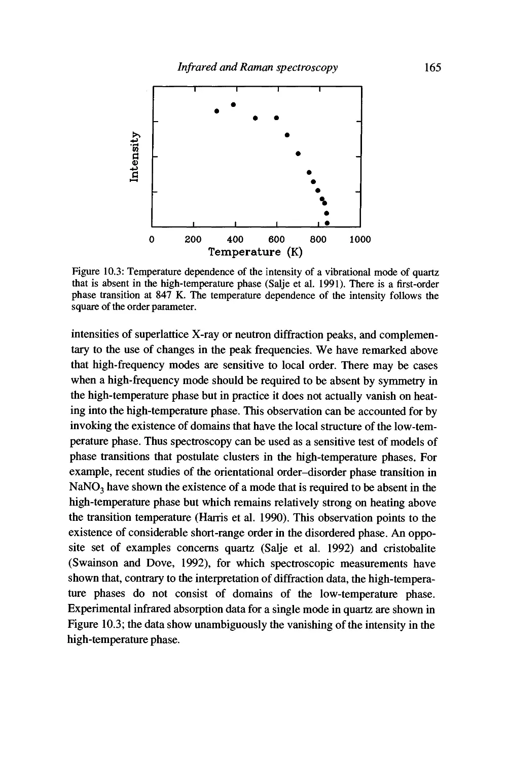
10 Infrared and Raman spectroscopy 151
Introduction 151
Vibrational spectroscopy by infrared absorption 153
Raman spectroscopy 156
Advantages and disadvantages of spectroscopy 159
Qualitative applications of infrared and Raman spectroscopy 161
Quantitative applications of infrared and Raman spectroscopy 162
Summary 166
11 Formal quantum-mechanical description of lattice vibrations 167
Some prehminaries 167
Quantum-mechanical description of the harmonic crystal 169
The new operators: creation and annihilation operators 171
The Hamiltonian and wave function with creation and
annihilation operators 172
Time and position dependence 174
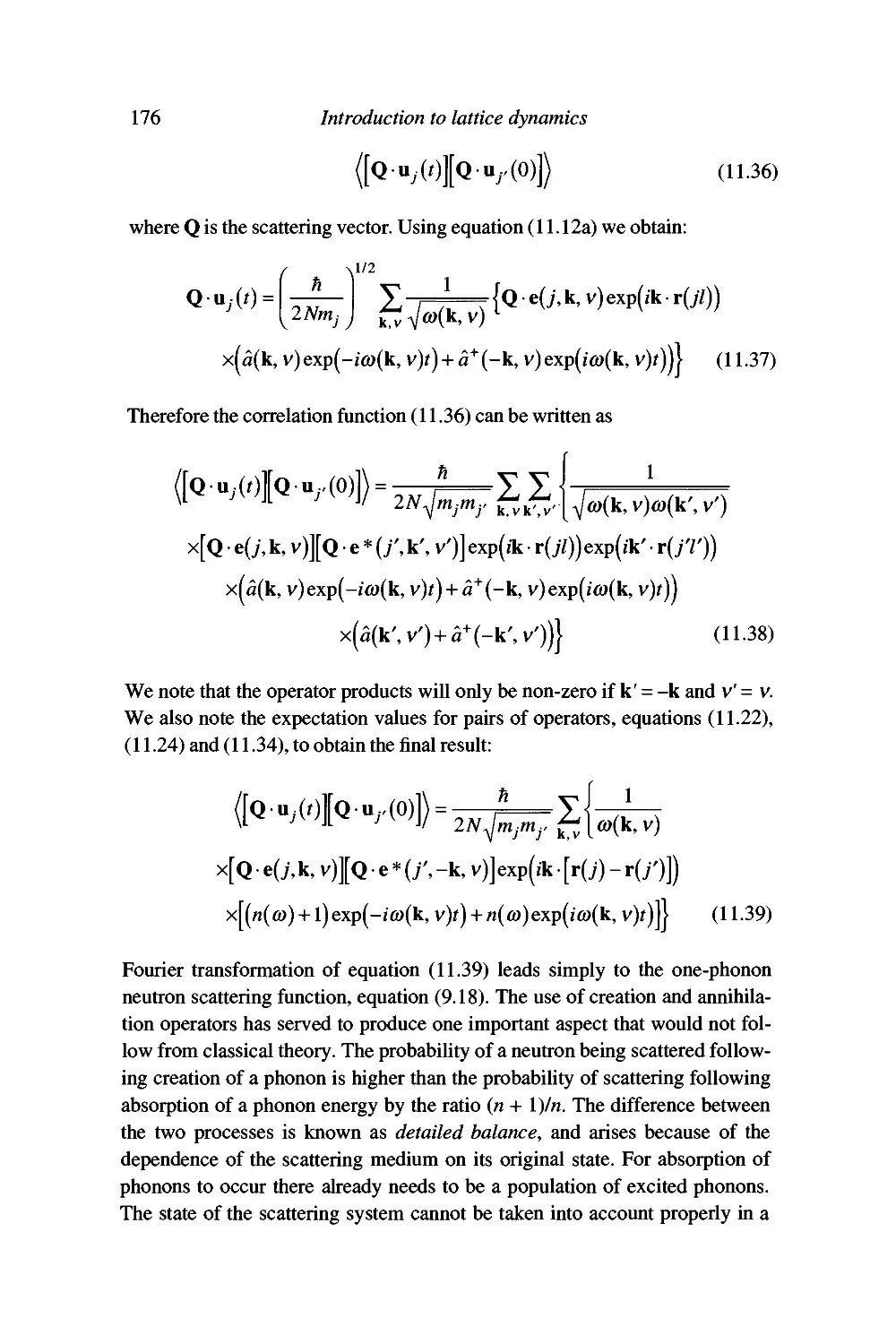
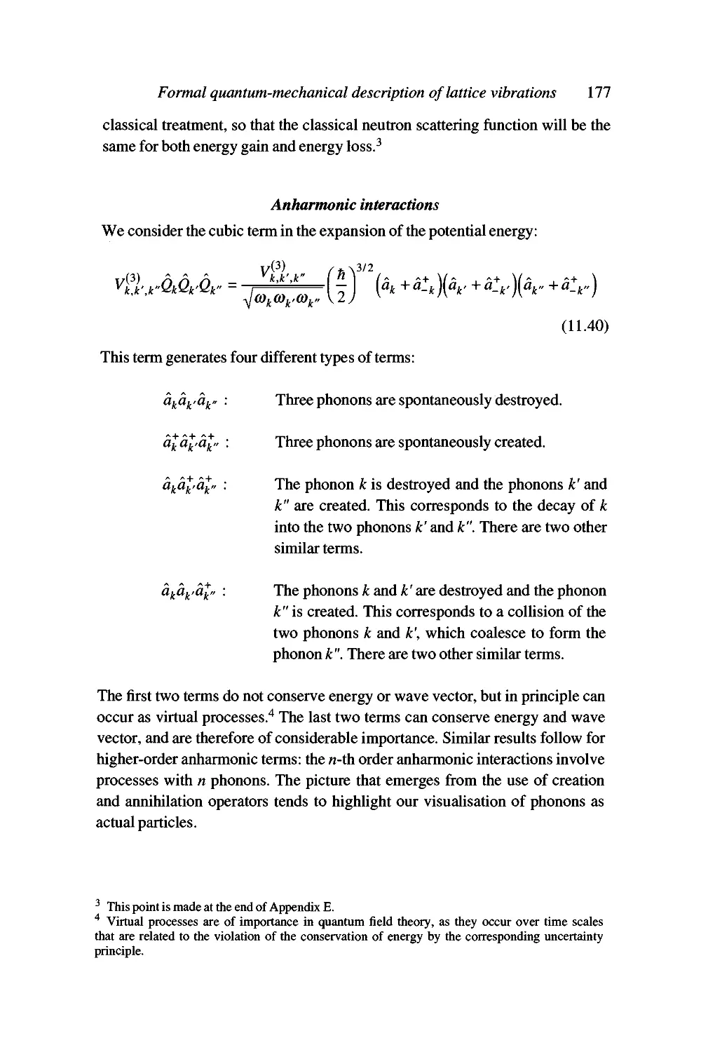
Apphcations 175
Summary 178
12 Molecular dynamics simulations 179
The molecular dynamics simulation method 179
Details of the molecular dynamics simulation method 181
Analysis of the results of a simulation 184
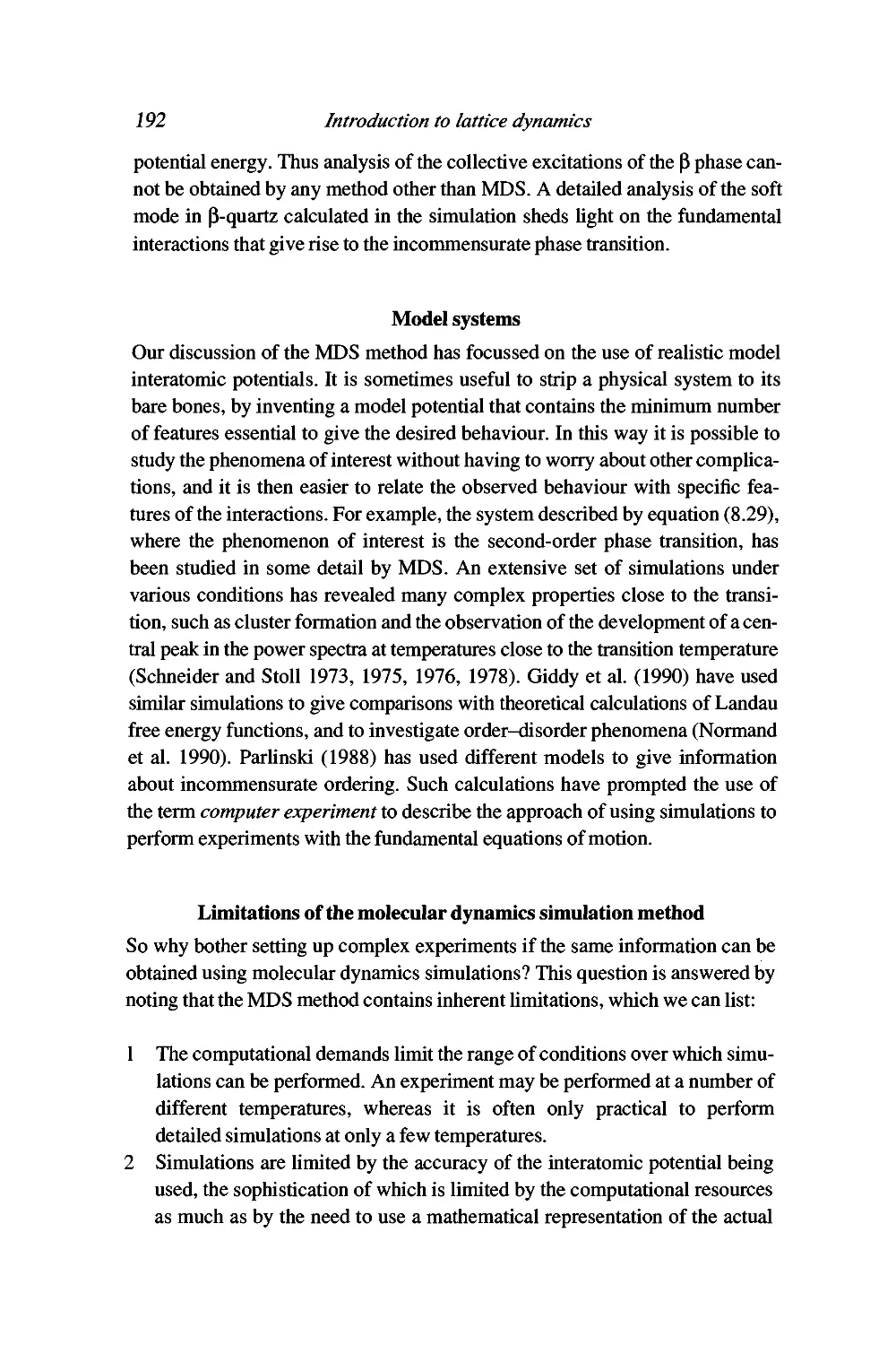
Model systems 192
Limitations of the molecular dynamics simulation method 192
Summary 194
xii Contents
Appendix A The Ewald method 195
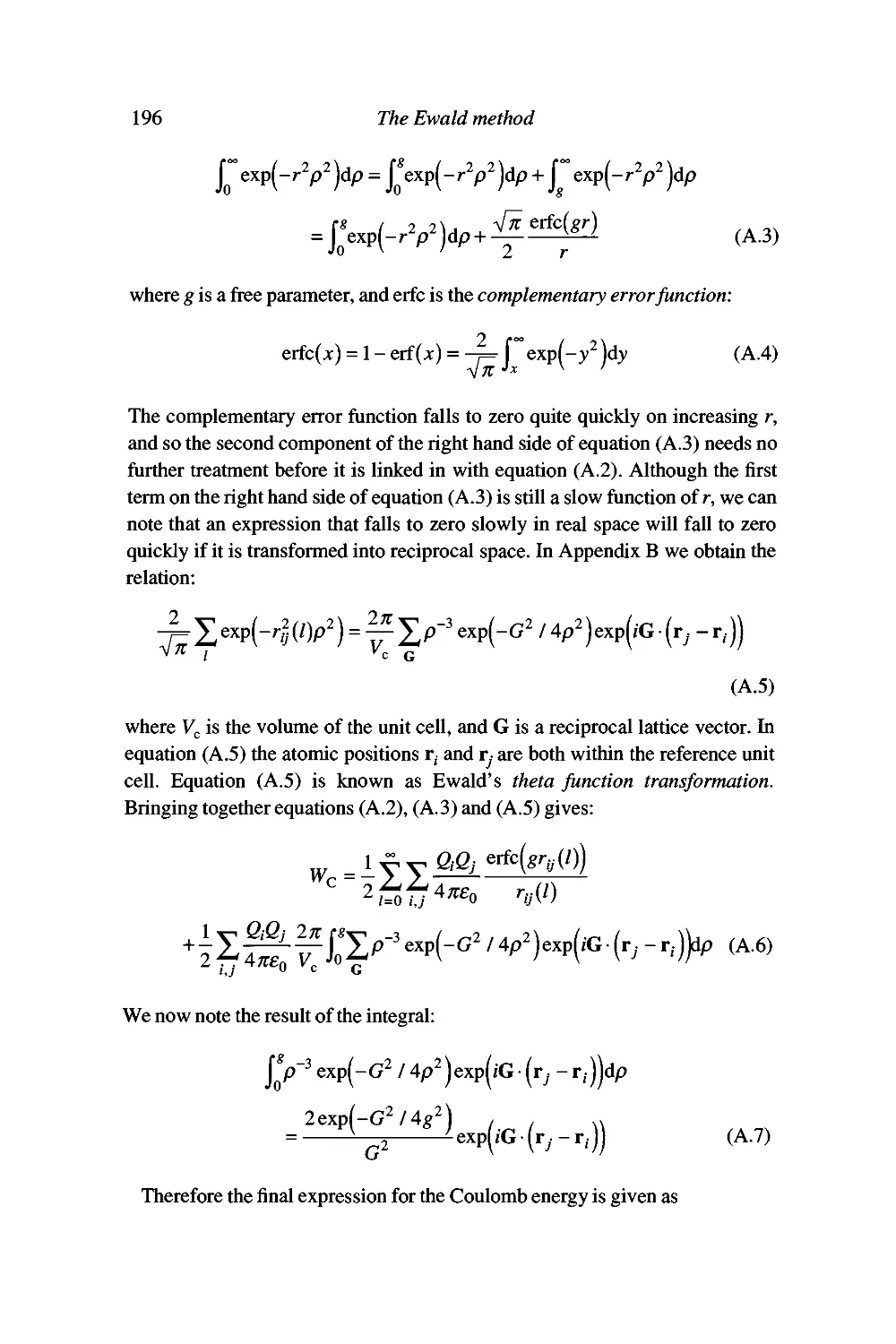
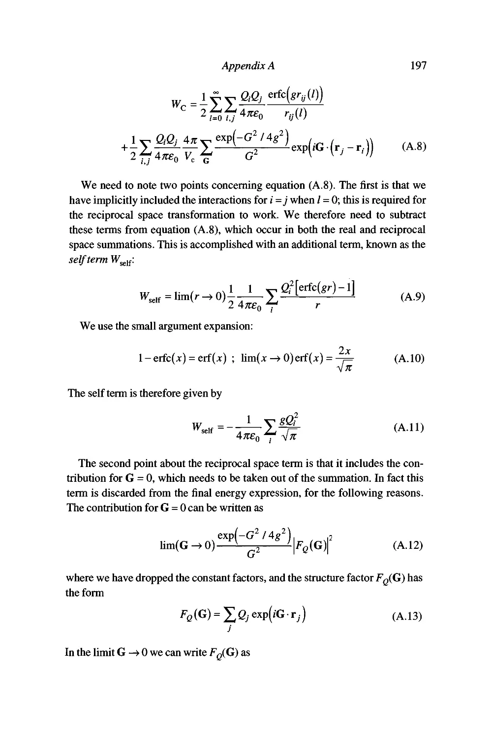
The Ewald sum for the Coulomb energy 195
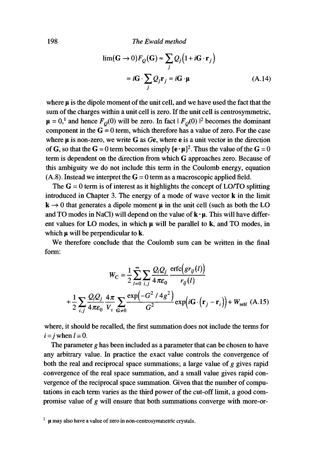
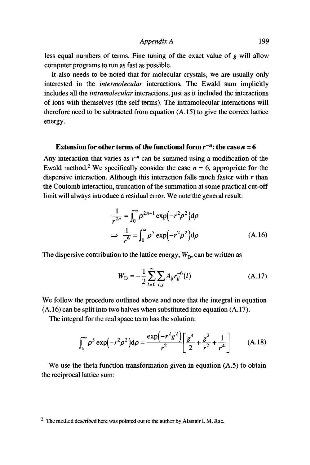
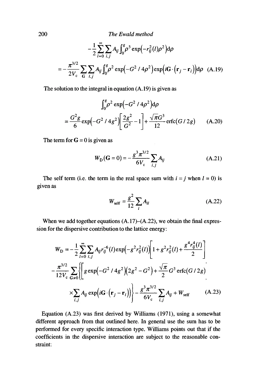
Extension for other terms of the functional form r-": the case n = 6 199
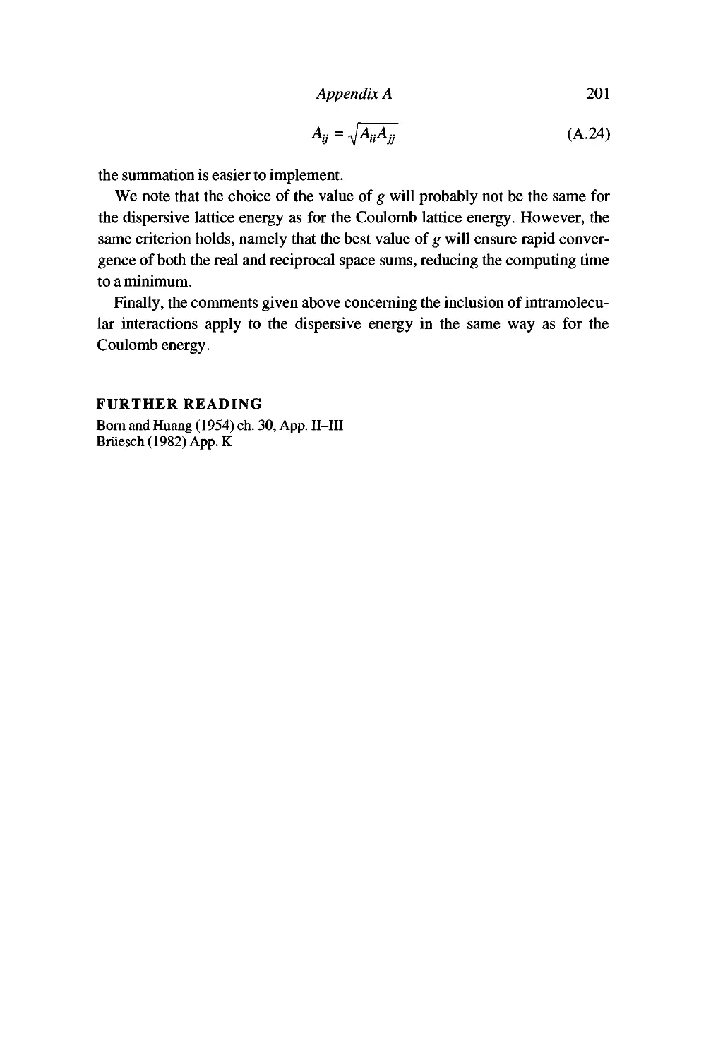
Appendix B Lattice sums 202
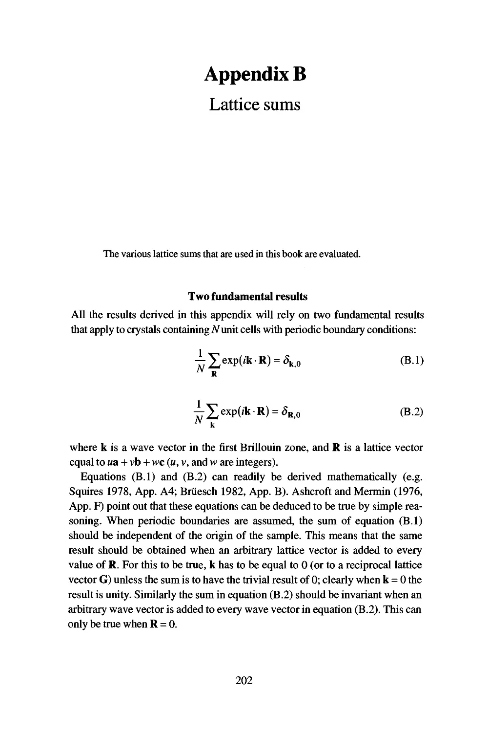
Two fundamental results 202
Derivation of equation (4.13) 203
Derivation of equation (4.20) 204
Derivation of equation (6.44) 204
Derivation of equation (A.5) 206
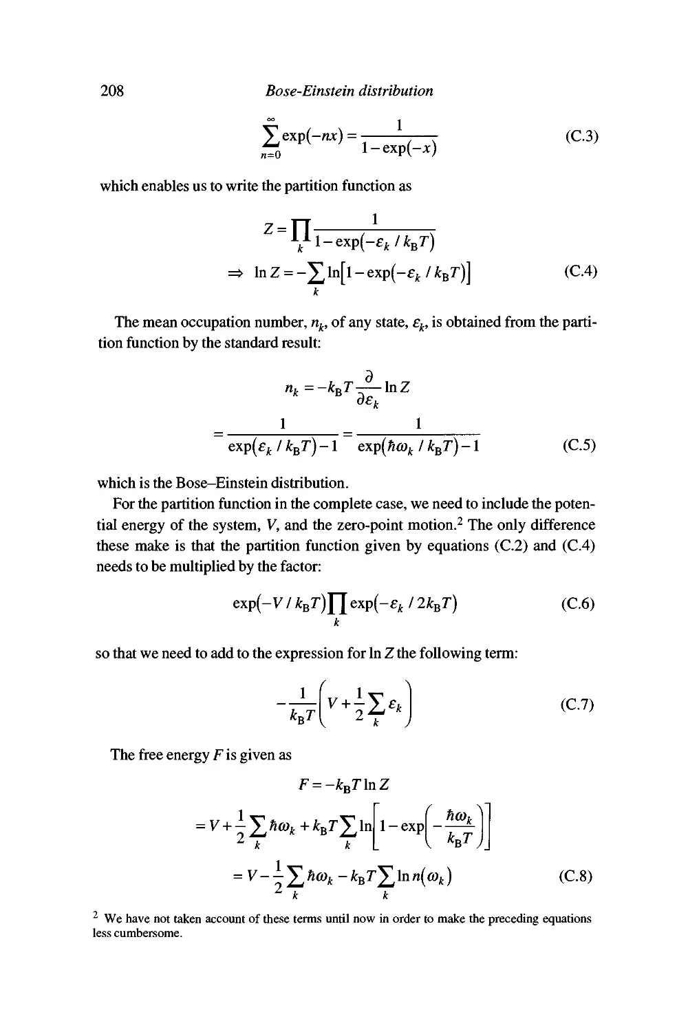
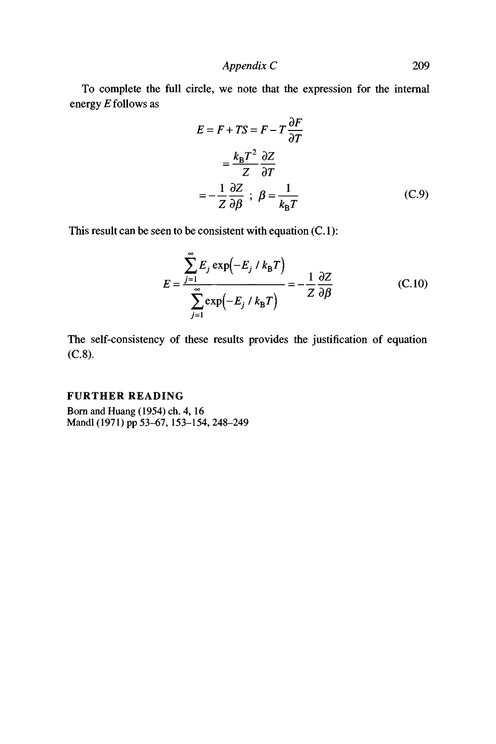
Appendix C Bose-Einstein distribution and the
thermodynamic relations for phonons 207
Appendix D Landau theory of phase transitions 210
The order parameter 210
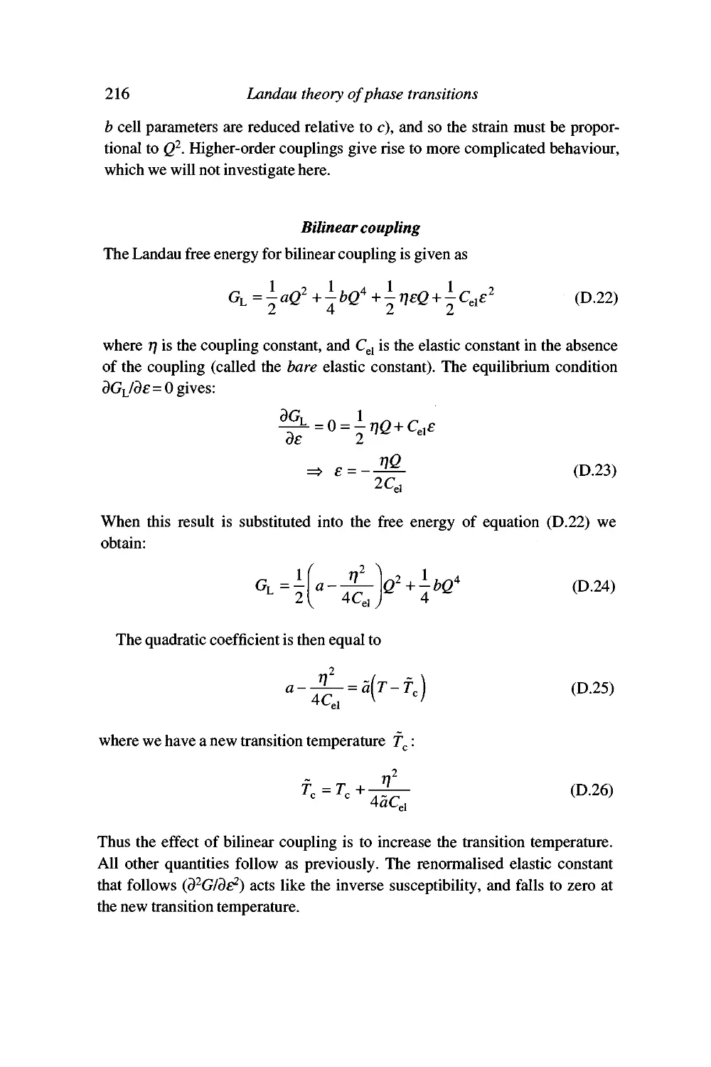
Landau free energy for second-order phase transitions 212
First-order phase transitions 214
Tricritical phase transitions 215
Interaction between the order parameter and other variables 215
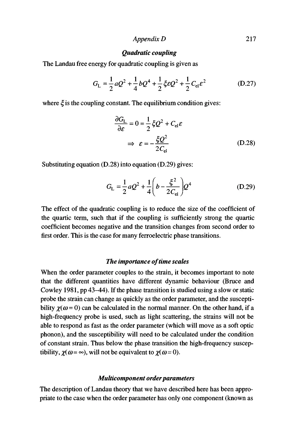
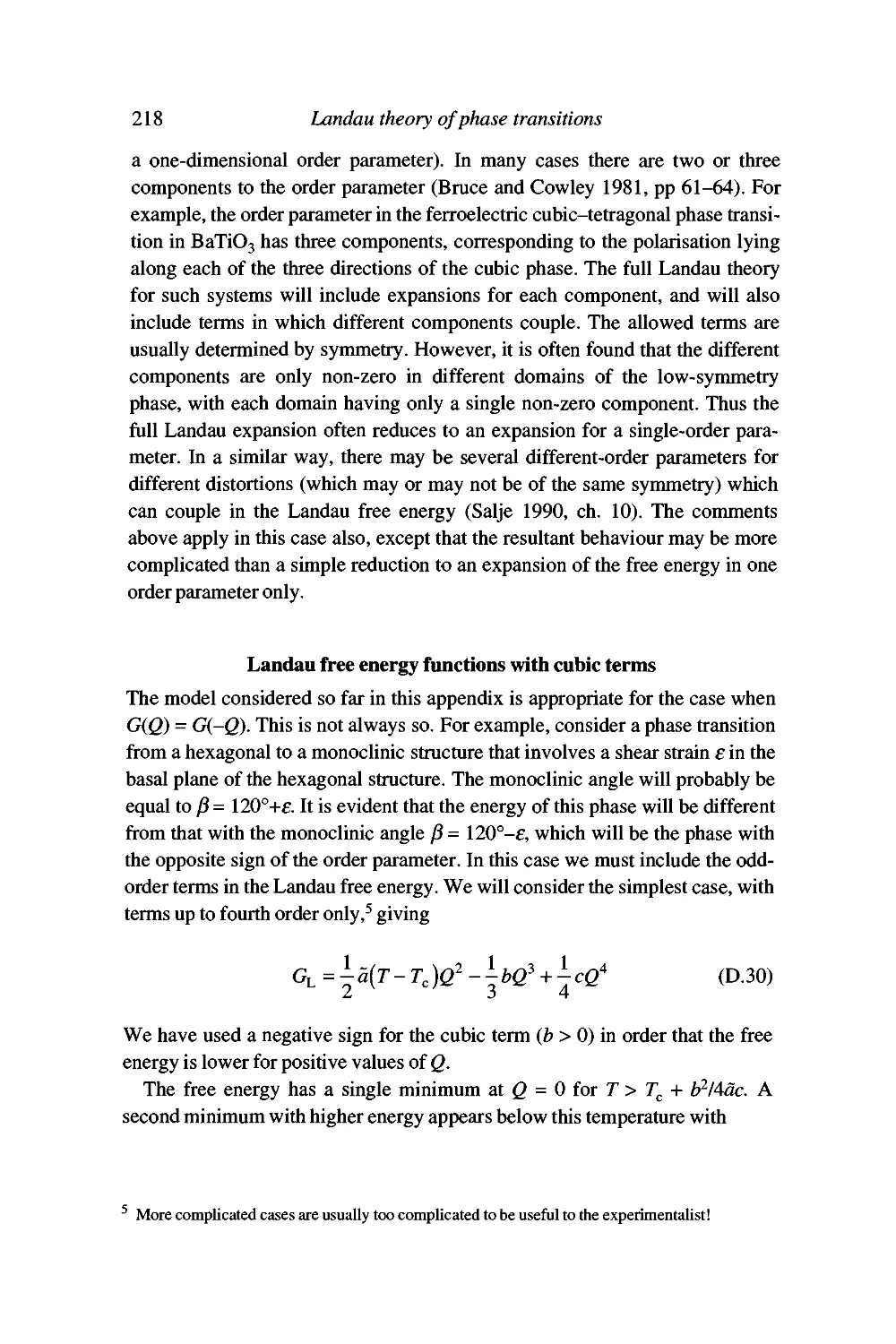
Landau free energy functions with cubic terms 218
Critique of Landau theory 219
Appendix E Classical theory of coherent neutron scattering 221
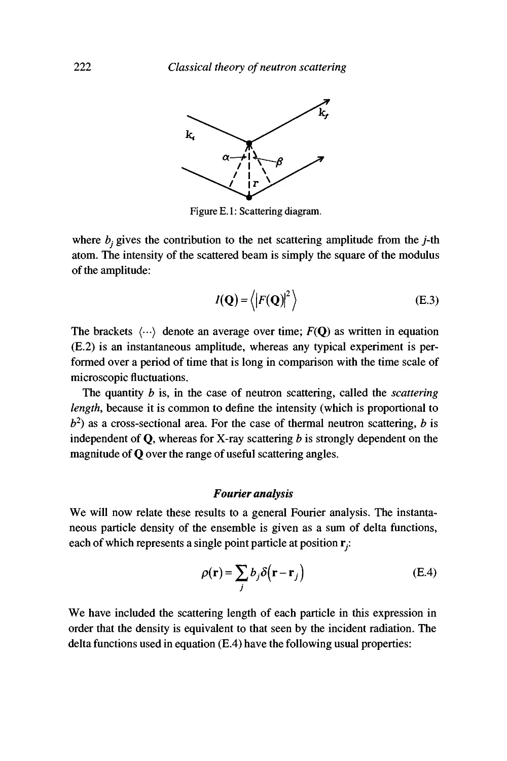
General scattering formalism 221
Time dependence and the inelastic scattering function 225
Scattering cross section 227
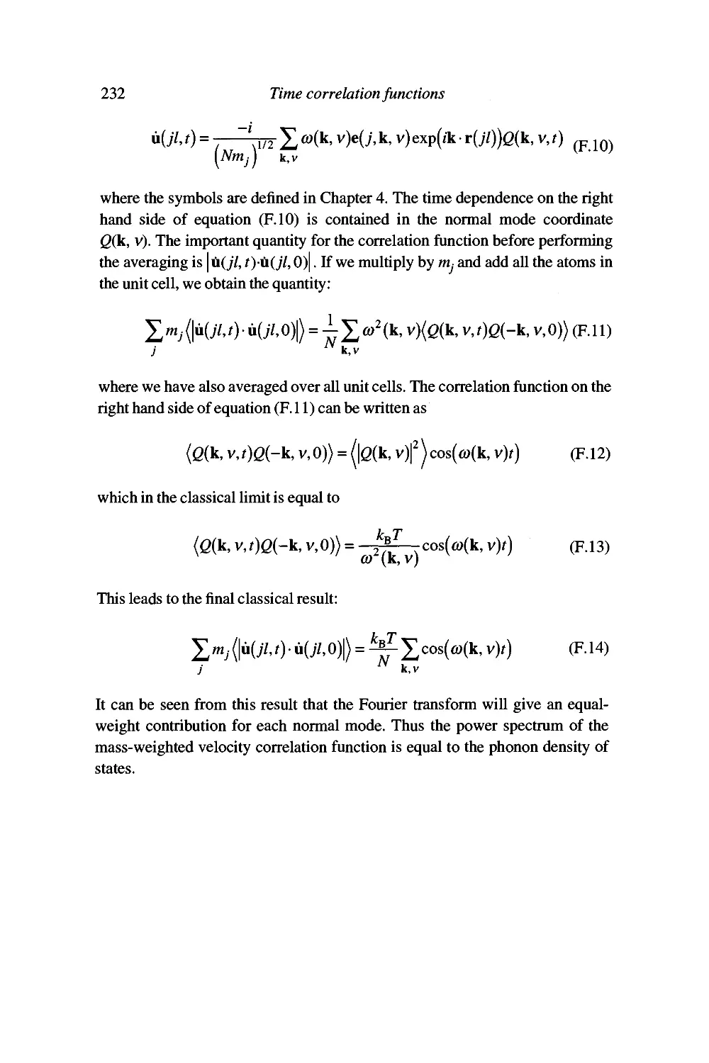
Appendix F Time correlation functions 229
Time-dependent correlation functions 229
Power spectra 230
Example: the velocity autocorrelation function and the
phonon density of states 231
Appendix G Commutation relations 233
Appendix H Published phonon dispersion curves for
non-metallic crystals: update of previous compilation 236
Molecular crystals 236
SiUcates 237
Ionic crystals 238
References 240
Index 254
Preface
The subject of lattice dynamics is taught in most undergraduate courses in
solid state physics, usually to a very simple level. The theory of lattice
dynamics is also central to many aspects of research into the behaviour of solids. In
writing this book I have tried to include among the readership both
undergraduate and graduate students, and established research workers who find
themselves needing to get to grips with the subject.
A large part of the book (Chapters 1-9) is based on lectures I have given to
second and third year undergraduates at Cambridge, and is therefore designed
to be suitable for teaching lattice dynamics as part of an undergraduate degree
course in solid state physics or chemistry. Where I have attempted to make the
book more useful for teaching lattice dynamics than many conventional solid
state physics textbooks is in using real examples of applications of the theory
to materials more complex than simple metals.
I perceive that among research workers there will be two main groups of
readers. The first contains those who use lattice dynamics for what I might call
modelling studies. Calculations of vibrational frequencies provide useful tests
of any proposed model interatomic interaction. Given a working microscopic
model, lattice dynamics calculations enable the calculation of macroscopic
thermodynamic properties. The systems that are tackled are usually more
complex than the simple examples used in elementary texts, yet the theoretical
methods do not need the sophistication found in more advanced texts.
Therefore this book aims to be a half-way house, attempting to keep the theory
at a sufficiently low level, but developed in such a way that its application to
complex systems is readily understood.
The second group consists of those workers who are concerned with dis-
placive phase transitions, for which the theory of soft modes has been so
successful that it is now essential that workers have a good grasp of the theory of
lattice dynamics. The theory of soft modes requires the anharmonic treatment
Xlll
xiv Preface
of the theory, but in many cases this treatment reduces to a modified harmonic
theory and therefore remains comprehensible to non-theorists. It seems to me
that there is a large gap in the literature for workers in phase transitions
between elementary and advanced texts. For example, several texts begin with
the second quantisation formaUsm, providing a real barrier for many. It is
hoped that this book will help to open the hterature on phase transition theory
for those who would otherwise have found it to be too intimidating.
I have attempted to write this book in such a way that it is useful to people
with a wide range of backgrounds, but it is impossible not to assume some
level of prior knowledge of the reader. I have assumed that the reader will have
a knowledge of crystal structures, and of the reciprocal lattice. I have also
assumed that the reader understands wave motion and the general wave
equation; in particular it is assumed that the concept of the wave vector will present
no problems. The mathematical background required for the first five chapters
is not very advanced. Matrix methods are introduced into Chapter 6, and
Fourier transforms (including convolution) are used from Chapter 9 onwards
and in the Appendices. The Kronecker and Dirac delta function representations
are used throughout. An appreciation of the role of the Hamiltonian in either
classical or quantum mechanics is assumed from Chapter 6 onwards. Chapter
11 requires an elementary understanding of quantum mechanics.
It is an unfortunate fact of life that usually one symbol has two or more
distinct meanings. This usually occurs because there just aren't enough symbols
to go around, but the problem is often made worse by the use of the same
symbol for two quantities that occur in similar situations. For example, Q can stand
for either a normal mode coordinate or an order parameter associated with a
phase transition, whereas Q is used for the change in neutron wave vector
following scattering by a crystal. Given that this confusion will probably have a
permanent status in science, I have adopted the symbols in common usage,
rather than invent my own symbols in an attempt to shield the reader from the
real world.
It is my view of this book as a stepping stone between elementary theory and
research hterature that has guided my choice of material, my treatment of this
material, and my choice of examples. It is a temptation to an author to attempt
to make the reader an expert in every area that is touched on in the book. This is
clearly an impossibihty, if for no other reason than the constraint on the
number of pages! Several of the topics discussed in the individual chapters of this
book have themselves been the subject of whole books. Thus a book such as
this can only hope to provide an introduction into the different areas of
specialisation. The constraints of space have also meant that there are related topics
that I have not even attempted to tackle; among these are dielectric properties.
Preface xv
electronic properties, imperfect crystals, and disordered systems. Moreover, I
have had to restrict the range of examples I have been able to include. Thus I
have not been able to consider metals in any detail. I therefore reiterate that my
aim in writing this book is to help readers progress from an elementary grasp of
lattice dynamics to the stage where they can read and understand current
research hterature with some intelligence, and I hope that the task of
broadening into the missing topics will be less daunting in consequence.
Acknowledgements
This book was written over the period 1990-1992. During that time a number
of people helped in a number of ways. Firstly I must thank the Series Editor,
Andrew Putnis, for encouraging me to transform my lecture handouts into this
book, and Catherine Flack of Cambridge University Press for helping in all the
practical aspects of this task. A number of people have helped by reading an
earher draft, and suggesting changes and providing encouragement: Mark
Harris (Oxford), Mark Hagen (Keele), Mike Bown (Cambridge), Ian Swainson
(Cambridge), Bjom Winkler (Saclay), and David Price (London). Of course
none of these people must share any responsibility for residual errors or for any
features that irritate the reader! However, the help given by all these people has
been greatly appreciated. The text for this book was prepared in camera-ready
format on my word processor at home, but this would not have been possible
without the constant help of Pat Hancock.
My own understanding of the subject of lattice dynamics has been helped by
a number of very enjoyable collaborations. It has been a great privilege to work
with Alastair Rae (my PhD supervisor), Stuart Pawley, Ruth Lynden-Bell and
David Fincham (with whom I did my post-doctoral work), Brian Powell and
Mark Hagen (with whom I have done all my inelastic neutron scattering work),
and Volker Heine, Ekhard Salje, Andrew Giddy, Bjom Winkler, Ian Swainson,
Mark Harris, Stefan Tautz, David Palmer and Tina Line (colleagues and
students in Cambridge).
To all these people, thank you.
Finally, special thanks are due to my wife, two daughters, and parents. Our
eldest daughter, Jennifer-Anne, was less than one year old when I started
writing in earnest, and during the period of writing our second daughter Emma-
Clare was bom. It will be readily appreciated that I could never have
completed this book without the considerable encouragement, cooperation and
patience of my wife Kate. Thank you!
XVI
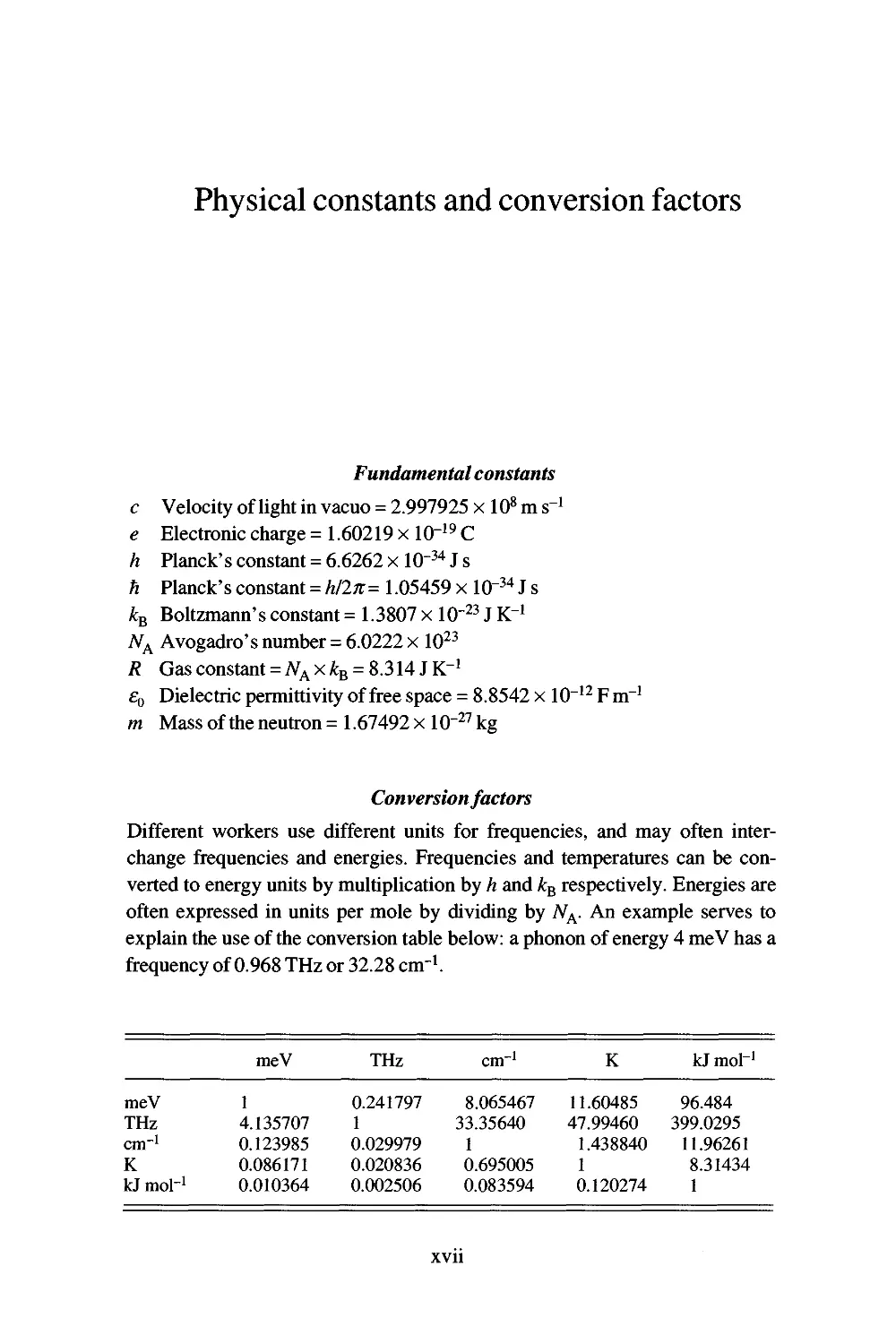
Physical constants and conversion factors
Fundamental constants
c Velocity of light in vacuo = 2.997925 x 10^ m s"'
e Electronic charge = 1.60219 x lOr^^ C
h Planck's constant = 6.6262 x 10-^"* J s
h Planck's constant = /?/2;r = 1.05459 x 10-^"* J s
k^ Boltzmann's constant = 1.3807 x 10'^^ J K"'
N^ Avogadro's number = 6.0222 x 10^^
R Gas constant = AfAX)fcB = 8.314 J K-i
£q Dielectric permittivity of free space = 8.8542 x 10"'^ F m"'
m Mass of the neutron = 1.67492 x 10"^^ kg
Conversion factors
Different workers use different units for frequencies, and may often
interchange frequencies and energies. Frequencies and temperatures can be
converted to energy units by multiplication by h and k^ respectively. Energies are
often expressed in units per mole by dividing by A^^. An example serves to
explain the use of the conversion table below: a phonon of energy 4 meV has a
frequency of 0.968 THz or 32.28 cm"!.
meV
THz
cm"
K
kJmol
meV
THz
cm"'
K
kJ mol"'
1
4.135707
0.123985
0.086171
0.010364
0.241797
1
0.029979
0.020836
0.002506
8.065467
33.35640
1
0.695005
0.083594
11.60485
47.99460
1.438840
1
0.120274
96.484
399.0295
11.96261
8.31434
1
XVll
1
Some fundamentals
We begin by describing the interatomic forces that cause the atoms to
move about. The main interactions that we will use later on are defined,
and methods for the determination of specific interactions are
discussed. The second part of the chapter is concerned with the behaviour
of travelling waves in any crystal.
Indications that dynamics of atoms in a crystal are important:
failure of the static lattice approximation
Crystallography is generally concerned with the static properties of crystals,
describing features such as the average positions of atoms and the symmetry of
a crystal. Sohd state physics takes a similar hne as far as elementary electronic
properties are concerned. We know, however, that atoms actually move around
inside the crystal structure, since it is these motions that give the concept of
temperature, and the structures revealed by X-ray diffraction or electron
microscopy are really averaged over all the motions. The only signature of
these motions in the traditional crystallographic sense is the temperature factor
(otherwise known as the Debye-Waller factor (Debye 1914; Waller 1923,
1928) or displacement amplitude), although diffuse scattering seen between
reciprocal lattice vectors is also a sign of motion (Willis and Pryor 1975). The
static lattice model, which is only concerned with the average positions of
atoms and neglects their motions, can explain a large number of material
features, such as chemical properties, material hardness, shapes of crystals,
optical properties, Bragg scattering of X-ray, electron and neutron beams,
electronic structure and electrical properties, etc. There are, however, a number of
properties that cannot be explained by a static model. These include:
- thermal properties, e.g. heat capacity;
2 Introduction to lattice dynamics
- effects of temperature on the lattice, e.g. thermal expansion;
- the existence of phase transitions, including melting;
- transport properties, e.g. thermal conductivity, sound propagation;
- the existence of fluctuations, e.g. the temperature factor;
- certain electrical properties, e.g. superconductivity;
- dielectric phenomena at low frequencies;
- interaction of radiation (e.g. hght and thermal neutrons) with matter.
Are the atomic motions that are revealed by these features random, or can
we find a good description for the dynamics of the crystal lattice? The answer
is that the motions are not random; rather they are determined by the forces that
atoms exert on each other. The aim of this book is to show that in fact we have
a very good idea of the way atoms move inside a crystal lattice. This is the
essence of the subj ect of lattice dynamics.
The classical motions of any atom are simply determined by Newton's law
of mechanics: force = mass x acceleration. Formally, if r,(0 is the position of
atomy at time t, then
9^r,W 1 / \
3r m
7
where mj is the atomic mass, and (pji^j, t) is the instantaneous potential energy
of the atom. Equation (1.1) is our key equation. We therefore need some
knowledge of the nature of the atomic forces found in a crystal. The potential
energy in equation (1.1) arises from the instantaneous interaction of the atom
with all the other atoms in the crystal. We will often assume that this can be
written as a sum of separate atom-atom interactions that depend only on the
distances between atoms:
<Pj=Y.<Pij(rij) (1-2)
where r^ is the distance between atoms / and j, and (Pi/jt^ is a specific
atom-atom interaction. The sum over / in equation (1.2) gives the interactions
with all other atoms in the crystal.
Of course, quantum mechanics rather than classical mechanics determines
the motions of atoms. But we will see that the main features of lattice dynamics
follow exactly from the classical equation (1.1), whilst quantum effects are
primarily revealed in the subsequent thermodynamic properties.
Our aim in this chapter is to set the scene for the rest of the book. In the first
part we will consider some elementary ideas associated with interatomic
Some fundamentals 3
potentials. These are essential if we are to use real examples to illustrate the
basic ideas we will develop in the following chapters. In the second part we
will present the basic formalism for describing the motions of waves in
crystals, which we will build upon in the rest of the book.
Interatomic forces
The variety of interatomic forces
The forces between atoms are all ultimately electrostatic in origin. However,
when quantum mechanics is taken into account, the different types of forces
can have some very different manifestations.
Direct electrostatic
The electrostatic interactions are long range and well understood, and have in
general a very simple mathematical representation. The Coulomb energy
follows the well known r^ form, and is strongest in ionic systems such as NaCl.
However, there is one complicating feature that can sometimes be neglected
but which in other cases plays a crucial role in stabihsing the structure. This is
the existence of inductive forces. Consider, for example, a simple spherical ion
on a symmetric site in a lattice, such that at equilibrium all the electric fields at
the syrranetric site cancel out. If the surrounding neighbours move around,
they will generate a residual electric field at the syrranetric site; also, if this ion
moves off its site it will experience an electric field. This residual field will
then polarise our ion under consideration, giving it a temporary dipole
moment. This dipole moment will then interact with the charges (and moments
if they exist) on the neighbouring ions, adding an extra contribution to the
energy of the crystal. In calculations of the dynamics of ionic crystals, this
induction energy has often been found to be of considerable importance. Such
calculations commonly use the shell model (Dick and Overhauser 1958;
Cochran 1971; Woods et al. 1960,1963). In this model, the ions are assumed to
comprise the rigid core of the nucleus plus the tightly bound inner electrons,
and a loosely bound outer layer, or shell, of the remaining electrons. It is then
assumed that the shell and core are held together by a harmonic interaction
(that is, the energy is proportional to the square of the distance between the
centres), which is the same as saying that the polarisation of the ion is directly
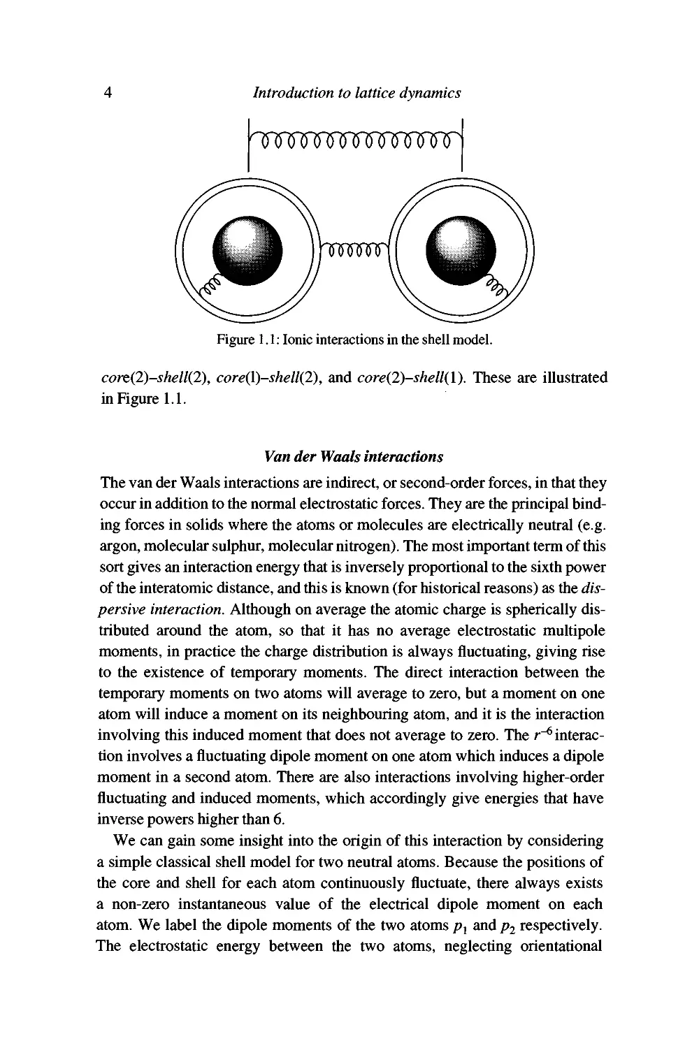
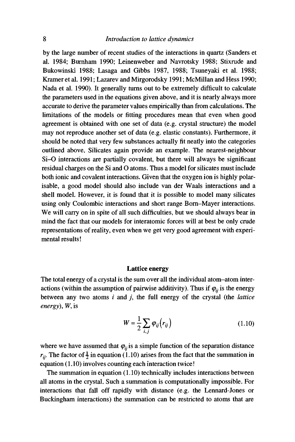
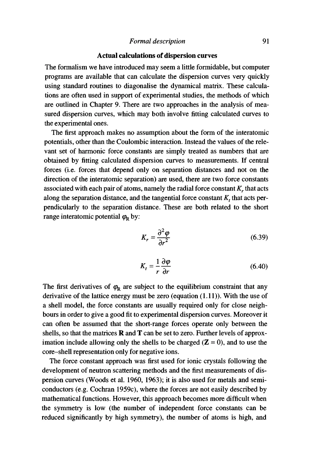
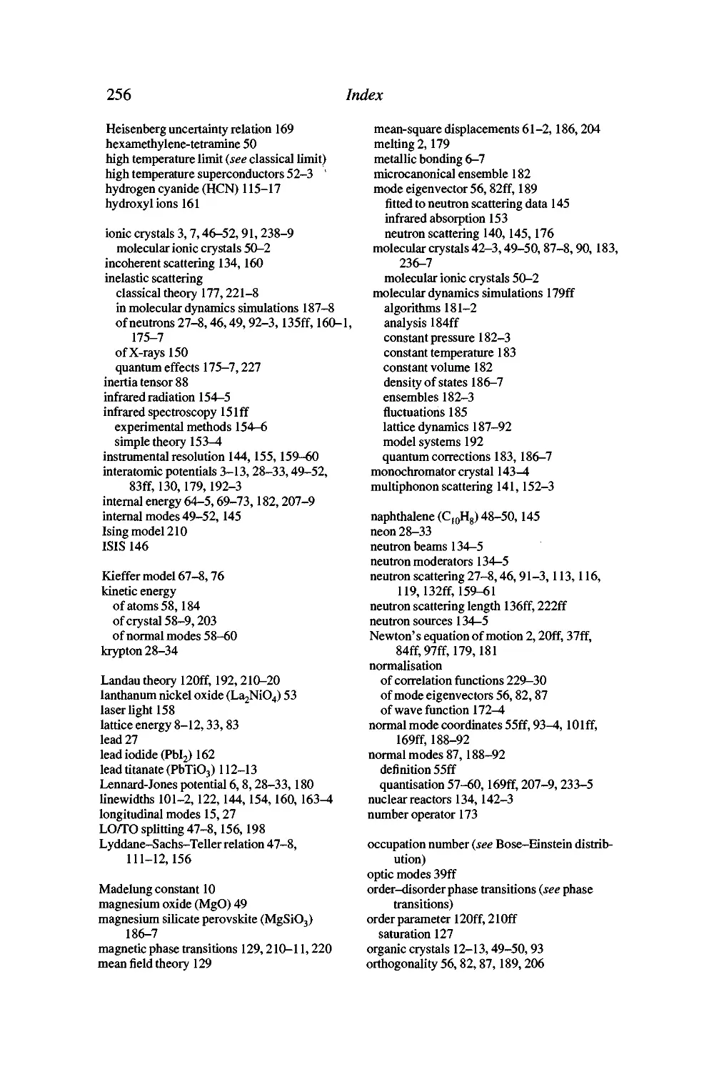
proportional to the local electric field. The energy between two ions is then the
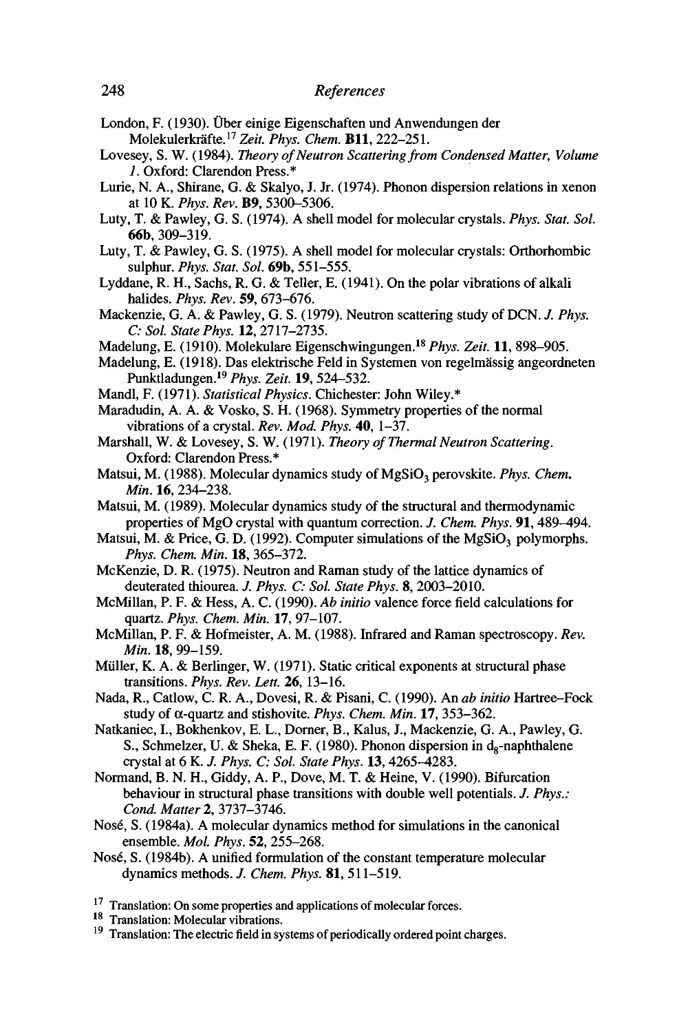
sum of six interactions: core(\)-core{2), shell(l)-shell(2), core(l)-shell(l),
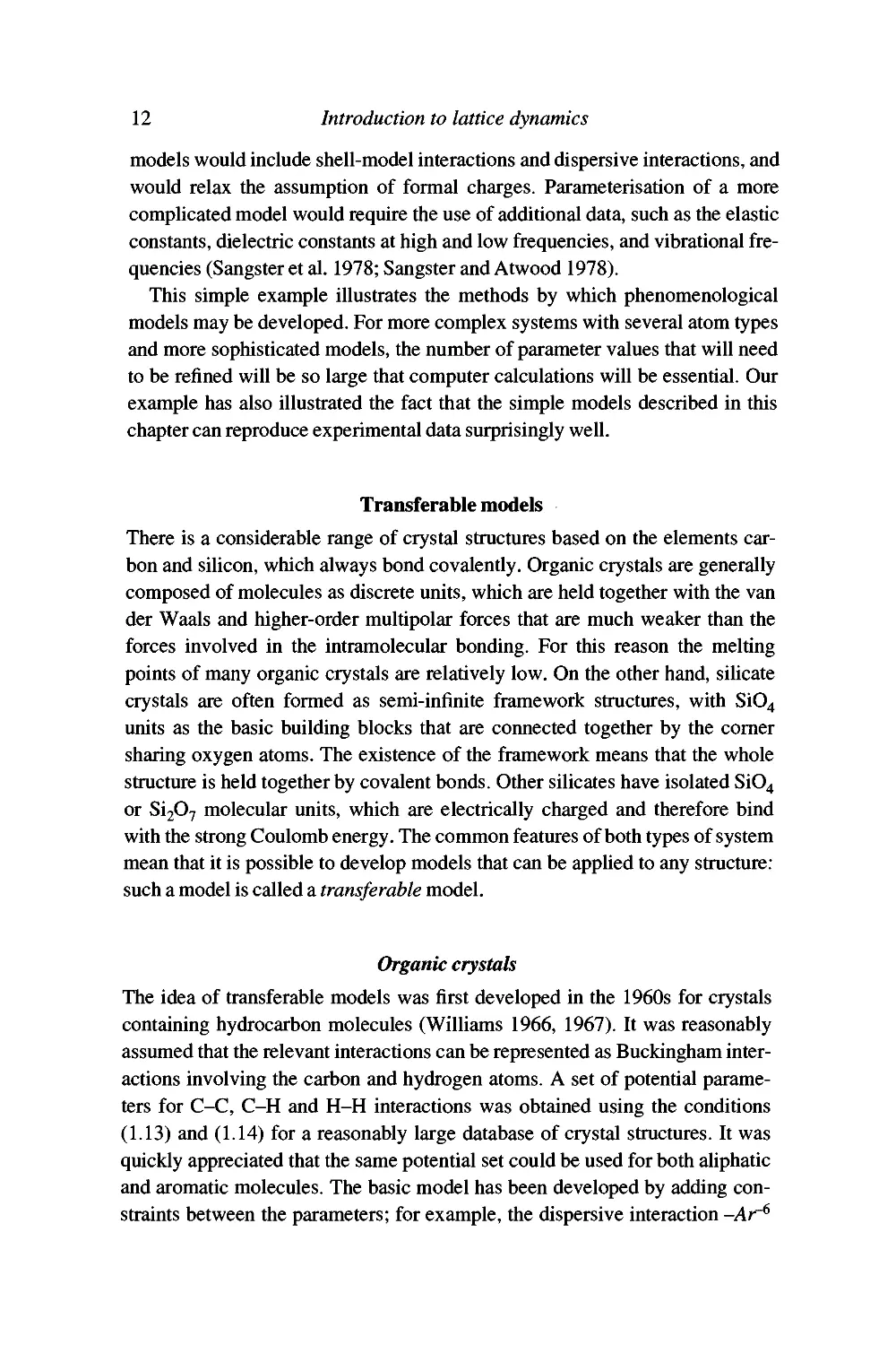
Introduction to lattice dynamics
nwwsTWUUwr
Figure 1.1: Ionic interactions in the shell model.
cort{2)-shell{2), core(l)-shell(2), and core{2)-shell{\). These are illustrated
in Figure 1.1.
Van der Waals interactions
The van der Waals interactions are indirect, or second-order forces, in that they
occur in addition to the normal electrostatic forces. They are the principal
binding forces in solids where the atoms or molecules are electrically neutral (e.g.
argon, molecular sulphur, molecular nitrogen). The most important term of this
sort gives an interaction energy that is inversely proportional to the sixth power
of the interatomic distance, and this is known (for historical reasons) as the
dispersive interaction. Although on average the atomic charge is spherically
distributed around the atom, so that it has no average electrostatic multipole
moments, in practice the charge distribution is always fluctuating, giving rise
to the existence of temporary moments. The direct interaction between the
temporary moments on two atoms will average to zero, but a moment on one
atom will induce a moment on its neighbouring atom, and it is the interaction
involving this induced moment that does not average to zero. The r"^
interaction involves a fluctuating dipole moment on one atom which induces a dipole
moment in a second atom. There are also interactions involving higher-order
fluctuating and induced moments, which accordingly give energies that have
inverse powers higher than 6.
We can gain some insight into the origin of this interaction by considering
a simple classical shell model for two neutral atoms. Because the positions of
the core and shell for each atom continuously fluctuate, there always exists
a non-zero instantaneous value of the electrical dipole moment on each
atom. We label the dipole moments of the two atoms p^ and P2 respectively.
The electrostatic energy between the two atoms, neglecting orientational
Some fundamentals 5
components,' is simply proportional to P]P2lf^- The mean values of these
dipole moments over any period of time are zero: (/?i) = (/?2) =0. Therefore
if these two moments are uncorrelated, the average value of the electrostatic
interaction will also be zero. However, both the dipole moments will generate
instantaneous electric fields. If the distance between the atoms is r, the field
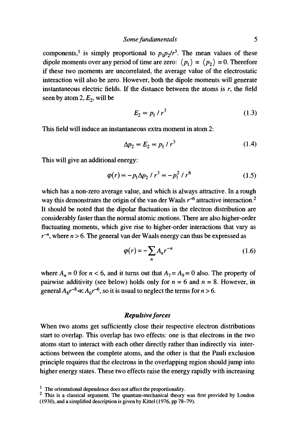
seen by atom 2, E2, will be
E^'^pjr' (1.3)
This field will induce an instantaneous extra moment in atom 2:
/^^ oc E2 °^ Px I r' (1.4)
This will give an additional energy:
(pir)^-p,Ap2/r'^-pf/r^ (1.5)
which has a non-zero average value, and which is always attractive. In a rough
way this demonstrates the origin of the van der Waals r~^ attractive interaction.^
It should be noted that the dipolar fluctuations in the electron distribution are
considerably faster than the normal atomic motions. There are also higher-order
fluctuating moments, which give rise to higher-order interactions that vary as
r~", where n > 6. The general van der Waals energy can thus be expressed as
(?)(r) = -XA„r-« (1.6)
n
where A„ = 0 for n < 6, and it turns out that A-j = Ag=0 also. The property of
pairwise additivity (see below) holds only for n = 6 and n = 8. However, in
general Agr~^ «; A^r"^, so it is usual to neglect the terms for n > 6.
Repulsive forces
When two atoms get sufficiently close their respective electron distributions
start to overlap. This overlap has two effects: one is that electrons in the two
atoms start to interact with each other directly rather than indirectly via
interactions between the complete atoms, and the other is that the Pauli exclusion
principle requires that the electrons in the overlapping region should jump into
higher energy states. These two effects raise the energy rapidly with increasing
' The orientational dependence does not affect the proportionality.
^ This is a classical argument. The quantum-mechanical theory was first provided by London
(1930), and a simplified description is given by Kittel (1976, pp 78-79).
6 Introduction to lattice dynamics
overlap, thereby giving a net repulsion that is short-ranged. Although it is
possible to calculate the repulsive interaction from first principles, it is common to
use a functional form of the repulsive interaction potential with model
parameters. One typically used function, which involves the interatomic distance r, is
Br~" (where n is often 12). The r"'^ repulsion is sometimes combined with
the dispersive interaction in a functional form known as the Lennard-Jones
potential:
(p{r) = -4£
_,6 / „\12
r I \r
(1.7)
It is easy to show that when two atoms interact via the Lennard-Jones potential,
£is equal to the potential energy at the equilibrium separation, and <7is the
distance between the atoms at which the energy is equal to zero.
Another commonly used function for the repulsive interaction is an
exponential term known as the Bom-Mayer interaction (Bom and Mayer 1932):
(p{r) = Bt\^{-rlp) (1.8)
The parameters B and p are usually determined empirically, although there is
some theoretical justification for the exponential repulsion and the parameters
can be calculated using quantum-mechanical methods (e.g. Post and Bumham
1986). p is related to the relative sizes of the atoms, and B is a measure of the
hardness of the interaction. The combination with the r"^ dispersive interaction
is known as the Buckingham potential, which is commonly used in many
different systems with and without electrostatic interactions.
It is worth pointing out that a large amount of work has been carried out in
which it has been assumed that atoms have effectively infinitely hard surfaces,
like billiard balls or ball bearings. This model - called the hard sphere model -
can sometimes give results that are surprisingly close to reality!
Metallic and covalent bonding
In metals the atomic cores (nuclei plus the tightly bound inner electrons) are
surrounded by a more-or-less uniform density of free electrons. It is this
general distribution of electrons that gives metals their electrical conductivity, and
the electrons also contribute significantly to the high thermal conductivity. On
the other hand, crystals in which the atoms are held together by covalent bonds
(such as diamond) prove to be good electrical and thermal insulators. The
common feature is that in neither type are the electrons that are important for the
cohesion of the crystal localised around the cores of the atoms as they are in an
Some fundamentals 7
ionic or molecular crystal. This means that it is difficult to calculate the forces
between atoms without taking into account the way the electron density
changes in response to these forces. Thus the motions of atoms in these
systems are accompanied by significant changes in the surrounding electron
distribution. It is possible to calculate the forces between atoms in these types of
solid, but these calculations are not easy and techniques for such calculations
are still topics of current research activity. For example, theoretical
calculations of the interactions in silica (Si02) are being carried out using the quantum
mechanics of small clusters (Lasaga and Gibbs 1987, 1988; Tsuneyuki et al.
1988; Kramer et al. 1991) or of ideal structures (Cohen 1991; Lazarev and
Mirgorodsky 1991; McMillan and Hess 1990; Nada et al. 1990). It is possible
to use approximate model potentials for covalent systems. For example, it
turns out that silicate minerals can be modelled surprisingly accurately using
simple model interactions (e.g. Buckingham interactions) for cation-oxygen
and oxygen-oxygen interactions, together with the normal Coulombic
interactions (Bumham 1990; Leinenweber and Navrotsky 1988; Stixrude and
Bukowinski 1988). Refined empirical models also include shell-model
interactions for the oxygen ions and O-Si-O bond-bending interactions that vary with
the bond angle 6:
(p{e) = ^K{e-e^f (1.9)
where ^o is the equilibrium bond angle, equal to 109.47° (= cos"'(-l/3)) for
tetrahedral angles and 90° for octahedral coordination (Sanders et al. 1984).
Additional comments
In this book, we will be using two approximations throughout. Our first is that
the energy of a system of three or more atoms can be represented as the sum of
interactions between the different pairs. This is called pairwise additivity. An
illustration of this is that the energy of the sun-earth-moon system is the sum
of the gravitational energies between the sun and earth, the sun and moon, and
the earth and moon. Our second approximation is to assume that because the
electrons move much faster than the atom cores, the electrons are always in an
equilibrium configuration when the atom cores are moving (this approximation
is known as the adiabatic or Bom-Oppenheimer approximation (Bom and
Oppenheimer 1927)). This is particularly relevant for covalent and metallic
systems, but we shall not say anything more on this point.
One might be tempted to think that the forces between atoms are reasonably
well understood nowadays. Unfortunately this is not the case, as is evidenced
8 Introduction to lattice dynamics
by the large number of recent studies of the interactions in quartz (Sanders et
al. 1984; Bumham 1990; Leinenweber and Navrotsky 1988; Stixrude and
Bukowinski 1988; Lasaga and Gibbs 1987, 1988; Tsuneyaki et al. 1988;
Kramer et al. 1991; Lazarev and Mirgorodsky 1991; McMillan and Hess 1990;
Nada et al. 1990). It generally turns out to be extremely difficult to calculate
the parameters used in the equations given above, and it is nearly always more
accurate to derive the parameter values empirically than from calculations. The
hmitations of the models or fitting procedures mean that even when good
agreement is obtained with one set of data (e.g. crystal structure) the model
may not reproduce another set of data (e.g. elastic constants). Furthermore, it
should be noted that very few substances actually fit neatly into the categories
outhned above. Sihcates again provide an example. The nearest-neighbour
Si-O interactions are partially covalent, but there will always be significant
residual charges on the Si and O atoms. Thus a model for silicates must include
both ionic and covalent interactions. Given that the oxygen ion is highly polar-
isable, a good model should also include van der Waals interactions and a
shell model. However, it is found that it is possible to model many sihcates
using only Coulombic interactions and short range Bom-Mayer interactions.
We will carry on in spite of all such difficulties, but we should always bear in
mind the fact that our models for interatomic forces will at best be only crude
representations of reality, even when we get very good agreement with
experimental results!
Lattice energy
The total energy of a crystal is the sum over all the individual atom-atom
interactions (within the assumption of pairwise additivity). Thus if ^^ is the energy
between any two atoms / and j, the full energy of the crystal (the lattice
energy), W, is
"^ = \j.%('-ii) (1-10)
where we have assumed that (pA% a simple function of the separation distance
r,-,. The factor of-j in equation (1.10) arises from the fact that the summation in
equation (1.10) involves counting each interaction twice!
The summation in equation (1.10) technically includes interactions between
all atoms in the crystal. Such a summation is computationally impossible. For
interactions that fall off rapidly with distance (e.g. the Lennard-Jones or
Buckingham interactions) the summation can be restricted to atoms that are
Some fundamentals 9
closer than a pre-determined limit (typically 5-10 A), since the terms for larger
distances will be negligibly small. Cut-off hmits cannot be used for Coulombic
interactions, since the summation does not converge on increasing the
interaction distance. For these interactions more complex mathematical techniques
are required in order to evaluate the lattice sums correctly. One such technique,
the Ewald Sum, is described in Appendix A.
The crystal is defined by a set of structural parameters {p,}, which includes
the unit cell parameters and the coordinates of each atom within the unit cell.
When the crystal is in equiUbrium, the average force on each atom is zero. At
the temperature of absolute zero for a classical crystal (for which there is no
motion at r= 0 K), this is equivalent to the conditions
dW
= 0 for all parameters pi (1 • 11)
dp,
If we take, for example, the unit cell parameter a, the equilibrium condition gives
The solution of the set of equations (1.11) gives the set of structural parameters
[p,] (WiUiams 1972). For complex structures this is a problem that has to be
solved on a computer. Although the condition (1.11) is strictly only appUcable
at r = 0 K, most people who work on modelling of crystals use the concept of
the equiUbrium lattice without worrying about temperature, mainly for reasons
of convenience. For many appUcations, the errors introduced by neglecting
temperature in the development of a model are not significant compared with
the errors inherent in the model interatomic potential, and are therefore not
always worth the effort trying to avoid. For certain applications though, for
example for the prediction of thermal expansion, the effects of temperature
must be fully considered, and a method based on the free energy rather than the
lattice energy is described in Chapter 5.
Many of the models that we will consider in this book contain a number of
phenomenological parameters such as the parameters B and p in equation
(1.8). The concept of the equilibrium lattice can be used with modelling
methods to obtain best estimates of these parameters. If P^ represents a parameter in
a model interatomic potential, the best estimate of its value is obtained using a
minimisation procedure, such that P^is found as a solution to the equation
'X
3^m /
dp,
2
= 0 (1.13)
10 Introduction to lattice dynamics
where Wis evaluated using the crystal structure determined experimentally. In
this equation, the sum is over all the structural parameters Pi- The best set of
parameters, {P^j, is that for which the sum
M-I
dp,
2
(1.14)
is at a global minimum value.
Worked example: a simple model for NaCl
Consider the crystal structure of NaCl. There is only one structural parameter,
namely the unit cell parameter a, with the value of 5.64 A. The lattice energy
has been measured as -764.4 kJ mol~' (data for NaCl have been taken from a
compilation given in Kittel 1976, p 92). We can try using a simple model for
this crystal. We will assume, quite reasonably, that the ions have their formal
charges (+1 electronic charge for Na, -1 electronic charge for CI). The total
Coulomb energy needs to be evaluated using the Ewald sum, but for systems
with simple cubic structures such as the NaCl structure the calculated Coulomb
energy, Wq, can be expressed in a simple manner due to Madelung (1918):
AkEq y^ ^ ' AuEq a
where the alternative signs account for the interactions between Uke and unUke
charges. The sum is over all atoms in the crystal with respect to a single
reference atom, and the factor of .7 in equation (1.10) is cancelled by the fact that
there are two atoms in the asymmetric unit. The constant a in equation (1.15) is
called the Madelung constant,^ and for the NaCl lattice it has the value a =
1.7476.
We need to add to this model a repulsive interaction between
nearest-neighbour Na and CI atoms, for which we will choose an exponential term as given
by equation (1.8). Since each atom is surrounded by 6 neighbours at distance
all, and there are 2 atom types, the total contribution to the lattice energy from
the repulsive interactions, W^, is
Wr =6Bexp(-a/2p) (1.16)
^ The Madelung constant is a simple way of expressing the Ewald summation (Appendix A) for
simple cubic crystals, as described in Kittel (1976, pp 86-91).
Some fundamentals 11
where B and p are constants that need to be determined empirically, and B has
the units of energy per mole. The total lattice energy, W, is therefore given as
W=Wc+Wb^ (1.17)
When we substitute the value for a in equation (1.15) we obtain the value Wq =
-861.0 kJ mol-'. We then obtain Wr = 96.6 kJ mol"' from equation (1.17).
The condition for equilibrium is that dW/da = 0. We therefore have
^_W^_Wk=0 (1.18)
da a 2p
Substitution of our values for Wq, W^, and a enables us to obtain the value p =
0.3164 A. We can now substitute these values into equation (1.16) to obtain
the value B = 1.1959 x 10^ kJ mol~'. This completes the development of the
model.
We now need to test our model against further experimental data. Let us take
the bulk modulus, K, defined as
K = V^ (1.19)
dV
where V is the equilibrium volume for 1 mole of NaCl ion pairs (= Npfl^lA).
The bulk modulus is a measure of the resistance of a crystal against
compression, and for NaCl it has the value K = 2Ax 10'" N m~^. We can use the partial
differential result.
3 (dvV a
dV \da) da 3Nf^a da
to show that the bulk modulus can be expressed as
(1.20)
Noting that
^ = -1-^ (1.21)
9Nf^a da^
^ = ^ + ^ (1.22)
da^ a^ Ap^
we can calculate a value iovK= 2.45 x 10'" N m'^. This compares rather nicely
with the experimental value given above, and indicates that our simple model,
which was derived only from the measured value of the lattice energy and the
equiUbrium unit cell length, has some general applicability. More sophisticated
12 Introduction to lattice dynamics
models would include shell-model interactions and dispersive interactions, and
would relax the assumption of formal charges. Parameterisation of a more
complicated model would require the use of additional data, such as the elastic
constants, dielectric constants at high and low frequencies, and vibrational
frequencies (Sangster et al. 1978; Sangster and Atwood 1978).
This simple example illustrates the methods by which phenomenological
models may be developed. For more complex systems with several atom types
and more sophisticated models, the number of parameter values that will need
to be refined will be so large that computer calculations will be essential. Our
example has also illustrated the fact that the simple models described in this
chapter can reproduce experimental data surprisingly well.
Transferable models
There is a considerable range of crystal structures based on the elements
carbon and silicon, which always bond covalently. Organic crystals are generally
composed of molecules as discrete units, which are held together with the van
der Waals and higher-order multipolar forces that are much weaker than the
forces involved in the intramolecular bonding. For this reason the melting
points of many organic crystals are relatively low. On the other hand, siUcate
crystals are often formed as semi-infinite framework structures, with Si04
units as the basic building blocks that are connected together by the comer
sharing oxygen atoms. The existence of the framework means that the whole
structure is held together by covalent bonds. Other silicates have isolated Si04
or Si207 molecular units, which are electrically charged and therefore bind
with the strong Coulomb energy. The common features of both types of system
mean that it is possible to develop models that can be appUed to any structure:
such a model is called a transferable model.
Organic crystals
The idea of transferable models was first developed in the 1960s for crystals
containing hydrocarbon molecules (Williams 1966, 1967). It was reasonably
assumed that the relevant interactions can be represented as Buckingham
interactions involving the carbon and hydrogen atoms. A set of potential
parameters for C-C, C-H and H-H interactions was obtained using the conditions
(1.13) and (1.14) for a reasonably large database of crystal structures. It was
quickly appreciated that the same potential set could be used for both aUphatic
and aromatic molecules. The basic model has been developed by adding
constraints between the parameters; for example, the dispersive interaction -Ar^
Some fundamentals 13
is usually subject to the constraint that A^jj = (A^fVijjjj)"^, which follows from
the fact that the dispersive interaction is proportional to the product of the
polarisabilities of the two interacting atoms. The model has also been
developed to allow for the existence of small charges on the atoms, and it has been
extended to include N, O, F and CI atoms (Williams 1973; WiUiams and Cox
1984; WiUiams and Houpt 1986; Hsu and WiUiams 1980; Cox et al. 1981).
Extensive databases of crystal structures are used for the development of these
models. The models have had considerable appUcation in the study of organic
crystals and polymers, and are used routinely for drug development.
Silicates
More recently the idea of transferability has been applied to silicates, although
the development of appropriate models has not followed as rigorous a path as
for the models for organic crystals. In general models have been developed for
quartz and then applied to other systems. A range of models has been used.
Some models assume formal charges (4e for Si, -2e for O etc., Bumham 1990;
Sanders et al. 1984) whilst other models account for the charge redistribution
through the covalent bonds by the use of partial charges. The simplest models
just use Bom-Mayer repulsive interactions in addition to the electrostatic
interactions, effectively treating the silicate crystal as an ionic crystal. A useful
set of parameters for these interactions has been obtained by ab initio calcula-
tions'' (Post and Bumham 1986). The most sophisticated empirical model uses
Buckingham interactions for Si-0 and 0-0 interactions, bond-bending
0-Si-O interactions of the form of equation (1.9) to account for the covalent
nature of the Si bonding, and a shell model for the oxygen atoms to account for
the relatively high polarisability of the 0^~ ion. This model was developed by
fitting against the stmcture and lattice dynamics of quartz (Sanders et al. 1984).
The model has been extended for other siUcates containing aluminium and
additional cations by including additional Bom-Mayer cation-oxygen
interactions, sometimes with parameters that have been obtained from ab initio
calculations. The transferable nature of these models has been weU-established by
application to a wide range of siUcates, thereby allowing these models to be
used as predictive tools (Price et al. 1987a,b; Jackson and Catlow 1988; Dove
1989; Purton and Catlow 1990; Winkler etal. 1991a; Pateletal. 1991).
"* ab initio calculations are exact calculations that do not use any experimental data. However, the
use of approximations in the methods that facilitate such calculations may lead to inaccurate
results.
14 Introduction to lattice dynamics
Waves in crystals
The wave equation
The equation of a travelling wave in one dimension is given, in complex
exponential form, by
u{x,t) = iiexp{i[kx-0}t]) (1-23)
where
u = dynamic variable (such as a displacement) that is modulated in
space, X, and time, t
u = ampUtude
k = wave vector = 2;i/A, where X = wavelength
CO = angular frequency = 2kx frequency
We prefer to work with the complex exponential rather than a single sine or
cosine because it gives the easiest representation for further manipulation,
although both solutions are perfectly acceptable. It should be noted that we
have subsumed all factors of 2k into the constants CO and k, which is the usual
practice of physicists if not of crystallographers! Equation (1.23) is a solution
of the general wave equation:
3 M _ 2 9 M (0
c'i-^ ; c = — (1.24)
The solution u(x, t) is a sinusoidal function with constant wavelength. The
motions described by this function are called harmonic motions. Any point
along X will vibrate with angular frequency CO. The form of equation (1.24) is
such that the wave will maintain its sinusoidal form with constant ampHtude
for all times, but the positions of the maxima and minima will change with time.
uix, t) is therefore a travelling wave rather than a standing wave. The position
of one of the maxima (for which x^^^=0 at f = 0) mo ves so that the exponent in
equation (1.23) remains at zero. The position of this maximum, at^j^, changes as
^max=y (1-25)
which corresponds to the maximum (or peak) moving with a constant velocity
c given as c = co/k (the same parameter c as in equation (1.24)). This velocity is
called the phase velocity; all the peaks and troughs in the wave move at this
constant velocity. We can also define another velocity, called the group
velocity, which is given by dco/dk. The group velocity gives the velocity of a wave
packet composed of a narrow distribution of frequencies about a mean value CO.
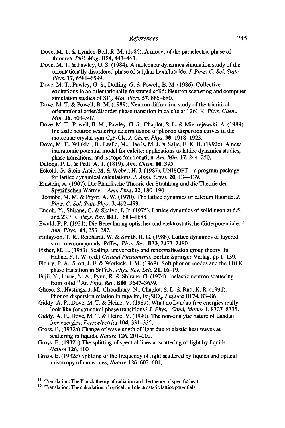
Some fundamentals 15
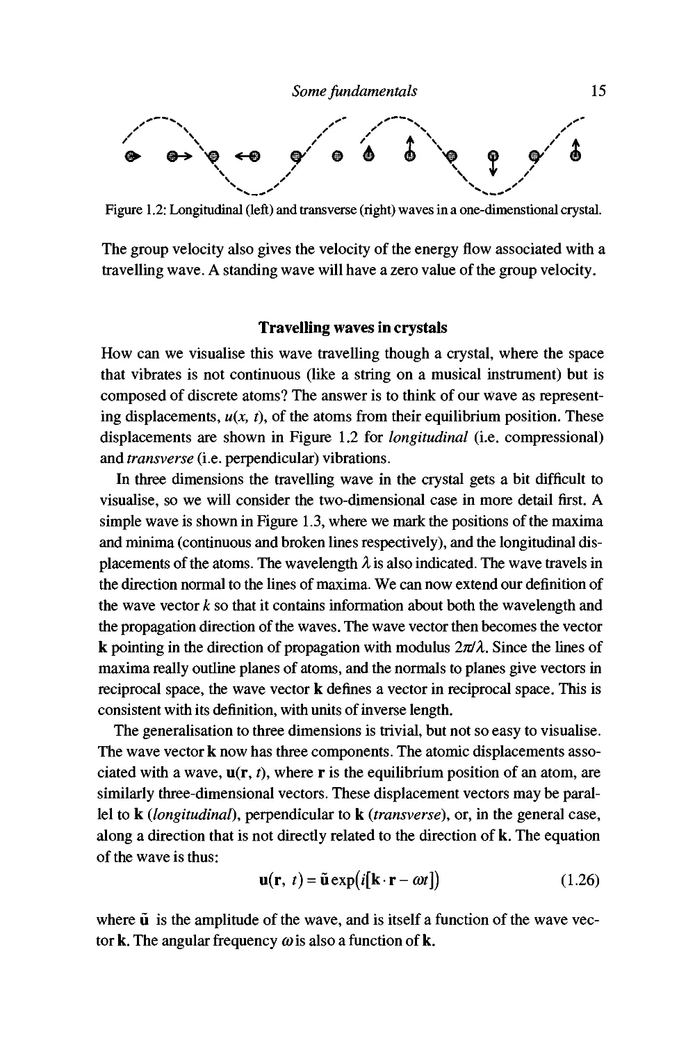
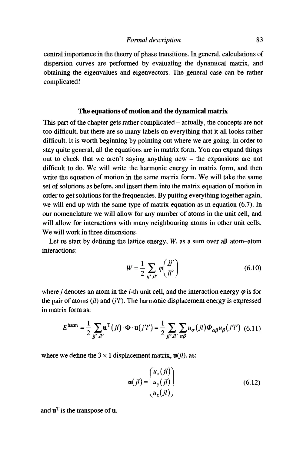
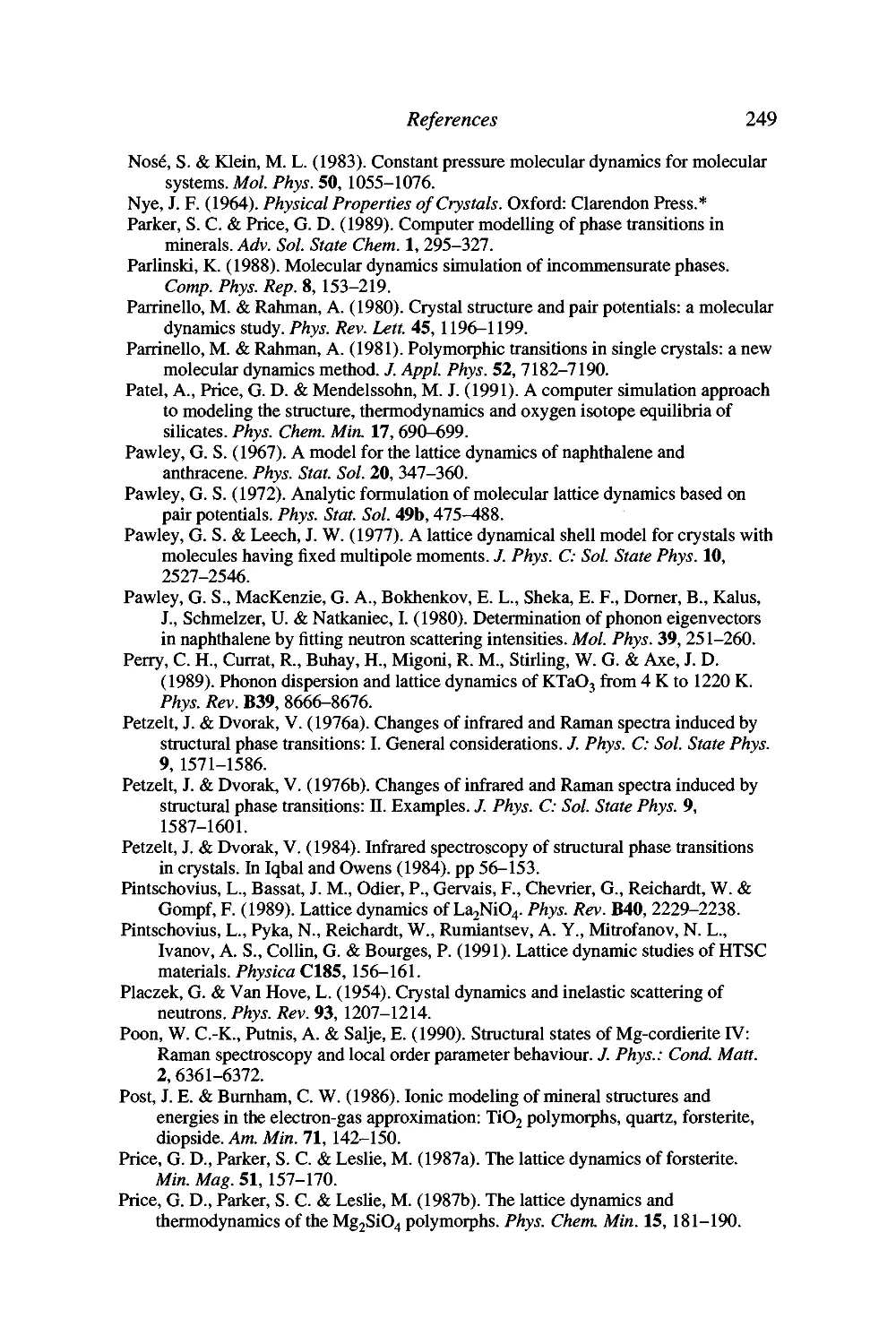
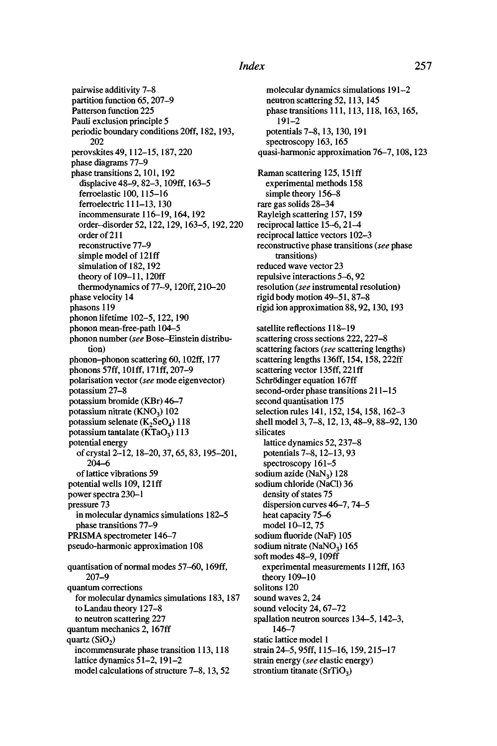
Figure 1.2: Longitudinal (left) and transverse (right) waves in a one-dimenstional crystal.
The group velocity also gives the velocity of the energy flow associated with a
travelling wave. A standing wave will have a zero value of the group velocity.
Travelling waves in crystals
How can we visualise this wave travelling though a crystal, where the space
that vibrates is not continuous (like a string on a musical instrument) but is
composed of discrete atoms? The answer is to think of our wave as
representing displacements, u(x, t), of the atoms from their equilibrium position. These
displacements are shown in Figure 1.2 for longitudinal (i.e. compressional)
and transverse (i.e. perpendicular) vibrations.
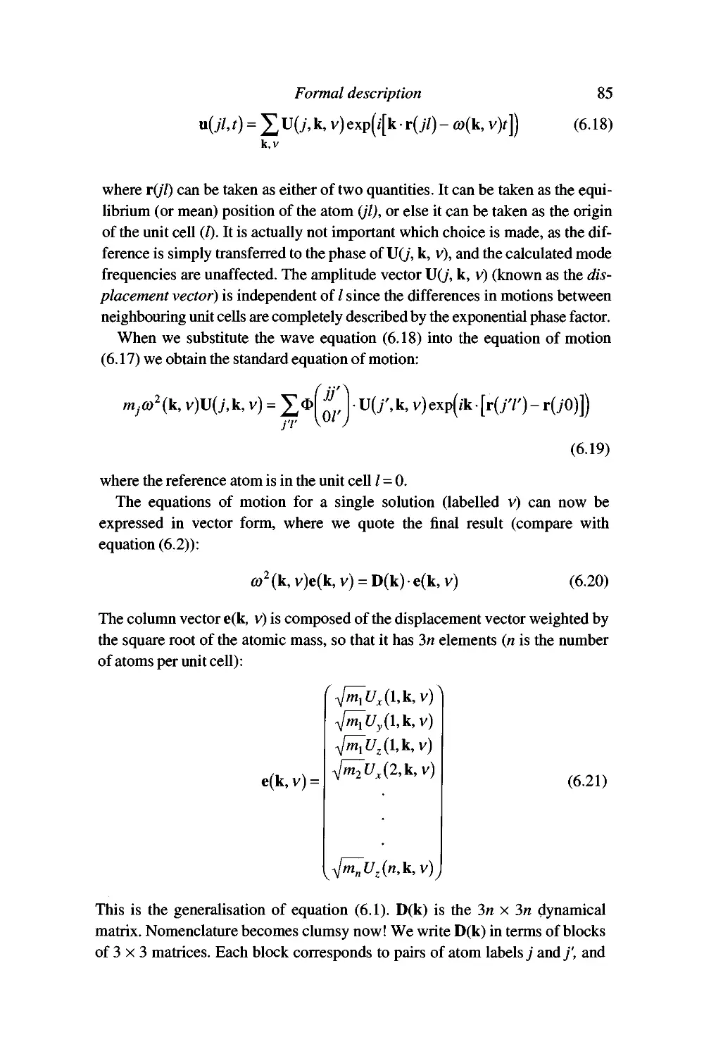
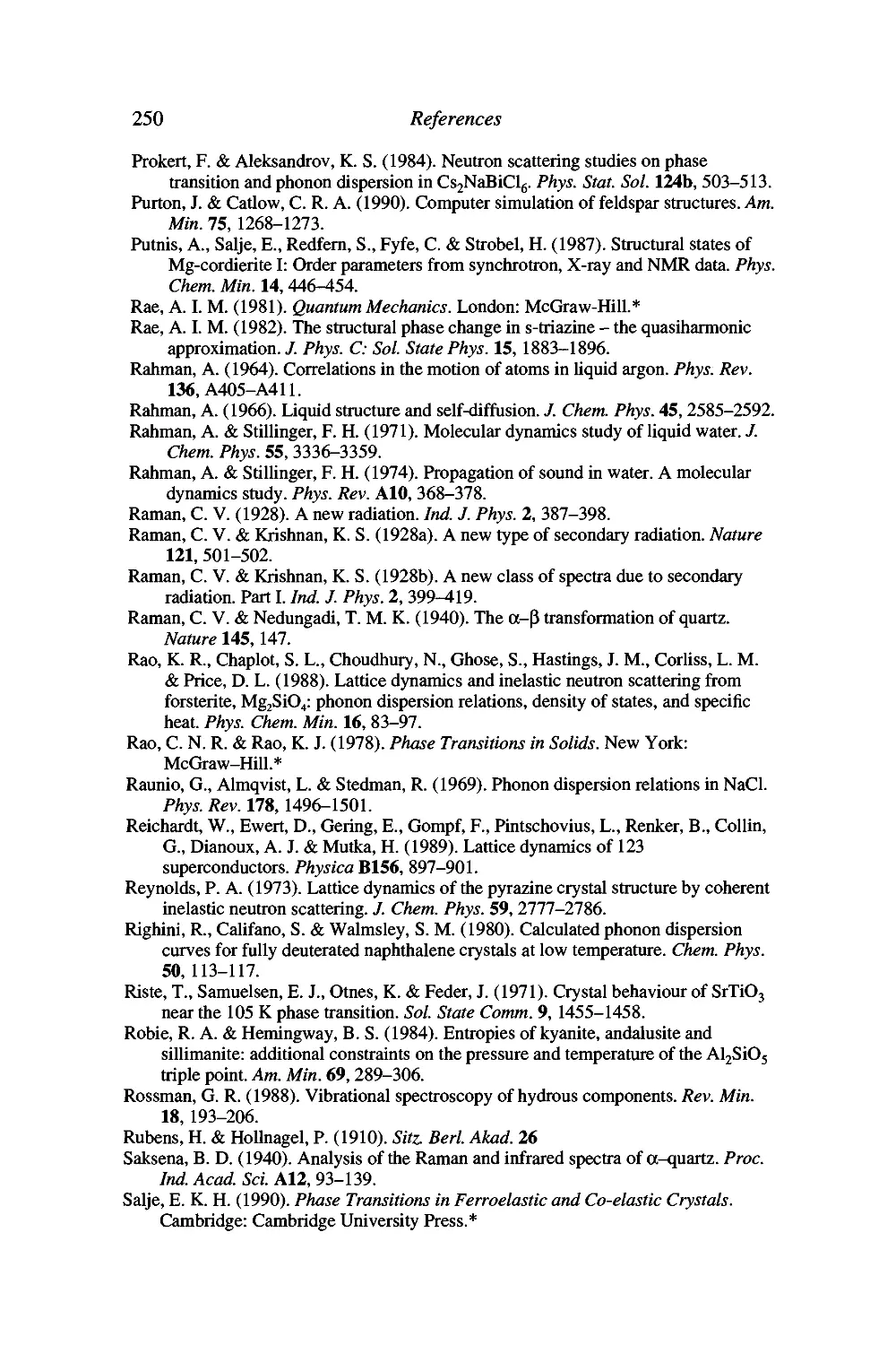
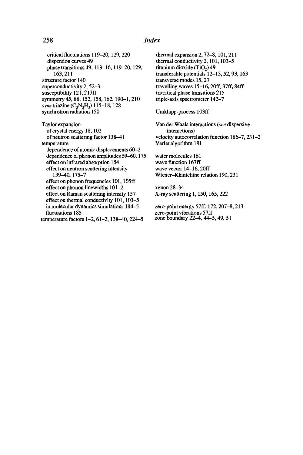
In three dimensions the travelling wave in the crystal gets a bit difficult to
visualise, so we will consider the two-dimensional case in more detail first. A
simple wave is shown in Figure 1.3, where we mark the positions of the maxima
and minima (continuous and broken lines respectively), and the longitudinal
displacements of the atoms. The wavelength A is also indicated. The wave travels in
the direction normal to the Unes of maxima. We can now extend our definition of
the wave vector k so that it contains information about both the wavelength and
the propagation direction of the waves. The wave vector then becomes the vector
k pointing in the direction of propagation with modulus 2;i/A. Since the Unes of
maxima really outline planes of atoms, and the normals to planes give vectors in
reciprocal space, the wave vector k defines a vector in reciprocal space. This is
consistent with its definition, with units of inverse length.
The generaUsation to three dimensions is trivial, but not so easy to visuaUse.
The wave vector k now has three components. The atomic displacements
associated with a wave, u(r, t), where r is the equiUbrium position of an atom, are
similarly three-dimensional vectors. These displacement vectors may be
parallel to k (longitudinal), perpendicular to k (transverse), or, in the general case,
along a direction that is not directly related to the direction of k. The equation
of the wave is thus:
u(r, t) = uexp(j[k • r - cot]) (1.26)
where u is the amplitude of the wave, and is itself a function of the wave
vector k. The angular frequency CO is also a function of k.
16
Introduction to lattice dynamics
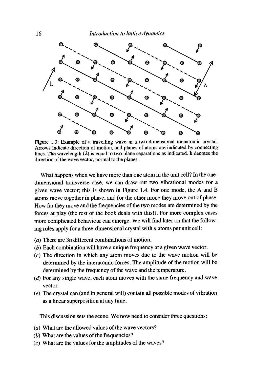
Figure 1.3: Example of a travelling wave in a two-dimensional monatomic crystal.
Arrows indicate direction of motion, and planes of atoms are indicated by connecting
lines. The wavelength (A) is equal to two plane separations as indicated, k denotes the
direction of the wave vector, normal to the planes.
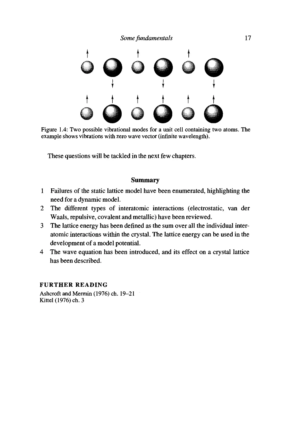
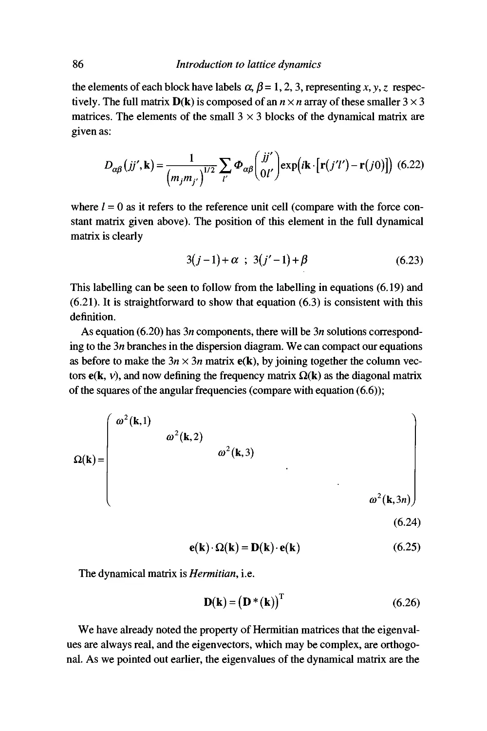
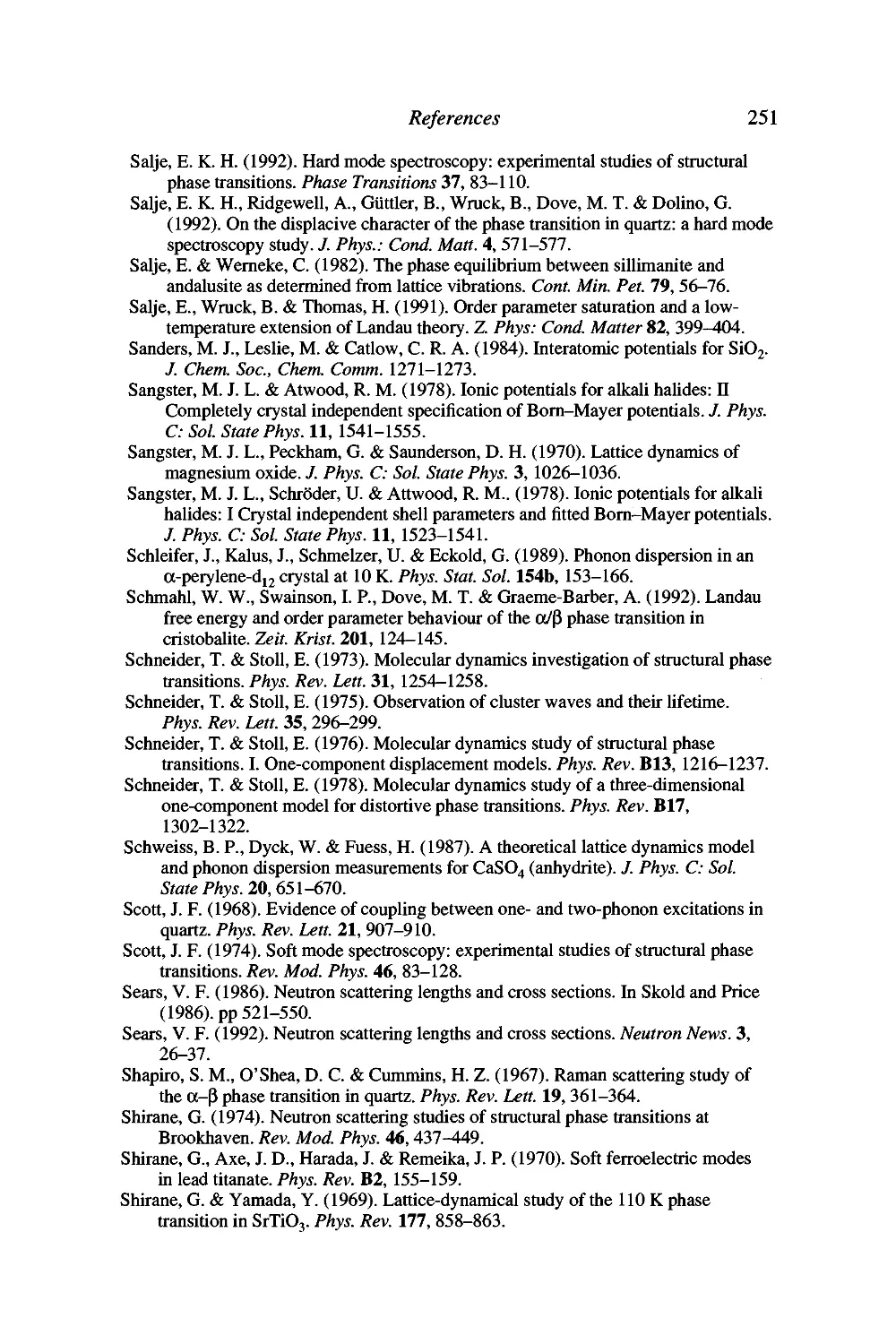
What happens when we have more than one atom in the unit cell? In the one-
dimensional transverse case, we can draw out two vibrational modes for a
given wave vector; this is shown in Figure 1.4. For one mode, the A and B
atoms move together in phase, and for the other mode they move out of phase.
How far they move and the frequencies of the two modes are determined by the
forces at play (the rest of the book deals with this!). For more complex cases
more complicated behaviour can emerge. We will find later on that the
following rules apply for a three-dimensional crystal with n atoms per unit cell:
(a) There are 3n different combinations of motion.
(b) Each combination will have a unique frequency at a given wave vector.
(c) The direction in which any atom moves due to the wave motion will be
determined by the interatomic forces. The amplitude of the motion will be
determined by the frequency of the wave and the temperature.
(d) For any single wave, each atom moves with the same frequency and wave
vector.
(e) The crystal can (and in general will) contain all possible modes of vibration
as a linear superposition at any time.
This discussion sets the scene. We now need to consider three questions:
(a) What are the allowed values of the wave vectors?
(b) What are the values of the frequencies?
(c) What are the values for the amplitudes of the waves?
Some fundamentals 17
t t t
I I I
t t t t t t
Figure 1.4: Two possible vibrational modes for a unit cell containing two atoms. The
example shows vibrations with zero wave vector (infinite wavelength).
These questions will be tackled in the next few chapters.
Summary
Failures of the static lattice model have been enumerated, highlighting the
need for a dynamic model.
The different types of interatomic interactions (electrostatic, van der
Waals, repulsive, covalent and metallic) have been reviewed.
The lattice energy has been defined as the sum over all the individual
interatomic interactions within the crystal. The lattice energy can be used in the
development of a model potential.
The wave equation has been introduced, and its effect on a crystal lattice
has been described.
FURTHER READING
Ashcroft and Mermin (1976) ch. 19-21
Kittel(1976)ch.3
The harmonic approximation and lattice
dynamics of very simple systems
A simple model for a monatomic crystal is described, and the first
results of the theory of lattice dynamics are obtained. The simple model
forces us to encounter some of the important general concepts that will
be used throughout this book. The chapter concludes with a detailed
study of the lattice dynamics of the rare gas crystals.
The harmonic approximation
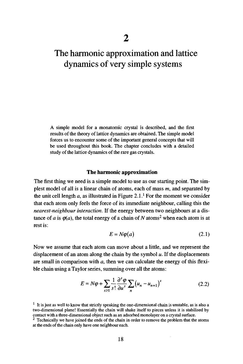
The first thing we need is a simple model to use as our starting point. The
simplest model of all is a Hnear chain of atoms, each of mass m, and separated by
the unit cell length a, as illustrated in Figure 2.1.' For the moment we consider
that each atom only feels the force of its immediate neighbour, calUng this the
nearest-neighbour interaction. If the energy between two neighbours at a
distance of a is (p(a), the total energy of a chain of A' atoms^ when each atom is at
rest is:
E = N(p{a) (2.1)
Now we assume that each atom can move about a little, and we represent the
displacement of an atom along the chain by the symbol u. If the displacements
are small in comparison with a, then we can calculate the energy of this
flexible chain using a Taylor series, summing over all the atoms:
^=^"?'+i7[0iK-«-ir (2.2)
s>\ '
' It is just as well to know that strictly speaking the one-dimensional chain is unstable, as is also a
two-dimensional plane! Essentially the chain will shake itself to pieces unless it is stabilised by
contact with a three-dimensional object such as an adsorbed monolayer on a crystal surface.
^ Technically we have joined the ends of the chain in order to remove the problem that the atoms
at the ends of the chain only have one neighbour each.
18
The harmonic approximation 19
Un-2 Un-\ Un Un+l Un+2
a
-* >-
Figure 2.1: Linear chain model. J is the harmonic force constant (the interactions are
represented by springs), and the atomic displacements are represented by u.
If M„ is the displacement of the n-th atom from its equilibrium position, the
distance between two atoms n and n + 1 is r = a + (m„ - m„+i). Thus the derivatives
of (p with respect to u are equivalent to the derivatives with respect to r. Since a
is the equilibrium unit cell length, the first derivative of (p is zero, so that the
linear term in the expansion (* = 1) can be dropped. All the other differentials
correspond to the point m = 0. As m is small in comparison to a, this series is a
convergent one, and we might expect that the dominant contribution will be the
term that is quadratic in u. Therefore we start with a model that includes only
this term (s = 2), neglecting all the higher-order terms. The energy of this
lattice is then the same as the energy of a set of harmonic oscillators, and so we
call this approximation the harmonic approximation. The higher-order terms
that we have neglected are called the anharmonic terms.
Why do we make this approximation? The main reason is that it is a
mathematically convenient approximation. We know that the harmonic equations
of motion have exact solutions, whereas even the simplest anharmonic
equations do not have exact solutions but require the use of approximation
schemes. Although this may not sound a very noble reason, the use of this
approximation can be justified in at least three related ways. Firstly, as will
be seen, the harmonic approximation in practice proves to be capable of
giving good results. The anharmonic part of the model usually leads to only a
small modification of the overall behaviour, and since the amplitudes of
the displacements will be expected to decrease on lowering the temperature
(i.e. the kinetic energy of the chain) the harmonic term will be the only
important term at low temperatures. Secondly, the harmonic approximation
allows us to obtain many of the important physical principles characteristic of
the system with only a minimum of effort, and it is these that we are hoping to
study. Thirdly, there is an often-used approach in physics when dealing with
complex problems, which is to solve the simple model first (in this case the
harmonic model), and then correct the simple solution for the more complex
parts (the anharmonic corrections). This is called the perturbation method.
In Chapter 8 we shall see that there are important features of real crystals
that the harmonic approximation fails to explain, but we will be able to
20 Introduction to lattice dynamics
progress by simply correcting the harmonic results without having to start
again!
The equation of motion of the one-dimensional monatomic chain
The harmonic energy of our chain from equation (2.2) is'
E'-=\j'L{u„-u„,,f ;/ = y? (2.3)
n
The equation of motion of the n-th atom from the classical Newton equation is
then
o u oE / \ ,„ jx
m-^ = ^—- = -/(2m„-m„^.,-m„_J (2.4)
If our chain contains A' atoms, we need to think about what happens to the
ends of the chain. The usual trick for a long chain is to join the ends; this is
called the Bom-von Kdrmdn periodic boundary condition (Bom and von
Karman 1912,1913; Bom and Huang 1954, pp 45^6, App. IV). We know that
the solution of the harmonic equation of motion is a sinusoidal wave, so the
motion of the whole system will correspond to a set of travelling waves as
given by equation (1.23). Our aim then is to find the set of frequencies of these
waves. We expect the time-dependent motion of the n-th atom to be a linear
superposition of each of the travelling waves allowed along the chain; the
mathematical representation is:
"«(0 = X "t exp(j[^ - (O^f ]) (2.5)
k
where k is any wave vector (= 2;i/wavelength), fflj^is the corresponding angular
frequency, Hj^ is the amphtude, and x is restricted to the values x = na. We will
find later that there is also a discrete set of allowed values of ^. However, if for
the moment we consider each wave vector separately, we can solve the
equation of motion for each individual wave. We simply substitute equation (2.5)
into equation (2.4), to obtain:
^ Note that this can also be written as -*^ AK~«,«,ti) .where *r = 27= —5- = for
all values of n. ^ » l9«. J \^M '
The harmonic approximation
21
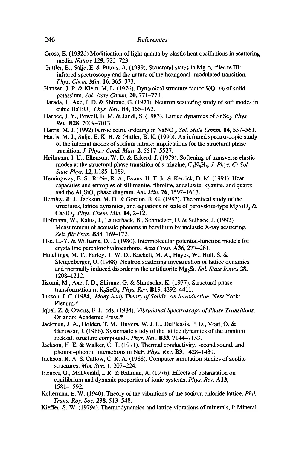
?
o
a
Wave vector, a*
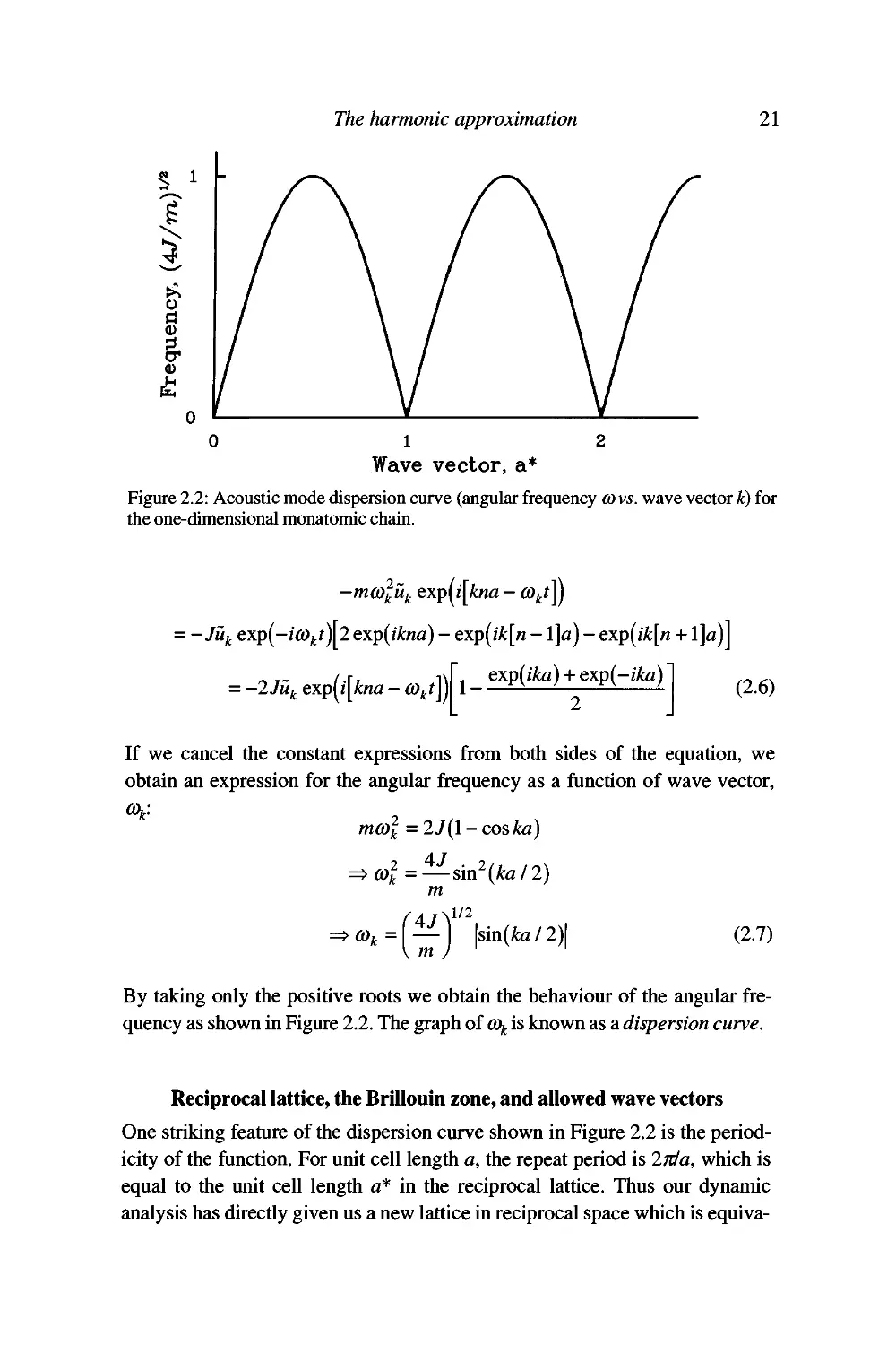
Figure 2.2: Acoustic mode dispersion curve (angular frequency a vs. wave vector k) for
the one-dimensional monatomic chain.
= -Ju^^ exp(-/ft);^f )[2 exp(j^«a) - exp(j^[« - l]a) - exp(/^[« + l]a)]
= —Uuj^ expn'[^«a - COj^tn
exp(jfaz) + exp(-j^a)
2
(2.6)
If we cancel the constant expressions from both sides of the equation, we
obtain an expression for the angular frequency as a function of wave vector,
mft);^ =2J(l-cos^a)
=^(ol =—sin^(jta/2)
m
COt
= [ — ] |sin(faz/2)|
m J
(2.7)
By taking only the positive roots we obtain the behaviour of the angular
frequency as shown in Figure 2.2. The graph of % is known as a dispersion curve.
Reciprocal lattice, the Brillouin zone, and allowed wave vectors
One striking feature of the dispersion curve shown in Figure 2.2 is the
periodicity of the function. For unit cell length a, the repeat period is iTda, which is
equal to the unit cell length a* in the reciprocal lattice. Thus our dynamic
analysis has directly given us a new lattice in reciprocal space which is equiva-
22
Introduction to lattice dynamics
Figure 2.3: The atomic motions associated with two waves that have wave vectors that
differ by a reciprocal lattice vector. We see that the two waves have identical effects.
lent to the standard reciprocal lattice. This feature will follow for
three-dimensional lattices also, even with non-orthogonal cells.
If we take any wave vector from the set used in equation (2.4), and add to it a
reciprocal lattice vector, the equation of motion for this second wave will be
identical to that for the original wave. Therefore the only useful information is
contained in the waves with wave vectors lying between the limits
— <k< —
(2.8)
We call this range of wave vectors the first Brillouin zone (Brillouin 1930).
The repeated zones are the second, third Brillouin zones etc. These zones will
be important when we consider anharmonic interactions in Chapter 8 and
neutron scattering in Chapter 9. We note that the wave vectors k = ± nia define
special points in reciprocal space, called Brillouin zone boundaries, which he
half-way between reciprocal lattice points. In our example the group velocity,
d(0/dk, is equal to zero at these points, meaning that the wave with this wave
vector is a standing wave. It will turn out that this is a general result in three
dimensions.
We can easily show that two wave vectors k and k' that differ by a reciprocal
lattice vector G, where k' = k+ G, have an identical effect on the atoms in the
chain. We know that <%=<%.. When ;c = «a we have
exp^ik'x) = exp{iGx) x exp(j^) = exp(j^)
(2.9)
Thus the travelling wave solution (1.23) is the same for k' as for k. This is
illustrated in Figure 2.3, where we see that two waves with wave vectors differing
by a reciprocal lattice vector give identical displacements at each lattice
position. This result can be generalised to three dimensions, and to unit cells
containing more than one atom.
In three dimensions, as in one dimension, the Brillouin zone boundaries are
defined as lying half-way between reciprocal lattice points, although now the
The harmonic approximation 23
--h-~.l''
/
/
/
?t--f-.
-^—y-
/
/
/
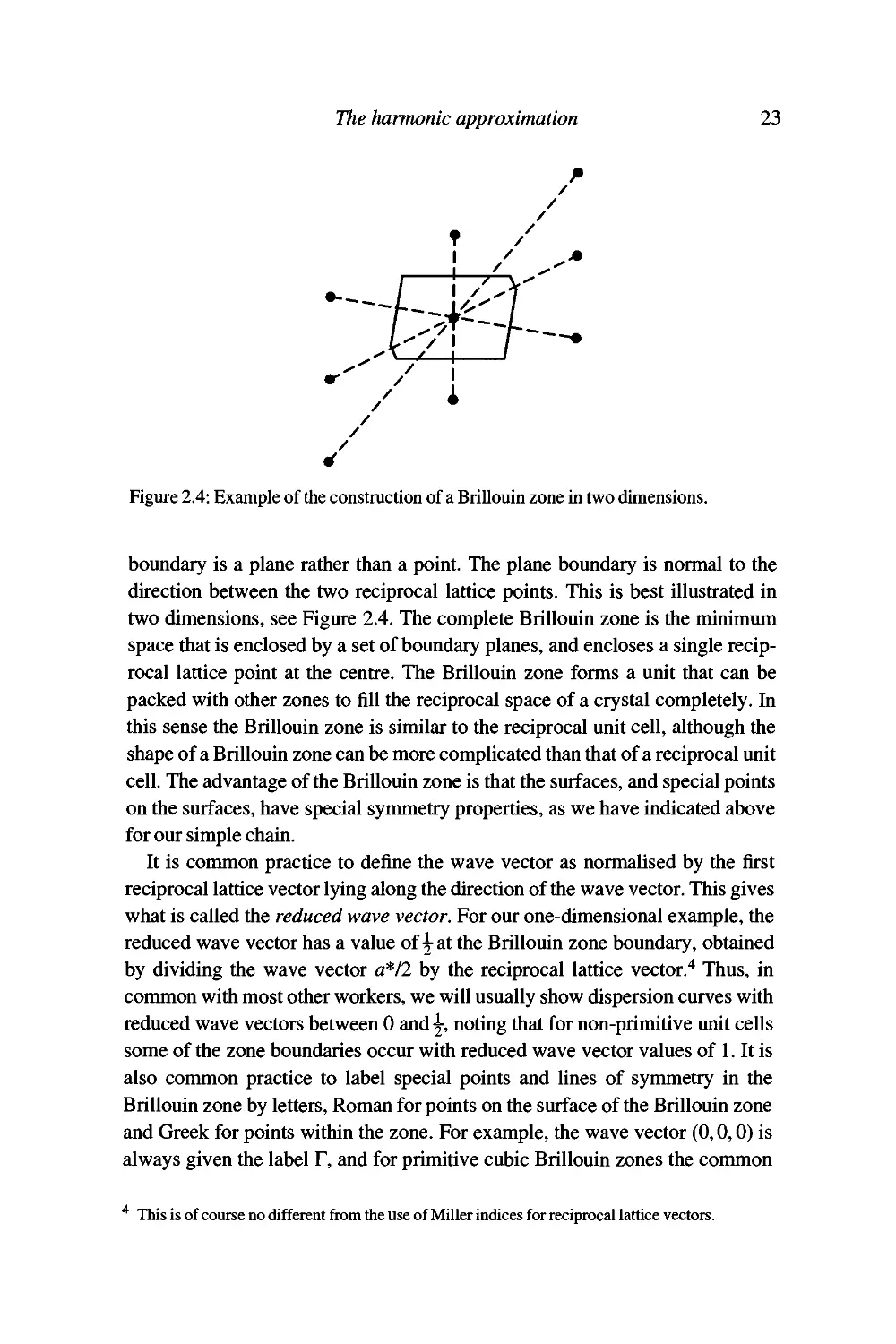
Figure 2.4: Example of the construction of a Brillouin zone in two dimensions.
boundary is a plane rather than a point. The plane boundary is normal to the
direction between the two reciprocal lattice points. This is best illustrated in
two dimensions, see Figure 2.4. The complete Brillouin zone is the minimum
space that is enclosed by a set of boundary planes, and encloses a single
reciprocal lattice point at the centre. The Brillouin zone forms a unit that can be
packed with other zones to fill the reciprocal space of a crystal completely. In
this sense the Brillouin zone is similar to the reciprocal unit cell, although the
shape of a Brillouin zone can be more complicated than that of a reciprocal unit
cell. The advantage of the Brillouin zone is that the surfaces, and special points
on the surfaces, have special symmetry properties, as we have indicated above
for our simple chain.
It is common practice to define the wave vector as normalised by the first
reciprocal lattice vector lying along the direction of the wave vector. This gives
what is called the reduced wave vector. For our one-dimensional example, the
reduced wave vector has a value of ^at the Brillouin zone boundary, obtained
by dividing the wave vector a*/2 by the reciprocal lattice vector.'* Thus, in
common with most other workers, we will usually show dispersion curves with
reduced wave vectors between 0 and \, noting that for non-primitive unit cells
some of the zone boundaries occur with reduced wave vector values of 1. It is
also common practice to label special points and Unes of symmetry in the
Brillouin zone by letters, Roman for points on the surface of the Brillouin zone
and Greek for points within the zone. For example, the wave vector (0,0,0) is
always given the label T, and for primitive cubic Brillouin zones the common
* This is of course no different from tlie use of Miller indices for reciprocal lattice vectors.
24 Introduction to lattice dynamics
labels are X for (^, 0, 0), M for (^, ^, 0), R for {\, \, ^), A for [^ 0, 0], I for
[^ 4 0], and A for [^ 4 a-
Although the dispersion curve is a continuous curve, a finite chain will
permit only a discrete set of wave vectors. Since with periodic boundary
conditions atom A^ is identical to atom 0, we have
exp ikNa = exp 0 = 1 (2.10)
Therefore the allowed values of ^ are given by the discrete set:
k = ^ (2.11)
where m is an integer. This is analogous (but not identical) to the fact that a
plucked string will allow only a discrete set of vibrations with integral
fractions of the string length as the set of wavelengths. Comparison of equations
(2.8) and (2.11) shows that there are A^ allowed wave vectors within one
Brillouin zone. In the general case, the number of allowed wave vectors within
one Brillouin zone is equal to the number of primitive unit cells in the crystal.
The long wavelength limit
As k approaches zero, we can take the hnear approximation to the dispersion
curve given by equation (2.7):
co{k-^0) = a\ — \ \k\ (2.12)
This gives the phase velocity c, which is equivalent to the velocity of sound in
the crystal:
c = ^ = a\-\ (2.13)
Because of this relationship to sound waves, a vibrational mode with a
dispersion curve of the form given in Figure 2.2, which goes to zero in the limit of
small k, is known as an acoustic mode. In addition, as the atomic displacements
are along the direction of the wave vector, the mode is known as a longitudinal
acoustic mode.
We can now make a connection with macroscopic elastic properties. If we
compress our chain by the strain e, the average distance between atoms is not a
but a' = a( 1 - e), where e « 1. The energy of the strained chain (neglecting the
energy due to the dynamic atomic motions) therefore becomes equal to:
The harmonic approximation 25
E = N<p + -NJ{a-a'f (2.14)
This result follows from the Taylor expansion introduced in equation (2.2),
together with our definition of the force constant J given by equation (2.3).
Thus the extra energy per atom, called the strain energy, is
^strain = \ J{a-af = \ Ja'e'= \ Ce' (2.15)
where the constant C = Ja^ is called the elastic constant. From the velocity of
sound given by equation (2.13) we have
c^ =co^/k^=Ja^/m = C/m (2.16)
Hence, in the long wavelength limit, we have
ap- = Ck^lm (2.17)
In a three-dimensional crystal the strain energy is defined relative to a unit
volume, so that conventionally our expressions (2.16) and (2.17) become
C = pc^ ; p(o^ = Ck^ (2.18)
where p is the density. The relationship between the acoustic modes and
macroscopic elasticity is examined in more detail in Chapter 7.
Extension to include distant neighbours
Our analysis is readily extended to include more interactions than only the
nearest-neighbour interaction. If <Pp{r^ is the energy between the p-th
neighbours separated by a distance r^ {=pa for equilibrium), the energy of our chain
is given by
2
P n,p
1 ( d 0 I 2
E = Nj^(Pp{pa) + -J^ -^ («„-«„+p) (2.19)
Note that we have again neglected the anharmonic terms. The harmonic energy
is therefore given as
n,p
26 Introduction to lattice dynamics
where
'p a..2
du^
drl
(2.21)
The equation of motion given by equation (2.4) is readily extended to
m-
dt^ du„
■ = -X-^p(2"n~"n-P~"n+p) ^^'^^^
Our travelling wave solution is still given by equation (2.5). Hence the solution
of equation (2.22) for each wave vector gives us
-mcolu^^ exp\i[kna - co^t]j
= -iij^ exp(-/ft);^f )^ Jp [2 exp(jfoza) - exp(j^[« - p\a)- exp(j^[« + p\a)\
p
(2.23)
This simply reduces to
mcof =^Jp[^~ exp(/^/?a) - exp(-/^a)]
p
= 2^ Jp[l-cos kpa] (2.24)
p
and we finally obtain the expression for the dispersion curve:
,2 _ 4 y , „:„2(kpa
p
».-=iI',-1 = l (2-25)
This result represents only a minor modification to the result for nearest
neighbours, equation (2.7). The general result has the same behaviour for ^ -> 0 and
at ^=Ttia as described above.
Three-dimensional monatomic crystals
If we preserve simplicity, our model can be easily extended to three
dimensions, if now in our equations of motion the variables u refer not to
displacements of atoms but of planes of atoms, and our force constants are similarly
redefined. This was discussed in Chapter 1, and is illustrated in Figure 1.3. We
also need to include motions that are perpendicular to the wave vector. These
follow as a simple extension of our one-dimensional model. One can imagine
The harmonic approximation
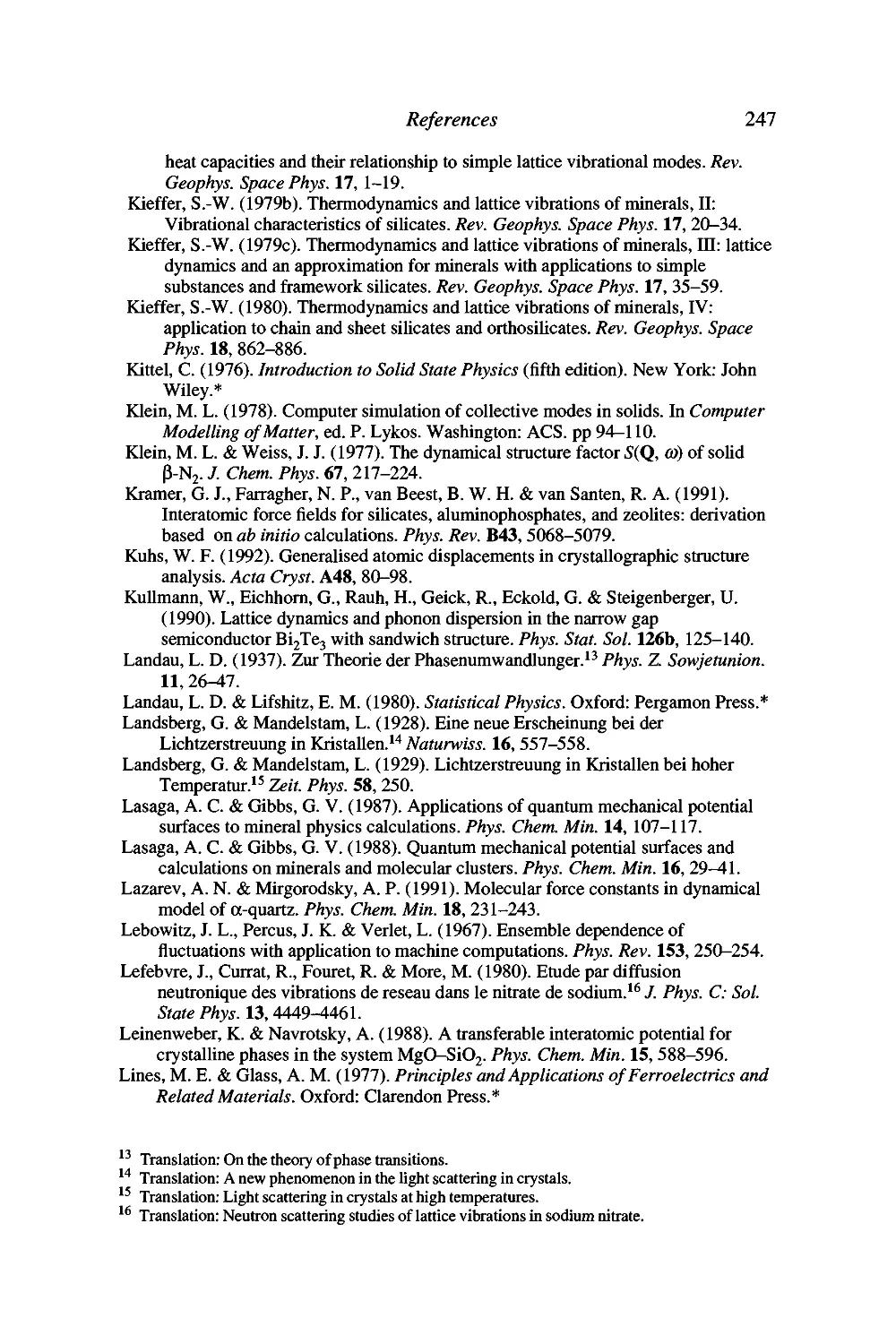
(to.o) (tto)
27
itU)
1 0
Reduced wave vector component, ^
0.5
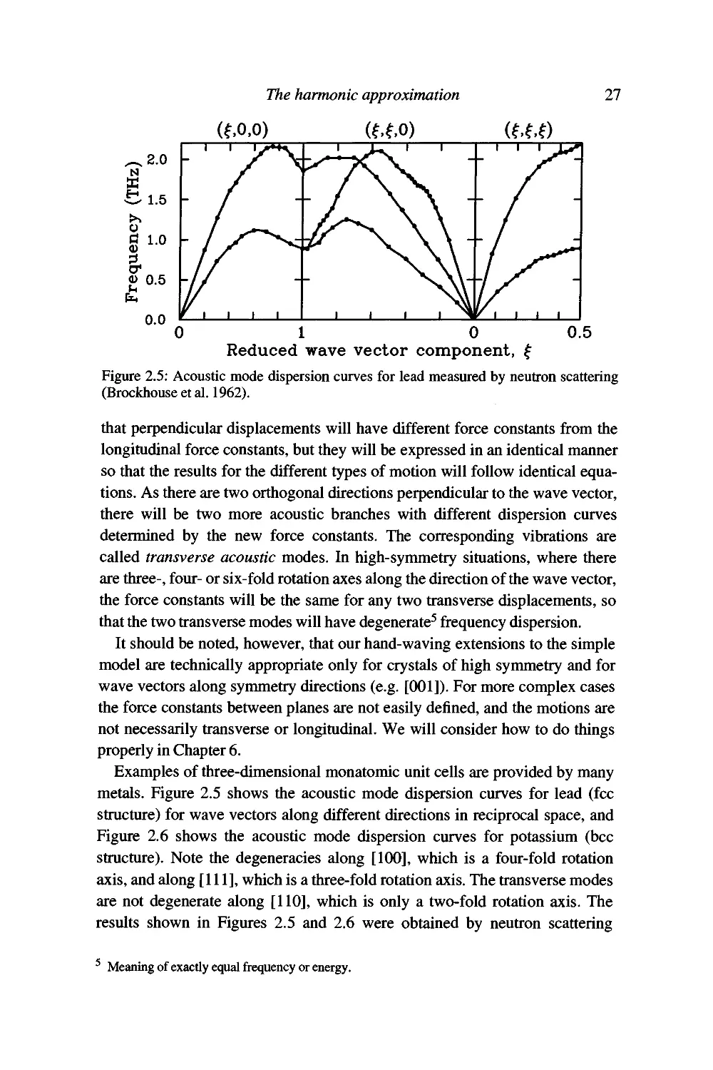
Figure 2.5: Acoustic mode dispersion curves for lead measured by neutron scattering
(Brockhouse et al. 1962).
that perpendicular displacements will have different force constants from the
longitudinal force constants, but they will be expressed in an identical manner
so that the results for the different types of motion will follow identical
equations. As there are two orthogonal directions perpendicular to the wave vector,
there will be two more acoustic branches with different dispersion curves
determined by the new force constants. The corresponding vibrations are
called transverse acoustic modes. In high-symmetry situations, where there
are three-, four- or six-fold rotation axes along the direction of the wave vector,
the force constants will be the same for any two transverse displacements, so
that the two transverse modes will have degenerate^ frequency dispersion.
It should be noted, however, that our hand-waving extensions to the simple
model are technically appropriate only for crystals of high symmetry and for
wave vectors along symmetry directions (e.g. [001]). For more complex cases
the force constants between planes are not easily defined, and the motions are
not necessarily transverse or longitudinal. We will consider how to do things
properly in Chapter 6.
Examples of three-dimensional monatomic unit cells are provided by many
metals. Figure 2.5 shows the acoustic mode dispersion curves for lead (fee
structure) for wave vectors along different directions in reciprocal space, and
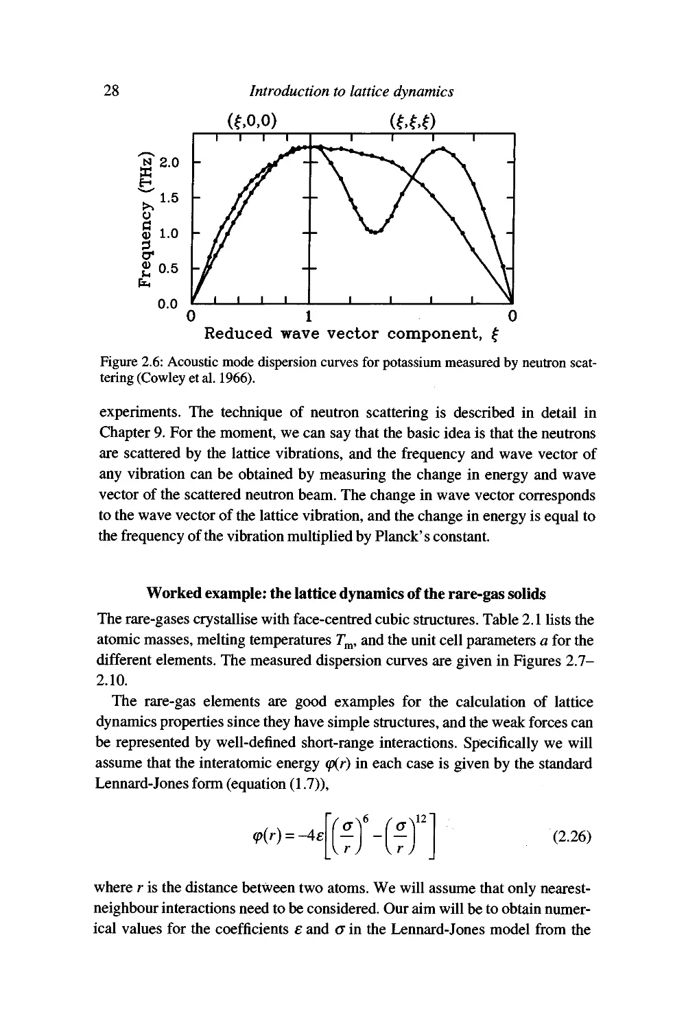
Figure 2.6 shows the acoustic mode dispersion curves for potassium (bcc
structure). Note the degeneracies along [1(X)], which is a four-fold rotation
axis, and along [111], which is a three-fold rotation axis. The transverse modes
are not degenerate along [110], which is only a two-fold rotation axis. The
results shown in Figures 2.5 and 2.6 were obtained by neutron scattering
Meaning of exactly equal frequency or energy.
28
Introduction to lattice dynamics
(to.o) (tt^)
0 10
Reduced wave vector component, ^
Figure 2.6: Acoustic mode dispersion curves for potassium measured by neutron
scattering (Cowley et al. 1966).
experiments. The technique of neutron scattering is described in detail in
Chapter 9. For the moment, we can say that the basic idea is that the neutrons
are scattered by the lattice vibrations, and the frequency and wave vector of
any vibration can be obtained by measuring the change in energy and wave
vector of the scattered neutron beam. The change in wave vector corresponds
to the wave vector of the lattice vibration, and the change in energy is equal to
the frequency of the vibration multiplied by Planck's constant.
Worked example: the lattice dynamics of the rare-gas solids
The rare-gases crystallise with face-centred cubic structures. Table 2.1 lists the
atomic masses, melting temperatures T^, and the unit cell parameters a for the
different elements. The measured dispersion curves are given in Figures 2.7-
2.10.
The rare-gas elements are good examples for the calculation of lattice
dynamics properties since they have simple structures, and the weak forces can
be represented by well-defined short-range interactions. Specifically we will
assume that the interatomic energy (p{r) in each case is given by the standard
Lennard-Jones form (equation (1.7)),
^(r) = -4e
12
(2.26)
where r is the distance between two atoms. We will assume that only nearest-
neighbour interactions need to be considered. Our aim will be to obtain
numerical values for the coefficients e and a in the Lennard-Jones model from the
The harmonic approximation
Table 2.1: Crystal data for the rare-gas solids (Kittel 1976, p 77)
Atom
Ne
Ar
Kr
Xe
Atomic mass
20.2
40.0
83.8
113.3
7"„(K)
23
84
117
161
a (A)
4.466
5.313
5.656
6.129
29
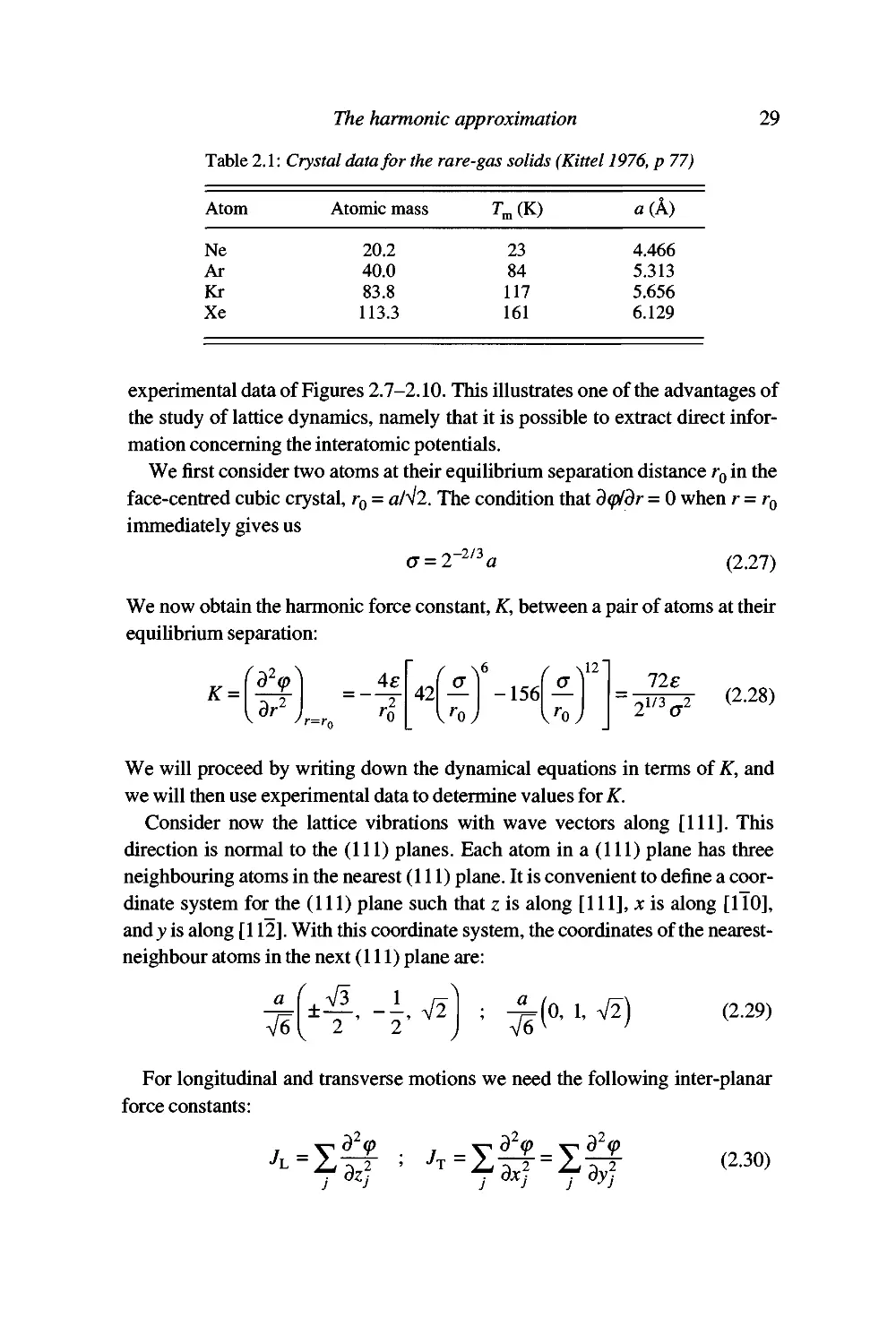
experimental data of Figures 2.7-2.10. This illustrates one of the advantages of
the study of lattice dynamics, namely that it is possible to extract direct
information concerning the interatomic potentials.
We first consider two atoms at their equilibrium separation distance Tq in the
face-centred cubic crystal, Tq = aN2. The condition that d(p/dr = 0 when r=rQ
immediately gives us
(7 = 2-^" a
(2.27)
We now obtain the harmonic force constant, K, between a pair of atoms at their
equihbrium separation:
/32„\
K =
dr'
4e
'r=rn
Al
^a^'
-156
^a^''
lie
-,1/3 _2 (2.28)
2 a
We will proceed by writing down the dynamical equations in terms of K, and
we will then use experimental data to determine values for K.
Consider now the lattice vibrations with wave vectors along [111]. This
direction is normal to the (111) planes. Each atom in a (111) plane has three
neighbouring atoms in the nearest (111) plane. It is convenient to define a
coordinate system for the (111) plane such that z is along [111], ;c is along [iTO],
and 3? is along [112]. With this coordinate system, the coordinates of the nearest-
neighbour atoms in the next (111) plane are:
^ V3 ' ^
a
V6
±^, -1 V2 ; ^(O, 1, V2)
2 2 J V6^ '
(2.29)
For longitudinal and transverse motions we need the following inter-planar
force constants:
-V^
4=1,
J -y££-
(2.30)
30
2.0 -
N
X
1.5 -
O
g 1.0
r^ 0.5
0.0
Introduction to lattice dynamics
(f.0.0) (O.f.f) (ff.f)
/ / ^^ \ \ / y^
0.0 0.5 1.0 0.5 0.0 0.5
Reduced wave vector component, ^
Figure 2.7; Acoustic mode dispersion curves for argon (Fujii et al. 1974). The lines give
the calculated dispersion curves using the model described in the text.
where the sum is over the three neighbouring atoms in the next plane. It can
easily be shown that
aV_rzf aV
dz'
dr'
etc.
(2.31)
This gives the result:
^x,^'
Jl=kJ, -^ ; iT = ^S — =^Z
V' y
V' y
/ \2
(2.32)
where we use the coordinates of equation (2.29), and for all neighbours the
nearest-neighbour distance is r = aN2.
Substitution of the coordinates of equation (2.29) into the expressions for
the inter-planar force constants, equation (2.32), yields:
Ji^=2K ; Jj=K/2 (2.33)
From equation (2.7) the zone boundary angular frequencies are given as:
CO, =
8K
m
1/2
m )
1/2
(2.34)
These results imply that ©l = 2ay^ for k =^[111], which can be seen from
Figures 2.7-2.10 to be approximately true for each example. From the experi-
N
X
1.5 -
O
a
$i 0.5
M
El,
1.0 -
0.0
0.0
The harmonic approximation
(fO.O) (O.ff) (ff.f)
31
• •
0.5
1.0
0.5
0.0
0.5
Reduced wave vector component,^
Figure 2.8; Acoustic mode dispersion curves for neon (Endoh et al. 1975). The lines
give the calculated dispersion curves using the model described in the text.
mental data we can obtain two estimates for the value of K for each system,
which are given in Table 2.2.
Consider now the dispersion curves along [001]. The nearest-neighbour
atoms in the next (001) plane from the atom at the origin have coordinates
-(±1, 0, 1)
f (0, ±1, 1)
(2.35)
We do not now need to change coordinate systems as the vibration is along a
unit cell vector. Using the results of equations (2.30)-(2.32) we obtain values
for the force constants for wave vectors along [001]:
y^ — 2^ J j'Y — K
which give zone boundary angular frequencies:
CO, =
J8K)
1/2
m J
(0-T
=f^Y'^
(2.36)
(2.37)
m J
The prediction that a\^ = V2ft)j. for k = ■^[OOl] is consistent with the data of
Figures 2.7-2.10. We now have another two estimates for the value of ^, and
all four estimates for each system are compared and averaged in Table 2.2. The
largest standard deviation on the average value of ^is only 10%, but improved
accuracy could have been obtained if we had fitted the curves over the whole
branches rather than taking only the zone boundary wave vectors. The errors in
32
Introduction to lattice dynamics
(fO.O) (O.f.f) (fff)
1.5 -
1.0
o
El,
0.0
/ y Nv \ \ / y^
0.0
0.5
1.0
0.5
0.0
0.5
Reduced wave vector component, ^
Figure 2.9: Acoustic mode dispersion curves for krypton (Skalyo et al. 1974). The lines
give the calculated dispersion curves using the model described in the text.
K are larger than the errors in a because K is proportional to the square of a.
The average values of ^ have been used to calculate the complete set of
dispersion curves shown as sohd lines in Figures 2.7-2.10. The agreement between
the calculations and the experimental data is generally reasonable, indicating
that our approximation of using only nearest-neighbour force constants is not
too far from reality.
The dispersion curves along [011] are slightly more comphcated, owing to
the fact that nearest-neighbour atoms Ue in the nearest and next-nearest planes.
We therefore need to use the extension for distant neighbours given by
equation (2.25). First we define a coordinate system such that z lies along [011], 3?
lies along [Oil], and x lies along [100]. The coordinates of the
nearest-neighbour atoms are
a f 1 1 1
nearest-neighbour: -^-1^^^-^
next-nearest-neighbour: -t= (0,0,1)
V2
, -L _1 +1
V2IV2' 2' 2
(2.38)
We note that this set of neighbours defines two neighbouring planes, so we
need to use equation (2.25) for/? = 1, 2. Moreover, along this direction the two
transverse force constants are not identical. However, the zone boundary along
this direction is identical to the zone boundary along [(X)l].
The force constants for this direction can readily be calculated using the
methods described above for the coordinates (equation (2.38)), giving:
The harmonic approximation 33
Table 2.2: Results for the force constant K. Units are J m'^.
[IIIJL
[111]T
[001] L
[001] T
mean
Ne
0.45
0.37
0.45
0.43
0.42 + 0.04
Ar
1.37
1.22
1.32
1.36
1.32 + 0.07
Kr
1.54
1.35
1.54
1.48
1.48 + 0.09
Xe
1.55
1.41
1.55
1.57
1.52 + 0.07
Table 2.3: Energy parameters for the rare-gas solids. The experimental values for the
lattice energies are taken from the compilation given by Kittel (1976, p 77).
Ne Ar Kr Xe
a (A)
£(kJmol-i)
^(calc.XkJmol-i)
WCobs-Xklmol-i)
2.813
0.350
-2.10
-1.88
3.347
1.56
-9.36
-7.74
3.563
1.98
-11.9
-11.2
3.861
2.39
-14.3
-16.0
nearest-neighbour: Ji^ = Jj = K ; Jj =2K
next-nearest-neighbour: Ji^=K ; Jj = J^ =0
(2.39)
where the superscripts on the transverse force constants label the directions of
motion. Using the estimates of K given in Table 2.2 the calculated dispersion
curves are shown in Figures 2.7-2.10. It can be seen that the agreement is as
good as for the other directions.
We finally come back to our main point, namely the evaluation of the
parameters in the assumed interatomic potential, equation (2.26). Using the values
of the cell parameters given in Table 2.1 and the average values of K given in
Table 2.2, we can use equations (2.27) and (2.28) to obtain values for <7 and e,
which are given in Table 2.3. We can then calculate the lattice energy W for
each system, which is equal to -3e. The calculated values are compared with
experimental data in Table 2.3. The agreement between the calculated and
measured lattice energies is reasonably good. It might be expected that the
results could be improved by including second-nearest-neighbour interactions,
and by fitting the force constants against the dispersion curves at all wave
vectors rather than only at the zone boundary points.
34
N
gl.O
o
a
(U
g.0.5
(U
El,
0.0
0.0
Introduction to lattice dynamics
(f.O.O) (O.f.f) (f.f.f)
0.5
1.0
0.5
0.0
0.5
Reduced wave vector component, ^
Figure 2.10: Acoustic mode dispersion curves for xenon (Lurie et al. 1974). The lines
give the calculated dispersion curves using the model described in the text.
Summary
1 We have defined and justified the use of the harmonic approximation.
2 We have obtained a general expression for the motion of an atom as given
by its displacement u{t) - equation (2.5).
3 We have calculated the frequency co^ for any vibrational mode of wave
vector k for our simple model.
4 We have obtained the complete set of allowed values of the wave vector k,
and from this we have introduced the concept of the Brillouin zone.
5 All we now need in order to complete the picture is an expression for the
mode amplitude Q^. This will be dealt with in Chapter 4. Also note that we
have not included the relative phase of any mode.
6 We have estabhshed the connection between sound waves and the elastic
properties - the essential hnk between microscopic interactions and
macroscopic behaviour.
7 We have defined the following general concepts:
- acoustic modes;
- longitudinal and transverse modes;
- dispersion curves.
8 We have extended our ideas from one-dimensional chains to
three-dimensional crystals.
The harmonic approximation 35
FURTHER READING
Ashcroft and Mermin (1976) ch. 22
Cochran (1973) ch. 3
Kittel(1976)ch.4
Dynamics of diatomic crystals:
general principles
The methods of the previous chapter are extended to the case of two
atoms in the unit cell. The picture that emerges is then generalised for
more complex cases, leaving aside the formalism for further
consideration in Chapter 6. The lattice dynamics of ionic crystals, covalently
bonded crystals, and molecular crystals are discussed.
The basic model
In this chapter we will build upon the results of the previous chapter with the
analysis of a more complex model, namely a harmonic chain with two different
atom types in the unit cell. The model is shown in Figure 3.1. The force
constants G and g, masses M and m, and displacements U and u are defined in this
figure. All atoms are separated by a/2 when at rest. We will consider only the
longitudinal motions, as the extension to include transverse motions is the
same as for the monatomic case. We will also only consider nearest-neighbour
interactions. This model will give us some new important characteristics, but
despite its simplicity it proves to be about as far as we can go before the
arithmetic becomes too comphcated. For anything more complex we need to resort
to the computer, as discussed in Chapter 6.'
Un-\ Un-\ Un Un Un+l "n+l Un+2
^ ^ . ^ . m M
Figure 3.1: Diatomic linear harmonic chain. The parameters are defined in the text.
' That said, it is interesting to note that Madelung (1910) undertook an analysis of the lattice
dynamics of NaCl even before the atomic structure of crystals had been experimentally verified
(Bragg 1913), and one of the major studies of the lattice dynamics of NaCl was performed in 1940
(Kellerman 1940).
36
Dynamics of diatomic crystals 37
Equations of motion
The harmonic energy for our model is given as
E = \j\G{U„-u„f+g{u„_,-U„f\ (3.1)
Following the procedure we used for the analysis of the monatomic chain in
the previous chapter, we can write down the equations of motion for our
model:
M
= -G{U„
= -(G +
m
dt' ~
-"«)-
■g)u„ +
dt' ~
dE
g{Un-'^n-
gu„_i + Gu,
_dE
.)
1
(3.2)
= -g{''n-U„^i)-G{u„-U„)
= -{G + g)u„+gU„^i + GU„ (3.3)
We can assume the same general solutions as used for the monatomic chain:
Un=^U^ exp(/[toja - o)^t]) (3.4)
k
"« = X "* exp( j[fc«a - ftj^r]) (3.5)
where k is the wave vector, co^ is the angular frequency of a given mode, and
Uj^ and Uj^ are the two ampUtudes for a single given mode (the two atoms
each have a different ampHtude for any one mode).
There is a point of potential confusion here. The ampUtudes are in general
complex, and contain the information about the relative phases of the motions
of the two atoms. We have defined the wave equations for the two atoms so
that they have the same origins, by which we mean that the exponents give the
positions of the origins of the unit cells rather than the mean positions of the
individual atoms. We could instead have written down the general solutions
38 Introduction to lattice dynamics
with the atomic positions, which would mean replacing na by (« +\)a in one of
equations (3.4) or (3.5). The phase difference would then have been transfered
to the amphtude, and we would end up with the same final equations.
We perform the same analysis as we used in the previous chapter for the
monatomic chain. We substitute the two solutions (3.4) and (3.5) for an
individual wave vector into the equations of motion, (3.2) and (3.3). After
cancelling the factors common to both sides of the resultant equations we obtain
the following simultaneous equations:
-Ma^Uf. = -{G + g)Ui, + (G + gexp{-ika))ui,
-mcolui^ = -{G + g)ui, + (G + gexp{ilca))Ui^
We can write these simultaneous equations in the matrix form:
(3.6)
'Mo)l-{G + g) G + gcxpi-ika)Yu,]^ ^3^^
^G-h^exp(j^) mo)l-{G + g)j[u^j
For this equation to have a solution, the determinant of the matrix must equal
zero. This then gives us a quadratic equation for the square of the angular
frequency:
[Mai -(G + ^)][ma)^ - (G-hg)] = [G + gexp{ika)][G + ^exp(-/^)]
=» Mmcot -{M + m){G + g)a)l + 4G^sin^ {kal2) = 0
^2 _(M + m){G + g)^(iM + mfiG + gf-l6MmGgsm\lca/2)f^
2Mm 2Mm
(3.8)
This equation can easily be solved, although the general solution is somewhat
cumbersome. The important point to note is that there are two solutions, so that
we will have two curves - usually called branches — in the dispersion diagram.
This follows from the fact that the two atoms have given two equations of
motion. If we had also considered the transverse modes (now allowing for
three-dimensional motion) we would then have had six equations and six
branches. By extension, the number of branches in a three-dimensional crystal
with Z atoms in the unit cell is 3Z.
Solution in tlie long-wavelengtli limit
When k is small, we can solve equation (3.8) for the angular frequencies by
taking the hnear limit on the sine:
Dynamics of diatomic crystals
39
0 n/a
Wave vector
Figure 3.2: Dispersion curves for the one-dimensional diatomic chain.
Mmo)^ - (Af + m){G + g)col + Ggk^a^ = 0
1/2
ft):
2Afm
^iM + m){G + g)
2Mm
{M + mf{G + gf
(3.9)
Note that we have taken a series expansion of the square root for the limit k -^
0, and have retained only the lowest-order term.
Equation (3.9) has the two roots for the frequency:
cot =
_iM + m){G + g)
Mm
-0(k^) ;
Ggk^a^
{M + m){G + g)
(3.10)
Clearly the first frequency is large and varies only weakly with k, whilst the
second frequency has the same behaviour as the acoustic mode we met in the
model for the monatomic chain. The first branch (flat at k = 0) is called the
optic mode,^ partly because it has a frequency that is in the vicinity of the
optical region of the electromagnetic spectrum^ (whereas the acoustic mode has an
acoustic frequency), but also because the atomic motions associated with this
branch are the same as the response to an oscillating electromagnetic field. We
^ These modes are often called optical modes in older texts.
^ Actually in the infrared region of the spectrum, with typical frequency values 1-30 THz.
40 Introduction to lattice dynamics
will discuss this later. For a more complicated crystal with Z atoms in the unit
cell, there will always be 3 acoustic branches (one longitudinal and two
transverse) and 3(Z-1) optic branches.
We expect that the frequencies of the acoustic and optic branches will curve
with increasing wave vector, as we expect that dca/dk = Oatk = Ttla. One
complete solution to equation (3.8) for all wave vectors is given in Figure 3.2.
Some specific solutions
Solution for equal force constants: representation of a crystal with two
different but equally spaced atoms
One simphfication to the model is to make the two force constants equal, i.e.
G = g. This model corresponds to having two types of atoms with constant
spacing between them, such as the alkali hahdes. From equation (3.10) the
angular frequencies for small k are
0),
i=2G(Ul-] ; -^ (3.11)
* Vm m) 2{M + m)
Inserting these two values into the matrix equation of motion (3.7), we can
solve for the relationship between f/^t and w^t. We find for the acoustic mode
in the limit k = 0 that both atoms move in the same direction by the same
amount:
^o=«o (3.12)
This is what we would expect for a vibration that corresponds to compressional
motion. On the other hand, for the optic mode we obtain:
MUQ=-muo (3.13)
The relative motions are opposite for the two atom types. If they have opposite
charges, then their motions correspond to their response to an electric field,
which is the point we made concerning the optical character above. The two
modes of motion are shown in Figure 3.3.
At the Brillouin zone boundary k = 7t/a, and sin\ka/2) = 1. In this case
equation (3.8) with G = g has the solutions:
2 2G 2G
col=— ; — (3.14)
M m
The matrix equation of motion (3.7) for k = Ttla simphfies to the form:
Dynamics of diatomic crystals
41
Figure 3.3: Exaggerated transverse atomic motions for a) acoustic mode (motions are in
phase) b) optic mode (motions are out of phase).
0
0
mcol-lG
= 0
(3.15)
When we substitute the two angular frequencies from equation (3.14) into this
equation, we obtain the solutions for the associated atomic displacements:
2G
Q)t =■
Q)t =-
M
2G_
m
Mjt = 0 , f/jt is undetermined
f/jt = 0 , Mjt is undetermined
(3.16)
(3.17)
So for both modes at the zone boundary one atom moves and the other
stands still. You should note that this is not a general feature but is specific to
this case. However, it is often the case that the distinction between the acoustic
and optic modes is lost for wave vectors close to the zone boundary.
Solution for equal masses: representation of a crystal with two atoms of the
same type in a primitive unit cell
Another simphfication is to set the two masses to equal values, i.e. M = m,
whilst the two force constants remain unequal. This model could represent the
case where there is only one atom type but two distinct environments, so that
there are different separation distances, such as in the diamond or hexagonal
close-packed structures. The angular frequencies for small k from equation
(3.10) become:
* M ' 2M{G + g)
(3.18)
42
Introduction to lattice dynamics
Inserting these values into equation (3.7) gives the two sets of
displacements. For the acoustic mode we have
and for the optic mode we have
Uq =Uq
Uq = -Mo
(3.19)
(3.20)
These relations are similar to the model for unequal masses but identical
force constants.
At the Brillouin zone boundary the solutions of equation (3.8) for Af = m are
2 2g 2G
* M M
For k = 7t/a equation (3.7) reduces to
^M(ol-{G + g) (G-g)
U,
(G-g) Mcol-{G + g)[u,
= 0
(3.21)
(3.22)
Substitution of the angular frequencies from equation (3.21) gives the
associated solution for the atomic displacements:
M
(3.23)
M
(3.24)
These results contrast with the case for unequal masses and identical force
constants. Our model now retains the distinction between the acoustic and
optic modes for all wave vectors.
Solution for equal masses but with G » g: representation of a
simple molecular crystal
The case when the masses are equal but the force constants are very different is
representative of systems where there are both strong covalent bonds and weak
interactions. One simple example is a lattice of diatomic molecules (e.g.
molecular nitrogen), where the two atoms are tightly bound, and the molecules
interact via weak dispersive and repulsive interactions. Anticipating our
results, we would expect the molecules to move as rigid bodies, with the inter-
Dynamics of diatomic crystals 43
nal molecular vibrations being separated from the normal lattice dynamics.
Another example is any mineral containing Si04 tetrahedra. In this case the
Si-O bond stretching vibrations are of much higher frequency than the
vibrations which involve displacements, rotations and bond-bending distortions of
the tetrahedra.
We can now re-write our general equation (3.8) for our limiting case G» g
as
Mmo}t-{M + m)Go}l+4Ggsm^{ka/2) = 0 (3.25)
The roots of the quadratic equation are given as:
col=-^.m\ka/2) ; ^^^^^^^ (3.26)
* (M + m) ^ ' Mm
with the two solutions for all k in the limiting case given as (respectively):
U,=u, {321)
MU^ = -mu,, (3.28)
The first solution represents an acoustic mode in which the molecule moves
as a rigid body with just one degree of freedom. This solution is equivalent to
the solution for the monatomic chain, equation (2.7), with the atomic mass
replaced by the molecular mass. The second solution, on the other hand,
represents the internal molecular bond-stretching frequency, which is effectively
constant for all wave vectors.
Generalisation to more complex cases
Acoustic and optic modes
We reinforce our descriptions of acoustic and optic modes by considering the
case of four atoms in a unit cell, all moving along the x direction, and with k ~
0. The atomic displacements associated with the four modes of vibration are
given in Table 3.1. These are the only four independent linear combinations of
positive or negative displacements. Except for mode 1, the sums of the
displacements are zero. Thus modes 2 to 4 correspond to the optic modes. Mode
1, for which all the atoms move in phase, is the acoustic mode. All other
possible displacement patterns correspond to hnear combinations of these basic
modes. For example:
44 Introduction to lattice dynamics
Table ZA: Atomic displacements for four modes.
Atom 1 Atom 2 Atom 3 Atom 4
Model
Model
Mode 3
Mode 4
+1
+1
+1
+1
+1
-1
+1
-1
+1
+1
-1
-1
+1
-1
-1
+1
displacements +1 -1 -1 -1 = ■j>^modes(2 + 3 + 4-1)
displacements +10 0 0= |xmodes(l + 2 + 3 + 4)
displacements +3 -1 -1 -1 = modes (2+ 3+ 4)
It is easy to generalise this argument for Z atoms per cell, showing that for
displacements along one direction there will always be 1 acoustic mode and
(Z - 1) optic modes. If we now allow motions along the y and z directions as
well, it is clear that we will have 3 acoustic modes and (3Z - 3) optic modes.
We can conclude that the principal difference between acoustic and optic
modes is that in the hmit fc -^ 0 the acoustic modes have all the atoms moving
in phase, whereas the optic modes have the atoms moving out of phase. This
distinction is not relevant for larger wave vectors, as we have seen in one case
for our simple one-dimensional model. Note that if the atoms have different
masses, the displacement patterns described above will be for mass-weighted
displacements.
Zone boundary behaviour
We pointed out earlier that the gradient of the dispersion curve goes to zero at
the boundaries of the Brillouin zone. This feature was noted for high symmetry
cases. In the general case, when the direction of the wave vector is not normal
to the plane of the surface of the Brillouin zone, it is the normal component that
has a zero gradient at the zone boundary.
There is one significant exception to this. If the crystal space group has a
screw-axis or a glide plane,'* the frequencies of pairs of branches for some zone
boundary wave vectors become degenerate, with the gradient of the upper
branch equal to the negative of the gradient of the lower branch. This feature is
illustrated in some of the examples given below. The simplest explanation of
this behaviour is that wave vectors along screw-axes are completely insensi-
'' Such a crystal is often called non-symmorphic.
Dynamics of diatomic crystals
45
0
ct*/2 0
a*/2
a"
Wave vector
Figure 3.4: The behaviour of the dispersion curve at a zone boundary along the
direction of a screw-axis. The dispersion curve on the left hand side can be unfolded as on the
right hand side, to give the dispersion curves for two symmetries.
tive to the rotations of the screw-axis, and hence it will appear as if the unit cell
has only half the repeat distance. This being so, the Brillouin zone will appear
to be twice as large, and the real zone boundary will not be noticed. It is then
possible to consider the dispersion curves for wave vectors along these special
directions in an extended zone scheme, as illustrated in Figure 3.4.
Symmetry of lattice vibrations
Any lattice vibration will lower the symmetry of the structure. Different modes
will have different effects on the symmetry, and it is possible to assign a
symmetry to each mode, which labels the symmetry operations that are not
removed by the vibration. In the language of group theory, each vibrational
mode will correspond to a single irreducible representation of the point group
of the particular wave vector.
The main effect of symmetry is that vibrations of the same symmetry can
interact, whereas those of different symmetry cannot. What this means is that
the displacement patterns of two modes of the same symmetry can mix, so that
one cannot identify a unique displacement pattern to a mode if another mode of
the same symmetry exists. Related to this is the fact that two modes of the same
symmetry cannot have dispersion curves that cross. Instead of crossing, two
modes will appear to cross but will in fact "repel" each other as they approach
each other in frequency. This effect is known as anti-crossing, and is
illustrated in Figure 3.5. Anti-crossing modes are quite common, and will be seen
in the examples shown below. Symmetry is described in more detail by
Bradley and Cracknell (1972).
46
Introduction to lattice dynamics
Wave vector
Figure 3.5: Representation of anti-crossing in a dispersion diagram.
Examples
Dispersion curves have now been measured in a wide variety of materials using
inelastic neutron scattering; here we give some representative examples. It
should be appreciated that the determination of a complete set of dispersion
curves for anything other than the simplest structures is a major undertaking, and
frequently only an incomplete set of branches is obtained. The usual motivation
for measuring dispersion curves is the information they give about interatomic
forces, and often an incomplete set of dispersion curves is adequate for this. We
will stress the importance of the particular examples in this regard. As we will
see in Chapter 9, the low-frequency branches are more easily measured by
neutron scattering than the high-frequency modes. But the low-frequency modes
have the greater dispersion and are therefore the most interesting. The
high-frequency modes are often only weakly dependent on wave vector, and therefore a
spectroscopic measurement (Chapter 10) at k = 0 will generally suffice for most
practical purposes. One of the key points to note from the examples given here is
the range of values of frequencies of the lattice vibrations, typically in the THz
region. Another feature that will be apparent is the complexity of the dispersion
curves! A catalogue of measured dispersion curves in insulators is given in Bilz
and Kress (1979), and an update of this compilation is given in Appendix H.
Ionic crystals: the alkali halides
The alkali hahdes are the best-studied family of insulator crystals, primarily
because of their relative simplicity and the ease with which high-quality single
crystals could be grown for neutron scattering experiments. Dispersion curves
for NaCl and KBr are shown in Figure 3.6.^ There are two ions in the primitive
' Dispersion curves for all the alkali halides are given in Bilz and Kress (1979).
N 8
X
>^
0)
0)
fa 0
Dynamics of diatomic crystals
(1.0,0) (ffO) (l.fl)
47
- 1 1 1 1 .
^ -
.*^ . ■ ■
1
NaCl
1
1 1 —1—I^
,j»—
1 1 1 ^^
r ' ' ' ' -
J^\ 1 1 1
1 0
Reduced wave vector coordinate, |
Figure 3.6: Measured dispersion curves for NaCl (Raunio et al. 1969) and KBr (Woods
et al. 1963). The transverse modes are shown as filled circles and continuous curves,
and the longitudinal modes are shown as open circles and dashed curves. The data for
KBr along [110] are incomplete.
cell, giving 3 acoustic and 3 optic modes for all wave vectors. Note, however,
the degeneracies of the transverse modes, acoustic and optic, for wave vectors
along the [001] and [111] symmetry directions. Also note that some branches
show significant anti-crossing effects.
The dispersion curves for the alkali halides highlight one feature of ionic
crystals, namely that the longitudinal and transverse optic modes have
different frequencies at the zone centre. At first sight this is a surprising observation,
since one might naively expect that transverse and longitudinal optic modes
should have the same frequency. The difference arises from the fact that the
longitudinal and transverse modes give rise to different long-range fields in the
hmit k -^ 0. This difference in frequencies is colloquially called the LO/TO
splitting. For the alkali halides this observation is described by the
Lyddane-Sachs-Teller (LST) relation (Lyddane et al. 1941):
£0 _«>L
(0^
(3.29)
where Eq and e^ are the dielectric constants for oscillating electric fields at zero
and infinite frequency respectively, and ®l and e>j. are the longitudinal and
48
Introduction to lattice dynamics
(0,1.0) (1.0.0) (0.5,1.0) (1.1,0) (0,0.1)
0.5 0 0.5,0 0.5 0
Reduced wave vector coordinate. |
0.5
Figure 3.7: Measured dispersion curves for the molecular crystal naphthalene
(Natkaniec et al. 1980).
transverse optic mode frequencies in the limit k ^ 0. The LST relation can be
generalised for more complex crystal structures (Cochran 1959b; Cochran and
Cowley 1962). The LST relation is derived in many solid state textbooks using
standard dielectric theory which is outside the scope of the present book
(Ashcroft and Mermin 1976, p 548; Kittel 1976, p 306). We will meet the LST
relation again in connection with the origin of displacive phase transitions
(Chapter 8).
There was a burst of activity in the 1960s, when neutron scattering became a
routine tool, to measure the dispersion curves for most alkali hahde crystals.
The motivation for this work was the development of force constant models
that could be tested against experimental data. During this activity the shell
model was found to be essential to model the lattice dynamics of these systems
(Woods et al. 1960, 1963; Cochran 1971), and this work led to many
refinements of the basic model (Bilz and Kress 1979, pp 8-14). The
significance of these developments has been in the insights they have provided
into crystal stabihty, which is a particularly crucial issue in the study of
displacive phase transitions (Cochran 1959c, 1960, 1961). The soft mode model
for ferroelectric phase transitions, described in Chapter 8, arose from this work.
Dynamics of diatomic crystals 49
Apart from the alkali halides, the dispersion curves in a number of related
systems has also been measured, e.g. MgO (Sangster et al. 1970). More
complex ionic crystals, such as CaFj (Elcombe and Pry or 1970), Ti02 (Traylor et
al. 1971) and perovskite SrTi03 (Stirling 1972) have also been studied by
inelastic neutron scattering. The latter system was studied in order to provide
information about the forces that give rise to the displacive phase transitions as
a detailed case study.
Molecular crystals: naphthalene
One of the main features of molecular crystals as far as the lattice dynamics are
concerned is that there is usually a large difference between the frequencies of
modes in which the molecules move as rigid units (the external modes) and the
modes which involve distortions of the molecules (the internal modes).
Typically the external modes have frequencies below 2i-A THz, whereas the
highest internal mode frequencies, which will involve stretching of covalent
bonds, will be an order of magnitude higher. The internal modes will usually
have only a weak dependence on wave vector, as we found earher in the
example with very different force constants.
The external modes involve translations and rotations of the molecules,
giving six degrees of freedom per molecule. For Z molecules in the unit cell there
will be 3 acoustic modes and (6Z- 3) external optic modes. If there are/atoms
per molecule, there will be a total of {2>Zf- 3) optic modes, of which 3Z(/'- 2)
will be the internal modes.
One system that has been studied in considerable detail is naphthalene,
CjoHg, which has two molecules in the unit cell. Neutron scattering studies of
the deuterated form have led to the identification of all 12 external branches for
the dispersion curves with wave vectors along the major symmetry directions
in reciprocal space (Natkaniec et al. 1980). The lowest-frequency internal
modes have also been measured. The results are shown in Figure 3.7. The
space group of naphthalene is monochnic P2/c, with the 2, screw-axis along
[010]. The dispersion curves at (0, \, 0) show the degeneracies due to the
screw-axis that was discussed above, and additional degeneracies are found for
the zone boundary wave vectors between (^, 0, 0) and (^, ^, 0). The dispersion
curves also show considerable anti-crossing effects. The motivation for this
work was to test basic models for interatomic interactions for hydrocarbons. A
basic Buckingham model was found to work fairly well, but it was later shown
that the calculations of the dispersion curves could be improved by including a
quadrupole moment on the molecules (Righini et al. 1980). Extensive work
was also performed on the related material anthracene (Cj4Hjo), which was
50
Introduction to lattice dynamics
y^^
>^
O
0)
1
rr
0)
u
10
8
6
4
2
■
O
1
o
•
o
•
o
•
o
•
o
•
o
•
o
1
o
o
•
o
•
o
o
•
o
a)
•
o
o
o
•
o
1
o
o
•
o
8
•
o
•
o
1
o
•
o
o
1
o
1
o
•
'
o o
« ,
• ~
o o
o
o
1
b)
50
40 -
12-30
O
a
0)
a<20
0)
u
b
10 -
0.0 0.1 0.2 0.3 0.4 0.5
0.0 0.1 0.2 0.3 0.4 0.5
Reduced wave vector
Figure 3.8: a) Measured dispersion curves of calcite for wave vectors along the
threefold axis (Cowley and Pant 1973). b) Calculated dispersion curves along the same axis
(Dove etal. 1992c).
chosen to illustrate the relationship between the external and lowest-frequency
internal modes (Domer et al. 1982). Other molecular systems that have been
studied in some detail include hexamethylene-tetramine (Dolling and Powell
1970), C4N2H4 (Reynolds 1973), C2(CN)4 (Chaplot et al. 1983), and CgFjClj
(Dove et al. 1989). These studies have provided useful insights into the
cohesive energies of molecular crystals.
Ionic molecular crystals: calcite
Calcite, CaC03, is an example of a crystal with a number of distinctly different
interactions. The atoms in the CO3 groups are held together by strong covalent
bonds, so that the carbonate groups move as rigid bodies in the low-frequency
modes. On the other hand, there are strong Coulombic interactions between the
Ca cations and the carbonate groups. Calcite has a rhombohedral structure with
two formula units per unit cell; the carbonate groups are oriented normal to the
three-fold axis. We therefore expect 18 external modes. Most of the external
modes have been measured for wave vectors along the three-fold symmetry
Dynamics of diatomic crystals
[^0.0] [u.o]
51
0.0 0.1 0.2 0.3 0.4 0.5 0.4 0.3 0.2 0.1
Reduced wave vector coordinate, f
Figure 3.9: Measured and calculated dispersion curves for quartz.
axis; along this direction the transverse modes are doubly-degenerate, thereby
reducing the number of branches in the dispersion curves to 12. The
experimental results for the 10 lowest branches are shown in Figure 3.8a (Cowley
and Pant 1973). Note the degeneracies at the zone boundary that arise from the
existence of the ghde plane, and the anti-crossing effects.
A model interatomic potential has been developed for calcite, which
includes interactions for the external and internal modes, and which was
optimised by fitting to the structure, elastic constants, and frequencies at k = 0
(Dove et al. 1992c). The complete set of calculated dispersion curves for wave
vectors along the same direction as the experimental data is shown in Figure
3.8b. The agreement with the experimental data is about as good as can be
obtained using models of the form described in Chapter 1. Better agreement
can usually be obtained with the use of force constant models, but this may be
due to the fact that such models can have more free parameters and fewer
constraints. One feature that should be noted from Figure 3.8b is the separation
between the external and internal mode frequencies. The external mode
frequencies are all below 12 THz, whereas the internal mode frequencies are in
the region 20-44 THz. The example of calcite provides an illustration of the
52 Introduction to lattice dynamics
value of lattice dynamics measurements for the development of model
potentials. The model has been used for the study of a high-temperature
order-disorder phase transition in calcite (Dove and Powell 1989; Dove et al. 1992c), and
for mineralogical apphcations (Dove et al. 1992c).
Covalent crystals: silicates
The covalently bonded sihcates are in many respects similar to molecular
crystals, in that they are composed of rigid Si04 tetrahedra. However, sihcates are
different from molecular crystals in that the tetrahedra are usually hnked
together at the comers.^ The high-frequency optic modes will be similar to the
internal modes for molecular crystals, in that they will involve distortions of
the tetrahedra through stretching of the Si-O bonds. However, modes of the
low-frequency vibrations will also involve some distortions of the tetrahedra
through bending of the O-Si-O bonds. Figure 3.9 shows the dispersion curves
that have been measured for quartz, Si02 (Domer et al. 1980), together with
calculations using the model of Sanders et al. (1984). Low-frequency
dispersion curves have also been measured for the silicates forsterite, Mg2Si04 (Rao
et al. 1988), and andalusite, AljSiOj (Winkler and Buehrer 1990). These
measurements are of value in the analysis of transferable model interatomic
potentials for silicates.
High-temperature superconductors
Classical superconductivity in metals involves an interaction between pairs of
electrons mediated by the lattice vibrations. The record high temperature for
the existence of superconductivity has recently risen dramatically with the
discovery of superconductivity in oxides containing copper that have structures
related to the perovskite structure. The crystal chemistry of these so-called
high-temperature superconductors is not simple, as the superconductivity is
associated with depletion of the oxygen content accompanied by changes in
the valence of the copper ions. The two classic examples are La2Cu04_j., with
superconductivity found below 45 K, and YBa2Cu307_^, with
superconductivity found below 96 K. It is not clear at the time of writing whether the
superconductivity is associated with the lattice dynamics in the same way as it is in
metals, or whether the superconducting mechanism involves pairing of
electrons by another mechanism. However, the lattice dynamics are certainly
involved in one way, in that the basic crystal structures are susceptible to dis-
* There are silicates that have unconnected Si04 tetrahedra.
Dynamics of diatomic crystals
20
53
0.5
[^0.0]
Figure 3.10: Dispersion curves along one symmetry direction in the high-temperature
superconductor La2Ni04 (Pintschovius et al. 1991). The different types of lines
represent different symmetries.
placive phase transitions depending on the oxygen content, and the structural
state does have an effect on the existence of the superconducting state. We will
see in Chapter 8 that there is a close connection between displacive phase
transitions and lattice dynamics. For all these reasons it is desirable to measure the
dispersion curves in high-temperature superconductors and related materials.
A number of high-temperature superconductor samples have had their lattice
dynamics measured (Birgeneau et al. 1987; Boni et al. 1988; Pintschovius et al.
1989, 1991; Reichardt et al. 1989). An example that illustrates the relative
complexity of the dispersion curves in these materials is shown in Figure 3.10.
Summary
For Z atoms in the unit cell there are 3Z branches in the dispersion diagram,
corresponding to 3Z modes of motion.
There are always 3 acoustic branches for any wave vector, with all atoms
moving in phase for small wave vectors.
The remaining branches are optic modes, with atoms moving out of phase.
Optic mode frequencies remain non-zero for zero wave vector.
54 Introduction to lattice dynamics
FURTHER READING
Ashcioft and Mermin (1976) ch. 22
Bilz and Kress (1979)
Califano et al. (1981)
Cochran (1973) ch. 3, 7
Kittel(1976)ch.4
4
How far do the atoms move?
In this chapter we tackle the question of the amplitudes of lattice
vibrations. We start by defining the normal mode coordinate. The effect of
quantum mechanics on the lattice vibrations introduces temperature
into the theory.
So far we have introduced most of the important features of lattice dynamics,
namely the dispersion curves, acoustic and optic branches, the harmonic
approximation, allowed wave vectors etc. We have used only simple models,
but the features these have given are general and are found in complex cases as
well. Leaving aside for now the discussion of the formal methods used for the
calculation of dispersion curves and displacement vectors in general cases
(dealt with in Chapter 6), we next need to tackle the question of the actual
ampUtudes of the lattice vibrations. We will need to introduce some formalism
- the concept of normal modes and normal mode coordinates - in order to be
able to draw some general conclusions.
Normal modes and normal mode coordinates
In Chapter 1 we introduced the general wave equation for a three-dimensional
crystal with a monatomic unit cell (equation (1.26)). The main point was that a
general wave causes the atoms to move in directions that are not necessarily
parallel or perpendicular to the direction of the wave vector. So far we
have included the information about the vibrational direction and the
amplitude in a single amplitude vector. This means that we would write the equation
for the displacement of any atom (labelled as the y-th atom in the /-th unit
cell) as
u(77, f) = X U(7, k, v) exp(/[k • r(77) - ft)(k, v)t]) (4.1)
k,v
55
56 Introduction to lattice dynamics
where we have summed over all wave vectors, k, and over all branches in the
dispersion diagram, v. Strictly speaking, we should really say that v labels the
mode for any wave vector. U(/, k, v) is the amphtude vector that tells us how
atomy moves under the influence of the wave (k, v), giving the direction and
amphtude of the motion.
It is usual to re-write equation (4.1) in a new form:
»(i'. 0 = , \i/2 X <J' ^' ^)«^P(* ■ ••(iO)e(k, V) (4.2)
\^Nmjj k,v
where mj is the mass of the y-th atom and A^ is the number of unit cells in the
crystal. The new quantity Q(k, v) has subsumed the time dependence, and is a
complex scalar quantity. In order that the net atomic displacement is always a
real quantity, Q{k, v) is subject to the constraint:
e(-k,v)=e*(k,v) (4.3)
2(k, V) gives both the amplitude of the wave and the time dependence. On the
other hand, the vector e(j, k, v), which is parallel to UO, k, v), gives the
direction in which each atom moves, and is normalised such that
X|e(7,k,v)f =1 (4.4)
J
The vector e(J, k, v) is called the displacement vector. Other terms used are the
mode eigenvector, since it is obtained as a solution of the eigenequations
introduced in Chapter 6, or the polarisation vector, since it is related to the
polarisation of the wave. It should be noted that within the harmonic approximation the
displacement vector is independent of the mode amplitude.
It is straightforward to obtain the reverse Fourier transform of equation
(4.1):
e(k, v) = -JtjX'")" exp(-Jk• r(77))e * (;,k, v) • u(77, t) (4.5)
^ Ji
The vibrational modes that we have calculated are called the normal modes
of the system. They are travelling waves, each with a unique frequency, and
have been defined by the formalism such that each normal mode is orthogonal.
This is expressed mathematically for two modes labelled vand v'as:
X e(7, k, v) • e(7, -k, V) = 5,,,, (4.6)
Howfardo the atoms move? 57
where the use of both k and -k takes account of the imaginary components of
e.
With the use of the new parameter Q(k, v) the equations for the energy of a
system gain a new simplicity. We will see later in Chapter 6 that the dynamic
energy of the harmonic system, called the Hamiltonian ^ can be written as:
9i = |X2(k. v)e(-k, v) + |X«'(»^' ^)2(k. v)e(-k, V) (4.7)
The simplicity of equation (4.7) makes the use of the new variables 2(k, v) so
popular. These variables look like coordinates, and so they are given the name
of normal mode coordinates. An important feature of equation (4.7) is that
there are no terms with interactions between different modes or between
modes of different wave vectors. This is consistent with one of the features of
harmonic systems, that there is no exchange of energy between one vibrational
mode and another - each mode is independent of all others. Equation (4.7)
represents a good starting point for further development, and we will meet this
again in our discussion of anharmonic effects in Chapter 8, and we will also
use it in Chapter 11 for detailed consideration of quantum mechanics.
The quantisation of normal modes
Everything that we have done so far has been classical. However, the
behaviour of nature is determined by quantum mechanics rather than classical
mechanics. For now we will simply cite the effects of quantum mechanics,
although we will use some of these results quite a lot later on; the quantum
picture will be derived in Chapter 11. Just as hght is a wave motion that can be
considered as composed of particles called photons, we can think of our
normal modes of vibration in a solid as being particle-like. We call these little
packets of energy phonons by analogy, the root of this word meaning sound.
So we can think of our vibrational modes as being particles, and from now on
we will regularly interchange between the particle and wave concepts, and will
always call our vibrations phonons. This is the common usage!
Just like light, the energy of a phonon is given by the product of Planck's
constant h (= hl2n) and the angular frequency (o. However, there is one feature
that is pecuhar to quantum mechanics that we need to take into account,
namely that the lowest energy state of a quantum harmonic oscillator Eq is not
zero energy but equal to
EQ=-h(o (4.8)
58 Introduction to lattice dynamics
This is called the zero-point energy, and the corresponding motions at 7= 0 K
are called the zero-point vibrations.
The energy of the vibration can be changed only by integral units of the
Planck energy, tio). The mean energy of each vibrational mode, ^(k, v), is then
given as:
^(k, v) = n(o{k, v)
— + n(k, v)
2 ^ '.
(4.9)
where n(k, v) is the number of phonons in the v-th branch with wave vector k,
and is called the phonon number or the occupation number. The phonon
number is related to the temperature Thy the expression
n(k, v) = n{(0, T) = [exp(^ft)(k, v) / k^T) - l]"' (4.10)
where k^ is Boltzmann's constant. This expression is derived in Appendix C,
and the function n{(0, T) is shown in Figure 4.1. It is a special case of the
Bose-Einstein distribution, and is essentially an energy distribution function
for quantum-mechanical particles (in our case the phonons) that are not subject
to the Pauli exclusion principle (unlike electrons). It should be noted that the
number of phonons depends only on frequency and temperature, and is
independent of wave vector and mode label other than via the dependence of
frequency on these quantities. This is why we write the phonon number as n{(0, T)
in equation (4.10), to reflect the actual dependence.
Vibrational enei^es and normal mode amplitudes
We are now in a position to be able to calculate the amplitudes of the normal
modes. We first calculate the average kinetic energy, {K), of the crystal,
defined in the normal way from the atomic velocities:
{K) = \'^mMn4) (4.11)
ji
The instantaneous velocity of a single atom simply follows from equation (4.2)
as
»(i'' 0 = . ~\i/2 X ^C^' ^)^0' ^' ^) «^P(* ■ '•(iO)2(k, v) (4.12)
\^Nmjj k,v
When we insert this equation for the velocity of an atom into equation (4.11)
for the average kinetic energy, the final result ends up looking rather simple:
0.0
How far do the atoms move?
2.5
2.0
i::
3 1.5
^
1.0
0.5
1 ■■ - |-
-
^^
.. \. 1 1
1 1 1
^/^
>^
-
1 i
0.5
2.5
1.0 1.5 2.0
ktT/hu
Figure 4.1: The Bose-Einstein distribution n(0), T)asa function of k^Tlhco.
3.0
59
k,v
(4.13)
The detailed derivation of this result is given in Appendix B.
We could repeat the whole procedure for the harmonic potential energy of
the crystal, V, which is dependent on the squared modulus of the displacement.
However, we are not yet in a position to do this, as the calculation requires
some of the formalism to be developed in Chapter 6. Instead we use the
property of a harmonic oscillator that (V) = {K). Therefore the total harmonic
energy of the crystal is
(£) = (/i:) + (y) = Xft>'(k,v)(|e(k,vf} (4.14)
k, V
This is the sum over the energies of the separate modes, so that we are able to
conclude that the energy of a single mode, ^(k, v), is equal to:
£(k,v)=ft)^(k,v)(|e(k,v)p)
(4.15)
We are now in a position to calculate the normal mode amplitude. It is
simply obtained by combining equations (4.9) and (4.15):
60 Introduction to lattice dynamics
We should comment on the thermal average brackets that we have introduced
into the picture. Although in an isolated harmonic oscillator there is no
exchange of energy between different modes, in practice there is always
contact with the outside world to change things around a bit inside the solid. In
addition there will in practice always be some exchange of energy between
modes because of phonon-phonon coUisions. These arise from the breakdown
of the harmonic approximation, which we will consider in more detail in
Chapter 8. It is sufficient to note though that even allowing for the breakdown
of the main model, the central ideas remain intact!
In the high-temperature limit, defined as
ksT»nco (4.17)
the distribution function for the phonon number in equation (4.10) reduces to
«(ft),r)+l = ^»i (4.18)
2 hco
In this case the normal mode amplitude has the simpler form:
(|e(k,vf) = ^B7'/ft)'(k,v) (4.19)
At high temperatures, therefore, all modes have the same energy, equal to k^T.
We noted at equation (4.14) that half of this energy is kinetic, and half is
potential. Thus the kinetic energy per mode in the classical limit is ^k^T.
Since the number of modes is equal to the number of degrees of freedom (3 x
number of atoms), it is clear that we have also ended up with the classical
equipartition result that each degree of motion has an average kinetic energy of
By combining the results expressed in equations (4.2) and (4.16) we have
finally achieved our original goal of obtaining a complete description of the
atomic motions in a crystal within the harmonic approximation.
So how far do the atoms actually move?
We can now consider the actual size of the atomic displacement. First let us
consider the size of the normal mode coordinate for a single phonon in the
high-temperature limit, equation (4.19). For a temperature T= 300 K and a
frequency co/2n = 2 THz, the root-mean-square value of Q is about 5 x 10"''*
kg"^ A. For a crystal with a monatomic unit cell and A^ atoms in the crystal, the
mean-square atomic displacement is given as
How far do the atoms move?
61
0.00
50 100 150
Temperature (K)
200
250
Figure 4.2: The full curve shows the calculated mean-squared displacement for an atom
of mass 40 a.m.u. in a monatomic unit cell, with the approximation that aU phonons
have the same frequency of 2 THz. Note the small non-zero value at 0 K, and the linear
temperature dependence at high temperatures. For comparison the broken curve shows
the same quantity calculated using the classical high-temperature approximation.
(I"a)l>il(le(-.v)f)
(4.20)
J k,v
This equation is derived from equation (4.2) in Appendix B. If we assume that
all vibrations have the same angular frequency' (O, and note that there will be
3Af modes, the root-mean-square value for the atomic displacement in the high-
temperature limit can be written as
(l"0-)l>
mj(0^
(4.21)
For a frequency of 2 THz and an atomic mass of 40 a.m.u., the root-mean-
square displacement at 300 K is calculated to be -0.34 A. This value is of
typical order of magnitude measured in crystal structure refinements. Two points
should be noted: firstly, heavier atoms vibrate with smaller amplitudes than
light atoms; secondly, the mean-square displacement varies linearly with T at
high temperatures (in the classical limit), as is generally observed
experimentally. The temperature dependence of the mean-squared displacement is shown
in Figure 4.2 for a range of temperatures, calculated without making the high-
The approximation that all phonons have the same frequency is known as the Einstein model,
and is discussed in more detail in Chapter 5. Whilst it is a crude approximation, and is unrealistic
for acoustic modes, with a suitable choice of the average frequency the Einstein model can give a
surprisingly good representation of real behaviour.
62 Introduction to lattice dynamics
temperature approximation. The range of validity of the high-temperature
approximation is apparent from this figure.
The crystallographic temperature factor
As we noted in the first chapter, the motions of atoms can be detected in an
X-ray diffraction experiment through the Debye-Waller or temperature factor,
which occurs in the expression for the structure factor (WiUis and Pryor 1975;
Castellano and Main 1985; Kuhs 1992). Formally the structure factor for
Bragg scattering can be written as:
/^(Q) = (X/y(e)exp(iQ-r,)\
= X/y(e)exp(/Q.{r,.»exp[-i([Q.u,f)] (4.22)
where
Q = /ia*+A;b*+/c* (4.23)
and^(2) is the amplitude for scattering from an individual atom (known as the
atomic scattering factor for X-ray diffraction and scattering length for neutron
scattering). The anisotropic temperature factor (WiUis and Pryor 1975) for a
crystal with orthogonal unit cell axes is given as
[Q-xij\yh'a*^{ul) + k^b*^{ul) + lh*^{ul)
+2hka *b* (miM2 ) + 2hla *c* (u^u^) + 2klb * c * (mjMs ) (4-24)
where u = (mj, Mj. "3)-
From the theory outlined above, we can write down an expression for the
anisotropic temperature factor in terms of the normal mode coordinates:
("a(i>^(i)> = T^X(2(k, v)e(-k, v))e„(7,k, v)e^(7,-k, v)
^'"y k,v
(4.25)
It is therefore expected, as observed, that the temperature factor will increase
hnearly with temperature except at low temperatures.
How far do the atoms move? 63
Summary
1 We have introduced the formalism for the mode amplitudes in terms of the
normal mode coordinates, and the harmonic energy of the crystal has been
written in terms of these new variables.
2 The effects of quantum mechanics have been introduced into the picture.
The lattice vibration quantum has been called the phonon. An expression
for the average number of phonons at any temperature has been used in our
energy equations.
3 The amphtudes of the vibrational modes have been related to the energy of
the mode.
4 The energy of the mode has been shown to be related to the frequency of
the mode and temperature.
5 We have derived an expression for the crystallographic temperature factor.
FURTHER READING
Ashcroft and Mermin (1976) ch. 23
Bom and Huang (1954) ch. 4,15-16,38
Briiesch (1982) pp 27-33,69-72
Willis and Pryor (1975) ch. 4-6
Lattice dynamics and thermodynamics
The results of the previous chapter are used to construct the lattice
dynamics contributions to the major thermodynamic functions. The
density of states method for the practical evaluation of these functions is
described. The Einstein and Debye models for the density of states are
discussed, and they are applied to the calculation of the heat capacity.
The main results are also applied to the study of reconstructive phase
transitions.
The basic thermodynamic functions
In Chapter 4 we obtained the following expression for the harmonic phonon
energy of the crystal:
~1
E = ^n(o{k,v)
k,v
- + n{(0,T)
= '^h(o{k,v) - + (exp(^ft)(k,v)//tB7')-l) *
k,v
(5.1)
This is equivalent to the internal energy; the harmonic model does not allow
for thermal expansion, so therefore this function is for constant volume. The
constant volume heat capacity, Cy, is then equal to
2;Mk.v)^=^
k,v
37-
k,v
fico{k, v)
exp(^ft) / k^T)
[exp(^ft)/A;Br)-l]^
(5.2)
64
Lattice dynamics and thermodynamics 65
In the high-temperature limit, i.e. k^T^i> h(0, E and Cy simply become equal to
SNZk^T and SNZk^ respectively, where Z is the number of atoms in the unit
cell, and A^ is the number of unit cells in the crystal. This latter result is the
classical Dulong-Petit result, which was found empirically in the early 19th
century (Dulong and Petit 1819) and which is consistent with classical statistical
mechanics. However, as T falls to zero, the heat capacity is observed also to
fall to zero. In fact, before the effects of quantum mechanics were appreciated,
the Dulong-Petit value for the heat capacity was the only value that could be
calculated with the knowledge of the day. The failure of this result for low
temperatures could not be understood until classical mechanics was superseded by
quantum mechanics - the results of this chapter represent one of the most
significant advances in the understanding of the crystalline state.
Using statistical thermodynamics any thermodynamic quantity can be
obtained from the partition function, Z, which following the definition in
Appendix C is given as
, ,TT exp(-^ft)(k, v) / 2A;Br)
^i-Jl-exp(-^ft)(k,v)/^B7') ^ ''
where <p is the potential energy of the crystal. The free energy at constant
volume, F (the Helmholtz free energy), is obtained from:
F = -A;BrinZ
= (p + -'^h(o{k,v) + k^T'^ln[l-exp{-h(o{k,v)/ksT)]
^ k, V k, V
= (p + k^T^ ln[2sinh(^ft)(k, v) / 2k^T)] (5.4)
k,v
The two forms for the free energy are given since they are both frequently
encountered in the literature. The entropy S follows from the first of the two
equations for Fas
S = -^ = ~k^'^ln[l-cxp{-n(oik,v)/k^T)]--'^n(oik,v)ni(0,T)
"^ k,v ^ k,v
= —'^h(Oy{k)coth{hco^ik)/2k^T)-k^'^ln[2siBh{hco{k,v)/2k^T)]
2T-
^^ k,v k,v
(5.5)
These results have three main applications. Firstly, they enable us to
understand the observed thermodynamic properties of solids, and we will develop
66 Introduction to lattice dynamics
models that can explain the quantitative details of experimental data (e.g. the
behaviour of the heat capacity at low temperatures). Secondly, the results can be
used as a predictive tool for calculating the thermodynamic properties of
materials within environments that cannot be reproduced in the laboratory. Thirdly, we
can can use these results to understand crystal stability and phase transitions.
Evaluation of the thermodynamic functions and the density of states
General considerations
The equations for the thermodynamic functions can in principle be evaluated
directly using a long hst of frequency values taken from the dispersion curves
calculated over a fine grid of wave vectors within the first Brillouin zone. Since
the energy of a vibration depends only on its frequency there is some
advantage in developing a formalism that rehes only on the frequency distribution.
We define a quantity called the density of states, g{(0), such that the number of
modes with angular frequencies between (o and (o+ <\(o'\s equal to g((o)A(o.
Thus the harmonic phonon energy of the crystal can be written in the new form:
' = ^hmg{m)
\ + n{(oJ)
<\(0 (5.6)
The heat capacity, for example, can then be written as:
Cy=—^hmg{m)n{m,T)(lm (5.7)
In many cases, however, a detailed model for the calculation of the
dispersion curves is not available. This is often a problem when trying to construct
the thermodynamic functions of minerals that are unstable at room temperature
and pressure. As a result, there are a number of schemes for approximating the
form of g{(0) for the interpretation of experimental data or the prediction of
thermodynamic quantities.
Optic modes
The simplest approach to modeUing the contribution of the optic branches to
the density of states is to make the assumption that all the optic modes have the
same frequency, whose value can be determined by fitting the calculated
thermodynamic functions against experimental data. This approach is known as
the Einstein model (Einstein 1907). Although this seems like a rather drastic
simplification, it turns out that with a suitable choice of the mean frequency
value - called the Einstein frequency, (O^ - the model can reproduce the heat
Lattice dynamics and thermodynamics 67
capacity over a wide range of temperatures. This is often extended to include
the acoustic modes with the same mean fi-equency value.
The next level of sophistication is to take a small number of representative
frequency values. This may be useful for systems that are so complex that the
accurate calculation of the density of states is computationally impractical, or
for cases when a good model is not available but when experimental
spectroscopic data have been obtained (Salje and Wemeke 1982). If one took the
values for k = 0 only, as given by spectroscopic measurements, the calculations
would neglect any effects due to dispersion. Baldereschi (1973) has shown that
there is a special point within any Brillouin zone for which the calculated
frequencies give accurate mean values for thermodynamic analysis. With this
approach calculations only need be performed at a single wave vector.
Finally, the density of states for the optic modes can be modelled assuming a
uniform distribution of frequencies between two cut-off values for the lower-
frequency modes, and delta functions for the high-frequency bond-stretching
vibrations. The acoustic modes can be incorporated using the Debye model
described below. The resultant density of states is often a good approximation
for relatively complex crystals. The cut-off values can be obtained from
spectroscopic measurements of the phonon frequencies at k = 0. This method is
often used for materials in non-ambient environments (e.g. high pressure),
when calorimetric experiments are impossible but when spectroscopy can be
used. In some cases the model can be refined by using two or more such
distributions when experimental data indicate significant separations between bands
of modes. This approach was largely pioneered by Kieffer (1979a-c, 1980),
and has been successfully appUed to a wide range of minerals - it is, of course,
known as the Kieffer model.
A number of different models to represent the density of states in the
complex aluminosiUcate andalusite, AljSiOj, are compared in Figure 5.1.
Acoustic modes
To calculate the contribution to the density of states from the acoustic modes we
will assume that the frequency dispersion is linear with wave vector, and for
simplicity we will also assume that we are able to replace the slopes of each branch
with the average slope.* This approach was introduced by Debye (1912), and is
known as the Debye model? We define an average velocity of sound, c, such that
' In practice this assumption is not necessary, but for our purposes it keeps the detail simple.
^ It is interesting to note that the Einstein and Debye models were proposed before the atomic
structure of crystals had been experimentally verified (Bragg 1913) and before the early work on
lattice dynamics by Bom and von K&mdn (1912,1913).
68
Introduction to lattice dynamics
500 1000
Frequency (cm"^)
Figure 5.1: The density of states of andalusite, AljSiOg, calculated using three models:
a) the Kieffer model (Kieffer 1980); b) using spectroscopic optic mode frequencies and a
Debye model for the acoustic modes (Salje and Wemeke 1982); c) a lattice dynamics
calculation using a fine grid of wave vectors in reciprocal space (Winkler and Buehrer 1990).
0) = ck
(5.8)
The volume of the Brillouin zone is equal to St^N/V, where V^is the volume
of the crystal. Remembering that there are A^ points in the Brillouin zone, the
density of points in reciprocal space will be equal to V/St^. The number of
points with wave vector between k and k + dk will then be equal to
g(k)dk = —:r4Kk^dk
(5.9)
We can convert this expression from wave vector to frequency (CO = ck, Aoi =
cdA:) to obtain an expression for the density of states:
g{o>)A<o = ^An[^"\^ (5.10)
8;r \c J c
where the extra factor of 3 comes from the fact that there are three acoustic
Lattice dynamics and thermodynamics
69
modes for each wave vector. Note that this gives the general result that the
density of states is proportional to co^ in the limit that O) <x k as O) —> 0. Thus the
contribution of the acoustic phonons to the thermal energy, equation (5.6), is
=1
0 [in^c^
[exp{ncD/ksT)-l] ^dcD (5.11)
where we have now dropped the constant zero-point energy from our
equations. We have defined a cut-off frequency, co^, called the Debye frequency.
The Debye frequency can be calculated from an effective cut-off wave vector
determined by the number of points within a sphere in reciprocal space:
Vk'
= N
0)n=C
/ 1 n1/3
(5.12)
Alternatively, the value of (Oq can be treated as an adjustable parameter to be
determined by fitting to experimental data. In this case we re-write equation
(5.11) as
£ = SivJ'"" 3^ — [txp{h(olk^T)-\] 'dft) (5.13)
(Oq can be treated as a constant, or can be assumed to be weakly temperature
dependent.
If we now make the substitutions
x = fiO)/kQT ; Xj^ = hcOj) / k^T
we obtain the following expression for the thermal energy:
(5.14)
E =
3vn
iTt^C^
k^
ll^'x^e^-iyAx (5.15)
This integral must be solved numerically. However, in the low-temperature
limit we can allow the upper limit on the integral, %, to go to infinity, since it will
already have a very large value. This gives a standard integral with the solution:
rxHe''-\)-'Ax = ^
k \ I 15
(5.16)
Thus the thermal energy due to the acoustic modes at low temperature is equal
to
70
Introduction to lattice dynamics
T
200 400 600 800 1000 1200 1400
Temperature (K)
Figure 5.2: Heat capacity of andalusite (AljSiOg) showing the experimental data for Cp
(full circles, Robie and Hemingway 1984; Hemingway et al. 1991), the results from a
lattice dynamics calculation of Cy (dashed curve, Winkler et al. 1991a; Winkler and
Buehrer 1990), and the calculated form of Cp obtained from the calculation of Cy using
equation (5.24) (continuous curve).
E =
( 3vn
\2n'
hT
V 15 J lOichf
(5.17)
The heat capacity
The heat capacity is the easiest thermodynamic quantity to measure
experimentally, and is worthy of a more detailed consideration. An example of the
heat capacity of a complex system, andalusite, is given in Figure 5.2, in which
the experimental values of Cp (rather than Cy) are compared with calculations
using the density of states obtained from a lattice dynamics calculation as
shown in Figure 5. Ic. We can explain the characteristic form of the
temperature dependence of the heat capacity in three stages.
Classical model
We have already quoted above the classical Dulong-Petit result for the heat
capacity, namely
Cy=3NZkB (5.18)
This result is obeyed at high temperatures for all systems (neglecting the
contribution from the electrons), although anharmonic effects may tend to lower
Lattice dynamics and thermodynamics 71
the value of the heat capacity slightly. For many systems the Dulong-Petit
regime may be rather higher than room temperature, particularly if there are
high-frequency vibrations, so that a full quantum-mechanical calculation of
the heat capacity is then required. For andalusite the value of Cy obtained from
equation (5.18) is 199.5 J mol~* K~*, and from Figure 5.2 it can be seen that the
Dulong-Petit regime for andalusite is above 1000 K.
Einstein model
On cooling, the heat capacity is found to decrease in value from the Dulong-Petit
Umit, eventually reaching zero at 0 K. As we have described above, Einstein
(1907) suggested making the simple approximation that all the frequencies be
set equal to just one value, cOg. The heat capacity will then be equal to
Cy = 3NZks
[cxp{n(>)E/k^T)-i]
This is known as the Einstein model for the heat capacity. It may be crude, but
it gives a reasonable picture; in particular, the Einstein model predicts the
decrease of the heat capacity on cooling. The main purpose of the Einstein
model was to demonstrate the fact that the temperature dependence of the heat
capacity arises from quantum-mechanical effects, rather than to give
quantitative results. When equation (5.19) is fitted against experimental data, the
model generally agrees with the data quite well, giving a useful estimate for the
appropriate value of cOg. However, the model does not correctly reproduce the
behaviour very close to absolute zero: the calculated heat capacity falls to zero
on decreasing temperature faster than is observed experimentally. The reason
for this is that at low temperature the acoustic modes with small wave vectors,
and hence low frequencies, will be the most populated modes, and these are
essentially neglected in the Einstein model. So we need to turn to a different
model for the acoustic mode contribution to the heat capacity.
Debye model
The Debye (1912) model for the heat capacity uses the acoustic mode density
of states (equation (5.10)). The heat capacity for this model can be obtained from
equations (5.2) and (5.13) for the internal energy, giving the general formula:
-=Wo
3%
(0
M^^do, (5.20)
dT
72 Introduction to lattice dynamics
At low temperature, we can use equation (5.17) to obtain the simple result:
Cv =
2k^V7C^]
cTi
(5.21)
The low-temperature heat capacity is thus predicted to vary as the third
power of the temperature, and this behaviour is observed experimentally in
many systems over a range of a few degrees above absolute zero. It is common
practice to make use of a particular temperature called the Debye temperature,
6^, defined as
1^
0D
T
0 - —
6k^N
sl/3
(5.22)
The low-temperature heat capacity can be re-expressed in terms of the
Debye temperature:
Cv =
nn^NK
y&Tyj
■■ 234Mf
I' J \^
V^Dy
(5.23)
Because the Debye model neglects any curvature of the acoustic mode
dispersion curves, we expect that the Debye temperature will have a weak
dependence on the temperature at which it is evaluated. In general application, a
single Debye frequency can be determined by fitting the calculated heat
capacity, equation (5.20), against experimental data over a range of temperatures, to
give a reasonable but not perfect agreement at any temperature, or else the
Debye frequency can be fitted at every temperature to give perfect agreement
at all temperatures but with a temperature-dependent Debye frequency.
Conversion to constant pressure
The theory outlined above for harmonic crystals is appUcable only under the
condition of constant volume: the harmonic model does not predict the existence
of thermal expansion. However, all experiments are performed under the
condition of constant pressure, since it is virtually impossible to design an
experiment that will prevent thermal expansion. There is a simple conversion between
the heat capacity at constant pressure, Cp, and Cy (e.g. Adkins 1975, p 115):
Cp = Cy + TVP^ I Kj
(5.24)
where )8is the thermal expansion coefficient.
Lattice dynamics and thermodynamics 73
and Kj is the isothermal compressibility,
^ VXdP
(5.26)
The compressibiUty can be calculated from the elastic constants (Nye 1964),
which can themselves be calculated by lattice energy programs if experimental
values are not available:
Kt= J,S,j (5.27)
i,y'=i,3
where S is the elastic compliance matrix, and is given by the inverse of the
elastic constant tensor, C~* (Nye 1964). On the other hand, the thermal
expansion coefficient is not so straightforward to obtain by calculation. Thermal
expansion is an anharmonic effect, but for the present purposes can be treated
within the spirit of the harmonic approximation. We first note that the pressure,
P, is given by the derivative of the Helmholtz free energy with respect to the
volume V. From equation (5.4) we have
Inserting this expression into the equation for the thermal expansion
coefficient yields:^
This can be represented in a manner which reflects the similarity to the heat
capacity. We define a quantity that gives the contribution of each mode to the
heat capacity:
Q,.=^a,(k,v)^^ (5.30)
We also define a quantity known as the mode Griineisen parameter.
' Note that we assume that the frequencies are independent of temperature for constant volume,
and depend on temperature only through the effects of thermal expansion. We will consider the
intrinsic temperature dependence of the frequencies in Chapter 8.
74 Introduction to lattice dynamics
(1.0.0) (M.O) (l.fl)
8
'n"
ge
>>
o
C 4
0)
3
C
<1> «
u 2
1 1 1 1
- /
(^ \ \ \ \
1 1 1 1
1 1 1 1 ^
1 1 1 1
-
- / ^ —
r \ \ \ \
0
0.5
1 0
Reduced wave vector coordinate, |
Figure 5.3: Calculated phonon dispersion curves for NaCl, using the model of Sangster
and Atwood (1978).
7k,v -■
V 3ft)(k,v)_ 3(lnft)(k,v))
(»(k,v) 'bV ~ 3(lnV^)
and the related mean GrUneisen parameter.
k,v
(5.31)
(5.32)
where the negative sign in (5.31) gives a positive contribution to y it is generally
found that frequencies tend to decrease in value as the volume increases, which
one might expect since interatomic forces will decrease as bond lengths increase.
The mean Griineisen parameter may be expected to be temperature
dependent (Barron et al. 1980), although for some systems (notably for monatomic
unit cells) /does not vary significantly with temperature. For the Debye model,
every mode frequency is simply proportional to the Debye frequency, so that
each mode Griineisen parameter has the same value, and the heat capacity
terms in equation (5.32) cancel.
Finally the thermal expansion coefficient can then be written as
(5.33)
Each of the quantities in this expression are calculable, although the
evaluation of /requires several rather lengthy calculations over a grid in reciprocal
space performed using different values of the unit cell volumes. Thus from a
harmonic lattice dynamics calculation it is possible to estimate the thermal
0.2 -
3
0.1
75
0.0
012345678
Frequency (THz)
Figure 5.4: Calculated density of states for NaCl. The inset shows the behaviour at
small 0), where the curve is a parabola fitted to the density of states. The scatter on the
histogram reflects the use of a finite grid size in the evaluation of the density of states.
expansion and hence the conversion from Cy to Cp. It may, however, often be
preferable to use experimental data for the conversion factor!
Worked example: the heat capacity of NaCl
NaCl is a good simple example to illustrate the methods described above. The
dispersion curves calculated with a model developed by Sangster and Atwood
(1978) are shown in Figure 5.3; they can be compared with the experimental
results shown in Figure 3.6a. The density of states for this model, evaluated
with a square grid in reciprocal space of 0. la* between grid points, is shown in
Figure 5.4. Note the co^ dependence at small co, which is highlighted in the
inset to Figure 5.4. The heat capacity calculated from this density of states is
given in Figure 5.5. The 7^ dependence at low temperatures is highlighted in
the inset to Figure 5.5.
In Figure 5.6 we compare the heat capacity with a calculation using the
Einstein model with a value of co^ chosen to give reasonable agreement at
higher temperatures. The detail at low temperature is highlighted in the inset to
Figure 5.6. We see that the Einstein model provides a reasonable description of
the heat capacity for temperatures above 50 K, and in particular it correctly
reproduces the departures from the Dulong-Petit limit. The value of cOg can
only be obtained by fitting. In some senses cOg gives an average of all the
frequencies appropriately weighted. For the calculations of some other
thermodynamic quantity using the Einstein model the best value of cOg may well be
different, reflecting a different weighting.
76
Introduction to lattice dynamics
200
300
400
500
Temperature (K)
Figure 5.5: The calculated heat capacity of NaCl. The inset shows the behaviour at low
temperature, where the curve is a fitted P function and the filled circles are the actual
calculated data.
Technically the Debye model does not apply to crystals such as NaCl,
because half the modes are optic modes. However, some authors do try to fit
the Debye model to measured heat capacities. In one sense this may be
possible for NaCl, if one considers the optic modes to be extensions of the acoustic
modes, but this justification is not valid for more complex crystals.
Accordingly we do not pursue this analysis here. In any case, the correction for
the acoustic modes can be incorporated into a Kieffer model.
Free energy minimisation methods and the
quasi-harmonic approximation
The use of the Griineisen parameters suggests that it may be possible to
incorporate anharmonic interactions into calculations of structure and lattice
dynamics via the dependence of the frequencies on volume and structure. The
equiUbrium structure at any temperature is always that with the lowest free
energy. This suggests that it may be possible to model temperature dependence
of a crystal structure by calculating the minimum of the free energy, equation
(5.4). The energy advantage of having as small a volume as possible is offset at
higher temperatures by the entropy advantage of lower frequencies, leading to
a net thermal expansion. The assumption that the anharmonicity is restricted to
thermal expansion, so that the temperature dependence of the phonon
frequencies arises only from the dependence on crystal structure and volume, is called
the quasi-harmonic approximation, since the lattice dynamics are still treated
within the harmonic approximation. Whilst this model is good for predicting
Lattice dynamics and thermodynamics
77
300 400 500
Temperature (K)
Figure 5.6: Comparison of the Einstein model for the heat capacity of NaCl with the
exact result. The inset shows the comparison in more detail at low temperature.
thermal expansion, it does neglect any intrinsic temperature dependence of the
phonon frequencies. For the calculation of thermal expansion this may not be a
problem, but the quasi-harmonic model described here is unable to model dis-
placive phase transitions which arise primarily through the intrinsic anhar-
monic interactions (Chapter 8). The free energy minimisation approach using
the quasi-harmonic approximation has been applied to the study of
high-temperature-high-pressure phenomena in minerals (Parker and Price 1989).
Reconstructive phase transitions
The stability of any crystal phase against transformation to another phase is
determined by the difference between the free energies of the two phases,
which is itself temperature dependent. The phase transition temperature at a
constant pressure can be calculated by comparing free energy curves
constructed using equation (5.4); the temperature at which the curves cross will be
the transition temperature. To calculate the complete pressure-temperature
phase diagram the Clausius-Clapeyron equation can be used, which relates the
slope of the phase diagram, dP/dT, to the differences in the entropy (AS) and
volume (AV) across the phase boundary (Adkins 1975, pp 188-189; Mandl
1971, pp 231-234):
dP AS
The change in volume can easily be obtained from lattice energy calculations.
The change in entropy can be calculated from a lattice dynamics calculation
78
Introduction to lattice dynamics
14
12
^ 10
'"' 8
u
09 6
0)
(h
PL,
4
2
rt
-
-
-
■ 1 1 ■- 1 1
/ /
/ /
//
//
Kyanite /^
/
// Sillimanite
y^^ Andalusite Xx
400 600 800 1000 1200
Temperature (K)
Figure 5.7: Comparison of calculated phase diagram for AljSiOg (dashed lines) and the
experimentally determined phase boundary Unes (continuous lines) taken from
Hemingway et al. (1991). It should be noted that the phase boundaries are particularly
sensitive to Al-Si disorder and the degree of crystallinity.
via equation (5.5). It can be demonstrated from a consideration of equation
(5.5) that at high temperatures AS is virtually independent of temperature.
Similarly AV will also be relatively independent of temperature if the thermal
expansion coefficients of both phases are similar. Therefore equation (5.34)
predicts that the phase boundary will be approximately straight, and a single
calculation of AS and A V will yield the full phase diagram
Examples of the calculations of phase diagrams are for Mg2Si04 (Price et al.
1987b) and Al2Si05 (Winkler et al. 1991a). The work on the polymorphs of
Mg2Si04 is a good example of what can be achieved with a reUable model
interatomic potential. The calculated structure and vibrational frequencies for
forsterite are in good agreement with experimental data. From a calculated
density of states the heat capacity, Griineisen parameter, and thermal expansion
coefficient were calculated. Finally, the structures and free energies of all three
polymorphs were calculated, from which the P-T phase diagram was
constructed. The final phase diagram is not in exact agreement with experimental
data, but it is clear how the model could be improved to remove this discrepancy.
The phase diagram for Al2Si05 is reproduced in Figure 5.7. This was
calculated using an extrapolation procedure for the evaluation of the phase bound-
Lattice dynamics and thermodynamics 79
aries. The limits of the model required that two fixed state points needed to be
taken from experimental data. The major success of this model was the
calculation of the triple point observed in this system, which was found to be in
qualitative agreement with experimental data (Bohlen et al. 1991; Hemingway
et al. 1991). From the examples that have appeared in the Uterature it appears
that the slopes of phase boundaries can be calculated with higher accuracy than
the positions of fixed points.
Summary
1 We have obtained expressions for the major thermodynamic functions
within the harmonic approximation.
2 The concept of the phonon density of states has been introduced, and
methods for its calculation have been described.
3 A number of different approaches to the calculation of the heat capacity
have been described. Different approaches are relevant for different
temperature regimes.
4 Thermal expansion coefficients can be estimated from lattice dynamics
calculations. This is important for converting calculations performed under
constant volume to constant pressure results for comparison with
experimental data.
5 The models give reasonable results for the phase boundaries associated
with reconstructive phase transitions.
FURTHER READING
Ashcroft and Mermin (1976) ch. 23
Bom and Huang (1954) ch. 4,6,41,43
Bruesch(I982)pp45-5I
Cochran (1973) ch. 6
Kittel (1976) ch. 5
MandI(I97I)ch. 6
6
Formal description
The standard formal methods of lattice dynamics are developed. As an
introduction to the formal methods we return to the diatomic chain and
recast the equations of motion in a more general form. The dynamical
matrix is introduced, and it is shown that the frequencies are obtained
from the eigenvalues of the dynamical matrix and that the atomic
motions are given by the eigenvectors. The Hamiltonian is written in
terms of the normal mode coordinates. The casual reader does not need
this chapter for the rest of the book, and may be advised to skip over the
details.
Review and problems
So far we have worked with rather simple models, which have given us a
number of results that are of general use. We have found, however, that the
calculations get exceedingly difficult even when we get as complicated as the
diatomic unit cell. The problems with our simple approach are the following:
- The simple approach only works in high-symmetry cases, where any
mode will contain only one direction of motion. In general there will be
mixing of different motions in each vibrational mode, and different
modes may correspond to different mixtures of the same atomic motions.
- The equations of motion are difficult to solve when there are many (i.e.
more than two) atoms in the unit cell.
- The equations get cumbersome when we include forces from distant
neighbours.
- We have not expUcitly considered how to treat atoms in general
positions in the unit cell.
For these reasons we need a general theoretical framework to define the
basic lattice dynamics problem. This can then be used in a computer program
80
Formal description
81
to calculate the dispersion curves and the mode eigenvectors, which form a
matrix of the Unear combinations of cartesian atomic displacements.
The diatomic cliain revisited
The basic ideas that we will develop in this chapter can be illustrated by
considering the one-dimensional diatomic model discussed in Chapter 3. We will
progress by re-writing the basic equations of motion. We will first make a
change of variables:
fl/2
E = M"^Ui, ; e = m
1/2-
(6.1)
so that we will solve our equations for (E, e) instead of {U,u). The equations of
motion in matrix form are now:
(E
«>|=D(k)
(E
V'
(6.2)
where the matrix D(k), which is known as the dynamical matrix, is given by:
D(k) =
M
(G + ge\^{ika))
{Mm)
111
{Mm)
M
(6.3)
We will see later that the dynamical matrix is of central importance in the
calculation of dispersion curves. It has two symmetry properties that are apparent
in our case, namely that D(-k) = D*(k), and that the matrix is Hermitian, i.e.
D^(k) - D*(k). This latter property gives the condition that the eigenvalues of
D(k) are real, that is that the squares of the frequencies of the lattice vibrations
are necessarily real. Equation (6.3) can be compared with equation (3.7).
Equations (6.2) and (6.3) have two general solutions:
solution 1: ft)j , {E^, e^)
solution 2: 0)2 , (£2' ^2)
(6.4)
If we include both solutions in the matrix equation of motion (6.2), we obtain
eQ = D(k).e (6.5)
where the frequency and displacement matrices are, respectively, equal to
82 Introduction to lattice dynamics
The frequency matrix Q can be obtained from the dynamical matrix D by a
simple procedure. Equation (6.5) can be simply rearranged to give:
Q = e"'De (6.7)
As the frequency matrix Q is diagonal by definition, all we have done is to
diagonalise the dynamical matrix D. The elements of the diagonal matrix are
simply the eigenvalues of the diagonalised matrix, and the elements of the
diagonalising matrix (in this case, the displacement matrix e) are simply the
eigenvectors of the matrix being diagonalised (here the dynamical matrix, D).
Thus we refer to the squares of the frequencies as the eigenvalues of the
dynamical matrix, and the displacements produced by the corresponding
modes of vibration as the mode eigenvectors. The solution to equation (6.7)
contains an arbitrary scale factor on the eigenvectors, which are therefore
defined to be normalised such that:
E^+e^=Ei+e^=l ^^.8)
The eigenvectors therefore give the relative atomic displacements rather than
their absolute values - we considered the magnitudes of the absolute
displacements in Chapter 4. We also note that the eigenvectors are orthogonal, which is
mathematically described by the condition:
The physical meaning is that different modes are independent, and can
therefore be added linearly without interacting.
It is clear therefore that all the information that determines both the
frequencies and displacements associated with the sets of vibrations of a system is
contained in the dynamical matrix, and the task of calculating the dispersion
curves resolves itself as the task of setting up the dynamical matrix. We shall
see below that the dynamical matrix is determined by the force constants
between a set of reference atoms and all their neighbours, as is clear in this
example. The Hermitian character of the dynamical matrix is the condition that
the eigenvalues are real, although they may be negative. Negative eigenvalues
imply unphysical imaginary frequencies. The existence of imaginary mode
frequencies impUes that the crystal is unstable with respect to the distortion
described by the corresponding eigenvector. Whilst this may often imply that a
model used in a calculation gives an unstable crystal structure, the concept is of
Formal description
83
central importance in the theory of phase transitions. In general, calculations of
dispersion curves are performed by evaluating the dynamical matrix, and
obtaining the eigenvalues and eigenvectors. The general case can be rather
compUcated!
The equations of motion and the dynamical matrix
This part of the chapter gets rather complicated - actually, the concepts are not
too difficult, but there are so many labels on everything that it all looks rather
difficult. It is worth beginning by pointing out where we are going. In order to
stay quite general, all the equations are in matrix form. You can expand things
out to check that we aren't saying anything new - the expansions are not
difficult to do. We will write the harmonic energy in matrix form, and then
write the equation of motion in the same matrix form. We will take the same
set of solutions as before, and insert them into the matrix equation of motion in
order to get solutions for the frequencies. By putting everything together again,
we will end up with the same type of matrix equation as in equation (6.7). In
our nomenclature we will allow for any number of atoms in the unit cell, and
will allow for interactions with many neighbouring atoms in other unit cells.
We will work in three dimensions.
Let us start by defining the lattice energy, W, as a sum over all atom-atom
interactions:
W-
is.
jj M
yii'j
(6.10)
where 7 denotes an atom in the /-th unit cell, and the interaction energy <p is for
the pair of atoms (/T) and (/7'). The harmonic displacement energy is expressed
in matrix form as:
E'^=\ Iu^(7/)0.u(yr) = ^ X I«aO0^a^«^(//') (6.11)
' jf-w
■ jj'jr ap
where we define the 3 x 1 displacement matrix, u(jl), as:
u(77)= Uy{jl)
«z(yO
(6.12)
V"z
J
and u^ is the transpose of u.
84 Introduction to lattice dynamics
The force constant matrix 4> is a 3 x 3 matrix, with elements:
^
ap
du„{jl)dup{jT)
(6.13)
The subscripts a and P denote the cartesian vector components x, y and z. All
that we have introduced is a compact way of writing the harmonic term in the
Taylor expansion of the crystal energy. But in previous chapters we haven't
quite written it this way. You can easily convince yourself, by writing out all
the terms, that our previous notation is consistent with the following matrix
equation:
^ha™^ 1 ^ [u07)-u(//')r-i|.ff }[u07)-u(//')] (6.14)
jj'.u'
where the matrix <|) has elements:
</•«,
aV
V" /
(6.15)
du„{jl)dup{jT)
Equation (6.14) contains an extra factor ^ (making a total factor of ^)
because of double counting backwards and forwards. As before, by expanding
all the terms it is straightforward to show that equation (6.14) is consistent with
equation (6.11), with
0
ap
yll'j
= -<t>at
yll'y
■^jy^ii'Y,1>ap
(6.16)
The second term in equation (6.16) arises from the interaction of any atom ijl)
with the rest of the crystal, and is known as the self term.
In the general case, therefore, the equation of motion for they-th atom in the
/-th unit cell is given in this matrix formulation by:
(6.17)
where w is the mass of the y-th atom. We have now included the time (f)
dependence in the displacement vector nijl, t).
The solution for u(Jl, t) will be a Unear superposition of travelling harmonic
waves of different wave vector k and mode label v:
Formal description 85
"O'/'O = XuO'k' v)exp(4kT(77)- ft)(k, v)f]) (6.18)
k,v
where r{jl) can be taken as either of two quantities. It can be taken as the
equilibrium (or mean) position of the atom {jl), or else it can be taken as the origin
of the unit cell (J). It is actually not important which choice is made, as the
difference is simply transferred to the phase of UO, k, v), and the calculated mode
frequencies are unaffected. The ampUtude vector UO', k, v) (known as the
displacement vector) is independent of / since the differences in motions between
neighbouring unit cells are completely described by the exponential phase factor.
When we substitute the wave equation (6.18) into the equation of motion
(6.17) we obtain the standard equation of motion:
mjm^(k, v)U(7, k, v) = X*| " I ■ U(7', k, v) exp(/k • [r(//') - r(70)])
j'V V"' J
(6.19)
where the reference atom is in the unit cell / = 0.
The equations of motion for a single solution (labelled v) can now be
expressed in vector form, where we quote the final result (compare with
equation (6.2)):
ft)^(k, v)e(k, v) = D(k) ■ e(k, v)
(6.20)
The column vector e(k, v) is composed of the displacement vector weighted by
the square root of the atomic mass, so that it has 3« elements («is the number
of atoms per unit cell):
e(k,v):
m^U,{\Xv)
m^UyilXv)
m^U^{\Xv)
m2f/^(2,k,v)
w„f/^(«,k,v)
(6.21)
This is the generalisation of equation (6.1). D(k) is the 3« x 3« dynamical
matrix. Nomenclature becomes clumsy now! We write D(k) in terms of blocks
of 3 X 3 matrices. Each block corresponds to pairs of atom labels j and j', and
86
Introduction to lattice dynamics
the elements of each block have labels a, P= 1,2,3, representing x, y, z
respectively. The full matrix D(k) is composed of an « x « array of these smaller 3x3
matrices. The elements of the small 3x3 blocks of the dynamical matrix are
given as:
DapUr^k)=
1
or
I^a^ ',, exp(;k.[r(//')-r(yO)]) (6.22)
where / = 0 as it refers to the reference unit cell (compare with the force
constant matrix given above). The position of this element in the full dynamical
matrix is clearly
3(y-l) + a ; 3(/-l)+;8
(6.23)
This labelling can be seen to follow from the labelling in equations (6.19) and
(6.21). It is straightforward to show that equation (6.3) is consistent with this
definition.
As equation (6.20) has 3« components, there will be 3« solutions
corresponding to the 3« branches in the dispersion diagram. We can compact our equations
as before to make the 3« x 3« matrix e(k), by joining together the column
vectors e(k, v), and now defining the frequency matrix Q(k) as the diagonal matrix
of the squares of the angular frequencies (compare with equation (6.6));
^ «'(k,l)
Q(k) =
«'(k,2)
«^(k,3)
«^(k,3n)
e(k)-Q(k) = D(k)-e(k)
The dynamical matrix is Hermitian, i.e.
D(k) = (D*(k)f
(6.24)
(6.25)
(6.26)
We have already noted the property of Hermitian matrices that the
eigenvalues are always real, and the eigenvectors, which may be complex, are
orthogonal. As we pointed out earUer, the eigenvalues of the dynamical matrix are the
Formal description 87
squares of the angular frequencies of the different vibrational modes, and the
eigenvectors give the relative displacements of the atoms associated with each
vibrational mode.
The equations of motion do not contain information about the ampUtude,
which was discussed in detail in Chapter 4. The eigenvectors calculated by this
procedure are normalised, such that:
(e(k)f(e(k))* = (e(k)fe(-k) = l (6.27)
The vector e(k, v) is called the polarisation vector, and was first introduced in
Chapter 4. Equation (6.27) is the generaUsation of equation (6.8).
Let us stop to summarise what we have done. We have gone through this
procedure in order to demonstrate how compact the equations for calculating
the lattice vibration frequencies can be, and the form of the equations given
here is now sufficiently general that they are readily incorporated into a
computer program. In detail, we have simply redefined our variables in equation
(6.21). The dynamical matrix includes both the force constant for any
particular atom-atom interaction and the phase factor for the atomic motion of any
wave. Thus the general equation (6.20) represents the equation of motion. The
use of mass-weighted variables enables us to find solutions for o)^ rather than
mo)^. The formaUsm always gives real values for the solutions 0)^. Moreover, it
generates the complete set of atomic motions associated with each wave.
These motions are linearly independent (orthogonal), in that the motions
associated with one wave do not generate the motions for any other. This can be
expressed as (compare with equations (6.8) and (6.9)):
(e(k,v)f ■e(-k,v') = 5,,, (6.28)
These are called normal modes, and are the fundamental vibrational
motions. Although the frequencies are real, the motions are in general
complex, which simply expresses through the real and imaginary parts the relative
phases of the motions of each atom.
Extension for molecular crystals
The theory we have outlined in this chapter can also be extended for molecular
crystals, where there are also rotational degrees of freedom. Each molecule has
six dynamical variables rather than three. It is easier to define a coordinate
system for each molecule such that the tensor for the moment of inertia is
diagonal, although for all but the highest-symmetry cases the coordinate system for
88 Introduction to lattice dynamics
one molecule will not be coincidental with that for other molecules or with the
crystal coordinate system. In the components of the mode eigenvectors
involving the rotational degrees of freedom, and in the terms in the dynamical matrix
involving the differentials with respect to rotations, the factors of "wT will be
replaced by yLj^, where L- is the relevant diagonal component of the inertia
tensor. The theory of the lattice dynamics of molecular crystals was originally
developed by Cochran and Pawley (1964) and Pawley (1967, 1972) for rigid
molecules, and has since been adapted to include internal degrees of freedom
(Chaplotetal. 1982,1983).
The dynamical matrix and symmetry
We remarked in Chapter 3 that the normal modes can be described by
symmetry, in that the displacements generated by the normal mode will transform
as a given representation of the symmetry of the wave vector. The dynamical
matrix formalism can be appUed directly to the determination of the symmetry
of the normal modes, and this approach lends itself to computer programming,
enabling the symmetries of normal modes to be calculated by computer rather
than hand. The essential theory is described by Maradudin and Vosko (1968)
and Warren (1968), and the actual implementation of this approach is outlined
by Warren and Worton (1974). The dynamical matrix is solved for modes that
involve displacements of one atom type only (by which we mean the set of
atoms that are related by the space group of the crystal). The calculated
eigenvectors are then grouped according to their symmetry. The actual mode
eigenvectors that are obtained from a lattice dynamics calculation will be a simple
linear combination of the symmetry-adapted eigenvectors, so the symmetry of
the normal modes can be assigned following the use of a simple routine to
solve the corresponding set of simultaneous equations. The group theory
computer program of Warren and Worton (1974) allows for the use of both atoms
and molecules.
Extension for tlie sliell model
The formalism presented so far has been appropriate for the case where all the
particles are atoms with mass. This is the so-called rigid-ion model, in which it
is assumed that the ions cannot deform. The alternative to the rigid-ion model
is the shell model, which was described in Chapter 1. The shell model is a
simple method for modelling the deformation of the electronic structure of an ion
due to the interactions with other atoms, notably associated with the polarisation
induced by local electric fields. It is straightforward to modify the dynamical
Formal description 89
matrix to take account of shell-model interactions. The shell model effectively
splits an atom into two charged particles: a massless shell and a core that
contains all the mass of the atom. We therefore have equations of motion for both
core and shell, although we will now show that this does not increase the
number of degrees of freedom of the system nor the number of normal modes. The
essential point is that the zero mass of the shell forces the motion of the shell to
be determined by the motion of the core. This is associated with the fact that
the shell is always in an equilibrium position, since its zero mass means that it
can move to a new position instantaneously. This is the adiabatic
approximation that was introduced in Chapter 1.
We can rewrite the equations of motion (6.17) for the cores and shells:
m.vi,{jl,t) = -X*cc -Uca'/'-O-X^cs •Us(//''0 (6.29)
0 = -X*sc-Uc(/nO-X*ss-Us(//''0 (6-30)
where the subscripts c and s indicate core and shell respectively. For the force
constants, the subscripts indicate that the derivatives are with respect to the
displacements of the core or shell; terms with both core and shell are of course
allowed. By analogy with equation (6.20) we can write the general equations
of motion for both cores and shells as:
ft>^(k,v)e, =D,,-e,+D,,-e, (6.31)
0 = D,, • e, + D,, • e, = D^, ■ e, + D,, • e, (6.32)
The eigenvectors e,. retain the factors of w"^ as in equation (6.21), but owing to
the mass of the shells being zero this is not the case for e^. Accordingly,
whereas the core-core dynamical matrix D^^ contains the weighting l/(WyWy.)"^,
Dgj is weighted only by 1/w"^ and there is no mass weighting of D^^. Equation
(6.32) gives us the equation that relates the displacements of the shells to the
cores, confirming that the core-shell model does not have more degrees of
freedom than a rigid-ion model:
e,=-D-'-D;.e, (6.33)
We substitute equation (6.33) into equation (6.31) to give the final equation of
motion:
(O^
(k, v)e, = [d,, - D,, • D-' • D:, ] • e, (6.34)
90 Introduction to lattice dynamics
This modified dynamical equation can be solved for the dispersion curves and
mode eigenvectors in the same way that equation (6.20) and subsequent
generalisation is solved for the rigid-ion case.
The treatment we have outlined is quite general, and, for example, it does
not assume that the positions of the shells are the same as the positions of the
corresponding cores. Thus an atom that does not occupy a centre of symmetry
in a crystal structure can be polarised at equihbrium, and this is usually the
case when a structure is relaxed in a lattice energy calculation with a reaUstic
interatomic potential model. In the early development of the shell model it was
assumed that the core and shell positions are coincident. This allowed equation
(6.34) to be written in a different form, which we give here for reference. The
core-core term can be written as
D<^=R-hZ-C-Z (6.35)
The matrix R contains the short-range interactions between cores, the matrix Z
is a diagonal matrix with each element being the charge of the core, and the
matrix C is the so-called "Coulomb matrix", which expresses the long-range
part of the dynamical matrix. Analogous equations follow for the shell-shell
term and the core-shell term:
D,, =S-hY-C-Y (6.36)
D,, =T-hZ-C-Y (6.37)
where the diagonal matrix Y contains the charges of the shells, S contains the
short-range interactions between the shells, and T contains the short-range
interactions between the cores and shells. The final dynamical matrix is
therefore given as
D = R-hZ-C-Z-h(T-hZ-C-Y)-(S + Y-C-Y)"'-(T-'-hY-C-Z)
(6.38)
An alternative parameterisation of equation (6.38) has also been used (Cochran
1971). Further developments of this basic shell model are described in Bilz and
Kress (1979, ch. 2).
The shell model has also been extended for molecular crystals by Luty and
Pawley (1974,1975) and Pawley and Leech (1977). In the simplest application
it is assumed that the whole molecule has a uniform polarisability. The early
work was applied to the lattice dynamics of sulphur (Luty and Pawley 1975),
but there have been relatively few other applications.
Formal description 91
Actual calculations of dispersion curves
The formalism we have introduced may seem a little formidable, but computer
programs are available that can calculate the dispersion curves very quickly
using standard routines to diagonaUse the dynamical matrix. These
calculations are often used in support of experimental studies, the methods of which
are outUned in Chapter 9. There are two approaches in the analysis of
measured dispersion curves, which may both involve fitting calculated curves to
the experimental ones.
The first approach makes no assumption about the form of the interatomic
potentials, other than the Coulombic interaction. Instead the values of the
relevant set of harmonic force constants are simply treated as numbers that are
obtained by fitting calculated dispersion curves to measurements. If central
forces (i.e. forces that depend only on separation distances and not on the
direction of the interatomic separation) are used, there are two force constants
associated with each pair of atoms, namely the radial force constant K^ that acts
along the separation distance, and the tangential force constant K^ that acts
perpendicularly to the separation distance. These are both related to the short
range interatomic potential (p^ by:
K,=^ (6.39)
or
K,= '-'^ (6.40)
r or
The first derivatives of (p^ are subject to the equilibrium constraint that any
derivative of the lattice energy must be zero (equation (1.11)). With the use of
a shell model, the force constants are usually required only for close
neighbours in order to give a good fit to experimental dispersion curves. Moreover it
can often be assumed that the short-range forces operate only between the
shells, so that the matrices R and T can be set to zero. Further levels of
approximation include allowing only the shells to be charged (Z = 0), and to use the
core-shell representation only for negative ions.
The force constant approach was first used for ionic crystals following the
development of neutron scattering methods and the first measurements of
dispersion curves (Woods et al. 1960, 1963); it is also used for metals and
semiconductors (e.g. Cochran 1959c), where the forces are not easily described by
mathematical functions. However, this approach becomes more difficult when
the symmetry is low (the number of independent force constants can be
reduced significantly by high symmetry), the number of atoms is high, and
92 Introduction to lattice dynamics
when forces are long-ranged - in each case a large number of force constants is
then required.
The second approach is to use a model interatomic potential energy
function, which will contain a few variables with values that can be determined by
fitting to the measured dispersion curves. The advantage of this approach is
that the given model provides a constraint that relates the values of the
individual force constants. For example, for a given pair of atoms the two force
constants K^ and K, are no longer independent. It is usual that the model is subject
to the additional constraint that the predicted equiUbrium crystal structure
should be close to the experimental structure. In general the calculations of the
dispersion curves should be performed using an equilibrium structure for the
model rather than the observed structure, so that the tangential force constants
(equation (6.40)) do not include non-equiUbrium contributions. This approach
works best for insulators, where the Coulombic, dispersive and repulsive
interactions can be modelled easily; the variables might relate to the size and
hardness of the atoms (Chapter 1).
The force constant models can usually be made to give a better
representation of the dispersion curves than the model interatomic potentials, owing to
the fewer number of constraints. Interatomic potentials are also subject to
correlations between parameters, which further reduces the number of degrees of
freedom in the model.
As an example of the comparison between the two approaches we consider
the case of calcite. Measured dispersion curves are given in Figure 3.8. The
measured dispersion curves were originally fitted by a force constant shell
model, which gave good agreement between the calculated and measured
frequencies (Cowley and Pant 1973). More recently the dispersion curves have
been calculated using an interatomic potential model (using rigid ions) that
was partly optimised by fitting to the elastic constants and frequencies at k = 0
(Dove et al. 1992c). The agreement between the calculated and measured
dispersion curves is poorer than for the force constant model, but is nevertheless
reasonable (the calculated dispersion curves using this model are also given in
Figure 3.8). However, the principal advantage of the interatomic potential
model is that it can be applied to other problems, whereas the force constant
model can be used only for calculations of dispersion curves. The model for
calcite has also been used to calculate the energies of different phases of
calcite, and in further studies of the structural properties (Dove et al. 1992c). In
this case the dispersion curves were primarily used to optimise the model, an
illustration of the importance of such measurements.
There are of course many cases when we already have a reasonable
interatomic potential model and do not need to optimise against experimental data.
Formal description 93
This is particularly true for classes of systems for which we have transferable
potentials, such as organic crystals and silicates (Chapter 1). In such cases
dispersion curves may be required for further calculations of thermodynamic
properties, for example, and having a good model means that expensive or
difficult (even impossible) experimental measurements of dispersion curves
are not required. In other cases, a good model calculation can be used to help
interpret measurements of dispersion curves.
A recent description of a computer program for lattice dynamics
calculations is given by Eckold et al. (1987). This program includes the group theory
program of Warren and Worton (1974), and routines for calculating intensities
for neutron scattering, using the formalism of Chapter 9, and for fitting force
constants to measured dispersion curves.
Normal mode coordinates
In Chapter 4 we introduced the normal mode coordinate, 2(k, v), such that:
<M = , \i/2X^0'''^' v)exp(*.r07))e(k, v) (6.41)
[Nnij^ k,v
"(^■'' 0 = , \i/2 X <}^ J^' ^) «^P(* • r(7/))e(k, v) (6.42)
[ATWyj k,V
The dynamic energy of the harmonic system, called the Hamiltonian ^ can be
written as
^ = 7S'"^Mr^l S u^07).oK1.u(//') (6.43)
' ii'M
V" /
This equation follows from equation (6.11). We can substitute for u and u in
equation (6.43). It turns out that when we do this, we end up with the satisfying
result introduced in equation (4.6):
^=jXeCk' v'jec-k, v)+i-Xft>^(k, v)e(k, v)e(-k, v) (6.44)
^k,v ^k,v
The first part of equation (6.44) was first introduced in Chapter 4, and is
derived in Appendix B (equation (B.6)). The second part of equation (6.44),
the potential energy term, is also derived in Appendix B. The derivation uses
the dynamical matrix transformation that is given by equations (6.17)-(6.25);
94 Introduction to lattice dynamics
the potential energy term in equation (6.44) is clearly a diagonalisation of the
same term in equation (6.43).
Summary
In this chapter we have bridged the gap between the simple models of earlier
chapters and real systems.
1 We have obtained general equations for the harmonic lattice vibrations that
can be used for any crystal.
2 We have defined the dynamical matrix, noting that the vibrational
frequencies are obtained as the square roots of the eigenvalues and the
corresponding atomic motions are given by the eigenvectors of the dynamical matrix.
3 The formalism has been extended to include shell-model interactions.
4 The formaUsm for the mode eigenvectors has been recast in terms of the
normal mode coordinates, and the harmonic energy of the crystal has been
written in terms of these new variables.
FURTHER READING
Ashcroft and Mermin (1976) ch. 22
Bom and Huang (1954) ch. 15,38
Briiesch (1982) ch. 2, 3,4; app. F-J
CaUfanoetal. (1981)
Cochran (1973) ch. 4
WilUs and Pryor (1975) ch. 3
7
Acoustic modes and macroscopic elasticity
The connection between the acoustic modes and the elastic properties of
a crystal is developed. The dynamical matrix for the acoustic modes is
written in terms of the elastic constant tensor.
The behaviour of long-wavelength acoustic modes
We pointed out in Chapter 2 that the acoustic modes in the long-wavelength
limit correspond to crystal strains, and that the force constants that determine
the dispersion curves are given by the appropriate elastic constants. The
purpose of this chapter is to develop the relationship between the acoustic modes
and the complete elastic constant tensor.
Consider first a longitudinal acoustic mode in a cubic crystal with wave vector
along [100], as illustrated in Figure 7.1. The magnitude of the wave vector is
small but non-zero, such that the wavelength is much larger than the unit cell
size. Each (100) plane of atoms is displaced in the x direction by a constant
amount relative to its neighbouring planes. Therefore the displacement m^ of
each plane is proportional to its position x. This corresponds to a uniform com-
pressional strain of the crystal, en = dujdx, which locally makes a cubic unit
cell tetragonal.
Now consider a transverse acoustic mode in a cubic crystal with wave vector
along [100], as illustrated in Figure 7.2. In this case the planes of atoms are
displaced along the y direction by a constant amount relative to its neighbouring
planes. Therefore the displacement u of each plane is also proportional to its
position X and du^/dx is constant. Because the direction of the displacements u^
is orthogonal to the x direction, the gradient duJdx describes the shear strain
6)2. This strain will locally make an orthogonal unit cell monocUnic.
Finally, consider the transverse acoustic mode in a cubic crystal with wave
vector along [110] illustrated in Figure 7.3. The planes of atoms are displaced
95
96
Introduction to lattice dynamics
[010]
1
—I
—I
-1
I
—[100]
Figure 7.1: Atomic displacements associated with a long-wavelength longitudinal
acoustic mode propagating along [100] in a cubic crystal.
along [110]. In this case the displacements that accompany the shear strain
give rise to a local tetragonal distortion of the unit cell plus a rotation of the
unit cell. There is also a subsidiary shear of the unit cell that makes the axes
non-orthogonal, but as this distortion is of higher order than the tetragonal
shear strain it is a much smaller effect and can be neglected.
Acoustic mode frequencies and tlie elastic constant tensor
In this section we present the method for calculating the slopes of the acoustic
phonon dispersion curves in the long-wavelength Umit, where the acoustic
modes give rise to strain distortions as described above. The pure strain
component Ey is classically defined as
1
du: duj
—'- + —-
dr; du:
=^(^ij+^ji)
(7.1)
' y
where u = (u^, U2, M3) is the displacement of a volume element caused by the
strain at the position r = (rj, rj, r-^), and the subscripts i andj denote the
components of the vectors u and r. The energy per unit volume U associated with a
set of strain distortions is given as'
U-
\1^:
ijkl^ij^kl
(7.2)
■ iJXl
' We have to take the complex conjugate of the second strain component in order to ensure that
the energy is a real quantity. This would not be necessary if we did not use a complex notation for
the travelling waves.
Acoustic modes and macroscopic elasticity
.,.—-,—1'"'!
97
0]
!
—1
^^^ ,«••■
^^^ ,«••■
,^-«-*
--""
---"
—[100]
Figure 7.2: Atomic displacements associated with a long-wavelength transverse
acoustic mode propagating along [100] in a cubic crystal and polarised along [010].
where C is the elastic constant tensor, which is of fourth rank. The energy of an
element of volume dV due to the strains is therefore given as^
AY
6E = my = ^Y.c.ue/u
(7.3)
i,iM.l
In the present context, the strains arise from the acoustic modes, which
propagate as
u(f) = uexp(4kr-ft)f]) (7.4)
where k = (k.^, k^, k^. Noting the definitions (7.1) and (7.4) we see that the
strain waves propagate as
= ^ («,-^; + ^jki) exp(j[k • r - ©f ])
(7.5)
To calculate the dynamics of the small volume element we use the standard
Newton equation of motion for the mass of the volume element to obtain:
puAY = --—AE
au:
(7.6)
where p is the density.
We have assumed that the diameter of the volume element is much smaller than the wavelength
of the acoustic modes we will be considering.
98
Introduction to lattice dynamics
r—T
[010]
L—4
1
1
-J
1—'
._!
___L._-L '
1
—>[100]
Figure 7.3: Atomic displacements associated with a long-wavelength transverse
acoustic mode propagating along [110] in a cubic crystal and polarised along [iTO].
We can solve equation (7.6) in two steps. Firstly, from equation (7.4) we
have:
pUidV = -pco^U/dV (7.7)
Secondly, from equation (7.3) and the first line of equation (7.5) we have:
du,
du:
2
^Ciji,,kj{ui,k,+u,ki,)
j.k.t
= -dV^Cijt,kjk,Ut
j.k,i
(7.8)
Gathering together these last two equations leads to the result:
pco% = ^Cijtikjktii,
j.k.t
(7.9)
which can be written in matrix form:
pft>^u = Mu
(7.10)
where the dynamical matrix M is given as
(7.11)
Acoustic modes and macroscopic elasticity
99
From equation (7.10) we see that po)^ is the eigenvalue of the matrix M
(obtained as one of the solutions of the determinant of M), and the
eigenvectors give the corresponding motions. M is therefore identical to the dynamical
matrix for the acoustic modes.
The reader is refered to Nye (1964, ch. VIII) for a discussion of the
symmetry properties of the elastic constant tensor. There is a general reduction of
the number of independent components from 81 to 21 in the least symmetric
case (triclinic), and in the most symmetric case (cubic) there are only 3
independent components. It is common practice to use the Voigt notation, in which
pairs of indices are replaced by single indices:
11^1
12,21^6
22^2
13,31^5
33^3
23,32^4
The elastic constant tensor can then be represented by a symmetric 6x6
matrix. Nye (1964) tabulates the elastic constant tensor in this representation
for each crystal symmetry.
One application of the formalism presented here is that it is possible to
obtain elastic constants from measurements of the acoustic mode dispersion
relations.
Worked example: acoustic waves in a cubic crystal
The elastic constant matrix for a cubic crystal is given as
C =
(Cn
Ci2
Ci2
Ci2
Cn
Ci2
Ci2
Ci2
Cn
-44
-44
(7.12)
-447
where the dots indicate zero values. The symmetric dynamical matrix M then
has the form (showing only the upper right half):
M =
11 1 441 2 3} 1^12 44/ 1 2
Cuki+C44(kf+k^)
\Cl2 +^44)^:1^3
(^12+^44)^2^3
Cnl4 + C44(ki+k^)
(7.13)
100 Introduction to lattice dynamics
The solutions for the three wave vectors, [^, 0,0], [^, ^, 0] and [^,^,^ ], are
tabulated below:
where the subscripts on ©denote the directions of motion of the atoms.
We can comment on the stabihty of the crystal. If C44 is negative, the crystal
is unstable against the shear given by one of the transverse acoustic modes with
wave vectors in the a*-b* plane (and related planes). Alternatively, if Cn <
C12 the crystal is unstable against the transverse acoustic mode with the wave
vector along [110] and polarisation vector along [llO]. There are a number of
phase transitions that occur in all crystal classes when these stability conditions
are broken on cooling, as discussed in Chapter 8. These phase transitions are
called ferroelastic; an extensive review of the properties of ferroelastic phase
transitions is given by Salje (1990). The stability conditions for the acoustic
modes for all crystal classes have been enumerated by Cowley (1976) and
Terhuneetal.(1985).
Summary
1 We have shown that the long-wavelength acoustic modes generate shear
distortions of the crystal structure.
2 We have derived the dynamical matrix for the acoustic modes, which is
constructed in the general case in terms of the elastic constants.
3 Using the acoustic dynamical matrix it is possible to obtain values for the
elastic constants from the acoustic mode dispersion curves.
FURTHER READING
Ashcroft and Mermin (1976) ch. 22
Bom and Huang (1954) ch. 11-13, 26-27
Briiesch (1982) pp 84-92
Nye (1964) ch. VIII
8
Anharmonic effects and phase transitions
The effects of anharmonic interactions are described in detail. Most of
the chapter is concerned with the role of anharmonic interactions as the
driving mechanism of displacive phase transitions. The soft mode
model of phase transitions is developed and discussed in connection
with various different kinds of phase transitions.
Failures of the harmonic approximation
The harmonic phonon model developed in the previous chapters has given us
many reasonable results (phonon frequencies, normal mode amplitudes, mean-
squared atomic displacements, elastic constants etc.). However, there are a
number of phenomena that cannot be explained within the harmonic
approximation. These are of three types:
1 Temperature dependence of equilibrium properties:
- thermal expansion;
- temperature dependence of elastic constants;
- temperature dependence of phonon frequencies;
- natural linewidths of phonon frequencies.
2 Occurrence of phase transitions.
3 Transport properties, e.g. thermal conductivity.
These effects result from the anharmonic interactions. The aim of this
chapter is to explore the effects of anharmonic interactions.
Anharmonic interactions
We can start by taking the harmonic Hamiltonian given in terms of normal
mode coordinates, equation (6.31), and then simply add to this the
corresponding anharmonic terms:
101
102
Introduction to lattice dynamics
6.0 I r
4.0
280 320 360
Temperature (K)
400
Figure 8.1: Linewidth of a k ~ 0 optic mode in KNO3 as a function of temperature. The
straight Une has been fitted to the data, and passes though zero width at 7= 0 K (Harris
1992).
^=tX 2(k' v)e(-k, v)+Ix ®o (k, v)e(k, v)e(-k, v)
k,v
k,v
K>2 'ki.vi k^,v^
(K-K
v^-v^y
e(k„v,)-e(k^,v^)4(k,+ -+k^)
(8.1)
where V^ is the K'-th order coupling constant, which gives the strength of the
interaction between the relevant phonons, ft%(k, v) is the harmonic frequency
of the mode (k, v), and the function A(G) has a value of unity if G is a
reciprocal lattice vector and zero otherwise.
We shall continue using the approximation of small oscillations so that we
need only consider the cubic and quartic terms. The anharmonic interactions
have two main effects on the phonons. Firstly, they change the phonon
frequencies from the harmonic values; we will consider this in some detail later in
this chapter. Secondly, they cause the phonon modes to dampen. This effect is
seen as a broadening of the spectral Unes in a scattering experiment. Figure 8.1
shows a phonon linewidth, measured in an infrared absorption experiment,
that increases Unearly with temperature. A spectral Unewidth (units of
frequency) is the inverse of a lifetime of an excited state. In this case the phonon
represents an excited state of the crystal, which after a period of time (the
lifetime) decays into another state. One can think of phonons scattering from one
another as atoms in a gas scatter from each other. The cubic and quartic terms
represent the scattering processes shown in Figure 8.2. There are strict
conservation laws that restrict the behaviour of phonon scattering processes, which we
illustrate with respect to three-phonon processes. The first is the conservation
Anharmonic effects and phase transitions
103
Figure 8.2: Schematic representations of plionon collisions corresponding to cubic (top)
and quartic (bottom) anharmonic interactions.
of energy. For two phonons combining to form a third this is given by the
frequency relationship:
ft), + ft)2 = ^3 (8.2)
The second is the conservation of wave vector. This has the property that
the total wave vector can change only by a reciprocal lattice vector G, as for
example,
ki+k2=k3+G (8.3)
This is like any scattering process (e.g. Bragg scattering of X-rays). The case
of G = 0 is called a normal scattering process (exact conservation of wave
vector); for non-zero values of G the process is called an Umklapp process after
the German for flipping over. For this reason the number of terms in the
anharmonic Hamiltonian are restricted to those cases that obey these conservation
laws. One other condition is given by symmetry: the Hamiltonian can contain
only terms that conserve the symmetry of the system. The symmetry of a
normal mode coordinate is an irreducible representation of the space group of the
crystal, whereas the Hamiltonian must have the full symmetry of the space
group. Therefore the terms in the Hamiltonian must contain products of the
irreducible representations that give the identity representation.
Simple treatment of thermal conductivity
The simple theory of thermal conductivity highlights nicely the anharmonic
phonon scattering processes. The thermal conductivity of an insulator along a
direction x can be represented by the equation:
104 Introduction to lattice dynamics
AT'
J = -K— (8.4)
dx
where J is the amount of heat energy passing through a unit area per unit time
(the heat flux), K is the thermal conductivity, and dT/dx is the temperature
gradient. If the crystal were harmonic, we could pump energy into one end (by
heating that end only) and generate phonons that would flow along the crystal
until reaching the other end. Hence the flux J would depend only on the
temperature difference between the two ends of the crystal, and not on the length
of the crystal. That this is not the case tells us that the phonons are being
scattered. There are a number of scattering mechanisms; the one we consider here
is phonon—phonon scattering.^
We can sketch a rough derivation for the thermal transport equation given
above and obtain an expression for the thermal conductivity K using an
analogy with the kinetic theory of gases, considering the phonons to be interacting
particles. We consider two small regions of a crystal separated by a phonon
mean-free-path length A. When there is a temperature gradient dT/dx through
the crystal (parallel to the distance between our two regions, defined as the x
direction), the temperature difference over this mean-free-path length is
Ar = A,^ = v,T^ (8.5)
dx dx
where Vj.is the jc-component of the average phonon drift velocity, and ris the
mean phonon lifetime. The difference between the phonon densities in our two
regions is simply given as
niT+AT)-niT) = AT^ = v,T^^ (8.6)
^ ' ^ ' dT " dx dT
The energy flux J is simply given as the product of the average drift velocity,
the phonon energies, and the difference between the occupation numbers:^
J = -y^'£timj[nj{T+AT)-njiT)] = -vlr^'£h<Oj^
J j
= -v^TCy — = — V rCy — = -K— (»./)
dx 3 dx dx
Other mechanisms include scattering by defects (which we will not go into here because we
have not considered the effects of defects on the phonon spectrum), scattering from the surfaces
(which we can neglect if we consider thick samples) and scattering of phonons by electrons, the so-
called electron-phonon interaction, which is the most important process in metals but not so
important in insulators.
We assume for simplicity that there is no correlation between the average phonon drift velocity
or phonon lifetime and the particular mode.
Anharmonic effects and phase transitions
rr
105
0 20 40 60
Temperature (K)
Figure 8.3: Thermal conductivity of a crystal of NaF (Jackson and Walker 1971).
where Cy is the heat capacity (considered here to be at constant volume). Note
that in equation (8.7) we have replaced the average of the squared velocity
component by the average of the squared total velocity. Hence we have
obtained the simple result:
3 ^ 3 ^
(8.8)
In Figure 8.3 the thermal conductivity of NaF is shown as a function of
temperature. As expected, it falls on increasing temperature because the number of
collisions increases so that the mean-free-path length decreases. This effect
dominates the increase in the heat capacity. At very low temperatures the
conductivity begins to fall on decreasing temperature because collisions with the
sides of the crystal limit the growth in the mean-free-path length, and the
decreasing heat capacity becomes the main determining factor for the
temperature dependence.
We need to ask ourselves what types of collisions are responsible for the
finite size of the thermal conductivity. It turns out that the main scattering
processes are the Umklapp processes. This is because the normal scattering
processes (G = 0 in equation (8.3)) will not change the net flow of phonons in
one direction, so that in ^he absence of the Umklapp processes the thermal
conductivity would be unaffected by the phonon-phonon scattering effects.
Temperature dependence of phonon frequencies
We will consider a simple model, known as the pseudo-harmonic
approximation, which will give a simple renormalisation of phonon frequencies due to
the anharmonic terms.^ The result we will find is that the phonon frequencies
■' This model is described in more detail in Blinc and Zeks (1974).
106 Introduction to lattice dynamics
vary approximately linearly with temperature, usually increasing on
increasing temperature. This mechanism is not the only one that causes phonon
frequencies to change with temperature. The effects of thermal expansion, which
are usually more important, generally cause a decrease in phonon frequency
on increasing temperature, because the average distance between atoms
increases leading to a decrease in the strength of the interatomic interactions.
The effects of thermal expansion are best expressed in terms of the Griineisen
parameters that were described in Chapter 5. The importance of the model
presented here is that it can predict the existence of displacive phase transitions.
The formal expression for the crystal Hamiltonian including only harmonic
and quartic terms obtained from equation (8.1) is:
^=IX e(k, v)e(-k, V)+1X < (k' ^)e(k. v)e(-k, v)
+iil 111 {vi'''';''^'^',le(k, v)e(k',v')e(p,^)e(p',^')
k,vk',v'p,/ip',/i' \v,v,ix,ixj
x4(k + k' + p + p')}
(8.9)
For the present purposes we assume that the quartic terms are the only
important anharmonic terms.* Moreover, we assume that the atoms undergo small
oscillations, so that the anharmonic terms are small in comparison with the
harmonic term. This second assumption implies that the character of the phonons
does not change significantly in the presence of the anharmonic interactions,
and that the only effect of the higher order terms, apart from the finite lifetime
effect, is a change in frequency.
The main approximation we make is to replace a pair of normal mode
coordinates in equation (8.9) by the thermal averages:
e(p, n)Q{\>', n') -^ (e(p, n)Q{\>', n')) (8.10)
The thermal average of a pair of normal mode coordinates is zero unless:
p' = -p ; n' = n (8.11)
which imposes the conservation requirement for the thermal averages:
'' The equations are easier to handle in this case, although Bruce and Cowley (1973) have shown
that the cubic terms are also important as regards the temperature dependence of the phonon
frequencies.
Anharmonic effects and phase transitions 107
(e(p, ^)e(p', ^0) - s^.-p'S^,M' (812)
This approximation effectively removes some of the fluctuations from the
theory, which is the main feature of what is known as a mean-field theory
(discussed later). In addition, we now only allow scattering processes in which two
phonons scatter to form two more; we neglect terms where one phonon breaks
into three or three phonons merge into one. Furthermore, we now neglect
Umklapp terms.
Bearing in mind the changes in the conservation requirements, the
approximate Hamiltonian becomes:
^"=^1, QiK v)Qi-k, V) + :J- X «o (k. v)e(k, v)e(-k, v)
+ 7H^^i^:~^'T.^W'^)e(-k,v)(e(p,n)Qi-p,H)) (8.13)
4
V, V, jU,jU
It should be noted that we gain a factor of 6 in the quartic term that comes
from the summation over all modes. This can be seen as arising from all
allowed scattering processes of the type (k, k) —> (p, pO- Two phonons of
wave vector k and k' scatter from each other to give two new phonons of wave
vector p and p'. In our approximation we include only the wave vectors that
obey the criterion k + k' + p + p'=0, and we also require that the terms include
only the wave vectors k, -k, p, and -p. Thus we only have the six terms
indicated in the table:
k k' p p
k -k P -P
k -k -p p
k p -k -p
k p -p -k
k -p -k p
k -p p -k
We recall the result from Chapter 4 for the thermal amplitude of a normal
mode coordinate in the high-temperature limit:
{Q{p,h)Q{-P,h)) = k^Tlo)^{p,n) (8.14)
We can substitute this result into the approximate Hamiltonian given by
equation (8.13):
108 Introduction to lattice dynamics
+h^Yl^i^' '''^' ^Wv)e(-k,v)/ft)^(p,^) (8.15)
J. ^1^ ^1^ \/ \/ It It
4
V, v,n,n J
This equation is then equivalent to a harmonic equation, if we replace the
harmonic frequencies in equation (8.15) with the modified, or renormalised,
frequencies ft)(k, v):
^^=jX e(k, v)e(-k, v)+jX ^' (1^' ^)e(k, v)e(-k, v) (8. i6)
where the renormalised frequencies are given by:
d)^(k,v) = a)o^(k,v) + :^XI^4fV!'!'?V^'(P'^) (^1^)
^ k,vp,/i V V, V, ^,^ y
This is called the pseudo-harmonic approximation, because we have
replaced the anharmonic Hamiltonian by an effective harmonic Hamiltonian,
and have replaced the harmonic force constants by effective force constants.^
The new frequencies are called renormalised frequencies because their values
have been renormaUsed by the anharmonic interactions. We can in principle
solve equation (8.17) for the new frequencies in two ways. We can put the
pseudo-harmonic frequencies in the denominator of equation (8.17) and solve
a set of equations for the renormalised frequencies self-consistently
(complicated!), or we can replace these renormalised frequencies in the denominator
by the harmonic frequencies and calculate the approximate shift in each
frequency from its harmonic value.
The important point to note is that we have been able to introduce
temperature explicitly into the phonon frequencies. If the coupUng constants V4(...) are
approximately independent of temperature, the phonon frequencies vary Un-
early with temperature. The temperature comes into the picture via the thermal
population of the phonons that interact with the phonon whose frequency we
are calculating, equation (8.14).
^ Some authors prefer to use the term quasi-harmonic instead of pseudo-harmonic. The former
term, however, has a number of other uses, one of which occurs later in this chapter, and is
generally taken to refer to any model in which the harmonic frequencies are modified by some change in
the crystal rather than renormalised by anharmonic interactions. We met an example of this in
Chapter 5, where thermal expansion was treated by considering the dependence of phonon
frequencies on volume. Yet another name for the model described here is the independent mode
approximation, as used by Bruce and Cowley (1981, pp 124-128).
Anharmonic effects and phase transitions 109
Figure 8.4: Anharmonic potential well for a single atom. The broken curve shows a
harmonic term that equals the anharmonic potential at one given energy.
The origin of the positive shift in frequency with temperature is illustrated in
Figure 8.4, which shows an anharmonic potential well. As the temperature
increases, the anharmonic potential well is narrower than the corresponding
harmonic well would be. The atoms are therefore constrained to a tighter
ampUtude, which gives rise to a higher frequency since the mode ampUtude is
proportional to or^.
Displacive phase transitions and soft modes
The simple picture of a phonon frequency that varies Unearly with temperature
is very relevant in the standard model of displacive phase transitions. Let us
consider a phonon frequency, of wave vector It, which has been renormalised
by the quartic anharmonic interactions and which can simply be expressed as
cb^ = (OQ+aT (8.18)
where a will in general be positive.
We recall from our discussion of the calculation of harmonic frequencies
that if e^ is negative the crystal is unstable against the displacements of the
corresponding mode eigenvector. We now consider a symmetric high-
temperature phase. If it has a harmonic frequency at any wave vector It that is
imaginary, then the structure is not stable at 0 K, and there is another structure
of lower symmetry that has a lower energy at 0 K. The lower energy structure
can be viewed as a small modification of the higher-symmetry structure:
the modification is caused by the distortion corresponding to the eigenvector
of the mode with the imaginary frequency. In other words, the stable structure
is equivalent to the symmetric structure with afrozen-in normal mode
coordinate of wave vector It corresponding to the imaginary harmonic frequency
no
Introduction to lattice dynamics
COo
Figure 8.5: Schematic representation of the temperature dependence of the square of the
frequency of a soft mode. Below the temperature T^ the frequency is imaginary and
hence unstable. The frequency at 7= 0 K is the harmonic value.
(U^Ck, v).^ On warming, the anharmonic contribution to the phonon frequency
increases until the renormalised frequency of (k, v) becomes zero and then
real. At this point the symmetric structure is now stable, and the point at which
the renormaUsed frequency reaches zero in value corresponds to the phase
transition between the low-temperature low-symmetry phase and the high-
temperature symmetric phase. This gives a transition temperature, T^, for the
phase transition which is related to the fundamental parameters:
T,=-(oila
(8.19)
This process is illustrated in Figure 8.5.
Another way of thinking about this mode is that in the high-temperature
symmetric phase the mode frequency decreases on cooUng until it becomes
zero in value. At that point the crystal is unstable against the corresponding
distortion and the crystal undergoes a phase transition to a lower-symmetry
phase. This mode (in the high-temperature phase) is called a soft mode,
because it has a low frequency and the crystal is essentially soft against the
corresponding displacements of the atoms. The frequency is said to soften on
cooUng towards the transition point. Often the wave vector k is a
high-symmetry point (a Brillouin zone boundary or the zone centre), but this need not
always be so. Also, the transition on cooUng occurs as soon as any one point on
a phonon branch reaches zero. There is also a soft mode on the
low-temperature side of the transition, which increases in frequency on cooling, associated
with the instabiUty that occurs on heating.
^ In practice the calculated frequencies for the high-symmetry structure will occur for a range of
wave vectors, and in some cases whole branches may be unstable. Usually though, the instability
will occur at the wave vector with the largest imaginary frequency.
a)
Anharmonic effects and phase transitions
b)
o o
111
T > Tc
o o
o o
T < Tc
o o
Figure 8.6: Schematic representations of a ferroelectric soft mode behaviour: a)
behaviour of the phonon dispersion curves; b) atomic distortions.
It should be noted that the anharmonic effects that drive a soft mode phase
transition need not be particularly strong (Bruce and Cowley 1981, p 91).
Rather, the soft mode harmonic frequency has a small imaginary value so that
it is particularly sensitive to the effects of the anharmonic interactions. This is
because the anharmonic interactions produce a shift in the value of a^ rather
than a rescaUng, and the shifts required to stabilise the soft mode need not be
significantly larger than the corresponding changes in the high-frequency
modes.
Ferroelectric and zone centre phase transitions
The soft mode theory of phase transitions was originally developed to explain
the origins and mechanisms of ferroelectric phase transitions^ (Cochran 1959a,
1960, 1961). A ferroelectric phase transition involves the loss of a centre of
symmetry in the unit cell, and in general this will give rise to a net dipole
moment of the unit cell (Lines and Glass 1977). This in turn gives rise to a
macroscopic dielectric polarisation of the whole crystal which can be
measured fairly easily, just as the alignment of atomic magnetic moments gives
rise to an observable magnetisation in a ferromagnetic material. One of the
Cochran (1981) and Dolino (1990) have noted that the soft mode theory had been anticipated
many years previously but that the ideas had not been appreciated. The first observation of a soft
mode was by Raman and Nedungadi (1940) in quartz, and at the same time Saksena (1940) had
predicted the existence of a soft mode in quartz theoretically. The Lyddane-Sachs-Teller
(Lyddane et al. 1941) relation was contemporaneous with these studies. The first experimental
verifications of the soft mode theory were by Barker and Tinkham (1962)andCowley(1962).
112
Introduction to lattice dynamics
T>Tc
T<Tc
Figure 8.7: The crystal structure of PbTi03 in the cubic high-temperature phase and the
tetragonal low-temperature phase, with the atomic displacements indicated.
characteristic properties of a ferroelectric phase transition is that it is
accompanied by a large dielectric constant that increases towards an infinite value
at the transition temperature. This effect is in fact predicted by the
Lyddane-Sachs-Teller relation (equation (3.29)), which preceded the
development of the soft mode theory and which shows that a diverging value of the
dielectric constant follows from the softening of a transverse optic phonon
frequency with zero wave vector. The atomic motions associated with the soft
phonon correspond to the displacements that accompany the ferroelectric
phase transition, and these are illustrated schematically in Figure 8.6.
One example of a soft mode ferroelectric phase transition is the perovskite
PbTiOj, which undergoes a cubic-tetragonal ferroelectric phase transition at
763 K (Bums and Scott 1970; Shirane et al. 1970). The distortion associated
with the transition is shown in Figure 8.7, and primarily involves small atomic
displacements along [001]. The transition in PbTi03 is first order, so the soft
mode frequency does not actually reach zero - this is the case for many
ferroelectric phase transitions, and is a consequence (discussed in Appendix D) of a
coupUng to a strain distortion. The temperature dependence of the soft mode
has been measured above and below the transition temperature, as shown in
Figure 8.8.
A large number of other perovskite crystals also undergo ferroelectric phase
transitions. The best known example is BaTiOj, which has a phase transition at
393 K which in some senses is similar to that observed in PbTi03. However,
whereas the soft mode in PbTiOj is observed to behave as a sharp phonon at all
temperatures, the soft mode in BaTi03 is found to be heavily damped (Yamada
et al. 1969; Harada et al. 1971). This is believed to be associated with a degree
of disorder in the BaTiOj structure - rather than the tetragonal phase simply
Anharmonic effects and phase transitions
113
200
400
600
800
1000
Temperature (K)
Figure 8.8: Temperature dependence of the soft ferroelectric mode in PbTi03. The soft
mode in the cubic phase is a transverse optic mode, and the square of its frequency
varies linearly with temperature. The data in the low-temperature phase were obtained
by Raman spectroscopy (Bums and Scott 1970), and the data in the high-temperature
phase were obtained by inelastic neutron scattering (Shirane et al. 1970).
consisting of the atoms moving along [001], in BaTiOj the Ti atoms are
located in potential minima lying away from their average position in the cubic
phase along the [111] directions. In the tetragonal phase there are then four
possible positions for the Ti atoms, and on further cooling there are subsequent
structural transitions involving progressive ordering of the Ti atoms, until at
low temperatures the structure becomes rhombohedral with the polarisation
along [111]. Well-behaved soft modes with zero wave vector are also found in
SrTiOj (Cowley 1962) and KTaOj (Comfes and Shirane 1972; Perry et al.
1989). However, in both of these cases the ferroelectric phase transition
appears to try to occur at low temperatures (-32 K in the case of SrTiOj), and
at such low temperatures quantum-mechanical effects actually suppress the
transition and allow it to occur only at 0 K.
There are also phase transitions that have soft modes with zero wave vector
but which are not ferroelectric. One example is quartz, which undergoes a
hexagonal-trigonal phase transition at 846 K (DoUno 1990),^ and although
both the high- and low-temperature phases are non-centrosymmetric, there is
not an accompanying change in the dielectric polarisation or a divergence of
the dielectric constant. The soft mode has recently been measured by neutron
scattering (Dolino et al. 1992).
Quartz is actually somewhat more complicated owing to the existence of an incommensurate
phase transition at a similar temperature to the transition to the trigonal phase, but the details are
only important close to the transition. This aspect will be discussed later in this chapter.
114
Introduction to lattice dynamics
a)
b)
o o o
T > Tc
o o o
T < Tc
Figure 8.9: Schematic representations of a) zone boundary soft acoustic and optic
modes, and b) atomic displacements showing doubling of the unit cell and the
cancelling induced dipole moments.
Zone boundary (antiferroelectric) phase transitions
A number of crystals undergo phase transitions which involve soft modes with
wave vectors at Brillouin zone boundaries. In these cases the soft phonons can
be either acoustic or optic modes since, as we have seen in Chapter 3, in many
cases the distinction between the two types of mode is unclear at zone
boundary wave vectors. The different types of soft mode, and the respective atomic
displacements, are shown schematically in Figure 8.9. One of the results of a
zone boundary soft mode phase transition is that the unit cell of the
low-temperature phase is doubled in one or more directions. In some cases
neighbouring unit cells of the high-temperature phase develop dipole moments, but as
these are in opposite directions the unit cell of the low-temperature has no net
moment. By analogy with antiferromagnetism this type of transition is
sometimes called an antiferroelectric phase transition, although the term is not often
used these days.
Undoubtedly the best example of a zone boundary phase transition is the
cubic-tetragonal transition in the perovskite SrTiOj, which has a soft mode
with wave vector (^, -^, ^) and a transition temperature of 110 K (Cowley et al.
1969; Shirane and Yamada 1969) in addition to the ferroelectric soft mode.
The atomic motions that are associated with the soft mode and which freeze
into the structure below the transition are shown in Figure 8.10. They mostly
consist of rotations of the interconnected TiOg octahedra about [001], with
neighbouring octahedra in the (001) plane rotating in opposite directions. The
rotations in neighbouring (001) planes are in opposite senses, so that the unit
cell doubles in each direction (the new low-temperature unit cell is actually an
Anharmonic effects and phase transitions
115
C\CkCk
T>Tc
T<Tc
Figure 8.10: The structure change associated with the phase transition in SrTiOj, where
we show only the oxygen atoms. The lines outline the unit cells in both phases. In the
low-temperature phase the atomic motions associated with the soft mode are identical
to the displacement pattern of the low-temperature phase.
unconventional C-centred tetragonal cell, and the cell vectors a and b of the
conventional I-centred cell are at 45° from the corresponding unconventional
cell vectors). The temperature dependence of the soft mode on both sides of the
transition temperature is shown in Figure 8.11.
Ferroelastic phase transitions
A ferroelastic phase transition is the macroscopic elastic analogue of
ferromagnetic or ferroelectric phase transitions, in that the transition involves the
creation of a reversible spontaneous shear strain that shows hysteresis
behaviour similar to that shown by spontaneous magnetisation or dielectric
polarisation (Salje 1990). Ferroelastic phase transitions are accompanied by a
combination of elastic constants that falls to zero at the transition temperature, which
implies that the gradient of one of the transverse acoustic modes at zero wave
vector falls to zero, as discussed in Chapter 7. This is a soft acoustic mode,
which may soften across most of the branch or just in the vicinity of zero wave
vector. The shear strains generated by transverse acoustic modes are shown in
Figures 7.2 and 7.3, and the behaviour of soft acoustic modes is illustrated
schematically in Figure 8.12. Experimental data for soft acoustic modes in
sym-triazine (hexagonal-monoclinic transition at 198 K) and HCN (tetrago-
nal-orthorhombic transition at 170 K) are shown in Figure 8.13.' In the case of
In both cases the transition temperatures are 10 K lower in the deuterated forms.
116
Introduction to lattice dynamics
2.0
& 1.5
g 1.0
0.0
•
• •
A
-
\ 44 a
1 1
•
•
•
•.
+
r
+''
1
1
1
+
1
1
+
-
I
50 100 150 200 250
Temperature (K)
300
Figure 8.11: The temperature dependence of the soft mode in SrTi03. The experimental
data were obtained from Raman scattering (circles, Fleury et al. 1968) and inelastic
neutron scattering (crosses, Cowley et al. 1969; triangles, Shirane and Yamada 1969).
The soft mode of the high-temperature phase is triply-degenerate, and splits into a
doubly-degenerate and singlet mode in the low-temperature phase.
Figure 8.12 Schematic representations of two types of acoustic mode softening,
involving the whole or part of the branch.
iym-triazine the softening is confined to wave vectors around k = 0, whereas
the whole branch softens in HCN.
Incommensurate phase transitions
In most cases soft modes occur with special values of the wave vector, either at
zero or at a zone boundary point. There are a number of cases in which the soft
mode falls to zero frequency at a wave vector that is at some point between the
zone centre and boundary. The distortions associated with such a soft mode are
shown in Figure 8.14. These distortions impose a periodicity on the structure
which is unrelated to (incommensurate with) the periodicity of the underlying
0.20
0.15 -
0.10 -
o
4)
u 0.05 h
Anharmonic effects and phase transitions
HCN Sym—triazine
0.5 -
0.4
0.3
0.2
0.1
117
0.00
0.0
_ 1 1 1
-
-
o
o
•
o
o •
^ f 1 1
—1 1
(
o
•
1
0.0 0.1 0.2 0.3 0.4 0.5
Reduced wave vector
0.0 0.1 0.2 0.3 0.4 0.5
Reduced wave vector
Figure 8.13 Measurements of the soft acoustic branch in deuterated HCN (Mackenzie
and Pawley 1979) and deuterated iym-triazine (Dove et al. 1983). For HCN the open
circles represent data at J;, + 67 K and the closed circles represent data at J^ + 2 K. For
iym-triazine the open circles represent data atT^+ 107 K and the closed circles
represent data at J,+21 K.
• • •
T > Tc
T < Tc
Figure 8.14 Representation of the atomic displacements associated with a soft
incommensurate mode.
crystal lattice,'" and the phase transition is accordingly termed an
incommensurate phase transition (Blinc and Levanyuk 1986). Another commonly used
term for the structure of the incommensurate phase is a modulated structure.
There are a number of possible mechanisms for incommensurate phase
transitions, one of which is described briefly below in connection with quartz. In
most cases an incommensurate phase transition is followed at a lower
temperature by a second transition at which the periodicity of the modulation changes
so that it is related to the periodicity of the underlying lattice. This transition is
known as a lock-in transition, since the modulation wave vector has locked in
to a value with a periodicity that is commensurate with that of the underlying
structure. The lock-in transition can occur just a few degrees below the incom-
Technically the reduced wave vector must not be equal to a fraction of two integers.
118
Introduction to lattice dynamics
N
£ 3
0)
0) 1
1 1^ I
• ^ 1
y ^
/ ^
y ^
/ \
/ *
/ ^
/ 1 *
/
— / 1
/ 1
/ 1
f < II
^v^
k
\
-^f'
1
9"
/
/
/
1
-—i
,'J
0.0 0.2 0.4 0.6 0.8
Reduced wave vector
1.0
Figure 8.15: Dispersion curve for the branch that softens at the incommensurate phase
transition in K2Se04 (lizumi et al. 1977), shown using an unfolded Brillouin zone.
The closed circles represent data at J;, + 122 K and the open circles represent data at
r, + 2K.
mensurate transition, or may occur some hundreds of degrees lower. In general
the lock-in wave vector is not very different from the incommensurate wave
vector, and it may have a simple value (such as zero, or be at a zone boundary),
but in some cases the lock-in wave vector may be some fraction of the
reciprocal lattice vector, such as ^ or ^.
Figure 8.15 shows the temperature dependence of the phonon dispersion
curve in K2Se04, which has an incommensurate phase transition at 128 K with
an incommensurate wave vector of ~0.3a*.
Quartz undergoes an incommensurate phase transition at 850 K and a lock-
in transition at 848 K. For many years the two transitions were not recognised
as distinct, and it was believed that the famous a-P phase transition involved a
single change. The history of the phase transition in quartz has recently been
reviewed by Dolino (1990). The soft optic branch is relatively flat in frequency
for wave vectors along [100] (Berge et al. 1986; Bethke et al. 1987; Dolino et
al. 1989, 1992; Vallade et al. 1992). As the soft optic mode falls to zero, it
interacts with an acoustic mode of the same symmetry for wave vectors along
[100] (as anti-crossing effect). However, these two modes have different
symmetries at k = 0, so that the interaction strength is zero at k = 0 but increases
with increasing wave vector (approximately as k^). The effect of the interaction
is to lower the frequency of the acoustic branch at wave vectors away from the
zone centre, and as the temperature is lowered this effect increases until the
minimum of the acoustic branch reaches zero.
There are a number of interesting properties of incommensurate phases. One
of the main characteristic features is the existence of sharp diffraction peaks
that are displaced from the main Bragg peaks by the incommensurate wave
vector. These are known as satellite reflections, and contain information about
Anharmonic effects and phase transitions 119
the actual structural distortions. There are two new types of lattice vibration
that are associated with the incommensurate modulation. The first is associated
with fluctuations in the amphtude of the modulation, and the second is
associated with fluctuations in the phase of the modulation with respect to the
underlying crystal lattice - these are termed amplitudons and phasons respectively.
Some comments on the experimental aspects of soft modes
The original picture of the mechanism of displacive phase transitions in terms
of the softening of a transverse optic phonon has been confirmed by a large
number of experimental studies. The early experimental work on the 'model'
examples has been summarised by Scott (1974), Shirane (1974) and Axe
(1971). The experimental studies on the lattice dynamical aspects of the
incommensurate phase transitions pointed to the generality of the idea - a
number of the articles in Blinc and Levanyuk (1986) describe measurements of
the lattice dynamical aspects of incommensurate phase transitions. Detailed
calculations on SrTi03 by Bruce and Cowley (1973) have confirmed the
essential correctness of the basic soft mode model.
The studies on materials such as BaTi03 showed that not all displacive
phase transitions are as simple as the model might suggest - in this case the
transition has more of the nature of an order-disorder phase transition, with
atoms hopping between sites that are different from the apparent
high-symmetry sites. Moreover, in a number of studies the soft phonon is found to dampen
on approaching the phase transition simply as a result of the relative
enhancement of the anharmonic interactions.
Further experimental studies of SrTi03 and other materials undergoing
second order phase (i.e. continuous, see Appendix D) transitions, however, have
shown additional complications with the simple model. The major
experimental point, as reviewed by Bruce and Cowley (1981, pp 220-249), is that the soft
mode frequency does not reach zero frequency at the transition temperature,
but saturates at a finite value. Instead the neutron scattering experiments show
the existence of a sharp peak at zero frequency which increases in temperature
on approaching the transition temperature from above. Bruce and Cowley
(1981, pp 249-316) have reviewed the different possible explanations for this
behaviour under three main ideas, all of which are undoubtedly important. The
first idea is that the soft mode picture is too simple in its neglect of higher-order
anharmonic processes, which should surely become important as the soft mode
frequency reaches small values. The second idea is that at temperatures close
to but still above the transition temperature the picture of a lattice of atoms
vibrating about symmetric positions is inadequate, and instead the crystal con-
120 Introduction to lattice dynamics
tains clusters of the low-temperature structure. The important dynamics in this
case concern the motions of the domain walls (called solitons) which will
occur over much longer time scales than phonon motions. The third idea is that
defects are important, particularly close to the transition temperature, and that
defects can locally change the energy required for the phase transition to occur.
These effects are, however, only important at temperatures close to the
transition temperature, and for an understanding of the fundamental origin of the
phase transition and the behaviour over a wide range of temperatures we do not
need to go beyond the basic ideas of the soft mode model.
Soft modes and the Landau theory of phase transitions
Order parameter and susceptibility
We have noted above that at a soft mode displacive phase transition, the
structure of the low-symmetry (low-temperature) phase is equivalent to that of the
high-symmetry phase distorted by the static atomic displacements associated
with the eigenvector of the soft mode. The distortion pattern is usually more-
or-less constant for all temperatures - only the amplitude is significantly
temperature dependent. The amphtude of the distortion is called the order
parameter, and is of central importance for the theory of any phase transition.
The first theoretical approach to any phase transition is Landau theory,
which is a phenomenological approach that gives useful information
concerning a wide range of physical and thermodynamic properties associated with the
phase transition (Salje 1990, ch. 13; Blinc and Zeks 1974, ch. 3; Bruce and
Cowley 1981, pp 1-74). Landau theory is described in detail in Appendix D.
The central idea is that the Gibbs free energy of a crystal,'' G, can be expressed
as a power series expansion in the order parameter, Q, about the free energy of
the high-symmetry structure, Gq.
G{Q) = G{Q = 0)+'^a{T-T,)Q' +Uq' + - (8.20)
From this expansion it is possible to calculate the temperature dependence of
the order parameter, as described in Appendix D.
In the high-symmetry phase ({Q) = 0), Q vibrates as a normal mode. The
prefactor, a(T-T^), is then equivalent to the square of the soft mode frequency
as given by equations (8.18) and (8.19). This prefactor is also, in the high-
'' We follow convention here and describe the phase transition in the language of Landau theory
using the Gibbs free energy rather than the Helmholtz free energy.
Anharmonic effects and phase transitions 121
temperature phase, equivalent to the inverse susceptibility, X'^ = d^GldQ^. The
soft mode concept as developed in this chapter provides some theoretical
justification for the application of Landau theory to displacive phase
transitions, and gives some physical interpretation of the phenomenological
parameters of equation (8.20).
For a phase transition to occur in a crystal, the potential energy of the crystal
(called the lattice energy in previous chapters) must be a double-well function
of the order parameter, e.g.,
y{Q) = -\K2Q^+\K,Q'+ ■■■ (8.21)
This potential is equivalent to the temperature-independent part of the Landau
free energy in equation (8.20). The harmonic prefactor, -K'j, is also equivalent
to the square of the harmonic component of the soft mode frequency, (Oq', at Q
= 0, which we have already pointed out must be negative.
Double-wellpotentiab: a simple model
Considerable theoretical work has been carried out on one simple atomic
model that displays a phase transition, which is illustrated in Figure 8.16. The
model consists of a lattice of atoms, which are allowed to vibrate along one
direction and which interact with their nearest neighbours with harmonic
forces (Bruce and Cowley 1981, pp 114-119; Giddy et al. 1989, 1990). Each
atom also experiences a force due to a static on-site double-well potential
which is assumed to arise from the interaction of the atom with the rest of the
crystal. The Hamiltonian for this system is
^ = T^^l^il(^j-^rf^lyM (8.22)
^JJ
where
y(',h--.
ax]+-bx*, (8.23)
2 V 4 V
One key parameter is the depth of the double-well, which is equal to
Vq = a^lAb. The transition is determined by the strength of the couphng
parameter J - the higher the value of J the higher the transition temperature.
There are two hmiting cases of the model. If Vg '^^ •^' the atoms tend to remain
near the minima of the potential wells, i.e. at ±;co, where Xq = {alby^, at all
122 Introduction to lattice dynamics
Figure 8.16: Simple atomic model showing nearest-neighbour harmonic interactions
and on-site double-well potentials.
temperatures, and the transition involves ordering of the positions of all the
atoms to either +Xq or -Xq. This transition is of order-disorder type, and will
not have an associated soft mode. We do not expect Landau theory to be valid
for this case.'^ The other limiting case is Vq « J. This is a typical soft mode
displacive transition, and the theory we have discussed in this chapter is
applicable in this case. In practice it turns out that a large number of phase
transitions fall into this limiting case, and it is found that Landau theory is
appropriate for these transitions over a wide temperature interval.
It is possible to have intermediate cases, where the height of the potential
barrier between two minima is similar to k^T^. It is found in such cases that
at temperatures well above the transition temperature the behaviour of the
crystal corresponds to the classic soft mode behaviour. On approaching the
transition, regions of the crystal fluctuate spontaneously into the low-
temperature ordered phase, and the transition takes on characteristics of an
order-disorder transition. The soft mode in these cases does not actually
reach zero, but instead the lineshape that is measured in an experiment
broadens significantly in frequency on cooling. When the width is
comparable to the mode frequency, the mode is said to be overdamped, since the
apparent hfetime of the phonon is no longer than one period of the oscillation.
We have previously mentioned overdamped soft modes as observed in
BaTiO,.
An exact model of a displacive phase transition
Our aim now is to draw the connection between Landau theory and the soft
mode theory of displacive phase transitions - we will find that the lattice
dynamical model of the mechanism of a displacive phase transition provides
the natural physical basis for the apphcation of Landau theory to these phase
transitions. We will use an approach first suggested by Chihara et al. (1973)
and subsequently developed by Rae (1982) and reviewed in more general
'^ If mean-field theory is applicable, an order-disorder phase transition may be better described by
the Bragg-WilUams model (Rao and Rao 1978, pp 184-190), which predicts that the coefficients
of an expansion of the free energy in the form of equation (8.27) will be temperature dependent.
Anharmonic effects and phase transitions
123
terms by Dove et al. (1992a). We start with the standard equation for the free
energy of a harmonic crystal:
k,v .
2sinh
^fi)(k, v)
2k^T
+ V
(8.24)
where V is the potential energy of the crystal, which is added to the normal
phonon free energy.
We now use the quasi-harmonic approximation. It is assumed that the
phonon free energy is a function of the order parameter Q through the
dependence of the harmonic phonon frequencies on Q. We retain only the Q-depen-
dent part of V as given in equation (8.21). The essence of the quasi-harmonic
approximation is that the harmonic model is used with new frequencies.
To make things simple, we will assume an Einstein model. For A^^ atoms,
we can rewrite equation (8.24) in the quasi-harmonic approximation as
F{Qj) = 3RT\n
2sinh
Me))
Ik^T )_
+ V{Q) = F.^{Q,T) + V{Q) (8.25)
We also assume the existence of a double-well potential for V{Q) of the form
of equation (8.21). In the high-temperature limit, we can develop the phonon
part of F{Q,T), F^^{Q,T), as an expansion about F^^^{Q = 0):
^ph(G)=^ph(e=o)+G
^1 ,Lq2
/a2
d'F,
ph
dQ'
(8.26)
e=o
We can readily obtain the differentials, noting the simplifications to the
expressions in the standard high-temperature limit:
dF,
^Pi = i-iV,coth
dQ 2 ^
h(o
\2k^T J
dco 3RT dco
dQ~ CO dQ
(8.27)
d'F,
dQ'
^ = -N,coth
h(o
d^O) 3 ^, h^ .2
— A^A —— cosech'
dQ^ 4 "k^T
h(o
(d(0_
dQ
3RT
(O
dQ'
1 (do>^^
(O
dQ
(8.28)
We now need to calculate the dependence of the Einstein frequency, 6), on
124 Introduction to lattice dynamics
Q. There are two cases to consider. In the first case, the potential energy of the
crystal also contains terms of the form:
V{Q,Qo) = \(o'oQ^+\aQiQ' (8.29)
where <0q is the harmonic frequency of the Einstein mode when Q = 0, and Qq
is the normal mode coordinate for the Einstein mode. The potential contains a
quartic anharmonic interaction between Qq and the normal mode coordinate of
the soft mode, Q, which becomes the order parameter in the low-symmetry
phase. In the low-symmetry phase, when the average value of Q is non-zero,
equation (8.29) can be written as
V{Q, fib) = I («o + aG' )Q^ (8-30)
The quasi-harmonic frequency for the Einstein mode is therefore equal to
(0^ = (0^ + aQ^ (8.31)
In this case, therefore, the differentials we require are
dco aQ
J
dQ (0 ydQ
= 0 (8.32)
d a> _ a aQ da>
dQ'
a
(8.33)
Substituting equations (8.32) and (8.33) into equation (8.25) gives the final
result for the free energy of the crystal in the high-temperature limit as
F{QJ)=^-^Q^-\k^Q^ ^\k,Q' (8.34)
This result is equivalent to the Landau free energy of equation (8.20),
provided that a is positive. It should be noted that the temperature-dependent term
is identical to that obtained from the pseudo-harmonic approximation,
equation (8.17) with different notation, which follows directly from the use of the
same quartic anharmonic interaction in both cases.
The effect of the order parameter on the phonon frequencies, as given by
equation (8.31), is often easily measurable using spectroscopic techniques.
Experimental data for the phase transition in AS2O5 are shown in Figure 8.17.
These measurements provide a convenient method for measuring the order
Anharmonic effects and phase transitions
40
125
=— • • •
S 35
o
>%
o 30
0)
2*25
u
b
20
200 300 400 500 600 700 800 900
Temperature (K)
Figure 8.17: The effect of the order parameter on the temperature dependence of a hard
mode frequency in AS2O5, as measured by Raman spectroscopy (Bismayer et al. 1986).
The Une indicates the extrapolation of the high-temperature data, and highlights the
frequency change in the low-temperature phase.
parameter, provided that (Oq, which will have some intrinsic temperature
dependence of its own, can be accurately extrapolated from high-temperature
measurements. These modes are called hard modes, since they do not soften at
the transition temperature, and the study of them is called hard mode
spectroscopy (Bismayer 1988; Salje 1992). Certainly it is often much easier to
obtain the temperature dependence of the order parameter from spectroscopic
measurements of hard mode frequencies than it is to obtain the same
information from crystal structure refinements or other techniques, and the accuracy is
often superior also.
The second case we consider is where the Einstein modes correspond to a set
of degenerate pairs in the high-symmetry phase, which do not remain
degenerate in the low-symmetry phase. The relevant potential is of the form:
v(G, G„ G2) = j (ol (Qi + el)+j l^(Qf - Ql) (8.35)
where we neglect higher-order terms. Q^ and Q2 are the normal mode
coordinates of the degenerate pair, and O)^ is the harmonic frequency of the
degenerate modes when 2 = 0. The relevant anharmonic interaction with Q in this case
is a cubic term, in which 2, and Q2 interact with Q with opposite sign. The
reason for this sign difference is that in the high-symmetry phase, where {Q\) =
(Qi/' there must be no resultant term that is linear in Q.
In the low-symmetry phase, where (Q) has a non-zero value, we can
rewrite equation (8.35) as
V{Q,Q„Q2) = \cofQi+\colQl
(8.36)
126
Introduction to lattice dynamics
where (o^ and o>2 are the two Einstein frequencies corresponding to the normal
mode coordinates Q^ and Q2 respectively:
In this case we have:
dcOi
(o^ = (ol + yQ
(ol=(ol-yQ
'Q=0
'e=o
26)n
(8.37a)
(8.37b)
(8.38)
^d^(0, ^
dQ'
^d^(0, ^
Jq=o
dQ'
Jq=o
(8.39)
Substituting equations (8.37) and (8.39) into equation (8.25), recalling that
half the modes are for o, and half for a^, gives the result:
8cOo 2 4
(8.40)
This is different from the expression for the Landau free energy in that the sign
of the temperature-dependent term is necessarily always negative, and hence
there is no instability on increasing temperature. The splitting of degenerate
modes therefore hinders rather than drives the phase transition.
Although this case does not provide a mechanism for a phase transition, it is
nevertheless useful for the measurement of the order parameter. The
relationships (8.37a) and (8.37b) give the splitting of the degenerate pair below the
transition temperature:
(0^-(ol=2yQ
•0)1-0)2" yQI Oio
(8.41)
This spUtting is also easily measured using spectroscopic techniques, and
experimental data are shown in Figure 8.18. Measurements of the order
parameter from spUttings of degenerate modes are usually quite accurate, and
unlike the previous case they do not require the extrapolation of O)^ below the
transition temperature.
The analysis of the exact model so far has used the high-temperature
approximation in order to show that Landau theory for displacive phase transi-
Anharmonic effects and phase transitions
127
»oo
'g 950
o
"r'945
>\
0
V 940
4) 935
1
•
•
1
1
• •
• •
1
1 1
• •
••
•
1 1
1
"■ •
1
1
-
1
50 100 150 200 250 300
Temperature (K)
350
Figure 8.18: The splitting of a degenerate mode below the transition temperature in
iy/n-triazine (Daunt et al. 1975). The line is the extrapolation of the high-temperature
data.
dons arises quite naturally from exact theories. However, in practice there is no
need to make this approximation, and instead we can use equation (8.25)
exactly, with appropriate values for the Einstein frequencies. By this means the
principal failure of Landau theory, namely the failure to reproduce the correct
thermodynamic Umiting behaviour that dQ/dT= 0 at r= 0 K, is avoided.
Let us put in some numbers. If we take the parameter values, C0(/27C= 3.61
THz, K2 = 1.0 J mol-', K4 = 0.8224 J mol-\ a = 4.14 x 10^^ s-^ 7= 0, we have
the following values for the coefficients in the Landau free energy:
a = £^ = 2.0xlO-^Jmor'
6)0
(8.42a)
T =
^ c
3ocR
= 500K
(8.42b)
b=K. =1.0 Jmor'
(8.42c)
The temperature dependence of the order parameter calculated from the
Landau expansion is compared with the exact calculation in Figure 8.19. It can
be seen that there is good agreement between the two curves at most
temperatures, but below about 100 K the order parameter in the exact calculation
flattens off (the effect known as order parameter saturation), whereas the
Landau model predicts that the order parameter will continue to rise on coohng
(Salje et al. 1991). The thermodynamic condition that dQ/dT= 0 at r= 0 K is
not built in to the Landau model since it is a high-temperature approximation
to the exact quantum-mechanical free energy. An example of an actual
128
Introduction to lattice dynamics
1.5
1.0
0.5 -
0.0
600
0 100 200 300 400 500
Temperature (K)
Figure 8.19: Calculated temperature dependence of the order parameter, Q, in the
model described in the text. The broken curve is the result from the Landau
approximation.
application of the exact model is given by the analysis of the ferroelastic phase
transitions in the molecular crystals .yy/n-triazine (Rae 1982) and NaN3
(Aghdaee and Rae 1983). In these cases, each mode used in the analysis was
degenerate in the high-temperature phase, and it was found that both cubic and
quartic anharmonic interactions were required to account for the observed
behaviour. From measurements of the temperature dependence of the order
parameter and the phonon frequencies at k = 0 it was possible to obtain values
for 0%, a and yfoi each Einstein mode considered. Thus it was possible to
construct the potentials given by equations (8.29) and (8.37), as merged into a
single potential, exactly. From the final equation for the free energy it was
possible to go back and calculate the temperature dependence of the order
parameter in both cases, which turned out to agree quite closely with the
experimental data. The model also predicted the transition temperatures to
within 1 K of the actual transition temperature.
Validity of Landau theory
Landau theory was originally developed to explain behaviour close to T^,
where a series expansion of the free energy might be expected to be valid. As
we have shown in this chapter, the lattice dynamics interpretation of Landau
theory indicates that when higher-order anharmonic interactions are negligible
compared to the quartic terms. Landau theory should be expected to work over
a wide temperature range. Moreover, since the effects of the anharmonic
interactions increase with temperature, it would be expected that this condition will
be met at temperatures well below the transition temperature.
Anharmonic effects and phase transitions 129
Where Landau theory often does fail in the general case - particularly for
order-disorder transitions with short-range interactions, such as magnetic
transitions (Fisher 1983), but also for some displacive phase transitions (Bruce
and Cowley 1981, pp 112-217) - is in the region for which it was supposed to
be most applicable, namely close to the transition temperature. In this region
the effects of fluctuations that are neglected by Landau theory become
important. The neglect of these fluctuations is equivalent to the assumption that each
atom in the crystal sees the same local environment (a mean-field). Landau
theory is thus an example of a mean-field theory, which in the general sense is a
theory in which each relevant variable is assumed to see an average
environment.'^ This mean-field approximation is a very powerful technique, since it
makes many difficult problems tractable. However, when fluctuations are
important, as in a magnetic phase transition, mean-field theory fails
spectacularly. In such cases mean-field theory overestimates the value of T^ and gives a
poor representation of the temperature dependence of the order parameter.*'*
An alternative description of the condition for the suitability of mean-field
theory is that the correlations associated with the new ordering are intrinsically
long-range, so that the continuity of the local environment is forced upon the
system. For example, in the simple model described by equations (8.22) and
(8.23), if y » Vq, the phonon dispersion curve is very steep compared with the
energy of the double well. Thus the ampUtudes associated with the minimum
point on the dispersion curve (the soft mode) are much larger than those for
modes with other wave vectors. In a real space picture this means that the
atoms prefer to move in the local double-well potential in a cooperative
manner. The fact that the soft regime on the dispersion curve is in a very narrow
range of wave vectors is equivalent to saying that the correlations are long-
range, and hence Landau theory as a mean-field theory is expected to be
applicable (Dove et al. 1992a). The phase transition in SrTi03 is known to be
dominated by fluctuations, and Landau theory is not well obeyed in the vicinity
ofthe transition temperature (Miiller and Berlinger 1971;Risteetal. 1971).
'^ In a magnetic system, the mean-field approximation is the assumption that each spin
experiences an average field generated by all the other spins in the system. In a site disordered model, as
in a binary alloy, the mean-field approximation is the assumption that each atom is surrounded by
the same number of neighbours of each atom type. In both these examples the mean-field
approximation neglects local configurations.
''^ Mean-field theories universally predict that Q"' (T^-T)^, with p = ^, whereas for phase
transitions that are dominated by fluctuations it is generally found that the value of p is nearer ^, e.g.
0.38.
130 Introduction to lattice dynamics
The origin of the anharmonic interactions
Logically the question of the origin of the anharmonic terms in equation (8.1)
comes rather earlier in the story than the end, but with a knowledge of the
effects of anharmonic interactions we can ask a rather more fundamental
question. The real interatomic interactions are obviously anharmonic in nature; for
example, both the Coulombic interaction and the short-range Bom-Mayer
interactions will contribute to the anharmonic terms. However, for the
existence of phase transitions we are interested in the more specific question of the
origin of the double minimum in the potential energy, as expressed in simplest
form by equation (8.21). This is still an open question! In some cases a simple
model potential contains a sufficiently correct representation of the
anharmonic interactions to be able to calculate properties associated with a phase
transition. In this regard recent work on quartz, in which a simple Buckingham
potential with Coulombic interactions within the rigid-ion approximation was
developed from ab initio quantum-mechanical calculations, provides a good
example (Tsuneyuki et al. 1988,1990; Tautz et al. 1991). However, for
materials that display ferroelectric phase transitions a shell-model description may be
essential. There is an idea that for these materials the interaction between the
core and shell of the 0^~ ion may be anharmonic, and it may be that this
interaction provides the important anharmonic interactions. The justification for
this idea lies in the fact that the O^ ion is intrinsically unstable, and is
stabilised in the solid state only by the crystal fields. Thus a double-well
core-shell interaction may reflect this instability. These ideas are as yet
untested, and at the present time there is a large amount of effort being spent on
attempting to calculate the interatomic forces in simple ferroelectric materials
by ab initio quantum-mechanical methods.
Summary
1 The harmonic approximation is found to fail in a number of key aspects,
particularly as temperature is increased.
2 Anharmonic interactions are essential for a realistic model of thermal
conductivity.
3 Anharmonic interactions have two effects on phonon frequencies. The first
is an indirect effect: the anharmonic interactions give rise to thermal
expansion which causes phonon frequencies to decrease. The second is a
direct effect that acts to increase phonon frequencies. This second effect is
present even when thermal expansion is absent, and is involved in the
mechanism of displacive phase transitions.
4 Displacive phase transitions are associated with a soft mode, which is a
Anharmonic effects and phase transitions 131
phonon mode of the high-temperature phase that is only stabilised by
anharmonic interactions. The soft mode frequency decreases to a zero
value on cooling towards the transition temperature.
The soft mode model is described in relation to a number of different types
of displacive phase transitions.
Anharmonic phonon theory and the soft mode model are shown to account
for the successfiil appUcation of Landau theory to displacive phase
transitions.
FURTHER READING
Ashcroft and Mermin (1976) ch. 25, 27
Blinc and Levanyuk (1986)
Blinc and Zeks (1974)
Bruesch(1982)ch. 5
Bruesch (1987) ch. 2-4
Cochran (1973) ch. 6
Iqbal and Owens (1984)
KitteI(I976)ch. 5, 13
Lines and Glass (1977)
Rao and Rao (1978)
Salje(1990)ch. 1-6, 10
9
Neutron scattering
This chapter deals with the use of coherent inelastic neutron scattering
for the measurement of phonon dispersion curves. The properties of
neutrons and the production of neutrons are described. The general for-
maUsm of scattering theory that is presented in Appendix E is
developed and apphed to the measurement of individual normal modes. Two
different approaches, using steady state and pulsed neutron sources, are
described.
Properties of the neutron as a useful probe
The fact that particles have wave properties means that we can use particle
beams to study the microscopic behaviour of matter. One common example is
the use of electron diffraction. We can also scatter beams of neutrons from
matter, and it turns out that neutrons have very nice properties for this purpose.
The energy, E, and momentum, p, of a neutron are related to its wave vector k
(= iTilwavelength) by
E = ^^-^ ■ p = ^k (9.1)
where m is the neutron mass. There are a number of useful properties of
neutrons with thermal energies.
1 The mass of the neutron (1.675 x 10~^^ kg) is of the same order as the mass
of a nucleus. Hence the neutrons can scatter elastically (no change in
energy) or inelastically (with energy change) from the nuclei.
2 The wavelength of a neutron beam is typically in the range ~l-5 A. This
means that the neutron beam has good wave vector resolution for studies
over the length scales at the unit cell level, comparable with that of X-rays
(with wavelengths in the range ~l-2 A).
132
Neutron scattering 133
3 Thermal neutrons will have energies of up to ~ 100 meV,' which are similar
to phonon energies. For example, a neutron beam of energy 20.68 meV
(3.31 X 10"'^ J per neutron) will have a wavelength of 2.0 A, and a
corresponding phonon frequency of 5.0 THz. This energy corresponds to a
temperature of 240 K. The fact that the neutron wavelength and energy are so
close to typical values for phonons arises from the size of the neutron mass.
X-ray frequencies are much higher than phonon frequencies (for Cu K„
radiation the frequency is 1.95 x 10^ THz), and it is generally too difficult
to obtain sufficient energy resolution of an X-ray beam to be able to use X-
rays to measure phonon frequencies.^ Electromagnetic radiation with
frequencies around the visible region can be used to measure phonon
frequencies, but in this case the wavelength is so much larger than phonon
wavelengths that measurements are restricted to phonon wave vectors close to
the centre of the Brillouin zone (Chapter 10).
4 The electrostatic charge on the neutron is zero, which means that the
neutrons do not interact with the electrons in matter via electrostatic forces.
Thus for materials that do not have any magnetic order (short- or long-
range) the neutrons are not coherently scattered by the electrons.
5 Neutrons interact with atomic nuclei via the strong nuclear force. This is a
short-range interaction, with an interaction length of the order of 10"'^ m.
This distance is much shorter than typical interatomic distances and the
wavelength of thermal neutrons, so the nuclei effectively behave as point
particles for scattering of thermal neutrons. This means that there is no
variation of the scattering amplitude with scattering angle.
6 The neutron has a magnetic moment, which arises from the internal quark
substructure of the neutron. Therefore the neutron is able to interact with
the magnetic moments of the atoms inside a crystal (which arise from the
electronic structure); we will not consider this any further.
7 Because the interactions are only with the nuclei, for most materials there
is only a very low absorption of the neutron beam. This means that it is
easy to control the sample environment (temperature or pressure) since the
neutrons are able to pass through the walls of sample chambers. It also
means that neutrons will be scattered from the bulk of the material being
studied. This is unlike the case of X-rays, which are strongly absorbed by
most materials, and which for crystals bigger than ~1 mm^ are scattered
primarily from the surface. It proves to be fortunate that there are some
' Neutron energies are typically given in units of meV. Given that it is energy changes that are
measured in neutron scattering, it is also common for phonon dispersion curves to be presented in
units of meV rather than THz.
^ Sufficiently high resolution can only be obtained using synchrotron radiation.
134 Introduction to lattice dynamics
materials (e.g. boron and cadmium) which are strong neutron absorbers;
these can be used to mask materials that necessarily he in the neutron
beam, so that there is no scattering from them.
These properties mean that neutrons provide an ideal probe of lattice
vibrations. In fact neutron scattering is the only available technique for measuring
phonon dispersion curves across the whole Brillouin zone. In this chapter we
will be concerned with coherent neutron scattering, in which each nucleus of
the same atom type in each unit cell contributes an equal amount of scattering
power. When there is a significant dependence of the scattering on the nuclear
spin state, or when significant fractions of different isotopes of the same atom
are present, there is an additional incoherent scattering intensity due to the fact
that the different nuclei of the same atom type scatter differently. Coherent and
incoherent scattering are sufficiently different that they are treated separately.
We will consider only coherent scattering here; incoherent scattering is
discussed in some detail by Bee (1988).
Sources of thermal neutron beams
Reactor sources
The most common source of neutrons is a nuclear reactor which has been
designed for the production of neutron beams rather than power. Neutrons are
produced by the fission reactions within the fuel elements inside the reactor, and
are immediately slowed down to lower energies by collisions with atoms in a
moderator that surrounds the fuel. In a power reactor the neutrons are used to
initiate further fission reactions, whereas in a research reactor the neutrons are
scattered from within the reactor down tubes that leave the reactor through beam
holes. The beam of neutrons that emerges from the beam hole has a spectrum of
energies that is determined by the temperature of the moderator within the
reactor, which is typically around room temperature. Higher- or lower-energy beams
can be produced by scattering the neutrons from a vessel containing hot (usually
heated graphite at ~ 2(X)0 K) or cold (hquid hydrogen at ~ 30 K) material.
The neutron scattering instruments are sited at the positions of the beam
holes. Careful shielding is required in order to absorb dangerous high-energy
radiation, such as fast neutrons or gamma rays, which apart from the risk to
health also give too high a background level in an experimental measurement.
Spallation sources
Spallation neutron sources have recently become available as competitive
alternatives to the use of reactor sources. The principle of a spallation source is that
Neutron scattering 135
the beam of neutrons is produced when a beam of high-energy protons strikes a
heavy metal target (e.g. ^^^U). The proton beam is produced as a pulse in a
moderate-sized accelerator. Each proton pulse creates a single pulse of neutrons with
a broad energy spectrum, which can be cooled to thermal energies using an
appropriate moderator. The pulse nature of the beam, which contains neutrons of
a wide range of energies, and the fact that neutrons of different energies travel at
different speeds can be exploited by building instruments that measure the time
taken by the neutrons in a single pulse to leave the target, pass through the
experiment, and reach the detector. The neutron flux from a spallation source is
considerably weaker than from a reactor source, but this is offset by the abiUty to use
all the neutrons within a single pulse with time-of-flight techniques.
Control of the neutron beam
When high beam flux is the principal criterion, the neutron scattering instrument
will be positioned at the face of the reactor. However, it is often preferable to be
able to locate the instrument some distance away from the reactor, either in order
to decrease the background radiation or in order to be able to place more
instruments on the beam Unes than could be accommodated bunched around the
reactor face. It is possible to guide neutron beams along tubes (called guide tubes)
without a major loss in intensity by exploiting the fact that neutrons can reflect
from surfaces if the glancing angle is small enough.
Interactions of neutrons with atomic nuclei
Neutrons are scattered from any object with a change in wave vector Q (called
the scattering vector or wave vector transfer), and a change in energy h(0
(called the energy transfer) which has a value of zero for elastic scattering and
a non-zero value (positive or negative) for inelastic scattering. The intensity of
scattering of any radiation from any single object will be a function of the
scattering vector Q. This Q-dependence will be determined by the Fourier
transform of the interaction potential, which is often related to the density of the
object that scatters the radiation. Since X-rays scatter from the electron density
of an atom, the intensity will be strongly dependent on the magnitude of Q, as
the X ray wavelength is of the same order of size as the radius of the atom.
However, in the case of neutron scattering, the interaction potential occurs
over a length scale of ~10~'^ m, which is considerably shorter than the
wavelength of the neutron beam and of the length scales that are probed by neutron
scattering. Thus the appropriate interaction potential is approximately a delta
function, which has a Fourier transform equal to a constant value. Hence the
intensity of neutron scattering is independent of the scattering vector.
136 Introduction to lattice dynamics
The strength of the interaction between the neutron and an atomic nucleus is
conventionally expressed as a cross-sectional area, a = At^?^, where b is the
scattering length. The scattering length therefore enters the theory of neutron
scattering developed in Appendix E as the quantity that determines the
amplitude of the scattered neutron beam.
Whereas the corresponding quantities in the X-ray case (called the atomic
form factors or scattering factors) vary monotonically with atomic number, the
scattering lengths in the case of neutron scattering vary erratically from one
atom type to another. Moreover, the scattering lengths for most nuclei are not
as dissimilar as they are for X-rays. Some representative values of neutron
scattering lengths are given below (in units of fm = 10"'^ m, data from Sears
(1986,1992), as reproduced in Bee (1988, pp 17-27)).
Atom
H
D
C
N
b
-3.74
6.67
6.65
9.36
Atom
O
Mg
Al
Si
b
5.81
5.38
3.45
4.15
Atom
P
S
Mn
Fe
b
5.13
2.85
-3.73
9.54
Note that the scattering lengths can be either positive or negative, since nuclei
can scatter neutrons with or without a change in phase {it) of the neutron wave
function. An interesting case is given by the two isotopes of hydrogen, which
scatter with opposite sign. The theory of the interaction between neutrons and
nuclei is given by Sears (1986).
The neutron scattering function
Summary of main results
The main general results of scattering theory are derived within the classical
approximation in Appendix E. An incoming beam of neutrons with wave
vector k, and energy £, will be scattered with final wave vector k^and final energy
Ef. We show in Appendix E that the intensity of a scattered beam of neutrons
with scattering vector Q = k, - k^ and energy transfer h(0= (£, - E^ is
proportional to the scattering function 5(Q, 6)), which is defined as
5(Q,6)) = JF(Q,0exp(-/e)f)df (9.2)
where the intermediate scattering function, F(Q, t), is given as
F{Q,t) = {p{Q,t)p{-Q,0)) (9.3)
Neutron scattering 137
and the density function p(Q, t) (sometimes called the density operator) is
defined as the Fourier transform of the instantaneous nuclear density weighted
by the scattering length:
piQ,t) = J^bjCxp(iQ-rjit)) (9.4)
The instantaneous position of they-th nucleus, rp), can be written as
rjit) = Rj+Ujit) (9.5)
where R^ is the equilibrium (or mean) position of the nucleus and Uj{t) is the
instantaneous displacement.
The full equation for the scattering function follows from these equations:
S{Q, 6>) = X {bibj exp(/Q • [r,. - R,. ])
X j (exp(/Q • [u,. (t) - Uj {0)\fl cxp{-io)t)dtj (9.6)
This expression includes diffraction by the crystal (no phonons involved in
the scattering process) and scattering involving one, two or more phonons.
Expansion of the neutron scattering function for harmonic crystals
All of the dynamic information in equation (9.6) is contained in the time
correlation function ^^(Q, 0^
gy {Q,t) = (exp(/Q • [u,. (t) - Uj (0)])) (9.7)
We can make more progress if we examine this function in more detail. It is
a standard result for a harmonic oscillator (whether classical or quantum) that
thermal averages involving two variables (or operators in the quantum case) A
and B can be expressed as (Ashcroft and Mermin 1976, p 792; Squires 1978,
pp 28-30):
(exp(A)exp(fi)) = exp((( A + fi)^ ) / 2) (9.8)
Although crystals are only approximately harmonic, the behaviour of an
anharmonic crystal is often close to that of a modified harmonic crystal (Chapter
8). In any case, the result (9.8) relies on the distribution functions of the two
variables being Gaussian, which will generally be approximately true. The
correlation function in equation (9.7) can then be re-expressed using equation (9.8):
138 Introduction to lattice dynamics
(exp(/Q-[u;0)-u,(0)]))
= exp[-l([Q.u,Wf}-|([Q-u,(0)f) + ([Q.u,(0][Q-u,(0)])
(9.9)
The first two terms in the right hand exponent are the time-independent
Debye-Waller factors:
([Q-u,Wf} = ([Q-u,(0)f} = 2W, ;([Q.u,(0)f) = 2W, (9.10)
Therefore the correlation function ^,y(Q, i) is given as
^,y(Q,0 = exp(-[w,. + Wy])exp([Q.u,(0][Q-Uy(O)]) (9.11)
We can now expand the exponential term of equation (9.11) as a power series:
exp([Q.u,(0][Q-Uy(0)])= |:-^([Q-u,W][Q-u,(0)]r (9.12)
which leads to the results:
S{Q,(o)=Y,S,n{^,(o) (9.13)
m=0
Sm{Q,(o) = ^X{^'^i ^''P('^■ [^> -^J1)^'^pH^' + ^J])
"^ .,J
xj{[Qu,{t)][Q.Uj{0)]yexp{-icat)dt'j (9.14)
The terms for different values of m each have a different but significant
interpretation. We will see below that we do not need to worry about the
convergence of this series, as the important information is contained in the lowest
two terms, OT = 0 and OT = 1.
The case m = 0: Bragg scattering
For the case /n = 0, the correlation function given by equation (9.12) is simply a
constant of value unity and is thus independent of t. Therefore the time Fourier
transform of equation (9.12) will give a delta function at e) = 0, so that the
m = 0 contribution to the scattering function will be:
Neutron scattering
139
TiWpi,, kpi,
Ei, k,
ha^, kpfc
k> = k,+V £•,, k, \^ k, = k,+kpi
Figure 9.1: Scattering of a neutron by one phonon, showing scattering involving
absorption of a phonon (left) and scattering involving creation of a phonon (right).
■^o (Q.«) = X ^i^J ^'^pI'Q ■ [^i - ^J ])e'^p(-[^.- + ^j ])<5(«) (9-15)
This contribution is purely elastic and involves scattering from no phonons
(the change in frequency is zero). In an experiment we would measure the
integral over energies, so that equation (9.15) reduces to
2
■50(0) =
X^,exp(/QR,.)exp(-W,.)
(9.16)
Thus the elastic scattering is equivalent to Bragg scattering, and is only non-zero
when Q is equal to a reciprocal lattice vector. It is important to note that the
definition of elastic scattering is not that 5(Q, ft)=0) -^ 0 but that 5(Q, (O) ^ 8{(o).
The case m = l: single-phonon scattering
The term for /n = 1 involves the interaction between the neutron and one
phonon; the neutron either absorbs a phonon and is scattered with a gain in
energy, or else the neutron creates a phonon and is scattered with a loss in
energy. These two processes are illustrated in Figure 9.1. The m= \ term of
equation (9.14) is equal to:
Sx (Q,«) = X [bib^ exp(«Q • [r, - R,. ]) exp(-[W,. + W^ ])
xj([Q-u,.(0][Q-u^(0)])exp(-/ft»)d?} (9.17)
We can now insert our general equation for the instantaneous displacements
u,(0, together with the amplitudes. The result, which is a quantum rather than
classical result, is derived in Chapter 11:
.[ n
x([l + n{(o)\5{(0 + 6)(k, v)) + n{(o)5{(0 - 6)(k, v)))
(9.18)
140 Introduction to lattice dynamics
where Q = k + G (G is a reciprocal lattice vector), k is a wave vector in the first
Brillouin zone (note the conservation laws discussed later in this chapter), n{co)
is the Bose-Einstein factor, and F/Q) is the structure factor for the v-th
normal mode:
Fv (Q) = X — ^M-^J) ^M'^ ■ ^J )Q ■ *(^'''' ^) (9-19)
j '"j
This should not be confused with the intermediate scattering function of
equation (9.3) or the Bragg structure factor of equation (E.2). The use of the mode
subscript (v) will avoid confusion. Popular usage has dictated the adoption of
the same symbol for the different functions, but it is clear that their definitions
are distinct though similar.
There are a number of points to note from equations (9.18) and (9.19). The
delta functions in equation (9.18) occur because the scattering involves only
one phonon, so that the scattering function will only be non-zero for values of
the phonon mode frequencies, 0) = ±0){k, v). Equation (9.18) shows that there
is always a greater probabiUty of scattering for co>0, corresponding to the
creation of a phonon, rather than for ex 0, corresponding to absorption of a
phonon. This is to be expected, in that at very low temperatures there is only a
very small number of thermally excited phonons with co>0, and therefore very
little chance of a neutron absorbing a phonon, whereas it is always possible for
the neutrons to lose energy by creation of phonons. At high temperatures the
difference between the intensities for the two processes becomes smaller. In
the high-temperature limit, as defined by equation (4.16), the scattering factor
for any mode v tends towards the Umiting form:
Si{Q,(o)o^!^d{(o-(o{k,v)) (9.20)
We note that the probabiUty for inelastic scattering increases with temperature.
The dependence on ar^ means that it is much harder to measure
high-frequency modes than low-frequency modes. Accordingly high-frequency modes
fall more in the domain of spectroscopy, as described in Chapter 10.
Equation (9.19) determines the intensity of single-phonon scattering, and
can be exploited to provide information about the atomic motions associated
with any normal mode. The first important factor is the term Q-e, where we
recall that e is a vector that lies along the direction of motion of the atom. This
factor means that the intensity of one-phonon scattering will be greatest if Q is
nearly parallel to the direction of atomic motion, and will be weakest if Q is
nearly perpendicular to e. Thus for measurements of a longitudinal mode.
Neutron scattering 141
where e is parallel to k, the instrument should be set with Q parallel to k. On the
other hand, Q has to be set nearly perpendicular to k for measurements of a
transverse mode. The second important factor in equation (9.19) is the phase
factor exp (/Q*R). The symmetry of the crystal will therefore cause some modes
to have zero intensity at certain values of Q, similar to the systematic absences
of crystallography. These conditions on the observations of modes are called
selection rules. Both factors prove to be extremely useful in performing neutron
scattering measurements of phonon dispersion curves, as appropriate choices of
Q can allow many branches to be assigned unambiguously.
Higher-order terms: muUiphonon scattering
We will not discuss the higher-order terms (m > 1) in equation (9.13) in any
detail. Each term corresponds to scattering processes involving m phonons,
and the scattering function has only a weak structure in the frequency domain
so that these higher-order terms will usually contribute only to the background
scattering. There are no selection rules. The conservation laws as outiined
below allow all modes to contribute to the multiphonon scattering for any Q.
Conservation laws for one-phonon neutron scattering
Consider again the scattering processes shown in Figure 9.1. The energies of
the incident and scattered beams are equal to:
Ei=^-!^ ; Ef = i- (9.21)
2m 2m
respectively. The conservation law for one-phonon scattering is therefore:
nco{Q) = Ei-Ef = ^ (kf - kj) (9.22)
If we keep £y constant (as is often the case; see below), and we recall that:
Q = k;-k. (9.23)
we can substitute for k^:
n'
MQ) = ^(e'-2Q-k,) (9.24)
For each value of (ft), Q) the experimentalist has two variables, namely the
magnitude and direction of the incident wave vector k,. Note that co can be pos-
142
Introduction to lattice dynamics
Collimator
Reactor core
Reactor face
Fixed shield
Rotating shield
Monochromator
crystal
Sample
Analyser crystal
Shielded
detector
Figure 9.2: Plan of a triple-axis neutron spectrometer.
itive or negative in the application of equation (9.24). Similar considerations
apply if we keep £, constant instead of E^. In either case the experimentalist
will scan in the space defined by (o), Q), and will observe peaks in intensity
corresponding to phonons that are matched at any point.
Experimental inelastic neutron scattering
Since the 1960s the most successful inelastic neutron scattering technique for
the measurement of phonons (and magnetic excitations) has been the use of the
triple-axis spectrometer (TAS), which works on steady-state reactor sources
(Brockhouse 1961). Other techniques were developed, but the versatility and
adaptability of the fundamental design of the TAS has meant that it has
become the almost universal instrument of choice for lattice dynamics
measurements. As we remarked in the introduction to this chapter, most present
neutron sources are nuclear reactors. However, it is quite likely that a
significant number of the new sources to be developed will instead be spallation
sources. The TAS cannot immediately be transferred to a spallation source,
although it is hoped that a TAS-lookalike might eventually be developed for
Neutron scattering 143
pulsed sources. At the present time the most promising instruments are indirect-
geometry time-of-flight spectrometers. Both techniques are now described.
Triple-axis spectrometer
An example of the design of a TAS is shown in Figure 9.2. As described by
equations (9.21) to (9.24), there are a number of variables in a scattering
process, which the TAS is able to control. The first of the three axes on the
TAS gives the orientation of the monochromator, which selects the incident
wave vector (k,) by normal Bragg scattering. The monochromator is often
made of a single crystal of a material such as silicon or germanium, or poly-
crystalline graphite with preferred orientation. The monochromator crystal is
usually so close to the reactor that it is generally shielded with a huge drum of
protective material. The second axis gives the orientation of the crystal sample
itself and the angle subtended by the incoming neutron beam and the scattered
neutrons that are to be detected. The third axis gives the angle of a second
monochromator crystal, known as the analyser. This scatters neutrons of only
one particular final wave vector (k^) into the detector. All these axes are
perpendicular to the scattering plane. All angles are variable, so that the second
axis moves in an arc about the first axis, and the third axis moves in an arc
about the second axis.
The most common method of operation is to preselect the scattering vector
Q relative to the crystal, so the energy is measured for a phonon of a
predetermined wave vector.^ The intensity of the scattered neutrons is measured as a
function of the energy transfer; we expect a sharp peak in the resultant
spectrum at an energy transfer corresponding to the phonon energy when we fulfil
the conservation requirements of equations (9.22) and (9.23).
In addition to working at constant-Q, one practice is to fix the analyser
angles 0^ ^^^ 20^ at preset values, so that £y will be constant. This means that
only neutrons of one wavelength (therefore one energy) will be Bragg
scattered by the analyser crystal into the detector. Measurements performed at
different values of E^ will allow some control of the resolution of the
instrument; the same is true if instead £, is kept fixed for a single measurement.
Having constrained the values of Q and E^ (hence k^, the only free variables
that remain are the orientation of the crystal, and the incident neutron
wavelength, which is changed by rotating the monochromator. This is in fact a
somewhat tricky procedure as it involves rotating the shielding, which is in the
^ There may be cases when it is preferable to preselect the energy transfer and scan values of Q; an
example is when the frequency of the phonon rises steeply with wave vector so that resolution
considerations mean that the phonon frequency will not be measured very accurately with a constant-
Qscan.
144
Introduction to lattice dynamics
800
>^600
0 12 3 4
Frequency (THz)
Figure 9.3: Measurements of phonon peaks in calcite (Dove et al. 1992b), obtained,
using a triple-axis spectrometer operating in constant-Q mode. The curves are
Gaussians that have been fitted to the data. The top graph is for Q = (2.225,0,3.1) and
the bottom graph is for Q = (0.5,0,10).
form of a huge drum that is several feet in diameter and may weigh several
tonnes! The crystal and the analyser assembly have to be rotated together in
order to keep Q constant. For fixed k^ and Q, all we have to vary are ^ (the
angle through which the neutron beam is scattered) and xjf (the orientation of
the crystal). As might be expected, the apparatus is completely controlled by
computer.
Some examples of results from experiments to measure phonon dispersion
curves in calcite are shown in Figure 9.3, and the corresponding measured
dispersion curves are given in Figure 9.4. In practice the phonon peaks are not
infinitely sharp as there is a finite resolution of the spectrometer (which is
chosen as a compromise by the experimentalist; too high a resolution will lead to a
loss in intensity). Also the peaks can be broadened as a result of anharmonic
interactions that lead to a finite lifetime for the phonon, as discussed in Chapter
8. The examples given in Figure 9.3 show quite clear phonon peaks. In many
cases the peaks may overlap.
For a general scattering vector Q there will in principle be the same number
of peaks as modes, which for complex crystals will give rise to very compU-
cated spectra. It is possible to interpret these spectra using the structure factor
of equation (9.19). Before the experiment is performed, a postulated model for
Neutron scattering
-r
145
0.0 0.1 0.2 0.3 0.4 0.5
Reduced wave vector
Figure 9.4: Dispersion curves of calcite for wave vectors along [1,0,4] as determined
by neutron scattering measurements on a triple-axis spectrometer (Dove et al. 1992b).
The data shown in Figure 9.3 are for the reduced wave vectors of 0.225 and 0.5.
the force constants of the crystal is used in a calculation of the dispersion
curves and mode eigenvectors. These pre-calculated mode eigenvectors for a
wide range of values of Q are used to calculate the neutron scattering intensity
for each mode. Some intensities will be calculated to be strong, and others will
be calculated to be weak. The experimentalist then chooses values of Q such
that only a few modes are expected to be strong. This makes it possible to
identify the observed modes with the calculated modes, provided that the original
model is reasonable. An experiment is never as straightforward as this sounds,
and sometimes the model only works well for high-symmetry wave vectors
(such as the centre and boundaries of the Brillouin zone), but there is usually
enough information to enable most of the observed modes to be interpreted,
albeit with a bit of thought.
With high-quality data it may be possible to extract the mode eigenvectors
for complex crystals, namely those for which the eigenvector is not determined
only by symmetry, by fitting data from a range of values of Q (but of course
with the same phonon wave vector k) against equation (9.19). This is usually
carried out only for special wave vectors, such as particular zone boundary
points. Two examples are the determination of the set of mode eigenvectors at
a zone boundary wave vector in the low-symmetry crystal of naphthalene,
where the structure factor was fitted to constant-Q measurements at 24 values
of Q (Pawley et al. 1980), and a zone boundary mode in quartz which was
observed to have a strong temperature dependence (Boysen et al. 1980).
Chaplot et al. (1981) have also determined the modes of motion associated
with the three lowest-frequency internal modes of the molecular crystal
anthracene from inelastic neutron scattering intensities.
146 Introduction to lattice dynamics
Time-of-flight spectrometers using indirect geometry
Experiments on the TAS are performed using measurements of scattering angles
to determine the energy and wave vector transfers, collecting data for one (Q, o))
value at a time. This type of measurement, and the use of Bragg reflection to
select the energies, exploits the high flux of a steady-state reactor as integrated
over time. The integrated neutron flux from a spallation source is much lower so
that the use of a TAS would be impractical. However, a high "effective flux" can
be obtained by exploiting the time structure of the neutron pulses produced with
a spallation source. For example, at the ISIS spallation source (UK) pulses of
neutrons with time width of 20 ^s are produced every 20 ms. The narrow pulse
width and long time between pulses allows the incident energy of a neutron to be
obtained from the measurement of its flight time. The flight time T for which a
neutron of energy E and wave vector k travels the distance L is given by
r = ^ = L(^T (9.25)
hk \2E)
If L = 10 m, T will be in the range 1-10 ms for neutrons with energy in the
range 5-500 meV. Since the initial pulse width is narrow compared with this
time, it is possible to separate the different incident neutron energies by their
flight times and to use them all simultaneously in a measurement. This
approach has so far been used only in time-of-flight spectrometer designs
based on the principle of indirect geometry.
Consider the diagram of a time-of-flight spectrometer shown in Figure 9.5
(Steigenberger et al. 1991). The crystal orientation and analyser angle are kept
fixed throughout the experiment, which means that k^is constant. Thus the time
taken to travel from the crystal to the detector (t^) is known exactly. Knowing by
measurement the total time taken for the neutron to travel from the target to the
detector, subtraction of t^gives the time taken for the neutrons to travel from the
target to the crystal. This therefore gives the incoming neutron wave vector k,.
Across the whole pulse we have a wide range of values of k, and hence of Q. But
given that the directions of both k, and k^are fixed, the locus of the values of Q in
reciprocal space is a straight line; this is illustrated in Figure 9.6. From equations
(9.22) and (9.23) we see that by measuring the intensity of the scattered neutrons
as a function of flight time we are actually measuring the intensity as a function
of a parabolic locus in (Q, (o) space, rather than as a function of only Q or ft) as is
common with a TAS. In order to improve the scope of measurements, several
analyser-detector systems are used which collect data simultaneously. For
example, the PRISMA spectrometer at ISIS has 16 detectors. It has been shown
(Steigenberger et al. 1991) that if each analyser and detector is set with a constant
Neutron scattering
Ul
Beam
Sample
Analysers
'ZdZ
Detectors
Figure 9.5: Diagram of a time-of-flight indirect-geometry spectrometer with 16
detectors (Steigenbergeretal. 1991).
value of the ratio sin ^ / sin 0^, with the angles defined in Figure 9.5, each
analyser-detector system gives measurements of different (Q, ft)) trajectories for
the same locus of values of Q. The advantage is that with the use of several
detectors the spectrometer measures phonons over an area of (Q, (o) space during
a single run, whereas a large number of measurements using different
spectrometer configurations are required with a TAS.
An example of a single detector spectrum from an experiment on calcite
(Dove et al. 1992b) is shown in Figure 9.7, and the corresponding set of
dispersion curves measured in several different Brillouin zones using just three
settings of the instrument is shown in Figure 9.8. The advantage of such a wide
coverage of (Q, ft)) space within a single measurement, which clearly enables
phonon dispersion curves to be mapped out in a relatively short time, is offset
by limitations on the flexibility to perform a range of measurements and to
vary the resolution. However, such instruments are sufficiently new that the
means to overcome these limitations may not be long in coming, enabling the
full potential of these spectrometers to be realised.
Advantages of neutron scattering and some problems with the technique
1 In principle, all phonon branches can be measured by neutron scattering,
provided that the Brillouin zone for the measurement is chosen with large
enough structure factor.
2 With neutron scattering we can measure phonon frequencies for all phonon
wave vectors. Neutron scattering is the only available technique for
measuring complete dispersion curves, and is the only technique for measuring
phonons with wave vectors other than k ~ 0.
148
Introduction to lattice dynamics
Figure 9.6: Scattering diagrams for two analyser-detector systems on an
indirect-geometry time-of-flight spectrometer, shown as a bold line and as a dashed line. Both
scattering diagrams have the same value of k^, and the values of Q lie along one given
direction in reciprocal space (Steigenberger et al. 1991).
It is fairly easy to control the sample environment. Neutron scattering
experiments are usually fairly large in scale, which greatly assists in
measuring temperature or applying external fields. Neutrons are only weakly
absorbed by the walls of sample chambers, which makes the apparatus for
control of the sample environment easier to construct.
Because neutron beams are relatively weak compared with X-ray or laser
sources, large single crystals are usually needed for inelastic neutron
scattering measurements. Typical sample sizes are of the order of 1 cm^ or
larger, but with high-intensity neutron beams and instruments designed
to optimise the scattered intensity and reduce the background scattering
it is possible to use crystals as small as a few mm^. Even crystals of this
size may be difficult or even impossible to obtain, either because the
crystals cannot be grown or because of twinning associated with phase
transitions.
Neutron scattering can be performed only at central facilities, rather than in
the local laboratory. The advantage of a laboratory-based facility is that it can
be accessed at all times, and experiments can be performed at the
experimentalists' convenience (or in immediate response to their impatience!). Most
neutron scatterers need to book beam time on a central facility some time in
advance of the experiment. However, for many the travelling that is required,
which may mean travelling abroad, is not seen as a disadvantage!
Typical neutron beam intensities are much lower than the intensities from
X-ray or light sources, which means that the time for a typical neutron
scattering measurement is much longer than for other techniques. The
consequence of this is that other experimental methods are much better if
measurements are required over a wide range of external conditions. Generally,
Neutron scattering
149
ISUU
150
^
m
B 100
9>
50
n
1
1
1
yw^
1
+1
/^
1
1
1
1
—
^W
-15 -10 -5 0 5
Energy transfer (meV)
10
15
Figure 9.7: The spectrum from one detector obtained on the indirect-geometry time-of-
flight spectrometer PRISMA. The sample was calcite aligned so that the wave vectors
of the phonons are along [ 1,0,4] (Dove et al. 1992b).
2.0
2.5 3.0 3.5
Wave vector [|,0.12-4|]
Figure 9.8: A set of dispersion curves measured in calcite using just three settings of the
time-of-flight spectrometer (Dove et al. 1992b). The data are shown across several
Brillouin zones. This figure can be compared with the corresponding measurements
obtained using a triple-axis spectrometer shown in Figure 9.3.
150 Introduction to lattice dynamics
if the interest is in the effects of changing conditions (e.g. temperature),
then the disadvantages of other methods such as hght scattering are less
important, unless the interesting phenomena occur at wave vectors away
from the zone centre.
It has recently been demonstrated that phonons can also be measured
directly by inelastic X-ray scattering'* (Domer et al. 1987; Burkel et al. 1989,
1991; Hofmann et al. 1992). Because the changes in photon energy are so
much smaller than the energy of the incoming beam, these experiments are
technically very demanding. For example, energy changes are measured by
changing the lattice spacing of a high-quality monochromator, which is
accomplished by changing the temperature.
Summary
1 The properties of neutrons have been shown to make neutron scattering an
ideal tool for the measurement of phonon dispersion curves.
2 The general formalism for neutron scattering has been developed to
provide an expression for the scattering of neutrons involving either creation
of a single phonon or absorption of a single phonon.
3 Two experimental techniques of neutron scattering have been described.
FURTHER READING
Ashcroft and Mermin (1976) ch. 24; app. N, O
Bacon (1986)
B6e(1988)ch. 2
Blinc and Zeks (1974)
Bruesch(1986)ch. 6
Cochran (1973) ch. 5, 8, 10
Domer (1982)
Iqbal and Owens (1984) ch. 5
Lovesey (1984)
Marshall and Lovesey (1971)
Squires (1978)
Skold and Price (1986)
Willis and Pryor (1975) ch. 7-8
'* Before neutron scattering methods were developed (Brockhouse and Stewart 1955; Brockhouse
1961) a number of efforts were made to deduce dispersion curves indirectly from X-ray thermal
diffuse scattering. The intensity of the diffuse scattering can be expressed in terms of lattice dynamics
(Willis and Pryor 1975, p 215; Ashcroft and Mermin 1976, pp 794-795), assuming that the
dominant contribution to the diffuse intensity is from single-phonon scattering. One of the more
important studies of this type was the determination of the dispersion curves for aluminium by Walker
(1956). As discussed by WiUis and Pryor (1975, pp 215-218), there are a number of experimental
problems with this approach, including the existence of multi-phonon scattering, which lead to
systematic errors in the determination of the dispersion curves that cannot be reliably estimated.
10
Infrared and Raman spectroscopy
Infrared spectroscopy and Raman scattering provide methods of
measuring phonon frequencies that are complementary to neutron
scattering. We show that the use of electromagnetic radiation leads to
constraints that do not exist for neutron scattering, but which can be
exploited. In this chapter we give an introductory description of the
background theory and the experimental methods. We then outline
some of the areas of application.
Introduction
Neutrons are complemented as probes of the dynamic behaviour of crystals by
the quanta of electromagnetic radiation, photons. Having zero rest mass,
photons do not scatter from phonons in the same way that neutrons do; the
differences are highlighted by considering photon scattering from the viewpoint of
neutron scattering.* We note from the start the numerical values of the
important quantities. The photon angular frequency (o and wave vector k are related
by ft)= ck, where c is the velocity of light (3 x 10^ m s"*). This Unear relation
contrasts with the quadratic relation for neutrons, equation (9.1). A change in
energy of the photon due to the absorption or creation of a phonon will
therefore cause a linear change in its wave vector. If the change in frequency is 5
THz, say, for a typical optic mode, the corresponding change in wave vector
M.I2n will be ^ X 10"^ A"'. This corresponds to a phonon wave vector that is
very close to the Brillouin zone centre in a crystal of typical unit cell
dimensions. These numbers demonstrate that photons will be scattered or absorbed
only by phonons with very long wavelength.
We will consider first the case where the photon is absorbed to create a
phonon of the same frequency and wave vector. Such an experiment will
' Not a viewpoint necessarily favoured by spectroscopists!
151
152 Introduction to lattice dynamics
involve shining a polychromatic beam of radiation on the sample, and
measuring the frequencies at which absorption occurs. These will typically be in the
infrared region of the electromagnetic spectrum, hence this technique is known
as infrared spectroscopy? Even when the conditions of energy and wave
vector conservation are met, there may be symmetry factors that prevent
absorption; in the language of scattering theory we would say that the cross section or
scattering (structure) factor is zero, and in the language of spectroscopy we
would say that the selection rules do not allow the absorption process.
We next consider a true scattering process, in which the photon is scattered
with a change in frequency. In this case it is common to perform experiments
using monochromatic radiation, usually lasers in the visible region of the
electromagnetic spectrum. If we take an optic mode with a frequency o\)
that has a neghgible dependence on wave vector, and consider the usual case
where the light beam is scattered through an angle of 90°, the scattering
equations are:
COf =COi±COQ (10.1)
iQp = |k,. ± k^ 1^ = k^ +kj= c^(o)f + co]) (10.2)
As with neutron scattering, photons can be scattered either by absorbing or
creating a single phonon. This type of scattering is called Raman scattering,^
named after one of its experimental discoverers.'* Similar scattering
processes can also occur that involve acoustic phonons; in this case the changes in
the frequency of the light beam are so small that different experimental
techniques are required. The scattering of photons by acoustic modes is called
Brillouin scattering, in this case named not in honour of the experimental
discovery of the effect but after the theoretical prediction^ (Brillouin 1914,
1922).
We noted in the previous chapter that neutrons can be scattered by more than
one phonon, but the conservation laws for multiphonon scattering are
sufficiently slack that the scattering is not constrained to give peaks.
Multiphonon scattering processes are also allowed in spectroscopy. However,
^ The early measurements include those of Rubens and HoUnagel (1910) and Barnes (1932).
Technica'ly, when a single phonon is involved it is known as first-order Raman scattering.
'* Raman and his co-workers (Raman 1928; Raman and Krishnan 1928a,b) were initially mainly
interested in Raman scattering from molecular vibrations. Raman scattering was observed in
quartz by Landsberg and Mandelstam (1928,1929) at around the same time.
Brillouin scattering was first observed by Gross (1932a-d), who recognised that this was
different from normal Raman scattering and took his observations as confirmation of the Debye model
for the elastic waves of a crystal.
Infrared and Raman spectroscopy 153
because the only phonons involved are those with small wave vector, the mul-
tiphonon processes still lead to sharp peaks in the measured spectra. These are
often called combination or overtone bands.
The interaction between photons and phonons, whether by scattering or
absorption, can be treated in a number of ways. The macroscopic approach
begins with Maxwell's equations of electromagnetism as apphed to a dielectric
medium, and connects with the normal modes at the stage when the response
of the crystal to the electric field of the photon is required. The microscopic
approach is to consider scattering and absorption processes as involving
transitions between different quantum states, and to calculate the appropriate matrix
elements in a perturbation treatment. Both approaches require a considerable
amount of background theory if one is to avoid merely quoting results; instead
we adopt a more phenomenological approach to the understanding of the
different processes.
Vibrational spectroscopy by infrared absorption
Fundamental principles
One can view the absorption of infrared radiation as an analogy to forced
harmonic motion in a macroscopic mechanical system. The long wavelength
infrared photon will cause a local dielectric polarisation of the crystal which
will oscillate in time. If the crystal cannot easily respond to this forced
vibration, the radiation will not be absorbed. However, absorption will be strong
when the frequency of the radiation is the same as that of a phonon frequency,
provided that the eigenvector of the phonon gives rise to the formation or
change of the local dipole moment. In this case, the phonon frequency
corresponds to a resonance frequency, and absorption of the infrared radiation is
significantly increased. In general the absorption A{(o) will be proportional to
the power spectrum of the fluctuations of the dipole moment M generated by
the relevant normal mode:
A{m) = j(M(0)M(f))exp(-«©f)df (10.3)
The instantaneous dipole moment can be expressed as a linear combination of
all the phonon modes that give rise to a polarisation:
M(f) = ^m-"^j)qje{jX v)e(k, v) (10.4)
154 Introduction to lattice dynamics
where qj is the effective charge of an ion.* Thus the absorption is formally
given as
A{0))'
J^m-"'ij)qjeij,k,v)
X j(e(k, v,f)e(-k, v,0))exp(-«©f)df
J^m-"'ij)qjeij,k,v)
2
(10.5)
This expression is similar in form to the expression for the inelastic scattering
of neutrons, equation (9.17)7 The effective charge of each atom has a role
similar to that of the neutron scattering length. Unlike neutron scattering, however,
infrared absorption occurs only for the set of normal modes that give rise to a
local dipole moment.^ These modes are said to be infrared active, and the set of
infrared active modes for any crystal can be determined from group theory.
The derivation of equation (10.4) assumed absorption by harmonic phonons.
In practice anharmonic interactions will cause the phonon absorption peaks to
be broadened, and this broadening can be easily measured on high-resolution
spectrometers. The absorption spectrum A((o) given by equation (10.5) should
therefore be modified by convoluting with a damped oscillator spectrum. In
more exact treatments of infrared absorption, the phonon lifetime is
incorporated into the theory at an earUer stage.
Transmission experiments with polycrystalline samples
Infrared absorption experiments with polycrystalUne samples performed by
measuring the transmission through the sample are the easiest infrared
absorption experiments, from the two viewpoints of the experimental methods and
the data analysis. The central idea is to use a filament source for the incident
infrared radiation, extending from a few cm"' to a few thousand cm"', and to
* For a rigid (unpolarisable) ion the effective charge will be identical to the actual ionic charge.
However, when polarisabiUty is taken into account, as in a shell model, it turns out that the
effective charge is not the same as the ionic charge. A more complete treatment would handle the cores
and shells separately by noting that part of the induced dipole moment associated with a given
normal mode arises from the ionic polarisation; equation (10.4) simply associates the induced
moment with the atomic displacements.
^ The definition of equation (10.5) differs slightly from equation (9.18) in that the sign of the
frequency of the created phonon is different in the two equations. We retain this difference since only
one process is involved in equation (10.5).
* These modes are calledpo/armodfei.
Infrared and Raman spectroscopy
500 1000
Frequency (cm"')
155
1500
Figure 10.1: An infrared absorption spectrum for cristobalite, Si02, at room
temperature. The peaks in the spectrum correspond to phonon absorption of the incident
radiation.
measure the amount of radiation transmitted through the sample by comparing
the measured spectrum with the spectrum of the source. The transmittance can
then be converted to a relative absorption. The absorption spectrum will
contain peaks corresponding to the phonon frequencies; a typical example is
shown in Figure 10.1.
The measurements on a modem spectrometer are performed using a Fourier
transform interferometer. This is a variant of a Michelson interferometer, in
which one of the mirrors moves backwards and forwards, yielding a spectrum
as a function of time for each traverse of the mirror. This spectrum is then
Fourier transformed on a computer to produce an absorption spectrum. A large
number of spectra are collected from many separate scans of the mirror, and
these are all averaged to produce a final spectrum with an excellent signal-to-
noise ratio. Older spectrometers use grating methods to monochromate the
infrared beam, leading to a direct measurement of the intensity of the
transmitted spectrum as a function of frequency. Fourier transform methods are much
faster than grating methods, they produce spectra of superior quality in terms
of the statistical noise and resolution, and grating methods are more
susceptible to stray light sources.
As the absorption can be quite strong, very thin samples are required. It is
common to produce pellets that contain a small quantity of material held in an
appropriate medium. For many appUcations alkali halides are good materials
for the sample medium, as their infrared spectra are simple and well
characterised, and for many appUcations their peaks do not overlap the spectral
regions of interest. For studies of low-frequency modes, polymers may be
preferred as medium materials, as they do not have spectral peaks in the low-
156 Introduction to lattice dynamics
frequency region. Both alkali halides and polymers compact well in the
preparation of the pellets.
Transmission experiments are sensitive only to the transverse optic modes.
However, with the use of powders it is possible to observe some absorption
from the longitudinal modes due to reflection from the surfaces of the
crystallites in the sample material.' Depending on the difference in frequencies
between the transverse and longitudinal modes, the effect of the longitudinal
modes may be to produce extra peaks, or to give an asymmetric broadening of
the transverse mode peaks. Generally these effects are weak, but in some cases
they can cause severe problems.
Single crystal measurements can be performed either by measuring the
absorption in transmission experiments, as in the measurements on polycrys-
talline samples described above, or by measuring the reflectance from a
surface. In the latter case the infrared radiation is reflected following the
excitation of the vibrations in the crystal by the incident radiation. The resultant
spectrum is not easily analysed; unlike absorption methods the reflectance
spectrum does not simply consist of peaks corresponding to phonon
frequencies. The deconvolution of the reflectance spectrum takes us beyond the scope
of this book. It should be noted that the reflectance spectrum will include
contributions from both transverse and longitudinal modes.
Raman spectroscopy
Fundamental principles
A small fraction of a hght beam that passes through any material will be
scattered. Most of this will be scattered elastically, that is, with no change in
frequency. This is known as Rayleigh scattering, and the amphtude is
proportional to the polarisability a of the material, appropriate to the relevant
scattering geometry. The dependence on the polarisabihty follows from the fact that
the scattered radiation originates from the dipole oscillations (polarisation
fluctuations) induced by the hght wave. The amplitude of the scattered wave
will be proportional to the induced moment M:
M = aE (10.6)
where E is the vector amphtude of the electric field of the incident radiation.
The polarisabihty at any region of the crystal will not be static, but will
fluctuate as the lattice vibrations change bond lengths and contact distances
' Recall that for polar modes the longitudinal and transverse optic modes at k = 0 have different
frequencies, as given by the Lyddane-Sachs-Teller relation, equation (3.29).
Infrared and Raman spectroscopy 157
and hence the local electron density. We can therefore write the
time-dependent polarisability a{t) when it has been modified by a lattice vibration of
frequency (o' as
a{t) = ao + a'(exp(«©'f) + exp(-«©'f))g (10.7)
where Oq is the static polarisability, a' is a constant, and Q is the amphtude of
the lattice vibration. The amplitude of the scattered wave is therefore given as
M{t) = Eexp{i(ot)a{t)
= Euq exp{i(ix) + £a'(exp(«(© + (o')t) + exp(«(© - e)')0) (10-8)
The first component of the scattered wave is the elastic Rayleigh scattering.
The other two components are scattered with a change in frequency; these are
the two Raman scattering processes corresponding to creation and absorption
of a phonon of frequency co'.
When these ideas are applied to the complete set of normal modes in a
crystal we need to note that the constant a' must be expressed as a tensor that takes
account of the directions of the incoming and scattered beams, and the
polarisations of the two beams. There will be a different form of this tensor
depending on the actual normal mode involved. We can therefore rewrite equation
(10.7) as
a{t) = ao + X "'('*'' v)(exp(«©(k, v)f) + exp(-«©(k, v)f ))g(k, v)
(10.9)
The intensity I((0) of the scattering will be determined by the power spectrum
of a(t):
I{o)) oc f (a(0)a(f))exp(-«©f)df = aod{o))
+^ 7(k, v){(«(©, T) +1)<5(© - ©(k, v)) + «(©, T)S{o) + ©(k, v))}
k,v
(10.10)
where the first term on the right hand side of the equation is the elastic
Rayleigh scattering. The coefficient Xk, v) subsumes the parameter a', and
therefore takes account of the polarisabiUty for the specific scattering geometry.
It is apparent that the equation for the intensity of Raman scattering is, apart
from the coupling constants, very similar in form to that for inelastic neutron
scattering, as one might have expected. The polarisability tensor has a similar
158 Introduction to lattice dynamics
role to the neutron scattering length, providing the coupling between the probe
and the material. UnUke the case of neutron scattering, however, the relevant
components of the polarisability tensor can be zero for particular phonon
modes irrespective of the relative orientations of the scattering geometry and
crystal. This is a symmetry property, and a group-theoretical analysis of the
crystal symmetry will indicate which modes are allowed to take part in Raman
scattering - these modes are said to be Raman active. Symmetry arguments
cannot, however, provide information on the strength of the Raman scattering,
that is, on the size of the components of the polarisability tensor. This is
determined by the electronic structure of the crystal.
Raman scattering involving creation of a phonon is called the Stokes
process, and scattering involving absorption of a phonon is called the anti-
Stokes process. As for neutron scattering, the processes of phonon creation and
absorption are weighted by different thermal factors, n{(0, T)+ \ and «(©, 7)
respectively.
Experimental techniques
The principles of the experimental methods of Raman scattering are
straightforward. The source of the monochromatic light beam is a laser. The Ught is
usually scattered through an angle of 90° and measured using a photomulti-
plier. The spectrum is obtained by using gratings to select and change the
measured frequency. The resolution can be controlled by apertures placed in the
incoming and scattered beams. Although grating methods are the most
common methods in use, Fourier transform methods similar to those used for
infrared spectroscopy have recently been developed for Raman spectroscopy.
Raman scattering experiments can be performed using both polycrystalline
and single crystal samples. If powders are used, the samples are usually
encapsulated in thin glass tubes. Single crystals are used when the symmetries of the
phonons are to be determined, because the selection rules operate differently
for different crystal orientations and different polarisations of the incoming
and scattered beams.
A typical Raman scattering spectrum from a polycrystalline sample is
shown in Figure 10.2.
Brillouin spectroscopy
Brillouin scattering is, in principle, similar to Raman spectroscopy, except that
it is used for measuring the acoustic modes rather than the optic modes. Using
the methods of Chapter 7 it is possible to express the normal mode coordinates
Infrared and Raman spectroscopy
159
■4->
m
a
0)
■4->
100
500
200 300 400
Frequency (cm"')
Figure 10.2: Raman scattering spectrum from cristobalite at room temperature. The
peaks correspond to the frequencies of the phonons that are created by the incident
radiation. The large peak at zero frequency is the elastic Rayleigh peak.
in terms of strain coordinates, and therefore derive the scattering cross section
in terms of the dependence of the polarisabiUty on strain.
The essential experimental difference between Raman and Brillouin
spectroscopy is that the changes in frequency for the scattered beam are much
smaller in Brillouin scattering. Therefore a more sensitive measurement of the
frequency of the scattered beam is required, for which it is usual to use a
Fabry-Perot interferometer. Moreover, it is important to know the wave vector
transfer accurately, which is not the case for Raman and infrared spectroscopy.
Hence it is essential to have an accurate ahgnment of the single crystal, and a
good knowledge of the refractive indices in order to correct for retardation of
the Ught beam within the crystal.
Advantages and disadvantages of spectroscopy
If one considers only the information content, the restriction of spectroscopic
methods to measurements of only long-wavelength phonons and the stringent
selection rules would appear to make neutron scattering a preferred technique.
However, there are a number of experimental advantages that in many cases
mean that spectroscopy is a more useful technique than neutron scattering:'"
1 Spectroscopy gives very good frequency resolution, typically of the order
of 1-2 cm"'. Typical resolution for neutron scattering is several times
larger. There is always a compromise between resolution and intensity of
^^ The conclusion of the comparison of the different techniques is that you choose the best
technique for the information you require!
160 Introduction to lattice dynamics
the measured spectra. Because neutron sources are relatively weak, greater
importance has to be attached to intensity rather than resolution. Intensity
is rarely a problem with spectroscopic techniques, so that the greater
importance can be placed on the resolution. Good resolution is important
for accurate measurements of phonon frequencies, and essential if small
changes in peak frequencies are to be measured. Good resolution is also
important if phonon lifetimes are to be measured. Generally the linewidth
of a phonon is larger than the resolution of a Raman or infrared absorption
spectrometer but smaller than the resolution of a neutron spectrometer in a
typical configuration.
2 The intensity of a spectrum is sufficiently high that the time taken to obtain
a complete spectrum is not very long; a matter of minutes rather than hours as
in a neutron scattering experiment. This means that measurements of phonon
peak frequencies, intensities or Ufetimes can be measured as detailed
functions of external conditions such as temperature or pressure. Spectroscopy
is better suited than neutron scattering for this kind of study, provided that
the mode of interest can be observed by spectroscopic methods.
3 The intensity of a spectrum is also so high that it is quite easy to measure
high-frequency modes. These modes are effectively inaccessible to most
neutron scattering instruments because the intensity will be too low. Thus
high-frequency modes will generally be better measured using infrared or
Raman spectroscopy." The restriction on measurements to small wave
vector is actually of less concern for these modes, for it is generally found that
the high-frequency modes have only a weak dependence on wave vector.
4 Given that small single crystals or powders can be used in both infrared
absorption and Raman spectroscopy, the techniques can be used for many
materials.'^ In general neutron scattering methods are restricted to the use
of large single crystals, which are frequently not available.'^
" In favourable circumstances it is still possible to measure high-frequency modes using neutron
scattering. The instrumental requirement is that the neutron beam should come from a hot
moderator, so that the maximum in the neutron flux is at a high energy. Neutron spectroscopy is easier if
the scattering is from hydrogenous samples, as hydrogen has a particularly large cross section for
incoherent scattering.
'^ There will be problems if the samples are completely opaque to the incoming light beam, or if
they fluoresce.
'^ It is in principle possible to do neutron spectroscopy on polycrystalline samples. However,
since neutron scattering is not restricted to only phonons with small wave vectors, the resultant
spectra will contain peaks associated with phonons of wave vectors throughout the Brillouin zone.
The spectra will therefore contain so many overlapping peaks that they will be difficult to interpret.
However, it is possible to perform careful experiments that give a correct averaging over all
scattering vectors to allow measurements of the phonon density of states weighted by the different
scattering lengths. Alternatively, if dispersion is small, as it often is for high-frequency modes, it
may be possible to extract useful results from neutron spectroscopy from polycrystalline samples;
see footnote 11.
Infrared and Raman spectroscopy 161
5 The sample environment can be easily controlled in both neutron scattering
and spectroscopic experiments. One advantage of the use of small samples
in spectroscopy is that it is possible to use diamond anvil cells to attain
much higher pressures than can be obtained on the larger hydrostatic
pressure cells designed for neutron scattering experiments. The only technical
difficulty with optical spectroscopy is that of finding optical windows that
will suit either high or low temperatures and high pressures. For
high-temperature work there is a problem with optical spectroscopy associated with
high background signals due to the black-body radiation from the sample
and furnace.
The major disadvantage of spectroscopy is the existence of the selection
rules, which means that to obtain as complete a picture as possible both Raman
and infrared methods need to be used. However, there will frequently be some
modes that are invisible to both techniques, and which can therefore be
measured only by neutron scattering. The positive aspect to the selection rules is
that they enable the symmetries of the modes to be determined. Moreover, in
some applications described below, the selection rules can be used to provide
information about the symmetry of local environments associated with short-
range order. The other disadvantage is that Raman and infrared spectroscopy
can measure only phonons with small wave vector, although the positive
aspect of this is that this enables the use of polycrystalline samples.
Qualitative applications of infrared and Raman spectroscopy
The set of vibrations for any material will be more-or-less unique to that
particular material. This property gives vibrational spectroscopy a valuable role for
quaUtative identification methods, both for crystal and molecular
identification. In this sense the vibrational spectra represent fingerprints for the phases
being identified. Because of the relative simplicity of the experimental
methods, vibrational spectroscopy is a relatively convenient and rapid method for
phase identification, which may be required after chemical treatment or
following large changes in sample environment. Examples are given in McMillan
and Hofmeister (1988).
Identification methods can also be apphed using specific features in the
spectra rather than the total spectra. For example, the vibrational spectrum of
water is significantly different from the single-line spectrum of the hydroxyl
OH" ion. The presence of either spectrum in the vibrational spectrum of a
hydrated mineral will give unambiguous information concerning the chemical
behaviour of the water molecules within the mineral (Rossman 1988). Similar
methods can be used in the structural studies of silicate glasses. The vibrational
162 Introduction to lattice dynamics
spectra of Si04 and SiOg units are sufficiently different that by observing the
internal modes of these units it is possible to deduce the presence or absence of
these coordination polyhedra. Moreover, different connectivities of Si04 tetra-
hedra will give rise to different vibrational frequencies; for example, a dan-
gUng Si-0 bond will have a different frequency for the bond-stretching
vibration than if the oxygen atom is bonded to two siUcon atoms.
Quantitative applications of infrared and Raman spectroscopy
Accurate measurements of phonon frequencies
The high resolution of spectroscopic measurements means that accurate
measurements can be obtained for phonon frequencies. Although the
low-frequency dispersion curves are better measured using neutron scattering, the
high-frequency modes, as we have pointed out, are usually more easily
measured by spectroscopy. All the modes are important for the development of an
interatomic potential model. For example, in the recent development of
empirical models for calcite (Dove et al. 1992c) and Pblj (Winkler et al. 1991b),
both the low-frequency modes measured by neutron scattering and the high-
frequency modes measured by Raman and infrared spectroscopy, as well as
elastic constant measurements, were included in the set of experimental data
against which the parameters of the model were fitted.
A key aspect of the measurement of phonon frequencies by spectroscopy is
the assignment of each peak to a mode of a given symmetry. Group-theoretical
analysis will give the expected numbers of modes for each symmetry, and
which modes are active in both Raman and infrared spectroscopy.
Furthermore, if single crystals are studied using polarised beams, group theory
is also able to tell which modes should appear in a spectrum for any geometric
configuration. This often enables all modes to be unambiguously assigned to
their symmetry representations. If polycrystaUine samples have to be used, the
process of assignment is more tricky, but can be helped if a realistic set of
calculated mode frequencies is already available.
Brillouin spectroscopy, on the other hand, is primarily used for the
determination of elastic constants. The alternative experimental methods are
ultrasound techniques and neutron scattering. Brillouin spectroscopy will usually
give more accurate results than neutron scattering simply because the
resolution is far superior, provided that sample alignment is accurate and that all the
corrections for the optical path through the crystal have been correctly made.
As an example of the value of detailed measurements of the complete set of
phonon frequencies and their assignments, we cite the work on Mg2Si04 (Price
Infrared and Raman spectroscopy 163
et al. 1987a,b). A set of models has recently been evaluated by comparing
calculated phonon frequencies with the measured values. One model was shown
to be far better than the others tested; this model has since been widely used as
a transferable model for silicates (Winkler et al. 1991a).
Measurements of soft modes
Vibrational spectroscopy is particularly suited for the measurements of soft
modes. Historically Raman spectroscopy has been the more useful technique,
for until recently infrared absorption methods could not work at sufficiently
low frequencies. Some of the earliest studies of soft modes were on quartz
(Landsberg and Mandelstam 1929; Raman and Nedungadi 1940; Shapiro et al.
1967; Scott 1968; Berge et al. 1986; see also the review by Dolino 1990), but
now a large number of soft mode phase transitions have been studied by
spectroscopy (Scott 1974). Apart from simply measuring the temperature
dependence of the soft mode frequency, which itself was a valuable contribution,
many studies were also able to provide information on the behaviour of the
linewidth of the soft mode on approaching the transition temperature. It was
often found that the soft mode becomes heavily damped or even overdamped
on approaching the transition temperature. One problem in this type of work is
that the selection rules may limit spectroscopic observations to the low-
temperature phase only. For example, the soft mode in SrTi03 has the wave
vector at the Brillouin zone boundary of the high-temperature phase, so it can
be measured only in the low-temperature phase where the zone boundary point
becomes a reciprocal lattice vector (Fleury et al. 1968), and in many cases the
selection rules for the soft mode at k = 0 mean that it can be observed by
spectroscopy only in the low-symmetry phase.
Measurements of the effects of phase transitions on the phonon spectra:
hard mode spectroscopy
The frequencies, linewidths and intensities of the peaks in the vibrational
spectra will be sensitive functions of the detailed structural state of the crystal. This
feature can be exploited for quantitative studies of phase transitions, including
displacive and order-disorder transitions, and electronic and magnetic
ordering transitions. We have already described in Chapter 8 how the frequency of a
mode will vary with the size of the order parameter, enabling the temperature
dependence of the order parameter to be obtained from careful measurements
of peak frequencies. A similar behaviour will also occur for order-disorder
phase transitions. Structural changes will affect the intensities of spectral
164 Introduction to lattice dynamics
peaks, especially when a particular mode can be observed only in one phase
due to the operation of the selection rules in the higher-symmetry phase.
Furthermore, the Unewidths will also be sensitive to structural changes. The
reaUsation that there is considerable information that can be extracted from the
high-frequency modes has resulted in many recent studies of these modes. The
phrase hard mode spectroscopy has been coined for this area of appUcation
(Petzeh and Dvorak 1976a,b, 1984; Bismayer 1988; Salje 1992).
We must remark on the fact that the high-frequency modes will have
frequencies that are virtually independent of wave vector. This means that the
bonds vibrate almost independently, so that spectroscopic measurements are in
fact acting as a local probe rather than a probe of collective motion''* (Salje
1992). For example, two Si-O bonds that have different environments in a
disordered structure will vibrate with sUghtly different frequencies, both of which
may be recorded in one vibrational spectrum. Moreover, in disordered high-
temperature phases, the local structure may be significantly different from the
average structure. This can occur when the high-temperature phase consists of
small domains or clusters that have the local structure of the low-temperature
ordered phase, but when the structure is averaged over all the domains the net
structure corresponds more closely to that of the higher-symmetry phase. In
this case the frequencies of the high-energy modes may be more sensitive to
the local order than the average structure, and can therefore give information
about the local ordering. One example of this is the mineral cordierite,
MgjSijA^Oig, which has a high-temperature phase in which the Al and Si
atoms are disordered over tetrahedral sites. When crystalline cordierite is
annealed from a glass of the correct stoichiometry, the first phase formed is the
disordered phase. Further annealing leads to the transformation to the ordered
form via a well-defined incommensurate intermediate phase (Putnis et al.
1987). The infrared absorption (Guttler et al. 1989) and Raman (Poon et al.
1990) spectra of cordierite show peaks with frequencies that are apparently
insensitive to the intermediate incommensurate phase, which has led to the
suggestion that the local structures of the ordered and incommensurate phases
are identical.
The clearest use of measurements of peak intensities is when the intensity of
a mode vanishes in the high-temperature phase, in which the mode is inactive.
In this case, the intensity gives direct information on the magnitude of the
order parameter, in a method analogous to the use of the measurements of the
''* This argument should not be applied to low-frequency modes, for which there is a significant
dependence of the phonon frequency on wave vector. In the language of Chapter 3, we are using
the approximation of very different force constants, equation (3.26).
Infrared and Raman spectroscopy
165
■4->
m
a
0)
■4->
200
400
600
800
1000
Temperature (K)
Figure 10.3: Temperature dependence of the intensity of a vibrational mode of quartz
that is absent in the high-temperature phase (Salje et al. 1991). There is a first-order
phase transition at 847 K. The temperature dependence of the intensity follows the
square of the order parameter.
intensities of superlattice X-ray or neutron diffraction peaks, and
complementary to the use of changes in the peak frequencies. We have remarked above
that high-frequency modes are sensitive to local order. There may be cases
when a high-frequency mode should be required to be absent by symmetry in
the high-temperature phase but in practice it does not actually vanish on
heating into the high-temperature phase. This observation can be accounted for by
invoking the existence of domains that have the local structure of the
low-temperature phase. Thus spectroscopy can be used as a sensitive test of models of
phase transitions that postulate clusters in the high-temperature phases. For
example, recent studies of the orientational order-disorder phase transition in
NaN03 have shown the existence of a mode that is required to be absent in the
high-temperature phase but which remains relatively strong on heating above
the transition temperature (Harris et al. 1990). This observation points to the
existence of considerable short-range order in the disordered phase. An
opposite set of examples concerns quartz (Salje et al. 1992) and cristobalite
(Swainson and Dove, 1992), for which spectroscopic measurements have
shown that, contrary to the interpretation of diffraction data, the
high-temperature phases do not consist of domains of the low-temperature phase.
Experimental infrared absorption data for a single mode in quartz are shown in
Figure 10.3; the data show unambiguously the vanishing of the intensity in the
high-temperature phase.
166 Introduction to lattice dynamics
Summary
1 Infrared and Raman spectroscopic techniques measure phonons with wave
vectors close to the centre of the Brillouin zone.
2 Infrared absorption occurs for normal modes that change the dipole
moment of the unit cell.
3 Raman spectroscopy measures the normal modes that change the polaris-
ability.
4 Infrared and Raman spectroscopic techniques have a number of advantages
over neutron scattering, which include better resolution and higher
intensities.
5 Infrared and Raman spectroscopy can be used for a wide range of appUca-
tions, including phase identification, local structures, accurate frequency
measurements, measurements of soft modes as functions of temperature or
pressure, and studies of phase transitions via the effects of the transitions
on high-frequency modes.
FURTHER READING
Blinc and Zeks (1974)
Briiesch (1986) ch. 2-4
Iqbal and Owens (1984)
11
Formal quantum-mechanical description of
lattice vibrations
The quantum-mechanical version of lattice dynamics is developed. We
introduce the important creation and annihilation operators, and the
Hamiltonian is recast in this new formalism. A number of results are
obtained using the quantum formalism.
Some preliminaries
We have previously introduced the quantum-mechanical nature of lattice
vibrations by noting the analogy with electromagnetic vibrations (phonons
instead of photons) and simply modifying the classical model accordingly. On
the other hand, the phonon picture emerges quite naturally when we start from
a quantum-mechanical basis. It is the purpose of this chapter to introduce the
essential ideas of the quantum-mechanical picture of lattice vibrations. You
may recall from the preface that this is a chapter that can be ignored by the
worried reader without any loss to the rest of the book. However, many
professional soUd state physicists Uke to start their theoretical discussions using the
quantum-mechanical basis (e.g. Bruce and Cowley 1981, p 6), with the result
that the reader who is unfamiliar with the basic concepts is effectively
excluded from large sections of the research literature.
Most of us meet quantum mechanics in the form of the Schrodinger equation
and the wave function, v^(e.g. Rae 1981). The one-dimensional Schrodinger
equation in its simple form for a single particle of mass m with associated
position coordinate q and momentum/? (= mq ) is given by
^{p,q)y/{p,q) = Ey/{p,q) (H.l)
where !H(p, q) is the Hamiltonian, y/(p, q) is the wave function, and E is the
corresponding energy. The Schrodinger equation is an eigenequation, with y^as
167
168 Introduction to lattice dynamics
the eigenvector and E as the eigenvalue. In the formalism of quantum
mechanics, :^^and/?enterequation(ll.l)asoperators 9{, q and p,such that
q\j/ = q\j/ (11.2a)
py/ = -ih^-\l/ (11.2b)
dq
If the particle experiences a potential V that depends only on q, the
Hamiltonian operator of equation (11.1) can be written as
A=P^ + V(q) = -^^+V(q) (11.3)
2ot ^' 2m dq^ ^'
The average (or most probable) value of q (called the expectation value in
the language of quantum mechanics) is obtained from the integral:
{q) = jll/*qil/dq (11.4)
where * denotes the complex conjugate. Replacing q by p in equation (11.4)
will give the most probable value for the momentum.
The wave function y^- for a single particle state is often written as \j), where
j is the label of a given excited state (i.e. j labels one solution of equation
(11.1)); \i/j* is then written as (j|. In the same language equation (11.4) is
written as
{^) = {jW) (11-5)
As well as describing the energy levels of a system, the wave function can
also describe systems with more than one particle. If nj gives the number of
particles in the j-th state of a system, the wave function can be written
as n,, n2, "3,..., n^,... K For particles subject to the Pauh exclusion principle
(called fermions), such as electrons, the values of n, are restricted to zero or
one. The quanta of lattice vibrations (phonons) are, however, not subject to this
restriction, so that nj can take on any value, including zero (the family of
particles with this property are called bosons - any particle is either a fermion or a
boson). The case of n, = 0 for all states j is the lowest energy state, and is
known as the ground state (it is the state for the temperature of absolute zero),
and in this case the wave function is simply written as 10). In the general case
where the particular state of a wave function is not specified, y^is simply
written as I ).
One important concept in the formalism of quantum mechanics is that of
Formal quantum-mechanical description of lattice vibrations 169
commutation. For two operators, say q and p, we define the commutation
relation as
[q,p] = qp-pq (11-6)
In this specific case:
[q,p] = ih (11.7)
If the commutation relation equals zero, we say that the two operators
commute. The concept of commutation is used in many applications of quantum
mechanics, as we will see below. It turns out that two operators that have a
Heisenberg uncertainty relation will not commute. All the important
commutation relations that are used in this chapter are given in Appendix G.
Quantum-mechanical description of the harmonic crystal
The Hamiltonian for the harmonic crystal in terms of the normal mode
coordinates was described in detail in Chapters 4 and 6 (equations (4.7) and (6.44)).
In its operator form, it can be written as
A = ^J^{p{k, v)P^{k, v) + o}\k, v)Q{k,v)Q^k, v)] (11.8)
where Q(k, v) is the operator corresponding to the normal mode coordinate,
and P(k, v) is the corresponding momentum variable. The superscript ^ denotes
the adjoint of the operators. We note that unUke the real space operators the
normal mode coordinate operators are not Hermitian, i.e.
Q^{k,v) = Q{-k,v)
^ , , (11.9)
P^{k,v) = P{-k,v)
It turns out that the picture looks a lot simpler if we define two new operators
a{k,v) and a'^(k, v) :•
^^^ ^) = rT~77~;W2"{^('^' ^)2(k, v) + iP{k, v)} (1 l.lOa)
[2h(j0{k, v)} ^ '
' In some books (e.g. Inkson, 1984, pp 46-47) the following definitions are rotated in the complex
plane. In discussions that are limited to the monatomic chain the atomic mass is sometimes also
included explicitly in the following definitions (also in Inkson 1984, pp 46-47). Neither of these
variants leads to different conclusions.
170 Introduction to lattice dynamics
a^k, V) = / UiK v)e^(k, v)-,-^^(k, V)} (ii.iob)
[2h(j0{k, v)} ^ '
According to these definitions, the operators for the normal mode
coordinates can be written as
P(k,v) = -/^^^1 (a{k,v)-a^-k,v)) (11.11b)
The corresponding real space operators (from equation (4.2)) are similarly
related to our new operators by
qtjl) = L^ y JI—^ I e(j, k, v) exp{ik • r(jl))
x(a(k,v) + a^(-k,v))} (11.12a)
(Nmj) k,v[V 2 ;
x(a(k,v)-a^(-k,v))} (11.12b)
When we substitute equation (11.11) into equation (11.8), noting the
relations (11.9), we obtain a new form for the Hamiltonian
A = ^J^ho}ik, v){(a(k, V) - a^ (-k, v)){a^ (k, v) - a(-k, v))
k,v
+(a(k, v) + a"" (-k, v))(a'' (k, v) + a(-k, v))}
= ^^h(a{k, v){a{k, v)a^{k, v) + a^{k, v)a{k, v)]
k,v
= ^ £ »fij(k, v){[a(k, v), a^ (k, v)] + 2a^ (k, v)a(k, v)}
2k.v
= J^hcoiK v)fa^(k, v)a(k, v)+^l (11.13)
Formal quantum-mechanical description of lattice vibrations 111
This looks a lot simpler than equation (11.8)! In deriving equation (11.13) we
have used the commutation relation (G. 10).
The new operators: creation and annihilation operators
Before we can exploit the form of our new Hamiltonian, we need to give
some meaning to the operators a{k, v) and a^(lc, v). To make the
nomenclature easier, we denote (k, v) by k and (-k, v) by -k. Consider a wave function
I y/) that is an eigenvector of yi, such that
A\W) = J, fico, [a; a, + i jl v^) = £| v^) (11.14)
Now consider the new wave function a^ly/). We then have:
^k\V) = Sfi>t(^4«t«t +|«t )¥) (11.15)
Using the commutation relation (G. 11a) we obtain the result:
^k\ V) = (^(Okat + at9{)\ y/)
= {E + hco^)at\il/) (11.16a)
Similarly, using the commutation relation (G.l lb), we can show that
^k\¥) = {E-fi<»Mv) (11.16b)
We have therefore shown that both «t|v^) and «t|v^) are eigenvectors of ^,
with the respective energies E + hcOi^ and E-fi(Oi^lt thus appears that the effect
of the operator a^ is to increase the energy by one quantum of ho),^,
whereas the effect of the operator a^ is to decrease the energy by one quantum
of Sft)|t. For this reason a^ and a^ are called creaHon and annjTiJZaHon
operators respectively, since they create or annihilate quanta of lattice vibrations
(phonons). Alternative names are raising and lowering operators, or ladder
operators.
172 Introduction to lattice dynamics
The Hamiltonian and wave function with creation and
annihilation operators
The ground state energy
Let us start with the ground state wave function |0). The definition of the
ground state means that:
aJO)=:0 (11.17)
Hence we have:
S(\0) = J^h(O,[ata,+^\Q)
= X^^«>.|0> (1118)
k ^
This means that the energy of the ground state is not zero but is equal to
£o=X7^«t (11.19)
This energy is called the zero-point energy. The existence of the zero-point
energy, which we encountered in Chapter 4, impUes that the atoms in the
crystal can never be at rest even at a temperature of absolute zero.^
Normalisation of the wave function
Consider now the wave function for the state k containing n^ phonons, |n^),
defined with an amplitude a which we have not yet determined:
|n,) = a(4)"» (11.20)
To obtain the normalisation of | n^) we consider the following operations:
Zero-point motion is particularly important for helium, as it prevents freezing of the liquid at
low pressure.
Formal quantum-mechanical description of lattice vibrations 173
4 «t W) = oiatak (at)"' 10)
= (mt(a,al)(atf~\Q)
= (mt(ata, + \)(aty~\o)
= a(at)\,(at)"-\Q) + \n,) (11.21)
We repeat the same procedure for the first term in the last line of equation
(11.21) until we obtain the end result:
«*«*!«*) = «(«*)"' «t|0> + «t|«t) = «t|«t) (11.22)
Equation (11.22) therefore defines the number operator, a^Oi^, which gives
the number of phonons as the eigenvalue of the wave function. Thus the
phonon Hamiltonian, equation (11.13), has the eigenvalues:
^|«t) = ^®t[«t+|j|«t) (11-23)
Using the commutation relation (G.lOa) we also obtain the result analogous
to equation (11.22):
«t«t|«t) = («t+l)|«t) (11.24)
The wave function is normalised such that:
(«t|«t) = l (11.25)
Hence,
(«t|«t«t|«t) = «t+l (11.26a)
(«t|«t«t I «*) = «* (11.26b)
These results suggest the following normaUsations:
«t|«t) = («t + l)"^|«t+l) (11.27a)
akh) = nr\nk-l) (11.27b)
From equation (11.27a) we have the following identity:
174 Introduction to lattice dynamics
(at)"'\0) = {n4'%) (11.28)
which leads to the normalisation of the wave fiinction:
h)=rij2\(^) (11-29)
thereby defining the value of a in equation (11.19)
Time and position dependence
The formalism using creation and annihilation operators gives information
concerning the phonon interactions and amphtudes, but does not contain time
or position dependence. Thus we know, for example, how two phonons merge
to form a third, but we do not know the time dependence of this process. We
can define the following time-dependent operators:
«t(0 = «texp(-jfiJtf) (11.30a)
«t(0 = «texp(j®tO (11.30b)
To include the spatial dependence as well, we define the following operators:
V^(r,0 = X^t(»-KW (11-3 la)
k
ijf^{r,t) = J^<l>^{r)at{t) (11.31b)
k
where ^^(r) is the wave function for the state k. These new operators are called
field operators, and a detailed analysis shows that despite the fact that they are
operators, they behave like wave functions and obey the Schrodinger equation.
However, unlike the SchrOdinger equation, the form of quantum mechanics
with the field operators also contains information about the statistics of the
system. The field operators obey the following commutation relation:
[V>(r,0, rir'j)] = J,Mr)<t>p{r')[a,{t),ap{t)]
k,k'
k
= 5{r-r') (11.32)
Formal quantum-mechanical description of lattice vibrations 175
At this point we have reached about as far in the development of the quantum
theory as we can usefully go. The formalism at this stage is generally given the
name second quantisation. In the form described here a number of results used
in this book can be derived (see below). Perhaps of greater importance is the
fact that the second quantisation formalism permits a straightforward method
of incorporating interactions between different types of excitation, one of the
most important of which is the electron-phonon interaction. The development
of quantum mechanics described in this chapter has been appropriate for
bosons only, but analogous results can be obtained for fermions.
Applications
Normal mode amplitude
From the definition of the normal mode coordinate, equations (11.9)-(11.11),
we note the operator product:
QkQl =J^(^k+ alk)(a-k + at)
= —— (a^a_^ + a^i^at + a^al + al,^a_,^) (11.33)
The terms that couple different wave functions vanish:
( ha-kl > = ( |«-t«t| > = 0 (11.34)
The remaining terms are given by equation (11.26), leading to the result for the
expectation value of Qi^Q^ '■
-(2nt+!)(«* hi)
20),
h
2(0,
^ {2n,+\) (11.35)
2ft>,
We obtained the same result in equation (4.15).
One-phonon scattering cross section and detailed balance
The important correlation function for one-phonon neutron scattering is
176 Introduction to lattice dynamics
([q.u,.W][Q-0^.^(0)]) (11.36)
where Q is the scattering vector. Using equation (11.12a) we obtain:
( h Y" 1
Q-u,.W= -— X / ,. ,{Q-eak,v)exp(,-k-r(j7))
x(a(k, v)exp(-jft>(k, v)t) + a*{-Vi, v)exp(jft>(k, v)f))j (11.37)
Therefore the correlation function (11.36) can be written as
x[Q • e(j,k, v)][Q • e * {j',k', v')]exp(«k • r(j7))exp(«k' • r(/Z'))
x(a(k, v)exp(-j(w(k, v)f) + a'^(-k, v)exp(j(w(k, v)f))
x(a(k',v') + a^(-k',v'))} (11-38)
We note that the operator products will only be non-zero if k' = -k and v' = v.
We also note the expectation values for pairs of operators, equations (11.22),
(11.24) and (11.34), to obtain the final result:
(fQ.u,(Ol[Q-u,,(0)l) = ^_yj—1-
x[Q • e(j, k, v)][Q • e * (/, -k, v)] exp(«k • [r(j) - r(/)])
x[(n(fij) + l)exp(-jfij(k, v)t) + n{w)exp{iw{k, v)f)]} (11.39)
Fourier transformation of equation (11.39) leads simply to the one-phonon
neutron scattering function, equation (9.18). The use of creation and
annihilation operators has served to produce one important aspect that would not
follow from classical theory. The probabiUty of a neutron being scattered
following creation of a phonon is higher than the probabiUty of scattering following
absorption of a phonon energy by the ratio (n + l)/n. The difference between
the two processes is known as detailed balance, and arises because of the
dependence of the scattering medium on its original state. For absorption of
phonons to occur there already needs to be a population of excited phonons.
The state of the scattering system cannot be taken into account properly in a
Formal quantum-mechanical description of lattice vibrations 177
classical treatment, so that the classical neutron scattering function will be the
same for both energy gain and energy loss.^
Anharmonic interactions
We consider the cubic term in the expansion of the potential energy:
1/(3) /fc\3/2
(11.40)
This term generates four different types of terms:
ai^ai^>ai^» : Three phonons are spontaneously destroyed.
a^apap : Three phonons are spontaneously created.
aj^apap : The phonon k is destroyed and the phonons k' and
k" are created. This corresponds to the decay of k
into the two phonons k' and k". There are two other
similar terms.
a^ttj^-ap, : The phonons k and k' are destroyed and the phonon
k" is created. This corresponds to a coUision of the
two phonons k and k', which coalesce to form the
phonon A;". There are two other similar terms.
The first two terms do not conserve energy or wave vector, but in principle can
occur as virtual processes.'* The last two terms can conserve energy and wave
vector, and are therefore of considerable importance. Similar results follow for
higher-order anharmonic terms: the n-th order anharmonic interactions involve
processes with n phonons. The picture that emerges from the use of creation
and annihilation operators tends to highUght our visualisation of phonons as
actual particles.
^ This point is made at the end of Appendix E.
'* Virtual processes are of importance in quantum field theory, as they occur over time scales
that are related to the violation of the conservation of energy by the corresponding uncertainty
principle.
178 Introduction to lattice dynamics
Summary
1 The quantum-mechanical operators for the normal mode coordinates can
be expressed in terms of two new operators, called creation and
annihilation operators. The names of these operators arise because their effects are
to create and annihilate phonons respectively.
2 The phonon Hamiltonian can be recast in terms of the creation and
annihilation operators.
3 The wave functions can also be recast in terms of the creation and
annihilation operators.
4 The creation and annihilation operators can be combined to give
information about the number of phonons that exist for a given state of the system.
5 A number of results have been obtained using the new formahsm.
FURTHER READING
Ashcroft and Mermin (1976) app. L-O
Bruesch (1982) pp 33^5, 69-72; App E
Inkson (1984) ch. 3,4
Rae (1981)
12
Molecular dynamics simulations
Molecular dynamics simulations provide a method for studying crystals
at high temperatures, taking full account of anharmonic interactions.
The essentials of the method are described, and technical aspects of the
calculation of normal mode coordinates and phonon frequencies are
discussed in some detail.
The molecular dynamics simulation method
We have noted that anharmonic effects are difficult to calculate in practice. Yet
these are often of considerable interest, as for example at a phase transition or
in a disordered system. The extreme example of the effect of anharmonicity is
the melting phase transition, about which anharmonic phonon theory is
practically unable to give very much quantitative information. One approach to these
sorts of problem might be to say that theory can give a qualitative
understanding at least, which we can then use to help interpret experimental data. We
don't, after all, always need a quantitative theory to understand phenomena we
can measure. But this approach will not always be enough, for it is often the
case that qualitative theory cannot be matched with experimental results. It is
for such cases that computer models have been developed. We will consider
one computer simulation method, the molecular dynamics simulation (MDS)
technique, which has proved to be particularly useful.
The essence of the MDS method is to solve Newton's equation of motion
(equation (1.1)) for a set of fictitious atoms, whose coordinates and velocities
are stored in a computer, and which are assumed to interact via a model
interatomic anharmonic potential. Any numerical solution of the continuous
equations of motion will involve using small discrete time steps, with a method (the
algorithm) to generate the atomic positions and velocities at a given time step
from the positions and velocities of the previous time steps. The MDS method
179
180 Introduction to lattice dynamics
will then be able to generate the classical trajectories of the collection of atoms
over a period of time that is long enough to be able to analyse with adequate
accuracy. The particular algorithm and the size of the time step will be chosen
so that the numerical solution will not contain any significant errors, but also so
that the simulation can be carried out within the constraints of available
computer power.
The MDS method was invented by Alder and Wainwright (1957, 1959) and
applied to a fluid of hard spheres. The motivation was to go beyond the Umita-
tions of the theory and experimental methods of the day in a search for new
insights into the behaviour of fluids. Hard sphere models do not give a true
Uquid state, and so the next stage in the development of the MDS technique
was to use reaUstic interatomic potentials. This was first implemented for a
model of Uquid argon using Lennard-Jones interactions (Rahman 1964,1966).
Further work estabUshed that the MDS method is capable of giving results that
are in quantitative agreement with experimental data. Simulations were then
also performed on ionic fluids (Woodcock 1971, 1972), molecular fluids such
as Nj (Cheung and Powles 1975, 1976) and Fj (Singer et al. 1977), and water
(Rahman and Stillinger 1971, 1974). Because of its importance in chemistry,
biology and geology, water has continued to be studied by MDS, particularly
as new potential models are developed. A detailed discussion of the
application of the MDS technique to liquids is given by Allen and Tildesley (1987).
The application of the MDS method to soUds came later, with studies of
argon, potassium (Hansen and Klein 1976), sodium chloride (Jacucci et al.
1976) and nitrogen (Weis and Klein 1975; Klein and Weis 1977). These were
aimed at testing calculations of anharmonic phonon frequencies and
investigating the effects of orientational disorder. The significant development given
by these studies was the development of methods to study the lattice dynamics.
The primary aim of this chapter is to enable the reader to understand the
essential details of the MDS method, particularly as applied to solids, so that
the scientific literature reporting MDS studies is more accessible. I have
resisted the temptation to attempt to help the reader become an expert
practitioner - the book of Allen and Tildesley (1987) does this task already. But it is
hoped that this chapter will be of some help to anyone wanting to use the MDS
technique for themselves. Further reviews of the MDS method as applied to the
study of solids are given by Klein (1978) and Dove (1988)'.
Which unfortunately contains more typographical errors than one would like.
Molecular dynamics simulations 181
Details of the molecular dynamics simulation method
Simulation algorithms
In its traditional formalism, the MDS method uses a constant number of atoms
(usually a few hundreds or thousands) in an imaginary box which has a
constant size and shape and periodic boundary conditions. All MDS studies use
model interatomic potentials similar to those described in Chapter 1. As well as
giving reasonable values for the first and second differentials, these models
also give reasonable approximations of the anharmonic forces. At each time
step, the forces between all atoms are calculated from these model potentials.
Newton's equation of motion is a continuous differential equation, which
for computational studies needs to be approximated by a discrete integral
equation. We can express the position of the j-th atom at a time t+At, rp+At), as a
Taylor expansion:
rj{t + At) = rj{t) + J^^ ^ (12.1)
«>i "' <^'
If we add to this the corresponding equation for rp-At) and neglect the terms
of order (Af)'* and higher, we can obtain a simple expression for the calculation
of the particle position after a single time step:
rj{t + At) = 2rj{t)-rj{t-At) + At^Fj{t)/mj (12.2)
where m is the mass of the j-th atom, and F (0 is the force experienced by this
atom at time t. If on the other hand we subtract the equation for Tjit-At) from the
equation for Tjit+At), we obtain an expression for the velocity of the atom at
timet:
These equations are known as the Verlet algorithm, after their inventor (Verlet
1967). The error in the expression for the velocity is of the order of (At)^,
whereas the error in the expression for the position is of the order (Af)'*- These
differences in accuracy are in fact unimportant, since the algorithm does not
use the velocity in the calculation of the position at the next time step.
Although this algorithm might appear to be a rather simple way of integrating
the equations of motion, it turns out to give solutions that are sufficiently stable
and accurate for routine use. In fact, it is hard to make major improvements to
the algorithm without incurring the cost of increased computational effort. A
182 Introduction to lattice dynamics
number of simple variations of the Verlet algorithm are in common use (e.g.
Beeman 1976).
It is quite common to simulate a system with periodic boundary conditions,
in order that surface effects are removed.^ The sample can be defined by three
vectors, X, Y and Z, which are usually taken as multiples of the unit cell
vectors. By comparison with the Bom-von K^rmdn model, the number of wave
vectors given by such a sample is hmited to integral multiples of the three
fundamental wave vectors X*, Y* and Z*:
X* = (YxZ)/V, (12.4a)
Y* = (ZxX)/V, (12.4b)
Z* = (XxY)/V, (12.4c)
where V^ is the sample volume. If small samples (for example 64 unit cells) are
used, the wave vector resolution is rather poor. Thus in the study of lattice
dynamics by MDS, it is desirable to use as large a sample as possible. The use
of 1000-4096 unit cells is a good compromise between the need for good wave
vector resolution and the limitations of computing resources.
Thermodynamic ensembles
The method that has been described here is appropriate for the study of
constant volume samples, and the equations of motion ensure that the total energy
(potential energy + kinetic energy) remains constant throughout the
simulation. The ensemble in which the number of particles, sample volume and total
energy are conserved (constant) quantities is known as the micro canonical
ensemble, and corresponds to an isolated system. This ensemble is particularly
good for the study of dynamic processes (such as phonon propagation). But if
we are interested in phase transitions, we may prefer to be able to let the
sample size and shape relax in response to changes in temperature or pressure.
For example, the cubic-tetragonal phase transition in cristobalite (Si02) leads
to a 5% volume reduction on cooling through the transition (Schmahl et al.
1992). For such cases, Parrinello and Rahman (1980, 1981) invented a
constant pressure algorithm in which the components of the three sample vectors
X, Y and Z, are also treated as dynamical variables. The equations of motion
^ When long-range interactions are included in the model, the use of periodic boundary conditions
means that the Ewald method (Appendix A) can be used to evaluate these interactions. In this case
the repeating unit is not the unit cell but the whole sample.
Molecular dynamics simulations 183
for the sample vector components are solved in exactly the same way as the
equations for the positions, so that a new sample shape is generated at each
time step. In this ensemble the conserved quantities are the number of
particles, the pressure and the enthalpy.^ A detailed review of the method,
containing an extension for molecular crystals and a description of the application of
the method to simulations using the Ewald method for handling long-range
interactions, is given by Nos6 and Klein (1983).
The standard experimental situation is that the sample is in thermal
equilibrium with the environment; it is said that the sample is in contact with a heat
bath of constant temperature. The ensemble in which the temperature of the
heat bath is constant, and the number of particles and sample volume are
conserved quantities, is called the canonical ensemble. This is the ensemble for
which most theoretical work is appropriate. Nose (1984a,b) has developed an
algorithm for generating trajectories that are consistent with the canonical
ensemble. One advantage of this method is that the sample temperature can be
carefully controlled.'* However, the main drawback of the method is that it
gives an ambiguity concerning the dynamic properties, since it introduces a
dynamic parameter that effectively scales the size of the time step. Nose's
method can be used for both constant volume and constant pressure
simulations.
We have noted that the normal MDS equations of motion generate classical
trajectories. For many properties quantum-mechanical effects are unimportant
- for example, we have already demonstrated in this book that the values of the
harmonic phonon frequencies are independent of whether they are obtained
within a classical or quantum-theoretical framework - but quantum effects are
certainly manifest in some quantities, even at room temperature. The clearest
evidence of the importance of quantum effects is the heat capacity, which for
many common materials has a value at room temperature that is significantly
less than the classical Dulong-Petit value. A number of methods have been
developed to incorporate quantum mechanics into the MDS method, which
vary depending upon the motivation (Allen and Tildesley 1987; Matsui 1989).
We will also see below that an alternative approach is to incorporate quantum
mechanics into the analysis stage of a classical simulation rather than into the
simulation method itself.
^ In practice the enthalpy is not exactly conserved, but the fluctuations in the enthalpy are much
smaller than the fluctuations in the kinetic or potential energies. The conserved quantity is the
constant pressure Hamiltonian.
'' The standard alternative approach to setting a desired temperature is to rescale the sample
velocities at each time step until the simulation is equilibrated at a temperature close to the required
temperature.
184 Introduction to lattice dynamics
Sample size and time steps
The scope of systems that can be studied by MDS depends on the computing
resources available. With smaller computers, it may only be possible to study
samples with 64 or 125 unit cells, each containing only a small number of
atoms. Larger computers, however, allow us to use samples of up to about
4096 unit cells with more than 20 atoms per unit cell (Tautz et al. 1991;
Winkler and Dove 1992).
The size of the time step will depend upon the forces used in the simulation.
The time step should certainly not be larger than about 5% of the shortest
vibrational period - typical time steps will vary from 10"*^ to 10"" s. The use
of a numerical algorithm for generating particle trajectories will necessarily
introduce some error into the trajectories. Thus conserved quantities like the
total energy in a simulation of a microcanonical ensemble will in practice
fluctuate owing to these errors; the size of the effect will be related to the size
of the time step. The time step is generally chosen as a compromise between
accuracy and computational resources. A simulation should then be run for
enough time steps so that the total simulated time is much longer than the
longest period oscillation in the sample. For accurate calculations of single
particle averages a few picoseconds will be adequate, but for calculations of
collective properties some tens of picoseconds will be required.
The simulation can be separated into two stages. The first stage will be for
equilibration of the sample, which will be completed once there is no long-time
drift of any variable quantities, such as the temperature. Moreover, it is also
important that the fluctuations settle into a pattern of constant amplitude. Only
then can the second stage begin, which is the stage that generates reliable
trajectories for detailed analysis.
Analysis of the results of a simulation
Macroscopic thermodynamics
Molecular dynamics simulations can give a range of thermodynamic
information. The temperature Tcan be obtained from the atomic velocities in the
normal classical manner, and the potential energy can be calculated from the
model at each time step. The pressure P can be obtained from the standard vir-
ial expression:
P = ^^—LYf.t,-^ (12.5)
Molecular dynamics simulations 185
where F^- is the force experienced by they'-th particle at position r^-, (p' is a
contribution to the lattice energy that does not give rise to a force,^ and A^ is the
number of particles. Similarly, the stress tensor is given by
Nk^T - 1 da
^,=-^5,--^ (12.6)
where (pis the potential energy, Ey is a component of the strain tensor, and S/j is
the Kronecker delta function. Depending on the ensemble modelled, any of
these quantities will vary in time, fluctuating about a mean value, so for
accurate results the simulations need to be performed over a period of time that
is large compared with the time scale of the fluctuations. Thermodynamic
quantities can be calculated by performing simulations under a range of
conditions, for example at different temperatures under conditions of either constant
volume or constant pressure. Thus the heat capacity, for example, can be
estimated from the difference in energy of the simulation sample between two
simulations performed at slightly different temperatures. This approach is
similar to the experimental measurement of macroscopic thermodynamic
quantities.
The theory of statistical thermodynamics gives relationships between
macroscopic thermodynamic quantities and fluctuations of related quantities.
For example, the fluctuations in the temperature of a microcanonical ensemble
are related to the heat capacity Cy-
Q = |Mb
3N{(T-t)
=^2^--'
(12.7)
where T is the mean temperature. This result was derived by Lebowitz et al.
(1967). Other important quantities that can be calculated from fluctuations are
the compressibility from the pressure fluctuations (Cheung 1977), and the
elastic constants from the strain fluctuations in a constant-pressure simulation. We
stress again that these quantities will all be calculated classically; a method for
calculating quantum thermodynamic quantities from classical simulations is
described later.
^ This may sound odd, but in some cases long-range interactions can be modelled as a volume-
dependent constant (Dove 1988).
186 Introduction to lattice dynamics
Structural information
The simulation can give direct information about the crystal structure. For
example, the mean position within the unit cell of a given atom can readily be
evaluated by averaging over all unit cells over a reasonable period of time. For
comparison with X-ray crystallographic data, the mean-square atomic
displacement, \^u^/=\j r-(r)|^^, is a straightforward and useful quantity to
calculate. This is one quantity that can be dependent on sample size. The main
contribution to the atomic displacements is from the long-wavelength acoustic
modes, but in small samples the coarse sampling of reciprocal space means
that these lattice vibrations are not present. For example, in a simulation of
MgSi03 perovskite using a large sample, Winkler and Dove (1992) obtained
larger values of the anisotropic mean-square displacements than Matsui
(1988), although both studies used the same interatomic potential model and
the same thermodynamic conditions.
It may often be useful to calculate the intensity for X-ray or neutron
scattering, either from Bragg peaks following equation (E.ll), or diffuse scattering
following equation (E.12). Bounds et al. (1980) used such calculations for
solid methane to test a theory of elastic and diffuse scattering from orientation-
ally disordered crystals (Dolling et al. 1979). One advantage of using
simulations for the calculation of diffuse scattering is that it is possible to identify
different contributions to the overall scattering, allowing a detailed interpretation
of experimental data (Dove and Pawley 1984).
Dynamic information: single particle correlation functions
Dynamic information from MDS studies is conveniently obtained by
calculations of time correlation functions, as described in Appendix F. If we have a
dynamic variable x associated with each atom, the correlation function C(t) for
the time t = nAt can be constructed from the general equation:
I N M-n
^(^) = TfTT} \L ^Xj{mM)x^{mAt + t) (12.8)
where M is the total number of time steps.
The quantity x in equation (12.8) may, for example, be an atomic velocity.
The velocity correlation function averaged over all atoms will yield the Fourier
transform of the phonon density of states, as described in Appendix F. The
phonon density of states is useful for one method of taking
quantum-mechanical effects into account in the evaluation of thermodynamic quantities. The
fundamental thermodynamic quantities can be calculated from the density of
Molecular dynamics simulations
187
0)
IS
■>->
m
m
a
0)
Q
5 10 15 20 25
Frequency (THz)
30
Figure 12.1: The density of states for MgSiO, perovskite calculated from simulations
performed at two different temperatures (Winkler and Dove 1992). The lowest curve is
for T= 300 K and nominally 1 bar pressure; the middle curve is for 7=1000 K and the
same cell volume as the lowest curve; the top curve is for T= 1000 K and nominally 1
bar pressure (i.e. larger cell volume). These calculations show the shifts in frequency
due to thermal expansion (lowering of the frequencies of the prominent peaks in the top
curve) and intrinsic anharmonic interactions (raising of the frequencies of the
prominent peaks in the middle curve).
states using equations (5.4)-(5.7). This approach can be called a semi-classical
approximation, in that the density of states g(0)) is calculated in the simulation
classically, but the thermodynamic functions are then calculated quantum-
mechanically. This method has recently been applied to an MDS study of
MgSi03 perovskite (Winkler and Dove 1992). It is expected that when
anharmonic effects are not very large, the quantum corrections to g(0)) will be
negligibly small. The quantum corrections arise through the difference between the
quantum-mechanical or classical calculations of the shifts in phonon
frequencies due to anharmonic interactions, equation (8.17). The density of states
calculated for MgSi03 is shown in Figure 12.1.
Dynamic information: phonons and collective fluctuations
For the study of individual phonons we need to consider the Fourier
components of the atomic trajectories. One straightforward method is to simulate a
scattering experiment by calculating the inelastic scattering function 5(Q, ft)),
as given by equation (9.2) (Klein 1978). For simple systems, where there is a
clear distinction between transverse and longitudinal modes, and between
acoustic and optic modes, this method gives reasonable results. However, for
188 Introduction to lattice dynamics
complex systems this approach suffers from the same problems that are
encountered in inelastic neutron scattering measurements, namely that it may
not yield unambiguous assignments of phonon modes to individual peaks in
the spectra, and that the determination of phonon eigenvectors is extremely
difficult. The alternative approach is to perform a calculation of the normal
mode coordinates (Dove and Lynden-Bell 1986).
Let us first consider a single atom in each unit cell. Each individual atom
(labelledy) has a value of some variable Xj, and an origin position R^, so that we
can define a general collective variable Z(k, 0 at wave vector k:
^(•^'^^ = 7^X^i(^)^M*"*y) (12-9)
N
N is now the number of unit cells in the sample (as opposed to its previous
definition as the total number of atoms in the sample). For the phonon normal
mode coordinates, the variable Xj will be equal to the displacement of the atom
from its average position along one of the principal axes, Uj, multiplied by the
square root of the atomic mass, ntj:
Uik,t) = -j^^^Uj{t)exp{ik-Rj) (12.10)
We need to extend this by defining collective variables for each of the
displacements along the three principal axes for each atom in the unit cell, giving a total
of 3Z collective variables (where Z is the number of atoms in each unit cell). In
the case of a molecular crystal, we would define three displacement variables
and three orientational variables for each molecule. For the orientational case
the mass should be replaced by the relevant component of the inertia tensor,
given that the molecular axes are chosen in such a way that the inertia tensor is
diagonal.
Two comments on the practical application of equation (12.10) can be made.
First, the displacements can be replaced by the actual positions (relative to the
unit cell origin) for the computation of f/(k, t). We can show that this works by
defining the displacement u(t) as being equal to the difference between the
instantaneous position, r(t), and the mean position, r .^ We can then write the
relevant part of equation (12.10) as
X«y(Oexp(jk-R,.) = XoWexp(*-R,)-Xoexp('kR,) ^12 ji)
J J J
* For the moment we preserve the distinction between r and R, although technically these may
be equivalent.
Molecular dynamics simulations 189
For wave vectors that are not also reciprocal lattice vectors, the second term on
the left hand side of equation (12.11) is equal to zero. The second comment is
that the value of R- in equation (12.10) can be replaced by the position of the
origin of the unit cell containing the particular atom. This difference merely
adds a phase factor to the equation, which is lost in subsequent analysis. The
advantage of using the unit cell origin is that there is then no need to determine
accurately the average position of the atom.
We now need to see how the 3Z collective variables given by equation
(12.10) can be converted to normal mode coordinates. First we gather the 3Z
collective variables for each time step into a single 3Z-component column
vector T(k, f). The set of normal mode coordinates is similarly defined in terms of
a 3Z- component column vector Q(k, 0- These two vectors are related by a
simple transformation equation:
Q(k, 0 = A(k)-T(k, 0 (12.12)
where A(k) is a 3Z x 3Z matrix with time-independent components. A(k) is
determined by calculating the following matrix equation for the thermal and
time averages:
(Q(k)-Q^(-k)) = A(k)-(T(k)-T^(-k))-A^(k) = A-S-A^
(12.13)
where the superscript T denotes the transpose, and equation (12.13) defines the
matrix S(k). S(k) is the quantity that is calculated over a period of time in a
simulation. Since the normal mode coordinates are orthogonal, the left hand
side of equation (12.13) is a diagonal matrix. Thus equation (12.13) represents
a matrix diagonalisation procedure, and the matrix A(k) is defined by the
eigenvectors of S(k). After using the simulation data to generate the matrix
A(k), the time-dependent normal mode coordinates can easily be constructed
from equation (12.11). The matrix A(k) contains the set of normal mode
eigenvectors.
Having used this procedure to generate the time-dependent normal mode
coordinates, the frequencies of the normal modes can be obtained by two
methods. Firstly, if Q(k, v, t) is the normal mode coordinate for the phonon mode
labelled v, the corresponding phonon frequency can be calculated using the
standard classical quasi-harmonic result (equation (4.19)):
190 Introduction to lattice dynamics
where the denominator is given by the eigenvalues of S(k), equation (12.13).
This method is in principle fairly straightforward, and involves less effort than
the second method described below. It is, however, not as accurate as the
second method, because it assumes that there is complete equipartition of energy
between all the normal modes. This may not be so, particularly if anharmonic
effects are weak and the transfer of energy between different normal modes is
slow compared with the period of time sampled by the simulation. This
limitation is most severe for the acoustic modes.^ In part this problem can be
circumvented by replacing equation (12.14) with:
(<2(k, v)0(-k, v))
® (k,v) = -P7—r^ ^ (12.15)
The momentum variables can be calculated using a formula analogous to
equation (12.12), where the matrix corresponding to T is constructed from the
velocities rather than the positions, and the matrix A is the same as determined
from the positions.
The second method is to use the time dependence of the normal mode
coordinates to construct the dynamic correlation function {Q{k, v,t)Q{-k, v,0)).
The frequency can be read from the period of the correlation function, or the
correlation function can be Fourier transformed (directly, or using the
Wiener-Khintchine method described in Appendix F). There should be a
single peak in the Fourier transform, with a mid-point frequency
corresponding to the phonon frequency. An alternative approach to Fourier
transformation, which overcomes problems associated with truncation of the correlation
function at a time less than the lifetime of the correlation function, is to fit the
correlation function with a damped oscillator function. This will yield both the
frequency and the mode Ufetime. The frequency obtained from the time
correlation function is not affected by the assumption of equipartition. However, for
complex structures the effort involved in analysing a large number of
correlation functions may be less tolerable than the hmitations on the accuracy
imposed using equation (12.14)!
The practical implementation of equation (12.13) can be simphfied by
incorporating the constraints of symmetry. Without these constraints, the symmetry
of the normal modes will not be completely retained owing to errors associated
with samphng only a short time during the simulation. If we include symmetry,
we automatically ensure that the normal modes have the correct symmetry as
^ Dove et al. (1986) give an analysis of an acoustic mode with a correlation function that has a
significant imaginary component which theoretically should be zero.
Molecular dynamics simulations 191
well as reducing the computational effort. Let us consider a crystal with four
identical atoms in the unit cell, and consider only the motions along the jc-axis.
We construct the following four collective variables:
Xiik) = J^^[xi{j) + X2{j) + X3{j) + X4{j)]exp(ik-Rj) (12.16a)
J
^2(k) = J^XhW~^2(y) + ^3(y')-^4(y)]exp(jk-R,.) (12.16b)
J
^3 (k) = -J^ X [^10) - ^2 U) - ^3 U) + X4 U)] exp(jk • Ry) (12.16c)
j
^4(k) = 1/^X^0') +^2(7')-^3(y)-^4(y)]exp(jk-R,.) (I2.16d)
J
These collective variables are used instead of the raw coordinates to form the
matrix S(k) in equation (12.13). Depending on the symmetry of the crystal
structure, these combinations will preserve some symmetry elements of the
structure but will break others; each of the four combinations will therefore be
defined as a particular symmetry. The analogy between equations (12.16a-d)
and Table 3.1 should be noted. Detailed application will require a knowledge
of the symmetry of the normal modes for a given wave vector. Although the
incorporation of symmetry is not essential, it is desirable since we can
construct small versions of equation (12.13) for each symmetry, rather than one
overall equation for all modes. Moreover, the symmetry gives an unambiguous
identification of a calculated frequency with a given branch in the dispersion
curves, particularly since the accuracy of the calculated frequencies may not be
high.
The dispersion curves have been calculated for P-quartz for k along [100] by
MDS by Tautz et al. (1991) using the model of Tsuneyuki et al. (1988, 1990).
In this example, there are 27 normal modes but the point symmetry of the wave
vector contains only two irreducible representations. The use of symmetry
constraints did not significantly affect the calculated frequencies, but the
unambiguous assignment of all the modes was impossible without the
symmetry constraints. This study of ^-quartz highlights the value of the MDS
method. Because the P phase is unstable at low temperatures, harmonic lattice
dynamics calculations for the P phase will give some imaginary branches,
reflecting the fact that the structure does not correspond to a minimum of the
192 Introduction to lattice dynamics
potential energy. Thus analysis of the collective excitations of the P phase
cannot be obtained by any method other than MDS. A detailed analysis of the soft
mode in ^-quartz calculated in the simulation sheds hght on the fundamental
interactions that give rise to the incommensurate phase transition.
Model systems
Our discussion of the MDS method has focussed on the use of realistic model
interatomic potentials. It is sometimes useful to strip a physical system to its
bare bones, by inventing a model potential that contains the minimum number
of features essential to give the desired behaviour. In this way it is possible to
study the phenomena of interest without having to worry about other
complications, and it is then easier to relate the observed behaviour with specific
features of the interactions. For example, the system described by equation (8.29),
where the phenomenon of interest is the second-order phase transition, has
been studied in some detail by MDS. An extensive set of simulations under
various conditions has revealed many complex properties close to the
transition, such as cluster formation and the observation of the development of a
central peak in the power spectra at temperatures close to the transition temperature
(Schneider and Stoll 1973, 1975, 1976, 1978). Giddy et al. (1990) have used
similar simulations to give comparisons with theoretical calculations of Landau
free energy functions, and to investigate order-disorder phenomena (Normand
et al. 1990). Parhnski (1988) has used different models to give information
about incommensurate ordering. Such calculations have prompted the use of
the term computer experiment to describe the approach of using simulations to
perform experiments with the fundamental equations of motion.
Limitations of the molecular dynamics simulation method
So why bother setting up complex experiments if the same information can be
obtained using molecular dynamics simulations? This question is answered by
noting that the MDS method contains inherent hmitations, which we can list:
1 The computational demands limit the range of conditions over which
simulations can be performed. An experiment may be performed at a number of
different temperatures, whereas it is often only practical to perform
detailed simulations at only a few temperatures.
2 Simulations are hmited by the accuracy of the interatomic potential being
used, the sophistication of which is limited by the computational resources
as much as by the need to use a mathematical representation of the actual
Molecular dynamics simulations 193
potential. For example, it is generally appreciated that ionic polarisability
is often an important component of the energy of the crystal, yet it is very
difficult to incorporate shell models into MDS calculations. Hence most
simulations are restricted to the use of the rigid-ion model.
3 The use of finite-sized samples and periodic boundary conditions also
imposes severe limitations. One example is that a traveUing wave will
traverse the sample in a short time, and the wavefront will reappear at the
same point. The interaction of this reappearing wave with the origin of the
wave is not understood. The use of finite sizes restricts the range of allowed
wave vectors. This is unfortunate if wave vector dependent behaviour is to
be studied, and requires the use of large samples if detailed analysis is
required. However, large samples generally require longer running times
owing to the existence of the long-wavelength acoustic modes, and hence
require even greater computational resources. The use of a restricted set of
wave vectors has an even more fundamental problem, in that small samples
may give different results from large samples. For example, the mean-
squared atomic displacement given by equation (4.21) involves a sum over
all normal modes. For a restricted set of wave vectors, many of the wave
vectors that exist in a macroscopic crystal will be absent. The important
modes for the displacement amplitude are the long-wavelength acoustic
modes, since the contribution of any mode is weighted by the inverse of the
square of the mode frequency. Most of these acoustic modes are absent in a
simulation using a small sample, and so in general the atomic displacement
amplitude calculated in a simulation will be an underestimate of the true
amplitude. This point has been demonstrated by Winkler and Dove (1992),
as discussed above.
4 The fact that a simulation can only be run for a length of time that is tiny
compared to the time scale of a normal experiment also presents a problem,
namely that the sample does not have enough time to evolve through the
whole of the multidimensional phase space in a true ergodic manner. This
means that the results will surely be biased by the starting conditions and
the length of time the simulation is run for. This bias will not generally give
wrong results, but will be reflected in the accuracy of the results. The
calculations of phonon dispersion curves highlight this factor.
Despite these hmitations, however, it is often the case that a good MDS
calculation performed in conjunction with experimental and theoretical work is
able to provide insights that cannot be obtained by any other method, since the
limitations of the technique are quite different from the hmitations experienced
with experiment or theory.
194 Introduction to lattice dynamics
Summary
1 The molecular dynamics simulation method gives a direct simulation of
the evolution with time of a small ensemble of atoms that obey classical
mechanics.
2 The continuous equations of motion are modelled using time-step
algorithms.
3 A number of different thermodynamic ensembles can be simulated.
4 Simulations are able to give macroscopic thermodynamic data, structural
data, and dynamic data.
5 The methods for extracting normal mode coordinates, eigenvectors, and
frequencies from a simulation are described.
FURTHER READING
Allen and Tildesley (1987)
Ciccotti et al. (1987)
Appendix A
The Ewald method
The Ewald method is a technique for the summation of long-range
interactions. The usual application, namely for the evaluation of the
Coulomb energy of a crystal, is described. The modifications that
enable the technique to be used for other inverse law forces are outlined
using the specific example of the dispersive r^ interaction.
The Ewald sum for the Coulomb energy
The contribution of the Coulomb energy to the lattice energy is extremely
difficult to evaluate by merely summing over enough neighbouring ion pairs
because the summation converges too slowly for accurate results to be
practicably obtained. Ewald (1921) developed a solution to this problem by noting
that the summation can be split into two separate summations, one in real space
and one in reciprocal space, which are both rapidly convergent. The starting
point is to note that \lr can be written as
The Coulomb contribution to the lattice energy of the crystal, W^. can then
be written as
(A.2)
where r,y(0 is the distance between the j-th atom in the reference unit cell
(labelled 0) and they'-th atom in the Z-th unit cell. Qj is the charge on the atom.
The integral can then be spht into two halves:
195
196 The Ewald method
j~exp(-rV^ )dp - jJexp(-rV^ )dp + j~ exp(-rV^ )dp
.j;exp(-.V)dp + f^ (A.3)
where ^ is a free parameter, and erfc is the complementary error Junction:
erfc(x) = 1 - erf (x) = ^ 1"°° exp(-y^ ]dy (A.4)
The complementary error function falls to zero quite quickly on increasing r,
and so the second component of the right hand side of equation (A.3) needs no
further treatment before it is linked in with equation (A.2). Although the first
term on the right hand side of equation (A.3) is still a slow function of r, we can
note that an expression that falls to zero slowly in real space will fall to zero
quickly if it is transformed into reciprocal space. In Appendix B we obtain the
relation:
-?^XM-^i(')p')~Ip-'M-G'/V)exp(iG.(r,-r,))
' Sexp(-,3(,)p=)=f:
/ "^c G
(A.5)
where V^ is the volume of the unit cell, and G is a reciprocal lattice vector. In
equation (A.5) the atomic positions r, and r,- are both within the reference unit
cell. Equation (A.5) is known as Ewald's theta Junction transformation.
Bringing together equations (A.2), (A.3) and (A.5) gives:
-{l^fKlp-' exp(-G^ /4p^)exp(,G.(r, -r,.))dp (A.6)
We now note the result of the integral:
jy' exp(-G' 14p2)exp(iG • (r,. - r,.))dp
2exp(-G2/V) I . ,.
= ^L /exp(iG.(r,-r,)) (A.7)
Therefore the final expression for the Coulomb energy is given as
w.
7II
Appendix A 197
QiQj erfc(gr,^(Z))
1 V QiQj 47r V exp(-G' / V) , .
+ -> ^ y 5^ 5 ^exp jG- r,-r,. (A.8)
We need to note two points concerning equation (A.8). The first is that we
have implicitly included the interactions for i =j when / = 0; this is required for
the reciprocal space transformation to work. We therefore need to subtract
these terms from equation (A.8), which occur in both the real and reciprocal
space summations. This is accomphshed with an additional term, known as the
self term W,^^:
^„„ = M-o)i-J-£^fc!^Mlll ,,,,
2 4neQ ^ r
We use the small argument expansion:
1 - erfc(x) = erf(x) ; lim{x-^0)eri{x) = -^ (A. 10)
■\Ik
The self term is therefore given by
47teo y' Vtt
The second point about the reciprocal space term is that it includes the
contribution for G = 0, which needs to be taken out of the summation. In fact this
term is discarded from the final energy expression, for the following reasons.
The contribution for G = 0 can be written as
exp(-G^/V), ,2
lim(G^O) 5--^2 -\pQiG)\ (A.12)
where we have dropped the constant factors, and the structure factor Fq(G) has
the form
FQiG) = ^Qjexp(iGrj) (a.13)
I
In the limit G —> 0 we can write Fq(G) as
198 The Ewald method
lim(G^O)Fe(G)»Xey(l + 'Gr,)
J
= JGXe,r,=iGn (A. 14)
J
where (i is the dipole moment of the unit cell, and we have used the fact that the
sum of the charges within a unit cell is zero. If the unit cell is centrosymmetric,
fi = 0,' and hence Fq(0) will be zero. In fact I Fq(0) f becomes the dominant
component in the G = 0 term, which therefore has a value of zero. For the case
where (i is non-zero, we write G as Ge, where e is a unit vector in the direction
of G, so that the G = 0 term becomes simply [e • n]^. Thus the value of the G = 0
term is dependent on the direction from which G approaches zero. Because of
this ambiguity we do not include this term in the Coulomb energy, equation
(A. 8). Instead we interpret the G = 0 term as a macroscopic applied field.
The G = 0 term is of interest as it highhghts the concept of LO/TO splitting
introduced in Chapter 3. The energy of a mode of wave vector k in the limit
k —> 0 that generates a dipole moment fi in the unit cell (such as both the LO
and TO modes in NaCl) will depend on the value of k • (i. This will have
different values for LO modes, in which fi will be parallel to k, and TO modes, in
which n will be perpendicular to k.
We therefore conclude that the Coulomb sum can be written in the final
form:
w ^lyyM.!!:!feiM
1V QtQj 4;r V exp(-G' /4^') , , ..
^i^i^^^"^^ ^exp,G.(r,-r,)) + lV,,.,(A.15)
where, it should be recalled, the first summation does not include the terms for
i =j when / = 0.
The parameter g has been included as a parameter that can be chosen to have
any arbitrary value. In practice the exact value controls the convergence of
both the real and reciprocal space summations; a large value of ^ gives rapid
convergence of the real space summation, and a small value gives rapid
convergence of the reciprocal space summation. Given that the number of
computations in each term varies as the third power of the cut-off limit, a good
compromise value of g will ensure that both summations converge with more-or-
' \i may also have a value of zero in non-centrosymmetric crystals.
Appendix A 199
less equal numbers of terms. Fine tuning of the exact value of g will allow
computer programs to run as fast as possible.
It also needs to be noted that for molecular crystals, we are usually only
interested in the intermolecular interactions. The Ewald sum implicitly
includes all the intramolecular interactions, just as it included the interactions
of ions with themselves (the self terms). The intramolecular interactions will
therefore need to be subtracted from equation (A. 15) to give the correct lattice
energy.
Extension for other terms of the functional form r~": the case n = 6
Any interaction that varies as r"" can be summed using a modification of the
Ewald method.^ We specifically consider the case n = 6, appropriate for the
dispersive interaction. Although this interaction falls much faster with r than
the Coulomb interaction, truncation of the summation at some practical cut-off
limit will always introduce a residual error. We note the general result:
-L = j;p--exp(-.V)dp
=^ -l = j~p^xp(-rV)dp (A.16)
The dispersive contribution to the lattice energy, W^, can be written as
■ 1=0 ij
We follow the procedure outlined above and note that the integral in equation
(A. 16) can be split into two halves when substituted into equation (A. 17).
The integral for the real space term has the solution:
J p^exp(-rV)dp = 4 -
T ^ 2 ^ 4
2 r r
(A. 18)
We use the theta function transformation given in equation (A.5) to obtain
the reciprocal lattice sum:
The method described here was pointed out to the author by Alastair I. M. Rae.
200
The Ewald method
-\t^^j\y--A-^ui)p>
' 1=0 ij
-3/2
frrll^Jo^' M-G' / 4p^)exp(iG.(r, - r,))dp (A.19)
c G iJ
The solution to the integral in equation (A. 19) is given as
= -^exp(-G^/V)
The term for G = 0 is given as
28'
-1
+ lI^lf-Qrfc{G/2g) (A.20)
„3 3/2
1Vd(G = 0) = -^^XA7
6V,
(A.21)
<= i.j
The self term (i.e. the term in the real space sum with i = j when / = 0) is
given as
2
^elf
12
(A.22)
When we add together equations (A.17)-(A.22), we obtain the final
expression for the dispersive contribution to the lattice energy:
^D=4il^'^^'^(0exp(-^V|(Z))
1=0 i,j
i..^^(0.4^
-^Y\g^^v(-G'lAg')(2g'-G')^^G'.MGI2g)
nv,
c GjsOl
xXA,exp(,G.(r,-r,.))|-^lA,..
w.
self
(A.23)
Equation (A.23) was first derived by Williams (1971), using a somewhat
different approach from that outUned here. In general use the sum has to be
performed for every specific interaction type. WilUams points out that if the
coefficients in the dispersive interaction are subject to the reasonable
constraint:
Appendix A 201
Ay=V^V47 (A.24)
the summation is easier to implement.
We note that the choice of the value of g will probably not be the same for
the dispersive lattice energy as for the Coulomb lattice energy. However, the
same criterion holds, namely that the best value of g will ensure rapid
convergence of both the real and reciprocal space sums, reducing the computing time
to a minimum.
Finally, the comments given above concerning the inclusion of
intramolecular interactions apply to the dispersive energy in the same way as for the
Coulomb energy.
FURTHER READING
Bom and Huang (1954) ch. 30, App. II-III
BrUesch(1982)App.K
Appendix B
Lattice sums
The various lattice sums that are used in this book are evaluated.
Two fundamental results
All the results derived in this appendix will rely on two fundamental results
that apply to crystals containing A^unit cells with periodic boundary conditions:
^Xexp('liR) = 5k,o (B.l)
^ R
^XexpO'kR) = Vo (B.2)
^ k
where k is a wave vector in the first Brillouin zone, and R is a lattice vector
equal to ua + vh + wc (m, v, and w are integers).
Equations (B.l) and (B.2) can readily be derived mathematically (e.g.
Squires 1978, App. A4; Bruesch 1982, App. B). Ashcroft and Mermin (1976,
App. F) point out that these equations can be deduced to be true by simple
reasoning. When periodic boundaries are assumed, the sum of equation (B.l)
should be independent of the origin of the sample. This means that the same
result should be obtained when an arbitrary lattice vector is added to every
value of R. For this to be true, k has to be equal to 0 (or to a reciprocal lattice
vector G) unless the sum is to have the trivial result of 0; clearly when k = 0 the
result is unity. Similarly the sum in equation (B.2) should be invariant when an
arbitrary wave vector is added to every wave vector in equation (B.2). This can
only be true when R = 0.
202
Appendix B 203
Derivation of equation (4.13)
The velocity of an atom is given as
"O'O = r~WX «(•/■'•*' v)exp(/kT(/))(2(k, v) (B.3)
[Nmj) k.v
wliere for simplicity we take the origin of each atom in the unit cell to be at the
same point as all others. The kinetic energy of a single atom is therefore given
as
j'^yKrf = :^I X{«(-/''k'^)-«*(-/^k>')exp(i(k-k')-r(/))
2 •" ' " 2N
k.vk'.v'
:e(k,v)e*(k',v')} (B.4)
In order to obtain the kinetic energy of the whole crystal, we need to sum
equation (B.4) over all atoms:
^I'«v|u(rf =:^II I{e(k. v).e*(k', v')exp(/(k-k')r(/))
,vk',v'
e(k,v)e*(k',v')] (B.5)
2^-1 J \ ^•' '\ 2N
j.l I k,vk',v'
where the mode eigenvector e has subsumed all the components of each atom
in the unit cell to form a 3Z-component vector. From equation (B.l) we note
that the only terms that do not sum to zero are those for k = k'. We also note
that in this case we lose the dependence on r, so the sum over all unit cells is
replaced by a factor ofN:
\'^mj\u{jlf=^ Xe(k,v).e*(k,v')e(k,v)e*(k,V')
k,v,v'
= jl|e(k,v)f (B.6)
2-^^ •" ' 2N
j,l k,v,v'
k,v
This result is used in equation (6.31). We note the result for harmonic normal
modes:
Q{Kv) = iC0y{k)Q{k,v) (B.7)
which on substitution into equation (B.6) gives the final result:
ll^jWf = |l«'v(k)|e(k, v)|' (B.8)
j,l k,v
204 Lattice sums
Derivation of equation (4.20)
The instantaneous displacement of an atom is given from equation (4.2) as
[Nmjj k,v ^ ' '^
The square of the displacement is therefore given as
Mf=lL^ X{«(k'^)-«*(k'. v')exp(/(k-k')r(/))
v'
xe(k,v)e*(k',v')} (B.IO)
^'"y k.vk'.v-
By using the same reasoning that led from equation (B.4) to equation (B.6) we
obtain the result:
I|uaof =—Ile(k,v)f (B.ii)
j,l "^J k,v
When we replace the sum over all unit cells by an average over all unit cells,
we obtain the final result:
•>0-)r)~l(|e(k,v)f) (B.12)
'^"'f k,v
Derivation of equation (6.44)
The kinetic energy term in equation (6.44) was derived above, equation (B.6).
The potential energy term, V, using normal mode coordinates is obtained from
the potential energy expressed in terms of atomic displacements, equation
(6.11):
V = ^'Zn^jl).JHu{rn (B.13)
^ jj',ir \J ' /
Substitution for the displacements (B.9) into equation (B.13) yields:
Appendix B
205
'A
u^(-/0*l ;;,!•«(//')
—4^X IPa.k. v).*Pi -eO'.k', V')
ynjiny] k,vk',v' V" y
X exp(/[k • r(77) + k' • r(//')])e(k, v)Q{W, v')}
(B.14)
We can write the exponential part of equation (B.14) as
exp(/[kr(77) + k'T(//')])
= exp(/[k + k'] • r(77)) x exp(ik' • [r(77') - r(77)])
(B.15)
Equation (B.13) involves summation over both / and /'. We can modify this
summation by defining:
r(//')-r(77) = r(/r)-r(70) (B.16)
and summing over /" instead of /'. Thus equation (B. 14) has the form:
JJ
'\
u^ao-o „ •«(//")
//'■
XI{e^(7.k,v).*r J.e(/,k',v')
Nyntjinyj k.vk'.v' V"'
X exp(/[k + k'] • r(77))exp(z-k' •[r(77") - r(70)])e(k, v)Q{k', v')}(B.17)
The summation over / in equation (B.13) implies, from equation (B.l) that
k' = -k, and the factor of l/N is also taken into account. Therefore the
expression for the total potential energy, equation (B.13), becomes:
jj'rynjmyj k,v,v' V"' J
X exp(/k • [r(//") - r(yO)])e(k, v)e(-k, v')}
= £e^(k,v)D(k)e(-k,v')xe(k,v)e(-k,v') (B.18)
k,v,v'
In the last step we have substituted in the dynamical matrix D(k), using
equation (6.22). This has allowed us to use the matrix form of the eigenvectors e to
206 Lattice sums
include all the atoms. We can now use the orthogonality condition on the
eigenvectors to note that terms with v^v' must vanish. We also note that we
are diagonalising the dynamical matrix, giving the normal eigenvalues:
e^ (k, v) • D(k) • e(-k, V') = col (k)^^. v- (B. 19)
Thus equation (B. 18) ends up as
y = ^J,(ol (k)e(k, v)Q{-k, v) (B.20)
k,v
which is the desired result.
Derivation of equation (A.5)
We start by noting the following Fourier transform:
-^exp(-rV^) = -\ \p'^ exp(-k^ 14p^)exp(ik• r)dk (B.21)
in ^ ' An •' ^ '
We also note the following relationship derived in Squires (1978, App. A.4):
Xexp(/k.r(/)) = ^X^(k-G) (^-22)
where V^. is the volume of the unit cell. We combine these two expressions by
simply summing equation (B. 18) over all values of /, but first noting that:
r|=|r(/) + r,.-r,f (B.23)
Thus we obtain:
^I-p(-^(/)p^)
= ^Jp-3exp(-/:2 /4p2)£exp(ikr(/))exp(/k-(r^ -r,.))dk
= ^ Jp-3 exp(-/:2 / 4p2)£5(k-G)exp(*• (r^. -r,))dk
= TT X/'"' e^P(-<^' I ^P") e^p('<^ • ('•y -»-.)) (B.24)
^ c G
Appendix C
Bose-Einstein distribution and the
thermodynamic relations for phonons
The partition function for phonons is used to obtain the Bose-Einstein
relation and the phonon free energy.
The Bose-Einstein distribution gives the mean number of phonons for any
frequency at a given temperature T. To derive the distribution we need to start
from the partition function,' Z, which is defined in its general form as
Z = Y^ex^[-Ejlk^T)
(C.l)
y=i
where £, is the energy of the j'-th excited state. The partition function for the
phonons associated with A^ normal modes of a crystal (not including the zero-
point motion, see below) is therefore given as
Z= X X" X ^^P
nx~On-,=0 rifj^O
— («l£l+«2£2+---+«Af%)
k^T
n
Y^^M-^k^k I k^T)
(C.2)
where the energy of an excitation, e^, is equal to ^ft\ for the branch and wave
vector of the fc-th normal mode of the crystal, and n^ is the number of phonons
excited into the fc-th normal mode. Equation (C.2) can be simplified by using
the series result:
' The partition function has a central role in the development of statistical thennodynamics.
207
208 Bose-Einstein distribution
2^exp(-Auc) = —-
which enables us to write the partition function as
z=n—7^—T
Vl-exp(-£,//:Br)
=> lnZ = -^ln[l-exp(-£^/fcB7')]
(C.3)
(C.4)
The mean occupation number, n^, of any state, e^^, is obtained from the
partition function by the standard result:
deu
ex^{e^ I k^T)-\ exp{hco^/ksT)-l
(C.5)
which is the Bose-Einstein distribution.
For the partition function in the complete case, we need to include the
potential energy of the system, V, and the zero-point motion.^ The only difference
these make is that the partition function given by equations (C.2) and (C.4)
needs to be multiplied by the factor:
exp{-V/ ksT)Ylexp{-ei, I Ik^T)
(C.6)
so that we need to add to the expression for In Z the following term:
/ +
2-
1
^4l'
/
The free energy F is given as
F = -ksT\nZ
= V + -^h(Ok+k^T^\n
1-exp
= V-\Y,^(o,-k^TY,\nn{co^)
(C.7)
(C.8)
^ k k
^ We have not taken account of these tenns until now in order to make the preceding equations
less cumbersome.
Appendix C 209
To complete the full circle, we note that the expression for the internal
energy £■ follows as
£ =
= -
= F+TS =
k^r
z
1 8Z
zdp '
-F-
■dz
dT
P =
1
(C.9)
This result can be seen to be consistent with equation (C. 1):
±E,e^^(-E,lk^T)
±e.^(-E,lk,T) ^^^
J=i
(CIO)
The self-consistency of these results provides the justification of equation
(C.8).
FURTHER READING
Bom and Huang (1954) ch. 4,16
Mandl (1971) pp 53-67,153-154,248-249
Appendix D
Landau theory of phase transitions
The basic ideas of Landau's theory of phase transition are reviewed, and
the basic results for first- and second-order phase transitions are
presented. The effects of coupling between the order parameter and other
variables are described to an elementary level.
The order parameter
Central to any theory of phase transitions is the order parameter, which is
conventionally denoted as Q (Salje 1990, p 13; Bruce and Cowley 1981, pp
13-40). The order parameter gives a quantitative measure of the extent to
which the phase transition has changed the structure.' The order parameter
concept is most easily understood for ferromagnetic phase transitions. We will
take the simplest model of this transition, the Ising model, in which the
moments on each site are constrained to lie only along the positive or negative
z directions (Rao and Rao 1978, pp 175-183). In the high-temperature
paramagnetic phase the atomic magnetic dipole moments do not have any
preferential long-range alignment, so the moment on each site has an equal probability
of pointing in either direction, giving an average moment of zero. Below the
transition temperature the moments spontaneously align along one direction,
although at non-zero temperatures thermal fluctuations mean that there is not
complete order. The average moment on each site is therefore equal to the
difference between the number of moments pointing along +z and the number
pointing along -z, scaled by the total number of sites in the crystal. The
average moment (and hence the net macroscopic magnetisation) varies
continuously from zero at the transition temperature to its maximum value at zero
' We assume the necessary condition that the symmetry of the low-temperature phase is a
subgroup of the symmetry of the high-temperature phase.
210
Appendix D 211
temperature, and gives a quantitative measure of the degree of order in the
system. The magnetisation can therefore be used as an order parameter for this
transition. It is sometimes appropriate to scale the average magnetisation by
the absolute size of the magnetic moment of a site in order to give the order
parameter a value of unity at zero temperature, indicating complete order.
The order parameter for displacive phase transitions is not so easily defined.
Given that a displacive transition follows from the condensation of a soft
mode, we can take the amplitude of the distortion of the soft mode eigenvector
below the transition temperature as an order parameter. For example, the angle
of the rotation of the TiOg octahedra in SrTi03 can be taken to be the order
parameter. For more complicated cases we can use the actual atomic
displacements associated with the phase transition as measures of the order parameter.
In these cases, however, we have a problem with the exact definition since
distances are affected by thermal expansion and any spontaneous strains that
accompany the transition. To some extent these problems can be removed by
considering the changes in fractional coordinates, but in any case provided the
displacements are not large these problems will not be crucial.
In the example of the ferromagnetic transition, we noted that the order
parameter varies continuously from a value of zero at the transition temperature to
a maximum value at zero temperature. Continuous transitions are common in
the displacive case also, and are generally known, for historical reasons,^ as
second-order transitions. There are also transitions in which the order
parameter jumps discontinuously to a non-zero value at the transition temperature;
these are known as first-order phase transitions. The Landau theory provides a
method of rationalising these different cases within a general framework in
which the order parameter is the important quantity. It should be noted that
Landau theory in its general use only has the purpose of providing a phenom-
enological description, which may not be quantitatively correct in detail.
However, as discussed in Chapter 8, Landau theory actually works rather well
for displacive phase transitions, and it is possible to give a physical
interpretation of the various parameters.
^ The order of a transition, first, second or whatever, was defined as the order of the differential of
the free energy with respect to temperature that is discontinuous at the transition. For a first-order
transition, the entropy is discontinuous at the transition, whereas for a second-order transition the
heat capacity is discontinuous. Although higher-order cases may exist, it is conventional to use
only the notions of first- and second-order transitions, and to note that a discontinuity in the order
parameter indicates a discontinuity in the entropy.
212 Landau theory of phase transitions
Landau free energy for second-order phase transitions ^
For a second-order phase transition we can expand the Gibbs free energy, G, as
a polynomial in Q about the value for Q = 0, Gq.
G{Q) = Go+^aQ^+hQU - (D.l)
Terms with odd powers of Q are usually, but not always, absent in the general
case, in order to preserve the symmetry G(-Q) = G(Q). We will meet cases
where this does not hold below, but in such cases the phase transition cannot be
second order. The equilibrium value of Q is that for which G is a minimum,
which is expressed as the conditions:
When the coefficients a and b are both positive, G(Q) has a single minimum at
2 = 0, so the free energy expansion describes the system in the high-symmetry
phase as its equilibrium state, which is generally the high-temperature phase.
On the other hand, when a is negative (b still positive) G(Q) has a maximum
value at 2 = 0 and minima at non-zero values of ±Q, so that the equilibrium
state of the system is the low-symmetry phase. Since the sign of the coefficient
a determines which phase is stable, we can assume that a changes sign on
cooling through the transition temperature T^. The simplest form of a that has this
property is
a = a{T-T^) (D.3)
where a is a positive constant. It is assumed that the coefficient b (and all
higher-order coefficients) have a much weaker temperature dependence such
that they can be considered to be approximately constant. This final form of the
free energy is known as the Landau free energy, Gl, and it is usually written
without the constant term GqI
G^{Q) = ^a{T-T,)Q'+^bQ' (DA)
We have, for the moment, neglected terms higher than fourth order, since for
many cases they are much smaller and of little effect.
A simple way of thinking about the Landau free energy is to relate it to the
general thermodynamic relation:
^ Salje 1990, ch 3; Bruce and Cowley 1981, Part I.
Appendix D 213
Gi^{Q) = AH-TAS (D.5)
where AH is the excess enthalpy (with respect to the high-symmetry phase),
and AS is the excess entropy. The excess entropy is then given as
AS = -^.-la' (D.6)
and, by substituting the entropy back into equation (D.4), we have:
AH = --aTM^+-bQ'^ (D.7)
2 4
The excess enthalpy is thus a double-well function, with minima at
(7,T ^'/2
e=±
(D.8)
Most of this enthalpy will be potential energy, but part of it may come from the
zero-point phonon free energy.
Application of the equilibrium condition (D.2) gives the temperature
dependence of the order parameter:
..nI/2
e(n=[fj {^.--rT (D.9)
The susceptibility J is defined as"'
r'=|| (D.io)
which gives
X'' = ~a{T-T,) for T>T,
X''=2a{T,-T) for T<T,
(D.ll)
Thus J —> oo at r = r^.. ;t~' is equal to the soft mode frequency in many cases.
The excess heat capacity, AC, follows from equations (D.6) and (D.9) as
Technically % is defined as dQ/dE, where £ is a field that generates a non-zero value of Q, which
may or may not have a physical realisation. From thermodynamics E is defined as £ = dG/dQ.
Equation (D.IO) follows from these two definitions.
214 Landau theory of phase transitions
AC=r(^] = 0 for T>T^
AC = ^-^ for T<T^ (D.12)
2b
with a discontinuity of a^ TJ2b at the transition temperature.
First-order phase transitions
The Landau free energy can be appHed to first-order phase transitions when the
quartic term is negative. We then need to include the next-higher term in the
free energy expansion so that the series expansion of Gl(0 converges
sensibly, giving:
G^=U{T-T,)Q'-hQ'+^cQ'' (D.13)
<jl(2) has a single minimum at Q = 0 for T > T^ + b^lAac. Immediately
below this temperature Gl(2) has three minima, at 2 = 0 and at
Q = +
b + [b^-Aac{T-T,)]
2c
\ii
111
(D.14)
The minima all have equal values of Gl (i.e. zero) when (^ = 3b/4c, which
occurs at the temperature Tq.
To=T,+^ (D.15)
Tq is the actual equilibrium phase transition temperature, at which the order
parameter jumps in value from 0 to ±(3b/4cy^. For T < Tg the order parameter
follows the form given by equation (D. 14).
The change in enthalpy at 7= Tg is obtained by substituting the value of Q at
Tq into equation (D. 13) and subtracting the entropy (D.6), giving:
■ ,,/^ ™, \ 3abTn aTnO
AH{T = To) = ^ = ^ (D.16)
This is equivalent to the latent heat of the transition.
The susceptibility for this case follows the relation:
Appendix D 215
X''=a{T-T,) for T>To
X''=a{T-T^)-3bQ^+5cQ'^ for T<To ^^'^''^
At Tq, X'^ jumps in value from 3b^l\6c to \2b^l\6c on cooling.
Tricritical phase transitions
The special case Z? = 0 in the Landau free energy is for a transition that is
balanced between first and second order, and which is called a tricritical phase
transition. The Landau free energy in this case has the form:
G^{Q) = ]--a{T-T,)Q^+^cQ'' (D.18)
with the transition &tT=T^ as for a second-order phase transition. The various
results that follow are
Q{T) = \-\ {T.-Tf" (D.19)
4
/'■xi\
1/2
T{T^ - T) (D.20)
X''=a{T-T^) for T>T^
X''=Aa{T,-T) for T<T,
(D.21)
Note that in this case the value of the heat capacity diverges at the transition
temperature.
Interaction between the order parameter and other variables
In many cases, the order parameter will interact with other distortions in the
crystal (Salje 1990, ch. 5; Bruce and Cowley 1981, pp 43-44). We will take the
example of strain, e. The resultant behaviour depends on the symmetries of Q
and e. If they have the same symmetry, the two quantities can couple bilinearly
in the free energy, and it turns out that Q and e will have the same temperature
dependence. Otherwise, the next-lowest coupling in the free energy will be
between e and 2^, which results in the relationship e °^ ^. An example is
SrTi03, which undergoes a displacive phase transition in which the soft mode
has a zone boundary wave vector. The strain can be of only one sign (the a and
216 Landau theory of phase transitions
b cell parameters are reduced relative to c), and so the strain must be
proportional to Q^. Higher-order couplings give rise to more complicated behaviour,
which we will not investigate here.
Bilinear coupling
The Landau free energy for bilinear coupling is given as
Gi^=^aQ^+^bQU^JieQ + ^C,,e^ (D.22)
where r] is the coupling constant, and C^j is the elastic constant in the absence
of the coupling (called the bare elastic constant). The equilibrium condition
8Gl/3£=Ogives:
^e-^ (D.23)
When this result is substituted into the free energy of equation (D.22) we
obtain:
f ^2 \
^ 2
a — -
V 4Qiy
Q^+^bQ"^ (D.24)
The quadratic coefficient is then equal to
■ = a[T-f,) (D.25)
a — - "'
4Cei
where we have a new transition temperature f^:
To=T,+-J— (D.26)
4aQ
Thus the effect of bilinear coupling is to increase the transition temperature.
All other quantities follow as previously. The renormalised elastic constant
that follows (d^G/de^) acts like the inverse susceptibility, and falls to zero at
the new transition temperature.
Appendix D 217
Quadratic coupling
The Landau free energy for quadratic coupling is given as
Gl = I «e' + ^ bQ' + \ ^eQ^ + \ Q£2 (D.27)
where t, is the coupUng constant. The equilibrium condition gives:
^ —i..
^^.=o=A^e^.Q.
2Q
(D.28)
Substituting equation (D.28) into equation (D.29) gives:
1 1 (^ b2 \
^ 2 "^ 4^ 2Q^
Q:^ (D.29)
The effect of the quadratic coupling is to reduce the size of the coefficient of
the quartic term, such that if the coupling is sufficiently strong the quartic
coefficient becomes negative and the transition changes from second order to
first order. This is the case for many ferroelectric phase transitions.
The importance of time scales
When the order parameter couples to the strain, it becomes important to note
that the different quantities have different dynamic behaviour (Bruce and
Cowley 1981, pp43-44). If the phase transition is studied using a slow or static
probe the strain can change as quickly as the order parameter, and the
susceptibility j(ft) = 0) can be calculated in the normal manner. On the other hand, if a
high-frequency probe is used, such as light scattering, the strains will not be
able to respond as fast as the order parameter (which will move as a soft optic
phonon), and the susceptibility will need to be calculated under the condition
of constant strain. Thus below the phase transition the high-frequency
susceptibility, j^(o= oo), will not be equivalent to j^(o= 0).
Multicomponent order parameters
The description of Landau theory that we have described here has been
appropriate to the case when the order parameter has only one component (known as
218 Landau theory of phase transitions
a one-dimensional order parameter). In many cases there are two or three
components to the order parameter (Bruce and Cowley 1981, pp 61-64). For
example, the order parameter in the ferroelectric cubic-tetragonal phase
transition in BaTi03 has three components, corresponding to the polarisation lying
along each of the three directions of the cubic phase. The full Landau theory
for such systems will include expansions for each component, and will also
include terms in which different components couple. The allowed terms are
usually determined by symmetry. However, it is often found that the different
components are only non-zero in different domains of the low-symmetry
phase, with each domain having only a single non-zero component. Thus the
full Landau expansion often reduces to an expansion for a single-order
parameter. In a similar way, there may be several different-order parameters for
different distortions (which may or may not be of the same symmetry) which
can couple in the Landau free energy (Salje 1990, ch. 10). The comments
above apply in this case also, except that the resultant behaviour may be more
complicated than a simple reduction to an expansion of the free energy in one
order parameter only.
Landau free energy functions with cubic terms
The model considered so far in this appendix is appropriate for the case when
G(Q) = G(-Q). This is not always so. For example, consider a phase transition
from a hexagonal to a monoclinic structure that involves a shear strain e in the
basal plane of the hexagonal structure. The monoclinic angle will probably be
equal to ;8 = 120°+£. It is evident that the energy of this phase will be different
from that with the monoclinic angle P = 120°-£, which will be the phase with
the opposite sign of the order parameter. In this case we must include the odd-
order terms in the Landau free energy. We will consider the simplest case, with
terms up to fourth order only,^ giving
G^=^a{T-T,)Q^-^bQ'+^cQ' (D.30)
We have used a negative sign for the cubic term (b > 0) in order that the free
energy is lower for positive values of Q.
The free energy has a single minimum at Q = 0 for T > T^ + iP-IAac. A
second minimum with higher energy appears below this temperature with
^ More complicated cases are usually too complicated to be useful to the experimentalist!
Appendix D 219
b + \b^-4aciT-TAf^
Q = ^- !^ -^^— (D.31)
2c
At the temperature Tq = T^ + 2b^/9dc the two minima have the same free
energy (G = 0), whereas below this temperature the minimum with the
nonzero value of Q has the lowest energy. Therefore the phase transition occurs
at r = Tq, when the order parameter changes discontinuously to the value
Q = 2b/3c. The minimum with a negative value of Q appears at 7= T^, with
b-\b^-4ac{T-TAf^
Q = ^- !^ -^^— (D.32)
2c
The latent heat for the transition follows as
',2
V o; £,^2 2
(D.33)
Finally, the susceptibility follows as
X''=a{T-T,) for T>To
X'^=a{T-T^)-2bQ + 3cQ^ for TkTq (D.34)
Unlike the case of the first-order phase transition discussed earlier, there is no
discontinuity in X'^ at the transition temperature. Instead, X'^ falls to a
minimum value of 2by9c at 7= Tq.
Critique of Landau theory
Landau theory was originally developed as a simple analysis of the behaviour
close to the transition temperature. Since then the theory has been applied to a
wide range of systems over a wide range of temperatures. It is essential to
appreciate that the theory has a number of shortcomings which qualify its use.
These are:
1 Landau theory neglects spatial and dynamic fluctuations of the order
parameter, which are particularly important close to the transition temperature
(Bruce and Cowley 1981). These fluctuations, known as critical
fluctuations, will lower the transition temperature and modify the temperature
dependence of the various quantities calculated in this section. It is possible
to add a term that accounts for spatial fluctuations, but this will not produce
220 Landau theory of phase transitions
the correct results.* The failure of Landau theory close to the transition
temperature is associated with the failure of the mean-field approximation,
which asserts that all regions of the system experience the same
environment. Critical fluctuations are particularly important in systems with short-
range interactions, such as magnetic materials. Some perovskites, e.g.
SrTi03, show important critical fluctuations (Miiller and Berlinger 1971;
Risteetal. 1971).
2 The coefficients in Landau theory may not be constant over a wide range of
temperatures. For order-disorder phase transitions, the higher-order
coefficients are proportional to temperature. For these systems it needs to
be recalled that the Landau free energy is an expansion of the free energy in
the vicinity of the transition temperature, over small temperature intervals
in which these coefficients vary more slowly than the coefficient of the
quadratic term.
3 Since the Landau free energy is an expansion of the free energy for small
values of Q it is not a good approximation for large Q. The main
implication of this is that the Landau free energy does not give the correct
thermodynamic behaviour close to 7= 0 K. In particular, we expect that the
derivatives of the order parameter and the free energy should fall to zero at T = 0
K. The Landau free energy does not predict this behaviour (Salje et al.
1991).
We demonstrate in Chapter 8, however, that these limitations are not very
important for displacive phase transitions. In particular, the mean-field
approximation is found to work rather well for displacive phase transitions and we
find in Chapter 8 that for displacive phase transitions the coefficients of the
Landau theory are not expected to be very dependent on temperature. Even
when the Landau free energy is a crude approximation to the true free energy,
there are features of the Landau free energy (such as the symmetry) that enable
detailed analysis to be taken quite some way.
FURTHER READING
Blinc and Zeks (1974)
Bruce and Cowley (1981)
Kittel(1976)ch. 13
Landau and Lifshitz (1980)
Salje(1990)ch. 1-6,10
Toledano and Toledano (1988)
* These tenns do nevertheless provide useful insights, such as applications to incommensurate
phase transitions (Salje 1990, ch. 11).
Appendix E
Classical theory of coherent neutron scattering
We derive the essential formalism for scattering theory using classical
methods. The results are directly applicable to elastic and inelastic
coherent neutron scattering. The results are extended to account for
quantum effects, and are recast into the formalism of scattering cross
sections.
General scattering formalism
Scattering from single particles and ensemble
We first consider the scattering of a radiation beam (electromagnetic or
neutron) from a point particle. This is illustrated in Figure E. 1 below. The particle
is at position r with respect to the origin, k, and ky are the initial (incoming)
and final (outgoing) wave vectors of the radiation beam respectively. When
compared with scattering from the origin, the additional contributions to the
path length are /, = r cos a and l^=r cos fi. These give a net phase difference of:
/,fc; - Ifkf = fc,r cos a - kfrcosP
= (k,.-k^)-r = Q.r (E.1)
where Q = k, - ky is called the scattering vector or wave vector transfer.
This analysis is readily extended to coherent scattering from an ensemble of
point particles, whether in an atom, crystal, liquid or whatever. The total
scattering amplitude relative to some origin, F(Q), is given as a sum over all the
individual phase factors:
F(Q) = X^exp(fQ-r^.) (E.2)
221
222 Classical theory of neutron scattering
Figure E. 1: Scattering diagram.
where i> gives the contribution to the net scattering amplitude from the j'-th
atom. The intensity of the scattered beam is simply the square of the modulus
of the amplitude:
/(Q) = (|F(Q)f) (E.3)
The brackets (•••) denote an average over time; F(Q) as written in equation
(E.2) is an instantaneous amplitude, whereas any typical experiment is
performed over a period of time that is long in comparison with the time scale of
microscopic fluctuations.
The quantity b is, in the case of neutron scattering, called the scattering
length, because it is common to define the intensity (which is proportional to
b^) as a cross-sectional area. For the case of thermal neutron scattering, b is
independent of Q, whereas for X-ray scattering b is strongly dependent on the
magnitude of Q over the range of useful scattering angles.
Fourier analysis
We will now relate these results to a general Fourier analysis. The
instantaneous particle density of the ensemble is given as a sum of delta functions,
each of which represents a single point particle at position r^:
p{r) = J^bj5(r-rj) (E.4)
j
We have included the scattering length of each particle in this expression in
order that the density is equivalent to that seen by the incident radiation. The
delta functions used in equation (E.4) have the following usual properties:
Appendix E 223
5(r-rJ = 0 forr^tFy
= 00 forr = r^. (E.5)
J5(r-r^)dr = l (E.6)
The Fourier transform of the delta function is readily obtained by
performing the integral over the two distinct ranges r ^ r, and r = r,:
J d{r - Tj )exp(iQ • r)dr
= 1 5(r-ryWp(iQr)dr + J 5(r - r^ Wp(iQ • r)dr (E.7)
The first integral on the right hand side is equal to zero, because the delta
function is zero over the whole range r i^ Tj. The second integral on the right hand
side becomes:
exp(iQ • r^.)J^^^ 5(r - Vj )dr = exp(iQ • r^.) (E.8)
Thus the Fourier transform of the particle density (E.4) is readily obtained:
p(Q) = Jp(r) exp(/Q • r)dr = £ bj j d(r - tj) exp(/Q • r)dr
j
= X^exp(iQ-r,) (E.9)
j
This is equal to the scattering amplitude, F(Q), as given by equation (E.2).
Thus the scattered intensity is simply given as
/(Q) = (p(QM-Q)) = X^-^(exp(/Q-h -r,])) (E.10)
Bragg and diffuse scattering
One important point about the intensity of the scattered beam is that it contains
information only about relative positions of pairs of particles, and essentially
no information about absolute positions. Let us consider this point by making
contact with Bragg scattering. The Bragg intensity is given by:
/Bragg(Q) = |(p(Q))|' (E-ll)
224 Classical theory of neutron scattering
where (p(Q)) is equivalent to the crystallographic structure factor. The
equation for the Bragg intensity is not the same as the scattering intensity given by
equation (E.IO). The residual intensity, namely the total scattering minus the
Bragg scattering, is called the diffuse scattering:
/Di«use(Q) = (p(Q)p(-Q))-|(p(Q))|' (E.12)
It is a standard result from crystallography that (p(Q)) is zero unless Q is a
reciprocal lattice vector, whereas the diffuse intensity can be non-zero for all
values of Q. We can explore equation (E.12) in more detail. We define the
time-dependent position of a particle rp) as:
rjit) = Rj+Uj{t) (E.13)
where up) gives the instantaneous displacement of the particle from its
equilibrium position R. Thus we can rewrite our Fourier expressions:
P(Q. 0 = X ^j e^p('Q • [Ry + "y (')]) (E. 14)
(P(Q)) = X^(M'Q-[Ry +"y])) = J,bj{exp(iQ-Uj))cxp(iQ-Rj)
J J
(E.15)
For harmonic motions the average over the fluctuating part can be expressed in
the form of the crystallographic temperature (or Debye-Waller) factor:
(exp(/Q • u^.)} = exp(-Wj (Q)) (E.16)
where
Hence,
and
Wj{Q) = ^(jQ-njf^ (E.17)
(P(Q)) = X*y exp(-lV^(Q))exp(,-Q.R,.) (E.18)
Appendix E 225
4ragg(Q) = Z^y^* exp(-[w^(Q) +W,(Q)])exp(iQ-[R^ -R,])
J.k
J^bjexp(-Wj{Q))exp(iQ-Rj)
(E.19)
This gives information only about the mean relative positions. If we take the
Fourier transform of the Bragg intensity, we will end up with a function that
involves delta functions with poles at (R,-R^) that are convoluted with the size
of the particles (as given by the scattering factor bj(Q)) and the temperature
factors. The temperature factors are Gaussian in Q, and hence their transforms
are also Gaussian in u. But aside from the details of the convolutions, the
Fourier transform of the Bragg intensity contains strong maxima at the
positions (Ry-R^) that are weighted by the product bjbj^ This can be recognised as
the famous Patterson Junction, which is often viewed simply as a
mathematical construction for the aid of crystallographers but which is in fact the
fundamental quantity in scattering theory.
Time dependence and the inelastic scattering function
The above analysis has neglected all time dependence, assuming that there is
no change in energy of the scattered beam and that all particles scatter at the
same time. We now allow for a change in energy ^ft) between the initial (/) and
final (J) beams, such that:
where hcOj is the energy of the incoming neutron beam and, hcoyis the energy of
the outgoing beam.
For scattering from a particle at time t compared with the time origin, the
scattered amplitude has an additional phase factor of cxp(-i6X). Thus the
contribution to the scattered intensity for any time t is equal to the time-dependent
density operator:
P(Q.O = X^y ^^P('Q • rj{t))cxp{-iO)t) (E 21)
J
But just as the total scattered intensity involves a sum over all atoms, we
need to extend the above sum to include all times. Thus the density operator
becomes:
226 Classical theory of neutron scattering
p(Q,«) = JX^ ^^P('Q ■ ^j ('))exp(-ift)f)df (E.22)
y
The resultant scattered intensity then follows from equation (E. 10) as:
/(Q,ft,) = Jp(Q,f')exp(-ift»')df'xJp(-Q,f")exp(-ift)r)df"
= JJp(Q, t')p{-Q, t' +1) exp{-i(Ut)dt'dt (E.23)
where we have used the property that a product of two Fourier transforms is
equal to the Fourier transform of a convolution function. The integral over t'
essentially gives a thermal average, so that we conclude that the dynamic
scattering intensity is given as
I{Q,(0) cc SiQ,(o) = j{p{Q,0)pi-Q,t))expi-i(Ot)dt (E.24)
The quantity S(Q, (o) is called the scattering function. We can simply write
equation (E.24) as
5'(Q,ft)) = jF(Q,f)exp(-jft»)df (£25)
where F(Q, 0 is called the intermediate scattering function, and is therefore
defined as
F(Q,?) = (p(Q,0)p(-Q,?)) (E.26)
We can view the intermediate scattering function as a correlation function
(see Appendix F), which gives information about the dynamic fluctuations of
the density of the crystal. These fluctuations will be dependent on the wave
vector, and the intermediate scattering function will give the fluctuations for
each wave vector. ^(Q, (o) gives the corresponding power spectrum.
We note that the integral of ^(Q, (o) over all frequencies gives equation
(E.10):
\s{Q,(o)d(o = F(Q,0) = (p(Q)p(-Q)) = S{Q) (E.27)
where we have performed an inverse Fourier transform on F(Q, t) and set f = 0.
Thus diffuse scattering from the present theory is given as a sum over the
scattering from all fluctuations (lattice vibrations).'
' There will of course be other contributions to diffuse scattering, such as from defects, but for
many systems this is the dominant source of diffuse scattering. As it increases with temperature, it
is often given the term thermal diffuse scattering to differentiate it from other sources of diffuse
scattering.
Appendix E 227
The basic results of this section do not change in the full
quantum-mechanical treatment of scattering theory. However, there will be a difference between
the classical and quantum results when the functions derived in this appendix
are evaluated. The principal difference between the classical and quantum
versions of scattering theory is that the classical model gives time-reversal
properties that are inconsistent with the quantum picture. Squires (1978, pp 65-70)
gives the essential quantum-mechanical relationships that are not obeyed by
classical mechanics:
F{Q,t) = F*{Q,-t) (E.28)
F{Q,t) = F{-Q,-t + in/k^T) (E.29)
S{Q,co) = S*{Q,co) (E.30)
^(Q, 0)) = cxp{no) I k^T)S{-Q, -co) (E.31)
For a classical system these functions should be independent of the sign of Q
or (o. The origin of the relationships expressed by equation (E.28)-(E.31) is the
principle of detailed balance. For scattering from phonons, there will be a
difference between creation and absorption of phonons, in that for absorption the
phonons need to be thermally excited. Thus at low temperatures there will be
few phonons for absorption but phonon creation will still be possible. This
accounts for the role of temperature in these relationships.
Scattering cross section
In practice the quantity that is measured in any scattering experiment is a cross
section.^ For measurements that simply detect all the neutrons that are
scattered into the solid angle di2in the direction given by the polar angles ©and ^,
we can define the differential cross section as
^ = ^L- (E.32)
dQ JdQ
where n is the number of neutrons scattered per second into dQin the direction
(6, <p), and / is the incident neutron flux.
When the experiment is set up to analyse the energy of the scattered
neutrons, the quantity measured is the partial or double differential cross section:
^ In a quantum treatment of neutron scattering the theory is developed from the beginning in tenns
of the cross section (Placzek and Van Hove 1954; Van Hove 1954), as for example in Squires
(1978, ch. 1^), Marshall and Lovesey (1971) and Lovesey (1984).
228 Classical theory of neutron scattering
(E.33)
d^(T _ n'
di2d£: ~ JdI2d£
where n' is the number of neutrons scattered per second into di2 in the direction
{0, <j>) with final energy between E and E + dE. These two cross sections are
clearly related by
do f- d^o
dQ Jo dQdE
The total cross section (T,o, is then given as
da
^=r±^dE (E.34)
dQ Jo dQdE ^
f dc
j'dO
dQ (E.35)
dQ
It can be shown from a more complete derivation of the neutron scattering
function (e.g. Squires 1978, ch. 4) that the cross section and the inelastic
scattering factor given by equation (E.24) are simply related by
•^'^ ^fs(Q,«) (E.36)
di2d£: L
FURTHER READING
Marshall and Lovesey (1971)
Squires (1978)
Appendix F
Time correlation functions
Any experiment will give information that is related to a static or
dynamic correlation function, and we have already shown that
correlation functions are extremely useful for neutron scattering and molecular
dynamics simulations. The main aspects of correlation functions are
described in this appendix.
Time-dependent correlation functions
Consider a time-dependent quantity, x(t), which may be a particle coordinate,
velocity or other quantity. Typically x(t) will oscillate about a mean value, but
its detailed time dependence will hide so many independent influences that it
will have the appearance of being a random oscillation. Of course, x(t) will not
really vary randomly, but will contain important information about the system.
The question is then how to extract any information from the function x(t). All
the influences that perturb the behaviour ofx(t) mean that we will never be able
to predict the actual behaviour of x(t), nor probably will we ever want to!
Instead we will need to consider trends within the behaviour ofx(t), and this is
the basic philosophy behind the correlation function.
The correlation function is a tool that enables us to describe the average way
the quantity x will change with time. The simplest correlation function for a
quantity with a mean value of zero, C(t), is defined as
c(„ = «^ ,P.i)
(Ko)f)
where the brackets (•••) denote an average over all starting times.' Thus we
can rewrite equation (F. 1) as
' The correlation function for which the two variables are the same is called an autocorrelation
function.
229
230 Time correlation functions
(lim T -^ oo) i- f'^ x{t')x{t + t')dt'
C{t) = 2_Jo (P2)
V)
If we have a number of identical particles in the system, the brackets will also
include the average over all particles. In general C(t) will be defined to have a
value of unity at t = 0, as in equations (F.l) and (F.2), although this is not
always necessary. Normalisation has the advantage that it highlights the
statistical nature of the correlation function. When C(t) = 1, as at r = 0, there is a
complete correlation of values, with a 100% certainty that the quantity will
have exactly the same value at two times separated by a time interval t. When
C(t) = 0, as it may often do when t is very large, there is no relationship
between any two values of the quantity over this particular time interval. Thus
the correlation function tells you how likely it is that values of a: at two times
separated by a period of time t are related
Consider now two examples. In the first x(t) varies as sin(GJf). The
correlation function, normalised to have a value of unity att = 0, then has the form:
C{t) = —j sm{m')sin{m + m')dt'= cos{m) (F.3)
In this case the correlation function exactly reflects the sinusoidal nature of the
original function. Our second example is for the case when x can have only two
equally probable values, ±1, and the probability of a: changing its value during
an infinitesimal time interval dt is dt/t. The corresponding correlation function
is then equal to
C{t) = exp{-\t\/t) (FA)
The time constant T gives the average length of time between changes of the
value of X In practice many correlation functions lie between the two extremes
of equations (F.3) and (F.4). Moreover, in general equation (F.4) will need to
be modified to take account of the time taken for x to change its value, a factor
that will be important for small values of time.
Power spectra
Most time-dependent quantities are determined by the superposition of a large
number of vibrations, so we are less interested in the time dependence itself
than in the distribution of vibrational frequencies that contribute to the
behaviour of our quantity. Thus we are interested in the power spectrum of C(t),
which is given by the Fourier transform Z(ft)):
Appendix F 231
Z(ft)) = f C{t)exp{-i(ix)dt (F.5)
The power spectram of equation (F.3) is a delta function at a frequency of CO,
showing that the behaviour ofx(t) is determined by a single vibrational mode.
The power spectrum of equation (F.4) is a Lorentzian centred about zero
frequency:
Z(ft)) = f exp(-|d / r)exp(-i(ix)dt = =- (F.6)
•'-~ l + (ft)T)
A typical exponentially-damped vibration, such as a normal mode vibration
that is damped by anharmonic effects, will have a correlation function that is
the product of a cosine and exponential function. The corresponding power
spectrum will therefore be the convolution of a delta function at the vibrational
frequency with the Lorentzian of equation (F.6), resulting in a Lorentzian
centred about the vibrational frequency.
The power spectrum of a correlation function can be obtained without
having to construct the correlation function, using a result known as the the
Wiener—Khintchine theorem. If we define a(co) as the Fourier transform of our
initial time-dependent quantity x(t):
a{a>)=\x{t)exp{-im)dt (F.7)
the power spectrum, Z(ft)), and correlation function, C(t), are given as
Z{(o) = \a{(of (F.8)
C{t) = jz{co)exp{iox)dt (F.9)
The results of this section are particularly useful for the analysis of data from
molecular dynamics simulations (Chapter 12), for which analyses of
correlation functions and the associated power spectra are often the major part of an
investigation.
Example: the velocity autocorrelation function and the phonon
density of states
One important correlation function, which serves as a good summary example,
is for the velocity of an atom in a harmonic crystal. The velocity of the y-th
atom in the l-th unit cell, u (jl, i), is given as
232 Time correlation functions
[Nnij^ k,v
where the symbols are defined in Chapter 4. The time dependence on the right
hand side of equation (F.IO) is contained in the normal mode coordinate
(3(k, V). The important quantity for the correlation function before performing
the averaging is | ii{jl, t)-ii{jl, 0)|. If we multiply by nij and add all the atoms in
the unit cell, we obtain the quantity:
X mj {|u(77, t) ■ u{jl, 0)1) = ^ X «' (^' ^)(e(k, V, t)Q{-k, v, 0)) (F. 11)
J Kv
where we have also averaged over all unit cells. The correlation function on the
right hand side of equation (F. 11) can be written as
(e(k, v,t)Q{-k, v,0)) = (|e(k, v)p)cos(ft)(k, v)t) (F.12)
which in the classical limit is equal to
(e(k, v,t)Qi-k, v,0)) = -^—cos(ft)(k, v)t) (F.13)
This leads to the final classical result:
fc«r-
J^mj{\u{jl,t)-u{jl,0)\) = !^J^cos{co{k,v)t) (F.14)
J k,v
It can be seen from this result that the Fourier transform will give an equal-
weight contribution for each normal mode. Thus the power spectrum of the
mass-weighted velocity correlation function is equal to the phonon density of
states.
Appendix G
Commutation relations
The main commutation relations used in Chapter 11 are derived in this
appendix.
The commutation relation for two operators, a and b , is defined as
[a,bj = ab-ba (G.l)
The commutation relation for the two fundamental operators, the position
q, and the momentum p, is given as
- .. 3
q = q ; p = -ih —
dq
[q,p] = iti (G.2)
We can define operators for the normal mode coordinates, following
equation (4.2):
qU' 0 = , \i/2 X<J' ^' ^)^^P(* • r(70)e(k, V) (G.3)
[Nnijj k,v
pU0 = 7—^TTTX«(>'^' ^)^^P(* • <Ji))HK ^) (G.4)
[Nmjj k,v
The normal mode operators are therefore defined as
233
234 Commutation relations
e(k, V) = 4r X'"]'' ^^P(-* • ^(>0)e * (7.k, v) • qij,l) (G.5)
P{k, V) = ^7 X '"j"' ^^P(-* • ^(^0)e * (7' k, v) • p(y, /) (G.6)
The commutation relations for the normal mode operators follow:
m.
[e(k, V), P(-k, V)] = XI J^ exp(*. (r(//') - r{jl)))
x^e*„ (7,k, v)e*p (/,-k, v)[^„(77),p^(//')]
a,i8 J
= i X ^^P(* • (^(^"^O - ^(>0))e * (i. k. v) • e * {j, -k, v)ih
= !^'£cxp(ik-{rin-ril))) = ih (G.7)
'^ 1,1'
Equation (G.7) is readily generalised:
[e(k, v), P(k', V')] = ih5^^_^.5,y (G.8)
We next form the products of the creation and annihilation operators:
a^(k, v)a(k, V)=—±—^[(o\k, v)e+(k, v)e(k, v)
+P+(k, v)P(k, v) + /ft)(k, v)(e+(k, v)P(k, v) - P+(k, v)e(k, v))}
(G.9a)
a(k, v)a^(k, V)=—±—^[(o\k, v)e+(k, v)e(k, v)
+P+(k, v)P(k, v) - /ft)(k, v)(e(k, v)P+(k, v) - P(k, v)e+(k, v))}
(G.9b)
Hence we obtain the commutation relations:
Appendix G 235
[a(k, v),a+(k, V)] = --l_^{/ft,(k, v)[p(k, v),e+(k, V)]
+/ft)(k, v)[p+(k, v),e(k, v)]} = 1 (G.lOa)
[a"'(k,v),a(k,v)] = -l (G.lOb)
[a(k, v),a(k, v)] = [a+(k, v),a+(k, v)] = 0 (G.lOc)
We next consider how the creation and annihilation operators commute with
the Hamiltonian:
[:k,a^{\i', V')] = X^<»(k' v){a*(k, v)a(k, v)a+(k', v')
k,v
-a+(k',v')a*(k,v)a(k,v)}
= ^^ft)(k, v){a+(k, v)a(k, v)a+(k', v')-a*(k, v)a+(k', v')a(k, v)}
k,v
= ^^ft)(k, v)a+(k, v)[a(k, v),a+(k', V')]
k,v
= ^ft)(k',v')a*(k',v') (G.lla)
\^, a(k', v')] = -^ft)(k', v')a(k', v') (G. 1 lb)
In the second step in the development of equation (G.lla) we have used the
commutation relations (G.lOc) to allow us to reverse the order of the two
operators.
FURTHER READING
Bruesch(1982)App.E
Appendix H
Published phonon dispersion curves for
non-metallic crystals: update of previous
compilation
Measurements of phonon dispersion curves for non-metallic crystals
that have been published since 1984 and some that have been published
during 1979-1983 are tabulated.
A compilation of the measured phonon dispersion curves, with references, for
a number of metals is given by Willis and Pryor (1975, p 226). A similar
compilation for insulators is given by Bilz and Kress (1979). The following tables
update the compilation of phonon dispersion curves measured in non-metallic
crystals. The references from 1984 have been extracted by searching through
computer databases, but given that the searches are based on a choice of
keywords it cannot be guaranteed that the list is exhaustive.
Sadly a large number of measured dispersion curves never get as far as
publication! However, each neutron scattering institute publishes an annual report,
which often contains such unpublished data. Alternative sources of dispersion
curves are conference proceedings.
The references have been grouped under three headings: molecular crystals,
silicates, and ionic crystals.
Material
Molecular crystals
Reference
Comments
Naphthalene,
Anthracene,
^14^10
Natkaniec et al.
(1980)
Domer et al.
(1982)
Monoclinic; deuterated sample; all
external modes and lowest-frequency
internal modes measured along
principal directions at 5 K
Monoclinic; deuterated sample; all
external modes and lowest-frequency
236
Appendix H
237
C2(CN),
jy^^^H
C6F3CI3
HCN
Thiourea,
SC(NH2)2
sym-tnazine,
C3N3H3
2,3-dimethyl-
naphthalene,
CioH6(CH3)2
a-perylene,
C2oH]2
Chaplot et al.
(1983)
Dove et al. (1989)
Mackenzie and Pawley
(1979)
McKenzie(1975)
Heilmann et al. (1979)
Dove etal. (1983)
Worlenetal.(1988)
Schleiferetal. (1989)
internal modes measured along
principal directions at 5 K
Monoclinic; deuterated sample; all
external modes and lowest-frequency
internal modes measured along
principal directions at 5 K
Hexagonal; all external modes
measured along three symmetry
directions at 5 K
Tetragonal phase; deuterated sample;
acoustic modes in a*-b* plane at
several temperatures above 160 K
High-temperature orthorhombic phase;
deuterated sample; acoustic modes and
some optic modes (including soft
transverse branch) along three
symmetry directions at room
temperature.
Rhombohedral phase; hydrogenated
sample; acoustic modes along b* at
several temperatures above 2(X3 K
Rhombohedral phase; deuterated
sample; acoustic modes along b* at
several temperatures above 200 K;
some optic modes
Monoclinic phase; deuterated sample;
acoustic and some optic modes along
a* at 123 K
Monoclinic; deuterated sample;
complete set of external modes and
some internal modes along principal
directions at 10 K
Silicates
Material
Reference
Comments
Quartz, Si02
Forsterite,
Mg2Si04
Boysenetal. (1980);
Domeretal. (1980)
Bergeetal. (1986);
Dolinoetal. (1992)
Rao etal. (1988)
Trigonal phase; measurements along
symmetry directions in basal plane at
room temperature
Hexagonal phase; measurements along
symmetry directions in basal plane at
several temperatures
Orthorhombic; measurements of lowest-
frequency acoustic and optic modes
along three symmetry directions at
room temperature
238
Update of previous compilation
Fayalite, Fe2Si04
Andalusite,
Al2Si05
Ghoseetal. (1991)
Winkler and Buehrer
(1990)
Leucite, KAlSi205 Boysen(1990)
Orthorhombic
Orthorhombic; acoustic modes and low-
frequency optic modes along one
direction at room temperature
Cubic phase; acoustic modes and low-
frequency optic modes measured along
three symmetry directions at high
temperature
Ionic crystals
Material
Reference
Comments
Calcite, CaCOj
Corundum
(Sapphire), AI2O3
NaNO,
Cs2NaBiCl5
CoSi,
KSCN
CaSO.
KTaO,
GaAs
Bi2Te3
Cowley and Pant (1970)
Dove etal. (1992b)
Bialas and Stolz (1975)
Lefebvreetal. (1980)
Prokert and
Aleksandrov (1984)
Weis et al. (1985)
Cooksonetal. (1987)
Schweissetal. (1987)
Perry etal. (1989)
Strauch and Domer
(1990)
KuUmann et al. (1990)
Rhombohedral; almost a complete set
of external modes along c*
Low-frequency modes along non-
symmetry direction with soft mode for
several temperatures
Trigonal; acoustic and several optic
branches along three-fold axis at room
temperature
Rhombohedral; complete set of
external modes along c*
Cubic; acoustic modes and low-
frequency optic modes along three
symmetry directions at room
temperature; soft optic branch for
temperatures between 100 K and 300 K
Cdl2 structure; acoustic modes along
three directions at room temperature
Orthorhombic; acoustic and some optic
modes along four directions at room
temperature
Orthorhombic; acoustic and some optic
modes along four directions at room
temperature
Cubic; acoustic and several optic
modes measured along three symmetry
directions at room temperature;
additional measurements repeated at
temperatures over the range 4-1220 K
Cubic; complete dispersion curves for
three symmetry directions and zone
boundary points at 10 K
Rhombohedral; acoustic and some
optic modes measured along three
directions at 77 K
Appendix H
239
Li,S
La,NiO.
La2Cu04
La2_,Sr,Cu04
Nd2Cu04
YBazCujOg
YBa2Cu30685
YBa2Cu307
RbAlF4
UX(X=C,N,
As, Sb, S, Se, Te)
PdTe2
SnSe2
MgSi2
Buehreretal. (1991)
Pintschovius et al.
(1989)
Birgeneauetal. (1987)
Pintschovius et al. (1991)
BOnietal. (1988)
Pintschovius et al. (1991)
Pintschovius et al. (1991)
Pintschovius et al. (1991)
Reichardt et al. (1989)
Pintschovius et al. (1991)
Bulou et al. (1989)
Jackmanetal. (1986)
Finlaysonetal. (1986)
Harbecetal. (1983)
Hutchingsetal. (1988)
Cubic; near-complete dispersion curves
for three symmetry directions and zone
boundary points at 10 K
Tetragonal; complete dispersion curves
for three symmetry directions and zone
boundary points at room temperature
Tetragonal; low-frequency modes
along [110] at 423 K
Near complete set of dispersion curves
along [110] at 580 K
Tetragonal; low-frequency modes
along symmetry directions at several
temperatures
Complete set of dispersion curves
along [110] at 295 K
Tetragonal; complete set of dispersion
curves along [100], [110] and [001] at
room temperature
Near complete set of dispersion curves
along [100]
Acoustic modes and some optic modes
along three directions.
Half-complete set of dispersion curves
along [100]
Tetragonal; low-frequency modes at
673 K
Cubic NaCl structure; dispersion curves
along all symmetry directions at room
temperature. Some of the results were
obtained by other workers as cited in
this reference
Cdl2-type structure; complete
dispersion curves along three symmetry
directions at room temperature
Cdl2-type structure; acoustic and some
optic dispersion curves along three
symmetry directions at room
temperature
Cubic antifluoride; acoustic modes and
some optic modes along three
symmetry directions at room
temperature
References
Adkins, C. J. (1975). Equilibrium Thermodynamics (second edition). London:
McGraw-Hill.*
Aghdaee, S. R. & Rae, A. I. M. (1983). The phase transition in sodium azide. J.
Chem. Phys. 79, 4558^563.
Alder, B. J. & Wainwright, T. W. (1957). Phase transition for a hard sphere system. J.
Chem. Phys. 27, 1208-1209.
Alder, B. J. & Wainwright, T. W. (1959). Studies in molecular dynamics. I. General
mefliod. J. Chem. Phys. 31, 459-466.
Allen, M. P. & Tildesley, D. J. (1987). Computer Simulation of Liquids. Oxford:
Clarendon.*
Ashcroft, N. W. & Mermin, N. D. (1976) Solid State Physics. New York: Holt,
Rinehart & Winston.*
Axe, J. D. (1971). Neutton studies of displacive phase transitions. Trans. Am. Cryst.
Ass. 7, 89-103.
Bacon, G. E., ed. (1986). Fifty Years of Neutron Diffraction: The Advent of Neutron
Scattering. Bristol: Hilger.*
Baldereschi, A. (1973). Mean value point in the Brillouin zone. Phys. Rev. B7,
5212-5215.
Barker Jr., A. S. & Tinkham, M. (1962). Far-infrared ferroelectric vibration mode in
SrTiOj. Phys. Rev. 125, 1527-1530.
Barnes, R. B. (1932). Die Ulttaroten Eigenfrequenzen der Alkalihalogenidkristalle.'
Zeit. Phys. 75, 723-734.
Barron, T. H. K., Collins, J. G. & White, G. K. (1980). Thermal expansion of solids at
low temperatures. Adv. Phys. 29, 609-730.
B6e, M. (1988). Quasielastic Neutron Scattering: Principles and Applications in Solid
State Chemistry, Biology and Materials Science. Bristol: Hilger.*
Beeman, D. (1976). Some multistep methods for use in molecular dynamics
calculations. 7. Comput. Phys. 20, 130-139.
Berge, B., Bachheimer, J. P., Dolino, J., Vallade, M. & Zeyen, C. (1986). Inelastic
neutron scattering study of quartz near the incommensurate phase transition.
Ferroelectrics 66, 73-84.
Beflike, J., Dolino, G., Eckold, G., Berge, B., Vallade, M., Zeyen, C, Hahn, T.,
Arnold, H. & Moussa, F. (1987). Phonon dispersion and mode coupling in high-
* An asterisk at the end of a reference indicates material for further reading.
' Translation: The infrared eigenfrequencies of alkalihalide crystals.
240
References 241
quartz near the incommensurate phase transition. Europhys. Lett. 3, 207-212.
Bialas, H. & Stolz, H. J. (1975). Lattice dynamics of sapphire (corundum). Zeit. Phys.
821,319-324.
Bilz, H. & Kress, W. (1979). Phonon Dispersion Relations in Insulators. Berlin:
Springer-Verlag. *
Birgeneau, R. J., Chen, C. Y., Gabbe, D. R., Jenssen, H. P., Kastner, M. A., Peters, C.
J., Picone, P. J., Thio, T., Thurston, T. R., TuUer, H. L., Axe, J. D., Boni, P. &
Shirane, G. (1987). Soft-phonon behaviour and transport in single-crystal
hajCuO^. Phys. Rev. 59, 1329-1332.
Bismayer, U. (1988). New developments in Raman spectroscopy on structural phase
transitions. In Salje, E. K. H. (ed.). Thermodynamic and Physical Properties of
Minerals. Dordrecht: Riedel. pp 143-183.
Bismayer, U., Salje, E., Jansen, M. & Dreher, S. (1986). Raman scattering near the
structural phase transition of AS2O5: order parameter treatment. J. Phys. C: Sol.
State Phys. 19,4537^545.
Blinc, R. & Levanyuk, A. P., eds. (1986). Incommensurate Phases in Dielectrics
volume 2: Materials. Amsterdam: North-Holland.*
Blinc, R. & Zeks, B. (1974). Soft Modes in Ferroelectrics and Antiferroelectrics.
Amsterdam: North-Holland.*
Bohlen, S. R., Montana, A. & Kerrick, D. M. (1991). Precise determinations of the
equilibria kyanite - sillimanite and kyanite - andalusite and a revised triple point
for Al2Si05 polymorphs. Am. Min. 76, 677-680.
Boni, P., Axe, J. D., Shirane, G., Birgeneau, R. J., Gubbe, D. R., Jenssen, H. P.,
Kastner, M. A., Peters, C. J., Picone, P. J. & Thurston, T. R. (1988). Lattice
instability and soft phonons in single-crystal h&j-x^'^x^^^A- Phys. Rev. 38,
185-194.
Bom, M. & Huang, K. (1954). Dynamical Theory of Crystal Lattices. Oxford: Oxford
University Press.*
Bom, M. & Mayer, J. E. (1932). Zur Gittertheorie der lonenkristalle.^ Zeit. Phys. 75,
1-18.
Bom, M. & Oppenheimer, J. (1927). Zur Quantentheorie der Molekeln.^ Ann. Phys.
84, 457^84.
Bom, M. & von Karmdn, Th. (1912). Uber Schwingungen in Raumgittem.'* Phys.
Zeit. 13, 297-309.
Bom, M. & von Karmdn, Th. (1913). Uber die Verteilung der Eigenschwingungen
von Punktgittem.' Phys. Zeit. 14, 65-71.
Bounds, D. G., Klein, M. L. & Patey, G. N. (1980). Molecular dynamics simulation of
the plastic phase of solid methane. J. Chem. Phys. 72, 5348-5356.
Boysen, H. (1990). Neutron scattering and phase transitions in leucite. In Salje (1990).
pp 334-349.
Boysen, H., Domer, B., Frey, F. & Grimm, H. (1980). Dynamic structure
determination for two interacting modes at the M point in a- and (J-quartz by
inelastic neutron scattering. J. Phys. C: Sol. State Phys. 13, 6127-6146.
Bradley, C. J. & Cracknell, A. P. (1972). The Mathematical Theory of Symmetry in
Solids. Oxford: Clarendon Press.*
Bragg, W. L. (1913). The structure of some crystals as indicated by their diffraction of
X-rays. Proc. Roy. Soc. London A89, 248-277.
^ Translation: On the lattice theory of ionic crystals.
^ Translation: On the quantum theory of molecules.
* Translation: On the vibrations in three-dimensional lattices.
' Translation: On the distribution of vibrational modes in point lattices.
242 References
Brillouin, L. (1914). Diffusion de la lumi^re par un corps transparent homogene.*
Comptes Rendus 158, 1331-1334.
Brillouin, L. (1922). Diffusion de la lumiere et des rayons X par un corps transparent
homog^ne. Influence de I'agitation thermique.^ Ann. de Phys. (Paris) 17, 88-122.
Brillouin, L. (1930). Les Electrons libre dans les mdtaux et le role des rdflexions de
Bragg.* J. Phys. Radium 1, 377^00.
Brockhouse, B. N. (1961). Methods for neutron spectrometry. In Inelastic Scattering
of Neutrons in Solids and Liquids. Vienna: IAEA, pp 113-151.
Brockhouse, B. N., Arase, T., Caglioti, G., Rao, K. R. & Woods, A. D. B. (1962).
Crystal dynamics of lead. I. Dispersion curves at 100 K. Phys. Rev. 128,
1099-1111.
Brockhouse, B. N. & Stewart, A. T. (1955). Scattering of neutrons by phonons in an
aluminum single crystal. Phys. Rev. 100, 756-757.
Bruce, A. D. & Cowley, R. A. (1973). Lattice dynamics of strontium titanate:
anharmonic interactions and structural phase transitions. J. Phys. C: Sol. State
Phys. 6, 2422-2440.
Bruce, A. D. & Cowley, R. A. (1981). Structural Phase Transitions. London: Taylor
& Francis Ltd.*
BrUesch, P. (1982). Phonons: Theory and Experiments I. Lattice lyynamics and
Models of Interatomic Forces. Berlin: Springer-Verlag.*
BrUesch, P. (1986). Phonons: Theory and Experiments II. Experiments and
Interpretation of Experimental Results. Berlin: Springer-Verlag.*
BrUesch, P. (1987). Phonons: Theory and Experiments III. Phenomena related to
Phonons. Berlin: Springer-Verlag.*
Buehrer, W., Altorfer, F., Mesot, J., Bill, H., Carron, P. & Smith, H. G. (1991).
Lattice dynamics and the diffuse phase transition of lithium sulfide investigated
by coherent neutron scattering. J. Phys.: Cond. Matter A3, 6202-6205.
Bulou, A., Rousseau, M., Nouet, J. & Hennion, B. (1989). Lattice dynamics and
structural phase transitions in RbAlF4: group theory, inelastic neutron scattering
results and the calculation of the phonon spectrum. J. Phys.: Cond. Matter 1,
4553^583.
Burkel, E., Domer, B., lUini, T. & Peisl, J. (1989). First observation of phonon
dispersion curves with inelastic X-ray scattering. Rev. Sci. Instr. 60, 1671-1673.
Burkel, E., Domer, B., lUini, Th. & Peisl, J. (1991). High-energy resolution in X-ray
scattering with the spectrometer INELAX. I. The principles and test instrument.
J. Appl. Cryst. 24, 1042-1050.
Bumham, C. W. (1990). The ionic model: perceptions and realities in mineralogy.
Am. Min. 75,443^63.
Bums, G. & Scott, B. A. (1970). Raman studies of underdamped soft modes in
PbTiOj. Phys. Rev Lett. 25, 167-170.
Califano, S., Schettino, V. & Neto, N. (1981). Lattice Dynamics of Molecular
Crystals. Berlin: Springer-Verlag.*
Castellano, E. E. & Main, P. (1985). On the classical interpretation of thermal
probability ellipsoids and the Debye-Waller factor. Acta Cryst. A41, 156-157.
Chaplot, S. L., Mierzejewski, A., Pawley, G. S., Lefebvre, J. & Luty, T. (1983).
Phonon dispersion of the extemal and low-frequency intemal vibrations in
monoclinic tetracyanoethylene at 5 K. J. Phys. C: Sol. State Phys. 16, 625-644.
Translation: Scattering of light by a homogenous transparent body.
^ Translation: Scattering of light and X-rays by a homogenous transparent body. Effect of thermal
excitations.
* Translation: Free electrons in metals and the role of Bragg reflections.
References 243
Chaplot, S. L., Pawley, G. S., Bokhenkov, E. L., Sheka, E. F., Domer, B., Kalus, J.,
Jindal, V. K. & Natkaniec, I. (1981). Eigenvectors of low frequency internal
phonons in crystalline anthracene-d]Q. Chem, Phys. SI, 407^14.
Chaplot, S. L., Pawley, G. S., Domer, B., Jindal, V. K., Kalus, J. & Natkaniec, I.
(1982). Calculated low frequency phonon dispersion in anthracene-djo. Phys.
Stat. Sol. 110b, 445^54.
Cheung, P. S. Y. (1977). On the calculation of specific heats, thermal pressure
coefficients and compressibilities in molecular dynamics simulations. Mol. Phys.
2,519-526.
Cheung, P. S. Y. & Powles, J. G. (1975). The properties of liquid nitrogen IV. A
computer simulation. Mol. Phys. 30, 921-949.
Cheung, P. S. Y. & Powles, J. G. (1976). The properties of liquid nitrogen V.
Computer simulation with quadrupole interaction. Mol. Phys. 32, 1383-1405.
Chihara, H., Nakamura, N. & Tachiki, M. (1973). Phase transition associated with a
soft mode of molecular libration in crystal. J. Chem. Phys. 59, 5387-5391.
Ciccotti, G., Frenkel, D. & McDonald, I. R., eds. (1987). Simulations of Liquids and
Solids: Molecular Dynamics and Monte Carlo Methods in Statistical Mechanics.
Amsterdam: North-Holland.*
Cochran, W. (1959a). Crystal stability and the theory of ferroelectricity. Phys. Rev.
Lett. 3,412-A14.
Cochran, W. (1959b). Dielectric constants and lattice vibrations of cubic ionic
crystals. Zeit. Krist. 112,465^71.
Cochran, W. (1959c). Theory of the lattice vibrations of germanium. Phys. Rev. Lett.
2, 495^97.
Cochran, W. (1960). Crystal stability and the theory of ferroelectricity. Adv. Phys. 9,
387^23.
Cochran, W. (1961). Crystal stability and the theory of ferroelectricity Part 11.
Piezoelectric crystals. Adv. Phys. 10, 401^20.
Cochran, W. (1971). Lattice dynamics of ionic and covalent crystals. CRC Crit. Rev.
Sol. State Sci. 2, 1-44.
Cochran, W. (1973). The Dynamics of Atoms in Crystals. London: Arnold.*
Cochran, W. (1981). Soft modes, a personal perspective. Ferroelectrics 35, 3-8.
Cochran, W. & Cowley, R. A. (1962). Dielectric constants and lattice vibrations. J.
Phys. Chem. Sol. 23, 447^50.
Cochran, W. & Cowley, R. A. (1967). Encyclopedia of Physics 25/2a. Berlin: Springer.*
Cochran, W. & Pawley, G. S. (1964). The theory of diffuse scattering of X-rays by a
molecular crystal. Proc. Roy. Soc. London A280, 1-22.
Cohen, R. E. (1991). Bonding and elasticity of stishovite Si02 at high pressure:
linearised augmented plane wave calculations. Am. Min. 76,733-742.
Com^s, R. & Shirane, G. (1972). Neutron scattering analysis of the linear
displacement correlations in KTaOj. Phys. Rev. B5,1886-1891.
Cookson, D. J., Finlayson, T. R. & Elcome, M. M. (1987). Phonon dispersion
relations for potassium thiocyanate. Sol. State Comm. 64, 357-359.
Cowley, E. R. & Pant, A. K. (1970). Lattice dynamics of calcite. Phys. Rev. B8,
4795^800.
Cowley, R. A. (1962). Temperature dependence of a transverse optic mode in
strontium titanate. Phys. Rev. Lett. 9, 159-161.
Cowley, R. A. (1976). Acoustic phonon instabilities and structural phase transitions.
Phys. Rev. B13, 4877^885.
Cowley, R. A., Buyers, W. L. & Dolling, G. (1969). Relationship of normal modes of
vibration of strontium titanate and its antiferroelectric phase transition at 110 K.
Sol. State Comm. 7, 181-184.
244 References
Cowley, R. A., Woods, A. D. B. & Dolling, G. (1966). Crystal dynamics of
potassium. I. Pseudopotential analysis of phonon dispersion curves at 9 K. Phys.
Rev. 150, 487^94.
Cox, S. R., Hsu, L.-Y. & Williams, D. E. (1981). Nonbonded potential function
models for crystalline oxyhydrocarbons. Acta Cryst. A37, 293-301.
Daunt, S. J., Shurvell, H. F. & Pazdemik, L. (1975). The solid state vibrational spectra
of s-triazine and s-triazine-d3 and the monoclinic to rhombohedral phase
transition. J. Raman Spectr. 4, 205-223.
Debye, P. (1912). Zur Theorie der Spezifischen Warmen.^ Ann. Phys. 39, 789-839.
Debye, P. (1914). Interferenz von Rttntgenstrahlen und Warmebewegung.'" Ann.
Phys. 43,49-95.
Dick, B. G., Jr. & Overhauser, A. W. (1958). Theory of the dielectric constants of
alkali halide crystals. Phys. Rev. 112, 90-103.
Dolino, G. (1990). The a-inc-P transitions of quartz: A century of research on
displacive phase transitions. Phase Transitions 21, 59-72.
Dolino, G., Berge, B., Vallade, M. & Moussa, F. (1989). Inelastic neutron scattering
studies of the origin of the incommensurate phase of quartz. Physica B156, 15-16.
Dolino, G., Berge, B., Vallade, M. & Moussa, F. (1992). Origin of the
incommensurate phase of quartz: I. Inelastic neutron scattering study of the high
temperature P phase of quartz. J. de Phys. 12, 1461-1480.
Dolling, G. & Powell, B. M. (1970). Intermolecular dynamics of hexamethylene-
tetramine. Proc. Roy. Soc. London A319, 209-235.
Dolling, G., Powell, B. M. & Sears, V. F. (1979). Neutron diffraction study of the
plastic phases of polycrystalline SFg and CBr4. Mol. Phys. 37,1859-1883.
Domer, B., ed. (1982). Coherent Inelastic Neutron Scattering in Lattice lyynamics.
Berlin: Springer-Verlag.*
Domer, B., Bokhenkov, E. L., Chaplot, S. E., Kalus, J., Natkaniec, I., Pawley, G. S.,
Schmelzer, U. & Sheka, E. F. (1982). The 12 external and the 4 lowest internal
phonon dispersion branches in djo-anthracene at 12 K. J. Phys. C: Sol. State
Phys. 15, 2353-2365.
Domer, B., Burkel, E., lUini, T. & Peisl, J. (1987). First measurement of a phonon
dispersion curve by inelastic X-ray scattering. Zeit. Phys. B: Cond. Matter 69,
179-183.
Domer, B., Grimm, H. & Rzany, H. (1980). Phonon dispersion branches in a-quartz.
J. Phys. C: Sol. State Phys. 13, 6607-6612.
Dove, M. T. (1988). Molecular dynamics simulations in the solid state sciences. In
Salje, E. K. H. (ed.). Thermodynamic and Physical Properties of Minerals.
Dordrecht: Riedel. pp 501-590.
Dove, M. T. (1989). On the computer modeling of diopside: toward a transferable
potential model for silicate minerals. Am. Min. 74, 774-779.
Dove, M. T., Giddy, A. P. & Heine, V. (1992a). On the application of mean-field and
Landau theory to displacive phase transitions. Ferroelectrics 136, 33-49.
Dove, M. T., Hagen, M. E., Harris, M. J., Powell, B. M., Steigenberger, U. &
Winkler, B. (1992b) Anomalous inelastic neutron scattering from calcite. J.
Phys.: Cond Matter 4, 2761-2774.
Dove, M. T., Heilmann, I. U., Kjems, J. K., Kurittu, J. & Pawley, G. S. (1983).
Neutron scattering of phonons in per-deuterated s-triazine. Phys. Stat. Sol. 120b,
173-181.
Translation: On the theory of specific heat.
'" Translation: Interference of X-rays and thermal motion.
References 245
Dove, M. T. & Lynden-Bell, R. M. (1986). A model of the paraelectric phase of
thiourea. Phil. Mag. B54, 443^63.
Dove, M. T. & Pawley, G. S. (1984). A molecular dynamics simulation study of the
orientationally disordered phase of sulphur hexafluoride. J. Phys. C: Sol. State
Phys. 17, 6581-6599.
Dove, M. T., Pawley, G. S., Dolling, G. & Powell, B. M. (1986). Collective
excitations in an orientationally frustrated solid: Neutron scattering and computer
simulation studies of SFg. Mol. Phys. 57, 865-880.
Dove, M. T. & Powell, B. M. (1989). Neutron diffraction study of the tricritical
orientational order/disorder phase transition in calcite at 1260 K. Phys. Chem.
Min. 16, 503-507.
Dove, M. T., Powell, B. M., Pawley, G. S., Chaplot, S. L. & Mierzejewski, A. (1989).
Inelastic neutron scattering determination of phonon dispersion curves in the
molecular crystal sym-QFjClj. J. Chem. Phys. 90, 1918-1923.
Dove, M. T., Winkler, B., Leslie, M., Harris, M. J. & Salje, E. K. H. (1992c). A new
interatomic potential model for calcite: applications to lattice dynamics studies,
phase transitions, and isotope fractionation. Am. Min. 17, 244—250.
Dulong, P. L. & Petit, A. T. (1819). Arm. Chem. 10, 395
Eckold, G., Stein-Arsic, M. & Weber, H. J. (1987). UNISOFT - a program package
for lattice dynamical calculations. J. Appl. Cryst. 20, 134-139.
Einstein, A. (1907). Die Plancksche Theorie der Strahlung und die Theorie der
Spezifischen Warme." Ann. Phys. 11, 180-190.
Elcombe, M. M. & Pryor, A. W. (1970). The lattice dynamics of calcium fluoride. J.
Phys. C: Sol. State Phys. 3, 492^99.
Endoh, Y., Shirane, G. & Skalyo, J. Jr. (1975). Lattice dynamics of solid neon at 6.5
and 23.7 K. Phys. Rev. Bll, 1681-1688.
Ewald, P. P. (1921). Die Berechnung optischer und elektrostatische Gitterpotentiale.'-^
Ann. Phys. 64,253-287.
Finlayson, T. R., Reichardt, W. & Smith, H. G. (1986). Lattice dynamics of layered
structure compounds: PdTe2. Phys. Rev. B33, 2473-2480.
Fisher, M. E. (1983). Scaling, universality and renormalisation group theory. In
Hahne, F. J. W. (ed.) Critical Phenomena. Berlin: Springer-Verlag. pp 1-139.
Fleury, P. A., Scott, J. F. & Worlock, J. M. (1968). Soft phonon modes and the 110 K
phase transition in SrTiOj. Phys. Rev. Lett. 21, 16-19.
Fujii, Y., Lurie, N. A., Pynn, R. & Shirane, G. (1974). Inelastic neutron scattering
from solid ^Ai. Phys. Rev. BIO, 3647-3659.
Ghose, S., Hastings, J. M., Choudhury, N., Chaplot, S. L. & Rao, K. R. (1991).
Phonon dispersion relation in fayalite, Fe2Si04. Physica B174, 83-86.
Giddy, A. P., Dove, M. T. & Heine, V. (1989). What do Landau free energies really
look like for structural phase transitions? J. Phys.: Cond. Matter 1, 8327-8335.
Giddy, A. P., Dove, M. T. & Heine, V. (1990). The non-analytic nature of Landau
free energies. Ferroelectrics 104, 331-335.
Gross, E. (1932a) Change of wavelength of light due to elastic heat waves at
scattering in liquids. Nature 126, 201-202.
Gross, E. (1932b) The splitting of spectral lines at scattering of light by liquids.
Nature 126, 400.
Gross, E. (1932c) Splitting of the frequency of light scattered by liquids and optical
anisotropy of molecules. Nature 126, 603-604.
'' Translation: The Planck theory of radiation and the theory of specific heat.
'^ Translation: The calculation of optical and electrostatic lattice potentials.
246 References
Gross, E. (1932d) Modification of light quanta by elastic heat oscillations in scattering
media. Nature 129, 722-723.
Guttler, B., Salje, E. & Putnis, A. (1989). Stiuctural states in Mg-cordierite III:
infrared spectroscopy and the nature of the hexagonal-modulated transition.
Phys. Chem. Min. 16, 365-373.
Hansen, J. P. & Klein, M. L. (1976). Dynamical structure factor S(Q, (o) of solid
potassium. Sol. State Comm. 20, 771-773.
Harada, J., Axe, J. D. & Shirane, G. (1971). Neutron scattering study of soft modes in
cubic BaTiOj. Phys. Rev. B4, 155-162.
Harbec, J. Y., Powell, B. M. & Jandl, S. (1983). Lattice dynamics of SnSe2. Phys.
Rev. B28,7009-7013.
Harris, M. J. (1992) Ferroelectric ordering in NaNOj. Sol. State Comm. 84, 557-561.
Harris, M. J., Salje, E. K. H. & Giittier, B. K. (1990). An infrared spectroscopic study
of the internal modes of sodium nitrate: implications for the structural phase
transition. J. Phys.: Cond. Matt. 2, 5517-5527.
Heilmann, I. U., EUenson, W. D. & Eckerd, J. (1979). Softening of transverse elastic
modes at the structural phase transition of s-triazine, C3N3H3. /. Phys. C: Sol.
State Phys. 12, L185-L189.
Hemingway, B. S., Robie, R. A., Evans, H. T. Jr. & Kerrick, D. M. (1991). Heat
capacities and entropies of sillimanite, fibrolite, andalusite, kyanite, and quartz
and the Al2Si05 phase diagram. Am. Min. 76, 1597-1613.
Hemley, R. J., Jackson, M. D. & Gordon, R. G. (1987). Theoretical study of the
structures, lattice dynamics, and equations of state of perovskite-type MgSi03 &
CaSi03. Phys. Chem. Min. 14, 2-12.
Hofmann, W., Kalus, J., Lauterback, B., Schmelzer, U. & Selback, J. (1992).
Measurement of acoustic phonons in beryllium by inelastic X-ray scattering.
Zeit.flir Phys. B»S, 169-172.
Hsu, L.-Y. & Williams, D. E. (1980). Intermolecular potential-function models for
crystalline perchlorohydrocarbons. Acta Cryst. A36, 277-281.
Hutchings, M. T., Farley, T. W. D., Kackett, M. A., Hayes, W., Hull, S. &
Steigenberger, U. (1988). Neutron scattering investigation of lattice dynamics
and thermally induced disorder in the antifluorite MgjSi. Sol. State Ionics 28,
1208-1212.
lizumi, M., Axe, J. D., Shirane, G. & Shimaoka, K. (1977). Structural phase
transformation in K2Se04. Phys. Rev. B15, 4392-4411.
Inkson, J. C. (1984). Many-body Theory of Solids: An Introduction. New York:
Plenum.*
Iqbal, Z. & Owens, F. J., eds. (1984). Vibrational Spectroscopy of Phase Transitions.
Orlando: Academic Press.*
Jackman, J. A., Holden, T. M., Buyers, W. J. L., DuPlessis, P. D., Vogt, O. &
Genossar, J. (1986). Systematic study of the lattice dynamics of the uranium
rocksalt structure compounds. Phys. Rev. B33, 7144-7153.
Jackson, H. E. & Walker, C. T. (1971). Thermal conductivity, second sound, and
phonon-phonon interactions in NaF. Phys. Rev. B3, 1428-1439.
Jackson, R. A. & Catlow, C. R. A. (1988). Computer simulation studies of zeolite
stioictures. Mol. Sim. 1, 207-224.
Jacucci, G., McDonald, I. R. & Rahman, A. (1976). Effects of polarisation on
equilibrium and dynamic properties of ionic systems. Phys. Rev. A13,
1581-1592.
Kellerman, E. W. (1940). Theory of the vibrations of the sodium chloride lattice. Phil.
Trans. Roy. Soc. 238, 513-548.
Kieffer, S.-W. (1979a). Thermodynamics and lattice vibrations of minerals, I: Mineral
References 247
heat capacities and their relationship to simple lattice vibrational modes. Rev.
Geophys. Space Phys. 17, 1-19.
Kieffer, S.-W. (1979b). Thermodynamics and lattice vibrations of minerals, II:
Vibrational characteristics of silicates. Rev. Geophys. Space Phys. 17, 20-34.
Kieffer, S.-W. (1979c). Thermodynamics and lattice vibrations of minerals. III: lattice
dynamics and an approximation for minerals with applications to simple
substances and framework silicates. Rev. Geophys. Space Phys. 17, 35-59.
Kieffer, S.-W. (1980). Thermodynamics and lattice vibrations of minerals, IV:
application to chain and sheet silicates and orthosilicates. Rev. Geophys. Space
Phys. 18, 862-886.
Kittel, C. (1976). Introduction to Solid State Physics (fifth edition). New York: John
Wiley.*
Klein, M. L. (1978). Computer simulation of collective modes in solids. In Computer
Modelling of Matter, ed. P. Lykos. Washington: ACS. pp 94-110.
Klein, M. L. & Weiss, J. J. (1977). The dynamical structure factor 5(Q, (o) of solid
P-Nj. /. Chem. Phys. 67, 217-224.
Kramer, G. J., Farragher, N. P., van Beest, B. W. H. & van Santen, R. A. (1991).
Interatomic force fields for silicates, aluminophosphates, and zeolites: derivation
based on ab initio calculations. Phys. Rev. B43, 5068-5079.
Kuhs, W. F. (1992). Generalised atomic displacements in crystallographic structure
analysis. Acta Cryst. A48, 80-98.
KuUmann, W., Eichhom, G., Rauh, H., Geick, R., Eckold, G. & Steigenberger, U.
(1990). Lattice dynamics and phonon dispersion in the narrow gap
semiconductor BijTCj with sandwich structure. Phys. Stat. Sol. 126b, 125-140.
Landau, L. D. (1937). Zur Theorie der Phasenumwandlunger." Phys. Z Sowjetunion.
11,26-47.
Landau, L. D. & Lifshitz, E. M. (1980). Statistical Physics. Oxford: Pergamon Press.*
Landsberg, G. & Mandelstam, L. (1928). Fine neue Erscheinung bei der
Lichtzerstreuung in Kristallen.''' Naturwiss. 16, 557-558.
Landsberg, G. & Mandelstam, L. (1929). Lichtzerstreuung in Kristallen bei hoher
Temperatur.'' Zeit. Phys. 58, 250.
Lasaga, A. C. & Gibbs, G. V. (1987). Applications of quantum mechanical potential
surfaces to mineral physics calculations. Phys. Chem. Min. 14, 107-117.
Lasaga, A. C. & Gibbs, G. V. (1988). Quantum mechanical potential surfaces and
calculations on minerals and molecular clusters. Phys. Chem. Min. 16, 29-41.
Lazarev, A. N. & Mirgorodsky, A. P. (1991). Molecular force constants in dynamical
model of a-quartz. Phys. Chem. Min. 18, 231-243.
Lebowitz, J. L., Percus, J. K. & Verlet, L. (1967). Ensemble dependence of
fluctuations with application to machine computations. Phys. Rev. 153, 250-254.
Lefebvre, J., Currat, R., Fouret, R. & More, M. (1980). Etude par diffusion
neutronique des vibrations de reseau dans le nitrate de sodium.'^ /. Phys. C: Sol.
State Phys. 13, AAA9-AA(,\.
Leinenweber, K. & Navrotsky, A. (1988). A transferable interatomic potential for
crystalline phases in the system MgO-SiOj. Phys. Chem. Min. 15, 588-596.
Lines, M. E. & Glass, A. M. (1977). Principles and Applications of Ferroelectrics and
Related Materials. Oxford: Clarendon Press.*
" Translation: On the theory of phase transitions.
''' Translation: A new phenomenon in the light scattering in crystals.
" Translation: Light scattering in crystals at high temperatures.
'^ Translation: Neutron scattering studies of lattice vibrations in sodium nitrate.
248 References
London, F. (1930). Uber einige Eigenschaften und Anwendungen der
Molekulerkrafte.i'' Zeit. Phys. Chem. Bll, 222-251.
Lovesey, S. W. (1984). Theory of Neutron Scattering from Condensed Matter, Volume
1. Oxford: Clarendon Press.*
Lurie, N. A., Shirane, G. & Skalyo, J. Jr. (1974). Phonon dispersion relations in xenon
at 10 K. Phys. Rev. B9, 5300-5306.
Luty, T. & Pawley, G. S. (1974). A shell model for molecular crystals. Phys. Stat. Sol.
66b, 309-319.
Luty, T. & Pawley, G. S. (1975). A shell model for molecular crystals: Orthorhombic
sulphur. Phys. Stat. Sol. 69b, 551-555.
Lyddane, R. H., Sachs, R. G. & TeUer, E. (1941). On the polar vibrations of alkali
halides. Phys. Rev. 59, 673-676.
Mackenzie, G. A. & Pawley, G. S. (1979). Neutron scattering study of DCN. /. Phys.
C: Sol. State Phys. 12, 2717-2735.
Madelung, E. (1910). Molekulare Eigenschwingungen.'* Phys. Zeit. 11, 898-905.
Madelung, E. (1918). Das elektrische Feld in Systemen von regelmassig angeordneten
Punktladungen.'' Phys. Zeit. 19, 524-532.
Mandl, F. (1971). Statistical Physics. Chichester: John Wiley.*
Maradudin, A. A. & Vosko, S. H. (1968). Symmetry properties of the normal
vibrations of a crystal. Rev. Mod. Phys. 40, 1-37.
Marshall, W. & Lovesey, S. W. (1971). Theory of Thermal Neutron Scattering.
Oxford: Clarendon Press.*
Matsui, M. (1988). Molecular dynamics study of MgSiOj perovskite. Phys. Chem.
Min. 16, 234-238.
Matsui, M. (1989). Molecular dynamics study of the structural and thermodynamic
properties of MgO crystal with quantum correction. /. Chem. Phys. 91, 489-494.
Matsui, M. & Price, G. D. (1992). Computer simulations of the MgSiOj polymorphs.
Phys. Chem. Min. 18, 365-372.
McKenzie, D. R. (1975). Neutron and Raman study of the lattice dynamics of
deuterated thiourea. /. Phys. C: Sol. State Phys. 8, 2003-2010.
McMillan, P. F. & Hess, A. C. (1990). Ab initio valence force field calculations for
quartz. Phys. Chem. Min. Yl, 97-107.
McMillan, P. F. & Hofmeister, A. M. (1988). Infrared and Raman spectroscopy. Rev.
Min. 18, 99-159.
Miiller, K. A. & Berlinger, W. (1971). Static critical exponents at structural phase
transitions. Phys. Rev. Lett. 26, 13-16.
Nada, R., Catlow, C. R. A., Dovesi, R. & Ksani, C. (1990). An ab initio Hartree-Fock
study of a-quartz and stishovite. Phys. Chem. Min. 17, 353-362.
Natkaniec, L, Bokhenkov, E. L., Domer, B., Kalus, J., Mackenzie, G. A., Pawley, G.
S., Schmelzer, U. & Sheka, E. F. (1980). Phonon dispersion in dg-naphthalene
crystal at 6 K. /. Phys. C: Sol. State Phys. 13, 4265-4283.
Normand, B. N. H., Giddy, A. P., Dove, M. T. & Heine, V. (1990). Bifurcation
behaviour in structural phase transitions with double well potentials. /. Phys.:
Cond. Matter!, 3737-3746.
Nos6, S. (1984a). A molecular dynamics method for simulations in the canonical
ensemble. Mol. Phys. 52, 255-268.
Nos6, S. (1984b). A unified formulation of the constant temperature molecular
dynamics methods. /. Chem. Phys. 81, 511-519.
'^ Translation: On some properties and applications of molecular forces.
'* Translation: Molecular vibrations.
" Translation: The electric field in systems of periodically ordered point charges.
References 249
Nos6, S. & Klein, M. L. (1983). Constant pressure molecular dynamics for molecular
systems. Mol. Phys. 50, 1055-1076.
Nye, J. F. (1964). Physical Properties of Crystals. Oxford: Clarendon Press.*
Parker, S. C. & Price, G. D. (1989). Computer modelling of phase transitions in
minerals. Adv. Sol. State Chem. 1, 295-327.
Parlinski, K. (1988). Molecular dynamics simulation of incommensurate phases.
Comp. Phys. Rep. 8, 153-219.
Parrinello, M. & Rahman, A. (1980). Crystal structure and pair potentials: a molecular
dynamics study. Phys. Rev. Lett. 45, 1196-1199.
Parrinello, M. & Rahman, A. (1981). Polymorphic transitions in single crystals: a new
molecular dynamics method. /. Appl. Phys. 52, 7182-7190.
Patel, A., Price, G. D. & Mendelssohn, M. J. (1991). A computer simulation approach
to modeling the structure, thermodynamics and oxygen isotope equilibria of
silicates. Phys. Chem. Min. 17, 690-699.
Pawley, G. S. (1967). A model for the lattice dynamics of naphthalene and
anthracene. Phys. Stat. Sol. 20, 347-360.
Pawley, G. S. (1972). Analytic formulation of molecular lattice dynamics based on
pair potentials. Phys. Stat. Sol. 49b, 475-488.
Pawley, G. S. & Leech, J. W. (1977). A lattice dynamical shell model for crystals with
molecules having fixed multipole moments. J. Phys. C: Sol. State Phys. 10,
2527-2546.
Pawley, G. S., MacKenzie, G. A., Bokhenkov, E. L., Sheka, E. F., Domer, B., Kalus,
J., Schmelzer, U. & Natkaniec, I. (1980). Determination of phonon eigenvectors
in naphthalene by fitting neutron scattering intensities. Mol. Phys. 39, 251-260.
Perry, C. H., Currat, R., Buhay, H., Migoni, R. M., Stiriing, W. G. & Axe, J. D.
(1989). Phonon dispersion and lattice dynamics of KTaOj from 4 K to 1220 K.
Phys. Rev. B39, 8666-8676.
Petzelt, J. & Dvorak, V. (1976a). Changes of infrared and Raman spectra induced by
structural phase transitions: I. General considerations. /. Phys. C: Sol. State Phys.
9, 1571-1586.
Petzelt, J. & Dvorak, V. (1976b). Changes of infrared and Raman spectra induced by
structural phase transitions: II. Examples. /. Phys. C: Sol. State Phys. 9,
1587-1601.
Petzelt, J. & Dvorak, V. (1984). Infrared spectroscopy of structural phase transitions
in crystals. In Iqbal and Owens (1984). pp 56-153.
Pintschovius, L., Bassat, J. M., Odier, P., Gervais, F., Chevrier, G., Reichardt, W. &
Gompf, F. (1989). Lattice dynamics of La2Ni04. Phys. Rev. B40, 2229-2238.
Pintschovius, L., Pyka, N., Reichardt, W., Rumiantsev, A. Y., Mitrofanov, N. L.,
Ivanov, A. S., Collin, G. & Bourges, P. (1991). Lattice dynamic studies of HTSC
materials. Physica C185,156-161.
Placzek, G. & Van Hove, L. (1954). Crystal dynamics and inelastic scattering of
neutrons. Phys. Rev. 93, 1207-1214.
Poon, W. C.-K., Putnis, A. & Salje, E. (1990). Structural states of Mg-cordierite FV:
Raman spectroscopy and local order parameter behaviour. /. Phys.: Cond. Matt.
2,6361-6372.
Post, J. E. & Bumham, C. W. (1986). Ionic modeling of mineral structures and
energies in the electron-gas approximation: Ti02 polymorphs, quartz, forsterite,
diopside. Am. Min. 71, 142-150.
Price, G. D., Parker, S. C. & Leslie, M. (1987a). The lattice dynamics of forsterite.
Min. Mag. 51, 157-170.
Price, G. D., Parker, S. C. & Leslie, M. (1987b). The lattice dynamics and
thermodynamics of the Mg2Si04 polymorphs. Phys. Chem. Min. 15, 181-190.
250 References
Prokert, F. & Aleksandrov, K. S. (1984). Neutron scattering studies on phase
transition and phonon dispersion in Cs2NaBiClg. Phys. Stat. Sol. 124b, 503-513.
Purton, J. & Catlow, C. R. A. (1990). Computer simulation of feldspar structures. Am.
Min. 75, 1268-1273.
Putnis, A., Salje, E., Redfem, S., Fyfe, C. & Strobel, H. (1987). Structural states of
Mg-cordierite I: Order parameters from synclirotron. X-ray and NMR data. Phys.
Chem. Min. 14, 446-454.
Rae, A. I. M. (1981). Quantum Mechanics. London: McGraw-Hill.*
Rae, A. I. M. (1982). The structural phase change in s-triazine - the quasiharmonic
approximation./. Phys. C: Sol. State Phys. 15, 1883-1896.
Rahman, A. (1964). Correlations in the motion of atoms in liquid argon. Phys. Rev.
136,A405-A411.
Rahman, A. (1966). Liquid structure and self-diffusion. /. Chem. Phys. 45, 2585-2592.
Rahman, A. & Stillinger, F. H. (1971). Molecular dynamics study of liquid water. /.
Chem. Phys. 55, 3336-3359.
Rahman, A. & Stillinger, F. H. (1974). Propagation of sound in water. A molecular
dynamics study. Phys. Rev. AlO, 368-378.
Raman, C. V. (1928). A new radiation. Ind. J. Phys. 2, 387-398.
Raman, C. V. & Krishnan, K. S. (1928a). A new type of secondary radiation. Nature
121, 501-502.
Raman, C. V. & Krishnan, K. S. (1928b). A new class of spectra due to secondary
radiation. Part L Ind. J. Phys. 2, 399-419.
Raman, C. V. & Nedungadi, T. M. K. (1940). The a-P transformation of quartz.
Nature 145, 147.
Rao, K. R., Chaplot, S. L., Choudhury, N., Ghose, S., Hastings, J. M., Corliss, L. M.
& Price, D. L. (1988). Lattice dynamics and inelastic neutron scattering from
forsterite, MgjSiOi: phonon dispersion relations, density of states, and specific
heat. Phys. Chem. Min. 16, 83-97.
Rao, C. N. R. & Rao, K. J. (1978). Phase Transitions in Solids. New York:
McGraw-Hill.*
Raunio, G., Almqvist, L. & Stedman, R. (1969). Phonon dispersion relations in NaCl.
Phys. Rev. 178, 1496-1501.
Reichardt, W., Ewert, D., Gering, E., Gompf, F., Pintschovius, L., Renker, B., Collin,
G., Dianoux, A. J. & Mutka, H. (1989). Lattice dynamics of 123
superconductors. Physica B156, 897-901.
Reynolds, P. A. (1973). Lattice dynamics of the pyrazine crystal structure by coherent
inelastic neutron scattering. /. Chem. Phys. 59, 2777-2786.
Righini, R., Califano, S. & Walmsley, S. M. (1980). Calculated phonon dispersion
curves for fully deuterated naphthalene crystals at low temperature. Chem. Phys.
50, 113-117.
Riste, T., Samuelsen, E. J., Otnes, K. & Feder, J. (1971). Crystal behaviour of SrTiOj
near the 105 K phase transition. Sol. State Comm. 9, 1455-1458.
Robie, R. A. & Hemingway, B. S. (1984). Entropies of kyanite, andalusite and
sillimanite: additional constraints on the pressure and temperature of the Al2Si05
triple point. Am. Min. 69, 289-306.
Rossman, G. R. (1988). Vibrational spectroscopy of hydrous components. Rev. Min.
18, 193-206.
Rubens, H. & Hollnagel, P. (1910). Sitz. Berl. Akad. 26
Saksena, B. D. (1940). Analysis of the Raman and infrared spectra of a-quartz. Proc.
Ind Acad Sci. All, 93-139.
Salje, E. K. H. (1990). Phase Transitions in Ferroelastic and Co-elastic Crystals.
Cambridge: Cambridge University Press.*
References 251
Salje, E. K. H. (1992). Hard mode spectroscopy: experimental studies of structural
phase transitions. Phase Transitions 37, 83-110.
Salje, E. K. H., Ridgewell, A., Guttler, B., Wruck, B., Dove, M. T. & Dolino, G.
(1992). On the displacive character of the phase transition in quartz: a hard mode
spectroscopy study. /. Phys.: Cond. Matt. 4, 571-577.
Salje, E. & Wemeke, C. (1982). The phase equilibrium between sillimanite and
andalusite as determined from lattice vibrations. Com Min. Pet. 79, 56-76.
Salje, E., Wruck, B. & Thomas, H. (1991). Order parameter saturation and a low-
temperature extension of Landau theory. Z. Phys: Cond. Matter 82, 399-404.
Sanders, M. J., Leslie, M. & Catlow, C. R. A. (1984). Interatomic potentials for SiOj.
/. Chem. Soc, Chem. Comm. XllX-XTTi.
Sangster, M. J. L. & Atwood, R. M. (1978). Ionic potentials for alkali halides: II
Completely crystal independent specification of Bom-Mayer potentials. /. Phys.
C: Sol. State Phys. 11, 1541-1555.
Sangster, M. J. L., Peckham, G. & Saunderson, D. H. (1970). Lattice dynamics of
magnesium oxide. /. Phys. C: Sol. State Phys. 3, 1026-1036.
Sangster, M. J. L., Schroder, U. & Attwood, R. M.. (1978). Ionic potentials for alkali
halides: I Crystal independent shell parameters and fitted Bom-Mayer potentials.
/. Phys. C: Sol. State Phys. 11, 1523-1541.
Schleifer, J., Kalus, J., Schmelzer, U. & Eckold, G. (1989). Phonon dispersion in an
a-perylene-di2 crystal at 10 K. Phys. Stat. Sol. 154b, 153-166.
Schmahl, W. W., Swainson, I. P., Dove, M. T. & Graeme-Barber, A. (1992). Landau
free energy and order parameter behaviour of the a/p phase transition in
cristobalite. Zeit. Krist. 201, 124-145.
Schneider, T. & StoU, E. (1973). Molecular dynamics investigation of structural phase
transitions. Phys. Rev. Lett. 31, 1254-1258.
Schneider, T. & StoU, E. (1975). Observation of cluster waves and their lifetime.
Phys. Rev. Lett. 35, 296-299.
Schneider, T. & Stoll, E. (1976). Molecular dynamics study of structural phase
transitions. I. One-component displacement models. Phys. Rev. B13, 1216-1237.
Schneider, T. & Stoll, E. (1978). Molecular dynamics study of a three-dimensional
one-component model for distortive phase transitions. Phys. Rev. B17,
1302-1322.
Schweiss, B. P., Dyck, W. & Fuess, H. (1987). A theoretical lattice dynamics model
and phonon dispersion measurements for CaS04 (anhydrite). /. Phys. C: Sol.
State Phys. 20, 651-610.
Scott, J. F. (1968). Evidence of coupling between one- and two-phonon excitations in
quartz. Phys. Rev. Lett. 21, 907-910.
Scott, J. F. (1974). Soft mode spectroscopy: experimental studies of structural phase
transitions. Rev. Mod. Phys. 46, 83-128.
Sears, V. F. (1986). Neutron scattering lengths and cross sections. In Skold and Price
(1986). pp 521-550.
Sears, V. F. (1992). Neutron scattering lengths and cross sections. Neutron News. 3,
26-37.
Shapiro, S. M., O'Shea, D. C. & Cummins, H. Z. (1967). Raman scattering study of
the a-P phase transition in quartz. Phys. Rev. Lett. 19, 361-364.
Shirane, G. (1974). Neutron scattering studies of structural phase transitions at
Brookhaven. Rev. Mod. Phys. 46,437-449.
Shirane, G., Axe, J. D., Harada, J. & Remeika, J. P. (1970). Soft ferroelectric modes
in lead titanate. Phys. Rev. B2, 155-159.
Shirane, G. & Yamada, Y. (1969). Lattice-dynamical study of the 110 K phase
transition in SrTiOj. Phys. Rev. 177, 858-863.
252 References
Singer, K., Taylor, A. & Singer, J. V. L. (1977). Thermodynamic and structural
properties of liquids modelled by '2-Lennard-Jones centres' pair potentials. Mol.
Phys. 33, 1757-1795.
Skalyo, J. Jr., Endoh, Y. & Shirane, G. (1974). Inelastic neutron scattering from solid
krypton at 10 K. Phys. Rev. B9, 1797-1803.
Skold, K. & Price, D. L., eds. (1986). Neutron Scattering. Orlando: Academic Press.*
Squires, G. (1978). Introduction to the Theory of Thermal Neutron Scattering.
Cambridge: Cambridge University Press.*
Steigenberger, U., Hagen, M., Caciuffo, R., Petrillo, C, Cilloco, F. & Sachetti, F.
(1991). The development of the PRISMA spectrometer at ISIS. Nucl. Instr.
Methods B53, 87-96.
Stirling, W. G. (1972). Neutron inelastic scattering study of the lattice dynamics of
strontium titanate: harmonic models. / Phys. C: Sol. State Phys. 5, 2711-2730.
Stixrude, L. & Bukowinski, M. S. T. (1988). Simple covalent potential models of
tetragonal Si02: applications to a-quartz and coesite at pressure. Phys. Chem.
Min. 16,199-206.
Strauch, D. & Domer, B. (1990). Phonon dispersion in GaAs. /. Phys: Cond. Matter
2, 1457-1474.
Swainson, I. P. & Dove, M. T. (1992). Low frequency floppy modes in P-cristobalite.
Phys. Rev. Lett, (in press).
Tautz, F. S., Heine, V., Dove, M. T. & Chen. X. (1991). Rigid unit modes in the
molecular dynamics simulation of quartz and the incommensurate phase
transition. Phys. Chem. Min. 18, 326-336.
Terhune, R. W., Kushida, T. & Ford, G. W. (1985). Soft acoustic modes in trigonal
crystals. Phys. Rev. B32, 8416-8419.
Toledano, J. C. & Toledano, P. (1988). The Landau Theory of Phase Transitions.
Singapore: World Scientific*
Traylor, J. G., Smith, H. G., Nicklow, R. M. & Wilkinson, M. K. (1971). Lattice
dynamics of rutile. Phys. Rev. B3, 'iASl-'WIl.
Tsuneyuki, S., Aoki, H. & Tsukada, M. (1990). Molecular dynamics study of the a to
P structural phase transition of quartz. Phys. Rev. Lett. 64, 776-779.
Tsuneyuki, S., Tsukada, M., Aoki, H. & Matsui, Y. (1988). First principles
interatomic potential of silica applied to molecular dynamics. Phys. Rev. Lett. 61,
869-872.
Vallade, M., Berge, B. & Dolino, G. (1992). Origin of the incommensurate phase of
quartz: 11. Interpretation of inelastic neutron scattering data. /. de Phys. L 2,
1481-1495.
Van Hove, L. (1954). Correlations in space and time and Bom approximation
scattering in systems of interacting particles. Phys. Rev. 95, 249-262.
Verlet, L. (1967). Computer "experiments" on classical fluids I: Thermodynamical
properties of Lennard-Jones molecules. Phys. Rev. 159, 98-103.
Walker, C. B. (1956). X-ray study of lattice vibrations in aluminum. Phys. Rev. 103,
547-561.
Waller, I. (1923). Zur Frage der Einwirkung der WMrmebewegung auf die Interferenz
von R6ntgenstrahlen.20 Zeit. Phys. Yl, 398-408.
Waller, I. (1928). tJber eine verallgemeinerte Streuungsformel.^' Zeit. Phys. 51,
213-231.
Warren, J. L. (1968). Further consideration on the symmetry properties of the normal
vibrations of a crystal. Rev. Mod. Phys. 40, 38-76.
^^ Translation: On the question of the effect of thennal motion on X-ray interference.
^' Translation: On a generalised scattering formula.
References 253
Warren, J. L. & Worton, T. G. (1974). Improved version of group-theoretical analysis
of lattice dynamics. Comp. Phys. Comm. 8, 71-84.
Weis, J. J. & Klein, M. L. (1975). The dynamical structure factor 5(Q, a) of solid a-
Nj. / Chem. Phys. 63, 2869-2873.
Weis, L., Rumyantsev, A. Y. & Ivanov, A. S. (1985). Acoustic phonon dispersion of
CoSij. Phys. Stat. Sol. 128b, Kl 11-Kl 15.
Williams, D. E. (1966). Nonbonded potential parameters derived from crystalline
aromatic hydrocarbons. / Chem. Phys. 45, 3770-3778.
Williams, D. E. (1967). Nonbonded potential parameters derived from crystalline
hydrocarbons. / Chem. Phys. 47,4680-4684.
Williams, D. E. (1971). Accelerated convergence of crystal-lattice potential sums.
Acta Cryst. A27, 452-455.
Williams, D. E. (1972). Molecular packing analysis. Acta Cryst. A28, 629-635.
Williams, D. E. (1973). Coulombic interactions in crystalline hydrocarbons. Acta
Cryst. A30, 71-77.
Williams, D. E. & Cox, S. R. (1984). Nonbonded potentials for azahydrocarbons: the
importance of the coulombic interactions. Acta Cryst. B40, 404-417.
Williams, D. E. & Houpt, D. J. (1986). Fluorine nonbonded potential parameters
derived for crystalline perfluorcarbons. Acta Cryst. B42, 286-295.
Willis, B. T. M. & Pryor, A. W. (1975). Thermal Vibrations in Crystallography.
Cambridge: Cambridge University Press.*
Winkler, B. & Buehrer, W. (1990). The lattice dynamics of andalusite: prediction and
experiment. Phys. Chem. Min. 17, 453-461.
Winkler, B., Dove, M. T. & Leslie, M. (1991a). Static lattice energy minimization and
lattice dynamics calculations on aluminosilicate minerals. Am. Min. 76, 313-331.
Winkler, B., Dove, M. T., Salje, E. K. H., Leslie, M. & Palosz, B. (1991b). Phonon
stabilised polytypism in Pbl2." in situ Raman spectroscopy and transferable
core-shell model calculations. /. Phys: Cond. Matt. 3, 539-550.
Winkler, B. & Dove, M. T. (1992). Thermodynamic properties of MgSiOj perovskite
derived from large scale molecular dynamics simulations. Phys. Chem. Min. 18,
407-415.
Woodcock, L. V. (1971). Isothermal molecular dynamics calculations for liquid salts.
Chem. Phys. Lett. 10, 257-261.
Woodcock, L. V. (1972). Some quantitative aspects of ionic melt microstructure.
Proc. Roy. Soc. A328, 83-95.
Woods, A. D. B., Brockhouse, B. N., Cowley, R. A. & Cochran, W. (1963). Lattice
dynamics of alkali halide crystals. II. Experimental studies of KBr and Nal. Phys.
Rev. 131, 1025-1039.
Woods, A. D. B., Cochran, W. & Brockhouse, B. N. (1960). Lattice dynamics of
alkali halide crystals. Phys. Rev. 119, 980-999.
Worlen, F., Kalus, J., Schmelzer, U. & Eckold, G. (1988). Phonon dispersion in a
deuterated 2,3-dimethylnaphthalene crystal at 123 K. Mol. Cryst. Uq. Cryst. 159,
297-314.
Yamada, Y., Shirane, G. & Linz, A. (1969). Study of critical fluctuations in BaTiOj
by neutron scattering. Phys. Rev. Yll, 848-857.
Index
afr inift'o potentials 7-8,13,130
acoustic modes 24ff, 39ff, 67ff, 95ff, 115-17,
152,158-9,186,190
adiabatic approximation 7
Al/Si order 164
amplitudons 119
analyser crystal 143-4,146-7
andalusite (Al2Si05)
density of states 67-8
dispersion curves 52
heat capacity 70-1
phase diagram 78-9
anharmonic interactions 19,10 Iff, 177,
179-80,187,190
annihilation operators 169ff, 234-5
anthracene (C,4H,o) 50,145
anti-crossing 45-7,51,118
argon 28-34
arsenic pentoxide (AS2O5) 124-5
atomic form factors (see scattering lengths)
barium titanate (BaTiOj) 112-13
bond-bending interactions 7,13
Bom-Mayer potential 6-11,13,130
Bom-Oppenheimer approximation 7
Bom-von Karm^ boundary conditions (see
periodic boundary conditions)
Bose-Einstein distribution 58ff, 207-9
bosons 168
Bragg scattering 62,138-9,143,223-5
Brillouin scattering 152,158-9,162
Brillouin zones 21-4,44-5
labelling 23-4
Buckingham potential 6-8,12-13,49,130
bulk modulus 11
calciteCCaCOj)
dispersion curves 50-2,144-5,147-9
model51-2,92,162
neutron scattering 144-5,147-9
phase transition 52
calcium fluoride (CaF2) 49
canonical ensemble 183
classical limit 60,65,107ff, 123ff, 140,232
Clausius-Clapeyron equation 77-8
coherent scattering 134,22Iff
commutation 168-9
commutation relations 168-9,233-5
compressibility 73
computer programs
for lattice dynamics 91 -3
for molecular dynamics simulations 184
for symmetry 88,93
conservation laws
energy 103
for light scattering 152
for neutron scattering 141-2
forphonon-phonon scattering 102-3,106-7
wave vector 103,106-7
constant-Q method 143-5
convolution 154,156,226
cordierite(Mg2Si5Al40,8) 164
correlation functions 137-8,186-92,229-32
Coulomb interactions 3,7-13,50,92,130,
195-201
covalent bonds 6-8,13,52
creation operators 169ff, 234-5
cristobalite (Si02)
infirared spectrum 155
phase transition 165,182
Raman spectrum 158-9
critical fluctuations 129
cross sections 222,227-8
Debye model 67-72,76
Debye temperature 72
Debye-Waller factor (see temperature factor)
degeneracies 27,44,47
density function 137ff,222ff
density of states 66ff, 231-2
254
Index
255
in molecular dynamics simulations 186-7
detailed balance 175-7,227
dielectric constants 2,47-8,112
diffuse scattering 1,186,223-4
Dirac delta function 139-40,222-3
dispersion curves 21,38ff, 91-3,145,147,191
degeneracies 27,44,47
of alkali halides 46-9
ofandalusite52
of argon 28-33
ofcalcite50-2,92,144-5,148-9
of calcium fluoride 49
of diatomic chain 36ff, 81 ff
offorsterite52
of high temperature superconductors 52-3
of krypton 28-33
oflead 27
of magnesium oxide 49
of metals 27-8
of molecular crystals 49-50
of monatomic chain 18ff
of naphthalene 48-50
of neon 28-34
of potassium 27-8
of potassium bromide 46-7
of quartz 51-2
of sodium chloride 46-7
of strontium titanate 49
of sulphur 90
of titanium dioxide 49
of xenon 28-34
unfolding 44-5
dispersive interactions 4-5,11-13,92,
199-201
displacement vector 56,8Iff
displacive phase transitions (see phase
transitions)
domain walls 120
Dulong-Petit heat capacity (see heat capacity)
dynamical matrix 8 Iff
for acoustic modes 98-100
effective charges 154
Einstein firequency 66,71,75-6,123-8
Einstein model 66-7,71,75-7,123-8
elastic compliance 73
elastic constants 25,73,95ff, 101,115-17,162
and the dynamical matrix 98-100
elastic energy 25,96ff
elastic scattering 135,138-9
empirical potentials 7-13,92,162
energy
elastic 25,96-7
of acoustic modes 67-70
of crystal 2ff, 8ff, 18ff, 83ff
of neutrons 132-3
of phonons 57-60,64ff
of vibrations 58-60,69-70
lattice 8-12,33,83
enthalpy 183,213ff
entropy 65,77-8,213ff
equipartition 60,190
Ewald sum 9-10,183,195-201
Ewald theta transformation 196
external modes 49-51
fermions 168
ferroelastic phase transitions (see phase
transitions)
ferroelectric phase transitions (see phase
transitions)
field operators 174
first-order phase transitions 211,214-15
fluctuations 129,185,187-90
force constant models 91-3
forsterite(Mg2Si04)
dispersion curves 52
model 78,162-3
phase diagram 78-9
spectroscopy 162-3
free energy
Gibbs fi«e energy 120,212
Helmholtz firee energy 65,73,76-7,123-6,
207-8
Landau free energy 120ff, 192,212-20
minimisation 76-7
gioup theory 88,154,158,162
group velocity 14-15,22
Griineisen parameters 73-5,78
guide tubes 135
Hamiltonian
anharmonic 102ff, 106ff
in terms of normal modes 57,93-4,102-3,
106ff, 169ff
model 121-2
operator formalism 169ff, 234-5
hard mode spectroscopy 124-7,163-5
hard sphere model 6,180
harmonic approximation 19ff, 36ff, 83ff, 101
harmonic force constants 20ff, 36ff, 84,91-3
heat capacity
constant pressure 72-5
constant volume 64-6,70-6,78,104-5
Debye model 71-2,76
Dulong-Petit model 65,70-1,183
Einstein model 71,75-7
high-temperature 70-1
in molecular dynamics simulations 183,185
low-temperature 71-2,75
of andalusite 70-1
of sodium chloride 75-7
phase transitions 214-15
256
Index
Heisenberg uncertainty relation 169
hexamethylene-tetramine 50
high temperature limit (see classical limit)
high temperature superconductors 52-3 '
hydrogen cyanide (HCN) 115-17
hydroxy 1 ions 161
ionic crystals 3,7,46-52,91,238-9
molecular ionic crystals 50-2
incoherent scattering 134,160
inelastic scattering
classical theory 177,221-8
in molecular dynamics simulations 187-8
of neutrons 27-8,46,49,92-3,135ff, 160-1,
175-7
of X-rays 150
quantum effects 175-7,227
inertia tensor 88
infirared radiation 154-5
infirared spectroscopy 15 Iff
experimental methods 154-6
simple theory 153-4
instrumental resolution 144,155,159-60
interatomic potentials 3-13,28-33,49-52,
83ff, 130,179,192-3
internal energy 64-5,69-73,182,207-9
internal modes 49-52,145
Ising model 210
ISIS 146
Kieffer model 67-8,76
kinetic energy
of atoms 58,184
of crystal 58-9,203
of normal modes 58-60
krypton 28-34
Landau theory 120ff, 192,210-20
lanthanum nickel oxide (La2Ni04) 53
laser light 158
lattice energy 8-12,33,83
lead 27
lead iodide (Pby 162
lead titanateCPbTiOj) 112-13
Lennard-Jones potential 6,8,28-33,180
linewidths 101-2,122,144,154,160,163-4
longitudinal modes 15,27
LO/TO splitting 47-8,156,198
Lyddane-Sachs-Teller relation 47-8,
111-12,156
Madelung constant 10
magnesium oxide (MgO) 49
magnesium silicate perovskite (MgSi03)
186-7
magnetic phase transitions 129,210-11,220
mean field theory 129
mean-square displacements 61-2,186,204
melting 2,179
metallic bonding 6-7
microcanonical ensemble 182
mode eigenvector 56,82ff, 189
fitted to neutron scattering data 145
infirared absorption 153
neutron scattering 140,145,176
molecular crystals 42-3,49-50,87-8,90,183,
236-7
molecular ionic crystals 50-2
molecular dynamics simulations 179ff
algorithms 181-2
analysis 184ff
constant pressure 182-3
constant temperature 183
constant volume 182
density of states 186-7
ensembles 182-3
fluctuations 185
lattice dynamics 187-92
model systems 192
quantum corrections 183,186-7
monochromator crystal 143-4
multiphonon scattering 141,152-3
naphthalene (CioHg) 48-50,145
neon 28-33
neutron beams 134-5
neutron moderators 134-5
neutron scattering 27-8,46,91-3,113,116,
119,132ff, 159-61
neutron scattering length 136ff, 222ff
neutron sources 134-5
Newton's equation of motion 2,20ff, 37ff,
84ff,97ff, 179,181
normalisation
of correlation functions 229-30
of mode eigenvectors 56,82,87
of wave function 172-4
normal mode coordinates 55ff, 93-4,101 ff,
169ff, 188-92
normal modes 87,188-92
definition 55ff
quantisation 57-60,169ff, 207-9,233-5
nuclear reactors 134,142-3
number operator 173
occupation number (see Bose-Einstein
distribution)
optic modes 39ff
order-disorder phase transitions (see phase
transitions)
order parameter 120ff, 210ff
saturation 127
organic crystals 12-13,49-50,93
orthogonality 56,82,87,189,206
Index
257
pairwise additivity 7-8
partition ftinction 65,207-9
Patterson function 225
Pauli exclusion principle 5
periodic boundary conditions 20ff, 182,193,
202
perovskites 49,112-15,187,220
phase diagrams 77-9
phase transitions 2,101,192
displacive48-9,82-3,109ff, 163-5
ferroelastic 100,115-16
ferroelectric 111-13,130
incommensurate 116-19,164,192
order-disorder 52,122,129,163-5,192,220
order of 211
reconstructive 77-9
simple model of 121ff
simulationof 182,192
theory of 109-1 l,120ff
thermodynamics of 77-9,120ff, 210-20
phase velocity 14
phasons 119
phonon lifetime 102-5,122,190
phonon mean-firee-path 104-5
phonon number (see Bose-Einstein
distribution)
phonon-phonon scattering 60,102ff, 177
phonons 57ff, lOlff, 171ff, 207-9
polarisation vector (see mode eigenvector)
potassium 27-8
potassium bromide (KBr) 46-7
potassium nitrate (KNO3) 102
potassium selenate (K2Se04) 118
potassium tantalate (KTa03) 113
potential energy
of crystal 2-12,18-20,37,65,83,195-201,
204-6
of lattice vibrations 59
potentialwellsl09,121ff
power spectra 230-1
pressure 73
in molecular dynamics simulations 182-5
phase transitions 77-9
PRISMA spectrometer 146-7
pseudo-harmonic approximation 108
quantisation of normal modes 57-60,169ff,
207-9
quantum corrections
for molecular dynamics simulations 183,187
to Landau theory 127-8
to neutron scattering 227
quantum mechanics 2,167ff
quartz (Si02)
incommensurate phase transition 113,118
lattice dynamics 51-2,191-2
model calculations of structure 7-8,13,52
molecular dynamics simulations 191-2
neutron scattering 52,113,145
phase transitions HI, 113,118,163,165,
191-2
potentials7-8,13,130,191
spectroscopy 163,165
quasi-harmonic approximation 76-7,108,123
Raman scattering 125,151ff
experimental methods 158
simple theory 156-8
rare gas solids 28-34
Rayleigh scattering 157,159
reciprocal lattice 15-6,21-4
reciprocal lattice vectors 102-3
reconstructive phase transitions (see phase
transitions)
reduced wave vector 23
repulsive interactions 5-6,92
resolution (see instrumental resolution)
rigid body motion 49-51,87-8
rigid ion approximation 88,92,130,193
satellite reflections 118-19
scattering cross sections 222,227-8
scattering factors (see scattering lengths)
scattering lengths 136ff, 154,158,222ff
scattering vector 135ff, 22Iff
SchrSdinger equation 167ff
second-order phase transitions 211-15
second quantisation 175
selection rules 141,152,154,158,162-3
shell model 3,7-8,12,13,48-9,88-92,130
silicates
lattice dynamics 52,237-8
potentials 7-8,12-13,93
spectroscopy 161-5
sodium azide (NaNj) 128
sodium chloride (NaCl) 36
density of states 75
dispersion curves 46-7,74-5
heat capacity 75-6
model 10-12,75
sodium fluoride (NaF) 105
sodium nitrate (NaNOj) 165
soft modes 48-9,109ff
experimental measurements 112ff, 163
theory 109-10
solitons 120
sound waves 2,24
sound velocity 24,67-72
spallation neutron sources 134-5,142-3,
146-7
static lattice model 1
strain 24-5,95ff, 115-16,159,215-17
strain energy (see elastic energy)
strontium titanate (SrTi03)
258
Index
critical fluctuations 119-20,129,220
dispersion curves 49
phase transitions 49,113-16,119-20,129,
163,211
structure factor 140
superconductivity 2,52-3
susceptibility 121,213ff
symmetry 45,88,152,158,162,190-1,210
iym-triazineCCjNjHj) 115-18,128
synchrotron radiation 150
thermal expansion 2,72-8,101,211
thermal conductivity 2,101,103-5
titanium dioxide (Ti02) 49
transferable potentials 12-13,52,93,163
transverse modes 15,27
travelling waves 15-16,20ff, 37ff, 84ff
tricritical phase transitions 215
triple-axis spectrometer 142-7
Umklapp-process 103ff
Taylor expansion
of crystal energy 18,102
of neutron scattering factor 138-41
temperature
dependence of atomic displacements 60-2
dependence of phonon amplitudes 59-60,175
effect on infirared absorption 154
effect on neutron scattering intensity
139-40,175-7
effect on phonon firequencies 101,105ff
effect on phonon linewidths 101-2
effect on Raman scattering intensity 157
effect on thermal conductivity 101,103-5
in molecular dynamics simulations 184-5
fluctuations 185
temperature factors 1-2,61-2,138^*0,224-5
Van der Waals interactions (see dispersive
interactions)
velocity autocorrelation function 186-7,231-2
Verlet algorithm 181
water molecules 161
wave function 167ff
wave vector 14-16,20ff
Wiener-Khintchine relation 190,231
xenon 28-34
X-ray scattering 1,150,165,222
zero-point energy 57ff, 172,207-8,213
zero-point vibrations 57ff
zone boundary 22-4,44-5,49,51