J
SERIES IN INTERACTIVE 3D TECHNOLOGY

Contents of the CD-ROM
The CD-ROM contains a snapshot of the full distribution of source code, documen-
documentation, and supporting materials that are located at the Magic Software, Inc. web site
(www.magic-software.com). The source code is located in the directory trees
Magi cSoftware/Wi1dMagi c2/Source
Magi cSoftware/Wi1dMagi c2/Renderers
Magi cSoftware/Wi1dMagi c2/Appli cati ons
A collection of documents is located in Magi cSof tware/Wi 1 dMagi c2/Documentati on.
SOURCE DIRECTORY
Approxi mation. Fitting of point sets with Gaussian distributions, lines, planes,
quadratic curves, quadric surfaces, and polynomials.
Containment. Containment of point sets by rectangles, boxes, capsules, cylin-
cylinders, ellipses, ellipsoids, lozenges, spheres. Point-in-polygon tests, separation of point
sets, convex hull construction. Containment by minimum area rectangles and circles,
and by minimum volume boxes and spheres.
Curves. Abstract curve class (position, derivatives, tangents, speed, arc length,
reparameterization by arc length, subdivision algorithms), 2D curves (curvature,
normals), 3D curves (curvature, torsion, normals, binormals), polynomial curves,
Bezier curves, B-spline curves, NURBS curves, cubic spline curves, tension-bias-
continuity curves.
Distance. Distance between pairs of objects of type point, segment, ray, line,
triangle, rectangle, ellipse, ellipsoid, quadratic curve, quadric surface.
Geometry. Definitions of the geometric objects that occur in the Wild Magic
library.
Graphics. The real-time 3D graphics engine. Scene graph management (tree
structures, internal nodes, leaf nodes, point and particle primitives, line primitives,
triangle primitives, surface primitives, bounding spheres), render state (alpha blend-
blending, dithering, fog, lighting, materials, shading, texturing, multitexturing, wireframe,
z-buffering). High-level effects (bump maps, gloss maps, planar reflection, planar
shadows, projected texture). Vertex and pixel shader infrastructure. Camera and
view frustrum. Object-oriented infrastructure (abstract object base class, run-time
type information, streaming, smart pointers for reference counting, controllers for
time-varying quantities). Animation (key frame, inverse kinematics, skin and bones,
morphing, points and particles). Collision detection (generic bounding volume and
bounding hierarchy support). Level of detail (discrete, continuous, billboards). Sort-
Sorting (binary space partitioning [BSP] trees, portals). Terrain (uses continuous level of
detail).

ImageAnalysis. Basic routines for 2D and 3D image analysis and processing.
Includes support for level curve extraction from 2D images and level surface extrac-
extraction from 3D images.
Interpolation. Interpolation of data. Akima, bilinear, bicubic, B-spline, piece-
wise quadratic, spherical interpolation, thin plate splines, trilinear, tricubic, vec-
vector field interpolation. Scattered data interpolation uses Delaunay triangulation/
tetrahedralization.
Intersection. A multitude of intersection routines for either a test query (does
intersection exist) or find query (what is the intersection set, and when does it occur
when one or both objects are moving).
Math. Basic support for points, vectors, matrices, quaternions, and polynomials.
Also provides fast function evaluation for a few trigonometric functions.
Meshes. Various implementations of vertex-edge-triangle tables for use in graph-
graphics and imaging applications.
Numerics. Root finding via bisection, eigensolver for symmetric matrices, inte-
integration, linear system solving, minimization without derivative calculations, solving
systems of ordinary differential equations, polynomial root finding.
Physics. Source code particularly relevant to this book. Deformable surface
meshes. Volume interpolation for free-form deformation. Numerical solver for lin-
linear complementarity problems (LCP). Support for the physics of particle systems.
Mass-spring systems. Computation of mass and inertia for rigid, convex polyhedral
bodies. Fast overlap detection for intervals (ID), axis-aligned rectangles BD), and
axis-aligned boxes CD) that allow for fast intersection testing using time coherence.
RationalArithmetic. Exact integer and rational arithmetic functions. Sup-
Supports exact conversion from floating-point types to rational numbers.
Surfaces. Abstract surface class (metric tensor, curvature tensor, principal cur-
curvatures and directions), parametric surfaces (position, derivatives, tangents, nor-
normals), implicit surfaces, polynomial surfaces, B-spline and NURBS surfaces.
System. Encapsulation of operating system specific needs (Windows, Linux, or
Macintosh).
Tessellation. Delaunay triangulation and tetrahedralization.
Renderers Directory
The graphics engine has an abstract API for the rendering system. The renderers for
specific platforms are implemented to use this API.
DX. The DirectX 9 renderer that runs on Microsoft Windows platforms.
OpenGL. The OpenGL renderers that run on Microsoft Windows, Linux, and
Macintosh. The nonwindowing portion of the OpenGL code is the same for all the
platforms. Window-specific code occurs for GLUT (for all platforms), Wgl (Windows
OpenGL), and Agl (Apple OpenGL).

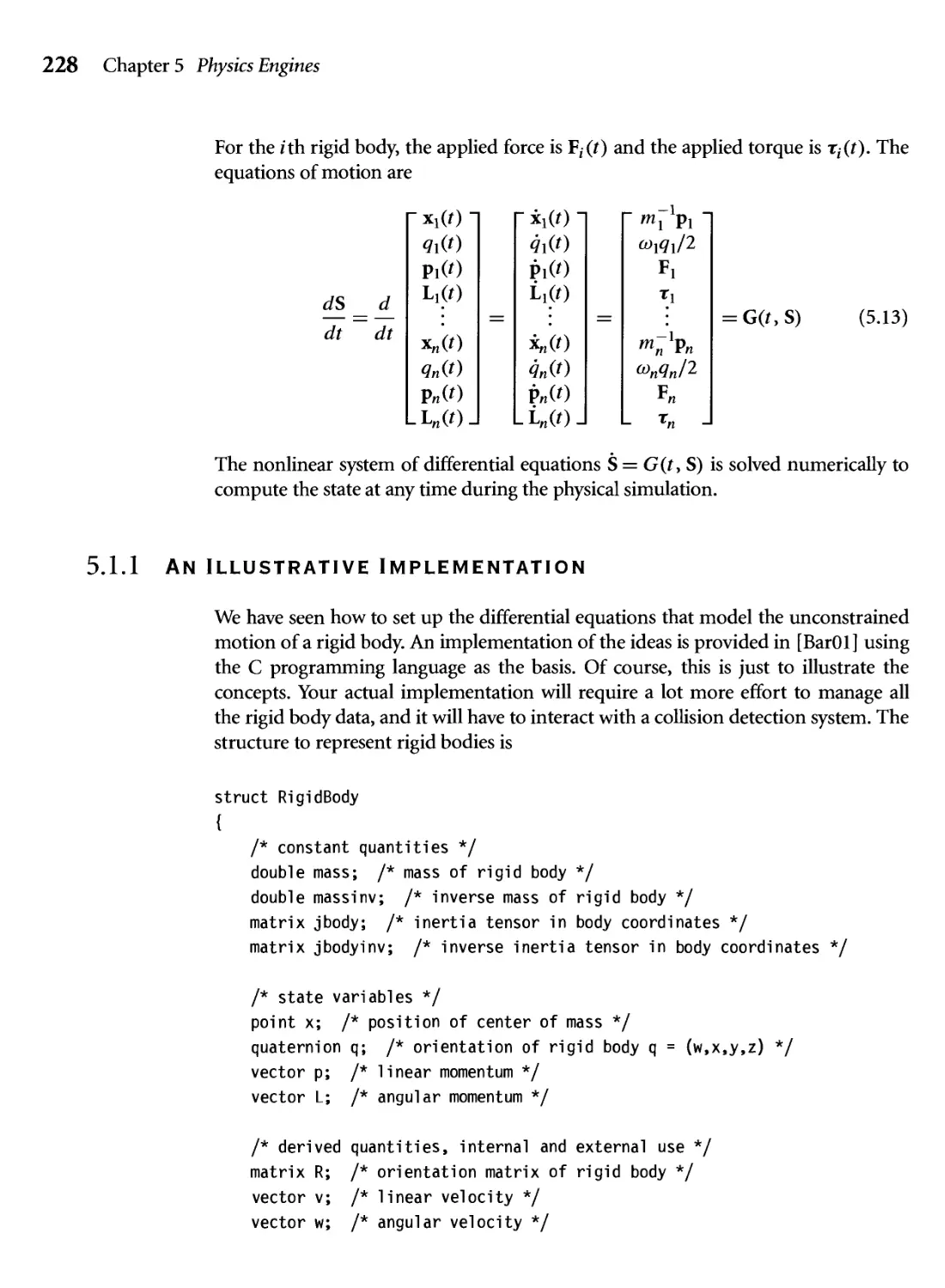
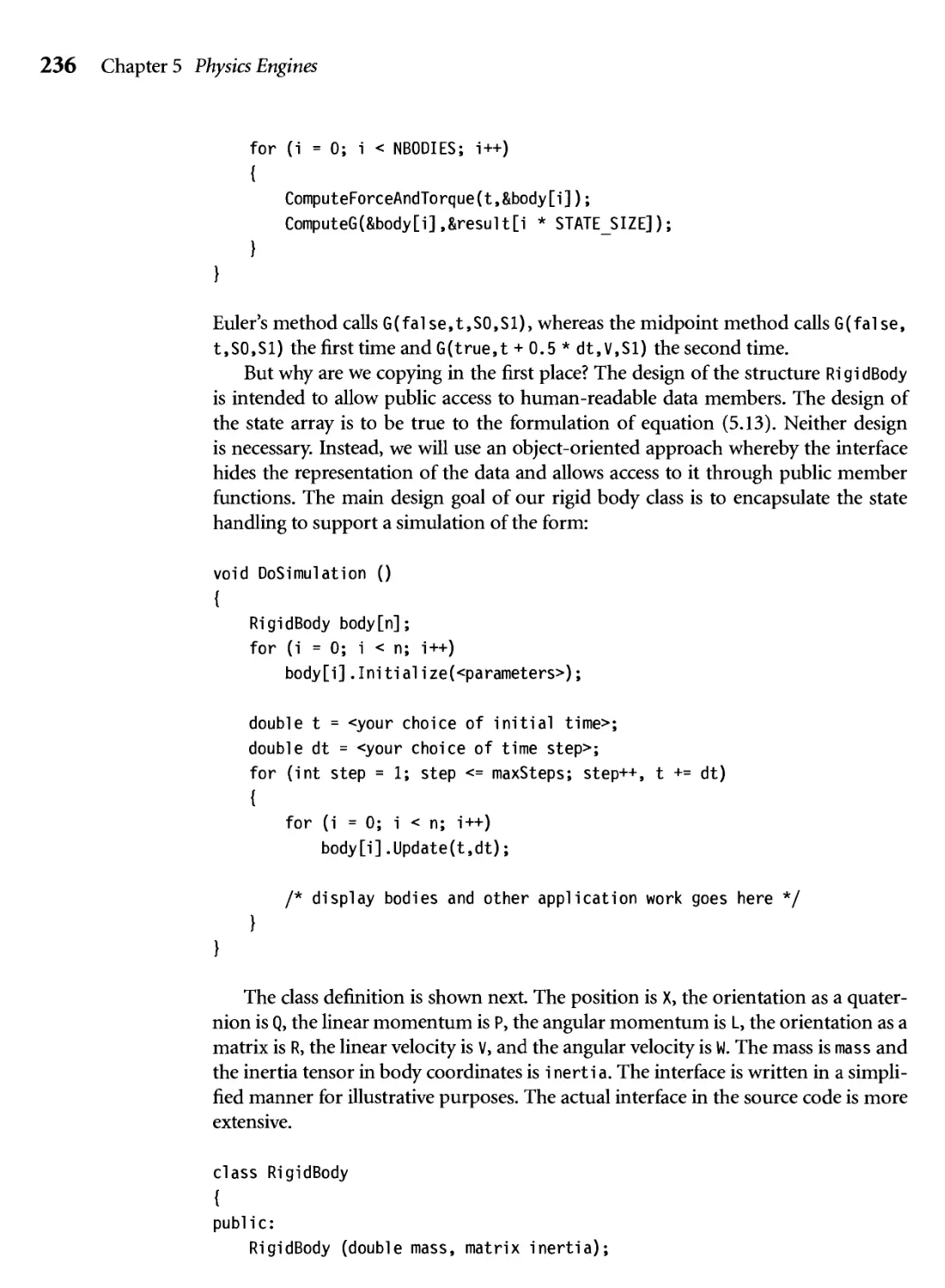
Implementing physical simulations for real-time games is a complex task that requires a solid
understanding of a wide range of concepts from the fields of mathematics and physics. Previously,
the relevant information could only be gleaned through obscure research papers. Thanks to Game
Physics, all this information is now available in a single, easily accessible volume. Dave has yet
again produced a must-have book for game technology programmers everywhere.
—Christer Ericson
Technology Lead
Sony Computer Entertainment
Game Physics is a comprehensive reference of physical simulation techniques relevant to games
and also contains a clear presentation of the mathematical background concepts fundamental to
most types of game programming. I wish I had this book years ago.
—Naty Hoffman
Senior Software Engineer
Naughty Dog, Inc.
Eppur si muove . . . and yet it moves. From Galileo to game development, this book will surely
become a standard reference for modeling movement.
—Ian Ashdown
President
byHeart Consultants Limited
This is an excellent companion volume to Dave's earlier 3D Game Engine Design. It shares the
approach and strengths of his previous book. He doesn't try to pare down to the minimum necessary
information that would allow you to build something with no more than basic functionality.
Instead, he gives you all you need to begin working on a professional-caliber system. He puts the
concepts firmly in context with current, ongoing research, so you have plenty of guidance on where
to go if you are inclined to add even more features on your own.
This is not a cookbook—it's a concise presentation of all the basic concepts needed to understand
and use physics in a modern game engine. It gives you a firm foundation you can use either to
build a complete engine of your own or to understand what's going on inside the new powerful
middleware physics engines available today.
This book, especially when coupled with Dave's 3D Game Engine Design, provides the most
complete resource of the mathematics relevant to modern 3D games that I can imagine. Along with
clear descriptions of the mathematics and algorithms needed to create a powerful physics engine
are sections covering pretty much all of the math you will encounter anywhere in the game—
quaternions, linear algebra, and calculus.
—Peter Lipson
Senior Programmer
Toys For Bob
This comprehensive introduction to the field of game physics will be invaluable to anyone interested
in the increasingly more important aspect of video game production, namely, striving to achieve
realism. Drawing from areas such as robotics, dynamic simulation, mathematical modeling, and
control theory, this book succeeds in presenting the material in a concise and cohesive way. As a
matter of fact, it can be recommended not only to video game professionals but also to students
and practitioners of the above-mentioned disciplines.
—Pal-Kristian Engstad
Senior Software Engineer
Naughty Dog, Inc.

The Morgan Kaufmann Series in Interactive 3D Technology
Series Editor: David H. Eberly, Magic Software, Inc.
The game industry is a powerful and driving force in the evolution of computer tech-
technology. As the capabilities of personal computers, peripheral hardware, and game
consoles have grown, so has the demand for quality information about the algo-
algorithms, tools, and descriptions needed to take advantage of this new technology. We
plan to satisfy this demand and establish a new level of professional reference for the
game developer with the Morgan Kaufmann Series in Interactive 3D Technology. Books
in the series are written for developers by leading industry professionals and academic
researchers and cover the state of the art in real-time 3D. The series emphasizes prac-
practical, working solutions and solid software-engineering principles. The goal is for the
developer to be able to implement real systems from the fundamental ideas, whether
it be for games or for other applications.
Game Physics
David H. Eberly
Collision Detection in Interactive 3D Environments
Gino van den Bergen
3D Game Engine Design: A Practical Approach to Real-Time Computer Graphics
David H. Eberly
Forthcoming
Essential Mathematics for Games and Interactive Applications: A Programmers Guide
Jim Van Verth and Lars Bishop
Physically-Based Rendering
Matt Pharr and Greg Humphreys
Real-Time Collision Detection
Christer Ericson

Game Physics
David H. Eberly
Magic Software, Inc.
with a contribution by
KEN SHOEMAKE
Otter Enterprises
ELSEVIER
AMSTERDAM • BOSTON • HEIDELBERG • LONDON
NEW YORK • OXFORD • PARIS • SAN DIEGO
SAN FRANCISCO • SINGAPORE • SYDNEY • TOKYO
MORGAN KAUFMANN IS AN IMPRINT OF ELSEVIER
MORGAN KAUFMANN PUBLISHERS

Publishing Director Diane D. Cerra
Senior Editor Tim Cox
Publishing Services Manager Simon Crump
Production Editor Sarah Manchester
Project Management Elisabeth Beller
Editorial Coordinator Rick Camp
Cover Design Chen Design Associates, San Francisco
Cover Image Chen Design Associates, San Francisco
Text Design Rebecca Evans
Composition Windfall Software, using ZzTeX
Technical Illustration Dartmouth Publishing
Copyeditor Yonie Overton
Proofreader Jennifer McClain
Indexer Steve Rath
Interior Printer The Maple-Vail Book Manufacturing Group
Cover Printer Phoenix Color Corporation
Morgan Kaufmann Publishers is an imprint of Elsevier.
500 Sansome Street, Suite 400, San Francisco, CA 94111
This book is printed on acid-free paper.
© 2004 by Elsevier, Inc. All rights reserved.
Designations used by companies to distinguish their products are often claimed as
trademarks or registered trademarks. In all instances in which Morgan Kaufmann
Publishers is aware of a claim, the product names appear in initial capital or all
capital letters. Readers, however, should contact the appropriate companies for more
complete information regarding trademarks and registration.
No part of this publication maybe reproduced, stored in a retrieval system, or trans-
transmitted in any form or by any means—electronic, mechanical, photocopying, scan-
scanning, or otherwise—without the prior written permission of the publisher.
Permissions may be sought directly from Elsevier's Science & Technology Rights
Department in Oxford, UK: phone: (+44) 1865 843830, fax: (+44) 1865 853333,
e-mail: permissions@elsevier.com.uk. You may also complete your request on-line via
the Elsevier homepage (http://elsevier.com) by selecting "Customer Support" and
then "Obtaining Permissions."
Library of Congress Control Number: 2003023187
ISBN: 1-55860-740-4
For information on all Morgan Kaufmann publications,
visit our website at www.mkp.com.
Printed in the United States of America
07 06 05 04 03 5 4 3 2 1

Trademarks
The following trademarks, mentioned in this book and the accompanying CD-ROM,
are the property of the following organizations:
■ DirectX, Direct3D, Visual C++, DOS, and Windows are trademarks of Microsoft
Corporation.
■ OpenGL is a trademark of Silicon Graphics, Inc.
■ Radeon is a trademark of ATI Technologies, Inc.
■ GeForce and the Cg Language are trademarks of nVIDIA Corporation.
■ Netlmmerse and R-Plus are trademarks of Numerical Design, Ltd.
■ MathEngine is a trademark of Criterion Studios.
■ The Havok physics engine is a trademark of Havok.com.
■ Softimage is a trademark of Avid Technology, Inc.
■ Falling Bodies is a trademark of Animats.
■ The Vortex physics engine is a trademark of CMLabs Simulations, Inc.
■ Prince of Persia 3D is a trademark of Broderbund Software, Inc.
■ XS-G and Canyon Runner are trademarks of Greystone Technology.
■ Mathematica is a trademark of Wolfram Research, Inc.
■ Turbo Pascal is a trademark of Borland Software Corporation.
■ The 8086 and Pentium are trademarks of Intel Corporation.
■ Macintosh is a trademark of Apple Corporation.
■ Gigi and VAX are trademarks of Digital Equipment Corporation.
■ MASPAR is a trademark of MasPar Computer Corporation.

Contents
Chapter
Chapter
Trademarks
Figures
Tables
Preface
About the CD-ROM
INTRODUCTION
1.1 a brief history of the world
1.2 a summary of the topics
1.3 Examples and Exercises
Basic Concepts from Physics
2.1 Rigid body Classification
2.2 Rigid body Kinematics
2.2.1 Single Particle
2.2.2 Particle Systems and Continuous Materials
2.3 Newton's Laws
2.4 Forces
2.4.1 Gravitational Forces
2.4.2 Spring Forces
2.4.3 Friction and Other Dissipative Forces
2.4.4
2.4.5
Torque
Equilibrium
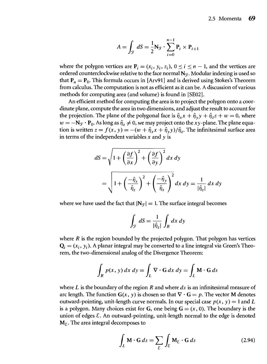
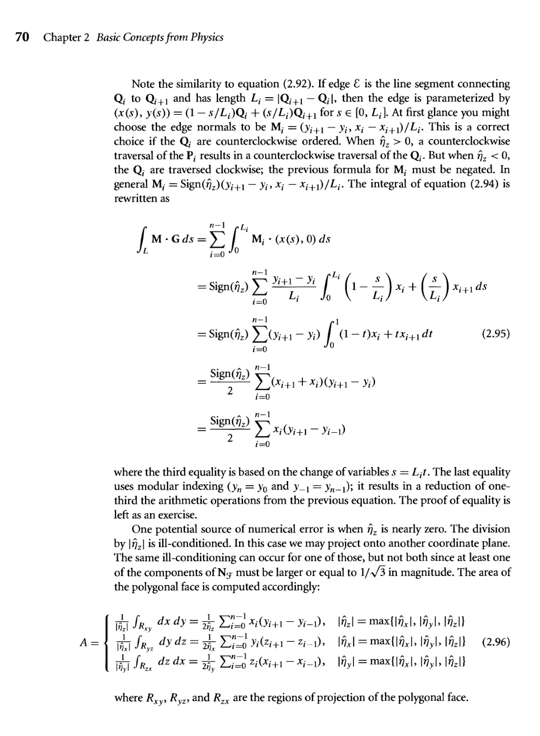
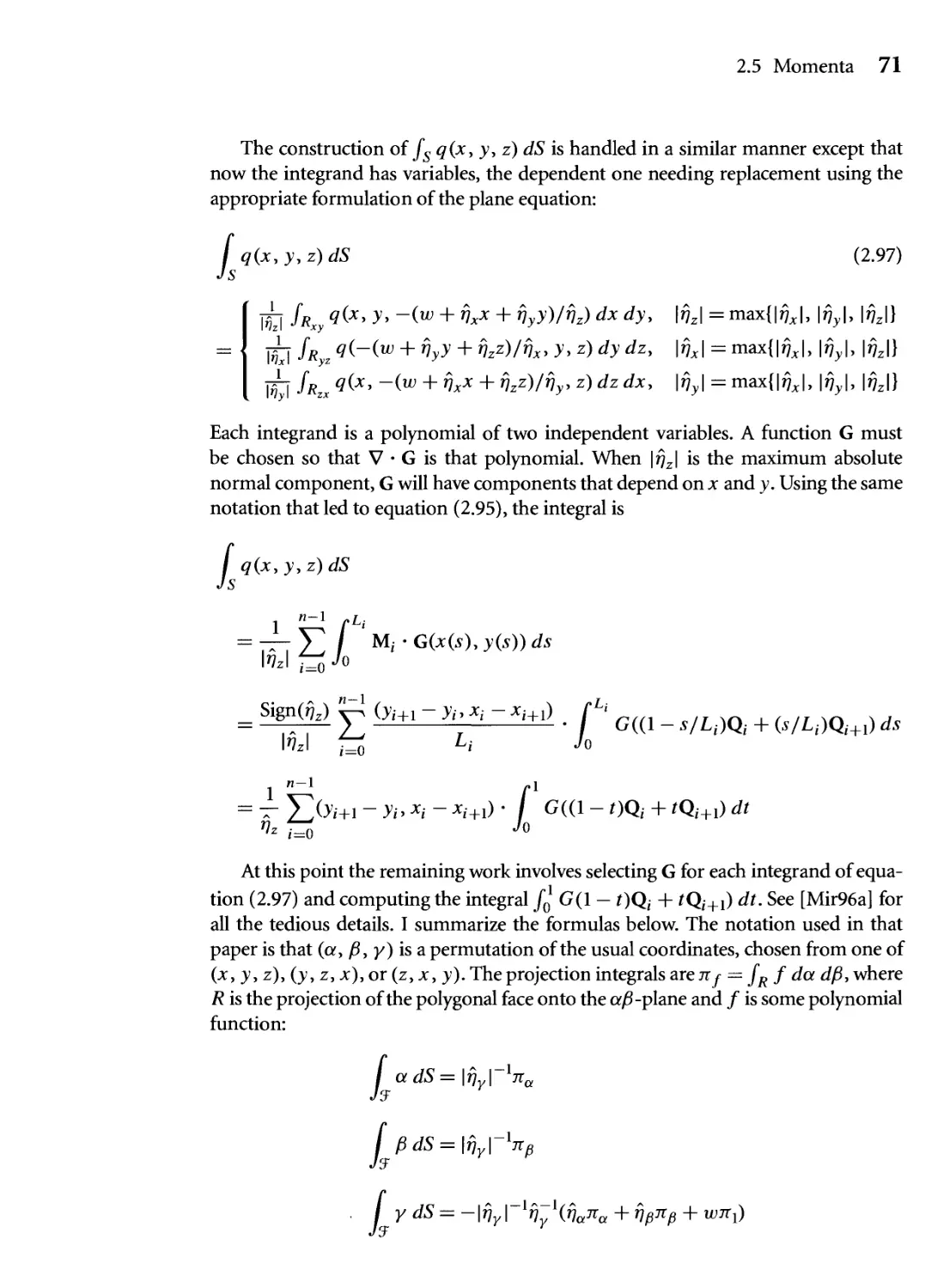
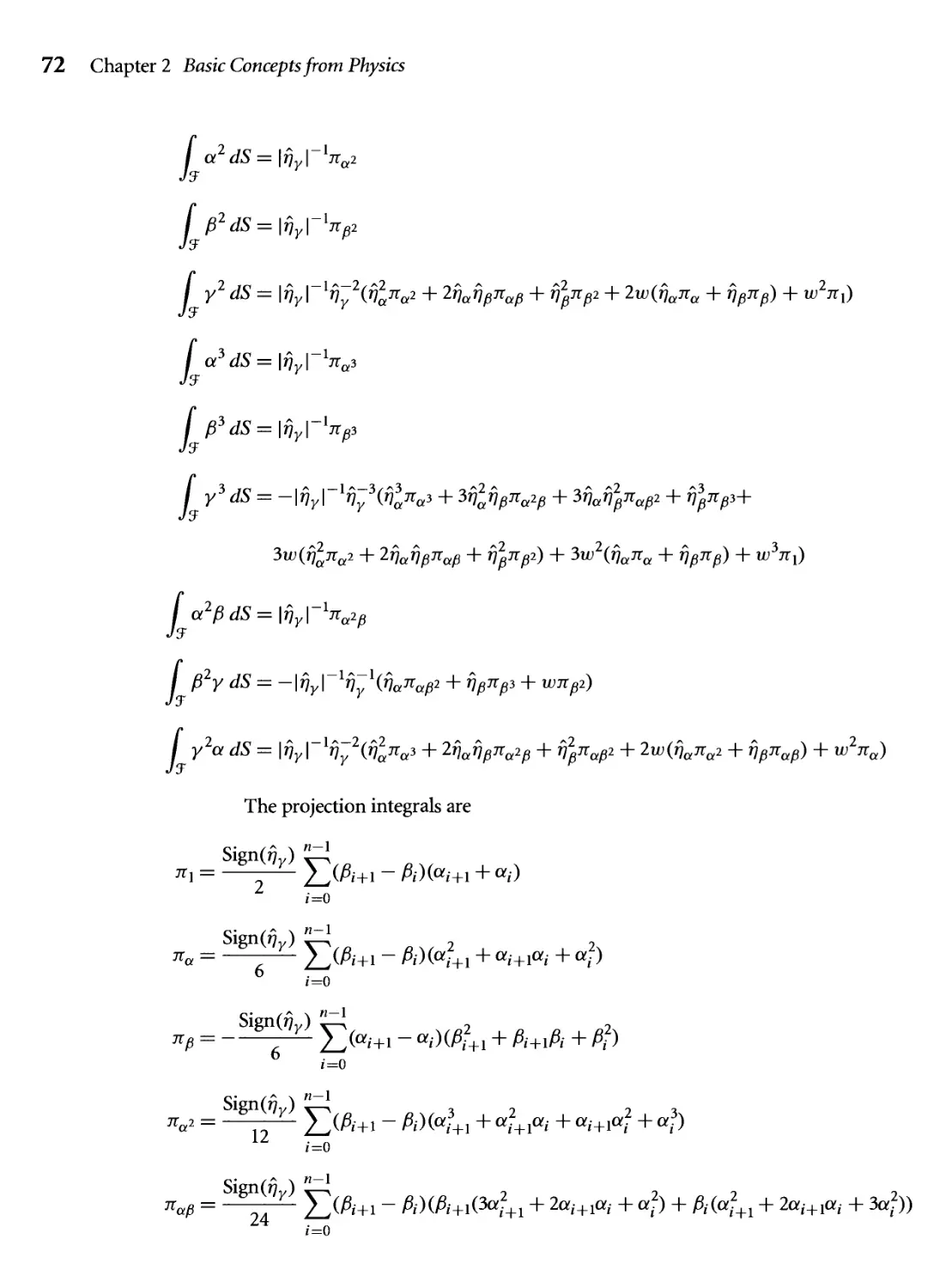
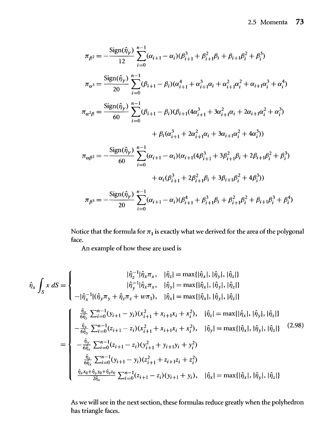
2.5 Momenta
2.5.1
2.5.2
2.5.3
2.5.4
Linear Momentum
Angular Momentum
Center of Mass
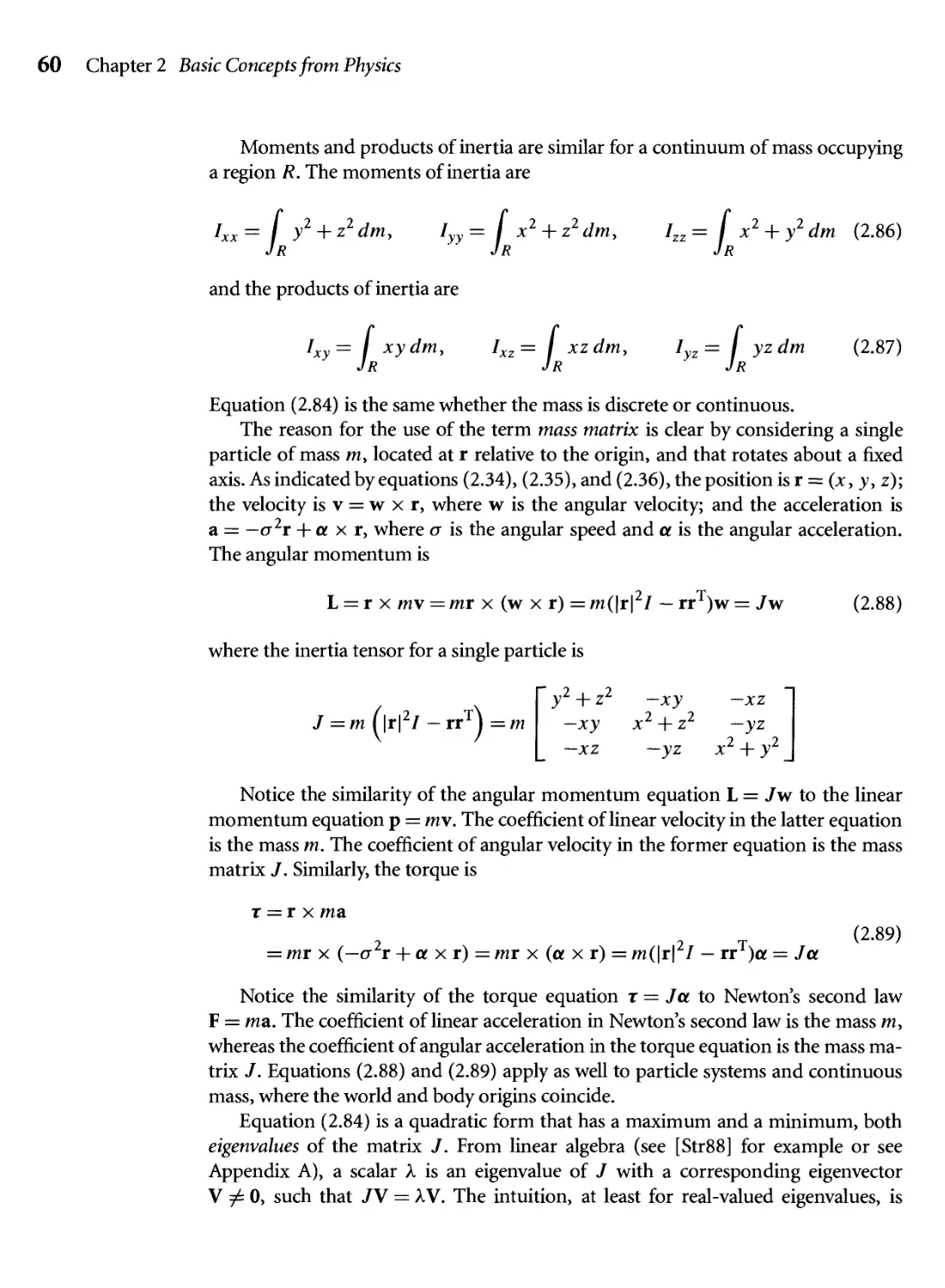
Moments and Products of Inertia
V
XV
xxvii
xxix
xxxiii
1
6
11
13
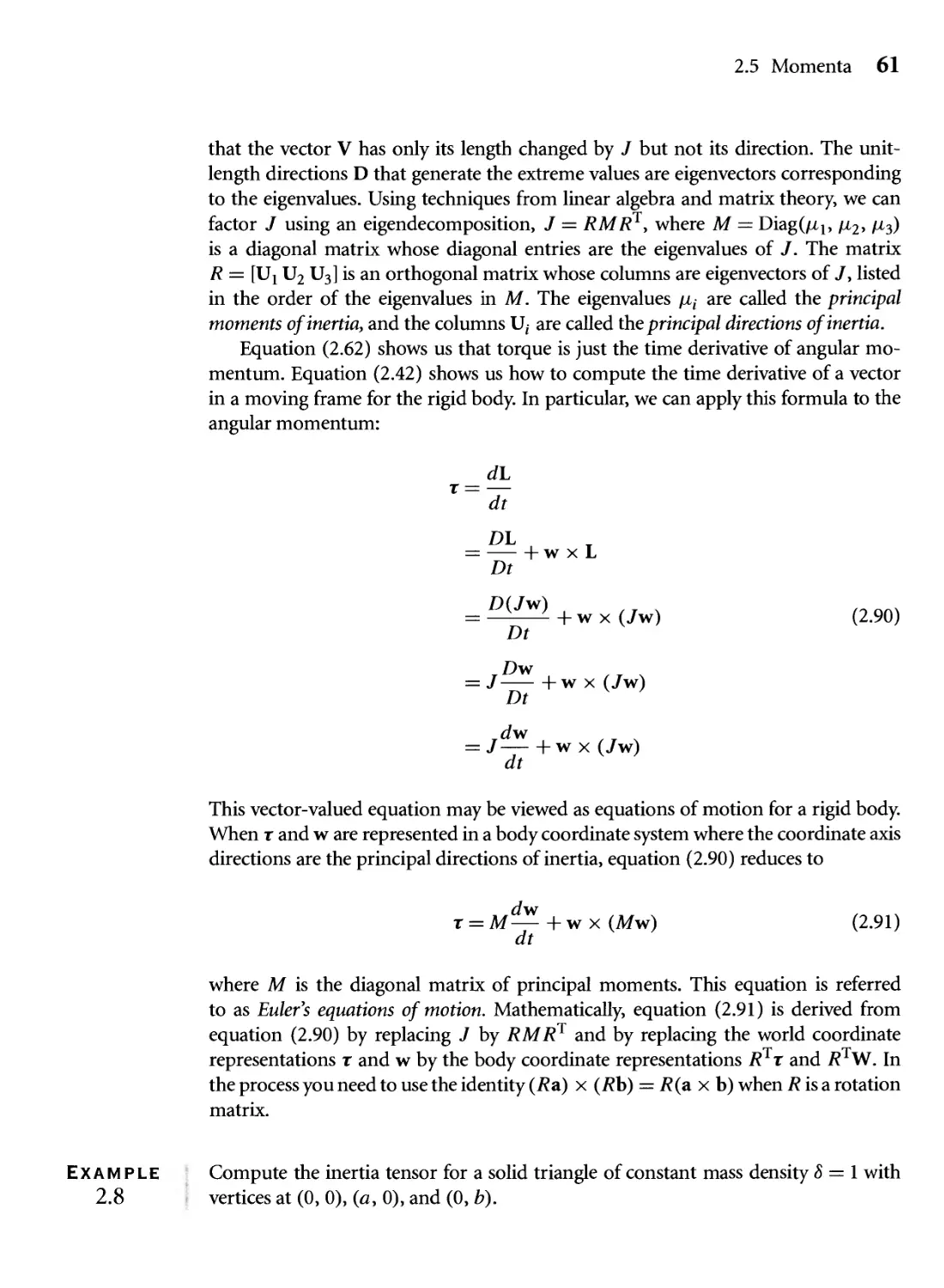
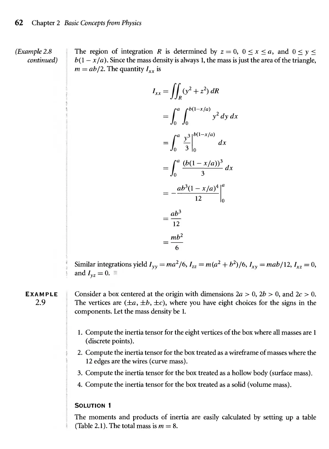
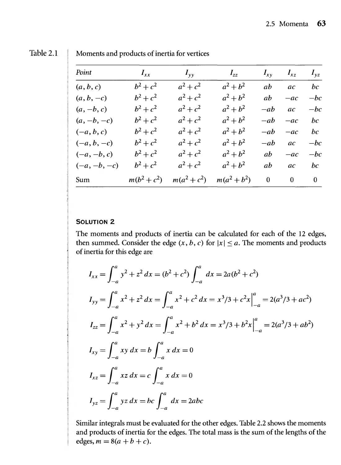
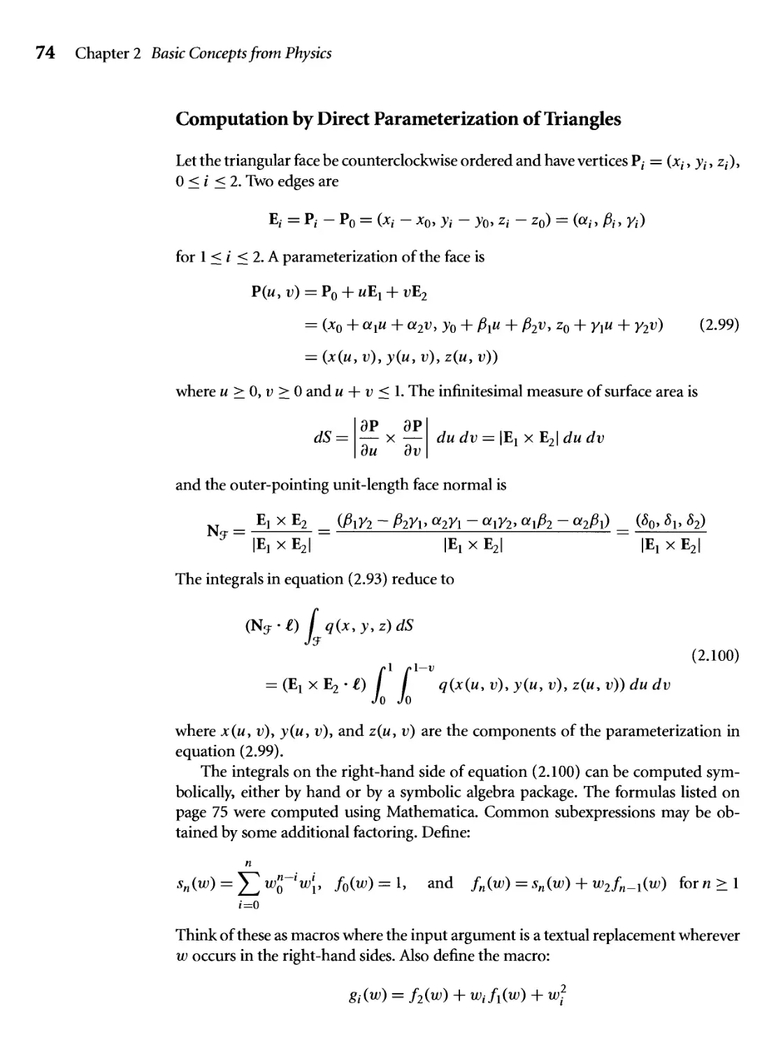
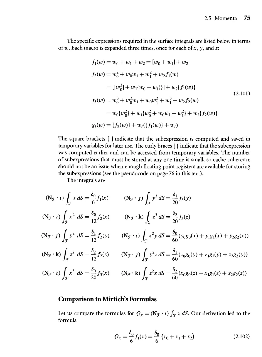
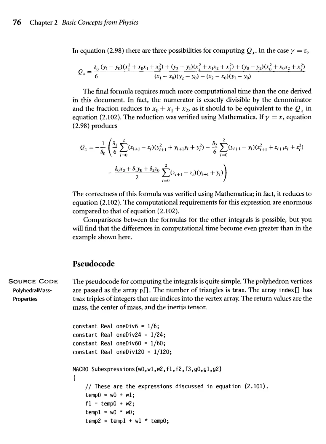
2.5.5 Mass and Inertia Tensor of a Solid Polyhedron
14
15
15
28
31
32
32
34
35
37
39
41
42
43
44
57
66
Vll

viii Contents
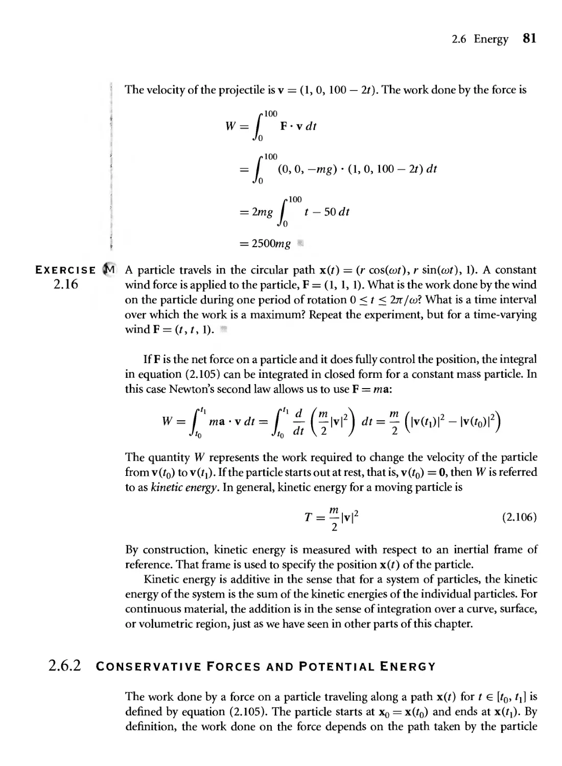
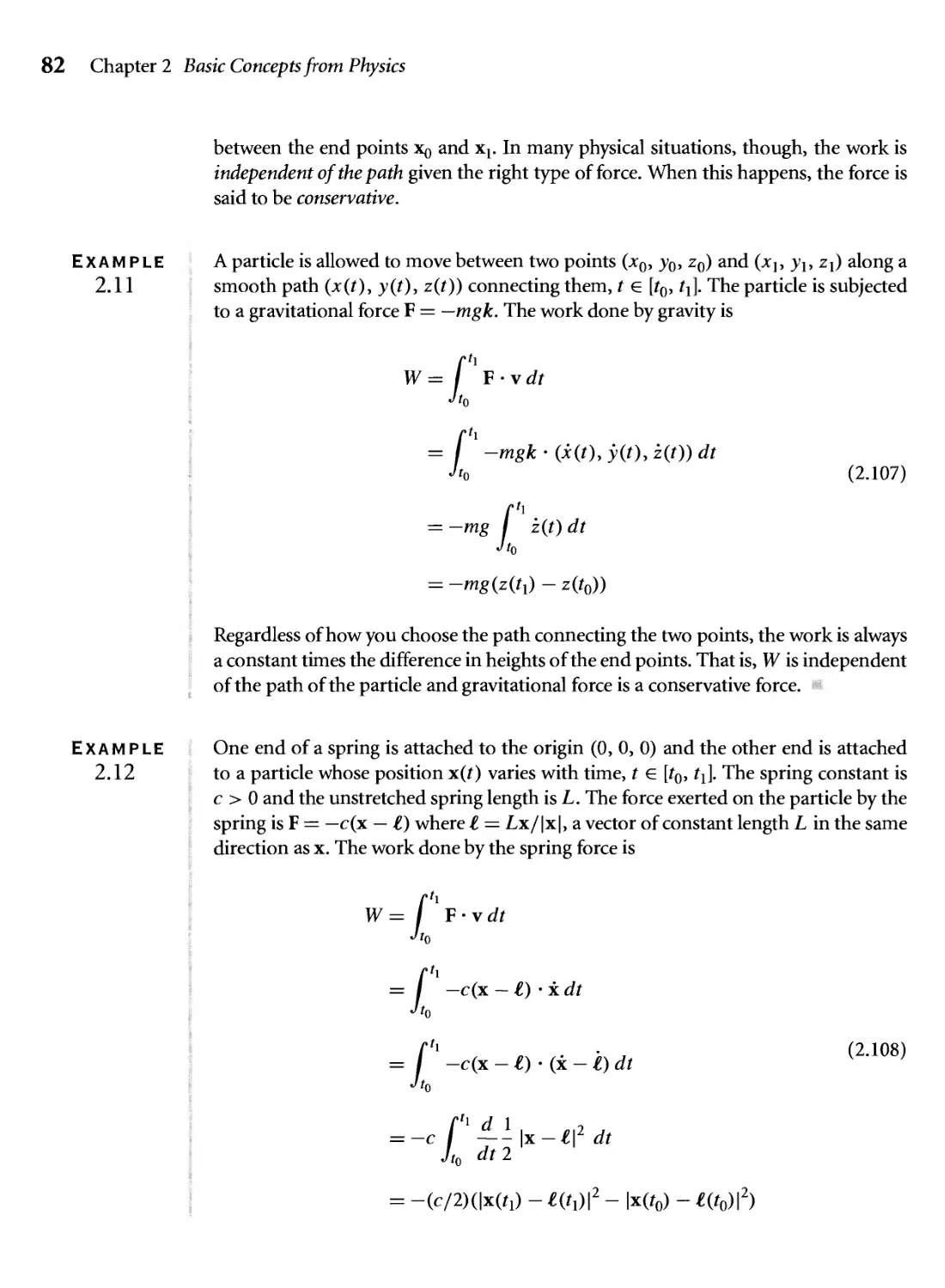
2.6 Energy 79
2.6.1 Work and Kinetic Energy 79
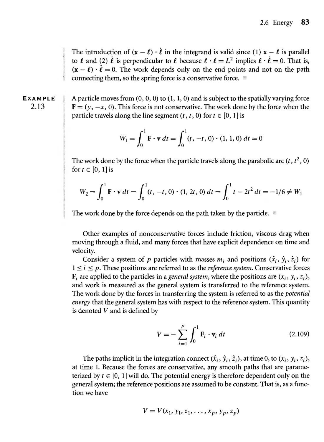
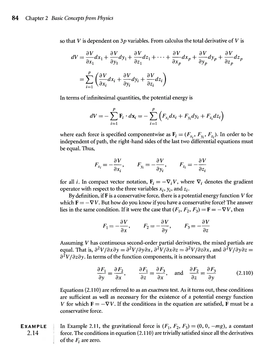
2.6.2 Conservative Forces and Potential Energy 81
Chapter
Rigid Body motion 87
3.1 Newtonian dynamics 88
3.2 Lagrangian dynamics 100
3.2.1 Equations of Motion for a Particle 102
3.2.2 Time-Varying Frames or Constraints 114
3.2.3 Interpretation of the Equations of Motion 117
3.2.4 Equations of Motion for a System of Particles 118
3.2.5 Equations of Motion for a Continuum of Mass 121
3.2.6 Examples with Conservative Forces 133
3.2.7 Examples with Dissipative Forces 139
3.3 Euler's Equations of motion 152
Chapter
*T DEFORMABLE BODIES 161
4.1 Elasticity, stress, and strain 161
4.2 Mass-Spring Systems 164
4.2.1 One-Dimensional Array of Masses 164
4.2.2 Two-Dimensional Array of Masses 166
4.2.3 Three-Dimensional Array of Masses 170
4.2.4 Arbitrary Configurations 171
4.3 Control point deformation 173
4.3.1 B-Spline Curves 173
4.3.2 NURBS Curves 183
4.3.3 B-Spline Surfaces 187
4.3.4 NURBS Surfaces 188
4.3.5 Surfaces Built from Curves 190
4.4 Free-Form deformation 197
4.5 Implicit Surface deformation 203
4.5.1 Level Set Extraction 206
4.5.2 Isocurve Extraction in 2D Images 208
4.5.3 Isosurface Extraction in 3D Images 212

Contents IX
Chapter
Physics Engines
221
5.1 Unconstrained Motion 223
5.1.1 An Illustrative Implementation 228
5.1.2 A Practical Implementation 234
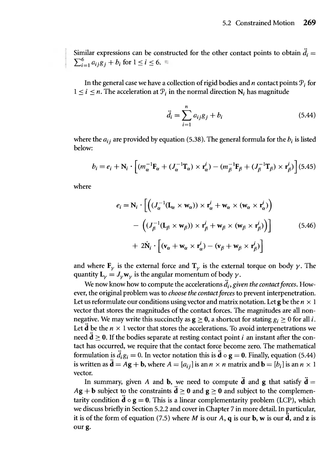
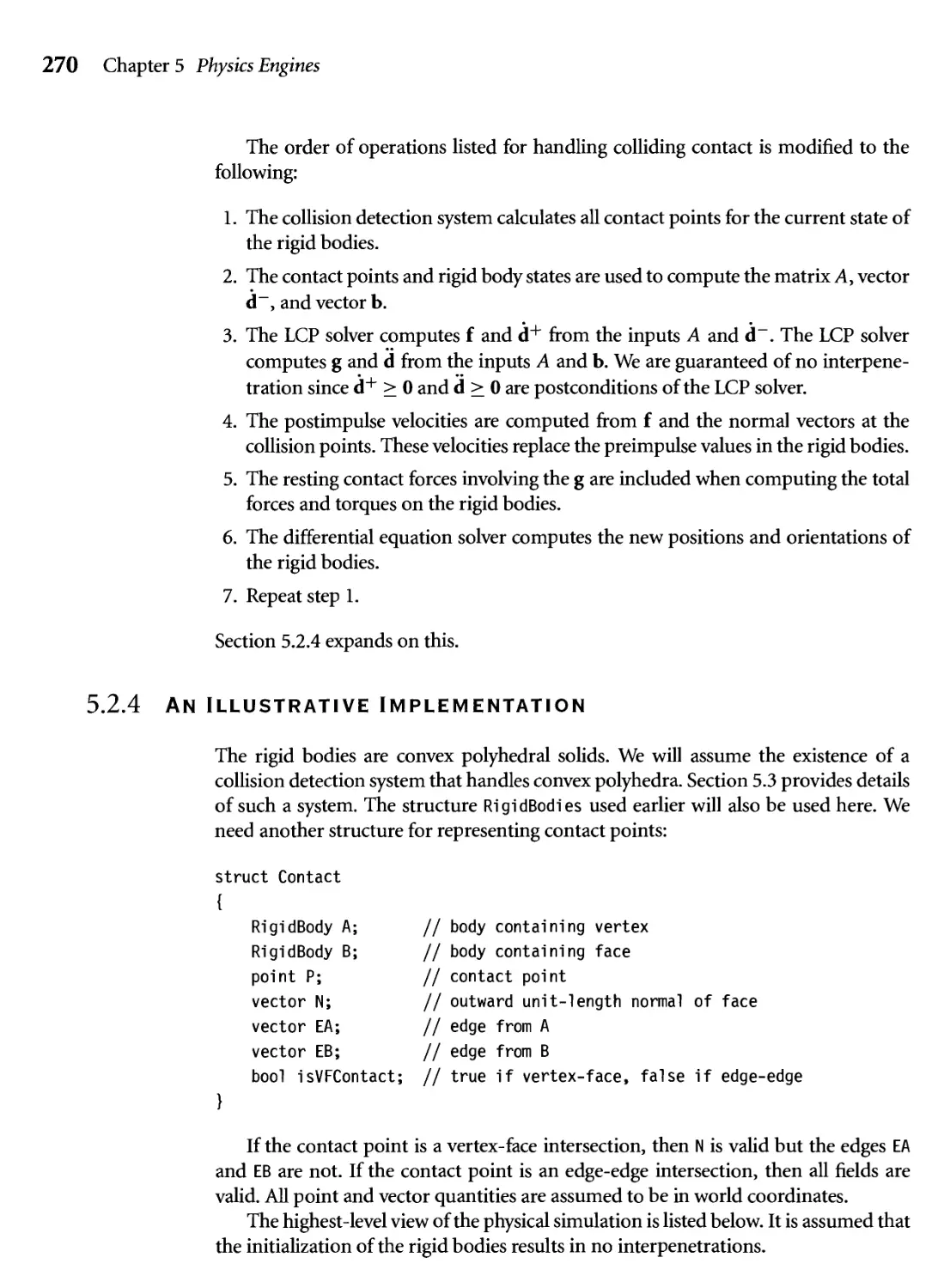
5.2 Constrained Motion 240
5.2.1 Collision Points 240
5.2.2 Collision Response for Colliding Contact 242
5.2.3 Collision Response for Resting Contact 265
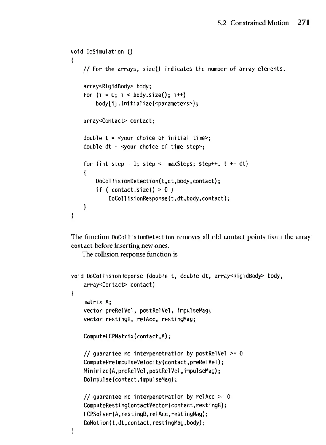
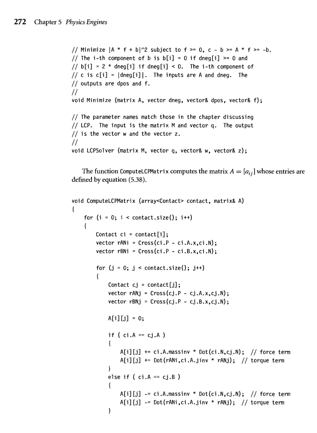
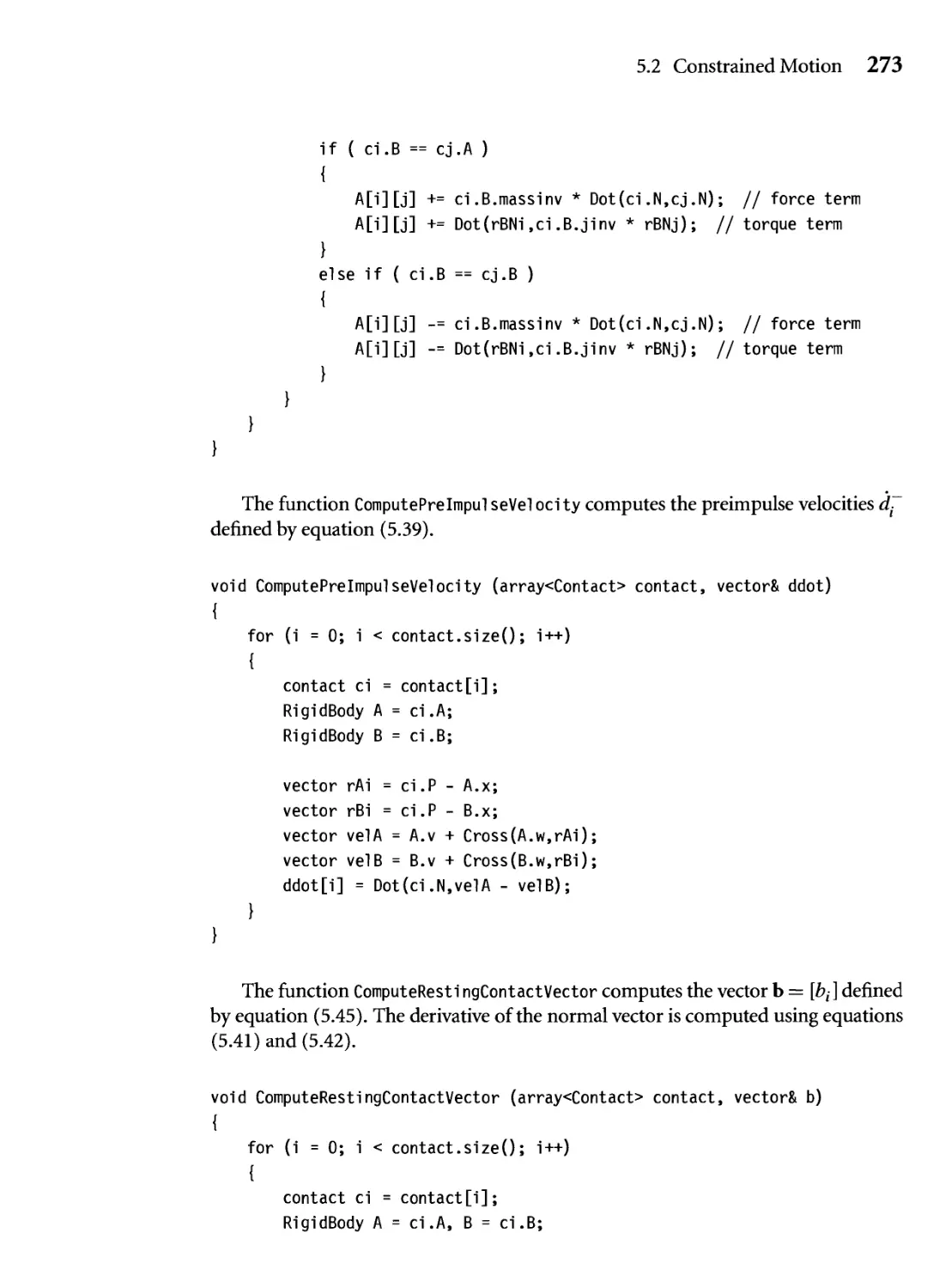
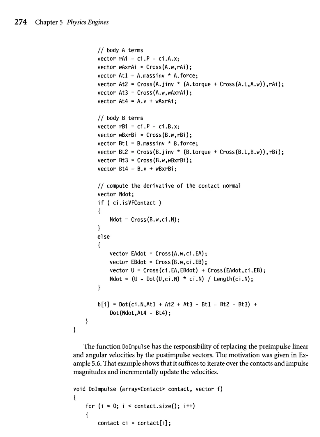
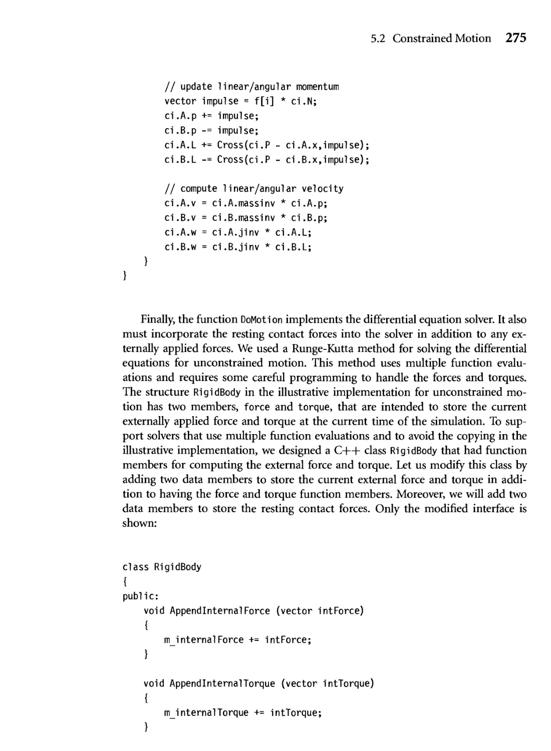
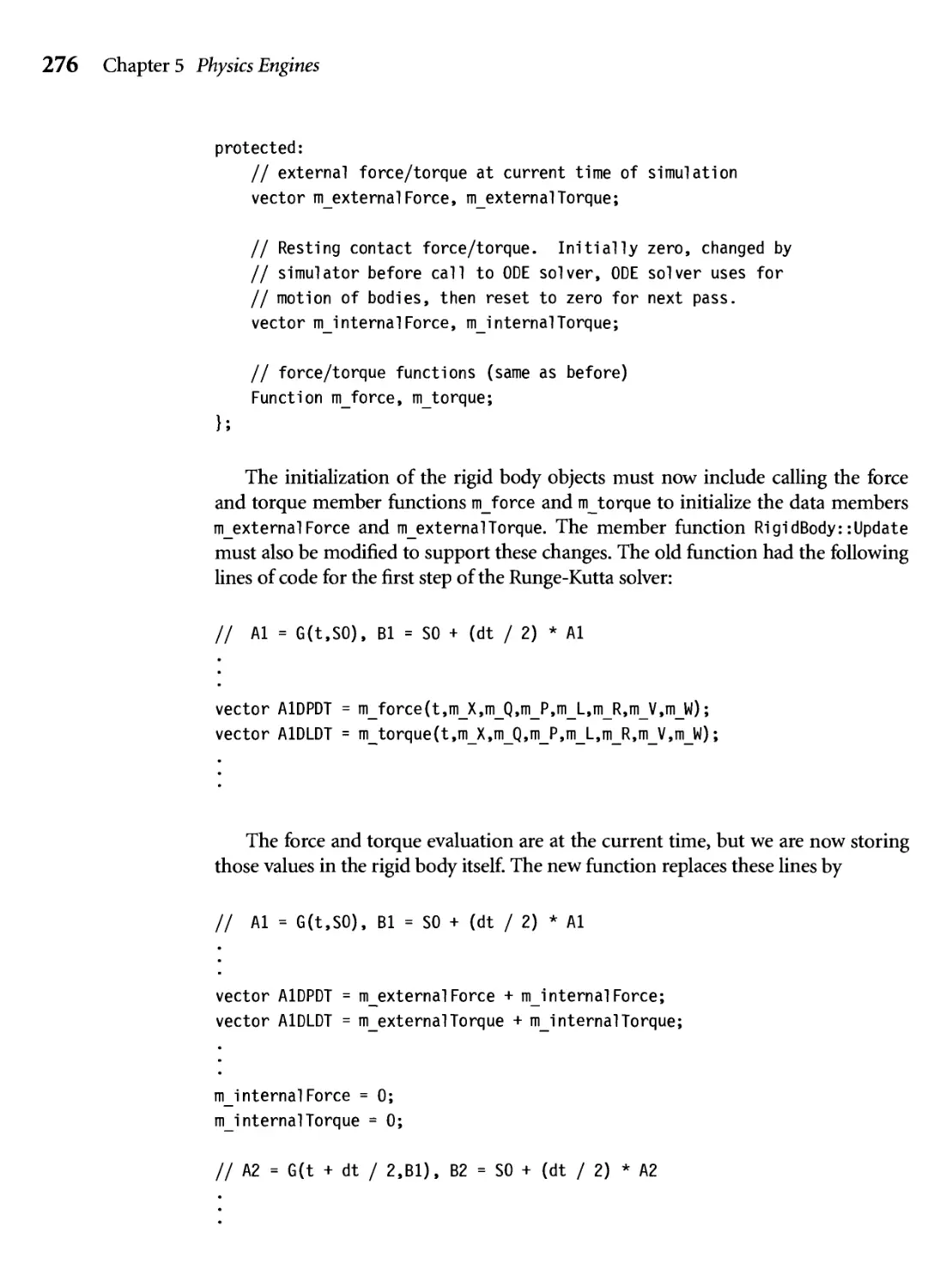
5.2.4 An Illustrative Implementation 270
5.2.5 Lagrangian Dynamics 278
5.3 Collision detection with Convex polyhedra 280
5.3.1 The Method of Separating Axes 284
5.3.2 Stationary Objects 286
5.3.3 Objects Moving with Constant Linear Velocity 311
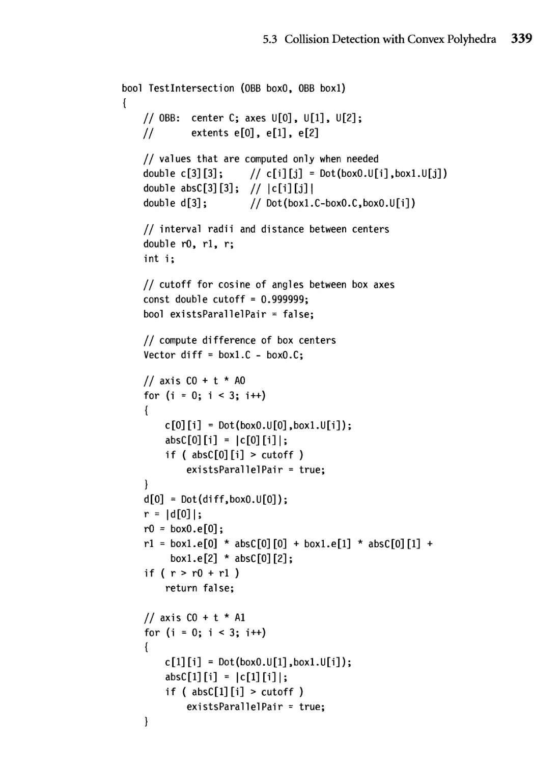
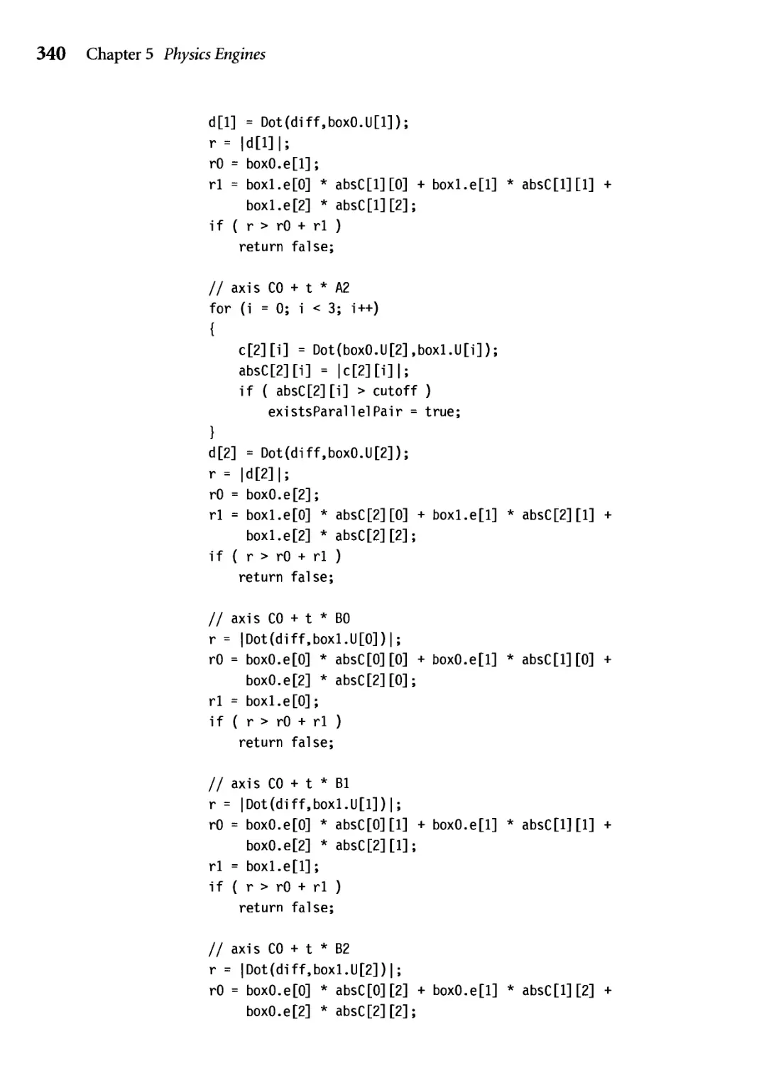
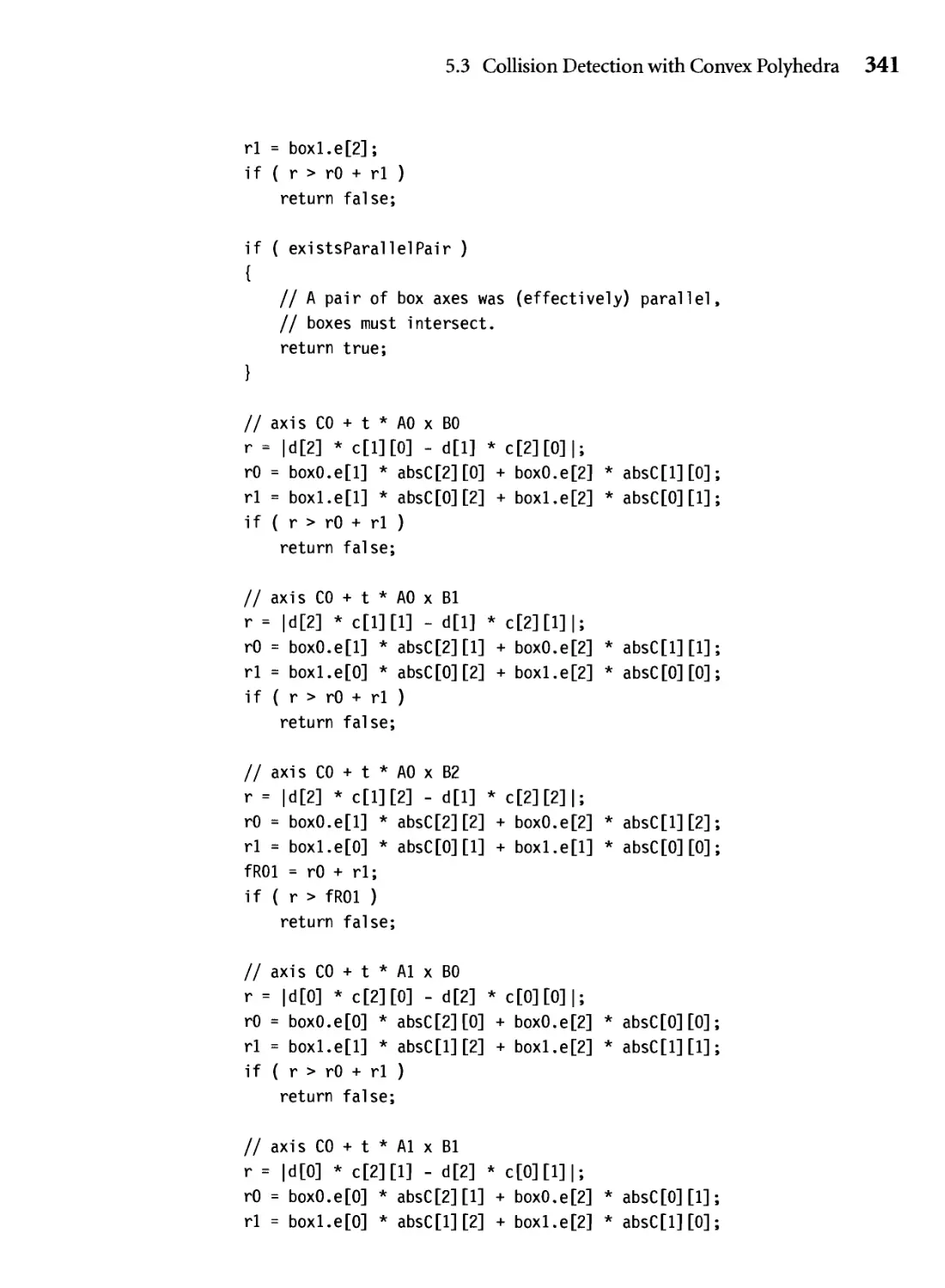
5.3.4 Oriented Bounding Boxes 334
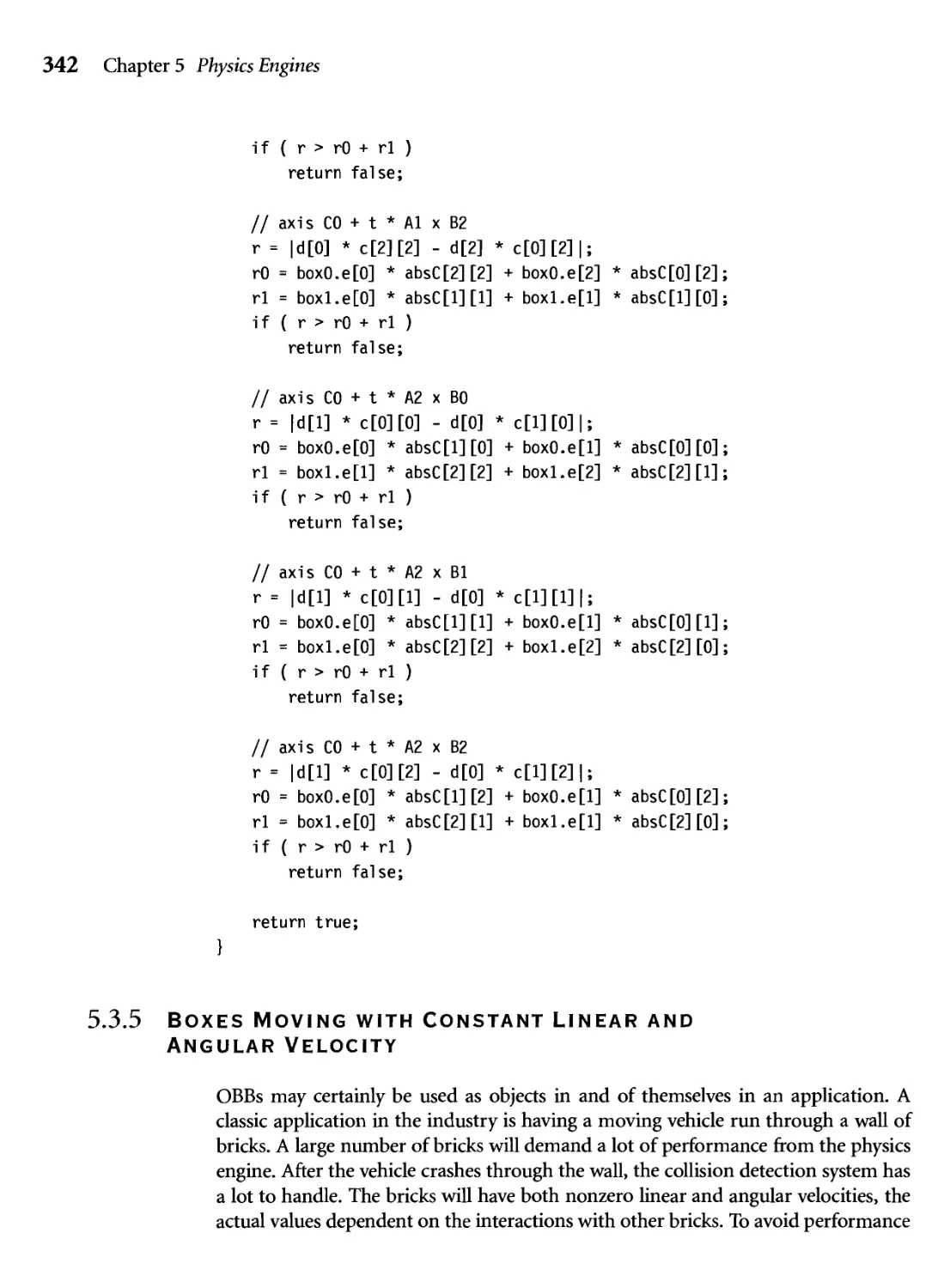
5.3.5 Boxes Moving with Constant Linear and Angular Velocity 342
5.4 Collision Culling: Spatial and Temporal Coherence 348
5.4.1 Culling with Bounding Spheres 349
5.4.2 Culling with Axis-Aligned Bounding Boxes 354
5.5 Variations 361
Chapter
Physics and Shader Programs
6.1 Introduction
6.2 vertex and pixel shaders
6.3 Deformation by vertex Displacement
6.4 Skin-and-Bones Animation
6.5 Rippling Ocean Waves
6.6 Refraction
6.7 Fresnel reflectance
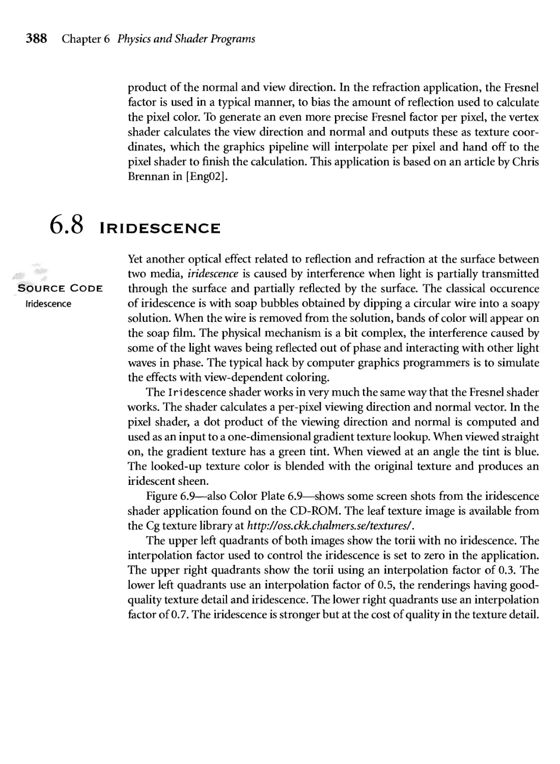
6.8 Iridescence
367
367
369
375
378
379
383
386
388

X Contents
Chapter
7
Chapter
Chapter
Linear Complementarity and Mathematical
Programming
7.1 Linear programming
7.1.1 A Two-Dimensional Example
7.1.2 Solution by Pairwise Intersections
7.1.3 Statement of the General Problem
7.1.4 The Dual Problem
7.2 The Linear Complementarity problem
7.2.1 The Lemke-Howson Algorithm
7.2.2 Zero Constant Terms
7.2.3 The Complementary Variable Cannot Leave the Dictionary
7.3 Mathematical Programming
7.3.1 Karush-Kuhn-Tucker Conditions
7.3.2 Convex Quadratic Programming
7.3.3 General Duality Theory
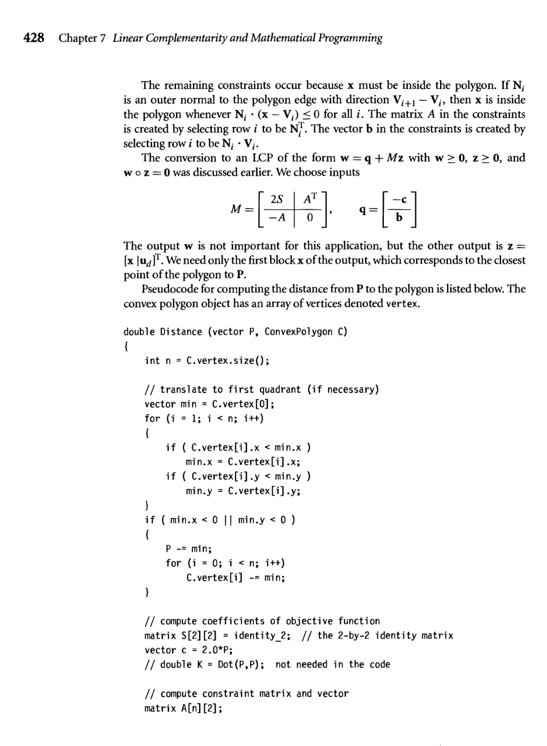
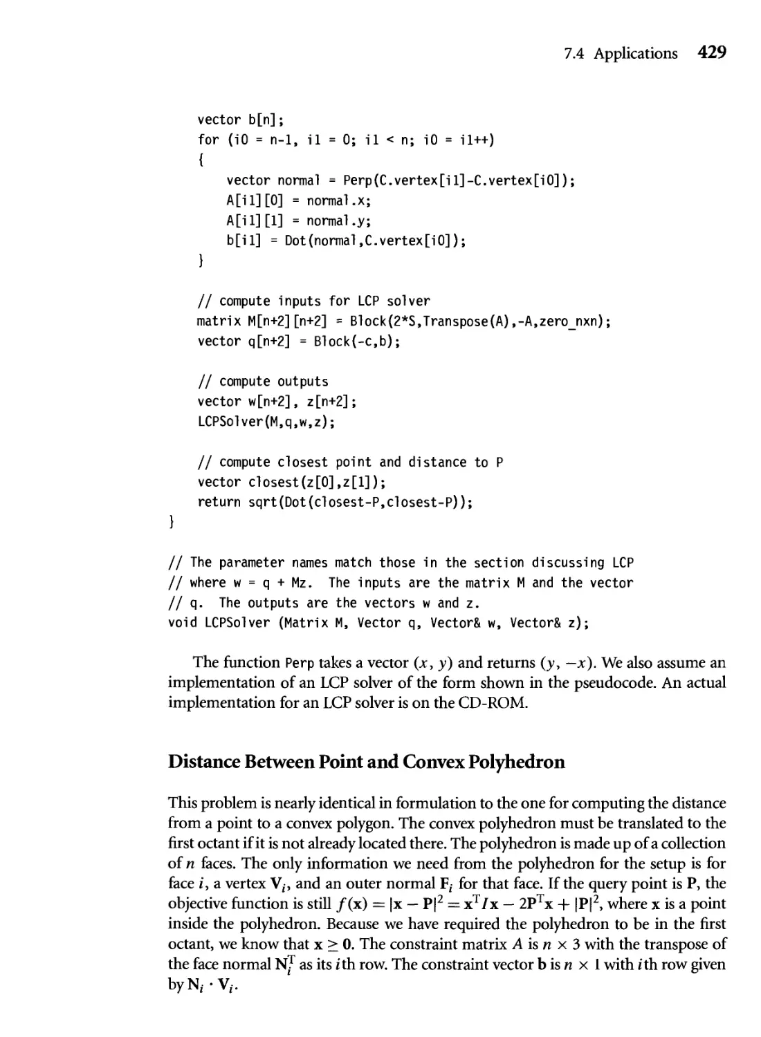
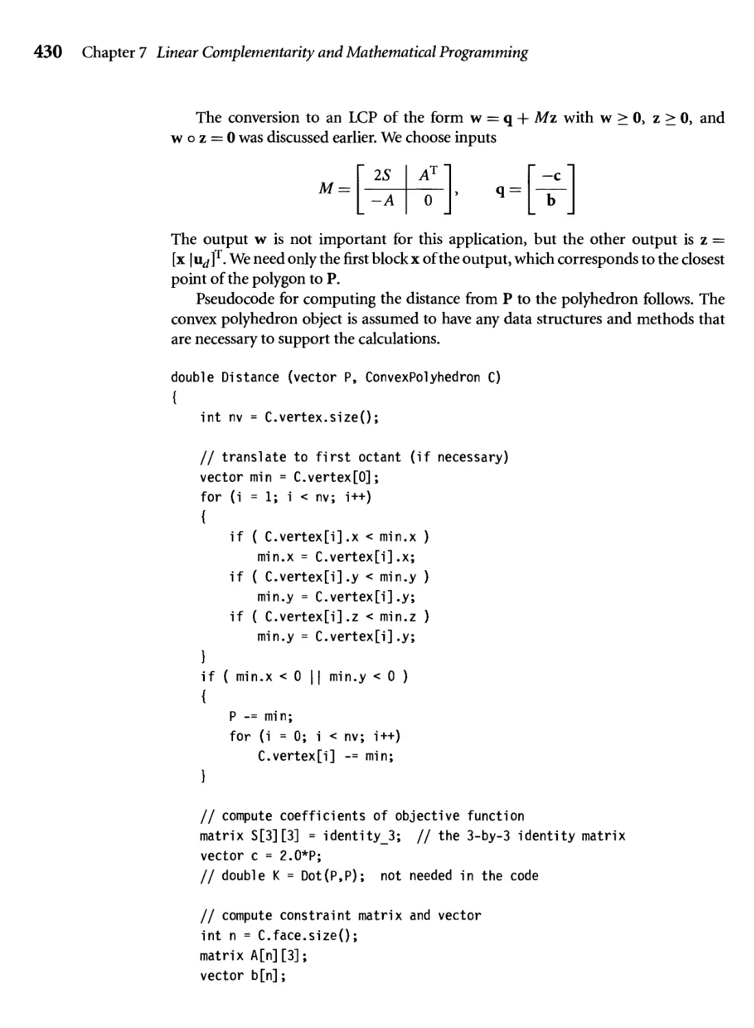
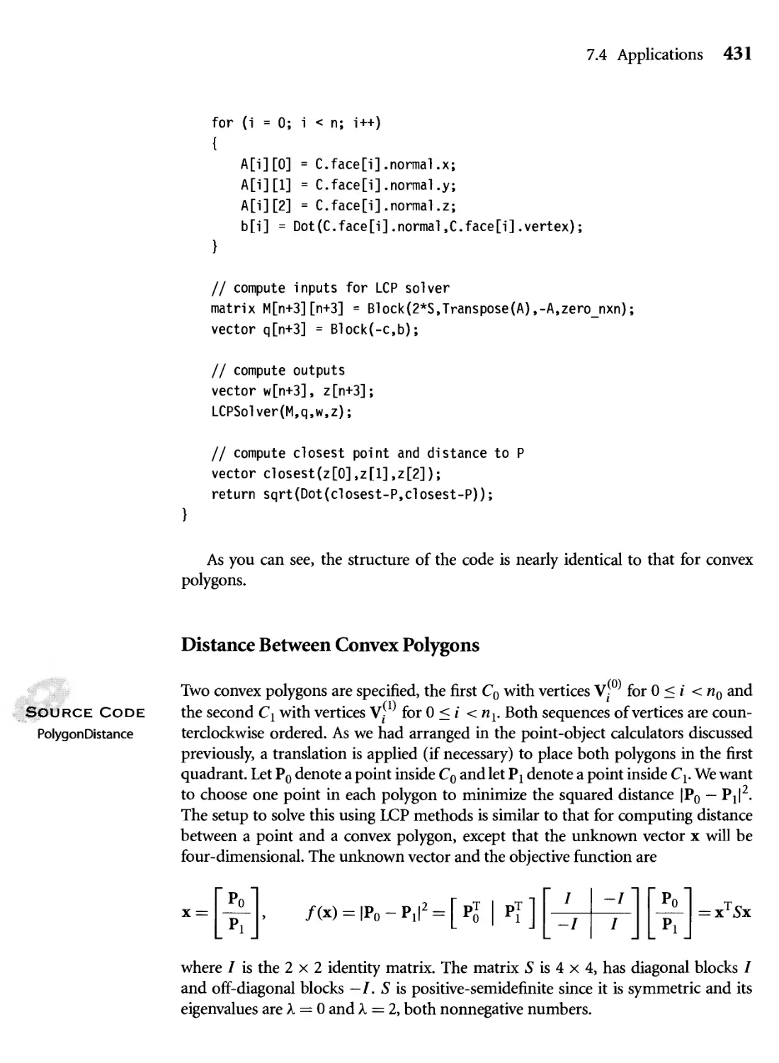
7.4 Applications
7.4.1 Distance Calculations
7.4.2 Contact Forces
Differential Equations
8.1 First-Order Equations
8.2 Existence, Uniqueness, and Continuous dependence
8.3 Second-order Equations
8.4 General-Order Differential Equations
8.5 Systems of Linear Differential Equations
8.6 Equilibria and Stability
8.6.1 Stability for Constant-Coefficient Linear Systems
8.6.2 Stability for General Autonomous Systems
Numerical methods
9.1 euler's method
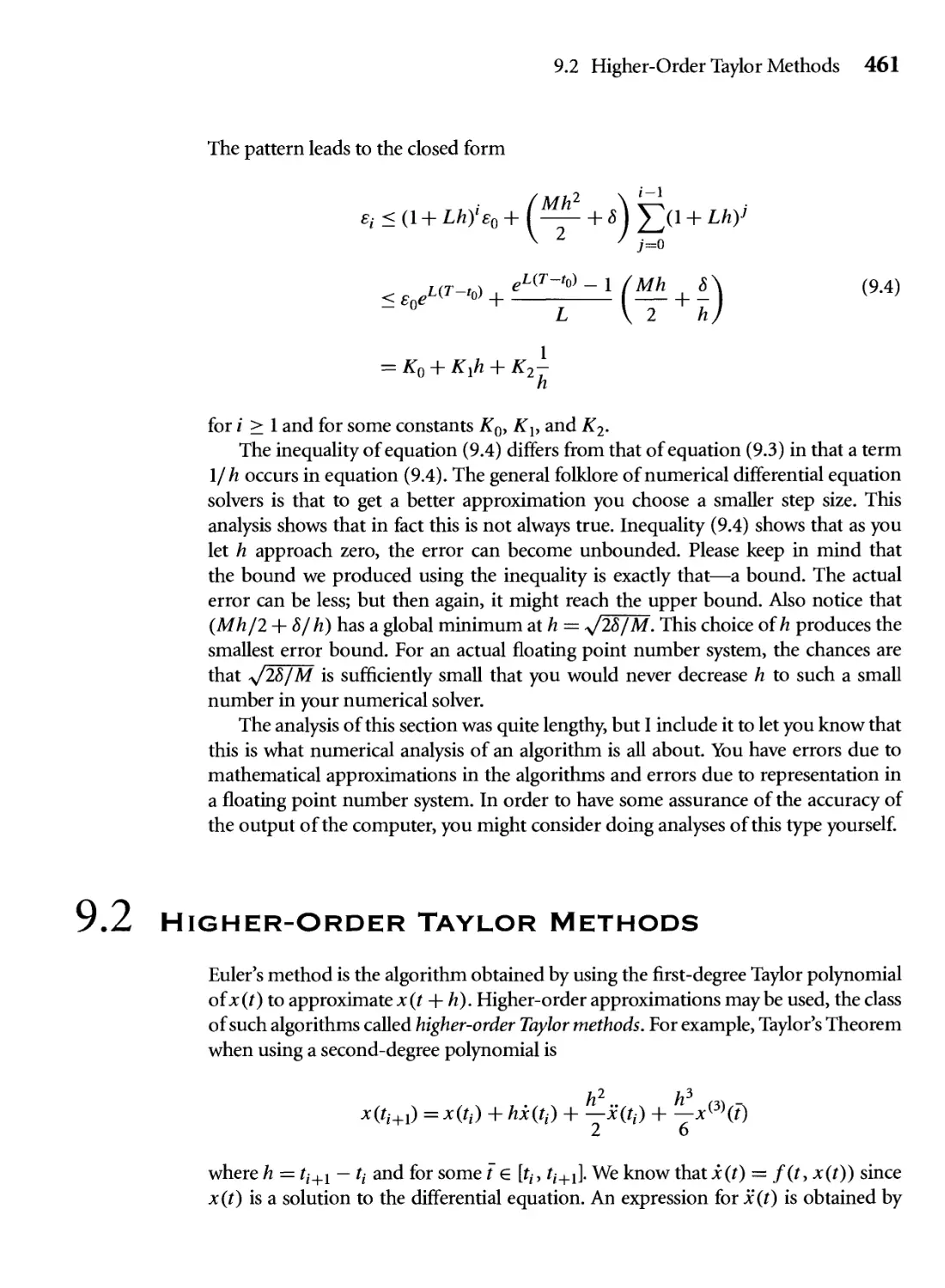
9.2 Higher-Order Taylor Methods
391
392
392
394
396
404
407
408
413
416
418
421
423
426
427
427
436
437
437
440
442
444
446
450
451
453
457
458
461

Contents XI
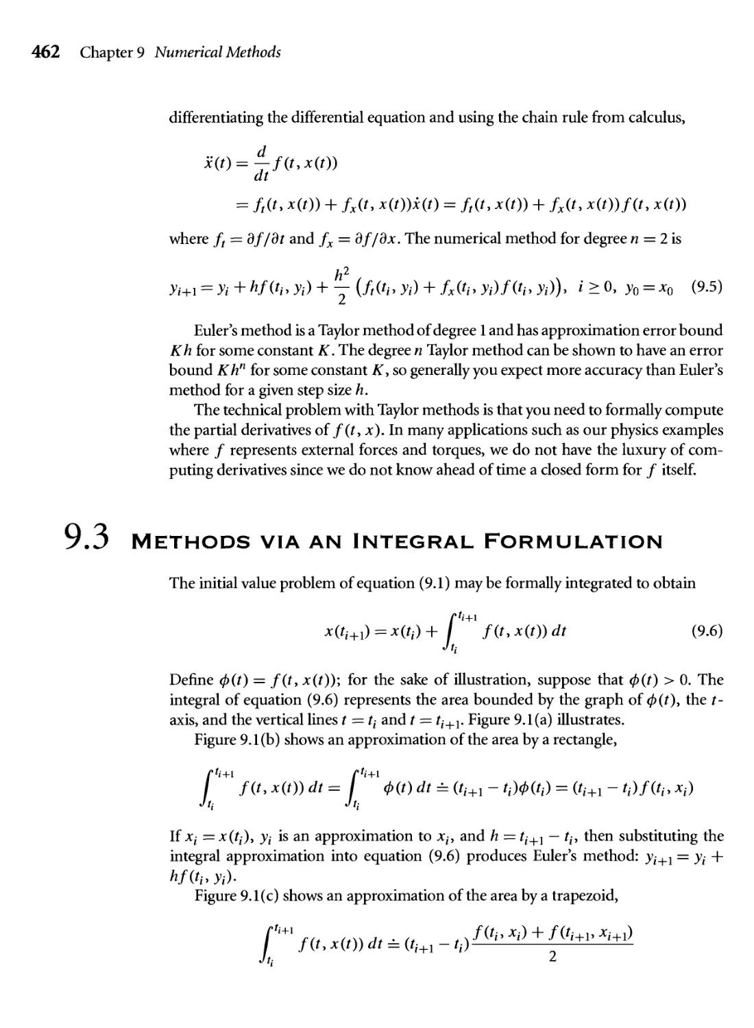
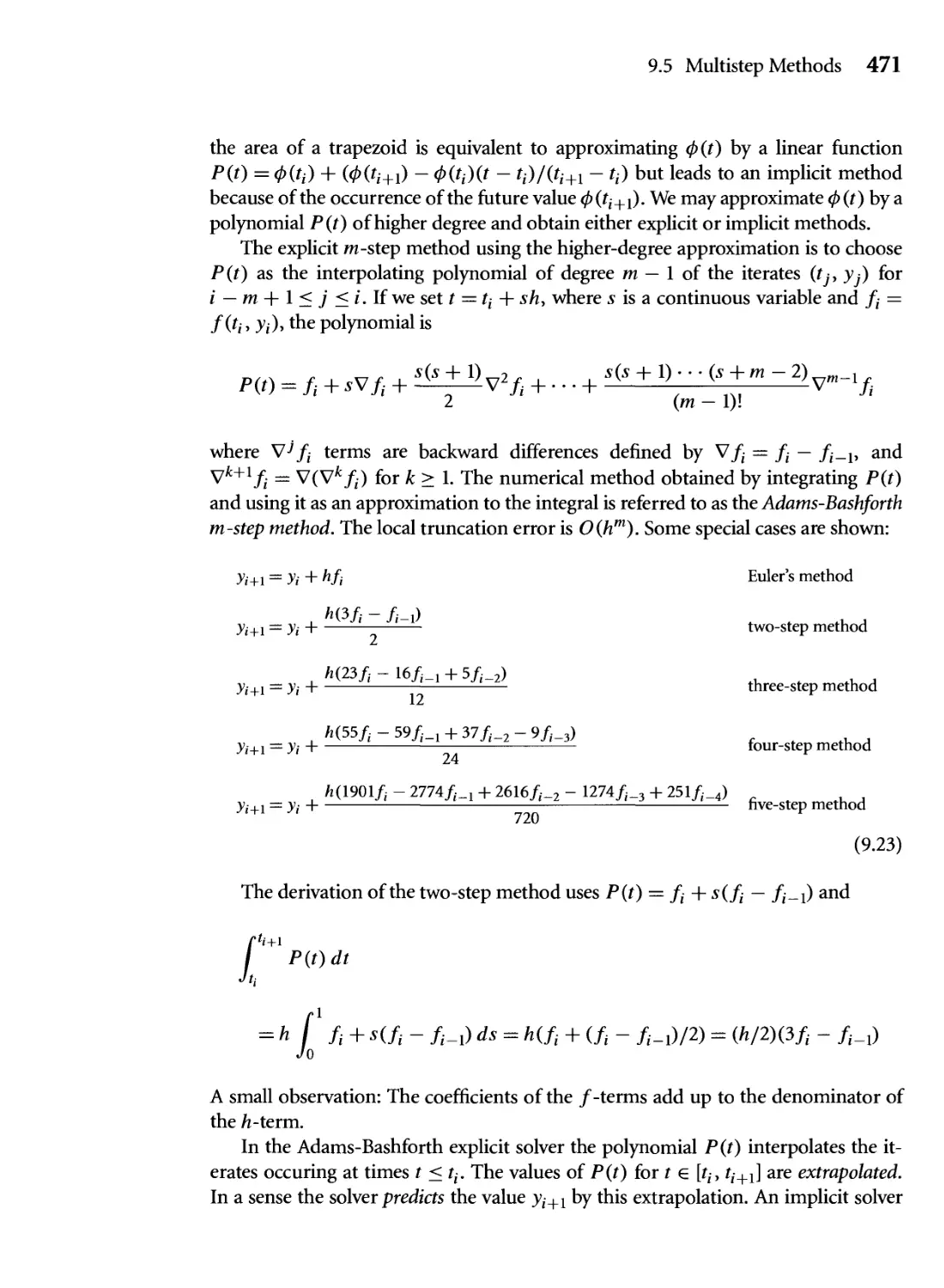
9.3 METHODS VIA AN INTEGRAL FORMULATION 462
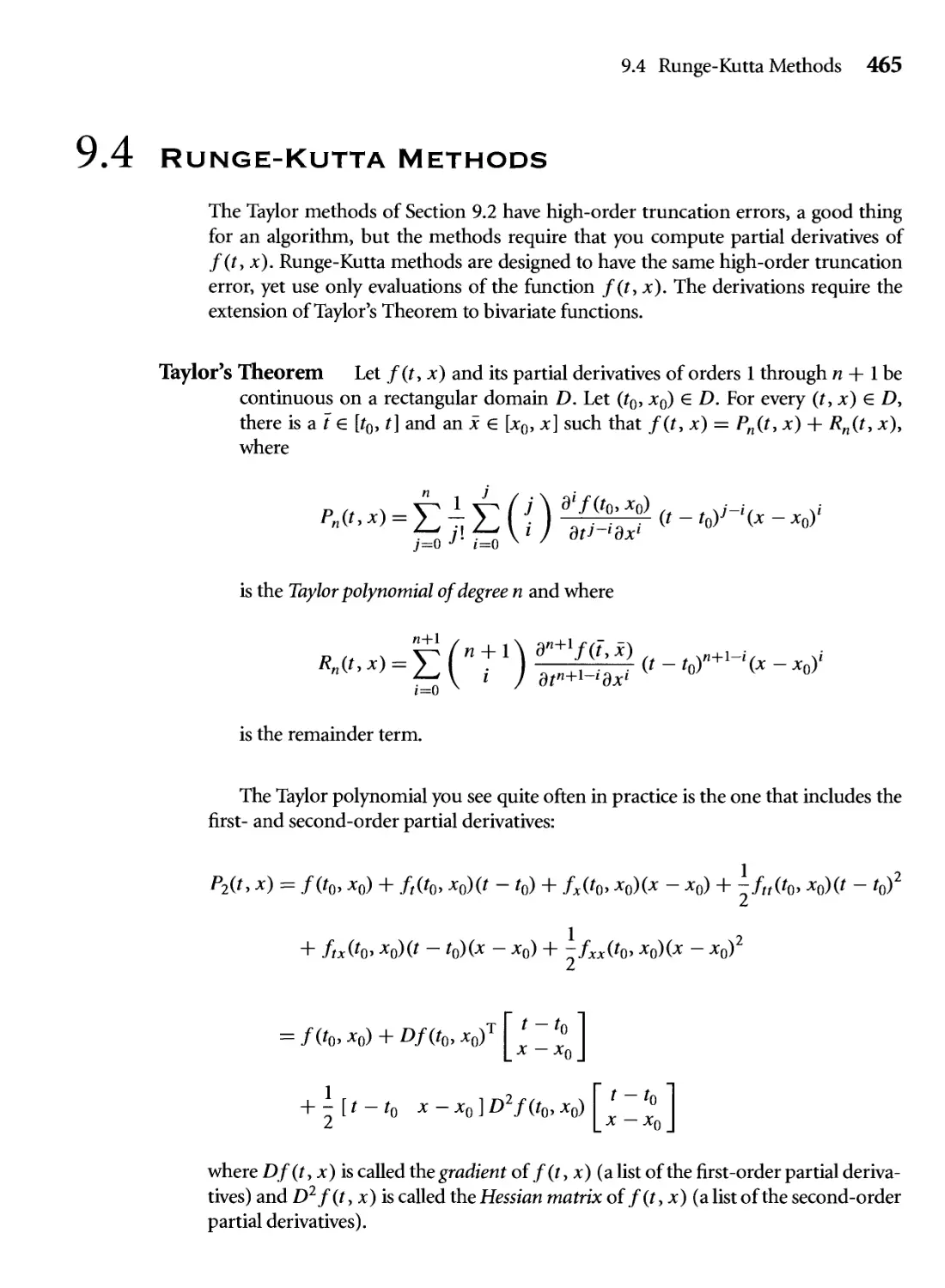
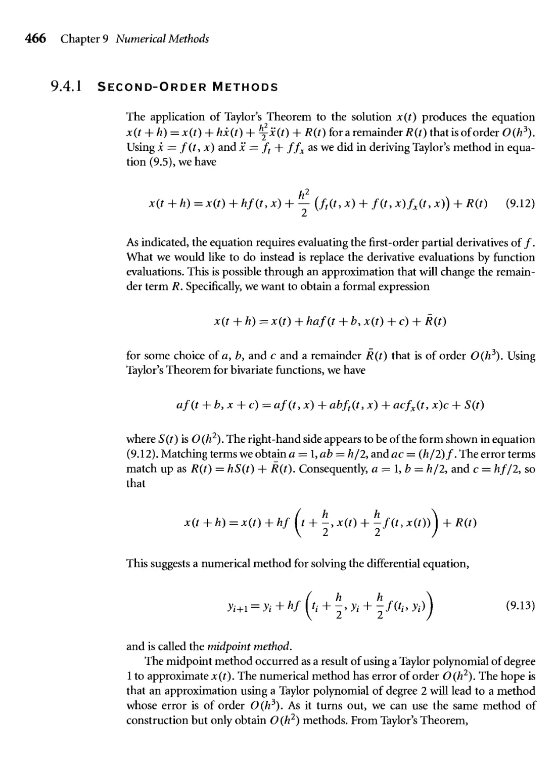
9.4 RUNGE-KUTTA METHODS 465
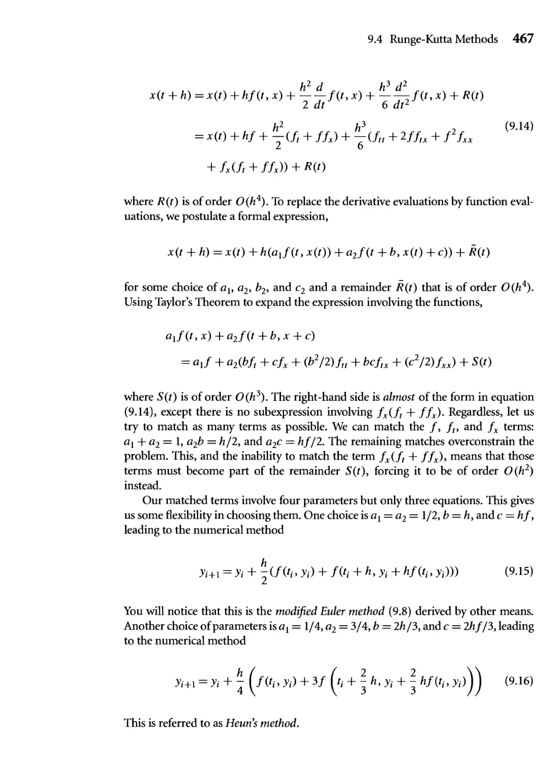
9.4.1 Second-Order Methods 466
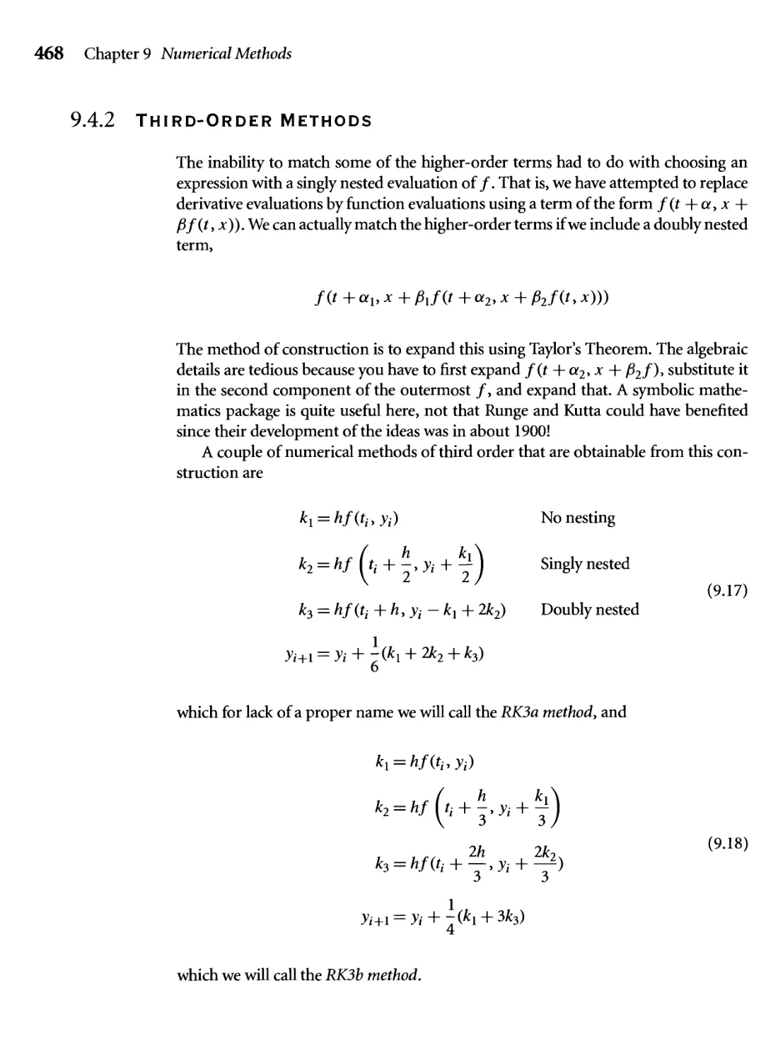
9.4.2 Third-Order Methods 468
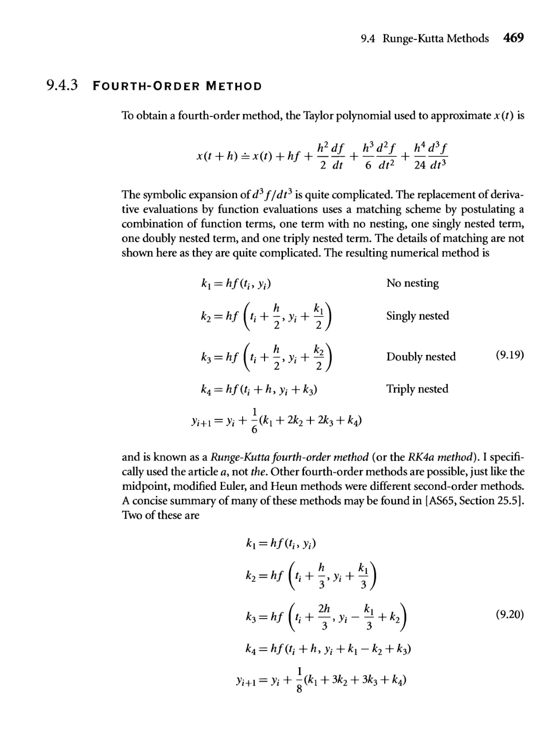
9.4.3 Fourth-Order Method 469
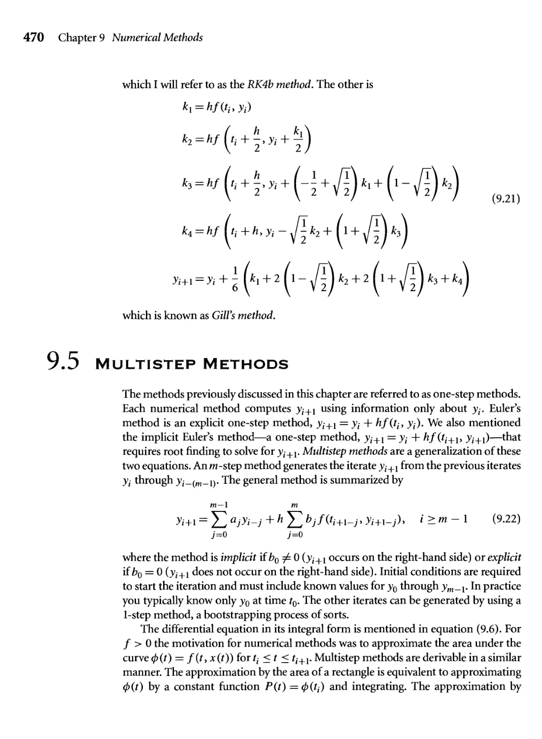
9.5 multistep methods 470
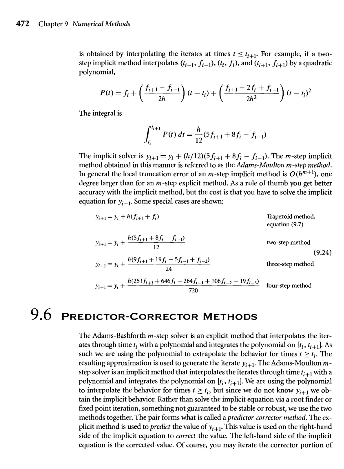
9.6 Predictor-Corrector methods 472
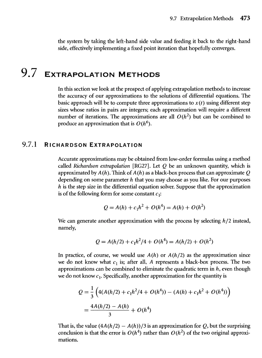
9.7 Extrapolation methods 473
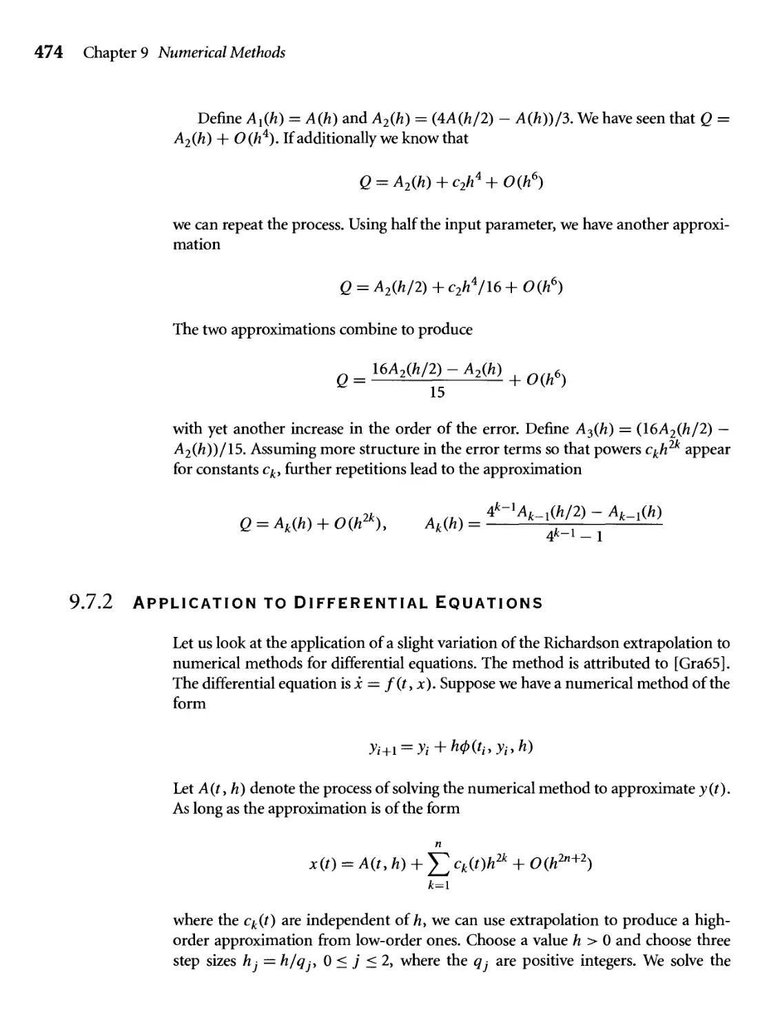
9.7.1 Richardson Extrapolation 473
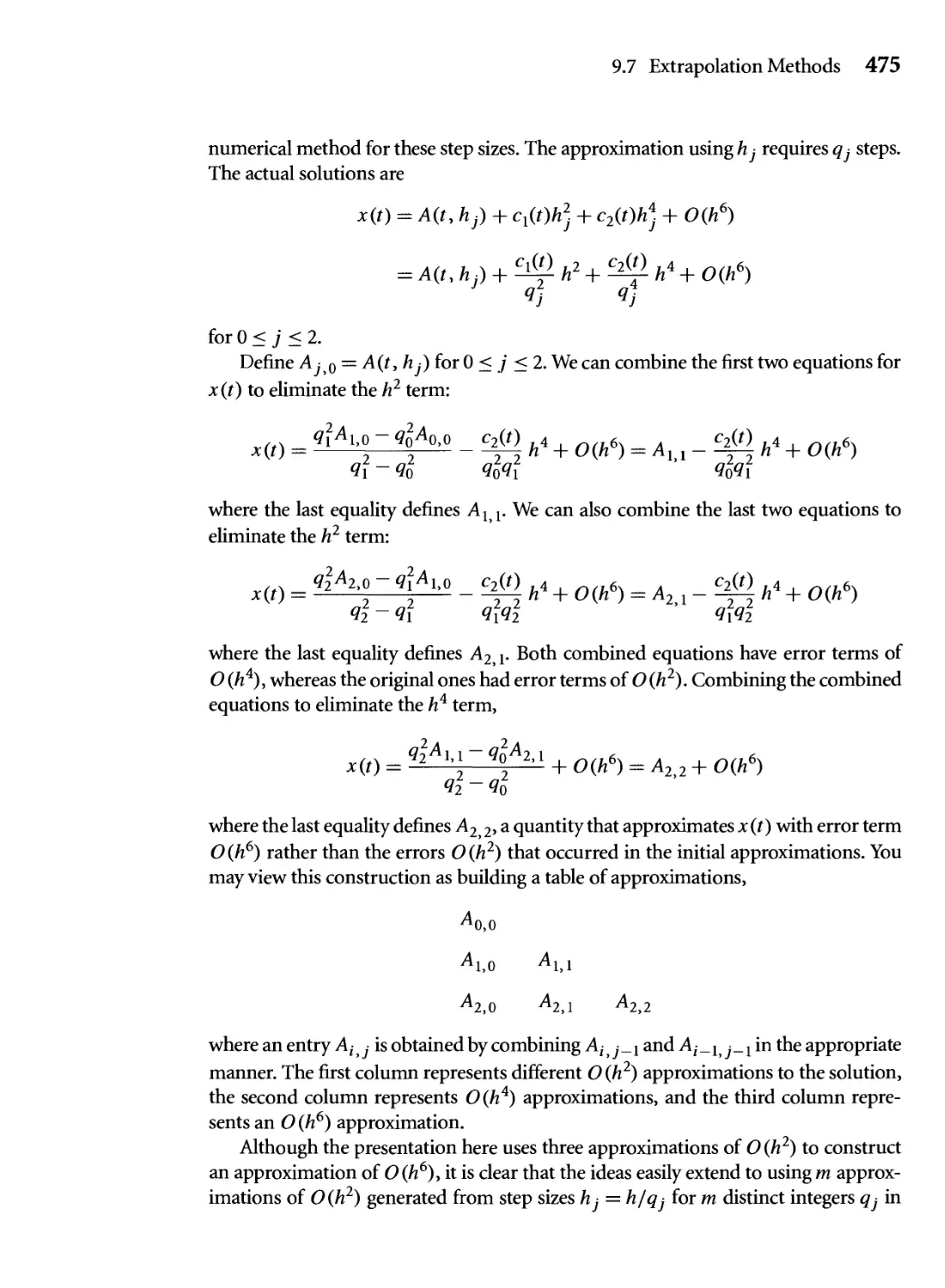
9.7.2 Application to Differential Equations 474
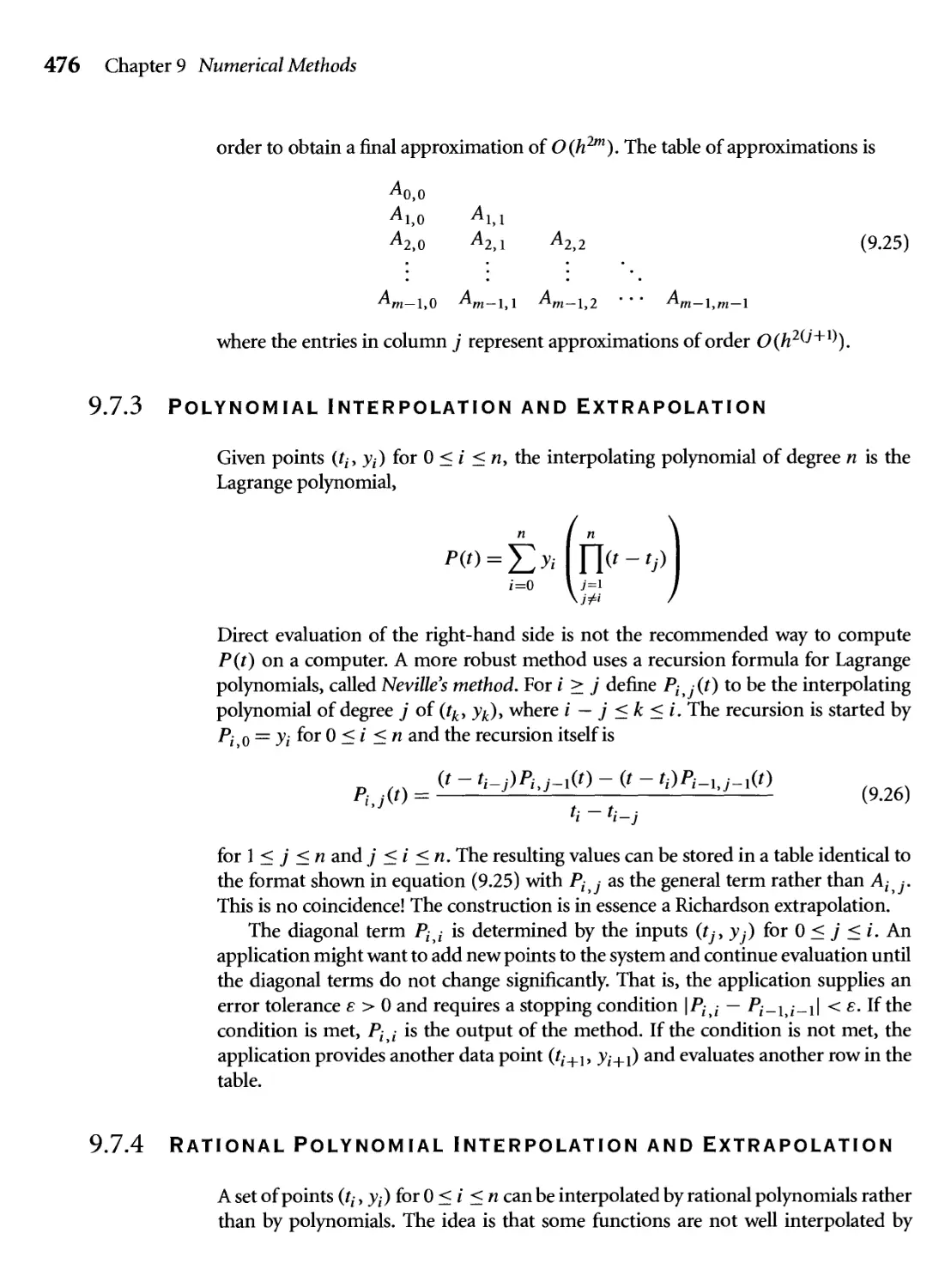
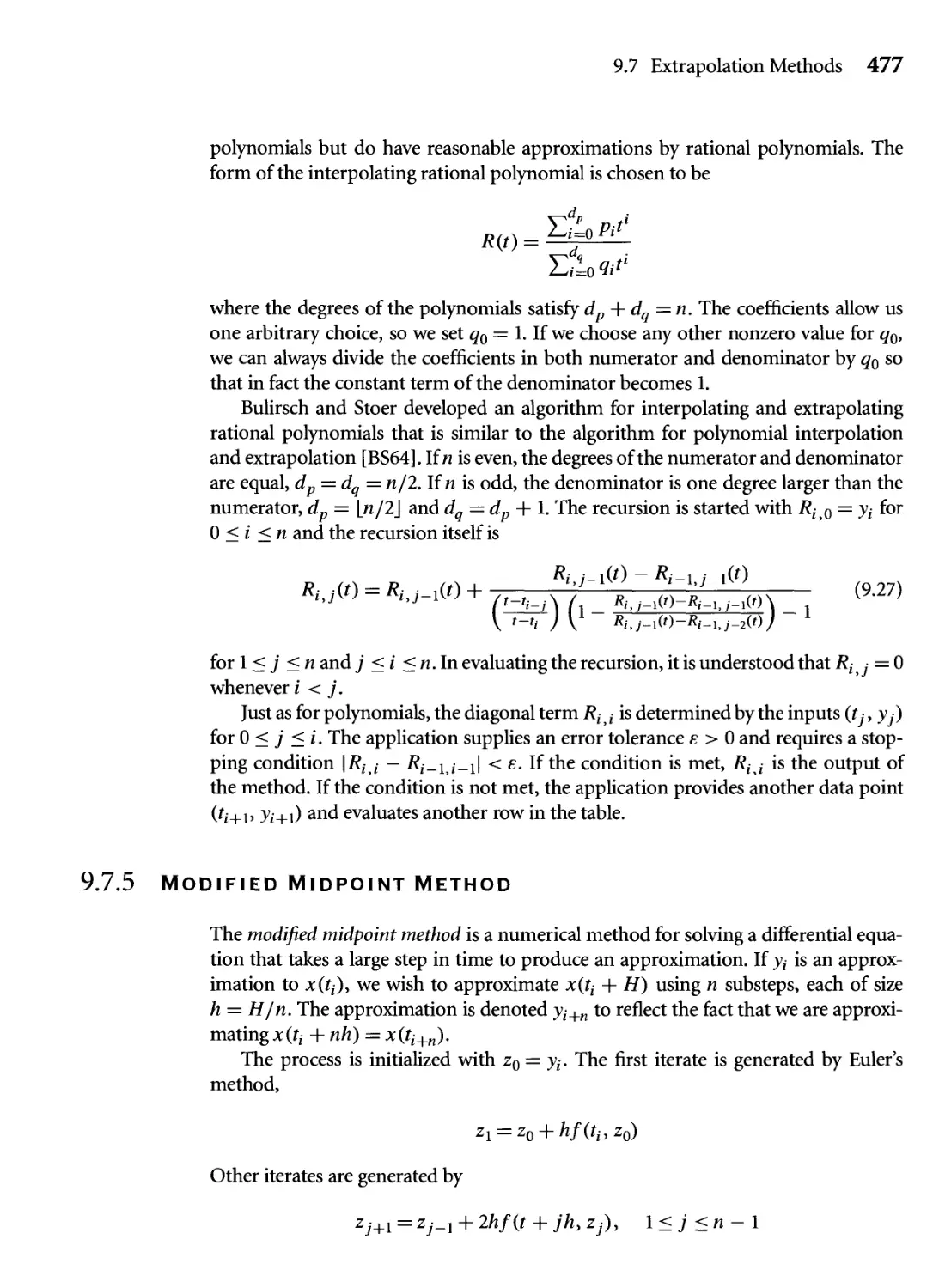
9.7.3 Polynomial Interpolation and Extrapolation 476
9.7.4 Rational Polynomial Interpolation and Extrapolation 476
9.7.5 Modified Midpoint Method 477
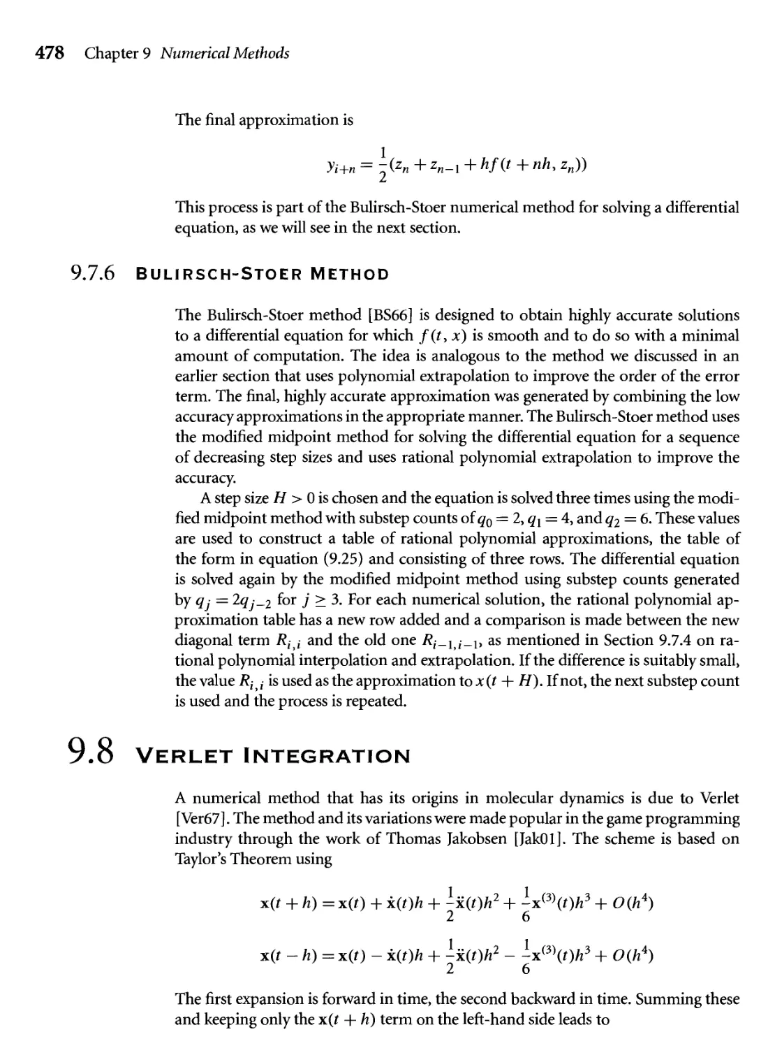
9.7.6 Bulirsch-Stoer Method 478
9.8 VERLET INTEGRATION 478
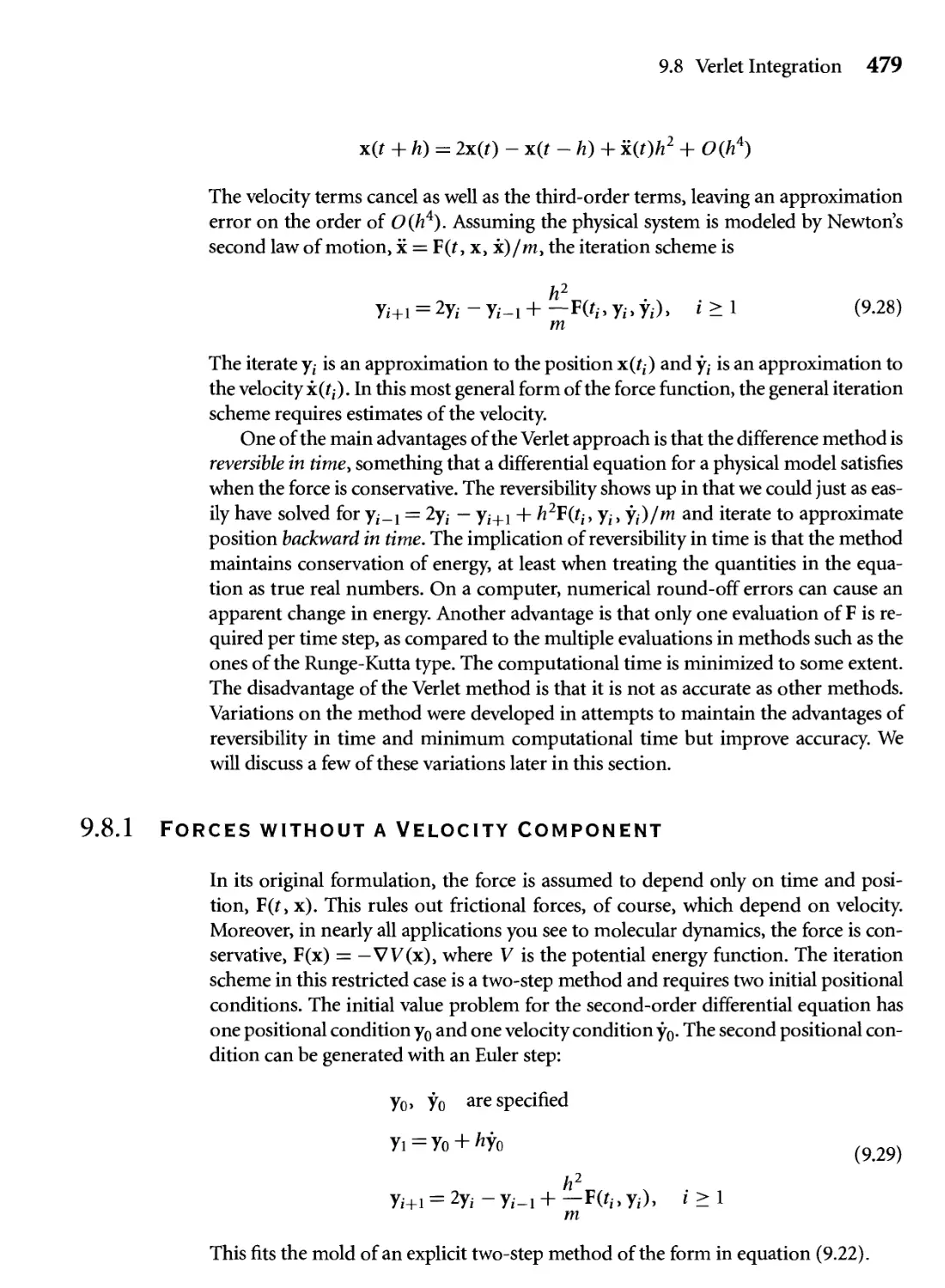
9.8.1 Forces without a Velocity Component 479
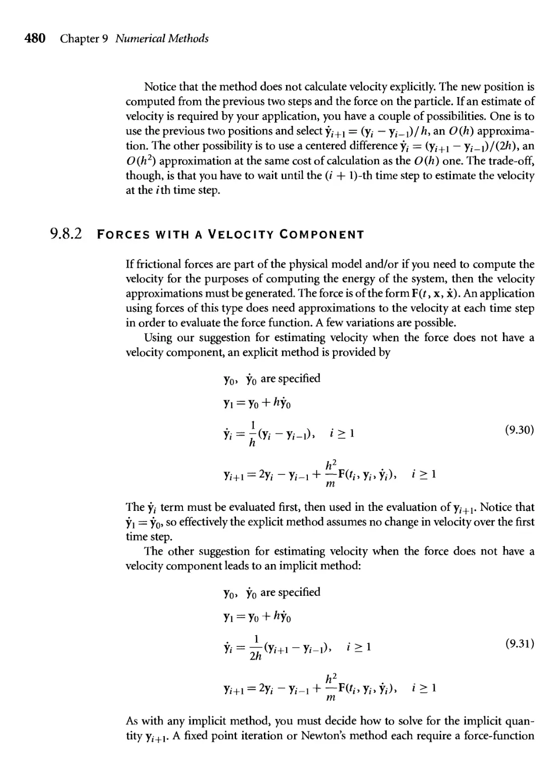
9.8.2 Forces with a Velocity Component 480
9.8.3 Simulating Drag in the System 481
9.8.4 Leap Frog Method 481
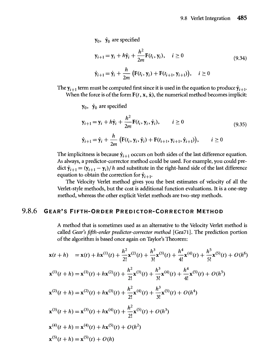
9.8.5 Velocity Verlet Method 483
9.8.6 Gear's Fifth-Order Predictor-Corrector Method 485
9.9 Numerical Stability and its relationship to Physical
Stability 487
9.9.1 Stability for Single-Step Methods 488
9.9.2 Stability for Multistep Methods 490
9.9.3 Choosing a Stable Step Size 491
9.10 Stiff Equations 503
Chapter
Quaternions 507
10.1 rotation Matrices 507
10.2 The Classical Approach 512
10.2.1 Algebraic Operations 512
10.2.2 Relationship of Quaternions to Rotations 515
10.3 A Linear Algebraic Approach 517

Xll Contents
10.4 From rotation Matrices to Quaternions 522
Contributed by Ken Shoetnake
10.4.1 2D Rotations 523
10.4.2 Linearity 525
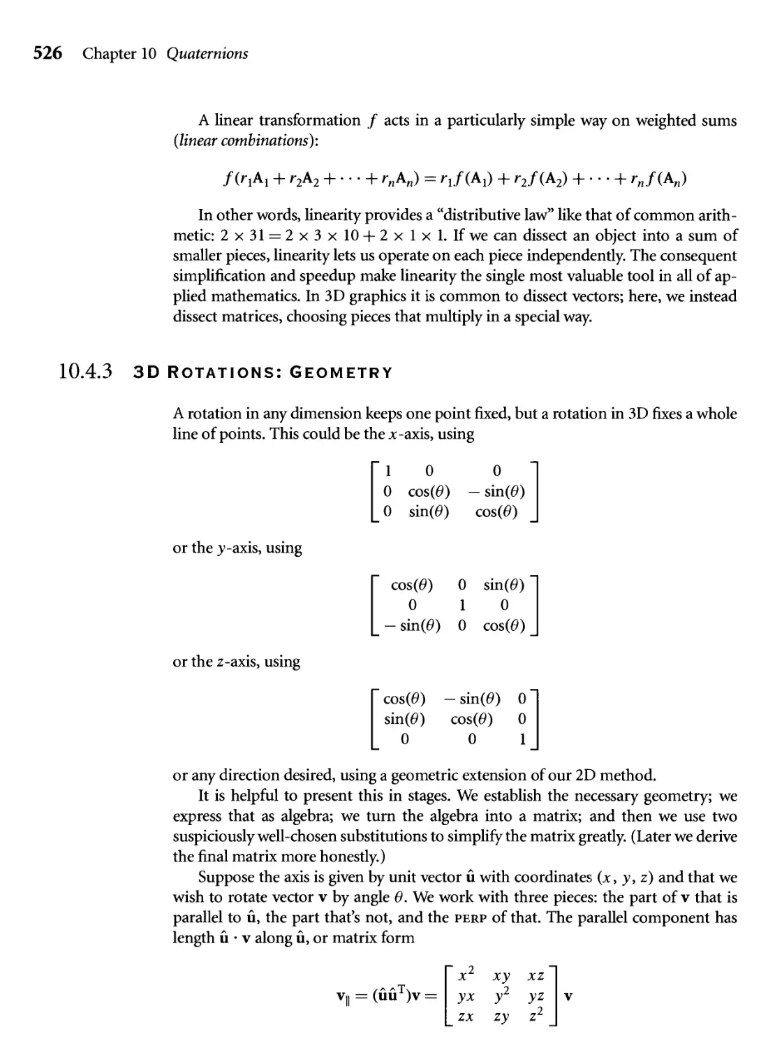
10.4.3 3D Rotations: Geometry 526
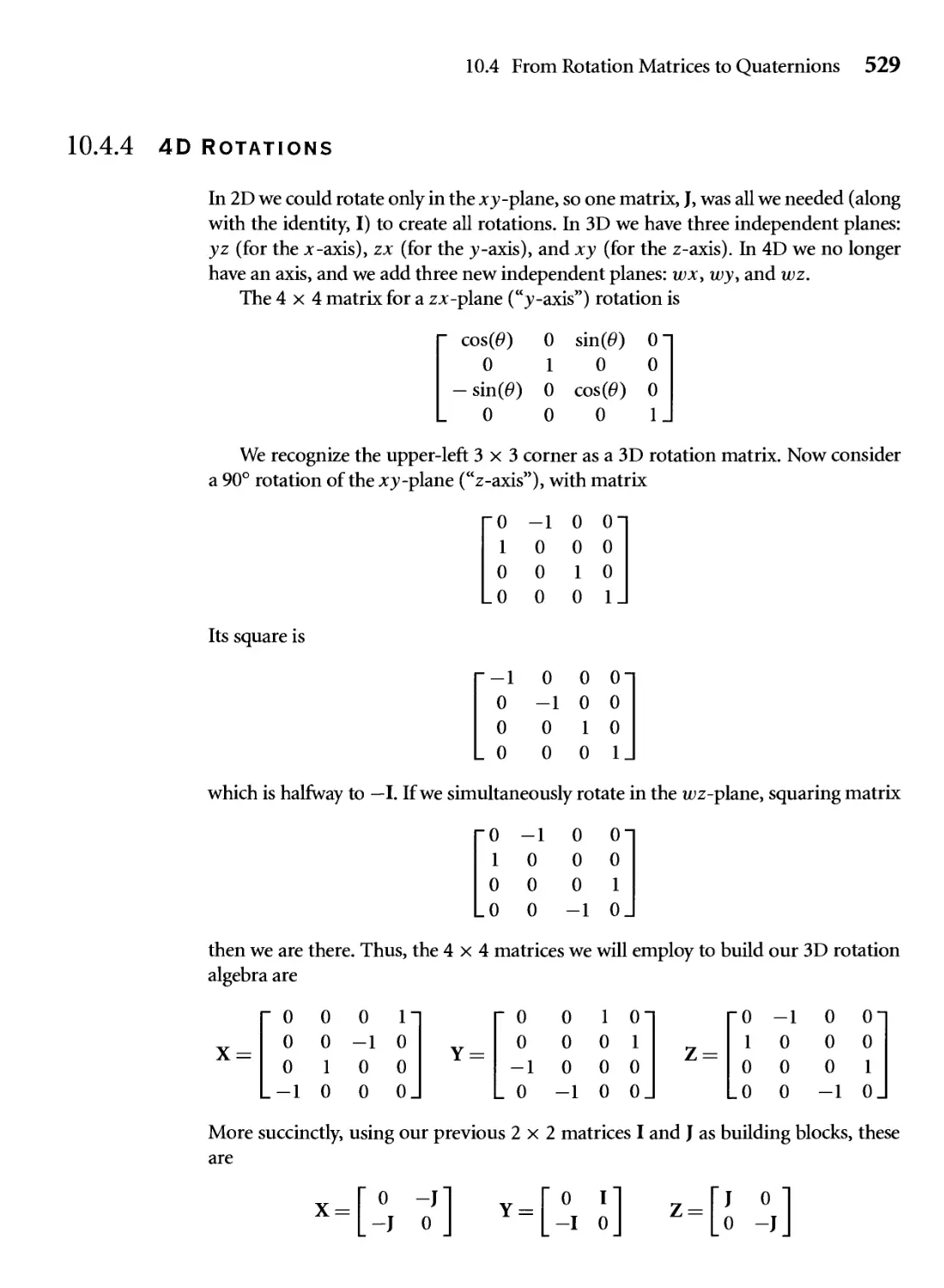
10.4.4 4D Rotations 529
10.4.5 3D Rotations: Algebra 531
10.4.6 4D Matrix 534
10.4.7 Retrospect, Prospect 538
10.5 Interpolation of Quaternions 539
10.5.1 Spherical Linear Interpolation 539
10.5.2 Spherical Quadrangle Interpolation 541
10.6 Derivatives of Time-Varying Quaternions 543
Appendix
Linear Algebra 545
A.1 A REVIEW OF NUMBER SYSTEMS 545
A. 1.1 The Integers 545
A. 1.2 The Rational Numbers 545
A. 1.3 The Real Numbers 546
A. 1.4 The Complex Numbers 546
A. 1.5 Fields 547
A.2 Systems of Linear Equations 548
A.2.1 A Closer Look at Two Equations in Two Unknowns 551
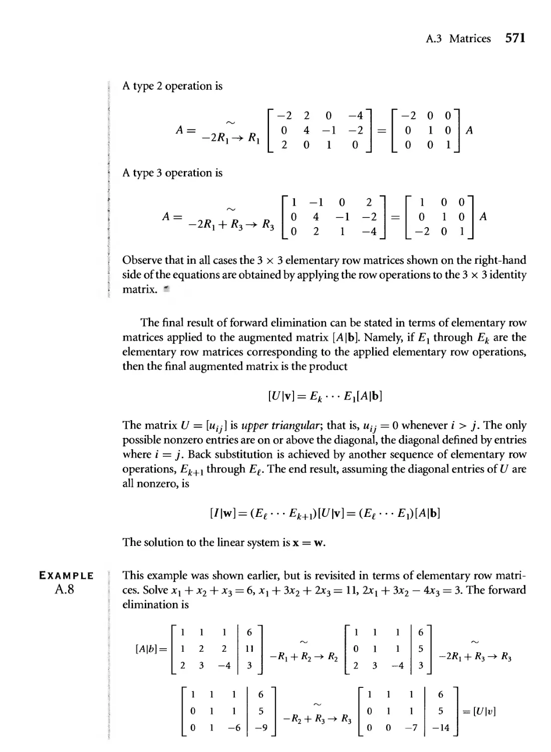
A.2.2 Gaussian Elimination and Elementary Row Operations 554
A.2.3 Nonsquare Systems of Equations 558
A.2.4 The Geometry of Linear Systems 559
A.2.5 Numerical Issues 562
A.2.6 Iterative Methods for Solving Linear Systems 565
A.3 Matrices 566
A.3.1 Some Special Matrices 569
A.3.2 Elementary Row Matrices 570
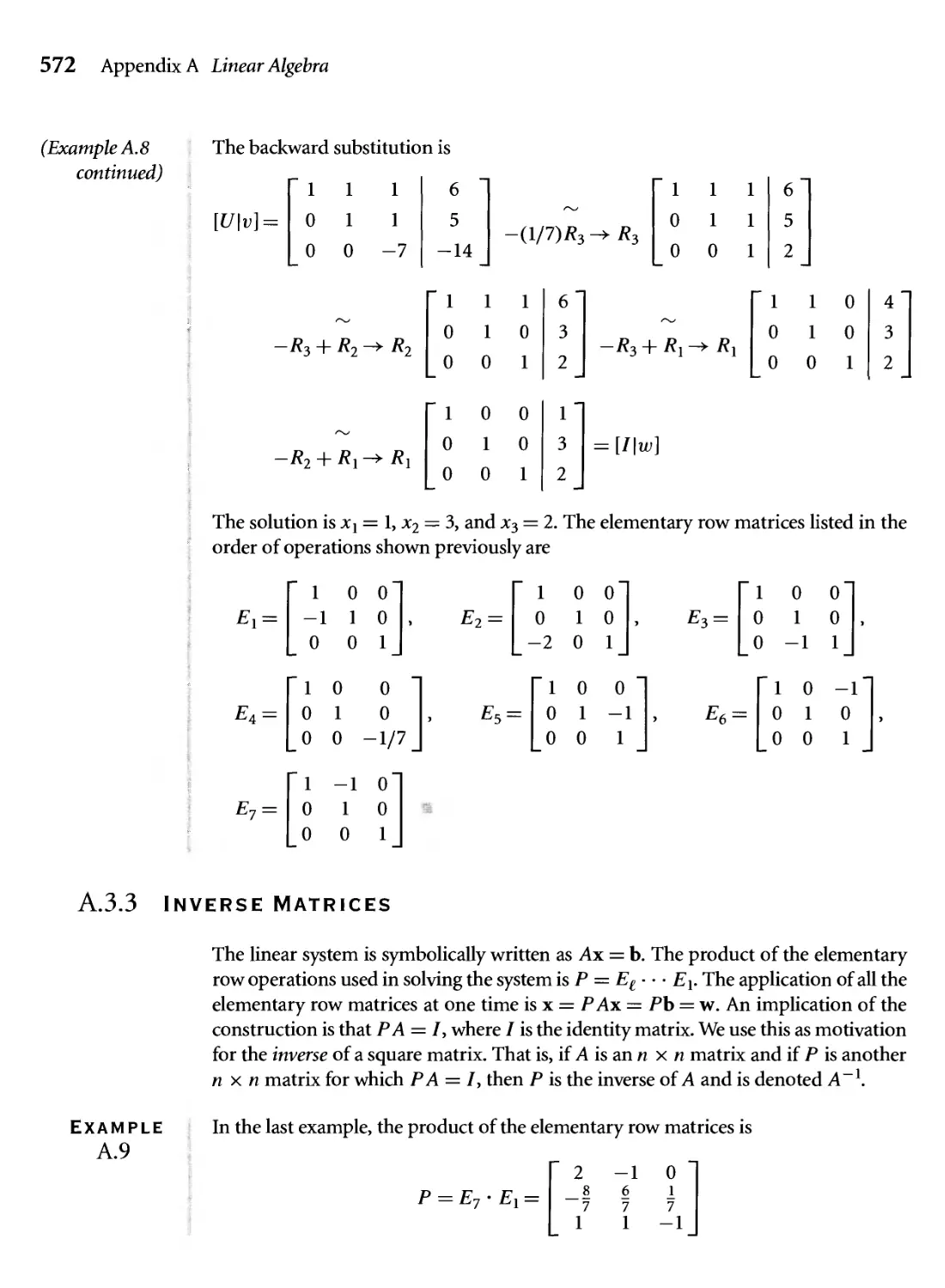
A.3.3 Inverse Matrices 572
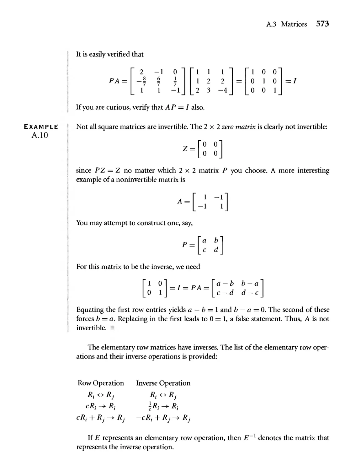
A.3.4 Properties of Inverses 574
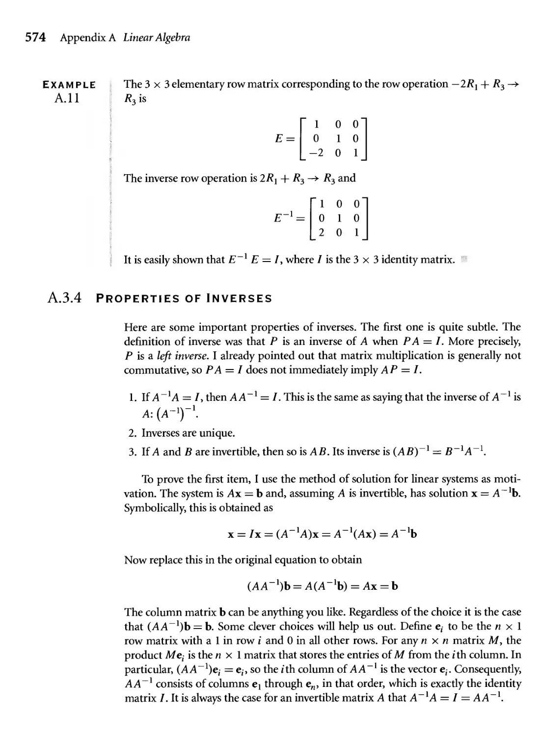
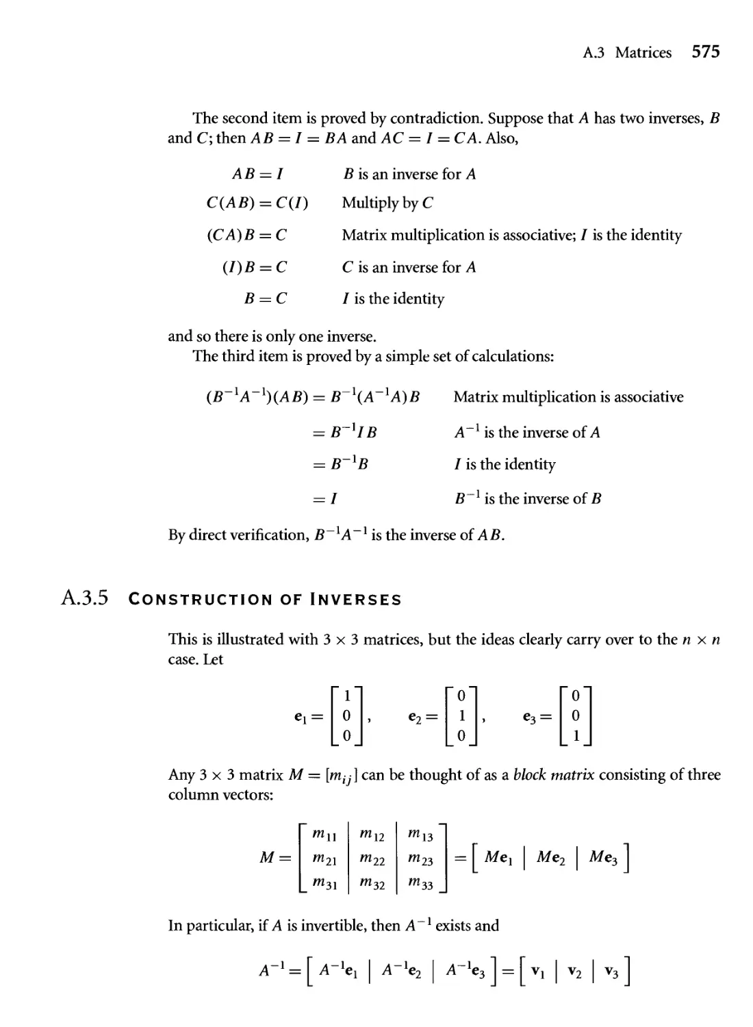
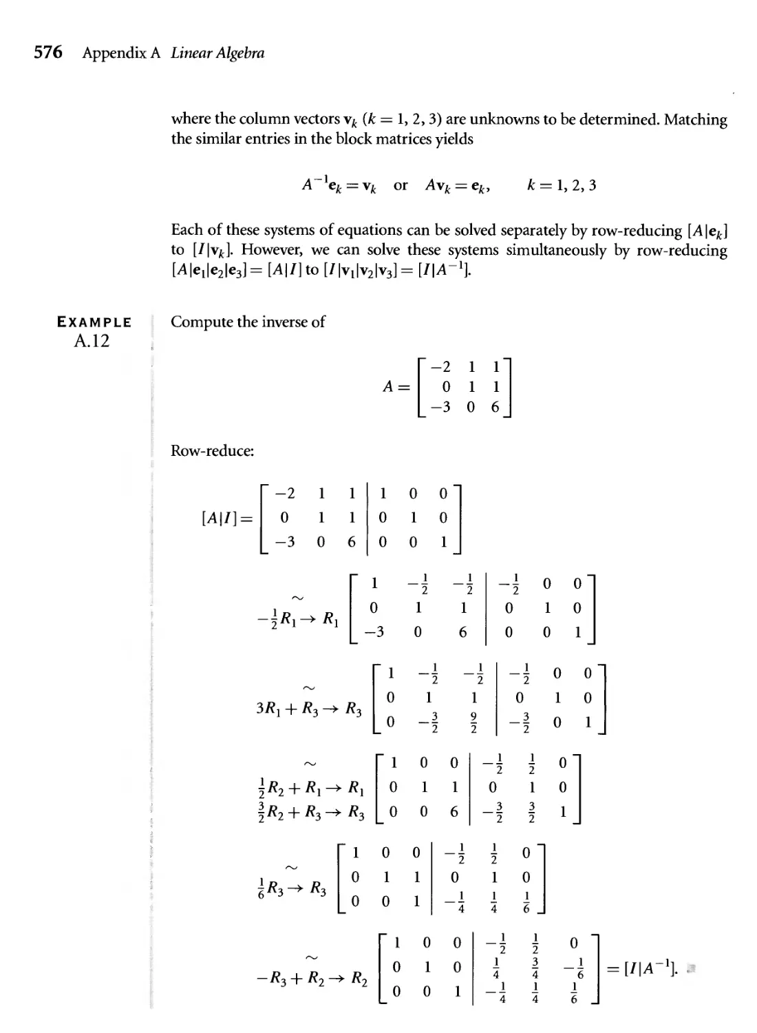
A.3.5 Construction of Inverses 575
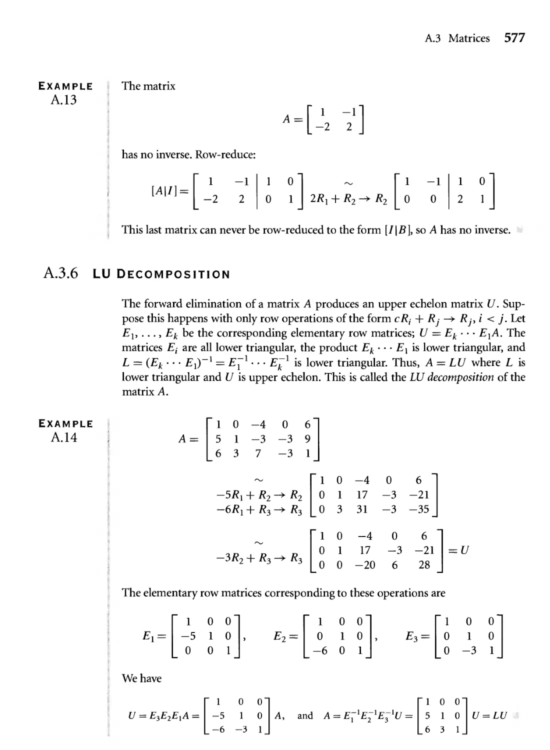
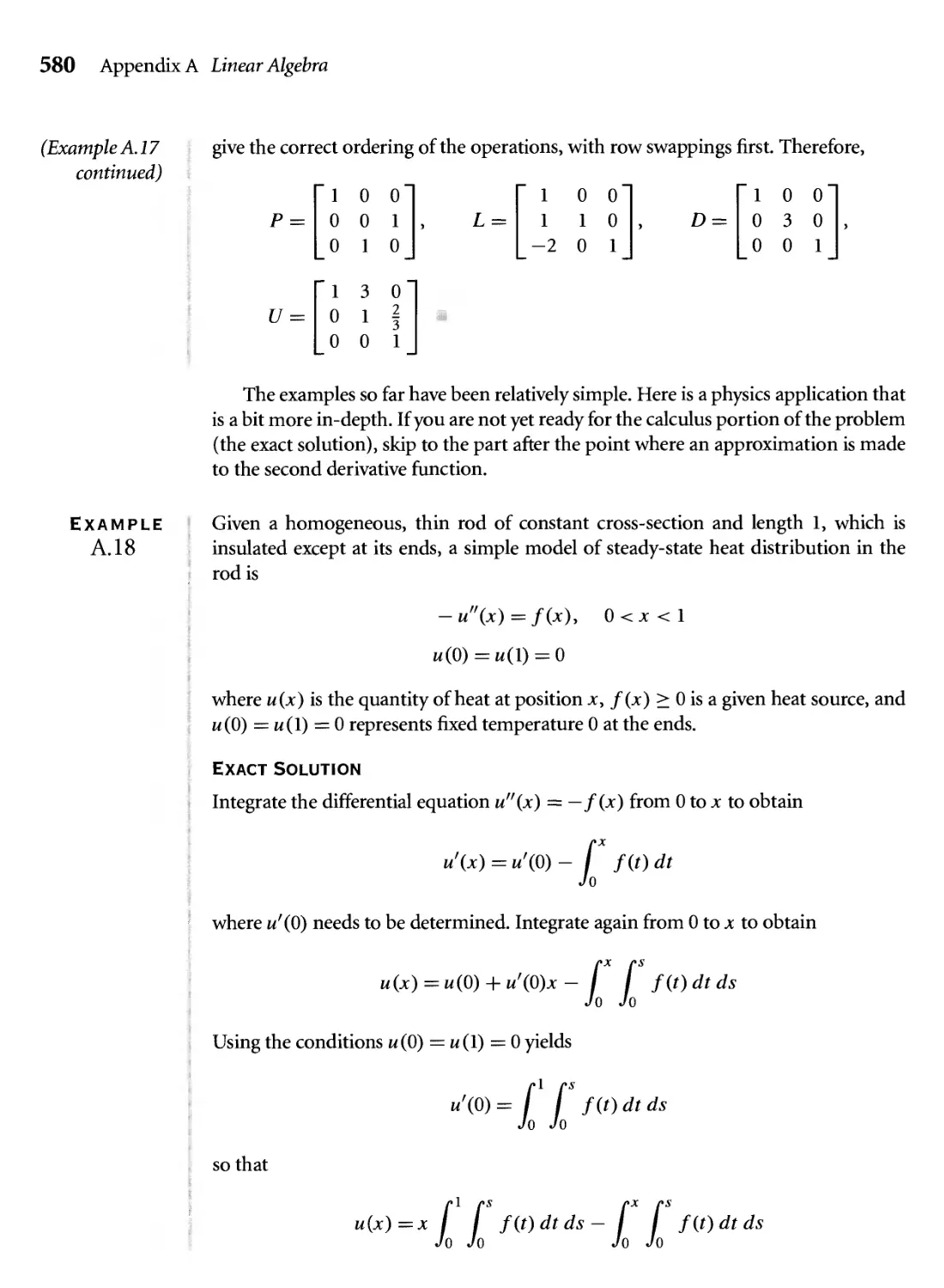
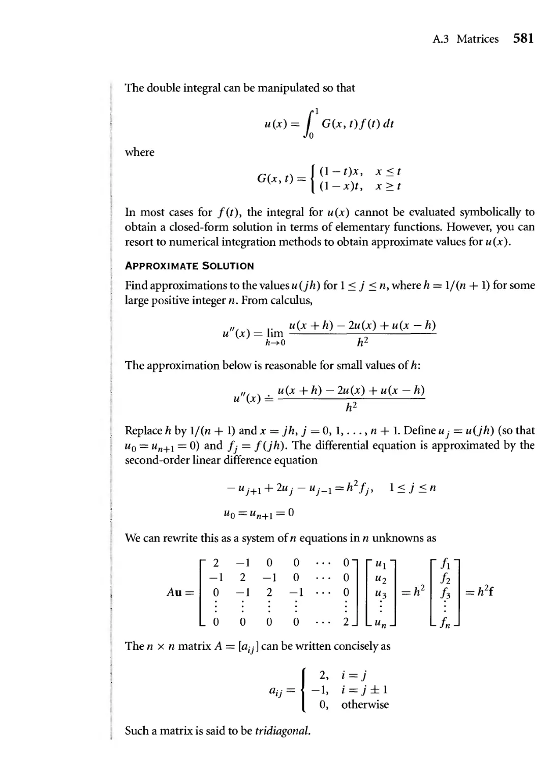
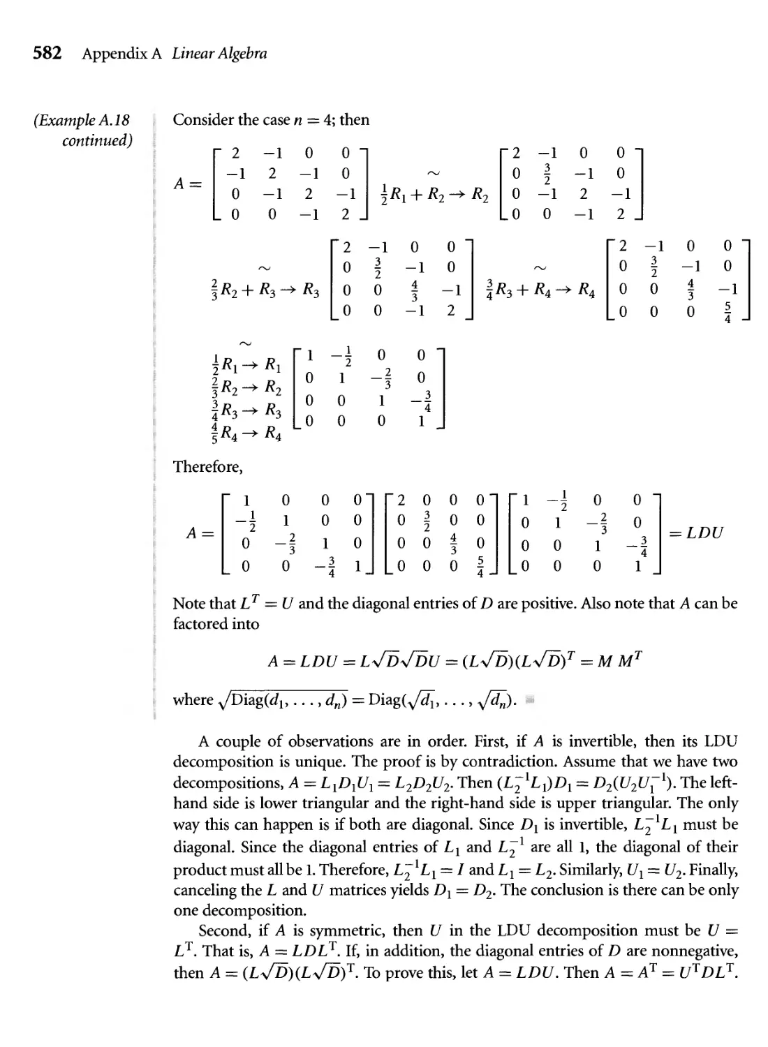
A.3.6 LU Decomposition 577
A.4 Vector Spaces 583
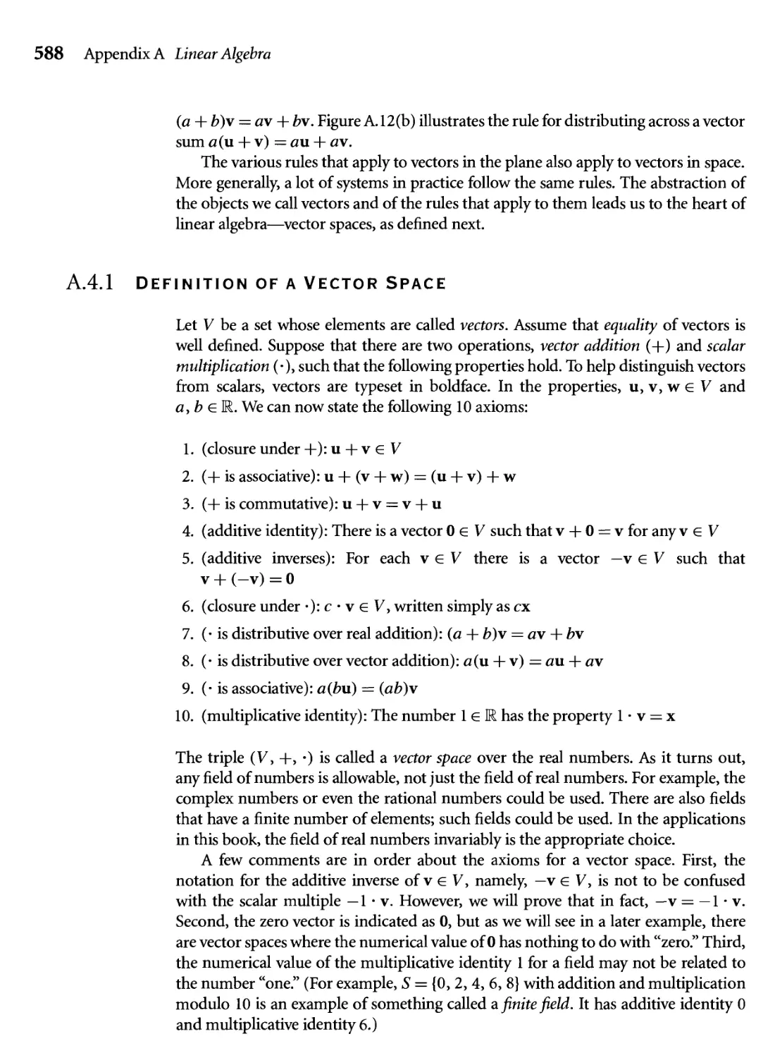
A.4.1 Definition of a Vector Space 588
A.4.2 Linear Combinations, Spans, and Subspaces 593

Contents ХШ
A.4.3 Linear Independence and Bases 595
A.4.4 Inner Products, Length, Orthogonality, and Projection 601
A.4.5 Dot Product, Cross Product, and Triple Products 606
A.4.6 Orthogonal Subspaces 613
A.4.7 The Fundamental Theorem of Linear Algebra 616
A.4.8 Projection and Least Squares 621
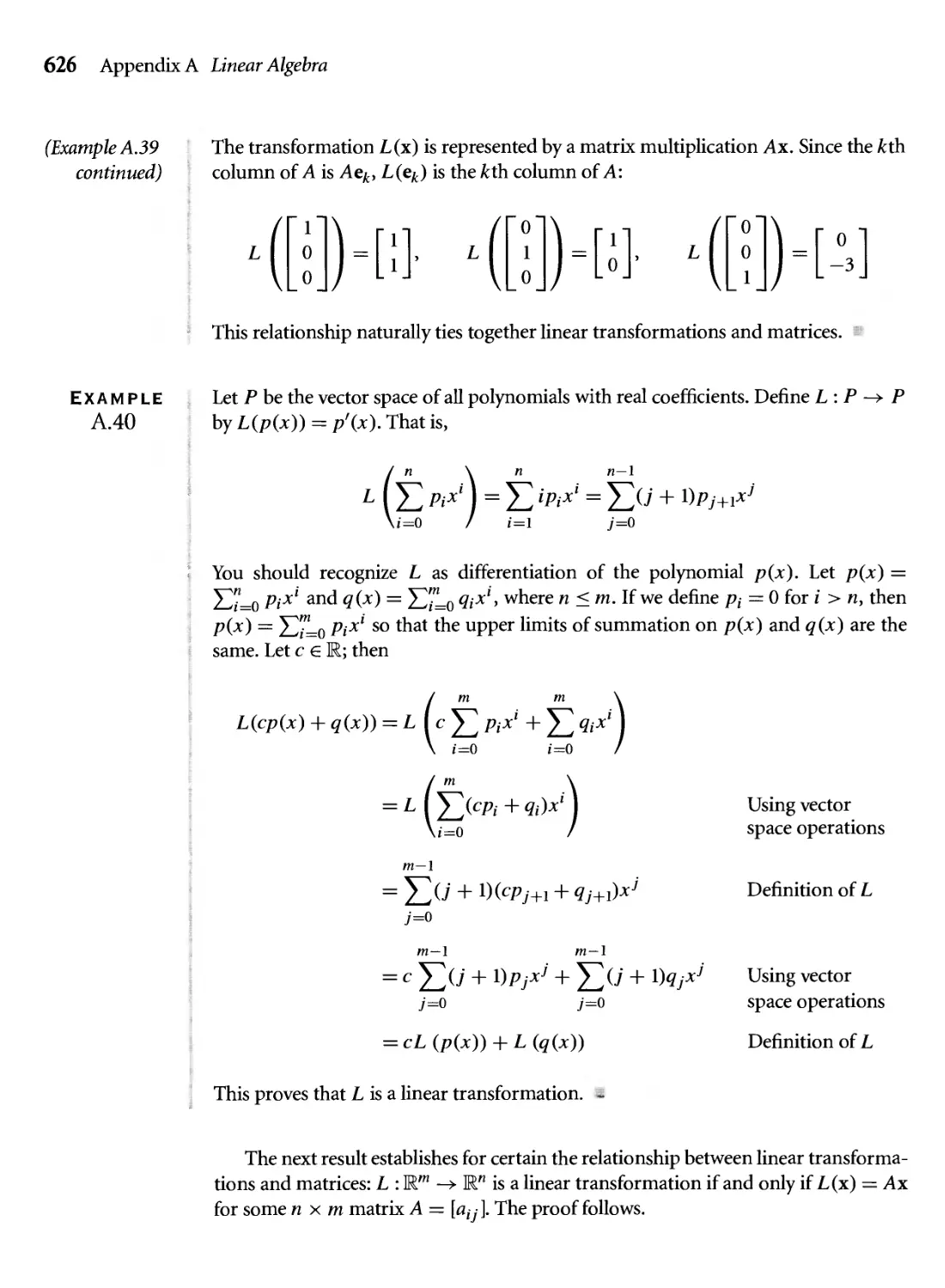
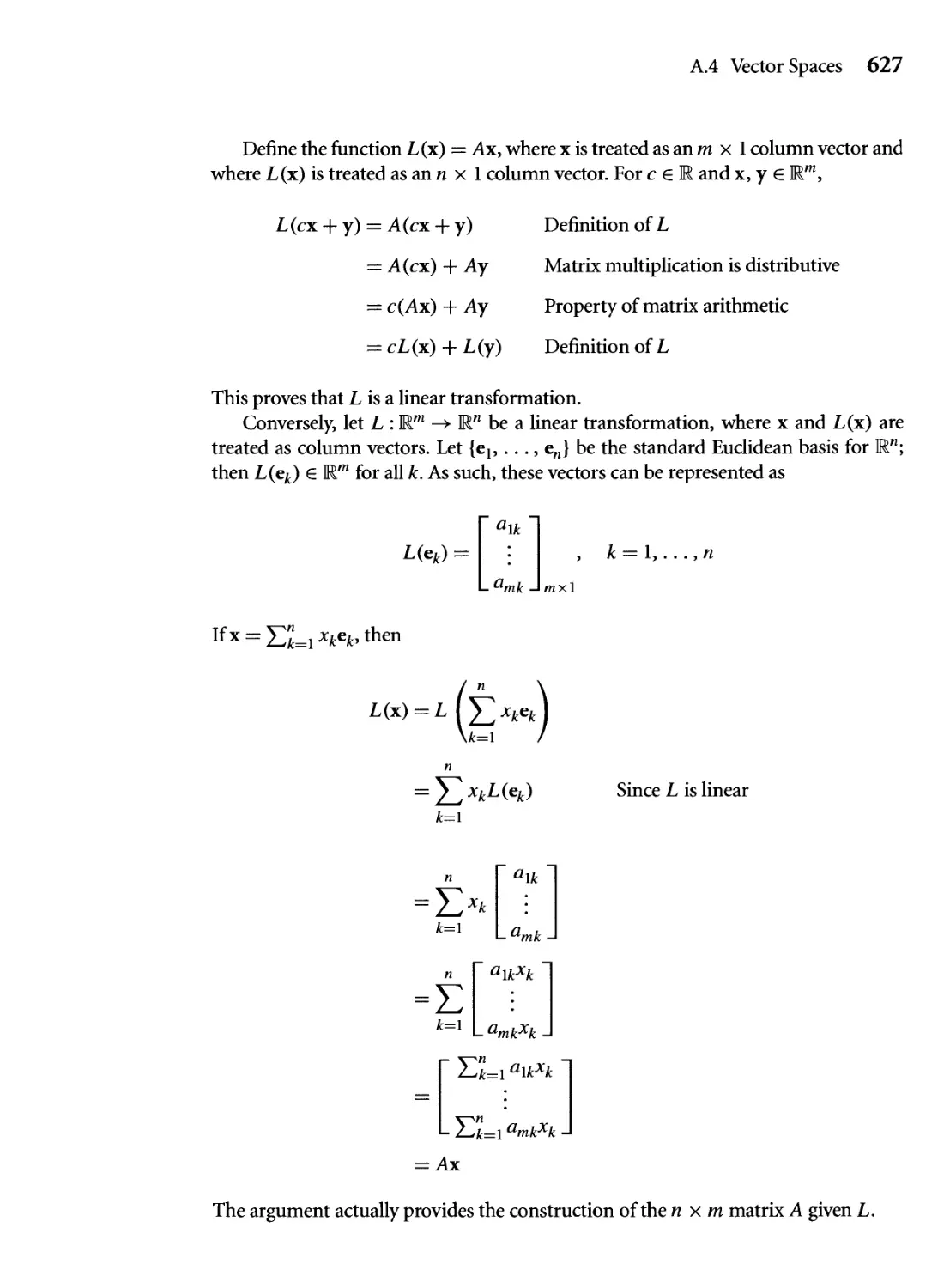
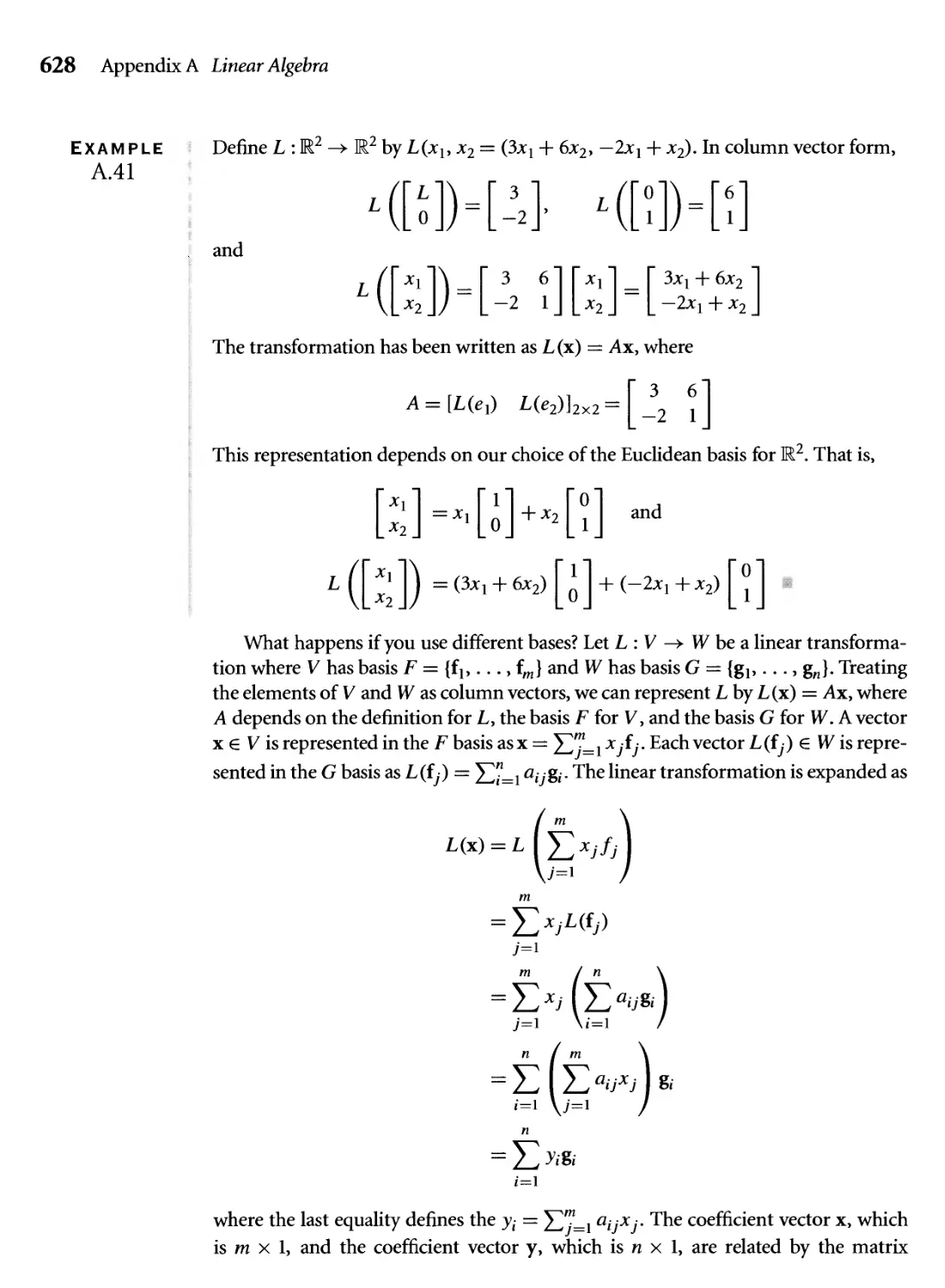
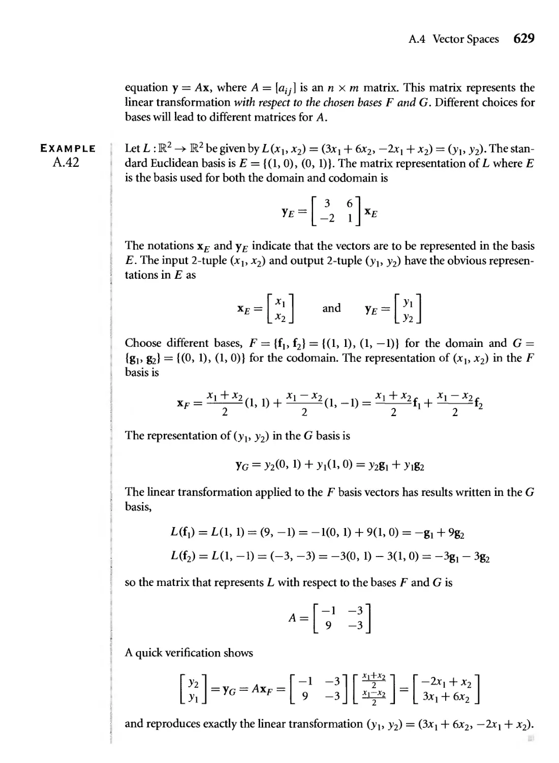
A.4.9 Linear Transformations 624
A.5 Advanced Topics 634
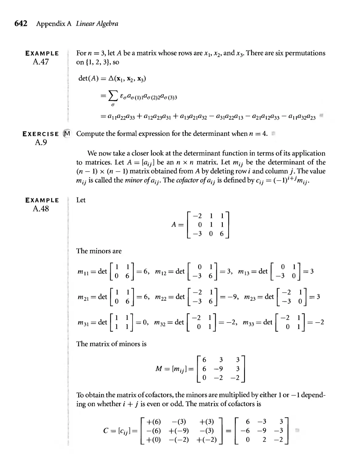
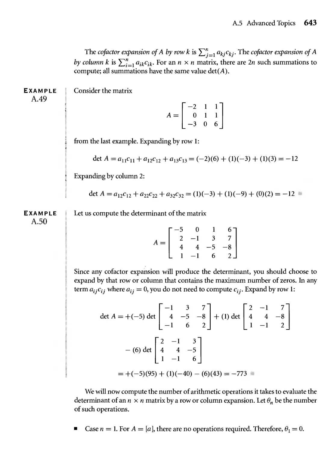
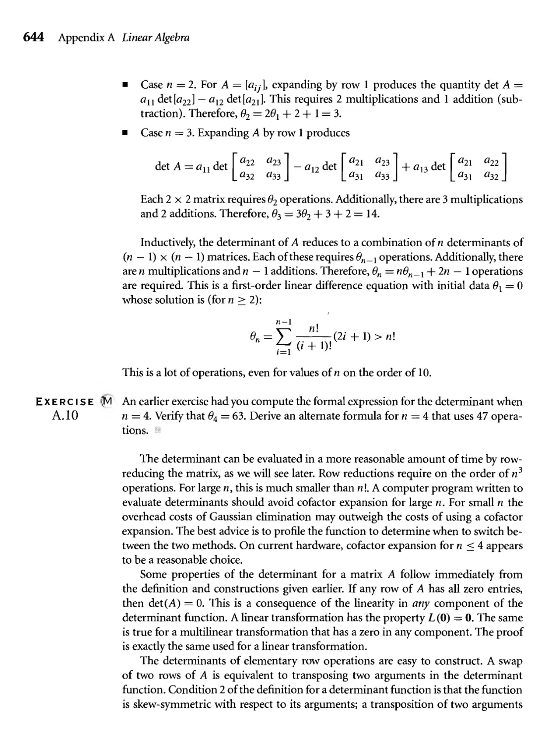
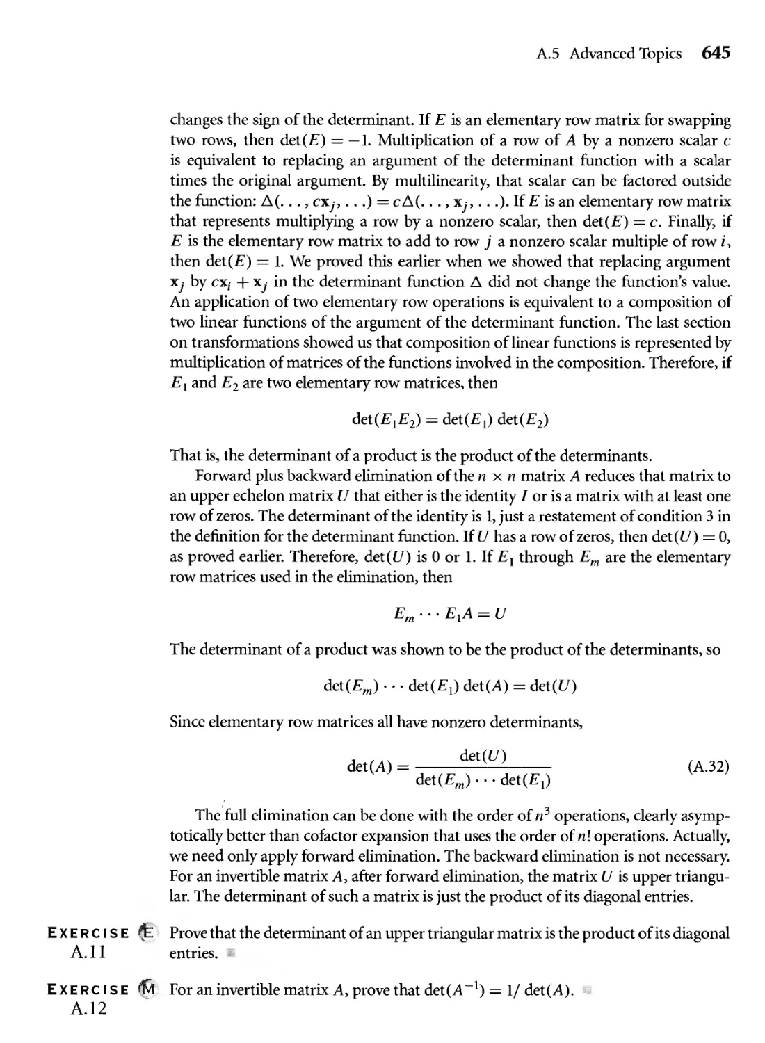
A.5.1 Determinants 634
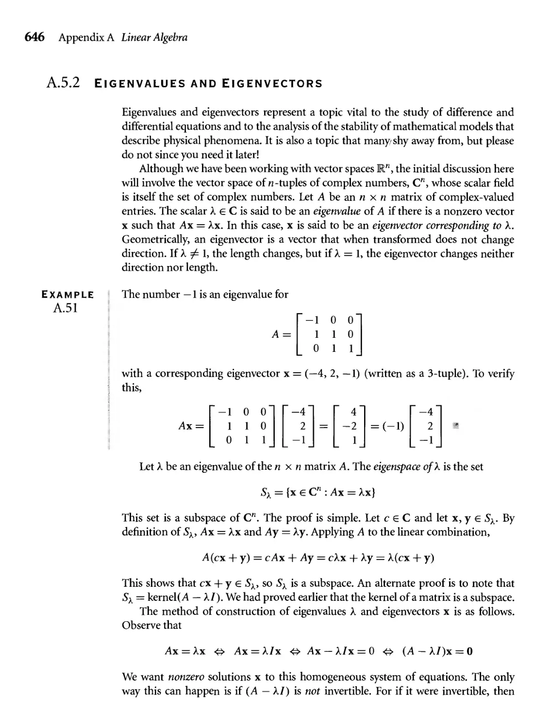
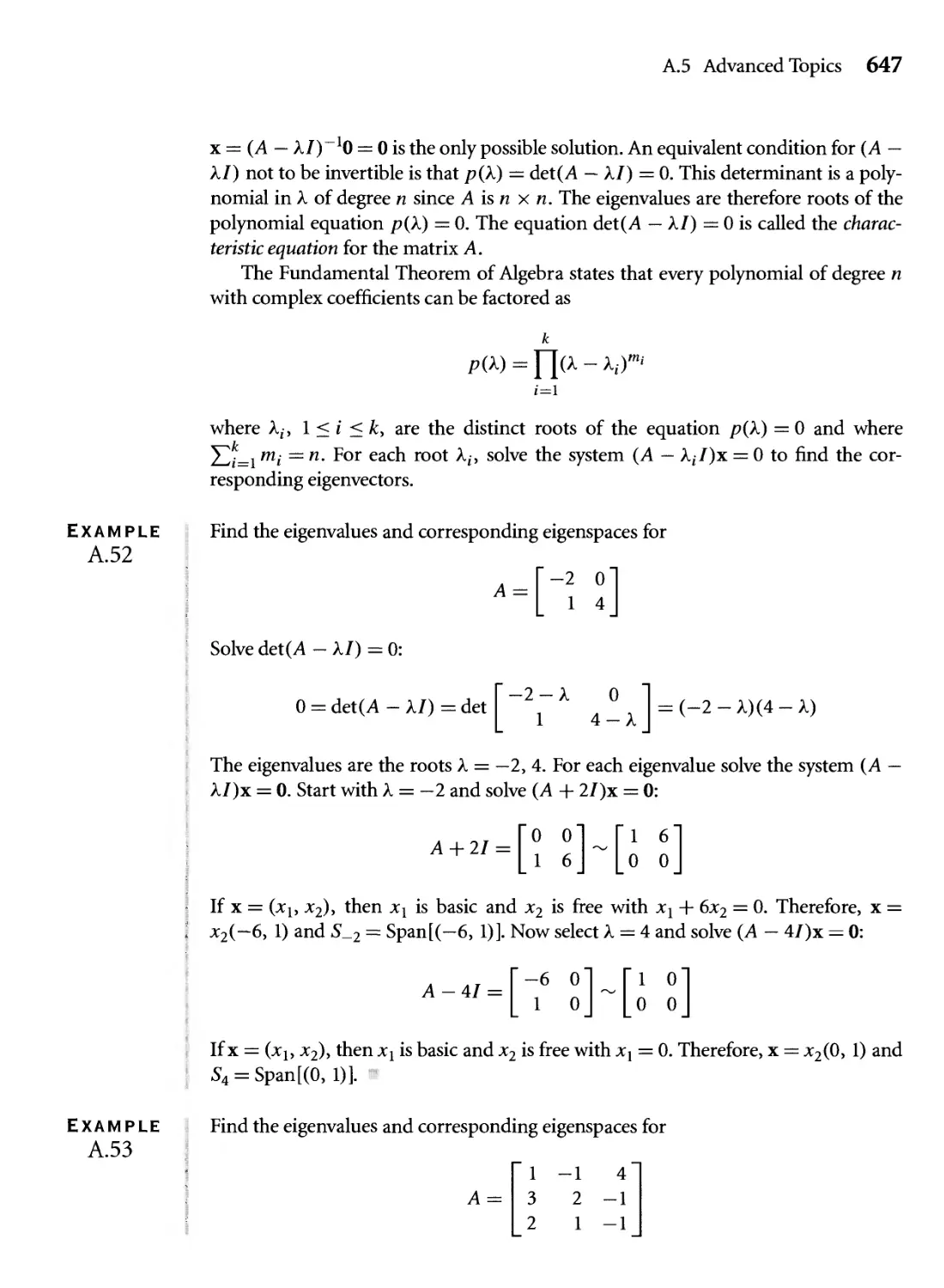
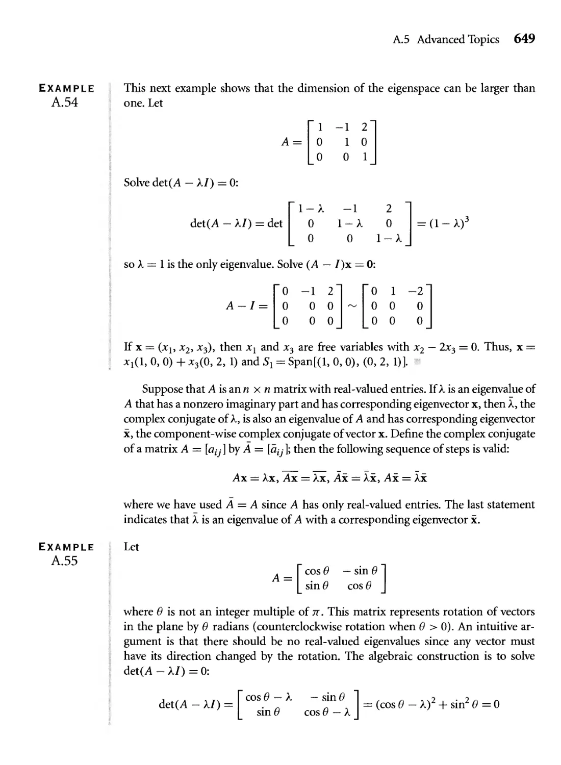
A.5.2 Eigenvalues and Eigenvectors 646
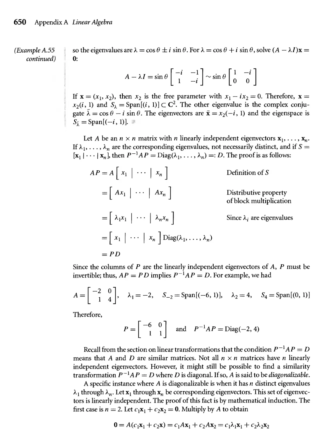
A.5.3 Eigendecomposition for Symmetric Matrices 652
A.5.4 S + N Decomposition 655
A.5.5 Applications 661
Appendix
Д5 Affine Algebra 669
B.I Introduction 669
B.2 Coordinate Systems 673
B.3 Subspaces 675
B.4 Transformations 676
B.5 Barycentric Coordinates 677
B.5.1 Triangles 678
B.5.2 Tetrahedra 679
B.5.3 Simplices 680
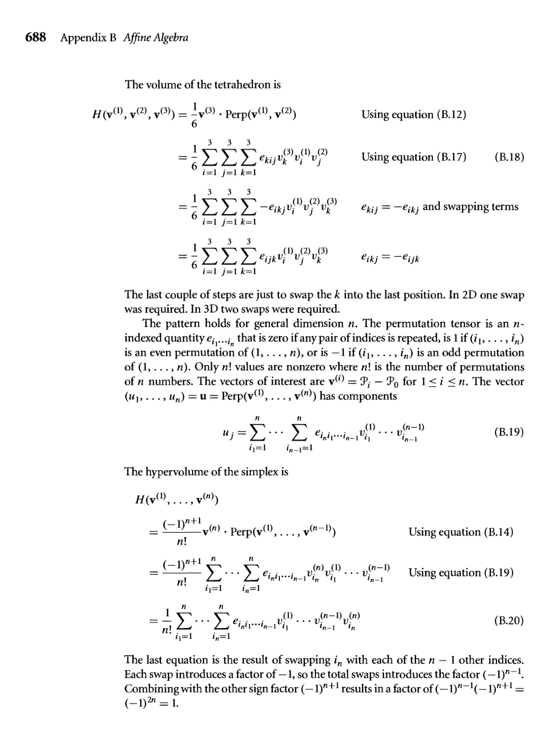
B.5.4 Length, Area, Volume, and Hypervolume 681
Appendix
Calculus 691
C.I Univariate Calculus 692
694
696
697
698
701
701
UNIVARIATE CALCULUS
C.1.1
С 1.2
C.1.3
С 1.4
C.1.5
С 1.6
Limits
Limits of a Sequence
Continuity
Differentiation
LHopital's Rule
Integration

xiv Contents
C.2 MULTIVARIATE CALCULUS 704
C.2.1 Limits and Continuity 704
C.2.2 Differentiation 705
C.2.3 Integration 708
C.3 Applications 710
C.3.1 Optimization 711
C.3.2 Constrained Optimization 715
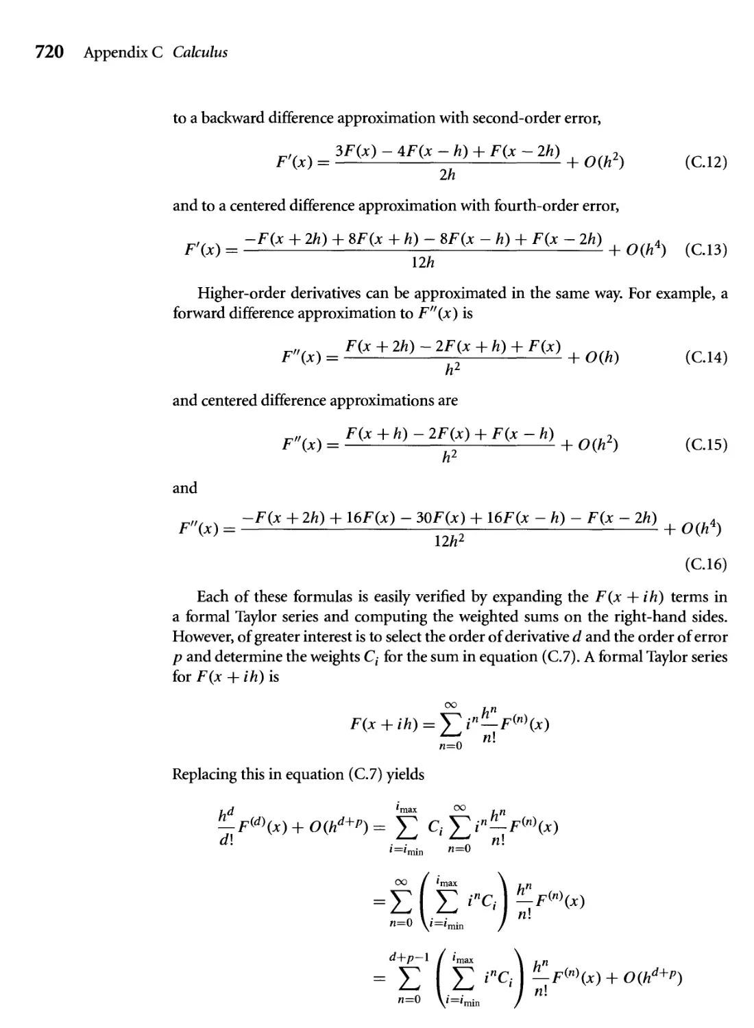
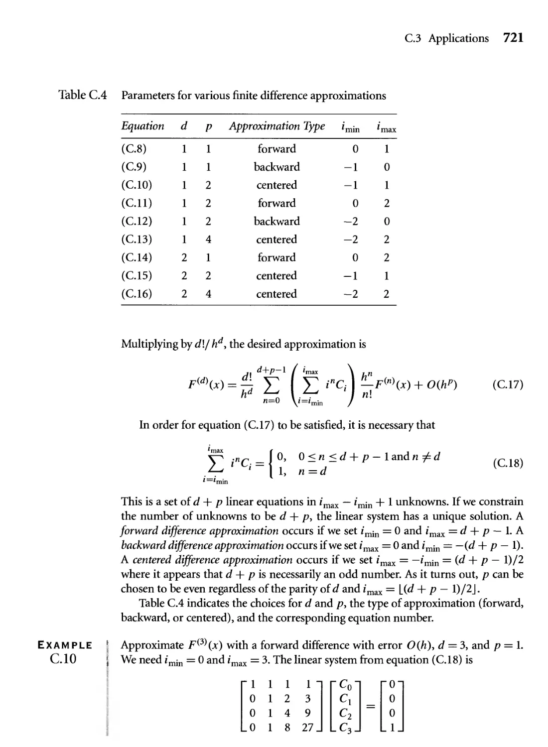
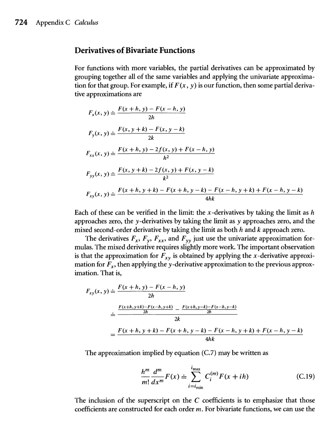
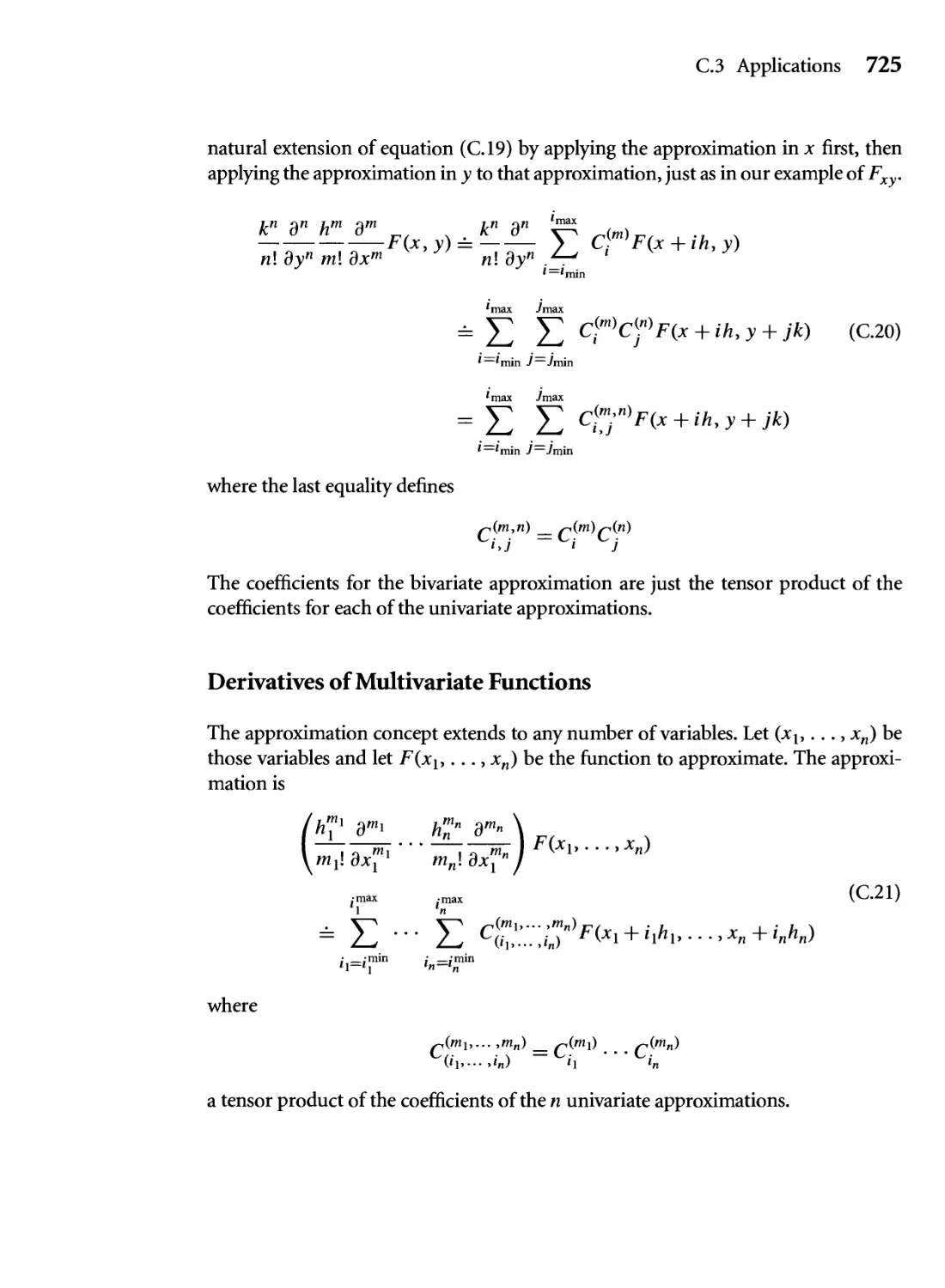
C.3.3 Derivative Approximations by Finite Differences 718
APPENDIX
Ordinary Difference Equations 727
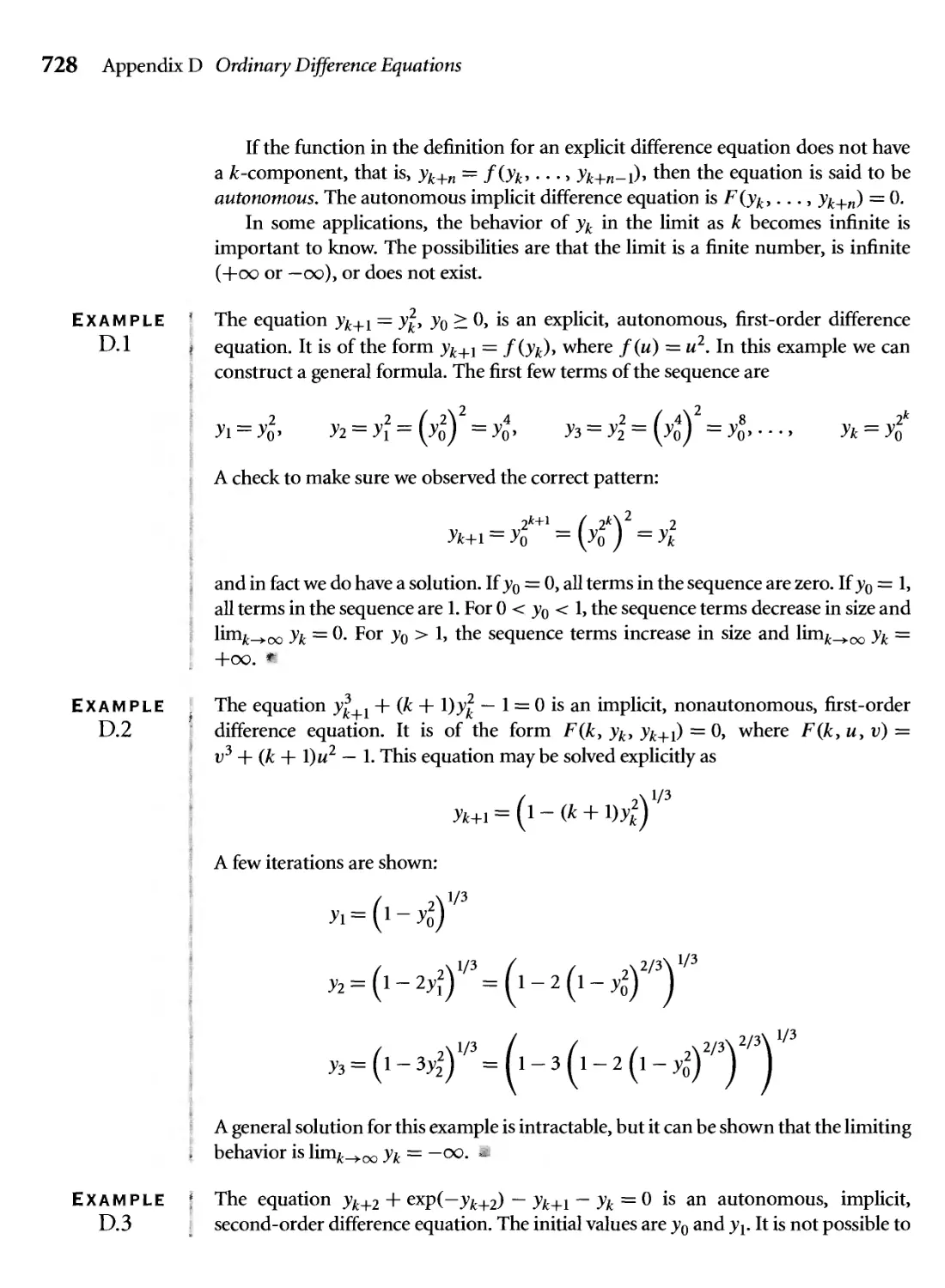
D.I Definitions 727
D.2 Linear Equations 730
D.2.1 First-Order Linear Equations 730
D.2.2 Second-Order Linear Equations 731
D.3 Constant-Coefficient equations 734
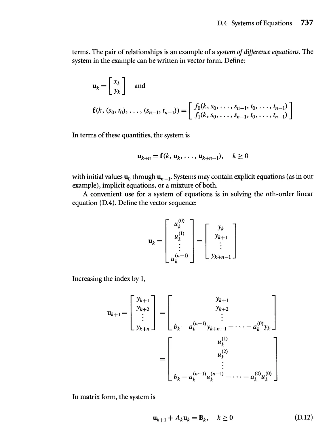
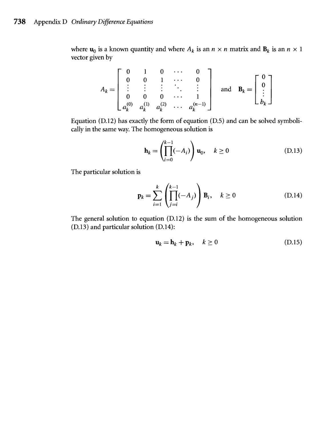
D.4 Systems of Equations 736
Bibliography 739
index 745

Figures
Color Plates
3.3 The Foucault pendulum.
3.7 A ball rolling down a hill.
3.14 A mass pulley spring system shown at two different times.
3.25 Two "snapshots" of a freely spinning top.
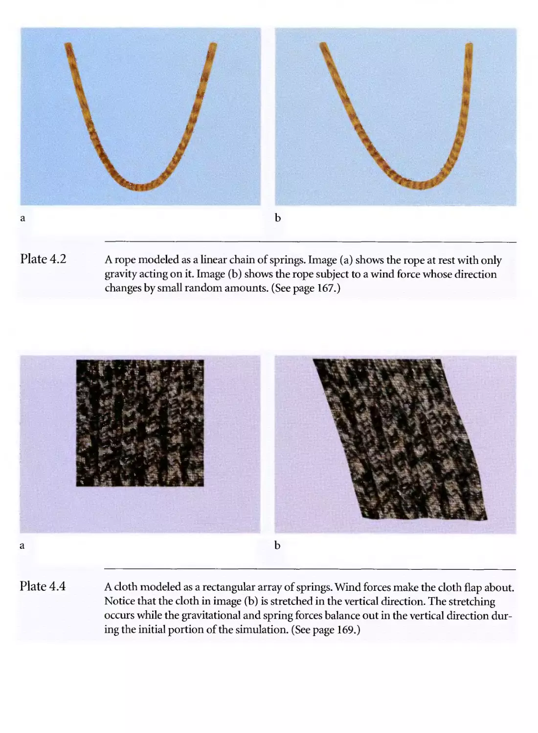
4.2 A rope modeled as a linear chain of springs.
4.4 A cloth modeled as a rectangular array of springs.
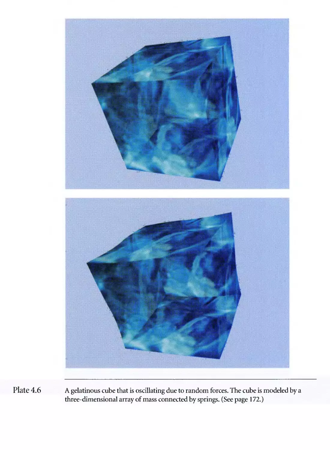
4.6 A gelatinous cube that is oscillating due to random forces.
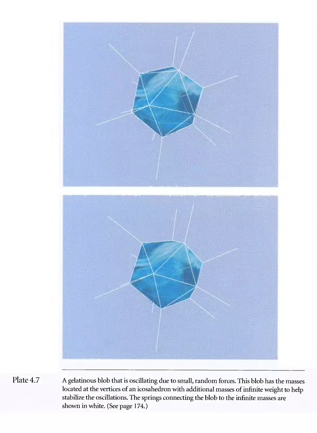
4.7 A gelatinous blob that is oscillating due to small, random forces.
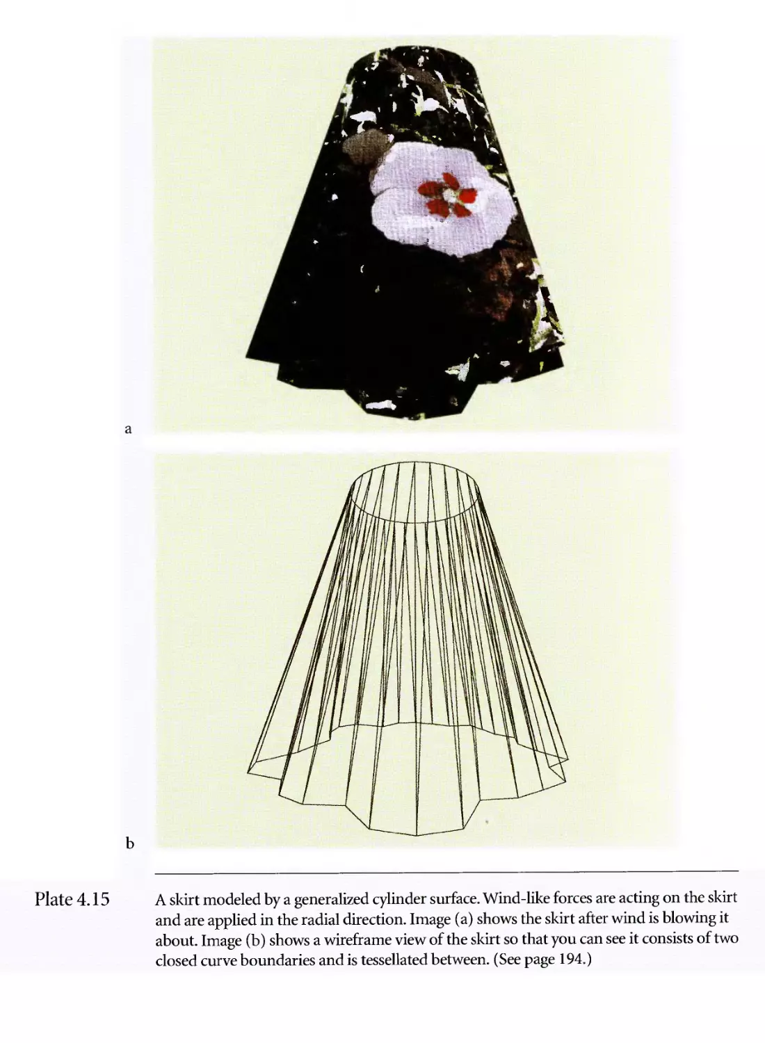
4.15 A skirt modeled by a generalized cylinder surface.
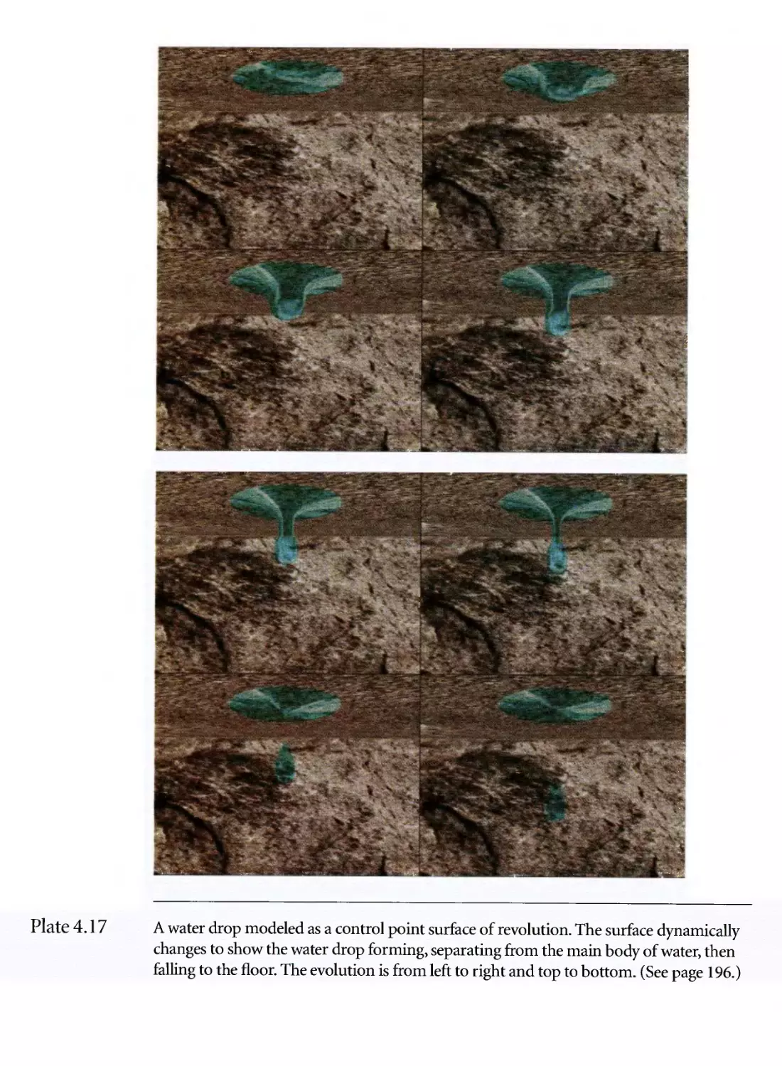
4.17 A water drop modeled as a control point surface of revolution.
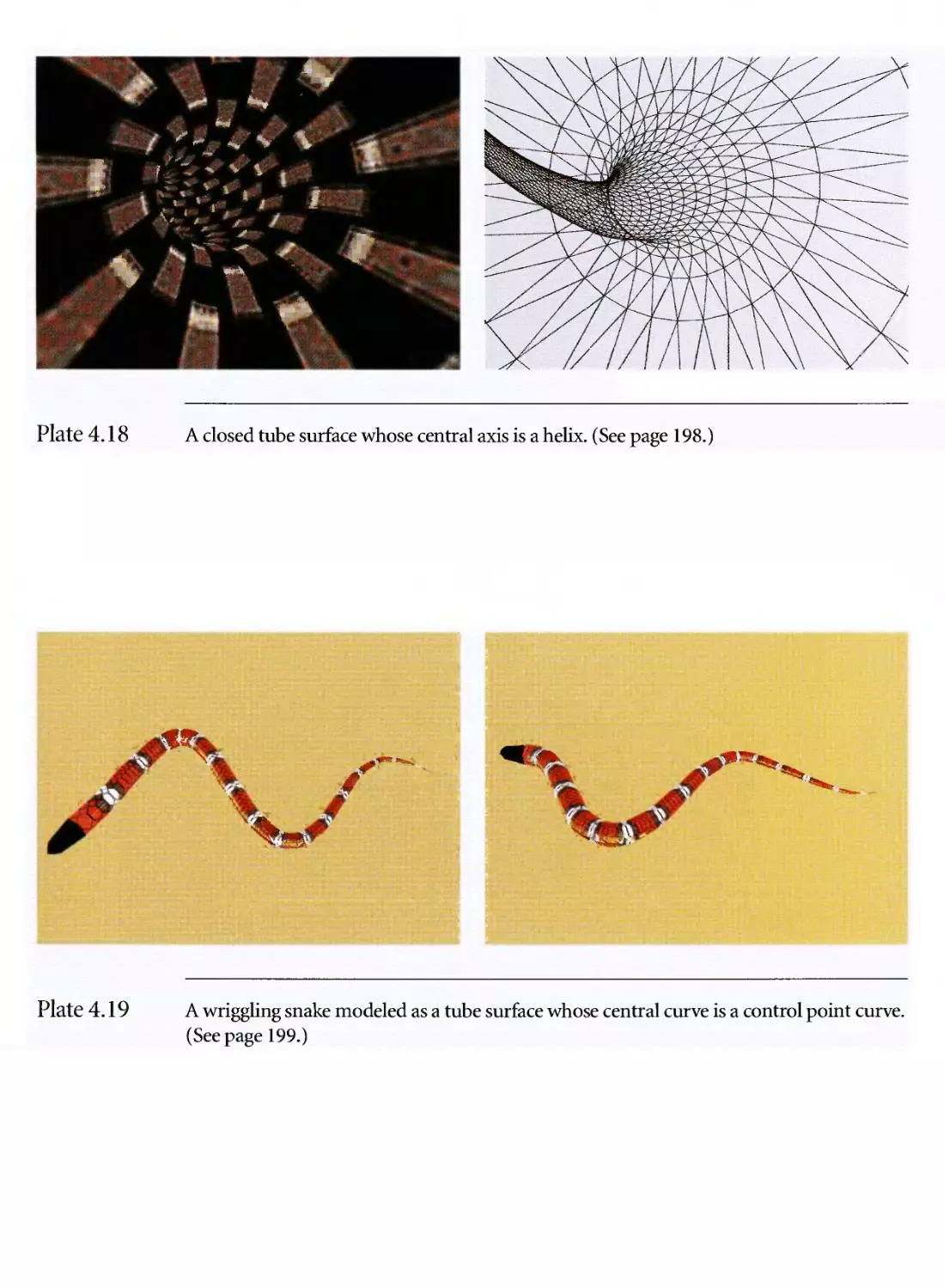
4.18 A closed tube surface whose central axis is a helix.
4.19 A wriggling snake modeled as a tube surface whose central curve is a
control point curve.
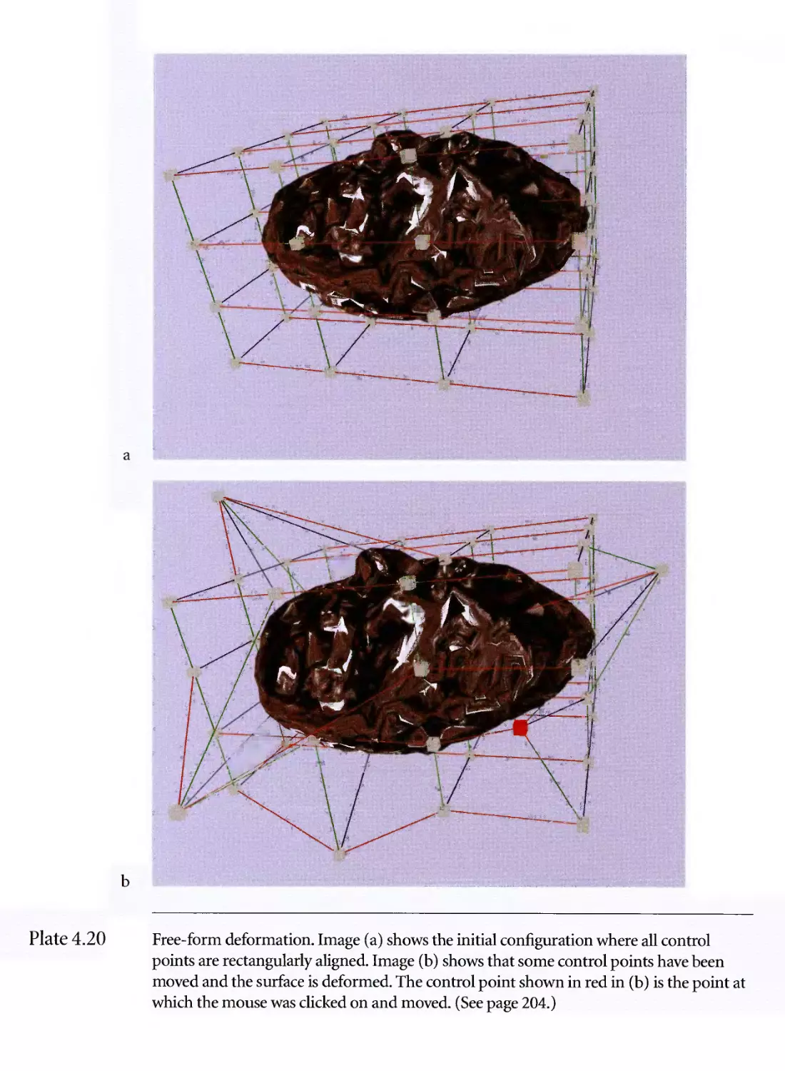
4.20 Free-form deformation.
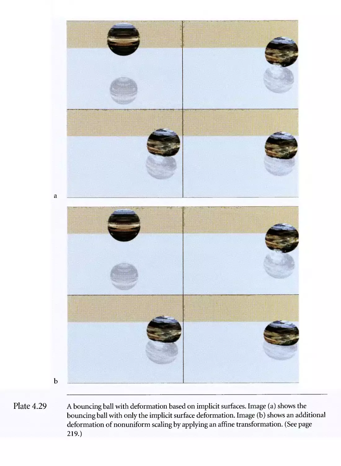
4.29 A bouncing ball with deformation based on implicit surfaces.
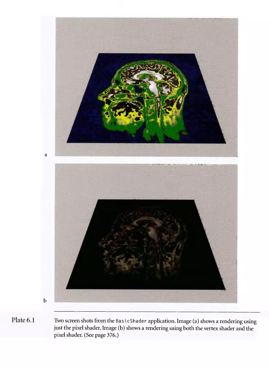
6.1 Two screen shots from the basic shader application.
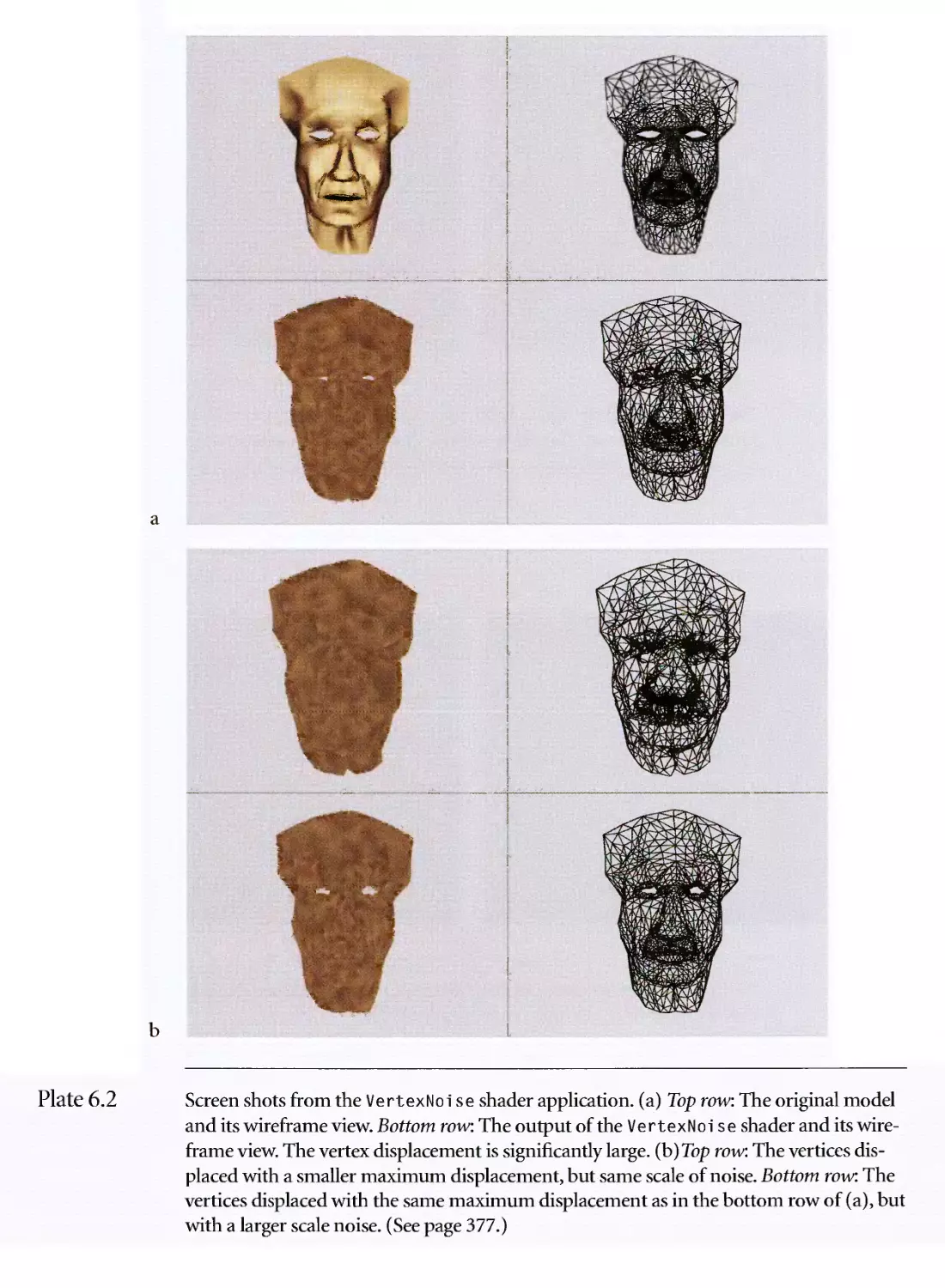
6.2 Screen shots from the vertex noise shader application.
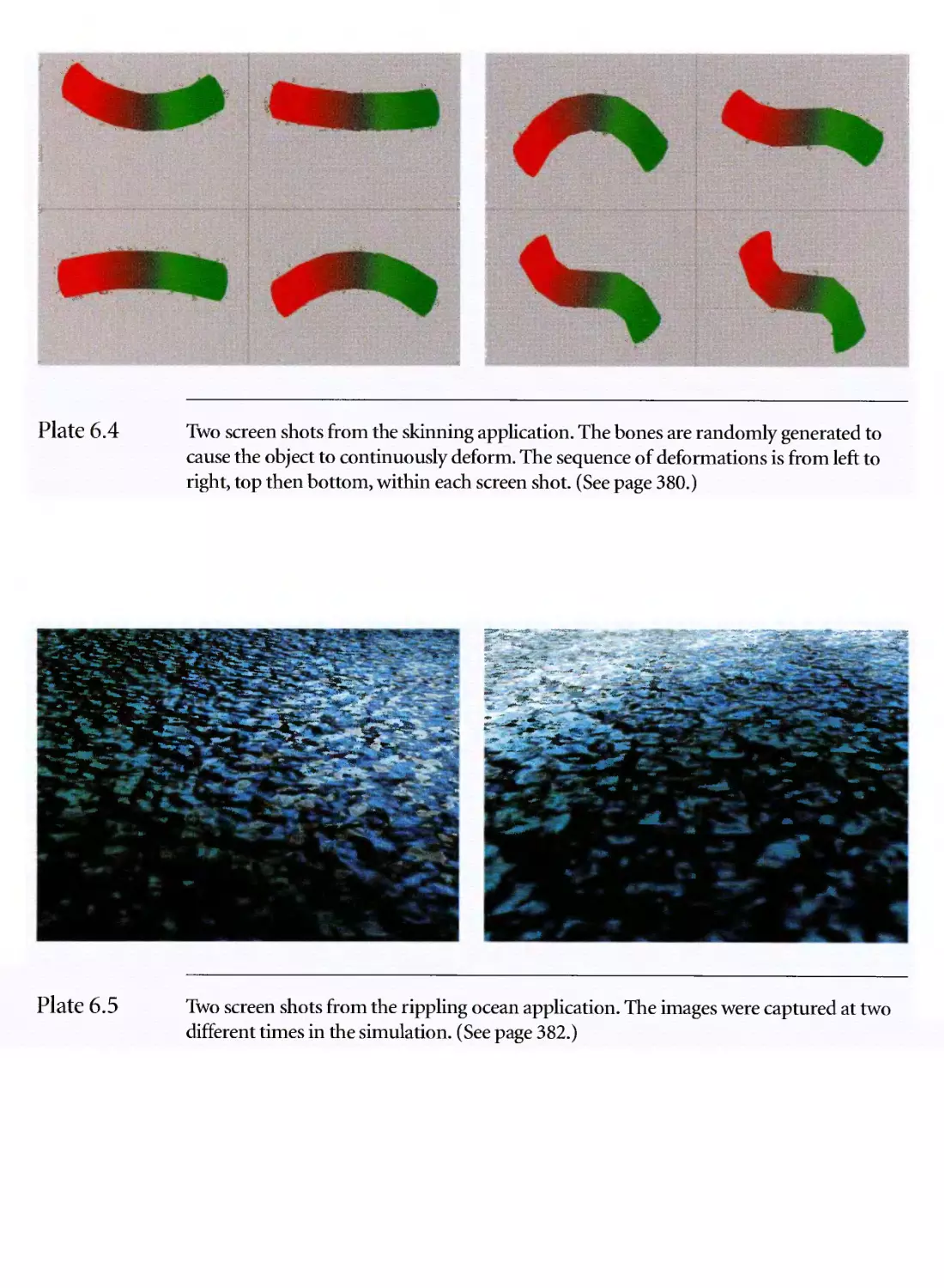
6.4 Two screen shots from the skinning application.
6.5 Two screen shots from the rippling ocean application.
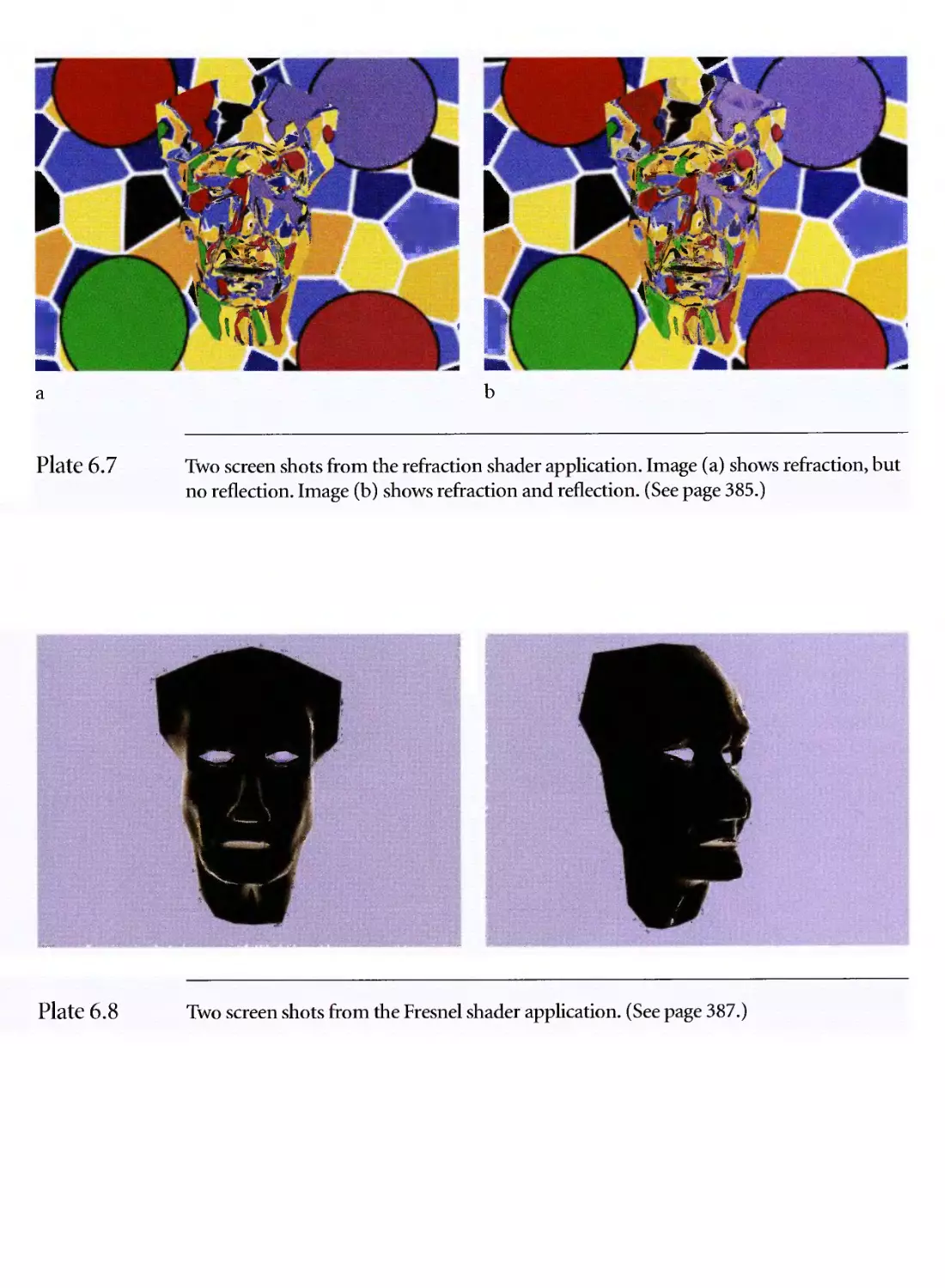
6.7 Two screen shots from the refraction shader application.
6.8 Two screen shots from the Fresnel shader application.
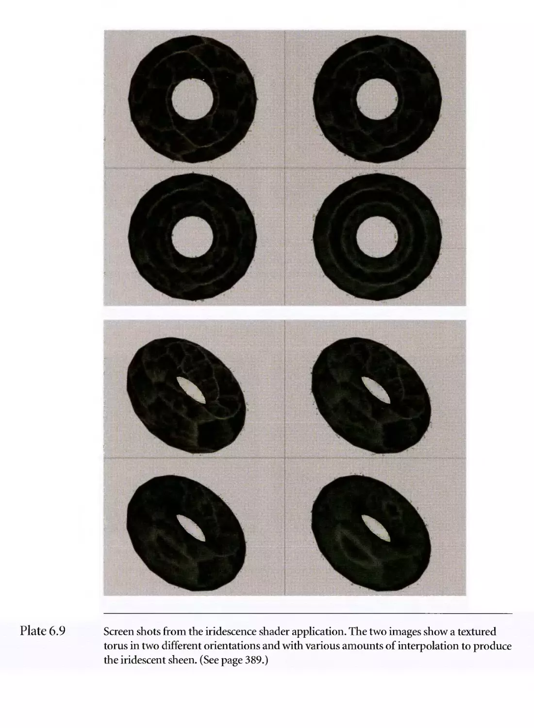
6.9 Screen shots from the iridescence shader application.
Figures in chapters
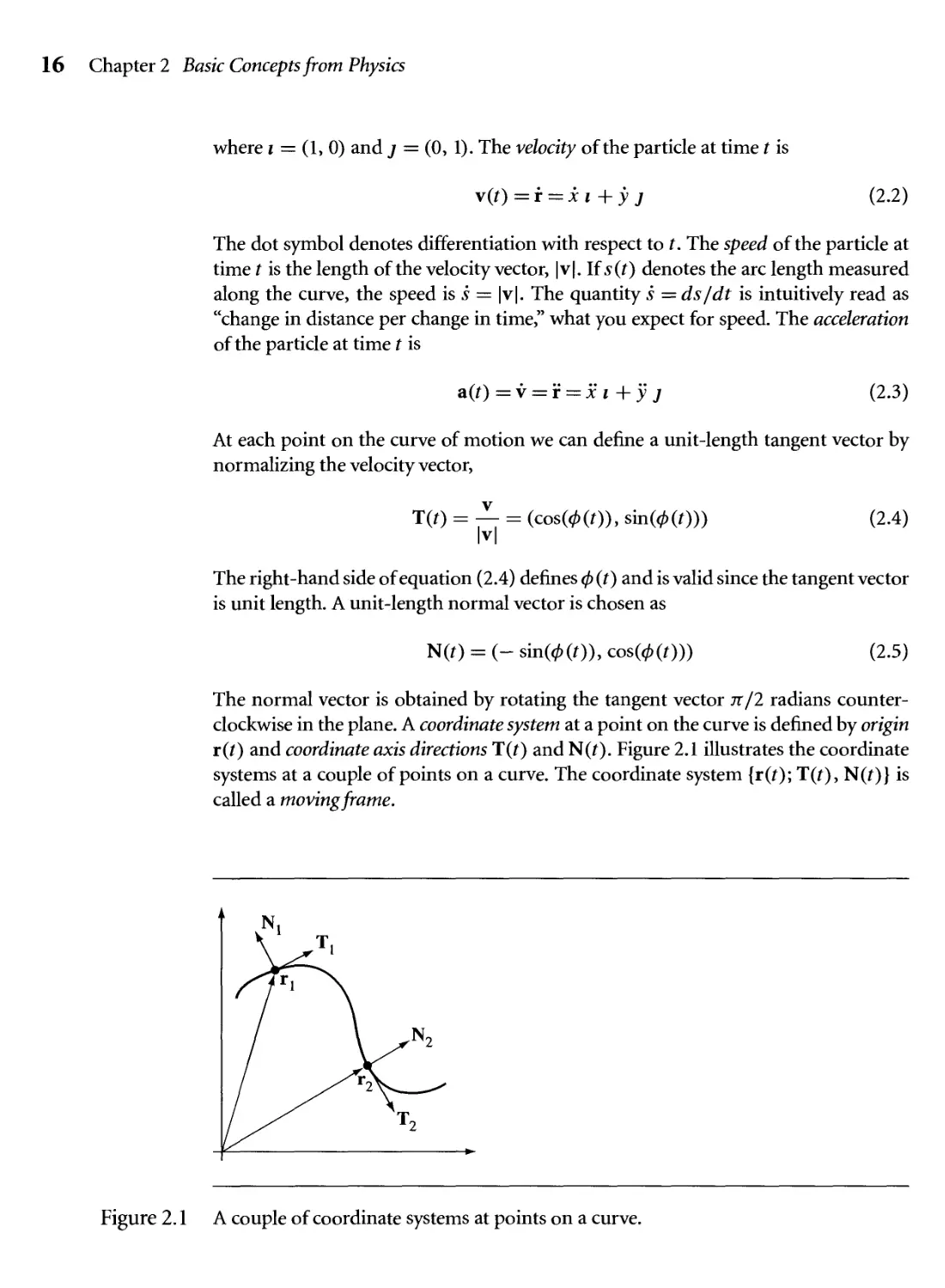
2.1 A couple of coordinate systems at points on a curve. 16
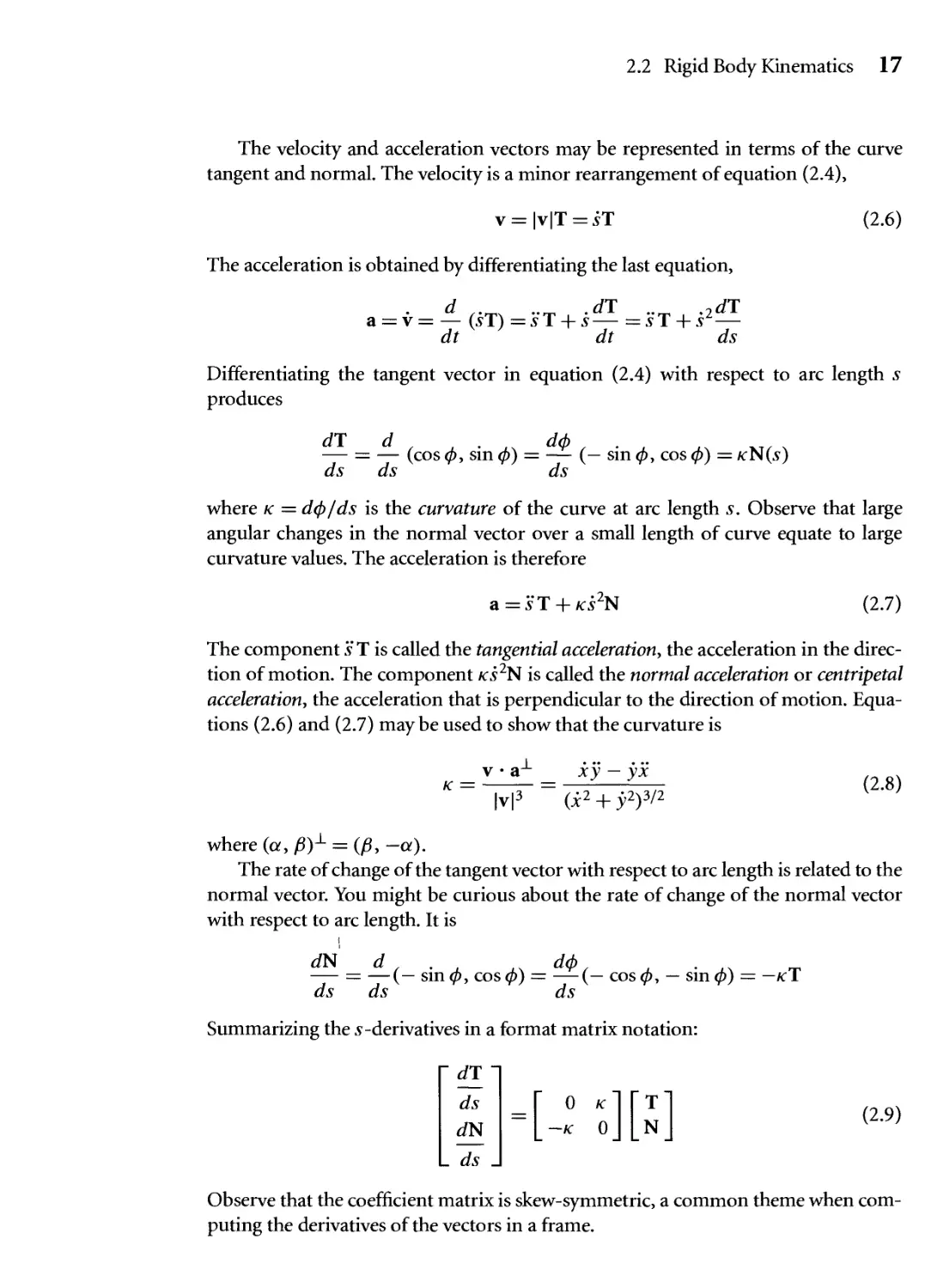
2.2 A polar coordinate frame at a point on a curve. 18
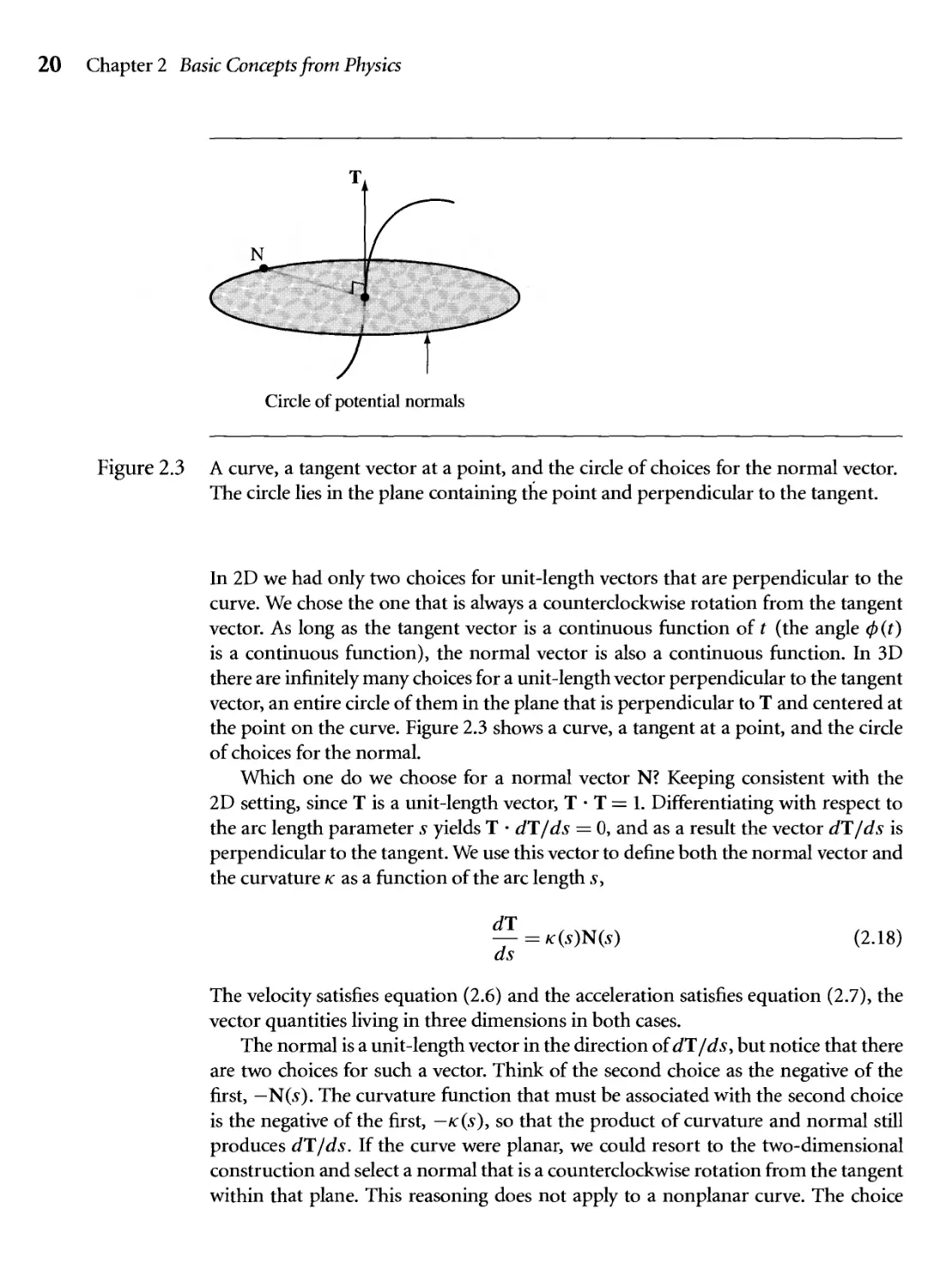
2.3 A curve, a tangent vector at a point, and the circle of choices for the
normal vector. The circle lies in the plane containing the point and
perpendicular to the tangent. 20
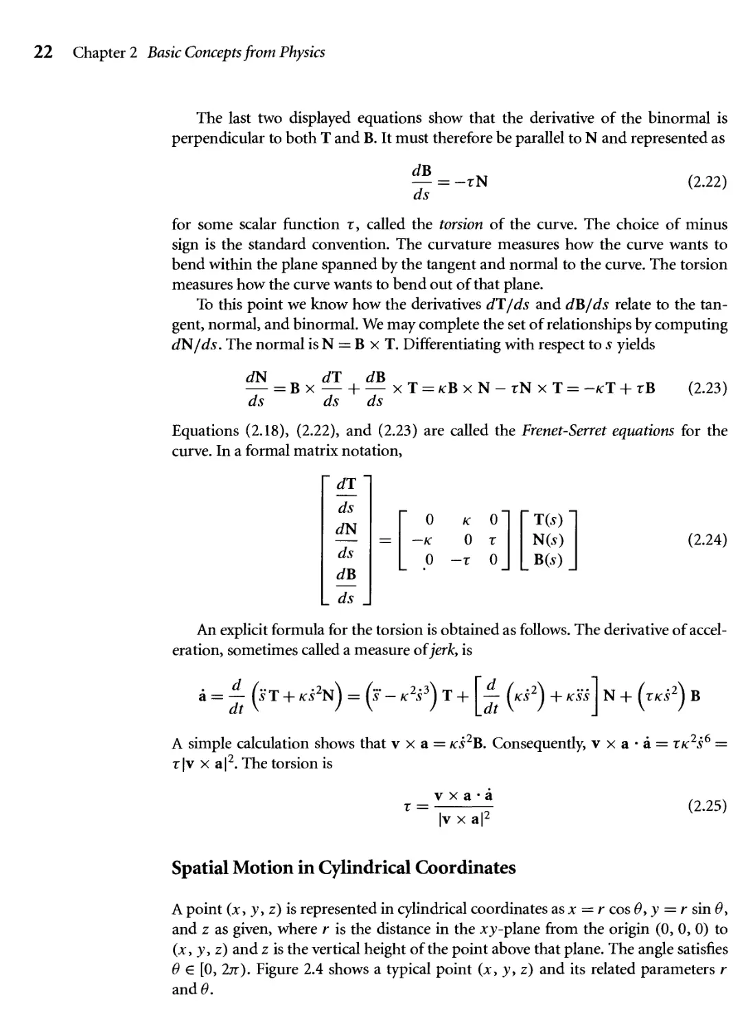
2.4 Cylindrical coordinates (jc, y, z) = (r cos 9, r sin в, z). 23
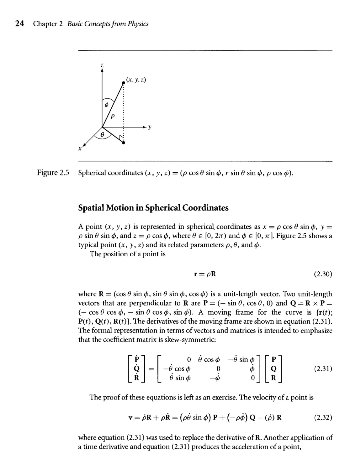
2.5 Spherical coordinates (x, y, z) = (p cos в sin ф, г sin в sin ф, p cos ф). 24
XV

xvi Figures
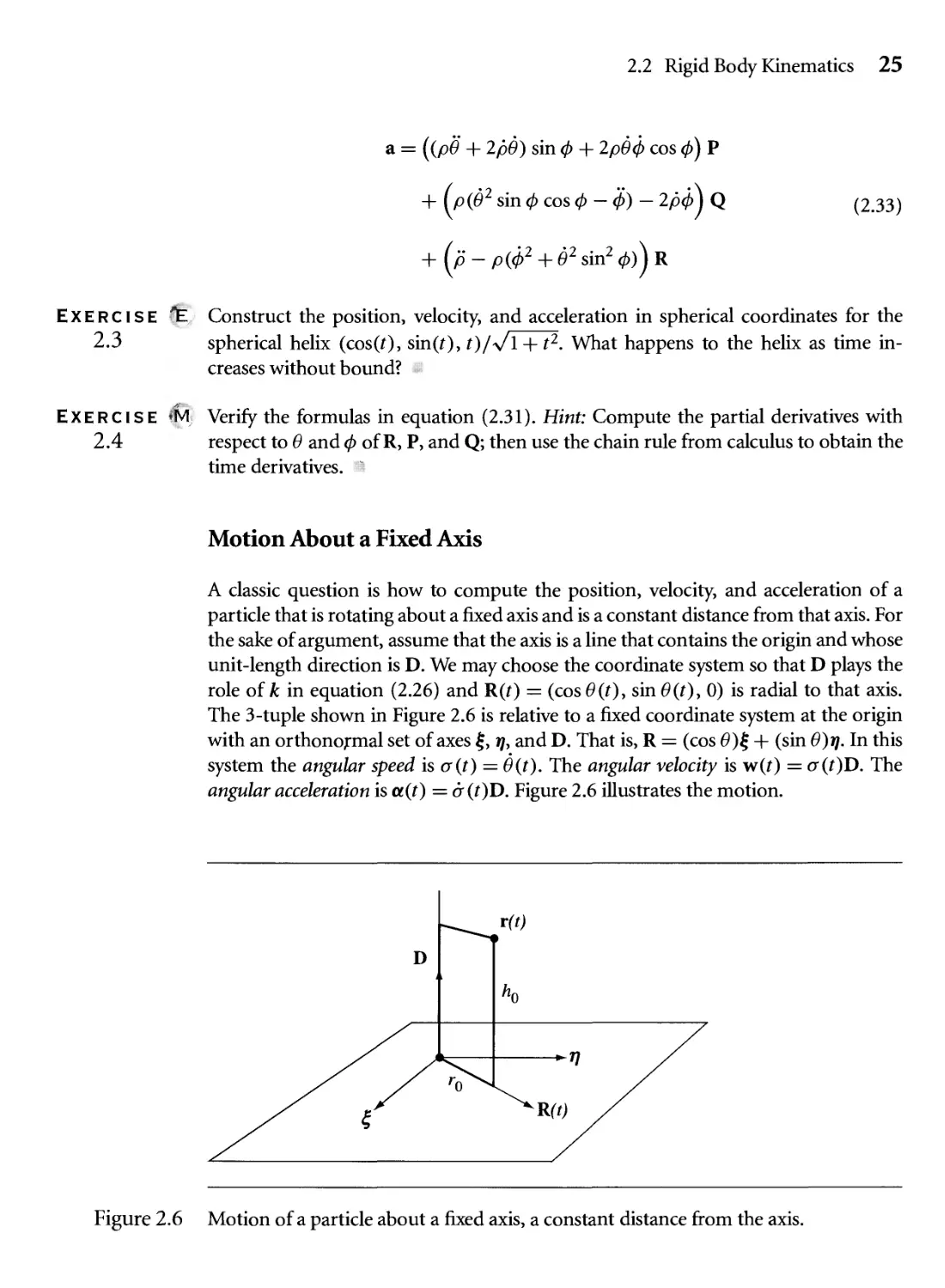
2.6 Motion of a particle about a fixed axis, a constant distance from the
axis. 25
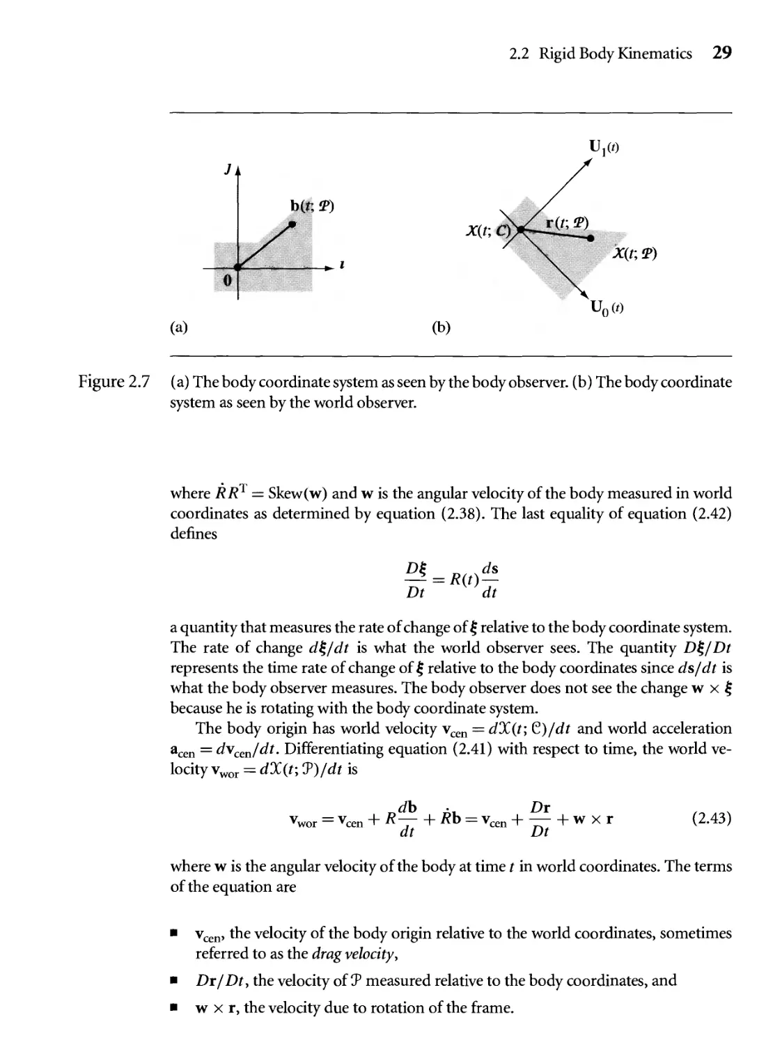
2.7 (a) The body coordinate system as seen by the body observer, (b) The
body coordinate system as seen by the world observer. 29
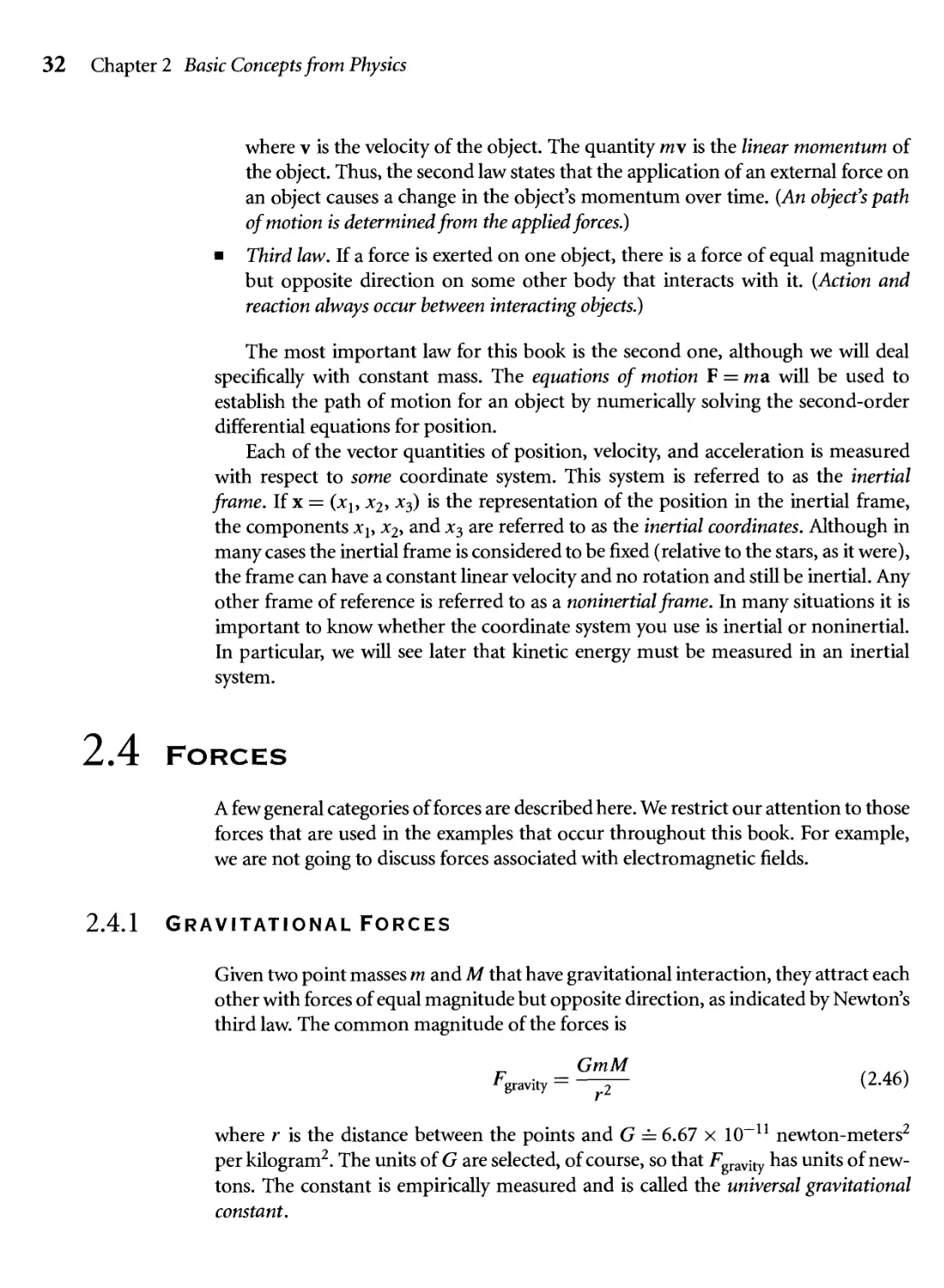
2.8 Gravitational forces on objects located at various places around the
Earth. 33
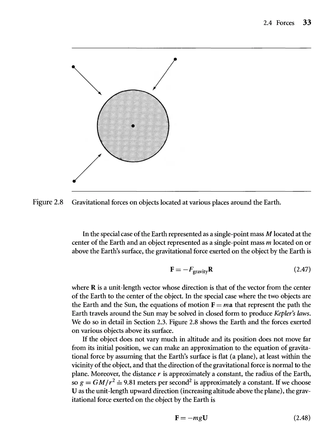
2.9 Gravitational forces on objects located nearly on the Earth's surface,
viewed as a flat surface. 34
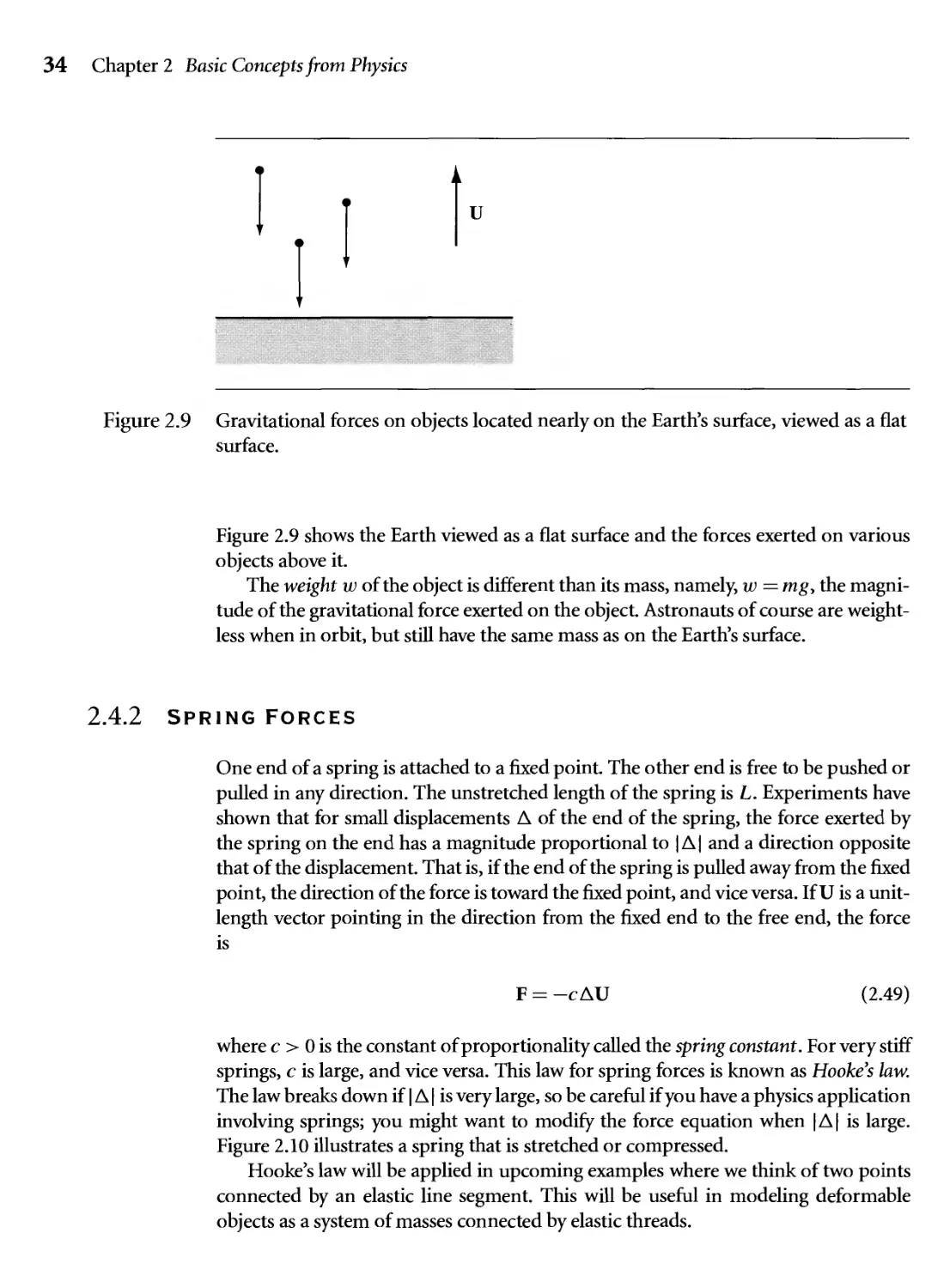
2.10 (a) Unstretched spring, (b) Force due to stretching the spring, (c)
Force due to compressing the string. 35
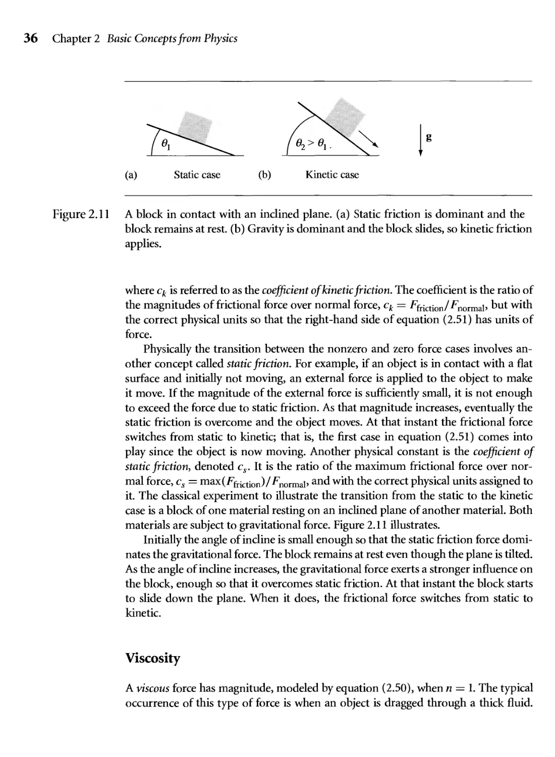
2.11 A block in contact with an inclined plane, (a) Static friction is
dominant and the block remains at rest, (b) Gravity is dominant and
the block slides, so kinetic friction applies. 36
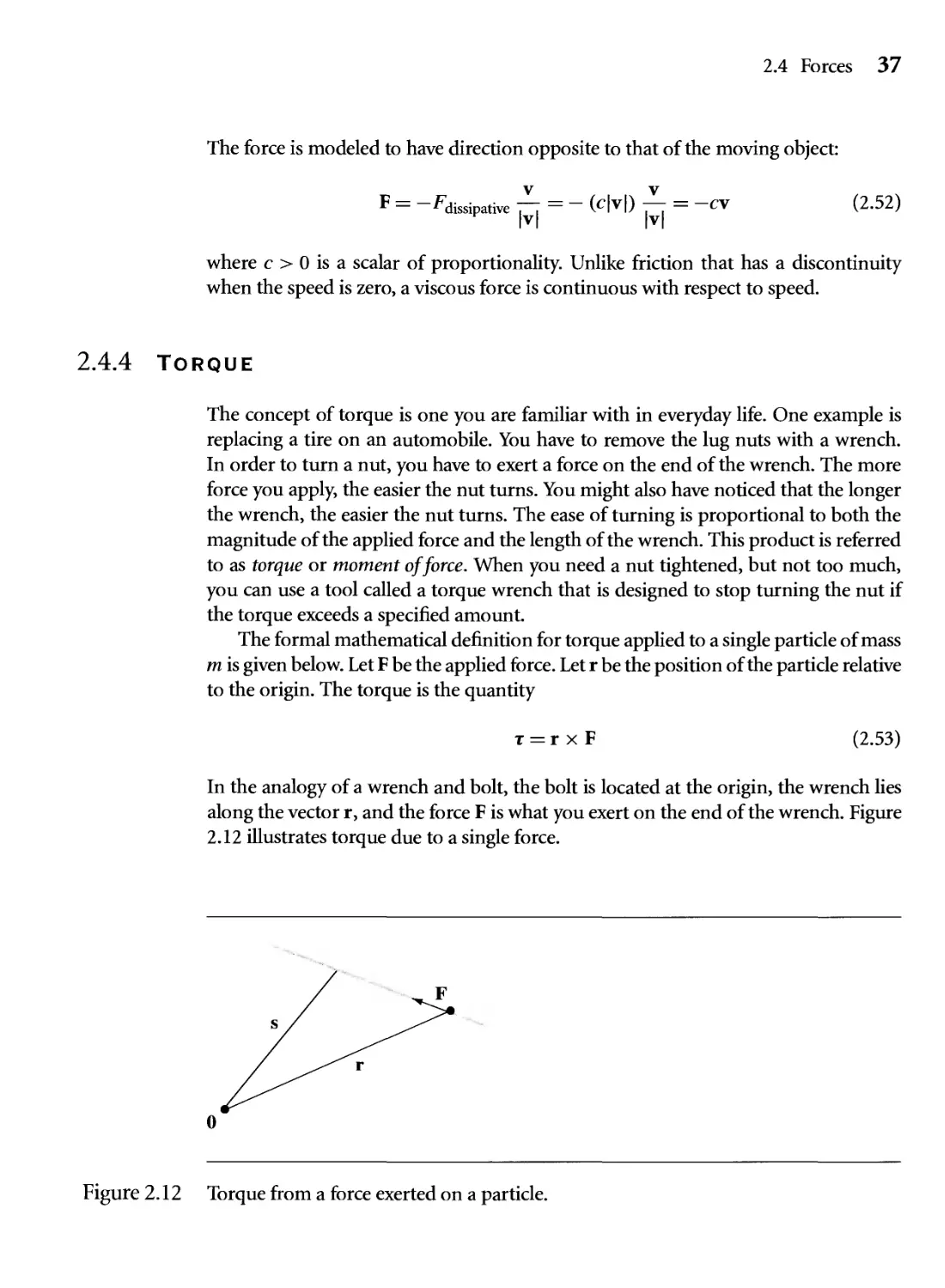
2.12 Torque from a force exerted on a particle. 37
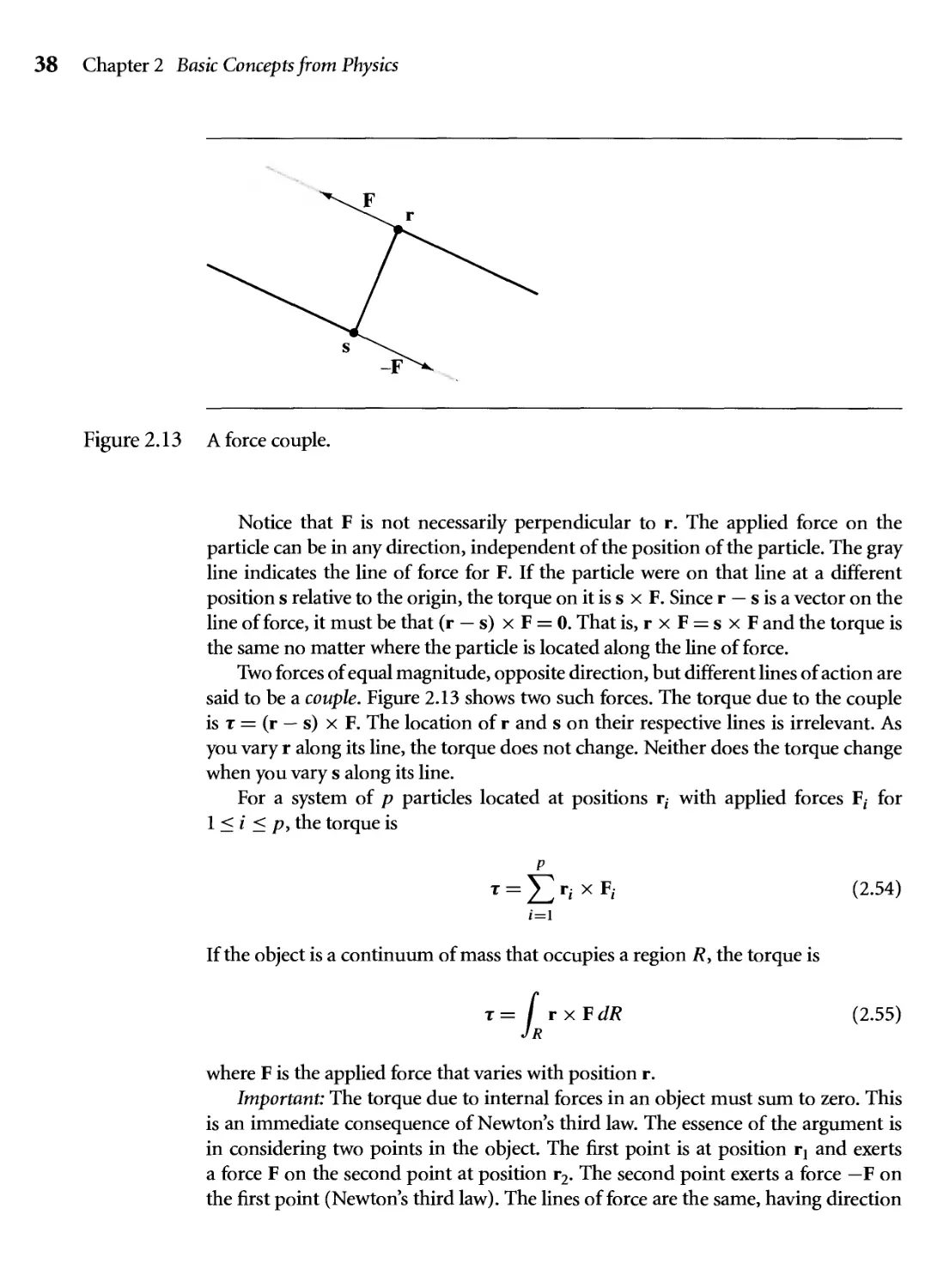
2.13 A force couple. 38
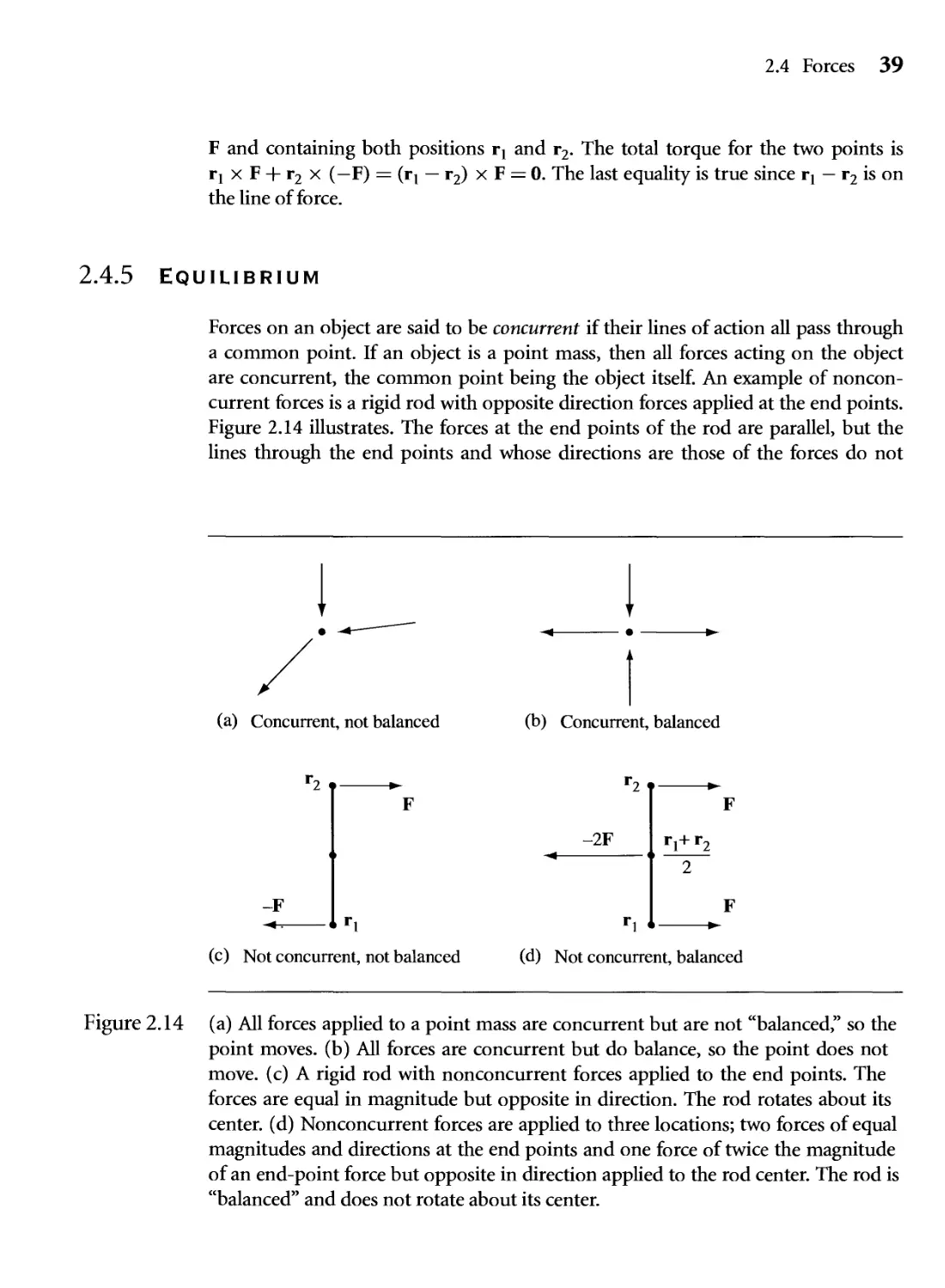
2.14 (a) All forces applied to a point mass are concurrent but are not
"balanced," so the point moves, (b) All forces are concurrent
but do balance, so the point does not move, (c) A rigid rod with
nonconcurrent forces applied to the end points. The forces are equal
in magnitude but opposite in direction. The rod rotates about its
center, (d) Nonconcurrent forces are applied to three locations; two
forces of equal magnitudes and directions at the end points and one
force of twice the magnitude of an end-point force but opposite in
direction applied to the rod center. The rod is "balanced" and does
not rotate about its center. 39
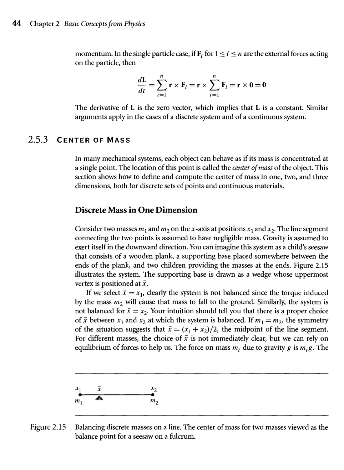
2.15 Balancing discrete masses on a line. The center of mass for two masses
viewed as the balance point for a seesaw on a fulcrum. 44
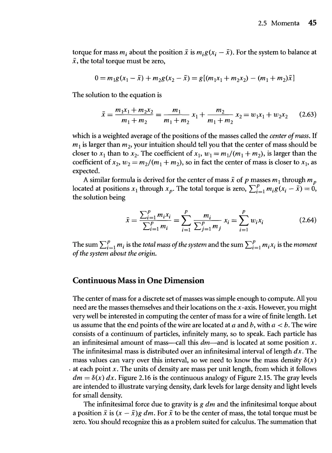
2.16 Balancing continuous masses on a line. The center of mass for the
wire is viewed as the balance point for a seesaw on a fulcrum. A
general point location jc is shown, labeled with its corresponding mass
density 8 (jc). 46
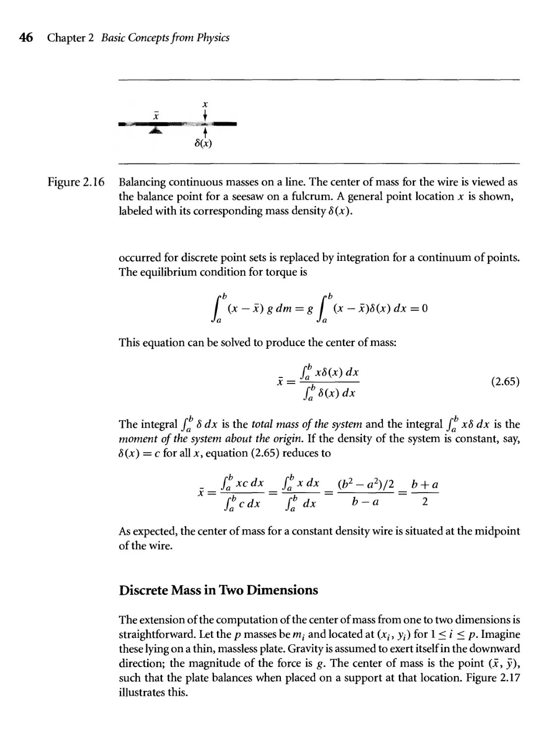
2.17 Balancing discrete masses in a plane. 47
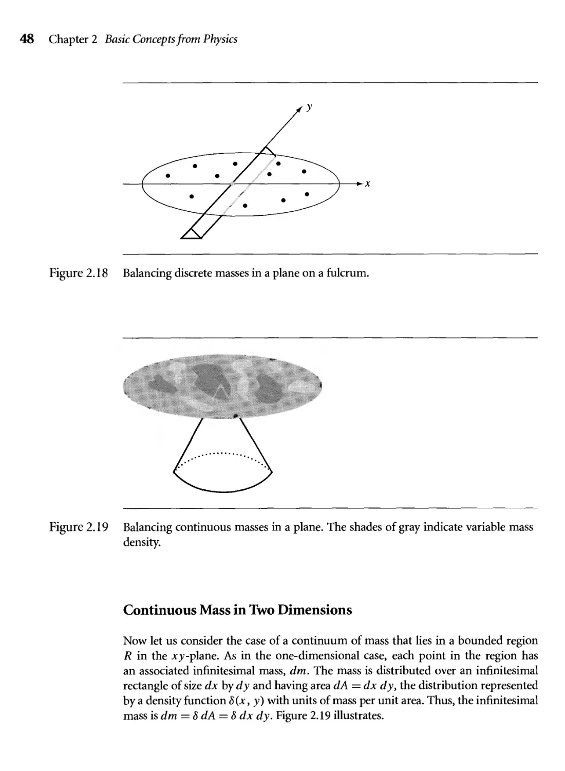
2.18 Balancing discrete masses in a plane on a fulcrum. 48
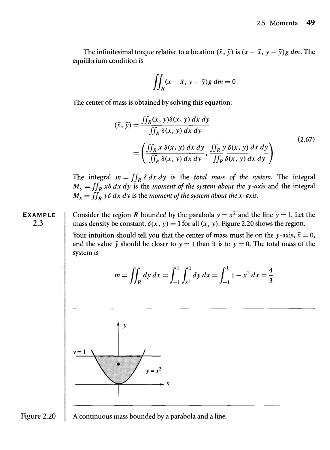
2.19 Balancing continuous masses in a plane. The shades of gray indicate
variable mass density. 48
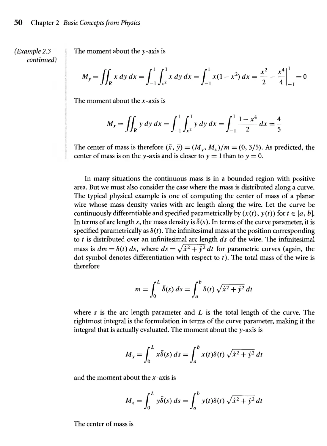
2.20 A continuous mass bounded by a parabola and a line. 49
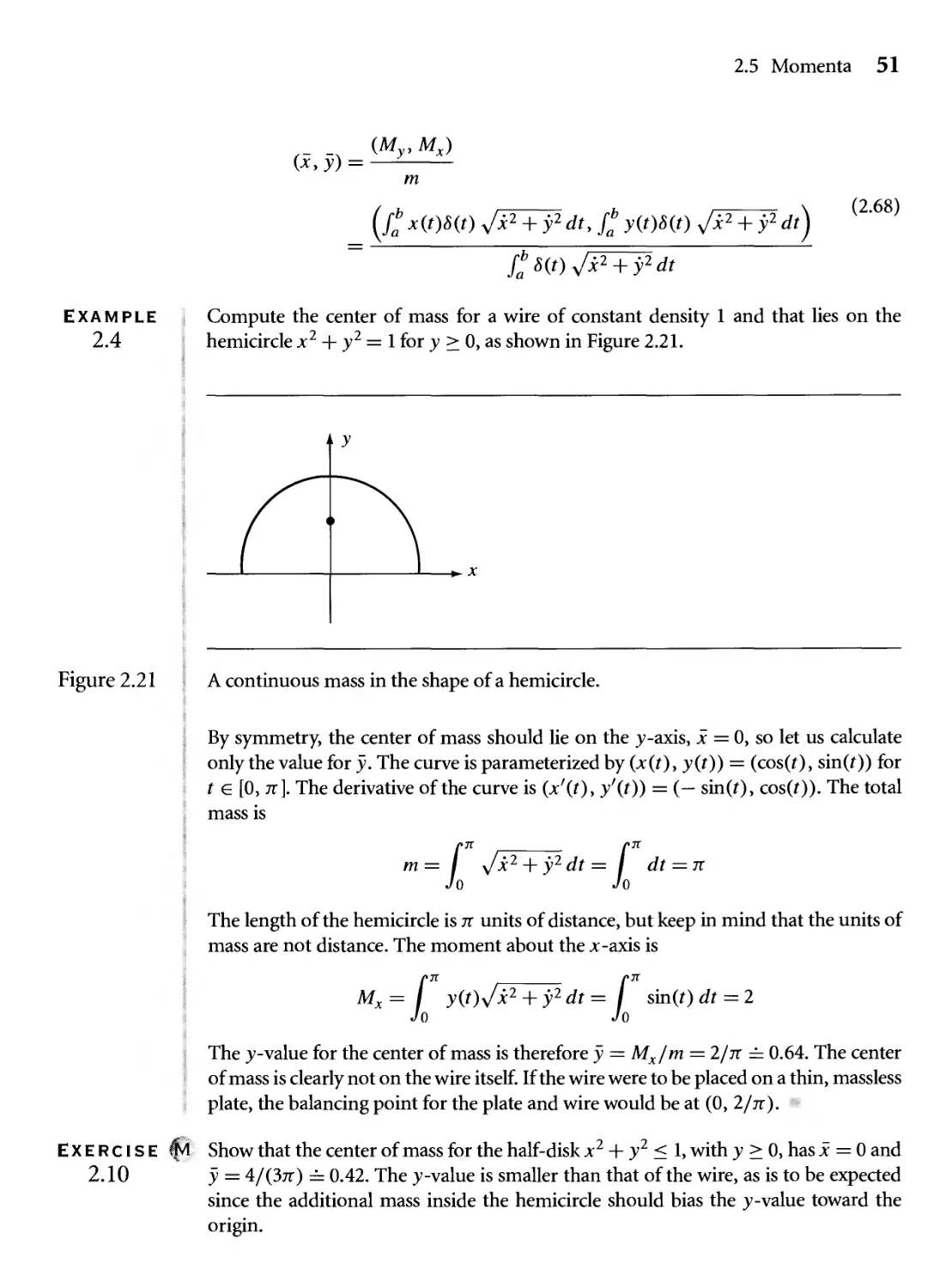
2.21 A continuous mass in the shape of a hemicircle. 51
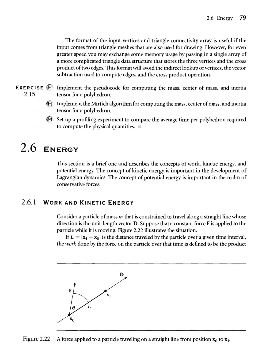
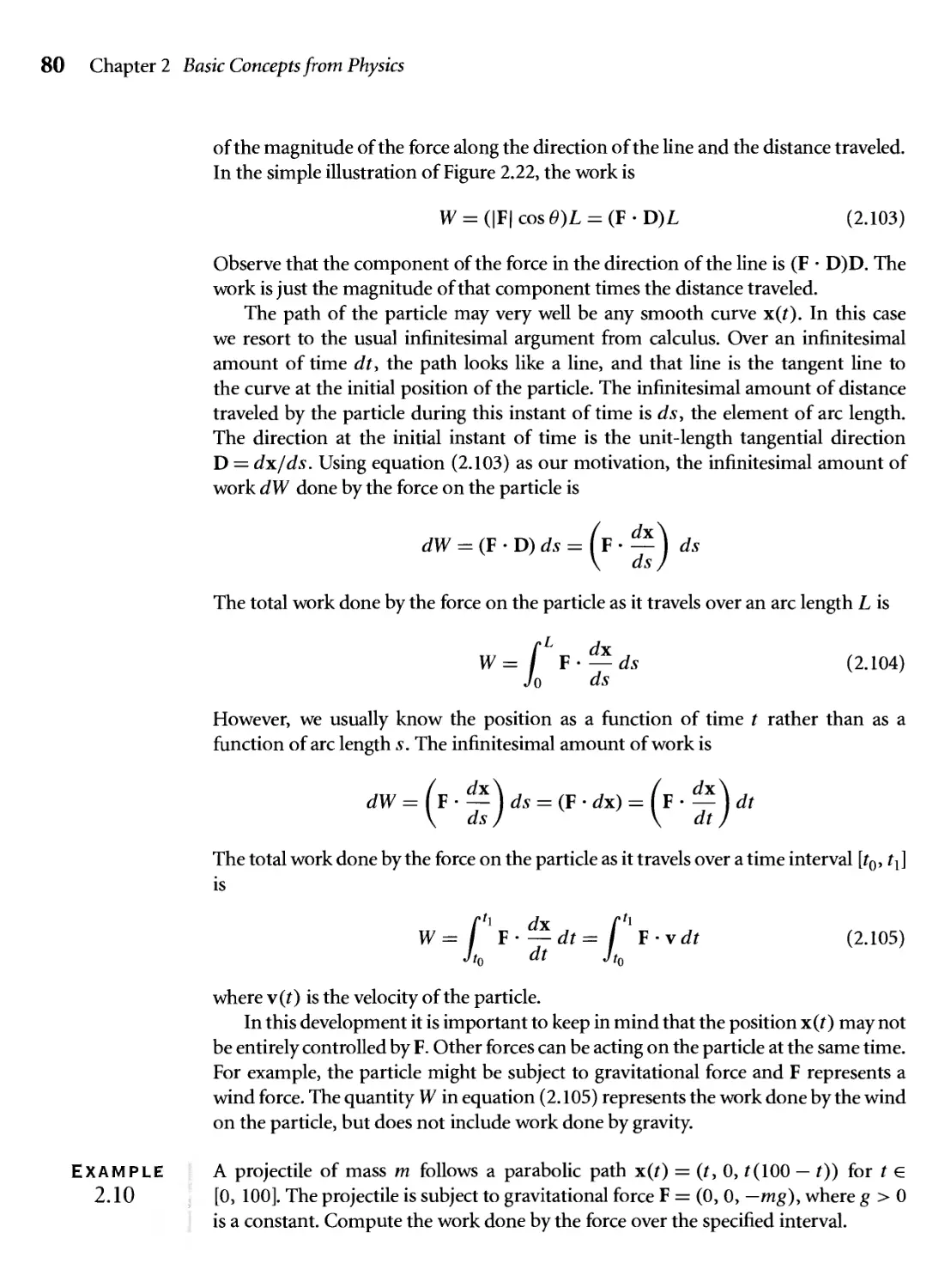
2.22 A force applied to a particle traveling on a straight line from position
Xo to Xj. 79

Figures xvii
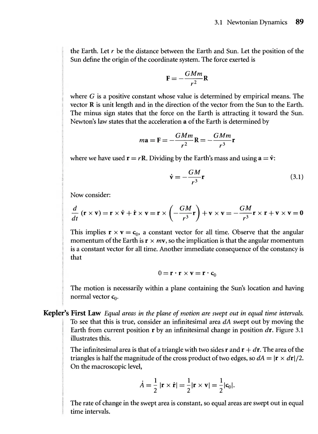
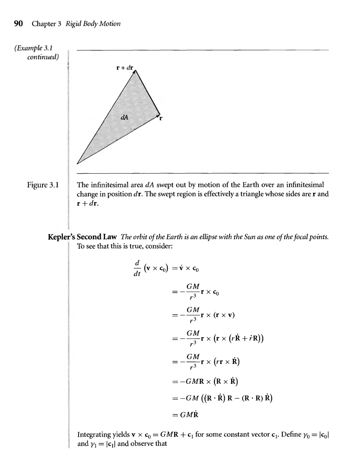
3.1 The infinitesimal area dA swept out by motion of the Earth over an
infinitesimal change in position dr. The swept region is effectively a
triangle whose sides are r and r + dr. 90
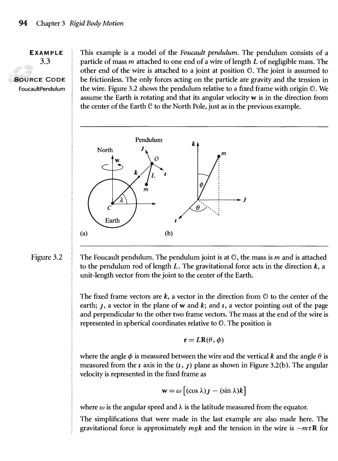
3.2 The Foucault pendulum. The pendulum joint is at 0, the mass is m
and is attached to the pendulum rod of length L. The gravitational
force acts in the direction k, a unit-length vector from the joint to the
center of the Earth. 94
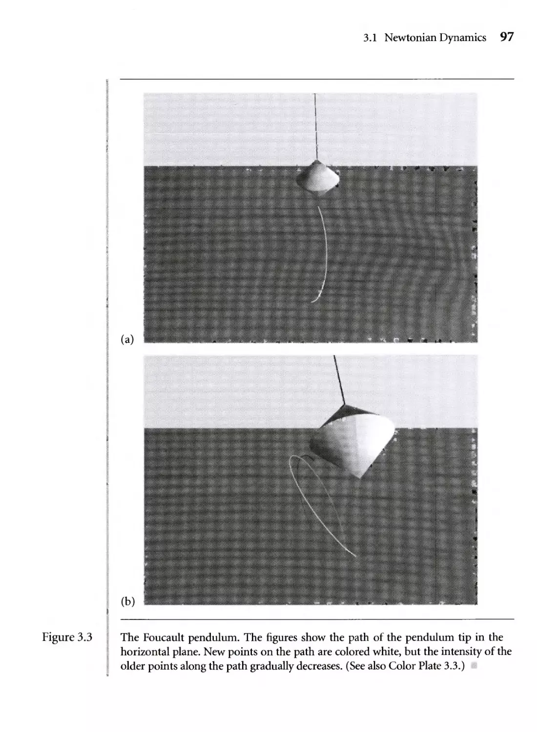
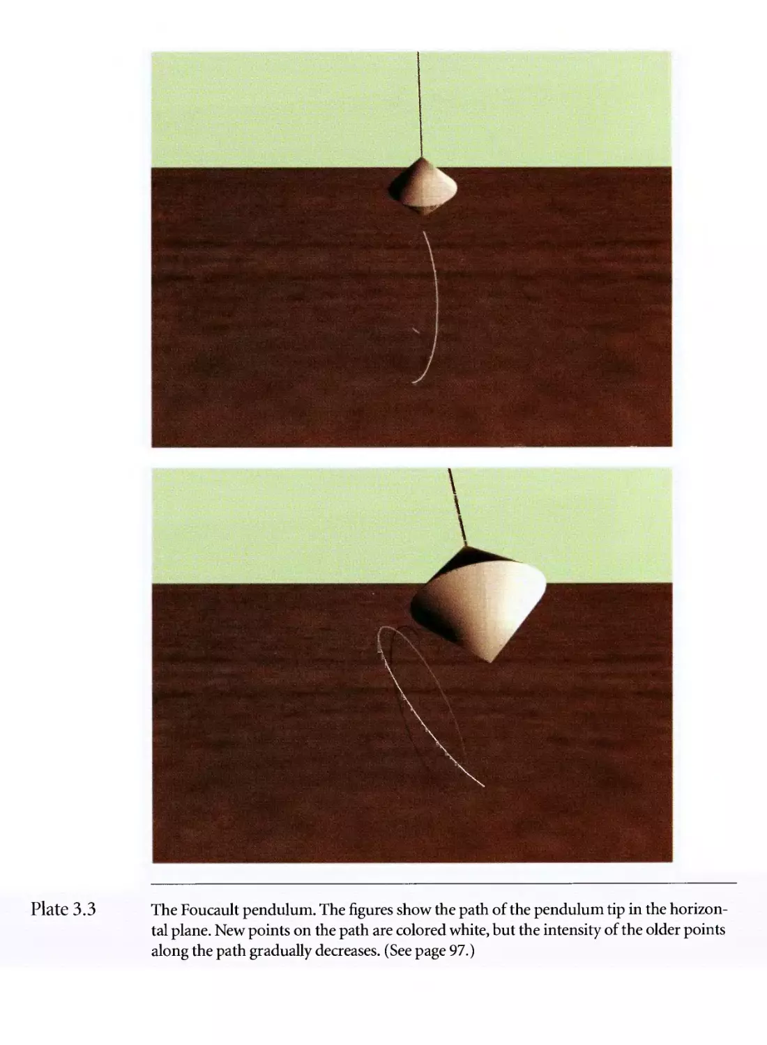
3.3 The Foucault pendulum. The figures show the path of the pendulum
tip in the horizontal plane. New points on the path are colored
white, but the intensity of the older points along the path gradually
decreases. (See also Color Plate 3.3.) 97
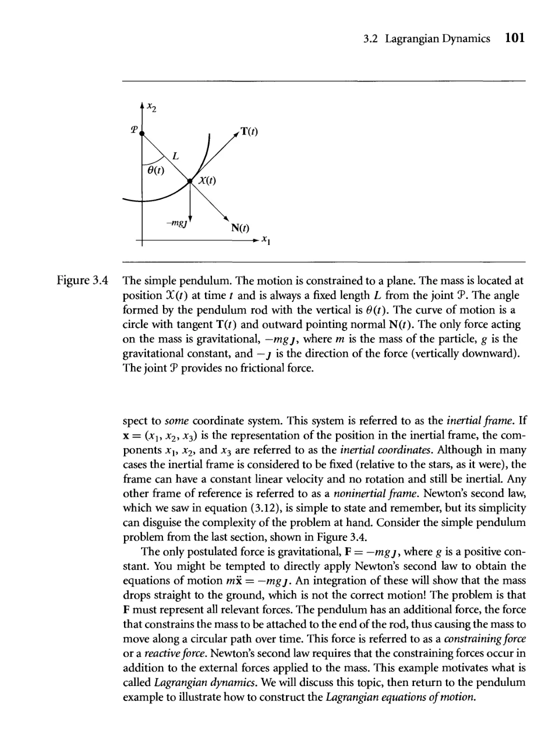
3.4 The simple pendulum. The motion is constrained to a plane. The
mass is located at position X(t) at time t and is always a fixed length
L from the joint CP. The angle formed by the pendulum rod with the
vertical is 9{t). The curve of motion is a circle with tangent T{t) and
outward pointing normal N@- The only force acting on the mass
is gravitational, —mgj, where m is the mass of the particle, g is the
gravitational constant, and —j is the direction of the force (vertically
downward). The joint CP provides no frictional force. 101
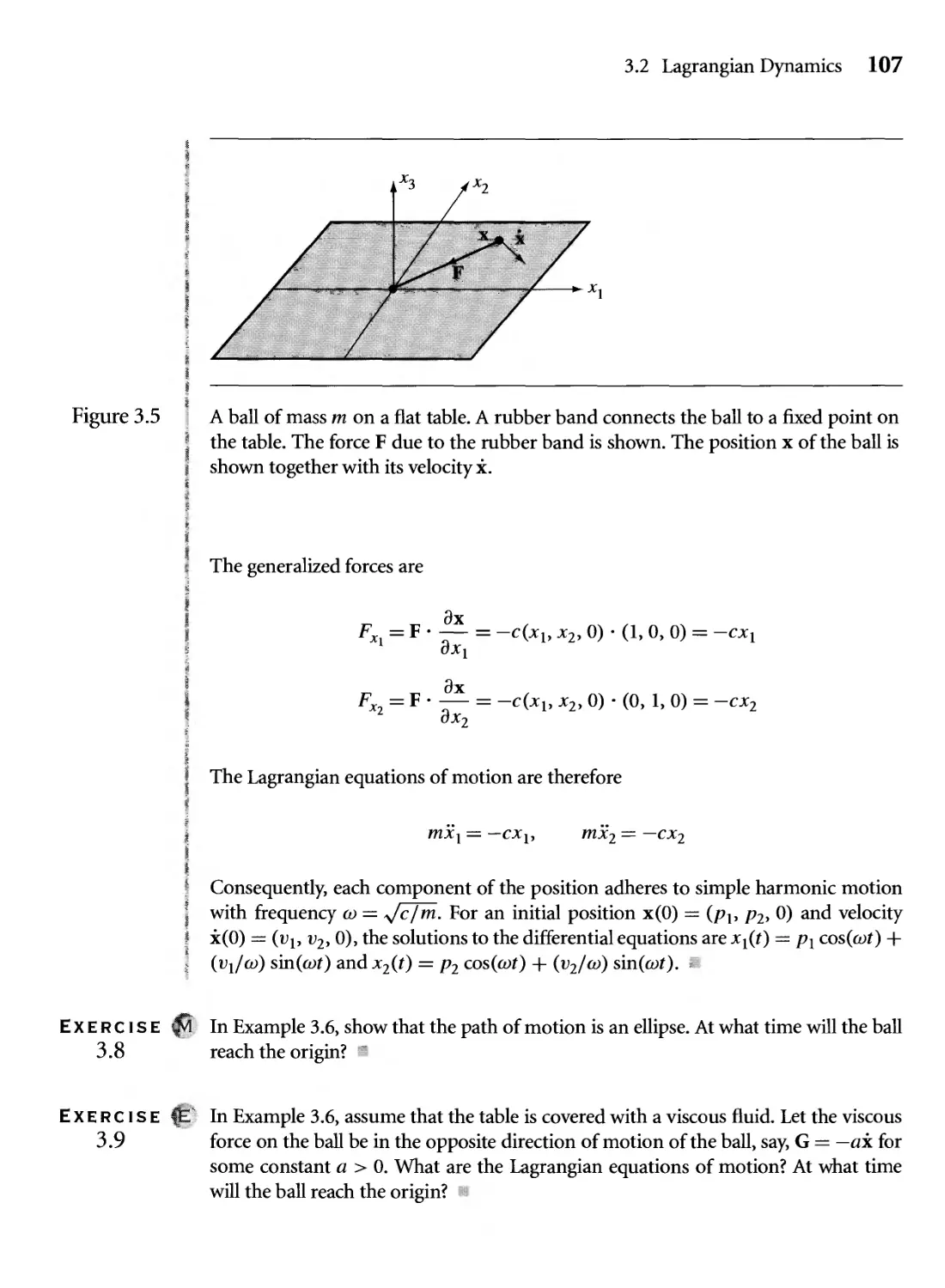
3.5 A ball of mass m on a flat table. A rubber band connects the ball to a
fixed point on the table. The force F due to the rubber band is shown.
The position x of the ball is shown together with its velocity x. 107
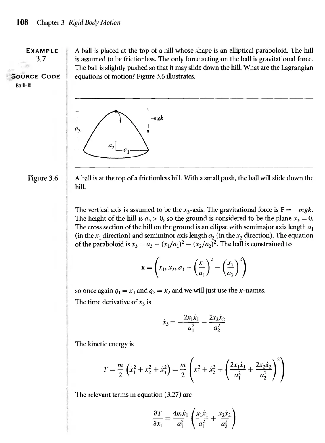
3.6 A ball is at the top of a frictionless hill. With a small push, the ball will
slide down the hill. 108
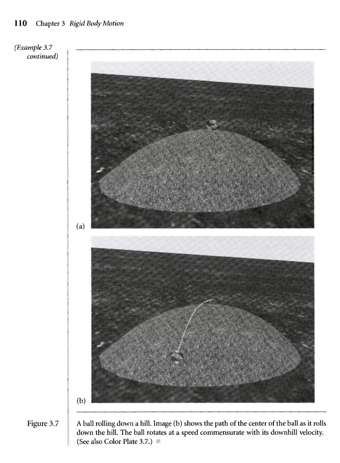
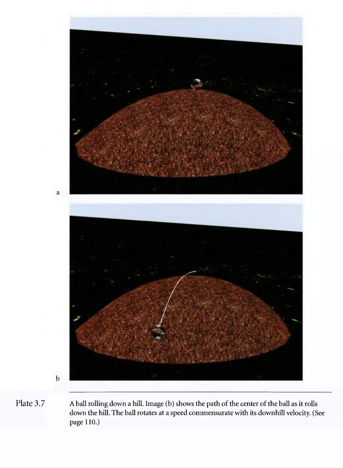
3.7 A ball rolling down a hill. Image (b) shows the path of the center of the
ball as it rolls down the hill. The ball rotates at a speed commensurate
with its downhill velocity. (See also Color Plate 3.7.) 110
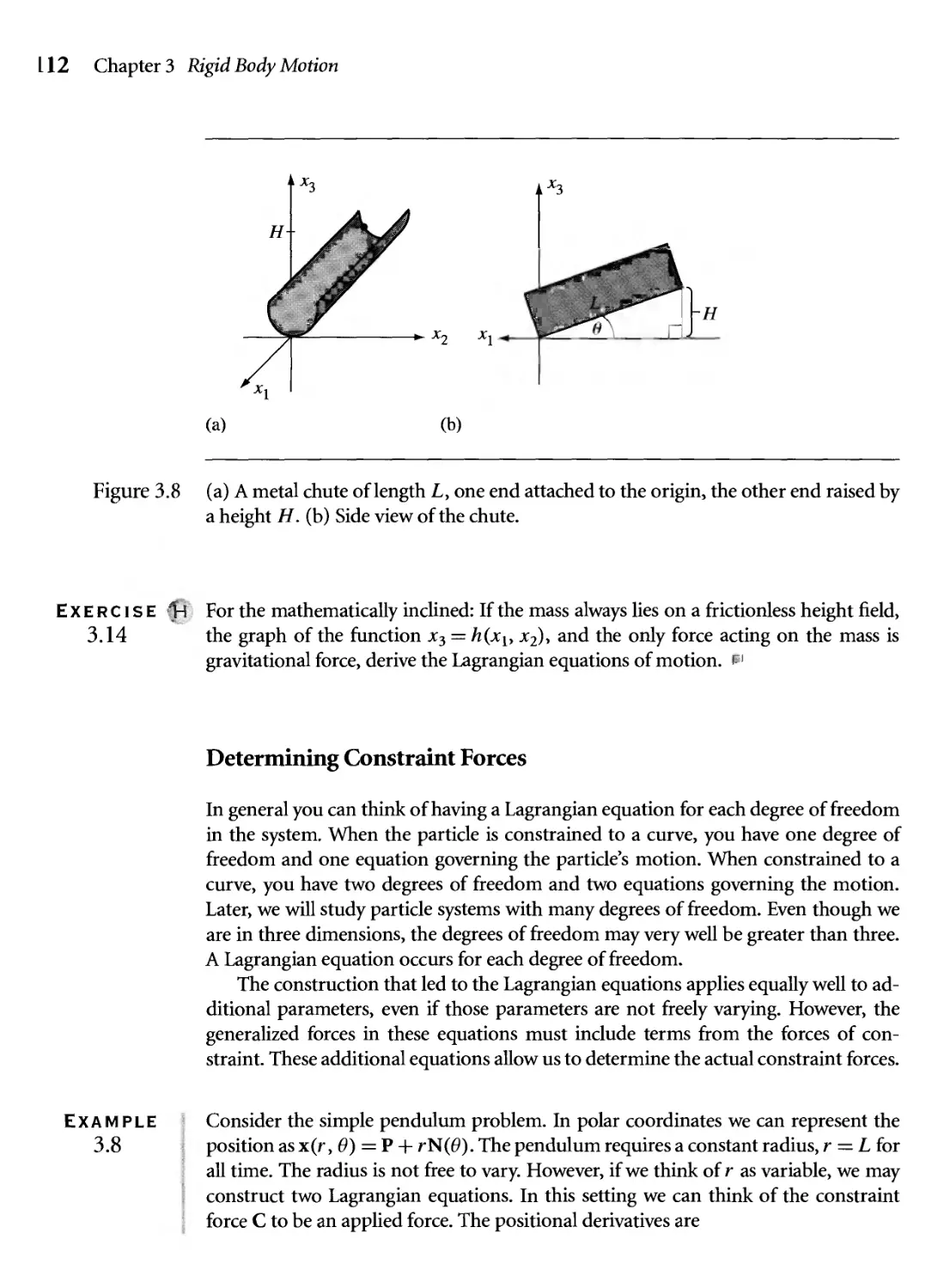
3.8 (a) A metal chute of length L, one end attached to the origin, the
other end raised by a height H. (b) Side view of the chute. 112
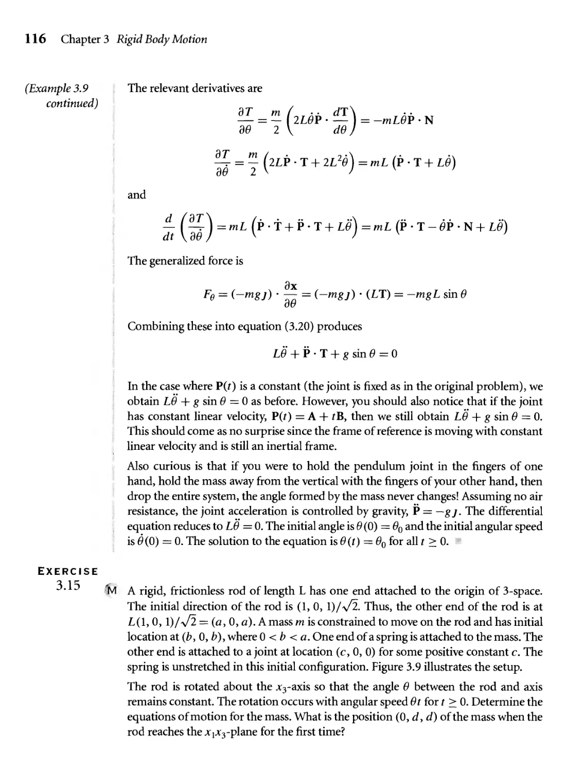
3.9 The initial configuration of a rigid rod containing a mass that is
attached to a spring. 117
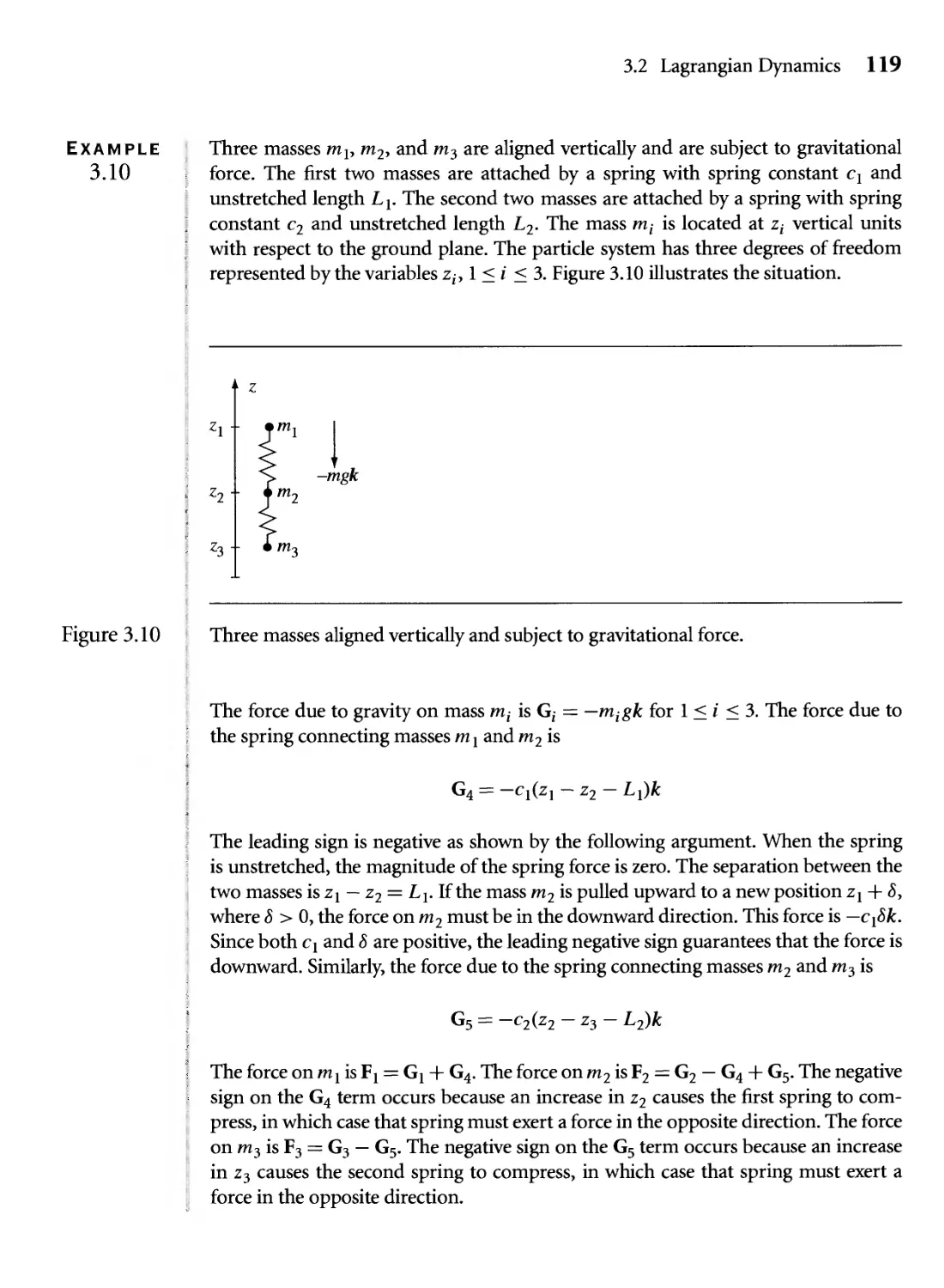
3.10 Three masses aligned vertically and subject to gravitational force. 119
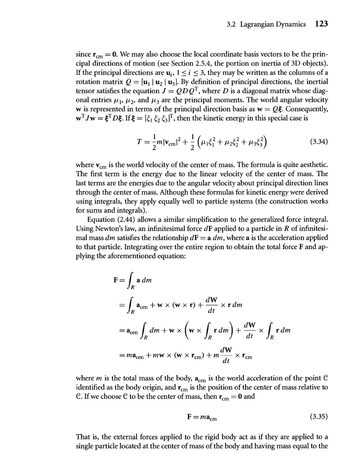
3.11 A modification of the simple pendulum problem. 121
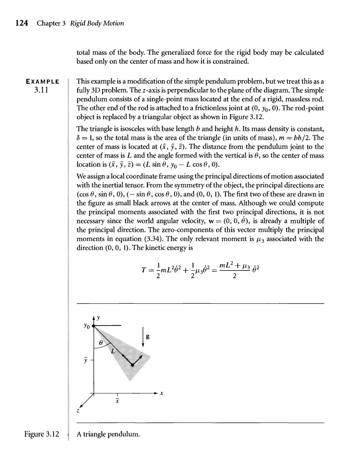
3.12 A triangle pendulum. 124
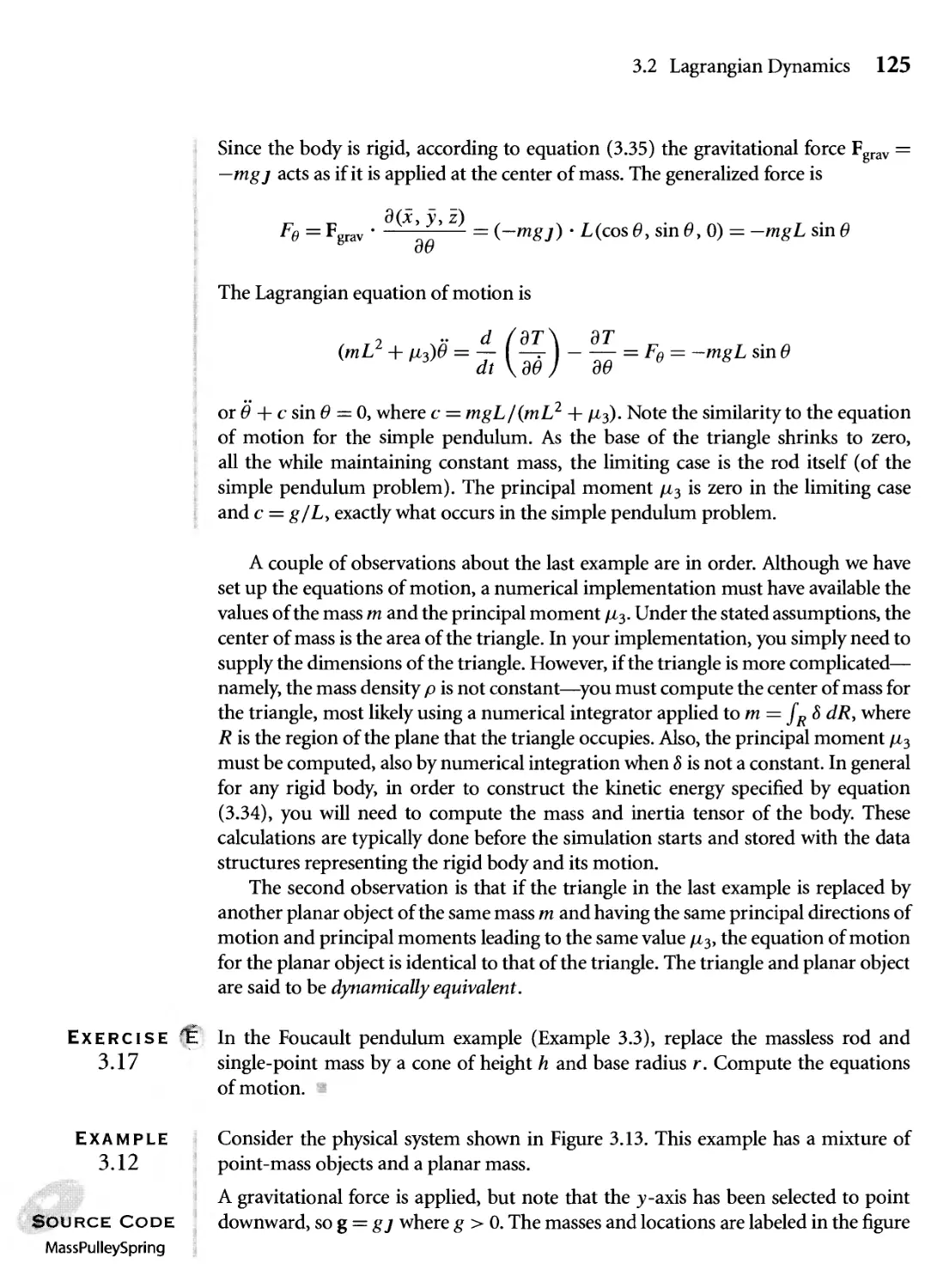
3.13 A system consisting of two masses, a pulley with mass, and a spring. 126
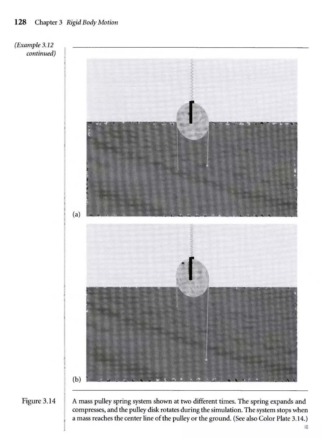
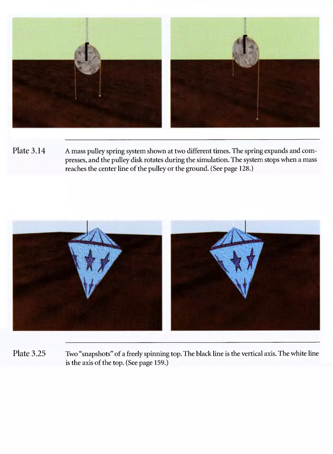
3.14 A mass pulley spring system shown at two different times. The spring
expands and compresses, and the pulley disk rotates during the
simulation. The system stops when a mass reaches the center line of
the pulley or the ground. (See also Color Plate 3.14.) 128
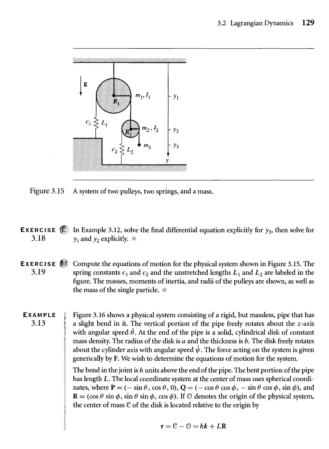
3.15 A system of two pulleys, two springs, and a mass. 129

xviii Figures
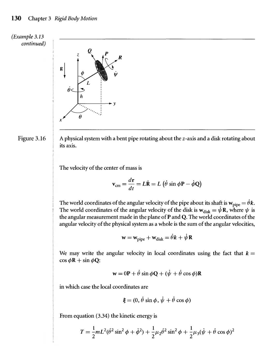
3.16 A physical system with a bent pipe rotating about the z-axis and a disk
rotating about its axis. 130
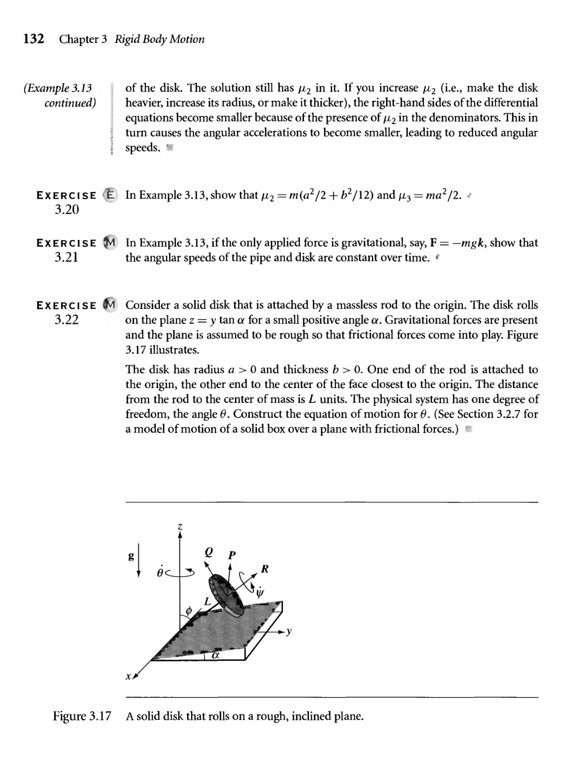
3.17 A solid disk that rolls on a rough, inclined plane. 132
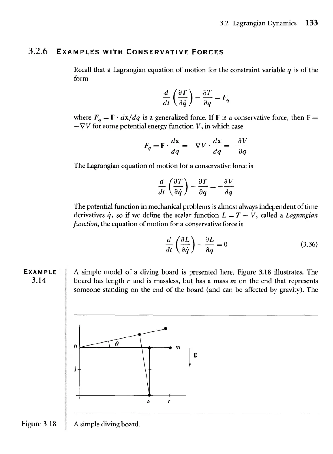
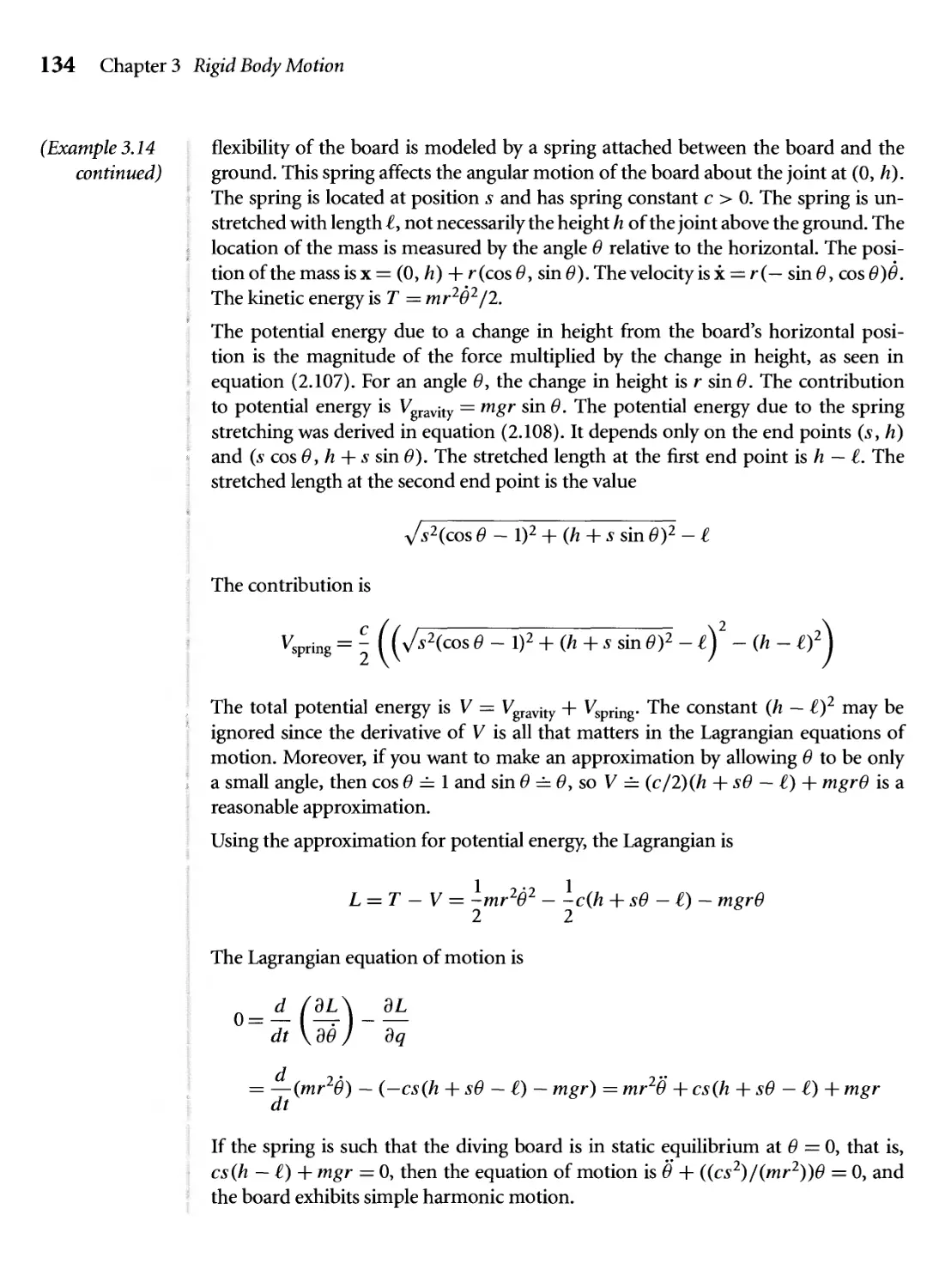
3.18 A simple diving board. 133
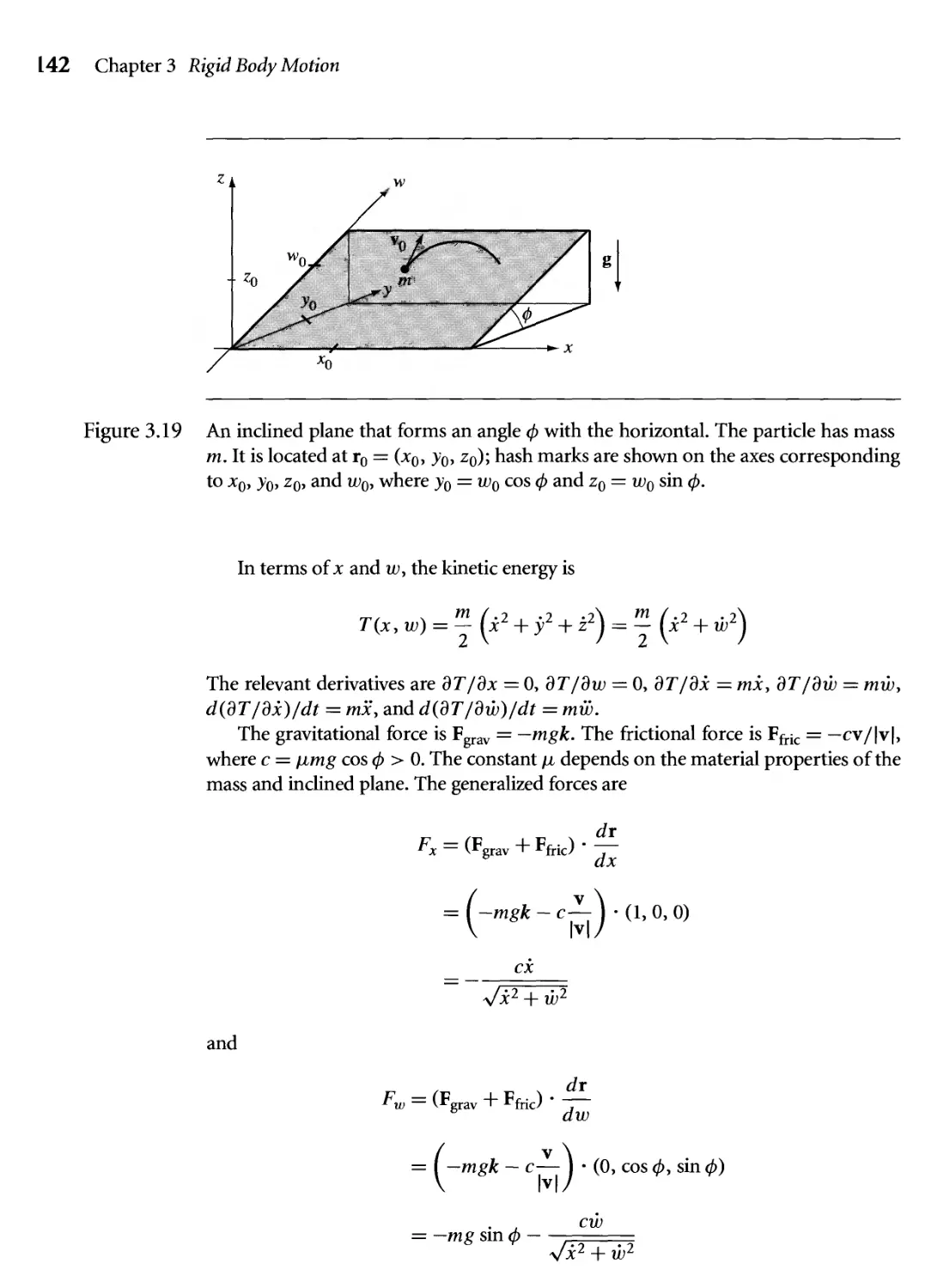
3.19 An inclined plane that forms an angle ф with the horizontal. The
particle has mass m. It is located at r0 = (jc0, y0, z0); hash marks
are shown on the axes corresponding to jc0, )>o, z0, and w0, where
yQ = w0 cos ф and z0 = Wq sin ф. 142
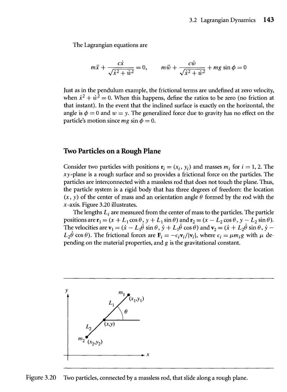
3.20 Two particles, connected by a massless rod, that slide along a rough
plane. 143
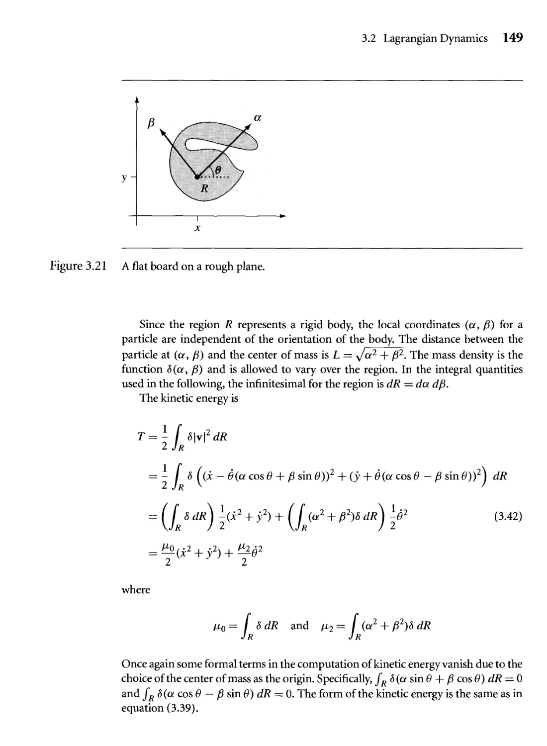
3.21 A flat board on a rough plane. 149
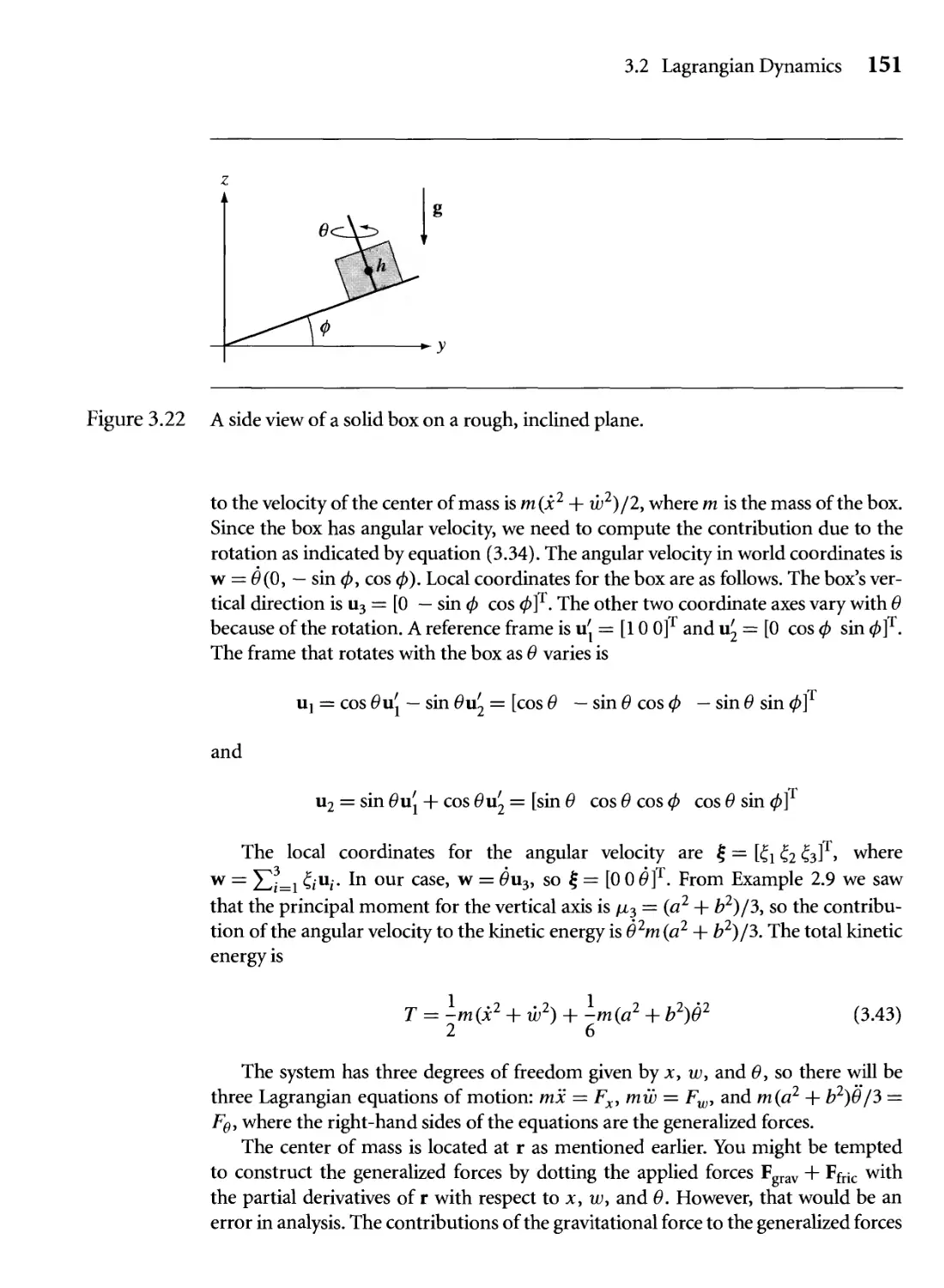
3.22 A side view of a solid box on a rough, inclined plane. 151
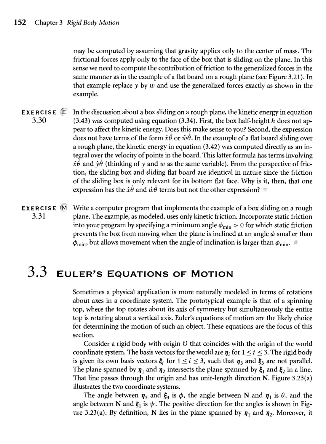
3.23 The world coordinates and body coordinates for a rigid body where
both systems have the same origin. 153
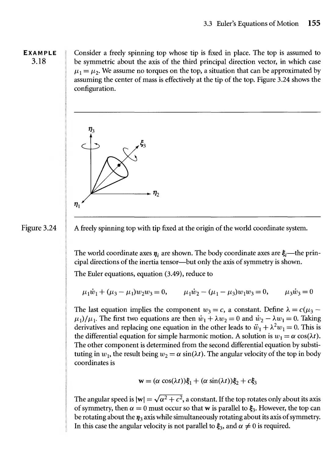
3.24 A freely spinning top with tip fixed at the origin of the world
coordinate system. 155
3.25 Two "snapshots" of a freely spinning top. The black line is the vertical
axis. The white line is the axis of the top. (See also Color Plate 3.25.) 159
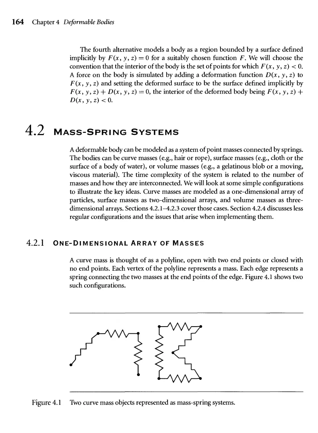
4.1 Two curve mass objects represented as mass-spring systems. 164
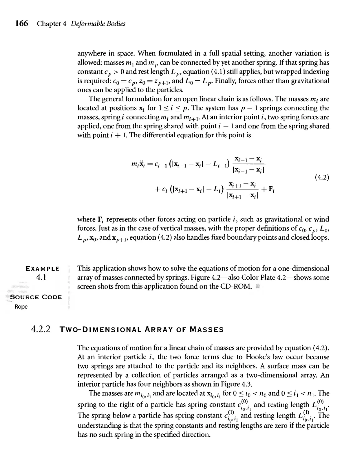
4.2 A rope modeled as a linear chain of springs. Image (a) shows the rope
at rest with only gravity acting on it. Image (b) shows the rope subject
to a wind force whose direction changes by small random amounts.
(See also Color Plate 4.2.) 167
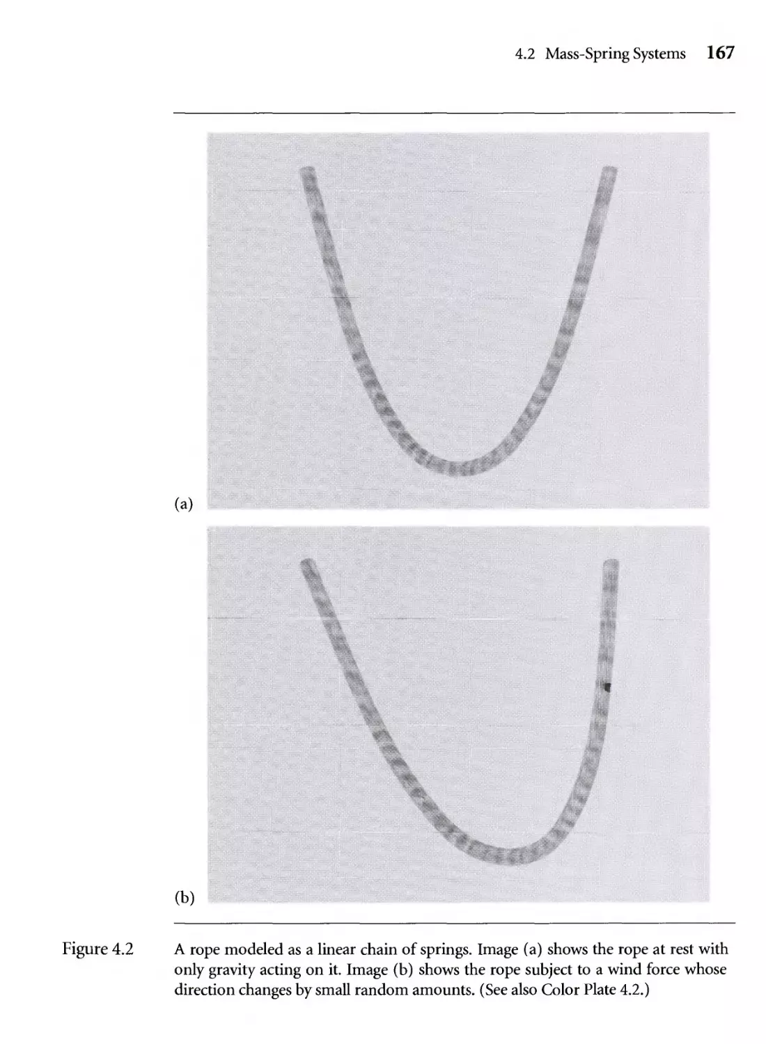
4.3 A surface mass represented as a mass-spring system with the masses
organized as a two-dimensional array. 168
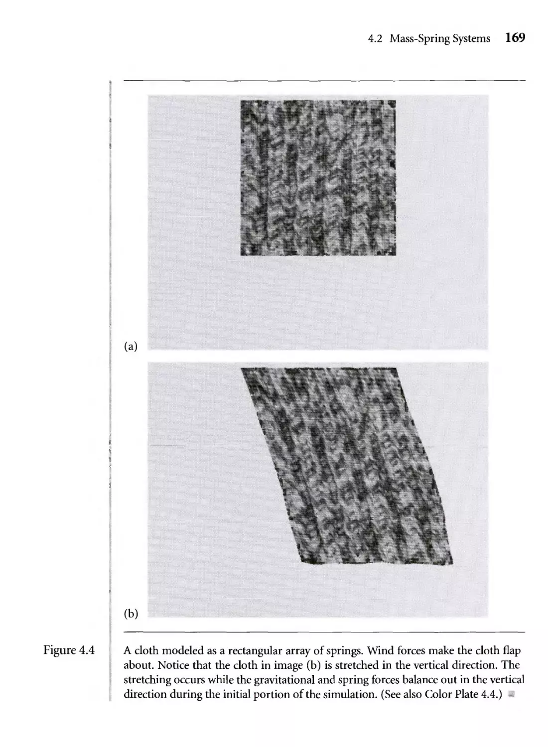
4.4 A cloth modeled as a rectangular array of springs. Wind forces make
the cloth flap about. Notice that the cloth in image (b) is stretched in
the vertical direction. The stretching occurs while the gravitational
and spring forces balance out in the vertical direction during the
initial portion of the simulation. (See also Color Plate 4.4.) 169
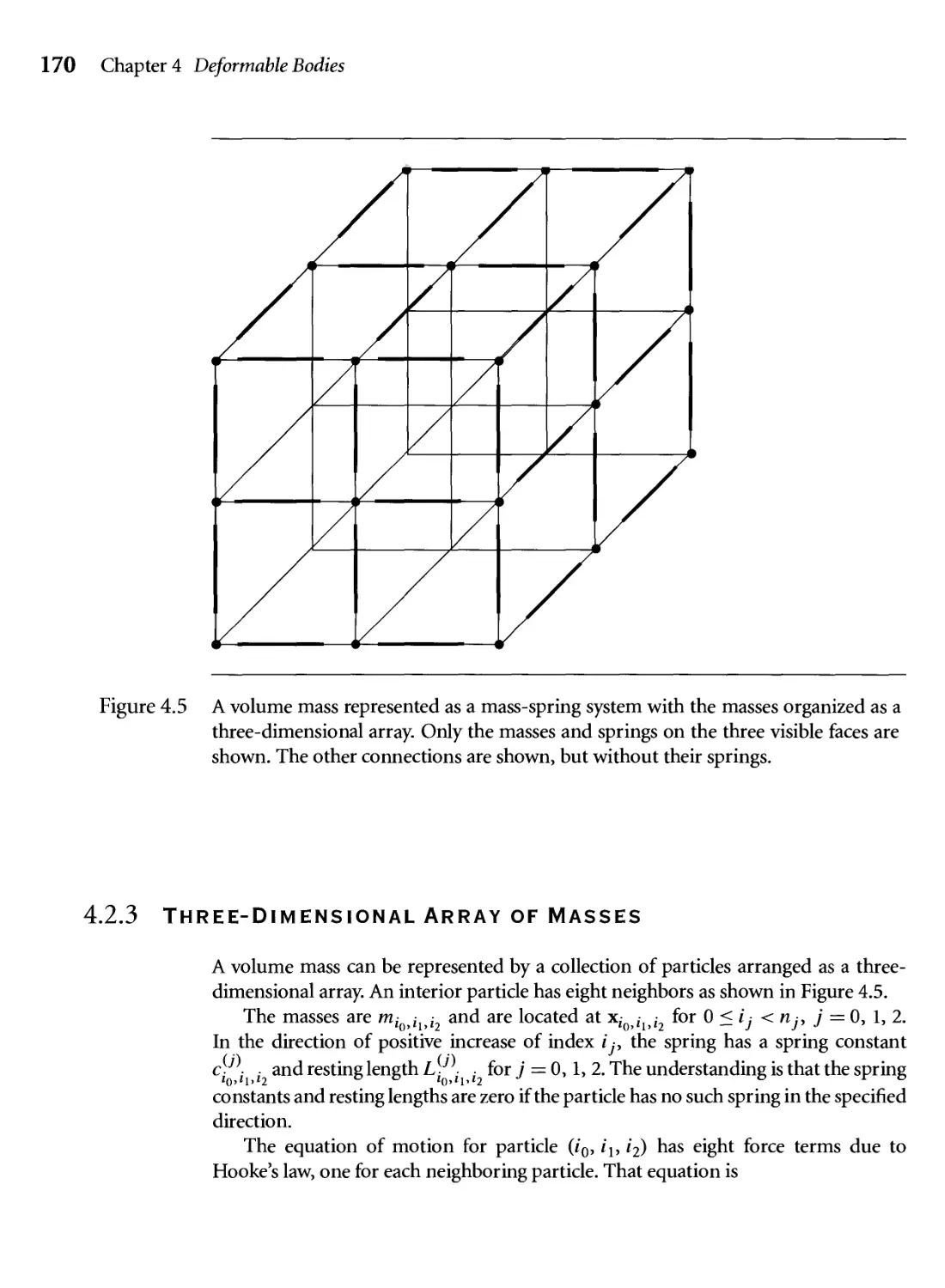
4.5 A volume mass represented as a mass-spring system with the masses
organized as a three-dimensional array. Only the masses and springs
on the three visible faces are shown. The other connections are shown,
but without their springs. 170
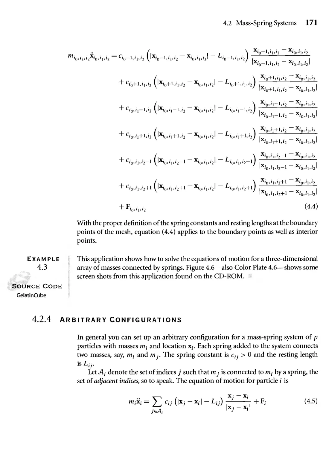
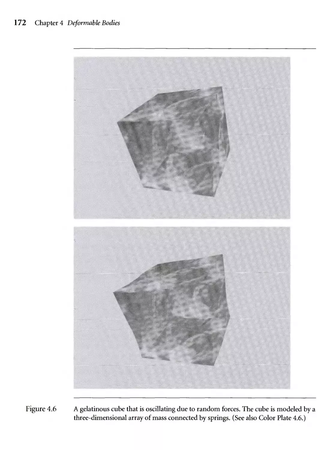
4.6 A gelatinous cube that is oscillating due to random forces. The cube is
modeled by a three-dimensional array of mass connected by springs.
(See also Color Plate 4.6.) 172
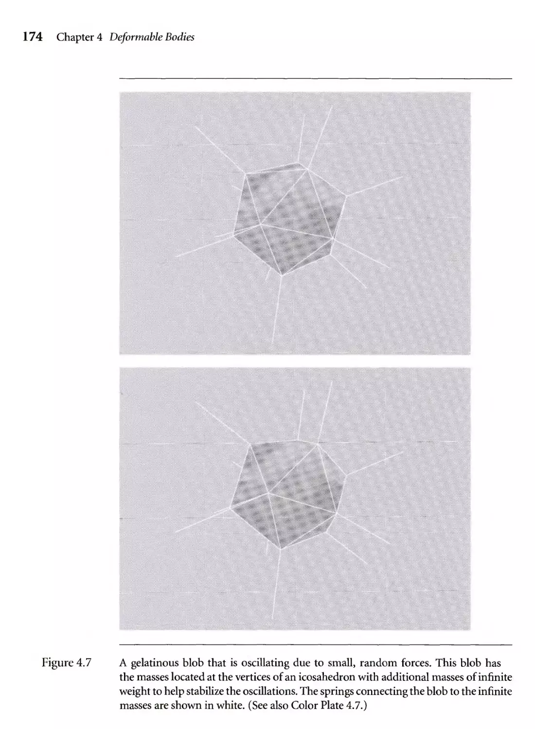
4.7 A gelatinous blob that is oscillating due to small, random forces. This
blob has the masses located at the vertices of an icosahedron with
additional masses of infinite weight to help stabilize the oscillations.

Figures xix
The springs connecting the blob to the infinite masses are shown in
white. (See also Color Plate 4.7.) 174
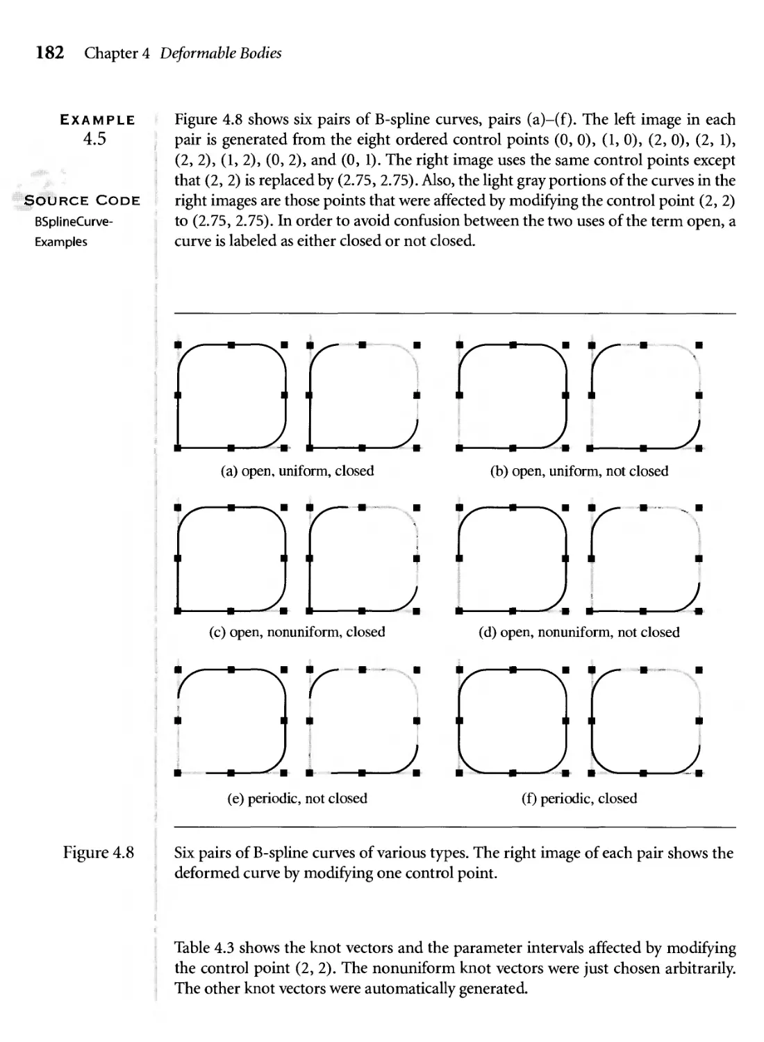
4.8 Six pairs of B-spline curves of various types. The right image of each
pair shows the deformed curve by modifying one control point. 182
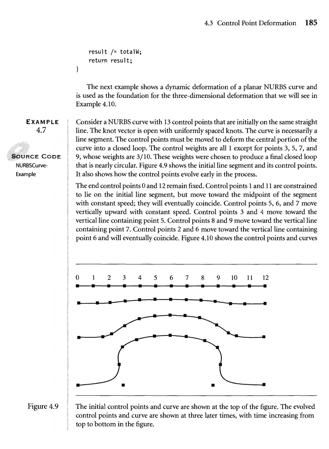
4.9 The initial control points and curve are shown at the top of the figure.
The evolved control points and curve are shown at three later times,
with time increasing from top to bottom in the figure. 185
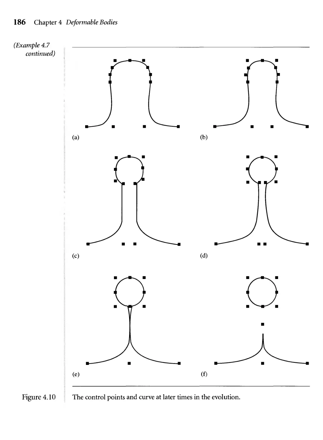
4.10 The control points and curve at later times in the evolution. 186
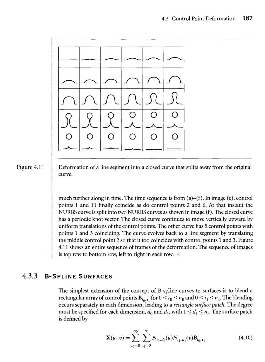
4.11 Deformation of a line segment into a closed curve that splits away
from the original curve. 187
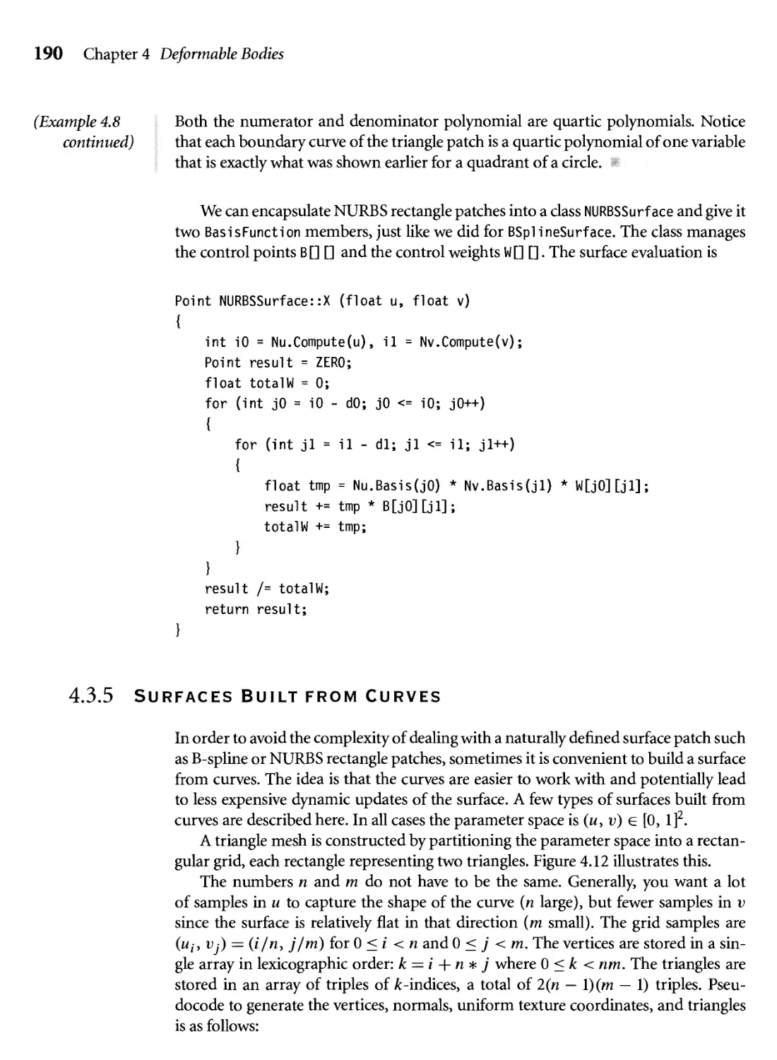
4.12 (a) The decomposition of (u, v) space into annxm grid of rectangles,
each rectangle consisting of two triangles. A typical rectangle is shown
in (b), with lower corner index (/, j) corresponding to и = i/n and
v = j/m. 191
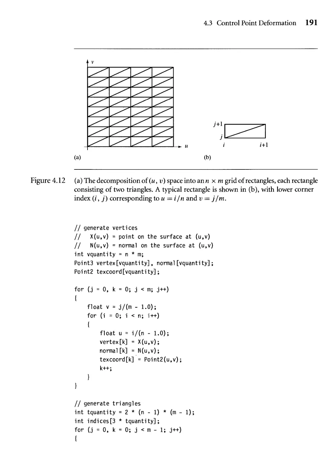
4.13 A cylinder surface (b) obtained by extruding the curve (a) in a
direction oblique to the plane of the curve. 192
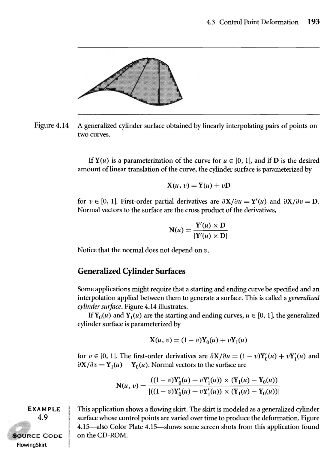
4.14 A generalized cylinder surface obtained by linearly interpolating pairs
of points on two curves. 193
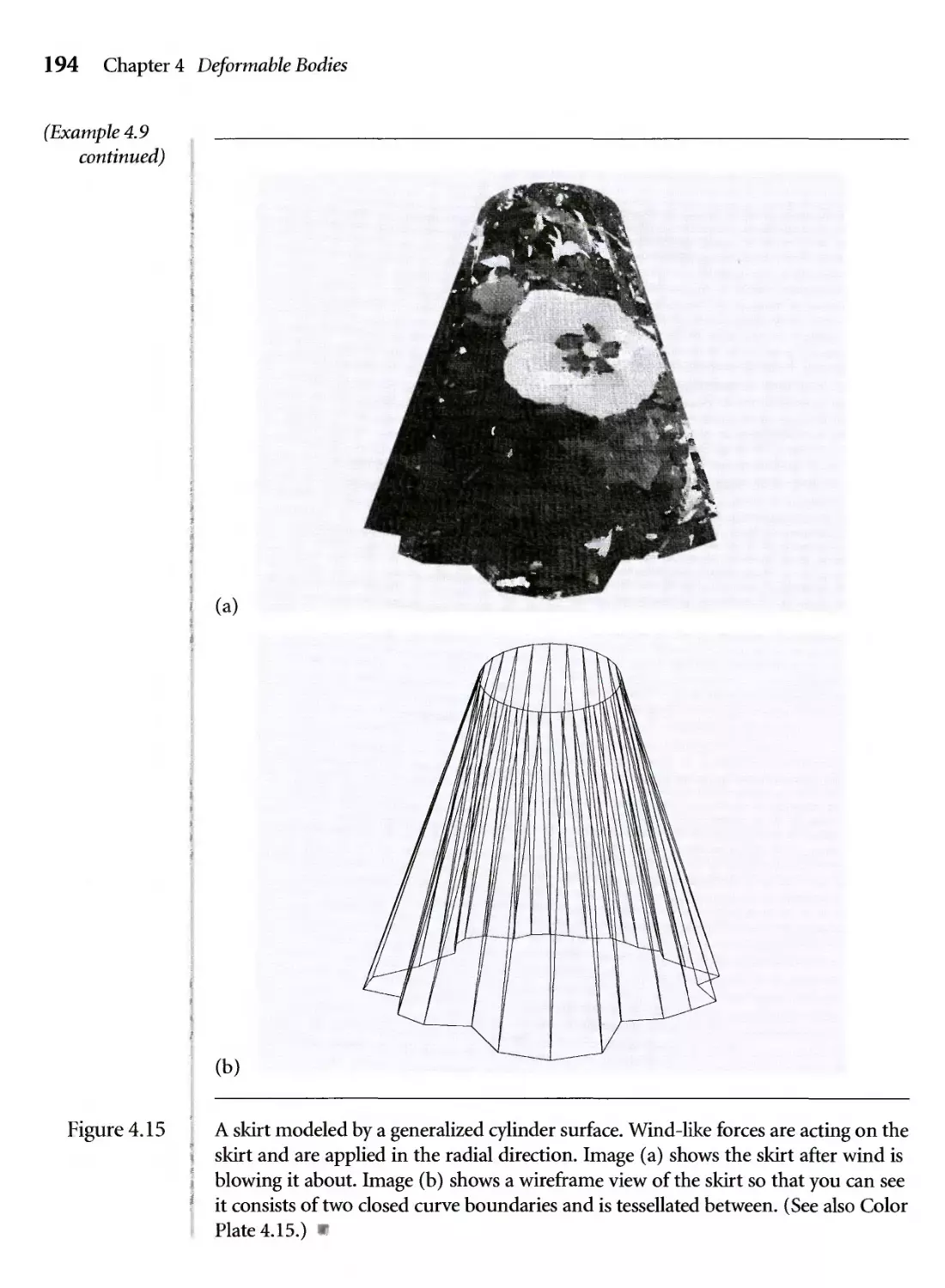
4.15 A skirt modeled by a generalized cylinder surface. Wind-like forces
are acting on the skirt and are applied in the radial direction. Image
(a) shows the skirt after wind is blowing it about. Image (b) shows a
wireframe view of the skirt so that you can see it consists of two closed
curve boundaries and is tessellated between. (See also Color Plate
4.15.) 194
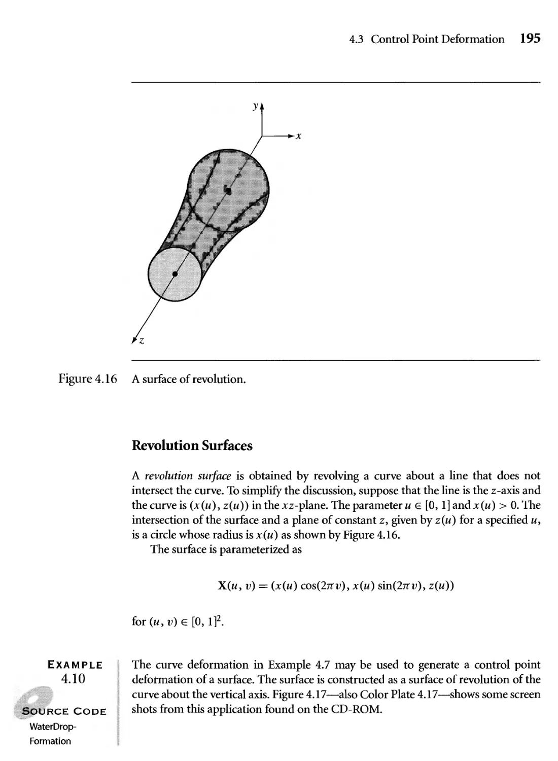
4.16 A surface of revolution. 195
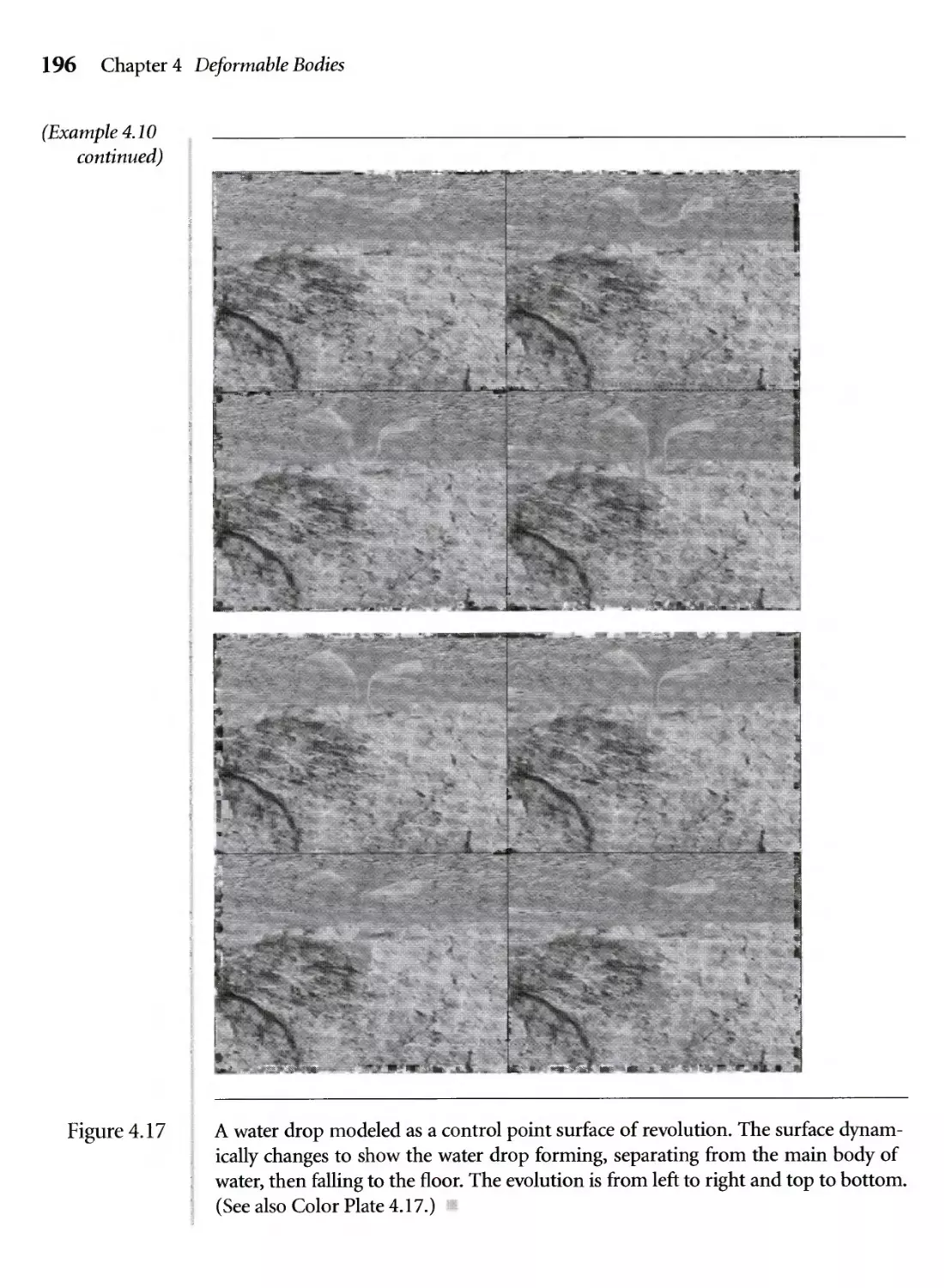
4.17 A water drop modeled as a control point surface of revolution.
The surface dynamically changes to show the water drop forming,
separating from the main body of water, then falling to the floor. The
evolution is from left to right and top to bottom. (See also Color Plate
4.17.) 196
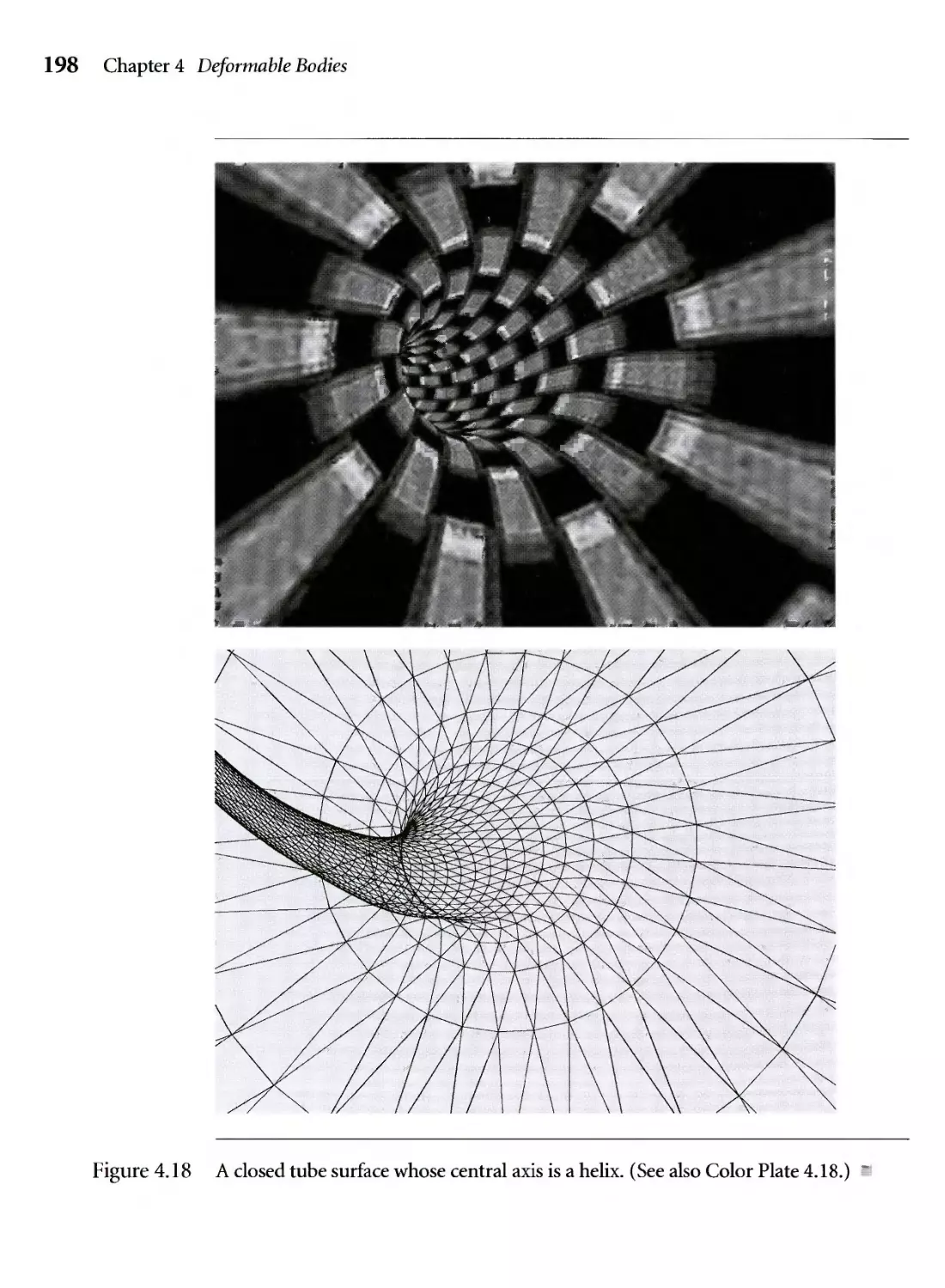
4.18 A closed tube surface whose central axis is a helix. (See also Color
Plate 4.18.) 198
4.19 A wriggling snake modeled as a tube surface whose central curve is a
control point curve. (See also Color Plate 4.19.) 199
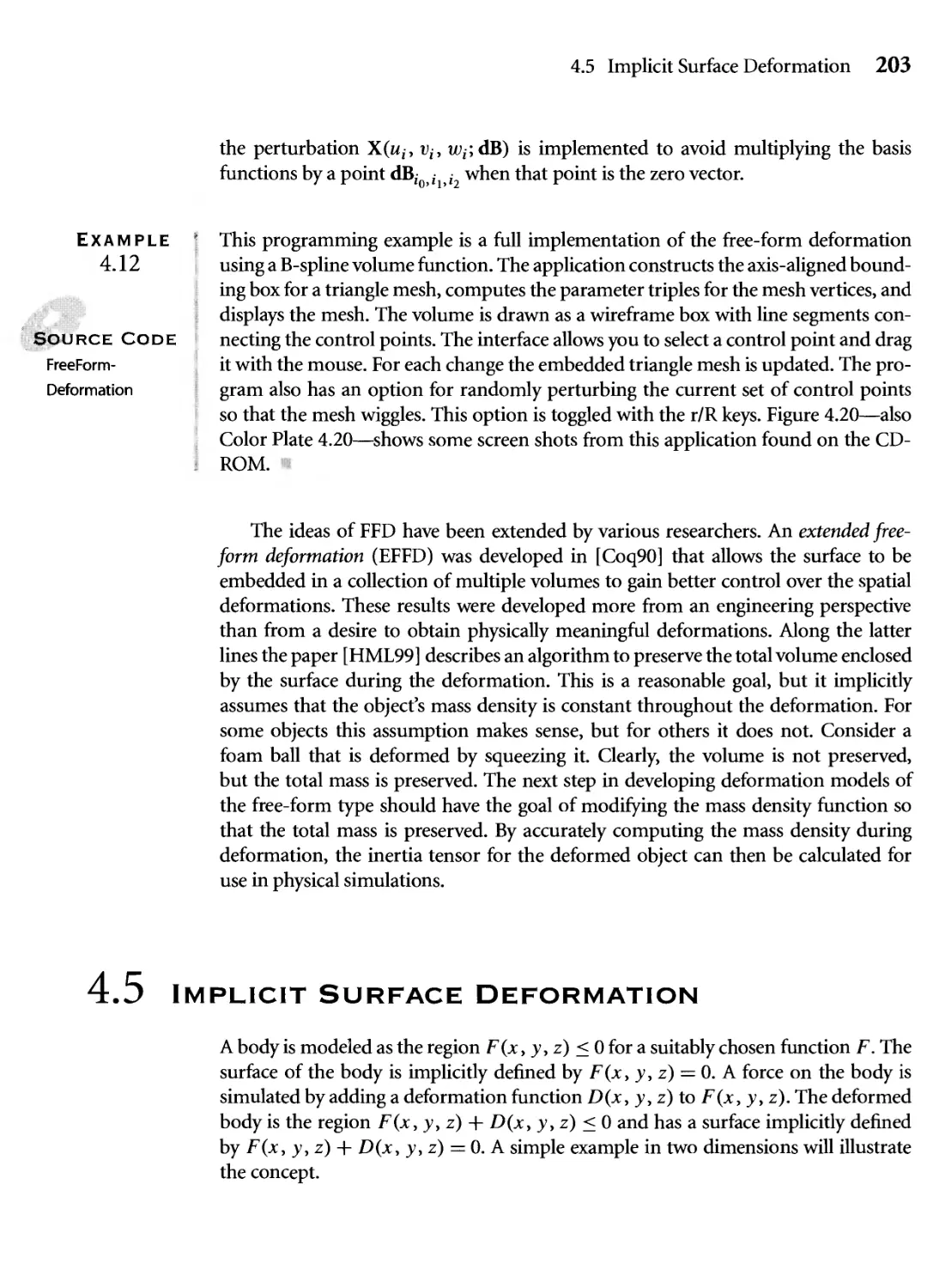
4.20 Free-form deformation. Image (a) shows the initial configuration
where all control points are rectangularly aligned. Image (b) shows
that some control points have been moved and the surface is
deformed. The control point shown in darker gray in (b) is the point
at which the mouse was clicked on and moved. (See also Color Plate
4.20.) 204
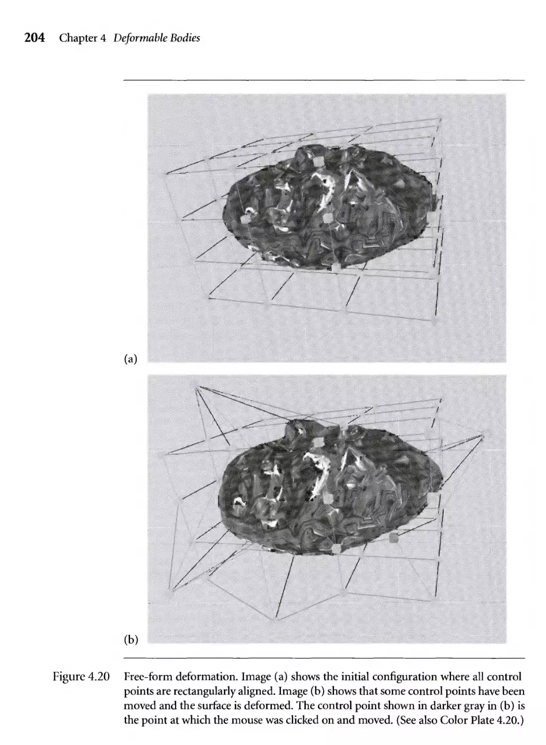
4.21 A disk-shaped body and various deformations of it. 205

XX Figures
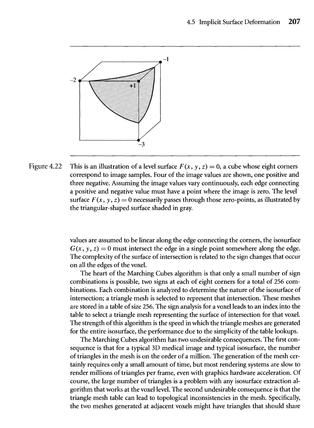
4.22 This is an illustration of a level surface F(x, y, z) = 0, a cube whose
eight corners correspond to image samples. Four of the image values
are shown, one positive and three negative. Assuming the image
values vary continuously, each edge connecting a positive and negative
value must have a point where the image is zero. The level surface
F(x, y, z) = 0 necessarily passes through those zero-points, as
illustrated by the triangular-shaped surface shaded in gray. 207
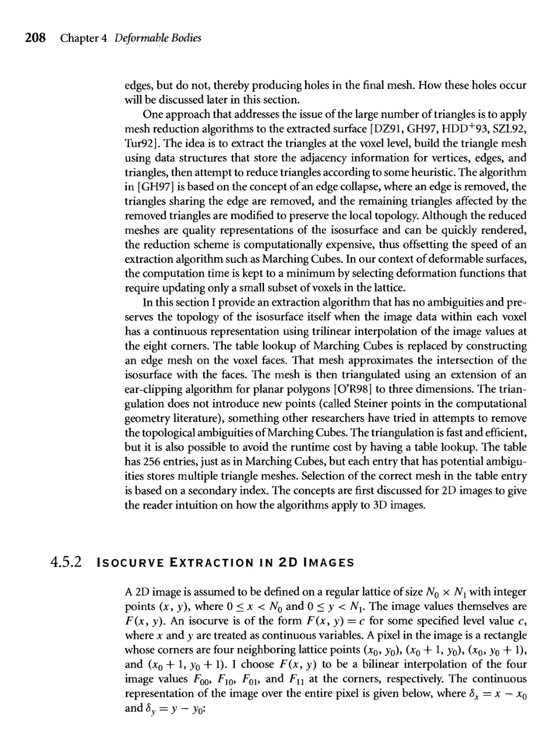
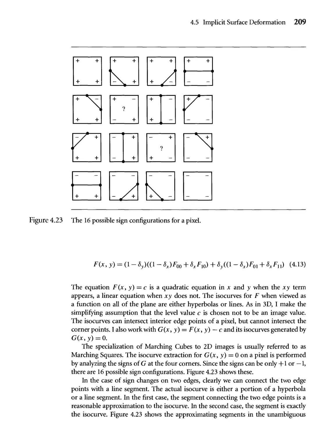
4.23 The 16 possible sign configurations for a pixel. 209
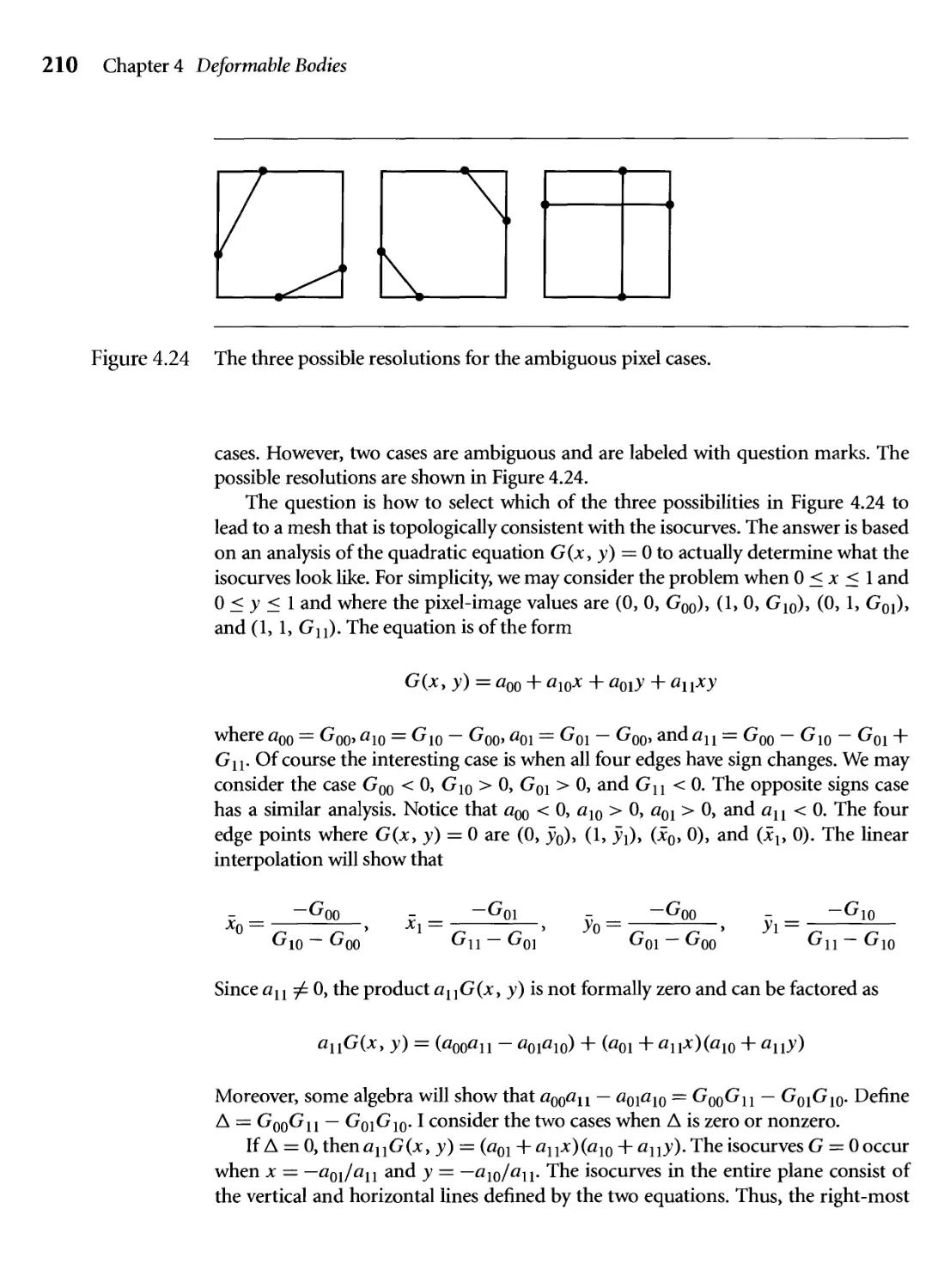
4.24 The three possible resolutions for the ambiguous pixel cases. 210
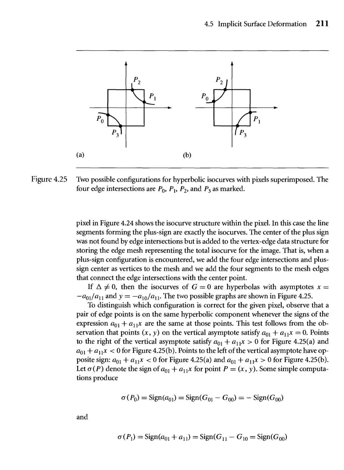
4.25 Two possible configurations for hyperbolic isocurves with pixels
superimposed. The four edge intersections are Po, Pv P2, and P3 as
marked. 211
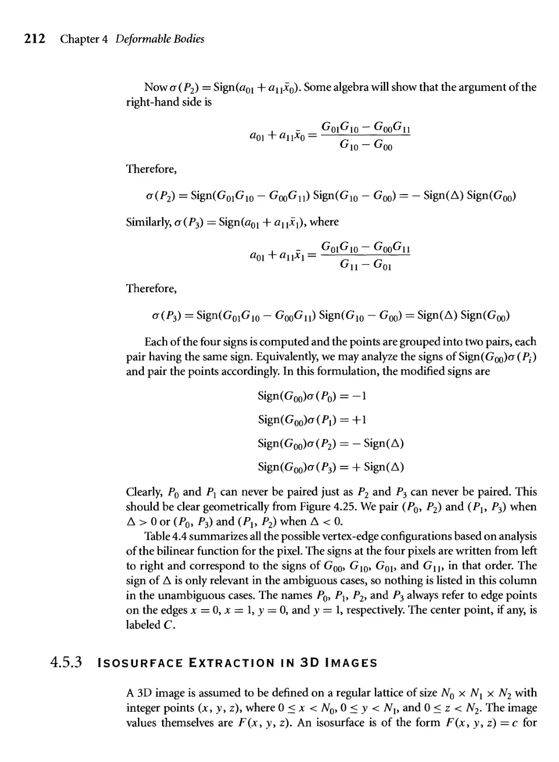
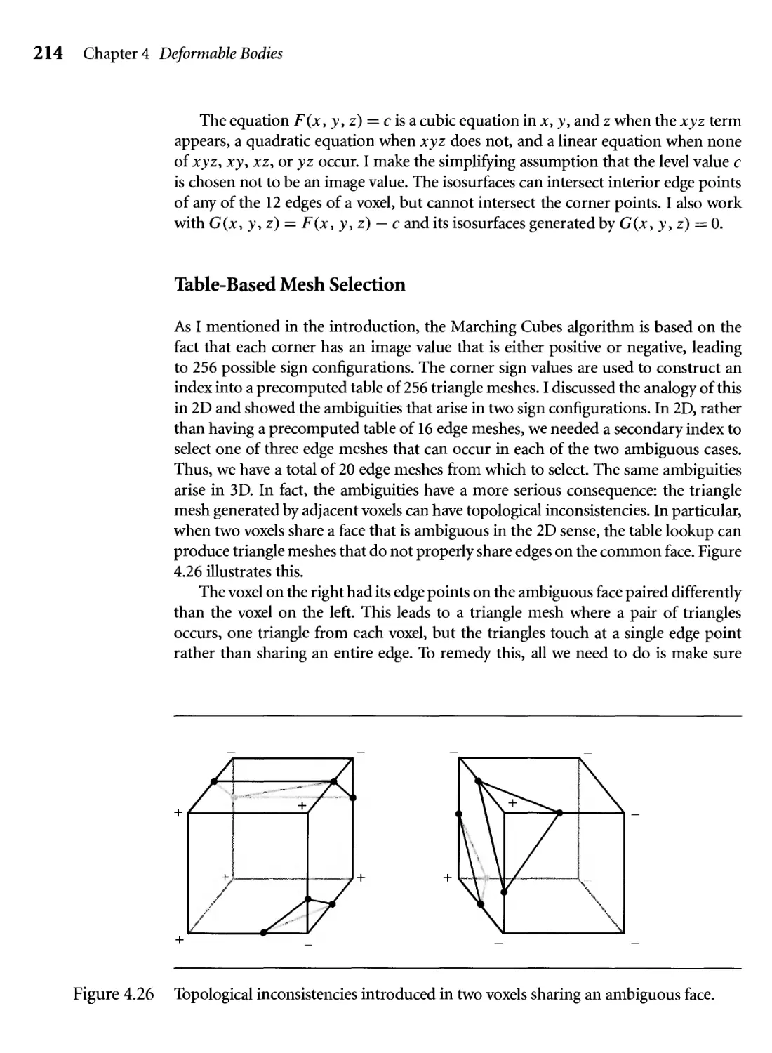
4.26 Topological inconsistencies introduced in two voxels sharing an
ambiguous face. 214
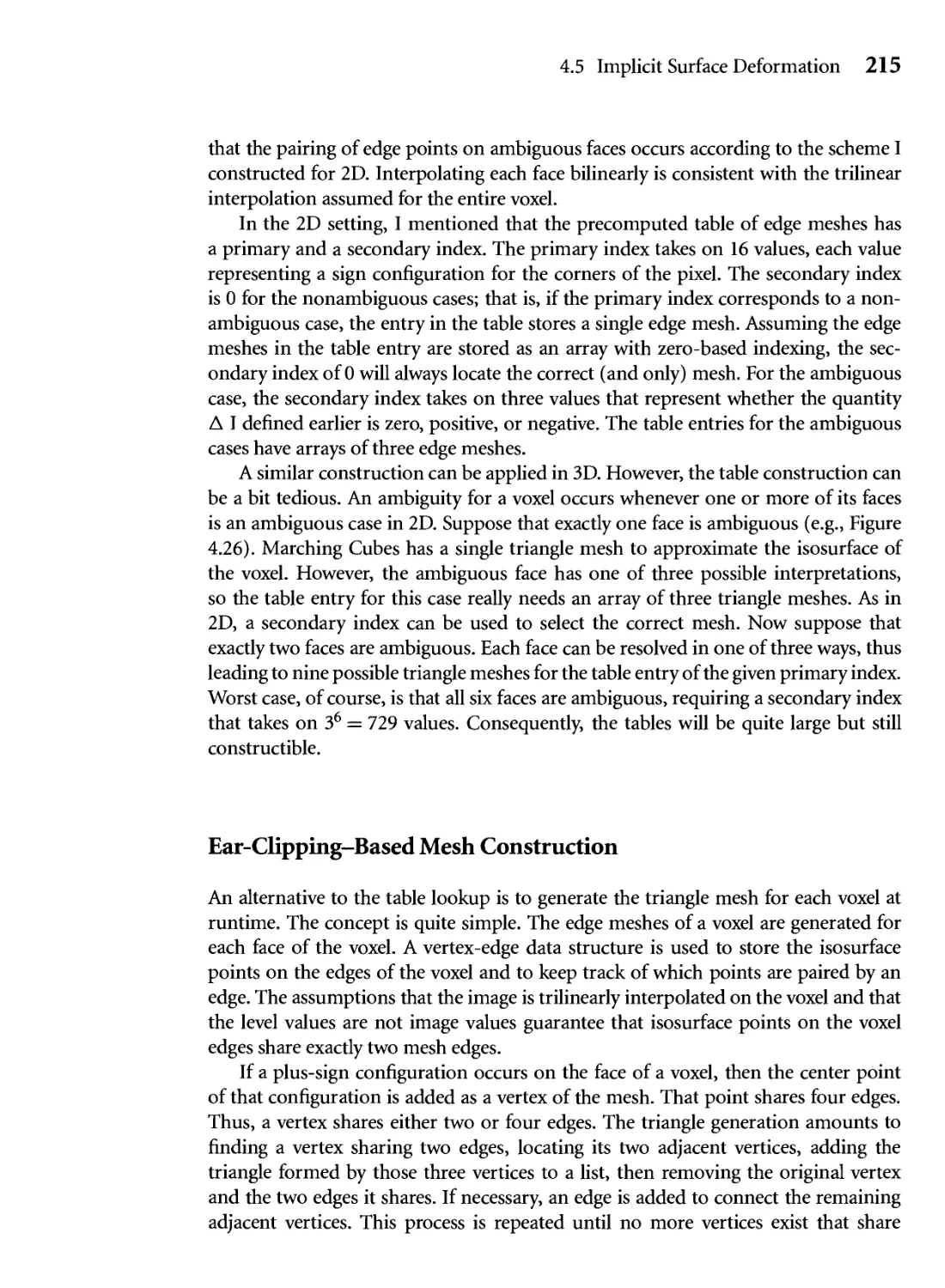
4.27 A voxel and its extracted edge mesh. 216
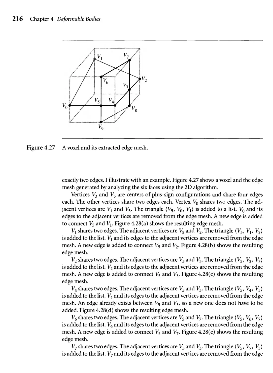
4.28 Triangle removal in the edge mesh of Figure 4.27. 217
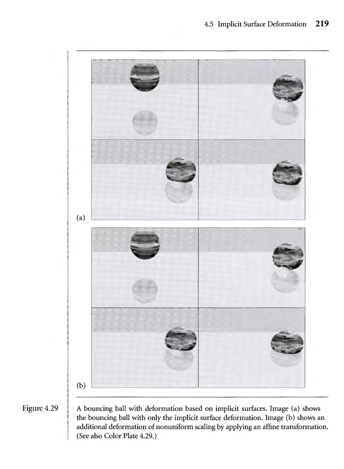
4.29 A bouncing ball with deformation based on implicit surfaces.
Image (a) shows the bouncing ball with only the implicit surface
deformation. Image (b) shows an additional deformation of
nonuniform scaling by applying an affme transformation. (See also
Color Plate 4.29.) 219
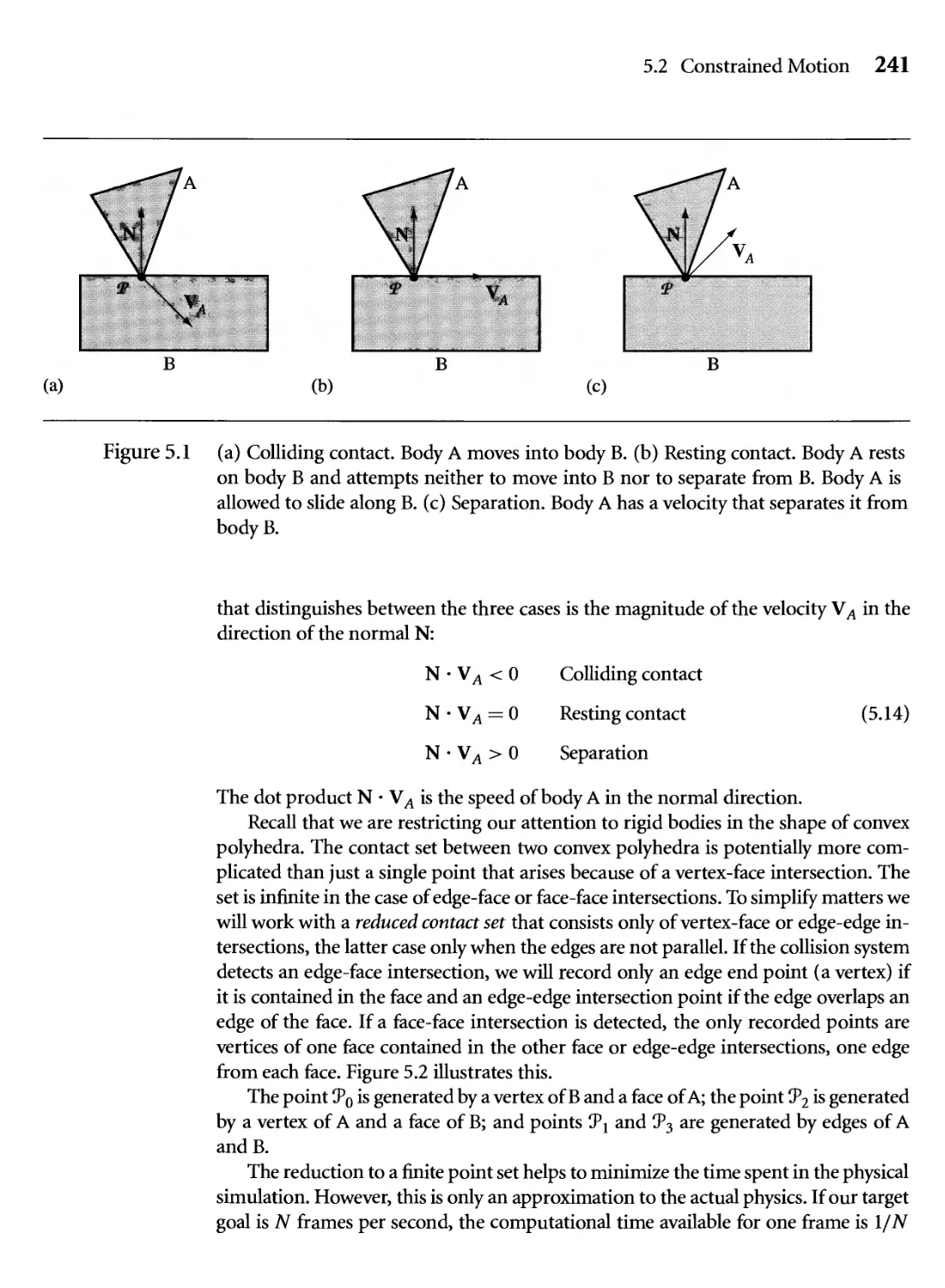
5.1 (a) Colliding contact. Body A moves into body B. (b) Resting contact.
Body A rests on body В and attempts neither to move into В nor to
separate from B. Body A is allowed to slide along В. (с) Separation.
Body A has a velocity that separates it from body B. 241
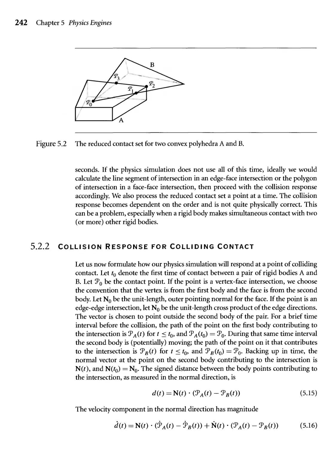
5.2 The reduced contact set for two convex polyhedra A and B. 242
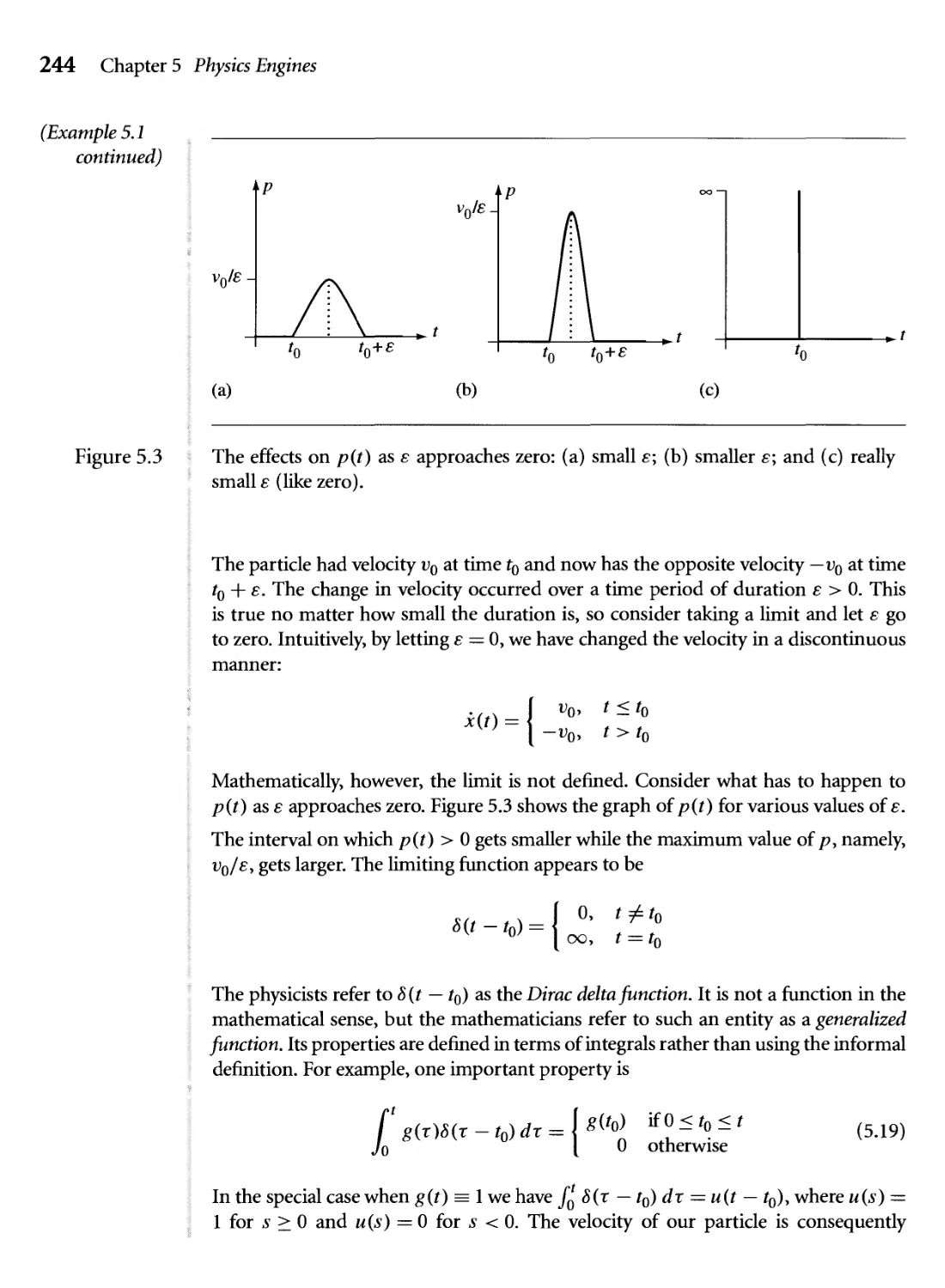
5.3 The effects on p(t) as s approaches zero: (a) small e; (b) smaller e;
and (c) really small e (like zero). 244
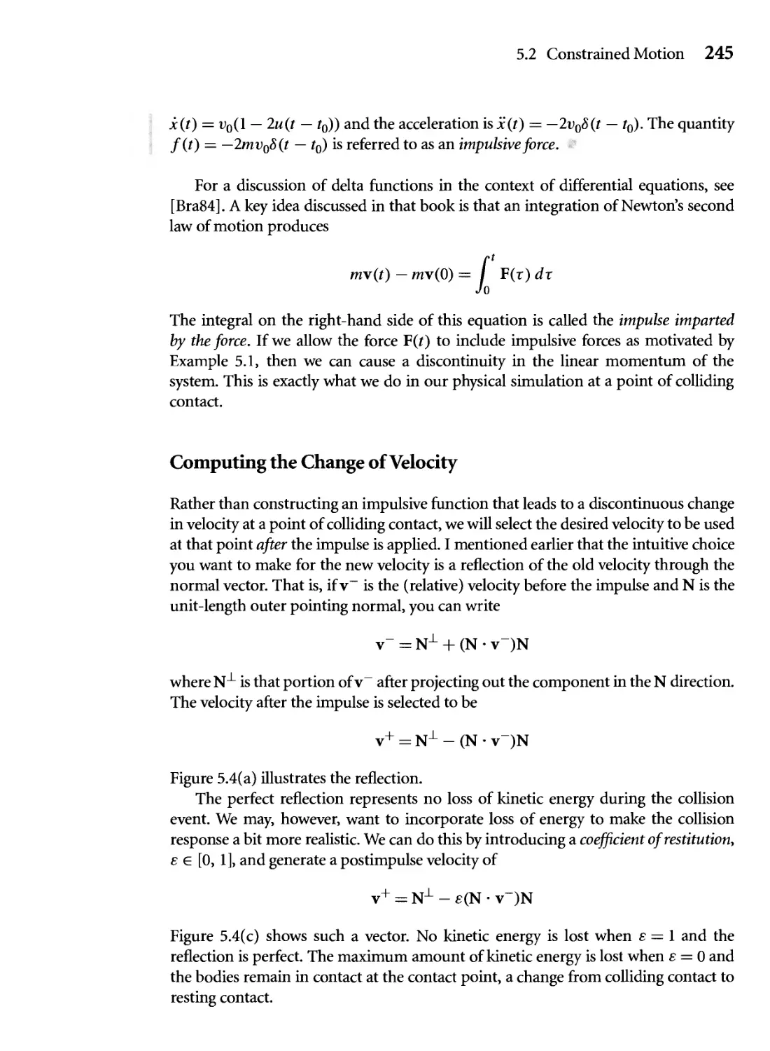
5.4 (a) Reflection of the preimpulse velocity v~ through the contact
normal to obtain the postimpulse velocity v+. (b) An imperfect
reflection that represents a loss of kinetic energy, (c) An imperfect
reflection that represents a maximum loss of kinetic energy. 246
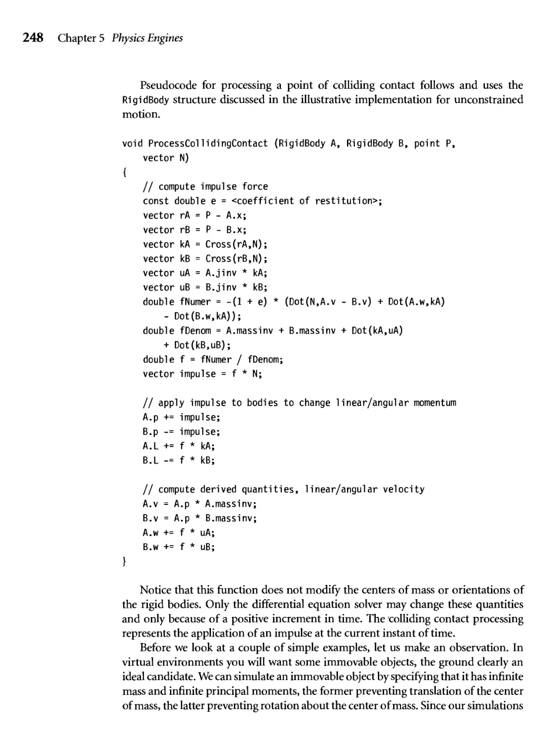
5.5 (a) The square traveling toward a sloped plane, (b) The preimpulse
configuration at the instant of contact, (c) The postimpulse
configuration at the instant of contact, (d) The square moving away
from the plane. 249
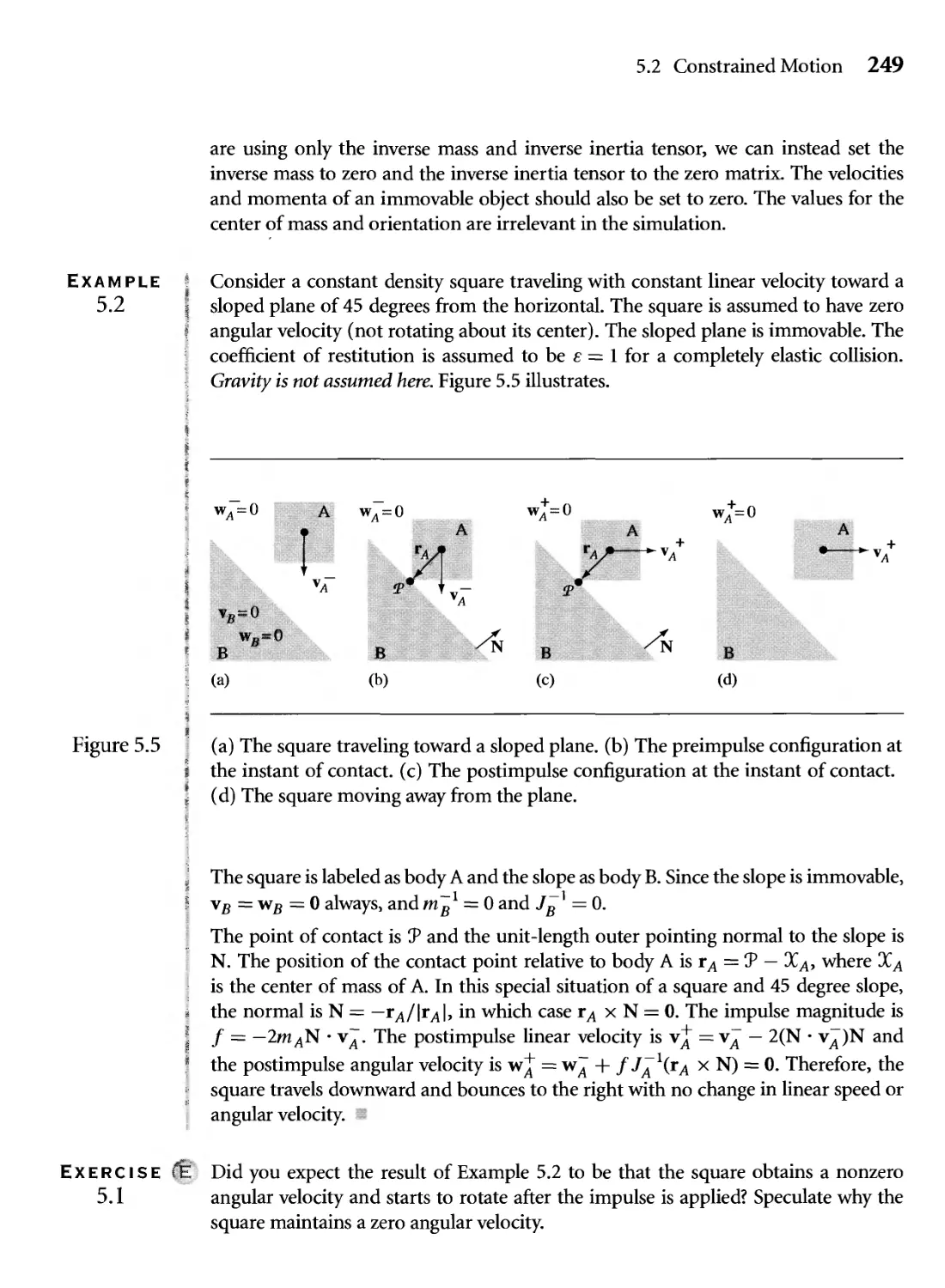
5.6 An axis-aligned box colliding with a sloped plane along an entire edge
of the box, A - s)90 + s?! for s e [0, 1]. 250
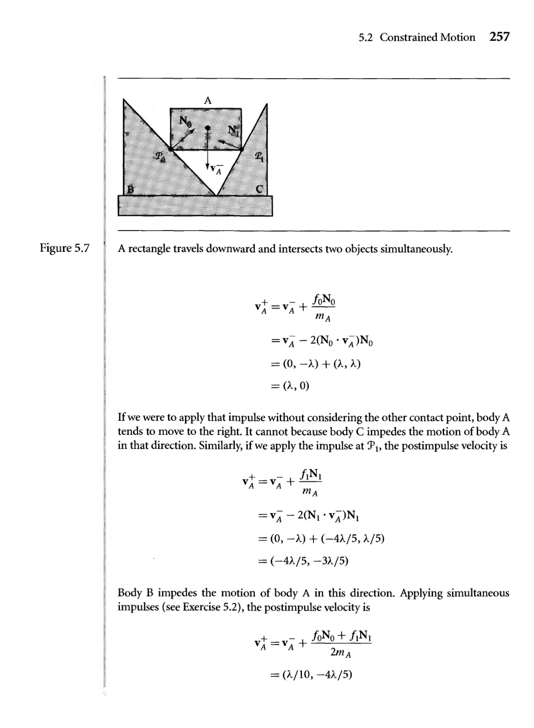
5.7 A rectangle travels downward and intersects two objects
simultaneously. 257

Figures xxi
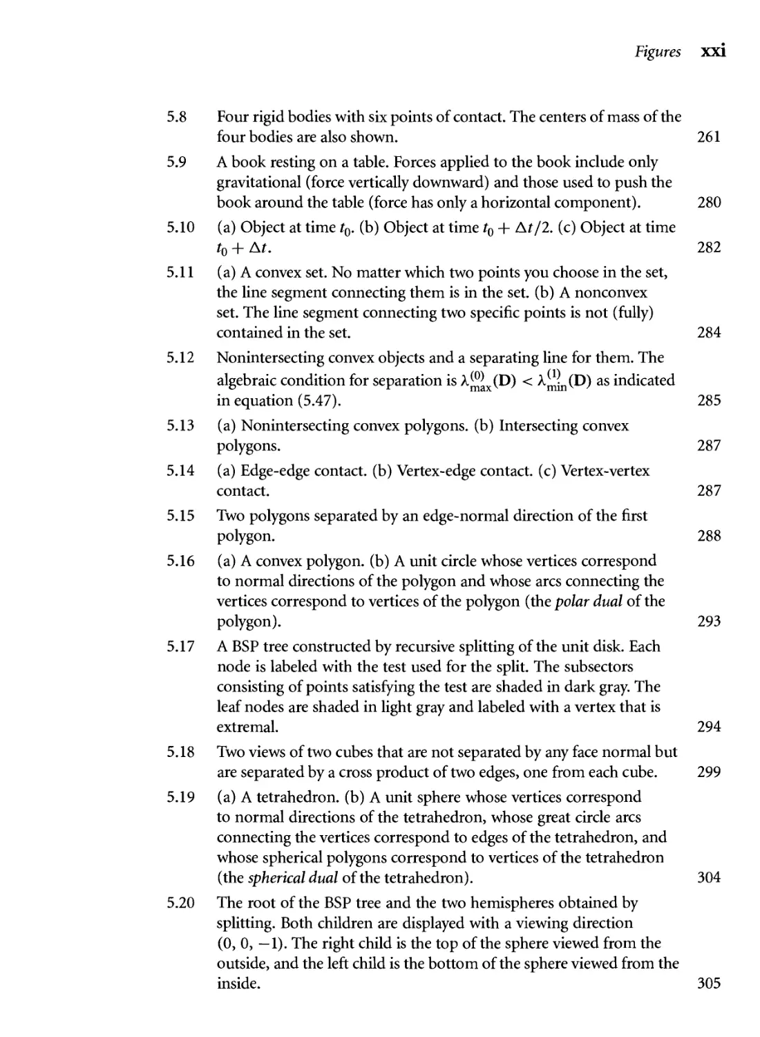
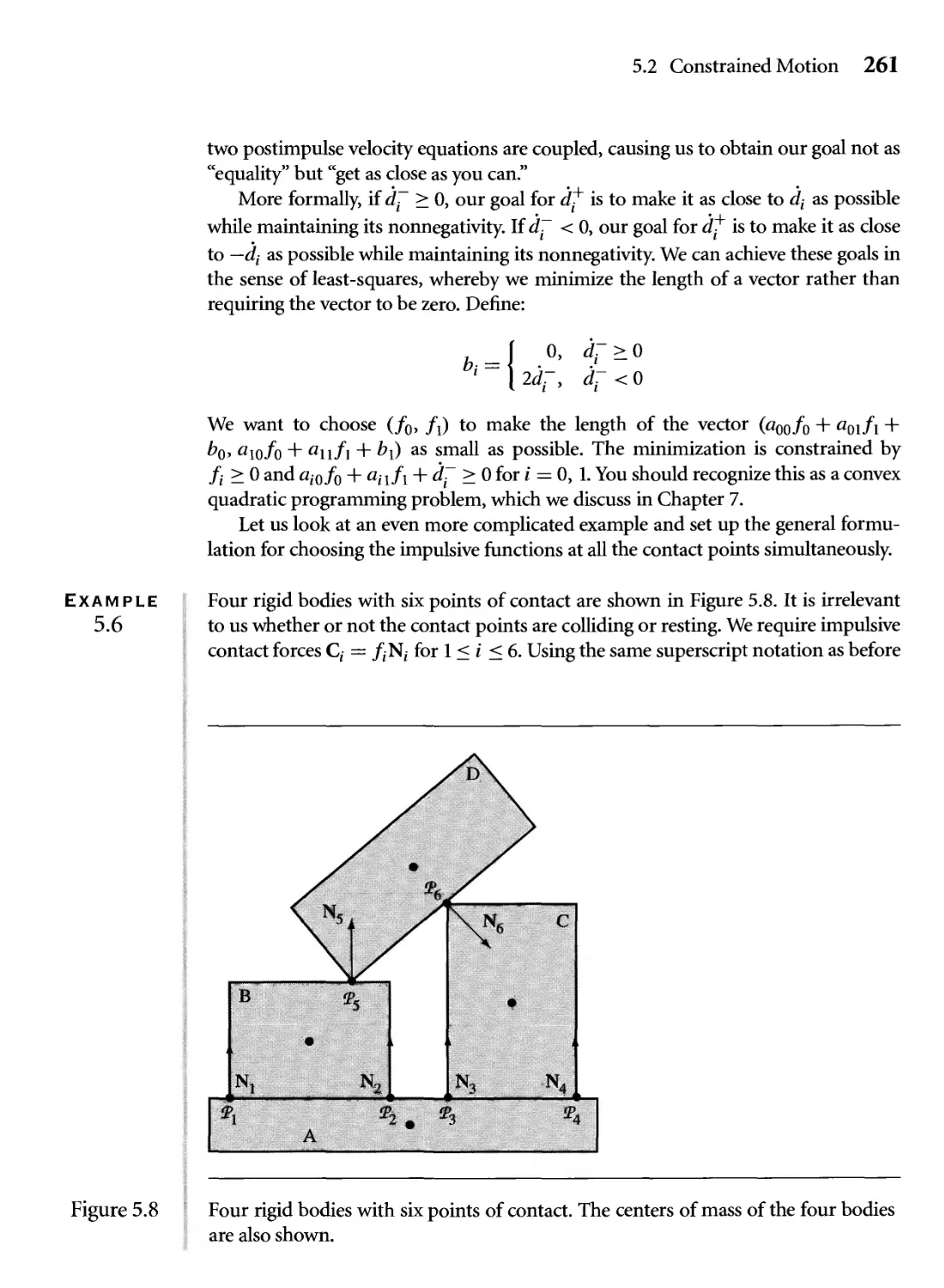
5.8 Four rigid bodies with six points of contact. The centers of mass of the
four bodies are also shown. 261
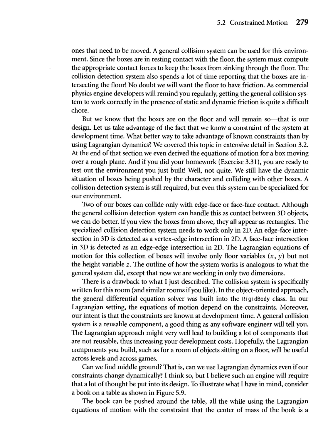
5.9 A book resting on a table. Forces applied to the book include only
gravitational (force vertically downward) and those used to push the
book around the table (force has only a horizontal component). 280
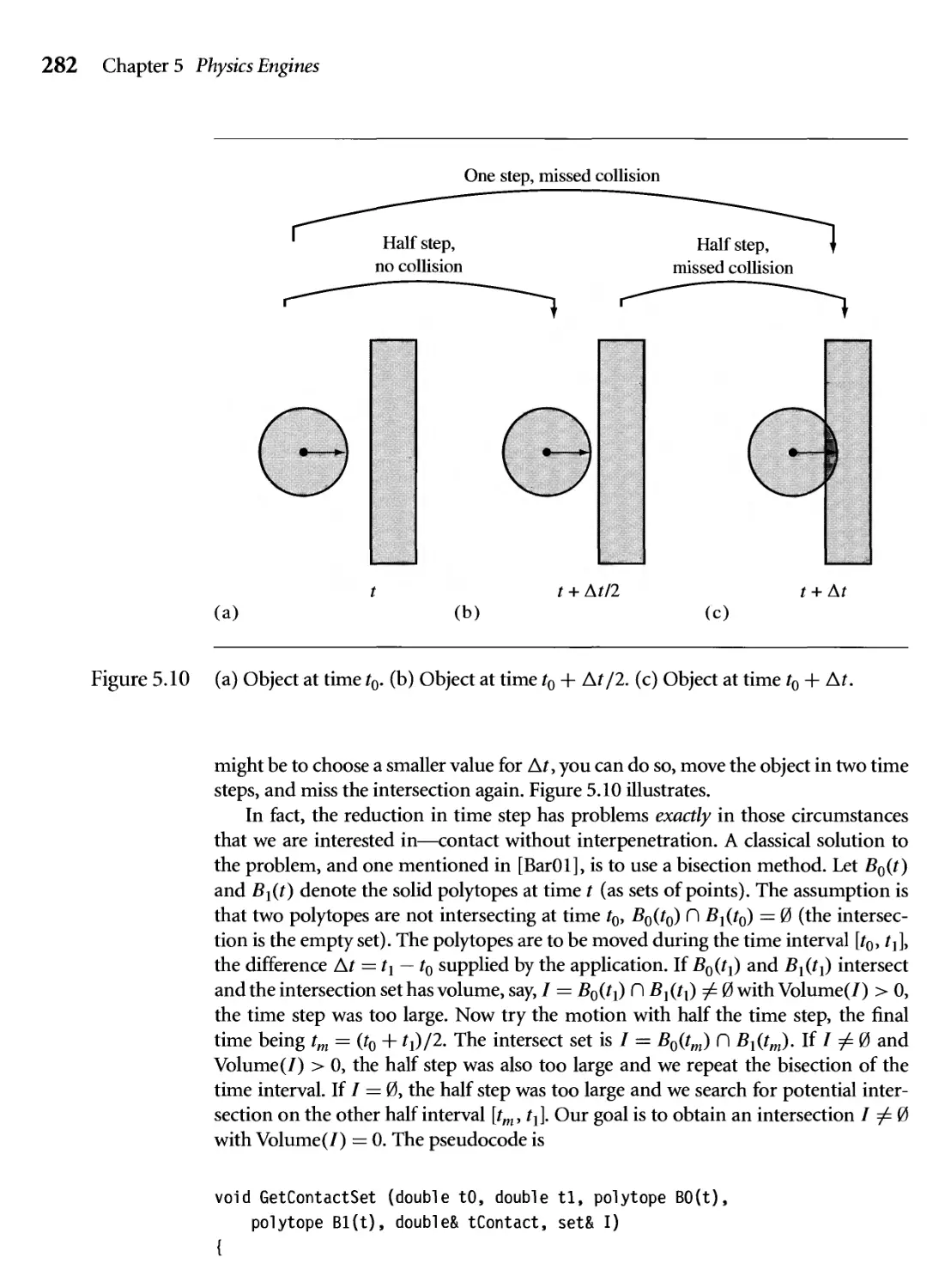
5.10 (a) Object at time t0. (b) Object at time t0 + At/2. (c) Object at time
t0 + At. 282
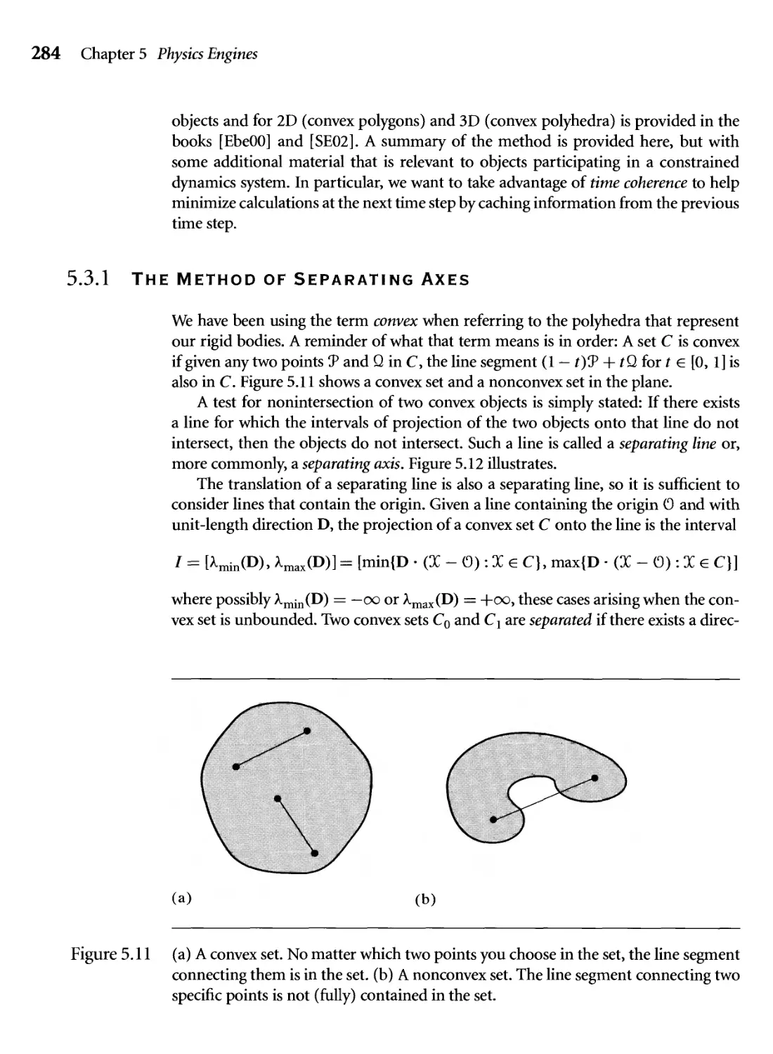
5.11 (a) A convex set. No matter which two points you choose in the set,
the line segment connecting them is in the set. (b) A nonconvex
set. The line segment connecting two specific points is not (fully)
contained in the set. 284
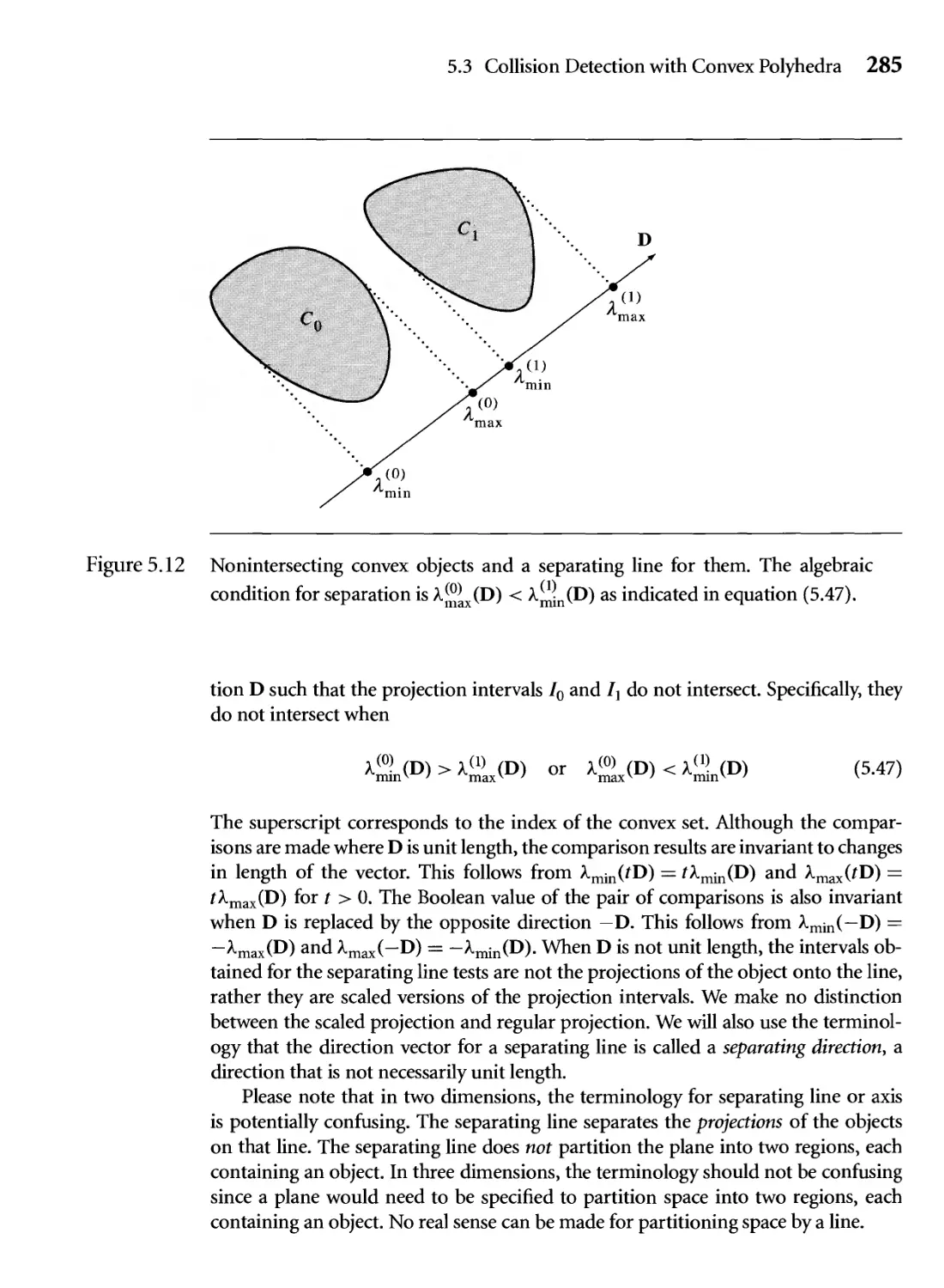
5.12 Nonintersecting convex objects and a separating line for them. The
algebraic condition for separation is A.^(D) < ^rnin(^) as indicated
in equation E.47). 285
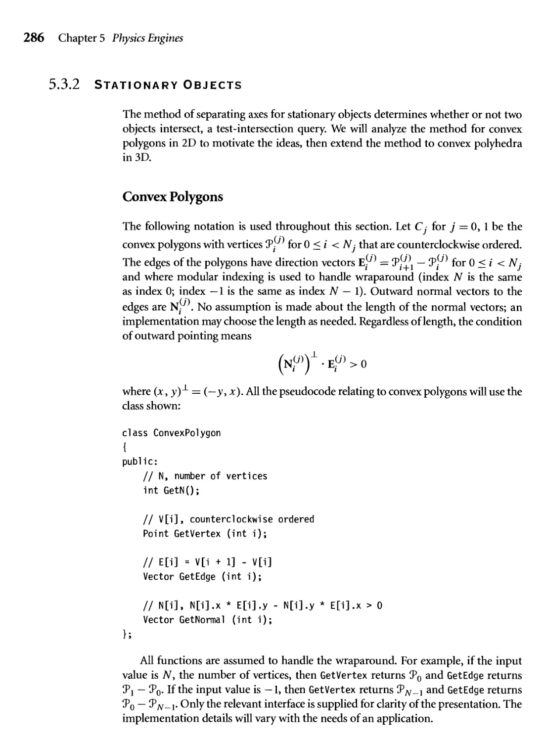
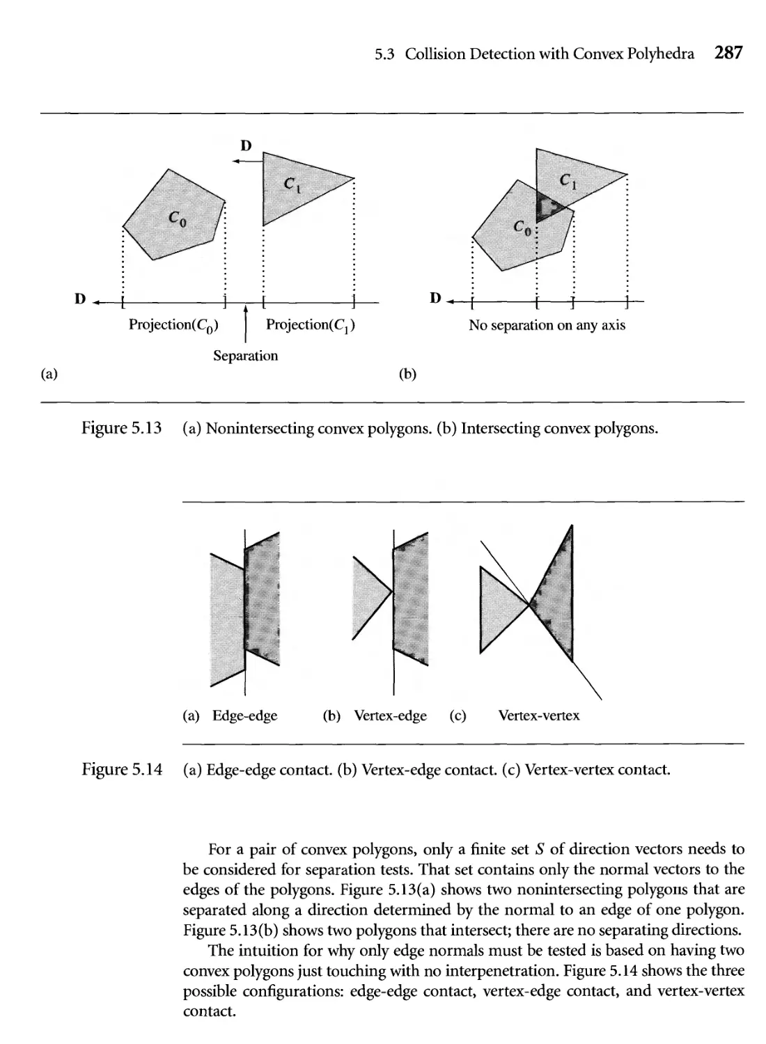
5.13 (a) Nonintersecting convex polygons, (b) Intersecting convex
polygons. 287
5.14 (a) Edge-edge contact, (b) Vertex-edge contact, (c) Vertex-vertex
contact. 287
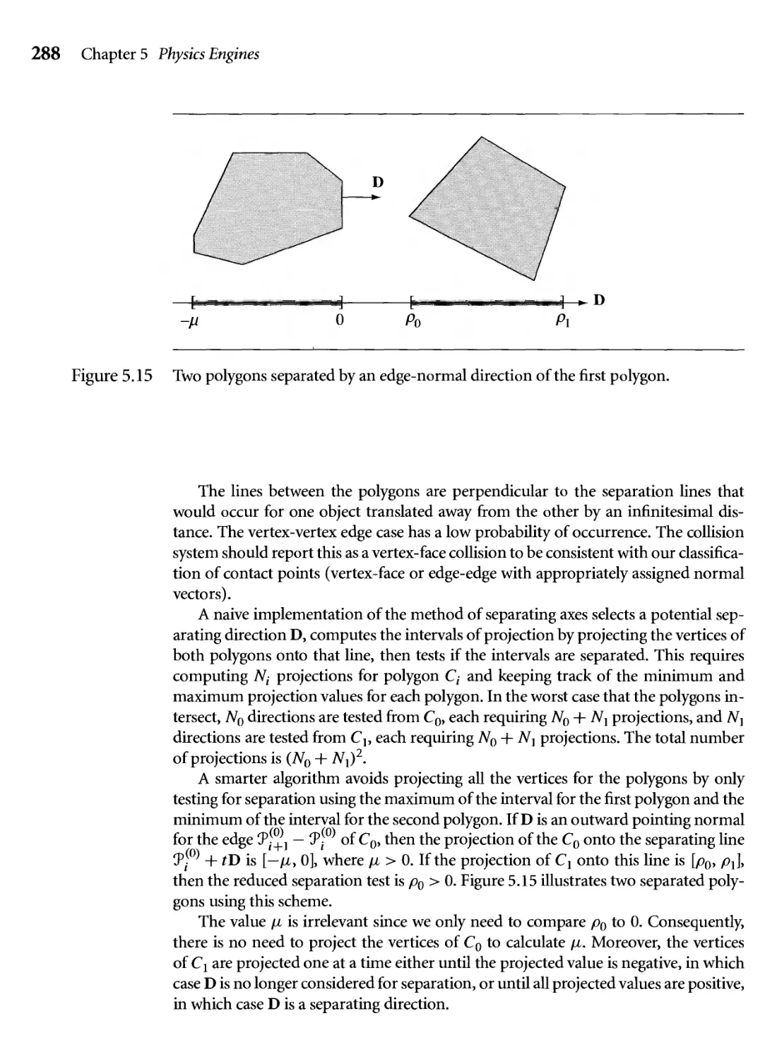
5.15 Two polygons separated by an edge-normal direction of the first
polygon. 288
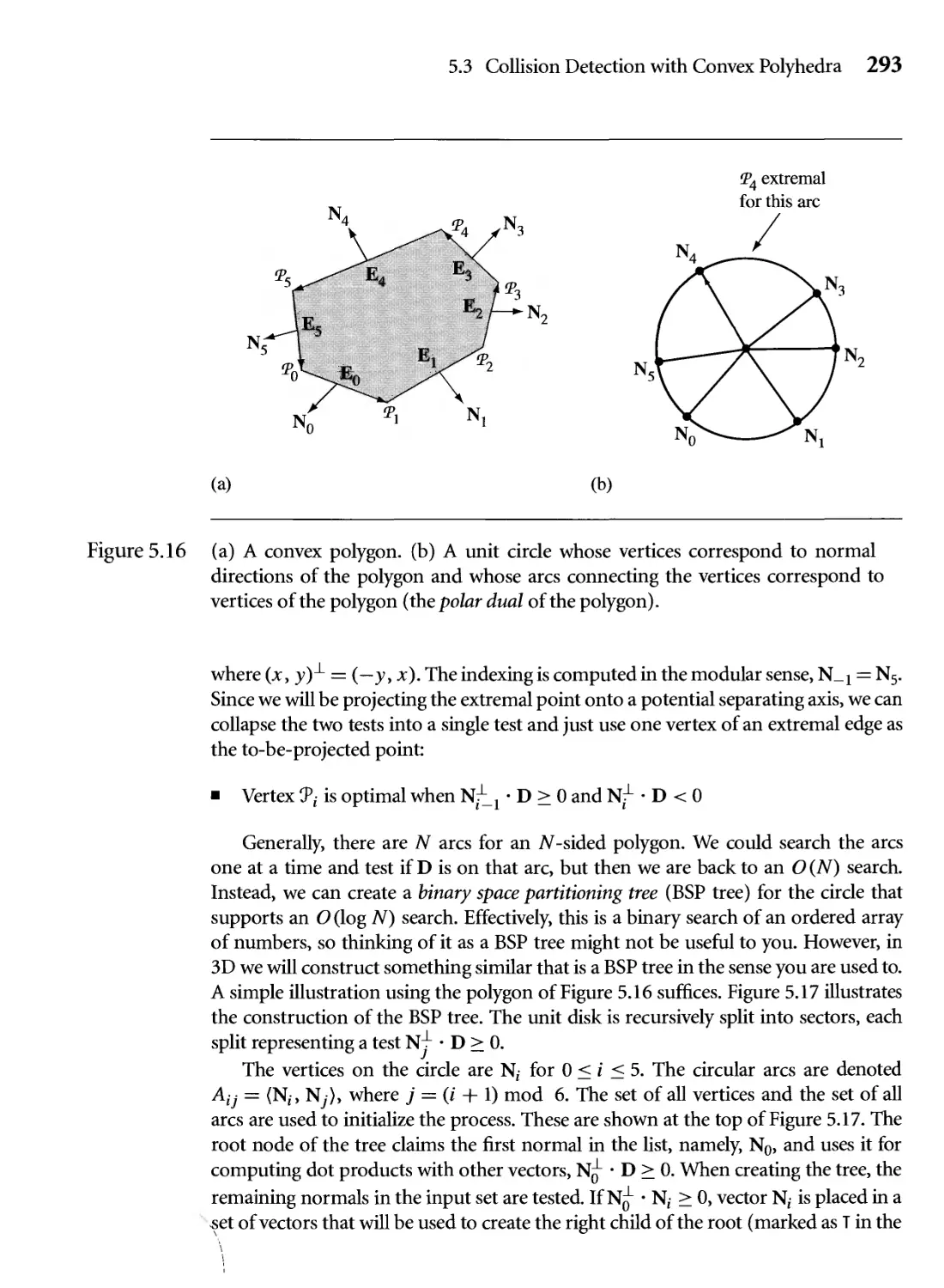
5.16 (a) A convex polygon, (b) A unit circle whose vertices correspond
to normal directions of the polygon and whose arcs connecting the
vertices correspond to vertices of the polygon (the polar dual of the
polygon). 293
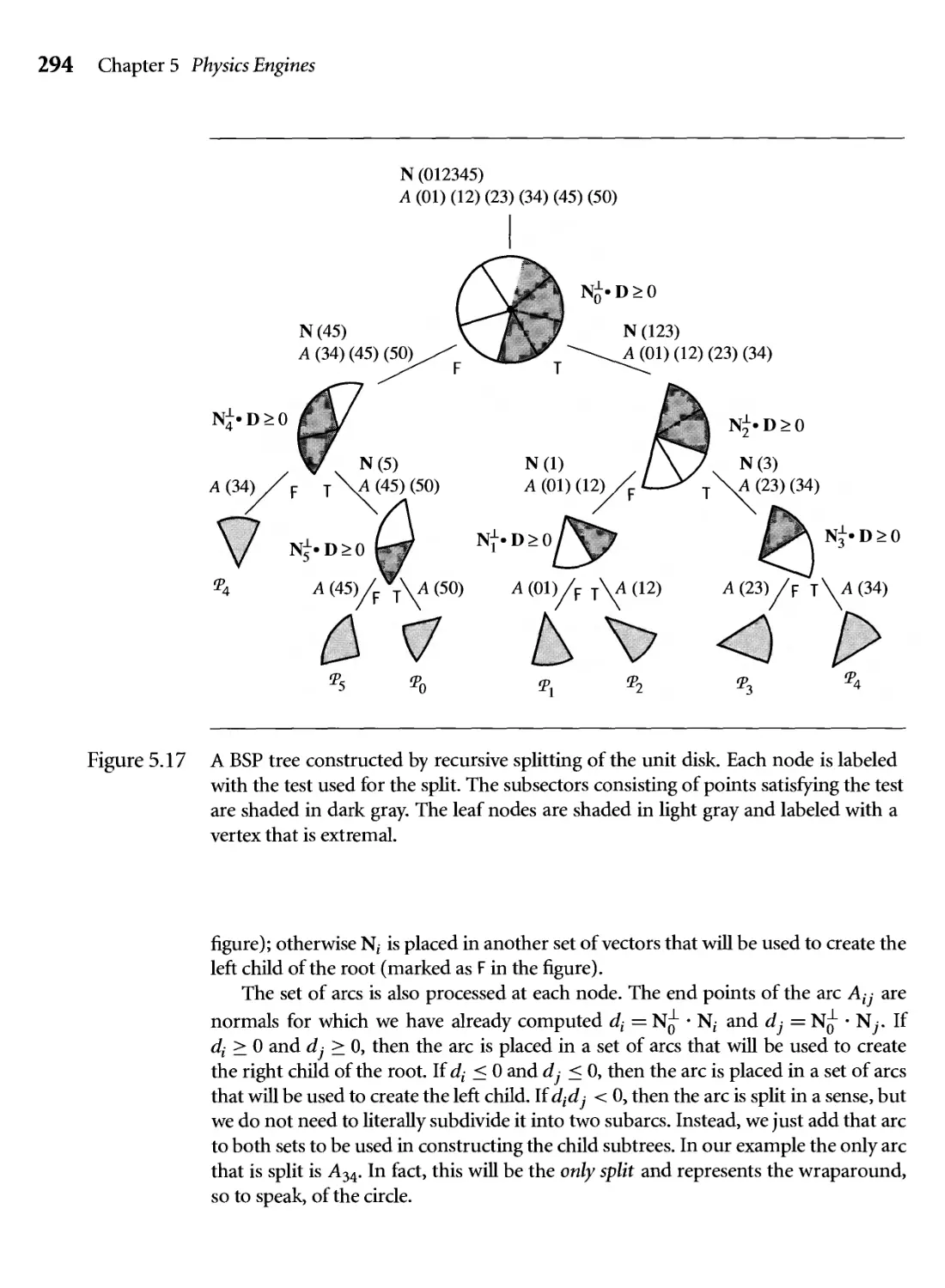
5.17 A BSP tree constructed by recursive splitting of the unit disk. Each
node is labeled with the test used for the split. The subsectors
consisting of points satisfying the test are shaded in dark gray. The
leaf nodes are shaded in light gray and labeled with a vertex that is
extremal. 294
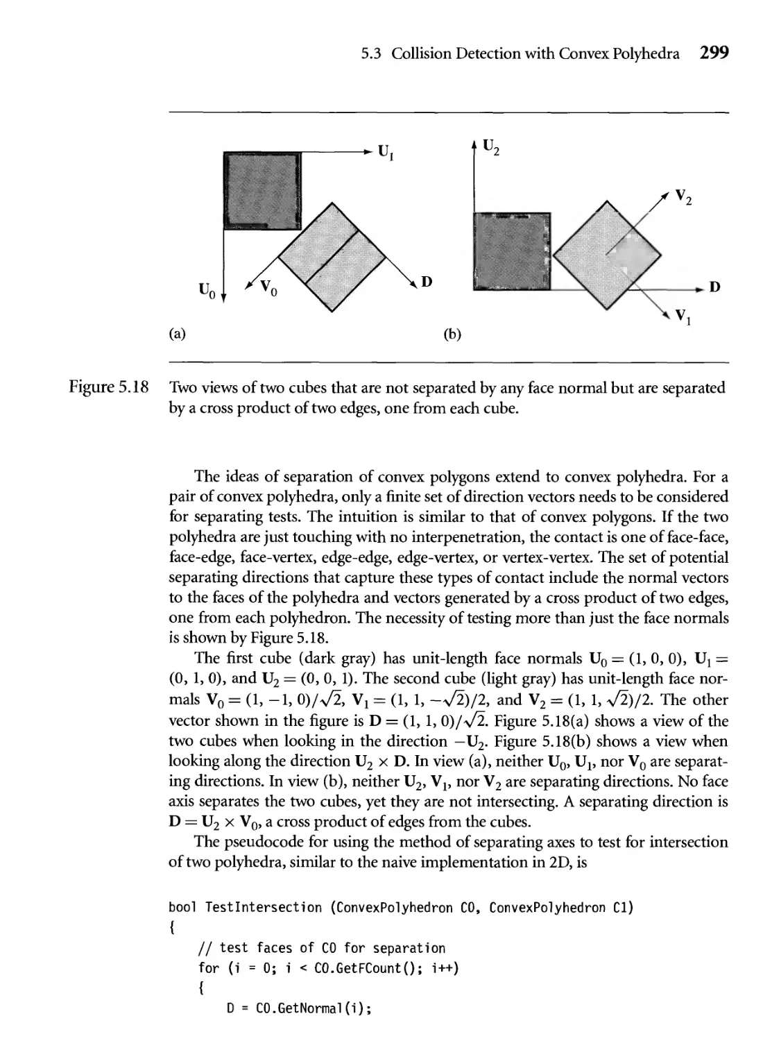
5.18 Two views of two cubes that are not separated by any face normal but
are separated by a cross product of two edges, one from each cube. 299
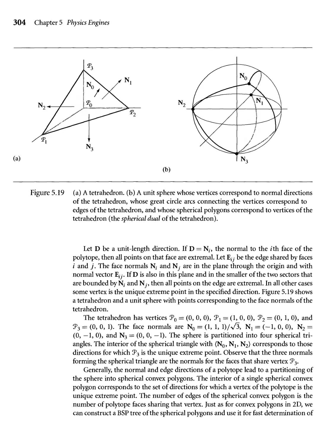
5.19 (a) A tetrahedron, (b) A unit sphere whose vertices correspond
to normal directions of the tetrahedron, whose great circle arcs
connecting the vertices correspond to edges of the tetrahedron, and
whose spherical polygons correspond to vertices of the tetrahedron
(the spherical dual of the tetrahedron). 304
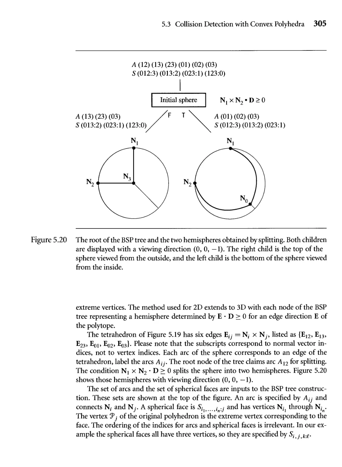
5.20 The root of the BSP tree and the two hemispheres obtained by
splitting. Both children are displayed with a viewing direction
@, 0, —1). The right child is the top of the sphere viewed from the
outside, and the left child is the bottom of the sphere viewed from the
inside. 305

xxii Figures
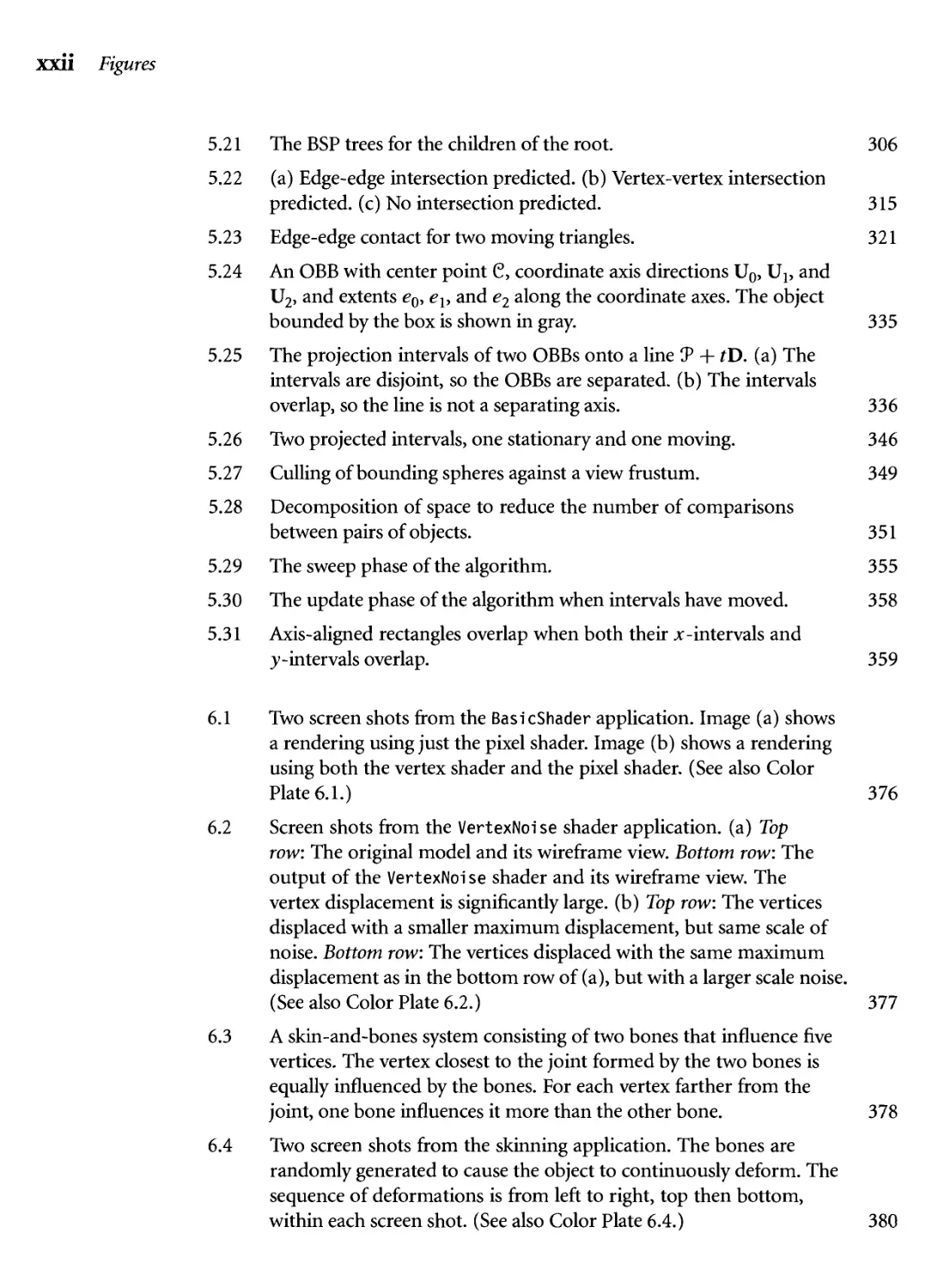
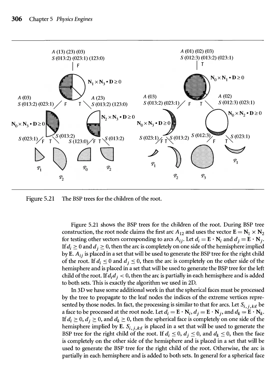
5.21 The BSP trees for the children of the root. 306
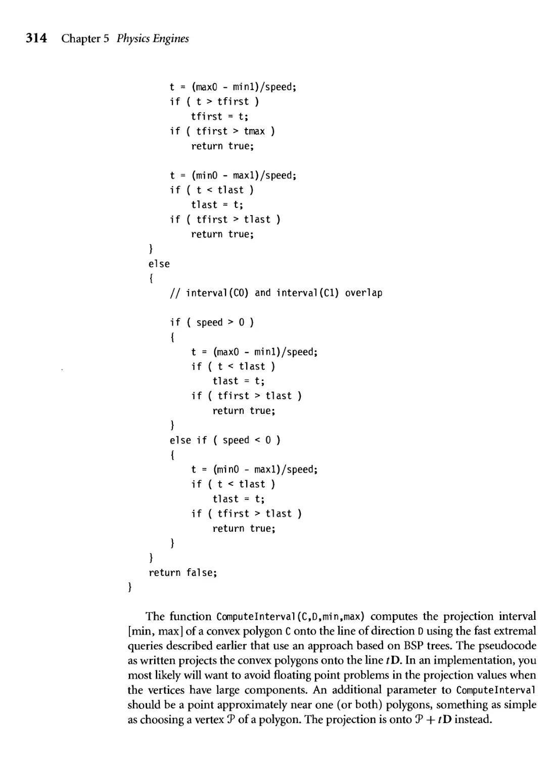
5.22 (a) Edge-edge intersection predicted, (b) Vertex-vertex intersection
predicted, (c) No intersection predicted. 315
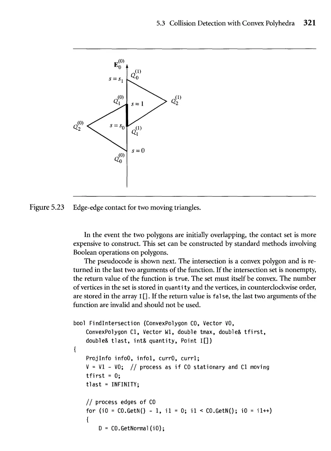
5.23 Edge-edge contact for two moving triangles. 321
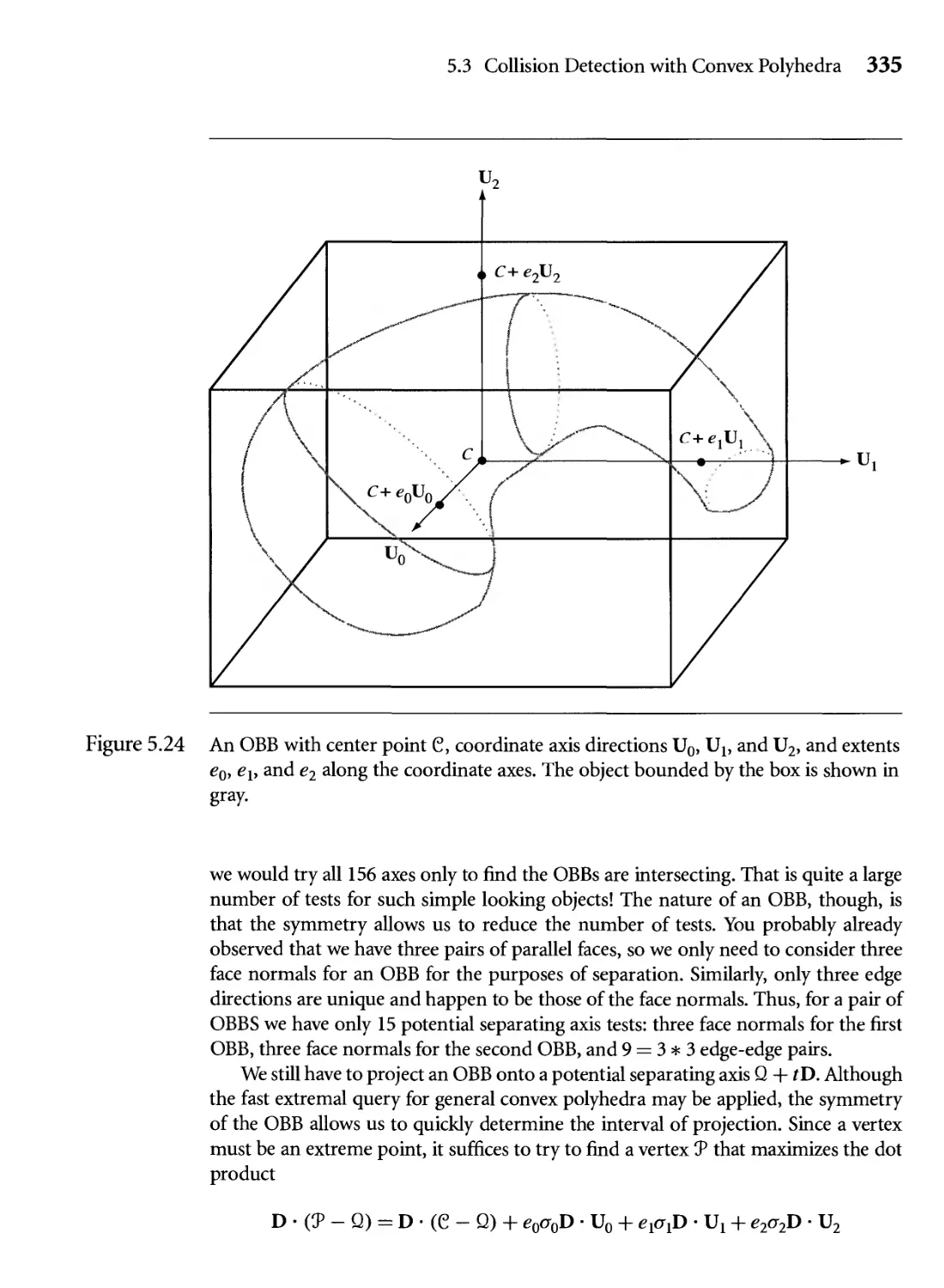
5.24 An OBB with center point C, coordinate axis directions Uo, Uj, and
U2, and extents e0, ev and e2 along the coordinate axes. The object
bounded by the box is shown in gray. 335
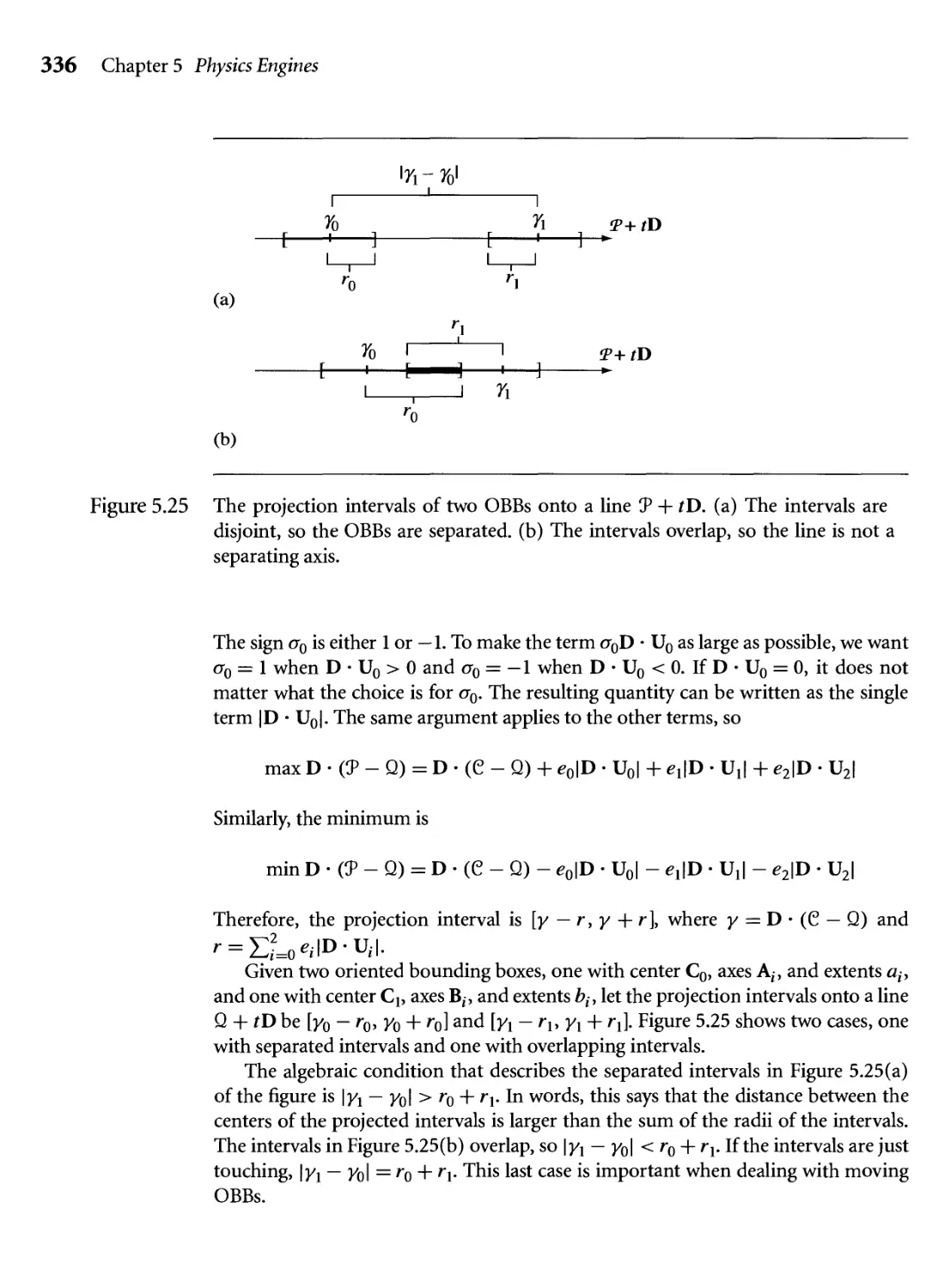
5.25 The projection intervals of two OBBs onto a line У + tD. (a) The
intervals are disjoint, so the OBBs are separated, (b) The intervals
overlap, so the line is not a separating axis. 336
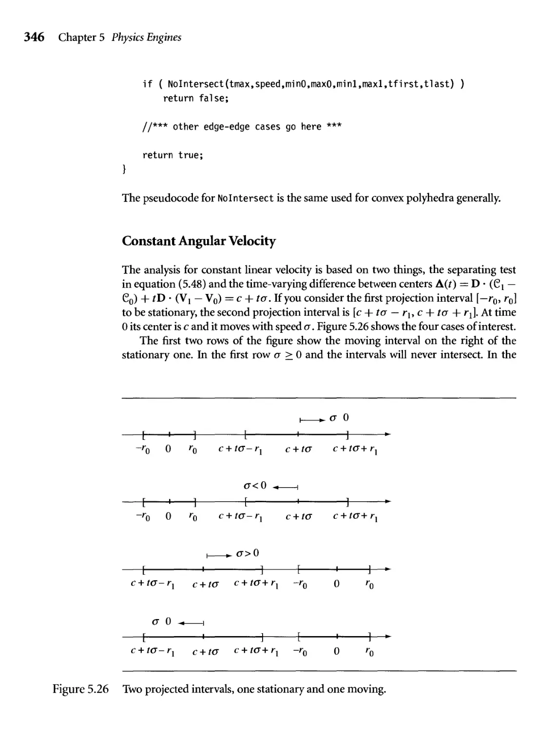
5.26 Two projected intervals, one stationary and one moving. 346
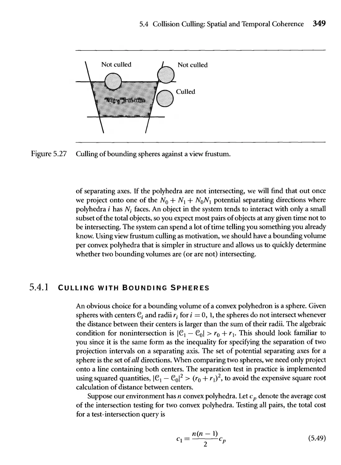
5.27 Culling of bounding spheres against a view frustum. 349
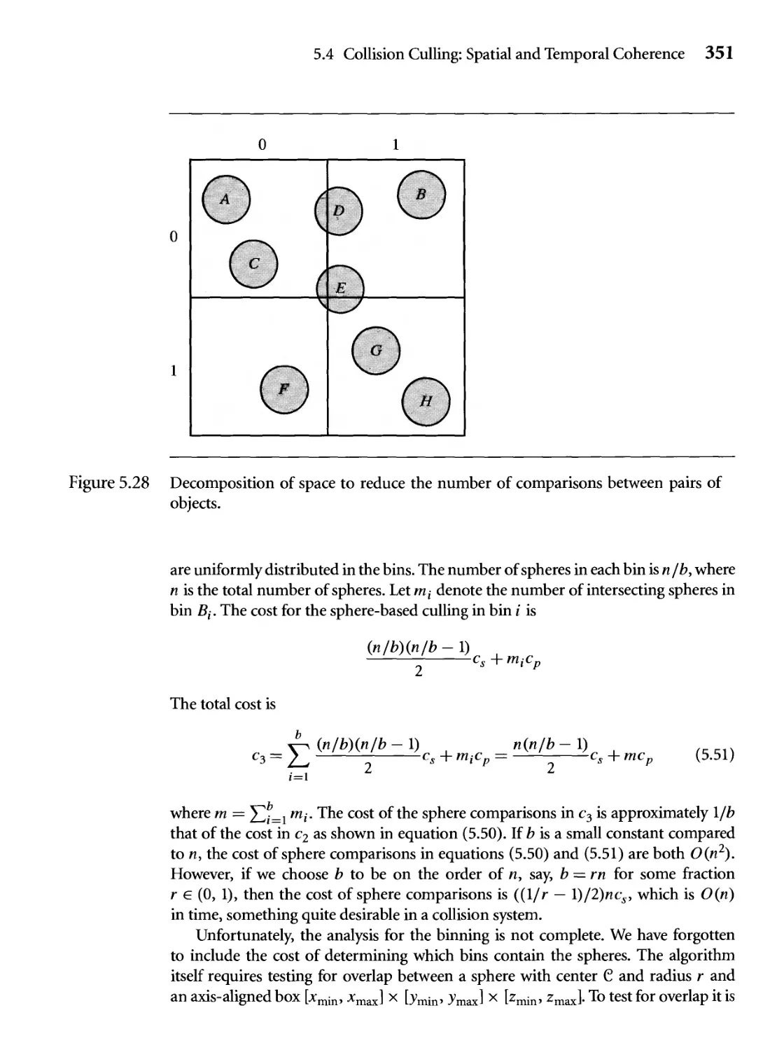
5.28 Decomposition of space to reduce the number of comparisons
between pairs of objects. 351
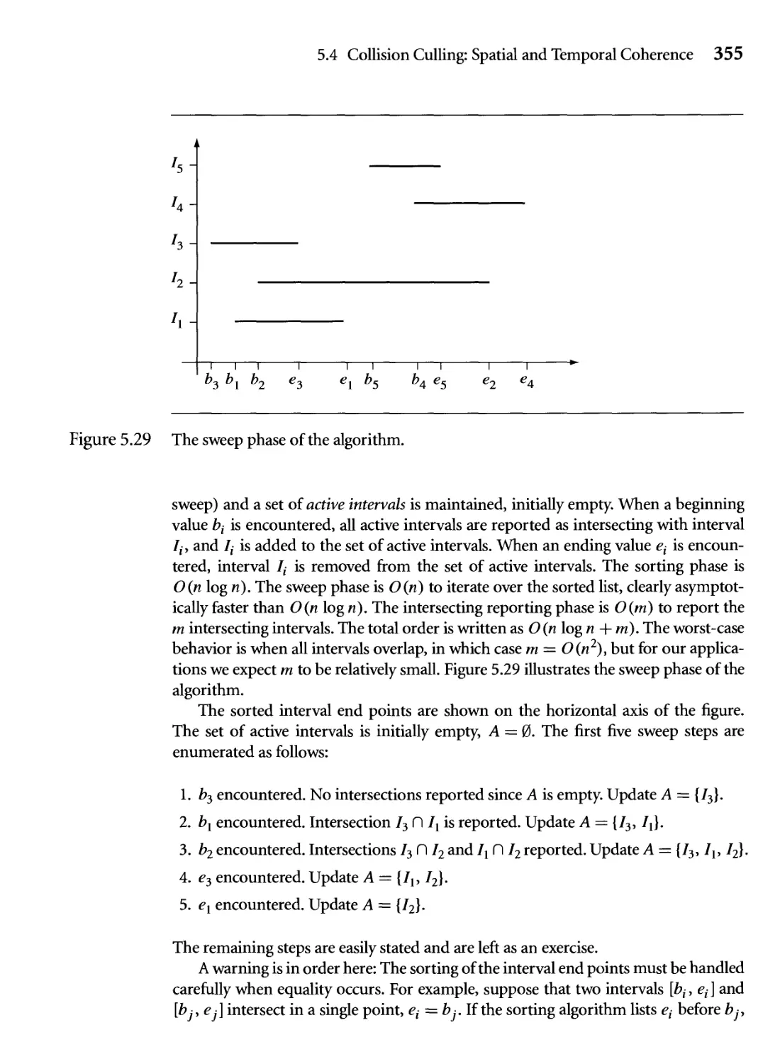
5.29 The sweep phase of the algorithm. 355
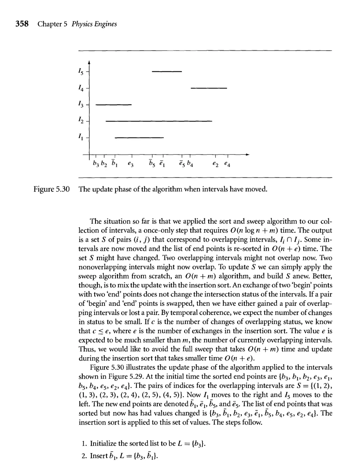
5.30 The update phase of the algorithm when intervals have moved. 358
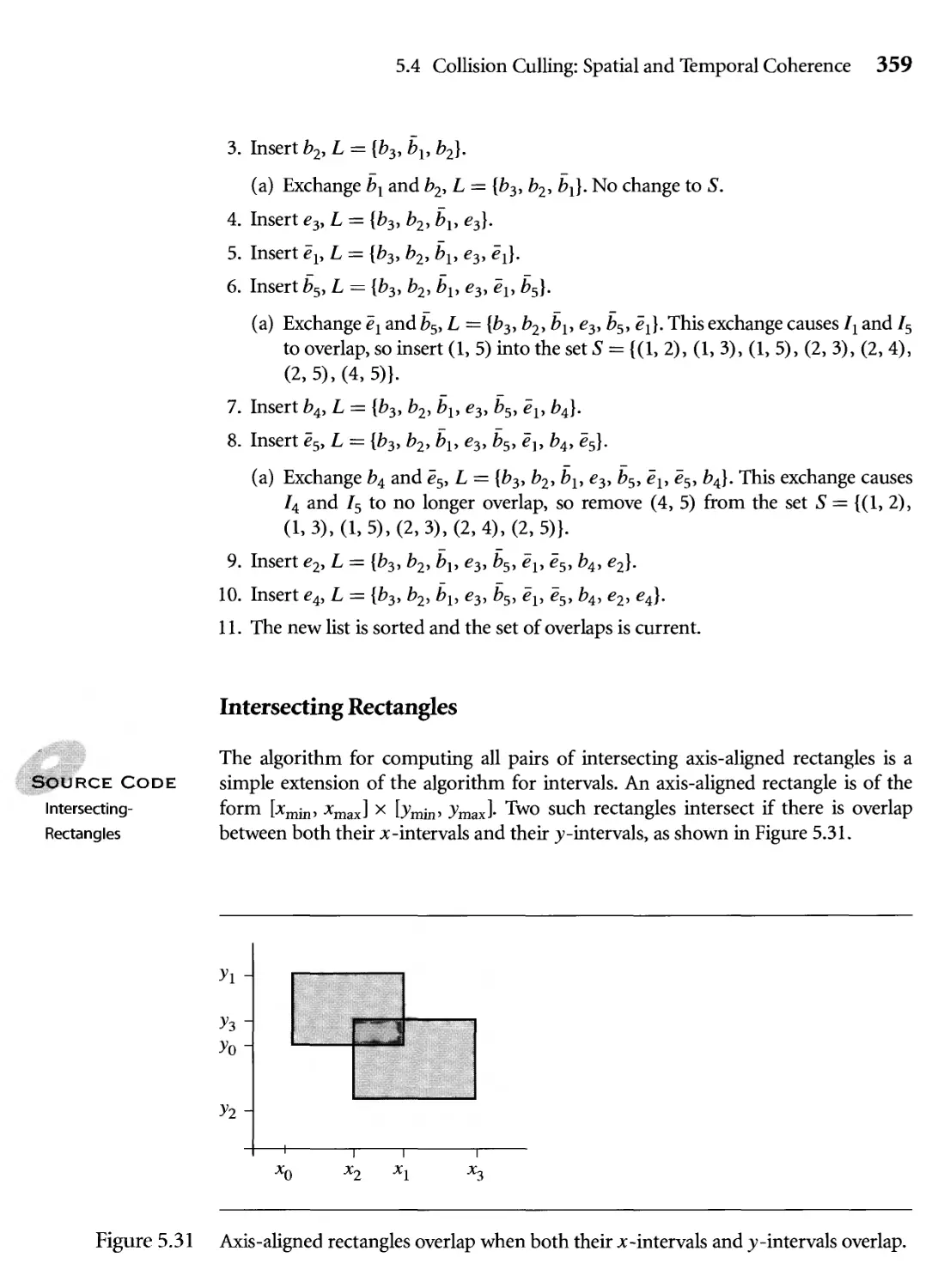
5.31 Axis-aligned rectangles overlap when both their x-intervals and
v-intervals overlap. 359
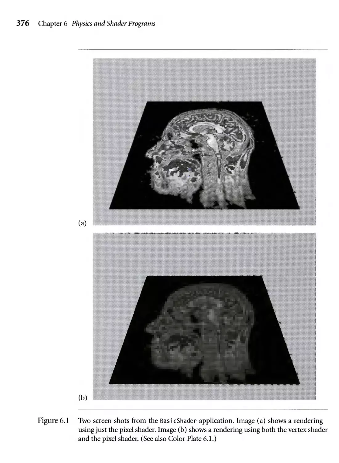
6.1 Two screen shots from the Basi cShader application. Image (a) shows
a rendering using just the pixel shader. Image (b) shows a rendering
using both the vertex shader and the pixel shader. (See also Color
Plate 6.1.) 376
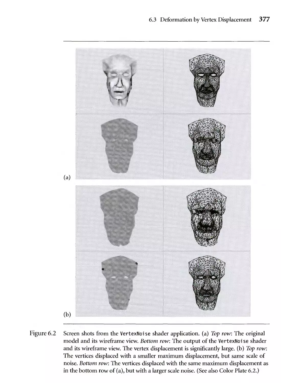
6.2 Screen shots from the VertexNoise shader application, (a) Top
row: The original model and its wireframe view. Bottom row: The
output of the VertexNoise shader and its wireframe view. The
vertex displacement is significantly large, (b) Top row: The vertices
displaced with a smaller maximum displacement, but same scale of
noise. Bottom row: The vertices displaced with the same maximum
displacement as in the bottom row of (a), but with a larger scale noise.
(See also Color Plate 6.2.) 377
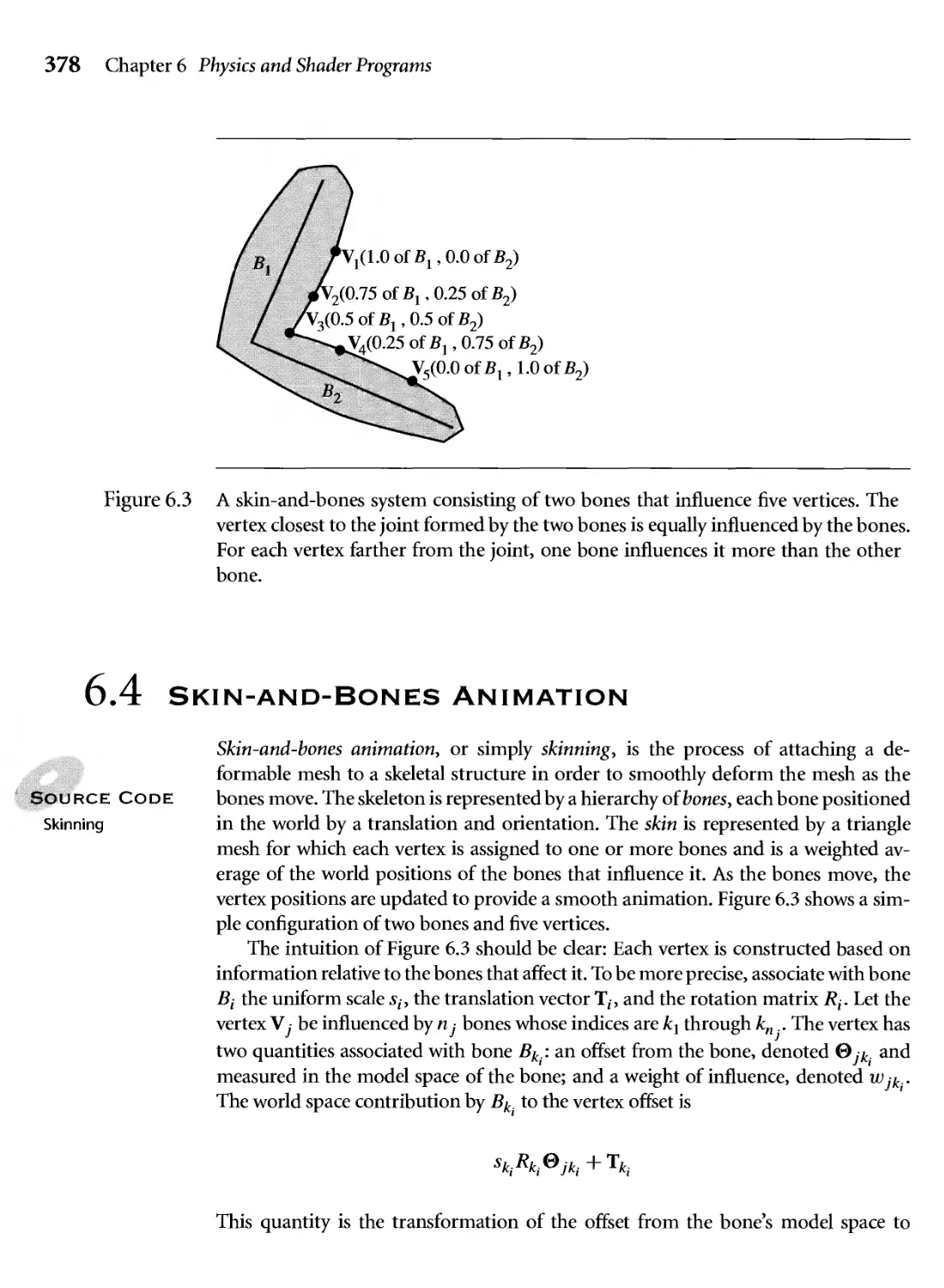
6.3 A skin-and-bones system consisting of two bones that influence five
vertices. The vertex closest to the joint formed by the two bones is
equally influenced by the bones. For each vertex farther from the
joint, one bone influences it more than the other bone. 378
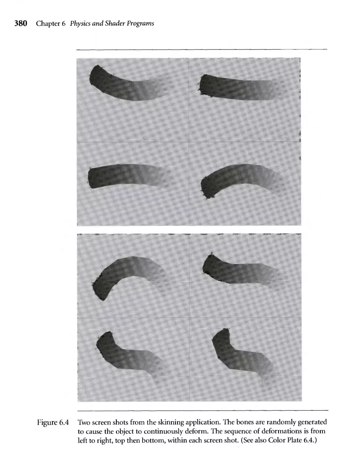
6.4 Two screen shots from the skinning application. The bones are
randomly generated to cause the object to continuously deform. The
sequence of deformations is from left to right, top then bottom,
within each screen shot. (See also Color Plate 6.4.) 380

Figures xxiii
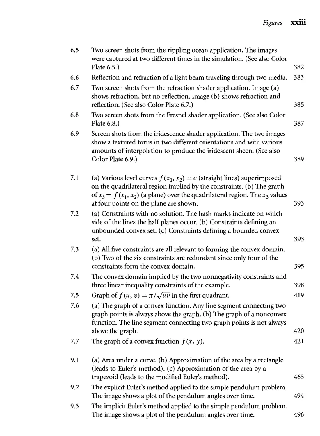
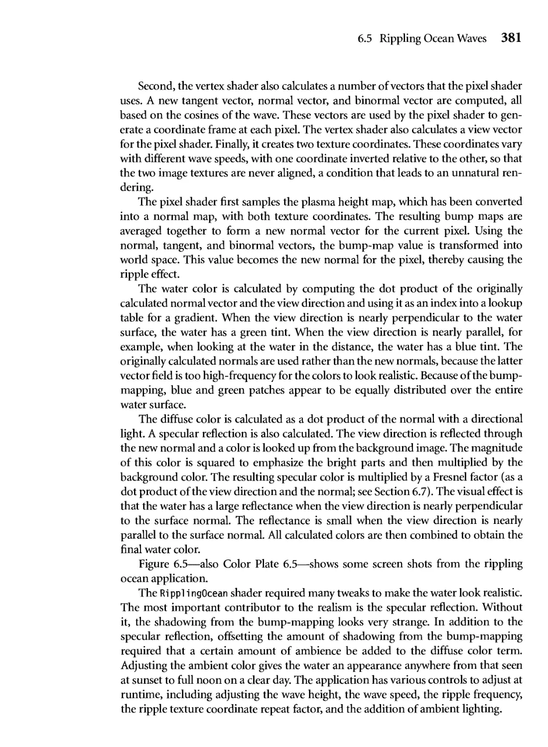
6.5 Two screen shots from the rippling ocean application. The images
were captured at two different times in the simulation. (See also Color
Plate 6.5.) 382
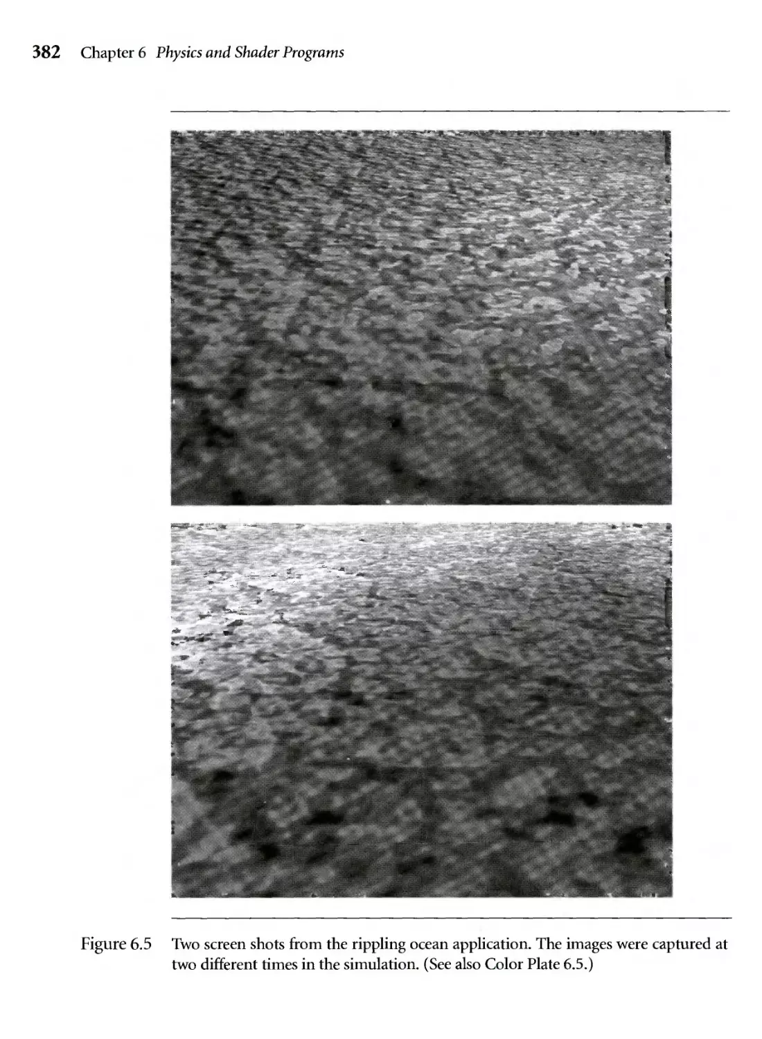
6.6 Reflection and refraction of a light beam traveling through two media. 383
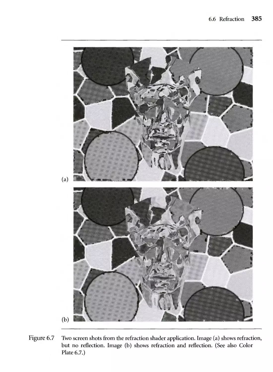
6.7 Two screen shots from the refraction shader application. Image (a)
shows refraction, but no reflection. Image (b) shows refraction and
reflection. (See also Color Plate 6.7.) 385
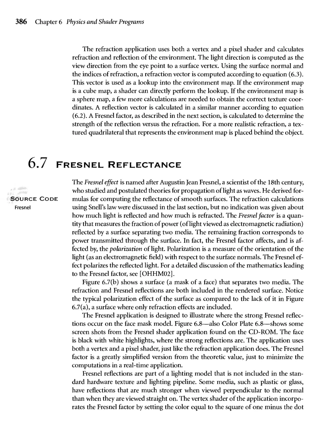
6.8 Two screen shots from the Fresnel shader application. (See also Color
Plate 6.8.) 387
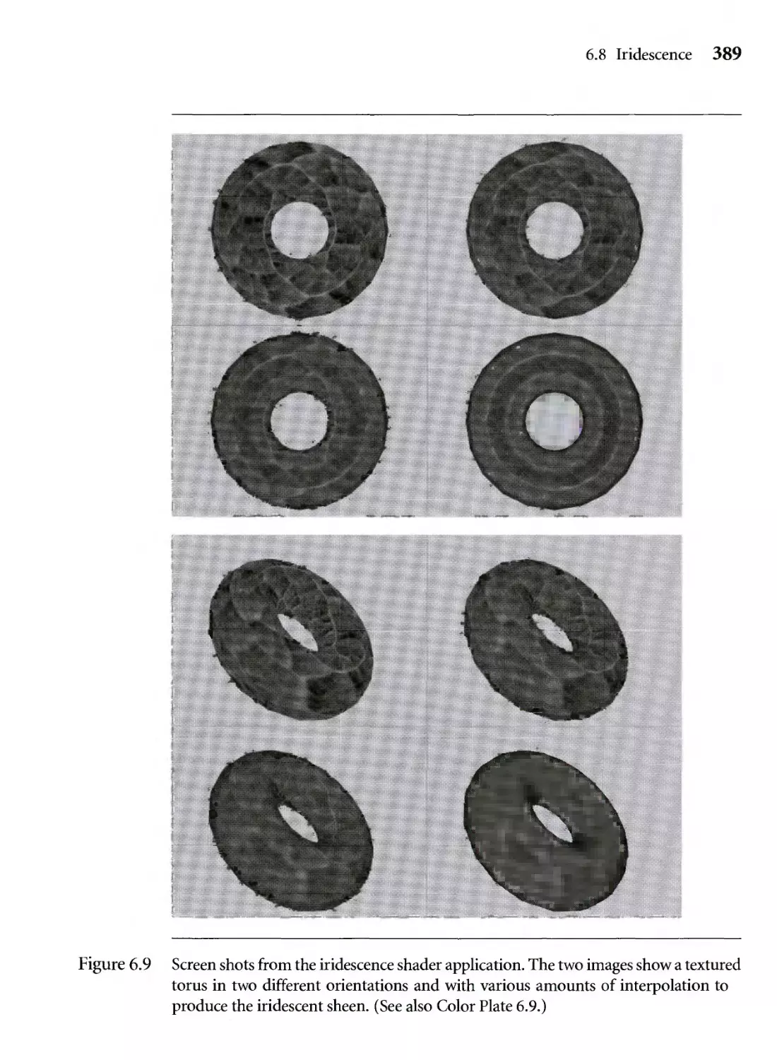
6.9 Screen shots from the iridescence shader application. The two images
show a textured torus in two different orientations and with various
amounts of interpolation to produce the iridescent sheen. (See also
Color Plate 6.9.) 389
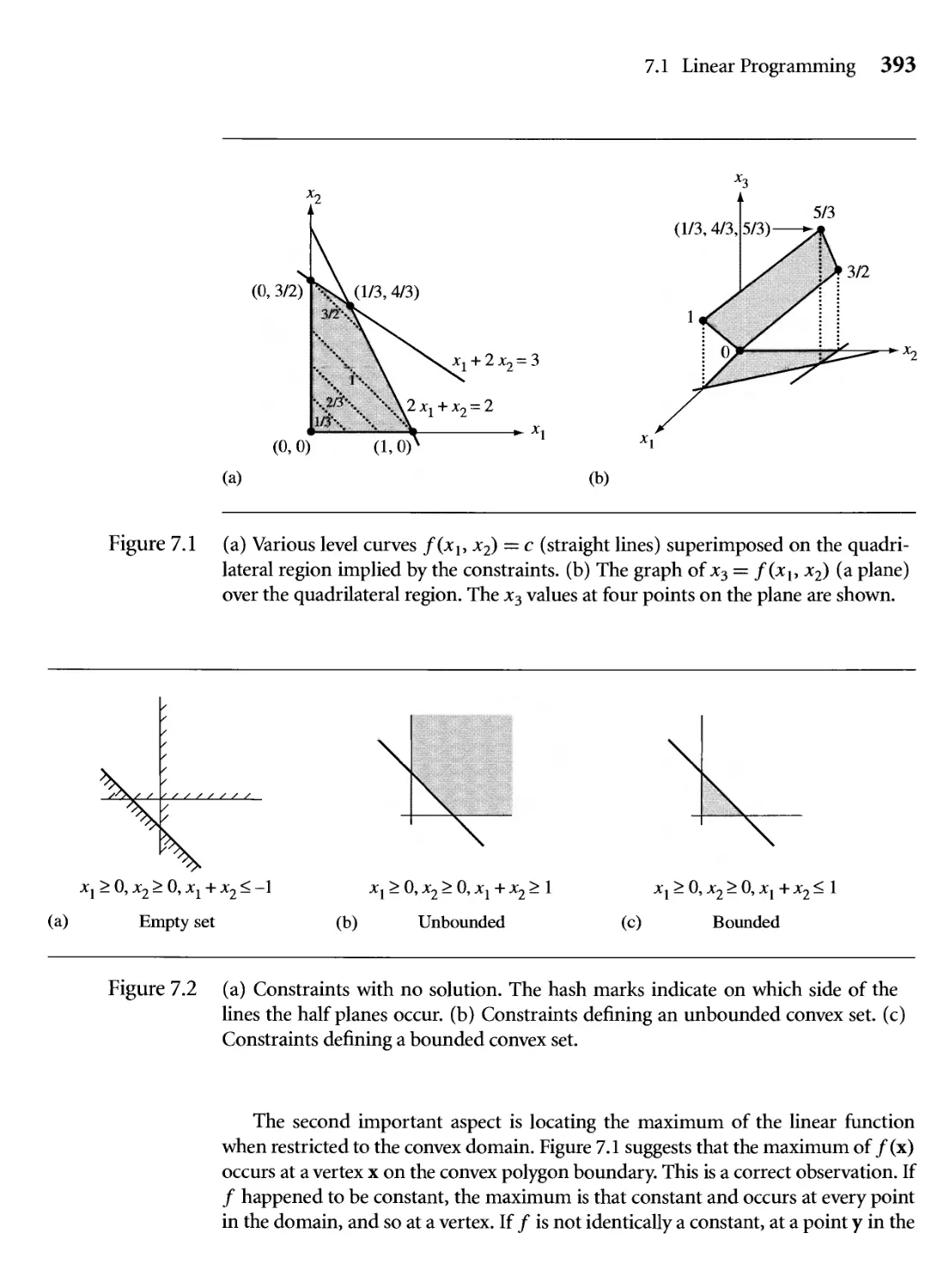
7.1 (a) Various level curves f(xb x2) = с (straight lines) superimposed
on the quadrilateral region implied by the constraints, (b) The graph
of jc3 = f{xy, x2) (a plane) over the quadrilateral region. The x3 values
at four points on the plane are shown. 393
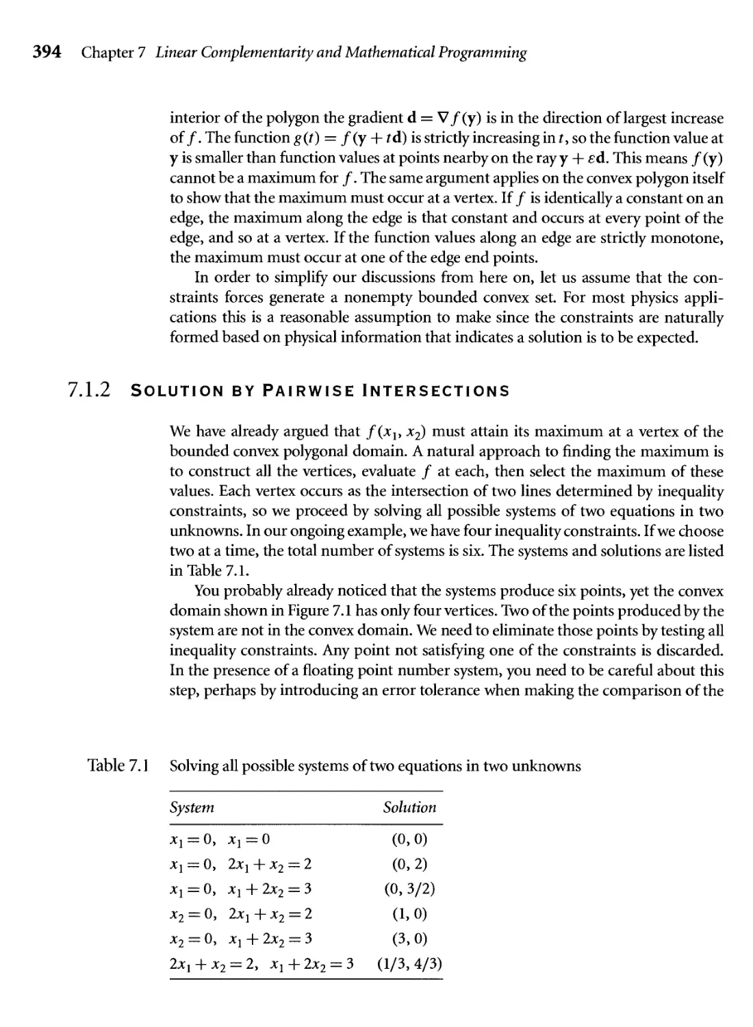
7.2 (a) Constraints with no solution. The hash marks indicate on which
side of the lines the half planes occur, (b) Constraints denning an
unbounded convex set. (c) Constraints defining a bounded convex
set. 393
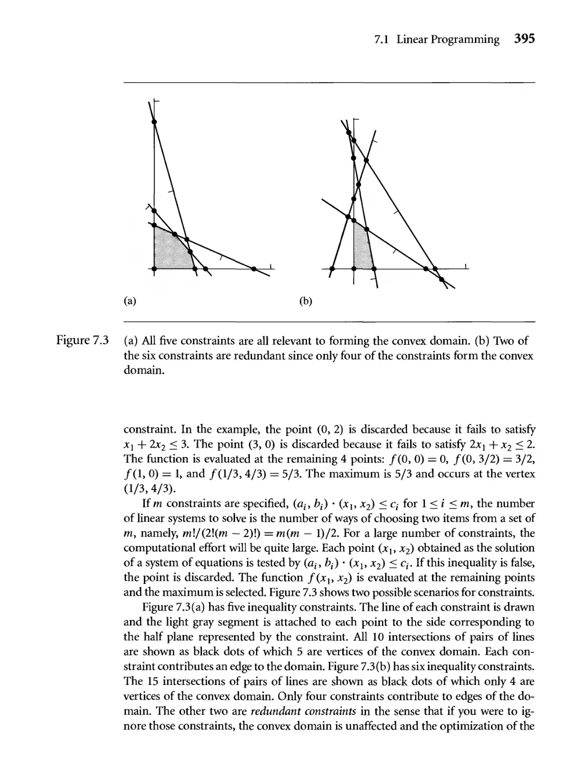
7.3 (a) All five constraints are all relevant to forming the convex domain,
(b) Two of the six constraints are redundant since only four of the
constraints form the convex domain. 395
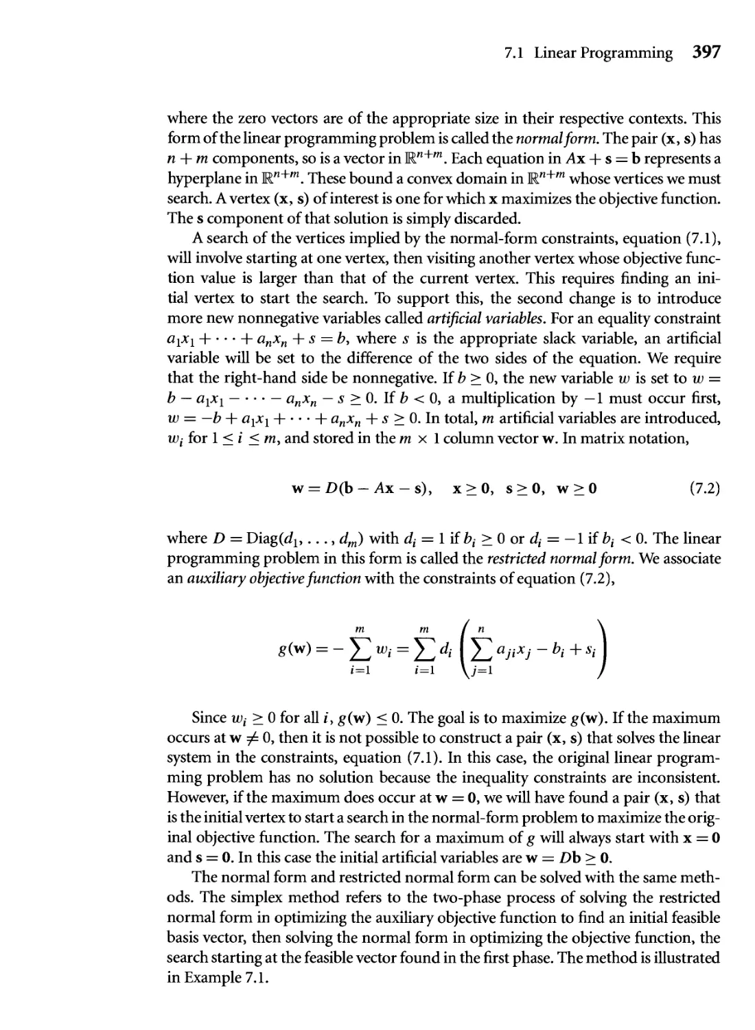
7.4 The convex domain implied by the two nonnegativity constraints and
three linear inequality constraints of the example. 398
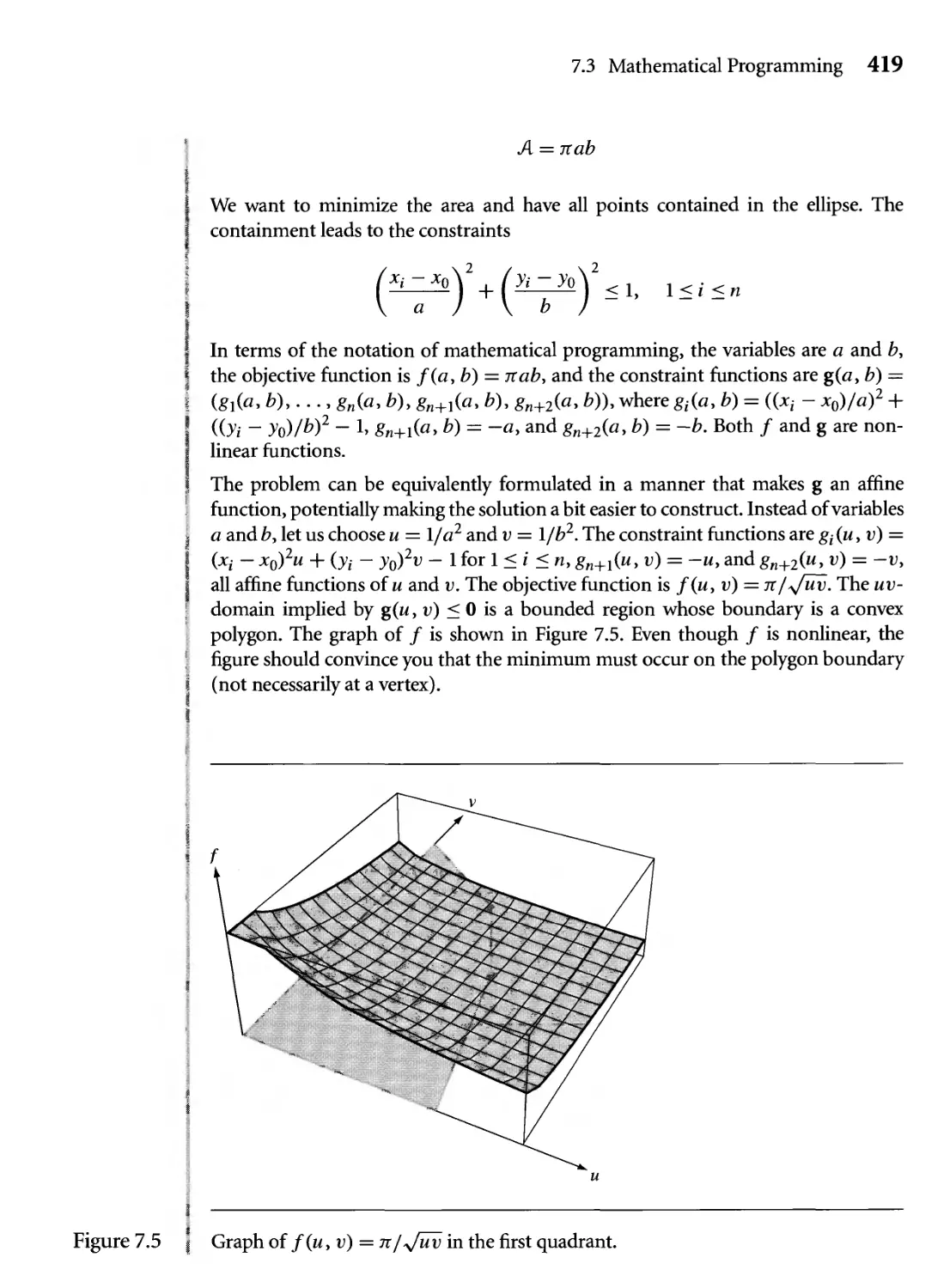
7.5 Graph of f(u, v) = n/y/uv in the first quadrant. 419
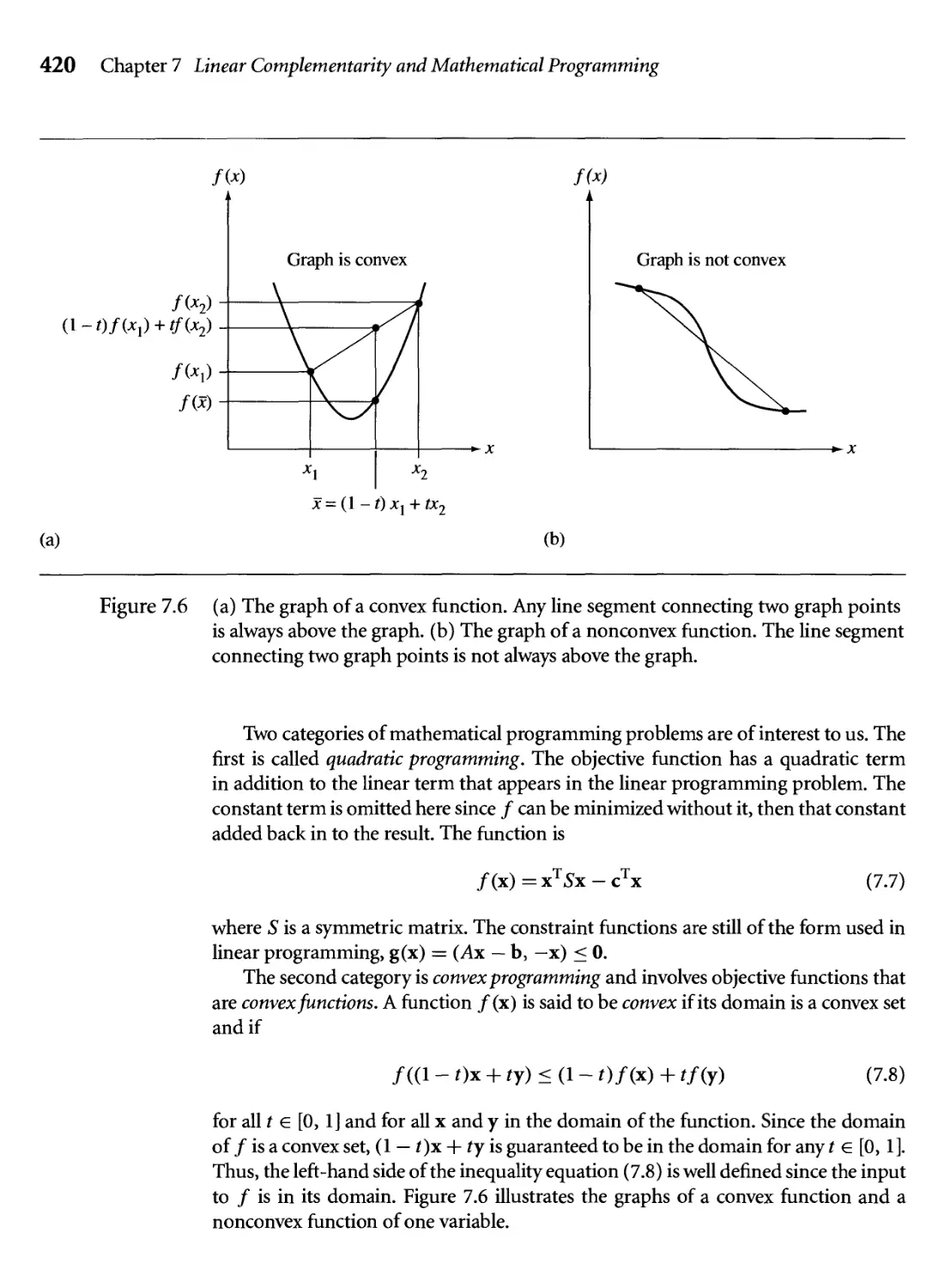
7.6 (a) The graph of a convex function. Any line segment connecting two
graph points is always above the graph, (b) The graph of a nonconvex
function. The line segment connecting two graph points is not always
above the graph. 420
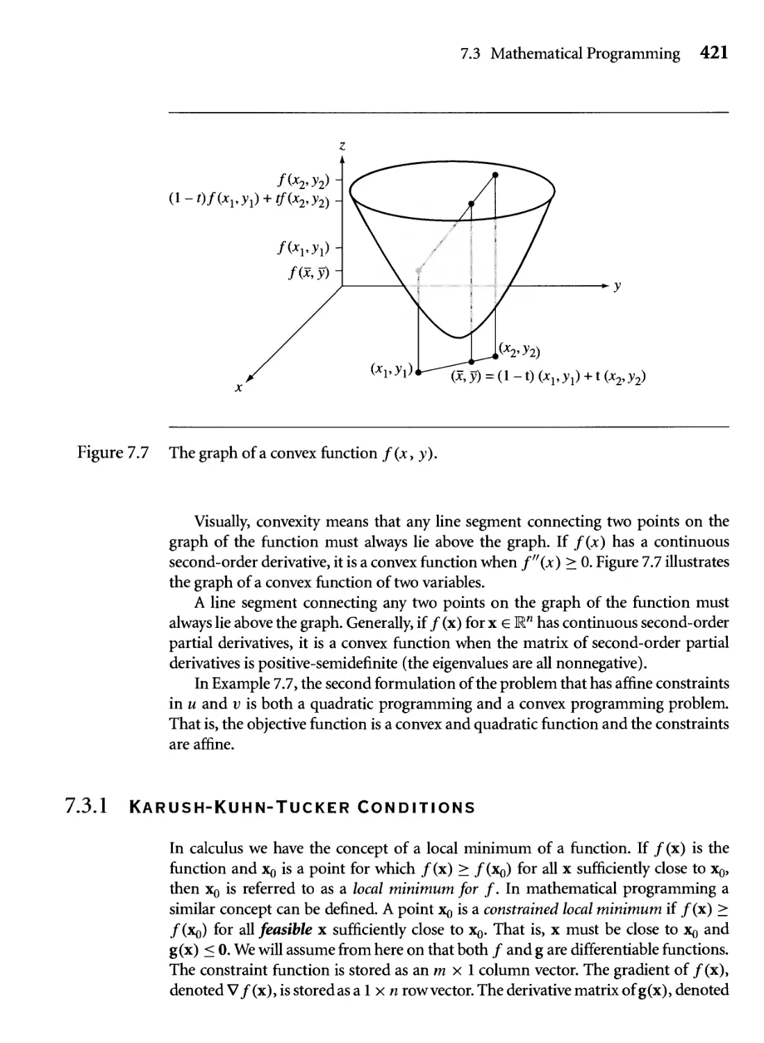
7.7 The graph of a convex function f(x, y). 421
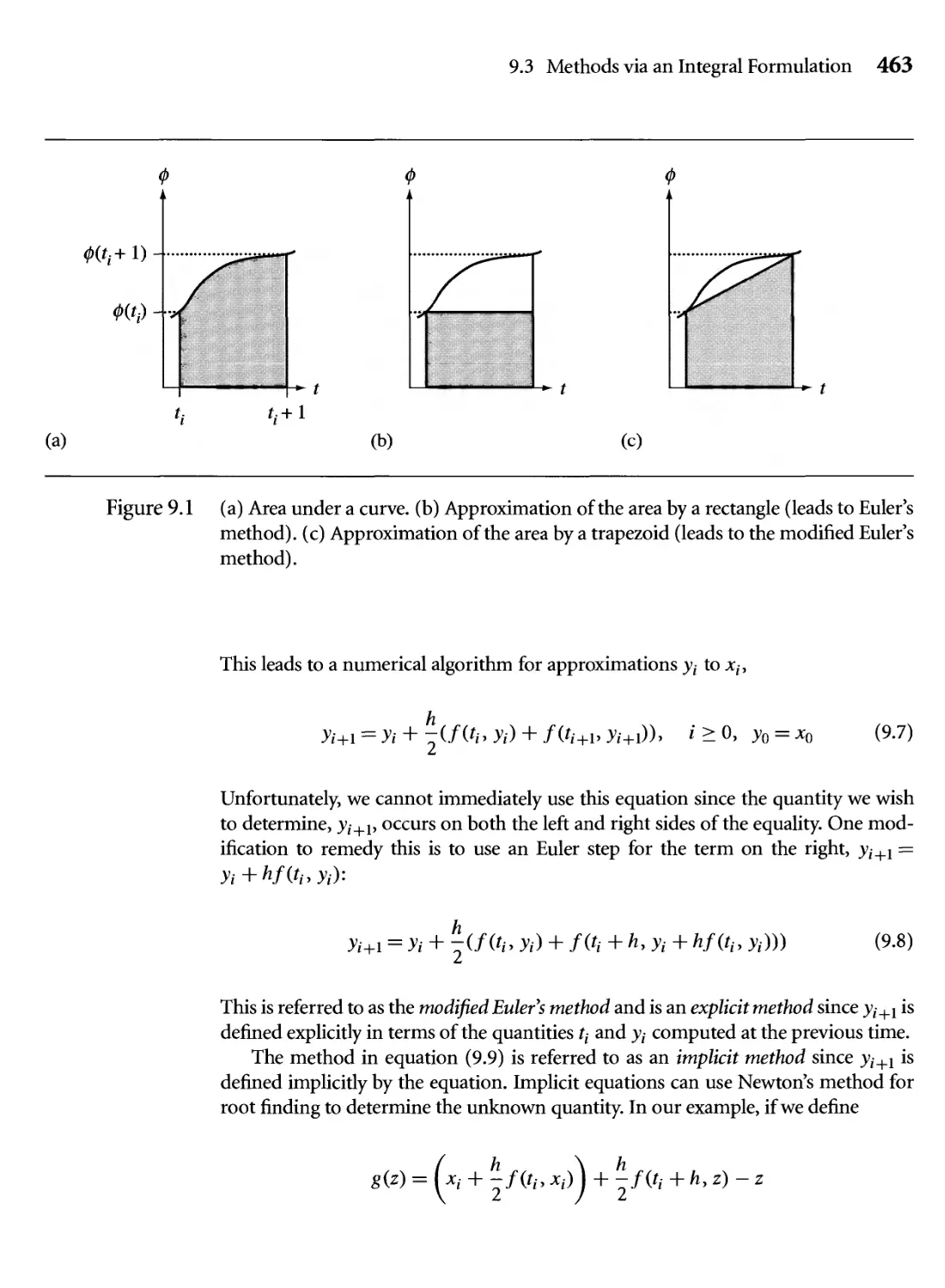
9.1 (a) Area under a curve, (b) Approximation of the area by a rectangle
(leads to Euler's method), (c) Approximation of the area by a
trapezoid (leads to the modified Euler's method). 463
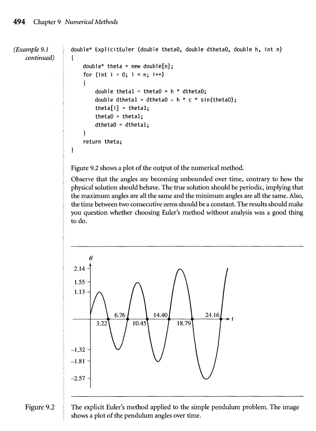
9.2 The explicit Euler's method applied to the simple pendulum problem.
The image shows a plot of the pendulum angles over time. 494
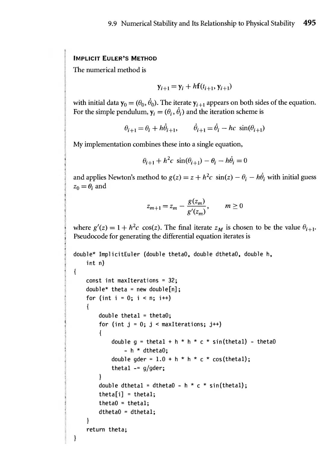
9.3 The implicit Euler's method applied to the simple pendulum problem.
The image shows a plot of the pendulum angles over time. 496

xxiv Figures
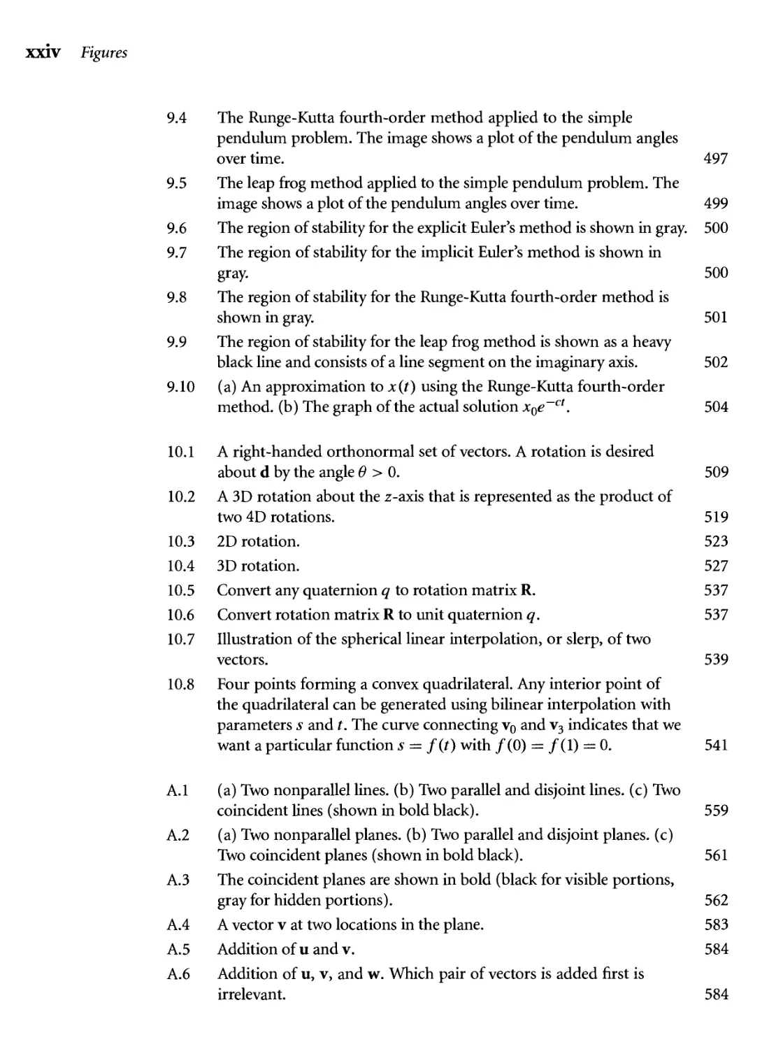
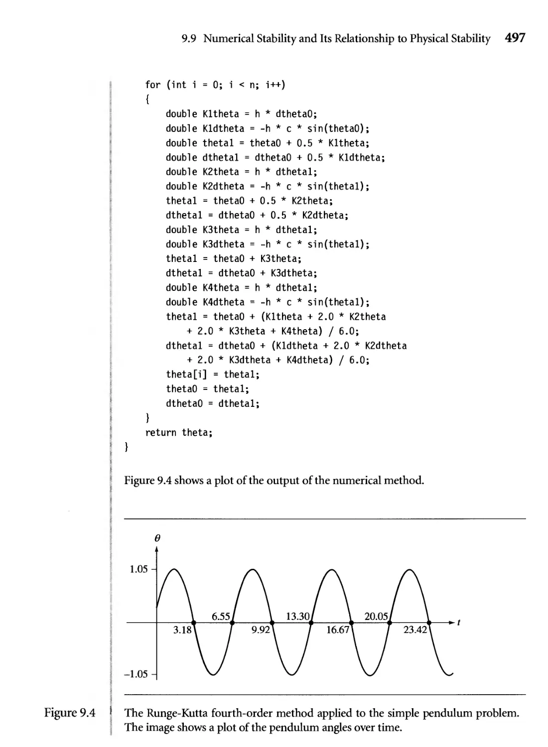
9.4 The Runge-Kutta fourth-order method applied to the simple
pendulum problem. The image shows a plot of the pendulum angles
over time. 497
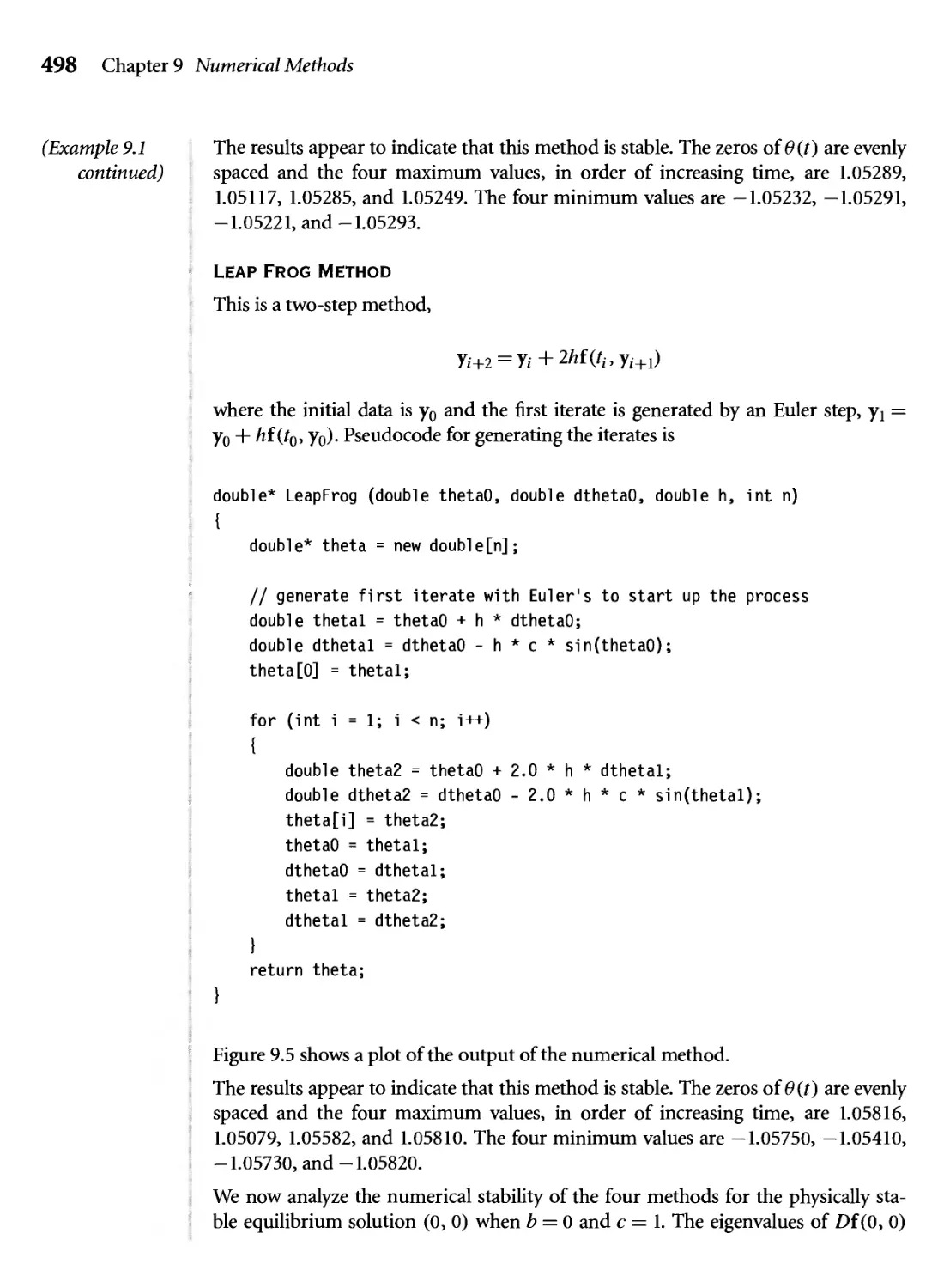
9.5 The leap frog method applied to the simple pendulum problem. The
image shows a plot of the pendulum angles over time. 499
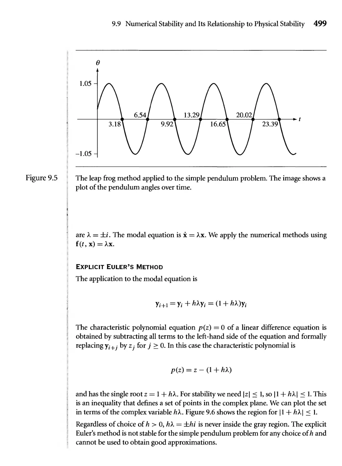
9.6 The region of stability for the explicit Euler's method is shown in gray. 500
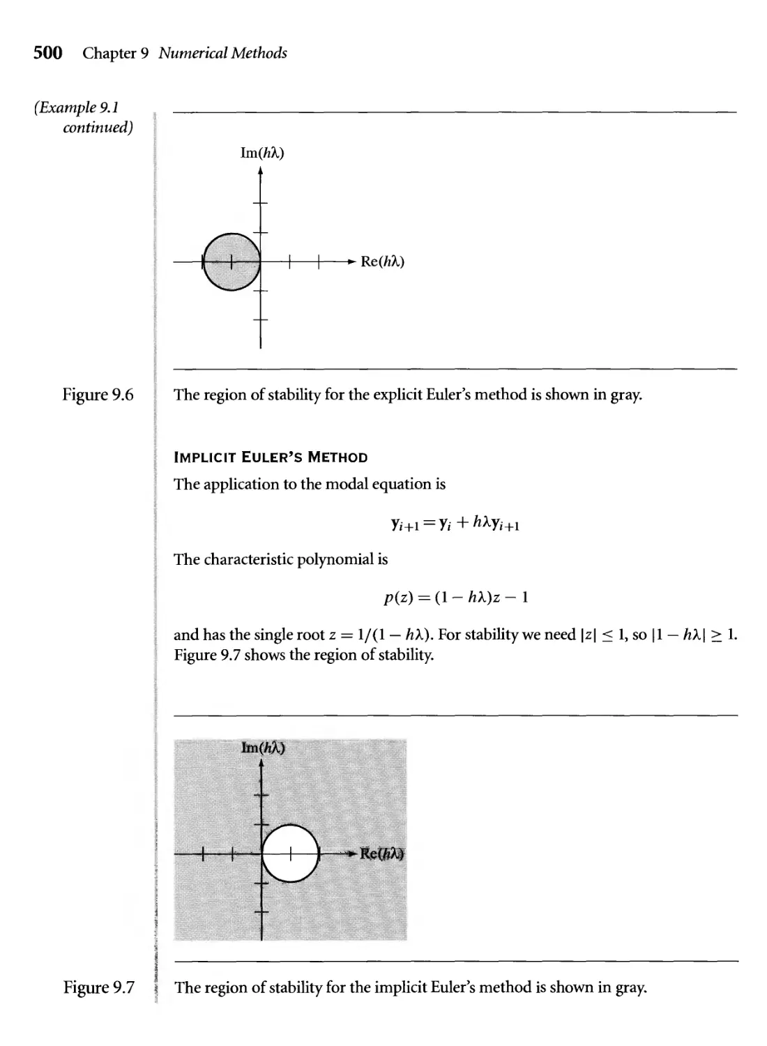
9.7 The region of stability for the implicit Euler's method is shown in
gray. 500
9.8 The region of stability for the Runge-Kutta fourth-order method is
shown in gray. 501
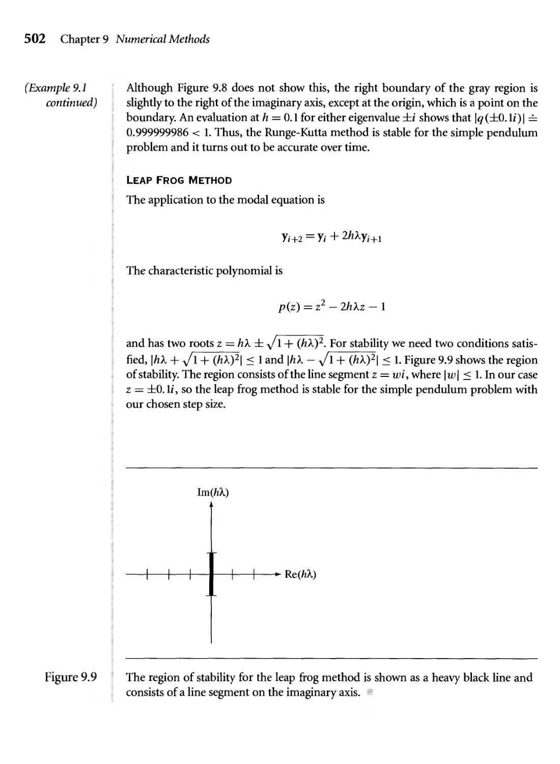
9.9 The region of stability for the leap frog method is shown as a heavy
black line and consists of a line segment on the imaginary axis. 502
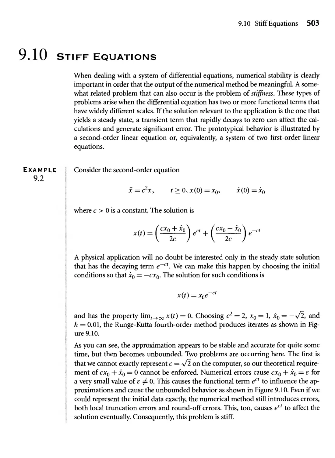
9.10 (a) An approximation to x(t) using the Runge-Kutta fourth-order
method, (b) The graph of the actual solution xoe~ct. 504
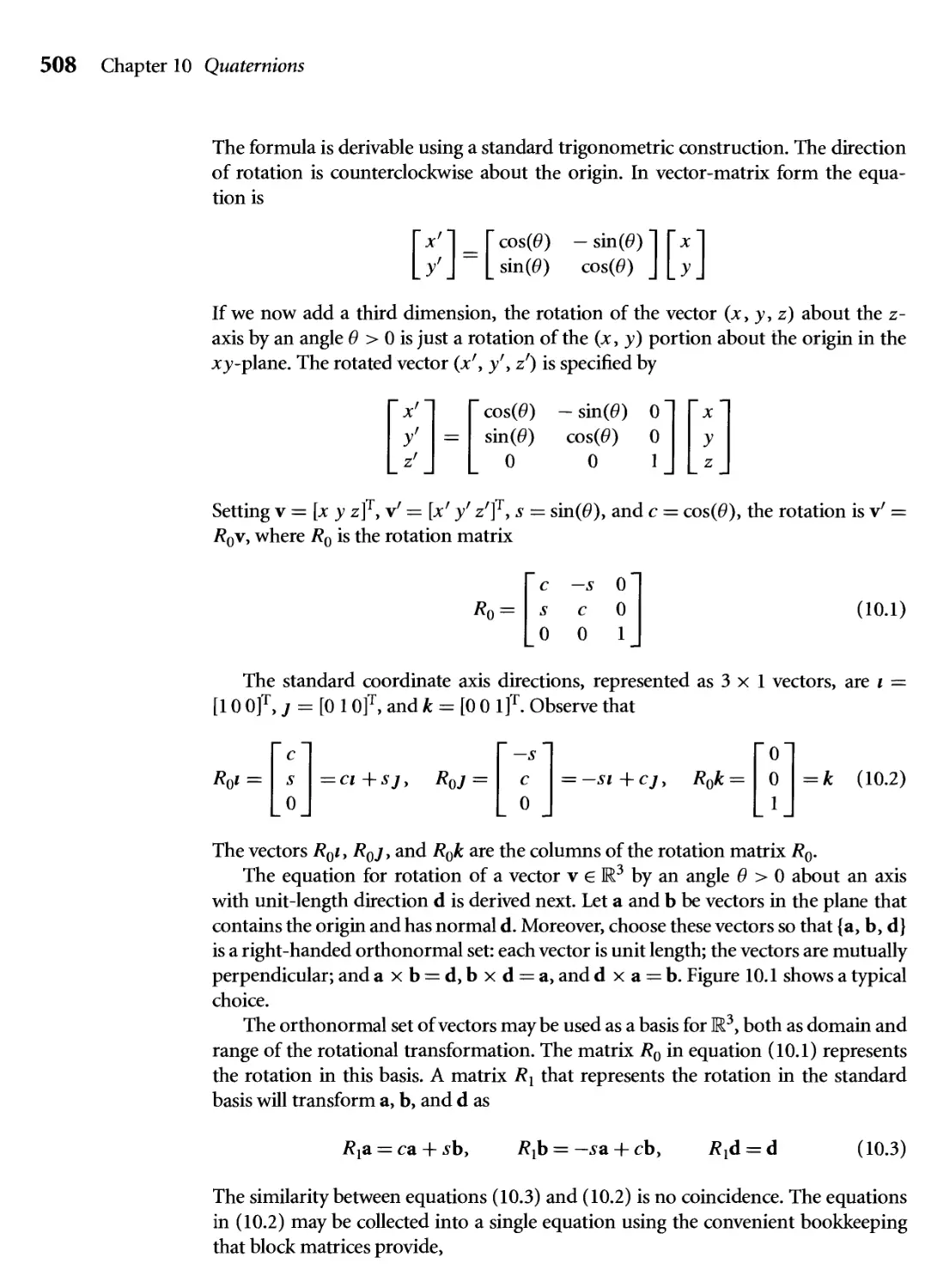
10.1 A right-handed orthonormal set of vectors. A rotation is desired
about d by the angle в > 0. 509
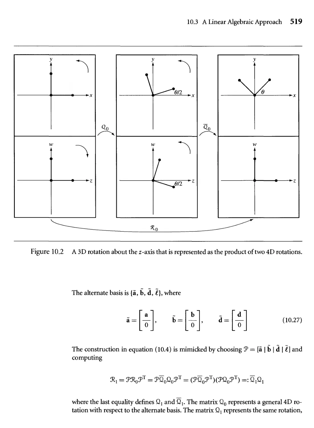
10.2 A 3D rotation about the z-axis that is represented as the product of
two 4D rotations. 519
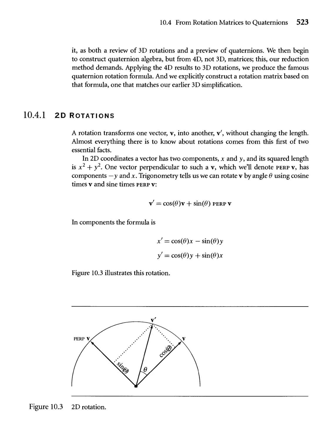
10.3 2D rotation. 523
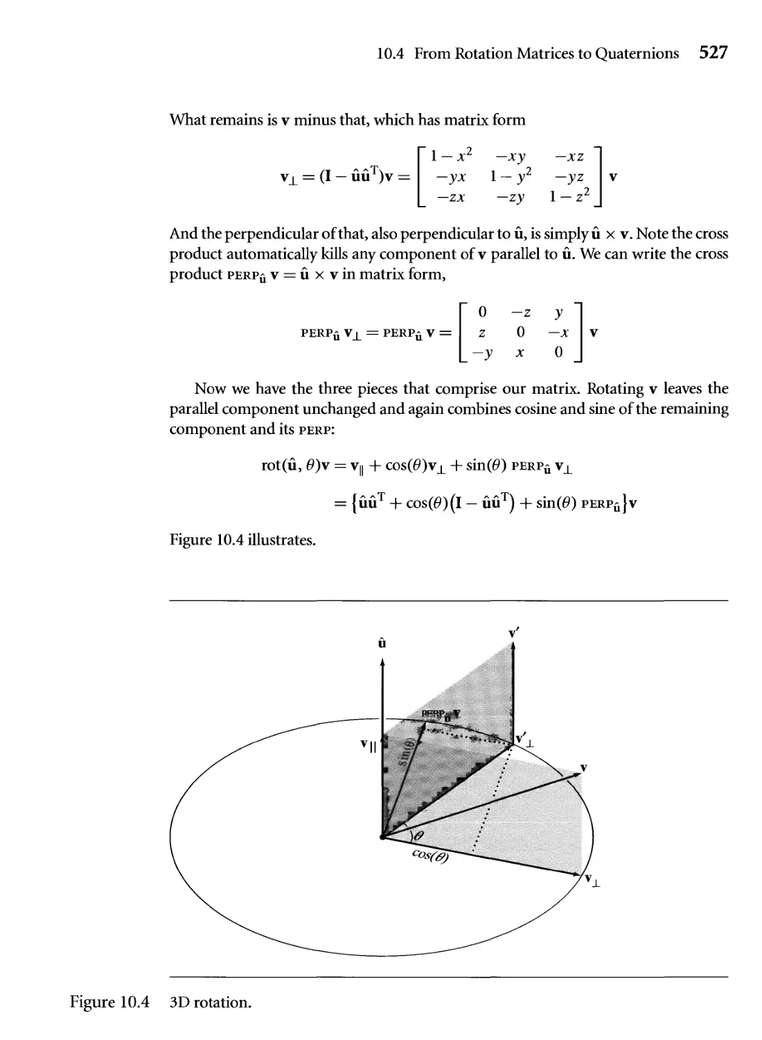
10.4 3D rotation. 527
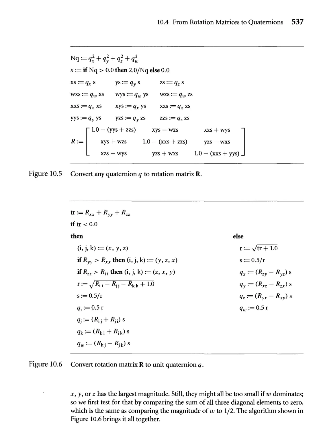
10.5 Convert any quaternion q to rotation matrix R. 537
10.6 Convert rotation matrix R to unit quaternion q. 537
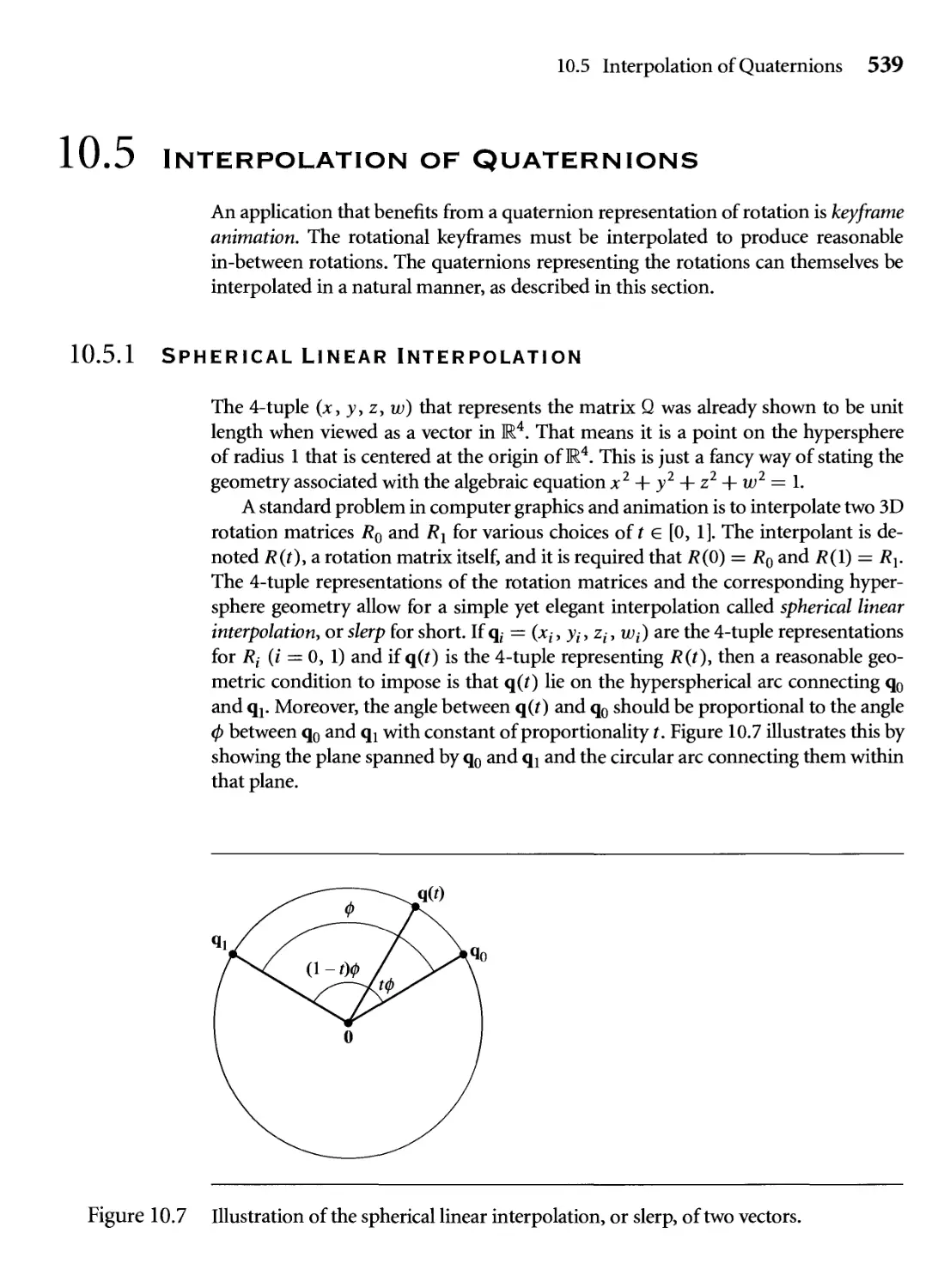
10.7 Illustration of the spherical linear interpolation, or slerp, of two
vectors. 539
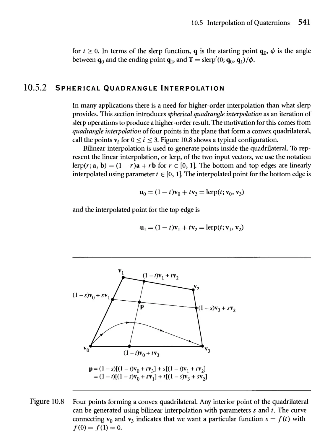
10.8 Four points forming a convex quadrilateral. Any interior point of
the quadrilateral can be generated using bilinear interpolation with
parameters s and t. The curve connecting v0 and v3 indicates that we
want a particular function s = f(t) with /@) = /A) = 0. 541
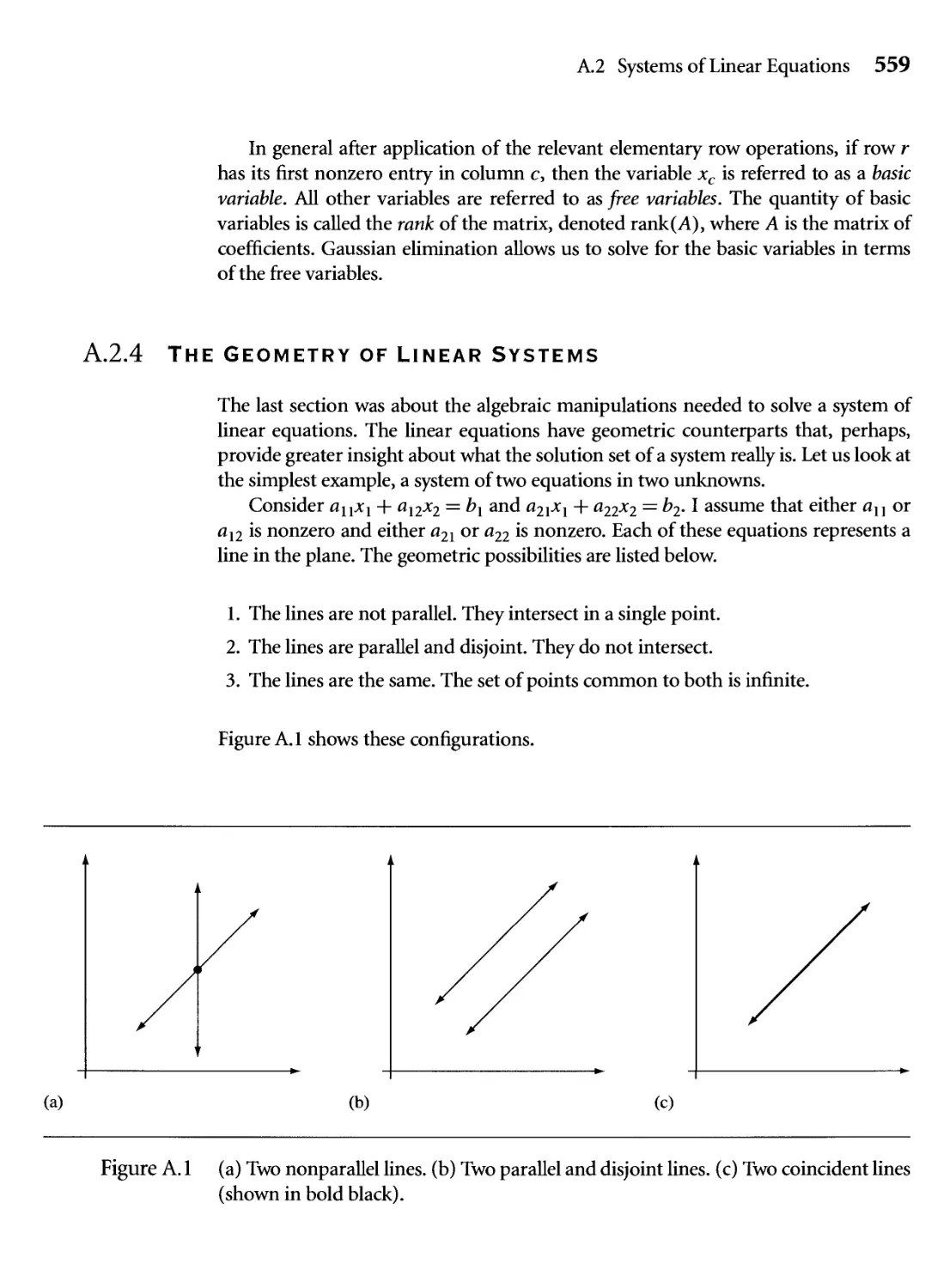
A.I (a) Two nonparallel lines, (b) Two parallel and disjoint lines, (c) Two
coincident lines (shown in bold black). 559
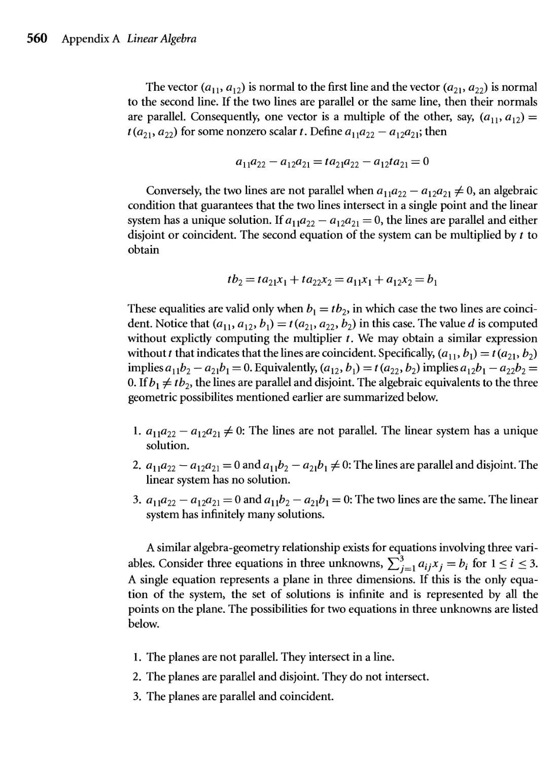
A.2 (a) Two nonparallel planes, (b) Two parallel and disjoint planes, (c)
Two coincident planes (shown in bold black). 561
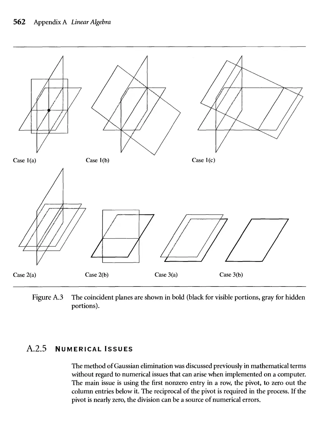
A.3 The coincident planes are shown in bold (black for visible portions,
gray for hidden portions). 562
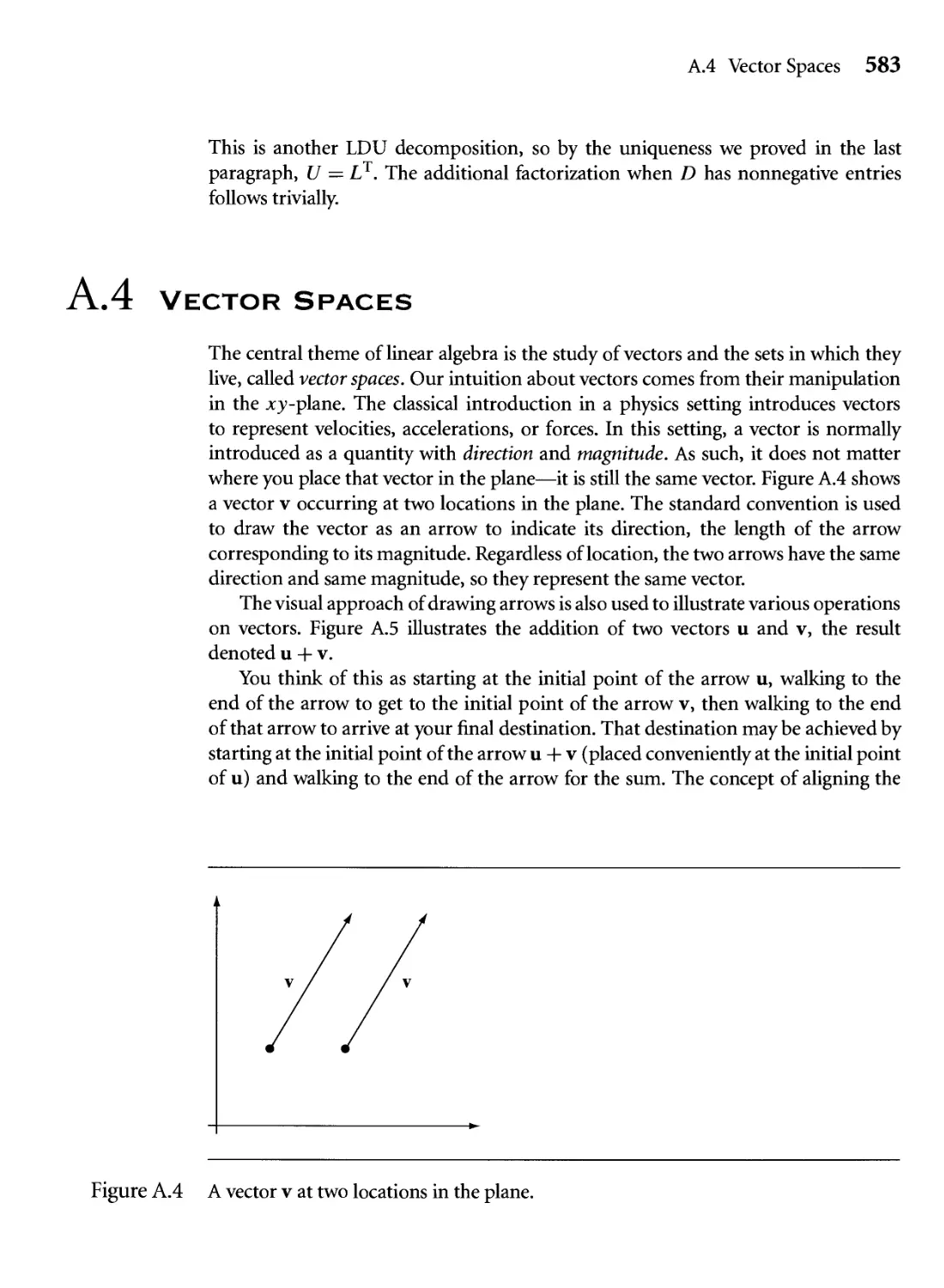
A.4 A vector v at two locations in the plane. 583
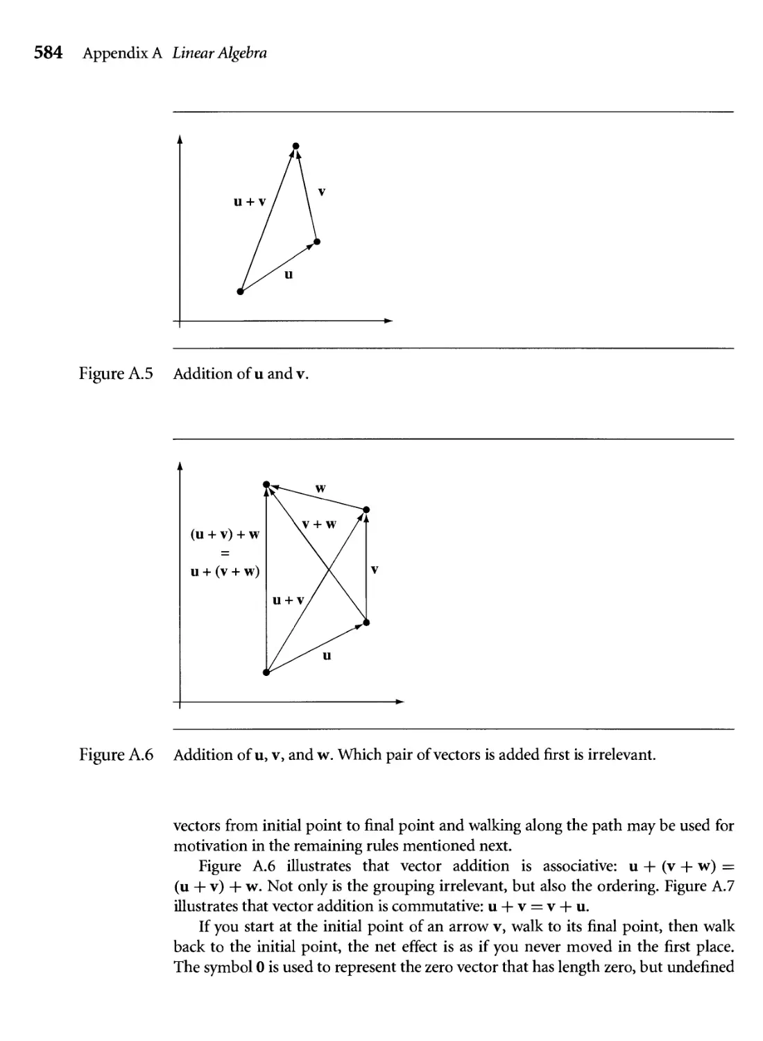
A.5 Addition of u and v. 584
A. 6 Addition of u, v, and w. Which pair of vectors is added first is
irrelevant. 584

Figures XXV
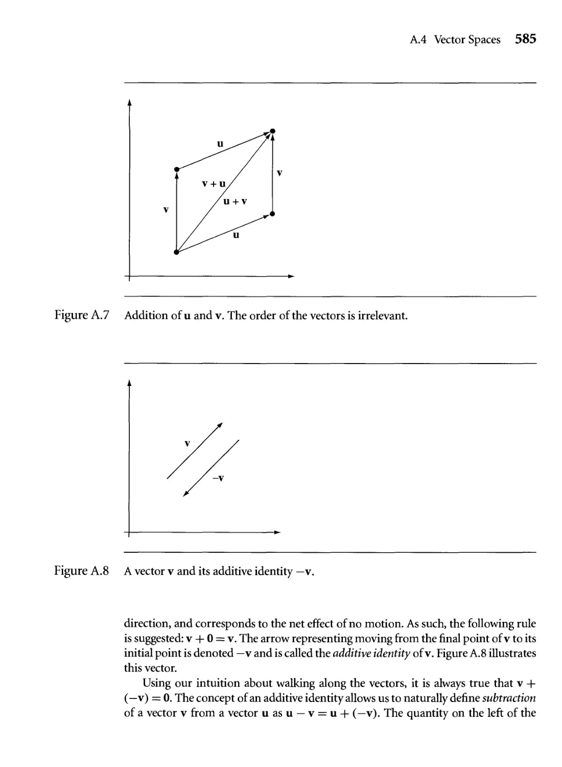
A. 7 Addition of u and v. The order of the vectors is irrelevant. 585
A.8 A vector v and its additive identity —v. 585
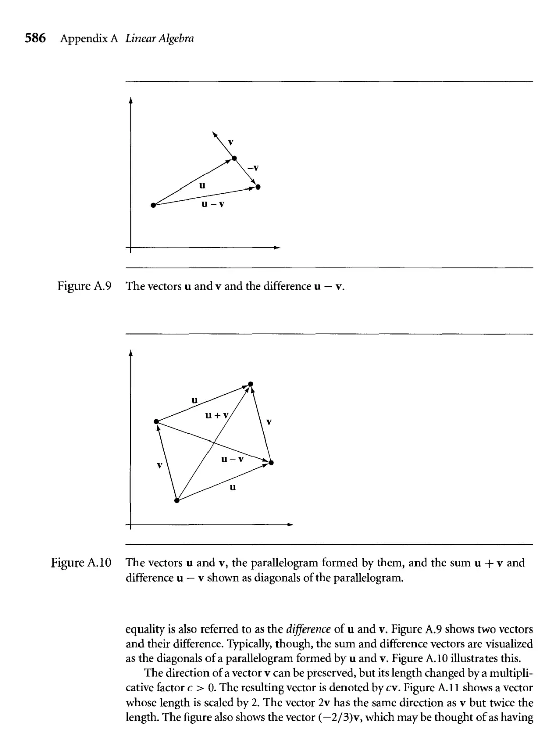
A.9 The vectors u and v and the difference u — v. 586
АЛО The vectors u and v, the parallelogram formed by them, and the sum
u + v and difference u — v shown as diagonals of the parallelogram. 586
A.I 1 The vector v and two scalar multiples of it, one positive and one
negative. 587
A. 12 (a) Distributing across a scalar sum. (b) Distributing across a vector
sum. 587
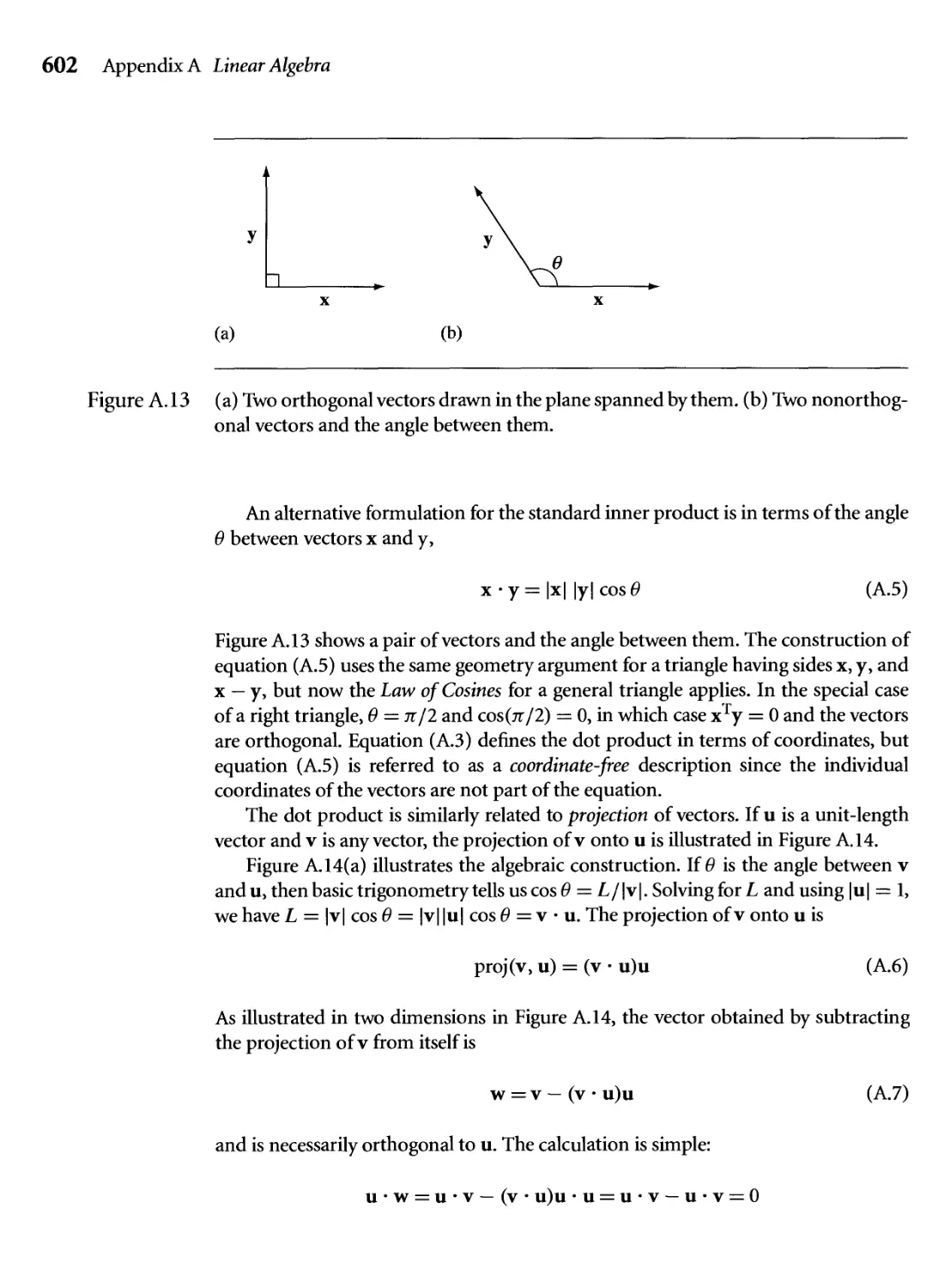
A. 13 (a) Two orthogonal vectors drawn in the plane spanned by them, (b)
Two nonorthogonal vectors and the angle between them. 602
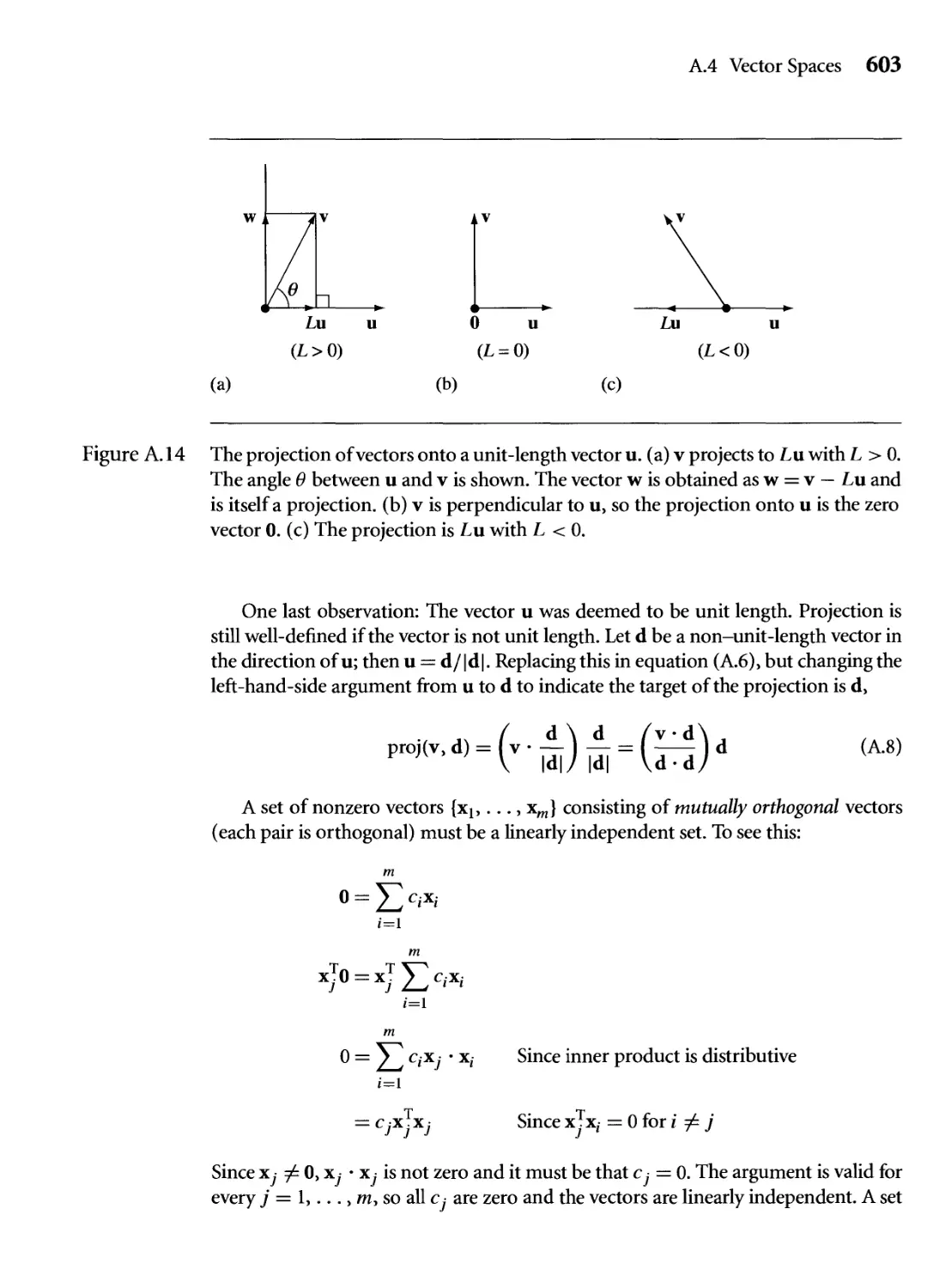
A. 14 The projection of vectors onto a unit-length vector u. (a) v projects
to Lu with L > 0. The angle в between u and v is shown. The vector
w is obtained as w = v - Lu and is itself a projection, (b) v is
perpendicular to u, so the projection onto u is the zero vector 0. (c)
The projection is Lu with L < 0. 603
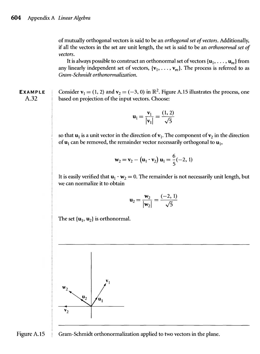
A. 15 Gram-Schmidt orthonormalization applied to two vectors in the
plane. 604
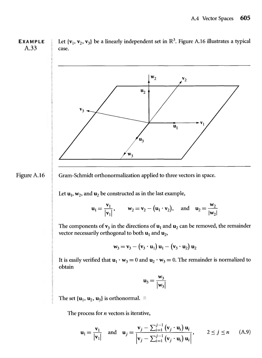
A. 16 Gram-Schmidt orthonormalization applied to three vectors in space. 605
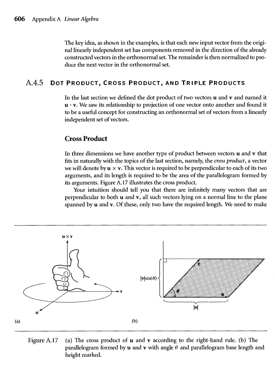
A. 17 (a) The cross product of u and v according to the right-hand rule, (b)
The parallelogram formed by u and v with angle в and parallelogram
base length and height marked. 606
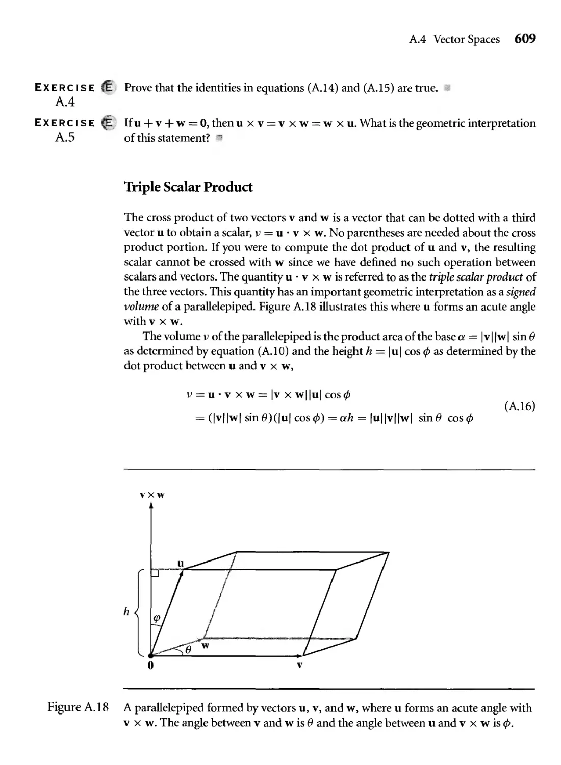
A. 18 A parallelepiped formed by vectors u, v, and w, where u forms an
acute angle with v x w. The angle between v and w is в and the angle
between u and v x w is ф. 609
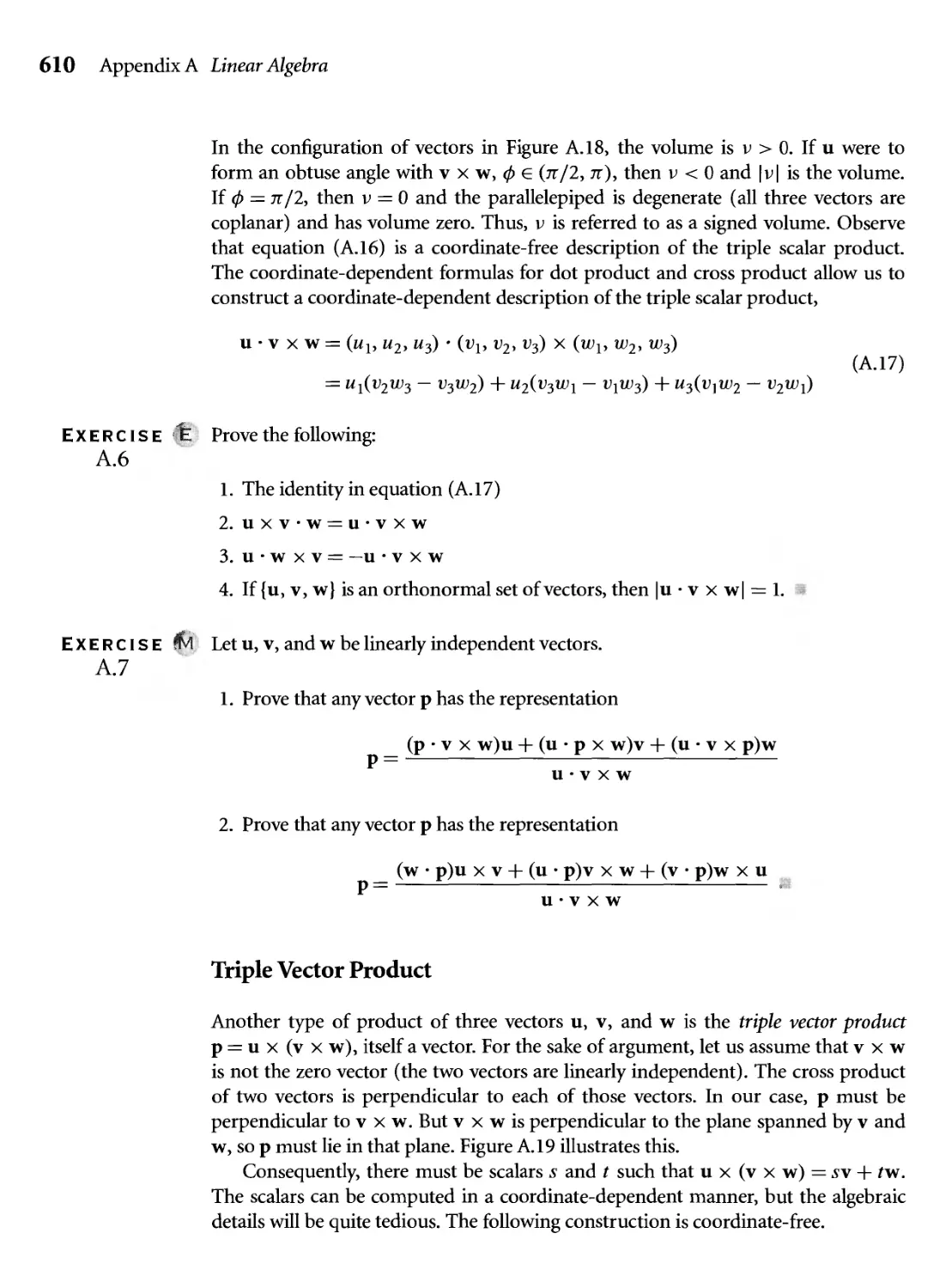
A. 19 The triple vector product p = u x (v x w). Note that p must lie in the
plane spanned by v and w. 611
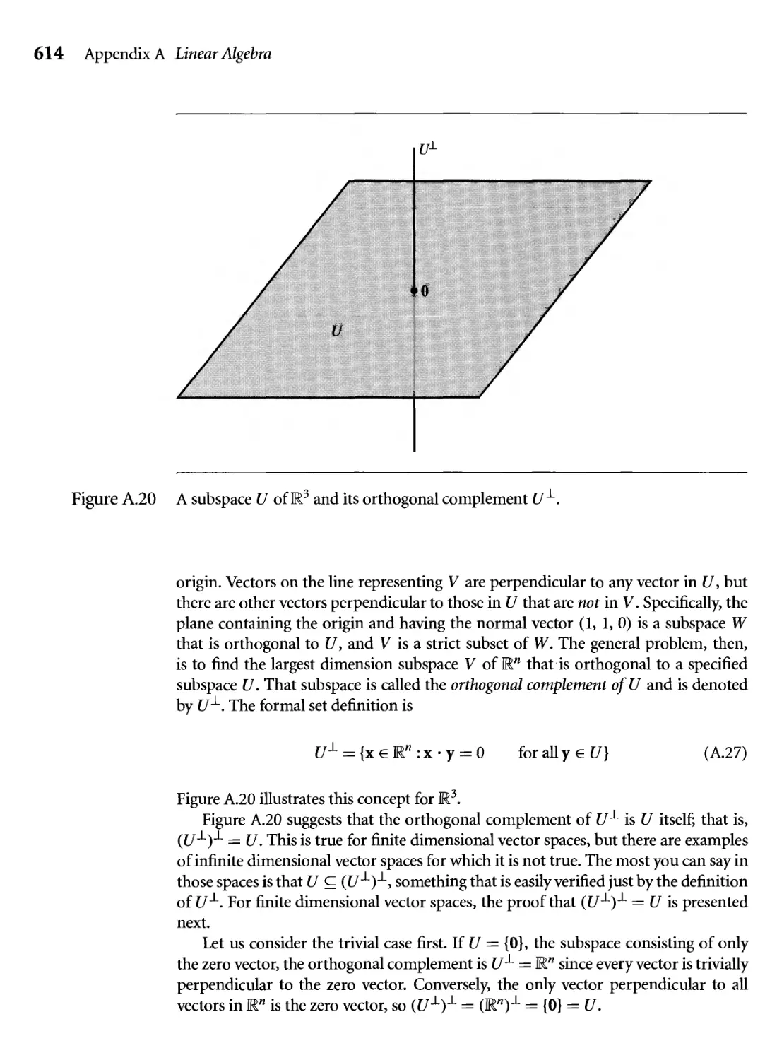
A.20 A subspace U of M3 and its orthogonal complement U^. 614
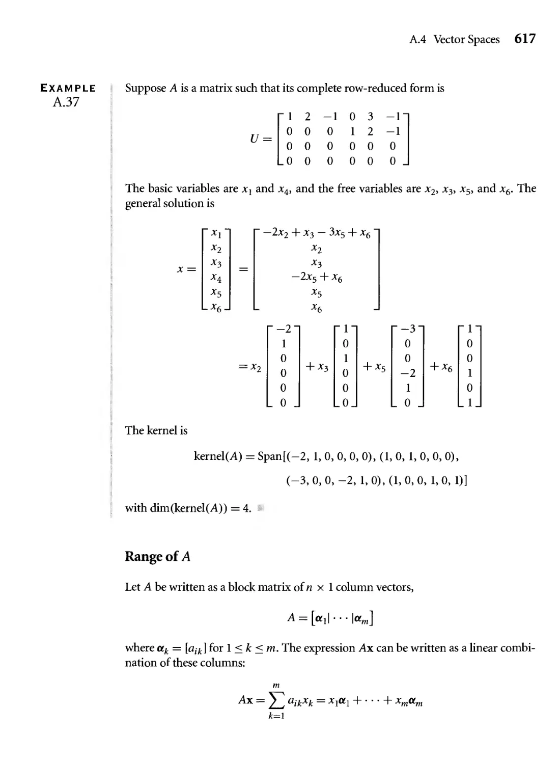
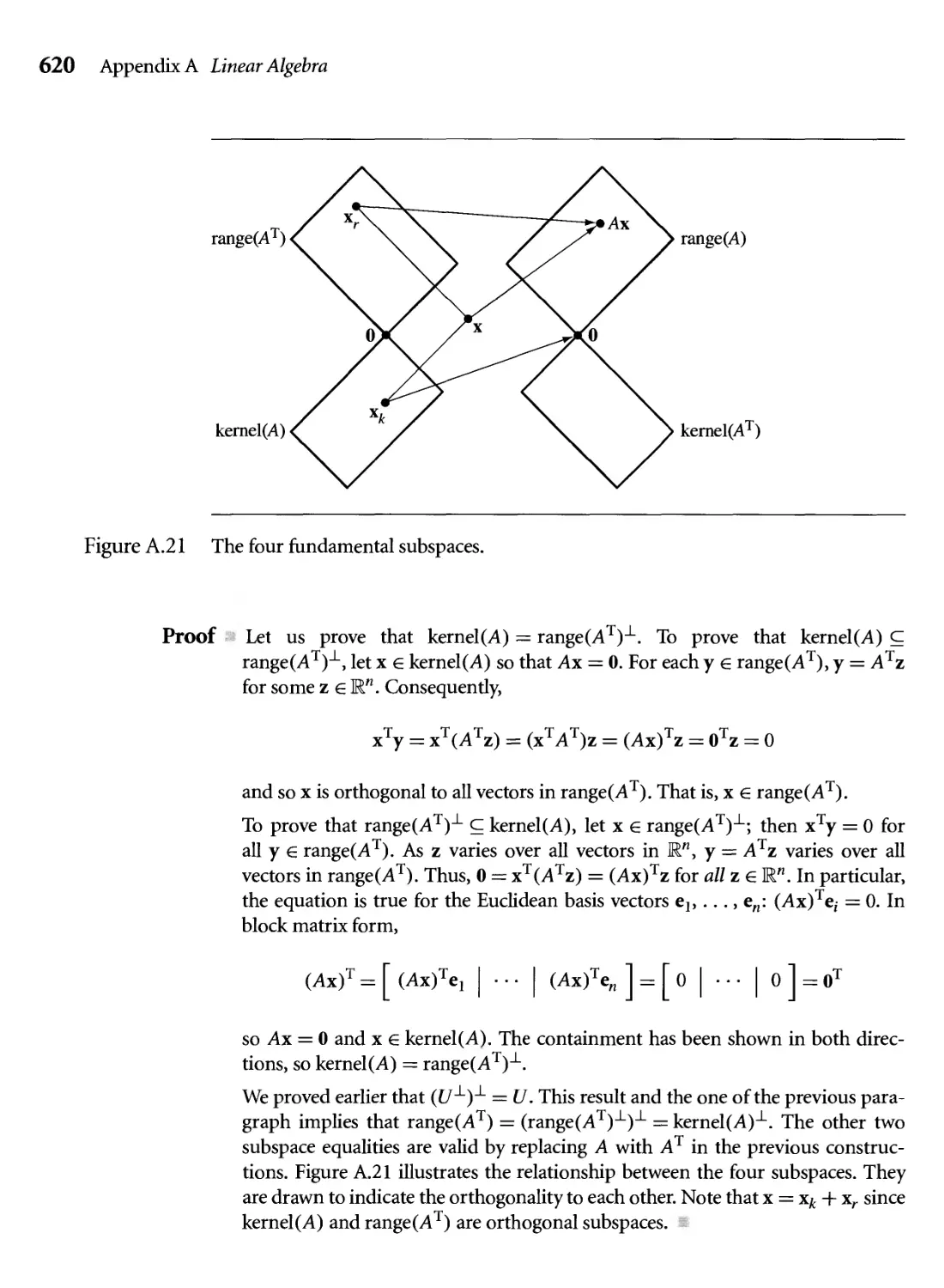
A.21 The four fundamental subspaces. 620
A.22 The projection p e S of b e M3, where S is a two-dimensional
subspace of M3 (a plane through the origin). 621
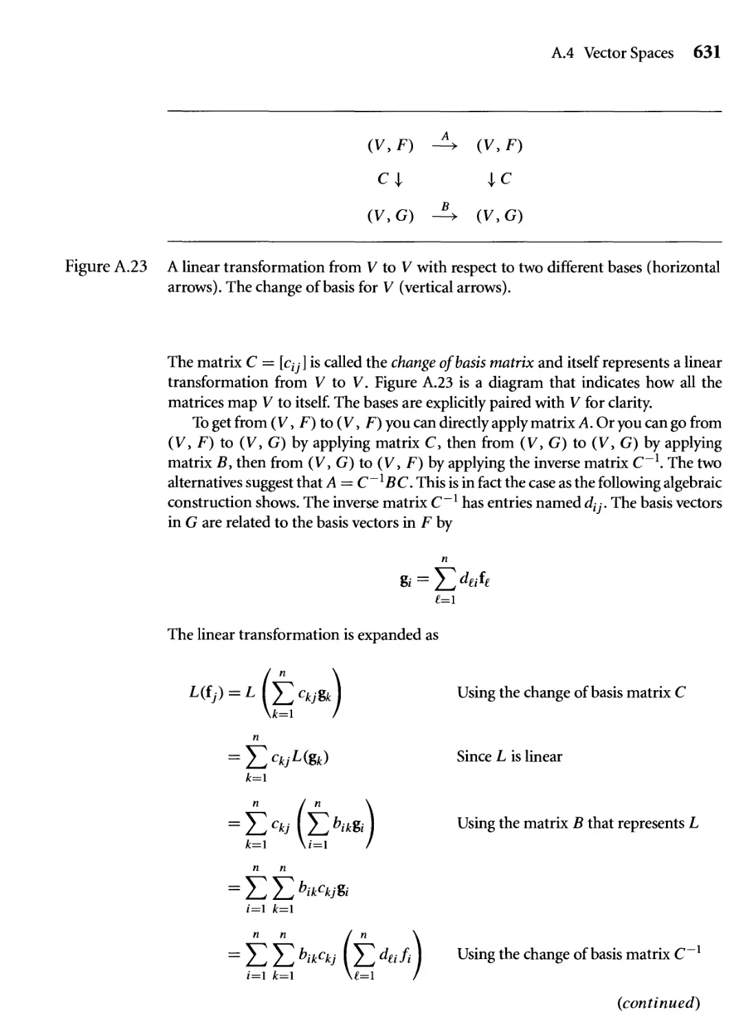
A.23 A linear transformation from V to V with respect to two different
bases (horizontal arrows). The change of basis for V (vertical arrows). 631
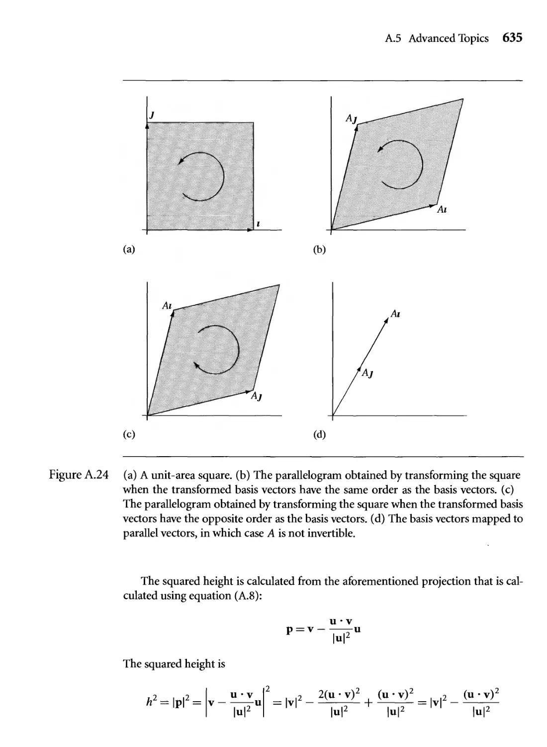
A.24 (a) A unit-area square, (b) The parallelogram obtained by
transforming the square when the transformed basis vectors have the
same order as the basis vectors, (c) The parallelogram obtained by
transforming the square when the transformed basis vectors have the
opposite order as the basis vectors, (d) The basis vectors mapped to
parallel vectors, in which case A is not invertible. 635

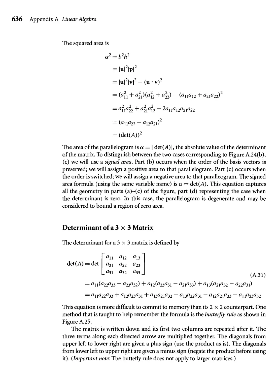
XXvi Figures
A.25 An illustration of the butterfly rule for the determinant of a 3 x 3
matrix. 637
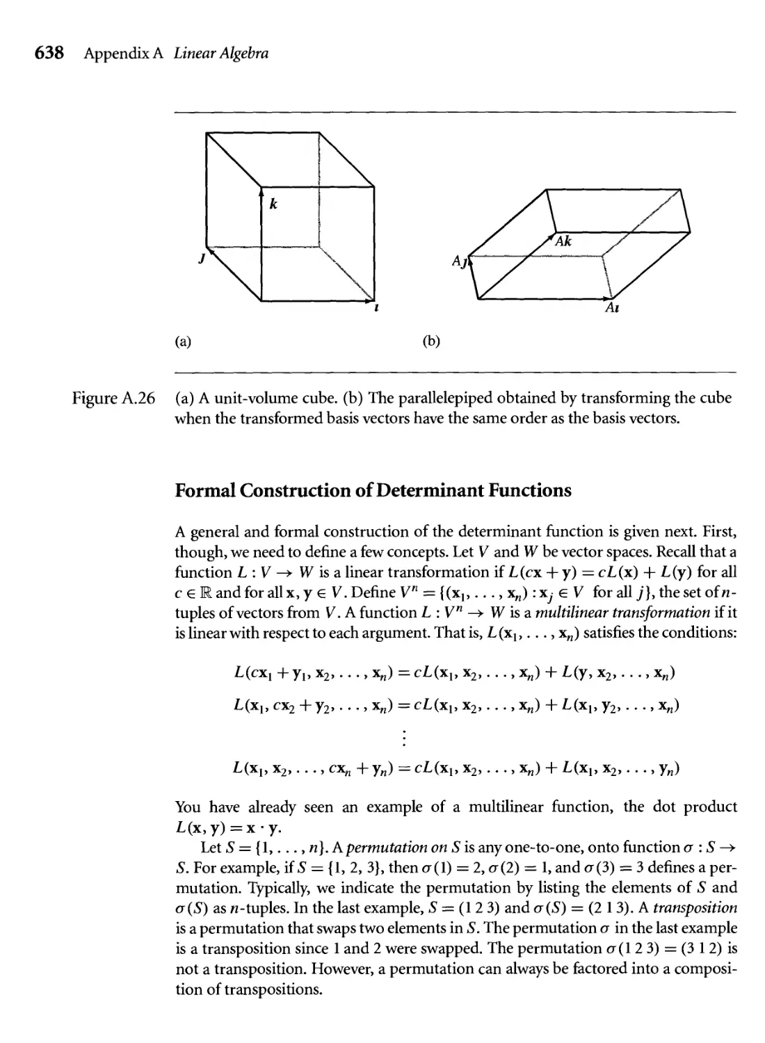
A.26 (a) A unit-volume cube, (b) The parallelepiped obtained by
transforming the cube when the transformed basis vectors have the
same order as the basis vectors. 638
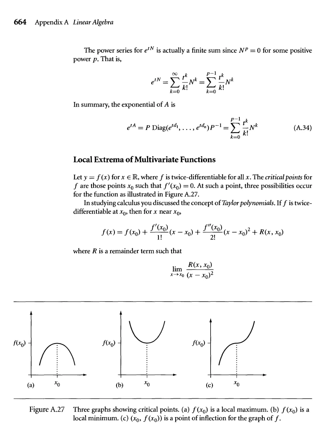
A.27 Three graphs showing critical points, (a) f(x0) is a local maximum,
(b) f(x0) is a local minimum, (c) (x0, f(x0)) is a point of inflection
for the graph of /. 664
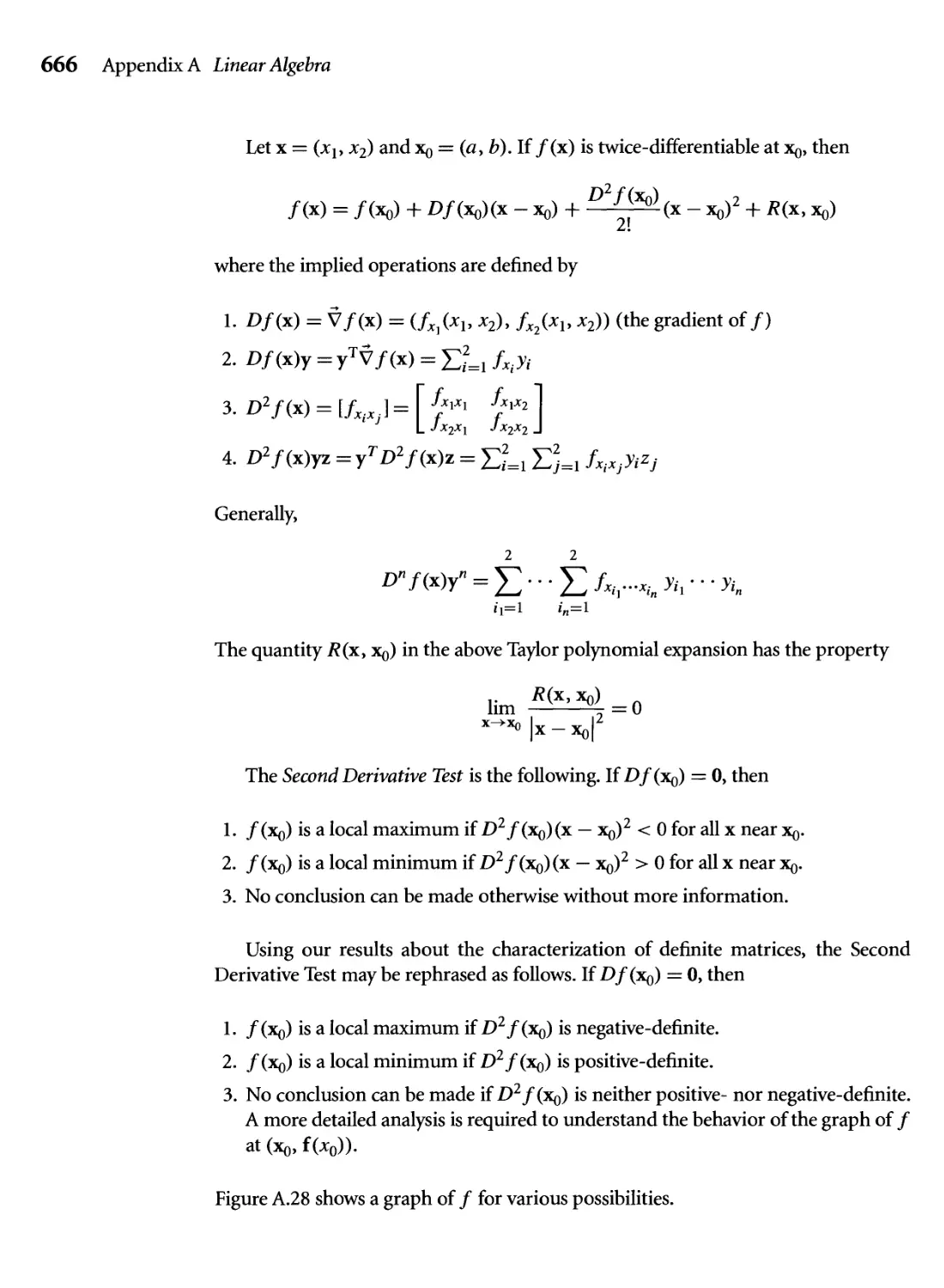
A.28 Three graphs showing critical points, (a) /(xq) is a local maximum,
(b) /(xq) is a local minimum, (c) (xq, /(xq)) is a saddle point on the
graph of /. The tangent planes at the graph points are shown in all
three figures. 667
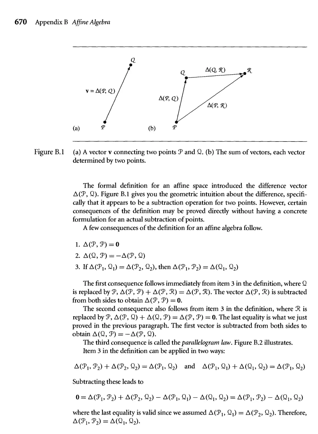
B. 1 (a) A vector v connecting two points У and Q. (b) The sum of vectors,
each vector determined by two points. 670
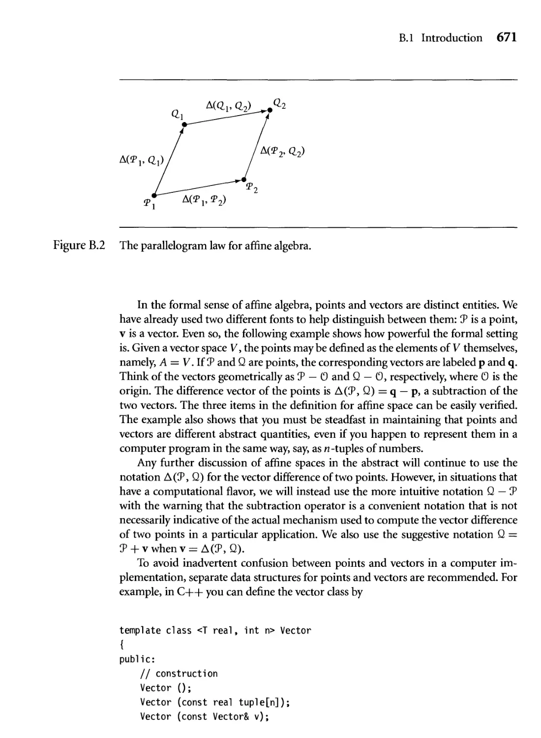
B.2 The parallelogram law for affme algebra. 671
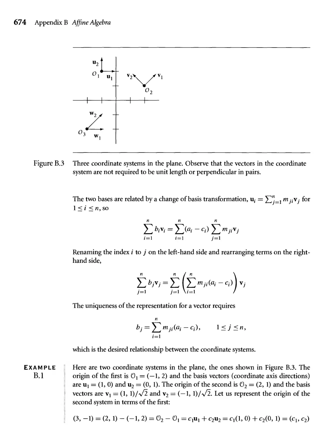
B.3 Three coordinate systems in the plane. Observe that the vectors in the
coordinate system are not required to be unit length or perpendicular
in pairs. 674
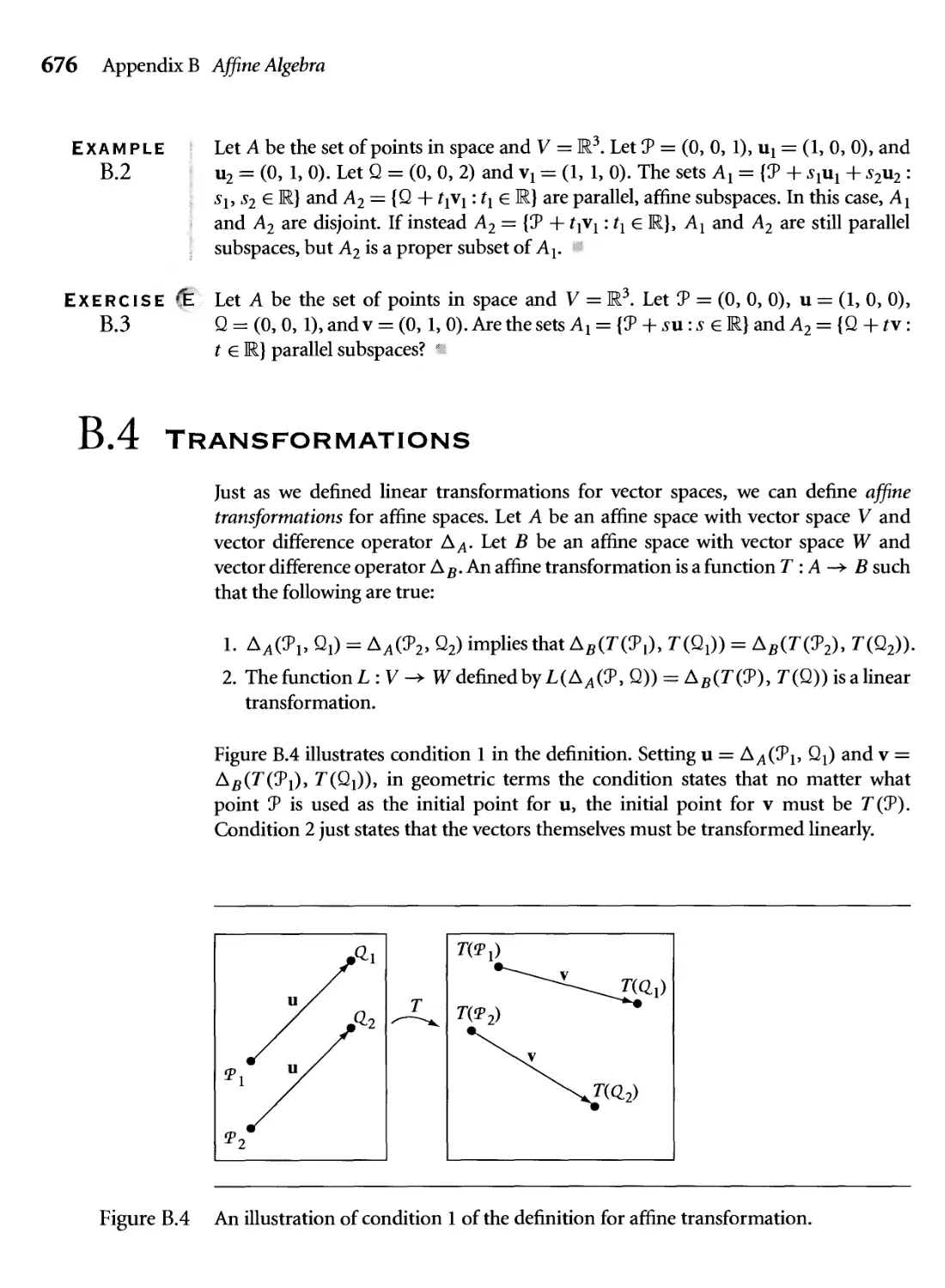
B.4 An illustration of condition 1 of the definition for affme
transformation. 676
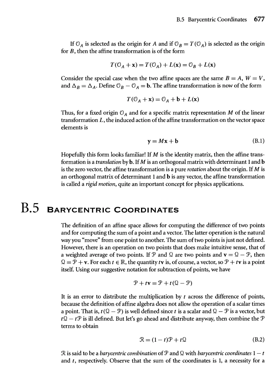
B.5 Various barycentric combinations of two points У and Q. 678
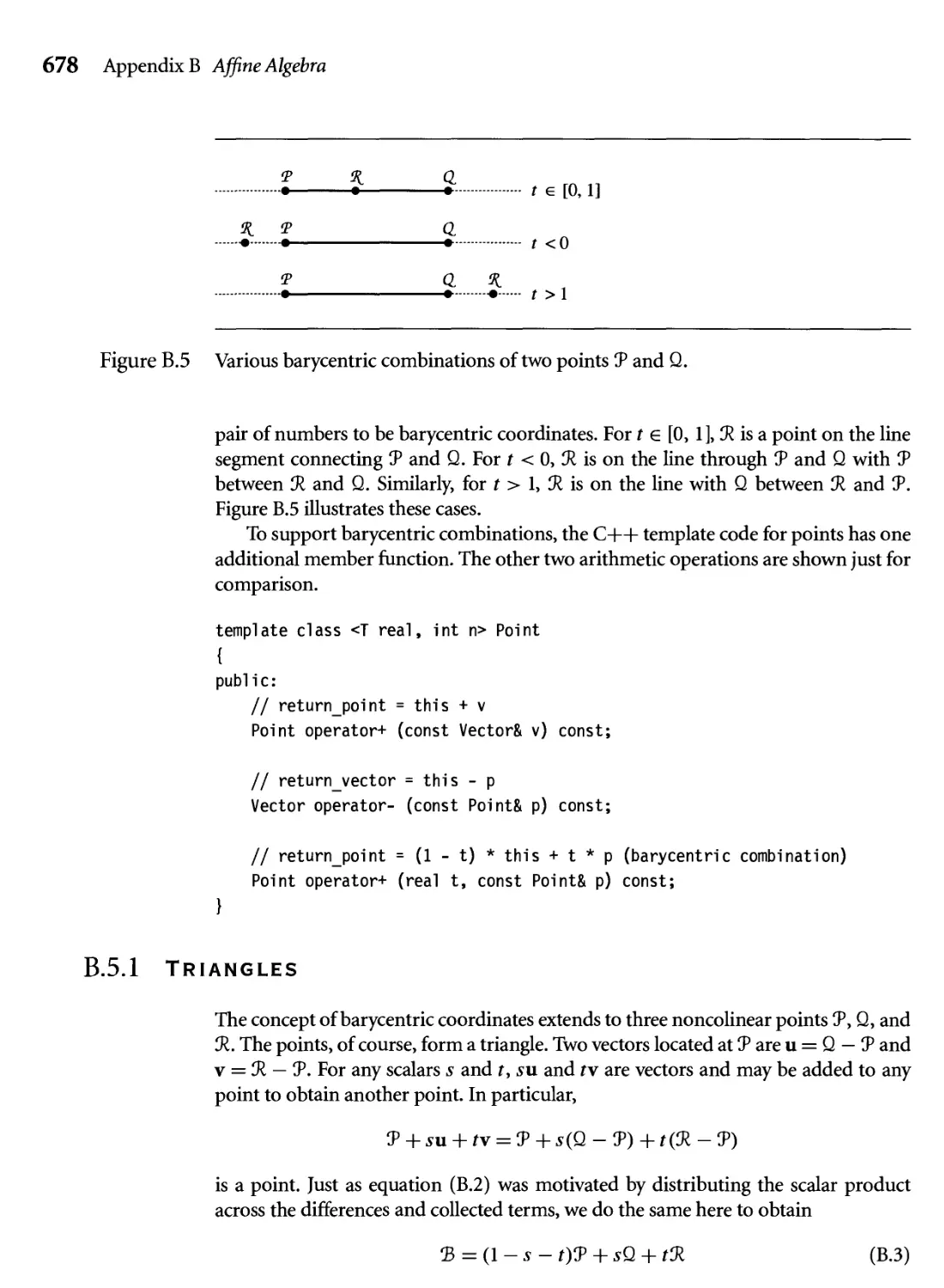
B.6 The triangle partitions the plane into seven regions. The signs of c\,
c2, and c3 are listed as ordered triples. 679
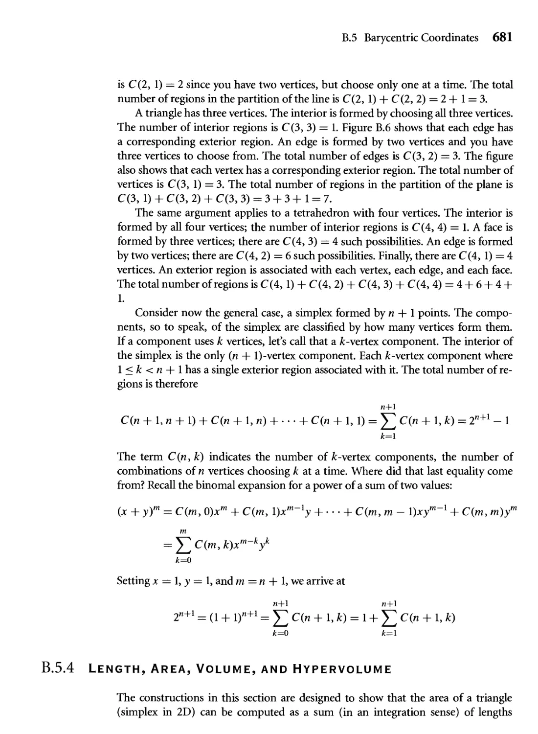
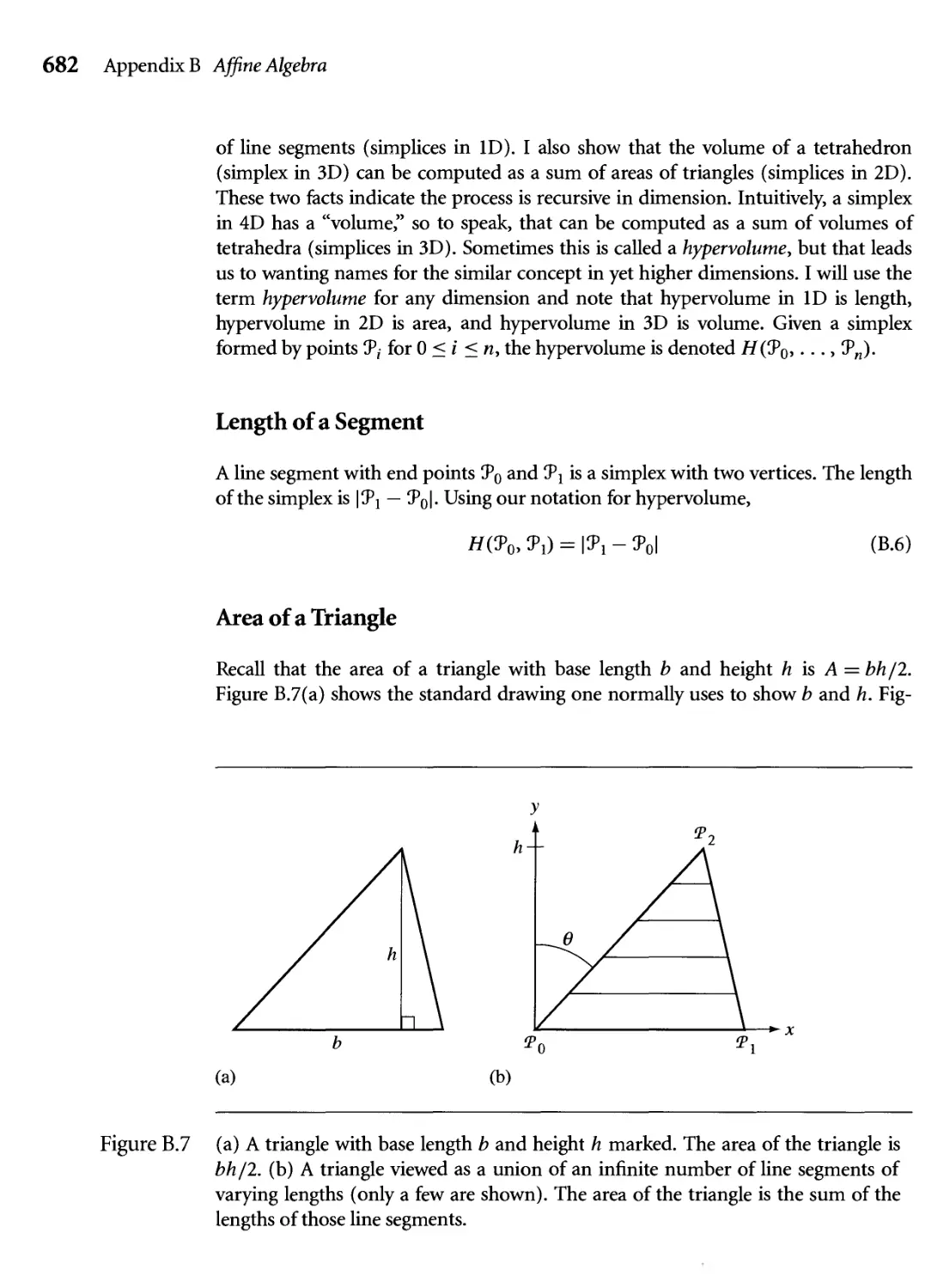
B.7 (a) A triangle with base length b and height h marked. The area of the
triangle is bh/2. (b) A triangle viewed as a union of an infinite number
of line segments of varying lengths (only a few are shown). The area
of the triangle is the sum of the lengths of those line segments. 682
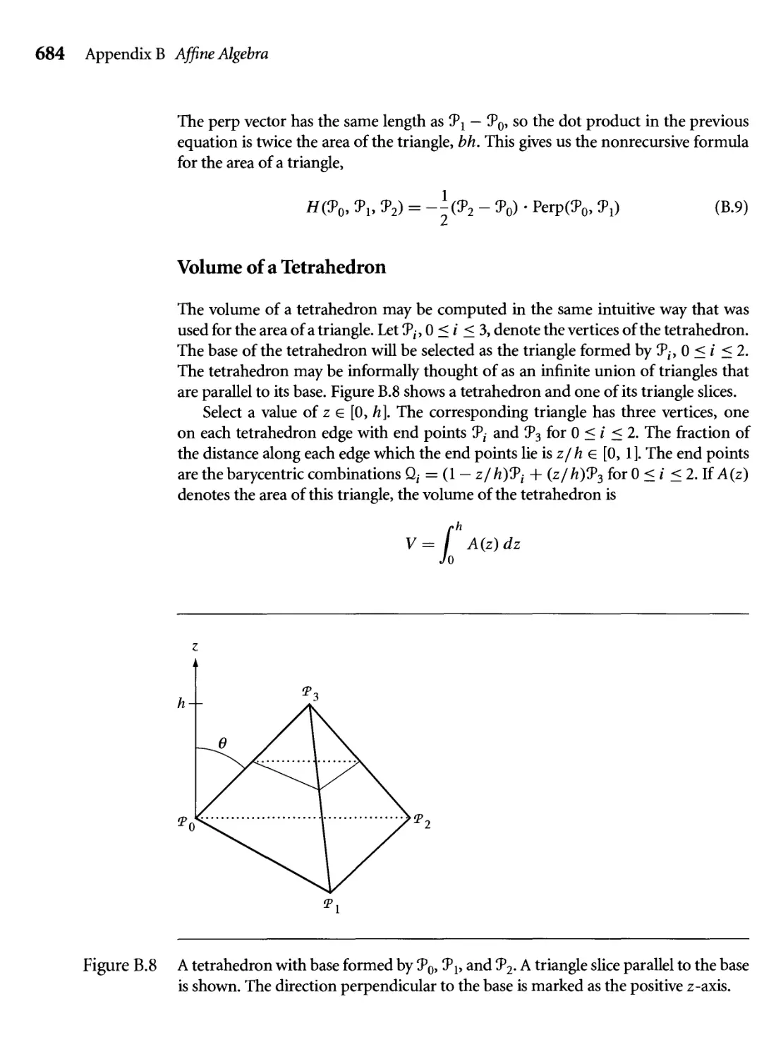
B.8 A tetrahedron with base formed by Уо, Уь and 3>2. A triangle slice
parallel to the base is shown. The direction perpendicular to the base
is marked as the positive z-axis. 684
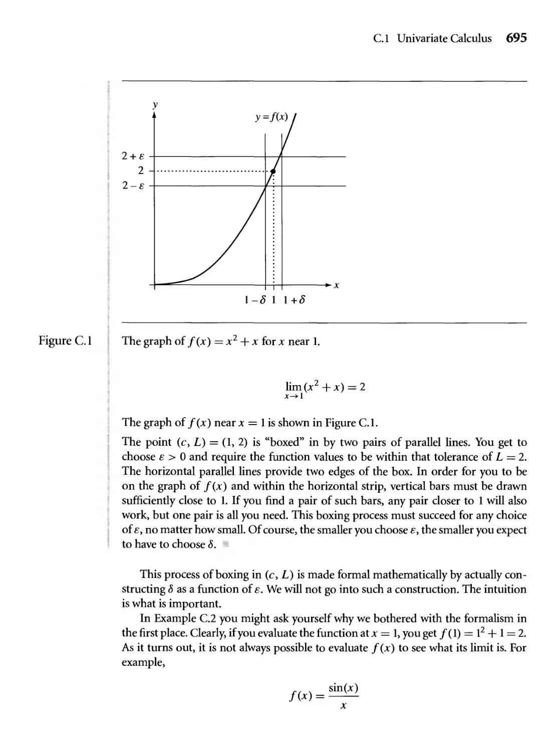
С1 The graph of f(x) = x2 + x for x near 1. 695
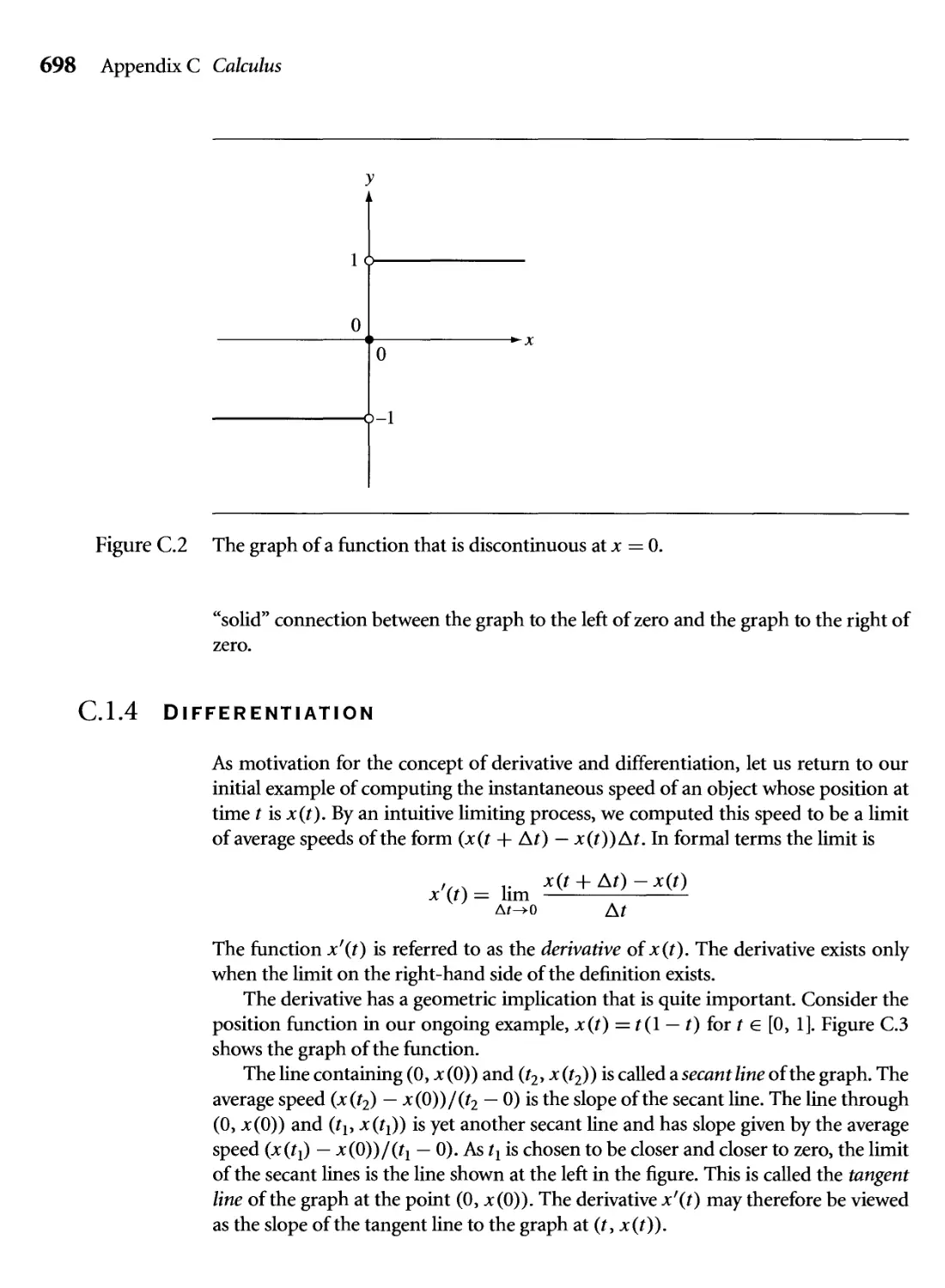
C.2 The graph of a function that is discontinuous at x = 0. 698
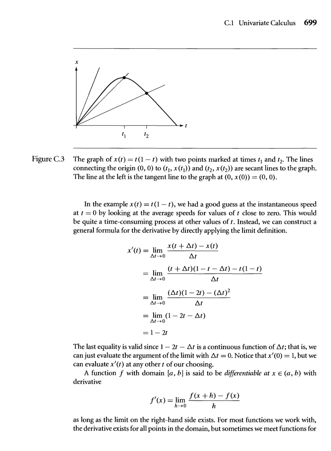
C.3 The graph of x(t) = t(l — t) with two points marked at times tx and
t2. The lines connecting the origin @, 0) to (?1? x(t{)) and (t2, x(t2))
are secant lines to the graph. The line at the left is the tangent line to
the graph at @, Jt(O)) = @, 0). 699
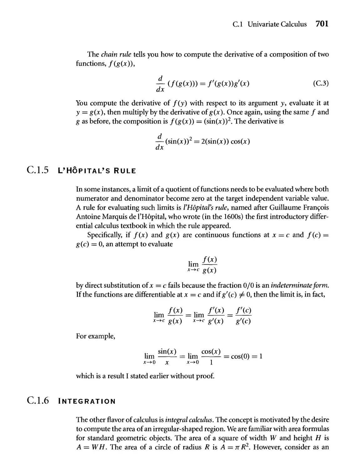
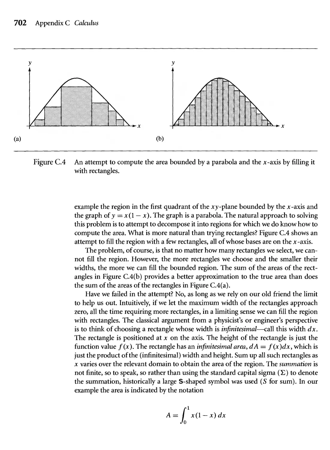
C.4 An attempt to compute the area bounded by a parabola and the x-axis
by filling it with rectangles. 702
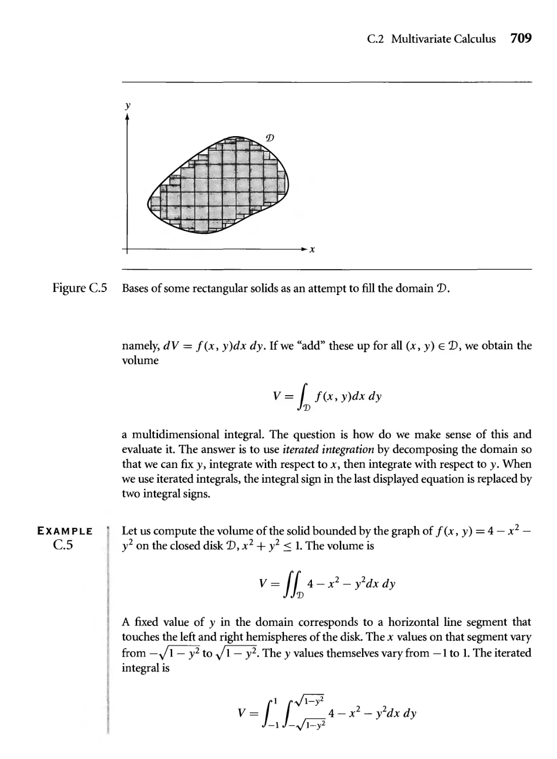
C.5 Bases of some rectangular solids as an attempt to fill the domain Ъ. 709
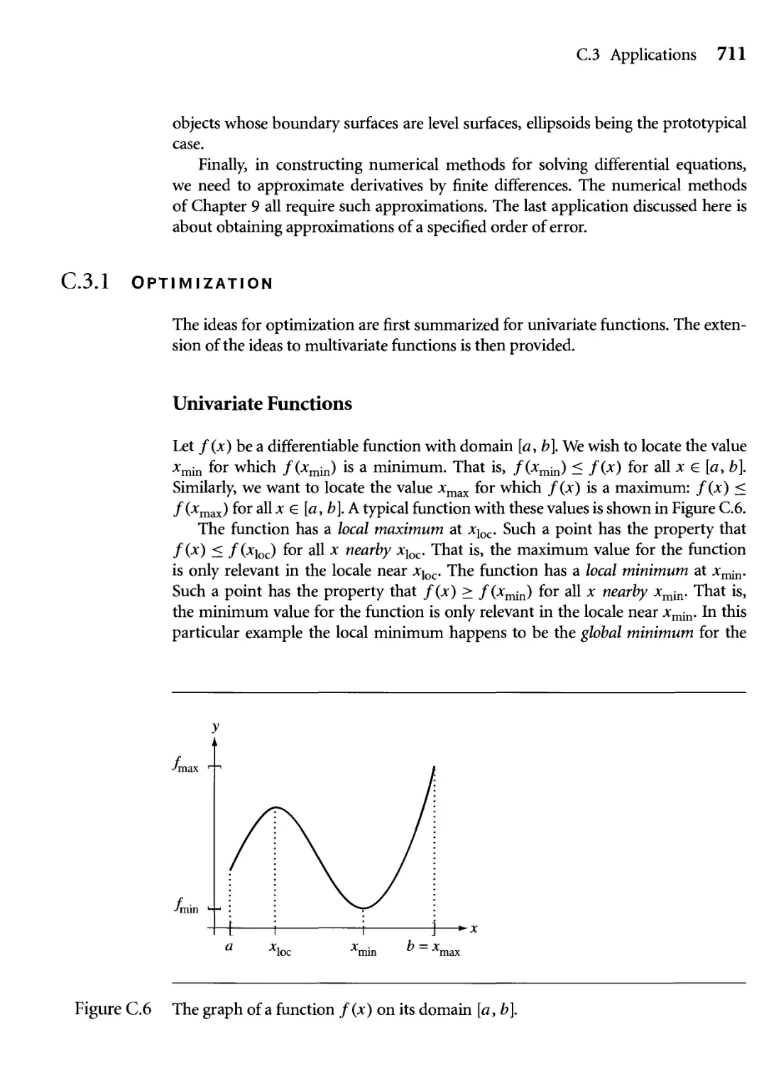
C.6 The graph of a function f(x) on its domain [a, b]. 711

Tables
2.1 Moments and products of inertia for vertices 63
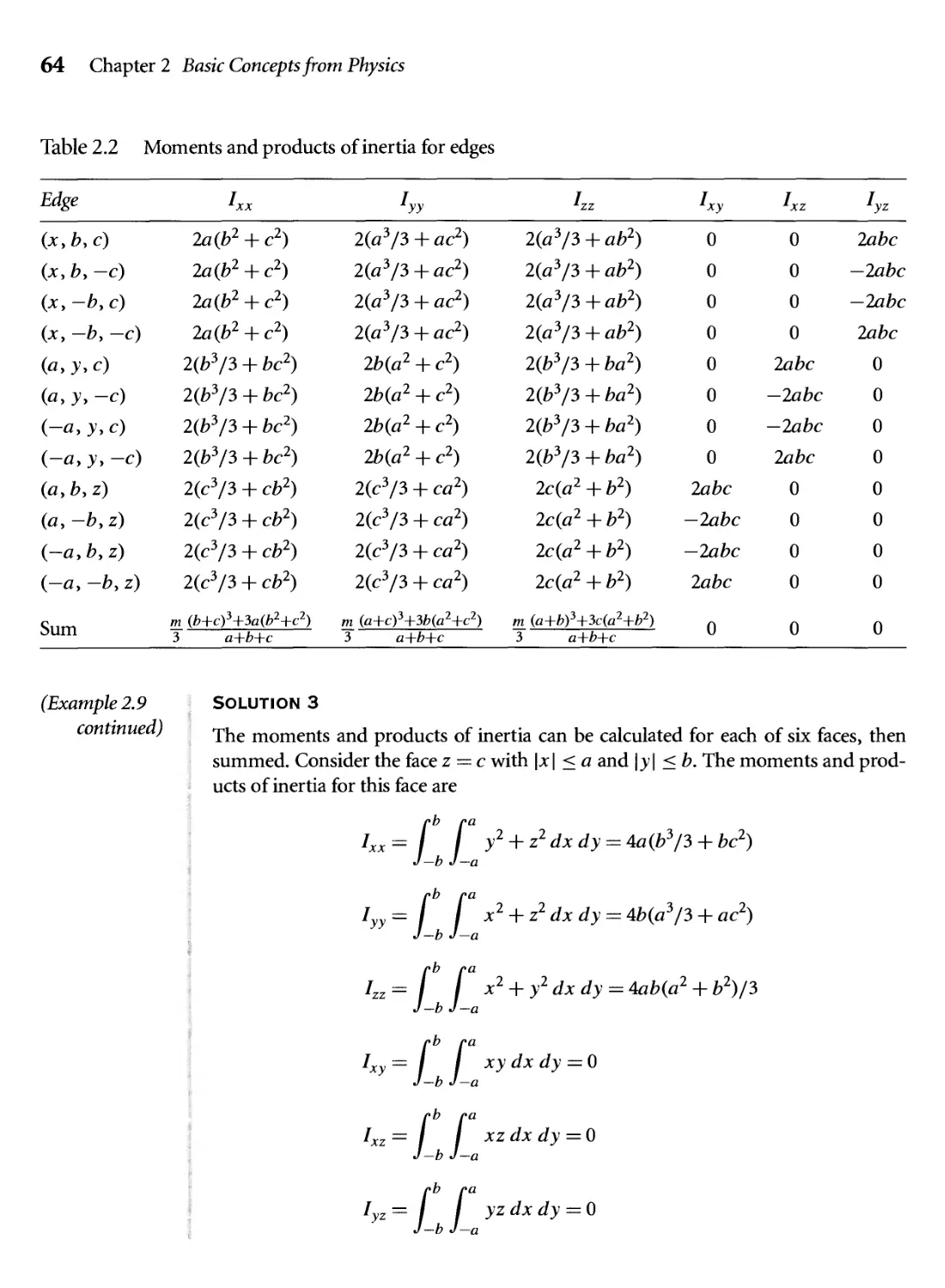
2.2 Moments and products of inertia for edges 64
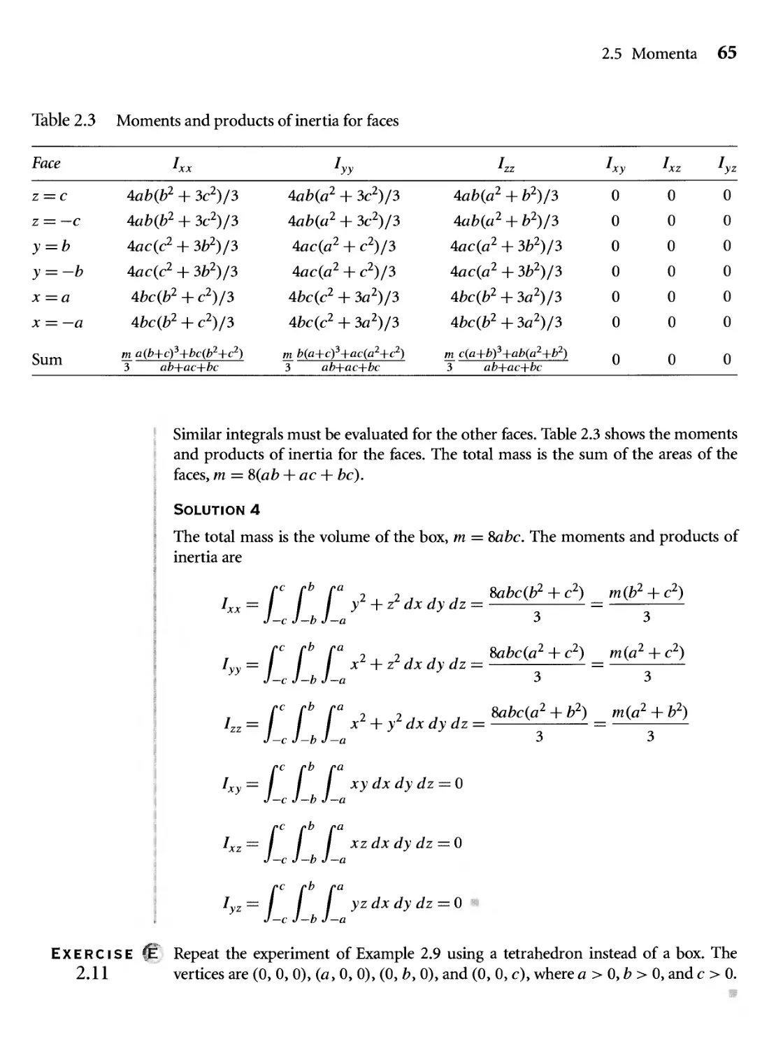
2.3 Moments and products of inertia for faces 65
2.4 Generation of polynomials by vector fields 68
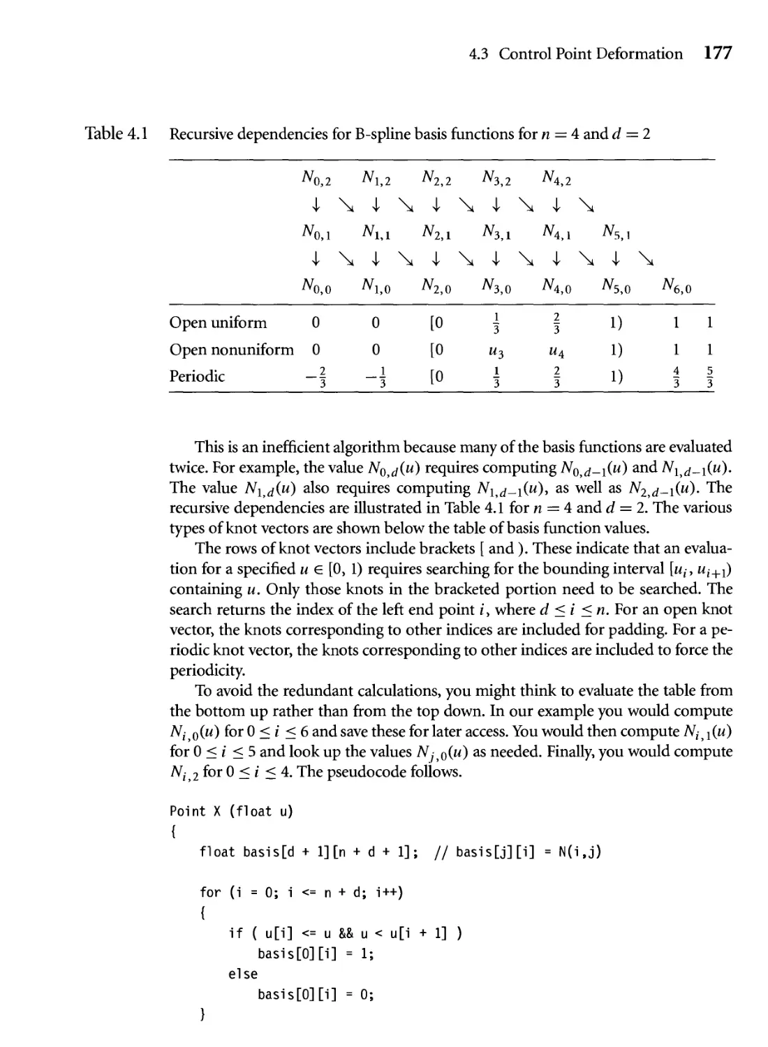
4.1 Recursive dependencies for B-spline basis functions for n = 4 and
d = 2 177
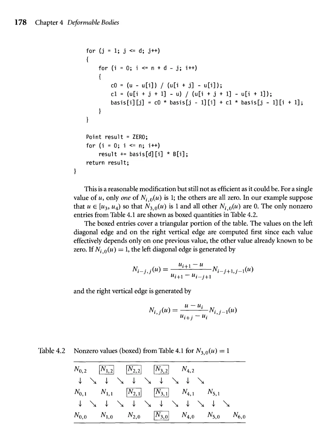
4.2 Nonzero values (boxed) from Table 4.1 for 7V3O(m) = 1 178
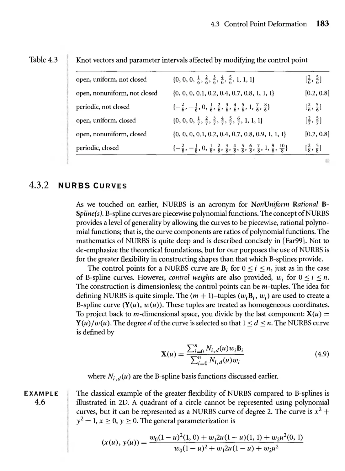
4.3 Knot vectors and parameter intervals affected by modifying the
control point 183
4.4 The vertex-edge configurations for a pixel 213
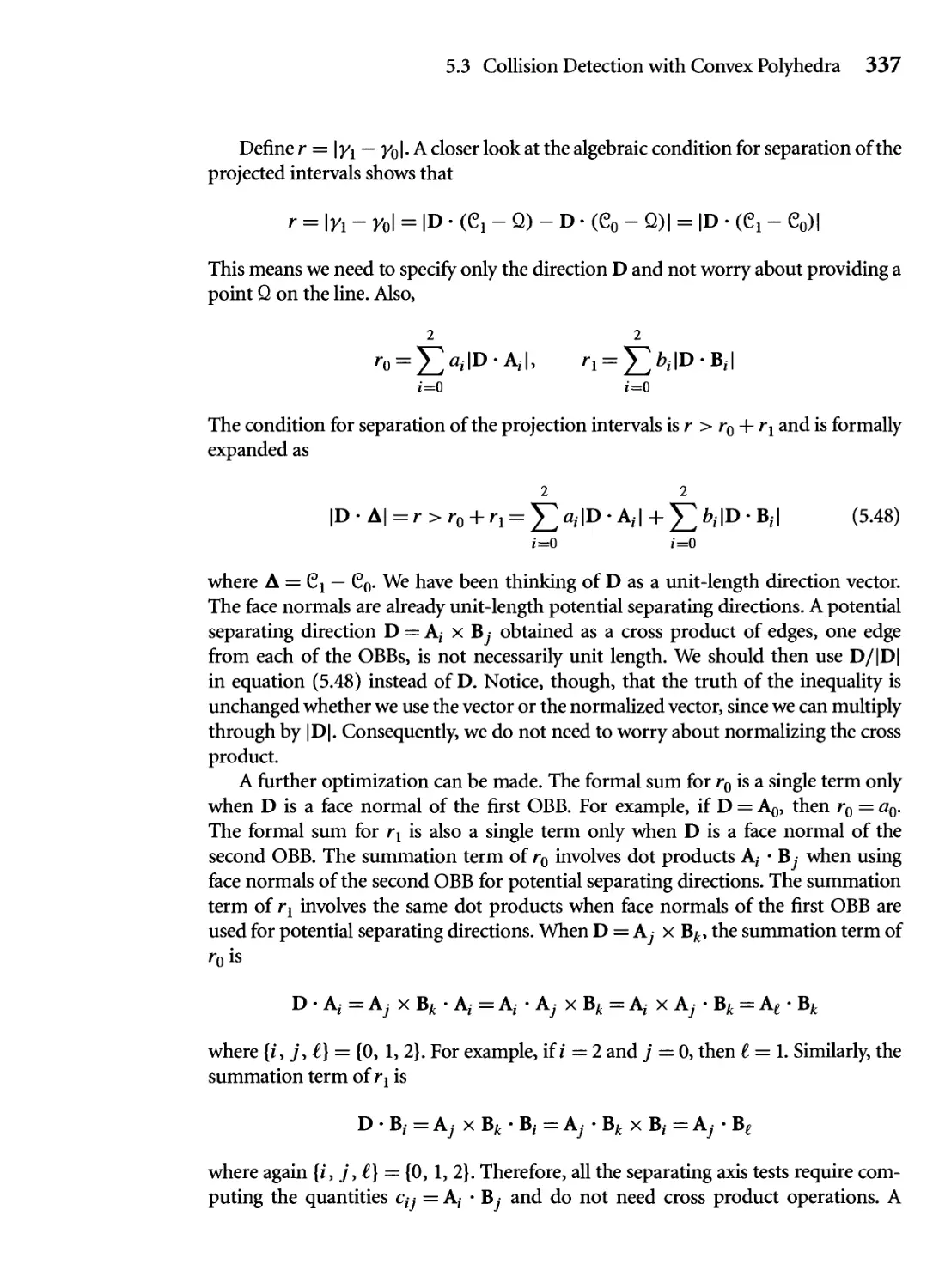
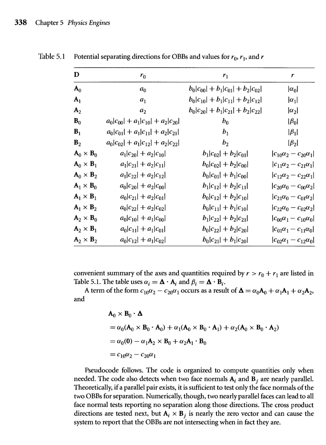
5.1 Potential separating directions for OBBs and values for r0, rv and r 338
7.1 Solving all possible systems of two equations in two unknowns 394
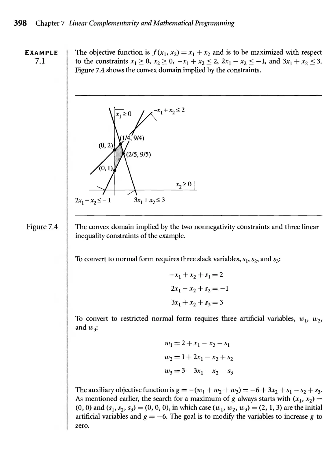
7.2 Tableau of coefficients and constants (Example 7.1) 399
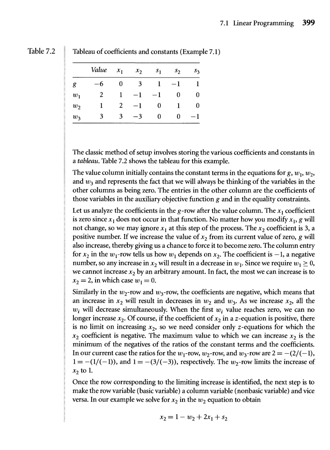
7.3 Updated tableau: Exchanging w2 with x2 400
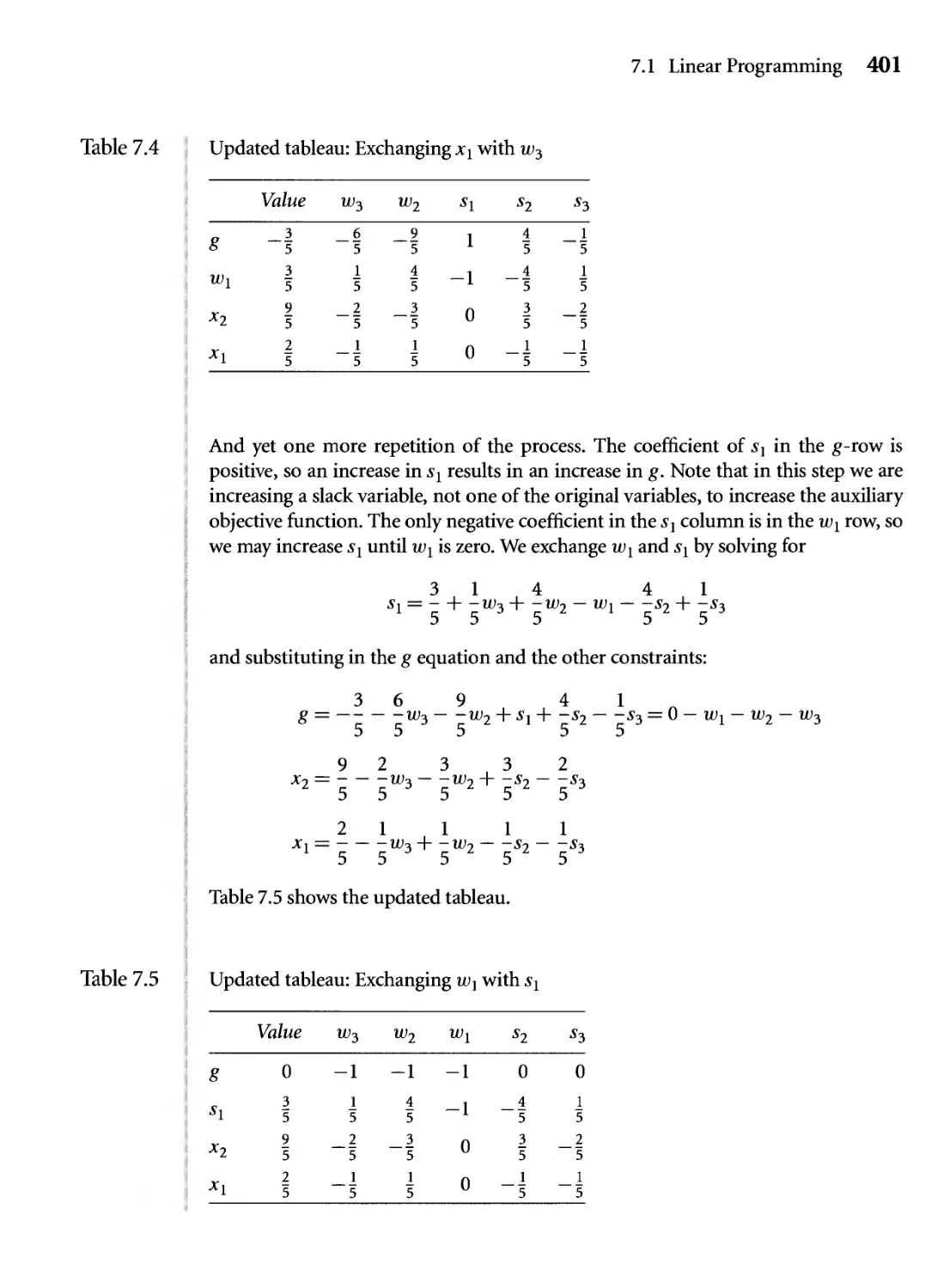
7.4 Updated tableau: Exchanging jcj with w3 401
7.5 Updated tableau: Exchanging ujj with 5j 401
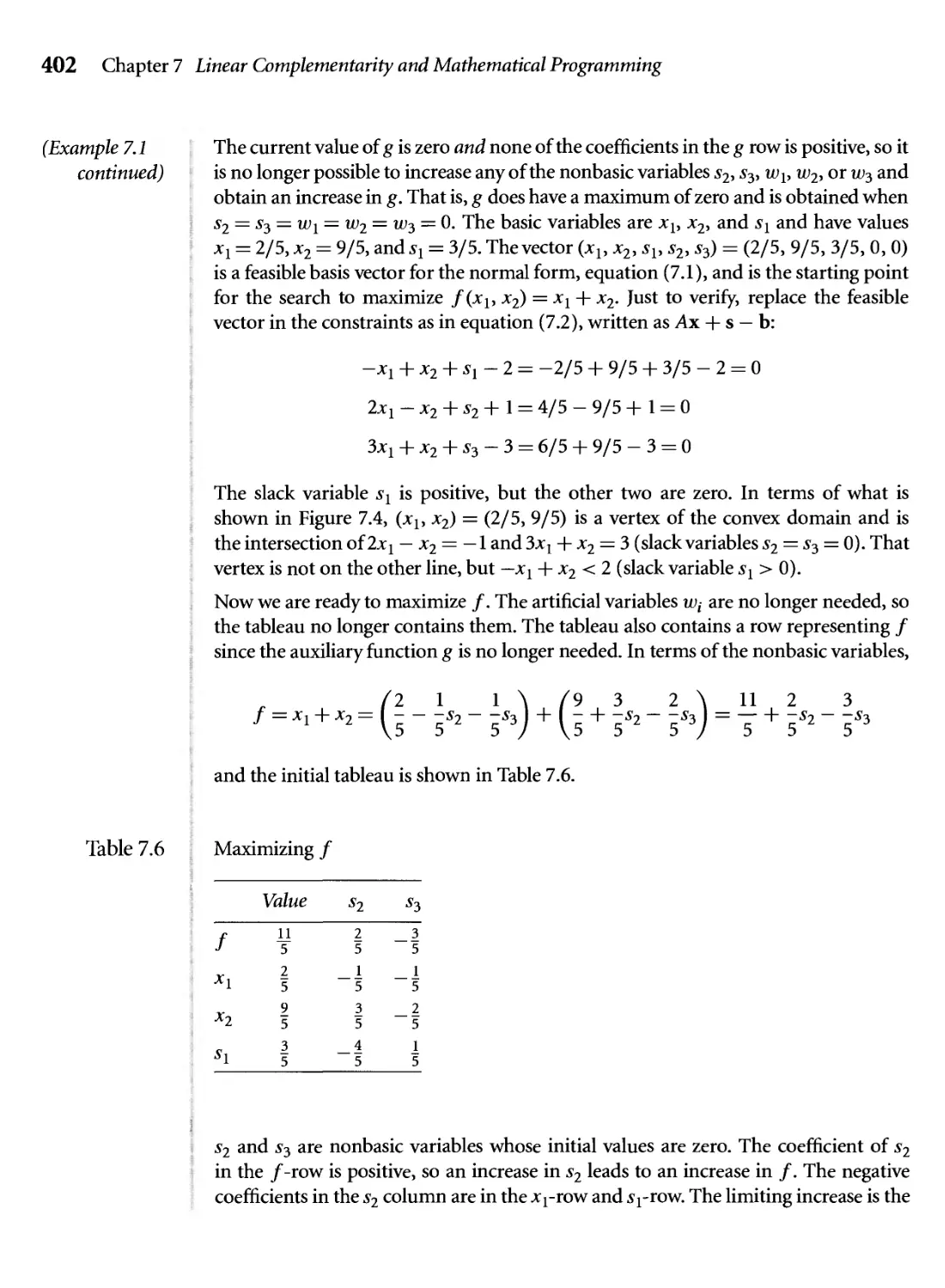
7.6 Maximizing / 402
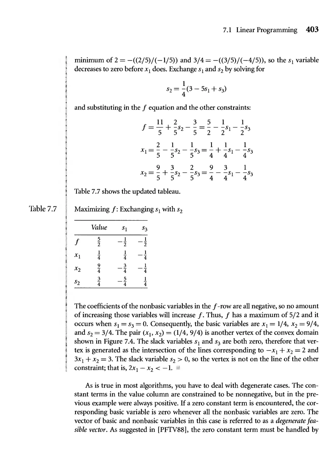
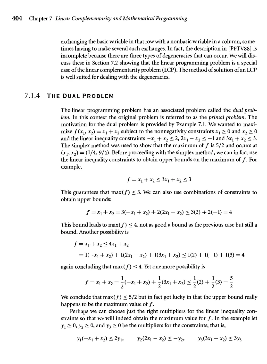
7.7 Maximizing /: Exchanging sr with s2 403
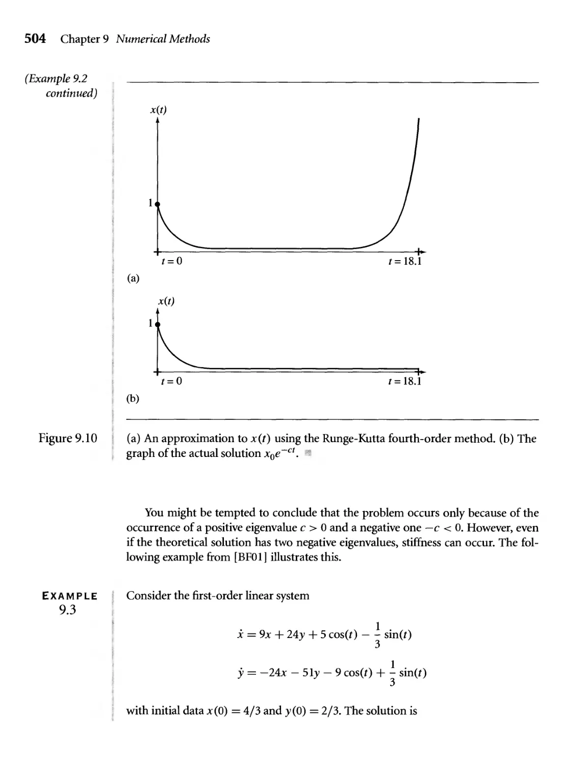
9.1 The actual and approximate values for the solution to the system of
equations 505
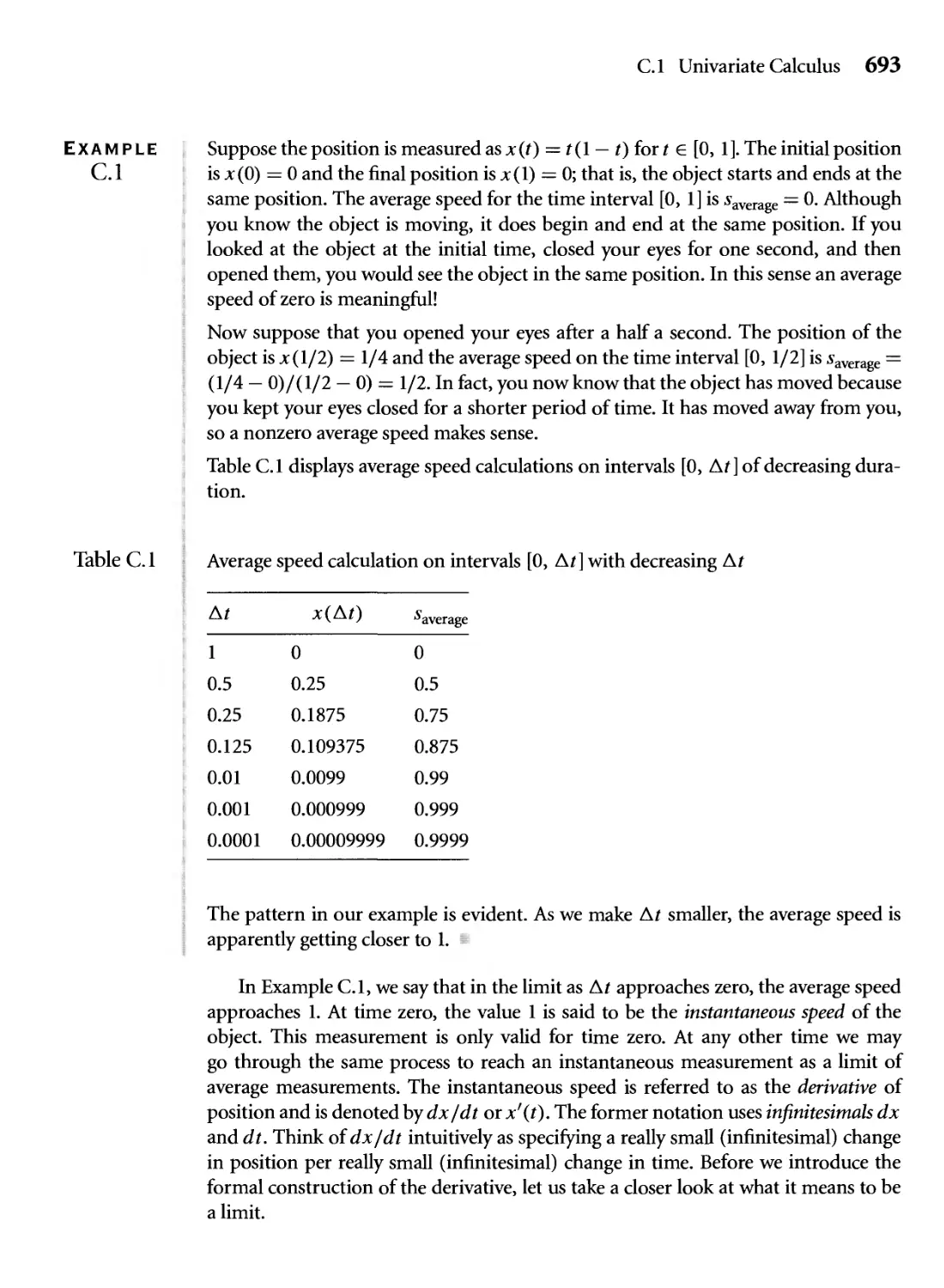
C.I Average speed calculation on intervals [0, At] with decreasing At 693
C.2 Function values for x near с 694
C.3 Derivatives of some common functions 700
C.4 Parameters for various finite difference approximations 721
xxvu

Preface
The evolution of the games industry clearly has been motivated by the gamers' de-
demands for more realistic environments. 3D graphics on a 2D graphics card necessarily
requires a classical software Tenderer. Historically, rasterization of triangles was the
bottleneck on 2D cards because of the low fill rate, the rate at which you can draw
pixels during rasterization. To overcome fill rate limitations on consumer cards the
graphics hardware accelerator was born in order to off-load the rasterization from the
2D card and the central processing unit (CPU) to the accelerator. Later generations
of graphics cards, called 3D graphics cards, took on the role of handling the stan-
standard work of a 2D graphics card (drawing windows, bitmaps, icons, etc.) as well as
supporting rasterization that the 3D graphics requires. In this sense the adjective "ac-
"accelerator" for a combined 2D/3D card is perhaps a misnomer, but the term remains
in use.
As fill rates increased, the complexity of models increased, further driving the
evolution of graphics cards. Frame buffer and texture memory sizes increased in
order to satisfy the gamers' endless desires for visual realism. With enough power
to render a large number of triangles at real-time rates, the bottleneck of the cards
was no longer the fill rate. Rather it was the front end of the graphics pipeline that
provides the rasterizers with data. The processes of transforming the 3D triangle
meshes from world coordinates to camera coordinates, lighting vertices, clipping, and
finally projecting and scaling to screen coordinates for the purposes of rasterization
became a performance issue.
The next generation of graphics cards arrived and were called hardware transform
and lighting (HW T&L) cards, the name referring to the fact that now the work of the
graphics pipeline had been off-loaded from the CPU to the graphics processing unit
(GPU). Although the intent of HW T&L cards was to support the standard graphics
pipeline, most of these cards also supported some animation, namely skin-and-bones
or skinning, in which the vertices of a triangle mesh (the "skin") are associated with
a matrix hierarchy (the "bones"), and a set of offsets and a set of weights relative to
the bones. As the matrices vary during runtime, the vertices are computed from the
matrices, offsets, and weights, and the triangle mesh deforms in a natural way. Thus,
we have some hardware support for deformable bodies.
The standard graphics pipeline is quite low-level when it comes to lighting of
vertices. Dynamic lights in a scene and normal vectors at vertices of a triangle mesh
are combined to produce vertex colors that are interpolated across the triangles by
the rasterizer. Textured objects are rendered by assigning texture coordinates to the
vertices of a mesh, where the coordinates are used as a lookup into a texture image.
The rasterizer interpolates these coordinates during rasterization, then performs a
lookup on a per-pixel basis for each triangle it rasterizes in the mesh. With a lot of
xxix

xxx Preface
creativity on the artists' end, the vertex coloring and texturing functions can be used
to produce high-quality, realistic renderings. Fortunately, artists and programmers
can create more interesting effects than a standard graphics pipeline can handle,
producing yet more impetus for graphics cards to evolve. The latest generation of
graphics cards are now programmable and support vertex shading, the ability to
incorporate per-vertex information in your models and tell the rasterizer how to
interpolate them. Clever use of vertex shading allows you to control more than color.
For example, displacement mapping of vertices transfers some control of positional
data to the rasterizer. And the cards support pixel shading, the ability to incorporate
per-pixel information via images that no longer are required to represent texture data.
Dot3 bump-mapping is the classic example of an effect obtained by a pixel-shader
function. You may view vertex shading as a generalization of the vertex coloring
function and pixel shading as a generalization of the basic texturing function.
The power of current generation graphics cards to produce high-quality visual
effects is enormous. Much of the low-level programming you would do for software
rendering is now absorbed in the graphics card drivers and the graphics APIs (appli-
(application programmer interfaces) built on top of them, such as OpenGL and DirectX,
which allows programmers to concentrate at a higher level in a graphics engine. From
a visual perspective, game designers and programmers have most of what they need
to create realistic-looking worlds for their gamer customers. But since you are reading
this preface, you already know that visual realism is only half the battle. Physical real-
realism is the other half. A well-crafted, good-looking character will attract your attention
for the wrong reasons if it walks through a wall of a room. And if the characters can-
cannot realistically interact with objects in their physical environment, the game will not
be as interesting as it could be.
Someday we programmers will see significant hardware support for physics by
off-loading work from the CPU to a physics processing unit (PPU). Until that day
arrives we are, so to speak, at the level of software rendering. We need to implement
everything ourselves, both low-level and high-level, and it must run on the CPU.
Moreover, we need real-time rates. Even if the renderer can display the environment
at 60 frames per second, if the physics system cannot handle object interactions
fast enough, the frame rate for the game will be abysmally low. We are required to
understand how to model a physical environment and implement that model in a
fast, accurate, and robust manner. Physics itself can be understood in an intuitive
manner—after all, it is an attempt to quantify the world around us. Implementing a
physical simulation on a computer, though, requires more than intuition. It requires
mathematical maturity as well as the ability and patience to synthesize a large system
from a collection of sophisticated, smaller components. This book is designed to help
you build such a large system, a physics engine as it were.
Game Physics focuses on the topic of real-time physical simulation on consumer
hardware. I believe it is a good companion to my earlier book, 3D Game Engine De-
Design, a large tome that discusses the topic of constructing a real-time graphics engine
for consumer hardware. The two disciplines, of course, will be used simultaneouly
in a game application. Game Physics has a similar philosophy to 3D Game Engine

Preface xxxi
Design in two ways. First, both books were conceived while working on commercial
engines and tools to be used for building games—the occurrence of the word "game"
in the titles reflects this—but the material in both books applies to more than just
game applications. For example, it is possible to build a virtual physics laboratory for
students to explore physical concepts. Second, both books assume that the reader's
background includes a sufficient level of mathematics. In fact, Game Physics requires
a bit more background. To be comfortable with the material presented in this book,
you will need some exposure to linear algebra, calculus, differential equations, and
numerical methods for solving differential equations. All of these topics are covered
in an undergraduate program in mathematics or computer science. Not to worry,
though: as a refresher, the appendices contain a review of the essential concepts of
linear algebra, affine algebra, calculus, and difference equations that you will need to
read this book. Two detailed chapters are included that cover differential equations
and numerical methods for solving them.
I did not call the book 3D Game Physics because the material is just as appropriate
for 1- or 2D settings. Many of the constrained physical models are of lower dimen-
dimension. For example, a simple pendulum is constrained to move within a plane, even
though a rendering of the physical system is in three dimensions. In fact, the mate-
material is applicable even to projects that are not game-related, for example, supporting
a virtual physics laboratory for students to explore physical concepts. I did call the
book Game Physics and I expect that some readers may object to the title since, in
fact, I do not cover all possible topics one might encounter in a game environment.
Moreover, some topics are not discussed in as much depth as some might like to see.
With even a few years to write a book, it is impossible to cover all the relevant topics
in sufficient detail to support building a fully-featured physics engine that rivals what
you see commercially. Some projects just require a team of more than one. I specifi-
specifically avoided getting into fluid dynamics, for example, because that is an enormous
topic all on its own. I chose to focus on the mechanics of rigid bodies and deformable
bodies so that you can build a reasonable, working system for physical simulation.
Despite this restricted coverage, I believe there is a significant amount of content in
this book to make it worth every minute of your reading time. This content includes
both the written text and a vast amount of source code on the CD-ROM that accom-
accompanies the book, including both the Wild Magic graphics engine and components and
applications for physics support. I have made every attempt to present all the content
in a manner that will suit your needs.
As in the production of any book, the author is only part of the final result. The
reviewers for an early draft of this book were extremely helpful in providing guidance
for the direction the book needed to take. The original scope of the book was quite
large, but the reviewers' wisdom led me to reduce the scope to a manageable size by
focusing on a few topics rather than providing a large amount of background material
that would detract from the main purpose of the book—showing you the essentials of
physical simulation on a computer. I wish to personally thank the reviewers for their
contributions: Ian Ashdown (byHeart Consultants), Colin Barrett (Havok), Michael
Doherty (University of the Pacific), Eric Dybsand (Glacier Edge Technology), David

xxxii Preface
Eberle (Havok), Todd Growney (Electronic Arts), Paul Hemler (Wake Forest Univer-
University), Jeff Lander (Darwin 3D), Bruce Maxim (University of Michigan—Dearborn),
Doug McNabb (Rainbow Studios), Jon Purdy (University of Hull), and Craig Rein-
hart (California Lutheran University). Thanks also go to Tim Cox, my editor; Stacie
Pierce, editorial coordinator; and Rick Camp, editorial assistant for the book. Tim has
been patient with my seemingly endless delays in getting a final draft to him. Well, the
bottom line is that the draft arrived. Now it is your turn to enjoy reading the book!

About the CD-ROM
Limited Warranty
The Publisher warrants the media on which the software is furnished to be free from
defects in materials and workmanship under normal use for 30 days from the date
that you obtain the Product. The warranty set forth above is the exclusive warranty
pertaining to the Product, and the Publisher disclaims all other warranties, express
or implied, including, but not limited to, implied warranties of merchantability and
fitness for a particular purpose, even if the Publisher has been advised of the pos-
possibility of such purpose. Some jurisdictions do not allow limitations on an implied
warranty's duration; therefore the above limitations may not apply to you.
Limitation of Liability
Your exclusive remedy for breach of this warranty will be the repair or replacement
of the Product at no charge to you or the refund of the applicable purchase price paid
upon the return of the Product, as determined by the publisher in its discretion. In no
event will the publisher, and its directors, officers, employees, and agents, or anyone
else who has been involved in the creation, production, or delivery of this software be
liable for indirect, special, consequential, or exemplary damages, including, without
limitation, for lost profits, business interruption, lost or damaged data, or loss of
goodwill, even if the Publisher or an authorized dealer or distributor or supplier
has been advised of the possibility of such damages. Some jurisdictions do not allow
the exclusion or limitation of indirect, special, consequential, or exemplary damages
or the limitation of liability to specified amounts; therefore the above limitations or
exclusions may not apply to you.
License Agreements
The accompanying CD-ROM contains source code that illustrates the ideas in the
book. Each source file has a preamble stating which license agreement pertains to it.
The formal licenses are contained in the files found in the following locations on the
CD-ROM:
Magi cSoftware/Wi1dMagi c2/Li cense/Wi1dMagi с.pdf
Magi cSoftware/Wi1dMagi c2/Li cense/GamePhysi cs.pdf
xxxiii

xxxiv About the CD-ROM
The source code in the following directory trees is covered by the GamePhysics.pdf
agreement:
Magi cSoftware/Wi1dMagi c2/Source/Physi cs
Magi cSoftware/Wi1dMagi c2/Appli cati ons/Physi cs
Use of the files in the Physics directories requires ownership of this book. All other
code is covered by the Wi 1 dMagi с. pdf agreement.
The grant clause of the Wi 1 dMagi c. pdf agreement is:
We grant you a nonexclusive, nontransferable, and perpetual license to use The
Software subject to the terms and conditions of the Agreement:
1. There is no charge to you for this license.
2. The Software may be used by you for noncommercial products.
3. The Software may be used by you for commercial products provided that such
products are not intended to wrap The Software solely for the purposes of sell-
selling it as if it were your own product. The intent of this clause is that you use
The Software, in part or in whole, to assist you in building your own original
products. An example of acceptable use is to incorporate the graphics portion
of The Software in a game to be sold to an end user. An example that vio-
violates this clause is to compile a library from only The Software, bundle it with
the headers files as a Software Development Kit (SDK), then sell that SDK to
others. If there is any doubt about whether you can use The Software for a
commercial product, contact us and explain what portions you intend to use.
We will consider creating a separate legal document that grants you permis-
permission to use those portions of The Software in your commercial product.
The grant clause of the GamePhysi cs. pdf agreement is:
We grant you a nonexclusive, nontransferable, and perpetual license to use The
Software subject to the terms and conditions of the Agreement:
1. You must own a copy of The Book ("Own The Book") to use The Software.
Ownership of one book by two or more people does not satisfy the intent of
this constraint.
2. The Software may be used by you for noncommercial products. A noncommer-
noncommercial product is one that you create for yourself as well as for others to use at
no charge. If you redistribute any portion of the source code of The Software
to another person, that person must Own The Book. Redistribution of any
portion of the source code of The Software to a group of people requires each
person in that group to Own The Book. Redistribution of The Software in bi-
binary format, either as part of an executable program or as part of a dynamic
link library, is allowed with no obligation to Own The Book by the receiving
person(s), subject to the constraint in item 4.

About the CD-ROM XXXV
3. The Software may be used by you for commercial products. The source code
of The Software may not be redistributed with a commercial product. Redis-
Redistribution of The Software in binary format, either as part of an executable
program or as part of a dynamic link library, is allowed with no obligation to
Own The Book by the receiving person(s), subject to the constraint in item
4. Each member of a development team for a commercial product must Own
The Book.
4. Redistribution of The Software in binary format, either as part of an exe-
executable program or as part of a dynamic link library, is allowed. The intent
of this Agreement is that any product, whether noncommercial or commer-
commercial, is not built solely to wrap The Software for the purposes of redistributing
it or selling it as if it were your own product. The intent of this clause is that
you use The Software, in part or in whole, to assist you in building your own
original products. An example of acceptable use is to incorporate the phys-
physics portion of The Software in a game to be sold to an end user. An example
that violates this clause is to compile a library from only The Software, bundle
it with the headers files as a Software Development Kit (SDK), then sell that
SDK to others. If there is any doubt about whether you can use The Software
for a commercial product, contact us and explain what portions you intend to
use. We will consider creating a separate legal document that grants you per-
permission to use those portions of The Software in your commercial product.
Installing and Compiling the Source Code
The Wild Magic engine is portable and runs on PCs with the Microsoft Windows
2000/XP operating systems or Linux operating systems. Renderers are provided for
both OpenGL (version 1.4) and Direct3D (version 9). The engine also runs on Apple
computers with the Macintosh OS X operating system (version 10.2.3 or higher).
Project files are provided for Microsoft Developer Studio (version 6 or 7) on Mi-
Microsoft Windows. Make files are provided for Linux. Project Builder files are provided
for the Macintosh.
For convenience of copying, the platforms are stored in separate directories on
the root of the CD-ROM. The root of the CD-ROM contains three directories and
one PDF file:
Windows
Linux
Macintosh
ReleaseNotes2pl.pdf
Copy the files from the directory of your choice. The directions for installing and
compiling are found in the PDF file. Please read the release notes carefully before
attempting to compile. Various modifications must be made to your development
environment and some tools must be installed in order to have full access to all the

xxxvi About the CD-ROM
features of Wild Magic. A portable graphics and physics engine is a nontrivial system.
If only we were so lucky as to have a "go" button that would set up our environment
automatically!
Updates and Bug Fixes
Regularly visit the Magic Software, Inc. web site, www.magic-software.com, for up-
updates and bug fixes. A history of changes is maintained at the source code page of the
site.

Chapter
Introduction
1.1 A Brief History of the World
The first real experience I had with a "computing device" was in the early 1970s when
I attended my first undergraduate college, Albright College in Reading, Pennsylvania,
as a premedical student. The students with enough financial backing could afford
handheld calculators. The rest of us had to use slide rules—and get enough significant
digits using them in order to pass our examinations. I was quite impressed with
the power of the slide rule. It definitely was faster than the previous generation
of computing to which I was accustomed: pencil and paper. I did not survive the
program at the college (my grades were low enough that I was asked to leave) and
took a few year's break to explore a more lucrative career.
"There is no reason anyone would want a computer in their home."
Ken Olson, founder and president of Digital Equipment Corporation
Deciding that managing a fast-food restaurant was not quite the career I thought
it would be, I returned to the college track and attended Bloomsburg University (BU)
in Bloomsburg, Pennsylvania, as a mathematics major, a field that suited me more
than chemistry and biology did. During my stay I was introduced to an even more
powerful computing device, a mainframe computer. Writing Fortran programs by
punching holes in Hollerith cards 1 was even better than having to use a slide rule,
1. Herman Hollerith used punched cards to represent the data gathered for the 1890 American census. The
cards were then used to read and collate the data by machines. Hollerith's company became International
Business Machines (IBM) in 1924.

2 Chapter 1 Introduction
except for the occasional time or two when the high-speed card reader decided it was
really hungry. By the end of my stay I had access to a monitor/terminal, yet another
improvement in the computing environment. Linear programming problems were a
lot easier to solve this way than with the slower modes of computing! I finished up at
BU and decided graduate school was mandated.
"I think there is a world market for maybe five computers."
Thomas J. Watson, former chairman of IBM
Next stop, the University of Colorado at Boulder (CU) in 1979.1 took a liking
to differential equations and got another shot at punching cards, this time to nu-
numerically solve the differential equations of motion for a particular physical system. I
understood the theory of differential equations and could properly analyze the phase
space of the nonlinear equations to understand why I should expect the solution to
have certain properties. However, I could not compute the solution that I expected—
my first introduction to being careless about applying a numerical method without
understanding its stability and how that relates to the physical system. The remainder
of my stay at CU was focused on partial differential equations related to combustion
with not much additional computer programming.
"Computers are useless. They can only give you answers."
Pablo Picasso
After graduating in 1984,1 started my academic career at the University of Texas at
San Antonio (UTSA) in the Division of Mathematics, Computer Science, and Statis-
Statistics. The university had recently started an engineering program and designed four
courses for applied mathematics and computer science relevant to the new program.
The two applied mathematics courses were your standard fare for an engineering pro-
program and included topics on differential equations, numerical methods, and physics
concepts. The two computer science courses were somewhat unique in that both re-
required students to work on the fast personal computers that were available at the time:
4.77 MHz Intel 8086 machines. The first course was introductory programming with
Borland's Turbo Pascal 3. The second course was on computer graphics. Although
Turbo Pascal supported graphics primitives, my requirements for the course included
writing device drivers for the state-of-the-art graphics card: the Enhanced Graph-
Graphics Adapter (EGA). With a blazingly fast CPU, Microsoft's Disk Operating System
(DOS), 20M of hard disk space, 640K of accessible system memory, and an EGA card
with four 64K memory chips (one chip per color plane), we were able to produce
some fine quality output rivaling that of the 2D computer games of that era. The
output was almost as good as what we could produce on the department's DEC Gigi
that was attached to a VAX 730 and allowed you to draw to the monitor by sending
cryptic escape sequences of the type that you normally see in printer drivers.

1.1 ABriefHistoryoftheWorld 3
40K ought to be enough for anybody."
William ("Bilt")H. Gams, cofounderofMicrosoftCorporation
During my tenure at UTSA, I became more involved in computer-related top-
topics and less involved in theoretical considerations in my research field of differential
equations. In particular I became involved with the University of Texas Health Science
Center's Department of Radiology. The field of medical imaging was quite interesting
to me with its inherent connection to computer graphics and visualization, but also of
interest were aspects of geometry and numerical methods since we were interested in
analyzing and extracting anatomical information from 3D medical images. My inter-
interest in the topic was strong enough that I decided to leave UTSA in 1991 and become
a "retread" by studying computer science and medical imaging at the University of
North Carolina (UNC) at Chapel Hill.
While at UNC I had access to more powerful equipment. We did not have a Cray
supercomputer with a couple of powerful processors, but we did have a massively
parallel machine appropriately named the MASPAR with 8196 processors, individu-
individually not very powerful, but a natural architecture for 2D image processing. Still, there
was a strong attraction to compute numerically on a personal computer, to see the re-
results graphically and immediately, if not sooner. At the time I had upgraded my Intel
8086 machine to an Intel 80486 machine with a floating point coprocessor. I was able
to implement many algorithms of interest in image analysis, including constructing
something called ridges that are defined in terms of differential equations. The same
programming issues that arose at CU bit me again: applying numerical methods for
differential equation solvers without thought about the stability of the methods or
about their applicability to the problem at hand. Another problem of interest was to
compute geodesic curves on surfaces, curves that represent the shortest surface path
between two points on the surface. The formulation of the problem is akin to what
you see in Lagrangian dynamics in physical modeling and results in yet more differ-
differential equations to solve numerically.2
"If you were plowing a field, which would you rather use?
Two strong oxen or 1024 chickens?"
! Seymour Cray, father ofsupercomputing
"The PC is the LSD of the '90s."
Timothy Leary, educator and psychologist
2. Specifically, a geodesic curve on a surface is the natural extension of a straight line in a plane—it has zero
curvature. The physical analogy is that a particle traveling along a geodesic has zero acceleration while
satisfying the constraint of remaining on the surface.

4 Chapter 1 Introduction
After leaving UNC, I eventually found my way into the games industry in 1997
by signing on at Numerical Design Ltd. (www.ndl.com), a company cofounded by
J. Turner Whitted, credited with the invention of ray tracing, and Robert Whitton,
a mathematics professor at Davidson College. The company's business model had
been focused on contract work in computer graphics, and they had developed a
photorealistic ray tracing package called R-Plus. Times were changing and they had
decided that a product-oriented business model was better than a contract-based
model. When I arrived the code base for Netlmmerse was in its infancy. The goal of
the product was a real-time graphics engine for 3D games. At the time the Voodoo 1
graphics accelerator from the company 3Dfx (now defunct) had arrived on the scene.
This was a true accelerator in the sense that it coexisted with a standard 2D graphics
card. As you are already aware, this type of graphics technology started a whole new
trend in the computer industry leading to significant evolution of central processing
units (CPUs) and off-loading of a lot of work to graphics processing units (GPUs).
The standard development machine at NDL in 1997 was a Pentium 133 MHz with
32M of system memory, not a lot of power compared to present-day machines but at
the time quite a good system.
One of the first customers for Netlmmerse was Broderbund, a software com-
company that intended to use the package for their upcoming game Prince of Persia
3D (POP3D). The game engine needed a lot of help to evolve and keep up with
the features that POP3D required. In particular, the collision detection system of
Netlmmerse was crude and needed improvement. The game engine was overhauled,
including the addition of quaternions to support fast keyframe animations. The col-
collision detection and response system was built from scratch, used hierarchical culling
for collision purposes, and used an oriented bounding box (OBB) tree-based hier-
hierarchy to support collision detection of the triangle mesh geometry [GLM96], but
with an enhancement to predict the time of first contact of moving objects (see Sec-
Section 5.3). The system also implemented 3D picking (intersection of line/ray/segment
with objects), something heavily used in POP3D to allow the Prince to jump and
catch ledges, and other related movements with constraints. The collision system was
functional, but not what I would call sophisticated. CPUs were finally reaching speeds
of 800 MHz by the time POP3D shipped in 1999, but they still did not have sufficient
power for complex geometric environments. The collision system was also used suc-
cesfully in an arcade game called XS-G (originally called Canyon Runner) that was
shipped by Greystone Technology in 1998.
As CPUs and GPUs evolved due to consumer demands in the gaming arena,
the graphics cards became powerful enough to give players a visually rich and
convincing environment for the games. But consumers are relentless and wanted
more physical realism. Predicting a trend in this direction, the company MathEngine
(www.mathengine.com) was started to build what was called a physics engine. The
product was a good one, but some of the demonstrations showed jittering objects
in resting contact with a flat surface. The problem is that applying numerical meth-
methods to the differential equations of motion is not enough. Stability of the methods is
important, but also important is having a robust system that integrates collision de-

1.1 A Brief History of the World 5
tection and collision response involving multiple rigid bodies. Resting contact is now
a classic problem that requires great care when implementing to avoid the jittering
objects. While I was at NDL, Steven Collins, the СТО of a Dublin-based company
called Telekinesys, Inc. contacted us to see what we thought about their physics en-
engine and how it handled problems like resting contact. The demonstrations were
very convincing and showed that, in fact, you can obtain physical realism with good
frame rates even on current consumer CPUs. Eventually, Telekinesys announced their
new technology, and the company name changed to Havok.com (www.havok.com).
Their commerical physics engine is an extremely good product. Many of the robust-
robustness issues that show up in any product attempting to handle geometric queries on
a computer with floating point arithmetic have been solved by the Havok folks. In
fact, in January of 2003 I walked into my favorite store, Intrex Computers, to sat-
satisfy my latest silicon craving. On display was a computer with an ATI Radeon 9700
graphics card running a demonstration from Havok.com that showed a creature in
exotic garb dancing about. The clothing was flowing in a very believable manner—
no self-intersections of the cloth and running at real-time rates. All I wanted was a
hard drive, but I also walked out with a new graphics card and the desire to write my
own physics engine. You know the feeling ....
Other companies, of course, have bought into the idea that you can do realis-
realistic physics in real time. The various modeling packages have plug-ins to help artists
with the physics. A particularly good and robust plug-in for the modeling package
Softimage (www.softimage.com) is the dynamics package Animats from John Nagle
(www.animats.com). John has spent a lot of time figuring out how to avoid all the
annoying floating point pitfalls that arise in any package that you build to handle
physics, collision, and distance and intersection calculations. Also noteworthy is the
Vortex physics engine from CMLabs (www.cm-labs.com). A commercial package for
robust distance calculations between convex polyhedra is named SOLID 3 and writ-
written by Gino van den Bergen (www.libsolid.com); earlier versions are available for free
(www.dtecta.com). No doubt you will discover many other related packages. Just as
the number of commercial graphics engines increases as the technology becomes
more commonly known to people, so will the commercial physics engines.
The games industry has gone through quite an evolutionary period over the past
few decades. The computers of 10 years ago are nowhere near the powerful machines
we have today. I started out with a 4.77 MHz Intel 8086 machine and a 2D EGA
graphics card. Now I have machines with very fast CPUs and lots of system memory,
and they all have 3D graphics hardware. These include a Macintosh system, a Linux
system, and a few Microsoft Windows PCs (maintaining portable source code comes
at a price). These systems are all capable of real-time graphics and real-time physics,
whereas the systems of a decade ago just did not have that kind of power.
"Grove giveth and Gates taketh away."
Bob Metcaffe, Ethernet inventor and founder of 3Com Corporation, on the trend of hardware
speedups not keeping up with software demands

6 Chapter 1 Introduction
1.2
Nevertheless, a major theme in this brief historical journey of mine is, The mathe-
mathematics and physics that you will deal with in this book is not new. Much of the computer
graphics research that appears in the literature of the past decade is motivated by the
power that machines have now (or soon will have). Much of what occurs in that re-
research is a reapplication of classic mathematical and physical concepts and shows that
the researchers appreciate the importance and power of mathematics and physics in
achieving their goals. Thus, you too should appreciate the power of all things math-
mathematical and physical. As readers of my books certainly know, I have not shied away
from mathematics, because it is my language for understanding the technical world
around me. I wish it to be your language, too. After all, you will need it in order to
appreciate fully the complexities and difficulties in implementing a robust physical
simulation on a computer. What else can I say!
"A mathematician is a device for turning coffee into theorems."
PaulErdos, mathematician. My variant: "A computer graphics researcher is a device
for tumingcoffee into SIGGRAPH papers."
"For the things of this worid cannot be made known without
a knowledge of mathematics.*
12th-century philosopher
"It Is the merest truism, evident at once to unsophisticated observation,
that mathematics is a human invention/
FromThe Logic of Modern Physics, by P. W.Bridgman,physipst
*Omnia apud me mathematica fiunt"
(With me everything turns into mathematics).
Rene Descartes
"A mathematician, like a painter or a poet, is a maker of patterns.
If his patterns are more permanent than theirs, it is because they are
made with ideas."
G. К Hardy, mathematician
A Summary of the Topics
Physics concepts and their application to games is quite a large topic. Rather than
attempt to provide brief summaries of all possible topics, in other words a survey
book, I decided to focus on the subset that most programmers seem to ask questions

1.2 A Summary of the Topics 7
about in the various Usenet newsgroups: mechanics, rigid bodies, deformable bodies,
and collision detection and response systems. These topics are discussed in depth
and require a minimum mathematical background that includes linear algebra and
calculus, both univariate and multivariate. Also helpful would be some exposure to
ordinary differential equations and to numerical methods that solve these, but if you
have not had this exposure, a couple of chapters provide enough material to support
what you will need for implementing a physical simulation.
Chapter 2 introduces curves in two dimensions and in three dimensions as repre-
representative paths of a particle. The chapter introduces the physical concepts of position,
velocity, and acceleration. The choice of coordinate system is important in an appli-
application, so the standard systems are covered, including polar coordinates, cylindrical
coordinates, and spherical coordinates. The motion of particles along paths in the ab-
absence of forces is called kinematics. In addition to kinematics of a single particle, we
also look into the kinematics of a particle system. This material is the all-important
foundation for the physics engines discussed in Chapter 5.
The remainder of Chapter 2 is an introduction to the standard concepts that you
see in a course on physics, starting with Newton's laws of motion. The topics of force,
torque, equilibrium, linear and angular momentum, center of mass, moments and
products of inertia, and kinetic and potential energy are discussed in detail with the
goal of being able to calculate these quantities on a computer. Computing the center
of mass and the inertia tensor for a solid convex polyhedron is necessary for the
physics engines of Chapter 5.
Chapter 3 is about dynamics: the interaction of rigid bodies when forces and
torques are present in the physical system. The classical approach in an introductory
physics course uses Newtonian dynamics and the famous formula of Newton's second
law of motion, F = ma, where m is the constant mass of an object, a is its acceleration,
and F is the applied force. I do not spend a lot of time delving into this approach.
The coverage is sufficient to support the general purpose physics engines that use
Newton's second law for simulation.
The majority of Chapter 3 is spent on Lagrangian dynamics, a framework for
setting up the equations of motion for objects when constraints are present. In La-
Lagrangian dynamics, the equations of motion naturally incorporate the constraints.
A Newtonian formulation requires that forces of constraint be part of the term F in
the equation of motion, and the constraint forces are sometimes difficult to derive.
For example, you will see in the Lagrangian approach that frictional forces are easier
to deal with than in the Newtonian approach. For many games, a designer's specific
knowledge of the physical system can be exploited to good effect by formulating the
simulation using Lagrangian dynamics, the result being that the computational time
of the simulation is reduced, compared to a general-purpose system using Newtonian
dynamics.
Euler's equations of motion are also discussed in Chapter 3, because a few prob-
problems are more naturally formulated in terms of Euler angles than in terms of other
dynamics systems. Although Hamiltonian dynamics is of importance, especially in
dealing with the n-body problem, I made the decision not to include a discussion of

8 Chapter 1 Introduction
it in this book, since the other approaches are sufficient to allow implementations on
a computer.
Chapter 4 is about deformable bodies. There are many ways to simulate defor-
deformation; we will address a subset in this book. In all cases you should consider these
"hacked" physics in the sense that at no time do we use a real physical model for the
actual material that makes up the bodies. The real models do not lend themselves to
the fast computation that a game requires. All that is required of a hacked physics
approach in a game is that the deformations look believable to the player. I do cover
mass-spring systems for the purposes of deformation, but even these might not be as
realistic a model for deformable objects as you might wish.
Another method that I have included for describing deformable objects includes
the use of control point surfaces where you vary the control points in some suitable
manner to cause the surface to deform as you desire. A brief discussion is given for B-
spline curves and surfaces and for nonuniform rational B-spline(s) (NURBS) curves
and surfaces. The presentation is limited to the computational aspects of curves and
surfaces, including optimizations that allow fast evaluation. You are referred to other
sources for a more detailed look at the properties of В-splines and NURBS.
Free-form deformation is a method for deforming an object and uses a volu-
volumetric approach. The object is embedded in a portion of space that is defined via
a control point lattice. The volume of space is deformed, causing the object itself to
deform.
The final deformation method is based on the object's surface being defined
implicitly. The popular term for such surfaces is metaballs. I prefer to call them what
they are, implicit surfaces. The discussion of this topic shows how you define a 3D
lattice of sample points, trilinearly interpolate to obtain a continuous representation
of a function defined on the volume occupied by the lattice, then extract the implicit
surface as the level surface of the constructed function. Implicit surfaces are deformed
by varying the constructed function itself.
Chapter 5 is about what most readers probably think of as the meat of game
physics—the physics engine. The chapter describes a general system for handling
a collection of rigid bodies, including collision detection and collision response. A
general system is one that uses Newton's second law of motion, F = ma, to control
the motion of objects. The constraint forces are unknown to the system and must be
calculated based on the information that is provided by the collision detection system.
I discuss the impulse-based approach that Brian Mirtich [Mir96b] and David
Baraff [BarOl ] made popular, but by all means this is not the only approach you can
take. My goal is to go into significant detail about the impulse-based approach so
that you A) understand the layout of a general physics engine, B) see what compli-
complications arise, and C) learn to evaluate what its strengths and weaknesses are. Other
approaches to building a robust physics engine are based on trying to fix the weak-
weaknesses of the previous-generation engine. Once you understand the impulse-based
engine, you should be able to start experimenting with modifications; references to
other approaches are provided, so you have a nearly endless supply of ideas to inves-
investigate. For instance, a good tutorial site for rigid body dynamics is [Hec98].

1.2 A Summary of the Topics 9
The first section of Chapter 5 is about unconstrained motion. This gives you an
idea of how to design a data structure to represent a rigid body and how to solve the
differential equations of motion for a body that does not interact with other bodies
in its environment. Section 5.2 complicates matters by allowing interaction between
bodies, referred to as constrained motion. As you will see, building a collision detec-
detection and response system for constrained motion is a formidable task! I have provided
enough pseudocode to allow you to build a working engine if you choose to do so.
Source code is provided for a working engine with which you can experiment. A lot
of code was written by George Innis of Magic Software, Inc. after reading a draft of
this book—hopefully evidence that other folks will be able to implement real systems
from my descriptions.
The last subsection of the material on constrained motion (Section 5.2.5) pro-
proposes a different approach that I think should be investigated. I propose that an
implementation can detect and provide enough information about the constraints
imposed by the contact set found by the collision detection system so that, rather
than continuing to solve the general F = ma, the system can construct the Lagrangian
equations of motion and switch to the appropriate set when necessary. This ap-
approach would be of particular importance when dealing with frictional forces since
Lagrangian- dynamics do a better job of incorporating the friction into the equations.
The physics engine that Thomas lakobsen designed and developed for IO Interactive
already hints at this [lakOl] by using projection of the system state variables onto a
manifold described by the constraints.
Section 5.3 is on collision detection with convex polyhedra. This is generally the
hardest part of a physics engine to implement in a robust manner while not using
too much computational time that is allotted per time frame. I discuss the method
of separating axes because it burdens you with the minimum information needed to
test if two objects overlap, but provides as much information as you need to actually
compute the contact set between two noninterpenetrating objects.
Section 5.4 is about using spatial and temporal coherence of the rigid body objects
to reduce the amount of time spent detecting collisions. A couple of basic systems
are mentioned, one using bounding spheres, but a more effective one using axis-
aligned bounding boxes. Many approaches to collision detection are abundant in the
literature. I do not attempt to describe any of them in great detail since my goal with
this book is not to focus heavily on the collision detection portion of an engine, but
rather to focus on the collision response. That said, I do provide references in Section
5.5 so that you can investigate the topics yourself, many of which are available through
the geometry web site of Ming Lin and Dinesh Manocha of the Computer Science
Department at the University of North Carolina [GAM03]. A couple of fine books on
collision detection are forthcoming from Morgan Kaufmann Publishers, one by Gino
van den Bergen [vdB03] and one by Christer Ericson of Sony Interactive [Eriar].
Chapter 6 is a brief discussion of how to obtain some physical effects through
the use of shader programs on programmable graphics cards. Vertex shaders allow
displacement of vertices to obtain visual effects of the physical simulation, but it is
important to note that the displaced vertices are not accessible to the main program.

10 Chapter 1 Introduction
Until that capability is added to programmable graphics cards, you will not be able
to use the vertex locations for any type of intersection or collision testing. The chap-
chapter has examples of vertex shaders for vertex displacement and for skin-and-bones
animation. Other examples are along the lines of optical effects (still in the realm of
physics), including reflection and refraction effects. In a sense shader programs pro-
provide a form of hacked physics. As graphics hardware evolves, look for the ability to
rapidly read data from the graphics card into system memory, thereby allowing for
intersection and collision testing.
The remaining four chapters of the book provide mathematical background. As
such they are a bit more difficult to read than the previous chapters. Chapter 7 is on
the topic of linear programming (LP), the linear complementarity problem (LCP),
and mathematical programming (MP) generally. One application of the material is to
use LCP methods to compute the distance between convex polygons or convex poly-
hedra. Another application is to use LCP methods to compute resting contact forces
and to use MP methods, namely, constrained quadratic minimization, to compute
impulsive contact forces at the points of contact among a collection of interacting
rigid bodies. The LCP method also is useful in computing distance between points,
convex polygons, and convex polyhedra.
Chapter 8 is a brief overview of the theory of differential equations. This material
is provided for those readers who want to understand the basic theory of differential
equations relevant to physical simulation. The overview is at the level of what you will
find in an undergraduate textbook on the topic; it is intentionally limited in scope but
should give you enough of the flavor of what analysis of differential equations is all
about.
Chapter 9 is on numerical methods for solving differential equations. This is a
large chapter that shows you a vast collection of methods, including how the meth-
methods are derived using basic mathematical principles. The methods include Euler's
method, higher-order Taylor methods, methods obtained by an integral formulation,
and the all-popular and robust Runge-Kutta methods. These are all single-step meth-
methods that require information only at the previous time step to generate information
at the current time step. I also discuss multistep methods that use multiple previous
times to generate information at the current step. These methods include the con-
concept of a predictor-corrector that attempts to provide good estimates of the solution
from ones that are less precise. Extrapolation methods are also covered, leading to the
Bulirsch-Stoer method that uses rational polynomial extrapolation to produce highly
accurate results with a minimum of computation cost. A class of methods that is very
popular now in the games arena, and has been used for a long time in molecular dy-
dynamics, is the Verlet methods. A section of the chapter is devoted to these methods,
including the standard Verlet method, the Leap Frog method, and the Velocity Verlet
method. I also included a reasonable alternative called the Gear fifth-order predictor-
corrector method. Thus, you have a large collection of solvers, all of them implemented
in the source code on the CD-ROM that accompanies the book.
Implementing a numerical method is only half the battle. Understanding the
stability of a method, how to choose an appropriate step size, and how to evaluate

1.3
1.3 Examples and Exercises 11
the trade-offs between accuracy and computation time is the other half of the battle.
Perhaps the most important part of Chapter 9 is the section on numerical stability
and its relationship to physical stability of equilibrium solutions. You might think of
this as an irrelevant mathematical exercise, but in fact I provide a stability analysis for
a handful of methods when applied to the simple pendulum problem. This gives you
the blueprint to follow when analyzing the stability of methods for your particular
applications. The last section of the chapter discusses the problem of stiffness, another
issue related to the stability of numerical solvers.
Chapter 10 is on quaternions, one of the most misunderstood and abused topics
in the Usenet newsgroups (in my opinion). Yes, these are mathematical in flavor,
but in fact a physical simulation benefits from using these because of the resulting
reduced memory in representing rotations and in the reduced computation time
in actually rotating or updating the equations of motion for a physical system. The
molecular dynamics folks have been using these for a really long time, so you can find
a lot of online material discussing quaternions in the context of that field, including
higher-order methods for numerically solving the quaternion differential equation
that shows up in the physical simulation.
I provide the classical approach to how quaternions relate to rotations and I pro-
provide a linear algebraic approach to try to motivate the connection by considering
rotation in four dimensions. Section 10.4, "From Rotation Matrices to Quaternions,"
was written by Ken Shoemake, famous for introducing the joys and necessities of
quaternions to the computer graphics and animation communities. The final two
sections involve interpolation of quaternions and derivatives of time-varying quater-
quaternions, the latter section being related to how you derive the equation of motion for
updating orientations of rigid bodies when quaternions are used to represent the ori-
orientations.
Examples and Exercises
Quite a few examples and exercises are provided in this book. The examples are
worked through in detail, of course, with some of them implemented in source code,
which is on the CD-ROM. The exercises are for you to try. They vary in difficulty
and are marked accordingly: easy it , medium fM , or hard (и . The assignment of
these labels is my own choosing and may not agree with someone else's assessment
of the level of difficulty. The answers to selected exercises are on the CD-ROM.
I recommend that you make a significant attempt to answer the questions before
looking up the answer. The answers to the remaining exercises are available only
through your instructor, with access provided by Morgan Kaufmann Publishers.

Chapter
Basic Concepts
from Physics
In this chapter we review some of the basic concepts of physics that are relevant to
the analysis of motion and interaction of rigid bodies. A rigid body is classified ac-
according to the type of region that contains its mass, the topic of Section 2.1. Section
2.2 introduces curves in two or three dimensions as representative paths of a particle
in the absence of forces. This topic is referred to as kinematics. The section intro-
introduces the physical concepts of position, velocity, and acceleration. Many applications
are better handled with an appropriate choice of coordinate system. The Cartesian
system is usually convenient, but we also take a look at polar coordinates, cylindrical
coordinates, and spherical coordinates. In addition to kinematics of a single particle,
we also look into the kinematics of particle systems and of solid bodies. This material
is the foundation for the physics engines discussed in Chapter 5.
The remainder of this chapter is an introduction to the standard concepts that
you see in a course on physics, starting with Newton's laws of motion in Section 2.3.
The topic of forces is discussed in Section 2.4 with specific reference to forces you
will see throughout the book in the examples: gravitational forces, spring forces, and
frictional forces. The closely related topics of torque and equilibrium are also covered
in the section. Various measures of momenta are discussed in Section 2.5, includ-
including linear and angular momentum, first-order moments and their relationship to the
center of mass of an object, and moments and products of inertia. The last part of Sec-
Section 2.5 shows how to compute the center of mass and the inertia tensor for a solid
polyhedron of constant mass, something you will need to implement in the physics
engines discussed in Chapter 5. Work and energy are the final topic of the chapter.
13

14 Chapter 2 Basic Concepts from Physics
The kinetic energy is an important quantity in the development of Lagrangian dy-
dynamics. The potential energy is important when dealing with conservative forces such
as gravity.
2.1 Rigid Body Classification
A rigid body is characterized by the region that its mass lives in. The simplest body
is a single particle of mass m that occupies a single location x. A particle system is a
collection of a finite number of particles, say, p of them, the /th particle having mass
m,- and located at x,-, 1 <i<p. Single particles and particle systems are examples of
discrete material since the number of particles is finite. Various physical quantities
involve summations over the particles in a system. The standard notation is
where <2, is some physical quantity associated with the /th particle and Btotal is the
summary quantity for all the particles. Although the equation here involves a scalar-
valued physical quantity, vector-valued quantities will be encountered as well.
Another type of body is referred to as a continuous material, consisting of in-
infinitely many particles that lie in a bounded region of space, denoted R. We refer
to such a rigid body as a continuum of mass. Within the category of a continuum of
mass we have a further set of classifications. The region R can be a bounded segment
of a curve, whether in one, two, or three dimensions. Mathematically we may refer to
such a rigid body as a curve mass. Physically we may call the body a wire. R can be a
bounded region in the plane (two-dimensional mass living in two dimensions) or a
bounded portion of a surface in space (two-dimensional mass living in three dimen-
dimensions). Mathematically we may refer to such a rigid body as a surface mass. Physically
we may call the body a lamina or, in two dimensions, a planar lamina. Finally, R can
be a solid occupying a bounded region of space. Mathematically we may refer to such
a body as a volume mass. Physically we may call the body a solid.
Various physical quantities involve summations over all particles of mass in the
region. The summation notation for particle systems no longer applies and is re-
replaced by integration over the region. The method of integration depends on the
category of region. Generically we will use the notation
<2total= / QdR
Jr
where R is the region, dR is an infinitesimal portion of the region, and Q is the
physical quantity of interest and can be scalar- or vector-valued. An analysis for a
particular type of rigid body, whether for mathematical purposes or for a computer
implementation, must provide the specific type of integration in order to compute

2.2 Rigid Body Kinematics 15
the integral. For a curve mass, the integration is computed as a line integral, where
the curve is parameterized by a single parameter and the limits of integration depend
on that parameterization. For a surface mass in the plane, the integration is computed
as a double integral, where the limits of integration depend on how the region is
represented. For a surface mass in space, the integration is via a surface integral
whose evaluation may very well involve Stokes's Theorem. For a volume mass, the
integration is computed as a triple integral, where the limits of integration depend on
how the region is represented. Throughout the book I will use the generic notation
fR Q dR when presenting general physical topics. I will resort to the specific type of
integration when demonstrating the concepts with examples.
2.2 Rigid Body Kinematics
The study of motion of objects without considering the influence of external forces
is referred to as kinematics. The basics of the topic are presented in this section. We
look at the three basic types of rigid bodies: a single particle, a particle system, and
a continuum of mass. For the purposes of rigid body kinematics, the analyses for
particle systems and continuous materials are the same.
2.2.1 Single Particle
Let us focus first on the kinematics of a single particle. Although we might start
directly with the analysis of a particle moving through space, many situations arise
where the particle is constrained to moving within a plane. We start our analysis
with particle motion in the jcy-plane, ignoring the z-component of the position. If
the constraining plane is another one at some arbitrary orientation in space, basic
methods of linear algebra may be applied to represent the particle's position with
respect to an orthonormal basis of two vectors in that plane. The ideas we present
here for the ky -plane apply directly to the coordinates within the general plane.
Whether in two or three dimensions we may choose Cartesian coordinates to rep-
represent the particle's position. However, some problems are better formulated in dif-
different coordinate systems. Particle motion is first discussed in Cartesian coordinates,
but we also look at polar coordinates for 2D motion and at cylindrical or spherical co-
coordinates for 3D motion since these coordinate systems are the most common ones
you will see in applications.
Planar Motion in Cartesian Coordinates
First let us consider when the particle motion is constrained to be planar. In Cartesian
coordinates, the position of the particle at time t is
r(t)=x(t)i+y(t)j B.1)

16 Chapter 2 Basic Concepts from Physics
where i = A, 0) and j = @, 1). The velocity of the particle at time t is
v(t) = i = xi+y j
B.2)
The dot symbol denotes differentiation with respect to t. The speed of the particle at
time t is the length of the velocity vector, |v|. If s(t) denotes the arc length measured
along the curve, the speed is i = |v|. The quantity i = ds/dt is intuitively read as
"change in distance per change in time," what you expect for speed. The acceleration
of the particle at time t is
B.3)
At each point on the curve of motion we can define a unit-length tangent vector by
normalizing the velocity vector,
T@ = — = (cos@(O), sm@(O))
||
B.4)
The right-hand side of equation B.4) defines ф (t) and is valid since the tangent vector
is unit length. A unit-length normal vector is chosen as
= (-sin@(O),cos@(O))
B.5)
The normal vector is obtained by rotating the tangent vector jt/2 radians counter-
counterclockwise in the plane. A coordinate system at a point on the curve is defined by origin
r(t) and coordinate axis directions T(t) and N(/). Figure 2.1 illustrates the coordinate
systems at a couple of points on a curve. The coordinate system {r(t); T(/), N(/)} is
called a moving frame.
Figure 2.1 A couple of coordinate systems at points on a curve.

2.2 Rigid Body Kinematics 17
The velocity and acceleration vectors may be represented in terms of the curve
tangent and normal. The velocity is a minor rearrangement of equation B.4),
v= |v|T = iT
The acceleration is obtained by differentiating the last equation,
B.6)
d
It
.dT
S~dt
,dT_
ds
Differentiating the tangent vector in equation B.4) with respect to arc length s
produces
— = — (cos ф, sin ф) = — (— sin ф, cos ф) = /cN(.s)
ds ds ds
where к = dф|ds is the curvature of the curve at arc length s. Observe that large
angular changes in the normal vector over a small length of curve equate to large
curvature values. The acceleration is therefore
a = 's'T + ks N
B.7)
The component s'T is called the tangential acceleration, the acceleration in the direc-
direction of motion. The component /ci2N is called the normal acceleration or centripetal
acceleration, the acceleration that is perpendicular to the direction of motion. Equa-
Equations B.6) and B.7) may be used to show that the curvature is
к =
xy — yx
|v|
B.8)
The rate of change of the tangent vector with respect to arc length is related to the
normal vector. You might be curious about the rate of change of the normal vector
with respect to arc length. It is
i
dN' _ d _dф . _
ds ds ds
Summarizing the s -derivatives in a format matrix notation:
dT
dN
L ~ds~ J
= L-k oJU
B.9)
Observe that the coefficient matrix is skew-symmetric, a common theme when com-
computing the derivatives of the vectors in a frame.

18 Chapter 2 Basic Concepts from Physics
Example
2.1
Construct the various vectors and quantities mentioned earlier for a parabolic curve
r(t) = ti + t1]. For simplicity of notation, we use r = (t, t2).
The velocity is v = A, 2t) and the speed is just the length of the velocity vector,
i = Vl + 4?2. The magnitude of tangential acceleration is s = 4?/VT+~4/A The ac-
acceleration is a = @, 2). The unit-length tangent and normal vectors are
T =
A, 20
'l + At2
Finally, the curvature is к = 2/A + 4t2K/2.
N =
Planar Motion in Polar Coordinates
The particle motion may also be represented using polar coordinates. The choice of
Cartesian form versus polar form depends on your application. The position vector
is represented as a unit-length vector R = r/|r| and a distance r = |r| from the origin,
= |r|- =rR
B.10)
Since R = r/|r| is unit length, we may write it as R = (cos в, sin 0), where в de-
depends on /. A unit-length vector perpendicular to R is P = (— sin в, cos в) and is
obtained by a 7t/2 counterclockwise rotation of R in the plane. The moving frame
{r(/); R(t), P@} provides an alternate coordinate system to the tangent-normal one.
Figure 2.2 shows the polar frames at points on a curve, the same curve shown in
Figure 2.1.
Figure 2.2 A polar coordinate frame at a point on a curve.

2.2 Rigid Body Kinematics 19
The derivatives of the frame directions with respect to time are summarized in
formal matrix notation:
Notice the similarity to equation B.9).
The velocity is represented in the polar frame by
v = i = — (rR)=rR + rR = rR + r0P B.12)
dt
The acceleration is represented in the polar frame by
a = v = rR + rR H (гв) P + r0V = (r - r62)R + (re + 2r0)P B.13)
dt v '
EXAMPLE Construct the various quantities for a spiral r =0, where 0 is a function of time t.
2-2 The position is r = 0R = @ cos 0, 0 sin 0), the velocity is v = 0R + 00V =
0(cos 0 - 0 sin 0, sin 0 + 0 cos 0), and the acceleration is a = @ - #02)R +
@0 + 202)P = 0(cos 0 - 0 sin 6», sin 0 + 0 cos 0) + в2(-0 cos 0 - 2 sin 0,
-0 sin 6» +2 cos 0).
Spatial Motion in Cartesian Coordinates
We now consider the spatial case. In Cartesian coordinates the position of a particle
at time t is
T(t)=x(t)i+y(t)j+z(t)k B.14)
where i = A, 0, 0), j = @, 1, 0), and k = @, 0, 1). The velocity of the particle at time
Ms
v(t)=i = xi+y j+zk B.15)
The speed of the particle at time t is the length of the velocity vector, |v|. If s(t)
denotes the arc length measured along the curve, the speed is i = |v|. The acceleration
of the particle at time t is
a(t)=v = i = xi +yj +zk B.16)
At each point on the curve of motion we can define a unit-length tangent vector by
normalizing the velocity vector:
^; BЛ7)
||

20 Chapter 2 Basic Concepts from Physics
Circle of potential normals
Figure 2.3 A curve, a tangent vector at a point, and the circle of choices for the normal vector.
The circle lies in the plane containing the point and perpendicular to the tangent.
In 2D we had only two choices for unit-length vectors that are perpendicular to the
curve. We chose the one that is always a counterclockwise rotation from the tangent
vector. As long as the tangent vector is a continuous function of t (the angle ф(г)
is a continuous function), the normal vector is also a continuous function. In 3D
there are infinitely many choices for a unit-length vector perpendicular to the tangent
vector, an entire circle of them in the plane that is perpendicular to T and centered at
the point on the curve. Figure 2.3 shows a curve, a tangent at a point, and the circle
of choices for the normal.
Which one do we choose for a normal vector N? Keeping consistent with the
2D setting, since T is a unit-length vector, T • T = 1. Differentiating with respect to
the arc length parameter s yields T • dT/ds = 0, and as a result the vector dT/ds is
perpendicular to the tangent. We use this vector to define both the normal vector and
the curvature к as a function of the arc length s,
^()() B.18)
ds
The velocity satisfies equation B.6) and the acceleration satisfies equation B.7), the
vector quantities living in three dimensions in both cases.
The normal is a unit-length vector in the direction of dT/ds, but notice that there
are two choices for such a vector. Think of the second choice as the negative of the
first, — N(.s). The curvature function that must be associated with the second choice
is the negative of the first, — k(s), so that the product of curvature and normal still
produces dT/ds. If the curve were planar, we could resort to the two-dimensional
construction and select a normal that is a counterclockwise rotation from the tangent
within that plane. This reasoning does not apply to a nonplanar curve. The choice

2.2 Rigid Body Kinematics 21
of normal should be made in an attempt to maintain a continuous function N(s).
Exercise 2.1 is designed to show that it is not always possible to do this. Once a
choice is made for the normal vector, the curvature is к = N • dT/ds. The sign of
the curvature depends on which of the two possible N was chosen.
EXERCISE JH л Consider a curve defined in two pieces. The first piece is r(t) = (t, t3, 0) for t < 0 and
2.1 the second piece is r(t) = (t, 0, t3) for t > 0. Prove that r, v, and a are continuous
at t = 0 by showing limr_^0 r(t) = r@), limr_^0 v(f) = v@), and limr_^0 a(t) = a@).
Construct the normal vectors for each piece as a function oft; call this N(f). Prove
thatlimr^0- N(t) = @, 1, 0) andlimr^0+ N(f) = @, 0, 1). Since the one-sided limits
have different values, N(?) is not continuous at t = 0. Changing the sign of the normal
on one piece of the curve cannot change the conclusion.
The acceleration vector in 3D satisfies the relationship shown in equation B.7).
The curvature, however, is
*=аЛ^! B.19)
M
where о is a sign parameter that is 1 or — 1 and chosen, if possible, to make the normal
vector continuous. A formula for the normal vector may be derived that contains the
sign parameter,
N=<r(vxa)xv B2Q)
|v x a| |v|
The tangent T and normal N only account for two of the three degrees of freedom
in space. A third unit-length vector, called the binormal vector, is defined by
B = TxN B.21)
The coordinate system {r(t); T(f), N(f), B(f)} is a moving frame for the curve. The
binormal is perpendicular to the tangent and normal vectors, so В • T = 0 and В •
N = 0 for all t. Differentiating with respect to arc length s, we obtain
0T + T + *N T
ds ds ds ds
The binormal is unit length, so В • В = 1 for all t. Differentiating with respect to s
and dividing by 2, we obtain
0 B
ds
1. Exercises vary in difficulty and are marked accordingly: easy (E , medium M , or hard н

22 Chapter 2 Basic Concepts from Physics
The last two displayed equations show that the derivative of the binormal is
perpendicular to both T and B. It must therefore be parallel to N and represented as
dB
— = —tN
ds
B.22)
for some scalar function r, called the torsion of the curve. The choice of minus
sign is the standard convention. The curvature measures how the curve wants to
bend within the plane spanned by the tangent and normal to the curve. The torsion
measures how the curve wants to bend out of that plane.
To this point we know how the derivatives dT/ds and dB/ds relate to the tan-
tangent, normal, and binormal. We may complete the set of relationships by computing
dN/ds. The normal is N = В х Т. Differentiating with respect to s yields
dN dT dB
— =Bx 1
ds ds ds
тВ
B.23)
Equations B.18), B.22), and B.23) are called the Frenet-Serret equations for the
curve. In a formal matrix notation,
dT
~ds~
dN
—
ds
dB
ds
0
—к
0
к
0
B.24)
An explicit formula for the torsion is obtained as follows. The derivative of accel-
acceleration, sometimes called a measure of jerk, is
a = — Os'T + ks2n) = (s - k2s3\ T + — (ks2) + kss N + (tks2) В
A simple calculation shows that v x a = ks2B. Consequently, v x a • a = tk2s6 =
t|v x a|2. The torsion is
v x a • a
|v x a|2
B.25)
Spatial Motion in Cylindrical Coordinates
A point (x, y, z) is represented in cylindrical coordinates as x = r cos в, у = г sin в,
and z as given, where r is the distance in the jcy-plane from the origin @, 0, 0) to
(x, y, z) and z is the vertical height of the point above that plane. The angle satisfies
в e [0, 2jt). Figure 2.4 shows a typical point (jc, y, z) and its related parameters r
and 0.

2.2 Rigid Body Kinematics 23
(x, y, z)
Figure 2.4 Cylindrical coordinates (jc, j, z) = (r cos #, r sin #, z).
Using notation similar to that of planar motion in polar coordinates, a unit-
length vector in the xy-plane is R = (cos в, sin в, 0). A perpendicular vector in the
plane is P = (— sin в, cos в, 0). The vertical direction is к = @, 0, 1). The moving
frame for the curve is {r(t); R(t), P(/)> k}. The position of a point is
The velocity is
The acceleration is
r = rR + zk
v = f = rR + rOV + zk
a = v = (r - r#2)R + (re + 2r(9)P + zk
B.26)
B.27)
B.28)
Exercise
2.2
Observe that the position, velocity, and acceleration have the same R and P compo-
components as the polar representations in two dimensions, but have additional compo-
components in the z-direction. The time derivatives of the frame vectors are shown below
in formal matrix notation:
B.29)
As always, the coefficient matrix for rates of change of frame vectors is skew-
symmetric.
Construct the position, velocity, and acceleration vectors in cylindrical coordinates
for the helix (cos(/)> sin(f), t).
R
P
к
0
-в
0
в
0
0
0
0
0
R
P
к

24 Chapter 2 Basic Concepts from Physics
(x. У. z)
Figure 2.5 Spherical coordinates (x, y, z) = (p cos в sin ф, г sin в sin ф, p cos ф).
Spatial Motion in Spherical Coordinates
A point (x, y, z) is represented in spherical, coordinates as x = p cos в sin ф, у =
p sin # sin 0, and z = p cos 0, where в e [0, 2л") and ф e [0, я]. Figure 2.5 shows a
typical point (jc, j, z) and its related parameters p,6, and 0.
The position of a point is
r = pR
B.30)
where R = (cos в sin фу sin 0 sin ф, cos 0) is a unit-length vector. Two unit-length
vectors that are perpendicular to R are P = (— sin 0, cos #, 0) and Q — R x P =
(— cos в cos ф, — sin 0 cos ф, sin 0). A moving frame for the curve is (r(t);
P(t), Q(t), R(t)}. The derivatives of the moving frame are shown in equation B.31).
The formal representation in terms of vectors and matrices is intended to emphasize
that the coefficient matrix is skew-symmetric:
p
Q
R
=
0
—6 cos ф
6sm(b
в COS ф —i
0
-Ф
? sin0
Ф
0
P
Q
R
B.31)
The proof of these equations is left as an exercise. The velocity of a point is
v = pR + pR = (p6 sin ф) P + (-рф) Q + (p) R B.32)
where equation B.31) was used to replace the derivative of R. Another application of
a time derivative and equation B.31) produces the acceleration of a point,

2.2 Rigid Body Kinematics 25
EXERCISE
2.3
EXERCISE
2.4
Щ
a = ((p§ + 2p'6) sin 0 + 2рвф cos 0) P
+ (р(в2 sin0 cosф - ф) - 2р'ф\ Q
B.33)
Construct the position, velocity, and acceleration in spherical coordinates for the
spherical helix (cos(/), sin(/)> t)/y/\ + t2. What happens to the helix as time in-
increases without bound?
Verify the formulas in equation B.31). Hint: Compute the partial derivatives with
respect to 6 and ф of R, P, and Q; then use the chain rule from calculus to obtain the
time derivatives.
Motion About a Fixed Axis
A classic question is how to compute the position, velocity, and acceleration of a
particle that is rotating about a fixed axis and is a constant distance from that axis. For
the sake of argument, assume that the axis is a line that contains the origin and whose
unit-length direction is D. We may choose the coordinate system so that D plays the
role of k in equation B.26) and R(/) = (cos 6(t), sin 6(t), 0) is radial to that axis.
The 3-tuple shown in Figure 2.6 is relative to a fixed coordinate system at the origin
with an orthonormal set of axes £, j/, and D. That is, R = (cos 6I; + (sin 6)r). In this
system the angular speed is o{t) — 6{t). The angular velocity is w(/) = a(t)D. The
angular acceleration is a(t) =a(t)D. Figure 2.6 illustrates the motion.
Figure 2.6 Motion of a particle about a fixed axis, a constant distance from the axis.

26 Chapter 2 Basic Concepts from Physics
The position for the particle in motion about the axis is
T(t)=r0R(t) + h0D B.34)
where r0 is the constant distance from the particle to the axis and where h0 is the
constant height above the plane D • r = 0. From equation B.27) the velocity is
v@ = roaP = roaD x R = w x r B.35)
where we have used the facts that r0 and h0 are constants, so their derivatives are al-
always zero, and в = о. This formula should be intuitive. The cross product of the axis
direction and the position vector is tangent to the circle of motion. From equation
B.28) the acceleration is
a@ = -roa2R + ro6V = Vr + rodDxR = Vr + axr B.36)
The vector — g2t is the centripetal acceleration of the particle. The vector a x r is the
tangential acceleration of the particle and, of course, is a vector that is tangent to the
circle of motion.
Motion About a Moving Axis
To motivate the concept of angular velocity for a time-varying axis with unit-length
direction vector D(/)> let us take a closer look at motion about a fixed axis. Equation
B.34) tells you the position of the particle that is rotating about the fixed axis, r(/) =
ro(cos@(f))£ + sin(#(f))j/) + /z0D. The initial position is r0 = r@) = ro£. Positions
at later times are determined by a rotation of r(/) about the axis D by an angle
6{t), namely, r(f) = R(t)r0, where R(t) is the rotation matrix corresponding to the
specified rotation about the axis. For any vector u = (и1? и2, u3), define the skew-
symmetric matrix:
Skew(u) =
0 —м3 u2
u3 0 —ul
—u2 M] 0
This matrix has the property that Skew(u)r = u x r. The derivation in Chapter 10
that leads to equation A0.14) shows that the rotation matrix is
R(t) = I + (sin@(f))) Skew(D) + A - cos@(f))) Skew(DJ
We can also write the linear velocity as
r(f) = w(f) x r@ = Skew(w@)r@

2.2 Rigid Body Kinematics 27
where the angular velocity is w(/) = в (t)D. Differentiating r(/) = R(t)r0 directly, we
obtain
f @ = R(t)r0 = R(t)RTRr0 = (R(t)RT)r(t) B.37)
Equating this to the previously displayed equation, we have
R(t)RT = Skew(w@)
or
R(t) = Skew(w(f)W0 B.38)
These equations tell us the rate of change of the rotation in terms of the current
rotation and the current angular velocity.
Now consider what happens if we allow the unit-length direction vector to vary
with time, D(/). The rotation matrix corresponding to this direction vector and
rotation angle 6(t) is
R(t) = 1 + (sin@(f))) Skew(D@) + A - cos@(f))) Skew(D(/)J B.39)
The initial point r0 is still transformed by r(/) — R(t)r0 and the linear velocity is still
provided by equation B.37). A rotation matrix satisfies the identity / = RRT. Tak-
Taking the time derivative, 0 = RRT + RRT = RRT + (RRT)T, or (RRT)T = -RR1.
Thus, S(t) = R(t)R^(t) is a skew-symmetric matrix. We have already made this
observation fof rotation matrices that arise in specific coordinate systems, namely,
equations B.9) and B.29). Since S(t) is a skew-symmetric matrix, it can be written
as S(t) = Skew(w(f)).
We saw that for a fixed axis D, the angular velocity is w = #D. A natural ques-
question to ask is how the angular velocity relates to 6(t) and D(/) in the general case.
We can directly calculate this by computing R(t) for the matrix in equation B.39)
followed by computing RRT. Some algebraic and trigonometric manipulations and
the identity Skew(DK = — Skew(D) for a unit-length vector D will lead you to
w = 6D + (sin 0)D + (cos 0 - 1)D x D B.40)
Because D is unit length, D • D = 0, in which case D is perpendicular to D. Thus, D,
D, and DxD are mutually orthogonal. The angular velocity is a linear combination
of these three vectors.
EXERCISE 'E! Prove equation B.40) is true.
2.5

28 Chapter 2 Basic Concepts from Physics
2.2.2 Particle Systems and Continuous Materials
In the last section we discussed the basic concepts of kinematics for a single particle.
Let us now look at the same concepts for a discrete set of particles, a particle system,
so to speak, or a continuous material. In this general discussion we are not assuming
the body is rigid.
When a body moves through the world, each point in the body travels along a
path that is measured in world coordinates. At time 0, if IP is a body point specified in
world coordinates, the position after time t in world coordinates is denoted X(t; 9).
The inclusion of 9 as an argument of the function indicates that we are thinking of
many paths, each path generated by a starting point 9. By our definition, X@; 9) —
9. The world coordinates of the body points are what an observer measures when
he is standing at the world origin using a known set of directions for the world
coordinate axes. We will refer to this observer as the world observer.
We can also measure points in body coordinates. You can imagine such a coor-
coordinate system as the one that an observer situated in the body uses to measure the
location of body points. We will refer to this observer as the body observer. The body
observer stands at a special point that we call the body origin. He also has his own
view of three coordinate axes called the body axes. The axis directions are assumed to
form a right-handed orthonormal set. The body origin and axes never change from
the body observer's point of view, but the world observer sees these change over time.
If the world observer measures the point at X(t; 9), the body observer sees this
point relative to his origin, measuring it as a vector b(/; 9). Again the inclusion of
9 as an argument indicates that there are many paths, one for each initial point 9.
If the body is rigid, then necessarily b is independent of time; its time derivative
is identically zero. If С is what the world observer sees as the body origin at time
0, at time t he sees X(t;G). Of course the body observer always measures this as a
relative difference 0 regardless of the time t. The world observer sees the body axis
directions as orthonormal vectors measured in world coordinates; call these U; it)
for / = 0, 1, 2. For convenience the world coordinate vectors can be stored as the
columns of a rotation matrix R it) = [U0@ 1^@ U2@]. Figure 2.7 illustrates the two
coordinate systems, but in two dimensions to keep the diagrams simple.
The relative difference between the world point and world center is r(/; C) —
X(t; 9) - X(t; G) = Rit)hit; 9). The transformation that produces the world coor-
coordinates of body points at time t, given the location of points as measured by the body
observer, is
X(t; 9) = X(t; C) + r(t; 9) = X(t; C) + R(t)h(t; 9) B.41)
The orientation changes are uncoupled from the translation changes.
Consider a time-varying vector written in the body coordinate system, £(f) =
Rit)sit). The body coordinates s(/) vary with time since £(/) does. The time deriva-
derivative is
^=^+«s=^ + ^=^+wx? {2A2)
dt dt dt Dt

2.2 Rigid Body Kinematics 29
(a)
b(f,
(b)
Figure 2.7 (a) The body coordinate system as seen by the body observer, (b) The body coordinate
system as seen by the world observer.
where RRT — Skew(w) and w is the angular velocity of the body measured in world
coordinates as determined by equation B.38). The last equality of equation B.42)
defines
Dt
dt
a quantity that measures the rate of change of £ relative to the body coordinate system.
The rate of change d%/dt is what the world observer sees. The quantity D%/Dt
represents the time rate of change of £ relative to the body coordinates since ds/dt is
what the body observer measures. The body observer does not see the change w x £
because he is rotating with the body coordinate system.
The body origin has world velocity vcen = dX(t; G)/dt and world acceleration
acen = dvcen/dt. Differentiating equation B.41) with respect to time, the world ve-
velocity vwor = dX(t;
is
dh • Dx
Vwor = Vcen + R— + ЯЬ = Vcen + — + W X Г
at Dt
B.43)
where w is the angular velocity of the body at time t in world coordinates. The terms
of the equation are
■ vcen, the velocity of the body origin relative to the world coordinates, sometimes
referred to as the drag velocity,
■ Dr/Dt, the velocity of 7 measured relative to the body coordinates, and
■ w x r, the velocity due to rotation of the frame.

30 Chapter 2 Basic Concepts from Physics
The world acceleration а^О1 = d\WOI/dt is obtained by differentiating equation
B.43) with respect to time,
dt V
„ ,Dt\ d ,
= acen + — ( J^l + -Jt (W X r)
The vector Dr/Dt is measured in the body coordinate system, so equation B.42)
applies to it,
d (Dt\ D (Dt\ Dt D2t Dt
— I — 1 = — I — 1+wx — = —- + w x —
dt \DtJ Dt \Dt) Dt Dt2 Dt
Similarly, equation B.42) is applied to w x r to obtain
d , ч D(vf x r) , Dt Dw ,
— (w x r) — |-wx(wxr)=wx 1 x r + w x (w x r)
dt Dt Dt Dt
Observe that Dw/Dt = dvt/dt since we may apply equation B.42) to w and
use the identity w x w = 0. The last three displayed equations combine to form an
equation for the acceleration,
D2t
x r + 2w x + —
x #w ^ Dt Dt ,„ ч
= acen + w x (w x r) + — x r + 2w x — + — B.44)
The terms of the equation are
■ acen, the translational acceleration of the body origin relative to the world coor-
coordinates,
■ w x (w x r), the centripetal acceleration due to rotation of the frame,
■ (Dvt/Dt) x r, the tangential acceleration due to angular acceleration,
■ 2w x (Dr/Dt), the Coriolis acceleration, and
■ D2r/Dt2, the acceleration of У relative to the body.
The first three terms collectively are called the drag acceleration.
EXERCISE ^Vi Consider a rigid sphere of radius 1 and center at 0 that rotates about its center. The
2.6 angular velocity is w(/) = (cos@, sin(f), л/3). Does the path of the point starting at
@,0, 1) ever reach this same point at a later time? If it were not to reach @,0, 1)
again, is there some other constant angular speed for which it will reach that point
again?
EXERCISE Ф[ Consider the same rigid sphere of the preceding exercise, but whose angular velocity
2.7 is unknown. Suppose the path of the point starting at @, 0, 1) is (A — t2) cos(nt),
A - t2) sinGrO> t2)/y/(\ - t2J + t4 for t e [-1, 1]. What is the angular velocity
w(/)? If r(t) is the path traversed by A, 0, 0) over the time interval [—1, 1], then by

2.3 Newton's Laws 31
definition r(—1) = A, 0, 0). What is r(l)? If you have difficulties constructing all the
components of this point, can you say something about any of the components?
EXERCISE fa In the constructions of this section, the standard first-derivative operator d/dt was
2.8 applied to vector quantities. This operator has certain rules associated with it. The
operator D/Dt was introduced in this section and I used the same rules for it. For
example, I used the rule D(A x B)/Dt = A x (DB/Dt) + (DA/Dt) x B. What is
the relationship between d/dt and D/Dt7. Use this relationship to prove that the
differentiation rules for d/dt are equally valid for D/Dt.
2.3 Newton's Laws
We have seen the concepts of position, velocity, and acceleration of a point; all are
relevant in describing the motion of an object. A key concept is one of inertia, the
tendency of an object at rest to remain at rest. Although we tend to think of the mass
of an object as a measure of the amount of matter making up the object, it is just as
valid to think of mass as a measure of the inertia of the object. The standard unit of
measurement for mass is a kilogram.
Another key concept is force, the general mechanism for changing the mechanical
state of an object. Empirically we know that a force is a vector quantity, so it has
a direction and a magnitude. For our purposes, forces are what lead to changes in
velocity of an object and cause objects to interact with each other. An external force
is one whose source is outside the system of interest. From experimental studies we
know that the net external force on an object causes it to accelerate in the direction of
the force. Moreover, the magnitude of the acceleration of the object is proportional
to the magnitude of the force (the larger the force, the more the object accelerates)
and inversely proportional to the mass of the object (the heavier the object, the less
it accelerates). The standard unit of measurement for the magnitude of a force is a
newton. One newton is the required magnitude of a force to give a one-kilogram mass
an acceleration of one meter per second2.
An introductory course to physics summarizes these concepts as a statement of
Newton s laws of physics:
■ First law. In the absence of external forces, an object at rest will remain at rest.
If the object is in motion and no external forces act on it, the object remains in
motion with constant velocity. {Only forces can change an object's motion.)
■ Second law. For an object of constant mass over time, its acceleration a is pro-
proportional to the force F and inversely proportional to the mass m of the object:
a = F/m. We normally see this written as F = ma. If the mass changes over time,
the more general statement of the law is
d , dm ,„ „,_.
F = — (mv) = ma -| v B.45)
dt dt

32 Chapter 2 Basic Concepts from Physics
where v is the velocity of the object. The quantity rav is the linear momentum of
the object. Thus, the second law states that the application of an external force on
an object causes a change in the object's momentum over time. (An object's path
of motion is determined from the applied forces.)
■ Third law. If a force is exerted on one object, there is a force of equal magnitude
but opposite direction on some other body that interacts with it. (Action and
reaction always occur between interacting objects.)
The most important law for this book is the second one, although we will deal
specifically with constant mass. The equations of motion F = ma will be used to
establish the path of motion for an object by numerically solving the second-order
differential equations for position.
Each of the vector quantities of position, velocity, and acceleration is measured
with respect to some coordinate system. This system is referred to as the inertia!
frame. If x = (jq, x2, x3) is the representation of the position in the inertial frame,
the components xb x2> and x3 are referred to as the inertial coordinates. Although in
many cases the inertial frame is considered to be fixed (relative to the stars, as it were),
the frame can have a constant linear velocity and no rotation and still be inertial. Any
other frame of reference is referred to as a noninertial frame. In many situations it is
important to know whether the coordinate system you use is inertial or noninertial.
In particular, we will see later that kinetic energy must be measured in an inertial
system.
2.4
Forces
A few general categories of forces are described here. We restrict our attention to those
forces that are used in the examples that occur throughout this book. For example,
we are not going to discuss forces associated with electromagnetic fields.
2.4.1 Gravitational Forces
Given two point masses m and M that have gravitational interaction, they attract each
other with forces of equal magnitude but opposite direction, as indicated by Newton's
third law. The common magnitude of the forces is
^gravity
GmM
where r is the distance between the points and G = 6.67 x 10~u newton-meters2
per kilogram2. The units of G are selected, of course, so that F&iay-lty has units of new-
tons. The constant is empirically measured and is called the universal gravitational
constant.

2.4 Forces 33
Figure 2.8 Gravitational forces on objects located at various places around the Earth.
In the special case of the Earth represented as a single-point mass M located at the
center of the Earth and an object represented as a single-point mass m located on or
above the Earth's surface, the gravitational force exerted on the object by the Earth is
where R is a unit-length vector whose direction is that of the vector from the center
of the Earth to the center of the object. In the special case where the two objects are
the Earth and the Sun, the equations of motion F = ma that represent the path the
Earth travels around the Sun may be solved in closed form to produce Kepler's laws.
We do so in detail in Section 2.3. Figure 2.8 shows the Earth and the forces exerted
on various objects above its surface.
If the object does not vary much in altitude and its position does not move far
from its initial position, we can make an approximation to the equation of gravita-
gravitational force by assuming that the Earth's surface is flat (a plane), at least within the
vicinity of the object, and that the direction of the gravitational force is normal to the
plane. Moreover, the distance r is approximately a constant, the radius of the Earth,
so g = GM/r2 = 9.81 meters per second2 is approximately a constant. If we choose
U as the unit-length upward direction (increasing altitude above the plane), the grav-
gravitational force exerted on the object by the Earth is
F = -mgV
B.48)

34 Chapter 2 Basic Concepts from Physics
U
Figure 2.9 Gravitational forces on objects located nearly on the Earth's surface, viewed as a flat
surface.
Figure 2.9 shows the Earth viewed as a flat surface and the forces exerted on various
objects above it.
The weight w of the object is different than its mass, namely, w = mg, the magni-
magnitude of the gravitational force exerted on the object. Astronauts of course are weight-
weightless when in orbit, but still have the same mass as on the Earth's surface.
2.4.2 Spring Forces
One end of a spring is attached to a fixed point. The other end is free to be pushed or
pulled in any direction. The unstretched length of the spring is L. Experiments have
shown that for small displacements Д of the end of the spring, the force exerted by
the spring on the end has a magnitude proportional to | Д| and a direction opposite
that of the displacement. That is, if the end of the spring is pulled away from the fixed
point, the direction of the force is toward the fixed point, and vice versa. If U is a unit-
length vector pointing in the direction from the fixed end to the free end, the force
is
F = -cAU
B.49)
where о 0 is the constant of proportionality called the spring constant. For very stiff
springs, с is large, and vice versa. This law for spring forces is known as Hooke's law.
The law breaks down if | Д | is very large, so be careful if you have a physics application
involving springs; you might want to modify the force equation when |Д| is large.
Figure 2.10 illustrates a spring that is stretched or compressed.
Hooke's law will be applied in upcoming examples where we think of two points
connected by an elastic line segment. This will be useful in modeling deformable
objects as a system of masses connected by elastic threads.

2.4 Forces 35
(a) (b) (c)
Figure 2.10 (a) Unstretched spring, (b) Force due to stretching the spring, (c) Force due to
compressing the string.
2.4.3 Friction and Other Dissipative Forces
A dissipative force is one for which energy of the system decreases when motion takes
place. Typically the energy is transferred out of the system by conversion to heat. A
simple model for the magnitude of a dissipative force applied to a rigid object is
^dissipative = C\V\" B.50)
where v is the object's velocity, с > 0 is a scalar of proportionality, and n > 0 is an
integer power. In most applications you probably will choose с to be a constant, but
in general it may vary with position, for example, when the underlying material on
which the object moves is not homogeneous. The value с may also vary with time.
A simple model for a dissipative force also usually includes the assumption that the
direction of the force is opposite the motion of the object, that is, in the direction
—v. In our applications in this book we will consider two special types of dissipative
forces, friction and viscosity.
Friction
К frictional force between two objects in contact opposes the sliding of one (moving)
object over the surface of the adjacent (nonmoving) object. The frictional force is
tangent to the surface of the adjacent object and opposite in direction to the velocity
of the moving object. The magnitude of the frictional force is assumed to be propor-
proportional to the magnitude of the normal force between surfaces. It is also assumed to be
independent of the area of contact and independent of the speed of the object once
that object starts to move. These assumptions argue that n = 0 in equation B.50), so
the frictional force is modeled as
R. v*° B.51)
0, v = 0

36 Chapter 2 Basic Concepts from Physics
(a) Static case (b) Kinetic case
Figure 2.11 A block in contact with an inclined plane, (a) Static friction is dominant and the
block remains at rest, (b) Gravity is dominant and the block slides, so kinetic friction
applies.
where c^ is referred to as the coefficient of kinetic friction. The coefficient is the ratio of
the magnitudes of frictional force over normal force, ck = ^friction/^normal» but with
the correct physical units so that the right-hand side of equation B.51) has units of
force.
Physically the transition between the nonzero and zero force cases involves an-
another concept called static friction. For example, if an object is in contact with a flat
surface and initially not moving, an external force is applied to the object to make
it move. If the magnitude of the external force is sufficiently small, it is not enough
to exceed the force due to static friction. As that magnitude increases, eventually the
static friction is overcome and the object moves. At that instant the frictional force
switches from static to kinetic; that is, the first case in equation B.51) comes into
play since the object is now moving. Another physical constant is the coefficient of
static friction, denoted cs. It is the ratio of the maximum frictional force over nor-
normal force, cs = max(Ffrictjon)/Fnormai, and with the correct physical units assigned to
it. The classical experiment to illustrate the transition from the static to the kinetic
case is a block of one material resting on an inclined plane of another material. Both
materials are subject to gravitational force. Figure 2.11 illustrates.
Initially the angle of incline is small enough so that the static friction force domi-
dominates the gravitational force. The block remains at rest even though the plane is tilted.
As the angle of incline increases, the gravitational force exerts a stronger influence on
the block, enough so that it overcomes static friction. At that instant the block starts
to slide down the plane. When it does, the frictional force switches from static to
kinetic.
Viscosity
A viscous force has magnitude, modeled by equation B.50), when n — 1. The typical
occurrence of this type of force is when an object is dragged through a thick fluid.

2.4 Forces 37
The force is modeled to have direction opposite to that of the moving object:
F = -^dissipative — = - (Ф1) — = -СУ B.52)
where с > 0 is a scalar of proportionality. Unlike friction that has a discontinuity
when the speed is zero, a viscous force is continuous with respect to speed.
2.4.4 Torque
The concept of torque is one you are familiar with in everyday life. One example is
replacing a tire on an automobile. You have to remove the lug nuts with a wrench.
In order to turn a nut, you have to exert a force on the end of the wrench. The more
force you apply, the easier the nut turns. You might also have noticed that the longer
the wrench, the easier the nut turns. The ease of turning is proportional to both the
magnitude of the applied force and the length of the wrench. This product is referred
to as torque or moment of force. When you need a nut tightened, but not too much,
you can use a tool called a torque wrench that is designed to stop turning the nut if
the torque exceeds a specified amount.
The formal mathematical definition for torque applied to a single particle of mass
m is given below. Let F be the applied force. Let r be the position of the particle relative
to the origin. The torque is the quantity
т = r x F B.53)
In the analogy of a wrench and bolt, the bolt is located at the origin, the wrench lies
along the vector r, and the force F is what you exert on the end of the wrench. Figure
2.12 illustrates torque due to a single force.
Figure 2.12 Torque from a force exerted on a particle.

38 Chapter 2 Basic Concepts from Physics
Figure 2.13 A force couple.
Notice that F is not necessarily perpendicular to r. The applied force on the
particle can be in any direction, independent of the position of the particle. The gray
line indicates the line of force for F. If the particle were on that line at a different
position s relative to the origin, the torque on it is s x F. Since г — s is a vector on the
line of force, it must be that (r — s) x F = 0. That is, г x F = s x F and the torque is
the same no matter where the particle is located along the line of force.
Two forces of equal magnitude, opposite direction, but different lines of action are
said to be a couple. Figure 2.13 shows two such forces. The torque due to the couple
is т = (r - s) x F. The location of г and s on their respective lines is irrelevant. As
you vary r along its line, the torque does not change. Neither does the torque change
when you vary s along its line.
For a system of p particles located at positions r,- with applied forces F,- for
1 < i < p, the torque is
p
T = J]rixFl- B.54)
i=\
If the object is a continuum of mass that occupies a region R, the torque is
T=/rxFJtf B.55)
where F is the applied force that varies with position r.
Important: The torque due to internal forces in an object must sum to zero. This
is an immediate consequence of Newton's third law. The essence of the argument is
in considering two points in the object. The first point is at position rj and exerts
a force F on the second point at position r2. The second point exerts a force —F on
the first point (Newton's third law). The lines of force are the same, having direction

2.4 Forces 39
F and containing both positions rj and r2. The total torque for the two points is
rj x F + r2 x (—F) = (rt — r2) x F = 0. The last equality is true since rj — r2 is on
the line of force.
2.4.5 Equilibrium
Forces on an object are said to be concurrent if their lines of action all pass through
a common point. If an object is a point mass, then all forces acting on the object
are concurrent, the common point being the object itself. An example of noncon-
current forces is a rigid rod with opposite direction forces applied at the end points.
Figure 2.14 illustrates. The forces at the end points of the rod are parallel, but the
lines through the end points and whose directions are those of the forces do not
(a) Concurrent, not balanced
(b) Concurrent, balanced
-F
-2F
[1 *
Г1+Г2
(с) Not concurrent, not balanced (d) Not concurrent, balanced
Figure 2.14 (a) All forces applied to a point mass are concurrent but are not "balanced," so the
point moves, (b) All forces are concurrent but do balance, so the point does not
move, (c) A rigid rod with nonconcurrent forces applied to the end points. The
forces are equal in magnitude but opposite in direction. The rod rotates about its
center, (d) Nonconcurrent forces are applied to three locations; two forces of equal
magnitudes and directions at the end points and one force of twice the magnitude
of an end-point force but opposite in direction applied to the rod center. The rod is
"balanced" and does not rotate about its center.

40 Chapter 2 Basic Concepts from Physics
intersect in a common point, so those forces are not concurrent. In Figure 2.14(c),
(d) the forces lead to a torque about the center of the rod.
An object is said to be in equilibrium if two conditions are met. The first condition
is that the sum of all external forces acting on the object must be zero. That is, if F,
for 1 < i < n are the external forces, then ]>Z"=1 F, = 0. The second condition is that
the torques on the object must sum to zero, as we see intuitively in Figure 2.14(c),
(d). The two end points have mass, but the rod connecting them is assumed to be
massless. Let the lower end point be at position rx and the upper end point be at
position r2. Let the force applied to the upper point be F and the force applied to
the lower point be —F. We have a force couple with total torque т = r2 x.F + rx x
(—F) = (r2 — rj) x F. The torque is a nonzero vector perpendicular to the plane
of the diagram. This configuration is not in equilibrium even though the sum of
the forces is F + (-F) = 0. In Figure 2.14(d), the center point is {rY + r2)/2. The
system shown has a total torque of zero, assuming the vectors at the end points are
both F and the vector at the center point {r^ + r2)/2 is —2F. The total torque is
т = rj x F + r2 x F + (rj + Гг)/2 x (—2F) = 0. This system is in equilibrium since
the forces sum to zero and the torques sum to zero.
An important observation is that an object in equilibrium is not necessarily sta-
stationary. It is possible that the inertial frame in which the object is measured is moving
with constant velocity. However, another coordinate system may be chosen in which
the object is not moving. A simple example, to a first approximation, is the fact
that you are currently reading this book while in equilibrium sitting in your chair,
even though the Earth is rotating with an angular speed of 1000 miles per hour! The
first approximation is that your current physical location moves along a straight line
with constant velocity, at least over a short period of time, thus making it an inertial
frame.
For a single particle, the second condition for equilbrium is a consequence of the
first condition. Let the particle be located at г and let the applied forces be Fj for
1 < i < n. Assume that the sum of forces is zero, YTt=\ ^i = °- The total torque on
the particle is
т = У2 r x F, = г x У2 F, = r x 0 = 0
For a particle system whose external forces sum to zero, the total torque is not
necessarily zero, in which case the second condition for equilibrium is independent
of the first. However, it is true that the torque relative to one point is the same as
the torque relative to another. Let the particles be at positions r, for 1 < i < p. Let
the forces on particle i be F^ for 1 < j < n,- (the number of forces per particle may
vary). The torque relative to an origin A for a single particle subject to a single force is

2.5 Momenta 41
The total torque for the particle is
2.5
The total torque for the particle system, relative to origin A, is
p щ p
т - V Vfr A^ v F(i) - Vfr A^ v fit')
where
G@=EF?
is the total applied force on particle i. The total torque relative to another origin В is
p
i=l
The difference is
p p
TA - TB = E^B ~ A) x g(° = (B - A) x E G(l) = (B - A) x 0 = 0
where the G^ summing to zero is the mathematical statement that the net force on
the particle system is zero. Thus, тА = тв and the torque is the same about any point.
A similar argument applies to a continuum of mass. When setting up equations of
equilibrium, it is enough to require the sum of the external forces to be zero and the
torque about a single point to be zero.
Momenta
In this section we are presented with the definitions for various physical quanti-
quantities that-are relevant to understanding the motion of an object undergoing external
forces. We already saw one such quantity, torque. The first portion of this section in-
introduces the concepts of linear and angular momentum. The second portion covers
the concept you should be most familiar with, mass of an object. We derive formulas
for computing the center of mass of an object, whether it consists of a finite number of
point masses (discrete) or is a solid body (continuous). The construction of the center
of mass involves a quantity called a moment, a summation for discrete masses and an

42 Chapter 2 Basic Concepts from Physics
integral for continuous masses. The third portion discusses moments and products
of inertia, a topic that is particularly important when discussing motion of a rigid
body.
2.5.1 Linear Momentum
We have already seen the concept oilinear momentum in the presentation of Newton's
second law of motion for a single particle. The linear momentum is the product,
p = mv B.56)
where m is the mass of the particle and v is its velocity. The applied force and momen-
momentum are related by F = dp/dt; that is, an applied force on the particle causes a change
in its linear momentum. For a system of p particles of masses m, and velocities v,- for
1 < i < p, the linear momentum is
p
P = J2 mivi B-57)
If the object is a continuum of mass that occupies a region R, the linear momen-
momentum is
I v dm = I
Jr Jr
p= \dm= I 8\dR B.58)
Jr Jr
where dm = 8 dR is an infinitesimal measurement of mass. The function 8 is the mass
density. The density and velocity v may depend on spatial location; they cannot be
factored outside the integral. In a loose sense the integration over the region is a
summation of the linear momenta of the infinitely many particles occupying that
region. You will find the trichotomy represented by equations B.56), B.57), and
B.58) throughout the rest of this book. We will consider physical systems that consist
of a single particle, of multiple particles, or of a continuum of mass.
An important physical law is the conservation of linear momentum. The law states
that if the net external force on a system of objects is zero, the linear momentum is a
constant. This law is an immediate consequence of Newton's second law. In the single
particle case, if F, for 1 < i < n are the external forces acting on the particle, then
d(mv) dp
'~ dt ~ dt
The derivative of p is the zero vector, which implies that p is a constant. Similar
arguments apply in the cases of a discrete system and of a continuous system.

2.5 Momenta 43
2.5.2 Angular Momentum
Linear momentum has some intuition about it. You think of it as a measure of inertia,
the tendency to remain in motion along a straight line in the absence of any external
forces. Angular momentum is less intuitive but is similar in nature. The quantity
measures the tendency to continue rotating about an axis. For a single particle of mass
ra, the angular momentum of that particle about the origin is
L = rxp = rx rav B.59)
where r is the vector from the origin to the particle and v is the velocity of the particle.
The angular momentum vector L is necessarily perpendicular to both r and v. The
direction of L is that of the axis of rotation at each instant of time. For a system
of p particles of masses mt, positions rt relative to the origin, and velocities Vj for
1 < i < p, the angular momentum is
If the object is a continuum of mass that occupies a region R, the angular momentum
is
L= / rxvdra= / SrxvdR B.61)
Jr Jr
where dm = 8 dR is an infinitesimal measurement of mass. The function 8 is the mass
density. The density, position r, and velocity v may depend on spatial location.
Just as force is the time derivative of linear momentum, torque is the time deriva-
derivative of angular momentum. To see this, differentiate equation B.59) with respect to
time:
From equation B.59)
Using the chain rule B.62)
From Newton's second law and vxv = O
From equation B.53)
Similar constructions may be applied to the pair of equations B.60) and B.54) or to
the pair B.61) and B.55).
Another important physical law is the conservation of angular momentum. The
law states that if the net external force on a system of objects is zero, the angular
momentum is a constant. The proof is similar to that of the conservation of linear
dL
~dt
d(r x p)
dt
dp
= rx- +
dt
= r x F
= T
dx
— x p
dt

44 Chapter 2 Basic Concepts from Physics
momentum. In the single particle case, if F, for 1 < i < n are the external forces acting
on the particle, then
dL n n
—
dt
i=i i=i
The derivative of L is the zero vector, which implies that L is a constant. Similar
arguments apply in the cases of a discrete system and of a continuous system.
2.5.3 Center of Mass
In many mechanical systems, each object can behave as if its mass is concentrated at
a single point. The location of this point is called the center of mass of the object. This
section shows how to define and compute the center of mass in one, two, and three
dimensions, both for discrete sets of points and continuous materials.
Discrete Mass in One Dimension
Consider two masses m i and m2 on the x -axis at positions jq and x2. The line segment
connecting the two points is assumed to have negligible mass. Gravity is assumed to
exert itself in the downward direction. You can imagine this system as a child's seesaw
that consists of a wooden plank, a supporting base placed somewhere between the
ends of the plank, and two children providing the masses at the ends. Figure 2.15
illustrates the system. The supporting base is drawn as a wedge whose uppermost
vertex is positioned at x.
If we select x = xb clearly the system is not balanced since the torque induced
by the mass m2 will cause that mass to fall to the ground. Similarly, the system is
not balanced for x = x2- Your intuition should tell you that there is a proper choice
of x between x1 and x2 at which the system is balanced. If raj = ra2, the symmetry
of the situation suggests that x = (xi + x2)/2, the midpoint of the line segment.
For different masses, the choice of x is not immediately clear, but we can rely on
equilibrium of forces to help us. The force on mass m, due to gravity g is ra,g. The
Figure 2.15 Balancing discrete masses on a line. The center of mass for two masses viewed as the
balance point for a seesaw on a fulcrum.

2.5 Momenta 45
torque for mass m, about the position x is m,g(jt,- — x). For the system to balance at
x, the total torque must be zero,
0 = mlg(xl -x)+ m2g(x2 - x) = g[{mxxx + m2x2) - (ml + m2)x]
The solution to the equation is
X = *1+*2 = _^1_ ^ + _^?_ ^ = ^ + WA B.63)
which is a weighted average of the positions of the masses called the center of mass. If
«i is larger than m2, your intuition should tell you that the center of mass should be
closer to jcx than to x2. The coefficient of jq, u^ = mj{mi + m2), is larger than the
coefficient of x2, w2 = т2/{т^ + ra2), so in fact the center of mass is closer to jq, as
expected.
A similar formula is derived for the center of mass x of p masses mj through mp
located at positions jq through xp. The total torque is zero, £]f=1 Jw,g(jt,- — x) = 0,
the solution being
\-^p P P
l^i = imiXi V^ mi V
x = yp = E yp-^- E
E
The sum 5Zf=1 m,- is the fofa/ mass o/fbe system and the sum 5Zf=1 mixi is the moment
of the system about the origin.
Continuous Mass in One Dimension
The center of mass for a discrete set of masses was simple enough to compute. All you
need are the masses themselves and their locations on the Jt-axis. However, you might
very well be interested in computing the center of mass for a wire of finite length. Let
us assume that the end points of the wire are located at a and b, with a < b. The wire
consists of a continuum of particles, infinitely many, so to speak. Each particle has
an infinitesimal amount of mass—call this dm—and is located at some position x.
The infinitesimal mass is distributed over an infinitesimal interval of length dx. The
mass values can vary over this interval, so we need to know the mass density 8(x)
at each point x. The units of density are mass per unit length, from which it follows
dm = 8(x) dx. Figure 2.16 is the continuous analogy of Figure 2.15. The gray levels
are intended to illustrate varying density, dark levels for large density and light levels
for small density.
The infinitesimal force due to gravity is g dm and the infinitesimal torque about
a position x is (x — x)g dm. For x to be the center of mass, the total torque must be
zero. You should recognize this as a problem suited for calculus. The summation that

46 Chapter 2 Basic Concepts from Physics
X
ж -у
8(x)
Figure 2.16 Balancing continuous masses on a line. The center of mass for the wire is viewed as
the balance point for a seesaw on a fulcrum. A general point location x is shown,
labeled with its corresponding mass density 8 (x).
occurred for discrete point sets is replaced by integration for a continuum of points.
The equilibrium condition for torque is
pb pb
I {x—x)gdm = g / {x — x)8{x) dx = 0
Ja Ja
This equation can be solved to produce the center of mass:
f x8(x) dx
x = J\ B.65)
!ba8{x)dx
The integral fa 8 dx is the total mass of the system and the integral fa x8 dx is the
moment of the system about the origin. If the density of the system is constant, say,
8(x) = с for all x, equation B.65) reduces to
_=fbxcdx = fbxdx = {b2-a2)/2 ^b + a
fbacdx fbadx b-a 2
As expected, the center of mass for a constant density wire is situated at the midpoint
of the wire.
Discrete Mass in Two Dimensions
The extension of the computation of the center of mass from one to two dimensions is
straightforward. Let the p masses be m, and located at (jc, , y{) for 1 < i < p. Imagine
these lying on a thin, massless plate. Gravity is assumed to exert itself in the downward
direction; the magnitude of the force is g. The center of mass is the point (Jc, y)y
such that the plate balances when placed on a support at that location. Figure 2.17
illustrates this.

2.5 Momenta 47
Figure 2.17 Balancing discrete masses in a plane.
The gravitational force exerted on each mass is m,g. The torque about (x, y) is
mi8(xi — *> J/ — У)- The total torque must be the zero vector,
p
^2 mig(xi - x, yt ~y) = @, 0)
1=1
The equation is easily solved to produce the center of mass:
(xy) =
The sum m = £f=1 m,- is the total mass of the system. The sum My = 5Zf=1 wt,jc,- is the
moment of the system about the y-axis and the sum Mx — 5Zf=1 wr,v,- is the moment
of the system about the x-axis.
The center of mass formula has some interesting interpretations. First, observe
that if you look only at the x-components of the mass locations (i.e., project the
masses onto the jc-axis), x is the center of mass of the projected points. Similarly, у
is the center of mass of the points projected onto the y-axis. Second, observe that the
thin, massless plate containing the masses balances when placed on a fulcrum whose
top edge contains the center of mass and is parallel to either of the coordinate axes.
Figure 2.18 illustrates this.
EXERCISE Ё Show that the plate balances on a fulcrum containing the center of mass regardless of
2.9 the fulcrum's orientation.

48 Chapter 2 Basic Concepts from Physics
Figure 2.18 Balancing discrete masses in a plane on a fulcrum.
Figure 2.19 Balancing continuous masses in a plane. The shades of gray indicate variable mass
density.
Continuous Mass in Two Dimensions
Now let us consider the case of a continuum of mass that lies in a bounded region
R in the jcj-plane. As in the one-dimensional case, each point in the region has
an associated infinitesimal mass, dm. The mass is distributed over an infinitesimal
rectangle of size dx by dу and having area dA = dx dy, the distribution represented
by a density function 8 (x, y) with units of mass per unit area. Thus, the infinitesimal
mass is dm = 8 dA = 8 dx dy. Figure 2.19 illustrates.

2.5 Momenta 49
The infinitesimal torque relative to a location (xf y) is (x — x, у — y)g dm. The
equilibrium condition is
r r
{x - x, у - y)g dm = 0
The center of mass is obtained by solving this equation:
ffR(x,y)8(x,y)dxdy
, y) =
IIr 8(х>У) dx dy
' ffRx8{x,y)dxdy ffRy8{x,y)dxdy
i JJR8(x,y)dxdy ' ffR8(x,y)dxdy
B.67)
The integral m = ffR 8 dx dy is the total mass of the system. The integral
My = ffR x8 dx dy is the moment of the system about the y-axis and the integral
Mx = ffR у 8 dx dy is the moment of the system about the x-axis.
EXAMPLE Consider the region R bounded by the parabola у =■ x2 and the line у = 1. Let the
2.3 mass density be constant, 8(x, y) = 1 for all (jc, y). Figure 2.20 shows the region.
Your intuition should tell you that the center of mass must lie on the y-axis, x = 0,
and the value у should be closer to у = 1 than it is to у — 0. The total mass of the
system is
m
= ff dydx= f f dydx= f l-x2dx = -
JJr J-iJx2 J-i 3
y=l
Figure 2.20 A continuous mass bounded by a parabola and a line.

50 Chapter 2 Basic Concepts from Physics
(Example 2.3 The moment about the y-axis is
continued)
= 11 x dy dx = I I x dy dx = I x(l —.
JjR J-\ Jx2 J-\
My=Uxdydx=l I xdydx= I x(l-xz)dx=—-— = 0
The moment about the jc-axis is
Л Г f1 f1 fl 1-х4 4
ydydx= / ydydx= ——- dx = -
r J-iJx2 J-\ 2 5
The center of mass is therefore (x, y) = (My, Mx)/m = @, 3/5). As predicted, the
center of mass is on the у -axis and is closer to у = 1 than to у = 0.
In many situations the continuous mass is in a bounded region with positive
area. But we must also consider the case where the mass is distributed along a curve.
The typical physical example is one of computing the center of mass of a planar
wire whose mass density varies with arc length along the wire. Let the curve be
continuously differentiable and specified parametrically by (x(t), y(t)) for t e[a, b].
In terms of arc length s, the mass density is 8 (s). In terms of the curve parameter, it is
specified parametrically as 8(t). The infinitesimal mass at the position corresponding
to t is distributed over an infinitesimal arc length ds of the wire. The infinitesimal
mass is dm = 8(t) ds, where ds = yjx1 + y2 dt for parametric curves (again, the
dot symbol denotes differentiation with respect to t). The total mass of the wire is
therefore
m
= f 8(s)ds= f
J0 Ja
where s is the arc length parameter and L is the total length of the curve. The
rightmost integral is the formulation in terms of the curve parameter, making it the
integral that is actually evaluated. The moment about the v-axis is
My = f x8(s) ds= f x(t)8(t) v/i2 + y2 dt
J0 Ja
and the moment about the jc-axis is
Mx = f y8(s) ds= [
Jo Ja
The center of mass is

2.5 Momenta 51
(Mv, МЛ
m
B.68)
EXAMPLE Compute the center of mass for a wire of constant density 1 and that lies on the
2.4 hemicircle x2 + y2 = 1 for у > 0, as shown in Figure 2.21.
Figure 2.21 A continuous mass in the shape of a hemicircle.
By symmetry, the center of mass should lie on the j-axis, x = 0, so let us calculate
only the value for y. The curve is parameterized by (x(t), y(t)) = (cos(Y), sin(Y)) for
t e [0, it]. The derivative of the curve is (x'(t), y\t)) = (- sin@, cos(O)- The total
mass is
m
nit pit
= I jx2 + y2dt= I dt = n
Jo Jo
The length of the hemicircle is я units of distance, but keep in mind that the units of
mass are not distance. The moment about the jc-axis is
sin(Y) dt = 2
EXERCISE
2.10
The j-value for the center of mass is therefore у = Mx/m = 2/jt = 0.64. The center
of mass is clearly not on the wire itself. If the wire were to be placed on a thin, massless
plate, the balancing point for the plate and wire would be at @, 2/jt).
Show that the center of mass for the half-disk x2 + y2 < 1, with у > 0, has x = 0 and
у = 4/(Зя) = 0.42. The у -value is smaller than that of the wire, as is to be expected
since the additional mass inside the hemicircle should bias the у -value toward the
origin.

52 Chapter 2 Basic Concepts from Physics
Discrete Mass in Three Dimensions
Let the p masses be m, and located at (л:,, у,, z,) for 1 < i < p. Imagine these lying
within a massless gel. Gravity is assumed to exert itself in the downward direction; the
magnitude of the force is g. The center of mass is the point (x, y,z), such that the gel
balances when a support is embedded at that location. The gravitational force exerted
on each mass is mtg. The torque about (x, y, z) is ra,g(jt,- — x, yt — y, zi — z). The
total torque must be the zero vector,
p
^2 miS(xi -x,yi-y,zi-z) = @, 0, 0)
i=i
The equation is easily solved to produce the center of mass:
, Z) —
The sum m = E/Li mi ls ше tota^mass of the system. The sum Myz = E/=i mjJCJ *s
the moment of the system about the yz-plane, the sum Mxz = E/Li тг.Уг *s ше mo-
moment of the system about thexz-plane, and the sum Mxy = E/Li mizi ^s ше moment
of the system about the xy-plane.
Continuous Mass in Three Dimensions
We have three different possibilities to consider. The mass can be situated in a
bounded volume, on a surface, or along a curve.
Volume Mass
In the case of a bounded volume V, the infinitesimal mass dm at (x, y, z) is dis-
distributed in an infinitesimal cube with dimensions dx, dy, and dz and volume dV =
dx dy dz. The density of the distribution is 8(x, y, z), so the infinitesimal mass is
dm = 8 dV = 8 dx dy dz. The total torque is the zero vector,
(л: - x, у - у, z - z)g dm = 0
The center of mass is obtained by solving this equation:
fffv(x,y,z)8dxdydz
(x,y,z) =
fffv8dxdydz
B.70)
Iffy xSdxdy dz fffv ySdxdy dz fffv z 8 dx dy dz\
fffv 8 dx dy dz ' fffy 8 dx dy dz ' fffy 8 dx dy dz I

2.5 Momenta 53
The integral m = fffv 8 dx dy dz is the total mass of the system. The integral
Myz = fffv x8 dx dy dz is the moment of the system about the yz-plane, the inte-
integral Mxz = fffy у 8 dx dy dz is the moment of the system about the xz-plane, and the
integral Mxy = fffv z8 dx dy dz is the moment of the system about the xy-plane.
EXAMPLE Compute the center of mass of the solid hemisphere x2 + y2 + z2 < 1, with z > 0,
2.5 assuming the density is a constant 5 = 1. From the symmetry, we know that x =
у = 0. The numerical value of the total mass should be the same as the volume of
the hemisphere, m = 2n/3. Let us verify that anyway. The mass integral is computed
using a change to spherical coordinates:
m= 111 dx dy dz
= 111
pn/2 p\ p
= / /
Jo Jo Jo
= 2лг/3
The moment about the xy -plane is
Mxy =111 zdx dy dz
rn/2 rl r2n
= I I I (p cos ф)р sin ф dO dp d$
Jo Jo Jo
= лг/4
The z-value of the center of mass is z = Mxy/m = 3/8 = 0.375. As you might have
predicted, the point is closer to the xy -plane than to the pole of the hemisphere.
Surface Mass
In the case of a bounded surface S, the infinitesimal mass dm at (x, y, z) is dis-
distributed in an infinitesimal surface area dS. The representation of dS depends on

54 Chapter 2 Basic Concepts from Physics
how the surface is defined. If the surface is the graph of the function z = f(x, y),
then
jxj \ду.
If the surface is defined parametrically as Р(м, v) = (x(u, v), y(u, v), z(u, v)), then
dS =
ЭР ЭР
— x —
ди dv
du dv
The density of the distribution is 8 and is assumed to be a function defined at each
point on the surface. Solving the equilibrium equation for torque, the center of mass
for the surface is
ffsy8dS ffszSdS\
= (
JJsSdS \ JfsSdS • ffs8dS ' JfsSdS
where the integration is performed over the two-dimensional surface (hence, the use
of double integrals). The integral m = ffs 8 dS is the total mass of the system. The
integral Myz = ffs x8 dS is the moment of the system about the yz-plane; the integral
Mxz = ffs y8 dS is the moment of the system about the xz-plane; and the integral
Mx = ffs z8 dS is the moment of the system about the xy-plane.
EXAMPLE Compute the center of mass of the hemisphere x2 + y2 + z2 = 1, with z > 0, assum-
2.6 ing the density is a constant 5 = 1. From the symmetry, we know that x = у = 0. The
numerical value of the total mass should be the same as the area of the hemisphere,
m = 2n. The mass integral is computed using a change to spherical coordinates with
8 = 1:
-11
m= I dS
pn/2 pin
= / sin (pd6d(t)
Jo Jo
= 2jt

2.5 Momenta 55
The moment about the xy-plane is
Mxy = N zdS
рл/2 р2тт
= I I (cos ф) sin ф dO dф
Jo Jo
= I I smфcosфdф\ I I de\
= 7Г
The z-value of the center of mass is z = Mxy/m = 1/2 = 0.5. This value is closer to
the pole than its counterpart for the solid hemisphere, as expected.
Curve Mass
Last of all, suppose that the continuous material is a wire that consists of mass dis-
distributed along a curve in three dimensions. Let the curve be continuously differen-
tiable and specified parametrically by (x(t), y(t), z(t)) for t e [a, b]. In terms of arc
length, s, the mass density is 8 (s). In terms of the curve parameter, it is specified
parametrically as 8(t). The infinitesimal mass at the position corresponding to t is
distributed over an infinitesimal arc length ds of the wire. The infinitesimal mass is
dm = 8(t) ds, where ds = у x2 + y2 + z2 dt for parametric curves in space; the dot
symbol denotes differentiation with respect to t. The total mass of the wire is there-
therefore
fL
m
= f 8(s)ds= f
Jo Ja
where s is the arc length parameter and L is the total length of the curve. The
rightmost integral is the formulation in terms of the curve parameter, making it the
integral that is actually evaluated. The moment about the yz-plane is
T ~ f
Myz = I x8(s) ds = I
Jo Ja
The moment about the xz-plane is
Mxz
= f y8(s)ds= f y(t)8(t)y/x2 + y2 + z
Jo Ja

56 Chapter 2 Basic Concepts from Physics
And the moment about the xy -plane is
M
=
Jo
xy= z8(s)ds = z(t)8(t) y/x2 + y2 + z2 dt
Jo Ja
The center of mass is
Wyz> M*z> Mxy)
(x,y,z) =
m
B.72)
EXAMPLE Compute the center of mass of a constant density wire in the shape of a helix,
2.7 (x@> y(t)> z(t)) = (cost, sint, t) for? e [0, 2n]. For simplicity, set the density to 1.
The mass of the wire is
«2л-
m
=
-С
-К"
w
yfx2 + y2 + Z2 dt
v/l +12 dt
Jl + t2 + ln(r + yfl
L + 4я2 + 1пBл" + -1
2я
0
/T+^I)^ 21.2563
The moment about the yz-plane is
/2л />2я
x(t)jx2 + y2 + z2dt = / (cos г) Vl + t2 dt ~ 0.386983
Jo
This integral cannot be evaluated in terms of elementary functions. A numerical
integration leads to the approximation shown in the equation. Similarly,
Mr
rln r2n
= / y(t)y/x2 + y2 + z2dt= / (sin 0\/l + t2 dt = -5.
Jo Jo
82756
The last moment can be calculated in closed form and is
M
xy
= f П Z(t)y/X2 + У2 + Z2 dt = Г
Jo Jo
+ 4лг2K/2
= 85.5115
The center of mass is
(x, y, z) = (Myz, Mxz, Mxy)/m
= @.018206, -0.274157, 4.022878)

2.5 Momenta 57
2.5.4 MOMENTS AND PRODUCTS OF INERTIA
Another moment quantity of physical significance is moment of inertia. This is a
measure of the rotational inertia of a body about an axis. The more difficult it is to set
the object into rotation, the larger the moment of inertia about that axis. Intuitively
this happens if the object's mass is large or if its distance from the axis is large.
Empirical studies for a single particle show that the moment of inertia is rar2, where
m is the mass of the particle and r is its distance to the axis. For completeness, we look
at the one- and two-dimensional problems and define moment of inertia with respect
to a point since there is no concept of rotation about a line in those dimensions.
Moment of Inertia in One Dimension
Given a discrete set of p particles with masses тг and located on the real line at
positions xt, the total mass is m = J^f^ mi- The moment with respect to the origin
x = 0 is Mo = Ylf=:i mixi- This quantity showed up when computing the center
of mass x = Ylf=zi mixi/ ^2f=i mi = M0/m. The motivation for x is that it is the
location for which Yif=i mi(xi —x)=0. The quantities J^f^ mi and ZX=i mixi are
special cases of Ylf-i mix\> where к = 0 for the mass and к = 1 for the moment. The
special case к = 2 has great physical significance itself. The quantity
B.73)
is referred to as the moment of inertia with respect to the origin of the real line. The
moment of inertia with respect to the center of mass is
B-74)
For a continuous mass located on the interval [a, b] of the real line and with mass
density 8(x), the total mass is m = fa 8(x) dx and the moment about the origin
is Mq = fa x8(x) dx. The center of mass is x = M0/m. The moment of inertia with
respect to the origin is
Cb
Io= x28(x)dx B.75)
and the moment of inertia with respect to the center of mass is
Cb
1=1 (x- xJ8(x) dx = I0- mx2 B.76)
Ja
with the right-hand side occurring just as in the discrete case.

58 Chapter 2 Basic Concepts from Physics
Moment of Inertia in Two Dimensions
Given a discrete set of p particles with masses гаг- and located in the plane at positions
(xt, yt), the total mass is m = XXa mi- The moment with respect to the y-axis was
defined as My = X^Li mixi andtne nioment with respect to the Jt-axis was defined
as Mx = Ylf=i тгУ1- The center of mass is (x, y) — (My/m, Mx/m). We can define
the moment of inertia with respect to the origin as
B-77)
The moment of inertia with respect to the center of mass is
p
For a continuous mass located in the region R of the plane and having mass density
8(x, y), the total mass is m = ffR 8(x, y) dx dy and the moments with respect to
the y- and x-axes are My = ffR x8(x, y) dx dy and Mx = ffR y8(x, y) dx dy. The
center of mass is (Jc, y) = (My/m, Mx/m). The moment of inertia with respect to the
origin is
h = jf
+ Л«(*. У) dx dy B.79)
and the moment of inertia with respect to the center of mass is
- xf + (y- yJ)8(x, y) dx dy = I0- m{x2 + f) B.80)
= Jf
f
with the right-hand side occurring just as in the discrete case.
Moment of Inertia in Three Dimensions
Of course the interesting case is in three dimensions. We could easily define a moment
of inertia relative to a point, just as we did in one and two dimensions. However,
keeping in mind that we are interested mainly in the motion of rigid bodies, if one
point on the body rotates about a line (even if only instantaneously), then all other
points rotate about that same line. In this sense it is more meaningful to define a
moment of inertia relative to a line.
Given an origin О and a discrete set of p particles with masses m{ located at
r; = (x;, yit Zj) relative to 0, the total mass is m = Ylf=i mi- The moments with re-
respect to the xy-, xz-, and yz-planes were defined, respectively, as Mxy = Xlf=i mizi>

2.5 Momenta 59
Mxz = XXa mi)>i> and Myz = Yl?=:imixi- The center of mass is (x, y, z) =
(Myz/m, Mxz/m, Mxy/m). The moments of inertia about the х-, y-, and z-axes are,
respectively,
p
1=1
and
B.81)
г"=1
The moment of inertia about a line L through 0, given parametrically as О + rD with
nonzero direction vector D = (dly d2, d3), is the sum of m,-r?, where r,- is the distance
from P,- to the line, or
i=l
i=i ' ' ' B.82)
ЩХ1У1 ~
mixizi ~
= d\lxx + d\lyy + d\la - 2dxd2Ixy - 2rf,rf3/« - 2^2^/yz
where the first three terms contain the moments of inertia about the coordinate axes
and the last three terms have newly defined quantities called the products of inertia,
ixizi, and
iyizi B.83)
Equation B.82) may be written in matrix form as
4 =
*xy *y
D =: DT7D
B.84)
where the last equality defines the symmetric matrix J, called the inertia tensor or
mass matrix,
J =
-h
ХУ УУ
-h
B.85)

60 Chapter 2 Basic Concepts from Physics
Moments and products of inertia are similar for a continuum of mass occupying
a region R. The moments of inertia are
hx= / y2 + z2dm, I = / x2 + z2dm, Izz= / x2 + y2 dm B.86)
Jr Jr Jr
and the products of inertia are
Ixy= I xydm, hz= I xzdm, hz= I yzdm B.87)
Jr Jr Jr
Equation B.84) is the same whether the mass is discrete or continuous.
The reason for the use of the term mass matrix is clear by considering a single
particle of mass m, located at r relative to the origin, and that rotates about a fixed
axis. As indicated by equations B.34), B.35), and B.36), the position is r = (x, y, z);
the velocity is v = w x r, where w is the angular velocity; and the acceleration is
a = — o2r + ct x r, where о is the angular speed and a is the angular acceleration.
The angular momentum is
L = r x mv = mx x (w x r) = ra(|r|2/ — rrT)w = 7w B.88)
where the inertia tensor for a single particle is
= m
г + z* —xy —xz
—xy x2 + z2 —yz
~xz ~yz x2 + у
Notice the similarity of the angular momentum equation L = Jw to the linear
momentum equation p = mv. The coefficient of linear velocity in the latter equation
is the mass m. The coefficient of angular velocity in the former equation is the mass
matrix J. Similarly, the torque is
т = r x ma
2 2 т B-89)
= mx x {—ox + a x r) = mx x {a x r) = m{\x\ I — xx)a = Ja
Notice the similarity of the torque equation т = Ja to Newton's second law
F = ma. The coefficient of linear acceleration in Newton's second law is the mass m,
whereas the coefficient of angular acceleration in the torque equation is the mass ma-
matrix J. Equations B.88) and B.89) apply as well to particle systems and continuous
mass, where the world and body origins coincide.
Equation B.84) is a quadratic form that has a maximum and a minimum, both
eigenvalues of the matrix J. From linear algebra (see [Str88] for example or see
Appendix A), a scalar X is an eigenvalue of J with a corresponding eigenvector
V/=0, such that УV = XV. The intuition, at least for real-valued eigenvalues, is

2.5 Momenta 61
that the vector V has only its length changed by / but not its direction. The unit-
length directions D that generate the extreme values are eigenvectors corresponding
to the eigenvalues. Using techniques from linear algebra and matrix theory, we can
factor J using an eigendecomposition, J = RMRT, where M = Diag(/zls /л2, /л3)
is a diagonal matrix whose diagonal entries are the eigenvalues of J. The matrix
R = [Ul U2 U3] is an orthogonal matrix whose columns are eigenvectors of J, listed
in the order of the eigenvalues in M. The eigenvalues fit are called the principal
moments of inertia, and the columns Uj are called the principal directions of inertia.
Equation B.62) shows us that torque is just the time derivative of angular mo-
momentum. Equation B.42) shows us how to compute the time derivative of a vector
in a moving frame for the rigid body. In particular, we can apply this formula to the
angular momentum:
DL
Dt
- w x
D(Jw) ^
Dt
Dw
j
j
Dt
dw
j
dt
I
_l_ w
I W
+ w
L
wx
x Gw)
x Gw)
B90)
This vector-valued equation may be viewed as equations of motion for a rigid body.
When г and w are represented in a body coordinate system where the coordinate axis
directions are the principal directions of inertia, equation B.90) reduces to
x = M—+wx(Mw) B.91)
dt
where M is the diagonal matrix of principal moments. This equation is referred
to as Eulefs equations of motion. Mathematically, equation B.91) is derived from
equation B.90) by replacing J by RMRT and by replacing the world coordinate
representations т and w by the body coordinate representations /?тт and /?TW. In
the process you need to use the identity (/?a) x (Rb) = /?(a x b) when R is a rotation
matrix.
Example Compute the inertia tensor for a solid triangle of constant mass density 8 = 1 with
2.8 vertices at @, 0), (a, 0), and @, b).

62 Chapter 2 Basic Concepts from Physics
(Example 2.8 The region of integration R is determined by z = 0, 0 < x <a, and 0 < у <
continued) b(\ — x/a). Since the mass density is always 1, the mass is just the area of the triangle,
m = ab/2. The quantity Ixx is
-п
Jo Jo
Jo 3
Jo
z2)dR
a pb(l—x/a)
y2 dy dx
dx
- x/a)I
ab\\ ~ x/a
dx
12
12
mb2
Similar integrations yield Iyy = ma2/6, /zz = m(a2 + b2)/b, Ixy = mab/12, Ixz = 0,
! and Iyz = 0.
EXAMPLE Consider a box centered at the origin with dimensions 2a > 0, 2b > 0, and 2c > 0.
2.9 The vertices are (±a, ±b, ±c), where you have eight choices for the signs in the
components. Let the mass density be 1.
1. Compute the inertia tensor for the eight vertices of the box where all masses are 1
(discrete points).
; 2. Compute the inertia tensor for the box treated as a wireframe of masses where the
12 edges are the wires (curve mass).
3. Compute the inertia tensor for the box treated as a hollow body (surface mass).
4. Compute the inertia tensor for the box treated as a solid (volume mass).
Solution 1
The moments and products of inertia are easily calculated by setting up a table
(Table 2.1). The total mass is m = 8.

2.5 Momenta 63
Table 2.1 Moments and products of inertia for vertices
Point
{a,b,c)
{a, by-с)
{a, -by c)
{a, -by -c)
{-ay by c)
(_fl>^_c)
{-a, -by c)
{-a, -by -c)
Sum
h
Ь2Л
ь2л
ь2л
ь2л
ь2л
ь2л
ь2л
ь2л
т{Ь2
iX
Yc2
Yc2
Yc2
Yc2
Yc2
Yc2
Yc2
Yc2
+ c2)
lyy
a2 +
a2 +
a2 +
a2 +
a2 +
a2 +
a2 +
a2 +
m{a2 ■+
c2
c2
c2
c2
c2
c2
c2
c2
-c2)
hz
a2 + b2
a2 + b2
a2 + b2
a2 + b2
a2 + b2
a2 + b2
a2 + b2
a2 + b2
m{a2 + b2)
J*y
ab
ab
-ab
-ab
—ab
-ab
ab
ab
0
hz
ac
—ac
ac
—ac
—ac
ac
—ac
ac
0
'yZ
be
-be
-be
be
be
-be
-be
be
0
SOLUTION 2
The moments and products of inertia can be calculated for each of the 12 edges,
: then summed. Consider the edge (x, b, c) for \x\ < a. The moments and products
* of inertia for this edge are
pa pa
hx = y2 + z2dx = (b2 + c2) / dx = 2a(b2 + c2)
J—a J—a
pa pa a
Iyy = x2 + z2 dx = I x2 + c2dx = x3/3 + c2x
J-a J-a ~a
pa pa
hz = x2 + y2dx= x2 + b2dx = хъ/Ъ + b2x
J—a J—a
pa pa
?xy — I xy dx = b I x dx = 0
J —a J —a
pa pa
hz= I xz dx = с I x dx — 0
J— a J—a
pa pa
lyz = / yzdx =bc I dx = labc
J—a J—a
= 2(a3/3 + ac2)
= 2(a3/3
Similar integrals must be evaluated for the other edges. Table 2.2 shows the moments
and products of inertia for the edges. The total mass is the sum of the lengths of the
edges, m = 8(a + b + c).

64 Chapter 2 Basic Concepts from Physics
Table 2.2 Moments and products of inertia for edges
Edge
(xyb,c)
0, by -c)
(Xy-byc)
(Xy-b, -c)
(а, у, с)
(а, у у -с)
(-а, у у с)
(-ay у у -с)
(a, b, z)
(a, -byz)
(-uybyZ)
(-a, -by z)
oum
Ixx
2a(b2 + c2)
2a(b2 + c2)
2a(b2 + c2)
2a(b2 + c2)
2(b3/3 + be2)
2(b3/3 + be2)
2(ЬЪ/Ъ + be2)
2(b3/3 + be2)
2(c3/3 + cb2)
2(c3/3 + cb2)
2(c3/3 + cb2)
2(c3/3 + cb2)
m (b+cK+3a(b2+c2)
3 a+b+c
iyy
2(a3/3 + ac2)
2(a3/3 + ac2)
2(a3/3 + ac2)
2(a3/3 + ac2)
2b(a2 + c2)
2b(a2 + c2)
2b(a2 + c2)
2b(a2 + c2)
2(c3/3 + ca2)
2(c3/3 + ca2)
2(c3/3 + ca2)
2(c3/3 + ca2)
те (a+cK+3fc(a2+c2)
3 a+fc+c
4z
2(a3/3 + ab2)
2(a3/3 + ab2)
2(a3/3+ab2)
2(a3/3 + ab2)
2(b3/3 + fca2)
2(Z?3/3 + ba2)
2(b3/3 + /?a2)
2(Z?3/3 + ba2)
2c(a2 + Z?2)
2c(a2 + b2)
2c(a2 + b2)
2c(a2 + Z?2)
3 a+b+c
JXy
0
0
0
0
0
0
0
0
2abc
—2abc
-2abc
2abc
n
и
hz
0
0
0
0
2abc
-2abc
-2abc
2abc
0
0
0
0
n
и
'yZ
2abc
—2abc
—2abc
2abc
0
0
0
0
0
0
0
0
n
и
(Example 2.9
continued)
Solution 3
The moments and products of inertia can be calculated for each of six faces, then
summed. Consider the face z = c with |jc| < a and |j| < b. The moments and prod-
products of inertia for this face are
pb pa
Ixx = / / У2 + z2 dx dy = 4a (b3/3 + be2)
J—b J—a
pb pa
Iyy= I x2 + z2 dx dy = 4b(a3/3 + ac2)
J—b J—a
Izz= f f x2 + y2 dx dy = 4ab(a2 + b2)/3
J-b J-a
pb pa
Ixy= / xydxdy = O
J-b J-a
pb pa
Ixz— I I xz dx dy = 0
J-b J-a
pb pa
Iyz= / yzdxdy = O
J—b J—a

2.5 Momenta 65
Table 2.3 Moments and products of inertia for faces
Face
z = c
z = —c
y = b
y = -b
x =a
x = —a
h
4ab(b2 H
4ab(b2 H
4ac(c2 4
4ac(c2 4
4bc(b2 -
4bc(b2 -
X
- 3c2)/3
- 3c2)/3
- 3b2)/3
- 3b2)/3
fc2)/3
fc2)/3
m a(b+cK+bc(b2+c2)
3 ab+ac+bc
4ab(a2 -
4ab(a2 -
4ac(a2
4ac(a2
4bc(c2 -
4bc(c2 H
те b(a+cK-
vy
f 3c2)/3
f 3c2)/3
+ c2)/3
+ c2)/3
h 3a2)/3
h 3a2)/3
Ыс(а2+с2)
3 ab+ac+bc
4z
4aZ?(a2 + Ь2)/3
4ab(a2 + Ь2)/3
4ac(a2 + 3Z?2)/3
4ac(a2 + 3Z?2)/3
4bc(b2 + 3a2)/3
4bc(b2 + 3a2)/3
те c(a+fcK+flfc(fl2+fc2)
3 ab+ac+bc
J*y
0
0
0
0
0
0
n
/«
0
0
0
0
0
0
n
0
0
0
0
0
0
n
Similar integrals must be evaluated for the other faces. Table 2.3 shows the moments
and products of inertia for the faces. The total mass is the sum of the areas of the
faces, m = S(ab + ac + be).
Solution 4
The total mass is the volume of the box, m = Sabc. The moments and products of
inertia are
Ixx
/•c /•fc pa
J—c J—b J —a
2 + z2
pc pb pa
Iyy= / / / xz + zz Jx dj Jz =
J—c J— b J —a
pc rb ra
hz= / / x2 + y2dxdydz =
J—c J—b J —a
pc pb pa
!xy= / / xydxdydz = O
J—c J—b J —a
Sabc(b2 -\
3
8abc(a2 -\
3
Sabc(a2 -
-c2)
-c2)
\-b2)
m(bl +
3
m(a2 4
3
m(a2-\
-cl)
-c2)
Yb2)
re pb pa
= I I I
J—c J—b J —a
re rb ra
= I j I
J—c J—b J—a
xz dx dy dz = 0
yz dx dy dz = 0
EXERCISE (E Repeat the experiment of Example 2.9 using a tetrahedron instead of a box. The
2.11 vertices are @, 0, 0), (a, 0, 0), @, b, 0), and @, 0, c), where a > 0, b > 0, and c> 0.

66 Chapter 2 Basic Concepts from Physics
EXERCISE 1h Compute the inertia tensor for the planar object in Example 2.3, but treated as a 3D
2.12 object (a surface mass).
EXERCISE d-f Compute the inertia tensor for the hemicircle wire in Example 2.4, but treated as a
2.13 3D object (a curve mass).
EXERCISE HM, Transfer of Axes. The derivation of equation B.82) used any specified origin 0 and
2.14 produced the quantities Ixx, Iyy> /zz, lxy> Ixz> and Iyz. Let the total mass of the
system be m. Suppose that the origin is chosen as the center of mass (Jc, y, z) and
that coordinate axes are chosen so that they are parallel to those used at origin 0. If
the corresponding inertia quantities are Ixx, Iyy, /zz, Ixy> Ixz, and Iyz> showthat Ixx =
Ixx +m(y2 + z2), Iyy = Iyy + mix2 + z2), /zz = Izz + m(x2 + y2), lxy = Ixy + mxy,
Ixz = Ixz + mxz, and Iyz = Iyz + myz. Compare this result with equations B.74),
B.76), B.78), and B.80).
Conclude that the moment of inertia about a line L containing the center of mass
and having unit-length direction D is
I,=Dl
-Уху + т*У) -УХг + mxz~)
Iyy +_mix2 + z2) _-yyz + myz)
-{Iyz + myz) Izz + mix2 + y2) _
D
The significance of this result is that an application needs only to compute the inertia
tensor relative to the body's center of mass. The inertia tensor for other coordinate
frames is then easily calculated from this tensor.
We will look at moments of inertia in more detail in Section 3.2 when dealing
with rigid body motion.
2.5.5 Mass and Inertia Tensor of a Solid Polyhedron
In a game environment the objects that physically interact typically are constructed
as simple polyhedra. In order to set up the equations of motion for such objects, we
need to compute the mass and inertia tensor for a solid polyhedron. This can be quite
a difficult task if the mass density of the object is variable but turns out to be relatively
simple for constant mass density. For the sake of simplicity we will assume that the
mass density is p = 1. For any other value you will need to multiply the mass and
inertia tensors by that value.
A mathematical algorithm for computing the mass and inertia tensor for solid
polyhedra of constant mass density is described by Mirtich [Mir96a]. The construc-
construction uses the Divergence Theorem from calculus for reducing volume integrals to
surface integrals, a reduction from three-dimensional integrals to two-dimensional
integrals. The polyhedron surface is a union of planar faces, so the surface integrals

2.5 Momenta 67
are effectively integrals in various planes. Projection of these faces onto coordinate
planes are used to set up yet another reduction in dimension. Green's Theorem, the
two-dimensional analog of the Divergence Theorem, is used to reduce the planar in-
integrals to line integrals around the boundaries of the projected faces.
Two important points emphasized in the paper are A) the projection of the poly-
polyhedron faces onto the appropriate coordinate planes to avoid numerical problems
and B) the reduction using Green's Theorem to obtain common subexpressions,
which are integrals of polynomials of one variable, to avoid redundant calculations.
Item B) occurs to handle polyhedron faces with four or more vertices. Item A)
is necessary in order to robustly compute what is required by item B). When the
polyhedron faces are triangles, neither items A) nor B) are necessary. A simpler con-
construction is provided here when the polyhedron faces are triangles. A consequence of
the formulas as derived in this document is that they require significantly less com-
computational time than Mirtich's formulas.
Reduction of Volume Integrals
The mass, center of mass, and inertia tensor require computing volume integrals of
the type
f p(x,y,z)dV
Jv
where V is the volumetric region of integration and dV is an infinitesimal measure
of volume. The function p{x, y, z) is a polynomial selected from 1, x, y, z, x2, y2y z2,
xy, xz, and yz. We are interested in computing these integrals where V is the region
bounded by a simple polyhedron. A volume integral may be converted to a surface
integral via the Divergence Theorem from calculus:
/ p(x, y,z)dV = I V • F dV = I N • F dS
Jv Jv Js
where S is the boundary of the polyhedron, a union of triangular faces, and where dS
is an infinitesimal measure of surface area. The function F(x, y, z) is chosen so that
V • F = p. The vector N denotes outward-pointing, unit-length surface normals. The
choices for F in the Mirtich paper are given in Table 2.4.
The computational effort is now devoted to calculating the integrals fs N • F dS.
The boundary S is just the union of polyhedral faces 3\ An outward-pointing, unit-
length normal to face $ is denoted by Ngr = (fjx, fjy, fjz). The surface integral decom-
decomposes to
Js
Щ-fdS B.92)

68 Chapter 2 Basic Concepts from Physics
Table 2.4 Generation of polynomials by vector fields
1 (*,0,0) у2 @,j3/3,0)
x (x2/2,0,0) z2 @,0, z3/3)
у @, j2/2,0) xy (x2y/2,0,0)
z @,0, z2/2) xz @,0,z2x/2)
x2 (jc3/3,0,0) jz @,j2z/2,0)
The integrals to be computed are now reduced to
I dV = J2fjx I xdS I y2 dV = -Y]rjy I y3dS
I xdV = -Г1 / x2dS I z2dV = - V /}. / z3dS
jv * jeS jj jv э ?eS j$
f 1 V^ - /" 2 /" lr^A I" ,
I у dV = - > r]y I у dS I xy dV = - > ^ / д: j J5
x2 dV = -У^ fix f x3dS f xzdV = - V /)z f z2x dS
We now need to compute integrals of the form
щ f q(X>y,z)dS B.93)
JJ
where £ is one of x, y, or z and where g is one of x, x2, y2, z2, x3, y3y z3, x2y, y2zy or
z2x.
Computation by Reduction to Line Integrals
Although we do not need to compute a surface integral when q(x, y, z) = 1, we use
it as motivation. Notice that f^ dS is the area A of the polygonal face. The area may
be computed as a three-dimensional quantity:

2.5 Momenta 69
= f dS = V
n-1
A = I dS = -NT • J2 Pi x P'+i
i=0
where the polygon vertices are P, = {xt, yt, zt), 0 <i <n — 1, and the vertices are
ordered counterclockwise relative to the face normal Ngr. Modular indexing is used so
that Pn = Po. This formula occurs in [Arv91] and is derived using Stokes's Theorem
from calculus. The computation is not as efficient as it can be. A discussion of various
methods for computing area (and volume) is found in [SE02].
An efficient method for computing the area is to project the polygon onto a coor-
coordinate plane, compute the area in two dimensions, and adjust the result to account for
the projection. The plane of the polygonal face is fjxx + fjyy + fjzz + w = 0, where
w = —Ngr • Po. As long as fjz ф 0, we may project onto the xy-plane. The plane equa-
equation is written z = f(x,y) = — (w + fjxx + fjyy)/fjz. The infinitesimal surface area
in terms of the independent variables x and у is
-f + M- dxdy
\
(-)
2
*+{-^) + (^4 dxdy = -±-dxdy
\4z
where we have used the fact that |Ngr| = 1. The surface integral becomes
/ dS = — / Jx Jу
h \vz\ Jr
where R is the region bounded by the projected polygon. That polygon has vertices
Q; = (xt, yt). A planar integral may be converted to a line integral via Green's Theo-
Theorem, the two-dimensional analog of the Divergence Theorem:
/ p(x,y)dxdy= / V • G dx dy = I M • G ds
Jr Jl Jl
where L is the boundary of the region R and where ds is an infinitesimal measure of
arc length. The function G(x, y) is chosen so that V • G = p. The vector M denotes
outward-pointing, unit-length curve normals. In our special case p(x, y) = 1 and L
is a polygon. Many choices exist for G, one being G = (x, 0). The boundary is the
union of edges £. An outward-pointing, unit-length normal to the edge is denoted
M£. The area integral decomposes to
/ M • G ds = V / M£ • G ds B.94)
Jl с •/£

70 Chapter 2 Basic Concepts from Physics
Note the similarity to equation B.92). If edge £ is the line segment connecting
Q, to Qi+\ and has length Lt = \Qi+l — Q,-|, then the edge is parameterized by
00), y(s)) = A — s/Li)Qi + 0/L,)Q;+1 for 5 G [0, L,-]. At first glance you might
choose the edge normals to be M,- = (j,+1 — yh xt — xi+l)/L{. This is a correct
choice if the Q, are counterclockwise ordered. When fjz > 0, a counterclockwise
traversal of the P, results in a counterclockwise traversal of the Q,. But when fjz < 0,
the Qj are traversed clockwise; the previous formula for M,- must be negated. In
general M,- = Sign(fjz)(yi+l — У{,х{ — xi+l)/Li. The integral of equation B.94) is
rewritten as
r
\
Jl
n~l
M • G ds =
U
M,- • (x(s), 0) ds
и-l „i
= Sign(/)z) T^C^+i - y() / A - 0*,- + txi+l
dt
B.95)
n-\
i=0
n-1
A =
where the third equality is based on the change of variables s = Ljt. The last equality
uses modular indexing (yn = y0 and y_x = jn_j); it results in a reduction of one-
third the arithmetic operations from the previous equation. The proof of equality is
left as an exercise.
One potential source of numerical error is when fjz is nearly zero. The division
by \fjz\ is ill-conditioned. In this case we may project onto another coordinate plane.
The same ill-conditioning can occur for one of those, but not both since at least one
of the components of Ngr must be larger or equal to 1/V3 in magnitude. The area of
the polygonal face is computed accordingly:
=0
\>\Vz\} B.96)
14,1 JRz
where Rxy> Ryz, and Rzx are the regions of projection of the polygonal face.

2.5 Momenta 71
The construction of fs q(x, y, z) dS is handled in a similar manner except that
now the integrand has variables, the dependent one needing replacement using the
appropriate formulation of the plane equation:
I q(x,y,z)dS B.97)
Js
Щ $Rxy q<<X> J> ~(w + Vxx + ЪУ)/Лг) dx dy, \fjz\ = max{|^|, \fjy\, \fjz\}
Щ Sr z 9(-(w + Vyy + Vzz)/Vx> У у z) dy dz, \i}x\ = max{|^|, |^|, \fjz\}
jh h q(x,-(w + fjxx + fjzz)/rjv,z)dzdx, \fjv\ = тах{|^|, \fjy\, \fjz\}
/V' ^) 4jl^J "•■"■> \4y
Each integrand is a polynomial of two independent variables. A function G must
be chosen so that V • G is that polynomial. When \r)z\ is the maximum absolute
normal component, G will have components that depend on x and y. Using the same
notation that led to equation B.95), the integral is
/ q(x,y,z)dS
Js
= 7^7 I] f lMrG(x(s),y(s))ds
\Vz\ -^ Jo
Sign(/?z)
■ ■■"■ j=u '
n-1
- 00,-
At this point the remaining work involves selecting G for each integrand of equa-
equation B.97) and computing the integral f* G(l - r)Q,- + rQ,-+1) dt. See [Mir96a] for
all the tedious details. I summarize the formulas below. The notation used in that
paper is that (a, /3,y)isa permutation of the usual coordinates, chosen from one of
(x, y, z), (y, z, x), or (z, x, y). The projection integrals are Jif — fRf da d/3, where
R is the projection of the polygonal face onto the afi -plane and / is some polynomial
function:
I,
lJ
adS=\fjY\ lJT
I,
ydS=-\fj \ lfj \Vana + Чрлр + w7Tl)
3"

72 Chapter 2 Basic Concepts from Physics
/ a2dS= \fjy\ l7Ta2
S p2ds=i^rv
I y2dS= \fjy\~lfj~2(fll^a2 + 2f]afjpjTap + ffapi + 2w(fjana
f
dS = -\
S a
dS = -l
y2adS= \fiy\~lri~2{f}2a7iab + 2fjafjpna2p + /}g7ra/82 + 2м;(^атга2 + ^тг^) + w2na)
The projection integrals are
Sign(fjy) ^
i=0
\ У E(i8 A)(? + + a2)
6 S
SignG}y) ^| 2 2
^^F(A+1-A)(«3 +«2 «;+«; + 1«2+«3)
12 ,-=o
SignG}y) ^| 2 2 2 2
/=0

2.5 Momenta 73
П — 1
12
Sign(?)y)
20
Sign(?)y)
60
n-l
i=0
n-\
i=0
n-l
60
20
/=o
n-l
to
f+1«t. + 3«i+1«f + 4«3))
3,? + 4/3f))
3? + tf)
Notice that the formula for 7ix is exactly what we derived for the area of the polygonal
face.
An example of how these are used is
/
Js
x dS =
^xKx' \Vy\ =
Zi)(yf+l
\rjz\}
\rjz\}
|, |/}y|, \f}z\}
\, \fjy\, \rjz\]
As we will see in the next section, these formulas reduce greatly when the polyhedron
has triangle faces.

74 Chapter 2 Basic Concepts from Physics
Computation by Direct Parameterization of Triangles
Let the triangular face be counterclockwise ordered and have vertices P, = (jc, , yt, z,-),
0 < i < 2. Two edges are
E,- = Pt - Po = (*,- - x0, yt - y0, zt - z0) = (or,-, Д-, yd
for 1 < i < 2. A parameterization of the face is
= (x0 + uxu + a2v, y0 + ftw + j82v, z0 + j/jM + y2u) B.99)
= (jc(m, v), y(u, v), z(u, v))
where и > 0, v > 0 and м + г; < 1. The infinitesimal measure of surface area is
dS =
ЭР ЭР
du dv
and the outer-pointing unit-length face normal is
N Ед x E2
du dv — |EX x E2\du dv
N
7 |E!XE2| |ElXE2| |ElXE2|
The integrals in equation B.93) reduce to
(Щ-l) f q(x,y,z)dS
B.100)
/>1 pi— V
= (Ex x E2 • £) I I q(x(u, v), y(u, v), z(u, v)) du dv
Jo Jo
where x(u, v), y(u, v), and z(u, v) are the components of the parameterization in
equation B.99).
The integrals on the right-hand side of equation B.100) can be computed sym-
symbolically, either by hand or by a symbolic algebra package. The formulas listed on
page 75 were computed using Mathematica. Common subexpressions may be ob-
obtained by some additional factoring. Define:
n
sn(w) = X! W0~lwV fo(w) = 1» and fn(w) = Sn(w) + W2fn-l(w) for П > 1
i=0
Think of these as macros where the input argument is a textual replacement wherever
w occurs in the right-hand sides. Also define the macro:
8i(w) = f2(w) + Wifriw) + wf

2.5 Momenta 75
The specific expressions required in the surface integrals are listed below in terms
of w. Each macro is expanded three times, once for each of x, y, and z:
f^w) = wo + wl + w2= [w0 + wj + w2
f2(w) = w2Q + w0Wi + w\ + w2/i(w;)
$ w2{fx{w)}
B.101)
w\ + w2f2{w)
The square brackets [ ] indicate that the subexpression is computed and saved in
temporary variables for later use. The curly braces {} indicate that the subexpression
was computed earlier and can be accessed from temporary variables. The number
of subexpressions that must be stored at any one time is small, so cache coherence
should not be an issue when enough floating point registers are available for storing
the subexpressions (see the pseudocode on page 76 in this text).
The integrals are
0 f x dS = -f{(x) (% • j) f y3dS = ^-
J? 6 l J J h 20'
(% -i) f x2 dS= ^/2(jc) (Ny -k) [ z3dS=^.
Jj 12 Jy 20
(% 'J) [ У2 dS = \f2(y) (Щ -i) f x2ydS=^-{
J? 12 Jy 60
(% -k) f z2 dS= ^/2(z) (% • y) /" j2z rf5 = ^(zogo(y) + zrfl(y) + z2g2(>;))
Jj 12 Jy 60
(Ngr-I) J X3 dS=^f3(x) (%'k) /<Z2X^=^(XogoB)+^lB)+^2B))
20 Jv 60
Comparison to Mirtich's Formulas
Let us compare the formulas for Qx — (Ny • 1) f^ x dS. Our derivation led to the
formula
Qx = "f/iOO = -7 (xq + Xl + x2) B.102)
6 6

76 Chapter 2 Basic Concepts from Physics
In equation B.98) there are three possibilities for computing Qx. In the case у = z,
_ 80
6
(y2 -
+ xxx2 + x]) + (y0 -
(x1-x0)(y2-y0)-(x2-x0)(y1-y0)
The final formula requires much more computational time than the one derived
in this document. In fact, the numerator is exactly divisible by the denominator
and the fraction reduces to x0 + jq + x2, as it should to be equivalent to the Qx in
equation B.102). The reduction was verified using Mathematica. If у = х, equation
B.98) produces
The correctness of this formula was verified using Mathematica; in fact, it reduces to
equation B.102). The computational requirements for this expression are enormous
compared to that of equation B.102).
Comparisons between the formulas for the other integrals is possible, but you
will find that the differences in computational time become even greater than in the
example shown here.
Source Code
PolyhedralMass-
Properties
Pseudocode
The pseudocode for computing the integrals is quite simple. The polyhedron vertices
are passed as the array p[]. The number of triangles is tmax. The array index [] has
tmax triples of integers that are indices into the vertex array. The return values are the
mass, the center of mass, and the inertia tensor.
constant Real oneDiv6 = 1/6;
constant Real oneDiv24 = 1/24;
constant Real oneDiv60 = 1/60;
constant Real oneDivl20 = 1/120;
MACRO Subexpressions(wO,wl,w2,fl,f2,f3,gO,gl,g2)
{
// These are the expressions discussed in equation B.101)
tempO = wO + wl;
fl = tempO + w2;
tempi = wO * wO;
temp2 = tempi + wl * tempO;

2.5 Momenta 77
f2 = temp2 + w2 * fl;
f3 = wO * tempi + wl * temp2 + w2 * f2;
gO = f2 + wO * (f 1 + wO);
gl = f2 + wl * (fl + wl);
g2 = f2 + w2 * (f 1 + w2);
void Compute (Point p[], int tmax, int index[], Real& mass, Point& cm,
Matrix& inertia)
{
// order: 1, x, y, z, хл2, ул2, гл2, ху, yz, zx
Real integral[10] = {0,0,0,0,0,0,0,0,0,0};
for (t = 0; t < tmax; t++)
{
// get vertices of triangle t
10 = index[3 * t];
11 = index[3 * t + 1];
12 = index[3 * t + 2];
xO = p[iO].x;
yO = p[iO].y;
zO = p[iO].z;
xl = p[il].x;
yl = p[il].y;
zl = p[il].z;
x2 = p[i2].x;
y2 = p[i2].y;
z2 = p[i2].z;
// get edges and cross product of edges
al = xl - xO;
Ы = yl - yO;
cl = zl - zO;
a2 = x2 - xO;
b2 = y2 - yO;
c2 = z2 - zO;
dO = Ы * c2 - b2 * cl;
dl = a2 * cl - al * c2;
d2 = al * b2 - a2 * Ы;
// compute integral terms
Subexpressions(x0,xl,x2,flx,f2x,f3x,g0x,glx,g2x);
Subexpressions(yO,yl,y2,fly,f2y,f3y,gOy,gly,g2y);
Subexpressions(z0,zl,z2,flz,f2z,f3z,g0z,glz,g2z);

78 Chapter 2 Basic Concepts from Physics
II update integrals
integral[0] += dO * fix;
integral[1] += dO * f2x;
integral[2] += dl * f2y;
integral[3] += d2 * f2z;
integral[4] += dO * f3x;
integral[5] += dl * f3y;
integral[6] += d2 * f3z;
integral[7] += dO * (yO * gOx + yl * glx + y2 * g2x);
integral[8] += dl * (zO * gOy + zl * gly + z2 * g2y);
integral[9] += d2 * (xO * gOz + xl * glz + x2 * g2z);
}
integral[0] *= oneDiv6;
integral[1] *= oneDiv24;
integral[2] *= oneDiv24;
integral[3] *= oneDiv24;
integral[4] *= oneDiv60;
integral[5] *= oneDiv60;
integral[6] *= oneDiv60;
integral[7] *= oneDivl20;
integral[8] *= oneDivl20;
integral[9] *= oneDivl20;
mass = integral[0];
// center of mass
cm.x = integral[1] / mass;
cm.у = integral[2] / mass;
cm.z = integral[3] / mass;
// inertia relative to world origin
inertia.xx = integral[5] + integral[6];
inertia.yy = integral[4] + integral[6];
inertia.zz = integral[4] + integral[5];
inertia.xy = -integral[7];
inertia.yz = -integral[8];
inertia.xz = -integral[9];
// inertia relative to center of mass
inertia.xx -= mass * (cm.у * cm.у + cm.z * cm.z);
inertia.yy -= mass * (cm.z * cm.z + cm.x * cm.x);
inertia.zz -= mass * (cm.x * cm.x + cm.у * cm.у);
inertia.xy += mass * cm.x * cm.y;
inertia.yz += mass * cm.y * cm.z;
inertia.xz += mass * cm.z * cm.x;

2.6 Energy 79
The format of the input vertices and triangle connectivity array is useful if the
input comes from triangle meshes that are also used for drawing. However, for even
greater speed you may exchange some memory usage by passing in a single array of
a more complicated triangle data structure that stores the three vertices and the cross
product of two edges. This format will avoid the indirect lookup of vertices, the vector
subtraction used to compute edges, and the cross product operation.
EXERCISE ф. Implement the pseudocode for computing the mass, center of mass, and inertia
2.15 tensor for a polyhedron.
U-i Implement the Mirtich algorithm for computing the mass, center of mass, and inertia
tensor for a polyhedron.
§A Set up a profiling experiment to compare the average time per polyhedron required
to compute the physical quantities.
2.6
Energy
This section is a brief one and describes the concepts of work, kinetic energy, and
potential energy. The concept of kinetic energy is important in the development of
Lagrangian dynamics. The concept of potential energy is important in the realm of
conservative forces.
2.6.1 Work and Kinetic Energy
Consider a particle of mass m that is constrained to travel along a straight line whose
direction is the unit-length vector D. Suppose that a constant force F is applied to the
particle while it is moving. Figure 2.22 illustrates the situation.
If L — |xx — XqI is the distance traveled by the particle over a given time interval,
the work done by the force on the particle over that time is defined to be the product
Figure 2.22 A force applied to a particle traveling on a straight line from position Xq to x^

80 Chapter 2 Basic Concepts from Physics
of the magnitude of the force along the direction of the line and the distance traveled.
In the simple illustration of Figure 2.22, the work is
W = (|F| cos 0)L = (F • D)L B.103)
Observe that the component of the force in the direction of the line is (F • D)D. The
work is just the magnitude of that component times the distance traveled.
The path of the particle may very well be any smooth curve x(t). In this case
we resort to the usual infinitesimal argument from calculus. Over an infinitesimal
amount of time dt, the path looks like a line, and that line is the tangent line to
the curve at the initial position of the particle. The infinitesimal amount of distance
traveled by the particle during this instant of time is ds, the element of arc length.
The direction at the initial instant of time is the unit-length tangential direction
D = dx/ds. Using equation B.103) as our motivation, the infinitesimal amount of
work dW done by the force on the particle is
dW = (F • D) ds = ( F • =p ) ds
dx\
~ds)
The total work done by the force on the particle as it travels over an arc length L is
fL dx
W= F ds B.104)
Jo ds
However, we usually know the position as a function of time t rather than as a
function of arc length s. The infinitesimal amount of work is
- —) ds = (¥- dx) = (f • —) dt
ds) \ dt)
The total work done by the force on the particle as it travels over a time interval [t0, tx]
is
С dx С
= I F • — dt= I F -\dt
Jtn dt Jtn
W= F dt= I f-vdt B.105)
Jt0 dt
where \(t) is the velocity of the particle.
In this development it is important to keep in mind that the position x(t) may not
be entirely controlled by F. Other forces can be acting on the particle at the same time.
For example, the particle might be subject to gravitational force and F represents a
wind force. The quantity W in equation B.105) represents the work done by the wind
on the particle, but does not include work done by gravity.
EXAMPLE A projectile of mass m follows a parabolic path x(t) = (t, 0, t(l00 — t)) for t e
2.10 [0, 100]. The projectile is subject to gravitational force F = @, 0, —mg), where g > 0
is a constant. Compute the work done by the force over the specified interval.

/100
V-xdt
2.6 Energy 81
The velocity of the projectile is v = A, 0, 100 — 2t). The work done by the force is
_
/.100
= / @, 0, -mg) • A, 0, 100 - It) dt
Jo
/.100
= 2mg I t - 50 dt
Jo
I = 2500rag
EXERCISE $A A particle travels in the circular path x(t) — (r cos(cot), r sm(eot), 1). A constant
2.16 wind force is applied to the particle, F = A, 1, 1). What is the work done by the wind
on the particle during one period of rotation 0 < t < 2л/со7. What is a time interval
over which the work is a maximum? Repeat the experiment, but for a time-varying
wind F = (t,t> 1).
If F is the net force on a particle and it does fully control the position, the integral
in equation B.105) can be integrated in closed form for a constant mass particle. In
this case Newton's second law allows us to use F = ma:
W= [lrrm-vdt= fl±(?L\vA ^=^(|v(?1)|2-|v(r0)|2)
Jt0 Jt0 dt \ 2 / 2 V /
The quantity W represents the work required to change the velocity of the particle
from v(?0) to v(r1). If the particle starts out at rest, that is, v(t0) = 0, then W is referred
to as kinetic energy. In general, kinetic energy for a moving particle is
T = -\v\2 B.106)
By construction, kinetic energy is measured with respect to an inertial frame of
reference. That frame is used to specify the position x(t) of the particle.
Kinetic energy is additive in the sense that for a system of particles, the kinetic
energy of the system is the sum of the kinetic energies of the individual particles. For
continuous material, the addition is in the sense of integration over a curve, surface,
or volumetric region, just as we have seen in other parts of this chapter.
2.6.2 Conservative Forces and Potential Energy
The work done by a force on a particle traveling along a path x(t) for t e [t0, t^ is
defined by equation B.105). The particle starts at Xq = x(f0) and ends at х(Гх). By
definition, the work done on the force depends on the path taken by the particle

82 Chapter 2 Basic Concepts from Physics
Example
2.11
between the end points Xq and xt. In many physical situations, though, the work is
independent of the path given the right type offeree. When this happens, the force is
said to be conservative.
A particle is allowed to move between two points (x0, y0, z0) and (jtj, yx, zx) along a
smooth path (x(t), y(t), z(t)) connecting them, t e [t0, ?J. The particle is subjected
to a gravitational force F = —mgk. The work done by gravity is
W = / F • v dt
Jt0
rh
= / -mgk-(x(t),y(t),z(t))dt
Jt0
B.107)
rh
= -mg / z(t)dt
Jt0
= -mg(z(tl)-z(t0))
Regardless of how you choose the path connecting the two points, the work is always
a constant times the difference in heights of the end points. That is, W is independent
of the path of the particle and gravitational force is a conservative force.
EXAMPLE One end of a spring is attached to the origin @, 0, 0) and the other end is attached
2.12 to a particle whose position x(t) varies with time, t G [t0, fj. The spring constant is
с > 0 and the unstretched spring length is L. The force exerted on the particle by the
spring is F = —c(x — £) where I — Lx/|x|, a vector of constant length L in the same
direction as x. The work done by the spring force is
rh
W= / F-vdt
-i"
rh
= / -c(x -l)-xdt
Jt0
rh
= / -c(x - €) • (x - €) dt
Jt0
f 1 d 1 о
Jtn dt 2
B.108)
- |x(fo) -

2.6 Energy 83
The introduction of (x — £) • £ in the integrand is valid since A) x — £ is parallel
to £ and B) £ is perpendicular to £ because £ • £ = L2 implies £ • £ = 0. That is,
(x — £)•£ = 0. The work depends only on the end points and not on the path
connecting them, so the spring force is a conservative force.
Example A particle moves from @, 0, 0) to A, 1, 0) and is subject to the spatially varying force
2.13 F = (y, — x, 0). This force is not conservative. The work done by the force when the
particle travels along the line segment (t, t, 0) for t e [0, 1 ] is
Jo Jo
The work done by the force when the particle travels along the parabolic arc (t, t2, 0)
for? e [0, 1]is
W2= I V-vdt= [ (t, -t, 0) • A, 2t, O)dt= j t- It2 dt = -\/6ф Wx
Jo Jo Jo
The work done by the force depends on the path taken by the particle.
Other examples of nonconservative forces include friction, viscous drag when
moving through a fluid, and many forces that have explicit dependence on time and
velocity.
Consider a system of p particles with masses m,- and positions (xiy yiy z,) for
1 < / < p. These positions are referred to as the reference system. Conservative forces
F,- are applied to the particles in a general system, where the positions are (a;,- , yt, z,),
and work is measured as the general system is transferred to the reference system.
The work done by the forces in transferring the system is referred to as the potential
energy that the general system has with respect to the reference system. This quantity
is denoted V and is defined by
P r\
= - У] / F,-
vtdt B.109)
The paths implicit in the integration connect (xt, yt, zt), at time 0, to (a;,- , yt, z;),
at time 1. Because the forces are conservative, any smooth paths that are parame-
parameterized by t g [0, 1 ] will do. The potential energy is therefore dependent only on the
general system; the reference positions are assumed to be constant. That is, as a func-
function we have
V = V(xlt ylt zl3..., x , у , z )

84 Chapter 2 Basic Concepts from Physics
so that V is dependent on Ър variables. From calculus the total derivative of V is
dV J dV J dV , dV J dV J dV
—dxx H dyx -\ dzx -\ 1 dx -\ dy -\
dxl ду} dzl дхр дур у dzp
9V, dV _, dV J
—dxt -\ dyt H dzt
f^dXi дУ1 dz,
In terms of infinitesimal quantities, the potential energy is
where each force is specified componentwise as F,- = (Fx , Fy., Fz.). In order to be
independent of path, the right-hand sides of the last two differential equations must
be equal. Thus,
av av _, av
Fx. = , F = , Fz. =
' °Xj dyt ' 3z,-
for all /. In compact vector notation, F,- = — V, V, where V, denotes the gradient
operator with respect to the three variables a;,-, j,, and z,.
By definition, if F is a conservative force, there is a potential energy function V for
which F = — V V. But how do you know if you have a conservative force? The answer
lies in the same condition. If it were the case that (Fly F2, F3) = F = — V V, then
dx dy dz
Assuming V has continuous second-order partial derivatives, the mixed partials are
equal. That is, d2V/dxdy = d2V/dydx, d2V/dxdz = d2V/dzdx, and d2V/dydz =
d2V/dzdy. In terms of the function components, it is necessary that
dy dx dz dx dz dy
Equations B.110) are referred to as an exactness test. As it turns out, these conditions
are sufficient as well as necessary for the existence of a potential energy function
V for which F = — VV. If the conditions in the equation are satisfied, F must be a
conservative force.
Example In Example 2.11, the gravitational force is (Fv F2, F3) = @, 0, —mg), a constant
2.14 force. The conditions in equation B.110) are trivially satisfied since all the derivatives
of the Fi are zero.

2.6 Energy 85
In Example 2.12, the spring force is (Fx, F2, F3) = —c(x, y, z). The exactness condi-
conditions are satisfied:
V o, 0
dy dx ' dz dx dz dy
so the force is conservative.
In Example 2.13, the force is {Flf F2, F5) = (y, —x, 0). This force is not conservative
since
1^1
dy dx
The other two exactness tests are true, but as long as one of the three fails, the force
is not conservative.
One very important consequence of having a conservative force is that the total
energy of the system is conserved. Let F(x) be the force and let V(x) be the potential
energy function for which F = — V V. The kinetic energy is T = m |x|2/2 and the total
energy is
-m\±\2 + V(x) B.111)
V) = mx • x + x • V V = x • (mi - F) = 0
dt dt
where the last equality follows from Newton's second law, rax = F.
The time derivative of the energy is

С Н А Р Т Е R
Rigid body Motion
Chapter 2 introduced the topic of kinematics, the motion of a body along a path
in the absence of external forces. Given the position, we can compute velocity
and acceleration by differentiation. This chapter is about dynamics, the interaction
of rigid bodies when forces and torques are present in the physical system. The
classical approach in an introductory physics course uses Newtonian dynamics and
the famous formula of Newton's second law of motion, F = ma, where m is the
constant mass of an object, a is its acceleration, and F is the applied force. The applied
force determines the acceleration of the object, so velocity and position are obtained
by integration, exactly the opposite process we saw in kinematics. The coverage of
Newtonian dynamics is brief, yet sufficient to support the general-purpose physics
engines that use Newton's second law for simulation, as described in Chapter 5.
The majority of this chapter is on the topic of Lagrangian dynamics, a frame-
framework for setting up the equations of motion for objects when constraints are present.
In Lagrangian dynamics, the equations of motion are derived from the kinetic en-
energy function and naturally incorporate the constraints. A Newtonian formulation
requires that forces of constraint be part of the term F in the equation of motion;
the constraint forces are sometimes difficult to derive. Frictional forces are difficult
to deal with in a general-purpose physics engine that uses Newtonian dynamics. In
the Lagrangian approach frictional forces are easier to deal with. An entire section
is devoted to various examples involving objects moving on a rough plane, that is, a
plane whose material causes frictional forces.
A game designer's specific knowledge of what the game physics will entail can ex-
exploit that knowledge to good effect by formulating the simulations using Lagrangian
dynamics. The result is that the computational time of the simulation is reduced com-
compared to a general-purpose system using Newtonian dynamics. Even more important
87

88 Chapter 3 Rigid Body Motion
is that the robustness problems with enforcing nonpenetration in a general-purpose
engine are reduced. In the situation where you explicitly know the constraining sur-
surface on which an object must lie, you can periodically check if numerical round-off
errors have caused the object to be slightly off the surface, then correct the position
accordingly. On the other hand, a simulation modeled with Lagrangian dynamics is
specific to each physics application, thus requiring more programming development
time. My choice is to spend more time on the programming and gain the faster and
more robust applications. In addition, Euler's equations of motion are discussed in
this chapter because a few problems are more naturally formulated in terms of Euler
angles than in terms of other dynamics systems.
The classic textbook covering mechanics, including the topics mentioned in this
chapter, is [GPS02]. The text is on the heavy side with mathematics compared to what
you see in a standard physics course. In my opinion, the ultimate textbook for La-
Lagrangian dynamics is a title in the Schaum's Outline Series, [Wel67]. The presentation
shirks away from many direct derivative computations and uses the infinitesimal ap-
approach that is popular among physicists to motivate some of the derivations (not my
personal preference), but the book has a lot of good examples for you to try. If you
are able to understand these and correctly work the exercises, you will be in a very
good position to solve any similar problem that comes your way in an application.
3.1 Newtonian Dynamics
The section on kinematics describes the position, velocity, and acceleration of a
particle in motion along a curve and having no external forces acting on it. Dynamics,
on the other hand, describes how the particle must move when external forces are
acting on it. I assume that the mass m of the particle is constant over time, so Newton's
law states that F = ma, where F are the external forces acting on the particle and a is
the acceleration of the particle. If there are no external forces, F = 0, the acceleration
is a(t) = 0. This equation integrates to v(t) = v0, a constant. That is, the particle
travels with constant velocity when the acceleration is zero. Integrating again yields
r(t) = t v0 + r0, where r0 is the initial location of the particle at time zero. The path
of motion is a straight line, as expected when no forces act on the object.
In the case of kinematics, we postulated the path of a particle and computed the
velocity and acceleration from it by differentiation. In the case of dynamics, we are
specifying the acceleration and must integrate to obtain the velocity and acceleration.
This is not always possible in a closed form, so many problems require numerical
methods to approximate the solution.
Example Let us take a look at a classic problem of motion of the Earth about the Sun. The
3.1 equations describing the motion are called Kepler's laws, after Johann Kepler, who
established the first two laws in 1609 and the third law in 1616. The basis for the
equation is that the Sun exerts a gravitational force on the Earth according to an
inverse-squared-distance law. Let M be the mass of the Sun and m be the mass of

3.1 Newtonian Dynamics 89
the Earth. Let r be the distance between the Earth and Sun. Let the position of the
Sun define the origin of the coordinate system. The force exerted is
where G is a positive constant whose value is determined by empirical means. The
vector R is unit length and in the direction of the vector from the Sun to the Earth.
The minus sign states that the force on the Earth is attracting it toward the Sun.
Newton's law states that the acceleration a of the Earth is determined by
GMm GMm
F R
where we have used r = rR. Dividing by the Earth's mass and using a = v:
C.1)
rJ
Now consider:
d ч . . / GM \ GM
— (rxv) = rxv + rxv = rx I r I + v x v=: r xr+vxv=O
dt \ r3 / r3
This implies r x v = c0, a constant vector for all time. Observe that the angular
momentum of the Earth is r x mv, so the implication is that the angular momentum
is a constant vector for all time. Another immediate consequence of the constancy is
that
0 = r-rxv = r-c0
The motion is necessarily within a plane containing the Sun's location and having
normal vector c0.
Kepler's First Law Equal areas in the plane of motion are swept out in equal time intervals.
To see that this is true, consider an infinitesimal area dA swept out by moving the
Earth from current position r by an infinitesimal change in position dr. Figure 3.1
illustrates this.
The infinitesimal area is that of a triangle with two sides r and r + dr. The area of the
triangles is half the magnitude of the cross product of two edges, so dA = \r x dr\/2.
On the macroscopic level,
• _ 1 1 1
2 2 2 ° '
The rate of change in the swept area is constant, so equal areas are swept out in equal
time intervals.

90 Chapter 3 Rigid Body Motion
(Example 3.1
continued)
r + dr
Figure 3.1 The infinitesimal area dA swept out by motion of the Earth over an infinitesimal
change in position dr. The swept region is effectively a triangle whose sides are r and
r + dr.
Kepler's Second Law The orbit of the Earth is an ellipse with the Sun as one of the focal points.
To see that this is true, consider:
— (v x со) = v x c0
dt
GM
r
GM
-rxc0
r x (r x v)
GM
r
GM
r x (r x (rR + rR))
г
з . .. (rr x R)
= -GMR x (R x R)
= -GM ((R • R) R - (R • R) R)
= GMR
Integrating yields v x c0 = GMR + c: for some constant vector cx. Define y0 = |co|
and Yi = Icjl and observe that

3.1 Newtonian Dynamics 91
v2-lc I2
Yq - |Col
= r x v • c0
= r • v x c0
= r • (GMR + q)
= GMr + r • q
= GMr + ryi cos в
where в is the angle between r and q. In polar coordinates (г, в), the equation is
solved for r as a function of в:
GM + ft cos 0 1 + e cos 0
C.2)
which gives an ellipse with eccentricity e = y1/(GM) and where p = Yq/Y\- The
major axis length is 2a = r@) + r(n) = 2pe/(l — e2). The minor axis length is 2b =
2flVl — e2. The area of the ellipse is A =
Kepler's Third Law The square of the period of the motion is proportional to the cube of
the major axis length. The proof is as follows. The areal rate of change is A = Yq/2.
Integrating over one period of time t e [0, T] yields the total area of the ellipse,
A = YqT/2. Therefore, the period is
T _2A _
2па
2n
3/2
EXERCISE
3.1
EXERCISE
3.2
Yo y/GMa(l - e2)
or T2 = К a3 for a constant of proportionality K.
Convert equation C.2) to Cartesian coordinates and verify that it does in fact repre-
sent an ellipse.
Solve equation C.1) using a differential equation solver. The left-hand side of that
equation is replaced by r, so the equation is second-order in position. Use GM = 1
for the right-hand side of the equation. Choose an initial position r@) and an initial
velocity f@) that are perpendicular vectors.
EXERCISE 1h Consider the polar coordinate form for acceleration given in equation B.13). We saw
in equation C.2) that the motion of the Earth is along an elliptical path that defines r
as a function of в. However, we had not considered how в varies in time. This exercise
is designed to give you that information.
1. Derive two second-order differential equations, r — гв2 = —GM/r2 and гв +
2гв = 0, that are the equations of motion in polar coordinates.
3.3
Source Code
KeplerPolarForm

92 Chapter 3 Rigid Body Motion
2. Show that the equation with 0 implies or = Mr26 is a constant. The value or
is angular momentum, so this physical system exhibits conservation of angular
momentum as well as conservation of total energy. Since or is a constant, argue
that 0 always has the same sign, in which case r may be thought of as a function
of0,r = r@).
3. Use the expression for or to eliminate 0 in the equation with r to obtain r —
or2/(M2r3) = —GM/r2. This may be solved numerically for r(t), but you might
find that the singularity at r = 0 causes quite a fuss!
4. The potential energy is V@) = —GM/r. Equivalently, r = —GM/ V. I empha-
emphasized earlier that I am thinking of r as a function of 0, so V is also a function of
0. Its first derivative with respect to 0 is denoted V' and its second derivative with
respect to 0 is denoted V". Dots above variables will still be reserved to indicate
time derivatives.
(a) Show that r - GMV'6/ V2 = aV'/(GM2).
(b) Show that r = aV"e/(GM2) = a2V"V2/(G5M5).
(c) Use the last result in r - or2/(M2r3) = -GM/r2 to obtain V" + V =
—G2M4/a2. Show that the general solution to this equation is V@) =
c0 sin@) + cx cos@) - G2M4/a2.
(d) Determine c0 and c] from the initial data r0, r0,0O, and 0O.
5. From conservation of momentum, show that 0 = aV2/(G2M3).
6. Using the formula for V(в) and the differential equation for 0, conclude that
c0 sin@) + Cl cos@) — ) , 0@) == 0O
The result of this exercise is a first-order nonlinear differential equation that can be
solved by standard numerical methods. Can you solve for 6{t) in closed form?
Example Here is a second example and it is formulated for motion of a particle relative to the
3.2 moving frame of a rigid body. Newton's second law is F = ma, where the acceleration
a is given in equation B.44). The problem is to determine the path of motion of a
, particle that is freely falling toward the Earth, the rigid body, subject only to gravita-
gravitational force. If the Earth were not rotating, the path of motion would clearly be a line
containing the center of the Earth and the initial particle location. Fortunately, the
Earth does rotate, so the problem is a bit more complex!
" The world coordinate system is chosen so that its origin is at the center of the Earth.
One of the coordinate axes is chosen to be in the direction from the Earth's center
to the North Pole. The Earth rotates about this axis with angular velocity w. Since
we are dealing with a single particle, the center of mass is the particle's location
and, subsequently, the origin of the moving frame. The moving frame directions are
chosen to be those of spherical coordinates, ^ = P, £2 = Q> and £3 = R. The force on

3.1 Newtonian Dynamics 93
the particle due to gravity is — mgR, where m is the mass of the particle and g > 0
is the gravitational constant. Since R points away from the Earth's center, the minus
sign in the force expression indicates the Earth is attracting the particle toward it.
Equation B.44) describes the path r of the particle relative to the Earth's center.
We will take the usual liberties that you see in many physics applications. The equa-
equation of motion is quite complicated, so we will make a few simplifying assumptions
that lead to a more tractable problem. First, let us assume that the time interval for
which we want to know the path of motion is small. Over this time the difference
between the particle and the world origin A is effectively a constant. If it were identi-
identically a constant, then A = 0. We also assume that the angular velocity does not change
significantly during the time interval. The mathematical approximation is w = 0. Fi-
Finally, the number of seconds per day is approximately 86,400. The angular speed is
|w| = 27r/86,400. The radius of the Earth is approximately 6440 kilometers. Assum-
Assuming the particle is relatively near the Earth's surface, its position r is of the order of
magnitude of the Earth's radius. The magnitude of w x (w x r) is of the order of
|w|2|r| = 3.4 x 10~5, a very small number. The mathematical approximation to this
term is w x (w x r) = 0.
Using all the approximations in the equation of motion leads to
This is a linear second-order system of ordinary differential equations in the un-
unknown r(t). If we supply an initial position r0 = r@) and an initial velocity v0 =
, Dr@)/Dt, the equation can be solved in closed form. We may integrate equation
C.3) to obtain
1 Dr
— = v0 - 2w x (r - r0) - gtR = -2w x r + (v0 + w x r0) - gtR C.4)
i Dt
Define w = cow where u is the normalized vector for w and со = |w|. Using methods
; for solving linear systems of differential equations, equation C.4) can be solved as
r = Rot(-2^,u)r0+(v0 + 2wxr0)?-(^2/2)R C.5)
where Rot(#, u) denotes the rotation matrix about the axis with unit-length direction
u by the angle в. Observe that if there were no rotation, that is, w = 0, equation C.5)
is instead r = r0 + tv0 — (gt2/2)R, exactly the equation you see in standard physics
for a freely falling body where the Earth's rotation is considered neglible.
EXERCISE (H Suppose that the particle represents a booster rocket that was fired from Cape
3.4 Canaveral. Suppose the rocket traveled vertically upward to an altitude of 10 kilo-
kilometers. At that point the rocket starts falling to Earth. Assuming the physical model
of the last example applies for all time, how long does it take for the rocket to reach
the ground? Where on Earth does it strike the ground?

94 Chapter 3 Rigid Body Motion
Example
3.3
Source code
FoucaultPendulum
This example is a model of the Foucault pendulum. The pendulum consists of a
particle of mass m attached to one end of a wire of length L of negligible mass. The
other end of the wire is attached to a joint at position 0. The joint is assumed to
be frictionless. The only forces acting on the particle are gravity and the tension in
the wire. Figure 3.2 shows the pendulum relative to a fixed frame with origin 0. We
assume the Earth is rotating and that its angular velocity w is in the direction from
the center of the Earth С to the North Pole, just as in the previous example.
North
Figure 3.2 The Foucault pendulum. The pendulum joint is at 0, the mass is m and is attached
to the pendulum rod of length L. The gravitational force acts in the direction к, а
unit-length vector from the joint to the center of the Earth.
The fixed frame vectors are к, a vector in the direction from 0 to the center of the
earth; j, a vector in the plane of w and к; and i, a vector pointing out of the page
and perpendicular to the other two frame vectors. The mass at the end of the wire is
represented in spherical coordinates relative to 0. The position is
where the angle ф is measured between the wire and the vertical к and the angle в is
measured from the i axis in the (i, j) plane as shown in Figure 3.2(b). The angular
velocity is represented in the fixed frame as
w
= o) [(
cos
— (sin
where со is the angular speed and A is the latitude measured from the equator.
The simplifications that were made in the last example are also made here. The
gravitational force is approximately mgk and the tension in the wire is -wtR for

3.1 Newtonian Dynamics 95
some scalar r > 0. The equation of motion for the pendulum is
D2x Dr
-— = -2w x — + gk - rR C.6)
dt2 dt
Equations B.32) and B.33) apply, but with p = L, a constant for all time. The
velocity is
Dr
and the acceleration is
D2r
dt2
= L[F sin ф + 2вф cos ф) Р
+ (в2 sin ф cos 0 - ф\ Q - (<£2 + 02 sin2 #) R]
These may be substituted into equation C.6) to obtain three equations, one for each
spherical frame direction.
The first equation of motion is
D2x
LF sin ф + 26<p cos ф) = P • —-
Dr
= -2w x — -P + gfc-P-rR-P
dt
= —2w • — x P
dt
= -2w •(L0R)
= -2L0 (w • R)
= 2Lcl)(J) (— cos Я sin в sin 0 + sin Я cos 0)
The L terms cancel, so the first equation of motion has been simplified to
6 sin ф + 2^0 cos 0 = 2соф (— cos Я sin в sin 0 + sin X cos 0) C.7)

96 Chapter 3 Rigid Body Motion
(Example 3.3 The second equation of motion is
continued)
L01 sin ф cos ф - 0) = Q • —
dt2
= -2w x— Q + gfcQ-rrQ
dt
= —2w • — x Q + g sin 0
= -2w • ((L# sin 0)R) + g sin 0
= 2L&># sin 0 (— cos X sin 0 sin 0 + sin Я cos 0) + g sin 0
Dividing by the L term, the second equation of motion simplifies to
62 sin 0 cos 0 — 0 = 2&># sin 0 (— cos к sin 0 sin 0 + sin X cos 0) H sin 0 C.8)
The third equation is
D2r
-Д02 + 62 sin2 0) = R • =-j
Dr
= -2w x — R + gfcR-rRR
= 2Lw • [@)P + @ sin 0)Q] + g (k • R) - r
which simplifies to
r = L |~02 + в2 sin2 0 + 20 (w P) + 20 sin 0 (w Q)l + g (k • R) C.9)
This is an equation of constraint and says that for static equilibrium, the tension in
the wire, —mrR, must have r satisfy the equation. Therefore, only the two equa-
equations C.7) and C.8) control the motion through the time-varying angles 6(t) and
0(f). (Figure 3.3—also Color Plate 3.3—shows some screen shots from the Foucault
pendulum application found on the CD-ROM.)

3.1 Newtonian Dynamics 97
: (a)
(b)
Figure 3.3 '., The Foucault pendulum. The figures show the path of the pendulum tip in the
■ horizontal plane. New points on the path are colored white, but the intensity of the
older points along the path gradually decreases. (See also Color Plate 3.3.)

98 Chapter 3 Rigid Body Motion
Example The simple pendulum model is obtained by neglecting the angular velocity over a
3.4 small period of time. The angle в is constant and the angular speed со may as well
be assumed to be zero. Under these assumptions, equation C.7) is a tautology and
offers no information. Equation C.8) is a single nonlinear differential equation in ф:
0+-sin0 = O C.10)
Let the initial conditions be ф@) = ф0 > 0 and ф@) = 0. That is, the mass at the end
of the wire starts off at some nonzero angle from the vertical and is released with
zero speed. Since the joint of the pendulum is frictionless, your intuition is that for
some future time T > 0, the angle ф(Т) = —ф$, the motion is periodic, and T is the
half-period. So what is this time Г?
Multiply equation C.10) by 2<p to obtain
0 = 2фф + ^-ф sin ф = — (ф2 - ^ cos ф )
L dt \ L )
An integration leads to
ф2 = — (cos ф — cos ф0)
We may take the square root and choose the appropriate sign to indicate that the angle
is initially decreasing in time,
Ф = -J у (
cos ф - cos
In differential form, we have
ty — cos фо V L
Since we require ф(Т) = —фо,
I
/cos ~ty — cos фо i i
Solving for the time,

3.1 Newtonian Dynamics 99
л (ЗЛ1)
■цг — cos 0о
Chapter 9 includes a section on the stability of numerical solutions that solve differ-
differential equations. In particular Example 9.1 is provided for a stability analysis of the
simple pendulum. It is not as easy as you might think to obtain a robust solution that
exhibits periodic behavior.
Under the assumption that we want the pendulum to continue swinging with no
other external forces acting on it, including friction, there is no reason to solve the
problem for more than one period of oscillation. The differential equation can be
solved over one period to produce a sequence of sampled angles. Angles for other
times during that period can be interpolated from the samples, and we can use
periodicity to calculate times larger than the first period. In order to proceed, we need
to calculate the half-period T, the time difference between the two angles where the
pendulum has stopped. Once known, we can use a stable numerical method to solve
the differential equation over that half-period, store the computed samples for use by
the application over its lifetime, and use periodicity and interpolate as needed.
The integral in equation C.11) is not solvable in closed form. The integral is improper
since the integrand becomes infinite at the upper limit of integration; that is, when
\J/ approaches ф0. Such integrals must be split into two integrals, the first integral
numerically integrated by standard methods. The integrand of the second integral is
approximated by some function to remove the singularity at the upper limit. Equa-
Equation C.11) is split into
гФо-£ df [Фо
JO л/cOS Ф — COS Фп Jd>n-i
^/cos \]s — cos ф0 J<po-e ^/cos \]s — cos ф0
for a sufficiently small e > 0. The quadratic approximation from the Taylor series for
cos \]s expanded about ф0 is
1 2
cos в = cos ф0 - (sin фоХф - фо) - -(cos фо)(г1г - фо)
Substituting this in the second integrand and making the change of variables z =
Фо — if leads to the approximation:
f*° df Г
J(An-£ ^COS Ф — COS Фо Jo
dz
^/(sin 0o)z — (cos фо)г2/2
2
sin

100 Chapter 3 Rigid Body Motion
(Example 3.4
continued)
EXERCISE
3.5
EXERCISE
3.6
As e approaches zero, the approximation (and integral itself) goes to zero. You need
to choose e in your numerical methods so that the calculations in the first integral are
well behaved; that is, the denominator of the integrand stays sufficiently away from
zero to avoid introducing significant floating point errors.
Selecting 2L/g — 1 and ф0 = тг/6, estimate T using numerical integration.
Redo the derivation that led to the integral for T in equation C.11) to take into
account that the initial speed is ф@) —фо>О. That is, the mass of the pendulum
is initially positioned at a nonzero angle from the vertical and is then given a small
push further away from the vertical.
1. What is the time r > 0 at which the mass reaches its maximum angle from the
vertical? Hint: Notice that ф(т) = О. If ф1 = ф(т) is the maximum angle, show
that
!>! = cos l I cos ф0 —
2g
Subsequently show that
2g(cos f - cos фо)/Ь
2. What is the half-period T > 0 of the pendulum? Hint: Use a numerical estimate
obtained from equation C.11) when the initial data of the pendulum is ф @) = фх
and ф0 — 0.
Example 9.1 uses ф0 = 0.1, ф0 = 1, and g/L = 1. In your constructions of the current
example, show that r = 1.59 and T = 3.37 and compare to the numerical results
obtained by the Runge-Kutta method in Example 9.1 as some assurance that your
results are good approximations.
3.2 Lagrangian Dynamics
Let us revisit the basic formulation of Newton's second law. For a constant mass m
undergoing a force F, the motion of the mass over time is governed by
F = ma = my — mi
C.12)
where x(t) is the position, v(/) = x(t) is the velocity, and a(t) — x(t) is the accel-
acceleration of the mass at time t. Each of these vector quantities is measured with re-

3.2 Lagrangian Dynamics 101
Figure 3.4 The simple pendulum. The motion is constrained to a plane. The mass is located at
position X(t) at time t and is always a fixed length L from the joint T. The angle
formed by the pendulum rod with the vertical is 6(t). The curve of motion is a
circle with tangent T(/) and outward pointing normal N(f). The only force acting
on the mass is gravitational, —mgj, where m is the mass of the particle, g is the
gravitational constant, and — j is the direction of the force (vertically downward).
The joint CP provides no frictional force.
spect to some coordinate system. This system is referred to as the inertial frame. If
x = (jcj, x2, x3) is the representation of the position in the inertial frame, the com-
components jq, x2, and jc3 are referred to as the inertial coordinates. Although in many
cases the inertial frame is considered to be fixed (relative to the stars, as it were), the
frame can have a constant linear velocity and no rotation and still be inertial. Any
other frame of reference is referred to as a noninertial frame. Newton's second law,
which we saw in equation C.12), is simple to state and remember, but its simplicity
can disguise the complexity of the problem at hand. Consider the simple pendulum
problem from the last section, shown in Figure 3.4.
The only postulated force is gravitational, F = —mgj, where g is a positive con-
constant. You might be tempted to directly apply Newton's second law to obtain the
equations of motion mx = —mgj. An integration of these will show that the mass
drops straight to the ground, which is not the correct motion! The problem is that
F must represent all relevant forces. The pendulum has an additional force, the force
that constrains the mass to be attached to the end of the rod, thus causing the mass to
move along a circular path over time. This force is referred to as a constraining force
or a reactive force. Newton's second law requires that the constraining forces occur in
addition to the external forces applied to the mass. This example motivates what is
called Lagrangian dynamics. We will discuss this topic, then return to the pendulum
example to illustrate how to construct the Lagrangian equations of motion.

102 Chapter 3 Rigid Body Motion
3.2.1 Equations of motion for a Particle
From Newton's second law, equation C.12), we may compute the small amount
of work dW that is done by F when we move the mass at position x by a small
displacement dx. Recall from Section 2.6.1 that the work done is
dW = F • dx
The displacement of the mass and the force need not be in the same direction. Using
equation C.12) we have
mx- dx = V-dx C.13)
The right-hand side is the small amount of work done by the force for the given
displacement. The left-hand side is the corresponding small change in the kinetic
energy of the mass. Equation C.13) is referred to as D'Alembert's equation.
Let x = (jq, x2, x3) and F = (Fx, F2, F3). With no constraints on the position,
the displacement can be in any direction. In particular, setting dx = i and substi-
substituting into D'Alembert's equation produces mxr = mx • i = F • i — Fx. Similarly, the
displacement can be j or k, producing mx2 — F2 or тхъ — F5. The three equations
written in vector form are mx — F, which is Newton's second law. Of course this
should come as no surprise. The power of D'Alembert's equation is in naturally sup-
supporting the idea of constraints on the position, as we now demonstrate.
Motion on a Curve
Consider the simplest situation when the mass is constrained to follow a curve in
space. The curve may be parameterized by a variable q, say, x{q). The derivative
vector dx/dq is tangent to the path of motion. The small displacements dx can now
occur only so that the mass remains on the curve. In this sense the displacement is
infinitesimal. The infinitesimal displacements dx in D'Alembert's equation may be
replaced by positional derivatives:
.. dx „ dx ,
mx = F C.14)
dq dq
This equation will be reformulated, the construction requiring a few derivative
identities from calculus. An application of the chain rule yields
dx dx dq dx .
x = — = = —q C.15)
dt dq dt dq
Treating x as a formal function of both q and q, we may compute the partial deriva-
derivative of equation C.15) with respect to q to obtain

3.2 Lagrangian Dynamics 103
dx 3 ( dx Л dx ,„ ,^\
— = — I —4 I = — C.16)
d# Эд \dq ) dq
Another identity is
(*\ ±(±\*(*±Л * C.17)
dt \dqj dq \dq) dq \dq ) dq
where the first equality is an application of the chain rule, the second equality treats
q as a variable independent of qy and the third equality uses equation C.15). Finally,
the product rule,
d /dx dx\ d2x dx dx d /dx\
dt \dt "dq) ~ ~dt* d~q+~dt d~t\dq)
produces the identity
d (. dx\ . d (dx\ /O1o4
= — x 1-х— ( — ) C.18)
dt \ dq) dt \dq)
.. dx
x •
dq
Replacing equations C.16) and C.17) into C.18) and multiplying by the mass m
yields
.. dx d ( . dx\ . dx
rax • — = — I rax • — I — rax • —
dq dt V dq) dq
dt
_d_(dT\ dT
~ dt V dq ) dq
where T = m |x|2/2 is the kinetic energy of the system. Replacing equation C.19) into
equation C.14) and defining Fq = F • dx/dq, we have the Lagrangian equation of
motion for a single particle constrained to a curve:
dt\dq) dq q
The scalar value Fq is referred to as a generalized force. Although called a force, it
is not a force since it is not vector valued and since the physical units are not those
of a force. An important distinction between the Newtonian equations of motion,
equation C.12), and the Lagrangian equations of motion, equation C.20), is that the
force term in equation C.12) includes external and constraining forces, but the force
term in equation C.20) eliminates the constraining forces.

104 Chapter 3 Rigid Body Motion
EXAMPLE Returning to our simple pendulum problem, let us set up the Lagrangian equations
3.5 of motion. The mass is constrained to lie on a circle of radius L centered at P. The
position is parameterized by the angle в, the constraint variable that we named q in
the general discussion of the Lagrangian equations of motion. The position is
xF») = P + LN@)
where N(#) = (sin 0, — cos 0) is normal to the circle and where T{9) = (cos в, sin 0)
is tangent to the circle. The derivative of position with respect to в and the velocity
are, respectively,
dx flN
— =L— = LT and :
de de
The kinetic energy is
T = -ra|x|2 =
2
. dx
K~~dt~
= -mL2t
2
and its derivatives with respect to e and § are
dT
— = 0 and
ъе
dT
~дё~
The left-hand side of equation C.20) becomes
dxde
= =L0T
de dt
92.
= mL20
d (дТ\ дТ d / 2.\ 2..
— I —- ) = — (mL 6 ) = mL 6
dt\de) дв dt V /
The right-hand side of equation C.20) is
dx
Fe = ¥-— = (-mgj) • (LT) = -mgL sin в
du
Equating the left-hand and right-hand sides produces mL20 = —mgL sin в, or 6' +
(g/L) sin 6 = 0, just like we derived in equation C.10). '
EXERCISE IM A bead of mass m is attached to a frictionless wire whose shape is defined by the spiral
3.7 curve x(#) = (q, q2-, q5). The bead is subject to the gravitational force F = —mgk,
where g is a positive constant. Initially, the bead is held fixed at A, 1, 1), then released
Sou rce Code to slide down the wire. How long does the bead take to reach the origin @, 0, 0)?
BeadSlide
Motion on a Surface
We now constrain the mass to lie on a parametric surface, x(qv q2), where ql and q2
are independent parameters. The infinitesimal displacements in equation C.13) are

3.2 Lagrangian Dynamics 105
now constrained to be tangential to the surface at the point in question. In particular,
the derivatives дх/dq^ and dx/dq2 are tangent vectors, so D'Alembert's equation
becomes
rax- — — F-—— / — 12 C 21)
Hi Hi
The construction used in the case of motion on a curve applies to these equations
as well to produce the Lagrangian equations of motion. An application of the chain
rule to the velocity yields
dx Эх dqi Эх dq2 Эх . Эх .
x = — = -| = qi -\ q2 C.22)
dt dq\ dt dq2 dt dqi dq2
Treating x as a formal function of qx, q2, qb and q2, we may compute the partial
derivative of equation C.22) with respect to qt to obtain
Эх Э / Эх Эх . \ Эх .
= I q\ ^ qi I = , i = 1,2 C.23)
Hi Hi \Hi Hi ) Hi
Another identity is
d f дх\ Э/Эх\. Э/Эх\. „ , , . ,
-г I — ) = 7— I — I Q\ + — 7— I 4i By the chain rule
dt \oqiJ dqi \oqiJ oq2 \oqiJ
Э/Эх\. Э/Эх\. л , . .... . .
= — I ) q\-\ I I qi Order of differentiation
H\ \Hi/ Hi KHiJ unimportant
Э / Эх . Эх . \ „„ . . ...
= ( —4i -I 4i I Differentiation is linear
dql \9^i 9^2 /
= Using equation C.22)
Hi
A similar construction applies to differentiating with respect to q2. The two formulas
are jointly represented as
_ l^L =_, 1 = 1,2 C.24)
dt \dqi/ dqi
Just as in equation C.18), the product rule may be applied to obtain
.. dx d (. dx\ d (dx\ , .
x = — ( x 1-х ( — 1 C.25)
dq dt \ dqj dt \dq)

106 Chapter 3 Rigid Body Motion
Example
3.6
Source Code
BallRubberBand
Replacing equations C.23) and C.24) into C.25) and multiplying by the mass m
yields
Эх
mx
— mx
C.26)
Эх d ( . Эх\
= — I mx • I
dqt dt V dqj
d ( Э /1 2\\ Э /1
= — I — -m\xr I -fflx
Jf \dqt \2 )) dqt \2
_d_ /Э7Л __ дТ
~ dt \dqj~~dq~i
where T = m|x|2/2 is the kinetic energy of the system. Replacing equation C.26) into
equation C.21) and denning Fq. = F • dx/dq^ we have the Lagrangian equations of
motion for a single particle constrained to a surface:
Э7
dJL
I I T?
C.27)
We have a ball constrained to lie on a flat, frictionless table. A rubber band is at-
attached to the ball, the other end attached to a point on the table. The rubber band is
unstretched when the ball is located at the same attachment point on the table. What
are the Lagrangian equations of motion?
The ball has mass m. The forces on the ball due to the rubber band are assumed
to follow Hooke's law: The magnitude of the force is negatively proportional to the
length of the rubber band. If the ball is pulled to stretch the rubber band, the force
is in the direction along the rubber band away from the ball and has magnitude cL,
where с > 0 is a constant and L is the length of the stretched rubber band. Figure 3.5
illustrates.
illustrates.
We may assume that the table surface is in the Jtjj^-plane, x3 = 0, in which
(jcj x2 0) The kinetic energy is T = m(xj + xj) and the force is F = — c(
We may assume that the table surface is in the Jtjj^-plane, x3 = 0, in which case x =
(jcj, x2, 0). The kinetic energy is T = m(xj + xj) and the force is F = — c(xx, x2, 0)
for some positive constant c. The constraint variables are q1 = xx and q2 = x2, so we
will use just the x -names rather than keep track of the q -names. The relevant partial
derivatives in equation C.27) are
дТ
дхх
дТ
дхх
d 1
Jt\
= 0,
-mxx
t от \
1
,9i, /
ЭГ
— = o,
dx2
дТ
дх2
= mjc'j,
= тх2>
дТ

3.2 Lagrangian Dynamics 107
Figure 3.5 A ball of mass m on a flat table. A rubber band connects the ball to a fixed point on
■ the table. The force F due to the rubber band is shown. The position x of the ball is
j shown together with its velocity x.
с The generalized forces are
F' = F
-^ = -с{хъ х2, 0) • A, 0, 0) = -cXl
дх1
= — c(xly x2> 0) • @, 1, 0) = — сх2
! The Lagrangian equations of motion are therefore
mx\ = —
m'x\ = —cx2
i; Consequently, each component of the position adheres to simple harmonic motion
j with frequency со = y/c/m. For an initial position x@) = (px, p2> 0) and velocity
i x@) = (vi, v2> 0), the solutions to the differential equations are X](t) = Pi cos(cot) +
5 (vi/co) sm(cot) andjc2@ = p2 cos(cot) + (v2/co) sin(cot). »
Exercise^ In Example 3.6, show that the path of motion is an ellipse. At what time will the ball
3.8 reach the origin?
EXERCISE |Ё In Example 3.6, assume that the table is covered with a viscous fluid. Let the viscous
3.9 force on the ball be in the opposite direction of motion of the ball, say, G = — ax for
some constant a > 0. What are the Lagrangian equations of motion? At what time
will the ball reach the origin?

108 Chapter 3 Rigid Body Motion
Example
3.7
Source Code
BallHill
A ball is placed at the top of a hill whose shape is an elliptical paraboloid. The hill
is assumed to be frictionless. The only force acting on the ball is gravitational force.
The ball is slightly pushed so that it may slide down the hill. What are the Lagrangian
equations of motion? Figure 3.6 illustrates.
-mgk
Figure 3.6 A ball is at the top of a frictionless hill. With a small push, the ball will slide down the
hill.
The vertical axis is assumed to be the x3-axis. The gravitational force is F = —mgk.
The height of the hill is a3 > 0, so the ground is considered to be the plane x3 = 0.
The cross section of the hill on the ground is an ellipse with semimajor axis length щ
(in the Xj direction) and semiminor axis length a2 (in the x2 direction). The equation
of the paraboloid is хъ = аъ — {xja{J — (x2/a2J. The ball is constrained to
x =
x2y a3
so once again qx = jtj and q2 = x2 and we will just use the x-names.
The time derivative of хъ is
2x2x2
a2 a2
The kinetic energy is
The relevant terms in equation C.27) are
ol 4mxi I
x2x2 \

3.2 Lagrangian Dynamics 109
дТ _Amx2 I xix1 x2x2
dx2 a\ \a\ a\
ОТ
dT
dT \ - rr, (r -I. 4X2 lX_}*±±A , *2*2+*22\ , 4i2 (xlXl X2X2\\
9X2/ у «2
a2 \ a\ a2 ))
The Lagrangian equations of motion are
Observe that this is a coupled system of second-order differential equations since x\
and x2 appear implicitly in both equations. The equations may be algebraically ma-
manipulated to obtain two explicit equations, one for each of the second derivatives.
(Figure 3.7—also Color Plate 3.7—shows some screen shots from the ball/hill appli-
application found on the CD-ROM.)

110 Chapter 3 Rigid Body Motion
(Example 3.7
continued)
(a)
(b)
Figure 3.7 A ball rolling down a hill. Image (b) shows the path of the center of the ball as it rolls
down the hill. The ball rotates at a speed commensurate with its downhill velocity.
(See also Color Plate 3.7.)

3.2 LagrangianDynamics 111
EXERCISE |M The equations of Example 3.7 appear to be quite complex. However, if the paraboloid
3.10 is circular, say, щ = a2 = 1, the radial symmetry of the surface should stoke your
intuition and allow you to deduce that the ball will roll directly down the hill. That
is, the path in the jc1x2-plane is along a ray that starts at the origin. If r is the radial
distance in the plane from the origin, prove that
4r2
Choose a3 = 1 so that the intersection of the hill and the ground plane occurs at
r = 1. Numerically solve this differential equation for g = 1 with the initial conditions
r @) = 0 and r @) = 1. Estimate the time T > 0 when the ball reaches the ground, that
is, the time T at which r(T) = l.
EXERCISE *E In Example 3.7, verify that a solution to the system of differential equations is
3.11 (xl(t
&1 Does this mean that the path of motion will always project to a straight line in the
plane x3 = 0?
(H lustify your answer.
EXERCISE In Example 3.7, include a second force in addition to the gravitational force. That
3.12 force is due to wind blowing on the particle with constant velocity W.
(Ё Derive the Lagrangian equations of motion.
|M Determine conditions on W that prevent the ball from rolling to the ground plane.
EXERCISE Щ A frictionless metal chute is constructed in the shape of half a cylinder of radius R
3.13 and length L. The chute is aligned to be parallel to the Xj axis. One end of the chute is
attached to the ground plane x3 = 0. The other end is raised by a height H. Figure 3.8
illustrates the situation: a ball is placed at the top of the chute and released (initial
velocity is zero). The only force acting on the ball is gravitational force. Construct
the Lagrangian equations of motion for the ball. What are these equations if you
modify the problem by coating the chute with a viscous oil? Assume that the viscous
force is negatively proportional to the ball's velocity. With or without viscosity, verify
that if the ball starts in the middle of the chute, the path of motion is a straight line.

L12 Chapter 3 Rigid Body Motion
(a)
(b)
Figure 3.8 (a) A metal chute of length L, one end attached to the origin, the other end raised by
a height H. (b) Side view of the chute.
Exercise 4hi For the mathematically inclined: If the mass always lies on a frictionless height field,
3.14 the graph of the function хъ = h{x^y jc2)> and the only force acting on the mass is
gravitational force, derive the Lagrangian equations of motion, i-"'
Determining Constraint Forces
In general you can think of having a Lagrangian equation for each degree of freedom
in the system. When the particle is constrained to a curve, you have one degree of
freedom and one equation governing the particle's motion. When constrained to a
curve, you have two degrees of freedom and two equations governing the motion.
Later, we will study particle systems with many degrees of freedom. Even though we
are in three dimensions, the degrees of freedom may very well be greater than three.
A Lagrangian equation occurs for each degree of freedom.
The construction that led to the Lagrangian equations applies equally well to ad-
additional parameters, even if those parameters are not freely varying. However, the
generalized forces in these equations must include terms from the forces of con-
constraint. These additional equations allow us to determine the actual constraint forces.
EXAMPLE Consider the simple pendulum problem. In polar coordinates we can represent the
3.8 position as x(r, в) = P + rN(#). The pendulum requires a constant radius, r — L for
all time. The radius is not free to vary. However, if we think of r as variable, we may
construct two Lagrangian equations. In this setting we can think of the constraint
force С to be an applied force. The positional derivatives are

3.2 Lagrangian Dynamics 113
Эх Зх T dx Зх- Зх. • „,
— =гТ, — =N, — = —6» + — г = г6»Т + rN
36» 3r df 36» Зг
The kinetic energy is
and the relevant derivatives are
Э-1=0
дТ
— = тгв'
3-1=тг2в2
дТ
— =mr
дг
d_
dt
d
It
(§)=»И+2^)
# The generalized force for the в variable is
Fe = {-mgj + C) • — = -mg sin 6» + С • T
i The generalized force for the r variable is
Fr = (-mgj + C) • — = mg cos 6» + С • N
дг
The equations of motion are
0 = — ( -^ ) - Fe= тЬв + 2mre + mg sin 6» - С • T
dt \дв J дв
and
0 = — ( — I Fr=mr- тгв2 - mg cos в - С • N
dt \dr J дг

114 Chapter 3 Rigid Body Motion
(Example 3.8 These may be solved to obtain С • N = m(r — гв'2) — mg cos 0 and С • T = m(rO +
continued) 2f6) + mg sin 0. Using the normal and tangent vectors as a basis, we have
С = (m(r - гв2) - mg cos 0)N + (т(гв + 2гв) + mg sin 0)T
When r = L for all time, we found earlier that L6 + g sin 0 = 0 for all time. The
constraint function reduces to
С = -m(L02 + g cos 0)N@)
Just to verify that this makes sense, consider when the mass is at the origin and
not moving; that is, 0 = 0 and 0=0. The constraint force is С = — ragN(O) =
—mg(sin@), — cos@)) = mgj. It exactly balances the gravitational force —mgj, as
expected.
Also observe that the normal component of the gravitational force is — mg cos 0. You
might have tried selecting — mg cos 0 as the constraining force, but the actual force
has the term —mL62 in addition to the gravitational one. The constraining force,
therefore, also must counter a force due to the motion of the particle itself. s
3.2.2 Time-Varying Frames or Constraints
If the frame of reference varies over time or if the constraining curve or surface varies
over time, the Lagrangian equations of motion in equations C.20) or C.27) still
apply. The method of proof is general, so covers both the curve and surface cases.
The constraining parameters may be written as a vector q. In the case of a curve,
the vector has one component q = (^j). In the case of a surface it is q = {q^ q2). In
general let m denote the number of constraining variables. The position as a function
of the constraining parameters and time is x(t, q). You need to be careful now about
what the time derivatives mean. The velocity vector is the total derivative of position
with respect to time. As such, you use ordinary differentiation with respect to t:
dt
But now the position has an explicit dependency on time that represents either the
reference frame moving or the constraining curve/surface changing. The rate of
change of position with respect to time in that sense is represented by the partial
derivative with respect to t. The chain rule from calculus relates the two:
dx dx v-л 3x . . .
— = — + > qt C.28)
dt dt ^da;1

3.2 Lagrangian Dynamics 115
Observe that this is the analogy of the identity from equation C.22). The extension
of equation C.23) to our new situation is
8t
^ dqt
C.29)
The extension of equation C.24) is
d ( Эх
I
+>
dt\dqj) dt\dqj
д /Эх\ ^ д
dqj\dtj ^dqj
о /о т о
о I dx x—v dx .
= I h > o,
By the chain rule
Order of differentiation
unimportant
... .....
Differentiation is linear
Using equation C.28)
Since all the identities are used in deriving the Lagrangian equations of motion,
whether equation C.20) or C.27), these identities must equally apply when the po-
position function has the explicit time component. The equations of motion for time-
varying frames or constraints are still
dt
for all indices j.
EXAMPLE Let us revisit the simple pendulum problem that is illustrated in Figure 3.4 and whose
3.9 equations of motion are derived in Example 3.5. Rather than having the joint remain
fixed over time, we allow it to vary in time, say, P(f )• The position function is
x(t, в) = P(f) + LN@)
The total time derivative is
The kinetic energy is
T = ™
2
. dx
X~ ~dl
\P+LOT
Эх Эх
= —+ —
dt дв
1 2 V
в = Р + L6T
P + 2L0V • T + L
02)

116 Chapter 3 Rigid Body Motion
(Example 3.9
continued)
The relevant derivatives are
EXERCISE
3.15
de
5J = — (UP • T + 2L2e) = mL (i» • T + Ьв)
and
— ( —- ) = mL (p • f + P • T + Ьв) = mL (P • T - 0P • N + L0)
The generalized force is
Fe = (-mgj) • -^ = (-mgj) • (LT) = -mgL sin 0
Combining these into equation C.20) produces
Ьв + P • T + g sin 0 = 0
In the case where P(t) is a constant (the joint is fixed as in the original problem), we
obtain L0 + g sin 0 = 0 as before. However, you should also notice that if the joint
has constant linear velocity, P(t) = A + fB, then we still obtain L0 + g sin 0 = 0.
This should come as no surprise since the frame of reference is moving with constant
linear velocity and is still an inertial frame.
Also curious is that if you were to hold the pendulum joint in the fingers of one
hand, hold the mass away from the vertical with the fingers of your other hand, then
drop the entire system, the angle formed by the mass never changes! Assuming no air
resistance, the joint acceleration is controlled by gravity, P = — gj. The differential
equation reduces to L0 = 0. The initial angle is 0 @) = 0O and the initial angular speed
is 0@) = 0. The solution to the equation is 0@ = 0O for all t > 0.
A rigid, frictionless rod of length L has one end attached to the origin of 3-space.
The initial direction of the rod is A, 0, 1)/л/2- Thus, the other end of the rod is at
L(l, 0, 1)/V2 = (a, 0, a). A mass m is constrained to move on the rod and has initial
location at (b, 0, b)y where 0 < b < a. One end of a spring is attached to the mass. The
other end is attached to a joint at location (c, 0, 0) for some positive constant c. The
spring is unstretched in this initial configuration. Figure 3.9 illustrates the setup.
The rod is rotated about the je3-axis so that the angle 0 between the rod and axis
remains constant. The rotation occurs with angular speed 6t for t > 0. Determine the
equations of motion for the mass. What is the position @, d> d) of the mass when the
rod reaches the jt^-plane for the first time?

3.2 Lagrangian Dynamics 117
(a,O,a)
(O,a,n)
(O,d,d)
Figure 3.9 The initial configuration of a rigid rod containing a mass that is attached to a spring.
3.2.3 Interpretation of the Equations of motion
We now look at a simple, yet elegant way of interpreting the Lagrangian equations of
motion. The position of the particle constrained to a curve or surface is x(t, q), where
q = (gj) for a curve or q = (q^ q2) for a surface. The partial derivatives of position
with respect to the qj are tangent vectors. Unit-length tangent vectors are therefore
Эх
1 Эх
\dx/dqj\ dqj
where the last equality defines Lj as the length of the partial derivative vector. The
component of acceleration of the particle in each of the tangent directions, denoted
by aq., is computed by projection onto the tangent:
дт
dT
mLj qJ

118 Chapter 3 Rigid Body Motion
We have used the Lagrangian equations of motion, equation C.31), in this con-
construction. Now recall that the generalized force is
F — F • -— — / F • T
Define the quantity fq. = F • Ту, the projection of the force onto the tangent vector
Tj. That is, fq. is the component of force in the tangent direction. Thus, aq. =
Fq./(mLj) or
maq. = fq. C.32)
for each constraining variable q^ You should recognize the similarity to Newton's
second law. As a matter of fact, the Lagrangian formulation is the natural extension of
Newton's second law when the motion is constrained to a manifold (curve or surface).
3.2.4 Equations of motion for a System of Particles
Consider a system of p particles, particle i having mass m,- and located at position
x,-, 1 < i < p. D'Alembert's equation C.13) applies to each particle when displaced
by an infinitesimal amount dx, and influenced by a force F,-. The derivations for
the equations of motion are applied for each such particle, to produce a Lagrangian
equation of motion for each constraint of interest:
dKj ^p Эх,-
where Kt = m^ |x,-12/2 is the kinetic energy of the particle. The total kinetic energy is
and the total generalized force for the qj coordinate is
Fn .=
The Lagrangian equations of motion are obtained by summing those for the individ-
individual particles, leading to
W3T\_37
dt Uqj) 9qt "'

3.2 Lagrangian Dynamics 119
EXAMPLE Three masses mlym2> and m3 are aligned vertically and are subject to gravitational
3.10 ; force. The first two masses are attached by a spring with spring constant c1 and
unstretched length Lx. The second two masses are attached by a spring with spring
] constant c2 and unstretched length L2. The mass m,- is located at zt vertical units
[ with respect to the ground plane. The particle system has three degrees of freedom
represented by the variables zt, 1 < i < 3. Figure 3.10 illustrates the situation.
z3-
-mgk
Figure 3.10 Three masses aligned vertically and subject to gravitational force.
The force due to gravity on mass m, is Gj = —
the spring connecting masses m j and m2 is
for 1 < i < 3. The force due to
G4 = ~
~ Z2
The leading sign is negative as shown by the following argument. When the spring
is unstretched, the magnitude of the spring force is zero. The separation between the
two masses is zt — z2 = Lj. If the mass m2 is pulled upward to a new position zx + 8,
where 8 > 0, the force on m2 must be in the downward direction. This force is — сфк.
Since both ct and 8 are positive, the leading negative sign guarantees that the force is
downward. Similarly, the force due to the spring connecting masses m2 and m3 is
G5 = ~C2(Z2 - Z3 - Lz)k
The force on mx is Ft = Gx + G4. The force on m2 is F2 = G2 — G4 + G5. The negative
sign on the G4 term occurs because an increase in z2 causes the first spring to com-
compress, in which case that spring must exert a force in the opposite direction. The force
on m3 is F3 = G3 — G5. The negative sign on the G5 term occurs because an increase
in z3 causes the second spring to compress, in which case that spring must exert a
force in the opposite direction.

120 Chapter 3 Rigid Body Motion
(Example 3.10
continued)
The kinetic energy for the system is
T = -
ra,zf
The relevant derivatives are dT /dzt = 0, dT/dz{ = m;ij, and d{dT /d'z^/dt = т,-2,-
for 1 < i < 3.
The Lagrangian equations of motion are therefore ra,z, = F, • k> or
- z2 - Lt) - mxg
2 - z3 - L2) + qCz! - z2
~ Z3 - L2)
m2z2 = -
Setting z = [zj z2 z3]T, the system of equations in matrix form is
clLl
l _l о
m
0 ^ --^
m,
c2L2-clLl
m2
This is a second-order linear system of differential equations. Using methods from
linear systems of differential equations, it may be reduced to a first-order system by
setting
x = [xx x2 x3 xA x5 x6] = [zx z2z3zx z2 Z3]1
leading to
x =
0
0
0
0
0
0
ml
m2 m2
0 —
m3
0
0
0
0
m2
m-x
1
0
0
0
0
0
0
1
0
0
0
0
0"
0
1
0
0
0
x +
m3

3.2 Lagrangian Dynamics 121
This is of the form x = Ax + b and may be solved in closed form using the methods
of linear systems of differential equations. The matrix A happens to be invertible, so
the solution is
Exercise
3.16
SOURCE CODE
DoublePendulum
where Xq is an initial condition (see Section 8.5). However, this solution will involve
trigonometric functions. Since these are expensive to calculate, a numerical differ-
differential equation solver may be used instead to obtain a good approximation to the
solution while requiring less computational time to calculate.
Consider a modification of the simple pendulum problem, a double pendulum prob-
problem, so to speak. In addition to the mass m] attached to a rigid rod of length гъ а
second mass ra2 is attached via a rigid rod of length r2 to the first mass. The second
rod pivots at the location of mj and does so without friction. Figure 3.11 illustrates.
Construct the equations of motion as two coupled differential equations in the un-
unknown angles 9\(t) and 02(t).
Figure 3.11 A modification of the simple pendulum problem.
3.2.5 Equations of Motion for a Continuum of Mass
As expected, the Lagrangian equations of motion are also valid for a continuum of
mass, whether a curve mass, a surface mass, or a volume mass. The summations that
occur in the formulas for kinetic energy and generalized forces for particle systems are
replaced by integrals. Rather than write separate formulas for curve masses (single
integral), surface masses (double integral), and volume masses (triple integral), we
use a suggestive notation with one integral whose domain of integration R generically
refers to the correct type of object. The mass density is <5 and varies over R. The
infinitesimal measure of mass is dm = 8 dR, where dR is an infinitesimal measure of

122 Chapter 3 Rigid Body Motion
arc length, surface area, or volume, depending on what type of object R represents.
The kinetic energy is
=4
2Jr
|v|2 dm
where the world velocity is v. That is, the kinetic energy must be measured in an
inertial frame; in our case this frame is labeled as the world frame. For each constraint
variable qj, the generalized force is
where F represents the applied forces on the object. The Lagrangian equations of
motion are
Tt\dqj)~dqj~ qj
for ally.
Although the kinetic energy is computed from the velocity in the inertial frame,
we may compute it using a transformation to local coordinates. For a rigid body we
do this by equation B.43):
v = vcen + w x r
where vcen is the velocity of the point С identified as the origin of the body and where
w is the angular velocity of the body measured in the inertial frame. The relative
position r is from a rigid body point to the body origin. The kinetic energy in this
case is
T = \ f \v\2dm
2 Jr
= ~ I lycen|2 + 2vcen * W X Г + |w X r|2 fifm
2 Jr
= ^cenl2 f dm + vcen • w f r dm + ^ f (|w|2|if - (w • rJ) dm
2 Jr Jr 2 Jr \ '
= -mlvcenl + m\cen • w x rcm + -wVw
where m is the total mass of the body, rcm is the position of the center of mass of the
rigid body relative to C, and J is the inertial tensor of the rigid body as specified in
equation B.84). If we choose С to be the center of mass, the middle term vanishes

3.2 Lagrangian Dynamics 123
since rcm = 0. We may also choose the local coordinate basis vectors to be the prin-
principal directions of motion (see Section 2.5.4, the portion on inertia of 3D objects).
If the principal directions are иг, 1 < i < 3, they may be written as the columns of a
rotation matrix Q = [щ | u2 | u3]. By definition of principal directions, the inertial
tensor satisfies the equation J = QD QT, where D is a diagonal matrix whose diag-
diagonal entries /х1э д2, ап^ Дз are the principal moments. The world angular velocity
w is represented in terms of the principal direction basis as w = <2£- Consequently,
wT/w = %TDI;. If £ = [^ £2 £з]т, then the kinetic energy in this special case is
C.34)
where vcm is the world velocity of the center of mass. The formula is quite aesthetic.
The first term is the energy due to the linear velocity of the center of mass. The
last terms are the energies due to the angular velocity about principal direction lines
through the center of mass. Although these formulas for kinetic energy were derived
using integrals, they apply equally well to particle systems (the construction works
for sums and integrals).
Equation B.44) allows a similar simplification to the generalized force integral.
Using Newton's law, an infinitesimal force d¥ applied to a particle in R of infinitesi-
infinitesimal mass dm satisfies the relationship d¥ = a dm, where a is the acceleration applied
to that particle. Integrating over the entire region to obtain the total force F and ap-
applying the aforementioned equation:
Ч,
a dm
— / acen + W X (W X Г) H X Г dm
Jr dt
f ( f \ dW f
= acen I dm + w x I w x I r dm I -\ x I r dm
Jr V Jr ) dt Jr
= macen + mw x (w x rcm) + m—— x rcm
dt
where m is the total mass of the body, acen is the world acceleration of the point С
identified as the body origin, and rcm is the position of the center of mass relative to
С If we choose С to be the center of mass, then rcm = 0 and
F = macm C.35)
That is, the external forces applied to the rigid body act as if they are applied to a
single particle located at the center of mass of the body and having mass equal to the

124 Chapter 3 Rigid Body Motion
total mass of the body. The generalized force for the rigid body may be calculated
based only on the center of mass and how it is constrained.
Example This example is a modification of the simple pendulum problem, but we treat this as a
3.11 fully 3D problem. The z-axis is perpendicular to the plane of the diagram. The simple
pendulum consists of a single-point mass located at the end of a rigid, massless rod.
The other end of the rod is attached to a frictionless joint at @, y0, 0). The rod-point
object is replaced by a triangular object as shown in Figure 3.12.
The triangle is isosceles with base length b and height h. Its mass density is constant,
8 = 1, so the total mass is the area of the triangle (in units of mass), m = bh/2. The
center of mass is located at (x, yy z). The distance from the pendulum joint to the
center of mass is L and the angle formed with the vertical is 0, so the center of mass
location is {x, y, z) = (L sin 0, y0 — L cos 0, 0).
We assign a local coordinate frame using the principal directions of motion associated
with the inertial tensor. From the symmetry of the object, the principal directions are
(cos 0, sin 0, 0), (— sin 0, cos 0, 0), and @, 0, 1). The first two of these are drawn in
the figure as small black arrows at the center of mass. Although we could compute
the principal moments associated with the first two principal directions, it is not
necessary since the world angular velocity, w = @, 0, 0), is already a multiple of
the principal direction. The zero-components of this vector multiply the principal
moments in equation C.34). The only relevant moment is /x3 associated with the
direction @, 0, 1). The kinetic energy is
T = X-
2
02
Figure 3.12 * A triangle pendulum.

3.2 Lagrangian Dynamics 125
Since the body is rigid, according to equation C.35) the gravitational force Fgrav
—mgj acts as if it is applied at the center of mass. The generalized force is
Exercise
3.17
Example
3.12
Source Code
MassPulleySpring
grav
d(x,y,z)
do
= (—mgj) • L(cos 9, sin 9, 0) = —mgL sin 9
The Lagrangian equation of motion is
I / r\ rji \ r\ rji
(mL2 + д3N> = — I ^ I = Fe = -mgL sin0
3 dt\dejde
ore + c sin 0 = 0, where с = mgL/(mL2 + /x3). Note the similarity to the equation
of motion for the simple pendulum. As the base of the triangle shrinks to zero,
all the while maintaining constant mass, the limiting case is the rod itself (of the
simple pendulum problem). The principal moment /x3 is zero in the limiting case
and с = g/L, exactly what occurs in the simple pendulum problem.
A couple of observations about the last example are in order. Although we have
set up the equations of motion, a numerical implementation must have available the
values of the mass m and the principal moment /x3. Under the stated assumptions, the
center of mass is the area of the triangle. In your implementation, you simply need to
supply the dimensions of the triangle. However, if the triangle is more complicated—
namely, the mass density p is not constant—you must compute the center of mass for
the triangle, most likely using a numerical integrator applied to m = fR 8 dR, where
R is the region of the plane that the triangle occupies. Also, the principal moment /x3
must be computed, also by numerical integration when 8 is not a constant. In general
for any rigid body, in order to construct the kinetic energy specified by equation
C.34), you will need to compute the mass and inertia tensor of the body. These
calculations are typically done before the simulation starts and stored with the data
structures representing the rigid body and its motion.
The second observation is that if the triangle in the last example is replaced by
another planar object of the same mass m and having the same principal directions of
motion and principal moments leading to the same value д3, the equation of motion
for the planar object is identical to that of the triangle. The triangle and planar object
are said to be dynamically equivalent.
In the Foucault pendulum example (Example 3.3), replace the massless rod and
single-point mass by a cone of height h and base radius r. Compute the equations
of motion.
Consider the physical system shown in Figure 3.13. This example has a mixture of
point-mass objects and a planar mass.
A gravitational force is applied, but note that the у-axis has been selected to point
downward, so g = gj where g > 0. The masses and locations are labeled in the figure

126 Chapter 3 Rigid Body Motion
(Example 3.12
continued)
У2-
У\-
Figure 3.13 A system consisting of two masses, a pulley with mass, and a spring.
as is the radius of the pulley. The other relevant quantities are the spring constant
c> 0, the unstretched spring length L > 0, and the principal moment of inertia of
the pulley /, measured with respect to the z-axis that is perpendicular to the plane of
the figure.
This system has two degrees of freedom, the vertical distance y3 from the ceiling
to the center of mass of the pulley and the vertical distance yx from the vertical
location of the center of mass of the pulley to the mass m x. The vertical distance y2
is automatically determined because the length of the wire connecting ml and m2,
namely, (yx — y3) + (y2 — y3) +ttR =£,a constant.
The kinetic energy of the first mass is mx{y2 + y2)/2 and the kinetic energy of the
second mass is m2(y2 + У2)/2 = m2(jf ~~ У\)/2- The kinetic energy of the pulley
is calculated using equation C.34). The component associated with the velocity of
the center of mass is тъу2/2. The component associated with the angular velocity is
10/2, where 0 is an angle measured from the horizontal line through the center of
the pulley, as shown in Figure 3.13. Notice that for an angle 0 as shown, the length of
the subtended arc on the pulley circumference is R6. The rate of change is R0, where
0 is the angular speed of the pulley. Any change in arc length amounts to a change in
the уi vertical distance; that is, jj = R0. The kinetic energy component is, therefore,
I(yl/RJ/2. The total kinetic energy is
T = -f(y3 + У1J + y(j3 - УхJ + -fy] + —2A
The principal moment, measured with respect to the center of the pulley, is / =
fDr2r dr dO, where D is the disk r < R. The integral is easily calculated to produce

3.2 Lagrangian Dynamics 127
The relevant derivatives of the kinetic energy are A) дТ/ду3 = О, ВТ/дух = 0,
дТ/дуз = ау3 + /?>>1,whereQ! = m1 + m2 + ra3and/} = ml — m2, and B) dT/dyl =
РУз + УУь where у — mx + m2 + ///?2.
The position of mass mx is (y3 + y{)j. The generalized forces for this mass are
The position of mass m2 is (y3 + yi)J- The generalized forces for this mass are
p 9((y3 + y2O)
^з = ™2gj = m2g
8
The negative sign on the right-hand side occurs because {yx — y3) + (y2 — y3) =
£ — nR (a constant) implies 3y2/9yi = — 1. The position of the center of the pulley
is y3j. The generalized forces for the pulley are
c(L - y3)) j • ^^ = m3g + c(L - y3)
dy
Fyi = (m3g + c(L - уз)) j • ^^ = 0
dyx
The Lagrangian equations of motion are
«Уз + РУ\ = Fy3 = m\g + m2g + m3g + c(L - y3) = ag + c(L - y3)
and
^Уз + УУ\ = Fyi = mlg - m2g = fig
The equations are uncoupled by solving the second for y\ and replacing in the first:
Уз= Кд2(^-У
ay — fil
This is a second-order linear differential equation with a nonhomogeneous term.
(Figure 3.14—also Color Plate 3.14—shows some screen shots from the mass/pulley/
spring application found on the CD-ROM.)

128 Chapter 3 Rigid Body Motion
(Example 3.12
continued)
(a)
(b)
Figure 3.14 A mass pulley spring system shown at two different times. The spring expands and
compresses, and the pulley disk rotates during the simulation. The system stops when
j a mass reaches the center line of the pulley or the ground. (See also Color Plate 3.14.)

3.2 Lagrangian Dynamics 129
Figure 3.15 A system of two pulleys, two springs, and a mass.
EXERCISE (Ё In Example 3.12, solve the final differential equation explicitly for y3, then solve for
3.18 у i and у2 explicitly.
EXERCISE fvi Compute the equations of motion for the physical system shown in Figure 3.15. The
3.19 spring constants cx and c2 and the unstretched lengths Lx and L2 are labeled in the
figure. The masses, moments of inertia, and radii of the pulleys are shown, as well as
the mass of the single particle. >.
EXAMPLE \ Figure 3.16 shows a physical system consisting of a rigid, but massless, pipe that has
3.13 • a slight bend in it. The vertical portion of the pipe freely rotates about the z-axis
I with angular speed 0. At the end of the pipe is a solid, cylindrical disk of constant
' mass density. The radius of the disk is a and the thickness is b. The disk freely rotates
\ about the cylinder axis with angular speed ф. The force acting on the system is given
generically by F. We wish to determine the equations of motion for the system.
The bend in the joint is h units above the end of the pipe. The bent portion of the pipe
has length L. The local coordinate system at the center of mass uses spherical coordi-
coordinates, where P = (— sin в, cos в, 0), Q = (— cos 0 cos ф, — sin в cos ф, sin </>), and
R = (cos 9 sin ф, sin 0 sin ф, cos </>). If 0 denotes the origin of the physical system,
{ the center of mass С of the disk is located relative to the origin by

130 Chapter 3 Rigid Body Motion
(Example 3.13
continued)
Figure 3.16 A physical system with a bent pipe rotating about the z-axis and a disk rotating about
its axis.
The velocity of the center of mass is
vcm = jt = LR = L (в sin фР - 0Q)
The world coordinates of the angular velocity of the pipe about its shaft is wpipe = 9k.
The world coordinates of the angular velocity of the disk is wdisk = i/rR, where тД is
the angular measurement made in the plane of P and Q. The world coordinates of the
angular velocity of the physical system as a whole is the sum of the angular velocities,
w = wpipe + wdisk = Ok + ijfR
We may write the angular velocity in local coordinates using the fact that к =
cos </>R + sin </>Q:
w = OP + в sin </>Q + (ijf + в cos </>)R
in which case the local coordinates are
£ = @, в sin </>, \jr + 6 cos ф)
From equation C.34) the kinetic energy is
T = -mL2@2 sin2 ф + ф2) + -ц202 sin2 ф + -Дз(^ + в cos фJ

3.2 Lagrangian Dynamics 131
where m is the mass of the disk and where д2 and д3 are principal moments for
the disk. Although we do not need the value here, by symmetry /x: = /x2. The only
degrees of freedom are в and 1Д since ф is constant. The relevant derivatives are
дТ дТ
— =0, — =0
С/ J. т "9 * "
—- = {mL + д2H sin ф + д3(^ + $ cos Ф) cos Ф->
дв
—- = ц,3{-ф + 0 cos ф)
а ( о1 \ т •• ? ....
— I —- I = {mL + д2)# sin ф + д3(^ + ^ cos Ф) cos 0>
л?/ V дв )
/атл
The generalized forces are
Fa = F • — = F • = F • L(— sin 0 sin ф, cos 0 sin ф, О)
and
The fact that F^ — 0 is to be expected. The center of mass is invariant with respect to
the rotation of the disk, so the applied force cannot affect it.
The equations of motion are therefore
{mL2 + /x2H sin2 ф + /x3(V> + в cos ф) cos ф = Fe
and
д3(тД + в cos </>) = 0
The equations may be solved explicitly for the second-derivative terms:
{mL2 + д2) sm2 0' {mL2 + д2) sin2 0
The principal moment /x3 does not enter into the solution. This does not mean
the angular speeds of the pipe and disk are unaffected by physical characteristics

132 Chapter 3 Rigid Body Motion
(Example 3.13 of the disk. The solution still has /x2 m it- If you increase /x2 (i-e-> make the disk
continued) heavier, increase its radius, or make it thicker), the right-hand sides of the differential
equations become smaller because of the presence of /x2 m the denominators. This in
I. turn causes the angular accelerations to become smaller, leading to reduced angular
i speeds. *
EXERCISER In Example 3.13, show that д2 = m{a2/2 + b2/\2) and /x3 = ma2/2. *
3.20
EXERCISE §vi In Example 3.13, if the only applied force is gravitational, say, F = —mgk, show that
3.21 the angular speeds of the pipe and disk are constant over time. ?
EXERCISE fvi Consider a solid disk that is attached by a massless rod to the origin. The disk rolls
3.22 on the plane z — y tan a for a small positive angle a. Gravitational forces are present
and the plane is assumed to be rough so that frictional forces come into play. Figure
3.17 illustrates.
The disk has radius a > 0 and thickness b > 0. One end of the rod is attached to
the origin, the other end to the center of the face closest to the origin. The distance
from the rod to the center of mass is L units. The physical system has one degree of
freedom, the angle в. Construct the equation of motion for 6. (See Section 3.2.7 for
a model of motion of a solid box over a plane with frictional forces.)
Figure 3.17 A solid disk that rolls on a rough, inclined plane.

3.2 Lagrangian Dynamics 133
3.2.6 Examples with Conservative Forces
Recall that a Lagrangian equation of motion for the constraint variable q is of the
form
d_
~dt
/Э7Л dT_ _
\dq~)~Jq~~
where Fq — F • dx/dq is a generalized force. If F is a conservative force, then F =
—V V for some potential energy function V, in which case
dq dq dq
The Lagrangian equation of motion for a conservative force is
d_
~dt
/Э7Л dT_ _
\dq~) ~~dq~~
dV
The potential function in mechanical problems is almost always independent of time
derivatives q, so if we define the scalar function L = T — V, called a Lagrangian
function, the equation of motion for a conservative force is
C.36)
dt \dqj dq
EXAMPLE A simple model of a diving board is presented here. Figure 3.18 illustrates. The
3.14 board has length r and is massless, but has a mass m on the end that represents
someone standing on the end of the board (and can be affected by gravity). The
Figure 3.18 A simple diving board.

134 Chapter 3 Rigid Body Motion
(Example 3.14 flexibility of the board is modeled by a spring attached between the board and the
continued) ground. This spring affects the angular motion of the board about the joint at @, h).
The spring is located at position s and has spring constant с > 0. The spring is un-
stretched with length I, not necessarily the height h of the joint above the ground. The
location of the mass is measured by the angle 6 relative to the horizontal. The posi-
position of the mass is x = @, h) + r (cos 6, sin 6). The velocity is x = r (— sin 6, cos 6N.
The kinetic energy is T = mr262/2.
The potential energy due to a change in height from the board's horizontal posi-
position is the magnitude of the force multiplied by the change in height, as seen in
equation B.107). For an angle 6, the change in height is r sin 6. The contribution
to potential energy is Vgravity = mgr sin 6. The potential energy due to the spring
stretching was derived in equation B.108). It depends only on the end points (s, h)
and (s cos 6, h + s sin 6). The stretched length at the first end point is h — I. The
stretched length at the second end point is the value
Vs2(cos 6 - IJ + (h + s sin 6J - I
The contribution is
= - И V
' spring
_ 1)
The total potential energy is V = Vgravjty + Vspring. The constant (h —IJ may be
ignored since the derivative of V is all that matters in the Lagrangian equations of
motion. Moreover, if you want to make an approximation by allowing 6 to be only
a small angle, then cos 0 = 1 and sin 6 = 6, so V = (c/2)(h + s6 — 1) + mgr6 is a
reasonable approximation.
Using the approximation for potential energy, the Lagrangian is
L = T - V = -mr262 - -c(h + s6-£)- mgr6
2 2
The Lagrangian equation of motion is
d I oL \ oL
~ dt \d6 ) dq
= —(mr26) - (-cs(h + s6 -£)- mgr) = mr26 +cs(h+s6 - I) + mgr
dt
If the spring is such that the diving board is in static equilibrium at 6 = 0, that is,
cs(h — I) + mgr — 0, then the equation of motion is 6 + ((cs2)/(mr2)N = 0, and
the board exhibits simple harmonic motion.

3.2 Lagrangian Dynamics 135
EXERCISE ffe Construct the equations of motion for Example 3.14, but without the approximation
3.23 involving a small angle 6.
EXAMPLE Consider a double pendulum that consists of two rigid and massless rods. The first
3.15 rod is attached to a frictionless joint on the ceiling and has length rx. The other end
of the rod has a mass Wj attached. The second rod is attached to the other end of the
first rod, this joint also frictionless, and has length r2. A mass m2 is attached to the
other end of the second rod. The only applied force is gravitational. See Figure 3.11
for an illustration.
Mass тг- is located at (jcj, yt) for i — 1, 2. The kinetic energy is T = Wj(jc2 + j2)/2 +
ra2(i| + У22)/2. However, we have only two degrees of freedom, which may as well
be chosen to be the angles 6X and 62. Trigonometric identities lead to xx = rx sin 6X,
h — yx = rx cos 6b x2 — xx = r2 sin 62, and yx — y2 = r2 cos 62. Solving for the com-
components:
jcj = rx sin #j
у i = h — Г] cos 6X
x2 — rx sin 6X + r2 sin 62
y2 = h — rx cos 6X — r2 cos 62
and the derivatives are
yx = rx6x sin 6X
x2 = rx6x cos 6X + г2в2 cos 62
y2 = гф^ cos 6i + г2в2 cos 62
The kinetic energy is therefore
T = —7
2
2гхг2вхв2
The contribution to potential energy from mass Wj is —mxg(h — yx) and the contri-
contribution from mass m2 is —m2g(h — y2), so the total potential energy is
V = -
- y{) - m2g{h - y2) = -{mx + m2)grx cos вх - m2gr2 cos в2

136 Chapter 3 Rigid Body Motion
(Example 3.15 The Lagrangian L = T — V is
continued)
L = ^rffi + ^ (rffi + rffi + гг^ёг cos(^! - 02))
2 l l 2
(wj + m2)grl cos #! + m2gr2 cos 62
and its relevant derivatives are
dL • .
= — m2r^26162 sin(^! — #2) — («i + m2)gri sin
тгх2вфг n^! - 02) ~ W2^^ sm 62
0V2
^0 + B0 + 6 cos@1 - 02))
Э02
d
T V^k\ 1& + 2(ll + 11{1{1 - 02) 8111@! - 02) + 02 COS@J - 02)))
ut \o6'j
7^ fir) = W2(^2 + Г1Г2(-01@1 - 62) Sin@! - в2)
at \o02
The two Lagrangian equations of motion are
(
dt \dej Э01
sin 0^ + m2r^202 cos@! - 02) + 0*2 sin@i - 02))
'2
dL_
dt \d62J дв2
— 02) — 02 sin@j — 02))
The two equations may be solved simultaneously to produce explicit formulas for the
second derivatives 0j and 02.

3.2 Lagrangian Dynamics 137
EXERCISE M In the double pendulum problem, replace the rigid rods by massless springs whose
3.24 spring constants are cx and c2 and whose unstretched lengths are tx and t2. Calculate
the kinetic energy, the potential energy, the Lagrangian, and the equations of motion.
EXERCISE Щ Compute the equations of motion for the triple pendulum problem where all the rods
3.25 are rigid. This problem adds one more massless rod to the system: one end is attached
to mass m2 (the joint is frictionless) and the free end has a mass w3 attached to it. The
rod length is r3.
EXAMPLE Two-body problem. This is the same problem discussed in Example 3.1 that was
3.16 derived with Newtonian dynamics and that led to Kepler's laws. We now derive
the equations of motion using Lagrangian dynamics. Consider two particles with
masses mt and positions (jcj, >,-, zt) for i = 1,2. The center of mass is (x, y, z) =
(mx(xx, у i, zx) + m2(x2, y2, z2))/(mx + m2). The particles maybe represented in the
coordinate system whose origin is the center of mass and whose axes are parallel to
the world coordinate axes. Specifically,
(*/> >';> zi) = (x,y,z) + г,-К@, ф)
where R(#, ф) = (cos в sin ф, sin в sin ф, cos ф) is in the direction from particle 1
to particle 2. Using the fact that the total moment about the center of mass is zero,
namely, $^=1 m;(jt,- — x, yt — y, z,- — z) = @, 0, 0), the radial values must satisfy
Wjrj + m2r2 — 0. Define r to be the distance between the particles, so r = r2 — rx.
Consequently, rx = —m2r/{mx + m2) and r2 = mxr/{mx + m2). In this notation the
gravitational force exerted by particle 1 on particle 2 is
where G is the gravitational constant. This force is conservative with potential energy
V = —Gmxm2/r. The kinetic energy is
i
ГПл
2(mx + m2)
(г2 + г\ф
2 + 62 sin2

138 Chapter 3 Rigid Body Motion
(Example 3.16 For simplicity we will assume that the center of mass travels through space with
continued) constant linear velocity. In this case the Lagrangian function is
L = T — V = — (r2 + г2(ф2 + в2 sin2<
2 V
where Cj = w1w2/(m1 + m2) and c2 = Gmxm2.
The relevant derivatives of L are
— = схг{ф2 + в2 sin2 0) - -f tt = Cir
— = 0 —= cxr26 sin2,
Э^ дв
а т а т
ОL, 2 '2 GL 2 "
=СлГ в Sm ф COS ф —г=СлГф
дф дф
The Lagrangian equations of motion are
0=^
at
0=— ( —r =c,— (r2e sin2 ф)
dt \дв) дв ldt V V
d (dL\ dL (d / 2 Л 2м . ^ Л
0 = — ( —-) = cj ( — [г2ф) - г2в2 sin ф cos ф )
The second equation implies r26 sin2 0 = a is a constant. If we choose в @) = 0, then
a = 0, which in turn implies #@ = 0 for all time. Therefore, the motion of the two
particles must be in the plane 9 = 6G. If the value ^@) ф 0, it is still the case that the
motion is in a plane, but the analysis is a bit more complicated and left as an exercise.
The third equation of motion reduces to d(r2<p)/dt = 0, so г2ф = f5, a constant for
all time. Replacing this in the first equation of motion, dividing by cb and defining
у = c2/cv we have
This equation may be solved numerically for r(t) when initial conditions r@) and
r@) are selected. The angle is obtained by one more integration, 0(f) =0@) +
/o /Vr2(r) dr, with 0@) selected as an initial condition.

3.2 Lagrangian Dynamics 139
How does this relate back to Example 3.1 on Kepler's laws? At first glance you might
have thought we found explicit solutions for r{t) and <p(t). This is not so. What we
found was a relationship between the two,
ep
1 + e cos
an equation of an ellipse. To obtain a numerical solution for r and ф as functions
of time, you would need to solve r = — (Gwj/r2)r, where r = rR. In the derivation
in that example we also showed that r x r = c0 for some constant vector c0. This
constant is determined from the initial position r@) and initial velocity f@), namely,
c0 = r@) x r@). This information can be used to reduce the differential equation to
one involving motion in a plane whose normal is c0.
As it turns out, the ellipse equation does satisfy the second-order equation for r(t)
that we just derived using Lagrangian dynamics. Taking a derivative leads to
21
Г —
e рф sin ф г ф sin ф /3 sin ф
A + e cos фJ
Taking another derivative:
KH-
p pr*- e \r j rJ epr*-
For this to equate to our Lagrangian equation we need f52 — epk.
Щ In Example 3.16, if 6@) ф 0, show that the motion of the particles is still in a plane.
What is the equation of that plane? Hint: The plane will depend on the choices for
0@) and 0@).
EXERCISE Ы Write a computer program to solve the Lagrangian equations of motion in Exam-
Example 3.16.
EXERCISE
3.26
3.27
3.2.7 Examples with Dissipative Forces
This section contains some examples for setting up the equations of motion when at
least one of the applied forces is dissipative. The first example is a slight modification
of the simple pendulum. Other examples are slightly more complicated.
EXAMPLE Consider the simple pendulum problem that is illustrated in Figure 3.4. The joint
3.17 at У is now assumed to apply a frictional force Ffric to impede the motion of
the rod. The gravitational force is F rav = —mgj. The position of the mass is x =
(r sin в, h — r cos в), where the joint is a height h above the ground. The velocity is

140 Chapter 3 Rigid Body Motion
(Example 3.17
continued)
Source Code
SimplePendulum-
Friction
v = r§(cos в, sin в). The kinetic energy is T = m\v\2/2 = mr202/2. The generalized
force is Fe = (Fgrav + Ffric) • dx/d8. The Lagrangian equation of motion is
1 / О rp \ s\ rp
тг2в = — l—jr\ - — = Fe = -mgr sin в + Ffric • r(cos в, sin в)
dt
ад
The frictional force is assumed not to contain a static friction component.
If the frictional force is kinetic friction, the force is modeled by Ffric = — cv/|v| for
some constant с > 0. The force is in the opposite direction of velocity. The equation
of motion reduces to
0 = 0 + ——- + - sin 0 = 0 + aoF) + b sin в
mr \6\ r
where a = c/(mr), b = g/r, and o(t) acts as a switch. If t > 0, then o(t) = 1. If? < 0,
then a{t) = — 1. To avoid the singularity at t = 0, we define a @) = 0.
If the dissipative force is viscous, for example, when the joint has a layer of oil to
prevent overheating, the force is modeled by Ffric = — cv for some constant с > 0.
The equation of motion reduces to
0 + — 0 + - sin в = 0
m r
If the pendulum has only small oscillations about the vertical so that в is nearly zero
and sin в = в, an approximation to the equation of motion is
0 + —0 + -0 = 0
m r
This is a second-order linear differential equation whose solution may be written
in closed form (see Section 8.3). If we set a = c/m and b = g/r, the characteristic
equation is X2 + ak + b = 0. If a2 > 4b, this equation has two negative real-valued
roots A.j = (-a - Vfl2 - 4b)/2 and k2 = (-a + Vfl2 - 4b)/2. The solution to the
differential equation with initial conditions в @) = в0ф0 and 60 — 6@) is
0(t) =
(Х2в0 - 0O) exp(V) - (кфр - 0O) exp(A.2Q
A.,-A.,
No sinusoidal terms occur, so the pendulum cannot continually oscillate about its
rest position. In the limit as t —>■ oo (physically after a large amount of time), the
right-hand side of the equation becomes zero, that is, в (oo) = Mra.t_^.oo в (t) = 0. The
condition a2 > 4b is equivalent to с > 2m^/g/r. The coefficient of friction of the
joint is sufficiently large to prevent oscillation about the rest position, and after a
large amount of time the damping causes the pendulum to stop. (Question: If 60 > 0
and 0O = 0> does the pendulum ever pass the origin? That is, does there exist a time
T > 0 for which 6(T) < 0? How about when в0 < 0?)

3.2 Lagrangian Dynamics 141
If a2 = 4b, the characteristic equation has a repeated real-valued root, X — —a/2. The
solution to the differential equation is
= «e0-M0)t+90)
Just as in the previous case, #(oo) = lim^^ 0@ = 0 and the pendulum eventually
stops. The condition a2 — 4b is equivalent to с = 2m-s/g/r and the coefficient is still
large enough to prevent oscillation about the rest position. {Question: If 60 > 0 and
0q = 0, does the pendulum ever pass the origin? That is, does there exist a time T > 0
for which 6{T) < 0? How about when в0 < О?)
The last case is a2 < 4b. The characteristic equation has two nonreal roots, Xx =
p — ico and Л2 = p + ico, where p = — a/2 and со = \/4b — a2j2. The solution to
the differential equation is
0@ = exp(pr) ( в0 cos{cot) + в° ~ Рв° sin{cot) |
\ /
In this case the pendulum does oscillate about the rest position, but the amplitude of
the oscillation decays exponentially over time. Once again co(oo) = Ит^^ 6{t) =
0, so the pendulum eventually stops. The condition a2 < 4b is equivalent to с <
2m-s/g/r. Physically this means the coefficient of friction is sufficiently small and
cannot prevent the oscillations, but the slightest amount of friction is enough to stop
the pendulum after a long time.
EXERCISE *JE Compute the equations of motion for the double pendulum of Example 3.15 assum-
3.28 ing that both joints have kinetic friction. Repeat the exercise when both joints have a
dissipative viscous force.
The next few examples deal with kinetic friction on flat surfaces. The examples
increase in complexity. The first involves a single particle, the second involves multi-
multiple particles, the third involves a curve mass, and the fourth involves an areal mass.
The last example is typical of what you can expect in a 3D simulation when one object
slides over another.
One Particle on a Rough Plane
Source Code A single particle is constrained to move on an inclined plane and is subject to grav-
RoughPlanePartidei itational force. The plane forms an acute angle ф with the horizontal, so the height
relative to the horizontal is z = у tan ф. The plane is two-dimensional. We choose co-
coordinates jc and w with w shown in Figure 3.19. Basic trigonometric definitions show
us that у — w cos ф and z = w sin ф. A single particle with mass m, initial position
r0 = (jt0, Уо, z0), and initial velocity v0 = {x0, yG, z0) is shown. A portion of the path
r@ traveled by the particle is also shown. The velocity, of course, is v@ = r@-

142 Chapter 3 Rigid Body Motion
-z0
Figure 3.19 An inclined plane that forms an angle ф with the horizontal. The particle has mass
m. It is located at r0 = (jc0, >'o> zG); hash marks are shown on the axes corresponding
to jc0, >'o> zG, and wG, where >0 = wG cos ф and z0 = wG sin ф.
In terms of jc and w, the kinetic energy is
The relevant derivatives are дТ/дх = 0, дТ/dw — 0, дТ/дх — mx, дТ/dw = mw,
d(dT/dx)/dt = mx, and d{dT/dw)/dt = miv.
The gravitational force is Fgrav = —mgk. The frictional force is Ffric = —cv/|v|,
where с = ixmg cos ф > 0. The constant д depends on the material properties of the
mass and inclined plane. The generalized forces are
dr
F — (F 4- Fr ■ 1 • —
л x VA grav ^^ A trie/ ,
= (-««*-c^
),0)
cx
and
^ = (Fgrav + Ffric)'4I
= — wg sin 0 —
cw

The Lagrangian equations are
3.2 Lagrangian Dynamics 143
mx +
ex
= 0,
mw +
cw
— + mg sin ф = 0
Just as in the pendulum example, the frictional terms are undefined at zero velocity,
when x2 + w2 = 0. When this happens, define the ratios to be zero (no friction at
that instant). In the event that the inclined surface is exactly on the horizontal, the
angle is ф = 0 and w = y. The generalized force due to gravity has no effect on the
particle's motion since mg sin 0 = 0.
Two Particles on a Rough Plane
Consider two particles with positions r, = (xt, yt) and masses m, for i = 1, 2. The
xy -plane is a rough surface and so provides a frictional force on the particles. The
particles are interconnected with a massless rod that does not touch the plane. Thus,
the particle system is a rigid body that has three degrees of freedom: the location
(x, y) of the center of mass and an orientation angle в formed by the rod with the
я-axis. Figure 3.20 illustrates.
The lengths Lt are measured from the center of mass to the particles. The particle
positions are r: = (x + L1cos6, у + Z^sin^) andr2 = (x — L2cos6, у — L2sin6).
The velocities are V! = (x — Ьф sin в, у + L]6 cos в) and v2 = {x + L20 sin в, у —
L20 cos в). The frictional forces are F,- = —c,v,/|v,|, where c,- = /xm,g with ц. de-
depending on the material properties, and g is the gravitational constant.
(х2,У2)
Figure 3.20 Two particles, connected by a massless rod, that slide along a rough plane.

144 Chapter 3 Rigid Body Motion
The kinetic energy is
$ sin вJ + (y + Lxe cos вJ\
^ ((jc + L26 sin вJ + (y- L2e cos вJ\
C-37)
where the last equality defines the constants fx0 and /x2. Formally, a term with
(m^ — m2L2) appears, but just as in Example 3.16 on the two-body problem,
mxLx — m2L2 = 0. If L = L1 — L2, then Lj = m2hl{mx + m2) and L2 = mxLI{mx +
m2). The relevant derivatives of kinetic energy are
дТ
— =0,
дх
дТ
дх
дТ п
=0,
ду
дТ
дх
дТ
—
дв
= 0,
дТ
дв
d (дТ
(
d (дТ
д_
dt
дв)
The generalized force corresponding to л: is
^jc — L^ sin в)
-Ьф sin
cos
с2(х + L2^ sin в)
i + L20 sin
cos в)

3.2 Lagrangian Dynamics 145
The generalized force corresponding to у is
F =\ p..^
у — / »
2
c2(y - L26 cos 0)
yj(x -Ьф sin 0J + (y + L$ cos0J yj(x + L20 sin0J + (y - L26 cos0J
The generalized force corresponding to 0 is
2
Э0~
г / ^i—. £i ^^« £i\ 2 2
^.cs)
A il
|v2|
—i" sin в + j cos б + L-fi) c2L2{x sin б — у cos б + L26)
J{x — L$ sin 0J + (y + L:0 cos 0J д/(jc + L20 sin 0J + (y — L26 cos0):
The Lagrangian equations of motion are
■■F0 C.38)
Multiple Particles on a Rough Plane
The example for two particles on a rough plane can be extended to more particles,
leading to only a slightly more complicated set of equations. Consider p>\ particles
with positions r,- = (я,-, yt) and masses m,- for 1 < i < p. The particle system is a
rigid body that has three degrees of freedom: the location (x, y) of the center of
mass and an orientation angle 6. At least one point is not located at the center of
mass. With a renumbering of the particles if necessary, let that point be (jc1} y{). We
choose в to be the angle between (xx — x, yx — y) and the jc-axis direction A, 0).
Thus, Xi = x + Z^cos^ and j: = L: sin 6, where Lx is the length of (jcj — x, yx — y).
The differences between the points and the center of mass form fixed angles with
=x + Lt- cosF> +0,-), yi = У + Lt sinF> +0,-),

146 Chapter 3 Rigid Body Motion
where L, is the length of (я,- — x, yt — y) and 0,- is the angle between (xt — x,yt — y)
and (*! — x, y! — y). By definition of в, it is the case that 0L = 0. The frictional forces
are F,- = — c,-v,-/|v,-|, where v,- = f,-, c,- = /xm,-g with \x depending on the material
properties, and g is the gravitational constant.
The kinetic energy is
C.39)
Л2
where the last equation defines the constants /x0 and /x2. Just as in the case of two
particles, the choice of the center of mass as the origin causes a few formal terms to
vanish when computing kinetic energy. Specifically, that choice implies
p p
2_] WiLi cosF + 0,) = 0 and У^ ffl,-L,- sinF> + 0t) = 0
i=i i=i
This is exactly the same form as equation C.37). The generalized forces are
р
Fx~h*1 [
р
F Y^ F С
р
Р ci
h
te h
i p
)r,- ^
30 ~^
L,.(-isin(
c,-v,-
|v,-| '
€iyi . @
c«v« . L {
К-
The Lagrangian equations of motion are
,4
1
ул
J=l
'ft А- я
У i 4
9 + ф
Ы
.
ciiy ~b J-4Q COSF + 0,'))
K-l
, x (Й A- /hW
which is the same as for two particles, equation C.38).

3.2 Lagrangian Dynamics 147
A Thin Rod on a Rough Plane
This example is an extension of the one for two particles connected by a thin, massless
rod. Now the rod itself has mass and is in contact with the rough plane at every
point. The system still has three degrees of freedom: the center of mass (x, y) of the
rod and the angle в formed by the rod with the positive я-axis direction. The rod is
parameterized by r(L) = (x + L cos в, у + L sin 6) for L e [—L2, LJ. The velocity
is v(L) = (x - LQ sin в, у + L0 cos в). The total length of the rod is Lx + L2. The
mass distribution is not necessarily uniform; mass density is the function 8{L). The
total mass fx0 and second moment fx2 are
до= / 8(L)dL and fM2= f 8(L)L2dL
J-L7 J-L7
The kinetic energy is
T(x,y,0)= f ' U(L)\v(L)\2dL
J-L2 2
= / l -8(L) ((x - L0 sin 0J + (y + L0 cos 0J) dL
J-Lj 2 V /
Just as in the case of particle systems, some terms in the formal construction of
kinetic energy vanish due to the choice of the center of mass as the origin. Specifically,
/_£ 8L cos в dh = 0 and f_^ 8L sin в dh = 0. This is exactly of the form shown in
equation C.37).
The frictional force is F(L) = —cv(L)/|v(L)|, where с is allowed to vary for each
particle in the rod (c is allowed to be a function of L), but is assumed not to vary with
position or velocity. The generalized force Fx is now formulated as an integral rather
than as a sum:
*-L2
L
U v
c— • A, 0) dL
-L2 |V|
1 -c(x - L0 sin g)
-L2 УСл: - L0 sin 0J + (j + Le cos 0J
dL

148 Chapter 3 Rigid Body Motion
Similarly, the generalized force Fy is
F , „,„ 3r(L)
1-L,
= I —c— ■ A,
J-L2 |V|
J—Lo \/(x -
cos
8 sin бJ + (у + L# cos i
and the generalized force Fe is
Fr
J-Li
rL\ v
= I —с—• L(— sin 6, cos 6) JL
J-L2 |V|
'^ -cL(-i sin 6» + j cos 6» +
dL
'-l2 sjix - L6 sin вJ + (у + L0 cos вJ
The Lagrangian equations of motion are the same as those in equation C.38).
EXERCISE ;Н How do the formulas for kinetic energy, generalized forces, and the Lagrangian equa-
3.29 tions of motion change if the mass is distributed along a curve rather than a straight
line segment?
A Flat Board on a Rough Plane
This example is an extension of the one for multiple particles on a rough surface. We
now consider a continuum of mass in the region R, as shown in Figure 3.21.
The system has three degrees of freedom: the center of mass (я, у) of the rod and
an angle в that represents the orientation of the region relative to the positive я-axis.
The rod is parameterized in a local coordinate system whose origin is the center of
mass and whose orthonormal axes are chosen to be (cos в, sin в) and (— sin в, cos в):
r(a, P) = (я, у) + a{cos6, sin в) + /3(— sin в, cos в)
The velocity is
v(a, ft) = (я, у) + в(а(- sin в, cos в) - P(cos6, sin в))

3.2 Lagrangian Dynamics 149
Figure 3.21 A flat board on a rough plane.
Since the region R represents a rigid body, the local coordinates (a, /3) for a
particle are independent of the orientation of the body. The distance between the
particle at (a, /3) and the center of mass is L = у/а1 + /32. The mass density is the
function 8 (a, /3) and is allowed to vary over the region. In the integral quantities
used in the following, the infinitesimal for the region is dR =da d@.
The kinetic energy is
± f 8\v\2dR
2 Jr
- / 8 ((x - 0(a cos 9 + P sin в)J + (у + 9 (a cos в
2 Jr \
- p sin в)J)
dR
C.42)
£2
where
До = / & dR and fx2 =
Once again some formal terms in the computation of kinetic energy vanish due to the
choice of the center of mass as the origin. Specifically, fR 8 (a sin в + /3 cos 0) dR = 0
and fR 8 (a cos в — /3 sin 6) dR = 0. The form of the kinetic energy is the same as in
equation C.39).

150 Chapter 3 Rigid Body Motion
The frictional forces are F = — cv/|v|, where с is allowed to vary with a and ft.
The generalized force Fx is
f ^r
Jr dx
= f -c— • A, 0) dR
Jr IvI
_ f -c(x-0(cism0 + Pcos0))
Jr IvI
dR
t> 1V!
i\ 11
The generalized force Fy is
=/.
—c(y + 0(a cos0 — в cos0)) ,„
— — dR
The generalized force Fq is
Г v
= I —c— • (—a sin 0 — p cos 0, a cos 0 — P sin 0) dR
Jr IvI
С —c(—(a sin 0 + P cos 0)x + (a cos б — ^ sin #)j + (a2 +
./л М
J/?
The Lagrangian equations of motion are exactly the ones shown in equation C.40).
A Solid Box on a Rough Plane
Source Code The problem we now look at is a variation on the one involving a particle on an
RoughPlaneSolidBox inclined plane as shown in Figure 3.19. Instead of a particle, we have a solid box of
dimensions 2a, 2b, and 2h. The box has constant mass density. A side view of the box
and plane is shown in Figure 3.22.
In addition to sliding down the plane, the box is also rotating about its lo-
local vertical axis with angular speed 0. The center of mass is located at r = (я,
w cos ф — h sin ф, w sin ф + h cos ф). The contribution to the kinetic energy due

3.2 Lagrangian Dynamics 151
Figure 3.22 A side view of a solid box on a rough, inclined plane.
to the velocity of the center of mass is m(x2 + w2)/2, where m is the mass of the box.
Since the box has angular velocity, we need to compute the contribution due to the
rotation as indicated by equation C.34). The angular velocity in world coordinates is
w = 6@, — sin 0, cos ф). Local coordinates for the box are as follows. The box's ver-
vertical direction is u3 = [0 — sin ф cos ф]т. The other two coordinate axes vary with в
because of the rotation. A reference frame is u'x =[10 0]T and u'2 = [0 cos ф sin 0]T.
The frame that rotates with the box as в varies is
and
= cos #Uj — sin 6u'2 = [cos в — sin в cos ф — sin в sin ф]
u2 = sin ви^ + cos 6u'2 = [sin в cos в cos ф cos в sin
The local coordinates for the angular velocity are £ = [^ £2 £з]Т> where
w = X^=i £iui- ш our case> w = ^U3> so ^ = [0 0 6]T. From Example 2.9 we saw
that the principal moment for the vertical axis is \хъ = {a2 + b2)/3, so the contribu-
contribution of the angular velocity to the kinetic energy is 62m {a2 + Ь2)/Ъ. The total kinetic
energy is
T = -m(x2 + w2) + -m(a2 + Ь2)в2
1 6
C.43)
The system has three degrees of freedom given by я, w, and в, so there will be
three Lagrangian equations of motion: mx = Fx, mw = Fw, and m(a2 + Ь2)в/Ъ =
Fg, where the right-hand sides of the equations are the generalized forces.
The center of mass is located at r as mentioned earlier. You might be tempted
to construct the generalized forces by dotting the applied forces Fgrav + Ffric with
the partial derivatives of г with respect to x, w, and в. However, that would be an
error in analysis. The contributions of the gravitational force to the generalized forces

152 Chapter 3 Rigid Body Motion
may be computed by assuming that gravity applies only to the center of mass. The
frictional forces apply only to the face of the box that is sliding on the plane. In this
sense we need to compute the contribution of friction to the generalized forces in the
same manner as in the example of a flat board on a rough plane (see Figure 3.21). In
that example replace у by w and use the generalized forces exactly as shown in the
example.
EXERCISE Ё In the discussion about a box sliding on a rough plane, the kinetic energy in equation
3.30 C.43) was computed using equation C.34). First, the box half-height h does not ap-
appear to affect the kinetic energy. Does this make sense to you? Second, the expression
does not have terms of the form x6 or w6. In the example of a flat board sliding over
a rough plane, the kinetic energy in equation C.42) was computed directly as an in-
integral over the velocity of points in the board. This latter formula has terms involving
x6 and у6 (thinking of у and w as the same variable). From the perspective of fric-
friction, the sliding box and sliding flat board are identical in nature since the friction
of the sliding box is only relevant for its bottom flat face. Why is it, then, that one
expression has the xO and w6 terms but not the other expression?
EXERCISE !M Write a computer program that implements the example of a box sliding on a rough
3.31 plane. The example, as modeled, uses only kinetic friction. Incorporate static friction
into your program by specifying a minimum angle 0min > 0 for which static friction
prevents the box from moving when the plane is inclined at an angle ф smaller than
0min, but allows movement when the angle of inclination is larger than фт\п.
3.3 Euler's Equations of Motion
Sometimes a physical application is more naturally modeled in terms of rotations
about axes in a coordinate system. The prototypical example is that of a spinning
top, where the top rotates about its axis of symmetry but simultaneously the entire
top is rotating about a vertical axis. Euler's equations of motion are the likely choice
for determining the motion of such an object. These equations are the focus of this
section.
Consider a rigid body with origin 0 that coincides with the origin of the world
coordinate system. The basis vectors for the world are rji for 1 < i < 3. The rigid body
is given its own basis vectors £, for 1 < i < 3, such that г\ъ and £3 are not parallel.
The plane spanned by r\x and r\2 intersects the plane spanned by %x and £2 in a line.
That line passes through the origin and has unit-length direction N. Figure 3.23(a)
illustrates the two coordinate systems.
The angle between rj3 and £3 is ф, the angle between N and rjl is в, and the
angle between N and £x is iff. The positive direction for the angles is shown in Fig-
Figure 3.23(a). By definition, N lies in the plane spanned by jy1 and rj2. Moreover, it

3.3 Euler's Equations of Motion 153
Figure 3.23 The world coordinates and body coordinates for a rigid body where both systems
have the same origin.
must lie on the unit circle centered at the origin. The vector also lies on the unit circle
centered at the origin of the plane spanned by £j and £2- As such we may write it as
N = (cos 6)-qx + (sin 6)jj2 — (cos ф)^ — (sin
C.44)
Figure 3.23(b) illustrates the location of N relative to the various axes of the planes.
The three angles ф, в, and \j/ completely determine the orientation of the body
relative to the world coordinates. Observe that ф is the angular speed of rotation
about N, 6 is the angular speed of rotation about j/3, and ф is the angular speed of
rotation about £3. The angular velocity of the rigid body is the sum of the axial angular
velocities w = </>N + вщ + ф^. The vector £3 is obtained from щ by a rotation
about the N axis through an angle ф. Using a standard rotation formula and using
equation C.44) for cross products:
= j/з + (sin </>)N x j/з + A — cos </>)N x (N x j/3)
= j/3 + (sin 0)(-(cos в)тJ + (sin 0Ll) + A - cos ф)(-щ) C.45)
= (sin в sin фI}\ — (cos # sin </>)j/2 + (cos'

154 Chapter 3 Rigid Body Motion
The angular velocity in world coordinates is
= </>((cos 0)i/i + (sin 6)rJ) + вг}ъ + ^((sin в sin ф)щ
— (cos в sin </>)j/2 + (cos </>)j/3) C.46)
= @ cos в + ф sin в sin 0)^ + @ sin в — ^ cos в sin </>)j/2
+ @ + ф COS
Similarly, the vector щ is obtained from £3 by a rotation about the N axis through
an angle —ф. Using a standard rotation formula and using equation C.44) for cross
products:
щ = £3 - (sin 0)N x £3 + A - cos 0)N x (N x ^3)
= |з - (sin 0)(-(cos ^)^2 - (sin ^)^) + A - cos 0)(-^) C.47)
= (sin ty sin ф)%! + (cos ^ sin ф)%2 + (cos </>)^3
The angular velocity in body coordinates is
w = 0
= </>((cos i/r)^ — (sin \J/)%2) + #((sin ■ф sin 0)^ + (cos ij/ sin 0)^2
+ (cos0)$3) + ^3 C.48)
= (ф cos ^ + 6 sin \^ sin ф)^х + (—</> sin \^ + 6 cos \^ sin
+ (^ + 0 cos
The angular velocity in world coordinates is useful in setting up Euler's general
equations of motion, equation B.90). The angular velocity in body coordinates,
when the £, are chosen to be principal directions of the inertia tensor, is useful
in setting up Euler's special equations of motion, equation B.91). If the principal
moments are д,-, the body coordinates of the torque are riy and the body coordinates
of the angular velocity are u;,-, then the special equations are
= xx
= r2 C.49)
= т3

3.3 Euler's Equations of Motion 155
EXAMPLE Consider a freely spinning top whose tip is fixed in place. The top is assumed to
3.18 be symmetric about the axis of the third principal direction vector, in which case
fjix = fji2. We assume no torques on the top, a situation that can be approximated by
assuming the center of mass is effectively at the tip of the top. Figure 3.24 shows the
configuration.
Figure 3.24 A freely spinning top with tip fixed at the origin of the world coordinate system.
The world coordinate axes j/, are shown. The body coordinate axes are £,■—the prin-
principal directions of the inertia tensor—but only the axis of symmetry is shown.
The Euler equations, equation C.49), reduce to
+ (д3 - ii\)w2w3 = 0,
- 0,
= 0
The last equation implies the component w3 = c, a constant. Define к = с(д3 —
/ii)//ii. The first two equations are then w\ + kw2 — 0 and w2 — kwx = 0. Taking
derivatives and replacing one equation in the other leads to u>j + k2u>i = 0. This is
the differential equation for simple harmonic motion. A solution is wx = a cos(Af).
The other component is determined from the second differential equation by substi-
substituting in wi, the result being w2 = a sin(Af). The angular velocity of the top in body
coordinates is
w = (a
+ (a sin(A/))£2 + df3
The angular speed is |w| = Va2 + c2, a constant. If the top rotates only about its axis
of symmetry, then a = 0 must occur so that w is parallel to £3. However, the top can
be rotating about the j/3 axis while simultaneously rotating about its axis of symmetry.
In this case the angular velocity is not parallel to £3, and a / 0 is required.

156 Chapter 3 Rigid Body Motion
(Example 3.18
continued)
Example
3.19
Source code
FreeTopFixedTip
In world coordinates the torque т and angular momentum L are related by т =
dL/dt. Since the torque is assumed to be zero, the rate of change of angular momen-
momentum is zero. Thus, the angular momentum vector is constant. Moreover, we know
that L = J\f in world coordinates. For L to be a constant and w to be time varying, /
must also be time varying. In the specified body coordinates, the angular momentum
vector is
L = Mw = (ii^a cos(Af))£i + (Mi« sm{Xt))%2 + (д3с)£3
The first two coefficients are time varying, but so are the principal directions, and
all must be in order to guarantee the angular momentum vector is constant. This
equation says that the angular momentum vector rotates about the body axis £3 with
constant angular speed X. However, we know L is fixed in world space, and it must be
parallel to j/3, so the body axis £3 is rotating about щ with angular speed —X.
This example is a modification of Example 3.18. Now we assume that the center of
mass is located I units of distance from the origin along the axis of symmetry. The
total mass of the top is m. Using the same notation as in our general discussion earlier
in this section, the torque is
x (~mg7}3)
= {mgl sin </>)N
= (mgl sin ф cos i]/)^ + (—mgl sin ф sin
Euler's equations are
ibi + (д3 — /i{)w2w3 = mg£ sin ф cos \j/
Wi — (д3 — /jl{)wiW3 = —mgl sin ф sin xj/
д3и;3 = О
As in the previous example, u;3 = c, a constant. Define X = с(д3 — ц,{)/ц,х and a
mgl/'iii. The first two equations of motion are
Wi + Xw2 = a sin ф cos \}r, w2 — Xu>i — —a sin ф sin \\r
Multiplying the first by w^ the second by w2, and adding:
— (w\ "*" W2) =
cos Ф ~
Equation C.48) maybe used to show that w\ + w\ = ф2 + в2 sin2 ф and wx cos
w2 sin if/ — ф. Consequently,

3.3 Euler's Equations of Motion 157
d/mr)")')\ • d
— [ф +6 sin ф) = 2аф sin ф = Ba cos ф)
dt V / Jf
dt
Integrating leads to
02 + 62 sin2 0 = £ - 2a cos 0
where the right-hand side is a constant.
In body coordinates we know that the angular momentum is
L =
Dotting with j/3 and defining у = L • }/3, we have
У = L • %
sin \^ sin 0 + fJL]W2 cos \^ sin ф + сд3 cos
where the last equality follows from dotting equation C.47) with the £,-. But т =
dL/dt and т • j/3 = 0 imply that d(L • ^)/dt — 0, so у = L • £3 is a constant. Once
again we may substitute the body coordinates for w from equation C.48) to obtain
li$ sin2 ф + сд3 cos ф = у
Finally, equation C.48) is used once more to produce
с — w3 — ф + 6 cos ф
This has been a long mathematical construction. Let us summarize what we have so
far, three differential equations involving the three angles ф, в, and -ф:
ф2 + в2 sin2 ф = /3 — 2а cos ф, ц,^ sin2 ф + сд3 cos ф — у, ф + в cos ф = с
The second equation can be solved for 6 = (у — сц3 cos </>)/(д! sin2 ф). Defining the
constants 8 = у /ц,\ and e = cfi^/fi^ and replacing # in the first equation:
• j /5 —ecos0\
02 + I = P - 2a cos 0
\ sin 0 /
This differential equation involves only the angle ф. Solving for the first derivative:
/ ,п ч / о — е cos ф )
= J(e-2acoscb)-\ 1
dt
(8 — е cosф\'
sin</> /

158 Chapter 3 Rigid Body Motion
(Example 3.19 You should convince yourself why the positive square root is chosen instead of the
continued) negative one. In a numerical implementation, to avoid the many trigonometric func-
function calls that can be expensive to evaluate, the change of variables p — cos ф may be
used. The derivative is p — —ф sin ф and sin2 0 = 1 — p2. The differential equation
becomes
^ = -V(l - P2)(P ~ 2ap) -(8- epJ
dt
C.50)
This equation cannot be solved in closed form, even if we were to separate variables
and solve for t as an integral of a function of p. It may be solved numerically to
obtain p as a function off, say, p(t). The other angles are computed by numerically
integrating
d6
dt
у — сдз cos ф 8 — ер
Д] sin2 ф 1 — p2
C.51)
and
EXERCISE
3.32
d\f/ . 8-ep
— = с — в cos ф = c — p
dt 1 — p2
C.52)
Although you can solve equations C.50), C.51), and C.52) as a system of differential
equations, an alternative is to solve the first equation by generating a sequence of
samples (tiy pt), fitting those samples with a parametric curve in t, then using that
curve in a numerical integration of the second and third equations with respect to
t. Yet another alternative is to multiply the second and third equations by dt/dp to
obtain d6/dp = F(p) and d}J//dp = G(p), where the right-hand sides are functions
of only p. Numerical integrators may be applied to solve for в and xj/ as functions
; of p. (Figure 3.25—also Color Plate 3.25—shows some screen shots from the free
top application found on the CD-ROM.)
H Write a computer program that uses a differential equation solver to solve equations
C.50), C.51), and C.52).
If you are feeling bold, add the following to your program. Assuming the top is a
cone of height h and radius r, detect when </>(f) reaches an angle for which the
cone becomes tangent to the horizontal plane. At that instant, the physical system
should change to one that models the cone rolling around the plane, still with its tip
connected to the origin (see Exercise 3.22).The plane is considered rough, so friction
comes into play. In this mode the cone should eventually stop rolling.

3.3 Euler's Equations of Motion 159
(Example 3.19
continued)
(a)
(b)
Figure 3.25 Two "snapshots" of a freely spinning top. The black line is the vertical axis. The white
line is the axis of the top. (See also Color Plate 3.25.)

160 Chapter 3 Rigid Body Motion
EXERCISE fH Compute the Lagrangian equations of motion for the freely spinning top subject to
3.33 torque as in Example 3.19.
EXERCISE - H Compute equations of motion (Eulerian or Lagrangian) for the freely spinning top
3.34 with no torque, where the tip is allowed to move on the Jty-plane.
EXERCISE H Compute equations of motion (Eulerian or Lagrangian) for the freely spinning top
3.35 with torque, where the tip moves in the лс-direction of the лсу-plane according to
x(t) = a sin Xt, y(t) = 0.

Chapter
DEFORMABLE BODIES
In the last chapter we focused on rigid bodies and their behavior under various
forces. In reality, no body is rigid, but for many bodies the assumption of rigidity
is a close approximation to the actual physical conditions. For example, a ball bearing
made of steel may be treated as a spherical rigid body. The equations of motion for
reasonable forces applied to the ball bearing are good approximations to the physics.
However, if the ball bearing is struck with a hard hammer with sufficient force, the
bearing will deform, most likely into an elliptical-shaped object.
In some physics applications, the objects we want to model are considered to
be deformable bodies, ones for which the rigid body analyses do not apply. This
first section of the chapter gives you a brief description of some concepts related to
deformation. The other sections provide four alternatives for modeling deformable
bodies in a manner that is computationally reasonable on current computers.
4.1 Elasticity, Stress, and strain
The primary concept for a deformable body is elasticity. This is the property by which
the body returns to its original shape after the forces causing the deformation are
removed. A plastic rod in the shape of a line segment can be easily bent and returned
to its original form. A similarly shaped rod made of steel is more difficult to bend but
will bend slightly and return to its original shape once the bending force is removed.
The rod can be significantly bent so that it does not return to its initial shape once
the force is removed. Such catastrophic behavior will not be dealt with in this book.
Clearly, the amount of force necessary to deform a steel rod is greater than that
required to deform a plastic rod.
161

162 Chapter 4 Defor triable Bodies
The stress within a solid object is the magnitude of the applied force divided by the
surface area over which the force acts. The stress is large when the force magnitude
is large or when the surface area is small, both intuitive behaviors. For example, if
a heavy rigid body of mass m subject to gravitational force sits on the circular top
of a cylinder of radius r, the stress on the cylinder is mg/(nr2), where g is the
gravitational constant. A heavier mass causes more stress. A thinner cylinder has
more stress generated by the same body. Since stress is the ratio offeree magnitude to
area of influence, it is effectively pressure and has the units of pressure, pascals. One
pascal is defined to be one newton per meter2.
The strain on an object is the fractional deformation caused by stress. The quan-
quantity is dimensionless since it measures a change in a dimension relative to the original
dimension. Although the method of measuring a change depends on the particular
type of object and how a force is applied, the simplest example to illustrate is a thin
rod of elastic material that is fixed at one end, the other end pulled. If the rod has
initial length L and changes length by AL due to the force pulling on the end, the
strain on the rod is AL/L.
By themselves, stress and strain do not appear to contain information about
the specific material to which a force is applied. The amount of stress to produce
a strain in a material does depend on that material. This suggests calculating the
ratio of stress to strain for materials. Three variations of this ratio are presented here:
Youngs modulus, the shear modulus, and the hulk modulus. Loosely speaking, the
three moduli represent the stress to strain ratio in a linear direction, along a planar
region, and throughout a volume region.
If a wire of length L and cross-sectional area A has a force with magnitude F
applied to one end, a change in length AL occurs. Young's modulus is the ratio of
stress to strain:
linear stress F/A
linear strain AL/L
Consider a thin rectangular slab whose thickness is L units and whose other
dimensions are x and y. L is assumed to be small relative to x and y. The large
faces have area A — xy. One face is attached to a flat table. A tangential force of
magnitude F and direction that of the x dimension is applied to the other face.
This causes a shearing stress of F/A units. The rectangular slab slightly deforms into
a parallelepiped whose volume is the same as the slab. The area of the large faces
also remains the same. The slab has an edge length of L, but increases slightly by
an amount AL due to the shearing. The shearing strain is AL/L and represents
the strain of the one face attempting to move parallel to the other. The shearing
modulus is
planar stress F/A
planar strain AL/L

4.1 Elasticity, Stress, and Strain 163
Finally, consider a material occupying a region of volume V. A force of magnitude
F is uniformly distributed over the surface of the material, the direction of the force
perpendicular at each point of the surface. You may consider the application of the
force as an attempt to compress the material. If the surface area is A, the pressure
on the material is P = F/A. If the pressure is increased by an amount AP, the
volume decreases by an amount A V. The volume stress is AP and the volume strain
is A VIV. The bulk modulus is
volume stress AP
В =
volume strain A V/ V
In all three cases the measurement is stress versus strain, but the difference lies in
the dimensionality, so to speak, of how the material changes shape due to the stress.
A calculus-based approach to understanding deformation of a solid material is
typically used in a course on continuum mechanics. However, the limitations of cur-
current consumer hardware preclude us from implementing such an approach while
maintaining a reasonable running time for a physics simulation of deformable bod-
bodies. Instead, we will look at a few alternatives to modeling deformable bodies. The
first one is based on physical principles and requires solving systems of differential
equations. The other alternatives are not physically based, but as long as the results
look physically correct, they are good choices for deformation in that they avoid the
numerical stability issues associated with differential equation solvers.
The first alternative models a body as a system of point masses connected by
springs. The quantity of masses, the configuration of springs, and the choice of
spring constants depend on the particular needs of an application. The mathematical
model of such a system will involve Hooke's law and result in a system of differential
equations that must be numerically solved.
The second alternative models a body by explicitly defining its boundary to be a
parametric surface with control points. In order to localize the deformation to small
portions of the surface, we would like a surface with local control. This suggests using
B-spline or NURBS surfaces (which we discuss in Section 4.3). The control points
may be varied over time to simulate time-varying forces applied to the surface of the
body.
The third alternative involves free-form deformation of a region that contains the
body. The surface of the body may be represented as a triangle mesh or as a para-
parametric surface with control points. In the latter case a triangle mesh can be generated
from the parametric surface for the purposes of display of the physical simulation.
The idea is that the deformation region is parameterized by three variables and has a
small number of control points that can be modified by the application. As the con-
control points change, the region is deformed. The vertices for the triangle mesh or the
control points for the parametric surface are located in the deformation region. As the
region is deformed, the vertices or surface control points are moved about, causing
the corresponding triangle meshes to deform.

164 Chapter 4 Deformable Bodies
The fourth alternative models a body as a region bounded by a surface defined
implicitly by F(x, v, z) = 0 for a suitably chosen function F. We will choose the
convention that the interior of the body is the set of points for which F(x, v, z) < 0.
A force on the body is simulated by adding a deformation function D(x, y, z) to
F(x, y, z) and setting the deformed surface to be the surface defined implicitly by
F(x, v, z) + D(x, v, z) = 0, the interior of the deformed body being F(x, y, z) +
D(x, y,z) <0.
4.2 Mass-Spring Systems
A deformable body can be modeled as a system of point masses connected by springs.
The bodies can be curve masses (e.g., hair or rope), surface masses (e.g., cloth or the
surface of a body of water), or volume masses (e.g., a gelatinous blob or a moving,
viscous material). The time complexity of the system is related to the number of
masses and how they are interconnected. We will look at some simple configurations
to illustrate the key ideas. Curve masses are modeled as a one-dimensional array of
particles, surface masses as two-dimensional arrays, and volume masses as three-
dimensional arrays. Sections 4.2.1-4.2.3 cover those cases. Section 4.2.4 discusses less
regular configurations and the issues that arise when implementing them.
4.2.1 One-Dimensional Array of Masses
A curve mass is thought of as a polyline, open with two end points or closed with
no end points. Each vertex of the polyline represents a mass. Each edge represents a
spring connecting the two masses at the end points of the edge. Figure 4.1 shows two
such configurations.
Figure 4.1 Two curve mass objects represented as mass-spring systems.

4.2 Mass-Spring Systems 165
A motivating example we looked at earlier is Example 3.10, in which three masses
aligned in the vertical direction were connected with two springs and allowed to fall
due to gravitational forces. The masses are mt and located at height z,- for 1 < i < 3.
Two springs connect the masses, one between mx and m2 with spring constant cx> 0
and rest length Ll and one between m2 and m3 with spring constant c2 > 0. The
gravitational force constant is g > 0. We determined the equations of motion as
m{zx = -cl(zl-z2-Ll) -mxg
m2z2 = +c1(z1-z2-L1) - c2(z2 - z3 - L2) - m2g
тъ'£ъ = + c2(z2 - z3 - L2) - m3g
The organization of the terms on the right-hand side of the equation are suggestive of
the pattern that occurs if more masses are added to a vertical chain of particles. The
force on the boundary particle at zx has a contribution due to the spring below the
mass, that contribution prefixed by a minus sign. The force on the boundary particle
at z3 has a contribution due to the spring above the mass, that contribution prefixed
by a plus sign. The force on the interior particle at z2 has two contributions, one from
the spring above the mass (prefixed with a plus sign) and one from the spring below
the mass (prefixed with a minus sign).
We can generalize the equations of motion to handle p particles in the chain. The
masses are m; and the positions are z,- for 1 < i < p. The system has p — 1 springs
with constants c,- > 0 and rest lengths L,- for 1 < i < p — 1. Spring i connects masses
mi and ml+1. The boundary points are at zx and zp. All other points are interior
points. The equation of motion for an interior point is modeled by
ЩЩ = c^Zi^ - zt - Lt_x) - Ci(zi - zi+l - Lt) - mig D.1)
for 1 < i < p. If we define co = zo = Lo = cp = Lp = zp+l = 0, then this equation
applies to all points in the system.
In our example every particle is falling due to gravitational forces. If we were to
attach the boundary point z1 to some rigid object, perhaps the ceiling in a room, a
constraint is introduced into the system. Since z1 is now a constant over time, the first
differential equation becomes 0 = — C](z] — z2 — L{) — m1(g and no longer applies in
solving the remaining equations. Rather, it becomes part of the forces of constraint
for the system (see Section 3.2.1). This is not to say that the physical attributes at zx no
longer affect the system. For example, if the joint at which zx is attached has friction,
that force becomes a term in the differential equation for z2. Similarly, other particles
in the system can be tacked down and their differential equations removed from the
system. If you tack down an interior point z,-, the linear chain is decomposed into two
smaller linear chains, each with a fixed boundary point. The smaller systems may be
solved separately.
Also in our example, the vertical chain of masses is only one-dimensional with
regard to position, in this case vertical position z. In general, the masses can be located

166 Chapter 4 Deformable Bodies
anywhere in space. When formulated in a full spatial setting, another variation is
allowed: masses тх and mp can be connected by yet another spring. If that spring has
constant cp > 0 and rest length Lp, equation D.1) still applies, but wrapped indexing
is required: c0 = cp, z0 = zp+l, and Lo = Lp. Finally, forces other than gravitational
ones can be applied to the particles.
The general formulation for an open linear chain is as follows. The masses m; are
located at positions щ for 1 < i < p. The system has p — 1 springs connecting the
masses, spring i connecting тг and ml+1. At an interior point i, two spring forces are
applied, one from the spring shared with point i — 1 and one from the spring shared
with point i + 1. The differential equation for this point is
xi-l ~~ xi
D.2)
where F; represents other forces acting on particle /, such as gravitational or wind
forces. Just as in the case of vertical masses, with the proper definitions of c0, cp, Lo,
Lp, Xq, and xp+1, equation D.2) also handles fixed boundary points and closed loops.
Example
4.1
Source Code
Rope
This application shows how to solve the equations of motion for a one-dimensional
array of masses connected by springs. Figure 4.2—also Color Plate 4.2—shows some
screen shots from this application found on the CD-ROM.
4.2.2 Two-dimensional Array of Masses
The equations of motion for a linear chain of masses are provided by equation D.2).
At an interior particle i, the two force terms due to Hooke's law occur because
two springs are attached to the particle and its neighbors. A surface mass can be
represented by a collection of particles arranged as a two-dimensional array. An
interior particle has four neighbors as shown in Figure 4.3.
The masses are т^ц and are located at x,- ^ for 0 < /0 < no and 0 < ^ < nx. The
|
spring to the right of a particle has spring constant c| t and resting length L • ■ .
Г11
Г11
Г11 Г11
The spring below a particle has spring constant c( t and resting length L\ t . The
understanding is that the spring constants and resting lengths are zero if the particle
has no such spring in the specified direction.

4.2 Mass-Spring Systems 167
■■&.
(a)
(b)
Figure 4.2 A rope modeled as a linear chain of springs. Image (a) shows the rope at rest with
only gravity acting on it. Image (b) shows the rope subject to a wind force whose
direction changes by small random amounts. (See also Color Plate 4.2.)

168 Chapter 4 Deformable Bodies
Figure 4.3 A surface mass represented as a mass-spring system with the masses organized as a
two-dimensional array.
The equation of motion for particle (i0, i{) has four force terms due to Hooke's
law, one for each neighboring particle. That equation is
+ c
%+hh xi0>lil Lio+l'h) ix. . _x. .1
*io>h-l - xl0)/l D.3)
0,h-l ( l^.ii-l ~ ^'o.iil ~ Li0.'i-
v I / \ x/0,/i+l ~ x/0,/
Ixii+1-Xii
Example
4.2
Source Code
Cloth
As in the case of linear chains, with the proper definition of the spring constants
and resting lengths at the boundary points of the mesh, equation D.3) applies to the
boundary points as well as the interior points.
This application shows how to solve the equations of motion for a two-dimensional
array of masses connected by springs. Figure 4.4—also Color Plate 4.4—shows some
screen shots from this application found on the CD-ROM.

4.2 Mass-Spring Systems 169
(a)
(b)
Figure 4.4 A cloth modeled as a rectangular array of springs. Wind forces make the cloth flap
about. Notice that the cloth in image (b) is stretched in the vertical direction. The
stretching occurs while the gravitational and spring forces balance out in the vertical
direction during the initial portion of the simulation. (See also Color Plate 4.4.) -

170 Chapter 4 Defortnable Bodies
/
/
7
/
Y
/
/
/
/
/
/
/
/
/
/
Figure 4.5 A volume mass represented as a mass-spring system with the masses organized as a
three-dimensional array. Only the masses and springs on the three visible faces are
shown. The other connections are shown, but without their springs.
4.2.3 Three-Dimensional Array of Masses
A volume mass can be represented by a collection of particles arranged as a three-
dimensional array. An interior particle has eight neighbors as shown in Figure 4.5.
The masses are m,- ^^ and are located at x,- ,-1э1- for 0 < ij < rij, j = 0, 1, 2.
In the direction of positive increase of index / •, the spring has a spring constant
cii i and resting length L:7^. . for j —0, 1, 2. The understanding is that the spring
constants and resting lengths are zero if the particle has no such spring in the specified
direction.
The equation of motion for particle (i0, /1? /2) has eight force terms due to
Hooke's law, one for each neighboring particle. That equation is

4.2 Mass-Spring Systems 171
ГП;
'2' io-i
|х. _х . . _ х. . . |
' io>h-l
_j \ ^o.M+1,12 *lp,h,4
^»o.»rH>'2 J ,_ _Y
lAii+li Aiii
Example
4.3
Source Code
GelatinCube
+ *io,iui2 D-4)
With the proper definition of the spring constants and resting lengths at the boundary
points of the mesh, equation D.4) applies to the boundary points as well as interior
points.
This application shows how to solve the equations of motion for a three-dimensional
array of masses connected by springs. Figure 4.6—also Color Plate 4.6—shows some
screen shots from this application found on the CD-ROM.
4.2.4 Arbitrary Configurations
In general you can set up an arbitrary configuration for a mass-spring system of p
particles with masses m,- and location щ. Each spring added to the system connects
two masses, say, mi and nij. The spring constant is ci} > 0 and the resting length
is Ьи.
Let Aj denote the set of indices j such that nij is connected to тг by a spring, the
set of adjacent indices, so to speak. The equation of motion for particle i is
m,X; =
flx-xl-
Vх/ A*i
X; — X;
D.5)

172 Chapter 4 Deformable Bodies
Figure 4.6 A gelatinous cube that is oscillating due to random forces. The cube is modeled by a
three-dimensional array of mass connected by springs. (See also Color Plate 4.6.)

4.3 Control Point Deformation 173
The technical difficulty in building a differential equation solver for an arbitrary
graph is encapsulated solely by a vertex-edge table that stores the graph. Whenever
the numerical solver must process particle i via equation D.5), it must be able to
iterate over the adjacent indices to evaluate the Hooke's law terms.
Example This application shows how to solve the equations of motion for a collection of
4.4 masses connected by springs. The mass-spring configuration forms an arbitrary
topology that is not representable as a two- or three-dimensional array of connec-
connections. Figure 4.7—also Color Plate 4.7—shows some screen shots from this applica-
Source CodE tion found on the CD-ROM.
GelatinBlob
4.3 Control Point Deformation
A deformable body can be modeled as a parametric surface with control points that
are varied according to the needs of an application. Although this approach is not
physically based, a careful adjustment of control points can make the surface deform
in a manner that is convincing to the viewer. To obtain localized deformations to
small portions of a surface, a good choice for surface representation is B-splines or
NURBS. A surface need not be a spline patch; it can be constructed from curves in a
couple of ways. A tube surface can be constructed from a central curve and a radius
function. If the control points of the central curve and the radius are time varying, the
resulting tube surface deforms. A surface may also be generated from a spline curve
as a surface of revolution or as a cylinder surface.
This chapter provides a brief summary of B-spline and NURBS curves, B-spline
and NURBS surfaces, tube surfaces, and cylinder surfaces. The summary is confined
to the processes of how such curves and surfaces are evaluated. The focus on eval-
evaluation is because you will want your deformable surfaces to be updated as rapidly
as possible so as not to unnecessarily consume cycles during the game application
runtime. A more thorough understanding of B-spline and NURBS curves and sur-
surfaces may be obtained by reading books such as [CRE01, Far90, Far99, RogOl]. The
construction here is closest to that of [RogOl], a good book for an engineering-style
approach to NURBS. Section 4.3.5 describes the applications on the CD-ROM that
use the ideas reviewed in Sections 4.3.1-4.3.4.
4.3.1 B-Spline Curves
The control points for a B-spline curve are B,, 0 < / < n. The construction is dimen-
sionless, so the control points can be in whatever dimension interests you. The degree

174 Chapter 4 Defortnable Bodies
Figure 4.7 A gelatinous blob that is oscillating due to small, random forces. This blob has
the masses located at the vertices of an icosahedron with additional masses of infinite
weight to help stabilize the oscillations. The springs connecting the blob to the infinite
masses are shown in white. (See also Color Plate 4.7.)

4.3 Control Point Deformation 175
d of the curve must be selected so that 1 < d < n. The curve itself is defined by
n
X(m) = Y^ Nitd(u)Bi D.6)
i=0
where the functions Ni(i(u) are called the B-spline basis functions. These functions
are defined recursively and require selection of a sequence of scalars u{ for 0 < i <
n + d + 1. The sequence must be nondecreasing, that is, и,- < ui+l. Each ut is referred
to as a knot, the total sequence a knot vector. The basis function that starts the
recursive definition is
Ni0(M)=\1> u^u<u^ D.7)
1>ov J \ 0, otherwise
for 0 < i < n + d. The recursion itself is
Nitj(M) = UU[ Ntj^iu) + Ui+j+1 Ni+hj^(u) D.8)
uj ~ ui ui+j+l ~ ui+\
for 1 < j < d and 0 < i <n + d — j. The support of a function is the closure of the
set of points on which the function is nonzero. The support of N,-0(w) is clearly
[и,-, ui+l]. In general, the support of N(j(u) is [ut, mi+7+1]. We will use this infor-
information later to show how Х(м) for a specific value of и depends only on a small
number of control points, the indices of those points related to the choice of u. This
property is called local control and will be important when you want to deform a
portion of a curve (or surface) by varying only those control points affecting that
portion.
The knots can be within any domain, but I will choose them to be in [0, 1] to
provide a standardized interface for B-spline and NURBS curves and surfaces.
Types of Knot Vectors
The main classification of the knot vector is that it is either open or periodic. If open,
the knots are either uniform or nonuniform. Periodic knot vectors have uniformly
spaced knots. The use of the term open is perhaps a misnomer since you can construct
a closed B-spline curve from an open knot vector. The standard way to construct a
closed curve uses periodic knot vectors.
An open, uniform knot vector is defined by
ui=
О, 0 < i < d
i—d j ■ i ^ ;

176 Chapter 4 Deformable Bodies
An open, nonuniform knot vector is in the same format except that the values w,-
for d + 1 < i < n are user denned. These must be selected to maintain monotonicity
0 < ud+i — ''' — un+i — 1- A periodic knot vector is denned by
0<i <n
n + 1 — d
Some of the knots are outside the domain [0, 1], but this occurs to force the curve to
have period 1. When evaluating Х(м), any input value of и outside [0, 1] is reduced
to this interval by periodicity before evaluation of the curve point.
Evaluation
The straightforward method for evaluation of Х(м) is to compute all of TV,- ^(w) for
0 < i < n using the recursive formulas from equations D.7) and D.8). The pseu-
pseudocode to compute the basis function values is shown below. The value n, degree d,
knots u [ ], and control points В [ ] are assumed to be globally accessible.
float N (int i, int j, float u)
{
if ( j > 0 )
{
cO = (u - u[i]) / (u[i + j] - u[i]);
cl = (u[i + j + 1] - u) / (u[i + j + 1] - u[i + 1]);
return cO * N(i,j - l,u) + cl * N(i + l,j - l,u);
}
else // j == 0
{
if ( u[i] <= u && u < u[i +1] )
return 1;
else
return 0;
Point X (float u)
{
Point result = ZERO;
for (i = 0; i <= n; i++)
result += N(i,d,u) * B[i];
return result;

4.3 Control Point Deformation 177
Table 4.1 Recursive dependencies for B-spline basis functions for n = 4 and d = 2
#0,2 #1,2 #2,2 #3,2 #4,2
#0,1 #1,1 #2,1 #3,1 #4,1 #5,1
#0,0 #1,0 #2,0 #3,0 #4,0 #5,0 #6,0
Open uniform
Open nonuniform
Periodic
0
0
2
3
0
0
1
3
[0
[0
[0
1
3
иъ
l
3
2
3
M4
2
3
1)
1)
1)
1
1
4
3
1
1
5
3
This is an inefficient algorithm because many of the basis functions are evaluated
twice. For example, the value Nq^(u) requires computing #o,d-i(w) and #i,^_i(m).
The value N^iu) also requires computing N±,</-i(M)> as well as #2,^-i(w). The
recursive dependencies are illustrated in Table 4.1 for n = 4 and d = 2. The various
types of knot vectors are shown below the table of basis function values.
The rows of knot vectors include brackets [ and). These indicate that an evalua-
evaluation for a specified и e [0, 1) requires searching for the bounding interval [ut, ui+l)
containing u. Only those knots in the bracketed portion need to be searched. The
search returns the index of the left end point /, where d <i <n. For an open knot
vector, the knots corresponding to other indices are included for padding. For a pe-
periodic knot vector, the knots corresponding to other indices are included to force the
periodicity.
To avoid the redundant calculations, you might think to evaluate the table from
the bottom up rather than from the top down. In our example you would compute
Ni0(u) for 0 < / < 6 and save these for later access. You would then compute Ni^iu)
for 0 < / < 5 and look up the values Nji0(u) as needed. Finally, you would compute
Ni2 for 0 < i < 4. The pseudocode follows.
Point X (float u)
{
float basis[d + 1] [n + d + 1]; // basis[j][i] = N(i,j)
for (i = 0; i <= n + d; i
if ( u[i] <= u && u < u[i +1] )
basis[0][i] = 1;
else
basis[0][i] = 0;

178 Chapter 4 Deformable Bodies
for (j = 1; j <= d; j
{
for (i =0; i <= n + d - j; i++)
{
cO = (u - u[i]) / (u[i + j] - u[i]);
cl = (u[i + j + 1] - u) / (u[i + j + 1] - u[i + 1]);
basis[i][j] = cO * basis[j - 1] [i] + cl * basis[j - 1] [i + 1];
Point result = ZERO;
for (i = 0; i <= n; i++)
result += basis[d][i] * B[i];
return result;
This is a reasonable modification but still not as efficient as it could be. For a single
value of u, only one of Ni0(u) is 1; the others are all zero. In our example suppose
that и e [w3, m4) so that N50(u) is 1 and all other Ni0(u) are 0. The only nonzero
entries from Table 4.1 are shown as boxed quantities in Table 4.2.
The boxed entries cover a triangular portion of the table. The values on the left
diagonal edge and on the right vertical edge are computed first since each value
effectively depends only on one previous value, the other value already known to be
zero. If Ni0(u) = 1, the left diagonal edge is generated by
ijji)
ui+\ ~~ ui-j
and the right vertical edge is generated by
Ntj(u) = U~U[
- щ
Table 4.2 Nonzero values (boxed) from Table 4.1 for N50(u) = 1
,2
#4,1 #5,1
хФ х
#0,0 #1,0 #2,0 [#Э #4,0 #5,0 #6,0

4.3 Control Point Deformation 179
both evaluated for 1 < j < d. The interior values are computed using the recursive
formula, equation D.8). The pseudocode for computing the curve point follows.
Point X (float u)
{
float basis[d + 1] [n + d + 1]; // basis[j][i] = N(i,j)
// get i for which u[i] <= u < u[i + 1]
i = GetKey(u);
// evaluate left diagonal and right vertical edges
for (j = 1; j <= d; j++)
{
CO = (u - u[i]) / (u[i + j] - u[i]);
cl = (u[i + 1] - u) / (u[i + 1] - u[i - j + 1]);
basis[j][i] = cO * basis [j - 1] [i];
basis[j][i - j] = cl * basis[j - 1] [i - j + 1];
// evaluate interior
for (j = 2; j <= d; j
for (k = i - j + 1; к < i; k++)
{
cO = (u - u[k]) / (u[k + j] - u[k]);
cl = (u[k + j + 1] - u) / (u[k + j + 1] - u[k + 1])
basis[j][k] = cO * basis [j - 1] [k] * flnvDO +
cl * basis[j - l][k + 1];
Point result = ZERO;
for (j = i - d; j <= i; j++)
result += basis[d][j] * B[j];
return result;
}
The only remaining issue is how to compute index i from the input parameter
u. For optimal efficiency, the computation should take into account whether the
knot vector is open or periodic and if open, whether the knots are uniformly or
nonuniformly spaced. The pseudocode follows. Observe that the choice is made to
clamp и to [0, 1] when the spline is open and to wrap и to [0, 1] when the spline is
periodic.

180 Chapter 4 Deformable Bodies
int GetKey (floats u) const
if ( knot vector is open ) // open splines clamp to [0,1]
if(u<=0){u=0; return d; }
if(u>=l){u=l; return n; }
else // periodic splines wrap to [0,1]
if(u<0 || u>l) u-= floor(u);
}
int i;
if ( knots are uniformly spaced )
i = d + floor((n + 1 - d) * u);
else // knots are nonuniformly spaced
for (i = d + 1; i <= n + 1; i++) { if ( u < u[i] ) break;
i —;
}
return i;
In all cases the search for the bounding interval [u{, ui+i\ of и produces an index
i, for which d <i <n (according to the discussion immediately following Table 4.1).
The basis function data and operations can be encapsulated into a class Basis-
Function so that a B-spline curve class has a basis function object for the parameter
u. For the purposes of curve evaluation, only two public interface functions must ex-
exist for a BasisFunction class. One function computes the basis function values at и
and returns the index i of the nonzero basis value Ni0(u), call it int Compute(float
u). The function returns the index i. The GetKey function described earlier becomes a
nonpublic helper function for Compute. Another function is an accessor to the values
Ni^(u), call it f 1 oat Basi s (i nt i). The Basi sFuncti on class stores the degree d inter-
internally, so only / needs to be passed. The curve evaluator does not need access to basis
function values Nij(u) for j < d. The B-spline curve itself can be encapsulated in a
class BSpl i neCurve. This class manages the control points В[], knows the degree d of
the curve, and has a Basi sFuncti on member called Nu. The curve evaluator becomes a
member function of BSpl i neCurve and is

4.3 Control Point Deformation 181
Point BSplineCurve::X (float u)
{
int i = Nu.Compute(u);
Point result = ZERO;
for (int j = i - d; j <= i; j++)
result += Nu.Basis(j) * B[j];
return result;
Local Control
Our goal is to dynamically modify the control points of the B-spline curve in order to
deform only a portion of that curve. If we were to change exactly one control point Bj
in equation D.6), what part of the curve is affected? The modified Bj is blended into
the curve equation via the basis function Njyd(u). The curve associated with those
parameters и for which this function is not zero is affected by the change. The set of
such и is exactly what we called the support of the function, in this case the interval
[uj, Uj+d+l]. The property such that changing a control point affects only a small
portion of the curve is referred to as local control.
The practical application of local control is that in drawing the curve, you create
a polyline approximation by selecting samples п^ G [0, 1] for 0 < к < m, with пк <
пк+1 for all k. The curve points are Pk = X(uk). The polyline consists of the line
segments (Pj., P^+i) for 0 < к < m — 1. If we were to change control point Bj, only
some of the line segments need to be recomputed. Specifically, define &mjn and ктах
to be the extreme indices for which wj. G [uj, My+^+i]- The polyline points Pk for
^min < ^ < ^max are tne onty ones to be recomputed.
Closed Curves
In order to obtain closed curves, additional control points must be included by the
curve designer or automatically generated by the B-spline curve implementation. If
the latter, and the implementation allows the user to dynamically modify control
points, the additional control points must be modified accordingly.
Closing a B-spline curve with an open knot vector is simple. If the curve has
control points B, for 0 < i <n, the first control point must be duplicated, Bn+1 = Bo.
An additional knot must also be added. The extra knot is automatically calculated
for uniformly spaced knots, but the curve design must specify the extra knot for
nonuniformly spaced knots.
Closing a B-spline curve with a periodic knot vector requires the first d control
points to be duplicated, Bn+i = B,- for 0 < i < d. Since a periodic knot vector has
uniformly spaced knots, the d additional knots are automatically calculated.

182 Chapter 4 Deformable Bodies
Example
4.5
Source Code
BSplineCurve-
Examples
Figure 4.8 shows six pairs of B-spline curves, pairs (a)-(f). The left image in each
pair is generated from the eight ordered control points @, 0), A,0), B, 0), B, 1),
B, 2), A, 2), @, 2), and @, 1). The right image uses the same control points except
that B, 2) is replaced by B.75, 2.75). Also, the light gray portions of the curves in the
right images are those points that were affected by modifying the control point B, 2)
to B.75, 2.75). In order to avoid confusion between the two uses of the term open, a
curve is labeled as either closed or not closed.
'^—^ "/
(a) open, uniform, closed
■ ■ Sm B B Уш
(b) open, uniform, not closed
(c) open, nonuniform, closed
■ ■ 'm ш ■ 'm
(d) open, nonuniform, not closed
■ ^- ■-
С
^ Г
m ■
J.
(e) periodic, not closed
(f) periodic, closed
Figure 4.8 Six pairs of B-spline curves of various types. The right image of each pair shows the
deformed curve by modifying one control point.
Table 4.3 shows the knot vectors and the parameter intervals affected by modifying
the control point B, 2). The nonuniform knot vectors were just chosen arbitrarily.
The other knot vectors were automatically generated.

4.3 Control Point Deformation 183
Table 4.3 Knot vectors and parameter intervals affected by modifying the control point
open, uniform, not closed {0, 0, 0, \, \, \, \, §, 1, 1, 1} [\, § ]
open, nonuniform, not closed {0, 0, 0, 0.1, 0.2, 0.4, 0.7, 0.8, 1, 1, 1} [0.2, 0.8]
periodic, not closed H.-j.O, j, §, f, |, |, 1, *, |} [|, |]
open, uniform, closed {0, 0, 0, ), f, f, f, f, f, 1, 1, 1} [f, f ]
open, nonuniform, closed {0, 0, 0, 0.1, 0.2, 0.4, 0.7, 0.8, 0.9, 1, 1, 1} [0.2, 0.8]
nerindir rinsed I 2 _] n 1 2 3 4 5 6 7 , ? 10, [2 5i
periodic, closed i-8, «>> U, 8, 8, 8, 8, 8, 8, 8, i, „,-тг) L8, 8J
4.3.2 NURBS CURVES
As we touched on earlier, NURBS is an acronym for NonUm/orm Rational B-
Spline(s). B-spline curves are piecewise polynomial functions. The concept of NURBS
provides a level of generality by allowing the curves to be piecewise, rational polyno-
polynomial functions; that is, the curve components are ratios of polynomial functions. The
mathematics of NURBS is quite deep and is described concisely in [Far99]. Not to
de-emphasize the theoretical foundations, but for our purposes the use of NURBS is
for the greater flexibility in constructing shapes than that which B-splines provide.
The control points for a NURBS curve are Вг for 0 < / < n, just as in the case
of B-spline curves. However, control weights are also provided, wt for 0 <i <n.
The construction is dimensionless; the control points can be m-tuples. The idea for
denning NURBS is quite simple. The (m + l)-tuples (и^-В,-, wt) are used to create a
B-spline curve (Y(m), w(u)). These tuples are treated as homogeneous coordinates.
To project back to m-dimensional space, you divide by the last component: Х(м) =
Y(u)/w(u). The degree d of the curve is selected so that 1 < d < n. The NURBS curve
is denned by
D'9)
where Nid{u) are the B-spline basis functions discussed earlier.
Example The classical example of the greater flexibility of NURBS compared to B-splines is
4.6 illustrated in 2D. A quadrant of a circle cannot be represented using polynomial
curves, but it can be represented as a NURBS curve of degree 2. The curve is x2 +
y2 = 1, x > 0, у > 0. The general parameterization is
(x(u) (u)) = W°(l ~ UJ{h 0)
wo(l — uJ + w{lu{\ — u) + w2u2

184 Chapter 4 Deformable Bodies
(Example4.6 foru e [0, 1]. The requirement that x2 + y2= 1 leads to the weights constraint 2 w2 =
continued) w0w2. The choice of weights w0 = 1, wl = l, and w2 = 2 leads to a well-known
parameterization:
(x(u), y(u)) = — —
1 + u2
If you were to tessellate the curve with an odd number of uniform samples of u, say,
ut = i/Bn) for 0 < / < 2n, then the resulting polyline is not symmetric about the
midpoint и — 1/2. To obtain a symmetric tessellation, you need to choose w0 = w2.
The weight constraint then implies w0 = wyjl. The parameterization is then
, , , , лл (л/2A - иJ + 2иA - и), 2иA - и) + V2u2)
(х(м), у(м)) = — —
^ V2(l - иJ + 2иA - и) + V2u2
In either case we have a ratio of quadratic polynomials.
An algebraic construction of the same type, but quite a bit more tedious to solve,
produces a ratio of quartic polynomials. The control points and control weights
are required to be symmetric to obtain a tessellation that is symmetric about its
midpoint. The middle weight is chosen as w2 — 4, as shown:
t (x(u),y(u))
_ A - uLw0(h 0) + 4A - u?uwx{xl3 yx) + 24A - uJu\x2, x2) + 4A - utfwfa, xQ + u4w0
~~ A - uLw0 + 4A - u)iuw1 + 24A - uJu2 + 4A - и)иъиI + u4w0
The parameters are xl — 1, уг — {у/Ъ — 1)/V3> *2 = (V^ + 1)/B-Уз)> W\ =
and u;0 = 4^3(^3 - 1).
We already have all the machinery in place to deal with the basis functions. The
NURBS curve can be encapsulated in a class NURBSCurve that manages the control
points B[], the control weights W[], the degree d, and has a Basis Function member
Nu. The curve evaluator is
Point NURBSCurve::X (float u)
{
int i = Nu.Compute(u);
Point result = ZERO;
float totalW = 0;
for (int j = i - d; j <= i; j
float tmp = Nu.Basis(j)*W[j];
result += tmp*B[j];
totalW += tmp;

4.3 Control Point Deformation 185
result /= totalW;
return result;
Example
4.7
Source Code
NURBSCurve-
Example
The next example shows a dynamic deformation of a planar NURBS curve and
is used as the foundation for the three-dimensional deformation that we will see in
Example 4.10.
Consider a NURBS curve with 13 control points that are initially on the same straight
line. The knot vector is open with uniformly spaced knots. The curve is necessarily a
line segment. The control points must be moved to deform the central portion of the
curve into a closed loop. The control weights are all 1 except for points 3, 5, 7, and
9, whose weights are 3/10. These weights were chosen to produce a final closed loop
that is nearly circular. Figure 4.9 shows the initial line segment and its control points.
It also shows how the control points evolve early in the process.
The end control points 0 and 12 remain fixed. Control points 1 and 11 are constrained
to lie on the initial line segment, but move toward the midpoint of the segment
with constant speed; they will eventually coincide. Control points 5, 6, and 7 move
vertically upward with constant speed. Control points 3 and 4 move toward the
vertical line containing point 5. Control points 8 and 9 move toward the vertical line
containing point 7. Control points 2 and 6 move toward the vertical line containing
point 6 and will eventually coincide. Figure 4.10 shows the control points and curves
10 11 12
Figure 4.9 The initial control points and curve are shown at the top of the figure. The evolved
control points and curve are shown at three later times, with time increasing from
top to bottom in the figure.

186 Chapter 4 Deformable Bodies
(Example 4.7
continued)
(a)
(b)
(c)
(d)
(e)
(f)
Figure 4.10 The control points and curve at later times in the evolution.

4.3 Control Point Deformation 187
r\
о
f\
о
S\
о
J\
о
о
SI
о
о
SI
О
о
Figure 4.11 Deformation of a line segment into a closed curve that splits away from the original
curve.
much further along in time. The time sequence is from (a)-(f). In image (e), control
points 1 and 11 finally coincide as do control points 2 and 6. At that instant the
NURBS curve is split into two NURBS curves as shown in image (f). The closed curve
has a periodic knot vector. The closed curve continues to move vertically upward by
uniform translations of the control points. The other curve has 5 control points with
points 1 and 3 coinciding. The curve evolves back to a line segment by translating
the middle control point 2 so that it too coincides with control points 1 and 3. Figure
4.11 shows an entire sequence of frames of the deformation. The sequence of images
is top row to bottom row, left to right in each row.
4.3.3 B-Spline Surfaces
The simplest extension of the concept of B-spline curves to surfaces is to blend a
rectangular array of control points Вг ,- for 0<i0<n0 and 0 < / ^ < n j. The blending
occurs separately in each dimension, leading to a rectangle surface patch. The degree
must be specified for each dimension, d0 and dx, with 1 < dt <nt. The surface patch
is denned by
n0 nl
X(n, v) =
D.10)
jo=O ii=0

188 Chapter 4 Deformable Bodies
Once again we already have the mechanism in place for computing the basis func-
functions. The B-spline surface is encapsulated in a class BSpl i neSurf ace and manages the
control points B[] [], the degrees dO and dl, and has Basi sFunction objects Nu and Nv.
The surface evaluation is
Point BSplineSurface::X (float u, float v)
{
int iO = Nu.Compute(u), il = Nv.Compute(v);
Point result = ZERO;
for (int jO = iO - dO; jO <= iO; jO++)
{
for (int jl = i 1 - dl; jl <= il; jl++)
result += Nu.Basis(jO) * Nv.Basis(jl) * B[jO][jl];
}
return result;
4.3.4 NURBS Surfaces
B-spline surface patches are piecewise polynomial functions of two variables. NURBS
surface patches are piecewise rational polynomial functions of two variables. Just as
for curves, the construction involves fitting homogeneous points in one higher di-
dimension with a B-spline surface (Y(u, v), w{u, v)), then projecting back to your ap-
application space by dividing by the w(u, v) term: X(u, v) = Y(u , v)/w(u, v). NURBS
surfaces have greater flexibility than B-spline surfaces.
A NURBS rectangle surface patch is built from control points Biojii and weights
Wi i for 0 <io< riQ and 0<i\< nx. The degrees di are user selected with 1 < dt < иг-.
The surface patch is denned by
Y, , E-O°=o П;=о Nio}do(u)Niudi(v)wio,BioJ]
X(u,v) = —iL-^ — D.11)
£го°=о TnU Nio^)NilA(v)wiotil
The B-spline construction in one higher dimension uses the homogeneous control
points KWlBiWi, wiQiil).
EXAMPLE The classical example of the greater flexibility of NURBS compared to B-splines is
4.8 illustrated in 3D. An octant of a sphere cannot be represented using a polynomial
surface patch, but it can be represented as a triangular NURBS surface patch of
degree 4. A simple parameterization of x2 + y2 + z2 = 1 can be made by setting
r2 — x2 + y2. The sphere is then r2 + z2 = 1. Now apply the parameterization for
a circle,

4.3 Control Point Deformation 189
But (x/rJ + iy/rJ — 1, so another application of the parameterization for a circle is
(x, y) A — i>2, 2v)
r ~ l+v2
Combining these produces
, , , , , , „ (A - u2)(l - v2), A - u2Jv, 2u(l + г;2))
(х(м, u), y(u, v), z(u, V)) — — —
The components are ratios of quartic polynomials. The domain is и > 0, v > 0, and
и + v < 1. In barycentric coordinates, set w = 1 — и — v so that и + v + w = 1 with
u, v, and u; nonnegative. In this setting, you can think of the octant of the sphere
as a mapping from the uvw -triangle with vertices A, 0, 0), @, 1, 0), and @, 0, 1).
Although a valid parameterization, a symmetric subdivision of the uvw -triangle does
not lead to a symmetric tessellation of the sphere.
Another parameterization is provided in [Far90]. This one chooses symmetric con-
control points and symmetric weights:
(x(u, v), y(u, v), z(u, v)) — ———y~—i^T—' —" ~
where
4!
ulvJ{\-u -vy l J, u>0, v>0, u + v <1
)l
are the Bernstein polynomials. The control points Рг>7д are denned in terms
of three constants, a0 = (V3 - 1)/л/3, ax = {y/b + 1)/B^3), and a2=l-
E- V2)G-v/3)/46:
P040 @,1,0)
P03i Рво @,1, flo) (flo, 1,0)
P022 P121 P220 = @, ax, Oj) (<32, 1, <32) (flj, Oj, 0)
P<I3 Pll2 Р2Ц РЗЮ @,fl0. 1) («2» «2»1) (l>«2.«2) (l.fl0,0)
P004 Рюз Р202 Р301 P400 @,0,1) (oo,0, 1) (fli.O.flx) A,0, oo) A,0,0)
The control weights Wij,k are denned in terms of four constants, b0 = 4-УЗ(-Уз — l),
bx = 3V2, b2 = 4, and Ъъ = V2C + 2^2 - V3)/V3:
^040 h
wm wm bx hx
^022 И>Ш ^220 = ^2 ^3 b2
wox3 wXX2 w2xx wm bx b3 b3 bx
^004 ^103 ^202 ^301 ^400 К Ьх Ь2 Ьх Ьо

190 Chapter 4 Deformable Bodies
(Example 4.8 Both the numerator and denominator polynomial are quartic polynomials. Notice
continued) that each boundary curve of the triangle patch is a quartic polynomial of one variable
that is exactly what was shown earlier for a quadrant of a circle.
We can encapsulate NURBS rectangle patches into a class NURBSSurf ace and give it
two BasisFunction members, just like we did for BSpi ineSurface. The class manages
the control points B[] [] and the control weights W[] []. The surface evaluation is
Point NURBSSurface::X (float u, float v)
{
int iO = Nu.Compute(u), il = Nv.Compute(v);
Point result = ZERO;
float totaiW = 0;
for (int jO = iO - dO; jO <= iO; J0++)
{
for (int jl = il - dl; jl <= il; jl++)
{
float tmp = Nu.Basis(jO) * Nv.Basis(jl) * W[jO][jl];
result += tmp * B[jO] [jl];
totalW += tmp;
result /= totalW;
return result;
4.3.5 Surfaces Built from curves
In order to avoid the complexity of dealing with a naturally denned surface patch such
as B-spline or NURBS rectangle patches, sometimes it is convenient to build a surface
from curves. The idea is that the curves are easier to work with and potentially lead
to less expensive dynamic updates of the surface. A few types of surfaces built from
curves are described here. In all cases the parameter space is (u, v) e [0, I]2.
A triangle mesh is constructed by partitioning the parameter space into a rectan-
rectangular grid, each rectangle representing two triangles. Figure 4.12 illustrates this.
The numbers n and m do not have to be the same. Generally, you want a lot
of samples in и to capture the shape of the curve (n large), but fewer samples in v
since the surface is relatively flat in that direction (m small). The grid samples are
(и,, Vj) — (i/n, j/m) for 0 < / < n and 0 < j < m. The vertices are stored in a sin-
single array in lexicographic order: k — i + и * j where 0 < к < пт. The triangles are
stored in an array of triples of ^-indices, a total of 2(n — l)(m — 1) triples. Pseu-
Pseudocode to generate the vertices, normals, uniform texture coordinates, and triangles
is as follows:

4.3 Control Point Deformation 191
(a)
7+1
i
(b)
Figure 4.12 (a) The decomposition of (u, v) space into an n x m grid of rectangles, each rectangle
consisting of two triangles. A typical rectangle is shown in (b), with lower corner
index (/, j) corresponding to и = i/n and v = j/m.
// generate vertices
// X(u,v) = point on the surface at (u,v)
// N(u,v) = normal on the surface at (u,v)
int vquantity = n * m;
Point3 vertex[vquantity], normal[vquantity];
Point2 texcoord[vquantity];
for (j = 0, к = 0; j < m; j++)
float v = j-/(m - 1.0);
for (i = 0; i < n; i++)
float u = i/(n - 1.0);
vertex[k] = X(u,v);
normal[k] = N(u,v);
texcoord[k] = Point2(u,v);
// generate triangles
int tquantity = 2 * (n - 1) * (m - 1);
int indices[3 * tquantity];
for (j = 0, к = 0; j < m - 1; j++)

192 Chapter 4 Deformable Bodies
for (i = 0; i <
i
int vO = i +
int vl = vO
int v2 = vl
int v3 = vO
indices[k++]
indices[k++]
indices[k++]
indices[k++]
indices[k++]
indices[k++]
n -
n
+ 1
+ n
+ n
=
=
=
=
=
=
l;
* j
>
»
vO;
vl;
v2;
vO;
v2;
v3;
If the surface is closed in the u-direction, that is, X(l, v) = X(O, t>), the first and
last columns of vertices of the mesh coincide. The texture coordinates of the first and
last columns do not coincide, since the first column has и = 0 and the last column
has u = \. The texture image should be designed accordingly to make sure the seam
is not visible. The same care must be taken if the surface is closed in the ^-direction
or in both directions.
Cylinder Surfaces
Surface patches might provide more curvature variation than is needed for a par-
particular model. For example, a curved archway is curved in one dimension and flat
in another. A single curve may be built to represent the curved dimension, then ex-
extruded linearly for the flat dimension. The surface obtained by this operation is said
to be a cylinder surface. Figure 4.13 illustrates the process.
(a)
(b)
Figure 4.13 A cylinder surface (b) obtained by extruding the curve (a) in a direction oblique to
the plane of the curve.

4.3 Control Point Deformation 193
Figure 4.14 A generalized cylinder surface obtained by linearly interpolating pairs of points on
two curves.
If Y(m) is a parameterization of the curve for и e [0, 1], and if D is the desired
amount of linear translation of the curve, the cylinder surface is parameterized by
X(u,v)=Y(u) + vD
for v e [0, 1]. First-order partial derivatives are дХ/ди = Y'(m) and dX/dv = D.
Normal vectors to the surface are the cross product of the derivatives,
N(n) =
Y'(m) x D
\Y'{u) x D|
Notice that the normal does not depend on v.
Example
4.9
Source Code
FlowingSkirt
Generalized Cylinder Surfaces
Some applications might require that a starting and ending curve be specified and an
interpolation applied between them to generate a surface. This is called a generalized
cylinder surface. Figure 4.14 illustrates.
If Y0(m) and Y^m) are the starting and ending curves, и е [0, 1], the generalized
cylinder surface is parameterized by
for v e [0, 1]. The first-order derivatives are дХ/ди = A - v)Y'0(u) + vY[(u) and
dX/dv — Yy{u) — Y0(m). Normal vectors to the surface are
(A - lOYjdO + vY[(u)) x (Y^m) - Y0(i0)
|(A - r)Yj(M) + vY[(u)) x (YjCm) - Y0(m))|
This application shows a flowing skirt. The skirt is modeled as a generalized cylinder
surface whose control points are varied over time to produce the deformation. Figure
4.15—also Color Plate 4.15—shows some screen shots from this application found
on the CD-ROM.

194 Chapter 4 Deformable Bodies
(Example 4.9
continued)
(a)
(b)
Figure 4.15 A skirt modeled by a generalized cylinder surface. Wind-like forces are acting on the
» skirt and are applied in the radial direction. Image (a) shows the skirt after wind is
i blowing it about. Image (b) shows a wireframe view of the skirt so that you can see
? it consists of two closed curve boundaries and is tessellated between. (See also Color
Plate 4.15.) ■:

4.3 Control Point Deformation 195
Figure 4.16 A surface of revolution.
Revolution Surfaces
A revolution surface is obtained by revolving a curve about a line that does not
intersect the curve. To simplify the discussion, suppose that the line is the z-axis and
the curve is (x(u), z{u)) in the xz-plane. The parameter и e [0, 1] and x(u) > 0. The
intersection of the surface and a plane of constant z, given by z(u) for a specified u,
is a circle whose radius is x(u) as shown by Figure 4.16.
The surface is parameterized as
X(m, v) = {x{u) cosB7ri/), x{u) sinB7ru), z(u))
for(u,v)e [0, I]2.
Example
4.10
Source code
WaterDrop-
Formation
The curve deformation in Example 4.7 may be used to generate a control point
deformation of a surface. The surface is constructed as a surface of revolution of the
curve about the vertical axis. Figure 4.17—also Color Plate 4.17—shows some screen
shots from this application found on the CD-ROM.

196 Chapter 4 Deformable Bodies
(Example 4.10
continued)
Figure 4.17 A water drop modeled as a control point surface of revolution. The surface dynam-
dynamically changes to show the water drop forming, separating from the main body of
water, then falling to the floor. The evolution is from left to right and top to bottom.
, (See also Color Plate 4.17.)

4.4 Free-Form Deformation 197
Example
4.11
Source Code
WrigglingSnake
Tube Surfaces
A surface in the shape of a tube can be generated by specifying the central curve of
the tube, say, C(v) for v E [0, 1], and by specifying a closed planar curve Y(m) =
(yi(M)> Уг{и)) to represent the boundary of a cross section of the surface. The cross
section for a given v is within a plane whose coordinate system has origin C(v) and
one unit-length coordinate direction T(v) = C'(v)/|C'(v)|, a tangent to the central
curve. The other two unit-length coordinate directions are chosen as desired, call
them N(u) and B(v). The three vectors form a right-handed orthonormal set. The
names are suggestive of using the Frenet frame for the curve, where N is the curve
normal and В = T x N is the curve binormal. However, other choices are always
possible. The tube surface is constructed as
Х(и, v) = ОД + У1(и)Щь) + y2B(v)
for (и, v) g [0, I]2. The classical tube surface is one whose cross sections are circu-
circular, Y(m) = r(cos u, sin u) for a positive radius r. More generally, the radius can be
allowed to vary with v. For example, a surface of revolution is a tube surface whose
central curve is a line segment and whose radius varies based on the curve that was
revolved about the line segment. Figure 4.18—also Color Plate 4.18—shows a tube
surface that was built so that the inside surface is visible to the camera.
We now look at an example of a deformation of a tube surface. The central curve
of the tube is a control point curve. The control points are modified over time,
thereby causing the tube surface itself to deform over time.
This application shows a wriggling snake. The snake is modeled as a tube surface
whose central curve is a control point curve. The control points are varied over time
to produce the deformation. Figure 4.19—also Color Plate 4.19—shows some screen
shots from this application found on the CD-ROM.
4.4 Free-Form deformation
The deformation methods of the last section are useful for deforming a surface that
is defined parametrically based on user-specified control points. In a game environ-
environment we need to display the deforming object in addition to handling it in a physical
simulation. The typical representation of an object in the game is a triangle mesh.
The parametric surface may be tessellated to produce that representation. Although
the resulting mesh is required for display, that same mesh might also be used if the ob-
object participates in a collision detection system. The mesh dynamically changes as the
control points are deformed, the vertices having to be recalculated after each mod-
modification of the control points. The triangle connectivity can be calculated once and
maintained during the deformations.

198 Chapter 4 Deformable Bodies
Figure 4.18 A closed tube surface whose central axis is a helix. (See also Color Plate 4.18.)

4.4 Free-Form Deformation 199
Figure 4.19 A wriggling snake modeled as a tube surface whose central curve is a control point
curve. (See also Color Plate 4.19.)

200 Chapter 4 Deformable Bodies
In many cases, though, the triangle meshes are constructed by artists using a
modeling package. No underlying control point surface is used to build those meshes.
If the game application requires deforming these meshes, how do we do this? Cer-
Certainly it is possible to construct a control point surface that, in some sense, approxi-
approximates the triangle mesh. However, that is generally a difficult algorithm to implement
and even more difficult to obtain approximations that an artist will agree looks like
the original mesh.
A good alternative is to embed the triangle mesh in a volume of space that itself
may be deformed via control points. The parameterization of the volume by three
parameters is just the natural extension of the parameterization of surfaces by two
parameters. The vertices of the triangle mesh initially are assigned parameters based
on where they lie in the volume. The control points of the volume are then modified
dynamically, causing a deformation of the volume, which in turn causes the vertices
to move about. This process is called free-form deformation (FFD) and was formally
introduced in [SP86], but earlier works exist regarding volume deformation with the
goal of analyzing surface deformation, for example, [Barr84]. The FFD algorithm
uses a blending of control points using Bernstein polynomials, producing a Bezier
volume patch that is a natural extension of a Bezier rectangle patch. A B-spline
representation of the volume may be used instead [GP89].
Equation D.10) extends to a lattice of control points B,o ^ ,2 for 0 < /0 < n0,
0 < i\ < nx, and 0 < i2 < n2. The degree must be specified for each dimension, d0,
dx, and d2 with 1 < dt < n,-. The volume patch is defined by
«o «i n2
X(u, v,w) = J2Y,Y, Nio,do^Niud^Ni2,d2(w)BioJui2 D.12)
;o=o ;,=o i2=o
Just as for B-spline curves and surfaces, we have the mechanism in place for com-
computing the basis functions. The B-spline volume is encapsulated in a class BSpl i neVol -
ume and manages the control points B[] [] [] and the degrees dO, dl, and d2 and has
Basi sFunction objects Nu, Nv, and Nw. The volume evaluation is
Point BSplineVolume::X (float u, float v, float w)
{
int iO = Nu.Compute(u);
int il = Nv.Compute(v);
int i2 = Nw.Compute(w);
Point result = ZERO;
for (int jO = iO - dO; JO <= iO; J0++)
{
for (int jl = il - dl; jl <= il; jl++)

4.4 Free-Form Deformation 201
for (int j2 = il - d2; j2 <= i2; J2++)
{
result += Nu.Basis(jO) * Nv.Basis(jl)
Nw.Basis(j2) *
return result;
Assuming the control points are selected so that the volume patch encloses the
application's triangle mesh, for each mesh vertex P, we need to compute the cor-
corresponding parameters (м,-, Vi, w{) so that Х(м;, vt, w{) = P,. In general, this is a
difficult problem in that this equation represents three polynomial equations of three
unknown variables that must be solved by some numerical method. Keeping in mind
our application is to deform the mesh, we can make this a simple problem. Choose
the control points so that the initial volume is an axis-aligned box containing the tri-
triangle mesh. If the box is Umin, xmax] x [ymin, ymax] x [zmin, zmax], then the control
points are
BMi>»2 = M + (Л*г'о' Vi' Azh)
where M = (.xmin, Ут1п, Zmin), Ax = (xmax - х^п)/п0, Ay = (ymax - ymin)/np and
^z — (zmax "~ zmin)/n2- The volume function reduces as follows:
«0 «1 «2
X(n, v, w) = Y, E E Nio,d№Nh,dx(v)Ni2yd2(wW + (Axi0, Ayiv AJ2))
io=O i1=o i2=0
= c0M + cxAxi + c2Ayj + c3Azk
where
П0
= 1-1-1=1

202 Chapter 4 Deformable Bodies
We used the well-known property for basis functions, ^"_0 N[ ^(f) = 1 for all
t e [0, 1]. Similarly,
n0 щ n2
/0=0 ц=0 i2=0
= и • 1 • 1 = и
where we use the property X^=o ^i,d(l) = г f°r ? £ [0, 1 ]. The same argument shows
that c2 = v and c3 = 2. Therefore,
X(m, v, w) = M + n0Axui + nx/S.yvj + n2Azwk
for the initially selected control points. The parameters to locate a mesh vertex P, =
X(«j, v(, wt) are simply ut = i • (P,- — M)/AJC, vt = j • (Pj — М)/Д>,, and w,- =
к •&- M)/Az.
The straightforward approach to deforming the surface is to modify the control
points and recompute Х(м^, viy w{) for all /. Although this certainly works, it is
less efficient than it can be. The input parameters never change for a mesh vertex.
Each time the B-spline volume function is calculated, the basis functions Л^ ^ (м,),
Ni d(vi), and Ni2^2(u>i) are calculated. These may be calculated once and stored for
use in later volume evaluations. Another optimization is possible if only a few control
points are modified at each step. To indicate the dependence of the volume function
on the control points, let us write the function as Х(м, v, w; B). The mesh vertex
positions for the initial set of control points are
for all i. The control points are modified to B,- ^ ,- + dB,- ^ ,- where the control
point perturbations might be nonzero only for a few control points. In an interactive
modeling package, the interface will most likely support dragging one control point
at a time, in which case dB,o ^ ,2 is nonzero for exactly one triple of indices, but zero
for all the others. The new mesh vertex positions are
Qi = X(m,-, vit wt; В + dB) = X(uh vt, wt; В) + Х(м,-, vt, wt; dB) = P,- + dP,-
where the perturbation of the old mesh vertices is denoted by dPj = Х(мг, и,-, Wi; dB).
If you keep track of the original mesh vertices and measure only the control point
perturbations, the new mesh vertices may be rapidly computed. The evaluation of

4.5 Implicit Surface Deformation 203
the perturbation X(ut, vt, u>,;dB) is implemented to avoid multiplying the basis
functions by a point dBIo г г when that point is the zero vector.
Example
4.12
Source Code
FreeForm-
Deformation
This programming example is a full implementation of the free-form deformation
using a B-spline volume function. The application constructs the axis-aligned bound-
bounding box for a triangle mesh, computes the parameter triples for the mesh vertices, and
displays the mesh. The volume is drawn as a wireframe box with line segments con-
connecting the control points. The interface allows you to select a control point and drag
it with the mouse. For each change the embedded triangle mesh is updated. The pro-
program also has an option for randomly perturbing the current set of control points
so that the mesh wiggles. This option is toggled with the r/R keys. Figure 4.20—also
Color Plate 4.20—shows some screen shots from this application found on the CD-
ROM.
The ideas of FFD have been extended by various researchers. An extended free-
form deformation (EFFD) was developed in [Coq90] that allows the surface to be
embedded in a collection of multiple volumes to gain better control over the spatial
deformations. These results were developed more from an engineering perspective
than from a desire to obtain physically meaningful deformations. Along the latter
lines the paper [HML99] describes an algorithm to preserve the total volume enclosed
by the surface during the deformation. This is a reasonable goal, but it implicitly
assumes that the object's mass density is constant throughout the deformation. For
some objects this assumption makes sense, but for others it does not. Consider a
foam ball that is deformed by squeezing it. Clearly, the volume is not preserved,
but the total mass is preserved. The next step in developing deformation models of
the free-form type should have the goal of modifying the mass density function so
that the total mass is preserved. By accurately computing the mass density during
deformation, the inertia tensor for the deformed object can then be calculated for
use in physical simulations.
4.5 Implicit Surface Deformation
A body is modeled as the region F(x, у, z) < 0 for a suitably chosen function F. The
surface of the body is implicitly defined by F(x, y, z) = 0. A force on the body is
simulated by adding a deformation function D(x, у, z) to F(x, у, z). The deformed
body is the region F(x, y, z) + D{x> y, z) < 0 and has a surface implicitly defined
by F(x, y, z) + D(x, y, z) = 0. A simple example in two dimensions will illustrate
the concept.

204 Chapter 4 Deformable Bodies
(a)
(b)
Figure 4.20 Free-form deformation. Image (a) shows the initial configuration where all control
points are rectangularly aligned. Image (b) shows that some control points have been
moved and the surface is deformed. The control point shown in darker gray in (b) is
the point at which the mouse was clicked on and moved. (See also Color Plate 4.20.)

4.5 Implicit Surface Deformation 205
Example
4.13
Consider a planar body in the shape of a circular disk defined by F(x, y) = x2 +
y2 — 1 < 0. The boundary of the object is the circle defined by F(x, y) = 0, namely,
x2 + y2 = 1. Figure 4.21 (a) illustrates the object before deformation.
(a) Original body
(b) Region of deformation
(c)A= 1/4
(d)A>l/4
(eH<A<l/4
(f)A<0
Figure 4.21 A disk-shaped body and various deformations of it.
A force is to be applied to the body at the point A, 0) to produce a deformed body,
with some possibilities shown in Figure 4.21(c)-(f). You have a lot of flexibility in
choosing the deformation functions. A simple one to illustrate is
D(Xj y) = I A(l - 4((x - IJ + y2)), (x - IJ + y2 < 1/4
I 0, otherwise
This function is continuous. It is differentiable everywhere except on the circle (x —
IJ + У2 = I/4- This small circle intersects the original one at x = 7/8. Outside this
circle the level curve is defined by F(x, у) = 0 and produces a large circular arc
x2 + y2 = 1 for x < 7/8. Inside this circle the level curve is
0=F(x,y) + D(x, y) = (\- 4A)jc2 + A - 4A)y2 + 8Ajc - A + ЗА)
If A = 1/4, the level curve is the line segment x = 7/8 with \y\< >/l5/8. For А ф 1/4,
divide by 1 — 4A and complete the square on x to obtain the factored equation:
1 - A + 4A2
A-4АJ

206 Chapter 4 Deformable Bodies
(Example 4.13 This is the equation for a circle. Notice that the end points of the large circular arc,
continued) G/8, ±v^15/8), are always on the arc defined by this new circle.
A time-varying deformation may be induced by allowing the amplitude A of the de-
deformation to vary with time. For example, A(t) = ct for a positive constant с causes
a gradual depression in the disk. Oscillatory behavior can be induced by something
like A(t) = с sin(/) for a positive constant c.
In the example the deformation D(x, v) is symmetric about the point A,0),
that center point considered to be the point of application of the simulated force.
Generally, D is required neither to be symmetric nor to be viewed as having a center
point that is on the boundary of the object. We could just as easily have added
D(x, y) = A(l - 4((jc - jcOJ + (y- yOJ)) for any point (jc0, y0) in the plane. Of
course, if the region of influence does not intersect the level curve defining the object
boundary, no deformation occurs.
The example is also a continuous one. In practice we will have discrete objects,
polygonal objects in the plane (approximations to the level curve object boundaries),
and triangle mesh objects in space (approximations to the level surface object bound-
boundaries). Given a continuous representation F = 0 of the object boundary, we need to
construct the approximations. This requires extraction of curves or surfaces from
data generated by sampling F on a regular lattice. The curves and surfaces are ex-
extracted from the data using methods from image analysis. Keeping in mind we want
to have a reasonably fast simulation, the deformation D can be defined to be nonzero
within a small region so that only a handful of pixels/voxels will be affected by the
deformation. The level curves/surfaces need be updated only at those pixels/voxels.
4.5.1 Level Set Extraction
A standard isosurface extraction algorithm for a 3D image is the Marching Cubes
algorithm [LC87]. The image is assumed to be defined on a regular lattice of size
Nq x Nx x N2 with integer points (x, v, z), where 0 < x < No> 0 < у < Л^, and
0 < z < N2. The image values themselves are F(x, v, z). An isosurface is of the form
F(Xy v, z) = с for some specified level value с where x, v, and z are treated as
continuous variables. A voxel in the image is a rectangular solid whose corners are
eight neighboring lattice points (x0, yQy z0), (x0 + 1, yQy z0), (x0, y0 + 1, z0), (x0 +
1, y0 + 1, z0), (x0, y0, z0 + 1), (x0 + 1, y0, z0 + 1), (x0, y0 + 1, z0 + 1), and (x0 +
1, y0 + 1, z0 + 1). Figure 4.22 illustrates the level surface contained by a single voxel.
The Marching Cubes algorithm analyzes each voxel in the image and determines
if the isosurface intersects it. If so, the algorithm produces a triangle mesh for the
voxel that is intended to approximate that portion of the isosurface inside the voxel.
By selecting a level value that cannot be an image value, for example, by selecting a
noninteger value when the image has only integer values, the voxel analysis requires
determining the signs of G(x, v, z) = F(x, v, z) — с at the eight corners, each sign
positive or negative. If two adjacent corners have opposite signs, and if the image

4.5 Implicit Surface Deformation 207
Figure 4.22 This is an illustration of a level surface F(x, у, z) = 0, a cube whose eight corners
correspond to image samples. Four of the image values are shown, one positive and
three negative. Assuming the image values vary continuously, each edge connecting
a positive and negative value must have a point where the image is zero. The level
surface F(x, у, z) = 0 necessarily passes through those zero-points, as illustrated by
the triangular-shaped surface shaded in gray.
values are assumed to be linear along the edge connecting the corners, the isosurface
G(x, y, z) = 0 must intersect the edge in a single point somewhere along the edge.
The complexity of the surface of intersection is related to the sign changes that occur
on all the edges of the voxel.
The heart of the Marching Cubes algorithm is that only a small number of sign
combinations is possible, two signs at each of eight corners for a total of 256 com-
combinations. Each combination is analyzed to determine the nature of the isosurface of
intersection; a triangle mesh is selected to represent that intersection. These meshes
are stored in a table of size 256. The sign analysis for a voxel leads to an index into the
table to select a triangle mesh representing the surface of intersection for that voxel.
The strength of this algorithm is the speed in which the triangle meshes are generated
for the entire isosurface, the performance due to the simplicity of the table lookups.
The Marching Cubes algorithm has two undesirable consequences. The first con-
consequence is that for a typical 3D medical image and typical isosurface, the number
of triangles in the mesh is on the order of a million. The generation of the mesh cer-
certainly requires only a small amount of time, but most rendering systems are slow to
render millions of triangles per frame, even with graphics hardware acceleration. Of
course, the large number of triangles is a problem with any isosurface extraction al-
algorithm that works at the voxel level. The second undesirable consequence is that the
triangle mesh table can lead to topological inconsistencies in the mesh. Specifically,
the two meshes generated at adjacent voxels might have triangles that should share

208 Chapter 4 Deformable Bodies
edges, but do not, thereby producing holes in the final mesh. How these holes occur
will be discussed later in this section.
One approach that addresses the issue of the large number of triangles is to apply
mesh reduction algorithms to the extracted surface [DZ91, GH97, HDD+93, SZL92,
Tur92]. The idea is to extract the triangles at the voxel level, build the triangle mesh
using data structures that store the adjacency information for vertices, edges, and
triangles, then attempt to reduce triangles according to some heuristic. The algorithm
in [GH97] is based on the concept of an edge collapse, where an edge is removed, the
triangles sharing the edge are removed, and the remaining triangles affected by the
removed triangles are modified to preserve the local topology. Although the reduced
meshes are quality representations of the isosurface and can be quickly rendered,
the reduction scheme is computationally expensive, thus offsetting the speed of an
extraction algorithm such as Marching Cubes. In our context of deformable surfaces,
the computation time is kept to a minimum by selecting deformation functions that
require updating only a small subset of voxels in the lattice.
In this section I provide an extraction algorithm that has no ambiguities and pre-
preserves the topology of the isosurface itself when the image data within each voxel
has a continuous representation using trilinear interpolation of the image values at
the eight corners. The table lookup of Marching Cubes is replaced by constructing
an edge mesh on the voxel faces. That mesh approximates the intersection of the
isosurface with the faces. The mesh is then triangulated using an extension of an
ear-clipping algorithm for planar polygons [O'R98] to three dimensions. The trian-
gulation does not introduce new points (called Steiner points in the computational
geometry literature), something other researchers have tried in attempts to remove
the topological ambiguities of Marching Cubes. The triangulation is fast and efficient,
but it is also possible to avoid the runtime cost by having a table lookup. The table
has 256 entries, just as in Marching Cubes, but each entry that has potential ambigu-
ambiguities stores multiple triangle meshes. Selection of the correct mesh in the table entry
is based on a secondary index. The concepts are first discussed for 2D images to give
the reader intuition on how the algorithms apply to 3D images.
4.5.2 Isocurve Extraction in 2D images
A 2D image is assumed to be defined on a regular lattice of size No x Nx with integer
points (xy v), where 0 < x < No and 0 < v < Л^. The image values themselves are
F(x, v). An isocurve is of the form F(x, у) = с for some specified level value c,
where x and у are treated as continuous variables. A pixel in the image is a rectangle
whose corners are four neighboring lattice points (x0, Уо), (x0 + 1, y0), (x0> y0 + 1),
and (jc0 + 1, y0 + 1). I choose F(x, y) to be a bilinear interpolation of the four
image values Foo, F10, F01, and Fu at the corners, respectively. The continuous
representation of the image over the entire pixel is given below, where Sx=x — x0
and Sy = у - y0:

4.5 Implicit Surface Deformation 209
+ +
+ \
+ -
+
1 (
+
+
-
-
+/* -
Figure 4.23 The 16 possible sign configurations for a pixel.
F(x, v) = A - Sy)((\ - SX)FOO + SXF1O) + Sy((\ - Sx)F0l + SxFn) D.13)
The equation F(xy v) = с is a quadratic equation in x and у when the xy term
appears, a linear equation when xy does not. The isocurves for F when viewed as
a function on all of the plane are either hyperbolas or lines. As in 3D, I make the
simplifying assumption that the level value с is chosen not to be an image value.
The isocurves can intersect interior edge points of a pixel, but cannot intersect the
corner points. I also work with G(x, y) = F(x, у) — с and its isocurves generated by
G(x, y) = 0.
The specialization of Marching Cubes to 2D images is usually referred to as
Marching Squares. The isocurve extraction for G(x, у) = О on a pixel is performed
by analyzing the signs of G at the four corners. Since the signs can be only +1 or — 1,
there are 16 possible sign configurations. Figure 4.23 shows these.
In the case of sign changes on two edges, clearly we can connect the two edge
points with a line segment. The actual isocurve is either a portion of a hyperbola
or a line segment. In the first case, the segment connecting the two edge points is a
reasonable approximation to the isocurve. In the second case, the segment is exactly
the isocurve. Figure 4.23 shows the approximating segments in the unambiguous

210 Chapter 4 Deformable Bodies
Figure 4.24 The three possible resolutions for the ambiguous pixel cases.
cases. However, two cases are ambiguous and are labeled with question marks. The
possible resolutions are shown in Figure 4.24.
The question is how to select which of the three possibilities in Figure 4.24 to
lead to a mesh that is topologically consistent with the isocurves. The answer is based
on an analysis of the quadratic equation G(x, v) = 0 to actually determine what the
isocurves look like. For simplicity, we may consider the problem when 0 < x < 1 and
0 < v < 1 and where the pixel-image values are @, 0, Goo), A, 0, G10), @, 1, G01),
and A, 1, Gn). The equation is of the form
G(x, v) = a00 + a10x + a01y + auxy
where a00 = Goo, al0 = GW- Goo, a0l = G0l - Goo, andan = Goo - G10 - G0l +
Gn- Of course the interesting case is when all four edges have sign changes. We may
consider the case Goo < 0, G10 > 0, GOi > 0, and Gn < 0. The opposite signs case
has a similar analysis. Notice that aOo < 0, a10 > 0, a01 > 0, and an < 0. The four
edge points where G(jc, v) = 0 are @, y0), A, 5^), (i0, 0), and (Jc^ 0). The linear
interpolation will show that
-G
oo
-G
01
roo
-G
10
Since au ф 0, the product auG(x, y) is not formally zero and can be factored as
auG(xt y) =
+ (floi + anx)(al0 + any)
Moreover, some algebra will show that aooan — «oi^io = ^00^11 ~ ^oi^io- Define
Д = G00Gu — G0iG10.1 consider the two cases when Д is zero or nonzero.
If Д = 0, thenauG(jc, v) = (a0l + anx)(al0 + any). The isocurves G = 0 occur
when x = —aol/an and у = —al0/au. The isocurves in the entire plane consist of
the vertical and horizontal lines defined by the two equations. Thus, the right-most

4.5 Implicit Surface Deformation 211
(a)
(b)
Figure 4.25 Two possible configurations for hyperbolic isocurves with pixels superimposed. The
four edge intersections are Po, Pb P2, and P$ as marked.
pixel in Figure 4.24 shows the isocurve structure within the pixel. In this case the line
segments forming the plus-sign are exactly the isocurves. The center of the plus sign
was not found by edge intersections but is added to the vertex-edge data structure for
storing the edge mesh representing the total isocurve for the image. That is, when a
plus-sign configuration is encountered, we add the four edge intersections and plus-
sign center as vertices to the mesh and we add the four segments to the mesh edges
that connect the edge intersections with the center point.
If Д ф 0, then the isocurves of G = 0 are hyperbolas with asymptotes x =
—aQl/an and у = —al0/an. The two possible graphs are shown in Figure 4.25.
To distinguish which configuration is correct for the given pixel, observe that a
pair of edge points is on the same hyperbolic component whenever the signs of the
expression a01 + anx are the same at those points. This test follows from the ob-
observation that points (x, v) on the vertical asymptote satisfy a0l + anx = 0. Points
to the right of the vertical asymptote satisfy a01 + aux > 0 for Figure 4.25(a) and
aoi + anx < 0 f°r Figure 4.25 (b). Points to the left of the vertical asymptote have op-
opposite sign: a0l + anx < 0 for Figure 4.25(a) and a0l + anx > 0 for Figure 4.25(b).
Let cr(P) denote the sign of a0l + anx for point P = (x, y). Some simple computa-
computations produce
a(P0) = Sign(a01) = Sign(G01 - Goo) = - Sign(G00)
and
= Sign(a01 + an) = Sign(Gn - G10 = Sign(G00)

212 Chapter 4 Deformable Bodies
Now cr(P2) = Sign (aOi + Щ i^o). Some algebra will show that the argument of the
right-hand side is
- GoiGio — G00Gn
a0] + anx0 =
"■io ~~ "oo
Therefore,
a(P2) = Sign(G01G10 - GOOGU) Sign(G10 - Goo) = - Sign(A) Sign(G00)
Similarly, a(P3) = Sign(a01 + anx{)y where
- ^oi^io ~ Goo^n
a0l + anxx = — —
^n - °ЧI
Therefore,
а{Ръ) = Sign(G01G10 - G00Gn) Sign(G10 - Goo) = Sign(A) Sign(G00)
Each of the four signs is computed and the points are grouped into two pairs, each
pair having the same sign. Equivalently, we may analyze the signs of Sign(G0o)or(^)i)
and pair the points accordingly. In this formulation, the modified signs are
Sign(G00)a(/>0) = -l
Sign(G00)a(/>2) = - Sign(A)
Sign(G00)a(/>3) = + Sign(A)
Clearly, Po and Pi can never be paired just as P2 and P$ can never be paired. This
should be clear geometrically from Figure 4.25. We pair (Po, P2) and (Piy P3) when
Д > 0 or (POt P3) and (Plt P2) when Д < 0.
Table 4.4 summarizes all the possible vertex-edge configurations based on analysis
of the bilinear function for the pixel. The signs at the four pixels are written from left
to right and correspond to the signs of Goo, Glo, GOi, and Gu, in that order. The
sign of Д is only relevant in the ambiguous cases, so nothing is listed in this column
in the unambiguous cases. The names Po, Piy P2, and Ръ always refer to edge points
on the edges x = 0, x = 1, у = 0, and у = 1, respectively. The center point, if any, is
labeled C.
4.5.3 Isosurface Extraction in 3D Images
A 3D image is assumed to be defined on a regular lattice of size No x Nx x N2 with
integer points (x, y, z), where 0 < x < No, 0 < у < Л^, and 0 < z < N2. The image
values themselves are F(x, y, z). An isosurface is of the form F(x, y, z) = с for

4.5 Implicit Surface Deformation 213
Table 4.4 The vertex-edge configurations for a pixel
Signs
1: -
+ + -
+ - +
+ - +
+ - -
+ - -
- + +
- + +
- + -
- + -
- - +
- - -
+
-
+
-
+
-
+
-
+
-
+
I
Sign of A
+
-
0
0
-
+
/ P P \
\ 0* 3/
(Pi, Рз)
(Po, Pi)
(Pi, Pi)
(Po, Pi)
(Po, Рз)
(P C)
(Pi, Рз)
(Po, Pi)
(Po, Pi)
IP p \
\rl, r3/
(Po, C),
(Po, Рз)
(Po, Pi)
(Pi, Pi)
(Po, Pi)
(Pi, Рз)
Edges
, (Pi, Рз)
, (Pi, Pi)
(P C) (P C) (Pi. C)
(Р„С),(Р2,С),(Рз,С)
, (Pi, Pi)
> (Л, Рз)
some specified level value c, where x, y, and z are treated as continuous variables.
A voxel in the image is a rectangular solid whose corners are eight neighboring lattice
points (x0, y0, z0), (x0 + 1, y0, z0), (xOi y0 + 1, z0), (x0 + 1, y0 + 1, z0), (дс0, y0, z0 +
1), (дс0 + 1, y0, z0 + 1), (xOi y0 + 1, z0 + 1), and (x0 + l,yo + 1, z0 + 1). I chose
F{x, y,z) to be a trilinear interpolation of the eight image values, which are Fooo,
^ioo> ^oio> ^no' ^ooi' ^ioi> ^oii>an<^ ^liiat the corners, respectively. The continuous
representation of the image over the entire voxel follows, where 8X = x — x0, 8y —
у - y0, and 8Z = z - z0:
F(x, y, z) = A - 5Z)(A - 8y)((l - 8x)Fmo + 8xFl00)
+ 8y((l - 8x)Folo + ^Fllo))) D.14)
+ 8z((l - 8y)((l - 8x)F00l + 8xFlol) + 8y((l - 8X)FOU + ^Fm)))

214 Chapter 4 Deformable Bodies
The equation F(x, y, z) = с is a cubic equation in x, y, and z when the xyz term
appears, a quadratic equation when xyz does not, and a linear equation when none
of xyz, xy, xz, or yz occur. I make the simplifying assumption that the level value с
is chosen not to be an image value. The isosurfaces can intersect interior edge points
of any of the 12 edges of a voxel, but cannot intersect the corner points. I also work
with G(x, y, z) — F(x, y, z) — с and its isosurfaces generated by G(x, y, z) = 0.
Table-Based Mesh Selection
As I mentioned in the introduction, the Marching Cubes algorithm is based on the
fact that each corner has an image value that is either positive or negative, leading
to 256 possible sign configurations. The corner sign values are used to construct an
index into a precomputed table of 256 triangle meshes. I discussed the analogy of this
in 2D and showed the ambiguities that arise in two sign configurations. In 2D, rather
than having a precomputed table of 16 edge meshes, we needed a secondary index to
select one of three edge meshes that can occur in each of the two ambiguous cases.
Thus, we have a total of 20 edge meshes from which to select. The same ambiguities
arise in 3D. In fact, the ambiguities have a more serious consequence: the triangle
mesh generated by adjacent voxels can have topological inconsistencies. In particular,
when two voxels share a face that is ambiguous in the 2D sense, the table lookup can
produce triangle meshes that do not properly share edges on the common face. Figure
4.26 illustrates this.
The voxel on the right had its edge points on the ambiguous face paired differently
than the voxel on the left. This leads to a triangle mesh where a pair of triangles
occurs, one triangle from each voxel, but the triangles touch at a single edge point
rather than sharing an entire edge. To remedy this, all we need to do is make sure
/
/
/
Figure 4.26 Topological inconsistencies introduced in two voxels sharing an ambiguous face.

4.5 Implicit Surface Deformation 215
that the pairing of edge points on ambiguous faces occurs according to the scheme I
constructed for 2D. Interpolating each face bilinearly is consistent with the trilinear
interpolation assumed for the entire voxel.
In the 2D setting, I mentioned that the precomputed table of edge meshes has
a primary and a secondary index. The primary index takes on 16 values, each value
representing a sign configuration for the corners of the pixel. The secondary index
is 0 for the nonambiguous cases; that is, if the primary index corresponds to a non-
ambiguous case, the entry in the table stores a single edge mesh. Assuming the edge
meshes in the table entry are stored as an array with zero-based indexing, the sec-
secondary index of 0 will always locate the correct (and only) mesh. For the ambiguous
case, the secondary index takes on three values that represent whether the quantity
Д I defined earlier is zero, positive, or negative. The table entries for the ambiguous
cases have arrays of three edge meshes.
A similar construction can be applied in 3D. However, the table construction can
be a bit tedious. An ambiguity for a voxel occurs whenever one or more of its faces
is an ambiguous case in 2D. Suppose that exactly one face is ambiguous (e.g., Figure
4.26). Marching Cubes has a single triangle mesh to approximate the isosurface of
the voxel. However, the ambiguous face has one of three possible interpretations,
so the table entry for this case really needs an array of three triangle meshes. As in
2D, a secondary index can be used to select the correct mesh. Now suppose that
exactly two faces are ambiguous. Each face can be resolved in one of three ways, thus
leading to nine possible triangle meshes for the table entry of the given primary index.
Worst case, of course, is that all six faces are ambiguous, requiring a secondary index
that takes on 36 = 729 values. Consequently, the tables will be quite large but still
constructible.
Ear-Clipping-Based Mesh Construction
An alternative to the table lookup is to generate the triangle mesh for each voxel at
runtime. The concept is quite simple. The edge meshes of a voxel are generated for
each face of the voxel. A vertex-edge data structure is used to store the isosurface
points on the edges of the voxel and to keep track of which points are paired by an
edge. The assumptions that the image is trilinearly interpolated on the voxel and that
the level values are not image values guarantee that isosurface points on the voxel
edges share exactly two mesh edges.
If a plus-sign configuration occurs on the face of a voxel, then the center point
of that configuration is added as a vertex of the mesh. That point shares four edges.
Thus, a vertex shares either two or four edges. The triangle generation amounts to
finding a vertex sharing two edges, locating its two adjacent vertices, adding the
triangle formed by those three vertices to a list, then removing the original vertex
and the two edges it shares. If necessary, an edge is added to connect the remaining
adjacent vertices. This process is repeated until no more vertices exist that share

216 Chapter 4 Deformable Bodies
/T
Figure 4.27 A voxel and its extracted edge mesh.
exactly two edges. I illustrate with an example. Figure 4.27 shows a voxel and the edge
mesh generated by analyzing the six faces using the 2D algorithm.
Vertices V3 and V5 are centers of plus-sign configurations and share four edges
each. The other vertices share two edges each. Vertex Vo shares two edges. The ad-
adjacent vertices are Vx and V5. The triangle (V5, Vo, V{) is added to a list. Vo and its
edges to the adjacent vertices are removed from the edge mesh. A new edge is added
to connect V5 and Vj. Figure 4.28(a) shows the resulting edge mesh.
Vj shares two edges. The adjacent vertices are V5 and V2. The triangle (V5, Vlt V2)
is added to the list. Vx and its edges to the adjacent vertices are removed from the edge
mesh. A new edge is added to connect V5 and V2. Figure 4.28(b) shows the resulting
edge mesh.
V2 shares two edges. The adjacent vertices are V5 and V3. The triangle (V5, V2, V3)
is added to the list. V2 and its edges to the adjacent vertices are removed from the edge
mesh. A new edge is added to connect V5 and V3. Figure 4.28(c) shows the resulting
edge mesh.
V4 shares two edges. The adjacent vertices are V5 and V3. The triangle (V5, V4, V3)
is added to the list. V4 and its edges to the adjacent vertices are removed from the edge
mesh. An edge already exists between V5 and V3, so a new one does not have to be
added. Figure 4.28(d) shows the resulting edge mesh.
V6 shares two edges. The adjacent vertices are V5 and V7. The triangle (V5, V6, V7)
is added to the list. V6 and its edges to the adjacent vertices are removed from the edge
mesh. A new edge is added to connect V5 and V7. Figure 4.28(e) shows the resulting
edge mesh.
V7 shares two edges. The adjacent vertices are V5 and V3. The triangle (V5, V7, V3)
is added to the list. V7 and its edges to the adjacent vertices are removed from the edge

4.5 Implicit Surface Deformation 217
(c) V9
/
.■ ■
/
т
(d) V9
(g)
Figure 4.28 Triangle removal in the edge mesh of Figure 4.27.
EXAMPLE
4.14
Source Code
BouncingBall
mesh. An edge already exists between V5 and V3, so a new one does not have to be
added. Figure 4.28(f) shows the resulting edge mesh.
V5 shares two edges. The adjacent vertices are V3 and V9. The triangle (V3, V5, V9)
is added to the list. V5 and its edges to the adjacent vertices are removed from the edge
mesh. A new edge is added to connect V3 and V9. Figure 4.28(g) shows the resulting
edge mesh.
Finally, V3 shares two edges. The adjacent vertices are V8 and V9. The triangle
(V8, V3, V9) is added to the list. V3 and its edges to the adjacent vertices are removed
from the edge mesh. No more vertices exist, so the triangulation is finished. Figure
4.28(h) shows the voxel with all vertices and edges removed.
An example of implicit surface deformation is provided in the source code on the
CD-ROM. A deformable body initially in the shape of a sphere is bounced on a
floor. When the body hits the floor, it starts to deform. At the instant of maximum
deformation, the body bounces off the floor and gradually returns to its spherical
shape.
The floor is represented by the jcj-plane (z = 0). The spherical body is defined im-
implicitly at time 0 by F(x, y, z) = x2 + y2 + (z — IJ — 1 = 0. The center point of
the body is denoted C(Y) = (cj(f), 0, c3(f)) and is a hard-coded path for the pur-
purposes of simplifying the demonstration. The body bounces back and forth striking

218 Chapter 4 Deformable Bodies
(Example 4.14 the plane in only the points B, 0, 0) and (—2, 0, 0). At time zero the center is at
continued) @, 0, 2) and the body is not in contact with the floor. The л:-coordinate of the center
is C]{t) = 2 s\x\{jzt/2) for t € [0, 1]. During that same time interval the z-coordinate
is defined as c3(t) = 2 — t2. The body is not in contact with the floor until the time
reaches one. At that instant a time-varying deformation is applied to the body. The
path of the center during the deformation is allowed to be downward only.
A slight complication arises because of the body motion. The body surface can be
defined implicitly using world coordinates, but then F should additionally depend
on t. To avoid this we will use a local coordinate system for the body and define the
deformations within that system. We may therefore consider F(x, y, z) = x2 + y2 +
(z — IJ — 1 = 0 as defining the body surface in local coordinates but translate the
surface itself to world coordinates when displaying the object.
The time interval of deformation and the actual z-value of the path of the center
depend on how the deformation is defined. Consider using
■x2-y2-z2); x2 + y2 + z2 < 1, t e [1, 1 + d]
0; otherwise
where A(t) = 4(t — 1)A + d — t)/d2. The time interval over which the deformation
is applied is [1, 1 + d] for some selected duration d > 0. The amplitude A(t) varies
from 0 at time t - 1, to 1 at time t = 1 + J/2, back to 0 at time t = 1 + d. The
deformation is implicitly defined by F(x, у, z) + D(x, y, z) = 0, leading to
2.?./ x \ i — A +
A-ЛJ
which is the equation for a sphere. The portion of the original sphere contained
in the region of influence x2 + y2 + z2 < 1 is replaced by a spherical section from
the previously displayed equation. By symmetry, the minimum point of that section
occurs at* = у = 0, so zmin = A - Vl - A + A2)/(l - A) e [0, 1/2] for A e [0, 1].
In the limit as A approaches 1, zmin approaches 1/2. When that limit is reached, the
deformed section of the body is a flat disk. So that the visual display of the body will
make it appear as if it is in contact with the floor, the locally defined level surface for
the deformed body should be translated downward by subtracting zmin from the z-
coordinates of the vertices. Figure 4.29—also Color Plate 4.29—shows some screen
shots from this application found on the CD-ROM.
The level surface extractor is configured to update only those voxels that are affected
by the deformation. We know by design that only the portion of the body below
z = 1/2 is affected. Moreover, we can limit our search for new voxels that define the
next deformable surface by examining those vertically neighboring voxels intersected
by the current deformable surface, thus taking advantage of continuity in time.

4.5 Implicit Surface Deformation 219
(a)
' (b)
Figure 4.29 \ A bouncing ball with deformation based on implicit surfaces. Image (a) shows
| the bouncing ball with only the implicit surface deformation. Image (b) shows an
~4- additional deformation of nonuniform scaling by applying an affine transformation.
(See also Color Plate 4.29.)

220 Chapter 4 Deformable Bodies
(Example 4.14 The deformed ball as constructed here most likely does not look physically realistic.
continued) You would expect a ball hitting the ground to flatten vertically and expand hori-
horizontally about its middle. The deformation function we used does not cause that to
happen. Although we could choose a different deformation function and/or increase
the region of influence of the function, a cheaper alternative involving more hacked
physics is to apply a nonuniform scaling to the vertices of the triangle mesh after the
effects of the deformation are calculated. The x- and j-components may be scaled
by a factor ox > 1. The z-component may be scaled by a factor o2 < 1. Figure 4.29(b)
shows some screen shots for the modified physical simulation that uses the affine de-
deformation to get nonuniform scaling.

Plate 3.3 The Foucault pendulum. The figures show the path of the pendulum tip in the horizon-
horizontal plane. New points on the path are colored white, but the intensity of the older points
along the path gradually decreases. (See page 97.)

Plate 3.7 A ball rolling down a hill. Image (b) shows the path of the center of the ball as it rolls
down the hill. The ball rotates at a speed commensurate with its downhill velocity. (See
page 110.)

Plate 3.14 A mass pulley spring system shown at two different times. The spring expands and com-
compresses, and the pulley disk rotates during the simulation. The system stops when a mass
reaches the center line of the pulley or the ground. (See page 128.)
Plate 3.25
Two "snapshots" of a freely spinning top. The black line is the vertical axis. The white line
is the axis of the top. (See page 159.)

Plate 4.2 A rope modeled as a linear chain of springs. Image (a) shows the rope at rest with only
gravity acting on it. Image (b) shows the rope subject to a wind force whose direction
changes by small random amounts. (See page 167.)
Plate 4.4 A cloth modeled as a rectangular array of springs. Wind forces make the cloth flap about.
Notice that the cloth in image (b) is stretched in the vertical direction. The stretching
occurs while the gravitational and spring forces balance out in the vertical direction dur-
during the initial portion of the simulation. (See page 169.)

Plate 4.6 A gelatinous cube that is oscillating due to random forces. The cube is modeled by a
three-dimensional array of mass connected by springs. (See page 172.)

Plate 4.7 A gelatinous blob that is oscillating due to small, random forces. This blob has the masses
located at the vertices of an icosahedron with additional masses of infinite weight to help
stabilize the oscillations. The springs connecting the blob to the infinite masses are
shown in white. (See page 174.)

Plate 4.15 A skirt modeled by a generalized cylinder surface. Wind-like forces are acting on the skirt
and are applied in the radial direction. Image (a) shows the skirt after wind is blowing it
about. Image (b) shows a wireframe view of the skirt so that you can see it consists of two
closed curve boundaries and is tessellated between. (See page 194.)

Plate 4.17 A water drop modeled as a control point surface of revolution. The surface dynamically
changes to show the water drop forming, separating from the main body of water, then
falling to the floor. The evolution is from left to right and top to bottom. (See page 196.)

Plate 4.18 A closed tube surface whose central axis is a helix. (See page 198.)
Plate 4.19 A wriggling snake modeled as a tube surface whose central curve is a control point curve.
(See page 199.)

Plate 4.20 Free-form deformation. Image (a) shows the initial configuration where all control
points are rectangularly aligned. Image (b) shows that some control points have been
moved and the surface is deformed. The control point shown in red in (b) is the point at
which the mouse was clicked on and moved. (See page 204.)

Plate 4.29 A bouncing ball with deformation based on implicit surfaces. Image (a) shows the
bouncing ball with only the implicit surface deformation. Image (b) shows an additional
deformation of nonuniform scaling by applying an affine transformation. (See page
219.)

Plate 6.1
Two screen shots from the BasicShader application. Image (a) shows a rendering using
just the pixel shader. Image (b) shows a rendering using both the vertex shader and the
pixel shader. (See page 376.)

Plate 6.2 Screen shots from the VertexNoi se shader application, (a) Top row: The original model
and its wireframe view. Bottom row: The output of the VertexNoi se shader and its wire-
wireframe view. The vertex displacement is significantly large, (b) Top row: The vertices dis-
displaced with a smaller maximum displacement, but same scale of noise. Bottom row. The
vertices displaced with the same maximum displacement as in the bottom row of (a), but
with a larger scale noise. (See page 377.)

Plate 6.4 Two screen shots from the skinning application. The bones are randomly generated to
cause the object to continuously deform. The sequence of deformations is from left to
right, top then bottom, within each screen shot. (See page 380.)
Plate 6.5 Two screen shots from the rippling ocean application. The images were captured at two
different times in the simulation. (See page 382.)

Plate 6.7 Two screen shots from the refraction shader application. Image (a) shows refraction, but
no reflection. Image (b) shows refraction and reflection. (See page 385.)
Plate 6.8 Two screen shots from the Fresnel shader application. (See page 387.)

Plate 6.9 Screen shots from the iridescence shader application. The two images show a textured
torus in two different orientations and with various amounts of interpolation to produce
the iridescent sheen. (See page 389.)

CHAPTER
Physics Engines
We arrive at the topic I believe most readers will think of as the heart of game
physics—the physics engine. This chapter describes a general system for han-
handling a collection of rigid bodies, including collision detection and collision response.
The system uses Newton's second law of motion, F = ma, to control the motion of
objects. The constraint forces are unknown to the system and must be calculated
based on the information that is provided by the collision detection system. A nat-
natural requirement for a general system is that the rigid bodies never interpenetrate. A
model for satisfying the requirement is the impulse-based approach that Brian Mir-
tich [Mir96b] and David Baraff [BarOl] made popular, but by all means this is not
the only approach one can take. My goal is to go into significant detail about the
impulse-based approach so that you
■ Understand the layout of a general physics engine.
■ See what complications arise.
■ Learn to evaluate its strengths and weaknesses.
Other approaches to building a robust physics engine are based on trying to fix
the weaknesses of the previous-generation engine. Once you understand the impulse-
based engine, you should be able to start experimenting with modifications; refer-
references to other approaches are provided, so you have a nearly endless supply of ideas
to investigate.
A physics engine naturally partitions the physical simulation into two phases,
collision detection and collision response. Collision detection refers to the process of
determining if two bodies are currently intersecting or will intersect at a future time.
Even though we are concerned with nonpenetration, an implementation has to deal
221

222 Chapter 5 Physics Engines
with penetration due to numerical round-off errors. A collision detection system
must be prepared to deal with all cases and report time-zero intersections and/or
penetrations when they occur. The time of intersection is important, especially in the
case of moving objects that are currently not intersecting but will do so at a later time.
The first such time is called the contact time. In many situations just knowing that
two objects will intersect is sufficient information. I refer to this as a test-intersection
query, the end result a Boolean value: true if an intersection will occur, false if not.
In other situations we will want to know where the objects intersect at the time
of contact. The set of intersection points is referred to as the contact set or contact
manifold, the latter term appropriate when the intersection set is not a finite set but
a continuum of points. For example, the intersection set of a box sitting on a table is
the set of points on a face of the box. When the contact set is desired, I refer to this as
a find-intersection query. As you would expect, in most cases a find-intersection query
is more expensive than a test-intersection query for a given pair of objects.
Collision detection is about determining the contact time and the contact set for
two moving objects. At the time they intersect we need to decide how the objects
will continue moving, the collision response, so to speak. For example, if a rigid
ball strikes a flat surface at an angle, you most likely want the ball to bounce away
from the surface. In particular, you will want to reflect the velocity vector through the
normal of the surface so that the angle of incidence is equal to the angle of reflection.
The method of response falls into two categories based on how the objects collide:
colliding contact and resting contact.
General analysis of two rigid bodies is quite intractable for real-time game phys-
physics. The geometric nature of the bodies can be quite complicated, preventing any
reasonable attempt at modeling their dynamics. To simplify matters, we will restrict
our attention to rigid bodies that are convex polyhedra.
Section 5.1 of this chapter is about unconstrained motion. The goal is to show you
the basic design and data structure to represent a rigid body that supports solving the
differential equations of motion for a body that does not interact with other bodies
in its environment. Section 5.2 complicates matters by allowing interaction between
bodies, referred to as constrained motion. Building a robust collision detection and
response system for constrained motion requires a lot of patience because there is a
lot of machinery to understand and implement. Enough pseudocode is provided to
allow you to build a working engine if you choose to do so. Source code is provided
for a rudimentary, working engine that you can experiment with.
Section 5.2.5 proposes a different approach to constrained motion than what
a general-purpose engine provides and one that I think should be investigated. I
propose that an implementation can detect and provide enough information about
the constraints imposed by the contact set found by the collision detection system so
that rather than continually solving Newton's equations of motion, the system can
construct the Lagrangian equations of motion and switch to the appropriate set of
equations when necessary This approach is of particular importance when dealing
with frictional forces since Lagrangian dynamics do a better job of incorporating the

5.1
5.1 Unconstrained Motion 223
friction into the equations. The paper [JakOl] by Thomas Jakobsen already hints at
this by using projection of the system state variables onto a manifold described by the
constraints.
Handling generally shaped rigid bodies is not tractable for real-time physics on
consumer hardware. Instead, the bodies are restricted to be convex polyhedra (or
unions of convex polyhedra). Collision detection of convex polyhedra is discussed
in Section 5.3. Perhaps it is debatable, but in my opinion this is the hardest part
of a physics engine to implement in a robust manner while not using too much
computational time that is allotted per time frame. I discuss the method of separating
axes because it provides the minimum information needed to test if two objects
overlap, but ample information to actually compute the contact set between two
noninterpenetrating objects.
Section 5.4 is about using spatial and temporal coherence of the rigid body ob-
objects to reduce the amount of time spent detecting collisions. Two basic systems are
mentioned, one using bounding spheres and one using axis-aligned bounding boxes,
the latter more likely to be effective in practice.
Finally, Section 5.5 briefly discusses some variations that researchers have tried
for collision detection or response.
Unconstrained Motion
For unconstrained motion, Newtonian dynamics maybe used rather than Lagrangian
dynamics to establish the equations of motion. The equations of motion for a single
particle of mass ra with world position x, world velocity v = x, and world acceleration
a = v = x are in the form of Newton's second law:
rax = rav = raa = F(f)
The right-hand side represents all forces applied to the particle. The dependence
on time is indicated just to remind you that the force can change dynamically. This
is a second-order differential equation in x. Numerical differential equation solvers
are typically set up to solve first-order systems. We can transform our single second-
order equation into two first-order equations by allowing the velocity to be one of the
variables: x = v, v = F/ra. The vector S(t) = [x v]T is referred to as the state vector for
the system. The system of differential equations is
dS_d_
dt ~ dt
The physical simulation is a matter of updating the state vector over time using the
differential equation solvers.

224 Chapter 5 Physics Engines
Newton's second law applies equally as well to a system of и particles. If the tth
particle has mass mt, position X;, velocity vf, and applied force F,-, then the state vector
is a list of all pairs of positions and velocities, S = [xt vt
differential equations is
xn vn
, and the system of
dS
~dt
d
~~dt
~xi ~
}
~ХГ
.
}
7
vi ~
This is conceptually the same as a system of one particle. The numerical differential
equation solver just has to deal with more variables and equations.
A typical game application, though, has rigid bodies that are not single points.
The physical concepts we introduced earlier come into play. Section 2.2.2 showed
us the kinematics for a solid rigid body. In particular, we saw how to construct the
position, velocity, and acceleration vectors for each point У in the solid. We identified
an object center point C. As noted many times, the equations of motion greatly
simplify when that point is chosen to be the center of mass of the object. The path of
the center of mass was denoted by X(t; C). To work solely with vectors in this section,
we will use the difference x(f) = X(t; C) — 0, where 0 is the origin of the world. The
velocity of the center of mass measured in world coordinates was denoted by vcen(f).
We will drop the subscript in this section and use just the notation \(t). The position
and velocity are related by
dt
= v@
E.1)
A restatement of equation B.56), the linear momentum of the rigid body, is
= mv(t) E.2)
where m is the total mass of the body. Since the mass is a constant, we may keep track
of either (linear) velocity or linear momentum in the state of the system. We choose
the state to include x and p. The driving force behind the center of mass is F(f), the
equations of motion provided by Newton's second law, equation B.45),
dy{t)
dt
= F@
E.3)
The abstract operations to determine the location of the center of mass given an
applied force F(f) are
1. Compute p from F by integrating equation E.3).

5.1 Unconstrained Motion 225
2. Compute v from p by dividing by m in equation E.2).
3. Compute x from v by integrating equation E.1).
In practice these steps are handled simultaneously by a numerical differential equa-
equation solver.
An analogous set of equations tells us how the orientation matrix R(t) is affected
by an externally applied torque. The analogy to mass m is the inertia tensor (mass ma-
matrix) J defined in equation B.85). Keep in mind that the inertia tensor is constructed
relative to some coordinate system. In this section we are computing it relative to the
center of mass of the object. The analogy to linear velocity v is the angular velocity w.
The analogy to linear momentum is angular momentum L. The relationship between
angular velocity and the orientation matrix is equation B.38),
E.4)
dt
The relationship between angular momentum and angular velocity is equation
B.88),
L@ = J@w@ E.5)
The inertia tensor is measured in world coordinates. Since the object is moving and
rotating, J does vary with time. The driving torque behind the orientation is r{t),
the equations of motion provided by equation B.62),
E.6)
dt
The abstract operations to determine the orientation of the rigid body given an
applied torque x{t) are analogous to those for determining the location:
1. Compute L from т by integrating equation E.6).
2. Compute w from L by dividing by J in equation E.5). The division is in the
matrix sense—you need to multiply by the inverse matrix J~l.
3. Compute R from w by integrating equation E.4).
Recomputing the inertia tensor J(t) and its inverse J~l(t) f°r eacn time step of
the simulation can be expensive depending on how complex the shape of the rigid
body is. We can eliminate the direct computation by an observation. Recall that
r(r; 3>) = R(t)hCP), where R(t) is the orientation matrix and bC>) is the location
of point "У measured in body coordinates. If В denotes the region of space that the
rigid body occupies, the inertia tensor is

226 Chapter 5 Physics Engines
J(t)= I (|r|2/ — rr J dm, Definition of inertia tensor
= / (\Rh\2I - (Rh)(RhT)J dm, Definition of г
— I (\h\2I - RhhTRTj dm, Rotation preserves length
= / (\h\2RRT - RhhTRT\ dm, Rotations satisfy / = RRT
I |b| — Rob i dm J R , Ris constant with respect to the integration
в ^ ' )
E.7)
= R(t)Jbod¥R(tV
where /body is ^e inertia tensor measured in the body coordinate frame and is inde-
independent of time since the body is rigid. The inverse matrix is easy to compute:
E.8)
Another observation that leads to a robust implementation is that we can use
quaternions to represent the orientation matrix. Chapter 10 provides a large amount
of background material on quaternions and how they relate to rotations. The main
problem when numerically integrating equation E.4) over many time steps is that
numerical error builds up, and the computed matrix R(t) is no longer precisely a
rotation matrix. We may easily correct for this situation. If R(t) = [u0 Щ u2] is the
output of the differential equation solver, Gram-Schmidt orthonormalization may
be applied to its columns to generate a set of orthonormal vectors that become the
columns of the orientation matrix, R(t) = [u0 щ u2]. Specifically,
uo— tt—
щ -
uo)uo
uo)uol
u2 = u0 x щ
The orthonormalization does not have to be applied at every step, but often enough
to avoid numerical problems. If q(t) is a quaternion that represents R(t), and if
a>(t) is the (not necessarily unit-length) quaternion that corresponds to the angular
velocity v?(t), then the differential equation for q{t) equivalent to equation E.4) is
dt
-oj(t)q(t)
2
E.9)
See Chapter 10 for the derivation of this equation. A numerical integration still occurs
and produces an output q{t) that can be normalized to unit length q{t) to account
for the numerical round-off errors, but the frequency of normalization can be chosen

5.1 Unconstrained Motion 227
smaller than for rotation matrices. Treating q(t) as a vector in four dimensions, the
normalization is
where \q\ is the length of the input 4-tuple. This normalization is less expensive to
compute than Gram-Schmidt orthonormalization for rotation matrices.
Now to put all this together. For a single rigid body, the state vector is expanded to
S@ =
q(t)
P@
LL(O
E.10)
dS d
dt~d~t
X
Я
p
L
X
Я
P
L
m p
coq/2
F
T
The applied force is F(f) and the applied torque is r(t). The equations of motion are
E.11)
The force F(f) and torque r(t) are always computable at time /. The state values for
p@> q{t)> and L(t) at time t are maintained by the physics simulator. The orientation
matrix R(t) is computed from q(t). The angular velocity is determined by equations
E.5) and E.8), namely,
w(f) =
The corresponding quaternion со is computed from w(t). After these calculations we
know all the quantities on the right-hand side of equation E.11) and can apply the
numerical differential equation solver to compute the values at the next time t + At
for a suitably chosen step size At > 0.
For n rigid bodies, the state vector contains n blocks of values, each block the
position, orientation, linear momentum, and angular momentum of a single rigid
body. The state vector of the entire system is
S@ =
Pi@
P»@
E.12)

228 Chapter 5 Physics Engines
For the ith rigid body, the applied force is F,-(f) and the applied torque is T,-(f). The
equations of motion are
dS d
dt dt
Pi(O
Li(O
x (t)
1n(t)
P»@
-Ln@J
Pi(O
Li(O
x @
Ш
P»@
. LM@ _
m-lp
u>lqnh
Fn
= G(r,S)
E.13)
The nonlinear system of differential equations S = G(t, S) is solved numerically to
compute the state at any time during the physical simulation.
5.1.1 An Illustrative Implementation
We have seen how to set up the differential equations that model the unconstrained
motion of a rigid body. An implementation of the ideas is provided in [BarOl] using
the С programming language as the basis. Of course, this is just to illustrate the
concepts. Your actual implementation will require a lot more effort to manage all
the rigid body data, and it will have to interact with a collision detection system. The
structure to represent rigid bodies is
struct RigidBody
{
/* constant quantities */
double mass; /* mass of rigid body */
double massinv; /* inverse mass of rigid body */
matrix jbody; /* inertia tensor in body coordinates */
matrix jbodyinv; /* inverse inertia tensor in body coordinates */
/* state variables */
point x; /* position of center of mass */
quaternion q; /* orientation of rigid body q = (w,x,y,z) */
vector p; /* linear momentum */
vector L; /* angular momentum */
/* derived quantities, internal and external use */
matrix R; /* orientation matrix of rigid body */
vector v; /* linear velocity */
vector w; /* angular velocity */

5.1 Unconstrained Motion 229
/* derived quantities, for differential equation solver */
matrix jinv; /* inverse inertia tensor in world coordinates
quaternion halfWQ; /* 0.5*w*q */
/* computed quantities */
vector force, torque;
A global array of bodies is used in the simulation. Before the simulation begins,
the mass and body-coordinate inertia and inverse inertia tensors are computed and
stored in the rigid body structures.
#define NBODIES <number of bodies goes here>
RigidBody body[NBODIES];
void InitializeBodyConstants ()
{
for (i = 0; i < NBODIES; i++)
{
/* The mass and inertia tensor of the body is specific to
the application. Whatever you need these to be, set
those values here. For rigid bodies that are convex
polyhedra, you will want to use the construction
provided in Section 2.5.5, "Mass and Inertia Tensor of
a Solid Polyhedron."
7
initialize body[i].mass;
initialize body[i].jbody;
body[i].massinv = 1.0/body[i].mass;
body[i].jbodyinv = InvertMatrix(body[i].jbody);
If the rigid bodies are polyhedra, the mass and inertia tensor can be computed
using the algorithm in Section 2.5.5. A function Initial izeBodyStateQ has the re-
responsibility to initialize the state variables and the derived quantities of the rigid
bodies.
void ComputeDerivedQuantities (RigidBody* rb)
{
rb->R = ConvertToMatrix(rb->q);
rb->jinv = rb->R * rb->jbodyinv*Transpose(rb->R);
rb->v = rb->massinv * rb->p;

230 Chapter 5 Physics Engines
rb->w = rb->jinv * rb->L;
rb->halfWQ = 0.5 * ConvertToQuaternion(rb->w) * rb->q;
void InitializeBodyState ()
{
/* initialized the body values at time t = 0 */
for (i = 0; i < NBODIES; i++)
{
/* state variables, your choice based on application */
initialize body[i].x;
initialize body[i].q;
initialize body[i].p;
initialize body[i].L;
ComputeDeri vedQuanti ti es(&body[i]);
The numerical differential equation solver is assumed to accept the input state
as an array of floating point numbers. The decision to represent a rigid body using
the structure Ri gi dBody requires you to copy the state variables into an array for each
rigid body.
void CopyRigidBodyToStateArray (RigidBody* rb, double* s)
{
for (i = 0; i < 3; i++)
*s++ = rb->x[i]; /* copy position */
for (i = 0; i < 4; i++)
*s++ = rb->q[i]; /* copy orientation */
for (i = 0; i < 3; i++)
*s++ = rb->p[i]; /* copy linear momentum */
for (i = 0; i < 3; i++)
*s++ = rb->L[i]; /* copy angular momentum */
The numerical solver computes an output state for the next time step based on
the input state. After doing so, the output state must be copied back into the rigid
body structure. The derived quantities are computed after the copy occurs.
void CopyStateArrayToRigidBody (double* s, RigidBody* rb)
{
for (i = 0; i < 3; i++)
rb->x[i] = *s++; /* copy position */
for (i = 0; i < 4; i++)
rb->q[i] = *s++; /* copy orientation */

5.1 Unconstrained Motion 231
for (i = 0; i < 3; i++)
rb->p[i] = *s++; /* copy linear momentum */
for (i = 0; i < 3; i++)
rb->L[i] = *s++; /* copy angular momentum */
ComputeDeri vedQuanti ti es(rb);
In fact, equation E.13) is set up so that the numerical solver can calculate output
state for the entire set of rigid bodies. The state array is a single array of sufficient size
to store all rigid body state. We assume two global state arrays, one for the input state
and one for the output state.
/* STATE_SIZE = (sizeof(point) + sizeof(quaternion) +
2 * sizeof(vector)) / sizeof(double) */
#define STATE_SIZE 13
double inState[STATE_SIZE], outState[STATE_SIZE];
The input state is initialized by
void CopyAllRigidBodiesToStateArray (double* s)
{
for (i =0; i < NBODIES; i++)
CopyRigidBodyToStateArray(&body[i],&s[i*STATE_SIZE]);
The differential equation solver will generate the output state, which must be copied
back to the rigid bodies.
void CopyStateArrayToAllRigidBodies (double* s)
{
for (i = 0; i < NBODIES; i++)
CopyStateArrayToRigidBody(&s[i * STATE_SIZE],&body[i]);
This copy occurs after each time step in case other parts of the application require
the information. For example, if the rigid body is represented by a triangle mesh
and stored in body coordinates, the position and orientation will be needed by the
graphics system for the model-to-world transformation matrix that is used to display
the object in the world. We will also need a helper function for transferring between
the input and output states.
void CopyOutStateToInState ()
{
memcpy(inState,outState,NBODIES * STATE_SIZE * sizeof(double));

232 Chapter 5 Physics Engines
This allows us to call the numerical solver within a loop, each time feeding it the input
state.
The numerical differential equation solver requires knowing the initial time t,
the initial state S(t), the time step At > 0, and the right-hand side functions G(t, S)
of the state differential equation. The output of the solver is an approximation to
S(t + At). Generic solvers require G to be provided as an array of functions. The
solver in [BarOl] is not quite in this form; rather ours takes advantage of the fact that
the functions to handle a single rigid body are the same for all other rigid bodies. The
solver also assumes a function that computes the force and torque for a rigid body.
Finally, the assumption is that the state information is correct for all rigid bodies for
the current time.
void ComputeForceAndTorque (double t, RigidBody* rb)
{
/* Application-specific calculations that compute the values
rb->force and rb->torque. */
void ComputeG (RigidBody* rb, double* result)
{
for (i = 0; i < 3; i++)
*result++ = rb->v[i]; // dx/dt = p/m = v
for (i = 0; i < 4; i++)
*result++ = rb->halfWQ[i]; // dq/dt = w*q/2
for (i = 0; i < 3; i++)
*result++ = rb->force[i]; // dp/dt = F
for (i = 0; i < 3; i++)
*result++ = rb->torque[i]; // dL/dt = T
void G (double t, double* input, double* result)
{
/* computation of force/torque require bodies to store
current state */
CopyStateArrayToAl1Ri gi dBodi es(i nput);
for (i = 0; i < NBODIES; i++)
{
ComputeForceAndTorque(t,&body[i]);
ComputeG(&body[i],&result[i * STATE_SIZE]);
The differential equation solver is available as a function:

5.1 Unconstrained Motion 233
typedef void (*GFunction)(double, double*, double*);
void Solve (double t, double dt, double* SO, double* SI, GFunction G);
where t is the current time, dt is the time step, SO is the input state, SI is the output
state, and G is the function corresponding to the right-hand side G(f, S) of the system
of equations. For the sake of illustration, a numerical solver that uses Euler's method
follows.
void Solve (double t, double dt, double* SO, double* SI,
GFunction G)
{
G(t,S0,Sl);
for (i = 0; i < NBODIES * STATE_SIZE; i++)
Sl[i] = S0[i] + dt * Sl[i];
In practice you will most likely use a Runge-Kutta fourth-order solver. Moreover, you
will include code for the renormalization of the orientation quaternion after the loop.
Finally, we arrive at the simulation loop, written as a self-contained operation.
void DoSimulation ()
{
Ini ti ali zeBodyConstants ();
Ini ti ali zeBodyState ();
CopyAl1Ri gi dBodi esToStateArray(outState);
double t = <your choice of initial time>;
double dt = <your choice of time step>;
for (int step = 1; step <= maxSteps; step++, t += dt)
{
CopyOutStateToInStateQ;
Sol ve(t,dt,instate,outState,G);
CopyStateArrayToAl1Ri gi dBodi es(outState);
/* display bodies and other application work goes here */
In practice you do not want to tie together the physics and graphics in this manner.
Instead, each iteration of the simulation loop is called within the application's idle
function to obtain a coarse-level form of time slicing. In that way the various game
systems (graphics, physics, networking, Al, etc.) can be scheduled in an appropriate
manner.

234 Chapter 5 Physics Engines
5.1.2 A Practical Implementation
Keep in mind that the code and pseudocode shown previously is designed to illustrate
how all the pieces come together in the physics simulation. In practice you will want
SOURCE Code an implementation that is object oriented and more efficient than the illustrative one.
RigidBody Let us take a closer look at the illustrative example.
The main sources of inefficiency are all the copying of data between the Rigi dBody
structures and the state arrays. Assuming Euler's method is in use, manually stepping
through the DoSimul ation function we have
initialize rigid bodies;
/* copy so that rbvalues == outstate */
CopyAl1Ri gi dBodi esToStateArray(outState);
step = 1;
/* copy so that instate == outstate */
CopyOutStateToInStateQ;
/* called in G, not necessary to do this */
CopyStateArrayToAl1Ri gi dBodi es(i nstate);
/* changed in Solve */
outstate = new values;
/* copy so that rbvalues == outstate */
CopyStateArrayToAlIRigidBodies(outstate);
An invariant of the loop is that the rigid bodies and the output state array always
store the same values. Note that the CopyStateArrayToAl IRigi dBodi es function call
within the function G is not necessary because the rigid bodies already have the same
values as the input state at that moment. A differential equation solver using multiple
function evaluations, when used in the illustrative code, does require the copy. For
example, the midpoint method uses two function evaluations. The implementation
of the solver for this method is
void Solve (double t, double dt, double* SO, double* SI,
GFunction G)
{
G(t.SO.Sl);
for (i = 0; i < NBODIES * STATE_SIZE; i++)
V[i] = S0[i] + 0.5 * dt * Sl[i];
G(t + 0.5 * dt.V.Sl);

5.1 Unconstrained Motion 235
for (i = 0; i < NBODIES * STATE_SIZE;
Sl[i] = S0[i] + dt * Sl[i];
This solver does require a temporary array V of the same size as the state arrays.
Manually stepping through the simulation:
initialize rigid bodies;
/* copy so that rbvalues == outstate */
CopyAllRigidBodiesToStateArray(outState);
step = 1;
/* copy so that instate == outstate */
CopyOutStateToInStateQ;
/* called in G, not necessary to do this */
CopyStateArrayToAl1Ri gidBodies(i nstate);
V = temporary values;
/* called in G, necessary since rbvalues != V */
CopyStateArrayToAl1Ri gi dBodies(V);
/* changed in Solve */
outstate = new values;
/* copy so that rbvalues == outstate */
CopyStateArrayToAl1Ri gi dBodi es(outstate);
The copy in the first call of G is not necessary, but the second one is. The rigid
body values are the same as the input state values after the first call, but the rigid
body values need to be set to temporary V values for the second call. The copy in
that second call guarantees that the computation for force and torque will occur with
the current body values and that the computations in ComputeG will occur with the
current values.
The redundant copy in the first call of G is easily remedied by adding a Boolean
parameter.
void G (bool doCopy, double t, double* input, double* result)
{
if ( doCopy )
CopyStateArrayToAl1Ri gi dBodi es(i nput);

236 Chapter 5 Physics Engines
for (i = 0; i < NBODIES; i++)
{
ComputeForceAndTorque(t,&body[i]);
ComputeG(&body[i],&result[i * STATESIZE])
Euler's method calls G(fal se.t, SO, SI), whereas the midpoint method calls G(fal se,
t.SO.Sl) the first time and G(true,t + 0.5 * dt,V,SI) the second time.
But why are we copying in the first place? The design of the structure RigidBody
is intended to allow public access to human-readable data members. The design of
the state array is to be true to the formulation of equation E.13). Neither design
is necessary. Instead, we will use an object-oriented approach whereby the interface
hides the representation of the data and allows access to it through public member
functions. The main design goal of our rigid body class is to encapsulate the state
handling to support a simulation of the form:
void DoSimulation ()
{
RigidBody body[n];
for (i = 0; i < n; i++)
body[i].Initialize(<parameters>);
double t = <your choice of initial time>;
double dt = <your choice of time step>;
for (int step = 1; step <= maxSteps; step++, t += dt)
{
for (i = 0; i < n; i++)
body[i].Update(t.dt);
/* display bodies and other application work goes here */
The class definition is shown next. The position is X, the orientation as a quater-
quaternion is Q, the linear momentum is P, the angular momentum is L, the orientation as a
matrix is R, the linear velocity is V, and the angular velocity is W. The mass is mass and
the inertia tensor in body coordinates is i nertia. The interface is written in a simpli-
simplified manner for illustrative purposes. The actual interface in the source code is more
extensive.
class RigidBody
{
public:
RigidBody (double mass, matrix inertia);

5.1 Unconstrained Motion 237
virtual -RigidBody ();
void SetState (point X, quaternion Q, vector P, vector L);
void GetState (point& X, quaternion& Q, vector& P, vector& L)
// force/torque function format
typedef vector (*Function)
(
double, // time of application
point, // position
quaternion, // orientation
vector, // linear momentum
vector, // angular momentum
matrix, // orientation
vector, // linear velocity
vector // angular velocity
// for computing external forces and torques
void SetForceFunction (Function force);
void SetTorqueFunction (Function torque);
// Runge-Kutta fourth-order differential equation solver
void Update (double t, double dt);
protected:
// convert (Q,P,L) to (R.V.W)
void Convert (quaternion Q, vector P, vector L,
matrix& R, vector& V, vector& W) const;
// constant quantities
double mjnass, m_invMass;
matrix m_inertia, minvlnertia;
// state variables
vector m_X; // position
quaternion m_Q; // orientation
vector m_P; // linear momentum
vector m_L; // angular momentum
// derived state variables
matrix m_R; // orientation matrix
vector m_V; // linear velocity
vector m_W; // angular velocity

238 Chapter 5 Physics Engines
II force and torque functions
Function mforce;
Function mtorque;
The constructor and the SetState member function make up the initialization
portion of the physical simulation. The conversion from the primary state (quater-
(quaternion orientation, linear momentum, and angular momentum) to the secondary state
(matrix orientation, linear velocity, and angular velocity) is handled via the member
function Convert. The conversions require access to the rigid body mass and inertia
tensor, thus this function is nonstatic.
void RigidBody::Convert (quaternion Q, vector P, vector L,
matrix& R, vector& V, vector& W) const
{
Q.ToRotationMatrix(R);
V = m_invMass * P;
W = R * m_invlnertia * Transpose(R) * L;
Rather than having force and torque data members to store the current force
and torque, we use function pointers. The force and torque vectors are required only
during the differential equation update step, so there is no need to store the vectors
with the rigid body. The force and torque functions take as input the current time and
a list of state information. As noted earlier, one of the reasons the illustrative example
code copies data from the state array to the rigid bodies during the multifunction
evaluation differential equation solver is to make sure that the force and torque
are computed with the current state values. These state values persist only for the
lifetime of the update call of the solver since they are only needed temporarily by the
multifunction evaluation algorithm. They may as well be stack variables, the main
consequence being that the global state arrays are no longer necessary; each rigid
body is now responsible for updating itself. The member function Update implements
a Runge-Kutta fourth-order solver.
void RigidBody::Update (double t, double dt)
{
double halfdt = 0.5 * dt, sixthdt = dt / 6.0;
double tphalfdt = t + halfdt, tpdt = t + dt;
vector XN, PN, LN, VN, WN;
quaternion QN;
matrix RN;
// Al = G(t,S0), Bl = SO + (dt / 2) * Al
vector A1DXDT = m V;

5.1 Unconstrained Motion 239
quaternion A1DQDT = 0.5 * m_W * m_Q;
vector A1DPDT = m_force(t,m_X,m_Q,m_P,m_L,m_R,m_V,m_W);
vector A1DLDT = m_torque(t,m_X,m_Q,m_P,m_L,m_R,m_V,m_W);
XIN = m_X + halfdt * A1DXDT;
QIM = m_Q + halfdt * A1DQDT;
PIN = m_P + halfdt * A1DPDT;
LIN = m_L + halfdt * A1DLDT;
Convert(QIN,PN,LN,RN,VN,WN);
// A2 = G(t + dt / 2,B1), B2 = SO + (dt / 2) * A2
vector A2DXDT = VN;
quaternion A2DQDT = 0.5 * WN * QN;
vector A2DPDT = m_force(tphalfdt,XN,QN,PN,LN,RN,VN,WN);
vector A2DLDT = m_torque(tphalfdt,XN,QN,PN,LN,RN,VN,WN);
XN = m_X + halfdt * A2DXDT;
QN = m_Q + halfdt * A2DQDT;
PN = m_P + halfdt * A2DPDT;
LN = m_L + halfdt * A2DLDT;
Convert(QN,PN,LN,RN,VN,WN);
// A3 = G(t + dt / 2,B2), B3 = SO + dt * A3
vector A3DXDT = VN;
quaternion A3DQDT = 0.5 * WN * QN;
vector A3DPDT = m_force(tphalfdt,XN,QN,PN,LN,RN,VN,WN);
vector A3DLDT = m_torque(tphalfdt,XN,QN,PN,LN,RN,VN,WN);
XN = m_X + dt * A3DXDT;
QN = m_Q + dt * A3DQDT;
PN = m_P + dt * A3DPDT;
LN = m_L + dt * A3DLDT;
Convert(QN,PN,LN,RN,VN,WN);
// A4 = G(t + dt,B3), SI = SO + (dt / 6) * (Al + 2 * A2 + 2 * A3 + A4)
vector A4DXDT = VN;
quaternion A4DQDT = 0.5 * WN * QN;
vector A4DPDT = m_force(tpdt,XN,QN,PN,LN,RN,VN,WN);
vector A4DLDT = m_torque(tpdt,XN,QN,PN,LN,RN,VN,WN);
m_X = m_X + sixthdt * (A1DXDT + 2.0 * (A2DXDT + A3DXDT) + A4DXDT);
m_Q = m_Q + sixthdt * (A1DQDT + 2.0 * (A2DQDT + A3DQDT) + A4DQDT);
m_P = m_P + sixthdt * (A1DPDT + 2.0 * (A2DPDT + A3DPDT) + A4DPDT);
m_L = m_L + sixthdt * (A1DLDT + 2.0 * (A2DLDT + A3DLDT) + A4DLDT);
Convert(m_Q,m_P,m_L,m_R,m_V,m_W);
After each call to Update, all rigid body state variables have correct and consistent
information due to the last call to Convert.

240 Chapter 5 Physics Engines
5.2 Constrained motion
The previous section was about the unconstrained motion of rigid bodies that are
assumed not to interact with each other. We used the equations of motion that fol-
follow from Newtonian dynamics, a natural choice in the absence of constraints on the
bodies. In realistic applications we, in fact, have to deal with interaction among many
objects. A physics engine must decide what to do when two objects collide. The ap-
approach in [BarOl] is to enforce nonpenetration constraints. When one object collides
with another, the two are not allowed to penetrate into each other. Despite the con-
constraints imposed by collisions between objects, the Newtonian approach is still used
to drive the physical simulation. The collision response for objects in contact falls into
two categories based on how the objects collide at a point, either a colliding contact or
a resting contact. When all contact points are known, the differential equation solver
is interrupted during the simulation and the various physical parameters are adjusted
based on the type of contact. The solver is then restarted using the new parameters.
Adjustment of the physical parameters at points of colliding contact requires the in-
introduction of impulsive forces. Adjustment of the physical parameters at points of
resting contact requires computing contact forces. Sections 5.2.1 and 5.2.2 cover these
topics in detail. The Baraff approach is quite popular with people interested in adding
physical simulations to their games, but this approach is not the only way to go about
handling the physics. For example, Section 5.2.5 presents an alternative that is based
on Lagrangian dynamics, a natural choice for dealing with motion in the presence of
constraints.
5.2.1 Collision points
Let us now define what is meant by colliding contact and resting contact. At a point
of contact of two objects we need to decide how the objects will continue moving, the
collision response, so to speak. For example, if a rigid ball strikes a flat surface at an
angle, you most likely want the ball to bounce away from the surface. In particular,
your natural instinct is to reflect the velocity vector through the normal of the surface
so that the angle of incidence is equal to the angle of reflection. This type of contact
between moving rigid bodies is called colliding contact because the velocities of the
bodies cause them to tend to penetrate into each other. Figure 5.1 (a) shows a point
of colliding contact.
The velocity of body A, shown in Figure 5.1 (a) as VA, has direction into the body
В at the point of contact У. If A has zero velocity at У or has velocity perpendicular
to the surface of body В at J", the point of contact is said to be a resting contact. This
situation is shown in part (b) of the figure. The last possibility is that bodies A and В
are separating, as shown in part (c) of the figure. The figure also shows a normal
vector N to the surface of body В at the contact point tS>. The algebraic quantity

5.2 Constrained Motion 241
(a)
(b)
(c)
Figure 5.1 (a) Colliding contact. Body A moves into body B. (b) Resting contact. Body A rests
on body В and attempts neither to move into В nor to separate from B. Body A is
allowed to slide along В. (с) Separation. Body A has a velocity that separates it from
body B.
that distinguishes between the three cases is the magnitude of the velocity VA in the
direction of the normal N:
N • VA < 0 Colliding contact
N • VA = 0 Resting contact
N • VA > 0 Separation
E.14)
The dot product N • VA is the speed of body A in the normal direction.
Recall that we are restricting our attention to rigid bodies in the shape of convex
polyhedra. The contact set between two convex polyhedra is potentially more com-
complicated than just a single point that arises because of a vertex-face intersection. The
set is infinite in the case of edge-face or face-face intersections. To simplify matters we
will work with a reduced contact set that consists only of vertex-face or edge-edge in-
intersections, the latter case only when the edges are not parallel. If the collision system
detects an edge-face intersection, we will record only an edge end point (a vertex) if
it is contained in the face and an edge-edge intersection point if the edge overlaps an
edge of the face. If a face-face intersection is detected, the only recorded points are
vertices of one face contained in the other face or edge-edge intersections, one edge
from each face. Figure 5.2 illustrates this.
The point To is generated by a vertex of В and a face of A; the point T2 is generated
by a vertex of A and a face of B; and points Ух and T3 are generated by edges of A
andB.
The reduction to a finite point set helps to minimize the time spent in the physical
simulation. However, this is only an approximation to the actual physics. If our target
goal is N frames per second, the computational time available for one frame is l/N

242 Chapter 5 Physics Engines
В
Figure 5.2 The reduced contact set for two convex polyhedra A and B.
seconds. If the physics simulation does not use all of this time, ideally we would
calculate the line segment of intersection in an edge-face intersection or the polygon
of intersection in a face-face intersection, then proceed with the collision response
accordingly. We also process the reduced contact set a point at a time. The collision
response becomes dependent on the order and is not quite physically correct. This
can be a problem, especially when a rigid body makes simultaneous contact with two
(or more) other rigid bodies.
5.2.2 Collision Response for Colliding Contact
Let us now formulate how our physics simulation will respond at a point of colliding
contact. Let /0 denote the first time of contact between a pair of rigid bodies A and
B. Let To be the contact point. If the point is a vertex-face intersection, we choose
the convention that the vertex is from the first body and the face is from the second
body. Let No be the unit-length, outer pointing normal for the face. If the point is an
edge-edge intersection, let No be the unit-length cross product of the edge directions.
The vector is chosen to point outside the second body of the pair. For a brief time
interval before the collision, the path of the point on the first body contributing to
the intersection is TA@ for t < t0, and УА(/0) = Уо. During that same time interval
the second body is (potentially) moving; the path of the point on it that contributes
to the intersection is TB@ for t < t0, and Уд(/0) = ^o- Backing up in time, the
normal vector at the point on the second body contributing to the intersection is
N(/)> and N(/o) = No. The signed distance between the body points contributing to
the intersection, as measured in the normal direction, is
d(t) =*i(t)-<? A(t)-VB(t)) E.15)
The velocity component in the normal direction has magnitude
d(t) = N@ • CPA(r) - Ув@) + N(f) • C>A(f) - Ув@) E.16)

5.2 Constrained Motion 243
At the instant of contact, d(t0) = 0 and d(t0) = No • (TA00) — Ув(*о))- The quantity
d(t0) is exactly what was mentioned in equation E.14) for determining the type of
contact point that To is-
In Section 2.2 on kinematics, we derived the velocity equation for a particle,
namely, equation B.43). We have two particles in motion, hence two velocity equa-
equations:
У A = VA + WA x rA> У В = VB + WB x rB E-17)
where \c is the velocity of the center of mass %c of body С (С is either A or B), wc
is the angular velocity of the body about its center of mass, and rc = Tc — Xc is the
location of the point relative to the center of mass. Equation B.43) also had a term
Drc/Dt, but for rigid bodies it is the zero vector. At the contact time, the speed of
To m the normal direction No is
d(t0) = No • ((vA(f0) + wA(«b) x rA(t0)) - (\B(t0) + wA(f0) x rB(*b))) E-18)
All the quantities on the right-hand side of this equation are known during the
physics simulation at the contact time and are stored as part of the state information
of the rigid body, just as in the case of unconstrained motion. Thus, after the collision
detection system reports all contact points, we may iterate over them and determine
which of them are colliding contacts, resting contacts, or separating points.
Impulses
To prevent interpenetration at To when d(t0) < 0, the relative velocity УА@ —
must be changed in a discontinuous manner. Of course, this is not physically possible
since any forces acting on the bodies takes some time to change the velocity smoothly.
Example To illustrate, consider a one-dimensional problem where a particle located at x(t)
5.1 on a line travels with constant velocity x(t) = v0 > 0. The implication, of course,
is that no forces are acting on the particle. The path of motion is x(t) — x0 + vot,
. where x0 is the initial position of the particle. If the particle strikes an object located
' at jcj > jc0 at time t0 > 0, so that xl=x0 + voto, you would expect the object to give
way over some time interval [t0, t0 + e], for a small positive e. During this interval
the particle and object remain in contact at the common position x(t) — xx + p(t)
' for some function p(t) such that p(t0) = 0, p(t0) = v0, p(t0 + e) = 0, and p(t) > 0
for t e (t0, t0 + e). For illustrative purposes, let p(t) = vo(t — to)(to + e — t)/e whose
graph is a parabola. During the interval of contact the velocity of the particle is
, x(t) = p(t) = vo(e — 2(t — to))/e. At the first contact, u0 = x(t0) = p(t0). At time
t0 + e/2 the particle and object come to rest, x(t0 + e/2) = 0. The particle then
reverses direction. At time t0 + e the particle's velocity is x(t0 + e) = — v0.

244 Chapter 5 Physics Engines
(Example 5.1
continued)
V0/£-|
vo/e.
t0 to+s
(a)
(b)
to+e
(c)
Figure 5.3 The effects on p(t) as e approaches zero: (a) small e; (b) smaller e; and (c) really
small e (like zero).
The particle had velocity v0 at time t0 and now has the opposite velocity — v0 at time
t0 + e. The change in velocity occurred over a time period of duration e > 0. This
is true no matter how small the duration is, so consider taking a limit and let e go
to zero. Intuitively, by letting e — 0, we have changed the velocity in a discontinuous
manner:
x{t) =
t>t0
Mathematically, however, the limit is not defined. Consider what has to happen to
p(t) as e approaches zero. Figure 5.3 shows the graph of p(t) for various values of e.
The interval on which p(t) > 0 gets smaller while the maximum value of/?, namely,
vo/s, gets larger. The limiting function appears to be
Sit-to) =
0, t^t0
oo, t = t0
The physicists refer to 8(t — t0) as the Dirac delta function. It is not a function in the
mathematical sense, but the mathematicians refer to such an entity as a generalized
function. Its properties are defined in terms of integrals rather than using the informal
definition. For example, one important property is
g(T)8(T-to)dT = \8it°) tf°5l°-
о [ 0 otherwise
E.19)
In the special case when g(t) = 1 we have /0' <5(т — t0) dx — u(t — to)> where u(s) =
1 for s > 0 and u(s) =0 for s < 0. The velocity of our particle is consequently

5.2 Constrained Motion 245
x(t) = uo(l — 2u(t — /0)) and the acceleration is x(t) = — 2vo8(t — t0). The quantity
f{t) — —2mvo8(t — t0) is referred to as an impulsive force.
For a discussion of delta functions in the context of differential equations, see
[Bra84]. A key idea discussed in that book is that an integration of Newton's second
law of motion produces
m\(t) - rav(O) = / F(t) dx
The integral on the right-hand side of this equation is called the impulse imparted
by the force. If we allow the force F(f) to include impulsive forces as motivated by
Example 5.1, then we can cause a discontinuity in the linear momentum of the
system. This is exactly what we do in our physical simulation at a point of colliding
contact.
Computing the Change of Velocity
Rather than constructing an impulsive function that leads to a discontinuous change
in velocity at a point of colliding contact, we will select the desired velocity to be used
at that point after the impulse is applied. I mentioned earlier that the intuitive choice
you want to make for the new velocity is a reflection of the old velocity through the
normal vector. That is, if v~ is the (relative) velocity before the impulse and N is the
unit-length outer pointing normal, you can write
v" = N1" + (N • v")N
where N1- is that portion of v~ after projecting out the component in the N direction.
The velocity after the impulse is selected to be
v+ = N1" - (N • v")N
Figure 5.4(a) illustrates the reflection.
The perfect reflection represents no loss of kinetic energy during the collision
event. We may, however, want to incorporate loss of energy to make the collision
response a bit more realistic. We can do this by introducing a coefficient of restitution,
e G [0, 1], and generate a postimpulse velocity of
v+ = N-1 - e(N • v~)N
Figure 5.4(c) shows such a vector. No kinetic energy is lost when e — 1 and the
reflection is perfect. The maximum amount of kinetic energy is lost when e = 0 and
the bodies remain in contact at the contact point, a change from colliding contact to
resting contact.

246 Chapter 5 Physics Engines
N
e= 1
(a)
-e(N-v~)N--
N
0 < e < 1
e = 0
(b)
(c)
Figure 5.4 (a) Reflection of the preimpulse velocity v through the contact normal to obtain the
postimpulse velocity v+. (b) An imperfect reflection that represents a loss of kinetic
energy, (c) An imperfect reflection that represents a maximum loss of kinetic energy.
In the following discussion, the contact time t0 is omitted from function argu-
arguments for clarity. Let Ф^ and T^ denote preimpulse and postimpulse velocities for
To as measured from body A. Let T^ and T^ denote the similar quantities for body
B. From equation E.17) we have
x rA, ^ =\± + w^ x rB E.20)
where the use of the plus and minus superscripts on the velocity terms is clear from
context. The impulsive force changes velocities at the contact time but not the posi-
positions of To relative to the centers of mass, so the r terms do not require plus/minus
superscripts.
Let us begin by postulating an impulsive force F = /No that affects body A at the
colliding contact point. The scalar / is the magnitude of the impulse that we need to
compute to obtain the desired postimpulse velocity vector. The impulsive force has a
contribution that changes the velocity of the center of mass, /N0/raA, where mA is
the mass of body A. The preimpulse and postimpulse linear velocities are related by
/No
mA
E.21)
The corresponding change in linear momentum is p^ = pA + /No. The impulsive
force also has a contribution that changes the angular velocity of the body via an
impulsive torque, J^ l(rA x /No), where JA is the inertia tensor at the contact time

5.2 Constrained Motion 247
and is measured in world coordinates. The preimpulse and postimpulse angular
velocities are related by
wJ=wX + V(rAx/N0) E.22)
The corresponding change in angular momentum is L^ = L^ + r^ x /No. Substi-
Substituting equations E.21) and E.22) into the velocity equation E.20) and applying a
few algebraic steps produces
(— + JAl(rA x No)) x rA
E.23)
The opposite direction impulsive force —F is applied to body B. A construction
similar to the previous one produces v^ = v^ — /N0/raB, p+ = p~ — /No, w^ =
wb ~ JB^rB x /No)> Lj = L~ - rB x /No, and
4 = У в ~ f (— + jb\*b x No)) x rB E.24)
\тв /
Equations E.23) and E.24) are combined to form the relative velocity
<?+-<?+ = (<?--<?-) E.25)
+ /(— + — + UA\rA x No)) x rA + Щ\тв x No)) x rB)
\mA mB )
The final step in computing the magnitude / involves our choice of how the
postimpulse relative velocity relates to the preimpulse one. In particular, we choose a
coefficient of restitution e e [0, 1] and require that
No • &X - 0>J) = -£N0 • @>- - 0>") E.26)
Dot equation E.25) with No, substitute equation E.26) into the left-hand side, use
equation E.20), and solve to obtain
f = -A + c)(N0 • (vA - Уд) + (w~ • (rA x No) - w" • (rB x Np))) ^ ^
mAl + m + (rA x Щ)т^\гА x No) + (rB x V0)TJg\rB x No)
where rA = Уо — XA and rB = Уо — XB. Some algebraic steps were performed to
factor out the common expressions r^ x No and rB x No. The right-hand side of
equation E.27) depends only on constants (e, m^1, JAl, m^1, Z^1), preimpulse rigid
body state (XA, \A, w^, XB, v^, w^), and the contact information (Уо, No). The
inverse inertia tensors JAl and J^1 axe positive definite, implying ^TJAY^ > 0 and
if^Jg1!; > 0 for any £ ф 0. Consequently, the denominator of / must be positive, so
the division is not of numerical concern in an implementation.

248 Chapter 5 Physics Engines
Pseudocode for processing a point of colliding contact follows and uses the
Rig id Body structure discussed in the illustrative implementation for unconstrained
motion.
void ProcessCollidingContact (RigidBody A, RigidBody B, point P,
vector N)
{
// compute impulse force
const double e = coefficient of restitutions
vector rA = P - A.x;
vector rB = P - B.x;
vector kA = Cross(rA.N);
vector kB = Cross(rB,N);
vector uA = A.jinv * kA;
vector uB = B.jinv * kB;
double fNumer = -A + e) * (Dot(N,A.v - B.v) + Dot(A.w.kA)
- Dot(B.w.kA));
double fDenom = A.massinv + B.massinv + Dot(kA,uA)
+ Dot(kB.uB);
double f = fNumer / fDenom;
vector impulse = f * N;
// apply impulse to bodies to change linear/angular momentum
A.p += impulse;
B.p -= impulse;
A.L += f * kA;
B.L -= f * kB;
// compute derived quantities, linear/angular velocity
A.v = A.p * A.massinv;
B.v = A.p * B.massinv;
A.w += f * uA;
B.w += f * uB;
Notice that this function does not modify the centers of mass or orientations of
the rigid bodies. Only the differential equation solver may change these quantities
and only because of a positive increment in time. The colliding contact processing
represents the application of an impulse at the current instant of time.
Before we look at a couple of simple examples, let us make an observation. In
virtual environments you will want some immovable objects, the ground clearly an
ideal candidate. We can simulate an immovable object by specifying that it has infinite
mass and infinite principal moments, the former preventing translation of the center
of mass, the latter preventing rotation about the center of mass. Since our simulations

5.2 Constrained Motion 249
are using only the inverse mass and inverse inertia tensor, we can instead set the
inverse mass to zero and the inverse inertia tensor to the zero matrix. The velocities
and momenta of an immovable object should also be set to zero. The values for the
center of mass and orientation are irrelevant in the simulation.
EXAMPLE ' Consider a constant density square traveling with constant linear velocity toward a
5.2 jj sloped plane of 45 degrees from the horizontal. The square is assumed to have zero
I angular velocity (not rotating about its center). The sloped plane is immovable. The
; coefficient of restitution is assumed to be e = 1 for a completely elastic collision.
Gravity is not assumed here. Figure 5.5 illustrates.
,=o
в
(а)
t
J
в
(Ъ)
D
,л
А
VA
Л
т
в
(с)
Л
в
(d)
Figure 5.5 (a) The square traveling toward a sloped plane, (b) The preimpulse configuration at
i the instant of contact, (c) The postimpulse configuration at the instant of contact.
' (d) The square moving away from the plane.
The square is labeled as body A and the slope as body B. Since the slope is immovable,
\B = wB = 0 always, and m^1 = 0 and J^x = 0.
The point of contact is У and the unit-length outer pointing normal to the slope is
N. The position of the contact point relative to body A is r^ = У — Хд, where Хд
is the center of mass of A. In this special situation of a square and 45 degree slope,
the normal is N = —rA/\rA\, in which case rA x N = 0. The impulse magnitude is
/ = — 2mAN • v^". The postimpulse linear velocity is v^ = v^~ — 2(N • v^ )N and
the postimpulse angular velocity is уг~^ = VfJ + fJA~1(rA x N) = 0. Therefore, the
square travels downward and bounces to the right with no change in linear speed or
angular velocity.
EXERCISE ГЁ Did you expect the result of Example 5.2 to be that the square obtains a nonzero
5.1 angular velocity and starts to rotate after the impulse is applied? Speculate why the
square maintains a zero angular velocity.

250 Chapter 5 Physics Engines
Suppose body A is rectangular in shape, but not a square, and axis-aligned as the
square was. At the point of contact the normal N and the relative position rA are not
parallel, so u = rA xN/0. Show that the postimpulse velocities are
vt=v4
2N-v
T
N,
2N-v
Make an intuitive argument that if the rectangle is wider than tall, the angular velocity
corresponds to a clockwise rotation around the vector pointing out of the plane of the
figure toward you. Similarly, argue that if the rectangle is taller than wide, the angular
velocity corresponds to a counterclockwise rotation about that same vector. Now
analyze the term JAlu and show how its values relate to the direction of rotation.
Multiple Contact Points
Example 5.2 and Exercise 5.1 are useful as a simple verification of the ideas regard-
regarding impulses. Both involve a two-dimensional setting. What happens in a three-
dimensional setting? Specifically, let us add thickness to the rectangle of Exercise 5.1
and consider an axis-aligned box that is traveling vertically toward the sloped plane
in such a way that the contact occurs along an entire edge of the box. Figure 5.6 illus-
illustrates.
According to the convention mentioned earlier, the collision detection system
will report only the end points of the edge as collision points. I previously made an
innocuous statement about processing the collision points sequentially. The conse-
Figure 5.6 An axis-aligned box colliding with a sloped plane along an entire edge of the box,
A - s)y0 + S1?! for s e [0, 1].

5.2 Constrained Motion 251
quences of doing so must be weighed against the extra time needed to implement a
system that can handle points simultaneously.
Let us process the contact points sequentially starting with Уо. The relative posi-
position in body A is r0 = Уо — X^. Define u0 = r0 x N. The magnitude of the impulsive
force and the postimpulse velocities are
2m aN • vT , , ,
/o = - " f A- > A=^A+ (№/™А, w+ = f0J~\
l + ^JA u0
In our full three-dimensional setting, J^^o is not the zero vector! This means
that the box's postimpulse angular velocity is not zero and the box will begin rotating.
Now for the conundrum. Do we process the impulsive force at 3^ next? Or should we
run one time step of the differential equation solver first? Either way we have issues to
consider. The impulsive force at Уо was used to change the state of the rigid body A.
Point У\ was a collision point determined based on the previous state. If you were to
run the differential equation solver first, it is quite possible that У] would no longer be
a collision point. In our example the angular velocity due to the impulse at Уо could
rotate the corner at 3^ up off the sloped plane, in which case we do not have to even
consider that point. On the other hand, the angular velocity could cause that corner of
the box to rotate through the plane, violating the nonpenetration constraint. To avoid
this dilemma, perhaps we should process the impulse at Ух first. The dilemma here is
that we just finished computing postimpulse velocities due to Уо. In order to retain a
dependence on that point, you would most likely use the postimpulse velocities from
Уо as preimpulse velocities for Ух. The relative position in body A is rx — Ух — XA.
Define U! = Г] х N. The magnitude of the impulsive force and the postimpulse (post-
postimpulse?) velocities are
2m aN • vi" ,_i_, , , _i_ i
/ = ~ Л * =Y ++ + ЛЧ
/i = т Л ' *A =YA
\ + \x[mAJA ux
It is not clear that this produces a reasonably correct physical response.
The simplest thing to do from an implementation perspective is to process a col-
collision point and change the state of the rigid bodies sharing that point, the changes
based on the impulsive force introduced at the point, then run the differential equa-
equation solver for one time step. Next, the collision detection system is enabled. If an
interpenetration has occurred, rerun the differential equation solver using a smaller
time step. Repeat until no interpenetrations occur or until a maximum number of
iterations has occurred.
The latter constraint is necessary because it is quite possible that interpenetration
occurs for any increase in time. In this case great care must be taken about how to pro-
proceed. You will need a system that can decide if motion is possible, and if so, what that
motion is. This is where even commercial packages can run into problems. Getting a
generic system to work in all cases is more of an art than a science. Invariably, you will
need to use knowledge of the types of objects you have and the environment in which
they are interacting in order to adapt the generic system for your application. A more

252 Chapter 5 Physics Engines
complicated solution is to process the points simultaneously. In our example of a box
colliding with a plane, let us make the problem even more general and determine how
to introduce an impulsive force that applies to the entire edge of intersection rather
than just to end points of the edge.
Our approach requires a better understanding of delta functions, introduced in
Example 5.1. The delta function of that example was motivated as the limit of a
function as a parameter e was decreased to zero. Equation E.19) shows the selection
property of a delta function; integrating a function g(t) against a delta function selects
the function value g(t0), where t0 is the discontinuity of the delta function. As shown
in that example, the selection is for the time variable. Delta functions can be defined
to select spatial variables as well.
Example Define the function u(x, y, rj, e) = 1/Dt]e) for |jc| < rj and \y\ < e, but zero oth-
5.3 erwise, for rj > 0 and e > 0. The volume of the region bounded by the graph of
u(x, y, rj, e) and the jty-plane is 1 regardless of the choice of e. For any continuous
function g(x, y), define the functions ф(х, у) and \}s(y) so that дф/дх = g(x, y)
and d\j//dy = g@, y). Consider the integral
Itn>e)= I g(x,y)u(x,y,r],e)dxdy= / — dx dy
JR2 J-e J-T} 4T]£
We may compute the limits of I(tj, e) as tj and e approach zero. This is done infor-
informally here (with apologies to mathematicians who cringe at swapping the order of
limit and integration without justification):
fE f*1 six v)
lim lim /(/7, e) = lim lim / / *K "y) dx dy
£-»o /?-»o £->o /?-»o J_E J^fj 4r]E
<Кч,у)-<К-ч,у) dy Definition of ф
4
г
= lim lim I
£->0 TJ-+O J_8
i- f£ i- Ф(г1уУ)~Ф(~г1^у) , i ,. .
= lim I lim dy Interchange limit,
£->o J_E /,->o 4r]E integration
= lim Г lim 8(п>У) + 8(-г}>У) dy i'H6pital's rule
/"£ ^(o. y)
=lim / —~— dy
2e
- Definition of
2e
g@^) FHopital'srule
= 8@,0)

5.2 Constrained Motion 253
If we informally think of 8 (x, y) as the limit of и (x, у, tj , e) when r\ and e go to zero,
we have the selection property
-1
-I
g(x, y)8(x -xQ,y- y0) dx dy
E.28)
g(xo,yo), хг<х<х2, уг<у<у2
0 otherwise
This is a two-dimensional analog of equation E.19).
We can use the last example to formulate the impulse function at a single point
of contact. The example showed the selection for a scalar function of two spatial
variables, but the idea clearly extends to vector-valued functions of three spatial
variables. The impulse occurs at a spatial point Уо and at a time t0, so the function
may be defined using the selection property of the delta function, both in time and
space. The function to which the selection is applied is G(X, t) — /No, a constant in
space and time. The formulation below is a bit loose with the mathematical notation
so as not to cloud the issue with facts:
'= f fG(X,t)8(t-to)8(X-'J)o)dXdt
Jx Jt
= f G(X,to)8(X-'J)o)dX
Jx
= /N0
Yet one more variation of the delta function is needed to handle the case of
colliding contact of a box edge with the sloped plane.
Example Define u(x, y, e) = l/De) for |jc| < 1 and \y\ < e, but zero otherwise, for e > 0.
5.4 The volume of the region bounded by the graph of u(x, y, e) and the л;_у-р1апе is 1
regardless of the choice of e. For any continuous function g(x, y), define the function
ф(х, у) so that дф/ду = g(x, y). Consider the integral
I(e)= f g(x,y)u(x,y,e)dydx= f f ^^ dy dx
Jm2 J-l J-e 4£
We may compute the limit of / (e) as e approaches zero. This is again done informally:

254 Chapter 5 Physics Engines
(Example 5.4 ш т=йа[ Г «C*oO dy dx
continued) e->o e-»o J_i J_£ 4e
f1 ф(х,е) -ф(х, -е)
= lim / dx Definition of ф
e-»o J_x 4e
f1 ,. ф(х, e) — ф(х, — e) , , ....
= I lim — dx Interchange limit, integration
'l g(x,e)+g(x,-£)
= I lim 2 dx 1 Hopital s rule
1 г->о 4
= A/2)
You might have noticed that the right-hand side is the average value (in the integral
sense of calculus) of g(x, 0) over the line segment (x, 0) for |jc j < 1. Informally,
f_ig(x,0) dx "adds" up all the g values along the segment. The "total number of
values" that are added is the length of the interval, in our case 2. The average is just
the ratio of these two numbers.
Informally, the delta function that is obtained by letting e approach zero in и (х, у, е)
has the averaging property rather than a selection property. The integral of g(x, y)
against the delta function produces the average value of g on the line segment con-
connecting (-1, 0) and A, 0).
Using some more informal notation, let S denote a line segment in space. Let
G(X) be a vector-valued function of the spatial variable X. Let <5(X, S) denote the
type of delta function we constructed in the last example. This delta function has the
averaging property
f A-cc G(X) dS /rv-cC G(X) JS1
/ G(X)g(X, S)dX= J%eSr = JXeS E.29)
Jx JXeSdS Length(S)
Now we can address the problem of computing an impulsive force when the con-
contact set is a line segment (the box edge in our example). Let / be a to-be-determined
scalar constant and let N be the outward unit-length normal to the sloped plane. Let
the edge have end points Уо and Ух. The edge is denoted by S and has an arc length
parameterization A - s/l)Уо + {s/iyS>l for s e [0, l\ where l = \91- %\. The up-
update of the linear velocity for body A is

5.2 Constrained Motion 255
v+ = у" + m~l f f fN8(t - to)8(X, S) dt dX
Jx Jt
= v~+m~1 f fN8(X,S)dX
Jx
_i -i f E30)
A JXeS
The update of the linear velocity for body В is
v+=vB-mB1/N E.31)
The update of the angular velocity for body A is
w+ = w~ + /71 f [rA(X, t) x /N 8(t - to)8(X, S) dt dX
JX Jt
= w~ + /Jl I rA(X, t0) x /N 8(X, S) dX
Jx
'X
IXeS
+ П1ГХ
.1 \
\ - XA ds x /N
+ JAl № + ?i)/2 - XA) x /N
where Ж = (90 + У{)/2. The update of the angular velocity for body В is
b) * /N E-33)
The update formulas for the angular velocities have a physically intuitive appeal.
The torque applied to the line segment shows up as a torque applied to the center
of mass of the line segment. The construction of equation E.27) from equations

256 Chapter 5 Physics Engines
E.20) through E.26) is still valid for the line segment of contact, but applied to the
midpoint. The magnitude of the impulse is therefore
-A + e)(N • (y~ - Уд) + (wj • (rA x N) - w~ • (гв х N)))
mT1  ( NO/-1^ N) ( NI/^ N)
mT1 + m + (rA x NO/-1^ x N) + (rB x
x N)
where rA = Ж — XA and rB = Ж — XB.
EXERCISE Н The collision system suggested in [BarO 1 ] computes only a finite set of contact points
5.2 (the reduced contact set; see Figure 5.2). If an edge of body A intersects a face of body
B, only the end points of the edge, Уо and Уь are stored by the system. Derive equa-
equations for the velocity updates and the impulse magnitude, analogous to equations
E.30) through E.34), that correspond to applying an impulsive force simultaneously
to the end points. {Hint: The delta function for a point and the delta function for a
segment are limits of functions whose volumes are always 1.)
EXERCISE TH Suppose your collision system computes the full set of intersection points for two col-
5.3 liding (but not interpenetrating) convex polyhedra. The set consists of either a single
point, a line segment, or a convex polygon. We have seen how to compute an impulse
force for a single point or for a line segment. If the intersection is a convex polygon,
derive equations for the velocity updates and the impulse magnitude, analogous to
equations E.30) through E.34).
Now suppose the collision system stores only the vertices of a convex polygon of
intersection. Derive equations for the velocity updates and the impulse magnitude,
analogous to equations E.30) through E.34), that correspond to applying an impul-
impulsive force simultaneously to the vertices. {Hint: Same as for Exercise 5.2.)
We finish the colliding contact discussion with an example that illustrates another
problem with which a collision system must deal.
EXAMPLE Consider a rectangle traveling downward that intersects two other objects simultane-
5.5 ously. Figure 5.7 illustrates. As shown in the figure, body A intersects body В at Уо
and body С at 3^. The outward unit-length normals at the contact points are No and
Nj. The velocity of body A is v^ = @, — A) for Л > 0. The slope of the diagonal line of
В is —1 and the slope of the diagonal line of С is 2. As we saw in Example 5.2, an im-
impulsive force applied to Уо (with coefficient of restitution e = 1) causes a postimpulse
velocity:

5.2 Constrained Motion 257
^
с
Figure 5.7 A rectangle travels downward and intersects two objects simultaneously.
mA
= (О, -A) + (A, A)
= (K 0)
If we were to apply that impulse without considering the other contact point, body A
tends to move to the right. It cannot because body С impedes the motion of body A
in that direction. Similarly, if we apply the impulse at 5^, the postimpulse velocity is
m
= @, -Л) + (-4А/5, A/5)
= (-4A/5, -3A/5)
Body В impedes the motion of body A in this direction. Applying simultaneous
impulses (see Exercise 5.2), the postimpulse velocity is
A 2mA
= (A/10, -4A/5)

258 Chapter 5 Physics Engines
(Example 5.5 The implied motion is to the right and downward, in which case both bodies В
continued) and С impede the motion of A. So how do you handle this situation in a physically
meaningful manner? Two choices are A) require body A to stop or B) require body
A to bounce upward.
If body A is very heavy compared to bodies В and C, the first choice is reasonable.
The choice is also reasonable when you have a body that you want to collide with an
immovable surface, and you want the body not to bounce at the instant of collision
but to slide down the surface. The initial contact is colliding contact, but you want
the component of velocity in the surface-normal direction set to zero rather than
reflected as in the impulse approach. This is an instantaneous change from being a
colliding contact to a resting contact. The body still has a nonzero velocity, but it is
now orthogonal to the surface normal, so the body can slide along the surface.
If instead you want the body to bounce upward, you will need an algorithm to
determine the new velocity of the center of mass of A. This might be as simple as
reversing the direction and choosing Уд = — v^. Of course, you also need to compute
a new angular velocity w^j". If the slope of the diagonal edge for С were chosen to be
1, the symmetry of the contact would imply w^ = 0. With a slope of 2 as shown
in Figure 5.7, your physical intuition says that body A should "slip downhill" a
little bit more at <J)l than at 3>0. The normals at the contact points can be used to
generate the angular velocity. For our current example, you might arbitrarily choose
w^ = £N0 x N1} where £ is the jc-component of No + Nx.
Simultaneous Processing of Contact Points
Either choice in Example 5.5 appears to require feedback from the user or application
about how to update the rigid body parameters when the body has multiple colliding
contact points. In hopes that we can build a collision detection and response system
that is completely automated, let us reconsider how impulse forces were chosen.
By definition, at a point of colliding contact the magnitude of the velocity in the
normal direction at the point of contact is negative. Equation E.16) provides us with
a formula for the relative velocity. At the instant of contact, d(tQ) = No • (Ра(*о) ~
^b(^o))> where No is the normal at the contact point 3>0. The paths on bodies A
and В for the points that meet at time tQ are УАA) and 9B(t)y with TA(?0) = To =
TB(r0). The relative velocity between the points on the path is УАЦ) - Фв@- The
construction of impulse functions was based on two assumptions:
1. The points of colliding contact will be processed one at a time.
2. The relative velocity must be reflected through the contact normal using equation
E.26).
In light of Example 5.5, both of these assumptions create problems.

5.2 Constrained Motion 259
What we want physically is to avoid interpenetration of body A into body В when
d(t0) < 0 is negative. To avoid the interpenetration, body В must exert a contact force
С on body A at the point of contact. Such a force must satisfy four conditions:
1. С acts only at the instant of contact, not before and not later.
2. С must be a repulsive force. It cannot act like glue between the bodies.
3. С must prevent the interpenetration of the bodies.
4. The system cannot gain kinetic energy from the introduction of this contact force.
We postulate an impulsive force of the form С = /No for some scalar / > 0 at
the point of contact 3>0. The use of an impulsive force satisfies condition 1. To satisfy
condition 2, we need / > 0 so that the force repels the first body away from the second
one.
Let us consider what condition 3 means at a single contact point such as the con-
configuration of Example 5.2 (using a square or a rectangle). The pre- and postimpulse
velocities are related by equation E.25), but with m~^1 = 0 Jgl — 0, and Фв = О:
+ Ua1(*a x N0)) x rA)
А /
The normal component of the preimpulse world velocity is d~ = No • (j^ — 0) and
the normal component of the postimpulse world velocity is d+ = No • (Уд — 0).
Thus,
(rA x N0)TJX\rA x No)) E.35)
If d~ > 0, the bodies are separating so we may select / = 0 (no impulse), in which
case d+ = d~ (no change in world velocity). If d~ < 0, body A is trying to penetrate
into body B. We must prevent this by choosing / > 0 large enough so that d+ > 0. If
/o > 0 is chosen so that d+ = 0, we have met our constraint of nonpenetration. But
any choice of / > /0 leads to d+ > 0 and we still satisfy the constraint. The larger
we choose /, the larger the impulse, and consequently the larger the magnitude of
the normal component of the postimpulse velocity. An unwanted degree of freedom
exists in the simplest of configurations.
This is where condition 4 comes into play. By choosing a sufficiently large value
for /, we obtain a postimpulse value for d+ that exceeds \d~\, causing an increase in
the kinetic energy of the system. We need to bound the postimpulse value so that the
kinetic energy remains the same or even decreases; that is, the constraint d+ < \d~\
is required. We are still analyzing the case for d~~ < 0, so the constraint is d+ < —d~.
Combining this with equation E.35) we obtain
/ < 1 — ; = /max E-36)
■/--1 + (N)T/-1(N)

260 Chapter 5 Physics Engines
where the last equality defines /max- This equation tells us that we need an impulsive
force to generate a nonnegative postimpulse velocity d+ > 0, but the impulsive force
cannot be too large. This limits our choice of / to a bounded interval [0, /max], but
we still have a degree of freedom to eliminate. We can do so by setting a goal for the
postimpulse velocity to be as close as possible to the reflected preimpulse velocity
while satisfying all the constraints of the system. In our special configuration of one
contact point, we can choose / = /max and the postimpulse velocity is the reflection
of the preimpulse velocity, just as we saw in Example 5.2.
Now for a slightly more complicated example, the multiple contact configuration
of Example 5.5. The impulse equation for linear velocity is
+ /0H.
A A «
and the impulse equation for angular velocity is
4a
mA
Define r, = XA — 3>,-, where XA is the center of mass of body A and 3>,- are the collision
points, / = 0, 1. The outer normals at the collision points are N,-. Bodies В and С are
not moving. The preimpulse and postimpulse world velocities of body A are related
by
^ fi (— + (JAl(*i x N,-)) x r,-)
=o K™A /
5>+ - 0 = (У" - 0) +
,-=o
The normal component of the preimpulse world velocity at the ith contact point is
d^~ = N,- • C>Г — 0) and the normal component of the postimpulse world velocity is
d+ = No • (У+ - 0). Thus,
do = do + aoo/o + «oi/i
for appropriate constants atj. Our constraints to satisfy conditions 1, 2, and 3 are
fi > 0 and A~У > 0. Condition 4 may be satisfied by requiring df < \d^\.
As in the example of a single point of contact, we must analyze cases based on
the signs of d^~. Taking a hint from that example, let us set goals for what we want
j-+ to be. If d^ > 0, our goal is d^ — d^. In the single-point example, we would
choose /0 = 0 to support the goal. This two-point example causes us to think twice
about doing so. The choice for /0 = 0 does not directly force the goal. Instead, we get
d,Q = Jq~ + aoi/i- Well, we can always then choose fx = 0 so that d^ = d^ as desired.
Unfortunately, the other postimpulse velocity equation becomes d^ = Jj~, which is a
problem when d^ < 0, the implication being that body A will penetrate body C. The

5.2 Constrained Motion 261
Example
5.6
two postimpulse velocity equations are coupled, causing us to obtain our goal not as
"equality" but "get as close as you can."
More formally, if d~[ > 0, our goal for d* is to make it as close to dt as possible
while maintaining its nonnegativity. If d7 < 0, our goal for d^ is to make it as close
to — d; as possible while maintaining its nonnegativity. We can achieve these goals in
the sense of least-squares, whereby we minimize the length of a vector rather than
requiring the vector to be zero. Define:
1
2dr
<0
We want to choose (/0, /x) to make the length of the vector (aOo/o + aoi/i +
^o> aio/o + an/i + ^i) as small as possible. The minimization is constrained by
fi > 0 and аго/о + anfi + d^~ >0 for / = 0, 1. You should recognize this as a convex
quadratic programming problem, which we discuss in Chapter 7.
Let us look at an even more complicated example and set up the general formu-
formulation for choosing the impulsive functions at all the contact points simultaneously.
Four rigid bodies with six points of contact are shown in Figure 5.8. It is irrelevant
to us whether or not the contact points are colliding or resting. We require impulsive
contact forces Q = /;N; for 1 < i < 6. Using the same superscript notation as before
Figure 5.8 Four rigid bodies with six points of contact. The centers of mass of the four bodies
are also shown.

262 Chapter 5 Physics Engines
(Example 5.6 for indicating preimpulse and postimpulse quantities, the simultaneous updates of
continued) the linear momenta of the centers of mass using the impulsive forces are
- /4N4
mBv+ = mBv~ + flNl + /2N2 - /5N5
mcv+ = mcv~ + /3N3 + /4N4 + /6N6
mDv+ = mDv~ + /5N5 - /6N6
The simultaneous updates of the angular momenta using the impulsive torques are
- fA xNr hA x N2 - fa\ x N3 - fA x N4
+ /irB x Ni + f2rl x N2 - fs^l x N5
+ f3r3c x N3 + /4r£ x N4 + f6r6c x N6
- f6r6D x N6
where rl = У1 — Xy for body у and contact point /.
Each contact point leads to a relative velocity equation, which we will index by /. For
example, consider the contact point Ух involving bodies A and B. By our convention,
the pair of bodies is ordered as (B, A) since a vertex of В intersects a face of A.
d+ =N! • ((v+ + w+ x rlB) - (v+ + w+ x r\))
+ (/д ЧМ xN, + f2r2B x N2 - /5r|)) x rlB
- m-'i-f.N, - /2N2 - /3N3 - /4N4)
-vx^-fA x Ni - fA x n2 - hA x n3 - /A x n4)) x r\] + d-
= «11/1 + «12/2 + «13/3 + «14/4 + «15/5 + «1б/б + d~
where
au = N1 • [(m-% + (J-\rlB x Nx)) x rlB) - (-т~% - (J^A x Щ) x r^
а12 = ^ • [(mBlN2 + (JB\r2B x N2)) x rlB) - (-т~^2 - (J-\r2A x N2)) x r^

5.2 Constrained Motion 263
al3
a14
= Ni • [@) - (-m-% - (J^\r3A x N3)) x r^
= Ni • [@) - (-т~Ч - (/r* x N4)) x r^
«is = Ni • [(-т-Ч - (/4 x N5)) x rlB) - @)]
a16 = Nr[@)-@)]
d~ =Ni • [(v- + w" x 4) - (у" + w" x r^
These expressions were not simplified to be suggestive of the general formula and
an algorithm to compute it. The simplest term to explain is a16 = 0. The two bodies
sharing the contact point CPA are В and A. Point <JN is not part of either of these bodies,
so the contact force /6N6 does not contribute to resolution at Ух. The term al2 has
a couple of similar expressions, one involving values for body B, the other involving
values for body A. The different subscripts В and A are one difference. The other
difference is that the second expression has minus signs. This has to do with the fact
that if the contact force on the first body is ±/N, then the contact force on the second
body is =p/N (reversed direction). Both expressions occur in al2 because T2 is also
shared by bodies В and A. The second expression in the term a13 occurs because <JK
is part of body A, thus indirectly affecting body B. However, the first expression is 0
because T3 is not a point of body B. Finally, an contains both expressions since 3^ is
shared by both bodies.
Similar expressions can be constructed for the other contact points to obtain df =
Z foil <i<6.
In the general case we have a collection of rigid bodies and n contact points 3^ for
1 < i <n. The velocity at Тг in the normal direction Ne has magnitude
where the contact force at Тг is ±/)N;, the sign chosen based on the body that is
sharing the contact point. The general formula for the a^ is listed next; the pair of
bodies is (a, fi):
aU = «i'K^N/ • N,- + (ij, x ^i)TJ-\rl x N,))
E.38)
where ol_J is +1 when 3^- is in the body у and the force direction is +N^, is — 1 when
tyj is in the body у and the force direction is — Ny, or is 0 when ^j is not in the body

264 Chapter 5 Physics Engines
y. Convince yourself from the physical situation that ay,- = щуу that is, the matrix
A = [aij] is symmetric. You can also verify this by direct manipulation of the general
formula for the atj values. The preimpulse velocities are
di = Ni • [(v- + w" x 4) - (v- + w- x rp] E.39)
Let us reformulate our conditions using vector and matrix notation. Let f be the
и x 1 vector that stores the magnitudes of the impulsive forces. The magnitudes are
nonnegative, a condition we may write succinctly as f > 0. Let d~ be the n x 1 vector
that stores the preimpulse velocities and let d+ be the n x 1 vector that stores the
postimpulse velocities. To avoid interpenetrations we need d+ > 0. Equation E.37)
is written as d+ = Af + d~ where A — [a(j] is an n x n matrix. Define the n x 1
vector b to have /th component b{ = 0 if dj~ > 0 and bt = 2d7~ if dj~ < 0. Define the
и x 1 vector с to have /th component c,- = \df\.
The problem is abstracted to the following. We want to choose f to minimize the
convex quadratic function \Ai + b|2 subject to the constraints f > 0 (forces are re-
repulsive), Ai + b > 0 (bodies cannot interpenetrate), and Ai + Ъ < с (kinetic energy
cannot be gained via impulses). This is a convex quadratic programming problem
that can be formulated as a linear complementarity problem (LCP) and solved using
the Lemke-Howson algorithm of Chapter 7.
An illustrative implementation will be provided later in this chapter. For now it is
sufficient to mention the general order of operations:
1. The collision detection system calculates all contact points for the current state of
the rigid bodies.
2. The contact points and rigid body states are used to compute the matrix A and
vector d~.
3. The LCP solver computes f and d+. We are guaranteed of no interpenetration
since d+ > 0 is a postcondition of the LCP solver.
4. The postimpulse velocities are computed from f and the normal vectors at the
collision points. These velocites replace the preimpulse values in the rigid bodies.
5. The differential equation solver computes the new positions and orientations of
the rigid bodies.
6. Repeat step 1.
This process will be modified when we take into account that some of the contact
points are resting contact, as described in Section 5.2.3.
EXERCISE w. The postcondition of any system that instantaneously updates the linear and angular
5.4 velocities for a collection of rigid bodies is that no instantaneous interpenetration
can occur at any contact point. The original design of processing the colliding points
sequentially does not satisfy this postcondition (see Example 5.5). The LCP-based

5.2 Constrained Motion 265
method of this subsection does satisfy the postcondition. The sequential processing is
conceptually simpler to implement. The LCP-based method requires a high-powered
piece of software that is difficult to implement (robustly). Is there a middle ground?
Explore the following two concepts (mentally or programatically, whatever):
1. In sequential processing, postimpulse velocities at a contact point shared by two
bodies is computed, call them v^ and v^. Before actually updating the rigid body
states, determine if the new velocity is consistent with the postcondition. That
is, if body A has contact points 3>,- and contact normals N,- for 1 < / < n, and if
body В has contact points Qj and contact normals My for 1 < j < m, compute
the values аг = Ne- • v| and fij = M • v+. If щ > 0 for all i and fij > 0 for all j,
then the postcondition is satisfied. If satisfied, update the rigid body states for
these two bodies, call the differential equation solver, and proceed as usual. If not
satisfied, repeat the process on the next contact point. If the set of current contact
points becomes empty because the postcondition was never satisfied, set the new
velocities to be zero.
2. In simultaneous processing, iterate over the rigid bodies. For a body A, let Тг-
be the contact points contained by that body and let N, be the contact normals,
1 < / < n. Assume that any body В that shares a contact point with A is at rest.
Construct vectors v+ and w+ using impulsive forces so that if body A is updated
with these velocities, no interpenetration can occur with any neighboring body
B. If at least one of these velocities is nonzero, update the state of body A, call the
differential equation solver, and proceed as usual. If both velocities are forced to
be zero, repeat the process on the next rigid body.
Both concepts require that your collision detection system support a query whose
input is a rigid body and whose output is the set of current contact points and
normals for that body.
5.2.3 Collision Response for Resting Contact
If two rigid bodies A and В are in contact at time t0 at a point 3>0> and if No is an
outward, unit-length normal for body B, we distinguish between colliding contact,
resting contact, or separation based on the normal component of the velocity of body
A relative to body B. Equation E.15) provides us with the function d(t), a measure of
signed distance between the two body points TA (t) and TB (t) that meet at 3>0 at time
t0. By the definition, d(t0) = 0. The relative velocity has a normal component given by
equation E.16). That component is d(t). A contact point is a colliding contact when
d(tQ) < 0 (body A moves into body B), a separation contact when d(t0) > 0 (body A
moves away from body B), or a resting contact when d(t0) = 0. The latter case is the
one we now analyze.

266 Chapter 5 Physics Engines
At a resting contact To the distance and relative velocity are zero. If body A has
an acceleration aN0 relative to body В at To with a < 0, body A is attempting to
accelerate into body В at the instant of contact. Clearly, we need to measure the
relative acceleration to determine if this situation occurs. The relative acceleration
is provided by the time derivative d{t)y which we can compute by differentiating
equation E.16):
d(t) E.40)
= N@ • (9A(t) - $B(t)) + 2N(f) • (ФА@ - 0>B(f)) + N • @>A(f) - 0>B(O)
At the time of contact, d(t0) = No • (9A(t0) - 9B(t0)) + 2N(t0) • @>A(r0) -
> where the last term of equation E.40) is zero since ^(fy) = ^o — ^в(^о)-
In order to compute the relative acceleration, we need a formula for the normal N(t)
so that we can compute the first derivative and evaluate N(%)- We have two cases to
consider. The first case is for a vertex-face intersection, where N(f0) is the face nor-
normal of body B. Equation B.42) tells us how a vector quantity changes in the world
coordinate system of a body. The normal vector derivative for this case is
E.41)
where DN/Dt = 0 since the body is rigid. The angular velocity of body В is used
since the normal rotates with B. The second case is for an edge-edge intersection,
where the normal is formed by taking the cross product of an edge of A and an
edge of B, then normalized. Since each edge rotates due to the angular velocity of its
respective body, the normal derivative is more complicated to compute. As a function
oftime the normal is N(r) = EA(r) x EB (t)/L(t) with L(t) = \EA(t) x EB(f)|. Using
the product and quotient rules from vector calculus, the derivative is
^ _ L(EA x EB + tA x EB) - L(EA x EB) _ EA x EB +EAxEfl-LN
L2 L
Now since L2 = (EA x EB) • (EA x EB), its derivative is ILL = 2(EA x EB) • (EA x
EB + EA x EB), in which case
L = (EA x Ёв + ЁА х Ев) ■ N
Using equation B.42), the edge derivatives are EA = wA x EA and EB = wB x EB.
Combining all these steps produces

5.2 Constrained Motion 267
An implementation for computing the normal derivative acts on whether the contact
point is a vertex-face or an edge-edge intersection and uses either equation E.41) or
equation E.42), accordingly.
We also need to compute ?A(t) - 7B{t) and $A(t) - $B(t). These follow from
an application of equations B.43) and B.44), the latter equation containing linear
acceleration terms with v = a and angular acceleration terms that can be evaluated
using equation B.90), w = J~l{x — w x 7w). The final formula for the relative
acceleration at the point and time of contact is
d\t0) = No • ((vA + wA x rA + wA x (wA x rA))
x rB + wB x (yrB x rB)))
E.43)
x No) • ((vA + wA x rA) - (vB + wB x rB))
= No • ((aA + (J~\A) x rA) - (&B + {JBlrB) x тв)) + е
where the second equality groups the acceleration and torque terms together for our
later convenience. The term e contains all the remaining terms from the first equality,
including those portions from the torque equation of the form J-1(w x /w).
To avoid the interpenetration of body A into body В when d(t0) < 0, body В must
exert a contact force С on body A. Such a force must satisfy three conditions:
1. С must prevent the interpenetration of the bodies.
2. С must be a repulsive force. It cannot act like glue between the bodies.
3. С must become zero when the bodies separate.
We postulate that С = gN0 for some scalar g > 0 at the point of contact 3>0- The
value of g is chosen to satisfy condition 1. The nonnegativity of the magnitude g
satisfies condition 2. To satisfy condition 3 we specify that gd(t0) = 0. If the bodies
separate an instant after the contact, we have d(t0 + e) > 0 and g = 0 is required. If
d(tQ) = 0, the bodies are not separating, so the choice of g is irrelevant.
Just as for colliding contact, the contact force at a resting contact of a rigid
body A has a contribution to changing the velocity of the center of mass, gm^No,
and a contribution to changing the angular velocity of the body about its center,
g(JAl(TA x No)) x rA. The computation of contact forces must be done simulta-
simultaneously for all points of contact, each point contributing terms of this type. We use
Example 5.6 to illustrate, the same one that was used to illustrate computing impulse
forces for the simultaneous handling of contact points.
EXAMPLE Let F^ denote the external forces applied to body у and let Ty denote the external
5.7 torques applied to body у. The external forces contribute to the linear acceleration of
the centers of mass, and the external torques contribute to the angular acceleration
of the bodies about their centers of mass. The postulated contact forces g,-N,- at the

268 Chapter 5 Physics Engines
(Example 5.7 points of contact T, contribute as well. A quick glance at Figure 5.8 will convince you
continued) that the resolution of forces at the centers of mass produces
- £5N5 + ¥B
The torque resolution is
x Ni - 82*a x N2 - £3*i x N3 - g4r^ x N4
тв = glrlB x N: + g2r2B x N2 - g5r| x N5
N3 + g4r4c x N4 + g6r^ x N6 + Tc
N5 - g6r^ xN6|TD
where r' = T,- — Xy for body у and contact point /.
Each contact point leads to a relative acceleration equation of the form in equation
E.43), so we will index those equations with /. In each equation the acceleration
terms we grouped together can have their accelerations and torques replaced by the
expressions we obtained in the resolution of forces. For example, consider the contact
point 3\ involving bodies A and B. By our convention, the pair of bodies is ordered
as (B, A) since a vertex of В intersects a face of A:
dx = Щ • ((aB + {J^tb) x rB) - (aA + (J^rA) x rA)) + ex
g5N5 + FB)
x N2 - g5r5B + TB)) x r^
3S3 - £4N4 + FA)
\-giT\ xNr g2r2A x N2 - g3rA x N3
r x N4 + TA)) x r\
+ «12^2 + «13^3 + fl14#4 + «15^5 + fl16#6 + b\
where the пц are exactly the same as those computed in Example 5.6! The term Ъх is
bi = e, + N! • [(т-^в + (J^) x rlB) - (т~1¥А + (J^) x rA)]

5.2 Constrained Motion 269
Similar expressions can be constructed for the other contact points to obtain d\ =
In the general case we have a collection of rigid bodies and n contact points T,- for
1 < / < n. The acceleration at T/ in the normal direction N, has magnitude
where the a^ are provided by equation E.38). The general formula for the bt is listed
below:
bt = et + N,- • [{m-% + (/"%) x i£) - (m"^ + (/^%) x ij)] E.45)
where
[(ЧЦ, x wa)) x r^ + wa x (wa x r^)
x W/>)) x r^ + w^ x (W/> x rp)] E.46)
2N,- • [(va + vta x r^) - (V/5 + w^ x r
and where Fy is the external force and Ty is the external torque on body y. The
quantity Ly = Jyv/y is the angular momentum of body y.
We now know how to compute the accelerations dif given the contact forces. How-
However, the original problem was to choose the contact forces to prevent interpenetration.
Let us reformulate our conditions using vector and matrix notation. Let g be the n x 1
vector that stores the magnitudes of the contact forces. The magnitudes are all non-
negative. We may write this succinctly as g > 0, a shortcut for stating gt > 0 for all /.
Let d be the n x 1 vector that stores the accelerations. To avoid interpenetrations we
need d > 0. If the bodies separate at resting contact point / an instant after the con-
contact has occurred, we require that the contact force become zero. The mathematical
formulation is fl?,-g,- = 0. In vector notation this is d о g = 0. Finally, equation E.44)
is written as d = Ag + b, where A = [a^] is an n x n matrix andb = [b,] is an n x 1
vector.
In summary, given Л and b, we need to compute d and g that satisfy d =
Ag + b subject to the constraints d > 0 and g > 0 and subject to the complemen-
complementarity condition d о g = 0. This is a linear complementarity problem (LCP), which
we discuss briefly in Section 5.2.2 and cover in Chapter 7 in more detail. In particular,
it is of the form of equation G.5) where M is our A, q is our b, w is our d, and z is
ourg.

270 Chapter 5 Physics Engines
The order of operations listed for handling colliding contact is modified to the
following:
1. The collision detection system calculates all contact points for the current state of
the rigid bodies.
2. The contact points and rigid body states are used to compute the matrix A, vector
d~, and vector b.
3. The LCP solver computes f and d+ from the inputs A and d~. The LCP solver
computes g and d from the inputs A and b. We are guaranteed of no interpene-
tration since d+ > 0 and d > 0 are postconditions of the LCP solver.
4. The postimpulse velocities are computed from f and the normal vectors at the
collision points. These velocities replace the preimpulse values in the rigid bodies.
5. The resting contact forces involving the g are included when computing the total
forces and torques on the rigid bodies.
6. The differential equation solver computes the new positions and orientations of
the rigid bodies.
7. Repeat step 1.
Section 5.2.4 expands on this.
5.2.4 An Illustrative Implementation
The rigid bodies are convex polyhedral solids. We will assume the existence of a
collision detection system that handles convex polyhedra. Section 5.3 provides details
of such a system. The structure RigidBodies used earlier will also be used here. We
need another structure for representing contact points:
struct Contact
{
RigidBody A; // body containing vertex
RigidBody B; // body containing face
point P; // contact point
vector N; // outward unit-length normal of face
vector EA; // edge from A
vector EB; // edge from В
boo! isVFContact; // true if vertex-face, false if edge-edge
If the contact point is a vertex-face intersection, then N is valid but the edges EA
and EB are not. If the contact point is an edge-edge intersection, then all fields are
valid. All point and vector quantities are assumed to be in world coordinates.
The highest-level view of the physical simulation is listed below. It is assumed that
the initialization of the rigid bodies results in no interpenetrations.

5.2 Constrained Motion 271
void DoSimulation ()
// For the arrays, size() indicates the number of array elements.
array<RigidBody> body;
for (i = 0; i < body.size(); i++)
body [i].Ini ti ali ze(<parameters>);
array<Contact> contact;
double t = <your choice of initial time>;
double dt = <your choice of time step>;
for (int step = 1; step <= maxSteps; step++, t += dt)
DoCollisionDetection(t,dt,body,contact);
if ( contact.size() > 0 )
DoCollisionResponse(t,dt,body,contact);
The function DoCollisionDetection removes all old contact points from the array
contact before inserting new ones.
The collision response function is
void DoColiisionReponse (double t, double dt, array<RigidBody> body,
array<Contact> contact)
{
matrix A;
vector preRelVel, postReiVel, impulseMag;
vector restingB, relAcc, restingMag;
ComputeLCPMatrix(contact,A);
// guarantee no interpenetration by postRelVel >= 0
ComputePreImpulseVelocity(contact,preRelVel);
Minimize(A,preRelVel,postRelVel.impulseMag);
Dolmpulse(contact,impulseMag);
// guarantee no interpenetration by relAcc >= 0
ComputeRestingContactVector(contact,restingB);
LCPSolver(A,resti ngB,relAce,resti ngMag);
DoMoti on(t,dt,contact,resti ngMag,body);

272 Chapter 5 Physics Engines
II Minimize |A * f + Ь|Л2 subject to f >= 0, с - b >= A * f >= -b.
// The i-th component of b is b[i] = 0 if dneg[i] >= 0 and
// b[i] = 2 * dneg[i] if dneg[i] < 0. The i-th component of
// с is c[i] = |dneg[i]|. The inputs are A and dneg. The
// outputs are dpos and f.
//
void Minimize (matrix A, vector dneg, vector& dpos, vector& f);
// The parameter names match those in the chapter discussing
// LCP. The input is the matrix M and vector q. The output
// is the vector w and the vector z.
//
void LCPSolver (matrix M, vector q, vector& w, vector& z);
The function ComputeLCPMatrix computes the matrix A = [а^\ whose entries are
defined by equation E.38).
void ComputeLCPMatrix (array<Contact> contact, matrix& A)
{
for (i =0; i < contact.size(); i++)
{
Contact ci = contact[i];
vector rANi = Cross(ci.P - ci.A.x.ci.N);
vector rBNi = Cross(ci.P - ci.B.x.ci.N);
for (j = 0; j < contact.size(); j++)
{
Contact cj = contact [j];
vector rANj = Cross(cj.P - cj.A.x.cj.N);
vector rBNj = Cross(cj.P - cj.B.x.cj.N);
A[i][j] = 0;
if ( ci.A == cj.A )
{
A[i][j] += ci.A.massinv * Dot(ci.N.cj.N); // force term
A[i][j] += Dot(rANi,ci.A.jinv * rANj); // torque term
}
else if ( ci.A == cj.B )
{
A[i] [j] -= ci.A.massinv * Dot(ci.N.cj.N); // force term
A[i] [j] -= Dot(rANi,ci.A.jinv * rANj); // torque term

5.2 Constrained Motion 273
if ( ci.B == cj.A )
{
A[i][j] += ci.B.massinv * Dot(ci.N.cj.N); // force term
A[i][j] += Dot(rBNi,ci.B.jinv * rBNj); // torque term
}
else if ( ci.B == cj.B )
{
A[i][j] -= ci.B.massinv * Dot(ci.N.cj.N); // force term
A[i][j] -= Dot(rBNi,ci.B.jinv * rBNj); // torque term
The function ComputePrelmpul seVel ocity computes the preimpulse velocities d.7
defined by equation E.39).
void ComputePrelmpulseVelocity (array<Contact> contact, vector& ddot)
{
for (i = 0; i < contact.size(); i++)
{
contact ci = contact[i];
RigidBody A = ci.A;
RigidBody В = ci.B;
vector rAi = ci.P - A.x;
vector rBi = ci.P - B.x;
vector velA = A.v + Cross(A.w.rAi);
vector velB = B.v + Cross(B.w.rBi);
ddot[i] = Dot(ci.N,velA - velB);
The function ComputeResti ngContactVector computes the vector b = [fc,-] defined
by equation E.45). The derivative of the normal vector is computed using equations
E.41) and E.42).
void ComputeRestingContactVector (array<Contact> contact, vector& b)
{
for (i = 0; i < contact.size(); i++)
{
contact ci = contact[i];
RigidBody A = ci.A, В = ci.B;

274 Chapter 5 Physics Engines
II body A terms
vector rAi = ci.P - ci.A.x;
vector wAxrAi = Cross(A.w.rAi);
vector Atl = A.massinv * A.force;
vector At2 = Cross(A.jinv * (A.torque + Cross(A.L,A.w)),rAi);
vector At3 = Cross(A.w.wAxrAi);
vector At4 = A.v + wAxrAi;
// body В terms
vector rBi = ci.P - ci.B.x;
vector wBxrBi = Cross(B.w,rBi);
vector Btl = B.massinv * B.force;
vector Bt2 = Cross(B.jinv * (B.torque + Cross(B.L,B.w)),rBi);
vector Bt3 = Cross(B.w.wBxrBi);
vector Bt4 = B.v + wBxrBi;
// compute the derivative of the contact normal
vector Ndot;
if ( ci.isVFContact )
{
Ndot = Cross(B.w.ci.N);
}
else
{
vector EAdot = Cross(A.w,ci.EA);
vector EBdot = Cross(B.w,ci.EB);
vector U = Cross(ci.EA,EBdot) + Cross(EAdot,ci.EB);
Ndot = (U - Dot(U.ci.N) * ci.N) / Length(ci.N);
i] = Dot(ci.N,Atl + At2 + At3 - Btl - Bt2 - Bt3)
Dot(Ndot,At4 - Bt4);
The function Dolmpul se has the responsibility of replacing the preimpulse linear
and angular velocities by the postimpulse vectors. The motivation was given in Ex-
Example 5.6. That example shows that it suffices to iterate over the contacts and impulse
magnitudes and incrementally update the velocities.
void Dolmpulse (array<Contact> contact, vector f)
{
for (i = 0; i < contact.size(); i
{
contact ci = contact[i];

5.2 Constrained Motion 275
// update linear/angular momentum
vector impulse = f[i] * ci.N;
ci.A.p += impulse;
ci.B.p -= impulse;
ci.A.L += Cross(ci.P - ci.A.x,impulse);
ci.B.L -= Cross(ci.P - ci.B.x,impulse);
// compute linear/angular velocity
ci.A.v = ci.A.massinv * ci.A.p;
ci.B.v = ci.B.massinv * ci.B.p;
ci.A.w = ci.A.jinv * ci.A.L;
ci.B.w = ci.B.jinv * ci.B.L;
Finally, the function DoMotion implements the differential equation solver. It also
must incorporate the resting contact forces into the solver in addition to any ex-
externally applied forces. We used a Runge-Kutta method for solving the differential
equations for unconstrained motion. This method uses multiple function evalu-
evaluations and requires some careful programming to handle the forces and torques.
The structure RigidBody in the illustrative implementation for unconstrained mo-
motion has two members, force and torque, that are intended to store the current
externally applied force and torque at the current time of the simulation. To sup-
support solvers that use multiple function evaluations and to avoid the copying in the
illustrative implementation, we designed a C++ class RigidBody that had function
members for computing the external force and torque. Let us modify this class by
adding two data members to store the current external force and torque in addi-
addition to having the force and torque function members. Moreover, we will add two
data members to store the resting contact forces. Only the modified interface is
shown:
class RigidBody
{
public:
void AppendlnternalForce (vector intForce)
{
minternalForce += intForce;
void AppendlnternalTorque (vector intTorque)
{
m_internalTorque += intTorque;

276 Chapter 5 Physics Engines
protected:
// external force/torque at current time of simulation
vector mexternalForce, mexternalTorque;
// Resting contact force/torque. Initially zero, changed by
// simulator before call to ODE solver, ODE solver uses for
// motion of bodies, then reset to zero for next pass,
vector m_internal Force, m_internal Torque;
// force/torque functions (same as before)
Function m_force, mtorque;
The initialization of the rigid body objects must now include calling the force
and torque member functions mforce and mtorque to initialize the data members
m_external Force and m_external Torque. The member function RigidBody:: Update
must also be modified to support these changes. The old function had the following
lines of code for the first step of the Runge-Kutta solver:
// Al = G(t,SO), Bl = SO + (dt / 2) * Al
vector A1DPDT = m_force(t,m_X,m_Q,m_P,m_L,m_R,m_V,m_W);
vector A1DLDT = m_torque(t,m_X,m_Q,m_P,m_L,m_R,m_V,m_W);
The force and torque evaluation are at the current time, but we are now storing
those values in the rigid body itself. The new function replaces these lines by
// Al = G(t,SO), Bl = SO + (dt / 2) * Al
vector A1DPDT = m_externalForce + minternalForce;
vector A1DLDT = m_externalTorque + m_internalTorque;
m_internalForce = 0;
minternalTorque = 0;
// A2 = G(t + dt / 2.B1), B2 = SO + (dt / 2) * A2

5.2 Constrained Motion 277
// A3 = G(t + dt / 2.B2), B3 = SO + dt * A3
// A4 = G(t + dt,B3), SI = SO + (dt / 6) * (Al + 2 * A2 + 2 * A3 + A4)
The inclusion of the internal quantities takes into account that, just before the
update function is called, the collision response system needs to set the internal
quantities to support resting contact. After using the internal values for the first step,
I have set them to zero. They are not used in steps 2, 3, or 4 because the time in those
steps is later than the current time; separation potentially has occurred and the resting
contact forces must become zero as specified in our analysis. However, it is possible
that after the half-step in time, resting contact still exists, so you might want to use
the internal force and torque terms in the later steps.
The dilemma is that we are now in the middle of running the differential equation
solver. If we want more accurate information about contact after the first step, we
would have to exit after the first step and rerun the other parts of the collision system
to once again find out which intersections are resting contacts. By doing so, our solver
is nothing more than an Euler's method and we suffer from its lack of robustness and
stability. I chose to zero out the internal values for simplicity. You might very well
experiment and rewrite the solver to use the internal values for all the steps. One last
change must be made to the solver to maintain the invariant that the external force
and torque members are those of the current simulation time. Two lines of code must
be added to the end of Rigi dBody:: Update after the fourth step is complete:
// A4 = G(t + dt,B3), SI = SO + (dt / 6) * (Al + 2 * A2 + 2 * A3 + A4)
Convert (m_Q,ni_P,ni_L,ni_R,ni_V,ni_W);
// new lines to make force and torque correspond to new time t + dt
m_externalForce = m_force(tpdt,m_X,m_Q,m_P,m_L,m_R,m_V,m_W);
mexternalTorque = m_torque(tpdt,m_X,m_Q,m_P,m_L,m_R,m_V,m_W);
void DoMotion (double t, double dt, array<Contact> contact, vector g,
array<RigidBody> body)
{
// update internal force/torque
for (i = 0; i < contact.size(); i++)
{
contact ci = contact[i];
vector resting = g[i] * ci.N;

278 Chapter 5 Physics Engines
ci.A.AppendlnternalForce(resting);
ci.A.AppendInternalTorque(Cross(ci.p - ci.A.x,resting));
ci.B.AppendlnternalForce(-resting);
ci.B.AppendInternalTorque(-Cross(ci.p - ci.B.x,resting)):
// update rigid bodies
for (i = 0; i < body.sizeO; i++)
body[i].Update(t,dt);
5.2.5 Lagrangian Dynamics
The extensive system for constrained motion that we have studied so far is designed to
be general. Other than requiring the rigid bodies to be modeled as convex polyhedra,
no assumptions are made about how the environment might constrain the objects.
In fact, the main role of the collision detection system is to determine the constraints
dynamically, then let the collision response system know with which constraints it
has to work. Such a general dynamics system is useful for many game applications
but is not necessary for all situations arising in a game. Just as game designers will
take into account the strengths and limitations of a graphics engine when deciding
on the complexity of art content, they will also consider the strengths and limitations
of a physics engine.
For example, automatic and efficient occlusion culling in a graphics engine is
a difficult task to implement. Portal systems are particularly useful for limiting the
depth complexity of an indoor scene while allowing the player to move in uncon-
unconstrained ways. However, if a level is built in such a way that the player looks through a
door (portal) of a room and can see through another door across the room, followed
by a long path of visible doors of yet more adjacent rooms, the portal system perfor-
performance can decrease quite rapidly. Yes, a general portal system is quite powerful, but it
has its limitations. A level designer will arrange for such a configuration not to hap-
happen, knowing that the portal system is good for a couple of doors along the line of
sight. Thus, the designer establishes the constraints during development time to keep
the performance reasonable at runtime.
Careful consideration of how to build an environment to allow the physics en-
engine to perform well is also called for. For example, suppose that a game requires a
character to navigate through a room rilled with boxes in order to reach an exit on
the other side of the room. The environment is designed to make it challenging—no
open path is available when the character enters the room. In order to reach the exit,
boxes must be moved around, some of them easy to move, others too heavy to move.
Moreover, the player must discover that some boxes need to be moved, but that can
happen only when they are pushed by other boxes; the other boxes block the path to

5.2 Constrained Motion 279
ones that need to be moved. A general collision system can be used for this environ-
environment. Since the boxes are in resting contact with the floor, the system must compute
the appropriate contact forces to keep the boxes from sinking through the floor. The
collision detection system also spends a lot of time reporting that the boxes are in-
intersecting the floor! No doubt we will want the floor to have friction. As commercial
physics engine developers will remind you regularly, getting the general collision sys-
system to work correctly in the presence of static and dynamic friction is quite a difficult
chore.
But we know that the boxes are on the floor and will remain so—that is our
design. Let us take advantage of the fact that we know a constraint of the system at
development time. What better way to take advantage of known constraints than by
using Lagrangian dynamics? We covered this topic in extensive detail in Section 3.2.
At the end of that section we even derived the equations of motion for a box moving
over a rough plane. And if you did your homework (Exercise 3.31), you are ready to
test out the environment you just built! Well, not quite. We still have the dynamic
situation of boxes being pushed by the character and colliding with other boxes. A
collision detection system is still required, but even this system can be specialized for
our environment.
Two of our boxes can collide only with edge-face or face-face contact. Although
the general collision detection system can handle this as contact between 3D objects,
we can do better. If you view the boxes from above, they all appear as rectangles. The
specialized collision detection system needs to work only in 2D. An edge-face inter-
intersection in 3D is detected as a vertex-edge intersection in 2D. A face-face intersection
in 3D is detected as an edge-edge intersection in 2D. The Lagrangian equations of
motion for this collection of boxes will involve only floor variables (x, y) but not
the height variable z. The outline of how the system works is analogous to what the
general system did, except that now we are working in only two dimensions.
There is a drawback to what I just described. The collision system is specifically
written for this room (and similar rooms if you like). In the object-oriented approach,
the general differential equation solver was built into the RigidBody class. In our
Lagrangian setting, the equations of motion depend on the constraints. Moreover,
our intent is that the constraints are known at development time. A general collision
system is a reusable component, a good thing as any software engineer will tell you.
The Lagrangian approach might very well lead to building a lot of components that
are not reusable, thus increasing your development costs. Hopefully, the Lagrangian
components you build, such as for a room of objects sitting on a floor, will be useful
across levels and across games.
Can we find middle ground? That is, can we use Lagrangian dynamics even if our
constraints change dynamically? I think so, but I believe such an engine will require
that a lot of thought be put into its design. To illustrate what I have in mind, consider
a book on a table as shown in Figure 5.9.
The book can be pushed around the table, all the while using the Lagrangian
equations of motion with the constraint that the center of mass of the book is a

280 Chapter 5 Physics Engines
FT 7ГП
Figure 5.9 A book resting on a table. Forces applied to the book include only gravitational (force
vertically downward) and those used to push the book around the table (force has
only a horizontal component).
constant height above the table. If the book is pushed to the edge of the table and
a small part of it extends past the edge, the book remains on the table, our constraint
still applies, and the Lagrangian equations of motion remain as they are. However, if
the book is pushed far enough past the table's edge, gravity will exert enough force to
make the book start to fall off the table. The collision detection system is constantly
reporting to us the polygon of intersection between the book and the table. This
information is what we use to decide if the book rests on the table or if the area of
intersection is small enough that torque causes the book to lift off the table and start
to fall to the floor.
At the instant the book starts to fall, our constraint of constant height center of
mass is invalid and we need a new set of equations of motion. The book will slide
along the edge of the table while rotating about a line through its center of mass (the
line perpendicular to the plane of the figure), constraints that might be difficult to
dynamically convert to equations of motion. A physics engine that is a hybrid between
the general collision system and a Lagrangian-based one appears to be called for. In
our book-table example, once the book starts to fall, we enable the general system.
Once the book strikes the floor and attains a resting position, we switch back to the
Lagrangian-based engine.
I will leave the ideas at that. The development of an engine of this type is a
challenge I pose to those of you who have the energy and desire to follow such a path!
5.3 Collision detection with
Convex Polyhedra
In this chapter our rigid bodies have been selected to be convex polyhedra of constant
mass density. The short name for convex polyhedron is polytope, a term we will use
throughout the remainder of this section. The invariant of the collision detection and
response system is nonpenetration of the polyhedra. The collision detection system
must compute points of contact between each pair of polytopes. The response of

5.3 Collision Detection with Convex Polyhedra 281
the system is designed so that at all points of contact, the polytopes move with
nonnegative velocity relative to the normal directions at the contact points, thus
maintaining the nonpenetration invariant.
Now we take a close look at how to compute the contact points. Since we must
find actual intersection points, a test-intersection geometric query will not suffice. A
find-intersection geometric query must be formulated. For two stationary polytopes
a find-intersection query must compute the polytope of intersection. If we were just
to use a generic intersection algorithm, we would be ignoring the fact that our invari-
invariant prevents interpenetration. Because of our invariant, the intersection must consist
of points, line segments, or convex polygons; intersection regions with volume are
disallowed. Assuming a collision detection and response system designed to handle a
finite set of contact points, the find-intersection query might very well detect a line
segment of intersection but need only report the end points as the contact points.
Similarly, only the vertices of a convex polygon of intersection need to be reported.
Thus, a find-intersection query should be tailored to our needs.
We have an additional problem to deal with. Time is a continuous variable in the
physical setting, but we are using a differential equation solver to estimate motion
over small time intervals. Let P{t) be the path of a point on a moving polytope.
The equations of motion determine this path, but we do not know the path in
closed form. Knowing the location of a point Уо = PUq) at the current time tQ,
our goal is to determine the location lS)x = ^(t^) at the next sampled simulation
time tx = t0 + At. The differential equation solver produces a point Q: that is an
approximation to P^ The collision system might very well report that Q: is outside
(or inside) another polytope when in fact 'Pi is inside (or outside) that polytope, the
collision result being in error. For most game applications, if a collision is reported
when in fact there is none, the system is effectively conservative in its handling in
that some action will be taken to "prevent" the collision; the only harm done is that
some extra cycles are spent on the event. More serious, though, is for the collision
system not to report a collision when in fact there is one. For those of you with some
experience programming with collision detection systems, I am certain you have seen
the situation where an object (whose motion is controlled by an input device such
as a mouse or joystick) slightly interpenetrates a wall because the collision system
failed to report the intersection. When you attempt to steer the object away from the
wall, it becomes stuck because now the collision system does detect an intersection, this
one between the object and the opposite side of the wall. In some collision detection
systems you might even see the object stutter, a high-frequency oscillation of a system
in conflict, one portion trying to pull the object out of the wall and another portion
pulling it into the wall. We would like to avoid such behavior in our collision detection
system.
Even if we were able to compute the exact value Уь the system can still be in error.
The problem now is that we have incremented t0 to tx by a positive increment in time.
It is possible that Ро and <P1 are both outside another polytope, but at some time
t2 e [t0, tx] the point Pfa) is inside that polytope. The time step At of the differential
equation solver was too large to "notice" the collision event. Although your instinct

282 Chapter 5 Physics Engines
One step, missed collision
t + At/2
t + At
(a)
(b)
(c)
Figure 5.10 (a) Object at time t0. (b) Object at time t0 + At/2. (c) Object at time t0 + At.
might be to choose a smaller value for At, you can do so, move the object in two time
steps, and miss the intersection again. Figure 5.10 illustrates.
In fact, the reduction in time step has problems exactly in those circumstances
that we are interested in—contact without interpenetration. A classical solution to
the problem, and one mentioned in [BarOl], is to use a bisection method. Let B0(t)
and Bx{t) denote the solid polytopes at time t (as sets of points). The assumption is
that two polytopes are not intersecting at time t0, B0(t0) П B^q) — 0 (the intersec-
intersection is the empty set). The polytopes are to be moved during the time interval [/0, t{\>
the difference At = tx — t0 supplied by the application. If 50(^) and B^t^ intersect
and the intersection set has volume, say, / = B0(t{) П BA (t{) ф 0 with Volume(/) > 0,
the time step was too large. Now try the motion with half the time step, the final
time being tm = (t0 +1{)/2. The intersect set is / = B0(tm) П Bx{tm). If / / 0 and
Volume (/) > 0, the half step was also too large and we repeat the bisection of the
time interval. If / = 0, the half step was too large and we search for potential inter-
intersection on the other half interval [tm, fj. Our goal is to obtain an intersection / ф 0
with Volume(/) = 0. The pseudocode is
void GetContactSet (double tO, double tl, polytope BO(t),
polytope Bl(t), double& tContact, set& I)

5.3 Collision Detection with Convex Polyhedra 283
// precondition: BO(tO) and Bl(tO) do not intersect
I = GetIntersection(BO(tl),Bl(tl));
if ( I is the empty_set )
{
tContact = <irrelevant>;
return;
}
if ( Volume(I) == 0 )
{
tContact = tl;
return;
for (i = 1; i <= maxlterations; i
tm = (tO + tl)/2;
I = Get Intersection(BO(tm).Bl(tm));
if ( I is the empty_set )
tO = tm;
else if ( Volume(I) > 0 )
tl = tm;
else
{
tContact = tm;
return;
Well, this is still not a correct algorithm for two reasons. First, it can terminate
immediately when B0(t{) and B^t^ do not intersect and the system reports that
no intersection has occurred. Second, it is possible that the system reports contact
points at the last time of contact. However, if the time steps are small compared to the
sizes and velocities of the polytopes, the algorithm should have reasonable behavior.
Observe that the pseudocode contains a function call Get Inter sect ion that requires
computing the polytope of intersection for two purposes, testing if the intersection
is empty and measuring the volume if not. As mentioned earlier, we want to avoid a
generic intersection calculator for polytopes because they can be somewhat expensive
to execute. Moreover, it would be useful to have an intersection system that can predict
the time of collision on the interval [f0, t{] rather than search for one by sampling the
interval.
This section addresses how we go about testing for intersection of polytopes and
predicting when they intersect. A powerful algorithm is used, called the method of
separating axes. A detailed description of the method for moving as well as stationary

284 Chapter 5 Physics Engines
objects and for 2D (convex polygons) and 3D (convex polyhedra) is provided in the
books [EbeOO] and [SE02]. A summary of the method is provided here, but with
some additional material that is relevant to objects participating in a constrained
dynamics system. In particular, we want to take advantage of time coherence to help
minimize calculations at the next time step by caching information from the previous
time step.
5.3.1 The Method of Separating Axes
We have been using the term convex when referring to the polyhedra that represent
our rigid bodies. A reminder of what that term means is in order: A set С is convex
if given any two points У and Q in C, the line segment A — t) 3> + tQ for t e [0, 1] is
also in С Figure 5.11 shows a convex set and a nonconvex set in the plane.
A test for nonintersection of two convex objects is simply stated: If there exists
a line for which the intervals of projection of the two objects onto that line do not
intersect, then the objects do not intersect. Such a line is called a separating line or,
more commonly, a separating axis. Figure 5.12 illustrates.
The translation of a separating line is also a separating line, so it is sufficient to
consider lines that contain the origin. Given a line containing the origin О and with
unit-length direction D, the projection of a convex set С onto the line is the interval
/ = [Amin(D), Amax(D)] = [min{D • (X - 0): X G C}, max{D ■ (X - 0): X G C}]
where possibly A.min(D) = —oo or Amax(D) = +oo, these cases arising when the con-
convex set is unbounded. Two convex sets Co and Cx are separated if there exists a direc-
(a) (b)
Figure 5.11 (a) A convex set. No matter which two points you choose in the set, the line segment
connecting them is in the set. (b) A nonconvex set. The line segment connecting two
specific points is not (fully) contained in the set.

5.3 Collision Detection with Convex Polyhedra 285
D
Figure 5.12 Nonintersecting convex objects and a separating line for them. The algebraic
condition for separation is ^^(D) < ^^(D) as indicated in equation E.47).
tion D such that the projection intervals /0 and /j do not intersect. Specifically, they
do not intersect when
or A«°>(D)<A2n(D)
E.47)
The superscript corresponds to the index of the convex set. Although the compar-
comparisons are made where D is unit length, the comparison results are invariant to changes
in length of the vector. This follows from Amin(/D) = /Amin(D) and Amax(/D) =
/Amax(D) for t > 0. The Boolean value of the pair of comparisons is also invariant
when D is replaced by the opposite direction — D. This follows from A.min(—D) =
—Amax(D) and A.max(—D) = —
. When D is not unit length, the intervals ob-
obtained for the separating line tests are not the projections of the object onto the line,
rather they are scaled versions of the projection intervals. We make no distinction
between the scaled projection and regular projection. We will also use the terminol-
terminology that the direction vector for a separating line is called a separating direction, a
direction that is not necessarily unit length.
Please note that in two dimensions, the terminology for separating line or axis
is potentially confusing. The separating line separates the projections of the objects
on that line. The separating line does not partition the plane into two regions, each
containing an object. In three dimensions, the terminology should not be confusing
since a plane would need to be specified to partition space into two regions, each
containing an object. No real sense can be made for partitioning space by a line.

286 Chapter 5 Physics Engines
5.3.2 Stationary Objects
The method of separating axes for stationary objects determines whether or not two
objects intersect, a test-intersection query. We will analyze the method for convex
polygons in 2D to motivate the ideas, then extend the method to convex polyhedra
in 3D.
Convex Polygons
The following notation is used throughout this section. Let Cj for у = 0, 1 be the
convex polygons with vertices tS>i for 0 < i < Nj that are counterclockwise ordered.
The edges of the polygons have direction vectors EJj) = 3^ - p\j) for 0 < i < Nj
and where modular indexing is used to handle wraparound (index N is the same
as index 0; index —1 is the same as index N — I). Outward normal vectors to the
edges are N^ . No assumption is made about the length of the normal vectors; an
implementation may choose the length as needed. Regardless of length, the condition
of outward pointing means
where (x, yI- — (—y, x). All the pseudocode relating to convex polygons will use the
class shown:
class ConvexPolygon
{
public:
// N, number of vertices
int GetNQ;
// V[i], counterclockwise ordered
Point GetVertex (int i);
Vector GetEdge (int i);
// N[i], N[i].x * E[i].y - N[i].y * E[i].x > 0
Vector GetNormal (int i);
All functions are assumed to handle the wraparound. For example, if the input
value is N, the number of vertices, then GetVertex returns З^ and GetEdge returns
<J)l — ^q. If the input value is —1, then GetVertex returns 3)^v_1 and GetEdge returns
'Pq — 35Л?_1. Only the relevant interface is supplied for clarity of the presentation. The
implementation details will vary with the needs of an application.

5.3 Collision Detection with Convex Polyhedra 287
Projection(C0) ProjectionCCj)
Separation
No separation on any axis
(a)
(b)
Figure 5.13 (a) Nonintersecting convex polygons, (b) Intersecting convex polygons.
(a) Edge-edge (b) Vertex-edge (c) Vertex-vertex
Figure 5.14 (a) Edge-edge contact, (b) Vertex-edge contact, (c) Vertex-vertex contact.
For a pair of convex polygons, only a finite set S of direction vectors needs to
be considered for separation tests. That set contains only the normal vectors to the
edges of the polygons. Figure 5.13(a) shows two nonintersecting polygons that are
separated along a direction determined by the normal to an edge of one polygon.
Figure 5.13(b) shows two polygons that intersect; there are no separating directions.
The intuition for why only edge normals must be tested is based on having two
convex polygons just touching with no interpenetration. Figure 5.14 shows the three
possible configurations: edge-edge contact, vertex-edge contact, and vertex-vertex
contact.

288 Chapter 5 Physics Engines
-Ц 0 Po P\
D
Figure 5.15 Two polygons separated by an edge-normal direction of the first polygon.
The lines between the polygons are perpendicular to the separation lines that
would occur for one object translated away from the other by an infinitesimal dis-
distance. The vertex-vertex edge case has a low probability of occurrence. The collision
system should report this as a vertex-face collision to be consistent with our classifica-
classification of contact points (vertex-face or edge-edge with appropriately assigned normal
vectors).
A naive implementation of the method of separating axes selects a potential sep-
separating direction D, computes the intervals of projection by projecting the vertices of
both polygons onto that line, then tests if the intervals are separated. This requires
computing Nj projections for polygon C,- and keeping track of the minimum and
maximum projection values for each polygon. In the worst case that the polygons in-
intersect, No directions are tested from Co> each requiring No + Л^ projections, and N^
directions are tested from Cb each requiring No + Nt projections. The total number
of projections is (No + NJ2.
A smarter algorithm avoids projecting all the vertices for the polygons by only
testing for separation using the maximum of the interval for the first polygon and the
minimum of the interval for the second polygon. If D is an outward pointing normal
for the edge O5^ — O5} of Co, then the projection of the Co onto the separating line
CPj. + ?D is [—/x, 0], where /x > 0. If the projection of Cx onto this line is [p0, pj,
then the reduced separation test is p0 > 0. Figure 5.15 illustrates two separated poly-
polygons using this scheme.
The value /x is irrelevant since we only need to compare p0 to 0. Consequently,
there is no need to project the vertices of Co to calculate /x. Moreover, the vertices
of Сi are projected one at a time either until the projected value is negative, in which
case D is no longer considered for separation, or until all projected values are positive,
in which case D is a separating direction.

5.3 Collision Detection with Convex Polyhedra 289
bool Testlntersection (ConvexPolygon CO, ConvexPolygon Cl)
{
// Test edges of CO for separation. Because of the
// counterclockwise ordering, the projection interval for
// CO is [m,0], where m <= 0. Only try to determine if Cl
// is on the 'positive' side of the line.
for (iO = CO.GetN()-l, il = 0; il < CO.GetNQ; iO = il++)
{
P = CO.GetVertex(il);
D = CO.GetNormal(iO);
if ( WhichSide(Cl.P.D) > 0 )
{
// Cl is entirely on 'positive' side of line P + t * D
return false;
// Test edges of Cl for separation. Because of the
// counterclockwise ordering, the projection interval for
// Cl is [m,0], where m <= 0. Only try to determine if CO
// is on the 'positive' side of the line.
for (iO = Cl.GetN()-l, il = 0; il < Cl.GetNQ; iO = il++)
{
P = Cl.GetVertex(il);
D = Cl.GetNormal(iO);
if ( WhichSide(CO,P,D) > 0 )
{
// CO is entirely on 'positive' side of line P + t * D
return false;
return true;
int WhichSide (ConvexPolygon C, Point P, Vector D)
{
// С vertices are projected onto line P + t * D. Return value
// is +1 if all t > 0, -1 if all t < 0, or 0 if the line
// splits the polygon.
posCount = 0;
negCount = 0;
zeroCount = 0;

290 Chapter 5 Physics Engines
for (i = 0; i < C.GetN(); i++)
{
t = Dot(D,C.GetVertex(i) - P);
if ( t > 0 )
posCount++;
else if ( t < 0 )
negCount++;
else
zeroCount++;
if ( (posCount > 0 and negCount > 0) or zeroCount > 0 )
return 0;
}
return posCount ? 1 : -1;
In the worst case, the polygons do not intersect. We have processed No edge
normals of Co, each requiring Nx projections for C\, and N^ edge normals of Cj,
each requiring No projections for Co. The total number of projections is 2N0Nly still
a quadratic quantity but considerably smaller than (No + N^J.
We can do even better in an asymptotic sense as the number of vertices be-
becomes large. A form of bisection may be used to find an extreme point of the
projection of the polygon [O'R98]. The bisection effectively narrows in on sign
changes of the dot product of edges with the specified direction vector. For a poly-
polygon of No vertices, the bisection is of order О (log No), so the total algorithm is
Given two vertex indices i0 and iA of a polygon with TV vertices, the middle index
of the indices is described by the following pseudocode.
int GetMiddlelndex (int iO, int il, int N)
{
if ( iO < il )
return (iO + il) / 2;
else
return ((iO + il + N) / 2) (mod N);
The division of two integers returns the largest integer smaller than the real-
value ratio and the mod operation indicates calculating the remainder after dividing
the argument by N. Observe that if i0 = i1 = 0, the function returns a valid index.
The condition when /0 < /t has an obvious result—the returned index is the average
of the input indices, certainly supporting the name of the function. For example, if
the polygon has N = 5 vertices, inputs /0 = 0 and i1 = 2 lead to a returned index of

5.3 Collision Detection with Convex Polyhedra 291
1. The other condition handles wraparound of the indices. If/0 = 2 and ix = 0, the
implied set of ordered indices is {2, 3, 4, 0}. The middle index is selected as 3 since
3 = B + 0 + 5)/2 mod 5).
The bisection algorithm to find the extreme value of the projection is
int GetExtremelndex (ConvexPolygon C, Vector D)
{
10 = 0;
11 = 0;
while ( true )
{
mid = GetMiddleIndex(iO,il,C.GetN());
if ( Dot(D,C.GetEdge(mid)) > 0 )
{
if ( mid != iO )
iO = mid;
else
return il;
else
if ( Dot(D,C.GetEdge(mid - 1)) < 0 )
il = mid;
else
return mid;
Using the bisection method, the intersection testing pseudocode is
bool Testlntersection (ConvexPolygon CO, ConvexPolygon Cl)
{
// Test edges of CO for separation. Because of the
// counterclockwise ordering, the projection interval for
// CO is [m,0], where m <= 0. Only try to determine if Cl
// is on the 'positive' side of the line.
for (iO = CO.GetN()-l, il = 0; il < CO.GetN(); iO = i
{
P = CO.GetVertex(il);
D = CO.GetNormal(iO);

292 Chapter 5 Physics Engines
if ( Dot(D,Cl.GetVertex(GetExtremeIndex(Cl,-D)) - P) > 0 )
{
// Cl is entirely on 'positive' side of line P + t * D
return false;
// Test edges of Cl for separation. Because of the
// counterclockwise ordering, the projection interval for
// Cl is [m,0], where m <= 0. Only try to determine if CO
// is on the 'positive' side of the line.
for (iO = Cl.N-1, il = 0; il < Cl.N; iO =
P = Cl.GetVertex(il);
D = Cl.GetNormal(iO);
if ( Dot(D,CO.GetVertex(GetExtremeIndex(CO,-D)) - P) > 0 )
{
// CO is entirely on 'positive' side of line P + t * D
return false;
return true;
Let us consider an alternate formulation of the bisection problem. Just as we
would do in the 3D problem, the vertices, edges, and normals of the convex polygon
are stored in body coordinates. The polygon additionally stores the center of mass
(the body origin) and an orientation matrix that transforms the body coordinate axes
to the world coordinates. We will transform a potential separating direction D from
world coordinates to body coordinates and continue the separation process in those
coordinates. Figure 5.16 illustrates the initial part of the process of determining which
polygon vertex or edge is extremal.
If D = N,-, then all points on the edge E,- are extremal. If D is strictly between No
and Nj, then 3^ is the unique extremal point in that direction. Similar arguments
apply for D strictly between any pair of consecutive normals. The normal points on
the circle decompose the circle into arcs, each arc corresponding to an extremal vertex
of the polygon. An end point of an arc corresponds to an entire edge being extremal.
The testing of D to determine the full set of extremal points is can be summarized as
follows.
■ Vertex Уi is optimal when N^ • D > 0 and N^ • D < 0
■ Edge E,- is optimal when N^ • D = 0 and N^ • D < 0

5.3 Collision Detection with Convex Polyhedra 293
!P4 extremal
for this arc
(a) (b)
Figure 5.16 (a) A convex polygon, (b) A unit circle whose vertices correspond to normal
directions of the polygon and whose arcs connecting the vertices correspond to
vertices of the polygon (the polar dual of the polygon).
where (x, yI- = (—y, x). The indexing is computed in the modular sense, N_! = N5.
Since we will be projecting the extremal point onto a potential separating axis, we can
collapse the two tests into a single test and just use one vertex of an extremal edge as
the to-be-projected point:
■ Vertex 9i is optimal when N^ • D > 0 and N^ • D < 0
Generally, there are N arcs for an TV-sided polygon. We could search the arcs
one at a time and test if D is on that arc, but then we are back to an О (N) search.
Instead, we can create a binary space partitioning tree (BSP tree) for the circle that
supports an О (log iV) search. Effectively, this is a binary search of an ordered array
of numbers, so thinking of it as a BSP tree might not be useful to you. However, in
3D we will construct something similar that is a BSP tree in the sense you are used to.
A simple illustration using the polygon of Figure 5.16 suffices. Figure 5.17 illustrates
the construction of the BSP tree. The unit disk is recursively split into sectors, each
split representing a test N • D > 0.
The vertices on the circle are N,- for 0 < i < 5. The circular arcs are denoted
A{j = (N,-, Ny), where j = (i + 1) mod 6. The set of all vertices and the set of all
arcs are used to initialize the process. These are shown at the top of Figure 5.17. The
root node of the tree claims the first normal in the list, namely, No, and uses it for
computing dot products with other vectors, Nq1 • D > 0. When creating the tree, the
remaining normals in the input set are tested. If N^ • N; > 0, vector N; is placed in a
set of vectors that will be used to create the right child of the root (marked as T in the

294 Chapter 5 Physics Engines
N@12345)
A @1) A2) B3) C4) D5) E0)
q • D > 0
ND5)
A C4) D5) E0)
NA23)
A @1) A2) B3) C4)
N4 • D > 0
NE)
AC4)/F T\AD5)E0)
N2 • D > 0
NC)
у V*B3)C4)
*A A D5)>/F jV E0> Л @1)Л T V A2> A B3У F T \A C4)
Figure 5.17 A BSP tree constructed by recursive splitting of the unit disk. Each node is labeled
with the test used for the split. The subsectors consisting of points satisfying the test
are shaded in dark gray. The leaf nodes are shaded in light gray and labeled with a
vertex that is extremal.
figure); otherwise N,- is placed in another set of vectors that will be used to create the
left child of the root (marked as F in the figure).
The set of arcs is also processed at each node. The end points of the arc Ai;- are
normals for which we have already computed dt = Nq • N,- and dj = N^" • N;-. If
dj > 0 and dj > 0, then the arc is placed in a set of arcs that will be used to create
the right child of the root. If dt < 0 and dj < 0, then the arc is placed in a set of arcs
that will be used to create the left child. \idtdj < 0, then the arc is split in a sense, but
we do not need to literally subdivide it into two subarcs. Instead, we just add that arc
to both sets to be used in constructing the child subtrees. In our example the only arc
that is split is A34. In fact, this will be the only split and represents the wraparound,
so to speak, of the circle.

5.3 Collision Detection with Convex Polyhedra 295
The process just described is applied recursively. At the end, each interior node
of the tree has been assigned a normal vector for testing purposes. Each leaf node
was given an arc A,;-, but not a normal. The last index j is that of the extreme vertex
represented by the leaf node.
Some pseudocode is provided. Let us assume a class for a BSP node as shown
next. The class ConvexPolygon described earlier is given a new data member of type
BSPNode.
class BSPNode
{
public:
// normal index (interior node), vertex index (leaf node)
int I;
// if Dot(E.D) >= 0, D gets propagated to this child
BSPNode R;
// if Dot(E.D) < 0, D gets propagated to this child
BSPNode L;
class ConvexPolygon
{
public:
// N, number of vertices
int GetN();
// P[i]. counterclockwise ordered
Point GetVertex (int i);
Vector GetEdge (int i);
// N[i], N[i].x * E[i].y
Vector GetNormal (int i);
BSPNode tree;
The BSP tree must be able to access the vertices and edges of the polygon, so the
creation of the tree involves passing the polygon as a parameter. Since N^ = E,, the
direction of the edge, and since we are assuming the edges are stored in the polygon,

296 Chapter 5 Physics Engines
we do not need a Perp function. The pseudocode is written for clarity and thus not
optimized.
void CreateTree (ConvexPolygon C)
{
// Create the root node first, knowing that the only split can
// occur here.
array<int> NIR, NIL; // normal index sets
// Arc index sets, array element written {jO.jl},
// AIR[i][0] = JO, AIR[i][l] = jl.
array<int,int> AIR, AIL;
array<int> d(C.GetN());
d[0] = 0;
for (i = 1; i < C.GetNO; i++)
{
d[i] = Dot(C.GetEdge@),C.GetNormal(i));
if ( d[i] >= 0 )
NIR.append(i);
else
NIL.append(i);
if ( d[i-l] >= 0 and d[i] >= 0 )
AIR.append({i-l,i});
else if ( d[i-l] <= 0 and d[i] <= 0 )
AIL.append({i-l,i});
else // d[i-l] * d[i] < 0
{
AIR.append({i-l,i});
AIL.append({i-l,i});
AIL.append({C.GetN()-l,O}); // always left!
C.tree = CreateNode(O.CreateNode(C,NIR,AIR),
CreateNode(C,NIL,AIL));
}
BSPNode CreateNode (int I, BSPTree R, BSPTree L)
BSPNode node;

5.3 Collision Detection with Convex Polyhedra 297
node.I = I;
node.R = R;
node.L = L;
return node;
BSPNode CreateNode (ConvexPolygon C, array<int> N1, array<int,int> AI)
{
array<int> NIR, NIL;
array<int> d(NI.size());
d[0] = NI[0];
for (i = 1; i < NI.size(); i++)
{
d[i] = Dot(C.GetEdge(NI[0]),C.GetNormal(NI[i]));
if ( d[i] >= 0 )
NIR.append(NI[i]);
else
NIL.append(NI[i]);
array<int,int> AIR, AIL;
for (i = 0; i < AI.size(); i++)
{
if ( d[AI[i][O]] >= 0 and d[AI[i][l]] >= 0 )
AIR.append(AI[i]);
else
AIL.append(AI[i]);
BSPNode RChild;
if ( NIR.size() > 0 )
RChild = CreateNode(C,NIR,AIR);
else
RChild = CreateNode(AIR[0][l],null,null);
BSPNode LChild;
if ( NIL.size() > 0 )
LChild = CreateNode(CNIL.AIL);
else
LChild = CreateNode(AIL[0][l], null, null);
return CreateNode(N1[0] ,RChi1d.LChi1d);

298 Chapter 5 Physics Engines
Once the BSP tree has been constructed, locating an extreme vertex for a poten-
potential separating direction D can be done using the following pseudocode. This function
replaces the one that was used for the bisection of indices shown earlier. The Test In-
Intersection function corresponding to that bisection remains the same.
int GetExtremeIndex (ConvexPolygon C, Vector D)
{
BSPTree node = C.tree;
while ( node.R )
{
if ( Dot(C.GetEdge(node.I),D) >= 0 )
node = node.R;
else
node = node.L;
}
return node.I;
The leaf nodes have no children and internal nodes have two children, so the test on
one child pointer is sufficient to identify leaf nodes.
Convex Polyhedra
The following notation is used throughout this section. Let Cj for у = 0, 1 be the
convex polyhedra with vertices Jy for 0 < i < Nj, edges with directions Ег- for
0 < i < Mj, and faces that are planar convex polygons whose vertices are ordered
counterclockwise as you view the face from outside the polyhedron. The outward
normal vectors for the faces are n| for 0 < / < Lj. All the pseudocode relating to
convex polyhedra will use the class shown next.
class ConvexPolyhedron
{
public:
int GetVCount (); // number of vertices
int GetECount (); // number of edges
int GetFCount (); // number of faces
Point GetVertex (int i);
Vector GetEdge (int i);
Vector GetNortnal (int i);
Only the relevant interface is supplied for clarity of the presentation. The implemen-
implementation details will vary with the needs of an application.

5.3 Collision Detection with Convex Polyhedra 299
(a)
(b)
Figure 5.18 Two views of two cubes that are not separated by any face normal but are separated
by a cross product of two edges, one from each cube.
The ideas of separation of convex polygons extend to convex polyhedra. For a
pair of convex polyhedra, only a finite set of direction vectors needs to be considered
for separating tests. The intuition is similar to that of convex polygons. If the two
polyhedra are just touching with no interpenetration, the contact is one of face-face,
face-edge, face-vertex, edge-edge, edge-vertex, or vertex-vertex. The set of potential
separating directions that capture these types of contact include the normal vectors
to the faces of the polyhedra and vectors generated by a cross product of two edges,
one from each polyhedron. The necessity of testing more than just the face normals
is shown by Figure 5.18.
The first cube (dark gray) has unit-length face normals Uo = A, 0, 0), Uj =
@, 1,0), and U2 = @, 0, 1). The second cube (light gray) has unit-length face nor-
normals Vo = A, -1, 0)/V2, Vj = A, 1, —v/2)/2, and V2 = A, 1, V2)/2. The other
vector shown in the figure is D = A, 1, 0)/V2. Figure 5.18(a) shows a view of the
two cubes when looking in the direction — U2. Figure 5.18(b) shows a view when
looking along the direction U2 x D. In view (a), neither Uo, U1? nor Vo are separat-
separating directions. In view (b), neither U2, V1? nor V2 are separating directions. No face
axis separates the two cubes, yet they are not intersecting. A separating direction is
D = U2 x Vo, a cross product of edges from the cubes.
The pseudocode for using the method of separating axes to test for intersection
of two polyhedra, similar to the naive implementation in 2D, is
bool Testlntersection (ConvexPolyhedron CO, ConvexPolyhedron Cl)
{
// test faces of CO for separation
for (i = 0; i < CO.GetFCount(); i++)
D = CO.GetNormal(i);

300 Chapter 5 Physics Engines
Computelnterval(CO,D,minO,maxO);
Computelnterval(Cl,D,minl,maxl);
if ( maxl < minO || maxO < mini )
return false;
// test faces of Cl for separation
for (j = 0; j < Cl.GetFCount(); j++)
{
D = Cl.GetNormal(j);
Computelnterval(C0,D,min0smax0);
Computelnterval(Cl.D.minl.maxl);
if ( maxl < minO || maxO < mini )
return false;
// test cross products of pairs of edges
for (i = 0; i < CO.GetECount(); i++)
{
for (j = 0; j < Cl.GetECountO; j++)
{
D = Cross(CO.GetEdge(i),Cl.Edge(j));
Computelnterval(CO.D.minO.maxO);
Computelnterval(Cl.D,mini,maxl);
if ( maxl < minO || maxO < mini )
return false;
return true;
}
void Computelnterval (ConvexPolyhedron C, Vector D, double& min,
double& max)
{
min = Dot(D,C.GetVertex@));
max = min;
for (i = 1; i < C.GetVCountO; i++)
{
value = Dot(D,C.GetVertex(i));
if ( value < min )
min = value;
else
max = value;

5.3 Collision Detection with Convex Polyhedra 301
The function Computelnterval is O(N) for a polyhedron of N vertices. A quick
glance at the code shows that you need LG(NG + N{) + L^Nq + N^ + MqMx(Nq +
Nx) = (Lo + Lx + MqM{){Nq + N{) units of time to execute the test (cubic order).
Since all pairs of edges are tested in the worst case, the time is at least quadratic. Our
only hope in reducing the time complexity is to have a faster algorithm for rinding
extreme vertices for convex polyhedra, just as we did for convex polygons.
The asymptotically better algorithm for finding the extreme points of a convex
polygon in 2D does have a counterpart for polytopes in 3D. Given N vertices, it is pos-
possible to find extreme points in О (log N) time [Kir83, DK90]. The algorithm requires
preprocessing the polytope to build a data structure, called the Dobkin-Kirkpatrick
hierarchy, that supports the queries. The preprocessing requires О (N) time. A well-
written presentation of the algorithm is provided in [O'R98] and has enough infor-
information and pseudocode to assist you in implementing the algorithm. The idea is to
construct a sequence of nested polytopes Co,..., Ck, where the innermost polytope
Ck is either a triangle or a tetrahedron and the outermost polytope Co is the original
one. The extremal query relies on quickly finding the extreme point on C,- given the
extreme point on Сг+1; in fact, this can be done in constant time, 0A). The construc-
construction of the nested polytopes shows that к = О (log N), so the total query executes in
O(logN) time.
Here is a brief summary of the ideas presented in [O'R98] to give you an idea of
the complexity of implementing the algorithm. The vertices and edges of a polytope
form a planar graph. The construction of Q+1 from Q is based on locating a maxi-
maximum independent set of vertices for the graph of Q. A set of vertices is independent if
no two vertices are adjacent. An independent set S is maximum if no other indepen-
independent set has more vertices than does S. The vertices in the maximum independent set
are removed from Q, one at a time. On removal of a vertex (P, a hole is introduced
into the current polytope. The neighboring vertices of (P—call this set NC*)—must
be triangulated to generate the faces that fill in the hole. The triangulation is accom-
accomplished via a convex hull algorithm. After removal of a maximum independent set
of vertices from C,-, we have Ci+1. However, the construction must support the ex-
extremal query; linking steps must occur between faces of Ci+l and Ct. The pseudocode
mentioned in [O'R98] is
void ComputeHierarchy (ConvexPolyhedron C)
{
int i = 0;
C.hier.poly[0] = C; // the assignment copies С into poly[0]
while ( C.hier.poly[0].N > 4 )
{
set<point> S = GetMaximumIndependentSet(C.hier.poly[i]);
C.hier.poly[i+1] = C.hier.poly[i];
for ( each P in S ) do
{
delete P from C.hier.poly[i+1];
triangulate the hole by constructing ConvexHull(N(V));

302 Chapter 5 Physics Engines
insert the triangles into C.hier.poly[i+1];
link each new triangle of C.hier.poly[i+1] to P;
}
link unchanged faces of C.hier.poly[i+1] to C.hier.poly[i]
As it turns out, constructing a maximum independent set of a graph is NP-
complete [CLR90, ch. 36]. To obtain a polynomial time construction of the hierar-
hierarchy, an approximation is required. This is provided by [Ede87, Theorem 9.8] and
is proved that the hierarchy construction remains О (N) and the extremal query re-
remains О (log N). The approximation produces a sufficiently large independent set,
although not necessarily a maximum independent set. The pseudocode is
set<point> GetLargelndependentSet (ConvexPolyhedron C)
{
set<point> S = empty;
mark all vertices P in С of degree(P) >= 9;
while ( some nodes remain unmarked ) do
{
choose an unmarked node P;
mark P and all neighbors in N(P);
S.insert(P);
The function call GetMaximumlndependentSet in the hierarchy construction is replaced
by a call to the function GetLargelndependentSet.
The extremal query is based on the following result, formulated for the direction
D = @, 0, 1), but easily adaptable to other directions [EM85]. If M; is the extreme
point for Cj and M,-+1 is the extreme point for Ci+l, then either Mt — Mi+l or
M,+1 has the largest z-value among the vertices adjacent to M,-. Although the obvious
approach now is just to search the neighbors directly, the problem is that the number
of neighbors can be quite large and lead to an O(N) query rather than an О (log N)
query. The search must be narrowed to some subset of neighbors.
The key is to project Ci+l onto a coordinate plane parallel to the z-axis. That
projection is a convex polygon whose extreme vertex М-+1 in the z-direction is the
projection of M,-+1. Two edges of the convex polygon share M[+1, call them Ц+1 and
R[+r These edges are projections of some edges L,-+1 and Rl+1 that share Ml+1. The
umbrella parents of an edge E of Ci+l are defined as follows. If E is not an edge of Q,
then it was generated for Ci+l by the removal of a vertex V from C-x. In this case V is
the sole umbrella parent of E ("umbrella" refers to the umbrella of faces sharing V).
If E is an edge of Сг, then its umbrella parents are the two vertices of Ci at the tips
of the triangle faces that share E. This allows us to narrow the search for the extreme

5.3 Collision Detection with Convex Polyhedra 303
point: If Мг- is the extreme point for C,- and MJ+1 is the extreme point for Q+1, then
either M,- = M,-+1 or M,-+1 has the largest z-value among the umbrella parents of the
edges Li+l and R,-+1. The pseudocode for the query as presented in [O'R98] is listed
below. It is assumed that the sequence of nested polytopes was already constructed.
point GetExtremePoint (ConvexPolyhedron C, Vector D)
{
// polys 0 through к = size - 1
int к = C.hier.size() - 1;
array<point> M[k + 1];
// extreme of triangle or tetrahedron
M[k] = GetExtremeVertex(C.hier.poly[k]);
compute extreme edges L[k] and R[k];
for (i = к - 1; i >= 0; i—)
{
M[i] = SelectExtremeFrom(M[i + 1].Parents(L[i +1]),
Parents(R[i +1]);
if ( M[i] not equal to M[i + 1] ) then
{
for (all edges incident to M[i]) do
save extreme edges L[i] and R[i];
else
compute L[i] from L[i + 1];
compute R[i] from R[i + 1];
return M[0];
The summary here should give you the idea that the implementation of the
Dobkin-Kirkpatrick hierarchy and the extremal queries is tractable, but tedious. An
alternative that is easier to implement is presented here and is the extension of the
BSP tree construction used for finding extreme points for convex polygons. The
construction of the BSP tree is О (N log N) and the query is О (log N) as long as
you have a balanced tree. The asymptotic order of construction of the BSP data
structure is worse than the O(N) construction of the data structure for the Dobkin-
Kirkpatrick hierarchy, but since a collision system does the constructions on start-up
of the simulation, and since the BSP tree is easy code to write, the comparison of
asymptotic times is irrelevant.

304 Chapter 5 Physics Engines
(a)
(b)
Figure 5.19 (a) A tetrahedron, (b) A unit sphere whose vertices correspond to normal directions
of the tetrahedron, whose great circle arcs connecting the vertices correspond to
edges of the tetrahedron, and whose spherical polygons correspond to vertices of the
tetrahedron (the spherical dual of the tetrahedron).
Let D be a unit-length direction. If D = N,, the normal to the tth face of the
polytope, then all points on that face are extremal. Let Etj be the edge shared by faces
i and j. The face normals N; and Ny are in the plane through the origin and with
normal vector Егу. If D is also in this plane and in the smaller of the two sectors that
are bounded by N; and Ny, then all points on the edge are extremal. In all other cases
some vertex is the unique extreme point in the specified direction. Figure 5.19 shows
a tetrahedron and a unit sphere with points corresponding to the face normals of the
tetrahedron.
The tetrahedron has vertices 9G = @, 0, 0), IP1 = A, 0, 0), 92 = @, 1, 0), and
0>3 = @, 0, 1). The face normals are No = A, 1, 1)/V3, N: = (-1, 0, 0), N2 =
@, —1, 0), and N3 = @, 0, —1). The sphere is partitioned into four spherical tri-
triangles. The interior of the spherical triangle with (No, N1? N2) corresponds to those
directions for which (P3 is the unique extreme point. Observe that the three normals
forming the spherical triangle are the normals for the faces that share vertex (P3.
Generally, the normal and edge directions of a polytope lead to a partitioning of
the sphere into spherical convex polygons. The interior of a single spherical convex
polygon corresponds to the set of directions for which a vertex of the polytope is the
unique extreme point. The number of edges of the spherical convex polygon is the
number of polytope faces sharing that vertex. Just as for convex polygons in 2D, we
can construct a BSP tree of the spherical polygons and use it for fast determination of

5.3 Collision Detection with Convex Polyhedra 305
A A2) A3) B3) @1) @2) @3)
S @12:3) @13:2) @23:1) A23:0)
Initial sphere
A A3)B3)@3)
S @13:2) @23:1) A23:0)
x N2 • D > 0
Л@1)@2)@3)
S @12:3) @13:2) @23:1)
Figure 5.20 The root of the BSP tree and the two hemispheres obtained by splitting. Both children
are displayed with a viewing direction @, 0, —1). The right child is the top of the
sphere viewed from the outside, and the left child is the bottom of the sphere viewed
from the inside.
extreme vertices. The method used for 2D extends to 3D with each node of the BSP
tree representing a hemisphere determined by E • D > 0 for an edge direction E of
the polytope.
The tetrahedron of Figure 5.19 has six edges E^- = Nj x N,-, listed as {E12, E13,
Е2з, EOi> E02> E03}. Please note that the subscripts correspond to normal vector in-
indices, not to vertex indices. Each arc of the sphere corresponds to an edge of the
tetrahedron, label the arcs Atj. The root node of the tree claims arc A12 for splitting.
The condition Nj x N2 • D > 0 splits the sphere into two hemispheres. Figure 5.20
shows those hemispheres with viewing direction @, 0, —1).
The set of arcs and the set of spherical faces are inputs to the BSP tree construc-
construction. These sets are shown at the top of the figure. An arc is specified by Aij and
connects N,- and Ny. A spherical face is Si ,• .j and has vertices N^ through N;n.
The vertex "Pj of the original polyhedron is the extreme vertex corresponding to the
face. The ordering of the indices for arcs and spherical faces is irrelevant. In our ex-
example the spherical faces all have three vertices, so they are specified by Sijk.e.

306 Chapter 5 Physics Engines
A A3)B3)@3)
S @13:2) @23:1) A23:0)
F
A @3)
Nx x N3 • D > 0
А B3)
@3)
A @1) @2) @3)
S @12:3) @13:2) @23:1)
T
No x Nx • D > 0
A @2)
) Щ_^ () Щ£
S @13:2) @23:1)/ F T \s @13:2) A23:0) S @13:2) @23:1)/ F T \ S @12:3) @23:1)
, Nn x N, • D > 0
N0xN3»D>0
5@23:l)/F
N2 x N3 • D > 0
0xN3
Figure 5.21 The BSP trees for the children of the root.
Figure 5.21 shows the BSP trees for the children of the root. During BSP tree
construction, the root node claims the first arc A12 and uses the vector E = Nj x N2
for testing other vectors corresponding to arcs Atj. Let dt = E • N,- and d} = E • Ny.
If di > 0 and dj > 0, then the arc is completely on one side of the hemisphere implied
by E. Aij is placed in a set that will be used to generate the BSP tree for the right child
of the root. If dt < 0 and dj < 0, then the arc is completely on the other side of the
hemisphere and is placed in a set that will be used to generate the BSP tree for the left
child of the root. If dtdj < 0, then the arc is partially in each hemisphere and is added
to both sets. This is exactly the algorithm we used in 2D.
In 3D we have some additional work in that the spherical faces must be processed
by the tree to propagate to the leaf nodes the indices of the extreme vertices repre-
represented by those nodes. In fact, the processing is similar to that for arcs. Let Sij^g be
a face to be processed at the root node. Let dt=E- N;, dj = E • Ny, and dk = E • Nfc.
If dt > 0, dj > 0, and dk > 0, then the spherical face is completely on one side of the
hemisphere implied by E. Si}jk.e is placed in a set that will be used to generate the
BSP tree for the right child of the root. If di < 0, dj < 0, and dk < 0, then the face
is completely on the other side of the hemisphere and is placed in a set that will be
used to generate the BSP tree for the right child of the root. Otherwise, the arc is
partially in each hemisphere and is added to both sets. In general for a spherical face

5.3 Collision Detection with Convex Polyhedra 307
with n vertices, the face is used for construction of the right child if all dot products
are nonnegative, for construction of the left child if all dot products are nonpositive,
or for construction of both children if some dot products are positive and some are
negative.
In a typical application we have a vertex-edge-face data structure to represent the
polygon vertices, edges, faces, and the adjacency information between them. The data
structure will support the BSP tree construction in a convenient manner. Finally, for
theoretical purposes, this algorithm is easily extendable to higher dimensions.
Pseudocode for the BSP tree construction in 3D follows. The class BSPNode is the
same as before, except that the index member stores an edge index к when the arc at
the node is Atj with N4 x N;- = E^. The convex polyhedron interface has what was
postulated earlier, plus additional support for the BSP construction and query. For
simplicity of the presentation, the code is not optimized.
class SArc
{
public:
// indices of polyhedron normals that form the spherical arc
int f[2];
// index of edge shared by polyhedron faces
int e;
class SPolygon
{
public:
// indices of polyhedron normals that form the spherical polygon
array<int> f;
// index of extreme vertex corresponding to this polygon
int v;
class ConvexPolyhedron
{
public:
// previous interface
int GetVCount (); // number of vertices
int GetECount (); // number of edges
int GetFCount (); // number of faces
Point GetVertex (int i);

308 Chapter 5 Physics Engines
Vector GetEdge (int i);
Vector GetNormal (int i);
// additional support for extremal queries
void GetFacesSharedByVertex (int i, array<int> f);
void GetFacesSharedByEdge (int i, int f[2]);
Vector GetFaceNormal (int i);
BSPNode tree;
The BSP tree construction is
void CreateTree (ConvexPolyhedron C)
{
array<SArc> A(C.GetECount());
for (i = 0; i < C.GetECount(); i++)
{
C.GetFacesSharedByEdge(i,A[i] .f);
A[i].e = i;
array<SPolygon> S(C.GetVCount());
for (i = 0; i < C.GetVertexCount(); i
C.GetFacesSharedByVertex(i,S[i] .f)
S[i].v = i;
C.tree = CreateNode(C.A.S);
BSPNode CreateNode (int I, BSPNode R, BSPNode L)
{
BSPNode node;
node.I = I;
node.R = R;
node.L = L;
return node;
BSPNode CreateNode (ConvexPolyhedron C, array<SArc> A,
array<SPolygon> S)
{
Vector E = C.GetEdge(A[O].e);

5.3 Collision Detection with Convex Polyhedra 309
array<SArc> AR, AL;
for (i = 1; i < A.size(); i
dO = Dot(E,C.GetNormal(A[i].f[0]))
dl = Dot(E,C.GetNormal(A[i].f[l]))
if ( dO >= 0 and dl >= 0 )
AR.append(A[i]);
else if ( dO <= 0 and dl <= 0 )
AL.append(A[i]);
else
{
AR.append(A[i]);
AL.append(A[i]);
array<SPolygon> SR, SL;
for (i = 0; i < S.size(); i
posCount = 0;
negCount = 0;
for (j = 0; j < S[i].f.size(); j++)
{
d = Dot(E,C.GetNormal(S[i].f[j]));
if ( d > 0 )
posCount++;
else if ( d < 0 )
negCount++;
if ( posCount > 0 and negCount > 0 )
break;
if ( posCount > 0 and negCount == 0 )
SR.append(S[i]);
else if ( neg > 0 and posCount == 0 )
SL.append(S[i]);
else
{
SR.append(S[i]);
SL.append(S[i]);
BSPNode RChild;

310 Chapter 5 Physics Engines
if ( AR.size() > 0 )
RChild = CreateNode(C,AR,SR);
else
RChild = CreateNode(SR[0].v,null,null);
BSPNode LChild;
if ( AL.size() > 0 )
LChild = CreateNode(C,AL,SL);
else
LChild = CreateNode(SL[0].v,null,null);
return CreateNode(A[0].e,RChild,LChild);
The query for an extreme point associated with a direction D is
int GetExtremelndex (ConvexPolyhedron C, Vector D)
t
BSPTree node = C.tree;
while ( node.R )
{
if ( Dot(C.GetEdge(node.I),D) >= 0 )
node = node.R;
else
node = node.L;
}
return node.I;
The О (log N) query requires a balanced BSP tree. An application can check the
output of the algorithm to see if it is balanced. If it is not, most likely a random
permutation of the input sets will increase the likelihood of a balanced tree.
With the extremal query support in place, the function Computelnterval called by
Testlntersection can be implemented as
void Computelnterval (ConvexPolyhedron C, Vector D, double& min,
double& max)
{
min = Dot(D,C.GetVertex(GetExtremeIndex(C,-D)));
max = Dot(D,C.GetVertex(GetExtremeIndex(C,D)));
The function involves two calls to О (log N) functions, making it also an О (log N)
function.

5.3 Collision Detection with Convex Polyhedra 311
5.3.3 Objects Moving with Constant Linear Velocity
The method of separating axes is used to test for intersection of two stationary convex
polyhedra. The set of potential separating axes consists of the face normals for the
polyhedra and cross products of edges, each product using an edge from each of
the participating polyhedra. As described earlier, a collision detection system can
be implemented using a bisection technique. At the first time step, no polyhedra
are intersecting. For the next time step, the physical simulation decides how each
polyhedron should move based on constraints (using a differential equation solver for
the equations of motion). All the polyhedra are moved to their desired locations. Each
pair of convex polyhedra are tested for intersection using the method of separating
axes. If any pair reports interpenetration, then the system is restarted at the first time
step, but with a time increment that is half of what was tried the first time.
The strategy is not bad when only a small number of polyhedra are in the system
and when the frequency of contact (or close contact) is small. However, for large
numbers of polyhedra in close proximity, a lot of time can be spent in restarting
the system. A quick hack to reduce the time is to restart the system only for those
pairs that reported an interpenetration. When the bisection is completed, all the
objects have been moved to a new state with no interpenetrations, but the time step
is (potentially) different for the objects, an implied change in the speeds of some of
the objects. For a system that runs on the order of 30 frames per second or larger, this
is not usually a noticeable problem.
An alternative to the bisection approach is to attempt to predict the time of colli-
collision between two polyhedra. For a small change in time an assumption we can make
is that the polyhedra are moving with constant linear velocity and zero angular ve-
velocity. Whether or not the assumption is reasonable will depend on your application.
The method of separating axes can be extended to handle polyhedra moving with
constant linear velocity and to report the first time of contact between a pair. The
algorithm is attributed to Ron Levine in a post to the SourceForge game developer
algorithms mailing list [LevOO]. As we did for stationary objects, let us first look at
the problem for convex polygons to illustrate the ideas for convex polyhedra.
Separation of Convex Polygons
If Co and Ci are convex polygons with linear velocities Vo and VL, it can be deter-
determined via projections if the polygons will intersect for some time T > 0. If they do
intersect, the first time of contact can be computed. It is enough to work with a sta-
stationary polygon Co and a moving polygon C\ with velocity V since one can always
use V = V: — Vo to perform the calculations as if Co were not moving.
If Co and Ci are initially intersecting, then the first time of contact is T = 0.
Otherwise, the convex polygons are initially disjoint. The projection of Cx onto a line
with direction D not perpendicular to V is itself moving. The speed of the projection
along the line is о = (V • D)/|D|2. If the projection interval of Cx moves away from

312 Chapter 5 Physics Engines
the projection interval of Co, then the two polygons will never intersect. The cases
when intersection might happen are those when the projection intervals for Cx move
toward those of Co.
The intuition for how to predict an intersection is much like that for selecting the
potential separating directions in the first place. If the two convex polygons intersect
at a first time T^xsX > 0, then their projections are not separated along any line at that
time. An instant before first contact, the polygons are separated. Consequently, there
must be at least one separating direction for the polygons at time T^xsX — e for small
e > 0. Similarly, if the two convex polygons intersect at a last time 7iast > 0, then
their projections are also not separated at that time along any line, but an instant
after last contact, the polygons are separated. Consequently, there must be at least one
separating direction for the polygons at time 7iast + e for small e > 0. Both rfirst and
7iast can be tracked as each potential separating axis is processed. After all directions
are processed, if rfirst < 7|ast, then the two polygons do intersect with first contact
time 7first- It is also possible that 7first > 7iast, in which case the two polygons cannot
intersect.
Pseudocode for testing for intersection of two moving convex polygons is given
next. The time interval over which the event is of interest is [0, Tmax]. If knowing
an intersection at any future time is desired, then set Tmax = oo. Otherwise, Tmax is
finite. The function is implemented to indicate there is no intersection on [0, Гтах],
even though there might be an intersection at some time T > Гтах.
bool Testlntersection (ConvexPolygon CO, Vector V0,
ConvexPolygon Cl, Vector VI, double tmax, double& tfirst,
double& tlast)
{
V = VI - V0; // process as if CO is stationary, Cl is moving
tfirst = 0;
tlast = INFINITY;
// test edges of CO for separation
for (iO = C0.GetN() - 1, il = 0; il < C0.GetN(); iO = i
{
D = CO.GetNormal(iO);
Computelnterval(C0,D,min0,max0);
Computelnterval(Cl,D,minl,maxl);
speed = Dot(D.V);
if ( Nolntersect(tmax,speed,minO.maxO,mini,maxl,
tfirst,tlast) )
{
return false;

5.3 Collision Detection with Convex Polyhedra 313
// test edges of Cl for separation
for (iO = Cl.N - 1, il = 0; il < Cl.N; iO = il++)
{
D = Cl.GetNormal(iO);
Computelnterval(CO.D.minO.maxO);
Computelnterval(C1,D,mini,maxl);
speed = Dot(D.V);
if ( Nolntersect(tmax,speed,minO.maxO,mini,maxl,
tfirst.tlast) )
{
return false;
return true;
}
bool Nolntersect (double tmax, double speed, double minO,
double maxO, double mini, double maxl, double& tfirst,
double& tlast)
{
if ( maxl < minO )
{
// interval(Cl) initially on "left1 of interval(CO)
if ( speed <= 0 ) // intervals moving apart
return true;
t = (minO - maxl)/speed;
if ( t > tfirst )
tfirst = t;
if ( tfirst > tmax )
return true;
t = (maxO - minl)/speed;
if ( t < tlast )
tlast = t;
if ( tfirst > tlast )
return true;
}
else if ( maxO < mini )
{
// interval(Cl) initially on 'right' of interval(CO)
if ( speed >= 0 ) // intervals moving apart
return true;

314 Chapter 5 Physics Engines
t =
if (
if (
t =
if (
if (
i
else
(maxO - mini)/speed;
t > tfirst )
tfirst = t;
tfirst > tmax )
return true;
(minO - maxl)/speed;
t < tlast )
tlast = t;
tfirst > tlast )
return true;
// interval(CO) and interval(Cl) overlap
if ( speed > 0 )
t
t = (maxO - minl)/speed;
if ( t < tlast )
tlast = t;
if ( tfirst > tlast )
return true;
}
else if ( speed < 0 )
t
t = (minO - maxl)/speed;
if ( t < tlast )
tlast = t;
if ( tfirst > tlast )
return true;
return false;
The function Computelnterval(C.D.min,max) computes the projection interval
[min, max] of a convex polygon С onto the line of direction D using the fast extremal
queries described earlier that use an approach based on BSP trees. The pseudocode
as written projects the convex polygons onto the line tD. In an implementation, you
most likely will want to avoid floating point problems in the projection values when
the vertices have large components. An additional parameter to Computelnterval
should be a point approximately near one (or both) polygons, something as simple
as choosing a vertex У of a polygon. The projection is onto У + tD instead.

5.3 Collision Detection with Convex Polyhedra 315
2 + 8 ~k—
2 + 8
2 + 8-
1 + 8 -
1
О 1
0<<5<1
i + s-
1
o-
О I
8=\
О 1
(а)
(b)
(c)
Figure 5.22 (a) Edge-edge intersection predicted, (b) Vertex-vertex intersection predicted, (c) No
intersection predicted.
The following example illustrates the ideas. The first box is the unit cube 0 < x < 1
and 0 < у < 1 and is stationary. The second box is initially 0 < x < 1 and 1 + 8 <
у < 2 + 8 for some 8 > 0. Let its velocity be A, — 1). Whether or not the second box
intersects the first box depends on the value of 8. The only potential separating axes
are A, 0) and @, 1). Figure 5.22 shows the initial configuration for three values of 8,
one where there will be an edge-edge intersection, one where there will be a vertex-
vertex intersection, and one where there is no intersection.
The black box is stationary. The gray box is moving. The black vector indi-
indicates the direction of motion. The dotted boxes indicate where the moving box first
touches the stationary box. In Figure 5.22(c), the dotted line indicates that the mov-
moving box will miss the stationary box. For D = A, 0), the pseudocode produces minO
= 0, maxO = 1, mini = 0, maxl = 1, and speed = 1. The projected intervals are initially
overlapping. Since the speed is positive, T = (maxO-minl)/speed = 1 < TLast = INFIN-
INFINITY and TLast is updated to 1. For D = @, 1), the pseudocode produces minO = 0,
maxO = 1, mini = 1+delta, maxl = 2+delta, and speed = -1. The moving projected in-
interval is initially on the right of the stationary projected interval. Since the speed is
negative, T = (maxO-minl)/speed = delta > TFirst = 0 and TFirst is updated to delta.
The next block of code sets T = (mi nO-maxl)/speed = 2+del ta. The value TLast is not
updated since 2 + 8 < 1 cannot happen for 8 > 0. On exit from the loop over po-
potential separating directions, T^Ist = 8 and 7|ast = 1. The objects intersect if and only
^ ^
first
f or 5 < 1. This condition is consistent with the images in Figure 5.22.

316 Chapter 5 Physics Engines
Figure 5.22(a) has 8 < 1 and Figure 5.22(b) has 8=1, intersections occurring in both
cases. Figure 5.22(c) has 8 > 1 and no intersection occurs.
Contact Set for Convex Polygons
Although we are interested in nonpenetration intersections for moving objects, I
mention the stationary case just for completeness. The find-intersection query for
two stationary convex polygons is a special example of Boolean operations on poly-
polygons. If the polygons have No and Л^ vertices, there is an intersection algorithm of
order O(N0 + Ni) for computing the intersection [O'R98]. A less efficient algorithm
is to clip the edges of each polygon against the other polygon. The order of this algo-
algorithm is O(NM). Of course, the asymptotic analysis applies to large N and M, so the
latter algorithm is potentially a good choice for triangles and rectangles.
Given two moving convex objects Co and C\, initially not intersecting and with
velocities Vo and V1? we showed earlier how to compute the first time of contact T, if
it exists. Assuming it does, the sets Co + T\o = {X + T\o: X e Co} and Cx + T\1 =
{X + TVj: X G CJ are just touching with no interpenetration. See Figure 5.14 for
the various configurations.
The Testlntersection function can be modified to keep track of which vertices
or edges are projected to the end points of the projection interval. At the first time of
contact, this information is used to determine how the two objects are oriented with
respect to each other. If the contact is vertex-edge or vertex-vertex, then the contact
set is a single point, a vertex. If the contact is edge-edge, the contact set is a line
segment that contains at least one vertex. Each end point of the projection interval
is generated by either a vertex (unique extreme) or an edge (nonunique extreme). A
class to store all the relevant projection information is
class Projlnfo
{
public:
double min, max; // projection interval [min.max]
int index[2];
bool isUnique[2];
The zero-indexed entries of the array correspond to the minimum of the interval.
If the minimum is obtained from the unique extreme vertex V4, then i ndex [0] stores
/ and i sUni que [0] is true. If the minimum is obtained from an edge Ej, then i ndex[0]
stores j and isUnique[0] stores false. The same conventions apply for the one-
indexed entries corresponding to the maximum of the interval.
To support calculation of the contact set and the new configuration structure,
we need to modify the extremal query GetExtremelndex. The version we developed
just returned the index of an extreme vertex with no information about whether it

5.3 Collision Detection with Convex Polyhedra 317
is unique or an end point of an extreme edge. We now need this information. The
revised query is
int GetExtremeIndex (ConvexPolyhedron C, Vector D, bool& isUnique)
{
BSPTree node = C.tree;
isUnique = true;
while ( node.R )
{
d = Dot(C.GetEdge(node.I),D);
if ( d > 0 )
node = node.R;
else if ( d < 0 )
node = node.L;
else // d == 0
{
// direction is an edge normal, edge is extreme
isUnique = false;
break;
return node.I;
Of course, in an implementation using floating point numbers, the test on the
dot product d would use some application-specified value e > 0 and replace d > 0 by
d > e and d < 0 by d < —e. Function Computelnterval must be modified to provide
more information than just the projection interval.
void Computelnterval (ConvexPolyhedron C, Vector D, Projlnfo& info)
{
info.index[0] = GetExtremeIndex(C,-D,info.isUnique[0]);
info.min = Dot(D,C.GetVertex(info.index[0]));
info.index[l] = GetExtremeIndex(C,+D,info.isUnique[l]);
info.max = Dot(D,C.GetVertex(info.index[l]));
The Nolntersect function accepted as input the projection intervals for the two
polygons. Now those intervals are stored in the Proj Info objects, so Nolntersect must
be modified to reflect this. In the event that there will be an intersection between
the moving polygons, it is necessary that the projection information be saved for
later use in determining the contact set. As a result, Nolntersect must keep track of
the Proj Info objects corresponding to the current first time of contact. Finally, the
contact set calculation will require knowledge of the order of the projection intervals.

318 Chapter 5 Physics Engines
Nolntersect will set a flag si de with value + 1 if the intervals intersect at the maximum
of the Co interval and the minimum of the Cl interval, or with value — 1 if the
intervals intersect at the minimum of the Co interval and the maximum of the Cx
interval. The modified pseudocode is
bool Nolntersect (double tmax, double speed, Projlnfo infoO,
Projlnfo infol, Projlnfo& currO, Projlnfo& currl, int& side,
double& tfirst, double& tlast)
{
if ( Cfgl.max < infoO.min )
{
if ( speed <= 0 )
return true;
t = (infoO.min - infol.max)/speed;
if ( t > tfirst )
{
tfirst = t;
side = -1;
currO = infoO;
currl = infol;
}
if ( tfirst > tmax )
return true;
t = (infoO.max - infol.min)/speed;
if ( t < tlast )
tlast = t;
if ( tfirst > tlast )
return true;
}
else if ( infoO.max < infol.min )
{
if ( speed >= 0 )
return true;
t = (infoO.max - infol.min)/speed;
if ( t > tfirst )
{
tfirst = t;
side = +1;
currO = infoO;
currl = infol;
}
if ( tfirst > tmax )
return true;

5.3 Collision Detection with Convex Polyhedra 319
t = (infoO.min - infol.max)/speed;
if ( t < tlast )
tlast = t;
if ( tfirst > tlast )
return true;
}
else
{ if ( speed > 0 )
{
t = (infoO.max - infol.min)/speed;
if ( t < tlast )
tlast = t;
if ( tfirst > tlast )
return true;
}
else if ( speed < 0 )
{
t = (infoO.min - infol.max)/speed;
if ( t < tlast )
tlast = t;
if ( tfirst > tlast )
return true;
return false;
With the indicated modifications, Testlntersection has the equivalent formu-
formulation
bool Testlntersection (ConvexPolygon CO, Vector VO,
ConvexPolygon Cl, Vector VI, double tmax, double& tfirst,
doubles tlast)
{
Projlnfo infoO, infol, currO, currl;
V = VI - VO; // process as if CO stationary and Cl moving
tfirst = 0;
tlast = INFINITY;
// process edges of CO
for (iO = CO.GetNO - 1, il = 0; il < CO.GetNQ; iO = il++)
{
D = CO.GetNormal(iO);
Computelnterval(CO.D.infoO);
Computelnterval(C1,D,infol);

320 Chapter 5 Physics Engines
speed = Dot(D.v);
if ( NoIntersectCtmax.speed.infoO.infol.currO.currl.side,
tfirst.tlast) )
{
return false;
// process edges of Cl
for (iO = Cl.GetNO - 1, il = 0; il < Cl.GetN(); iO = i
D = Cl.GetNormal(iO);
Computelnterval (CO.D.infoO);
ComputeInterval(Cl,D,infol);
speed = Dot(D.v);
if ( NoIntersect(tmax,speed,infoO,infol,currO,currl,side,
tfirst.tlast) )
{
return false;
return true;
The Findlntersection pseudocode has exactly the same implementation as
Testlntersection, but with one additional block of code (after the two loops) that
is reached if there will be an intersection. When the polygons will intersect at time
T, they are effectively moved with their respective velocities and the contact set is
calculated. Let Qt = Jy + TV: represent the polygon vertices after motion. In the
case of edge-edge contact, for the sake of argument, suppose that the contact edges
are Eq and Ey . Figure 5.23 illustrates the configurations for two triangles.
Because of the counterclockwise ordering of the polygons, observe that the two
edge directions are parallel, but in opposite directions. The edge of the first polygon
is parameterized as Qq + sEp for s G [0, 1]. The edge of the second polygon has the
same parametric form, but with s g [s0, Si\ where
and
|E0|2 |E0|2
The overlap of the two edges occurs for s g / = [0, 1] П [s0, si] ф 0. The correspond-
corresponding points in the contact set are 3q + ГУ0 + ^Eq for s g /.

5.3 Collision Detection with Convex Polyhedra 321
E
@)
5 = 0
Figure 5.23 Edge-edge contact for two moving triangles.
In the event the two polygons are initially overlapping, the contact set is more
expensive to construct. This set can be constructed by standard methods involving
Boolean operations on polygons.
The pseudocode is shown next. The intersection is a convex polygon and is re-
returned in the last two arguments of the function. If the intersection set is nonempty,
the return value of the function is true. The set must itself be convex. The number
of vertices in the set is stored in quanti ty and the vertices, in counterclockwise order,
are stored in the array I []. If the return value is fal se, the last two arguments of the
function are invalid and should not be used.
bool Findlntersection (ConvexPolygon CO, Vector VO,
ConvexPolygon Cl, Vector Wl, double tmax, double& tfirst,
double& tlast, int& quantity, Point I[])
Projlnfo infoO, infol, currO, currl;
V = VI - VO; // process as if CO stationary and Cl moving
tfirst = 0;
tlast = INFINITY;
// process edges of CO
for (iO = CO.GetNO - 1, il = 0; il < CO.GetNQ; iO = il++)
D = CO.GetNormal(iO);

322 Chapter 5 Physics Engines
Computelnterval(CO.D.infoO);
Computelnterval(Cl.D.infol);
speed = Dot(D.v);
if ( Nolntersect(tmax,speed,infoO,infol,currO,currl,side,
tfirst.tlast) )
{
return false;
// process edges of Cl
for (iO = Cl.GetNO - 1, il = 0; il < Cl.GetNQ; iO = il++)
{
D = Cl.GetNormal(iO);
Computelnterval(CO.D.infoO);
Computelnterval(Cl.D.infol);
speed = Dot(D.v);
if ( Nolntersect(tmax,speed,infoO.infol.currO.currl,side,
tfirst.tlast) )
{
return false;
// compute the contact set
Get Intersection(CO,V0.C1,VI,currO.currl,side,tfirst,quantity,I);
return true;
The intersection calculator pseudocode is shown next. Observe how the projec-
projection types are used to determine if the contact is vertex-vertex, edge-vertex, or edge-
edge.
void Getlntersection (ConvexPolygon CO, Vector V0, ConvexPolygon Cl,
Vector VI, Projlnfo infoO, Projlnfo infol, int side,
double tfirst, int& quantity, Point I[])
{
if ( side == 1 ) // C0-max meets Cl-min
{
if ( info0.isUnique[l] )
{
// vertex-vertex or vertex-edge intersection
quantity = 1;
I[0] = CO.GetVertex(info0.index[l]) + tfirst * V0;

5.3 Collision Detection with Convex Polyhedra 323
else if ( infol.isUnique[0] )
{
// vertex-vertex or edge-vertex intersection
quantity = 1;
I[0] = Cl.GetVertex(infol.index[0]) + tfirst * VI;
else
// edge-edge intersection
P = CO.GetVertex(info0.index[l]) + tfirst * VO;
E = CO.GetEdge(info0.index[l]);
QO = Cl.GetVertex(infol.index[0]);
Ql = Cl.GetVertex(infol.index[0] + I);
sO = Dot(E.Ql-P) / Dot(E.E);
si = Dot(E.QO-P) / Dot(E.E);
Findlnterval Intersection^,l,sO,si,quantity,interval)
for (i = 0; i < quantity; i++)
I[i] = P + interval[i] * E;
else if ( side == -1 ) // Cl-max meets C0-min
{
if ( infol.isUnique[l] )
{
// vertex-vertex or vertex-edge intersection
quantity = 1;
I[0] = Cl.GetVertex(infol.index[l]) + tfirst * VI;
}
else if ( info0.isUnique[0] )
{
// vertex-vertex or edge-vertex intersection
quantity = 1;
I[0] = CO.GetVertex(info0.index[0]) + tfirst * VO;
else
// edge-edge intersection
P = Cl.GetVertex(infol.index[l]) + tfirst * VI;
E = Cl.GetEdge(infol.index[l]);
QO = CO.GetVertex(info0.index[0]);
Ql = CO.GetVertex(infoO.index[0] + 1);
sO = Dot(E.Ql-P) / Dot(E.E);
si = Dot(E.QO-P) / Dot(E.E);
Findlnterval Intersection^,l,sO,si,quantity,interval);

324 Chapter 5 Physics Engines
for (i = 0; i < quantity; i++)
I[i] = P + interval[i] * E;
else // polygons were initially intersecting
{
ConvexPolygon COMoved = CO + tfirst * V0;
ConvexPolygon CIMoved = Cl + tfirst * VI;
FindPolygonlntersection(COMoved,CIMoved,quantity,I)
The final case is the point at which the two polygons were initially overlapping so
that the first time of contact is T = 0. FindPolygonlntersecti on is a general routine
for computing the intersection of two polygons. In our collision detection system
with the nonpenetration constraint, we should not need to worry about the last case,
although you might want to trap the condition for debugging purposes.
Separation of Convex Polyhedra
The structure of the algorithm for convex polyhedra moving with constant linear
velocity is similar to the one for convex polygons, except for the set of potential
separating axes that must be tested. The pseudocode is
bool Testlntersection (ConvexPolyhedron CO, Vector V0,
ConvexPolyhedron Cl, Vector VI, double tmax,
doubles tfirst, double& tlast)
{
V = VI - V0; // process as if CO stationary, Cl moving
tfirst = 0;
tlast = INFINITY;
// test faces of CO for separation
for (i = 0; i < CO.GetFCount(); i++)
{
D = CO.GetNormal(i);
Computelnterval(C0,D,min0,max0);
Computelnterval(Cl,D,minl,maxl);
speed = Dot(D.V);
if ( Nolntersect(tmax,speed,minO.maxO,mini,maxl,
tfirst,tlast) )
{
return false;

5.3 Collision Detection with Convex Polyhedra 325
// test faces of Cl for separation
for (j = 0; j < Cl.GetFCount(); j++)
{
D = Cl.GetNormal(j);
Computelnterval(C0,D,min0,max0);
Computelnterval(C1,D,mini,maxl);
speed = Dot(D.V);
if ( Nolntersect(tmax,speed,minO.maxO,mini,maxl,
tfirst.tlast) )
{
return false;
// test cross products of pairs of edges
for (i = 0; i < CO.GetECountQ; i++)
{
for (j = 0; j < Cl.GetECountQ; j++)
{
D = Cross(CO.GetEdge(i),Cl.GetEdge(j));
Computelnterval(C0,D,min0,max0);
Computelnterval(C1,D,mini,maxl);
speed = Dot(D.V);
if ( Nolntersect(tmax,speed,minO.maxO,mini,maxl,
tfirst.tlast) )
{
return false;
return true;
The function Nolntersect is exactly the one used in the two-dimensional problem.
Contact Set for Convex Polyhedra
The find-intersection query for two stationary convex polyhedra is a special example
of Boolean operations on polyhedra. Since we are assuming nonpenetration in our
collision system, we do not need to implement this.
Given two moving convex objects Co and Cb initially not intersecting, with
velocities Vo and V1} if T > 0 is the first time of contact, the sets Co + TVW0 =
{X + TV0 : X G Co} and Cx + T\x = {X + TVX : X e Cx] are just touching with no

326 Chapter 5 Physics Engines
interpenetration. As indicated earlier for convex polyhedra, the contact is one of face-
face, face-edge, face-vertex, edge-edge, edge-vertex, or vertex-vertex. The analysis is
slightly more complicated than that of the 2D setting, but the ideas are the same—the
relative orientation of the convex polyhedra to each other must be known to properly
compute the contact set.
The Testlntersection function can be modified to keep track of which vertices,
edges, or faces are projected to the end points of the projection interval. At the
first time of contact, this information is used to determine how the two objects are
oriented with respect to each other. If the contact is vertex-vertex, vertex-edge, or
vertex-face, then the contact point is a single point, a vertex. If the contact is edge-
edge, the contact is typically a single point, but can be an entire line segment. If the
contact is edge-face, the contact set is a line segment. Finally, if the contact is face-
face, the intersection set is a convex polygon. This is the most complicated scenario
and requires a two-dimensional convex polygon intersector. Each end point of the
projection interval is generated either by a vertex, an edge, or a face. Similar to the
implementation for the two-dimensional problem, a projection information class can
be denned.
class Projlnfo
{
public:
double min, max; // projection interval [min.max]
int index[2];
enum Type { V, E, F };
Type type [2];
The zero-indexed values correspond to the minimum of the interval, the one-
indexed values to the maximum. If the extreme point is exactly a vertex, the type is
set to V. If the extreme points are exactly an edge, the type is set to E. If the extreme
points are exactly a face, the type is set to F.
Just as for convex polygons, the extremal query must be modified to support
calculation of the contact set via Projlnfo. In particular, we need to know the enu-
enumerated type to assign based on the extremal set.
int GetExtremelndex (ConvexPolyhedron C, Vector D,
Projlnfo::Type& type)
{
BSPTree node = C.tree;
array<int> edges;
while ( node.R )
{
d = Dot(C.GetEdge(node.i),D);

5.3 Collision Detection with Convex Polyhedra 327
if ( d > 0 )
node = node.R;
else if ( d < 0 )
node = node.L;
else
{
node = node.R;
edges.append(node.I);
type++;
if ( edges.size() == 0 )
type = Projlnfo::V;
return node.I; // vertex index at leaf node
else if ( edges.size() == 1 )
type = Projlnfo::E;
return edges[0]; // edge index at interior node
else
type = Projlnfo::F;
return C.GetFaceFromEdges(edges);
}
Note that you need another interface function for ConvexPolyhedron,
class ConvexPolyhedron
public:
// other members...
int GetFaceFromEdges (array<int> edges);
that can determine the face bounded by the input edges. Alternatively, you could
build more information into the BSP tree nodes so that this information is imme-
immediately available. Function Computelnterval must be modified to provide more infor-
information than just the projection interval.

328 Chapter 5 Physics Engines
void Computelnterval (ConvexPolyhedron C, Vector D, Projlnfo& info)
{
info.index[0] = GetExtremeIndex(C,-D,info.type[0]);
info.min = Dot(D,C.GetVertex(info.index[0]));
info.index[l] = GetExtremeIndex(C,+D,info.type[l]);
info.max = Dot(D,С GetVertex(info.index[l]));
The Nolntersect function that was modified in two dimensions to accept Proj-
Info objects instead of projection intervals is used exactly as is for the three-dimen-
three-dimensional problem, so I do not restate that code here. With all modifications to this point,
Testlntersection is rewritten as
bool Testlntersection (ConvexPolyhedron CO, Vector VO,
ConvexPolyhedron Cl, Vector VI, double tmax, double& tfirst,
double& tlast)
{
ProjInfo infoO, infol, currO, currl;
V = VI - VO; // process as if CO stationary, Cl moving
tfirst = 0;
tlast = INFINITY;
// test faces of CO for separation
for (i = 0; i < CO.GetFCount(); i++)
{
D = CO.GetNormal(i);
Computelnterval(CO,D,infoO);
Computelnterval(Cl.D,infol);
speed = Dot(D.V);
if ( Nolntersect(tmax,speed,infoO,infol,currO,currl,side,
tfirst,tlast) )
{
return false;
// test faces of Cl for separation
for (j = 0; j < Cl.GetFCount(); j+
{
D = Cl.GetNormal(j);
Computelnterval(CO.D.infoO);
Computelnterval(Cl.D,infol);
speed = Dot(D.V);

5.3 Collision Detection with Convex Polyhedra 329
if ( Nolntersect(tmax,speed,infoO.infol.currO.currl,side,
tfirst.tlast) )
{
return false;
// test cross products of pairs of edges
for (i = 0; i < CO.GetECount(); i++)
for (j = 0; j < Cl.GetECount(); j
D = Cross(CO.GetEdge(i),Cl.GetEdge(j));
Computelnterval(CO.D.infoO);
Computelnterval(Cl.D.infol);
speed = Dot(D.V);
if ( Nolntersect(tmax,speed,infoO.infol.currO.currl,
side,tfirst.tlast) )
{
return false;
return true;
The Find Intersection pseudocode has exactly the same implementation as
Testlntersection but with one additional block of code (after all the loops) that is
reached if there will be an intersection. When the polyhedra intersect at time T, they
are effectively moved with their respective velocities and the contact set is calculated.
The pseudocode follows. The intersection is a convex polyhedron and is returned
in the last argument of the function, but keep in mind that for nonpenetration we
should have only a convex polygon in 3D. If the intersection set is nonempty, the re-
return value is true. Otherwise, the original moving convex polyhedra do not intersect
and the function returns f al se.
bool Findlntersection (ConvexPolyhedron CO, Vector WO,
ConvexPolyhedron Cl, Point Wl, double tmax, double& tfirst,
double& tlast, ConvexPolyhedron& I)
{
Projlnfo infoO, infol, currO, currl;
V = VI - V0; // process as if CO stationary, Cl moving

330 Chapter 5 Physics Engines
tfirst = 0;
tlast = INFINITY;
// test faces of CO for separation
for (i =0; i < CO.GetFCount(); i++)
{
D = CO.GetNormal(i);
Computelnterval(CO.D.infoO);
Computelnterval(Cl.D.infol);
speed = Dot(D.V);
if ( Nolntersect(tmax,speed,infoO.infol.currO.currl,side,
tfirst,tlast) )
{
return false;
// test faces of Cl for separation
for (j = 0; j < Cl.GetFCount(); j++)
{
D = Cl.GetNormal(j);
Computelnterval(CO.D.infoO);
Computelnterval(Cl.D.infol);
speed = Dot(D.V);
if ( Nolntersect(tmax,speed,infoO.infol.currO.currl,side,
tfirst,tlast) )
{
return false;
// test cross products of pairs of edges
for (i = 0; i < CO.GetECount(); i++)
{
for (j = 0; j < Cl.GetECount(); j++)
{
D = Cross(CO.GetEdge(i),Cl.GetEdge(j));
Computelnterval(CO.D.infoO);
Computelnterval(Cl.D.infol);
speed = Dot(D.V);
if ( Nolntersect(tmax,speed,infoO.infol.currO.currl,
side,tfirst,tlast) )

5.3 Collision Detection with Convex Polyhedra 331
return false;
// compute the contact set
GetIntersection(CO,VO,Cl,Vl,currO,currl,side,tfirst,I);
return true;
The intersection calculator pseudocode follows.
void Getlntersection (ConvexPolyhedron CO, Vector VO,
ConvexPolyhedron Cl, Vector VI, Projlnfo infoO,
Projlnfo infol, int side, double tfirst,
ConvexPolyhedron& I)
{
if ( side == 1 ) // CO-max meets Cl-min
{
if ( info0.type[l] == Projlnfo::V )
{
// vertex-{vertex/edge/face} intersection
I.InsertFeature(CO.GetVertex(info0.index[l]) + tfirst * VO);
}
else if ( infol.type[0] == Projlnfo::V )
{
// {vertex/edge/face}-vertex intersection
I.InsertFeature(Cl.GetVertex(infol.index[0]) + tfirst * VI);
}
else if ( info0.type[l] == Projlnfo::E )
{
Segment EO = CO.GetESegment(info0.index[l]) + tfirst * VO;
if ( infol.type[0] == Projlnfo::E )
{
Segment El = Cl.GetESegment(infol.index[0]) + tfirst * VI;
I.InsertFeature(IntersectSegmentSegment(EO,El));
else
Polygon Fl = Cl.GetFPolygon(infol.index[0]) + tfirst * VI;
I.InsertFeature(IntersectSegmentPolygon(EO,Fl));

332 Chapter 5 Physics Engines
else if ( infol.type[0] == ProjInfo::E )
{
Segment El = Cl.GetESegment(infol.index[0]) + tfirst * VI;
if ( info0.type[l] == ProjInfo::E )
{
Segment EO = CO.GetESegment(info0.index[l]) + tfirst * VO;
I.InsertFeature(IntersectSegmentSegment(El,EO));
else
Polygon FO = CO.GetFPolygon(info0.index[l]) + tfirst * VO;
I.InsertFeature(IntersectSegmentPolygon(El,FO));
else // info0.type[l] and infol.type[0] both ProjInfo::F
{
// face-face intersection
Polygon FO = CO.GetFPolygon(info0.index[l]) + tfirst * VO;
Polygon Fl = Cl.GetFPolygon(infol.index[0]) + tfirst * VI;
I.InsertFeature(IntersectPolygonPolygon(FO,Fl));
else if ( side == -1 ) // Cl-max meets CO-min
{
if ( infol.type[l] == ProjInfo::V )
{
// vertex-{vertex/edge/face} intersection
I.InsertFeature(Cl.GetVertex(infol.index[l]) + tfirst * VI);
}
else if ( info0.type[0] == ProjInfo::V )
{
// {vertex/edge/face}-vertex intersection
I.InsertFeature(CO.GetVertex(info0.index[0]) + tfirst * VO);
}
else if ( infol.type[l] == ProjInfo::E )
{
Segment El = Cl.GetESegment(infol.index[l]) + tfirst * VI;
if ( info0.type[0] == ProjInfo::E )
{
Segment EO = CO.GetESegment(info0.index[0]) + tfirst * VO;
I.InsertFeature(IntersectSegmentSegment(El,EO));
}
else

5.3 Collision Detection with Convex Polyhedra 333
Polygon FO = CO.GetFPolygon(info0.index[0]) + tfirst * VO;
I.InsertFeature(IntersectSegmentPolygon(El,FO));
else if ( info0.type[0] == ProjInfo::E )
{
Segment EO = CO.GetESegment(info0.index[0]) + tfirst * VO;
if ( infol.type[l] == ProjInfo::E )
{
Segment El = Cl.GetESegment(infol.index[l]) + tfirst * VI;
I.InsertFeature(IntersectSegmentSegment(EO,El));
else
Polygon Fl = Cl.GetFPolygon(infol.index[l]) + tfirst * VI;
I.InsertFeature(IntersectSegmentPolygon(EO,Fl));
else // infol.type[l] and info0.type[0] both ProjInfo::F
{
// face-face intersection
Polygon FO = CO.GetFPolygon(info0.index[0]) + tfirst * VO;
Polygon Fl = Cl.GetFPolygon(infol.index[l]) + tfirst * VI;
I.InsertFeature(Intersection(FO,Fl));
else // polyhedra were initially intersecting
{
ConvexPolyhedron MO = CO + tfirst * VO;
ConvexPolyhedron Ml = Cl + tfirst * VI;
I = IntersectionPolyhedronPolyhedron(MO.Ml);
The type Segment refers to a line segment and the type Polygon refers to a convex
polygon in 3D. The various functions Intersect<Typel><Type2> are almost generic
intersection calculators. I say "almost" meaning that you know the two objects must
intersect since the separating axis results say so. Given that they intersect, you can
optimize generic intersection calculators to obtain your results. The possible out-
outputs from the intersection calculators are points, line segments, or convex polygons,
referred to collectively as "features." The class ConvexPolyhedron must support con-
construction by allowing the user to insert any of these features. I simply used the name
InsertFeature to cover all the cases (overloading of the function name, so to speak).

334 Chapter 5 Physics Engines
The function GetESegment returns some representation of a line segment, for exam-
example, a pair of points. The calculation S+t*V where S is a Segment, V is a vector, and
t is a floating point number requires the vector class to support scalar-times-vector.
Moreover, the expression requires addition to be defined for a Segment object and
a Vector object. Similarly, GetFPolygon returns some representation of the convex
polygon face, for example, an ordered array of points. The calculation F+t*V requires
addition to be defined for a Polygon object and a Vector object.
As you can see, this is the workhorse of the collision system, the geometric de-
details of calculating intersections of line segments and convex polygons. You should
expect that this is a likely candidate for the bottleneck in your collision system. For
this reason you will see simplified systems such as [BarOl], where the contact set is
reduced to a container of points. The preceding intersection calculator can be greatly
optimized for such a system.
5.3.4 Oriented bounding boxes
So far we have discussed collision detection for convex polyhedra in general terms.
A very common polyhedron used in applications is an oriented bounding box, the
acronym OBB used for short. The term box is enough to describe the shape, but the
modifier bounding applies when the box contains a more complex object and is used
as a coarse measure of that portion of space the object occupies. The modifier oriented
refers to the fact that the box axes are not necessarily aligned with the standard
coordinate axes. Details are presented in Section 5.4 on the use of bounding boxes
(and volumes) in the context of minimizing the work the collision detection system
must do by not processing pairs of objects, if you can cheaply determine that they
will not intersect. A descriptive name for this process is collision culling, suggestive of
the culling that a graphics engine does in order not to draw objects if you can cheaply
determine that they are not visible.
An OBB is defined by a center point С that acts as the origin for a coordinate
system whose orthonormal axis directions are Ut- for /= 0, 1, 2. The directions are
normal vectors to the faces of the OBB. The half-widths or extents of the box along
the coordinate axes are et > 0 for / = 0, 1, 2. Figure 5.24 shows an OBB and the
intersection of the coordinate axes with three faces of the box.
The eight vertices of the OBB are of the form
У = С + cto<?oUo + olelVl + o2e2V2
where \ot\ — 1 for /=0,1,2; that is, we have eight choices for the signs a,-.
Our interest is restricted to testing when two OBBs intersect, whether stationary
or moving. As a convex polyhedron, an OBB has six faces and 12 edges. If we just
blindly applied the test-intersection query for a pair of convex polyhedra, the number
of potential separating axis tests is 156: six face normals for the first OBB, six face
normals for the second OBB, and 144 = 12 * 12 edge-edge pairs. In the worst case

5.3 Collision Detection with Convex Polyhedra 335
Figure 5.24 An OBB with center point C, coordinate axis directions Uo, U1} and U2, and extents
e0, eb and e2 along the coordinate axes. The object bounded by the box is shown in
gray.
we would try all 156 axes only to find the OBBs are intersecting. That is quite a large
number of tests for such simple looking objects! The nature of an OBB, though, is
that the symmetry allows us to reduce the number of tests. You probably already
observed that we have three pairs of parallel faces, so we only need to consider three
face normals for an OBB for the purposes of separation. Similarly, only three edge
directions are unique and happen to be those of the face normals. Thus, for a pair of
OBBS we have only 15 potential separating axis tests: three face normals for the first
OBB, three face normals for the second OBB, and 9 = 3*3 edge-edge pairs.
We still have to project an OBB onto a potential separating axis Q +1D. Although
the fast extremal query for general convex polyhedra may be applied, the symmetry
of the OBB allows us to quickly determine the interval of projection. Since a vertex
must be an extreme point, it suffices to try to find a vertex У that maximizes the dot
product
D • @> - Q) = D • (e - Q) + eoaoD • Uo
+ e2a2D ■ U2

336 Chapter 5 Physics Engines
(a)
[
(b)
Figure 5.25 The projection intervals of two OBBs onto a line У + tD. (a) The intervals are
disjoint, so the OBBs are separated, (b) The intervals overlap, so the line is not a
separating axis.
The sign cr0 is either 1 or —1. To make the term cr0D • Uo as large as possible, we want
Oq = 1 when D • Uo > 0 and cr0 = — 1 when D • Uo < 0. If D • Uo = 0, it does not
matter what the choice is for cr0. The resulting quantity can be written as the single
term |D • Uo|. The same argument applies to the other terms, so
max D • C> - Q) = D • (C - Q) + eo\D • Uo| + ex\D • Щ + e2\D • U2|
Similarly, the minimum is
min D • CP - Q) = D • (C - Q) - eo\D • Uo| - ex\D ■ Щ - e2\D • U2|
Therefore, the projection interval is [y — г, у + r], where у = D • (C — Q) and
Given two oriented bounding boxes, one with center Co, axes At-, and extents aif
and one with center C1} axes Bj, and extents bt, let the projection intervals onto a line
Q + tD be [y0 — r0, y0 + r0] and [yx — г1э ух + rx]. Figure 5.25 shows two cases, one
with separated intervals and one with overlapping intervals.
The algebraic condition that describes the separated intervals in Figure 5.25(a)
of the figure is \yx — yo\ > r0 + rx. In words, this says that the distance between the
centers of the projected intervals is larger than the sum of the radii of the intervals.
The intervals in Figure 5.25(b) overlap, so \yx — yo\ < r0 + ^i- If the intervals are just
touching, \yx — yo\ = r0 + rx. This last case is important when dealing with moving
OBBs.

5.3 Collision Detection with Convex Polyhedra 337
Define r = \y\ — уо\. A closer look at the algebraic condition for separation of the
projected intervals shows that
r = \Yi~ Kol = ID • (Ci - Q) - D • (Co - Q)| = |D • (d - Co)|
This means we need to specify only the direction D and not worry about providing a
point Q on the line. Also,
i=0 i=0
The condition for separation of the projection intervals is r > r0 + rx and is formally
expanded as
|D • A| = r > r0 + rY = J2 а№ ' Ai\
where A = Cl — Co. We have been thinking of D as a unit-length direction vector.
The face normals are already unit-length potential separating directions. A potential
separating direction D = A, x By obtained as a cross product of edges, one edge
from each of the OBBs, is not necessarily unit length. We should then use D/|D|
in equation E.48) instead of D. Notice, though, that the truth of the inequality is
unchanged whether we use the vector or the normalized vector, since we can multiply
through by |D|. Consequently, we do not need to worry about normalizing the cross
product.
A further optimization can be made. The formal sum for r0 is a single term only
when D is a face normal of the first OBB. For example, if D = Ад, then r0 = a0.
The formal sum for rx is also a single term only when D is a face normal of the
second OBB. The summation term of r0 involves dot products A; • By when using
face normals of the second OBB for potential separating directions. The summation
term of rx involves the same dot products when face normals of the first OBB are
used for potential separating directions. When D = Ay x Bk, the summation term of
rois
D • A,- = Ay x Bk • A,- = A,- • Ay x B* = A,- x Ay • Bk = A£ • Bk
where {i, j, 1} = {0, 1, 2}. For example, iff = 2 and j = 0, then I = 1. Similarly, the
summation term of rx is
D • B, = Ay x Bk • В, -Ay • Вк х В, -Ay • Be
where again {i, j, 1} = {0, 1, 2}. Therefore, all the separating axis tests require com-
computing the quantities c,y = A,- • By and do not need cross product operations. A

338 Chapter 5 Physics Engines
Table 5.1 Potential separating directions for OBBs and values for r0, r1? and r
D
Ao
Ai
A2
Bo
Bi
B2
Ao
Ao
Ao
Ai
Ai
Ai
A2
A2
A2
X
X
X
X
X
X
X
X
X
flokool +
«okO]l +
«оког! +
Bo a\\c:
Bi flik:
B2 Oik;
Bo «ok:
Bi oq\c
B2 ^ok:
Bo flok:
Bi Oq\c
b2 flOk
a0 I
ax I
a2 I
flikiol + fl2k2O|
fl]knl + fl2k2]l
fliki2l +a2\c22\
m\+a2\c10\
2ll+«2klll
n\ +fl2ki2l
20I +«гкоо1
211 + fl2koil
22I +fl2lcO2l
Lol +«lkool
111 +flllc0ll
12I +flikO2|
ri
7okool + bikoil + Ь2|с02|
?okiol+^iknl + b2|c12|
?o\c2o\+bAc2l\+b2\c22\
bo
bi
b2
bi\cO2\ + b2\c01\
^оког! + Ь2|сОо1
^okoil + o^cqqI
^iki2l+b2knl
b0ki2l + ь2к10|
bo\cn\ + b^ol
bi\c22\ + b2\c21\
ь0к22| + b2\c20\
bo\c2i\ + bi\c20\
r
l«ol
l«il
I«2I
\fa\
Ш
Ш
|CjqO!2 — ^20^11
kll^2 — ^21^ll
kl2^2 — ^1lP^\\
k2O«O-Coo«2l
k22a0 ~ c02a2l
kooai ~ cioaol
koi«i - cua0\
1с02«1 - C12«ol
convenient summary of the axes and quantities required by r > r0 + rx are listed in
Table 5.1. The table uses at■, = A • A, and ^■, = A • B,-.
A term of the form cwa2 — c^a-^ occurs as a result of A = a0A0 + o^Aj + a2A2,
and
Ao x Bo • A
= ao(Ao x Bo
+
= ao(O) - a^ x Bo
x Bo
Bo
x Bo • A2)
Pseudocode follows. The code is organized to compute quantities only when
needed. The code also detects when two face normals A,- and B^- are nearly parallel.
Theoretically, if a parallel pair exists, it is sufficient to test only the face normals of the
two OBBs for separation. Numerically, though, two nearly parallel faces can lead to all
face normal tests reporting no separation along those directions. The cross product
directions are tested next, but A, x B^ is nearly the zero vector and can cause the
system to report that the OBBs are not intersecting when in fact they are.

5.3 Collision Detection with Convex Polyhedra 339
bool Testlntersection (OBB boxO, OBB boxl)
{
// OBB: center C; axes U[0], U[l], U[2];
// extents e[0], e[l], e[2]
// values that are computed only when needed
double c[3][3]; // c[i][j] = Dot (boxO. U [i ], boxl. U[j])
double absC[3][3]; // |c[i][j]|
double d[3]; // Dot(boxl.C-boxO.C,boxO.U[i])
// interval radii and distance between centers
double rO, rl, r;
i nt i;
// cutoff for cosine of angles between box axes
const double cutoff = 0.999999;
bool existsParallei Pair = false;
// compute difference of box centers
Vector diff = boxl.С - boxO.C;
// axis CO + t * АО
for (i = 0; i < 3; i++)
] = Dot(boxO.U[0],boxl.U[i]);
absC[0][i] = |c[0][i]|;
if ( absC[0][i] > cutoff )
existsParallei Pair = true;
}
d[0] = Dot(diff,boxO.U[0]);
г = |d[0]|;
rO = box0.e[0];
rl = boxl.e[0] * absC[0][0] + boxl.e[l] * absC[O][l] +
boxl.e[2] * absC[0][2];
if ( r > rO + rl )
return false;
// axis CO + t * Al
for (i = 0; i < 3; i++)
{
c[l][i] = Dot(boxO.U[l],boxl.U[i]);
absC[l][i] = |c[l][1]|;
if ( absC[l][i] > cutoff )
existsParallei Pair = true;

340 Chapter 5 Physics Engines
= Dot(diff,boxO.U[l]);
г = |d[l]|;
rO = box0.e[l];
rl = boxl.e[0] * absC[l][O] + boxl.e[l] * absC[l][l] +
boxl.e[Z] * absC[l][2];
if ( r > rO + rl )
return false;
// axis CO + t * A2
for (i = 0; i < 3; i++)
{
c[Z][i] = Dot(boxO.U[Z],boxl.U[i]);
absC[Z][i] = |c[2][i]|;
if ( absC[Z][i] > cutoff )
existsParallei Pair = true;
}
d[Z] = Dot(diff,boxO.U[Z]);
г = |d[2]|;
rO = box0.e[Z];
rl = boxl.e[0] * absC[2][0] + boxl.e[l] * absC[2][l] +
boxl.e[Z] * absC[2][2];
if ( r > rO + rl )
return false;
// axis CO + t * BO
r = |Dot(diff,boxl.U[0])|;
rO = box0.e[0] * absC[O][O] + box0.e[l] * absC[l][O] +
box0.e[2] * absC[2][0];
rl = boxl.e[0];
if ( r > rO + rl )
return false;
// axis CO + t * Bl
r = |Dot(diff,boxl.U[l])|;
rO = box0.e[0] * absC[O][l] + box0.e[l] * absC[l][l] +
box0.e[2] * absC[2][l];
rl = boxl.e[l];
if ( r > rO + rl )
return false;
// axis CO + t * B2
r = |Dot(diff,boxl.U[Z])|;
rO = box0.e[0] * absC[0][2] + box0.e[l] * absC[l][2] +
box0.e[2] * absC[2][2];

5.3 Collision Detection with Convex Polyhedra 341
rl = boxl.e[Z];
if ( r > rO + rl )
return false;
if ( existsParallei Pair )
{
// A pair of box axes was (effectively) parallel
// boxes must intersect.
return true;
// axis CO + t * АО x BO
r = |d[2] * c[l][0] - d[l] * c[2][0]|;
rO = box0.e[l] * absC[2][0] + box0.e[2] * absC[l][O];
rl = boxl.e[l] * absC[0][2] + boxl.e[2] * absC[O][l];
if ( r > rO + rl )
return false;
// axis CO + t * АО x Bl
г = |d[2] * c[l][l] - d[l] * c[2][l]|;
rO = box0.e[l] * absC[2][l] + box0.e[2] * absC[l][l];
rl = boxl.e[0] * absC[0][2] + boxl.e[2] * absC[O][O];
if ( r > rO + rl )
return false;
// axis CO + t * АО x B2
r = |d[2] * c[l][2] - d[l] * c[2][2]|;
rO = box0.e[l] * absC[2][2] + box0.e[2] * absC[l][2];
rl = boxl.e[0] * absC[O][l] + boxl.e[l] * absC[O][O];
fROl = rO + rl;
if ( r > fROl )
return false;
// axis CO + t * Al x BO
r = |d[0] * c[2][0] - d[2] * c[0][0]|;
rO = box0.e[0] * absC[2][0] + box0.e[2] * absC[O][O];
rl = boxl.e[l] * absC[l][2] + boxl.e[2] * absC[l][l];
if ( r > rO + rl )
return false;
// axis CO + t * Al x Bl
г = |d[0] * c[2][l] - d[2] * c[0][l]|;
rO = box0.e[0] * absC[2][l] + box0.e[2] * absC[O][l];
rl = boxl.e[0] * absC[l][2] + boxl.e[2] * absC[l][O];

342 Chapter 5 Physics Engines
if ( r > rO + rl )
return false;
// axis CO + t * Al x B2
r = |d[0] * с[2] [2] - d[2] * c[0][2]|;
rO = box0.e[0] * absC[2][2] + box0.e[2] * absC[0][2];
rl = boxl.e[0] * absC[l][l] + boxl.e[l] * absC[l][O];
if ( r > rO + rl )
return false;
// axis CO + t * A2 x BO
r = |d[l] * c[0][0] - d[0] * c[l][0]|;
rO = box0.e[0] * absC[l][O] + box0.e[l] * absC[O][O];
rl = boxl.e[l] * absC[2][2] + boxl.e[2] * absC[2][l];
if ( r > rO + rl )
return false;
// axis CO + t * A2 x Bl
r- |d[l] *c[O][l] - d[O] * c[l][l]|;
rO = box0.e[0] * absC[l][l] + box0.e[l] * absC[O][l];
rl = boxl.e[0] * absC[2][2] + boxl.e[2] * absC[2][0];
if ( r > rO + rl )
return false;
// axis CO + t * A2 x B2
r = |d[l] * c[0][2] - d[O] * c[l][2]|;
rO = box0.e[0] * absC[l][2] + box0.e[l] * absC[O][2];
rl = boxl.e[0] * absC[2][l] + boxl.e[l] * absC[2][0];
if ( r > rO + rl )
return false;
return true;
5.3.5 Boxes Moving with Constant Linear and
Angular Velocity
OBBs may certainly be used as objects in and of themselves in an application. A
classic application in the industry is having a moving vehicle run through a wall of
bricks. A large number of bricks will demand a lot of performance from the physics
engine. After the vehicle crashes through the wall, the collision detection system has
a lot to handle. The bricks will have both nonzero linear and angular velocities, the
actual values dependent on the interactions with other bricks. To avoid performance

5.3 Collision Detection with Convex Polyhedra 343
issues with the bisection approach to collision, we would like to predict collisions
at later times and reduce the desired time step accordingly. But is that not what the
differential equation solving is about, predicting future behavior from current state?
Taking the time step with the solver just to predict that we should take half the time
step puts us right back in the bisection algorithm. The question: Can we predict
collisions without actually running the solver?
Well, the answer is "almost." For a physical simulation running at real-time rates,
the time step will be a fraction of a second. During the time interval [0, At], where
At > 0 is small, the linear and angular velocities should not change very much. If you
assume that the linear and angular velocities are constant over the time step, you can
estimate the location of the center of mass and the orientation of the body at the end
of that time. The general equations of motion for these quantities are x(t) = \(t) and
R(t) = Skew(w(t))R(t), where v(t) is linear velocity and w(t) is angular velocity.
In mathematical terms the assumption of constancy over the time interval produces
the approximate equations x(t) = v0 and R(t) = Skew(wo)R(t), where v0 = v@) and
w0 = w@). These have exact solutions,
x(t) = Xq + tv0, R(t) = Rot(f |wo|, wo/K|)tfo
where Xq = x@), Ro — R@), and Rot(#, u) is the rotation matrix by an angle 0
about an axis whose direction is the unit-length vector u. We can run our collision
detection system using x(t) and R(t) produced by these equations to predict if any
collisions will occur on the time interval [0, At]. If not, we can solve the differential
equations using the desired step At. If collisions are predicted, the system should
report the largest time T e [0, At] for which no collisions occur on the interval
[0, T]. The time step for the differential equation solver is chosen to be T instead
of At. Our estimates x(t) and R(t) are essentially a numerical method of the Euler
type for solving differential equations, but in our case we are using these estimates
in conjunction with the collision system to provide an adaptive time step for the
actual differential equation solver (such as Runge-Kutta) that our physical simulator
is using.
A collision detection system built on the method of separating axes can handle
constant linear and angular velocities with a minimum of computational effort when
the objects are oriented bounding boxes.
Constant Linear Velocity
Consider two OBBs whose centers are moving with constant linear velocity, C,- + tVt
for / = 0, 1 and t>0. The OBB axes are assumed not to rotate over time; that is, there
is no angular velocity. The general analysis that led to Test Intersect ion for convex
polyhedra moving with constant linear velocities applies here. The difference is that
the general case required Computelnterval for computing the projection intervals of
the polyhedra. The intervals are simpler to compute for OBBs. Partial pseudocode

344 Chapter 5 Physics Engines
for the test-intersection query is listed below. The organization is similar to the pseu-
pseudocode for testing stationary OBBs. Blocks of the form
if ( r > rO + rl )
return false;
are replaced by
speed = Dot(D.V);
if ( Nolntersect(tmax,speed,minO,maxO,mini,maxl.tfirst.tlast) )
return false;
where speed is of type doubl e, D is the relevant potential separating axis, and V is the
velocity of the second box relative to the first. The input to No Intersect consisted
of two projection intervals [min0, max0] and [min^ maxj on a line 0 + tD, where
0 is the origin. Now we are projecting onto a line with the same direction but
containing the center of the first box. A brief look at the code for No Intersect will
convince you that only the relative position of the projection intervals matters, not
the absolute location of their centers. In the pseudocode that follows, the interval
values are computed relative to the projected center of the first box.
bool Testlntersection (OBB boxO, Vector VO, OBB boxl, Vector VI,
double tmax, double& tfirst, double& tlast)
{
// OBB: center C; axes U[0], U[l], U[2];
// extents e[0], e[l], e[2]
// values that are computed only when needed
double c[3][3]; // c[i][j] = Dot (boxO. U [i ], boxl. U[j])
double absC[3][3]; // |c[i][j]|
double udc[3]; // Dot(boxO.U[i].boxl.C-boxO.C)
double udv[3]; // Dot(boxO.U[i].Vl-VO)
double center, speed, rO, rl, minO, maxO, mini, maxl;
i nt i;
// cutoff for cosine of angles between box axes
const double cutoff = 0.999999;
bool existsParallei Pair = false;
// compute difference of box centers and velocities
Vector CDiff = boxl.С - boxO.C;
Vector VDiff = VI - VO;

5.3 Collision Detection with Convex Polyhedra 345
tfirst = 0;
tlast = INFINITY;
// axis CO + t * АО
for (i = 0; i < 3; i++)
i] = Dot(boxO.U[0],boxl.U[i]);
absC[0][i] = |c[0][i]|;
if ( absC[0][i] > cutoff )
existsParallei Pair = true;
}
udc[0] = Dot(boxO.U[0],CDiff);
udv[0] = Dot(boxO.U[0],VDiff);
center = udc[0];
speed = udv[0];
rO = box0.e[0];
rl = boxl.e[0] * absC[0][0] + boxl.e[l] * absC[O][l] +
boxl.e[Z] * absC[0][2];
minO = -rO;
maxO = +rO;
mini = center - rl;
maxl = center + rl;
if ( Nolntersect(tmax,speed,minO.maxO,mini,maxl,tfirst.tlast) )
return false;
//*** other face normal cases go here ***
if ( existsParallei Pair )
{
// A pair of box axes was (effectively) parallel,
// boxes must intersect.
return true;
// axis CO + t * АО x BO
center = udc[2] * c[l][0] - udc[l] * c[2][0];
speed = udv[2] * c[l][0] - udv[l] * c[2][0];
rO = box0.e[l] * absC[2][0] + box0.e[2] * absC[l][O];
rl = boxl.e[l] * absC[0][2] + boxl.e[2] * absC[O][l];
minO = -rO;
maxO = +rO;
mini = center - rl;
maxl = center + rl;

346 Chapter 5 Physics Engines
if ( Nolntersect(tmax,speed,minO.maxO,mini,maxl.tfirst.tlast) )
return false;
//*** other edge-edge cases go here ***
return true;
}
The pseudocode for No Intersect is the same used for convex polyhedra generally.
Constant Angular Velocity
The analysis for constant linear velocity is based on two things, the separating test
in equation E.48) and the time-varying difference between centers A(f) = D • (Qx —
Co) + f D • (Vi — Vo) = с + to. If you consider the first projection interval [—r0, r0]
to be stationary, the second projection interval is [c + to — r1? с + to + rj. At time
0 its center is с and it moves with speed a. Figure 5.26 shows the four cases of interest.
The first two rows of the figure show the moving interval on the right of the
stationary one. In the first row о > 0 and the intervals will never intersect. In the
a<0
a 0
c + to-rx c + to c + m+rx
c + t<7-rx c + tO
h
—t ' 3
c + tO-rx c + t(T c + tO+rx -r
о О
—I i 1 [ h.
c + tO-rx c + tO c + tO+rx -rQ 0
Figure 5.26 Two projected intervals, one stationary and one moving.

5.3 Collision Detection with Convex Polyhedra 347
second row о < 0 and the intervals will intersect at time t = (r0 + r, — c)/o. The
last two rows of the figure show the moving interval on the left of the stationary one.
In the third row о > 0 and the intervals will intersect at time t — — (r0 + rx + c)/o.
In the fourth row о < 0 and the intervals will never intersect. The constant linear
velocities of the bodies leads to a linear equation in t for computing the first time of
contact.
We are not so lucky to obtain a simple formulation for bodies moving with
constant angular velocities wk ,k = 0,1, but we can obtain a formulation nonetheless.
The constant angular speeds are cok = \wk | and the unit-length directions for the axes
of rotation are \Jk = Wfc/lwJ. The rotation matrices corresponding to the angular
velocities are
Rk{t) = I + sin(to)k)Sk + A - cos(to)k))Sl
where Sk = Skew(Ufc). Let A, and Bj be the OBB axes at time zero. At a later time
the axes are R0(t)Ai and Rx(t)Bj. The separation condition along an axis based on
equation E.48) is
|D(r) • A| = r(r) > ro(r) + itfO = J2Y,j
j=0 7=0
where A = Cj — Co does not vary with time (the box centers are stationary). The
choices for potential separating direction D@ are /?0(?)A,, Ri(t)Bj, and (R0(t)At) x
(ЭДВ,.).
To get an idea of the complexity of the separating equation, let us look at the
case D(?) = R0(t)AQ. The simplest distance quantity is ro(t) = a0. For r(t) and rx(t),
define ot{t) = sin(?&>,) and yt(t) = cos(?&>,). The quantity r(t) is
r(t) = |(A0 • A) + (SqAq • А)оь@ + (S02A0 • A)A - y0@)l
for some constants c0, c1? and 1Д. The last equality follows from an application of
trigonometric identities. The general term in the summation for rx(t) involves the
absolute value of
j = dooh + dQxjox{t) + dO2j(l -
dlOjao(t) + dnjaQ{t)ax{t) + dnjao(t)(l -
- yo(t)) + d2Xj{\ - yo(OM(O + d22j{\ -
where йщ = SJ^A0 • S^Bj. Trigonometric identities may be used to reduce this to

348 Chapter 5 Physics Engines
3
where ej, fjt, and ф( are constants. The frequencies are Ao = co0, Xx = cox, X2 =
co0 + соi, and A3 = coq — cox. The separating equation becomes
ко + ci s
7=0
Computing the first time t for which you get equality in the above expression requires
a numerical root finder. And keep in mind that the worst case is having to process all
15 separating axes, each yielding a complicated inequality of this form.
We could make yet another approximation and replace sin(cokt) = cokt and 1 —
cos{cokt) = 0. The separating equation for potential separating axis R0(t)AQ with
these approximations is of the form
2
2i
5.4
\g0 + gxt\ > a0 + J2 bj\hj0 + hjxt + hj2t2\
7=0
This looks less formidable, but still requires a bit of work to find when equality occurs.
Collision Culling: Spatial and
Temporal Coherence
In a graphics system a standard approach to improving the performance of rendering
is to avoid drawing objects that are outside the view frustum. This process is called
culling. The classic algorithm is to associate a bounding volume with each drawable
object and use plane-at-a-time culling. For each frustum plane, the bounding volume
is tested to see if it is on the side outside the frustum. If so, then the object contained
by it is outside the frustum and need not be drawn. If the bounding volume is not
outside any of the planes, the object is drawn. This is not an exact culling algorithm
because the bounding volume can be outside the frustum even though not outside
any of the six planes. Figure 5.27 illustrates this for bounding spheres.
However, any culling that occurs is better than attempting to draw all objects in
the system. Of course, it is essential that the time it takes to cull an object is less than
the time spent by the rendering system transforming its triangles into view space and
clipping, only to find out that all triangle vertices are outside the frustum.
The essence of view frustum culling is that a bounding volume is a simple geo-
geometric entity for which intersection testing with the frustum is much cheaper than
intersection testing between the original object and the frustum. The performance of
collision detection systems can be enhanced using culling in a similar manner. Our
algorithm for determining if two convex polyhedra are intersecting uses the method

5.4 Collision Culling: Spatial and Temporal Coherence 349
Not culled
Figure 5.27 Culling of bounding spheres against a view frustum.
of separating axes. If the polyhedra are not intersecting, we will find that out once
we project onto one of the No + Nr + N0Ni potential separating directions where
polyhedra / has Nt faces. An object in the system tends to interact with only a small
subset of the total objects, so you expect most pairs of objects at any given time not to
be intersecting. The system can spend a lot of time telling you something you already
know. Using view frustum culling as motivation, we should have a bounding volume
per convex polyhedra that is simpler in structure and allows us to quickly determine
whether two bounding volumes are (or are not) intersecting.
5.4.1 Culling with Bounding Spheres
An obvious choice for a bounding volume of a convex polyhedron is a sphere. Given
spheres with centers C, and radii r, for i = 0, 1, the spheres do not intersect whenever
the distance between their centers is larger than the sum of their radii. The algebraic
condition for nonintersection is [Cj — Co| > r0 + rx. This should look familiar to
you since it is the same form as the inequality for specifying the separation of two
projection intervals on a separating axis. The set of potential separating axes for a
sphere is the set of all directions. When comparing two spheres, we need only project
onto a line containing both centers. The separation test in practice is implemented
using squared quantities, \GX — C0|2 > (r0 + r{J, to avoid the expensive square root
calculation of distance between centers.
Suppose our environment has n convex polyhedra. Let cp denote the average cost
of the intersection testing for two convex polyhedra. Testing all pairs, the total cost
for a test-intersection query is
с, = ^с„ E.49)

350 Chapter 5 Physics Engines
Let cs denote the cost of the intersection testing for two spheres. We still compute
an all-pairs, test-intersection query, this time for spheres. If two spheres intersect,
the contained polyhedra might or might not intersect. We still have to perform the
polyhedra intersection test in this case. If m pairs of spheres intersect where 0 < m <
n(n — l)/2, the total cost for a test-intersection query is
c2 = cs + mcp E.50)
The culling system needs to be more efficient, so we require that c2 < cx. This happens
when
cp n(n — 1)
If the expected number of separating axis tests for a pair of polyhedra is k, where
l<k<N0 + Ni + N0Np then we expect the ratio to be cs/cp = 1/k to a first ap-
approximation. Consequently, c2 < cx implies
m < | 1 "
к,
That is, the sphere-based culling system is more efficient as long as the number of
intersecting spheres does not exceed the fraction A — l/k) of total objects in the
system.
Despite the benefits from sphere-based culling, the system requires a comparison
of all pairs of n objects. The objects are moving about, so the comparisons occur
at each time step. When n is large, this culling system still might not be enough
to remedy the sluggishness of the application. Another improvement is called for,
one that uses coherence of the objects in the system. We have two possibilities for
coherence, spatial coherence where we take advantage of knowledge about the spatial
locations of the objects in the system (locality in space), and temporal coherence where
we take advantage of the fact that with a small change in time, the new state of the
system does not deviate much from its old state (locality in time).
We may modify the sphere-based culling to illustrate how to use spatial coherence
to improve the performance of the collision system. A simple idea is to decompose
the space known to be occupied by all the objects during the life of the simulation.
If the total space is an axis-aligned box, we decompose it into a regular lattice of
disjoint, smaller axis-aligned boxes. Each box maintains a list of spheres that are fully
or partially inside the box. Figure 5.28 illustrates for a collection of eight spheres and
a partition into four boxes.
If Btj denotes the bin in row i and column j, the bins are Boo = {A, C, D, E},
B0l = {B, D, E}, Bl0 = {E, F}, and Bn = {E, G, H}. As you can see, if a sphere
overlaps any box in the decomposition, it is placed into the list of spheres for that
bin. For the sake of argument, suppose that we have b bins labeled Bt and the spheres

5.4 Collision Culling: Spatial and Temporal Coherence 351
Figure 5.28 Decomposition of space to reduce the number of comparisons between pairs of
objects.
are uniformly distributed in the bins. The number of spheres in each bin is n /b, where
n is the total number of spheres. Let m, denote the number of intersecting spheres in
bin Bj. The cost for the sphere-based culling in bin i is
(л/Ь)(л/Ь-1) , „
The total cost is
{n/b){n/b - 1)
n{n/b-\)
cx + me.
E.51)
where m = ^2i=1 fnt. The cost of the sphere comparisons in c3 is approximately \/b
that of the cost in c2 as shown in equation E.50). If b is a small constant compared
to n, the cost of sphere comparisons in equations E.50) and E.51) are both O(n2).
However, if we choose b to be on the order of n, say, b = rn for some fraction
r e @, 1), then the cost of sphere comparisons is (A/r — \)/2)ncs, which is O(n)
in time, something quite desirable in a collision system.
Unfortunately, the analysis for the binning is not complete. We have forgotten
to include the cost of determining which bins contain the spheres. The algorithm
itself requires testing for overlap between a sphere with center С and radius r and
an axis-aligned box [*min, xmax] x [ymin, ymax] x [zmin, zmax]. To test for overlap it is

352 Chapter 5 Physics Engines
sufficient to compute the distance from the center of the sphere to the solid box and
show that it is less than the radius. The algorithm is listed next. The Sphere class is
assumed to have members С for the center and r for the radius. The AxisAl ignedBox
class has six members for the minimum and maximum values on the coordinate axes.
bool Testlntersection (Sphere S, AxisAlignedBox B)
double sqrDist = 0.0, d;
if ( S.C.x < B.xmin )
d = S.C.x - B.xmin;
sqrDist += d * d;
else if ( S.C.x > B.xmax )
d = S.C.x - B.xmax;
sqrDist += d * d;
if ( S.C.y < B.ymin )
d = S.C.y - B.ymin;
sqrDist += d * d;
else if ( S.C.y > B.ymax )
d = S.C.y - B.ymax;
sqrDist += d * d;
if ( S.C.z < B.zmin )
d = S.C.z - B.zmin;
sqrDist += d * d;
else if ( S.C.z > B.zmax )
d = S.C.z - B.zmax;
sqrDist += d * d;
}
return ( sqrDist < S.r * S.r );

5.4 Collision Culling: Spatial and Temporal Coherence 353
The return value is true whenever the sphere intersects the box and the intersec-
intersection has positive volume. The cost of this test is denoted ct, a relatively small cost. The
naive algorithm for determining the bins containing the spheres just iterates over all
spheres and tests each sphere against all boxes, a double loop, leading to a cost of bnct.
The cost of the sphere-based culling with binning is now
С л =
n{n/b -
-cs + mc +bnct
E.52)
We argued earlier that to make the cost of sphere comparisons O(n), we needed
b = rn for some fraction r. Unfortunately, this makes the cost of binning O(n2).
This is to be expected: The more bins you select, the cheaper the cost of sphere
comparisons, but the more expensive the cost of deciding which bins contain the
spheres.
EXERCISE §Л Develop a more efficient algorithm than the naive one for determining which bins
5.5 are intersected by a sphere. How does the cost equation E.52) change with your new
algorithm?
In a dynamic simulation the polyhedra (and spheres) will move each time step of
the simulation. The binning algorithm can be applied at each step if you so desire,
but we can do better by modifying the algorithm to take advantage of temporal
coherence. When the simulation is initialized we can determine which boxes the
spheres intersect. On the next step of the simulation the spheres are moved. Under
reasonable assumptions on the speeds of the objects, the maximum distance traveled
by the spheres should be small compared to the dimensions of a box in the partition,
or at least no worse than a couple of box extents. The set of candidate boxes that
a sphere now intersects should be quite small, restricted to the current boxes that
the sphere intersects and a small ring of neighboring boxes. The set size is constant
compared to the total number of spheres in the system, so we can update for each bin
the set of spheres overlapping it in O(n) time.
EXERCISE |M Develop an efficient algorithm that updates each bin's set of spheres overlapping it.
5.6 (Hint: Use a breadth-first search starting with the current box containing the sphere.)
EXERCISE §A Write a computer program to implement sphere-based culling as described in this
5.7 section. The program should use binning to take advantage of spatial coherence and
should efficiently update the overlap information of the bins to take advantage of
temporal coherence. l
One final issue is to be mentioned: The convex polyhedra are both translated and
rotated at each time step of the simulation. The bounding spheres after the motion
still must be bounds. Depending on how you chose your spheres, you might have to
update the bounding spheres for each time step, adding yet one more term to the cost

354 Chapter 5 Physics Engines
equation. However, we can avoid this extra cost by choosing the bounding sphere
center to be the center of mass of the polyhedron. No matter how the polyhedron
rotates about its center of mass, the bounding sphere will contain it. Consequently,
the update of the bounding sphere requires translating its center, the exact same
translation that is applied to the polyhedron.
5.4.2 Culling with Axis-Aligned Bounding Boxes
Here we investigate another culling system that uses both spatial and temporal coher-
coherence. This one performs particularly well in practice. To each convex polyhedron, we
associate an axis-aligned bounding box (AABB). If two AABBs do not intersect, then
the convex polyhedra contained by them do not intersect. If the AABBs do intersect,
we then test if the enclosed polyhedra intersect. Of course, this is the same approach
we used for bounding spheres.
We have the same issues to deal with as we did for sphere-based culling. Each
time step the convex polyhedra move, their AABBs move. First, we need to update
the AABB to make sure it contains the polyhedron. When we used a sphere whose
center is the center of mass, only a translation was applied to the center since the
sphere is guaranteed to contain the polyhedron regardless of its orientation. This is
not the case for AABBs. If the polyhedron rotates, the current AABB is not necessarily
a bound and we need to compute a new one. Certainly, an iteration over the vertices
of the newly moved polyhedron may be used to compute the extremes along each
coordinate axis, but if we have added the fast extremal query support to the convex
polyhedra discussed earlier, we can use six queries to compute the AABB.
Second, once the AABBs are updated for all the polyhedra we expect that the in-
intersection status of pairs of polyhedra/AABBs has changed—old intersections might
no longer exist, new intersections might now occur. Spatial and temporal coherence
will be used to make sure the update of status is efficient.
Intersecting Intervals
The idea of determining intersection between AABBs is based on sorting and update
of intervals on the real line, a one-dimensional problem that we will analyze first.
Source Code The method we describe here is mentioned in [BarOl]. A more general discussion of
Intersectinglntervals intersections of rectangles in any dimension is provided in [PS85]. Consider a collec-
collection of n intervals /, = [bt, et] for 1 < i <n. The problem is to efficiently determine
all pairs of intersecting intervals. The condition for a single pair /, and Ij to intersect
is bj < et and bt < ej. The naive algorithm for the full set of intervals just compares
all possible pairs, an O(n2) algorithm.
A more efficient approach uses a sweep algorithm, a concept that has been used
successfully in many computational geometry algorithms. First, the interval end
points are sorted into ascending order. An iteration is made over the sorted list (the

5.4 Collision Culling: Spatial and Temporal Coherence 355
el b5
Figure 5.29 The sweep phase of the algorithm.
sweep) and a set of active intervals is maintained, initially empty. When a beginning
value bt is encountered, all active intervals are reported as intersecting with interval
/,-, and /, is added to the set of active intervals. When an ending value et is encoun-
encountered, interval /, is removed from the set of active intervals. The sorting phase is
O(n log n). The sweep phase is O(n) to iterate over the sorted list, clearly asymptot-
asymptotically faster than O(n log n). The intersecting reporting phase is O(m) to report the
m intersecting intervals. The total order is written as О (n log n + ra). The worst-case
behavior is when all intervals overlap, in which case m = O(n2), but for our applica-
applications we expect m to be relatively small. Figure 5.29 illustrates the sweep phase of the
algorithm.
The sorted interval end points are shown on the horizontal axis of the figure.
The set of active intervals is initially empty, A = 0. The first five sweep steps are
enumerated as follows:
1. Ьъ encountered. No intersections reported since A is empty. Update A = {/3}.
2. bx encountered. Intersection /3 П lx is reported. Update A = {/3, /j}.
3. b2 encountered. Intersections /3 П /2 and lx П /2 reported. Update A = {/3, Iv /2}.
4. еъ encountered. Update A = [Ily /2}.
5. ex encountered. Update A = {/2}.
The remaining steps are easily stated and are left as an exercise.
A warning is in order here: The sorting of the interval end points must be handled
carefully when equality occurs. For example, suppose that two intervals [bt, et] and
[bj, ej] intersect in a single point, et = bj. If the sorting algorithm lists e, before bj,

356 Chapter 5 Physics Engines
when et is encountered in the sweep we remove /, from the set of active intervals.
Next, bj is encountered and intersections of Ij with the active intervals are reported.
The interval /, was removed from the active set on the previous step, so Ij П /, is
not reported. In the sort, suppose instead that bj is listed before et by the sorting
algorithm. Since bt was encountered earlier in the sweep, the set of active intervals
contains /,. When bj is encountered Ij П /, is reported as an intersection. Clearly, the
order of equal values in the sort is important. Our application will require that we
report just-touching intersections, so the interval end points cannot be sorted just
as a set of floating point numbers. Tags need to be associated with each end point
indicating whether it is a beginning point or an ending point. The sorting must take
the tag into account to make sure that equal end point values are sorted so that values
with a 'begin' tag occur before values with an 'end' tag. The tags are not a burden
since, in fact, we need them anyway to decide during the sweep what type of end
point we have encountered. Pseudocode for the sort and sweep is
struct EndPoint
{
enum Type { BEGIN = 0, END = 1 };
Type type;
double value;
int interval; // index of interval containing this end point
// EndPoint El, E2;
// El < E2 when
// El.value < E2.value, or
// El.value == E2.value AND El.type < E2.type
struct Interval
{
EndPoint P[2];
};
void SortAndSweep (int n, Interval I[])
{
// use 0(n log n) sort
array<EndPoint> L = Sort(n.I);
// active set of intervals (stored by index in array)
set<int> A = empty;
// O»j) in S means I[i] and I[j] overlap
set<int,int> S = empty;

5.4 Collision Culling: Spatial and Temporal Coherence 357
for (i = 0; i < L.sizeQ; i++)
{
if ( L[i].type == EndPoint::BEGIN )
{
for (each j in A) do
S.Insert(j,L[i].interval);
A.Insert(L[i].interval);
}
else // L[i].type == EndPoint::END
{
A.Remove([L[i].interval]);
Once the sort and sweep has occurred, the intervals are allowed to move about,
thus invalidating the order of the end points in the sorted list. We can re-sort the
values and apply another sweep, an O(n log n + m) process. However, we can do
better than that. The sort itself may be viewed as a way to know the spatial coherence
of the intervals. If the intervals move only a small distance, we expect that not many of
the end points will swap order with their neighbors. The modified list is nearly sorted,
so we should re-sort using an algorithm that is fast for nearly sorted inputs. Taking
advantage of the small number of swaps is our way of using temporal coherence to
reduce our workload. The insertion sort is a fast algorithm for sorting nearly sorted
lists. For general input it is O(«2), but for nearly sorted data it is O(n + e), where e
is the number of exchanges used by the algorithm. Pseudocode for the insertion sort
is
// input: A[0] through A[n-1]
// output: array sorted in-place
void InsertionSort (int n, type A[])
for (j = 1; j < n;
key = A[j];
i = j-l;
while ( i >= 0
Swap (A [i] ,1
i —;
A[i+1] = key;
and A[i] >
Hi JJ»
key )

358 Chapter 5 Physics Engines
h-
h-
h-
-|—i—n 1 и г
b3b2 bx e3 b5 Ix
Figure 5.30 The update phase of the algorithm when intervals have moved.
The situation so far is that we applied the sort and sweep algorithm to our col-
collection of intervals, a once-only step that requires O(n log n +m) time. The output
is a set S of pairs (/, j) that correspond to overlapping intervals, /,- П Ij. Some in-
intervals are now moved and the list of end points is re-sorted in O(n + e) time. The
set S might have changed. Two overlapping intervals might not overlap now. Two
nonoverlapping intervals might now overlap. To update S we can simply apply the
sweep algorithm from scratch, an O(n + m) algorithm, and build S anew. Better,
though, is to mix the update with the insertion sort. An exchange of two 'begin' points
with two 'end' points does not change the intersection status of the intervals. If a pair
of 'begin' and 'end' points is swapped, then we have either gained a pair of overlap-
overlapping intervals or lost a pair. By temporal coherence, we expect the number of changes
in status to be small. If с is the number of changes of overlapping status, we know
that с < e, where e is the number of exchanges in the insertion sort. The value e is
expected to be much smaller than m, the number of currently overlapping intervals.
Thus, we would like to avoid the full sweep that takes O(n + m) time and update
during the insertion sort that takes smaller time O(n + e).
Figure 5.30 illustrates the update phase of the algorithm applied to the intervals
shown in Figure 5.29. At the initial time the sorted end points are {b3, bx, b2, e3, ev
b5, b4, e5, e2, eA}. The pairs of indices for the overlapping intervals are S = {A, 2),
A, 3), B, 3), B, 4), B, 5), D, 5)}. Now Ix moves to the right and /5 moves to the
left. The new end points are denoted bv ёх, b5, and ё5. The list of end points that was
sorted but now has had values changed is {b3, bv b2, e3, ely b5, bA, e5, e2, eA}. The
insertion sort is applied to this set of values. The steps follow.
1. Initialize the sorted list to be L = {b3}.
2. Insert Z?!, L = {b3,b\}-

5.4 Collision Culling: Spatial and Temporal Coherence 359
3. Insert b2, L = {b3, bx, b2}.
(a) Exchange bx and b2, L = {b3, b2, bx). No change to S.
4. Insert e3, L = {b3, b2, bly e3}.
5. Insert ej, L = [b3, b2, bb e3, ej.
6. Insert b5, L — {b3, b2, biy e3, ex, b5}.
(a) Exchange ex and b5, L = [b3, b2, b~i, e3, b5, e{\. This exchange causes lx and /5
to overlap, so insert A, 5) into the set S = {A, 2), A, 3), A, 5), B, 3), B, 4),
B, 5), D, 5)}.
7. Insert b4, L = [b3, b2, bx, e3, b5, ex, b4}.
8. Insert ё5, L = {b3, b2, bx, e3, b5, ёъ bA, ё5}.
(a) Exchange b4 and e5, L = {b3, b2, Ьъ e3, b5, ex, e5, bA]. This exchange causes
/4 and /5 to no longer overlap, so remove D, 5) from the set S = {A, 2),
A,3), A,5), B,3), B, 4), B, 5)}.
9. Insert e2, L = {b3, b2, bl3 e3, b5, ё1у ё5, b4, e2}.
10. Insert e4, L = {b3, b2, bb e3, b5, ё1г ё5, b4, e2, e4}.
11. The new list is sorted and the set of overlaps is current.
Source Code
Intersecting-
Rectangles
Intersecting Rectangles
The algorithm for computing all pairs of intersecting axis-aligned rectangles is a
simple extension of the algorithm for intervals. An axis-aligned rectangle is of the
form Lxmjn, xmax\ x [jmjn, Jmax]. Two such rectangles intersect if there is overlap
between both their x-intervals and their _y-intervals, as shown in Figure 5.31.
У\ -
Уз
Уо~
Уг-
Figure 5.31 Axis-aligned rectangles overlap when both their jc-intervals and _y-intervals overlap.

360 Chapter 5 Physics Engines
The rectangles are [xQ, xj x [y0, yj and [x2, x3] x [y2, y3]. The rectangles overlap
because [x0, xj П [x2, х3] ф 0 and [y0, jj П [y2, J3] Ф ®-
In the two-dimensional setting we maintain two sorted lists, one for the end
points of the x-intervals and one for the end points of the j-intervals. The initial
step of the algorithm sorts the two lists. The sweep portion is only slightly more
complicated than for one dimension. The condition for overlap is that the x -intervals
and у -intervals overlap. If we were to sweep the sorted x-list first and determine that
two x -intervals overlap, that is not sufficient to say that the rectangles of those x-
intervals overlap. We could devise some fancy scheme to sweep both x- and _y-lists
at the same time, but it is simpler just to do a little extra work. If two x -intervals
overlap, we will test for overlap of the corresponding rectangles in both dimensions
and update the set of overlapping rectangles as needed.
Once we have the sorted lists and a set of overlapping rectangles, we will move the
rectangles and must update the lists and set. The process will use an insertion sort to
take advantage of spatial and temporal coherence. The x-list is processed first. If an
exchange occurs so that two previously overlapping intervals no longer overlap, the
corresponding rectangles no longer overlap so we can remove that pair from the set
of overlaps. If an exchange occurs so that two previously nonoverlapping intervals
now overlap, the corresponding rectangles may or may not overlap. Just as we did for
the initialization phase, we will simply test the corresponding rectangles for overlap
in both dimensions and adjust the set of overlaps accordingly.
Intersecting Boxes
You should see clearly that the algorithm for axis-aligned rectangles in two dimen-
Source Code sions extends easily to axis-aligned boxes in three dimensions. The collision system
IntersectingBoxes itself has the following outline:
1. Generate AABBs for the convex polyhedra of the system using the fast extremal
query support built into the polyhedra.
2. Using the sort-and-sweep method, compute the set S of all pairs of intersecting
AABBs.
3. Determine which AABBs intersect using the fast insertion sort update.
4. For each pair of intersecting AABBs, determine if the contained convex polyhedra
intersect. For those pairs that do, compute the contact sets.
5. The contact sets are inputs for the collision response system that uses impulsive
forces to modify the linear/angular velocities and resting contact forces to modify
the forces/torques. Apply one step of the differential equation solver to move the
convex polyhedra.
6. Recompute the AABBs using the fast extremal query support.
7. Repeat step 3.

5.5 Variations 361
5.5 Variations
Most of this chapter is about how to architect a general rigid body simulation using
Newton's second law of motion, F = ma, and its implications for how position, ori-
orientation, linear velocity/momentum, and angular velocity/momentum change over
time. In particular, a simulation based on impulsive forces to adjust linear and an-
angular velocities and to prevent interpenetration and based on resting contact forces
to prevent interpenetration is covered in detail. The simulation relies on a collision
detection system to provide information about the constraints of motion. One re-
requirement for a relatively simple system is that the rigid bodies be convex polyhedra.
The intersection testing that we have discussed uses the method of separating axes,
both for stationary and for moving objects. The goal is for you to assemble a simula-
simulation of this type and see how it performs and what its strengths and weaknesses are.
Academic and industrial researchers alike have tried various alternatives in building
rigid body simulations. I briefly discuss a few of them here. References are provided to
papers so that you can explore them once you are comfortable with the architecture
of a simulation system as described in this book.
An alternative to impulsive forces is to use penalty-based methods in order to sat-
satisfy nonpenetration constraints. The idea is to track the distance between each pair
of polytopes by maintaining the closest features for each pair [LC91, Lin93, CLMP95,
Mir98]. This is done using Voronoi regions and allows an 0A) update of the features
(temporal and spatial coherence). An algorithm for tracking closest features using
BSP trees in the style of what was discussed earlier for extremal queries is [GV91]
on multidimensional space partitioning. A recent paper on computing a directional
lookup table for finding extremal points uses 0(n) preprocessing time for an 0A)
lookup [ELOO]. Instead of using impulsive forces, the system internally modifies the
simulation by adding springs between a pair of closest features that will lead to a col-
colliding contact; the forces due to the springs are part of the force/torque calculations in
the differential equation solver. As the distance between the closest features becomes
small, the springs exert repulsive forces between the polytopes owning those features.
A drawback of this approach is that the springs have large constants in the Hooke's
law model, leading to stiff equations that cause numerical stability problems in the
differential equation solver (see Chapter 9, "Numerical Methods," and in particular
Sections 9.9 and 9.10 on stability and stiff equations, respectively). Maintaining non-
penetration is also difficult with this approach.
People have also tried relaxing the constraint of nonpenetration. The differen-
differential equation solver computes the updates for position and orientation and the rigid
bodies are moved. The objects may interpenetrate after the motion. The penetration
distances can be computed for the polytopes and the objects are moved to undo the
penetration. In this approach you need to compute distances between the polyhedra.
The Gilbert-Johnson-Keerthi (GJK) distance algorithm [GJK88, vdB99, vdBOlb] or
the enhanced GJK distance algorithm [Cam97] is suitable for this system. The clos-
closest features [LC91] can be tracked to allow fast updating of the distance, another

362 Chapter 5 Physics Engines
application of spatial and temporal coherence. The book [vdB03] covers these con-
concepts in detail.
Variations have been tried regarding the linear complementarity problem (LCP)
approach. The idea of contact force calculation is revisited in [Bar94], addressing the
issues both of speed and of robustness when frictional forces are present. Nonlinear
complementarity problems (NCP) have also been used to improve the robustness of
calculation of contact forces. Resting contact has problems due to numerical round-
roundoff errors. The paper [BS99] deals with this by formulating the problem as an NCP.
The brief paper [HKL+99] quickly summarizes the mathematics that goes into set-
setting up an NCP problem for contact force calculation and provides pseudocode for
an implementation. The NCP solver itself uses an LCP solver as a subtask. An energy-
based approach for contact force computation is [Fau96]. An iterative scheme is used,
the first pass handling force and torque computations and a global energy calcula-
calculation. Subsequent passes redistribute energy about the system of objects. The method
also handles static and sliding friction. A change of paradigm occurs in [RKC02b]
and uses what is called Gauss's principle of least constraints. The LCP-based method is
referred to as a contact space formulation. The number of degrees of freedom in this
formulation is not explicit. The Gauss principle is formulated in what is called motion
space and makes use of the explicit degrees of freedom to avoid unnecessary calcula-
calculations. The abstract idea is that a kinetic norm is computed involving the constrained
acceleration. In the current contact configuration, the norm is minimized to produce
the constrained acceleration that is the closest acceleration to the unconstrained ac-
acceleration.
A variation on the impulsive force method allows you to simulate friction, as
proposed by Gino van den Bergen [vdBOla] in the Usenet newsgroup, сотр.games
.devel opment.programmi ng.al gori thms, excerpted as follows:
Contacts are resolved using impulses. At the time of collision, I have the contact
points (I use only points, no higher-dimension simplices), a contact normal and
a relative velocity for the contact points. The relative velocity is decomposed
into a normal component and a tangential (along the surface) component. I
compute the impulse in the direction of the normal that will result in the normal
component of the relative velocity being set to zero. (In order to avoid, the objects
drifting into each other, you'll have to do a correction using translations of the
objects, such that the objects stay in contact, i.e., do not interpenetrate too much.)
I do the same for the tangential component. I compute the impulse that will set
the relative velocity along the surface to zero. However, by applying this impulse,
your objects will stick to the surface. They cannot slip since the friction is infinite.
According to Coulomb's friction law, there is a maximum to the magnitude of
the friction impulse that is proportional to the magnitude of the normal impulse.
The ratio between the magnitude of the normal impulse and the magnitude of
the maximum friction impulse is the friction coefficient. So, given the normal
impulse, the magnitude of the maximum friction impulse is computed, and if the
magnitude of the tangential impulse is greater than the maximum, the tangential

5.5 Variations 363
impulse's magnitude is set to the maximum. In this way, it is possible to have
slipping objects.
If the need for realism is really high, you should use different friction coefficients
for slipping objects and "sticking" objects (the kinetic friction coefficient is usu-
usually smaller than the static coefficient for the same material), but I reckon that
you can get by with only one coefficient. This is a games newsgroup after all.
(Although, I guess that realistic racing games will use two coefficients for the max-
maximum friction of the tyres.)
Finally, a lot of research has been done on collision detection systems themselves
to develop fast, accurate, and robust systems. Some of the earliest work was simply
based on algorithms for computing intersections of polyhedra. Nonconvex polyhe-
dra naturally make the problem complicated, but hierarchical bounding volumes
provide a relatively simple intersection system for two polyhedra represented as tri-
triangle meshes. The general idea is to localize where the intersections can occur by
rapid culling of regions where they cannot be. Sphere trees were made popular by
[Hub96], whereas oriented bounding box trees (OBB trees) and the method of sep-
separating axes were made popular by [GLM96]. A paper on hierarchical trees using
axis-aligned bounding boxes is [vdB97]. The Wild Magic source code (also on the
CD-ROM for this book) has an implementation for hierarchical bounding volumes.
A class in the system is BoundingVolume, an abstract base class whose interface sup-
supports constructing the bounding volume tree and supports the intersection queries.
The currently supported derived classes implement bounding volumes for spheres,
oriented bounding boxes, and the sphere-swept volume types of capsule (sweep a
line segment) and lozenge (sweep a rectangle). The class BoundingVol umeTree is used
for constructing a bounding volume tree. The Col 1 isionGroup and Col 1 isionRecord
classes support the intersection query using the bounding volume trees of two ob-
objects. The Intersect! ngCyl i nder application shows how this collision system is used.
More sophisticated collision detection systems have been developed by one of the
foremost groups in this area, the University of North Carolina GAMMA Research
Group [GAM03]. GAMMA is the acronym for Geometric Algorithms for Modeling,
Motion, and Animation). One of their original systems was RAPID (Robust and
Accurate Polygon Interference Detection), which implements the OBB tree hierarchy
of [GLM96] and is the basis for the Wild Magic code. RAPID did not use any coher-
coherence for intersection testing. Each test- or find-intersection query started anew the
comparison between two OBB trees. If the tree is sufficiently deep, say five or six lev-
levels deep, the system can spend a lot of time comparing bounding volumes, especially
when the two original triangle meshes are in close proximity to each other. Various
systems have been built by UNC GAMMA over the years to improve on the disad-
disadvantages of the previous systems. Brief descriptions of some of these are provided
here.
I-COLLIDE is an interactive and exact collision detection system that handles
large environments of convex polyhedra [CLMP95]. Nonconvex polyhedra must be

364 Chapter 5 Physics Engines
decomposed into convex polyhedra for this system to apply. The system uses tempo-
temporal coherence via Voronoi regions as mentioned earlier in this section [LC91, Lin93].
V-COLLIDE [HLC+97] is a collision detection system that attempts to be more gen-
general than I-COLLIDE and is designed for environments with a large number of polyg-
polygonal objects. The input models are allowed to be arbitrary (polygon soups). The sys-
system uses OBB trees as defined in RAPID but uses temporal coherence to speed up the
location of possibly intersecting triangles in the system. The intersection candidate
triangles are then tested for exact intersection. Similarities and differences among
RAPID, I-COLLIDE, and V-COLLIDE are mentioned at [GAM03].
Another alternative intended to be more powerful than I-COLLIDE is SWIFT,
Speedy Walking via Improved Feature Testing [ELOO]. This is a package for collision
detection, distance computation, and contact determination for polygonal objects
undergoing rigid motions. The distance calculations can be approximate when the
user specifies an error bound for the distance between objects, or they can be exact.
The contact determination uses bounding volume hierarchies and fast updating of
closest features, just as earlier packages at UNC do. An evolution of the package is
SWIFT++ [ELOl] and it supports nonconvex polyhedra. It also supports a proximity
query that detects whether two objects are closer than a specified tolerance.
Other research at UNC includes DEEP (Dual-space Expansion for Estimating
Penetration depth between convex polytopes) [KLM02]; PIVOT (Proximity Infor-
Information from VOronoi Techniques) [IZLM01, IZLM02], systems that use graph-
graphics hardware acceleration to support the queries; PQP (Proximity Query Package)
[LGLM99], a system that uses sphere-swept volumes and supports overlap test-
testing, distance computation, and tolerance verification; and IMMPACT (Interactive
Massive Model Proximity And Collision Testing, a system for partitioning and han-
handling massive models for interactive collision detection [WLML99], where overlap
graphs are used for localizing regions of interest. No surprise that IMMPACT also
uses bounding volume hierarchies and spatial and temporal coherence.
Recent research regarding speedups, robustness, and accuracy of collision detec-
detection are provided by the following papers.
A non-UNC paper on a variation of I-COLLIDE and V-COLLIDE is called Q-
COLLIDE [CW96] and it uses separating axes to determine intersections rather than
tracking closest features but still uses spatial and temporal coherence to speed up the
calculations.
An efficient algorithm for collision detection for moving polyhedra is presented
in [ST99]. Generally, it has been accepted that two polyhedra, each of O(n) features
(vertices, edges, or faces), requires О in2) time to compute collisions. This paper
shows that in the case of translational movements you can compute intersections
in O(«8/5 + e) time, and in the case of rotational movements you can compute
intersections in O(n5/3 + e) time; both are asymptotically subquadratic.
The paper [SSW99] describes the following setting. A polyhedron is moved
through an environment that contains fixed polyhedral obstacles. Given a sequence
of prescribed translations and rotations of the single polyhedron, the question is
whether or not it can follow those transformations without colliding with the ob-

5.5 Variations 365
stacks. Integer arithmetic is used for this algorithm. The maximum number of bits
needed for intermediate calculations is shown to be 14L + 22 where L is the maximal
bit size for any input value. By knowing the maximum number of bits needed for the
intermediate calculations, you can implement an exact arithmetic library with a fixed
number of bytes for the integer type. The time performance of such a library is bet-
better than one supporting arbitrary precision arithmetic, the latter relying on dynamic
memory management to allocate the integer objects. In a game application that uses
floating point values to represent the data, an interface would be needed to hide the
details of converting the floating point values to integer values needed as input in the
exact arithmetic collision system.
A paper about reducing the time it takes to compute the collision time of two
objects is [RKCOO]. Under some restrictions on the object motion it is shown that
the collision time can be determined by solving polynomial equations of at most
degree 3. A similar reduction to small degree polynomials can be made regarding the
collision of two rotating OBBs. I showed earlier that the collision time of the intervals
of projection of the OBBs onto a potential separating axis is a root to an equation
f(t) = 0, where f(t) involves sinusoidals of different frequencies. By replacing sine
and cosine by polynomials with a bounded error of approximation, the collision time
is then computed as the root of a polynomial. Polynomial approximations to sine and
cosine can be found on the CD-ROM in the source directory called Numerics.
In the discussion of OBBs moving with linear and/or angular velocity, I made the
observation that during the time step of a differential equation solver, you can assume
that an OBB is moving with constant linear velocity and constant angular velocity as
an approximation to the theoretical motion (which you do not know; that is why
the numerical solver is being used). Along these lines the papers [RKC01, RKC02a]
propose arbitrary in-between motions in order to accurately predict the first time of
contact.
These variations are by no means exhaustive. I apologize in advance for not
including references to topics that readers believe should have been included here.
An online search of some common terms in game physics (rigid body simulation,
collision detection, etc.) will net you a lot of links. With a solid understanding of
the material in this book, you should be able to quickly identify those links that are
relevant to your pursuit of further knowledge in the field of game physics.

Chapter
Physics and Shader
Programs
6.1
A brief introduction to programmable graphics hardware is presented here, the
programs called shader programs. The ability to program graphics cards was
driven by a need for producing more sophisticated visual effects than what previous-
generation hardware and drivers have allowed. Shader programming examples that
illustrate interesting effects are becoming fairly easy to find on the Internet. Although
these are usually visual in nature, creative graphics programmers and researchers have
produced surprisingly interesting physical effects using shader programs. This chap-
chapter discusses the two major categories of shader programs, vertex shaders and pixel
shaders. A few applications are also included to illustrate how you can obtain some
physical effects through shaders. The applications include deformation by random
vertex displacement, skin-and-bones animation, rippling ocean waves, refraction,
Fresnel reflection, and iridescence, the last three illustrating optical effects.
Introduction
As of the writing of this book, many graphics cards are programmable, the programs
themselves called shader programs or shaders. The term shading refers to the process
of assigning colors to points on a surface. The classical model is Gouraud shading,
where the vertices of a triangle are assigned colors by the user or through some
algorithmic process. The algorithmic assignment is typically based on lighting models
involving: ambient, directional, point, and/or spot lights; material properties that
are associated with the surface; and geometric considerations such as the shape of
367

368 Chapter 6 Physics and Shader Programs
the surface and how light is reflected based on the normal vector field. The vertex
colors are linearly interpolated across the screen-space pixels that correspond to the
rendered triangle. In many cases the resulting colors meet only minimal requirements
for physical realism. To remedy this and provide the viewer with a more convincing
rendering, other sources of color are combined with the vertex colors. The most
common method is to combine texture images with the vertex colors.
As with most technology, consumers always have demands for more advanced
features. Gamers have ever increasing appetites for better looking special effects. Even
with lit and textured surfaces, what happens if an object interferes with a light source
that illuminates the surface? The object most likely casts a shadow on the surface.
Ambient lighting still allows you to see the surface, albeit dimmer. The shadow might
only cover a portion of the surface, the remaining area fully lit by the light source.
Real-time shadows have been possible even before programmable graphics cards, but
those cards needed to be quite powerful to maintain the real-time frame rate. Effects
such as reflection have also been possible in real time. The problem, though, is that
the creativity of artists and programmers evolves faster than the graphics cards and
drivers can support. Shader programming is designed to allow us to create special
effects at our own rate and to implement them immediately.
This chapter is by no means a comprehensive discussion of the topic of shader
programming. In my opinion the best book to date that covers both the general
theory and the practical aspects of shader languages is [OHHM02]. Although the
book does discuss the OpenGL 2.0 API and how it supports shaders, currently that
API is not available to the general programmer. For now we have to rely on the
OpenGL extension mechanism to access the programmable features of the graphics
cards. The book [OHHM02] also mentions DirectX 9.0 and the High Level Shading
Language, but at the time the book was printed, not much information was available
about that API. As always, the current state of DirectX is available at Microsoft's web
site.
By the time this book is in print, the state of shader programming will no doubt
have evolved even further. For example, some researchers are already investigating
clever uses of depth buffering and occlusion culling that together provide collision
detection by the graphics hardware. Real-time performance of such methods depends
heavily on the rate at which the depth buffer and other information can be transferred
from the graphics card to system memory. Graphics accelerators were designed with
the idea of fast writes, not fast reads. At the moment the reading rate is not large
enough for the types of complex models we see in games, but eventually the rate will
increase.
Initially, shader programs consisted of a small maximum number of sequentially
executed statements. The current-generation technology includes the ability to loop,
branch, and call subroutines. For example, nVIDIA's GeForce FX series of graphics
cards and ATI's Radeon 9800 Pro graphics card support looping, branching, subrou-
subroutines, and a large maximum number of statements, giving us fully functional and
powerful shader languages. Such languages invariably support physical simulation,
including solving the differential equations of motion that are discussed in this book.

6.2
6.2 Vertex and Pixel Shaders 369
Specifically, a shader now has the ability to translate the center of mass of a rigid
body and set its orientation. The translation and orientation are the components of
the model-to-world transformation, a Tenderer quantity that is always initialized by
vertex shaders. The translation and orientation are what are computed by equation
E.11) for a single rigid body or E.13) for multiple rigid bodies.
VERTEX AND PIXEL SHADERS
A vertex shader is a program that allows you to modify attributes of the vertices of
a triangle mesh, including the positions and colors of the vertices. The output of the
vertex shader is interpolated by the hardware to produce the final colors of the screen-
space pixels corresponding to the triangles in the mesh.
Vertex shaders are designed to give you control of only the attributes of the
vertices of a triangle. The user has control over the final pixel colors by modifying
the vertex attributes. Many special effects require control at the pixel level itself. A
pixel shader is a program that gives the user such control. The prototypical case is
the application of a texture image to the triangle. Recall that the two-dimensional
texture coordinates at a vertex are used as lookups into the texture image. During
rasterization the vertex texture coordinates are interpolated for each pixel in the final
rendering. The interpolated coordinates are used as lookups into the texture image
to assign a color per pixel. The responsibility of the programmer is to assign texture
coordinates to each vertex and a texture image to be used for the color lookups.
More complex features can be implemented by extending the texture image con-
concept, for example, Dot3 bump-mapping. Additional images are supplied, but they are
not used for color lookups. The images contain surface tangent and surface normal
information that is used to create the bump-mapped effect.
The Wild Magic source code, found on the CD-ROM, has shader programs writ-
Source Code ten in nVIDIA'sCg language. The Cg Toolkit provided by nVIDIA includes a compiler
CgConverter that produces output for both DirectX and OpenGL. Each scene graph object to
which a shader program is assigned must also have an associated set of constants that
are inputs to the program. Trying to put it all together is a tedious chore of data man-
management. To ease the programmer's burden, a tool is provided, called CgConverter.
The tool runs the Cg compiler on a shader program (extension .eg), produces out-
output for both DirectX and OpenGL, and bundles these and other constants together
into files that are loaded by Wild Magic applications.
Vertex shaders are compiled to files with an extension of. wvs (Wild Magic Vertex
Shader) and pixel shaders are compiled to files with an extension of .wps (Wild Magic
Pixel Shader). That said, a programmer can create his own .wvs and .wps files without
using the Cg language, instead directly using shader assembly language. There is no
"standard" shader language for developers that could minimize the effort in creating
shaders for graphics engines. As in most industries, the powers that be will tell you
that having standards are important—as long as the standards are theirs. Look for an

370 Chapter 6 Physics and Shader Programs
extended battle of companies jockeying for position to have the most influence on the
outcome. For the time being developers just have to deal with the morass of variations
that must be handled for different platforms and graphics APIs. The CgConverter tool
and Wild Magic shader layer were written by Nolan Walker of the University of North
Carolina. Equally important is his diary of comments about his experiences—and
frustrations—trying to put it all together. The diary is named ShaderNotes. pdf and is
on the CD-ROM.
The first release of the CgConverter tool contains the source code and project
files for the Microsoft Windows platform. To use the tool you must download and
install the Cg Toolkit from nVIDIA (www.nvidia.com). In order to include shader
programs directly in a project and have the converter process them during a build or
rebuild command, you need to modify the compiler's global search paths for header
files, library files, and executable files to include paths to the appropriate directories
created by the installation of Cg. The custom build step for the shader programs must
also be set up. Please read the release notes on the CD-ROM that describe how all this
is accomplished. The file name is Rel easeNotes2pl. pdf.
A simple application, BasicShader, that illustrates vertex and pixel shaders is
Source Code found on the CD-ROM. The file BasicShader. eg contains a basic vertex shader and a
BasicShader basic pixel shader. The basic vertex shader is
void vmain(
// In order for this shader to work, your Geometry object must have all
// of the inputs or the Renderer will give you an assertion error,
in float4 i_f4Position : POSITION,
in float3 i_f3Normal : NORMAL,
in float2 i_f2Tex : TEXCOORDO,
out float4 o_f4Position : POSITION,
out float3 o_f3Lighting : COLOR,
out float2 o_f2Tex : TEXCOORDO,
// State variables beginning with Wml will be filled in by Wild Magic
// automatically. Some state, such as lights, must be attached to the
// scene graph.
uniform float4x4 WmlRendererModViewProj,
uniform float4x4 WmlRendererMod,
// Wild Magic will fill out constants to a float4, but you can specify
// float<n> if you do not need the other information,
uniform float3 WmlLightPositionO,
uniform float3 WmlLightAmbientO,
uniform float3 WmlLightDiffuseO)

6.2 Vertex and Pixel Shaders 371
// transform the position
o_f4Position = mul(WmlRendererModViewProj,i_f4Position);
// Calculate the diffuse lighting. This is a point light, so we calculate
// the world position first. Because model->view transform is really a
// 3x3 matrix, we will save some instructions by changing it to that.
float3 f3WorldPos = mul((float3x3)WmlRendererMod,(float3)i_f4Position);
// transform the normal
float3 f3WorldNorm = mul((float3x3)WmlRendererMod,i_f3Normal);
// calculate the negative light direction and associated diffuse component
float3 f3LightDir = (WmlLightPositionO - f3WorldPos);
float fDiffuse = dot(f3LightDir,f3WorldNorm);
// return the lit color
o_f3Lighting = WmlLightDiffuseO * fDiffuse + WmlLightAmbientO;
// pass through the texture coordinates
o_f2Tex = i_f2Tex;
The shader assigns each vertex a color based on the vertex position, vertex normal,
and a point-light source. The lit color is returned and the shader just allows the
texture coordinates to pass through the program unchanged. The constants prefixed
with a Wml are automatically assigned by the Wild Magic scene management system.
The OpenGL output of the Cg compiler for the vertex shader is
# ARB_vertex_program generated by NVIDIA Cg compiler
# cgc version 1.1.0003, build date Mar 4 2003 12:32:10
# command line args: -q -profile arbvpl -entry vmain
# nv30vp backend compiling 'vmain1 program
PARAM ell = { 0, 1, 2, 0 };
#vendor NVIDIA Corporation
#version 1.0.02
#profile arbvpl
#program vmain
#semanti с vmai n.WmlRendererModVi ewProj
#semantic vmain.WmlRendererMod
#semanti с vmai n.WmlLightPosi tionO
#semantic vmain.WmlLightAmbientO
#semantic vmain.WmlLightDiffuseO
#var float4 i f4Position : $vin.POSITION : POSITION : 0 : 1

372 Chapter 6 Physics and Shader Programs
#var float3 i_f3Normal : $vin.NORMAL : NORMAL : 1 : 1
#var float2 i_f2Tex : $vin.TEXCOORDO : TEXCOORDO : 2 : 1
#var float4 o_f4Position : $vout.POSITION : POSITION : 3 : 1
#var float3 o_f3Lighting : $vout.COLOR : COLOR : 4 : 1
#var float2 o_f2Tex : $vout.TEXCOORDO : TEXCOORDO : 5 : 1
#var float4x4 WmlRendererModViewProj : : c[0], 4 : 6 : 1
#var float4x4 WmlRendererMod : : с [4], 4 : 7 : 1
#var float3 WmlLightPositionO : : c[8] : 8 : 1
#var float3 WmlLightAmbientO : : с[9] : 9 : 1
#var float3 WmlLightDiffuseO : : с [10] : 10 : 1
TEMP RO, Rl;
ATTRIB v24 = vertex.texcoord[0];
ATTRIB vl8 = vertex.normal;
ATTRIB vl6 = vertex.position;
PARAM c9 = program.local[9];
PARAM clO = program.local[10];
PARAM c8 = program.local[8];
PARAM c4[4] = { program.local[4..7] };
PARAM cO[4] = { program.local[0..3] };
MOV result.texcoord[0] .xy, v24;
DP4 result.position.x, c0[0], vl6;
DP4 result.position.y, cO[l], vl6;
DP4 result.position.z, cO[2], vl6;
DP4 result.position.w, cO[3], vl6;
DP3 RO.x, c4[0].xyzx, vl6.xyzx;
DP3 RO.y, c4[l].xyzx, vl6.xyzx;
DP3 RO.z, c4[2].xyzx, vl6.xyzx;
ADD Rl.xyz, c8.xyzx, -RO.xyzx;
DP3 RO.x, c4[0].xyzx, vl8.xyzx;
DP3 RO.y, c4[l].xyzx, vl8.xyzx;
DP3 RO.z, c4[2].xyzx, vl8.xyzx;
DP3 RO.w, Rl.xyzx, RO.xyzx;
MOV RO.xyz, clO;
MAD result.color.front.primary.xyz, RO.xyzx, RO.w, c9.xyzx;
END
§ 15 instructions
# 2 temp registers
# End of program
The DirectX output is
// DX8 Vertex shader generated by NVIDIA Cg compiler
// cgc version 1.1.0003, build date Mar 4 2003 12:32:10

6.2 Vertex and Pixel Shaders 373
// command line args: -q -profile vsll -entry vmain
// nv30vp backend compiling 'vmain1 program
def ell, 0, 1, 2, 0
//vendor NVIDIA Corporation
//version 1.0.02
//profile vsll
//program vmain
//semanti с vmai n.WmlRendererModVi ewProj
//semantic vmain.WmlRendererMod
//semantiс vmain.WmlLightPositionO
//semantic vmain.WmlLightAmbientO
//semanti с vmai n.WmlLi ghtDi ffuseO
//var float4 i_f4Position : $vin.POSITION : POSITION : 0 : 1
//var float3 i_f3Normal : $vin.NORMAL : NORMAL : 1 : 1
//var float2 i_f2Tex : $vin.TEXCOORDO : TEXCOORDO : 2 : 1
//var float4 o_f4Position : $vout.POSITION : POSITION : 3 : ]
//var float3 o_f3Lighting : $vout.COLOR : COLOR : 4 : 1
//var float2 o_f2Tex : $vout.TEXCOORDO : TEXCOORDO : 5 : 1
//var float4x4 WmlRendererModViewProj : : c[0], 4 : 6 : 1
//var float4x4 WmlRendererMod : : с [4], 4 : 7 : 1
//var float3 WmlLightPositionO : : с[8] : 8 : 1
//var float3 WmlLightAmbientO : : с[9] : 9 : 1
//var float3 WmlLightDiffuseO : : с[10] : 10 : 1
//const c[ll] =0120
mov oTO.xy, v7
dp4 oPos.x, cO, vO
dp4 oPos.y, cl, vO
dp4 oPos.z, c2, vO
dp4 oPos.w, c3, vO
dp3 rO.x, c4.xyz, vO.xyz
dp3 rO.y, c5.xyz, vO.xyz
dp3 rO.z, c6.xyz, vO.xyz
add rl.xyz, c8.xyz, -rO.xyz
dp3 rO.x, c4.xyz, v3.xyz
dp3 rO.y, c5.xyz, v3.xyz
dp3 rO.z, c6.xyz, v3.xyz
dp3 rO.w, rl.xyz, rO.xyz
mov rO.xyz, clO
mad oDO.xyz, rO.xyz, rO.w, c9.xyz
// 15 instructions
// 2 temp registers
// End of program

374 Chapter 6 Physics and Shader Programs
Both outputs are packaged together, with a small amount of "glue," into Basic-
Shader. wvs, which is a file that Wild Magic knows how to load and parse.
The basic pixel shader in BasicShader.cg is
void pmain(
in float3 i_f3Lighting : COLOR,
in float2 i_f2Tex : TEXC00RD0,
out float3 o_f3Color : COLOR,
uniform sampler2D s2Tex)
{
// look up texture with coordinates
float3 f3TexColor = tex2D(s2Tex,i_f2Tex).rgb;
// multiply texture color with lighting
о f3Color = i f3Lighting * f3TexColor;
The input variables for the pixel shader are the output lit color and texture coor-
coordinates of the vertex shader.
The OpenGL output of the Cg compiler for the pixel shader is
# ARB_fragment_program generated by NVIDIA Cg compiler
# cgc version 1.1.0003, build date Mar 4 2003 12:32:10
# command line args: -q -profile arbfpl -entry pmain
#vendor NVIDIA Corporation
#version 1.0.02
#profile arbfpl
#program pmain
#semantic pmain.s2Tex
#var float3 i_f3Lighting : $vin.COLOR : COLOR : 0 : 1
#var float2 i_f2Tex : $vin.TEXC00RD0 : TEXCOORDO : 1 : 1
#var float3 o_f3Color : $vout.COLOR : COLOR : 2 : 1
#var sampler2D s2Tex : : texunit 0:3:1
TEMP R0;
TEX RO.xyz, fragment.texcoord[0]. texture[0], 2D;
MUL result.color.xyz, fragment.col or.primary, R0;
END
# 2 instructions, 1 R-regs, 0 H-regs.
# End of program

6.3
6.3 Deformation by Vertex Displacement 375
The DirectX output is
// DX8 Vertex shader generated by NVIDIA Cg compiler
// cgc version 1.1.0003, build date Mar 4 2003 12:32:10
// command line args: -q -profile psll -entry pmain
//vendor NVIDIA Corporation
//version 1.0.02
//profile psll
//program pmain
//semantic pmain.s2Tex
//var float3 i_f3Lighting : $vin.COLOR : COLOR : 0 : 1
//var float2 i_f2Tex : $vin.TEXC00RD0 : TEXCOORDO : 1 : 1
//var float3 o_f3Color : $vout.COLOR : COLOR : 2 : 1
//var sampler2D s2Tex : : texunit 0:3:1
ps.1.1
def cO, 0.000000, 0.000000, 0.000000, 0.000000
tex tO
mul rO.rgb, vO, tO
+ mov rO.a, cO.b
// 2 instructions
// End of program
Again, both outputs are packaged together, with a small amount of "glue," into
BasicShader.wps, which is a file that Wild Magic knows how to load and parse.
Figure 6.1—also Color Plate 6.1—shows some screen shots from the BasicShader
application.
DEFORMATION BY VERTEX DISPLACEMENT
Vertex displacement is one of the simplest methods to obtain deformation of an
object using a shader. The sample application VertexNoi se has a shader that per-
Source Code mutes the vertex positions based on three-dimensional Perlin noise [EMP+03]. The
VertexNoise table of permutations and gradients is precomputed at start-up time and passed
as a uniform constant to the vertex shader. This type of noise also can be used to
create procedural textures. The vertex shader is a slightly modified version of the
one from the nVIDIA Cg Toolkit, the original shader also available at the web site
www.cgshaders. org.
The shader is applied to a model of a face. Figure 6.2—also Color Plate 6.2—
shows some screen shots from the VertexNoise application.

376 Chapter 6 Physics and Shader Programs
(a)
(b)
Figure 6.1 Two screen shots from the BasicShader application. Image (a) shows a rendering
using just the pixel shader. Image (b) shows a rendering using both the vertex shader
and the pixel shader. (See also Color Plate 6.1.)

6.3 Deformation by Vertex Displacement 377
~tt *
(a)
(b)
Figure 6.2 Screen shots from the VertexNoi se shader application, (a) Top row: The original
model and its wireframe view. Bottom row: The output of the VertexNoi se shader
and its wireframe view. The vertex displacement is significantly large, (b) Top row:
The vertices displaced with a smaller maximum displacement, but same scale of
noise. Bottom row: The vertices displaced with the same maximum displacement as
in the bottom row of (a), but with a larger scale noise. (See also Color Plate 6.2.)

378 Chapter 6 Physics and Shader Programs
.@.75 of Bt, 0.25 of B2)
,0.5ofB2)
^4@.25of5j,0.75ofB2
Figure 6.3 A skin-and-bones system consisting of two bones that influence five vertices. The
vertex closest to the joint formed by the two bones is equally influenced by the bones.
For each vertex farther from the joint, one bone influences it more than the other
bone.
6.4
Skin-and-Bones Animation
Skin-and-bones animation, or simply skinning, is the process of attaching a de-
formable mesh to a skeletal structure in order to smoothly deform the mesh as the
Source Code bones move. The skeleton is represented by a hierarchy of bones, eachbone positioned
Skinning in the world by a translation and orientation. The skin is represented by a triangle
mesh for which each vertex is assigned to one or more bones and is a weighted av-
average of the world positions of the bones that influence it. As the bones move, the
vertex positions are updated to provide a smooth animation. Figure 6.3 shows a sim-
simple configuration of two bones and five vertices.
The intuition of Figure 6.3 should be clear: Each vertex is constructed based on
information relative to the bones that affect it. To be more precise, associate with bone
Вi the uniform scale st, the translation vector Tt, and the rotation matrix /?,-. Let the
vertex Vj be influenced by Hj bones whose indices are kx through kn.. The vertex has
two quantities associated with bone Bk.: an offset from the bone, denoted 0 д. and
measured in the model space of the bone; and a weight of influence, denoted wд..
The world space contribution by Bk. to the vertex offset is
This quantity is the transformation of the offset from the bone's model space to

6.5
6.5 Rippling Ocean Waves 379
world space. The world space location of the vertex is the weighted sum of all such
contributions,
vj=E wJ
i=\
The skinning application demonstrates the use of a vertex shader to compute
the vertex locations of equation F.1). The application loads four bones (i.e., matrix
transformations) as uniform constants to the vertex shader and passes the weights in
as texture coordinates. In this application the bone matrices are created procedurally,
but other applications can load these from a file of animation data. Skinning anima-
animation has been supported by graphics cards before shader support was available, but
the number of bones per vertex was limited. With the ability to specify a large num-
number of constants in a shader program, a much larger number of bones per vertex may
be used, thus supporting more complex animation sequences. The skinned mesh of a
standard biped model such as the one in the Ski nnedBi ped graphics application found
on the CD-ROM can be completely handled by a single shader program. Figure 6.4—
also Color Plate 6.4—shows some screen shots from the skinning application.
Rippling Ocean Waves
A shader program that is more complex than the previously mentioned ones shows
a rippling ocean water effect with large waves and small bump-mapped ripples.
Source Code This shader is built using ideas from the book [EngO2], in particular the arti-
RipplingOcean cle, "Rendering Ocean Water," by John Isodoro, Alex Vlachos, and Chris Bren-
nan. The sky texture is edited from Jeremy Engleman's page of public textures
httpU7art.net/'-Jeremy/photo/public_texture/. The plasma height map was made with
the GNU Image Manipulation Program (GIMP), using the render sky plasma2 ef-
effect with the "tile horizontally" and "tile vertically" options enabled. The GIMP is
available at www.gimp.org.
The Ri ppl i ngOcean application has both a vertex shader and a pixel shader. The
vertex shader is responsible for creating the wave displacement effect. The pixel
shader is responsible for calculating the water color, the diffuse lighting, and the
specular reflection and for putting it all together.
The vertex shader is responsible for many aspects of the rendering. First, the
wave effect is obtained by creating a surface that is the sum of four sinusoidal waves,
each propagating in the two-dimensional tangent space of the surface. The waves
have a specific height along the normal direction, as well as a speed, direction, and
offset in that direction. Using only one or two sinusoidal components gives the water
an unrealistic appearance. Four sinusoidal waves gives it a very undulating effect.
You can easily add another four waves if you want yet more control over fine-scale
variations.

380 Chapter 6 Physics and Shader Programs
Figure 6.4 Two screen shots from the skinning application. The bones are randomly generated
to cause the object to continuously deform. The sequence of deformations is from
left to right, top then bottom, within each screen shot. (See also Color Plate 6.4.)

6.5 Rippling Ocean Waves 381
Second, the vertex shader also calculates a number of vectors that the pixel shader
uses. A new tangent vector, normal vector, and binormal vector are computed, all
based on the cosines of the wave. These vectors are used by the pixel shader to gen-
generate a coordinate frame at each pixel. The vertex shader also calculates a view vector
for the pixel shader. Finally, it creates two texture coordinates. These coordinates vary
with different wave speeds, with one coordinate inverted relative to the other, so that
the two image textures are never aligned, a condition that leads to an unnatural ren-
rendering.
The pixel shader first samples the plasma height map, which has been converted
into a normal map, with both texture coordinates. The resulting bump maps are
averaged together to form a new normal vector for the current pixel. Using the
normal, tangent, and binormal vectors, the bump-map value is transformed into
world space. This value becomes the new normal for the pixel, thereby causing the
ripple effect.
The water color is calculated by computing the dot product of the originally
calculated normal vector and the view direction and using it as an index into a lookup
table for a gradient. When the view direction is nearly perpendicular to the water
surface, the water has a green tint. When the view direction is nearly parallel, for
example, when looking at the water in the distance, the water has a blue tint. The
originally calculated normals are used rather than the new normals, because the latter
vector field is too high-frequency for the colors to look realistic. Because of the bump-
mapping, blue and green patches appear to be equally distributed over the entire
water surface.
The diffuse color is calculated as a dot product of the normal with a directional
light. A specular reflection is also calculated. The view direction is reflected through
the new normal and a color is looked up from the background image. The magnitude
of this color is squared to emphasize the bright parts and then multiplied by the
background color. The resulting specular color is multiplied by a Fresnel factor (as a
dot product of the view direction and the normal; see Section 6.7). The visual effect is
that the water has a large reflectance when the view direction is nearly perpendicular
to the surface normal. The reflectance is small when the view direction is nearly
parallel to the surface normal. All calculated colors are then combined to obtain the
final water color.
Figure 6.5—also Color Plate 6.5—shows some screen shots from the rippling
ocean application.
The Ri ppl i ngOcean shader required many tweaks to make the water look realistic.
The most important contributor to the realism is the specular reflection. Without
it, the shadowing from the bump-mapping looks very strange. In addition to the
specular reflection, offsetting the amount of shadowing from the bump-mapping
required that a certain amount of ambience be added to the diffuse color term.
Adjusting the ambient color gives the water an appearance anywhere from that seen
at sunset to full noon on a clear day. The application has various controls to adjust at
runtime, including adjusting the wave height, the wave speed, the ripple frequency,
the ripple texture coordinate repeat factor, and the addition of ambient lighting.

382 Chapter 6 Physics and Shader Programs
Figure 6.5 Two screen shots from the rippling ocean application. The images were captured at
two different times in the simulation. (See also Color Plate 6.5.)

6.6 Refraction 383
J
Incoming
ni ^4
N
Reflected
Infracted
Figure 6.6 Reflection and refraction of a light beam traveling through two media.
6.6
REFRACTION
Source Code
Refraction
A beam of light travels through two semitransparent media that are separated by a
planar surface. The speed of light through a medium depends on the density of that
medium. The difference in densities at the planar surface causes the light to slightly
change direction as it crosses from one medium into the other. This bending effect
is called refraction. The planar surface typically has reflective properties. A portion of
the light is reflected, the other portion refracted. Figure 6.6 depicts a beam of light
that is reflected and refracted.
The incoming light has direction L and the unit-length outward surface normal
is N. A unit-length normal to the plane spanned by L and N is L x N/|L x N|. The
vector N-1 is also unit length and is defined by
NJ- =
LxN
|LxN|
The angles of incidence and reflection are both в. Notice that cos в = —L • N. Some
basic trigonometry and linear algebra will convince you that
L = (- cos #)N + (sin
The reflected light has direction
R = (cos #)N + (sin ^)N± = L + B cos #)N = L - 2(N • L)N F.2)

384 Chapter 6 Physics and Shader Programs
The refraction angle ф is different than the reflection angle 6 because of the
difference in densities of the media. The actual amount of bending depends on the
ratio of densities, or equivalently, on the ratio of speeds through the media. Physicists
assign an equivalent measure called the index of refraction. In Figure 6.6 the index of
refraction of the first medium is n± and the index of refraction of the second medium
is n2. If t^i and v2 are the speeds of light through the media, then ni/n2 — v2/vi.
The indices of refraction, the reflection angle, and the refraction angle are related
by SnelVs law:
nx sin6> = n2 sin0
It follows that
(пЛ ■
— I S1I
\n2/
The refracted light has direction
P = (- cos 0)N + (sin
F.3)
The formula is expressed in terms of the independent input values: the surface nor-
normal N, the incoming light direction L, the angle of incidence в, and the indices of
refraction nx and n2.
Refraction is clearly observed when placing a stick into water. The stick appears
to bend at the water surface. Empirical measurements have shown that the index
of refraction for air is 1.00029 and the index of refraction for water is 1.333. If the
first medium in Figure 6.6 is air and the second medium is water, and if the angle of
incidence (angle of reflection) is 7r/4 radians D5 degrees), then the refraction angle
is ф = 0.559328 radians. This angle is slightly larger than я/6 radians C0 degrees).
Figure 6.7—also Color Plate 6.7—shows some screen shots from the refraction
shader application found on the CD-ROM. The texture image is a modification of
one that is available from the Cg texture library at http://oss.ckk.chalmers.se/textures/.
The reflection effects in Figure 6.7(b) are produced by Fresnel reflectance, the
topic of the next section. Notice that rendering using both refraction and reflection
appears to be more realistic than with refraction alone; the model has a glassier look
to it.

6.6 Refraction 385
(a)
(b)
Figure 6.7 Two screen shots from the refraction shader application. Image (a) shows refraction,
but no reflection. Image (b) shows refraction and reflection. (See also Color
Plate 6.7.)

386 Chapter 6 Physics and Shader Programs
6.7
The refraction application uses both a vertex and a pixel shader and calculates
refraction and reflection of the environment. The light direction is computed as the
view direction from the eye point to a surface vertex. Using the surface normal and
the indices of refraction, a refraction vector is computed according to equation F.3).
This vector is used as a lookup into the environment map. If the environment map
is a cube map, a shader can directly perform the lookup. If the environment map is
a sphere map, a few more calculations are needed to obtain the correct texture coor-
coordinates. A reflection vector is calculated in a similar manner according to equation
F.2). A Fresnel factor, as described in the next section, is calculated to determine the
strength of the reflection versus the refraction. For a more realistic refraction, a tex-
textured quadrilateral that represents the environment map is placed behind the object.
Fresnel Reflectance
The Fresnel effect is named after Augustin Jean Fresnel, a scientist of the 18th century,
who studied and postulated theories for propagation of light as waves. He derived for-
Source Code mulas for computing the reflectance of smooth surfaces. The refraction calculations
Fresnel using SnelFs law were discussed in the last section, but no indication was given about
how much light is reflected and how much is refracted. The Fresnel factor is a quan-
quantity that measures the fraction of power (of light viewed as electromagnetic radiation)
reflected by a surface separating two media. The remaining fraction corresponds to
power transmitted through the surface. In fact, the Fresnel factor affects, and is af-
affected by, the polarization of light. Polarization is a measure of the orientation of the
light (as an electromagnetic field) with respect to the surface normals. The Fresnel ef-
effect polarizes the reflected light. For a detailed discussion of the mathematics leading
to the Fresnel factor, see [OHHM02].
Figure 6.7(b) shows a surface (a mask of a face) that separates two media. The
refraction and Fresnel reflections are both included in the rendered surface. Notice
the typical polarization effect of the surface as compared to the lack of it in Figure
6.7(a), a surface where only refraction effects are included.
The Fresnel application is designed to illustrate where the strong Fresnel reflec-
reflections occur on the face mask model. Figure 6.8—also Color Plate 6.8—shows some
screen shots from the Fresnel shader application found on the CD-ROM. The face
is black with white highlights, where the strong reflections are. The application uses
both a vertex and a pixel shader, just like the refraction application does. The Fresnel
factor is a greatly simplified version from the theoretic value, just to minimize the
computations in a real-time application.
Fresnel reflections are part of a lighting model that is not included in the stan-
standard hardware texture and lighting pipeline. Some media, such as plastic or glass,
have reflections that are much stronger when viewed perpendicular to the normal
than when they are viewed straight on. The vertex shader of the application incorpo-
incorporates the Fresnel factor by setting the color equal to the square of one minus the dot

6.7 Fresnel Reflectance 387
Figure 6.8 Two screen shots from the Fresnel shader application. (See also Color Plate 6.8.)

388 Chapter 6 Physics and Shader Programs
6.8
product of the normal and view direction. In the refraction application, the Fresnel
factor is used in a typical manner, to bias the amount of reflection used to calculate
the pixel color. To generate an even more precise Fresnel factor per pixel, the vertex
shader calculates the view direction and normal and outputs these as texture coor-
coordinates, which the graphics pipeline will interpolate per pixel and hand off to the
pixel shader to finish the calculation. This application is based on an article by Chris
Brennan in [EngO2].
IRIDESCENCE
Yet another optical effect related to reflection and refraction at the surface between
two media, iridescence is caused by interference when light is partially transmitted
Source Code through the surface and partially reflected by the surface. The classical occurence
Iridescence of iridescence is with soap bubbles obtained by dipping a circular wire into a soapy
solution. When the wire is removed from the solution, bands of color will appear on
the soap film. The physical mechanism is a bit complex, the interference caused by
some of the light waves being reflected out of phase and interacting with other light
waves in phase. The typical hack by computer graphics programmers is to simulate
the effects with view-dependent coloring.
The I ri descence shader works in very much the same way that the Fresnel shader
works. The shader calculates a per-pixel viewing direction and normal vector. In the
pixel shader, a dot product of the viewing direction and normal is computed and
used as an input to a one-dimensional gradient texture lookup. When viewed straight
on, the gradient texture has a green tint. When viewed at an angle the tint is blue.
The looked-up texture color is blended with the original texture and produces an
iridescent sheen.
Figure 6.9—also Color Plate 6.9—shows some screen shots from the iridescence
shader application found on the CD-ROM. The leaf texture image is available from
the Cg texture library at http://oss.ckk.chalmers.se/textures/.
The upper left quadrants of both images show the torii with no iridescence. The
interpolation factor used to control the iridescence is set to zero in the application.
The upper right quadrants show the torii using an interpolation factor of 0.3. The
lower left quadrants use an interpolation factor of 0.5, the renderings having good-
quality texture detail and iridescence. The lower right quadrants use an interpolation
factor of 0.7. The iridescence is stronger but at the cost of quality in the texture detail.

6.8 Iridescence 389
Figure 6.9 Screen shots from the iridescence shader application. The two images show a textured
torus in two different orientations and with various amounts of interpolation to
produce the iridescent sheen. (See also Color Plate 6.9.)

Chapter
N
Complementarity
and Mathematical
Programming
The collision response system of a generic physics engine described in Chapter 5
enforces nonpenetration constraints among all the rigid bodies participating in
a physical simulation. When a set of rigid bodies collides simultaneously, the system
must guarantee that the velocities and accelerations of the objects do not cause a
pair of rigid bodies to start to interpenetrate at a contact point. The mathematical
model that arises from the nonpenetration constraints requires us to solve a couple
of problems in the form of what is called a linear complementarity problem (LCP),
which we discussed briefly in Chapter 5. As it turns out, calculation of distances
between convex polygons or convex polyhedra can be formulated as an LCP. The
applications to nonpenetration and to distance calculations are presented at the end
of this chapter. The first part of the chapter is devoted to showing how you can solve
an LCP.
The Lemke-Howson algorithm is a pivoting method for solving an LCP and is
motivated by the classical linear programming problem. We discuss this problem first
as well as how you go about solving it. Convex quadratic programming is also solvable
by converting to an LCP. The typical convex quadratic functions you encounter are
squared distance functions that arise when attempting to compute the separation
distance between two convex objects. Linear and quadratic programming are special
391

392 Chapter 7 Linear Complementarity and Mathematical Programming
cases of what is known as mathematical programming, a term not to be confused with
programming mathematical algorithms.
Applications are provided at the end of the chapter for computing distance be-
between a point and a convex polygon, distance between a point and a convex poly-
Source Code hedron, distance between two convex polygons, and distance between two convex
LCPSolver polyhedra. The application to computing contact forces in order to enforce nonpen-
etration constraints in the collision response system is also summarized, although
you will need to read Chapter 5 to see exactly how the LCP formulation is derived.
Source code is provided on the CD-ROM for solving the LCP problem and is based
on the algorithm discussed in this chapter, using both direct numerical calculations
in the pivoting scheme and symbolic manipulations to handle degenerate behavior
in the system.
7.1 Linear Programming
The topic of linear programming has to do with maximizing a linear function sub-
subject to a set of linear inequality contraints. Let us first look at the problem in two
dimensions to obtain some intuition about how to solve such problems in higher
dimensions.
7.1.1 A Two-dimensional Example
Consider the problem of maximizing the linear function f(xly x2) = xl + x2 subject
to the linear inequality constraints xx > 0, x2 > 0, 2xx + x2 < 2, and xx + 2x2 < 3.
Figure 7.1 shows two ways of visualizing the problem.
The four inequality constraints define a convex quadrilateral in the plane. Figure
7.1 (a) shows four level curves f(xb x2) = с in the quadrilateral: с = 1/3, с = 2/3,
с = 1, and с = 3/2. The largest value of с for any level curve in the quadrilateral is
с = 5/3 and occurs at the vertex A/3, 4/3). Figure 7.1(b) shows the graph of jc3 =
f{xx, x2)y a plane in three dimensions. The point on the portion of the plane over the
quadrilateral domain with largest x3 value occurs at (jc1} x2> jc3) = A/3, 4/3, 5/3).
The example shows that the maximization problem has two important aspects.
The first aspect is determining the region defined by the linear inequality constraints.
Each constraint defines a half plane. Points satisfying two constraints must be in the
intersection of the half planes implied by the constraints. Generally, the intersection
of the half planes of all the constraints is either the empty set, in which case the
maximization problem has no solution, or a convex set that is possibly unbounded.
In most applications the constraints are set up to generate a bounded convex set.
Because the boundary of the convex sets is generated by the lines corresponding
to equality in the linear inequality constraints, a bounded convex set must be a
solid convex polygon. An unbounded convex set has a boundary consisting of linear
components (lines, rays, or line segments). Figure 7.2 illustrates various cases.

7.1 Linear Programming 393
@, 3/2)
x1 + 2 x2 = 3
@, 0) A, 0)
A/3,4/3,
5/3
(a)
(b)
Figure 7.1 (a) Various level curves f{xx, x2) = с (straight lines) superimposed on the quadri-
quadrilateral region implied by the constraints, (b) The graph of x5 = f(xx, x2) (a plane)
over the quadrilateral region. The x5 values at four points on the plane are shown.
к
Xj > 0, x2 > 0, x1 + x2 < -1
(a) Empty set
\
\
X! > 0, X2 > 0, Xx + X2 > 1
(b) Unbounded
jtj > 0, x2 > 0, xt + x2 < 1
(c) Bounded
Figure 7.2 (a) Constraints with no solution. The hash marks indicate on which side of the
lines the half planes occur, (b) Constraints defining an unbounded convex set. (c)
Constraints defining a bounded convex set.
The second important aspect is locating the maximum of the linear function
when restricted to the convex domain. Figure 7.1 suggests that the maximum of/(x)
occurs at a vertex x on the convex polygon boundary. This is a correct observation. If
/ happened to be constant, the maximum is that constant and occurs at every point
in the domain, and so at a vertex. If / is not identically a constant, at a point у in the

394 Chapter 7 Linear Complementarity and Mathematical Programming
interior of the polygon the gradient d = V/(y) is in the direction of largest increase
of/. The function g(t) = f(y + td) is strictly increasing in t, so the function value at
у is smaller than function values at points nearby on the ray у + ed. This means /(y)
cannot be a maximum for /. The same argument applies on the convex polygon itself
to show that the maximum must occur at a vertex. If / is identically a constant on an
edge, the maximum along the edge is that constant and occurs at every point of the
edge, and so at a vertex. If the function values along an edge are strictly monotone,
the maximum must occur at one of the edge end points.
In order to simplify our discussions from here on, let us assume that the con-
constraints forces generate a nonempty bounded convex set. For most physics appli-
applications this is a reasonable assumption to make since the constraints are naturally
formed based on physical information that indicates a solution is to be expected.
7.1.2 Solution by Pairwise Intersections
We have already argued that f(xly x2) must attain its maximum at a vertex of the
bounded convex polygonal domain. A natural approach to finding the maximum is
to construct all the vertices, evaluate / at each, then select the maximum of these
values. Each vertex occurs as the intersection of two lines determined by inequality
constraints, so we proceed by solving all possible systems of two equations in two
unknowns. In our ongoing example, we have four inequality constraints. If we choose
two at a time, the total number of systems is six. The systems and solutions are listed
in Table 7.1.
You probably already noticed that the systems produce six points, yet the convex
domain shown in Figure 7.1 has only four vertices. Two of the points produced by the
system are not in the convex domain. We need to eliminate those points by testing all
inequality constraints. Any point not satisfying one of the constraints is discarded.
In the presence of a floating point number system, you need to be careful about this
step, perhaps by introducing an error tolerance when making the comparison of the
Table 7.1 Solving all possible systems of two equations in two unknowns
System
*l ^^ 0, *j ^^ 0
*! = 0, 2*!+*2=2
*1=0, *! + 2*2 = 3
Х2 == 0, 2*| -г" *2 ^ ^
*2 = 0, *] + 2*2 = 3
2*! + *2 = 2, *!+2*2 =
Solution
@,0)
@,2)
@, 3/2)
A,0)
C,0)
3 A/3,4/3)

7.1 Linear Programming 395
(a)
(b)
Figure 7.3 (a) All five constraints are all relevant to forming the convex domain, (b) Two of
the six constraints are redundant since only four of the constraints form the convex
domain.
constraint. In the example, the point @, 2) is discarded because it fails to satisfy
JC] + 2jc2 < 3. The point C, 0) is discarded because it fails to satisfy 2jC] + x2 < 2.
The function is evaluated at the remaining 4 points: /@, 0) — 0, /@, 3/2) = 3/2,
/A, 0) = 1, and /A/3, 4/3) = 5/3. The maximum is 5/3 and occurs at the vertex
A/3,4/3).
If m constraints are specified, (a,-, fc,-) • (jcj, x2) < c,- for 1 < i < m, the number
of linear systems to solve is the number of ways of choosing two items from a set of
m, namely, m!/B!(m — 2)!) = ra(ra — l)/2. For a large number of constraints, the
computational effort will be quite large. Each point (jc1} x2) obtained as the solution
of a system of equations is tested by (a,-, bt) • (jq, x2) < c,-- If this inequality is false,
the point is discarded. The function f{xx, x2) is evaluated at the remaining points
and the maximum is selected. Figure 7.3 shows two possible scenarios for constraints.
Figure 7.3 (a) has five inequality constraints. The line of each constraint is drawn
and the light gray segment is attached to each point to the side corresponding to
the half plane represented by the constraint. All 10 intersections of pairs of lines
are shown as black dots of which 5 are vertices of the convex domain. Each con-
constraint contributes an edge to the domain. Figure 7.3(b) has six inequality constraints.
The 15 intersections of pairs of lines are shown as black dots of which only 4 are
vertices of the convex domain. Only four constraints contribute to edges of the do-
domain. The other two are redundant constraints in the sense that if you were to ig-
ignore those constraints, the convex domain is unaffected and the optimization of the

396 Chapter 7 Linear Complementarity and Mathematical Programming
objective function produces the same result. Notice that redundant constraints jointly
generate 9 of the 30 pairwise intersections. Had these constraints not occurred, we
would have to solve only six linear systems.
Given m constraints, the pairwise intersection method of the last section requires
solving on the order of m2 linear systems. Effectively this is an exhaustive search for
a vertex of the convex domain that produces the maximum function value. In the
general dimensional case when you have n independent variables xl through xn and
m > n constraints, the exhaustive search for a vertex of the convex domain requires
solving all possible combinations of m equations choosing n at a time for a total
of m\/{n\{m — 2)!). This can be quite an expensive endeavor. The exhaustive search
turns out to be suboptimal. A better method that uses a smart search is the simplex
method invented by Dantzig [Dan63]. We will take a look at this for the general
dimensional case.
7.1.3 STATEMENT OF THE GENERAL PROBLEM
Stated in its most general terms for xeR", the linear programming problem is about
maximizing the linear function /(x) = cTx subject to the n nonnegativity constraints
x > 0 and the m linear inequality constraints Ax < b. The m x n matrix A, the n x 1
column vector c, and the m x 1 column matrix b are all application-specified values.
The inequality notation for vectors is shorthand to denote that the inequality holds
for each pair of components, that is, («],..., u^) > (i^,..., ufc) if and only if и, > i>,-
for 1 < i < k. The function / is called the objective function. Any vector that satisfies
the inequality constraints is called г feasible vector. A feasible vector that maximizes
the objective function is called an optimal feasible vector; there may be more than
one such vector. The constraints trim IR" to a convex domain (possibly empty or
nonempty and possibly unbounded). Each vertex of the domain is a solution to
exactly n of the n + m constraints and is called a feasible basis vector. Using our
motivation in two dimensions, the feasible basis vectors are the only feasible vectors
that need to be searched for optimality.
The method of solution requires two changes to the constraints Ax < b. We are
interested in constructing feasible basis vectors that, by definition, are the vertices
of the convex domain. These vectors occur as solutions to constraints where the
inequality has been replaced by equality. This suggests that we eliminate inequalities
in the first place. The first change is therefore to introduce new nonnegative variables
called slack variables; these take up the slack, so to speak, between the two sides of the
inequalities. For a constraint axxx + • —\- anxn < by the slack is s = b — aixl — • • • —
anxn > 0. The single inequality constraint is replaced by a new equality constraint
a\x\ + '"' + anxn + s =b and a new nonnegativity constraint s > 0. In total m slack
variables are introduced, 5,- for 1 < i < m, and stored in the m x 1 column vector s.
In matrix notation, the constraints Ax < b and x > 0 are transformed to
Ax + s = b, x>0, s>0 G.1)

7.1 Linear Programming 397
where the zero vectors are of the appropriate size in their respective contexts. This
form of the linear programming problem is called the normal form. The pair (x, s) has
n + m components, so is a vector in Шп+т. Each equation in Ax + s = b represents a
hyperplane in M.n+m. These bound a convex domain in M.n+m whose vertices we must
search. A vertex (x, s) of interest is one for which x maximizes the objective function.
The s component of that solution is simply discarded.
A search of the vertices implied by the normal-form constraints, equation G.1),
will involve starting at one vertex, then visiting another vertex whose objective func-
function value is larger than that of the current vertex. This requires finding an ini-
initial vertex to start the search. To support this, the second change is to introduce
more new nonnegative variables called artificial variables. For an equality constraint
a-fii + • • • + anxn + s = b, where s is the appropriate slack variable, an artificial
variable will be set to the difference of the two sides of the equation. We require
that the right-hand side be nonnegative. If b > 0, the new variable w is set totv =
b — a^x^ — ••• — anxn — s > 0. If b < 0, a multiplication by — 1 must occur first,
w = — b + axxx -\— • + anxn + s > 0. In total, m artificial variables are introduced,
Wi for 1 < / < m, and stored in the m x 1 column vector w. In matrix notation,
w = £>(b-Ax-s), x>0, s>0, w>0 G.2)
where D = DiagC^,..., dm) with J, = 1 if fc, > 0 or J, = — 1 if bt < 0. The linear
programming problem in this form is called the restricted normal form. We associate
an auxiliary objective function with the constraints of equation G.2),
Since Wi > 0 for all /', g(w) < 0. The goal is to maximize g(w). If the maximum
occurs at w ф 0, then it is not possible to construct a pair (x, s) that solves the linear
system in the constraints, equation G.1). In this case, the original linear program-
programming problem has no solution because the inequality constraints are inconsistent.
However, if the maximum does occur at w = 0, we will have found a pair (x, s) that
is the initial vertex to start a search in the normal-form problem to maximize the orig-
original objective function. The search for a maximum of g will always start with x = 0
and s = 0. In this case the initial artificial variables are w = Dh > 0.
The normal form and restricted normal form can be solved with the same meth-
methods. The simplex method refers to the two-phase process of solving the restricted
normal form in optimizing the auxiliary objective function to find an initial feasible
basis vector, then solving the normal form in optimizing the objective function, the
search starting at the feasible vector found in the first phase. The method is illustrated
in Example 7.1.

398 Chapter 7 Linear Complementarity and Mathematical Programming
Example The objective function is /(jq, x2) = jq + x2 and is to be maximized with respect
7.1 to the constraints jq > 0, x2 > 0, —jq + x2 < 2, 2jq — jc2 < — 1, and 3jq + x2 < 3.
Figure 7.4 shows the convex domain implied by the constraints.
Figure 7.4 The convex domain implied by the two nonnegativity constraints and three linear
inequality constraints of the example.
To convert to normal form requires three slack variables, sly s2, and s3:
-jq + x2 + sl = 2
3jq + x2 + 53 = 3
To convert to restricted normal form requires three artificial variables, wb w2,
and Wy.
wl = 2 + xl — x2 — Si
The auxiliary objective function is g = —(w^ + w2 + \юъ) = —6 + 3jc2 + ^ — 52 + s3.
As mentioned earlier, the search for a maximum of g always starts with (jq, x2) =
@, 0) and (s\, s2, 53) = @, 0, 0), in which case (w^, w2, ш3) = B, 1, 3) are the initial
artificial variables and g = —6. The goal is to modify the variables to increase g to
zero.

7.1 Linear Programming 399
Table 7.2 Tableau of coefficients and constants (Example 7.1)
8
Щ
w2
Щ
Value
-6
2
1
3
*i
0
1
2
3
3
-1
-1
-3
1
-1
0
0
*2
-1
0
1
0
*3
1
0
0
-1
The classic method of setup involves storing the various coefficients and constants in
a tableau. Table 7.2 shows the tableau for this example.
The value column initially contains the constant terms in the equations for g, wb w2,
and w3 and represents the fact that we will always be thinking of the variables in the
other columns as being zero. The entries in the other column are the coefficients of
those variables in the auxiliary objective function g and in the equality constraints.
Let us analyze the coefficients in the g-row after the value column. The jcj coefficient
is zero since jq does not occur in that function. No matter how you modify jcj, g will
not change, so we may ignore jq at this step of the process. The x2 coefficient is 3, a
positive number. If we increase the value of x2 from its current value of zero, g will
also increase, thereby giving us a chance to force it to become zero. The column entry
for x2 in the Wj-row tells us how wx depends on x2. The coefficient is — 1, a negative
number, so any increase in x2 will result in a decrease in wx. Since we require w: > 0,
we cannot increase x2 by an arbitrary amount. In fact, the most we can increase is to
x2 = 2, in which case wx = 0.
Similarly in the w2-row and w;3-row, the coefficients are negative, which means that
an increase in x2 will result in decreases in w2 and \юъ. As we increase x2, all the
Wi will decrease simultaneously. When the first if,- value reaches zero, we can no
longer increase x2. Of course, if the coefficient of x2 in a z-equation is positive, there
is no limit on increasing jc2, so we need consider only z-equations for which the
x2 coefficient is negative. The maximum value to which we can increase x2 is the
minimum of the negatives of the ratios of the constant terms and the coefficients.
In our current case the ratios for the Wj-row, w2-row, and tu3-row are 2 = — B/(— 1),
1 = —(l/(—1)), and 1 = —C/(—3)), respectively. The w2-row limits the increase of
x2 to 1.
Once the row corresponding to the limiting increase is identified, the next step is to
make the row variable (basic variable) a column variable (nonbasic variable) and vice
versa. In our example we solve for x2 in the w2 equation to obtain
x2 = 1 - w2 + 2xx + s2

400 Chapter 7 Linear Complementarity and Mathematical Programming
(Example 7.1 This equation is substituted into the x2 terms in the g equation and the other equality
continued) constraints:
g = -6 + 3x2 + s1- s2 + s3 = —3- 3w2 + 6xx + Si + 2s2 + 53
tfj := L ~\~ X^ — X2 — S^ ^ 1 — X^ -\- U>2 — S^ — ^2
lf3 ^ L — ЭДГ j ~~т~ W2 — ^2 — ^з
The tableau is updated in Table 7.3 by swapping the row variable w2 with the column
, variable x2. The invariant in this process is that the resulting tableau represents a
linear programming problem in restricted normal form.
Table 7.3 Updated tableau: Exchanging w2 with x2
8
Щ
*2
Щ
Value
-3
1
1
2
*i
6
-1
2
-5
w2
-3
1
-1
1
*i
1
-1
0
0
2
-1
1
-1
1
0
0
J
We repeat the process. The column variables are thought of as having value zero. The
Xi coefficient in the g-row is positive, so an increase in jcx results in an increase in g.
The jcj coefficients in the u^-row and it>3-row are negative, so Wi and w3 will decrease
when jcj is increased. The limiting factor is the minimum of the ratios 1 = — (l/(— 1))
and 2/5 — B/(—5)); that is, w3 will reach zero before wx does. We now need to
exchange jcx and tu3 by solving for
X\ = -B + W2 - W3 - S2 - 53)
and substituting in the g equation and the other constraints:
3 6 9 4 1
g — — 3 + 6xi — 3w2 + s2 + 2s2 + 53 = w3 w2 + sx + -s2 53
3
-H
5
1
5
4
+ ~w2-s
5
4
l s2-\
5
1
- —
5
9 2 3 3 2
x2 = 1 + 2xx - w2 + s2 = - - -w3 - -w2 + -s2 - -
Table 7.4 shows the updated tableau.

7.1 Linear Programming 401
Table 7.4 Updated tableau: Exchanging jq with tu3
Value
9 3
8 5
w -
9
2 ^
2
1 5
W,
6
5
1
5
2
5
1
5
w2
9
5
4
5
3
5
1
5
1
-1
n
n
S2
4
5
4
5
3
5
1
5
1
5
1
5
2
5
1
5
And yet one more repetition of the process. The coefficient of S] in the g-row is
positive, so an increase in Si results in an increase in g. Note that in this step we are
increasing a slack variable, not one of the original variables, to increase the auxiliary
objective function. The only negative coefficient in the si column is in the w^ row, so
we may increase s1 until wx is zero. We exchange wx and s± by solving for
3 14 4 1
Si = - + -W3 + -W2 — WX S2 + -53
5 5 5 5 5
and substituting in the g equation and the other constraints:
3 6 9 4 1
g = W-i Wj+ S-i-\ Sj S-x = 0 — УОл — W7 — Wb
55555
9 2 3 3 2
2 5 5 5 5 5
2 11 11
JCi = W?. -\ Wo So S*
5 5 5 5 5
Table 7.5 shows the updated tableau.
Table 7.5 Updated tableau: Exchanging wA with s±
8
sv
xi
xv
Value
0
3
5
9
5
2
5
w3
-1
1
Ul
2
5
1
5
-1
4
5
3
5
1
5
-1
1
n
n
*2
0
4
5
3
5
1
5
*3
0
l
5
2
5
1
5

402 Chapter 7 Linear Complementarity and Mathematical Programming
(Example 7.1 The current value of g is zero and none of the coefficients in the g row is positive, so it
continued) is no longer possible to increase any of the nonbasic variables s2,53, w-^, w2, or tu3 and
obtain an increase in g. That is, g does have a maximum of zero and is obtained when
s2 = s3 — wl — w2 = w3 = 0. The basic variables are xh jc2, and Si and have values
x1 = 2/5, x2 = 9/5, and 5: = 3/5. The vector (л^, x2, sit s2, s3) = B/5, 9/5, 3/5, 0, 0)
is a feasible basis vector for the normal form, equation G.1), and is the starting point
for the search to maximize f(xi, x2) = jcx + x2. Just to verify, replace the feasible
vector in the constraints as in equation G.2), written as Ax + s — b:
-jq + x2 + Si - 2 = -2/5 + 9/5 + 3/5-2 = 0
2Xl - x2 + 52 + 1 = 4/5 -9/5+1 = 0
3Xl + jc2 + 53 - 3 = 6/5 + 9/5-3 = 0
The slack variable Sj is positive, but the other two are zero. In terms of what is
shown in Figure 7.4, (jq, x2) = B/5, 9/5) is a vertex of the convex domain and is
the intersection of 2x1 — x2 = — 1 and Зхг + x2 — 3 (slack variables s2 = s3 = 0). That
vertex is not on the other line, but — x1 + x2 < 2 (slack variable s1 > 0).
Now we are ready to maximize /. The artificial variables wt are no longer needed, so
the tableau no longer contains them. The tableau also contains a row representing /
since the auxiliary function g is no longer needed. In terms of the nonbasic variables,
/2 1 1 \ /9 3 2 \ 11 2 3
/ = X1 + X2 = I S2 53 I + I - + -S2 53 I = h ~S2 53
\5 5 5 / \5 5 5 7 5 5 5
and the initial tableau is shown in Table 7.6.
Table 7.6 Maximizing /
J
xi
X2
SL
Value
и
5
2
Ul
9
Ull
3
Ul
*2
2
5
1
5
3
Ull
4
5
*3
3
5
1
5
?
5
1
Ul
s2 and 53 are nonbasic variables whose initial values are zero. The coefficient of s2
in the /-row is positive, so an increase in s2 leads to an increase in /. The negative
coefficients in the s2 column are in the jcrrow and .s^-row. The limiting increase is the

7.1 Linear Programming 403
minimum of 2 = -(B/5)/(-l/5)) and 3/4 = -(C/5)/(-4/5)), so the sx variable
decreases to zero before x1 does. Exchange ^ and s2 by solving for
s2 = -
4
and substituting in the / equation and the other constraints:
11
1
= \~ ~S2 = *1
5 5 5 2 2 2
2
5
9
5
1
3
5*2~
1
5 3
2
5 3
1
~4
9
~ 4
1
+ 4*'-
3
4
1
4
1
4
J Table 7.7 shows the updated tableau.
Table 7.7 Maximizing /: Exchanging s\ with s2
Value
f 5
J 2
l
Л1 4
9
Л2 4
3
2 л
*l
1
2
1
4
3
4
5
4
*3
1
2
1
4
1
4
1
4
The coefficients of the nonbasic variables in the /-row are all negative, so no amount
of increasing those variables will increase /. Thus, / has a maximum of 5/2 and it
occurs when Sj = s3 = 0. Consequently, the basic variables are x1 = 1/4, x2 — 9/4,
and s2 = 3/4. The pair (jcj, x2) = A/4, 9/4) is another vertex of the convex domain
shown in Figure 7.4. The slack variables Si and s3 are both zero, therefore that ver-
vertex is generated as the intersection of the lines corresponding to — x1 + x2 = 2 and
3xx + x2 = 3. The slack variable s2 > 0, so the vertex is not on the line of the other
constraint; that is, 2x± — x2 < — 1.
As is true in most algorithms, you have to deal with degenerate cases. The con-
constant terms in the value column are constrained to be nonnegative, but in the pre-
previous example were always positive. If a zero constant term is encountered, the cor-
corresponding basic variable is zero whenever all the nonbasic variables are zero. The
vector of basic and nonbasic variables in this case is referred to as a degenerate fea-
feasible vector. As suggested in [PFTV88], the zero constant term must be handled by

404 Chapter 7 Linear Complementarity and Mathematical Programming
exchanging the basic variable in that row with a nonbasic variable in a column, some-
sometimes having to make several such exchanges. In fact, the description in [PFTV88] is
incomplete because there are three types of degeneracies that can occur. We will dis-
discuss these in Section 7.2 showing that the linear programming problem is a special
case of the linear complementarity problem (LCP). The method of solution of an LCP
is well suited for dealing with the degeneracies.
7.1.4 The dual problem
The linear programming problem has an associated problem called the dual prob-
problem. In this context the original problem is referred to as the primal problem. The
motivation for the dual problem is provided by Example 7.1. We wanted to maxi-
maximize f{xb x2) = jci + x2 subject to the nonnegativity constraints xx > 0 and x2 > 0
and the linear inequality constraints — xx + x2 < 2, 2xx — x2 < — 1 and 3xx + x2 < 3.
The simplex method was used to show that the maximum of / is 5/2 and occurs at
(jq, x2) — A/4, 9/4). Before proceeding with the simplex method, we can in fact use
the linear inequality constraints to obtain upper bounds on the maximum of /. For
example,
f = xl + x2<3x1 + x2<3
This guarantees that max(/) < 3. We can also use combinations of constraints to
obtain upper bounds:
/ = Xl + x2 = 3(-*! + x2) + 2B*! - x2) < 3B) + 2(-1) = 4
This bound leads to max(/) < 4, not as good a bound as the previous case but still a
bound. Another possibility is
/ = xx + x2 < 4*! + x2
= 1(-JC! + X2) + 1B*! - X2) + 1C*! + X2) < 1B) + 1(-1) + 1C) = 4
again concluding that max(/) < 4. Yet one more possibility is
/ = Xl + x2 = -(-*! + x2) + -C*! + x2) < -B) + -C) = -
We conclude that max(/) < 5/2 but in fact got lucky in that the upper bound really
happens to be the maximum value of /.
Perhaps we can choose just the right multipliers for the linear inequality con-
constraints so that we will indeed obtain the maximum value for /. In the example let
Уi > 0> Уг — 0> and уъ > О be the multipliers for the constraints; that is,
yi(-xx + x2) < 2yx, y2i2xx - x2) < -y2, y3Cxx + x2) < Ъуъ

7.1 Linear Programming 405
The constraints are combined to form the following:
2У\ ~У2 + Ьз > yi(-*i + хг) + У2Bх1 - xi)
= (-yx + 2y2 + Зуз)^! + (yx -y2
The last inequality is what we want to be true, so we have to choose y1 >0,y2> 0,
and уз > 0 to make that happen. Specifically, choose —y1 + 2y2 + Ъуъ > 1 and y1 —
У2 + Уз > 1- Our goal is to make the quantity 2y1 — y2 + 3y3 as small as possible. That
is, we want to minimize g(y\, y2, y?,) = 2y1 — y2 + Ъуъ subject to the nonnegativity
constraints y± > 0, y2 > 0, and уъ > 0 and the linear inequality constraints —у\ +
2y2 + 3y3 > 1 and У\ — У2 + Уз> 1. You will notice that this is nearly identical in
structure to the original problem with the exceptions that we are now minimizing a
function and have instead greater-or-equal constraints. This problem is referred to as
the dual problem for the original problem.
In general, and using vector notation, the primal problem is
Maximize /(x) = cTx subject to x > 0 and Ax < b G.3)
The dual problem is
Minimize g(y) = bTy subject to у > 0 and ATy > с G.4)
You should convince yourself from the previous example of why AT, b, and с show
up as they do in the general definition for the dual problem. The dual problem may
be solved with the simplex method by introducing slack and artificial variables. Of
course the process requires you to decrease the objective function values rather than
increase as the primal problem requires.
A few relationships hold between the primal and dual problems. These are re-
referred to as weak duality, unboundedness property, and strong duality.
Weak Duality Principle
If x is a feasible vector for the primal problem and if у is a feasible vector for the dual
problem, then /(x) < g(y).
The proof is simple. Since x is a feasible vector for the primal problem, we know
that it satisfies the constraints Ax < b. The components of the vectors Ax and b must
be ordered by the inequality, so the transposition of the vectors satisfies the same
ordering:
xTAT = (Ax)T < bT

406 Chapter 7 Linear Complementarity and Mathematical Programming
The у components are nonnegative, so multiplying the previous equation by у
does not change the direction of inequality,
xTATy < bTy
Also, у is a feasible vector for the dual problem so we know that it satisfies the
constraints с < ATy. Since x has nonnegative components, multiplying by x does
not change the direction of the inequality,
xTc < xTATy
Combining this with the previous displayed equation yields
f(x) = cTx = xTc < xTATy < bTy =
and the proof is complete.
Unboundedness Property
A linear programming problem is said to have an unbounded solution if you can make
the objective function arbitrarily large. Figure 7.2(b) shows a domain for which the
objective function /(x) can be made as large as you like by choosing values of x far
away from the origin. The unboundedness property is stated in three ways:
1. If the primal problem has an unbounded solution, then the dual problem has no
solution and is said to be infeasible.
2. If the dual problem has an unbounded solution, then the primal problem is
infeasible.
3. The primal problem has a finite optimal solution if and only if the dual problem
has a finite optimal solution.
These results are direct consequences of the weak duality principle. For example,
if the primal problem has an unbounded solution, then you can force /(x) to be
arbitrarily large by choosing appropriate feasible vectors. You can visualize this in 2D
by sketching a convex domain for /. One of the boundary components will be a ray.
Choose x along that ray with increasing length to force the corresponding / values
to become large. Given that you can do this, and given /(x) < g(y) for a feasible
solution y, you would also force g to become arbitrarily large. This cannot happen,
so there is no such feasible vector у and the dual problem cannot be solved.

7.2 The Linear Complementarity Problem 407
Strong Duality Principle
If x is a feasible vector for the primal problem and у is a feasible vector for the dual
problem, then these vectors optimize / and g if and only if /(x) = g(j).
Let us assume that x is a feasible vector for the primal problem, у is a feasible
vector for the dual problem, and /(x) = g(y). From the weak duality principle we
know that /(u) < g(v) for any feasible vectors u and v. Thus, max(/) < min(g).
The fact that equality occurs in /(x) = g(y) guarantees that max(/) = /(x) and
min(g) = g(y).
The proof in the other direction is more complicated and is not proved here. The
essence is that in constructing the optimal solution for the primal problem using
the simplex method, the details of the construction also allow you to construct the
optimal solution for the dual problem with the same function value as that of the
primal solution.
7.2 The Linear Complementarity Problem
In the last section we saw a brief overview of the linear programming problem and
introduced the concepts of primal problem and dual problem. The strong duality
principle states that you can optimize the primal problem or optimize the dual prob-
problem to arrive at the same optimum value. An important consequence of this principle
is called complementary slackness. The vector of slack variables for the primal problem
is s = b — Ax > 0. The vector of slack variables for the dual problem is u = ATy — с
Complementary slackness presents the following challenge. If x = (jc1} ..., xn) is a
feasible vector for the primal problem and у = (yx,..., ym) is a feasible vector for
the dual problem, then these vectors optimize / and g if and only if both of the fol-
following apply:
1. Either Xj — 0 or Uj = 0.
2. Either y, = 0 or s, = 0.
In vector notation we write these conditions as x о u = 0 and у о s = 0, where the
circle operator defines a new vector whose components are the products of the com-
components from the input vectors, u о v = (uu ..., uk) о (yX)..., vk) = (uxvx,...,
ukvk).
The primal and dual problems combined fit the format for a more general prob-
problem (which we discussed briefly in Chapter 5) called the linear complementarity prob-
problem (LCP): Given ahl vector q and а к х к matrix M, construct к x 1 vectors w
and z such that
w = q + Mz, w о z = 0, w > 0, and z > 0 G.5)
The variables w, and z, are said to be complementary. The reduction of the primal
and dual problems to this form is straightforward. The various quantities in the LCP

408 Chapter 7 Linear Complementarity and Mathematical Programming
are written in block matrix form as
q =
-A
0
w =
u
s
, and
z =
X
У
G.6)
Make sure you understand the difference in formulations for the linear program-
programming problem and the linear complementarity problem. In the former problem your
goal is to optimize a function based on various constraints. In the latter your goal is
to satisfy the complementarity condition w о z = 0.
7.2.1 The Lemke-Howson Algorithm
The simplex method may be used to solve an LCP. Although the tableau method
works fine, a modern approach uses slightly different terminology which we intro-
introduce here. The presentation here is based on loel Friedman's nicely written online
summary of LCP and MP [Fri98]. The equation w = q + Мг is considered to be a
dictionary for the basic variables w defined in terms of the nonbasic variables z. The
analogy to a dictionary makes sense since each wt is a new "word" whose definition
is provided in terms of already defined "words," Zj. If q > 0, the dictionary is said to
he feasible. In this case, the LCP has a trivial solution of w = q and z = 0.
If the dictionary is not feasible, then a two-phase algorithm called the Lemke-
Howson algorithm [PSC97] is applied. The first phase of the algorithm adds an auxil-
auxiliary variable z0 > 0 by modifying the dictionary to
w = q + Мг + zol
where 1 is the appropriately sized vector whose components are all one. An exchange
is made, much like that in the tableau method, between z0 and some basic variable
Wj. That is, z0 enters the dictionary and wt leaves the dictionary. Not just any exchange
will do; we need an exchange that will make the modified dictionary feasible.
The second phase of the Lemke-Howson algorithm is designed to obtain a dictio-
dictionary such that both of two conditions hold:
1. z0 is nonbasic.
2. For each i either z, or wt is nonbasic.
Note that z0 is nonbasic to start, enters the dictionary in the first phase, and
eventually leaves the dictionary to once again become nonbasic. When z0 leaves the
dictionary, we know that as a nonbasic variable it is thought of as z0 = 0 (just like in
the tableau method) and the modified dictionary w = q + Мг + zol is restored to
the original one w = q + Мг. The condition that z, or u;, is nonbasic for each i > 1
means that either z, = 0 or u;, = 0; that is, w о z = 0 and we have solved the LCP. A

7.2 The Linear Complementarity Problem 409
Example
7.2
dictionary that satisfies conditions 1 and 2 is said to be a terminal dictionary. If the
dictionary satisfies only condition 2, it is said to be a balanced dictionary. The first
phase produces a balanced dictionary, but since z0 is in the dictionary, the dictionary
is nonterminal. The procedure to reach a terminal dictionary is iterative, each iter-
iteration designed so that a nonbasic variable enters the dictionary and a basic variable
leaves the dictionary. The invariant of each iteration is that the dictionary remain fea-
feasible and balanced. To guarantee this happens and (hopefully) avoid returning to the
same dictionary twice (a cycle, so to speak), if a variable has just left the dictionary,
then its complementary variable must enter the dictionary on the next iteration (a
variable cannot leave on one iteration and enter on the next iteration and vice versa).
The Lemke-Howson algorithm is illustrated with a simple linear programming
problem in Example 7.2.
Maximize f(xly x2) = 2xx + x2 with respect to the constraints xx > 0, x2 > 0, and
X\ + x2< 3. The vectors and matrices implied by this are
A = [l 1], b=[3], and
Equation G.6) makes the conversion to an LCP:
q =
z ^^
-2
-1
M =
0 0
0 0
-1 -1
1
1
0
, w =
Mt
M2
=
Щ
w2
_w3 _
, and
=
zl
Z2
_Z3_
The initial dictionary with auxiliary variable z0 is
wx = -2 + z0 + z3
U>3 = 3 + Zq — ZX — Z2
The first phase involves moving z0 to the dictionary. In order to obtain a feasible
dictionary, we need consider only solving for z0 in an equation that has a negative
constant term. Moreover, that constant term should be the largest in magnitude so
that, when substituting the new z0 equation into the other equations, all constant
terms are guaranteed to be nonnegative. In this example the first equation is the one

410 Chapter 7 Linear Complementarity and Mathematical Programming
(Example 7.2 to use. We solve for z0 (so wx leaves the dictionary) and substitute that expression
continued) into the other equations:
z0 = 2 + wx — z3
W2 = 1 + U>x
w$ = 5 + wx — zx — z2 — z3
The new constant vector is B, 1, 5) > @, 0, 0), so we have a feasible dictionary. Since
the z, are nonbasic for all i > 1, we have a balanced dictionary. The dictionary is not
terminal since z0 is still in it.
The second phase is now initiated. The variable wx just left the dictionary, so its
complementary variable zx must now enter the dictionary. The only way this can
happen is by solving the u;3 equation for zx. The other two equations have no zx terms
in them, so no substitution by the newly formed zx equation is necessary:
z0 = 2 + wi - z3
w2 = 1 + u>i
zx = 5 +' wx — w3 — z2 — z3
The variable w5 left the dictionary, so its complementary variable z3 must enter the
dictionary. We have two equations involving z3. Just as in the tableau method, we
should choose the one that limits an increase in z3 so that the constant terms in the
other equations remain nonnegative. The first equation is limiting since the ratio of
constant term and negative z3 coefficient is 2, whereas the ratio in the last equation is
5. Solving for z3 and substituting in any other equations containing z3:
z3 = 2 + wx - z0
W2 — 1 + Wx
Example
7.3
Since z0 has left the dictionary to return as a nonbasic variable, the process is com-
complete. The dictionary is terminal. The solution to the LCP is z0 = z2 = wx = w5 = 0
(nonbasic variables are zero) and z3 = 2, w2 = 1, and z1 = 3. In vector form w =
@, 1, 0) and z = C, 0, 2). As required, w о z = @, 0, 0). •-
Now we look at a more complicated problem in the context of the LCP, Exam-
Example 7.1 solved earlier in this chapter.
We want to maximize f(xx, x2) = xx + x2 with respect to the constraints xx > 0,
x2 > 0, —xx + x2 < 2, 2xx — x2 < — 1, and Ъхх + x2 < 3. The vectors and matrices
implied by this are

7.2 The Linear Complementarity Problem 411
A =
~-l 1
2 -1
3 1
, b =
2
-1
3
Equation G.6) makes the conversion to an LCP:
-1
-1
q =
2
-1
3
M =
I
—
Z2
Z3
z4
and c =
0
0
1
-2
-3
0
0
-1
1
-1
-1
1
0
0
0
2
-1
0
0
0
3
1
0
0
0
[i]
, w =
" ux~
u2
53
=
w2
Щ
W5 _
and z =
The initial dictionary with auxiliary variable z0 is
wx = — 1 + zQ — z3 + 2z4 + 3z5
u;2 = -1 + z0 + z3 — z4 + z5
u;3 = 2 + z0 + zx — z2
w5 = 3 + z0 — 3z! - z2
The first phase involves moving z0 to the dictionary. We do so using the first equation,
solve for Zq (so u>i leaves the dictionary), and substitute that expression into the other
equations:
— 2z4- 3z5
w2 = 0 + u>i + 2z3 — 3z4 — 2z5
w3 — 3 + wx + zx — z2 + z3 — 2z4 — 3z5
w4 = 0 + wx — 2zx + z2 + z3 — 2z4 — 3z5
w5 = 4 + wx — 3zx — z2 + z3 — 2z4 — 3z5
The new constant vector is A, 0, 3, 0,4) > @, 0, 0, 0, 0), so we have a feasible dictio-
dictionary. Since all z, for i > 1 are nonbasic, we have a balanced dictionary. The dictionary
is not terminal since z0 is still in it. The tableau method requires extra care when any

412 Chapter 7 Linear Complementarity and Mathematical Programming
(Example 7.3 of the constant terms becomes zero. The Lemke-Howson algorithm is itself not ex-
continued) empt from the potential problems of zero constants as we will see.
The second phase is now initiated. The variable wx just left the dictionary, so its
complementary variable zx must now enter the dictionary. We have three equations
involving zx from which to choose one to solve for zt, but only two have negative
coefficients for zx, the wA and w5 equations. The limiting value for the ratio of the
constant term and the negative of the zx coefficient comes from the wA equation, a
ratio of 0 as compared to the ratio 4/3 for the w5 equation. Solving the wA equation
for zx and substituting into other equations:
z0 = 1 + wx + z3 — 2z4 — 3z5
w2 = 0 + wx + 2z3 — 3z4 — 2z5
3 1 1 3 „ 9
w* = 3 H—wx Wa z2 H—z3 — 3z4 zs
2222 2
1111 3
Z, = 0 + -Wi Wa + -Z2 + ~Z3 — Z4 Zs
2222 2
13 5 1 3
w5 = 4 wx + -u>4 z2 z3 + z4 + -z5
2222 2
The variable u;4 left the dictionary, so its complementary variable z4 must enter the
dictionary, all the while maintaining a feasible, balanced dictionary. Four equations
contain z4 with a negative coefficient. Two of the equations lead to a limiting ratio of
zero. Choosing the w2 equation, solving for z4, and substituting in other equations:
л 12 15
z0 = 1 + -wx + -w2 z3 z5
3 3 3 3
112 2
z4 = 0 -\—u;, w2 -\—z3 zc
3 3 3 3
1 1115
Ub = 3 H U)i + W2 Wa Z-y Z3 Zs
2 2222
1
Z, = 0 + ~W
6
11
5 6
The variable it;2 left the dictionary, so z2 must enter the dictionary. As before we
need to maintain a feasible and balanced dictionary. Two equations contain z2 with
a negative coefficient, the u;5 equation providing a limiting ratio of 8/5 whereas the
w$ equation has a ratio of 6. Solving the u;5 equation for z2 and substituting in other
equations:
1
-W2~
3
1
3 2
1
2
3
1
+ -z2-
2
5
—л +
1
7Z3~
6
1
6Z3+
5
—
6
5
6

7.2 The Linear Complementarity Problem 413
1 12 15
' zo = 1 + -w1+ -w2 z3 z5
I 3 3 3 3
112 2
z4 = 0 H—ifi w7 -\—zs Zc
i 3 3 3 3
i 11 8 16 4 1 8 8
' W. = 1 U)i H W7 Wa H We Zq Zc
3 5 15 * 15 5 5 5 15 3 3 5
I 4 2 4 13 2 2
S 5 15 * 15 5 15 5 15 3
8 1 2 3 2 11
Z-> = УОл W2 ~\ W4 lUc -\ Zs H Z<z
I 2 5 15 * 15 5 5 15 3
I
? The variable w5 left the dictionary, so z5 must enter the dictionary. Four equations
contain z5 with a negative coefficient. The limiting equation is the z4 equation with a
> ratio of zero and must be solved for z5. In doing so, we are now in a predicament. The
I variable z4 leaves the dictionary and on the next step wA must enter the dictionary.
! But an earlier step saw us removing wA from the dictionary and adding z4. Contin-
Continuing along our present path, we will undo all the work we have done only to arrive
■ back at the start. What we have is a cycle in the processing. This occurred due to the
t presence of a zero constant term. The problem occurred in the first phase; to move
■ z0 into the dictionary, we had multiple choices for the leaving variable, either choice
forcing an equation to have a zero constant term. =
With our last example in mind, now is a good time to mention two potential
problems that might be encountered when using the Lemke-Howson algorithm:
1. Cycling due to degeneracies.
2. The variable complementary to the leaving variable cannot enter the dictionary.
The term degeneracy refers to a constant term becoming zero. As we saw in Ex-
Example 7.3, a zero constant term arises when there are multiple choices for the leaving
variable. Cycling refers to removing a variable from the dictionary that was inserted
at an earlier step. In Example 7.3, the cycling occurs because of a degeneracy—a con-
constant term became zero. As it turns out, if we can modify the algorithm to prevent
degeneracies, no cycling can occur.
7.2.2 Zero Constant Terms
The classical method for handling degeneracies is to apply a perturbation to the
constant terms. The fcth constant term is modified (perturbed) by a power ek for
some small e € @, 1). The value of e is made so that the choice of leaving variable
is unambiguous, thus never forcing zero constant terms to occur. The perturbed
problem is solved using the Lemke-Howson algorithm. The final solution will be a

414 Chapter 7 Linear Complementarity and Mathematical Programming
Example
7.4
continuous function of e, so we can evaluate the solution at e = 0 (formally, take the
limit as e approaches zero) to obtain the solution to the original problem.
Maximize f(xXi x2) — xx + x2 subject to the constraints jq > 0, x2 > 0, and xx + x2 <
2. The vectors and matrices implied by this are
1],
b=[2], and c =
[i]
Equation G.6) makes the conversion to an LCP:
q =
-1
-1
M =
z\
Z2
0 0
0 0
-1 -1
1
1
0
, w =
ux
u2
_ 5i _
=
w2
. W3_
and
'' The initial dictionary with auxiliary variable z0 is
w2 = —\
w3 = 2 + Zq — Zj — z2
The limiting equations for moving z0 to the dictionary are the w1 and w2 equations,
; an ambiguous choice. Solving the first leads to z0 = 1 — z3 + u^. Replacing it in the
second produces w2 = 0 + wit a degeneracy.
Instead, add powers of a small number e e @, 1) to the constant terms:
W3 — \2 ~T~ E ) ~~т~ Zq — Zj Z2
Since e2 < e, we are forced to use the w2 equation to solve for z0. Do so and substitute
! in the other equations:
w1 — (e — e2) + w2
z0 = A - e2) + w2-z3
„, _ гч-i-p3 - p2^-i-hi -7 -v -v
Observe that the constant terms are all positive for small e. The variable w2 left the

7.2 The Linear Complementarity Problem 415
dictionary, so z2 must now enter the dictionary. The only equation containing z2 is
the u;3 equation:
wx = (e — e2) + w2
z2 — C + e3 - e2) + w2 - w3 - zx - z3
The variable w$ left the dictionary, so z3 must enter the dictionary. For small, positive
e, 1 — e2 is smaller than 3 + e3 — e2, so the limiting equation is the z0 equation. Solve
for z3 and substitute in other equations:
wx — (e — e2) + u;2
z3 = A - e2) + w2 - z0
z2 = B + e3) -w3 + z0-zx
Since z0 has left the dictionary, the process ends and the dictionary is terminal.
The solution to the LCP is w = (wx, w2, u>3) = (e — e2, 0, 0) and z = (zl5 z2, z3) —
@, 2 + e3, 1 — e2). Clearly, w о z = @, 0, 0). This argument applies for arbitrarily
small e, so we may take the limit as £ approaches zero to obtain w = @, 0, 0) and
z = @, 2, 1). Since xx = zx = 0 and x2 = z2 = 2, the solution to the original linear
programming problem is max(/) = /@, 2) = 2.
In order to evaluate the perturbed solution at e = 0, a numerical implementa-
implementation of the Lemke-Howson algorithm must allow for the inclusion of e symbolically.
This can be done by maintaining a data structure that implements a polynomial in
e (stored as an array of coefficients), one structure for each equation in the dictio-
dictionary. The constant term of the polynomial is the constant term of the equation. The
higher-order polynomial terms represent the perturbation of the constant term. The
implementation also maintains a variable that represents the current value of e so
that the perturbed constant term in the equation can be computed by evaluating the
corresponding polynomial at e. When a terminal dictionary is found, the solution
to the original problem is obtained by setting the nonbasic variables to zero and the
basic variables to the constant terms of the polynomials.
If no degeneracies occur during the algorithm, there can be no cycling. The proof
of this uses an analogy—referred to as the museum principle in [Fri98]—to visiting a
finite collection of rooms that have the following properties:
1. Each room is labeled "stop" or "continue."
2. All "continue" rooms have one or two doors.
3. If you reach a "stop" room, then your visiting stops.
4. If you reach a "continue" room with one door, then your visiting stops.
5. If you reach a "continue" room with two doors, then your visiting continues, but
you must leave the room through the other door from which you entered.

416 Chapter 7 Linear Complementarity and Mathematical Programming
The museum principle states that you will never enter a room twice; that is, your
path of visitation does not have a cycle. This principle may be used to show that the
second phase of the Lemke-Howson algorithm, in the absence of degeneracies, has
no cycles and terminates in a finite number of steps.
The analogy is as follows. The feasible, balanced dictionaries are the rooms. Each
door corresponds to the act of one variable entering the dictionary and another leav-
leaving. A room is labeled "stop" if it is a terminal dictionary. All other rooms are labeled
"continue." Each "continue" room corresponds to a feasible, balanced dictionary with
z0 as a basic variable. The dictionary has exactly one pair of complementary variables,
both of which are nonbasic. The "continue" room has at most two doors; each of the
complementary variables can enter the dictionary in at most one way. Finally, the first
phase of the Lemke-Howson algorithm produces a "continue" room that has exactly
one door, and this is the room in which you start the visitation. To see that there is
only one door, consider that z0 enters the dictionary and a basic variable Wj leaves
the dictionary, the choice of w, made so that the constant terms of the equations are
nonnegative. Because we have assumed that there are no degeneracies, there can be
only one such iu,-. The corresponding equation is solved for z0 and the u;, term shows
up as a nonbasic variable that has a positive coefficient (with value 1). Substituting
the z0 into all other equations, w, shows up with a positive coefficient (with value 1)
in every case. Because all the wt coefficients are positive and the constant terms are
nonnegative, wt cannot reenter the dictionary. For if you were to solve for u;,, the
constant term on the right-hand side would be a negative number, contradicting the
fact the invariant of each step is that the dictionary is feasible. Thus, there is no door
in which wt can enter the room, in which case the room has one door (correspond-
(corresponding to z,- entering the dictionary). The rooms satisfy the conditions of the museum
principle, and the Lemke-Howson algorthm cannot cycle.
7.2.3 The Complementary Variable Cannot Leave
the Dictionary
Degeneracies are one problem with the method of solving an LCP, but the pertur-
perturbation method discussed earlier circumvents the problems. Another problem with
the method is that at some point the variable complementary to the leaving variable
cannot enter the dictionary, in which case you cannot proceed with the algorithm.
Example Maximize f(xu x2) — 2xx + x2 subject to the constraints xx > 0, x2 > 0, and — xx —
7.5 x2 < — 1. The initial dictionary with auxiliary variable z0 is
wx = -2 + z0 - z3

7.2 The Linear Complementarity Problem 417
The first phase is to move z0 into the dictionary by solving the first equation, z0
2 + w1 + z3, and substituting into the other equations:
z0 = 2 + wx + z3
The variable u>j left the dictionary, so zx must enter it. The only equation containing
Zj is the last, but the coefficient of Zj is positive. In solving for zj we would obtain a
negative constant term, violating the feasibility of the dictionary. Therefore, zx cannot
enter the dictionary.
A sketch of the convex domain defined by the constraints shows us what the prob-
problem is. The domain is unbounded, so in fact / is unbounded and has no maximum.
The linear programming problem has no solution. Some general statements can be
made about the matrix M in the LCP regarding the inability for the complementary
variable to enter the dictionary.
First, some definitions. The matrix M is said to be copositive if xTMx > 0 for all
x > 0. M is said to be copositive-plus if A) it is copositive and B) x > 0, Mx > 0, and
xTMx = 0 imply (M + MT)x = 0. Recall from linear algebra that a matrix M is said
to be positive-semidefinite if M is symmetric and xTMx > 0 for all x. In contrast,
a copositive matrix is not required to be symmetric and the vectors for which we
require xTMx > 0 are only those whose components are all nonnegative.
A simple fact to verify is that the matrix M that comes from complementary slack-
slackness and is shown in equation G.6) is copositive. For any skew-symmetric matrix M,
it is the case that zTMz = 0. Setting M = [m^] and z = [z,]:
z Мг =
zimUzJ
= 2^ ztmijzj + 0 — У_\ zimjizj> Skew symmetry
i<j i>j means mij = ~mji
= 2_\ zimijzj + 0 "" /_] zi>nijzjy Swapping names i and
i<j j>j j in the last summation
= 0
This is true for all z, so it is true for z > 0. Thus, a skew-symmetric matrix is coposi-
copositive. M in equation G.6) is skew-symmetric, therefore copositive.

418 Chapter 7 Linear Complementarity and Mathematical Programming
The main result of this section is
Let M be copositive. If the Lemke-Howson algorithm reaches the stage where
a complementary variable cannot leave the dictionary, then the linear com-
complementarity problem has no solution.
The proof is somewhat tedious and not presented here. The consequence of the
linear complementarity problem regarding a numerical implementation is that when
you reach a stage where the complementary variable cannot leave the solution, the
program terminates and reports to the caller that the LCP has no solution.
7.3 Mathematical Programming
Now that we have a good understanding of linear programming, I will briefly discuss
a generalization called mathematical programming (MP). The goal is to minimize
/(x) subject to the constraints g(x) < 0, where / :Шп -> Ш, the objective function,
and g : Жп -> Жт, the constraining functions, are arbitrary functions. The conven-
convention used in the mathematical programming is that the objective function is to be
minimized. If an application requires maximizing /, you can minimize instead the
function — /.
Here is some further terminology that will be used later. A point x satisfying the
constraints g(x) < 0 is said to be a feasible point. If gt (x) = 0 for some i, we say that
g{ is active at x.
Example The linear programming problem can be rephrased as a mathematical programming
7.6 problem. The original problem is to maximize cTx subject to x > 0 and Ax < b. As
a mathematical programming problem, the objective function is /(x) = —cTx, we
want to minimize /, and the constraints are combined into g(x) < 0 as
Лх-bl
J
In this case / is a linear function and g is an affine function.
Example You are given a set of points { (jc, , yt)}"_ x with at least three noncollinear points. Let
7.7 (x0, y0) be the average of the points. Compute the minimum area, axis-aligned ellipse
centered at the average that contains all the points.
The average is (xq, y0) = Q^"=1 (■*,-, yi))/n. The axis-aligned ellipse centered at the
average is of the form,
x —
i
where a > 0 and b > 0 are the half-lengths of the ellipse axes. The area of the ellipse is

7.3 Mathematical Programming 419
A = nab
We want to minimize the area and have all points contained in the ellipse. The
containment leads to the constraints
In terms of the notation of mathematical programming, the variables are a and b,
the objective function is f(a, b) = nab, and the constraint functions are g(a, b) =
(g^a, b),..., gn(a, b), gn+l{a, b), gn+2(a, b)), where gt(a, b) = ((xt - xo)/af +
((У1 ~ Уо)/ЬJ - 1, gn+i(a, b) = -a, and gn+2(a, b) = -b. Both / and g are non-
nonlinear functions.
The problem can be equivalently formulated in a manner that makes g an affine
function, potentially making the solution a bit easier to construct. Instead of variables
a and b, let us choose и = I/a2 and v = l/b2. The constraint functions are gt (uyv) =
(xt - xoJu + (yt - yoJv - 1 for 1 < i < n, gn+l(u, v) = -u, and gn+2(u, v) = -v,
all affine functions of и and v. The objective function is f(u, v) = п/л/uv. The uv-
domain implied by g(w, v) < 0 is a bounded region whose boundary is a convex
polygon. The graph of / is shown in Figure 7.5. Even though / is nonlinear, the
figure should convince you that the minimum must occur on the polygon boundary
(not necessarily at a vertex).
Figure 7.5 j Graph of f(u, v) = тт/^/uv in the first quadrant.

420 Chapter 7 Linear Complementarity and Mathematical Programming
(I-
X = (I - t) X, + tXj
fix)
Graph is not convex
(a)
(b)
Figure 7.6 (a) The graph of a convex function. Any line segment connecting two graph points
is always above the graph, (b) The graph of a nonconvex function. The line segment
connecting two graph points is not always above the graph.
Two categories of mathematical programming problems are of interest to us. The
first is called quadratic programming. The objective function has a quadratic term
in addition to the linear term that appears in the linear programming problem. The
constant term is omitted here since / can be minimized without it, then that constant
added back in to the result. The function is
/(x)=xTSx-cTx
G.7)
where S is a symmetric matrix. The constraint functions are still of the form used in
linear programming, g(x) = (Ax — b, —x) < 0.
The second category is convex programming and involves objective functions that
are convex functions. A function /(x) is said to be convex if its domain is a convex set
and if
/(A - t)x + tf) < A - t)f(x) + tf(y)
G.8)
for all t g [0, 1] and for all x and у in the domain of the function. Since the domain
of / is a convex set, A — t)x + ty is guaranteed to be in the domain for any t e [0, 1 ].
Thus, the left-hand side of the inequality equation G.8) is well defined since the input
to / is in its domain. Figure 7.6 illustrates the graphs of a convex function and a
nonconvex function of one variable.

7.3 Mathematical Programming 421
Figure 7.7 The graph of a convex function / (x, y).
Visually, convexity means that any line segment connecting two points on the
graph of the function must always lie above the graph. If /(jc) has a continuous
second-order derivative, it is a convex function when f"{x) > 0. Figure 7.7 illustrates
the graph of a convex function of two variables.
A line segment connecting any two points on the graph of the function must
always lie above the graph. Generally, if / (x) for xeffi" has continuous second-order
partial derivatives, it is a convex function when the matrix of second-order partial
derivatives is positive-semidefinite (the eigenvalues are all nonnegative).
In Example 7.7, the second formulation of the problem that has affine constraints
in и and v is both a quadratic programming and a convex programming problem.
That is, the objective function is a convex and quadratic function and the constraints
are affine.
7.3.1 Karush-Kuhn-Tucker Conditions
In calculus we have the concept of a local minimum of a function. If /(x) is the
function and Xq is a point for which fix) > /(xq) for all x sufficiently close to Xo,
then Xo is referred to as a local minimum for f. In mathematical programming a
similar concept can be defined. A point Xq is a constrained local minimum if /(x) >
/(xq) for all feasible x sufficiently close to x^. That is, x must be close to Xq and
g(x) < 0. We will assume from here on that both / and g are differentiable functions.
The constraint function is stored as an m x 1 column vector. The gradient of /(x),
denoted V/(x), is stored as a 1 x n row vector. The derivative matrix of g(x), denoted

422 Chapter 7 Linear Complementarity and Mathematical Programming
Dg(x), is stored as an m x n matrix. The /th row corresponds to the gradient of the
/th component, Vgj(x).
An important result for mathematical programming is stated here without proof:
If Xo is a constrained local minimum for the MP problem, then there exists nonneg-
ative иi for 0 < / < m, such that
moV/(xo) + J2 uiVSi(^i) = 0 G.9)
and such that ut = 0 whenever gj(x;) < 0. The left-hand side of equation G.9) is
effectively a summation over active constraints since the wr are zero for inactive
constraints. If the constraints of the MP problem are allowed to include equality
constraints, equation G.9) is still valid, except that the Uj for an equality constraint is
allowed to be negative. By making this minor adjustment, the generalized result stated
above includes the classical theory of Lagrange multipliers. One final observation: If
u0 = 0, equation G.9) contains information only about the constraint functions and
nothing about /. In most applications of interest, information about / allows us to
choose u0 = 1.
A feasible x that satisfies equation G.9) with w0 = 1, the other ut as specified in
that equation, is said to be a Karush-Kuhn-Tucker point, or KKT point for short. The
conditions for being a KKT point are summarized in vector notation:
g(x)<0, V/(x) + uT£>g(x) = 0 foru>0, and uog(x)=0 G.10)
where u is the m x 1 vector whose components are ux through um mentioned in
equation G.9). Notice that the last expression of equation G.10) is a complementarity
condition.
Recall from calculus that the candidates for minimizing a differentiable function
f(x) on an interval [a, b] are those points for which f'(x) = 0 and the end points x =
a and x = b. These points were named critical points. For a multivariate differentiable
function /(x) defined on a closed and bounded domain, the critical points are those
for which V/(x) = 0 and boundary points of the domain. The KKT points are the
analogy of critical points in the realm of mathematical programming. Specifically,
a constrained local minimum of the MP problem must be a KKT point when the
constraints are any of the following types:
1. The constraint function is affine, g(x) = Mx +1 for a matrix M and vector t.
2. The constraint components g;(x) are convex functions and there is at least one
feasible x at which all constraints are inactive.
3. For any feasible x, the vectors Vgt (x) are linearly independent.

7.3 Mathematical Programming 423
Example
7.8
The linear programming problem is to minimize /(x) = —cTx subject to g(x) =
(Ax — b, —x) < 0. The three KKT conditions for this problem are as follows.
The first condition is g(x) < 0, which simply states that x is feasible.
The second condition is
0 = V/(x) + uTDg(x) = -cT + uT Г _Aj
where / is the identity matrix of the appropriate size. Partitioning u into two blocks
of the appropriate sizes, u = (ud, us), the last displayed equation is equivalent to
us = -c + ATud
That is, us are the slack variables for the primal problem and ud are the regular
variables for the dual problem. The condition u > 0 is a statement of dual feasibility.
Using the same block decomposition of u just described, the third condition is
0 = u о g(x) = (ud, us) о (Ах - b, -x)
or ud о (Ax — b) = 0 and us о х = 0, just statements of complementary slackness.
7.3.2 Convex Quadratic Programming
The quadratic programming problem is to minimize /(x) = xTSx — cTx + К for a
constant symmetric matrix S1, a constant vector c, and a constant scalar K, subject
to g(x) = (Ax — b, —x) < 0. We additionally want / to be a convex function; it is
sufficient to require S to be positive-semidefinite.
The first KKT condition is a statement of feasibility: Ax < b and x > 0. The
second KKT condition is
0 = V/(x) + uTDg(x) = 2xTS - c
Using the decomposition of u = (ud, u2) as in the linear programming problem, the
last equation implies
щ = -x + 2Sx + ATud
G.П)
and is called the dual slack equation. The third KKT condition is the same as in the
linear programming problem,
ud о (Ax — b) = 0 and и$ох =
and is called complementary slackness.
G.12)

424 Chapter 7 Linear Complementarity and Mathematical Programming
Example
7.9
These conditions allow us to reformulate the quadratic programming problem as
a linear complementarity problem,
, woz = 0, w > 0, z>0
where
xs = b — Ax, q =
—с
M =
2S
-A
z=
Moreover, the matrix M is positive-semidefinite. To see this,
yT»/ _ Т
25
-А
Дт
0
0
-А
Ат
0
0
0
0
where the last equality is valid since the matrix involving just A and —A is skew-
symmetric, causing its quadratic form to be zero. The last matrix in the equations
is positive-semidefinite since S is positive-semidefinite. The lower right-hand zero
block only introduces zero eigenvalues in the larger matrix. As a result, M is also
copositive-plus, which means that the Lemke-Howson algorithm may be applied,
using a perturbation if necessary to eliminate degeneracies, and allowing for proper
termination either because a solution is found or because a complementary variable
could not leave the dictionary, in which case / has no minimum.
Because the linear complementarity problem is just a reformulated set of KKT
conditions, any solution to it must be a KKT point. The additional assumption of
convexity allows us to use the following result: If / and gx through gm are convex
functions, then any KKT point for the MP problem must be a global minimum.
In summary, the solution to a convex quadratic programming problem may be
constructed by solving the corresponding linear complementarity problem using
the Lemke-Howson algorithm. That algorithm will properly terminate and produce
either a minimum for / or indicate that / has no minimum. Since / is convex and
the affine constraints are convex, the minimum found by the algorithm must be the
global minimum of/.
A solid triangle has vertices @, 0), A, 0), and @, 1). Compute the closest triangle
point to A, 2). A sketch of the triangle and point will convince you that the closest
point is on the edge connecting A,0) and @, 1). Although you can use a simple
geometric argument to construct the closest point, we will solve this as a convex
quadratic programming problem.
We must minimize the squared distance {xx — IJ + (x2 — 2J = xj + jc2 — 2xx —
4x2 + 5, where (xj, x2) is any point in the solid triangle. We can ignore the constant
term and equivalently minimize f(xb x2) = x\ + x\ — 2xx — 4jc2. The interior of
the triangle is the intersection of half planes: xx > 0, x2 > 0 and xx + x2 < 1. The

7.3 Mathematical Programming 425
quantities of interest in the quadratic programming problem are
A=[l 1], and b=[l]
The quantities of interest in the linear complementarity problem are
and q =
M =
2
0
-1
0
2
-1
1 "
1
0
-2
-4
1
The initial modified dictionary is
wx = -2 + z0 + 2zx + z3
w2 = — 4 + z0 + 2z2 + z3
Щ = l + zo ~ zi ~ 4
In the first phase z0 enters the dictionary and w2 leaves the dictionary,
Wi = 2+ w2 + 2zl — 2z2
zo = 4 + w2-2z2- z3
w$ = 5 + w2 — Zj — 3z2 — z3
Since w2 left the dictionary, z2 must enter it. The limiting equation is the w} equation,
so solve that equation for z2 and substitute in the others:
1
2~ 2
zQ = 2 + wx
3
w3 = 2+ -u
2
1
h+-w2 +
- 2zx - z3
1
h W2 ~
2
Since wY left the dictionary, zx must enter it. The limiting equation is the w3 equation,
so solve that equation for zx and substitute in the others:
3 13 1
2 2 8 8 4
z0 =
11
-w2 + -
4 2 2
13 11
Zi = 1 W] W2
2 8 8 4
Zo.
4 3
z3
2
1
Zo.
4 3

426 Chapter 7 Linear Complementarity and Mathematical Programming
(Example 7.9 Finally, u>3 left, so z3 must enter. Two equations are limiting, the z0 and zt equations.
continued) No need to apply a perturbation here. We know that cycling should not occur, so
solve the z0 equation for z3 and substitute:
1111
z2 = 1 w} + -w2 w3 + -z0
4 J 4 2 2 3 2 °
z3 = 2 + -u^ + -u>2 + w3 - 2z0
1111
Zj = 0 + -UJj W2 W3 + -Z0
4 4 2 2
The solution is w = (wx, w2, w3) = @, 0, 0) and z = (zj, z2, z3) = @,1, 2). In terms
of the original variables, xx = zx = 0 and x2 = z2 = 1. The closest point on the triangle
to A, 2) is the vertex @, 1).
7.3.3 General Duality Theory
The linear programming problem was referred to as the primal problem. We discov-
discovered an equivalent problem, called the dual problem. The mathematical program-
programming problem has a similar concept of duality. The primal MP problem is
Minimize /(x) subject to g(x) < 0
Define h(x, u) = /(x) + uTg(x). Notice that the (row) vector of derivatives of
L with respect to x, denoted dh/дх, is dh/dx — V/(x) + uTDg(x), exactly the
expression that appears in the second KKT condition. Define the Lagrangian function,
L(u) = min h(x, u)
xeM"
The dual MP problem is
Maximize L(u) subject to u > 0
If min(/) is the minimum of the primal problem and max(L) is the maximum of
the dual problem, then it is the case that max(L) < min(/). The difference min(/) —
max(L) is called the duality gap. For the linear programming problem we saw that the
duality gap is zero.
We had used the terminology that x is feasible if g(x) < 0. Similarly, we say that u
is feasible for the dual problem if u > 0. Results similar to the strong duality principle
for linear programming are the following:
1. If there are feasible vectors x and u such that L(u) = /(x), then x is an optimal
solution to the primal problem.

7.4 Applications 427
2. If there are feasible vectors x and u such that /(x) + uTg(x) = L(u) and u о
g(x) = 0, then x is an optimal solution to the primal problem.
In either case, the duality gap is zero.
7.4 Applications
A few applications of LCP methods are presented here. The first subsection includes
distance calculations between a point and a convex polygon, a point and a convex
polyhedron, two convex polygons, and two convex polyhedra. The second subsection
is a brief summary of how one goes about computing impulsive forces and resting
contact forces at points of contact between two rigid bodies represented as convex
polyhedra.
7.4.1 Distance Calculations
The origin of the coordinate system in any of these applications is always chosen to
be 0. The distinction between point and vector is not necessary in this situation, so
all quantities are typeset using vector notation.
Distance Between Point and Convex Polygon
Let V,- for 0 < i < n — 1 be the counterclockwise-ordered vertices for a convex poly-
polygon. The vertices may occur anywhere in the plane, but to support distance calcu-
calculations using LCP methods, we require that all the vertices lie in the first quadrant.
If the polygon is not in the first quadrant, it is always possible to place it there by a
translation of all vertices. Let P be a point that is outside the polygon. We wish to
compute the distance between the point and the polygon.
In order to apply LCP methods to solve this problem, we need to formulate it
in terms of convex quadratic programming as discussed in Section 7.3.2. The objec-
objective function must be of the form /(x) = xTSx — cTx + K, where S is a positive-
semidefinite matrix. The constraints are of the form Ax < b and x > 0. The objective
function is simple enough to construct. The vector x is a point that is inside the poly-
polygon (includes points on the boundary). We want to choose x to minimize the squared
distance,
/(x) = |x - P|2 = xT/x - 2PTx -I- |P|2
where / is the 2x2 identity matrix. Clearly, we should choose S = /, which is
positive-definite, с = 2P, and К = |Р|2. Since the polygon vertices are in the first
quadrant, we know that x > 0.

428 Chapter 7 Linear Complementarity and Mathematical Programming
The remaining constraints occur because x must be inside the polygon. If Nj
is an outer normal to the polygon edge with direction VI+1 — Vj, then x is inside
the polygon whenever Nj • (x — Vj) < 0 for all i. The matrix A in the constraints
is created by selecting row i to be NT. The vector b in the constraints is created by
selecting row i to be Nj • Vj.
The conversion to an LCP of the form w = q + Mz with w > 0, z > 0, and
woz = 0 was discussed earlier. We choose inputs
M =
2S
-A
AT
о
-ft
The output w is not important for this application, but the other output is z =
[x |u^]T. We need only the first block x of the output, which corresponds to the closest
point of the polygon to P.
Pseudocode for computing the distance from P to the polygon is listed below. The
convex polygon object has an array of vertices denoted vertex.
double Distance (vector P, ConvexPolygon C)
{
int n = C.vertex.size();
// translate to first quadrant (if necessary)
vector min = С vertex [0];
for (i = 1; i < n; i++)
{
if ( C.vertex[i].x < min.x )
min.x = C.vertex[i].x;
if ( C.vertex[i].y < min.у )
min.у = C.vertex[i].у;
}
if ( min.x < 0 || min.у < 0 )
{
P -= min;
for (i = 0; i < n; i++)
C.vertex[i] -= min;
// compute coefficients of objective function
matrix S[2][2] = identity_2; // the 2-by-2 identity matrix
vector с = 2.0*Р;
// double К = Dot(P.P); not needed in the code
// compute constraint matrix and vector
matrix A[n][2];

7.4 Applications 429
vector b[n];
for (iO = n-1, il = 0; i1 < n; iO = i
vector normal = Perp(C.vertex[il]-C.vertex[iO]);
A[il] [0] = normal.x;
A[il] [1] = normal .y;
b[il] = Dot (normal, С vertex [iO]);
// compute inputs for LCP solver
matrix M[n+2][n+2] = BlockB*S,Transpose(A),-A,zero_nxn)
vector q[n+2] = Block(-c.b);
// compute outputs
vector w[n+2], z[n+2];
LCPSolver(M,q,w,z);
// compute closest point and distance to P
vector closest(z[0],z[l]);
return sqrt(Dot(closest-P,closest-P));
// The parameter names match those in the section discussing LCP
// where w = q + Mz. The inputs are the matrix M and the vector
// q. The outputs are the vectors w and z.
void LCPSolver (Matrix M, Vector q, Vectors w, Vectors z);
The function Perp takes a vector (x, y) and returns (y, —x). We also assume an
implementation of an LCP solver of the form shown in the pseudocode. An actual
implementation for an LCP solver is on the CD-ROM.
Distance Between Point and Convex Polyhedron
This problem is nearly identical in formulation to the one for computing the distance
from a point to a convex polygon. The convex polyhedron must be translated to the
first octant if it is not already located there. The polyhedron is made up of a collection
of n faces. The only information we need from the polyhedron for the setup is for
face i, a vertex Vj, and an outer normal ¥t for that face. If the query point is P, the
objective function is still /(x) = |x — P|2 = xT/x — 2PTx + |P|2, where x is a point
inside the polyhedron. Because we have required the polyhedron to be in the first
octant, we know that x > 0. The constraint matrix A is n x 3 with the transpose of
the face normal NT as its ith row. The constraint vector b is n x 1 with /th row given

430 Chapter 7 Linear Complementarity and Mathematical Programming
The conversion to an LCP of the form w = q + Mz with w > 0, z > 0, and
w о z = 0 was discussed earlier. We choose inputs
The output w is not important for this application, but the other output is z =
[x |urf]T. We need only the first block x of the output, which corresponds to the closest
point of the polygon to P.
Pseudocode for computing the distance from P to the polyhedron follows. The
convex polyhedron object is assumed to have any data structures and methods that
are necessary to support the calculations.
double Distance (vector P, ConvexPolyhedron C)
{
int nv = C.vertex.size();
// translate to first octant (if necessary)
vector min = C.vertex[0];
for (i = 1; i < nv; i++)
{
if ( C.vertex[i].x < min.x )
min.x = C.vertex[i].x;
if ( C.vertex[i].y < min.у )
min.у = C.vertex[i].у;
if ( С vertex[i].z < min.z )
min.у = C.vertex[i].у;
}
if ( min.x < 0 || min.у < 0 )
{
P -= min;
for (i = 0; i < nv; i++)
C.vertex[i] -= min;
// compute coefficients of objective function
matrix S[3][3] = identity_3; // the 3-by-3 identity matrix
vector с = 2.0*Р;
// double К = Dot(P.P); not needed in the code
// compute constraint matrix and vector
int n = C.face.size();
matrix A[n] [3];
vector b[n];

7.4 Applications 431
for (i = 0; i < n; i++)
{
A[i][0] = C. f ace [i]. normal, x;
A[i][l] = C.face[i] .normal .y;
A[i][2] = C.face[i] .normal.z;
b[i] = Dot(C.face[i].normal,С face[i].vertex)
// compute inputs for LCP solver
matrix M[n+3][n+3] = BlockB*S,Transpose(A),-A,zero_nxn):
vector q[n+3] = Block(-c.b);
// compute outputs
vector w[n+3], z[n+3];
LCPSolver(M,q,w,z);
// compute closest point and distance to P
vector closest(z[0],z[l],z[2]);
return sqrt(Dot(closest-P,closest-P));
As you can see, the structure of the code is nearly identical to that for convex
polygons.
Distance Between Convex Polygons
Two convex polygons are specified, the first Co with vertices VJ for 0 < i < nQ and
Source Code the second C± with vertices \\ for 0 < i < n1# Both sequences of vertices are coun-
PolygonDistance terclockwise ordered. As we had arranged in the point-object calculators discussed
previously, a translation is applied (if necessary) to place both polygons in the first
quadrant. Let Po denote a point inside Co and let Рг denote a point inside Cx. We want
to choose one point in each polygon to minimize the squared distance |P0 — P^2.
The setup to solve this using LCP methods is similar to that for computing distance
between a point and a convex polygon, except that the unknown vector x will be
four-dimensional. The unknown vector and the objective function are
x =
/(x) = |P0 - P/ =
where / is the 2x2 identity matrix. The matrix S is 4 x 4, has diagonal blocks /
and off-diagonal blocks — /. S is positive-semidefinite since it is symmetric and its
eigenvalues are X = 0 and X = 2, both nonnegative numbers.

432 Chapter 7 Linear Complementarity and Mathematical Programming
Since the polygons are in the first quadrant, both Po > 0 and Рг > О and the non-
negativity constraint x > 0 are satisfied. The other constraints arise from requiring
that the points be in their convex polygons. Let NV denote outer normals for poly-
polygon Cj for the edge of direction V^ — V/ . The point containment imposes the
constraints
for 0 < i <rij. The constraint matrix A is (nQ + n{) x 4 and is a block diagonal
matrix A = Diag(A0, Ax), where Aj is n; x 2. The /th row of Aj is the transposed
normal vector Щ . The constraint vector b is (n0 + пг) х 1 and consists of two
blocks b;- of size ny- x 1. The /th row of b, is N^. • V; . As before the inputs to the
LCP solver are
M =
2S
-A
AT
0
but in this case с = 0. The output z = [x |*]T where the first block produces a pair of
closest points on the polygons.
The pseudocode is similar yet again to what we had before.
double Distance (ConvexPolygon CO, ConvexPolygon Cl)
int nO = CO.vertex.size(), nl = Cl.vertex.size();
// translate to first quadrant (if necessary)
vector min = CO.vertex[0];
for (i = 1; i < nO; i++)
if ( CO.vertex[i].x < min.x )
min.x = C0.vertex[i].x;
if ( C0.vertex[i].y < min.у )
min.у = CO.vertex[i].у;
for (i = 0; i < nl; i++)
if ( Cl.vertex[i].x < min.x )
min.x = Cl.vertex[i].x;
if ( Cl.vertex[i].y < min.у )
min.у = Cl.vertex[i].у;

7.4 Applications 433
if ( min.x < 0 || min.y < 0 )
{
for (i = 0; i < nO; i++)
CO.vertex[i] -= min;
for (i = 0; i < nl; i++)
Cl.vertex[i] -= min;
// Compute coefficients of objective function, identity_2 is the
// 2-by-2 identity matrix.
matrix S[4][4] = Block(identity_2,-identity_2,
-i denti ty_2,i denti ty_2);
vector с = zero_4; // the 4-by-l zero vector
// double К = 0; not needed in the code
// compute constraint matrix and vector
matrix A0[n0][2], Al[nl][2];
vector bO[nO], bl[nl];
for (iO = nO-1, i1 = 0; il < nO; iO = i
vector normal = Perp(CO.vertex[il]-CO.vertex[iO]);
A0[il] [0] = normal.x;
A0[il] [1] = normal .y;
bO[il] = Dot (normal, CO. vertex [iO]);
for (iO = nl-1, il = 0; il < nO; iO = i
vector normal = Perp(Cl.vertex[il]-Cl.vertex[iO]);
Al[il] [0] = normal.x;
Al[i1] [1] = normal.y;
bl[il] = Dot(normal,Cl.vertex[iO]);
}
matrix A[nO+nl][4] = BlockDiagonal(A0.A1);
vector b[nO+nl] = Block(bO.bl);
// compute inputs for LCP solver
int n = nO+nl;
matrix M[n+4][n+4] = BlockB*S,Transpose(A),-A,zero_nxn);
vector q[n+4] = Block(-c.b);
// compute outputs
vector w[n+4], z[n+4];
LCPSolver(M,q,w,z);

434 Chapter 7 Linear Complementarity and Mathematical Programming
II compute closest points PO in CO and PI in Cl and
// distance |PO-P1|
vector P0(z[0],z[l]), Pl(z[Z],z[3]);
return sqrt(Dot(PO-Pl,PO-Pl));
Distance Between Convex Polyhedra
The LCP formulation is similar to the previous ones. The convex polyhedra are Co
Source Code and C\. A translation must be applied to make sure both polyhedra are in the first
PolyhedronDistance octant. Let the number of faces of С} be denoted nj. The outer pointing normal
for face i is N> and a vertex on the face for use in constraints is V^ . The goal is
to find points Pj e Cj that minimize |P0 — P^. The construction parallels that of
distance between convex polygons. The unknown vector is xT = [P^ |P|] and is six-
dimensional. The objective function is /(x) = xT5x, where S is a 6 x 6 matrix whose
diagonal blocks are the 3x3 identity matrix / and whose off-diagonal blocks are —/.
The eigenvalues of S are 0 and 2, so S is positive-semidefinite. The constraint matrix
A is (n0 + n{) x 6 and the constraint vector b is (n0 + n{) x 1, both constructed
similarly to what was done for convex polygons. Pseudocode is
double Distance (ConvexPolyhedron CO, ConvexPolyhedron Cl)
{
int nvO = CO.vertex.size(), nvl = Cl.vertex.size();
// translate to first octant (if necessary)
vector min = CO.vertex[0];
for (i = 1; i < nvO; i++)
{
if ( CO.vertex[i].x < min.x )
min.x = C0.vertex[i].x;
if ( C0.vertex[i].y < min.у )
min.у = C0.vertex[i].у;
}
for (i = 0; i < nvl; i++)
{
if ( Cl.vertex[i].x < min.x )
min.x = Cl.vertex[i].x;
if ( Cl.vertex[i].y < min.у )
min.у = Cl.vertex[i].у;
}
if ( min.x < 0 || min.y < 0 )

7.4 Applications 435
for (i = 0; i < nvO; i++)
CO.vertex[i] -= min;
for (i = 0; i < nvl; i++)
Cl.vertex[i] -= min;
// Compute coefficients of objective function, identity_3 is the
// 3-by-3 identity matrix.
matrix S[6][6] = Block(identity_3,-identity_3,
-i denti ty_3,i denti ty_3);
vector с = zero_6; // the 6-by-l zero vector
// double К = 0; not needed in the code
// compute constraint matrix and vector
int nO = CO.face.sizeQ, nl = Cl.face.sizeQ;
matrix A0[n0][2], Al[nl][2];
vector bO[nO], bl[nl];
for (iO = nO-1, il = 0; il < nO; iO = i
vector normal = CO.face[i].normal;
A0[il][0] = normal, x;
A0[il][l] = normal .y;
A0[i 1] [2] = normal, z;
bO[il] = Dot(normal,CO.face[i].vertex);
for (iO = nl-1, il = 0; il < nO; iO = i
vector normal = Cl.face[i].normal;
Al[il][0] = normal, x;
Al[il][l] = normal .y;
Al[il][2] = normal, z;
bl[il] = Dot(normal,Cl.face[i].vertex);
}
matrix A[n0+nl][6] = BlockDiagonal(А0.А1);
vector b[nO+nl] = Block(bO,bl);
// compute inputs for LCP solver
int n = nO+nl;
matrix M[n+6][n+6] = BlockB*S,Transpose(A),-A,zero_nxn);
vector q[n+6] = Block(-c,b);
// compute outputs
vector w[n+6], z[n+6];

436 Chapter 7 Linear Complementarity and Mathematical Programming
LCPSolver(M,q,w,z);
// compute closest points PO in CO and PI in Cl and
// distance |P0-P1|
vector P0(z[0],z[l],z[2]), Pl(z[3],z[4],z[5]);
return sqrt(Dot(P0-P1,P0-P1));
Once again we have assumed that the data members and methods of the class for
the convex polyhedron have enough structure to support the queries required in the
distance calculator.
7.4.2 Contact Forces
The derivation of contact forces for colliding rigid bodies is presented in detail in
Section 5.2. The impulsive force construction to modify the linear and angular ve-
velocities simultaneously for all contact points was formulated as the following ab-
abstract problem: Minimize | At + b|2 subject to the constraints f > 0, Af + b > 0, and
Af + b < c, where A is a known n x n matrix and b and с are known n x 1 vec-
vectors. The impulse magnitudes f are required by the collision response system. The
postimpulse velocities d+ = Af + b are also required, but can be computed once f
is known. The quadratic function expands to fT(ATA)f + BbTA)f + |b|2. This is a
classical problem of quadratic programming, but it cannot be formulated as an LCR
First, the matrix M that would result in such an attempt is not necessarily positive-
semidefinite. Second, there is no complementarity condition.
The resting contact force construction to prevent the rigid bodies from interpen-
interpenetrating was formulated as equation E.44), d = Ag + b. The outer normals at the n
contact points are as before. The resting contact forces are postulated as g/Nj, where
gt > 0 is required to satisfy the nonpenetration constraints. The force magnitudes
are stored as a vector g > 0. The acceleration of the first body in the direction Nj
has magnitude df,-. The magnitudes are stored as a vector d. The nonpenetration con-
constraint requires that d > 0. The matrix A is the same one used for impulsive force
calculations. The vector b is defined by equation E.45). We also had a complemen-
complementarity condition d о g = 0. Once again an LCP solver can be applied, where M = A,
q = b, w = d, and z = g. The outputs d and g are what the collision response system
needs to adjust the forces and torques that are used by the differential equation solver
to update the rigid body states. Pseudocode for both of these problems is presented
in Section 5.2 immediately following their derivations.

Chapter
Differential
Equations
This chapter is a brief summary of the basic concepts you need for working with
ordinary differential equations. The modifier ordinary refers to equations that
involve functions of a single independent variable. Rates of change of functions of
multiple independent variables fall under the topic of partial differential equations,
something we will not cover here. Thus, I will refer to ordinary differential equations
in this chapter by only the term differential equations. A very good undergraduate
textbook on the topic of ordinary differential equations is [Bra84], and it emphasizes
an applied approach of the flavor of the problems in this book. A graduate textbook
that is oriented toward physical applications and covers the advanced mathematical
topics you need to fully understand the analysis of the physical models is [HS74].
Since our applications have time-varying quantities in physical simulations, the
independent variable in the differential equations is always time t. The derivatives of
dependent variables will use the dot notation. For example, if x(t) is a function of
t, the first derivative with respect to t is denoted x(t) and the second derivative is
denoted x(t).
8.1 First-Order Equations
К first-order differential equation of a real-valued function x{t) of the independent
variable t is
x = f(tt x) (8.1)
437

438 Chapter 8 Differential Equations
The function fit, x) is a known quantity. The left-hand side of the equation is the
formal expression for the first derivative of x with respect to t, which measures the
rate of change of x over time. The right-hand side is what we wish the rate of change
to be. For the sake of illustration, suppose that x{t) measures the position of an object
moving along a straight line. The velocity of the object is x{t) and the acceleration is
x(t). Equation (8.1) is what we want the velocity to be. Knowing the velocity x(t) at
any time t, our goal is to determine what the position x(t) is at any time. In a sense
we want to integrate the velocity to obtain position.
An instinctive method for solving for position is the following. If we were to
specify an initial position x@), equation (8.1) tells us immediately that the initial
velocity is x@) = /@, x@)). We can differentiate equation (8.1) with respect to t
and apply the chain rule from calculus to obtain
where ft = df/dt and fx = df/дх. The initial acceleration is therefore x@) =
fti0, x@)) + /^@, x@))x@). Assuming that /(/, x) is differentiable of all orders,
we could continue differentiating and evaluating to obtain the value of every deriva-
derivative of xit). If x^it) denotes the nth derivative of xit), then we can compute the
initial values of all derivatives x^@). If you recall from calculus, the formal Taylor
series of x it) expanded about t = 0 is
xit) = /_] tn
n=0 "•
If we can compute all the derivatives of xit) at time 0, it appears that we have an
expression for xit). I used the term formal. The right-hand side is an infinite sum.
As you are aware, such a sum does not necessarily have a value. The general topic in
calculus is convergence (or divergence) of the series. Moreover, not all functions have
a Taylor series representation. Functions that do and for which the series converges
for some interval oft are called analytic functions.
Unfortunately, the reality is that the Taylor series approach is not useful, especially
for a computer application. We do not have the luxury of computing an infinite
number of derivatives! At any rate, the process would require some general expression
for partial derivatives of fit, x). Since / arises in our physical applications as applied
forces, we might not even know a formula for it. In most cases fit,x) itself is not an
analytic function, which means, most likely, that xit) is not representable as a Taylor
series. What we need to do instead is numerically solve the equation. That is the topic
of Chapter 9. We will look at a few relevant concepts for differential equations before
pursing numerical methods for solving them.
An initial value problem for a first-order differential equation is of the form
x = fit,x), t>t0, xito)=xo (8.2)

8.1 First-Order Equations 439
The differential equation is specified together with a selected initial time t0 and initial
function value x0 = x(t0). These are the types of problems we will see in practice.
Some initial value problems can be solved in closed form. For example, consider
x = f(t), t>t0, x(to)=xo
where fit) depends only on time. Formally we can write the solution as an integral,
/'
x(t)=xo+ / fix)dx
If a closed form exists for / fit) dt, we can immediately write down the solution
for xit). For example, if fit) — tp, a polynomial term, then / fit) dt — tp+l/(p +
1). The solution to the differential equation is then x(t) — x0 + (tp+l — t{j+ )/{p +
1). In many cases, though, we do not have a closed form for f fit) dt. The integral
itself must be evaluated numerically using a standard numerical integrator.
Another type of problem that can be solved in closed form, so to speak, is г. first-
order linear differential equation. This is of the form
x=ait)x + bit), t>t0, x(fo) = xo (8.3)
where ait) and bit) are known functions of time. If bit) = 0 for all t, the equation
x = ait)x is said to be homogeneous. The formal solution is
=xo + exp
Of \ Г Г / Г \ 1
' air) dx \ \xQ + / exp - / a(r) dx 1 bis) ds
к / L Jto \ A> / J
If we can integrate the various integrals in this equation in closed form, we can easily
evaluate xit). If not, numerical integrators are required. The homogeneous equation
(8.3) can be solved in closed form when the coefficient a it) is a constant for all time.
That is, x = ax for some constant a with x(/0) = x0 has the solution
х@=е°('~'о)хо (8-4)
as you can well verify.
Another special type of equation is a separable equation. These are of the form
dx/dt =x = fit)/gix), t > t0, xit0) = x0
The variables may be separated and placed on different sides of the equation,
gix) dx = fit) dt, then integrated:
/ 8@ d£= t fix) dx

440 Chapter 8 Differential Equations
The same issue occurs regarding closed formulas for the integrals. If we do not
have closed formulas, we must resort to numerical integration to estimate a solution.
Even if we do have closed formulas, there is still a potential problem. If G(x) is an
antiderivative of g(x), that is, dG/dx = g, and if F(t) is an antiderivative of /(/)>
so that dF/dt = /, then the separated and integrated equation becomes G(x) —
G(x0) = F(t) — F(t0). To solve explicitly for x, we need to be able to invert the
function G(x); that is, x = G~l(F(t) — F(Iq) + G(x0)). The inversion might not be
possible in closed form, and once again you must resort to numerical techniques. We
already saw an application of separable equations to solving the simple pendulum
problem, Example 3.4. The separation was not for numerically solving the angle as
a function of time; rather, it was to determine an estimate for the period of the
pendulum.
The existence of closed formulas for the integrals or for inverse functions might
be of pedagogic importance in a class on differential equations but not so in appli-
applications. The numerical differential equation solvers work directly with /(?, x) in the
equation and only require evaluations of that function.
8.2 Existence, Uniqueness, and
Continuous Dependence
Perhaps you might object to the title of this section—just like a mathematician to
cloud the issue with facts! There is a good chance that the tutorials you find about
physics simulations using differential equations of motion do not discuss the topic
mentioned in the section title. Our interest is in numerically solving the initial value
problem of equation (8.2). You can apply your favorite numerical solver to the dif-
differential equations of your application. A computer is quite happy to produce output
without any thought, so to speak. The fundamental question on computer output:
Can you trust it?
In the case of the initial value problem, in order for you to trust your output
you really should be assured that the problem has a solution. This is the existence
question about the initial value problem. Does there exist a solution to the problem?
If there is a solution, your chances of finding it with a computer have just improved.
If there is no solution, your output is useless. Better to do some type of analysis
before implementing the problem or running a program to solve the problem. To
make an analogy, consider solving a linear system of equations Ax = b, where the
n x n coefficient matrix A and the n x 1 vector b are inputs into the program. The
output must be the solution x, an n x 1 vector. Well, it is quite possible that the
linear system does not have a solution. Your linear system solver must be prepared
to inform you that is the case. If you implemented Gaussian elimination to row-
reduce the augmented matrix [A | b] to upper echelon form H = [U |c], where U
is upper triangular, there is no solution to the system when rank(C/) < гапк(Я). The

8.2 Existence, Uniqueness, and Continuous Dependence 441
consequence of not trapping the rank condition is that you most likely will generate
an exception due to division by zero.
Even if there is a solution, you still might not be able to trust the output of the
program. What if there are multiple solutions to the same initial value problem? This
is the uniqueness question about the initial value problem. Using our analogy of linear
systems, it is possible that Ax = b has multiple solutions. In fact, the theory says that
if it has two solutions, it must have infinitely many solutions. This happens when
rank(£/) = гапк(Я) < п. An algorithm based on Gaussian elimination can trap this,
report that there are multiple solutions, and terminate. However, your application
might want to know more information. For example, the output might be a basis for
the affine space of solutions. In the case of differential equations, if the initial value
problem has multiple solutions, the physical modeling is more than likely in error.
We expect that the modeling produces equations of motion for which there exists a
unique solution.
Although I will not delve into the gory mathematical details, you can find in
[Bra84], as well as in any other textbook on differential equations, the following
theorem regarding existence and uniqueness of a solution to the initial value problem
of equation (8.2).
Theorem Let f(t, x) and fx(t, x) be continuous in the rectangle R defined by
*o — f — fo + a an°l Iх ~~ xol — ^ f°r some positive constants a and b. Let M —
max(t,jt)eR l/(*> X)U a bound on the absolute value of f(t, x) on the rectangle.
Define a = min(a, b/M). The initial value problem x = f(t, x) with x(t0) = x0
has a unique solution x(t) defined for t0 < t < t0 + a.
The bound M is guaranteed because a continuous function on a closed and
bounded rectangle must have a minimum and a maximum, a standard result from
calculus. The proof is not important to us, but the result is. As long as our function
f(t,x) has a continuous derivative in x in a small region about the initial point
(to> jc0), we have a unique solution. In fact, weaker conditions on / than having a
continuous x -derivative still lead to existence-uniqueness results. But for all practical
purposes the types of functions you expect to occur in the equations of motion will
have continuous derivatives.
WARNING If your application "switches on and off" input forces and torques, you
do not even have a continuous function. The theory of differential equations will
provide you with yet more tools on showing existence and uniqueness, so feel
free to investigate this topic in detail. A field of particular interest is control theory,
by which you try to select f(t, x) to force the solution x(t) to behave in certain
ways. For example, a pendulum with a metal end is swinging between two electric
magnets. The magnets are either on or off; you get to choose their on/off status
over time in order to get the pendulum to stop in the minimum amount of time.

442 Chapter 8 Differential Equations
The third portion of the section title is about continuous dependence of the so-
solution on the input parameters. If there exists a unique solution for each choice of
initial values (t0, x0), we can write the solution to indicate its dependence on the val-
values: x(t\ t0, x0). Our concern is that this function is continuous in t0 and x0. Why
should we care? Think about it from the perspective of numerical round-off errors. If
a small change in the input x0 results in a very large change in the solution near initial
time, we have an ill-conditioned problem whose numerical errors can propagate and
lead to significantly incorrect outputs. In the applications we encounter with physi-
physical simulation, invariably we do have continuous dependence, so we will not concern
ourselves at the moment with theoretical results.
8.3 Second-Order Equations
A second-order differential equation of a real-valued function x(t) of the independent
variable t is
x = f(t,x,x) (8.5)
The function f(t, x, x) is a known quantity. The left-hand side of the equation is
the formal expression for the second derivative of x with respect to t. For physical
applications where x(t) measures position, the second derivative measures accelera-
acceleration, the rate of change of velocity x(t). The right-hand side is what we wish the rate
of change to be. From this second-derivative information we wish to construct x(t)
itself. The initial value problem for the second-order equation is
x = f(t1x1x)y />/0» x(to)=xo, X(to)=xo (8.6)
where t0, x0, and x0 are user-supplied inputs.
The initial value problem for a second-order linear differential equation is
x=a(t)x+b(t)x + c(t)t t>t0, x(to)=xo> x(to)=xo (8.7)
The homogeneous equation is the case с it) = 0 for all /. Additionally, the equation
with constant coefficients is
x=ax + bx, t>t0, x(to)=xo, x(t0)=x0
From the classical theory, at least one solution is of the form x(t) = ert for a constant
r that is possibly complex-valued. To determine r, compute the derivatives x{t) =
rert and k\t) = r2ert and substitute into the equation to obtain
0 = x - ax - bx = r2ert - arert - bert = (r2 - ar - b)ert
For this equation to be true for all t> we need r2 — ar — b — 0, a quadratic equation in
r. If the equation has two distinct real roots rx and r2, both eri' and er2t are solutions

8.3 Second-Order Equations 443
to the differential equation. The solution to the initial value problem is
*0 er2(t-t0)
r2-rx
This equation is valid even if the roots are distinct, complex-valued numbers. How-
However, the coefficients are then complex-valued and the exponential functions have
powers that are complex-valued. If the roots are a ± ifi, where /3 / 0, then Euler's
identity el6 — cos 0 + / sin 0) yields
e(a+iP)t =
Some complex arithmetic applied to our solution in order to rearrange it into only
real-valued expressions leads to
= (
x(t) = (x0 oos(fi(t - to))
Finally, the quadratic equation can have a repeated real root r — a/2 (when b —
a2/4). The theory shows that two solutions to the differential equation are ert and
tert. The solution to the initial value problem is
x{f) = (x0 + (x0 - rxo)(t - to)) er{t~^ (8.10)
An understanding of this example is important for higher-order linear equations
with constant coefficients. In particular, the relationship between the roots of the
quadratic equation r2 — ar — b = 0 and the types of solutions to the differential
equation, namely, ert, eat cos(fit), eat sin(/?/), and tert, is important.
The theory of differential equations includes analysis of second-order equations
in the form of equation (8.6). From our perspective we want only to solve the initial
value problem numerically. We can do so by formulating the second-order equa-
equation as two first-order equations. If we define v(t) = x, then v — x — f(t, x, x) =
f{t, x, v). The first-order system of equations with initial conditions corresponding to
equation (8.6) is
0> L^J~UJ ( }
To be suggestive of the form of equation (8.2), define у = [x u]T, g(t, y) =
[v f(t, x, u)]T, and y0 = [x0 xo]t. The initial value problem for the first-order sys-
system is
y = g('>y)> t>t0, y(?o)=yo (8.12)
The importance of maintaining the form of the equation has to do with developing
numerical methods for solving it. Methods that apply to equation (8.2) naturally

444 Chapter 8 Differential Equations
extend to systems in the form of equation (8.12). The repackaging also applies to a
system of n second-order equations to generate a first-order system of 2n equations.
This latter case is exactly what we do in our physical simulations. For instance, see
Example 3.10.
8.4 general-Order Differential Equations
The nth-order differential equation of a real-valued function x(t) of the independent
variable t is
х(л) = /(Г,х,хA),...,х(л-1)) (8.13)
where x^k\t) denotes the &th-order derivative of x(t). The function f(ty yx,..., yn)
is a known quantity. The left-hand side of the equation is the formal expression for
the nth-order derivative of x with respect to t. The right-hand side is what we wish
that derivative to be. We wish to construct x(t) itself from the equation. The initial
value problem for the nth-order equation is
x(n) = f(t,x,x(l\...,x(n-l)), t>t0, xik)(to)=x^\ 0<k<n-l (8.14)
where t0 and Xq for 0 < к < n — 1 are user-supplied inputs.
The initial value problem for an nth-order linear differential equation is
n-l
x(n) = J2ak@x(k)+Ht), t>t0, x(k)(tQ)=x^\ 0<k<n-l (8.15)
k=0
The homogeneous equation is the case b(t) = 0 for all t. Additionally, the equa-
equation with constant coefficients is
n-l
х(и)= ^акх{к\ t>t0, x(k)(to)=x^k\ 0<k<n-l (8.16)
k=o
for some constants a^ for 0 < к < n — 1. Using the second-order linear equation with
constant coefficients as the model, we expect a general solution of the form x(t) = ert.
The derivatives are x^k\t) — rkert. Substituting into the differential equation leads to
0 = xW -£>** = rV - £ akrkert = (rn - £ akA ert = p{r)ert
к=0 к=0 \ k=0 I
where p(r) is a polynomial of degree n and is called the characteristic polynomial for
the differential equation. The only way to make p(r)ert = 0 for all t is if p(r) = 0.

8.4 General-Order Differential Equations 445
Thus, r must be a root of a polynomial. The Fundamental Theorem of Algebra states
that p{r) is factorable into
7=1
where r: through rd are the distinct roots, w,- is the multiplicity of root r,, and
X! =i mj = n- We know that the a^ are real-valued, so if a nonreal root occurs, say,
r = a + if) for /3 / 0, then its conjugate r = a — if) is also a root. The values r and
r are considered to be distinct roots, of course. Thus, nonreal roots occur in pairs. If
Tj is a real-valued root, the contribution to the solution of the differential equation
is the set of functions tleril for 0 < £ < my If r}; = cij + ifij is a nonreal root, the
contribution of r} and Fj to the solution of the differential equation is the set of
functions 11еаI cos(P jt) and t^eail sin(fijt) for 0 < £ < nij. If the real-valued roots
are indexed by 1 < j < Jo and the complex-valued roots have indices Jo < j < J, the
general solution to the initial value problem is of the form
Jo rrij-l d rrij-l
= EE Ce,Arjt +E E 1DU co^Jl) + ^.i ^(^jO] 'Vi' (8.17)
7=1 £=0 7=4+1 ^=0
where the n constants Q, j, ^£,j» an(i ^£, j are determined by the initial conditions
of the problem.
Just as we converted the second-order equation to a first-order system, we may
convert the nth-order equation to a system. Define j^(/) = x^k~x\t) for 1 < к < п.
Differentiating the equation we obtain
The last equation is
In vector form, define у = [yY • ■- jn]T, g(t, y) = [y2 • • • Jn /(^, Ji» • • •» ^)f» and
y0 = [x0 Xq • • • Xq ]t. The initial value problem for the first-order system is
y = g('>y)> t>t0> у(/о)=Уо (8-18)
which is identical to equation (8.12) except for the dimension of y. Thus, numerical
solvers for first-order systems are all that we need to solve nth-order equations.

446 Chapter 8 Differential Equations
8.5 Systems of Linear Differential Equations
We have already observed that an nth-order differential equation can be reformulated
as a system of n first-order equations. This applies to linear differential equations,
of course. A special case of interest, both generally and for physical applications, is
the nth-order linear equation with constant coefficients. These equations arise in the
stability analysis of the differential equation, a topic discussed Section 8.6.
The nth-order homogeneous linear equation with constant coefficients is equa-
equation (8.16), and it has a general solution given by equation (8.17). We can reformulate
the equation and its solution in vector-matrix form. Recall that we defined an n x 1
vector у whose components are у kit) = x^k~x\t) for 1 < к < п. The system of equa-
equations is
у = Ay, t > t0, y(t0) = y0
(8.19)
where A is an n x n matrix of constants and y0 is the vector of initial conditions for
the original equation. The matrix A is specifically
A =
- о
0
0
0
_a0
1
0
0
0
ax
0
1
0
0
«2
0
0
1
0
• • • an-2
о -
0
0
1
an~\-
The solution to the system of equations may be written as
y@ =
To
(8.20)
where eA(<t ^ is formally the exponential of a matrix power. Of course we need to
define what this means. Notice the similarity of this solution to the one for a single
first-order, linear, constant-coefficient, homogeneous equation (8.4).
Recall that the Taylor series for the exponential function is
X
e —
k=o
and that it converges for any real-valued input x. If we formally replace x by an n x n
matrix of constants A, we have an expression for exponentiating a matrix:
An advanced course on matrix analysis covers the topic of convergence of such a
series; for example, see [HJ85]. The series does in fact converge for any matrix. The

8.5 Systems of Linear Differential Equations 447
practical issue, though, is evaluating the series in order to compute the differential
equation solution in equation (8.20). Since we already know the format of the general
solution for the nth-order equation with constant coefficients, equation (8.17), we
expect that evaluation of the exponential eA(-1 ~to) to depend somehow on the roots of
the characteristic polynomial p(r) = rn — Yl"k=o акУк-
The characteristic polynomial does, in fact, show up in the problem. From linear
algebra, the characteristic equation of a square matrix A is defined to be det(r/ —
A) = 0. The determinant is indeed the characteristic polynomial p(r) = det(r / — A).
A fact well known in linear algebra is the Cayley-Hamilton Theorem that states
p(A) = 0, whereby you replace r formally by the matrix A in the characteristic
polynomial. In our case we obtain the equation
n-\
The nth power of A is decomposed into a linear combination of smaller powers
of the matrix. The ramification for evaluating eA is that the term A" in the power
series formula can be replaced by a linear combination of smaller powers. The next
term is
A"+1 = A-An
n-\
it=O
A (aol + axA -\ \- an_xAn~
aol + axA2 + • • • + an_xAn
n-\
aol + axA2 H h an_x ^ akAk
k=o
n-\
it=0
where the constants bk are computed by grouping together like powers of A. We can
repeat this procedure to obtain
\n-\-m __ X л д/:
*=0
for any m > 0. When m = 0 we have сОд = ak and when m = 1 we have clk = bk
from the formula we derived for A"+1. Replacing in the power series:

448 Chapter 8 Differential Equations
~ Ak ^ Ak ^л Ak
k=0 ' k=0 ' k=n
n—1 лк °° лп+т
^ ^ /л. ^ ^ /л.
it=O
и—1 / oo
— Y^ I _ 4- Y^ cm,k
+
£Hn + mVt
n-\
Jk=O
where the last equation defines ^ = Yl™=o cm,k/(n + m)' Thus, the infinite sum is
replaced by a finite sum of the powers Ak with к <n. Unfortunately, this does not
help us reach our final goal of computability because the d^ are still infinite sums.
Well, it takes quite a bit more of the power of linear algebra to get us to our goal.
We need to be able to decompose A in such a way as to make the computation of
eA a reasonable endeavor. The motivation comes from diagonalizable matrices. The
matrix A is diagonalizable if there exists a diagonal matrix D and an invertible matrix
P such that A = PDP~1. Powers of such matrices are easy to compute. For example,
A2 = (PDP~l)(PDP~l) = PD(P~1P)DP~1 = PDIDP~l = PD2P~l
The square of a diagonal matrix D = Diag(rf1}..., dn) is D2 = Dmg(d2,..., d2).
Repeating the process we see that
Ak = (PDP~l)k = PDkP~l
where Dk = Diag(d*,..., dk). The exponential matrix is
k=o IV- *=o
A special case where A is diagonalizable is when it is a symmetric matrix. The
factorization is A = RDRT, where the columns of R are eigenvectors of A and the

8.5 Systems of Linear Differential Equations 449
diagonal entries of D are eigenvalues. Not all matrices are diagonalizable, so what to
do? A handful of decomposition formulas can help you compute eA, some good for
mathematical reasons and others good for numerical reasons. Your best bet numer-
numerically is to use what is called the S plus N decomposition. The mathematical details
of the decomposition are presented in [HS74]. A square matrix A with real-valued
entries can always be decomposed as A = S + N, where S is a semisitnple matrix and
TV is a nilpotent matrix. A real-valued matrix N is said to be nilpotent if Np — 0 for
some power p > 0, but Nk ф 0 for powers 1 < к < p. A real-valued matrix S is said
to be semisimple if, as an operator on и-tuples of complex number, it is diagonaliz-
diagonalizable. If we were to attempt to use the diagonalizability of S directly, we would have
S = PDP~A for a diagonal matrix D and an invertible matrix P. The problem is
that D can have nonreal diagonal terms (complex conjugate roots of the characteris-
characteristic equation) and P can have nonreal terms. To avoid the nonreal values we need to
factor S = PEP~l, where P is a real-valued invertible matrix and E is of the form
E =
Г aJ0+l -
[4 -h]
[fid <*d J-
(8.21)
where the distinct real-valued roots of the characteristic equation are r, for l<j<J0
and the distinct nonreal roots are r,- = cij ± ifij for /0 < j < d. The factorization
S = PEP~l is always possible for a semisimple matrix.
First, it is important to know that the properties of the exponential function of
a matrix are not always the same as for real numbers. If a and b are real numbers,
then ea+b = eaeb = ebea = eb+a. If A and В are matrices, generally eA+B ф еАев
and generally eAeB ф евеА. The failure for equality of eAeB and eBeA should be
intuitive; you are already aware that matrix multiplication is not commutative. The
failure for equality of eA+B and eAeB is not obvious. Now these terms are equal under
very special conditions, in particular when the input matrices themselves commute,
AB = BA.
The decomposition A = S + N has the property that SN = NS, so in fact we
can write eA = es+N = eseN. Since S is semisimple, it is factorable as S = PEP~l,
where P is invertible and E is a matrix of the form in equation (8.21). Since N is
nilpotent, the infinite sum of eN is really a finite one because Nk — 0 for к > p,
k=o
k=o

450 Chapter 8 Differential Equations
Combining these leads to a concise formula for eA,
= PeEP~1 V —
tokl
when D = DiagCdj,..., dn). The only remaining computation is eE, a matrix that is
shown to be
- ЯП(/3/о+1)
8.6
L cos(^)
(8.22)
The solution to the linear system of differential equations in equation (8.20) is
therefore
y@ = И^'о)уо = (p e^-^P'1 J2 N(tto)\ y0 (8.23)
I
The bulk of the work in computing the solution is therefore in numerically comput-
computing the decomposition A = S + N and factoring S = PEP~\
Equilibria and Stability
An intuitive description of the concepts of equilibria and stability of solutions comes
from the simple pendulum problem of Example 3.4. The differential equation that
models the motion of the pendulum relative to the vertical, and measured in terms
of the angle 9(t) formed with the vertical, is
0 + -sin 0=0, t>0, 0@) =0O, 0@) =в0
If we were to let the pendulum hang straight down and not give it an initial
push, it would remain in the vertical position forever. The initial conditions for
this configuration are 60 = 0 and 60 = 0. The solution to the differential equation
is 6{t) = 0, where the three-barred symbol denotes "equal for all tV This solution is
referred to as an equilibrium solution. Moreover, the solution is stable in the sense that
if you were to just slightly push the pendulum, the motion is about the equilibrium
solution and remains so for all time.

8.6 Equilibria and Stability 451
Now suppose you were to position the pendulum so that it was vertically upward
and had no initial velocity. The initial conditions are 00 — n and 60. Observe that
в (t) = n is a solution to the differential equation with the specified initial conditions.
This solution is also an equilibrium solution, but it is unstable in the sense that if you
were to just slightly push the pendulum, the motion would take the pendulum far
away from во = п.
We can write the simple pendulum model as a system of equations of the form
of equation (8.18) by denning yi = 6(t), y2 = 6(t), y(t) = [yx j2f, y0 = [60 %\ and
%(t, y) = [y2 ~ (g/L) sin y^, namely,
In this form the equilibrium solutions are у = @, 0) and у = (л, 0).
In general, an equilibrium solution to equation (8.18) isy(O = y0 where g(t, y0) =
0. Just as in the pendulum problem we want to know if we start the system near an
equilibrium solution, will it remain nearby for all time (stable)? Or will it immedi-
immediately move away from the equilibrium (unstable)? To answer this question we need a
formal definition for stability. The definition is more general in that it maybe applied
to any solution of the differential equation, not just to an equilibrium solution. The
intuitive concept is that a solution is stable when other solutions nearby at initial time
tend to stay nearby for all time.
The classical stability results are developed for autonomous systems of equations.
These are differential equations where the right-hand side does not explicitly depend
on t; that is, the differential equation is у = g(y).
Definition Let у = фA) be a solution to у = g(y). The solution is stable if every so-
solution ifr(t) of the differential equation that is close to <j>(t) at initial time t = 0
remains close for all future time. In mathematical terms, this is reminiscent of
the definition for a limit: For each choice of e > 0 there is a 8 > 0 such that
\ijr(t) — 0@1 < £ whenever |^@) — 0@) | < 8. If at least one solution ijr(t) does
not remain close, then фA) is said to be unstable.
For a stable solution the e-8 definition says that you select the maximum amount
of error e you can tolerate between $(t) and фA). The value 8, which depends on
your choice of e, tells you how close to 0@) you have to start in order to stay within
that error.
8.6.1 STABILITY FOR CONSTANT-COEFFICIENT LINEAR SYSTEMS
The stability of solutions for constant-coefficient linear systems у = Ay is completely
determinable. The motivation for the general results is provided by the following
example.

452 Chapter 8 Differential Equations
Consider a second-order equation with characteristic polynomial r2 — ar — b —
0. Suppose that the polynomial has two distinct real-valued roots rj and r2. The
solution to the initial value problem is listed in equation (8.8). Generally,
An equilibrium solution is ф (t) = 0. In order for x (t) to remain close to ф (t) for
all time, we need to understand what happens to x(t) as t becomes large (as t —► сю
in the mathematical vernacular). The behavior of x{t) for large t is dependent, of
course, on the behavior of its components ent and erit. If rx < 0 and r2 < 0, both
exponentials decay to zero, in which case lim^^ x(t) = 0. In fact, x(t) remains
"close" to zero. However, if rx > 0, the exponential term erit becomes unbounded
regardless of the value of r2 and x(t) does not stay close to zero. The same instability
occurs if r2 > 0 regardless of the value of rx. That brings us to the case of rx = 0 and
r2 < 0 (or similarly, rx < 0 and r2 = 0). The solution is x(t) = Cx + C2er2t and the
limiting behavior is lim^^ x(t) = Cx. The solution remains close to zero but does
not approach zero when Cx ф 0. Being stable does not require the limit to be zero,
only that you stay close for all time. Thus, the equilbrium solution is stable when
rx < 0 and r2 < 0 but unstable when either rx > 0 or r2 > 0.
If the roots of the characteristic equation are a ± i/3, where /3 ф 0, the initial value
problem has a solution provided by equation (8.9). Generally,
x(t) = (Cj cos(j80 + C2 sin(pt))eat
The graph of this function has sinusoidal oscillations, but the amplitude is exponen-
exponential. If a < 0, then the amplitude decays to zero over time. That is, Нт^^.^ x(t) = 0.
The equilibrium solution фA) = 0 is stable in this case. If a > 0, the oscillations are
unbounded and the equilibrium solution is unstable. If a — 0, the function x(t) re-
remains bounded for all time, which means it remains close to the zero solution ("close"
in the sense that it does not move unboundedly away from the zero solution). The
equilbrium solution is stable when a < 0, but unstable when a > 0.
Another case occurs when the characteristic polynomial has a repeated real root
r — a/2. Equation (8.10) provides the solution to the initial value problem. Generally,
x(t) = (Cl + C2t)ert
If r < 0, the solution decays to zero; the equilibrium solution is stable. If r > 0, the
solution becomes unbounded; the equilibrium solution is unstable. If r = 0, x(t) still
becomes unbounded (generally for any nonzero C2) and the equilbrium solution is
unstable. This behavior is slightly different than the previous cases when a root was
zero or the real part of a root was zero: The equilibrium solution is stable when r < 0
but unstable when r > 0. The general stability result is listed next without proof.

8.6 Equilibria and Stability 453
Theorem Consider the constant-coefficient linear equation у = Ay.
1. Every solution is stable if all the eigenvalues of A have negative real parts.
2. Every solution is unstable if at least one eigenvalue of A has positive real parts.
3. Suppose that the eigenvalues of A all have real parts that are zero or negative.
List those eigenvalues with zero real parts as rj = ifij for 1 < j < I and let the
multiplicity of r} relative to the characteristic equation be ntj. Every solution
is stable if A has rrij linearly independent eigenvectors for each rj. Otherwise,
every solution is unstable. »
The first two conditions of the theorem are clearly illustrated by our example for a
second-order equation, when the characteristic roots are distinct. The third condition
is illustrated regardless of whether the characteristic roots are repeated or distinct. In
the case of two distinct real roots, when r\ = 0 and r2 < 0 we have stability. The matrix
A has an eigenvalue r = 0 of multiplicity 1 and one linearly independent eigenvector
to go with it. In the case of two distinct nonreal roots, when a = 0we have stability.
Each nonreal root is an eigenvalue of A with multiplicity 1, each eigenvalue having
one linearly independent eigenvector to go with it. In the case of a repeated real
root, the matrix A has an eigenvalue r = a/2 of multiplicity 2, but only one linearly
independent eigenvector A, a/2), so the equilibrium solution is unstable.
Notice that when all the eigenvalues of A have negative real parts, the limit of any
solution x (t) as t approaches infinity is 0. Thus, the equilibrium solution ф (t) =0
is stable. The limit being zero is quite a strong condition. In this case we say that the
zero solution is asymptotically stable. The concept applies to any solution:
Definition Let у = <f>{t) be a solution to у = g(y). The solution is asymptotically stable
if it is stable and if every solution ^(t) that is close to (f>(t) at initial time t = 0
approaches <])(t) as t approaches infinity.
8.6.2 Stability for General Autonomous Systems
This last section shows the stability properties for constant-coefficient, linear systems
of equations. Other than the mass-spring systems, our physics applications were
invariably nonlinear. We would still like to know the stability of the physical systems
at equilibrium points. Consider the general autonomous system,
У = Ay + g(y)
where A is an n x n matrix of constants and where g(y) is an n x 1 vector for which
g(y)/llyll is continuous and which is zero when у is zero. The norm of the vector is
the max norm, \\y\\ = maxflvjl,..., \yn\), and is not the length of the vector. The
stability analysis is summarized by the following.

454 Chapter 8 Differential Equations
Theorem Consider the equilibrium solution y(t) =0 of у = Ay + g(y), where
g(y)/llyll is continuous andlimy^0 g(y)/||y|| = 0.
1. The equilibrium solution is asymptotically stable if all the eigenvalues of A
have negative real parts.
2. The equilibrium solution is unstable if at least one eigenvalue of A has positive
real parts.
3. The stability of the equilibrium solution cannot be determined from the sta-
stability of the equilibrium solution for the linear system у = Ay when all the
eigenvalues of A have real parts zero or negative with at least one eigenvalue
having real part zero.
The classical way this result is applied to a general autonomous system у = f (у),
where f @) = 0, is to use Taylor's Theorem with Remainder from calculus to write
f (y) = f @) + Ay + g(y) = Ay + g(y)
where A is the matrix of first-order partial derivatives of f (y) evaluated at zero and
g(y) is the remainder term of second- and higher-order expressions.
The three conditions of the theorem mimic those shown in the theorem for
stability of linear systems with constant matrix A. The last condition is problematic.
In the case of linear systems, having some eigenvalues with negative real parts and
the rest with zero real parts puts you on the border of stability versus instability.
This is a particular problem in the numerical solution of differential equations. If
you have a physical model for which theoretically there is a zero eigenvalue of the
linearized system, numerical error can make it appear as if the model actually has a
small positive eigenvalue, causing the numerical solution to behave erratically.
As an example consider the damped, simple pendulum problem. The equation of
motion is 6 + (g/L) sin в = —ев, о 0, where the right-hand side represents viscous
friction at the pendulum joint. Setting y} = в, y2 = 0, у = [у1 T
f (у) = Г /l(j1' У2)
L /2(^1» У2)
the system that models the pendulum is у = f (y), where f @) = 0. The linearized
system is у = Ay, where
A =
The eigenvalues are r — (—с ± у/с2 — 4g/L)/2. If с > 0 and с2 > 4g/L, the eigen-
eigenvalues are negative real numbers and we have asymptotic stability of у = 0. What
this means physically is that if you start the pendulum nearly vertical and give it a
small velocity, it will move to the vertical position and stop without oscillating about

8.6 Equilibria and Stability 455
the vertical position (strong damping). If с > 0 and c2 < 4g/L, the eigenvalues are
complex-valued with nonzero imaginary parts and negative real parts. If you start the
pendulum nearly vertical and give it a small velocity, it will oscillate about the vertical
position and eventually stop in the vertical position (weak damping). If you remove
the damping so that с = 0, the eigenvalues are ±i/3 for a value /3 ф 0. The theorem
does not provide us any information on the stability in this case. A more detailed
analysis will show that the zero solution is stable, but not asymptotically stable. That
is, if you start the pendulum in a nearly vertical position and give it a small velocity,
it will oscillate about the vertical forever (never stopping).
If you have shied away from eigenvalues and eigenvectors, change your ways!
The eigendecomposition of a matrix is related to solving linear systems of differen-
differential equations that in turn occur as part of a physical simulation. And you want to
program physics in a game environment, do you not? We did not avoid eigenvalues
and eigenvectors in the previous chapters of this book, but one topic I intentionally
avoided was choosing a differential equation solver for the equations of motion of
a physical model. Part of the decision process involves choosing a step size for the
numerical solver. This choice depends on the physical stability of equilibria of the
system, an analysis that requires eigendecomposition. The choice also depends on
the numerical stability of the solver. The relationship between physical stability and
numerical stability is discussed in the next chapter.

Chapter
Numerical methods
This chapter is the most fitting one for a computer implementation of a physical
simulation. The focus of the book has been on understanding the basic concepts
of physics, modeling a physical system, and deriving the equations of motion for
that system. The physical simulation itself requires us to implement methods that
numerically solve the differential equations that we derive. Many choices exist for
numerical solvers. Each choice has its trade-offs to consider, the usual one being
an exchange of speed for accuracy and/or stability. We want the solver to be fast,
accurate, and robust. In most cases it is not possible to obtain all three simultaneously.
A variety of algorithms for numerically solving differential equations are provided
here, some to give you a flavor of the ideas even if they are not the best choices for
a real application. The issue of stability is revisited, as promised in the chapter on
differential equations.
To keep the discussion simple, let us look at a single first-order differential equa-
equation with initial conditions
x = f(t,x), t>t0, x(to) = xo (9.1)
The methods presented here extend easily to vector-valued functions that we en-
encounter in the physics applications. Much of the analysis depends on looking at the
derivatives of x(t). In particular, recall the following result from calculus:
457

458 Chapter 9 Numerical Methods
Taylor's Theorem If x(t) and its derivatives x^k\t) for 1 < к < п axe continuous on
the closed interval [t0, fj and x^n\t) is differentiable on the open interval (t0, /j),
then there exists t e [t0,tx] such that
k=0
By convention x@)@ = x(t). The polynomial Pn(t) = £J=0
is called the Taylor polynomial of degree n and may be used to approximate x(t).
The remainder term is Rn(t) = ;t(n+1)(F)(f - to)n+l/(n + 1)! In practice we estimate
a bound M for which |л:^и+1^(г)| < M for all f e [t0, tx], thus leading to a bound on
the total error \Rn{t)\ < M(^ - to)n+1/(n + 1)! for f e [f0, rx].
9.1
EULER'S METHOD
No discussion of numerical methods is complete without mentioning Euler's
method, a very simple and popular method for solving differential equations. Its at-
attraction is its simplicity. Its downfall is its large amount of truncation error compared
to other methods and its lack of stability and accuracy for many practical examples.
Euler's method is a matter of using Taylor's Theorem with n = 2 on the interval
[ti, ti+l], where h = ti+1 — t{ > 0. Using dot notation, since we only have a couple of
derivatives to look at,
_ h2 - h2
x(ti+l)=x(ti)+x(ti)h+x(t)—=x(ti) + hf(ti,x(ti))+x(t) —
for some I e [tiy ti+i\. Observe that we replaced x(tt) by /(?,-, x(ti)) since we know
that Jt (t) is a solution to the differential equation (9.1). Define xt = x (tt) for all i; keep
in mind that xt refers to the exact value of the solution to the differential equation at
time tt. Discarding the remainder term and using yt to denote the approximation to
Xj, we obtain Euler's method,
yi+l = yt + hf(ti, yt), i > 0, y0 = x0 (9.2)
Certainly this is an easy method to implement. The important question, though, is
how well уi approximates xt for large i. In particular we would like to know a bound
on the error term \xi — yd-
In Chapter 8, "Differential Equations," we mentioned an existence and unique-
uniqueness theorem whose hypotheses included the continuity of the partial derivative
fx(t, x) on a rectangle containing the initial point (t0, x0). This condition implies

9.1 Euler's Method 459
for some constant L > 0 and for any (t, x) and (t, x) in the rectangle. Let us assume
that there is a value M > 0 for which \x(t) \ < M for all / of interest in our differential
equation solving. We can use these facts to obtain an upper bound on the error term
\xt -^.Specifically,
\xi+l - yi+l\ =
h2
xt + hf(tit xt) + x(t)- ~ У1 ~ hf(tit yt)
< \Xf - yt\ +h\f(ti,Xi) - f(tt, yt)\ + Mh2/2
<\xt - yt\ + L\xt - yt\ + Mh2/2
Lh)\xi-yi\ + Mh2/2
Define et = \x{ — yt\. The preceding inequality is of the form ei+i < A + Lh)ei +
с for с > 0. We know that e0 = 0. The inequality for i = 1 is
g] < A + Lh)e0 + с = с
The inequality for / = 2 is
e2 < A + Lh)ex + с < A + Lh)c + с = (A + Lh) + l)c
For i=3 the inequality is
e3 < A + Lh)e2 + с < A + L/i)((l + Lh) + l)c = (A + LhJ + A + L/г) + \)c
You should recognize the pattern and deduce that, in general,
7=0
_ Mh2 A + LhI - 1
~ 2 L/г
< Mh2eiLh-\
~ 2 Lh
_ M(eL('<-'°) - 1)
~ 2L
<Kh
for i > 1. We have used the fact that A + x)p < epx for x > 0 and p > 0. We also
used Гг- =to + ih. The final bound ^ is a constant that absorbs M and L and uses the
fact that exp(L(tt — t0) is bounded when we are solving the differential equation on
an already specified interval [t0, T], namely, exp(L(tt — t0)) < exp(L(T — t0)). The

460 Chapter 9 Numerical Methods
bound K is independent of h; the smaller h is, the more iterations it takes to get to
time T, but К is independent of this process.
What we have shown is that the amount of error et between the true value of the
iterate xt and the approximate value >>,• is bounded by e; < Kh for some constant K.
If you were to halve the step size, you would expect only half the error and a better
approximation. However, it takes you twice as many steps to reach the maximum
time T. This is one of the promised trade-offs you have to decide on: smaller errors
in exchange for more computing time.
The analysis that led to the inequality of equation (9.3) is based on truncation
error in the mathematical formulation. That is, we discarded the remainder term
from Taylor's Theorem and argued how much error occurs in the iterates. As you
are well aware, a full numerical analysis of the problem must also deal with errors
introduced by a floating point number system. In particular, when you compute
уi + hf(tt, yi) using floating point arithmetic, a small round-off error will occur.
If 8j+i is the round-off error that occurs when computing ;y,-+i, we can formulate
yet another equation for determining the actual floating point values obtained from
Euler's method:
zi+l = z,- + hf{fiy zt) + 8i+l
The iterate z{ is the floating point number that occurs when trying to compute the
theoretical value >>,-. An argument similar to the one used in the truncation error can
be applied to estimate the error |л;г- — z,-|. Specifically,
х{)+хA)—-г{-
Lh)\xi-zi\ + — +8
where 8 is an upper bound on all the \8t| values. Define e = \х; — zt\. In this case e0
is not necessarily zero since the floating point representation z0 for x0 might not be
an exact representation. The inequality for i = 1 is
The inequality for i = 2 is
e2 < A + Lh)ex + 8 < A + Lhfe0 + (A + Lh) + \){Mh2/2 + 8)
For i = 3 the inequality is
e3 < A + Lh)e2 + «5 < A + LhKe0 + (A + LhJ + A + Lh) + l)(Mh2/2 + 8)

9.2 Higher-Order Taylor Methods 461
The pattern leads to the closed form
/ Mh \ ^—v
^ 2 ' 7=0
9.2
L \ 2 h.
— Aq -\- Л\n ■+" Л2 —
for / > 1 and for some constants Ko, Kly and K2.
The inequality of equation (9.4) differs from that of equation (9.3) in that a term
\/h occurs in equation (9.4). The general folklore of numerical differential equation
solvers is that to get a better approximation you choose a smaller step size. This
analysis shows that in fact this is not always true. Inequality (9.4) shows that as you
let h approach zero, the error can become unbounded. Please keep in mind that
the bound we produced using the inequality is exactly that—a bound. The actual
error can be less; but then again, it might reach the upper bound. Also notice that
(Mh/2 + 8/ h) has a global minimum at h = y/28/M. This choice of h produces the
smallest error bound. For an actual floating point number system, the chances are
that y/28/M is sufficiently small that you would never decrease h to such a small
number in your numerical solver.
The analysis of this section was quite lengthy, but I include it to let you know that
this is what numerical analysis of an algorithm is all about. You have errors due to
mathematical approximations in the algorithms and errors due to representation in
a floating point number system. In order to have some assurance of the accuracy of
the output of the computer, you might consider doing analyses of this type yourself.
Higher-Order Taylor Methods
Euler's method is the algorithm obtained by using the first-degree Taylor polynomial
ofx(t) to approximate x (t + h). Higher-order approximations maybe used, the class
of such algorithms called higher-order Taylor methods. For example, Taylor's Theorem
when using a second-degree polynomial is
x(ti+l) =x(tt) + hx(ti) -\ x\ti) -\ xC\t)
2 6
where h =ti+l — tt and for some t e [t,-, ti+l]. We know that x(t) = f(t,x(t)) since
x(t) is a solution to the differential equation. An expression for x(t) is obtained by

462 Chapter 9 Numerical Methods
differentiating the differential equation and using the chain rule from calculus,
dt
= ft(t, x(t)) + fxit, x(t))x(t) = ft(t, x(t)) + fx(t, x(t))f(tt x(t))
where ft = df/dt and fx = df/дх. The numerical method for degree n = 2 is
yi+l = yt + hf(tt, yt) H {ft(ti> Уд + fx(h' yi)f(ti> Ji))' * — 0> Jo = ло (9-5)
Euler's method is a Taylor method of degree 1 and has approximation error bound
Кh for some constant K. The degree n Taylor method can be shown to have an error
bound Кhn for some constant K, so generally you expect more accuracy than Euler's
method for a given step size h.
The technical problem with Taylor methods is that you need to formally compute
the partial derivatives of f(t, x). In many applications such as our physics examples
where / represents external forces and torques, we do not have the luxury of com-
computing derivatives since we do not know ahead of time a closed form for / itself.
9.3 Methods via an Integral Formulation
The initial value problem of equation (9.1) maybe formally integrated to obtain
x(ti+l) = x(tt) + / '+1 f(t, x(t)) dt (9.6)
Define фи) = fit у xit)); for the sake of illustration, suppose that фи) > О. The
integral of equation (9.6) represents the area bounded by the graph of фи), the t-
axis, and the vertical lines t = tt and t = ti+l. Figure 9.1 (a) illustrates.
Figure 9.1(b) shows an approximation of the area by a rectangle,
f '+1 f(t, X(t)) dt= f '
Jti Jti
If xt = x(ti), yi is an approximation to xt, and h = ti+1 — tt, then substituting the
integral approximation into equation (9.6) produces Euler's method: yi+1 = yt +
(ti,yi).
Figure 9.1(c) shows an approximation of the area by a trapezoid,

9.3 Methods via an Integral Formulation 463
(a)
(b)
(c)
Figure 9.1 (a) Area under a curve, (b) Approximation of the area by a rectangle (leads to Euler's
method), (c) Approximation of the area by a trapezoid (leads to the modified Euler's
method).
This leads to a numerical algorithm for approximations yt to xt,
-(/(*,-■ yd
> o, yo =
(9.7)
Unfortunately, we cannot immediately use this equation since the quantity we wish
to determine, j/+i, occurs on both the left and right sides of the equality. One mod-
modification to remedy this is to use an Euler step for the term on the right, yi+l =
yi+l = Уг + |(/(f,-, yd + fdi + h, yt + hf(t{,
(9.8)
This is referred to as the modified Euler's method and is an explicit method since yi+l is
defined explicitly in terms of the quantities tt and y{ computed at the previous time.
The method in equation (9.9) is referred to as an implicit method since yi+l is
defined implicitly by the equation. Implicit equations can use Newton's method for
root finding to determine the unknown quantity. In our example, if we define
g(z) =
h,z) -z

464 Chapter 9 Numerical Methods
then yi+l is a root of g(z) = 0; that is, g(j;+i) = 0. A reasonable starting guess for z
is z0 = jj. The Newton iterates are
You may well compute iterates until you are assured of convergence to a root that
is used for jJ+1. An alternative that uses a bounded amount of time is just to iterate
once and use that as your choice for yi+l, in which case
(ry))
(h/2)fx(ti+h,yi)- 1
This does require knowing the partial derivative fx(t, x) in order that you may
evaluate it.
An implicit method that occurs in a simpler manner is to think of Euler's method
as an algorithm that uses a forward difference to approximate the first derivative of
x(t). That is,
x(t) = lim x(<ti+h)x(ti) ^ x(fj + h) -
A™
h h h
Choosing уi as the approximation to xt and substituting into the differential equation
leads to the approximation (yi+i — уд/h = f(tt, У{) or yi+l = yt +hf(th y{), which
is Euler's method. If we were to use a backward difference to approximate the first
derivative:
x(ti+1)x(ti+1h) . x(ti+l) x(ti+l - h)
x(ti+l) — lim
h h h
then substituting into the differential equation and multiplying by h leads to an
implicit Euler's method,
(9.10)
The equation is implicit since xi+l occurs on both sides of the equality. Just as
we tried earlier, define g(z) = yt + hf(tt +h,z) — z and compute yi+l as a root of
g(z) = 0. Using Newton's method with an initial iterate z0 = Xj and iterating only
once, we have
yi+1=y,- */(*+*■*> (9.n)
+ hfx(t, + h,y,)-l
This also requires knowing the partial derivative fx(t, x) in order that you may
evaluate it.

9.4 Runge-Kutta Methods 465
9.4 RUNGE-KUTTA METHODS
The Taylor methods of Section 9.2 have high-order truncation errors, a good thing
for an algorithm, but the methods require that you compute partial derivatives of
f(t,x). Runge-Kutta methods are designed to have the same high-order truncation
error, yet use only evaluations of the function f(t,x). The derivations require the
extension of Taylor's Theorem to bivariate functions.
Taylor's Theorem Let f(t,x) and its partial derivatives of orders 1 through n + 1 be
continuous on a rectangular domain D. Let (t0, x0) G D. For every (t, x) G D,
there is a / e [t0, t] and an x e [x0, x] such that f(t, x) = Pn(t, x) + Rn{t, x),
where
is the Taylor polynomial of degree n and where
i=0
is the remainder term.
The Taylor polynomial you see quite often in practice is the one that includes the
first- and second-order partial derivatives:
, x) = f(t0, x0) + ft(t0, xo)(t - t0) + fx(t0, x0Xx - x0) + -ftt(t0, xo)(t - t0J
1 -
+ ftx(h> xo)(t ~ to)(x ~ x0) + -fxx(t0, xo)(x - x0)
-[t-t0 x-x0
where Df(t, x) is called the gradient of f(t, x) (a list of the first-order partial deriva-
derivatives) and D2f (t, x) is called the Hessian matrix of / (t, x) (a list of the second-order
partial derivatives).

466 Chapter 9 Numerical Methods
9.4.1 Second-Order Methods
The application of Taylor's Theorem to the solution x(t) produces the equation
x(t + h)=x(t) + hx(t) + yi'O) + R(t) for a remainder R(t) that is of order O(h3).
Using x = f(t, x) and jc = ft + //_,. as we did in deriving Taylor's method in equa-
equation (9.5), we have
x(t +h)= x(t) + hf(t, *) + у (ft(t, x) + f(t, x)fx(t, x)) + R(t) (9.12)
As indicated, the equation requires evaluating the first-order partial derivatives of/.
What we would like to do instead is replace the derivative evaluations by function
evaluations. This is possible through an approximation that will change the remain-
remainder term R. Specifically, we want to obtain a formal expression
x(t +h)=x(t)+ haf(t + b, x(t) + c) + R(t)
for some choice of a, b, and с and a remainder R(t) that is of order O(h3). Using
Taylor's Theorem for bivariate functions, we have
af(t + b,x + c)= af(t, x) + abft(t, x) + acfx(t, x)c + S(t)
where S(t) is O(h2). The right-hand side appears to be of the form shown in equation
(9.12). Matching terms we obtain a = 1, ab = h/2, andac = (/г/2)/. The error terms
match up as R(t) = hS(t) + R(t). Consequently, a = 1, b = h/2, and с = hf/2, so
that
x(t +h)= x(t) + hf(t + ^ x(t) + lf(t, x(t))\ + R(t)
This suggests a numerical method for solving the differential equation,
U + ^У1 + \fD, уЛ (9.13)
and is called the midpoint method.
The midpoint method occurred as a result of using a Taylor polynomial of degree
1 to approximate x(t). The numerical method has error of order O(h2). The hope is
that an approximation using a Taylor polynomial of degree 2 will lead to a method
whose error is of order O(h3). As it turns out, we can use the same method of
construction but only obtain О (h2) methods. From Taylor's Theorem,

9.4 Runge-Kutta Methods 467
, x) + ^f(tyX) + ^^-f(t,x) + R(t)
2 at 6 dtL
h2 h3 , (9.14)
= x(t) + hf+-(ft + ffx) + -(/„ + 2fftx + f2fxx
L о
+ /*(/» +/Л))+ Д@
where /?(?) is of order O(h4). To replace the derivative evaluations by function eval-
evaluations, we postulate a formal expression,
x(t + h)= x(t) + /K«i/('> JC(O) + a2f(t + fc, jc(r) + с))
for some choice of «j, a2> ^2> anc^ C2 anc^ a remainder R(t) that is of order O(h4).
Using Taylor's Theorem to expand the expression involving the functions,
alf(ttx)+a2f(t
= aj + fl2(b/r + cfx + (b2/2)/fr + bcftx
where S(t) is of order O(h3). The right-hand side is almost of the form in equation
(9.14), except there is no subexpression involving fx(ft + ffx). Regardless, let us
try to match as many terms as possible. We can match the /, /r, and fx terms:
ax+a2= 1, a2b = h/2, and a2c = hf/2. The remaining matches overconstrain the
problem. This, and the inability to match the term fx(ft + ffx)> means that those
terms must become part of the remainder S(t)y forcing it to be of order O(h2)
instead.
Our matched terms involve four parameters but only three equations. This gives
us some flexibility in choosing them. One choice is ax = a2 = 1/2, b = h, and с = hf,
leading to the numerical method
yi+l = yt + \(f<!it Уд + /(*,- + h, yi + hf(tit yt))) (9.15)
You will notice that this is the modified Euler method (9.8) derived by other means.
Another choice of parameters is ax = 1/4, a2 = 3/4, b = 2/z/3, and с = 2/z//3, leading
to the numerical method
yi+1 = У1 + \ (/('<> Уд + 3/ U + \н>У1 + \ hf^i> Уд\) (9.16)
This is referred to as Heun's method.

468 Chapter 9 Numerical Methods
9.4.2 Third-Order Methods
The inability to match some of the higher-order terms had to do with choosing an
expression with a singly nested evaluation of/. That is, we have attempted to replace
derivative evaluations by function evaluations using a term of the form f(t + a, x +
fif(t, x)). We can actually match the higher-order terms ifwe include a doubly nested
term,
/(/ + «!, jc + A/C + «2> x + P2f(t, x)))
The method of construction is to expand this using Taylor's Theorem. The algebraic
details are tedious because you have to first expand f(t + a2, x + /?2/), substitute it
in the second component of the outermost /, and expand that. A symbolic mathe-
mathematics package is quite useful here, not that Runge and Kutta could have benefited
since their development of the ideas was in about 1900!
A couple of numerical methods of third order that are obtainable from this con-
construction are
*i = hf(ti у Уд No nesting
k2 = hf U + - > У1 + у j Singly nested
(9.17)
къ = hf (fi +h,yi-kl + 2k2) Doubly nested
which for lack of a proper name we will call the RK3a method, and
2h 2k (9Л8)
-(ki
which we will call the RK3b method.

9.4 Runge-Kutta Methods 469
9.4.3 Fourth-Order Method
To obtain a fourth-order method, the Taylor polynomial used to approximate x (t) is
, ,ч ,, ,, h2df h3d2f h4 d3f
x(t + h)=x(t) + hf H -H -H V
KJJ 2 dt 6 dt2 24 d£
The symbolic expansion of d3f/dt3 is quite complicated. The replacement of deriva-
derivative evaluations by function evaluations uses a matching scheme by postulating a
combination of function terms, one term with no nesting, one singly nested term,
one doubly nested term, and one triply nested term. The details of matching are not
shown here as they are quite complicated. The resulting numerical method is
kx = к/(Ц, yt) No nesting
k2 = u/ U + ^ > У, + у J Singly nested
k3 = hf (tt + -, y, + -) Doubly nested (9.19)
k4 = hf(tt +h,yi+ k3) Triply nested
1+1 = У1 + 1 (h + 2*2 + 2*3 + *4)
6
and is known as a Runge-Kutta fourth-order method (or the RK4a method). I specifi-
specifically used the article a, not the. Other fourth-order methods are possible, just like the
midpoint, modified Euler, and Heun methods were different second-order methods.
A concise summary of many of these methods maybe found in [AS65, Section 25.5].
Two of these are
kA = hf(tt +hyyi+kl-k2 + k3)
= У1 + -(*i + 3£2 + 3*3

470 Chapter 9 Numerical Methods
which I will refer to as the RK4b method. The other is
*2=Л/ (,. + *, у. + ^1
(9.21)
9.5
which is known as Gill's method.
Multistep Methods
The methods previously discussed in this chapter are referred to as one-step methods.
Each numerical method computes yi+l using information only about yt. Euler's
method is an explicit one-step method, yl+1 = уг- + hf{ti, y{). We also mentioned
the implicit Euler's method—a one-step method, vl+1 = уг- + hf(ti+l, vl+1)—that
requires root finding to solve for vl+1. Multistep methods are a generalization of these
two equations. An m-step method generates the iterate yl+1 from the previous iterates
yi through v;_(/n_1). The general method is summarized by
m—1 m
yi+l = J2 ajyi-J +hJ2 bjf(ti+l_jt yi+l-j), i > m - 1 (9.22)
7=0 7=0
where the method is implicit if b0 / 0 (vl+1 occurs on the right-hand side) or explicit
if b0 = 0 (yi+i does not occur on the right-hand side). Initial conditions are required
to start the iteration and must include known values for _y0 through ym_\. In practice
you typically know only _y0 at time t0. The other iterates can be generated by using a
1-step method, a bootstrapping process of sorts.
The differential equation in its integral form is mentioned in equation (9.6). For
/ > 0 the motivation for numerical methods was to approximate the area under the
curve 0@ = f(t, x(t)) for tj <t < ti+l. Multistep methods are derivable in a similar
manner. The approximation by the area of a rectangle is equivalent to approximating
by a constant function P(t) = 0(^) and integrating. The approximation by

9.5 Multistep Methods 471
the area of a trapezoid is equivalent to approximating 0@ by a linear function
P(t) =ф(^) + @O;+i) - 0(Л)О - ti)/(ti+1 - Ц) but leads to an implicit method
because of the occurrence of the future value 0(^+1). We may approximate (p{t) by a
polynomial P(t) of higher degree and obtain either explicit or implicit methods.
The explicit m-step method using the higher-degree approximation is to choose
P(t) as the interpolating polynomial of degree m — 1 of the iterates (tjy yj) for
/ — m + 1 < j < i. If we set t = tt + sh, where s is a continuous variable and ft =
f(h, j,), the polynomial is
(m-1)!
where V-'/) terms are backward differences denned by V'/j = ft — /;_i, and
Vfc+1/- = V(Vfc/) for к > 1. The numerical method obtained by integrating P@
and using it as an approximation to the integral is referred to as the Adams-Bashforth
m-step method. The local truncation error is O(hm). Some special cases are shown:
yi+l = уi + hfi Euler's method
= y,; 4 '——'—^- two-step method
three-step method
2
hE5ft -
16/| 1 + 5Л 2>
12
59/-_1 + 37/-_2 - 9/;_3)
yi+1 = yt + v -" -"-1 ' Jl~z Jl~3/ four-step method
24
ЛA901/; - 2774 Л_! + 2616/;_2 - 1274/;_3 + 251/1_4) _ , ,
yi+l = У|. + — ii ^ ii-^ J-!-± J-L^L five-step method
(9.23)
The derivation of the two-step method uses P(t) = /, + s(fi — /j_i) and
Jti
= h [ fi+ s(ft - fi_0 ds = h(ft + (A - ft_0/2) = (h/2)Ofi - fi-i)
Jo
A small observation: The coefficients of the /-terms add up to the denominator of
the h -term.
In the Adams-Bashforth explicit solver the polynomial P(t) interpolates the it-
iterates occuring at times t <ц. The values of P(t) for t e [ti, ti+1] are extrapolated.
In a sense the solver predicts the value yi+1 by this extrapolation. An implicit solver

472 Chapter 9 Numerical Methods
is obtained by interpolating the iterates at times t < ^+1. For example, if a two-
step implicit method interpolates (fj_i, fi-i), (tt, /;), and (ti+l, fi+l) by a quadratic
polynomial,
The integral is
Г+1 Л = ^
The implicit solver is yi+1 = _y,- + (h/12)Efi+l + 8/) — /;_i). The m-step implicit
method obtained in this manner is referred to as the Adams-Moulton m-step method.
In general the local truncation error of an m-step implicit method is O(hm+1), one
degree larger than for an m-step explicit method. As a rule of thumb you get better
accuracy with the implicit method, but the cost is that you have to solve the implicit
equation for yf-+1. Some special cases are shown:
yi+i = yt+ h(fi+i + ft) Trapezoid method,
equation (9.7)
9.6
yi+1 = уi 4 two-step method
(9.24)
_,_ h(9fi+1 + 19ft - 5У-_! + f{_2)
yi+i = yt 4 x three-step method
_,_ K25lfi+l + 646/, - 264У-,! + 106/;_2 - 19/f_3)
yi+l = yt -\ tour-step method
Predictor-Corrector Methods
The Adams-Bashforth m-step solver is an explicit method that interpolates the iter-
iterates through time f, with a polynomial and integrates the polynomial on [tt, ti+i\. As
such we are using the polynomial to extrapolate the behavior for times t >tt. The
resulting approximation is used to generate the iterate yt+\. The Adams-Moulton m-
step solver is an implicit method that interpolates the iterates through time ti+i with a
polynomial and integrates the polynomial on [ti, ti+i\. We are using the polynomial
to interpolate the behavior for times t >tit but since we do not know yi+l we ob-
obtain the implicit behavior. Rather than solve the implicit equation via a root finder or
fixed point iteration, something not guaranteed to be stable or robust, we use the two
methods together. The pair forms what is called a predictor-corrector method. The ex-
explicit method is used to predict the value of _yl+1. This value is used on the right-hand
side of the implicit equation to correct the value. The left-hand side of the implicit
equation is the corrected value. Of course, you may iterate the corrector portion of

9.7 Extrapolation Methods 473
the system by taking the left-hand side value and feeding it back to the right-hand
side, effectively implementing a fixed point iteration that hopefully converges.
9.7 Extrapolation Methods
In this section we look at the prospect of applying extrapolation methods to increase
the accuracy of our approximations to the solutions of differential equations. The
basic approach will be to compute three approximations to x(t) using different step
sizes whose ratios in pairs are integers; each approximation will require a different
number of iterations. The approximations are all О (h2) but can be combined to
produce an approximation that is O(h6).
9.7A Richardson Extrapolation
Accurate approximations may be obtained from low-order formulas using a method
called Richardson extrapolation [RG27]. Let Q be an unknown quantity, which is
approximated by A (h). Think of A (h) as a black-box process that can approximate Q
depending on some parameter h that you may choose as you like. For our purposes
h is the step size in the differential equation solver. Suppose that the approximation
is of the following form for some constant Cj:
Q = A(h) + cxh2 + O(h4) = A(h) + O(h2)
We can generate another approximation with the process by selecting h/2 instead,
namely,
Q = A(h/2) + cxh2/A + O(h4) = A(h/2) + O(h2)
In practice, of course, we would use A(h) or A(h/2) as the approximation since
we do not know what cx is; after all, A represents a black-box process. The two
approximations can be combined to eliminate the quadratic term in h, even though
we do not know C]. Specifically, another approximation for the quantity is
Q = - D(A(h/2) + cxh2/A + O(h4)) - (A(h) + cxh2
= 4A(/,/2)-A(/Q
3
That is, the value DA(h/2) — A(h))/3 is an approximation for Q, but the surprising
conclusion is that the error is О (h4) rather than О (h2) of the two original approxi-
approximations.

474 Chapter 9 Numerical Methods
Define Ax(h) = A(h) and A2(h) = DA(A/2) - A(A))/3. We have seen that 0 =
А2(Л) + 0(h4). If additionally we know that
Q = A2(h) + c2h4+O(h6)
we can repeat the process. Using half the input parameter, we have another approxi-
approximation
Q = A2(h/2)+c2h4/l6+O(h6)
The two approximations combine to produce
Q = '^2№/2)A2W + Q(ff)
with yet another increase in the order of the error. Define A3(h) = A6A2(h/2) —
A2{h))/\5. Assuming more structure in the error terms so that powers ckh2k appear
for constants ck, further repetitions lead to the approximation
Ak(h) = i^rri
9.7.2 Application to Differential Equations
Let us look at the application of a slight variation of the Richardson extrapolation to
numerical methods for differential equations. The method is attributed to [Gra65].
The differential equation is x = f(ty x). Suppose we have a numerical method of the
form
Let A{t,h) denote the process of solving the numerical method to approximate y{t).
As long as the approximation is of the form
n
x(t) = A(t, h) + Y, ck(*)h2k + O(h2n+2)
k=l
where the ck(t) are independent of h-, we can use extrapolation to produce a high-
order approximation from low-order ones. Choose a value h > 0 and choose three
step sizes hj = h/q^ 0 < j < 2, where the q} are positive integers. We solve the

9.7 Extrapolation Methods 475
numerical method for these step sizes. The approximation using h j requires qj steps.
The actual solutions are
x(t) = A(t, hj) + Cl(t)h) + c2(t)h4 + O(h6)
V
for 0 < j < 2.
Define Aj 0 = A(t, hj) for 0 < j < 2. We can combine the first two equations for
x(t) to eliminate the h2 term:
X(t) = g?Al'
where the last equality defines Axx. We can also combine the last two equations to
eliminate the h2 term:
where the last equality defines A2) i- Both combined equations have error terms of
О (h4), whereas the original ones had error terms of О (h2). Combining the combined
equations to eliminate the h4 term,
l2,2
where the last equality defines A2) 2, a quantity that approximates x (t) with error term
O(h6) rather than the errors O(h2) that occurred in the initial approximations. You
may view this construction as building a table of approximations,
^0,0
^1,0 ^1,1
^2,0 ^2,1 ^2,2
where an entry Atj is obtained by combining Ai j-i and A;_j j_1 in the appropriate
manner. The first column represents different О (h2) approximations to the solution,
the second column represents O(h4) approximations, and the third column repre-
represents an О (h6) approximation.
Although the presentation here uses three approximations of О (h2) to construct
an approximation of О (/г6), it is clear that the ideas easily extend to using m approx-
approximations of О (h2) generated from step sizes hj = h/qj for m distinct integers qj in

476 Chapter 9 Numerical Methods
order to obtain a final approximation ofO(h2m). The table of approximations is
A),o
^1,0 ^1,1
A2,0 A2,l A2,2 (9.25)
where the entries in column j represent approximations of order O(h2^+V)).
9.7.3 Polynomial Interpolation and Extrapolation
Given points (tt, yt) for 0 < / < n, the interpolating polynomial of degree n is the
Lagrange polynomial,
i"=0
Direct evaluation of the right-hand side is not the recommended way to compute
P(t) on a computer. A more robust method uses a recursion formula for Lagrange
polynomials, called Neville's method. For / > j define Pij(t) to be the interpolating
polynomial of degree j of (fy., yk)y where i — j <k <i. The recursion is started by
Pi о = уi for 0 < i < n and the recursion itself is
= (t-t^p^-it-w^m
'J ч - 11Ч
for 1 < j < n and j <i <n. The resulting values can be stored in a table identical to
the format shown in equation (9.25) with Ptj as the general term rather than Atj.
This is no coincidence! The construction is in essence a Richardson extrapolation.
The diagonal term Pit is determined by the inputs (tj, yj) for 0 < j < /. An
application might want to add new points to the system and continue evaluation until
the diagonal terms do not change significantly. That is, the application supplies an
error tolerance e > 0 and requires a stopping condition \Piti — /5I-_ljI-_1| < e. If the
condition is met, Piti is the output of the method. If the condition is not met, the
application provides another data point (ti+i, jl+i) and evaluates another row in the
table.
9.7.4 Rational Polynomial Interpolation and Extrapolation
A set of points (/,-, _y;) for 0 < / < n can be interpolated by rational polynomials rather
than by polynomials. The idea is that some functions are not well interpolated by

9.7 Extrapolation Methods 477
polynomials but do have reasonable approximations by rational polynomials. The
form of the interpolating rational polynomial is chosen to be
where the degrees of the polynomials satisfy dp + dq =n. The coefficients allow us
one arbitrary choice, so we set q0 = 1. If we choose any other nonzero value for q0,
we can always divide the coefficients in both numerator and denominator by q0 so
that in fact the constant term of the denominator becomes 1.
Bulirsch and Stoer developed an algorithm for interpolating and extrapolating
rational polynomials that is similar to the algorithm for polynomial interpolation
and extrapolation [BS64]. If n is even, the degrees of the numerator and denominator
are equal, dp = dq = n/2. If n is odd, the denominator is one degree larger than the
numerator, dp = [n/2\ and dq=dp + 1. The recursion is started with Ri0 = y( for
0 < i < n and the recursion itself is
y_i(r) - Rt-i f-
t-tt ) \v Ri,j-i{t)-Ri-i,i-2(t))
(9-27)
for 1 < j < n and j <i < n. In evaluating the recursion, it is understood that Rtj = 0
whenever / < j.
Just as for polynomials, the diagonal term Rt , is determined by the inputs (tj, y^)
for 0 < j < i. The application supplies an error tolerance e > 0 and requires a stop-
stopping condition \Rtj — /?,_i;,_il < e. If the condition is met, /?, , is the output of
the method. If the condition is not met, the application provides another data point
(ti+i, y,+1) and evaluates another row in the table.
9.7.5 Modified Midpoint Method
The modified midpoint method is a numerical method for solving a differential equa-
equation that takes a large step in time to produce an approximation. If yt is an approx-
approximation to x(tt), we wish to approximate x(tt + H) using n substeps, each of size
h = H/n. The approximation is denoted yi+n to reflect the fact that we are approxi-
approximating x fa + nh) = x(ti+n).
The process is initialized with z0 = y,. The first iterate is generated by Euler's
method,
Other iterates are generated by
zj+i = Zj_A + 2hf(t + jh, zj), 1 < j < n - 1

478 Chapter 9 Numerical Methods
The final approximation is
yi+n = -(zn+ 4-х + hf(t+nh, zn))
This process is part of the Bulirsch-Stoer numerical method for solving a differential
equation, as we will see in the next section.
9.7.6 Bulirsch-Stoer method
The Bulirsch-Stoer method [BS66] is designed to obtain highly accurate solutions
to a differential equation for which f(t,x) is smooth and to do so with a minimal
amount of computation. The idea is analogous to the method we discussed in an
earlier section that uses polynomial extrapolation to improve the order of the error
term. The final, highly accurate approximation was generated by combining the low
accuracy approximations in the appropriate manner. The Bulirsch-Stoer method uses
the modified midpoint method for solving the differential equation for a sequence
of decreasing step sizes and uses rational polynomial extrapolation to improve the
accuracy.
A step size H > 0 is chosen and the equation is solved three times using the modi-
modified midpoint method with substep counts of q0 = 2yqY = 4, and q2 = 6. These values
are used to construct a table of rational polynomial approximations, the table of
the form in equation (9.25) and consisting of three rows. The differential equation
is solved again by the modified midpoint method using substep counts generated
by qj = 2qj_2 for j > 3. For each numerical solution, the rational polynomial ap-
approximation table has a new row added and a comparison is made between the new
diagonal term /?, , and the old one /?,-_1)I-_1> as mentioned in Section 9.7.4 on ra-
rational polynomial interpolation and extrapolation. If the difference is suitably small,
the value Rj t is used as the approximation to x(t + H). If not, the next substep count
is used and the process is repeated.
9.8 Verlet Integration
A numerical method that has its origins in molecular dynamics is due to Verlet
[Ver67]. The method and its variations were made popular in the game programming
industry through the work of Thomas Jakobsen [JakOl]. The scheme is based on
Taylor's Theorem using
x(t + h)= x(f) + x(t)h + -x(t)h2 + -x{3\t)h3 + О (h4)
2 6
x(t -h)= x(f) - x{t)h + -x{t)h2 - -xC\t)h3 + О (h4)
2 6
The first expansion is forward in time, the second backward in time. Summing these
and keeping only the x(t + h) term on the left-hand side leads to

9.8 Verlet Integration 479
x(f + h) = 2x(f) - x(f - /г) + х(Г)й2 + О (/г4)
The velocity terms cancel as well as the third-order terms, leaving an approximation
error on the order of O(h4). Assuming the physical system is modeled by Newton's
second law of motion, x = ¥(t, x, x)/m, the iteration scheme is
h2
Yi+i = 2У/ - У.--1 + —Fft, ъ>ъ)> i > 1 (9.28)
m
The iterate y, is an approximation to the position x(?,) and y^ is an approximation to
the velocity x(?j). In this most general form of the force function, the general iteration
scheme requires estimates of the velocity.
One of the main advantages of the Verlet approach is that the difference method is
reversible in time., something that a differential equation for a physical model satisfies
when the force is conservative. The reversibility shows up in that we could just as eas-
easily have solved for y^_j = 2y^ — yi+1 + h2F(tiy yiy у,)/т and iterate to approximate
position backward in time. The implication of reversibility in time is that the method
maintains conservation of energy, at least when treating the quantities in the equa-
equation as true real numbers. On a computer, numerical round-off errors can cause an
apparent change in energy. Another advantage is that only one evaluation of F is re-
required per time step, as compared to the multiple evaluations in methods such as the
ones of the Runge-Kutta type. The computational time is minimized to some extent.
The disadvantage of the Verlet method is that it is not as accurate as other methods.
Variations on the method were developed in attempts to maintain the advantages of
reversibility in time and minimum computational time but improve accuracy. We
will discuss a few of these variations later in this section.
9.8.1 Forces without a Velocity Component
In its original formulation, the force is assumed to depend only on time and posi-
position, F(r, x). This rules out frictional forces, of course, which depend on velocity.
Moreover, in nearly all applications you see to molecular dynamics, the force is con-
conservative, F(x) = — VV(x), where V is the potential energy function. The iteration
scheme in this restricted case is a two-step method and requires two initial positional
conditions. The initial value problem for the second-order differential equation has
one positional condition y0 and one velocity condition y0. The second positional con-
condition can be generated with an Euler step:
y0, y0 are specified
Yi = Уо
(9.29)
И2„
Yi+l = 2у; - y,-_i + —
m
This fits the mold of an explicit two-step method of the form in equation (9.22).

480 Chapter 9 Numerical Methods
Notice that the method does not calculate velocity explicitly. The new position is
computed from the previous two steps and the force on the particle. If an estimate of
velocity is required by your application, you have a couple of possibilities. One is to
use the previous two positions and selecty;+1 = (уг- — Yi-i)/h, an O(h) approxima-
approximation. The other possibility is to use a centered difference y, = (y,+1 — Yi-i)/Bh), an
О (h2) approximation at the same cost of calculation as the О (h) one. The trade-off,
though, is that you have to wait until the (i + l)-th time step to estimate the velocity
at the ith time step.
9.8.2 Forces with a Velocity Component
If frictional forces are part of the physical model and/or if you need to compute the
velocity for the purposes of computing the energy of the system, then the velocity
approximations must be generated. The force is of the form ¥(t, x, x). An application
using forces of this type does need approximations to the velocity at each time step
in order to evaluate the force function. A few variations are possible.
Using our suggestion for estimating velocity when the force does not have a
velocity component, an explicit method is provided by
Уо» Уо
У1 = Уо
Yi ~ ~h
У.+1 =
are specified
+ /гу0
(У/ -У1-1)»
2Yi ~ Yi-i +
1
h2
m
>!
■Fft-,
Уг> Уг>
I, I > 1
(930)
The у,- term must be evaluated first, then used in the evaluation of y,-+1. Notice that
yj = y0, so effectively the explicit method assumes no change in velocity over the first
time step.
The other suggestion for estimating velocity when the force does not have a
velocity component leads to an implicit method:
y0, y0 are specified
У1 = Уо
m
As with any implicit method, you must decide how to solve for the implicit quan-
quantity y,_|_i. A fixed point iteration or Newton's method each require a force-function

9.8 Verlet Integration 481
evaluation per iteration, something that would negate the advantage of minimum
computational time in the Verlet method. A cheaper alternative is to use a predictor-
corrector approach where you predict У, = (y,- — у, _ i) / /* > use it to compute y^+1 from
the other difference equation, then correct the value with y^ = (y,+1 — y,_i)/B/i).
9.8.3 Simulating drag in the System
The iteration of the Verlet equation can be modified to simulate drag in the system.
The difference equation is rewritten as
h2
Yi+i = Yi + (Yi ~Yi-i) + — F0>У,-»У.)
m
The term y, — y,_i is related to an estimate of velocity. Drag is introduced by includ-
including a drag coefficient 8 e [0, 1),
h2
Yt+i = Yi + A - 5)(y,- - y,-_i) + —F(r, У/, у,-)
m
A reasonable requirement is that you choose 8 to be a small positive number, say, on
the order of 10~2.
9.8.4 Leap Frog Method
The velocity estimates in the standard Verlet approach might not be as accurate as
an application requires. The estimate y^ = (y, —yi_{)/h is О(h) and the estimate
y; = (y/+1 — yt)/Bh) is O(h2). The leapfrog method is designed to improve on the
velocity estimates.
Let us take a different look at the velocity by using Taylor's Theorem:
x(r + h) = x(f) + hx(t) + — xC)@ + — xD)@ + — xE)@ + О (h5)
2 6 24
h2 h3 h4
x(t -h)= x(t) - hx(t) + — x°\t) xD)@ + —xE)@ + O{h5)
Subtracting leads to
h3
x(t +h)= x(t -h)+ 2hx(t) + —xD)@ + О (h5) = x(t - h) + 2hx(t) + O(h3)
This represents a time step of h. If we were to use half the step /г/2, the equation
becomes
h3
x(t + /г/2) = x(t - /г/2) + hx(t) + —xD)@ + O(h5)
= x(t - /г/2) + hx(t) + О (/г3)

482 Chapter 9 Numerical Methods
The order term is O(h3) in either case, and the third-order term includes x^(?)
in both cases. By using only a half step, the second equation produces a coefficient of
/г3/24, which is 1/8 of the coefficient generated by the full step h. The intuitive appeal
is that the error generated by the second equation is less than that of the first, so the
velocity estimates should be better than with the straightforward Verlet method.
We need to estimate the position as well, but our goal is to approximate the
positions using the full step h. The previous paragraph tells us how to estimate
the velocities for half steps h/2. The leap frog method interleaves the velocity and
position iteration. The informal manner in which you normally see the leap frog
method stated is
v(f + h/2) = v(r - h/2)
x(t + h) = x(r) + h\(t + h/2)
where x(t) is position, v(t) is velocity, and a(t) is acceleration given by F/m. The
velocity is updated on the time interval [t — h/2, t + h/2] by using the acceleration
computation at the midpoint t of the interval. The position is updated on the time
interval [t> t + h] by using the velocity estimate at the midpoint of the interval,
t + h/2. As with any second-order differential equation, the initial conditions x@)
and v@) must be specified. The leap frog method requires \{h/2), not v@), to
approximate the first position x(h) = x@) = hv(h/2). We may not use v(/z/2) =
\(—h/2) + /m@) since we have no information about the velocity at negative times.
Instead, we should estimate \{h/2) = v@) + (/г/2)а@), an Euler iterate for the half
step h/2.
The implicit assumption in this formulation is that the force F is a function of
time t and position x(f) only. If the force were also to depend on velocity \(t), then
the velocity approximations involve times t — h/2, t, and / + /г/2, thereby requiring
velocity estimates at all times t + ih/2 for i > 0. In this setting, the method is no
longer the one intended by leap frog, yet is still a valid numerical method.
When the force is of the form ¥(t, x), the formulation of the difference equations
in the style to which we have become accustomed is shown next, where Ц = ih/2 and
initial time is 0.
y0, y0 are specified
У1 = Уо + —F@, y0)
m
(9.32)
h
yi+i = y,_i + — Р(Г|, у;), i > 1
m
Notice the "leap frog" behavior in that the velocity iterates are computed for the odd
indices and the position iterates are computed for the even indices. When the force is
of the form F(?, x, x), the formulation is in terms of an explicit two-step solver. The

9.8 Verlet Integration 483
step size H = /z/2, where h is the original step size and tt =iH where initial time is 0.
y0> y0 are specified
У1 = Уо + HYo
IT
Yl = УО + —F@, Уо, Уо) /q „ч
Yi+2 = Yi + 2#yi+1> i > 0
9 M
Yi+2 = Yi + —Щ+iy Yi+i» Yi+i)» * > 0
m
An Euler step is also needed to estimate yj. The position and velocity iterates are
computed for all indices, so no leap-frogging going on here.
The general rule of thumb on the advantages of the leap frog over the standard
Verlet method is that the position and velocity estimates are better but come at the
cost of slightly more computation time.
9.8.5 Velocity Verlet Method
Another variation on the Verlet method is called the Velocity Verlet method. The
velocity estimate is produced using an integral formulation of the same type that led
to equation (9.7), using d\/dt = a(t) and an integration:
ft+h h
v(r + h) = v(r) + / a(r) dx = v(f) + -(a(f) + a(f + h))
2
ft
/
Jt
This provides a slightly better estimate than what the leap frog method used. Specifi-
Specifically, Taylor's Theorem gives us
h3
v(r + h) - v(r - h) - 2Ла(Г) = —a(r) + О (h5)
6
Taylor expansions for velocity and acceleration are
h2 h3
v(r + h) = v@ + ha(t) + — k(t) + —а(Г) + O(h4)
2 6
h2
a(r + h) = a(f) + hk(t) + — a(r) + O(h4)
2
so that
v(r + h) - v(r) - (Л/2)(а(Г) + а(Г + Й)) = ~^a@

484 Chapter 9 Numerical Methods
The velocity in the leap frog method is
h3
v(r + h) = v(r - /г) + 2йа(Г) + —a@ + О (h5)
6
and the velocity using the Velocity Verlet method is
v(r + h) = v(f) + -(a@ + a(f + A)) - — a(f)
All other things being equal, you expect the latter velocity estimate to have about half
the error of the former since the coefficient of the h3 term is half that in the other
expression. The price for less error, though, is more computational time. The leap
frog method uses one evaluation of acceleration whereas the Velocity Verlet method
uses two evaluations. But the comparison is not quite fair. The leap frog computes
velocity on every other time step. The Velocity Verlet method computes velocity on
each time step. If you need the velocity information in the leap frog method, such as
in the implicit scheme of equation (9.33), then both methods use the same number of
acceleration evaluations. The Velocity Verlet produces a better estimate for the same
cost.
The position in the Velocity Verlet method is estimated from Taylor's Theorem.
The numerical method stated in the manner in which it normally is found in the
literature is
h2
x(t + h) = x(t) + Av(f) + —a(r)
v(r + h) = v@ + -(a@ + a(f + h))
Once again the implicit assumption is that the force is of the form F(?, x) with no ex-
explicit dependence on velocity. The idea of the iteration is that x(?)> v(f), and a(t) =
F(?, x(t))/m are known. The next position x(t + h) is calculated from the first differ-
difference equation. This value is used to compute a(? + h) = ¥(t + /г, x(t + h))/m and
is substituted into the second difference equation to obtain the next velocity v(f +
h). Many literature sources describe the process with one intermediate step. First,
x(t + h) is computed. Second, the velocity for a half step is computed, \(t + /г/2) =
v(r) + (Л/2)а(Г). Third, a(t + h) = V(t + h> x(t + h))/m is computed. Fourth, the
velocity for the full step is computed, v(f + h)= v(f + h/2) + (й/2)а(Г + h). How-
However, it is not necessary to do so in an implementation unless for some reason you
need estimates of the velocities at the half steps. In our standard formulation, the
numerical method is

9.8 Verlet Integration 485
y0> y0 are specified
h2
Yi+i = Yi+ hYi + ^F^' >Yi)> i > ° (9.34)
= Yi + ^ (Hti,Yi) + Щ+i, Y/+i))> « > 0
The y,+1 term must be computed first since it is used in the equation to produce y,+i.
When the force is of the form F(r, x, x), the numerical method becomes implicit:
y0> y0 are specified
h2
Yi+i =Yi+ hyt + — Щ, y,-, y,-), i > 0 (9 35)
Yi+i =Ъ + ^ №»Yi > Yi) + F(?i+i> У.+1 > У.+i)) > i > 0
The implicitness is because y,+1 occurs on both sides of the last difference equation.
As always, a predictor-corrector method could be used. For example, you could pre-
predict y,+1 = (y,+1 — Yi)/h and substitute in the right-hand side of the last difference
equation to obtain the correction for y;+i.
The Velocity Verlet method gives you the best estimates of velocity of all the
Verlet-style methods, but the cost is additional function evaluations. It is a one-step
method, whereas the other explicit Verlet methods are two-step methods.
9.8.6 Gear's Fifth-Order Predictor-Corrector Method
A method that is sometimes used as an alternative to the Velocity Verlet method is
called Gear's fifth-order predictor-corrector method [Gea71]. The prediction portion
of the algorithm is based once again on Taylor's Theorem:
x(t + h) = x(f) + йхA)(О + —^2\t) + ^xC)@ + ^xD)@ + ^xE)@ + O(h6)
+ h)= xA>(f) + hi62\t) + ^xC)@ + -*{A\t) + ^xE)@ + O(h5)
h2 h3
+ h) = xB)@ + /гхC)(О + — xD)@ + —xE)@ + О (h4)
+ h)= xD)@ + /гхE)(О + О (h2)

486 Chapter 9 Numerical Methods
Subscripting the predicted values with p and the corrected values with c, the matrix
form of the prediction step is
11111
0 12 3 4
0 0 13 6
0 0 0 14
0 0 0 0 1
L0 0 0 0 0
hxf{t+h)
hi*fit + h)
L 5!
1 -
5
10
10
5
1 _
" hS\t)'
h2 CB)
~2\Xc О
—xC)(r)
h4 C(
Notice that the nonzero entries of the columns of the 6x6 matrix are the rows of
Pascal's Triangle. The predicted values are used to evaluate the force function and
obtain a corrected second-order derivative,
1
h) = -F(f + h, xJt + h),iJt + h))
m
Define:
The corrected values are
xc(t + h)
xp(t + h)
+ A
" к ~
251/360
1
11/18
1/6
_ 1/60 _
where к = 3/16 if the force is of the form ¥(t, x) or к = 3/20 if the force is of the form
¥(t> x, x). Starting the iteration does require that estimates be made for the second-
and higher-order derivatives at initial time.
Compared to the Velocity Verlet method, the Gear method will require more
memory usage, potentially of importance if your physical system has a large number
of rigid bodies. The trade-off, though, is that the Gear method makes one func-
function evaluation per time step, whereas the Velocity Verlet method uses two function
evaluations. Thus, we have the classic space versus time trade-off. Experience in the
molecular dynamics field has shown that the velocity estimates from the Velocity
Verlet method tend to degenerate over time faster than those computed in the Gear

9.9 Numerical Stability and Its Relationship to Physical Stability 487
method. The Gear method also has a higher degree of energy conservation with a
larger time step compared to the Velocity Verlet method. However, the Gear method
is not reversible in time as are the Verlet methods.
Finally, if you should want to choose variable step sizes for the Verlet methods
rather than fixed step sizes, see [HOS99].
9.9 Numerical Stability and its Relationship
to Physical Stability
Stability of solutions to a system of differential equations was discussed in Section
8.6. The intuitive description is that a solution <j>(t) is stable if each solution ifr(t) that
starts out close to <j>(t) remains close to it for all time. In effect this is a statement
about the continuous dependence of a solution on its initial conditions. If x = i(t, x)
is the system of differential equations with initial data x(t0) = Xq, the solution is
denoted x(?;xq). If we compare solutions x(?;xq + 8) and x(?;xq), where 8 is a
nonzero vector of small length, we want to know about the differences \x(t; Xq +
8) — x(t; Xq) I as time t increases. We do know that \x(t0; Xq + 8) — x(t0; Xq) | = | (xq +
8) — Xq| = \8\, which is small. The question is whether or not the differences remain
bounded or become unbounded with increasing time. I will refer to this measure
of stability as physical stability since the differential equations are obtained as the
equations of motion for a physical system.
Our earlier discussion involved understanding the stability of linear systems x =
Ax for which A has constant entries. As we saw, the stability is directly related to
the signs on the real parts of the eigenvalues of A. If all eigenvalues have negative
real parts, the system is stable. If at least one eigenvalue has positive real parts, the
system is unstable. If all eigenvalues have negative or zero real parts with at least
one eigenvalue having zero real parts, the stability depends on the dimension of the
eigenspace of the eigenvalue.
We then used our knowledge of linear stability to determine the stability prop-
properties of equilibrium solutions to nonlinear autonomous systems x = f (x). For the
sake of argument, let us assume that the equilibrium solution of interest is x(t) = 0.
If this were not the case and x(t) = Xq / 0 were an equilibrium solution, we could
always transform the system to one that does have a zero equilibrium solution by
у = x — Xq and F(y) = f (y + Xq), so у = F(y) has the equilibrium solution y(t) = 0.
Taylor's Theorem allows us to write
f (x) = Ax + R(x)
where A is the matrix of first-order derivatives of the components of f that are
evaluated at 0. The remainder R consists of quadratic and higher-order terms. The
linearized system is x = Ax. If the eigenvalues of A all have negative real parts, then
the equilibrium solution of the physical system is stable. If at least one eigenvalue has
positive real parts, the equilibrium solution is unstable. No immediate conclusions

488 Chapter 9 Numerical Methods
can be drawn when the eigenvalues have negative or zero real parts with at least one
having zero real parts.
This result addresses the physical stability of the equilibrium solution. However,
we will solve x = f (x) using a numerical method. It is important that the approxima-
approximations generated by the method are themselves close to the true solution. The concept
of closeness in this context is referred to as numerical stability. In general, to obtain
numerical stability, you will need to carefully choose your step size h in the numeri-
numerical solvers. The end result of our discussion will be that you can do this safely only by
understanding the relationship between numerical stability and physical stability.
9.9.1 Stability for Single-Step methods
Three concepts are of interest: consistency, convergence, and stability. Recall that the
local truncation error refers to the terms we discard when generating a numerical
method from something such as a Taylor expansion. For example, Euler's method
arose from Taylor's Theorem in representing a solution to i = /(/, x) as
h2 h2
*(f,-+i) = x(tt) + пх{Ц) + —Щ) = x(t{) + hf(titx(ti)) + —Щ)
where tt e [t{, ti+l], but whose value is generally unknown to us. We discarded the
second-order term to obtain the numerical method,
where j,- is the approximation to x(tt). The discarded term is the local truncation er-
error for Euler's method and is of order О (h2). As we make h small, the local truncation
error for a single iteration is small. If we can make the local truncation errors become
small for n iterations, that is a good thing for our numerical method. This leads us to
the definition that follows.
Definition Let xt denote the local truncation error at the ith step of the numerical
method. The method is said to be consistent with the differential equation it
approximates if
lim max | т,-1 =0
h-rO \<i<n
Intuitively, this says that for very small step sizes, the local truncation error made
at any time t is very small.
According to this definition, Euler's method is consistent. In general having very
small local truncation errors at any time is not enough to guarantee that j,- is a good
approximation to x(tt). We need a definition about closeness.

9.9 Numerical Stability and Its Relationship to Physical Stability 489
Definition A numerical method is said to be convergent with respect to the differential
equation if
lim max |jc(^) — yt\=0
й0 1<<
Intuitively, this says that for very small step sizes, the maximum error at any time
t between the approximation and the true solution is very small.
Our derivation that led to the inequality of equation (9.3) shows that Euler's
method is convergent. Our last definition is about stability itself.
Definition A numerical method is said to be stable if small changes in the initial data
for the differential equation produce correspondingly small changes in the sub-
subsequent approximations. In formal terms, let jc0 and jq be two initial values for
the differential equation. Let yt be the approximation to х{Ц; jc0) and let yt be the
approximation to jc(^-; x{). For each e > 0, there is a 8 > 0 sufficiently small so
that |_y; — yj\ < £ whenever |jcj — xo\ < 8.
This definition is a statement about continuous dependence of solutions on the
initial data. The relationship between consistency, convergence, and stability for a
one-step numerical method is summarized by the following result.
Theorem Consider the initial value problem i = f(t, x) for t e [t0, t0 + a] with initial
data x(t0) = jc0. Let a numerical method for the equation be of the form y0 =
x0 and yi+l = уi + кфA}, у,-, h) for / > 0. If there is a value h0 > 0 such that
4>(t, y, h) is continuous on the domain
D = {(t,y,h):t e[to,to + a], yeR, h e [0, Ло]}
and if there exists a constant L > 0 such that
\ФA, у, h) - фA, у, h)\ < L\y - y\
for all (t, y, h), (t, y, h) e D, which is called a Lipschitz condition.
1. The numerical method is stable.
2. The method is convergent if and only if it is consistent; that is, if and only if
0O,jc,O) = /0,Jt,0)forallf G [f0, to + a].
3. If the local truncation errors are bounded by |тг| < T (h) for some function
B(h) independent of г and for h e [0, h0], then
- to))/L.

490 Chapter 9 Numerical Methods
The condition in item 2 of the conclusion is easily verified for all the single-step
numerical methods we have encountered. Notice that for Euler's method, ф (t, у, 0) =
f(t,y). The same is true for the Runge-Kutta methods. Item 3 of the conclusion gives
us an upper bound on the error of the approximation and looks similar to what we
derived for Euler's method.
9.9.2 Stability for Multistep methods
A stability result for multistep methods is only slightly more complicated than the
one for single-step methods. The general multistep method can be formulated as
m-\
J2 » • • • > Уг+1-т)> i > °
with start-up conditions yt = b{ for selected constants bt with 0 < i < m — 1. Since we
started with a differential equation with initial condition x(t0) = jc0, we choose _y0 =
jc0. The other start-up values are generated by some single-step method. The proto-
prototypical explicit method is Adams-Bashforth and the prototypical implicit method is
Adams-Moulton.
The concepts of convergence and stability are the same as for single-step methods,
but consistency requires there be a slight bit more to it. The local truncation errors
for a multistep method are of the form
F(tit h,
The analysis of the algorithm for the m-step Adams-Bashforth method will show
that the local truncation error is ri+l = О (hm). The m-step Adams-Moulton method
has a local truncation error of ri+l = O(hm+l). The definition for consistency of a
multistep method includes the same condition we used for single-step methods,
lim max \т{\ =0
so the local truncation errors go to zero as the step size becomes small. But, in
addition, we need to make sure that the local truncation errors for the start-up
conditions become small also.
lim max \x(t;) — ЬА = О
h-*-0 l<i<m-l
The result for multistep methods that is the analogy of the one for single-step
methods follows.

9.9 Numerical Stability and Its Relationship to Physical Stability 491
Theorem Consider the initial value problem i = f(t, x) for t e [t0, t0 + a ] with initial
datajt(fo) = jc0. Consider a multistep method of the form yi+l = X^=To aj^»-j "*~
/*/^-, h, yi+1, y{,..., yi+i-m) with start-up conditions y0 = x0 and yt = b( for
specified constants b{ with 1 < / < m — 1. Suppose that T7 = 0 whenever / = 0.
Suppose that F satisfies a Lipschitz condition,
< L У^ |j/_)_i_y — jf+i-yl for each / with m — \<i <n
7=0
Define the polynomial p(X) = Xm - JJJ'q ajXm-l-J.
1. The numerical method is stable if and only if all roots of p(k) = 0 satisfy
| A, | < 1 and any root such that \k \ = 1 must be a simple root (multiplicity is 1).
2. If the numerical method is consistent with the differential equation, the
method is stable if and only if it is convergent.
The important aspect of this theorem for practical purposes is the analysis of the
roots of p(A). Note that the roots can be nonreal. Also note that p(l) = 0 because
of the way the fly were denned for multistep methods. Thus, Л = 1 is always a root
and has magnitude |A| = 1. If к = 1 is the only root of magnitude 1, all other roots
satisfying |A| < 1, then the numerical method is said to be strongly stable. If more than
one root has magnitude one, the others satisfying |A| < 1, the numerical method is
said to be weakly stable. The numerical method is said to be unstable if any root has
magnitude \k\ > 1,
9.9.3 Choosing a Stable Step Size
In fact, we can go one step further. The analysis of the roots of p(k) when using the
linearized equation instead of the original f (x) allows us to decide what step sizes h
lead to stability, an important issue for solving the equations on a computer. More
details can be found in Chapter 5 of [BF01], although they are listed in the section
on stiff equations. A presentation of the material in the context of game development
may also be found in [RhoOl].
Assuming an equilibrium solution of x(t) = 0, the linearized equation is x =
Ax, where A is an n x n matrix of constants occuring in the expansion f (x) =
Ax + R. Let us assume that the eigenvalues of A all have negative real parts so that
the equilibrium solution is physically stable. For each eigenvalue A, consider what
is called the modal equation, x = Ax. An m-step method (m > 1) is applied to the
modal equation. The resulting difference equation is linear and has a characteristic
polynomial of the type p{z) whose coefficients involve the eigenvalue A and the step
size h. This polynomial includes the linear contribution from the function F in the

492 Chapter 9 Numerical Methods
multistep method. The conditions of \z\ < 1 for all roots and unit-magnitude roots
being simple are required for a stable method. These in turn impose conditions on
how we can choose h.
The best way to illustrate this is with an example. We will once again revisit the
simple pendulum problem of Example 3.4.
EXAMPLE The equation of motion for a simple pendulum with viscous friction at the joint is
9.1
0 + Ь0 + с sin@) = 0, t>0, 0@) = 0O,
where b > 0 represents the coefficient of viscous friction (b = 0 for a frictionless joint)
and с = g/L > 0, where g is the gravitational constant and L is the length of the
pendulum rod. The angle 6{t) is measured from the vertical position. The initial
angle is 60 and the initial angular speed is 60. We may write this equation as a first-
order system x = f {t, x) by defining
—bx2 —
In fact, the system is autonomous since f does not depend explicitly on t, only on jq
and x2. The first-derivative matrix is
0 :
-c cosCjq) —
г Э/i
9/2
Ldx,
Э/i-i
dx2
Э/2
dx2 J
The equilibrium solutions of the system are x^f) = @, 0) and x^t) = (ж, 0). The
first equilibrium solution corresponds to the pendulum hanging vertically downward
with no angular speed. Physically you expect this to be stable. If you move the pendu-
pendulum slightly, you expect it to stay near the vertical. The second solution corresponds
to the pendulum positioned vertically upward with no angular speed. Physically you
expect this to be unstable because any slight movement of the pendulum will cause it
to fall downward. Let us see what the mathematical model has to say about this.
The first-derivative matrix at the first equilibrium solution is
Dt@, 0) =
-
л]
and has the characteristic equation X2 + bk + с = 0. For the case of viscous friction
where b > 0, the roots are
Both roots are negative real numbers when b2 > Ac or are complex numbers with
negative real parts when b2 < Ac. In either case the real parts are both negative, so

9.9 Numerical Stability and Its Relationship to Physical Stability 493
@, 0) is a stable equilibrium solution. For the case of no friction where b = 0, the
roots are
A = 0 ± ci
Both roots are complex-valued with zero real parts. Each root is an eigenvalue of
Di@, 0) with one linearly independent eigenvector. According to our theorem on
stability of linear systems, the equilibrium solution is stable. Thus, the equilibrium
solution @, 0) is stable for any b > 0, so the mathematical model appears to be a
reasonable match to what we expect physically.
The first-derivative matrix at the second equilibrium solution is
-b]
and has the characteristic equation X2 + bX — с = 0. The roots are
Regardless of b = 0 or b > 0, both roots are real-valued with one negative and one
positive. The second equilibrium solution is therefore unstable, once again showing
that the mathematical model exhibits properties that we expect in the physical system.
Before doing the analysis for numerical stability, let us try four different numerical
methods for the simple pendulum problem where b = 0, с = 1, 60 = 0.1, 60 = 1.0,
and h = 0.1. The experiments generate n = 256 iterates. The test driver is
double с = l.Of; // global constant used by numerical methods
void SolveSystem (double* (*NumericalMethod)(double,double,double,int))
{
int n = 256;
double thetaO = 0.1, dthetaO = 1.0, h = 0.1;
double theta* = NumericalMethod(thetaO,dthetaO,h,n);
// plot the output...
Explicit Euler's Method
The numerical method is
with initial data y0 = (в0, 60). Pseudocode for generating the iterates is

494 Chapter 9 Numerical Methods
(Example9.1 double* ExplicitEuler (double thetaO, double dthetaO, double h, int n)
continued) {
double* theta = new double[n];
for (int i = 0; i < n; i++)
I {
double thetal = thetaO + h * dthetaO;
double dthetal = dthetaO - h * с * sin(thetaO);
theta[i] = thetal;
thetaO = thetal;
dthetaO = dthetal;
}
return theta;
Figure 9.2 shows a plot of the output of the numerical method.
Observe that the angles are becoming unbounded over time, contrary to how the
physical solution should behave. The true solution should be periodic, implying that
the maximum angles are all the same and the minimum angles are all the same. Also,
the time between two consecutive zeros should be a constant. The results should make
you question whether choosing Euler's method without analysis was a good thing
to do.
Figure 9.2 The explicit Euler's method applied to the simple pendulum problem. The image
shows a plot of the pendulum angles over time.

9.9 Numerical Stability and Its Relationship to Physical Stability 495
Implicit Euler's Method
The numerical method is
У/+1 = Yi + hf(ti+l, Yi
with initial data y0 = (в0, в0). The iterate y/+1 appears on both sides of the equation.
For the simple pendulum, y{ = (fii, 6{) and the iteration scheme is
My implementation combines these into a single equation,
■ 0/+1 + h2c sin@,-+1) - 0,- - hej = 0
i and applies Newton's method to g{z) = z + /i2c sin(z) — 0,- — Л0,- with initial guess
: z0 = 0,- and
; ^m+l — ^m —-, ш ^ и
i
• where g'{z) = 1 + h2c cos(z). The final iterate zM is chosen to be the value 0i+l.
I Pseudocode for generating the differential equation iterates is
i
i double* ImplicitEuler (double thetaO, double dthetaO, double h,
s int n)
const int maxlterations = 32;
double* theta = new double[n];
? for (int i = 0; i < n; i++)
i double thetal = thetaO;
\ for (int j = 0; j < maxlterations; j++)
; double g = thetal + h * h * с * sin(thetal) - thetaO
5 - h * dthetaO;
■ double gder = 1.0+h*h*c* cos(thetal);
thetal -= g/gder;
■ }
double dthetal = dthetaO - h * с * sin(thetal);
■ theta[i] = thetal;
; thetaO = thetal;
: dthetaO = dthetal;
return theta;

496 Chapter 9 Numerical Methods
(Example 9.1
continued)
Figure 9.3 The implicit Euler's method applied to the simple pendulum problem. The image
shows a plot of the pendulum angles over time.
For simplicity, no convergence or stopping criterion is used in the inner loop that
constructs the Newton's iterates; the loop just runs a fixed number of times. A more
sophisticated loop with an eye toward minimizing inner loop cycles may certainly be
tried. Figure 9.3 shows a plot of the output of the numerical method.
Now the angles are dampened over time, contrary to how the physical solution should
behave, although in this case someone observing the numerical pendulum behavior
might think the physical system had friction at the joint causing the oscillations to
dampen. The time between two consecutive zeros in the Euler's method was signifi-
significantly increasing over time. In the implicit Euler's method, the time between zeros is
only gradually decreasing.
Runge-Kutta Fourth-Order Method
The numerical method is
k1 = hf(ti,yi)
h/2,yi+k1/2)
h/2,Yi+k2/2)
Yi+1 = Yi + (kl + 2^2 + 2k3 + K)/6
with initial data y0 = (в0, 60). Pseudocode for generating the iterates is
double* RungeKutta (double thetaO, double dthetaO, double h, int n)
double* theta = new double[n];

9.9 Numerical Stability and Its Relationship to Physical Stability 497
for (int i = 0; i < n; i++)
{
double Kltheta = h * dthetaO;
double Kldtheta = -h * с * sin(thetaO);
double thetal = thetaO + 0.5 * Kltheta;
double dthetal = dthetaO + 0.5 * Kldtheta;
double K2theta = h * dthetal;
double K2dtheta = -h * с * sin(thetal);
thetal = thetaO + 0.5 * K2theta;
dthetal = dthetaO + 0.5 * K2dtheta;
double K3theta = h * dthetal;
double K3dtheta = -h * с * sin(thetal);
thetal = thetaO + K3theta;
dthetal = dthetaO + K3dtheta;
double K4theta = h * dthetal;
double K4dtheta = -h * с * sin(thetal);
thetal = thetaO + (Kltheta + 2.0 * K2theta
+ 2.0 * K3theta + K4theta) /6.0;
dthetal = dthetaO + (Kldtheta + 2.0 * K2dtheta
+ 2.0 * K3dtheta + K4dtheta) /6.0;
theta[i] = thetal;
thetaO = thetal;
dthetaO = dthetal;
}
return theta;
Figure 9.4 shows a plot of the output of the numerical method.
1.05-
-1.05 -
Figure 9.4 I The Runge-Kutta fourth-order method applied to the simple pendulum problem.
The image shows a plot of the pendulum angles over time.

498 Chapter 9 Numerical Methods
(Example 9.1 The results appear to indicate that this method is stable. The zeros of 6(t) are evenly
continued) spaced and the four maximum values, in order of increasing time, are 1.05289,
1.05117, 1.05285, and 1.05249. The four minimum values are -1.05232, -1.05291,
-1.05221, and-1.05293.
Leap Frog method
This is a two-step method,
where the initial data is y0 and the first iterate is generated by an Euler step,
y0 + hi(t0, y0). Pseudocode for generating the iterates is
double* LeapFrog (double thetaO, double dthetaO, double h, int n)
{
double* theta = new double[n];
// generate first iterate with Euler1s to start up the process
double thetal = thetaO + h * dthetaO;
double dthetal = dthetaO - h * с * sin(thetaO);
theta[0] = thetal;
for (int i = 1; i < n; i++)
{
double theta2 = thetaO + 2.0 * h * dthetal;
double dtheta2 = dthetaO - 2.0 * h * с * sin(thetal);
theta[i] = theta2;
thetaO = thetal;
dthetaO = dthetal;
thetal = theta2;
dthetal = dtheta2;
}
return theta;
Figure 9.5 shows a plot of the output of the numerical method.
The results appear to indicate that this method is stable. The zeros of 6{t) are evenly
spaced and the four maximum values, in order of increasing time, are 1.05816,
1.05079, 1.05582, and 1.05810. The four minimum values are -1.05750, -1.05410,
-1.05730, and-1.05820.
We now analyze the numerical stability of the four methods for the physically sta-
stable equilibrium solution @, 0) when b = 0 and с — 1. The eigenvalues of Di@, 0)

9.9 Numerical Stability and Its Relationship to Physical Stability 499
1.05-
-1.05 -
Figure 9.5 The leap frog method applied to the simple pendulum problem. The image shows a
plot of the pendulum angles over time.
are A = ±i. The modal equation is x = Ax. We apply the numerical methods using
f(f,x) = Ax.
Explicit Euler's method
The application to the modal equation is
= У/
The characteristic polynomial equation p(z) = 0 of a linear difference equation is
obtained by subtracting all terms to the left-hand side of the equation and formally
replacing yi+j by Zj for j > 0. In this case the characteristic polynomial is
p(z) = z-(l + hk)
and has the single root z = 1 + Kk. For stability we need \z\ < 1, so 11 + hX\ < 1. This
is an inequality that defines a set of points in the complex plane. We can plot the set
in terms of the complex variable h A. Figure 9.6 shows the region for 11 + hX\ < 1.
Regardless of choice of h > 0, hX = ±/w is never inside the gray region. The explicit
Euler's method is not stable for the simple pendulum problem for any choice of h and
cannot be used to obtain good approximations.

500 Chapter 9 Numerical Methods
(Example 9.1
continued)
Im(hX)
Re(hl)
Figure 9.6 The region of stability for the explicit Euler's method is shown in gray.
Implicit Euler's method
The application to the modal equation is
The characteristic polynomial is
p(z) = A - hk)z - 1
and has the single root z = 1/A — hX). For stability we need \z\ < 1, so |1 — hk\ > 1.
Figure 9.7 shows the region of stability.
Figure 9.7 | The region of stability for the implicit Euler's method is shown in gray.

9.9 Numerical Stability and Its Relationship to Physical Stability 501
Regardless of choice of h > 0, hX = ±/» is always inside the gray region. The implicit
Euler's method is always stable for the simple pendulum problem for any choice of h.
However, the approximations are not accurate over time.
Runge-Kutta Fourth-Order Method
The application to the modal equation is
kj = hkYi
k2 = hX{\
k3 = hk{\ + (AX/2)A + hk/2))Yi
k4 = hk{\ + hk{\
These combine to form
-[■
У.ч-i = I 1 + (hk) + \{hkf + -(hkf + J-
where the last equality defines the fourth-degree polynomial q(hk). The characteris-
characteristic polynomial is
p(z) = z - qifik)
and has a single root z = q{hk). For stability we need \q(hk)\ < 1. Figure 9.8 shows
the region of stability.
Re(Wi)
Figure 9.8 The region of stability for the Runge-Kutta fourth-order method is shown in gray.

502 Chapter 9 Numerical Methods
(Example 9.1
continued)
Although Figure 9.8 does not show this, the right boundary of the gray region is
slightly to the right of the imaginary axis, except at the origin, which is a point on the
boundary. An evaluation at h = 0.1 for either eigenvalue ±i shows that |g(±0.1/)| =
0.999999986 < 1. Thus, the Runge-Kutta method is stable for the simple pendulum
problem and it turns out to be accurate over time.
Leap Frog method
The application to the modal equation is
У/+2 = У/ + 2ЛХу,-+1
The characteristic polynomial is
p{z) = z2 - 2hkz - 1
and has two roots z = hk ± y/l + (hkJ. For stability we need two conditions satis-
satisfied, \hk + y/l+(hkJ\ < 1 and \hk - y/l+(hkJ\ < 1. Figure 9.9 shows the region
of stability. The region consists of the line segment z = wi, where \w\ < 1. In our case
z = ±0.1/, so the leap frog method is stable for the simple pendulum problem with
our chosen step size.
Im(hX)
Re(fcX)
Figure 9.9 The region of stability for the leap frog method is shown as a heavy black line and
consists of a line segment on the imaginary axis.

9.10 Stiff Equations 503
9.10 Stiff Equations
When dealing with a system of differential equations, numerical stability is clearly
important in order that the output of the numerical method be meaningful. A some-
somewhat related problem that can also occur is the problem of stiffness. These types of
problems arise when the differential equation has two or more functional terms that
have widely different scales. If the solution relevant to the application is the one that
yields a steady state, a transient term that rapidly decays to zero can affect the cal-
calculations and generate significant error. The prototypical behavior is illustrated by
a second-order linear equation or, equivalently, a system of two first-order linear
equations.
EXAMPLE Consider the second-order equation
9.2
x = c2x, t > 0, x@) = x0, i@) = i0
where с > 0 is a constant. The solution is
X(t) = ( п^1ЛН )ect +[ ^—^ ) e~ct
\ 2c ) \ 2c )
A physical application will no doubt be interested only in the steady state solution
that has the decaying term e~ct. We can make this happen by choosing the initial
conditions so that i0 = — cx0. The solution for such conditions is
x(t) =xoe~ct
and has the property lim^^ x(t) — 0. Choosing c2 = 2, x0 = 1, x0 = —л/2, and
h = 0.01, the Runge-Kutta fourth-order method produces iterates as shown in Fig-
Figure 9.10.
As you can see, the approximation appears to be stable and accurate for quite some
time, but then becomes unbounded. Two problems are occurring here. The first is
that we cannot exactly represent с = л/2 on the computer, so our theoretical require-
requirement of cxq + i0 = 0 cannot be enforced. Numerical errors cause cx0 + xo = s for
a very small value of s ф 0. This causes the functional term ect to influence the ap-
approximations and cause the unbounded behavior as shown in Figure 9.10. Even if we
could represent the initial data exactly, the numerical method still introduces errors,
both local truncation errors and round-off errors. This, too, causes ect to affect the
solution eventually. Consequently, this problem is stiff.

504 Chapter 9 Numerical Methods
(Example 9.2
continued)
x(t)
(a)
x(t)
t = 0
(b)
r= 18.1
t=lS.l
Figure 9.10 (a) An approximation to x(t) using the Runge-Kutta fourth-order method, (b) The
graph of the actual solution xoe~ct.
You might be tempted to conclude that the problem occurs only because of the
occurrence of a positive eigenvalue с > 0 and a negative one — с < 0. However, even
if the theoretical solution has two negative eigenvalues, stiffness can occur. The fol-
following example from [BF01] illustrates this.
Example
9.3
Consider the first-order linear system
1 .
x = 9x + 24v + 5 cos@ sin@
у = -24* - 51v - 9 cos@ + - sin(O
with initial data jc(O) = 4/3 and v@) = 2/3. The solution is

9.10 Stiff Equations 505
~3t
39t
x(t) = 2e~3t - e~39t + - cos(f)
y(t) = -e
~3t
- - cos(f)
The homogeneous linear system is physically stable about the equilibrium solution
@, 0) since the eigenvalues of the first-derivative matrix are Л = — 3 and A = — 39.
The Runge-Kutta fourth-order method was used to numerically solve this problem
with step sizes of h = 0.1 and h — 0.05. Table 9.1 shows the iterates for times between
0 and 1. It also shows the actual values.
Table 9.1 The actual and approximate values for the solution to the system of equations
t
0.1
0.2
0.3
0.4
0.5
0.6
0.7
0.8
0.9
1.0
x(t)
1.793063
1.423902
1.131577
0.909409
0.738788
0.605710
0.499860
0.413671
0.341614
0.279675
y(t)
-1.032002
-0.874681
-0.724999
-0.608214
-0.515658
-0.440411
-0.377404
-0.322953
-0.274409
-0.229888
h
Xi
1.712221
1.414072
1.130526
0.909278
0.738752
0.605684
0.499837
0.413650
0.341595
0.279658
= 0.05
У1
-0.870315
-0.855015
-0.722892
-0.607948
-0.515581
-0.440356
-0.377355
-0.322908
-0.274368
-0.229852
h =
Xi
-2.645182
-18.451691
-87.473297
-394.077576
-1760.050049
-7848.706055
-34990.457031
-155983.609375
-695351.062500
-3099763.500000
= 0.1
У1
7.844543
38.876595
176.484833
789.365967
3521.062256
15698.184570
69981.546875
311967.750000
1390702.750000
6199527.500000
As you can see, the method appears to be stable when h = 0.05 but not when h = 0.1.
The differences in behavior for the two step sizes is explained by something we already
talked about: determining if the chosen step size puts us in the region of stability
associated with the numerical method. The region of stability for the Runge-Kutta
fourth-order (RK4) method is shown in Figure 9.8. The eigenvalues for the current
problem are A] = —3 and A2 = —39. For step size h = 0.1, hk1 = —0.3 is in the
region of stability, but hk2 — —3.9 is outside the region (to the left of it). However,
when h = 0.05, both hkl = —0.15 and hk2 = —1.95 are inside the region, so the RK4
method is stable. Our experiments agree with this analysis.
As the last example shows, the analysis of numerical stability for the linearized
system is important for choosing a step size for which the method is stable and,

506 Chapter 9 Numerical Methods
hopefully, that avoids the problems of stiffness. Numerical methods that lead to as
large a region of stability as possible are clearly desirable. Of course, since the physical
stability requires eigenvalues with negative real parts and since the step sizes are
positive, the only relevant portion of the region of stability is that part in the left
half of the complex plane. For example, the region of stability for the implicit Euler's
method includes the entire left half of the complex plane. In general, if the region
of stability for a numerical method includes the entire left half of the complex plane,
the method is called A-stable. Another example of an A-stable method is the trapezoid
method listed in equation (9.7). This happens to be the only multistep method that
is A-stable.
Although I have not discussed the topic here, the numerical methods of this
chapter all use fixed-size steps. A class of numerical methods that might be important
to you are those involving variable-size steps. It is not clear if variable step sizes
gain you much in a real-time physics simulation, but if you do decide to use such
a method, you need to balance the desire to choose large steps against the need to
retain stability and avoid stiffness. Error monitoring is implemented in methods
using variable step sizes in order to allow you to decide that the local truncation
errors warrant choosing a larger step size. However, that larger step could take you
outside the region of stability. Your implementation should additionally determine,
if possible, whether the desired larger step size keeps you in the region of stability.

Chapter
Quaternions
10.1
Quaternions are a powerful way to represent rotations within computer graph-
graphics and physics applications. Unfortunately, the mathematical complexity of
quaternions seems to discourage some practitioners from any attempt at understand-
understanding them. As an aid to such understanding, a section is provided that constructs a
matrix representing rotation about an arbitrary axis. The matrix is based on know-
knowing how to rotate about the z-axis and uses the concept of change of basis from linear
algebra. Afterwards, three sections are presented, each with a different view of what
a quaternion is. Section 10.1 is the classical approach that defines quaternions in
terms of symbols i, j, and к and shows how they are related to rotation. Section 10.2
presents quaternions based solely on concepts from linear algebra. In this setting a
quaternion is a rotation matrix in 4D whose geometric actions are easy to under-
understand. Section 10.4, written by Ken Shoemake, is yet another view of quaternions
using matrices.
Rotation Matrices
Let us review a concept that you are no doubt already familiar with, rotation in the
xy-plane. The rotation of the vector (x, y) about the origin by an angle в > 0 is the
vector (xf, y') specified by
x' = cosF)x — smF)y, y' = sinF)x + cosF)y
507

508 Chapter 10 Quaternions
The formula is derivable using a standard trigonometric construction. The direction
of rotation is counterclockwise about the origin. In vector-matrix form the equa-
equation is
oos@) -
cos@)
If we now add a third dimension, the rotation of the vector (x, y, z) about the z-
axis by an angle в > 0 is just a rotation of the (x, _y) portion about the origin in the
jc_y-plane. The rotated vector (xr, y', z') is specified by
cos@) - sinF>) 0
sinF>) cosF>) 0
0 0 1
Setting v = [x у z]T, v' = [xr y' z']T, s = sin@), and с = cosF), the rotation is v' =
Rq\, where Ro is the rotation matrix
с -s 0
s с 0
0 0 1
(ЮЛ)
The standard coordinate axis directions, represented as 3 x 1 vectors, are i =
[10 0]T, j = [0 10]T, and k = [0 0 1]T. Observe that
Roi =
Roj =
—s
с
0
= k A0.2)
The vectors Roi, Roj, and Rok are the columns of the rotation matrix Ro.
The equation for rotation of a vector v e IR3 by an angle в > 0 about an axis
with unit-length direction d is derived next. Let a and b be vectors in the plane that
contains the origin and has normal d. Moreover, choose these vectors so that {a, b, d}
is a right-handed orthonormal set: each vector is unit length; the vectors are mutually
perpendicular; and axb = d,bxd = a, and dxa = b. Figure 10.1 shows a typical
choice.
The orthonormal set of vectors maybe used as a basis for Ж3, both as domain and
range of the rotational transformation. The matrix Ro in equation A0.1) represents
the rotation in this basis. A matrix Rr that represents the rotation in the standard
basis will transform a, b, and d as
= ca + shy
= —sa + cb,
= d
A0.3)
The similarity between equations A0.3) and A0.2) is no coincidence. The equations
in A0.2) may be collected into a single equation using the convenient bookkeeping
that block matrices provide,

10.1 Rotation Matrices 509
Figure 10.1 A right-handed orthonormal set of vectors. A rotation is desired about d by the angle
0>O.
Rl\ a. b d 1 = Г ca + sh —sa + cb d 1
]
с
s
0
—s
с
0
0
0
1
The matrix P = [a | b | d] is itself a rotation since {a, b, d} is a right-handed
orthonormal set, so its inverse is just its transpose. The last displayed equation is
RrP = PR0. Solving for Ri = PR0PTy we have
= a
b d
с
s
0
—s
с
0
0
0
1
Га | b | dl
с
s
0
—s
с
0
0
0
1
=[a | b | dl
+ cb
dT
= а(сат - shT) + b(.?aT + cbT) + ddT
= c(aaT + bbT) + s(baT - abT) + ddT
A0.4)

510 Chapter 10 Quaternions
Keep in mind that aaT is the product of a 3 x 1 matrix and a 1 x 3 matrix, the
result being a 3 x 3 matrix. This is not the same as aTa, a product of a 1 x 3 matrix
and a 3 x 1 matrix, the result being a 1 x 1 matrix (a scalar). Similarly, bbT, ddT,
baT, and abT are 3x3 matrices. From a computational perspective, Rx is easily
computed from equation A0.4), but requires selecting a and b for the specified axis
direction d. Your intuition, though, should tell you that the rotation about the axis
is independent of which pair of orthonormal vectors you choose in the plane. The
following construction shows how to remove the dependence.
The representation of v in the basis {a, b, d} is
v = (a • v)a + (b • v)b + (d • v)d = ал + fib + Sd
A0.5)
where the last equality defines a, fi, and S as the dot products of the basis vectors with
v. This renaming is done for simplicity of notation in the ensuing constructions. A
couple of vector quantities of interest are
d x v = d x (aa + fib + Sd) = ad x a + fid x b + 5d x d = -fia. + ah A0.6)
and
d x (d x v) = d x (ab - fia) =ad x b - fid x a = -aa - fib A0.7)
The cross product d x v can be written as a matrix multiplied by a vector:
d x v =
=
=
d\
Л.
~d2v2
d3v
_d\v7
С
d3
-d2
X
-d3v2
-dxv3
-d3
0
d\
d2
~d\
0
~<
A0.8)
where the last equality defines the 3x3 matrix D. This matrix is skew-symmetric
since DT = — D. The cross product d x (d x v) is written as a matrix multiplied by
a vector by applying equation A0.8) twice:
d x (d x v) = D(d x v) = D(Dv) = D2v
(Ю.9)
We now take a closer look at the vectors v = /v, dxv = Dv, and d x (d x v) =
Dhr to determine how a, b, and their various products are related to the matrices /,
D, and D2.

10.1 Rotation Matrices 511
First, observe that equation A0.5) maybe manipulated as
/v = v
= (a • v)a + (b • v)b + (d • v)d
= a(aTv) + b(bTv) + d(dTv)
= (aaT + bbT + ddT)v
The equation is true for all vectors v, so
/ = aaT + bbT + ddT A0.10)
Second, equations A0.5), A0.6), and A0.8) imply the relationship
Dv = d x v
= ah — /8a
= (a • v)b — (b • v)a
= b(aTv) - a(bTv)
= (baT - abT)v
This equation is true for all vectors v, so
D = baT-abT A0.11)
Third, equations A0.5), A0.7), and A0.9) imply the relationship
D2\ = dx(dxv)
= -ota - /3b
= (d • v)d - v
= d(dTv) - v
= (ddT - /)v
This equation is true for all vectors v, so
D2 = ddT-/ A0.12)

512 Chapter 10 Quaternions
Combining these relationships with equation A0.4),
Rx = c(aaT + bbT) + s (baT - abT) + ddT Restatement of equation A0.4)
= c(/ - ddT) + s (baT - abT) + ddT By equation A0.10)
= с (I - ddT) + sD + ddT By equation A0.11) A0.13)
= I + sD + A - c)D2 By equation A0.12)
This equation provides the rotation matrix Rx in terms of the unit-length axis direc-
direction d stored as the matrix D and the angle в occurring in s = sin(#) and с = cos(#).
The application of the rotation matrix to a vector is
Rx\ = (I +SD + A- c)D2)v
(l-c)D2\ A0.14)
+ (l- c)d x (d x v)
Make sure you understand the constructions used to obtain equations A0.4) and
A0.13). The same idea is used in Section 10.3 to explain how a quaternion is related
to a rotation matrix in four dimensions.
10.2 The Classical Approach
A quaternion is specified by the abstract quantity q = w + xi + yj + zky where wy x,
y, and z are real numbers. This quantity can be thought of as a vector (w, x, v, z) €
IR4. As it turns out, the quaternions that are related to rotations are unit-length
quaternions, those quaternions for which the length of (w, x, y, z) is 1. As vectors
in Ж4, the unit-length quaternions are located on the hypersphere of radius 1, given
algebraically as w2 + x2 + v2 + z2 = 1. Many practitioners use the term quaternion
in place of unit-length quaternion. In this section I will use quaternion to mean any
quantity of the form w + xi + yj + zk and unit-length quaternion when I intend the
vector (w, x, v, z) to have length 1.
10.2.1 Algebraic Operations
Addition of two quaternions is defined by
= (w>o + V + yoj + zok) + («>i + *i* + yd
A0.15)
= (w0 + wx) + (xQ + xx)i + (y0 + y{)j + (z0 + zx)k

10.2 The Classical Approach 513
Scalar multiplication of a quaternion by a real number с is defined by
cq = c(w + xi + yj + zk) = (cw) + (cx)i + (cy)j + (cz)k A0.16)
The subtraction operation is defined as a consequence of these two definitions, q0 —
Multiplications are allowed between quaternions. The symbols i, j, and к have
multiplicative properties similar to pure imaginary numbers: i2 = — 1, j2 = — 1, and
k2 = — 1. They also have multiplicative properties that are superficially similar to
cross products of the 3D vectors i, j, and k: ij = —ji = ky jk = —kj = iy and ki =
—ik = j. Observe that ij ф ji, so multiplication is not a commutative operation.
The analogy to cross products is not fully valid, though. Multiplication is associative;
for example, (ij)k = — 1 = i{jk), but the cross product operation is not associative.
Generally, the product of quaternions is defined by allowing the distributive law to
apply and by using the various product formulas for the i, j, and к terms:
= (w0 + xoi + yoj + zok)(wl + д^" + yj + zxk)
A0.17)
(ЩУ1
As noted multiplication is not generally commutative. The product in the other order
obtained from equation A0.17) by interchanging the 0 and 1 subscripts is
qxq0 = (wj + xxi + yj + zxk)(w0 + xoi + yoj + zok)
= (wowx - XqXX - yoyx - zozx)
+ (woxx + wxx0 + yxz0 - yozx)i A0.18)
+ (ЩУ1 + w^iJo + zi*o - zoxi)J
The ш-components of qoqx and qxq0 are the same. On the other hand, the last
two terms of each of the i-, j-, and ^-components in the second equation of A0.18)
are opposite in sign to their counterparts in the first equation. Those terms should
remind you of the components of a cross product. Symbolically, equations A0.17)
and A0.18) are different, but it is possible for some (but not all) quaternions that

514 Chapter 10 Quaternions
qQqx = qiqo- For this to happen we need
(*o> Уо> zo) x (*i> У1> zi) =
= (*1» Jl' zl) X (*0> У0' Z0>
The only way the two cross products can be the same for a pair of vectors is if they are
parallel. In summary, qoql = qxqQ if and only if (xly ylt z{) = t(x0, y0, z0) for some
real-valued scalar t.
The complex number £ = w + xi has real part w and imaginary part x. I refer
to jd as the imaginary portion of £. To allow a closer parallel between properties of
quaternions and properties of complex numbers, a quaternion may be written as
q = w + v, where v = xi + yj + zk. The separation of quaternions into two portions
allows us to think of w as the real part ofq and v as the imaginary portion ofq. The
conjugate of £ is defined as £ = if — xi; that is, the sign of the imaginary portion
is changed. A consequence is that ££ = w2 + x2. The right-hand side is called the
norm of £ and is denoted N(£) = £4.As long as N (£) ф 0, the multiplicative inverse
of £ exists and is £-1 = £/7V(£)- If N(£) = 1, the complex number is said to be unit
length. Similar definitions apply to a quaternion q = w + 0. The conjugate is
4* = u;-{) A0.19)
For historical reasons and reasons of mathematical nomenclature, a superscript
asterisk is used to denote the conjugate rather than an overiine bar as is done for
complex numbers. The norm ofq is N(#) = qq* = w2 + x2 + y2 + z2 and the length
ofq is naturally defined as the square root of the norm, L(q) = y/N(q). If L(q) = 1,
q is said to be unit length. As long as N(q) ф 0, the inverse ofq is q~x = q*/N(q). If
L(q)= 1, the inverse and conjugate are the same, q~l = q*. For purposes of rotations
the norm, length, and inverse do not play a role, so I mention them here merely for
completeness.
The polar form of a unit-length complex number is £ = cos ф + i sin ф. A unit-
length quaternion has a similar representation,
q=cosф + dsiпф A0.20)
where d = xi +yj + zk and x2 + y2 + z2 = 1. Note the similarity in form to £. The
imaginary number i has the property i2 = — 1. The imaginary portion d has the
similar property d2 — — 1. The polar form is important in understanding how unit-
length quaternions are related to rotations, the topic of Section 10.2.2.
The representation of any quaternion as q = w + 0 may be viewed in a sense
as a coordinate-free description. We may identify v = xi + yj + zk with the vector
v = (x, y, z). This allows us to define two operations on the imaginary portions

10.2 The Classical Approach 515
based on how those operations apply to vectors. The dot product of v0 and Cj is
denoted v0 • 61 and defined to be the real-valued vector dot product v0 • Vj. The
cross product of v0 and Vi is denoted v0 x vh another quaternion with a zero w-
component. Its x, y, and z values are the components of the vector cross product
v0 xvj. In this formulation, the product of two quaternions is
(Wq + VO)(W1 + Vx) = (WQW1 - Vq • fij) + WQVi + WyVq + VqXVx A0.21)
We will make use of this identity in the next section. Other identities are provided:
1. (q*)* = q
2. {pqY = q*p*
3. If d = xi + yj + zk with x2 + y2 + z2 = 1, then J2 = -1
4. (w0 + vo)(w] + Oj) = (u^! + v^iwQ + iH) if and only iiv0xvl = 0
I leave the proofs of these as an exercise.
10.2.2 Relationship of Quaternions to Rotations
A vector v is to be rotated about an axis with unit-length direction d by an angle
в. The sense of the rotation is counterclockwise: If you look at the origin of a plane
perpendicular to d, your view direction is —d, and в > 0, then any vector in that
plane is rotated counterclockwise about the origin. Let u be the rotation of v about
axis d by angle 6. Figure 10.1 illustrates the rotation.
The quaternions d, v, and и are those identified with the vectors d, v, and u. De-
Define the quaternion q = у + crd, where у = cos(#/2) and a = sinF/2). The quater-
quaternion u = qvq* has a zero if-component; the left-hand side is written as if there is no
ш-component, but we do need to verify this. The vector u turns out to be the rotation
of v. The formal calculations are shown:
qvq* = (y 4- ad)@ + v)(y — ad) Definition of q and q*
= (—ad • v + у v + ad x v)(y — ad) Using equation A0.21)
= [(—ad • v)(y) - (yv +ad x v)(—ad)]
+ (y)(Yv + ad x v) + (—ad • v)(—ad) Using equation A0.21)
+ (yv + ad x v) x (—ad)
= y2v + a2(d • v)d + layd x v + a2d x (d x v)

516 Chapter 10 Quaternions
The last equality uses the facts that (d x v) • d = 0, v x d = —d x v and d x
(d x v) = — (J x v) x d, the same identities that the vector counterparts of d and v
satisfy. Continuing with the calculations:
qvq* = A - o2)v + 2aydxv + o2[(d • v)d + d x (d x £)]
= v + 2oyd x. v +o2[(d • v)d — v + J x (d x {))]
An identity from vector algebra is d x (d x v) = (d • v)d — (d • d)v = (d • v)d — v,
the last equality a consequence of d being unit length. The quaternion counterpart
satisfies the same identity, so
qvq* = v + loyd x v + 2o2d x (d x v)
Recall also the trigonometric identities sin в = 2 sinF/2) cos@/2) = 2oy and 1 —
cos 6=2 sin2F/2) = 2o2, so we finally arrive at
qvq* = v + (sin 6)d x v + A - cos 6)d x (d x {)) A0.22)
This is the quaternion counterpart of equation A0.14), the general rotation of v
about an axis d by an angle 6. The vector u corresponding to и = qvq* is therefore
the rotation of v.
The rotation matrix R corresponding to the quaternion q may be obtained by
symbolically computing the right-hand side of и = qvq* and factoring the coeffi-
coefficients of the i-, j-y and fc-terms to obtain u = Rv, where
R =
L - 2y2 - 2z2 2xy - 2wz 2xz + 2wy
2xy + 2wz 1 — 2л:2 — 2z2 2yz — 2wx
2xz — 2wy 2yz + 2wx 1 — 2x — 2y
A0.23)
Composition of rotations is easily stated in terms of quaternion algebra. If p and
q are unit-length quaternions that represent rotations, and if 0 is the quaternion
identified with vector v, then the rotation represented by q is accomplished by и =
qvq* as shown earlier. The vector u identified with и is further modified by the
rotation represented by p:
pup* = p(qvq*)p*
= (pq)v(q*p*) Quaternion multiplication is associative
= (pq) v (pq) * Property of conjugation
This equation shows that composite rotation is represented by the quaternion prod-
product pq.

10.3 A Linear Algebraic Approach 517
10.3 A Linear Algebraic Approach
The classical approach of the last section is unappealing to those who are new to the
topic because it neither appeals to the geometric nature of quaternions nor indicates
what reasoning led to the definitions in the first place. This section provides a ge-
geometric understanding of quaternions, one that is based only on concepts of linear
algebra. Instead of analyzing a rotation in three dimensions, we analyze it in a four-
dimensional setting. A unit-length quaternion is shown to correspond to a rotation
matrix in 4D and a transformation equation analogous to equation A0.22) is con-
constructed. The construction is motivated by a change of basis, the same motivation
used in the construction of equations A0.4) and A0.13).
Let us return to the standard basis {i, j ,k} and the rotation matrix Ro from equa-
equation A0.1) that represents rotation about the z-axis by angle в. Instead of viewing the
rotation as an operation on vectors v = (x, у, z) e R3, let us look at it as an operation
on vectors v = (jc, _y, z, w) e R4. The inclusion of the fourth component gives us an
additional degree of freedom that allows the creation of a more efficient representa-
representation of rotations than what is possible in three dimensions. By efficient, I mean in the
sense of a computer implementation. The 4D representation requires less memory
than its 3D counterpart. Composition of rotations in 3D involves multiplication of
rotation matrices. Composition using the 4D representation can be computed faster
than its 3D counterpart.
A natural choice for representing the rotation in 4D is
с -s 0 О
s с О О
0 0 10
о о о и
—
' Ro
0T
0
1
—
Rxy
0T
0
/
A0.24)
where the first equality defines a 2 x 2 block matrix whose upper-left block is the
3x3 rotation matrix, whose upper-right block is the 3x1 zero vector, whose lower-
left block is the 1x3 zero vectors, and whose lower-right block is the scalar 1. The
second equality defines a 2 x 2 block matrix where each block is itself a 2 x 2 matrix.
The matrix Rxy is just the rotation within the xy -plane, the matrices 0 and 0T have
all zeros, and / is the 2 x 2 identity matrix. The vector (jc, v, z, w) is transformed
to (ex — sy,sx + cy,z,w). The next step, a strange thing to do at first glance, is the
key observation in the construction. The rotation by angle в within the xy -plane can
be thought of as a composition of two rotations, each by angle 6/2:
«A* ?№ Tit
where a = sin(#/2), У = cosF/2), and H is the rotation matrix for the half angle

518 Chapter 10 Quaternions
в/2 that controls the rotation in the xy-plane. The matrix in equation A0.24) may
be factored into
H
0T
0
/
H
0T
0
/
Although certainly the simplest factorization you might think of, the identity
matrix / that keeps z and w fixed during the rotations can be replaced by H and HT.
That is, we actually can allow z and w to change during each half-angle rotation in
the xy -plane as long as we make sure z returns to its original value after both operations.
The corresponding factorization is
H
0T
0
H
H
0T
0
HT
=:Q0Q0
A0.25)
where the last equality defines the matrices Qo and Qo, themselves rotations in 4D.
In summary, the half-angle rotation H is applied twice to (jc, y) to obtain the full-
angle rotation in the xy -plane. The inverse half-angle rotation HT is applied to
(z, u>), a rotation within the zw-plane, but that rotation is undone by H in the
second operation, the end result being that (z, w) is unchanged by the composition.
Figure 10.2 illustrates this.
What does this really gain us? For the 3D rotation matrix Ro we have a loss
rather than a gain. The 3D matrix requires storing two precomputed numbers, s
and c. The zeros and one are in known positions and do not need to be stored in
general memory. The application of R to (x, y, z) is computed as Rxy(x, y) since z
is unchanged. This requires a product of a 2 x 2 matrix and a 2 x 1 vector that uses 6
operations (four multiplications and two additions). The 4D matrix requires storing
a and у—no change in memory requirements. However, the blind application of
the right-hand-side matrices in equation A0.25) leads to computing terms //(jc, v),
H(H(x, y)), HT(z, w), and H(HT(z, w)) for a total of 24 operations. We could be
clever and realize that (z, w) will not change, but that still leaves us with computing
H(x, y) and H(H(x, y)) for a total of 12 operations. Being even more clever, we
realize that H2 = Rxy and just compute Rxy(x, y). This just brings us full circle with
no gain.
The real gain occurs by constructing a 4D rotation matrix 01} that corresponds
to the general 3D rotation matrix /?j constructed by equations A0.4) and A0.13).
We need to "lift" all our basis vectors into R4 by appending a zero w -component.
These vectors will be written as block matrices to preserve the notion of the first three
components living in R3. Additional vectors are defined to allow us to have a standard
basis and an alternate basis for R4. The standard basis is {Г, j, k, t], where
i =
I
J =
J
к'
1 =
' 0 "
T
A0.26)

10.3 A Linear Algebraic Approach 519
:
V
1
i>
1
V
1
6/2
612
Figure 10.2 A 3D rotation about the z-axis that is represented as the product of two 4D rotations.
The alternate basis is {a, b, d, I}, where
a
0~
b =
b"
d =
d"
0
A0.27)
The construction in equation A0.4) is mimicked by choosing У = [a | b | d 11] and
computing
where the last equality defines Qj and Q^ The matrix Qo represents a general 4D ro-
rotation with respect to the alternate basis. The matrix Q: represents the same rotation,

520 Chapter 10 Quaternions
but with respect to the standard basis, and is obtained by
Qj = ?Q0?T
= a
У
a
0
0
—a
У
0
0
0
0
У
—a
0
0
a
У
bT
A0.28)
= у(aa"T + bbT + ddT + И )+а(Ыт - abT + dl - Id1)
A construction analogous to the one that produced equation A0.10) maybe used
to obtain
0 = aaT + bbT + ddT + if A0.29)
where J is the 4x4 identity matrix. Equation A0.11) extends to four dimensions as
baT - abT =
baT - abT
It is easy to verify that
0J
df - W =
D
0
-dT
d
0
The two matrices may be added to form a new matrix,
D
-dT
d
0
"L ~ 1
-Id1
A0.30)
Equations A0.29) and A0.30) are replaced in equation A0.28), leading to the
representation:
yl + aD
-adT
A0.31)

10.3 A Linear Algebraic Approach 521
where / is the 3x3 identity and D is the skew-symmetric matrix defined in the last
section. A similar construction leads to
yl + aD
-ad
ad1
A quick calculation that uses equation A0.13) will verify that
A0.32)
yl + cxD
adT
-ad
yl + aD
-adT
ad
=
0T
0
1
The application to a vector v e Ш3 is to apply Oil as shown:
The 3D result is v' = /^v.
v'
The matrix Qj has a special form:
у —ad$ <
ad$ у —
—ad2 adx
_ —adi —od2 — <
7d2
У
~ l
adx~
ad2
ad3
У -
V
"о
_
w
z
■y
—z
w
X
У
—x
w
X
У
z
L—x —y —z w J
A0.33)
where the last equality defines x = adx, у = ad2, z = ad$, and w — у. The names jc,
v, z, and w of these quantities are not to be confused with the names of the variable
components for vectors in R4.1 use these names because that is the standard choice
for the components of a quaternion to which Q: happens to be related. Although Qj
has 16 entries, only 4 of them are unique—the last column values. Moreover, Q: uses
those same 4 values. The 4x4 matrix Q requires less storage than the 9 values for a
3x3 rotation matrix.
One issue that has not yet been addressed is composition of rotations. Let us do
so now. Let 01 = QQ and S = У? be two of our 4D rotations that correspond to 3D
rotation matrices R and S, respectively. The composition in the 4D setting is
= 9
Q =
The astute reader will say, Wait a moment, and remind me that matrix multipli-
multiplication is generally not commutative, so how can we switch the order in CPQ = QCP? As
it turns out, the matrices У and Q do commute. This can be verified with a moderate
amount of symbolic manipulation. What this means is that we can store Q to repre-
represent 01, store "? to represent S, and compute the product "PQ and store to represent

522 Chapter 10 Quaternions
the composition SIR. If Q is stored as the 4-tuple (jc0, _y0, z0, w0) and "? is stored as
the 4-tuple (xx, yly zx, u^), we need compute only the unique values in CPQ, call them
(jc2, y2, z2, w2). We can do this by computing У times the last column of Q, the result
being the last column of У:
X2
У2
Z2
wl
zl
-У1
- ~xl
~z\
wx
x\
~У\
У\
—Xi
Щ
~z\
xx
У\
z\
Xq
Уо
zo
-Щ
The product ?Q effectively represents the composition of the 3D rotations. Notice
that the right-hand side values in the equation are those of equation A0.18), the
definition for quaternion multiplication, when computing qxqG — (wx + xxi + yxj +
+ xoi + yoj + zok). To rotate a vector using ft = QQ,
This is the matrix equivalent of equation A0.22).
10.4 From Rotation Matrices to Quaternions1
Quaternions are a valuable supplement to 3D matrices. Here we distill them from
rotation matrices and their algebra, reducing space and time costs. We implicitly gen-
generate spin groups within Clifford algebras made from complex structures, but despite
that exotic connection our tools are elementary. Any reader who understands rota-
rotation matrices can learn quaternions.
Although rotation matrices are the most efficient way known to transform the
many points and vectors comprising a 3D scene and combine well with other trans-
transforms such as translation and scaling, they are not ideal for every task. They are triply
redundant, using nine numbers instead of the minimal three. Maintaining that bulk
requires enforcing constraints, another unwelcome expense. And when two rotations
are combined the result is again a rotation, but matrix arithmetic is again redundant.
Interpolation, used to smoothly animate from one rotation to another to another, is
a notable task for which matrices are both expensive and poorly behaved.
Quaternions, on the other hand, are compact, easy to maintain, quick to com-
combine, and nice to animate. To build intuition, we proceed as follows.
Beginning in 2D, we not only recall necessary facts about all rotations, but also
get a first taste of methods we will use later. After that brief warm-up, we construct a
general 3D rotation matrix and show how trigonometric substitution can simplify
1. Section 10.4 (pages 522-538) was written by Ken Shoemake.

10.4 From Rotation Matrices to Quaternions 523
it, as both a review of 3D rotations and a preview of quaternions. We then begin
to construct quaternion algebra, but from 4D, not 3D, matrices; this, our reduction
method demands. Applying the 4D results to 3D rotations, we produce the famous
quaternion rotation formula. And we explicitly construct a rotation matrix based on
that formula, one that matches our earlier 3D simplification.
10.4.1 2D Rotations
A rotation transforms one vector, v, into another, v', without changing the length.
Almost everything there is to know about rotations comes from this first of two
essential facts.
In 2D coordinates a vector has two components, x and v, and its squared length
is x2 + v2. One vector perpendicular to such a v, which we'll denote perp v, has
components — у and jc. Trigonometry tells us we can rotate v by angle в using cosine
times v and sine times perp v:
v' = cos(#)v + sin(#) perp v
In components the formula is
x' = cos(#)jc — sin(#) v
/ = cosF>) v + sinF>);c
Figure 10.3 illustrates this rotation.
PERP V
Figure 10.3 2D rotation.

524 Chapter 10 Quaternions
Abbreviating с = cos(#), s = sin(#), and using the trigonometric identity c2 + s2
1, we confirm the (squared) length does not change:
(x'J + (y'f = (ex - syJ + (cy + sxJ
= cV-
+ c2y2
= (c2 + s
Icsxy
+ 2csi
v+
+
cy
(c
s2y
+ s
2+
2
2x
s2
2
)y2
Writing v' = Rv, in matrix form the transformation formula is
x' 1 _ Г
cos(^)
1 Г x 1
\[y\
We can also restate length preservation in matrix form. Denoting the transpose
of R as RT, the requirement is (vTRT)(Rv) = vTv, or simply
RTR = I
For any rotation angle в the determinant of R is the constant cos2(#) + sin2(#) =
1. This fits the second and last essential fact about rotations: A rotation matrix must
have determinant +1 (otherwise, we have reflection).
Rotation by 90° gives a particularly simple and important matrix, our perp oper-
operator,
Thus, any rotation matrix is a weighted sum of this matrix and the identity:
[cos@) -sin@I ,m[l 0"| . . ,mf0 -l"|
[sin^) cos@) J=COS(^LO lJ+Sm(^[l 0 J
If we call the identity matrix I and the 90° rotation matrix J, a little calculation
reveals some interesting facts.
II = I IJ = J Iх = I
]] = -l JI = J JT = -J
Suppose a and b are real numbers. Then a\ + b] is a 2 x 2 matrix but not nec-
necessarily a rotation. It is redundant compared to a simple 2D vector but works well
with our rotations. For if instead of multiplying one of our rotation matrices times

10.4 From Rotation Matrices to Quaternions 525
a vector, we rather multiply it times such a 2 x 2 matrix, we can reduce each matrix
product using our known products:
(cl + s])(al + b]) = call + sbJJ + sa]l + cbl]
= ca\ — sb\ + sa] + cb]
= (ca - sb)I + (sa + cb)]
So we can replace the four elements of a 2 x 2 matrix with a two-element pair
(c, s) or (a, b) accompanied by a simple multiplication table. That is, all we really
need are the multiplication properties of I and J. Rotations look like points (c, s) on
a unit circle, c2 + s2 = 1.
Remarkably, we have rediscovered complex numbers, a + bi, and the fact that
multiplying by a unit magnitude complex number acts like a rotation, as the follow-
following summarizes:
Matrix Form acts like Complex Form
matrix I acts like real 1
scaled г I acts like real r
matrix J acts like imaginary i = yf—i
transpose -T acts like complex conjugation •*
Complex numbers require half the space of 2 x 2 matrices, distilling four num-
numbers to two; and their multiplication, a perfect substitute for matrix multiplication,
requires half the time. We cannot do this with just any matrix, such as a shear matrix,
but that's not important for our needs here. Quite unexpectedly, the clear distinction
between matrix and vector has given way to a unified framework where both take the
same form.
Attempting to do this for 3D, we encounter a few obstacles, but nothing we can't
get around. Our principal tool is linearity.
10.4.2 LINEARITY
Mathematics uses the term "linear" in several different ways. We will depend espe-
especially on the fact that matrix multiplication is a linear transformation, meaning that,
for matrices M, А, В and scalar r,
M(A + B) = MA + MB
M(r A) = rMA
Matrix multiplication acts as a linear transformation from the right as well as
from the left—it is bilinear.
(A + B)M = AM + BM
(r A)M = r AM

526 Chapter 10 Quaternions
A linear transformation / acts in a particularly simple way on weighted sums
(linear combinations):
r2A2
rnAn) =
r2f(A2)
rnf(An)
In other words, linearity provides a "distributive law" like that of common arith-
arithmetic: 2x31 = 2x3x10 + 2x1x1. If we can dissect an object into a sum of
smaller pieces, linearity lets us operate on each piece independently. The consequent
simplification and speedup make linearity the single most valuable tool in all of ap-
applied mathematics. In 3D graphics it is common to dissect vectors; here, we instead
dissect matrices, choosing pieces that multiply in a special way.
10.4.3 3D Rotations: Geometry
A rotation in any dimension keeps one point fixed, but a rotation in 3D fixes a whole
line of points. This could be the jc-axis, using
10 0
0 cos@) - sin@)
0 sin@) cos@)
or the v-axis, using
or the z-axis, using
cos@) 0 sin@)
0 1 0
- sin@) 0 cos@)
cos@) - sin@) 0
sin@) cos@) 0
0 0 1
or any direction desired, using a geometric extension of our 2D method.
It is helpful to present this in stages. We establish the necessary geometry; we
express that as algebra; we turn the algebra into a matrix; and then we use two
suspiciously well-chosen substitutions to simplify the matrix greatly. (Later we derive
the final matrix more honestly.)
Suppose the axis is given by unit vector u with coordinates (jc, v, z) and that we
wish to rotate vector v by angle 0. We work with three pieces: the part of v that is
parallel to u, the part that's not, and the perp of that. The parallel component has
length u • v along u, or matrix form
V.| = (UU )V =
x xy xz
ух у2 yz
zx zy z2

10.4 From Rotation Matrices to Quaternions 527
What remains is v minus that, which has matrix form
1-х2 —xy —xz
Vj_ = (I — UU )V =
—yx 1 — у —yz
—zx —zy 1 — z2
And the perpendicular of that, also perpendicular to ii, is simply ii x v. Note the cross
product automatically kills any component of v parallel to ii. We can write the cross
product perp^ v = ii x v in matrix form,
= PERPU V =
0 -z у
z 0 -x
-y x 0
Now we have the three pieces that comprise our matrix. Rotating v leaves the
parallel component unchanged and again combines cosine and sine of the remaining
component and its perp:
rot(ii, 0)v = V|| + cos(#)v± + sin(#) perpu vj_
= {iiuT + cos@)(l - iniT) + sin@) perpu}v
Figure 10.4 illustrates.
Figure 10.4 3D rotation.

528 Chapter 10 Quaternions
Abbreviating c$ = cos(#), s$ = sin(#), the matrix is
(l-x2)ce+x2 -zse-xyce+xy yse -xzce+xz
zse
yse
zse - xyce +xy A - у2)св + у2 -xse - yzce + yz
xz xse - yzce +yz A - z2)ce + z2
We can often simplify trigonometric polynomials by using half angles, and we do so
here. Let с = cosF/2), s = sinF/2), so that
ce = 1 - 2s2
se = 2cs
and substitute to get a revised matrix,
2x2s2 — 2s2 + 1 2xys2 — 2zcs 2xzs2 + 2ycs
2xys2 + 2zcs 2y2s2 - 2s2 + 1 2yzs2 - 2xcs
2xzs2 — 2ycs 2yzs2 + 2xcs 2z2s2 — 2s2 +
All components of u occur scaled by s, so rename them x', y', z', and replace u with
u = su, switching to new variable meanings
w = c
X
У
z
= s
' x'
у'
z' _
Now s2 — ||u||2, and we get a much cleaner four-parameter matrix,
2x2 - 2||u||2 4
2xy + 2wz
2jcz — 2wy
2xy — 2wz
2v2-2||u||2+l
2vz + 2wx
2xz + 2wy
2yz — 2wx
2z2-2||u||2+l
Numerically, the four parameters x, y, z, w make up a quaternion; but this
derivation gives no hint of algebraic properties. To reveal the algebra we need a
set of basis matrices with simple multiplication, as we saw in 2D. We also note the
occurrence of two parameters in each term, suggesting we'll need not just linearity,
but bilinearity.
We soon discover that 3D rotations provide no matrix that squares to minus the
identity, which is critical for our distillation. Luckily, we can detour through 4D to
get around that problem.

10.4 From Rotation Matrices to Quaternions 529
10.4.4 4D Rotations
In 2D we could rotate only in the xy -plane, so one matrix, J, was all we needed (along
with the identity, I) to create all rotations. In 3D we have three independent planes:
yz (for the jc-axis), zx (for the v-axis), and xy (for the z-axis). In 4D we no longer
have an axis, and we add three new independent planes: wx, wy, and wz.
The 4x4 matrix for a zx -plane ("v-axis") rotation is
cos@) 0 sin@) 0
0 10 0
-sin@) 0 cos@) 0
0 0 0 U
We recognize the upper-left 3x3 corner as a 3D rotation matrix. Now consider
a 90° rotation of the xy -plane ("z-axis"), with matrix
Its square is
-о
1
0
_0
-_!
0
0
_ 0
ultai

1
0
_0
-1
0
0
0
0
-1
0
0
leous]
-1
0
0
0
0
0
1
0
0
0
1
0
у ro
0
0
0
-1
o-
0
0
o-
0
0
l-
;ate
0"
0
1
0_
which is halfway to —I. If we simultaneously rotate in the wz-plane, squaring matrix
then we are there. Thus, the 4x4 matrices we will employ to build our 3D rotation
algebra are
X =
0 0 0 1
0 0-10
0 10 0
L-l 0 0 0J
Y =
0 0 10
0 0 0 1
-10 0 0
_ 0 -1 0 0J
z =
Г0 -1 0 0
10 0 0
0 0 0 1
0 0 -1 0J
More succinctly, using our previous 2x2 matrices I and J as building blocks, these
are
Ч-°, "о1] Ч--!] 45-i]

530 Chapter 10 Quaternions
Using either the explicit 4x4 forms or the block 2x2 forms, we can begin to
build a multiplication table. Note that we always use I to mean an identity matrix; its
size should be clear from context.
XX = -I YY = -I ZZ = -I
All three matrices square as intended, so no surprises here. As with J, transposi-
transposition simply negates each matrix; thus, we easily verify the first essential property of
rotation matrices for all.
XT = -X YT = -Y ZT = -Z
XTX = 1 YTY = I ZTZ = I
We leave it as an exercise to verify that all have determinant +1, the second
essential property. (Three simple rules suffice: The determinant as a function of the
columns is linear on each column, changes sign if any two columns are swapped, and
equals +1 on the identity matrix.)
Next we explore mixed multiplication.
XY = Z YZ = X ZX=Y
YX = -Z ZY = -X XZ = -Y
These mixed products, impossible in 2D, are both a curse and a blessing. We must
constantly take care because the sign of the result depends on the order—that's the
curse. The blessing: that same difference will give us our route back to 3D.
We will explore this shortly; but for now the important thing is that we again have
a basis for a new number system. It is somewhat like complex numbers, but with four
terms instead of two. From our experiments we can write the general multiplication
rule:
(aX + bY + cL + dl)(xX + vY + zZ + wl) = (dx +aw+bz- cy)X
+ (dy + bw + ex — az)Y
+ (dz + cw + ay — bx)Z
+ (dw — ax — by — cz)\
Using rotations without an I component, we get a revealing special case.
(aX + bY + cZ) (xX + уY + zZ) = (bz - cy)X
+ (ex - az)Y
+ (ay - Ьх)Ъ
— (ax + by + cz)\

10.4 From Rotation Matrices to Quaternions 531
Thinking of (a, b, c) and (x, y, z) as vectors, this is a cross product minus a dot
product, and a nice way to remember the general case.
We call these new four-part numbers quaternions, and again list correspondences.
Matrix Form
matrix
scaled
matrix
matrix
matrix
transpose
I
rl
X
Y
Z
.T
acts like
acts like
acts like
acts like
acts like
acts like
acts like
Quaternion Form
real 1
real r
one imaginary i = \f—\
another imaginary j = л/^l
yet another imaginary к = л/—1
conjugation •*
Conjugation of a quaternion negates all three imaginary components. We can
summarize our multiplication results with Hamilton's famous equation,
i2 = j2 = k2 = ijk = —1
Instead of the 16 components of a 4 x 4 rotation matrix, or even the nine com-
components of a 3 x 3 rotation matrix, we have an algebra on just four components,
[(x, v, z), w], or jri + vj + zk + wl, three with negative squares and one with a
positive square. Rather than multiply matrices, we merely refer to a small table of
precomputed combinations. The product of any two of our four base matrices is
plus-or-minus another base matrix; and that plus linearity is enough to compute the
product of weighted sums of them.
The rotation matrix constraint QTQ = I, with
implies the scalar equation
x2 + v2 + z2 + w2 = 1
as can be shown with little computation. (Because QTQ equals its own transpose,
only the I component of the product can be nonzero; and the transpose merely
negates the X, Y, and Z components of Q.) Furthermore, though we won't prove
it here, any matrix constructed from weights satisfying the scalar equation is a 4D
rotation. Not all 4D rotations can be written this way, but we have all we need for our
purposes.
10.4.5 3D Rotations: Algebra
Now let's make our way back to 3D. Our X, Y, Z base rotations alter all four com-
components of a 4D vector. We need a way to isolate the last dimension and leave it
unchanged so that all the rotation is restricted to the first three dimensions. Our tool

532 Chapter 10 Quaternions
will be the similarity transform,
M' = QMCT
routinely used to rewrite a matrix M in a different basis.
To get more familiar with our new algebra, we'll use its notation for our next
calculations. Suppose that q is either i, j, k, or 1. We know that
and we also can easily show that
q*q =
qq* =
So we can avoid rotating w 1 by making a "sandwich" with q for "bread."
q{w\)q* = (wl)qq*
= w\
In fact, any rotation q constructed as a weighted sum of i, j, k, and 1 (so that the sum
of the squares is 1) satisfies qq* = 1 and will also preserve wl unchanged.
But have we done too much? Have we completely canceled all rotation? Thanks
to product order dependence, we have not. For example, we can combine weights
of i, j, k, and 1 and put that "meat" inside a sandwich with i for bread. Because
matrix (and now quaternion) multiplication is linear, and from both sides, we can
distribute inside the parentheses term by term. We then pull the weight outside each
term and simplify using what we know about mixed multiplication and conjugation
(transposition).
i(jci + yj + zk + wl)i* = i(jci)i* + i(vj)i* + i(zk)i* + i(wl)i*
= x(—iii) + v(—iji) + z(—iki) + w(—ili)
= jci + (-y)j + (-z)k + wl
This duplicates the effect of a homogeneous rotation matrix for a 180° flip around
the x -axis.
10 0 0
0-100
0 0-10
L0 0 0 U
We leave it as an exercise to verify that

10.4 From Rotation Matrices to Quaternions 533
matches a 180° flip around v,
and
-10 0 0
0 10 0
0 0-10
L 0 0 0 1
k(jri + vj + zk + wl)k*
matches a 180° flip around z,
-10 0 0
0-100
0 0 10
L 0 0 0 1
Apparently in the process of getting back to 3D we doubled our rotation angle.
We did use the rotation twice, so this is understandable. Thus, we find, for example,
that a 45° sandwich made with
namely,
gives a 90° x rotation,
sinD5°)i + cosD5°)l
——{х\ + у) + zk + wl) ——
xi + (—z)j + vk + wl
The savings for single rotations are welcome, but it's also important to be able
to combine rotations. Does angle doubling make this expensive? Not at all, because
applying first qY, then q2, gives
q2(ql(xi + y) + zk + wl)q*)q* = (q2q0(xi + vj + zk + wl)(q*q*)
= fe#i)(*i + vj + zk + wl)(q2ql)*
= q(xi + vj + zk + wl)q*
where

534 Chapter 10 Quaternions
The simplification of quaternion conjugation follows from the same well-known
property of matrix transposition. Thus, a modest quaternion product replaces a
full matrix product. Also note that because the inverse of a rotation matrix is its
transpose, the inverse of q is q*.
So we must remember product order and angle doubling, a minor burden given
the savings in space and time. A four-component quaternion can replace a nine-
component matrix, and one quaternion multiply requires only 16 real multiplies
and 12 real additions to replace a matrix multiply's 27 real multiplies and 18 real
additions. Also, the expensive constraint on the rotation matrix,
RTR = I
has been replaced by a cheap unit quaternion constraint
q*q = \
As noted earlier, this merely says that the sum of the squares of the weights must be
1. Actually, we can loosen even this requirement. We know that
N(<?) =q*q
is just the sum of the squares of the weights. If, as similarity transforms suggest, we
replace q* in our sandwich by the more general inverse,
we can show that
q(xi + y) + zk + wl)q~l
is always a rotation, so long as N(g) is not zero. That's about as cheap a constraint as
we could hope for!
, We have gone from 3x3 rotation matrices to 4 x 4 rotation matrices to quater-
quaternions, and discovered how to cheaply replace any 3D rotation with a quaternion
sandwich. But we have left a gap we must now close.
10.4.6 4D MATRIX
Because of the way we use a quaternion twice to perform a 3D rotation, it does not
directly give a single 4x4 rotation matrix to act on a vector. We need a way to
combine Q and QT, taking account of the fact that they're on opposite sides of the
"meat." We cannot do this in the quaternion algebra (nor do we need to), but we can
do it with matrices.

10.4 From Rotation Matrices to Quaternions 535
When we multiply Q from the left times the matrix aX + bY + cL + dl, we get
a matrix result that is consistent with multiplying Q from the left times the column
vector [a b с d ] . For example,
X(aX + bY + cZ + dl) = dX + (-c)Y + bZ + (-a)I
X[a b с d]1 = [d -c b -a?
However, when we multiply Q from the right times the matrix, we get a matrix result
that is consistent with multiplying some other matrix, say, Q, from the left times the
column vector. For example,
(aX
X[a
Z + dl)X = dX + cY + (-b)Z + (-a)I
d]T =[d
-b
-a
A brief inspection shows that all we need for right-left "mutation" is transposition
of the upper-left 3x3 corner.
X =
Y =
Z =
0 0 0 1
0 0-10
0 10 0
.-1 0 0 0.
о о io-
0 0 0 1
-10 0 0
. 0 -10 0.
0 -1 0 0-
10 0 0
0 0 0 1
.0 0 -1 0.
x =
Y =
z =
0 0 0 1
0 0 10
0-100
-1 0 0 0
0 0 -1 0
0 0 0 1
10 0 0
0 -1 0 0.
0 10 0'
-10 0 0
0 0 0 1
0 0-10.
Of course, 1=1, and linearity assures us weighted sums mutate term by term.
Conveniently, the mutation of a transpose is the transpose of the mutation. With
these results in hand, we can immediately state that the 4 x 4 rotation matrix cor-
corresponding to 3D rotation by the unit quaternion
q — x\ + y) + zk + w\

536 Chapter 10 Quaternions
is the product
w —z у x ~
z w —x у
—у x w z
—x —y —z w _
R 0
0 xx + yy + zz +
w —z у —x
z w —x —y
—y x w —z
L x у z w
with
R =
ww — zz — yy + xx
zw + wz + xy + vjc
-yit) + jcz — wy + zx
—wz — zw + yx + xy wy + zx + yw + xz
—zz + ww — xx + yy zy — wx — xw + yz
yz + xw + wx + zv —vv — xx + wu; + zz
The term in the bottom right corner is N(g), and since we assume it is 1 we can
simplify R to
l-2(z2 + v2)
2(xy + wz)
2(zx — wy)
2(xy — wz)
1 - 2(x2 + z2)
2(vz + wx)
2{zx + wy)
2(vz — wx)
1 - 2(x2 + y2)
Although its diagonal looks different, this matrix agrees with the one derived earlier
in 3 x 3 form.
For the more relaxed case when N(g) = s, we need merely replace each 2 with
2/s. Even in the formally disallowed case when 5 = 0, we can replace each 2 with a 0
and get a rotation matrix: the identity!
Taking advantage of common subexpressions, we arrive at the algorithm shown
in Figure 10.5 for constructing a 3 x 3 rotation matrix from any quaternion, whether
zero or of any norm.
Naturally we also want the opposite conversion, from rotation matrix to quater-
quaternion. Properly done, this can be both efficient and numerically robust, especially
compared to other forms of reduction. However, the quaternion components always
appear in pairs, so some manipulation is unavoidable.
In weighing our algebraic options, we must be careful to avoid two pitfalls: loss
of sign information and loss of precision. To begin, look at signed sums, along either
the diagonal or the cross-diagonal. For example, attach a plus sign to the corner two
diagonal entries and a minus sign to the inner two and sum to get Ax2. Or add the
two cross-diagonal entries adjacent to the top left corner to get 4jcv, from which у
can be obtained with the correct sign, if x is known and not too small.
To avoid sign loss, we extract only one component using the diagonal and divide
that into cross-diagonal sums. We can freely choose the sign for the square root;
either yields a correct result. To avoid precision loss, we look for a component of
large magnitude as our divisor, with subtlety. The first diagonal element is 2x2 +1,
where t = w2 — x2 — y2 — z2. Similarly, the second diagonal element is 2v2 +1 and
the third is 2z2 +1. Thus, the largest of those three diagonal elements tells us which of

10.4 From Rotation Matrices to Quaternions 537
s := if Nq > 0.0 then 2.0/Nq else 0.0
xs := qx s ys := qy s zs := qz s
wxs := qw xs wys := qw ys wzs := qw zs
xxs := qx xs xys := qx ys xzs := qx zs
yys := qy ys yzs := qy zs zzs := qz zs
1.0 — (yys + zzs) xys — wzs
R :— xys + wzs 1.0 — (xxs + zzs)
xzs — wys yzs + wxs
xzs + wys
yzs — wxs
1.0 — (xxs + yys)
Figure 10.5 Convert any quaternion q to rotation matrix R.
tt := Rxx + Ryy + Rzz
if tr < 0.0
then
if Ryy > Rxx then (i, j, k) := (y, z, x)
ifRzz > Ri{ then (i, j, k) := (z, x, y)
s := 0.5/r
qx := 0.5 г
Figure 10.6 Convert rotation matrix R to unit quaternion q.
x, y, or z has the largest magnitude. Still, they might all be too small if w dominates;
so we first test for that by comparing the sum of all three diagonal elements to zero,
which is the same as comparing the magnitude of w to 1/2. The algorithm shown in
Figure 10.6 brings it all together.

538 Chapter 10 Quaternions
10.4.7 Retrospect, Prospect
The nine entries of a 3 x 3 rotation matrix are redundant, since a 3D rotation has only
three degrees of freedom; but we have seen how to create any 3D rotation matrix from
four parameters having the same minimal redundancy as homogeneous coordinates,
an overall scale factor. We also learned how to combine rotations more quickly, in the
process discovering a new algebra that blurs the line between number and matrix.
An even-dimensional rotation matrix that squares to minus the identity is called a
complex structure. Necessarily, it is skew, since RTR = I and RR = — I together imply
RT = —R. The technique employed, a set of such matrices that anticommute with
each other, extends to rotations in any dimension by generating a Clifford algebra,
which is an algebra built up from vectors by using a special bilinear product. The
general construction of a spin group within a Clifford algebra differs slightly from
what we have done here, because we took advantage of simplifying coincidences. (The
spin group in 2D acts just like a ID Clifford algebra, which acts like complex numbers;
and the spin group in 3D acts like a 2D Clifford algebra, which acts like quaternions.)
So, in one sense, complex numbers, quaternions, and general Clifford algebras
are no more exotic than matrices. This once again attests to the generality of matrices,
though historically it was quaternions that inspired matrix algebra, not the other way
around.
However, this account does not do justice to the remarkable properties of quater-
quaternions in their own right. The most glaring omission is the beautiful link between the
geometry of quaternions seen as 4D vectors and the geometry of 3D rotations.
A hint of this connection, so essential to interpolation, can be seen by looking at
the 4D dot product of two unit quaternions:
[a b с d] • [x у z w ] — ax + by + cz + dw
In geometric terms, it gives the cosine of the angle between the two quaternions
considered as vectors. But it can also be written in terms of the quaternion algebra
as the 1-component of
(ai + b) + ck + dl)(xi + y) + zk + wl)*
which from our 3D reduction is the cosine of half the angle between the two rotations
represented. Thus, we have, in one view, two points on a sphere with a central angle
between them; and in another view, two rotations with a direct turn connecting them.
We exploit this to interpolate the two rotations in a surprisingly simple but effective
way: we draw the spherical arc between the two quaternions.
Matrix notation streamlines linear transformations; quaternion notation goes
even further in the case of 3D rotations. I hope exploring the similarity of the two,
as we have done here, illuminates both. Some complexity remains, but that is an
inevitable consequence of the behavior of rotations, not a quirk of quaternions.

10.5 Interpolation of Quaternions 539
10.5 Interpolation of Quaternions
An application that benefits from a quaternion representation of rotation is keyframe
animation. The rotational keyframes must be interpolated to produce reasonable
in-between rotations. The quaternions representing the rotations can themselves be
interpolated in a natural manner, as described in this section.
10.5.1 Spherical Linear Interpolation
The 4-tuple (*, y, z, w) that represents the matrix Q was already shown to be unit
length when viewed as a vector in 1R4. That means it is a point on the hypersphere
of radius 1 that is centered at the origin of 1R4. This is just a fancy way of stating the
geometry associated with the algebraic equation x2 + y2 + z2 + w2 = 1.
A standard problem in computer graphics and animation is to interpolate two 3D
rotation matrices Ro and R1 for various choices of t e [0, 1]. The interpolant is de-
denoted R(t), a rotation matrix itself, and it is required that R@) = Ro and R(l) — Rb
The 4-tuple representations of the rotation matrices and the corresponding hyper-
hypersphere geometry allow for a simple yet elegant interpolation called spherical linear
interpolation, or slerp for short. If q, = (x,■, yit zt, w,) are the 4-tuple representations
for Rt (i = 0, 1) and if q@ is the 4-tuple representing R(t), then a reasonable geo-
geometric condition to impose is that q(t) lie on the hyperspherical arc connecting q0
and qv Moreover, the angle between q(f) and q0 should be proportional to the angle
ф between q0 and q! with constant of proportionality t. Figure 10.7 illustrates this by
showing the plane spanned by q0 and q! and the circular arc connecting them within
that plane.
Figure 10.7 Illustration of the spherical linear interpolation, or slerp, of two vectors.

540 Chapter 10 Quaternions
The angle ф е @, n) between q0 and qx is indirectly obtained by a dot product,
cos@) = qo • qx. The interpolant is required to be of the form q(f) = co(f)qo +
ci@4i f°r some to-be-determined coefficient functions cG(t) and c^it). Construction
of q(f) uses only trigonometry and solving two equations in two unknowns. As t
uniformly varies between 0 and 1, the values q(t) are required to uniformly vary along
the circular arc from q0 to q^ That is, the angle between q(/) and q0 is гф and the
angle between q(t) and ql is A — 00- Dotting the equation for q(t) with q0 yields
COs(f0) = C0@
and dotting the equation with ql yields
cos((l — Оф) = cos@)co(f) + cx(t)
These are two equations in the two unknowns c0 and Cj. The solution for c0 is
cos(£0) — cos@) cos((l — 00) sin((l — 00)
co@= ^ 77TT = : 7TT
1 — cos2@) sin@)
The last equality is obtained by applying double-angle formulas for sine and cosine.
By symmetry, cx{t) = co(l — t). Or solve the equations for
,,, cos((l -
Cl@ =
1 — cos2@)
The spherical linear interpolation is
slerpfr; q0, 4I) = 'J"(A
sin0
for 0 < t < 1. It is easy to verify that slerp@; q0, q:) = qo, and slerp(l; q0, q^ = q^
Using trigonometry applied directly to equation A0.34), you can also verify that
| slerpO; q0, q])| = 1 for all t.
The derivative of slerp with respect to time is
slerp'fr q0, q.) = ~Ф COS<A '^)q° + Ф COS(^)qi A0.35)
sin0
It is easy to verify that slerpr@; qo, qi) = ф{—(cos 0)qo + qi)/ sin ф, and
slerp'(l; q0, q^ = ф{—q0 + (cos 0)qi)/ sin ф. Using trigonometry applied directly
to equation A0.35), you can also verify that | slerp'(t;q0, q{)\ =ф for all t. The
derivative vector has constant length, so a uniform sampling oft produces a uniform
sampling of points on the circular arc.
If you were to specify a unit-length vector T that is tangent to the unit hypersphere
at a point q on the hypersphere, and if you specify an angular speed ф, a circular arc
starting at q in the direction of T is
A0.36)

10.5 Interpolation of Quaternions 541
for t > 0. In terms of the slerp function, q is the starting point q0, ф is the angle
between q0 and the ending point ql5 and T = slerp'@; q0, qi)/0.
10.5.2 Spherical Quadrangle Interpolation
In many applications there is a need for higher-order interpolation than what slerp
provides. This section introduces spherical quadrangle interpolation as an iteration of
slerp operations to produce a higher-order result. The motivation for this comes from
quadrangle interpolation of four points in the plane that form a convex quadrilateral,
call the points v, for 0 < i < 3. Figure 10.8 shows a typical configuration.
Bilinear interpolation is used to generate points inside the quadrilateral. To rep-
represent the linear interpolation, or lerp, of the two input vectors, we use the notation
lerp(r; a, b) = A — r)a + rb for r e [0, 1]. The bottom and top edges are linearly
interpolated using parameter f e [0, 1]. The interpolated point for the bottom edge is
u0 = A - t)v0 + t\3 = lerp(f; v0, v3)
and the interpolated point for the top edge is
ii! = A - f)v! + t\2 = lerp(f; vlt v2)
+ t\2
p = A - s)[(\ - t)\0 + t\3] + s[(\ - OVj + t\2]
= A-O[(i-^
Figure 10.8 Four points forming a convex quadrilateral. Any interior point of the quadrilateral
can be generated using bilinear interpolation with parameters ж and t. The curve
connecting v0 and v3 indicates that we want a particular function s = f(t) with
/@) = /A) = 0.

542 Chapter 10 Quaternions
The line segment connecting u0 and щ can itself be generated by linear interpolation
of the end points using parameter s G [0, 1]. Such points are of the form
p = A - s)u0 + suY
= A - j)[A - r)v0 + tv3] + s[(l - Ovi + tv2]
; lerp(f; v0, v3), lerp(f; ylt v2))
We want a curve that connects the initial point v0 and the final point v3. This re-
requires imposing a functional constraint s = f(t) for some function /. It is necessary
that f(t) G [0, 1] since s G [0, 1]. For the curve to contain the initial point and final
point, we need /@) = 0 and /A) = 6, respectively. The function f(t) should also
be symmetric about the f-interval midpoint 1/2 so that the curve generated by the
ordered input points and the curve generated by the reverse-ordered input points are
the same. The constraint is therefore /A — t) = f(t) for all t G [0, 1]. The simplest
function to use that satisfies the constraints is the quadratic f(t) = ct A — t) for some
с < 4; the bound on с guarantees f(t) < 1. Although there are many choices for с, а
natural one is с = 2 so that at the midpoint t = 1/2, the interpolation produces the
average of the four points. The curve is given parametrically as
p(t) = quad(f; v0, Vj, v2, v3)
A0.37)
= lerpBf A - f); lerp(f; v0, v3), lerp(f; \ly v2))
A couple of observations are in order. First, as a function of s and t the interpo-
interpolation scheme is bilinear. The coefficients of the input points are quadratic functions;
however, once the constraint s — 2t A — t) is imposed, the coefficients are cubic poly-
polynomials in t. Second, equation A0.37) is not the cubic Bezier curve corresponding to
four control points. The Bezier curve is
b(f) = A - fKv0 + 3A - rJrv: + 3A - t)t\2 + t\3
= lerp(f; lerp(/; lerp(Y; v0, у:), lerp(f; vlt v2)),
lerp(f; lerp(f; vl3 v2), lerp(f; v2, v3)))
The coefficient of v0 in equation A0.37) is A - 2f(l - f))(l - t) and is not the
same as the coefficient of v0 in b(f), namely, A — tK. The Bezier curve has end
tangents b'@) = 3(v: — v0) and b'(l) = 3(v3 — v2). The quadratic interpolation curve
has end tangents p'@) = (v3 - v0) + 2(v: - v0) and p'(l) = (v3 - v0) - 2(v2 - v3).
Using the analogy of the iterated lerp function to define the quad function, we
define the squad function of quaternions as
squad(f; q0, q:, q2, q3) = slerpBr(l - t); slerp(f, q0, q3), slerp(r, q1? q2)) A0.38)
You may verify that squad@; q0, ql5 q2, q3) = qo and squad(l; q0, ql5 q2, q3) = q3.

10.6 Derivatives of Time-Varying Quaternions 543
10.6 DERIVATIVES OF TlME-VARYING QUATERNIONS
In equation E.9) of Section 5.1 we stated that the derivative of a time-varying quater-
quaternion <?@ is
at 2
where co(t) is the quaternion representation of the angular velocity vector w(f) =
(wv w2, w3). As such, co(t) = wxi + w2j + w3k; that is, co(t) has a zero real part. It
is not necessary that со (t) be a unit-length quaternion since we know that the angular
velocity w(f) is not necessarily a unit-length vector.
The derivative formula is proved according to the following construction that is a
slightly more formal and detailed version of what occurs in the fine book [Kui99]. Let
q(t) = cosF>(f)/2) + u(t) sinF>(f)/2), where и = uxi + u2j + u3k with u\ + u\ +
игъ = 1. The rotation angle for q(t) is в and the rotation axis has unit-length direction
u = (uv u2, u3). The quaternions q(t + h) and q(t) are both unit length, so the
product q(t + h)q~l(t) is unit length; write it as
q(t + h)q~\t) = p(t, h) = cos(a(t, h)/2) + v(t, h) sin(a(r, h)/2) A0.39)
where v = i;^" + v2j + v3k with v\ + v\ + v* = 1. The quaternion p(t,h) has angle
of rotation a(t, h) and rotation axis direction v = (i^, v2, v3). When h = 0 the left-
hand side is q(t)q~1(t) — 1, so a(t, 0) = 0. Multiplying equation A0.39) by q(t),
subtracting q{t), and dividing by h leads to
q(t + h)- q(t) = cos(a(f, h)/2) - 1 + v(t, h) sinjajt, h)/2)
h h
Taking the limit as h goes to zero:
dq_ = Hm q(t+h)-q(t)
dt h^o h
cosjajt, h)/2) - 1 + v(t, h) sinjajt, h)/2) \
)
h
= / cos(cr(r^)/2)l
/ -(ah(t,h)/2) sinjajt, h)/2) (ah(t,h)/2)cos(a(t,h)/2)\
= I hm h м(Г) hm I q(t)
\ho l ho l / y
/
= I h
\h

544 Chapter 10 Quaternions
where the next to last equality uses l'Hopital's rule and af,(t, h) = da(t, h)/dh. So
we have
^ = -(ah(t, 0)u(t))q(t) = -coq A0.40)
at 2 2
Alternatively, we can use the approach taken in [DKL98]. Specify q(t) = y +ou,
where у = cosF(t)/2), a = smF(t)/2), and и = u(t) has a zero real part and its
corresponding vector u is unit length. Differentiating directly with respect to t:
*1 = -ф/2)а + аи + (в/2)уи
dt
= {6/2){yu -a) + au
= {0/2)uq + аи
= - (ви + 2cruq~lJ q
Since u • u = 1, the derivative u satisfies u • u = 0; that is, u is perpendicular to u.
Consider:
uq~l — й{у — аи)
= yu — auu
= yu — a(—u - и + и х и) By equation A0.21)
= у и — а {и хм) Since и and и are perpendicular as vectors
= 0 + (yu — a(u x и))
The last equality stresses the fact that the real part is zero. This is true since и and
и x и both have zero real parts. The derivative of q (t) is therefore
— = -(ви + 2ayu — 2а2й х u)q
dt 2
A0.41)
= -фи + sin(^)M + (cos(^) — 1)m x u)q = -coq
Notice that u, u, and и х и in the term for angular velocity form an orthonormal set
as vectors. Compare this to equation B.40) to see, indeed, that the quaternion co(t)
does correspond to the angular velocity vector w(f).
Yet another approach is given in [KKS96] and uses logarithmic and exponential
maps. However, this complicated approach is unnecessary as evidenced by the sim-
simplicity of the preceding proofs.

Appendix
Linear Algebra
A.1
A Review of Number Systems
A.1.1 The integers
We are all familiar with various number systems whose properties we take for
granted. The simplest set of numbers is the integers. The basic operations on this
set are addition and multiplication. Each operation takes a pair of integers and pro-
produces another integer. If n and m are integers, then n + m and n • m are integers. The
result of the operation does not depend on the order of the operands: n + m =m + n
and n • m = m - n. The operations are said to be commutative. When adding or mul-
multiplying three integers n, m, and p, the grouping of the operands is unimportant:
n + (m + p) = (n + m) + p and n • (m • p) = (n • m) • p. The operations are said
to be associative. Because the grouping is unimportant, we may unambiguously write
the sum as n + m + p and the product as n • m • p. Multiplication is distributive
across a sum: n • (m + p) = n • m + n ■ p. The number zero is the additive identity
in that n + 0 = n. Each integer n has an additive inverse —n where n + (—n) = 0.
This concept supports the definition of subtraction of two numbers n and m, namely,
n — m = n + (—m). Finally, the number one is the multiplicative identity in that
n • l = n.
A.I.2 The rational Numbers
The set of integers is deficient in a sense. Other than the numbers 1 and —1, no
integer has a multiplicative inverse that is itself an integer. If n is an integer such that
\n | ф 1, there is no integer m for which n • m = l. The remedy for this is to define a
superset of numbers that do have multiplicative inverses within that set. You are also
545

546 Appendix A Linear Algebra
familiar with this set, the rational numbers, that consists of all ratios n/m where n
and m are integers and m/0.A single rational number has many representations,
for example, 2/5 and 4/10 represent the same number. The standard representative
is one for which the greatest common divisor of the numerator and denominator is
1. In the example, the greatest common divisor of 2 and 5 is 1, so this is the standard
representative. The greatest common divisior of 4 and 10 is 2, so this number is not
the standard, but can be reduced by dividing both numerator and denominator by 2.
An integer n represented as a rational number is n/1, but for notational convenience,
we still use n to represent the number.
Addition of rational numbers is based on addition of integers. If n \/mx andn2/m2
are rational numbers, then the sum and product are defined by
—- H = — and —!-•—£- = —l- -
ml m2 tnl • m2 tnl m2 ml • m2
The addition and multiplication operators on the left-hand sides of the definitions
are those for the rational numbers. The addition and multiplication operators on the
right-hand sides of the definitions are those for the integers. The rational operations
have all the properties that the integer operations do: commutative, associative, and
distributive. The rational number 0/1 (or 0 for short) is the additive identity. The
additive inverse of n/m is (—n)/m (or —n/m for short). The rational number 1/1
(or 1 for short) is the multiplicative identity. The multiplicative inverse of n/m with
n ф 0 is m/n.
A.1.3 The real Numbers
The rational numbers may also be thought of as deficient in the sense that certain
algebraic equations with rational coefficients may not have rational roots. For exam-
example, the equation 16*2 = 9 has two rational roots, x = ±3/4. The equation x2 = 2
does not have rational roots. Looking ahead, we need the concept of irrational num-
numbers. The remedy is, once again, to define a superset of numbers, in this case the real
numbers. The formal construction is nontrivial, normally taught in a course on real
analysis, and is not presented here. The construction includes defining the addition
and multiplication operations for real numbers in terms of the operations for rational
numbers. The operations are commutative and associative and multiplication dis-
distributes across addition. The additive identity is the real number 0 and each number
r has an additive inverse denoted —r. The multiplicative identity is the real number
1 and each nonzero number r has a multiplicative inverse denoted 1/r. In this book,
the set of real numbers is denoted by Ж.
A.I.4 The Complex Numbers
And yet one more time we have another deficiency. Algebraic equations with real
coefficients may not have real roots. We can now solve x2 = 2 to obtain two real

АЛ A Review of Number Systems 547
solutions x = ±V2, but x1 = — 1 does not have real solutions since the square of a
nonzero real number must be positive. The remedy is to define a subset of numbers,
in this case the complex numbers. The symbol / is denned to be a complex number for
which i2 = — 1. Complex numbers are written in the form x + iy, where x and у are
real numbers. Addition is denned by
(*i + iyO + (x2 + iy2) = (*i + *г) + i(yi + У2)
and multiplication is denned by
(x2 + iy2) = {pcxx2 - yxy2) + i(x\y2 + x2y{)
The additive identity is 0 + /0 (or 0 for short). The additive inverse of x + iy is
(—x) + /(—y) (or —jc — /y for short). The multiplicative identity is 1 + /0 (or 1 for
short). The multiplicative identity of x + iy, assuming not both x and у are zero, is
. у
— i ■
x + iy x2 + y2 x2 + y2
The addition and multiplication operators are commutative and associative and mul-
multiplication distributes across addition. The set of complex numbers is finally complete
in the sense that the roots of any polynomial equation with complex-valued coeffi-
coefficients are always representable as complex numbers. This result is the Fundamental
Theorem of Algebra.
A. 1.5 Fields
The arithmetic properties of the rational numbers, the real numbers, and the complex
numbers may be abstracted. The general concept is afield that consists of a set F of
numbers, an addition operator (+), and a multiplication operator (•) that satisfy the
following axioms. In the axioms, x, y, and z are elements of F.
1. x + у is in F (set is closed under addition).
2. x + y = y + x (addition is commutative).
3. {x + y) + z = x + (y + z) (addition is associative).
4. There is an element 0 in F such that x + 0 = x for all x in F (additive identity).
5. For each x in F, there is an element —x in F such that x + (—x) = 0 (additive
inverses).
6. x • у is in F (set is closed under multiplication).
7. x • у = у • x (multiplication is commutative).
8. (x • y) • z = x • (y • z) (multiplication is associative).
9. x • (y + z) = x • у + x • z (multiplication distributes across addition).

548 Appendix A Linear Algebra
10. There is an element 1 in F such that x • 1 = с for all x in F (multiplicative
identity).
11. For each x ф 0 in Fy there is an element x~A such that x • x~l = 1 (multiplicative
inverses).
This topic and related ones are usually presented in an undergraduate course in
abstract algebra.
A.2 Systems of Linear Equations
Suppose that а± through am and b are known constants and that jq through xm are
variables. The equation
alxl + ■■■+ anxm = b
is called a linear equation. A common problem in applications is to have to solve a
system of и linear equations in m unknown variables. In most cases n = m, but the
method of solution applies even if this is not the case. As we shall see, the system
has no solutions, one solution, or infinitely many solutions. The method of solution
involves elimination of one variable at a time from the equations. This phase is
referred to as forward elimination. At the end of the phase, the first equation has m
variables, the second equation has m — 1 variables, and so on, the last equation having
1 variable. The equations are then processed in reversed order to eliminate variables
and obtain the final solution (if any). This phase is referred to as back substitution.
EXAMPLE Here is a simple example for mixing two acid solutions to obtain a desired ratio of
A. 1 acid to water. Determine how many liters of a 10% and a 15% solution of acid must
be used to produce 3 liters of a 12% solution of acid. Let x and у represent the number
of liters of 10% and 15% solutions, respectively. Intuitively, x > у since 12 is closer to
10 than 15. Two conservation rules apply. Conservation of volume implies
x + у = 3
Liters of 10 % solution Liters of 15% solution Liters of 12% solution
Conservation of acid implies
0.10* + 0.15y = 0.12C)
Acid in 10 % solution Acid in 15% solution Acid in 12% solution
Thus, we have two equations in two unknowns, x + у = 3 and O.IOjc + 0.15y =
0.36. Forward elimination is used to remove x from the second equation. The first
equation implies x = 3 — y. Substitute in the second equation to eliminate x and

A.2 Systems of Linear Equations 549
Example
A.2
Example
A.3
obtain 0.36 = 0.10C — y) + 0.15y = 0.05y + 0.30. The last equation is solved for
у = 6/5. Back substitution is used to replace the occurrence of у in the first equation,
x = 3 - 6/5 = 9/5. The final answer is that 9/5 liters of the 10% solution and 6/5
liters of the 15% solution combine to produce 3 liters of the 12% solution.
Here is an example of a system of three linear equations in three unknowns:
A) x + у + z = 6, B) x + 2y + 2z = 11, and C) 2x + Ъу - Az = 3. The forward
elimination process is applied first. Use the first equation to eliminate x in the other
equations. Multiply equation 1 by —1 and add to equation 2:
—x — у — z = —6
x + 2y + 2z = 11
у + z = 5
Multiply equation 1 by —2 and add to equation 3:
-2x - 2y - 2z = -12
2x + Ъу - Az = 3
у - 6z = -9
We now have two equations in two unknowns: у + z = 5 and у — 6z = — 9. Multiply
equation 1 by — 1 and add to equation 2:
-y - z = -5
у - 6z = -9
-Iz = -14
We now have one equation in one unknown: — Iz = 14. In summary, forward elim-
elimination has produced the equations x +y + z = 6, у + z = 5, and — Iz = 14. Back
substitution is the next process. Solve equation 3 for z = 2. Substitute this z value in
equation 2, 5 = y + z = y + 2, and solve for у = 3. Substitute the z and у values in
equation l,6 = * + y + z = jt + 3 + 2, and solve for x = 1. The system has a single
solution x = 1, у = 3, and z = 2.
There are a couple of snags that can be encountered in forward elimination. The
next two examples illustrate these and how to get around them.
In this example, the right-hand side values are unimportant in the illustration. We
simply put asterisks in these places. Consider
x i
2x ^
4jc H
h у -
h 2y -
h 6y -
г z
1- 5z
h 8z
= *
= *
= *

550 Appendix A Linear Algebra
(Example A3 Use equation 1 to eliminate x from equations 2 and 3. Multiply equation 1 by — 1 and
continued) add to equation 2. Multiply equation 1 by —4 and add to equation 3 to obtain the
system
x + у + z = *
+ 3z = *
2y + 4z = *
There is no у-term in equation 2, so you cannot use it to eliminate the у-term in
equation 3. In order to continue the formal elimination process, you must swap the
last two equations. The swap has no effect on the algebraic process of solving the
equations, but it is convenient in establishing an algorithm that a computer could
use in solving systems. After swapping we have
x + у + z = *
2y + 4z = *
3z = *
Forward elimination is now complete and back substitution maybe applied to obtain
a solution.
EXAMPLE In the following system, the constants on the right-hand side of the equations are
A.4 denoted a, b, and c, but are still considered to be known values:
x + у + z = a
2x + 2y + 5z = b
Ax + Ay + 8z = с
Use equation 1 to eliminate x from equations 2 and 3. Multiply equation 1 by —2 and
add to equation 2. Multiply equation 1 by —4 and add to equation 3. The resulting
system is
x + у + z = a
Ъz = b-2a
4z = с — 4a
There is no y-term in either equation 2 or 3. Instead we proceed to the next variable,
z, in the second equation and use it to eliminate z in the third equation. Multiply
equation 2 by —4/3 and add to equation 3.

A.2 Systems of Linear Equations 551
x + у + z = а
3z = fc - 2a
0 = (с - Ad) - A(b - 2a)IЪ
The last equation contains none of the original variables, but nonetheless must still
be a true statement. That is, the constants o, b, and c, whatever they might be, must
satisfy (c — Ad) — A(b — 2a)/3 = 0. If they do not, the system of equations has no
solutions; no choice of x, y, and z can force the last equation to be true. For example,
if a = 1, b = — 1, and с = 1, (с — Ad) — A(b — 2o)/3 = 1^0, and the system has no
solutions. If the constants do satisfy the last equation, the first two equations can be
manipulated further. The second equation is solved for z = (b — 2a)/3. Replacing
this in the first equation and moving the constant terms to the right-hand side,
we have
x-\-y = a-(b- 2a)/Ъ = Ea - Ь)/Ъ
One of the variables may be freely chosen, the other variable depending on the choice.
If у is freely chosen, then x = Ea — Ь)/Ъ — у. There are infinitely many choices for
у (any real number), so the system of equations has infinitely many solutions. For
example, if a — 1, b = — 1, and с = 0, (с — Ad) — A(b — 2a) /3 = 0 and the solutions
are tabulated as
(x, y, z) = (-y + 2, y, -1) = y(-l, 1, 0) + B, 0, -1)
which emphasizes the dependence on the free parameter y.
A.2.1 A Closer Look at Two Equations in Two unknowns
Let us take a closer look at the forward elimination for a system of two equations,
«11*1 + «12*2 = bx
«21*1 + «22*2 = h
The coefficients atj and the right-hand sides bj are known constants. The Xj are the
unknowns. For the sake of argument, assume an ф 0 so that no row-swapping is
needed. To eliminate xx from equation 2, multiply equation 1 by o2i/«n an<^ subtract
from equation 2. The resulting system is
(«12) *2 = К
( °2l\
I a22 — an * — I *2 =
V «11/

552 Appendix A Linear Algebra
Observe that you do not need to compute o2i -flu* a2i/fln since the multiplier was
chosen so that this term is zero. To solve using back substitution, solve the second
equation for x2:
b2-
C2 =
«22 ~~ «12 *
Substitute this in the first equation and solve for jq:
t?j — «12 ^ ^2
The method of solution needs to be implemented for a computer. A practical con-
concern is the amount of time required to compute a solution. The number of cycles for
floating point addition/subtraction, multiplication, and division can vary on differ-
different processors. Historically, additions and subtractions were the fastest to compute,
multiplication somewhat slower, and division the slowest. A speedy implementation
had to be concerned about the cycle counts for the operations, sometimes replacing
the slower operations with fast ones. For example, if addition requires a cycles and
multiplication requires (л cycles, then the floating point expression 2 * x requires (л
cycles to compute. The expression written instead as x + x requires a cycles. If a < /z,
then the application most likely would choose to use the latter expression. A variation
on this is to compute 3 * x using \x cycles or x + x + x using 2a. cycles. Again, if the cost
for an addition is less than half that for a multiplication, then the latter expression is
a better choice for speed.
A more interesting example is in the product of two complex numbers, (a + bi) *
(c + di) = (a * с — b * d) + (a * d + b * c)i. The expression on the right-hand side
requires 4 multiplications and 2 additions for a cost of 4/z + 2a cycles. An alternate
form of the right-hand side is (d * (a — b) + a * (c — d)) + (d * (a — b) + b * (c +
d))i. The expression d * (a — b) is common to the real and imaginary parts, so only
needs to be computed once. The alternate form requires 3 multiplications and 5
additions for a cost of 3/z + 5a. As long as an addition is less than one-third the cost
of a multiplication, the alternate form is cheaper to compute.
On some current-generation processors, additions and multiplications require
the same number of cycles. Tricks of the form discussed previously are no longer of
use in this setting. In fact, as hardware has evolved to eliminate the disparity between
cycle counts for basic arithmetic operations, other issues have become important.
Inexpensive comparisons were once used to steer the flow of computation along a
path that minimizes the cycle count for arithmetic operations. Now comparisons
can be more expensive to compute than additions or multiplications, so the steering
might lead to a larger cycle count than by just using a direct path. Cache misses,
floating point stalls, branch penalties, parallel integer and floating point units, and
a collection of other issues must be dealt with when implementing algorithms. They
will certainly make your programming life interesting!

A.2 Systems of Linear Equations 553
Well, that was a long digression. How does it relate to linear systems? In the
example of a system of two equations, the expressions that are computed, in order,
are listed below:
1. Compute cx = a2i/an.
2. Compute dx = a22 ~~ au * ci-
3. Compute ex = b2 — b1 * c^
4. Solve for x2 — ei/di.
5. Compute fl = b1 — au * x2.
6. Solve for jq = /i/оц.
The algorithm requires 3 additions, 3 multiplications, and 3 divisions. Divisions
are still typically more expensive to compute than additions and multiplications, so
you might try to eliminate them (if possible). Convince yourself that the following
sequence also leads to a solution:
1. Compute c2 = an * a22 — o2i * an.
2. Compute d2 = au*b2 — o2i * ^i-
3. Solve for x2 = c2/d2.
4. Compute e2 = b1 — o12 * x2.
5. Solve for xx = e2/an.
This algorithm requires 3 additions, 5 multiplications, and 2 divisions. The trade-off
is that 1 division has been replaced by 2 multiplications. Whether that is a reduction
in cycles depends on your processor. On most current processors, it is.
Other time-saving options depend on how you plan on using the solution (x iyx2).
For example, if your application needs only to compare the solution to see if it lies
in a rectangle, the divisions are not required at all. Suppose the comparisons to be
tested are jq e [м1? fj and x2 e [u2, v2]. The pseudocode using xx and x2 directly is
bool Contains (float xl, float x2, float ul, float vl, float u2, float v2)
{
return ul <= xl && xl <= vl && u2 <= x2 && x2 <= v2;
The divisions can be avoided:
bool Contains (float e2, float all, float c2, float d2, float ul, float vl
float u2, float v2)

554 Appendix A Linear Algebra
if ( all > 0 )
if ( d2 > 0 )
return all * ul <= e2 && e2 <= all * vl && d2 * u2 <= c2
c2 <= d2 * v2;
else
return all * ul >= e2 && e2 >= all * vl && d2 * u2 >= c2
c2 >= d2 * v2;
else
if ( dZ > 0 )
return all * ul >= e2 && e2 >= all * vl && d2 * u2 >= c2
c2 >= d2 * v2;
else
return all * ul <= e2 && e2 <= all * vl && d2 * u2 <= c2
c2 <= d2 * v2;
The 2 divisions have been replaced by 4 multiplications and 2 comparisons, in worst
case. It is possible that not all multiplications are performed since an early return can
occur if one of the Boolean subexpressions is false. On most current processors, the
alternate method will reduce the cycle count.
A.2.2 Gaussian Elimination and Elementary Row Operations
I believe we now have a sufficient grasp on the methods of forward elimination and
back substitution to look at the general setting. The total process is called Gaussian
elimination and starts with n linear equations in m unknowns:
+ ••• + almxn = bx
a21xx + a22x2 + ••• + a2mxm = b2
anlxx + an2x2 + ••• + anmxm = bn
where the coefficients atj and inputs bt are known and where the Xj are unknown
A < / <n, l< j <tn). The system can be written more concisely as
7=1

A.2 Systems of Linear Equations 555
The coefficients atj can be written in tabular form, called a matrix, A = [atj].
The table has n rows indexed by / and m columns indexed by j. The numbers bt
can be written in tabular form, called a column matrix, b = [bi ]. This table also has
n rows indexed by / but only a single column. The variables Xj can be written as
a column matrix, x = [xj], that has m rows indexed by j. Using the tabular forms,
the system may be suggestively written as Ax = b, where the implied product Ax
denotes the operations necessary to reconstruct the left-hand sides of the equations
in the system. In a later section I will define the general operation for multiplying
matrices. The elimination process algebraically manipulates the entries of the A and
b matrices. The bookkeeping is concisely represented in terms of operations on A, b,
and the augmented matrix [A|b], the matrix with n rows and m + 1 columns that is
obtained by appending b on the right of A.
Forward elimination is equivalent to applying what are called elementary row
operations to the augmented matrix. These operations are
1. Interchange row i with row j. Notation: Rt -o- Rj.
2. Multiply row / by a scalar с ф 0. Notation: cRt —» Rt.
3. Multiply row i by a scalar ciy multiply row j by a scalar Cj, then add the results
and replace row j. Notation: CjRj + CjRj —► Rj.
The sequential application of the operations is performed until the following rules
are satisfied:
1. If row r has its first nonzero entry in column c, then every entry in column с
below row r is zero.
2. If row rj has its first nonzero entry in column cb row r2 has its first nonzero entry
in column c2, and r: < r2, then cx < c2 is required.
3. Each row having all zero entries must lie below any other row having at least one
nonzero entry.
Example Solve x1 + x2 + x3 = 6, xx + Ъх2 + 2x3 =11, 2xx + 3jc2 - 4x3 = 3. The augmented
A. 5 matrix is
[A|b] =
1 1 1
1 2 2
2 3-4
6
11
3
Apply elementary row operations to [A|b] so that the above rules are satisfied. For
each row of the matrix, try to satisfy rule 1. The entry in the row that is used to
eliminate the column entries below it is called a pivot and is nonzero. The pivots are
indicated by boxes (in the following matrices). The process of getting from one matrix
to another is denoted by the operator symbol ~ (row equivalent). The elementary

556 Appendix A Linear Algebra
(Example A.5
continued)
row operations applied in that step are written below that symbol.
Ш
1
2
-R7 + R?
1
2
3
1
2
-4
6 "
11
3
-R i + fl2
R3
1
0
0
1
1
0
1
1
-7
6
5
-14
1
ш
1
1
1
-6
6
5
-9
The system of equations corresponding to this reduced matrix is xx + x2 + x3 = 6,
x2 + x3 = 5, and -7jc3 = -14.
Back substitution involves solving for xn, xn__lt..., jq, one at a time using the
system obtained by forward elimination. In the last example we can solve the third
equation for x3 = 2. Substituting x3 in the second equation: x2 — 5 — x3 = 5 — 2 = 3.
Substituting x2 and x3 in the first equation: jc1 = 6 — x2 — x3 = 6 — 3 — 2=1.
We will now count operations, just like we did for the case of two equations in
two unknowns. To simplify matters, let us assume that m = n and that no rows need
to be swapped. The first step of forward elimination is to zero out all entries below
an in the first column.
[A|b] =
o2i о22
о„1 аг
а2п
— a2\R\
anRn — anlRx -^ Rn
а\2
O21O12 •' ■ ono2n - a2laln aub2 - a2lbx
0 o11on2-onlo12
a\\ann ~ an\a\n
anbn -
оц
0
/
n-l.n-1
и—1
Note that the (n — 1) x n submatrix consisting of the a't. and b't is set up for the next
forward elimination step, thus leading to a recursive process.

A.2 Systems of Linear Equations 557
Define Cn to be the cost of the arithmetic operations for solving the system of
equations using Gaussian elimination. Let Fn be the cost of forward elimination and
let Bn be the cost of back substitution; then Cn = Fn + Bn. The forward elimination
phase takes an augmented matrix of size n x (n + 1) and reduces the problem to one
involving an augmented matrix of size (n — 1) x n. The cost for forward elimination
on the reduced augmented matrix is Fn_l. The elimination requires n — \ elementary
row operations. Each row operation modifies n column entries; we do not count the
replacement of the first column entry by zero. Each modified column entry requires
2 multiplications and 1 addition. If a represents the cost of an addition and /л rep-
represents the cost of a multiplication, the zeroing of the first column entries has a cost
B/i + a)n(n — 1). The forward elimination cost must satisfy
Fn = Bfi + a)n(n -
n_lt
n>2
For a single equation in a single unknown (n = 1), no forward elimination is
necessary, so Fl = 0. This is an example of a linear difference equation. This equation,
though, is easy to solve. Note that
i=2
i=2
i=2
The summation on the left-hand side is called a telescoping sum. The quantity —Fj
appears in one term of the summation, then appears as Fj in the next term and
is canceled. The cancellation occurs for all but /^ and Fn. The right-hand summa-
summation is evaluated using standard formulas for summation, Xl/Li' = n(n + 1)/^ an<^
Xl"=i '2 = n(n + l)Bw + l)/6. The number of operations for forward elimination is
therefore on the order of пъ.
Now let us compute the cost of back substitution. After forward elimination, the
augmented matrix is of the form
«11
0
«12
«
In
«„
0 0 ••
where a,. = 0 for i > j. The back substitution is

558 Appendix A Linear Algebra
xn = —2- 1 division
Pfj 1 ^fi 1 fi ^ И
xn_l = : 1 multiply, 1 add, 1 division
an-\,n-\
n - 1 multiplies, n — \ adds, 1 division
If 8 is the cost of a division and a and /i are as before,
Bn = (8) + (ц + a + 8) + • • • + ((n - l)/i + (n - l)a + 5)
n-l
= 5n + J^(M + a)i
i=0
The number of operations is on the order of и2, so clearly forward elimination is
the dominant cost in solving the system. The total cost for Gaussian elimination is
Cn = Fn + Bn =
A long story, but this is the classical method for solving linear systems and counting
how many operations it takes to estimate the cost of solving systems. The cost is not
particularly important for small n, but for very large n it becomes an issue.
EXERCISE IE The forward elimination is designed to satisfy the constraint mentioned earlier: If
A. 1 row r has its first entry in column c, then every entry in column с below row r is zero.
Change this constraint to: If row r has its first entry in column c, then every other
entry in column с is zero. The entries above as well as below entry (r, c) must be
zeroed out using elementary row operations. Determine the total cost Cn for this new
elimination method. Compare it to the cost for Gaussian elimination. *
A.2.3 nonsquare Systems of Equations
Although I illustrated Gaussian elimination for systems of equations with the same
number of unknowns as equations, the same process applies to systems with any
number of equations and unknowns. Some examples are shown below for solving
general linear systems.

A.2 Systems of Linear Equations 559
In general after application of the relevant elementary row operations, if row r
has its first nonzero entry in column c, then the variable xc is referred to as a basic
variable. All other variables are referred to as free variables. The quantity of basic
variables is called the rank of the matrix, denoted rank (A), where A is the matrix of
coefficients. Gaussian elimination allows us to solve for the basic variables in terms
of the free variables.
A.2.4 The Geometry of Linear Systems
The last section was about the algebraic manipulations needed to solve a system of
linear equations. The linear equations have geometric counterparts that, perhaps,
provide greater insight about what the solution set of a system really is. Let us look at
the simplest example, a system of two equations in two unknowns.
Consider auxx + «12*2 = ^1 an<^ a2\x\ + fl22*2 — ^2-1 assume that either au or
al2 is nonzero and either a21 or a22 *s nonzero. Each of these equations represents a
line in the plane. The geometric possibilities are listed below.
1. The lines are not parallel. They intersect in a single point.
2. The lines are parallel and disjoint. They do not intersect.
3. The lines are the same. The set of points common to both is infinite.
Figure A. 1 shows these configurations.
(a)
(b)
(c)
Figure A. 1 (a) Two nonparallel lines, (b) Two parallel and disjoint lines, (c) Two coincident lines
(shown in bold black).

560 Appendix A Linear Algebra
The vector (an, al2) is normal to the first line and the vector (a2l, a22) *s normal
to the second line. If the two lines are parallel or the same line, then their normals
are parallel. Consequently, one vector is a multiple of the other, say, (an, al2) =
t(a21, a22) for some nonzero scalar t. Define ana22 — dl2a2lr, then
ana22 - al2a2l = ta2la22 - al2ta2l = 0
Conversely, the two lines are not parallel when «1^22 ~~ ana2i Ф 0, an algebraic
condition that guarantees that the two lines intersect in a single point and the linear
system has a unique solution. liana22 — al2a2l = 0, the lines are parallel and either
disjoint or coincident. The second equation of the system can be multiplied by t to
obtain
tb2 = ta2XXx + ta22X2 = a\\x\
These equalities are valid only when bx = tb2, in which case the two lines are coinci-
coincident. Notice that (an, al2, Ьг) — t(a2l, a22, b2) in this case. The value d is computed
without explictly computing the multiplier t. We may obtain a similar expression
without t that indicates that the lines are coincident. Specifically, (an, b{) = t(a2l, b2)
impliesalXb2 — а21Ьх = 0. Equivalently, (a12, b{) =t(a22, b2) impliesal2bi — a22b2 =
0. If bx ф tb2, the lines are parallel and disjoint. The algebraic equivalents to the three
geometric possibilites mentioned earlier are summarized below.
1. ana22 — aua2l ф 0: The lines are not parallel. The linear system has a unique
solution.
2. «1^22 ~ ai2a2i = 0 and anb2 — a2lbx ф 0: The lines are parallel and disjoint. The
linear system has no solution.
3. ana22 — al2a21 = 0 and anb2 — агфх = 0: The two lines are the same. The linear
system has infinitely many solutions.
A similar algebra-geometry relationship exists for equations involving three vari-
variables. Consider three equations in three unknowns, Yl =1 atjXj = b, for 1 < / < 3.
A single equation represents a plane in three dimensions. If this is the only equa-
equation of the system, the set of solutions is infinite and is represented by all the
points on the plane. The possibilities for two equations in three unknowns are listed
below.
1. The planes are not parallel. They intersect in a line.
2. The planes are parallel and disjoint. They do not intersect.
3. The planes are parallel and coincident.

A.2 Systems of Linear Equations 561
(a)
(b)
(c)
Figure A.2 (a) Two nonparallel planes, (b) Two parallel and disjoint planes, (c) Two coincident
planes (shown in bold black).
Figure A.2 shows these configurations.
Three equations in three unknowns lead to yet more possibilities.
1. No two planes are parallel.
(a) The planes intersect in a single point.
(b) The planes intersect in a line.
(c) The three planes have no common point.
2. Two planes are parallel; the third is not parallel to them.
(a) The two parallel planes are disjoint. The three planes have no common point.
(b) The two parallel planes are coincident. The three planes intersect in a line.
3. All three planes are parallel.
(a) All planes are coincident. The intersection set is the common plane.
(b) At least two planes are not coincident. The three planes have no common
point.
Figure A.3 shows these configurations. The intersection set is either empty, a single
point, a line, or a plane. Further geometric interpretations of linear equations and
their solutions are discussed later in Section A.4.7.

562 Appendix A Linear Algebra
Case l(a)
Case 2(a)
Case 2(b)
Case 3(a)
Case 3(b)
Figure A.3 The coincident planes are shown in bold (black for visible portions, gray for hidden
portions).
A.2.5 NUMERICAL ISSUES
The method of Gaussian elimination was discussed previously in mathematical terms
without regard to numerical issues that can arise when implemented on a computer.
The main issue is using the first nonzero entry in a row, the pivot, to zero out the
column entries below it. The reciprocal of the pivot is required in the process. If the
pivot is nearly zero, the division can be a source of numerical errors.

A.2 Systems of Linear Equations 563
Consider a system whose augmented matrix is
-1
(АЛ)
where e is a number that is nearly zero. If that entry is used as the pivot, then formally
we can row-reduce the augmented matrix to
1 1/e
0 2 - 1/e
1/e
-1- 1/e
This matrix now has very large entries due to 1/e. The numerical representations of
some of the numbers are now suspect. For example, the floating point calculation for
2 — 1/e could effectively ignore the 2 if 1/e is so large that in matching the exponents
of the two numbers to allow the floating point sum of the mantissas, the intermediate
representation of 2 is the floating point number zero.
A better algorithm involves searching the entries in the first column of the aug-
augmented matrix and looking for the pivot that is largest in absolute magnitude. In the
example we should have swapped the two equations:
The forward elimination produces
1 2
e 1
2
l-2e
(A.2)
-1
1 + e
The last equation is solved for jc2 = A + e)/(l — 2e). For e nearly zero, the denom-
denominator is nearly 1 and the division is numerically well behaved. The other variable is
Xl = -3/A - 2e).
EXERCISE Write a computer program to solve the system in equation (A.1) using Gaussian
A.2 elimination so that the first pivot is e. Allow this parameter to be supplied by the
caller of the function for solving the system. The program should also have a function
for solving the system in the form of equation (A.2), where e is a parameter to the
function. The test program should implement a loop that starts with e = 0.1 and
solves the system. On each successive iteration, replace e by e/2. The system should
be solved using each of the two functions. Compare the results as e becomes very
small.

564 Appendix A Linear Algebra
The search for a pivot entry of largest absolute magnitude is a good approach in
solving systems. However, the next example shows that even this can be a problem.
The system is
elxl + x2 = 1
s2xl + 2x2 — — 1
where e: and e2 are both nearly zero. Regardless of which of these entries is largest in
absolute magnitude, forward elimination will require a division by a number that is
nearly zero. A close inspection of the system will show that we were unfortunate to
name the variables as shown! Had we made x2 the "first" variable and xr the "second"
variable, the division problem disappears. That is, name yx = x2 and y2 = xl and
obtain the system
У1 + £1У2 = 1
The augmented matrix and the forward elimination are shown:
1
-1
e2
1
-3
The forward elimination step is well behaved numerically, but now we need to solve
for x2 = — 3/(e2 — 2е:) where the denominator is nearly zero. This is unavoidable; the
system is ill-conditioned in the sense that if e± and e2 really were zero, the equations
would be уx = 1 and 2y} = — 1, implying that y^ = 1 and yx = —1/2, an impossibility.
Even so, the divisions in the back substitution can be deferred (by using back elim-
elimination instead) to make sure any numerical round-off errors from one division are
not propagated (and magnified) through the remaining divisions. In our example,
the operation is /?j <— (e2 — 2e{)Ri — £iR2:
e2 - 2el 0
0 e2 — 2el
-3
If the application decides inversion of e2 — 2^ is justified, the division Л = 1/(е2 ~
2e{) is calculated once. The system solution is yx = {ex + £2)A and y2 = — ЗА.
The renaming of xx and x2 to y2 and yl amounts to swapping columns of the aug-
augmented matrix. This is not an elementary row operation, so additional bookkeeping
must be done to reconstruct the solution components in the order in which they
were specified. You can do this by maintaining a permutation vector of indices. In
the example the original variable indices are stored as A, 2). When the column swap
is deemed appropriate, and memory swapping is actually performed in a computer
implementation, the permutation vector indices are swapped to B, 1). If the final val-
values obtained on the right-hand sides of the equations after Gaussian elimination are

A.2 Systems of Linear Equations 565
(cl5 c2) and the permutation vector is (j^, i2), one of A, 2) or B, 1), then the system
solution is xix = cx and jc,2 = c2.
Generally, for a system of n equations in n unknowns, you can search the entire
matrix of coefficients looking for the entry of largest absolute magnitude to be used
as the pivot. This process is known as full pivoting. If that entry occurs in row r
and column c, then rows r and 1 are swapped followed by a swap of column с and
column 1. The original permutation vector is A, 2,..., c,..., n); the new vector
is (c, 2,..., 1,..., ri). After both swaps, the entry in row 1 and column 1 is the
largest absolute magnitude entry in the matrix. If nearly zero, the linear system is ill-
conditioned and you may choose to stop solving and notify the user of this situation.
If you choose to continue, the division can be performed to make the pivot 1 and
forward elimination commences. The process is repeated for the submatrix of n — 1
rows and n — 1 columns. Many column swaps can occur during the process. Let the
final values obtained on the right-hand sides of the equation be listed as (clt..., cn).
Let the permutation vector be (ily..., in), a permutation of A,..., n). The system
solution is jc, = Cj for 1 < j <n.
A.2.6 Iterative Methods for Solving Linear Systems
As it turns out, Gaussian elimination is not the final word in solving systems. Iterative
methods can be used. After all, why look for the exact mathematical solution when a
good numerical approximation will do! Such algorithms are typically used in sparse
linear systems. These systems have a large number of equations, but each equation
involves only a small subset of the variables. The matrix A for the system is large, but
has only a small number of nonzero entries. I will not go into great detail as this topic
is quite extensive, but here are a couple of possibilities on which to ponder.
The first method we look at is known as a splitting method. I will illustrate for a
system of two equations in two unknowns:
«21*1 + «22*2 = Ь2
For simplicity of the presentation, suppose that an ф 0 and a22 ф 0. The system can
be rewritten as
_ bx - anx2
*i —
*2 =
«11
- «21*1
a
22
The term splitting refers to splitting up the equations into the terms correspond-
corresponding to the diagonal entries and the terms corresponding to the nondiagonal entries.
Why bother with this form when it clearly does not give us a solution? The concept

566 Appendix A Linear Algebra
is to generate a sequence of iterates x^l\ x^2\ ..., x^n\ where n is large enough that
jc(n) is an acceptable approximation to the actual solution to the equation. At the same
time we want n small enough to minimize the computational time in producing the
approximation. Each iterate is of the form jc(i) = (jc[ , x^ ). The key idea is to relate
the iterates by modifying the split equations to
(i+i) _ fri — anx2
xi —
an
(i+l) _ £> «*
x2 —
2
«22
The left-hand side is the next iterate and is obtained by substituting the current
iterate into the right-hand side. Whether or not the sequence of iterates converges to
the exact solution depends on your particular system. Another issue is that if any
of the ац are nearly zero, the division by that small number can cause numerical
problems. The splitting used here to illustrate the concept is not the only one. In fact,
each equation on the right-hand side of the split system might very well contain all
of the original variables. Such is the case when one of the ati is zero or nearly zero.
Ideally, you want to split your terms so that you get rapid convergence and avoid
numerical problems.
The second iterative method involves formulating the linear system Ax = b as
a minimization problem. The illustration here is for a system of two equations in
two unknowns. The two equations may be written as anxx + anx2 — bl — 0 and
«21*1 + «22*2 ~~ b2 = 0- The sum of squares of the left-hand sides must be zero:
> X2) = (an*! + «12*2 - blf + («21*1 + «22*2 ~ blf = °
A.3
Observe that f(x]y x2) > 0 no matter the choice of input. Assuming the system has
a unique solution, the graph of this function is a paraboloid whose vertex lies in the
xix2~plane an°l *s the solution to the system of equations. An iterative minimization
algorithm takes the current iterate x^\ where f(x^) > 0, and produces the next
iterate jc^'+1^ so that (hopefully) f(x^l+l^) < f(x^). You can visualize the iterates on
the graph of / as a sequence of points (jc[ , x2 , /(*[ > xj_ )) for i > 1 that descend
toward the vertex of the paraboloid. A good choice for generating the iterates is the
conjugate gradient method, but other methods may be applied as well. See [PFTV88]
for a discussion of numerical methods for function minimization.
Matrices
Gaussian elimination applied to a system of linear equations is accomplished by set-
setting up a table of numbers called an augmented matrix. The algebraic operations are
applied only to the equation coefficients. The variable names themselves are unim-
unimportant in the manipulations. The concept of matrices is more powerful if we allow

A.3 Matrices 567
additional structure to be placed on them. Part of that structure is introduced here in
the context of solving linear systems of equations. More structure is introduced later
where matrices are shown to be naturally related to the concept of a linear transfor-
transformation.
The matrix of coefficients for the system of и equations in m unknowns is denoted
A = [atj] and has n rows and m columns. The column matrix for the right-hand side
values is denoted b = [b,] and has n rows and, of course, one column. Similarly we
define the column matrix x = [xj] that has m rows and one column. The concise
representation for a linear system using summation notation is
A suggestive shorthand notation is Ax = b and makes the linear system appear sym-
symbolically to be a single linear equation with known values A and b and unknown
value x. For this to really make sense, we need to formalize what it means to multiply
the matrices A and x and obtain the product Ax. Consider a system with two equa-
equations and three unknowns: anx^ + «12*2 + «13*3 = ^i> «21*1 + «22*2 + «23*3 = bi-
The symbolic form Ax = b with juxtaposed matrices is
|_ «21 «22 «23 J
ХЪ
b
In order to re-create the linear equations, it appears that we need to multiply each
row of A with the column x, then equate the resulting product with the correspond-
corresponding row of the column b. For this to work, clearly the number of columns of A must
equal the number of rows of x. We will use this as motivation for defining the prod-
product of two matrices A and B. Let A have n rows and m columns. For the product
С = AB to make sense, the number of rows of В must be m. Let В have p columns.
The product С itself is a matrix of numbers. Your intuition from the example of a
linear system should convince you that С has n rows and p columns. Symbolically
А В — С is shown next.
'n hi ••• ht
'21 ^22 * ' ' h
an\ an2 "•• anm-1 L6ml bm2 ■■■ bmp_
anbn H h almbml) (anbn -\ h almbm2)
(«21*11 H Ь a2mK\) («21^12 H Ь «2m^m2)
- (amhi
1" anmbmi) (anlbu H h anmbm2)
(anblp-\ \-almbmp)
(a2lhp H 1" a2mbmp)
(Onlhp H Ь anmbmp) -
cll C12 ' " ' С\р
С2\ С22 ' ' ' С2р
-сп\ сп2 ' " ' спр

568 Appendix A Linear Algebra
Example
A.6
In summation notation, the general entry of the product is
k=\
for 1 < i < n and 1 < j < p.
Consider the matrices
The product А В is
Г1 о -n
[-I 2 0 J
and fi =
-1 1 2
0 1 -3
-2 3 0
AB =
-1
0
-2
1
1
3
2
-3
0
_
_ cn
LC21
C12
C22
C13
C23
To compute c,-y, use the summation formula shown earlier,
anbxj
In the example, the product is
+ ai3b3j = [a
i2 ai3
AB =
Г1 -2 2]
[l 1 -8j
A matrix that has n rows and m columns is referred to as an n x m matrix. In
defining the product С = AB, A is an n x m matrix, В is an m x p matrix, and С is
an и x p matrix. It is important to note that the order of the matrices in a product
is relevant. For example, if A is 2 x 3 and В is 3 x 4, the product А В is defined and
is 2 x 4. On the other hand, В A is not defined since the number of columns of В
is different than the number of rows of A. Now, it is possible that both products
are defined. This is the case when A is n x m and В ism x n. The product А В is
n x n and the product В A ism хт.Ипфт, then А В and В A cannot be the same
matrix since their sizes are different. Even if n = m, the products still might differ. For
example,
._

A.3 Matrices 569
Matrix multiplication is therefore considered not commutative. It is the case that
matrix multiplication is associative. That is, A(BC) = (AB)C for matrices A, B, and
С where the relevant pairwise products are defined.
A.3.1 Some Special matrices
A few special types of matrices arise frequently in practice. Here are some that are of
interest, some of general size n x m and some that are called square matrices where
n — m (number of rows and number of columns are the same).
The diagonal entries of an и x m matrix A = [a^] are those entries au. A square
matrix A — [a^] is a diagonal matrix if a^ = 0 whenever i ф j. That is, the nondi-
agonal terms are all zero. The diagonal terms can be anything, including zero. For
example, consider
2 3
5 б
"| , _ ГО 0]
] and B = [0 l\
The diagonal entries of A are 1 and 5. The matrix В is diagonal. A shorthand notation
for the diagonal matrix is to list only its diagonal entries, В = Diag@, 1).
A special diagonal matrix is the identity matrix I. All the diagonal entries are 1.
The identity matrices for n = 2 and n = 3 are shown:
and / =
The identity matrix has the property that IA = A. That is, the product of the n x n
identity matrix with the n x m matrix A does not change A.
If A = [ciij] is an n x m matrix, the transpose of A is the m x n matrix AT = [а^\
That is, the entry a^ in the i th row and jih column of A becomes the entry in the
jth row and ith column of AT. For example,
"l
0
0
0
1
0
0
0
1
A =
Г1 2 3]
L4 5 6J
and AT =
1 4
2 5
3 6
EXERCISE fe Verify that the transpose satisfies the property (AB)T = BTAT.
A.3
A square matrix A is symmetric if A = AT. It is skew-symmetric if A = — AT. For
example, consider
A =
1
2
3
2
4
5
3
5
6
and
B =
0
-1
-2
1
0
-3
2
3
0

570 Appendix A Linear Algebra
The matrix A is symmetric and the matrix В is skew-symmetric. The diagonal entries
of a skew-symmetric matrix are necessarily zero.
Annxm matrix U = [u^] is said to be upper echelon if utj = 0 for i > j. In
addition, if и = га, then U is said to be upper triangular. Similarly, an n x ra matrix
L = [lij] is said to be lower echelon ii^ij = 0 for i < j. If n = ra, then L is said to be
lower triangular. For example, consider
4o \ i] - ч; з]
The matrix U is upper echelon and the matrix L is lower triangular.
A.3.2 Elementary row Matrices
Now that we have a concise symbolic representation of a system of equations, Ax = b,
let us review the forward elimination algorithm that reduces the augmented matrix
[A|b]. In our earlier discussion, the elimination was accomplished by applying ele-
elementary row operations to the augmented matrix in order to zero out various column
entries below pivot elements. A reminder of the operations:
Example
A.7
1. Interchange row i with row j. Notation: Rt <+
2. Multiply row i by a scalar с ф§. Notation: cRt
Rt.
3. Multiply row i by a scalar ct, multiply row j by a scalar Cj, then add the results
and replace row j. Notation: c,-/?,- +
Rj.
Each elementary row operation can be represented by a square matrix that multiplies
the augmented matrix on its left.
Consider a general matrix A that isnxm (not necessarily an augmented matrix
for a linear system). Let 0 be an elementary row operation applied to A to obtain
a matrix В of the same size as A. The notation we introduced in Example 4.5 was
A ~0 B. There is an и x n matrix E such that В = EA. The elementary row matrix
E corresponding to the elementary row operation 0 is obtained by applying 0 to the
n x n identity matrix: I ~q E.
Consider the 3 x 4 matrix
A =
A type 1 operation is
A =
0
1
2
1
0
_2
4
-1
0
-1
4
0
-1
0
1
0
2
-1 -2
1
-2"
2
0
0
=
"o
1
0
1
0
0
0
0
1

A.3 Matrices 571
A type 2 operation is
A=-2R1->R1
'• A type 3 operation is
-2
0
2
2
4
0
0
-1
1
-4
-2
0
=
-2
0
0
0
1
0
0
0
1
A =
-2RX + R3
R3
1
0
0
-1
4
2
0
-1
1
2
-2
-4
=
1
0
-2
0
1
0
0
0
1
'. Observe that in all cases the 3x3 elementary row matrices shown on the right-hand
side of the equations are obtained by applying the row operations to the 3x3 identity
• matrix. *
The final result of forward elimination can be stated in terms of elementary row
matrices applied to the augmented matrix [A|b]. Namely, if Ex through Ek are the
elementary row matrices corresponding to the applied elementary row operations,
then the final augmented matrix is the product
The matrix U = [utj] is upper triangular; that is, utj = 0 whenever i > j. The only
possible nonzero entries are on or above the diagonal, the diagonal defined by entries
where i = j. Back substitution is achieved by another sequence of elementary row
operations, Ek+l through Eg. The end result, assuming the diagonal entries of U are
all nonzero, is
[/|w] = {Et--- Ek+l)[U\v] =
The solution to the linear system is x = w.
Е{)[А\Ъ]
EXAMPLE This example was shown earlier, but is revisited in terms of elementary row matri-
A.8 ces. Solve xx + x2 + x5 = 6, xx + 3x2 + 2x5 =11, 2xx + 3x2 — 4jc3 = 3. The forward
elimination is
[A\b] =
= [U\v]
1
1
2
1
2
3
1
2
-4
6
11
3
1
0
2
1
1
3
1
1
-4
б"
5
3
1
0
0
1
1
1
1
1
-6
6
5
-9
1
0
0
1
1
0
1
1
-7
6
5
-14

572 Appendix A Linear Algebra
(Example A.8
continued)
The backward substitution is
[U\v] =
1
0
0
1
1
0
1
1
-7
6
5
-14
1
0
0
1
1
0
1
1
1
6~
5
2
1
0
0
1
1
0
1
0
1
6"
3
2
R\ —*■ R\
1
0
0
0
1
0
0
0
1
1"
3
2
-R3
= [I\w]
1
0
0
1
1
0
0
0
1
4"
3
2
The solution is x2 = 1, x2 — 3, and jc3 = 2. The elementary row matrices listed in the
order of operations shown previously are
£,=
EA =
1
-1
0
1
0
0
1
0
0
0
1
0
0
1
0
-1
1
0
0
0
1
0
0
-1/7
o"
0
1
1
0
-2
"l
0
0
0
1
0
0
1
0
0
0
1
0
-1
1
1
0
0
"l
0
0
0
1
-1
0
1
0
0
0
1
-1
0
1
A.3.3 Inverse Matrices
Example
A.9
The linear system is symbolically written as Ax = b. The product of the elementary
row operations used in solving the system is P = E£- • • E\. The application of all the
elementary row matrices at one time is x = PAx = РЪ = w. An implication of the
construction is that PA = I, where / is the identity matrix. We use this as motivation
for the inverse of a square matrix. That is, if A is an и x n matrix and if P is another
n x n matrix for which PA = I, then P is the inverse of A and is denoted A.
In the last example, the product of the elementary row matrices is
= E7- Ел =
2-10
_8 6 1
7 7 7
1 1 -1

A.3 Matrices 573
Example
АЛО
It is easily verified that
PA =
2
8
7
1
-1
6
7
1
0 "
1
7
-1
1
1
2
1
2
3
1
2
-4
=
1
0
0
0
1
0
0
0
1
= /
If you are curious, verify that AP = I also.
Not all square matrices are invertible. The 2x2 zero matrix is clearly not invertible:
since PZ — Z no matter which 2x2 matrix P you choose. A more interesting
example of a noninvertible matrix is
'■[-: ■:
You may attempt to construct one, say,
P =
For this matrix to be the inverse, we need
_
a-b b-
c-d d
-al
-c\
Equating the first row entries yields a — b = 1 and b — a = 0. The second of these
forces b = a. Replacing in the first leads to 0 = 1, a false statement. Thus, A is not
invertible.
The elementary row matrices have inverses. The list of the elementary row oper-
operations and their inverse operations is provided:
Row Operation Inverse Operation
cRi -> Ri
cRi + Rj -> Rj -cRt + Rj -> Rj
If E represents an elementary row operation, then E~l denotes the matrix that
represents the inverse operation.

574 Appendix A Linear Algebra
Example
A.11
The 3x3 elementary row matrix corresponding to the row operation — 2RX + R3
/Ms
E =
1 0 0
0 1 0
-2 0 1
The inverse row operation is 2RX + R3 —>■ R3 and
1 0 0
0 1 0
2 0 1
It is easily shown that E E — I, where / is the 3x3 identity matrix.
A.3.4 Properties of Inverses
Here are some important properties of inverses. The first one is quite subtle. The
definition of inverse was that P is an inverse of A when PA = I. More precisely,
P is a left inverse. I already pointed out that matrix multiplication is generally not
commutative, so PA = I does not immediately imply AP = I.
1. If A~XA = I, then AA~X = I. This is the same as saying that the inverse of A~l is
A: (A).
2. Inverses are unique.
3. If A and В are invertible, then so is AB. Its inverse is {AB)~l = B~lA~l.
To prove the first item, I use the method of solution for linear systems as moti-
motivation. The system is Ax = b and, assuming A is invertible, has solution x = A~*b.
Symbolically, this is obtained as
x = /x = {А~хА)ъ = A~\Ak) = A-1b
Now replace this in the original equation to obtain
(AA-1)b = ACA^b) = Ax = b
The column matrix b can be anything you like. Regardless of the choice it is the case
that (AA-1)b = b. Some clever choices will help us out. Define e, to be the n x 1
row matrix with a 1 in row i and 0 in all other rows. For any n x n matrix M, the
product Me, is the n x 1 matrix that stores the entries of M from the ith column. In
particular, (AA-1)e,- = e,-, so the ith column of AA~l is the vector e,-. Consequently,
AA~X consists of columns e! through en, in that order, which is exactly the identity
matrix /. It is always the case for an invertible matrix A that A~XA = I — AA~X.

A.3 Matrices 575
The second item is proved by contradiction. Suppose that A has two inverses, В
and C; then AB = I = В A and AC = I = С A. Also,
А В — I B is an inverse for A
C(AB) = C(I) Multiply by С
(СА) В = С Matrix multiplication is associative; / is the identity
(I)B = C С is an inverse for A
В = С / is the identity
and so there is only one inverse.
The third item is proved by a simple set of calculations:
(B~lA~l)(AB) = B~l(A~lA)B Matrix multiplication is associative
= B~lIB A is the inverse of A
= B~XB /is the identity
= / B~l is the inverse of В
By direct verification, B~lA~l is the inverse of AB.
A.3.5 Construction of Inverses
This is illustrated with 3x3 matrices, but the ideas clearly carry over to the n x n
case. Let
*i =
1
0
0
e2 =
0
1
0
e3 =
0
0
1
Any 3x3 matrix M = [m^ ] can be thought of as a block matrix consisting of three
column vectors:
Me,
mu
m2i
_m31
m12
™22
m32
m13"
m23
m33_
= Mex Me2
M =
In particular, if A is invertible, then A exists and
A~x =

576 Appendix A Linear Algebra
where the column vectors v^ (k — 1, 2, 3) are unknowns to be determined. Matching
the similar entries in the block matrices yields
A~let = -
or A\k —
к =1,2,3
Each of these systems of equations can be solved separately by row-reducing [A|e^]
to [/|vj. However, we can solve these systems simultaneously by row-reducing
[A|e1|e2|e3]= [A|/]to ИЫъЫ 1
Example
A. 12
Compute the inverse of
A =
-2 1 1
0 1 1
-3 0 6
Row-reduce:
[A\I] =
-2 1 1
0 1 1
-3 0 6
1 0 0
0 1 0
0 0 1
0
-3
-5 0
0
1 0
0 1
R3 -> R3
0 0
1 0
0 1
1 0 0
0 1 1
0 0 6
1 0 0
0 1 1
0 0 1
0
_1 1
2 2
0 1 0
-ill
4 4 6
R2
1 0 0
0 1 0
0 0 1

A.3 Matrices 577
Example
A.13
The matrix
has no inverse.
[A\I] =
Row-reduce:
1 -1
-2 2
i ol ~
0 1 J 2RX + R2 -* R2
1 -1
0 0
1 0
This last matrix can never be row-reduced to the form [I\B], so A has no inverse.
A.3.6 LU Decomposition
The forward elimination of a matrix A produces an upper echelon matrix U. Sup-
Suppose this happens with only row operations of the form cRt + Rj —> Rj, i < j. Let
Ex, ..., Ek be the corresponding elementary row matrices; U = Ek • • • EXA. The
matrices Et are all lower triangular, the product Ek • • • Ex is lower triangular, and
L = (Ek • • • EY)~l = E^1 • • • E^1 is lower triangular. Thus, A = LU where L is
lower triangular and U is upper echelon. This is called the LU decomposition of the
matrix A.
Example
A. 14
A =
10-4 0 6
5 1-3-39
6 3 7 -3 1
-5/?,
R2
Яз
R2
-ЗД9 + Ro -*
10-40 6
0 1 17 -3 -21
0 3 31 -3 -35
10-4 0 6
0 1 17-3 -21
0 0 -20 6 28
= u
The elementary row matrices corresponding to these operations are
1
-5
0
0
1
0
0
0
1
E2 =
1
0
-6
0
1
0
0
0
1
£3 =
1
0
0
0
1
-3
0
0
1
We have
U = ЕъЕгЕхА =
1 0 0
-5 1 0
-6 -3 1
A, and A = E-lE~lE~lU =
' 1
5
_6
0
1
3
0"
0
1_

578 Appendix A Linear Algebra
Example
A.15
The matrix U can be factored further by applying row operations of the type
cRi —> Rt to obtain pivot values of 1. With a renaming of U to DU, we have the LDU
decomposition of the matrix, A = LDU, where L is lower triangular, D is a diagonal
matrix, and U is upper echelon with diagonal entries either 1 or 0.
This is the continuation of the last example.
U = ЕъЕгЕхА =
1 0 -4
О 1 17
О 0 -20
'20'
R,
0
-3
6
~1
0
0
0
1
0
6
-21
28
—4
17
1
0
-3
3
10
6
-21
7
5 _
The elementary row matrix representing this last row operation is
EA =
1
0
0
0
1
0
0
0
1
20 _
Let D = E4l = Diag(l, 1, —20), a diagonal matrix. With a renaming of U to be the
upper echelon matrix whose diagonal elements are 1,
A = LDU =
"l
5
6
0
1
3
0~
0
1_
1
0
0
0
1
0
0
0
-20
10-40 6
0 1 17 -3 -21
0 0 1
10
5 J
Example
A.16
If row swappings are needed in the forward elimination, then the LDU decom-
decomposition method must be slightly modified since matrices representing row swap-
swappings are not lower triangular. A matrix that represents swapping rows is called a
permutation matrix.
A =
1 1 0
2 2 1
-1 0 1
-2Rl + R2
ТУ I D

0
0
1
0
1
о"
1
1
R3
"l
0
0
1
1
0
0
1
1
= u
If Ek (k = 1, 2, 3) represent the row operations, then U = E3E2EiA. Consequently,
A = E~lE~lE~lU =
1
2
-1
0
0
1
0
1
0
"l
0
0
1
1
0
0
1
Г—1

A.3 Matrices 579
Example
A.17
The first matrix in the decomposition is not lower triangular. However, apply the
operation R2 о R3 to A first. Let P = E3, a permutation matrix. Then
PA =
1
-1
2
1
0
2
o"
1
1
=
1
-1
2
0
1
0
0
0
1

0
0
1
1
0
0
1
1
= LU
In general, the factorization can be written as PA = LDU, where
1. P represents row operations of type Rt *> Rj]
2. L is lower triangular, represents row operations of type ct Rt + Rj —> Rj, and has
diagonal entries 1;
3. D is diagonal and represents row operations of type cRt —> Rt; and
4. U is upper echelon with diagonal entries 1.
In practice, we cannot expect to know which row swappings must be performed
first in order to obtain PA = LDU. The following procedure allows us to postprocess
the elementary row operations so that the row swappings are applied first. Apply row
operations in the usual manner: Do cRt + Rj —> Rj and Rt *> Rj first, cRt —> Rt
last.
A =
1
2
-1
R2<
3
6
0
о"
1
2
>
"l
0
0
-2R
Ri
3
3
0
1 +
+ R
о"
CN r-i
R
3
2 ""
—►
► /?2
*3
"l
0
0
2 —^ ^2
3
0
3
" 1
0
0
0
1
2
3
1
0
0
2
3
1
Instead of switching rows 2 and 3 of A first and re-reducing, do the following. Write
down the operations in the order applied:
—2/ц + R2
R2,
\ -\~ Л3 —>■ Л3,
R2 -о- Л3,
The row swapping operations should appear first. Interchange the row swapping
operation with the one directly to its left. In doing so, swap any row indices on that
operation matching those of the row interchange. In the example,
R2
R2,
R2
Я.
Ri>
and
R2
R3,
R3,
Ri
Ri,

580 Appendix A Linear Algebra
(Example A. 17
continued)
give the correct ordering of the operations, with row swappings first. Therefore,
Example
A.18
p =
u =
1
0
0
" 1
0
0
0
0
1
3
1
0
0
1
0
o"
2
3
1
, L —
1
1
-2
0
1
0
о"
0
1
D =
1
0
0
0
3
0
о"
0
1
The examples so far have been relatively simple. Here is a physics application that
is a bit more in-depth. If you are not yet ready for the calculus portion of the problem
(the exact solution), skip to the part after the point where an approximation is made
to the second derivative function.
Given a homogeneous, thin rod of constant cross-section and length 1, which is
insulated except at its ends, a simple model of steady-state heat distribution in the
rod is
-u"(x)=f(x), 0<jc<1
where u(x) is the quantity of heat at position x, fix) > 0 is a given heat source, and
м@) = и A) = 0 represents fixed temperature 0 at the ends.
Exact Solution
Integrate the differential equation u"{x) = —fix) from 0 to x to obtain
и\х) = и'{0)~ Г f(t)dt
Jo
where u'@) needs to be determined. Integrate again from 0 to л to obtain
u(x) = u@) + u'@)x- I I f(t)dtds
Jo Jo
Using the conditions м@) = и (I) = 0 yields
•1 ps
u'@)=f Г
Jo Jo
f(t) dt ds
so that
u(x)=x / / fit)dtds- / / fit)dtds
Jo Jo Jo Jo

A.3 Matrices 581
The double integral can be manipulated so that
u(x)= f G(x,t)f(t)dt
Jo
where
G(x, t) =
A — t)x, x < t
A — x)t, x>t
In most cases for /(f), the integral for u(x) cannot be evaluated symbolically to
obtain a closed-form solution in terms of elementary functions. However, you can
resort to numerical integration methods to obtain approximate values for u(x).
Approximate solution
Find approximations to the values и (jh) for 1 < j <n, where h = \/{n + 1) for some
large positive integer n. From calculus,
u"(x) = lim
h0
u(x + h) — 2u{x) + u(x — h)
h2
The approximation below is reasonable for small values of h:
„t u(x + h) - 2u(x) + u(x - h)
-Cx) = p
Replace h by \/{n + 1) and x = jh, j — 0, 1,..., n + 1. Define Uj = u(jh) (so that
uQ = un+i = 0) and fj = f(jh). The differential equation is approximated by the
second-order linear difference equation
- uj+l + 2uj - Uj_x = h2fjy l<j<n
We can rewrite this as a system of и equations in n unknowns as
Au =
~ 2
-1
0
_ 0
-1
2
-1
0
0
-1
2
0
0
0
-1
0
... о
... о
... о
-•• 2
u2
-U _
= h2
h
h
-fn-
= h4
The n x n matrix A = [a^ ] can be written concisely as
2, i = y
au= \ -1, i=j±l
0, otherwise
Such a matrix is said to be tridiagonal.

582 Appendix A Linear Algebra
(Example A. 18
continued)
Consider the case n = 4; then
A =
2-100
-12-10
0-12-1
L 0 0 -1 2 J
~ R2 + R3
2*1
3
4*3
R2
1 -i
0
0 0
0 0
2-10 0
0 \ -1 0
0 0 | —1
0 0-12
1 -I
1
о
2—1 0 0 1
0 f -1 0
0-12-1
0 0 -1 2 J

0
0
0
-1
3
2
0
0
0
-1
4
3
0
0
0
-1
5
4
Therefore,
A =
1
0
0
1
2
"з
0
0
0
1
_3
0
0
0
1
2
0
0
0
о
о
о
5
4 -J
1
2
1
0
0
0
2
3
1
0
0
0
3
4
1
= LDU
Note that LT = U and the diagonal entries of D are positive. Also note that A can be
factored into
where
A = LDU =
,..., dn) =
= (LVD)(LVD)T = M Mt
A couple of observations are in order. First, if A is invertible, then its LDU
decomposition is unique. The proof is by contradiction. Assume that we have two
decompositions, A = LlDlUl = L2D2U2. Then (L^L^Di = D2(U2U~l). The left-
hand side is lower triangular and the right-hand side is upper triangular. The only
way this can happen is if both are diagonal. Since D± is invertible, L21Ll must be
diagonal. Since the diagonal entries of Ll and L^ are all 1, the diagonal of their
product must all be 1. Therefore, L2lLl = I and Ll = L2. Similarly, Ul = U2. Finally,
canceling the L and U matrices yields Dx = D2. The conclusion is there can be only
one decomposition.
Second, if A is symmetric, then U in the LDU decomposition must be U =
LT. That is, A = LDLT. If, in addition, the diagonal entries of D are nonnegative,
then A = (Ly/~D)(Lj~D)T. To prove this, let A = LDU. Then A = AT = UTDLT.

A.4 Vector Spaces 583
This is another LDU decomposition, so by the uniqueness we proved in the last
paragraph, U — LT. The additional factorization when D has nonnegative entries
follows trivially.
A.4 vector Spaces
The central theme of linear algebra is the study of vectors and the sets in which they
live, called vector spaces. Our intuition about vectors comes from their manipulation
in the xy -plane. The classical introduction in a physics setting introduces vectors
to represent velocities, accelerations, or forces. In this setting, a vector is normally
introduced as a quantity with direction and magnitude. As such, it does not matter
where you place that vector in the plane—it is still the same vector. Figure A.4 shows
a vector v occurring at two locations in the plane. The standard convention is used
to draw the vector as an arrow to indicate its direction, the length of the arrow
corresponding to its magnitude. Regardless of location, the two arrows have the same
direction and same magnitude, so they represent the same vector.
The visual approach of drawing arrows is also used to illustrate various operations
on vectors. Figure A.5 illustrates the addition of two vectors u and v, the result
denoted u + v.
You think of this as starting at the initial point of the arrow u, walking to the
end of the arrow to get to the initial point of the arrow v, then walking to the end
of that arrow to arrive at your final destination. That destination may be achieved by
starting at the initial point of the arrow u + v (placed conveniently at the initial point
of u) and walking to the end of the arrow for the sum. The concept of aligning the
Figure A.4 A vector v at two locations in the plane.

584 Appendix A Linear Algebra
u +v
Figure A.5 Addition of u and v.
Figure A.6 Addition of u, v, and w. Which pair of vectors is added first is irrelevant.
vectors from initial point to final point and walking along the path may be used for
motivation in the remaining rules mentioned next.
Figure A.6 illustrates that vector addition is associative: u + (v + w) =
(u + v) + w. Not only is the grouping irrelevant, but also the ordering. Figure A.7
illustrates that vector addition is commutative: u + v = v + u.
If you start at the initial point of an arrow v, walk to its final point, then walk
back to the initial point, the net effect is as if you never moved in the first place.
The symbol 0 is used to represent the zero vector that has length zero, but undefined

A.4 Vector Spaces 585
Figure A. 7 Addition of u and v. The order of the vectors is irrelevant.
Figure A. 8 A vector v and its additive identity — v.
direction, and corresponds to the net effect of no motion. As such, the following rule
is suggested: v + 0 = v. The arrow representing moving from the final point of v to its
initial point is denoted —v and is called the additive identity of v. Figure A.8 illustrates
this vector.
Using our intuition about walking along the vectors, it is always true that v +
(—v) = 0. The concept of an additive identity allows us to naturally define subtraction
of a vector v from a vector uasu — v = u + (—v). The quantity on the left of the

586 Appendix A Linear Algebra
Figure A.9 The vectors u and v and the difference u — v.
Figure A. 10 The vectors u and v, the parallelogram formed by them, and the sum u + v and
difference u — v shown as diagonals of the parallelogram.
equality is also referred to as the difference of u and v. Figure A.9 shows two vectors
and their difference. Typically, though, the sum and difference vectors are visualized
as the diagonals of a parallelogram formed by u and v. Figure АЛО illustrates this.
The direction of a vector v can be preserved, but its length changed by a multipli-
multiplicative factor с > 0. The resulting vector is denoted by cv. Figure A. 11 shows a vector
whose length is scaled by 2. The vector 2v has the same direction as v but twice the
length. The figure also shows the vector (—2/3) v, which may be thought of as having

A.4 Vector Spaces 587
Figure A. 11 The vector v and two scalar multiples of it, one positive and one negative.
a(u + v)
u + v
(a)
(b)
Figure A. 12 (a) Distributing across a scalar sum. (b) Distributing across a vector sum.
the direction of —v but two-thirds of the length. We may as well allow с to be negative
in the definition.
A simple yet relevant observation: If you multiply a vector by the scalar 1, the
length is unchanged. This suggests the rule 1 • v = v. The dot is included to emphasize
that the left-hand side is a scalar multiple of the vector. It should also be intuitive that
you can scale a vector by a, scale that vector by b, and obtain the same vector if you
just scaled by ab. The formal rule is a(Jb\) = (ab)v.
Figure A. 12 shows two distributive laws that apply to scalar multiplication of
vectors. Figure A.12(a) illustrates the rule for distributing across a scalar sum

588 Appendix A Linear Algebra
(a + b)v — av + bv. Figure A. 12(b) illustrates the rule for distributing across a vector
sum a(u +v)=flu + av.
The various rules that apply to vectors in the plane also apply to vectors in space.
More generally, a lot of systems in practice follow the same rules. The abstraction of
the objects we call vectors and of the rules that apply to them leads us to the heart of
linear algebra—vector spaces, as defined next.
A.4.1 definition of a Vector Space
Let V be a set whose elements are called vectors. Assume that equality of vectors is
well defined. Suppose that there are two operations, vector addition (+) and scalar
multiplication (•), such that the following properties hold. To help distinguish vectors
from scalars, vectors are typeset in boldface. In the properties, u, v, w e V and
a,b еШ. We can now state the following 10 axioms:
1. (closure under +): u + v e V
2. (+ is associative): u + (v + w) = (u + v) + w
3. (+ is commutative): u + v = v + u
4. (additive identity): There is a vector 0 e V such that v + 0 = v for any v e V
5. (additive inverses): For each v e V there is a vector — v e V such that
v + (-v) = 0
6. (closure under •):c-vgV, written simply as ex
7. (-is distributive over real addition): (a + b)v = av + bv
8. (-is distributive over vector addition): a(u + v) = аи + av
9. (-is associative): a(bu) = (ab)v
10. (multiplicative identity): The number leM has the property 1 • v = x
The triple (V, +, •) is called a vector space over the real numbers. As it turns out,
any field of numbers is allowable, not just the field of real numbers. For example, the
complex numbers or even the rational numbers could be used. There are also fields
that have a finite number of elements; such fields could be used. In the applications
in this book, the field of real numbers invariably is the appropriate choice.
A few comments are in order about the axioms for a vector space. First, the
notation for the additive inverse of v e V, namely, —v e V, is not to be confused
with the scalar multiple — 1 • v. However, we will prove that in fact, — v = — 1 • v.
Second, the zero vector is indicated as 0, but as we will see in a later example, there
are vector spaces where the numerical value of 0 has nothing to do with "zero." Third,
the numerical value of the multiplicative identity 1 for a field may not be related to
the number "one." (For example, S = {0, 2, 4, 6, 8} with addition and multiplication
modulo 10 is an example of something called a finite field. It has additive identity 0
and multiplicative identity 6.)

A.4 Vector Spaces 589
Example
A.19
Example
A.20
This is the classic example of a vector space, n -tuples of numbers whose components
are real numbers. Let V = W1 = {(xx,..., xn): xk e R, к = 1,..., n] be the set of
ordered n-tuples of real numbers. Let x, у e V, where x = (xx,..., xn) and у =
(yi,..., уи), and let с eR.
Define vector equality by x = у if and only if xk = yk for every к — 1,..., п. That is,
the vectors must be the same component-wise. Define vector addition by
yn)
x + у = (*i, ...,*„) + (ylt ...,yn) = (
and define scalar multiplication by
с • x = ex = c(xy, ..., xn) = (cxi,..., cxn)
The triple (Mw, +, •) is a vector space over the real numbers. The additive identity is
0 = @,..., 0). For x = (jcj, ..., ли), the additive inverse is —x = (—xx,..., —xn).
Each of the 10 axioms for a vector space must be verified. For example, the proof that
axiom 3 is satisfied is given as
x + у = (xlt ...,*„) + (yx, ...,yn)
= (x1 + y1,...,xn + yn)
= (У1 + Х1,...уУп+ Xn)
= СУ1> ...,>'„) + (xlt ...,xn)
— y + x
Definition of x and у
Definition of vector addition
Since real addition is commutative
Definition of vector addition
Definition of x and у
The verification of the other axioms is left as an exercise.
Consider the set of all polynomials with real-valued coefficients,
V = R[x] = I ^ akxk : ak e M, n G W J
l*=o J
where W = {0, 1, 2,...} is the set of whole numbers. Let p.qeV where
;=o
j=0
In the following verifications, we can assume for the sake of argument that n>m.
Define vector equality by p = q iff n — m and pk — qk for all к = 0,..., п. Define
vector addition, p + q, by
22(pi + qi)xi+ 22
i=0 i=m+\

590 Appendix A Linear Algebra
(Example A.20 By convention, if in the summation S = ^2i=L tv the lower index L is larger than
continued) the upper index U, then S = 0. Thus, in the above definition if n = m, in which case
m + 1 > n, the second summation is zero. Finally, define scalar multiplication, cp for
с е Ш, by
i=0
For example, if p = p0 + pxx + p2x2 and q = q0 + ^jc, then
P + q = (Po + 0o)
P2*
= (cp0)
The triple (M[jc], +, •) is a vector space. The additive identity is the zero polynomial,
which can be represented as 0 = 0, where the right-hand side denotes a constant poly-
polynomial (degree zero) whose only coefficient is the scalar zero. The additive inverse for
ry == \ DhX IS
Example
A.21
-p = 2^<~*№
£=0
Of course, you need to verify the 10 axioms for a vector space.
Define V = F(R, Ш) to be the set of all real-valued functions of a real-valued variable.
Two functions f(x) and g(x) are represented as the vectors f, g e V. The vectors are
equal, denoted f = g, whenever
f(x) = g(x), for alb el
Define vector addition, f + g, to be the usual addition of functions:
(f + gXx) = f(x) + g(x)t
That is, the vector f + g represents the function f + g. Note that the addition on the
left represents vector addition, whereas the addition on the right is real addition. Let
с е Ш and f e V. Define scalar multiplication, с • f, to be the usual scalar multiplica-
multiplication for functions:
(cf)(x) = с • f(x), for all x e I
The scalar multiplication on the left is that for V, but the scalar multiplication on the
right is multiplication of real numbers. The triple (F(M, M), +, •) is a vector space.
EXAMPLE The final example is a strange one, but illustrates how abstract the concept of vector
A. 22 space really is. Let V = @, oo) denote the set of positive real numbers. Each positive

A.4 Vector Spaces 591
number jc e V is a vector. Define vector equality by jc = у iff jc and у are equal as real
numbers. Define vector addition, denoted © because of its lack of resemblance to real-
l valued addition, by jc © у = xy. That is, the vector addition of two positive numbers
is defined to be their product! Define scalar multiplication, denoted О because of its
lack of resemblance to real-valued multiplication, by с © jc = jcc, where с is a scalar
and jc is a vector. That is, scalar multiplication of a positive number by a real number
is defined to be the positive number raised to a power! Note that the additive identity
is the positive number 1, not the real number 0. The multiplicative identity is the scalar
1 € M. The additive inverse of jc is the reciprocal 1/jc. The triple (V, ©, ©) is a vector
* space, albeit a strange one.
Some consequences of the axioms for a vector space are listed here.
1. The additive identity 0 is unique.
2. The additive inverse of x is unique.
3. For any x, Ox = 0.
4. For any ceK,c0 = 0.
5. If —x is the additive inverse of x, then —x = (— 1) • x.
6. If ex = 0, then either с = 0 or x = 0.
Proof of Item 1 Suppose there are two additive identities, call them 0j and 02. Then
0l = 0l + 02 Since 02 is an additive identity
= 02 Since 0x is an additive identity
so there can only be one additive identity. <•
Proof of Item 2 * Suppose x has two additive inverses, call them у and z. Then
z = z + 0 Since 0 is the additive identity
= z + (x + y) Since у is an additive inverse for x
= (z + x) + у Since vector addition is associative
= (x + z) + у Since vector addition is commutative
= 0 + у Since z is an additive inverse for x
= у + 0 Since vector addition is commutative
= у Since 0 is the additive identity
Therefore, x has only one additive inverse.

592 Appendix A Linear Algebra
Proof of Item 3 Let у be the additive inverse for Ox. Then
Ox = @ + 0)x Since 0 = 0 + 0
= Ox + Ox By axiom 7
Ox + у = (Ox + Ox) + у
= Ox + (Ox + y) By axiom 2
0 = Ox + 0 Since у is the additive inverse for Ox
= Ox Since 0 is the additive identity
Proof of Item 4 Let с е Ш and let у be the additive inverse for cO. Then
cO = c@ + 0) Since 0 is the additive identity
= cO + cO By axiom 8
cO + у = (cO + cO) + у
= cO + (cO + y) By axiom 2
0 = cO + 0 Since у is the additive inverse for cO
= cO Since 0 is the additive identity
Proof of Item 5 x + (- l)x = lx + (- l)x By axiom 10
= [l + (-l)]x By axiom 7
= 0x Since 1 + (—1) = 0
= 0 By item 3, proved earlier
The vector (— l)x is the additive inverse of x. By item 2 above, additive inverses
are unique; therefore, —x = (—l)x.
Proof of Item 6 If с = 0, then the conclusion is clearly true. If с ф 0, then
0 = ex By hypothesis
-0=-(cx)
с с

A.4 Vector Spaces 593
0 = - (ex) By item 4, proved earlier
с
= (- c)x By axiom 9
с
= lx
= x By axiom 10
so x = 0.
A.4.2 Linear Combinations, Spans, and Subspaces
Let xk e V, a vector space, and let ck e Ш for к — 1,..., п. The expression
= J2 ckxk
k=\
is called a linear combination of the vectors.
EXAMPLE All vectors in Ш2 can be written as a linear combination of the vectors A,1) and
A.23 A, —1). To prove this, we verify that each vector (x,y) — c^l, 1) + c2(l, —1) for
some choice of c1} c2.
= (ci> cx) + (c2, — c2) By definition of scalar multiplication
= (cx + c2,cl — c2) By definition of vector addition
Using the definition for vector equality, x —cx + c2 and у — cl — c2. We have two
equations in the two unknowns със2. Solve these to obtain cx = ^^- and c2 = ^^.
Thus,
(x,y) = ^A,1) + ^A,-1)
a unique representation of (jc , y) as a linear combination of A, 1) and A,-1).
Let V be a vector space and let А с V. The span of A is the set
Span[A] = I ^ckxk :n > 0,скеШ,хке A\
U=i J
That is, the span is the set of all finite linear combinations of vectors in A. The
subset A need not be finite, and the number of terms in the sums can be arbitrarily

594 Appendix A Linear Algebra
large. For example, in the last example all vectors (x, у) е M2 can be written as linear
combinations of A, 1) and A, —1), which implies R2 = Span[(l, 1), A, —1)].
A general result may be stated now. Let (V, +, •) be a vector space. Let A be a
nonempty subset of V. The triple (Span[A], +, •) is also a vector space. To prove
this, we must verify the 10 axioms for a vector space.
1. Let x, у e Span [A]. Then x = 5Zf!=i aixi an(^ У = Yl™=i bjYj f°r some щ, bj e Ш
and for some xt, y7- e V. Thus, x + у = J2"=i aixi + Y^j=\ biYj = J2l~=i ckzk e
Span [A] where
Idk, 1<к<П 1 _ J x*> 1<к<П 1
bk_n, n + l<k<n+m J' *~1Уа:-и> п + 1<к<п + т \
2. Since + is associative in V, it is associative in any subset of V. The set Span [A] of
linear combinations of elements in А с V must itself be a subset of V. Thus, +
is associative in Span [A].
3. Since + is commutative in V, it is commutative in any subset of V. Thus, + is
commutative in Span [A].
4. If 0 is the additive identity in V, then we show also that 0 e Span [A]. The set
Аф& implies Span [А] ф 0. Let x e Span [A]. Then x = YTi=\ aixi f°r some at e
Ж and for some x; e A. Moreover, x + (—l)x = Y^=i\.ai + (~l)fl/]x/ e Span [A].
But 0 = x + (— l)x by an earlier result, so 0 e Span [A].
5. Let x e Span [А] с V. We need to show that —x e Span [A]. Since x is in the
span, x = 5Z"=i aixi f°r some at e M. and for some X; e A. Then —x = (—l)xx =
5Z"=i ~aixi is a linear combination of elements of A, so —x e Span[A].
6. Let с е Ш and x e Span[A]. Then x = Yl"=i aixi f°r some at e Ш and for some
x, e A. But
cx = c
By axiom 8 for V
By axiom 9 for V
e Span [A]
7. Since scalar multiplication is distributive over real addition in V, it is distributive
in any subset of V. Thus, scalar multiplication is distributive over real addition in
Span [A].

EXAMPLE
A.24
A.4 Vector Spaces 595
8. Since scalar multiplication is distributive over vector addition in V, it is distribu-
distributive in any subset of V. Thus, scalar multiplication is distributive over vector
addition in Span [A].
9. Since scalar multiplication is associative in V, it is associative in any subset of V.
Thus, scalar multiplication is associative in Span [A].
10. Since 1 • x = x for all vectors in V, the same property is true in any subset. Thus,
1 • x = x for x e Span[A].
If a nonempty subset S of a vector space V is itself a vector space, S is said to be a
subspace of V. For any given subset S, the 10 axioms for a vector space can be checked
to see if S is a subspace. However, an analysis of the proof that the span of a set is a
subspace shows that many of the vector space axioms are automatically satisfied just
because of the fact that you are working with a subset of V. As it turns out, to show
that S С V is a subspace, we need only to verify closure under scalar multiplication
and vector addition. That is, S С V is a subspace if and only if ax + by e S for any
a,b elRandx, у е S.
Let V = R3 and S = {(xv x2, x3) :xl = x2]. The subset S is a subspace. To verify, let
a, b e Randx,y eS; then
Notation
Since x, yeS
Definition of scalar multiplication
ax + by = a(xly x2, x3) + b(yv y2, y3)
= a(xl,xl,x3)+b(yl,yl,y3)
= (axv axv, ax3) + (byv byv by3)
* = (clxy + Ьу1г ах^ + by i, ax3 + by3) Definition of vector addition
Since the first two components of the last vector in the displayed equation are equal,
that vector is in S. That is, ax + by e S and S must be a subspace of V.
EXAMPLE Let V = M2and5' = {(х17х2) :x2 = xl+ 1}. The subset S is not a subspace for many
A.25 reasons, one of which is that @, 0) ^ S.
A.4.3 Linear Independence and Bases
Let V be a vector space. If possible, we would like to find sets А с V such that
Span[A] = V. For example, let V = M2. If A = {(jc, y): x > 0}, then it is easily shown
that Span[A] = R2. If В = {A, 1), A, -1)}, then also Span[fi] = R2. In some sense,
В is a "smaller" set than A. Given a suitable definition for "smallness," we want to
find the "smallest" sets А с V for which Span [A] = V. The following concept gives

596 Appendix A Linear Algebra
us a handle on this. Let (V, +, •) be a vector space. The vectors xx,..., xn e V. The
vectors are linearly dependent if
Example
A.26
= cix
ixi
+ cnxn = 0
k=\
for some set of scalars c1? ..., cn which are not all zero. If there is no such set of
scalars, then the vectors are linearly independent. A set of vectors is said to be a
linearly independent set (linearly dependent set) if the vectors in that set are linearly
independent (linearly dependent).
For V = M3, the vectors xx = A, 0, -1), x2 = B, 1, 0), x3 = @, 0, 1), and x =
(—1, 1, 2) are linearly dependent. Set:
@, 0, 0) = Cl(l, 0, -1) + c2B, 1, 0) + c3@, 0, 1) + c4(-l, 1, 2)
= (cx + 2c2 — c4, c2 + c4, —cx + c3 + 2c4)
This equation can be formulated as a linear system of equations,
1
0
-1
2
1
0
0
0
1
-1
1
2
C\
C2
СЪ
_C4_
"о"
0
0
This system of three equations in four unknowns has infinitely many solutions. In
particular, it must have a nonzero solution. We could also solve the system:
A =
-10 1
2 0-1
10 1
2
12 0-1
0 10 1
0 2 11
-2R2-
-2R2-
The general solution is
R3
10 0-3
0 10 1
0 0 1-1
~c\~
c2
съ
-Ca-
- з -
-1
1
_ 1 _
Choose c4 = 1; then cx — 3, c2 = — 1, and c3 = 1. We can write
3A, 0, -1) - 1B, 1, 0) + 1@, 0, 1) + 1(-1, 1, 2) = @, 0, 0)
and the vectors are linearly dependent.

A.4 Vector Spaces 597
EXAMPLE ; In V = R2, the vectors A, 1) and A, —1) are linearly independent. Let c^l, 1) +
A.27 c2(l, -1) = @, 0). Then (cx + c2, cx - c2) = @, 0) and so cx + c2 = 0, cx - c2 = 0.
The only solution to this system is cx = c2 = 0, so the vectors are linearly independent.
EXAMPLE Let V = F(R, Ж) be the vector space of all real-valued functions whose domain is
A.28 the set of real numbers. The vectors f and g that represent the functions f(x) = sin x
and g(x) = cos x, respectively, are linearly independent. The vector h = cxi + c2g
represents the function h(x) = cxf(x) + c2g(x). Setting h = 0 is equivalent to re-
requiring h(x) = 0; that is, h(x) = 0 is true for all values of x. In particular, 0 =
/i@) = cx sin@) + c2 cos@) = c2 and 0 = h(n/2) = cx sinGr/2) + c2 cosGr/2) =
cx. Since both cx = 0 and c2 = 0, the vectors f and g are linearly independent.
The following result is an important one. Let V be a vector space and let A — {x, e
V : i = 1,..., n} be a linearly independent set of vectors. Each vector x e Span [A]
has a unique representation x = 5Zf=i aixi • The proof of this result is by contradiction.
Suppose that there are two distinct representations x = Y11=i aixi andx = Yl"=i bixi>
where not all at — bt. Subtract x from itself:
0 = x - x =
i=\
where c, = a, — bj. Since the vectors in A are linearly independent, all c, — 0, so at —
b, for all i = 1,..., n, a contradiction to the assumption that not all at = bt. Thus,
there can be only one representation of x. The values av in the unique representation
are called the coefficients ofx with respect to A.
Example
A.29
In an earlier example we had shown that Ж2 = Span[{(l, 1), A, —1)]}, where
X = (*!, X2) =
l, -1)
The coefficients ofx with respect to A = {A, 1), A, -1)} are ^^ and ^^, where
the order is important.
A couple of useful algorithms are provided for manipulating sets based on linear
independence or dependence.

598 Appendix A Linear Algebra
Removing Vectors from a Linearly Dependent Set
to Obtain a Linearly Independent Set
Let Xj,..., xn (n > 2) be linearly dependent vectors; then X^=i ckxk = 0 f°r coeffi-
coefficients ck that are not all zero. Suppose that cm ф 0 for some index m. We can solve
for xm to obtain
n
xm — ~/, xk
1 * г
k=\ rn
кфт
Moreover,
!,..., xn} \ {xm}] = Spanffxj,..., xn}]
since for any vector у that is a linear combination of the xk, just replace the xm term
by the relationship given above for xm as a linear combination of the other x^.
Inserting Vectors into a Linearly Independent Set
to Retain a Linearly Independent Set
Let A = {X],..., х„} be a linearly independent set. Let у £ Span [A]; then A U {y},
the union of A and the singleton set containing y, is also a linearly independent set.
Consider the linear combination
C0y + CjXj + • • • CnXn = 0
If c0 ф 0, then we can solve the equation for y,
у = -^Xl C-±xn e SpanfA]
a contradiction to the assumption that у £ Span [A]. It must be that c0 — 0. Con-
Consequently, qX] H— • + cnxn = 0. But the xk are linearly independent, so ck = 0 for
к=\,...уП. We have shown that q = 0 for к = 0,..., n, and so A U {y} is a linearly
independent set.
This leads us to an important concept in linear algebra. Let У be a vector space
with subset A<zV. The set A is said to be a basis for У if A is linearly independent
and Span [A] = У. The plural of the term basis is bases.
EXAMPLE Let У = M2 with the usual vector addition and scalar multiplication. Accordingly,
A.30
1. {A, 0), @, 1)} is a basis for V. It is easy to show that the two vectors are linearly
independent. To show that they span У, note that

A.4 Vector Spaces 599
(x, у) = (ху 0) + @, у) = x(ly 0) + y@, 1)
2. {A,1), A, — 1), @, 1)} is not a basis for V since the vectors are linearly dependent:
1A, 1)-1A,-1)-2@, 1)-@,0)
However, they do span V since
(jc, у) = Х + У~2A, 1) + X~l + 2(h -1) + 2@, 1)
3. {@, 1)} is not a basis for V. The set is linearly independent, but v /:Span[{@,1)}],
since A, 0) e V but A, 0) £ Span[{@, 1)}].
The last example is designed to illustrate that, in fact, a basis for V is the "small-
"smallest" set of vectors whose span is V. The term "smallest" in this sense is the number
of vectors in the set. Now it is the case that V can have many bases. For example,
{A, 0), @, 1)} and {A, 1), A, -1)} are bases for R2. Note that the two bases have the
same number of elements. The number of elements of a set A, called the cardinality
of the set, is denoted by |A|. The properties in the following list are valid for a vector
space V that has a basis В of cardinality |B| = n. The set A in the first three items is
any subset of V.
1. If |A| > n, then A is linearly dependent. The contrapositive of this statement is,
If Л is linearly independent, then |A| < n.
2. If SpanfA] = У, then \A\>n.
3. Every basis of V has cardinality n. The vector space is said to have dimension
dim(V) = n and is referred to as г finite dimensional vector space.
Proof of Item 1 Let the known basis be В — {vj,..., yn}. Choose A = {x1?..., xn+1}
to be a linearly independent set of n + 1 vectors, so \A \ = n + 1. Since В is a basis,
each vector x, has a unique representation with respect to that basis,
cUYj
7=1
for 1 << n + 1. To show that the x, are linearly dependent, show that there are
values dj, not all zero, such that X^=i ^ixi = ®:

600 Appendix A Linear Algebra
И+1
и+1 / и
Since the y7 are linearly independent, X^=/ c«7^« = 0 for 1 < у < n. But this is a
system of n equations in n + 1 unknowns, so there must be a nonzero solution.
That is, there must be a solution for which not all d, are zero. Indeed, the x, must
be linearly dependent and Л is a linearly dependent set. -
Proof of Item 2 The proof is by contradiction. Suppose that А с V and V = Span [A].
Assume that \A\ = m < ny say, A = {xly ..., xm}. Remove linearly dependent
vectors until we have a set A' = {yb ..., y£} that is linearly independent and
for which V = Span [A']. Since we have potentially removed vectors from the set,
I < m <n. The fact that A' is a linearly independent set and the fact that the
span of A' is V means that A' is a basis for V with cardinality £. The basis В
is a set whose cardinality \B\ = n > £, to which (by item 1), В must be a linearly
dependent set, a contradiction to В being a basis. The assumption | A \ < n cannot
be valid, so in fact |A| > n.
Proof of Item 3 The basis В for V has cardinality n, the number mentioned in the first
two items. Let С be a basis for V. Since С is a linearly independent set, item 1 says
that \C\ <n. Since V = SpanfC], item 2 says that \C\ > n. The two conditions
require that \C\ = n.
EXAMPLE Observe that dim(Rn) = n since a basis is given by {e1?..., en}, where ey is the n-
A.31 tuple whose jth. component is 1, and all other components are 0. It is easy to verify
that these vectors are linearly independent. To see that they span Rn:
(jq,.. ., xn) = (jq, 0, . .., 0) + @, x2, 0,. . ., 0) + • • • + @, . . ., 0, xn)
= Xl(l, 0,..., 0) + jc2(O, 1, 0,..., 0) + • • • + xn@,..., 0, 1)
+ x2e2 + ■■-+ xnen

A.4 Vector Spaces 601
The basis of vectors {ej,..., en} is called the standard Euclidean basis for M.n.
The vector space Шп is an example of a finite dimensional vector space; that is,
dim(]R") is a finite number. Not all vector spaces are finite dimensional. For example,
F(M, Ш), the set of all real-valued functions whose domain is the real numbers, is
infinite dimensional.
The remaining material in this section is restricted to the vector spaces Шп. The
concepts generalize to other vector spaces, but for the purposes of this book are not
necessary to investigate in detail.
A.4.4 Inner Products, length, Orthogonality,
and projection
Let x = (лг1э ..., xn), у = (ji, . • •, yn) € №.n. When they are represented as n x 1
column vectors, the standard inner product of x and у is the real number,
n
(x, y) = xTy = ^ хгУ1 (A-3)
j=l
The inner product satisfies the conditions (ex + у, z) = c(x, z) + (y, z) and (x, cy +
z) = c(x, y) + (x, z). It is possible to define other inner products that satisfy the same
constraints, hence the use of the adjective standard in this definition. Treating x and
у as n-tuples, a common notation for the standard inner product is x • y, called the
dot product. The length of x is defined by
The dot product is related to orthogonality of vectors. Two vectors x and у are
orthogonal (perpendicular) if and only if x • у = 0. To see that this is true, Figure A. 13
shows two orthogonal vectors drawn in the plane that they span.
Applying the Pythagorean Theorem,
|x|2+|y|2 = |x-y|2
= (x - y) • (x - y)
= (x • x) - (x • y) - (y • x) + (y • y)
= |x|2 + |y|2 - 2x • у
Subtracting |x|2 + |y|2 from both sides and dividing by —2 yields x • у = 0. The
argument is reversible; the converse of the Pythagorean Theorem is, If |x|2 + |y|2 =
Iх ~ у|2> then the triangle must be a right triangle. Thus, x • у = 0 implies x and у
are orthogonal.

602 Appendix A Linear Algebra
(a) (b)
Figure A. 13 (a) Two orthogonal vectors drawn in the plane spanned by them, (b) Two nonorthog-
onal vectors and the angle between them.
An alternative formulation for the standard inner product is in terms of the angle
в between vectors x and y,
x • у = |x| |y| cos в (А.5)
Figure A.13 shows a pair of vectors and the angle between them. The construction of
equation (A.5) uses the same geometry argument for a triangle having sides x, y, and
x — y, but now the Law of Cosines for a general triangle applies. In the special case
of a right triangle, в — n/2 and cosGr/2) = 0, in which case xTy = 0 and the vectors
are orthogonal. Equation (A.3) defines the dot product in terms of coordinates, but
equation (A.5) is referred to as a coordinate-free description since the individual
coordinates of the vectors are not part of the equation.
The dot product is similarly related to projection of vectors. If u is a unit-length
vector and v is any vector, the projection of v onto u is illustrated in Figure A. 14.
Figure A.14(a) illustrates the algebraic construction. If в is the angle between v
and u, then basic trigonometry tells us cos в = LJ |v|. Solving for L and using |u| = 1,
we have L = |v| cos в = |v| |u| cos в = v • u. The projection of v onto u is
proj(v, u) = (v • u)u (A.6)
As illustrated in two dimensions in Figure A. 14, the vector obtained by subtracting
the projection of v from itself is
w = v — (v • u)u (A.7)
and is necessarily orthogonal to u. The calculation is simple:
u • w = u • v — (v • u)u • u = u • v — u • v = 0

A.4 Vector Spaces 603
(a)
0 u
(L = 0)
(b)
(c)
(L<0)
Figure A. 14 The projection of vectors onto a unit-length vector u. (a) v projects to Lu with L > 0.
The angle в between u and v is shown. The vector w is obtained as w = v — Lu and
is itself a projection, (b) v is perpendicular to u, so the projection onto u is the zero
vector 0. (c) The projection is Lu with L < 0.
One last observation: The vector u was deemed to be unit length. Projection is
still well-defined if the vector is not unit length. Let d be a non-unit-length vector in
the direction of u; then u = d/|d|. Replacing this in equation (A.6), but changing the
left-hand-side argument from u to d to indicate the target of the projection is d,
(a.8)
A set of nonzero vectors {x1?..., xm} consisting of mutually orthogonal vectors
(each pair is orthogonal) must be a linearly independent set. To see this:
X.I
C;X;
i=l
Since inner product is distributive
— CjX.Xj Sincex!x,- = 0 for i ф j
Since Xy ф 0, Xj • Xj is not zero and it must be that c; — 0. The argument is valid for
every j = 1,..., m, so all Cj are zero and the vectors are linearly independent. A set

604 Appendix A Linear Algebra
EXAMPLE
A. 32
of mutually orthogonal vectors is said to be an orthogonal set of vectors. Additionally,
if all the vectors in the set are unit length, the set is said to be an orthonormal set of
vectors.
It is always possible to construct an orthonormal set of vectors {u^ ..., um} from
any linearly independent set of vectors, {\ly..., \m}. The process is referred to as
Gram-Schmidt orthonormalization.
Consider \i — A, 2) and v2 = (—3, 0) in Ш2. Figure A. 15 illustrates the process, one
based on projection of the input vectors. Choose:
A,2)
so that Uj is a unit vector in the direction of v^ The component of v2 in the direction
of щ can be removed, the remainder vector necessarily orthogonal to щ,
™2 = v2 - (щ • v2) u: = -(-2, 1)
It is easily verified that u: • w2 = 0. The remainder is not necessarily unit length, but
we can normalize it to obtain
«2 =
w2 _ (-2, 1)
V5
The set {щ, u2} is orthonormal.
Figure A. 15 Gram-Schmidt orthonormalization applied to two vectors in the plane.

A.4 Vector Spaces 605
EXAMPLE Let {v1} v2, v3} be a linearly independent set in M3. Figure A. 16 illustrates a typical
A. 33 case.
Figure A. 16 Gram-Schmidt orthonormalization applied to three vectors in space.
Let Uj, w2, and u2 be constructed as in the last example,
, and u2 =
|W2|
The components of v3 in the directions of щ and u2 can be removed, the remainder
vector necessarily orthogonal to both щ and u2,
= V3 - (V3 ' Щ
u2) u2
It is easily verified that щ • w3 = 0 and u2 • w3 = 0. The remainder is normalized to
obtain
U3 =
The set {u1? u2, u3} is orthonormal.
The process for n vectors is iterative,
= -j—г and u, =
Ы
2<j<n (A.9)

606 Appendix A Linear Algebra
The key idea, as shown in the examples, is that each new input vector from the origi-
original linearly independent set has components removed in the direction of the already
constructed vectors in the orthonormal set. The remainder is then normalized to pro-
produce the next vector in the orthonormal set.
A.4.5 Dot product, Cross Product, and triple products
In the last section we defined the dot product of two vectors u and v and named it
u • v. We saw its relationship to projection of one vector onto another and found it
to be a useful concept for constructing an orthonormal set of vectors from a linearly
independent set of vectors.
Cross Product
In three dimensions we have another type of product between vectors u and v that
fits in naturally with the topics of the last section, namely, the cross product, a vector
we will denote by u x v. This vector is required to be perpendicular to each of its two
arguments, and its length is required to be the area of the parallelogram formed by
its arguments. Figure A. 17 illustrates the cross product.
Your intuition should tell you that there are infinitely many vectors that are
perpendicular to both u and v, all such vectors lying on a normal line to the plane
spanned by u and v. Of these, only two have the required length. We need to make
uxv
M
(a)
(b)
Figure A. 17 (a) The cross product of u and v according to the right-hand rule, (b) The
parallelogram formed by u and v with angle в and parallelogram base length and
height marked.

A.4 Vector Spaces 607
a selection between the two. The standard convention uses what is called the right-
hand rule. If you place your right hand so the ringers point in the direction of u (the
first argument) as shown in Figure A.17(a), then rotate your fingers toward v (the
second argument) so that you make a closed fist, the cross product is selected to be
that vector in which direction your thumb points.
The area of the parallelogram is a = bh, where b is the length of the base (the
length of u) and h is the height (the length of the projection of v onto a vector
perpendicular to u):
a = bh = \u\\\\ sinF) (АЛО)
Let w be a unit-length vector perpendicular to both u and v and in the direction con-
consistent with the right-hand rule. The coordinate-free definition of the cross product
is therefore
u x v = (|u||v| sin@)) w (A.ll)
A coordinate-dependent definition can be constructed by solving a system of two
linear equations in three unknowns plus the length and direction constraints. Let
uxv = (^,^, x3). The orthogonality conditions are
0 = u • (u x v) = (ux, u2, u3) • (*!, x2, x3) = uxxx + u2x2 + u3x3
0 = v • (u x v) = (vx, v2, v3) • (*!, x2, x3) = vxxx + v2x2 + v3x3
We solve this system symbolically by choosing x3 to be the free parameter and solve
for xx and x2 as basic parameters:
uxxx + u2x2 = —u3x3
vxxx + v2x2 = -v3x3
Multiplying the first equation by v2, the second equation by u2, and subtracting
second from first yields
(uxv2 — u2vx)xx = (u2v3 — u3v2)x3
Multiplying the first equation by vx, the second equation by ux, and subtracting the
first from the second yields
(uxv2 — u2vx)x2 = (u3vx — uxv3)x3
The term и xv2 — u2vx appears on the left-hand side of both equations, so a con-
convenient replacement for the free parameter is x3 = t(uxv2 — u2vx), where t now is
the free variable. In terms off, the two basic parameters are xx = t{u2v3 — u3v2) and
x2 = t{u3vx — uxv3). Thus,
(xx, x2, x3) = t(u2v3 — u3v2, u3vx — uxv3, uxv2 — u2vx)

608 Appendix A Linear Algebra
The value of t is determined by the length and direction constraints. In the enforce-
enforcement of the length constraint, we use equations (A.ll) and (A.5):
|u x v|2 = |u|2|v|2 sin2
= |u|2|v|2(l-cos260
= |u|2|v|2 A - ^
(A.12)
= |u|2|v|2-(u-vJ
2 + u2)(v2 + u2 + v2) (uV + uv + uvJ
= (w2 + u2 + u2)(v2 + u2, + v2) — (uYVi + u2v2 + u3v3)
= (U2V3 — U3V2J
The last equality is obtained by quite a few algebraic manipulations, albeit simple
ones. From earlier,
О
|u x v| =
0/
=t \(u2v3 — u3v2)
For the last two displayed equations to be equal we need t2 = 1. The direction con-
constraint narrows our final choice to t = 1. That is, the coordinate-dependent definition
for the cross product of two vectors is
u x v = (u2v3 — u3v2, u3vi — uxv3, uxv2 — u2v{) (A.13)
The coordinate-dependent and coordinate-free descriptions of the dot product are
equations (A.3) and (A.5), respectively. The coordinate-dependent and coordinate-
free descriptions of the cross product are equations (A.13) and (A.ll), respectively.
There are a couple of important properties of the cross product of which to be
aware. First, the cross product is not commutative; in general u x v and v x u are
not the same vector. The two vectors, however, point in opposite directions. The cross
product is said to be anti-commutative,
v x u = —u x v (A.14)
The geometric intuition for this identity is given in Figure A. 17. If you apply the
right-hand rule to v and u, in that order, you should get a vector that is opposite
in direction touxv. Equation (A.14) is simple to verify algebraically by use of
equation (A.13). The other important property is that the cross product is a linear
transformation in each component (called a bilinear transformation). That is,
(cu + w) x v = c(u x v) + (u x v) Linear in first component
(A.15)
u x (cv + w) = (u x v) + c(u x w) Linear in second component

A.4 Vector Spaces 609
EXERCISE (k Prove that the identities in equations (A. 14) and (A. 15) are true.
A.4
EXERCISE (E Ifu + v + w = 0, then uxv = vxw = wxu. What is the geometric interpretation
A. 5 of this statement? '"•
Triple Scalar Product
The cross product of two vectors v and w is a vector that can be dotted with a third
vector u to obtain a scalar, v = u • v x w. No parentheses are needed about the cross
product portion. If you were to compute the dot product of u and v, the resulting
scalar cannot be crossed with w since we have defined no such operation between
scalars and vectors. The quantity u-vxwis referred to as the triple scalar product of
the three vectors. This quantity has an important geometric interpretation as a signed
volume of a parallelepiped. Figure A. 18 illustrates this where u forms an acute angle
with v x w.
The volume v of the parallelepiped is the product area of the base a = |v| |w| sin в
as determined by equation (A. 10) and the height h = |u| cos ф as determined by the
dot product between u and v x w,
v = u • v x w = |v x w||u| cos0
|u| cos0) — ah = |u|
cos0
(A.16)
vx w
Figure A. 18 A parallelepiped formed by vectors u, v, and w, where u forms an acute angle with
v x w. The angle between v and w is в and the angle between u and v x w is ф.

610 Appendix A Linear Algebra
In the configuration of vectors in Figure A. 18, the volume is v > 0. If u were to
form an obtuse angle with v x w, ф e (n/2, n), then v < 0 and |v| is the volume.
If ф = 7г/2, then v = 0 and the parallelepiped is degenerate (all three vectors are
coplanar) and has volume zero. Thus, v is referred to as a signed volume. Observe
that equation (A. 16) is a coordinate-free description of the triple scalar product.
The coordinate-dependent formulas for dot product and cross product allow us to
construct a coordinate-dependent description of the triple scalar product,
u • v x w =
u2, u3)
v2,
x (u>i, w2, w3)
— V3W2)
EXERCISE ■% Prove the following:
A.6
1. The identity in equation (A.17)
2. uxv-w = u-vxw
3. u • w x v = —u • v x w
4. If {u, v, w} is an orthonormal set of vectors, then |u • v x w| = 1.
Let u, v, and w be linearly independent vectors.
1. Prove that any vector p has the representation
(p • v x w)u + (u • p x w)v + (u • v x p)w
(A.17)
EXERCISE
A.7
p=
u • v x w
2. Prove that any vector p has the representation
(w • p)u x v + (u • p)v x w + (v • p)w x u
p =
u • v x w
Triple Vector Product
Another type of product of three vectors u, v, and w is the triple vector product
p = u x (v x w), itself a vector. For the sake of argument, let us assume that v x w
is not the zero vector (the two vectors are linearly independent). The cross product
of two vectors is perpendicular to each of those vectors. In our case, p must be
perpendicular to v x w. But v x w is perpendicular to the plane spanned by v and
w, so p must lie in that plane. Figure A. 19 illustrates this.
Consequently, there must be scalars s and t such that u x (v x w) = ^v + tvt.
The scalars can be computed in a coordinate-dependent manner, but the algebraic
details will be quite tedious. The following construction is coordinate-free.

A.4 Vector Spaces 611
vxw
Figure A. 19 The triple vector product p = ux (vxw). Note that p must lie in the plane spanned
by v and w.
Consider the special case
v x (vxw)=sv
(A.18)
Dotting equation (A.18) with v and using the fact that v is perpendicular to the cross
product v x w, we have
0 = v • v x (v x w) = (v • x)s + (v • vf)t (A.19)
Now dot equation (A.18) with w. The left-hand side is
w • v x (v x w) = (w x v) • (v x w)
= — (v x w) • (v x w) By equation (A. 14)
= — |v x w|2
The second equation in s and t is
-|v x w|2 = (v • vt)s + (w • \f)t (A.20)
The equations (A.19) and (A.20) are a system of two linear equations in two
unknowns that can be written in matrix form as
Г vv v w "I [~s~| _ Г 0 
[vw w • w J [ t J ~~ |_ — |v x w|2 J

612 Appendix A Linear Algebra
The matrix of coefficients on the right-hand side is inverted to produce the solution
[s~\ _ 1 Г w • w — v • w "I Г 0 1 __ Г v ' w 1
t J ~~ (v • v)(w • w) - (v • wJ [_ -v • w v • v J [ -|v x w|2 J ~~ [ -v • v J
where we have used the fact that |v x w|2 = (v • v)(w • w) — (v • wJ from the deri-
derivation in equation (A. 12). Therefore, we have the identity
v x (v x w) = (v • w)v — (v • v)w (A.21)
This identity may be used to construct a formula for the general case. We need to
determine scalars s and t such that
u x (v x w) = sx + rw (A.22)
Dotting equation (A.22) with u produces
(u • v)s + (u • vf)t = u-ux(vxw)=0 (А.23)
Dotting equation (A.22) with v produces
(v • v)s + (v • v?)t = u x (v x w) • v
= u • (v x w) • v (A.24)
= —u • (v x w) x v By equation (A. 14)
= —u • ((v • w)v — (v • v)w) By equation (A.21)
= (v • v)(u • w) — (v • w)(u • v)
The equations (A.23) and (A.24) are a system of two linear equations in two
unknowns that can be written in matrix form as
[u-v u-wl|"xl_f 0 1
v • v v • w J |_ * J |_(v' v)(u • w) — (v • w)(u • v) J
The matrix of coefficients on the right-hand side is inverted to produce the solution
s~\ 1 |~vw -u-w~ir 0 "I
t J ~~ (U • v)(v • w) - (u • w)(v • v) |_ -v • v u-v J L (v • v)(u • w) - (v • w)(u • v) J
Therefore, we have the identity
u x (v x w) = (u • w)v — (u • v)w (A.25)

A.4 Vector Spaces 613
EXERCISE
A.8
A similar formula is
(u x v) x w = (u x w)v — (v • w)u
(A.26)
Equations (A.25) and (A.26) show that, in general, u x (v x w) ф (u x v) x w.
That is, the cross product operation is not associative.
Prove the following:
1. The identity in equation (A.26)
2. (u x v) • (w x p) = (u • w)(v • p) — (u ■ p)(v • w)
3. (u x v) x (w x p) = (u x v • p)w — (u x v • w)p
A.4.6 Orthogonal Subspaces
Let U and V be subspaces of M". The subspaces are said to be orthogonal subspaces if
x • у = 0 for every x e U and for every у е V.
EXAMPLE Let U = Span[(l, 1)] and V = Span[(l, -1)] in M2. Geometrically, these sets are per-
A.34 pendicular lines in R2 passing through the origin. A vector x e U is of the form
x = a(l, 1) and a vector у e V is of the form у = ЬA, —1). The inner product is
(a, a) • (b, —b) = ab — ab = 0, so U and V are orthogonal subspaces.
EXAMPLE Let U = Span[(l, 0, 0, 0), A, 1, 0, 0)]and V = Span[@, 0, 4, 5)]. Letx e U andy e
A.35 V; then
x = a
and so
-1"
0
0
_0_
+ b
-\-
1
0
_0_
—
~a + b~
b
0
_ 0 _
-o-
0
4
_5_
- о -
0
4c
_5c_
x-y= [a + b b 0 0]
0
0
Ac
l_5cJ
= (a + b)@)
@)Dc) + @)Ec) = 0
The subspaces are therefore orthogonal. "
Given two subspaces U and V, some analysis of the subspaces is applied to verify
that they are (or are not) orthogonal subspaces. For example, U = Span[(l, 1, 0)] and
V = Span[(l, — 1, 0)] are orthogonal subspaces since a general vector in U is (a, a, 0),
a general vector in V is (b, —b, 0), and (a,a,0) • (by — b, 0) = 0, regardless of choice
for a and b. Geometrically, the two subspaces are perpendicular lines containing the

614 Appendix A Linear Algebra
V.
Figure A.20 A subspace U of M3 and its orthogonal complement LJ-
origin. Vectors on the line representing V are perpendicular to any vector in U, but
there are other vectors perpendicular to those in U that are not in V. Specifically, the
plane containing the origin and having the normal vector A, 1,0) is a subspace W
that is orthogonal to U, and V is a strict subset of W. The general problem, then,
is to find the largest dimension subspace V of Шп that is orthogonal to a specified
subspace U. That subspace is called the orthogonal complement ofU and is denoted
by £/ The formal set definition is
UL = {x e M" :x • у = 0 for ally e U}
(A.27)
Figure A.20 illustrates this concept for IR3.
Figure A.20 suggests that the orthogonal complement of U1- is U itself; that is,
(U1-)-1 = U. This is true for finite dimensional vector spaces, but there are examples
of infinite dimensional vector spaces for which it is not true. The most you can say in
those spaces is that U с (U1-)^, something that is easily verified just by the definition
of U1-. For finite dimensional vector spaces, the proof that (U1-I- = U is presented
next.
Let us consider the trivial case first. If U = {0}, the subspace consisting of only
the zero vector, the orthogonal complement is U1- = Шп since every vector is trivially
perpendicular to the zero vector. Conversely, the only vector perpendicular to all
vectors in Rn is the zero vector, so (U1-I- = (W1I- = {0} = U.

A.4 Vector Spaces 615
The nontrivial cases require a bit more work. Let U be a nontrivial subspace of
Ш". It has a basis A = [щ,..., um}, 1 < m < n, that is an orthonormal set of vectors.
Given any basis of U, it is always possible to construct an orthonormal one from it
using Gram-Schmidt orthonormalization. Let В be a basis for W1. The set A can be
extended to a basis for W1 by attempting to insert, one at a time, the vectors from В
into A. The insertion of a vector is allowed only if the resulting set of vectors is linearly
independent. See the subsection on linear independence and bases to understand why
this algorithm works. Let the resulting basis for M" be [щ, ..., um, v1?..., \n_m].
Now define:
w, = Vj — 2 (vi " uj) uj > \<i <n — m
The set С = {wj,..., ww_m} is linearly independent. To see this, set
m In—m m
j=\ \i=\ j=\
where the last equality defines the coefficients dj. The right-hand side is a linear
combination of basis vectors for M", so all the q and dj must be zero. Since all the q
are zero, the set of Wj vectors are in fact linearly independent. Moreover, observe that
Щ ■ W; = lift • V,- - ^ (v,- * Uj) Щ • Uj
j=l
= 0
The n — m vectors in С are all orthogonal to the m vectors in A. The set С is therefore
a basis for U1-. The construction applies equally to U1- to obtain a basis D of m
vectors for (С/-1)-1. At this point we know that U С {UL)L and that dim(C/) = m —
^^), the last condition disallowing proper containment; that is, U = (U^)^.

616 Appendix A Linear Algebra
A.4.7 The Fundamental Theorem of Linear Algebra
Let us revisit linear systems of equations. Given an n x m matrix A, there are four
subspaces associated with it. Each of these subspaces—kernel (A), range (A), kernel
(AT), and range (AT)—is discussed in this section.
Kernel of A
Define the kernel or nullspace of A to be the set
kernel(A) = {x e Rm : Ax = 0}
This subset of M.m is a subspace. As discussed earlier we only need to verify that
ax + by e kernel (A) for any a,b еШ and any x, у е kernel(A). This is the case since
A(ax + by) = aAx + bAy = aO + Ы) = 0
If U = EA, where E is a product of elementary row matrices and U is upper echelon,
then Ax = 0 and Ux = 0 have the same set of solutions. Therefore, kernel(A) =
kernel(C/). A basis for kernel(A) is constructed by solving the system Ax = 0. If
r = rank(A), then dim(kernel(A)) =m — r.
EXAMPLE
A.36
Consider Ax = 0 where
A =
1 3 2
2 6 9
3 9 8
—2/?2 ~Ь Л]
-2R, + /?.
-f Д2^/
13 0
0 0 1
0 0 0
2
3
1
0
0
3
0
0
2
5
2
! ~
5 2-" 2
1
0
0
3
0
0
2
1
2
= £/
The basic variables are xx and x3, and the only free variable is x2. The general solu-
solution is
x =
~*1
x2
_X3_
=
" -3X2 "
x2
0
= *2
"-3
1
0
The kernel is kernel(A) = Span[(—3, 1, 0)] and dim(kernel(A)) = 1.

Example
A.37
A.4 Vector Spaces 617
Suppose A is a matrix such that its complete row-reduced form is
U =
12-103-1
0 0 0 12-1
0 0 0 0 0 0
L0 0 0 0 0 0 J
The basic variables are X} and x4, and the free variables are x2, x3, x5, and x6. The
general solution is
X =
X5
L*6J
" — 2x2 + x3 —
-2x5 + x6
x6
~ -2~
1
0
0
0
_ 0 _
+ x3
"
0
1
0
0
_0_
+ x5
--3"
0
0
-2
1
_ 0 _
+ x6
-1-
0
0
1
0
_1_
The kernel is
kernel(A) = Span[(-2, 1, 0, 0, 0, 0), A, 0, 1, 0, 0, 0),
(-3, 0, 0, -2, 1, 0), A, 0, 0, 1, 0, 1)]
with dim (kernel (A)) = 4.
Range of A
Let A be written as a block matrix of n x 1 column vectors,
where a^ = [a^] for 1 < к < т. The expression Ax can be written as a linear combi-
combination of these columns:
Ax =

618 Appendix A Linear Algebra
Treating A as a function A : Шт —» Шп, the range of the function is
range(A) = {у € Шт : у — Ax for some x e Rn} = Spanfc^,..., am]
This subset of Rn is a subspace since the span of any subset is itself a subspace. The
columns of A are not required to be linearly independent, in which case they do not
form a basis for the range.
Suppose that U = EA, where E is a product of elementary row matrices and U is
upper echelon. It is usually the case that range(A) ф range(f/). However, if the pivot
elements of U are in columns kj,..., kr where r = rank(A), then the corresponding
columns of A form a basis for the range(A). That is,
range(A) = Spanfa^ ,..., ak ]
with dim(range(A)) = r. We prove this assertion. Construct the block matrices U =
[cokl\ ■ • ■ \cokr] and A = [akl\ • ■ ■ \akr]. Note that
uJ—^—1
where Irxr is an identity matrix, r = rank(A), and 0^n_r^xr is a block matrix with all
zero entries. Also note that U = EA implies U = EA.
Set XT-=i cjak. = 0. To show linear independence, we need to show that the only
possibility is c}; = 0 for all j = 1, ..., r. But this equation is simply Ac = 0 where
с = [cj] is an r x 1 column vector, so
П I S-lfi г-lf 7"r 1
\j — /1С — Hi С С — Hi I I С
I ^(n—r)xr
which implies
Г Jrxr
The only solution is с = 0, and so the vectors aly..., ar are linearly independent.
Moreover, range(A) = Spanfc^, • • • > <*& ]• The proof is as follows. Suppose
{a^, ..., ctkr, ct£} is a linearly independent set for some £ & {kly ..., kr}; then
[A|a£]c = 0, where с is (r + 1) x 1, has the unique solution с = 0. Consequently,
0 = £[A|a£]c = [ЕА\Еаг]с = [U\h]c
This row-reduced system has more unknowns than equations, so it has infinitely
many solutions c, a contradiction to the uniqueness с = 0. Therefore, {ak ,..., ak }

A.4 Vector Spaces 619
Example
A.38
is the maximal linearly independent set of columns of A and must form a basis for
the range of A.
Consider the same matrix A as in Example A. 36:
A =
1
2
3
3
6
9
2
9
8
1
0
0
3
0
0
0
1
0
Then
U =
and
range(A) = Span[(l, 2, 3), B, 9, 8)],
Note that range(A) ф range(f/).
= £/
1
0
0
0
1
0
A =
1
2
3
2
9
8
range(f/) = Span[(l, 0, 0), @, 1, 0)]
Kernel of A T
As a function, AT : M" —» Жт since AT is an m xn matrix when A is an и х т matrix.
The kernel of AT is
kernel(AT) = {yeKm: ATy = 0}
and is a subspace of M". Construction of a basis is similar to that of kernel(A). Since
rank AT = rank(A) = r, dim(kernel(AT)) = n — r.
Range of A T
Write AT as a block matrix of column vectors: AT = [/?j| • • • \fin], where fii isanmxl
column vector for each i = 1,... ,n. The range of the transpose is
range(AT) = Span [ft,..., fin]
and is a subspace of Шт with dimension dim(range(AT)) = r.
These four subspaces are related by the following theorem.
The Fundamental Theorem of Linear Algebra If A is an n x m matrix with
kernel(A) and range(A), and if AT is the m x n transpose of A with kernel(AT)
and range(AT), then kernel(A) = rangeCA1)-1-, kernel(A)-1- = range(AT),
kernel(AT) = range(A)-1, and kerneKA7)-1 = range(A).

620 Appendix A Linear Algebra
range(AT)
kernel(A)
range(A)
kernel(AT)
Figure A.21 The four fundamental subspaces.
Proof Let us prove that kernel(A) = rangeCA7)-1. To prove that kernel(A) с
rangeCA7)-1-, let x e kernel(A) so that Ax = 0. For each у e range(AT), у = ATz
for some z e Шп. Consequently,
xTy = xT(ATz) = (xTAT)z = (Ax)Tz = 0Tz = 0
and so x is orthogonal to all vectors in range(AT). That is, x € range(AT).
To prove that rangetA7)-1 с kernel(A), let x e rangeCA7)-1; then xTy = 0 for
all у e range(AT). As z varies over all vectors in Шп, у = ATz varies over all
vectors in range(AT). Thus, 0 = xT(ATz) = (Ax)Tz for all z e Шп. In particular,
the equation is true for the Euclidean basis vectors e^ ..., en: (Ax)Te,- = 0. In
block matrix form,
(Ax)T=[(Ax)Tei | ••• | (Ax)Ten] =
о =
so Ax = 0 and x € kernel(A). The containment has been shown in both direc-
directions, so kernel(A) = range(AT)-L.
We proved earlier that (U^I- = U. This result and the one of the previous para-
paragraph implies that range(AT) = (range(A7)-1)-1- = kernel(A)-1-. The other two
subspace equalities are valid by replacing A with AT in the previous construc-
constructions. Figure A.21 illustrates the relationship between the four subspaces. They
are drawn to indicate the orthogonality to each other. Note that x = x^ + xr since
kernel (A) and range (AT) are orthogonal subspaces.

A.4 Vector Spaces 621
Figure A.22 The projection p e S of b e M3, where S is a two-dimensional subspace of M3 (a plane
through the origin).
A.4.8 PROJECTION AND LEAST SQUARES
The projection p of a vector b e Шп onto a line through the origin with direction
a (not necessarily unit length) is provided by equation (A.8). I will write this in a
different form by grouping together the terms involving a. This form appears strange
at first but is suggestive of what is to follow:
= a(aTa)
-l
iTb
(A.28)
The line is a one-dimensional subspace of M.n. The projection of b onto a higher-
dimensional subspace S may be similarly constructed. In this context, projection of a
vector b onto a subspace S will amount to rinding the point in S that is closest to b.
Figure A.22 illustrates this for a two-dimensional subspace in M3.
The quantity aTa appears in equation (A.28). For higher-dimensional subspaces,
the analogous quantity is ATA, where A is a matrix.
The construction of a projection onto a subspace is motivated by attempting to
solve the system of linear equations Ax = b, where A is an n x m matrix, x is an
m x 1 column matrix, and b is an n x 1 column matrix. A solution exists if and only
if b e range(A). If b is not in the range of A, an application might be satisfied with a
vector x that is "close enough"; that is, find an x so that Ax — b is as close to the zero
vector as possible. Rather than attempting to solve the linear system, we can instead
try to find x that minimizes the length |Ax — b|2. This is called the least-squares
problem. "Least" refers to minimum and "squares" refers to the distance-squared
quantity to be minimized. If the squared distance has a minimum of zero, any such x

622 Appendix A Linear Algebra
that attains that minimum must be a solution to the linear system. If the minimum
distance is positive, the linear system has no solution, but the minimization problem
always does.
Geometrically, the minimizing process amounts to finding the point p e
range(A) that is closest to b. Such a point p always exists and is obtained by a
projection onto range(A). As shown in Figure A.22, there is also always a point
q e range(A)-1 = kernel(AT) such that the distance from b to kernel(AT) is a mini-
minimum. The figure should also make it clear that the quantity | Ax — b|2 is minimized if
and only if Ax — b e kernel(AT). Since p e range(A), there must be a vector x e Шт
such that p = Ax, and Ax — be kernel(AT). Therefore, |Ax — b|2 is a minimum
and AT(Ax — b) = 0. The equations ATAx = ATb are called the normal equations
corresponding to the linear system Ax = b.
Solving the normal equations requires the following information. If A is an n x m
matrix, then ATA is symmetric and rank(ATA) — rank(A). The symmetry of ATA
follows from (AJA)T = AT(AJ)T — ATA. The equality of the ranks is proved by
showing that kernel(A) = kernel(ATA). Let x e kernel(A); then Ax = 0. Multiply
by AT to obtain
0 = AT0 = AJAx
which implies x e kernel(ATA). Thus, kernel(A) с kernel(ATA). To show the subset
inclusion in the other direction, let x e kernel(AT A); then ATAx = 0. Multiply by xT
to obtain
0=xT0=xTATAx=|Ax|2
The length of Ax is zero, so Ax = 0 is the only possibility. This implies x e kernel( A),
so we have shown kernel(ATA) с kernel(A). The subset inclusion is true in both
directions, so kernel(A) — kernel(ATA). The equality of the ranks follows by a di-
direct application of the Fundamental Theorem of Linear Algebra. As we saw earlier,
dim(kernel(A)) + rank(A) = m. Similarly, dim(kernel(ATA)) + rank(ATA) = m.
Since dim(kernel(A)) = dim(kernel(ATA)), a subtraction of the two equations leads
to rank(A) = rank(ATA).
A consequence of this result is that if the columns of A are linearly independent,
then ATA is an invertible matrix. The linear independence of the columns means
that m = rank(A) = rank(ATA). The matrix ATA is an m x m matrix of full rank m,
so it must be invertible. In this case the normal equations have the unique solution
x = (ATA)~1AT. Finally, the projection of b onto range(A) is
p = Ax = A (aTa) ATb (A.29)
Observe the similarity in form between this and equation (A.28). Also observe that
the matrix M = (ATA)~1AT has the property MA = I. It is called the left inverse of

A.4 Vector Spaces 623
A, but note that A is not a square matrix! The product P = AM = A(ATA) lAT is
not generally the identity matrix. Geometrically, this is clear since p — Ph. And, P
cannot be the identity when b ^ range (A).
Let us take a closer look at the projection matrix P = A(A^A)~lAT. As shown
previously, the projection of b onto range( A) is p = Ph. If we attempt to project p
itself onto range(A), nothing should happen since p is already in the range. That is,
Pb = p = Pp = P2b
This equation suggests that P2 = P, intuitively saying that projecting a second time
does not produce anything different than projecting once. We can verify the identity
using the definition of P:
P2 - ((
= А(АТАУ\АТА)(АТАУ1АТ = А(АТАУ1АТ = P
Also notice that
pT = (A(AJA)-1AJ)J
= (AT)T((ATA)~1)TAT = A((ATA)TylAT = A(ATA)~lAT = P
so P is a symmetric matrix. Finally, Figure A.22 suggests the following. Let Q be
the projection matrix onto kernel(AT). The subspaces range(A) and kernel(AT) are
orthogonal complements of each other. The sum of the projections onto those sub-
spaces should be the original vector. That is, b = Pb + Qh = (P + Q)h. This equa-
equation is true for all vectors b, so it must be that P -\- Q = I, or Q = I — P. A pro-
projection onto one subspace followed by a projection onto the orthogonal comple-
complement should always produce the zero vector. Algebraically, we can see this is true:
P Q = P(I - P) = P - p2 = 0, which is the zero matrix.
So far all is well as long as the m x m matrix ATA is invertible, which is the case if
and only if rank(A) = m. What if r — rank(A) < m? The range of A is spanned by the
columns of A. Let the columns of A be denoted C; for 1 < i < m. Reorder the columns
as Cj. for 1 < ij < m, where the first r vectors are linearly independent (l<j<r) and
the last m — r vectors are dependent on them (r < j < m). The left-hand side of the
equation Ax = b is expanded into a linear combination of the columns of A, then
reordered:
m r m
b = Ax= y^XjC- = y^Xj.Cj. + У^ Xj.c,-
i—i ' ' Z—f lj lj i—i lj lj
i=l j=l j=r+l
The dependent ct. terms are written as linear combinations of the independent ones.
The linear combination of the dependent vectors becomes a linear combination of

624 Appendix A Linear Algebra
the independent vectors and is folded into the already existing combination of inde-
independent vectors:
7=1
where yt. is a linear combination of xt. and xt where r <k <m. We now have a linear
system where the n x r matrix С has linearly independent columns. Moreover, by the
construction range(C) = range(A), and the projection p of b onto the range of A is
exactly the projection onto the range of С Thus, the projection matrix is
= с (cTc)
"Vb
Since all we need is C, and not a vector у from the previous construction, it is enough
to identify the columns of A that form a basis for range(A) and use them to construct
C, then P.
A.4.9 Linear Transformations
The discussion of systems of linear equations naturally leads us to the concept of a
matrix, whether it be the n x m coefficient matrix A of the system, the m x 1 column
matrix x of the unknown variables, or the n x 1 column matrix of outputs b. The
definition for the product of matrices was motivated by solving linear systems using
elementary row operations that are represented by matrices. In this section we will
discover an approach to defining matrices and operations on them, one that is more
natural in the framework of vector spaces.
Let V and W be vector spaces. A function L : V -> W is said to be a linear
transformation whenever
1. L(x + y) = L(x) + L(y) for all x, у е V, and
2. L(cx) = cL(x) for all с e К and for all x e V.
In words, the linear transformation of a sum of vectors is the sum of linear transfor-
transformations of those vectors, and the linear transformation of a scalar multiple of a vector
is the scalar multiple of the linear transformation of that vector. The two conditions
can be summarized as a single condition, L(cx + у = cL (x) + L (y) for all с е М and
for all x, у e V. We will refer to V as the domain of L and W as the codomain of L.
The last term is used to avoid confusion in nomenclature. Sometimes W is said to be
the range of the function, but in our development we use the term range to refer to the
set of vectors in W that are obtained by applying the function to the domain vectors.
In many cases the range is a proper subset of W.

A.4 Vector Spaces 625
A couple of simple consequences of the definition: L@) = 0 and L(—x) =
L(x). The first identity follows from
The first and third equalities are a consequence of the fact that the scalar zero multi-
multiplied by any vector is the zero vector. The second equality is valid since L is a linear
transformation (item 2 in the definition). The second identity is proved similarly:
L(-x) = L(-lx) = (-l)L(x) = -L(x)
In a finite dimensional vector space, if a vector is written as an «-tuple x =
(*!,..., xn)y you would write L(x) — L((xly..., xn)). In these specific cases the
extra parentheses are dropped for readability: L(jc15 ..., xn).
EXAMPLE \ DefineL:M3->IR2byL{xx,x2,x3) = (x1 + x2,x1 — 3x3).Letc еШ,х = (xly x2, x3),
A. 39 I and у = (уг, у2, y3); then
L(cx + y) = L(c(xlt x2, x3)
= L(ax1 + fevp од:2 + by2, ax3
= ((cx1 + v}) + (cx2 + y2), (cx1 + v}) - 3(cx3 + y3))
= (c(x1 + x2) + (y1 + y2), c(x1 - Ъх3) + (y1 - 3y3))
= c(x1 + x2, хг - 3x3) + (y1 + y2,y1- 3y3)
=cL(x) + L(y)
so L is a linear transformation.
If {e^ e2, ез} is the standard Euclidean basis, then x = (л^, x2, x3) — л:^] + x2e2 +
д:3е3 and
L(x) = Lix
since L is linear. Thus, L is determined completely by the values of £(ег) for 1 < / < 3.
As we will see, in general L is determined by its values for any specified basis.
In column vector form,
L(x) = L
X2
+
= Г i i о ]
L1 ° -3J
X3
= Ax

626 Appendix A Linear Algebra
(Example A.39
continued)
Example
A.40
The transformation L(x) is represented by a matrix multiplication Ax. Since the Ath
column of A is Aek, L(ek) is the fcth column of A:
[:]■
=[->}
This relationship naturally ties together linear transformations and matrices.
Let P be the vector space of all polynomials with real coefficients. Define L: P
by L(p(x)) = p'(x). That is,
n-\
7=0
You should recognize L as differentiation of the polynomial p(x). Let p(x) =
Y^=o Pi*1 an°l Я(х) = Y^T=o Qi*1' wnere n <m. If we define pt = 0 for i > n, then
p(x) = Yl?=o Pi*1 so tnat tne uPPer limits of summation on p(x) and q(x) are the
same. Let ceR; then
L(cp(x) + q(x)) = L I с 2_^ Pixl
V i=0 i=0
= L
m-1
7=0
m-1
m-\
7=0 7=0
= cL(p(x)) + L(q(x))
This proves that L is a linear transformation. -
Using vector
space operations
Definition of L
vect°r
space operations
Definition of L
The next result establishes for certain the relationship between linear transforma-
transformations and matrices: L : Жт —» W1 is a linear transformation if and only if L(x) = Ax
for some n x m matrix A = [д,-у ]. The proof follows.

A.4 Vector Spaces 627
Define the function L(x) = Ax, where x is treated as an m x 1 column vector and
where L(x) is treated as an n x 1 column vector. For с е Е and x, у е Em,
L(cx + y) = A(cx + y)
= A(cx) + Ay
= c(Ax) + Ay
Definition of L
Matrix multiplication is distributive
Property of matrix arithmetic
Definition of L
This proves that L is a linear transformation.
Conversely, let L : Em —► E" be a linear transformation, where x and L(x) are
treated as column vectors. Let {e^ ..., en} be the standard Euclidean basis for W1;
then L(ek) e Em for all k. As such, these vectors can be represented as
a\k
-amk-
, k=\,...,n
mxl
If X = Y11=\ хкек>tnen
L(x)=L
\k=\
Since L is linear
)t=i
k=i
\-amkl
a\kxk
- amkxk-
£=1 a\kxk
l=1 amkxk _
= Ax
The argument actually provides the construction of the n x m matrix A given L.

628 Appendix A Linear Algebra
EXAM PLE Define L : E2 ->- E2 by L(xx, x2 = Cjct + 6x2, —2хг + х2). In column vector form,
A.41
L
and
~l\ г о
i I i
*2_|/~ L~2 l\Vxi
The transformation has been written as L (x) = Ax, where
A=[L(e{)
This representation depends on our choice of the Euclidean basis for E2. That is,
Ul-МЧ:] -
'([«;]) -№'-"->[j]-"-2-■•■"■>[*]
What happens if you use different bases? Let L : V —► W be a linear transforma-
transformation where V has basis F = {fj,..., fm} and W has basis G = {g1?..., gn}. Treating
the elements of V and W as column vectors, we can represent L by L(x) = Ax, where
A depends on the definition for L, the basis F for V, and the basis G for W. A vector
xe Vis represented in the F basis asx = Ylm=i xj^j- Each vector L(fy) e W is repre-
represented in the G basis as L(fy) = ^Z"=i й«у8' ■ e ^near transformation is expanded as
where the last equality defines the y, = Ylm=i aijxj- The coefficient vector x, which
is m x 1, and the coefficient vector y, which is n x 1, are related by the matrix

A.4 Vector Spaces 629
equation у = Ax, where A = [atj] is an n x m matrix. This matrix represents the
linear transformation with respect to the chosen bases F and G. Different choices for
bases will lead to different matrices for A.
Example Let L : Ш2 -► Ш2 be given by L(xx, x2) = Cjcx + 6jc2, —2jcx + x2) = (yit y2). The stan-
A.42 dard Euclidean basis is E = {A, 0), @, 1)}. The matrix representation of L where £
is the basis used for both the domain and codomain is
The notations xE and yE indicate that the vectors are to be represented in the basis
E. The input 2-tuple (xlt x2) and output 2-tuple (ylt y2) have the obvious represen-
representations in E as
Choose different bases, F = {fj, f2} = {A, 1), A, —1)} for the domain and G =
{g1? g2} = {@, 1), A, 0)} for the codomain. The representation of (jc1? x2) in the F
basis is
_ Xl+X2( n ^1 ~^2n *l+*2r ■ ^1~^2г
XF - A, 1) H A, -1) - ^ H 12
The representation of (yv y2) in the G basis is
Ус = У2(°> 1) + У\0* 0) = J2gi + У\%2
The linear transformation applied to the F basis vectors has results written in the G
basis,
= L(l, 1) = (9, -1) = -1@, 1) + 9A, 0) = -gl + 9g2
L(f2) = L(l, -1) = (-3, -3) = -3@, 1) - 3A, 0) = -3gl - 3g2
so the matrix that represents L with respect to the bases F and G is
A quick verification shows
and reproduces exactly the linear transformation (ylt y2) = Cjcx + 6jc2, — 2xx + x2).

630 Appendix A Linear Algebra
EXAMPLE Let Pn be the set of polynomials with real-valued coefficients and of degree at most
A.43 n. That is,
i=0
Define L:P1^P2hy
pit) dt
You should recognize this as the definite integral of the polynomial over the interval
[0, x], where the upper limit x is variable. Polynomials in Px are of the form p(x) =
uq + ciiX and polynomials in P2 are of the form p(x) = b0 + bxx + b2Jt2. The linear
transformation can be restated as L(a0 + axx) = aojt + (a1/2)x2. A basis for Рг is
F = {fj, f2} = {1, л} and a basis for P2 is G = {&, g2, g2} = {1, x, x2}. Applying the
linear transformation to the F basis vectors produces
L(fj) =
The matrix A that represents the linear transformation with respect to the bases F
and G is
A =
In terms of the polynomial coefficients, the application of the matrix is
0
1
0
o"
0
1
2 _
L 2 -1
Let L : V —► V be a linear transformation where V is both the domain and
codomain and has dimension n. A matrix representation of L is an n x n matrix. We
have seen that the matrix representation depends on the bases selected for the domain
and codomain. If a basis F = {ix,..., fn} is chosen for domain and codomain with
corresponding matrix representation A, and a basis G = {gj,..., gn} is chosen for
domain and codomain with corresponding matrix representation B, the question is
how are A and В related? The key idea is change of basis, the process of representing
basis vectors in F in terms of the basis G. Each vector ij is represented in G as
1=1

A.4 Vector Spaces 631
Л (V,F)
(V,G) -Л (V,G)
Figure A.23 A linear transformation from V to V with respect to two different bases (horizontal
arrows). The change of basis for V (vertical arrows).
The matrix С = [с/у] is called the change of basis matrix and itself represents a linear
transformation from V to V. Figure A.23 is a diagram that indicates how all the
matrices map V to itself. The bases are explicitly paired with V for clarity.
To get from (V, F) to (V, F) you can directly apply matrix A. Or you can go from
(V, F) to (V, G) by applying matrix C, then from (V, G) to (V, G) by applying
matrix B, then from (V, G) to (V, F) by applying the inverse matrix C. The two
alternatives suggest that A = C~1BC. This is in fact the case as the following algebraic
construction shows. The inverse matrix C1 has entries named dij. The basis vectors
in G are related to the basis vectors in F by
£=1
The linear transformation is expanded as
Using the change of basis matrix С
Since L is linear
Using the matrix В that represents L
Using the change of basis matrix С l
(continued)

632 Appendix A Linear Algebra
[
e=i \i=i k=i
n
= Y~^ aejfj Using the matrix A that represents L
e=i
so agj = Yl*i=i Yli-i dti^ikckj- Using the definition of matrix multiplication, we have
A = C~lBC.
The relationship between A and В is called a similarity relationship. In general
if A and В are square matrices for which there exists an invertible matrix С with
A = C~XBC, then A and В are said to be similar. The importance of similarity of
matrices will become more apparent in Sections A.5.2 and A.5.3 on eigenvalues and
eigenvectors.
Example Consider the linear transformation L : 1R2 —► E2 defined by L{xx, x2) = {xx — 3jc2,
A.44 xx + x2). Two bases for R2 are F = {B, 1), A, -1)}, and G = {@, 1), A, 0)}.
Compute the matrix A representing L : (Ж2, F) —► (E2, F). Solve
L(i{) - LB, 1) = (-1, 3) = anB, 1) + я21A, -1) = anix + a21f2
L(f2) - L(l, -1) = D, 0) = fll2B, 1) + fl22(l, -1) = fl12f! + «22f2
The coefficients atj are solutions to
>1 Й22
therefore,
and
\ [ 3 Oj
Compute the matrix В representing L : (E2, G) -► (E2, G). Solve
L(gl) = L@, 1) = (-3, 1) = bn@, 1) + b2l{\, 0) = bllgl +
L(g2) = L(l, 0) = A, 1) = fc12@, 1) + Ь22A, 0) = fc12gl + b22g2
The coefficients b/y- are solutions to
l оJ [^21 bn] L i i

A.4 Vector Spaces 633
therefore,
в-[ь2, b22\-[i oj [ i ij-L-3 i
and
L(%i) = gi - 3g2, b(g2) = gi + g2
Finally, compute the change of basis matrix С from
f! = B, 1) = cn@, 1) + c21(l, 0) = cllgl + c2lg2
f2 = A, -1) = c12@, 1) + c22(l, 0) = c12gl + c22g2
the solution being
The similarity relationship between A and В is
There is one last topic on vector spaces to consider, finally. Composition of linear
transformations is the foundation for the definition of matrix multiplication. Let R :
Rn -+ RP and S : Rm -+ Rn be linear transformations, say у = S(x) and z = R(y).
The composition is T = R о S(x)R(S(x)) and is a linear function T : Rm -► Rp.
(The circle symbol denotes composition of functions.) To see that T is linear, let с е Ш
andx1,x2eEm:
T (cxj + x2) = R(S(cx1 + x2)) Definition of T
= Л (cS(x!) + S(x2)) S is linear
= cRiSixJ) + ЛE(х2)) Л is linear
= cT(xj) + Г(x2) Definition of Г
If A is a matrix representation of R and В is a matrix representation of S, with
respect to specified bases, of course, then what is the matrix representation of T with
respect to those same bases? The answer is simply put: R(y) is represented by z = Ay
and S(x) is represented byy = fix. The composition is z = Ay = A(Bx) = (AB)x =
Cx. The matrix representing Г is С and is a product of A and B. Observe that A is
p x n, В is n x m, and С is p x m.

634 Appendix A Linear Algebra
A.5 Advanced Topics
A.5.1 Determinants
A determinant is a scalar quantity associated with a square matrix and is encountered
frequently in applications. You are most likely familiar with the determinant formulas
for 2 x 2 and 3x3 matrices. I will take a closer look at these definitions and provide
a geometric interpretation for them.
Determinant of a 2 x 2 Matrix
The determinant for a 2 x 2 matrix A is defined by
det(A) = det Г У У1 = ana22 - ana21 (A.30)
which is a simple enough formula to commit to memory. As it turns out, det(A)
is nonzero if and only if A is an invertible matrix. Formally, the inverse of A is the
matrix
A~l=
J Г «22 -«12 1
— ai2a2] |_ —«21 «и J
Verify for yourself that AA l = A lA = I, where / is the identity matrix. Observe
that the scalar before the matrix is the reciprocal of the determinant, 1/ det (A),
so clearly the determinant must not be zero in order that A exist. This algebraic
requirement is perhaps unsatisfying to someone wanting a geometric understanding
of the problem. Let us go ahead and take a closer look.
Let i = [10]T and j = [0 1]T be the standard basis vectors for Ш2. These vectors
are transformed to Ai = [an a2\Y and Aj = [al2 a22^, the columns of the matrix
A. Figure A.24 shows the unit-area square whose sides are determined by the basis
vectors and shows various possibilities for the transformed square.
Although Figure A.24(d) shows Ai and Aj as nonzero vectors, either or both
can be the zero vector; that is, one or both columns of A can be the zero vector. It
is also possible that the transformed basis vectors are nonzero but point in opposite
directions.
Set u = Ai and v = Aj. The area of the parallelogram formed by u and v is
a = bh, where b is the base (the length of u) and where h is the height (the length
of the projection of v onto a vector perpendicular to u). We will do the calculations
in squared form, that is, a2 = b2h2. The squared base is just
b2=\u\2

A.5 Advanced Topics 635
Л/
Ai
(a)
(b)
Ai
(c)
(d)
Figure A.24 (a) A unit-area square, (b) The parallelogram obtained by transforming the square
when the transformed basis vectors have the same order as the basis vectors, (c)
The parallelogram obtained by transforming the square when the transformed basis
vectors have the opposite order as the basis vectors, (d) The basis vectors mapped to
parallel vectors, in which case A is not invertible.
The squared height is calculated from the aforementioned projection that is cal-
calculated using equation (A.8):
p = v
u • v
The squared height is
u • v
v — u
l,,|2

636 Appendix A Linear Algebra
The squared area is
a2 = b2h2
= Iu|2|p|2
= |u|2|v|2 - (u • vJ
= (a2u + a\j{a\2 + я22) - (aua12 + a2la22J
= a\xa221 + а\ха\г - 2aual2a2la22
= («11«22 - «12«2lJ
= (det(A)J
The area of the parallelogram is a = | det(A) |, the absolute value of the determinant
of the matrix. To distinguish between the two cases corresponding to Figure A.24(b),
(c) we will use a signed area. Part (b) occurs when the order of the basis vectors is
preserved; we will assign a positive area to that parallelogram. Part (c) occurs when
the order is switched; we will assign a negative area to that paralleogram. The signed
area formula (using the same variable name) is or = det(A). This equation captures
all the geometry in parts (a)-(c) of the figure, part (d) representing the case when
the determinant is zero. In this case, the parallelogram is degenerate and may be
considered to bound a region of zero area.
Determinant of a 3 x 3 Matrix
The determinant for a 3 x 3 matrix is defined by
det(A) = det
au an au
«21 «22 «23
«31 «32 «33
(A.31)
= «ll(«22«33 - «23«32) + «12(«23«31 ~ «21«3з) + «1з(«21«32 ~ «22«3l)
= «11«22«33 + «12«23«31 + «13«21«32 ~ «13«22«31 ~ «12«21«33 ~ «11«23«32
This equation is more difficult to commit to memory than its 2 x 2 counterpart. One
method that is taught to help remember the formula is the butterfly rule as shown in
Figure A.25.
The matrix is written down and its first two columns are repeated after it. The
three terms along each directed arrow are multiplied together. The diagonals from
upper left to lower right are given a plus sign (use the product as is). The diagonals
from lower left to upper right are given a minus sign (negate the product before using
it). {Important note: The buttefly rule does not apply to larger matrices.)

A. 5 Advanced Topics 637
*1,1 al,2 al,3 fll,l «1,2
X X X X
*2,1 a2,2 a2,3 a2,l a2,2
X X X X
гЗД аЗ,2 «3,3 a3,l a3,2
XXX
+ + +
Figure A.25 An illustration of the butterfly rule for the determinant of a 3 x 3 matrix.
The inverse of a 3 x 3 matrix A is formally
det(A)
al3a32 - aua33 al2a23 - aua22
«11«33 - a13«31 «13«21 ~ «lla23
a2la32 - a22a3l al2a3l - ana32 ana21 - al2a2l
and may be verified by symbolically calculating AA 1 = A lA = I, where / is the
identity matrix. As in the 2x2 case, the scalar before the matrix is the reciprocal of
the determinant, 1/ det(A), so the determinant must be nonzero for the inverse to
exist.
The geometric interpretation of the determinant for a 3 x 3 matrix is analogous
to that of the 2 x 2 matrix. Let i = [10 0]T, j = [0 10]T, and k = [0 0 if be the
standard basis vectors for M3. These vectors are transformed to Ai = [au a21 fi^if,
Aj = [ax2 a22 a32f, and Ak = [al3 a23 a33f, the columns of the matrix A. Figure
A.26 shows a typical situation when the transformed vectors are linearly independent
and have the same ordering as the basis vectors.
The degenerate cases that have zero volume occur when all three transformed vec-
vectors are coplanar or coUinear. The signed volume v of a parallelepiped formed by Ai,
Aj, and Ak is computed in a coordinate-dependent manner using equation (A. 17):
v = Ai • (Aj x Ak)
= («n> a2l, a3l) ■ (al2, a22, a32) x (al3, a23, a33)
= an{a22a33 - a23a32) + al2(a23a31 - a21a33) + al3(a2la32 - a22a3l)
= det(A)
This is exactly the determinant as defined by equation (A.31).

638 Appendix A Linear Algebra
\
к
\
\
\
\
(a)
(b)
Figure A.26 (a) A unit-volume cube, (b) The parallelepiped obtained by transforming the cube
when the transformed basis vectors have the same order as the basis vectors.
Formal Construction of Determinant Functions
A general and formal construction of the determinant function is given next. First,
though, we need to define a few concepts. Let V and W be vector spaces. Recall that a
function L : V —* W is a linear transformation if L (ex + y) = cL (x) + L (y) for all
с е Ш and for all x, у <= V. Define Vn = {(xv ..., xn): Xj e V for all у}, the set of n-
tuples of vectors from V. A function L : Vn —► W is a multilinear transformation if it
is linear with respect to each argument. That is, L (xt,..., х„) satisfies the conditions:
, x2,..., xn) + L(y, x2,..., х„)
, x2,..., xn) +L(xx, y2,..., xj
ly x2,..., х„) =
L(xlt cx2 + y2,..., х„) =
L(xl5 x2,..., cxn + у„) = cL(x!, x2,..., х„)
u x2,..., у„)
You have already seen an example of a multilinear function, the dot product
L(x,y)=x-y.
Let S = {1,..., n}. A permutation on S is any one-to-one, onto function о : S —>-
S. For example, if S = {1, 2, 3}, then a (I) = 2, crB) = 1, and crC) = 3 defines a per-
permutation. Typically, we indicate the permutation by listing the elements of S and
о (S) as и-tuples. In the last example, S = A2 3) and a(S) = B 13). A transposition
is a permutation that swaps two elements in £. The permutation о in the last example
is a transposition since 1 and 2 were swapped. The permutation a A2 3) = C 12) is
not a transposition. However, a permutation can always be factored into a composi-
composition of transpositions.

A. 5 Advanced Topics 639
EXAMPLE Let 5 = A2 3 4 5) and define a by a(l 2 3 4 5) = D 3 5 2 1). Begin swapping pairs of
A.45 numbers. The circle symbol denotes composition of functions.
A2 3 4 5) 5
D2315) Transpose 1, 4, xx{S)
D3215) Transpose 2, 3, t2{t1(S)) = r2 о nE)
D3251) Transpose 1, 5, т3(т2 о x^S)) = т3 о т2 о т:E)
D3521) Transpose 2, 5, т4(т3 о т2 о xx(S)) — т4 о т3 о т2 о t^S) = аE)
Note that r^S) = D2315), т2E) = A3245), T3(S) = E2341), and т4E) =
A5 34 2).
The factorization of a permutation into transpositions is not unique. However,
the parity of the number of transpositions in the factorizations is. That is, if a per-
permutation can be factored into an even number of transpositions, then any other
factorization contains an even number of transpositions. We call such a permuta-
permutation an even permutation. A similar statement can be made for a permutation with
an odd number of transpositions in the factorization. We call such a permutation an
odd permutation.
Let V be a vector space with dim( V) =n.A determinant function is any function
Д : Vn -+ R such that:
1. Д is a multilinear transformation; and
2. Д is skew-symmetric with respect to all arguments. That is, given a permutation
a on {1,..., n}, Д (xCTA),..., xCT(n)) =eCT(x1,..., xn), where ea = lifer is even,
and eo = — 1 if о is odd.
We will work with V = R", so Vn is the set of и-tuples of vectors in Rn. If we represent
the vectors as n x 1 row vectors, the и-tuple of rows may be represented as an и х п
matrix. In this framework the domain of a determinant function is the set of all n xn
matrices. When the argument is explicitly a matrix A, we will use det(A) to denote a
determinant. If we specify an additional constraint,
3. Д(е1,...,е„) = 1
where the ey- are the standard Euclidean basis vectors, then the three conditions
uniquely determine Д.
Assuming the three conditions, let us proceed to construct the determinant func-
function. If {xl5..., xn} is a set of linearly dependent vectors, then Д(х1?..., xn) = 0. For

640 Appendix A Linear Algebra
simplicity, let xn be dependent on the other vectors in the set. That is, xn = Yl^-l cixi
for some coefficients c,- that are not all zero; then
n-l n-1
1=1
where the last equality is a consequence of A being a multilinear transformation.
Define (yt,..., уг-,..., yn) = (xb ..., xt,..., хг). If or is a transposition of/ and
n, then с is odd, and by condition 2 in the definition of a determinant function:
v ..., xt,..., xt) = АСУ!, ...,>>,•,..., yn)
The only way a number can equal its negative is if that number is zero, A(xly...,
xt,..., xt) — 0. Replacing this in the summation expansion for A(xx,..., xn) pro-
produces A^!,..., xn) = 0.
Let с e M and / ф j. Replace the jth argument Xy in the determinant function by
cx; +Xy; then
A(*!,..., xt,..., cxt + Xj,..., xn) = A(xx,..., xn)
That is, the determinant function does not change value. To see that this is true, use
the linearity in component /:
A(xlt..., xiy..., cxj + Xj,..., xn) = cA(xly ...,xi,...,xi,...,xn)
+ A(xlt..., xt,.. .,Xj,. . .,xn)
= c@) + A(xlt ...,Xi,...yXj,..., xn)
where the zero term is obtained by the argument of the previous paragraph.
We are now ready to construct the determinant function. Let el5..., en be the
standard Euclidean basis vectors. Let x, = XT-=i ajiej f°r 1 — *' — n- Using linearity
of A a component at a time:

A.5 Advanced Topics 641
A(*i,..., хя) = А ( 2^ ahlejlt }_^ а&ек> • ■ •' Е ал.1«л.
= 1 /2=1 Л = 1
И И
Е\—^ \—V
п : 1 А (в : , / п ; 2^ j ■>•'•■> / О- j \€ j
Л Л ' > J2 J2 ' j Jn Jn
J2=l
= E E aJiiah2*(eJi> eh> ■ • •' E flyA)
Л=1 Л=! Уп=1
' j ' j ' j /I-1 -/2Z Jnn v Л /2 /n
/1=1 /2=1 /и=1
If _/M = j^ for some и фу, then A(e •,..., еун,..., e^,..., eyn) = 0 using the
skew symmetry of A. Therefore, in the above summations, the only nonzero terms
occur when all components of the multi-index (ju j2,..., jn) are distinct. Each such
multi-index is just a permutation of the numbers 1 through n. That is, (jb j2,...,
jn) = a (I,..., n) for some permuation o. Consequently,
, . . . , Xn) = 2_^ aa{l)\aaBJ ' ' "
5 e2, ...Зеп)
where the summation is over all permutations о (there are n\ of them) and where we
have used condition 3 in the definition of the determinant function.
Example Let n = 2. Let A be the block matrix whose first row is vector x: and whose second
A.46 row is vector x2. There are only two permutations on {1, 2), namely, 0^A, 2) = A, 2)
: and <T2A, 2) = B, 1) with sOl = +1 and £CT2 = — 1. The determinant of A is
= /_^ ea aa A) \aa BJ

642 Appendix A Linear Algebra
EXAMPLE For n = 3, let A be a matrix whose rows are xb x2, and x3. There are six permutations
A.47 on {1, 2, 3}, so
det(A) = A(xb x2, x3)
_ \"^
— 2^, £oao(l)laaBJaaCK
о
+ ana23a31
a31a22al3 - a2lal2a33 - ana32a23
Exercise jvi Compute the formal expression for the determinant when n = 4.
A.9
We now take a closer look at the determinant function in terms of its application
to matrices. Let A = [a^] be an n x n matrix. Let m^ be the determinant of the
(n — 1) x (n — 1) matrix obtained from A by deleting row / and column j. The value
rriij is called the minor ofa^. The cofactor ofatj is defined by ctj = (—l)l+jmij.
EXAMPLE
A.48
Let
A =
-2 1 1
0 1 1
-3 0 6
The minors are
= det[
j
o б]=6' mi2 = d
o б]=6' m22 = d
= det L l\= 0, m32 = det I Q l \ = -2, m33 = det Q 1
= -2
The matrix of minors is
6 3 3
6-9 3
О -2 -2
To obtain the matrix of cofactors, the minors are multiplied by either 1 or — 1 depend-
depending on whether / + j is even or odd. The matrix of cofactors is
C=[Cij] =
+F) -C) +C)
-F) +(-9) -C)
+@) -(-2) +(-2)
6-3 3
-6 -9 -3
0 2-2

A.5 Advanced Topics 643
EXAMPLE
A.49
Example
A.50
The cofactor expansion of A by row к is Y^-i akjckj- The cofactor expansion of A
by column к is Xl"=i aikcik- F°r an и х и matrix, there are In such summations to
compute; all summations have the same value det (A).
Consider the matrix
A =
-2 1 1
0 1 1
-3 0 6
from the last example. Expanding by row 1:
det A = ancn + aucu + al3cl3 = (-2)F) + (l)(-3) + A)C) = -12
Expanding by column 2:
det A = aucn + a22c22 + аЪ1сЪ1 = (l)(-3) + (l)(-9) + @)B) = -12
Let us compute the determinant of the matrix
A =
-5016
2-137
4 4-5-8
L 1 -1 6 2J
Since any cofactor expansion will produce the determinant, you should choose to
expand by that row or column that contains the maximum number of zeros. In any
term atjCjj where а1} = 0, you do not need to compute ctj. Expand by row 1:
det A = +(-5) det
- F) det
-1
4 -5 -i
-1
+ A) det
2 -1
4 -i
1 -1
2 -1
4 -5
1 -1 6
= +(-5)(95) + (l)(-40) - F)D3) = -773
We will now compute the number of arithmetic operations it takes to evaluate the
determinant of an и х п matrix by a row or column expansion. Let Qn be the number
of such operations.
Case n = 1. For A = [a], there are no operations required. Therefore, вх = О.

644 Appendix A Linear Algebra
Case n =2. For A = [atj], expanding by row 1 produces the quantity det A =
an det[a22] — «12 det[a2i]- This requires 2 multiplications and 1 addition (sub-
(subtraction). Therefore, 6>2 = 26>x + 2+1 = 3.
Case n = 3. Expanding A by row 1 produces
- an det Г 1 °» 1 + *13 det Г ^ "
La31 «33 J La31 «
n + 13
_«32 «33 J La31 «33 J La31 «32 J
Each 2x2 matrix requires 62 operations. Additionally, there are 3 multiplications
and 2 additions. Therefore, въ = Ъв2 + 3 + 2 = 14.
Inductively, the determinant of A reduces to a combination of и determinants of
(n — 1) x (n — 1) matrices. Each of these requires #n_! operations. Additionally, there
are n multiplications and n — 1 additions. Therefore, #n = nQn__x + 2n — 1 operations
are required. This is a first-order linear difference equation with initial data Qx = 0
whose solution is (for n > 2):
n\
This is a lot of operations, even for values of и on the order of 10.
Exercise (M An earlier exercise had you compute the formal expression for the determinant when
АЛО n — 4. Verify that 6A = 63. Derive an alternate formula for n = 4 that uses 47 opera-
operations.
The determinant can be evaluated in a more reasonable amount of time by row-
reducing the matrix, as we will see later. Row reductions require on the order of n3
operations. For large n, this is much smaller than n\. A computer program written to
evaluate determinants should avoid cofactor expansion for large n. For small n the
overhead costs of Gaussian elimination may outweigh the costs of using a cofactor
expansion. The best advice is to profile the function to determine when to switch be-
between the two methods. On current hardware, cofactor expansion for n < 4 appears
to be a reasonable choice.
Some properties of the determinant for a matrix A follow immediately from
the definition and constructions given earlier. If any row of A has all zero entries,
then det (A) = 0. This is a consequence of the linearity in any component of the
determinant function. A linear transformation has the property L @) = 0. The same
is true for a multilinear transformation that has a zero in any component. The proof
is exactly the same used for a linear transformation.
The determinants of elementary row operations are easy to construct. A swap
of two rows of A is equivalent to transposing two arguments in the determinant
function. Condition 2 of the definition for a determinant function is that the function
is skew-symmetric with respect to its arguments; a transposition of two arguments

A. 5 Advanced Topics 645
changes the sign of the determinant. If E is an elementary row matrix for swapping
two rows, then det(£) = — 1. Multiplication of a row of A by a nonzero scalar с
is equivalent to replacing an argument of the determinant function with a scalar
times the original argument. By multilinearity, that scalar can be factored outside
the function: A(..., cxj, ...) = cA(..., Xj,...). If E is an elementary row matrix
that represents multiplying a row by a nonzero scalar, then det(£) = c. Finally, if
E is the elementary row matrix to add to row j a nonzero scalar multiple of row /,
then det(£) = 1. We proved this earlier when we showed that replacing argument
Xj by cxt + Xj in the determinant function A did not change the function's value.
An application of two elementary row operations is equivalent to a composition of
two linear functions of the argument of the determinant function. The last section
on transformations showed us that composition of linear functions is represented by
multiplication of matrices of the functions involved in the composition. Therefore, if
Ex and E2 are two elementary row matrices, then
detC^^) = detC^O det(£2)
That is, the determinant of a product is the product of the determinants.
Forward plus backward elimination of the n x n matrix A reduces that matrix to
an upper echelon matrix U that either is the identity / or is a matrix with at least one
row of zeros. The determinant of the identity is 1, just a restatement of condition 3 in
the definition for the determinant function. Iff/ has a row of zeros, then det(f/) = 0,
as proved earlier. Therefore, det(f/) is 0 or 1. If Ex through Em are the elementary
row matrices used in the elimination, then
Em-ElA = U
The determinant of a product was shown to be the product of the determinants, so
det(£w) • • • detC^O det(A) = det(f/)
Since elementary row matrices all have nonzero determinants,
det(A) =
det(£w)
(A.32)
The full elimination can be done with the order of n3 operations, clearly asymp-
asymptotically better than cofactor expansion that uses the order of n! operations. Actually,
we need only apply forward elimination. The backward elimination is not necessary.
For an invertible matrix A, after forward elimination, the matrix U is upper triangu-
triangular. The determinant of such a matrix is just the product of its diagonal entries.
EXERCISE *$E Prove that the determinant of an upper triangular matrix is the product of its diagonal
A. 11 entries.
EXERCISE Ш For an invertible matrix A, prove that det (A ~l) — 1/ det (A).
A. 12

646 Appendix A Linear Algebra
A.5.2 Eigenvalues and eigenvectors
Eigenvalues and eigenvectors represent a topic vital to the study of difference and
differential equations and to the analysis of the stability of mathematical models that
describe physical phenomena. It is also a topic that many shy away from, but please
do not since you need it later!
Although we have been working with vector spaces IRn, the initial discussion here
will involve the vector space of и-tuples of complex numbers, Cn, whose scalar field
is itself the set of complex numbers. Let A be an n x n matrix of complex-valued
entries. The scalar А е С is said to be an eigenvalue of A if there is a nonzero vector
x such that Ax = Ax. In this case, x is said to be an eigenvector corresponding to A.
Geometrically, an eigenvector is a vector that when transformed does not change
direction. If А ф 1, the length changes, but if Л = 1, the eigenvector changes neither
direction nor length.
Example
A.51
The number — 1 is an eigenvalue for
A =
-10 0
1 1 0
0 1 1
with a corresponding eigenvector x = (—4, 2, —1) (written as a 3-tuple). To verify
this,
-10 0
1 1 0
0 1 1
"-4"
2
-1
=
4~
-2
1
= (-1)
"-4"
2
-1
Ax =
Let A be an eigenvalue of the n x n matrix A. The eigenspace ofX is the set
Sk = {xeCn:Ax = Ax}
This set is a subspace of Cn. The proof is simple. Let с е С and let x, у е Sk. By
definition of Sk, Ax = Ax and Ay = Ay. Applying A to the linear combination,
A(cx + у) = с Ax + Ay = cAx + Ay = A(cx + y)
This shows that ex + у e S^, so S^ is a subspace. An alternate proof is to note that
Si = kernel(A — A/). We had proved earlier that the kernel of a matrix is a subspace.
The method of construction of eigenvalues A and eigenvectors x is as follows.
Observe that
Ax = Ax
Ax = A/x <£> Ax-A/x = 0 <£> (A - A/)x = 0
We want nonzero solutions x to this homogeneous system of equations. The only
way this can happen is if (A — A/) is not invertible. For if it were invertible, then

A. 5 Advanced Topics 647
x = (A — XI) *0 = 0 is the only possible solution. An equivalent condition for (A —
XI) not to be invertible is that p(X) = det(A — XI) = 0. This determinant is a poly-
polynomial in X of degree n since A is и х n. The eigenvalues are therefore roots of the
polynomial equation p{X) = 0. The equation det(A — XI) = 0 is called the charac-
characteristic equation for the matrix A.
The Fundamental Theorem of Algebra states that every polynomial of degree n
with complex coefficients can be factored as
Example
A.52
Example
A.53
where A.,-, 1 < i < k, are the distinct roots of the equation p(X) = 0 and where
Щ;=1 mi — n- F°r each root ^-h solve the system (A — A.,-/)x = 0 to find the cor-
corresponding eigenvectors.
Find the eigenvalues and corresponding eigenspaces for
41:]
Solve det(A - XI) = 0:
0 = det(A - XI) =,
M-«-
«D-А)
The eigenvalues are the roots X = —2, 4. For each eigenvalue solve the system (A —
XI)x = 0. Start with X = -2 and solve (A + 2/)x = 0:
'♦»-[;:]-[! «I
If x = (jc1} jc2), then Xi is basic and x2 is free with jcx + 6x2 = 0. Therefore, x =
jc2(—6, 1) and S_2 = Span[(—6, 1)]. Now select X = 4 and solve (A — 4/)x — 0:
А-4/-Г-6 "UT1 °1
If x = (jc1} jc2), then xl is basic and x2 is free with jcj = 0. Therefore, x = jc2@, 1) and
54 = Span[@, 1)].
Find the eigenvalues and corresponding eigenspaces for
A =
1 -1
2-1
1 -1

648 Appendix A Linear Algebra
(Example A.53 \ Solve det(A - XI) = 0:
continued)
0 = det(A - XI) =
1-Х -1 4
3 2-Х -1
2 1 -1-Х
= -A3 + 2A2 + 5A - 6
The eigenvalues are the roots A = —2, 1, 3. For each eigenvalue, solve the system
(A - A/)x = 0. For A = -2, solve (A + 2/)x = 0:
A + 21 =
3
3
2
-1
4
1
4"
-1
1
1 0 1
0 1 -1
0 0 0
where the row operations are —R3 + /?i —> /?1} —3/?j + R2^> R2, —2R^ + /?з —»■ /?з>
^/?2^ /?2,-5/?2 +/?3 ^ /?3, and2/?2 + /?!^ /?1.lfx=(jc1,jc2,jc3), then the only-
free variable is jc3, so 5L2 = Span[(—1, 1, 1)].
For A = 1, solve (A - /)x = 0:
/ =
0
3
2
-1
1
1
4"
-1
-2
1 0 1
0 1 -4
0 0 0
where the row operations are — R3 + R2 —>■ /?2> ^l "^ ^2> —2/?i + /?3 -^- R3, R2 +
/?3 -^- R3, and —/?2 -^- /?2* If x = (*i> X2> хз)> tnen tne only ffee variable is x3, so
For A = 3 solve (A - 3/)x = 0:
A-31 =
where the row operations are Rx + R2 —>■ /?2> ^l + ^3 —* ^з> ^l "^ ^2> 2/?i + /?2 -^>
/?2, — ^/?2 ^ ^2» an<^ 2/?2 + ^i —>■ R\- If x = (jc1} jc2, x3), then the only free variable
is x3, so 53 = Span[(l, 2, 1)].
2
3
2
-1
-1
1
4
-1
-4
1
0
0
0
1
0
-1
-2
0

A. 5 Advanced Topics 649
Example
A.54
Example
A.55
This next example shows that the dimension of the eigenspace can be larger than
one. Let
A =
1 -1 2
О 1 О
О 0 1
Solve det(A - X/) = 0:
det(A - X/) = det
1-Х -1 2
0 1-Х О
0 0 1-Х
so X = 1 is the only eigenvalue. Solve (A — /)x = 0:
= (l-XY
0
0
0
-1
0
0
2
0
0
0 1 -2
0 0 0
0 0 0
If x = (jcx, jc2, jc3), then Xi and jc3 are free variables with x2 — 2x3 = 0. Thus, x =
JCiCl, 0, 0) + *3@, 2, 1) and SY = Span[(l, 0, 0), @, 2, 1)].
Suppose that A is an и x n matrix with real-valued entries. If X is an eigenvalue of
A that has a nonzero imaginary part and has corresponding eigenvector x, then X, the
complex conjugate of X, is also an eigenvalue of A and has corresponding eigenvector
x, the component-wise complex conjugate of vector x. Define the complex conjugate
of a matrix A = [a^] by A = [atj]; then the following sequence of steps is valid:
Ax = Xx, Ax = Xx, Ax = Xx, Ax = Xx
where we have used A = A since A has only real-valued entries. The last statement
indicates that X is an eigenvalue of A with a corresponding eigenvector x.
Let
_ Г cos в — sin 6 "I
|_ sin 6 cos 6 J
where в is not an integer multiple of тт. This matrix represents rotation of vectors
in the plane by 6 radians (counterclockwise rotation when 6 > 0). An intuitive ar-
argument is that there should be no real-valued eigenvalues since any vector must
have its direction changed by the rotation. The algebraic construction is to solve
det(A - X/) = 0:
j ./ л •> гч [ COS6 — X — sin 6 I . „ , 42 ■ • 2 /i ^
det(A - X/) = . . = (cos в - Xy + si^ в = 0
|_ sin в cos в — X J

650 Appendix A Linear Algebra
(Example A.55 so the eigenvalues are X = cos в ± / sin в. For к = cos в + i sin в, solve (A — A/)x
continued) 0:
7]
If x = (xi, x2), then x2 is the free parameter with jcx — ix2 = 0. Therefore, x =
x2{i, 1) and Sk = Span[G, 1)] С С2. The other eigenvalue is the complex conju-
conjugate A, = cos в —i sin 6. The eigenvectors are x = x2{—i, 1) and the eigenspace is
Sx = Span[(-*,l)].
Let A be an и x и matrix with n linearly independent eigenvectors xl5..., xn.
If A^..., kn are the corresponding eigenvalues, not necessarily distinct, and if S =
[xj | • • • | xn], then P~^AP = Diag(A1}..., kn) =: D. The proof is as follows:
Definition of S
Distributive property
of block multiplication
.*„]
Since A,- are eigenvalues
xn I Diag(A1}..., kn)
= PD
Since the columns of P are the linearly independent eigenvectors of A, P must be
invertible; thus, AP = PD implies P~lAP = D. For example, we had
Г-2 Ol
A= , Aj = —2, S_2 = Span[(—6, 1)], A2 = 4, S4 = Span[@, 1)]
Therefore,
Г-6 0] _!
~[ 1 lj Wg
Recall from the section on linear transformations that the condition P~lAP = D
means that A and D are similar matrices. Not all n x n matrices have n linearly
independent eigenvectors. However, it might still be possible to find a similarity
transformation P~1AP = D where D is diagonal. If so, A is said to be diagonalizable.
A specific instance where A is diagonalizable is when it has n distinct eigenvalues
A.J through kn. Let Xj through xn be corresponding eigenvectors. This set of eigenvec-
eigenvectors is linearly independent. The proof of this fact is by mathematical induction. The
first case is n = 2. Let c^Xj + c2x2 = 0. Multiply by A to obtain
0 = A(ciXi + c2x) = c^Ax.1 + c2Ax2 = c^AjXj + c2A2x2

A. 5 Advanced Topics 651
Replace c2x2 = — CjXj in this equation and group terms to obtain
A2)xj = 0
where Xj ф 0 since it is an eigenvector and Х1фХ2Ъу assumption, so cx = 0. Replac-
Replacing in the original equation yields c2x2 = 0. Again, x2 / 0 since it is an eigenvector,
so it must be that cx — 0. Therefore, xx and x2 are linearly independent.
The inductive hypothesis is that xx through xk are linearly independent. We need
to use this to show that xx through xk+1 are linearly independent. Let CjXj + • • • +
ck+lxk+l = 0. Multiply by A to obtain
H h ск+1Ахк+1 = с^^ H h ск+1Хк+1хк+1
Replace ск+1хк+1 = — CjXj — • • • — скхк in this equation and group terms to obtain
h+iL = 0
By the inductive hypothesis, the к vectors in the linear combination are linearly
independent, so all the coefficients must be zero: c,(A,- — Xk+l) = 0. The eigenvalues
are distinct, so А.,- ф Xk+1 for 1 < i < k, thus forcing c,- = 0 for 1 < / < k. Replacing
in the original equation yields ck+lxk+l = 0. Amd, again, xk+l ф 0 since it is an
eigenvector, so it must be that ck+l = 0. Therefore, the vectors Xj through xk+i are
linearly independent. The result is true for all n > 2 by the principle of mathematical
induction.
Generally, two similar matrices A and В have the same characteristic polynomial,
so their eigenvalues are identical. Because the matrices are similar, В = P~lAP for
some invertible matrix P. The characteristic polynomial of B, det(B — XI) = 0, can
be manipulated as
0 = det(B - XI)
= det(P~lAP -XP~lIP)
= det(p-\A-XI)P)
= detCP) det(A - XI) det(P)
= det(A - XI)
since detCP") det(P) = det(P-1P) = det(/) = 1. Although the eigenvalues are the
same for A and B, the corresponding eigenvectors are not necessarily the same, but
are related. Define у = P~~lx where Ax = Ax. Multiplying the eigensystem by P~l
and replacing x = Py leads to
By = P~lAPy = XP~lPy = Ay
The vector у = P-1x is an eigenvector for В corresponding to A whenever x is an
eigenvector for A with respect to the same eigenvalue.

652 Appendix A Linear Algebra
A.5.3 ElGENDECOMPOSITION FOR SYMMETRIC MATRICES
A special class of matrices that arises most frequently in applications, especially phys-
physics applications, is the class of n x n symmetric matrices with real-valued entries. A
symmetric matrix A satisfies the condition that AT = A. Within the class of symmet-
symmetric matrices are subclasses of importance.
■ If xTAx > 0 for all x ф 0, then A is said to be positive definite.
■ If xTAx > 0 for all x ф 0, then A is said to be positive semidefinite or nonnegative
definite.
■ If xTAx < 0 for all x ф 0, then A is said to be negative definite.
■ If xTAx < 0 for all x ф 0, then A is said to be negative semidefinite or nonpositive
definite.
The eigenvalues of a real-valued symmetric matrix must themselves be real-
valued, and the corresponding eigenvectors are naturally real-valued. If A were to
have a possibly complex-valued eigenvector x, then xTAx must be real-valued. To see
this:
^ТДУ_ V4 Г/7.Г.
А* ./а Л. — F "/ С*-» j Л -.
X *ia4XJ + X xiaUxj + X xiaijxj
= 2_\ пц \xt |2 + 22 *iaijxj + /_, *jajixi Interchange names on / and j
i i<j j>i
= ^J au \xt |2 + ^J XjuijXj + ^J xiaijXj Since A is symmetric
'*'■|2 + X (xiaUxj + xiaijxj)
|jc,-|2 + 2~2 2^(xi^ijxj) Re(z) denotes the real part of z
The right-hand side of the last equality is a real number, so xTAx is real-valued. Also,
xTx = |x|2, another real number. Since x is an eigenvector, Ax = Ax, where X is the
corresponding eigenvalue. Thus, xTAx = AxTx and
xTAx
x1x

A.5 Advanced Topics 653
The right-hand side is the ratio of real numbers, so must be real-valued itself. That is,
the eigenvalue A must be real. Moreover, since the eigenvalues are real, the nonzero
solutions to (A — A/)x = 0 must be real-valued.
Another interesting result for a real-valued symmetric matrix: If A.! and A2 are
distinct eigenvalues for A, then corresponding eigenvectors Xj and x2 are orthogonal.
The proof is straightforward:
X2 —
X2
= (Axj) x2 Xi is an eigenvector for A^
= x^Ax2 A is symmetric
= x^(A2x2) Since x2 is an eigenvector for A2
But then (A.! — Л2)х^х2 = 0 and A.! / A2 imply that xjx2 = 0. That is, xl and x2 are
orthogonal.
We are now in a position to characterize the eigenvectors for a real-valued sym-
symmetric matrix A. The construction makes use of a more general result that applies to
square matrices. If Л is a square matrix, there always exists an orthogonal matrix Q
such that QTAQ = U, where U is an upper triangular matrix. The diagonal entries
of U are necessarily the eigenvalues of A. The proof is as follows. Let AL be an eigen-
eigenvalue for A. There is at least one linearly independent eigenvector y! corresponding
to it. Let xl = yi/|yil, such that xl is a unit-length eigenvector. Define the matrix
where {z2, ..., zn} is an orthonormal basis for the orthogonal complement of
Span[xJ. The matrix Qx is orthogonal by construction and
0
0
* ■ • •
* ...
* • • •
*
*
*

654 Appendix A Linear Algebra
The process is recursively applied to the lower right-hand corner submatrix to obtain
an orthogonal matrix P2 such that
and
' 1
0
0
Pi
0
0
0
*
A2
0
0
*
*
*
*
... *
... *
... *
... *
At the last step of the reduction, we have Q = Y["=i Qi an<^ QTA Q — U, where U is
upper triangular and its diagonal entries are the eigenvalues of A.
The primary consequence of this result is that if A is symmetric and QTA Q =
U, where Q is orthogonal and U is upper triangular, then in fact U must be a
diagonal matrix. This follows from UT = (QTAQ)T = QTAT(QT)T = QTAQ = U,
which forces U to be symmetric. The only upper triangular symmetric matrices are
the diagonal matrices. The diagonal entries of U are the eigenvalues of A and the
columns of Q are the corresponding eigenvectors. This means that an n x n real-
valued symmetric matrix always has n linearly independent eigenvectors.
Finally, an important classification for the "definite" matrices: The symmetric
matrix A is (positive, nonnegative, negative, nonpositive) definite if and only if its
eigenvalues are (positive, nonnegative, negative, nonpositive). Let us prove this for
the case of positive-definite matrices. The other cases are similar.
(=>): Let A be positive-definite. Let A be an eigenvalue for A with corresponding
eigenvector x; then Ax = Ax, xTAx = xT(Ax) = AxTx, and so X = (xTAx)/(xTx).
But A is positive-definite, so xTAx > 0. Moreover, xTx is the squared length of
x, so it is positive. Thus, A. = (xTAx)/(xTx) > 0. The argument works for every
eigenvalue of A.
(■<=): Let к be an eigenvalue for A and assume that A > 0. Then as in the first
part, 0 < A = (xTAx)/(xTx), where x is a corresponding eigenvector. Therefore,
xTAx > 0 for every eigenvector of A. Since A is symmetric, it must have a set of
linearly independent eigenvectors x1?..., xn given by the columns of Q in the
decomposition. Let x = а^щ + • • • + я„хи ф 0; then

A.5 Advanced Topics 655
<zf x,- areorthonormal
> 0 since A,- > 0 and x ф О
Similar arguments apply to negative, nonpositive, or nonnegative definite matrices.
The eigenvalues of a symmetric matrix can be calculated directly by solving the
characteristic equation det(A — XI) = 0; however, for large n, root finding in this
manner is typically ill-conditioned. A better approach reduces A to a tridiagonal ma-
matrix T via a finite sequence of similarity transformations by orthogonal matrices (i.e.,
Householder reduction) followed by an iterative reduction to a diagonal matrix using
the QR algorithm. In the second phase, the reductions involve more similarity trans-
transformations by orthogonal matrices. In the end, A = RDR~1, where D is a diagonal
matrix whose diagonal entries are the eigenvalues of A, and R is an orthogonal ma-
matrix whose columns are the corresponding linearly independent eigenvectors, ordered
according to the eigenvalue ordering on the diagonal of D.
A.5.4 S +N Decomposition
Given a square matrix A, we are going to show that it may be decomposed into a sum
A — S + Ny where S is diagonalizable (the S comes from semisimple, a term that is
synonymous with diagonalizable) and N is nilpotent, a matrix for which Np = 0 for
some p > 0, but Nl фО for 0 < i < p, and SN = NS. The decomposition allows
us to efficiently compute powers Ak that arise in solving linear difference equations
and to compute the exponential eA (a formal power series eA = X^=o -^AO tnat
arise in solving linear differential equations. Both types of equations occur in physics
applications.
Let V be an n-dimensional vector space. Let V\,..., Vr be subspaces of V. V
is said to be the direct sum of the V^- if every x e V can be written uniquely as
x = X^=i x;> where x, 6 V^-. The notation for indicating that V is the direct sum of
the subspaces is

656 Appendix A Linear Algebra
We have already seen this concept in the section introducing orthogonal subspaces.
If U is an m-dimensional subspace of Жп and U1- is its (n — m)-dimensional or-
orthogonal complement, we proved that Шп = U © U1- by constructing a basis of
vectors, the first m in U and the last n - m in i/1. A special case comes from
the Fundamental Theorem of Linear Algebra. If A is an и x m matrix, then Rm =
kernel(A) © range(AT) and Rm = kernel(AT) © range(A). Let's look at one last ex-
example. Let {fj,..., fn} be a basis for M.n; then Шп = 0"=1 Span[f,- ] since every vector
in W1 can be written uniquely as a linear combination of basis vectors.
Linear transformations can be decomposed in a manner similar to the vector
space. Let L : V —> V be a linear transformation. Let L, : V; —>■ V,for 1 < i < r be
linear transformations. Define L(V,) = {L(x): x g V^}. L is said to be the direct sum
of the Lt if
1. V = 0Г=1 V- (V is the direct sum of the V-);
2. L(Vi) С Vi for all i (Vi is invariant under L); and
3. L(jc) = Lt:(x) for jc g Vi (L restricted to the set V, is just the transformation L,).
The notation for indicating L is a direct sum of the transformations is
r
Lt == Z-/J VL7 * * * 4L7 -i-'^ ~~ ( I J Lti
A direct sum of transformations is applied as follows,
1=1
If L,- is represented by the matrix At with respect to the basis f5t for V^-, then the
union of the bases /3 = U/=i A ^s a basis for V and the diagonal block matrix A =
Diag(A1}..., Ar) represents L with respect to fi.
EXAMPLE Let V = Ш2 and L(jc1? x2) = (—2л:!, jcx + 4x2)- The matrix that represents L with
A.56 respect to basis Bx = {A, 0), @, 1)} is
Another basis for V is B2 = {v^ v2}, where vx = (—6, 1) and v2 = @, 1). Note that
Vj is an eigenvector of M corresponding to the eigenvalue A.j = —2 and v2 is an
eigenvector of A corresponding to the eigenvalue A2 = 4. Let Vt = Span[v, ] for each
i, so M2 = Spanfv^ © Span[v2], a direct sum of the eigenspaces of M.

A.5 Advanced Topics 657
Define Lx: Vx -» Vj by Lx(a\x) = —2a\x. Since Vx is one-dimensional, we can think
of Lj as Ьх{а) = —2a. Its matrix of representation is Ax = [—2]. Similarly, define
L2 : V2 -» V2 by L2(/3v2) = 4/Jv2. As a one-dimensional transformation, L2(fi) = 4/J
and the matrix representation is A2 = [4]. Observe that
L(a(-6, 1)) = c*L(-6, 1) = aA2, -2) = -2a(-6, 1) = ^(«(-6, 1))
L(/J(O, 1)) = PW, 1) = £@, 4) = 4K@, 1) = L2(/J@, D)
Consequently, L is the direct sum L = Lx 0 L2. The matrix representing L with
respect to the basis B2 is
_Г-2 0]
"L ° 4J
= Diag(A1,A2) =
The intent of the example is to show that the behavior of L is determined by its
behavior on certain special subspaces. In this particular case, the subspaces are one-
dimensional eigenspaces and L acts like the classic linear function f(x) = ax on each
eigenspace. In some cases it is possible to have eigenspaces of dimension larger than
1, but the vector space V is a direct sum of eigenspaces. The representation of L as a
direct sum of transformations on the eigenspaces is constructed in a manner similar
to the example. In other cases, though, V is not a direct sum of eigenspaces, but it is
a direct sum of generalized eigenspaces.
Since a change of basis is a similarity transformation between two matrix repre-
representations of a linear transformation L : V -> V, the characteristic polynomials of
the matrix representations are the same (we proved this earlier), call it
where dim(V) = £]/c=i nk and where the kk are the distinct roots of the polynomial.
This allows us to refer to eigenvalues kk of L rather than having to explicitly associate
the eigenvalues with a specific matrix A that represents L. Similarly, we will refer
to the eigenspace of Xk as the set kernel(L — XkI) without reference to a specific
matrix A since L — kkl is itself a linear transformation with a kernel and a range.
The generalized eigenspace ofL corresponding to Xk is the set
Ek = kernel (L — kkl)
nk

658 Appendix A Linear Algebra
The sets Ek are invariant subspaces of L; that is, L(E/C) с Е^. To see this, select
у G L(Ek); then у = L(x) for some x e E^. Also,
(L -
= ((L — Хк1)Пк о L)(x) Definition of composition
= (L о (L - Afc/)"*)(x) L commutes with itself
= L(L — Хк1)Пк)(х)) Definition of composition
= L@) Since xe^
= 0 L is a linear transformation
Thus, у e Ek and so L(E/C) с £^.
The main result is now stated, without proof. Let L : V —> V be a linear trans-
transformation. The vector space is a direct sum of the generalized eigenspaces, V =
0)t=i £jfc> Where £^ is the generalized eigenspace of L with respect to eigenvalue Xk.
The proof involves showing that A) Ey. has a basis of nk vectors and B) eigenvectors
corresponding to distinct eigenvalues are linearly independent. If L^ is the restriction
of L to E^, a consequence of the direct sum decomposition and the result L(Ek) С Е^
(proved in the last paragraph) is that L can be decomposed as L = 0£=1 Lk.
The most important consequence of the direct sum decomposition is that there
are transformations S and N such that L = S + N (a sum of transformations), any
matrix representation of S is a diagonalizable matrix, any matrix representation of N
is a nilpotent matrix, and the order of composition of S and N is irrelevant: SN —
NS. To prove this, let us look at the special case when there is a single eigenvalue A^
The characteristic polynomial is p(X) = (X — Xi)n. The generalized eigenspace is E =
kernel(L - Aj/)n. Define S = XJ and N = L-XJ. Clearly, SoN = NoS since
the identity transformation commutes with any transformation. E = kernel(^V")
implies Nn = 0 since the only transformation that maps everything to 0 is the zero
transformation.
Let L^ be the restriction of L to E^. Each L^ has characteristic polynomial
(X — ХкУ1 (just the special case mentioned in the previous paragraph) so Lk =
Sfc + N^ where Sk = XkI and Л^ = L^. — Ад./ are defined on Ek with SkNk = NkSk-
Define S = 0£=1 Sk and N = 0£=1 Nk. First,
)fc=l
Jk=l

A.5 Advanced Topics 659
г г
к=\ к=\
= S + N
so L = S + N as claimed. Second,
k=\
Example
A.57
Example
A.58
k=i
= (Ф^)
= NS
so SN = NS as claimed.
Let L : Ш3 —> IR3 be defined by Ь(х\, x2> jc3) = (jcj — x2 + 2дс3, jc2> *3). The matrix
representing L with respect to the Euclidean basis is
A =
1 -1 2
0 1 0
0 0 1
The characteristic polynomial is p(X) = — (X — IK, so
0-12
0 0 0
0 0 0
Note that N2 — 0, so N is nilpotent. Clearly, S is diagonalizable since it is already
diagonal.
Let L : IR3 —> IR3 be defined by L{x^ x2, x3) = (—Xi + x2 — 2дг3, — x2 + 4дс3, дс3). The
matrix representing L with respect to the Euclidean basis is
A =
-1 1 -2
0-14
0 0 1

660 Appendix A Linear Algebra
(Example A. 58
continued)
The characteristic polynomial is p(X) = — (A + 1J(A — 1). The generalized eigen-
spaces are Ex — ker(A + IJ and E2 = ker(A — /). To construct these, row-reduce:
"o
0
0
0
0
0
0~
8
4
"o
0
0
0
0
0
1
0
0
so that Ex = Span[(l, 0, 0), @, 1, 0)]. Also,
-2
0
0
1
-2
0
-2
4
0
1 0 0
0 1 -2
0 0 0
so that E2 = Span[@, 2, 1)].
Restrict L to Ex:
L(a(l, 0, 0) + 0@, 1, 0)) = aL{\, 0, 0) + 0L(O, 1, 0)
= «(-1,0,0) + 0A, -1,0)
= @-a)(l,O,O) + (-0)(O, 1,0)
Therefore, L^a, fi) = (/3 — a, — 0). Similarly, restrict LtoE2:
L(y@,2,l)) = yL@,2,l)
= y@,2,l)
so L2(y) = y.
The matrix representing Lj with respect to the basis {A, 0, 0), @, 1, 0)} is
and the matrix representing L2 with respect to the basis {@, 2, 1)} is
We can write Ax = Sx + Nb where
and A2 = S2 + Л^, where
S2=[l],

A.5 Advanced Topics 661
Therefore, L = Lx 0 L2 is represented by
В = Diag^, A2) =
-1
0
0
1
-1
0
0"
0
1
=
-1
0
0
0
-1
0
0"
0
1
+

0
0
1
0
0
0"
0
0
= S + N
The original matrix A and this matrix В are similar, В — P~lAP. The columns of
the matrix P consist of the generalized eigenvectors:
p —
The decomposition is not necessarily unique. For example, we could choose Ex =
Span[(l, 1,0), A,-1,0)]; then
1
0
0
0
1
0
0
2
1
p-i =
1
0
0
0
1
0
0
-2
1
L(a(l, 1, 0) + 0A, -1, 0)) = a@, -1, 0) + 0(-2, 1, 0)
I vA, A,
A,-1,0)
? and
(a, P) = I —, —-—I
The matrix representing L j with respect to this new basis is
47 :i№ -H
Finally,
B=Diag(Al,A2) =
-1
0
0
0
-1
0
0"
0
1
+
- 1
2
1
2
0
1
2
1
2
0
o"
0
0
A.5.5 Applications
Three applications of interest regarding eigendecomposition are computing the pow-
powers of a matrix, computing the exponential of a matrix, and constructing the local
extrema of multivariate functions. We discuss each application in this section.

662 Appendix A Linear Algebra
Powers of a Matrix
The decomposition of a matrix A = S + N where S is diagonalizable, N is nilpotent
with Np = 0 and Nl фО for i < p> and SN = NS allows us to efficiently evaluate
powers A-7 for j > 2. Because SN = NSy the binomial expansion formula applies to
(S + N)J. That is,
k=0
min(/,p-l)
(I)
The last equality follows since Nfc = 0 for к > p. Since 5 is diagonalizable, S =
PDP~l for some diagonal matrix D. The powers on S are efficiently computed as
Sj-k _ (pDp-iy-k _ PDJ-kp-\
Let us do an operation count to see why the right-hand side of equation (A.33) is
a more efficient way of computing AJ than the obvious iterative product. We will do
this in general for an n x n matrix. Let © j denote the number of operations needed
to compute AJ in the usual manner. The product A2 requires n multiplications and
n — 1 additions per entry. The matrix has n2 entries, so the total operations are given
by ©2 — n2{2n — 1). For j > 2, A-i' = A • A-7', so each additional multiplication
requires n2Bn — 1) operations. The total count is @y- = (j — I)n2Bn — 1) for j > 2.
Define <$>j to be the number of operations needed to compute A7 using the S + N
decomposition. The simplest case is when A is already diagonalizable, A = PDP~l,
so that N = 0. The powers are AJ = PDJP~x. The product DP~X requires n2 mul-
multiplications. Once computed and cached, the next product is D2P~X = D(DP~X),
which takes an additional n2 multiplications. Once D* P~x is computed in this man-
manner, the last multiplication on the left by P requires n2Bn — 1) operations. The total
count is <&j = jn2 + n2Bn - 1). It is the case that Фу- > ©j when j > 1 + Bn —
1)/Bи - 2).
When N ф 0, the operation count increases as the power of nilpotency, p, be-
becomes large. Consider the case when N Ф 0, but N2 = 0; then
Aj = Sj + jSJ^N = PDJP'1 + jPDj~xp-xN = PDj-\DP~x + jP~xN)
Y requires (j — \)n2 multiplications; DP~X requires n2 multiplications; P~XN
requires n2Bn — 1) operations; the product j(P~lN) requires an additional n2
multiplications; the sum (DP~X) + {jP~xN) requires n2 additions; and finally
{PDj~x){DP~x + jP~lN) uses n2Bn - 1) operations. The total count is Ф, =
0' - \)n2 + 2n2Bn + 1). It is the case that Фу- > @j when j > 1 + Bn + l)/Bn - 2).
The break-even point for j occurs when N2 = 0 is larger than in the case N = 0.
As it turns out, the power of nilpotency p is bounded by the matrix size, p < n.
Even though A^ might be more cheaply computed for small j using the obvious
multiplication, as j becomes large the S + N decomposition will be cheaper.

A. 5 Advanced Topics 663
Exponential of a Matrix
A system of ordinary differential equations with constant coefficients is of the form
dx
— = Ax, t > 0, x@) = Хл
dt
where A is an n x n matrix of constants and Xq is a specified initial condition. As we
will see, the solution is
x(t) = etAXQ, t > 0
where etA is the power series for the function f(x) = ex formally evaluated with the
matrix argument t A. Recall that
00 £
ex =J^ —
k=0
a power series that converges for any real-valued x. Although not proved here, the
formal series
е? УА
k=o •
also converges for any real-valued matrix A. We could use the A = S + N decompo-
decomposition to calculate Ak for each к, but we can actually do better. The exponential of a
matrix happens to satisfy the condition eA+B — eAeB whenever AB = В A. However,
do not make the mistake of using this formula when А В ф В A; the formula is not
true in these cases. Using A — S + N, the fact that SN = NS, and the exponential
identity,
etA _ et(S+N) _ etS+tN _ etSetN
The right-hand side requires evaluating the power series for ex twice. The power
series for etS is simplified by using the fact that S is diagonalizable, S = PDP~l. The
series is
*=o Km k=o K- k=o K- \k=o K-
= PetDP~l
The diagonal matrix is D = Diag(rf1,..., dn) and the exponential of tD is
etD = eDiag(^,... ,tdn) = D[ag(etdly _^ etdn)

664 Appendix A Linear Algebra
The power series for etN is actually a finite sum since Np = 0 for some positive
power p. That is,
00 tk p~l tk
k=0 ' k=0 '
In summary, the exponential of Л is
p-\ k
etA = P Diag(e"\..., etd-)P~l = ^ —Nk
k=o
(A.34)
Local Extrema of Multivariate Functions
Let у = f(x) for x e E, where / is twice-differentiable for all x. The critical points for
/ are those points дг0 such that f'(x0) = 0. At such a point, three possibilities occur
for the function as illustrated in Figure A. 2 7.
In studying calculus you discussed the concept ofTaylor polynomials. If/ is twice-
differentiable at x0, then for x near дг0,
fix) =
where R is a remainder term such that
lim
(x - xoy
(a)
(b)
(c)
Figure A.27 Three graphs showing critical points, (a) f(x0) is a local maximum, (b) f(x0) is a
local minimum, (с) (дс0, f(x0)) is a point of inflection for the graph of /.

A.5 Advanced Topics 665
Suppose that f'(x0) = 0; then
2 Г/"(
fix) = f(x0) + \(x- x0J Г/"(*о)
2 L
\X ~ Xq)
where
Km
Consequently,
sign f"(x0) + 2 X'X°2 = sign f"(x0)
L (x — x0) J
for x sufficiently close to x0, where
11 x >0
0 x =0
-1 jc <0
From the above we can develop the Second Derivative Test: If f'(x0) — 0, then
1. f(x0) is a local maximum if f"(x0) < 0.
2. /(jcq) is a local minimum if f"(xo) > 0.
3. No conclusion can be made if f"(x0) = 0. A more detailed analysis is required to
understand the behavior of the graph of/ at (x0, f(x0)).
The idea is that for x near дс0, f"(x0) > 0 implies that f"(x0) + 2R(x, xo)/(x —
дс0J > 0, so f(x) > f(x0) for x near дс0. A similar argument holds if f"(x0) < 0
[fix) < f(x0) for x near x0].
The concept of Taylor polynomials can be generalized to functions w = /(x),
where x g Iй. We will look at the case n = 2.A function /(дг1э х2) is differentiable at
(xx, x2) if the partial first derivatives
- and
! dx2
exist. Similarly, /(дс!, х2) is twice-differentiable at(xx, x2) if the partial second deriva-
derivatives
aV э2/ э2/
Лл~Эх2> Jx**~ Ъх2Ъх1 Jx2Xl~ dXldx2' Л2Х2
exist.

666 Appendix A Linear Algebra
Let x = (jcj, x2) and Xq = (a,b). If /(x) is twice-differentiable at Xq, then
/(x) = /(xo) + £>/(xo)(x - xo) + ° f^°\x - xoJ + tf(x, xo)
where the implied operations are defined by
1. Df(x) = V/(x) = (fXj(Xl, x2)y fX2(xly x2)) (the gradient of/)
2. /)/(x)y = yTV/(x) = ELi Л,И
4. £>2/(x)yz =yr£>2/(x)z = ELi £j=i fxiXjyizJ
Generally,
2 2
«1=1 «"„=!
The quantity /?(x, Xq) in the above Taylor polynomial expansion has the property
lim -*£lSUo
2
The Second Derivative Test is the following. If Df(xo) = 0, then
1. /(xq) is a local maximum if D2f(xo)(x — XqJ < 0 for all x near Xq.
2. /(xq) is a local minimum if D2/(xq)(x — XqJ > 0 for allx near Xq.
3. No conclusion can be made otherwise without more information.
Using our results about the characterization of definite matrices, the Second
Derivative Test may be rephrased as follows. If Dfix^) = 0, then
1. /(xq) is a local maximum if D2f(xo) is negative-definite.
2. /(xq) is a local minimum if D2/(xq) is positive-definite.
3. No conclusion can be made if D2/(xq) is neither positive- nor negative-definite.
A more detailed analysis is required to understand the behavior of the graph of /
at (xq, f O0)).
Figure A.28 shows a graph of / for various possibilities.

A.5 Advanced Topics 667
(a)
(b)
(c)
Figure A.28 Three graphs showing critical points, (a) /(xq) is a local maximum, (b) /(xq) is
a local minimum, (c) (xq, /(xq)) is a saddle point on the graph of /. The tangent
planes at the graph points are shown in all three figures.
Example
A.59
Consider f(xv x2) = x* + 4*2jt2 + *2 + 5*f — 2xxx2\ then
, X2) =
2x\ ~ 2x2>
lGx2 - 2xl)
and
Г 12*? + Sx2 + 2 8jc, - 21
L &ci - 2 10 J
Solve D/ = @, 0):
- 2x2 = 0
4jc2 + 10л:2 - 2jct = 0
j -.2
The second equation implies jc2 = ' 5 '. Replacing in the first equation yields 0 =
!*!(*! + !)(*! + 2). The critical points are @, 0), (-1, -3/5), and (-2, -2).
Case 1: @, 0)
2 -2
-2 10
det(D2/@, 0) - A/) = A2 - 12Л + 16 = 0
so the eigenvalues are к = 1.53, 0.76. Thus, ZJ/@, 0) is positive-definite and
/@, 0) = 0 is a local minimum.

668 Appendix A Linear Algebra
(Example A.59 ■ Case 2: (-1, -3/5)
continued)
det(D2/(-l> -3/5) - XI) = X2 - — X - 8 = 0
so the eigenvalues are X = 19.61, —0.41. The Second Derivative Test gives no
conclusions. Actually, the function has a saddle point at (—1, —3/5).
Case 3: (-2, -2)
f(-2 -2)-\
det(D2/(-2, -2) - A/) = X2 - 44Л + 16 = 0
so the eigenvalues are X = 43.63, 0.37. Thus, D2f{—2, —2) is positive-definite
and /(—2, —2) = 0 is a local minimum.
Note that f(xv x2) = (xr — x2J + (x2 + 2x2J, so 0 is the absolute minimum for the
function. .'

Appendix
Affine Algebra
B.I Introduction
As we saw earlier, linear algebra is the study of vectors and vector spaces. In two
dimensions, a vector was treated as a quantity with direction and magnitude. It does
not matter where you place the vector in the plane; it represents the same vector (see
Figure A.4) since the directions and magnitudes are the same. In physics applications,
among others, the location of the vector, that is, where its initial point is, may very
well be significant. For example, if a particle has a certain velocity at a given instant,
the velocity vector necessarily applies to the position of the particle at that instant.
Similarly, the same force applied to two different positions on a rod have different
effects on the rod. The point of application of the force is relevant.
Clearly, there needs to be a distinction between points and vectors. This is the
essence of affine algebra. Let У be a vector space of dimension n. Let A be a set
of elements that are called points. A is referred to as an n-dimensional affine space
whenever the following conditions are met:
1. For each ordered pair of points T, Q g Л, there is a unique vector in V called the
difference vector and denoted by A OP, Q).
2. For each point !PgA and \ eV, there is a unique point Q e A such that v =
ДСР, Q).
3. For any three points У, Q, Л e A, it must be that A OP, Q) + A(Q, Я) = A OP, Я).
Figure B.I illustrates these three items.
If У and Q are specified, v is uniquely determined (item 1). If У and v are
specified, Q is uniquely determined (item 2). Figure B.l(b) illustrates item 3.
669

670 Appendix B Affine Algebra
(a)
v = AC>, Q)
Figure B.I (a) A vector v connecting two points 9 and Q. (b) The sum of vectors, each vector
determined by two points.
The formal definition for an affine space introduced the difference vector
A OP, Q). Figure B.I gives you the geometric intuition about the difference, specifi-
specifically that it appears to be a subtraction operation for two points. However, certain
consequences of the definition may be proved directly without having a concrete
formulation for an actual subtraction of points.
A few consequences of the definition for an affine algebra follow.
1. AC\ ?) = 0
2. A(Q, У) = -ДСР, Q)
3. If AC?!, Qx) = A(92, Q2), then A(9lt 92) = A(QT, Q2)
The first consequence follows immediately from item 3 in the definition, where Q
is replaced by 9, AC\ 9) + A(P, Я) = А (У, К). The vector А (У, К) is subtracted
from both sides to obtain AC\ 9) = 0.
The second consequence also follows from item 3 in the definition, where Л is
replaced by У, AC\ Q) + A(Q, 9) = A CP, 9) = 0. The last equality is what we just
proved in the previous paragraph. The first vector is subtracted from both sides to
obtain A(Q, 9) = -ДСР, Q).
The third consequence is called the parallelogram law. Figure B.2 illustrates.
Item 3 in the definition can be applied in two ways:
2) and A(^, QT) + A(Qi, Q2) = A№, Q2)
Subtracting these leads to
0 = AC>!, 92) + AC>2, Q2) - AC>!, QT) - A(QT, Q2) = A(9lt 92) - A^, Q2)
where the last equality is valid since we assumed А(^1, Q{) = А(У2, Q2). Therefore,

B.I Introduction 671
Figure B.2 The parallelogram law for affine algebra.
In the formal sense of affine algebra, points and vectors are distinct entities. We
have already used two different fonts to help distinguish between them: У is a point,
v is a vector. Even so, the following example shows how powerful the formal setting
is. Given a vector space V, the points may be defined as the elements of V themselves,
namely, A = V. If У and Q are points, the corresponding vectors are labeled p and q.
Think of the vectors geometrically as У — 0 and Q — 0, respectively, where 0 is the
origin. The difference vector of the points is ДC\ Q) = q — p, a subtraction of the
two vectors. The three items in the definition for affine space can be easily verified.
The example also shows that you must be steadfast in maintaining that points and
vectors are different abstract quantities, even if you happen to represent them in a
computer program in the same way, say, as n -tuples of numbers.
Any further discussion of affine spaces in the abstract will continue to use the
notation ДC\ Q) for the vector difference of two points. However, in situations that
have a computational flavor, we will instead use the more intuitive notation Q — У
with the warning that the subtraction operator is a convenient notation that is not
necessarily indicative of the actual mechanism used to compute the vector difference
of two points in a particular application. We also use the suggestive notation Q =
9 + v when v = Д C>, Q).
To avoid inadvertent confusion between points and vectors in a computer im-
implementation, separate data structures for points and vectors are recommended. For
example, in C++ you can define the vector class by
template class <T real, int n> Vector
public:
// construction
Vector ();
Vector (const real tuple[n]);
Vector (const Vector& v);

672 Appendix B Affine Algebra
II tuple access as an array
operator const real* () const;
operator real* ();
real operator[] (int i) const;
real& operator[] (int i);
// assignment and comparison
Vector& operator= (const Vector& v);
bool operator== (const Vector& v) const;
bool operator!= (const Vector& v) const;
// arithmetic operations
Vector operator+ (const Vector& v) const;
Vector operator- (const Vector& v) const;
Vector operator* (real scalar) const;
Vector operator/ (real scalar) const;
Vector operator- () const;
friend Vector operator* (real scalar, const Vector& v)
private:
real m_tuple[n];
where real allows you to support both f 1 oat and doubl e and where n is the dimension
of the underlying vector space. The point class is defined by
template class <T real, int n> Point
{
public:
// construction
Point ();
Point (const real tuple[n]);
Point (const Point& p);
// tuple access as an array
operator const real* () const;
operator real* ();
real operator[] (int i) const;
real& operator[] (int i);
// assignment and comparison
Point& operator= (const Point& p);
bool operator== (const Point& p) const;
bool operator!= (const Point& p) const;

B.2 Coordinate Systems 673
// arithmetic operations
Point operator+ (const Vector& v) const;
Vector operator- (const Point& p) const;
private:
real m_tuple[n];
Of course, these are just the basic operations, but other members can be added as
needed for your applications.
B.2 Coordinate Systems
Let -A be an n -dimensional affine space. Let a fixed point 0 e A be labeled as the
origin and let {v^ ..., vn} be a basis for V. The set {0; v1}..., vn} is called an affine
coordinate system. Each point P e A can be uniquely represented in the coordinate
system as follows. The difference У — 0 is a vector and can be represented uniquely
with respect to the basis for V,
or using our suggestive notation for sum of a point and a vector,
1=1
The numbers {аъ ..., an) are called the affine coordinates of У relative to the spec-
specified coordinate system. The origin 0 has coordinates @,..., 0). Figure B.3 shows
three coordinate systems in the plane.
A natural question is how to change coordinates from one system to another. Let
{0^ u1?..., un} and {(D25 vl5..., vn} be two affine coordinate systems for A. A point
!PgA has affine coordinates (a1?..., an) and (bi,..., bn), respectively. The origin
(D2 has affine coordinates (cj,..., cn) in the first coordinate system. The relationship
? = Ol + E aiUi = °2 + E biyi = °1 + E CiUi + E biyi
i=l i=l i=l i=l
implies
i=\ i=\

674 Appendix B Affine Algebra
Figure B.3 Three coordinate systems in the plane. Observe that the vectors in the coordinate
system are not required to be unit length or perpendicular in pairs.
The two bases are related by a change of basis transformation, иг =
1 < / < w, so
T-=i mjiwj f°r
1=1
Renaming the index i to j on the left-hand side and rearranging terms on the right-
hand side,
The uniqueness of the representation for a vector requires
n
b, = V m Ащ - c,-), 1 < 7 < n,
which is the desired relationship between the coordinate systems.
EXAMPLE Here are two coordinate systems in the plane, the ones shown in Figure B.3. The
B.I origin of the first is 0х = (—1, 2) and the basis vectors (coordinate axis directions)
are щ = A, 0) and u2 = @, 1). The origin of the second is (D2 = B, 1) and the basis
vectors are Vj = A, 1)/V2 and v2 = (—1, 1)/V2. Let us represent the origin of the
second system in terms of the first:
C, -1) = B, 1) - (-1, 2) = O2 - Oj = clUl + c2u2 = Cl(l, 0) + c2@, 1) = (Cl, c2)

B.3 Subspaces 675
Exercise
B.I
The change of basis matrix is determined by щ = mn\i + *w21v2 and u2 =
2. In block matrix form where the basis vectors are written as columns,
1 -
11Гтп mn]
l\[m2X m22\
\mn m12l J_T 1
Lm21 ^22 J V2L-1
+ a2u2 = 02
+
> then
1
The solution is
If У =
The point @, 0) is represented as (Dj + (l)u! + (—2)u2 in the first coordinate system.
Using the change of coordinate relationship above, verify that the representation
in the second coordinate system is (D2 + (—Ъ/л/2)\х + A/V2)v2. Carefully sketch a
picture to convince yourself that the coordinates are accurate. >
How does the analysis of Example B. 1 change when you have the common origin
Oj = О2 = @, 0)? In the first coordinate system, let R be the matrix that represents
a counterclockwise rotation about the origin by an angle n/4. What is the matrix /??
How is it related to the change of basis matrix? "
1~| = Гтп ml2~\ Г «1-^1 =J_
2j [m21 m22][a2-c2j ^
EXERCISE |p Repeat the construction in Example B.I, but use the coordinate system {(D3;
B.2 instead of {O2; vls v2}, where O3 = (-2, -2), щ = A, 0), and w2 = A, 1).
j, w2}
B.3 Subspaces
Let A be an affine space. An affine subspace of A is a set А! с A such that V^ =
{AC\ Q) e V : 3\ Q e S} is a subspace of V. The geometric motivation for this
definition is quite simple. If V = M3, the one-dimensional subspaces are lines through
the origin and the two-dimensional subspaces are planes through the origin. If A is
the set of points in space, the one-dimensional subspaces are lines (not necessarily
through the origin) and the two-dimensional subspaces are planes (not necessarily
through the origin). That is, the affine subspaces are just translations of the vector
subspaces.
Let A! and A2 be affine subspaces of A with corresponding vector subspaces V^
and V2 of V, respectively. The subspaces are said to he parallel if Vt с V2 or if V2 с Vj.
If it is the case that Vx с V2, then as sets either Aj and A2 are disjoint {AXC\ A2 = №)
or Aj is contained in A2 (Aj с А2).

676 Appendix B Affine Algebra
EXAM PLE Let A be the set of points in space and V = M3. Let 9 = @, 0, 1), щ = A, 0, 0), and
B.2 u2 = @, 1, 0). Let Q = @, 0, 2) and V! = A, 1, 0). The sets Ax = {? + s^ + s2u2 :
s^ s2 € Щ and A2 = {Q + t{Vi: tx e Ш] are parallel, affine subspaces. In this case, A!
and A2 are disjoint. If instead A2 = {J> + tr\l i^gR], Ax and A2 are still parallel
, subspaces, but A2 is a proper subset of A^
EXERCISE^ Let A be the set of points in space and V =
B.3 Q = @,0, l),andv = @, l,0).Arethesets A1 =
t e Ш} parallel subspaces? *
Let 9 = @, 0, 0), u = A, 0, 0),
eM}andA2 = {Q
B.4 Transformations
Just as we defined linear transformations for vector spaces, we can define affine
transformations for affine spaces. Let A be an affine space with vector space V and
vector difference operator Д^. Let В be an affine space with vector space W and
vector difference operator Д B. An affine transformation is a function T : A—> В such
that the following are true:
1. AACPl5 Q0 = ДЛСР2, Q2) implies that Ьв(Тф{), T(Q{)) = AB(T(J>2), T(Q2)).
2. The function L : V -► W defined by L(AAC\ Q)) = bB(T(9), T(Q)) isalinear
transformation.
Figure B.4 illustrates condition 1 in the definition. Setting u = A^(JI, Q^ and v =
Д£(Г(У1), T(Qi)), in geometric terms the condition states that no matter what
point У is used as the initial point for u, the initial point for v must be
Condition 2 just states that the vectors themselves must be transformed linearly.
Figure B.4 An illustration of condition 1 of the definition for affine transformation.

B.5 Barycentric Coordinates 677
If 0A is selected as the origin for A and if 0B = T@A) is selected as the origin
for B, then the affine transformation is of the form
T@A + x) = T@A) + L(x) = 0B+ L(x)
Consider the special case when the two affine spaces are the same В = A, W = V,
and AB = AA. Define Ов — Од = b. The affine transformation is now of the form
B.5
Thus, for a fixed origin 0A and for a specific matrix representation M of the linear
transformation L, the induced action of the affine transformation on the vector space
elements is
y = Mx + b (B.I)
Hopefully this form looks familiar! If M is the identity matrix, then the affine trans-
transformation is a translation by b. If M is an orthogonal matrix with determinant 1 and b
is the zero vector, the affine transformation is a pure rotation about the origin. If M is
an orthogonal matrix of determinant 1 and b is any vector, the affine transformation
is called a rigid motion, quite an important concept for physics applications.
Barycentric Coordinates
The definition of an affine space allows for computing the difference of two points
and for computing the sum of a point and a vector. The latter operation is the natural
way you "move" from one point to another. The sum of two points is just not defined.
However, there is an operation on two points that does make intuitive sense, that of
a weighted average of two points. If У and Q are two points and v = Q — 3\ then
Q = У + v. For each t еШ, the quantity tv is, of course, a vector, so У + t\ is a point
itself. Using our suggestive notation for subtraction of points, we have
It is an error to distribute the multiplication by t across the difference of points,
because the definition of affine algebra does not allow the operation of a scalar times
a point. That is, t (Q — У) is well defined since t is a scalar and Q — У is a vector, but
t Q — t У is ill defined. But let's go ahead and distribute anyway, then combine the У
terms to obtain
R = (l-t)9 + t Q (B.2)
% is said to be a barycentric combination of У and Q with barycentric coordinates 1 — t
and t, respectively. Observe that the sum of the coordinates is 1, a necessity for a

678 Appendix B Affine Algebra
Т Я Q,
• » • t e [0, 1]
я t a
■■• • • t <o
т Q Я
Figure В.5 Various barycentric combinations of two points 9 and Q.
pair of numbers to be barycentric coordinates. For t e [0, 1], CR is a point on the line
segment connecting 9 and Q. For t < 0, Л is on the line through 9 and Q with 9
between % and Q. Similarly, for t > 1, % is on the line with Q between % and 3\
Figure B.5 illustrates these cases.
To support barycentric combinations, the C++ template code for points has one
additional member function. The other two arithmetic operations are shown just for
comparison.
template class <T real, int n> Point
{
public:
// return_point = this + v
Point operator+ (const Vector& v) const;
// return_vector = this - p
Vector operator- (const Point& p) const;
// return_point = A - t) * this + t * p (barycentric combination)
Point operator+ (real t, const Point& p) const;
B.5.1 Triangles
The concept of barycentric coordinates extends to three noncolinear points T, Q, and
31. The points, of course, form a triangle. Two vectors located at У are u = Q — У and
v = Л — У. For any scalars s and t, su and tv are vectors and may be added to any
point to obtain another point. In particular,
У + su + tv = 9 + s(Q - 9) +1(R - 9)
is a point. Just as equation (B.2) was motivated by distributing the scalar product
across the differences and collected terms, we do the same here to obtain
Ъ = A - 5 - i)9 + sQ + t% (B.3)

B.5 Barycentric Coordinates 679
Figure B.6 The triangle partitions the plane into seven regions. The signs of c1? c2, and c3 are
listed as ordered triples.
Ъ is said to be a barycentric combination of 3\ Q, and $ with barycentric coordinates
cl = l — s — t,c2=s, and c3 = t, respectively. As with a barycentric combination of
two points, the barycentric coordinates must sum to 1: cx + c2 + c3 = 1. The location
of Ъ relative to the triangle formed by the three points is illustrated in Figure B.6.
The signs of c1? c2, and c3 are listed as ordered triples. On a boundary between
two regions, not including the vertices, one of the c, is 0. At a vertex, two of the c,
are 0, the other coordinate necessarily 1. The coordinates cannot be simultaneously
negative since the sum of three negative numbers cannot be 1.
EXERCISE (jM Linear interpolation over a triangle. A real-valued function f(x, y), unknown to
B.4 you, has been sampled at three noncolinear points (xh y,) with function values fiy
0 < / < 2. If you are given the information that / : Ж2 —► Ж is a linear transformation,
construct an explicit formula for /. •-
B.5.2 Tetrahedra
The concept of barycentric coordinates also extends to four noncoplanar points T,-,
0 < / < 3. The points form a tetrahedron. Using a construction similar to that for a
segment and a triangle, a barycentric combination of the points is
Ъ = A - с, - c2 - c3K>0 + cA + c23>2 + c33>3 (B.4)
The values c0 = 1 — cl — c2 — c3, c1? c2, and c3 are the barycentric coordinates of Ъ
and they sum to 1. The tetrahedron partitions space into 15 regions, each region
labeled with an ordered quadruple of signs for the four coefficients. The only invalid

680 Appendix B Affine Algebra
combination of signs is all negative since the sum of four negative numbers cannot
equal 1.
EXERCISE 4a Linear interpolation over a tetrahedron. A real-valued function /(x, у, z), unknown
B.5 to you, has been sampled at four noncoplanar points (*,- , yt, z,-) with function values
//> 0 < / < 3. If you are given the information that / : Ш3 ->■ R is a linear transfor-
transformation, construct an explicit formula for /.
B.5.3 SlMPLICES
We have seen barycentric coordinates relative to a segment, a triangle, and a tetrahe-
tetrahedron. The concept extends to affine spaces of и-tuples for any n>2. The name of the
object that generalizes triangle and tetrahedron is simplex (plural simplices). A sim-
simplex is formed by n + 1 points У,-, 0 < / < n, such that the set of vectors {T,- — 3\)}"=i
are linearly independent. A barycentric combination of the points is
;=o
and the c,- are the barycentric coordinates of Ъ with respect to the given points. As
before, the coefficients sum to 1, ^"_0 c, = 1.
Although we tend to work in 2D or 3D, let us be abstract for a moment and
ask the same question we did for segments, triangles, and tetrahedra. A segment, a
simplex in Ж, partitioned Ш into 3 regions. A triangle, a simplex in Ш2, partitioned
Ж2 into 7 regions. A tetrahedron, a simplex in Ш3, partitioned Ш3 into 15 regions.
How many regions in Шп are obtained by a partitioning of a simplex? The sequence
with increasing dimension is 3, 7,15, so you might guess that the answer is 2n+l — 1.
This is correct. An intuitive reason is supported by looking at the signs of the n + 1
coefficients. Each region is labeled with an ordered (n + 1)-tuple of signs, each sign
positive or negative. There are two choices of sign for each of the n + 1 components,
leading to 2n+l possibilities. As in the cases we've already looked at, all negative signs
are not allowed since the sum would be negative and you cannot obtain a sum of 1.
This means only B"+1 — 1) tuples of signs are possible.
A more geometric approach to counting the regions is based on an analysis of the
components of the simplices. A segment has two vertices. The interior of the segment
is formed by both vertices, so you can think of that region as occuring as the only
possibility when choosing two vertices from a set of two vertices. That is, the number
of interior regions is С B, 2) = 1, where
C(n,k) =
k\{n - k)\
is the number of combinations of n items choosing к at a time. The segment has
two exterior regions, each formed by a single vertex. The number of such regions

В. 5 Barycentric Coordinates 681
is С B, 1) = 2 since you have two vertices, but choose only one at a time. The total
number of regions in the partition of the line is С B, 1) + С B, 2) = 2 + 1 = 3.
A triangle has three vertices. The interior is formed by choosing all three vertices.
The number of interior regions is CC, 3) = 1. Figure B.6 shows that each edge has
a corresponding exterior region. An edge is formed by two vertices and you have
three vertices to choose from. The total number of edges is CC, 2) = 3. The figure
also shows that each vertex has a corresponding exterior region. The total number of
vertices is CC, 1) = 3. The total number of regions in the partition of the plane is
CC, 1) + CC, 2) + CC, 3) = 3 + 3 + 1 = 7.
The same argument applies to a tetrahedron with four vertices. The interior is
formed by all four vertices; the number of interior regions is С D, 4) = 1. A face is
formed by three vertices; there are СD, 3) = 4 such possibilities. An edge is formed
by two vertices; there are CD, 2) = 6 such possibilities. Finally, there are CD, 1) = 4
vertices. An exterior region is associated with each vertex, each edge, and each face.
The total number of regions is С D, 1) + С D, 2) + CD, 3) + CD, 4) = 4 + 6 + 4 +
1.
Consider now the general case, a simplex formed by n + 1 points. The compo-
components, so to speak, of the simplex are classified by how many vertices form them.
If a component uses к vertices, let's call that а к -vertex component. The interior of
the simplex is the only (n + 1)-vertex component. Each к -vertex component where
1 < к < n + 1 has a single exterior region associated with it. The total number of re-
regions is therefore
И+1
C(n + 1, n + 1) + C(n + 1, n) + • • • + C(n + 1, 1) = J] C(n + l,k) = 2n+1 - 1
k=i
The term C(n,k) indicates the number of fc-vertex components, the number of
combinations of n vertices choosing к at a time. Where did that last equality come
from? Recall the binomal expansion for a power of a sum of two values:
(x + y)m = C(m, 0)xm + C(m, \)хт~1у + ••• + C(m, m - \)хут~1 + C(m, m)ym
k=0
Setting x = 1, у = 1, and m = n + 1, we arrive at
2n+l = A + l
и+1
= J2 С(п + !' k)
к=0
n+l
1 = 1 + 2_, с(п +
к=\
B.5.4 Length, Area, Volume, and Hypervolume
The constructions in this section are designed to show that the area of a triangle
(simplex in 2D) can be computed as a sum (in an integration sense) of lengths

682 Appendix B Affine Algebra
of line segments (simplices in ID). I also show that the volume of a tetrahedron
(simplex in 3D) can be computed as a sum of areas of triangles (simplices in 2D).
These two facts indicate the process is recursive in dimension. Intuitively, a simplex
in 4D has a "volume," so to speak, that can be computed as a sum of volumes of
tetrahedra (simplices in 3D). Sometimes this is called a hypervolume, but that leads
us to wanting names for the similar concept in yet higher dimensions. I will use the
term hypervolume for any dimension and note that hypervolume in ID is length,
hypervolume in 2D is area, and hypervolume in 3D is volume. Given a simplex
formed by points Tr for 0 < / < n, the hypervolume is denoted
Length of a Segment
A line segment with end points To and ^1 *s a simplex with two vertices. The length
of the simplex is |Tj — CP0| _ Using our notation for hypervolume,
ЯСР„, ?i) = |3>! - 3>0|
(B.6)
Area of a Triangle
Recall that the area of a triangle with base length b and height h is A = bh/2.
Figure B.7(a) shows the standard drawing one normally uses to show b and h. Fig-
h--
2»,
(a)
(b)
Figure B.7 (a) A triangle with base length b and height h marked. The area of the triangle is
bh/2. (b) A triangle viewed as a union of an infinite number of line segments of
varying lengths (only a few are shown). The area of the triangle is the sum of the
lengths of those line segments.

B.5 Barycentric Coordinates 683
ure B.7(b) shows a triangle viewed as the union of line segments of varying lengths.
The drawing shows the bottom edge aligned with the x-axis, but the ensuing argu-
arguments do not depend on this. The area of the triangle may be thought of as the sum
of the lengths of all the line segments in the union. This is an informal and mathe-
mathematically nonrigorous view of the situation, but intuitively it works quite well. The
number of line segments is infinite, one segment per у-value in the interval [0, h].
The sum cannot be computed in the usual sense. In this setting it becomes an inte-
integration of the lengths as a function of y.
Select a value of у е [0, h]. The line segment has two end points, one on the
triangle edge from To to ^2 and one on the triangle edge from 7>l to T2. The fraction
of the distance along each edge on which the end points lie is y/h e [0, 1]. That is,
the end points are the barycentric combinations (I — у / h^Q + (y / h)tJ}2 an(^ A ~
y/h)'J>l + (y/h^j- The length of the segment is the length of the vector connecting
the end points,
v = (A - у/ВД + (y/h)9£ - A - У/ВД + (y/h)92 = A - y/hWi - 3>0)
The length of the segment as a function of у is
L(y) = |v| = A - у/ВД - 3>0| = A - y/h)b
where b is the length of the base of the triangle. To "add" all the values L{y) for
у е [0, h] in order to obtain the area A, we need to integrate
= / L(y)dy= f (l-y/h)bdy=b
Jo Jo
-hiX-y/h)
bh
2
In terms of our hypervolume notation,
^ (В.7)
where h = |T2 — ^ol cos ^ w^ @ ^e angle as shown in figure B.7.
The height h also may be computed as the length of the projection of T2 ~~ ^o
onto the vertical axis. A convenient vector to use, whose direction is that of the
vertical axis, is the following. Let Tj —t3}0=y = (i^, Dj). A perpendicular vector in
the direction of the positive vertical axis as shown in Figure B.7 is — Perp(T0> ^i)>
where
PerpC>0, TO = (v2, -vj (B.8)
is called the perp vector. You will notice that the perp vector itself is in the direction of
the negative vertical axis as shown in Figure B.7. Using the coordinate-free definition
of dot product, equation (A.5),
- 3>0) • (- PerpCP0, 3>!)) = |3>2 - To|| PerpCP0, 3>,)l cos в = h\ PerpC>0,

684 Appendix B Affine Algebra
The perp vector has the same length as Ух — Уо> so the dot product in the previous
equation is twice the area of the triangle, bh. This gives us the nonrecursive formula
for the area of a triangle,
0, 9lt 3>2) = -\<?2~ ?o)
(B.9)
Volume of a Tetrahedron
The volume of a tetrahedron may be computed in the same intuitive way that was
used for the area of a triangle. Let У,, 0 < / < 3, denote the vertices of the tetrahedron.
The base of the tetrahedron will be selected as the triangle formed by T,-, 0 < / < 2.
The tetrahedron may be informally thought of as an infinite union of triangles that
are parallel to its base. Figure B.8 shows a tetrahedron and one of its triangle slices.
Select a value of z e [0, h]. The corresponding triangle has three vertices, one
on each tetrahedron edge with end points T, and T3 for 0 < / < 2. The fraction of
the distance along each edge which the end points lie is z/h e [0, 1]. The end points
are the barycentric combinations Q,- = A - z/h^i + (z/h)'P3 for 0 < i < 2. If A(z)
denotes the area of this triangle, the volume of the tetrahedron is
V
-f
Jo
A(z)dz
h —
Figure B.8 A tetrahedron with base formed by To> ^i> and ^2- A triangle slice parallel to the base
is shown. The direction perpendicular to the base is marked as the positive z-axis.

В. 5 Barycentric Coordinates 685
We would like to use equation (B.9) to compute A(z), but there is a problem. Even
though that equation is written in a coordinate-free manner, it is implicitly tied to 2D
points via the definition of the perp vector in equation (B.8) that requires points in
two dimensions. For the time being, let's instead use the area formula from equation
(АЛО). We will later return to the issue of the perp vector and provide a definition
that is valid in any dimension.
Set v; = Q,- - Qo = A - z/ h)(?i - 90) for 1 < i < 2. The triangle slice is half of a
parallelogram formed by vl and v2, so using equation (A. 10) the area of the triangle is
A(z) = i|Vl x v2| = {l~zJh) K^ _ 3>o) x C>2 - 3>0)| = A - z/hfb
where b is the area of the base of the tetrahedron. The volume of the tetrahedron is
bh
h rh -h(l-z/hKh
rh rh
V= A(z)dz= {\-z/hJbdz =
Jo Jo
In our hypervolume notation, the volume is
where h = \'3}3 — 'Pq] cos в with в the angle shown in Figure B.8.
The height may also be computed as the length of the projection of <JK — To onto
the vertical axis. We already know a vector with that direction, the cross product
(CPj — To) x (^2 ~~ ^o)- Using equation (B.8) as motivation, define
PerpC>0, *Plt 3>2) = (?! - 3>0) x C>2 - 3>0) (B.ll)
Using the coordinate-free definition of dot product, equation (A. 5),
CP3 - 3>0) ' PerpCP0, 3>!, 3>2) = |3>3 - To|| Perp(T0, ^i, ^2)l cos0
where b is the area of the triangle base of the tetrahedron. Dividing by 6 we have a
nonrecursive formula for the volume,
i» T2> 3>з) = 7(^3 - ^o)
6

686 Appendix B Affine Algebra
Hypervolume of a Simplex
Notice the strong similarities between equations (B.7) and (B.10) and between equa-
equations (B.9) and (B.12). The first pair of equations suggests that for a simplex formed
from n + 1 points У,-, О < i <n, the recursive formula for the hypervolume is
?)
where h = \Уп — Tol cos # with в the angle between tPn — To and a vector that is
perpendicular to the base of the simplex. The base is itself a simplex but formed
by n points T, for 0 < / < n — 1. As we saw in the cases n = 2 and n = 3, we
want the perpendicular vector chosen so that в is an acute angle. In 2D we used
— PerpC\)> ^i) and in 3D we used Perp(T0> ^i> ^2)- This suggests that in general di-
dimension n, we will use a vector (—l)n+1 Perp(T0> • • • > ^«-i)> where the perp vector
Perp(T0> • • • > ^и-i) ls appropriately defined. The second pair of equations suggests
the nonrecursive formula
Perp(T0,..., 9n_0
n\
This leaves us with the task of finding a formula for Perp(T0> • • • > Tn-i)> hopefully
in a way that applies to any dimensional input points. We accomplish this last goal
by introducing an indexed quantity that stores information about permutations. In
tensor calculus, this is called the Levi-Civita permutation tensor, but the name and
tensor calculus are not really important in our context.
Let's look at the 2D problem first. The doubly indexed quantity e,,- for 1 < / < 2
and 1 < j < 2 represents four numbers, each number in the set {—1, 0, 1}. The value is
0 if the two indices are the same: eu = 0 and e22 — 0- The other values are eu = 1 and
e2i = — 1- The choice of 1 or — 1 is based on whether the ordered index pair (/, j) is an
even or odd permutation of A, 2). In the current case, A, 2) is an even permutation
of A, 2) (zero transpositions, zero is an even number) so en = 1. The pair B, 1) is
an odd permutation of A, 2) (one transposition, one is an odd number) so e2i — ~ 1-
You should notice that e7,- = — e^-. Treating e,7 as the elements of a 2 x 2 matrix E,
that matrix is skew-symmetric: ET = —E.
The arguments of the area function and perp operation are points. Since the
area and perp vector are invariant under translations, we may as well replace the
arguments by vectors v(i) = 9t - To for * > 1-In 2D, v(i) = (v(^\ vf). Thus,
(И1, u2) = u = Perp(vA)) = {V™, -v^) = (euv?\ e2lv[l))

B.5 Barycentric Coordinates 687
In summation notation the components of u are
Uj = У
i=i
The area of the triangle is
H(y(i) ^ yB)) = _ 1 yB) . perp(v(D) Using equation (B.9)
TvX)
eJivTviX) Usin8 equation (B.15)
1 2 2
= - \] /_/ ^О'Ч e0" ~ ~eji an<^ swaPPmg terms
2 ii ji
In 3D the triply indexed permutation tensor is el}k for 1 < i < 3, 1 < _/ < 3, and
1 < к < 3. Each value is in the set {—1,0, 1}. If any pair of indices is the same, the value
is zero; for example, eul = 0, eU2 = 0, and е2зз = 0 (there are 21 zero elements).
Otherwise, ei]k = 1 if (i, y, fc) is an even permutation of A, 2, 3) or е,д = — 1 if
(i, у, /:) is an odd permutation of A, 2, 3). Under these conditions only six elements
are nonzero: еХ1ъ — егъ\ — еъи — 1 ап<^ е132 = е321 = е213 = — 1- As in the 2D case, if
a pair of indices is swapped, the sign is changed: e^ik = eikj = ekjt = —е^к. Define
v(l) = У,- - Уо = (v(j\ vf, vf)t 1 < i < 3; then
(ult u2, u3) = u
= Perp(vA),vB))
= v(l)xvB)
2 +^321^2 V\
In summation notation the components of u are

688 Appendix B Affine Algebra
The volume of the tetrahedron is
A) vB) vC)) = -vC) •
A) vB))
H(v(l), y(Z\ vw) = -vw • Perp(v^, vu>)
6
3 3 3
2
6 i=\ j=\ k=
333
«=i j=\ k=\
3 3 3
(i) B) C)
~eikjvi vj vk
A) B) C)
eUkvi v) 4
Using equation (B.12)
Using equation (B.17) (B.18)
ekij = ~eikj and swapping terms
The last couple of steps are just to swap the к into the last position. In 2D one swap
was required. In 3D two swaps were required.
The pattern holds for general dimension n. The permutation tensor is an n-
indexed quantity e,- ...,• that is zero if any pair of indices is repeated, is 1 if (|1?..., in)
is an even permutation of A,..., n), or is — 1 if (/j,..., in) is an odd permutation
of A,..., n). Only n\ values are nonzero where n\ is the number of permutations
of n numbers. The vectors of interest are v(l) = У, — 90 for 1 < i < n. The vector
(mj, ..., un) = u = Perp(vA),..., v(n)) has components
J / ' / '
The hypervolume of the simplex is
/ 1Л
n\
»I ■
Perp(v
A)
П П
y...y
.., v(n~1})
«n-i in h
f~X)
Using equation (B.14)
vf~X) Using equation (B.19)
The last equation is the result of swapping in with each of the n — 1 other indices.
Each swap introduces a factor of — 1, so the total swaps introduces the factor (—I)"".
Combining with the other sign factor (-l)n+1 results in a factor of (-l)n-1(-l)n+1 =

B.5 Barycentric Coordinates 689
The final interesting observation is that the summations in the hypervolume
equation (B.20) are just the determinant of a matrix. The и-indexed quantity eiy..in
is the same quantity as eo introduced in Section A.5.1 on determinants. If the vectors
v^ are written as the columns of an и x n matrix, say, [v^ | • • • | v^], then the
hypervolume of the simplex is
n\
The formula was developed with a certain ordering in mind for the input vectors.
For general ordering, equation (B.21) can produce negative numbers, in which case
the formula generates the signed hypervolume. To be sure you have the nonnegative
hypervolume, just take the absolute value of the right-hand side of the equation.

Appendix
Calculus
This appendix provides a brief summary of topics in calculus that you should be
familiar with in order to fully understand how to model a physical system and
implement the physical simulation on a computer. Calculus occurs in two flavors,
differential calculus and integral calculus. Both disciplines are founded on the concepts
ofinfinitesimal quantities and a limits the measurement of what happens to a quantity
as one or more parameters are varied.
Calculus involves processing functions, the topic further subdivided based on the
number of independent and dependent variables. Univariate calculus studies func-
functions у = f(x), where x is an independent variable and у is the dependent variable.
Formally, the function is written as / : D —>■ ft, where D С Ж is the domain of the
function and % С Ж is the range of the function. To be somewhat loose with the no-
notation, an emphasis will be placed on the sets containing the domain and range by
writing / : Ж —>■ Ж. The domain and range are most likely proper subsets of IR, but
those will be known within the context of the problem at hand.
Multivariate calculus studies functions у = f(xx,..., xn), where xx through xn
are n independent variables and у is a single dependent variable. The function may
be written as / : Жп —>■ IR, where Жп denotes the set of и-tuples of real numbers. As
indicated in the last paragraph, the domain of / may be a proper subset of Жп and
the range of / may be a proper subset of IR.
The next natural extension is to study a collection of functions ytг = fx,{xx,..., xn)
for 1 < i < m. We now have n independent variables and m dependent variables. Us-
Using vector notation, let Y = (yx,..., ym), Х = (хх,..., xn), and F = (fb ..., fm).
The function may be written as Y = F(X), or F: Жп -» Жт. This coordinate-free
representation looks just like the univariate case where n = m = 1. For physical appli-
applications attention is focused on the case of m — 1 and n = 2 or n = 3. That is, yt = ft (t)
691

692 Appendix C Calculus
for all i with a single independent variable t (time). Extensive discussion of this case
is already a large portion of Chapter 2!
Section C.I is a summary of the key ideas for univariate calculus, whereas Section
C.2 is a summary for multivariate calculus. Section C.3 provides a few applications
that are related to physical simulations. Optimization involves computing maxima
and minima of functions. Constrained optimization also involves computing max-
maxima and minima, but with additional constraints related to the problem at hand. This
appendix will cover only equality constraints that can be solved using the method of
Lagrange multipliers. Inequality constraints are a bit more challenging, but we actually
talk about these in this book! See Chapter 7 for the details. The final topic in Section
C.3 on applications covers approximation of derivatives by finite differences. This
topic is relevant to constructing numerical methods for solving differential equations.
C.I Univariate Calculus
Differential calculus generalizes the idea of the rate of change of a quantity over a fixed
time interval to the limit of rate of change over time intervals of decreasing duration.
The prototypical example is a measurement of speed of an object traveling along a
straight-line path. If the position of an object at an initial time tinitia\ is д^пща1 and
the position at a final time %nai is Jtfinai, the average speed of the object on the time
interval is
-*final ~ ^initial
лaverage —
4inal ^initial
The measurement is the difference of final and initial positions divided by the differ-
difference of final and initial times. As an average, the measurement does not give you any
information about the position or speed of the object at intermediate times. It is sim-
simply a statistic that summarizes the behavior of the object on the given time interval.
If we think of the position as a function of time, say, x(t), the initial position of
the object at time t is JCinitiai = x(t), the final position at time t + At for some At > 0
is Xfinai = x(t + At), and the average speed is
average
(\t t i
»
I have included the time interval on the left-hand side to stress over which time
interval the average is computed. Now suppose we are able to compute the position of
the object at any time. Consider how the average speed changes as we look at smaller
and smaller time intervals; that is, we will choose smaller values of At to make the
measurements. Example C.I illustrates.

C.I Univariate Calculus 693
EXAMPLE Suppose the position is measured as x {t) = t A — /) for / e [0, 1 ]. The initial position
C. 1 is x@) = 0 and the final position is x(\) = 0; that is, the object starts and ends at the
same position. The average speed for the time interval [0, 1] is Average — 0. Although
you know the object is moving, it does begin and end at the same position. If you
looked at the object at the initial time, closed your eyes for one second, and then
opened them, you would see the object in the same position. In this sense an average
speed of zero is meaningful!
Now suppose that you opened your eyes after a half a second. The position of the
object is jcA/2) = 1/4 and the average speed on the time interval [0, 1/2] is Average =
A/4 — 0)/(l/2 — 0) = 1/2. In fact, you now know that the object has moved because
you kept your eyes closed for a shorter period of time. It has moved away from you,
so a nonzero average speed makes sense.
Table C.I displays average speed calculations on intervals [0, At] of decreasing dura-
duration.
Table C.I Average speed calculation on intervals [0, At] with decreasing At
At
1
0.5
0.25
0.125
0.01
0.001
0.0001
x(At)
0
0.25
0.1875
0.109375
0.0099
0.000999
0.00009999
■^average
0
0.5
0.75
0.875
0.99
0.999
0.9999
The pattern in our example is evident. As we make At smaller, the average speed is
apparently getting closer to 1.
In Example C.I, we say that in the limit as At approaches zero, the average speed
approaches 1. At time zero, the value 1 is said to be the instantaneous speed of the
object. This measurement is only valid for time zero. At any other time we may
go through the same process to reach an instantaneous measurement as a limit of
average measurements. The instantaneous speed is referred to as the derivative of
position and is denoted by dx/dt or x'(t). The former notation uses infinitesimals dx
and dt. Think of dx/dt intuitively as specifying a really small (infinitesimal) change
in position per really small (infinitesimal) change in time. Before we introduce the
formal construction of the derivative, let us take a closer look at what it means to be
a limit.

694 Appendix C Calculus
C.I.I Limits
Given a univariate function f(x) that may be computed for values of x near a spec-
specified value c, we can repeat the experiment of Example C.I by looking at how the
function values change for values of x closer and closer to c. If those function values
appear to be getting close to some number L, we may formally state this using limit
notation:
Km f(x) = L
The notation x -+ с means that you think of choosing x closer and closer to c, or
phrased mathematically: The limit as x approaches с of f(x) is L. The intuition for
what a limit is should come from our earlier example. A more formal presentation
uses the limit notation. The mathematicians say: For each e > 0 you can find a 8 > 0
such that \f(x) — L\ < e whenever \x — c\ < 8. In less formal terms, think of e as an
error tolerance that you select to be small. Your goal is to make the function values
f(x) to be within this tolerance of the number L; that is, \f(x) — L\ < e is just a
requirement on how large the absolute error can be between the function values and
L. The allowable error is most likely not met by any value of x you so choose. Rather,
the error will cause you to constrain your attention to values of x close to c. That is,
as long as \x — c\ is small enough (i.e., the absolute difference is smaller than 8), then
you will achieve your goal of bounding the function error.
Visually you can think of this process as "boxing the point (/(*), L)" in the xy-
plane. An example will illustrate this.
EXAMPLE Let /(x) = x2 + x and let с = 1. Table C.2 shows various function values for x near c.
C.2 The pattern shows that as x approaches 1, f(x) approaches 2. In our limit notation,
Table C.2 Function values for x near с
X
0.9
0.99
0.999
1.001
1.01
1.1
fix)
1.71
1.9701
1.997001
2.003001
2.0301
2.31

C.I Univariate Calculus 695
l+S
Figure C. 1 The graph of f(x) = x2 + x for x near 1.
Km (jT + x) = 2
The graph of f(x) near л; = 1 is shown in Figure C.I.
The point (c, L) = A, 2) is "boxed" in by two pairs of parallel lines. You get to
choose e > 0 and require the function values to be within that tolerance of L = 2.
The horizontal parallel lines provide two edges of the box. In order for you to be
on the graph of f(x) and within the horizontal strip, vertical bars must be drawn
sufficiently close to 1. If you find a pair of such bars, any pair closer to 1 will also
work, but one pair is all you need. This boxing process must succeed for any choice
of e, no matter how small. Of course, the smaller you choose e, the smaller you expect
to have to choose 8.
This process of boxing in (c, L) is made formal mathematically by actually con-
constructing 8 as a function of e. We will not go into such a construction. The intuition
is what is important.
In Example C.2 you might ask yourself why we bothered with the formalism in
the first place. Clearly, if you evaluate the function at x — 1, you get /A) = 12 + 1 = 2.
As it turns out, it is not always possible to evaluate f(x) to see what its limit is. For
example,
/(*) =
sin(x)

696 Appendix C Calculus
is defined for all x ф 0. You cannot evaluate /@) because the denominator is zero.
However, the limit as x approaches 0 does exist:
Jt->-0
Construct a table of numbers x and f(x) for x closer and closer to zero to see why this
is the case. The formal proof of the limit is provided in standard calculus textbooks
and requires some trigonometry, algebra, and a bit of patience to complete.
C.1.2 Limits of a sequence
The concept of a limit was discussed in terms of a continuous variable x; that is, x is
a real-valued number that is allowed to approach some other real-valued number. A
similar concept exists for a limit of a sequence of numbers fn for n > 1. The formal
notation for a sequence is {fn}^=l to indicate that the index и is a positive integer and
is allowed to become increasingly large. For example, fn = 1/n denotes a sequence
of real numbers 1, 1/2, 1/3, and so on. You should notice that the numbers in this
sequence are decreasing in size as n increases. In fact, your intuition should tell you
that the numbers have a limiting value of zero.
Just as we had a formal notation for a limit of a function, we have one for a limit
of a sequence. The definitions are quite similar. We say that the limit of the sequence
[fn}(^L1 as n increases without bound is L, denoted as
lim fn — L
П-ЮО
when the following is true: For each e > 0 you can find an integer N >0 such that
\fn — L\ < e whenever n> N. The intuition is similar to that of a function. Your
goal is to make the sequence values fn be within the error tolerance e of the number
L; that is, \fn — L\ < e is just a requirement on how large the absolute error can be
between the sequence values and L. In order for this to happen, you most likely have
to choose n significantly large, the condition indicated by и > N. Generally, as you
choose e smaller, the index N becomes larger. In our example of fn = 1/n, we believe
that the limit is L = 0. If you choose a small e > 0, \fn — L\ = \l/n\ < e happens
whenever n > 1/e. You may choose N to be the smallest integer that is larger than
1/e. Clearly, the smaller you choose e, the larger N is.
Limits of sequences are more commonly encountered when working with iter-
iterative methods in computer science. Although we have not reached the point in the
appendix where we discuss derivatives, you no doubt are familiar with derivatives
since computational physics requires that you be so. An iterative method that you
most likely encountered is Newton's method for estimating the root of a function
F(x) = 0. An initial guess x0 is made for the root. The guess is refined by a sequence

C.I Univariate Calculus 697
xn+\=xn —, n > О
+ F\xn)
where F'(x) is the derivative of F(x). What you hope is that the limit
lim xn = L
really is a root to F, namely, F(L) = 0. In order to have a good estimate, you get to
choose how close to the root L you would like to be by selecting the error tolerance e.
The corresponding index TV tells you how many times to apply the iteration method
before you can be confident that xN is an estimate that meets your tolerance criterion.
C.1.3 Continuity
Example C.2 illustrated the limit L = 2 of a function f{x)=x2 + xasx approaches
с = 1. As noted earlier, the function value /A) and limit 2 are the same number. This
happens for most functions you tend to encounter in your applications. The property
has a special name. If
lim/(jc) = /(c)
JC—»C
then / is said to be continuous at x — c. The idea is shown in Figure C. 1. The graph of
f(x) at я: = 1 is a solid curve; that is, the graph to the left of A, /A)) and the graph
to the right of A, /A)) both meet at the common point A, /A)).
The function f(x) = sui(a:)/a: is not continuous at x = 0 because the function is
not even denned there. However, if we extend the function as follows:
the function g(x) is continuous at x — 0 since lim^^o 8(x) = 1 = £@)-
If lim^^p f(x) = L exists and f(c) is denned, but /(с) ф L, the function / is
said to be discontinuous at с For example, consider:
11, x> 0
0, x=0
-1, *<0
The graph of this function is shown in Figure C.2.
The function is discontinuous at я: = 0. In fact, no matter how we define /@),
we cannot make this function continuous at zero because there is no way to make a

698 Appendix C Calculus
J
i
0
0
Figure C.2 The graph of a function that is discontinuous at x = 0.
"solid" connection between the graph to the left of zero and the graph to the right of
zero.
C.1.4 Differentiation
As motivation for the concept of derivative and differentiation, let us return to our
initial example of computing the instantaneous speed of an object whose position at
time t is x(t). By an intuitive limiting process, we computed this speed to be a limit
of average speeds of the form (x(t + АО — x(t)) At. In formal terms the limit is
x'(t)= lim
A
x(t + At) - x(t)
At
The function x'{t) is referred to as the derivative of x(t). The derivative exists only
when the limit on the right-hand side of the definition exists.
The derivative has a geometric implication that is quite important. Consider the
position function in our ongoing example, x(t) = t(l — t) for t E [0, 1]. Figure C.3
shows the graph of the function.
The line containing @, x @)) and (t2, x (t2)) is called a secant line of the graph. The
average speed (x(t2) — x@))/(t2 — 0) is the slope of the secant line. The line through
@, x@)) and (ti, xfa)) is yet another secant line and has slope given by the average
speed (x(t{) — х@))/(^ — 0). As tx is chosen to be closer and closer to zero, the limit
of the secant lines is the line shown at the left in the figure. This is called the tangent
line of the graph at the point @, jc(O)). The derivative xr(t) may therefore be viewed
as the slope of the tangent line to the graph at (?, x(t)).

C.I Univariate Calculus 699
Figure C.3 The graph of x(t) = t{\ — t) with two points marked at times t1 and t2- The lines
connecting the origin @, 0) to (tb x(t{)) and (t2, x(t2)) are secant lines to the graph.
The line at the left is the tangent line to the graph at @, x@)) = @, 0).
In the example x(t) = t(l — t),we had a good guess at the instantaneous speed
at t = 0 by looking at the average speeds for values of t close to zero. This would
be quite a time-consuming process at other values of?. Instead, we can construct a
general formula for the derivative by directly applying the limit definition.
x'(t) = lim
= lim
дг->-с
= lim
x(t
-x{t)
At
(t + AOA -
(AOA - 20
t-At)
At
- (AtJ
-t(l
-o
At
= lim A - It - At)
Ar-»0
= l-2t
The last equality is valid since 1 — It — At is a continuous function of At; that is, we
can just evaluate the argument of the limit with At = 0. Notice that x'@) = 1, but we
can evaluate x'{t) at any other t of our choosing.
A function / with domain [a, b] is said to be differentiable at x e (a, b) with
derivative
f'{x) = lim
ho
fix+h)-f(x)
h
as long as the limit on the right-hand side exists. For most functions we work with,
the derivative exists for all points in the domain, but sometimes we meet functions for

700 Appendix C Calculus
Table C.3 Derivatives of some common functions
/(*)
xP
sui(a:)
cos(a;)
tan(jc)
/'(*)
pxp~l
cos(jc)
— sin(jr)
sec2(jr)
/00
cot(jc)
exp(*)
\n(x)
fix)
csc2(jc)
exp(jc)
l
X
which this is not the case. The typical example is the function f(x) = \x\. The graph
consists of two rays, у = x for я: > О and у = —я: for л: < 0. The derivative for л: > 0 is
f'(x) = 1 (the slope of the ray for x > 0). The derivative for л; < 0 is f'{x) = — 1 (the
slope of the ray for x < 0). However, /'@) is not denned, so / is not differentiable at
л: = 0. The graph of / has a cusp, or kink, at the origin.
In a standard calculus course you will spend a lot of time constructing derivatives
for many functions that you will encounter in your applications. Table C.3 provides
some common derivatives without going through the formal constructions here.
The function exp(jc) is the natural exponential function and ln(jc) is the natural
logarithm function. Derivatives of other functions can be found in calculus or other
reference books.
Also of use are some standard identities for working with derivatives. The product
rule is
4- (/(*)#(*))
dx
The notation on the left-hand side indicates the derivative of the product of two
functions fix) and gix). The right-hand side is that derivative. For example, if
fix) = x2 and gix) = sin(A:), then
— (x2 sin(jc)) = x2 cos(jc) + 2x sin(jc)
dx \ /
The quotient rule is
f'(x)g(x)-f(x)g'(x)
dx\g(x)J igix)J
Using the same / and g as in the last example,
d / x2 \ _ 2x sin(x) - x2 cosjx)
dx \sin(A:)/ sin2(я:)

C.I Univariate Calculus 701
The chain rule tells you how to compute the derivative of a composition of two
functions, f(g(x)),
£(/(*())) = /'(*(*))*'(*) (C3)
dx
You compute the derivative of f(y) with respect to its argument y, evaluate it at
у = g(x), then multiply by the derivative of g(x). Once again, using the same / and
g as before, the composition is f(g(x)) = (sin(jc)J. The derivative is
— (sin(A:)) = 2(sin(A:)) cos(jc)
dx
C.I.5 L'HOPITAL'S RULE
In some instances, a limit of a quotient of functions needs to be evaluated where both
numerator and denominator become zero at the target independent variable value.
A rule for evaluating such limits is VHopitaVs rule, named after Guillaume Francois
Antoine Marquis de l'Hopital, who wrote (in the 1600s) the first introductory differ-
differential calculus textbook in which the rule appeared.
Specifically, if f(x) and g(x) are continuous functions at x — с and f(c) —
g(c) = 0, an attempt to evaluate
by direct substitution of я: = с fails because the fraction 0/0 is an indeterminate form.
If the functions are differentiable atx =c and if g'{c) Ф 0, then the limit is, in fact,
*->c g(x) x^c g'(x)
For example,
sinO) cos(j:)
hm = lim = cos@) = 1
*-»o x *-»o l
which is a result I stated earlier without proof.
C.1.6 Integration
The other flavor of calculus is integral calculus. The concept is motivated by the desire
to compute the area of an irregular-shaped region. We are familiar with area formulas
for standard geometric objects. The area of a square of width W and height H is
A = WH. The area of a circle of radius R is A = nR2. However, consider as an

702 Appendix C Calculus
(a)
(b)
Figure C.4 An attempt to compute the area bounded by a parabola and the я:-axis by filling it
with rectangles.
example the region in the first quadrant of the xy -plane bounded by the л:-axis and
the graph ofy=x(l — x). The graph is a parabola. The natural approach to solving
this problem is to attempt to decompose it into regions for which we do know how to
compute the area. What is more natural than trying rectangles? Figure C.4 shows an
attempt to fill the region with a few rectangles, all of whose bases are on the л:-axis.
The problem, of course, is that no matter how many rectangles we select, we can-
cannot fill the region. However, the more rectangles we choose and the smaller their
widths, the more we can fill the bounded region. The sum of the areas of the rect-
rectangles in Figure C.4(b) provides a better approximation to the true area than does
the sum of the areas of the rectangles in Figure C.4(a).
Have we failed in the attempt? No, as long as we rely on our old friend the limit
to help us out. Intuitively, if we let the maximum width of the rectangles approach
zero, all the time requiring more rectangles, in a limiting sense we can fill the region
with rectangles. The classical argument from a physicist's or engineer's perspective
is to think of choosing a rectangle whose width is infinitesimal—call this width dx.
The rectangle is positioned at x on the axis. The height of the rectangle is just the
function value f{x). The rectangle has an infinitesimal area, dA = f(x)dx, which is
just the product of the (infinitesimal) width and height. Sum up all such rectangles as
я: varies over the relevant domain to obtain the area of the region. The summation is
not finite, so to speak, so rather than using the standard capital sigma (£) to denote
the summation, historically a large S-shaped symbol was used (S for sum). In our
example the area is indicated by the notation
A= / x(l-x)dx
>o

C.I Univariate Calculus 703
The right-hand side is referred to as the definite integral of f(x) =x(l — x) on the
domain [0, 1]. For a function f(x) on a domain [a, b\ the definite integral is
1
b
f{x) dx (C.4)
The function f(x) is referred to as the integrand of the definite integral.
The process of computing the definite integrals is called integration. Our intuitive
approach leads us to believe that the sum of the infinitesimal areas should be the
area of the bounded region, but to obtain the actual area we would need to provide
more formal details on computing a general formula for the area. Once again, these
are details you discuss in a standard calculus course. For our purposes, we just need
to know the end result, the mechanical means by which you integrate the function
f(x). One of the most important results from calculus relates differentiation and
integration:
Fundamental Theorem of Calculus If F(x) — f* /(£) d£ is the definite integral of
/(O on the interval [a, x], then F'(x) — f(x). That is, the derivative of F(x) is
just the integrand f(x). The function F(x) is said to be an antiderivative of f(x).
The relationship is sometimes written concisely as
-f
dx Ja
№d£=f(x)
which says that the derivative is the inverse operation of integration.
The result is general knowledge for us, but historically differential calculus and in-
integral calculus were developed independently. Pierre de Fermat and Rene Descartes
worked on the aspects of computing tangent lines to graphs (differential calculus),
whereas Bonaventura Francesco Cavalieri and Christian Huygens worked on the as-
aspects of calculating areas (integral calculus), all of this in the 1600s. Also in the 1600s,
Isaac Newton and Gottfried Wilhelm von Leibniz independently discovered that, in
fact, differentiation and integration were directly related, the result being the Funda-
Fundamental Theorem of Calculus.
With the Fundamental Theorem at hand, let us revisit the problem of computing
the area bounded by a parabola and the я:-axis. We had stated this as a definite
integral, A — fQ x(l — x) dx. An antiderivative F(x) for f(x) = x(l — x) = x — x2
is a function for which F'(x) — f(x). Using our knowledge about derivatives of
polynomial terms, we can integrate a polynomial term in the reverse manner. That is,
an antiderivative of xp is xp+1/(p + 1) as long as p Ф — 1. An antiderivative of я: — x2
is therefore F(x) = x2/2 — jc3/3. The antiderivative mentioned in the Fundamental
Theorem has the property that F{a) — 0, but in general an antiderivative can be any

704 Appendix C Calculus
function for which F'(x) = f(x). That is, the antiderivative is not unique. When we
choose one, we integrate by
Ja
f{x)dx=F{x)\b = F{b)-F{a)
C.2
where the vertical bar in the middle expression is a notation that says to evaluate F
at the top number and subtract from it F evaluated at the bottom number. The area
of the bounded region is, therefore,
a f1 n u x2 x51 Л Л /0 0\ 1
A= I x{\-x)dx= =( -I ) = -
Jo 2 3 о \2 3/ \2 3/ 6
MULTIVARIATE CALCULUS
Multivariate calculus involves studying functions у = f(x1}..., xn) with n indepen-
independent variables xx through xn and one dependent variable y. The heart of the topic
is once again limits, but the introduction of multiple independent variables makes it
somewhat more challenging and interesting. For the sake of making the constructions
look like the ones for univariate functions, define x = (хъ ..., xn) and у = /(x).
C.2.1 Limits and Continuity
If we choose values of x close to a specified point с and if the corresponding function
values /(x) are close to a number L, we say that L is the limit of/(x) as x approaches
с The formal notation is
lim /(x) = L
The mathematical definition is just like the one for univariate functions. The limit
exists and is the value L if for each e > 0, there is a 8 > 0 such that |/(x) — L\ < e
whenever |x — c| < 8. The value e may once again be viewed as an error tolerance. In
order to make /(x) differ from L by no more than the tolerance, we need to choose
x suitably close to с The value 8 tells you how close. Observe that |y| denotes the
length of the vector y. This definition applies for any number n > 1 of independent
variables, so the univariate case n = 1 is automatically covered by the definition.
The function /(x) is said to be continuous at с whenever / is denned at c, the
limit of / as x approaches с exists, and the limit is

C.2 Multivariate Calculus 705
Many functions you will encounter in physical applications are continuous. For ex-
example, polynomial functions are continuous at all points and the process of comput-
computing the limit is simply one of evaluating the function.
C.2.2 Differentiation
A univariate function у = f(x) that is differentiable has derivative dy/dx = f'(x),
a measure of instantaneous rate of change of / at the value x. We can make simi-
similar measurements of instantaneous rates of change for a multivariate function у =
f(xi, ..., xn) with respect to each independent variable. If xt is the independent
variable of interest, the rate of change is called the partial derivative of f with respect
to Xj. Its definition is similar to the one for univariate functions,
d£_ _ /(*!,..., xt + h,..., xn) - /Cq,..., xit■.., xn)
dxt h^o h
The term partial is used to indicate that the rate of change is with respect to only
one of the variables. The univariate differential operator was named d/dx and uses a
regular italic letter d. The partial derivative operator is Э/Эл:,-; the symbol 9 is used to
indicate that the setting involves multiple independent variables.
EXAMPLE When working with two independent variables, rather than indexing them, we some-
C.3 times use z = f(x, y). The partial derivatives are df/дх and df/ду. Consider z =
f(x, y) — x2y3. The partial derivatives are
дх ду
Notice that in computing df/дх, the variable у was treated as a constant as far as я: is
concerned. As a function of я: alone, think of F(x) = ex2 (the constant с is j3) whose
derivative is F'(x) = lex1.
All the derivative formulas that you know for univariate functions apply to mul-
multivariate functions. You simply treat the function as one that depends only on the
independent variable xt of interest, with all other jc,- (j фг) treated as constants. The
product rule and quotient rule both apply to multivariate differentiation.
The Chain Rule
The chain rule, that differentiation rule that applies to composition of functions,
is more complicated when multiple independent variables are present. The issue is
that each independent variable may be a function of other variables; composition

706 Appendix C Calculus
can occur in multiple components. For example, consider the function g(ji, у 2) =
f(xi(yi> Уг)у хг(Уъ Уг)> хъ(.Уъ Уг))> where / is a function of three independent vari-
variables xb x2, and jc3, but each of these variables is a function of two other variables jj
and у 2- The resulting composition is named g(y\, у 2)-, a function of two independent
variables. We would like to see how g varies with respect to each of the independent
variables. As y± varies, notice that each of the three components of / varies since
those components are compositions involving yx. You should expect that the rate of
change of g with respect to jj involves the rates of change of / with respect to all of
its independent variables. In fact, the partial derivative of g with respect to jj is
dg_= d£dx1+df_ dx2+df_ а*з
дух дхг dyi дх2 дуг дхъ дуг
Each term in the summation on the right-hand side looks like the term you see in the
univariate version of the chain rule. Similarly, the partial derivative of g with respect
to у2 is
dg_ = df_ dxi df_ 8x2 df_ Э*з
ду2 дхг ду2 дх2 ду2 дх3 ду2
Generally, if/ depends on n independent variables хг through xn and each of the
Xi depends on m independent variables j] through ym, then the partial derivative of
/ when viewed as a function of the j7 is
fct dXi dyJ
In the event that the *, depend only on another single variable t—say, X; (t) are
the components as functions of t—then the notation changes slightly (but not the
idea):
d fix x^-^TdfdXi
/ \Хл, . . . , Xn) — /
dt ~T dxi dt
The change is due to the fact that / viewed as a function of t alone is univariate, so
the d notation is used rather than 9.
We used the chain rule many times in our coverage of Lagrangian dynamics to
compute the partial derivatives of the kinetic energy function.
Directional Derivatives
Consider a multivariate function /(x) where xeMn. The partial derivatives measure
rates of change with respect to each independent variable of the function. Effectively,
the rate of change is measured with respect to the direction vector associated with the
independent variable. For example, the function /(jcj, x2) has partial derivatives

C.2 Multivariate Calculus 707
df_ _ Um f(xY + h, x2) - f(xlt x2)
dxx h^o h
The measurements are made in the Jt^-plane in the direction A, 0) associated with
jcj. That is, the limit formula can be thought of as
_9/ = Um f«xl,x2)+h(l,0))-f«xl,x2))
dxx h-^o h
Similarly,
df = Um f(xl,x2 + h)-f(xl,x2) = Um f«Xl,x2)+h@, 1))-
dx2 h^O h h^O h
and the rate of change is measured in the direction @, 1) associated with x2.
It is natural to ask how / changes in another unit-length direction (м1? и2). Using
the pattern you see in the partial derivatives, that rate of change should be as shown:
, u2)) - f{{xx, x2))
lim
h^o h
As it turns out, this quantity can be shown to be equal to
9/ 3/
ux^- + u2-±-
дхх дх2
which is a weighted sum of the partial derivatives of /. The sum is called the direc-
directional derivative off in the specified direction. We can write this in a coordinate-free
manner by defining x = (xx,x2), and u = (м1? и2), and by defining the gradient off
to be the vector of partial derivatives of /, namely,
\дХ1' дх2)
The directional derivative at x in the direction u is u • V/(x). This form of the
directional derivative applies to any number of independent variables,
1 = 1
EXAMPLE Let f{x, y) = x2y3. The directional derivative at A, 2) in the direction C/5, 4/5) is
C.4
C/5, 4/5) • Bxy\ 3*2y2)
A,2)
= C/5, 4/5) • A6, 12) = 19.2
The vertical bar notation means that you evaluate the variable terms on the right
using the specific point that occurs as a subscript on the bar.

708 Appendix C Calculus
The partial derivatives df/дх and df/ду of /(лс, y) have a geometric interpreta-
interpretation, just as the ordinary derivative fix) of /(лс) did. In the univariate case, fix)
is the slope of the tangent line to the graph of f{x) at x. That is, the tangent line at
(лс, fix)) has direction A, f'{x)). In the multivariate case, and assuming the func-
function is differentiable, the graph at (лс, у, /(лс, у)) has a tangent plane. If you walk in a
specific direction in the лсу-plane, there is a corresponding tangent line in the tangent
plane. If the planar direction is A,0), the corresponding tangent line has direction
A, 0, df/дх). If the direction is @, 1), the tangent line has direction @, 1, df/dy).
Generally, the direction (м1? и2) in the xy -plane generates a tangent line whose di-
direction is
/ 3/ df\
[ul,u2,u1—+u2—\
V dx dyj
In coordinate-free form, this vector is (u, u • V/). Given two linearly independent
tangent line directions, the tangent plane normal N must be the normalized cross
product of those directions. In particular, as long as V/ ^ 0, the tangent line di-
directions corresponding to A, 0) and @, 1) are linearly independent and the tangent
plane normal is
N= A, 0, df/дх) x @, 1, df/dy) i-df/dx, -df/dy, 1)
|A, 0, df/dx) x @, 1, df/dy)\ ^1 + {df/dxJ + idf/dyf
C.2.3 Integration
The motivation for the definite integral of a univariate function was based on com-
computing the area bounded by the graph of a function /(лс) and the лс-axis. A similar
motivation applies for multivariate functions. In particular, let us consider bivariate
functions f{x, y) that are nonnegative. Let Ъ С Ж2 be the domain of the function
whose boundary is a simple closed curve. The region % bounded by the graph of
z = f{x, y), the лсу-plane, and the boundary of T) extruded vertically has a finite
volume. We can attempt to "fill" "R with vertical rectangular solids whose bases are
axis-aligned in the лсу-plane. Figure C.5 shows the bases of some rectangular solids as
an attempt to fill the region.
Naturally, just as in the univariate case, we cannot fill % with a finite number of
rectangular solids because the graph of the function has variable slope. Moreover, we
cannot even fill Ъ with rectangular bases because its shape is also not a union of a
finite number of rectangles. In a limiting sense, though, we can obtain better and
better approximations by using rectangles with smaller area bases and lots more of
them. From the infinitesimal perspective, if an axis-aligned rectangular base is chosen
to be very small, say, of dimensions dx by dy, and placed at (лс, у) e Ъ, the height
of the rectangle is /(лс, у). The infinitesimal volume covered by the rectangular solid
is the product of the infinitesimal area of the base, dx dy, with the height /(лс, у),

C.2 Multivariate Calculus 709
Figure C.5 Bases of some rectangular solids as an attempt to fill the domain V.
namely, dV = f(x, y)dx dy. If we "add" these up for all (x, y) eD,we obtain the
volume
V
= f f(x,y)dxdy
a multidimensional integral. The question is how do we make sense of this and
evaluate it. The answer is to use iterated integration by decomposing the domain so
that we can fix y, integrate with respect to x, then integrate with respect to y. When
we use iterated integrals, the integral sign in the last displayed equation is replaced by
two integral signs.
Example
C.5
Let us compute the volume of the solid bounded by the graph of f(x, y) = 4 — x2 —
y2 on the closed disk £>, x2 + y2 < 1. The volume is
V = / / 4-х2- y2dx dy
J Jt>
A fixed value of у in the domain corresponds to a horizontal line segment that
touches the left and right hemispheres of the disk. The x values on that segment vary
from —y/l — y2 to -y/l — y2. The у values themselves vary from — 1 to 1. The iterated
integral is
V
У-i S-JT-
4 — x — у dx dy

710 Appendix C Calculus
(Example C.5 Treating у as a constant, the "innermost integral" is evaluated.
continued)
'l-y1
C.3
The last integral is univariate. Although one is apparently taught in calculus courses
that closed-form antiderivatives are the goal, in practice that is typically not the case.
An integral of the type we now have can be approximated using numerical integration
algorithms.
The same iterated integration method applies in more dimensions. The technical
challenge in higher dimensions is invariably the decomposition of the domain of
the function in order to construct the limits of integration. However, numerical
methods do exist for numerical integration without having to formally decompose
the domain. These methods are discussed in standard numerical analysis textbooks
suchas[BF01].
Other examples of multivariate integrals are found in Section 2.5. Computing
centers of mass and inertia tensors are the main application of multivariate integra-
integration in a physics simulation.
Applications
This section contains a few applications that are relevant to physical simulation. The
first section is on optimization of a function, the process of constructing minima
and/or maxima of the function. An illustrative example of optimization for a uni-
univariate function is provided: determining whether or not an oriented bounding box
intersects a plane where the box is both translating and rotating in space. The speci-
specified time interval is [0, T]. The distance between the box and plane is time varying,
say, D(t). The box will intersect the plane if the minimum value of D(t) on [0, T] is
zero. An example for a multivariate function is provided and arises in the problem of
computing the closest point on a triangle to a specified point.
Constrained optimization involves computing minima and/or maxima of a func-
function, but with additional constraints on the variables. Only equality constraints are
considered here. The method of solution uses Lagrange multipliers. An illustrative ex-
example of constrained optimization is provided: computing the distance between two

C.3 Applications 711
objects whose boundary surfaces are level surfaces, ellipsoids being the prototypical
case.
Finally, in constructing numerical methods for solving differential equations,
we need to approximate derivatives by finite differences. The numerical methods
of Chapter 9 all require such approximations. The last application discussed here is
about obtaining approximations of a specified order of error.
C.3.1 Optimization
The ideas for optimization are first summarized for univariate functions. The exten-
extension of the ideas to multivariate functions is then provided.
Univariate Functions
Let f(x) be a differentiable function with domain [a, b]. We wish to locate the value
jcmin for which /(*min) is a minimum. That is, f(xmin) < f(x) for all x e [a, b].
Similarly, we want to locate the value xmax for which f(x) is a maximum: f(x)<
/(jcmax) for all x e [a, b]. A typical function with these values is shown in Figure C.6.
The function has a local maximum at X\oc. Such a point has the property that
/(•*) < /(-*ioc) f°r aU x nearby X\oc. That is, the maximum value for the function
is only relevant in the locale near jc1oc. The function has a local minimum at лс^.
Such a point has the property that f(x) > /(*min) for all x nearby xmin. That is,
the minimum value for the function is only relevant in the locale near Jtmjn. In this
particular example the local minimum happens to be the global minimum for the
Чос
Figure C.6 The graph of a function f(x) on its domain [a, b].

712 Appendix C Calculus
function. The global maximum for the function occurs at JCmax = b, an end point of
the domain interval.
Generally, a global extremum (minimum or maximum) occurs at a point where
the derivative of the function exists and is zero, or where the derivative does not
exist, or at an end point of the interval. The process of function optimization involves
locating all such candidate points, evaluating the function at these points, and then
choosing the optimum value. In Figure C.6 we would find jcjoc and JCmin as solutions
to f'(x) = 0 and we would look at x = a and x = b since they are the end points
of the domain interval. An analysis of f(a), f(b), f(xioc), and f(xmin) shows that
/min = /(*min) and /max = f{b).
The technical challenge in computing global extrema is, of course, solving the
equation f'(x) = 0 and/or determining where f'(x) is undefined. Even when f{x)
is a polynomial, implementing fast and robust numerical methods to solve for zeros
of the derivative is sometimes difficult.
Example
C.6
Compute the global extrema of f(x) =x3 — 2x2 — 4x — 5 on the interval [—1, 3].
The derivative of / is f'(x) = Зле2 — 4x — 4. The roots to f'(x) = 0 are computed
using the quadratic equation: x — 2 and x — —2/3. The function values that contain
the extrema are /(-1) = -4, /C) = -8, /B) = -13, and /(-2/3) = -95/27 =
—3.518. The global minimum is /mjn = —13 and the global maximum is /max =
-95/27.
Example An oriented bounding box (OBB) is translating and rotating through space. Its center
C.7 at time t is C{t). The box axis directions are Uo(/), Vx(t), and V2{t). The directions
are unit length and mutually perpendicular. The extents (half-widths) along each axis
1 гге е0, еь and e2. Points in the OBB are
R(t)Y
where R(t) = [\J0(t) \ \JY(t) \ U2@] is a rotation matrix whose columns are the box
axis directions and where Y(t) = (y0, уг, y2) with |yt \ < et for all i.
We are interested in when the OBB will first contact a stationary plane given by
N • X = d, where N is a unit-length normal to the plane and X is any point on
the plane. At first time of contact, the distance between the OBB and the plane is
a minimum.
At time zero, the OBB and plane are assumed not to be intersecting and the OBB is
on the side of the plane to which the normal points. The distance from the OBB to
the plane at time t is the distance between the plane and a corner of the OBB that is
closest to the plane. This corner has the property that its projection onto the normal
line sN is closer to the plane than are other corners (possibly two or more corners are
equally close). The projection of any OBB point X(t) is s (t)N, where
5@ = N • X(f) = N • (C(f) + R(t)Y)

C.3 Applications 713
At first time of contact it is the case that s =d, the plane constant. The smallest s(t)
for all points occurs at one of the eight corners. These corners occur for one of the
eight possibilities Y = (±e0, ~^е\-> i^)- The eight projection values are
= N • (C@ ± e0V0(t) ± exVx{t) ± e2V2(t))
= N • C@ ± e0N • U0@ ± ejN • Uj(f) ± e2N • U2(f)
The closest corner occurs when s(t) is as small as possible, so
5@ = N • C@ - eo|N • U0@l - ^ilN • U^OI - *2|N • U2@l
Because we required the OBB to be initially on the side of the plane to which N points,
it is the case that 5@) > d. If we define f(t) = (s(t) — dJ and limit our collision
query to t e [0, T] for some user-specified maximum time T > 0, we have reduced
the problem to calculating the minimum of f(t) on the interval [0, T] and testing if
that minimum is zero. The roots to f'(t) = 0 occur when s(t) = d or when s'(t) — 0.
The ease or difficulty with which we can solve this problem depends on the simplicity
or complexity of the translation C(t) and the orientation matrix R(t).
Multivariate Functions
Locating the global extrema of multivariate functions has similarities to the univari-
univariate case but is geometrically more challenging. The abstract idea of the univariate case
extends naturally. A global extremum must occur either at a point where the "deriva-
"derivative" is zero, a point where the "derivative" is undefined, or at a boundary point of
the domain. The "derivative" in the multivariate case is the gradient vector of the
function /(x), namely, V/.
When we have n independent variables, the equation V/ = 0 represents n equa-
equations in n unknowns. The equations are generally nonlinear, so numerical methods
must be applied to solve them. The standard method is a multidimensional New-
Newton's method. Once the solutions are found, they can be classified as maxima points,
minima points, or saddle points by using second-order partial derivatives. The classi-
classification requires knowing about eigenvalues and eigenvectors and is covered in detail
in Section A.5.5.
The analysis of the function / restricted to its boundary points can itself be
complicated depending on the function, but in fact the analysis is one of recursive
descent in dimension. Consider a bivariate function f(x, y) with an irregular-shaped
domain Ъ in the jcv-plane. Suppose that the boundary of Ъ is a simple closed curve
parameterized by (x(t), y(t)) for t e[a, b]. The restriction of / to the boundary
is g(t) = f(x(t), y(t)). The global extrema of g(t) on [a, b] may be found. This
is a one-dimensional problem (one independent parameter t), whereas finding the
points where V/ = 0 is a two-dimensional problem (two independent variables x

714 Appendix C Calculus
and у). Thus, the analysis of the boundary is in one fewer dimensions than that of
the interior of Ъ.
The recursive descent for a function f{x, y, z) is similar. Let Ъ be the domain
of the function whose boundary is a simple closed surface. The candidate extrema
points in the interior of Ъ are obtained by solving V/ = 0, a system of three equa-
equations in three unknowns. The boundary surface can be parameterized by two vari-
variables, say, s and t, that parameterization being (x(s, t), y(s, t), z(s, t)). The param-
parameter domain is denoted У; that is, each parameter pair (s, t) e У. The function /
restricted to the boundary is g(s, t) = f{x{s, t), y{s, t), z{s, t)). We now need to
compute the global extrema of g(s, t) for {s, t) e T. This is a two-dimensional prob-
problem, whereas the original was in three dimensions. The two-dimensional problem,
involves determining where Vg = 0, a system of two equations in two unknowns.
The global extrema of g on the boundary of У (a curve) is performed by parameter-
parameterizing the boundary by a parameter r. The boundary curve is (s (r), t (r)) for re [a,b]
and the restriction of g to the boundary is h(r) = g(s{r), t(r)). The reduction in di-
dimension has led us to a one-dimensional problem.
EXAMPLE Compute the global minimum of f(s, t) = a00s2 + 2a0iSt + ant2 + 2b0s + 2b\t + с
С.8 for (s, t) in the triangular domain s > 0, t > 0, and s + t < 1. We will assume that
a00 > 0 and aooan — a^ > 0 so that the graph of / is a paraboloid opening upward,
thus a global minimum exists.
The gradient of / is
1 V/ = 2(aoos + a01t + b0, ams + aut + b{)
The equation V/ = 0 leads to two linear equations in the two unknowns s and t. The
solution is
- = np + pii =
«oofln-floi '
If (s, t) is inside the triangular domain, then f(s,t) must be the global minimum
since the graph is a paraboloid opening upward. If it is not in the triangular domain,
then we need to search for the minimum of / restricted to the boundary.
On the boundary s = 0 with t e [0, 1], the function is g(t) = /@, t) — aut2 + 2bxt +
c. The minimum of g occurs when g'(t) = 0 or at t = 0 or t = 1. The equation
g'(t) = 0 has solution
The candidate minima are g@) = c, g(l) = an + 2bx + c, and g(t).

C.3 Applications 715
On the boundary t = 0 with s e [0, 1], the function is h(s) = f(s, 0) = a00s2 +
2b0s + c. The minimum of h occurs when h'(s) — 0 or at s = 0 or s = 1. The equation
h'(s) = 0 has solution
«00
The candidate minima are h@) = c, h{\) = aOo + 2&o + c> an
Finally, on the boundary s + t = 1 with 5 e [0, 1], the function is p(s) = f(s,l —
s) = («oo - 2floi + tfn)s2 + 2(«oi - an + ^o - ^iM + (au + 2bi + c)- Tne mini-
mum of p occurs when p'(s) = 0 or at s = 0 or s = 1. The equation pr(s) = 0 has
solution
The candidate minima are p@) = an + 2bx + c, p(l) = a00 + 2b0 + c, and /?(^).
The global minimum is the smallest of g@), g(l), g(t), /i(l), h(s), and /?(^). Notice
that g@) corresponds to /@, 0), g(l) corresponds to /@, 1), and h{\) corresponds
to /A, 0), the function values at the vertices of the triangular domain. The values
g(i),h(s), and p(s) correspond to local minima on the lines containing the edges of
the triangular domain.
By the way, this exact problem arises when computing the distance from a point
to a triangle in 2D or in 3D. The s and t values are the variables of the standard
parameterization for a triangle. The point (s, t) at which the global minimum of /
occurs corresponds to the closest point on the triangle to the specified point.
EXERCISE flVI Establish the connection just described in Example C.8 between distance from point
C. 1 to triangle and minimization of f(s, t).
C.3.2 Constrained Optimization
We have already seen that local extrema of multivariate functions /(x) occur when
the gradient is zero, V/(x) = 0. Sometimes an additional equality constraint is
placed on the independent variable, say, g(x) = 0 for some multivariate function
g. The constraint causes dependencies within the set of independent variables, thus
reducing the number of independent ones.
Constrained optimization is the term used to refer to problems of this type.
A classical method for handling these is called the method ofLagrange multipliers.
The method involves introducing another parameter into the problem, call it A, and
analyzing

716 Appendix C Calculus
The constraint g — 0 generally causes a reduction from n independent variables to
n — 1. The introduction of A raises this back to n independent variables. The function
h is optimized in the manner mentioned earlier, by determining those x and A for
which the gradient of h is zero. Notice that the gradient of h has one more component
than the gradient of /. To stress this difference, we use the notation
dh dh
Setting V/z = 0 leads to V/ + AVg = 0 and g = 0. The second equation is just the
constraint with which we started. The first equation is solved by dotting with Vg,
assuming of course that Vg is not identically the zero vector. Resubstituting this in
the first equation, we obtain
V/J^Vg = 0
This equation provides n equations in the n unknown variables Jtj through xn and
may be solved by numerical methods for multidimensional root finding.
If m multiple constraints are specified, say, g/(x) = 0 for 1 < j < m, the same
introduction of parameters kj allows for a similar method of solution. The Xj are
called Lagrange multipliers. The new function to optimize is
7=1
The gradient of h is
Setting the first component of the gradient vector to the zero vector yields
Setting the other components to zero reproduces the constraints gj — 0 for all j.

C.3 Applications 717
Dotting equation (C.5) with Vg, for 1 < i < m gives us a set of m equations in the
m unknown Lagrange multipliers,
7=1
If A = [aij] is an m x m matrix with пц = Vg, • Vg^, if В = [£,] is an m x 1 vector
with b( = — V / • Vg,-, and if A = [Xj], the system of equations is A A = B, a linear
system that can be solved whenever A is invertible: A = A-1B. The Xj from the
solution are resubstituted into equation (C.5), thereby giving us a single vector-
valued equation of и equations in the n unknowns xx through xn.
EXAMPLE Two ellipsoids are defined implicitly by the quadratic equations gj(x) = xTAyX +
C.9 bTx + Cj = 0, j = 1 and j = 2. The 3x3 matrices A. are positive-definite (symmet-
J J J
ric with positive eigenvalues). Let us assume that the ellipsoids are separated, so the
distance between them is positive. How do we go about computing the distance?
Let x be a point on the first ellipsoid, so gx(x) = 0. Let у be a point on the second
ellipsoid, so g2(y) = 0. The squared distance between these two points is
/(x,y) = |x-y|2
We wish to select x and у that minimize /(x, y) subject to the constraints that
gi(x) = 0 and g2(y) = 0. The number of independent variables is six, three for the
first ellipsoid and three for the second ellipsoid. Each constraint reduces the number
of independent variables by one, leaving us (implicitly) with four independent vari-
variables. This makes sense in that x and у each lie on an ellipsoid, a two-dimensional
surface. We have two degrees of freedom for each point, a total of four degrees of
freedom.
Using the method of Lagrange multipliers, define
h(x, y, Xx, X2) = /(x, y) + Xxgx(x) + A2g2(y)
= |x - y|2 + A1(xTA1x + bjx + cx) + A2(yTA2y + Цу + c2)
Setting the gradient of h to zero yields four vector-valued equations:
dh/дх = 2(x - y) + A!BAlX + b:) = 0
dh/ду = 2(y - x) + A2BA2y + b2) = 0
T - (C.6)
ah/aXx = x AjX + bjгx + cx = 0
TAy + bj
dh/dX2 = yTA2y + bjy + c2 = 0

718 Appendix C Calculus
(Example C.9 The last two equations of equation C.6 are just the original constraints. The first
continued) two equations have a geometric interpretation. The minimum distance between the
ellipsoids is attained by points x on the first and у on the second and is the closest
pair of points, one point per ellipsoid. Sketch a picture to convince yourself that the
vector connecting these two, x — y, is perpendicular to both ellipsoids at the closest
points. The gradient vectors of the implicitly defined surfaces are perpendicular to
their respective surfaces. The gradient of the first ellipsoid is Vg:(x) = 2Axx + bl5
the gradient of the second is Vg2(y) = 2A2y + b2. The vectors x — у and 2Axx + bt
are parallel, so some linear combination of the two vectors must be the zero vector.
This is exactly what the first equation in (C.6) says. The same argument applies to
x — у and 2A2y + b2; the second equation of (C.6) says the two vectors are parallel.
The first two equations of (C.6) may be solved directly to obtain the Lagrange multi-
multipliers, then we resubstitute the multipliers into the equations to obtain the following
system of two equations in two vector-valued unknowns:
and
A multidimensional numerical root finder may be used to compute the solutions.
C.3.3 DERIVATIVE APPROXIMATIONS BY FINITE DIFFERENCES
In numerical methods for solving ordinary differential equations of the type shown
in Chapter 9, and in numerical methods for solving partial differential equations, we
invariably need to use approximations to ordinary derivatives and to partial deriva-
derivatives in order to establish the iterative method itself. The following material shows
how to obtain such approximations.
Given a small value h > 0, the Jth-order derivative satisfies the following equa-
equation where the integer order of error p > 0 may be selected as desired,
d, -^CiF(x + ih) (C.7)
'—'min
for some choice of extreme indices imin and imax and for some choice of coefficients
Q. The equation becomes an approximation by throwing away the O(hd+P) term.
The vector С = (Qmin> • • • > Qmax) is called the template for the approximation. Ap-
Approximations for the derivatives of multivariate functions are constructed as tensor
products of templates for univariate functions.

C.3 Applications 719
Derivatives of Univariate Functions
The following approximations are valid for the derivative of Fix). A forward differ-
difference approximation is
, F(x + h) - F(x)
F (x) = h O(h) (C.8)
h
a backward difference approximation is
F4r) = F(X) ~ FiX ~ h) + O(ft) (C.9)
h
and a centered difference approximation is
2h
The approximations are obtained by throwing away the error terms indicated by the
О notation. The order of the error for each of these approximations is easily seen
from formal expansions as Taylor series about the value x,
h2 °° hn
F{x + h) = Fix) + hF\x) + — F"ix) + • • • = Y* —F{n\x)
2! *-i n\
and
h2 °° hn
Fix -h) = Fix) - hF\x) + ^-F"ix) + ■■■ = J](-l)»^FW(x)
n=0
where F^n\x) denotes the nth-order derivative of F. The first equation leads to
the forward difference F\x) = (F(x + h) — Fix))/ h + OQi). The second equation
leads to the backward difference F\x) = (F(x) - Fix - h))/h + Оф). Both ap-
approximations have error Оф). The centered difference is obtained by subtracting the
second equation from the first to obtain (F(jc + h) - Fix - И))Ц2И) + Оih2).
Higher-order approximations to the first derivative can be obtained by using
more Taylor series, more terms in the Taylor series, and cleverly weighting the various
expansions in a sum. For example,
Yj^ and F{x - 2Л) = f^(-l^
n=0 W! n=0 W!
lead to a forward difference approximation with second-order error,
) (cn)
2h

720 Appendix C Calculus
to a backward difference approximation with second-order error,
and to a centered difference approximation with fourth-order error,
= -FO + 2ft) + 8F(» + ft) - 8F(» - A) + FU - 2*) + p(ft4) (c
12/г
Higher-order derivatives can be approximated in the same way. For example, a
forward difference approximation to F"(x) is
and centered difference approximations are
h2
and
wV л -F(x + 2/i) + 16FQQ - 30FQQ + 16F(jc - h) - F{x - 2h)
(C.16)
Each of these formulas is easily verified by expanding the F(x + ih) terms in
a formal Taylor series and computing the weighted sums on the right-hand sides.
However, of greater interest is to select the order of derivative d and the order of error
p and determine the weights C, for the sum in equation (C.7). A formal Taylor series
for F{x + ih) is
F{x + ih) = 2_jl —
n=0 П'
Replacing this in equation (C.7) yields
'max 0°
O(hd+P) = E C E i
OO / 'max
=E E
n=0 \j=«min
= E

C.3 Applications 721
Table C.4 Parameters for various finite difference approximations
Equation
(C.8)
(C9)
(CIO)
(C.ll)
(C.12)
(C.13)
(C.14)
(C.15)
(C.16)
d
1
1
1
1
1
1
2
2
2
P
1
1
2
2
2
4
1
2
4
Approximation Type
forward
backward
centered
forward
backward
centered
forward
centered
centered
'min
0
-1
-1
0
-2
-2
0
j
-2
'max
1
0
1
2
0
2
2
1
2
Example
CIO
Multiplying by d\/ hd, the desired approximation is
O{hP) (C17)
In order for equation (C.I7) to be satisfied, it is necessary that
ЕШаХ
0, 0 <n
1, n=d
d + p — landn / d
This is a set of d + p linear equations in imax — imin + 1 unknowns. If we constrain
the number of unknowns to be d + p, the linear system has a unique solution. A
forward difference approximation occurs if we set imin = 0 and imax = d + p — 1. A
backward difference approximation occurs if we set imax = 0 and imin = — (d + p — 1).
A centered difference approximation occurs if we set imax = — imin = (d + p — l)/2
where it appears that d + p is necessarily an odd number. As it turns out, p can be
chosen to be even regardless of the parity of d and imax = l(d + p — 1)/2J.
Table C.4 indicates the choices for d and p, the type of approximation (forward,
backward, or centered), and the corresponding equation number.
Approximate
We need imin = 0 and /max
with a forward difference with error O(h), d = 3, and /7
= 3. The linear system from equation (C.I8) is
1
0
0
0
1
1
1
1
1
2
4
8
1 "
3
9
27 _
Q
Lc3J
"
0
0
_1_

722 Appendix C Calculus
(Example С. 10
continued)
and has solution (Co, Cj, C2> C3) = (—1, 3, —3, l)/6. Equation (C.17) becomes
x) + 3F{x + h)- 3F(x + 2h) + F(x + 3h)
FC)(JC) =
^
Approximate FC)(x) with a centered difference with error O(h2), d = 3, and p = 2.
We need imax = — /mjn = 2. The linear system from equation (C.18) is
- 1
-2
4
-8
_ 16
1
-1
1
-1
1
1
0
0
0
0
1
1
1
1
1
1 -
2
4
8
16 _
~ c_2 ~
c-i
Q
c,
L c2 J
=
~ 0
0
0
1
_o
and has solution (C_2, C_b Co, Cb C2) = (-1, 2, 0, -2, 1)/12. Equation (C.17)
becomes
C) _
- 2ft)
2h)
2
Finally, approximate with a centered difference with error O(h4), d = 3, and p =4.
We need imax = —/щщ = 3. The linear system from equation (C.18) is
1
-3
9
-27
81
-243
729
1
-2
4
-8
16
-32
64
1
-1
1
-1
1
-1
1
1
0
0
0
0
0
0
1
1
1
1
1
1
1
1
2
4
8
16
32
64
1
3
9
27
81
243
729
~ С_з
c_2
C-i
Q
cx
c2
L c3 J
=
"
0
0
1
0
0
_o_
and has solution (C_3, C_2, C_x, Co, Cl5 C2, C3) = A, -8, 13, 0, -13, 8, -l)/48.
Equation (C.17) becomes
F(x - 3h) - 8F(x - 2h) + l3F(x - h) - l3F(x +h) + 8F(x + 2h) - F(x + 3h)
8/i3
+
EXAMPLE Approximate F^\x) with a forward difference with error O(h), d = 4, and p = 1.
C. 11 We need imjn = 0 and /max = 4. The linear system from equation (C. 18) is
1
0
0
0
0
1
1
1
1
1
1
2
4
8
16
1
3
9
27
81
1"
4
16
64
256 _
Г Col
c,
c3
=

0
0
0
_ 1

C.3 Applications 723
and has solution (Co, Clt C2, C3, C4) = A, -4, 6, -4, l)/24. Equation (C.17)
becomes
=
F(x) - 4F(x + h) + 6F(x + 2h) - 4F(x
F(x + 4h)
hA
Approximate F^{x) with a centered difference with error O{h2), d = 4, and p = 2.
We need imax = — imjn = 2. The linear system from equation (C.18) is
- 1
2
4
-8
_ 16
1
-1
1
-1
1
1
0
0
0
0
1
1
1
1
1
1-
2
4
8
16 _
" C-2 ~
С-i
Co
C\
- c2 -
=

0
0
0
_ 1
and has solution (C_2, C_x, Co, Clt C2) = A, -4, 6, -4, l)/24. Equation (C.17)
becomes
- 2ft) -
6F(jc) -
h)
2
Finally, approximate with a centered difference with error O(h4), d = 4, and p = 4.
We need /max = — imin = 3. The linear system from equation (C.18) is
1
-3
9
-27
81
-243
_ 729
and has solution
1
-2
4
-8
16
-32
64
1
_j
1
-1
1
-1
1
1
0
0
0
0
0
0
1
1
1
1
1
1
1
1
2
4
8
16
32
64
1
3
9
27
81
243
729
ГС-з1
C-2
C-y
Co
c1
c2
L c3 J
=
"
0
0
0
1
0
_o_
(C_3, C_2, C_!, Co, Cl5 C2, C3) = (-1, 12, -39, 56, -39, 12, -
Equation (C.17) becomes
l2F(x - 2h) - 39F(x - h) + 56F(x) - 39F(x + h) + l2F(x + 2h) - F(x + ЪК)
6h~4
-F(x -
+

724 Appendix C Calculus
Derivatives of Bivariate Functions
For functions with more variables, the partial derivatives can be approximated by
grouping together all of the same variables and applying the univariate approxima-
approximation for that group. For example, if F(x, v) is our function, then some partial deriva-
derivative approximations are
F(x + h,
y)-
2h
F(x,y + k)-
F(x + h,
F(x,y +
y)-
F(x-
F(x,
2 fix
h2
-h,y)
y-k)
, y) + F{x - h,
, y) + F(x, у -
У)
к)
F (jc> y) ^
_ . . F(x + h,y + k)
rxy(.x, y) =
4hk
Each of these can be verified in the limit: the x -derivatives by taking the limit as h
approaches zero, the у -derivatives by taking the limit as у approaches zero, and the
mixed second-order derivative by taking the limit as both h and к approach zero.
The derivatives Fx, Fy, Fxx, and Fyy just use the univariate approximation for-
formulas. The mixed derivative requires slightly more work. The important observation
is that the approximation for Fxy is obtained by applying the x-derivative approxi-
approximation for Fx, then applying the у -derivative approximation to the previous approx-
approximation. That is,
f ( л ■ F(x + h>y) ~ F{x ~ h'y)
*(ху)
лу 2h
F(x+h,y+k)-F(x-h,y+k) _ F(x+h,y-k)-F(x-h,y-k)
_. 2Л 2Л
Ik
F(x + h, у + к) - F(x + h, у - к) - F(x - h, у + к) + F(x -h,y-k)
_ _
The approximation implied by equation (C.7) may be written as
clm)F(x + ih) (C.19)
The inclusion of the superscript on the С coefficients is to emphasize that those
coefficients are constructed for each order m. For bivariate functions, we can use the

C.3 Applications 725
natural extension of equation (C.19) by applying the approximation in x first, then
applying the approximation in v to that approximation, just as in our example of Fxy.
kn dn hm дт кп дп l™^
п\ дуп т\ дхт 'У ~ n\ dyn .jr1 ' ' У
^—'min
'max 7max
= V V c\m)C^F{x + ih,y +jk) (C.20)
'—'min J—./min
'max ./max
'='min J=Jmin
where the last equality defines
r(m,n) _ r(m)r(n)
The coefficients for the bivariate approximation are just the tensor product of the
coefficients for each of the univariate approximations.
Derivatives of Multivariate Functions
The approximation concept extends to any number of variables. Let (j^, ..., xn) be
those variables and let F(xly..., xn) be the function to approximate. The approxi-
approximation is
( ' "'
,max
= 7 • ■ ■ 7 Cy- - л г (Xi -\- i\h\,.. ., х„ -\-1„1
: ;min ; —;min
where
a tensor product of the coefficients of the n univariate approximations.

/' i
Appendix
Ordinary Difference
Equations
D.I
Definitions
Let {jjtJ^o ^e a sequence of numbers whose terms are dependent based on the
equation
Ук+п = f(k, yk, yk+l,.. -, yk+n-i) (D.I)
for some function /, for some n > 0, and for all к > 0. The equation is called an
explicit nth-order difference equation. The first n terms of the sequence y0 through
yn_i are called the initial values for the difference equation. Once selected, the next
term is determined from the previous terms by yn = /@, y0,..., yn-\)- The terms
jj through yn may in turn be used to construct yn+1. The process is repeated as often
as an application requires. The adjective explicit refers to the explicit occurrence of the
next term yk+n on the left-hand side of the equation. An implicit nth-order difference
equation is
F(k,yk,...,yk+n)=0 (D.2)
For all practical purposes, the function is assumed to be differentiable in its last com-
component with dF/dyk+n Ф 0 for any generated sequence. If it is possible to solve the
implicit equation in closed form for yk+n, then the solution is an explicit equation.
In many cases it is not possible to solve in closed form, so yk+n must be calculated by
some numerical method.
727

728 Appendix D Ordinary Difference Equations
Example
D.I
Example
D.2
Example
D.3
If the function in the definition for an explicit difference equation does not have
a ^-component, that is, yk+n = /(jjt> • • • > yk+n-{), then the equation is said to be
autonomous. The autonomous implicit difference equation is F(yk,..., yk+n) = 0.
In some applications, the behavior of yk in the limit as к becomes infinite is
important to know. The possibilities are that the limit is a finite number, is infinite
(+00 or —00), or does not exist.
* The equation yk+\ — yk, Уо>О, is an explicit, autonomous, first-order difference
j equation. It is of the form yk+l = f(yk), where f(u) = u2. In this example we can
construct a general formula. The first few terms of the sequence are
A check to make sure we observed the correct pattern:
2k+l ( 2k\2
= У0 ={У0) =
2
Ук
and in fact we do have a solution. If y0 = 0, all terms in the sequence are zero. If y0 = 1,
all terms in the sequence are 1. For 0 < y0 < 1, the sequence terms decrease in size and
lim^oo yk = 0. For y0 > 1, the sequence terms increase in size and lim^^.^ yk =
+00. *
The equation y|+1 + (k + l)j^ — 1 = 0 is an implicit, nonautonomous, first-order
difference equation. It is of the form F(k, yk, yk+{) = 0, where F(k,u,v) =
v3 + (k + X)u2 — 1. This equation may be solved explicitly as
1/3
A few iterations are shown:
У1 = U -
1/3
1/3
A general solution for this example is intractable, but it can be shown that the limiting
behavior is Нт^^.^ ук = —00. -
The equation jfc+2 + exp(—jfc+2) — yk+\ — yk=0 is an autonomous, implicit,
second-order difference equation. The initial values are y0 and j^ It is not possible to

D.I Definitions 729
explicitly solve for yk+2. Define g{x) = x + exp(—x) — c, where с = yk+i + yk. The
value yk+2 is a ro°t to g(;t) = 0. First, g(x) = 0 might not have roots. The first and
second derivatives are g'(x) = 1 — exp(—x) and g"(x) = exp(—x). The first deriva-
derivative is zero when x = 0. The second derivative is always positive. These conditions
imply that g(x) has a global minimum at x = 0, so g(x) > g@) = 1 — c. If с < 1, then
g{x) > 0 for all x, which means g has no roots. In order to have a next (real-valued)
term yk+2 in the sequence, it is necessary that yk+i + yk > 1. If this constraint is met,
then g(Q) < 0. Because g@) is a global minimum and g"{x) > 0, there are exactly
two roots to g{x) = 0. We will always choose the positive one.
Let's look at constructing y2 when the initial values satisfy the constraint с = yl +
Jo — 1- We must solve g(x) = 0 for its positive root. Newton's method can be applied
to approximate the root. For x > 0, define h(x) = x — c. A quick sketch of the graph
shows that the h(x) < g(x), so the positive root must be in @, c) since h{c) = 0. We
may as well choose the initial guess for Newton's method to be x0 = c. The other
iterates are
X=X J°
This is yet another ordinary difference equation, an autonomous and first-order
one. A few iterates Xj are generated until some stopping condition is met, usually
a combination of making sure g(Xj) is close to zero and |*y+i — Xj\ is close to zero.
The last iterate is the number used for y2. The iterate y3 can now be computed in a
similar manner as long as с = y2 + Ji > 1. Assuming jfc+1 + y^ > 1 at each step of
the process, the limit as к becomes infinite exists, call it L, and it must be a solution
to 0 = L + exp(—L) — 2L (replace the yk, yk+\, and yk+2 terms in the difference
equation by L). This simplifies to exp(—L) = L. The equation cannot be solved in
closed form. A numerical construction leads to the approximation L = 0.567143.
Observe that when the yk terms are close to L, ук+1 + ук will in fact be larger than 1
(the sum is approximately 1.134286). *
EXAMPLE Compute an approximation to \/y/x for x > 0. Let у = \/y/x. Equivalently, x =
D.4 1/j2. We may formulate the problem in terms of root finding. For a specified x, define
g(y) = \/y2 — x. The root to g(y) = 0 is the number l/sqrtx. Applying Newton's
method, let y0 be some initial guess to the root. The other iterates are determined by
Ук+i =Ук — Ук -, —
S'Ofc) -4 2
Once again we have an autonomous, first-order, explicit difference equation. The
number of iterations to produce a reasonable approximation to l/y/x depends on
how good an initial guess you choose. Suppose that x is written as x = A + mJe,

730 Appendix D Ordinary Difference Equations
(Example DA where 0 < m < 1; then l/^/x = 1/Vl + ^2 e^2. This reduces the problem to com-
continued) puting 1/s/z for 0 < z < 2, where z = 1 + m. Now we need to select a good initial
guess. One way to do this is to approximate the function R(m) = 1/Vl + rn for
m G [0, 1] by a straight line L(m) and use L(m) as the approximation to R(m). One
such line is L(m) = 0.966215 - 0.25m.
To illustrate, let m = 0.5. Using a hand calculator, 1/Vl + m = 1/VT5 = 0.81649658.
The initial guess is j0 = Ь @.5) = 0.841215. A couple of iterations of Newton's
method are shown next:
joC - A + m)yh yxC - A + m)yh
У1 = — — = 0.81536277, y2 = — -^- = 0.81649422
One iteration is a reasonable approximation. Two iterations is a really good approxi-
approximation.
D.2
Linear Equations
A restricted class of explicit difference equations is the set ofnth-order linear difference
equations,
*f Л = Ьк, к>0 (D.3)
where the a^" and b^ coefficients are known sequences. The initial values for the
equation are y0 through yn. The order of the equation is degenerate if a^1 = 0 for
some к. In many applications we have a^1 ф 0 for all k. In this case equation (D.3) is
of the form
Ук+п + 4" V«-i + • • • + 4Х)Ук+1 + аГУк = h, k>0 (DA)
which will be used in the remainder of Section D.2. The linear difference equation is
homogeneous ifbk — 0 for all k; otherwise, it is nonhomogeneous. The theory of linear
difference equations is analogous to the theory of ordinary differential equations as
the following sections will show.
D.2.1 First-Order Linear Equations
The first-order linear equation is
Ук+i + акУк = h, k>0 (D.5)
The initial value y0 and the coefficient sequences ak and bk are known quantities.

D.2 Linear Equations 731
The homogeneous equation sets bk = 0 for all k. The homogeneous solution is
presented here with hk denoting the sequence. The equation is rewritten as hk+1 =
—akhk for к > 0 with h0 = y0. The first few iterations are
hx = -aoho = -aoyo, h2 = -axhx = ахаоуо, h3 = -a2h2 = -a2ala0y0
The observed pattern of terms leads to
where the "capital pi" symbol (П) denotes a product of terms, analogous to "capital
sigma" (E) denoting a sum of terms. The convention for products is П/Lf ^i = 1
whenever u<l.A similar convention for sums is Yl'i—i T[=0 whenever и < £.
A particular solution is a sequence pk such that pk+l + akpk = bk for ^ > 0, but
with initial value p0 = 0. This equation can also be solved by iterating and observing
the pattern:
Pi = b0- aopo = b0, Рг = Ьх- ахрх =bx- аф0,
p3 = b2- a2p2 = b2- a2bx
The observed pattern of terms leads to
The general solution to equation (D.5) is the sum of the homogeneous solution
(D.6) and particular solution (D.7):
Ук = К + Рк> к>0 (D.8)
D.2.2 Second-Order Linear Equations
The second-order linear equation is
Ук+i + akyk+1 + bkyk = ck, k>0 (D.9)
where y0 and уг are known initial values. The coefficient sequences ak, bk, and ck are
known quantities. Establishing a pattern for the solution by writing down the first
few iterates is difficult at best, although it can be done as we will see in the section on
systems of equations.

732 Appendix D Ordinary Difference Equations
For now, let us take a look at the homogeneous equation where ck = О for all
k. The homogeneous solution hk can be written as two other solutions uk and vk,
where the second sequence is not a constant multiplied by the first. In this sense
the sequences uk and vk are linearly independent. Any linear combination of the
sequences is also a homogeneous solution, so hk = auk + /3vk, where a and /3 are
chosen so that y0 = h0 = au0 + fiv0 and yl = hl = aux + fivx.
Define Ak = ukvk+l — uk+lvk. This quantity is analogous to the Wronskian of
two linearly independent solutions to a second-order linear differential equation.
The initial value is До = Mq^i ~~ Mivo- We know that uk+2 + akuk+i + bkuk — 0 and
vk+2 + akvk+\ + bkvk = 0- Multiplying the first equation by vk+l, the second equa-
equation by uk+l, and subtracting produces
0 = (uk+2vk+l - uk+lvk+2) + bk(ukvk+l - uk+lvk) = -Ak+l + bkAk
which is a first-order equation whose solution is
fc-i
i=0
If we happen to know in advance the solution uk, we can determine vk from the first-
order equation in the v-terms:
fc-]
uk4+l ~ uk+lvk = \\bk
i=0
Another method for obtaining one homogeneous solution from another is re-
reduction of order. lfuk is a known homogeneous solution, we attempt a solution of the
form vk = kkuk. Replacing this in the homogeneous equation yields
0 = vk+2 + akvk+1 + bkvk
where Dk = Afc+1 — Xk. The term Dk satisfies a first-order linear equation that we
know how to solve,
fc-i
i i _ n - П fe'M'
Summing over к and canceling all the common terms on the left,

D.2 Linear Equations 733
n-lk-l
fc=0 i=0 Ui+2
The value Ao is chosen so that the solutions uk and i^ are linearly independent.
Now let us try to construct a particular solution pk whose initial values are p0 =
pl = 0. The method shown here is analogous to the variation of parameters that is
used for second-order linear differential equations. Let uk and vk be linearly indepen-
independent solutions to the homogeneous equation. Assume that a particular solution is of
the form pk = dkuk + ekvk. The initial values for pk require do = dl = eo = el = 0.
Replacing this in equation (D.9) yields
Ck = Pk+2 + akPk+\ + bkPk
= (dk+2uk+2 + ek+2vk+2) + ak(dk+1uk+l + ek+lvk+1) + bk{dkuk + ekvk)
= (dk+2uk+2 + ek+2vk+2) - dk+l(uk+2 + bkuk) - ek+1(vk+2 + bkvk)
+ h(dkuk + efcvfc)
= [uk+2(dk+2 - dk+1) + Vfc+2(efc+2 - ek+l)] - bk[uk(dk+1 - dk) + vk(ek+1 - efc)]
As in the variation of parameters for ordinary differential equations, an arbitrary
equation may be selected to relate the parameters dk and ek. The simplest is to require
uk(dk+i — dk) + vk{ek+l — ek) = 0. The previously displayed equation reduces to
uk+2(dk+2 - 4+1) + vk+2(ek+2 - ek+l) = 0. Incrementing the index к by 1 in the
arbitrary equation and defining Dk = dk+2 — dk+l and Ek = ek+2 — ek+l, the two
equations are written as the system
L
uk+2 4+2 JlEk
The solution follows, where Ak = Ukvk+i ~ uk+ivk:
Г dk+2 - 4+i 1 _ Г Dk 1 _ 1 Г -ckvk+1 "I
L ^k+2 ~ Ч+i J lEk\ Ak+l I ckuk+1 J
Summing over k, canceling all the common terms on the left, and using dx = el = 0,
we obtain
fc-2 fc-2
CV ^v CtUi+l
and
,=о A'+i ,-=о Л'-
k-2
Pk = Y, Ч "~К'> k^2> Po = Pi = O (D.10)

734 Appendix D Ordinary Difference Equations
D.3 Constant-Coefficient Equations
For the general linear difference equation, obtaining closed-form homogeneous so-
solutions can be difficult, if not impossible. A special class of linear equations includes
those whose coefficient sequences are all constants:
Ук+п + аи-1:У*+п-1 + • • • + «iJfc+i + aoyk = 0 (D.ll)
where the cij are constant and a0 ф 0. We attempt a solution of the form yk = rkt
where г ф 0 is a constant. Replacing this in equation (D.I 1) and dividing by rk leads
to
rn + an_xrn~x + • • • + axr + a0 = 0
This is a polynomial equation, say, p{r) = 0, whose roots may be found in closed
form for 1 < n < 4 or by numerical root finding for any n.
Let rx through rt be the distinct roots of p(r). Let each root r; have multiplicity
rttj. That is, the polynomial is factored into
Necessarily, n = ^ =1 nij. If r is a real-valued root with multiplicity m, then by the
construction, r is a solution to the difference equation. However, there are m linearly
independent solutions to the difference equation corresponding to r:
Л krk, k2rk,..., km~xrk
If r is a complex-valued root with a nonzero imaginary part, say, r = a + /3i with /3 ф
0, and if r has multiplicity m, then the conjugate r is also a root with multiplicity m.
There are 2m linearly independent solutions corresponding to r and r. In complex-
valued form, these are
fcrfckm-lrk; rk krk
Л
lrk; rk, krk,...,
Using the polar representation r = p(cos в + i sin ^), the real-valued form for the
solutions are generated from klrk and k'rJ by taking combinations k* (rk + fk)/2 and
**(#•*-r*)/Bi). These are
'pk
k'pk sin(k0), 0 < t < m - 1
When a root r has multiplicity m > 1, the question is how did we arrive at the
solutions klrk for t > 0? The answer is variation of parameters, a method discussed

D.3 Constant-Coefficient Equations 735
in Section D.2.2. As an example, consider the fourth-order equation
Ук+4 ~ Ьк+з ~ 6jfc+2 + 2Ьк+\ - 24 = 0
The polynomial equation obtained by trying a solution yk = rkisp{r) — rA — 3r3 —
6r2 + 28r - 24 - 0. The polynomial factors into p(r) = (r - 2K(r + 3). The root
r = 2 has multiplicity 3, and the root r = — 3 has multiplicity 1. Two linearly inde-
independent solutions to the difference equation are _yfc = 2k and yk = (—3)k. Since r = 2
has multiplicity larger than 1, attempt a reduction by yk = afc2* for some sequence
ak. Replacing this in the difference equation yields
0 = Ук+4 ~ 3jfc+3 - 6yk+2 + 28yk+1 - 24
= <W*+4 - 3«fc+32fc+3 - 6ak+22k+2 + 28«fc+12fc+1 - 24**2*
= 8 • 2kBak+4 - Зак+3 - 3ak+2 + 7ak+1 - 3ak)
Consequently, the ak satisfy yet another fourth-order constant-coefficient equation:
2ak+4 - 3ak+3 - 3ak+2 + 7ak+1 -3ak = 0
An important observation is that the sum of the coefficients is zero. This allows the
following reduction:
0 = 2ak+4 - 3ak+3 - 3ak+2 + 7ak+1 - 3ak
~ ак+ъ) ~ ак+Ъ ~ $ак+2 + 7ak+l ~ ^k
- ak+3) - (ak+3 - ak+l) - 4ak+2 + 7ak+l ~ Ъак
= 2(ak+4 ~ ак+ъ) ~ (ak+3 ~ ak+l) ~ 4(ak+2 ~ ak+l) + 3afc+l - 3afc
= 2(ak+4 ~ ak+3) ~ («fc+3 - ak+l) ~ 4(«fc+2 - ak+l) + 3(«fc+l - ak)
Define bk = ak+l — ak. The previous equation is restated as
2h+3 - h+2 - 4h+i + ык = о
This is a third-order equation, a reduction in order by one from the original equa-
equation. The sum of the coefficients in this equation is also zero, allowing yet another
reduction:
0 = 2bk+3-bk+2-4bk+l + 3bk
= 2(h+3 - h+2) + h+2 - 4h+i + ^h
= 2(h+3 - h+2) + (h+2 - h+i) - Щ+i + зьк
= 2(bk+3 - bk+2) + (bk+2 - bk+1) - 3(bk+1 - bk)

736 Appendix D Ordinary Difference Equations
Define ck = bk+l — bk. The previous equation is restated as
- Ъск = 0
The order has been reduced by one again. The sum of the coefficients in this equation
is zero, allowing yet one more reduction:
0 = 2ck+2 + Cfc+l - Ъск
= 2(c*+2 - ck+l) + 3(ck+i - ck)
Define dk = ck+l — ck. The previous equation is restated as
24+1 + 34 = 0
The general solution is dk = do(—3/2)k, but as it turns out, we need consider only
the instance when d0 = 0, in which case dk = 0 for all k. Backtracking, we now know
that Cfc+i — ck = dk = 0. The ck must be constant, so choose ck = c0 Ф 0 for all k.
Backtracking again, bk+l — bk — ck = c0. Summing over к and canceling terms leads
to bk = b0 + J2iZo co = ^0 + co^- Backtracking for the last time, ak+l — ak=bk =
b0 + cok. Summing over к and canceling terms leads to
k~\
= ao + bok + co(k — l)k/2 — a + fik + yk2
i=0
for appropriately selected values a, fi, and у. The choice of a = 1 and /3 = у = 0 leads
to ak = 1 and the already known solution 2k. The choice of /3 = 1 and a = }/ = 0 leads
to ak = & and a new solution £2*. The choice of у = 1 and a = fi = 0 leads to a^ = &2
and a new solution k22k.
D.4 Systems of Equations
Equation (D.I) provides a relationship between the terms of a single sequence. Some
applications might involve multiple sequences that are interrelated. For example, two
sequences {л:^}^0 and {л:^}^_0 might be interrelated by
xk+n = /o(£> *k> • • • > xk+n-l> Ук> • • • > Ук+n-l)
Ук+п — /l(^> xk> • • • » xk+n-\> Ук>- ■ •■> Ук+n-l)
for some n > 0, for all & > 0, and for some specified functions /0 and fv The initial
values are x0 through xn_l and y0 through yn_x. The pair of equations is evaluated to
obtain the next terms xn and yn, which in turn can be used to generate subsequent

D.4 Systems of Equations 737
terms. The pair of relationships is an example of a system of difference equations. The
system in the example can be written in vector form. Define:
u*=[**l and
f(k (<: t ^ ( t W /Ov^> *0' • • • ' ^n—1> ^0' • • • ' tn—V
L /l(^> -Sc • • • > ^n-l' ?0> • • • ' ?n-l) J
In terms of these quantities, the system is
with initial values u0 through ип_х. Systems may contain explicit equations (as in our
example), implicit equations, or a mixture of both.
A convenient use for a system of equations is in solving the nth-order linear
equation (D.4). Define the vector sequence:
" uf -
uk
=
Ук
Ук+i
- Ук+п-1 -
Increasing the index by 1,
Ук+i
Ук+2
- Ук+П -
Ук+i
Ук+2
_bk—ak yk+n-i —
..B)
@)
(п-1) (п-1)
U
— al 'u
al'u
■к "к J
In matrix form, the system is
= Bk, k>0
(D.12)

738 Appendix D Ordinary Difference Equations
where Uq is a known quantity and where A^ is an n x n matrix and B^ is an n x 1
vector given by
О 1 О
О 0 1
0 0 0
Д°)
а;' а
2)
An-i)
and Bt =
О
О
Equation (D.12) has exactly the form of equation (D.5) and can be solved symboli-
symbolically in the same way. The homogeneous solution is
/k-l
k>0
(D.13)
The particular solution is
к /к-i
(D.14)
«=l \J=i
The general solution to equation (D.12) is the sum of the homogeneous solution
(D.13) and particular solution (D.14):
= h + Рь к > 0
(D.15)

Bibliography
[Arv91] James Arvo, editor. Graphics Gems II. Academic Press, San Diego, CA, 1991.
[AS65] Milton Abramowitz and Irene A. Stegun. Handbook of Mathematical Func-
Functions with Formulas, Graphs, and Mathematical Tables. Dover, New York, 1965.
[Bar94] David Baraff. Fast contact force computation for nonpenetrating rigid bod-
bodies. Proceedings ofSIGGRAPH 1994,1994, pp. 23-34.
[BarOl ] David Baraff. Physically based modeling: Rigid body simulation, www.pixar
.comlcompanyinfolresearchlpbm2001lnotesg.pdf, 2001, F8 pages).
[Barr84] A. Barr. Global and local deformations of solid primitives. Proceedings of
SIGGRAPH1984,1984, pp. 21-30.
[BF01] Richard L. Burden and J. Douglas Faires. Numerical Analysis, 7th ed. Brooks/
Cole, Belmont, CA, 2001.
[Bra84] Martin Braun. Differential Equations and Their Applications, Applied Math-
Mathematical Sciences. Springer-Verlag, Heidelberg, Germany, 1984, vol. 15.
[BS64] R. Bulirsch and J. Stoer. Fehlerabschatzungen und extrapolation mit ratio-
nalen Funktionen bei Verfahren von Richardson-typus. Numerische Mathematik,
6:413-427,1964.
[BS66] R. Bulirsch and J. Stoer. Numerical treatment of ordinary differential equa-
equations by extrapolation methods. Numerische Mathematik, 8:1-13,1966.
[BS99] Matthias Buck and Elmar Schemer. Interactive rigid body manipulation
with obstacle contacts. www.mpi-sb.mpg.de/~schoemer/publications/JVCA98.pdf,
1999.
[Cam97] S. Cameron. Enhancing GJK: Computing minimum and penetration dis-
distances between convex polyhedra. Proceedings of the IEEE Conference on Robotics
and Automation, 1997, pp. 591-596.
[CLMP95] J. Cohen, M. Lin, D. Manocha, and K. Ponamgi. I-COLLIDE: An interac-
interactive and exact collision detection system for large-scaled environments. Proceed-
Proceedings of ACM International 3D Graphics Conference, 1995, pp. 189-196.
[CLR90] Thomas H. Cormen, Charles E. Leiserson, and Ronald L. Rivest. Introduc-
Introduction to Algorithms. MIT Press, Cambridge, MA, 1990.
[Coq90] S. Coquillart. Extended free form deformation: A sculpturing tool for 3D
geometric design. Proceedings ofSIGGRAPH 1990,1990, pp. 187-193.
[CRE01] Elaine Cohen, Richard F. Riesenfeld, and Gershon Elber. Geometric Model-
Modeling with Splines: An Introduction. A. K. Peters, Natick, MA, 2001.
739

740 Bibliography
[CW96] К. Chung and W. Wang. Quick collision detection of polytopes in virtual
environments. Proceedings of ACM Symposium on Virtual Reality Software and
Technology, 1996, pp. 125-131.
[Dan63] G. B. Dantzig. Linear Programming and Extensions. Princeton University
Press, Princeton, NJ, 1963.
[DK90] D. P. Dobkin and D. G. Kirkpatrick. Determining the separation of prepro-
cessed polyhedra—a unified approach. In Proceedings of the 17th International
Colloquium on Automata, Languages, and Programming (ICALP), Lecture Notes
in Computer Science. Springer-Verlag, Heidelberg, Germany, vol. 443, 1990, pp.
400-413.
[DKL98] Erik B. Dam, Martin Koch, and Martin Lillholm. Quaternions, animation
and interpolation, http://citeseer.nj.nec.com/dam98quaternions.html, 1998, A03
pages).
[DZ91 ] Michael J. Dehaemer and Michael J. Zyda. Simplification of objects rendered
by polygonal approximations. Computer & Graphics, 15B):175-184,1991.
[EbeOO] David H. Eberly. 3D Game Engine Design. Morgan Kaufmann, San Fran-
Francisco, CA, 2000.
[Ede87] H. Edelsbrunner. Algorithms in Computational Geometry. Springer-Verlag,
Heidelberg, Germany, 1987.
[EL00] S. Ehmann and M. C. Lin. Accelerated proximity queries between convex
polyhedra using multi-level Voronoi marching. Proceedings oflEEE/RSJ Interna-
International Conference on Intelligent Robots and Systems, 2000, p. 7.
[EL01 ] S. Ehmann and M. C. Lin. Accurate and fast proximity queries between poly-
polyhedra using surface decomposition. In Computer Graphics Forum (Proceedings of
Eurographics 2001), 2001, p. 11.
[EM85] H. Edelsbrunner and H. A. Maurer. Finding extreme points in three dimen-
dimensions and solving the post-office problem in the plane. Information Processing
Letters, 21:39-47,1985.
[EMP+03] David S. Ebert, F. Kenton Musgrave, Darwyn Peachey, Ken Perlin, and
Steve Worley. Texturing and Modeling: A Procedural Approach, 3rd ed. Morgan
Kaufmann, San Francisco, С A, 2003.
[EngO2] Wolfgang F. Engel. ShaderX: Vertex and Pixel Shader Tips and Tricks. Word-
ware, Piano, TX, 2002.
[Eriar] Christer Ericson. Real Time Collision Detection. Morgan Kaufmann, San
Francisco, CA, forthcoming.
[Far90] Gerald Farin. Curves and Surfaces for Computer Aided Geometric Design: A
Practical Guide. Academic Press, San Diego, CA, 1990.
[Far99] Gerald Farin. NURBS: From Protective Geometry to Practical Use. A. K. Pe-
Peters, Natick, MA, 1999.

Bibliography 741
[Fau96] Francois Faure. An energy-based approach for contact force computation.
In Computer Graphics Forum (Proceedings of Eurographics 1996), vol. 16,1996, pp.
357-366.
[Fri98] Joel Friedman. Linear complementarity and mathematical (non-linear) pro-
programming. www.math.ubc.ca/~jf/courses/340/pap.pdf, April 1998, B2 pages).
[GAM03] GAMMA, or Geometric Algorithms for Modeling, Motion, and Anima-
Animation), University of North Carolina, www.cs.unc.edu/~geom, 2003.
[ Gea71 ] C. W. Gear. Numerical Initial- Value Problems in Ordinary Differential Equa-
Equations. Prentice Hall, Englewood Cliffs, NJ, 1971.
[GH97] Michael Garland and Paul Heckbert. Surface simplification using quadric
error metrics. Proceedings ofSIGGRAPH 1997,1997, pp. 209-216.
[GJK88] E. G. Gilbert, D. W. Johnson, and S. S. Keerthi. A fast procedure for com-
computing the distance between complex objects in three-dimensional space. IEEE
Journal of Robotics and Automation, 4B): 193-203, 1988.
[GLM96] Stefan Gottschalk, Ming Lin, and Dinesh Manocha. OBBtree: A hierar-
hierarchical structure for rapid interference detection. Proceedings ofSIGGRAPH 1996,
1996, pages 171-180.
[GP89] J. Griessmair and W. Purgathofer. Deformation of solids with trivariate B-
splines. In Proceedings of Eurographics 1989,1989, pp. 134-148.
[GPS02] Herbert Goldstein, Charles Poole, and John Safko. Classical Mechanics, 3rd
ed. Addison-Wesley, San Francisco, CA, 2002.
[Gra65] W. B. Gragg. On extrapolation algorithms for ordinary initial-value prob-
problems. SIAM Journal on Numerical Analysis, 2:384-403,1965.
[GV91] G. Vanecek, Jr. Brep-index: A multi-dimensional space partitioning tree. In
ACM/SIGGRAPH Symposium on Solid Modeling Foundations and CAD Applica-
Applications, 1991, pp. 35-44.
[HDD+93] Hugues Hoppe, Tony DeRose, Tom Duchamp, John McDonald, and
Werner Stuetzle. Mesh optimization. Proceedings of SIGGRAPH 1993, 1993,
pp. 19-26.
fHec98] Chris Hecker. Rigid body dynamics, www.d6.com/users/checker/dynamics
.htm, 1998.
[HJ85] Roger A. Horn and Charles R. Johnson. Matrix Analysis. Cambridge Univer-
University Press, Cambridge, England, 1985.
[HKL+99] G. Hotz, A. Kerzmann, С Lennerz, R. Schmid, E. Schmer, and T. Warken.
Calculation of contact forces. In Proceedings of the ACM Symposium on Virtual
Reality Software and Technology, 1999, pp. 180-181.
[HLC+97] T. Hudson, M. Lin, J. Cohen, S. Gottschalk, and D. Manocha.
V-COLLIDE: Accelerated collision detection for VRML. Proceedings of VRML
1997,1997, p. 7.

742 Bibliography
[HML99] Gentaro Hirota, Renee Maheshwari, and Ming C. Lin. Fast volume-
preserving free form deformation using multi-level optimization. ACM Solid
Modeling 1999, 1999, pp. 234-245.
[HOS99] D. J. Hardy, D. I. Okunbor, and R. D. Skeel. Symplectic variable stepsize in-
integration for N-body problems. Applied Numerical Mathematics, 29:19-30,1999.
[HS74] Morris W. Hirsch and Stephen Smale. Differential Equations, Dynamical Sys-
Systems, and Linear Algebra. Academic Press, San Diego, CA, 1974.
[Hub96] P. M. Hubbard. Approximating polyhedra with spheres for time-critical
collision detection. ACM Transactions on Graphics, 15C):179-210, 1996.
[IZLM01] Kenneth E. Hoff III, Andrew Zaferakis, Ming Lin, and Dinesh Manocha.
Fast and simple 2D geometric proximity queries using graphics hardware. Pro-
Proceedings of ACM Symposium on Interactive 3D Graphics, 2001.
[IZLM02] Kenneth E. Hoff III, Andrew Zaferakis, Ming Lin, and Dinesh Manocha.
Fast 3D geometric proximity queries between rigid and deformable models us-
using graphics hardware acceleration. Technical Report TR02-004, Department of
Computer Science, University of North Carolina, 2002.
[JakOl] Thomas Jakobsen. Advanced character physics. In Game Developers Confer-
Conference Proceedings 2001, CMP Media, Inc., San Francisco, CA, 2001, pp. 383-401.
[Kir83] D. G. Kirkpatrick. Optimal search in planar subdivisions. SIAM Journal on
Computing, 12:28-35,1983.
[KKS96] Myoung-Jun Kim, Myung-Soo Kim, and Sung Yong Shin. A compact dif-
differential formula for the first derivative of a unit quaternion curve. The Journal of
Visualization and Computer Animation, 7(l):43-58,1996.
[KLM02] Young J. Kim, Ming C. Lin, and Dinesh Manocha. DEEP: Dual-space ex-
expansion for estimating penetration depth between convex polytopes. Proceedings
of the IEEE International Conference on Robotics and Automation, 2002, p. 6.
[Kui99] Jack B. Kuipers. Quaternions and Rotation Sequences: A Primer with Applica-
Applications to Orbits, Aerospace, and Virtual Reality. Princeton University Press, Prince-
Princeton, NJ, 1999.
[LC87] William E. Lorensen and Harvey Cline. Marching cubes: A high resolution
3D surface construction algorithm. Proceedings of SIGGRAPH 1987, 1987, pp.
163-169.
[LC91] Ming C. Lin and John F. Canny. A fast algorithm for incremental distance
calculation. In Proceedings of IEEE International Conference on Robotics and Auto-
Automation, 1991, pp. 1008-1014.
[LevOO] Ron Levine. Collision of moving objects. On the game developer algorithms
list, www.sourceforce.net, November 2000.

Bibliography 743
[LGLM99] Eric Larsen, Stefan Gottschalk, Ming С Lin, and Dinesh Manocha. Fast
proximity queries with swept sphere volumes. Technical Report TR99-018, De-
Department of Computer Science, University of North Carolina, 1999.
[Lin93] Ming C. Lin. Efficient Collision Detection for Animation and Robotics. Doc-
Doctoral dissertation, University of California at Berkeley, Berkeley, California, 1993.
[Mir96a] Brian Mirtich. Fast and accurate computation of polyhedral mass proper-
properties. Journal of Graphics Tools, lB):31-50,1996.
[Mir96b] Brian Mirtich. Impulse-Based Dynamic Simulation of Rigid Body Systems.
Doctoral dissertation, University of California at Berkeley, Berkeley, California,
1996.
[Mir98] Brian Mirtich. V-Clip: Fast and robust polyhedral collision detection. ACM
Transactions on Graphics, 17C):177-208, 1998.
[OHHM02] Marc Olano, John С Hart, Wolfgang Heidrich, and Michael McCool.
Real-Time Shading. A. K. Peters, Natick, MA, 2002.
[O'R98] Joseph O'Rourke. Computational Geometry in C, 2nd ed. Cambridge Uni-
University Press, Cambridge, England, 1998.
[PFTV88] W. H. Press, B. P. Flannery, S. A. Teukolsky, and W. T. Vetterling. Numer-
Numerical Recipes in C: The Art of Scientific Computing. Cambridge University Press,
Cambridge, England, 1988.
[PS85] Franco P. Preparata and Michael I. Shamos. Computational Geometry: An
Introduction. Springer-Verlag, Heidelberg, Germany, 1985.
[PSC97] Jong-Shi Pang, Richard E. Stone, and Richard W. Cottle. The Linear Com-
Complementarity Problem. Academic Press, San Diego, CA, 1997.
[RG27] L. F. Richardson and J. A. Gaunt. The deferred approach to the limit. Philo-
Philosophical Transactions of the Royal Society of London, 226A:299-361, 1927.
[RhoOl] Graham S. Rhodes. Stable rigid-body physics. In Game Developers Confer-
Conference Proceedings 2001, CMP Media, Inc., San Francisco, CA, 2001, pp. 651-669.
[RKC00] S. Redon, A. Kheddar, and S. Coquillart. An algebraic solution to the prob-
problem of collision detection for rigid polyhedral objects. In Proceedings of IEEE
International Conference on Robotics and Automation, 2000, pp. 3733-3738.
[RKC01] S. Redon, A. Kheddar, and S. Coquillart. Contact: Arbitrary in-between
motions for continuous collision detection. In Proceedings of the 10th IEEE Inter-
International Workshop on Robot-Human Interactive Communication, 2001, p. 6.
[RKC02a] S. Redon, A. Kheddar, and S. Coquillart. Fast continuous collision detec-
detection between rigid bodies. In Proceedings of Eurographics, 2002, p. 9.
[RKC02b] S. Redon, A. Kheddar, and S. Coquillart. Gauss' least constraints principle
and rigid body simulations. In Proceedings of IEEE International Conference on
Robotics and Automation, 2002, p. 6.

744 Bibliography
[RogOl ] David F. Rogers. An Introduction to NURBS with Historical Perspective. Mor-
Morgan Kaufmann, San Francisco, CA, 2001.
[SE02] Philip J. Schneider and David H. Eberly. Geometric Tools for Computer Graph-
Graphics. Morgan Kaufmann, San Francisco, CA, 2002.
[SP86] T. Sederberg and S. Parry. Free-form deformation of solid geometric models.
Proceedings ofSIGGRAPH 1986,1986, pp. 151-160.
[SSW99] Elmar Schemer, Jurgen Sellen, and Markus VVelsch. Exact geometric colli-
collision detection. www.mpi-sb.mpg.de/~schoemer/publications/EGCD.pdfy 1999.
[ST99] Elmar Schomer and Christian Tiel. Efficient collision detection for moving
polyhedra. www.mpi-sb.mpg.de/~schoemer/publications/ECDFMP.pdf, 1999.
[Str88] Gilbert Strang. Linear Algebra and Its Applications, 3rd ed. International
Thomson Publishing, 1988.
[SZL92] William J. Schroeder, Jonathan A. Zarge, and William E. Lorensen. Decima-
Decimation of triangle meshes. Proceedings ofSIGGRAPH 1992, 1992, pp. 65-70.
[Tur92] Greg Turk. Re-tiling of polygonal surfaces. Proceedings ofSIGGRAPH 1992,
1992, pp. 55-64.
[vdB97] Gino van den Bergen. Efficient collision detection of complex deformable
models using AABB trees. Journal of Graphics Tools, 2D):1-13,1997.
[vdB99] Gino van den Bergen. A fast and robust GJK implementation for collision
detection of convex objects. Journal of Graphics Tools, 4B):7-25,1999.
[vdBOla] Gino van den Bergen. Physical behavior and resting contacts with fric-
friction. Post to the USENET newsgroup comp.games.development.programming
.algorithms, August 2001.
[vdBOlb] Gino van den Bergen. Proximity queries and penetration depth computa-
computation on 3D game objects. In Proceedings of the Game Developers Conference 2001,
2001, pp. 821-837.
[vdB03] Gino van den Bergen. Collision Detection in Interactive 3D Environments.
Morgan Kaufmann, San Francisco, CA, 2003.
[Ver67] L. Verlet. Computer experiments on classical fluids. I. Thermodynamic
properties of Lennard-Jones molecules. Physical Review, 159:98-103,1967.
[Wel67] D. A. Wells. Lagrangian Dynamics. Schaum's Outline Series. McGraw-Hill,
New York, 1967.
[WLML99J A. Wilson, E. Larsen, D. Manocha, and M. Lin. Partitioning and han-
handling massive models for interactive collision detection. In Computer Graphics
Forum (Proceedings of Eurographics 1999), vol. 18,1999, pp. 319-329.
[WuOO] David Wu. Penalty methods for contact resolution, www.pseudointeractive
. com/games/penaltymethods.ppt, 2000.

index
Numbers
2x2 matrix determinant,
634-636
2D images
continuous representation,
208
definition, 208
isocurve extraction in,
208-212
Marching Cubes to, 209
2D rotations, 523-525
3x3 matrix determinant,
636-638
butterfly rule, 636-637
denned, 636
inverse, 637
See also determinants
3D images
definition, 212
isosurface extraction in,
212-220
3D rotations, 522
algebra, 531-534
base, 531
fixed x-axis, 526
fixed y-axis, 526
fixed z-axis, 526
geometry, 526-528
illustrated, 527
matrix, 529
See also rotation(s)
4D rotation matrices, 518, 529,
534-537
3D rotation correspondence,
518, 535
for xy-plane, 529
4D rotations, 517, 521, 529-531
acceleration
angular, 25
centripetal, 17, 26
drag, 30
equation for, 30
Foucault pendulum, 95
normal, 17
of particles, 16,19
of points, 23,24-25
polar coordinate form, 91
polar frame representation,
19
relative, 266
tangential, 17, 26
Taylor expansion for, 483
world, 30
acid solutions example,
548-549
active intervals
defined, 355
not reported, 356
reported, 356
See also intersecting intervals
Adams-Bashforth m-step
method, 471,490
Adams-Moulton m-step
method, 472,490
addition
complex numbers, 547
number of cycles, 552
quaternions, 512
vector, 584, 588
additive identity, 585, 588
complex numbers, 547
integer, 545
rational numbers, 546
real numbers, 546
zero polynomial, 590
additive inverse, 545, 546, 590
adjacent indices, 171
affine algebra, 669-689
barycentric coordinates,
677-689
consequences, 670
coordinate systems, 673-675
essence, 669
introduction, 669-673
parallelogram law, 670, 671
points and vectors, 669, 671
subspaces, 675-676
transformations, 676-677
affine constraints, 421
affine coordinate systems,
673-675
defined, 673
illustrated, 674
relationship between, 674
affine coordinates, 673
affine space, «-dimensional,
669
affine transformations, 676-677
condition 1 of definition of,
676
defined, 676
as functions, 676
as pure rotation, 677
as translations, 677
See also affine algebra
algebra
affine, 669-689
linear, 545-668
analytic functions, 438
angular acceleration, 25
angular momentum, 43-44,
225
angular velocity relationship,
225
745

746 Index
angular momentum (contin-
(continued)
change in, 247
conservation of, 43
defined, 43
simultaneous updates, 262
angular speed, 25, 98
defined, 25
freely spinning top example,
155
See also speed
angular velocity, 25, 27
angular momentum
relationship, 225
of body, 29
of body, about center of
mass, 243
in body coordinates, 154
change in, 246
clockwise rotation
correspondence, 250
constant, 346-348
determination, 227
edge rotation due to, 266
in fixed frame, 94
freely spinning top example,
155
impulse equation, 260
instantaneous update, 264
orientation matrix
relationship, 225
postimpulse, 247,249
preimpulse, 247
of rigid body, 153
solid box (rough plane), 151
update, 255
world, 123,130,154
anti-commutative cross
product, 608
antiderivative, 703-704
applications (calculus),
710-725
constrained optimization,
715-718
derivative approximations by
finite differences, 718-725
optimization, 711-715
applications (linear algebra),
661-668
exponential of a matrix,
663-664
local extrema of multivariate
functions, 664-668
power of a matrix, 662
arbitrary mass-spring system,
171-173
defined, 171
differential equation solver,
173
equations of motion, 171
illustrated, 174
See also mass-spring systems
artificial variables
defined, 397
need for, 402
restricted normal form
conversion and, 398
A-stable method, 506
augmented matrix, 563, 564
after forward elimination,
557
defined, 555, 566
elementary row operations
to, 570
row-reducing, 563
searching entries in, 563
swapping columns of, 564
autonomous systems
of equations, 451
general, stability for, 453-455
auxiliary objective function,
398
defined, 397
increase, 401
See also objective function
auxiliary variables, 409, 411,
414,416
averaging property, 254
axis-aligned bounding boxes
(AABBs), 354
computation queries, 354
culling with, 354-360
generating, 360
intersecting intervals,
354-359
intersection determination,
360
intersection with, 354
polyhedra pairs, 354
update, 354
axis-aligned box
collision example, 253-254
postimpulse angular velocity,
251
sloped plane collision, 250
axis-aligned ellipse, 418
axis-aligned rectangles, 359
Axi sAl ignedBox class, 352
back elimination, 564
back substitution, 572
applying, 550-551
cost computation, 557
defined, 548
divisions in, 564
backward difference
approximation
defined, 719
occurrence, 721
parameters, 721
with second-order error,
720
See also derivative
approximations
backward elimination, 645
balanced dictionary, 409
barycentric combinations, 679,
680
defined, 677
of two points, 678

Index 747
barycentric coordinates,
677-689
denned, 677-678
simplices, 680-681
tetrahedra, 679-680
triangles, 678-679
See also affine algebra
bases
change of, 630
choices, 629
denned, 598
linear transformations, 629
linear transformations (two
different), 631
standard Euclidean, 601, 629
vector representation relative
to, 599
See also vector spaces
BasicShader application, 370
rendering with pixel shader,
376
rendering with vertex and
pixel shader, 376
BasisFunction class, 180
bent pipe physical system
example, 129-132
center of mass velocity, 130
defined, 129
generalized forces, 131
illustrated, 130
kinetic energy, 130-131
Lagrangian equations of
motion, 131
world angular velocity, 130
Bernstein polynomials, 189
Bezier curve, 542
bilinear interpolation, 541
bilinear transformations, 608
binary space partitioning (BSP)
tree, 293
balanced, 310
for children of root, 306
code, 303
construction, 306
construction pseudocode,
307-310
interior nodes, 295
recursive splitting
construction, 294
root, 305
of spherical polygons,
304
vertice/edge access, 295
binning, 353
binormal vectors
defined, 21
derivative, 22
unit length, 21
bisection
algorithm, 291
alternative, 311
intersection testing
pseudocode, 291-292
performance issues, 343
problem, 292
bivariate approximation,
724-725
block matrix, 619,675
body axes, 28
body coordinates
angular velocity in, 154
denned, 28
illustrated, 29
of rigid body, 153
time variance, 28
body observer
body coordinate system by,
29
defined, 28
location of points by, 28
body origin
defined, 28
world velocity, 29
body points, 242
bouncing ball example,
217-220
defined, 217
deformed ball, 220
floor, 217
illustrated, 219
level surface extractor, 218
spherical body definition,
217
time interval, 218
See also implicit surface
deformation
bounding spheres, 348
center choice, 354
culling, 349-354
culling, against view frustum,
349
update, 353
Boundi ngVol umeTree class, 363
brick wall application, 342-343
B-spline curves, 173-183
basis functions, 175
closed, 181-183
computation pseudocode,
179
control points, 173
defined, 175
evaluation, 176-181
knot vectors, 175-176
local control, 175, 181
open, nonuniform, 182
open, uniform, 182
periodic, 182
recursive dependencies,
177
six pairs of, 182
B-spline surfaces, 187-188
defined, 187
encapsulation, 188
B-spline volume, 200
BSpl ineSurface class, 188
BSpl i neVol ume class, 200
BSPNode class, 307
Bulirsch-Stoer method, 478
bulk modulus, 162,163
butterfly rule, 636-637
defined, 636
illustrated, 637

748 Index
calculus, 691-725
applications, 710-725
differential, 691
infinitesimal quantities, 691
integral, 691, 701-704
limits, 691
multivariate, 691
processing functions, 691
univariate, 691
Cartesian coordinates
acceleration of particle, 16,
19
planar motion in, 15-18
position of particle, 15-16,
19
spatial motion in, 19-22
speed of particle, 16,19
velocity of particle, 16,19
Cayley-Hamilton Theorem,
447
center of mass, 41,44-56
change of velocity, 246
computing, 51
construction, 41
continuous mass in one
dimension, 45-46
continuous mass in three
dimensions, 52-56
continuous mass in two
dimensions, 48-51
defined, 44,45
discrete mass in one
dimension, 44-45
discrete mass in three
dimensions, 52
discrete mass in two
dimensions, 46-48
formula, 45
location determination,
224-225
modification, 248
moment of inertia with
respect to, 57, 58
polyhedron rotation about,
354
resolution of forces at, 268
two-body problem, 137
values, 249
velocity, 130,243
world velocity, 123
у -value, 51
z-value, 55
See also mass(es)
centered difference
approximation, 720
defined, 719
example, 722, 723
with fourth-order error, 720
occurrence, 721
parameters, 721
See also derivative
approximations
centripetal acceleration, 17, 26
Cg
CgConverter tool, 370
compiler, 369
installation, 370
Toolkit, 369, 370
chain rule, 114, 704, 705-706
applied to velocity, 105
defined, 705
use of, 706
change of basis matrix
computing, 633
defined, 631
change of velocity, 243,245-250
of center of mass, 246
discontinuous, 245
impulsive force, 246
characteristic equations, 647
characteristic polynomials, 444,
447, 659, 660
explicit Euler's method, 499
general-order differential
equations, 444,447
implicit Euler's method, 500
leap frog method, 502
of matrix representation, 657
Runge-Kutta fourth-order
method, 501
second-order differential
equations, 452
classes
AxisAlignedBox, 352
BasisFunction, 180
BoundingVolumeTree, 363
BSplineSurface, 188
BSplineVolume, 200
BSPNode, 307
CollisionGroup, 363
CollisionRecord, 363
ConvexPolygon, 286, 295
ConvexPolyhedron, 298
NURBSCurve, 184
NURBSSurface, 190
RigidBody, 275-276,279
Sphere, 352
Clifford algebras, 522, 538
closed B-spline curves, 181-183
with open knot vector, 181
with periodic knot vector,
181
See also B-spline curves
closed formulas, 440
coefficient vectors, 628
coefficients of restitution, 245
cofactors
defined, 642
expansion, 643
matrix of, 642
coherence, 350
spatial, 350
temporal, 350, 358
collection of functions, 691
colliding contact, 242-265, 243,
258
change of velocity at, 245
change to resting contact,
245
collision response for,
242-265

Index 749
defined, 240
illustrated, 241
operation order, 270
physical simulation at point
of, 245
processing point of, 248
See also contact; resting
contact
collision culling. See culling
collision detection, 221-222
for constrained motion,
222
contact set, 222, 316-324,
325-334
contact time, 222
of convex polyhedra, 9, 223,
280-348
defined, 221
enabling, 251
with nonpenetration
constraint, 324
collision detection systems, 4-5,
280, 281, 324
intersection detection, 281
not reporting collisions, 281
on method of separating
axes, 343
outline, 360
performance, 348
collision points, 240-242
object movement at, 240
processing, 251,252
collision response
for colliding contact,
242-265
function, 271
for resting contact, 265-270
system, 277, 278
Col 1 i sionGroup class, 363
Col 1 isionRecord class, 363
column matrices, 555
column swap, 564
complementary slackness, 407,
423
complementary variables, 407,
410,412
dictionary, 416
nonbasic, 416
not leaving dictionary,
416-418
complex numbers, 546-547
addition, 547
defined, 547
imaginary part, 514
multiplication, 547
real part, 514
complex structures, 538
Computelnterval function, 301,
310,314,317
ComputeLCPMatrix function,
272-273
ComputePrelmpulseVelocity
function, 273
ComputeResti ngContactVector
function, 273-274
conjugate gradient method, 566
conservative forces, 82-83
applied in general system, 83
consequences, 85
defined, 82
exactness conditions and, 85
examples, 82-83,133-139
gravitational, 82
Lagrangian equation of
motion for, 133
See also forces
consistency, 488
constant angular velocity,
346-348
distance quantity, 347
moving bodies formulation,
347
rotation matrices, 347
separating equation, 348
See also angular velocity
constant linear velocity,
311-334
analysis basis, 346
boxes moving with, 343-346
contact set for convex
polygons, 316-324
contact set for convex
polyhedra, 325-334
separation of convex
polygons, 311-316
separation of convex
polyhedra, 324-325
time-varying distance
between centers, 346
See also linear velocity
constant-coefficient difference
equations, 734-736
constrained local minimum,
421
constrained motion, 240-280
change of velocity
computation, 245-250
collision points, 240-242
collision response for resting
contact, 265-270
illustrative implementation,
270-278
impulses, 243-245
Lagrangian dynamics,
278-280
multiple contact points,
250-258
simultaneous processing of
contact points, 258-265
constrained optimization, 692,
715-718
defined, 710, 715
method of Lagrange
multipliers, 715-716, 717
See also applications
(calculus)
constraining forces
balancing, 114
defined, 101
determining, 112-114
equations of motion, 113
generalized forces and, 113

750 Index
constraining forces (continued)
kinetic energy, 113
See also forces
constraining functions, 418,
419
contact
colliding, 240, 241, 242-265
convex polyhedra, 325-326
edge-to-edge, 320
at instant of, 258
last time of, 283
line segment of, 256
resolution, 362
resting, 5,240,241
contact forces
acceleration computation
and, 269
choosing, 269
computing, 240
derivation of, 436
exerting, 267
at resting contact, 267
zero, 269
See also forces
contact points
of colliding contact, 248-250
computing, 281
edge-to-edge intersection,
270
finite set of, 256,281
four rigid bodies, 261
magnitude of velocity at, 258
multiple, 250-258
processing, 251
simultaneous processing of,
258-265
vertex-face intersection, 270
contact sets
calculation, 316, 317
for convex polygons,
316-324
convex polyhedra, 325-334
defined, 222
determining, 222
as line segments, 254, 316
reduced, 241,242
See also collision detection
contact space formulation, 362
contact time, 246
defined, 222
determining, 222
last, 283
continuity
multivariate calculus,
704-705
univariate calculus, 697-698
continuous dependence, 442
continuous functions
multivariate calculus, 704
univariate calculus, 697
continuous mass
balancing, on a line, 46
bounded by parabola and
line, 49
moments for, 60
in one dimension, 45-46
products of inertia for, 60
in shape of hemicircle, 51
in three dimensions, 52-56
in two dimensions, 48-51
See also mass(es)
continuous materials
defined, 14
kinematics, 28-31
continuous variables, 696
continuum of mass
defined, 14
equations of motion,
121-132
linear momentum, 42
continuum of points, 46
control points
B-spline curves, 173
deformation, 173-197
in free-form deformation,
204
knot vectors and, 183
lattice of, 200
management, 190
mesh vertex positions, 202
modified, 202
NURBS curves, 183, 185,186
for parametric surface, 163
perturbations, 202-203
symmetric, 189
vertices, 163
control theory, 441
control weights, 183,185
definition, 189
management, 190
symmetric, 189
convergent methods, 489
conversion
toLCP,409,411
planar integral, 69
primary state to secondary
state, 238
restricted normal form, 398
to rotation matrix, 537
Convert function, 238,239
convex functions
defined, 420
graph of, 420,421
of two variables, 421
convex polygons, 286-298
bisection formula, 291
Boolean operations on, 316
contact set, 316-324
counterclockwise-ordered
vertices, 427
distance between, 431-434
distance between point and,
427-429
edge-edge contact, 287
edges, 286, 302
find-intersection query for,
316
illustrated, 293
intersecting, 287, 312
intersection testing
pseudocode, 312-314
linear velocities, 311

Index 751
lines between, 288
nonintersecting, 287
number of edges, 304
planar, 298
separation of, 299, 311-316
spherical, 304
two-dimensional intersector,
326
vertex-edge contact, 287
vertex-vertex contact, 287
convex polyhedra, 223,298-310
colliding, intersection points
for, 256
collision detection of, 223,
280-348
computing points of contact
between, 280
contact set for, 325-334
contact type, 326
denned, 284
distance between, 434-436
distance between points and,
429-431
finite set of direction vectors
and, 299
interfaces, 307
intersection calculator for,
283
intersection testing cost, 349
intersections, 283, 329
moving, 282, 329
moving with constant linear
velocity, 324-325
nonconvex polyhedra
decomposition into,
363-364
penetration of, 280
reduced contact set for, 242
rigid bodies as, 270
separation of, 324-325
translation, 429
vertices, 281
convex programming
defined, 420
problem, 421
quadratic, 264,423-426
convex quadrilaterals, 392, 541
convexity, 421
ConvexPolygon class, 286, 295
ConvexPolyhedron class, 298
coordinate systems
affine, 673-675
coordinate axis directions, 16
illustrated, 16
inertial, 32
moving frame, 16,21
noninertial, 32
origin, 16
CopyStateArrayToAl1Ri gi dBodi es
function, 234
critical points, 667
cross product, 606-609
anti-commutative, 608
defined, 515,606
illustrated, 606
not associative operation,
613
vector, 515
cubic polynomials, 542
culling
algorithm, 348
with axis-aligned bounding
boxes (AABBs), 354-360
with bounding spheres,
349-354
with bounding spheres,
against view frustum, 349
collision, 334, 348-360
defined, 348
occlusion, 278
for performance
enhancement, 348
system, 350
time, 348
view frustum, 348
curvature, 20, 21
curve mass
center of mass, 55-56
defined, 14
equations of motion for,
121-132
integration, 15
as polyline, 164
See also mass(es)
curves, 7
area under, 463
B-spline, 173-183
closed, 181-183
Frenet-Serret equations for,
22
motion on, 102-104
NURBS, 8, 173,183-187
parametric, 50, 55
surfaces built from, 190-197
torsion, 22
cusp, 700
cycling, 413
cylinder surfaces, 192-193
defined, 192
generalized, 193-194
illustrated, 192
parameterization, 193
See also surface(s)
cylindrical coordinates
acceleration of points, 23
illustrated, 23
position of points, 23
spatial motion in, 22-24
velocity of points, 23
D'Alembert's equation, 102
DEEP, 364
definite integrals
defined, 703
motivation, 708
deformable bodies, 8,161-220
elasticity, 161
first alternative models, 163
fourth alternative models,
164

752 Index
deformable bodies (continued)
mass-spring systems,
164-173
parametric surface modeling,
173
physics simulation of, 163
second alternative models,
163
strain, 162
stress, 162,163
third alternative models, 163
deformation
by vertex displacement,
375-377
control points, 173-183
free-form, 197-203
functions, 205
illustrated, 205
implicit surface, 203-220
model development, 203
time interval, 218
time-varying, 206
degeneracy, 413,415
degenerate feasible vector, 403
degrees of freedom
particle systems, 112,119
solid box (rough plane), 151
unwanted, 259
delta functions
averaging property, 254
in differential equations
context, 245
Dirac, 244
selection property, 252,253
dependent vectors, 623
derivative approximations,
718-725
backward difference, 719,
720
bivariate functions, 714-715
centered difference, 719, 720
denned, 718
examples, 721-723
forward difference, 719
higher-order, 719
multivariate functions, 725
parameters, 721
template, 718
univariate functions,
719-723
derivatives, 700, 701
of bivariate functions,
724-725
computing, 701
directional, 706-708
list of, 700
of multivariate functions,
725
partial, 705
total, 114
of univariate functions,
719-723
determinant functions,
638-645
denned, 639
formal construction of,
638-645
determinants, 634-646
of 2 x 2 matrix, 634-636
of 3 x 3 matrix, 636-638
computing formal expression
for, 642
denned, 634
of elementary row
operations, 644
evaluation, 644
evaluation program, 644
geometric interpretation of,
637
of identity, 645
of matrix, computing, 643
of matrix, properties, 644
of product, 645
See also linear algebra
diagonal matrices, 448,449
denned, 569
identity, 569
power computation, 448
square, 448
dictionaries
balanced, 409,416
for basic variables, 408
complementary variables,
416
entering, 408,410,415,425
feasible, 409,410,41]
initial, 409,411,414,416
leaving, 408,415,417,425
modified, initial, 425
moving to, 409
moving variables from, 413
obtaining, 408
terminal, 409, 411
difference equations, 727-738
autonomous, 728
constant-coefficient,
734-736
implicit nth-order, 727
linear, 730-733
nth-order, 727
systems of, 736-738
difference vectors, 669
differentiable functions, 699
differential calculus, 691
differential equation solver
implementation, 275
multifunction evaluation,
238
time step, 343
differential equations, 2,
437-455
characteristic polynomial for,
444
equilibria, 450-455
extrapolation methods
application to, 474-476
first-order, 92, 437-440
general-order, 444-445
integration, 580
linear, 140,446-450
for motion, 2
nonlinear, 92

Index 753
numerical methods, 10-11
ridges and, 3
second-order, 91, 140,
442-444
solution computation, 447
solutions, 140, 141
solving with Runge-Kutta
method, 275
stability, 450-455
stiffness, 503-506
system of, 223,224
differentiation
multivariate calculus,
705-708
univariate calculus, 698-701
Dirac delta function, 244
direct sum, 655, 656
defined, 656
of eigenspaces, 657
of transformations, 656
direction vectors, 285, 337
directional derivatives, 706-708
denned, 707
example, 707
independent variables form,
707
DirectX, 368
pixel shader output, 375
vertex shader output,
372-373
discontinuous functions,
697-698
discrete mass
balancing, in a plane, 47
balancing, in a plane on a
fulcrum, 48
balancing, on a line, 44
in one dimension, 44-45
in three dimensions, 52
in two dimensions, 46-48
See also mass(es)
displacement, 102
of force, 102
infinitesimal, 102
of mass, 102
dissipative forces
examples with, 139-152
flat board on rough plane,
148-150
multiple particles on rough
plane, 145-146
one particle on rough plane,
141-143
solid box on rough plane,
150-152
thin rod on rough plane,
147-148
two particles on rough plane,
143-145
viscous, 140
See also forces
distance
calculations, 427-436
between convex polygons,
431-434
between convex polyhedra,
434-436
between point and convex
polygon, 427-429
between point and convex
polyhedron, 429-431
Divergence Theorem, 66, 67,69
diving board example, 133-134
board flexibility, 133-134
defined, 133
illustrated, 133
Lagrangian equation of
motion, 134
potential energy, 134
See also conservative forces
division
avoiding, 553-554
in back substitution, 564
computation expense, 553
Dobkin-Kirpatrick hierarchy,
301,303
data structure for, 303
implementation of, 303
DoCol1i sionDetect i on
function, 271
Dolmpul se function, 274-275
domain vectors, 624
DoMotion function, 275
DoSimulation function, 234
dot product
coordinate-dependent, 608
coordinate-free, 608, 683,
685
denned, 515, 601
orthogonality and, 601
real-valued vector, 515
in terms of coordinates, 602
dotting equation, 612
double-pendulum problem,
135-136
denned, 121,135
illustrated, 121
kinetic energy, 135
with kinetic friction, 141
Lagrangian equations of
motion, 136
potential energy, 135
drag acceleration, 30
drag coefficient, 481
drag simulation, 481
dual MP problem, 426
dual problem, 404-407
denned, 404, 405
feasible vector for, 406,407
optimizing, 407
primal problem
relationships, 405
strong duality principle, 407
unboundedness property,
406
with vector notation, 405
vector of slack variables, 407
work duality principle,
405-406
See also linear programming
dual slack equation, 423
duality gap, 426

754 Index
dynamic equivalence, 125
dynamics, 7
denned, 87
Lagrangian, 7, 14, 87,
100-152
Newtonian, 87, 88-100
ear-clipping-based mesh
construction, 215-220
Earth
orbit, 90
particle attraction, 93
rotation, 92,93
edge meshes
adjacent vertices removal
from, 216-217
for each voxel face, 215
extracted, 216
precomputed table, 215
triangle removal, 217
edge-edge contact, 287, 321
edge(s)
convex polygon, 286, 302
input, 327
interactions, 211
isosurface intersection, 207
moments for, 63-64
oriented bounding boxes
(OBBs), 334
overlap, 320
products of inertia for, 63-64
projections, 302
sign changes on, 209
tetrahedrons, 305
umbrella parents, 302
vertex configurations, 213
See also intersections
edge-to-edge intersections, 242,
270,315
edge-to-face intersections, 241,
242
eigendecomposition, 652-655
eigenspaces
dimension of, 649
direct sum of, 657
finding, 647-648
generalized, 657,658
eigenvalues, 60, 455, 632,
646-651,667-668
defined, 646
diagonal entries, 654
example, 646
finding, 647,647-648
of first-derivative matrix, 505
method of construction, 646
negative, 504
of negative real parts, 487
real-valued, 60-61,649
as roots, 647, 648
of symmetric matrix, 655
eigenvectors, 455,632, 646-651
characterizing, for real-
valued symmetric
matrices, 653
corresponding, 647
defined, 646
example, 646
linearly independent, 650
method of construction, 646
unit-length, 653
elastic collision, 249
elasticity, 161
elementary row matrices,
570-572
defined, 570
examples, 570-572
inverses, 573
last row operation, 578
listing, 572
nonzero determinants, 645
product of, 572
elementary row operations
determinants of, 644
order of, 572
representation, 570
ellipse
area, 91,418-419
axis-aligned, 418
path of motion, 107, 108
points contained in, 419
energy, 79-85
kinetic, 14, 79-81
potential, 83-85,92
time derivative, 85
total, 85
equality constraints, 692
equations of motion, 32, 93,
165, 224, 227, 228, 343
arbitrary mass-spring
system, 171
constraining forces, 113
for continuum of mass,
121-132
for Foucault pendulum, 95,
96
interpretation of, 117-118
Lagrangian, 87, 101, 103
motion on a curve, 102-104
motion on a surface, 104-112
Newton's second law, 224
for particle systems, 118-121
for particles, 102-114
simple pendulum, 492
three-dimensional array
(masses), 170-171
for time-varying frames, 115
two-dimensional array
(masses), 168
unconstrained motion, 228
equilibrium, 39-41, 450-455
defined, 40,450
equations for, 41
objects in, 40
physical stability, 488
solution, 450,451
stability properties and, 487
unstable, 487
zero, 487

Index 755
Euler's equations of motion, 7,
61,152-160
Euler's method, 234,277
consistency, 488
denned, 458
explicit, 463, 493-494,
499-500
implicit, 464, 495-496,
500-501
local truncation error, 488
modified, 463, 467
numerical solver using, 233,
343
obtaining, 458
See also numerical methods
even permutation, 639, 686,
687
exactness test
defined, 84
satisfaction, 85
examples/exercises, this book,
11
existence question, 440
explicit Euler's methods, 463,
493-494
application to modal
equation, 499
applied to simple pendulum
problem, 494
characteristic polynomial,
499
iterate generation
pseudocode, 493-494
numerical method, 493
region of stability, 500
See also Euler's method
exponent matrices, 448,
663-664
extended free-form
deformation (EFFD),
203
external forces, 31,267
applied to rigid bodies, 123
motion of objects
undergoing, 41
particle reaction to, 88
particle system, 40
See also forces
external torque, 267
extraction
isocurve, in 2D images,
208-212
isosurface, in 3D images,
212-220
level set, 206-208
triangle, 208
extrapolation methods,
473-478
application to differential
equations, 474-476
Bulirsch-Stoer, 478
modified midpoint, 477-478
Neville's, 476
polynomial interpolation
and, 476
rational polynomial
interpolation and,
476-477
Richardson extrapolation,
473-474
See also numerical methods
extreme point, 302-303
search for, 302
unique, 304
face(s)
moments for, 64-65
oriented bounding boxes
(OBBs), 334
polygonal, area, 70
polygonal, projection, 71
polyhedron, 67
products of inertia for, 64-65
spherical, 305,306
triangle, 73, 74-75
See also intersections
face-to-face intersection, 241,
242
feasible basis vectors
defined, 396
for normal form, 402
feasible dictionary, 409, 410,
411
feasible points, 418
feasible vectors
choosing, 406
in constraints, 402
denned, 396
degenerate, 403
for dual problem, 406,407
optimal, 396
for primal problem, 405, 407
fields, 547-548
finite, 588
vector, 68
Find Intersect ion function,
329-331
find-intersection queries
for convex polygons, 316
for convex polyhedra, 325
defined, 222
See also queries
finite dimensional vector
spaces, 599,625
finite fields, 588
first-derivative matrix, 492,493
first-order differential
equations, 437-440
closed form solution, 439
initial conditions, 457
with initial time, 439
initial value problem, 438,
445
linear, 439
numerical solvers, 445
separable, 439
See also differential equations

756 Index
first-order linear difference
equations, 730-731
fixed axis, motion about, 25-26
flat board (rough plane),
148-150
defined, 148
frictional forces, 150
generalized force, 150
illustrated, 149
kinetic energy, 149
Lagrangian equations of
motion, 150
velocity, 148
forces, 32-41
applied, 227,228
computing, 238
concurrent, 39
conservative, 82
constraining, 101,112-114
contact, 240, 267
couple, 38
defined, 31
displacement, 102
dissipative, 139-152
equilibrium, 39-41
evaluation, 276
external, 31, 267
frictional, 35-36
generalized, 103
gravitational, 32-34
impulsive, 240,245,246
infinitesimal, 123
moment of, 37-39
nonconcurrent, 39
nonconservative, 83
product of magnitude of,
79-80
reactive, 101
resolution, at center of mass,
268
spring, 34-35
torque, 37-39
with velocity component,
480-481
viscous, 36-37
without velocity component,
479-480
forward difference
approximation
defined, 719
example, 721-723
occurrence, 721
parameters, 721
with second-order error, 719
See also derivative
approximations
forward elimination, 563, 564
augmented matrix, 557
defined, 548
design, 558
elementary row operations
and, 555
first step, 556
snags, 549-550
two equations in two
unknowns, 551-554
Foucault pendulum, 94-97
acceleration, 95
defined, 94
equation of motion, 95,96
illustrated, 94,97
tip path, 97
velocity, 95
four rigid bodies contact points
example, 261-263
defined, 261
illustrated, 261
impulsive contact forces, 261
relative velocity equation,
262
simultaneous updates of
angular momenta, 262
simultaneous updates of
linear momenta, 262
fourth-order Runge-Kutta
methods, 469-470
defined, 469
Gill's, 470
RK4a, 469-470
See also Runge-Kutta
methods
free-form deformation (FFD),
197-203
algorithm, 200
with B-spline volume
function, 200-201,203
control points, 204
defined, 200
extended (EFFD), 203
illustrated, 204
freely spinning top example,
155-156
angular speed, 155
defined, 155
Euler equations, 155
illustrated, 155
top angular velocity, 155
world coordinate axes, 155
freely spinning top
modification, 156-158
angular momentum, 157
defined, 156
differential equations,
157-158
Euler's equations, 156
snapshots, 159
torque, 156
Frenet-Serret equations, 22
Fresnel effect, 386
Fresnel factor
defined, 386
per pixel,
388
in refraction application, 388
Fresnel reflectance, 386-388
defined, 386
reflection effects produced
by, 384
Fresnel shader application,
386-388
design, 386
illustrated, 387

Index 757
friction, 35-36
coefficient of, 140
defined, 35
flat board on rough plane,
148-150
kinetic, coefficient of, 36
Lagrangian dynamics and, 87
magnitude, 35
multiple particles on rough
plane, 145-146
Newtonian dynamics and, 87
on flat surfaces, 141
one particle on rough plane,
141-143
simple pendulum friction
example, 140
solid box on rough plane,
150-152
static, 36
static, coefficient of, 36
thin rod on rough plane,
147-148
two particles on rough plane,
143-145
velocity computation and,
480
See also forces
frictionless metal chute
example, 111-112
frustum, object outside, 348
full pivoting, 565
functions (calculus)
bivariate, derivatives,
724-725
collection of, 691
continuous, 697, 704
defined, 691
derivatives, 698, 700, 701
differentiable, 699
discontinuous, 697-698
domain, 691
global maximum, 712
global minimum, 711-712,
714,715
as indeterminate form, 701
local maximum, 711
local minimum, 711
multivariate, 691
multivariate, derivatives, 725
multivariate, local extrema,
664-668
multivariate, optimization,
713-715
range, 691
recursive descent, 713-714
univariate, derivatives,
719-723
univariate, optimization,
711-713
value change, 694
Fundamental Theorem of
Algebra, 445, 547,
616-620, 647, 656
Fundamental Theorem of
Calculus, 703
GAMMA, 363
Gaussian elimination, 554-558
defined, 554
elementary row operations
and, 554-558
total cost, 558
Gauss's principle of least
constraints, 362
Gear's fifth-order predictor-
corrector method,
485-487
energy conservation, 487
matrix prediction step, 486
reversibility and, 487
Taylor's Theorem basis, 485
Velocity Verlet method vs.,
486, 487
gelatinous cube, 172,174
general autonomous systems
defined, 453
stability analysis, 453-454
stability of, 453-455
general duality theory, 426^127
generalized cylinder surfaces,
193-194
defined, 193
normal vectors, 193
skirt model, 194
See also surface(s)
generalized eigenspaces, 657,
658
generalized forces, 118
bent pipe physical system
example, 131
constraint force
determination and,
113
defined, 103
flat board (rough plane), 150
multiple particles (rough
plane), 146
pulley and mass system
example, 127
of rigid bodies, 124
single particle (rough plane),
142
thin rod (rough plane),
147-148
total, 118
two particles (rough plane),
144-145
generalized function, 244
general-order differential
equations, 444^145
characteristic polynomial for,
444,447
constant coefficients, 444
converting, 445
defined, 444
homogeneous linear, 446
initial-value problem, 444
See also differential equations
geodesic curves, 3
GetESegment function, 334

758 Index
GetFPolygon function, 334
Get Intersect ion function, 283
Get Key function, 180
GetMaximumlndependentSet
function, 302
Gill's method, 470
global extremum, 711-712
global state arrays, 231,238
GNU Image Manipulation
Program (GIMP), 379
Gouraud shading, 367
Gram-Schmidt orthonor-
malization, 226, 227,
615
applied to three vectors in
space, 605
applied to two vectors in the
plane, 604
denned, 604
illustrated, 604,605
graphics processing units
(GPUs), 4
graphs
cusp, 700
illustrated, 699
kink, 700
nonconvex functions, 420
secant line of, 698
tangent line of, 698, 708
gravitational forces, 32-34
conservative, 82
constraint force balance, 114
infinitesimal, 45
on objects by Earth, 33
on objects located near
Earth's surface, 34
one-dimensional array
(masses), 165
single particle on rough
plane, 142
two-body problem, 137
universal constant, 32
Green's Theorem, 67,69
H
half angles, 517-518, 528
Hessian matrix, 465
Heun's method, 467
High Level Shading Language,
368
higher-order Taylor methods,
461-462
defined, 461
example, 461
Hollerith cards, 1
Hooke's law, 34,106,173
Householder reduction, 655
hypervolume
defined, 682
notation, 683, 685
recursive formula, 686
signed, 689
of simplex, 682, 686-689
summations in, 689
I-J
I-COLLIDE, 363-364
defined, 363
variations, 364
identity matrices, 569, 572, 574
IMPACT, 364
implicit Euler's method, 463,
464
application to modal
equation, 500
applied to simple pendulum
problem, 496
characteristic polynomial,
500
iterate generation
pseudocode, 495
numerical method, 495
time between zeros, 496
See also Euler's method
implicit nth-order difference
equation, 727
implicit surface deformation,
203-220
example, 217-220
functions, 205
illustrated, 205
isocurve extraction, 208-212
isosurface extraction,
212-220
level set extraction, 206-208
time-varying, 206
impulse functions, 258
impulse-based approach, 221
impulses, 243-245
angular velocity after, 247,
249
angular velocity before, 247
imparted by force, 245
simultaneous, 257
at spatial points, 253
velocity after, 245
velocity before, 245, 246
impulsive forces, 240
change of angular velocity,
246
change of velocity, 246
computing, 254
defined, 245
magnitude, 251,264
opposite direction, 247
postulating, 246, 259
variation, 362
impulsive torque, 246
incidence angles, 383
independent vectors, 624
index of refraction, 384
inequality, 459, 460
inequality constraints, 394,
692
four, 392
linear, 392,398
lines, 395
redundant, 395
six, 394

Index 759
inertia
defined, 31
moment, about line, 59
moment, in one dimension,
57
moment, in three
dimensions, 58-66
moment, in two dimensions,
58
moments, about х-, у- and
z-axes, 59
products of, 57-66
inertia tensor, 225-226
in body coordinates, 226,236
computing, 66, 225-226
coordinate system
construction, 225
defined, 59
inverse, 249
measurement, 225
for single particle, 60
solid polyhedron, 66-79
for solid triangle, 61
inertial coordinates, 32,101
inertial frame, 32,101
infinitesimal area, 702
infinitesimal displacement, 102
infinitesimal forces, 123
infinitesimal mass, 45,48,121
distribution, 45
for parametric curves, 50,55
infinitesimal quantities, 691
infinitesimal volume, 708
initial value problem
defined, 437
first-order differential
equations, 438,445
general-order differential
equations, 444
positional condition, 479
second-order differential
equations, 442,479
solution, 443
velocity condition, 479
InitializeBodyState function,
229,230
input states, 231,234
insertion sort, 357
instantaneous speed, 693,
699
integers, 545
integral calculus, 691, 701-704
integral formulation, 462-464
integrand, 703
integration
defined, 703
iterated, 709, 710
multivariate calculus,
708-710
univariate calculus, 701-704
interpolation
bilinear, 541
linear, over a tetrahedron,
680
linear, over a triangle, 679
polynomial, A76-A77
quadrangle, 541, 542
quaternions, 539-542
spherical linear, 539-541
spherical quadrangle,
541-542
intersecting boxes, 360
intersecting intervals, 354-359
active, 355
determining, 354
moved, 358
nonoverlapping, 358, 360
sorted end points, 355
sweep algorithm, 354-355
intersecting rectangles, 359-360
intersection calculators
features, 333
possible outputs, 333
pseudocode, 322-324,
331-333
intersection set, 282
intersections
convex polygons, 312
convex polygons, testing
pseudocode, 312-314
detection, 281
edge-edge, 242,266, 270
edge-face, 241, 242
face-face, 241,242
pairwise, 394-396
of polytopes, 283
prediction, 312, 315
testing pseudocode, 291-292
vertex-face, 241, 242, 270
vertex-vertex, 315
intervals
active, 355, 356
average speed calculation on,
693
intersecting, 354-359
OBB computation, 343
projection, 317, 318, 336,
344, 346
time, 343
inverse matrices, 572-574
computing, 226
defined, 572
examples, 572-573, 574
inverses
computing, 576
construction of, 575-577
defined, 574
left, 574, 622-623
properties, 574-575
invertible matrix, 449
iridescence, 388-389
defined, 388
shader application, 388
shader application screen
shots, 389
isocurves
in entire plane, 210-211
extraction, 208-212
form, 208
hyperbolic, configurations,
211
intersection, 209

760 Index
isocurves (continued)
mesh consistency with, 210
isosurfaces
extraction, 212-220
form, 212-213
interior edge point
intersection, 214
iterated integration
denned, 709
dimensions, 710
See also calculus; integration
К
Karush-Kuhn-Tucker (KKT)
points
conditions, 423
critical points analogy, 422
denned, 422
first condition, 423
reformulated conditions, 424
second condition, 423
third condition, 423
See also mathematical
programming (MP)
Kepler's laws
defined, 88
first law, 89-90
second law, 90-91
kinematics, 15-31
continuous materials, 28-31
defined, 13,15
particle systems, 28-31
single particle, 15-27
kinetic energy, 14, 108
additive nature, 81
bent pipe physical system
example, 130-131
constraining forces, 113
defined, 81
double-pendulum problem,
135
flat board (rough plane), 149
Lagrangian dynamics and, 14
masses aligned vertically
example, 120
maximum, 245
measurement, 81
multiple particles (rough
plane), 146
pulley and mass system
example, 126
simple pendulum friction
example, 140
single particle (rough plane),
142
solid box (rough plane), 151,
152
of system, 81
thin rod (rough plane), 147
time-varying frames, 115
two particles (rough plane),
144
two-body problem, 137
kinetic norm, 362
kink, 700
knot vectors, 175-176
control point modification
and, 183
nonuniform, 175
open, nonuniform, 176
open, uniform, 175
periodic, 175
rows of, 177
See also B-spline curves
Lagrange multipliers, 692
defined, 716
method of, 715-716, 717
Lagrangian dynamics, 7,
100-152
constrained motion, 278-280
defined, 87,101
frictional forces and, 87,222
kinetic energy and, 14
See also dynamics
Lagrangian equations of
motion, 87,101
ball at top of frictionless hill
example, 109
ball constrained on
frictionless table example,
107
bent pipe physical system
example, 131
conservative force, 133
constraining force, 103
for constraint variable, 133
for constraints of interest,
118
for continuum of mass,
121-132
diving board example, 134
double-pendulum problem,
136
external force, 103
flat board (rough plane),
150
frictionless metal chute
example, 111
interpretation of, 117-118
masses aligned vertically
example, 120
multiple particles (rough
plane), 146
for particle constrained on a
surface, 106
for particle constrained to a
curve, 103
for particle systems, 118-121
pulley and mass system
example, 127
simple pendulum friction
example, 140
simple pendulum problem,
104
single particle on rough
plane, 143
thin rod (rough plane), 148
triangle pendulum, 125

Index 761
two particles (rough plane),
145
two-body problem, 138
See also equations of motion
Lagrangian function, 133,426
lamina, 14
Law of Cosines, 602
LCP applications, 427-436
contact forces, 436
distance calculations,
427-436
See also linear
complementarity problem
(LCP)
LDU decomposition method,
578, 582, 583
leap frog method, 481-483
advantages, 483
application to modal
equation, 502
applied to simple pendulum
problem, 499
characteristic polynomial,
502
denned, 481
first position approximation,
482
implicit assumption, 482
iterate generation
pseudocode, 498
region of stability, 502
velocity, 482, 484
least-squares problem, 621
left inverse, 622-623
Lemke-Howson algorithm, 391,
408-413
complementary variable
cannot leave dictionary,
418
denned, 408
example, 409-413
first phase, 408, 416
numerical implementation
of, 415
problems of zero constants,
412
second phase, 408,416
level set extraction, 206-208
Levi-Civita permutation tensor,
686
l'Hopital's rule, 701
limit notation, 694
limits, 694-696
approach of, 694,696
continuous variables and,
696
defined, 691
multivariate calculus,
704-705
of a sequence, 696-697
univariate calculus, 694-696
See also calculus
line integrals
computation by reduction
to, 68-73
planar integral conversion to,
69
line segments
contact sets as, 254, 316
end points, 683
as function of y, 683
length of, 681-682
vector-valued function, 254
linear algebra, 545-668
advanced topics, 634-668
applications, 661-668
determinants, 634-646
eigendecomposition,
652-655
eigenvalues and eigenvectors,
646-651
fundamental theorem of,
616-620
matrices, 566-583
number systems, 545-548
S + N decomposition,
655-661
systems of linear equations,
548-566
vector spaces, 583-633
linear combinations, 593-594
defined, 593
example, 593
finite, 593
linear complementarity
problem (LCP), 10, 264,
269,407-418
complementary variables
and, 416-418
conversion to, 409,411
defined, 391,407
formulation, 392
Lemke-Howson algorithm
and, 391,408-413
online summary, 408
overview, 391-392
quantities in, 407-408
simplex method solution,
408
software requirement, 265
solution, 410
solver, 264
variations, 362
zero constant terms and,
413-416
linear difference equations,
730-733
defined, 730
first-order, 730-731
homogeneous, 730
second-order, 731-733
See also difference equations
linear differential equations,
446-450
nth-order homogeneous, 446
solution, 450
systems of, 446^150
linear equations
defined, 548
nonhomogeneous, 730

762 Index
linear equations (continued)
nonsquare systems of,
558-559
re-creating, 567
systems of, 548-566
linear independence, 595-601
linear inequality constraints,
392
linear interpolation
over a tetrahedron, 680
over a triangle, 679
linear momentum, 42,225
change in, 246
conservation of, 42
continuum of mass, 42
defined, 42
discontinuity in, 245
simultaneous updates, 262
linear programming (LP), 10,
392-407
defined, 392
dual problem, 404-407
general problem, 396^104
problems, 2
solution by pairwise
intersections, 394-396
two-dimensional example,
392-394
linear systems, 548-566
geometry, 559-562
iterative methods for solving,
565-566
nonsquare, 558-559
sparse, 565
linear transformations,
525-526, 624-633
applied to basis vectors, 629
bilinear, 525,608
composition of, 633
defined, 526,624
examples, 625-626
expansion, 628, 631
matrix notation and, 538
on weighted sums, 526
with respect to chosen bases,
629
with respect to two different
bases, 631
of sum of vectors, 624
linear velocity, 26
constant, 311-334, 343-346
convex polygons, 311
impulse equation, 260
instantaneous update, 264
postimpulse, 246,249
preimpulse, 246
update, 254, 255
linearity, 525-526
"distributed law," 526
weighted sums mutation
and, 535
linearly dependent sets
cardinality, 599
defined, 506
example, 596
inserting vectors into,
598-601
removing vectors from, 598,
600
See also vectors
linearly independent sets
cardinality, 599
defined, 596
examples, 597
obtaining, 598
retaining, 598-601
See also vectors
lines
coincident, 559
horizontal parallel, 695
nonparallel, 559
parallel, 559
secant, 698
tangent, 698, 708
local control, 175,181
local minimum, 421
local truncation error, 488
lower echelon matrices, 570
lower triangular matrices, 571
LU decomposition, 577,
577-583
approximate solution,
581-583
defined, 577
exact solution, 580-581
LDU, 578, 582, 583
M
magnitude
computing, 247
of forces, product of, 79-80
impulsive forces, 251, 264
normal component, 259
vectors, 583
velocity, 258,263
Marching Cubes algorithm,
206-208
2D images and, 209
defined, 206
sign analysis, 207
sign combinations, 207
table lookup, 208
triangle mesh, 215
undesirable consequences,
207
voxel analysis, 206
Marching Squares, 209
mass matrix, 59
mass(es)
ball, 106,107
bead, 104
center of, 41,44-56
constrained, 116
continuous, 42
continuous, in one
dimension, 45-46
continuous, in three
dimensions, 52-56
continuous, in two
dimensions, 48-51
continuum of, 14, 42, 60

Index 763
curve, 14, 15, 55-56
defined, 31
density, 121,125
discrete, in one dimension,
44-45
discrete, in three dimensions,
52
discrete, in two dimensions,
46-48
displacement, 102
infinitesimal, 45,48, 50,121
integral computation, 53
inverse, 249
measurement, 31
motion, over time, 100
one-dimensional array of,
164-166
particle, 93
pendulum, 100
projectile, 80
solid polyhedron, 66-79
surface, 14,15, 53-55
three-dimensional array of,
170-171
torque, 44^5
total, of body, 122,224
total, of system, 46, 47, 53, 54
total, of wire, 50, 55
two-dimensional array of,
166-170
volume, 14, 15, 52-53
masses aligned vertically
example, 119-121
defined, 119
force, 119
illustrated, 119
kinetic energy, 120
Lagrangian equations of
motion, 120
mass-spring systems, 164-173
arbitrary configurations,
171-173
one-dimensional array of
masses, 164-166
three-dimensional array of
masses, 170-171
two-dimensional array of
masses, 166-169
volume mass representation,
170
Mathematica, 74, 76
mathematical programming
(MP), 10, 418-427
convex, 420
defined, 392,418
dual problem, 426
goal, 418
notation, 419
objective function, 418
primal problem, 426
problem categories, 420
quadratic, 420
matrices, 566-583
augmented, 555, 557, 563,
566
block, 619, 675
change of basis, 631,633
of cofactors, 642
column, 555
concept, 566-567
decomposition of, 662
diagonal, 448,449, 569
diagonal entries, 569
elementary row, 570-572
exponential of, 663-664
identity, 569, 572
inverse, 572-574
juxtaposed, 567
lower echelon, 570
lower triangular, 570
LU decomposition, 577-583
of minors, 642
nilpotent, 655
permutation, 578, 579
power of, 662
projection, 623, 624
skew-symmetric, 569, 570
special, 569-570
symmetric, 448, 569, 570,
623
tridiagonal, 581
upper echelon, 577
upper triangular, 571
zero, 573
matrix multiplication, 569
matrix of coefficients, 567,612
maximum independent set of
vertices, 301, 302
medical imaging, 3
mesh
consistency with isocurves,
210
ear-clipping-based
construction, 215-220
edge, precomputed table, 215
extracted edge, 216
reduction algorithms, 208
table-based selection,
214-215
triangle, 190, 214, 215
vertex positions, 202
method of Lagrange
multipliers, 715-716
defined, 715-716
using, 717
See also constrained
optimization
method of separating axes,
284-285
collision detection systems
built on, 343
defined, 283
naive implementation of, 288
use of, 311
middle index, 290,291
midpoint method, 466
defined, 466
modified, 477-478
See also numerical methods
minors, 642
Mirtich's formulas, 75-76
comparison to, 75-76

764 Index
Mirtich's formulas (continued)
implementing, 79
modal equation
denned, 491
explicit Euler's method, 499
implicit Euler's method, 500
leap frog method, 502
Runge-Kutta fourth-order
method, 501
modified Euler's method, 463,
467
modified midpoint method,
477-478
moments
about x-axis, 47, 49, 50
about xy-plane, 52, 53, 54, 56
about xz-plane, 52, 53, 54, 55
about y-axis, 47,49, 50, 51
about yz-plane, 52, 53, 54, 55
calculating, 62, 63,64
for continuum of mass, 60
defined, 41
for edges, 63-64
for faces, 64-65
inertia about line, 59
inertia about х-, y- and
z-axes, 59
inertia in one dimension, 57
inertia in three dimensions,
58-66
inertia in two dimensions, 58
inertia with respect to center
of mass, 57, 58
inertia with respect to origin,
57,58
products of inertia and,
57-66
for vertices, 63
momentum, 41-79
angular, 43-44, 225, 247, 262
linear, 42, 225, 245,262
motion
about fixed access, 25-26
about moving axis, 26-27
circle of, 26
constrained, 240-280
equations, for Foucault
pendulum, 95, 96
equations, in Lagrangian
dynamics, 87
equations of, 32, 87, 93, 95,
96, 102-114
Euler's equations of, 61
on a curve, 102-104
on a surface, 104-112
path of, 88
period, square of, 91-92
plane, equal areas in, 89-90
rigid, 677
rigid body, 87-160
unconstrained, 222,223-239
moving axis, motion about,
26-27
moving frames, 16,21
multidimensional integrals, 709
multilinear transformations
defined, 638
equality as consequence of,
640
multiple contact points,
250-258
multiple particles (rough
plane), 145-146
defined, 145
frictional forces, 146
kinetic energy, 146
Lagrangian equations of
motion, 146
multiplication
as associative operation, 513
complex numbers, 547
matrix, 569
number of cycles, 552
quaternions, 514-515
scalar, 588, 589
vector, 587-588
multiplicative identity, 545,
546, 588, 591
multiplicative inverse, 545, 546
multistep methods, 470-472
Adams-Bashforth m-step,
471, 490
Adams-Moulton m-step,
472,490
defined, 470
derivable, 470
explicit, 471
formulation, 490
generalization, 472
implicit, 70
stability, 490-491
two-step, 471
See also numerical methods
multivariate calculus, 704-710
continuity, 704-705
defined, 691
differentiation, 705-708
integration, 708-710
limits, 704-705
See also calculus
museum principle, 415-416
defined, 415
path of visitation, 416
satisfying, 416
N
n -dimensional affine space, 669
Netlmmerse, 4
Neville's method, 476
Newtonian dynamics, 87,
88-100
examples, 91-100
frictional forces and, 87
for unconstrained motion,
223
See also dynamics
Newton's laws, 31-32
Newton's second law, 100,223
equations of motion, 224
Lagrangian formulation as
extension of, 118

Index 765
for object motion control,
221
nipotent, 655
No Intersect function, 317, 318
nonbasic variables, 402,403
nonconvex functions, 420
noninertial frame, 32, 101
nonlinear complementarity
problems (NCP), 362
nonpenetration constraints,
240
nonuniform rational B-splines.
See NURBS
normal equations, 622
normal form
constraints, 397
denned, 397
feasible basis vector for, 402
restricted, 397
solving, 397
nth-order difference equation,
727
nth-order differential
equations. See general-
order differential
equations
number systems, 545-548
complex numbers, 546-547
fields, 547-548
integers, 545
rational numbers, 545-546
real numbers, 546
numerical methods, 10-11,
457-506
convergent, 489
Euler's method, 458-461
explicit, 463
extrapolation methods,
473-478
Gear's fifth-order predictor-
corrector method,
485-487
higher-order Taylor methods,
461-462
implementing, 10
implicit, 463, 464
leap frog method, 481-483
multistep methods, 10,
470-472
predictor-corrector methods,
472-473
Runge-Kutta methods,
465-470
single-step, 10
stability, 487-502
stiffness, 11
Velocity Verlet method,
483-485
Verlet method, 478-487
via integral formulation,
462-464
numerical round-off errors, 226
numerical stability, 487-502
defined, 489
explicit Euler's method, 500
implicit Euler's method, 500
leap frog method, 502
multistep methods, 490-491
Runge-Kutta fourth-order
method, 501
single-step methods,
488-490
stable step-size selection,
491-502
strongly stable, 491
unstable, 491
weakly stable, 491
NURBS curves, 8,173, 183-187
concept, 183
control points, 183, 185, 186
control weights, 183, 185
defined, 183
encapsulation, 184
evaluator, 184-185
examples, 183-187
initial control points, 185
later control points, 186
split, 187
NURBS surfaces, 173
defined, 188
encapsulation, 190
example, 188-190
flexibility, 188
NURBSCurve class, 184
NURBSSurf ace class, 190
objective function, 398, 418,
419,427
auxiliary, 397, 398,401
defined, 396
MP and, 418
quadratic term, 420
objects
coherence, 350
in equilibrium, 40
gravitational forces on, 33,
34
moving, constant linear
velocity, 311-334
number of comparisons
between, 351
OBBs as, 342
stationary, 286-310
weight of, 34
occlusion culling, 278
odd permutation, 639,686,687
one-dimensional array
(masses), 164-166
configurations, 164
defined, 164
equations of motion, 165
gravitational forces, 165
illustrated, 167
open linear chain, 166
See also mass-spring systems
OpenGL
pixel shader output, 374
shader support, 368
vertex shader output,
371-372

766 Index
optimal feasible vector, 396
optimization (calculus),
711-715
constrained, 692,710
denned, 692
multivariate functions,
713-715
univariate functions,
711-713
organization, this book, 6-11
orientation
modification, 248
quaternions, 233,236
values, 249
orientation matrix, 225
angular velocity relationship,
225
computing, 227
oriented bounding boxes
(OBBs), 4, 334-342
axes, 343
axes at time zero, 347
center point, 334, 335
with constant angular
velocity, 346-348
with constant linear velocity,
343-346
coordinate axis directions,
335
defined, 334
edges, 334
extents, 335
face normals, 338
faces, 334
illustrated, 335
intervals computation, 343
as objects, 342
potential separating axis
tests, 335
potential separating
directions, 338
projecting, 335
projection intervals, 336
symmetry, 335
testing, 334
test-intersection query, 344
trees, 363
use of, 334
vertices, 334
orthogonal set of vectors, 6
orthogonal subspaces, 613-615,
620
complement, 614
defined, 613
illustrated, 614
orthogonal vectors
defined, 601
illustrated, 602
orthonormal set of vectors, 508,
510, 604
already constructed, 606
constructing, 604
defined, 604
right-handed, 509
orthonormalization
application, 226
Gram-Schmidt, 226, 227,
604, 615
for rotation matrices, 227
output states, 231,234
pairwise intersections, 394-396
parabolas
area bounded by, 702
continuous mass bounded
by, 49
parallelogram law
defined, 670
illustrated, 671
parallelograms
area of, 634
obtained by transforming
cube, 638
obtained by transforming
square, 635
parameterization
arc length, 254
cylinder surfaces, 193
revolution surfaces, 195
triangle faces, 74
parametric curves, 50,55
parametric surfaces
control points, 163
for deformable body
modeling, 173
partial derivatives, 705
defined, 705
first, 665
rates of change measurement,
706, 707
second, 665
vector of, 707
See also derivatives
particle systems
defined, 14
degrees of freedom, 112,
119
equations of motion for,
118-121
external forces, 40
kinematics, 28-31
total torque for, 41
particles
acceleration of, 16,19
defined, 14
discrete set of, 58
equations of motion for,
102-114
inertia tensor for, 60
kinematics, 15-27
kinetic energy of, 81
mass, 93
motion about fixed axis,
25-26
motion about moving axis,
26-27
multiple, on rough plane,
145-146
path of, 80
planar motion in Cartesian
coordinates, 15-18

Index 767
planar motion in polar
coordinates, 18-19
position of, 15-16, 19
single, on rough plane,
141-143.
spatial motion in Cartesian
coordinates, 19-22
spatial motion in cylindrical
coordinates, 22-24
spatial motion in spherical
coordinates, 24-25
speed of, 16,19
total torque, 41
two, on rough plane,
143-145
velocity equation, 243
velocity of, 16,19
path(s)
Foucault pendulum tip, 97
of motion, 88
work independence of, 82
permutation matrix, 579
denned, 578
factorization of, 639
permutations
denned, 638
even, 639, 686,687
multi-index as, 641
odd, 639, 686,687
summation over, 641
tensor, 688
transposition, 638
Perp function, 429
perp vectors
denned, 683
length, 684
physical stability
denned, 487
of equilibrium solution, 488
physics
concepts, 6,13-85
in real time, 5
shader programs and,
367-389
physics engines, 8,221-365
constrained motion, 240-280
defined, 4
performance, 278
unconstrained motion,
223-239
pixel shaders, 367
basic, 374
denned, 369
DirectX output, 375
OpenGL output, 374
rendering with, 376
rippling ocean waves, 381
See also shader programs
pixels
ambiguous, resolutions for,
210
sign configurations, 209
vertex-edge configurations,
213
planar lamina, 14
planar motion
in Cartesian coordinates,
15-18
in polar coordinates, 18-19
planes
coincident, 561, 562
disjoint, 561
nonparallel, 561
tangent, 708
points
affine coordinates, 673
body, 242
collision, 240-242, 251,
252
contact, 248-258, 270, 281
continuum of, 46
control, 173-197, 202-203
denned, 669
extreme, 302-303
feasible, 418
separating, 243
spatial, 253
tetrahedron, 679
vectors vs., 671
polar coordinates
equations of motion in, 91
frame at point on curve, 18
planar motion in, 18-19
polarization, 386
polygonal faces
area, 70
projection, 71
polygons
clockwise ordering, 320
overlapping, 324
projection intervals, 317
See also convex polygons
polyhedra
boundary of, 67
faces, 67
inertia tensor, 66-79
mass, 66-79
mass pseudocode, 76-78
rigid bodies, 229
triangle faces, 73, 74-75
See also convex polyhedra
polynomial coefficients, 630
polynomial interpolation,
476-477
extrapolation and, 476
rational, 476-477
polynomials
Bernstein, 189
characteristic, 444, 447,
659-660
generation by vector fields,
68
interpolation, 476-477
quartic, 190
Taylor, 458, 465
polytope. See convex polyhedra
portal systems, 278
position
of particles, 15-16,19
of points, 23,24
total derivative of, 114
vector, 26

768 Index
postimpulse velocities, 259
angular, 247, 249
linear, 246, 249
magnitude, 251
nonnegative, 260
rectangle intersecting two
objects, 257
as reflection of preimpulse
velocity, 260
relative, 247
sequential processing, 265
simultaneous processing, 265
world, 259, 260
potential energy, 83-85,92
denned, 83
dependency, 83-84
diving board example, 134
double-pendulum problem,
135
infinitesimal quantities, 84
quantity, 83
potential separating axes, 311,
315
separating equation, 348
for sphere, 349
tests, 335
power series, 663, 664
powers of a matrix, 662
predictor-corrector methods,
472-473
preimpulse velocities, 246, 264
angular, 247
computing, 273
linear, 246
as reflection to postimpulse
velocity, 260
replacing by postimpulse
vectors, 274
world, 259, 260
pressure, 162
primal MP problem, 426
primal problem
defined, 404
dual problem relationships,
405
feasible vector for, 405,407
optimizing, 407
with vector notation, 405
vector of slack variables, 407
See also linear programming
product rule, 700
products of inertia, 57-66
calculation, 62,63,64
for continuum of mass, 60
defined, 59
for edges, 63-64
for faces, 64-65
for vertices, 63
See also inertia; moments
projection integrals, 71-73
projection intervals
intersection, 318
one stationary, one moving,
346
order, 317
overlapping, 336
polygons, 317
relative position, 344
separated, 336
sum of the radii, 336
of two OBBs, 336
values computation, 344
projection matrix, 623,624
projection of vectors, 602, 603,
621-624
equation, 621
onto range, 622
onto subspace, 621
See also vectors
pulley, spring, and mass system
example, 125-128
defined, 125
generalized forces, 127
gravitational force, 125
illustrated, 126,128
kinetic energy, 126
Lagrangian equations of
motion, 127
mass position, 127
principle moment, 126
pulley, 128
spring, 128
pulleys, springs, and mass
system example, 129
Pythagorean Theorem, 601
Q
Q-COLLIDE, 364
quadrangle interpolation, 541,
542
quadratic programming
convex, 423-426
defined, 420
problem, 421, 423,436
quantities of interest, 425
See also mathematical
programming
quaternions, 11, 507-544
addition, 512
algebraic operations,
512-515
classical approach, 512-516
conversion to rotation
matrix, 537
defined, 507, 512
geometric understanding,
517
interpolation of, 539-542
linear algebraic approach,
517-522
multiplication, 513-515
notation, 538
orientation, 233, 236
product of, 515
representation as coordinate-
free description, 514
rotation matrix, 516, 537

Index 769
rotations relationship,
515-516
scalar multiplication, 513
specification, 512
square function of, 542
subtraction, 513
time-varying, derivatives of,
543-544
unit constraint, 534
unit-length, 512, 517, 543
queries
AABB computation, 354
external, 326
find-intersection, 316, 325
test-intersection, 222, 344,
349, 350
quotient rule, 700
range of the function, 624
RAPID, 363
rational numbers, 545-546
addition, 546
defined, 546
ray tracking, 4
reactive forces, 101
real numbers, 546, 588
rectangles
approximation of area by,
463
axis-aligned, 359
height, 702
infinitesimal area, 702
infinitesimal width, 702
intersecting, 359-360
overlapping, 360
two-object intersection,
256-257
rectangular surface patch, 187
recursive descent in dimension,
713
reduced contact set, 241
for convex polyhedra, 242
processing, 242
See also contact sets
redundant constraints, 395
reference system, 83
reflection, 383
angles, 383, 384
effects, 384
Fresnel, 386-388
illustrated, 383
light direction, 383
refraction with, 384
refraction, 383-386
angle, 384
application, 386
application screen shots,
385
defined, 383
illustrated, 383
index of, 384
light direction, 384
observation, 384
reflection with, 384
relative acceleration, 266
relative velocity, 243, 245
equation, 262
formula, 258
normal component, 265
between points on path, 258
postimpulse, 247
at resting contact, 266
resolution of forces, 268
resting contact, 5,243
colliding contact change to,
245
collision response for,
265-270
contact force at, 267
defined, 240
distance, 266
illustrated, 241
relative velocity, 266
support, 277
See also colliding contact;
contact
restricted normal form
conversion, 398
defined, 397
solving, 497
revolution surfaces, 195-196
defined, 195
example, 195-196
illustrated, 195
parameterization, 195
See also surface(s)
Richardson extrapolation,
473-474
approximation combination,
474
approximation form, 473
defined, 473
variation, 474
See also extrapolation
methods
ridges, 3
right-hand rule, 607
rigid bodies
angular velocity, 153
basis vectors, 152
body coordinates, 153
characterization, 14
classification, 13,14-15
continuous material, 14,
28-31
continuum of mass, 14
as convex polyhedral solids,
270
curve mass, 14,15
derived quantities of,
229-230
external forces applied to,
123
generalized force for, 124
global array of, 229
initialization, 276
integration, 14-15
kinematics, 15-31
lamina, 14
motion, 87-160

770 Index
rigid bodies (continued)
as not single points, 224
orientation determination,
225
output state calculation, 231
particle systems, 28-31
planar lamina, 14
polyhedra, 229
preimpulse state, 247
single particle, 15-27
spatial coherence of, 223
state variables, 239
surface mass, 14,15
temporal coherence of, 223
values, 235
volume mass, 14,15
world coordinates, 153
rigid frictionless rod example,
116-117
rigid motion, 677
RigidBody class, 275-276, 279
RigidBody function, 276
rippling ocean waves, 379-382
diffuse color calculation, 381
GIMP, 379
pixel shader, 381
screen shots, 382
tweaks, 381
vertex shader, 379, 381
water color calculation, 381
RK3a method, 468
RK3b method, 468
RK4a method, 469-470
rotation matrices, 26, 27, 343,
507-512
3D, 518, 521, 522
4D, 518, 529,534-537
angular velocities, 347
application of, 512
defined, 26
direction vector and, 27
equation, 512
for half angles, 517-518
homogeneous, 532
quaternions, 516
rotation (s)
2D, 523-525
3D, 522, 526-528, 531-
534
4D, 517, 521, 529-531
about z-axis, 519
by angle, 517
composite, 516
composition of, 516
counterclockwise, 515
direction, 508
fixed point, 526
half-angle, 518
quaternions relationship,
515-516
vector, 508, 649
inxy-plane, 507, 518
rough planes
flat board on, 148-150
multiple particles on,
145-146
one particle on, 141-143
solid box on, 150-152
solid disk rolling on, 132
thin rod on, 147-148
two particles on, 143-145
round-off errors, 226,460
row swapping, 579, 580
R-Plus, 4
Runge-Kutta fourth-order
solver, 233, 238, 275
Runge-Kutta methods,
465-470, 496-498
applied to model equation,
501
applied to simple pendulum
problem, 497
characteristic polynomial,
501
design, 465
fourth-order, 469-470
Gill's, 470
Heun's, 467
iterate generation
pseudocode, 496-497
midpoint, 466
numerical method, 496
output plot, 497
region of stability, 501
RK3a, 468
RK3b, 468
RK4a, 469-470
second-order, 466-467
third-order, 468
See also numerical methods
S + N decomposition, 655-661
denned, 449, 655
direct sum, 655-656
examples, 656-657, 659-661
scalar multiplication, 588
associativity, 595
denning, 589, 590, 591
distributive over real
addition, 594
distributive over vector
addition, 595
on left, 590
on right, 590
See also multiplication
secant lines, 698
Second Derivative Test, 666,
668
second-order differential
equations, 442-444
characteristic polynomial,
452
defined, 442
initial value problem, 442,
479
linear, 442
second-order linear difference
equations, 731-733
coefficient sequences, 731
denned, 731

Index 771
homogeneous solution, 732
variation of parameters and,
733
second-order Runge-Kutta
methods, 466-467
semisimple, 655
semisimple matrices, 449
separable equation, 439
separating axes
denned, 284
direction vector, 285
method of, 283,284-285
potential, 311,315
potential, for sphere, 349
potential, separating
equation, 348
potential tests, 335
results, 333
terminology, 285
translation of, 284
separating direction
denned, 285
potential, 288
potential, for OBBs, 338
separating equations, 348
separating points, 243
SetState function, 238
shader programs, 9, 367-389
abilities, 369
categories, 367
custom build step, 370
denned, 367
directly in projects, 370
Fresnel reflectance, 386-388
introduction, 367-369
iridescence, 388-389
OpenGL support, 368
physical effects with, 367
pixel, 367, 369-375
refraction, 383-386
rippling ocean waves,
379-382
sequentially executed
statements, 368
skinning, 378-379
vertex, 367, 369-375
shading, 367
shear modulus, 162,163
signed area, 636
signed hypervolume, 689
signed volume, 609,610
similarity relationship, 632
similarity transform, 532
simple pendulum friction
example, 139-141
defined, 139
differential equation
solutions, 140, 141
frictional force, 140
kinetic energy, 140
Lagrangian equation of
motion, 140
velocity, 139-140
simple pendulum problem,
98-100
equations of motion, 492
explicit Euler's method
applied to, 494
illustrated, 101
implicit Euler's method
applied to, 496
integral equation, 99
Lagrangian equations of
motion, 104
leap frog method applied to,
499
modification, 121
motion constraint, 101
obtaining, 98
Runge-Kutta method applied
to, 497
swinging assumption, 99
simplex method, 396,404
denned, 396
for solving LCP, 408
simplices
barycentric coordinates,
680-681
denned, 680
formation, 680, 681
hypervolume of, 686-689
single particle (rough plane),
141-143
defined, 141
frictional force, 142
generalized forces, 142
gravitational force, 142
kinetic energy, 142
Lagrangian equations of
motion, 143
single particles. See particles
skew-symmetric matrices,
569-570
defined, 569
diagonal entries, 570
See also matrices
skinning animation, 378-
379
defined, 378
illustrated, 378
screen shots, 380
skin, 378
vertex shader, 379
See also shader programs
slack variables, 403
denned, 396
positive, 402
vector of, 407
zero, 403
slerp. See spherical linear
interpolation
Snell's law, 384
Softimage, 5
SOLID 3, 5
solid box (rough plane),
150-152
angular velocity, 151
defined, 150-151
degrees of freedom, 151
frictional forces, 152
illustrated, 151
kinetic energy, 151,152

772 Index
sort and sweep
algorithm, 358
pseudocode, 356-357
spans, 593-594
denned, 593
subset, 618
See also vector spaces
sparse linear systems, 565
spatial coherence, 350
spatial motion
in Cartesian coordinates,
19-22
in cylindrical coordinates,
22-24
in spherical coordinates,
24-25
spatial points, 253
spatial variables, 253,254
speed, 243
angular, 25,98
average calculation on
intervals, 693
instantaneous, 693,699
of particles, 16,19
Sphere class, 352
sphere trees, 363
sphere-based culling, 350
with binning, cost, 353
cost, 351
modification, 350
See also culling
spheres
candidate intersection boxes,
353
comparison cost, 351
intersecting, number of, 351
number, in each bin, 351
spherical coordinates
acceleration of points, 24-25
illustrated, 24
position of points, 24
spatial motion in, 24-25
velocity of points, 24
spherical linear interpolation,
539-541
defined, 539
derivative, 540
illustrated, 539
spherical quadrangle
interpolation, 541-542
spin groups, 522, 538
splitting, 565-566
defined, 565
method, 565
spring forces, 34-35
compression, 35
spring constant, 34
stretch, 34, 35
See also forces
squared area, 636
squared height, 635
stability, 450-455
asymptotic, 453, 454
for constant-coefficient
linear systems, 451-453
explicit Euler's method,
500
for general autonomous
systems, 453-455
implicit Euler's method, 500
leap frog method, 502
numerical, 487-502
physical, 487
results, 451
Runge-Kutta fourth-order
method, 501
for single-step methods,
488-490
solution, 450
stack variables, 238
standard Euclidean basis, 601
state arrays
copying data from, 238
copying of data and, 234
design, 236
global, 231,238
size, 235
state variables
copying, 230
initialization, 229
projection of, 223
rigid body, 239
state vectors
defined, 223
of entire system, 227
as list of pairs, 224
n blocks of values, 227
updating, 223
static friction, 36
stationary objects, 286-310
convex polygons, 286-298
convex polyhedra, 298-310
Steiner points, 208
stiff equations, 503-506
Stokes's Theorem, 15
strain, 162
stress
defined, 162
ratio to strain, 162
volume, 163
strong duality principle, 407,
426
subsets, span of, 618
subspaces
affine, 675-676
analysis, 613
defined, 595
four fundamental, 620
one-dimensional, 621
orthogonal, 613-615, 620
parallel, 675
projection, 621
span of subsets as, 618
subsets as, 595
two-dimensional, 621, 675
subtraction, 545
quaternions, 513
vector, 585
superscript asterisk, 514
surface integrals
decomposition, 67-68
volume integral conversion
to, 67
surface mass, 14,15, 53-55
center of mass, 53-55
defined, 14
equations of motion for,
121-132

Index 773
integration, 15
in space, 15
See also mass(s)
surface(s)
B-spline, 187-188
built from curves, 190-197
closed, 192
cylinder, 192-193
generalized cylinder, 193-194
motion on, 104-112
NURBS, 188-190
parametric, 163,173
revolution, 195-196
tube, 197,198,199
swapping, 688
sweep algorithm, 354-355
denned, 354
illustrated, 355
SWIFT, 364
symmetric matrices, 448, 570,
623
denned, 569
eigendecomposition for,
652-655
eigenvalues of, 655
example, 569
real-valued, 652
systems of difference equations,
736-738
denned, 737
homogeneous solution, 738
uses, 737
tableau
of coefficients and constants,
399
defined, 399
rows, 402
updated, 400,401
table-based mesh selection,
214-215
tangent line, 708
defined, 698
direction, 708
tangent plane, 708
tangential acceleration, 17, 26
Taylor expansions
for acceleration, 483
for velocity, 483
Taylor polynomials, 458, 465,
664, 665
Taylor series, 720
approach, 438
for exponential function, 446
Taylor's Theorem, 454, 458,
467,478,481
application of, 466
extension to bivariate
functions, 465
with second-degree
polynomial, 461
temporal coherence, 350, 358
terminal dictionary, 409,411
Testlntersection function,
289, 291-292, 298, 316,
326, 328-329, 339-341,
344-346
test-intersection queries, 344
defined, 222
total cost, 349, 350
See also queries
tetrahedrons
barycentric coordinates,
679-680
edges, 305
illustrated, 304
spherical dual of, 304
triangle base, 685
triangle slices, 684, 685
vertices, 304
volume of, 684-685, 688
thin rod (rough plane),
147-148
defined, 147
frictional force, 147
generalized force, 147-148
kinetic energy, 147
Lagrangian equations of
motion, 148
third-order Runge-Kutta
methods, 468
three-dimensional array
(masses), 170-171
defined, 170
equation of motion, 170-171
illustrated, 170
three-dimensional Perlin noise,
375
time
coherence, 284
collision, predicting, 283
as continuous variable, 281
culling, 348
intervals, constancy over, 343
last, of contact, 283
object at, 282
step, 343
time-varying frames, 114-116
equations of motion, 115
generalized force, 116
kinetic energy, 115
relevant derivatives, 116
total time derivative, 115
time-varying quaternions,
derivatives, 543-544
topics, this book, 6-11
torque, 37-39
applied, 227, 228
computing, 238
defined, 37
driving, 225
due to internal forces, 38
equation, 60
evaluation, 276
external, 267
impulsive, 246
infinitesimal, 49
mass, 44^45
nonzero vector, 40
quantity, 37
resolution, 268

774 Index
torque (continued)
total, 39,41
See also forces
torsion, 22
total derivatives, 114
transfer of axes, 66
transpositions, 638,639
trapezoids, approximation of
area by, 462-463
triangle faces, 73, 74-75
counterclockwise ordered, 74
parameterization of, 74
triangle pendulum, 124-125
denned, 124
illustrated, 124
Lagrangian equation of
motion, 125
mass density, 125
triangle slices, 684,685
triangles
area of, 682-684,687
barycentric coordinates,
678-679
base length, 682
direct parameterization of,
74-75
extraction, 208
generation, 215
height, 682
large number issue, 208
linear interpolation over, 679
mesh, 190,214,215
moving, edge-to-edge
contact, 321
removal in edge mesh, 217
tridiagonal matrices, 581
triple pendulum problem, 137
triple scalar product, 609-610
denned, 609
signed volume, 609,610
triple vector product, 610-613
denned, 610
illustrated, 611
tube surfaces, 197
closed, 198
construction, 197
denned, 197
wriggling snake modeled as,
199
See also surface(s)
two particles (rough plane),
143-145
defined, 143
generalized force, 144-145
illustrated, 143
kinetic energy, 144
Lagrangian equations of
motion, 145
two-body problem, 137-139
center of mass, 137
denned, 137
gravitational force, 137
kinetic energy, 137
Lagrangian equations of
motion, 138
See also conservative forces
two-dimensional array
(masses), 166-169
equations of motion, 168
illustrated, 169
mass location, 166
surface mass representation,
168
See also mass-spring systems
two-dimensional example
(linear programming),
392-394
U
umbrella parents, 302
unboundedness property, 406
unconstrained motion, 9, 222,
223-239
equations of motion, 228
illustrative implementation,
228-233
Newtonian dynamics for, 223
practical implementation,
234-239
unique representation, 597
unique solution, 441
uniqueness question, 441
unit-area square, 635
unit-length quaternions, 512,
517, 543
unit-volume cube, 638
univariate calculus, 692-704
continuity, 697-698
denned, 691
differentiation, 698-701
functions, 691
integration, 701-704
l'Hopital's rule, 701
limits, 694-696
limits of a sequence, 696-697
See also calculus
universal gravitational constant,
32
Update function, 238,239
upper echelon matrices, 577
upper triangular matrices, 571
V-COLLIDE, 364
vector addition, 584, 588
associative, 584
commutative, 585
denning, 589-590, 591
scalar multiplication
distributive over, 595
vector class, 671
vector equality, 588, 589
vector multiplication, 587
vector spaces, 583-633
axiom consequences, 591
axiom verification, 589, 594
bases, 598-601
cross product, 606-609
denned, 583
definition of, 588-593
dot product, 601,602
finite dimensional, 599, 625
linear combinations,
593-594

Index 775
linear independence,
595-601
linear transformations,
624-633
orthogonal subspaces,
613-615
over real numbers, 588
projections, 621-624
properties, 599
spans, 593-594
subspaces, 595
triple products, 609-613
See also linear algebra
vector subtraction, 79, 585
vector sum, 586
distributing across, 587, 588
linear transformation of, 624
vectors
acceleration, 17, 21
additive identity, 585
basis, 152
binormal, 21
coefficient, 628
degenerate feasible, 403
dependent, 623
difference, 586, 669
direction, 285, 337, 583
domain, 624
feasible, 396,402
feasible basis, 396,402
frame, 23
independent, 624
knot, 175-176
linear combination of,
593-594
linearly dependent, 596
linearly independent, 596,
600, 610
magnitude, 583
nonorthogonal, 602
norm of, 453
normal, 20, 21
orthogonal, 601,602
orthogonal set of, 604
orthonormal set of, 508, 510,
604
parallelepiped formed by,
609
partial derivative, 117, 707
perp, 683, 684
points vs., 671
position, 26
projection of, 602, 603,
621-624
quantities, 510
right-handed orthonormal
set of, 509
rotation, 508, 649
rotation matrix application
to, 512
state, 223, 224, 227
triple scalar product,
609-610
triple vector product,
610-613
unique representation, 597
unit-length, 20,27
velocity, 17, 114
zero, 243, 251, 261, 338, 614
velocity
about fixed axis, 26
angular, 25, 27, 29, 94, 225,
346-348
of body origin, 29
center of mass, 130,243
chain rule application to, 105
change of, 243, 245-250
due to rotation of frame, 29
estimating, 480
flat board (rough plane), 148
Foucault pendulum, 95
leap frog method, 482,484
linear, 26, 225, 343-346
magnitude of, 258,263
of particles, 16,19,243
of points, 23, 24
polar frame representation,
19
postimpulse, 245, 259
preimpulse, 246, 264
relative, 243, 245
simple pendulum friction
example, 139-140
Taylor expansion for, 483
vector, 17,114
Velocity Verlet method, 484
world, 29
Velocity Verlet method,
483-485
cost, 485
defined, 483
Gear's fifth-order predictor-
corrector method vs.,
486
position in, 484
velocity, 484
velocity estimate, 483,485
Verlet method, 478-487
advantages, 479
disadvantages, 479
drag simulation, 481
forces with velocity
component, 480-481
forces without velocity
component, 479-480
Gear's fifth-order predictor-
corrector, 485-487
leap frog, 481-483
reversibility, 479
Taylor's Theorem basis, 478
Velocity, 483-485
See also numerical methods
vertex displacement, 375-377
defined, 375
deformation by, 375-377
vertex shaders, 367
basic, 370-371
compilation, 369
defined, 369
DirectX output, 372-373
OpenGL output, 371-372
rendering with, 376

776 Index
vertex shaders (continued)
rippling ocean waves, 379,
381
skinning, 379
See also shader programs
vertex-edge contact, 287
VertexNoise application, 375
defined, 375
screen shots, 377
vertex-to-face intersection, 241,
242, 270
vertex-to-vertex intersection,
315
vertex-vertex contact, 287
vertices
counterclockwise-ordered,
427
independent, 301
maximum independent set
of, 301, 302
neighboring, 301
oriented bounding boxes
(OBBs), 334
polygon, 307
polygon, after motion, 320
tetrahedrons, 304
umbrella parents, 302
viscous force, 36-37
volume
B-spline, 200
infinitesimal measure of, 67
integrals, 67-68
nonrecursive formula, 685
stress, 163
of tetrahedron, 684-685,688
volume mass
center of mass, 52-53
defined, 14
equations of motion for,
121-132
integration, 15
See also mass(es)
Vortex physics engine, 5
voxels
analysis, 206
edge meshes, 215
extracted edge mesh; 216
sharing ambiguous face, 214
W
weak duality, 405-406
weight, of objects, 34
Wild Magic
Pixel Shader, 369
scene management system,
371
source code, 369
Vertex Shader, 369
work
computing, 80-81
defined, 80
gravity and, 82
independent of path, 82
infinitesimal amount of, 80
world acceleration, 30
world coordinates, 28, 92
of angular velocity, 130,
154
of body points, 28
of rigid body, 153
world velocity, 29
angular, 123
center of mass, 123
postimpulse, 259,260
preimpulse, 259, 260
x-z
Young's modulus, 162
zero constants, 413-416
cycling and, 413
Lemke-Howson algorithm
and, 412
never forcing, 413
zero matrix, 249, 573
zero vectors, 243,251, 261, 338
614

Dave Eberly is the president of Magic Software, Inc. (www.magic-software.com), a
company known for its web site that offers free source code and documentation for
computer graphics, image analysis, and numerical methods. Previously, he was the
director of engineering at Numerical Design Limited, the company responsible for
the real-time 3D game engine, Netlmmerse. His background includes a B.A. degree
in mathematics from Bloomsburg University, M.S. and Ph.D. degrees in mathematics
from the University of Colorado at Boulder, and M.S. and Ph.D. degrees in com-
computer science from the University of North Carolina at Chapel Hill. He is author of
3D Game Engine Design B001) and coauthor with Philip Schneider of Geometric Tools
for Computer Graphics B003), both published by Morgan Kaufmann.
As a mathematician, Dave did research in the mathematics of combustion, signal
and image processing, and length-biased distributions in statistics. He was an asso-
associate professor at the University of Texas at San Antonio with an adjunct appointment
in radiology at the U.T. Health Science Center at San Antonio. In 1991 he gave up his
tenured position to re-train in computer science at the University of North Carolina.
After graduating in 1994, he remained for one year as a research associate professor
in computer science with a joint appointment in the Department of Neurosurgery,
working in medical image analysis. His next stop was the SAS Institute, working for
a year on SAS/Insight, a statistical graphics package. Finally, deciding that computer
graphics and geometry were his real calling, Dave went to work for Numerical De-
Design Limited, then later to Magic Software, Inc. Dave's participation in the newsgroup
comp.graphics.algorithms and his desire to make 3D graphics technology available to
all are what has led to the creation of his company's web site and this book.
Ken Shoemake first caught the attention of the computer graphics community by
using unit quaternions and spherical curves to animate rotation. Trained in computer
science and mathematics at Yale, Stanford, and the University of Pennsylvania, he
supplemented his formal education with experience in compilers, digital music, flight
graphics, video, and user interfaces in a career spanning CCRMA, Link, Ampex, PDI,
and Xerox PARC. Beyond his quaternion papers, he has also taught mathematics
to SIGGRAPH audiences. Ken now consults, and he still enjoys research bringing
together abstract mathematics and practical tasks.

Applications Directory
The directory has two important subdirectories, Application that contains a 2D-
application layer and Applications that contains a 3D-application layer. The appli-
application layer is an abstract API. Each platform of interest implements this (DirectX,
GLUT, Wgl, Agl). The other subdirectories are
Graphics. Illustrations of the real-time graphics engine. Bezier surface tessella-
tessellation, bump maps, camera and light nodes, environment maps, gloss maps, intersec-
intersection of cylinders (uses bounding volume hierarchy), inverse kinematics, light maps,
morphing face, particle system, point system, polygon offset (to avoid z-buffer fight-
fighting), polylines, portals, projected textures, skinned and animated biped, specular
lighting after texturing is applied, terrain (uses continuous level of detail), illustration
of combine modes for texturing.
I magics. Illustrations of some basic image analysis. Binary operations on 2D im-
images, extraction of level curves from 2D images, extraction of level surfaces from 3D
images (two different algorithms), image tessellation based on continuous level of
detail.
Miscellaneous. Reduction of control points for B-spline curves using least-
squares methods. Continuous level of detail for polylines. Ray trace implicit surfaces.
Dynamic intersection of circle and rectangle. TCB keyframe animation. Perspective
mapping of a texture onto a quadrilateral. Perspective and bilear mappings between
quadrilaterals. Perspective projection of convex polyhedron (useful for shadow calcu-
calculations and occlusion culling). Tessellation of a sphere. Dynamic intersection of two
triangles.
Physics. Applications, examples, and exercises that come directly out of this
book. Ball rolling down frictionless hill. Bouncing ball (deformation of implicit sur-
surfaces). B-spline curves for deformation. Cloth flapping in a breeze. Flowing skirt
subject to gravity and wind (generalized cylinder surface). Foucault pendulum. Free-
form deformation using B-spline volumes. Gelatin blob (arbitrary mass-spring sys-
system with energy dissipation). Gelatin cube CD array mass-spring system with energy
dissipation). Fly-thro ugh of tube surface. Mass-pulley-spring system. NURBS curves
for deformation. Distance between convex polygons or between convex polyhedra
using LCP methods. Rope blowing in a breeze. Spinning top. Water drop formation
using deformable NURBS surfaces of revolution. Wriggling snake (deformable tube
surface with B-spline medial curve).
Shaders. Applications that are based on vertex and/or pixel shaders. A basic ex-
example illustrating a vertex shader and a pixel shader. Shading with a charcoal ap-
appearance. Fresnel reflectance. Iridescence. Refraction and reflection. Rippling ocean
waves (mixture of vertex shaders to handle the physics and pixel shaders for specular
effects). Skin and bones animation. Deformation by vertex displacement.

Greek Alphabet
Here are the names for all the Greek letter symbob in this book:
alpha
beta
gamma
delta
epsilon
zeta
a
y>
8,
€
,r
л
eta
theta
iota
kappa
lambda
mu
n
0,0
i
к
К А
{i
nu
xi
omicron
pi
rho
sigma
V
о
я,
p
E
П
tau
upsil
phi
chi
psi
omq
T
on v
X
га (o,Q

GAME PHYSICS
DAVID H. EBERLY
THE MORGAN KAUFMANN SERIES IN INTERACTIVE 3D TECHNOLOGY
К
"I keep at most a dozen reference texts within easy reach of my workstation computer.
This book will replace two of them." — ian Ashdown, President, byHeart Consultants Limited
Game Physics is an introduction to the ideas and techniques needed to create physically realistic 3D graphic
environments. As a companion volume to Dave Eberly's industry standard 3D Game Engine Design, Game
Physics shares a similar practical approach and format. Dave includes simulations to introduce the key problems
involved and then gradually reveals the mathematical and physical concepts needed to solve them. He then
describes all the algorithmic foundations and uses code examples and working source code to show how they
are implemented, culminating in a large collection of physical simulations. This book tackles the complex,
challenging issues that other books avoid, including Lagrangian dynamics, rigid body dynamics, impulse
methods, resting contact, linear complementarity problems, deformable bodies, mass-spring systems, friction,
numerical solution of differential equations, numerical stability and its relationship to physical stability, and
Verlet integration methods. Dave even describes when real physics isn't necessary—and hacked physics will do.
FEATURES
* CD-ROM with extensive C++ source code that supports physical simulation; has many illustrative
applications for Windows» Linux, and OS X; and is compatible with many game engines—Including
the Wiid Magic engine, for which the complete source code Is included.
*Contaios sample applications for shader programs (OpenGL and DirectX), including deformation
by vertex displacement, skin and bones for smooth object animation, rippling ocean waves with
realistic lighting, refraction effects, Fresnei reflectance, and iridescence.
* Includes exercises for instructional use and a review of essential mathematics.
Dave Eberly is the president of Magic Software, Inc. iwww.magic-software.com), a company known for its free
source code and documentation for computer graphics, image analysis, and numerical methods. Previously, he
was the director of engineering at Numerical Design Ltd., the company responsible for the real-time 3D game
engine, Netlmmerse. His background includes a Ph.D. degree in mathematics from the University of Colorado
at Boulder and a Ph.D. degree in computer science from the University of North Carolina at Chapel Hill. Dave
is author of 3D Game Engine Design and (with Philip Schneider) of Geometric Tools for Computer Graphics.
Ken Shoemake is known for introducing quaternions to computer graphics and for creating quaternion
tools such as Slerp, Squad, and Arcball. His education and career include Yale» Stanford, PDI, and Xerox PARC.
Ken is currently an independent consultant.
ELSEVIER
MORGAN KAUFMANN PUBLISHERS
AN IMPRINT OF ELSEVIER
www.mkp.com
GAME PROGRAMMING
COMPUTER GRAPHICS